Design and Cryptanalysis of Post-Quantum Cryptosystems

HAL Id: tel-03460923https://tel.archives-ouvertes.fr/tel-03460923v2

Submitted on 1 Dec 2021

HAL is a multi-disciplinary open accessarchive for the deposit and dissemination of sci-entific research documents, whether they are pub-lished or not. The documents may come fromteaching and research institutions in France orabroad, or from public or private research centers.

L’archive ouverte pluridisciplinaire HAL, estdestinée au dépôt et à la diffusion de documentsscientifiques de niveau recherche, publiés ou non,émanant des établissements d’enseignement et derecherche français ou étrangers, des laboratoirespublics ou privés.

Design and Cryptanalysis of Post-QuantumCryptosystemsOlive Chakraborty

To cite this version:Olive Chakraborty. Design and Cryptanalysis of Post-Quantum Cryptosystems. Cryptography andSecurity [cs.CR]. Sorbonne Université, 2020. English. �NNT : 2020SORUS283�. �tel-03460923v2�

https://tel.archives-ouvertes.fr/tel-03460923v2

https://hal.archives-ouvertes.fr

THÈSE DE DOCTORANT DE

SORBONNE UNIVERSITÉ

Spécialité

Informatique

École Doctorale Informatique, Télécommunications et Électronique (Paris)

Présentée parOLIVE CHAKRABORTY

Pur obtenir le grade deDOCTEUR DE SORBONNE UNIVERSITÈ

DESIGN AND CRYPTANALYSIS OF POST

QUANTUM CRYPTOSYSTEMS

Thèse dirigée par JEAN-CHARLES FAUGÈRE

et LUDOVIC PERRET

après avis des rapporteurs:

Mme. Delaram KAHROBAEI Professeur, University of York, U.KM. Jacques PATARIN Professeur, Université de Versailles

devant le jury composé de :

M. Jean-Charles FAUGÈRE Directeur de recherche, INRIA ParisM. Stef GRAILLAT Professeur, Sorbonne Université, LIP6Mme. Delaram KAHROBAEI Professeur, University of York, U.KM. Jacques PATARIN Professeur, Université de VersaillesM. Ludovic PERRET Maître de Conférences, Sorbonne Université, LIP6M. Mohab SAFEY EL DIN Professeur, Sorbonne Université, LIP6

Résumé

La résolution de systèmes polynomiaux est l’un des problèmes les plus anciens etdes plus importants en Calcul Formel et a de nombreuses applications. C’est unproblème intrinsèquement difficile avec une complexité, en générale, au moinsexponentielle en le nombre de variables. Dans cette thèse, nous nous concen-trons sur des schémas cryptographiques basés sur la difficulté de ce problème.Cependant, les systèmes polynomiaux provenant d’applications telles que la cryp-tographie multivariée, ont souvent une structure additionnelle cachée. En parti-culier, nous donnons la première cryptanalyse connue du crypto-système « Exten-sion Field Cancellation ». Nous travaillons sur le schéma à partir de deux aspects,d’abord nous montrons que les paramètres de challenge ne satisfont pas les 80bits de sécurité revendiqués en utilisant les techniques de base Gröbner pourrésoudre le système algébrique sous-jacent. Deuxièmement, en utilisant la struc-ture des clés publiques, nous développons une nouvelle technique pour montrerque même en modifiant les paramètres du schéma, le schéma reste vulnérableaux attaques permettant de retrouver le secret. Nous montrons que la varianteavec erreurs du problème de résolution d’un système d’équations est encore dif-ficile à résoudre. Enfin, en utilisant ce nouveau problème pour concevoir unnouveau schéma multivarié d’échange de clés nous présentons un candidat quia été soumis à la compétition Post-Quantique du NIST.Mots clés : cryptographie, post-quantique, Multivariée, cryptage à clé publique,base de Gröbner, cryptanalyse algébrique, système polynomial avec erreurs, NIST.

Abstract

Polynomial system solving is one of the oldest and most important problems incomputational mathematics and has many applications in computer science. Itis intrinsically a hard problem with complexity at least single exponential in thenumber of variables. In this thesis, we focus on cryptographic schemes based onthe hardness of this problem. In particular, we give the first known cryptanalysisof the Extension Field Cancellation cryptosystem. We work on the scheme fromtwo aspects, first we show that the challenge parameters don’t satisfy the 80 bitsof security claimed by using Gröbner basis techniques to solve the underlyingalgebraic system. Secondly, using the structure of the public keys, we developa new technique to show that even altering the parameters of the scheme stillkeeps the scheme vulnerable to attacks for recovering the hidden secret. Weshow that noisy variant of the problem of solving a system of equations is stillhard to solve. Finally, using this new problem to design a new multivariate key-exchange scheme as a candidate for NIST Post Quantum Cryptographic Stan-dards.Keywords: Post-quantum, Cryptography, Multivariate, Public-key Encryption,Gröbner basis, Algebraic Cryptanalysis, Polynomial systems with Errors, NIST.

To my dearest mother Moushumi and heavenly father Haridash

Acknowledgements

My thesis has only been possible because of a lot of effort, help and support ofthe people that I came across during this process.

First and foremost, I thank my mother and my heavenly father, it is becauseof them I am where I am. Without their thankless efforts for all these years noth-ing of this would have been possible. I am in your debt for my entire life.

I thank my advisors Jean-Charles Faugère and Ludovic Perret for their guid-ance throughout this journey. I learned an incredible amount of things fromthem, but in particular how to do research and, more importantly how to dealwith roller coaster of emotions that is associated with PhD. They inspired mylove for the subjects on which I worked and my decision to pursue an academiccareer. They are the role models for the scientists that I would like to become.

I would like to thank Jacques Patarin and Deleram Kahrobaei for reviewingthis manuscript and for their comments that helped me to improve it. I thankStef Graillant and Mohan Safey El Din for accepting to be part of the jury of mythesis. Additionally I thank Stef and Jacques again for being a part of my midPhD evaluation committees and their advice on many topics.

I thank the members of the PolSys, both present and past, for their compan-ionship all these years. In particular, my heartiest thanks to Mohab Safey El Dinfor his invaluable advice every time I went to him, whether it be academic, ad-ministrative or personal. To Jérémy Berthomieu for his unconditional help withevery possible thing I can think of (especially teaching me French). I thank myfellow PhD mates, Huu-Phuoc, Xuan, Jocelyn, Eliane, Solane, Nagarjun, Andrew,Jorge and Hieu, for their time shared. I thank the secretaries of our team, laband école doctoral, for their help all these years.

I would like to thank the CROUS and its staffs who took care of our healthproviding delicious and healthy food, which I consider is one of the crucial thingsthat allowed me to carry on with my work without worrying about food.

iii

I thank the people that this work gave me who now I proudly call as friends.To Matias, Rachel, James, and Kaie for making my time at work and after it mem-orable. To Elias Tsigaridas, who I can’t thank enough for everything he has donefor me during this time and treated me like his own. To Mme. Corado, Rahma,Maurice, Alice, Andrina, Rafa, George, Steph for being the best flatmates everand making this quarantine a little fun for me.

I thank Saptaparni for being a constant by my side, for her love and supportduring all this time.

Contents

List of Figures ix

List of Tables xi

1 Introduction 11.1 Organization and Contributions of the thesis . . . . . . . . . . . . 51.2 Publications . . . . . . . . . . . . . . . . . . . . . . . . . . . . . . 8

I Preliminaries 9

2 Polynomial System Solving 112.1 General Framework . . . . . . . . . . . . . . . . . . . . . . . . . 112.2 Combinatorial Methods . . . . . . . . . . . . . . . . . . . . . . . 12

2.2.1 Classical Setting . . . . . . . . . . . . . . . . . . . . . . . 122.2.2 Quantum Setting . . . . . . . . . . . . . . . . . . . . . . . 14

2.3 Gröbner Basis . . . . . . . . . . . . . . . . . . . . . . . . . . . . . 152.3.1 Preliminary Definitions and Properties . . . . . . . . . . . 152.3.2 Gröbner Basis Algorithms . . . . . . . . . . . . . . . . . . 222.3.3 Complexity of Gröbner Basis Computation . . . . . . . . . 32

2.4 Hybrid Combinatorial-Algebraic methods . . . . . . . . . . . . . . 372.4.1 Classical Hybrid Algorithms . . . . . . . . . . . . . . . . . 372.4.2 Quantum Hybrid Approach . . . . . . . . . . . . . . . . . 40

2.5 Conclusion . . . . . . . . . . . . . . . . . . . . . . . . . . . . . . 41

3 Quantum-Safe Public-key Cryptography 433.1 Multivariate Public-Key Cryptography . . . . . . . . . . . . . . . . 43

3.1.1 General Structure . . . . . . . . . . . . . . . . . . . . . . . 443.1.2 Historical Cryptosystems . . . . . . . . . . . . . . . . . . . 463.1.3 Generic Modifications on MQ-schemes . . . . . . . . . . . . 483.1.4 EFC Scheme . . . . . . . . . . . . . . . . . . . . . . . . . . 50

3.2 Standard attacks on MPKCs . . . . . . . . . . . . . . . . . . . . . 533.2.1 Key Recovery Attacks . . . . . . . . . . . . . . . . . . . . . 53

v

3.2.2 Message Recovery Attacks . . . . . . . . . . . . . . . . . . 573.3 Lattice Based Cryptosystems . . . . . . . . . . . . . . . . . . . . . 59

3.3.1 Frodo Key Exchange . . . . . . . . . . . . . . . . . . . . . 63

II Contribution 67

4 Cryptanalysis of EFC Cryptosystem 694.1 Introduction . . . . . . . . . . . . . . . . . . . . . . . . . . . . . . 69

4.1.1 Main Results and Organization . . . . . . . . . . . . . . . 694.2 Algebraic Cryptanalysis of EFC . . . . . . . . . . . . . . . . . . . 71

4.2.1 A Key Recovery Attack . . . . . . . . . . . . . . . . . . . . 714.2.2 A Message Recovery Attack . . . . . . . . . . . . . . . . . 724.2.3 Lower Degree of Regularity . . . . . . . . . . . . . . . . . 744.2.4 Analysis of the EFCq(0) and EFCFq (0) instances . . . . . . . 744.2.5 Extending to EFC−q (a) . . . . . . . . . . . . . . . . . . . . . 784.2.6 Analysis on the case EFC−2 (1) . . . . . . . . . . . . . . . . . 834.2.7 Analysis on the case EFC−2 (2) . . . . . . . . . . . . . . . . . 844.2.8 Analysis on the case EFC−3 (1) and EFC−3 (2) . . . . . . . . . 85

4.3 A Method to Find Degree Fall Equations . . . . . . . . . . . . . . 874.3.1 An improvement on the method . . . . . . . . . . . . . . . 89

4.4 Are the Degree Fall Equations Useful? . . . . . . . . . . . . . . . 914.5 Experimental Results and Observations . . . . . . . . . . . . . . . 93

4.5.1 Attack on Challenge Parameters . . . . . . . . . . . . . . . 944.6 Conclusion . . . . . . . . . . . . . . . . . . . . . . . . . . . . . . 96

5 Solving Polynomials with Noise 975.1 Motivation . . . . . . . . . . . . . . . . . . . . . . . . . . . . . . . 975.2 Hardness of the PoSSoWN Problem . . . . . . . . . . . . . . . . . 98

5.2.1 Hardness of PoSSoWN: The Linear Case . . . . . . . . . . 995.2.2 Hardness of PoSSoWN: The Non-Linear Case . . . . . . . 100

5.3 Algorithms to Solve PoSSoWN . . . . . . . . . . . . . . . . . . . . . 1045.3.1 Arora-Ge Gröbner Basis Method . . . . . . . . . . . . . . . 1045.3.2 Arora-Ge Method with Linearization . . . . . . . . . . . . 1065.3.3 Exhaustive Search . . . . . . . . . . . . . . . . . . . . . . 1075.3.4 Max-PoSSo Gröbner Basis Attack . . . . . . . . . . . . . . 108

5.4 Conclusion . . . . . . . . . . . . . . . . . . . . . . . . . . . . . . 109

6 CFPKM: A Submission to NIST 1116.1 Background . . . . . . . . . . . . . . . . . . . . . . . . . . . . . . 1116.2 Passively Secure KEM . . . . . . . . . . . . . . . . . . . . . . . . 112

6.2.1 Parameter Space . . . . . . . . . . . . . . . . . . . . . . . 1126.2.2 Construction . . . . . . . . . . . . . . . . . . . . . . . . . 113

6.2.3 Correctness . . . . . . . . . . . . . . . . . . . . . . . . . . 1176.2.4 Failure Rate . . . . . . . . . . . . . . . . . . . . . . . . . . 123

6.3 Analysis of Attacks Considered in Submission . . . . . . . . . . . 1246.3.1 Arora-Ge Gröbner Basis Method . . . . . . . . . . . . . . . 1246.3.2 Exhaustive Search . . . . . . . . . . . . . . . . . . . . . . 1256.3.3 Hybrid Attacks . . . . . . . . . . . . . . . . . . . . . . . . 128

6.4 Detailed Performance Analysis . . . . . . . . . . . . . . . . . . . 1296.4.1 Time . . . . . . . . . . . . . . . . . . . . . . . . . . . . . . 1306.4.2 Space . . . . . . . . . . . . . . . . . . . . . . . . . . . . . 1306.4.3 How parameters affect performance . . . . . . . . . . . . 130

6.5 Advantages and Limitations . . . . . . . . . . . . . . . . . . . . . 1306.6 Why the Scheme Failed . . . . . . . . . . . . . . . . . . . . . . . 1316.7 Can This Issue be Resolved? . . . . . . . . . . . . . . . . . . . . . 1326.8 Conclusion . . . . . . . . . . . . . . . . . . . . . . . . . . . . . . 133

Bibliography 135

Appendices

Appendix A EFC-Source Code 151

Appendix B CFPKM-Source Code 171

Appendix C A small example to compute the matrix αm(x) 195

Appendix D Proofs from Section 4.2.5 197

Appendix E Some Additional Intermediate Equations 199

List of Figures

1.1 Public-key cryptosystem. . . . . . . . . . . . . . . . . . . . . . . . 3

2.1 A snippet of the F4 algorithm on MAGMA: Part 1 . . . . . . . . . 292.2 A snippet of the F4 algorithm: Part 2 . . . . . . . . . . . . . . . . 30

3.1 Another snippet of GB computation on MAGMA- Part 1 . . . . . . . 603.2 Another snippet of GB computation on MAGMA- Part 2 . . . . . . . 613.3 A general behaviour of degree of critical pairs in affine case . . . 623.4 An example of finding closest element with the hint bit b . . . . . 643.5 Frodo Key-exchange Scheme . . . . . . . . . . . . . . . . . . . . . 65

4.1 Hybrid attack on EFC−2 (10) with varying k . . . . . . . . . . . . . 734.2 Observed and Expected Dreg for EFC . . . . . . . . . . . . . . . . 75

5.1 Game PoSSoWN . . . . . . . . . . . . . . . . . . . . . . . . . . . . 995.2 Game LWEn,q,χ . . . . . . . . . . . . . . . . . . . . . . . . . . . . . 1005.3 Game GBN . . . . . . . . . . . . . . . . . . . . . . . . . . . . . . . 1015.4 Game PoSSo . . . . . . . . . . . . . . . . . . . . . . . . . . . . . . 103

6.1 Our KEM Scheme based on POSSOWN . . . . . . . . . . . . . . . 1146.2 Relationship of the range s with n . . . . . . . . . . . . . . . . . . 123

ix

List of Tables

1.1 Current Security of State-of-the-Art Schemes . . . . . . . . . . . . 4

2.1 Hybrid attack for Example 2.4.5 . . . . . . . . . . . . . . . . . . . 39

3.1 List of multivariate cryptosystems. . . . . . . . . . . . . . . . . . 513.2 Challenge Parameters EFC [SDP16] . . . . . . . . . . . . . . . . . 53

4.1 Hybrid Gröbner basis attack on EFC parameters. . . . . . . . . . . 734.2 Rank of EFC decryption polynomials . . . . . . . . . . . . . . . . 764.3 Max degree for EFCq(0) and EFCFq (0) . . . . . . . . . . . . . . . . 794.4 Experiments for q = 2, a = 1 with n = (50, 75) . . . . . . . . . . . 844.5 Experiments for q = 2, a = 2 with n = (45, 50) . . . . . . . . . . . 854.6 Experiments for q = 3, a = 1 with n = (10, 20, 30) . . . . . . . . . 864.7 Experiments for n = 75, a = 1, q = 2 . . . . . . . . . . . . . . . . . 924.8 Experiment with added equations for n = 75, a = 2, q = 2 . . . . . 934.9 Timing gains in EFC−2 (1) . . . . . . . . . . . . . . . . . . . . . . . 934.10 Timing gains in EFC−2 (2) . . . . . . . . . . . . . . . . . . . . . . . 934.11 Timing gains in EFCF−2 (1) . . . . . . . . . . . . . . . . . . . . . . . 944.12 A list of new polynomials for an instance of EFC−2 (5) . . . . . . . . 944.13 Experiments for Challenge parameters 1 and 2 . . . . . . . . . . . 964.14 Adding new equations to . . . . . . . . . . . . . . . . . . . . . . 96

6.1 Complexity of Arora-Ge GB attack on CFPKM-Table 1 . . . . . . . . 1266.2 Complexity of Arora-Ge GB attack on CFPKM-Table 2 . . . . . . . . 1266.3 Complexity of various attacks on CFPKM . . . . . . . . . . . . . . . 1296.4 Platform for designing CFPKM . . . . . . . . . . . . . . . . . . . . 129

xi

Chapter 1

Introduction

The word cryptography derives its roots from the two Greek words “κρυπτ oς” (hid-den) and “γραϕη” (writing). Cryptography combines both the science of designingcryptosystems and the science of analyzing the security of the cryptosystems withan effort to break them. Historically, the use of cryptography was limited toensuring the secrecy of communication. This means guaranteeing two users cancommunicate over an insecure channel such that no third party can either under-stand or modify the message. The principal idea of designing a cryptosystem isto modify the message, also called the plaintext, such that no one other than theintended receiver can recover the plaintext message from the modified message,which is also known as ciphertext.

Over time, cryptography has become the most integral component in infor-mation security with such a wide range of applications: secrecy of data, ensuringanonymity, ensuring authenticity of communications and data, etc. Currently,some of the most prominent examples where the use of cryptography is funda-mental are web-encryption (HTTPS), end-to-end message encryption (OpenPGPand Whatsapp-Signal protocol), e-money (Bitcoins, Ethereum etc.), ATM andSim cards (RFIDs) and secure digital-key storage (Hardware Security Module), toname a few.

Cryptography in general can be broadly classified in two types: symmetric (orsecret-key) and asymmetric (or public-key) cryptography. Consider a case whenAlice wants to send some message to Bob over some insecure channel. In symmetriccryptography, Alice and Bob initially agree on a shared secret-key. This key isused in both encryption and decryption processes. Some of the famous examplesof symmetric cryptosystems include One Time Pads [Sha49], AES [DR99]. Onelimitation of such cryptosystems is the prior establishment of a secure secret-keythat allows for a secure channel of communication. This is answered by public-keycryptography. The idea of such an asymmetric protocol is to securely share thesecret-key to the intended recipient such that no third party can get hold of thesecret-key even when the information is shared over an insecure channel. The firstexample of such a scheme can be credited to Diffie and Hellman, who proposed

1

the Diffie-Hellman Key-exchange protocol [DH76a].In the asymmetric case, Bob generates two sets of keys, a public-key and a

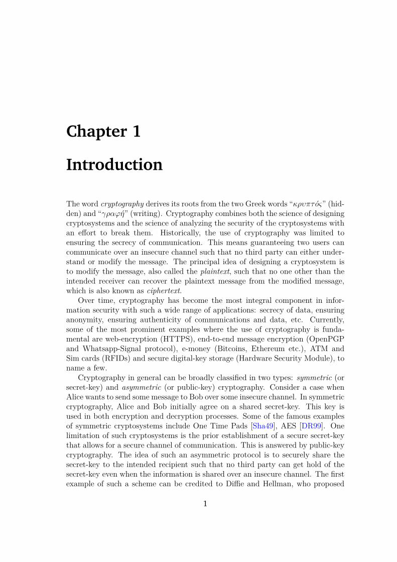
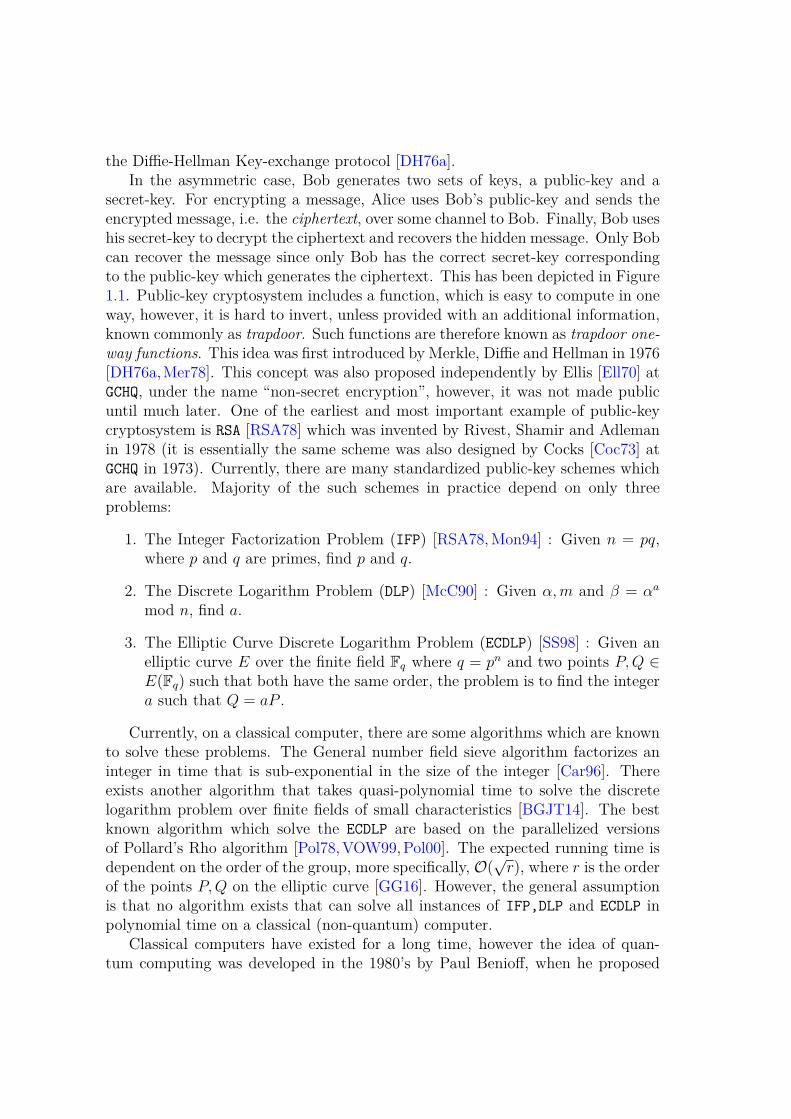
secret-key. For encrypting a message, Alice uses Bob’s public-key and sends theencrypted message, i.e. the ciphertext, over some channel to Bob. Finally, Bob useshis secret-key to decrypt the ciphertext and recovers the hidden message. Only Bobcan recover the message since only Bob has the correct secret-key correspondingto the public-key which generates the ciphertext. This has been depicted in Figure1.1. Public-key cryptosystem includes a function, which is easy to compute in oneway, however, it is hard to invert, unless provided with an additional information,known commonly as trapdoor. Such functions are therefore known as trapdoor one-way functions. This idea was first introduced by Merkle, Diffie and Hellman in 1976[DH76a,Mer78]. This concept was also proposed independently by Ellis [Ell70] atGCHQ, under the name “non-secret encryption”, however, it was not made publicuntil much later. One of the earliest and most important example of public-keycryptosystem is RSA [RSA78] which was invented by Rivest, Shamir and Adlemanin 1978 (it is essentially the same scheme was also designed by Cocks [Coc73] atGCHQ in 1973). Currently, there are many standardized public-key schemes whichare available. Majority of the such schemes in practice depend on only threeproblems:

1. The Integer Factorization Problem (IFP) [RSA78, Mon94] : Given n = pq,where p and q are primes, find p and q.

2. The Discrete Logarithm Problem (DLP) [McC90] : Given α,m and β = αa

mod n, find a.

3. The Elliptic Curve Discrete Logarithm Problem (ECDLP) [SS98] : Given anelliptic curve E over the finite field Fq where q = pn and two points P,Q ∈E(Fq) such that both have the same order, the problem is to find the integera such that Q = aP .

Currently, on a classical computer, there are some algorithms which are knownto solve these problems. The General number field sieve algorithm factorizes aninteger in time that is sub-exponential in the size of the integer [Car96]. Thereexists another algorithm that takes quasi-polynomial time to solve the discretelogarithm problem over finite fields of small characteristics [BGJT14]. The bestknown algorithm which solve the ECDLP are based on the parallelized versionsof Pollard’s Rho algorithm [Pol78,VOW99,Pol00]. The expected running time isdependent on the order of the group, more specifically, O(√r), where r is the orderof the points P,Q on the elliptic curve [GG16]. However, the general assumptionis that no algorithm exists that can solve all instances of IFP,DLP and ECDLP inpolynomial time on a classical (non-quantum) computer.

Classical computers have existed for a long time, however the idea of quan-tum computing was developed in the 1980’s by Paul Benioff, when he proposed

Alice Bob

Encryption Decryption

Bob’s public-key Bob’s secret-key

Message:

m = (m1, . . . ,mn)

Ciphertext

c = (c1, . . . , ck)

Message:m = (m1, . . . ,mn)

Figure 1.1 – Public-key cryptosystem.

the quantum mechanical model of a Turning machine [Ben80]. It was realisedthat one could design quantum computers which were able to simulate physicalprocesses that are not possible on a classical computer [Fey82]. Computationson a quantum computer can be to be much faster than on a classical computer.More so, several of the previously mentioned problems can be solved by Shor’salgorithm [Sho99] on a quantum computer. Especially, IFP is solved by the Shor’salgorithm (with an error probability of maximum 1/3) and requires the use ofO((log n)2(log log n)(log log log n)) number of quantum gates 1, where n is theinteger to factorize [Sho99]. Further research by Beauregard has shown that avariant of the Shor’s algorithm exists that solves integer factorization using 2n+3qubits and O(n3 log n) operations [Bea02]. Recently, [Bea02] showed that Shor’salgorithm can solve an instance of ECDLP using (9n + 2⌈log2 n⌉ + 10) qubits and(448n3 log2 n + 4090n3) quantum gates. Grover’s algorithm [Gro96] is anotherquantum algorithm which essentially provides a speed up on a brute force searchfrom its classical counterpart. Grover’s algorithm very briefly can be described asfollows: given a function f : [0, 2n) 7→ [0, 2), find a x ∈ [0, 2n) such that f(x) = 0.Grover’s algorithm finds a root of f using only about 2n/2 quantum evaluationsof f from a total of 2n possible inputs. Therefore, this algorithm comes in handy

1These gates are the quantum counterparts of the classical logical gates. Refer to Section2.2.2 for more details.

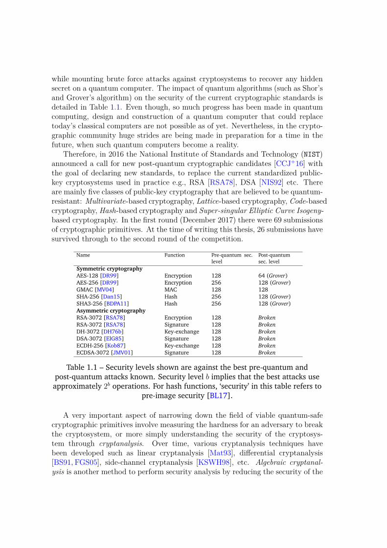
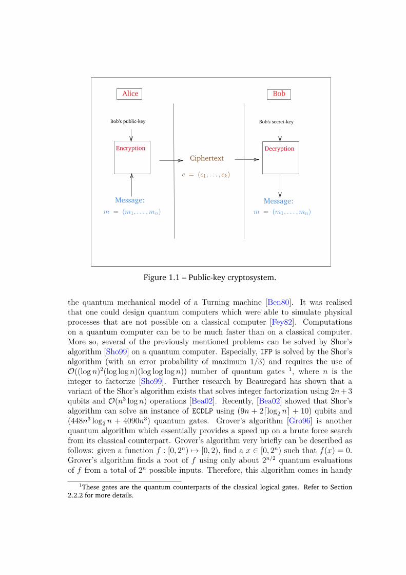
while mounting brute force attacks against cryptosystems to recover any hiddensecret on a quantum computer. The impact of quantum algorithms (such as Shor’sand Grover’s algorithm) on the security of the current cryptographic standards isdetailed in Table 1.1. Even though, so much progress has been made in quantumcomputing, design and construction of a quantum computer that could replacetoday’s classical computers are not possible as of yet. Nevertheless, in the crypto-graphic community huge strides are being made in preparation for a time in thefuture, when such quantum computers become a reality.

Therefore, in 2016 the National Institute of Standards and Technology (NIST)announced a call for new post-quantum cryptographic candidates [CCJ+16] withthe goal of declaring new standards, to replace the current standardized public-key cryptosystems used in practice e.g., RSA [RSA78], DSA [NIS92] etc. Thereare mainly five classes of public-key cryptography that are believed to be quantum-resistant: Multivariate-based cryptography, Lattice-based cryptography, Code-basedcryptography, Hash-based cryptography and Super-singular Elliptic Curve Isogeny-based cryptography. In the first round (December 2017) there were 69 submissionsof cryptographic primitives. At the time of writing this thesis, 26 submissions havesurvived through to the second round of the competition.

Name Function Pre-quantum sec.level

Post-quantumsec. level

Symmetric cryptographyAES-128 [DR99] Encryption 128 64 (Grover)AES-256 [DR99] Encryption 256 128 (Grover)GMAC [MV04] MAC 128 128SHA-256 [Dan15] Hash 256 128 (Grover)SHA3-256 [BDPA11] Hash 256 128 (Grover)Asymmetric cryptographyRSA-3072 [RSA78] Encryption 128 Broken

RSA-3072 [RSA78] Signature 128 Broken

DH-3072 [DH76b] Key-exchange 128 Broken

DSA-3072 [ElG85] Signature 128 Broken

ECDH-256 [Kob87] Key-exchange 128 Broken

ECDSA-3072 [JMV01] Signature 128 Broken

Table 1.1 – Security levels shown are against the best pre-quantum andpost-quantum attacks known. Security level b implies that the best attacks useapproximately 2b operations. For hash functions, ‘security’ in this table refers to

pre-image security [BL17].

A very important aspect of narrowing down the field of viable quantum-safecryptographic primitives involve measuring the hardness for an adversary to breakthe cryptosystem, or more simply understanding the security of the cryptosys-tem through cryptanalysis. Over time, various cryptanalysis techniques havebeen developed such as linear cryptanalysis [Mat93], differential cryptanalysis[BS91, FGS05], side-channel cryptanalysis [KSWH98], etc. Algebraic cryptanal-ysis is another method to perform security analysis by reducing the security of the

problem to the hardness of solving a polynomial system of equations. Overall, itcan be divided into two steps: The first step involves transforming the cryptosys-tem’s algorithms into a system of multivariate polynomial equations that allowsus to recover the secret. After building the system, one estimates the hardnessof solving this system. A practical algebraic attack against the cryptosystem if asolution is found to the system of equations.

This problem of solving a multivariate polynomial system of equations, knownas the Polynomial System Solving (PoSSo) problem, is NP-Complete [GJ79]. Typ-ically, a random non-linear multivariate system of equations is hard to solve (hasexponential complexity). However, in practice, system of equations derived fromalgebraic modelling of cryptosystems are in general, not random. Algebraic crypt-analysis techniques focus on exploiting the hidden structures of such system ofequations, and has resulted in a lot of success over the years [FJ03,CB07,FPS09,BFP08, FJPT10, SK99]. The goal of this thesis is to explore the aspects of al-gebraic cryptanalysis over multivariate encryption cryptographic primitives andfurther try designing a new multivariate scheme that are safe from such algebraicattacks.

1.1 Organization and Contributions of the thesis

To present our work, the thesis has been divided into two parts. In the first part,we present the preliminaries for the work of this thesis. In Chapter 2, we presentthe PoSSo problem on which multivariate cryptography is based. We introducesome state-of-the-art methods to solve this problem. In particular, we focus onalgebraic techniques that take use of a mathematical object called Gröbner basis.

In Chapter 3, we give an overview of multivariate cryptography. We intro-duce the Matsumoto-Imai cryptosystem [MI88], which is one of the first knownexamples of a multivariate scheme. We also introduce the Hidden Field Equations(HFE) [Pat96]. HFE has provided with the foundation for most of the current multi-variate primitives which we also discuss in quite some detail. In particular, we arealso interested in one such multivariate encryption scheme, the Extension FieldCancellation cryptosystem [SDP16].

In the second part of the thesis, we present our contributions. More precisely,we address the following topics.

Algebraic cryptanalysis of EFC. The Extension Field Cancellation scheme (EFC)is a recent multivariate public-key cryptosystem that was presented at PQCryptoin 2016. It proposes a new trapdoor for multivariate quadratic cryptographicprimitive that allows for encryption, in contrast to most time-tested multivariatetrapdoors, like Unbalanced Oil and Vinegar and Hidden Field Equations, whichonly allow for digital signatures. Numerous multivariate encryption schemes, pro-

posed over the years, have been either broken or have been cryptanalyzed, however,EFC has stood untouched. This motivates us to look at the security of the scheme.

In Chapter 4, we present algebraic attacks against EFC. We report the results ofa hybrid Gröbner basis attack [BFP09] on all three challenge parameters of EFC.Using this message recovery attack, for the first and the second challenge parameterwe recover the hidden secret message in 265 and 277 operations respectively, whichis contrary to the claims of 80 bits of security for these parameters. As previouslymentioned, like other multivariate cryptographic schemes, the public-key of EFC

also possesses a hidden structure. We provide experimental evidence of the non-random behavior of the public polynomials of EFC. On the EFC scheme with nodisregarded public-key polynomials (which we shall see later is called a minusversion of a multivariate scheme), denoted below as EFC(0), we show that there isa polynomial time attack, polynomial in the number of variables n. This has beenstated informally in Theorem 1 below:

Theorem 1 (informal). Given a public-key (f1, . . . , f2n) ∈ F2nq [x1, . . . , xn] and the

ciphertext (c1, . . . , c2n) ∈ F2nq from an instance of EFC(0) using Gröbner basis, we

can recover the hidden secret message inO(n3ω) which is polynomial in n and where

2 ≤ ω < 3 is the linear algebra constant.

We present the full version of Theorem 1 as well as the proof in Section 4.2.4.Extending the idea of this theorem, we explain how a degree 3 linear combination ofthe public-keys of EFC(0) yield linear equations (see Section 4.2.4 for more details).

We extend this methodology to the minus variant of EFC, denoted as EFC−,where we recover quadratic equations from a high degree (degree ≥ 3) combi-nations of the public-keys. This technique is quite similar to the approach usedagainst the HFE scheme [FJ03] where the authors show the public-keys exhibitingsome algebraic properties are easier to solve than a random system of quadraticequations of the same sizes. We introduce a new technique of explicitly computingand recovering low-degree relations from the public-keys of EFC−. To do so, weconsider the initial public-keys and their Frobenius powers. The following Claim1 informally describes the basic idea.

Claim 1 (informal). Given the public-keys equations for an instance of EFC−, we

can always find some combinations of the public-keys and their Frobenius powers

which produce new low-degree relations.

Using this technique, we can recover the quadratic relations from degree 3 com-binations in 151 minutes for the first challenge parameter and 110 minutes for thesecond challenge parameter. This computation is polynomial-time in the numberof variables. Furthermore, we show that adding these new equations along withthe public equations make the Gröbner basis computation much more efficient aswell as reducing the time complexity by a huge factor. For instance, in the case ofEFC− with n = 75 and 2 public-key polynomials excluded, adding such intermedi-ate equations reduces the run time of F4 from more than a day to 66.05 seconds to

compute the Gröbner basis. Thus, this scheme has structural weaknesses that canbe easily exploited by an adversary to recover secret messages and thus makingthe scheme unsuitable for encryption.

The PoSSoWN problem. The Leaning With Errors (LWE) problem [Reg09], pro-posed by Regev in 2009, can be modelled as a problem solving a system of noisylinear equations. Results from [Reg09, BLP+13] have shown that the hardness ofthis problem can be reduced to the hardness of some of the worst case latticeproblems. Naturally, this leads us to the question, whether one can generalize theLWE problem to a non-linear system of noisy equations. In this thesis, we try toanswer this exact problem. The non-linear generalization of the LWE problem leadsto a noisy variant of the PoSSo problem that we discussed in Chapter 2. We callthis problem as the Polynomial System Solving With Noise (PoSSoWN) problem.Particularly, some work in this direction was made in [AFFP11] by introducingthe noisy version of the ideal membership problem and the Gröbner basis problem,however, since then not much progress has been made.

In Chapter 5, we describe the PoSSoWN problem. Recalling from Chapter 2Gröbner bases are mathematical objects that are useful in solving a system of non-linear equations. Interestingly, an algorithm that solves the Gröbner basis problem,which is the problem of computing a Gröbner basis of a system of equations, alsosolves the PoSSo problem. A variant of the Gröbner basis problem, i.e. the Gröbnerbasis with Noise problem (GBN), was also introduced and has already been shownto be as hard as the LWE problem [AFFP11]. Naturally, one question arises: canan algorithm that solves the Gröbner basis with Noise (GBN) problem be modelledas an algorithm to solve the PoSSoWN problem ? Or, in other terms, is the PoSSoWNproblem NP-Hard?

In this work, we reduce the hardness of PoSSoWN to the LWE problem and theGBN problem for the linear and the non-linear instance of PoSSoWN. To our knowl-edge, this is the first work which also present the algorithms and the techniques tosolve this problem. To solve the problem, one can employ algorithms that solve thePoSSo problem. However, we due to the presence of errors, algorithms presentedin Chapter 2 cannot be directly applied. One contribution of this thesis is that wepresent algorithms to solve any instance of the PoSSoWN problem.

The CFPKM scheme. Since the first multivariate cryptosystem C∗ [MI88] was pro-posed, many schemes based on the PoSSo problem have been designed. In Chap-ter 5 we presented another hard problem based on solving a polynomial system,called the PoSSoWN. This problem is relatively new in comparison to the PoSSo

problem and therefore, hasn’t been looked into from the point of view of design-ing multivariate cryptosystems. The PoSSoWN problem, like the PoSSo problem isanother candidate for post-quantum cryptography. This motivated us to designa cryptosystem which relies on the hardness of the PoSSoWN problem. We build

a multivariate public-key cryptosystem for key-exchange, which can be naturallytransformed into a public-key Key encapsulation scheme.

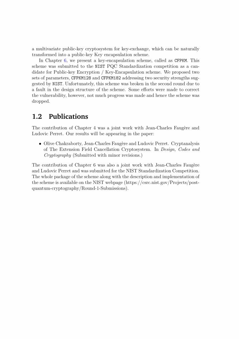
In Chapter 6, we present a key-encapsulation scheme, called as CFPKM. Thisscheme was submitted to the NIST PQC Standardization competition as a can-didate for Public-key Encryption / Key-Encapsulation scheme. We proposed twosets of parameters, CFPKM128 and CFPKM182 addressing two security strengths sug-gested by NIST. Unfortunately, this scheme was broken in the second round due toa fault in the design structure of the scheme. Some efforts were made to correctthe vulnerability, however, not much progress was made and hence the scheme wasdropped.

1.2 Publications

The contribution of Chapter 4 was a joint work with Jean-Charles Faugère andLudovic Perret. Our results will be appearing in the paper:

• Olive Chakraborty, Jean-Charles Faugère and Ludovic Perret. Cryptanalysisof The Extension Field Cancellation Cryptosystem. In Design, Codes andCryptography (Submitted with minor revisions.)

The contribution of Chapter 6 was also a joint work with Jean-Charles Faugèreand Ludovic Perret and was submitted for the NIST Standardization Competition.The whole package of the scheme along with the description and implementation ofthe scheme is available on the NIST webpage (https://csrc.nist.gov/Projects/post-quantum-cryptography/Round-1-Submissions).

Part I

Preliminaries

9

Chapter 2

Polynomial System Solving

Abstract

Solving a system of polynomial equations is a fundamental problemin mathematics with a wide range of applications. Cryptography isone such field and is the main focus of this work. Multivariate cryp-tography relates to cryptosystems which are based on the hardness ofsolving a system of multivariate polynomial equations over a finite field(the PoSSoq problem, which is NP-Hard). It is therefore important tounderstand the cost of solving PoSSoq. In particular, Gröbner basis aremathematical objects that are very useful in solving PoSSoq, which weintroduce and describe in great detail. Also in this chapter, we con-sider combinatorial techniques (such as exhaustive search) for solvingPoSSoq.

2.1 General Framework

Throughout this thesis, we use some common notations. Let F be a field andF[x1, . . . , xn] be the polynomial ring in n variables x1, . . . , xn. In this chapter, wefocus our attention to the problem of finding – if any – solution(s) to a system ofm algebraic equations in n unknowns over F:

f1(x1, . . . , xn) = 0...

fm(x1, . . . , xn) = 0

This problem of finding the roots of a system of multivariate polynomials is mostcommonly known as the PoSSo problem. In this work, we deal with system ofequations which are defined over finite field of order q ∈ N elements (denoted byFq) where q is some positive power of a prime number. Consequently, we denotethis problem as PoSSoq.

11

PoSSoqInput: f1, . . . , fm ∈ Fq[x1, . . . , xn]Goal: Find - if any - a vector (z1, . . . , zn) ∈ Fn

q such that

f1(z1, . . . , zn) = 0...

fm(z1, . . . , zn) = 0

For linear systems, i.e. degree of each fi is 1, the problem can be solved inpolynomial time, thanks to Gaussian elimination. However, for non-linear cases,the problem is significantly harder to solve and is an NP-Complete [FY79]. Whenthe system of equations is quadratic, this problem is also known as the MQq problem,and is still NP-Complete [FY79]. In the following sections we shall present sometechniques to solve the PoSSoq in general and the MQq problem in particular.

2.2 Combinatorial Methods

2.2.1 Classical Setting

Since we work with polynomials over a finite field, exhaustive search or brute forcesearch is the most obvious and natural choice for solving a system of polynomialsf1, . . . , fm ∈ Fq[x1, . . . , xn]. This type of combinatorial technique exhaustivelysearches for values of the variables (x1, . . . , xn) ∈ Fn

q such that they satisfy each ofthe polynomial equations. The complexity of such an algorithm is exponential inthe number of variables. Particularly, [BCC+10] details the complexity of a bruteforce algorithm which computes the solution to a system of quadratic equations inF2. This has a complexity of 2n+2 · log2 n bit operations.

Example 2.2.1. We want to compute the common roots of a system of 90 generic

quadratic equations over 80 variables in F2[x1, . . . , x80]. Using the exhaustive search

method of [BCC+10], the total complexity is 285 binary operations.

Remark 2.2.2 (A brief remark about the time complexity analysis). Complexity

of algorithms are generally given in terms of Big-Oh notation (O()). For a given

positive function g(x), one can denote O(g(x)) the set of functions [CLRS09]

O(g(x)) = {f(x) : there exists positive constants M and x0 such that

0 ≤ f(x) ≤ Mg(x) for all x ≥ x0}.

This constant M depends mainly on the algorithm itself. The implementation of al-

gorithm as well as the architecture of the machine on which the algorithm has been

implemented also impacts the constant. Some algorithms have large overheads in

their actual run time on a particular machine, which in turn are reflected in this

constant. Therefore in general, the constant M is not easy to determine. However,

estimating the running time without the constants gives an overview of how algo-

rithms compare to each other asymptotically. Thus, even though the constant is

not completely precise, as a conservative choice we assume the constant M to be 1.

In the rest of the work, we analyze the running time of the algorithms with this

assumption. In the following theorem (see Theorem 2.2.3), authors of [LPT+17]

denote this by O∗, which omits the polynomial factors of the O notation.

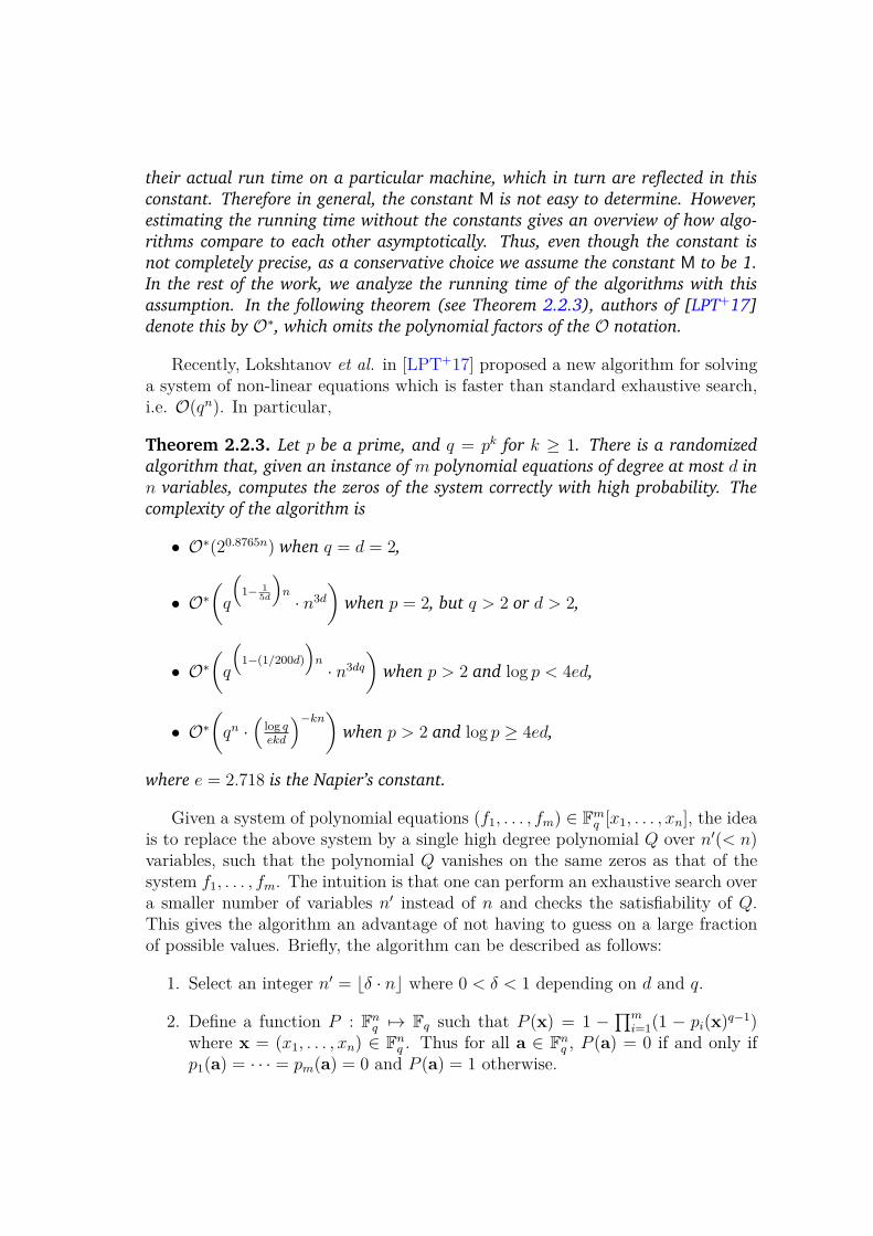
Recently, Lokshtanov et al. in [LPT+17] proposed a new algorithm for solvinga system of non-linear equations which is faster than standard exhaustive search,i.e. O(qn). In particular,

Theorem 2.2.3. Let p be a prime, and q = pk for k ≥ 1. There is a randomized

algorithm that, given an instance of m polynomial equations of degree at most d in

n variables, computes the zeros of the system correctly with high probability. The

complexity of the algorithm is

• O∗(20.8765n) when q = d = 2,

• O∗(q

(1− 1

5d

)n · n3d

)when p = 2, but q > 2 or d > 2,

• O∗(q

(1−(1/200d)

)n · n3dq

)when p > 2 and log p < 4ed,

• O∗(qn ·

(log qekd

)−kn)when p > 2 and log p ≥ 4ed,

where e = 2.718 is the Napier’s constant.

Given a system of polynomial equations (f1, . . . , fm) ∈ Fmq [x1, . . . , xn], the idea

is to replace the above system by a single high degree polynomial Q over n′(< n)variables, such that the polynomial Q vanishes on the same zeros as that of thesystem f1, . . . , fm. The intuition is that one can perform an exhaustive search overa smaller number of variables n′ instead of n and checks the satisfiability of Q.This gives the algorithm an advantage of not having to guess on a large fractionof possible values. Briefly, the algorithm can be described as follows:

1. Select an integer n′ = ⌊δ · n⌋ where 0 < δ < 1 depending on d and q.

2. Define a function P : Fnq 7→ Fq such that P (x) = 1 −∏m

i=1(1 − pi(x)q−1)

where x = (x1, . . . , xn) ∈ Fnq . Thus for all a ∈ Fn

q , P (a) = 0 if and only ifp1(a) = · · · = pm(a) = 0 and P (a) = 1 otherwise.

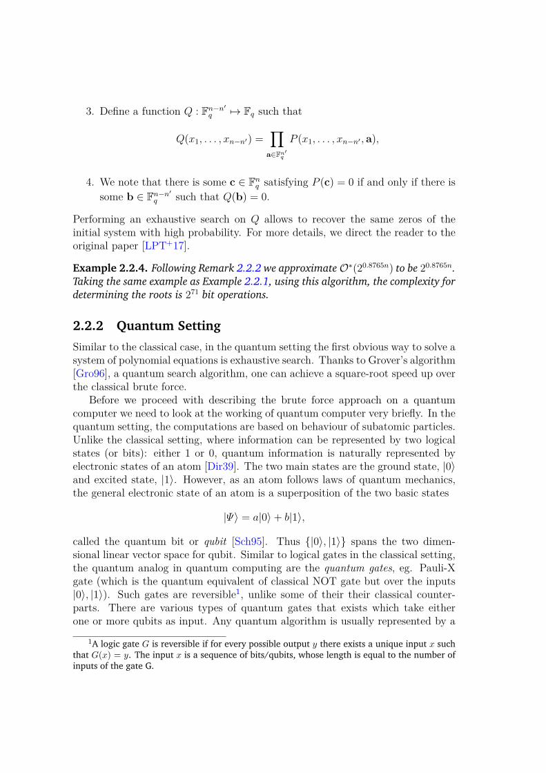
3. Define a function Q : Fn−n′

q 7→ Fq such that

Q(x1, . . . , xn−n′) =∏

a∈Fn′q

P (x1, . . . , xn−n′ , a),

4. We note that there is some c ∈ Fnq satisfying P (c) = 0 if and only if there is

some b ∈ Fn−n′

q such that Q(b) = 0.

Performing an exhaustive search on Q allows to recover the same zeros of theinitial system with high probability. For more details, we direct the reader to theoriginal paper [LPT+17].

Example 2.2.4. Following Remark 2.2.2 we approximateO∗(20.8765n) to be 20.8765n.

Taking the same example as Example 2.2.1, using this algorithm, the complexity for

determining the roots is 271 bit operations.

2.2.2 Quantum Setting

Similar to the classical case, in the quantum setting the first obvious way to solve asystem of polynomial equations is exhaustive search. Thanks to Grover’s algorithm[Gro96], a quantum search algorithm, one can achieve a square-root speed up overthe classical brute force.

Before we proceed with describing the brute force approach on a quantumcomputer we need to look at the working of quantum computer very briefly. In thequantum setting, the computations are based on behaviour of subatomic particles.Unlike the classical setting, where information can be represented by two logicalstates (or bits): either 1 or 0, quantum information is naturally represented byelectronic states of an atom [Dir39]. The two main states are the ground state, |0〉and excited state, |1〉. However, as an atom follows laws of quantum mechanics,the general electronic state of an atom is a superposition of the two basic states

|Ψ〉 = a|0〉+ b|1〉,

called the quantum bit or qubit [Sch95]. Thus {|0〉, |1〉} spans the two dimen-sional linear vector space for qubit. Similar to logical gates in the classical setting,the quantum analog in quantum computing are the quantum gates, eg. Pauli-Xgate (which is the quantum equivalent of classical NOT gate but over the inputs|0〉, |1〉). Such gates are reversible1, unlike some of their their classical counter-parts. There are various types of quantum gates that exists which take eitherone or more qubits as input. Any quantum algorithm is usually represented by a

1A logic gate G is reversible if for every possible output y there exists a unique input x suchthat G(x) = y. The input x is a sequence of bits/qubits, whose length is equal to the number ofinputs of the gate G.

sequence of quantum gates and is known as a quantum circuit.

In [SW16], the authors proposed a quantum algorithm for solving MQ2 problem.The main principle is to perform a fast exhaustive search by using Grover’s algo-rithm. One can solve (m−1) binary quadratic equations in (n−1) binary variableswith the Grover’s algorithm using a circuit consisting of (m + n + 2) qubits andrequiring the evaluation of 2n/2

(2m(n2 + 2n) + 1

)quantum gates. They also pro-

pose a variant for the quantum circuit which in comparison uses 3 + n+ ⌈log2 m⌉qubits but with twice as many quantum gates required.

Example 2.2.5. Solving 90 binary quadratic equations over 80 variables by ex-

haustive search with Grover’s algorithm thus has expected cost of 174 qubits and

requires a use of minimum 260 quantum gates. Using the variant the expected cost

is 90 qubits using 261 quantum gates.

2.3 Gröbner Basis

In this thesis, the mathematical object that we use most frequently is Gröbnerbasis [Buc65]. We will see how the calculation of such a basis makes it possibleto solve the PoSSo problem. In this section, we present the notations and theessentials around Gröbner bases that are going to be used in the second part ofthis thesis.

2.3.1 Preliminary Definitions and Properties

We start by defining two mathematical objects naturally associated with Gröbnerbases: ideals and varieties.

Definition 2.3.1 (Ideal). [CLO15] An ideal I ⊆ Fq[x1, . . . , xn] is a set of elements

such that

• 0 ∈ I,

• If f, g ∈ I, then f + g ∈ I,

• If f ∈ I and g ∈ Fq[x1, . . . , xn], then fg ∈ I.

We define the ideal generated by the polynomials (f1, . . . , fm) ∈ Fmq [x1, . . . , xn] as

〈f1, . . . , fm〉 :={ m∑

i=1

gifi : (g1, . . . , gm) ∈ Fmq [x1, . . . , xn]

}.

We define the affine algebraic variety of I ⊆ Fq[x1, . . . , xn], denoted by V(I),as the set of the common zeros of all the polynomials in I, over the algebraicallyclosed finite field Fq:

V(I) = {(a1, . . . , an) ∈ (Fq)n|∀f ∈ I : f(a1, . . . , an) = 0}.

When the variety is finite, i.e. |V(I)| <∞, then the ideal is called zero-dimensional.In this work, we are interested in the set of solutions which belong to Fq ⊂ Fq (notin its algebraic closure Fq). The set of solutions to the equation xq = x is theentirety of the field Fq. Thus by appending xq

1 − x1, . . . , xqn − xn ∈ Fq[x1, . . . , xn]

to the input ideal I = 〈f1, . . . , fm〉, we have

V(〈f1, . . . , fm, xq1 − x1, . . . , x

qn − xn〉) = V(I) ∩ Fn

q ,

the variety consisting of solutions to the system which lie only in Fq.To solve a system of equations (f1, . . . , fm) ∈ Fm

q [x1, . . . , xn], we calculate thevariety, which is denoted by VFq

(f1, . . . , fm). Any solution to the system of equa-tions also cancels all the polynomials in the ideal 〈f1, . . . , fm〉. Therefore, thevariety V(〈f1, . . . , fm〉) does not depend on the exact choice of the polynomialsf1, . . . , fm, rather, it depends only on the ideal generated by these polynomials.Thus, one can try to find another system of polynomial equations that generatesthe same ideal I = 〈f1, . . . , fm〉 and are easier to solve than the system f1, . . . , fm.Thanks to Gröbner basis, we are able to do so. Informally, Gröbner basis is the gen-erating basis for an ideal that allows to identify in particular the roots of a systemas well as deduce many properties of an ideal. Thus, Gröbner basis computationprovides us with tools to solve a system of multivariate system of equations. Wenow look into Gröbner basis in some detail.

We shall recall that a monomial in the polynomial ring Fq[x1, . . . , xn] is apower-product of variables. We write a monomial xα1

1 · · · xαnn as xα where α =

(α1, . . . , αn) ∈ Nn. The degree of a monomial is deg(xα) =∑

i αi. We say that amonomial xα divides another monomial xβ if and only if for all 1 ≤ i ∈ n, we haveαi ≤ βi. This is also denoted as xα|xβ.

In the case of polynomial ideals with one variable, the largest term is consideredwith respect to the order xd > xd−1 > · · · > x2 > x > 1. Choosing any otherterm leads to an infinite division process. While dealing with multiple variables,we consider a particular type of total order relation2 on the set of monomials ofFq[x1, . . . , xn], which we define as follows:

Definition 2.3.2 (Monomial Ordering [CLO15]). A monomial ordering on a poly-

nomial ring Fq[x1, . . . , xn] is a binary relation ≻ on Nn such that

2A total order is a type of binary relation on a set which has three principal properties: anti-symmetry (a ≤ b & b ≤ a =⇒ a = b ), transitivity (a ≤ b & b ≤ c =⇒ a ≤ c) and connexity(a ≤ b or b ≤ a)

• ≻ is a total ordering on Nn.

• For a triplets of monomials (xα, xβ, xγ);

xα ≻ xβ, implies xαxγ ≻ xβxγ,

where α, β, γ ∈ Nn.

• ≻ is a well-ordering [CLO15, Lem. 2.2.2] on Nn, that is every non-empty

subset of Nn has a minimal element with respect to ≻.

For instance, the Lexicographic (Lex) and Degree Reverse Lexicographic(GRevLex) - which are widely used in practice- are defined as follows:

Definition 2.3.3. Let ≻ be a monomial ordering such that x1 ≻ x2 ≻ · · · ≻ xn. Let

α = (α1, . . . , αn) ∈ Nn and β = (β1, . . . , βn) ∈ Nn

• Lexicographic ordering (LEX): we say xα ≻LEX xβ, if and only if there is

1 ≤ k ≤ n such that {(∀ 1 ≤ i < k) αi = βi,

αk > βk.

• Graded Reverse Lexicographic ordering (GREVLEX): given two monomials

xα and xβ, we say xα ≻GREVLEX xβ, if and only if,

|α| =n∑

i=1

αi > |β| =n∑

i=1

βi, or,

|α| = |β| and ∃ k such that (∀ i > k) αi = βi and αk < βk.

Example 2.3.4. Consider the LEX ordering ≻Lex on Fq[x, y], such that x ≻Lex y.

Then x3 ≻Lex xy2, x ≻Lex y

50 and xy3 ≻Lex xy2.

Example 2.3.5. Consider the GREVLEX ordering ≻GRevLex on Fq[x, y, z], such that

x ≻GRevLex y and y ≻GRevLex z. Then xy2 ≻GrevLex x2z, and y50 ≻GRevLex x .

There are many other monomial orderings which exist and refer the reader to[CLO15] for more details. Now, that we have defined ordering amongst monomials,it is easy to note that any polynomial f ∈ Fq[x1, . . . , xn] has a unique leading term.Hereby, we provide its formal definition:

Definition 2.3.6 (Leading Monomial, Coefficient and Term). Let f =∑

α∈Nn cαxα ∈

Fq[x1, . . . , xn] be a non zero polynomial and let ≻ be the monomial ordering, then

• The leading monomial of f with respect to≻, denoted by LM≻(f), is the largest

monomial (with respect to ≻), i.e.

LM≻(f) := max{xα : cα 6= 0},

• The leading coefficient of f with respect to ≻, denoted by LC≻(f), is the coef-

ficient associated to the leading monomial of f , i.e.

LC≻(f) := cα such that LM≻(f) = xα,

• The leading term of f , denoted by LT≻(f), is the product of the leading mono-

mial and coefficient of f , i.e.

LT≻(f) := LC≻(f)LM≻(f).

Next, we shall define the notion of a particular type of ideal which can begenerated by a set of monomials. This is known as monomial ideal.

Definition 2.3.7 (Monomial Ideal). We say that an ideal I ′ ⊂ Fq[x1, . . . , xn] is

a monomial ideal if I ′ can be generated by a family of monomials, i.e. I ′ =〈xα()

, · · · , xα(m)〉 where α(i) ∈ Nn.

Example 2.3.8. An example of monomial ideal is given by I = 〈x4y2, x3y4, x2y5〉 ⊂Fq[x, y].

A monomial xβ belongs to the monomial ideal I ′ = 〈xα(), · · · , xα(m)〉, if and

only if xβ is divisible by xα(i). Additionally, a polynomial f belongs to monomial

ideal I ′, if and only if all monomials that occur in f with non-zero coefficient alsobelong to I ′.

A special kind of monomial ideal is the ideal generated by the leading mono-mials of the polynomials (see Definition 2.3.6). This ideal is called the initial idealand we formally define it as follows:

Definition 2.3.9 (Initial Ideal). Let≻ be a monomial ordering and I ⊆ Fq[x1, . . . , xn]be an ideal. Then the initial ideal of I, denoted by LM≻(I), is the monomial ideal

generated by the leading monomials of the all the polynomials in I, i.e.,

〈LM≻(I)〉 := 〈LM≻(f) : f ∈ I〉.

When I is already a monomial ideal then 〈LM≻(I)〉 = I. Now, from definition,〈LM≻(I)〉 is generated by the monomials LM≻(f) for f ∈ I−{0}. Dickson’s Lemma[CLO15, Theorem 2.4.5] states that a monomial ideal I has a finite basis. Usingthis property, one can show that for any polynomial ideal, I ⊆ Fq[x1, . . . , xn], thereexists a finite basis (g1, . . . , gm) ∈ Fm

q [x1, . . . , xn] of I, which has the property,〈LM≻(I)〉 = 〈LM(g1), . . . , LM(gm)〉. This is most famously known as the HilbertBasis Theorem [CLO15, Theorem 2.5.4]. Any basis which satisfies such a propertyis called the Gröbner basis of the ideal I. We define it more formally as follows:

Definition 2.3.10 (Gröbner basis). Let ≻ be a monomial ordering on the poly-

nomial ring Fq[x1, . . . , xn]. A finite subset G of an ideal I ⊆ Fq[x1, . . . , xn] is a

Gröbner basis of I with respect to ≻ if and only if

〈LM≻(I)〉 = 〈{LM≻(g) : g ∈ G}〉.

Equivalently, we also say that G is a Gröbner basis if, for every f ∈ I, there exist

some g ∈ G such that LM(g) | LM(f).

From a practical point of view, computing a Lex Gröbner basis much slowerthan computing a Gröbner basis with respect to another monomial ordering. Onthe other hand, it is quite well known that computing GRevLex Gröbner basesis much faster in practice.

One might encounter a case where there exists a polynomial in the Gröbner basisg ∈ G, such that its leading monomial can be generated by the leading monomialsof the other elements in the basis G. Then the basis G−{g} is also a Gröbner basisfor the same ideal I [CLO15, Lemma 2.7.4]. Removing all such dependent g ∈ Ghaving this property leads us to the notion of a minimal Gröbner basis. However,for an ideal I, one can encounter multiple minimal Gröbner bases. Fortunately,we can find a minimal basis, with the additional property that for any elementg ∈ G, no monomial of g lie in monomial ideal 〈LM(G− {g})〉. This is the notionof reduced Gröbner basis that we formally define below.

Definition 2.3.11 (Reduced Gröbner basis [CLO15]). A Gröbner basis G for some

ideal in the polynomial ring Fq[x1, . . . , xn] is said to be reduced Gröbner basis if and

only if

• every polynomial in G is monic, i.e. ∀g ∈ G, LC≻(g) = 1, and

• ∀g ∈ G, no monomial appearing in g belongs to 〈LM≻(G− {g})〉

For any ideal I 6= 0, such a reduced Gröbner basis is always unique [CLO15,Proposition 2.7.6].

While working with Gröbner bases, broadly two types of polynomial systemsare encountered: homogeneous and affine system of equations.

Definition 2.3.12. Given a multivariate polynomial f ∈ Fq[x1, . . . , xn], it is said

to be homogeneous if and only if all the monomials of f with non-zero coefficients

have the same total degree, i.e., with (α1, . . . , αn) ∈ N, all monomials of f are of

the form xα11 xα2

2 · · · xαnn such that

∑ni=1 αi is a constant value for the polynomial f .

Otherwise its called an affine polynomial.

As we shall see in Section 2.3.2, one of the most common aspect in Gröbnerbasis algorithms is the idea of incremental degree by degree computation of the

basis. More precisely, such algorithms consider all polynomials at a certain degreein order to find the generating elements for the Gröbner basis at that degree beforeproceeding to the next degree. This is made possible by considering the idealsubset, I≤d ⊆ I ⊆ Fq[x1, . . . , xn], such that I≤d consists of all the polynomialsin the ideal whose degree is less than or equal to d. We also call this as thedegree d-truncated ideal. Using this notion of degree truncated ideal, we definethe generating Gröbner basis for this ideal I≤d as follow:

Definition 2.3.13 (d-Gröbner basis). Let ≻ be a monomial ordering, d ∈ N be an

integer and I ⊆ Fq[x1, . . . , xn] be an ideal. A degree d truncated Gröbner basis for Iwith respect to the monomial ordering ≻ is a finite set Gd ⊂ I≤d ⊆ I such that for

every f ∈ Id with deg(f) ≤ d, we have LM≻(f) ∈ 〈{LM≻(g) : g ∈ Gd}〉And as a direct consequence of the Ascending Chain condition [CLO15, The-

orem 2.5.7] and Hilbert Basis theorem [CLO15, Theorem 2.5.4], we have the fol-lowing theorem.

Theorem 2.3.14. Let Gd ⊂ Fq[x1, . . . , xn] be a degree d-Gröbner basis of a system

of homogeneous polynomials in the polynomial ring Fq[x1, . . . , xn] with respect to

some monomial ordering ≻. Then we have the inclusion of truncated Gröbner bases

with incremental degree and we can find a D such that

G2 ⊂ G3 ⊂ · · · ⊂ GD = GD+1 = G,

where G ⊂ Fq[x1, . . . , xn] is the Gröbner basis of input system of polynomials with

respect to ≻.

The step of computing the basis is usually the most difficult step as generallythe input polynomials have no mathematical structure. This notion of truncatedGröbner basis comes in handy to provide some kind of structure to this [Fau99].We shall see later (Section 2.3.2), state-of-the-art Gröbner basis algorithms suchas Buchberger and F4 incrementally solve a system of equations by computingGröbner basis degree by degree.

2.3.1.1 Gröbner Basis and Ideal Membership

One of the important applications of Gröbner basis is that it allows to solve theIdeal Membership Problem. Formally, given a polynomial and an ideal, the decisionIdeal Membership Problem decides whether the polynomial belongs to the ideal.The testing for ideal membership requires an understanding of the notion of thepolynomial division with respect to a set of polynomials. One might recall, divisionof a polynomial by another polynomial iterates the process of division by the divisorpolynomial until the leading term of the remainder in each step of division is notdivisible by the leading term of the divisor. The following theorem gives the generalform of the division algorithm of a polynomial by an ordered set by building onthe previous algorithm.

Theorem 2.3.15. [CLO15, Theorem 2.3.3] Let F = (f1, . . . , fm) ∈ Fmq [x1, . . . , xn]

be a m-tuple of polynomials and let ≻ be a fixed monomial ordering. Then every

f ∈ Fq[x1, . . . , xn] can be written as

f = a1f1 + · · ·+ amfm + r,

where ai, r ∈ Fq[x1, . . . , xn]. We call r the remainder of the division of f by F .

The remainder is either r = 0 or a linear combination, with coefficients in Fq, of

monomials none of which are divisible by any of LM≻(f1), . . . , LM≻(fm).

Example 2.3.16. Let f = xy2 + x2y ∈ Fq[x, y] where q is a large prime. Dividing fby f1 = xy − 1, f2 = y + 1 ∈ Fq[x, y], the division algorithm described above gives

us

f = (y + x) · f1 + 1 · f2 + x

Having r = 0 is a sufficient condition for testing the ideal membership of apolynomial f ∈ Fq[x1, . . . , xn] in an ideal I ⊆ Fq[x1, . . . , xn]. However, it is not anecessary condition. Consider the following example.

Example 2.3.17. Let f = xy2 − x ∈ Fq[x, y] and let f1 = xy + 1, f2 = y2 − 1 ∈Fq[x, y] be the two divisors. Dividing f by F = (f1, f2) in this particular order gives

us

xy2 − x = y · (xy + 1) + 0 · (y2 − 1) + (−x− y).

While with the choice of F = (f2, f1) we have

xy2 − x = x · (y2 − 1) + 0 · (xy + 1) + 0.

From this above example we see that r = 0 when the choice of divisors is(f2, f1) and thus f ∈ 〈f1, f2〉. However, the with the choice of order of divisors as(f1, f2), we have r 6= 0. Therefore, one might look for a better generator set ofthe ideal such that with just r = 0 we have a necessary and sufficient conditionfor ideal membership testing. Gröbner basis properties allow the remainder of apolynomial division by the ideal to be uniquely determined [CLO15, Proposition2.6.1], thus making r = 0 a necessary as well as a sufficient condition for idealmembership.

Definition 2.3.18 (Normal Form). [CLO15, Page 82] Let I ⊆ Fq[x1. . . . , xn] be an

ideal and G be a Gröbner basis of I. Then any polynomial f ∈ Fq[x1, . . . , xn] can be

represented as f = h+r where h ∈ I and r ∈ Fq[x1, . . . , xn] has no monomials that

are divisible by any of LM≻(g1), . . . , LM≻(gm) for G = (g1, . . . , gm) ∈ Fmq [x1, . . . , xn].

This polynomial r is called the normal form of f with respect to I and ≻. We

denote it as fG

.

Now, with this we can represent any polynomial uniquely by their normal form.Since this normal form is unique for any polynomial, we now have a necessary andsufficient condition to test the ideal membership. More formally we have thefollowing:

Corollary 2.3.19 (Test for Ideal Membership). Let G be a Gröbner basis for an

ideal I ⊆ Fq[x1, . . . , xn]. A polynomial f ∈ Fq[x1, . . . , xn] belongs to the ideal I, if

and only if the normal form of f with respect to the Gröbner basis is 0, i.e. fG= 0.

Now, that we have discussed the testing for ideal membership, we now focuson the problem of deciding whether an input generating set of an ideal is a Gröb-ner basis. A generating set (f1, . . . , fm) ∈ Fm

q [x1, . . . , xn] for an ideal cannot bea Gröbner basis if the leading term of any polynomial combination of the gener-ator polynomials is not in the ideal 〈LM≻(fi)〉 for some fixed monomial ordering≻. This can occur in cases when the leading terms in the combination cancel,leaving only smaller terms, which are not divisible by any of LM≻(f1), . . . , LM≻(fm).Such a combination of two polynomials is known as the S-polynomial of a pair ofpolynomials:

Definition 2.3.20 (S-polynomial). Let f, g ∈ Fq[x1, . . . , xn] be two non-zero poly-

nomials. Let us denote the least common multiple of LM≻(f) and LM≻(g) by xγ. The

S-polynomial of f and g is the combination

Spol≻(f, g) :=LT≻(g)

xγ· f − LT≻(f)

xγ· g.

Using S-polynomials, Buchberger proposes the following decision criteria todetermine if the basis (the generating set) of an ideal is a Gröbner basis.

Theorem 2.3.21 (Buchberger’s Criterion ). [Buc76, Theorem 3.3] Consider a

polynomial ideal I ⊆ Fq[x1, . . . , xn]. Then a basis G = (g1, · · · , gm) ⊂ I is a

Gröbner basis of I with respect to monomial ordering ≻ if and only if for all pairs

(gi, gj) ∈ F2q[x1, . . . , xn] with i 6= j, the remainder on division of Spol≻(gi, gj) ∈

Fq[x1, . . . , xn] by G is zero.

Thus using this previous criterion one can test whether a given basis is aGröbner basis. In the following section, we can now describe the state-of-the-artalgorithms to compute Gröbner bases for a system of polynomials.

2.3.2 Gröbner Basis Algorithms

2.3.2.1 Buchberger Algorithm

Buchberger [Buc76] proposed the first general algorithm to compute the Gröbnerbasis by using the criterion of Theorem 2.3.21. Now we present the algorithmin brief. Given a system of polynomials, say L ⊂ Fq[x1, . . . , xn], belonging to anideal, the goal is to decide whether this set, L is a Gröbner basis for the ideal, andif not, then compute the Gröbner basis. The idea of the algorithm is as follows:

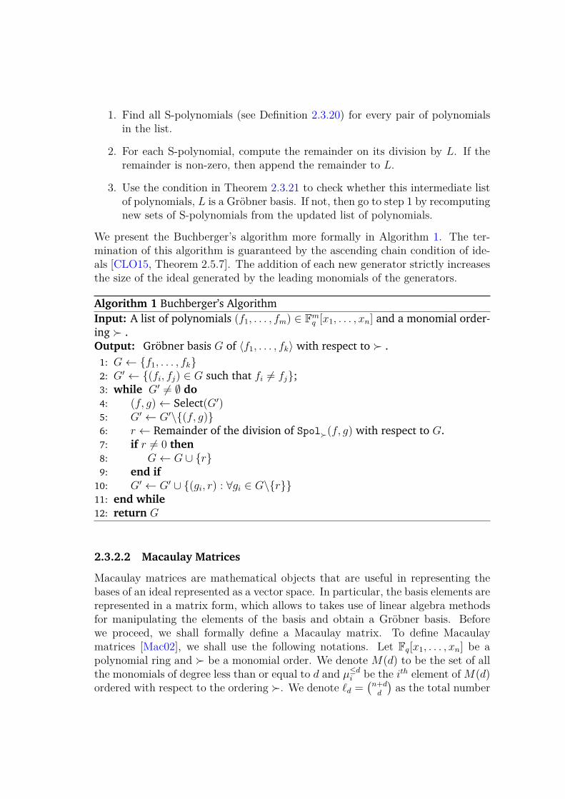
1. Find all S-polynomials (see Definition 2.3.20) for every pair of polynomialsin the list.

2. For each S-polynomial, compute the remainder on its division by L. If theremainder is non-zero, then append the remainder to L.

3. Use the condition in Theorem 2.3.21 to check whether this intermediate listof polynomials, L is a Gröbner basis. If not, then go to step 1 by recomputingnew sets of S-polynomials from the updated list of polynomials.

We present the Buchberger’s algorithm more formally in Algorithm 1. The ter-mination of this algorithm is guaranteed by the ascending chain condition of ide-als [CLO15, Theorem 2.5.7]. The addition of each new generator strictly increasesthe size of the ideal generated by the leading monomials of the generators.

Algorithm 1 Buchberger’s AlgorithmInput: A list of polynomials (f1, . . . , fm) ∈ Fm

q [x1, . . . , xn] and a monomial order-ing ≻ .Output: Gröbner basis G of 〈f1, . . . , fk〉 with respect to ≻ .

1: G← {f1, . . . , fk}2: G′ ← {(fi, fj) ∈ G such that fi 6= fj};3: while G′ 6= ∅ do4: (f, g)← Select(G′)5: G′ ← G′\{(f, g)}6: r ← Remainder of the division of Spol≻(f, g) with respect to G.7: if r 6= 0 then8: G← G ∪ {r}9: end if

10: G′ ← G′ ∪ {(gi, r) : ∀gi ∈ G\{r}}11: end while12: return G

2.3.2.2 Macaulay Matrices

Macaulay matrices are mathematical objects that are useful in representing thebases of an ideal represented as a vector space. In particular, the basis elements arerepresented in a matrix form, which allows to takes use of linear algebra methodsfor manipulating the elements of the basis and obtain a Gröbner basis. Beforewe proceed, we shall formally define a Macaulay matrix. To define Macaulaymatrices [Mac02], we shall use the following notations. Let Fq[x1, . . . , xn] be apolynomial ring and ≻ be a monomial order. We denote M(d) to be the set of allthe monomials of degree less than or equal to d and µ≤di be the ith element of M(d)ordered with respect to the ordering ≻. We denote ℓd =

(n+dd

)as the total number

of monomials in M(d). Finally, for f ∈ Fq[x1, . . . , xn], we denote Coeff(f, µ≤di ) thecoefficient of f associated with the monomial µ≤di .

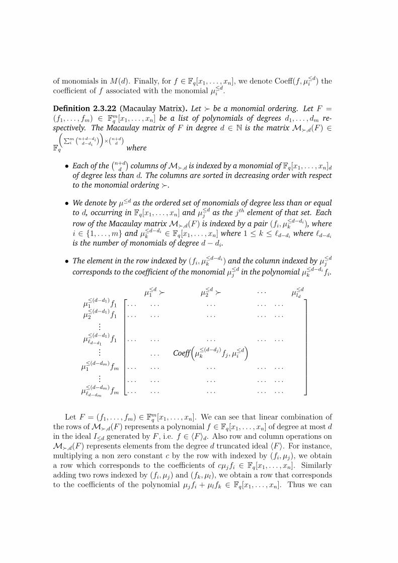
Definition 2.3.22 (Macaulay Matrix). Let ≻ be a monomial ordering. Let F =(f1, . . . , fm) ∈ Fm

q [x1, . . . , xn] be a list of polynomials of degrees d1, . . . , dm re-

spectively. The Macaulay matrix of F in degree d ∈ N is the matrix M≻,d(F ) ∈

F

(∑m

i (n+d−did−di

))×(n+d

d )q where

• Each of the(n+dd

)columns ofM≻,d is indexed by a monomial of Fq[x1, . . . , xn]d

of degree less than d. The columns are sorted in decreasing order with respect

to the monomial ordering ≻.

• We denote by µ≤d as the ordered set of monomials of degree less than or equal

to d, occurring in Fq[x1, . . . , xn] and µ≤dj as the jth element of that set. Each

row of the Macaulay matrixM≻,d(F ) is indexed by a pair (fi, µ≤d−dik ), where

i ∈ {1, . . . ,m} and µ≤d−dik ∈ Fq[x1, . . . , xn] where 1 ≤ k ≤ ℓd−di where ℓd−diis the number of monomials of degree d− di.

• The element in the row indexed by (fi, µ≤d−dik ) and the column indexed by µ≤dj

corresponds to the coefficient of the monomial µ≤dj in the polynomial µ≤d−dik fi.

µ≤d1 ≻ µ≤d2 ≻ · · · µ≤dld

µ≤(d−d1)1 f1 . . . . . . . . . . . . . . .

µ≤(d−d1)2 f1 . . . . . . . . . . . . . . .

...

µ≤(d−d1)ℓd−d1

f1 . . . . . . . . . . . . . . .... . . . Coeff

(µ≤(d−dj)k fj, µ

≤di

)

µ≤(d−dm)1 fm . . . . . . . . . . . . . . .

... . . . . . . . . . . . . . . .

µ≤(d−dm)ℓd−dm

fm . . . . . . . . . . . . . . .

Let F = (f1, . . . , fm) ∈ Fmq [x1, . . . , xn]. We can see that linear combination of

the rows ofM≻,d(F ) represents a polynomial f ∈ Fq[x1, . . . , xn] of degree at most din the ideal I≤d generated by F , i.e. f ∈ 〈F 〉d. Also row and column operations onM≻,d(F ) represents elements from the degree d truncated ideal 〈F 〉. For instance,multiplying a non zero constant c by the row with indexed by (fi, µj), we obtaina row which corresponds to the coefficients of cµjfi ∈ Fq[x1, . . . , xn]. Similarlyadding two rows indexed by (fi, µj) and (fk, µl), we obtain a row that correspondsto the coefficients of the polynomial µjfi + µlfk ∈ Fq[x1, . . . , xn]. Thus we can

say that the matrixM′≻,d(F ) resulting from some linear algebra operations on the

rows of M≻,d(F ) represents polynomials in 〈F 〉d.A connection between the degree d Macaulay matrices M≻,d and truncated

d-Gröbner basis for an ideal I≤d was first provided by Lazard in [Laz83]. For a

matrix M ∈ Fm×nq , we denote by M the Gauss-Jordan elimination of M . It is also

known as the row echelon form of the matrix M .

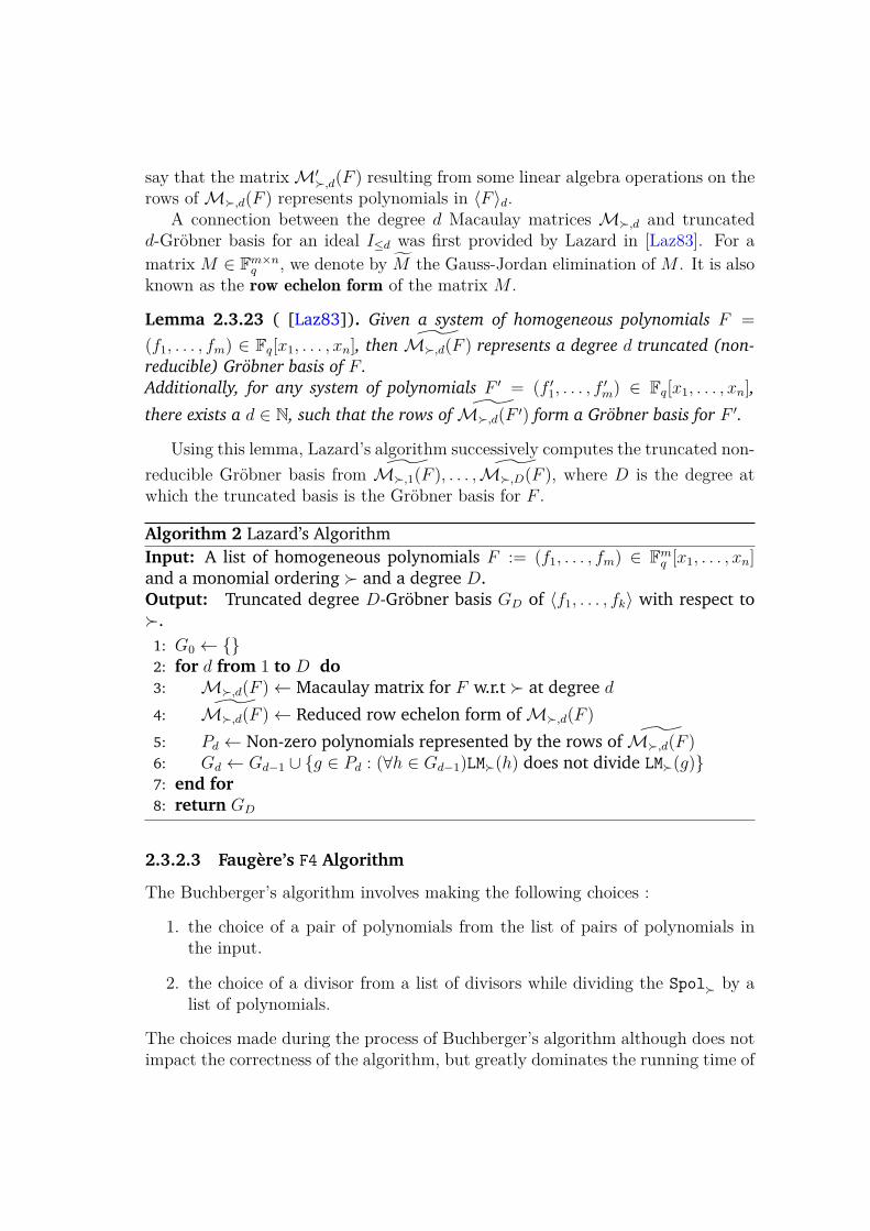
Lemma 2.3.23 ( [Laz83]). Given a system of homogeneous polynomials F =

(f1, . . . , fm) ∈ Fq[x1, . . . , xn], then M≻,d(F ) represents a degree d truncated (non-

reducible) Gröbner basis of F .

Additionally, for any system of polynomials F ′ = (f ′1, . . . , f′m) ∈ Fq[x1, . . . , xn],

there exists a d ∈ N, such that the rows of M≻,d(F ′) form a Gröbner basis for F ′.

Using this lemma, Lazard’s algorithm successively computes the truncated non-

reducible Gröbner basis from M≻,1(F ), . . . ,M≻,D(F ), where D is the degree atwhich the truncated basis is the Gröbner basis for F .

Algorithm 2 Lazard’s AlgorithmInput: A list of homogeneous polynomials F := (f1, . . . , fm) ∈ Fm

q [x1, . . . , xn]and a monomial ordering ≻ and a degree D.Output: Truncated degree D-Gröbner basis GD of 〈f1, . . . , fk〉 with respect to≻.

1: G0 ← {}2: for d from 1 to D do3: M≻,d(F )← Macaulay matrix for F w.r.t ≻ at degree d

4: M≻,d(F )← Reduced row echelon form ofM≻,d(F )

5: Pd ← Non-zero polynomials represented by the rows of M≻,d(F )6: Gd ← Gd−1 ∪ {g ∈ Pd : (∀h ∈ Gd−1)LM≻(h) does not divide LM≻(g)}7: end for8: return GD

2.3.2.3 Faugère’s F4 Algorithm

The Buchberger’s algorithm involves making the following choices :

1. the choice of a pair of polynomials from the list of pairs of polynomials inthe input.

2. the choice of a divisor from a list of divisors while dividing the Spol≻ by alist of polynomials.

The choices made during the process of Buchberger’s algorithm although does notimpact the correctness of the algorithm, but greatly dominates the running time of

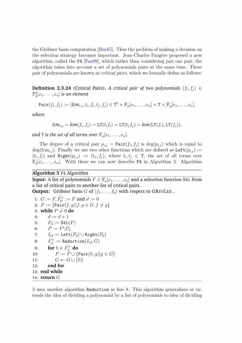
the Gröbner basis computation [Buc65]. Thus the problem of making a decision onthe selection strategy becomes important. Jean-Charles Faugère proposed a newalgorithm, called the F4 [Fau99], which rather than considering just one pair, thealgorithm takes into account a set of polynomials pairs at the same time. Thesepair of polynomials are known as critical pairs, which we formally define as follows:

Definition 2.3.24 (Critical Pairs). A critical pair of two polynomials (fi, fj) ∈F2q[x1, . . . , xn] is an element

Pair(fi, fj) := (lcmi,j, ti, fi, tj, fj) ∈ T2 × Fq[x1, . . . , xn]× T× Fq[x1, . . . , xn],

where

lcmi,j = lcm(fi, fj) = LT(tifi) = LT(tjfj) = lcm(LT(fi), LT(fj)),

and T is the set of all terms over Fq[x1, . . . , xn].

The degree of a critical pair pi,j = Pair(fi, fj) is deg(pi,j) which is equal todeg(lcmi,j). Finally we use two other functions which are defined as Left(pi,j) :=(ti, fi) and Right(pi,j) := (tj, fj), where ti, tj ∈ T, the set of all terms overFq[x1, . . . , xn]. With these we can now describe F4 in Algorithm 3. Algorithm

Algorithm 3 F4 AlgorithmInput: A list of polynomials F ∈ Fq[x1, . . . , xn] and a selection function SEL froma list of critical pairs to another list of critical pairs.Output: Gröbner basis G of 〈f1, . . . , fk〉 with respect to GREVLEX .

1: G := F, F+0 := F and d := 0

2: P := {Pair(f, g)|f, g ∈ G, f 6= g}3: while P 6= 0 do4: d := d+ 15: Pd := SEL(P )6: P := P\Pd

7: Ld := Left(Pd) ∪ Right(Pd)

8: F+d := Reduction(Ld, G)

9: for h ∈ F+d do

10: P := P ∪ {Pair(h, g)|g ∈ G}11: G← G ∪ {h}12: end for13: end while14: return G

3 uses another algorithm Reduction in line 8. This algorithm generalizes or ex-tends the idea of dividing a polynomial by a list of polynomials to idea of dividing

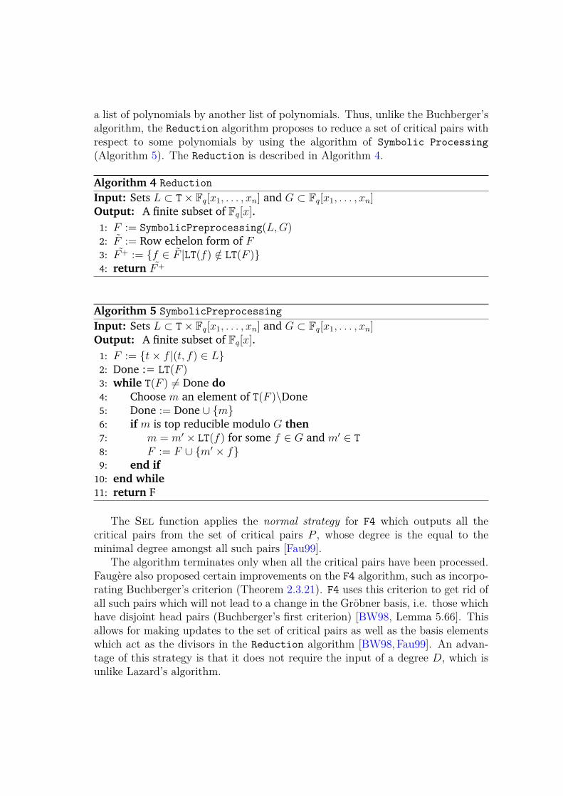
a list of polynomials by another list of polynomials. Thus, unlike the Buchberger’salgorithm, the Reduction algorithm proposes to reduce a set of critical pairs withrespect to some polynomials by using the algorithm of Symbolic Processing

(Algorithm 5). The Reduction is described in Algorithm 4.

Algorithm 4 Reduction

Input: Sets L ⊂ T× Fq[x1, . . . , xn] and G ⊂ Fq[x1, . . . , xn]Output: A finite subset of Fq[x].

1: F := SymbolicPreprocessing(L,G)2: F := Row echelon form of F3: F+ := {f ∈ F |LT(f) /∈ LT(F )}4: return F+

Algorithm 5 SymbolicPreprocessing

Input: Sets L ⊂ T× Fq[x1, . . . , xn] and G ⊂ Fq[x1, . . . , xn]Output: A finite subset of Fq[x].

1: F := {t× f |(t, f) ∈ L}2: Done := LT(F )3: while T(F ) 6= Done do4: Choose m an element of T(F )\Done5: Done := Done ∪ {m}6: if m is top reducible modulo G then7: m = m′ × LT(f) for some f ∈ G and m′ ∈ T

8: F := F ∪ {m′ × f}9: end if

10: end while11: return F

The Sel function applies the normal strategy for F4 which outputs all thecritical pairs from the set of critical pairs P , whose degree is the equal to theminimal degree amongst all such pairs [Fau99].

The algorithm terminates only when all the critical pairs have been processed.Faugère also proposed certain improvements on the F4 algorithm, such as incorpo-rating Buchberger’s criterion (Theorem 2.3.21). F4 uses this criterion to get rid ofall such pairs which will not lead to a change in the Gröbner basis, i.e. those whichhave disjoint head pairs (Buchberger’s first criterion) [BW98, Lemma 5.66]. Thisallows for making updates to the set of critical pairs as well as the basis elementswhich act as the divisors in the Reduction algorithm [BW98, Fau99]. An advan-tage of this strategy is that it does not require the input of a degree D, which isunlike Lazard’s algorithm.

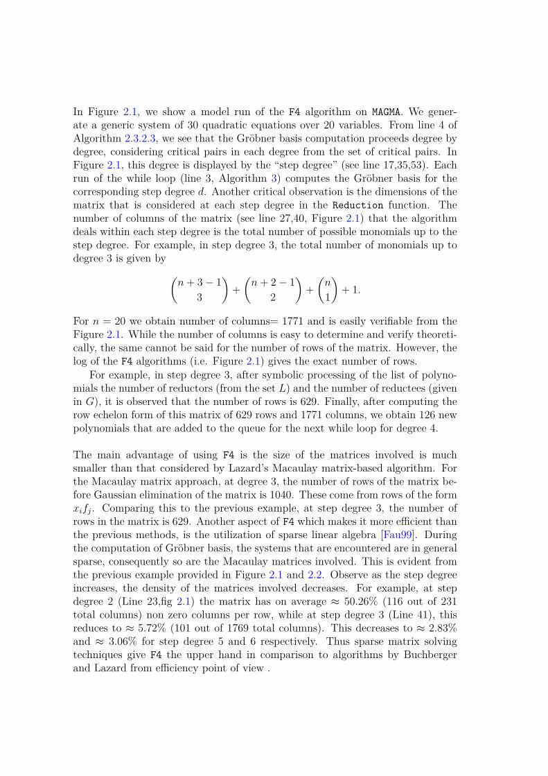
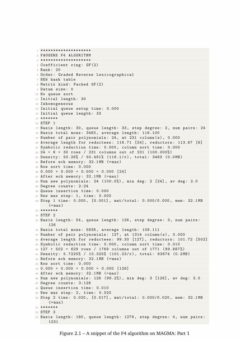
In Figure 2.1, we show a model run of the F4 algorithm on MAGMA. We gener-ate a generic system of 30 quadratic equations over 20 variables. From line 4 ofAlgorithm 2.3.2.3, we see that the Gröbner basis computation proceeds degree bydegree, considering critical pairs in each degree from the set of critical pairs. InFigure 2.1, this degree is displayed by the “step degree” (see line 17,35,53). Eachrun of the while loop (line 3, Algorithm 3) computes the Gröbner basis for thecorresponding step degree d. Another critical observation is the dimensions of thematrix that is considered at each step degree in the Reduction function. Thenumber of columns of the matrix (see line 27,40, Figure 2.1) that the algorithmdeals within each step degree is the total number of possible monomials up to thestep degree. For example, in step degree 3, the total number of monomials up todegree 3 is given by

(n+ 3− 1

3

)+

(n+ 2− 1

2

)+

(n

1

)+ 1.

For n = 20 we obtain number of columns= 1771 and is easily verifiable from theFigure 2.1. While the number of columns is easy to determine and verify theoreti-cally, the same cannot be said for the number of rows of the matrix. However, thelog of the F4 algorithms (i.e. Figure 2.1) gives the exact number of rows.

For example, in step degree 3, after symbolic processing of the list of polyno-mials the number of reductors (from the set L) and the number of reductees (givenin G), it is observed that the number of rows is 629. Finally, after computing therow echelon form of this matrix of 629 rows and 1771 columns, we obtain 126 newpolynomials that are added to the queue for the next while loop for degree 4.

The main advantage of using F4 is the size of the matrices involved is muchsmaller than that considered by Lazard’s Macaulay matrix-based algorithm. Forthe Macaulay matrix approach, at degree 3, the number of rows of the matrix be-fore Gaussian elimination of the matrix is 1040. These come from rows of the formxifj. Comparing this to the previous example, at step degree 3, the number ofrows in the matrix is 629. Another aspect of F4 which makes it more efficient thanthe previous methods, is the utilization of sparse linear algebra [Fau99]. Duringthe computation of Gröbner basis, the systems that are encountered are in generalsparse, consequently so are the Macaulay matrices involved. This is evident fromthe previous example provided in Figure 2.1 and 2.2. Observe as the step degreeincreases, the density of the matrices involved decreases. For example, at stepdegree 2 (Line 23,fig 2.1) the matrix has on average ≈ 50.26% (116 out of 231total columns) non zero columns per row, while at step degree 3 (Line 41), thisreduces to ≈ 5.72% (101 out of 1769 total columns). This decreases to ≈ 2.83%and ≈ 3.06% for step degree 5 and 6 respectively. Thus sparse matrix solvingtechniques give F4 the upper hand in comparison to algorithms by Buchbergerand Lazard from efficiency point of view .

1 ********************

2 FAUGERE F4 ALGORITHM

3 ********************

4 Coefficient ring: GF(2)

5 Rank: 20

6 Order: Graded Reverse Lexicographical

7 NEW hash table

8 Matrix kind: Packed GF(2)

9 Datum size: 0

10 No queue sort

11 Initial length: 30

12 Inhomogeneous

13 Initial queue setup time: 0.000

14 Initial queue length: 33

15 *******

16 STEP 1

17 Basis length: 30, queue length: 33, step degree: 2, num pairs: 24

18 Basis total mons: 3483, average length: 116.100

19 Number of pair polynomials: 24, at 231 column(s), 0.000

20 Average length for reductees: 116.71 [24], reductors: 113.67 [6]

21 Symbolic reduction time: 0.000, column sort time: 0.000

22 24 + 6 = 30 rows / 231 columns out of 231 (100.000%)

23 Density: 50.26% / 50.491% (116.1/r), total: 3483 (0.0MB)

24 Before ech memory: 32.1MB (=max)

25 Row sort time: 0.000

26 0.000 + 0.000 + 0.000 = 0.000 [24]

27 After ech memory: 32.1MB (=max)

28 Num new polynomials: 24 (100.0%) , min deg: 2 [24], av deg: 2.0

29 Degree counts: 2:24

30 Queue insertion time: 0.000

31 New max step: 1, time: 0.000

32 Step 1 time: 0.000, [0.001] , mat/total: 0.000/0.000 , mem: 32.1MB

(=max)

33 *******

34 STEP 2

35 Basis length: 54, queue length: 126, step degree: 3, num pairs:

126









44 0.000 + 0.000 + 0.000 = 0.000 [126]


46 Num new polynomials: 126 (99.2%) , min deg: 3 [126], av deg: 3.0





(=max)

51 *******

52 STEP 3


1231

Figure 2.1 – A snippet of the F4 algorithm on MAGMA: Part 1

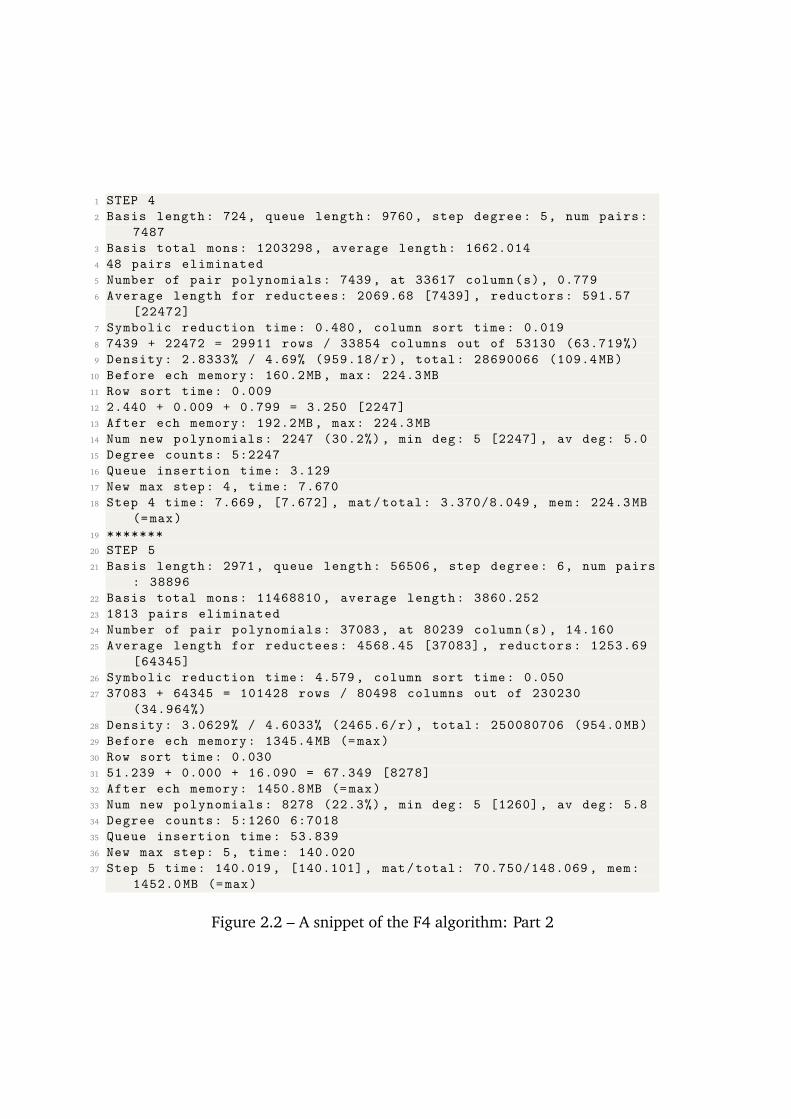
1 STEP 4


7487

3 Basis total mons: 1203298 , average length: 1662.014

4 48 pairs eliminated


6 Average length for reductees: 2069.68 [7439] , reductors: 591.57

[22472]



9 Density: 2.8333% / 4.69% (959.18/r), total: 28690066 (109.4 MB)

10 Before ech memory: 160.2MB , max: 224.3MB


12 2.440 + 0.009 + 0.799 = 3.250 [2247]

13 After ech memory: 192.2MB , max: 224.3MB

14 Num new polynomials: 2247 (30.2%) , min deg: 5 [2247] , av deg: 5.0





(=max)

19 *******

20 STEP 5

21 Basis length: 2971, queue length: 56506, step degree: 6, num pairs

: 38896





[64345]


27 37083 + 64345 = 101428 rows / 80498 columns out of 230230

(34.964%)


29 Before ech memory: 1345.4 MB (=max)


31 51.239 + 0.000 + 16.090 = 67.349 [8278]

32 After ech memory: 1450.8 MB (=max)

33 Num new polynomials: 8278 (22.3%) , min deg: 5 [1260] , av deg: 5.8

34 Degree counts: 5:1260 6:7018



37 Step 5 time: 140.019 , [140.101] , mat/total: 70.750/148.069 , mem:

1452.0 MB (=max)

Figure 2.2 – A snippet of the F4 algorithm: Part 2

Another interesting observation is that amount of time spent by individual sub-processes inside the F4 algorithm process. The majority time for each individualwhile loop is spent in computing the row echelon form of the matrix, which wasdiscussed previously. For example, let us consider the Step 4 (line 1) and Step 5(linen 20) from Figure 2.2. Step 4 takes a total time of 7.669 seconds (line 18).However, a majority amount of time (3.25 seconds) is spent inside the Reduction

process. Interestingly, an equivalent amount of time is spent by the queue insertionprocedure. This is because the implementation of F4 on MAGMA also implements anadditional procedure of updating the set of critical pairs and reductors by usingthe Buchberger criterion. Step 5 in Figure 2.2 we observe that selecting the num-ber of critical pairs at step degree 6 takes 14.16 seconds. Once the critical pairsare shortlisted, the algorithm proceeds to symbolically processing the list of pairswhich can be expected to reduce down to zero later taking 4.6 seconds. Finallyonce the matrix of polynomials is obtained, computing the row echelon form takes67.35 seconds.

2.3.2.4 Faugère’s F5 Algorithm

In the previous sections, we looked at some of the algorithms for computing Gröb-ner basis. Even though these are efficient algorithms however, these algorithmsshare a common aspect. Recalling Buchberger’s algorithm, computing the re-mainder of the S-polynomial division is redundant when the remainder is zero.Similarly in Lazard’s algorithm, it is seen that a large fraction of the polynomialsthat are constructed reduces to zero. Thus a large fraction of the running time ofthese algorithms is spent in computing and reducing these polynomials which arediscarded. Hence this part of the process is redundant.

From the Gröbner basis point of view, when an algorithm considers polyno-mials, which after performing some linear algebra operations reduces to zero, wesay that the algorithm performs reductions to zero. These “reductions to zero”are also known as syzygies. The practical efficiency of Gröbner basis algorithmsare greatly impacted by such reductions to zero [Fau02, Table 9]. Thus it is im-portant to avoid them as much as we can. There are several ways to predict suchreductions to zero [GM88,Fau02,EF14]. We shall focus on one such method, theF5 criterion [Fau02].

Assume we have two polynomials f1, f2 in the commutative polynomial ring F[x]of degrees d1 and d2. Constructing the matrix which contains all the multiples upto degree d1 + d2, the relation f1f2 − f2f1 = 0 induces reduction to zero duringthe linear algebra. These special reductions to zero are called trivial syzygies. Theidea of the F5 criterion is to use the index of the rows of the Macaulay matrix to

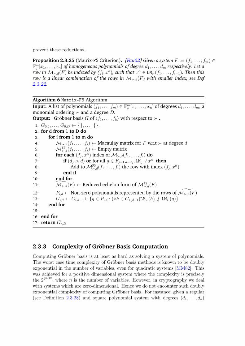
prevent these reductions.

Proposition 2.3.25 (Matrix-F5 Criterion). [Fau02] Given a system F := (f1, . . . , fm) ∈Fmq [x1, . . . , xn] of homogeneous polynomials of degree d1, . . . , dm respectively. Let a

row inM≻,d(F ) be indexed by (fi, xα), such that xα ∈ LM≻(f1, . . . , fi−1). Then this

row is a linear combination of the rows in M≻,d(F ) with smaller index, see Def

2.3.22.

Algorithm 6 Matrix-F5 AlgorithmInput: A list of polynomials (f1, . . . , fm) ∈ Fm

q [x1, . . . , xn] of degrees d1, . . . , dm, amonomial ordering ≻ and a degree D.Output: Gröbner basis G of 〈f1, . . . , fk〉 with respect to ≻ .

1: G0,0, . . . , G0,D ← {}, . . . , {}.2: for d from 1 to D do3: for i from 1 to m do4: M≻,d(f1, . . . , fi)← Macaulay matrix for F w.r.t ≻ at degree d5: MF5

≻,d(f1, . . . , fi)← Empty matrix6: for each (fj, x

α) index ofM≻,d(f1, . . . , fi) do7: if (dj > d) or for all g ∈ Fj−1.d−dj , LMg 6 | xα then8: Add toMF5

≻,d(f1, . . . , fi) the row with index (fj, xα)

9: end if10: end for11: M≻,d(F )← Reduced echelon form ofMF5

≻,d(F )

12: Pi,d ← Non-zero polynomials represented by the rows of M≻,d(F )13: Gi,d ← Gi,d−1 ∪ {g ∈ Pi,d : (∀h ∈ Gi.,d−1)LM≻(h) 6 | LM≻(g)}14: end for15:16: end for17: return Gr,D

2.3.3 Complexity of Gröbner Basis Computation

Computing Gröbner basis is at least as hard as solving a system of polynomials.The worst case time complexity of Gröbner basis methods is known to be doublyexponential in the number of variables, even for quadratic systems [MM82]. Thiswas achieved for a positive dimensional system where the complexity is preciselythe 22

n/10, where n is the number of variables. However, in cryptography we deal

with systems which are zero-dimensional. Hence we do not encounter such doublyexponential complexity of computing Gröbner basis. For instance, given a regular(see Definition 2.3.28) and square polynomial system with degrees (d1, . . . , dn)

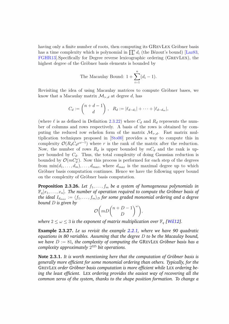
having only a finite number of roots, then computing its GRevLex Gröbner basishas a time complexity which is polynomial in

∏ni di (the Bézout’s bound) [Laz83,

FGHR13].Specifically for Degree reverse lexicographic ordering (GrevLex), thehighest degree of the Gröbner basis elements is bounded by

The Macaulay Bound: 1 +n∑

i=1

(di − 1).

Revisiting the idea of using Macaulay matrices to compute Gröbner bases, weknow that a Macaulay matrixM≻,d at degree d, has

Cd :=

(n+ d− 1

d

), Rd := |ℓd−d1 |+ · · ·+ |ℓd−dm |,

(where ℓ is as defined in Definition 2.3.22) where Cd and Rd represents the num-ber of columns and rows respectively. A basis of the rows is obtained by com-puting the reduced row echelon form of the matrix M≻,d. Fast matrix mul-tiplication techniques proposed in [Sto00] provides a way to compute this incomplexity O(RdCdr

ω−1) where r is the rank of the matrix after the reduction.Now, the number of rows Rd is upper bounded by mCd and the rank is up-per bounded by Cd. Thus, the total complexity of doing Gaussian reduction isbounded by O(mCω

d ). Now this process is performed for each step of the degreesfrom min(d1, . . . , dm), . . . , dmax, where dmax is the maximal degree up to whichGröbner basis computation continues. Hence we have the following upper boundon the complexity of Gröbner basis computation.

Proposition 2.3.26. Let f1, . . . , fm be a system of homogeneous polynomials in

Fq[x1, . . . , xn]. The number of operation required to compute the Gröbner basis of

the ideal Idmax := 〈f1, . . . , fm〉D for some graded monomial ordering and a degree

bound D is given by

O(mD

(n+D − 1

D

)ω),

where 2 ≤ ω ≤ 3 is the exponent of matrix multiplication over Fq [Wil12].

Example 2.3.27. Le us revisit the example 2.2.1, where we have 90 quadratic

equations in 80 variables. Assuming that the degree D to be the Macaulay bound,

we have D := 81, the complexity of computing the GREVLEX Gröbner basis has a

complexity approximately 2325 bit operations.

Note 2.3.1. It is worth mentioning here that the computation of Gröbner basis is

generally more efficient for some monomial ordering than others. Typically, for the

GREVLEX order Gröbner basis computation is more efficient while LEX ordering be-

ing the least efficient. LEX ordering provides the easiest way of recovering all the

common zeros of the system, thanks to the shape position formation. To change a

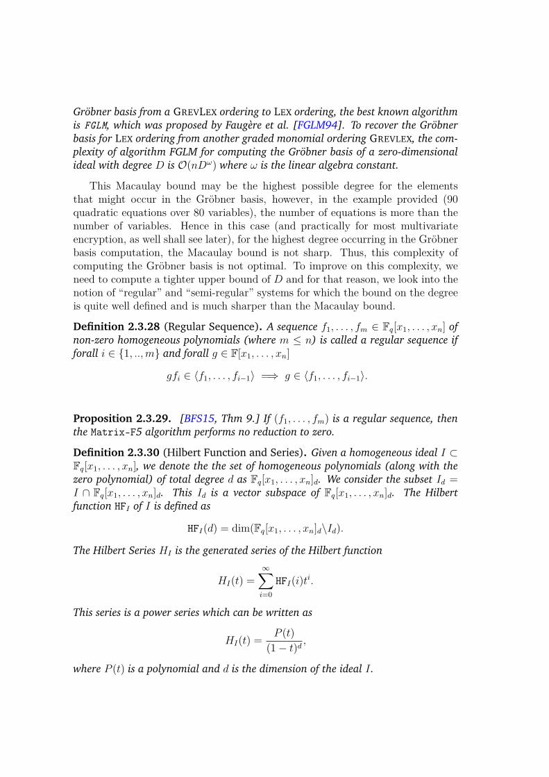
Gröbner basis from a GREVLEX ordering to LEX ordering, the best known algorithm

is FGLM, which was proposed by Faugère et al. [FGLM94]. To recover the Gröbner

basis for LEX ordering from another graded monomial ordering GREVLEX, the com-

plexity of algorithm FGLM for computing the Gröbner basis of a zero-dimensional

ideal with degree D is O(nDω) where ω is the linear algebra constant.

This Macaulay bound may be the highest possible degree for the elementsthat might occur in the Gröbner basis, however, in the example provided (90quadratic equations over 80 variables), the number of equations is more than thenumber of variables. Hence in this case (and practically for most multivariateencryption, as well shall see later), for the highest degree occurring in the Gröbnerbasis computation, the Macaulay bound is not sharp. Thus, this complexity ofcomputing the Gröbner basis is not optimal. To improve on this complexity, weneed to compute a tighter upper bound of D and for that reason, we look into thenotion of “regular” and “semi-regular” systems for which the bound on the degreeis quite well defined and is much sharper than the Macaulay bound.

Definition 2.3.28 (Regular Sequence). A sequence f1, . . . , fm ∈ Fq[x1, . . . , xn] of

non-zero homogeneous polynomials (where m ≤ n) is called a regular sequence if

forall i ∈ {1, ..,m} and forall g ∈ F[x1, . . . , xn]

gfi ∈ 〈f1, . . . , fi−1〉 =⇒ g ∈ 〈f1, . . . , fi−1〉.

Proposition 2.3.29. [BFS15, Thm 9.] If (f1, . . . , fm) is a regular sequence, then

the Matrix-F5 algorithm performs no reduction to zero.

Definition 2.3.30 (Hilbert Function and Series). Given a homogeneous ideal I ⊂Fq[x1, . . . , xn], we denote the the set of homogeneous polynomials (along with the

zero polynomial) of total degree d as Fq[x1, . . . , xn]d. We consider the subset Id =I ∩ Fq[x1, . . . , xn]d. This Id is a vector subspace of Fq[x1, . . . , xn]d. The Hilbert

function HFI of I is defined as

HFI(d) = dim(Fq[x1, . . . , xn]d\Id).

The Hilbert Series HI is the generated series of the Hilbert function

HI(t) =∞∑

i=0

HFI(i)ti.

This series is a power series which can be written as

HI(t) =P (t)

(1− t)d,

where P (t) is a polynomial and d is the dimension of the ideal I.

Property 2.3.31. [BFS04]

• A sequence of homogeneous polynomials (f1, . . . , fm) ∈ Fq[x1, . . . , xn], of de-

grees d1, . . . , dm, is regular if and only if its Hilbert series

H(t) :=

∏mi=1(1− tdi)

(1− t)n,

• The highest degree of elements of a Gröbner basis for the GREVLEX ordering

is less than the Macaulay bound,i.e.

n∑

i=1

(di − 1) + 1.

When the number of polynomials is greater than the number of variables (i.e.m > n), this notion of regular system doesn’t hold. However, a weak notion ofregular system can be introduced.

Definition 2.3.32 (d-regular system). [BFS04] A zero-dimensional over-determined

(m ≥ n) sequence of homogeneous equations (f1, . . . , fm) is called d-regular, if for

all i = 1, . . . ,m there exists a g such that

deg(g) < d− di and gfi ∈ 〈f1, . . . , fi−1〉,

then g ∈ 〈f1, . . . , fi−1〉.Definition 2.3.33 (Degree of regularity). For a zero-dimensional ideal I := 〈f1, . . . , fm〉(m ≥ n), the degree of regularity is given by

Dreg = min

{d ≥ 0 | dimFq({f ∈ I, deg(f) = d}) =

(n+ d− 1

d

)}.

Thus the monomials in degree Dreg are the leading terms for the elements inthe ideal. Thus this value is clearly an upper bound on the degree of the elementsoccurring in the Gröbner basis for any monomial ordering.

Remark 2.3.34. The degree of regularity for regular sequences (m ≤ n) is given by

the Macaulay bound∑m

i=0(di − 1) + 1 [Laz83,Mac02].

Definition 2.3.35 (Semi-regular system). [BFS04] If a system of equations is

Dreg-regular, then it is also called as semi-regular system.

From the Definition 2.3.33 we can compute the degree of regularity, however,the following proposition gives another more efficient quantitative approach tocompute this degree of regularity for a system of semi-regular system.

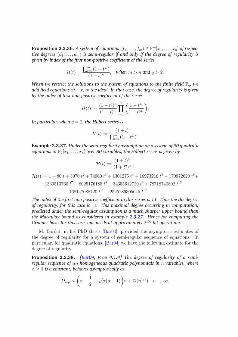
Proposition 2.3.36. A system of equations (f1, . . . , fm) ∈ Fmq [x1, . . . , xn] of respec-

tive degrees (d1, . . . , dm) is semi-regular if and only if the degree of regularity is

given by index of the first non-positive coefficient of the series

H(t) =∏m

i=1(1− tdi)

(1− t)n, when m > n and q > 2.

When we restrict the solutions to the system of equations to the finite field Fq, we

add field equations xqi −xi to the ideal. In that case, the degree of regularity is given

by the index of first non-positive coefficient of the series

H(t) :=(1− tq)n

(1− t)n

m∏

i=1

(1− tdi

1− tqdi

).

In particular, when q = 2, the Hilbert series is

H(t) :=(1 + t)n∏mi=1(1 + tdi)

.

Example 2.3.37. Under the semi-regularity assumption on a system of 90 quadratic

equations in F2[x1, . . . , xn] over 80 variables, the Hilbert series is given by

H(t) := (1 + t)80

(1 + t2)90,

H(t) := 1 + 80 t+ 3070 t2 + 74960 t3 + 1301275 t4 + 16973216 t5 + 170972620 t6+

1339513760 t7 + 8025176185 t8 + 34355612720 t9 + 78718740802 t10−168147088720 t11 − 2525289305045 t12 − · · · .

The index of the first non positive coefficient in this series is 11. Thus the the degree

of regularity, for this case is 11. This maximal degree occurring in computation,

predicted under the semi-regular assumption is a much sharper upper bound than

the Macaulay bound as considered in example 2.3.27. Hence for computing the

Gröbner basis for this case, one needs at approximately 2100 bit operations.

M. Bardet, in his PhD thesis [Bar04], provided the asymptotic estimates ofthe degree of regularity for a system of semi-regular sequence of equations. Inparticular, for quadratic equations, [Bar04] we have the following estimate for thedegree of regularity.

Proposition 2.3.38. [Bar04, Prop 4.1.4] The degree of regularity of a semi-

regular sequence of αn homogeneous quadratic polynomials in n variables, where

α ≥ 1 is a constant, behaves asymptotically as

Dreg ∼(α− 1

2−√

α(α− 1)

)n+O(n1/3), n→∞.

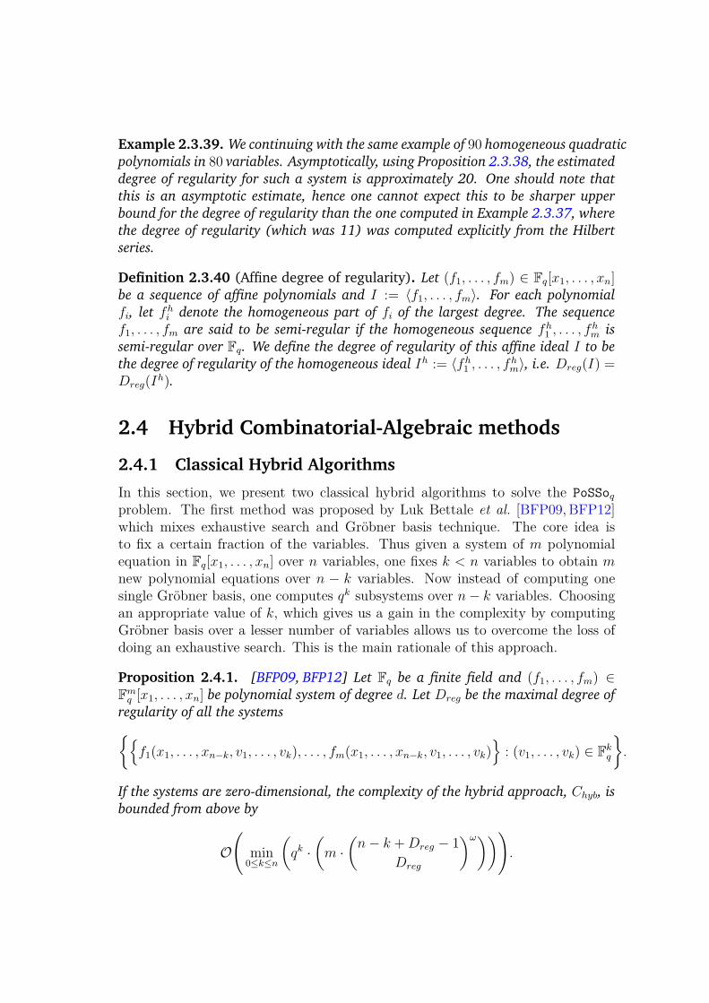
Example 2.3.39. We continuing with the same example of 90 homogeneous quadratic

polynomials in 80 variables. Asymptotically, using Proposition 2.3.38, the estimated

degree of regularity for such a system is approximately 20. One should note that

this is an asymptotic estimate, hence one cannot expect this to be sharper upper

bound for the degree of regularity than the one computed in Example 2.3.37, where

the degree of regularity (which was 11) was computed explicitly from the Hilbert

series.

Definition 2.3.40 (Affine degree of regularity). Let (f1, . . . , fm) ∈ Fq[x1, . . . , xn]be a sequence of affine polynomials and I := 〈f1, . . . , fm〉. For each polynomial

fi, let fhi denote the homogeneous part of fi of the largest degree. The sequence

f1, . . . , fm are said to be semi-regular if the homogeneous sequence fh1 , . . . , f

hm is

semi-regular over Fq. We define the degree of regularity of this affine ideal I to be

the degree of regularity of the homogeneous ideal Ih := 〈fh1 , . . . , f

hm〉, i.e. Dreg(I) =

Dreg(Ih).

2.4 Hybrid Combinatorial-Algebraic methods

2.4.1 Classical Hybrid Algorithms

In this section, we present two classical hybrid algorithms to solve the PoSSoqproblem. The first method was proposed by Luk Bettale et al. [BFP09, BFP12]which mixes exhaustive search and Gröbner basis technique. The core idea isto fix a certain fraction of the variables. Thus given a system of m polynomialequation in Fq[x1, . . . , xn] over n variables, one fixes k < n variables to obtain mnew polynomial equations over n − k variables. Now instead of computing onesingle Gröbner basis, one computes qk subsystems over n− k variables. Choosingan appropriate value of k, which gives us a gain in the complexity by computingGröbner basis over a lesser number of variables allows us to overcome the loss ofdoing an exhaustive search. This is the main rationale of this approach.

Proposition 2.4.1. [BFP09, BFP12] Let Fq be a finite field and (f1, . . . , fm) ∈Fmq [x1, . . . , xn] be polynomial system of degree d. Let Dreg be the maximal degree of

regularity of all the systems

{{f1(x1, . . . , xn−k, v1, . . . , vk), . . . , fm(x1, . . . , xn−k, v1, . . . , vk)

}: (v1, . . . , vk) ∈ Fk

q

}.

If the systems are zero-dimensional, the complexity of the hybrid approach, Chyb, is

bounded from above by

O(

min0≤k≤n

(qk ·

(m ·(n− k +Dreg − 1

Dreg

)ω))).

where d is the maximal degree of the ideal (i.e. number of solutions counted with

multiplicities in the algebraic closure of Fq) generated by the each qk subsystem and

2 ≤ ω ≤ 3 is a linear algebra constant.

Proposition 2.4.1 does not give any method to compute the best trade-off forthe number of fixed variables, k, such that the gain in the hybrid Gröbner basisalgorithm can be maximized with respect to generic Gröbner basis algorithms.However, for a semi-regular system (see Definition 2.3.35), knowing sharp esti-mates of the degree of regularity allows us to directly compute this trade-off. Asseen earlier, Proposition 2.3.38 gives us an asymptotic estimate to the degree ofregularity. Powered with this asymptotic estimate the idea is to find the value ofk for which the Chyb has a global minimum. The value of the k depends on m andq. Putting it more formally,

Theorem 2.4.2. [BFP09,BFP12] Let F = (f1, . . . , fm) ⊂ Fq[x1, . . . , xn] be a semi-

regular sequence of quadratic equations with m = αn (α > 0) and where for

all values of 0 ≤ k ≤ n and all possible vectors (v1, . . . , vk) ∈ Fkq , the quadratic

equations

f1(x1, xn−k, v1, . . . , vk), . . . , fm(x1, xn−k, v1, . . . , vk),

are semi-regular. Let A(β)

A(β) = log q + ω(log n+ log(1− β))

− ω

2

(1 +

√α

α + β − 1

)(log n+ log

(α +

1− β

2−√α(α + β − 1)

))

− ω

2

(1−

√α

α + β − 1

)(log n+ log

(α− 1− β

2−√α(α + β − 1)

)),

and let β0 be a non negative real root of A(β). The best trade off is to fix k = ⌊β0n⌋variables.

The values of this root β0 can be computed explicitly (see Table 4.1 of [Bet11]).For example, over a finite field of F2, with 2n quadratic equations over n variables,fixing k = ⌊0.51n⌋ variables gives the best complexity for the hybrid approach.However, with the same number of equations but over a finite field F22 , the mostoptimal value of k is ⌊0.042n⌋.

Example 2.4.3. We again revisit the example 2.2.1, where we have 90 quadratic

equations over 80 variables in F2[x1, . . . , xn]. According to [Bet11], in this case we

have k = ⌊0.7n⌋. The degree of regularity of the subsystems is bounded by index of

the first non positive coefficient of the Hilbert series

H(t) := (1 + t)24

(1 + t2)90,

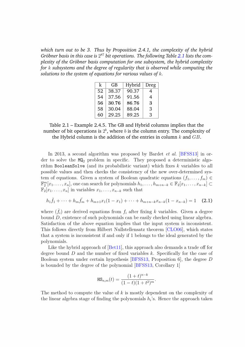
which turn out to be 3. Thus by Proposition 2.4.1, the complexity of the hybrid

Gröbner basis in this case is 287 bit operations. The following Table 2.1 lists the com-

plexity of the Gröbner basis computation for one subsystem, the hybrid complexity

for k subsystems and the degree of regularity that is observed while computing the

solutions to the system of equations for various values of k.

k GB Hybrid Dreg52 38.37 90.37 454 37.56 91.56 456 30.76 86.76 3

58 30.04 88.04 360 29.25 89.25 3

Table 2.1 – Example 2.4.5. The GB and Hybrid columns implies that thenumber of bit operations is 2b, where b is the column entry. The complexity of

the Hybrid column is the addition of the entries in column k and GB.

In 2013, a second algorithm was proposed by Bardet et al. [BFSS13] in or-der to solve the MQ2 problem in specific. They proposed a deterministic algo-rithm BooleanSolve (and its probabilistic variant) which fixes k variables to allpossible values and then checks the consistency of the new over-determined sys-tem of equations. Given a system of Boolean quadratic equations (f1, . . . , fm) ∈Fm2 [x1. . . . , xn], one can search for polynomials h1, . . . , hm+n−k ∈ F2[x1, . . . , xn−k] ⊂

F2[x1. . . . , xn] in variables x1, . . . , xn−k such that

h1f1 + · · ·+ hmfm + hm+1x1(1− x1) + · · ·+ hm+n−kxn−k(1− xn−k) = 1 (2.1)

where ¯(fi) are derived equations from fi after fixing k variables. Given a degreebound D, existence of such polynomials can be easily checked using linear algebra.Satisfaction of the above equation implies that the input system is inconsistent.This follows directly from Hilbert Nullstellensatz theorem [CLO06], which statesthat a system is inconsistent if and only if 1 belongs to the ideal generated by thepolynomials.

Like the hybrid approach of [Bet11], this approach also demands a trade off fordegree bound D and the number of fixed variables k. Specifically for the case ofBoolean system under certain hypothesis [BFSS13, Proposition 6], the degree Dis bounded by the degree of the polynomial [BFSS13, Corollary 1]

HSn,m(t) =(1 + t)n−k

(1− t)(1 + t2)m.

The method to compute the value of k is mostly dependent on the complexity ofthe linear algebra stage of finding the polynomials hi’s. Hence the approach taken

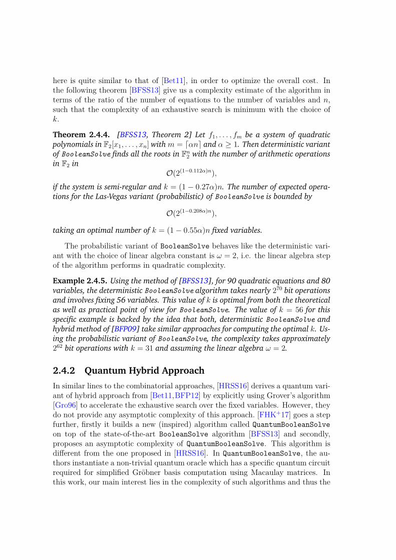
here is quite similar to that of [Bet11], in order to optimize the overall cost. Inthe following theorem [BFSS13] give us a complexity estimate of the algorithm interms of the ratio of the number of equations to the number of variables and n,such that the complexity of an exhaustive search is minimum with the choice ofk.

Theorem 2.4.4. [BFSS13, Theorem 2] Let f1, . . . , fm be a system of quadratic

polynomials in F2[x1, . . . , xn] with m = ⌈αn⌉ and α ≥ 1. Then deterministic variant

of BooleanSolve finds all the roots in Fn2 with the number of arithmetic operations

in F2 in

O(2(1−0.112α)n),if the system is semi-regular and k = (1− 0.27α)n. The number of expected opera-

tions for the Las-Vegas variant (probabilistic) of BooleanSolve is bounded by

O(2(1−0.208α)n),

taking an optimal number of k = (1− 0.55α)n fixed variables.

The probabilistic variant of BooleanSolve behaves like the deterministic vari-ant with the choice of linear algebra constant is ω = 2, i.e. the linear algebra stepof the algorithm performs in quadratic complexity.

Example 2.4.5. Using the method of [BFSS13], for 90 quadratic equations and 80

variables, the deterministic BooleanSolve algorithm takes nearly 270 bit operations

and involves fixing 56 variables. This value of k is optimal from both the theoretical

as well as practical point of view for BooleanSolve. The value of k = 56 for this

specific example is backed by the idea that both, deterministic BooleanSolve and

hybrid method of [BFP09] take similar approaches for computing the optimal k. Us-

ing the probabilistic variant of BooleanSolve, the complexity takes approximately

262 bit operations with k = 31 and assuming the linear algebra ω = 2.

2.4.2 Quantum Hybrid Approach

In similar lines to the combinatorial approaches, [HRSS16] derives a quantum vari-ant of hybrid approach from [Bet11,BFP12] by explicitly using Grover’s algorithm[Gro96] to accelerate the exhaustive search over the fixed variables. However, theydo not provide any asymptotic complexity of this approach. [FHK+17] goes a stepfurther, firstly it builds a new (inspired) algorithm called QuantumBooleanSolve

on top of the state-of-the-art BooleanSolve algorithm [BFSS13] and secondly,proposes an asymptotic complexity of QuantumBooleanSolve. This algorithm isdifferent from the one proposed in [HRSS16]. In QuantumBooleanSolve, the au-thors instantiate a non-trivial quantum oracle which has a specific quantum circuitrequired for simplified Gröbner basis computation using Macaulay matrices. Inthis work, our main interest lies in the complexity of such algorithms and thus the

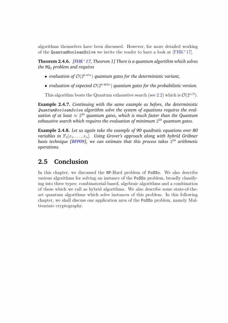
algorithms themselves have been discussed. However, for more detailed workingof the QuantumBooleanSolve we invite the reader to have a look at [FHK+17].

Theorem 2.4.6. [FHK+17, Theorem 1] There is a quantum algorithm which solves

the MQ2 problem and requires

• evaluation of O(20.47n) quantum gates for the deterministic variant,

• evaluation of expected O(20.462n) quantum gates for the probabilistic version.

This algorithm beats the Quantum exhaustive search (see 2.2) which isO(2n/2).

Example 2.4.7. Continuing with the same example as before, the deterministic

QuantumBooleanSolve algorithm solve the system of equations requires the eval-

uation of at least ≈ 238 quantum gates, which is much faster than the Quantum

exhaustive search which requires the evaluation of minimum 259 quantum gates.

Example 2.4.8. Let us again take the example of 90 quadratic equations over 80

variables in F2[x1, . . . , xn]. Using Grover’s approach along with hybrid Gröbner

basis technique [BFP09], we can estimate that this process takes 259 arithmetic

operations.

2.5 Conclusion

In this chapter, we discussed the NP-Hard problem of PoSSo. We also describevarious algorithms for solving an instance of the PoSSo problem, broadly classify-ing into three types: combinatorial-based, algebraic algorithms and a combinationof these which we call as hybrid algorithms. We also describe some state-of-the-art quantum algorithms which solve instances of this problem. In this followingchapter, we shall discuss one application area of the PoSSo problem, namely Mul-tivariate cryptography.

Chapter 3

Quantum-Safe Public-keyCryptography

Abstract

Public-key cryptography is based on certain problems that are knownto be hard to solve. Unfortunately, with the advent of quantum com-puters, some of these hard problems are solvable. Although, a subsetof such problems are known to be still safe from quantum attacks.Thus, quantum-safe public-key cryptography has become major fieldof interest for security researchers and is exhibited by the strong stepstaken by NIST to standardize new quantum-safe cryptosystems. Inthis chapter, we present some historical as well as current cryptosys-tems that are quantum safe. In particular, we focus on multivariatebased cryptography which is also the main focus of this thesis.

In the following sections we take special interest in one category of post-quantumcryptosystems: Multivariate based cryptography. We start with discussions onsome of the most prominent state-of-the-art multivariate cryptosystems and alsolist the known attacks on such systems in some detail. The final part of thechapter discusses lattice based cryptography briefly, where we list one of the mainlattice based hard problems that forms the security foundation of lattice basedcryptosystems. In addition, we also present a lattice based scheme: Frodo, thatinfluenced the design of a multivariate key-exchange scheme by us, the details ofwhich have been discussed in great detail in Chapter 6.

3.1 Multivariate Public-Key Cryptography

Multivariate Public-Key Cryptography (MPKC) is a subclass of asymmetric cryp-tography that deals with the cryptographic schemes whose hardness are basedon the PoSSoq problem (see Section 2.1). MPKC is a very active area of research

43

that culminated with the NIST Post-Quantum Cryptography standardization pro-cess [CCJ+16]. As mentioned previously in Chapter 1, it is one of the candidateareas for design of post-quantum cryptosystems. About 10% out of 69 submis-sions were multivariate. In the following section, we give an overview of the mostprominent multivariate schemes.

3.1.1 General Structure

A special subclass of MPKC is Multivariate Quadratic (MQ) cryptography, that relieson the hardness of solving the MQ problem (see Chapter 2). The design principleof a MQ cryptosystem can be traced back to the first ever known example, C∗, thatwas proposed by Matsumoto Imai [MI88]. Before we discuss the public and theprivate keys, we give a few prerequisites.

Definition 3.1.1. Let E be a simple extension field of Fq of degree n, ω ∈ E be

the primitive element E/Fq and let Fnq be the corresponding vector space. Then E

can be considered as a vector space over Fnq through a vector space isomorphism

φ : E = Fqn → Fnq such that for any element v = v1 + v2ω + · · · + vnω

n−1 ∈ E, we

have

φ(v) = (v1, v2, . . . , vn) ∈ Fnq .

With these definitions we can now enlist the secret-key of the C∗ scheme. Itincludes a function F : Fn

q 7→ Fnq such that ∀w ∈ Fn

q we have,

F (w) = φ ◦ (φ−1(w))1+qα ,

where φ is a map from Fqn to Fnq (see Definition 3.1.1). The choice of α ∈ N

is such that gcd(1 + qα, qn − 1) = 1. The polynomials resulting from F are ofdegree 2 and have a certain structure. Therefore, it becomes imperative to maskthe system of polynomials. We define Affn(Fq) ≃ Fn×n

q × Fnq as the collection of

the invertible affine transformations over Fnq . The secret-key also comprises of two

transformations S = (S, s) ∈ Affn(Fq) and T = (T, t) ∈ Affn(Fq) where n is apositive integer.

The public-key is given by the construction P = T ◦ F ◦ S where ◦ functioncomposes two maps. Thus public-key is a system of polynomials (p1, . . . , pn) ∈Fnq [x1, . . . , xn] such that

(p1, . . . , pn) = T · (f1(x′1, . . . , x′n), . . . , fn(x′1, . . . , x′n)) + t,

where F = (f1, . . . , fn) ∈ Fnq [x1, . . . , xn] and (x′1, . . . , x

′n) = S ·(x1, . . . , xn)+s. The

main idea is to mask the polynomial system F with the application of the affinetransformations S and T .

The number of public-key equations is equal to the number of variables in thecase of C∗, however, for other multivariate schemes, it is not always the case. Hencefrom now on, we shall denote the number of public-key equations as m and thenumber of variables as n.

Most current multivariate cryptosystems employ the same design principle asC∗ to construct the public-key P : composing a m-tuple quadratic polynomialsF : Fn

q 7→ Fmq , which we call as a central trapdoor, with two invertible affine

transformations S ∈ Affn(Fq) and T ∈ Affm(Fq). These schemes differ in theconstruction of the central map F as we shall see in Section 3.1.2. We point out thatwe can also use linear transformations S, T instead of the affine transformationsS, T . This restriction may be used for ease of notation.

3.1.1.1 Encryption and Decryption

To encrypt a message a = (a1, . . . , an) ∈ Fnq , one computes the ciphertext c ∈ Fm

q

by evaluating the public-key (p1, . . . , pm) ∈ Fmq [x1, . . . , xn] over the message a, i.e.

c = (c1, . . . , cm) = (p1(a1, . . . , an), . . . , pm(a1, . . . , an)) ∈ Fmq .

The number of operations required for encryption is effectively upper bounded by(n+22

)multiplications and

(n+22

)− 1 additions for each of the m quadratic polyno-

mials in the public-key. Thus, overall we have O(mn2) arithmetic operations overFq.

The holder of the secret-key can then decrypt the ciphertext c ∈ Fmq by invert-

ing each polynomial map that composes the public-key. It should be noted thatthe central trapdoor F in general is not a bijection. Inverting the map F impliesthe application of the decryption procedure. For ease of notation, we denote thisdecryption process by F−1. Hence we have

a′ = S−1 ◦ F−1 ◦ T −1(c) ∈ Fnq ,

where ◦ is the composition map previously defined. For decryption to output aunique plaintext, one requires the public-key to be an injective map. Thus weneed m ≥ n. The number of operations for decryption depends on the choice ofthe trapdoor chosen for constructing the map F .

3.1.1.2 Signature

A digital signature can also be constructed using similar ideas. Digital signatureinvolves two processes: signature generation and signature verification. To gen-erate a signature s ∈ Fn

q for a message a ∈ Fmq , one can apply the decryption

process to find a solution. However, unlike the decryption process in encryptionschemes, signature generation need not be unique. Thus one can have m < n. Soany s ∈ Fn

q which is a solution to

s = S−1 ◦ F−1 ◦ T −1(a),

is a possible signature to the message a, where ◦ is the composition map. Signatureverification is simply the process of evaluating the public-key P = T ◦F ◦S over thesignature s. The signature s is a correct signature for the corresponding messagea if P (s) = a.

3.1.2 Historical Cryptosystems

Amongst the current cryptosystems, the most significant multivariate primitive,which was proposed by Patarin, is Hidden Field Equations (HFE) [Pat96]. Thecentral trapdoor of HFE is quite different from C∗. For HFE, it is a degree boundedextended Dembowski-Ostrom polynomial [DO68,CM97] map

g : X ∈ Fqn 7→ y =∑

0≤i,j≤d

αijXqi+qj +

∑

0≤i≤d

βiXqi + γ0,

where

αijXqi+qj with αij ∈ Fqn are the quadratic terms,

βiXqi with βi ∈ Fqn are the linear terms,

γ0 with γ0 ∈ Fqn is the constant term,

for i, j ∈ N and some degree d ∈ N. Inverting g implies solving a univariateequation of high degree over Fqn . This inversion has been quite extensively studiedin [Ber67, CZ81]. The expected cost of computing using the algorithm of [Ber67]is O(nD2 log q +D3), where D is the maximal degree of g. For efficient inversionof g, the degree D should be small, which in turn implies d should be small.

In HFE, it is important to note that the central trapdoor is defined as a poly-nomial map over some extension field Fqn and has a univariate representation.However, this polynomial also has an equivalent multivariate representation overthe field Fq.

Note 3.1.1. Due to Frobenius automorphism, X → Xq is a linear mapping in the

finite field Fq as well as the extension field Fqn. Therefore, all sums of monomials

that are of the form Xqi ∈ Fqn [X], 0 ≤ i < n are also linear over Fq[x1, . . . , xn][SK99], where X = φ−1(x1, . . . , xn).

Lemma 3.1.2. Let Fq be the base field and Fqn , a degree n extension. Then for a

polynomial F ∈ Fqn [X]

F(X) =∑

0≤i,j≤n−1

αi,jXqi+qj +

n−1∑

i=0

βiXqi + γ0,

with αi,j .βi, γ0 ∈ Fqn , there exists a unique system of quadratic polynomials F =(f1, . . . , fn) ∈ Fn

q [x1, . . . , xn], such that F(X) = φ−1(F (φ(X))), where φ : Fqn 7→Fnq is a isomorphism as defined in Definition 3.1.1.

The Oil and Vinegar construction is another family of MQ schemes that wasproposed by Patarin [Pat97]. This construction of the central trapdoor uses twosets of variables, called oil and vinegar. Let o ∈ N be the number of oil variableswhile v ∈ N be the number of vinegar variables, such that n = (o + v). Werepresent the oil variables as {x1, . . . , xo} and the vinegar variables are representedas {x′1, . . . , x′v}. We say that the polynomial f(x1, . . . , xo, x

′1, . . . , x

′v) : F

oq×Fv

q → Fq

below has a Oil and Vinegar shape if it has the following structure

f(x1, . . . , xo, x′1, . . . , x

′v) =

∑

0≤i,j≤v

αijx′ix′j +

∑

0≤i≤v,0≤j≤o

α′ijx′ixj

+∑

0≤i≤v

βix′i +

∑

0≤i≤o

β′ixi + γ0.(3.1)

where αij, α′ij , βi, β

′i, γ0 ∈ Fq. The vinegar variables (x′1, . . . , x

′v) can combine

quadratically while the oil variables (x1, . . . , xo) do not mix with the oil variables.To construct the cryptographic trapdoor based on this structure, one constructs

a map F : Fo+vq → Fo

q,

F (x1, . . . , xo, x′1, . . . , x

′v) = (f1(x1, . . . , xo, x

′1, . . . , x

′v), . . . , fo(x1, . . . , xo, x

′1, . . . , x

′v)),

where the polynomials (f1, . . . , fo) ∈ Foq[x1, . . . , xo, x

′1, . . . , x

′v] have the structure

of Equation (3.1). This scheme is mostly useful in the design of digital signatures.Given a message a ∈ Fo

q, one sets the vinegar variables to some random value(b1, . . . , bv) ∈ Fv

q and solve the resulting system of linear equations

F (x1, . . . , xo, b1, . . . , bv) = a.

A non-zero solution to this system of equation is a candidate signature for the mes-sage a. A variant of this scheme was suggested with an unequal number of oil andvinegar variables (o 6= v), most famously known as the Unbalanced Oil and Vine-gar signature (UOV) scheme [KPG99] after Kipnis and Shamir broke the balancedOil and Vinegar scheme [KS98], which fixed o = v = n/2. This attack by Kipnisand Shamir also works on UOV in a probabilistic manner and has a complexity ofO(qn−2o−1o4). So this scheme should have v ≥ 3o for a secure construction. Thelatest security evaluations for UOV can be found in [BWP05]. The Rainbow sig-nature scheme [DS05] is another derivative of the UOV construction with multiplelayers of oil and vinegar variables. Lifted-UOV (LUOV) [BPSV19] is a multivariatesignature scheme that slightly modifies on the existing structure of UOV to reducethe size of public-keys. The scheme accomplishes this by lifting the public-key toan extension field. More specifically, instead of working over F2, LUOV works overan extension field F2r keeping the coefficients unchanged. Thus even though thepublic-key have the same coefficients, solving the system for some ciphertexts inFm2r is more difficult than that for some ciphertext over Fm

2 . However, very recentlyan attack against LOUV was proposed [DZD+19]. The attack takes use of the fact

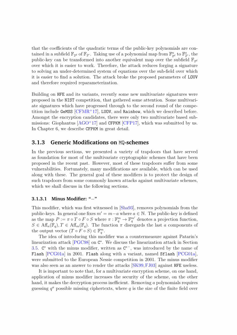
that the coefficients of the quadratic terms of the public-key polynomials are con-tained in a subfield F2d of F2r . Taking use of a polynomial map from Fn

2dto Fo

2r , thepublic-key can be transformed into another equivalent map over the subfield F2d

over which it is easier to work. Therefore, the attack reduces forging a signatureto solving an under-determined system of equations over the sub-field over whichit is easier to find a solution. The attack broke the proposed parameters of LOUV

and therefore required reparameterization.

Building on HFE and its variants, recently some new multivariate signatures wereproposed in the NIST competition, that gathered some attention. Some multivari-ate signatures which have progressed through to the second round of the compe-tition include GeMSS [CFMR+17], LUOV, and Rainbow, which we described before.Amongst the encryption candidates, there were only two multivariate based sub-missions: Giophantus [AGO+17] and CFPKM [CFP17], which was submitted by us.In Chapter 6, we describe CFPKM in great detail.

3.1.3 Generic Modifications on MQ-schemes

In the previous sections, we presented a variety of trapdoors that have servedas foundation for most of the multivariate cryptographic schemes that have beenproposed in the recent past. However, most of these trapdoors suffer from somevulnerabilities. Fortunately, many modifications are available, which can be usedalong with these. The general goal of these modifiers is to protect the design ofsuch trapdoors from some commonly known attacks against multivariate schemes,which we shall discuss in the following sections.

3.1.3.1 Minus Modifier: “−”

This modifier, which was first witnessed in [Sha93], removes polynomials from thepublic-keys. In general one fixes m′ = m−a where a ∈ N. The public-key is definedas the map P := π ◦ T ◦ F ◦ S where π : Fm

q → Fm′

q denotes a projection function,S ∈ Affn(Fq), T ∈ Affm(Fq). The function π disregards the last a components ofthe output vector (T ◦ F ◦ S) ∈ Fm

q .The idea of introducing this modifier was a countermeasure against Patarin’s

linearization attack [PGC98] on C∗. We discuss the linearization attack in Section3.5. C∗ with the minus modifier, written as C∗−, was introduced by the name ofFlash [PCG01a] in 2001. Flash along with a variant, named Sflash [PCG01a],were submitted to the European Nessie competition in 2001. The minus modifierwas also seen as an answer to render the attacks [SK99,FJ03] against HFE useless.

It is important to note that, for a multivariate encryption scheme, on one hand,application of minus modifier increases the security of the scheme, on the otherhand, it makes the decryption process inefficient. Removing a polynomials requiresguessing qa possible missing ciphertexts, where q is the size of the finite field over

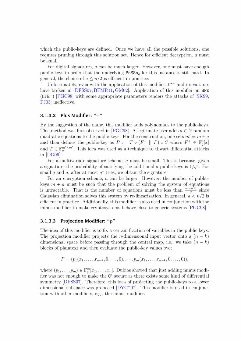
which the public-keys are defined. Once we have all the possible solutions, onerequires pruning through this solution set. Hence for efficient decryption, a mustbe small.

For digital signatures, a can be much larger. However, one must have enoughpublic-keys in order that the underlying PoSSoq for this instance is still hard. Ingeneral, the choice of a ≤ n/2 is efficient in practice.

Unfortunately, even with the application of this modifier, C∗− and its variantshave broken in [DFSS07, BFMR11, GM02]. Application of this modifier on HFE

(HFE−) [PGC98] with some appropriate parameters renders the attacks of [SK99,FJ03] ineffective.

3.1.3.2 Plus Modifier: “+”

By the suggestion of the name, this modifier adds polynomials to the public-keys.This method was first observed in [PGC98]. A legitimate user adds a ∈ N randomquadratic equations to the public-keys. For the construction, one sets m′ = m+ aand then defines the public-key as P := T ◦ (F+ || F ) ◦ S where F+ ∈ Fa

q [x]

and T ∈ Fm′×m′

q . This idea was used as a technique to thwart differential attacksin [DG06].

For a multivariate signature scheme, a must be small. This is because, givena signature, the probability of satisfying the additional a public-keys is 1/qa. Forsmall q and a, after at most qa tries, we obtain the signature.

For an encryption scheme, a can be larger. However, the number of public-keys m + a must be such that the problem of solving the system of equationsis intractable. That is the number of equations must be less than n(n+1)

2since

Gaussian elimination solves this system by re-linearization. In general, a < n/2 isefficient in practice. Additionally, this modifier is also used in conjunction with theminus modifier to make cryptosystems behave close to generic systems [PGC98].

3.1.3.3 Projection Modifier: “p”

The idea of this modifier is to fix a certain fraction of variables in the public-keys.The projection modifier projects the n-dimensional input vector onto a (n − k)dimensional space before passing through the central map, i.e., we take (n − k)blocks of plaintext and then evaluate the public-key values over

P = (p1(x1, . . . , xn−k, 0, . . . , 0), . . . , pm(x1, . . . , xn−k, 0, . . . , 0)),

where (p1, . . . , pm) ∈ Fmq [x1, . . . , xn]. Dubios showed that just adding minus modi-

fier was not enough to make the C∗ secure as there exists some kind of differentialsymmetry [DFSS07]. Therefore, this idea of projecting the public-keys to a lowerdimensional subspace was proposed [DYC+07]. This modifier is used in conjunc-tion with other modifiers, e.g., the minus modifier.

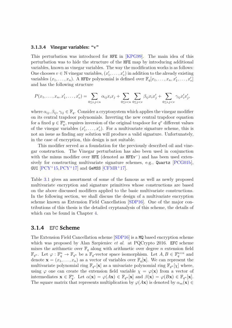
3.1.3.4 Vinegar variables: “v”

This perturbation was introduced for HFE in [KPG99]. The main idea of thisperturbation was to hide the structure of the HFE map by introducing additionalvariables, known as vinegar variables. The way the modification works is as follows:One chooses v ∈ N vinegar variables, (x′1, . . . , x

′v) in addition to the already existing

variables (x1, . . . , xn). A HFEv polynomial is defined over Fq[x1, . . . , xn, x′1, . . . , x

′v]

and has the following structure

P (x1, . . . , xn, x′1, . . . , x

′v) =

∑

0≤i,j<n

αijxixj +∑

0≤i<n

∑

0≤j<v

βijxix′j +

∑

0≤i,j<v

γijx′ix′j,

where αij , βij , γij ∈ Fq. Consider a cryptosystem which applies the vinegar modifieron its central trapdoor polynomials. Inverting the new central trapdoor equationfor a fixed y ∈ Fn

q , requires inversion of the original trapdoor for qv different valuesof the vinegar variables (x′1, . . . , x

′v). For a multivariate signature scheme, this is

not an issue as finding any solution will produce a valid signature. Unfortunately,in the case of encryption, this design is not suitable.

This modifier served as a foundation for the previously described oil and vine-gar construction. The Vinegar perturbation has also been used in conjunctionwith the minus modifier over HFE (denoted as HFEv−) and has been used exten-sively for constructing multivariate signature schemes, e.g., Quartz [PCG01b],GUI [PCY+15,PCY+17] and GeMSS [CFMR+17].

Table 3.1 gives an assortment of some of the famous as well as newly proposedmultivariate encryption and signature primitives whose constructions are basedon the above discussed modifiers applied to the basic multivariate constructions.In the following section, we shall discuss the design of a multivariate encryptionscheme known as Extension Field Cancellation [SDP16]. One of the major con-tributions of this thesis is the detailed cryptanalysis of this scheme, the details ofwhich can be found in Chapter 4.

3.1.4 EFC Scheme

The Extension Field Cancellation scheme [SDP16] is a MQ based encryption schemewhich was proposed by Alan Szepieniec et al. at PQCrypto 2016. EFC schememixes the arithmetic over Fq along with arithmetic over degree n extension fieldFqn . Let ϕ : Fn

q → Fqn be a Fq-vector space isomorphism. Let A,B ∈ Fn×nq and

denote x = (x1, . . . , xn) as a vector of variables over Fq[x]. We can represent themultivariate polynomial ring Fqn [x] as a univariate polynomial ring Fqn [χ] where,using ϕ one can create the extension field variable χ = ϕ(x) from a vector ofintermediates x ∈ Fn

q . Let α(x) = ϕ(Ax) ∈ Fqn [x] and β(x) = ϕ(Bx) ∈ Fqn [x].The square matrix that represents multiplication by ϕ(Ax) is denoted by αm(x) ∈

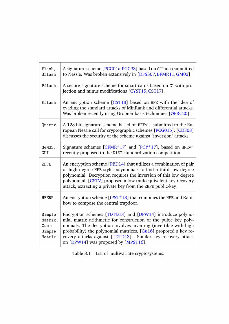
Flash,

Sflash

A signature scheme [PCG01a,PGC98] based on C∗− also submittedto Nessie. Was broken extensively in [DFSS07,BFMR11,GM02]

Pflash A secure signature scheme for smart cards based on C∗ with pro-jection and minus modifications [CYST15,CST17].

Eflash An encryption scheme [CST18] based on HFE with the idea ofevading the standard attacks of MinRank and differential attacks.Was broken recently using Gröbner basis techniques [ØFRC20].

Quartz A 128 bit signature scheme based on HFEv−, submitted to the Eu-ropean Nessie call for cryptographic schemes [PCG01b]. [CDF03]discusses the security of the scheme against "inversion" attacks.

GeMSS,

GUI

Signature schemes [CFMR+17] and [PCY+17], based on HFEv−

recently proposed to the NIST standardization competition.

ZHFE An encryption scheme [PBD14] that utilizes a combination of pairof high degree HFE style polynomials to find a third low degreepolynomial. Decryption requires the inversion of this low degreepolynomial. [CSTV] proposed a low rank equivalent key recoveryattack, extracting a private key from the ZHFE public-key.

HFERP An encryption scheme [IPST+18] that combines the HFE and Rain-bow to compose the central trapdoor.

Simple

Matrix,

Cubic

Simple

Matrix

Encryption schemes [TDTD13] and [DPW14] introduce polyno-mial matrix arithmetic for construction of the pubic key poly-nomials. The decryption involves inverting (invertible with highprobability) the polynomial matrices. [Gu16] proposed a key re-covery attacks against [TDTD13]. Similar key recovery attackon [DPW14] was proposed by [MPST16].

Table 3.1 – List of multivariate cryptosystems.

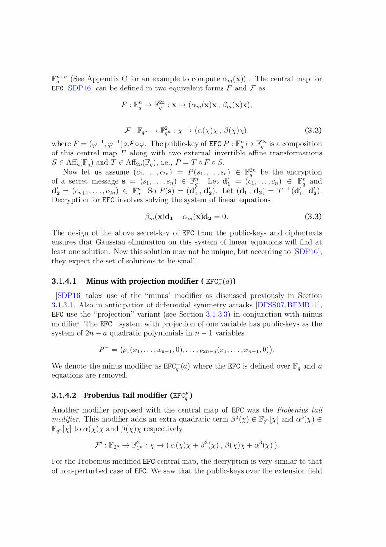
Fn×nq (See Appendix C for an example to compute αm(x)) . The central map for

EFC [SDP16] can be defined in two equivalent forms F and F as

F : Fnq → F2n

q : x→ (αm(x)x , βm(x)x),

F : Fqn → F2qn : χ→ (α(χ)χ , β(χ)χ). (3.2)

where F = (ϕ−1, ϕ−1)◦F ◦ϕ. The public-key of EFC P : Fnq 7→ F2n

q is a compositionof this central map F along with two external invertible affine transformationsS ∈ Affn(Fq) and T ∈ Aff2n(Fq), i.e., P = T ◦ F ◦ S.

Now let us assume (c1, . . . , c2n) = P (s1, . . . , sn) ∈ F2nq be the encryption

of a secret message s = (s1, . . . , sn) ∈ Fnq . Let d′

1= (c1, . . . , cn) ∈ Fn

q andd′2= (cn+1, . . . , c2n) ∈ Fn

q . So P (s) = (d′1, d′

2). Let (d1 , d2) = T−1 (d′

1, d′

2).

Decryption for EFC involves solving the system of linear equations

βm(x)d1 − αm(x)d2 = 0. (3.3)

The design of the above secret-key of EFC from the public-keys and ciphertextsensures that Gaussian elimination on this system of linear equations will find atleast one solution. Now this solution may not be unique, but according to [SDP16],they expect the set of solutions to be small.

3.1.4.1 Minus with projection modifier ( EFC−q (a))

[SDP16] takes use of the “minus" modifier as discussed previously in Section3.1.3.1. Also in anticipation of differential symmetry attacks [DFSS07,BFMR11],EFC use the “projection” variant (see Section 3.1.3.3) in conjunction with minusmodifier. The EFC− system with projection of one variable has public-keys as thesystem of 2n− a quadratic polynomials in n− 1 variables.

P− =(p1(x1, . . . , xn−1, 0), . . . , p2n−a(x1, . . . , xn−1, 0)

).

We denote the minus modifier as EFC−q (a) where the EFC is defined over Fq and aequations are removed.

3.1.4.2 Frobenius Tail modifier (EFCFq )

Another modifier proposed with the central map of EFC was the Frobenius tailmodifier. This modifier adds an extra quadratic term β3(χ) ∈ Fqn [χ] and α3(χ) ∈Fqn [χ] to α(χ)χ and β(χ)χ respectively.

F ′ : F2n → F22n : χ→ (α(χ)χ+ β3(χ) , β(χ)χ+ α3(χ) ).

For the Frobenius modified EFC central map, the decryption is very similar to thatof non-perturbed case of EFC. We saw that the public-keys over the extension field

Fqn [χ] are represented as α(χ)χ+β3(χ) and β(χ)χ+α3(χ) and let the correspond-ing ciphertext be represented as D1,D2 ∈ Fqn . The decryption for EFCFq involvessolving a system of linear equations over Fn

q that, over the extension field Fqn , isrepresented by the following univariate polynomial equation

β(χ)D1 − α(χ)D2 = β4(χ)− α4(χ). (3.4)

The problem with the minus modifier is that the decryption complexity is ex-ponential to the number of polynomials removed, hence higher the a, more timedecryption takes while on the other hand decreasing a, reduces security of thescheme. The rationale suggested behind adding this modifier is to achieve thesame level of security for an EFC instance but with a low value of a, allowingefficient decryption.

3.1.4.3 Proposed Challenge Parameters

To ensure at least 80 bits of security, [SDP16] proposed the following three param-eters. The first and the third parameter sets have the projection modifier addedto it, while the second parameter has the projection as well as the Frobenius tailmodifier in the definition of the public-keys.

Challenge q n a Modifiers

1 2 83 10 Minus, Projection2 2 83 8 Minus, Projection & Frobenius3 3 59 6 Minus, Porjection

Table 3.2 – Challenge Parameters EFC [SDP16]

3.2 Standard attacks on MPKCs

Having looked at some of the state of the art multivariate primitives, in this section,we will have a brief look at some standard line of attacks that have been used bycryptographers in order to find vulnerabilities of these cryptosystems. Broadly,attacks on multivariate schemes can be classified into Key Recovery attacks andMessage Recovery attacks. In the following sections, we shall give a brief overviewof some of the most prominent key and message recovery attacks that are generallythe primary form of attacks on multivariate schemes.

3.2.1 Key Recovery Attacks

The first class of attacks focuses on recovering the secret-keys of a multivariatescheme. Recall from Section 3.1.1, the public-key is a composition of three trans-formations: two invertible linear transformations S ∈ Fn×n

q , T ∈ Fm×mq and a

quadratic map F : Fnq 7→ Fm

q . Key recovery attacks focus on retrieving these mapsby exploiting the hidden structural vulnerabilities in the design of the public-keysof the multivariate schemes. In the following subsection, we shall describe threemajor types of key-recovery attacks.

3.2.1.1 Linearization attack

We recall that the central map equation of the Matsumoto-Imai scheme C∗ is givenby y = xqα+1, for some α ∈ N. However, an algebraic implication of this equationis that

yqα− = xqα− =⇒ xyq

α

= yxqα . (3.5)

Hence over Fq, these are equations of the form

n∑

i=1

n∑

j=1

βijxiyj +n∑

i=1

γixi +n∑

i=1

δiyi + ζ = 0, (3.6)

where βij , γi, δi, ζ ∈ Fq, (x1, . . . , xn) and (y1, . . . , yn) are the equivalent base fieldvector representations of x and y respectively (all xi and yi are elements of Fq).These equations hold for all pairs of plaintexts x and ciphertexts y. Hence givenenough plaintexts-ciphertexts pairs (x, y), we obtain linear equations in (n + 1)2

variables βij, γi, δi and ζ, which are the coefficients of equation (3.6). These co-efficients can be obtained by Gaussian elimination over these linear equations.Once the equations are recovered, we can substitute the value of ciphertexts into(y1, . . . , yn) yielding a linear system of equations in variables (x1, . . . , xn). Gaus-sian elimination allows us to recover the kernel whose size depends on the numberof independent equations. This attack was proposed by Patarin in [Pat95].

3.2.1.2 Differential Attacks

For a MQ central map F ∈ Fqn [x], consider the differential dFk(x) = F (x+k)−F (x),where k ∈ Fqn . Now, let us consider the operation DF = dFk(x)− dFk(0). SinceF is quadratic over the base field Fn

q , hence the differential is linear and so is theoperation DF . We can also write

DF = F (x+ k)− F (x)− F (k) + F (0).

This differential proves handy for cryptanalysis of many multivariate cryptosys-tems. Even so, the previously mentioned Patarin’s linearization attack can beseen as a form of a differential attack. For f(x) = xqα , the differential Df is asymmetric bilinear function

Df(y, xqα+1) = yxq2α+qα + yqα

xqα+1 = xqα(yxq2α + xyq

α)= 0.

Dividing both sides by xqα , we get Equation (3.5). Fouque et al. [FGS05] showthat C∗ and C∗− exhibit multiplicative symmetry in their bilinear differential whichwhen further analyzed on their rank or kernel gave insights of the secret-key. Thisattack also works on the Perturbed C∗ [Din04] which was proposed by Jintai Ding.

Another example of the differential attack is the differential cryptanalysis ofthe Hidden Matrix (HM) cryptosystem by Faugère et al. [FJPT10]. The centralmap of HM is given by

F (X) = X2 +M ·X, with X,M ∈Mn(Fq),

whereMn(Fq) is the set of matrices of size n×n over Fq. Applying the differentialgives us DF (X, Y ) = X ·Y +Y ·X. Fixing X = X0 ∈Mn(Fq) we get a system ofn2 linear equations in n2 coefficients of Y . Depending on the number of solutionsto this system, they show that the system of polynomials in the public-key of HM

has a behavior that is totally unlike a random system of equations. We refer thereader to [FJPT10] for more details.

3.2.1.3 Rank attacks

In order to understand rank based attacks on such central maps, one quantitywhich is most vital is the quadratic rank of the public-key.

Definition 3.2.1 (Quadratic rank). The quadratic rank (or Q-rank) of a multi-

variate quadratic map f : Fnq → Fn

q is the rank of the quadratic form Q on Fqn [X],defined by Q = φ ◦ f ◦ φ−1(X), under the identification X = φ−1(x).

This term is important from a cryptanalytic point of view is because Q-rank isnot invariant under a linear transformation. However, the minimum Q-rank, whichis minimum possible rank observed amongst all linear images of the quadratic mapf , remains invariant. Consider the external linear transformations S and T liftedfrom Fn

q to Fqn and thus have the form

S(X) =n−1∑

i=0

siXqi , T−1(X) =

n−1∑

i=0

tiXqi ,

where si, ti ∈ Fqn . This allows representing the public-key P of the HFE cryp-tosystem over the extension field Fqn , P (X) = T (F (S(X))) with a univariaterepresentation. Now consider the public-key polynomial P (X) in the matrix formwritten as follows:

P (X) =n−1∑

i=0

n−1∑

j=0

pijXqi+qj = XPX t,

where P = [pij ] is a n×n matrix over Fqn , X = (X,Xq, . . . , Xqn−1) is a vector over

Fqn and X t is its transpose. This implies that

T−1(P (X)) =n−1∑

k=0

tk

n−1∑

i=0

n−1∑

j=0

(pi−k,j−k)qkXqi+qj ,

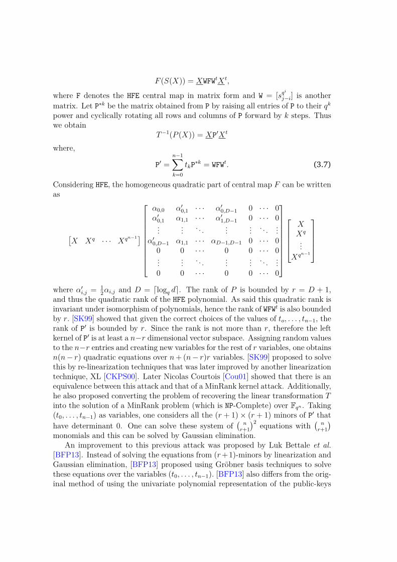
F (S(X)) = XWFWtX t,

where F denotes the HFE central map in matrix form and W = [sqi

j−i] is another

matrix. Let P∗k be the matrix obtained from P by raising all entries of P to their qk

power and cyclically rotating all rows and columns of P forward by k steps. Thuswe obtain

T−1(P (X)) = XP′X t

where,

P′ =n−1∑

k=0

tkP∗k = WFWt. (3.7)

Considering HFE, the homogeneous quadratic part of central map F can be writtenas

[X Xq · · · Xqn−1]

α0,0 α′0,1 · · · α′0,D−1 0 · · · 0α′0,1 α1,1 · · · α′1,D−1 0 · · · 0

......

. . ....

.... . .

...α′0,D−1 α1,1 · · · αD−1,D−1 0 · · · 0

0 0 · · · 0 0 · · · 0...

.... . .

......

. . ....

0 0 · · · 0 0 · · · 0

XXq

...

Xqn−1

where α′i,j = 12αi,j and D = ⌈logq d⌉. The rank of P is bounded by r = D + 1,

and thus the quadratic rank of the HFE polynomial. As said this quadratic rank isinvariant under isomorphism of polynomials, hence the rank of WFWt is also boundedby r. [SK99] showed that given the correct choices of the values of to, . . . , tn−1, therank of P′ is bounded by r. Since the rank is not more than r, therefore the leftkernel of P′ is at least a n−r dimensional vector subspace. Assigning random valuesto the n−r entries and creating new variables for the rest of r variables, one obtainsn(n− r) quadratic equations over n+ (n− r)r variables. [SK99] proposed to solvethis by re-linearization techniques that was later improved by another linearizationtechnique, XL [CKPS00]. Later Nicolas Courtois [Cou01] showed that there is anequivalence between this attack and that of a MinRank kernel attack. Additionally,he also proposed converting the problem of recovering the linear transformation Tinto the solution of a MinRank problem (which is NP-Complete) over Fqn . Taking(t0, . . . , tn−1) as variables, one considers all the (r + 1)× (r + 1) minors of P′ that

have determinant 0. One can solve these system of(

nr+1

)2equations with

(n

r+1

)

monomials and this can be solved by Gaussian elimination.An improvement to this previous attack was proposed by Luk Bettale et al.

[BFP13]. Instead of solving the equations from (r+1)-minors by linearization andGaussian elimination, [BFP13] proposed using Gröbner basis techniques to solvethese equations over the variables (t0, . . . , tn−1). [BFP13] also differs from the orig-inal method of using the univariate polynomial representation of the public-keys

by using the multivariate representation of the public-keys with the coefficientsrepresented over the base field. This is known as the minors modeling of theKipnis-Shamir attack. The asymptotic complexity of this attack is O(n(D+1)ω)where ω is the linear algebra constant.

This approach also works with the minus variants of HFE. Removing one equa-tion from the public-key leads to an increase in the quadratic rank by one. Untilthe number of removed equation is small enough compared to n, the minors model-ing attack still holds, but the asymptotic complexity increases to O(n(logq d+1+a)ω)where a is the number of public equations removed.

3.2.2 Message Recovery Attacks

From Chapter 2, we recall the discussions of the various methods to solve PoSSoq.Naturally, such techniques are useful in mounting attacks to recover the hiddensecret from the multivariate schemes, since from Section 3.1 we know such cryp-tosystems are based on PoSSoq.

3.2.2.1 Exhaustive Search

In Section 2.2.1, we presented the state of the art combinatorial algorithms forthe PoSSoq problem. The total number of possible values that the variables inpublic-key equations can have is qn. For each possible value, the correspondingciphertext is evaluated and checked against the input ciphertext. The candidatesolution with matching ciphertext is the correct solution. However, such attacksare usually exponential in the number of variables. As seen earlier in Section 2.3.1,this technique can be used in combination with other message recovery attacks,such as Gröbner basis attacks.

3.2.2.2 Gröbner Basis Algorithms

Recalling from Chapter 2, Gröbner basis computation also provides us with amethod to compute the solution to a system of polynomial equations. Hencemultivariate cryptographic primitives are vulnerable to direct algebraic attacks bycomputing the Gröbner basis.

One common observation from the previously discussed multivariate cryptosys-tems is that the public-keys are far more structured than a generic or randomsystem of polynomials. We know that the degree of regularity for a regular systemis given by the index of the first non-positive coefficient of the Hilbert series (seeproperty 2.3.31). For a structured semi-regular system, the above defined degreeof regularity works as an upper bound for the maximal degree observed in theGröbner basis computation. However, more accurate computations of this degreeof regularity for multivariate schemes have made some advances in recent years.

A prime example is the new upper bound for the degree of regularity for HFE andHFE− proposed by Ding et al. [DK12].

Theorem 3.2.2. [DK12] LetQ be the quadratic map of HFE. If the Q-rank(Q) > 1,

the degree of regularity of the system is upper bounded by

(q − 1)(⌊logq(d− 1)⌋+ 1)

2+ 2.

If Q-rank(Q) = 1, then the degree of regularity is less than equal to q.Let r = ⌊logq(d−1)⌋+1. The degree of regularity for HFE− with a equations removed

is upper bounded by

(q − 1)(⌊logq(d− 1)⌋+ 1 + a)

2+ 2,

if q is odd or if q is even and r + a is even,

(q − 1)(⌊logq(d− 1)⌋+ a)

2+ 2,

if q is even and r + a is odd.

Although these upper bounds do give an idea about the degree of regularityfor a system of public-keys, however, these are not always tight, as we have en-countered in the cryptanalysis of EFC (see Chapter 3.1.4). Now, let us see whyis this important for any multivariate cryptosystem. When any such multivariatescheme is designed, the complexity of algebraic attacks plays the most importantrole in setting the secure parameters for the scheme. This is because, in event ofany such algebraic attacks being launched, the hardness of recovering the secretmessage without the use of the private key remains intact. We shall also recallthat the complexity of the algebraic attack on such systems is directly related tothe degree of regularity of the public-keys.

Unfortunately, most of the current multivariate schemes use non-tight upperbounds, such as the one in Theorem 3.2.2, for the degree of regularities. Thusfrom a cryptanalytic point of view, it becomes quite imperative to get the exactdegree of regularities of the multivariate schemes. Accurate measurement of thedegree of regularity leads us to determine the complexity of algebraic attacks withgood accuracy. Hence experimental analysis is a modus operandi for this.

As discussed in Chapter 2, MAGMA proves quite useful to gather the degree ofregularity from standard Gröbner basis algorithms. Especially, the F4 algorithmon MAGMA provides an incremental degree by degree computation of bases until nonew relations are recovered. In Figures 3.1 and 3.2, we provide a snippet of aGröbner basis computation on MAGMA. Here there are certain observations, firstlyfor each degree, the F4 algorithm enumerates the number of new relations observed,

indicating the total degrees of such new relations. Secondly, the Gröbner basiscomputation terminates after it has recovered linearly independent linear equationsthat belong to the same ideal of the public-keys. The degree of regularity is thehighest degree that is reached during this process before we recover close to fullrank set of linear equations. This is because it is the maximal degree after whichthere are no new polynomials that are discovered and thus no new basis elementsadd to the already recovered Gröbner basis elements for any degree greater thanthis degree.

For the case of an non-homogeneous or affine system of polynomials, there is anapparition of lower degree relations at some particular step degree. For example,looking at Figure 3.1, in line 46, we observe 43 new quadratic polynomials in stepdegree 3. Similarly in Figure 3.2, line 31 shows that in degree 4, there is apparitionof 41 linear polynomials. In this thesis, we use these experimental observations toperform cryptanalysis of a multivariate scheme. Thus, from this section, we havea general idea about multivariate cryptography: state of the art design of schemes,new ways of designing schemes from the pre-existing schemes using modifiers andthe attacks on multivariate primitives.

In this thesis, we have present a new multivariate key encapsulation scheme,namely CFPKM. It has been presented in great detail in Chapter 6. The designof the scheme is loosely based on a lattice-based key exchange primitive calledFrodo. Therefore, for understanding the working of the information exchange, itis important to have a look at this scheme. This scheme is based on a lattice basedproblem, the Learning With Errors problem [Reg09]. In this following section weshall very briefly present the LWE problem and the Frodo key-exchange scheme.

3.3 Lattice Based Cryptosystems

Among all the post-quantum computational problems, lattice-based problems havereceived a bulk of the attention from researchers in the past decade. Lattice prob-lems have the advantage of worst-case to average-case reduction. This informallymeans that private keys in the easiest case are as hard to break as in the worstcase. For example, take an instance of RSA, where the choice of the keys involveschoosing two large random primes and expect that this yields a hard instanceof integer factorization problem. However, there is a probability of choosing thewrong pair, resulting in a lower level of security. In lattice based cryptosystem, allpossible key choices are equally hard to solve.

There are several NP hard lattice problems, namely, Shortest (Approximate)Vector problem (SVP and SVPγ) [Ajt96], Bounded Distance Decoding (BDD) [LM09]and Closest Vector Problem (CVP) [GMSS99] whose hardness assumptions acts asa security for lattice based cryptographic primitives against classical as well asquantum adversaries. One of the most recent lattice problem is Learning With

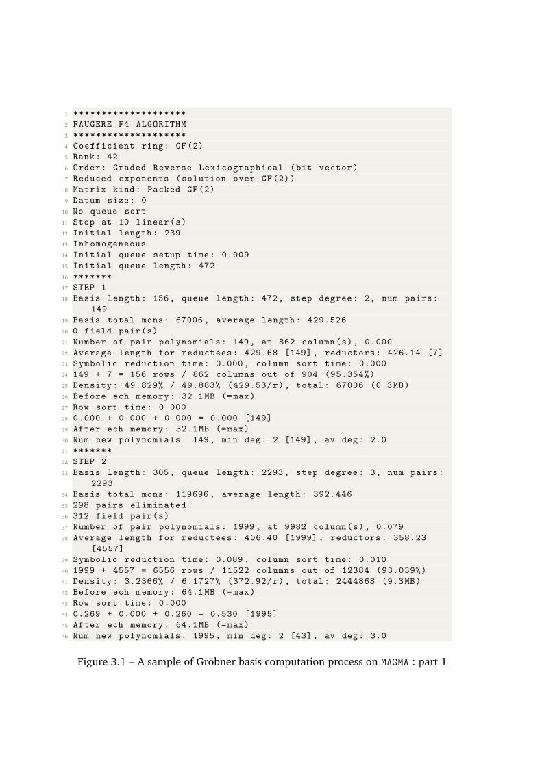
1 ********************

2 FAUGERE F4 ALGORITHM

3 ********************

4 Coefficient ring: GF(2)

5 Rank: 42

6 Order: Graded Reverse Lexicographical (bit vector)

7 Reduced exponents (solution over GF(2))

8 Matrix kind: Packed GF(2)

9 Datum size: 0

10 No queue sort

11 Stop at 10 linear(s)

12 Initial length: 239

13 Inhomogeneous

14 Initial queue setup time: 0.009

15 Initial queue length: 472

16 *******

17 STEP 1


149


20 0 field pair(s)








28 0.000 + 0.000 + 0.000 = 0.000 [149]


30 Num new polynomials: 149, min deg: 2 [149], av deg: 2.0

31 *******

32 STEP 2


2293



36 312 field pair(s)



[4557]






44 0.269 + 0.000 + 0.260 = 0.530 [1995]



Figure 3.1 – A sample of Gröbner basis computation process on MAGMA : part 1

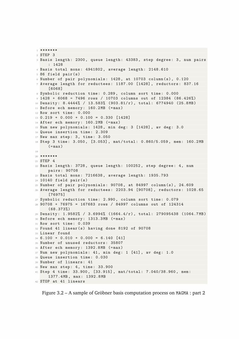
1 *******

2 STEP 3

3 Basis length: 2300, queue length: 43383, step degree: 3, num pairs

: 1428


5 86 field pair(s)



[6068]






13 0.219 + 0.000 + 0.100 = 0.330 [1428]


15 Num new polynomials: 1428, min deg: 3 [1428] , av deg: 3.0




(=max)

19

20 *******

21 STEP 4

22 Basis length: 3728, queue length: 100252 , step degree: 4, num

pairs: 90708


24 10140 field pair(s)



[76975]


28 90708 + 76975 = 167683 rows / 84997 columns out of 124314

(68.373%)


30 Before ech memory: 1313.3 MB (=max)


32 Found 41 linear(s) having done 8192 of 90708

33 Linear found

34 6.100 + 0.010 + 0.000 = 6.140 [41]

35 Number of unused reductors: 35807

36 After ech memory: 1392.8 MB (=max)



39 Number of linears: 41


41 Step 4 time: 33.900 , [33.915] , mat/total: 7.040/38.960 , mem:

1377.4MB, max: 1392.8 MB

42 STOP at 41 linears

Figure 3.2 – A sample of Gröbner basis computation process on MAGMA : part 2

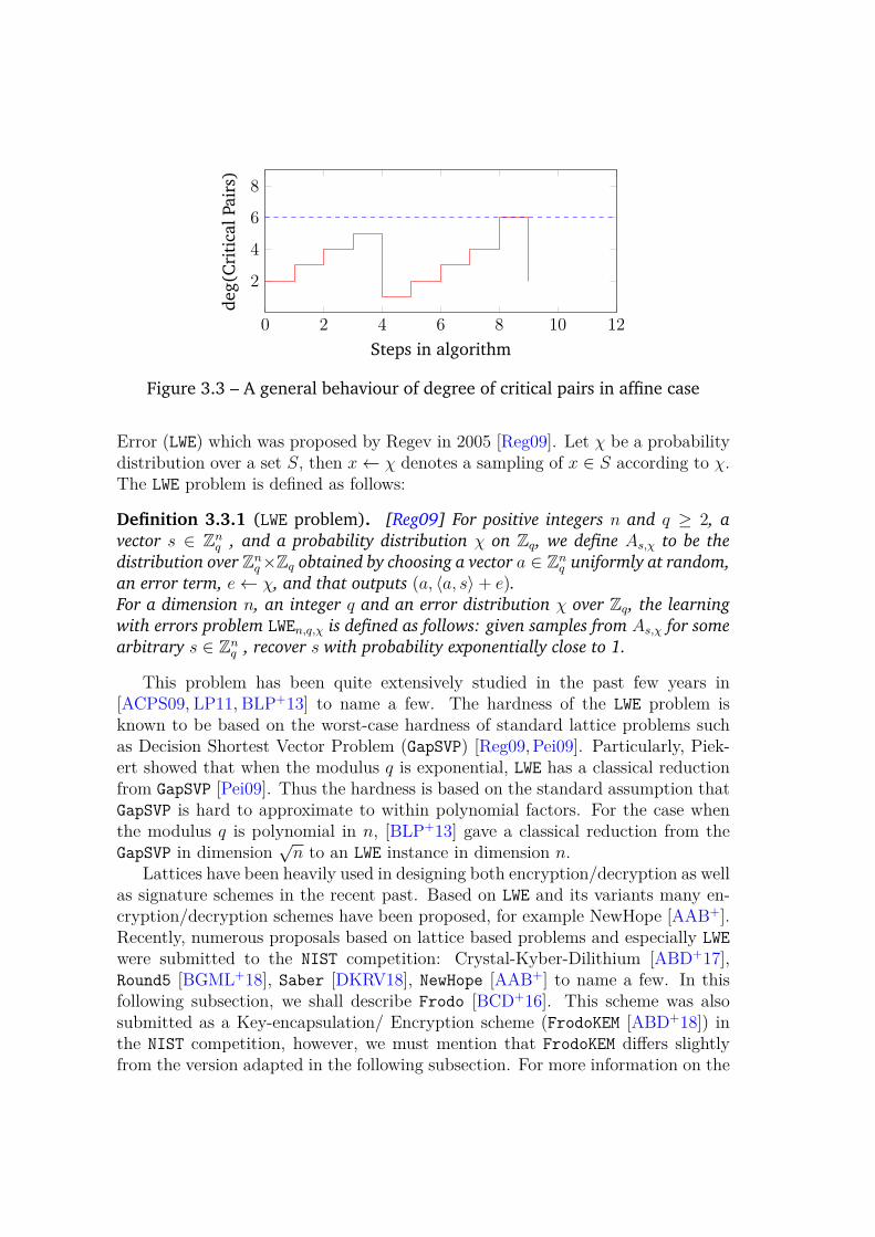
0 2 4 6 8 10 12

2

4

6

8

Steps in algorithm

deg(

Cri

tica

lPai

rs)

Figure 3.3 – A general behaviour of degree of critical pairs in affine case

Error (LWE) which was proposed by Regev in 2005 [Reg09]. Let χ be a probabilitydistribution over a set S, then x← χ denotes a sampling of x ∈ S according to χ.The LWE problem is defined as follows:

Definition 3.3.1 (LWE problem). [Reg09] For positive integers n and q ≥ 2, a

vector s ∈ Znq , and a probability distribution χ on Zq, we define As,χ to be the

distribution over Znq×Zq obtained by choosing a vector a ∈ Zn

q uniformly at random,

an error term, e← χ, and that outputs (a, 〈a, s〉+ e).For a dimension n, an integer q and an error distribution χ over Zq, the learning

with errors problem LWEn,q,χ is defined as follows: given samples from As,χ for some

arbitrary s ∈ Znq , recover s with probability exponentially close to 1.

This problem has been quite extensively studied in the past few years in[ACPS09, LP11, BLP+13] to name a few. The hardness of the LWE problem isknown to be based on the worst-case hardness of standard lattice problems suchas Decision Shortest Vector Problem (GapSVP) [Reg09, Pei09]. Particularly, Piek-ert showed that when the modulus q is exponential, LWE has a classical reductionfrom GapSVP [Pei09]. Thus the hardness is based on the standard assumption thatGapSVP is hard to approximate to within polynomial factors. For the case whenthe modulus q is polynomial in n, [BLP+13] gave a classical reduction from theGapSVP in dimension

√n to an LWE instance in dimension n.

Lattices have been heavily used in designing both encryption/decryption as wellas signature schemes in the recent past. Based on LWE and its variants many en-cryption/decryption schemes have been proposed, for example NewHope [AAB+].Recently, numerous proposals based on lattice based problems and especially LWE

were submitted to the NIST competition: Crystal-Kyber-Dilithium [ABD+17],Round5 [BGML+18], Saber [DKRV18], NewHope [AAB+] to name a few. In thisfollowing subsection, we shall describe Frodo [BCD+16]. This scheme was alsosubmitted as a Key-encapsulation/ Encryption scheme (FrodoKEM [ABD+18]) inthe NIST competition, however, we must mention that FrodoKEM differs slightlyfrom the version adapted in the following subsection. For more information on the

FrodoKEM scheme, we redirect the reader to [ABD+18].

3.3.1 Frodo Key Exchange

3.3.1.1 Notation

Matrices are denoted by bold capital letters, e.g A,B. For a distribution χ, A←χ(Sn×m) defines a matrix with each component chosen independently accordingto the distribution χ(S). As seen previously, the LWE problem is characterizedby three parameters: the modulus q, the dimensions of the matrix n, and anerror distribution χ. For designing this scheme, the authors of [BCD+16] choosea discrete Gaussian distribution that is defined as follows.

Definition 3.3.2 (Discrete Gaussian Distribution). Let α be a real number and

q ∈ N. A Gaussian distribution is a continuous probability distribution function

that centers around a mean value with a standard deviation αq. The discrete Gaus-

sian distribution χα,q is a Gaussian distribution rounded to the nearest integer and

reduced modulo q.

3.3.1.2 Reconciliation method

In a key-exchange protocol, reconciliation refers to the methodology and the collec-tion of procedures utilized by two communicating parties allowing them to arriveat exactly the same keys without having to exchange the key directly. The rec-onciliation mechanism used by Frodo is a generalised version of the Piekert’s keyagreement mechanism [Pei14]. Unlike Piekert’s mechanism, which extracts a singlebit, this allows a larger but fixed number of bits to be extracted. This increasesin the number of extracted bits also lead to an increased failure of reconciliation.However, this rate of failure is small for practical applications [BCD+16].

Now we shall give a short description of functions that help in exact key agree-ment using this new reconciliation method. Let B be the number of bits thatone aims to extract from one coefficient in Zq be such that B < (log2 q − 1) LetB = (log2 q −B). For any v ∈ Zq the rounding function ⌊·⌉2B is defined as

⌊v⌉2B := ⌊2−B · v⌉ mod 2B.

This returns the B most significant bits of (v + 2B−1) mod q. The crossroundfunction 〈·〉2B is defined as

〈v〉2B := ⌊2−B+1 · v⌋ mod 2.

This function returns the (B + 1)th most significant bit of v. Now with these twofunction, we finally define the function Rec. This function is built on the foun-dations of the reconciliation function proposed by Piekert [Pei14]. The function

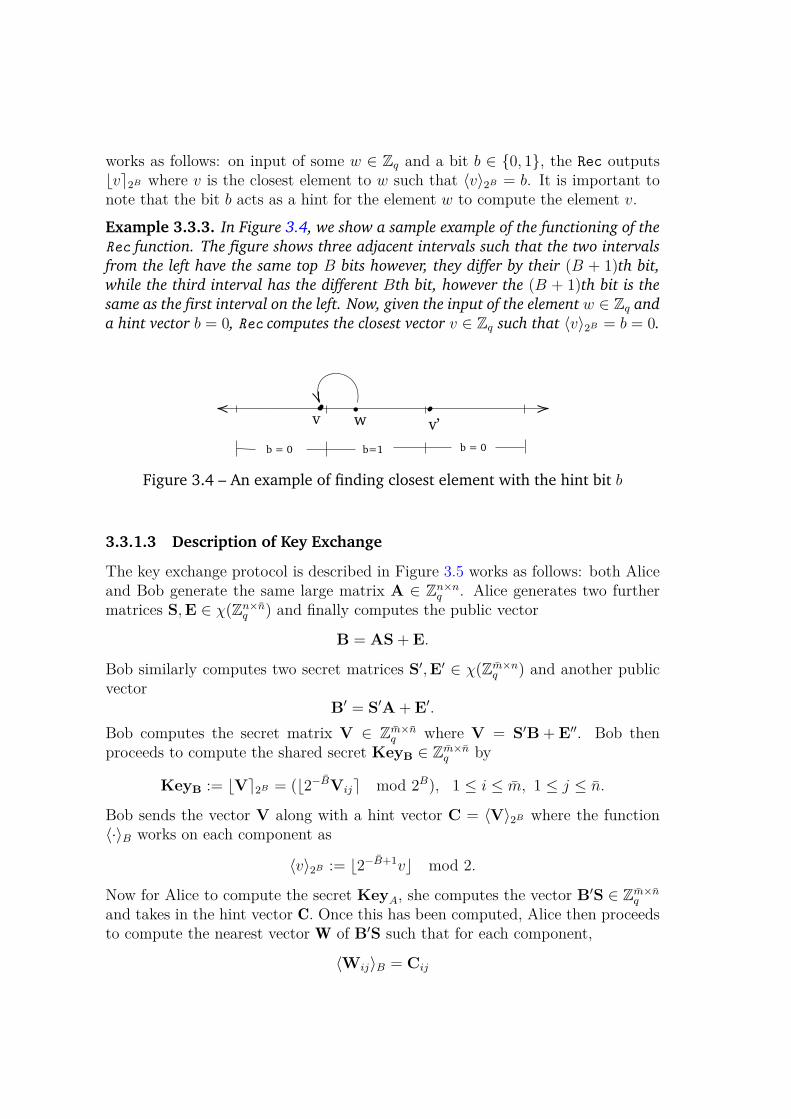
works as follows: on input of some w ∈ Zq and a bit b ∈ {0, 1}, the Rec outputs⌊v⌉2B where v is the closest element to w such that 〈v〉2B = b. It is important tonote that the bit b acts as a hint for the element w to compute the element v.

Example 3.3.3. In Figure 3.4, we show a sample example of the functioning of the

Rec function. The figure shows three adjacent intervals such that the two intervals

from the left have the same top B bits however, they differ by their (B + 1)th bit,

while the third interval has the different Bth bit, however the (B + 1)th bit is the

same as the first interval on the left. Now, given the input of the element w ∈ Zq and

a hint vector b = 0, Rec computes the closest vector v ∈ Zq such that 〈v〉2B = b = 0.

wv

b = 0 b=1

v’b = 0

Figure 3.4 – An example of finding closest element with the hint bit b

3.3.1.3 Description of Key Exchange

The key exchange protocol is described in Figure 3.5 works as follows: both Aliceand Bob generate the same large matrix A ∈ Zn×n

q . Alice generates two furthermatrices S,E ∈ χ(Zn×n

q ) and finally computes the public vector

B = AS+ E.

Bob similarly computes two secret matrices S′,E′ ∈ χ(Zm×nq ) and another public

vectorB′ = S′A+ E′.

Bob computes the secret matrix V ∈ Zm×nq where V = S′B+ E′′. Bob then

proceeds to compute the shared secret KeyB ∈ Zm×nq by

KeyB := ⌊V⌉2B = (⌊2−BVij⌉ mod 2B), 1 ≤ i ≤ m, 1 ≤ j ≤ n.

Bob sends the vector V along with a hint vector C = 〈V〉2B where the function〈·〉B works on each component as

〈v〉2B := ⌊2−B+1v⌋ mod 2.

Now for Alice to compute the secret KeyA, she computes the vector B′S ∈ Zm×nq

and takes in the hint vector C. Once this has been computed, Alice then proceedsto compute the nearest vector W of B′S such that for each component,

〈Wij〉B = Cij

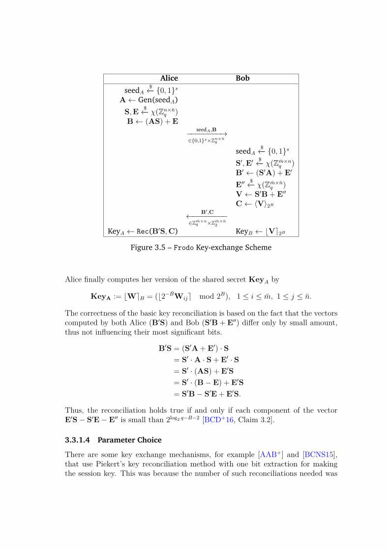
Alice Bob

seedA$←− {0, 1}s

A← Gen(seedA)

S,E$←− χ(Zn×n

q )B← (AS) + E

seedA,B−−−−−−−−→∈{0,1}s×Zn×n

q

seedA$←− {0, 1}s

S′,E′$←− χ(Zm×n

q )B′ ← (S′A) + E′

E′′$←− χ(Zm×n

q )V← S′B+ E′′

C← 〈V〉2BB′,C←−−−−−−−−

∈Zm×nq ×Zm×n

2

KeyA ← Rec(B′S,C) KeyB ← ⌊V⌉2B

Figure 3.5 – Frodo Key-exchange Scheme

Alice finally computes her version of the shared secret KeyA by

KeyA := ⌊W⌉B = (⌊2−BWij⌉ mod 2B), 1 ≤ i ≤ m, 1 ≤ j ≤ n.

The correctness of the basic key reconciliation is based on the fact that the vectorscomputed by both Alice (B′S) and Bob (S′B+ E′′) differ only by small amount,thus not influencing their most significant bits.

B′S = (S′A+ E′) · S= S′ ·A · S+ E′ · S= S′ · (AS) + E′S

= S′ · (B− E) + E′S

= S′B− S′E+ E′S.

Thus, the reconciliation holds true if and only if each component of the vectorE′S− S′E− E′′ is small than 2log2 q−B−2 [BCD+16, Claim 3.2].

3.3.1.4 Parameter Choice

There are some key exchange mechanisms, for example [AAB+] and [BCNS15],that use Piekert’s key reconciliation method with one bit extraction for makingthe session key. This was because the number of such reconciliations needed was

far greater than the number of bits required to make the session key. In this case,we have a total of m · n reconciliations. So to achieve a post-quantum security of128 bits, one requires mn · B > 256. With a larger number of bits extracted, onecan achieve smaller parameters of m and n, which in turn implies smaller sizes ofLWE matrices. Finally, we redirect the reader to [BCD+16] for more informationand therefore the detailed working of the scheme has been omitted.

3.3.1.5 Failure rate

The probability of reconciliation is 1 when the distance between the two vectors:is less than q/2B+2, whereas, when it is larger than 3q/2B+2, the scheme fails everytime [BCD+16]. The success probability decreases from 1 to 0 in between these twoextremes. This is described in the figure of example 3.3.2. the Rec function can findanother vector v′ in the interval to the right of the interval containing w. However,it should be noted that this interval does not have the same B most significantbits even though 〈v′〉 = b = 0. Thus the function doesn’t choose v′. However forsome cases, especially when w lies in the exact middle of the sub-interval, there isa choice to be made, that determines the success of the reconciliation.

Part II

Contribution

67

Chapter 4

Cryptanalysis of Extension FieldCancellation Cryptosystem

Abstract

We investigate the Extension Field Cancellation (EFC) scheme, whichwe presented in Section 3.1.4. The organization of the chapter is asfollows: first, we present a successful Gröbner basis attack on the firstand the second proposed parameters of the scheme. The attack wasmounted with complexity much smaller than the claimed security level.We further show that the algebraic system arising from EFC are mucheasier to solve than a random system of the same size. Briefly, this isdue to the apparition of many lower degree equations during Gröbnerbasis computation. We present a polynomial time method to recoversuch lower degree relations and also show their usefulness in improvingthe Gröbner basis attack complexity on EFC.

4.1 Introduction

In this chapter, we investigate a new encryption scheme: Extension Field Can-cellation (EFC) [SDP16] which is based on using high degree polynomials over anextension field as a part of public-key construction. We presented the workingof this scheme briefly in Section 3.1.4. As seen before, on one hand, most of themultivariate encryption schemes proposed have been subjected to cryptanalysis,on the other hand, EFC has stood so far with no cryptanalysis yet.

4.1.1 Main Results and Organization

This chapter is organized as follows. Section 4.2.2 reports the results of a hybridGröbner basis attack [BFP09] on all three challenge parameters of EFC. Using

69

this message recovery attack, for the first and the second challenge parameter werecover the hidden secret message in 265 and 277 operations respectively, contraryto the claims of 80 bits of security for these parameter. For the third parameter,although the worst-case hybrid Gröbner basis attack takes 280 operations, in anaverage case, we expect it to be about 279. Section 4.2.3 provides experimentalevidence of the non-random behavior of the public polynomials of EFC. In Section4.2.4, we show why EFCq(0), the scheme without any modifiers, is weak. Particu-larly, we show that a polynomial-time attack exists on EFCq(0) and EFCFq (0), whichhas been stated informally in Theorem 1 below:

Theorem 4.1.1 (informal). Given a public-key (f1, . . . , f2n) ∈ F2nq [x1, . . . , xn] and

the ciphertext (c1, . . . , c2n) ∈ F2nq from an instance of EFCq(0) or EFCFq (0), using

Gröbner basis, we can recover the hidden secret message in O(n3ω) which is polyno-

mial in n and where 2 ≤ ω < 3 is the linear algebra constant.

We present the full version of Theorem 4.1.1 as well as the proof in Section4.2.4. We explain how a degree 3 linear combination of the public-keys of EFCq(0)or EFCFq (0) yield linear equations (see Section 4.2.4 for more details).

We extend this methodology to EFC−q as well, where we recover quadratic equa-tions from a high degree (degree ≥ 3) combinations of the public-keys. This hasbeen discussed in some details in Sections 4.2.5, 4.2.6, and 4.2.7. This techniqueis quite similar to the approach used against HFE [FJ03] and the Hidden Matrixscheme [?] schemes where the authors show the public-keys exhibiting some alge-braic properties are easier to solve than a random system of quadratic equationsof the same sizes. We introduce a new technique of explicitly computing andrecovering low-degree relations from the public-keys of EFC−q . To do so, we con-sider the initial public-keys and their Frobenius powers. The following Claim 4.1.1informally describes the basic idea. We refer to Section 4.3 for further details.

Claim 4.1.1 (informal). Given the public-keys equations for an instance of EFC−q ,

we can always find some combinations of the public-keys and their Frobenius powers

which produce new low-degree relations.

Using this technique, we can recover the quadratic relations from degree 3combinations in 151 minutes for the first challenge parameter and 110 minutesfor the second challenge parameter. This computation is polynomial-time in thenumber of variables. Furthermore, we show that adding these new equations alongwith the public equations make the Gröbner basis computation much more efficientas well as reducing the time complexity by a huge factor. For instance, in case ofEFC−q (2) with n = 75, adding such intermediate equations reduces the run time ofF4 from more than a day to 66.05 seconds to compute the Gröbner basis. Thus,this scheme has structural weaknesses that can be easily exploited by an adversaryto recover secret messages and thus making the scheme unsuitable for encryption.

4.2 Algebraic Cryptanalysis of EFC

In this section, we show how Gröbner basis (see Section 2.3) and Gröbner basisalgorithms can be utilized to attack the EFC scheme. To break the EFCq scheme,as described in section 3.1.4, the underlying problem is to find a solution to thesystem of equations given by public-key ciphertext pairs. In this section, firstlywe present a polynomial time key recovery attack on EFCq(0), Secondly, we reportthe results of a Gröbner basis based message recovery attack on the proposedparameters of EFC. Finally, we show why a system of public-keys arising from EFC

is much easier to solve than a random system of algebraic equations with the samesize. This is supported by both theoretical and experimental observations.

4.2.1 A Key Recovery Attack

In section 3.2.1.1, we presented Patarin’s affine multiple attack [Pat96] on C∗ wheredue to an algebraic property, one can find a bi-linear relation between the plaintextsand the ciphertexts. EFCq(0), like C∗, is vulnerable to a form of linearization attack,which recovers the secret-key equations. Recall that decryption of EFCq(0) requiressolving a system of linear equations which are derived from Equation (3.3). Assaid earlier, given the ciphertexts (c1, . . . , c2n) ∈ F2n

q , these decryption equationshave an equivalent univariate representation over the extension field Fqn , which isof the following form

β(χ)C1 − α(χ)C2 = 0,

where C1 = ϕ(c1, . . . , cn) ∈ Fqn , C2 = ϕ(cn+1, . . . , c2n) ∈ Fqn , while α(χ) ∈ Fqn [χ]and β(χ) ∈ Fqn [χ] are defined as in Equation (3.2). This is a bi-linear relationbetween the plaintext, χ (since both α(χ) and β(χ) are linear over the base field Fq)and the ciphertexts C1 and C2. So choosing enough plaintexts and correspondingciphertexts, one can recover the coefficients of α(χ) and β(χ), which were unknownto the attacker.

Hence, using the public-key P ∈ Fq[x1, . . . , xn], we can generate several plaintext-ciphertext pairs. For each pair of plaintext-ciphertext (x′1, . . . , x

′n) ∈ Fn

q , (y′1, . . . , y′2n) ∈

F2nq given by P (x′1, . . . , x

′n) = (y′1, . . . , y

′2n), we can substitute

X = ϕ(x′1, . . . , x′n), Υ1 = ϕ(y′1, . . . , y

′n), Υ2 = ϕ(y′n, . . . , y

′2n) ∈ Fqn ,

into the following linearization equation

Ψ(X, Υ1, Υ2) =

( n−1∑

i=0

giXqi−1

)· Υ2 −

( n−1∑

i=0

hiXqi−1

)· Υ1 = 0,

to get a linear equation in 2n unknowns gi, hi ∈ Fqn . Therefore, choosing roughly2n plaintext-ciphertext pairs, we can very likely solve the resulting system for theunknown coefficients in O(n3) time complexity. Once we have the resulting linear

system of equations, for a given ciphertext (c1, . . . , c2n) ∈ F2nq , we can recover

the actual secret message by solving the univariate equation Ψ(X) = 0, whichover the base field Fq represents a system of n linear equations in n variables(x1, . . . , xn). Solving this system has O(n3) complexity. This attack was known tothe authors of [SDP16]. This idea of recovering the secret-key from the public-keysto obtain the hidden message can also be realised using Gröbner bases. This hasbeen presented in great detail in Section 4.2.4.

For the case of a > 0, an attacker needs to guess the correct ciphertext for eachof the a public-keys for every choice of 2n plaintexts such that these 2n plaintext-ciphertext pairs solve for the unknown coefficients of the linear equation Ψ . Inworst-case, the complexity is O(q2na), which is exponential in n and the numberof missing public-keys, a. Therefore, choosing appropriate value of the parametera can foil such a key-recovery attack using linearization techniques on EFC−q (a).

4.2.2 A Message Recovery Attack

In this part, we show that the challenge parameters of EFC (see Table 3.2) can beattacked thanks to the hybrid Gröbner basis algorithm [BFP09, Bet11] which wediscussed in Section 2.4. This attack combines both exhaustive search as well asGröbner basis computation by fixing k out of the n variables and then computingGröbner basis. The complete set of solutions is recovered from the computationof all qk Gröbner bases. The attack relies on the idea that the cost of computingGröbner basis decreases when the ratio between the number of equations andthe number of variables increases [BFSY05]. Table 4.1 lists the number of fixedvariables and the expected number of operations of the message recovery attackfor EFC parameters. The expected number of operations for the hybrid attack iscalculated explicitly and is given by:

Nhyb = log2 (t · qk · 2.93× 109),

where t is the time taken for computing a Gröbner basis over the public-keysin which we fix k variables. In our experiments, we take this time t to be theaverage time over 100 runs. The number of expected operations, Nhyb, is notan asymptotic estimate as we do not use the expected degree of regularity forcomputing the complexity of the hybrid Gröbner basis attack.

From Table 4.1, we see that the first parameter EFC−2 (10) with n = 83 isbroken just by using 265 bit operations, while the second parameter EFCF−2 (8) withn = 83 is broken by using 277 bit operations. We have not been able to findan attack with number of operations strictly less than 280 on the third challengeparameter of EFC−3 (6) with n = 56, however, fixing 25 variables gives us a sharpupper bound of 280. Therefore, if this parameter is used, in the worst case instance,the hybrid attack will take 280 bit operations, however, in average case, we expectthe number of operations to be about 279. This is simply because, the total number

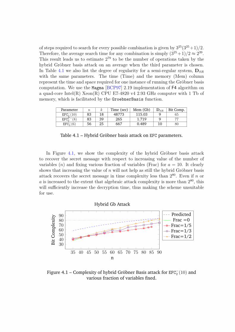
of steps required to search for every possible combination is given by 325(325+1)/2.Therefore, the average search time for any combination is simply (325+1)/2 ≈ 239.This result leads us to estimate 279 to be the number of operations taken by thehybrid Gröbner basis attack on an average when the third parameter is chosen.In Table 4.1 we also list the degree of regularity for a semi-regular system, DSR

with the same parameters. The time (Time) and the memory (Mem) columnrepresent the time and space required for one instance of running the Gröbner basiscomputation. We use the Magma [BCP97] 2.19 implementation of F4 algorithm ona quad-core Intel(R) Xeon(R) CPU E7-4820 v4 2.93 GHz computer with 1 Tb ofmemory, which is facilitated by the GroebnerBasis function.

Parameter n k Time (sec) Mem (Gb) DSR Bit Comp.EFC−2 (10) 83 18 48773 115.03 9 65

EFCF−2 (8) 83 39 265 1.719 9 77EFC−3 (6) 56 25 667 0.489 10 80

Table 4.1 – Hybrid Gröbner basis attack on EFC parameters.

In Figure 4.1, we show the complexity of the hybrid Gröbner basis attackto recover the secret message with respect to increasing value of the number ofvariables (n) and fixing various fraction of variables (Frac) for a = 10. It clearlyshows that increasing the value of n will not help as still the hybrid Gröbner basisattack recovers the secret message in time complexity less than 280. Even if n ora is increased to the extent that algebraic attack complexity is more than 280, thiswill sufficiently increase the decryption time, thus making the scheme unsuitablefor use.

35 40 45 50 55 60 65 70 75 80 85 90

30405060708090

n

Bit

Com

plex

ity

Hybrid Gb Attack

PredictedFrac =0

Frac=1/5Frac=1/3Frac=1/2

Figure 4.1 – Complexity of hybrid Gröbner Basis attack for EFC−2 (10) andvarious fraction of variables fixed.

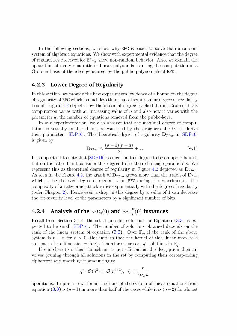
In the following sections, we show why EFC is easier to solve than a randomsystem of algebraic equations. We show with experimental evidence that the degreeof regularities observed for EFC−q show non-random behavior. Also, we explain theapparition of many quadratic or linear polynomials during the computation of aGröbner basis of the ideal generated by the public polynomials of EFC.

4.2.3 Lower Degree of Regularity

In this section, we provide the first experimental evidence of a bound on the degreeof regularity of EFC which is much less than that of semi-regular degree of regularitybound. Figure 4.2 depicts how the maximal degree reached during Gröbner basiscomputation varies with an increasing value of n and also how it varies with theparameter a, the number of equations removed from the public-keys.

In our experimentation, we also observe that the maximal degree of compu-tation is actually smaller than that was used by the designers of EFC to derivetheir parameters [SDP16]. The theoretical degree of regularity DTheo in [SDP16]is given by

DTheo ≤(q − 1)(r + a)

2+ 2. (4.1)

It is important to note that [SDP16] do mention this degree to be an upper bound,but on the other hand, consider this degree to fix their challenge parameters. Werepresent this as theoretical degree of regularity in Figure 4.2 depicted as DTheo.As seen in the Figure 4.2, the graph of DTheo grows more than the graph of DObs

which is the observed degree of regularity for EFC during the experiments. Thecomplexity of an algebraic attack varies exponentially with the degree of regularity(refer Chapter 2). Hence even a drop in this degree by a value of 1 can decreasethe bit-security level of the parameters by a significant number of bits.

4.2.4 Analysis of the EFCq(0) and EFCFq (0) instances

Recall from Section 3.1.4, the set of possible solutions for Equation (3.3) is ex-pected to be small [SDP16]. The number of solutions obtained depends on therank of the linear system of equation (3.3). Over Fq, if the rank of the abovesystem is n − r for r > 0, this implies that the kernel of this linear map, is asubspace of co-dimension r in Fn

q . Therefore there are qr solutions in Fnq .

If r is close to n then the scheme is not efficient as the decryption then in-volves pruning through all solutions in the set by computing their correspondingciphertext and matching it amounting to

qr · O(n3) = O(nζ+3), ζ =r

logq n

operations. In practice we found the rank of the system of linear equations fromequation (3.3) is (n−1) in more than half of the cases while it is (n−2) for almost

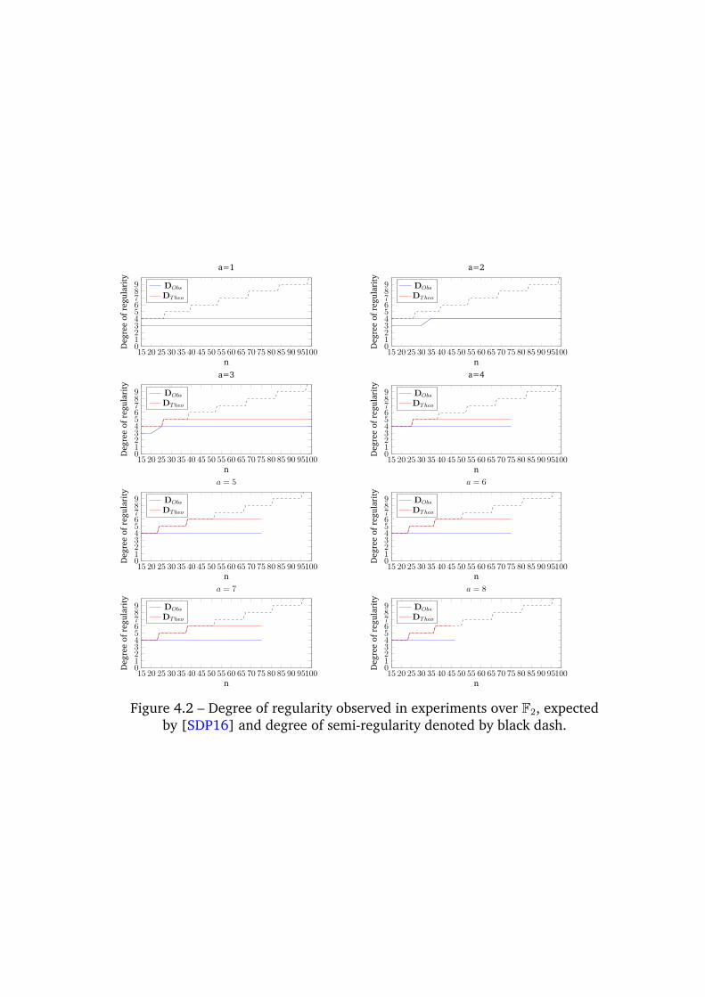
15 20 25 30 35 40 45 50 55 60 65 70 75 80 85 90 951000123456789

n

Deg

ree

ofre

gula

rity

a=1

DObs

DTheo

15 20 25 30 35 40 45 50 55 60 65 70 75 80 85 90 951000123456789

nD

egre

eof

regu

lari

ty

a=2

DObs

DTheo

15 20 25 30 35 40 45 50 55 60 65 70 75 80 85 90 951000123456789

n

Deg

ree

ofre

gula

rity

a=3

DObs

DTheo

15 20 25 30 35 40 45 50 55 60 65 70 75 80 85 90 951000123456789

n

Deg

ree

ofre

gula

rity

a=4

DObs

DTheo

15 20 25 30 35 40 45 50 55 60 65 70 75 80 85 90 951000123456789

n

Deg

ree

ofre

gula

rity

a = 5

DObs

DTheo

15 20 25 30 35 40 45 50 55 60 65 70 75 80 85 90 951000123456789

n

Deg

ree

ofre

gula

rity

a = 6

DObs

DTheo

15 20 25 30 35 40 45 50 55 60 65 70 75 80 85 90 951000123456789

n

Deg

ree

ofre

gula

rity

a = 7

DObs

DTheo

15 20 25 30 35 40 45 50 55 60 65 70 75 80 85 90 951000123456789

n

Deg

ree

ofre

gula

rity

a = 8

DObs

DTheo

Figure 4.2 – Degree of regularity observed in experiments over F2, expectedby [SDP16] and degree of semi-regularity denoted by black dash.

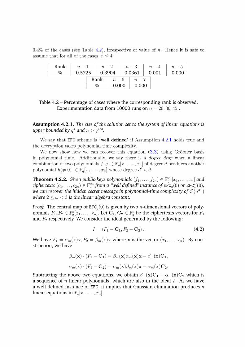
0.4% of the cases (see Table 4.2), irrespective of value of n. Hence it is safe toassume that for all of the cases, r ≤ 4.

Rank n− 1 n− 2 n− 3 n− 4 n− 5% 0.5725 0.3904 0.0361 0.001 0.000

Rank n− 6 n− 7% 0.000 0.000

Table 4.2 – Percentage of cases where the corresponding rank is observed.Experimentation data from 10000 runs on n = 20, 30, 45 .

Assumption 4.2.1. The size of the solution set to the system of linear equations is

upper bounded by q4 and n > q4/3.

We say that EFC scheme is “well defined" if Assumption 4.2.1 holds true andthe decryption takes polynomial time complexity.

We now show how we can recover this equation (3.3) using Gröbner basisin polynomial time. Additionally, we say there is a degree drop when a linearcombination of two polynomials f, g ∈ Fq[x1, . . . , xn] of degree d produces anotherpolynomial h( 6= 0) ∈ Fq[x1, . . . , xn] whose degree d′ < d.

Theorem 4.2.2. Given public-keys polynomials (f1, . . . , f2n) ∈ F2nq [x1, . . . , xn] and

ciphertexts (c1, . . . , c2n) ∈ F2nq from a “well defined" instance of EFCq(0) or EFCFq (0),

we can recover the hidden secret message in polynomial-time complexity of O(n3ω)where 2 ≤ ω < 3 is the linear algebra constant.

Proof. The central map of EFCq(0) is given by two n-dimensional vectors of poly-nomials F1, F2 ∈ Fn

q [x1, . . . , xn]. Let C1,C2 ∈ Fnq be the ciphertexts vectors for F1

and F2 respectively. We consider the ideal generated by the following:

I = 〈F1 −C1, F2 −C2〉 . (4.2)

We have F1 = αm(x)x, F2 = βm(x)x where x is the vector (x1, . . . , xn). By con-struction, we have

βm(x) · (F1 −C1) = βm(x)αm(x)x− βm(x)C1,

αm(x) · (F2 −C2) = αm(x)βm(x)x− αm(x)C2.

Subtracting the above two equations, we obtain βm(x)C1 − αm(x)C2 which isa sequence of n linear polynomials, which are also in the ideal I. As we havea well defined instance of EFC, it implies that Gaussian elimination produces nlinear equations in Fq[x1, . . . , xn].

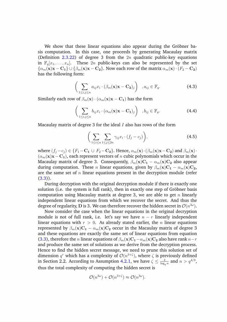
We show that these linear equations also appear during the Gröbner ba-sis computation. In this case, one proceeds by generating Macaulay matrix(Definition 2.3.22) of degree 3 from the 2n quadratic public-key equationsin Fq[x1, . . . , xn]. These 2n public-keys can also be represented by the set{αm(x)x−C1} ∪ {βm(x)x−C2}. Now each row of the matrix αm(x) · (F2−C2)has the following form:

( ∑

1≤i,j≤n

aijxi · (βm(x)x−C2)j

), aij ∈ Fq. (4.3)

Similarly each row of βm(x) · (αm(x)x−C1) has the form( ∑

1≤i,j≤n

bijxi · (αm(x)x−C1)j

), bij ∈ Fq. (4.4)

Macaulay matrix of degree 3 for the ideal I also has rows of the form( ∑

1≤i≤n

∑

1≤j≤2n

γijxi · (fj − cj)

), (4.5)

where (fj−cj) ∈ {F1−C1 ∪ F2−C2}. Hence, αm(x) ·(βm(x)x−C2) and βm(x) ·(αm(x)x−C1), each represent vectors of n cubic polynomials which occur in theMacaulay matrix of degree 3. Consequently, βm(x)C1 − αm(x)C2 also appearduring computation. These n linear equations, given by βm(x)C1 − αm(x)C2,are the same set of n linear equations present in the decryption module (refer(3.3)).

During decryption with the original decryption module if there is exactly onesolution (i.e. the system is full rank), then in exactly one step of Gröbner basiscomputation using Macaulay matrix at degree 3, we are able to get n linearlyindependent linear equations from which we recover the secret. And thus thedegree of regularity, D is 3. We can therefore recover the hidden secret inO(n3ω).

Now consider the case when the linear equations in the original decryptionmodule is not of full rank, i.e. let’s say we have n − r linearly independentlinear equations with r > 0. As already stated earlier, the n linear equationsrepresented by βm(x)C1 − αm(x)C2 occur in the Macaulay matrix of degree 3and these equations are exactly the same set of linear equations from equation(3.3), therefore the n linear equations of βm(x)C1−αm(x)C2 also have rank n−rand produce the same set of solutions as we derive from the decryption process.Hence to find the hidden secret message, we need to prune this solution set ofdimension qr which has a complexity of O(n3+ζ), where ζ is previously definedin Section 2.2. According to Assumption 4.2.1, we have ζ ≤ 4

logq nand n > q4/3,

thus the total complexity of computing the hidden secret is

O(n3ω) +O(n3+ζ) ≈ O(n3ω).

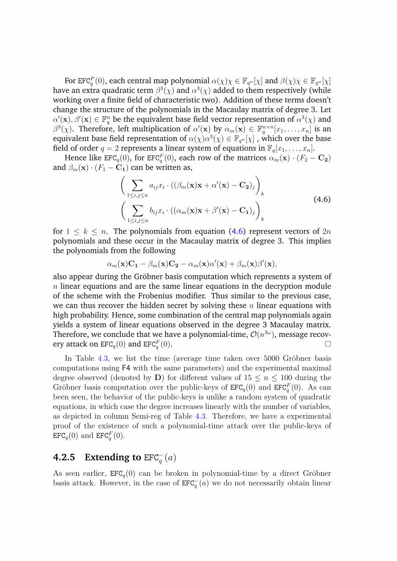
For EFCFq (0), each central map polynomial α(χ)χ ∈ Fqn [χ] and β(χ)χ ∈ Fqn [χ]have an extra quadratic term β3(χ) and α3(χ) added to them respectively (whileworking over a finite field of characteristic two). Addition of these terms doesn’tchange the structure of the polynomials in the Macaulay matrix of degree 3. Letα′(x), β′(x) ∈ Fn

q be the equivalent base field vector representation of α3(χ) andβ3(χ). Therefore, left multiplication of α′(x) by αm(x) ∈ Fn×n

q [x1, . . . , xn] is anequivalent base field representation of α(χ)α3(χ) ∈ Fqn [χ] , which over the basefield of order q = 2 represents a linear system of equations in Fq[x1, . . . , xn].

Hence like EFCq(0), for EFCFq (0), each row of the matrices αm(x) · (F2 − C2)and βm(x) · (F1 −C1) can be written as,

( ∑

1≤i,j≤n

aijxi · ((βm(x)x+ α′(x)−C2)j

)

k( ∑

1≤i,j≤n

bijxi · ((αm(x)x+ β′(x)−C1)j

)

k

(4.6)

for 1 ≤ k ≤ n. The polynomials from equation (4.6) represent vectors of 2npolynomials and these occur in the Macaulay matrix of degree 3. This impliesthe polynomials from the following

αm(x)C1 − βm(x)C2 − αm(x)α′(x) + βm(x)β

′(x),

also appear during the Gröbner basis computation which represents a system ofn linear equations and are the same linear equations in the decryption moduleof the scheme with the Frobenius modifier. Thus similar to the previous case,we can thus recover the hidden secret by solving these n linear equations withhigh probability. Hence, some combination of the central map polynomials againyields a system of linear equations observed in the degree 3 Macaulay matrix.Therefore, we conclude that we have a polynomial-time, O(n3ω), message recov-ery attack on EFCq(0) and EFCFq (0).

In Table 4.3, we list the time (average time taken over 5000 Gröbner basiscomputations using F4 with the same parameters) and the experimental maximaldegree observed (denoted by D) for different values of 15 ≤ n ≤ 100 during theGröbner basis computation over the public-keys of EFCq(0) and EFCFq (0). As canbeen seen, the behavior of the public-keys is unlike a random system of quadraticequations, in which case the degree increases linearly with the number of variables,as depicted in column Semi-reg of Table 4.3. Therefore, we have a experimentalproof of the existence of such a polynomial-time attack over the public-keys ofEFCq(0) and EFCFq (0).

4.2.5 Extending to EFC−q (a)

As seen earlier, EFCq(0) can be broken in polynomial-time by a direct Gröbnerbasis attack. However, in the case of EFC−q (a) we do not necessarily obtain linear

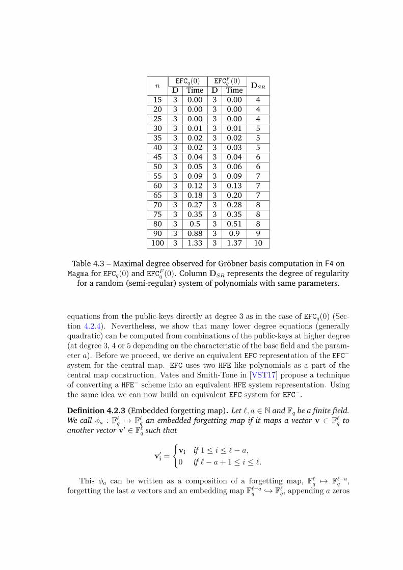
nEFCq(0) EFCFq (0) DSRD Time D Time

15 3 0.00 3 0.00 420 3 0.00 3 0.00 425 3 0.00 3 0.00 430 3 0.01 3 0.01 535 3 0.02 3 0.02 540 3 0.02 3 0.03 545 3 0.04 3 0.04 650 3 0.05 3 0.06 655 3 0.09 3 0.09 760 3 0.12 3 0.13 765 3 0.18 3 0.20 770 3 0.27 3 0.28 875 3 0.35 3 0.35 880 3 0.5 3 0.51 890 3 0.88 3 0.9 9

100 3 1.33 3 1.37 10

Table 4.3 – Maximal degree observed for Gröbner basis computation in F4 onMagma for EFCq(0) and EFCFq (0). Column DSR represents the degree of regularity

for a random (semi-regular) system of polynomials with same parameters.

equations from the public-keys directly at degree 3 as in the case of EFCq(0) (Sec-tion 4.2.4). Nevertheless, we show that many lower degree equations (generallyquadratic) can be computed from combinations of the public-keys at higher degree(at degree 3, 4 or 5 depending on the characteristic of the base field and the param-eter a). Before we proceed, we derive an equivalent EFC representation of the EFC−

system for the central map. EFC uses two HFE like polynomials as a part of thecentral map construction. Vates and Smith-Tone in [VST17] propose a techniqueof converting a HFE− scheme into an equivalent HFE system representation. Usingthe same idea we can now build an equivalent EFC system for EFC−.

Definition 4.2.3 (Embedded forgetting map). Let ℓ, a ∈ N and Fq be a finite field.

We call φa : Fℓq 7→ Fℓ

q an embedded forgetting map if it maps a vector v ∈ Fℓq to

another vector v′ ∈ Fℓq such that

v′i=

{vi if 1 ≤ i ≤ ℓ− a,

0 if ℓ− a+ 1 ≤ i ≤ ℓ.

This φa can be written as a composition of a forgetting map, Fℓq 7→ Fℓ−a

q ,forgetting the last a vectors and an embedding map Fℓ−a

q → Fℓq, appending a zeros

to a (ℓ − a)-dimensional vector. Hence, for clarity of notation, we shall denotesuch a embedding map φa as follows

φa : Fℓq 7→ Fℓ−a

q → Fℓq.

The minus modifier of EFC is formed by removing ‘a’ polynomials from the public-keys. So P− = (p1, . . . , p2n−a) = E ′ ◦ T ◦ F ◦ S ∈ F2n−a

q [x1, . . . , xn], where E ′ :F2nq 7→ F2n−a

q and S ∈ Fn×nq , T ∈ F2n×2n

q are invertible linear transformations.We can now define φa : F2n

q 7→ F2n−aq → F2n

q , an embedded forgetting map suchthat it φa(G) = (E ′(G), 0, . . . , 0) for any G ∈ F2n

q [x1, . . . , xn]. Thus, building anew system P 0 ∈ F2n

q [x1, . . . , xn] by appending zero polynomials to P−, we getP 0 = (p1, . . . , p2n−a, 0, . . . , 0) = φa ◦ T ◦ F ◦ S. One should note that the map φa

maps a vector in F2nq to another vector in F2n

q . This is a linear map and can alsobe written as a matrix Φa ∈ F2n×2n

q . Thus for an embedded forgetting map φa, weshall interchangeably use its matrix representation Φa.

Before proceeding further, we recall that the central map F of EFC (Section3.1.4) is composed of two polynomial sets

F1 = ϕ−1(α(χ)χ),

F2 := ϕ−1(β(χ)χ),

where ϕ : Fqn 7→ Fnq is the natural isomorphism as defined in Section 3.1.4.

Proposition 4.2.4. Let F1, F2 ∈ Fnq [x1, . . . , xn] represent the central map polyno-

mials of EFCq and T ∈ F2n×2nq be the linear transformation that composes with

the central map F ∈ F2nq [x1, . . . , xn] to form the public-key of EFC. Suppose there

is a embedded forgetting map φa : F2nq 7→ F2n−a

q → F2nq . Then for the public-

keys of EFC−, there is an equivalent representation of the linear transformation

Φa ◦ T using two distinct embedded forgetting maps φa1 : Fnq 7→ Fn−a1

q → Fnq and

φa2 : Fnq 7→ Fn−a2

q → Fnq such that a1 + a2 = a and φa1 acts in composition with F1

while φa2 composes with F2 of the central map, where ◦ is the composition map.

Proof. The composition Φa ◦ T ∈ F2n×2nq represents a 2n× 2n matrix. This matrix

has a co-rank of a. Now the rows of the this matrix which on composition withthe central map F ∈ F2n

q produces a vector of polynomials of which a polynomialsare zero polynomials.

Now consider the first n rows of Φa◦T ◦F ∈ F2nq [x1, . . . , xn]. We have supposedthat out of these n rows a1 rows are zero rows. This can be represented as acomposition of a n× n matrix Φa1 , comprising the same exact a1 zero rows, withF1 ∈ Fn

q [x1, . . . , xn] giving out the same equations as the first n rows of Φa ◦T ◦F .Similarly take the last n rows of Φa ◦T ◦F . We can have another n×n matrix

Φa2 with a2 zero rows which on composition with F2 ∈ Fnq [x1, . . . , xn] results in

the same last n rows of Φa ◦ T ◦ F .

Recall that the public-key is made from the composition of two invertible lineartransformations S ∈ Fn×n

q and T ∈ Fm×mq along with the central map polynomial

F . So, composition T ◦ F can be written as

T ◦ F =

[T1 T2

T3 T4

]·[F1

F2

]=

[In 00 In

]·[F ′1F ′2

]= I2n ·

[F ′1F ′2

],

where F ′1 = T1·F1+T2·F2 ∈ Fnq [x1, . . . , xn] and F ′2 = T3·F1+T4·F2 ∈ Fn

q [x1, . . . , xn].These new polynomials F ′1 and F ′2 are linear combinations of the previous centralmap polynomials. Hence, without loss of generality, from now we consider thelinear transformation T as I2n, where I2n is an identity matrix of size 2n.

Lemma 4.2.5. Let Φa ∈ F2n×2nq be a linear transformation of co-rank ‘a’. Also

let T ∈ F2n×2nq be a linear transformation that composes with the central map

polynomials (F1, F2) ∈ F2nq [x1, . . . , xn]. Using Proposition 4.2.4, consider there

exists equivalent forgetting maps, Φa1 ∈ Fn×nq and Φa2 ∈ Fn×n

q . Also consider, the

linear transformation T ∈ F2n×2nq to be the identity matrix. There exist a non-

singular linear transformation U ∈ F2n×2nq and polynomials π1, π2 ∈ Fqn [X] of

degrees qa1 and qa2 respectively, such that a1 + a2 = a and Φa ◦ T = Φa ◦ I2n =U ◦ (ϕ−1, ϕ−1) ◦ (π1, π2) ◦ (ϕ, ϕ), where I2n is the identity matrix, ϕ : Fn

q 7→ Fqn and

the composition function ◦ works component wise.

Proof. As stated earlier, we shall consider the linear transformation T to be theidentity matrix I2n. Using Proposition 4.2.4, the linear transformation Φa ◦ T =Φa ◦ I2n ∈ F2n×2n

q can be considered as collection of two separate embedded for-getting maps, Φa1 , Φa2 ∈ Fn×n

q , each acting on the first n, F1 ∈ Fnq [x1 . . . , xn] and

last n polynomials, F2 ∈ Fnq [x1 . . . , xn] of the central map, respectively. Suppose

we have a1 polynomials removed from F1 and a2 removed from F2. Thus, wehave a = a1 + a2. Let V1 ∈ Fqn be the kernel of Φa1 ◦ In ∈ Fn×n

q and similarlyV2 ∈ Fqn be the kernel of Φa2 ◦ In ∈ Fn×n

q . Let π1 ∈ Fqn [X] be the minimal poly-nomial of the algebraic set V1 and π2 ∈ Fqn [X] be the minimal polynomial forV2. Now removing a1 polynomials implies that nullity of V1 is qa1 and similarly|V2| = qa2. Thus π1 and π2 have degrees qa1 and qa2 respectively and are of theform

π1 =

a1∑

i=0

ciXqi , π2 =

a2∑

i=0

c′iXqi ,

where ci, c′i ∈ Fqn Taking the same approach as Vates and Smith-Tone [VST17,

Lemma 1], we argue that there exists linear transformations U1, U2 ∈ Fn×nq such

thatΦa1 ◦ I = U1 ◦ ϕ−1 ◦ π1 ◦ ϕ , Φa2 ◦ I = U2 ◦ ϕ−1 ◦ π2 ◦ ϕ. (4.7)

Using (D.1), we have

Φa ◦ I2n =

[Φa1 ◦ InΦa2 ◦ In

]=

[U1 ◦ ϕ−1 ◦ π1 ◦ ϕU2 ◦ ϕ−1 ◦ π2 ◦ ϕ

]=

[U1 00 U2

]·[ϕ−1 ◦ π1 ◦ ϕϕ−1 ◦ π2 ◦ ϕ

].

This above matrix representation can be also written as

Φa ◦ I2n = U ◦ (ϕ−1, ϕ−1) ◦ (π1, π2) ◦ (ϕ, ϕ),

where U =

[U1 00 U2

].

We can now prove the following result:

Proposition 4.2.6. Let F1 ∈ Fqn [χ] and F2 ∈ Fqn [χ] be the central map poly-

nomials of EFCq(0) in the extension field representation. Let there be two poly-

nomials π1, π2 ∈ Fqn [X] of degrees qa1 and qa2 respectively, as defined in Lemma

4.2.5. Additionally, we also have a = a1 + a2. Then the central map polynomials

F ′1,F ′2 ∈ Fqn [χ] for an instance of EFC−q (a) can be written as

F ′1 = π1 ◦ F1 =

a1∑

i=0

ci(α(χ)χ)qi , F ′2 = π2 ◦ F2 =

a2∑

i=0

c′i(β(χ)χ)qi . (4.8)

Proof. The public-keys for an instance of EFC−q is derived from the following com-position of maps

P− = Φa ◦ T ◦ (ϕ−1, ϕ−1) ◦ (F1,F2) ◦ (ϕ, ϕ) ◦ S, (4.9)

where Φa, T ∈ F2n×2nq and S ∈ Fn×n

q are linear transformations, and the centralmap comprises of the two quadratic polynomials F1,F2 ∈ Fqn [χ]. AssumingT = I2n to be the identity matrix, from Lemma 4.2.5, we have

Φa ◦ I2n = U ◦ (ϕ−1, ϕ−1) ◦ (π1, π2) ◦ (ϕ, ϕ).Thus, replacing this in Equation (4.9), we have

P− = Φa ◦ I2n ◦ (ϕ−1, ϕ−1) ◦ (F1,F2) ◦ (ϕ, ϕ) ◦ S= U ◦ (ϕ−1, ϕ−1) ◦ (π1, π2) ◦ (ϕ, ϕ) ◦ (ϕ−1, ϕ−1) ◦ (F1,F2) ◦ (ϕ, ϕ) ◦ S= U ◦ (ϕ−1, ϕ−1) ◦ (π1 ◦ F1, π2 ◦ F2) ◦ (ϕ, ϕ) ◦ S

This is an EFC equivalent public-key representation of the public-keys of EFC−,whose central map polynomials are given by π1 ◦ F1 and π2 ◦ F2.

From here on we shall denote the ciphertexts from the evaluation of the cen-tral map polynomials F ′1,F ′2 ∈ Fqn [χ] over some secret message as C1 ∈ Fqn andC2 ∈ Fqn respectively.Now that we have built an extension field representation of EFC− central map poly-nomials, we show how we can recover lower degree relations from these equations.First, we illustrate our approach for small values of a. For ease of notation, fromnow on we shall denote the polynomial α(χ) as α and similarly β(χ) as β. Hencethe product α(χ)χ has been represented as αχ (and βχ for β(χ)χ similarly).

Now that we have build an equivalent EFC key representation of EFC−, we showusing examples how for various values of a, we can recover lower degree relations.

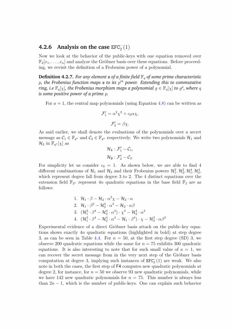
4.2.6 Analysis on the case EFC−2 (1)

Now we look at the behavior of the public-keys with one equation removed overF2[x1, . . . , xn] and analyze the Gröbner basis over these equations. Before proceed-ing, we revisit the definition of a Frobenius power of a polynomial.

Definition 4.2.7. For any element z of a finite field Fq of some prime characteristic

p, the Frobenius function maps z to its pth power. Extending this to commutative

ring, i.e Fq[χ], the Frobenius morphism maps a polynomial g ∈ Fq[χ] to gp, where qis some positive power of a prime p.

For a = 1, the central map polynomials (using Equation 4.8) can be written as

F ′1 = α2χ2 + c0αχ,

F ′2 = βχ.

As said earlier, we shall denote the evaluations of the polynomials over a secretmessage as C1 ∈ Fqn and C2 ∈ Fqn respectively. We write two polynomials H1 andH2 in Fqn [χ] as

H1 : F ′1 − C1,H2 : F ′2 − C2.

For simplicity let us consider c0 = 1. As shown below, we are able to find 4different combinations of H1 and H2 and their Frobenius powers H2

1,H22,H4

1,H42,

which represent degree fall from degree 3 to 2. The 4 distinct equations over theextension field F2n represent 4n quadratic equations in the base field F2 are asfollows:

1. H1 · β −H2 · α2χ−H2 · α2. H1 · β2 −H2

2 · α2 −H2 · αβ3. (H2

1 · β4 −H42 · α4) · χ2 −H4

2 · α2

4. (H21 · β4 −H4

2 · α4 −H1 · β4) · χ−H22 · αβ2

Experimental evidence of a direct Gröbner basis attack on the public-key equa-tions shows exactly 4n quadratic equations (highlighted in bold) at step degree3, as can be seen in Table 4.4. For n = 50, at the first step degree (SD) 3, weobserve 200 quadratic equations while the same for n = 75 exhibits 300 quadraticequations. It is also interesting to note that for such small value of a = 1, wecan recover the secret message from in the very next step of the Gröbner basiscomputation at degree 3, implying such instances of EFC−2 (1) are weak. We alsonote in both the cases, the first step of F4 computes new quadratic polynomials atdegree 2, for instance, for n = 50 we observe 93 new quadratic polynomials, whilewe have 142 new quadratic polynomials for n = 75. This number is always lessthan 2n − 1, which is the number of public-keys. One can explain such behavior

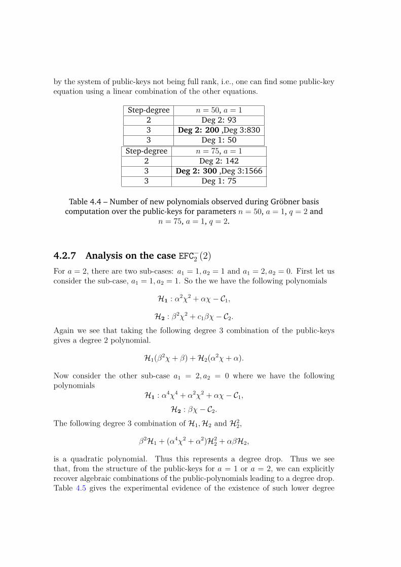
by the system of public-keys not being full rank, i.e., one can find some public-keyequation using a linear combination of the other equations.

Step-degree n = 50, a = 12 Deg 2: 933 Deg 2: 200 ,Deg 3:8303 Deg 1: 50

Step-degree n = 75, a = 12 Deg 2: 1423 Deg 2: 300 ,Deg 3:15663 Deg 1: 75

Table 4.4 – Number of new polynomials observed during Gröbner basiscomputation over the public-keys for parameters n = 50, a = 1, q = 2 and

n = 75, a = 1, q = 2.

4.2.7 Analysis on the case EFC−2 (2)

For a = 2, there are two sub-cases: a1 = 1, a2 = 1 and a1 = 2, a2 = 0. First let usconsider the sub-case, a1 = 1, a2 = 1. So the we have the following polynomials

H1 : α2χ2 + αχ− C1,

H2 : β2χ2 + c1βχ− C2.Again we see that taking the following degree 3 combination of the public-keysgives a degree 2 polynomial.

H1(β2χ+ β) +H2(α

2χ+ α).

Now consider the other sub-case a1 = 2, a2 = 0 where we have the followingpolynomials

H1 : α4χ4 + α2χ2 + αχ− C1,H2 : βχ− C2.

The following degree 3 combination of H1,H2 and H22,

β2H1 + (α4χ2 + α2)H22 + αβH2,

is a quadratic polynomial. Thus this represents a degree drop. Thus we seethat, from the structure of the public-keys for a = 1 or a = 2, we can explicitlyrecover algebraic combinations of the public-polynomials leading to a degree drop.Table 4.5 gives the experimental evidence of the existence of such lower degree

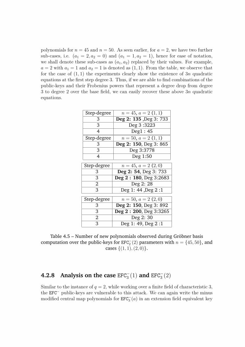
polynomials for n = 45 and n = 50. As seen earlier, for a = 2, we have two furthersub-cases, i.e. (a1 = 2, a2 = 0) and (a1 = 1, a2 = 1), hence for ease of notation,we shall denote these sub-cases as (a1, a2) replaced by their values. For example,a = 2 with a1 = 1 and a2 = 1 is denoted as (1, 1). From the table, we observe thatfor the case of (1, 1) the experiments clearly show the existence of 3n quadraticequations at the first step degree 3. Thus, if we are able to find combinations of thepublic-keys and their Frobenius powers that represent a degree drop from degree3 to degree 2 over the base field, we can easily recover these above 3n quadraticequations.

Step-degree n = 45, a = 2 (1, 1)3 Deg 2: 135 ,Deg 3: 7333 Deg 3 :32234 Deg1 : 45

Step-degree n = 50, a = 2 (1, 1)3 Deg 2: 150, Deg 3: 8653 Deg 3:37784 Deg 1:50

Step-degree n = 45, a = 2 (2, 0)3 Deg 2: 54, Deg 3: 7333 Deg 2 : 180, Deg 3:26832 Deg 2: 283 Deg 1: 44 ,Deg 2 :1

Step-degree n = 50, a = 2 (2, 0)3 Deg 2: 150, Deg 3: 8923 Deg 2 : 200, Deg 3:32652 Deg 2: 303 Deg 1: 49, Deg 2 :1

Table 4.5 – Number of new polynomials observed during Gröbner basiscomputation over the public-keys for EFC−2 (2) parameters with n = {45, 50}, and

cases {(1, 1), (2, 0)}.

4.2.8 Analysis on the case EFC−3 (1) and EFC−3 (2)

Similar to the instance of q = 2, while working over a finite field of characteristic 3,the EFC− public-keys are vulnerable to this attack. We can again write the minusmodified central map polynomials for EFC−3 (a) in an extension field equivalent key

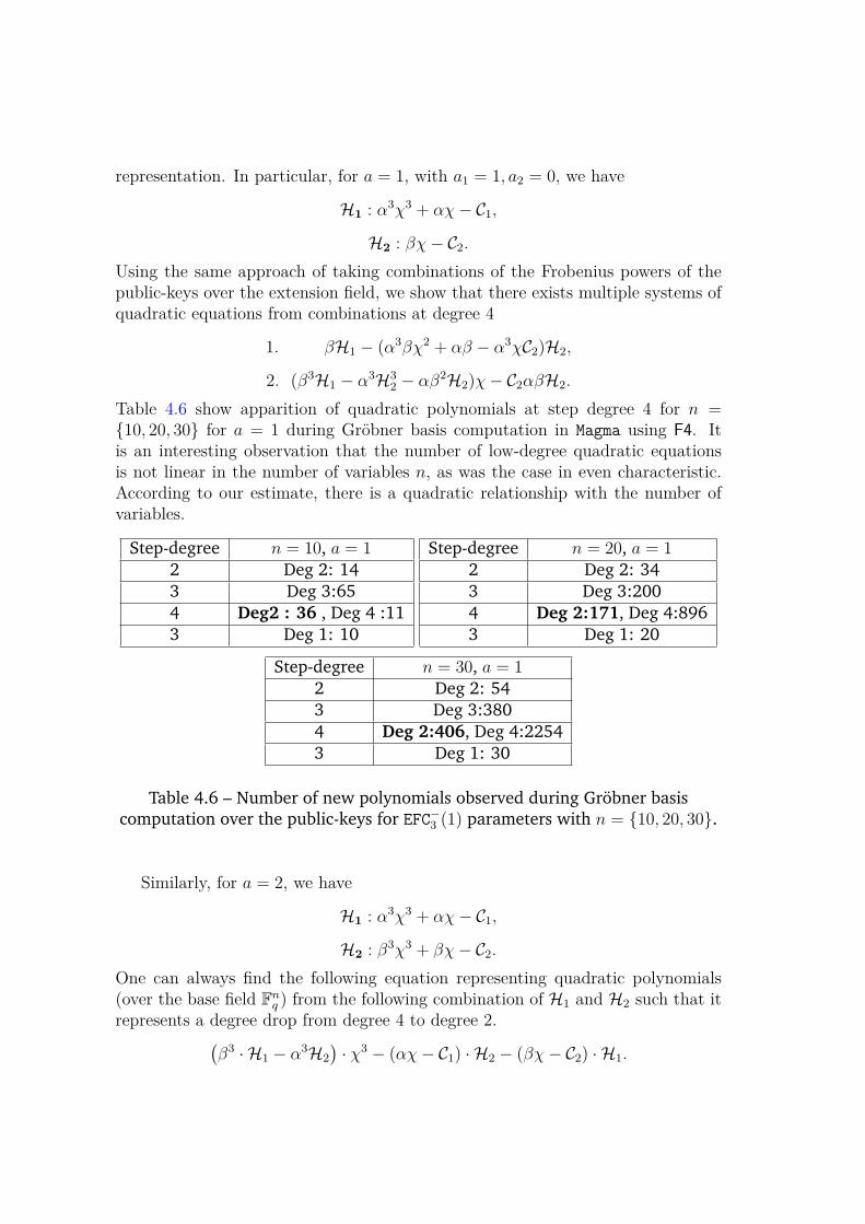
representation. In particular, for a = 1, with a1 = 1, a2 = 0, we have

H1 : α3χ3 + αχ− C1,H2 : βχ− C2.

Using the same approach of taking combinations of the Frobenius powers of thepublic-keys over the extension field, we show that there exists multiple systems ofquadratic equations from combinations at degree 4

1. βH1 − (α3βχ2 + αβ − α3χC2)H2,

2. (β3H1 − α3H32 − αβ2H2)χ− C2αβH2.

Table 4.6 show apparition of quadratic polynomials at step degree 4 for n ={10, 20, 30} for a = 1 during Gröbner basis computation in Magma using F4. Itis an interesting observation that the number of low-degree quadratic equationsis not linear in the number of variables n, as was the case in even characteristic.According to our estimate, there is a quadratic relationship with the number ofvariables.

Step-degree n = 10, a = 12 Deg 2: 143 Deg 3:654 Deg2 : 36 , Deg 4 :113 Deg 1: 10

Step-degree n = 20, a = 12 Deg 2: 343 Deg 3:2004 Deg 2:171, Deg 4:8963 Deg 1: 20

Step-degree n = 30, a = 12 Deg 2: 543 Deg 3:3804 Deg 2:406, Deg 4:22543 Deg 1: 30

Table 4.6 – Number of new polynomials observed during Gröbner basiscomputation over the public-keys for EFC−3 (1) parameters with n = {10, 20, 30}.

Similarly, for a = 2, we have

H1 : α3χ3 + αχ− C1,H2 : β3χ3 + βχ− C2.

One can always find the following equation representing quadratic polynomials(over the base field Fn

q ) from the following combination of H1 and H2 such that itrepresents a degree drop from degree 4 to degree 2.

(β3 · H1 − α3H2

)· χ3 − (αχ− C1) · H2 − (βχ− C2) · H1.

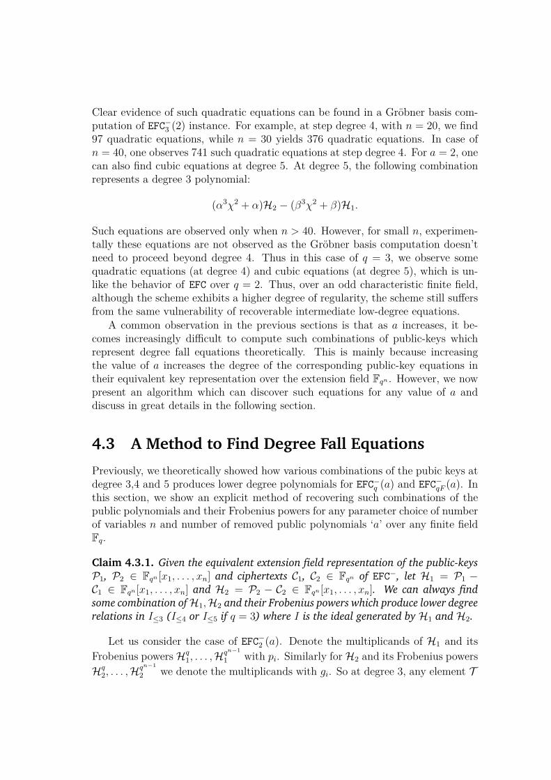
Clear evidence of such quadratic equations can be found in a Gröbner basis com-putation of EFC−3 (2) instance. For example, at step degree 4, with n = 20, we find97 quadratic equations, while n = 30 yields 376 quadratic equations. In case ofn = 40, one observes 741 such quadratic equations at step degree 4. For a = 2, onecan also find cubic equations at degree 5. At degree 5, the following combinationrepresents a degree 3 polynomial:

(α3χ2 + α)H2 − (β3χ2 + β)H1.

Such equations are observed only when n > 40. However, for small n, experimen-tally these equations are not observed as the Gröbner basis computation doesn’tneed to proceed beyond degree 4. Thus in this case of q = 3, we observe somequadratic equations (at degree 4) and cubic equations (at degree 5), which is un-like the behavior of EFC over q = 2. Thus, over an odd characteristic finite field,although the scheme exhibits a higher degree of regularity, the scheme still suffersfrom the same vulnerability of recoverable intermediate low-degree equations.

A common observation in the previous sections is that as a increases, it be-comes increasingly difficult to compute such combinations of public-keys whichrepresent degree fall equations theoretically. This is mainly because increasingthe value of a increases the degree of the corresponding public-key equations intheir equivalent key representation over the extension field Fqn . However, we nowpresent an algorithm which can discover such equations for any value of a anddiscuss in great details in the following section.

4.3 A Method to Find Degree Fall Equations

Previously, we theoretically showed how various combinations of the pubic keys atdegree 3,4 and 5 produces lower degree polynomials for EFC−q (a) and EFC−qF (a). Inthis section, we show an explicit method of recovering such combinations of thepublic polynomials and their Frobenius powers for any parameter choice of numberof variables n and number of removed public polynomials ‘a’ over any finite fieldFq.

Claim 4.3.1. Given the equivalent extension field representation of the public-keys

P1, P2 ∈ Fqn [x1, . . . , xn] and ciphertexts C1, C2 ∈ Fqn of EFC−, let H1 = P1 −C1 ∈ Fqn [x1, . . . , xn] and H2 = P2 − C2 ∈ Fqn [x1, . . . , xn]. We can always find

some combination ofH1,H2 and their Frobenius powers which produce lower degree

relations in I≤3 (I≤4 or I≤5 if q = 3) where I is the ideal generated by H1 and H2.

Let us consider the case of EFC−2 (a). Denote the multiplicands of H1 and its

Frobenius powers Hq1, . . . ,Hqn−1

1 with pi. Similarly for H2 and its Frobenius powers

Hq2, . . . ,Hqn−1

2 we denote the multiplicands with gi. So at degree 3, any element T

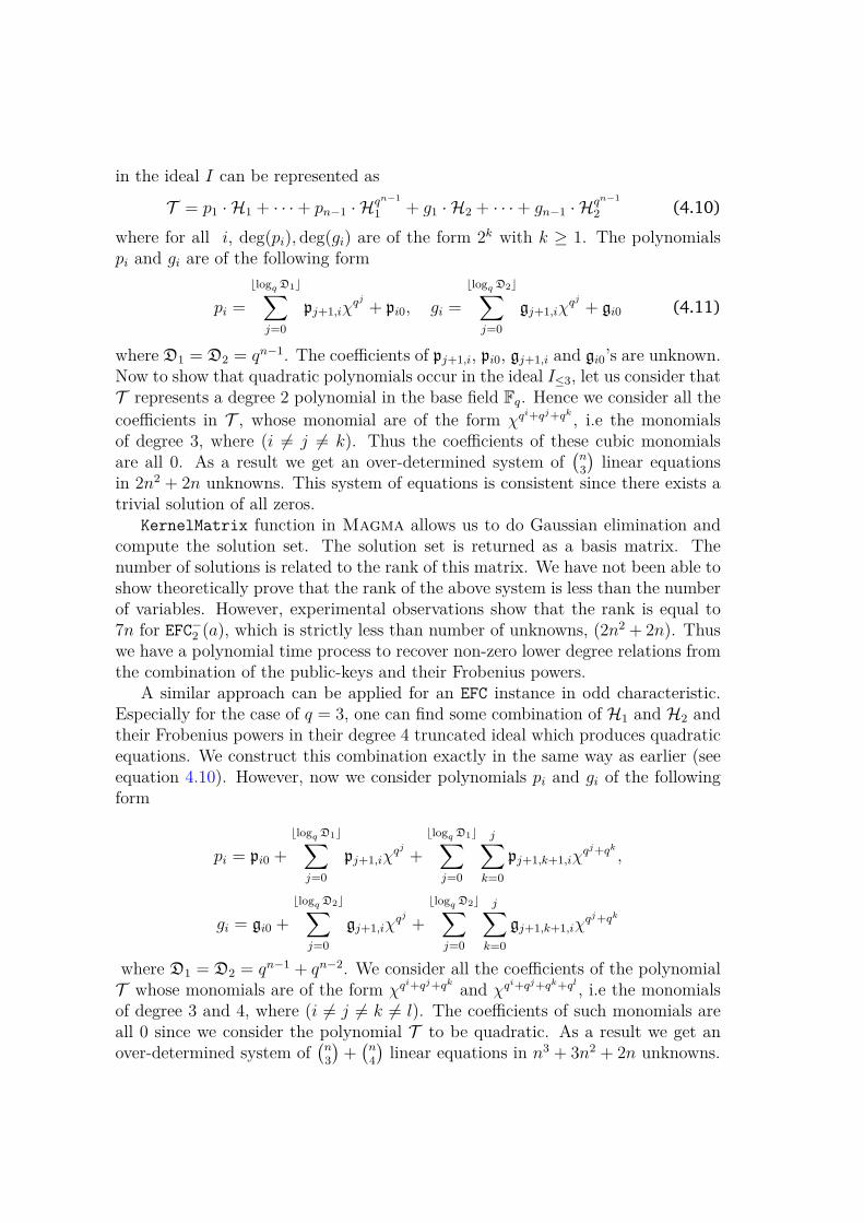
in the ideal I can be represented as

T = p1 · H1 + · · ·+ pn−1 · Hqn−1

1 + g1 · H2 + · · ·+ gn−1 · Hqn−1

2 (4.10)

where for all i, deg(pi), deg(gi) are of the form 2k with k ≥ 1. The polynomialspi and gi are of the following form

pi =

⌊logq D1⌋∑

j=0

pj+1,iχqj + pi0, gi =

⌊logq D2⌋∑

j=0

gj+1,iχqj + gi0 (4.11)

where D1 = D2 = qn−1. The coefficients of pj+1,i, pi0, gj+1,i and gi0’s are unknown.Now to show that quadratic polynomials occur in the ideal I≤3, let us consider thatT represents a degree 2 polynomial in the base field Fq. Hence we consider all the

coefficients in T , whose monomial are of the form χqi+qj+qk , i.e the monomialsof degree 3, where (i 6= j 6= k). Thus the coefficients of these cubic monomialsare all 0. As a result we get an over-determined system of

(n3

)linear equations

in 2n2 + 2n unknowns. This system of equations is consistent since there exists atrivial solution of all zeros.

KernelMatrix function in Magma allows us to do Gaussian elimination andcompute the solution set. The solution set is returned as a basis matrix. Thenumber of solutions is related to the rank of this matrix. We have not been able toshow theoretically prove that the rank of the above system is less than the numberof variables. However, experimental observations show that the rank is equal to7n for EFC−2 (a), which is strictly less than number of unknowns, (2n2 + 2n). Thuswe have a polynomial time process to recover non-zero lower degree relations fromthe combination of the public-keys and their Frobenius powers.

A similar approach can be applied for an EFC instance in odd characteristic.Especially for the case of q = 3, one can find some combination of H1 and H2 andtheir Frobenius powers in their degree 4 truncated ideal which produces quadraticequations. We construct this combination exactly in the same way as earlier (seeequation 4.10). However, now we consider polynomials pi and gi of the followingform

pi = pi0 +

⌊logq D1⌋∑

j=0

pj+1,iχqj +

⌊logq D1⌋∑

j=0

j∑

k=0

pj+1,k+1,iχqj+qk ,

gi = gi0 +

⌊logq D2⌋∑

j=0

gj+1,iχqj +

⌊logq D2⌋∑

j=0

j∑

k=0

gj+1,k+1,iχqj+qk

where D1 = D2 = qn−1 + qn−2. We consider all the coefficients of the polynomialT whose monomials are of the form χqi+qj+qk and χqi+qj+qk+ql , i.e the monomialsof degree 3 and 4, where (i 6= j 6= k 6= l). The coefficients of such monomials areall 0 since we consider the polynomial T to be quadratic. As a result we get anover-determined system of

(n3

)+(n4

)linear equations in n3 + 3n2 + 2n unknowns.

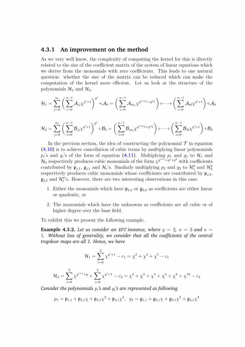
4.3.1 An improvement on the method

As we very well know, the complexity of computing the kernel for this is directlyrelated to the size of the coefficient matrix of the system of linear equations whichwe derive from the monomials with zero coefficients. This leads to one naturalquestion: whether the size of the matrix can be reduced which can make thecomputation of the kernel more efficient. Let us look at the structure of thepolynomials H1 and H2.

H1 =

a1∑

j=0

( n−1∑

i=0

Aijχqi+1

)qj

+A0 =

( n−1∑

i=0

Aia1χqi+a1+qa1

)+· · ·+

( n−1∑

i=0

Ai0χqi+1

)+A0

H2 =

a2∑

j=0

( n−1∑

i=0

Bijχqi+1

)qj

+B0 =( n−1∑

i=0

Bia2χqi+a2+qa2

)+· · ·+

( n−1∑

i=0

Bi0χqi+1

)+B0

In the previous section, the idea of constructing the polynomial T in equation(4.10) is to achieve cancellation of cubic terms by multiplying linear polynomialspi’s and gi’s of the form of equation (4.11). Multiplying p1 and g1 to H1 andH2 respectively produces cubic monomials of the form χqi+j+qj+qk with coefficientscontributed by pj,1, gj,1 and Hi’s. Similarly multiplying p2 and g2 to Hq

1 and Hq2

respectively produces cubic monomials whose coefficients are contributed by pj,2,gj,2 and Hq

i ’s. However, there are two interesting observations in this case:

1. Either the monomials which have p2,2 or g2,2 as coefficients are either linearor quadratic, or

2. The monomials which have the unknowns as coefficients are all cubic or ofhigher degree over the base field.

To exhibit this we present the following example.

Example 4.3.2. Let us consider an EFC instance, where q = 2, n = 3 and a =1. Without loss of generality, we consider that all the coefficients of the central

trapdoor maps are all 1. Hence, we have

H1 =2∑

i=0

χqi+1 − c1 = χ2 + χ3 + χ5 − c1

H2 =2∑

i=0

χqi+1+q +2∑

i=0

χqi+1 − c2 = χ2 + χ3 + χ4 + χ5 + χ6 + χ10 − c2

Consider the polynomials pi’s and gi’s are represented as following

p1 = p1,1 + p2,1χ+ p3,1χ2 + p4,1χ

4, g1 = g1,1 + g2,1χ+ g3,1χ2 + g4,1χ

4

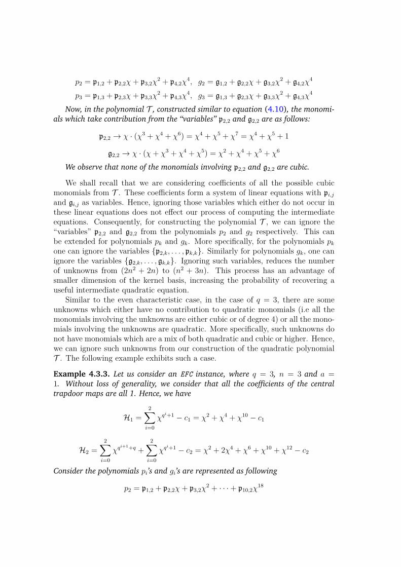
p2 = p1,2 + p2,2χ+ p3,2χ2 + p4,2χ

4, g2 = g1,2 + g2,2χ+ g3,2χ2 + g4,2χ

4

p3 = p1,3 + p2,3χ+ p3,3χ2 + p4,3χ

4, g3 = g1,3 + g2,3χ+ g3,3χ2 + g4,3χ

4

Now, in the polynomial T , constructed similar to equation (4.10), the monomi-

als which take contribution from the “variables” p2,2 and g2,2 are as follows:

p2,2 → χ · (χ3 + χ4 + χ6) = χ4 + χ5 + χ7 = χ4 + χ5 + 1

g2,2 → χ · (χ+ χ3 + χ4 + χ5) = χ2 + χ4 + χ5 + χ6

We observe that none of the monomials involving p2,2 and g2,2 are cubic.

We shall recall that we are considering coefficients of all the possible cubicmonomials from T . These coefficients form a system of linear equations with pi,jand gi,j as variables. Hence, ignoring those variables which either do not occur inthese linear equations does not effect our process of computing the intermediateequations. Consequently, for constructing the polynomial T , we can ignore the“variables” p2,2 and g2,2 from the polynomials p2 and g2 respectively. This canbe extended for polynomials pk and gk. More specifically, for the polynomials pkone can ignore the variables {p2,k, . . . , pk,k}. Similarly for polynomials gk, one canignore the variables {g2,k, . . . , gk,k}. Ignoring such variables, reduces the numberof unknowns from (2n2 + 2n) to (n2 + 3n). This process has an advantage ofsmaller dimension of the kernel basis, increasing the probability of recovering auseful intermediate quadratic equation.

Similar to the even characteristic case, in the case of q = 3, there are someunknowns which either have no contribution to quadratic monomials (i.e all themonomials involving the unknowns are either cubic or of degree 4) or all the mono-mials involving the unknowns are quadratic. More specifically, such unknowns donot have monomials which are a mix of both quadratic and cubic or higher. Hence,we can ignore such unknowns from our construction of the quadratic polynomialT . The following example exhibits such a case.

Example 4.3.3. Let us consider an EFC instance, where q = 3, n = 3 and a =1. Without loss of generality, we consider that all the coefficients of the central

trapdoor maps are all 1. Hence, we have

H1 =2∑

i=0

χqi+1 − c1 = χ2 + χ4 + χ10 − c1

H2 =2∑

i=0

χqi+1+q +2∑

i=0

χqi+1 − c2 = χ2 + 2χ4 + χ6 + χ10 + χ12 − c2

Consider the polynomials pi’s and gi’s are represented as following

p2 = p1,2 + p2,2χ+ p3,2χ2 + · · ·+ p10,2χ

18

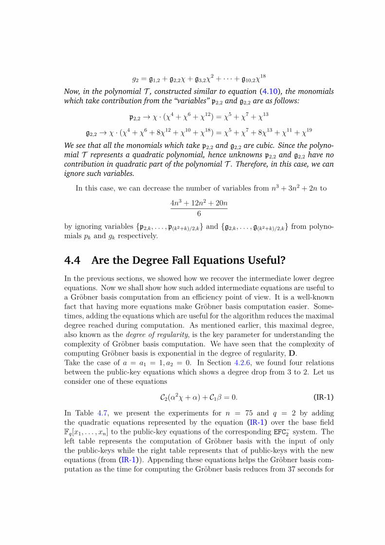
g2 = g1,2 + g2,2χ+ g3,2χ2 + · · ·+ g10,2χ

18

Now, in the polynomial T , constructed similar to equation (4.10), the monomials

which take contribution from the “variables” p2,2 and g2,2 are as follows:

p2,2 → χ · (χ4 + χ6 + χ12) = χ5 + χ7 + χ13

g2,2 → χ · (χ4 + χ6 + 8χ12 + χ10 + χ18) = χ5 + χ7 + 8χ13 + χ11 + χ19

We see that all the monomials which take p2,2 and g2,2 are cubic. Since the polyno-

mial T represents a quadratic polynomial, hence unknowns p2,2 and g2,2 have no

contribution in quadratic part of the polynomial T . Therefore, in this case, we can

ignore such variables.

In this case, we can decrease the number of variables from n3 + 3n2 + 2n to

4n3 + 12n2 + 20n

6

by ignoring variables {p2,k, . . . , p(k2+k)/2,k} and {g2,k, . . . , g(k2+k)/2,k} from polyno-mials pk and gk respectively.

4.4 Are the Degree Fall Equations Useful?

In the previous sections, we showed how we recover the intermediate lower degreeequations. Now we shall show how such added intermediate equations are useful toa Gröbner basis computation from an efficiency point of view. It is a well-knownfact that having more equations make Gröbner basis computation easier. Some-times, adding the equations which are useful for the algorithm reduces the maximaldegree reached during computation. As mentioned earlier, this maximal degree,also known as the degree of regularity, is the key parameter for understanding thecomplexity of Gröbner basis computation. We have seen that the complexity ofcomputing Gröbner basis is exponential in the degree of regularity, D.Take the case of a = a1 = 1, a2 = 0. In Section 4.2.6, we found four relationsbetween the public-key equations which shows a degree drop from 3 to 2. Let usconsider one of these equations

C2(α2χ+ α) + C1β = 0. (IR-1)

In Table 4.7, we present the experiments for n = 75 and q = 2 by addingthe quadratic equations represented by the equation (IR-1) over the base fieldFq[x1, . . . , xn] to the public-key equations of the corresponding EFC−2 system. Theleft table represents the computation of Gröbner basis with the input of onlythe public-keys while the right table represents that of public-keys with the newequations (from (IR-1)). Appending these equations helps the Gröbner basis com-putation as the time for computing the Gröbner basis reduces from 37 seconds for

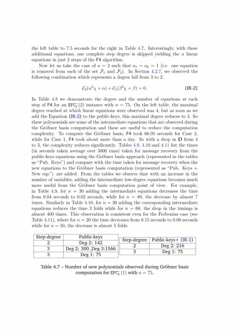
the left table to 7.5 seconds for the right in Table 4.7. Interestingly, with theseadditional equations, one complete step degree is skipped yielding the n linearequations in just 2 steps of the F4 algorithm.

Now let us take the case of a = 2 such that a1 = a2 = 1 (i.e. one equationis removed from each of the set F1 and F2). In Section 4.2.7, we observed thefollowing combination which represents a degree fall from 3 to 2.

C2(α2χ+ α) + C1(β2χ+ β) = 0. (IR-2)

In Table 4.8 we demonstrate the degree and the number of equations at eachstep of F4 for an EFC−2 (2) instance with n = 75. On the left table, the maximaldegree reached at which linear equations were observed was 4, but as soon as weadd the Equation (IR-2) to the public-keys, this maximal degree reduces to 3. Sothese polynomials are some of the intermediate equations that are observed duringthe Gröbner basis computation and these are useful to reduce the computationcomplexity. To compute the Gröbner basis, F4 took 66.05 seconds for Case 2,while for Case 1, F4 took about more than a day. So with a drop in D from 4to 3, the complexity reduces significantly. Tables 4.9, 4.10 and 4.11 list the times(in seconds taken average over 5000 runs) taken for message recovery from thepublic-keys equations using the Gröbner basis approach (represented in the tablesas “Pub. Keys”) and compare with the time taken for message recovery when thenew equations to the Gröbner basis computation (represented as “Pub. Keys +New eqs.”) are added. From the tables we observe that with an increase in thenumber of variables, adding the intermediate low-degree equations becomes muchmore useful from the Gröbner basis computation point of view. For example,in Table 4.9, for n = 30 adding the intermediate equations decreases the timefrom 0.04 seconds to 0.02 seconds, while for n = 80, the decrease by almost 7times. Similarly in Table 4.10, for n = 30 adding the corresponding intermediateequations reduces the time 3 folds while for n = 60, the drop in the timings isalmost 400 times. This observation is consistent even for the Frobenius case (seeTable 4.11), where for n = 20 the time decreases from 0.15 seconds to 0.08 secondswhile for n = 50, the decrease is almost 5 folds.

Step-degree Public-keys2 Deg 2: 1423 Deg 2: 300 ,Deg 3:15663 Deg 1: 75

Step-degree Public-keys+ (IR-1)2 Deg 2: 2163 Deg 1: 75

Table 4.7 – Number of new polynomials observed during Gröbner basiscomputation for EFC−2 (1) with n = 75.

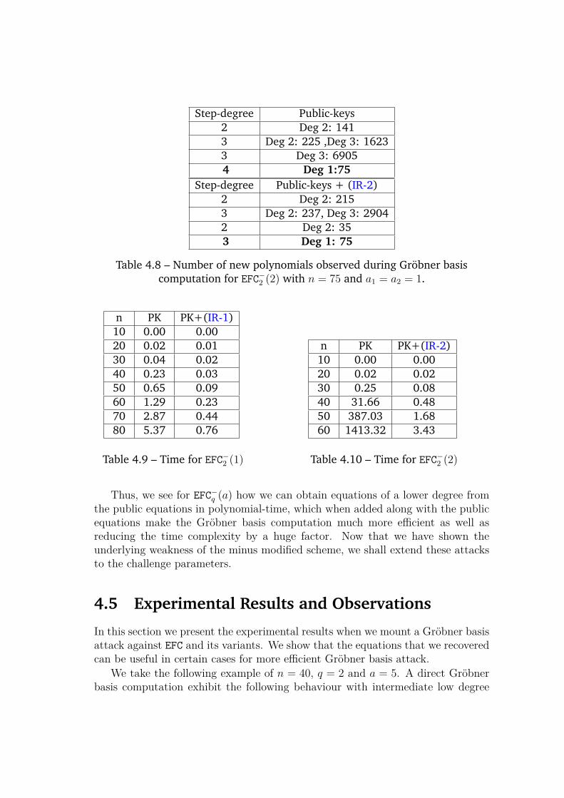
Step-degree Public-keys2 Deg 2: 1413 Deg 2: 225 ,Deg 3: 16233 Deg 3: 69054 Deg 1:75

Step-degree Public-keys + (IR-2)2 Deg 2: 2153 Deg 2: 237, Deg 3: 29042 Deg 2: 353 Deg 1: 75

Table 4.8 – Number of new polynomials observed during Gröbner basiscomputation for EFC−2 (2) with n = 75 and a1 = a2 = 1.

n PK PK+(IR-1)10 0.00 0.0020 0.02 0.0130 0.04 0.0240 0.23 0.0350 0.65 0.0960 1.29 0.2370 2.87 0.4480 5.37 0.76

Table 4.9 – Time for EFC−2 (1)

n PK PK+(IR-2)10 0.00 0.0020 0.02 0.0230 0.25 0.0840 31.66 0.4850 387.03 1.6860 1413.32 3.43

Table 4.10 – Time for EFC−2 (2)

Thus, we see for EFC−q (a) how we can obtain equations of a lower degree fromthe public equations in polynomial-time, which when added along with the publicequations make the Gröbner basis computation much more efficient as well asreducing the time complexity by a huge factor. Now that we have shown theunderlying weakness of the minus modified scheme, we shall extend these attacksto the challenge parameters.

4.5 Experimental Results and Observations

In this section we present the experimental results when we mount a Gröbner basisattack against EFC and its variants. We show that the equations that we recoveredcan be useful in certain cases for more efficient Gröbner basis attack.

We take the following example of n = 40, q = 2 and a = 5. A direct Gröbnerbasis computation exhibit the following behaviour with intermediate low degree

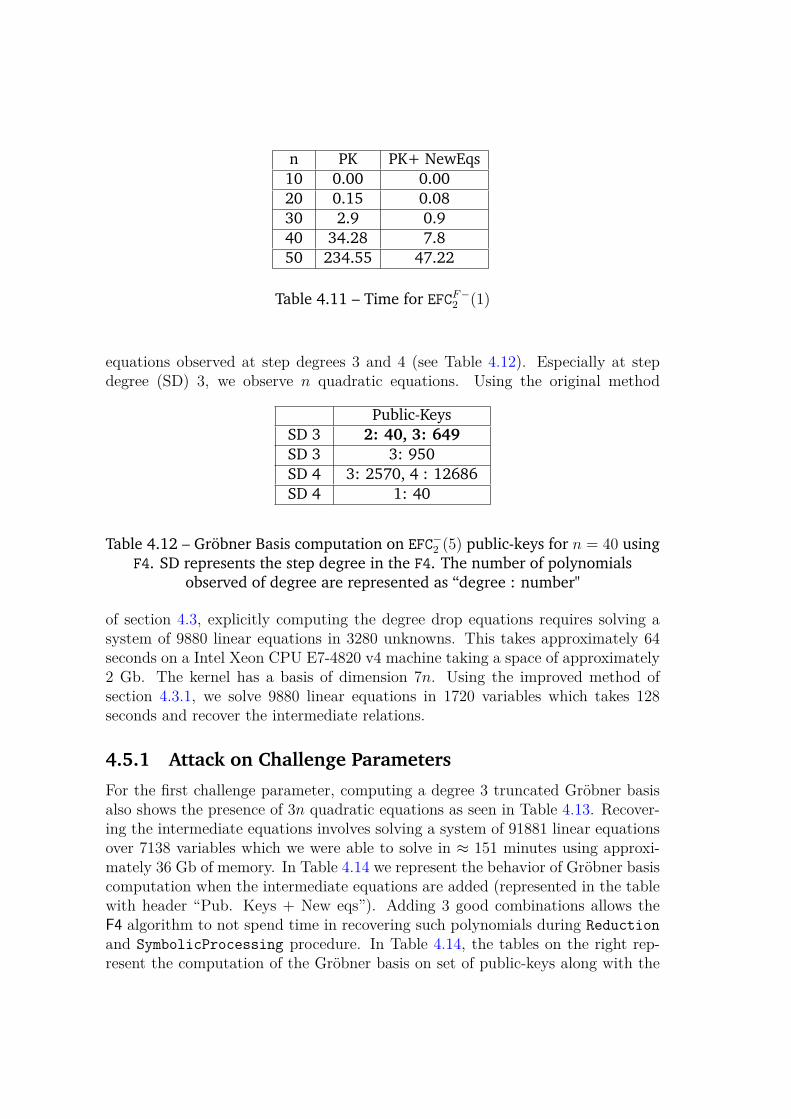
n PK PK+ NewEqs10 0.00 0.0020 0.15 0.0830 2.9 0.940 34.28 7.850 234.55 47.22

Table 4.11 – Time for EFCF−2 (1)

equations observed at step degrees 3 and 4 (see Table 4.12). Especially at stepdegree (SD) 3, we observe n quadratic equations. Using the original method

Public-KeysSD 3 2: 40, 3: 649SD 3 3: 950SD 4 3: 2570, 4 : 12686SD 4 1: 40

Table 4.12 – Gröbner Basis computation on EFC−2 (5) public-keys for n = 40 usingF4. SD represents the step degree in the F4. The number of polynomials

observed of degree are represented as “degree : number"

of section 4.3, explicitly computing the degree drop equations requires solving asystem of 9880 linear equations in 3280 unknowns. This takes approximately 64seconds on a Intel Xeon CPU E7-4820 v4 machine taking a space of approximately2 Gb. The kernel has a basis of dimension 7n. Using the improved method ofsection 4.3.1, we solve 9880 linear equations in 1720 variables which takes 128seconds and recover the intermediate relations.

4.5.1 Attack on Challenge Parameters

For the first challenge parameter, computing a degree 3 truncated Gröbner basisalso shows the presence of 3n quadratic equations as seen in Table 4.13. Recover-ing the intermediate equations involves solving a system of 91881 linear equationsover 7138 variables which we were able to solve in ≈ 151 minutes using approxi-mately 36 Gb of memory. In Table 4.14 we represent the behavior of Gröbner basiscomputation when the intermediate equations are added (represented in the tablewith header “Pub. Keys + New eqs”). Adding 3 good combinations allows theF4 algorithm to not spend time in recovering such polynomials during Reduction

and SymbolicProcessing procedure. In Table 4.14, the tables on the right rep-resent the computation of the Gröbner basis on set of public-keys along with the

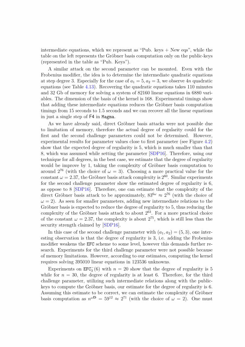
intermediate equations, which we represent as “Pub. keys + New eqs”, while thetable on the left represents the Gröbner basis computation only on the public-keys(represented in the table as “Pub. Keys”).

A similar attack on the second parameter can be mounted. Even with theFrobenius modifier, the idea is to determine the intermediate quadratic equationsat step degree 3. Especially for the case of a1 = 5, a2 = 3, we observe 4n quadraticequations (see Table 4.13). Recovering the quadratic equations takes 110 minutesand 32 Gb of memory for solving a system of 82160 linear equations in 6880 vari-ables. The dimension of the basis of the kernel is 168. Experimental timings showthat adding these intermediate equations reduces the Gröbner basis computationtimings from 15 seconds to 1.5 seconds and we can recover all the linear equationsin just a single step of F4 in Magma.

As we have already said, direct Gröbner basis attacks were not possible dueto limitation of memory, therefore the actual degree of regularity could for thefirst and the second challenge parameters could not be determined. However,experimental results for parameter values close to first parameter (see Figure 4.2)show that the expected degree of regularity is 5, which is much smaller than that8, which was assumed while setting the parameter [SDP16]. Therefore, using ourtechnique for all degrees, in the best case, we estimate that the degree of regularitywould be improve by 1, taking the complexity of Gröbner basis computation toaround 276 (with the choice of ω = 3). Choosing a more practical value for theconstant ω = 2.37, the Gröbner basis attack complexity is 260. Similar experimentsfor the second challenge parameter show the estimated degree of regularity is 6,as oppose to 8 [SDP16]. Therefore, one can estimate that the complexity of thedirect Gröbner basis attack to be approximately, 836ω ≈ 276 (with the choice ofω = 2). As seen for smaller parameters, adding new intermediate relations to theGröbner basis is expected to reduce the degree of regularity to 5, thus reducing thecomplexity of the Gröbner basis attack to about 263. For a more practical choiceof the constant ω = 2.37, the complexity is about 275, which is still less than thesecurity strength claimed by [SDP16].

In this case of the second challenge parameter with (a1, a2) = (5, 3), one inter-esting observation is that the degree of regularity is 3, i.e. adding the Frobeniusmodifier weakens the EFC scheme to some level, however this demands further re-search. Experiments for the third challenge parameter were not possible becauseof memory limitations. However, according to our estimates, computing the kernelrequires solving 395010 linear equations in 123536 unknowns.

Experiments on EFC−3 (6) with n = 20 show that the degree of regularity is 5while for n = 30, the degree of regularity is at least 6. Therefore, for the thirdchallenge parameter, utilizing such intermediate relations along with the public-keys to compute the Gröbner basis, our estimate for the degree of regularity is 6.Assuming this estimate to be correct, we can estimate the complexity of Gröbnerbasis computation as nωD = 5912 ≈ 271 (with the choice of ω = 2). One must

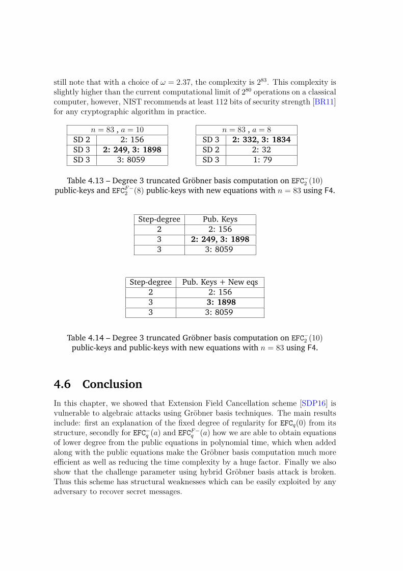
still note that with a choice of ω = 2.37, the complexity is 283. This complexity isslightly higher than the current computational limit of 280 operations on a classicalcomputer, however, NIST recommends at least 112 bits of security strength [BR11]for any cryptographic algorithm in practice.

n = 83 , a = 10SD 2 2: 156SD 3 2: 249, 3: 1898SD 3 3: 8059

n = 83 , a = 8SD 3 2: 332, 3: 1834SD 2 2: 32SD 3 1: 79

Table 4.13 – Degree 3 truncated Gröbner basis computation on EFC−2 (10)public-keys and EFCF−2 (8) public-keys with new equations with n = 83 using F4.

Step-degree Pub. Keys2 2: 1563 2: 249, 3: 18983 3: 8059

Step-degree Pub. Keys + New eqs2 2: 1563 3: 18983 3: 8059

Table 4.14 – Degree 3 truncated Gröbner basis computation on EFC−2 (10)public-keys and public-keys with new equations with n = 83 using F4.

4.6 Conclusion

In this chapter, we showed that Extension Field Cancellation scheme [SDP16] isvulnerable to algebraic attacks using Gröbner basis techniques. The main resultsinclude: first an explanation of the fixed degree of regularity for EFCq(0) from itsstructure, secondly for EFC−q (a) and EFCF−q (a) how we are able to obtain equationsof lower degree from the public equations in polynomial time, which when addedalong with the public equations make the Gröbner basis computation much moreefficient as well as reducing the time complexity by a huge factor. Finally we alsoshow that the challenge parameter using hybrid Gröbner basis attack is broken.Thus this scheme has structural weaknesses which can be easily exploited by anyadversary to recover secret messages.

Chapter 5

Solving Polynomials with Noise

Abstract

Solving a system of equations (PoSSoq) is already known to be anNP-Hard problem. In this past decade, some research work has beenput into understanding the mathematical problem of solving a systemof noisy equations. This problem has been shown to be as hard as someof the well known hard problems over lattices. Our goal in this chapteris to provide a latest state of the art on the problem. In addition tothat, we provide a survey of all the attacks that are solve this problemof PoSSoq with noise.

5.1 Motivation

In Chapter 2, we discussed the problem of solving a system of polynomial equa-tions. Solving a system of polynomials with noise is another variant that hasappeared in cryptography recently, however, formally, this problem has not beendiscussed in texts at all. In this chapter, we formalize this problem of solving a sys-tem of polynomial equations which are erroneous, which we call as the PolynomialSystem Solving With Noise (PoSSoWN).

This problem was briefly introduced (in a poster) as Polynomials With Error(PWE) problem [ALFP] in 2011. [AFFP11] was the first work which took a steptowards formalizing a new class of noisy ideal based problems. Based on theseproblems, the paper takes a particular focus on a class of multivariate schemes,which are known as “Polly Cracker”. Polly Cracker schemes in general are thosemultivariate schemes whose secret key is a Gröbner basis of a multivariate ideal. Inparticular, the secret key comprises of the Gröbner basis, say G ⊂ P , where P is apolynomial ring. The public key is comprised of a degree bounded system of poly-nomials F ⊂ 〈G〉 and a set of terms, say T ⊂ P , which maps to itself bijectivelyunder the normal form map of the Gröber basis G. This set T therefore comprises

97

of all the terms which lie below the Gröbner basis staircase. The plaintext spaceis a vector space spanned by the terms of T . Decryption involves computing anormal form over the ciphertexts, which removes all the terms in the ideal 〈G〉,yielding the plaintext message. [AFFP11] extended this idea of a scheme to de-sign a secure and somewhat homomorphic Polly Cracker-like encryption primitivebased on noisy ideal hard problems. In the same year, Albrecht et al. proposeda family of closely related problem known as Max-PoSSo which is the problem offinding any vector that satisfies the maximum number of polynomials in the inputsystem [AC11].

Even though these problems have been proposed for quite some time, not muchattention has been paid to them since then. The goal of this chapter, is to have adetailed look at the one common underlying problem of all these family of prob-lems discussed above, which is the problem of solving a noisy polynomial system(PoSSoWN). This is unlike [AFFP11], where the goal was to formalize a particularclass of hard problems that are suitable for the design of a Polly Cracker scheme.In addition to it, we also present the current state of the art algorithms that solvethis problem. The PoSSoWN problem can be defined as follows

Definition 5.1.1 (PoSSoWN). Let Fq be a finite field, P = (f1, . . . , fm) ∈ Fq[x1, . . . , xn]m

be a system of polynomials and χ be some probability distribution on Fq. The prob-

lem of PoSSoWN is to find -if any- (s1, . . . , sn) ∈ Fnq such that for all fi ∈ P , we

have fi(s1, . . . , sn) = ei, where ei ∈ Fq is some error chosen uniformly from the

distribution χ.

5.2 Hardness of the PoSSoWN Problem

In this section, we investigate the hardness of the PoSSoWN problem. We first con-sider the PoSSoWN problem in the linear case and relate it to the well establishedLWE problem [Reg09]. Then we deal with the non-linear case of PoSSoWN and relateit to another problem which has been proved to be NP hard.

Notation. We shall write x := a for assigning value a to a variable x, and x←$ χfor sampling x from a set χ. We also denote Fq[x1, . . . , xn] as a polynomial ringwith n variables (x1, . . . , xn) over a finite field Fq. Fq[x1, . . . , xn]≤d denotes the setof polynomials in the polynomial ring with degree less than or equal to d. Finally,we call an algorithm to PPT if it runs in probabilistic polynomial time.

In complexity theory, to prove the hardness of any mathematical problem, a tech-nique which is very commonly used is reduction. Reduction is an algorithm thatallows transformation of a problem to another problem. Game-based formalizationof computational problems [BR06] is one method which allows us to perform such

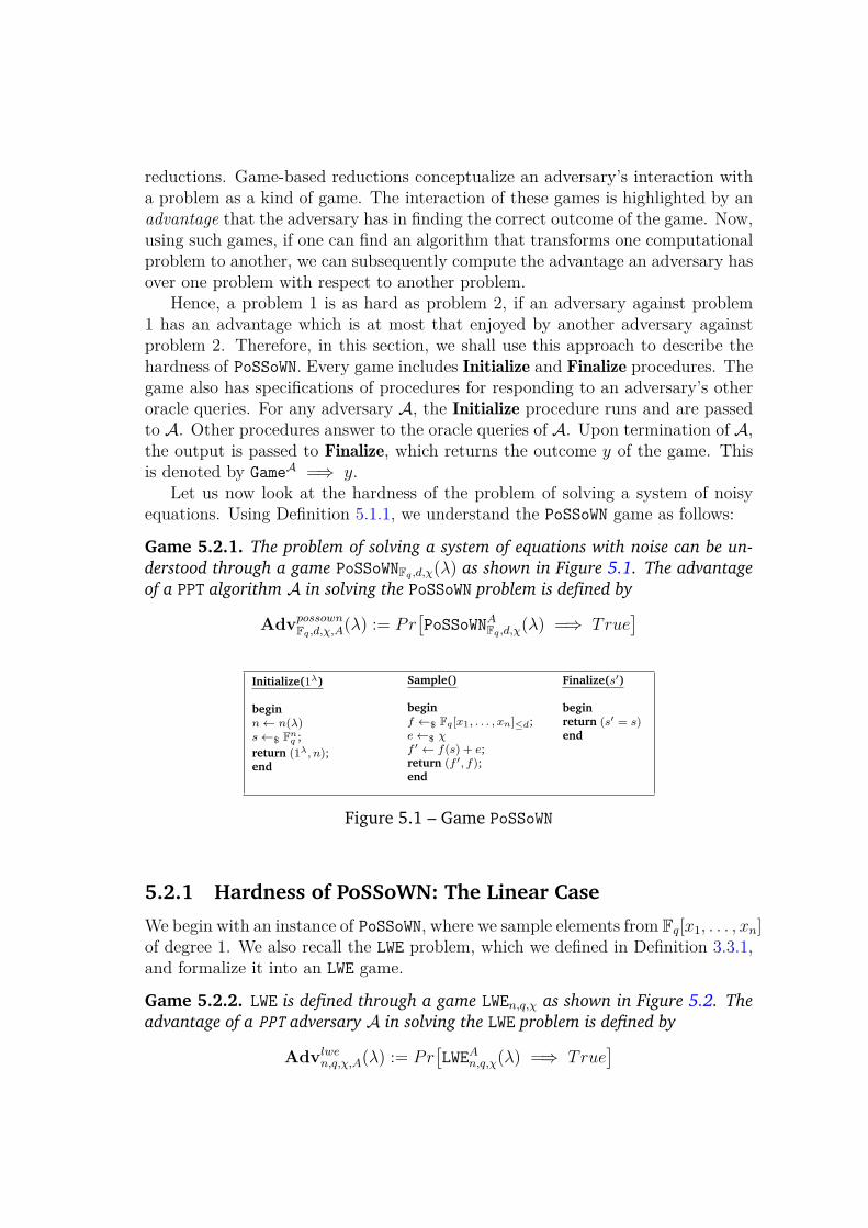
reductions. Game-based reductions conceptualize an adversary’s interaction witha problem as a kind of game. The interaction of these games is highlighted by anadvantage that the adversary has in finding the correct outcome of the game. Now,using such games, if one can find an algorithm that transforms one computationalproblem to another, we can subsequently compute the advantage an adversary hasover one problem with respect to another problem.

Hence, a problem 1 is as hard as problem 2, if an adversary against problem1 has an advantage which is at most that enjoyed by another adversary againstproblem 2. Therefore, in this section, we shall use this approach to describe thehardness of PoSSoWN. Every game includes Initialize and Finalize procedures. Thegame also has specifications of procedures for responding to an adversary’s otheroracle queries. For any adversary A, the Initialize procedure runs and are passedto A. Other procedures answer to the oracle queries of A. Upon termination of A,the output is passed to Finalize, which returns the outcome y of the game. Thisis denoted by GameA =⇒ y.

Let us now look at the hardness of the problem of solving a system of noisyequations. Using Definition 5.1.1, we understand the PoSSoWN game as follows:

Game 5.2.1. The problem of solving a system of equations with noise can be un-

derstood through a game PoSSoWNFq ,d,χ(λ) as shown in Figure 5.1. The advantage

of a PPT algorithm A in solving the PoSSoWN problem is defined by

AdvpossownFq ,d,χ,A

(λ) := Pr[PoSSoWNAFq ,d,χ(λ) =⇒ True

]

Initialize(1λ)

beginn← n(λ)s←$ Fn

q ;return (1λ, n);end

Sample()

beginf ←$ Fq [x1, . . . , xn]≤d;e←$ χf ′ ← f(s) + e;return (f ′, f);end

Finalize(s′)

beginreturn (s′ = s)end

Figure 5.1 – Game PoSSoWN

5.2.1 Hardness of PoSSoWN: The Linear Case

We begin with an instance of PoSSoWN, where we sample elements from Fq[x1, . . . , xn]of degree 1. We also recall the LWE problem, which we defined in Definition 3.3.1,and formalize it into an LWE game.

Game 5.2.2. LWE is defined through a game LWEn,q,χ as shown in Figure 5.2. The

advantage of a PPT adversary A in solving the LWE problem is defined by

Advlwen,q,χ,A(λ) := Pr

[LWEAn,q,χ(λ) =⇒ True

]

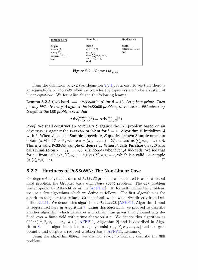
Initialize(1λ)

beginn← n(λ)s←$ Zn


Sample()

begina←$ Zn

q ;e←$ χb←

∑i aisi + e;

return (a, b);end

Finalize(s′)


Figure 5.2 – Game LWEn,q,χ

From the definition of LWE (see definition 3.3.1), it is easy to see that there isan equivalence of PoSSoWN when we consider the input system to be a system oflinear equations. We formalize this in the following lemma.

Lemma 5.2.3 (LWE hard =⇒ PoSSoWN hard for d = 1). Let q be a prime. Then

for any PPT adversary A against the PoSSoWN problem, there exists a PPT adversary

B against the LWE problem such that

AdvpossownFq ,1,χ,A

(λ) = Advlwen,q,χ,B(λ)

Proof. We shall construct an adversary B against the LWE problem based on anadversary A against the PoSSoWN problem for b = 1. Algorithm B initializes Awith λ. When A calls its Sample procedure, B queries its own Sample oracle toobtain (a, b) ∈ Zn

q × Zq where a = (a1, . . . , an) ∈ Znq . It returns

∑i aixi − b to A.

This is a valid PoSSoWN sample of degree 1. When A calls Finalize on s, B alsocalls Finalize on s = (s1, . . . , sn). B succeeds whenever A succeeds. We see thatfor a s from PoSSoWN,

∑i aixi − b gives

∑i aisi = e, which is a valid LWE sample

(a,∑

i aisi + e).

5.2.2 Hardness of PoSSoWN: The Non-Linear Case

For degree d > 1, the hardness of PoSSoWN problem can be related to an ideal-basedhard problem, the Gröbner basis with Noise (GBN) problem. The GBN problemwas proposed by Albrecht et al. in [AFFP11]. To formally define the problem,we use a few algorithms which we define as follows. The first algorithm is thealgorithm to generate a reduced Gröbner basis which we derive directly from Def-inition 2.3.11. We denote this algorithm as ReduceGB [AFFP11, Algorithm 1] andis represented here in Algorithm 7. Using this algorithm, we proceed to describeanother algorithm which generates a Gröbner basis given a polynomial ring de-fined over a finite field with prime characteristic. We denote this algorithm asGBGen(1λ,Fq[x1, . . . , xn], d,≻) [AFFP11, Algorithm 2] and is described in Algo-rithm 8. The algorithm takes in a polynomial ring Fq[x1, . . . , xn] and a degreebound d and outputs a reduced Gröbner basis [AFFP11, Lemma 6].

Using the algorithm GBGen, we are now ready to formally describe the GBN

problem.

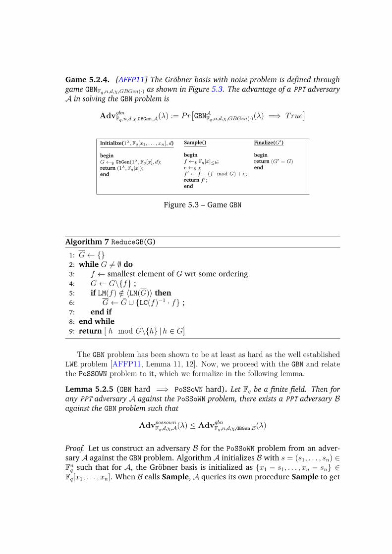
Game 5.2.4. [AFFP11] The Gröbner basis with noise problem is defined through

game GBNFq ,n,d,χ,GBGen(·) as shown in Figure 5.3. The advantage of a PPT adversary

A in solving the GBN problem is

AdvgbnFq ,n,d,χ,GBGen,A

(λ) := Pr[GBNAFq ,n,d,χ,GBGen(·)(λ) =⇒ True

]

Initialize(1λ,Fq [x1, . . . , xn], d)

beginG←$ GbGen(1λ,Fq [x], d);return (1λ,Fq [x]);end

Sample()

beginf ←$ Fq [x]≤b;e←$ χf ′ ← f − (f mod G) + e;return f ′;end

Finalize(G′)

beginreturn (G′ = G)end

Figure 5.3 – Game GBN

Algorithm 7 ReduceGB(G)

1: G← {}2: while G 6= ∅ do3: f ← smallest element of G wrt some ordering4: G← G\{f} ;5: if LM(f) /∈ 〈LM(G)〉 then6: G← G ∪ {LC(f)−1 · f} ;7: end if8: end while9: return [ h mod G\{h} |h ∈ G]

The GBN problem has been shown to be at least as hard as the well establishedLWE problem [AFFP11, Lemma 11, 12]. Now, we proceed with the GBN and relatethe PoSSOWN problem to it, which we formalize in the following lemma.

Lemma 5.2.5 (GBN hard =⇒ PoSSoWN hard). Let Fq be a finite field. Then for

any PPT adversary A against the PoSSoWN problem, there exists a PPT adversary Bagainst the GBN problem such that

AdvpossownFq ,d,χ,A

(λ) ≤ AdvgbnFq ,n,d,χ,GBGen,B

(λ)

Proof. Let us construct an adversary B for the PoSSoWN problem from an adver-sary A against the GBN problem. Algorithm A initializes B with s = (s1, . . . , sn) ∈Fnq such that for A, the Gröbner basis is initialized as {x1 − s1, . . . , xn − sn} ∈

Fq[x1, . . . , xn]. When B calls Sample, A queries its own procedure Sample to get

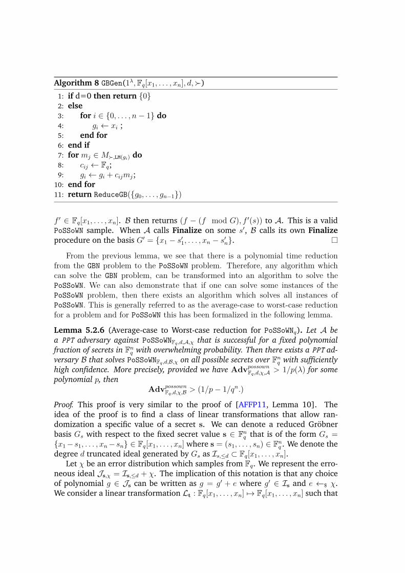
Algorithm 8 GBGen(1λ,Fq[x1, . . . , xn], d,≻)

1: if d=0 then return {0}2: else3: for i ∈ {0, . . . , n− 1} do4: gi ← xi ;5: end for6: end if7: for mj ∈M≻,LM(gi) do8: cij ← Fq;9: gi ← gi + cijmj;

10: end for11: return ReduceGB({g0, . . . , gn−1})

f ′ ∈ Fq[x1, . . . , xn]. B then returns (f − (f mod G), f ′(s)) to A. This is a validPoSSoWN sample. When A calls Finalize on some s′, B calls its own Finalizeprocedure on the basis G′ = {x1 − s′1, . . . , xn − s′n}.

From the previous lemma, we see that there is a polynomial time reductionfrom the GBN problem to the PoSSoWN problem. Therefore, any algorithm whichcan solve the GBN problem, can be transformed into an algorithm to solve thePoSSoWN. We can also demonstrate that if one can solve some instances of thePoSSoWN problem, then there exists an algorithm which solves all instances ofPoSSoWN. This is generally referred to as the average-case to worst-case reductionfor a problem and for PoSSoWN this has been formalized in the following lemma.

Lemma 5.2.6 (Average-case to Worst-case reduction for PoSSoWNq). Let A be

a PPT adversary against PoSSoWNFq ,d,A,χ that is successful for a fixed polynomial

fraction of secrets in Fnq with overwhelming probability. Then there exists a PPT ad-

versary B that solves PoSSoWNFq ,d,B,χ on all possible secrets over Fnq with sufficiently

high confidence. More precisely, provided we have AdvpossownFq ,d,χ,A

> 1/p(λ) for some

polynomial p, then

AdvpossownFq ,d,χ,B

> (1/p− 1/qn.)

Proof. This proof is very similar to the proof of [AFFP11, Lemma 10]. Theidea of the proof is to find a class of linear transformations that allow ran-domization a specific value of a secret s. We can denote a reduced Gröbnerbasis Gs with respect to the fixed secret value s ∈ Fn

q that is of the form Gs ={x1− s1, . . . , xn− sn} ∈ Fq[x1, . . . , xn] where s = (s1, . . . , sn) ∈ Fn

q . We denote thedegree d truncated ideal generated by Gs as Is,≤d ⊂ Fq[x1, . . . , xn].

Let χ be an error distribution which samples from Fq. We represent the erro-neous ideal Js,χ = Is,≤d + χ. The implication of this notation is that any choiceof polynomial g ∈ Js can be written as g = g′ + e where g′ ∈ Is and e ←$ χ.We consider a linear transformation Lt : Fq[x1, . . . , xn] 7→ Fq[x1, . . . , xn] such that

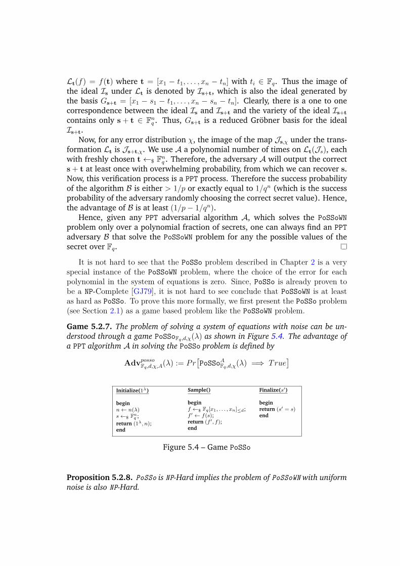
Lt(f) = f(t) where t = [x1 − t1, . . . , xn − tn] with ti ∈ Fq. Thus the image ofthe ideal Is under Lt is denoted by Is+t, which is also the ideal generated bythe basis Gs+t = [x1 − s1 − t1, . . . , xn − sn − tn]. Clearly, there is a one to onecorrespondence between the ideal Is and Is+t and the variety of the ideal Is+t

contains only s+ t ∈ Fnq . Thus, Gs+t is a reduced Gröbner basis for the ideal

Is+t.Now, for any error distribution χ, the image of the map Js,χ under the trans-

formation Lt is Js+t,χ. We use A a polynomial number of times on Lt(Js), eachwith freshly chosen t ←$ F

nq . Therefore, the adversary A will output the correct

s+ t at least once with overwhelming probability, from which we can recover s.Now, this verification process is a PPT process. Therefore the success probabilityof the algorithm B is either > 1/p or exactly equal to 1/qn (which is the successprobability of the adversary randomly choosing the correct secret value). Hence,the advantage of B is at least (1/p− 1/qn).

Hence, given any PPT adversarial algorithm A, which solves the PoSSoWN

problem only over a polynomial fraction of secrets, one can always find an PPT

adversary B that solve the PoSSoWN problem for any the possible values of thesecret over Fq.

It is not hard to see that the PoSSo problem described in Chapter 2 is a veryspecial instance of the PoSSoWN problem, where the choice of the error for eachpolynomial in the system of equations is zero. Since, PoSSo is already proven tobe a NP-Complete [GJ79], it is not hard to see conclude that PoSSoWN is at leastas hard as PoSSo. To prove this more formally, we first present the PoSSo problem(see Section 2.1) as a game based problem like the PoSSoWN problem.

Game 5.2.7. The problem of solving a system of equations with noise can be un-

derstood through a game PoSSoFq ,d,χ(λ) as shown in Figure 5.4. The advantage of

a PPT algorithm A in solving the PoSSo problem is defined by

AdvpossoFq ,d,χ,A

(λ) := Pr[PoSSoAFq ,d,χ(λ) =⇒ True

]

Initialize(1λ)

beginn← n(λ)s←$ Fn


Sample()

beginf ←$ Fq [x1, . . . , xn]≤d;f ′ ← f(s);return (f ′, f);end

Finalize(s′)


Figure 5.4 – Game PoSSo

Proposition 5.2.8. PoSSo is NP-Hard implies the problem of PoSSoWN with uniform

noise is also NP-Hard.

Proof. As previously mentioned, the PoSSo is a special case of PoSSoWN whereall the errors are chosen to be specifically 0. When the noise is chosen from auniform distribution, the probability of choosing zero error is same as choosingany other error. Thus, any algorithm which solves the PoSSoWN problem, cansolve any instance of PoSSo and there is a polynomial time reduction betweenthese two algorithms. Since PoSSo is NP-Hard, any instance of PoSSoWN withuniform noise is also NP-Hard.

In the next section, we shall look at some of the algorithms which can solvethis PoSSoWN problem.

5.3 Algorithms to Solve PoSSoWN

In the following sections, we discuss the possible methods of solving this problemand thus provide the hardness results, which relates to our problem.

5.3.1 Arora-Ge Gröbner Basis Method

An algorithm to solve the LWE problem with small Gaussian noise was proposedby Sanjeev Arora and Rong Ge in [AG11]. They rely on constructing a higherdegree univariate polynomial from a given public key equation, such that it takesinto consideration all the possible values of error the noisy public key could have,irrespective of the noise distribution. Consider an LWE instance, where the errorsare chosen uniformly from a distribution Ψk, which has a range [−k, k] of integers.Additionally, the value of k ∈ Z is such that 2k + 1 < q, i.e., the error is alwaysan integer in the range (−(q− 1)/2, (q− 1)/2), where q is a prime. The algorithmconstructs the following polynomial P ∈ Zq[x1, . . . , xn] such that P (η) = 0, whereη is the error.

P (η) = ηk∏

j=1

(η − j)(η + j).

This polynomial P is of degree 2k + 1. Recall from Section 3.3, an LWE instancecould be written as a system of equations of the form b = a·z+e where a, b ∈ Fn

q , e ∈Ψk and z is an n-dimensional variable vector. So substituting the error variableη with a · z + b in the polynomial P (η), we obtain a degree 2k + 1 polynomial inthe variables z = (z1. . . . , zn). Linearization of the polynomial produces a linearequation from P but over N =

(n+(2k+1)

n

)new variables. If we query the LWE oracle

≈ O(N log q) number of times and apply this above described technique, we obtaina system of linear equations, which one can solve with Gaussian elimination withsome high probability. We can apply a similar approach to solve PoSSoWN and thusalso holds true for a system of noisy quadratic equations.

An instance of PoSSoWNq involves equations which are of the form fi − bi =fi − fi(s)− ei ∈ Fq[x1, . . . , xn], where fi ∈ Fq[x1, . . . , xn], s ∈ Fn

q and ei ∈ Ψk is anerror.

Alternatively, we can represent the error (η) by the following error polynomial:

η = b− f(x), (5.1)

where x is vector of variables (x1, . . . , xn). We construct the polynomial P (η) ∈Fq[x1, . . . , xn] such that

P (η) = η

k∏

j=1

(η − j)(η + j). (5.2)

An instance of PoSSoWN comprises of a system F ∈ Fmq [x1, . . . , xn] of m quadratic

noisy equations. Therefore, corresponding to each polynomial fi ∈ F , we canconstruct a polynomial Pi ∈ Fq[x1, . . . , xn] of degree 4k+2. It is quite intuitive tosee that the polynomial Pi equals zero when x = s. In addition to our system ofpolynomials 6.6, we have another set of n equations of the form

(x1 + k) · · · (x1 + 1)x1(x1 − 1) · · · (x1 − k) = 0,

(x2 + k) · · · (x2 + 1)x2(x2 − 1) · · · (x2 − k) = 0,

...

(xn + k) · · · (xn + 1)xn(xn − 1) · · · (xn − k) = 0.

So if we are able to find a Gröbner basis of this system of equations along withsystem Pi(x) = 0, then we will recover s.

Recall from Chapter 2, Gröbner basis algorithms such as F4 and F5 are tech-niques to recover solutions to a system of equations. The complexity of F5 algo-rithm [Fau02] over a system of m polynomials in Fq is upper bounded by

O(m′Dreg

(n+Dreg

Dreg

)ω),

where Dreg is the degree of regularity of 〈P1, P2, ...Pm′〉 and 2 ≤ ω < 3 is the linearalgebra constant. Before, we proceed, we present some assumptions, which areimportant for the results of this section.

Assumption 5.3.1. For our problem, the instance of PoSSoWNq consists of a system

of noisy quadratic polynomials denoted by F = (f1, . . . , fm) ∈ Fq[x1, . . . , xn] where

each fi are of the form

f(x1, . . . , xn) =∑

1≤i,j≤n

aijxixj +∑

1≤i≤n

bixi + e,

where aij, bi ∈ Fq and e←$ Ψk.

Assumption 5.3.2. Let (G1, G2,∑

ij G1ij,kxixj +∑

i G2kxi + ek) = (G1, G2, c) ∈Fn2×mq × Fn×m

q × Fmq be such that G1, G2 are sampled uniformly at random and e is

chosen uniformly from the distribution Ψk. Let P (x) be the polynomial as defined

in Equation (5.2). We define

P1 = P (c1 −∑

ij

G1ij,1xixj −∑

i

G21xi) = 0

...

Pm = P (cm −∑

ij

G1ij,mxixj −∑

i

G2mxi) = 0.

It holds that 〈P1, . . . , Pm〉 is semi-regular (See Definition 2.3.35).

Using Assumption 5.3.2, we consider the system of polynomials {P1 . . . , Pm}as semi-regular. Therefore, its Hilbert polynomial [CLO06] is given by

H(z) =(1− z2k+1)n(1− zd)m

(1− z)n, (5.3)

where d = 4k+2 and m is the number of available equations and n is the numberof variables. The degree of regularity Dreg is given by the index of the first non-positive coefficient in the expansion of the Hilbert polynomial (Equation 5.3).

Note 5.3.1. The results of complexity in this section rely majorly on the assump-

tion that the system of equations occurring from the Arora-Ge style construction

are semi-regular. The semi-regularity assumption essentially states that solving this

system of polynomials is as hard as solving a random system of equations. If this

were to the contrary, one might deduce that the degree of regularity bound pro-

vided by the Hilbert series is not tight, and hence a sharper bound could be found.

This would imply that the complexity analysis could be improved and thus possibly

might lead towards a classical algorithm for solving the PoSSoWN problem that is

not exponential to the very least.

5.3.2 Arora-Ge Method with Linearization (For q = 2 and m =O(n2)

In this subsection we consider the particular sub-case of the PoSSoWNq when q = 2and the number of samples available m = O(n2). Given a system of ǫn2 quadraticpolynomials in n variables, we can use linearization techniques in conjunction withthe above mentioned Arora-Ge technique to solve PoSSoWN2. The product P (η) =η(η − 1) produces an equation of degree 4. We have ǫn2 such equations. Using

linearization, we can produce a system of ǫn2 quadratic equations in n2/2 variablesyij = xixj. Additionally, a monomial xaxbxcxd be written in three possible manner.

(xaxb)(xcxd) = (xaxc)(xbxd) = (xaxd)(xbxc) = yabycd = yacybd = yadybc,

There are n4/4! different ways to choose the 4-tuples of distinct indices, and eachchoice gives rise to 2 equations. We thus have about n4/12 additional quadraticequations in n2/2 yij variables. This number of variables can be reduced to about(1/2− ǫ)n2 by replacing each of yij variables by its parametric representation as alinear combination of new variables zk. These (ǫn2+n4/12) quadratic equations inthe new (1/2−ǫ)n2 can be linearized again by replacing each product zizj by a newvariable vij. This new system has (ǫn2+n4/12) linear equations in ((1/2−ǫ)n2)2/2variables vij. This new system is uniquely solvable when

(ǫn2 + n4/12) ≥ ((1/2− ǫ)n2)2/2.

If this previous condition holds true, then the system of equations originatingfrom the Arora-Ge method can be solved by linearization, however, in the othercase, the previously proposed method from Section 5.3.1 of using Gröbner basistechniques still holds.

5.3.3 Exhaustive Search

We also consider the class of combinatorial attacks on the PoSSoWN problem. Suchattacks can be mounted on either the secret directly, or could be used to recoverthe noise in order to recover the PoSSo instance from the PoSSoWN instance. Wepresent the two algorithms as follows.

The first type of exhaustive search is over all the possible values of the secrets ∈ Fn

q . Since s is a vector with dimension n, hence in the worst-case scenario, theattacker has to compute qn possible solutions. For an instance of PoSSo, evaluat-ing the public-key polynomials over qn candidate solutions and comparing with theciphertexts is the method of pruning. However, for the case of PoSSoWN, withoutthe knowledge of the error, such an attack is not possible. This can be used in con-junction with other attacks such as the previously mentioned Arora-Ge approach(see Section 5.3.1) that proposes a method of disregarding the error by construct-ing a higher degree polynomial. The complexity of such an attack depends on thedegree of the polynomial P as defined in Equation (5.2). In particular, from thecomplexity results of enumerating the common zeros of a system of multivariatepolynomials over F2[x1, . . . , xn] [BCC+10], the expected number of operations is4(4k + 2) log2 n · 2n where k is the upper bound on the magnitude of the error.

Another possible way to look at a system of m noisy quadratic equations overn variables is to consider it as a system of m equations over n + m variables,i.e counting the errors as unknown variables. Thus enumerating the errors withexhaustive search, the problem reduces to just solving a system of m quadraticequations in n variables. Recall from Section 2.2, [LPT+17] introduces such amethod that allows us to solve the system of equations. Once the error valueshave been recovered, substituting them back into the system of noisy polynomialsyields an instance of PoSSo. Now [LPT+17] states the time complexity is

O(qn ·

(log q

2e

)−n), where e = 2.718 . . . the Napier constant,

for finding the satisfiability of a system of equations where the solutions are in Fq.So the total time complexity of performing an exhaustive search over the error andthen the proposed algorithm of [LPT+17] is therefore

km · O(qn ·

(log q

2e

)−n).

In this previous approach, instead of performing exhaustive search or a fastbrute force attack of [LPT+17], one can use Gröbner basis to solve the system ofequations. Using F5 [Fau02], the expected number of operations is upper boundedby

O(m ·Dreg

((n+Dreg

Dreg

)ω)).

Hence, the total complexity including the exhaustive search over the errors is

km ·(m ·Dreg

((n+Dreg

Dreg

)ω)),

where Dreg is the degree of regularity over the system of m quadratic equations inn variables (Refer to Proposition 2.3.36 from Section 2.3.3).

5.3.4 Max-PoSSo Gröbner Basis Attack

In this section, we propose an algorithm which solves an instance of the Max-PoSSoproblem (see Section 5.1), and whose solution can be turned into a solution for aninstance PoSSoWN problem. Previously, we performed a Gröbner basis attack onthe input system of equations which were erroneous. Without loss of generality, wecan assume that only a certain fraction of the equations is non-noisy. So if we selectonly such non-noisy equations and then solve the Gröbner basis just over these nonnoisy equations gives us a solution (or a set of solutions) to the system of equations.

Suppose we are given a system of m equations in n variables. Let us assume

that only t < m equations are error-free. Therefore, one can perform Gröbnerbasis computation over this subsystem of t quadratic equations over n variables,whose complexity is upper bounded by

(tDreg

(n+Dreg

Dreg

)ω)

Since, we perform this for a particular correct choice of t equations, the numberof expected operations for the entire attack is upper bounded by

(m

t

)·(tDreg

(n+Dreg

Dreg

)ω)

Furthermore, one can also perform an exhaustive search for this fraction of t equa-tions and then compute the Gröbner basis of the corresponding subsystem. Thisformalization of the problem differs from the attack presented in the previous Sec-tion 5.3.2. It should be noted that, the degree of regularity of the two systems inconsideration vary since in the previous approach, the number of equations m > n,while now we consider only a fraction t of these m polynomials.

5.4 Conclusion

In this chapter, we provide the first complete state-of-the-art of the PoSSoWN prob-lem, the noisy variant of the well known NP-Hard PoSSo problem. We show that thehardness of the PoSSoWN can be reduced to some well known hard problems. Wealso define the decision and the search variants of the problem and show that thereis an equivalence between these variants when the number of samples is boundedby some polynomial factor of the number of variables. Additionally, we providea survey of all known algorithms which solve the PoSSoWN problem which includesome techniques to solve the LWE problem modified as algorithms for PoSSoWN. Weconclude that the PoSSoWN problem is a good candidate to construct multivariatecryptosystems that are guaranteed post-quantum security via the hardness of thehard problem.

Chapter 6

CFPKM: A Submission to NIST

Abstract

The problem of solving a system of noisy polynomial equations hasbeen shown to be a NP-Hard problem. As a submission to the NIST

Post-quantum standardization completion, we designed a new multi-variate key encapsulation scheme based on this hard problem. Weprovided a new design which takes use of errors in polynomials in or-der to blind the information passed over open channels. We describethe scheme along with security analysis and complete analysis of thepotential algebraic attacks on it along with a proposal of two securityparameters satisfying various security strengths. Finally we show whybecause of structural defect, the scheme was broken.

6.1 Background

In Chapter 3, we discussed Public-key cryptosystems in great detail. However,public-key algorithms are generally very slow as compared to symmetric crypto-graphic algorithms, one of the main reasons being a large key size resulting ina larger requirement of computation power. Therefore, it is not efficient to usepublic-key algorithms when Bob wants to send large amounts of data. But ifpublic-key encryption techniques are used to exchange a shared key between Aliceand Bob, by using a fast symmetric mechanism with the shared key, Bob can sendlarge amounts of data to Alice much more efficiently.

However, as mentioned previously, symmetric cryptosystems suffer from an“issue”. The parties need to exchange the secret-key before the cryptosystem isready for use. A key-exchange mechanism provides a method to do this. A key-exchange scheme works as follows: two parties exchange a sequence of information,without exchanging the actual secret key. The key-exchange is also equipped witha reconciliation mechanism such that both users can agree to the same key.

111

Previously in Chapter 1, we also talked about another possible way a key-exchange can be done: via public-key algorithms. These types of public-key al-gorithms are also commonly known as Key Encapsulation Mechanisms (KEM).It is not hard to see that using such techniques, one can convert any encryption-decryption public-key cryptosystem into a key encapsulation scheme.

Recently many key-exchange schemes have been published, most famously byDing et. al in [DXL12], Chris Peikert in [Pei14] and Costello et al [BCD+16] toname a few. Peikert in his paper [Pei14] detailed the construction of a passivelysecure KEM based on the key exchange using an innovative key reconciliationmechanism.

As already mentioned, the NIST PQC standardization process involved the callof proposals for post-quantum key exchange schemes. Amongst all the submissions,the majority of the key-exchange cryptosystems that have been proposed are basedon the hard problem of LWE, which are lattice-based. In this chapter, we presenta KEM, that is based on the hard problem of PoSSoWN, which we discussed ingreat detail in Chapter 5.

6.2 Passively Secure KEM

In this section we construct a KEM, based on problem of solving a system of poly-nomials with error, i.e PoSSoWN. First we describe the design an un-authenticatedkey exchange protocol.

6.2.1 Parameter Space

The scheme involves the following parameters :

1. q, a large positive prime power, which defines the finite field Fq for thePolynomial Ring P, where we define our system of equations. It is taken ofthe form of 2k for some k ∈ Z+,

2. Zq defines the field of integers modulus q,

3. n, the number of variables which defines the Polynomial Ring P,

4. m, number of equations in the system of equations,

5. s, is an integer which defines the range of values from where the secret anderrors are chosen uniformly,

6. B, is the number of most significant bits which are chosen to create a sessionkey,

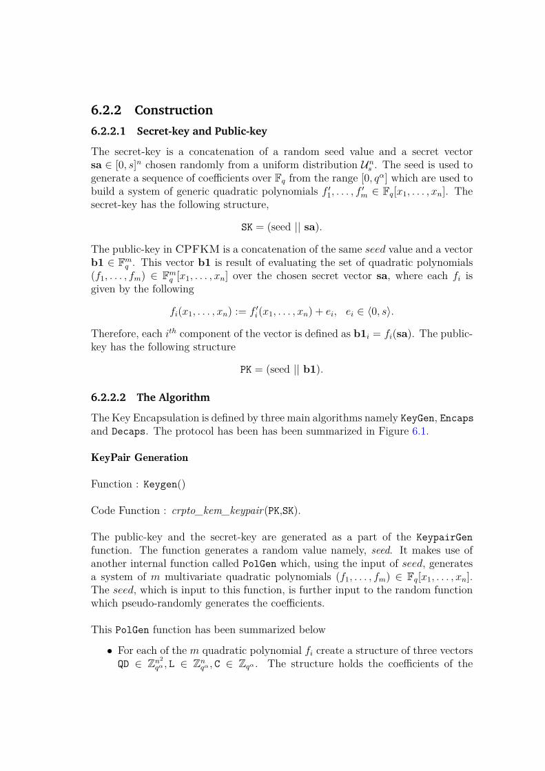
6.2.2 Construction

6.2.2.1 Secret-key and Public-key

The secret-key is a concatenation of a random seed value and a secret vectorsa ∈ [0, s]n chosen randomly from a uniform distribution Un

s . The seed is used togenerate a sequence of coefficients over Fq from the range [0, qα] which are used tobuild a system of generic quadratic polynomials f ′1, . . . , f

′m ∈ Fq[x1, . . . , xn]. The

secret-key has the following structure,

SK = (seed || sa).

The public-key in CPFKM is a concatenation of the same seed value and a vectorb1 ∈ Fm

q . This vector b1 is result of evaluating the set of quadratic polynomials(f1, . . . , fm) ∈ Fm

q [x1, . . . , xn] over the chosen secret vector sa, where each fi isgiven by the following

fi(x1, . . . , xn) := f ′i(x1, . . . , xn) + ei, ei ∈ 〈0, s〉.

Therefore, each ith component of the vector is defined as b1i = fi(sa). The public-key has the following structure

PK = (seed || b1).

6.2.2.2 The Algorithm

The Key Encapsulation is defined by three main algorithms namely KeyGen, Encapsand Decaps. The protocol has been has been summarized in Figure 6.1.

KeyPair Generation

Function : Keygen()

Code Function : crpto_kem_keypair(PK,SK).

The public-key and the secret-key are generated as a part of the KeypairGen

function. The function generates a random value namely, seed. It makes use ofanother internal function called PolGen which, using the input of seed, generatesa system of m multivariate quadratic polynomials (f1, . . . , fm) ∈ Fq[x1, . . . , xn].The seed, which is input to this function, is further input to the random functionwhich pseudo-randomly generates the coefficients.

This PolGen function has been summarized below

• For each of the m quadratic polynomial fi create a structure of three vectorsQD ∈ Zn2

qα , L ∈ Znqα , C ∈ Zqα . The structure holds the coefficients of the

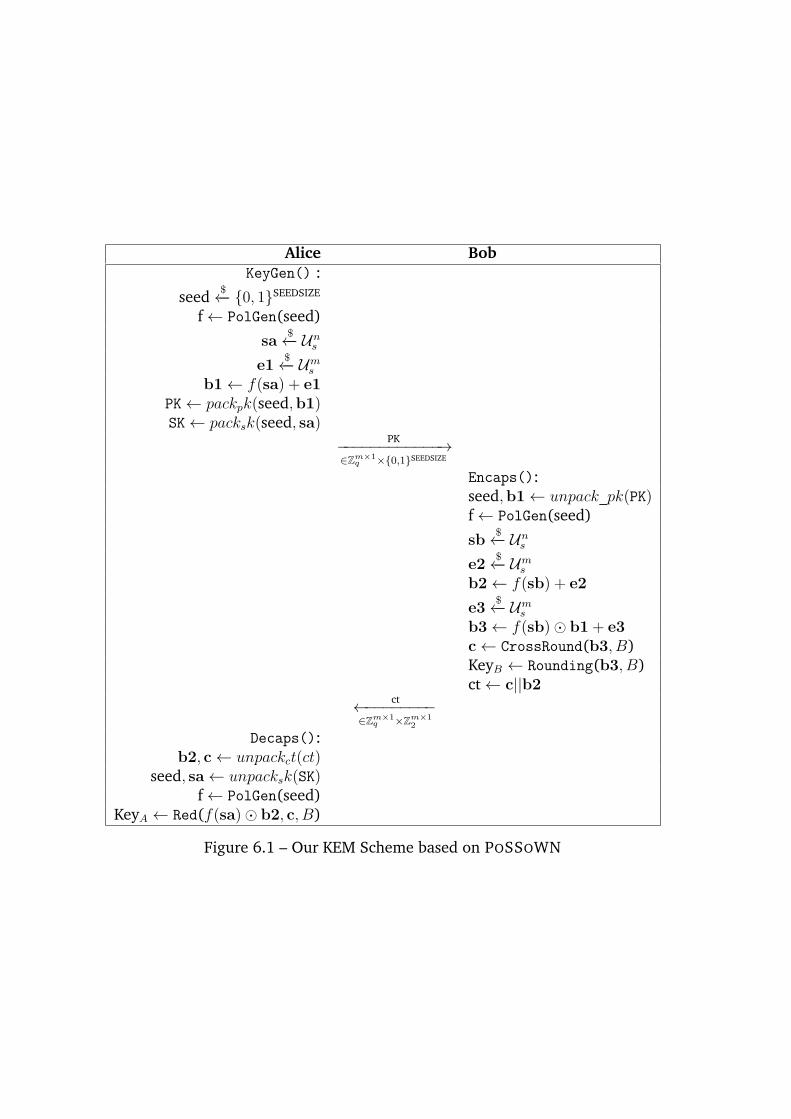
Alice BobKeyGen() :

seed $←− {0, 1}SEEDSIZE

f← PolGen(seed)

sa$←− Un

s

e1$←− Um

s

b1← f(sa) + e1

PK← packpk(seed,b1)SK← packsk(seed, sa)

PK−−−−−−−−−−−−→∈Zm×1

q ×{0,1}SEEDSIZE

Encaps():seed,b1← unpack_pk(PK)f← PolGen(seed)

sb$←− Un

s

e2$←− Um

s

b2← f(sb) + e2

e3$←− Um

s

b3← f(sb)⊙ b1+ e3

c← CrossRound(b3, B)KeyB ← Rounding(b3, B)ct← c||b2

ct←−−−−−−−−∈Zm×1

q ×Zm×12

Decaps():b2, c← unpackct(ct)

seed, sa← unpacksk(SK)f← PolGen(seed)

KeyA ← Red(f(sa)⊙ b2, c, B)

Figure 6.1 – Our KEM Scheme based on POSSOWN

polynomials such that QD holds the coefficients of the quadratic monomials,L holds the coefficients for the linear monomials and C holds the constantterm,

• using a random function and the seed, populate these vectors

• return fi

Once the PolGen function creates the polynomials, the KeyGen algorithm randomlygenerates a secret vector sa of dimension n from the uniform distribution Un

s . Anerror vector e1 ∈ Um

s is also generated. Each of the polynomials fi, from thepreviously generated system of quadratic polynomials using PolGen, are evaluatedover the secret vector sa and noise is added to them to generate another vectorb1 where

b1i = fi(sa) + e1i mod q,

for ith component of the vector.

Finally the Public Key PK is constructed by concatenating the seed along withthis vector b1 using the pack_pk function. The Secret Key SK is formed by con-catenating seed and the secret vector sa using the pack_sk function. The functionthen outputs the PK and SK.

Key Encapsulation

Function : Encaps()

Code Function : crypto_kem_enc()

The encapsulation process encodes the shared secret using the public-key of Alice.It takes use of some extra functions which have been defined below.

1. CrossRound(w,B): This function takes in an integer w ∈ [0, q) and given B,outputs the (B +1)’th most significant bit of log q-bit binary representationof w, which has been referred to as the crossround bit.

CrossRound(w,B) = ⌊w · 2−B+1⌋ mod 2.

The function can also be extended to a vector of integers w ∈ [0, q)m. Thuson an input of a vector, CrossRound works independently on each componentof vector and outputs another vector carrying the crossround bit.

2. Rounding(w,B): This function takes in an integer w ∈ Z+ and given B,outputs the B most significant bits of log q-bit binary representation of (w+2B−1) mod q , where B = ⌈log q⌉ − B.

Rounding(w,B) = ⌊((w + 2B−1) mod q) · 2−B⌋,

where ⌊·⌋ is the Floor function. Similar to the previous function, this can alsobe extended to a vector of integers w ∈ Zm

+ . Thus on an input of a vector,Rounding works independently on each component of vector and outputsanother vector carrying the Rounding value of each component.

3. ⊙ : This function takes in two vectors a and b returns a vector y which isa component wise scalar product of a and b. I.e., yi = ai · bi for each ith

component of the vectors.

Thus the function for Key encapsulation follows the following procedure forcreation and encapsulation of the shared key.

1. Encaps() takes in the PK and then uses the unpack_pk process to get b1 andthe seed.

2. Uses the seed and the PolGen function to generate the same system ofquadratic polynomials (f1, . . . , fm) ∈ Fm

q [x1, . . . , xn].

3. Randomly sample vectors sb← Uns , e2← Um

s and e3← Ums .

4. Computes b2i = (fi(sb)+ e2i) mod q for each ith component of the vector.

5. Compute b3i = fi(sb)⊙ b1i + e3i for each of the ith component.

6. Uses the CrossRound(b3, B) function over the vector b3 to output a hintvector c ∈ Zm

2 .

7. The key for Bob, KeyBob is derived using the Rounding(b3, B) functionthus giving the B most significant bits of each of the ith component of b3.

8. Returns ct = pack_ct(b2, c) and SS = KeyBob.

Key Decapsulation

Function : Decaps()

Code function : crypto_kem_dec(SS,ct,SK)

Alice does the decapsulation process, which uses the ciphertext ct from Bob andAlice’s secret-key SK, to derive the shared secret-key SS. The kem_dec functioncalls another function called Red. The function is described below.

Red(w, c, B): On input of vectors w ∈ Zm+ and c ∈ Zm

2 , Red(w, c, B) outputsRounding(v, B), where v is the closest element to w such that CrossRound(v, B)= c. This function takes in w = f(sa)⊙ b2, and follows the procedure below foreach ith component of the vector independently,

• checks if CrossRound(wi mod q, B) is equal to ci or not. If its true, then itreturns Rounding(wi, B).

• If the value is false, then it adds 2B−2−1 to wi and then checks if CrossRound(wi+2B−2−1 mod q, B) is equal to ci or not. If true then returns Rounding(wi+2B−2 − 1, B)

• If still false, then subtracts 2B−2−1 from wi and checks if CrossRound(wi−2B−2+1 mod q, B) is equal to ci or not. If true then returns Rounding(wi−2B−2 + 1, B).

• If still false, then it returns 0 .

Overall decapsulation function follows the steps below

1. Uses unpack_sk(SK) to get the secret vector sa and seed used by Alice earlierto generate her public-key PK.

2. Unpacks the ciphertext ct using unpack_ct, to get b2 and the hint vector c

3. Use the seed to generate the same system of polynomials fi.

4. Computes fi(sa)⊙ b2i for each ith component.

5. Calls the Red function on the input of f(sa)⊙ b2, the hint vector c and B,the number of bits over which the key reconciliation has been agreed upon.The Red function outputs SS= KeyAlice .

6. Returns KeyAlice.

6.2.3 Correctness

We consider a large modulus q as a power of 2. For a choice of 1 ≤ B < log q − 1let, B = log q − B . We define the following terms just for purpose of our proof.

Definition 6.2.1 (Interval). A set of 2B consecutive positive integers which is rep-

resented as [i · 2B, (i+ 1) · 2B − 1] for i = 0 to∞.

Definition 6.2.2 (Sub-interval). A set of 2B−1 consecutive positive integers which

is represented as [i · 2B−1, (i+ 1) · 2B−1 − 1] for i = 0 to∞.

Thus an interval has positive integers with the same most significant bits exceptthe B least significant bits in their binary representation, whereas a sub-intervalhas positive integers with the same most significant bits except for the B− 1 leastsignificant bits. Thus, a sub-interval splits up an interval equally according totheir Bth least significant bit.

Let us denote a simple modulus map h : Z+ → [0, q − 1] as

h(v) = v mod q.

The idea of this modulus map can also be extended to a set of integers. Therefore,for any set of integers can be mapped to a set of integers in the range [0, q] withthe h map.

Lemma 6.2.3. Suppose we have a large modulus q being a power of 2. With the

definition of the modulus map as above, a sub-interval I ∈ Z+ maps to a sub-

interval in [0, q − 1], i.e. h(I) ∈ [0, q − 1] is another sub-interval.

Proof. Now we have q = 2k, such that k is large enough, then q mod 2B−1 = 0.Thus it is a starting value/point of some sub-interval. So for any sub-intervalI = [i · 2B−1, (i+ 1) · 2B−1 − 1],

h(I) = [i · 2B−1 mod q, ((i+ 1) · 2B−1 − 1) mod q]

= [i · 2B−1 mod 2k, ((i+ 1) · 2B−1 − 1) mod 2k]

= [i · 2B−1 mod (2k−B+1 · 2B−1), ((i+ 1) · 2B−1 − 1) mod (2k−B+1 · 2B−1)]

= [(i mod 2k−B+1) · 2B−1, (((i+ 1) mod 2k−B+1) · 2B−1 − 1) mod 2k]

= [(i mod 2k−B+1) · 2B−1, ((i mod 2k−B+1 + 1) · 2B−1 − 1) mod 2k]

= [j · 2B−1, ((j + 1) · 2B−1 − 1) mod 2k]

Now j < 2k−B+1, this implies that (j + 1) · 2B−1 ≤ 2k, which means that (j + 1) ·2B−1 − 1 < 2k. Hence we can write

h(I) = [j · 2B−1, (j + 1) · 2B−1 − 1],

where j = (i mod 2k−B+1) is an integer. We see that h(I) is also has a formof an sub-interval. Thus any sub-interval ∈ Z+ is mapped to some sub-intervalI ′ = h(I) ⊂ [0, q − 1].

Assumption 6.2.4. We assume that any integer in [0, q− 1] has a binary represen-

tation in log q bits.

Lemma 6.2.5. For a large modulus q = 2k, when two positive integers v and wlie in the same sub-interval, their crossround bits are same, while when in adjacent

intervals, then their crossround bits are different.

Proof. Let’s assume they lie in the same sub-interval I, then

v, w ∈ I = [i · 2B−1, (i+ 1) · 2B−1 − 1]

for some particular value of i. From the definition of the mapping h, we see thatv mod q ∈ h(I) and w mod q ∈ h(I), i.e. they are in the same sub-interval h(I).This implies that the Bth least significant bit of v mod q and w mod q are thesame, since in an sub-interval all the bits except the B − 1 least significant bitsare same for all integers in the sub-interval (Definition 6.2.2). And from the def-inition of the CrossRound function, this Bth least significant bit is the crossround

bit. Hence when both v and w are in the same sub-interval, their crossround bitsare equal.

Now let v and w lie in two adjacent sub-intervals. We denote the two sub-intervals as v ∈ I1 = [i ·2B−1, (i+1) ·2B−1−1] and w ∈ I2 = [(i+1) ·2B−1, (i+2) ·2B−1 − 1] for some i. Then I1 maps onto some sub-interval I ′1 = h(I1) ⊂ [0, q − 1]and I2 onto I ′2 = h(I2) ⊂ [0, q − 1]. Here

I ′1 = h(I1) = [j · 2B−1, (j + 1) · 2B−1 − 1]

I ′2 = h(I2) = [((j + 1) mod 2k−B+1) · 2B−1, ((j + 2) mod 2k−B+1) · 2B−1 − 1]

where j = (i mod 2k−B+1). As j 6= ((j + 1) mod 2k−B+1), hence I ′1 6= I ′2, i.e.they do not map on to the same sub-interval in [0, q − 1].It is also important to note that as h is just a simple modulus map and the mod-ulus q is a power of 2, so for any v ∈ Z+, h(v) is the log q least significant bits ofbinary representation of v. Hence there is no change in the Bth least significantbit after the modulo operation.

As I1 and I2 are two adjacent sub-intervals, they differ by their Bth least sig-nificant bit. This implies that h(I1) and h(I2) have different Bth least significantbit, as the mapping does not change the log q least significant bits of any integerin I1 or I2.Now v mod q ∈ h(I1) and w mod q ∈ h(I2). So their crossround bits, which isthe Bth least significant bit are different.

Thus now to prove the correctness of the key reconciliation algorithm, we pro-pose the following Theorem.

Theorem 6.2.6. Let the choice of a large modulus q which is a power of 2. Let us

represent for any ith component of the vectors b3 and f(sa) · b2 as v = b3i ∈ Z+

and w = fi(sa) · b2i ∈ Z+. The above Key exchange protocol is correct with a

high probability i.e. KAlice = KBob when for all i components of the vectors of

dimension m,

w ∈ (v′ − 2B−2 − 1, v] ∪ [v, v′′ + 2B−2 + 1)

where v′ = ⌊v · 2−B+1⌋ · 2B−1, v′′ = v′+2B−1 and B = ⌈log q⌉−B. B is the number

of most significant bits chosen for key agreement such that 1 ≤ B < ⌈log q⌉− 1 and

| · | gives the absolute value component wise.

Proof. Let us consider the integers, b31 = v ∈ Z+ and f1(sa) · b21 = w ∈ Z+.Consider the sub-intervals I1 and I2 such that v ∈ I1 and w ∈ I2.

1. Case 1 : When v and w lie in the same sub-interval,i.e. I1 = I2. So fromLemma 6.2.5, we conclude that CrossRound(v mod q,B) = CrossRound(wmod q,B).Thus Alice performs Rounding(w,B) as a part of the Red function to get⌊((w + 2B−1) mod q) · 2−B⌋ and Bob does Rounding(v,B)= ⌊((v + 2B−1)mod q) · 2−B⌋.Since both v and w are in same sub-interval, this implies that v + 2B−1 andw + 2B−1 are also in same sub-interval. Now from Lemma 6.2.3,we caninfer that both (v + 2B−1 mod q) and (w + 2B−1 mod q) lie again in thesame sub-interval in [0, q− 1]. We assumed that any integer in [0, q− 1] hasa log q-bit binary representation, Hence the B most significant bits for bothare also equal, as in a sub-interval for any two integers all the bits exceptthe B − 1 least significant bits are equal. Hence we conclude that

⌊((w + 2B−1) mod q) · 2−B⌋ = ⌊((v + 2B−1) mod q) · 2−B⌋

=⇒ KAlice = KBob

2. Case 2: When v and w lie in adjacent intervals. From Lemma 6.2.5,CrossRound(v mod q,B) 6= CrossRound(w mod q,B).So, according to the Red function, first we add 2B−2 − 1 to w to get w′ =w + 2B−2 − 1 . Now, as per Lemma 6.2.7, only two sub-cases are possible,either w′ ∈ I1 or w′ ∈ I2.

If w′ ∈ I1, then this implies that by Lemma 6.2.5, CrossRound(v mod q,B)= CrossRound(w′ mod q,B). This is another instance of Case 1. ThereforeAlice performs Rounding(w′, B) inside the Red function and Bob computesRounding(v,B). As per Case 1 we conclude, KAlice = KBob.

Now consider the other sub-case, i.e. when w′ ∈ I2. By Lemma 6.2.5it means that CrossRound(v mod q,B) 6= CrossRound(w′ mod q,B). Hencefollowing steps of the Red function, we subtract, 2B−2 − 1 from w to getw′′ = w − 2B−2 + 1. Now again two sub-cases are possible (Lemma 6.2.7),w′′ ∈ I1 or w′′ ∈ I2.

If w′′ ∈ I1, then we have CrossRound(v mod q,B) = CrossRound(w′′ modq,B) by Lemma 6.2.5. We thus find another instance of Case 1. Hence,

Alice does Rounding(w′′, B) and Bob does Rounding(v,B), which gives usKAlice = KBob.

Now let us look at the remaining case of w′′ ∈ I2. At this stage of Redfunction, we already have that w′ ∈ I2 and w ∈ I2 while v ∈ I1 and I1 6= I2.w′ ∈ I2 and w′′ ∈ I2 implies that w lies in middle of the sub-interval I2. Thismeans that

w /∈ (v′ − 2B−2 − 1, v′ − 1] ∪ I1 ∪ [v′′ + 1, v′′ + 2B−2 + 1)

But this is in contradiction to our initial assumption.

3. Case 3: When v and w lie in two different sub-intervals separated by atleast one interval. This implies that |w − v′| > 2B−1 or |w − v′′| > 2B−1.From our assumption, we have that if w /∈ I1, then either |w−v′| < 2B−2−1or |w − v′′| < 2B−2 − 1. We find a clear contradiction to our assumption.

So, if the assumption of our theorem holds, after the Rounding operation, theprotocol produces the same key for Alice and Bob.

Lemma 6.2.7. Suppose we have two sub-intervals I1 and I2 such that for two

positive integers, v ∈ I1 and w ∈ I2. We also have

w ∈ (v′ − 2B−2 − 1, v′ − 1] ∪ I1 ∪ [v′′ + 1, v′′ + 2B−2 + 1)

where v′ = ⌊v · 2−B+1⌋ · 2B−1 and v′′ = v′ + 2B−1 . For w′ = w + 2B−2 − 1 and

w′′ = w − 2B−2 + 1, only two cases are possible, w′ and w′′ are either in I1 or I2.

Proof. To see that this is true, suppose w′ /∈ I1 and w′ /∈ I2. This means that|w′−v′′| > 2B−1. Which further implies that |w−v′′| > 2B−2−1, which is in clearcontradiction to our initial assumption about w being in the range given. So w′

must lie in either I1 or I2. The proof is similar for w′′.

Now the assumption in the Theorem 6.2.6 is dependent on the range s. Wewould like to determine the range by fixing the rest of the parameters. Let thechoice of q be 2k. The choice of the range from which the error and secret is chosen,let’s suppose be s = Round(2β).From Theorem 6.2.6, we get

|b3i − fi(sa) · b2i| < 2(log q−B−2)

=⇒ |e3i + e1i · b2i − e2i · b1i| < 2(log q−B−2)

=⇒ s+ s · |b1|max + s · |b2|max < 2(log q−B−2)

If we replace |b1|max and |b2|max by |b| = max(|b1|max, |b2|max) we get

s+ 2 · s · |b| < 2(log q−B−2) (6.1)

The choice of the coefficients is from [0, qα], hence the maximum possible value ofa coefficient is qα ≈ 2αk. First we need to determine the maximum possible valuefor |b|.Now,

b = f(s) + e

b = (n∑

i,j

aijxixj +n∑

i

bixi + c) + e

= O(n2) · 2αk · 22β + n · 2αk · 2β + 2αk + 2β

Now that we have a maximum value of |b| in terms of n, we can now look atleft-hand-side of Equation 6.1,

s+ 2 · s · |b|Replacing the corresponding values we obtain

LHS = 23β22 logn+αk+1 + 22β(2log nαk+1 + 1) + 2β(2αk+1 + 1) (6.2)

Right-hand-side of Equation 6.1 is 2log q−B−2. Replacing we get

RHS =2k

2B+2

So putting together the LHS and RHS of Eq 6.1, we have

23β22 logn+αk+1 + 22β(2lognαk+1 + 1) + 2β(2αk+1 + 1) <2k

2B+2(6.3)

Corollary 6.2.8 (Asymptotic Result). With the choice of large modulus q = 2k, the

above proposed protocol succeeds with high probability , if following holds

β <

(k(1− α)−B − 2− 2 log n

3

)

Corollary 6.2.8 gives an approximate upper bound for the range s = 2β. Thuschoosing the range accordingly (see Figure 6.2) for sampling our error and secret,our key exchange and agreement works correctly with very high probability. Al-though for accurate working of the protocol with probability 1, we need a muchstricter bound which can be obtained by solving the Equation 6.3 for the variableβ, in terms of the other variables α, B and k. Through experiments, we find thata good choice of the other parameters are k > 7 log n, B = 25 and α = 0.3

The choice for B, the number of most significant bits chosen per sample hasbeen set to 4 (for our recommended parameters), as compared to the reconciliationmechanism by Peikert [Pei14] which extracts a single bit per sample. This choice isbacked by the fact that an exhaustive search for directly finding the shared secretwill take at least 24m operations and our goal is that 4m should be larger than atleast our initial target of 128 bits of classical security.

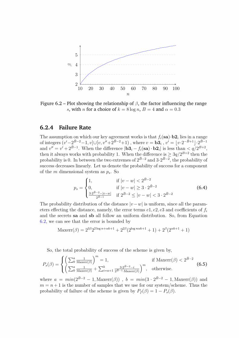
10 20 30 40 50 60 70 80 90 1002

3

4

5

n

β

Figure 6.2 – Plot showing the relationship of β, the factor influencing the ranges, with n for a choice of k = 8 log n, B = 4 and α = 0.3

6.2.4 Failure Rate

The assumption on which our key agreement works is that fi(sa)·b2i lies in a rangeof integers (v′−2B−2−1, v]∪[v, v′′+2B−2+1) , where v = b3i , v′ = ⌊v·2−B+1⌋·2B−1and v′′ = v′+2B−1. When the difference |b3i− fi(sa) ·b2i| is less than < q/2B+2,then it always works with probability 1. When the difference is ≥ 3q/2B+2 then theprobability is 0. In between the two extremes of 2B−2 and 3·2B−2, the probability ofsuccess decreases linearly. Let us denote the probability of success for a componentof the m dimensional system as ps. So

ps =

1, if |v − w| < 2B−2

0, if |v − w| ≥ 3 · 2B−23·2B−2−|v−w|

2B−1 if 2B−2 ≤ |v − w| < 3 · 2B−2(6.4)

The probability distribution of the distance |v−w| is uniform, since all the param-eters effecting the distance, namely, the error terms e1, e2, e3 and coefficients of fiand the secrets sa and sb all follow an uniform distribution. So, from Equation6.2, we can see that the error is bounded by

Maxerr(β) = 23β22 logn+αk+1 + 22β(2lognαk+1 + 1) + 2β(2αk+1 + 1)

So, the total probability of success of the scheme is given by,

Ps(β) =

(∑a0

1Maxerr(β)

)m= 1, if Maxerr(β) < 2B−2(∑a

01

Maxerr(β)+∑b

i=a+13·2B−2−i

2B−1·Maxerr(β)

)m, otherwise.

(6.5)

where a = min(2B−2 − 1,Maxerr(β)) , b = min(3 · 2B−2 − 1,Maxerr(β)) andm = n+1 is the number of samples that we use for our system/scheme. Thus theprobability of failure of the scheme is given by Pf (β) = 1− Ps(β).

6.3 Analysis of Attacks Considered in Submission

In this section we present a summary of the main algebraic attacks against CFPKM.In Section 6.3.1 we consider the Arora-Ge method of solving a system of noisyequations by removing the error and then using Gröbner basis techniques. In Sec-tion 5.3.3, we consider the possibility of an exhaustive search over the secret. Wealso consider the exhaustive search over the secret and then using Gröbner basistechniques to solve the resultant system of equations with Gröbner basis.

In order to break our protocol, the main goal is to recover the secret sa or sb

used by either of Alice or Bob. We have a system of equations

b11 = f1(x) + e11

b12 = f2(x) + e12

...

b1m = fm(x) + e1m

This is a system of non-linear multivariate polynomials, whose solution is x = sa.The process of finding this solution is the exact hard problem of PoSSoWN. In thefollowing sections, we discuss the possible methods of solving this problem andthus provide the hardness results, which relates to our problem.

6.3.1 Arora-Ge Gröbner Basis Method

CFPKM requires solving a two systems of equations given by b1 = f(sa) + e1 andb2 = f(sb) + e2 where f ∈ Fm

q [x1, . . . , xn] and b1,b2, e1, e2 ∈ Fmq . The errors

e1, e2 are chosen from a discrete uniform distribution from a range [0, s].We can rewrite the above polynomial equations as e1 = b1− f(sa) and e2 =

b2−f(sb). In Section 5.3.1, we presented the approach of using Gröbner basis withthe Arora-Ge approach. For our scheme, we can similarly construct the Arora-Gepolynomial (Equation (5.2)) as follows:

P (η) = η

s∏

j=1

(η − j),

where η is the error polynomial (See Section 5.3.1). Therefore, for each ith com-ponent of the error vectors e1 ∈ Fm

q and e2 ∈ Fmq , we can substitute the error

polynomials by b1i − fi(x) and b2i − fi(x) respectively where x = (x1, . . . , xn).

Consequently, we get two system of polynomial equations corresponding to eachof e1 and e2 respectively, and whose ith components are given by,

Pi(b1i − fi(x)) = (b1i − fi(x))s∏

j=1

(b1i − fi(x)− j), (6.6)

Pi(b2i − fi(x)) = (b2i − fi(x))s∏

j=1

(b2i − fi(x)− j). (6.7)

We have two systems of m polynomials in n variables of degree d = 2s + 2, keeping in account of the degree of each fi being 2 (i.e quadratic). It is quiteintuitive to see that the polynomial Pi from Equation (6.6) equals zero whenx = sa, and the same for Equation (6.7) when x = sb.Additional constraints on the set of variables (x1, . . . , xn) come from the fact thateven the secrets sa and sb are chosen from the range [0, s]n.

x1(x1 − 1) · · · (x1 − s) = 0

x2(x2 − 1) · · · (x2 − s) = 0

...

xn(xn − 1) · · · (xn − s) = 0

So if we are able to find a Gröbner basis of the system of equations along withsystem Pi(x) = 0 of Equation (6.6) (or Equation (6.7)), then we will be able torecover sa (or sb respectively). The minimum number of samples that is assumedthe attacker can have and running the F5 is m′ = n+ 1. In Table 6.1 we presentthe degree of regularities and the bit-complexities of the Arora-Ge Gröbner basisattack with the choice of m′ = n + 1. The degree of regularity for our system isgiven by the degree of regularity for a semi-regular system of same parameters.Table 6.2 shows the time complexity of the Arora-Ge Gröbner basis attack on theKEM when different number of equations are made available to the attacker.

6.3.2 Exhaustive Search

In this section, we take use of the combinatorial attacks from Section 5.3.3.

6.3.2.1 Over the Shared Secret

An adversary can perform an exhaustive search over the shared secret constructedbetween Alice and Bob. The size of the shared key is determined by the total num-ber of bits chosen for each component of the m-dimensional shared secret. Eachcomponent of the shared secret is of size B bits. Thus for an attacker to mount a

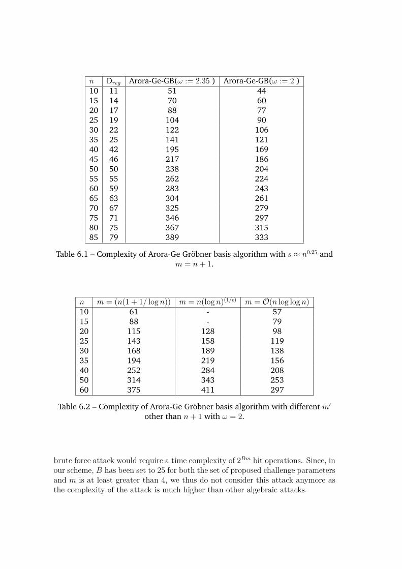
n Dreg Arora-Ge-GB(ω := 2.35 ) Arora-Ge-GB(ω := 2 )10 11 51 4415 14 70 6020 17 88 7725 19 104 9030 22 122 10635 25 141 12140 42 195 16945 46 217 18650 50 238 20455 55 262 22460 59 283 24365 63 304 26170 67 325 27975 71 346 29780 75 367 31585 79 389 333

Table 6.1 – Complexity of Arora-Ge Gröbner basis algorithm with s ≈ n0.25 andm = n+ 1.

n m = (n(1 + 1/ log n)) m = n(log n)(1/ǫ) m = O(n log log n)10 61 - 5715 88 - 7920 115 128 9825 143 158 11930 168 189 13835 194 219 15640 252 284 20850 314 343 25360 375 411 297

Table 6.2 – Complexity of Arora-Ge Gröbner basis algorithm with different m′

other than n+ 1 with ω = 2.

brute force attack would require a time complexity of 2Bm bit operations. Since, inour scheme, B has been set to 25 for both the set of proposed challenge parametersand m is at least greater than 4, we thus do not consider this attack anymore asthe complexity of the attack is much higher than other algebraic attacks.

6.3.2.2 Over the Secret

Next we consider the brute force attack by an adversary to recover the hiddensecrets sa, sb ∈ Fn

q , as mentioned in Section 5.3.3. The secrets are chosen from[0, s]n. Therefore, the attacker has to compute sn possible solutions. Also, weassume that the range s ≈ nβ, hence the number of operations in exhaustivesearch turns out to be 2nβn. Once these secrets have been recovered, with highprobability the shared secret can be recovered by taking the B most significantbits of the product fi(sa) · fi(sb).

Note 6.3.1. If we increase the value of our range s, then the time for exhaustive

search increases. But this in turn also increases the degree of regularity and hence

also the time complexity of the Arora-Ge GB attack.

6.3.2.3 Over the Error

Now, we take the other possibility of performing an exhaustive search over theerrors. We take use of the technique presented in Section 5.3.3, where we considerthe same system of noisy polynomials as a system of m equations over n + mvariables, i.e counting the errors as unknown variables. So once the error valueshave been recovered, for example e1, we have the following system of equations

f1(x)− b1′1 = 0,

f2(x)− b1′2 = 0,

...

fm(x)− b1′m = 0,

where fi(x) ∈ Fq[x] with x = (x1, . . . , xn) and b1′ = b1− e1 ∈ Fmq . We can solve

this above system using the algorithm of [LPT+17] which has a complexity of

O(sn ·

(log s

2e

)−n),

where the values of xi are chosen from the range [0, s]. Therefore, the total com-plexity of doing a exhaustive search of the error followed by the proposed algorithmof [LPT+17] is expected to be

sm · O(sn ·

(log s

2e

)−n).

6.3.3 Hybrid Attacks

In this section, we present the hybrid attacks which combines combinatorial meth-ods, like exhaustive search, with algebraic techniques such as Gröbner basis meth-ods. The first algorithm is the hybrid method of exhaustive search over the errorsand Gröbner basis algorithms, which was presented in Section 5.3.3. For ourscheme, the total complexity of this attack is

sm ·(m ·Dreg

((n+Dreg

Dreg

)ω)),

where Dreg is the degree of regularity over the system of m quadratic equations inn variables (Refer to Equation 5.3 for how to determine the Dreg in Section 5.3.1).

In Table 6.3 , we observe that an exhaustive search over the secret or the er-ror is a faster and much efficient attack on our scheme. This is because our searchspace for both the secret as well as the error is much smaller than the finite fieldrelated to the polynomial ring in which the polynomials have been defined.

The next algorithm we present is the Max-PoSSo Gröbner basis attack that waspresented in Section 5.3.4. Suppose we are given a system of m equations in nvariables. Now the errors can be achieved by doing an exhaustive search. Sonow assuming that the error distribution is uniform over the range [0, s], we cansay that t = m/(s + 1) number of equations may be the exact solutions. That tequations are such that

f1 = · · · = ft = 0,

where f1, . . . , ft ∈ Fq[x1, . . . , xn]. Now the Gröbner basis attack on this sub-systemtakes (

tDreg

(n+Dreg

Dreg

)ω),

number of operations, where Dreg is the degree of regularity of this sub-system.So, the total complexity of this attack turns out to be

(m

t

)·(tDreg

(n+Dreg

Dreg

)ω).

Though comparing the performance of this attack with exhaustive search, we seethat for n = 20, we are getting a security of 130 bits. But on the other hand, withn = 30 and the secret vector being chosen from a small range [0, s], the exhaustivesearch performs much better. It is also important to mention that in case of thisattack, the minimum number of equations m will not suffice with n+ 1. It has tobe much larger than this, big enough such that t > n for the Gröbner basis attackto work. Hence we just report the performance of this attack in Table 6.3.

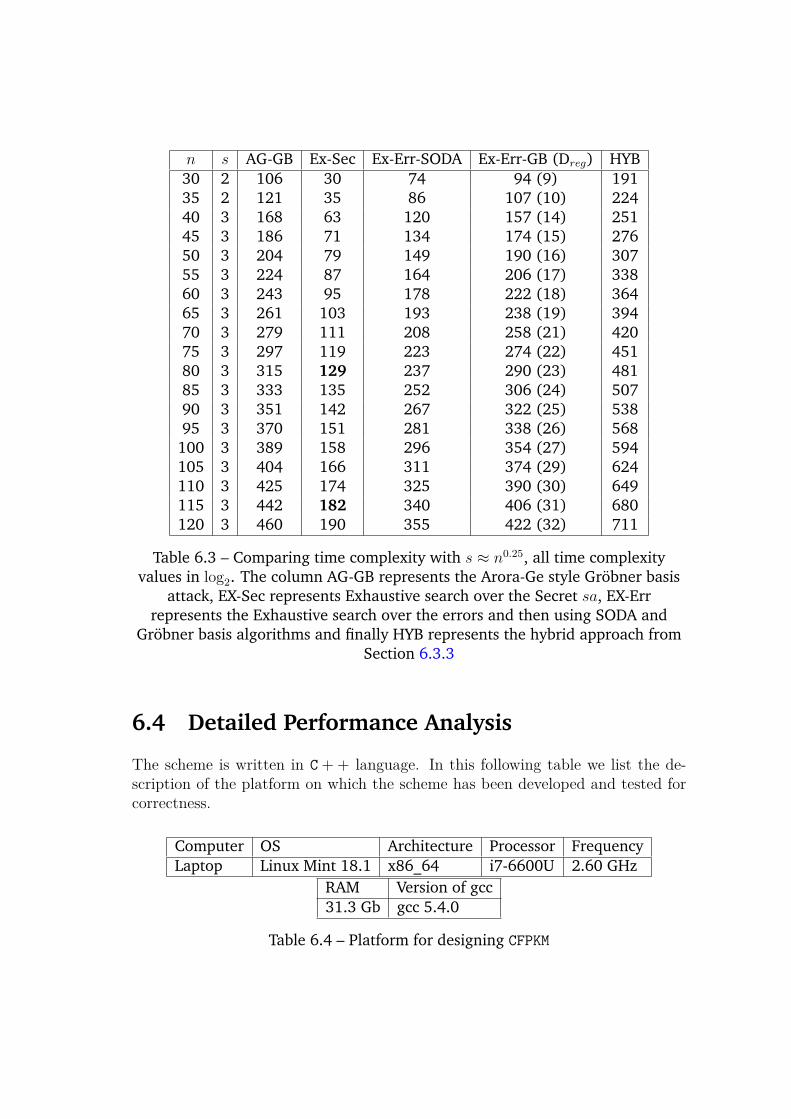
n s AG-GB Ex-Sec Ex-Err-SODA Ex-Err-GB (Dreg) HYB30 2 106 30 74 94 (9) 19135 2 121 35 86 107 (10) 22440 3 168 63 120 157 (14) 25145 3 186 71 134 174 (15) 27650 3 204 79 149 190 (16) 30755 3 224 87 164 206 (17) 33860 3 243 95 178 222 (18) 36465 3 261 103 193 238 (19) 39470 3 279 111 208 258 (21) 42075 3 297 119 223 274 (22) 45180 3 315 129 237 290 (23) 48185 3 333 135 252 306 (24) 50790 3 351 142 267 322 (25) 53895 3 370 151 281 338 (26) 568100 3 389 158 296 354 (27) 594105 3 404 166 311 374 (29) 624110 3 425 174 325 390 (30) 649115 3 442 182 340 406 (31) 680120 3 460 190 355 422 (32) 711

Table 6.3 – Comparing time complexity with s ≈ n0.25, all time complexityvalues in log2. The column AG-GB represents the Arora-Ge style Gröbner basis

attack, EX-Sec represents Exhaustive search over the Secret sa, EX-Errrepresents the Exhaustive search over the errors and then using SODA and

Gröbner basis algorithms and finally HYB represents the hybrid approach fromSection 6.3.3

6.4 Detailed Performance Analysis

The scheme is written in C++ language. In this following table we list the de-scription of the platform on which the scheme has been developed and tested forcorrectness.

Computer OS Architecture Processor FrequencyLaptop Linux Mint 18.1 x86_64 i7-6600U 2.60 GHz

RAM Version of gcc31.3 Gb gcc 5.4.0

Table 6.4 – Platform for designing CFPKM

6.4.1 Time

The following measurements are for the KEM. For the measures, it runs a numberof tests such that the global used time is greater than 10 seconds and the globaltime is divided by the number of tests. For our scheme with CFPKM128 the keygeneration, takes 72 ms. The key encapsulation scheme takes on an average about108 ms (over a run of 30 tests). The decapsulation of the shared secret key takesabout 143 ms. For CFPKM182 key generation takes 120 ms. The key-encapsulationtakes for this parameter 150 ms on an average of 30 tests, while the decapsulationtakes about 190 ms.

6.4.2 Space

The key sizes of the parameters are calculated directly (and confirmed in variousexperiments) from the structure of keys. Recall that the public key was constructedby concatenating the seed value and the public vector b1, while the secret key is aconcatenation of the same seed value and the secret sa. The ciphertext comprisesof two vectors, the crossround bit vector c and the vector b1.

The total size of public key for CFPKM128 turns out to be 696 bytes. The se-cret key is 128 bytes for the parameters of CFPKM128. The ciphertexts, which aresent from Bob to Alice, are 729 bytes long, whereas the shared secret is of 81 bytes.

For CFPKM182, the public key size turns out to be 995 bytes which include a 48byte long seed value. The secret key is 182 bytes long while the shared secret atthe end of the key exchange is 116 bytes. The size of the ciphertexts from Bob toAlice amounts to 1044 bytes.

6.4.3 How parameters affect performance

The Key Encapsulation is mainly affected by the number of equations m in oursystem, the range s and also by the number of most significant bits B that we usein our scheme. From Section 6.2.4, we see that the scheme’s failure probability isa function of the range s. This probability is over the m equations used in thescheme. Hence, the efficiency of the scheme is dependent on both s and m. Alsofrom Section 6.3, the fastest attack, exhaustive search over the secret, tells us thatthe security of the scheme is a factor of both s and m.

6.5 Advantages and Limitations

CFPKM, is dependent on small secrets and errors, which is one limitation of theproposed scheme. It has been left a future work for further improving the perfor-mance of the scheme. But on the other hand, CFPKM has a lot of advantages.

The hardness of our key exchange can be reduced down to the PoSSoWN prob-lem. The idea of the design for the key-exchange is that to recover the sharedsecret-key, one needs to solve two systems of noisy quadratic system of equations,and recover the contribution of the secret into the shared secret-key from bothAlice and Bob. Recovering these contributions is the problem of PoSSoWN. Thekey-exchange mechanism has been built in such a way that, it uses input fromboth the users to get a shared key, rather than the trivial way a Key encapsulationworks. The hardness of our key exchange can be reduced down to the PoSSoWN

problem. The idea of the design for the key-exchange is that to recover the sharedsecret-key, one needs to solve two systems of noisy quadratic system of equations,and recover the contribution of the secret into the shared secret-key from bothAlice and Bob. Recovering these contributions is the problem of PoSSoWN, whichis NP-hard. One of the major advantages that CFPKM has, is the cheap communi-cation costs and key sizes. In comparison to similar KEM’s based on Learning withErrors, this protocol is able to achieve similar levels of security with much lowervalues of comparable parameters.

6.6 Why the Scheme Failed

After the first round of submissions, the scheme was broken by Martin Albrechtand his team at Royal Holloway 1. The main issue that lied in the scheme was notfrom an algebraic security point of view, but rather a very rudimentary practicalfault in the design of the scheme.

Let us have a close look at the design of the shared secret. On Bob’s side, theRounding function computes the shared secret from the B most significant bits ofeach component of the vector b3. The b3 vector is constructed as follows:

b3 = f(sb)⊙ b1+ e3

= f(sb)⊙ f(sa) + f(sb)⊙ e1+ e3(6.8)

By the choice of the parameters, the errors and the coefficients of the polyno-mials f ∈ Fm

q [x1, . . . , xn] are “small". Now we will show how small are they withrespect to evaluations we are dealing with. In particular, we shall demonstrate thisfor the first set of parameters, i.e., for CFPKM128. The errors are chosen uniformlyfrom a range upper bounded by Range = 7. The coefficients of the polynomials aregenerated by the seed value but are taken modulo Cofsize = 4096 = 212. Now,we see that evaluation of the polynomial f(sb) is upper bounded by

(80)2 · (212 · 72) + 80 · (212 · 7) + 212 ≤ 231

1There is no citation as the issue was pointed out through NIST forums

Thus, the product f(sb) ⊙ e1 is upper bounded by 234. Since the shared secretare the B = 6 most significant bits of b3, which is an m dimensional vector whereeach component is log q = 50 bits, the product f(sb)⊙ e1 has no contribution tothe shared secret.

Now let us consider the two public values b1 and b2. Taking the special compo-nent wise product of these public vectors we have

b1⊙ b2 = (f(sa) + e1)⊙ (f(sb) + e2)

= f(sa)⊙ f(sb) + f(sa)⊙ e2+ f(sb)⊙ e1+ e1⊙ e2.(6.9)

Consider the B most significant bits of this product b1⊙b2. With the same intu-ition, the B most significant bits have no influence from f(sb)⊙ e1+ f(sa)⊙ e2.Thus, the shared secret is always computed from the product f(sa)⊙ f(sb).

Hence any adversary who can get access to the public values b1 and b2, theycan just compute the product and the B most significant bits of it to recover theshared secret.

6.7 Can This Issue be Resolved?

As soon as the scheme was broken, efforts were made to correct the scheme. Thefirst approach taken was to have a fixed support for the polynomials in the publickeys. Let us define a square coefficient matrix, say A of size m×m over Fq wherethe columns of the matrix represent the monomials in the fixed support. By thiswe are fixing the public polynomials to have the same m monomials. Now, wedefine the construction of the vectors b1,b2 and b3.

b1 = A× sa′ + e1.

b2 = sb′ × A+ e2.

b3 = sb′ × b1+ e3.

where sa′ ( and sb′) is the evaluation of the monomials in the fixed support Sup

over the secret value sa ( and sb respectively). On one hand this surely solves theissue of any passive adversary, who has access to the public vectors b1 and b2,being able to recover the hidden secret from b2⊙ b1.

On the other hand, this reflects another instance of the LWE problem and canbe viewed as a parameterization of the NewHope key exchange protocol which isbased on Ring-LWE [AAB+]. Thus we had to drop this approach.

Another idea was to increase the bound on the coefficient size of the polyno-mials (i.e qα) such that we can expect the effect of the product f(sb)⊙ e1 to alsoinfluence the B most significant bits. However, according to Corollary 6.2.8 wealready have

β <

(k(1− α)−B − 2− 2 log n

3

),

which gives a bound on the range to choose our secret and error required forcorrect decryption with high probability. Thus increasing the size of the coefficientsimplies, increasing α. Increasing α, decreases the upper bound on β, which thenalso decreases the values for the secret and the error. Hence, we don’t achieve theexpected effect of the product f(sb)⊙ e1 affecting the shared secret.

6.8 Conclusion

We presented a new multivariate key exchange scheme based on the problem ofsolving a system of noisy multivariate equations, as a submission to the NIST Post-quantum standardization process. This key encapsulation was the first of its kindusing the NP-Hard problem of PoSSoWN. We provided a new design that utilizesthe use of an error in polynomials in order to blind the information passed overopen channels. We provided the scheme along with security analysis against allpotential algebraic attacks on it. Finally, we show why because of a structuraldefect, the scheme was broken.

Bibliography

[AAB+] Erdem Alkim, Roberto Avanzi, Joppe Bos, Léo Ducas, Antonio de laPiedra, Peter Schwabe Thomas Pöppelmann, and Douglas Stebila.Newhope. Technical report, Technical report, National Institute ofStandards and Technology, 2017 . . . .

[ABD+17] Roberto Avanzi, Joppe Bos, Léo Ducas, Eike Kiltz, Tancrède Lep-oint, Vadim Lyubashevsky, John M Schanck, Peter Schwabe, Gre-gor Seiler, and Damien Stehlé. Crystals-kyber algorithm specifica-tions and supporting documentation. Submission to the NIST post-quantum project, 9:11, 2017.

[ABD+18] Erdem Alkim, Joppe Bos, Léo Ducas, Patrick Longa, Ilya Mironov,Michael Naehrig, Valeria Nikolaenko, Chris Peikert, Ananth Raghu-nathan, Douglas Stebila, et al. Frodokem–learning with errors keyencapsulation, 2017. URL: https://frodokem. org/files/FrodoKEM-specification-20171130. pdf, 2018.

[AC11] Martin Albrecht and Carlos Cid. Cold boot key recovery by solv-ing polynomial systems with noise. In International Conference onApplied Cryptography and Network Security, pages 57–72. Springer,2011.

[ACPS09] Benny Applebaum, David Cash, Chris Peikert, and Amit Sahai.Fast cryptographic primitives and circular-secure encryption basedon hard learning problems. In Annual International Cryptology Con-ference, pages 595–618. Springer, 2009.

[AFFP11] Martin R Albrecht, Pooya Farshim, Jean-Charles Faugere, and Lu-dovic Perret. Polly cracker, revisited. In International Conference onthe Theory and Application of Cryptology and Information Security,pages 179–196. Springer, 2011.

[AG11] Sanjeev Arora and Rong Ge. New algorithms for learning in presenceof errors. Automata, languages and programming, pages 403–415,2011.

135

[AGO+17] Koichiro Akiyama, Yasuhiro Goto, Shinya Okumura, Tsuyoshi Tak-agi, Koji Nuida, Goichiro Hanaoka, Hideo Shimizu, and YasuhikoIkematsu. A public-key encryption scheme based on non-linear inde-terminate equations (giophantus). IACR Cryptology ePrint Archive,2017:1241, 2017.

[Ajt96] Miklós Ajtai. Generating hard instances of lattice problems. In Pro-ceedings of the twenty-eighth annual ACM symposium on Theory ofcomputing, pages 99–108, 1996.

[ALFP] Martin Albrecht, D Lin, Jean-Charles Faugere, and Ludovic Perret.Polynomials with error.

[Bar04] Magali Bardet. Étude des systèmes algébriques surdéterminés. Ap-plications aux codes correcteurs et à la cryptographie. PhD thesis,2004.

[BCC+10] Charles Bouillaguet, Hsieh-Chung Chen, Chen-Mou Cheng, TungChou, Ruben Niederhagen, Adi Shamir, and Bo-Yin Yang. Fast ex-haustive search for polynomial systems in f2. In International Work-shop on Cryptographic Hardware and Embedded Systems, pages 203–218. Springer, 2010.

[BCD+16] Joppe Bos, Craig Costello, Léo Ducas, Ilya Mironov, Michael Naehrig,Valeria Nikolaenko, Ananth Raghunathan, and Douglas Stebila.Frodo: Take off the ring! practical, quantum-secure key exchangefrom lwe. In Proceedings of the 2016 ACM SIGSAC Conference onComputer and Communications Security, pages 1006–1018. ACM,2016.

[BCNS15] Joppe W Bos, Craig Costello, Michael Naehrig, and Douglas Stebila.Post-quantum key exchange for the tls protocol from the ring learn-ing with errors problem. In Security and Privacy (SP), 2015 IEEESymposium on, pages 553–570. IEEE, 2015.

[BCP97] Wieb Bosma, John Cannon, and Catherine Playoust. The magma al-gebra system i: The user language. Journal of Symbolic Computation,24(3-4):235–265, 1997.

[BDPA11] Guido Bertoni, Joan Daemen, Michaël Peeters, and GV Assche. Thekeccak reference. Submission to NIST (Round 3), 13:14–15, 2011.

[Bea02] Stephane Beauregard. Circuit for shor’s algorithm using 2n+ 3 qubits.arXiv preprint quant-ph/0205095, 2002.

[Ben80] Paul Benioff. The computer as a physical system: A microscopicquantum mechanical hamiltonian model of computers as representedby turing machines. Journal of statistical physics, 22(5):563–591,1980.

[Ber67] Elwyn R Berlekamp. Factoring polynomials over finite fields. BellSystem Technical Journal, 46(8):1853–1859, 1967.

[Bet11] Luk Bettale. Cryptanalyse algébrique: outils et applications. PhDthesis, Paris 6, 2011.

[BFMR11] Charles Bouillaguet, Pierre-Alain Fouque, and Gilles Macario-Rat.Practical key-recovery for all possible parameters of sflash. In In-ternational Conference on the Theory and Application of Cryptologyand Information Security, pages 667–685. Springer, 2011.

[BFP08] Luk Bettale, Jean-Charles Faugère, and Ludovic Perret. Cryptanal-ysis of the trms signature scheme of pkc’05. In International Confer-ence on Cryptology in Africa, pages 143–155. Springer, 2008.

[BFP09] Luk Bettale, Jean-Charles Faugere, and Ludovic Perret. Hybrid ap-proach for solving multivariate systems over finite fields. Journal ofMathematical Cryptology, 3(3):177–197, 2009.

[BFP12] Luk Bettale, Jean-Charles Faugère, and Ludovic Perret. Solving poly-nomial systems over finite fields: improved analysis of the hybridapproach. In Proceedings of the 37th International Symposium onSymbolic and Algebraic Computation, pages 67–74, 2012.

[BFP13] Luk Bettale, Jean-Charles Faugère, and Ludovic Perret. Cryptanal-ysis of hfe, multi-hfe and variants for odd and even characteristic.Designs, Codes and Cryptography, 69(1):1–52, 2013.

[BFS04] Magali Bardet, Jean-Charles Faugere, and Bruno Salvy. On the com-plexity of gröbner basis computation of semi-regular overdeterminedalgebraic equations. In Proceedings of the International Conferenceon Polynomial System Solving, pages 71–74, 2004.

[BFS15] Magali Bardet, Jean-Charles Faugère, and Bruno Salvy. On the com-plexity of the f5 gröbner basis algorithm. Journal of Symbolic Com-putation, 70:49–70, 2015.

[BFSS13] Magali Bardet, Jean-Charles Faugère, Bruno Salvy, and Pierre-JeanSpaenlehauer. On the complexity of solving quadratic boolean sys-tems. Journal of Complexity, 29(1):53–75, 2013.

[BFSY05] Magali Bardet, Jean-Charles Faugere, Bruno Salvy, and Bo-YinYang. Asymptotic behaviour of the index of regularity of quadraticsemi-regular polynomial systems. In The Effective Methods in Alge-braic Geometry Conference (MEGA’05)(P. Gianni, ed.), pages 1–14.Citeseer, 2005.

[BGJT14] Razvan Barbulescu, Pierrick Gaudry, Antoine Joux, and EmmanuelThomé. A heuristic quasi-polynomial algorithm for discrete logarithmin finite fields of small characteristic. In Annual International Con-ference on the Theory and Applications of Cryptographic Techniques,pages 1–16. Springer, 2014.

[BGML+18] Sauvik Bhattacharya, Oscar Garcia-Morchon, Thijs Laarhoven,Ronald Rietman, Markku-Juhani O Saarinen, Ludo Tolhuizen, andZhenfei Zhang. Round5- compact and fast post-quantum public-keyencryption. IACR Cryptology ePrint Archive, 2018:725, 2018.

[BL17] Daniel J Bernstein and Tanja Lange. Post-quantum cryptography.Nature, 549(7671):188–194, 2017.

[BLP+13] Zvika Brakerski, Adeline Langlois, Chris Peikert, Oded Regev, andDamien Stehlé. Classical hardness of learning with errors. In Pro-ceedings of the forty-fifth annual ACM symposium on Theory of com-puting, pages 575–584, 2013.

[BPSV19] Ward Beullens, Bart Preneel, Alan Szepieniec, and Frederik Ver-cauteren. Luov. Csrc. nist. gov, 2019.

[BR06] Mihir Bellare and Phillip Rogaway. The security of triple encryp-tion and a framework for code-based game-playing proofs. In AnnualInternational Conference on the Theory and Applications of Crypto-graphic Techniques, pages 409–426. Springer, 2006.

[BR11] Elaine Barker and Allen Roginsky. Transitions: Recommendation fortransitioning the use of cryptographic algorithms and key lengths.NIST Special Publication, 800:131A, 2011.

[BS91] Eli Biham and Adi Shamir. Differential cryptanalysis of des-like cryp-tosystems. Journal of CRYPTOLOGY, 4(1):3–72, 1991.

[Buc65] Bruno Buchberger. An algorithm for finding the base elements of theresidual class ring after a zero-dimensional polynomial ideal. PhDthesis, Universitat Insbruck, 1965.

[Buc76] Bruno Buchberger. A theoretical basis for the reduction of polyno-mials to canonical forms. SIGSAM Bull., 10:19–29, 08 1976.

[BW98] Th Becker and V Weispfennig. H. kredel (1998): Gröbner bases: acomputational approach to commutative algebra, corr. 2. print, 1998.

[BWP05] An Braeken, Christopher Wolf, and Bart Preneel. A study of thesecurity of unbalanced oil and vinegar signature schemes. In Cryptog-raphers’ Track at the RSA Conference, pages 29–43. Springer, 2005.

[Car96] PA Carl. Tale of two sieves. Notices American Mathematical Society,43(12):1473–85, 1996.

[CB07] Nicolas T Courtois and Gregory V Bard. Algebraic cryptanalysis ofthe data encryption standard. In IMA International Conference onCryptography and Coding, pages 152–169. Springer, 2007.

[CCJ+16] Lily Chen, Lily Chen, Stephen Jordan, Yi-Kai Liu, Dustin Moody,Rene Peralta, Ray Perlner, and Daniel Smith-Tone. Report on post-quantum cryptography. US Department of Commerce, National In-stitute of Standards and Technology, 2016.

[CDF03] Nicolas T Courtois, Magnus Daum, and Patrick Felke. On the securityof hfe, hfev-and quartz. In International Workshop on Public KeyCryptography, pages 337–350. Springer, 2003.

[CFMR+17] Antoine Casanova, Jean-Charles Faugère, Gilles Macario-Rat,Jacques Patarin, Ludovic Perret, and Jocelyn Ryckeghem. Gemss:A great multivariate short signature. Submission to NIST, 2017.

[CFP17] Olive Chakraborty, Jean-Charles Faugère, and Ludovic Perret. Cf-pkm: A key encapsulation mechanism based on solving system ofnon-linear multivariate polynomials. 2017.

[CKPS00] Nicolas Courtois, Alexander Klimov, Jacques Patarin, and AdiShamir. Efficient algorithms for solving overdefined systems of mul-tivariate polynomial equations. In International Conference on theTheory and Applications of Cryptographic Techniques, pages 392–407.Springer, 2000.

[CLO06] David A Cox, John Little, and Donal O’shea. Using algebraic geom-etry, volume 185. Springer Science & Business Media, 2006.

[CLO15] David Cox, John Little, and Donal O’Shea. Ideals, varieties, andalgorithms. 2015.

[CLRS09] Thomas H Cormen, Charles E Leiserson, Ronald L Rivest, and Clif-ford Stein. Introduction to algorithms. MIT press, 2009.

[CM97] Robert S Coulter and Rex W Matthews. Planar functions and planesof lenz-barlotti class ii. Designs, Codes and Cryptography, 10(2):167–184, 1997.

[Coc73] Clifford C Cocks. A note on non-secret encryption. CESG Memo,1973.

[Cou01] Nicolas T Courtois. The security of hidden field equations (hfe).In Cryptographers’ Track at the RSA Conference, pages 266–281.Springer, 2001.

[CST17] Ryann Cartor and Daniel Smith-Tone. An updated security analysisof pflash. In International Workshop on Post-Quantum Cryptography,pages 241–254. Springer, 2017.

[CST18] Ryann Cartor and Daniel Smith-Tone. Eflash: A new multivariateencryption scheme. In International Conference on Selected Areas inCryptography, pages 281–299. Springer, 2018.

[CSTV] Daniel Cabarcas, Daniel Smith-Tone, and Javier A Verbel. Practicalkey recovery attack for zhfe.

[CYST15] Ming-Shing Chen, Bo-Yin Yang, and Daniel Smith-Tone. Pflash-secure asymmetric signatures on smart cards. In Lightweight Cryp-tography Workshop, 2015.

[CZ81] David G Cantor and Hans Zassenhaus. A new algorithm for factoringpolynomials over finite fields. Mathematics of Computation, pages587–592, 1981.

[Dan15] Quynh H Dang. Secure hash standard. Technical report, 2015.

[DFSS07] Vivien Dubois, Pierre-Alain Fouque, Adi Shamir, and Jacques Stern.Practical cryptanalysis of sflash. In Annual International CryptologyConference, pages 1–12. Springer, 2007.

[DG06] Jintai Ding and Jason E Gower. Inoculating multivariate schemesagainst differential attacks. In International Workshop on Public KeyCryptography, pages 290–301. Springer, 2006.

[DH76a] Whitfield Diffie and Martin Hellman. New directions in cryptography.IEEE transactions on Information Theory, 22(6):644–654, 1976.

[DH76b] Whitfield Diffie and Martin Hellman. New directions in cryptography.IEEE transactions on Information Theory, 22(6):644–654, 1976.

[Din04] Jintai Ding. A new variant of the matsumoto-imai cryptosystemthrough perturbation. In International Workshop on Public KeyCryptography, pages 305–318. Springer, 2004.

[Dir39] Paul Adrien Maurice Dirac. A new notation for quantum mechanics.In Mathematical Proceedings of the Cambridge Philosophical Society,volume 35, pages 416–418. Cambridge University Press, 1939.

[DK12] Jintai Ding and Thorsten Kleinjung. Degree of regularity for hfeminus (hfe-). JMI: journal of math-for-industry, 4:97–104, 2012.

[DKRV18] Jan-Pieter D’Anvers, Angshuman Karmakar, Sujoy Sinha Roy, andFrederik Vercauteren. Saber: Module-lwr based key exchange, cpa-secure encryption and cca-secure kem. In International Conferenceon Cryptology in Africa, pages 282–305. Springer, 2018.

[DO68] Peter Dembowski and Thedore G Ostrom. Planes of order nwith collineation groups of ordern 2. Mathematische Zeitschrift,103(3):239–258, 1968.

[DPW14] Jintai Ding, Albrecht Petzoldt, and Lih-Chung Wang. The cubicsimple matrix encryption scheme. volume 8772, pages 76–87, 10 2014.

[DR99] Joan Daemen and Vincent Rijmen. The rijndael block cipher: Aesproposal. In First candidate conference (AeS1), pages 343–348, 1999.

[DS05] Jintai Ding and Dieter Schmidt. Rainbow, a new multivariable poly-nomial signature scheme. In International Conference on AppliedCryptography and Network Security, pages 164–175. Springer, 2005.

[DXL12] Jintai Ding, Xiang Xie, and Xiaodong Lin. A simple provably se-cure key exchange scheme based on the learning with errors problem.IACR Cryptology EPrint Archive, 2012:688, 2012.

[DYC+07] Jintai Ding, Bo-Yin Yang, Chen-Mou Cheng, Chia-Hsin Owen Chen,and Vivien Dubois. Breaking the symmetry: a way to resist the newdifferential attack. IACR Cryptology ePrint Archive, 2007:366, 2007.

[DZD+19] Jintai Ding, Zheng Zhang, Joshua Deaton, Kurt Schmidt, andF Vishakha. New attacks on lifted unbalanced oil vinegar. In the2nd NIST PQC Standardization Conference, 2019.

[EF14] Christian Eder and Jean-Charles Faugère. A survey onsignature-based gr\" obner basis computations. arXiv preprintarXiv:1404.1774, 2014.

[ElG85] Taher ElGamal. A public key cryptosystem and a signature schemebased on discrete logarithms. IEEE transactions on information the-ory, 31(4):469–472, 1985.

[Ell70] James H Ellis. The possibility of secure non-secret digital encryption.UK Communications Electronics Security Group, page 6, 1970.

[Fau99] Jean-Charles Faugere. A new efficient algorithm for computing gröb-ner bases (f4). Journal of pure and applied algebra, 139(1-3):61–88,1999.

[Fau02] Jean Charles Faugère. A new efficient algorithm for computing gröb-ner bases without reduction to zero (f 5). In Proceedings of the2002 international symposium on Symbolic and algebraic computa-tion, pages 75–83. ACM, 2002.

[Fey82] Richard P Feynman. Simulating physics with computers. Int. J.Theor. Phys, 21(6/7), 1982.

[FGHR13] Jean-Charles Faugère, Pierrick Gaudry, Louise Huot, and GuénaëlRenault. Polynomial systems solving by fast linear algebra. arXivpreprint arXiv:1304.6039, 2013.

[FGLM94] JC Faugere, P Gianni, D Lazard, and T Mora. Efficient computationof zero dimensional gröbner bases by change of ordering. J. SymbolicComputation, 11:1–000, 1994.

[FGS05] Pierre-Alain Fouque, Louis Granboulan, and Jacques Stern. Differen-tial cryptanalysis for multivariate schemes. In Annual InternationalConference on the Theory and Applications of Cryptographic Tech-niques, pages 341–353. Springer, 2005.

[FHK+17] Jean-Charles Faugère, Kelsey Horan, Delaram Kahrobaei, Marc Ka-plan, Elham Kashefi, and Ludovic Perret. Fast quantum algo-rithm for solving multivariate quadratic equations. arXiv preprintarXiv:1712.07211, 2017.

[FJ03] Jean-Charles Faugere and Antoine Joux. Algebraic cryptanalysis ofhidden field equation (hfe) cryptosystems using gröbner bases. InAnnual International Cryptology Conference, pages 44–60. Springer,2003.

[FJPT10] Jean-Charles Faugere, Antoine Joux, Ludovic Perret, and JoanaTreger. Cryptanalysis of the hidden matrix cryptosystem. In In-ternational Conference on Cryptology and Information Security inLatin America, pages 241–254. Springer, 2010.

[FPS09] Jean-Charles Faugère, Ludovic Perret, and Pierre-Jean Spaenlehauer.Algebraic-differential cryptanalysis of des. In Western EuropeanWorkshop on Research in Cryptology-WEWoRC, volume 2009, pages1–5. Citeseer, 2009.

[FY79] Aviezri S Fraenkel and Yaacov Yesha. Complexity of problems ingames, graphs and algebraic equations. Discrete Applied Mathemat-ics, 1(1-2):15–30, 1979.

[GG16] Steven D Galbraith and Pierrick Gaudry. Recent progress on theelliptic curve discrete logarithm problem. Designs, Codes and Cryp-tography, 78(1):51–72, 2016.

[GJ79] Michael R Garey and David S Johnson. Computers and intractability,volume 174. freeman San Francisco, 1979.

[GM88] Rüdiger Gebauer and H Michael Möller. On an installation of buch-berger’s algorithm. Journal of Symbolic computation, 6(2-3):275–286,1988.

[GM02] Henri Gilbert and Marine Minier. Cryptanalysis of sflash. In Inter-national Conference on the Theory and Applications of CryptographicTechniques, pages 288–298. Springer, 2002.

[GMSS99] Oded Goldreich, Daniele Micciancio, Shmuel Safra, and J-P Seifert.Approximating shortest lattice vectors is not harder than approximat-ing closest lattice vectors. Information Processing Letters, 71(2):55–61, 1999.

[Gro96] Lov K Grover. A fast quantum mechanical algorithm for databasesearch. arXiv preprint quant-ph/9605043, 1996.

[Gu16] Chunsheng Gu. Cryptanalysis of simple matrix scheme for encryp-tion. IACR Cryptology ePrint Archive, 2016:1075, 2016.

[HRSS16] Andreas Hülsing, Joost Rijneveld, Simona Samardjiska, and PeterSchwabe. From 5-pass mq-based identification to mq-based signa-tures. IACR Cryptology ePrint Archive, 2016:708, 2016.

[IPST+18] Yasuhiko Ikematsu, Ray Perlner, Daniel Smith-Tone, Tsuyoshi Tak-agi, and Jeremy Vates. Hferp-a new multivariate encryption scheme.In International Conference on Post-Quantum Cryptography, pages396–416. Springer, 2018.

[JMV01] Don Johnson, Alfred Menezes, and Scott Vanstone. The elliptic curvedigital signature algorithm (ecdsa). International journal of informa-tion security, 1(1):36–63, 2001.

[Kob87] Neal Koblitz. Elliptic curve cryptosystems. Mathematics of compu-tation, 48(177):203–209, 1987.

[KPG99] Aviad Kipnis, Jacques Patarin, and Louis Goubin. Unbalanced oiland vinegar signature schemes. In International Conference on theTheory and Applications of Cryptographic Techniques, pages 206–222.Springer, 1999.

[KS98] Aviad Kipnis and Adi Shamir. Cryptanalysis of the oil and vinegarsignature scheme. In Annual International Cryptology Conference,pages 257–266. Springer, 1998.

[KSWH98] John Kelsey, Bruce Schneier, David Wagner, and Chris Hall. Sidechannel cryptanalysis of product ciphers. In European Symposium onResearch in Computer Security, pages 97–110. Springer, 1998.

[Laz83] Daniel Lazard. Gröbner bases, gaussian elimination and resolution ofsystems of algebraic equations. In European Conference on ComputerAlgebra, pages 146–156. Springer, 1983.

[LM09] Vadim Lyubashevsky and Daniele Micciancio. On bounded distancedecoding, unique shortest vectors, and the minimum distance prob-lem. In Annual International Cryptology Conference, pages 577–594.Springer, 2009.

[LP11] Richard Lindner and Chris Peikert. Better key sizes (and attacks) forlwe-based encryption. In Cryptographers’ Track at the RSA Confer-ence, pages 319–339. Springer, 2011.

[LPT+17] Daniel Lokshtanov, Ramamohan Paturi, Suguru Tamaki, RyanWilliams, and Huacheng Yu. Beating brute force for systems ofpolynomial equations over finite fields. In Proceedings of the Twenty-Eighth Annual ACM-SIAM Symposium on Discrete Algorithms, pages2190–2202. SIAM, 2017.

[Mac02] Francis Sowerby Macaulay. Some formulae in elimination. Proceedingsof the London Mathematical Society, 1(1):3–27, 1902.

[Mat93] Mitsuru Matsui. Linear cryptanalysis method for des cipher. In Work-shop on the Theory and Application of of Cryptographic Techniques,pages 386–397. Springer, 1993.

[McC90] Kevin S McCurley. The discrete logarithm problem. In Proc. ofSymp. in Applied Math, volume 42, pages 49–74. USA, 1990.

[Mer78] Ralph C Merkle. Secure communications over insecure channels.Communications of the ACM, 21(4):294–299, 1978.

[MI88] Tsutomu Matsumoto and Hideki Imai. Public quadratic polynomial-tuples for efficient signature-verification and message-encryption. InWorkshop on the Theory and Application of of Cryptographic Tech-niques, pages 419–453. Springer, 1988.

[MM82] Ernst W Mayr and Albert R Meyer. The complexity of the word prob-lems for commutative semigroups and polynomial ideals. Advancesin mathematics, 46(3):305–329, 1982.

[Mon94] Peter L Montgomery. A survey of modern integer factorization algo-rithms. CWI quarterly, 7(4):337–366, 1994.

[MPST16] Dustin Moody, Ray Perlner, and Daniel Smith-Tone. Key recovery at-tack on the cubic abc simple matrix multivariate encryption scheme.In International Conference on Selected Areas in Cryptography, pages543–558. Springer, 2016.

[MV04] David A McGrew and John Viega. The security and performance ofthe galois/counter mode (gcm) of operation. In International Con-ference on Cryptology in India, pages 343–355. Springer, 2004.

[NIS92] CORPORATE NIST. The digital signature standard. Communica-tions of the ACM, 35(7):36–40, 1992.

[ØFRC20] Morten Øygarden, Patrick Felke, Håvard Raddum, and Carlos Cid.Cryptanalysis of the multivariate encryption scheme eflash. In Cryp-tographers’ Track at the RSA Conference, pages 85–105. Springer,2020.

[Pat95] Jacques Patarin. Cryptanalysis of the matsumoto and imai public keyscheme of eurocrypt’88. In Annual International Cryptology Confer-ence, pages 248–261. Springer, 1995.

[Pat96] Jacques Patarin. Hidden fields equations (hfe) and isomorphisms ofpolynomials (ip): Two new families of asymmetric algorithms. InInternational Conference on the Theory and Applications of Crypto-graphic Techniques, pages 33–48. Springer, 1996.

[Pat97] Jacques Patarin. The oil and vinegar signature scheme. In DagstuhlWorkshop on Cryptography September, 1997, 1997.

[PBD14] Jaiberth Porras, John Baena, and Jintai Ding. Zhfe, a new multi-variate public key encryption scheme. In International workshop onpost-quantum cryptography, pages 229–245. Springer, 2014.

[PCG01a] Jacques Patarin, Nicolas Courtois, and Louis Goubin. Flash, a fastmultivariate signature algorithm. In Cryptographers’ Track at theRSA Conference, pages 298–307. Springer, 2001.

[PCG01b] Jacques Patarin, Nicolas Courtois, and Louis Goubin. Quartz, 128-bit long digital signatures. In Cryptographers’ Track at the RSAConference, pages 282–297. Springer, 2001.

[PCY+15] A Petzoldt, MS Chen, BY Yang, C Tao, and J Ding. Design principlesfor hfevbased signature schemes. asiacrypt 2015-part 1, lncs vol. 9452,2015.

[PCY+17] A Petzoldt, MS Chen, BY Yang, C Tao, and J Ding. Gui documen-tation,https://csrc. nist.gov/projects/post-quantum-cryptography/round-1-submissions, 2017.

[Pei09] Chris Peikert. Public-key cryptosystems from the worst-case shortestvector problem. In Proceedings of the forty-first annual ACM sympo-sium on Theory of computing, pages 333–342, 2009.

[Pei14] Chris Peikert. Lattice cryptography for the internet. In InternationalWorkshop on Post-Quantum Cryptography, pages 197–219. Springer,2014.

[PGC98] Jacques Patarin, Louis Goubin, and Nicolas Courtois. C-+* and hm:Variations around two schemes of t. matsumoto and h. imai. In In-ternational Conference on the Theory and Application of Cryptologyand Information Security, pages 35–50. Springer, 1998.

[Pol78] John M Pollard. Monte carlo methods for index computation. Math-ematics of computation, 32(143):918–924, 1978.

[Pol00] John M Pollard. Kangaroos, monopoly and discrete logarithms. Jour-nal of cryptology, 13(4):437–447, 2000.

[Reg09] Oded Regev. On lattices, learning with errors, random linear codes,and cryptography. Journal of the ACM (JACM), 56(6):34, 2009.

[RSA78] Ronald L Rivest, Adi Shamir, and Leonard Adleman. A method forobtaining digital signatures and public-key cryptosystems. Commu-nications of the ACM, 21(2):120–126, 1978.

[Sch95] Benjamin Schumacher. Quantum coding. Physical Review A,51(4):2738, 1995.

[SDP16] Alan Szepieniec, Jintai Ding, and Bart Preneel. Extension field can-cellation: A new central trapdoor for multivariate quadratic systems.In International workshop on post-quantum cryptography, pages 182–196. Springer, 2016.

[Sha49] Claude E Shannon. Communication theory of secrecy systems. Bellsystem technical journal, 28(4):656–715, 1949.

[Sha93] Adi Shamir. Efficient signature schemes based on birational permu-tations. In Annual International Cryptology Conference, pages 1–12.Springer, 1993.

[Sho99] Peter W Shor. Polynomial-time algorithms for prime factorizationand discrete logarithms on a quantum computer. SIAM review,41(2):303–332, 1999.

[SK99] Adi Shamir and Aviad Kipnis. Cryptanalysis of the hfe public keycryptosystem. In Advances in Cryptology, Proceedings of Crypto, vol-ume 99, 1999.

[SS98] Joseph H Silverman and Joe Suzuki. Elliptic curve discrete logarithmsand the index calculus. In International Conference on the Theoryand Application of Cryptology and Information Security, pages 110–125. Springer, 1998.

[Sto00] Arne Storjohann. Algorithms for matrix canonical forms. PhD thesis,ETH Zurich, 2000.

[SW16] Peter Schwabe and Bas Westerbaan. Solving binary mq with grover’salgorithm. In International Conference on Security, Privacy, andApplied Cryptography Engineering, pages 303–322. Springer, 2016.

[TDTD13] Chengdong Tao, Adama Diene, Shaohua Tang, and Jintai Ding. Sim-ple matrix scheme for encryption. In International Workshop on Post-Quantum Cryptography, pages 231–242. Springer, 2013.

[VOW99] Paul C Van Oorschot and Michael J Wiener. Parallel collision searchwith cryptanalytic applications. Journal of cryptology, 12(1):1–28,1999.

[VST17] Jeremy Vates and Daniel Smith-Tone. Key recovery attack for all pa-rameters of hfe. In International Workshop on Post-Quantum Cryp-tography, pages 272–288. Springer, 2017.

[Wil12] Virginia Vassilevska Williams. Multiplying matrices faster thancoppersmith-winograd. In Proceedings of the forty-fourth annualACM symposium on Theory of computing, pages 887–898, 2012.

Appendices

149

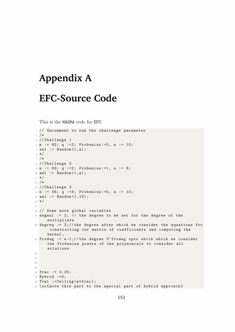
Appendix A

EFC-Source Code

This is the MAGMA code for EFC.

1 // Uncomment to run the challenge parameter

2 /*

3 // Challenge 1

4 n := 83; q :=2; Frobenius :=0, a := 10;

5 aa1 := Random(1,a);

6 */

7 /*

8 // Challenge 2

9 n := 83; q :=2; Frobenius :=1, a := 8;

10 aa1 := Random(1,a);

11 */

12 /*

13 // Challenge 3

14 n := 56; q :=3; Frobenius :=0, a := 10;

15 aa1 := Random (1,10);

16 */

17

18 // Some more global variables

19 degmul := 2; // the degree to be set for the degree of the

multipliers

20 degreq := 2;// the degree after which we consider the equations for

constructing our matrix of coefficients and computing the

kernel ,

21 Frodeg := n-1;// the degree 2^ frodeg upto which which we consider

the frobenius powers of the polynomials to consider all

solutions

22

23

24

25

26 frac := 0.35;

27 Hybrid :=0;

28 Tval := Ceiling(n*frac);

29 \oc{move this part to the special part of hybrid approach}

151

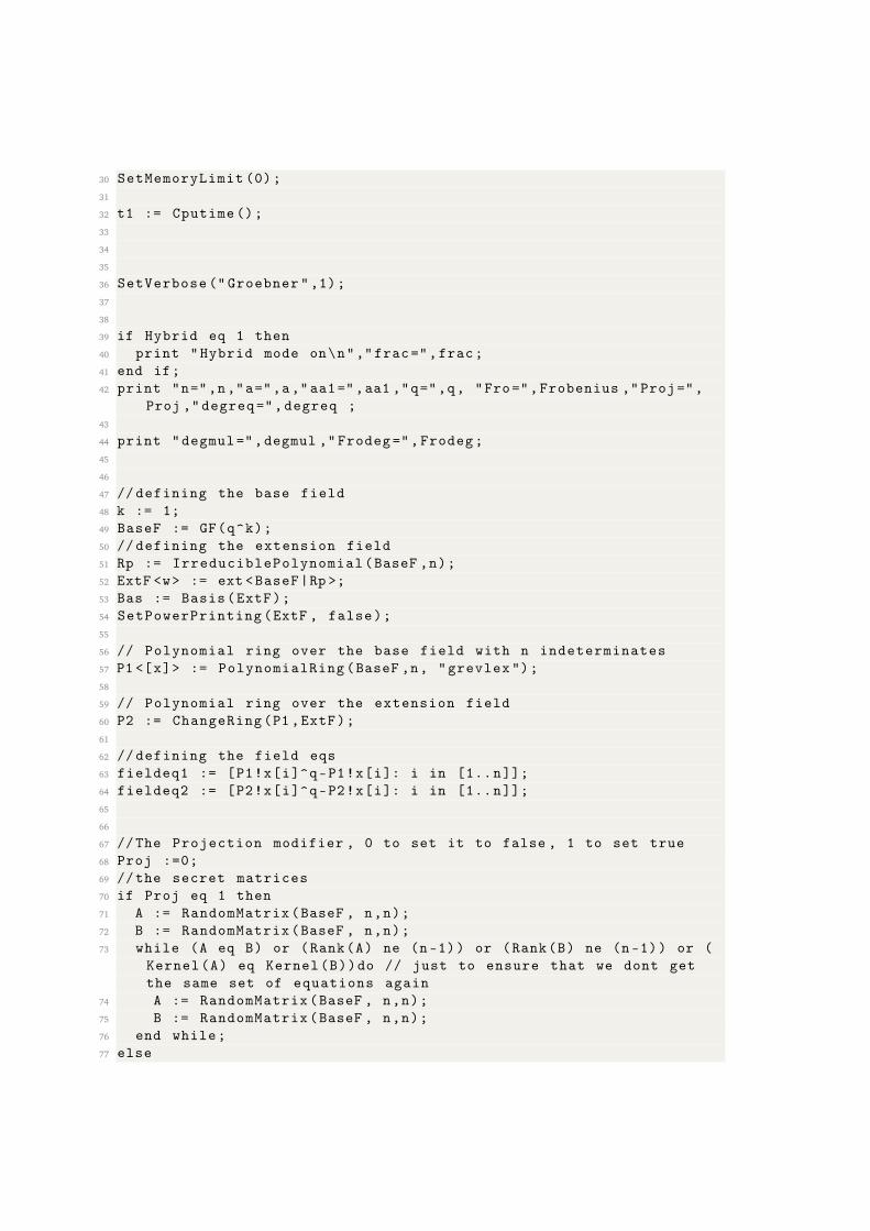
30 SetMemoryLimit (0);

31

32 t1 := Cputime ();

33

34

35

36 SetVerbose (" Groebner ",1);

37

38

39 if Hybrid eq 1 then

40 print "Hybrid mode on\n","frac=",frac;

41 end if;

42 print "n=",n,"a=",a,"aa1=",aa1 ,"q=",q, "Fro=",Frobenius ,"Proj=",

Proj ," degreq=",degreq ;

43

44 print "degmul=",degmul ," Frodeg=",Frodeg;

45

46

47 // defining the base field

48 k := 1;

49 BaseF := GF(q^k);

50 // defining the extension field

51 Rp := IrreduciblePolynomial(BaseF ,n);

52 ExtF <w> := ext <BaseF|Rp >;

53 Bas := Basis(ExtF);

54 SetPowerPrinting(ExtF , false);

55

56 // Polynomial ring over the base field with n indeterminates

57 P1 <[x]> := PolynomialRing(BaseF ,n, "grevlex ");

58

59 // Polynomial ring over the extension field

60 P2 := ChangeRing(P1,ExtF);

61

62 // defining the field eqs

63 fieldeq1 := [P1!x[i]^q-P1!x[i]: i in [1..n]];

64 fieldeq2 := [P2!x[i]^q-P2!x[i]: i in [1..n]];

65

66

67 //The Projection modifier , 0 to set it to false , 1 to set true

68 Proj :=0;

69 //the secret matrices

70 if Proj eq 1 then

71 A := RandomMatrix(BaseF , n,n);

72 B := RandomMatrix(BaseF , n,n);

73 while (A eq B) or (Rank(A) ne (n-1)) or (Rank(B) ne (n-1)) or (

Kernel(A) eq Kernel(B))do // just to ensure that we dont get

the same set of equations again

74 A := RandomMatrix(BaseF , n,n);

75 B := RandomMatrix(BaseF , n,n);

76 end while;

77 else

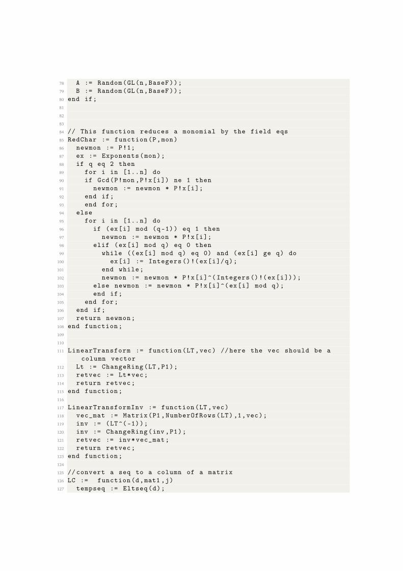
78 A := Random(GL(n,BaseF));

79 B := Random(GL(n,BaseF));

80 end if;

81

82

83

84 // This function reduces a monomial by the field eqs

85 RedChar := function(P,mon)

86 newmon := P!1;

87 ex := Exponents(mon);

88 if q eq 2 then

89 for i in [1..n] do

90 if Gcd(P!mon ,P!x[i]) ne 1 then

91 newmon := newmon * P!x[i];

92 end if;

93 end for;

94 else


96 if (ex[i] mod (q-1)) eq 1 then

97 newmon := newmon * P!x[i];

98 elif (ex[i] mod q) eq 0 then

99 while ((ex[i] mod q) eq 0) and (ex[i] ge q) do

100 ex[i] := Integers ()!(ex[i]/q);

101 end while;

102 newmon := newmon * P!x[i]^( Integers ()!(ex[i]));

103 else newmon := newmon * P!x[i]^(ex[i] mod q);

104 end if;

105 end for;

106 end if;

107 return newmon;

108 end function;

109

110

111 LinearTransform := function(LT,vec) //here the vec should be a

column vector

112 Lt := ChangeRing(LT,P1);

113 retvec := Lt*vec;

114 return retvec;

115 end function;

116

117 LinearTransformInv := function(LT,vec)

118 vec_mat := Matrix(P1 ,NumberOfRows(LT),1,vec);

119 inv := (LT^(-1));

120 inv := ChangeRing(inv ,P1);

121 retvec := inv*vec_mat;

122 return retvec;

123 end function;

124

125 // convert a seq to a column of a matrix

126 LC := function(d,mat1 ,j)

127 tempseq := Eltseq(d);

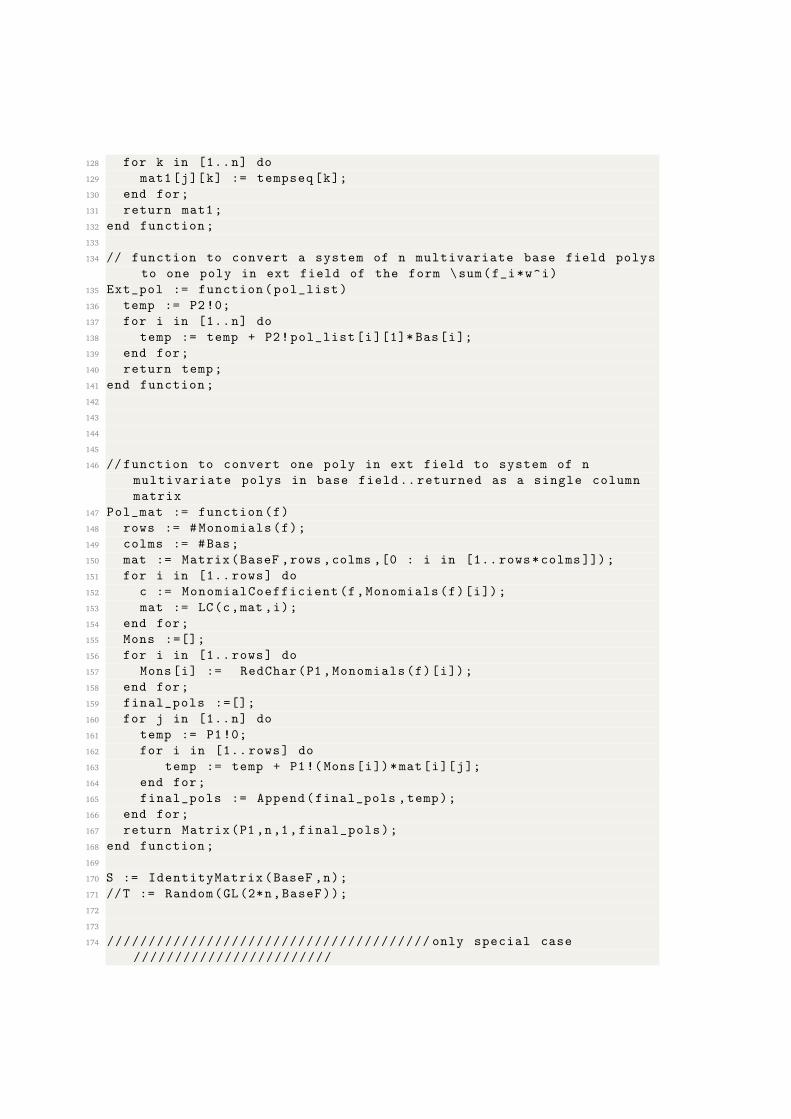
128 for k in [1..n] do

129 mat1[j][k] := tempseq[k];

130 end for;

131 return mat1;

132 end function;

133

134 // function to convert a system of n multivariate base field polys

to one poly in ext field of the form \sum(f_i*wî)

135 Ext_pol := function(pol_list)

136 temp := P2!0;


138 temp := temp + P2!pol_list[i][1]* Bas[i];

139 end for;

140 return temp;

141 end function;

142

143

144

145

146 // function to convert one poly in ext field to system of n

multivariate polys in base field.. returned as a single column

matrix

147 Pol_mat := function(f)

148 rows := #Monomials(f);

149 colms := #Bas;

150 mat := Matrix(BaseF ,rows ,colms ,[0 : i in [1.. rows*colms ]]);

151 for i in [1.. rows] do

152 c := MonomialCoefficient (f,Monomials(f)[i]);

153 mat := LC(c,mat ,i);

154 end for;

155 Mons :=[];


157 Mons[i] := RedChar(P1 ,Monomials(f)[i]);

158 end for;

159 final_pols :=[];

160 for j in [1..n] do

161 temp := P1!0;


163 temp := temp + P1!(Mons[i])*mat[i][j];

164 end for;

165 final_pols := Append(final_pols ,temp);

166 end for;

167 return Matrix(P1,n,1, final_pols);

168 end function;

169

170 S := IdentityMatrix(BaseF ,n);

171 //T := Random(GL(2*n,BaseF));

172

173

174 /////////////////////////////////////// only special case

////////////////////////

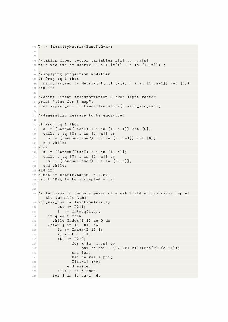
175 T := IdentityMatrix(BaseF ,2*n);

176

177

178 // taking input vector variables x[1],....,x[n]

179 main_vec_enc := Matrix(P1,n,1,[x[i] : i in [1..n]]) ;

180

181 // applying projection modifier


183 main_vec_enc := Matrix(P1 ,n,1,[x[i] : i in [1..n-1]] cat [0]);

184 end if;

185

186 // doing linear transformation S over input vector

187 print "time for S map";

188 time inpvec_enc := LinearTransform(S,main_vec_enc);

189

190 // Generating message to be encrypted

191


193 s := [Random(BaseF) : i in [1..n-1]] cat [0];

194 while s eq [0: i in [1..n]] do

195 s := [Random(BaseF) : i in [1..n-1]] cat [0];

196 end while;

197 else

198 s := [Random(BaseF) : i in [1..n]];

199 while s eq [0: i in [1..n]] do

200 s := [Random(BaseF) : i in [1..n]];

201 end while;

202 end if;

203 s_mat := Matrix(BaseF , n,1,s);

204 print "Msg to be encrypted =",s;

205

206

207 // function to compute power of a ext field multivariate rep of

the varaible \chi

208 Ext_var_pow := function(chi ,i)

209 kai := P2!1;

210 I := Intseq(i,q);

211 if q eq 2 then

212 while Index(I,1) ne 0 do

213 //for j in [1..#I] do

214 i1 := Index(I,1) -1;

215 // print j, i1;

216 phi := P2!0;

217 for k in [1..n] do

218 phi := phi + (P2!(P1.k))*(Bas[k]^(qî1));

219 end for;

220 kai := kai * phi;

221 I[i1+1] :=0;

222 end while;

223 elif q eq 3 then

224 for j in [1..q-1] do

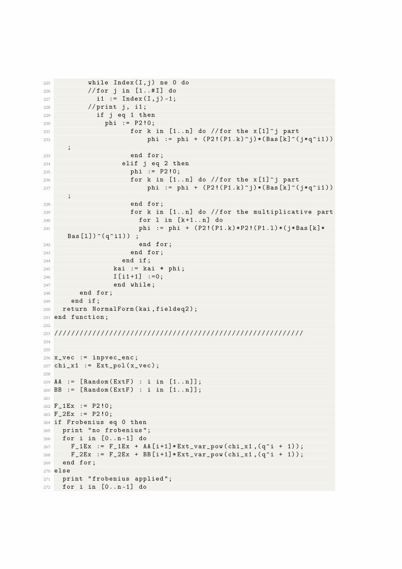
225 while Index(I,j) ne 0 do

226 //for j in [1..#I] do

227 i1 := Index(I,j) -1;

228 // print j, i1;

229 if j eq 1 then

230 phi := P2!0;

231 for k in [1..n] do //for the x[1]^j part

232 phi := phi + (P2!(P1.k)^j)*(Bas[k]^(j*qî1))

;

233 end for;

234 elif j eq 2 then

235 phi := P2!0;

236 for k in [1..n] do //for the x[1]^j part

237 phi := phi + (P2!(P1.k)^j)*(Bas[k]^(j*qî1))

;

238 end for;

239 for k in [1..n] do //for the multiplicative part

240 for l in [k+1..n] do

241 phi := phi + (P2!(P1.k)*P2!(P1.l)*(j*Bas[k]*

Bas[l])^(qî1)) ;

242 end for;

243 end for;

244 end if;

245 kai := kai * phi;

246 I[i1+1] :=0;

247 end while;

248 end for;

249 end if;

250 return NormalForm(kai ,fieldeq2);

251 end function;

252

253 ///////////////////////////////////////////////////////////

254

255

256 x_vec := inpvec_enc;

257 chi_x1 := Ext_pol(x_vec);

258

259 AA := [Random(ExtF) : i in [1..n]];

260 BB := [Random(ExtF) : i in [1..n]];

261

262 F_1Ex := P2!0;

263 F_2Ex := P2!0;

264 if Frobenius eq 0 then

265 print "no frobenius ";

266 for i in [0..n-1] do

267 F_1Ex := F_1Ex + AA[i+1]* Ext_var_pow(chi_x1 ,(qî + 1));

268 F_2Ex := F_2Ex + BB[i+1]* Ext_var_pow(chi_x1 ,(qî + 1));

269 end for;

270 else

271 print "frobenius applied ";

272 for i in [0..n-1] do

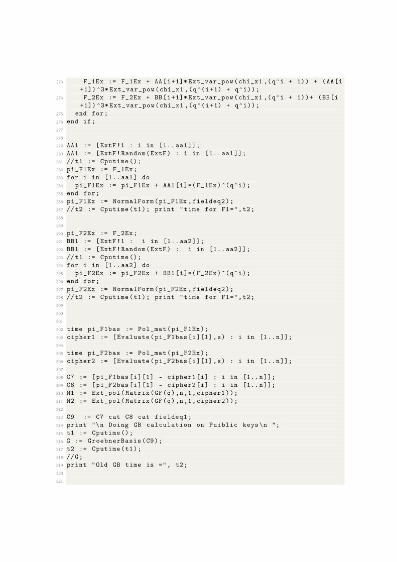
273 F_1Ex := F_1Ex + AA[i+1]* Ext_var_pow(chi_x1 ,(qî + 1)) + (AA[i

+1]) ^3* Ext_var_pow(chi_x1 ,(q^(i+1) + qî));

274 F_2Ex := F_2Ex + BB[i+1]* Ext_var_pow(chi_x1 ,(qî + 1))+ (BB[i

+1]) ^3* Ext_var_pow(chi_x1 ,(q^(i+1) + qî));

275 end for;

276 end if;

277

278

279 AA1 := [ExtF!1 : i in [1.. aa1]];

280 AA1 := [ExtF!Random(ExtF) : i in [1.. aa1 ]];

281 //t1 := Cputime ();

282 pi_F1Ex := F_1Ex;

283 for i in [1.. aa1] do

284 pi_F1Ex := pi_F1Ex + AA1[i]*( F_1Ex)^(qî);

285 end for;

286 pi_F1Ex := NormalForm(pi_F1Ex ,fieldeq2);

287 //t2 := Cputime(t1); print "time for F1=",t2;

288

289

290 pi_F2Ex := F_2Ex;

291 BB1 := [ExtF!1 : i in [1.. aa2]];

292 BB1 := [ExtF!Random(ExtF) : i in [1.. aa2 ]];

293 //t1 := Cputime ();


295 pi_F2Ex := pi_F2Ex + BB1[i]*( F_2Ex)^(qî);

296 end for;

297 pi_F2Ex := NormalForm(pi_F2Ex ,fieldeq2);

298 //t2 := Cputime(t1); print "time for F1=",t2;

299

300

301

302 time pi_F1bas := Pol_mat(pi_F1Ex);

303 cipher1 := [Evaluate(pi_F1bas[i][1],s) : i in [1..n]];

304

305 time pi_F2bas := Pol_mat(pi_F2Ex);

306 cipher2 := [Evaluate(pi_F2bas[i][1],s) : i in [1..n]];

307

308 C7 := [pi_F1bas[i][1] - cipher1[i] : i in [1..n]];

309 C8 := [pi_F2bas[i][1] - cipher2[i] : i in [1..n]];

310 M1 := Ext_pol(Matrix(GF(q),n,1,cipher1));

311 M2 := Ext_pol(Matrix(GF(q),n,1,cipher2));

312

313 C9 := C7 cat C8 cat fieldeq1;

314 print "\n Doing GB calculation on Puiblic keys\n ";

315 t1 := Cputime ();

316 G := GroebnerBasis(C9);

317 t2 := Cputime(t1);

318 //G;

319 print "Old GB time is =", t2;

320

321

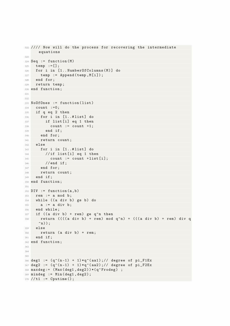
322 //// Now will do the process for recovering the intermediate

equations

323

324 Seq := function(M)

325 temp :=[];

326 for i in [1.. NumberOfColumns(M)] do

327 temp := Append(temp ,M[i]);

328 end for;

329 return temp;

330 end function;

331

332

333 NoOfOnes := function(list)

334 count :=0;

335 if q eq 2 then

336 for i in [1..# list] do

337 if list[i] eq 1 then

338 count := count +1;

339 end if;

340 end for;

341 return count;

342 else

343 for i in [1..# list] do

344 //if list[i] eq 1 then

345 count := count +list[i];

346 //end if;

347 end for;

348 return count;

349 end if;

350 end function;

351

352 DIV := function(a,b)

353 rem := a mod b;

354 while ((a div b) ge b) do

355 a := a div b;

356 end while;

357 if ((a div b) + rem) ge q^n then

358 return ((((a div b) + rem) mod q^n) + (((a div b) + rem) div q

^n));

359 else

360 return (a div b) + rem;

361 end if;

362 end function;

363

364

365

366 deg1 := (q^(n-1) + 1)*q^(aa1);// degree of pi_F1Ex

367 deg2 := (q^(n-1) + 1)*q^(aa2);// degree of pi_F2Ex

368 maxdeg := (Max(deg1 ,deg2))*(q^Frodeg) ;

369 mindeg := Min(deg1 ,deg2);

370 //t1 := Cputime ();

371 novar :=[];

372 curr_k:= 1;

373 prevtmpdeg := 0;

374 for k in [1..2*( Frodeg +1)] do

375 tmpnovar := [0];

376 if IsEven(k) then // for the multiplicand of F_2 and its

frobenius powers the multipicand is bounded by the degree of

deg1

377 if q eq 2 then

378 tmpdeg1 := q^(n-1)+q^(n-2);


380 tmpdeg1 :=deg1*(q^Frodeg);

381 end if;

382 tmpdeg2 := deg2*(q^(k/2-1));

383 else // for the multiplicand of F_1 and its frobenius powers

the multipicand is bounded by the degree of deg2

384 if q eq 2 then

385 tmpdeg1 := q^(n-1)+q^(n-2);


387 tmpdeg1 :=deg2*(q^Frodeg);

388 end if;

389 tmpdeg2 := deg1*(q^((k+1)/2-1));

390 end if;

391 if IsEven(k) then

392 for j in [(k/2-1).. Ceiling(Log(q,tmpdeg1))] do

393 if DIV(q^j,q^n) notin tmpnovar then

394 Append (~tmpnovar ,DIV(q^j,q^n));

395 end if;

396 if degmul gt 1 then

397 for i in [0..j] do

398 if q^j+qî le tmpdeg1 then

399 if DIV(q^j+qî,q^n) notin tmpnovar then

400 Append (~tmpnovar ,DIV(q^j+qî,q^n));

401 end if;

402 end if;

403 end for;

404 end if;

405 end for;

406 else

407 for j in [((k+1)/2-1).. Ceiling(Log(q,tmpdeg1))] do

408 if DIV(q^j,q^n) notin tmpnovar then

409 Append (~tmpnovar ,DIV(q^j,q^n));

410 end if;

411 if degmul gt 1 then

412 for i in [0..j] do

413 if q^j+qî le tmpdeg1 then

414 if DIV(q^j+qî,q^n) notin tmpnovar then

415 Append (~tmpnovar ,DIV(q^j+qî,q^n));

416 end if;

417 end if;

418 end for;

419 end if;

420 end for;

421 end if;

422 prevtmpdeg := Max(tmpdeg1 ,prevtmpdeg);

423 if prevtmpdeg eq tmpdeg1 then

424 curr_k := k;

425 end if;

426 //if syzygy eq 0 then

427 // Exclude (~tmpnovar ,tmpdeg2);

428 //end if;

429 Sort(~ tmpnovar);

430 Append (~novar ,tmpnovar);

431 end for;

432

433

434 novar3 :=[];

435 degc_x := deg1*(q^Frodeg)+deg2*(q^Frodeg);

436

437 //////// declairing the number of variabels

438 numvar := 0;

439 for i in [1..# novar] do

440 numvar := numvar + #novar[i];

441 end for;

442 print "Done computing number of variables=",numvar , "time=",t2;

443

444 P4 := PolynomialRing(ExtF ,numvar ,"glex");

445 P5<Y> := PolynomialRing(P4);

446

447

448

449 ModofY := function(f)

450 tmp_f := Parent(f)!0;

451 tmpSup ,tmpCof := Support(f);

452 for i in [1..# tmpSup] do

453 tmp_f := tmp_f + tmpCof[i]*Y^((( tmpSup[i] mod (q^n))));//

tmpSup[i] div (2^n)) +

454 end for;

455 return tmp_f;

456 end function;

457

458

459 // create new variabels for the coefficients

460 AA_var := [];

461 for i in [1..#AA] do

462 Append (~AA_var ,"A" cat IntegerToString(i));

463 end for;

464

465 BB_var := [];

466 for i in [1..#BB] do

467 Append (~BB_var ,"B" cat IntegerToString(i));

468 end for;

469

470 new_var := AA_var cat BB_var;

471

472

473

474 F_1ex := P5!0;

475 F_2ex := P5!0;

476 count :=0;

477 F_1exS := [];

478 F_1exSup := [];

479

480 for i in [0..n-1] do

481 Append (~F_1exS ,qî + 1);

482 Append (~F_1exSup ,P4!AA[i+1]);

483 end for;

484

485 F_2exS := [];

486 F_2exSup := [];

487

488 for i in [0..n-1] do

489 Append (~F_2exS ,qî + 1);

490 Append (~F_2exSup ,P4!BB[i+1]);

491 end for;

492

493 t1 := Cputime ();

494 pi_F1exS := F_1exS;

495 pi_F1exSup := F_1exSup;

496 pi_F1ex := F_1ex;


498 for j in [1..# F_1exS] do

499 if ( DIV(F_1exS[j]*(qî),(q^n))) notin pi_F1exS then

500 Append (~pi_F1exS ,( DIV(F_1exS[j]*(qî), (q^n))));

501 Append (~ pi_F1exSup , AA1[i]* F_1exSup[j]^(qî));

502 ParallelSort (~pi_F1exS ,~ pi_F1exSup);

503 else

504 k := Index(pi_F1exS ,( DIV(F_1exS[j]*(qî),(q^n))));

505 pi_F1exSup[k] := pi_F1exSup[k] + AA1[i]* F_1exSup[j]^(qî);

506 end if;

507 end for;

508 end for;

509 Append(~pi_F1exS ,Degree(P5!M1));

510 Append(~ pi_F1exSup ,P5!-M1);


512

513 t2 := Cputime(t1);print "Time pi_f1=",t2;

514 t1 := Cputime ();

515 pi_F2ex := F_2ex;

516

517 pi_F2exS := F_2exS;

518 pi_F2exSup := F_2exSup;


520 for j in [1..# F_2exS] do

521 if (DIV(F_2exS[j]*(qî), (q^n))) notin pi_F2exS then

522 Append (~pi_F2exS ,(DIV(F_2exS[j]*(qî) ,(q^n))));

523 Append (~ pi_F2exSup , BB1[i]* F_2exSup[j]^(qî));


525 else

526 k := Index(pi_F2exS ,(DIV(F_2exS[j]*(qî),(q^n))));

527 pi_F2exSup[k] := pi_F2exSup[k] + BB1[i]* F_2exSup[j]^(qî);

528 end if;

529 end for;

530 end for;

531 Append (~pi_F2exS ,Degree(P5!M2));

532 Append (~ pi_F2exSup ,P5!-M2);


534

535 t2 := Cputime(t1);print "Time pi_f2=",t2;

536

537 s1 := Ext_pol(s_mat);

538 ////// using univariate

539 t1 := Cputime ();

540 mul :=[];

541 count :=0;

542

543 SSmul :=[];

544 Supmul := [];

545

546 for j in [1..# novar] do //the last +1 is for c_y

547

548 tmpmul :=[];

549 tmpSS :=[];

550 for i in [1..# novar[j]] do

551 tmpSS := Append(tmpSS ,novar[j][i]);

552 tmpmul := Append(tmpmul ,P4.(i+count));

553 end for;

554 count := count + #novar[j];

555 Append (~SSmul ,tmpSS);

556 Append (~Supmul ,tmpmul);

557 end for;

558

559 count1 := count;

560

561 t2 := Cputime(t1);print "Time for novar =",t2;

562

563

564 ///////////////////////////////////////////////////////////////////////////////////

565

566

567 t1 := Cputime ();

568

569 T1 :=P5!0;T2 := P5!0;

570 if novar3 ne [] then

571 S3 := SSmul[# novar];

572 SC := Supmul [# novar];

573 else S3,SC := Support(P5!0);

574 end if;

575

576 t1 := Cputime ();

577 SSact :=[];

578 Supact :=[];

579

580

581 tmpS1 := pi_F1exS;

582 tmpSup1 := pi_F1exSup;

583 tmpSup2 := pi_F2exSup;

584 tmpS2 := pi_F2exS;

585

586

587 for k in [0.. Frodeg] do

588 tmpS11 := [];

589 tmpSup11 := [];

590 for i in [1..# tmpS1] do

591 if (DIV((tmpS1[i]*(q^k)),(q^n))) notin tmpS11 then

592 Append (~tmpS11 ,(DIV((tmpS1[i]*(q^k)),(q^n)) ));

593 Append (~tmpSup11 ,ExtF!tmpSup1[i]^(q^k));

594 ParallelSort (~tmpS11 ,~ tmpSup11);

595 else

596 l := Index(tmpS11 ,(DIV(( tmpS1[i]*(q^k)) ,(q^n))));

597 tmpSup11[l] := tmpSup11[l] + ExtF!tmpSup1[i]^(q^k);

598 end if;

599 end for;

600 Append (~SSact ,tmpS11);

601 Append (~Supact ,tmpSup11);

602 tmpS22 := [];

603 tmpSup22 := [];

604 for i in [1..# tmpS2] do

605 if (DIV((tmpS2[i]*(q^k)),(q^n)) ) notin tmpS22 then

606 Append (~tmpS22 ,(DIV((tmpS2[i]*(q^k)), (q^n)) ));

607 Append (~tmpSup22 ,ExtF!tmpSup2[i]^(q^k));

608 ParallelSort (~tmpS22 ,~ tmpSup22);

609 else

610 l := Index(tmpS22 ,(DIV(( tmpS2[i]*(q^k)), (q^n))));

611 tmpSup22[l] := tmpSup22[l] + ExtF!tmpSup2[i]^(q^k);

612 end if;

613 end for;

614 Append (~SSact ,tmpS22);

615 Append (~Supact ,tmpSup22);

616 end for;


618 print "Time taken for making all the frobenius powers of public

keys , time=", t2;

619

620

621

622 TT11 := [];

623 SS11 := [];

624 SS11act := [];

625 t1 := Cputime ();

626 for k in [1..2*( Frodeg +1)] do

627 for i in [1..# SSmul[k]] do

628 for j in [1..# SSact[k]] do

629 if (DIV(( SSmul[k][i]+ SSact[k][j]) ,(q^n))) notin SS11 then

630 Append (~TT11 ,Supmul[k][i]* Supact[k][j]);

631 Append (~SS11 ,( DIV(( SSmul[k][i]+ SSact[k][j]) ,(q^n))));

632 if ( DIV(( SSmul[k][i]+SSact[k][j]) ,(q^n))) gt q^n then

633 print "true",(SSmul[k][i]+ SSact[k][j]) ,( DIV(( SSmul[k][i

]+ SSact[k][j]) ,(q^n)));

634 end if;

635 ParallelSort (~SS11 ,~TT11);

636 else

637 l := Index(SS11 ,( DIV(( SSmul[k][i]+ SSact[k][j]) ,(q^n))));

638 TT11[l] := TT11[l] + Supmul[k][i]* Supact[k][j];

639 end if;

640 end for;

641 end for;

642 end for;


644 print "Time for multiplyuing the multiplicand and public keys and

frobenius , time=",t2;

645 #SS11;

646

647 Eqs4 := [];

648 Supsup :=[];

649 for i in [1..# SS11] do

650 if NoOfOnes(Intseq(SS11[i],q)) gt degreq then

651 Append (~Supsup ,SS11[i]);Append (~Eqs4 ,TT11[i]);

652 end if;

653 end for;

654

655 print "Done making the linear eqs";

656 Eqs := Eqs4;

657

658

659 if Index(Eqs ,0) gt 1 then

660 rows := Index(Eqs ,0) -1;

661 else rows := #Eqs;

662 end if;

663 print "rows=", rows;

664 colms := Rank(P4);

665 print "colms=",colms;

666

667

668 t1 := Cputime ();

669 print "Most time consuming step in whole";

670 Eqs1:=Eqs;


672 print "Time for converting to lower dim poly ring=",t2;

673

674 print "Time for initialization of coeff mat";

675

676

677 // Do this when i want to find the kernel

678 time Matmat1 := ZeroMatrix(ExtF ,rows ,colms);

679 print "Done initialization ";

680 t1 := Cputime ();


682 temp_c ,temp_m := CoefficientsAndMonomials(Eqs1[i]);

683 count :=1;

684 for j in [1..# temp_m] do

685 temp_mon := Sprint(temp_m[j]);

686 k := StringToInteger(Split(temp_mon ,".") [2]);

687 // print k;

688 Matmat1[i][k] := Matmat1[i][k] + temp_c[j];

689 end for;

690 end for;


692 print "Time for Matmat1=",t2;

693 Matmat := Matmat1;

694

695 print "\n Calculating Kernel\n";

696 t12 := Cputime ();

697

698

699 // do this when I want to know the struucture

700

701 /*

702 time Matmat1 := ZeroMatrix(P4,rows ,colms);

703 print "Done initialization ";

704 t1 := Cputime ();

705


707

708 temp_c ,temp_m := CoefficientsAndMonomials(Eqs1[i]);

709 count :=1;

710 for j in [1..# temp_m] do

711 temp_mon := Sprint(temp_m[j]);

712 kk := Split(temp_mon ,"*");

713 // print kk;

714 if #kk gt 1 then

715 k := StringToInteger(Split(kk[2] ,".") [2]);

716 kkk := Split(kk[1] ,".") [2];

717 kkkk := Split(kkk ,"^");

718 if #kkkk eq 1 then

719 Append (~kkkk ,"1");

720 end if;

721 // print kkkk;

722 Matmat1[i][k] := Matmat1[i][k] + temp_c[j]*P4.

StringToInteger(kkkk [1])^StringToInteger(kkkk [2]);

723 else

724 k := StringToInteger(Split(kk[1] ,".") [2]);

725 // print k;

726 Matmat1[i][k] := Matmat1[i][k] + temp_c[j];

727 end if;

728 end for;

729 end for;


731 print "Time for Matmat1=",t2;

732

733

734

735 J,K := Support(pi_F1ex);

736 pi_F1Extst := P2!0;

737 for i in [1..#J] do

738 pi_F1Extst := pi_F1Extst + P2!(P2!K[i]*( chi_x1 ^(J[i])));

739 end for;

740 // pi_F1Extst := NormalForm(pi_F1Extst ,fieldeq2);

741 */

742

743 Matmat := Matmat1;

744 time KK := KernelMatrix(Transpose(Matmat));

745 t13 := Cputime(t12);

746 print "\n DOne computing kernel , time req=", t13 , "\n";

747 print "\ nNumber of rows in Kernel=", NumberOfRows(KK);

748 Model :=[ ExtF!Random(q) : i in [1.. NumberOfRows(KK)]]; // seq of

constants to multiply with

749 KK2 := Model [1]*KK[1];

750

751

752 for i in [2.. NumberOfRows(KK)] do

753 if i gt colms then

754 break;

755 end if;

756 KK2 := KK2 + Model[i]*KK[i];

757 end for;

758 // print "Model=",Model;

759 KK1 :=KK2;

760

761 Sol := [KK1[i] : i in [1.. NumberOfColumns(KK1)]];

762 //Sol2 := [ExtF!0 : i in [1.. NumberOfColumns(KK)]];

763 for i in [1..# Supsup] do

764 if Evaluate(TT11[Index(SS11 ,Supsup[i])],Sol) ne 0 then

765 print "Anamonly here";

766 end if;

767 end for;

768

769 t1:= Cputime ();

770 c1_x := P2!0;

771 time restSup := SetToSequence(SequenceToSet(SS11) diff

SequenceToSet(Supsup));

772 Sort(~ restSup);

773 for j in [1..# restSup] do

774 c1_x := c1_x + Evaluate(TT11[Index(SS11 ,restSup[j])],Sol)*

Ext_var_pow(chi_x1 ,restSup[j]);// SS11[j]);

775 //c1_x := c1_x + Evaluate(TT11[Index(SS11 ,restSup[j])],Sol)*((

chi_x1^restSup[j]));

776 end for;

777 t2 := Cputime(t1);print "New intermediate pols created , time =",t2

;

778 t10 := Cputime ();

779

780 /*

781 if c1_x eq 0 then

782 print "No new quations found";

783 else print "Good New quations found";

784 end if;

785

786 time c1_x1 := NormalForm(c1_x ,fieldeq2);

787 t11 := Cputime(t10);

788 print "time req to calc c1_x= ", t11;

789

790

791

792 //if c1_x ne P2!0 then

793 c1_x1_mat := Pol_mat(c1_x1);

794 c1_x1_bas := [c1_x1_mat[i][1] : i in [1.. NumberOfRows(c1_x1_mat)

]];

795 ciph :=[];

796 zerociph := [0 : i in [1..# c1_x1_bas ]];

797 for i in [1..# c1_x1_bas] do

798 Evaluate(c1_x1_bas[i],s);

799 end for;

800

801

802 print "\n Doing GB calculation with new eqs\n ";

803 t1 := Cputime ();

804 //G1 := GroebnerBasis(C9 cat c1_x1_bas);

805 G1 := GroebnerBasis(C9 cat c1_x1_bas ,4);// cat c2_x2_bas ,3);

806


808 print "new Gb time is =", t2;

809 G1;

810

811 */

812 //the following is to recover all possible intermediate equations

813 countloop :=0;

814 eqsset :=0;


816 print "c1x eq 0";

817 else eqsset :=1;

818 end if;

819

820 while (c1_x eq 0) and (eqsset eq 0) do

821 print "In loop ", countloop;


823 Model :=[ ExtF!Random(q) : i in [1.. NumberOfRows(KK)]];

824 KK2 := Model [1]*KK[1];

825

826



829 break;

830 end if;

831 KK2 := KK2 + Model[i]*KK[i];//

832 end for;

833 KK1 :=KK2;


835 c1_x := P2!0;




838 c1_x := c1_x + Evaluate(TT11[Index(SS11 ,restSup[j])],Sol)*


839 //c1_x := c1_x + Evaluate(TT11[j],Sol)*Ext_var_pow(chi_x1 ,SS11

[j]);

840 end for;


842 countloop := countloop +1;

843 if countloop gt 1000 then

844 print "Too many loops with no result ";


846 eqsset :=0;

847 break;

848 end if;

849 end while;

850 // check to see if the equations chosen are actually evaluating to

0 or not

851 //Sol := [KK1[i] : i in [1.. NumberOfColumns(KK1)]];

852 //Sol2 := [ExtF!0 : i in [1.. NumberOfColumns(KK)]];

853 //for i in [1..# Supsup] do

854 // Evaluate(Eqs4[i], Sol);

855 //end for;

856

857 if eqsset eq 1 then

858 print "Good New quations found";


860 t11 := Cputime(t10);



863 c1_x1_bas := [c1_x1_mat[i][1] : i in [1..n]];

864 for i in [1..# c1_x1_bas] do

865 Evaluate(c1_x1_bas[i],s);

866 end for;

867

868 /////////////////////////////////////////////////////////////////

869 /////// Second polynomial ///////////////

870 /*

871 tmpbas :=[];

872 for k in [1..4] do

873 Model2 :=[ ExtF!Random (0,1) : i in [1.. NumberOfRows(KK)]];

874 KK4 := Model2 [1]*KK[1];

875

876



879 break;

880 end if;

881 KK4 := KK4 + Model2[i]*KK[i];//

882 end for;

883 Sol2 := [KK4[i] : i in [1.. NumberOfColumns(KK4)]];

884


886

887 c2_x := P2!0;



889


891 //for j in [1..# SS11] do

892 c2_x := c2_x + Evaluate(TT11[Index(SS11 ,restSup[j])],Sol2)*


893 // c1_x := c1_x + Evaluate(TT11[j],Sol)*Ext_var_pow(chi_x1 ,SS11[j

]);

894 end for;

895 t2 := Cputime(t1);print "New intermediate pols created , time =",t2

;

896

897 t10 := Cputime ();

898



901 else print "Good New quations found";

902 end if;

903


905 // print "Normally",c1_x1;

906 t11 := Cputime(t10);


908

909 //if c1_x ne P2!0 then


911 c2_x2_bas := [c2_x2_mat[i][1] : i in [1..n]];

912

913 tmpbas := tmpbas cat c2_x2_bas;

914 end for;

915

916

917 */

918 ///////////////////////////////////////////////////////////

919

920 print "\n Doing GB calculation with new eqs\n ";

921 t1 := Cputime ();

922 G1 := GroebnerBasis(C9 cat c1_x1_bas);// cat c2_x2_bas ,3);


924 print "new Gb time is =", t2;

925 end if;

926 G1;

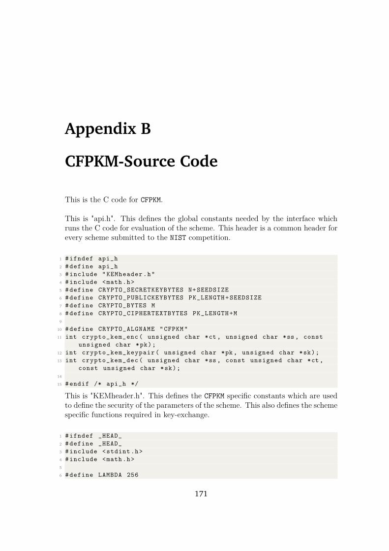
Appendix B

CFPKM-Source Code

This is the C code for CFPKM.

This is "api.h". This defines the global constants needed by the interface whichruns the C code for evaluation of the scheme. This header is a common header forevery scheme submitted to the NIST competition.

1 #ifndef api_h

2 #define api_h

3 #include "KEMheader.h"

4 #include <math.h>

5 #define CRYPTO_SECRETKEYBYTES N+SEEDSIZE

6 #define CRYPTO_PUBLICKEYBYTES PK_LENGTH+SEEDSIZE

7 #define CRYPTO_BYTES M

8 #define CRYPTO_CIPHERTEXTBYTES PK_LENGTH+M

9

10 #define CRYPTO_ALGNAME "CFPKM"

11 int crypto_kem_enc( unsigned char *ct , unsigned char *ss, const

unsigned char *pk);

12 int crypto_kem_keypair( unsigned char *pk , unsigned char *sk);

13 int crypto_kem_dec( unsigned char *ss , const unsigned char *ct,

const unsigned char *sk);

14

15 #endif /* api_h */

This is "KEMheader.h". This defines the CFPKM specific constants which are usedto define the security of the parameters of the scheme. This also defines the schemespecific functions required in key-exchange.

1 #ifndef _HEAD_

2 #define _HEAD_

3 #include <stdint.h>

4 #include <math.h>

5

6 #define LAMBDA 256

171

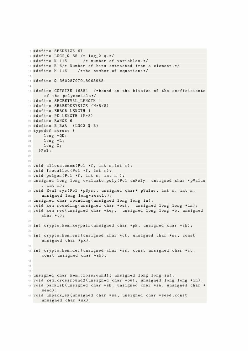
7 #define SEEDSIZE 67

8 #define LOG2_Q 55 /* log_2 q.*/

9 #define N 115 /* number of variables .*/

10 #define B 6/* Number of bits extracted from a element .*/

11 #define M 116 /*the number of equations */

12

13 #define Q 36028797018963968

14

15 #define COFSIZE 16384 /* bound on the bitsize of the coeffeicients

of the polynomials */

16 #define SECRETVAL_LENGTH 1

17 #define SHAREDKEYSIZE (M*B/8)

18 #define ERROR_LENGTH 1

19 #define PK_LENGTH (M*8)

20 #define RANGE 6

21 #define B_BAR (LOG2_Q -B)

22 typedef struct {

23 long *QD;

24 long *L;

25 long C;

26 }Pol;

27

28

29 void allocatemem(Pol *f, int n,int m);

30 void freealloc(Pol *f, int m);

31 void polgen(Pol *f, int m, int n );

32 unsigned long long evaluate_poly(Pol unPoly , unsigned char *pValue

, int n);

33 void Eval_sys(Pol *pSyst , unsigned char* pValue , int m, int n,

unsigned long long*result);

34 unsigned char rounding(unsigned long long in);

35 void kem_rounding(unsigned char *out , unsigned long long *in);

36 void kem_rec(unsigned char *key , unsigned long long *b, unsigned

char *c);

37

38 int crypto_kem_keypair(unsigned char *pk , unsigned char *sk);

39

40 int crypto_kem_enc(unsigned char *ct, unsigned char *ss, const

unsigned char *pk);

41

42 int crypto_kem_dec(unsigned char *ss, const unsigned char *ct ,

const unsigned char *sk);

43

44

45

46 unsigned char kem_crossround1( unsigned long long in);

47 void kem_crossround2(unsigned char *out , unsigned long long *in);

48 void pack_sk(unsigned char *sk , unsigned char *sa , unsigned char *

seed);

49 void unpack_sk(unsigned char *sa, unsigned char *seed ,const

unsigned char *sk);

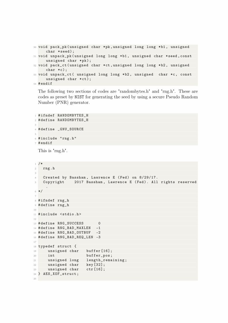
50 void pack_pk(unsigned char *pk,unsigned long long *b1, unsigned

char *seed);

51 void unpack_pk(unsigned long long *b1 , unsigned char *seed ,const

unsigned char *pk);

52 void pack_ct(unsigned char *ct,unsigned long long *b2, unsigned

char *c);

53 void unpack_ct( unsigned long long *b2, unsigned char *c, const

unsigned char *ct);

54 #endif

The following two sections of codes are "randombytes.h" and "rng.h". These arecodes as preset by NIST for generating the seed by using a secure Pseudo RandomNumber (PNR) generator.

1 #ifndef RANDOMBYTES_H

2 #define RANDOMBYTES_H

3

4 #define _GNU_SOURCE

5

6 #include "rng.h"

7 #endif

This is "rng.h".

1 /*

2 rng.h

3

4 Created by Bassham , Lawrence E (Fed) on 8/29/17.

5 Copyright 2017 Bassham , Lawrence E (Fed). All rights reserved

.

6 */

7

8 #ifndef rng_h

9 #define rng_h

10

11 #include <stdio.h>

12

13 #define RNG_SUCCESS 0

14 #define RNG_BAD_MAXLEN -1

15 #define RNG_BAD_OUTBUF -2

16 #define RNG_BAD_REQ_LEN -3

17

18 typedef struct {

19 unsigned char buffer [16];

20 int buffer_pos;

21 unsigned long length_remaining;

22 unsigned char key [32];

23 unsigned char ctr [16];

24 } AES_XOF_struct;

25

26 typedef struct {

27 unsigned char Key [32];

28 unsigned char V[16];

29 int reseed_counter;

30 } AES256_CTR_DRBG_struct;

31

32

33 void

34 AES256_CTR_DRBG_Update(unsigned char *provided_data ,

35 unsigned char *Key ,

36 unsigned char *V);

37

38 int

39 seedexpander_init(AES_XOF_struct *ctx ,

40 unsigned char *seed ,

41 unsigned char *diversifier ,

42 unsigned long maxlen);

43

44 int

45 seedexpander(AES_XOF_struct *ctx , unsigned char *x, unsigned long

xlen);

46

47 void

48 randombytes_init(unsigned char *entropy_input ,

49 unsigned char *personalization_string ,

50 int security_strength);

51

52 int

53 randombytes(unsigned char *x, unsigned long long xlen);

54 void AES256_ECB(unsigned char *key , unsigned char *ctr , unsigned

char *buffer);

55

56 #endif /* rng_h */

This is "kem.c". This is the implementation of the key Encapsulation mechanismof CFPKM[◮oc: nned to mention for which parameter is this].

1 #include <stdlib.h>


3 #include <stdint.h>


5 #include <string.h>

6 #include "api.h"


8 #include "rng.h"

9 #include "randombytes.h"

10

11

12

13 void allocatemem(Pol *f, int n,int m){

14

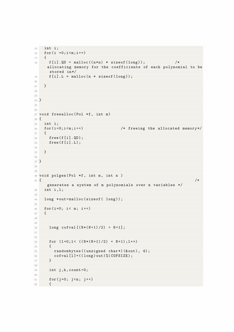
15 int i;

16 for(i =0;i<m;i++)

17 {

18 f[i].QD = malloc ((n*n) * sizeof(long)); /*

allocating memory for the coefficients of each polynomial to be

stored in*/

19 f[i].L = malloc(n * sizeof(long));

20

21 }

22

23

24 }

25

26

27 void freealloc(Pol *f, int m)

28 {

29 int i;

30 for(i=0;i<m;i++) /* freeing the allocated memory */

31 {

32 free(f[i].QD);

33 free(f[i].L);

34

35 }

36

37 }

38

39

40 void polgen(Pol *f, int m, int n )

41 { /*

generates a system of m polynomials over n variables */

42 int i,l;

43

44 long *out=malloc(sizeof( long));

45

46 for(i=0; i< m; i++)

47 {

48

49

50 long cofval [(N*(N+1) /2) + N+1];

51

52

53 for (l=0;l< ((N*(N+1)/2) + N+1);l++)

54 {

55 randombytes (( unsigned char*)(&out), 4);

56 cofval[l]=(( long)out)%( COFSIZE);

57 }

58

59 int j,k,count =0;

60

61 for(j=0; j<n; j++)

62 {

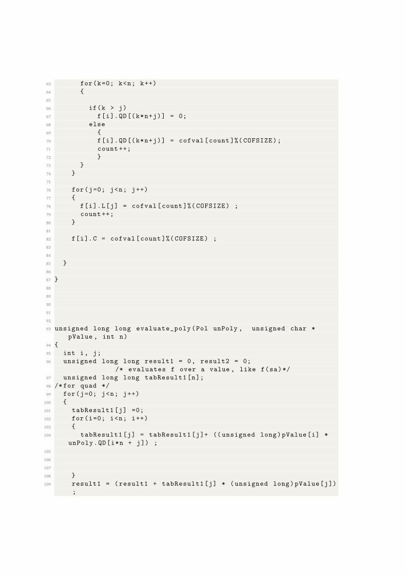
63 for(k=0; k<n; k++)

64 {

65

66 if(k > j)

67 f[i].QD[(k*n+j)] = 0;

68 else

69 {

70 f[i].QD[(k*n+j)] = cofval[count ]%( COFSIZE);

71 count ++;

72 }

73 }

74 }

75

76 for(j=0; j<n; j++)

77 {

78 f[i].L[j] = cofval[count ]%( COFSIZE) ;

79 count ++;

80 }

81

82 f[i].C = cofval[count ]%( COFSIZE) ;

83

84

85 }

86

87 }

88

89

90

91

92

93 unsigned long long evaluate_poly(Pol unPoly , unsigned char *

pValue , int n)

94 {

95 int i, j;

96 unsigned long long result1 = 0, result2 = 0;

/* evaluates f over a value , like f(sa)*/

97 unsigned long long tabResult1[n];

98 /*for quad */

99 for(j=0; j<n; j++)

100 {

101 tabResult1[j] =0;

102 for(i=0; i<n; i++)

103 {

104 tabResult1[j] = tabResult1[j]+ (( unsigned long)pValue[i] *

unPoly.QD[i*n + j]) ;

105

106

107

108 }

109 result1 = (result1 + tabResult1[j] * (unsigned long)pValue[j])

;

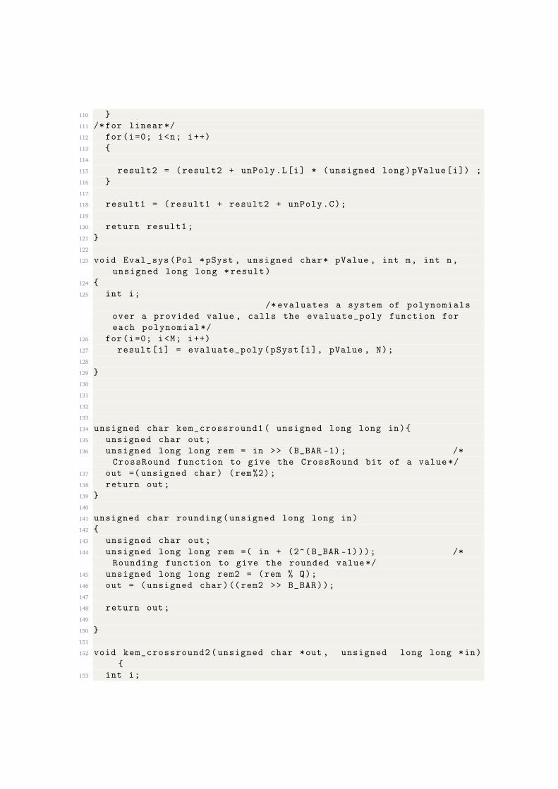
110 }

111 /*for linear */

112 for(i=0; i<n; i++)

113 {

114

115 result2 = (result2 + unPoly.L[i] * (unsigned long)pValue[i]) ;

116 }

117

118 result1 = (result1 + result2 + unPoly.C);

119

120 return result1;

121 }

122

123 void Eval_sys(Pol *pSyst , unsigned char* pValue , int m, int n,

unsigned long long *result)

124 {

125 int i;

/* evaluates a system of polynomials

over a provided value , calls the evaluate_poly function for

each polynomial */

126 for(i=0; i<M; i++)

127 result[i] = evaluate_poly(pSyst[i], pValue , N);

128

129 }

130

131

132

133

134 unsigned char kem_crossround1( unsigned long long in){

135 unsigned char out;

136 unsigned long long rem = in >> (B_BAR -1); /*

CrossRound function to give the CrossRound bit of a value*/

137 out =( unsigned char) (rem %2);

138 return out;

139 }

140

141 unsigned char rounding(unsigned long long in)

142 {

143 unsigned char out;

144 unsigned long long rem =( in + (2^( B_BAR -1))); /*

Rounding function to give the rounded value*/

145 unsigned long long rem2 = (rem % Q);

146 out = (unsigned char)((rem2 >> B_BAR));

147

148 return out;

149

150 }

151

152 void kem_crossround2(unsigned char *out , unsigned long long *in)

{

153 int i;

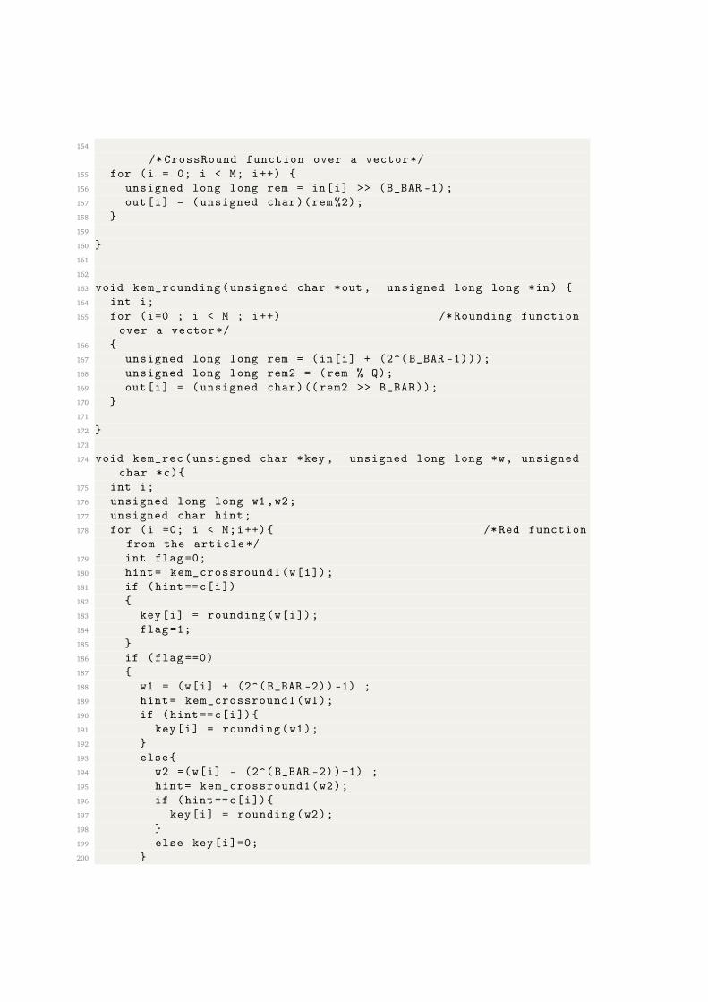
154

/* CrossRound function over a vector */

155 for (i = 0; i < M; i++) {

156 unsigned long long rem = in[i] >> (B_BAR -1);

157 out[i] = (unsigned char)(rem %2);

158 }

159

160 }

161

162

163 void kem_rounding(unsigned char *out , unsigned long long *in) {

164 int i;

165 for (i=0 ; i < M ; i++) /* Rounding function

over a vector */

166 {

167 unsigned long long rem = (in[i] + (2^( B_BAR -1)));

168 unsigned long long rem2 = (rem % Q);

169 out[i] = (unsigned char)((rem2 >> B_BAR));

170 }

171

172 }

173

174 void kem_rec(unsigned char *key , unsigned long long *w, unsigned

char *c){

175 int i;

176 unsigned long long w1,w2;

177 unsigned char hint;

178 for (i =0; i < M;i++){ /*Red function

from the article */

179 int flag =0;

180 hint= kem_crossround1(w[i]);

181 if (hint==c[i])

182 {

183 key[i] = rounding(w[i]);

184 flag =1;

185 }

186 if (flag ==0)

187 {

188 w1 = (w[i] + (2^( B_BAR -2)) -1) ;

189 hint= kem_crossround1(w1);

190 if (hint==c[i]){

191 key[i] = rounding(w1);

192 }

193 else{

194 w2 =(w[i] - (2^( B_BAR -2))+1) ;

195 hint= kem_crossround1(w2);

196 if (hint==c[i]){

197 key[i] = rounding(w2);

198 }

199 else key[i]=0;

200 }

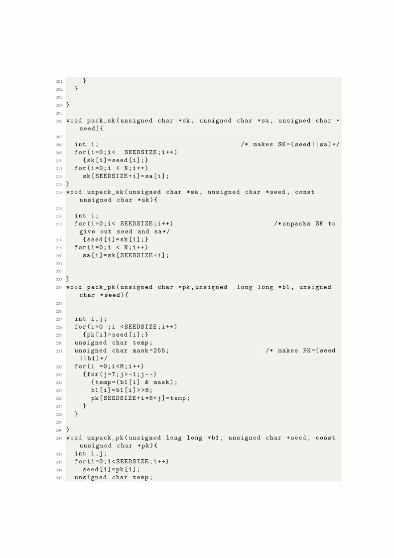
201 }

202 }

203

204 }

205

206 void pack_sk(unsigned char *sk, unsigned char *sa , unsigned char *

seed){

207

208 int i; /* makes SK=(seed||sa)*/

209 for(i=0;i< SEEDSIZE;i++)

210 {sk[i]=seed[i];}

211 for(i=0;i < N;i++)

212 sk[SEEDSIZE+i]=sa[i];

213 }

214 void unpack_sk(unsigned char *sa , unsigned char *seed , const

unsigned char *sk){

215

216 int i;

217 for(i=0;i< SEEDSIZE;i++) /* unpacks SK to

give out seed and sa*/

218 {seed[i]=sk[i];}

219 for(i=0;i < N;i++)

220 sa[i]=sk[SEEDSIZE+i];

221

222

223 }

224 void pack_pk(unsigned char *pk,unsigned long long *b1 , unsigned

char *seed){

225

226

227 int i,j;

228 for(i=0 ;i <SEEDSIZE;i++)

229 {pk[i]=seed[i];}

230 unsigned char temp;

231 unsigned char mask =255; /* makes PK=(seed

||b1)*/

232 for(i =0;i<M;i++)

233 {for(j=7;j>-1;j--)

234 {temp=(b1[i] & mask);

235 b1[i]=b1[i]>>8;

236 pk[SEEDSIZE+i*8+j]=temp;

237 }

238 }

239

240 }

241 void unpack_pk(unsigned long long *b1 , unsigned char *seed , const

unsigned char *pk){

242 int i,j;

243 for(i=0;i<SEEDSIZE;i++)

244 seed[i]=pk[i];


246 for(i=0;i<M;i++)

247 b1[i]=0;

248 for(i=0;i<M;i++)

249 { /* unpacks PK to give out seed

and the public vector b1*/

250 for(j=0;j<7;j++)

251 {

252 temp = pk[i*8+j+SEEDSIZE ];

253 b1[i]=b1[i]+temp;

254 b1[i]=b1[i]<<8;

255 }

256 b1[i]=b1[i]+pk[i*8+7+ SEEDSIZE ];

257 }

258

259

260 }

261 void pack_ct(unsigned char *ct , unsigned long long *b2,unsigned

char *c){

262

263

264 int i,j;

265 for (i=0;i < M;i++)

266 ct[i]=c[i];

267 /* makes ct=(c||b2)*/


269 unsigned char mask =255;

270 for(i =0;i<M;i++)

271 {for(j=7;j>-1;j--)

272 {temp=( unsigned char)(b2[i] & mask);

273 b2[i]=b2[i]>>8;

274 ct[M+i*8+j]=temp;

275 }

276 }

277

278

279

280

281 }

282 void unpack_ct(unsigned long long *b2,unsigned char *c, const

unsigned char *ct){

283

284 int i,j;

285 for (i=0;i < M;i++)

286 c[i]=ct[i];

287


289 for(i=0;i<M;i++) /* unpacks ct to give out

the hint vector c and b2*/

290 b2[i]=0;

291 for(i=0;i<M;i++)

292 {

293 for(j=0;j<7;j++)

294 {

295 temp = ct[i*8+j+M];

296 b2[i]=b2[i]+temp;

297 b2[i]=b2[i]<<8;

298 }

299 b2[i]=b2[i]+ct[i*8+7+M];

300 }

301

302 }

303

304

305 int crypto_kem_keypair(unsigned char *pk , unsigned char *sk){

306

307 unsigned char *seed=malloc(SEEDSIZE*sizeof(unsigned char));if (

seed==NULL) {printf ("EXIT");return 0;}

308 randombytes(seed ,SEEDSIZE);

309

310

311 Pol *f1 = malloc(M * sizeof(Pol));

312 allocatemem(f1,N,M);

313

314 randombytes_init(seed ,NULL ,256);

315 polgen(f1,M,N);

316

317 int i;

318

319 unsigned char *sa=malloc(N*sizeof(unsigned char));if (sa==NULL)

{printf ("EXIT");return 0;}

320

321

322 randombytes(sa,N*SECRETVAL_LENGTH);

323

324 unsigned char *e1=malloc(M*sizeof(unsigned char));if (e1==NULL)


325 randombytes(e1,M*ERROR_LENGTH);

326

327

328 for(i=0;i < N;i++)

329 sa[i]=( unsigned char)((sa[i])%RANGE);

330

331

332 for(i=0;i < M;i++)

333 {e1[i]=( unsigned char)((e1[i])%RANGE); }

334

335

336 unsigned long long *b1=malloc(M*sizeof(unsigned long long));if (

b1==NULL) {printf ("EXIT");return 0;}

337 Eval_sys(f1 ,sa,M,N,b1);

338 for (i =0;i <M ;i++)

339 {

340 b1[i] = (b1[i] + e1[i]) ;

341

342

343 }

344

345 pack_sk(sk ,sa,seed);

346

347 pack_pk(pk ,b1,seed);

348

349

350 return 0;

351 }

352

353 int crypto_kem_enc(unsigned char *ct, unsigned char *ss, const

unsigned char *pk){

354 int i;

355 unsigned long long *b1=malloc(M*sizeof(unsigned long long));

356 unsigned char *seed=malloc(SEEDSIZE*sizeof(unsigned char));

357 unpack_pk(b1, seed , pk);

358

359

360 Pol *f2 = malloc(M*sizeof(Pol));

361 allocatemem(f2 ,N,M);

362


364 polgen(f2,M,N);

365

366

367

368 unsigned char *seed1=malloc(SEEDSIZE*sizeof(unsigned char));

369 randombytes(seed1 ,SEEDSIZE);

370

371 randombytes_init(seed1 ,NULL ,256);

372 unsigned char *sb=malloc(N*sizeof(unsigned char));





375

376 randombytes(sb , N*SECRETVAL_LENGTH);

377

378 randombytes(e2 ,M*ERROR_LENGTH);

379 randombytes(e3 ,M*ERROR_LENGTH);

380

381 for(i=0;i < N;i++)

382 {sb[i]=( unsigned char)((sb[i])%RANGE);}

383

384

385 for(i=0;i < M;i++)

386 {e2[i]=( unsigned char)((e2[i])%RANGE);

387 e3[i]=( unsigned char)((e3[i])%RANGE); }

388

389

390





393

394 Eval_sys(f2 ,sb,M,N,b2);

395

396 for (i =0;i<M;i++){

397 b3[i] = (b2[i]*b1[i] + e3[i]);

398 b2[i] = (b2[i] + e2[i]);

399

400 }

401

402 kem_rounding(ss, b3);

403

404 unsigned char *c=malloc(M*sizeof(unsigned char));

405 kem_crossround2(c, b3);

406 pack_ct(ct, b2, c);

407

408 return 0;

409 }

410

411

412 int crypto_kem_dec(unsigned char *ss , const unsigned char *ct,

const unsigned char *sk){

413 int i;

414 unsigned char *sa=malloc(N*sizeof(unsigned char));

415 unsigned char *seed=malloc(SEEDSIZE*sizeof(unsigned char));

416 unpack_sk(sa ,seed ,sk);

417 unsigned long long *b2=malloc(M*sizeof(unsigned long long));

418 unsigned char *c=malloc(M*sizeof(unsigned char));

419

420 unpack_ct(b2 ,c,ct);

421 Pol *f = (Pol*) malloc(M*sizeof(Pol));

422 allocatemem(f,N,M);

423


425 polgen(f,M,N);

426

427 unsigned long long *w = malloc(M*sizeof(unsigned long long));

428 Eval_sys(f,sa,M,N,w);

429 for (i=0;i < M;i++)

430 {

431 w[i]=(w[i]*b2[i]) ;}

432

433

434

435

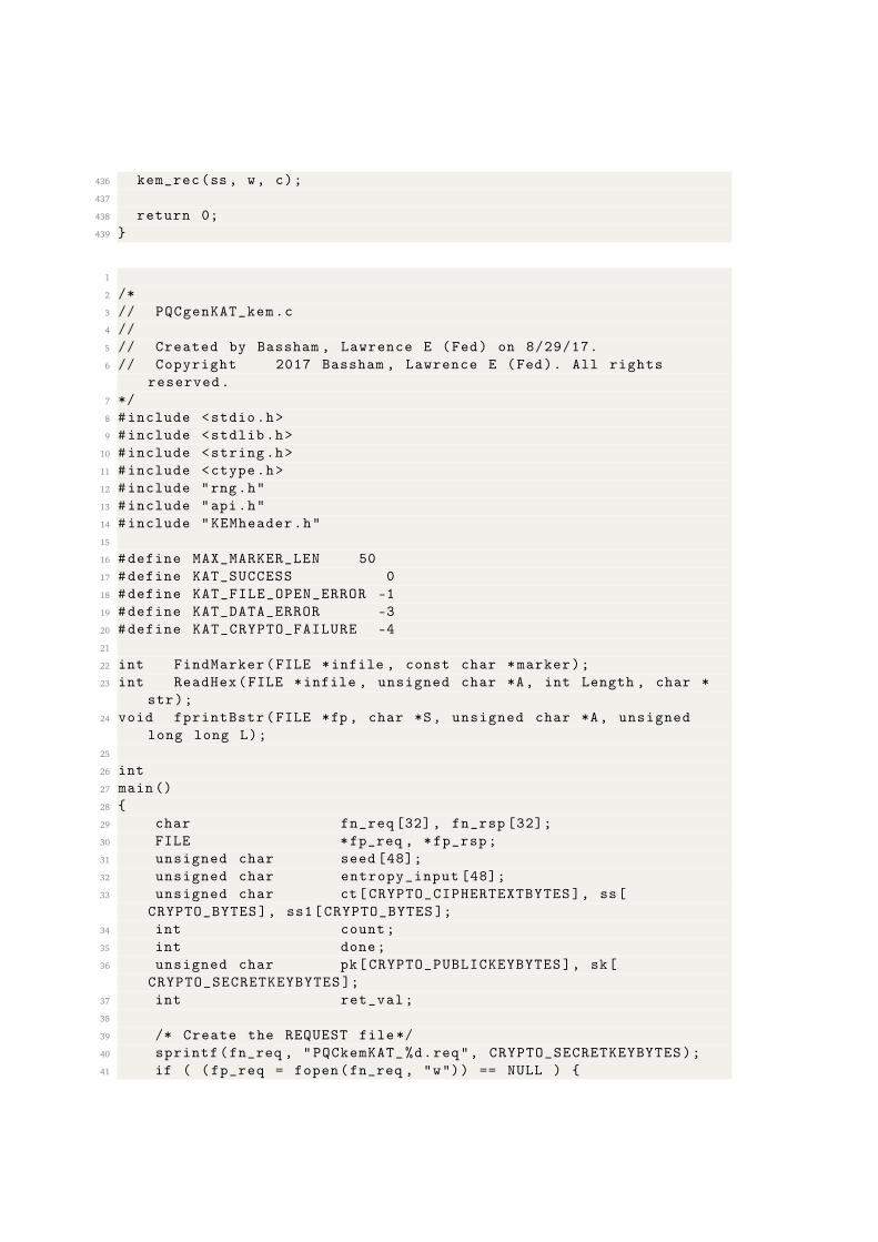
436 kem_rec(ss , w, c);

437

438 return 0;

439 }

1

2 /*

3 // PQCgenKAT_kem.c

4 //

5 // Created by Bassham , Lawrence E (Fed) on 8/29/17.

6 // Copyright 2017 Bassham , Lawrence E (Fed). All rights

reserved.

7 */



10 #include <string.h>

11 #include <ctype.h>

12 #include "rng.h"

13 #include "api.h"


15

16 #define MAX_MARKER_LEN 50

17 #define KAT_SUCCESS 0

18 #define KAT_FILE_OPEN_ERROR -1

19 #define KAT_DATA_ERROR -3

20 #define KAT_CRYPTO_FAILURE -4

21

22 int FindMarker(FILE *infile , const char *marker);

23 int ReadHex(FILE *infile , unsigned char *A, int Length , char *

str);

24 void fprintBstr(FILE *fp , char *S, unsigned char *A, unsigned

long long L);

25

26 int

27 main()

28 {

29 char fn_req [32], fn_rsp [32];

30 FILE *fp_req , *fp_rsp;

31 unsigned char seed [48];

32 unsigned char entropy_input [48];

33 unsigned char ct[CRYPTO_CIPHERTEXTBYTES], ss[

CRYPTO_BYTES], ss1[CRYPTO_BYTES ];

34 int count;

35 int done;

36 unsigned char pk[CRYPTO_PUBLICKEYBYTES], sk[

CRYPTO_SECRETKEYBYTES ];

37 int ret_val;

38

39 /* Create the REQUEST file*/

40 sprintf(fn_req , "PQCkemKAT_%d.req", CRYPTO_SECRETKEYBYTES);

41 if ( (fp_req = fopen(fn_req , "w")) == NULL ) {

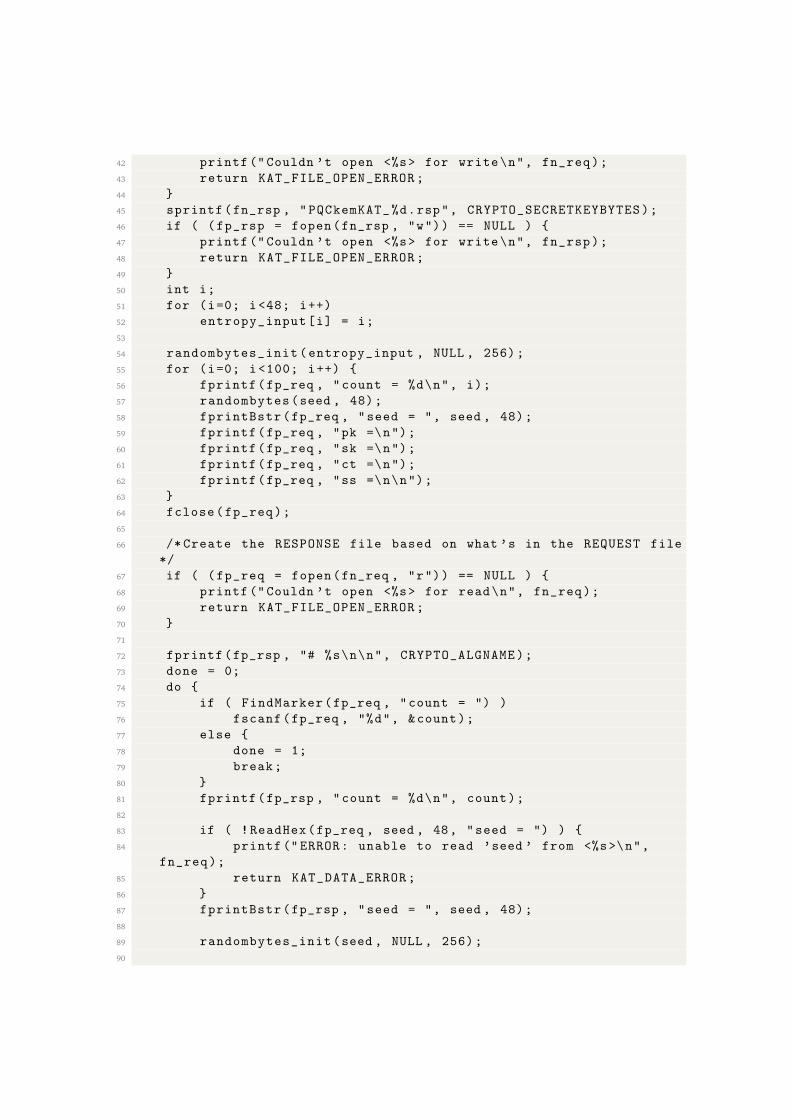
42 printf ("Couldn ’t open <%s> for write\n", fn_req);

43 return KAT_FILE_OPEN_ERROR ;

44 }

45 sprintf(fn_rsp , "PQCkemKAT_%d.rsp", CRYPTO_SECRETKEYBYTES);

46 if ( (fp_rsp = fopen(fn_rsp , "w")) == NULL ) {

47 printf ("Couldn ’t open <%s> for write\n", fn_rsp);


49 }

50 int i;

51 for (i=0; i<48; i++)

52 entropy_input[i] = i;

53

54 randombytes_init(entropy_input , NULL , 256);

55 for (i=0; i <100; i++) {

56 fprintf(fp_req , "count = %d\n", i);

57 randombytes(seed , 48);

58 fprintBstr(fp_req , "seed = ", seed , 48);

59 fprintf(fp_req , "pk =\n");

60 fprintf(fp_req , "sk =\n");

61 fprintf(fp_req , "ct =\n");

62 fprintf(fp_req , "ss =\n\n");

63 }

64 fclose(fp_req);

65

66 /* Create the RESPONSE file based on what ’s in the REQUEST file

*/

67 if ( (fp_req = fopen(fn_req , "r")) == NULL ) {

68 printf ("Couldn ’t open <%s> for read\n", fn_req);


70 }

71

72 fprintf(fp_rsp , "# %s\n\n", CRYPTO_ALGNAME);

73 done = 0;

74 do {

75 if ( FindMarker(fp_req , "count = ") )

76 fscanf(fp_req , "%d", &count);

77 else {

78 done = 1;

79 break;

80 }

81 fprintf(fp_rsp , "count = %d\n", count);

82

83 if ( !ReadHex(fp_req , seed , 48, "seed = ") ) {

84 printf (" ERROR: unable to read ’seed ’ from <%s>\n",

fn_req);

85 return KAT_DATA_ERROR;

86 }

87 fprintBstr(fp_rsp , "seed = ", seed , 48);

88

89 randombytes_init(seed , NULL , 256);

90

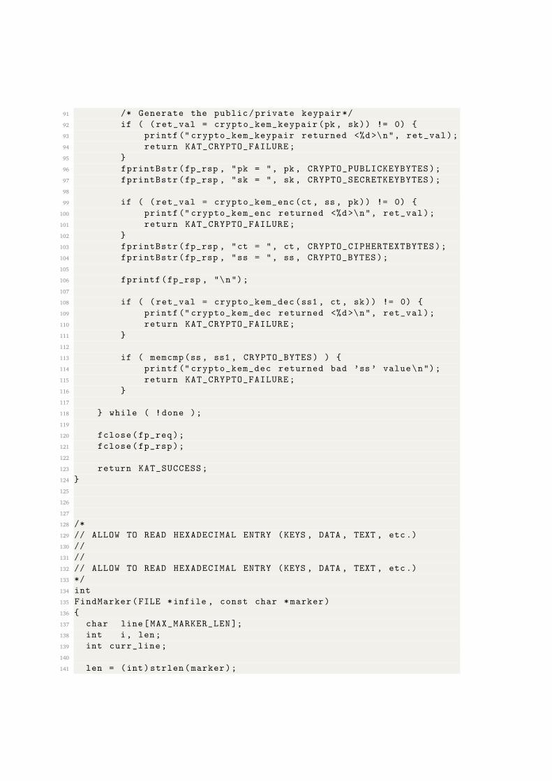
91 /* Generate the public/private keypair */

92 if ( (ret_val = crypto_kem_keypair(pk, sk)) != 0) {

93 printf (" crypto_kem_keypair returned <%d>\n", ret_val);

94 return KAT_CRYPTO_FAILURE;

95 }

96 fprintBstr(fp_rsp , "pk = ", pk, CRYPTO_PUBLICKEYBYTES);

97 fprintBstr(fp_rsp , "sk = ", sk, CRYPTO_SECRETKEYBYTES);

98

99 if ( (ret_val = crypto_kem_enc(ct, ss, pk)) != 0) {

100 printf (" crypto_kem_enc returned <%d>\n", ret_val);


102 }

103 fprintBstr(fp_rsp , "ct = ", ct, CRYPTO_CIPHERTEXTBYTES);

104 fprintBstr(fp_rsp , "ss = ", ss, CRYPTO_BYTES);

105

106 fprintf(fp_rsp , "\n");

107

108 if ( (ret_val = crypto_kem_dec(ss1 , ct, sk)) != 0) {

109 printf (" crypto_kem_dec returned <%d>\n", ret_val);


111 }

112

113 if ( memcmp(ss , ss1 , CRYPTO_BYTES) ) {

114 printf (" crypto_kem_dec returned bad ’ss’ value\n");


116 }

117

118 } while ( !done );

119

120 fclose(fp_req);

121 fclose(fp_rsp);

122

123 return KAT_SUCCESS;

124 }

125

126

127

128 /*

129 // ALLOW TO READ HEXADECIMAL ENTRY (KEYS , DATA , TEXT , etc.)

130 //

131 //


133 */

134 int

135 FindMarker(FILE *infile , const char *marker)

136 {

137 char line[MAX_MARKER_LEN ];

138 int i, len;

139 int curr_line;

140

141 len = (int)strlen(marker);

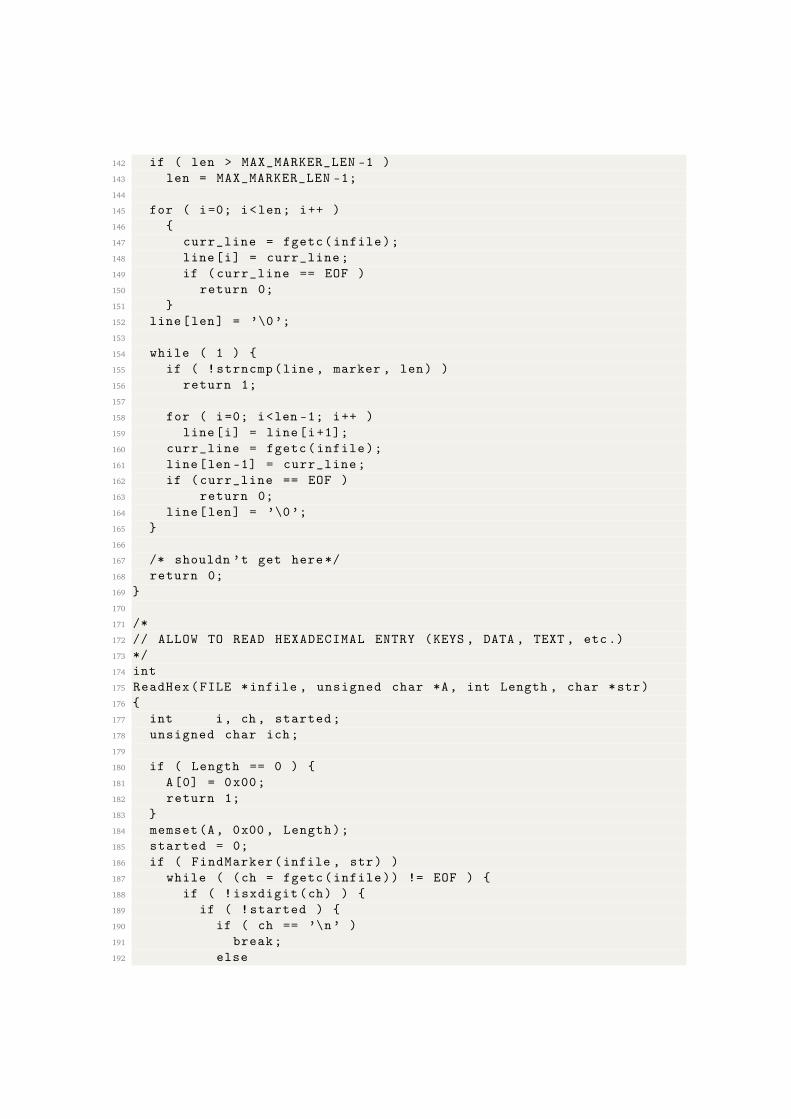
142 if ( len > MAX_MARKER_LEN -1 )

143 len = MAX_MARKER_LEN -1;

144

145 for ( i=0; i<len; i++ )

146 {

147 curr_line = fgetc(infile);

148 line[i] = curr_line;

149 if (curr_line == EOF )

150 return 0;

151 }

152 line[len] = ’\0’;

153

154 while ( 1 ) {

155 if ( !strncmp(line , marker , len) )

156 return 1;

157

158 for ( i=0; i<len -1; i++ )

159 line[i] = line[i+1];

160 curr_line = fgetc(infile);

161 line[len -1] = curr_line;

162 if (curr_line == EOF )

163 return 0;

164 line[len] = ’\0’;

165 }

166

167 /* shouldn ’t get here*/

168 return 0;

169 }

170

171 /*


173 */

174 int

175 ReadHex(FILE *infile , unsigned char *A, int Length , char *str)

176 {

177 int i, ch, started;

178 unsigned char ich;

179

180 if ( Length == 0 ) {

181 A[0] = 0x00;

182 return 1;

183 }

184 memset(A, 0x00 , Length);

185 started = 0;

186 if ( FindMarker(infile , str) )

187 while ( (ch = fgetc(infile)) != EOF ) {

188 if ( !isxdigit(ch) ) {

189 if ( !started ) {

190 if ( ch == ’\n’ )

191 break;

192 else

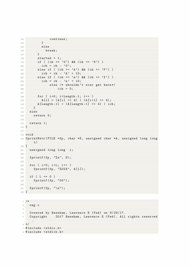
193 continue;

194 }

195 else

196 break;

197 }

198 started = 1;

199 if ( (ch >= ’0’) && (ch <= ’9’) )

200 ich = ch - ’0’;

201 else if ( (ch >= ’A’) && (ch <= ’F’) )

202 ich = ch - ’A’ + 10;

203 else if ( (ch >= ’a’) && (ch <= ’f’) )

204 ich = ch - ’a’ + 10;

205 else /* shouldn ’t ever get here*/

206 ich = 0;

207

208 for ( i=0; i<Length -1; i++ )

209 A[i] = (A[i] << 4) | (A[i+1] >> 4);

210 A[Length -1] = (A[Length -1] << 4) | ich;

211 }

212 else

213 return 0;

214

215 return 1;

216 }

217

218 void

219 fprintBstr(FILE *fp, char *S, unsigned char *A, unsigned long long

L)

220 {

221 unsigned long long i;

222

223 fprintf(fp , "%s", S);

224

225 for ( i=0; i<L; i++ )

226 fprintf(fp, "%02X", A[i]);

227

228 if ( L == 0 )

229 fprintf(fp, "00");

230

231 fprintf(fp , "\n");

232 }

1 /*

2 rng.c

3

4 Created by Bassham , Lawrence E (Fed) on 8/29/17.

5 Copyright 2017 Bassham , Lawrence E (Fed). All rights reserved

.

6 */



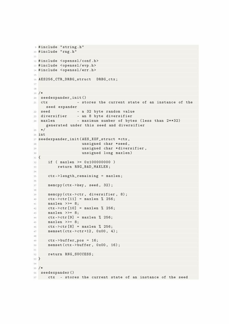
9 #include "string.h"

10 #include "rng.h"

11

12 #include <openssl/conf.h>

13 #include <openssl/evp.h>

14 #include <openssl/err.h>

15

16 AES256_CTR_DRBG_struct DRBG_ctx;

17

18

19 /*

20 seedexpander_init ()

21 ctx - stores the current state of an instance of the

seed expander

22 seed - a 32 byte random value

23 diversifier - an 8 byte diversifier

24 maxlen - maximum number of bytes (less than 2**32)

generated under this seed and diversifier

25 */

26 int

27 seedexpander_init(AES_XOF_struct *ctx ,

28 unsigned char *seed ,

29 unsigned char *diversifier ,

30 unsigned long maxlen)

31 {

32 if ( maxlen >= 0x100000000 )

33 return RNG_BAD_MAXLEN;

34

35 ctx ->length_remaining = maxlen;

36

37 memcpy(ctx ->key , seed , 32);

38

39 memcpy(ctx ->ctr , diversifier , 8);

40 ctx ->ctr [11] = maxlen % 256;

41 maxlen >>= 8;

42 ctx ->ctr [10] = maxlen % 256;

43 maxlen >>= 8;

44 ctx ->ctr[9] = maxlen % 256;

45 maxlen >>= 8;

46 ctx ->ctr[8] = maxlen % 256;

47 memset(ctx ->ctr+12, 0x00 , 4);

48

49 ctx ->buffer_pos = 16;

50 memset(ctx ->buffer , 0x00 , 16);

51

52 return RNG_SUCCESS;

53 }

54

55 /*

56 seedexpander ()

57 ctx - stores the current state of an instance of the seed

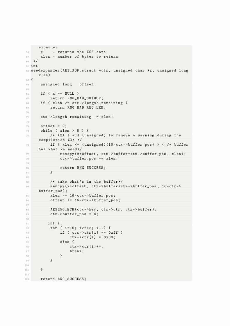
expander

58 x - returns the XOF data

59 xlen - number of bytes to return

60 */

61 int

62 seedexpander(AES_XOF_struct *ctx , unsigned char *x, unsigned long

xlen)

63 {

64 unsigned long offset;

65

66 if ( x == NULL )

67 return RNG_BAD_OUTBUF;

68 if ( xlen >= ctx ->length_remaining )

69 return RNG_BAD_REQ_LEN;

70

71 ctx ->length_remaining -= xlen;

72

73 offset = 0;

74 while ( xlen > 0 ) {

75 /* XXX I add (unsigned) to remove a warning during the

compilation XXX */

76 if ( xlen <= (unsigned)(16-ctx ->buffer_pos) ) { /* buffer

has what we need*/

77 memcpy(x+offset , ctx ->buffer+ctx ->buffer_pos , xlen);

78 ctx ->buffer_pos += xlen;

79


81 }

82

83 /* take what ’s in the buffer */

84 memcpy(x+offset , ctx ->buffer+ctx ->buffer_pos , 16-ctx ->

buffer_pos);

85 xlen -= 16-ctx ->buffer_pos;

86 offset += 16-ctx ->buffer_pos;

87

88 AES256_ECB(ctx ->key , ctx ->ctr , ctx ->buffer);

89 ctx ->buffer_pos = 0;

90

91 int i;

92 for ( i=15; i>=12; i--) {

93 if ( ctx ->ctr[i] == 0xff )

94 ctx ->ctr[i] = 0x00;

95 else {

96 ctx ->ctr[i]++;

97 break;

98 }

99 }

100

101 }

102


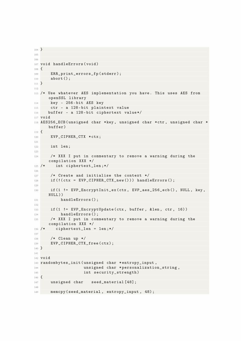
104 }

105

106

107 void handleErrors(void)

108 {

109 ERR_print_errors_fp (stderr);

110 abort();

111 }

112

113 /* Use whatever AES implementation you have. This uses AES from

openSSL library

114 key - 256-bit AES key

115 ctr - a 128-bit plaintext value

116 buffer - a 128-bit ciphertext value*/

117 void

118 AES256_ECB(unsigned char *key , unsigned char *ctr , unsigned char *

buffer)

119 {

120 EVP_CIPHER_CTX *ctx;

121

122 int len;

123

124 /* XXX I put in commentary to remove a warning during the

compilation XXX */

125 /* int ciphertext_len ;*/

126

127 /* Create and initialise the context */

128 if(!( ctx = EVP_CIPHER_CTX_new ())) handleErrors ();

129

130 if(1 != EVP_EncryptInit_ex(ctx , EVP_aes_256_ecb (), NULL , key ,

NULL))

131 handleErrors ();

132

133 if(1 != EVP_EncryptUpdate(ctx , buffer , &len , ctr , 16))

134 handleErrors ();

135 /* XXX I put in commentary to remove a warning during the

compilation XXX */

136 /* ciphertext_len = len ;*/

137

138 /* Clean up */

139 EVP_CIPHER_CTX_free (ctx);

140 }

141

142 void

143 randombytes_init(unsigned char *entropy_input ,

144 unsigned char *personalization_string ,

145 int security_strength)

146 {

147 unsigned char seed_material [48];

148

149 memcpy(seed_material , entropy_input , 48);

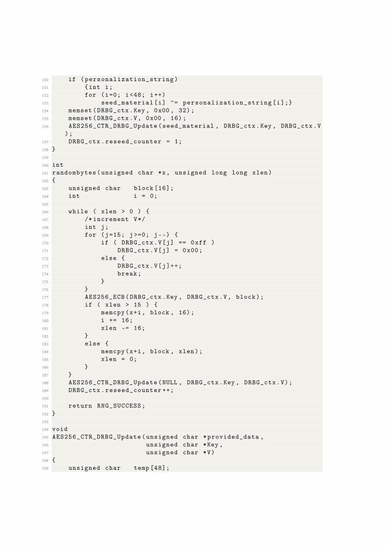
150 if (personalization_string)

151 {int i;

152 for (i=0; i<48; i++)

153 seed_material[i] ^= personalization_string[i];}

154 memset(DRBG_ctx.Key , 0x00 , 32);

155 memset(DRBG_ctx.V, 0x00 , 16);

156 AES256_CTR_DRBG_Update(seed_material , DRBG_ctx.Key , DRBG_ctx.V

);

157 DRBG_ctx.reseed_counter = 1;

158 }

159

160 int

161 randombytes(unsigned char *x, unsigned long long xlen)

162 {

163 unsigned char block [16];

164 int i = 0;

165

166 while ( xlen > 0 ) {

167 /* increment V*/

168 int j;

169 for (j=15; j>=0; j--) {

170 if ( DRBG_ctx.V[j] == 0xff )

171 DRBG_ctx.V[j] = 0x00;

172 else {

173 DRBG_ctx.V[j]++;

174 break;

175 }

176 }

177 AES256_ECB(DRBG_ctx.Key , DRBG_ctx.V, block);

178 if ( xlen > 15 ) {

179 memcpy(x+i, block , 16);

180 i += 16;

181 xlen -= 16;

182 }

183 else {

184 memcpy(x+i, block , xlen);

185 xlen = 0;

186 }

187 }

188 AES256_CTR_DRBG_Update(NULL , DRBG_ctx.Key , DRBG_ctx.V);

189 DRBG_ctx.reseed_counter ++;

190


192 }

193

194 void

195 AES256_CTR_DRBG_Update(unsigned char *provided_data ,

196 unsigned char *Key ,

197 unsigned char *V)

198 {

199 unsigned char temp [48];

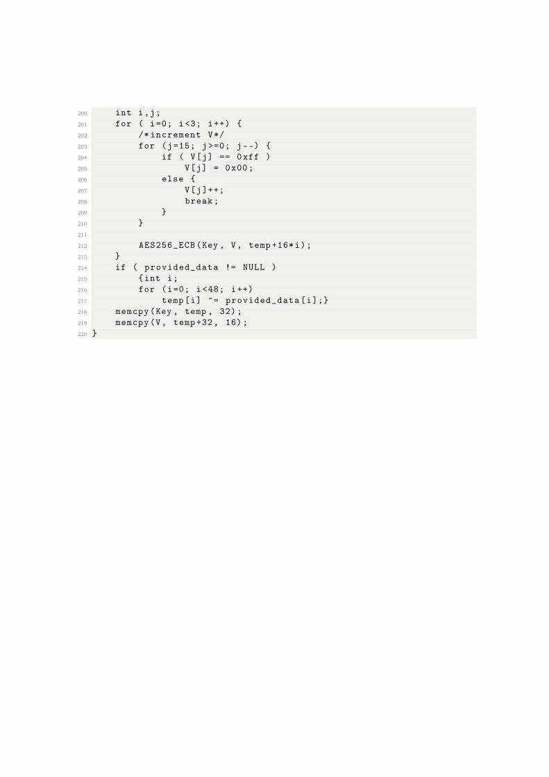
200 int i,j;

201 for ( i=0; i<3; i++) {

202 /* increment V*/

203 for (j=15; j>=0; j--) {

204 if ( V[j] == 0xff )

205 V[j] = 0x00;

206 else {

207 V[j]++;

208 break;

209 }

210 }

211

212 AES256_ECB(Key , V, temp +16*i);

213 }

214 if ( provided_data != NULL )

215 {int i;

216 for (i=0; i<48; i++)

217 temp[i] ^= provided_data[i];}

218 memcpy(Key , temp , 32);

219 memcpy(V, temp+32, 16);

220 }

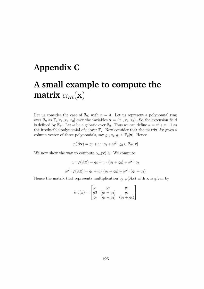
Appendix C

A small example to compute thematrix αm(x)

Let us consider the case of F2, with n = 3. Let us represent a polynomial ringover F2 as F2[x1, x2, x3] over the variables x = (x1, x2, x3). So the extension fieldis defined by F23 . Let ω be algebraic over F2. Thus we can define κ = z3+ z+1 asthe irreducible polynomial of ω over F2. Now consider that the matrix Ax gives acolumn vector of three polynomials, say g1, g2, g3 ∈ F2[x]. Hence

ϕ(Ax) = g1 + ω · g2 + ω2 · g3 ∈ F23 [x]

We now show the way to compute αm(x) ∈. We compute

ω · ϕ(Ax) = g3 + ω · (g1 + g3) + ω2 · g2

ω2 · ϕ(Ax) = g2 + ω · (g2 + g3) + ω2 · (g1 + g3)

Hence the matrix that represents multiplication by ϕ(Ax) with x is given by

αm(x) =

g1 g2 g3g3 (g1 + g3) g2g2 (g2 + g3) (g1 + g3)

195

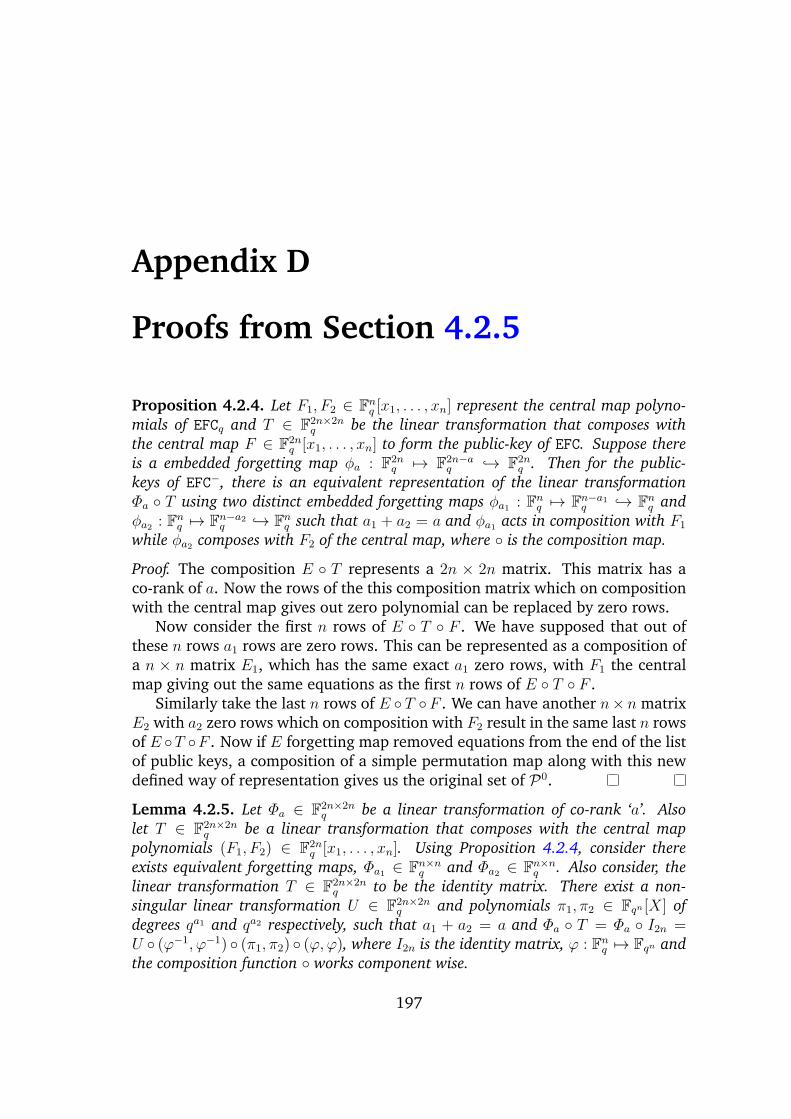
Appendix D

Proofs from Section 4.2.5

Proposition 4.2.4. Let F1, F2 ∈ Fnq [x1, . . . , xn] represent the central map polyno-

mials of EFCq and T ∈ F2n×2nq be the linear transformation that composes with

the central map F ∈ F2nq [x1, . . . , xn] to form the public-key of EFC. Suppose there

is a embedded forgetting map φa : F2nq 7→ F2n−a

q → F2nq . Then for the public-

keys of EFC−, there is an equivalent representation of the linear transformation

Φa ◦ T using two distinct embedded forgetting maps φa1 : Fnq 7→ Fn−a1

q → Fnq and

φa2 : Fnq 7→ Fn−a2

q → Fnq such that a1 + a2 = a and φa1 acts in composition with F1

while φa2 composes with F2 of the central map, where ◦ is the composition map.

Proof. The composition E ◦ T represents a 2n × 2n matrix. This matrix has aco-rank of a. Now the rows of the this composition matrix which on compositionwith the central map gives out zero polynomial can be replaced by zero rows.

Now consider the first n rows of E ◦ T ◦ F . We have supposed that out ofthese n rows a1 rows are zero rows. This can be represented as a composition ofa n × n matrix E1, which has the same exact a1 zero rows, with F1 the centralmap giving out the same equations as the first n rows of E ◦ T ◦ F .

Similarly take the last n rows of E ◦ T ◦F . We can have another n×n matrixE2 with a2 zero rows which on composition with F2 result in the same last n rowsof E ◦T ◦F . Now if E forgetting map removed equations from the end of the listof public keys, a composition of a simple permutation map along with this newdefined way of representation gives us the original set of P0.

Lemma 4.2.5. Let Φa ∈ F2n×2nq be a linear transformation of co-rank ‘a’. Also

let T ∈ F2n×2nq be a linear transformation that composes with the central map

polynomials (F1, F2) ∈ F2nq [x1, . . . , xn]. Using Proposition 4.2.4, consider there

exists equivalent forgetting maps, Φa1 ∈ Fn×nq and Φa2 ∈ Fn×n

q . Also consider, the

linear transformation T ∈ F2n×2nq to be the identity matrix. There exist a non-

singular linear transformation U ∈ F2n×2nq and polynomials π1, π2 ∈ Fqn [X] of

degrees qa1 and qa2 respectively, such that a1 + a2 = a and Φa ◦ T = Φa ◦ I2n =U ◦ (ϕ−1, ϕ−1) ◦ (π1, π2) ◦ (ϕ, ϕ), where I2n is the identity matrix, ϕ : Fn

q 7→ Fqn and

the composition function ◦ works component wise.

197

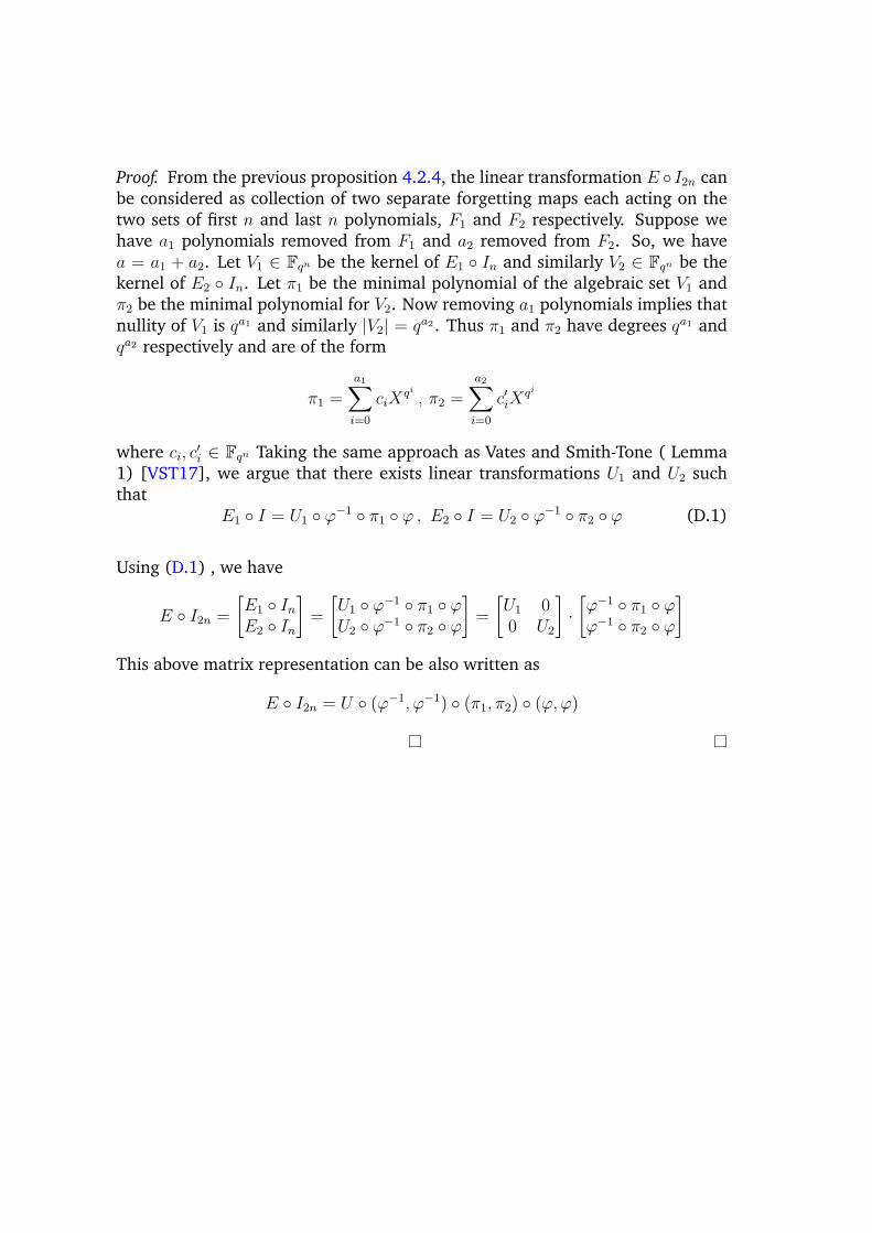
Proof. From the previous proposition 4.2.4, the linear transformation E ◦ I2n canbe considered as collection of two separate forgetting maps each acting on thetwo sets of first n and last n polynomials, F1 and F2 respectively. Suppose wehave a1 polynomials removed from F1 and a2 removed from F2. So, we havea = a1 + a2. Let V1 ∈ Fqn be the kernel of E1 ◦ In and similarly V2 ∈ Fqn be thekernel of E2 ◦ In. Let π1 be the minimal polynomial of the algebraic set V1 andπ2 be the minimal polynomial for V2. Now removing a1 polynomials implies thatnullity of V1 is qa1 and similarly |V2| = qa2. Thus π1 and π2 have degrees qa1 andqa2 respectively and are of the form

π1 =

a1∑

i=0

ciXqi , π2 =

a2∑

i=0

c′iXqi

where ci, c′i ∈ Fqn Taking the same approach as Vates and Smith-Tone ( Lemma

1) [VST17], we argue that there exists linear transformations U1 and U2 suchthat

E1 ◦ I = U1 ◦ ϕ−1 ◦ π1 ◦ ϕ , E2 ◦ I = U2 ◦ ϕ−1 ◦ π2 ◦ ϕ (D.1)

Using (D.1) , we have

E ◦ I2n =

[E1 ◦ InE2 ◦ In

]=

[U1 ◦ ϕ−1 ◦ π1 ◦ ϕU2 ◦ ϕ−1 ◦ π2 ◦ ϕ

]=

[U1 00 U2

]·[ϕ−1 ◦ π1 ◦ ϕϕ−1 ◦ π2 ◦ ϕ

]

This above matrix representation can be also written as

E ◦ I2n = U ◦ (ϕ−1, ϕ−1) ◦ (π1, π2) ◦ (ϕ, ϕ)

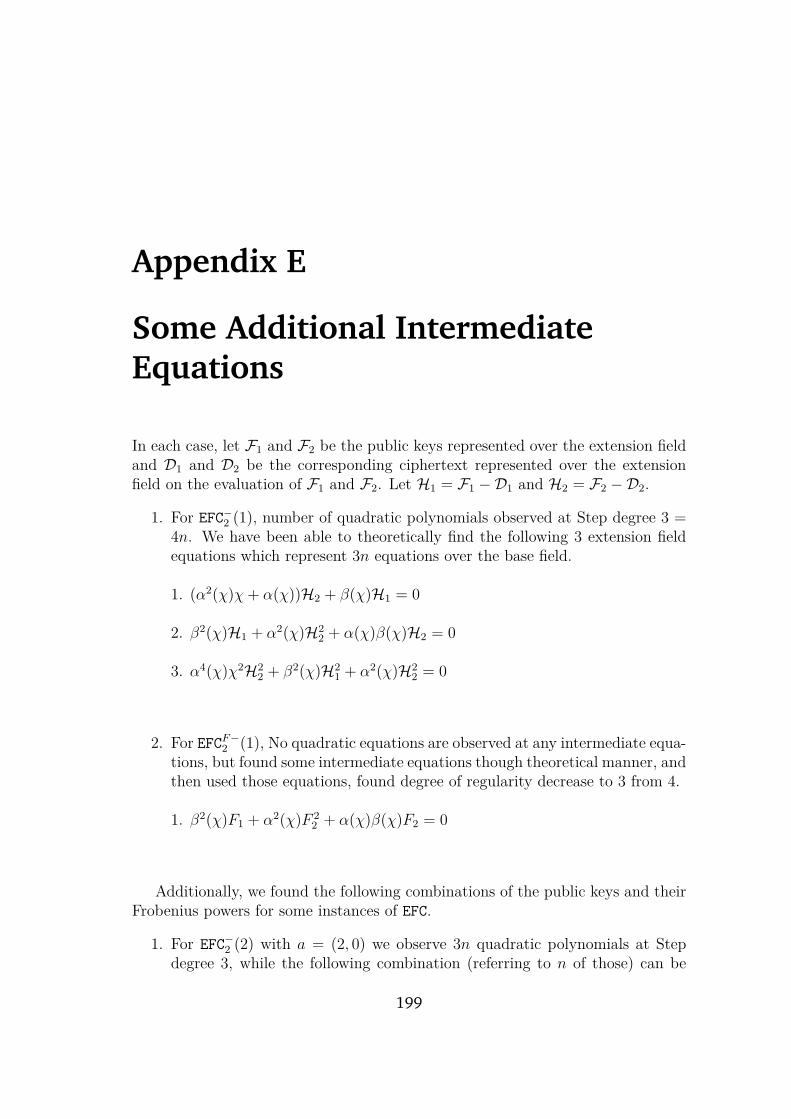
Appendix E

Some Additional IntermediateEquations

In each case, let F1 and F2 be the public keys represented over the extension fieldand D1 and D2 be the corresponding ciphertext represented over the extensionfield on the evaluation of F1 and F2. Let H1 = F1 −D1 and H2 = F2 −D2.

1. For EFC−2 (1), number of quadratic polynomials observed at Step degree 3 =4n. We have been able to theoretically find the following 3 extension fieldequations which represent 3n equations over the base field.

1. (α2(χ)χ+ α(χ))H2 + β(χ)H1 = 0

2. β2(χ)H1 + α2(χ)H22 + α(χ)β(χ)H2 = 0

3. α4(χ)χ2H22 + β2(χ)H2

1 + α2(χ)H22 = 0

2. For EFCF−2 (1), No quadratic equations are observed at any intermediate equa-tions, but found some intermediate equations though theoretical manner, andthen used those equations, found degree of regularity decrease to 3 from 4.

1. β2(χ)F1 + α2(χ)F 22 + α(χ)β(χ)F2 = 0

Additionally, we found the following combinations of the public keys and theirFrobenius powers for some instances of EFC.

1. For EFC−2 (2) with a = (2, 0) we observe 3n quadratic polynomials at Stepdegree 3, while the following combination (referring to n of those) can be

199

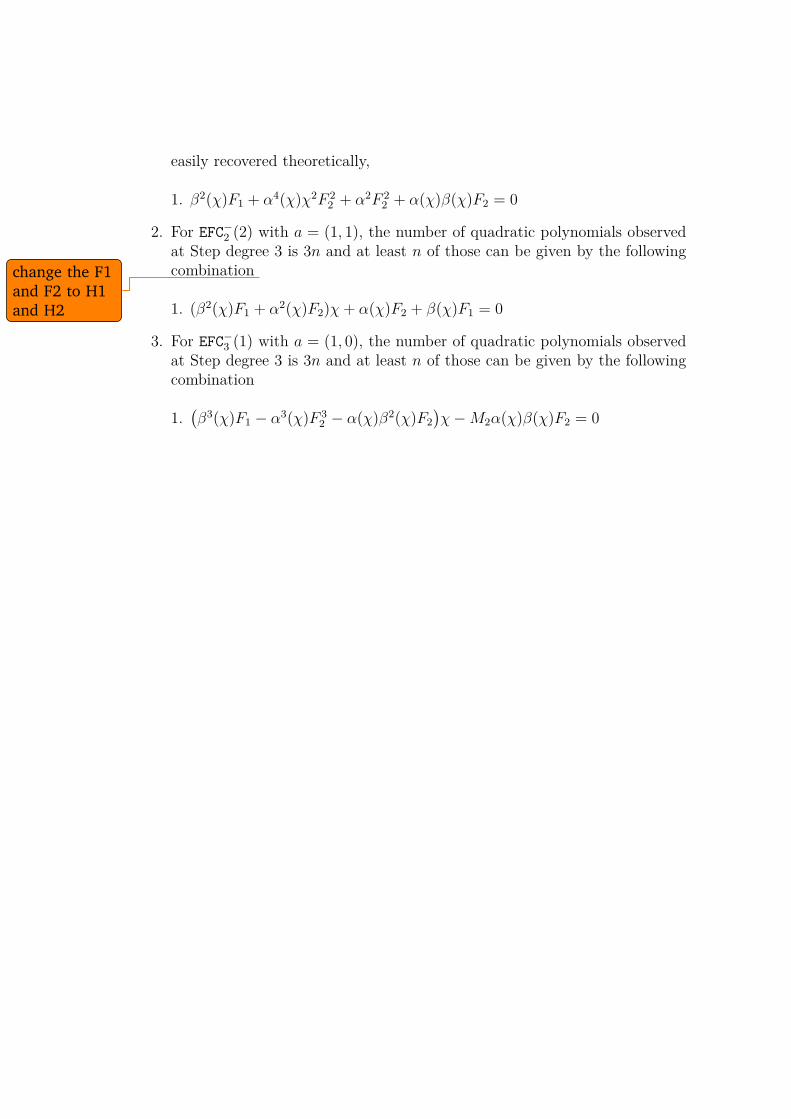
easily recovered theoretically,

1. β2(χ)F1 + α4(χ)χ2F 22 + α2F 2

2 + α(χ)β(χ)F2 = 0

2. For EFC−2 (2) with a = (1, 1), the number of quadratic polynomials observedat Step degree 3 is 3n and at least n of those can be given by the followingcombinationchange the F1

and F2 to H1and H2 1. (β2(χ)F1 + α2(χ)F2)χ+ α(χ)F2 + β(χ)F1 = 0

3. For EFC−3 (1) with a = (1, 0), the number of quadratic polynomials observedat Step degree 3 is 3n and at least n of those can be given by the followingcombination

1.(β3(χ)F1 − α3(χ)F 3

2 − α(χ)β2(χ)F2

)χ−M2α(χ)β(χ)F2 = 0

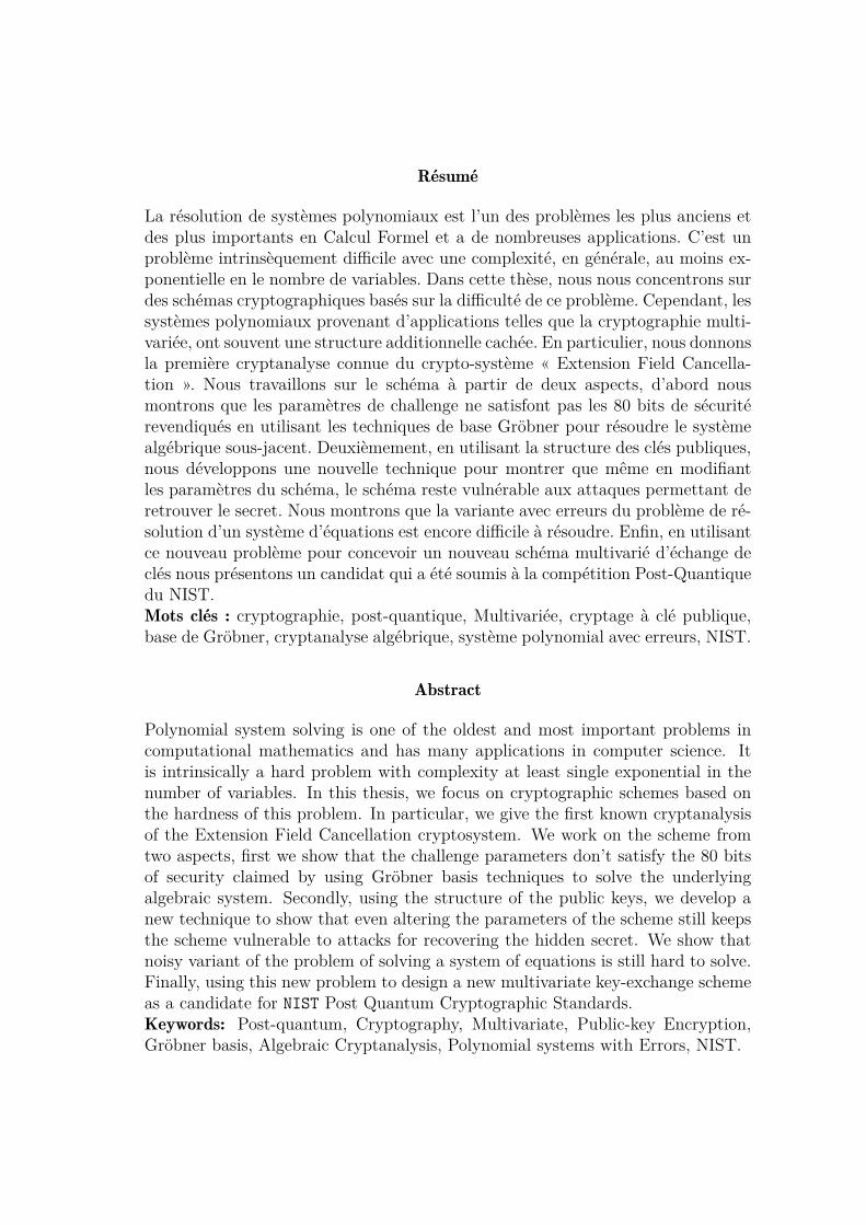
Résumé

La résolution de systèmes polynomiaux est l’un des problèmes les plus anciens etdes plus importants en Calcul Formel et a de nombreuses applications. C’est unproblème intrinsèquement difficile avec une complexité, en générale, au moins ex-ponentielle en le nombre de variables. Dans cette thèse, nous nous concentrons surdes schémas cryptographiques basés sur la difficulté de ce problème. Cependant, lessystèmes polynomiaux provenant d’applications telles que la cryptographie multi-variée, ont souvent une structure additionnelle cachée. En particulier, nous donnonsla première cryptanalyse connue du crypto-système « Extension Field Cancella-tion ». Nous travaillons sur le schéma à partir de deux aspects, d’abord nousmontrons que les paramètres de challenge ne satisfont pas les 80 bits de sécuritérevendiqués en utilisant les techniques de base Gröbner pour résoudre le systèmealgébrique sous-jacent. Deuxièmement, en utilisant la structure des clés publiques,nous développons une nouvelle technique pour montrer que même en modifiantles paramètres du schéma, le schéma reste vulnérable aux attaques permettant deretrouver le secret. Nous montrons que la variante avec erreurs du problème de ré-solution d’un système d’équations est encore difficile à résoudre. Enfin, en utilisantce nouveau problème pour concevoir un nouveau schéma multivarié d’échange declés nous présentons un candidat qui a été soumis à la compétition Post-Quantiquedu NIST.Mots clés : cryptographie, post-quantique, Multivariée, cryptage à clé publique,base de Gröbner, cryptanalyse algébrique, système polynomial avec erreurs, NIST.

Abstract

Polynomial system solving is one of the oldest and most important problems incomputational mathematics and has many applications in computer science. Itis intrinsically a hard problem with complexity at least single exponential in thenumber of variables. In this thesis, we focus on cryptographic schemes based onthe hardness of this problem. In particular, we give the first known cryptanalysisof the Extension Field Cancellation cryptosystem. We work on the scheme fromtwo aspects, first we show that the challenge parameters don’t satisfy the 80 bitsof security claimed by using Gröbner basis techniques to solve the underlyingalgebraic system. Secondly, using the structure of the public keys, we develop anew technique to show that even altering the parameters of the scheme still keepsthe scheme vulnerable to attacks for recovering the hidden secret. We show thatnoisy variant of the problem of solving a system of equations is still hard to solve.Finally, using this new problem to design a new multivariate key-exchange schemeas a candidate for NIST Post Quantum Cryptographic Standards.Keywords: Post-quantum, Cryptography, Multivariate, Public-key Encryption,Gröbner basis, Algebraic Cryptanalysis, Polynomial systems with Errors, NIST.

Documents

Design and Cryptanalysis of Post-Quantum Cryptosystems