Embed Size (px)
Citation preview
�����������������
Citation: Nowroth, C.; Gu, T.;
Grajczak, J.; Nothdurft, S.; Twiefel, J.;
Hermsdorf, J.; Kaierle, S.; Wallaschek,
J. Deep Learning-Based Weld
Contour and Defect Detection from
Micrographs of Laser Beam Welded
Semi-Finished Products. Appl. Sci.
2022, 12, 4645. https://doi.org/
10.3390/app12094645
Academic Editors: Jean-Pierre
Bergmann and Jörg Hildebrand
Received: 1 April 2022
Accepted: 4 May 2022
Published: 5 May 2022
Publisher’s Note: MDPI stays neutral
with regard to jurisdictional claims in
published maps and institutional affil-
iations.
Copyright: © 2022 by the authors.
Licensee MDPI, Basel, Switzerland.
This article is an open access article
distributed under the terms and
conditions of the Creative Commons
Attribution (CC BY) license (https://
creativecommons.org/licenses/by/
4.0/).
applied sciences
Article
Deep Learning-Based Weld Contour and Defect Detection fromMicrographs of Laser Beam Welded Semi-Finished ProductsChristian Nowroth 1,* , Tiansheng Gu 1 , Jan Grajczak 2 , Sarah Nothdurft 2 , Jens Twiefel 1 ,Jörg Hermsdorf 2 , Stefan Kaierle 2,3 and Jörg Wallaschek 1
1 Institute of Dynamics and Vibration Research, Leibniz University Hannover, An der Universität 1,30823 Garbsen, Germany; [email protected] (T.G.); [email protected] (J.T.);[email protected] (J.W.)
2 Laser Zentrum Hannover e.V., Hollerithallee 8, 30419 Hannover, Germany; [email protected] (J.G.);[email protected] (S.N.); [email protected] (J.H.); [email protected] (S.K.)
3 Institute of Automation and Transport Technology, Leibniz University Hannover, An der Universität 2,30823 Garbsen, Germany
* Correspondence: [email protected]; Tel.: +49-511-762-4330
Abstract: Laser beam welding is used in many areas of industry and research. There are manystrategies and approaches to further improve the weld seam properties in laser beam welding.Metallography is often needed to evaluate welded seams. Typically, the images are examinedand evaluated by experts. The evaluation process qualitatively provides the properties of thewelds. Particularly in times when artificial intelligence is being used more and more in processes,the quantization of properties that could previously only be determined qualitatively is gainingimportance. In this contribution, we propose to use deep learning to perform semantic segmentationof micrographs of complex weld areas to achieve the automatic detection and quantization of weldseam properties. A semantic segmentation dataset is created containing 282 labeled images. Thetraining process is performed with DeepLabv3+. The trained model achieves a value of around 95%for weld contour detection and 76.88% of mean intersection over union (mIoU).
Keywords: weld seam; weld defects; deep learning; semantic segmentation; dataset creation;quantization; automatic detection
1. Introduction
The weld quality has a direct impact on the performance and lifespan of weldedcomponents. Weld defects reduce the weld quality and deteriorate its properties, whichis why they should be avoided. There are many approaches to reduce the occurrence ofweld defects such as cracks, pores, lack of fusion or incomplete penetration. Therefore, aneffective and efficient method of detection and analysis of weld defects is an importanttopic. To study the physical structure of metals, metallography is typically used for thispurpose. After the preparation of the specimens, an expert has to identify the weld seam’sproperties qualitatively. This evaluation of welds is done manually with the aid of software.The area is marked with lines, whereupon the program specifies it in accordance with thescale. This procedure is time-consuming, and the result depends on the operator. Thesoftware cannot reliably distinguish between cracks, pores and other microstructures. Itlooks for transitions from light to dark areas depending on the set limit, and it can onlyindicate the roundness of dark particles in bright unetched matrix. For better analysisand comparison between different welds, it is beneficial to describe the weld properties asscalar quantities. However, since the artificial intelligence is being applied more and morein research and industry, quantized values are needed, especially for machine learning.By determining the ratio of significant areas within a micrograph, the effects of parameterchanges can be investigated better and compared to each other.
Appl. Sci. 2022, 12, 4645. https://doi.org/10.3390/app12094645 https://www.mdpi.com/journal/applsci
Appl. Sci. 2022, 12, 4645 2 of 14
Researchers are gradually applying artificial intelligence to the field of laser welding,such as using the quality inspection system to achieve non-destructive weld measurementand defect detection [1], in-process monitoring based on deep learning [2] or using the se-mantic segmentation algorithm to detect weld defects in safety vents of power batteries [3].Long et al. [4] opened the era of fully convolutional networks (FCN) for semantic segmen-tation. There are currently many variants of FCN-based models that have contributed tothe exploration of semantic segmentation [5–9]. Gyasi et al. provide an overview of theuse of artificial intelligence in welding technology [10]. Tantrapiwat describes a methodof defect detection using a synthetic image dataset if a large number of input images onconvolutional neural networks is not accessible [11].
Due to the non-uniformity of the shape, position and size of weld defects, it is acomplicated task to manually analyse and evaluate the recorded weld defect patterns.For example, cracks are sometimes wide and sometimes narrow, and there is no fixedstandard for length. The pore is not always an ideal circle, and sometimes cracks and poresare connected. These are some of the difficulties in artificially distinguishing the typesof weld defects. There are cases in which it is difficult to identify weld defects, such asidentifying the boundary of the weld area from the fuzzy heat-affected zone. At the sametime, a fair quantitative analysis is also particularly important for the evaluation of weldingperformance. Therefore, human participation is still always necessary for the analysis ofcomplex weld defects. Hence, it is a very time-consuming and therefore expensive task.
This contribution provides a weld contour and weld defect identification and analysisbased on a self-created data set. This leads to convenience for further research in thefuture. This preliminary work is used to create datasets suitable for processing withmachine learning algorithms. From these, predictions can be made about weld qualityunder different parameter configurations. While many AI-based methods focus on real-time data during the welding process, the deep learning-based detection of structures inthe micrographs simplifies the link between real-time data recorded during the weldingprocess and the micrographs evaluated afterwards.
2. Methodology
There are many studies on laser weld defect detection. Since different studies requiredifferent data sets, a data set of deep welds has been created in order to broaden theapplication of deep learning in welding processes. It contains micrographs of differentwelding situations to ensure a wide range of applications in the field of weld propertydetection. The methodology includes obtaining the micrographs from welds, labelingthe obtained micrographs, building the training environment of the neural network andquantifying and analyzing the prediction results.
2.1. Data Set Creation and Training Process
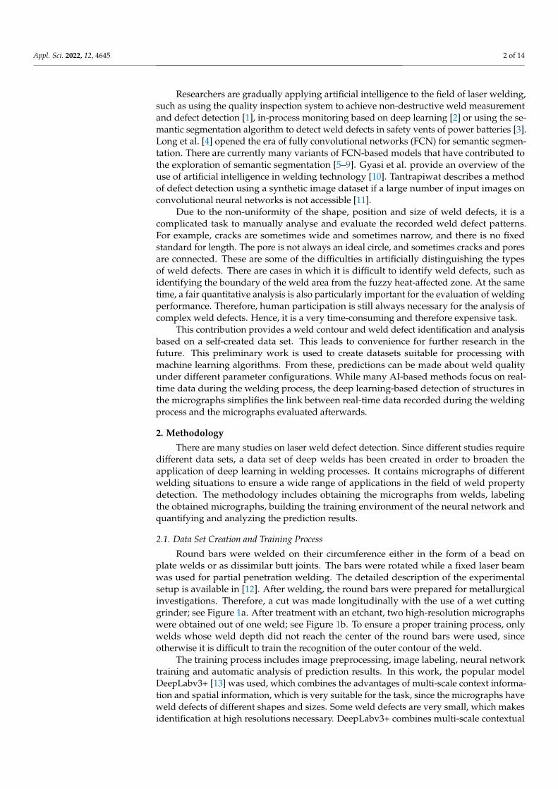
Round bars were welded on their circumference either in the form of a bead onplate welds or as dissimilar butt joints. The bars were rotated while a fixed laser beamwas used for partial penetration welding. The detailed description of the experimentalsetup is available in [12]. After welding, the round bars were prepared for metallurgicalinvestigations. Therefore, a cut was made longitudinally with the use of a wet cuttinggrinder; see Figure 1a. After treatment with an etchant, two high-resolution micrographswere obtained out of one weld; see Figure 1b. To ensure a proper training process, onlywelds whose weld depth did not reach the center of the round bars were used, sinceotherwise it is difficult to train the recognition of the outer contour of the weld.
The training process includes image preprocessing, image labeling, neural networktraining and automatic analysis of prediction results. In this work, the popular modelDeepLabv3+ [13] was used, which combines the advantages of multi-scale context informa-tion and spatial information, which is very suitable for the task, since the micrographs haveweld defects of different shapes and sizes. Some weld defects are very small, which makesidentification at high resolutions necessary. DeepLabv3+ combines multi-scale contextual
Appl. Sci. 2022, 12, 4645 3 of 14
information and rich spatial information. The model is already packaged in MATLAB [14],and the corresponding backbone pre-trained network can be easily downloaded. All datawere split into a training dataset, validation dataset and test dataset using random sam-pling, but in order to reproduce the results, the random seed was fixed. The training processwas carried out with the created dataset using MATLAB version R2020a on a total of fourGPUs of model 2080Ti and at least 160 GB of hard disc space reserved. The epochs wereset to 50, which turned out to be large enough, because the accuracy of the model hardlychanged as the epochs became larger than 20.
Cut
ting
plan
e
Picture 1
Picture 2
(a) (b)Weld seam
Figure 1. Obtaining images from welds: (a) Circumferential welds formed during welding of twocylindrical specimens cut as preparation for metallography. (b) Two micrographs resulting frommetallography.
2.2. Preprocessing
Since the size and shape of each class in the micrographs are different and uncertain, inorder to allow the neural network to learn the characteristics of each class and distinguishthem sufficiently, it is necessary to make the model have a different receptive field. The“atrous spatial pyramid polling” (ASPP) in the DeepLabv3+ model solves this problem.Different dilation rates are used to extract features from images, which gives the model agood understanding of features of different sizes. The use of atrous or dilated convolutionensures that the receptive field is expanded without increasing computational pressure [15].In the traditional direct upsampling operation, semantic information and spatial informa-tion contradict each other. As the number of network layers increases, the feature mapwill gradually become smaller and the semantic information will become more and moreabundant. One pixel covers more information from the original image, but it comes alongwith the loss of more spatial information. Making a reasonable weight distribution betweensemantic information and spatial information is very important. In the DeepLabv3+ model,Chen et al. [13] introduced a novel decoder module, which is different from the traditionaldirect upsampling operation. The low-level feature map is cascaded with the output fromthe encoder that contains multi-scale rich semantic information.
2.3. Image Labeling
At present, the popular image labeling tools for computer vision are “labelme”, “labe-lImg” or “CVAT”. In this work, the image labeling tool “Image Labeler” that comes alongwith the MATLAB software was used. The semantic segmentation model used belongs tosupervised learning. In order for the neural network to achieve better results in learningand to clearly identify weld defects and weld metal, each class was labeled. An originalimage and a labeled image are shown in Figure 2. Both were used as input to the neuralnetwork. The original image was needed for the training of the neural network. Finally, thepredicted segmented image was compared with the labeled image.

Appl. Sci. 2022, 12, 4645 4 of 14
Original image Labeled image Classes
Seam shape defect
Cracks
Pores
Background
Weld metal
Figure 2. Original image, labeled image and class differentiation.
Five classes were initially defined for the classification, as follows:
• The part inside the base material having a clear weld boundary belongs to the weldarea, while the rest belongs to the background colored in red;
• A weld reinforcement or sagging that causes a deviation in the expected weld seamshape requirements is defined as a seam shape defect. The label color is pink;
• The remaining parts that are in the weld area without defects are weld metal. Thelabel color of weld metal is blue;
• If there is a long and thin weld defect within the weld area, it is defined as crack. Thelabel color is green;
• Weld defects formed like a bubble are defined as pores. The label color of poresis purple.
Since some defects are very small, image labeling is done pixel-by-pixel. Althoughthere is a clear rule for image labeling, there is still the problem of ambiguous error in theprocess of image labeling, which can mainly be divided into the following three situations:
• Ambiguous defects between weld metal and background:From the original image in Figure 3a, it can be seen that the fusion line of weld metalis difficult to distinguish from the background. The reason is that the colors of weldmetal and base metal or heat affected zone are very similar, so no clear boundary canbe obtained. In this case, image labeling requires enlarging the image to obtain a finertexture for an artificially based estimation of the position of the boundary;
• Ambiguous defects between pores and cracks:The purple label in Figure 3b represents pores. According to the definition, pores arespherical cavities formed by gas inclusions. It should be spherical, but in the actualimage labeling, it refers to voids that do not match the thin and long properties ofcracks and which are located in the weld area;
• Ambiguous defects between seam shape defects and the background:The pink label stands for seam shape defects. Seam shape defects describe the devi-ation between the actual weld geometry and the expected weld geometry, but it isdifficult to determine a fixed shape standard for a weld reinforcement. To solve thisproblem, in the case that the weld metal is higher than the base metal, it is assumedthat there is no seam shape defect. In the case that the weld metal is lower than the
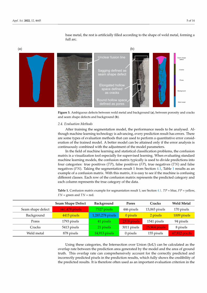
Appl. Sci. 2022, 12, 4645 5 of 14
base metal, the rest is artificially filled according to the shape of weld metal, forming afull arc.
Seam shape defect
Cracks
Pores
Background
Weld metal
(a) (b)
Unclear fusion line
Elongated hollowspace defined
as cracks
Round hollow spacedefined as pores
Sagging defined as seam shape defect
Figure 3. Ambiguous defects between weld metal and background (a), between porosity and cracksand seam shape defects and background (b).
2.4. Evaluation Methods
After training the segmentation model, the performance needs to be analysed. Al-though machine learning technology is advancing, every prediction result has errors. Thereare some types of evaluation methods that can used to perform a quantitative error consid-eration of the trained model. A better model can be attained only if the error analysis iscontinuously combined with the adjustment of the model parameters.
In the field of machine learning and statistical classification problems, the confusionmatrix is a visualization tool especially for supervised learning. When evaluating standardmachine learning models, the confusion matrix typically is used to divide predictions intofour categories: true positives (TP), false positives (FP), true negatives (TN) and falsenegatives (FN). Taking the segmentation result 1 from Section 4.1, Table 1 results as anexample of a confusion matrix. With this matrix, it is easy to see if the machine is confusingdifferent classes. Each row of the confusion matrix represents the predicted category andeach column represents the true category of the data.
Table 1. Confusion matrix example for segmantation result 1; see Section 4.1. TP = blue, FP = yellow,FN = green and TN = red.
Seam Shape Defect Background Pores Cracks Weld Metal
Seam shape defect 661,478 pixels 7327 pixels 446 pixels 13,065 pixels 170 pixels
Background 4415 pixels 1,285,278 pixels 0 pixels 2 pixels 1009 pixels
Pores 1793 pixels 41 pixels 2318 pixels 1541 pixels 94 pixels
Cracks 5413 pixels 21 pixels 3011 pixels 25,964 pixels 8 pixels
Weld metal 878 pixels 14,913 pixels 0 pixels 155 pixels 67,812 pixels
Using these categories, the Intersection over Union (IoU) can be calculated as theoverlap rate between the prediction area generated by the model and the area of groundtruth. This overlap rate can comprehensively account for the correctly predicted andincorrectly predicted pixels in the prediction results, which fully shows the credibility ofthe predicted results. It is therefore often used as an important evaluation criterion in the
Appl. Sci. 2022, 12, 4645 6 of 14
field of image semantic segmentation. The model can be evaluated using the followingequations [16,17]:
Accuracy =TP + TN
FP + TP + FN + TN(1)
Precision =TP
FP + TP(2)
IoU =TP
FP + TP + FN(3)
As there are different methods used to evaluate the model, the results can be seenin Table 2. Equation (1) calculates the ratio of all correctly predicted pixels to all pixels.Equation (2) calculates the probability of being correct among all outcomes predicted for aspecific class. Equation (3) calculates the ratio of the intersection of the predicted result andthe ground truth to the union of the predicted result and the ground truth for a specificclass, but it only considers all cases related to a specific class (TP, FP and FN), and it doesnot consider the positive effects brought by other classes (TN). As shown in Table 1 withcolored cells (TP = blue, FP = yellow, FN = green and TN = red), the use of Equation (3)only considers the results in relation to a particular class. In order to evaluate the welds,the calculation method of Equation (3) is chosen.
Table 2. Comparison of different values calculated with the Equations (1)–(3) based on the confusionmatrix in Table 1.
Equation (1) (2) (3)
Value 97.41% 80.96% 79.74%
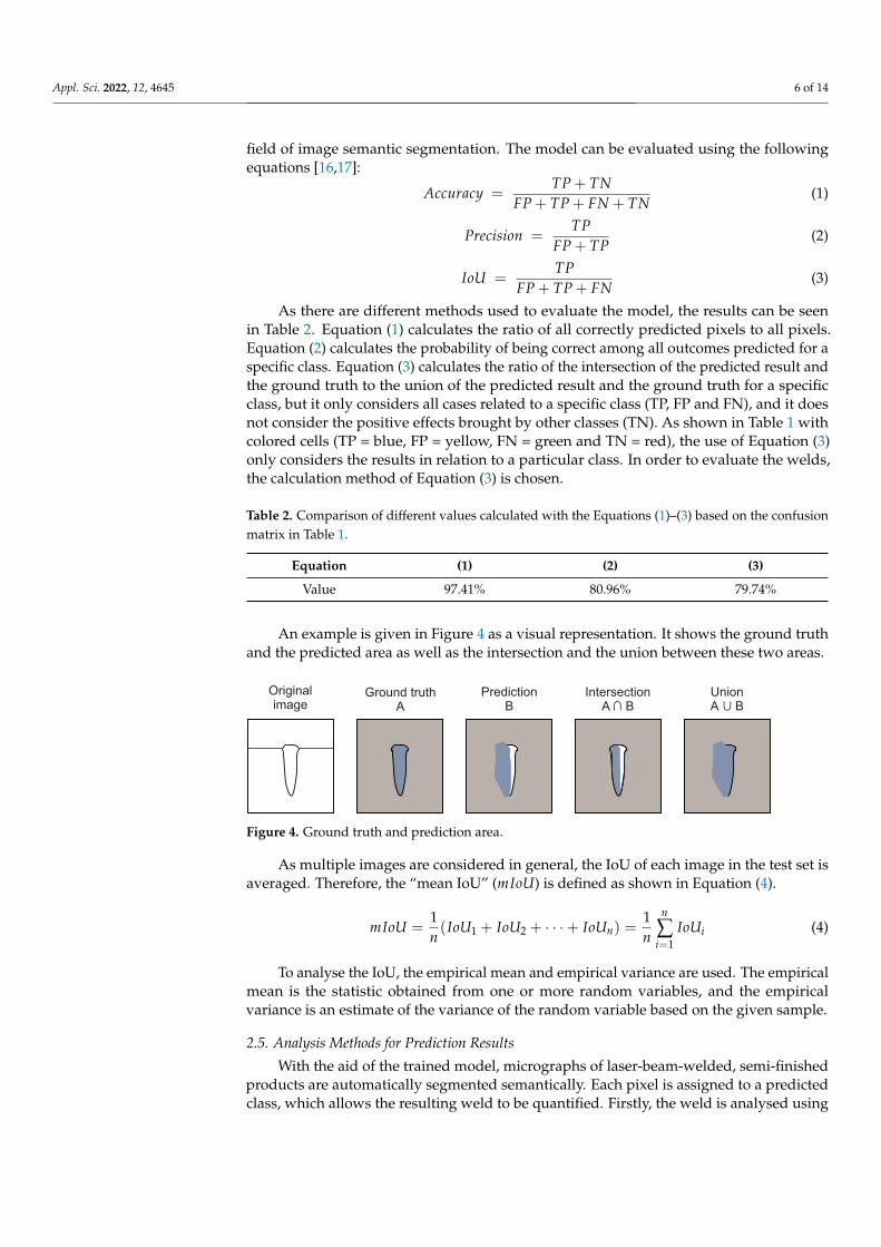
An example is given in Figure 4 as a visual representation. It shows the ground truthand the predicted area as well as the intersection and the union between these two areas.
Ground truthA
PredictionB
Intersection A ∩ B
Union A B
∩
Original image
Figure 4. Ground truth and prediction area.
As multiple images are considered in general, the IoU of each image in the test set isaveraged. Therefore, the “mean IoU” (mIoU) is defined as shown in Equation (4).
mIoU =1n(IoU1 + IoU2 + · · ·+ IoUn) =
1n
n
∑i=1
IoUi (4)
To analyse the IoU, the empirical mean and empirical variance are used. The empiricalmean is the statistic obtained from one or more random variables, and the empiricalvariance is an estimate of the variance of the random variable based on the given sample.
2.5. Analysis Methods for Prediction Results
With the aid of the trained model, micrographs of laser-beam-welded, semi-finishedproducts are automatically segmented semantically. Each pixel is assigned to a predictedclass, which allows the resulting weld to be quantified. Firstly, the weld is analysed using
Appl. Sci. 2022, 12, 4645 7 of 14
the number of pixels corresponding to each weld defect. For example, the calculation forthe ratio of pores is shown in Equation (5).
Ratio(Pores) =PixelCount(Pores)
PixelCount(Weld metal+Cracks+Pores+Seam shape de f ect)(5)
With this calculation, it is possible to compare multiple pictures with different resolu-tions with each other as the predicted area is related in ratio to the size of the weld area.
3. Experimental Results
To evaluate the perfomance of the deep learning model, an ablation study was carriedout. Therefore, the influence of different factors on the experimental results, the analysis ofthe final model and the achievements with the final model are described in detail.
3.1. Initialization of Weights
The essence of the deep learning model training process consists of updating theweights. Each parameter must have an appropriate initial value for network training. Poorinitialization parameters can cause gradient propagation problems and reduce trainingspeed, while good initialization parameters can speed up convergence and are morelikely to find better solutions. In addition, the output of the middle layer of the modelis intransparent, and the influence of the previous weights on the output of subsequentneurons is not unique. Even with such advanced parameter passing and updating, aninappropriate initialization of weights can cause laborious parameter learning and even theoutput loss gradient of the layer activation function to explode or vanish during forwardpropagation of the deep neural network. In either case, if the loss gradient is too large ortoo small, it cannot effectively backpropagate, and even if it can backpropagate, it takeslonger for the network to reach convergence.
To ensure that low-frequency classes can be learned during the training process,weights were initialized according to the proportion of pixels occupied by each class inall images. The higher the proportion, the lower the initial weight of the class. Artificialadjustments were then made according to the results of the generated images. For example,if the class “cracks” was under-predicted, it was multiplied by a coefficient greater thanone in the initial weight. Therefore, many different initial weights were tested. The bestcombination of initial weights in comparison with the unweighted combination is shownin Table 3. In the case that the backbone was “Xception”, the result after adjustment wassignificantly improved. The initial weights from left to right stand for the weld metal,background, pores, cracks and seam shape defects.
Table 3. Comparison of training results with different initial weights.
Initial Weights Backbone Image Resolution mIoU
1, 1, 1, 1, 1 Xception 2048 × 1024 60.96%0.95, 1.14, 0.15, 0.014, 0.062 Xception 2048 × 1024 76.88%
3.2. Optimization Algorithm
The function of the optimization algorithm is to minimize or to maximize the lossfunction by improving the training method. When adjusting the weighting and deviationparameters for model updating, a suitable optimization algorithm can make the modelachieve better and faster results. Due to the choice of the DeepLabv3+ model, threeoptimization algorithms were available: “SGDM”, “RMSprop” and “Adam”. Details of alloptimization algorithms can be found in [18].
To investigate the influence of the pre-trained network on the prediction result, acertain data set of micrographs was used with a variation of the network. From the neuralnetwork training results in Table 4, it can be seen that the optimization algorithm of SGDMwas more suitable for this project requirements, so SGDM was finally adopted.
Appl. Sci. 2022, 12, 4645 8 of 14
Table 4. Comparison of training results with different optimization algorithms.
Optimization Algorithm Backbone Image Resolution mIoU
SGDM Xception 2048 × 1024 76.88%RMSprop Xception 2048 × 1024 17.40%
Adam Xception 2048 × 1024 38.08%
3.3. Backbone
The backbone is a pre-trained network used by neural networks for simple featureextraction of the original image. In the Deeplabv3+ model, there are five pre-trainednetworks available, namely “ResNet-18”, “ResNet-50”, “MobileNet-v2”, “Xception” and“Inception-ResNet-v2”. The depth gradually increases from ResNet-18 to Inception-ResNet-v2, and the model needs to learn more parameters. The deeper the pre-trained network,the stronger the learning ability, but therefore the more training data that are needed. Forthe training process, an image resolution of 2048 × 1024 was used. The neural networkwas trained with different pre-trained networks with 169, images which is about 60% ofthe total amount of images of the data set. The results are shown in Table 5.
Table 5. Comparison of results with different pre-trained networks with improved parameters.
Backbone Image Resolution mIoU
ResNet-18 2048 × 1024 51.14%ResNet-50 2048 × 1024 71.53%
MobileNet-v2 2048 × 1024 66.15%Xception 2048 × 1024 76.88%
Inception-ResNet-v2 2048 × 1024 57.92%
3.4. Hyperparameter
Hyperparameters include the initial learning rate, the learning rate drop factor, thelearning drop period and the regularization coefficient. Adjusting the hyperparameters iscomputationally intensive and time consuming. With “Xception” as a pre-trained network,two different hyperparameters were used to train the neural network. Specifically, theNesterov momentum optimizer was parameterized with momentum = 0.9, initial learningrate = 0.05, learning rate drop factor = 0.94, learning drop period = 2 and regularizationcoefficient = 4 × 10⁻⁵. The results are shown in Table 6. After comparison, it can be foundthat hyperparameters have a great impact on the performance of the model.
Table 6. Comparison of results with different hyperparameters.
Hyperparameter Image Resolution mIoU
Original Xception 2048 × 1024 56.49%Improved Xception 2048 × 1024 76.88%
3.5. Amount of Data for Training
Training data were used for the neural network model to learn the properties of eachclass. The larger the amount of training data, the stronger the ability for the neural networkto generalize the properties of each class. An inadequate amount of data can easily leadto overfitting of the neural network because it cannot summarize the rules from moredata. To improve the training accuracy, the neural network continuously adapts the modelparameters to the characteristics of the training data set, which eventually leads to a hightraining accuracy, but the test accuracy is not ideal. As the training error decreases, the testerror increases instead and overfitting occurs.
To evaluate the influence of the amount of data on the performance of the model, 5%,10%, 30% and 60% of the total data were used as the training data set. The comparisonresults are shown in Table 7.
Appl. Sci. 2022, 12, 4645 9 of 14
Table 7. Comparison of results with different amounts of training data using the pre-trained network“Xception” with improved hyperparameters.
Amount of Data for Training Backbone Image Resolution mIoU
14 (5% of the whole images) Xception 2048 × 1024 37.13%28 (10% of the whole images) Xception 2048 × 1024 56.95%85 (30% of the whole images) Xception 2048 × 1024 70.12%
169 (60% of the whole images) Xception 2048 × 1024 76.88%
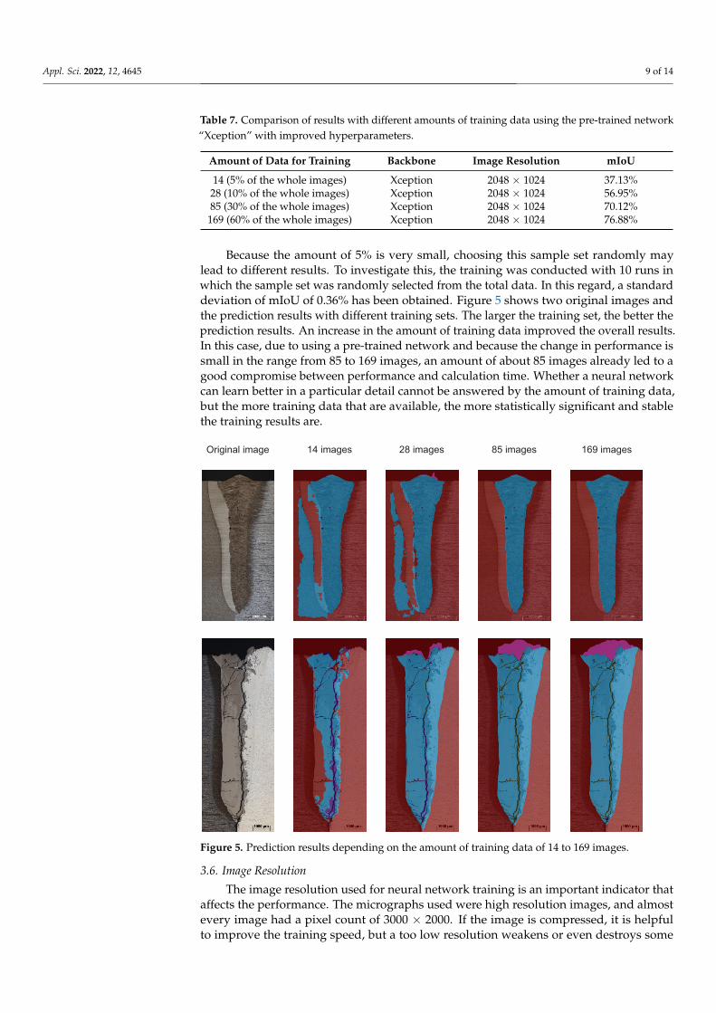
Because the amount of 5% is very small, choosing this sample set randomly maylead to different results. To investigate this, the training was conducted with 10 runs inwhich the sample set was randomly selected from the total data. In this regard, a standarddeviation of mIoU of 0.36% has been obtained. Figure 5 shows two original images andthe prediction results with different training sets. The larger the training set, the better theprediction results. An increase in the amount of training data improved the overall results.In this case, due to using a pre-trained network and because the change in performance issmall in the range from 85 to 169 images, an amount of about 85 images already led to agood compromise between performance and calculation time. Whether a neural networkcan learn better in a particular detail cannot be answered by the amount of training data,but the more training data that are available, the more statistically significant and stablethe training results are.
Original image 14 images 28 images 85 images 169 images
Figure 5. Prediction results depending on the amount of training data of 14 to 169 images.
3.6. Image Resolution
The image resolution used for neural network training is an important indicator thataffects the performance. The micrographs used were high resolution images, and almostevery image had a pixel count of 3000 × 2000. If the image is compressed, it is helpfulto improve the training speed, but a too low resolution weakens or even destroys some
Appl. Sci. 2022, 12, 4645 10 of 14
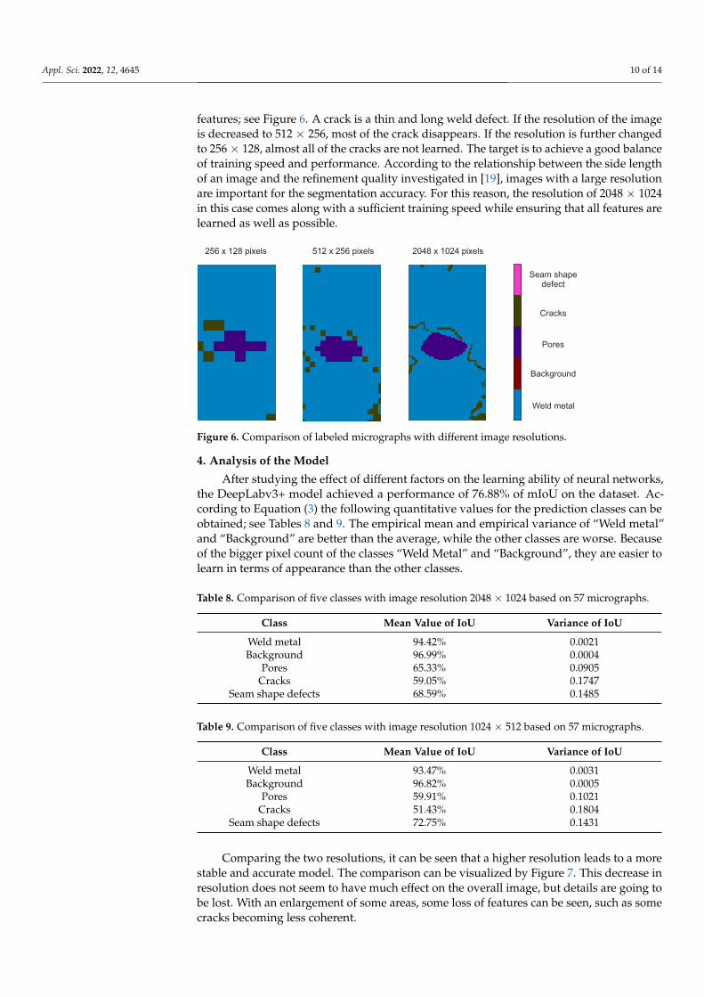
features; see Figure 6. A crack is a thin and long weld defect. If the resolution of the imageis decreased to 512 × 256, most of the crack disappears. If the resolution is further changedto 256 × 128, almost all of the cracks are not learned. The target is to achieve a good balanceof training speed and performance. According to the relationship between the side lengthof an image and the refinement quality investigated in [19], images with a large resolutionare important for the segmentation accuracy. For this reason, the resolution of 2048 × 1024in this case comes along with a sufficient training speed while ensuring that all features arelearned as well as possible.
2048 x 1024 pixels512 x 256 pixels256 x 128 pixels
Pores
Cracks
Seam shapedefect
Background
Weld metal
Figure 6. Comparison of labeled micrographs with different image resolutions.
4. Analysis of the Model
After studying the effect of different factors on the learning ability of neural networks,the DeepLabv3+ model achieved a performance of 76.88% of mIoU on the dataset. Ac-cording to Equation (3) the following quantitative values for the prediction classes can beobtained; see Tables 8 and 9. The empirical mean and empirical variance of “Weld metal”and “Background” are better than the average, while the other classes are worse. Becauseof the bigger pixel count of the classes “Weld Metal” and “Background”, they are easier tolearn in terms of appearance than the other classes.
Table 8. Comparison of five classes with image resolution 2048 × 1024 based on 57 micrographs.
Class Mean Value of IoU Variance of IoU
Weld metal 94.42% 0.0021Background 96.99% 0.0004
Pores 65.33% 0.0905Cracks 59.05% 0.1747
Seam shape defects 68.59% 0.1485
Table 9. Comparison of five classes with image resolution 1024 × 512 based on 57 micrographs.
Class Mean Value of IoU Variance of IoU
Weld metal 93.47% 0.0031Background 96.82% 0.0005
Pores 59.91% 0.1021Cracks 51.43% 0.1804
Seam shape defects 72.75% 0.1431
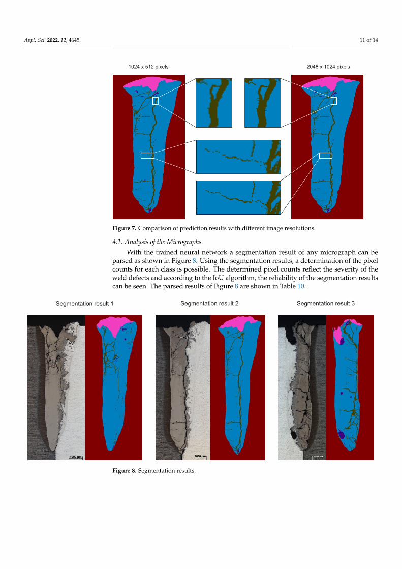
Comparing the two resolutions, it can be seen that a higher resolution leads to a morestable and accurate model. The comparison can be visualized by Figure 7. This decrease inresolution does not seem to have much effect on the overall image, but details are going tobe lost. With an enlargement of some areas, some loss of features can be seen, such as somecracks becoming less coherent.
Appl. Sci. 2022, 12, 4645 11 of 14
1024 x 512 pixels 2048 x 1024 pixels
Figure 7. Comparison of prediction results with different image resolutions.
4.1. Analysis of the Micrographs
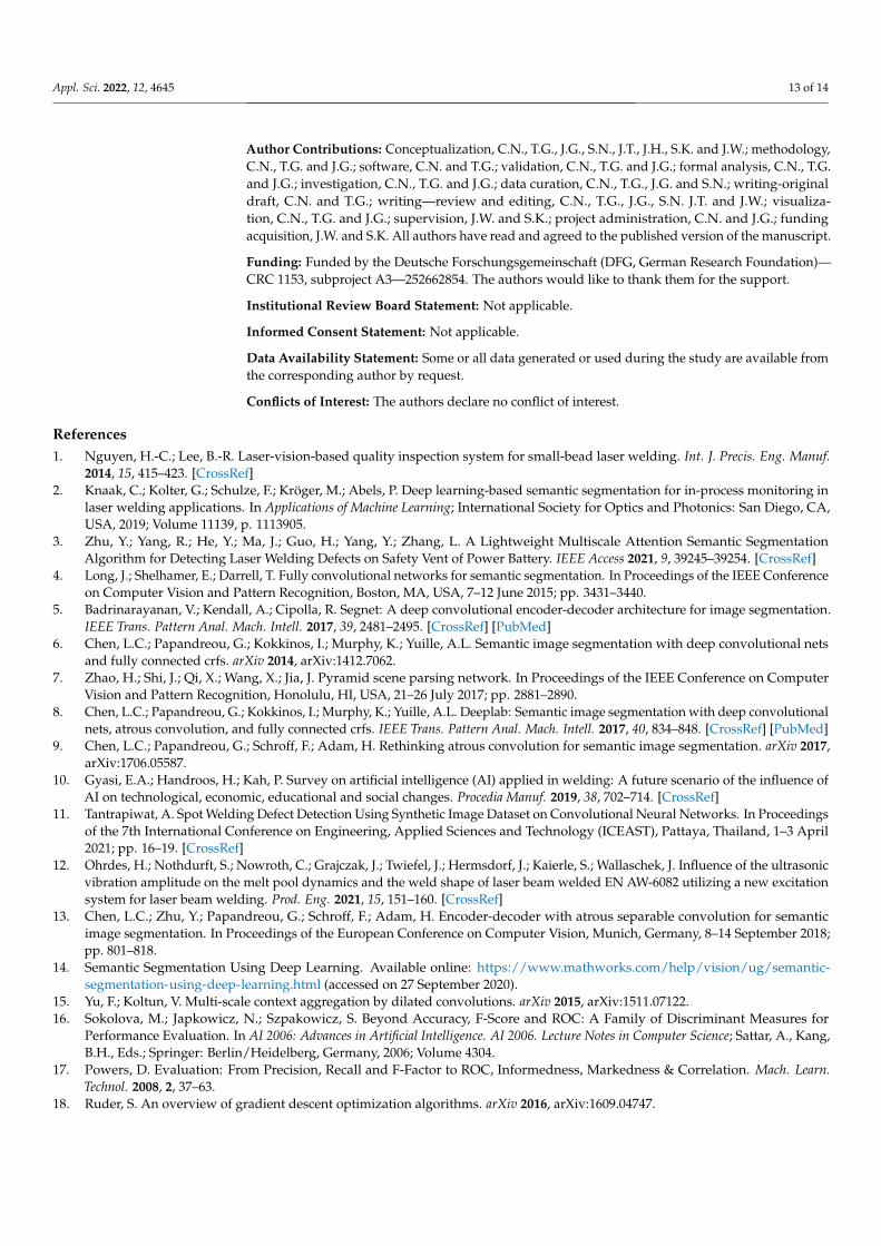
With the trained neural network a segmentation result of any micrograph can beparsed as shown in Figure 8. Using the segmentation results, a determination of the pixelcounts for each class is possible. The determined pixel counts reflect the severity of theweld defects and according to the IoU algorithm, the reliability of the segmentation resultscan be seen. The parsed results of Figure 8 are shown in Table 10.
Segmentation result 1 Segmentation result 2 Segmentation result 3
Figure 8. Segmentation results.

Appl. Sci. 2022, 12, 4645 12 of 14
Table 10. Numerical values of segmentation results.
Segmentation Result Class Predicted Pixel Count Labeled Pixel Count IoU
Weld metal 8.6303 × 10⁵ 8.5214 × 10⁵ 95.17%Background 1.6287 × 10⁶ 1.6501 × 10⁶ 97.89%
1 Pores 7329 7284 25.18%Cracks 43,485 51,612 52.67%
Seam shape defects 1.0602 × 10⁵ 87,489 79.76%
Weld metal 1.0318 × 10⁶ 1.0313 × 10⁶ 96.20%Background 1.5617 × 10⁶ 1.5646 × 10⁶ 98.13%
2 Pores 2033 6410 15.94%Cracks 70,341 70,487 67.09%
Seam shape defects 92,548 85,578 84.28%
Weld metal 1.0517 × 10⁶ 1.0315 × 10⁶ 93.85%Background 1.8082 × 10⁶ 1.84 × 10⁶ 97.30%
3 Pores 35,269 18,796 47.90%Cracks 1.0546 × 10⁵ 1.0574 × 10⁵ 65.57%
Seam shape defects 59,646 64,209 51.59%
With the aid of the standardized pixel numbers, the parsed results are comparabledespite different scaling of the images. When the certain pixel numbers of defects areknown, the ratio of each defect in the weld area can be calculated by Equation (5). Accordingto the data in Table 10, the quantitative values given in Table 11 are calculated. Afterwards,the different parsed results can be compared.
Table 11. Comparison of parsed results using the ratio of each defect in the weld area.
Segmentation Result Pores Cracks Seam Shape Defect
1 0.72% 4.26% 10.40%2 0.17% 5.88% 7.73%3 2.82% 8.42% 4.76%
5. Conclusions
This contribution aims to introduce the current state-of-the-art deep learning tech-niques to detect weld metal and weld defects. A pre-trained neuronal network was trainedand optimized according to the initialization of weights, optimization algorithm, backboneand hyperparameters. By pre-processing the data and adjusting the neural network model,a value of 76.88% of the mIoU was finally obtained for the defined classes. The neuralnetwork can automatically detect different areas within micrographs. The detection ofweld metal has a high reliability, with an IoU of around 95%. Throughout the researchprocess, a high-definition data set containing 282 images was created. It can be applied toany semantic segmentation model, which has significant implications for future research.Further research can continuously improve the neural network model based on the createddata set to achieve better process improvement and quality assurance. With the automateddetection of certain features within the weld area, it would also be possible to evaluatethe quality of the welds. The results from the deep learning-based weld contour anddefect detection could be compared with the established standards, such as DIN EN ISO13919-1:2020-03, and the weld seam could be evaluated accordingly [20].
Appl. Sci. 2022, 12, 4645 13 of 14
Author Contributions: Conceptualization, C.N., T.G., J.G., S.N., J.T., J.H., S.K. and J.W.; methodology,C.N., T.G. and J.G.; software, C.N. and T.G.; validation, C.N., T.G. and J.G.; formal analysis, C.N., T.G.and J.G.; investigation, C.N., T.G. and J.G.; data curation, C.N., T.G., J.G. and S.N.; writing-originaldraft, C.N. and T.G.; writing—review and editing, C.N., T.G., J.G., S.N. J.T. and J.W.; visualiza-tion, C.N., T.G. and J.G.; supervision, J.W. and S.K.; project administration, C.N. and J.G.; fundingacquisition, J.W. and S.K. All authors have read and agreed to the published version of the manuscript.
Funding: Funded by the Deutsche Forschungsgemeinschaft (DFG, German Research Foundation)—CRC 1153, subproject A3—252662854. The authors would like to thank them for the support.
Institutional Review Board Statement: Not applicable.
Informed Consent Statement: Not applicable.
Data Availability Statement: Some or all data generated or used during the study are available fromthe corresponding author by request.
Conflicts of Interest: The authors declare no conflict of interest.
References1. Nguyen, H.-C.; Lee, B.-R. Laser-vision-based quality inspection system for small-bead laser welding. Int. J. Precis. Eng. Manuf.
2014, 15, 415–423. [CrossRef]2. Knaak, C.; Kolter, G.; Schulze, F.; Kröger, M.; Abels, P. Deep learning-based semantic segmentation for in-process monitoring in
laser welding applications. In Applications of Machine Learning; International Society for Optics and Photonics: San Diego, CA,USA, 2019; Volume 11139, p. 1113905.
3. Zhu, Y.; Yang, R.; He, Y.; Ma, J.; Guo, H.; Yang, Y.; Zhang, L. A Lightweight Multiscale Attention Semantic SegmentationAlgorithm for Detecting Laser Welding Defects on Safety Vent of Power Battery. IEEE Access 2021, 9, 39245–39254. [CrossRef]
4. Long, J.; Shelhamer, E.; Darrell, T. Fully convolutional networks for semantic segmentation. In Proceedings of the IEEE Conferenceon Computer Vision and Pattern Recognition, Boston, MA, USA, 7–12 June 2015; pp. 3431–3440.
5. Badrinarayanan, V.; Kendall, A.; Cipolla, R. Segnet: A deep convolutional encoder-decoder architecture for image segmentation.IEEE Trans. Pattern Anal. Mach. Intell. 2017, 39, 2481–2495. [CrossRef] [PubMed]
6. Chen, L.C.; Papandreou, G.; Kokkinos, I.; Murphy, K.; Yuille, A.L. Semantic image segmentation with deep convolutional netsand fully connected crfs. arXiv 2014, arXiv:1412.7062.
7. Zhao, H.; Shi, J.; Qi, X.; Wang, X.; Jia, J. Pyramid scene parsing network. In Proceedings of the IEEE Conference on ComputerVision and Pattern Recognition, Honolulu, HI, USA, 21–26 July 2017; pp. 2881–2890.
8. Chen, L.C.; Papandreou, G.; Kokkinos, I.; Murphy, K.; Yuille, A.L. Deeplab: Semantic image segmentation with deep convolutionalnets, atrous convolution, and fully connected crfs. IEEE Trans. Pattern Anal. Mach. Intell. 2017, 40, 834–848. [CrossRef] [PubMed]
9. Chen, L.C.; Papandreou, G.; Schroff, F.; Adam, H. Rethinking atrous convolution for semantic image segmentation. arXiv 2017,arXiv:1706.05587.
10. Gyasi, E.A.; Handroos, H.; Kah, P. Survey on artificial intelligence (AI) applied in welding: A future scenario of the influence ofAI on technological, economic, educational and social changes. Procedia Manuf. 2019, 38, 702–714. [CrossRef]
11. Tantrapiwat, A. Spot Welding Defect Detection Using Synthetic Image Dataset on Convolutional Neural Networks. In Proceedingsof the 7th International Conference on Engineering, Applied Sciences and Technology (ICEAST), Pattaya, Thailand, 1–3 April2021; pp. 16–19. [CrossRef]
12. Ohrdes, H.; Nothdurft, S.; Nowroth, C.; Grajczak, J.; Twiefel, J.; Hermsdorf, J.; Kaierle, S.; Wallaschek, J. Influence of the ultrasonicvibration amplitude on the melt pool dynamics and the weld shape of laser beam welded EN AW-6082 utilizing a new excitationsystem for laser beam welding. Prod. Eng. 2021, 15, 151–160. [CrossRef]
13. Chen, L.C.; Zhu, Y.; Papandreou, G.; Schroff, F.; Adam, H. Encoder-decoder with atrous separable convolution for semanticimage segmentation. In Proceedings of the European Conference on Computer Vision, Munich, Germany, 8–14 September 2018;pp. 801–818.
14. Semantic Segmentation Using Deep Learning. Available online: https://www.mathworks.com/help/vision/ug/semantic-segmentation-using-deep-learning.html (accessed on 27 September 2020).
15. Yu, F.; Koltun, V. Multi-scale context aggregation by dilated convolutions. arXiv 2015, arXiv:1511.07122.16. Sokolova, M.; Japkowicz, N.; Szpakowicz, S. Beyond Accuracy, F-Score and ROC: A Family of Discriminant Measures for
Performance Evaluation. In AI 2006: Advances in Artificial Intelligence. AI 2006. Lecture Notes in Computer Science; Sattar, A., Kang,B.H., Eds.; Springer: Berlin/Heidelberg, Germany, 2006; Volume 4304.
17. Powers, D. Evaluation: From Precision, Recall and F-Factor to ROC, Informedness, Markedness & Correlation. Mach. Learn.Technol. 2008, 2, 37–63.
18. Ruder, S. An overview of gradient descent optimization algorithms. arXiv 2016, arXiv:1609.04747.

Appl. Sci. 2022, 12, 4645 14 of 14
19. Cheng, H.K.; Chung, J.; Tai, Y.W.; Tang, C.K. CascadePSP: Toward Class-Agnostic and Very High-Resolution Segmentation viaGlobal and Local Refinement. In Proceedings of the IEEE/CVF Conference on Computer Vision and Pattern Recognition, Seattle,WA, USA, 13–19 June 2020; pp. 8890–8899.
20. ISO 13919-1:2019; Electron and Laser-Beam Welded Joints—Requirements and Recommendations on Quality Levels forImperfections—Part 1: Steel, Nickel, Titanium and Their Alloys. International Organization for Standardization: Geneva,Switzerland, 2020.


