The Astronomical Journal, 141:189 (12pp), 2011 June doi:10.1088/0004-6256/141/6/189C© 2011. The American Astronomical Society. All rights reserved. Printed in the U.S.A.

DECISION TREE CLASSIFIERS FOR STAR/GALAXY SEPARATION

E. C. Vasconcellos1, R. R. de Carvalho

2, R. R. Gal

3, F. L. LaBarbera

4,

H. V. Capelato2, H. Frago Campos Velho

5, M. Trevisan

6, and R. S. R. Ruiz

11 CAP, National Institute of Space Research, Av. dos Astronautas 1758, Sao Jose dos Campos 12227-010, Brazil2 DAS, National Institute of Space Research, Av. dos Astronautas 1758, Sao Jose dos Campos 12227-010, Brazil

3 Institute for Astronomy, University of Hawaii, 2680 Woodlawn Dr., Honolulu, HI 96822, USA4 INAF-Osservatorio Astronomico di Capodimonte, via Moiariello 16, Napoli 80131, Italy

5 LAC, National Institute of Space Research, Av. dos Astronautas 1758, Sao Jose dos Campos 12227-010, Brazil6 IAG, University of Sao Paulo, Rua do Matao 1226, Sao Paulo 05508-090, Brazil

Received 2010 October 27; accepted 2011 February 11; published 2011 May 9

ABSTRACT

We study the star/galaxy classification efficiency of 13 different decision tree algorithms applied to photometricobjects in the Sloan Digital Sky Survey Data Release Seven (SDSS-DR7). Each algorithm is defined by a set ofparameters which, when varied, produce different final classification trees. We extensively explore the parameterspace of each algorithm, using the set of 884,126 SDSS objects with spectroscopic data as the training set. Theefficiency of star–galaxy separation is measured using the completeness function. We find that the FunctionalTree algorithm (FT) yields the best results as measured by the mean completeness in two magnitude intervals:14 � r � 21 (85.2%) and r � 19 (82.1%). We compare the performance of the tree generated with the optimal FTconfiguration to the classifications provided by the SDSS parametric classifier, 2DPHOT, and Ball et al. We find thatour FT classifier is comparable to or better in completeness over the full magnitude range 15 � r � 21, with muchlower contamination than all but the Ball et al. classifier. At the faintest magnitudes (r > 19), our classifier is theonly one that maintains high completeness (>80%) while simultaneously achieving low contamination (∼2.5%).We also examine the SDSS parametric classifier (psfMag−modelMag) to see if the dividing line between stars andgalaxies can be adjusted to improve the classifier. We find that currently stars in close pairs are often misclassifiedas galaxies, and suggest a new cut to improve the classifier. Finally, we apply our FT classifier to separate starsfrom galaxies in the full set of 69,545,326 SDSS photometric objects in the magnitude range 14 � r � 21.

Key words: catalogs – methods: data analysis – surveys – virtual observatory tools

Online-only material: color figures, machine-readable table

1. INTRODUCTION

Astronomical data acquisition has experienced a revolutionboth in quality and complexity during the last three decades. Themain driver has been the deployment of, and enormous growthin, modern digital CCD detectors which replaced venerablephotographic plates in the 1980s. Digital images provided byCCDs, coupled with rapid developments in computation anddata storage, made it possible and even routine to produceterabytes of astrophysical data in a year. Moreover, several large-scale surveys are being planned for the next 10 years, which willgenerate a vast quantity of deep and wide photometric images.These surveys will provide data at rates and volumes muchgreater than any previous projects. Therefore, it is necessaryto not only develop new methods for processing and analyzingsuch huge data volumes, but also to ensure that the techniquesapplied to extract information from the data are optimal.

A basic step in the extraction of sensible astronomical datafrom photometric images is separating intrinsically pointlikesources (stars) from extended ones (galaxies). Distinguishingbetween these two classes becomes increasingly difficult assources become fainter because of the lack of spatial resolu-tion and signal to noise. Our goal in this work is to test a varietyof decision tree (DT) classifiers, and ultimately perform reliablestar/galaxy separation for objects from the Seventh Data Re-lease of the Sloan Digital Sky Survey (SDSS-DR7; Abazajianet al. 2009) based on photometric data. We use the SDSS becauseit also contains an enormous number of objects with spectro-scopic data (which give true object classes), and because of the

quality, consistency, and accuracy of its photometric data. In the1970s and 1980s, when digitized images became widespreadin astronomy, many authors undertook projects to create auto-mated methods to separate stars from galaxies. The first effortsrelied on purely parametric methods, such as the pioneeringworks of MacGillivray et al. (1976), Heydon-Dumbleton et al.(1989), and Maddox et al. (1990). MacGillivray et al. (1976)used a plot of transmission versus log (area),7 fitting a dis-criminant function to separate stars and galaxies. Their star/galaxy separation had a completeness (i.e., the fraction of allgalaxies classified as such; also known as the True PositiveRate) of 95% and a contamination (fraction of non-galaxy ob-jects classified as galaxies; also known as the False PositiveRate) of 5%–10%. Heydon-Dumbleton et al. (1989) performedstar/galaxy separation on 200 photographic plates digitized byCOSMOS. Rather than use object attributes measured directlyfrom the plate scans, they generated classification parametersformed from various combinations and functions of the at-tributes, plotting these as a function of magnitude in bidimen-sional parametric diagrams. In these classification spaces, theythen used an automated procedure to derive separation functions.They reached 98%±2% completeness with 8%±2% contamina-tion. Maddox et al. (1990) used a set of 10 parameters measuredby Automatic Plate Measuring in 600 digitized photographicplates from the UK Schmidt Telescope. They reached 90% com-pleteness with 10% contamination at magnitudes Bj < 20.5.

7 Decimal logarithm of occupied area of the object in the image. The area ismeasured as the number of squares with the side equals to 8 μm.

1

The Astronomical Journal, 141:189 (12pp), 2011 June Vasconcellos et al.

All these completenesses and contaminations must be treatedwith caution, as they are based on comparison to expected num-ber counts, and the plate overlaps, instead of a spectroscopic“truth” sample. Sebok (1979) suggested a classifier based onBayesian pattern recognition theory. A numerical function wasconstructed from a statistical model defining the probability of agiven object being a star or a galaxy. The main advantage of thismethod is that there are no free parameters and its calibrationdepends solely on obtaining a set of images of definite stars.The value of the function establishes the classification.

As the volume of digital data expanded, along with the avail-able computing power, many authors began to apply machinelearning methods like DTs (see below, Section 3) and neuralnetworks to address star/galaxy separation. Unlike paramet-ric methods, machine learning methods do not suffer from thesubjective choice of discriminant functions and are more ef-ficient at separating stars from galaxies at fainter magnitudes(Weir et al. 1995). These methods can incorporate a large num-ber of photometric measurements, allowing the creation of aclassifier more accurate than those based on parametric meth-ods. Weir et al. (1995) applied two different DT algorithms, theGID*3 (Fayyad 1994) and the O-Btree (Fayyad & Irani 1992)as star/galaxy separators for images from the Digitized Sec-ond Palomar Observatory Sky Survey (DPOSS), obtaining 90%completeness and 10% contamination. Odewahn et al. (1999)applied a neural network to DPOSS images and established acatalog spanning 1000 deg 2. Odewahn et al. (2004) used a DTand a neural network to separate objects in DPOSS and foundthat both methods have the same accuracy, but the DT con-sumes less time in the learning process. Suchkov et al. (2005)were the first to apply a DT to separate objects from the SDSS.The authors applied the oblique DT classifier ClassX, based onOC1, to the SDSS-DR2 (Abazajian et al. 2004). They classifiedobjects into stars, red stars (type M or later), active galactic nu-clei (AGNs), and galaxies, giving a percentage table of correctclassifications that allows one to estimate their completenessand contamination. Ball et al. (2006) applied an axis-parallelDT. These authors used 477,068 objects from SDSS-DR3(Abazajian et al. 2005) to build the DT—the largest training setever used. They obtained a completeness of 93.8% for galaxiesand 95.4% for stars.

In this paper, we employ a DT machine learning algorithmto separate objects from SDSS-DR7 into stars and galaxies. Weevaluate 13 different DT algorithms provided by the WaikatoEnvironment for Knowledge Analysis (WEKA) data miningtool. We use a training data set containing only objects withmeasured spectra. The algorithm with the best performance onthe training data is used to separate objects in the much largerdata set of objects having only photometric data. This is the firstwork published testing such a large variety of algorithms andusing all of the data in the final SDSS data release (see also Ruizet al. 2009).

Improving star/galaxy separation at the faintest depths ofimaging surveys is not merely an academic exercise. By signifi-cantly improving the completeness in faint galaxy samples, andreducing the contamination by misclassified stars, many astro-physically important questions can be better addressed. Map-ping the signature of baryon acoustic oscillations requires largegalaxy samples—and the more complete at higher redshift, thebetter. The measurement of galaxy–galaxy correlation functionsis of course improved, both by increasing the number of galaxiesused, and by reducing the washing out of the signal due to thesmooth distribution of erroneously classified stars. Weak lensing

surveys, which need the largest and purest sample of background(lensed) galaxies and excellent photometric redshifts benefit onboth fronts. Similarly, searches for galaxy clusters using galaxyoverdensities increase their efficiency when there are fewer con-taminant stars and more constituent galaxies. Searches for rareobjects, both stellar and extended, also win with reduced con-tamination, as do any programs that target objects for follow-upspectroscopy based on the source type.

For future imaging surveys, optimized classifiers will requirea new breed of training set. Because they cover large sky ar-eas, programs like the Dark Energy Survey, the Large Synop-tic Survey Telescope, and Pan-STaRRS can utilize all availablespectroscopy to create training samples, even to quite faint mag-nitudes. Because most spectroscopy has targeted galaxies, theinclusion of definite stars must be accomplished in another way.Hubble Space Telescope (HST) images have superb resolutionand can be used to determine the morphological class (star orgalaxy) of almost all objects observed by HST. Although cov-ering only a tiny fraction of the sky, the depth of even single-orbit HST images and the area overlap with these large surveyswill provide star/galaxy (and perhaps even galaxy morphology)training sets that are more than sufficient to implement withinan algorithm like the one we describe.

The structure of this paper is as follows. In Section 2, wedescribe the SDSS data used to evaluate the WEKA algorithms.In Section 3, we give a brief description of the DT methodand discuss the technique used to choose the best WEKA DTbuilding algorithm. In Section 4, we discuss the evaluationprocess and the results for each algorithm tested. In Section 5,we compare our best star/galaxy separation method to the SDSSparametric method (York et al. 2000), the 2DPHOT parametricmethod (La Barbera et al. 2008), and the axis-parallel DT usedby Ball et al. (2006). We also examine whether the SDSSparametric classifier can be improved by modifying the dividingline between stars and galaxies in the classifier’s parameterspace. We summarize our results in Section 6.

2. THE DATA

We used simple Structured Query Language (SQL) queriesto select data from the SDSS Legacy survey.8 Objects were se-lected having r-magnitudes in the range 14m–21m. We obtainedtwo different data samples: the spectroscopic, or training, sam-ple and the application sample. The spectroscopic sample (seeSection 4.1) contains only those objects with both photometricand spectroscopic measurements, while objects in the applica-tion sample have only photometric measurements. The spectro-scopic sample was obtained through the following query:

SELECTp.objID, p.ra, p.dec, s.specObjID,p.psfMag_r, p.modelMag_r, p.petroMag_r,p.fiberMag_r, p.petroRad_r, p.petroR50_r,p.petroR90_r, p.lnLStar_r,p.lnLExp_r,p.lnLDeV_r, p.mE1_r, p.mE2_r, p.mRrCc_r,p.type_r,p.type, s.specClass

FROM PhotoObj AS pJOIN SpecObj AS s ON s.bestobjid = p.objid

WHEREp.modelMag_r BETWEEN 14.0 AND 21.0

8 These queries were written for the SDSS Sky Server database which is theDR7 Catalog Archive Server (CAS); see http://cas.sdss.org/astrodr7/en/.Photometric data were obtained through the photoObj view of the databaseand spectroscopic data through the specObj view.

2

The Astronomical Journal, 141:189 (12pp), 2011 June Vasconcellos et al.

This query returned slightly over one million objects assignedto six different classes according to their SDSS spectral class.9

However, only objects with a spectral class of star or galaxywere used, leaving us with 884,378 objects for the spectroscopicsample. The majority of excluded objects are spectroscopicallyQSOs (9.1% of the query results), many of which have oneor more saturated pixels in photometry. We also removed 51stars and 147 galaxies with non-physical values (e.g., −9999)for some of their photometric attributes. Finally, we excluded 54objects found to be repeated SDSS spectroscopic targets, leavinga final training sample of 884,126 objects, consisting of 84,043stars and 800,083 galaxies. These all have reliable SDSS staror galaxy spectral classifications and meaningful photometricattributes.

The application sample was built similarly to the spectro-scopic sample with the following query:

SELECTobjID, ra, dec, psfMag_r, modelMag_r,petroMag_r, fiberMag_r, petroRad_r,petroR50_r, petroR90_r, lnLStar_r,lnLExp_r, lnLDeV_r, mE1_r, mE2_r,mRrCc_r, type_r, type

FROM PhotoObjWHEREmodelMag_r BETWEEN 14.0 AND 21.0

This retrieved photometric data for nearly 70 million objectsfrom the Legacy survey. We use the Legacy survey rather thanSEGUE because we are interested in classifying distant objectsat the faint magnitude limit of the SDSS catalog.

3. THE DECISION TREE METHOD

Machine learning methods are algorithms that allow a com-puter to distinguish between classes of objects in massive datasets by first “learning” from a fraction of the data set for whichthe classes are known and well defined—the training set. Ma-chine learning methods are essential when searching for poten-tially useful information in large, high-dimensional data sets.

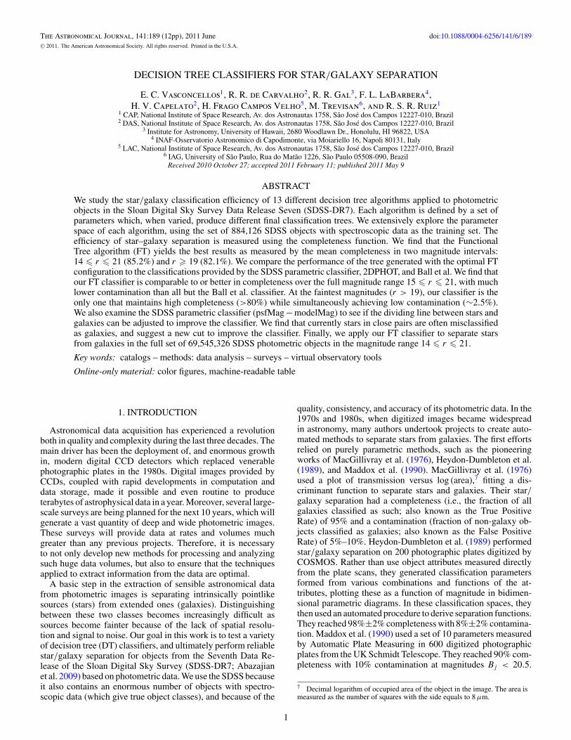
A DT is a well-defined machine learning method consistingof nodes which are simple tests on individual or combineddata attributes. Each possible outcome of a test correspondsto an outgoing branch of the node, which leads to another noderepresenting another test and so on. The process continues untila final node, called a leaf, is reached. Figure 1 shows a graphicalrepresentation of a simple DT constructed with 50,000 randomlychosen SDSS objects having spectroscopic data. At its topmostnode (the root node), the tree may branch left or right dependingon whether the value of the data attribute petroR90 is less thanor greater than 2.359318. Either of these branches may lead toa child node which may test the same attribute, a different one,or a combination of attributes. The path from the root node to aleaf corresponds to a single classification rule.

Building up a DT is a supervised learning process, i.e., the DTis built node by node based on a data set where the classes arealready known. This data set is formed from training examples,each consisting of a combination of attribute values that leads toa class. The process starts with all training examples in theroot node of the tree. An attribute is chosen for testing inthe node. Then, for each possible result of the test a branchis created and the data set is split into subsets of trainingexamples that have the attribute values specified by the branch.A child node is created for each branch and the process is

9 For more information about spectral class please refer to Section 4.1.

Figure 1. Simple decision tree built with the J48 algorithm (Witten & Frank2000). This tree was trained with 50,000 objects from the spectroscopic sample,as described in Section 2, and has a minimum number of objects per leaf equalto 50.

repeated, splitting each subset into new subsets. Child nodesare created recursively until all training examples have thesame class or all the training examples at the node have thesame values for all the attributes. Each leaf node gives either aclassification, a set of classifications, or a probability distributionover all possible classifications. The main difference betweenthe different algorithms for constructing a DT is the method(s)employed to select which attribute or combination of attributeswill be tested in a node.

3.1. WEKA and Tree Construction

WEKA10 is a Java Software package for data mining tasksdeveloped by the University of Waikato, New Zealand. Itconsists of a collection of machine learning algorithms that caneither be applied directly or called from an another Java code.WEKA contains tools for data pre-processing, classification,regression, clustering, association rules, and visualization.

In this work, we use the WEKA DT tools, which include 13different and independent algorithms for constructing DTs.11 Inthe following, we give a brief description of each algorithm.

J48 is the WEKA implementation of the C4.5 algorithm(Quinlam 1993). Given a data set, it generates a DT by recursivepartitioning of the data. The tree is grown using a depth-firststrategy, i.e., the algorithm calculates the information gain forall possible tests that can split the data set and selects a test thatgives the greatest value. This process is repeated for each newnode until a leaf node has been reached.

J48graft generates a grafted DT from a J48 tree. The graftingtechnique (Geoffrey & Geelong 1999) adds nodes to an exist-ing DT with the purpose of reducing prediction errors. Thisalgorithm identifies regions of the multidimensional space ofattributes not occupied by training examples, or occupied onlyby misclassified training examples, and considers alternativebranches for the leaf containing the region in question. In otherwords, a new test will be performed in the leaf, generating newbranches that will lead to new classifications.

BFTree (Best-First DT; Haijian 2007) has a constructionprocess similar to C4.5. The main difference is that C4.5 usesa fixed order to build up a node (normally left to right), whileBFTree uses the best-first order. This method first builds the

10 http://www.cs.waikato.ac.nz/ml/weka/11 There are other DT algorithms in WEKA that are not capable of workingwith numerical attributes.

3

The Astronomical Journal, 141:189 (12pp), 2011 June Vasconcellos et al.

nodes that will lead to the longest possible paths (a path is theway from the root node to a leaf).

FTs (functional trees; Gama 2004) combines a standardunivariate DT, such as C4.5, with linear functions of theattributes by means of linear regressions. While a univariateDT uses simple value tests on single attributes in a node, FT canuse linear combinations of different attributes in a node or in aleaf.

LMTs (Logistic Model Trees; Landwehr et al. 2006) buildstrees with linear functions in leafs as does the FT algorithm. Themain difference is that instead of using linear regression, LMTuses logistic regression.

Simple Cart is the WEKA implementation of the CARTalgorithm (Breiman et al. 1984). It is similar to C4.5 in theprocess of tree construction, but while C4.5 uses informationgain to select the best test to be performed on a node, CARTuses the Gini index.

REPTree is a fast DT learner that builds a decision/regressiontree using information gain/variance as the criterion to selectthe attribute to be tested in a node.

Random tree models have been extensively developed inrecent years. The WEKA Random Tree algorithm builds a treeconsidering K randomly chosen attributes at each node.

Random Forest (Breiman 2001) generates an ensemble oftrees, each built from random samples of the training set. Thefinal classification is obtained by majority vote.

NBTree (Naive Bayesian Tree learner algorithm; Kohavi1996) generates a hybrid of a Naive-Bayesian classifier anda DT classifier. The algorithm builds up a tree in whichthe nodes contain univariate tests, as in a regular DT,but the leaves contains Naive-Bayesian classifiers. In the finaltree, an instance is classified using a local Naive Bayes on theleaf in which it fell. NBTree frequently achieves higher accuracythan either a Naive-Bayesian classifier or a DT learner.

ADTree (Alternating DT; Freund et al. 1999) is a boosted DT.An ADTree consists of prediction nodes and splitter nodes. Thesplitter nodes are defined by an algorithm test, as, for instance,in C4.5, whereas a prediction node is defined by a single valuex ∈ R2. In a standard tree like C4.5, a set of attributes willfollow a path from the root to a leaf according to the attributevalues of the set, with the leaf representing the classification ofthe set. In an ADTree, the process is similar but there are noleaves. The classification is obtained by the sign of the sum ofall prediction nodes existing in the path. Different from standardtrees, a path in an ADTree begins at a prediction node and endsin a prediction node.

LADTree (Holmes et al. 2001) produces an ADTree capableof dealing with data sets containing more than two classes.The original formulation of the ADTree restricted it to binaryclassification problems; the LADTree algorithm extends theADTree algorithm to the multi-class case by splitting theproblem into several two-class problems.

Decision Stump is a simple binary DT classifier consistingof a single node (based on one attribute) and two leaves. Allattributes used by the other trees are tested and the one givingthe best classifications (petroR50 in our case) is chosen to usein the single node.

3.2. Accuracy and Performance: the Cross-Validation Method

The accuracy of any method for star/galaxy separationdepends on the apparent magnitude of the objects and is oftenmeasured using the completeness function CP(m) (fraction ofall galaxies classified as such) and the contamination function

CT(m) (fraction of all stars classified as galaxies) in a magnitudeinterval δm. These are defined as

CP(m) = 100 ∗ Ngal−gal(m)δm

N totgalaxy(m)δm

(1)

and

CT(m) = 100 ∗ Nstar−gal(m)δm

N totstar(m)δm

, (2)

where Ngal−gal(m)δm is the number of galaxy images correctlyidentified as galaxies within the magnitude interval (m −δm/2,m + δm/2); Nstar−gal(m)δm is the number of star imagesfalsely identified as galaxies; N tot

galaxy(m)δm is the total numberof galaxies and N tot

star(m)δm is the total number of stars.It is also useful to define the mean values of these functions

within a given magnitude interval. Thus for the mean com-pleteness we have 〈Compl〉Δm = (1/Δm)

∑CP(mi)δmi , with

Δm = ∑δmi . A similar definition holds for the mean contami-

nation. Note that 〈Compl〉Δm · Δm gives the area under the com-pleteness function in the interval Δm. Unless otherwise stated,we calculate the completeness and contamination functions us-ing a constant bin width δm = 0.m5.

Our first goal is to find the best performing DT algorithmamong those described in Section 3.1, in terms of accuracy,especially at faint magnitudes. However, for large data sets, theprocessing time is also a concern in this evaluation.

There are various approaches to determining the performanceof a DT. The most common approach is to split the trainingset into two subsets, usually in a 4:1 ratio, and construct atree with the larger subset and apply it to the smaller. A moresophisticated method is called Cross Validation (CV; Witten &Frank 2000). The CV method, which is used here, consists ofsplitting the training set into 20 subsamples, each with the samedistribution of classes as the full training set. While the numberof subsamples, 20, is arbitrary, each subsample must providea large training set for the CV method. For each subsample,a DT is built and applied to the other 19 subsamples. Theresulting completeness and contamination functions are thencollected and the median and dispersion over all subsets isfound. This gives the CV estimate of the robustness in termsof a completeness function.

4. STAR/GALAXY SEPARATION FOR SDSS

The spectroscopic information provided by SDSS providesthe true classification—star or galaxy—of an object. Despitethe size of the SDSS spectroscopic sample (∼1 million ob-jects), it represents only a tiny fraction of all objects in theSDSS-DR7 photometry (230 million). How can we classifythe SDSS objects for which there is no spectroscopic data? TheSDSS pipeline already produces a classification using a para-metric method based on the difference between the magnitudespsfMag and modelMag (see Section 4.1). However, it is known(see Figure 6) that this classification is not very accurate atmagnitudes fainter than 19.0.

We will take advantage of the large spectroscopic samplefrom SDSS, for which we know the correct classes for allobjects, to train a DT to classify SDSS objects based only ontheir photometric attributes. We expect that by using such a vasttraining set, the resulting DT will be capable of maintaininggood accuracy even at faint magnitude.

4

The Astronomical Journal, 141:189 (12pp), 2011 June Vasconcellos et al.

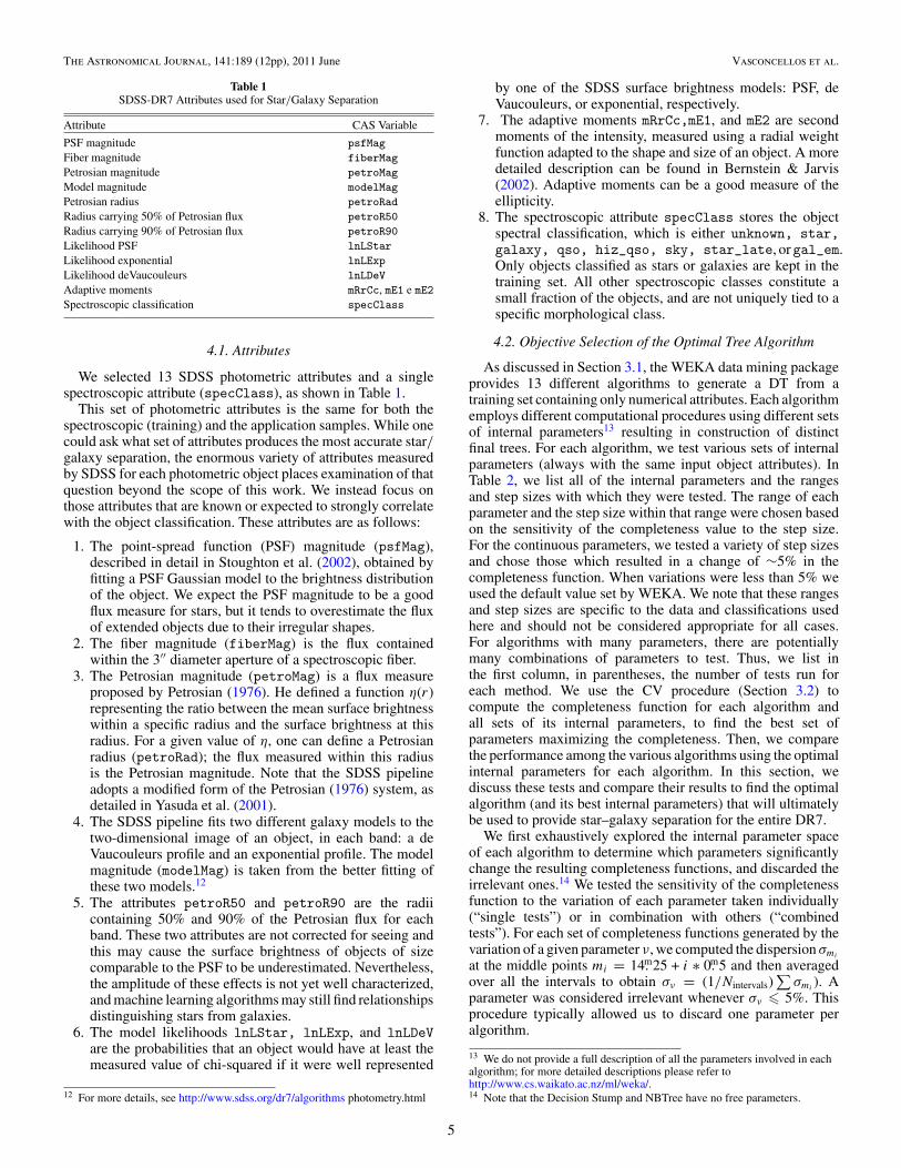
Table 1SDSS-DR7 Attributes used for Star/Galaxy Separation

Attribute CAS Variable

PSF magnitude psfMag

Fiber magnitude fiberMag

Petrosian magnitude petroMag

Model magnitude modelMag

Petrosian radius petroRad

Radius carrying 50% of Petrosian flux petroR50

Radius carrying 90% of Petrosian flux petroR90

Likelihood PSF lnLStar

Likelihood exponential lnLExp

Likelihood deVaucouleurs lnLDeV

Adaptive moments mRrCc, mE1 e mE2Spectroscopic classification specClass

4.1. Attributes

We selected 13 SDSS photometric attributes and a singlespectroscopic attribute (specClass), as shown in Table 1.

This set of photometric attributes is the same for both thespectroscopic (training) and the application samples. While onecould ask what set of attributes produces the most accurate star/galaxy separation, the enormous variety of attributes measuredby SDSS for each photometric object places examination of thatquestion beyond the scope of this work. We instead focus onthose attributes that are known or expected to strongly correlatewith the object classification. These attributes are as follows:

1. The point-spread function (PSF) magnitude (psfMag),described in detail in Stoughton et al. (2002), obtained byfitting a PSF Gaussian model to the brightness distributionof the object. We expect the PSF magnitude to be a goodflux measure for stars, but it tends to overestimate the fluxof extended objects due to their irregular shapes.

2. The fiber magnitude (fiberMag) is the flux containedwithin the 3′′ diameter aperture of a spectroscopic fiber.

3. The Petrosian magnitude (petroMag) is a flux measureproposed by Petrosian (1976). He defined a function η(r)representing the ratio between the mean surface brightnesswithin a specific radius and the surface brightness at thisradius. For a given value of η, one can define a Petrosianradius (petroRad); the flux measured within this radiusis the Petrosian magnitude. Note that the SDSS pipelineadopts a modified form of the Petrosian (1976) system, asdetailed in Yasuda et al. (2001).

4. The SDSS pipeline fits two different galaxy models to thetwo-dimensional image of an object, in each band: a deVaucouleurs profile and an exponential profile. The modelmagnitude (modelMag) is taken from the better fitting ofthese two models.12

5. The attributes petroR50 and petroR90 are the radiicontaining 50% and 90% of the Petrosian flux for eachband. These two attributes are not corrected for seeing andthis may cause the surface brightness of objects of sizecomparable to the PSF to be underestimated. Nevertheless,the amplitude of these effects is not yet well characterized,and machine learning algorithms may still find relationshipsdistinguishing stars from galaxies.

6. The model likelihoods lnLStar, lnLExp, and lnLDeVare the probabilities that an object would have at least themeasured value of chi-squared if it were well represented

12 For more details, see http://www.sdss.org/dr7/algorithms photometry.html

by one of the SDSS surface brightness models: PSF, deVaucouleurs, or exponential, respectively.

7. The adaptive moments mRrCc,mE1, and mE2 are secondmoments of the intensity, measured using a radial weightfunction adapted to the shape and size of an object. A moredetailed description can be found in Bernstein & Jarvis(2002). Adaptive moments can be a good measure of theellipticity.

8. The spectroscopic attribute specClass stores the objectspectral classification, which is either unknown, star,galaxy, qso, hiz_qso, sky, star_late, orgal_em.Only objects classified as stars or galaxies are kept in thetraining set. All other spectroscopic classes constitute asmall fraction of the objects, and are not uniquely tied to aspecific morphological class.

4.2. Objective Selection of the Optimal Tree Algorithm

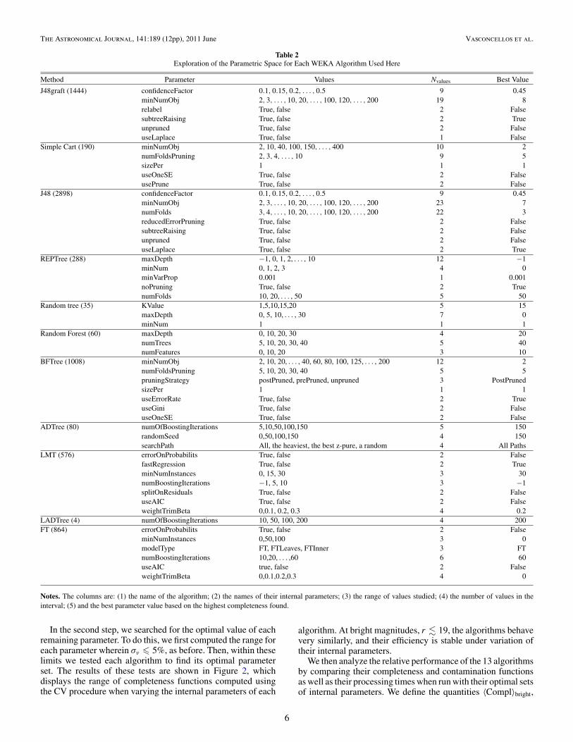
As discussed in Section 3.1, the WEKA data mining packageprovides 13 different algorithms to generate a DT from atraining set containing only numerical attributes. Each algorithmemploys different computational procedures using different setsof internal parameters13 resulting in construction of distinctfinal trees. For each algorithm, we test various sets of internalparameters (always with the same input object attributes). InTable 2, we list all of the internal parameters and the rangesand step sizes with which they were tested. The range of eachparameter and the step size within that range were chosen basedon the sensitivity of the completeness value to the step size.For the continuous parameters, we tested a variety of step sizesand chose those which resulted in a change of ∼5% in thecompleteness function. When variations were less than 5% weused the default value set by WEKA. We note that these rangesand step sizes are specific to the data and classifications usedhere and should not be considered appropriate for all cases.For algorithms with many parameters, there are potentiallymany combinations of parameters to test. Thus, we list inthe first column, in parentheses, the number of tests run foreach method. We use the CV procedure (Section 3.2) tocompute the completeness function for each algorithm andall sets of its internal parameters, to find the best set ofparameters maximizing the completeness. Then, we comparethe performance among the various algorithms using the optimalinternal parameters for each algorithm. In this section, wediscuss these tests and compare their results to find the optimalalgorithm (and its best internal parameters) that will ultimatelybe used to provide star–galaxy separation for the entire DR7.

We first exhaustively explored the internal parameter spaceof each algorithm to determine which parameters significantlychange the resulting completeness functions, and discarded theirrelevant ones.14 We tested the sensitivity of the completenessfunction to the variation of each parameter taken individually(“single tests”) or in combination with others (“combinedtests”). For each set of completeness functions generated by thevariation of a given parameter ν, we computed the dispersion σmi

at the middle points mi = 14.m25 + i ∗ 0.m5 and then averagedover all the intervals to obtain σν = (1/Nintervals)

∑σmi

). Aparameter was considered irrelevant whenever σν � 5%. Thisprocedure typically allowed us to discard one parameter peralgorithm.

13 We do not provide a full description of all the parameters involved in eachalgorithm; for more detailed descriptions please refer tohttp://www.cs.waikato.ac.nz/ml/weka/.14 Note that the Decision Stump and NBTree have no free parameters.

5

The Astronomical Journal, 141:189 (12pp), 2011 June Vasconcellos et al.

Table 2Exploration of the Parametric Space for Each WEKA Algorithm Used Here

Method Parameter Values Nvalues Best Value

J48graft (1444) confidenceFactor 0.1, 0.15, 0.2, . . . , 0.5 9 0.45minNumObj 2, 3, . . . , 10, 20, . . . , 100, 120, . . . , 200 19 8relabel True, false 2 FalsesubtreeRaising True, false 2 Trueunpruned True, false 2 FalseuseLaplace True, false 1 False

Simple Cart (190) minNumObj 2, 10, 40, 100, 150, . . . , 400 10 2numFoldsPruning 2, 3, 4, . . . , 10 9 5sizePer 1 1 1useOneSE True, false 2 FalseusePrune True, false 2 False

J48 (2898) confidenceFactor 0.1, 0.15, 0.2, . . . , 0.5 9 0.45minNumObj 2, 3, . . . , 10, 20, . . . , 100, 120, . . . , 200 23 7numFolds 3, 4, . . . , 10, 20, . . . , 100, 120, . . . , 200 22 3reducedErrorPruning True, false 2 FalsesubtreeRaising True, false 2 Falseunpruned True, false 2 FalseuseLaplace True, false 2 True

REPTree (288) maxDepth −1, 0, 1, 2, . . . , 10 12 −1minNum 0, 1, 2, 3 4 0minVarProp 0.001 1 0.001noPruning True, false 2 TruenumFolds 10, 20, . . . , 50 5 50

Random tree (35) KValue 1,5,10,15,20 5 15maxDepth 0, 5, 10, . . . , 30 7 0minNum 1 1 1

Random Forest (60) maxDepth 0, 10, 20, 30 4 20numTrees 5, 10, 20, 30, 40 5 40numFeatures 0, 10, 20 3 10

BFTree (1008) minNumObj 2, 10, 20, . . . , 40, 60, 80, 100, 125, . . . , 200 12 2numFoldsPruning 5, 10, 20, 30, 40 5 5pruningStrategy postPruned, prePruned, unpruned 3 PostPrunedsizePer 1 1 1useErrorRate True, false 2 TrueuseGini True, false 2 FalseuseOneSE True, false 2 False

ADTree (80) numOfBoostingIterations 5,10,50,100,150 5 150randomSeed 0,50,100,150 4 150searchPath All, the heaviest, the best z-pure, a random 4 All Paths

LMT (576) errorOnProbabilits True, false 2 FalsefastRegression True, false 2 TrueminNumInstances 0, 15, 30 3 30numBoostingIterations −1, 5, 10 3 −1splitOnResiduals True, false 2 FalseuseAIC True, false 2 FalseweightTrimBeta 0,0.1, 0.2, 0.3 4 0.2

LADTree (4) numOfBoostingIterations 10, 50, 100, 200 4 200FT (864) errorOnProbabilits True, false 2 False

minNumInstances 0,50,100 3 0modelType FT, FTLeaves, FTInner 3 FTnumBoostingIterations 10,20, . . . ,60 6 60useAIC true, false 2 FalseweightTrimBeta 0,0.1,0.2,0.3 4 0

Notes. The columns are: (1) the name of the algorithm; (2) the names of their internal parameters; (3) the range of values studied; (4) the number of values in theinterval; (5) and the best parameter value based on the highest completeness found.

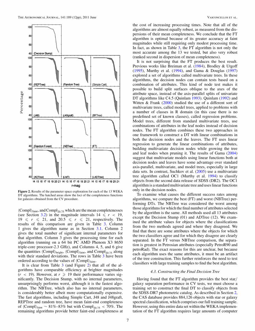
In the second step, we searched for the optimal value of eachremaining parameter. To do this, we first computed the range foreach parameter wherein σν � 5%, as before. Then, within theselimits we tested each algorithm to find its optimal parameterset. The results of these tests are shown in Figure 2, whichdisplays the range of completeness functions computed usingthe CV procedure when varying the internal parameters of each

algorithm. At bright magnitudes, r � 19, the algorithms behavevery similarly, and their efficiency is stable under variation oftheir internal parameters.

We then analyze the relative performance of the 13 algorithmsby comparing their completeness and contamination functionsas well as their processing times when run with their optimal setsof internal parameters. We define the quantities 〈Compl〉bright,

6

The Astronomical Journal, 141:189 (12pp), 2011 June Vasconcellos et al.

Figure 2. Results of the parameter space exploration for each of the 13 WEKADT algorithms. The hatched areas show the loci of the completeness functionsfor galaxies obtained from the CV procedure.

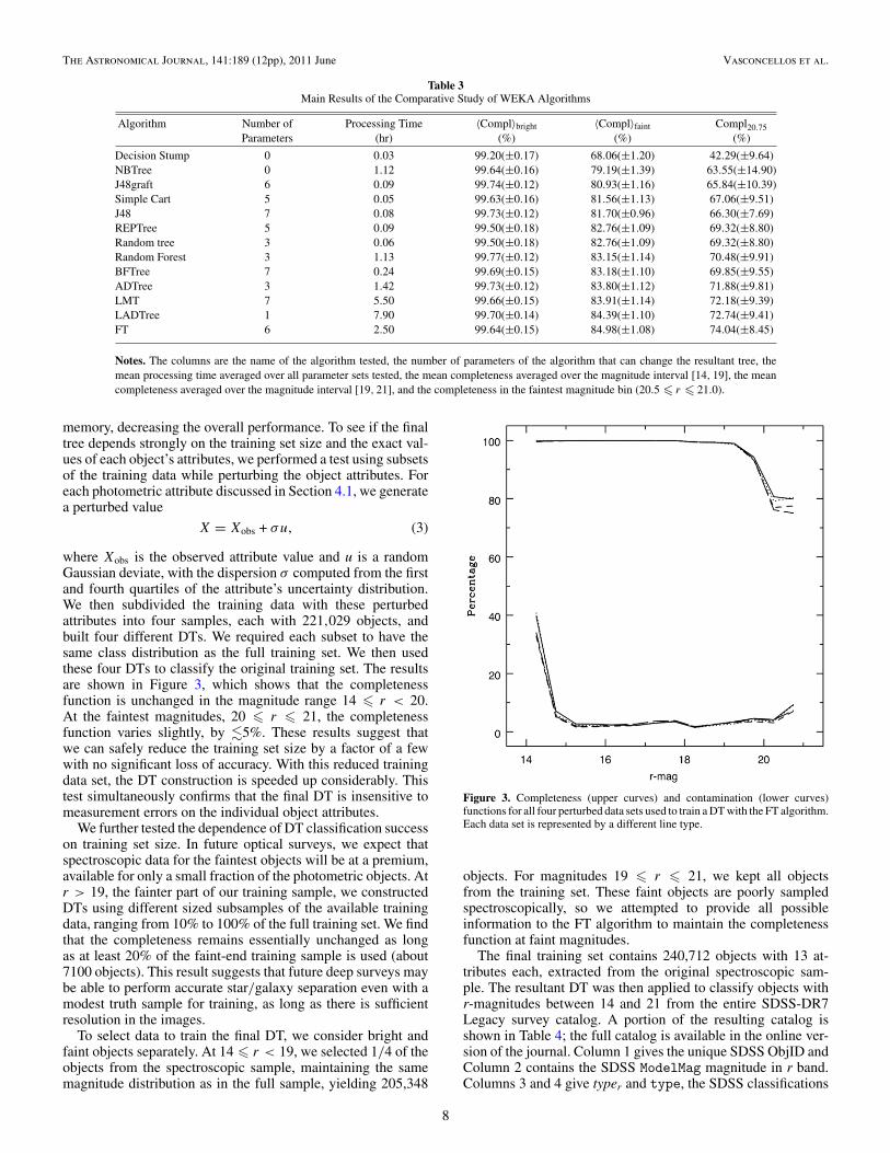
〈Compl〉faint, and Compl20.75 which are the mean completenesses(see Section 3.2) in the magnitude intervals 14 � r < 19,19 � r � 21, and 20.5 � r � 21, respectively. Theresults of this comparison are given in Table 3. Column1 gives the algorithm name as in Section 3.1. Column 2gives the total number of significant internal parameters forthat algorithm. Column 3 gives the processing time for eachalgorithm (running on a 64 bit PC AMD Phenom X3 8650triple-core processor-2.3 GHz), and Columns 4, 5, and 6 givethe quantities 〈Compl〉bright, 〈Compl〉faint, and Compl20.75 alongwith their standard deviations. The rows in Table 3 have beenordered according to the values of 〈Compl〉faint.

It is clear from Table 3 (and Figure 2) that all of the al-gorithms have comparable efficiency at brighter magnitudes(r < 19). However, at r � 19 their performance varies sig-nificantly. The Decision Stump, with no internal parameters,unsurprisingly performs worst, although it is the fastest algo-rithm. The NBTree, which also has no internal parameters,is considerably better albeit more computationally expensive.The fast algorithms, including Simple Cart, J48 and J48graft,REPTree and random tree, have mean faint-end completenessof 〈Compl〉faint ∼ 81%–83% but with Compl20.75 < 70%. Theremaining algorithms provide better faint-end completeness at

the cost of increasing processing times. Note that all of thealgorithms are almost equally robust, as measured from the dis-persions of their mean completeness. We conclude that the FTalgorithm is optimal because of its greater accuracy at faintmagnitudes while still requiring only modest processing time.In fact, as shown in Table 3, the FT algorithm is not only themost accurate among the 13 we tested, but also very robust(ranked second in dispersion of mean completeness).

It is not surprising that the FT produces the best result.Previous works like Breiman et al. (1984), Brodley & Utgoff(1995), Murthy et al. (1994), and Gama & Douglas (1997)explored a set of algorithms called multivariate trees. In thesealgorithms, the decision nodes can contain tests based on acombination of attributes. This kind of node test makes itpossible to build split surfaces oblique to the axes of theattribute space, instead of the axis-parallel splits of univariateDT algorithms like C4.5 (Quinlam 1993). Quinlam (1992) andWitten & Frank (2000) studied the use of a different sort ofmultivariate trees, called model trees, applied to problems witha number of classes in R domain (in this case there is nopredefined set of known classes), called regression problems.Model trees, different from standard multivariate trees, usecombinations of attributes in the leaf nodes instead of decisionnodes. The FT algorithm combines these two approaches inone framework to construct a DT with linear combinations inboth the decision nodes and the leaves. The FT uses linearregression to generate the linear combinations of attributes,building multivariate decision nodes while growing the treeand leaf nodes when pruning it. The results of Gama (2004)suggest that multivariate models using linear functions both atdecision nodes and leaves have some advantage over standardaxis-parallel, multivariate, and model trees, especially in largedata sets. In contrast, Suchkov et al. (2005) use a multivariatetree algorithm called OC1 (Murthy et al. 1994) to classifyobjects from the second data release of SDSS (DR2). The OC1algorithm is a standard multivariate tree and uses linear functionsonly in the decision nodes.

To examine what causes the different success rates amongalgorithms, we compare the best (FT) and worst (NBTree) per-forming DTs. The NBTree was considered the worst amongthose algorithms for which the final number of attributes selectedby the algorithm is the same. All methods used all 13 attributesexcept the Decision Stump (01) and ADTree (12). We exam-ined the attribute values for objects where the classificationsfrom the two methods agreed and where they disagreed. Wefind that there are some attributes where the objects for whichthe two classifiers agree and for which they disagree are clearlyseparated. In the FT versus NBTree comparison, the separa-tion is greatest in Petrosian attributes (especially PetroR90 andpetroRad). The exact reasons for this are unclear, but becauseeach algorithm uses the same attributes, it must be an artifactof the tree construction. This further reinforces the need to testclassifiers with large training samples to find the best algorithm.

4.3. Constructing the Final Decision Tree

Having found that the FT algorithm provides the best star/galaxy separation performance in CV tests, we must choose atraining set to construct the final DT to classify objects fromthe SDSS-DR7 photometric catalog. As described in Section 2,the CAS database provides 884,126 objects with star or galaxyspectral classification, which comprises our full training sample.However, using this entire data set within the WEKA implemen-tation of the FT algorithm requires large amounts of computer

7

The Astronomical Journal, 141:189 (12pp), 2011 June Vasconcellos et al.

Table 3Main Results of the Comparative Study of WEKA Algorithms

Algorithm Number of Processing Time 〈Compl〉bright 〈Compl〉faint Compl20.75Parameters (hr) (%) (%) (%)

Decision Stump 0 0.03 99.20(±0.17) 68.06(±1.20) 42.29(±9.64)NBTree 0 1.12 99.64(±0.16) 79.19(±1.39) 63.55(±14.90)J48graft 6 0.09 99.74(±0.12) 80.93(±1.16) 65.84(±10.39)Simple Cart 5 0.05 99.63(±0.16) 81.56(±1.13) 67.06(±9.51)J48 7 0.08 99.73(±0.12) 81.70(±0.96) 66.30(±7.69)REPTree 5 0.09 99.50(±0.18) 82.76(±1.09) 69.32(±8.80)Random tree 3 0.06 99.50(±0.18) 82.76(±1.09) 69.32(±8.80)Random Forest 3 1.13 99.77(±0.12) 83.15(±1.14) 70.48(±9.91)BFTree 7 0.24 99.69(±0.15) 83.18(±1.10) 69.85(±9.55)ADTree 3 1.42 99.73(±0.12) 83.80(±1.12) 71.88(±9.81)LMT 7 5.50 99.66(±0.15) 83.91(±1.14) 72.18(±9.39)LADTree 1 7.90 99.70(±0.14) 84.39(±1.10) 72.74(±9.41)FT 6 2.50 99.64(±0.15) 84.98(±1.08) 74.04(±8.45)

Notes. The columns are the name of the algorithm tested, the number of parameters of the algorithm that can change the resultant tree, themean processing time averaged over all parameter sets tested, the mean completeness averaged over the magnitude interval [14, 19], the meancompleteness averaged over the magnitude interval [19, 21], and the completeness in the faintest magnitude bin (20.5 � r � 21.0).

memory, decreasing the overall performance. To see if the finaltree depends strongly on the training set size and the exact val-ues of each object’s attributes, we performed a test using subsetsof the training data while perturbing the object attributes. Foreach photometric attribute discussed in Section 4.1, we generatea perturbed value

X = Xobs + σu, (3)

where Xobs is the observed attribute value and u is a randomGaussian deviate, with the dispersion σ computed from the firstand fourth quartiles of the attribute’s uncertainty distribution.We then subdivided the training data with these perturbedattributes into four samples, each with 221,029 objects, andbuilt four different DTs. We required each subset to have thesame class distribution as the full training set. We then usedthese four DTs to classify the original training set. The resultsare shown in Figure 3, which shows that the completenessfunction is unchanged in the magnitude range 14 � r < 20.At the faintest magnitudes, 20 � r � 21, the completenessfunction varies slightly, by �5%. These results suggest thatwe can safely reduce the training set size by a factor of a fewwith no significant loss of accuracy. With this reduced trainingdata set, the DT construction is speeded up considerably. Thistest simultaneously confirms that the final DT is insensitive tomeasurement errors on the individual object attributes.

We further tested the dependence of DT classification successon training set size. In future optical surveys, we expect thatspectroscopic data for the faintest objects will be at a premium,available for only a small fraction of the photometric objects. Atr > 19, the fainter part of our training sample, we constructedDTs using different sized subsamples of the available trainingdata, ranging from 10% to 100% of the full training set. We findthat the completeness remains essentially unchanged as longas at least 20% of the faint-end training sample is used (about7100 objects). This result suggests that future deep surveys maybe able to perform accurate star/galaxy separation even with amodest truth sample for training, as long as there is sufficientresolution in the images.

To select data to train the final DT, we consider bright andfaint objects separately. At 14 � r < 19, we selected 1/4 of theobjects from the spectroscopic sample, maintaining the samemagnitude distribution as in the full sample, yielding 205,348

Figure 3. Completeness (upper curves) and contamination (lower curves)functions for all four perturbed data sets used to train a DT with the FT algorithm.Each data set is represented by a different line type.

objects. For magnitudes 19 � r � 21, we kept all objectsfrom the training set. These faint objects are poorly sampledspectroscopically, so we attempted to provide all possibleinformation to the FT algorithm to maintain the completenessfunction at faint magnitudes.

The final training set contains 240,712 objects with 13 at-tributes each, extracted from the original spectroscopic sam-ple. The resultant DT was then applied to classify objects withr-magnitudes between 14 and 21 from the entire SDSS-DR7Legacy survey catalog. A portion of the resulting catalog isshown in Table 4; the full catalog is available in the online ver-sion of the journal. Column 1 gives the unique SDSS ObjID andColumn 2 contains the SDSS ModelMag magnitude in r band.Columns 3 and 4 give typer and type, the SDSS classifications

8

The Astronomical Journal, 141:189 (12pp), 2011 June Vasconcellos et al.

Table 4Star/Galaxy Classification Provided by SDSS and by Our FT Decision Tree

SDSS ObjID ModelMagr Typer Type FT Class

588848900971299281 20.230947 3 3 2588848900971299284 20.988880 3 3 2588848900971299293 20.560146 3 3 2588848900971299297 19.934738 3 3 2588848900971299302 20.039648 3 3 2588848900971299310 20.714321 3 3 2588848900971299313 20.742567 3 3 2588848900971299314 20.342773 3 3 2588848900971299315 20.425304 3 3 2588848900971299331 20.582634 3 3 2

Notes. Column 1 lists the unique SDSS ObjID, Column 2 contains the SDSSmodelMag magnitude in r-band. Columns 3 and 4 give typer and type, theSDSS classifications using r-band alone and using all five bands, respectively.Column 5 provides our FT Decision Tree classification, where 1 is a star and 2is a galaxy.

(This table is available in its entirety in a machine-readable form in the onlinejournal. A portion is shown here for guidance regarding its form and content.)

using the r band alone and using all five bands, respectively.The SDSS classifications are 0 = unknown, 3 = Galaxy, 6 =Star, and 8 = Sky. Column 5 provides our FT DT classification,where 1 is a star and 2 is a galaxy. We note that we classifiedall objects with 14 < ModelMagr < 21, regardless of theirSDSS classification. Detections which the SDSS has classifiedas type = 0 or 8 should be viewed with caution as there is ahigh likelihood that they are not truly astrophysical objects.

In the next section, we present a comparative study of ourcatalog and other catalogs providing star/galaxy classificationfor the SDSS.

5. COMPARISON WITH OTHER SDSS CLASSIFICATIONS

We compare the results of our DT classification of objects inthe SDSS photometric catalog with those from the parametricclassifier used in the SDSS pipeline, the 2DPHOT softwarefor image processing (La Barbera et al. 2008) and the DTclassification from Ball et al. (2006). These comparisons utilizeonly objects with spectroscopic classifications so that the trueclasses are known. All three methods give classifications otherthan just stars or galaxies. However, as we are interested onlyin stars and galaxies, all samples described in this section areexclusively composed of objects which were classified by therespective methods as star or galaxy.

5.1. FT Algorithm Versus 2DPHOT Method

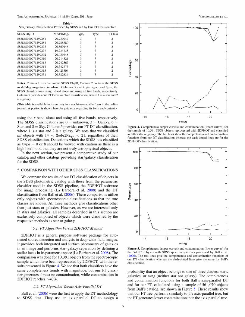
2DPHOT is a general purpose software package for auto-mated source detection and analysis in deep wide-field images.It provides both integrated and surface photometry of galaxiesin an image and performs star–galaxy separation by defining astellar locus in its parametric space (La Barbera et al. 2008). Thecomparison was done for 10,391 objects from the spectroscopicsample which have been reprocessed by 2DPHOT, with the re-sults presented in Figure 4. We see that both classifiers have thesame completeness trends with magnitude, but our FT classi-fier generates almost no contamination, while contamination in2DPHOT reaches ∼40%.

5.2. FT Algorithm Versus Axis-Parallel DT

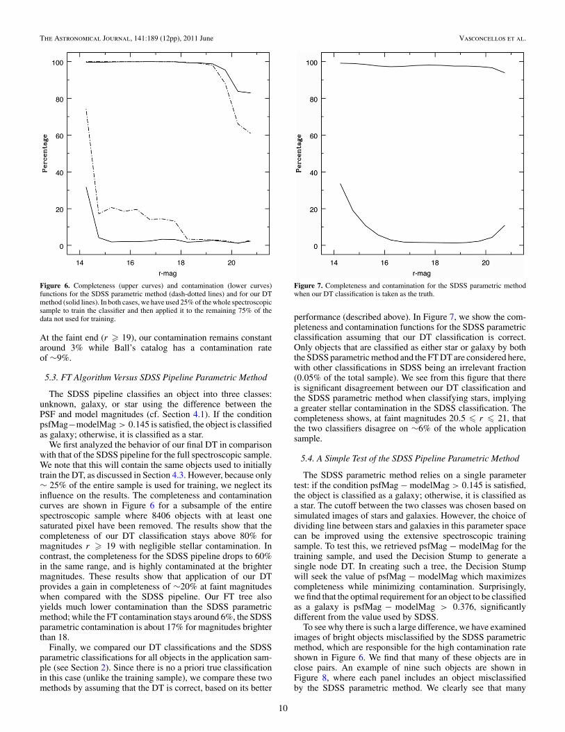
Ball et al. (2006) were the first to apply the DT methodologyto SDSS data. They use an axis-parallel DT to assign a

Figure 4. Completeness (upper curves) and contamination (lower curves) forthe sample of 10,391 SDSS objects reprocessed with 2DPHOT and classifiedas either star or galaxy. The full lines show the completeness and contaminationfunctions from our DT classification whereas the dash-dotted lines are for the2DPHOT classification.

Figure 5. Completeness (upper curves) and contamination (lower curves) forthe 561,070 objects with SDSS spectroscopic data processed by Ball et al.(2006). The full lines give the completeness and contamination functions ofour DT classification whereas the dash-dotted lines give the same for Ball’sclassification.

probability that an object belongs to one of three classes: stars,galaxies, or nsng (neither star nor galaxy). The completenessand contamination functions for both Ball’s axis-parallel DTand for our FT, calculated using a sample of 561,070 objectsfrom Ball’s catalog, are shown in Figure 5. These results showthat our FT tree performs similarly to the axis-parallel tree, butthe FT generates lower contamination than the axis-parallel tree.

9

The Astronomical Journal, 141:189 (12pp), 2011 June Vasconcellos et al.

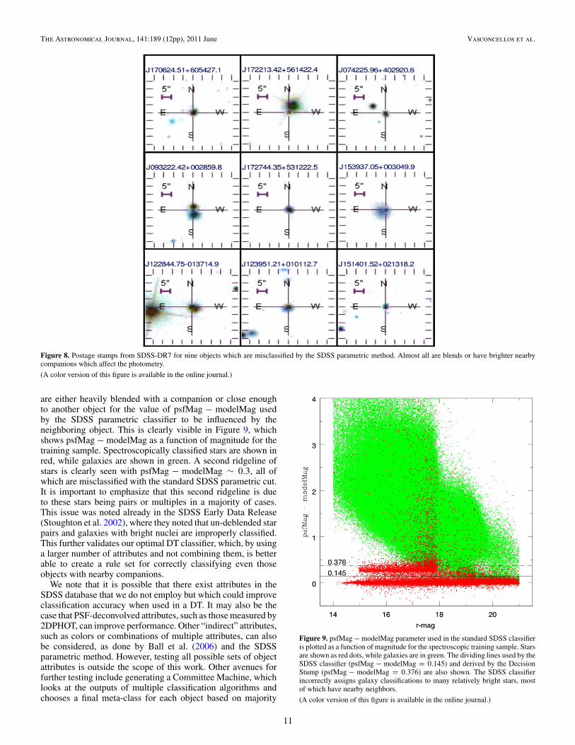
Figure 6. Completeness (upper curves) and contamination (lower curves)functions for the SDSS parametric method (dash-dotted lines) and for our DTmethod (solid lines). In both cases, we have used 25% of the whole spectroscopicsample to train the classifier and then applied it to the remaining 75% of thedata not used for training.

At the faint end (r � 19), our contamination remains constantaround 3% while Ball’s catalog has a contamination rateof ∼9%.

5.3. FT Algorithm Versus SDSS Pipeline Parametric Method

The SDSS pipeline classifies an object into three classes:unknown, galaxy, or star using the difference between thePSF and model magnitudes (cf. Section 4.1). If the conditionpsfMag−modelMag > 0.145 is satisfied, the object is classifiedas galaxy; otherwise, it is classified as a star.

We first analyzed the behavior of our final DT in comparisonwith that of the SDSS pipeline for the full spectroscopic sample.We note that this will contain the same objects used to initiallytrain the DT, as discussed in Section 4.3. However, because only∼ 25% of the entire sample is used for training, we neglect itsinfluence on the results. The completeness and contaminationcurves are shown in Figure 6 for a subsample of the entirespectroscopic sample where 8406 objects with at least onesaturated pixel have been removed. The results show that thecompleteness of our DT classification stays above 80% formagnitudes r � 19 with negligible stellar contamination. Incontrast, the completeness for the SDSS pipeline drops to 60%in the same range, and is highly contaminated at the brightermagnitudes. These results show that application of our DTprovides a gain in completeness of ∼20% at faint magnitudeswhen compared with the SDSS pipeline. Our FT tree alsoyields much lower contamination than the SDSS parametricmethod; while the FT contamination stays around 6%, the SDSSparametric contamination is about 17% for magnitudes brighterthan 18.

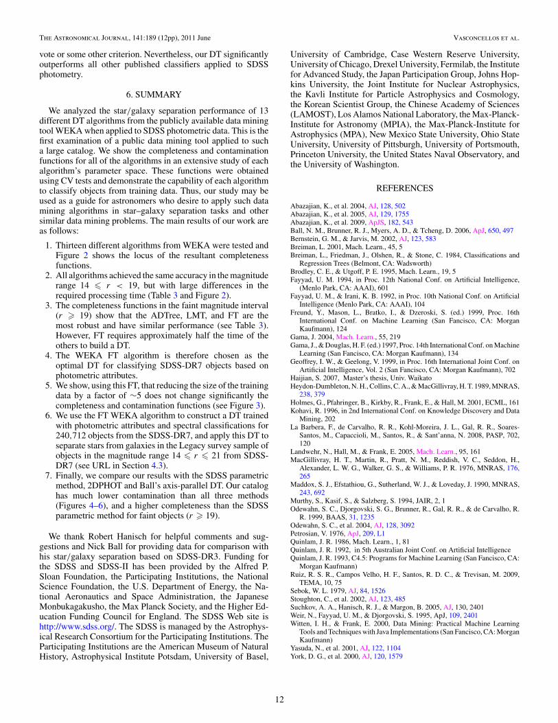
Finally, we compared our DT classifications and the SDSSparametric classifications for all objects in the application sam-ple (see Section 2). Since there is no a priori true classificationin this case (unlike the training sample), we compare these twomethods by assuming that the DT is correct, based on its better

Figure 7. Completeness and contamination for the SDSS parametric methodwhen our DT classification is taken as the truth.

performance (described above). In Figure 7, we show the com-pleteness and contamination functions for the SDSS parametricclassification assuming that our DT classification is correct.Only objects that are classified as either star or galaxy by boththe SDSS parametric method and the FT DT are considered here,with other classifications in SDSS being an irrelevant fraction(0.05% of the total sample). We see from this figure that thereis significant disagreement between our DT classification andthe SDSS parametric method when classifying stars, implyinga greater stellar contamination in the SDSS classification. Thecompleteness shows, at faint magnitudes 20.5 � r � 21, thatthe two classifiers disagree on ∼6% of the whole applicationsample.

5.4. A Simple Test of the SDSS Pipeline Parametric Method

The SDSS parametric method relies on a single parametertest: if the condition psfMag − modelMag > 0.145 is satisfied,the object is classified as a galaxy; otherwise, it is classified asa star. The cutoff between the two classes was chosen based onsimulated images of stars and galaxies. However, the choice ofdividing line between stars and galaxies in this parameter spacecan be improved using the extensive spectroscopic trainingsample. To test this, we retrieved psfMag − modelMag for thetraining sample, and used the Decision Stump to generate asingle node DT. In creating such a tree, the Decision Stumpwill seek the value of psfMag − modelMag which maximizescompleteness while minimizing contamination. Surprisingly,we find that the optimal requirement for an object to be classifiedas a galaxy is psfMag − modelMag > 0.376, significantlydifferent from the value used by SDSS.

To see why there is such a large difference, we have examinedimages of bright objects misclassified by the SDSS parametricmethod, which are responsible for the high contamination rateshown in Figure 6. We find that many of these objects are inclose pairs. An example of nine such objects are shown inFigure 8, where each panel includes an object misclassifiedby the SDSS parametric method. We clearly see that many

10

The Astronomical Journal, 141:189 (12pp), 2011 June Vasconcellos et al.

Figure 8. Postage stamps from SDSS-DR7 for nine objects which are misclassified by the SDSS parametric method. Almost all are blends or have brighter nearbycompanions which affect the photometry.

(A color version of this figure is available in the online journal.)

are either heavily blended with a companion or close enoughto another object for the value of psfMag − modelMag usedby the SDSS parametric classifier to be influenced by theneighboring object. This is clearly visible in Figure 9, whichshows psfMag − modelMag as a function of magnitude for thetraining sample. Spectroscopically classified stars are shown inred, while galaxies are shown in green. A second ridgeline ofstars is clearly seen with psfMag − modelMag ∼ 0.3, all ofwhich are misclassified with the standard SDSS parametric cut.It is important to emphasize that this second ridgeline is dueto these stars being pairs or multiples in a majority of cases.This issue was noted already in the SDSS Early Data Release(Stoughton et al. 2002), where they noted that un-deblended starpairs and galaxies with bright nuclei are improperly classified.This further validates our optimal DT classifier, which, by usinga larger number of attributes and not combining them, is betterable to create a rule set for correctly classifying even thoseobjects with nearby companions.

We note that it is possible that there exist attributes in theSDSS database that we do not employ but which could improveclassification accuracy when used in a DT. It may also be thecase that PSF-deconvolved attributes, such as those measured by2DPHOT, can improve performance. Other “indirect” attributes,such as colors or combinations of multiple attributes, can alsobe considered, as done by Ball et al. (2006) and the SDSSparametric method. However, testing all possible sets of objectattributes is outside the scope of this work. Other avenues forfurther testing include generating a Committee Machine, whichlooks at the outputs of multiple classification algorithms andchooses a final meta-class for each object based on majority

Figure 9. psfMag − modelMag parameter used in the standard SDSS classifieris plotted as a function of magnitude for the spectroscopic training sample. Starsare shown as red dots, while galaxies are in green. The dividing lines used by theSDSS classifier (psfMag − modelMag = 0.145) and derived by the DecisionStump (psfMag − modelMag = 0.376) are also shown. The SDSS classifierincorrectly assigns galaxy classifications to many relatively bright stars, mostof which have nearby neighbors.

(A color version of this figure is available in the online journal.)

11

The Astronomical Journal, 141:189 (12pp), 2011 June Vasconcellos et al.

vote or some other criterion. Nevertheless, our DT significantlyoutperforms all other published classifiers applied to SDSSphotometry.

6. SUMMARY

We analyzed the star/galaxy separation performance of 13different DT algorithms from the publicly available data miningtool WEKA when applied to SDSS photometric data. This is thefirst examination of a public data mining tool applied to sucha large catalog. We show the completeness and contaminationfunctions for all of the algorithms in an extensive study of eachalgorithm’s parameter space. These functions were obtainedusing CV tests and demonstrate the capability of each algorithmto classify objects from training data. Thus, our study may beused as a guide for astronomers who desire to apply such datamining algorithms in star–galaxy separation tasks and othersimilar data mining problems. The main results of our work areas follows:

1. Thirteen different algorithms from WEKA were tested andFigure 2 shows the locus of the resultant completenessfunctions.

2. All algorithms achieved the same accuracy in the magnituderange 14 � r < 19, but with large differences in therequired processing time (Table 3 and Figure 2).

3. The completeness functions in the faint magnitude interval(r � 19) show that the ADTree, LMT, and FT are themost robust and have similar performance (see Table 3).However, FT requires approximately half the time of theothers to build a DT.

4. The WEKA FT algorithm is therefore chosen as theoptimal DT for classifying SDSS-DR7 objects based onphotometric attributes.

5. We show, using this FT, that reducing the size of the trainingdata by a factor of ∼5 does not change significantly thecompleteness and contamination functions (see Figure 3).

6. We use the FT WEKA algorithm to construct a DT trainedwith photometric attributes and spectral classifications for240,712 objects from the SDSS-DR7, and apply this DT toseparate stars from galaxies in the Legacy survey sample ofobjects in the magnitude range 14 � r � 21 from SDSS-DR7 (see URL in Section 4.3).

7. Finally, we compare our results with the SDSS parametricmethod, 2DPHOT and Ball’s axis-parallel DT. Our cataloghas much lower contamination than all three methods(Figures 4–6), and a higher completeness than the SDSSparametric method for faint objects (r � 19).

We thank Robert Hanisch for helpful comments and sug-gestions and Nick Ball for providing data for comparison withhis star/galaxy separation based on SDSS-DR3. Funding forthe SDSS and SDSS-II has been provided by the Alfred P.Sloan Foundation, the Participating Institutions, the NationalScience Foundation, the U.S. Department of Energy, the Na-tional Aeronautics and Space Administration, the JapaneseMonbukagakusho, the Max Planck Society, and the Higher Ed-ucation Funding Council for England. The SDSS Web site ishttp://www.sdss.org/. The SDSS is managed by the Astrophys-ical Research Consortium for the Participating Institutions. TheParticipating Institutions are the American Museum of NaturalHistory, Astrophysical Institute Potsdam, University of Basel,

University of Cambridge, Case Western Reserve University,University of Chicago, Drexel University, Fermilab, the Institutefor Advanced Study, the Japan Participation Group, Johns Hop-kins University, the Joint Institute for Nuclear Astrophysics,the Kavli Institute for Particle Astrophysics and Cosmology,the Korean Scientist Group, the Chinese Academy of Sciences(LAMOST), Los Alamos National Laboratory, the Max-Planck-Institute for Astronomy (MPIA), the Max-Planck-Institute forAstrophysics (MPA), New Mexico State University, Ohio StateUniversity, University of Pittsburgh, University of Portsmouth,Princeton University, the United States Naval Observatory, andthe University of Washington.

REFERENCES

Abazajian, K., et al. 2004, AJ, 128, 502Abazajian, K., et al. 2005, AJ, 129, 1755Abazajian, K., et al. 2009, ApJS, 182, 543Ball, N. M., Brunner, R. J., Myers, A. D., & Tcheng, D. 2006, ApJ, 650, 497Bernstein, G. M., & Jarvis, M. 2002, AJ, 123, 583Breiman, L. 2001, Mach. Learn., 45, 5Breiman, L., Friedman, J., Olshen, R., & Stone, C. 1984, Classifications and

Regression Trees (Belmont, CA: Wadsworth)Brodley, C. E., & Utgoff, P. E. 1995, Mach. Learn., 19, 5Fayyad, U. M. 1994, in Proc. 12th National Conf. on Artificial Intelligence,

(Menlo Park, CA: AAAI), 601Fayyad, U. M., & Irani, K. B. 1992, in Proc. 10th National Conf. on Artificial

Intelligence (Menlo Park, CA: AAAI), 104Freund, Y., Mason, L., Bratko, I., & Dzeroski, S. (ed.) 1999, Proc. 16th

International Conf. on Machine Learning (San Fancisco, CA: MorganKaufmann), 124

Gama, J. 2004, Mach. Learn., 55, 219Gama, J., & Douglas, H. F. (ed.) 1997, Proc. 14th International Conf. on Machine

Learning (San Fancisco, CA: Morgan Kaufmann), 134Geoffrey, I. W., & Geelong, V. 1999, in Proc. 16th International Joint Conf. on

Artificial Intelligence, Vol. 2 (San Fancisco, CA: Morgan Kaufmann), 702Haijian, S. 2007, Master’s thesis, Univ. WaikatoHeydon-Dumbleton, N. H., Collins, C. A., & MacGillivray, H. T. 1989, MNRAS,

238, 379Holmes, G., Pfahringer, B., Kirkby, R., Frank, E., & Hall, M. 2001, ECML, 161Kohavi, R. 1996, in 2nd International Conf. on Knowledge Discovery and Data

Mining, 202La Barbera, F., de Carvalho, R. R., Kohl-Moreira, J. L., Gal, R. R., Soares-

Santos, M., Capaccioli, M., Santos, R., & Sant’anna, N. 2008, PASP, 702,120

Landwehr, N., Hall, M., & Frank, E. 2005, Mach. Learn., 95, 161MacGillivray, H. T., Martin, R., Pratt, N. M., Reddish, V. C., Seddon, H.,

Alexander, L. W. G., Walker, G. S., & Williams, P. R. 1976, MNRAS, 176,265

Maddox, S. J., Efstathiou, G., Sutherland, W. J., & Loveday, J. 1990, MNRAS,243, 692

Murthy, S., Kasif, S., & Salzberg, S. 1994, JAIR, 2, 1Odewahn, S. C., Djorgovski, S. G., Brunner, R., Gal, R. R., & de Carvalho, R.

R. 1999, BAAS, 31, 1235Odewahn, S. C., et al. 2004, AJ, 128, 3092Petrosian, V. 1976, ApJ, 209, L1Quinlam, J. R. 1986, Mach. Learn., 1, 81Quinlam, J. R. 1992, in 5th Australian Joint Conf. on Artificial IntelligenceQuinlam, J. R. 1993, C4.5: Programs for Machine Learning (San Fancisco, CA:

Morgan Kaufmann)Ruiz, R. S. R., Campos Velho, H. F., Santos, R. D. C., & Trevisan, M. 2009,

TEMA, 10, 75Sebok, W. L. 1979, AJ, 84, 1526Stoughton, C., et al. 2002, AJ, 123, 485Suchkov, A. A., Hanisch, R. J., & Margon, B. 2005, AJ, 130, 2401Weir, N., Fayyad, U. M., & Djorgovski, S. 1995, ApJ, 109, 2401Witten, I. H., & Frank, E. 2000, Data Mining: Practical Machine Learning

Tools and Techniques with Java Implementations (San Fancisco, CA: MorganKaufmann)

Yasuda, N., et al. 2001, AJ, 122, 1104York, D. G., et al. 2000, AJ, 120, 1579

12