Embed Size (px)
Citation preview
Databases in 131 Pages
Jyrki Nummenmaa and Aarne Ranta
Faculty of Natural Sciences, University of TampereCSE, Chalmers University of Technology and University of
GothenburgDraft Version October 25, 2018
1
Contents
1 Introduction* 71.1 Data vs. programs . . . . . . . . . . . . . . . . . . . . . . . . . . 71.2 A short history of databases . . . . . . . . . . . . . . . . . . . . . 71.3 SQL . . . . . . . . . . . . . . . . . . . . . . . . . . . . . . . . . . 81.4 DBMS . . . . . . . . . . . . . . . . . . . . . . . . . . . . . . . . . 91.5 The book contents . . . . . . . . . . . . . . . . . . . . . . . . . . 91.6 The big picture . . . . . . . . . . . . . . . . . . . . . . . . . . . . 11
2 Tables and SQL 122.1 SQL database table . . . . . . . . . . . . . . . . . . . . . . . . . . 122.2 SQL in a database management system . . . . . . . . . . . . . . 132.3 Creating an SQL table . . . . . . . . . . . . . . . . . . . . . . . . 142.4 Grammar rules for SQL . . . . . . . . . . . . . . . . . . . . . . . 152.5 A further analysis of CREATE TABLE statements . . . . . . . . 162.6 Inserting rows to a table . . . . . . . . . . . . . . . . . . . . . . . 172.7 Deleting and updating . . . . . . . . . . . . . . . . . . . . . . . . 192.8 Querying: selecting columns and rows from a table . . . . . . . . 202.9 Sets in SQL queries . . . . . . . . . . . . . . . . . . . . . . . . . . 232.10 Sorting the results . . . . . . . . . . . . . . . . . . . . . . . . . . 252.11 Aggregation and grouping . . . . . . . . . . . . . . . . . . . . . . 252.12 Using data from several tables . . . . . . . . . . . . . . . . . . . . 282.13 Foreign keys and references . . . . . . . . . . . . . . . . . . . . . 302.14 Join operations (JOIN) . . . . . . . . . . . . . . . . . . . . . . . 312.15 Local definitions and views . . . . . . . . . . . . . . . . . . . . . 332.16 SQL pitfalls . . . . . . . . . . . . . . . . . . . . . . . . . . . . . . 342.17 SQL in the Query Converter* . . . . . . . . . . . . . . . . . . . . 36
3 Entity-Relationship diagrams 383.1 E-R syntax . . . . . . . . . . . . . . . . . . . . . . . . . . . . . . 383.2 From description to E-R . . . . . . . . . . . . . . . . . . . . . . . 403.3 Converting E-R diagrams to database schemas . . . . . . . . . . 403.4 A word on keys . . . . . . . . . . . . . . . . . . . . . . . . . . . . 423.5 E-R diagrams in the Query Converter* . . . . . . . . . . . . . . . 43
4 Data modelling with relations 454.1 Relations and tables . . . . . . . . . . . . . . . . . . . . . . . . . 454.2 Functional dependencies . . . . . . . . . . . . . . . . . . . . . . . 474.3 Definitions of closures, keys, and superkeys . . . . . . . . . . . . 484.4 Modelling SQL key and uniqueness constraints . . . . . . . . . . 494.5 Referential constraints . . . . . . . . . . . . . . . . . . . . . . . . 504.6 Operations on relations . . . . . . . . . . . . . . . . . . . . . . . 514.7 Multiple tables and joins . . . . . . . . . . . . . . . . . . . . . . . 524.8 Transitive closure* . . . . . . . . . . . . . . . . . . . . . . . . . . 534.9 Multiple values . . . . . . . . . . . . . . . . . . . . . . . . . . . . 54
2
4.10 Null values . . . . . . . . . . . . . . . . . . . . . . . . . . . . . . 55
5 Dependencies and database design 565.1 Relations vs. functions . . . . . . . . . . . . . . . . . . . . . . . . 565.2 Dependency-based design workflow . . . . . . . . . . . . . . . . . 575.3 Examples of dependencies and normal forms . . . . . . . . . . . . 57
5.3.1 Functional dependencies, keys, and superkeys . . . . . . . 575.3.2 BCNF . . . . . . . . . . . . . . . . . . . . . . . . . . . . . 585.3.3 3NF . . . . . . . . . . . . . . . . . . . . . . . . . . . . . . 595.3.4 Multivalued dependencies and the fourth normal form . . 60
5.4 A bigger example . . . . . . . . . . . . . . . . . . . . . . . . . . . 615.5 Mathematical definitions for dependencies and normal forms . . . 62
5.5.1 Relationas, tuples, and depencencies . . . . . . . . . . . . 625.5.2 Closures, keys, and superkeys . . . . . . . . . . . . . . . . 635.5.3 Decomposition algorithms . . . . . . . . . . . . . . . . . . 63
5.6 More definitions for functional dependencies* . . . . . . . . . . . 665.7 Design intuition* . . . . . . . . . . . . . . . . . . . . . . . . . . . 695.8 More definitions and algorithms for database design* . . . . . . . 725.9 Acyclicity* . . . . . . . . . . . . . . . . . . . . . . . . . . . . . . 735.10 Optimal database design* . . . . . . . . . . . . . . . . . . . . . . 745.11 Inclusion dependencies* . . . . . . . . . . . . . . . . . . . . . . . 755.12 Combining practice and theory in database design . . . . . . . . 765.13 Relation analysis in the Query Converter* . . . . . . . . . . . . . 775.14 Further reading on normal forms and functional dependencies* . 77
6 Relational algebra and query compilation 786.1 The compiler pipeline . . . . . . . . . . . . . . . . . . . . . . . . 786.2 Relational algebra . . . . . . . . . . . . . . . . . . . . . . . . . . 786.3 Variants of algebraic notation . . . . . . . . . . . . . . . . . . . . 806.4 From SQL to relational algebra . . . . . . . . . . . . . . . . . . . 80
6.4.1 Basic queries . . . . . . . . . . . . . . . . . . . . . . . . . 806.4.2 Grouping and aggregation . . . . . . . . . . . . . . . . . . 816.4.3 Sorting and duplicate removal . . . . . . . . . . . . . . . . 83
6.5 Query optimization . . . . . . . . . . . . . . . . . . . . . . . . . . 836.5.1 Algebraic laws . . . . . . . . . . . . . . . . . . . . . . . . 836.5.2 Example: pushing conditions in cartesian products . . . . 84
6.6 Relational algebra in the Query Converter* . . . . . . . . . . . . 846.7 Indexes . . . . . . . . . . . . . . . . . . . . . . . . . . . . . . . . 85
7 SQL in software applications 877.1 A minimal JDBC program* . . . . . . . . . . . . . . . . . . . . . 877.2 Building queries and updates from input data . . . . . . . . . . . 887.3 Managing the primitive datatypes* . . . . . . . . . . . . . . . . . 917.4 Wrapping relations and views in classes* . . . . . . . . . . . . . . 947.5 SQL injection . . . . . . . . . . . . . . . . . . . . . . . . . . . . . 967.6 Three-tier architecture and connection pooling* . . . . . . . . . . 97
3
7.7 Authorization and grant diagrams . . . . . . . . . . . . . . . . . 987.8 Table modification and triggers . . . . . . . . . . . . . . . . . . . 997.9 Active element hierarchy . . . . . . . . . . . . . . . . . . . . . . . 997.10 Referential constraints and policies . . . . . . . . . . . . . . . . . 1007.11 CHECK constraints . . . . . . . . . . . . . . . . . . . . . . . . . 1017.12 ALTER TABLE . . . . . . . . . . . . . . . . . . . . . . . . . . . 1027.13 Triggers . . . . . . . . . . . . . . . . . . . . . . . . . . . . . . . . 1027.14 Transactions . . . . . . . . . . . . . . . . . . . . . . . . . . . . . 1077.15 Maintaining isolation* . . . . . . . . . . . . . . . . . . . . . . . . 1107.16 Interferences and isolation levels . . . . . . . . . . . . . . . . . . 1117.17 The ultimate query language?* . . . . . . . . . . . . . . . . . . . 113
8 Introduction to alternative data models 1158.1 XML and its data model . . . . . . . . . . . . . . . . . . . . . . . 1158.2 The XPath query language . . . . . . . . . . . . . . . . . . . . . 1198.3 XML and XPath in the query converter* . . . . . . . . . . . . . . 1198.4 JSON . . . . . . . . . . . . . . . . . . . . . . . . . . . . . . . . . 1208.5 Querying JSON . . . . . . . . . . . . . . . . . . . . . . . . . . . . 1228.6 YAML . . . . . . . . . . . . . . . . . . . . . . . . . . . . . . . . . 1238.7 MongoDB* . . . . . . . . . . . . . . . . . . . . . . . . . . . . . . 1248.8 Pivot tables and OLAP* . . . . . . . . . . . . . . . . . . . . . . . 1248.9 NoSQL data models* . . . . . . . . . . . . . . . . . . . . . . . . . 1248.10 The Cassandra DBMS and its query language CQL* . . . . . . . 1258.11 Physical arrangement of data on disk* . . . . . . . . . . . . . . . 1278.12 NoSQL and MapReduce* . . . . . . . . . . . . . . . . . . . . . . 1288.13 Further reading on NoSQL* . . . . . . . . . . . . . . . . . . . . . 129
A Appendix: SQL in a nutshell 130
4
Note on the the current edition
These notes have been expanded from Aarne’s 2017 version by Jyrki, who hasalso reorganized the chapters. Many more changes are coming during Spring2018! This is in particular the case with exercises, which are currently separatefrom the book but available through the course web page.
Tampere and Gothenburg, October 25, 2018
Jyrki Nummenmaa and Aarne Ranta
Preface
This book originates from the courses given by the authors. More specifi-cally, the Databases course (TDA357/DIT620) at the IT Faculty of Universityof Gothenburg and Chalmers, and the courses Introduction to Databases andDatabase programming given at the University of Tampere. The text is intendedto support the reader’s intuition while at the same time giving sufficiently pre-cise information so that the reader can apply the methods given in the book fordifferent applications. The book proceeds from experimentation and intuitionto more formal and precise treatment of the topics, thereby hopefully makinglearning easier. In particular, Chapters 2, 3 and 4 are suitable as study materialfor people who in practice have no background in computing studies.
A particular virtue of the book is its size. The book is not meant to be ahandbook or manual, as such information is better offered in the Internet, buta concise, intuitive, and precise introduction to databases.
The real value from the book only comes with practice. To build a properunderstanding, you should build and use your own database on a computer. Youshould also work on some theoretical problems by pencil and paper. To helpyou with these exercises, we have developed a tool, Query Converter, which canbe used on-line to explore the theoretical concepts and link them with practicaldatabase applications.
By far the best way to study the book is to participate in a course witha teacher - this gives regularity to the study, as it is easy to try to consumetoo much too quickly when self-studying. For self-study purposes each chapterincludes an estimate on how fast the student who has no initial knowledgeshould progress. The human mind needs time to arrange the new materials andtherefore a reasonable steady pace is prefereable even though the student wouldhave time to study the book all day long.
We will use a running example that deals with geographical data: countriesand their capitals, neighbours, currencies, and so on. This is a bit different frommany other slides, books, and articles. In them, you can find examples such ascourse descriptions, employer records, and movie databases. Such examples mayfeel more difficult since they are not completely common knowledge. This meansthat, when learning new mathematical and programming concepts, you have tolearn new content at the same time. We find it easier to study new technicalmaterial if the contents are familiar. For instance, it is easier to test a query
5
that is supposed to assign ”Paris” to ”the capital of France” than a query thatis supposed to assign ”60,000” to ”the salary of John Johnson” - even thoughof course most people are familiar with work and salaries, but a particular summay seem strange, etc. There is simply one thing less to keep in mind. It alsoeliminates the need to show example tables all the time, because we can simplyrefer to ”the table containing all European countries and their capitals”, whichmost readers will have clear enough in their minds. No geographical knowledgeis required, and it is not important at all if the reader can position the countriesand cities on the map.
Of course, we will have the occasion to show other kinds of databases as well.The country database does not have all the characteristics that a database mighthave, for instance, very rapid changes in the data. The exercises and suggestedprogramming assignments will include such material.
The book can be read in the given order of chapters. It is, however, possibleto deviate from this to some extent. The following diagram shows the relation-ships between chapters and following the diagram it is perfectly doable to pickanother order or, depending on the readers interest, skip some parts of the book.
(Diagram TODO)
This book has drawn inspiration from various sources, even if it seems tobe quite an original compilation of content. A lot of inspiration obviouslycomes from other database textbooks, such as Garcia-Molina, Ullman, andWidom, Database systems: The Complete Book), and by earlier course ma-terial at Chalmers by Niklas Broberg and Graham Kemp. We are grateful to(list needs to be expanded) Gregoire Detrez on general advice and commentson the contents, and to Simon Smith, Adam Ingmansson, and Viktor Blomqvistfor comments during the course. More comments, corrections, and suggestionsare therefore most welcome - your name will be added here if you don’t object!
Gothenburg, March 2016
Aarne Ranta
6
1 Introduction*
This chapter is an overview of the field of databases and of this course. Inaddition to the material printed here, the lecture will also talk about practicalquestions such as assignments, exercises, and the exam. This information canbe found on the course web page. The goal of this chapter (and the whole firstlecture) is to give you a clear picture of what you are expected to do and learnduring the course.
1.1 Data vs. programs
Computers run programs that process data. Sometimes this data comes fromuser interaction and is thrown away after the program is run. But often thedata must be stored for a longer time, so that it can be accessed again. Banks,for instance, have to store the data about bank accounts so that no penny islost.
It is typical that data lives much longer than the programs that processit: decades rather than just years. Programs, even programming languages,may be changed every five years or so, while the data has permanent value forthe organizations. On the other hand, while data is maintained for decades,it may also be changed very rapidly. For instance, a bank can have millionsof transactions daily, coming from ATM’s, internet purchases, etc. This meansthat account balances must be continuously updated. At the same time, thehistory of transactions may be kept for years, for e.g. legal reasons.
A database is any collection of data that can be accessed and processed bycomputer programs. A database system consists of a database storage andsoftware through which the data in the database is accessed. The system mustsupport both updates (i.e. changes in the data) and queries (i.e. questionsabout the data). The data must be structured so that these operations can beperformed efficiently and accurately. For instance, English texts describing thedata would be both too slow and too inaccurate. But the data structure mustalso be generic enough so that it can be accessed in different ways. For instance,the data structures of some advanced programming language may be too hardto access from programs written in other languages. A further requirement isthat the database should support multiple concurrent users.
1.2 A short history of databases
When databases came to wide use, for instance in banks in the 1960’s, they werenot yet standardized. They could be vendor specific, domain specific, or evenmachine specific. It was difficult to exchange data and maintain it when forinstance computers were replaced. As a response to this situation, relationaldatabases were invented in around 1970. They turned out to be both struc-tured and generic enough for most purposes. They have a mathematical theorythat is both precise and simple. Thus they are easy enough to understand by
7

users and easy enough to implement in different applications. As a result, re-lational databases are often the most stable and reliable parts of informationsystems. They can also be the most precious ones, since they contain the resultsfrom decades of work by thousands of people.
Despite their success, relational databases have recently been challengedby other approaches. Some of the challengers want to support more complexdata than relations. For instance, XML (Extended Markup Language) supportshierarchical databases, which were popular in the 1960’s but were deemed toocomplicated by the proponents of relational databases. On the other end, bigdata applications have called for simpler models. In many applications, suchas social media, accuracy and reliability are not so important as for instancein bank applications. Speed is much more important, and then the traditionalrelational models can be too rich. Non-relational approaches are known asNoSQL, by reference to the SQL language introduced in the next section.
1.3 SQL
Relational databases are also known as SQL databases. SQL is a computerlanguage designed in the early 1970’s, originally called Structured Query Lan-guage. The full name is seldom used: one says rather ”sequel” or ”es queue el”.SQL is a special purpose language. Its purpose is to process of relationaldatabases. This includes several operations:• queries, asking questions, e.g. ”what are the neighbouring countries of
France”• updates, changing entries, e.g. ”change the currency of Estonia from
Crown to Euro”• inserts, adding entries, e.g. South Sudan with all the data attached to it• removals, taking away entries, e.g. German Democratic Republic when
it ceased to exist• definitions, creating space for new kinds of data, e.g. for the main domain
names in URL’sThese notes will cover all these operations and also some others. SQL is
designed to make it easy to perform them - easier than a general purposeprogramming language, such as Java or C. The idea is that SQL shouldbe easier to learn as well, so that it is accessible for instance to bank employ-ees without computer science training. However, as we will see, most users ofdatabases today don’t even need SQL. They use some end user programs, forintance an ATM interface with menus, which are simpler and less powerful thanfull SQL. These end user programs are written by programmers as combinationsof SQL and general purpose languages.
Now, since a general purpose language could perform all operations thatSQL can, isn’t SQL superfluous? No, since SQL is a useful intermediate layerbetween user interaction and the data. One reason is the high level of abstractionin SQL. Another reason is that SQL implementations are highly optimized andreliable. A general purpose programmer would have a hard time matching theperformance of them. Losing or destroying data would also be a serious risk.
8
1.4 DBMS
The implementations of SQL are called SQL database management systems(DBMS). Here are some popular systems, in an alphabetical order:• IBM DB2, proprietary• Microsoft SQL Server, proprietary• MySQL, open source, supported by Oracle• MariaDB, open source, successor of MySQL,• Oracle, proprietary• PostgreSQL, open source• SQLite, open source• Teradata, designed for large amounts of data and database analytics.Each DBMS has a slightly different dialect of SQL. There is also an official
standard, but no existing system implements all of it, or only it. In these notes,we will most of the time try to keep to the parts of SQL that belong to thestandard and are implemented by at least most of the systems.
However, since we also have to do some practical work, we have to choosea DBMS to work in. The choice for the course in 2016 is PostgreSQL. Earliercourses have used Oracle, so this is in a way an experiment. The main reasonsto try PostgreSQL are the following advantages over Oracle:• it follows the standard more closely• it is free and open source, hence easier to get hold of
1.5 The book contents
Chapter 1: Introduction
This is the chapter you are reading now. The goal of this chapter is to make itclear what you are expected to learn and to do to study this book.
Chapter 2: Tables and SQL
We start by getting our hands dirty with SQL, which is based on the simpleconcept of a table. This will give us the intuition on how data is stored andretrieved from SQL databases. We will explain the main language constructsof SQL. We will define SQL tables. We will build a database by insertions. Wewill query it by selections, projections, joins, renamings, unions, intersections,and SQL groupings and aggregations. We will also take a look at low-levelmanipulations of strings and at the different datatypes of SQL.
Chapter 3: Entity-Relationship diagrams
A popular device in modelling is E-R diagrams (Entity-Relationship dia-grams). This chapter explains how different kinds of data are modelled byE-R diagrams. We will also tell how E-R diagrams can be constructed fromdescriptive texts. Finally, we will explain how they are, almost mechanically,converted to relational schemes (and thereby eventually to SQL).
9
Chapter 4: Data modelling with relations
This chapter is about the mathematical concepts that underlie relational databases.Not all data is ”naturally” relational, so that some encoding is necessary. Manythings can go wrong in the encoding, and lead to redundancy or even to unin-tended data loss. This lecture gives several examples of different kinds of data.It introduces the notion of relational schemas, which are in SQL implementedby table definitions. But the level here is a bit more abstract than SQL. Thischapter also explains the basics of the mathematics of relations, which are de-rived from set theory.
Chapter 5: Dependencies and database design
This chapter builds on the relational model and explains a technique that helpsdesign consistent databases. Mathematically, a relation can relate an objectwith many other objects. For instance, a country can have many neighbours.A function, on the other hand, relates each object with just one object. Forinstance, a country has just one number giving its area in square kilometres (ata given time). In this perspective, relations are more general than functions.However, it is important to acknowledge that some relations are functions. Oth-erwise, there is a risk of redundancy, repetition of the information. Redun-dancy can lead to inconsistency, if the information that should be the samein different places is actually not the same. Inconsistency and redundancy areexamples of problems with database design. In this chapter, we study how touse dependencies to design databases free of theses problems.
Lecture 6: Relational algebra and query compilation
The relational model is not only used when designing databases: it is alsothe ”machine language” used when executing queries. Relational algebra is amathematical query language. It is much simpler than SQL, as it has only a fewoperations, each denoted by Greek letters. Being so simple, relational algebrais more difficult to use for complex queries than SQL. But for the very samereason, it is easier to analyse and optimize. Relational algebra is therefore usefulas an intermediate language in a DBMS. SQL queries can be first translated torelational algebra, which is optimized before it is executed. This chapter willtell the basics about this translation and some query optimizations.
Chapter 7: SQL in software applications
End user programs are often built by combining SQL and a general purposeprogramming language. This is called embedding, and the general purposelanguage is called a host language. In this lecture, we will look at how SQL isembedded in Java. We will also cover some pitfalls in embedding. For instanceSQL injection is a security hole where an end user can include SQL code inthe data that she is asked to give. In one famous example, the name of a studentincludes a piece of SQL code that deletes all data from a student database.
10
We also take a deeper look at inserts, updates, and deletions, in the presenceof constraints. The integrity constraints of the database may restrict theseactions or even prohibit them. An important problem is that when one piece ofdata is changed, some others may need to be changed as well. For instance, whenvalue is deleted or updated, how should this affect other rows that reference itas foreign key? Some of these things can be guaranteed by constraints in basicSQL. But some things need more expressive power. For example, when makinga bank transfer, money should not only be taken from one account, but the sameamount must be added to the other account. For situations like this, DBMSssupport triggers, which are programs that do many SQL actions at once.
Chapter 8: Introduction to alternative data models
The relational data model has been dominating the database world for a longtime. But there are alternative models, some of which are gaining popularity.XML is an old model, often seen as a language for documents rather thandata. In this perspective, it is a generalization of HTML. But it is a verypowerful generalization, which can be used for any structured data. XML dataobjects need not be just tuples, but they can be arbitrary trees. XML alsohas designated query languages, such as XPath and XQuery. This chapterintroduces XML and gives a summary of XPath. On the other end of the scale,there are models simpler than SQL, known as ”NoSQL” models. These modelsare popular in so-called big data applications, since they support the distributionof data on many computers. NoSQL is implemented in systems like Cassandra,originally developed by Facebook and now also used for instance by Spotify.
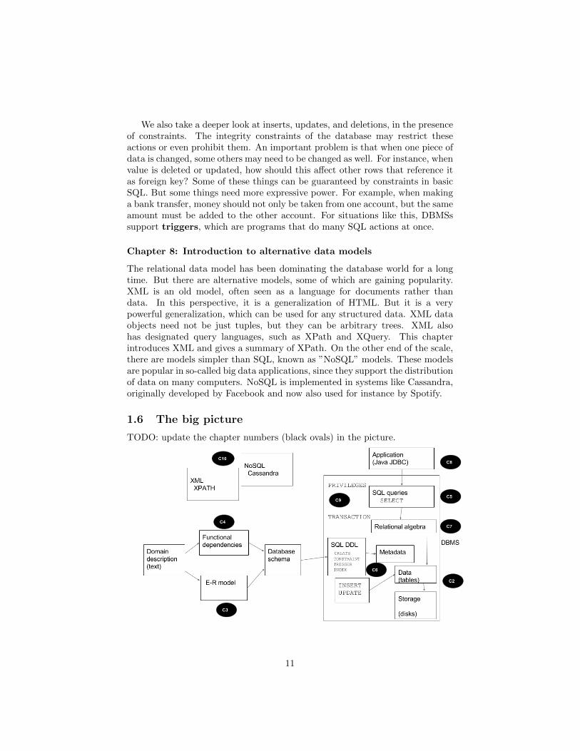
1.6 The big picture
TODO: update the chapter numbers (black ovals) in the picture.
11
2 Tables and SQL
This chapter is about tables as a basic abstraction for present-day databases.We will study them using a common database language, SQL, starting from thebasics and advancing little by little. The concepts are introduced using examples,and no prior knowledge of databases is required. This chapter covers two lec-tures. At first lecture, we will explain the main language constructs of SQL byusing just one table. We will learn to define database tables using SQL. We willinsert data to the tables using SQL. We will query it by selections, projections,renamings, unions, intersections, groupings, and aggregations. We will alsotake a look at low-level manipulations of strings and at the different datatypes ofSQL. The second lecture generalizes the treatment to many tables. This general-ization involves just a few new SQL constructs (foreign keys, cartesian products,joins). But it is an important step conceptually, since it raises the question ofhow a database should be divided to separate tables. This question will be thetopic of the subsequent chapters on database design.
2.1 SQL database table
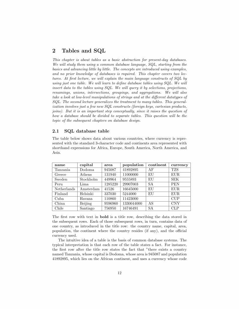
The table below shows data about various countries, where currency is repre-sented with the standard 3-character code and continents area represented withshorthand expressions for Africa, Europe, South America, North America, andAsia.
name capital area population continent currencyTanzania Dodoma 945087 41892895 AF TZSGreece Athens 131940 11000000 EU EURSweden Stockholm 449964 9555893 EU SEKPeru Lima 1285220 29907003 SA PENNetherlands Amsterdam 41526 16645000 EU EURFinland Helsinki 337030 5244000 EU EURCuba Havana 110860 11423000 CUPChina Beijing 9596960 1330044000 AS CNYChile Santiago 756950 16746491 SA CLP
The first row with text in bold is a title row, describing the data stored inthe subsequent rows. Each of those subsequent rows, in turn, contains data ofone country, as introduced in the title row: the country name, capital, area,population, the continent where the country resides (if any), and the officialcurrency used.
The intuitive idea of a table is the basis of common database systems. Thetypical interpretation is that each row of the table states a fact. For instance,the first row after the title row states the fact that ”there exists a countrynamed Tanzania, whose capital is Dodoma, whose area is 945087 and population41892895, which lies on the African continent, and uses a currency whose code
12

is TZS”. Each row states a fact of this very form: ”there exists a countrynamed in the row, with the given capital, area and population, residing in thegiven continent, and using the given official currency”. Those familiar with logicshould see a similarity between rows and logical propositions. The table is aset of facts, which means that the order of the rows is seen unimportant, andre-ordering the rows does not change the information content.
All the vertical columns in the table seem to have similar formats. Somecolumns are strings (name, capital), some numbers (area, population). Some arestrings with a fixed length (currency length 3, continent length 2). Moreover,each country seems intuitively have a unique name, but different countries mighthave the same area or population, use the same currency, be situated on thesame continent, and even, at least theoretically, even have the same capitalname.
These conclusions are superficial, drawn from the outlook of the table. Fromthat table we cannot know if some currency has 4-character code or if we wouldwant to store areas as a non-integer decimal values. We don’t even know ifall values must exist: in the above table, Cuba has no continent, since it is anisland outside continents. However, when we use a table to store values in adatabase, we will define such properties explicitly, and then the database systemwill ensure that the values stored fulfill those properties.
In this chapter, we will learn to create and manipulate database tables usingthe SQL language, commonly used in both commercial and open-source systems.The first thing to learn is how to create a table and to populate it with values.After that, we will learn how to write queries, that is, ask questions about thetables.
2.2 SQL in a database management system
We will in the following assume that you have a working installation of Post-greSQL and access to a command line shell. It can be a Unix shell, calledTerminal in Mac, or command line in Windows.
In your command line shell, you can start PostgreSQL with the command
psql Countries
if Countries is the name of the database that you are using. If you are ad-ministrating your own PostgreSQL installation, you may use the Unix shellcommand
createdb Countries
to create such a database; this you will only have to do once. After this, youcan start PostgreSQL with the command psql Countries. 1
1If you use the school’s PostgreSQL installation, you already have a database created, andyou should work under that.
13
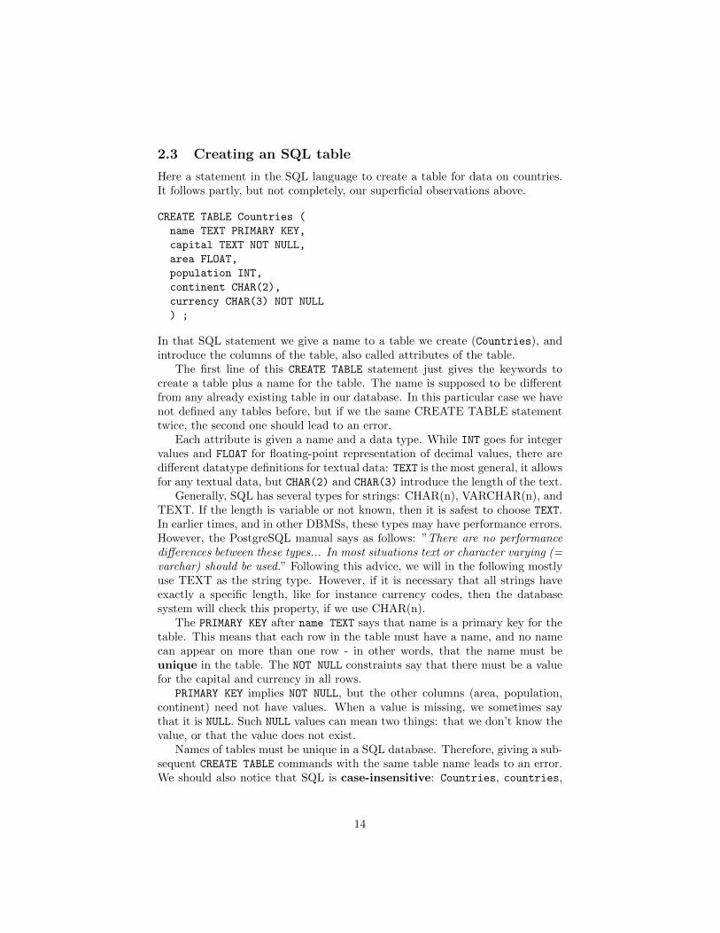
2.3 Creating an SQL table
Here a statement in the SQL language to create a table for data on countries.It follows partly, but not completely, our superficial observations above.
CREATE TABLE Countries (
name TEXT PRIMARY KEY,
capital TEXT NOT NULL,
area FLOAT,
population INT,
continent CHAR(2),
currency CHAR(3) NOT NULL
) ;
In that SQL statement we give a name to a table we create (Countries), andintroduce the columns of the table, also called attributes of the table.
The first line of this CREATE TABLE statement just gives the keywords tocreate a table plus a name for the table. The name is supposed to be differentfrom any already existing table in our database. In this particular case we havenot defined any tables before, but if we the same CREATE TABLE statementtwice, the second one should lead to an error.
Each attribute is given a name and a data type. While INT goes for integervalues and FLOAT for floating-point representation of decimal values, there aredifferent datatype definitions for textual data: TEXT is the most general, it allowsfor any textual data, but CHAR(2) and CHAR(3) introduce the length of the text.
Generally, SQL has several types for strings: CHAR(n), VARCHAR(n), andTEXT. If the length is variable or not known, then it is safest to choose TEXT.In earlier times, and in other DBMSs, these types may have performance errors.However, the PostgreSQL manual says as follows: ”There are no performancedifferences between these types... In most situations text or character varying (=varchar) should be used.” Following this advice, we will in the following mostlyuse TEXT as the string type. However, if it is necessary that all strings haveexactly a specific length, like for instance currency codes, then the databasesystem will check this property, if we use CHAR(n).
The PRIMARY KEY after name TEXT says that name is a primary key for thetable. This means that each row in the table must have a name, and no namecan appear on more than one row - in other words, that the name must beunique in the table. The NOT NULL constraints say that there must be a valuefor the capital and currency in all rows.
PRIMARY KEY implies NOT NULL, but the other columns (area, population,continent) need not have values. When a value is missing, we sometimes saythat it is NULL. Such NULL values can mean two things: that we don’t know thevalue, or that the value does not exist.
Names of tables must be unique in a SQL database. Therefore, giving a sub-sequent CREATE TABLE commands with the same table name leads to an error.We should also notice that SQL is case-insensitive: Countries, countries,
14

and COUNTRIES are all interpreted as the same name. But a good practice thatis often followed is to use• capital initials for tables: Countries• small initials for attributes: name• all capitals for SQL keywords: CREATEIf you want to get rid of the table you created, you can remove it with the
following command, and then create it with different properties.
DROP TABLE Countries
This must obviously be used with caution, since all the data in the table getslost!
2.4 Grammar rules for SQL
There are different variations or dialects of the SQL language, and our aim isnot to cover them all nor compare them, but to introduce a subset suitable forour course and giving a reasonable overview of the language.
While different database language feature come up, we will introduce theirgrammatical description, which makes it possible to understand ”what all” onecan do with the statements. Without raising the abstraction with a grammarof our grammars, we rather introduce the grammar structures as they are used.
To represent the grammars, we use BNF (Backus Naur form, and you maycontinue reading even if you do not know what it means) with the followingconventions:
• CAPITAL words are SQL keywords, to take literally
• small character words are names of syntactic categories, defined each intheir own rules
• | separates alternatives
• + means one or more, separated by commas
• * means zero or more, separated by commas
• ? means zero or one
• in the beginning of a line, + * ? operate on the whole line; elsewhere,they operate on the word just before
• ## start comments, which explain unexpected notation or behaviour
• text in double quotes means literal code, e.g. "*" means the operator *
• other symbols, e.g. parentheses, also mean literal code (quotes are usedonly in some cases, to separate code from grammar notation)
15
• parentheses can be added to disambiguate the scopes of operators Anotherimportant aspect of SQL syntax is case insensitivity:
• keywords are usually written with capitals, but can be written by anycombinations of capital and small letters
• the same concerns identifiers, i.e. names of tables, attributes, constraints
• however, string literals in single quotes are case sensitive
As the first example, the grammar of CREATE TABLE statements is as fol-lows:
statement ::=
CREATE TABLE tablename (
* attribute type inlineconstraint*
* [CONSTRAINT name]? constraint
);
2.5 A further analysis of CREATE TABLE statements
In the grammar for CREATE TABLE statements, the first line just gives the key-words to create a table plus a name for the table. The second line introduceszero or more attributes. Their names are supposed to be unique for the table.The type, instead, is a syntactic category defined below, and so are the inlineconstraints, that is, the constraints given on the same line with the constrainedattribute.
type ::=
CHAR ( integer ) | VARCHAR ( integer ) | TEXT | INT | FLOAT | BOOLEAN
inlineconstraint ::=
PRIMARY KEY | UNIQUE | NOT NULL | DEFAULT value
| REFERENCES tablename ( attribute )
An example of an inline constraint is PRIMARY KEY after name TEXT, it saysthat name is a primary key for the table. Another example that appeared inthe previous section is the NOT NULL inline constraints.
The other inline constraints given now are UNIQUE which means there mustbe a unique value for that attribute in each row, and DEFAULT value whichallows us to define a default value for data insertion. REFERENCES is used whenthe attribute refers to some other table; Section 2.13 will explain this.
Some constraints are not for a single attribute value. The primary key maybe a composite key, that is, composed from several attributes, which is usefulwhen a combination of attribute values is unique even if none of the attributesalone is unique. Since such constraints refer to several attibutes, they must beseparately from the introduction of the respective attributes, in the constraintpart of the CREATE TABLE statement. Their grammar is:
16
constraint ::=
PRIMARY KEY ( attribute+ )
| UNIQUE ( attribute+ )
| NOT NULL ( attribute )
| FOREIGN KEY tablename ( attribute+ )
As an example of composite keys, let us suppose, for the moment, that coun-try names are only unique within a continent and we have to use the country,
continent pair as a primary key. Then we would have a constraint
PRIMARY KEY (continent, name)
If countries were identified, instead, by a number, we could still state the unique-ness of continent,name pairs by stating the following constraint, to which wenow give a name.
CONSTRAINT continent-name-pair-is-unique UNIQUE continent, name
And what might the name be used for? Well, some database managementsystems use the name when they report situations where the constraint wouldbe violated. What, then, is the difference of PRIMARY KEY and UNIQUE inSQL? The difference, if any, is that some systems are more reluctant to changeor remove from existing tables their key definitions than their unique definitions.
There are also further constraints, not relevant to us now.
2.6 Inserting rows to a table
A new table, when created, is empty. To insert table rows, we use the INSERT
statement. The statements below create the contents that we saw before, justthe order is different. However, we assume that the interpretation of data con-tent is ”per row” and, thus, the order of the rows carries no meaning. Equallywell, you may give the statements in any order. The most convenient way is toprepare a file that contains the statements and then read in the statements ina SQL interface.
INSERT INTO Countries VALUES (’Sweden’,’Stockholm’,449964,9555893,’EU’,’SEK’) ;
INSERT INTO Countries VALUES (’Finland’,’Helsinki’,337030,5244000,’EU’,’EUR’) ;
INSERT INTO Countries VALUES (’Tanzania’,’Dodoma’,945087,41892895,’AF’,’TZS’) ;
INSERT INTO Countries VALUES (’Peru’,’Lima’,1285220,29907003,’SA’,’PEN’) ;
INSERT INTO Countries VALUES (’Chile’,’Santiago’,756950,16746491,’SA’,’CLP’) ;
INSERT INTO Countries VALUES (’China’,’Beijing’,9596960,1330044000,’AS’,’CNY’) ;
INSERT INTO Countries VALUES (’Slovenia’,’Ljubljana’,20273,2007000,’EU’,’EUR’) ;
INSERT INTO Countries VALUES (’Greece’,’Athens’,131940,11000000,’EU’,’EUR’) ;
INSERT INTO Countries VALUES (’Cuba’,’Havana’,110860,11423000,NULL,’CUP’) ;
Some database systems allow to combine several rows into the same state-ment:
17
INSERT INTO Countries VALUES
(’Sweden’,’Stockholm’,449964,9555893,’EU’,’SEK’),
(’Finland’,’Helsinki’,337030,5244000,’EU’,’EUR’),
(’Tanzania’,’Dodoma’,945087,41892895,’AF’,’TZS’),
(’Peru’,’Lima’,1285220,29907003,’SA’,’PEN’),
(’Chile’,’Santiago’,756950,16746491,’SA’,’CLP’),
(’China’,’Beijing’,9596960,1330044000,’AS’,’CNY’),
(’Slovenia’,’Ljubljana’,20273,2007000,’EU’,’EUR’),
(’Greece’,’Athens’,131940,11000000,’EU’,’EUR’),
(’Cuba’,’Havana’,110860,11423000,NULL,’CUP’) ;
Even though the order of rows is unimportant, here the order of valueswithin each row is highly important, and it is assumed to follow the order ofthe attributes as given when the table has been created.
The grammar for basic insert statement is given below.
INSERT INTO tablename tableplaces? value+ ;
tablespaces = ( attribute+ )
value ::=
integer | float | ’string’
| value operation value
| NULL
operation ::= "+" | "-" | "*" | "/" | "%" | "||"
The operations listed stand for arithmetic addition (+), subtraction (-),multiplication (*), division (/), remainder of integer division (%), and stringconcatenation (||), and the tablespaces definition lets us specify the attributesfor which values are given, as well as their default order. This means that wecan, e.g. try the following additions.
INSERT INTO countries VALUES (’Cuba1’,’Ha’ || ’vana’,
110000 + 860,11423000,NULL,’CUP’) ;
INSERT INTO countries (capital, name) VALUES (’Havana’,’Cuba2’) ;
INSERT INTO countries VALUES (’Cuba3’,’Havana’,110860,11423000,,’CUP’) ;
In addition to experimenting with the arithmetics and string concatenation,we also used three different ways to introduce NULL values. In the first, wewrite NULL explicitly in the place of a value. In the second, we only give valuesfor the country name and capital, and the rest of the values will be NULL. Thethird option is to leave a value out between commas, in which case a NULL willbe stored.
In the above cases the NULL value was used indicating that Cuba is not onany continent. Below, you see an example where NULL is used for a value thatexists but we consider not known.
INSERT INTO Countries Values
(’India’, ’New Delhi’, 3287590, NULL, ’AS’, ’INR’);
18
Even though we had different ways to define strings, in SQL the values forall those types are string literals in single quotes (e.g. ’foo bar’). Spaces arepreserved.
What can go wrong, if we write a grammatically correct insert statement?Many things, of course. The data types of the values may be incorrect, theremay be NULL values where they are not allowed, the primary key constraintmay be violated (more than one row with the same primary key value), anduniqueness constraint may be violated. You are urged to try out these, to seewhat happens.
In PostgreSQL, there is a quick way to insert values from tab-separated files:
COPY tablename FROM filepath
Notice that a complete filepath is required. The data in the file must of coursematch your database schema. To give an example, if you have a table
Countries (name,capital,area,population,continent,currencycode,currencyname)
you can read data from a file that looks like this:
Andorra Andorra la Vella 468 84000 EU EUR Euro
United Arab Emirates Abu Dhabi 82880 4975593 AS AED Dirham
Afghanistan Kabul 647500 29121286 AS AFN Afghani
The file
http://www.cse.chalmers.se/edu/year/2018/course/TDA357/VT2018/notes/countries.tsv
can be used for this purpose. It is extracted from the Geonames database,http://www.geonames.org/
An alternative method is to generate lots of INSERT commands into a file.Such a file can also include other SQL commands - you can, for instance, saveall your work in it. Then you can build your database, or parts of it, with thePostgreSQL command
\i file.sql
2.7 Deleting and updating
To get rid of all of your rows you have inserted, you may either remove the tablecompletely with the DROP TABLE command or use the following form of DELETEFROM command:
DELETE FROM Countries
This will delete all rows from the table but keep the empty table. To select justa part of the rows for deletion, a WHERE clause can be used:
19
DELETE FROM Countries
WHERE continent = ’EU’
will delete only the European countries. The condition in the WHERE part canbe any SQL condition, which will be explained in more detail below.
Using a sequence of DELETE and INSERT statements we can modify the con-tents of the table row by row. It is, however, also practical to be able to changethe a part of the contents of rows without having to delete and insert whoserows. For this purpose, the UPDATE statement is to be used:
UPDATE Countries
SET currency = ’EUR’
WHERE name = ’Sweden’
is the command to issue the day when Sweden joins the Euro zone. The com-mand can also refer to the old values. For instance, when a new person is bornin Finland, we can celebrate this by updating the population as follows:
UPDATE Countries
SET population = population + 1
WHERE country = ’Finland’
2.8 Querying: selecting columns and rows from a table
The motivation for storing the data is to seach necessary information from it.This is done with the SELECT FROM WHERE statements. in SQL. We study thatstatement little by little. First, the statement
SELECT * FROM countries
will output the whole countries table. Now, * implies that all attributes areselected for the result.
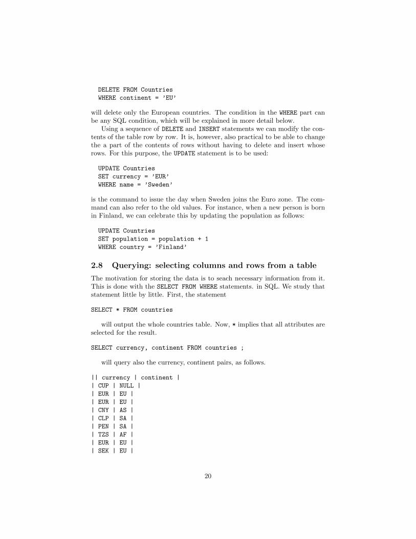
SELECT currency, continent FROM countries ;
will query also the currency, continent pairs, as follows.
|| currency | continent |
| CUP | NULL |
| EUR | EU |
| EUR | EU |
| CNY | AS |
| CLP | SA |
| PEN | SA |
| TZS | AF |
| EUR | EU |
| SEK | EU |
20
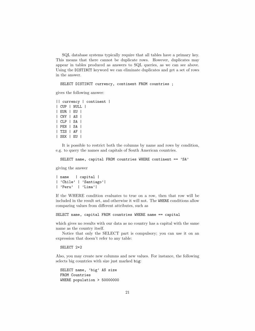
SQL database systems typically require that all tables have a primary key.This means that there cannot be duplicate rows. However, duplicates mayappear in tables produced as answers to SQL queries, as we can see above.Using the DISTINCT keyword we can eliminate duplicates and get a set of rowsin the answer.
SELECT DISTINCT currency, continent FROM countries ;
gives the following answer:
|| currency | continent |
| CUP | NULL |
| EUR | EU |
| CNY | AS |
| CLP | SA |
| PEN | SA |
| TZS | AF |
| SEK | EU |
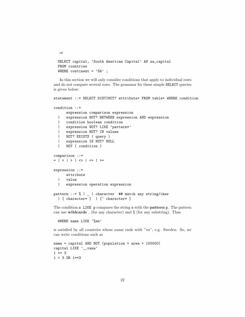
It is possible to restrict both the columns by name and rows by condition,e.g. to query the names and capitals of South American countries.
SELECT name, capital FROM countries WHERE continent == ’SA’
giving the answer
| name | capital |
| ’Chile’ | ’Santiago’|
| ’Peru’ | ’Lima’|
If the WHERE condition evaluates to true on a row, then that row will beincluded in the result set, and otherwise it will not. The WHERE conditions allowcomparing values from different attributes, such as
SELECT name, capital FROM countries WHERE name == capital
which gives no results with our data as no country has a capital with the samename as the country itself.
Notice that only the SELECT part is compulsory; you can use it on anexpression that doesn’t refer to any table:
SELECT 2+2
Also, you may create new columns and new values. For instance, the followingselects big countries with size just marked big:
SELECT name, ’big’ AS size
FROM Countries
WHERE population > 50000000
21
or
SELECT capital, ’South American Capital’ AS sa_capital
FROM countries
WHERE continent = ’SA’ ;
In this section we will only consider conditions that apply to individual rowsand do not compare several rows. The grammar for these simple SELECT queriesis given below:
statement ::= SELECT DISTINCT? attribute+ FROM table+ WHERE condition
condition ::=
expression comparison expression
| expression NOT? BETWEEN expression AND expression
| condition boolean condition
| expression NOT? LIKE ’pattern*’
| expression NOT? IN values
| NOT? EXISTS ( query )
| expression IS NOT? NULL
| NOT ( condition )
comparison ::=
= | < | > | <> | <= | >=
expression ::=
attribute
| value
| expression operation expression
pattern ::= % | _ | character ## match any string/char
| [ character* ] | [^ character* ]
The condition s LIKE p compares the string s with the pattern p. The patterncan use wildcards (for any character) and % (for any substring). Thus
WHERE name LIKE ’%en’
is satisfied by all countries whose name ends with ”en”, e.g. Sweden. So, wecan write conditions such as
name = capital AND NOT (population > area + 100000)
capital LIKE ’__vana’
1 == 3
1 < 3 OR 1==3
22
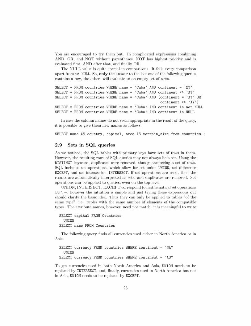
You are encouraged to try them out. In complicated expressions combiningAND, OR, and NOT without parentheses, NOT has highest priority and isevaluated first, AND after that, and finally OR.
The NULL value is quite special in comparisons. It fails every comparisonapart from is NULL. So, only the answer to the last one of the following queriescontains a row, the others will evaluate to an empty set of rows.
SELECT * FROM countries WHERE name = ’Cuba’ AND continent = ’XY’
SELECT * FROM countries WHERE name = ’Cuba’ AND continent <> ’XY’
SELECT * FROM countries WHERE name = ’Cuba’ AND (continent = ’XY’ OR
continent <> ’XY’)
SELECT * FROM countries WHERE name = ’Cuba’ AND continent is not NULL
SELECT * FROM countries WHERE name = ’Cuba’ AND continent is NULL
In case the column names do not seem appropriate in the result of the query,it is possible to give them new names as follows.
SELECT name AS country, capital, area AS terrain_size from countries ;
2.9 Sets in SQL queries
As we noticed, the SQL tables with primary keys have sets of rows in them.However, the resulting rows of SQL queries may not always be a set. Using theDISTINCT keyword, duplicates were removed, thus guaranteeing a set of rows.SQL includes set operations, which allow for set union UNION, set differenceEXCEPT, and set intersection INTERSECT. If set operations are used, then theresults are automatically interpreted as sets, and duplicates are removed. Setoperations can be applied to queries, even on the top level.
UNION, INTERSECT, EXCEPT correspond to mathematical set operations∪,∩,−, however the intuition is simple and just trying these expressions outshould clarify the basic idea. Thus they can only be applied to tables ”of thesame type”, i.e. tuples with the same number of elements of the compatibletypes. The attribute names, however, need not match: it is meaningful to write
SELECT capital FROM Countries
UNION
SELECT name FROM Countries
The following query finds all currencies used either in North America or inAsia.
SELECT currency FROM countries WHERE continent = "NA"
UNION
SELECT currency FROM countries WHERE continent = "AS"
To get currencies used in both North America and Asia, UNION needs to bereplaced by INTERSECT, and, finally, currencies used in North America but notin Asia, UNION needs to be replaced by EXCEPT.
23
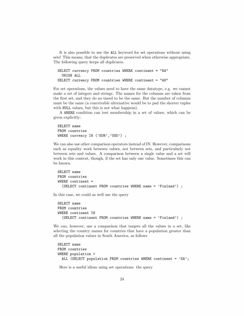
It is also possible to use the ALL keyword for set operations without usingsets! This means, that the duplicates are preserved when otherwise appropriate.The following query keeps all duplicates.
SELECT currency FROM countries WHERE continent = "NA"
UNION ALL
SELECT currency FROM countries WHERE continent = "AS"
For set operations, the values need to have the same datatype, e.g. we cannotmake a set of integers and strings. The names for the columns are taken fromthe first set, and they do no tneed to be the same. But the number of columnsmust be the same (a conceivable alternative would be to pad the shorter tupleswith NULL values, but this is not what happens).
A WHERE condition can test membership in a set of values, which can begiven explicitly:
SELECT name
FROM countries
WHERE currency IN (’EUR’,’USD’) ;
We can also use other comparison operators instead of IN. However, comparisonssuch as equality work between values, not between sets, and particularly notbetween sets and values. A comparison between a single value and a set willwork in this context, though, if the set has only one value. Sometimes this canbe known.
SELECT name
FROM countries
WHERE continent =
(SELECT continent FROM countries WHERE name = ’Finland’) ;
In this case, we could as well use the query
SELECT name
FROM countries
WHERE continent IN
(SELECT continent FROM countries WHERE name = ’Finland’) ;
We can, however, use a comparison that targets all the values in a set, likeselecting the country names for countries that have a population greater thanall the population values in South America, as follows
SELECT name
FROM countries
WHERE population >
ALL (SELECT population FROM countries WHERE continent = ’SA’;
Here is a useful idiom using set operations: the query
24
SELECT name, ’big’ AS size
FROM countries WHERE population >= 50000000
UNION
SELECT name, ’small’ AS size
FROM countries WHERE population < 50000000
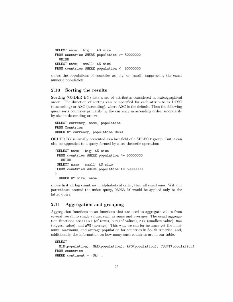
shows the populations of countries as ’big’ or ’small’, suppressing the exactnumeric population.
2.10 Sorting the results
Sorting (ORDER BY) lists a set of attributes considered in lexicographicalorder. The direction of sorting can be specified for each attribute as DESC(descending) or ASC (ascending), where ASC is the default. Thus the followingquery sorts countries primarily by the currency in ascending order, secondarilyby size in descending order:
SELECT currency, name, population
FROM Countries
ORDER BY currency, population DESC
ORDER BY is usually presented as a last field of a SELECT group. But it canalso be appended to a query formed by a set-theoretic operation:
(SELECT name, ’big’ AS size
FROM countries WHERE population >= 50000000
UNION
SELECT name, ’small’ AS size
FROM countries WHERE population >= 50000000
)
ORDER BY size, name
shows first all big countries in alphabetical order, then all small ones. Withoutparentheses around the union query, ORDER BY would be applied only to thelatter query.
2.11 Aggregation and grouping
Aggregation functions mean functions that are used to aggregate values fromseveral rows into single values, such as sums and averages. The usual aggrega-tion functions are COUNT (of rows), SUM (of values), MIN (smallest value), MAX(biggest value), and AVG (average). This way, we can for instance get the mini-mum, maximum, and average population for countries in South America, and,additionally, the information on how many such countries are in our table.
SELECT
MIN(population), MAX(population), AVG(population), COUNT(population)
FROM countries
WHERE continent = ’SA’ ;
25
We can also group the rows by continent and then calculate the values forall continents, using the GROUP BY construction, as follows
SELECT
MIN(population), MAX(population), AVG(population), COUNT(population)
FROM countries
GROUP BY continent ;
WHERE is used to write conditions on which rows are selected to the result.We can also restrict the result set using values obtained in aggregation, usingthe HAVING construct, e.g. to calculate the statistics only when there are rowsfrom at least 2 countries of a continent:
SELECT
MIN(population), MAX(population), AVG(population)
FROM countries
GROUP BY continent
HAVING COUNT (population) > 1;
Removing duplicates by the DISTINCT keyword also works inside aggrega-tions:
SELECT DISTINCT currency
SELECT COUNT(DISTINCT currency)
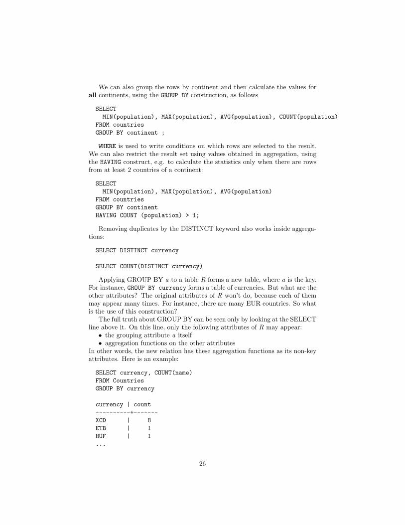
Applying GROUP BY a to a table R forms a new table, where a is the key.For instance, GROUP BY currency forms a table of currencies. But what are theother attributes? The original attributes of R won’t do, because each of themmay appear many times. For instance, there are many EUR countries. So whatis the use of this construction?
The full truth about GROUP BY can be seen only by looking at the SELECTline above it. On this line, only the following attributes of R may appear:• the grouping attribute a itself• aggregation functions on the other attributes
In other words, the new relation has these aggregation functions as its non-keyattributes. Here is an example:
SELECT currency, COUNT(name)
FROM Countries
GROUP BY currency
currency | count
----------+-------
XCD | 8
ETB | 1
HUF | 1
...
26

Now, most rows in this table will have count 1. We may be interested in onlythose currencies that are used by more than one country. The standard way ofdoing this is by a subquery:
SELECT *
FROM (
SELECT currency, COUNT(name) AS number
FROM Countries
GROUP BY currency) AS C
WHERE number > 1
This shows clearly that GROUP BY really forms a table. But SQL also providesa shorthand way of expressing conditions on the groups (i.e. the rows of therelation formed by GROUP BY): HAVING:
SELECT currency, COUNT(name)
FROM Countries
GROUP BY currency
HAVING COUNT(name) > 1
If you want to order this from the biggest to the smallest count, just add theline
ORDER BY COUNT(name) DESC
currency | count
----------+-------
EUR | 35
USD | 17
XOF | 8
...
The other aggregation functions (SUM, AVG, MAX, MIN) work in the sameway. The grouped table can have more than one of them:
SELECT currency, COUNT(name), AVG(population)
FROM countries
GROUP BY currency
As a final subtlety: the relation formed by GROUP BY also contains the ag-gregations used in the HAVING clause or the ORDER BY clause:
SELECT currency, AVG(population)
FROM Countries
GROUP BY currency
HAVING COUNT(name) > 1
SELECT currency, AVG(population)
27
FROM Countries
GROUP BY currency
ORDER BY COUNT(name) DESC
From the semantic point of view, GROUP BY is thus a very complex operator,because one has to look at many different places to see exactly what relation itforms. We will get more clear about this when looking at relational algebra andquery compilation in Chapter 6
2.12 Using data from several tables
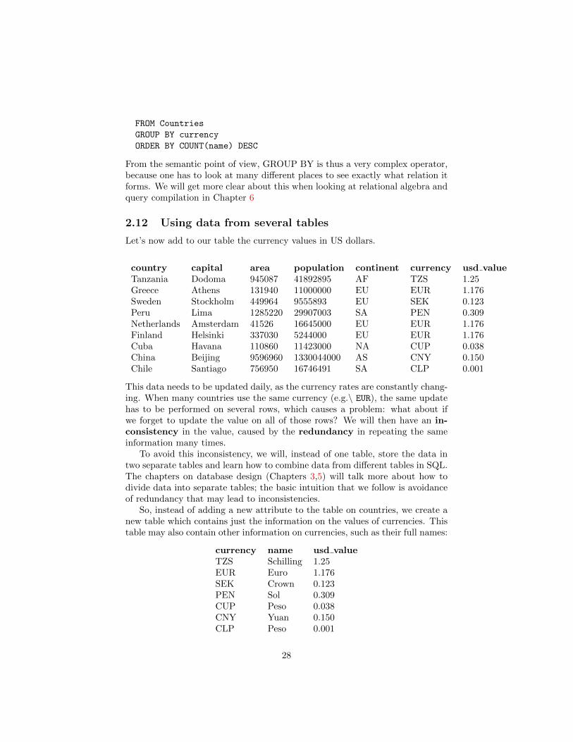
Let’s now add to our table the currency values in US dollars.
country capital area population continent currency usd valueTanzania Dodoma 945087 41892895 AF TZS 1.25Greece Athens 131940 11000000 EU EUR 1.176Sweden Stockholm 449964 9555893 EU SEK 0.123Peru Lima 1285220 29907003 SA PEN 0.309Netherlands Amsterdam 41526 16645000 EU EUR 1.176Finland Helsinki 337030 5244000 EU EUR 1.176Cuba Havana 110860 11423000 NA CUP 0.038China Beijing 9596960 1330044000 AS CNY 0.150Chile Santiago 756950 16746491 SA CLP 0.001
This data needs to be updated daily, as the currency rates are constantly chang-ing. When many countries use the same currency (e.g.\ EUR), the same updatehas to be performed on several rows, which causes a problem: what about ifwe forget to update the value on all of those rows? We will then have an in-consistency in the value, caused by the redundancy in repeating the sameinformation many times.
To avoid this inconsistency, we will, instead of one table, store the data intwo separate tables and learn how to combine data from different tables in SQL.The chapters on database design (Chapters 3,5) will talk more about how todivide data into separate tables; the basic intuition that we follow is avoidanceof redundancy that may lead to inconsistencies.
So, instead of adding a new attribute to the table on countries, we create anew table which contains just the information on the values of currencies. Thistable may also contain other information on currencies, such as their full names:
currency name usd valueTZS Schilling 1.25EUR Euro 1.176SEK Crown 0.123PEN Sol 0.309CUP Peso 0.038CNY Yuan 0.150CLP Peso 0.001
28
The SQL statement to create the table is
CREATE TABLE currencies (
code TEXT PRIMARY KEY,
name TEXT,
usd_value FLOAT )
Now that we have split the information about countries to two separatetables, we need a way to combine that information. The general term for thisis joining the tables. We will below introduce a set of JOIN operations in SQL.But a more elementary method is to use the WHERE part of SELECT FROM WHERE
statements - to give a list of tables that are used, instead of just one table.Let us star with a table that shows, for each country, its capital and its
currency code:
SELECT capital, code
FROM Countries, Currencies
WHERE currency = code
This query compares the currency attribute of Countries with the code at-tribute of Currencies to select the matching rows.
But what about if we want to show the names of the countries and thecurrencies? Following the model of the previous query, we would have
SELECT name, name
FROM Countries, Currencies
WHERE currency = code
This query is not understandable to a human, neither is it to a database system.This is because now both Countries and Currencies contain a column namedname, and it is not clear which one is referred to in the query. The solution isto use qualified names where the attribute is prefixed by the table name:
SELECT Countries.name, Currencies.name
FROM Countries, Currencies
WHERE currency = code
We can also introduce shorthand names to the tables with the AS construct, anduse these names elsewhere in the table (recalling that the FROM part, where thenames are introduced, is executed first in SQL):
SELECT co.name, cu.name
FROM Countries AS co, Currencies AS cu
WHERE co.currency = cu.code
The first step in evaluating a query is to form the table in accordance withthe FROM part. When it has two tables like here, their cartesian product isformed first: a table where each row of Countries is paired with each row of
29
Currencies. This is of course a large table: it has 9 × 7 = 63 rows, becauseCountries has 9 rows and Currencies has 7. But the WHERE clause shrinks itssize to 9, because the currency is the same code on only 9 of the rows. 2
The condition is in the WHERE part is called a join condition, as it controlshow rows from tables are joined together. We can state also other conditions inthe WHERE part, e.g. WHERE co.currency = cu.currency AND co.continent
= ’EU’ would only include European countries. Leaving out a join conditionwill produce all pairs of rows - the whole cartesian project - in the result. Thereader is urged to try out e.g.
SELECT name.capital, currencies.name
FROM countries, currencies
and see the big table that results. (Hint: you can use COUNT(*) on the SELECT
line to see the number of rows created.)
2.13 Foreign keys and references
The natural way to join data from two table is to compare the keys of the tables.For instance, currency values in Countries are intended to match code valuesin Currencies. If we want to require this to always be the case, we can usea FOREIGN KEY clause within the CREATE TABLE statement for Countries. Wecan either do this next to the column declaration,
currency REFERENCES Currencies(code)
or add a constraint to the end of the statement,
FOREIGN KEY currency REFERENCES Currencies(code)
If the foreign key is composite, only the latter method works, just as withprimary keys.
The FOREIGN KEY clause in the CREATE TABLE statement for Countries addsa requirement that every value in the column for currencies must be founduniquely found in the code column of the currencies table. It is the job ofa database management system to check this requirement, prohibiting all dele-tions from Currencies or inserts so Countries that would violate the foreignkey requirement. In this way, the database management system maintains theintegrity of the database.
Any conditions in the WHERE part can be used for joining data from tables.However, there are some particularly interesting cases, like joining a table withitself. Consider the following query listing the names of pairs of countries thathave the same currency:
2In practice, SQL systems are smart enough not to build the large cartesian products if itis possible to optimize the query and shrink the table in advance. Chapter 6 will show someways in which this is done.
30
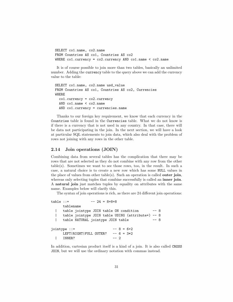
SELECT co1.name, co2.name
FROM Countries AS co1, Countries AS co2
WHERE co1.currency = co2.currency AND co1.name < co2.name
It is of course possible to join more than two tables, basically an unlimitednumber. Adding the currency table to the query above we can add the currencyvalue to the table:
SELECT co1.name, co2.name usd_value
FROM Countries AS co1, Countries AS co2, Currencies
WHERE
co1.currency = co2.currency
AND co1.name < co2.name
AND co1.currency = currencies.name
Thanks to our foreign key requirement, we know that each currency in theCountries table is found in the Currencies table. What we do not know isif there is a currency that is not used in any country. In that case, there willbe data not participating in the join. In the next section, we will have a lookat particular SQL statements to join data, which also deal with the problem ofrows not joining with any rows in the other table.
2.14 Join operations (JOIN)
Combining data from several tables has the complication that there may berows that are not selected as they do not combine with any row from the othertable(s). Sometimes we want to see those rows, too, in the result. In such acase, a natural choice is to create a new row which has some NULL values inthe place of values from other table(s). Such an operation is called outer join,whereas only selecting tuples that combine successfully is called an inner join.A natural join just matches tuples by equality on attributes with the samename. Examples below will clarify this.
The syntax of join operations is rich, as there are 24 different join operations:
table ::= -- 24 = 8+8+8
tablename
| table jointype JOIN table ON condition -- 8
| table jointype JOIN table USING (attribute+) -- 8
| table NATURAL jointype JOIN table -- 8
jointype ::= -- 8 = 6+2
LEFT|RIGHT|FULL OUTER? -- 6 = 3*2
| INNER? -- 2
In addition, cartesian product itself is a kind of a join. It is also called CROSS
JOIN, but we will use the ordinary notation with commas instead.
31
Luckily, the JOINs have a compositional meaning. INNER is the simplestjoin type, and the keyword can be omitted without change of meaning. ThisJOIN with an ON condition gives the purest form of join, similar to cartesianproduct with a WHERE clause:
FROM table1 JOIN table2 ON condition
is equivalent to
FROM table1, table2
WHERE condition
The condition is typically looking for attributes with equal values in the twotables. With good luck (or design) such attributes have the same name, andone can write
L JOIN R USING (a,b)
as a shorthand for
L JOIN R ON L.a = R.a AND L.b = R.b
well... almost, since when JOIN is used with ON, it repeats the values of a an bfrom both tables, like the cartesian product does. JOIN with USING eliminatesthe duplicates of the attributes in USING.
An important special case is NATURAL JOIN, where no conditions are needed.It is equivalent to
L JOIN R USING (a,b,c,...)
which lists all common attributes of L and R.Cross join, inner joins, and natural join only include tuples where the join
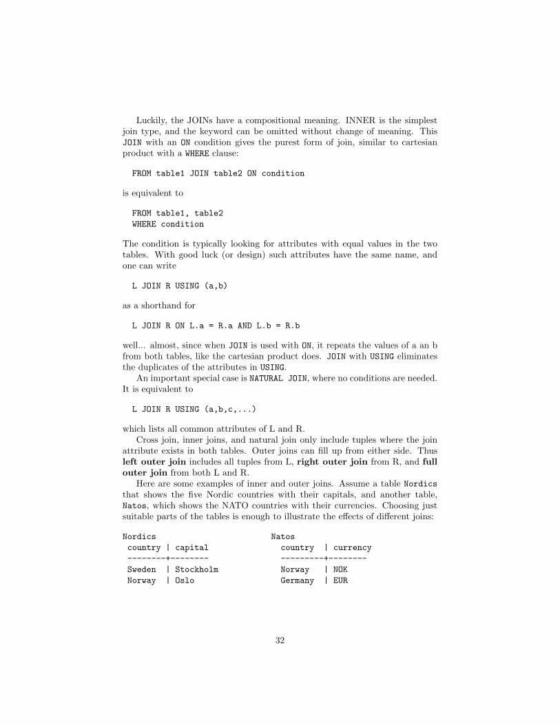
attribute exists in both tables. Outer joins can fill up from either side. Thusleft outer join includes all tuples from L, right outer join from R, and fullouter join from both L and R.
Here are some examples of inner and outer joins. Assume a table Nordics
that shows the five Nordic countries with their capitals, and another table,Natos, which shows the NATO countries with their currencies. Choosing justsuitable parts of the tables is enough to illustrate the effects of different joins:
Nordics Natos
country | capital country | currency
--------+-------- ---------+--------
Sweden | Stockholm Norway | NOK
Norway | Oslo Germany | EUR
32
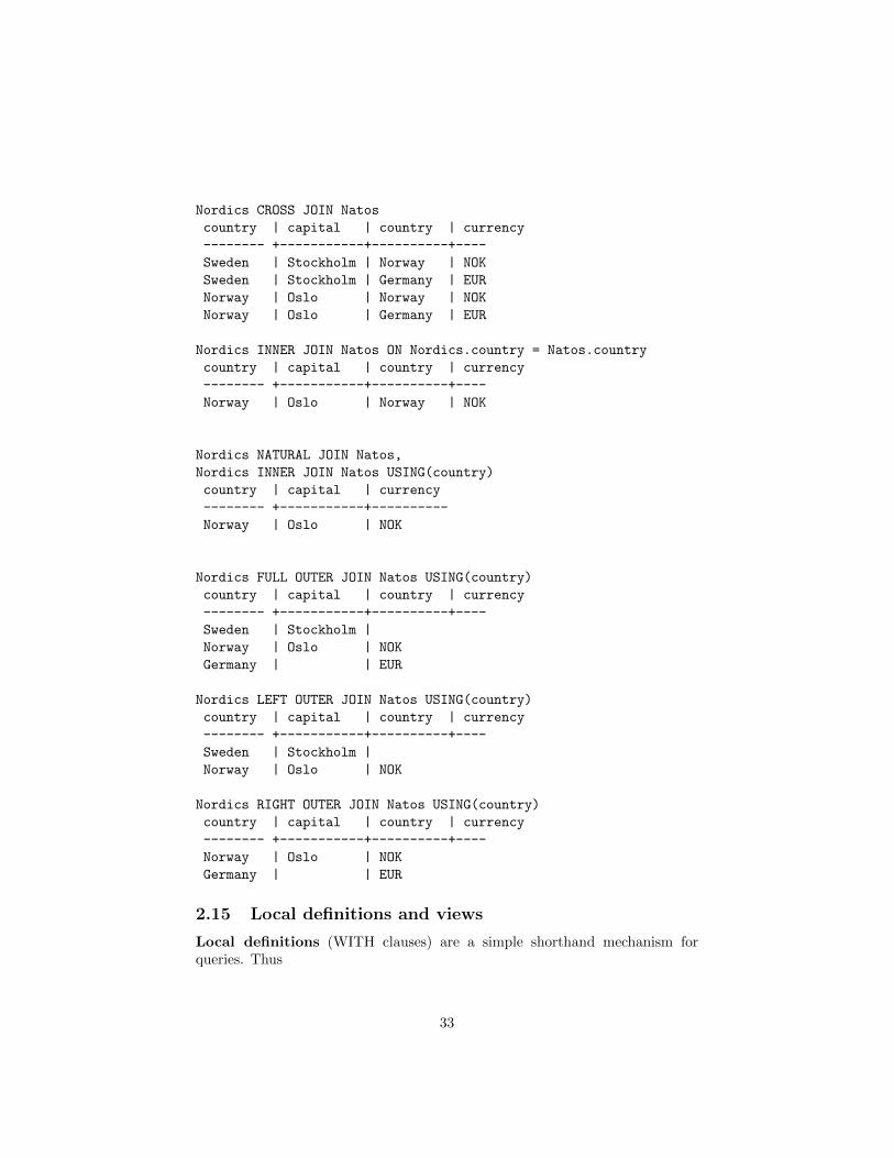
Nordics CROSS JOIN Natos
country | capital | country | currency
-------- +-----------+----------+----
Sweden | Stockholm | Norway | NOK
Sweden | Stockholm | Germany | EUR
Norway | Oslo | Norway | NOK
Norway | Oslo | Germany | EUR
Nordics INNER JOIN Natos ON Nordics.country = Natos.country
country | capital | country | currency
-------- +-----------+----------+----
Norway | Oslo | Norway | NOK
Nordics NATURAL JOIN Natos,
Nordics INNER JOIN Natos USING(country)
country | capital | currency
-------- +-----------+----------
Norway | Oslo | NOK
Nordics FULL OUTER JOIN Natos USING(country)
country | capital | country | currency
-------- +-----------+----------+----
Sweden | Stockholm |
Norway | Oslo | NOK
Germany | | EUR
Nordics LEFT OUTER JOIN Natos USING(country)
country | capital | country | currency
-------- +-----------+----------+----
Sweden | Stockholm |
Norway | Oslo | NOK
Nordics RIGHT OUTER JOIN Natos USING(country)
country | capital | country | currency
-------- +-----------+----------+----
Norway | Oslo | NOK
Germany | | EUR
2.15 Local definitions and views
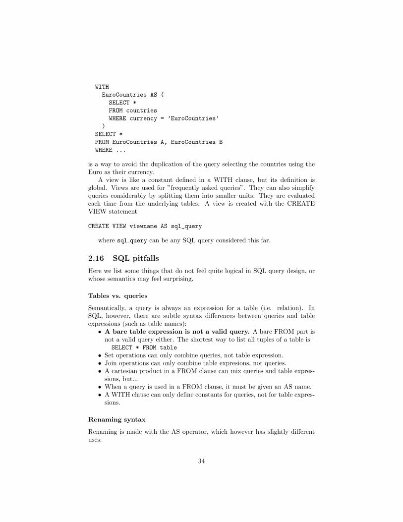
Local definitions (WITH clauses) are a simple shorthand mechanism forqueries. Thus
33
WITH
EuroCountries AS (
SELECT *
FROM countries
WHERE currency = ’EuroCountries’
)
SELECT *
FROM EuroCountries A, EuroCountries B
WHERE ...
is a way to avoid the duplication of the query selecting the countries using theEuro as their currency.
A view is like a constant defined in a WITH clause, but its definition isglobal. Views are used for ”frequently asked queries”. They can also simplifyqueries considerably by splitting them into smaller units. They are evaluatedeach time from the underlying tables. A view is created with the CREATEVIEW statement
CREATE VIEW viewname AS sql_query
where sql query can be any SQL query considered this far.
2.16 SQL pitfalls
Here we list some things that do not feel quite logical in SQL query design, orwhose semantics may feel surprising.
Tables vs. queries
Semantically, a query is always an expression for a table (i.e. relation). InSQL, however, there are subtle syntax differences between queries and tableexpressions (such as table names):• A bare table expression is not a valid query. A bare FROM part is
not a valid query either. The shortest way to list all tuples of a table isSELECT * FROM table
• Set operations can only combine queries, not table expression.• Join operations can only combine table expresions, not queries.• A cartesian product in a FROM clause can mix queries and table expres-
sions, but...• When a query is used in a FROM clause, it must be given an AS name.• A WITH clause can only define constants for queries, not for table expres-
sions.
Renaming syntax
Renaming is made with the AS operator, which however has slightly differentuses:
34

• In WITH clauses, the name is before the definition: name AS (query).• In SELECT parts, the name is after the definition: expression AS name.• In FROM parts, the name is after the definition but AS may be omitted:table AS? name.
Cartesian products
The bare cartesian product from a FROM clause can be a huge table, sincethe sizes are multiplied. With the same logic, if the product contains an emptytable, its size is always 0. Then it does not matter that the empty table mightbe ”irrelevant”:
SELECT A.a FROM A, Empty
results in an empty table. This is actually easy to understand, if you keep inmind that the FROM part is executed before the SELECT part.
NULL values and three-valued logic
Because of NULL values, SQL follows a three-valued logic: TRUE, FALSE,UNKNOWN. The truth tables as such are natural. But the way they are usedin e.g WHERE clauses is good to keep in mind. Recalling that a comparisonwith NULL results in UNKNOWN, and that WHERE clauses only select TRUEinstances, the query
SELECT ...
FROM ...
WHERE v = v
gives no results for tuples where v is NULL. The same concerns
SELECT ...
FROM ...
WHERE v < 10 OR v >= 10
Hence if v is NULL, SQL does not even be assume that it has the same valuein all occurrences.
Another example, given in
https://www.simple-talk.com/sql/t-sql-programming/ten-common-sql-programming-mistakes/
as the first one among the ”Ten common SQL mistakes”, involves NOT IN:since
u NOT IN (1,2,v)
means
35

NOT (u = 1 OR u = 2 OR u = v)
this evaluates to UNKNOWN if v is NULL. In that case, NOT IN is useless as atest.
More precisely, conditions have a three-valued logic, because of the presenceof NULL. Comparisons with NULL always result in UNKNOWN. Logical oper-ators have the following meanings (T = TRUE, F = FALSE, U = UNKNOWN)
p q NOT p p AND q p OR qT T F T TT F ” F TT U ” U TF T T F TF F ” F FF U ” F UU T U U TU F ” F UU U ” U U
A tuple satisfies a WHERE clause only if it returns T, not one with U. Keep inmind, in particular, that NOT U = U!
Set operations are set operations
Being a set means that duplicates don’t count. This is what holds in the mathe-matical theory of relations (Chapter˜\refrelations). But SQL is usually aboutmultisets, so that duplicates do count. However, the set operations UNION,INTERSECT, EXCEPT do remove duplicates! Hence
SELECT * FROM table
UNION
SELECT * FROM table
has the same effect as
SELECT DISTINCT * FROM table
2.17 SQL in the Query Converter*
Notice: The query converter is an experimental program that you might wantto try. It is in no way a compulsory part of these lectures.
You can find the query converter (command qconv) in
https://github.com/GrammaticalFramework/gf-contrib/blob/master/query-converter/
which contains its source code. There is also an emerging web interface in
http://www.grammaticalframework.org/qconv/
36

The Query Converter has an SQL parser and interpreter, which works much thesame way as the PostgreSQL shell. 3 Thus you can give SQL commands in theqconv shell, and the database is queried and updated accordingly.
The query converter will give access to various concepts of this book, notjust the SQL: relational algebra, E-R diagrams, functional dependencies, SQL.This is the main reason sometimes to use qconv as an SQL interpreter insteadof PostgreSQL.
Only a part of SQL is currently recognized by qconv. The interpreter maymoreover be buggy. The database is only built in memory, not stored on a disk.Thus you should store your work in an SQL source file. Such files can be readwith the i (”import”) command, for instance,
> i countries.sql
which uses the file
https://github.com/GrammaticalFramework/gf-contrib/blob/master/query-converter/countries.sql
3As for , the SQL interpreter is not yet available in the web interface.
37
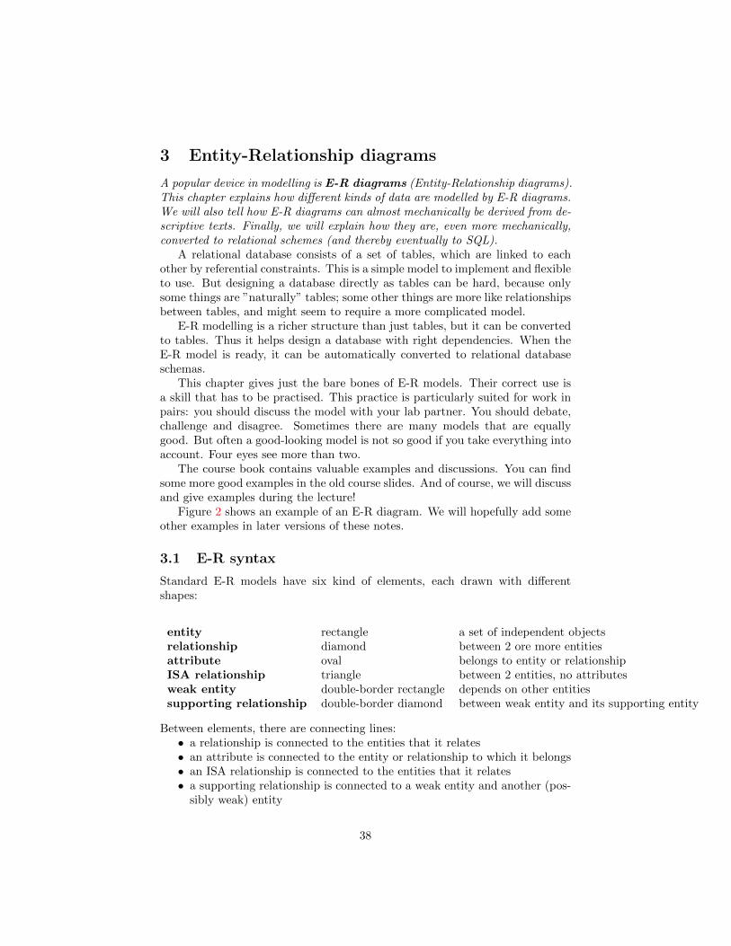
3 Entity-Relationship diagrams
A popular device in modelling is E-R diagrams (Entity-Relationship diagrams).This chapter explains how different kinds of data are modelled by E-R diagrams.We will also tell how E-R diagrams can almost mechanically be derived from de-scriptive texts. Finally, we will explain how they are, even more mechanically,converted to relational schemes (and thereby eventually to SQL).
A relational database consists of a set of tables, which are linked to eachother by referential constraints. This is a simple model to implement and flexibleto use. But designing a database directly as tables can be hard, because onlysome things are ”naturally” tables; some other things are more like relationshipsbetween tables, and might seem to require a more complicated model.
E-R modelling is a richer structure than just tables, but it can be convertedto tables. Thus it helps design a database with right dependencies. When theE-R model is ready, it can be automatically converted to relational databaseschemas.
This chapter gives just the bare bones of E-R models. Their correct use isa skill that has to be practised. This practice is particularly suited for work inpairs: you should discuss the model with your lab partner. You should debate,challenge and disagree. Sometimes there are many models that are equallygood. But often a good-looking model is not so good if you take everything intoaccount. Four eyes see more than two.
The course book contains valuable examples and discussions. You can findsome more good examples in the old course slides. And of course, we will discussand give examples during the lecture!
Figure 2 shows an example of an E-R diagram. We will hopefully add someother examples in later versions of these notes.
3.1 E-R syntax
Standard E-R models have six kind of elements, each drawn with differentshapes:
entity rectangle a set of independent objectsrelationship diamond between 2 ore more entitiesattribute oval belongs to entity or relationshipISA relationship triangle between 2 entities, no attributesweak entity double-border rectangle depends on other entitiessupporting relationship double-border diamond between weak entity and its supporting entity
Between elements, there are connecting lines:• a relationship is connected to the entities that it relates• an attribute is connected to the entity or relationship to which it belongs• an ISA relationship is connected to the entities that it relates• a supporting relationship is connected to a weak entity and another (pos-
sibly weak) entity
38
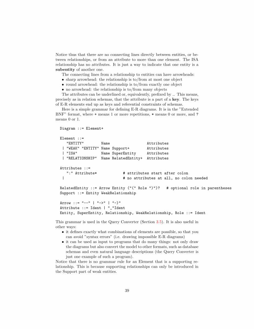
Notice thus that there are no connecting lines directly between entities, or be-tween relationships, or from an attribute to more than one element. The ISArelationship has no attributes. It is just a way to indicate that one entity is asubentity of another one.
The connecting lines from a relationship to entities can have arrowheads:• sharp arrowhead: the relationship is to/from at most one object• round arrowhead: the relationship is to/from exactly one object• no arrowhead: the relationship is to/from many objectsThe attributes can be underlined or, equivalently, prefixed by . This means,
precisely as in relation schemas, that the attribute is a part of a key. The keysof E-R elements end up as keys and referential constraints of schemas.
Here is a simple grammar for defining E-R diagrams. It is in the ”ExtendedBNF” format, where + means 1 or more repetitions, * means 0 or more, and ?
means 0 or 1.
Diagram ::= Element+
Element ::=
"ENTITY" Name Attributes
| "WEAK" "ENTITY" Name Support+ Attributes
| "ISA" Name SuperEntity Attributes
| "RELATIONSHIP" Name RelatedEntity+ Attributes
Attributes ::=
":" Attribute* # attributes start after colon
| # no attributes at all, no colon needed
RelatedEntity ::= Arrow Entity ("(" Role ")")? # optional role in parentheses
Support ::= Entity WeakRelationship
Arrow ::= "--" | "->" | "-)"
Attribute ::= Ident | "_"Ident
Entity, SuperEntity, Relationship, WeakRelationship, Role ::= Ident
This grammar is used in the Query Converter (Section 3.5). It is also useful inother ways:• it defines exactly what combinations of elements are possible, so that you
can avoid ”syntax errors” (i.e. drawing impossible E-R diagrams)• it can be used as input to programs that do many things: not only draw
the diagrams but also convert the model to other formats, such as databaseschemas and even natural language descriptions (the Query Converter isjust one example of such a program).
Notice that there is no grammar rule for an Element that is a supporting re-lationship. This is because supporting relationships can only be introduced inthe Support part of weak entities.
39
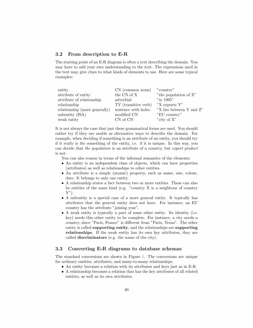
3.2 From description to E-R
The starting point of an E-R diagram is often a text describing the domain. Youmay have to add your own understanding to the text. The expressions used inthe text may give clues to what kinds of elements to use. Here are some typicalexamples:
entity CN (common noun) ”country”attribute of entity the CN of X ”the population of X”attribute of relationship adverbial ”in 1995”relationship TV (transitive verb) ”X exports Y”relationship (more generally) sentence with holes ”X lies between Y and Z”subentity (ISA) modified CN ”EU country”weak entity CN of CN ”city of X”
It is not always the case that just these grammatical forms are used. You shouldrather try if they are usable as alternative ways to describe the domain. Forexample, when deciding if something is an attribute of an entity, you should tryif it really is the something of the entity, i.e. if it is unique. In this way, youcan decide that the population is an attribute of a country, but export productis not.
You can also reason in terms of the informal semantics of the elements:• An entity is an independent class of objects, which can have properties
(attributes) as well as relationships to other entities.• An attribute is a simple (atomic) property, such as name, size, colour,
date. It belongs to only one entity.• A relationship states a fact between two or more entities. These can also
be entities of the same kind (e.g. ”country X is a neighbour of countryY”).
• A subentity is a special case of a more general entity. It typically hasattributes that the general entity does not have. For instance, an EUcountry has the attribute ”joining year”.
• A weak entity is typically a part of some other entity. Its identity (i.e.key) needs this other entity to be complete. For instance, a city needs acountry, since ”Paris, France” is different from ”Paris, Texas”. The otherentity is called supporting entity, and the relationships are supportingrelationships. If the weak entity has its own key attributes, they arecalled discriminators (e.g. the name of the city).
3.3 Converting E-R diagrams to database schemas
The standard conversions are shown in Figure 1. The conversions are uniquefor ordinary entities, attributes, and many-to-many relationships.• An entity becomes a relation with its attributes and keys just as in E-R.• A relationship becomes a relation that has the key attributes of all related
entities, as well as its own attributes.
40

Figure 1: Translating E-R diagrams to database schemas. Picture by JonasAlmstrom-Duregard 2015.
41
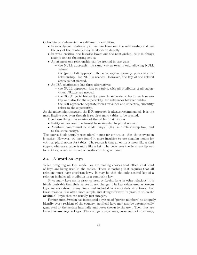
Other kinds of elements have different possibilities:• In exactly-one relationships, one can leave out the relationship and use
the key of the related entity as attribute directly.• In weak entities, one likewise leaves out the relationship, as it is always
exactly-one to the strong entity.• An at-most-one relationship can be treated in two ways:
– the NULL approach: the same way as exactly-one, allowing NULLvalues
– the (pure) E-R approach: the same way as to-many, preserving therelationship. No NULLs needed. However, the key of the relatedentity is not needed.
• An ISA relationship has three alternatives.– the NULL approach: just one table, with all attributes of all suben-
tities. NULLs are needed.– the OO (Object-Oriented) approach: separate tables for each suben-
tity and also for the superentity. No references between tables.– the E-R approach: separate tables for super-and subentity, subentity
refers to the superentity.As the name might suggest, the E-R approach is always recommended. It is themost flexible one, even though it requires more tables to be created.
One more thing: the naming of the tables of attributes.• Entity names could be turned from singular to plural nouns.• Attribute names must be made unique. (E.g. in a relationship from and
to the same entity).The course book actually uses plural nouns for entites, so that the conversionis easier. However, we have found it more intuitive to use singular nouns forentities, plural nouns for tables. The reason is that an entity is more like a kind(type), whereas a table is more like a list. The book uses the term entity setfor entities, which is the set of entities of the given kind.
3.4 A word on keys
When designing an E-R model, we are making choices that effect what kindof keys are being used in the tables. There is nothing that requires that allrelations must have singleton keys. It may be that the only natural key of arelation includes all attributes in a composite key.
Since many keys are in practice used as foreign keys in other relations, it ishighly desirable that their values do not change. The key values used as foreignkeys are also stored many times and included in search data structures. Forthese reasons, it is often more simple and straightforward in practice to createartificial keys that are usually just integers.
For instance, Sweden has introduced a system of ”person numbers” to uniquelyidentify every resident of the country. Artificial keys may also be automaticallygenerated by the system internally and never shown to the user. Then they areknown as surrogate keys. The surrogate keys are guaranteed not to change,
42

Figure 2: An E-R diagram generated from the Query Converter qconv.
whereas natural values, no matter how stable they seem, might do that. An-other related issue is that keys are used to compose indices for the data, usedin joins, and one may not like to grow these structures unnecessarily.
3.5 E-R diagrams in the Query Converter*
In the Query Converter (Section 2.17), you can specify an E-R model using thesyntax described above. For example:
ENTITY Country : _name population
WEAK ENTITY City Country IsCityOf : _name population
ISA EUCountry Country : joiningDate
ENTITY Currency : _code name
RELATIONSHIP UsesAsCurrency -- Country -- Currency
The result is the diagram shown in Figure 2. You will also get a databaseschema:
Country(_name,population)
City(_name,population,_name)
name => Country.name
43
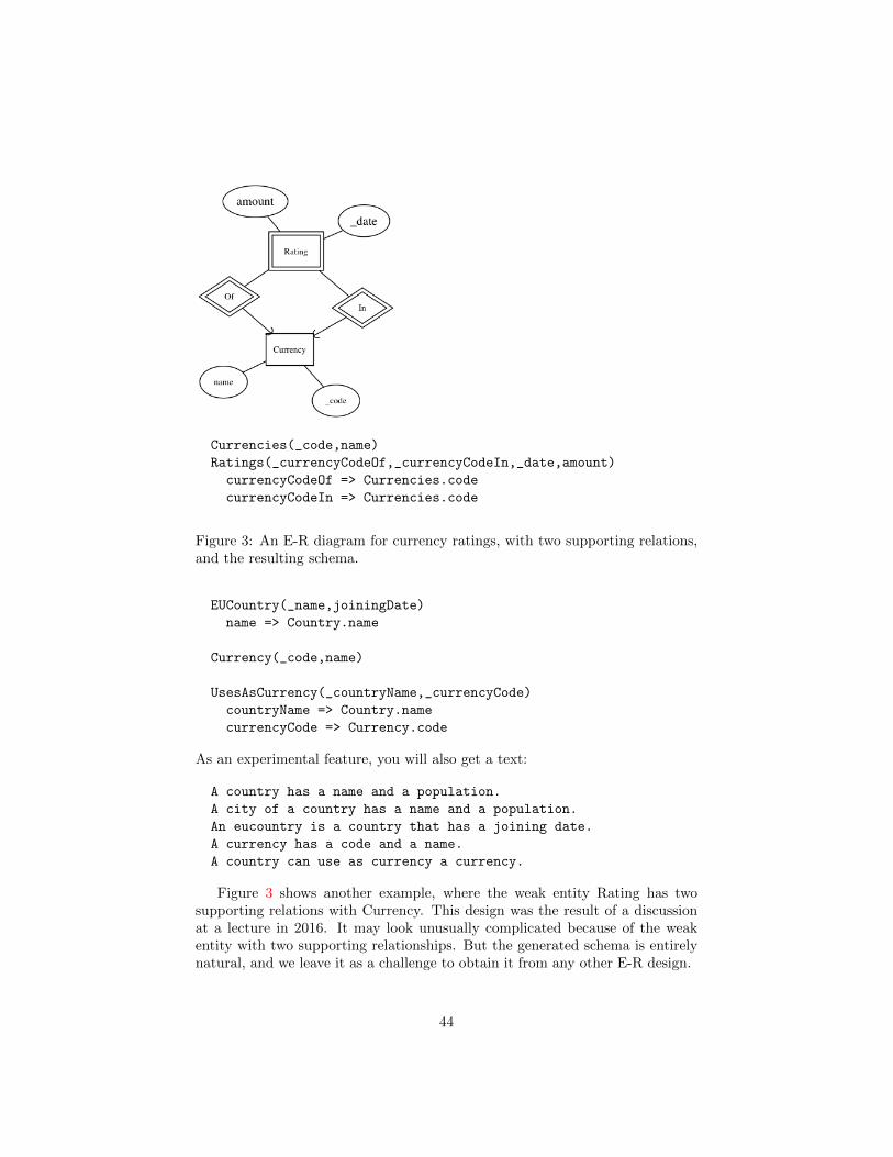
Currencies(_code,name)
Ratings(_currencyCodeOf,_currencyCodeIn,_date,amount)
currencyCodeOf => Currencies.code
currencyCodeIn => Currencies.code
Figure 3: An E-R diagram for currency ratings, with two supporting relations,and the resulting schema.
EUCountry(_name,joiningDate)
name => Country.name
Currency(_code,name)
UsesAsCurrency(_countryName,_currencyCode)
countryName => Country.name
currencyCode => Currency.code
As an experimental feature, you will also get a text:
A country has a name and a population.
A city of a country has a name and a population.
An eucountry is a country that has a joining date.
A currency has a code and a name.
A country can use as currency a currency.
Figure 3 shows another example, where the weak entity Rating has twosupporting relations with Currency. This design was the result of a discussionat a lecture in 2016. It may look unusually complicated because of the weakentity with two supporting relationships. But the generated schema is entirelynatural, and we leave it as a challenge to obtain it from any other E-R design.
44
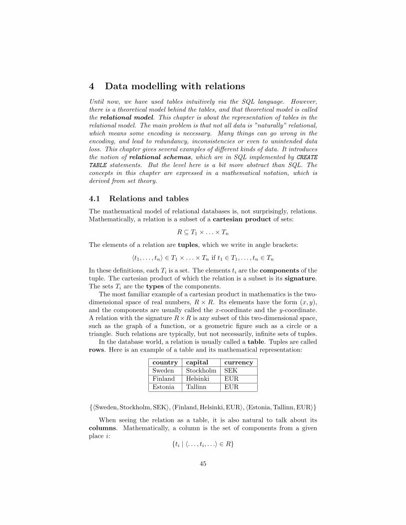
4 Data modelling with relations
Until now, we have used tables intuitively via the SQL language. However,there is a theoretical model behind the tables, and that theoretical model is calledthe relational model. This chapter is about the representation of tables in therelational model. The main problem is that not all data is ”naturally” relational,which means some encoding is necessary. Many things can go wrong in theencoding, and lead to redundancy, inconsistencies or even to unintended dataloss. This chapter gives several examples of different kinds of data. It introducesthe notion of relational schemas, which are in SQL implemented by CREATE
TABLE statements. But the level here is a bit more abstract than SQL. Theconcepts in this chapter are expressed in a mathematical notation, which isderived from set theory.
4.1 Relations and tables
The mathematical model of relational databases is, not surprisingly, relations.Mathematically, a relation is a subset of a cartesian product of sets:
R ⊆ T1 × . . .× Tn
The elements of a relation are tuples, which we write in angle brackets:
〈t1, . . . , tn〉 ∈ T1 × . . .× Tn if t1 ∈ T1, . . . , tn ∈ Tn
In these definitions, each Ti is a set. The elements ti are the components of thetuple. The cartesian product of which the relation is a subset is its signature.The sets Ti are the types of the components.
The most familiar example of a cartesian product in mathematics is the two-dimensional space of real numbers, R × R. Its elements have the form (x, y),and the components are usually called the x -coordinate and the y-coordinate.A relation with the signature R×R is any subset of this two-dimensional space,such as the graph of a function, or a geometric figure such as a circle or atriangle. Such relations are typically, but not necessarily, infinite sets of tuples.
In the database world, a relation is usually called a table. Tuples are calledrows. Here is an example of a table and its mathematical representation:
country capital currencySweden Stockholm SEKFinland Helsinki EUREstonia Tallinn EUR
〈Sweden,Stockholm,SEK〉, 〈Finland,Helsinki,EUR〉, 〈Estonia,Tallinn,EUR〉
When seeing the relation as a table, it is also natural to talk about itscolumns. Mathematically, a column is the set of components from a givenplace i :
ti | 〈. . . , ti, . . .〉 ∈ R
45
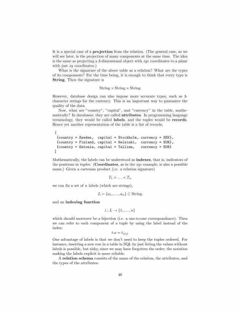
It is a special case of a projection from the relation. (The general case, as wewill see later, is the projection of many components at the same time. The ideais the same as projecting a 3-dimensional object with xyz coordinates to a planewith just xy coordinates.)
What is the signature of the above table as a relation? What are the typesof its components? For the time being, it is enough to think that every type isString. Then the signature is
String× String× String
However, database design can also impose more accurate types, such as 3-character strings for the currency. This is an important way to guarantee thequality of the data.
Now, what are ”country”, ”capital”, and ”currency” in the table, mathe-matically? In databases, they are called attributes. In programming languageterminology, they would be called labels, and the tuples would be records.Hence yet another representation of the table is a list of records,
[
country = Sweden, capital = Stockholm, currency = SEK,
country = Finland, capital = Helsinki, currency = EUR,
country = Estonia, capital = Tallinn, currency = EUR
]
Mathematically, the labels can be understood as indexes, that is, indicators ofthe positions in tuples. (Coordinates, as in the xyz example, is also a possiblename.) Given a cartesian product (i.e. a relation signature)
T1 × . . .× Tn
we can fix a set of n labels (which are strings),
L = a1, . . . , an ⊂ String
and an indexing function
i : L→ 1, . . . , n
which should moreover be a bijection (i.e. a one-to-one correspondance). Thenwe can refer to each component of a tuple by using the label instead of theindex:
t.a = ti(a)
One advantage of labels is that we don’t need to keep the tuples ordered. Forinstance, inserting a new row in a table in SQL by just listing the values withoutlabels is possible, but risky, since we may have forgotten the order; the notationmaking the labels explicit is more reliable.
A relation schema consists of the name of the relation, the attributes, andthe types of the attributes:
46
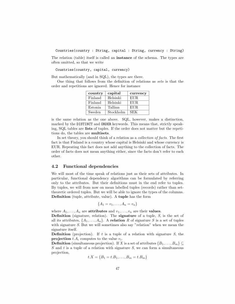
Countries(country : String, capital : String, currency : String)
The relation (table) itself is called an instance of the schema. The types areoften omitted, so that we write
Countries(country, capital, currency)
But mathematically (and in SQL), the types are there.One thing that follows from the definition of relations as sets is that the
order and repetitions are ignored. Hence for instance
country capital currencyFinland Helsinki EURFinland Helsinki EUREstonia Tallinn EURSweden Stockholm SEK
is the same relation as the one above. SQL, however, makes a distinction,marked by the DISTINCT and ORDER keywords. This means that, strictly speak-ing, SQL tables are lists of tuples. If the order does not matter but the repeti-tions do, the tables are multisets.
In set theory, you should think of a relation as a collection of facts. The firstfact is that Finland is a country whose capital is Helsinki and whose currency isEUR. Repeating this fact does not add anything to the collection of facts. Theorder of facts does not mean anything either, since the facts don’t refer to eachother.
4.2 Functional dependencies
We will most of the time speak of relations just as their sets of attributes. Inparticular, functional dependency algorithms can be formulated by referringonly to the attributes. But their definitions must in the end refer to tuples.By tuples, we will from now on mean labelled tuples (records) rather than set-theoretic ordered tuples. But we will be able to ignore the types of the columns.Definition (tuple, attribute, value). A tuple has the form
A1 = v1, . . . , An = vn
where A1, . . . , An are attributes and v1, . . . , vn are their values.Definition (signature, relation). The signature of a tuple, S, is the set ofall its attributes, A1, . . . , An. A relation R of signature S is a set of tupleswith signature S. But we will sometimes also say ”relation” when we mean thesignature itself.Definition (projection). If t is a tuple of a relation with signature S, theprojection t.Ai computes to the value vi.Definition (simultaneous projection). If X is a set of attributes B1, . . . , Bm ⊆S and t is a tuple of a relation with signature S, we can form a simultaneousprojection,
t.X = B1 = t.B1, . . . , Bm = t.Bm
47
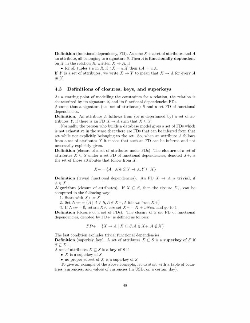
Definition (functional dependency, FD). Assume X is a set of attributes and Aan attribute, all belonging to a signature S. Then A is functionally dependenton X in the relation R, written X → A, if• for all tuples t,u in R, if t.X = u.X then t.A = u.A.
If Y is a set of attributes, we write X → Y to mean that X → A for every Ain Y.
4.3 Definitions of closures, keys, and superkeys
As a starting point of modelling the constraints for a relation, the relation ischaraterized by its signature S, and its functional dependencies FDs.Assume thus a signature (i.e. set of attributes) S and a set FD of functionaldependencies.Definition. An attribute A follows from (or is determined by) a set of at-tributes Y, if there is an FD X → A such that X ⊆ Y .
Normally, the person who builds a database model gives a set of FDs whichis not exhaustive in the sense that there are FDs that can be inferred from thatset while not explicitly belonging to the set. So, when an attribute A followsfrom a set of attributes Y it means that such an FD can be inferred and notnecessarily explicitly given.Definition (closure of a set of attributes under FDs). The closure of a set ofattributes X ⊆ S under a set FD of functional dependencies, denoted X+, isthe set of those attributes that follow from X.
X+ = A | A ∈ S, Y → A, Y ⊆ X
Definition (trivial functional dependencies). An FD X → A is trivial, ifA ∈ X.Algorithm (closure of attributes). If X ⊆ S, then the closure X+, can becomputed in the following way:
1. Start with X+ = X2. Set New = A | A ∈ S,A /∈ X+, A follows from X+3. If New = ∅, return X+, else set X+ = X + ∪New and go to 1
Definition (closure of a set of FDs). The closure of a set FD of functionaldependencies, denoted by FD+, is defined as follows:
FD+ = X → A | X ⊆ S,A ∈ X+, A /∈ X
The last condition excludes trivial functional dependencies.Definition (superkey, key). A set of attributes X ⊆ S is a superkey of S, ifS ⊆ X+.A set of attributes X ⊆ S is a key of S if• X is a superkey of S• no proper subset of X is a superkey of STo give an example of the above concepts, let us start with a table of coun-
tries, currencies, and values of currencies (in USD, on a certain day).
48
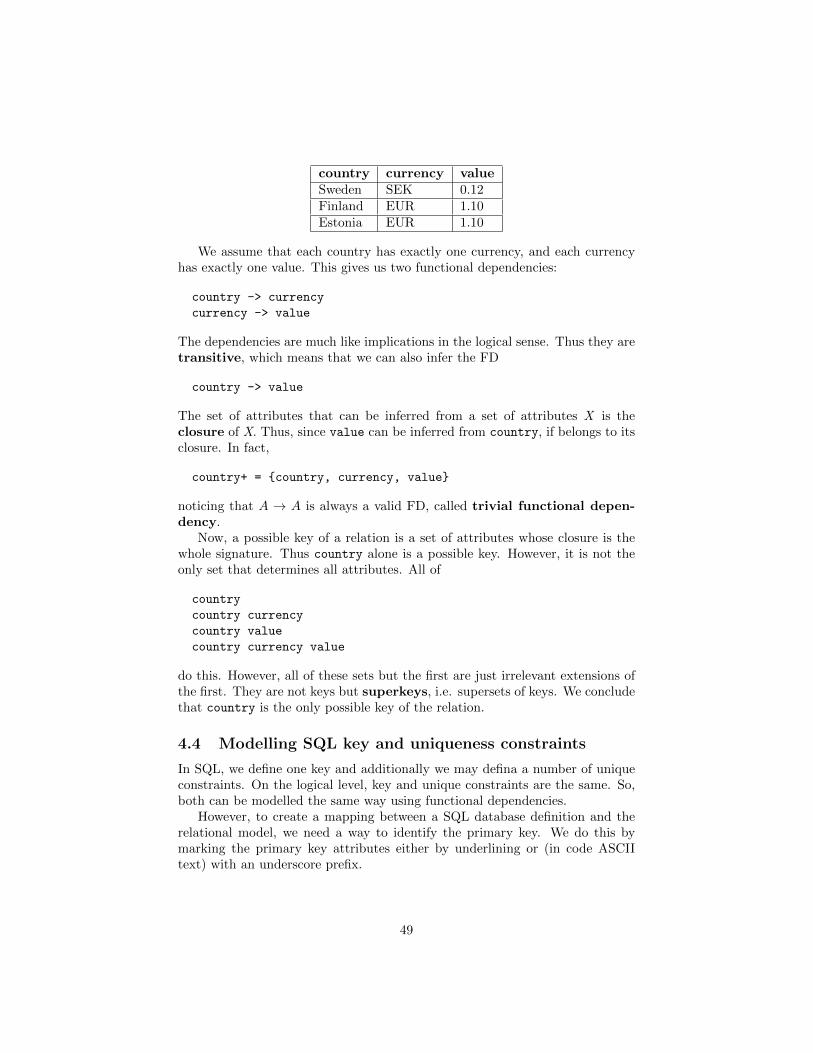
country currency valueSweden SEK 0.12Finland EUR 1.10Estonia EUR 1.10
We assume that each country has exactly one currency, and each currencyhas exactly one value. This gives us two functional dependencies:
country -> currency
currency -> value
The dependencies are much like implications in the logical sense. Thus they aretransitive, which means that we can also infer the FD
country -> value
The set of attributes that can be inferred from a set of attributes X is theclosure of X. Thus, since value can be inferred from country, if belongs to itsclosure. In fact,
country+ = country, currency, value
noticing that A → A is always a valid FD, called trivial functional depen-dency.
Now, a possible key of a relation is a set of attributes whose closure is thewhole signature. Thus country alone is a possible key. However, it is not theonly set that determines all attributes. All of
country
country currency
country value
country currency value
do this. However, all of these sets but the first are just irrelevant extensions ofthe first. They are not keys but superkeys, i.e. supersets of keys. We concludethat country is the only possible key of the relation.
4.4 Modelling SQL key and uniqueness constraints
In SQL, we define one key and additionally we may defina a number of uniqueconstraints. On the logical level, key and unique constraints are the same. So,both can be modelled the same way using functional dependencies.
However, to create a mapping between a SQL database definition and therelational model, we need a way to identify the primary key. We do this bymarking the primary key attributes either by underlining or (in code ASCIItext) with an underscore prefix.
49
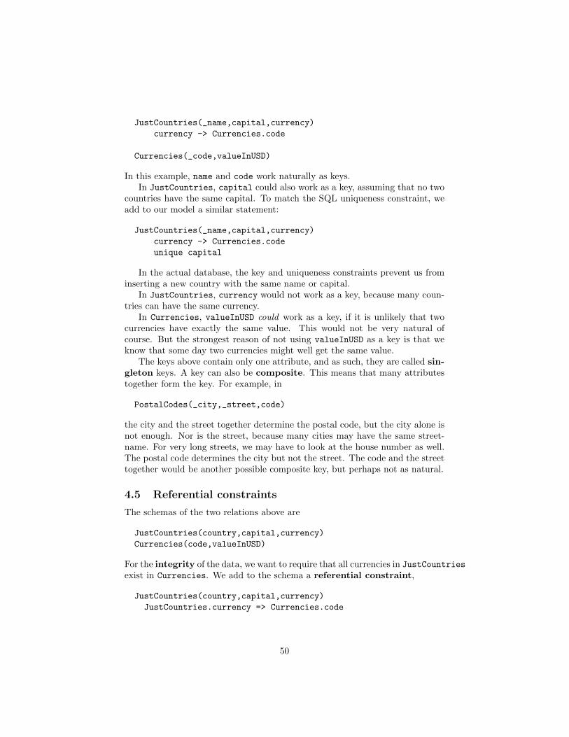
JustCountries(_name,capital,currency)
currency -> Currencies.code
Currencies(_code,valueInUSD)
In this example, name and code work naturally as keys.In JustCountries, capital could also work as a key, assuming that no two
countries have the same capital. To match the SQL uniqueness constraint, weadd to our model a similar statement:
JustCountries(_name,capital,currency)
currency -> Currencies.code
unique capital
In the actual database, the key and uniqueness constraints prevent us frominserting a new country with the same name or capital.
In JustCountries, currency would not work as a key, because many coun-tries can have the same currency.
In Currencies, valueInUSD could work as a key, if it is unlikely that twocurrencies have exactly the same value. This would not be very natural ofcourse. But the strongest reason of not using valueInUSD as a key is that weknow that some day two currencies might well get the same value.
The keys above contain only one attribute, and as such, they are called sin-gleton keys. A key can also be composite. This means that many attributestogether form the key. For example, in
PostalCodes(_city,_street,code)
the city and the street together determine the postal code, but the city alone isnot enough. Nor is the street, because many cities may have the same street-name. For very long streets, we may have to look at the house number as well.The postal code determines the city but not the street. The code and the streettogether would be another possible composite key, but perhaps not as natural.
4.5 Referential constraints
The schemas of the two relations above are
JustCountries(country,capital,currency)
Currencies(code,valueInUSD)
For the integrity of the data, we want to require that all currencies in JustCountries
exist in Currencies. We add to the schema a referential constraint,
JustCountries(country,capital,currency)
JustCountries.currency => Currencies.code
50
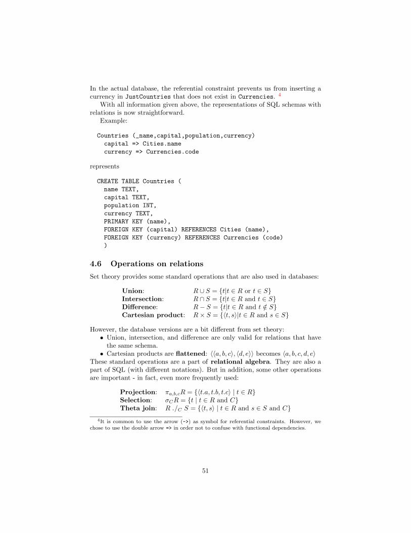
In the actual database, the referential constraint prevents us from inserting acurrency in JustCountries that does not exist in Currencies. 4
With all information given above, the representations of SQL schemas withrelations is now straightforward.
Example:
Countries (_name,capital,population,currency)
capital => Cities.name
currency => Currencies.code
represents
CREATE TABLE Countries (
name TEXT,
capital TEXT,
population INT,
currency TEXT,
PRIMARY KEY (name),
FOREIGN KEY (capital) REFERENCES Cities (name),
FOREIGN KEY (currency) REFERENCES Currencies (code)
)
4.6 Operations on relations
Set theory provides some standard operations that are also used in databases:
Union: R ∪ S = t|t ∈ R or t ∈ SIntersection: R ∩ S = t|t ∈ R and t ∈ SDifference: R− S = t|t ∈ R and t /∈ SCartesian product: R× S = 〈t, s〉|t ∈ R and s ∈ S
However, the database versions are a bit different from set theory:• Union, intersection, and difference are only valid for relations that have
the same schema.• Cartesian products are flattened: 〈〈a, b, c〉, 〈d, e〉〉 becomes 〈a, b, c, d, e〉
These standard operations are a part of relational algebra. They are also apart of SQL (with different notations). But in addition, some other operationsare important - in fact, even more frequently used:
Projection: πa,b,cR = 〈t.a, t.b, t.c〉 | t ∈ RSelection: σCR = t | t ∈ R and CTheta join: R ./C S = 〈t, s〉 | t ∈ R and s ∈ S and C
4It is common to use the arrow (->) as symbol for referential constraints. However, wechose to use the double arrow => in order not to confuse with functional dependencies.
51
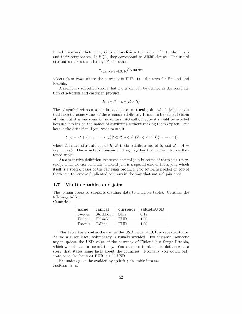
In selection and theta join, C is a condition that may refer to the tuplesand their components. In SQL, they correspond to WHERE clauses. The use ofattributes makes them handy. For instance.
σcurrency=EURCountries
selects those rows where the currency is EUR, i.e. the rows for Finland andEstonia.
A moment’s reflection shows that theta join can be defined as the combina-tion of selection and cartesian product:
R ./C S = σC(R× S)
The ./ symbol without a condition denotes natural join, which joins tuplesthat have the same values of the common attributes. It used to be the basic formof join, but it is less common nowadays. Actually, maybe it should be avoidedbecause it relies on the names of attributes without making them explicit. Buthere is the definition if you want to see it:
R ./S= t+ 〈u.c1, . . . , u.ck〉|t ∈ R, u ∈ S, (∀a ∈ A ∩B)(t.a = u.a)
where A is the attribute set of R, B is the attribute set of S, and B − A =c1, . . . , ck. The + notation means putting together two tuples into one flat-tened tuple.
An alternative definition expresses natural join in terms of theta join (exer-cise!). Thus we can conclude: natural join is a special case of theta join, whichitself is a special cases of the cartesian product. Projection is needed on top oftheta join to remove duplicated columns in the way that natural join does.
4.7 Multiple tables and joins
The joining operator supports dividing data to multiple tables. Consider thefollowing table:Countries:
name capital currency valueInUSDSweden Stockholm SEK 0.12Finland Helsinki EUR 1.09Estonia Tallinn EUR 1.09
This table has a redundancy, as the USD value of EUR is repeated twice.As we will see later, redundancy is usually avoided. For instance, someonemight update the USD value of the currency of Finland but forget Estonia,which would lead to inconsistency. You can also think of the database as astory that states some facts about the countries. Normally you would onlystate once the fact that EUR is 1.09 USD.
Redundancy can be avoided by splitting the table into two:JustCountries:
52
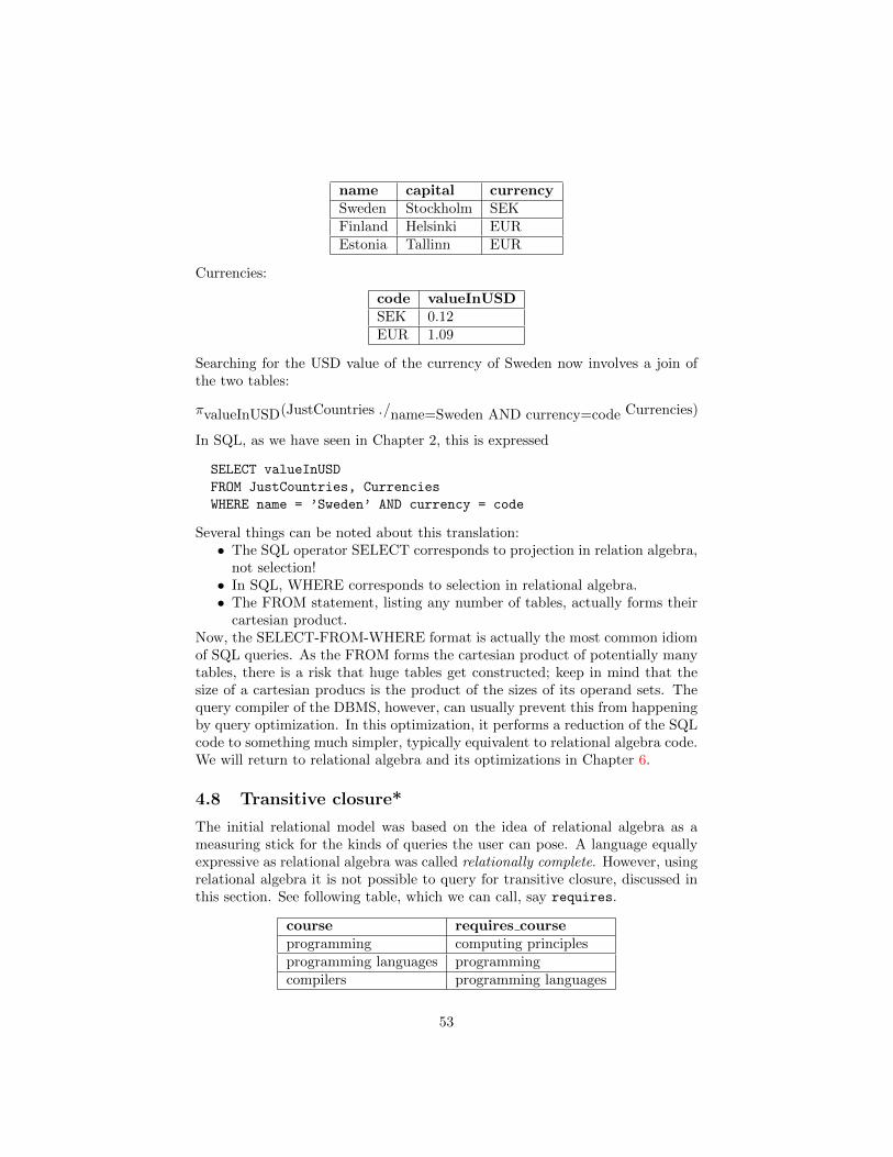
name capital currencySweden Stockholm SEKFinland Helsinki EUREstonia Tallinn EUR
Currencies:
code valueInUSDSEK 0.12EUR 1.09
Searching for the USD value of the currency of Sweden now involves a join ofthe two tables:
πvalueInUSD(JustCountries ./name=Sweden AND currency=code Currencies)
In SQL, as we have seen in Chapter 2, this is expressed
SELECT valueInUSD
FROM JustCountries, Currencies
WHERE name = ’Sweden’ AND currency = code
Several things can be noted about this translation:• The SQL operator SELECT corresponds to projection in relation algebra,
not selection!• In SQL, WHERE corresponds to selection in relational algebra.• The FROM statement, listing any number of tables, actually forms their
cartesian product.Now, the SELECT-FROM-WHERE format is actually the most common idiomof SQL queries. As the FROM forms the cartesian product of potentially manytables, there is a risk that huge tables get constructed; keep in mind that thesize of a cartesian producs is the product of the sizes of its operand sets. Thequery compiler of the DBMS, however, can usually prevent this from happeningby query optimization. In this optimization, it performs a reduction of the SQLcode to something much simpler, typically equivalent to relational algebra code.We will return to relational algebra and its optimizations in Chapter 6.
4.8 Transitive closure*
The initial relational model was based on the idea of relational algebra as ameasuring stick for the kinds of queries the user can pose. A language equallyexpressive as relational algebra was called relationally complete. However, usingrelational algebra it is not possible to query for transitive closure, discussed inthis section. See following table, which we can call, say requires.
course requires courseprogramming computing principlesprogramming languages programmingcompilers programming languages
53
This relation is transitive in the sense that if course B is required for courseA, and course C is required for course B, then course C is also required forcourse A.
Now, how can we compute all courses required for compilers? We candirectly see, just by selection, that programming languages is required. Joiningrequires with itself, and taking a projection and a union, we get a tuple sayingthat also programming is required. A further join with projection and union tothe previous results gives us tuples for all the required courses.
If we know exactly how many times we need to join a relation with itself, wecan answer this question. If not, then it is not doable with relational algebra.
For transitive closure computation, let us consider a transitive relation R
that has only two attributes, the first being called A and the second B. Thus, itonly contains one transitive relation and no additional attributes. The followingrelation composition for two-attribute relations may be used in search of newtransitive relationships:
R ·R = 〈t.A, s.B〉|t ∈ R, s ∈ R, t.B = s.A
We can compute the transitive closure, denoted by R+, by repeatedly replac-ing R by R ∪ (R ·R) as long as the replacement adds new tuples.
If our relational algebra contains attribute renaming, then we can implementrelation composition using join, projection, and attribute renaming.
To implement a practical transitive closure, the following things need to beconsidered:• There may be more than one transitive relationship in a relation as well
as more attributes, and the attributes to be used need to be specified.• Some transitive relationship may not be just from A to B but also at the
same time from B to A. As an example consider a table where each tuplecontains two countries sharing a border and the order is unimportant.
• There may be some other values we want in the result apart from justthe transitive relationship attributes, and their computation needs to bespecified.
• In some cases that transitive relation may be split into different relations.It should, however, be possible to join them first into a single table toavoid this situation.
SQL did not initially contain a transitive closure operation. This lead to the sit-uation that different SQL implementations may contain different ways to specifytransitive closure. The reader is urged to check from online documentation howthis is done in different language implementations such as PostgreSQL.
4.9 Multiple values
The guiding principle of relational databases is that all types of the componentsare atomic. This means that they may not themselves be tuples. This is whatis guaranteed by the flattening of tuples of tuples in the relational version ofthe cartesian product. Another thing that is prohibited is list of values. Think
54
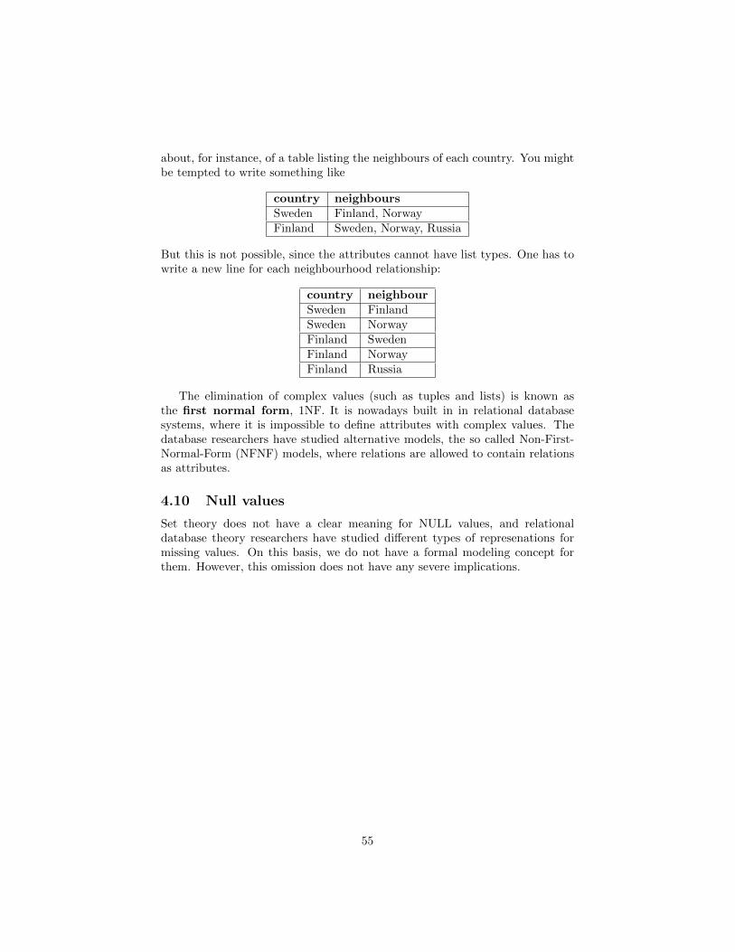
about, for instance, of a table listing the neighbours of each country. You mightbe tempted to write something like
country neighboursSweden Finland, NorwayFinland Sweden, Norway, Russia
But this is not possible, since the attributes cannot have list types. One has towrite a new line for each neighbourhood relationship:
country neighbourSweden FinlandSweden NorwayFinland SwedenFinland NorwayFinland Russia
The elimination of complex values (such as tuples and lists) is known asthe first normal form, 1NF. It is nowadays built in in relational databasesystems, where it is impossible to define attributes with complex values. Thedatabase researchers have studied alternative models, the so called Non-First-Normal-Form (NFNF) models, where relations are allowed to contain relationsas attributes.
4.10 Null values
Set theory does not have a clear meaning for NULL values, and relationaldatabase theory researchers have studied different types of represenations formissing values. On this basis, we do not have a formal modeling concept forthem. However, this omission does not have any severe implications.
55
5 Dependencies and database design
The use of E-R diagrams implies a design that can automatically be producedfrom the E-R design. But is it a good design? To approach that question, wewant to have in independent and more formal definition. This is what functionaldependencies are for. They give us a way to formalize some of the propertiesof good design. They also give methods and algorithms to carry out the design.Functional dependencies are independent of E-R diagrams, but they also addexpressive power: they allow us to define relationships between attributes thatE-R diagrams cannot express. In this chapter, we will define the different kindsof dependencies, study their use, and see how they combine with E-R diagrams.
5.1 Relations vs. functions
Mathematically, a relation can relate an object with many other objects. Forinstance, a country can have many neighbours. A function, on the other hand,relates each object with just one object. For instance, a country has just onenumber giving its area in square kilometres (at a given time). In this perspective,relations are more general than functions.
However, it is important to acknowledge that some relations are functions.Otherwise, there is a risk of redundancy, repetition of the same information(in particular, of the same argument-value pair). Redundancy can lead to in-consistency, if the information that should be the same in different places isactually not the same. This can happen for instance as a result of updates,which is known as an update anomaly. To avoid such inconsistency in abadly designed database, it may be necessary to execute an extensive amountof database updates as a knock-on effect of a single update. This could be auto-mated by using triggers (Section 7.13). But it is better to design the databasein a way that avoids the problem altogether.
Intuitively, we can require the following properties from a database design.
1. We can store our data in the database and retrieve it from there as westored it.
2. Processing queries and updates should be simple and efficient.
3. Unnecessary data redundancy should be avoided.
4. It should be possible to ensure that the semantic constraints are fulfilled.
These properties are informal, and functional dependencies are an attemptto formalize them. To get started with the formalization, we need to define anumber of new concepts and notations. Some of the basic concepts have alreadybeen defined in Section 4.2 and 4.3 above: functional dependency (FD), closure,key, superkey. We will start with a notion of normal forms based on theseconcepts, and continue with a more theoretical discussion of the properties ofthe normal forms.
56

5.2 Dependency-based design workflow
Functional dependency analysis is a mathematical tool for database design. Itis quite different from E-R diagrams and should ideally be used independentlyof it. One way to do this (common in textbook examples), is the followingprocedure:1. Collect all attributes into one and the same relation. At this point, it isenough to consider the relation as a set of attributes,
S = A1, . . . , An
2.Specify the functional dependencies and among the attributes. Informally,• a functional dependency (FD) A→ B means that, if you set the value
of A, there is only one possible value of B. This generalizes to sets ofattributes on both sides of the arrow.
3. From the functional dependencies, calculate the possible keys of the relation.Informally,• a key is a combination X of attributes such that X → S, i.e. all attributes
of the relation are determined by the attributes in X.4. From the FDs and keys together, calculate the violations of normal forms:• the third normal form (3NF)• the Boyce-Codd normal form (BCNF)
5. From the normal form violations, compute a decomposition of the relationto a set of smaller relations. These smaller relations each have their own FDsand keys. But it is always possible to reach a state with no violations by iteratingthe decomposition. The result is a set of tables, each with their own keys, whichhave no violations.6. Decide what decomposition you want. All normal forms have their pros andcons. At this point, you may want to compare the dependency-based designwith the E-R design.
Dependency-based design is, in a way, more mechanical than E-R design.In E-R design, you have to decide many things: the ontological status of eachconcept (whether it is an entity, attribute, relationship, etc). You also have todecide the keys of the entities. In dependency analysis, you only have to decidethe basic dependencies. Lots of other dependencies are derived from these bymechanical rules. Also the possible keys - candidate keys - are mechanicallyderived. The decomposition to normal forms is mechanical as well. You justhave to decide what normal form (if any) you want to achieve. In addition, youhave to decide which of the candidate keys to declare as the primary key ofeach table.
5.3 Examples of dependencies and normal forms
5.3.1 Functional dependencies, keys, and superkeys
Let us start with a table of countries, currencies, and values of currencies (inUSD, on a certain day).
57
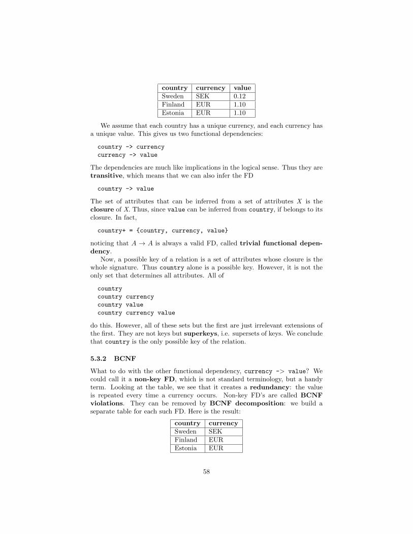
country currency valueSweden SEK 0.12Finland EUR 1.10Estonia EUR 1.10
We assume that each country has a unique currency, and each currency hasa unique value. This gives us two functional dependencies:
country -> currency
currency -> value
The dependencies are much like implications in the logical sense. Thus they aretransitive, which means that we can also infer the FD
country -> value
The set of attributes that can be inferred from a set of attributes X is theclosure of X. Thus, since value can be inferred from country, if belongs to itsclosure. In fact,
country+ = country, currency, value
noticing that A → A is always a valid FD, called trivial functional depen-dency.
Now, a possible key of a relation is a set of attributes whose closure is thewhole signature. Thus country alone is a possible key. However, it is not theonly set that determines all attributes. All of
country
country currency
country value
country currency value
do this. However, all of these sets but the first are just irrelevant extensions ofthe first. They are not keys but superkeys, i.e. supersets of keys. We concludethat country is the only possible key of the relation.
5.3.2 BCNF
What to do with the other functional dependency, currency -> value? Wecould call it a non-key FD, which is not standard terminology, but a handyterm. Looking at the table, we see that it creates a redundancy: the valueis repeated every time a currency occurs. Non-key FD’s are called BCNFviolations. They can be removed by BCNF decomposition: we build aseparate table for each such FD. Here is the result:
country currencySweden SEKFinland EUREstonia EUR
58
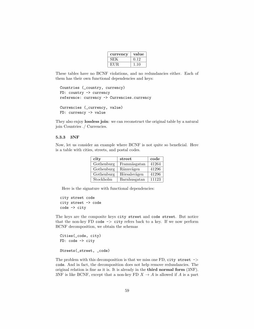
currency valueSEK 0.12EUR 1.10
These tables have no BCNF violations, and no redundancies either. Each ofthem has their own functional dependencies and keys:
Countries (_country, currency)
FD: country -> currency
reference: currency -> Currencies.currency
Currencies (_currency, value)
FD: currency -> value
They also enjoy lossless join: we can reconstruct the original table by a naturaljoin Countries ./ Currencies.
5.3.3 3NF
Now, let us consider an example where BCNF is not quite so beneficial. Hereis a table with cities, streets, and postal codes.
city street codeGothenburg Framnasgatan 41264Gothenburg Rannvagen 41296Gothenburg Horsalsvagen 41296Stockholm Barnhusgatan 11123
Here is the signature with functional dependencies:
city street code
city street -> code
code -> city
The keys are the composite keys city street and code street. But noticethat the non-key FD code -> city refers back to a key. If we now performBCNF decomposition, we obtain the schemas
Cities(_code, city)
FD: code -> city
Streets(_street, _code)
The problem with this decomposition is that we miss one FD, city street ->code. And in fact, the decomposition does not help remove redundancies. Theoriginal relation is fine as it is. It is already in the third normal form (3NF).3NF is like BCNF, except that a non-key FD X → A is allowed if A is a part
59
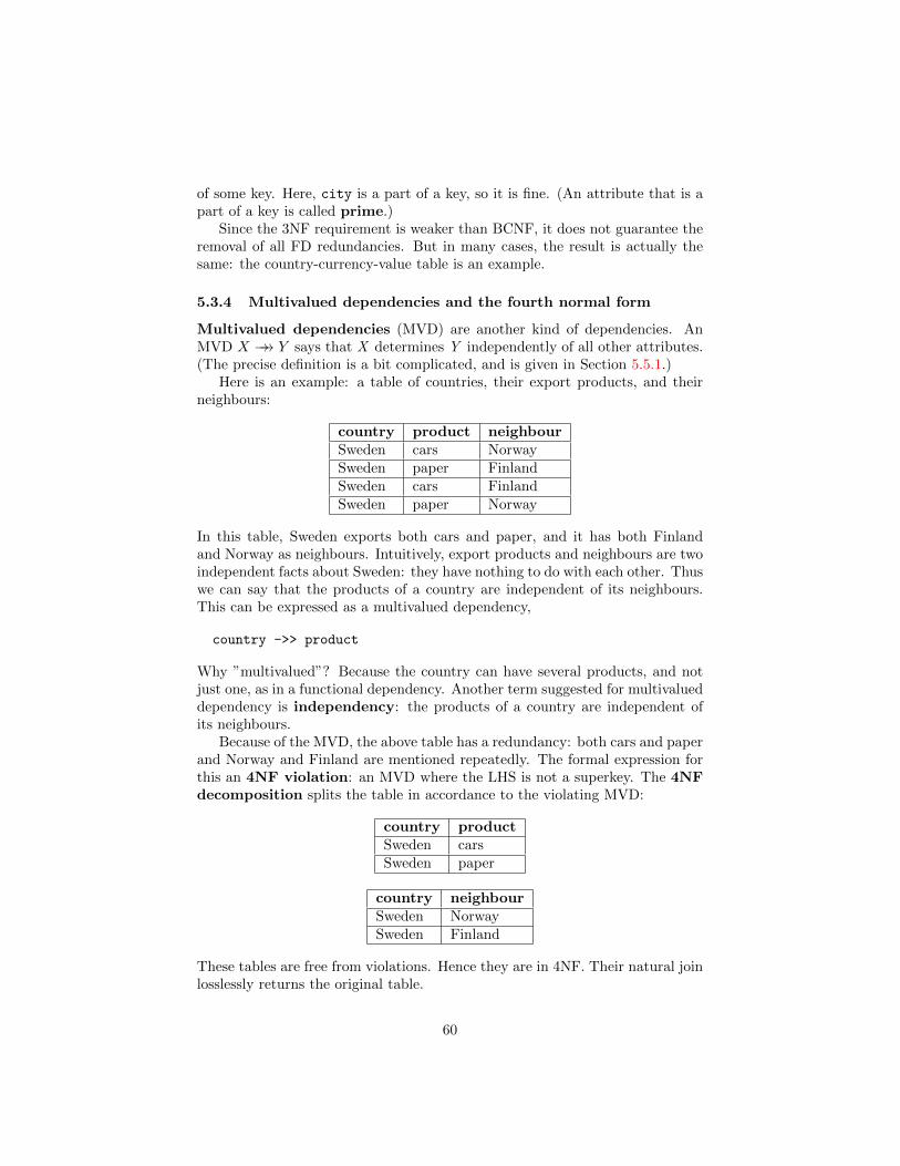
of some key. Here, city is a part of a key, so it is fine. (An attribute that is apart of a key is called prime.)
Since the 3NF requirement is weaker than BCNF, it does not guarantee theremoval of all FD redundancies. But in many cases, the result is actually thesame: the country-currency-value table is an example.
5.3.4 Multivalued dependencies and the fourth normal form
Multivalued dependencies (MVD) are another kind of dependencies. AnMVD X →→ Y says that X determines Y independently of all other attributes.(The precise definition is a bit complicated, and is given in Section 5.5.1.)
Here is an example: a table of countries, their export products, and theirneighbours:
country product neighbourSweden cars NorwaySweden paper FinlandSweden cars FinlandSweden paper Norway
In this table, Sweden exports both cars and paper, and it has both Finlandand Norway as neighbours. Intuitively, export products and neighbours are twoindependent facts about Sweden: they have nothing to do with each other. Thuswe can say that the products of a country are independent of its neighbours.This can be expressed as a multivalued dependency,
country ->> product
Why ”multivalued”? Because the country can have several products, and notjust one, as in a functional dependency. Another term suggested for multivalueddependency is independency: the products of a country are independent ofits neighbours.
Because of the MVD, the above table has a redundancy: both cars and paperand Norway and Finland are mentioned repeatedly. The formal expression forthis an 4NF violation: an MVD where the LHS is not a superkey. The 4NFdecomposition splits the table in accordance to the violating MVD:
country productSweden carsSweden paper
country neighbourSweden NorwaySweden Finland
These tables are free from violations. Hence they are in 4NF. Their natural joinlosslessly returns the original table.
60
In the previous example, we could actually prove the MVD by looking at thetuples (see definition of MVD below). Finding a provable MVD in an instance ofa database can be difficult, because so many combinations must be present. AnMVD might of course be assumed to hold as a part of the domain description.This can lead to a better structure and smaller tables. However, the naturaljoin from those tables can produce combinations not existing in the reality.
5.4 A bigger example
Let us collect everything about a domain into one big table:
country capital popCountry popCapital currency value product neighbour
We identify some functional dependencies and multivalued dependencies:
country -> capital popCountry currency
capital -> country popCapital
currency -> value
country ->> product
country ->> neighbour
One possible BCNF decomposition gives the following tables:
_country capital popCountry popCapital currency
_currency value
_country _product _neighbour
This looks like a good structure, except for the last table. Applying 4NF de-composition to this gives the final result
_country capital popCountry popCapital currency
_currency value
_country _product
_country _neighbour
A word of warning: mechanical decomposition can randomly choose some otherdependencies to split on, and lead to less natural results. For instance, it canuse capital rather than country as the key of the first table.
In the next section, we will show the precise algorithms that are involved,and which you should learn to execute by hand. The definitions might lookmore scary than they actually are. Most of the concepts are intuitively simple,but their precise definitions can require some details that one usually doesn’tthink about. The notion of MVD is usually the most difficult one.
In the sections that follow, we will go a bit deeper in analysing what makesthe normal forms beneficial and what design questions they raise. In the lastsection of this chapter, we will look at the support given by the Query Converter(qconv) for dependency analysis and normal form decomposition.
61
5.5 Mathematical definitions for dependencies and nor-mal forms
5.5.1 Relationas, tuples, and depencencies
Before introducing new concepts, we will repeat some of the definitions abouttuples from Chapter 4. We will most of the time speak of relations just as theirsets of attributes. Also the dependency algorithms refer only to the attributes.But the definitions in the end do refer to tuples. By tuples, we will now meanlabelled tuples (records) rather than set-theoretic ordered tuples as in Chapter 4.Definition (tuple, attribute, value). A tuple has the form
A1 = v1, . . . , An = vn
where A1, . . . , An are attributes and v1, . . . , vn are their values.Definition (signature, relation). The signature of a tuple, S, is the set ofall its attributes, A1, . . . , An. A relation R of signature S is a set of tupleswith signature S. But we will sometimes also say ”relation” when we mean thesignature itself.Definition (projection). If t is a tuple of a relation with signature S, theprojection t.Ai computes to the value vi.Definition (simultaneous projection). If X is a set of attributes B1, . . . , Bm ⊆S and t is a tuple of a relation with signature S, we can form a simultaneousprojection,
t.X = B1 = t.B1, . . . , Bm = t.Bm
Definition (functional dependency, FD). Assume X is a set of attributes and Aan attribute, all belonging to a signature S. Then A is functionally dependenton X in the relation R, written X → A, if• for all tuples t,u in R, if t.X = u.X then t.A = u.A.
If Y is a set of attributes, we write X → Y to mean that X → A for every Ain Y.Definition (multivalued dependency, MVD). Let X,Y,Z be disjoint subsets of asignature S such that S = X∪Y ∪Z. Then Y has a multivalued dependencyon X in R, written X →→ Y , if• for all tuples t,u in R, if t.X = u.X then there is a tuple v in R such that
– v.X = t.X– v.Y = t.Y– v.Z = u.Z
An alternative notation is X →→ Y | Z, emphasizing that Y is independentof Z.
To see the power of these definitions, we can now easily prove a slightlysurprising result saying that every FD is an MVD:Theorem. If X → Y then X →→ YProof. Assume that t,u are tuples in R such that t.X = u.X. We select v = u.This is a good choice, because
1 u.X = t.X by assumption
62
2 u.Y = t.Y by the functional dependency X → Y3 u.Z = u.Z by reflexivity of identity.
Note. MVDs are symmetric on their right hand side: if X →→ Y , which meansX →→ Y | Z where Z = S −X − Y , then also X →→ Z. Thus in the example inSection 5.3.4, we could have written, equivalently,
country ->> exportedTo
5.5.2 Closures, keys, and superkeys
As a starting point of dependency analysis, a relation is charaterized by itssignature S, its functional dependencies FD, and its multivalued dependenciesMVD. We start with things where we don’t need MVD.Assume thus a signature (i.e. set of attributes) S and a set FD of functionaldependencies.Definition. An attribute A follows from a set of attributes Y, if there is anFD X → A such that X ⊆ Y .Definition (closure of a set of attributes under FDs). The closure of a set ofattributes X ⊆ S under a set FD of functional dependencies, denoted X+, isthe set of those attributes that follow from X.Algorithm (closure of attributes). If X ⊆ S, then the closure X+, can becomputed in the following way:
1. Start with X+ = X2. Set New = A | A ∈ S,A /∈ X+, A follows from X+3. If New = ∅, return X+, else set X+ = X + ∪New and go to 1
Definition (closure of a set of FDs). The closure of a set FD of functionaldependencies, denoted by FD+, is defined as follows:
FD+ = X → A | X ⊆ S,A ∈ X+, A /∈ X
The last condition excludes trivial functional dependencies.Definition (trivial functional dependencies). An FD X → A is trivial, ifA ∈ X.Definition (superkey, key). A set of attributes X ⊆ S is a superkey of S, ifS ⊆ X+.A set of attributes X ⊆ S is a key of S if• X is a superkey of S• no proper subset of X is a superkey of S
5.5.3 Decomposition algorithms
Definition (Boyce-Codd Normal Form, BCNF violation). A functional depen-dency X → A violates BCNF if• X is not a superkey• the dependency is not trivial
63

A relation is in Boyce-Codd Normal Form (BCNF) if it has no BCNFviolations.Note. Any trivial dependency A→ A always holds even if A is not a superkey.Definition (prime). An attribute A is prime if it belongs to some key.Definition (Third Normal Form, 3NF violation). A functional dependencyX → A violates 3NF if• X is not a superkey• the dependency is not trivial• A is not prime
Note. 3NF is a weaker normal form than BCNF: Any violation X → A of 3NFis also a violation of BCNF, because it says that X is not a superkey. Hence,any relation that is in BCNF is also in 3NF.Definition (trivial multivalued dependency). A multivalued dependencyX →→ Ais trivial if Y ⊆ X or X ∪ Y = S.Definition (Fourth Normal Form, 4NF violation). A multivalued dependencyX →→ A violates 4NF if• X is not a superkey• the MVD is not trivial.
Note. 4NF is a stronger normal form than BCNF: If X → A violates BCNF,then it also violates 4NF, because• it is an MVD by the theorem above• it is not trivial, because
– if A ⊆ X, then X → A is a trivial FD and cannot violate BCNF– if X ∪ A = S, then X is a superkey and X → A cannot violate
BCNFAlgorithm (BCNF decomposition). Consider a relation R with signature Sand a set F of functional dependencies. R can be brought to BCNF by thefollowing steps:
1. If R has no BCNF violations, return R2. If R has a violating functional dependency X → A, decompose R to two
relations
• R1 with signature X ∪ A• R2 with signature S − A
3. Apply the above steps to R1 and R2 with functional dependencies pro-jected to the attributes contained in each of them.
One can combine several violations with the same left-hand-side X to producefewer tables. Then the violation X → Y decomposes R to R1(X,Y ) and R2(S−Y ).Note. Step 3 of the BCNF decomposition algorithm involves the projectionof functional dependencies. This can in general be a complex procedure.However, for most cases handled during this course, it is enough just to filterout those dependencies that do not appear in the new relations.Algorithm (4NF decomposition). Consider a relation R with signature S anda set M of multivalued dependencies. R can be brought to 4NF by the followingsteps:
64
1. If R has no 4NF violations, return R2. If R has a violating multivalued dependency X →→ Y , decompose R to
two relations
• R1 with signature X ∪ Y • R2 with signature S − Y
3. Apply the above steps to R1 and R2Note. This algorithm has the same structure as the BCNF decomposition.For 3NF decomposition, a very different algorithm is used, seemingly with noiteration. But an iteration can be needed to compute the minimal basis of theFD set.Concept (minimal basis of a set of functional dependencies; not a rigorousdefinition). A minimal basis of a set F of functional dependencies is a set F-that implies all dependencies in F. It is obtained by first weakening the left handsides and then dropping out dependencies that follow by transitivity. Weakeningan LHS in X → A means finding a minimal subset of X such that A can stillbe derived from F-.Algorithm (3NF decomposition). Consider a relation R with a set F of func-tional dependencies.
1. If R has no 3NF violations, return R.2. If R has 3NF violations,
• compute a minimal basis of F- of F• group F- by the left hand side, i.e. so that all depenencies X → A
are grouped together• for each of the groups, return the schema XA1 . . . An with the com-
mon LHS and all the RHSs• if one of the schemas contains a key of R, these groups are enough;
otherwise, add a schema containing just some keyExample (minimal basis). Consider the schema
country currency value
country -> currency
country -> value
currency -> value
It has one 3NF violation: currency -> value. Moreover, the FD set is not aminimal basis: the second FD can be dropped because it follows from the firstand the third ones by transitivity. Hence we have a minimal basis
country -> currency
currency -> value
Applying 3NF decomposition to this gives us two schemas:
country currency
currency value
i.e. exactly the same ones as we would obtain by BCNF decomposition. Theserelations are hence not only 3NF but also BCNF.
65
5.6 More definitions for functional dependencies*
Let f = X → Y be a functional dependency. We call X the left hand sideof f and Y the right hand side of f . We assume that all left hand sides arenon-empty.
We say that a functional dependency X → Y is embedded in a relationschema R if X ∪ Y ⊆ R. For a set of dependencies F , we denote the set of lefthand sides of F by LHS(F ).
Usually, functional dependencies are given as semantic constraints, and onlythose database states where all dependencies hold in all respective relations areconsidered legal; the constraints can be used in the design process as well as laterwhen the database is being used. As an input to database design, the depen-dencies are normally given before the relation schemas are being decided upon.With this purpose in mind, we may say that a set F of functional dependenciesis given over a universe U .
Some dependencies may get embedded in some relation schema in the databaseschema while some may not. If all dependencies in a given set of dependenciesF are embedded in some relation schema of a database schema R, we say thatF is embedded in R.
The idea of a relation satisfying a functional dependency is fairly simple. Itis not quite as clear what it should mean for a database to satisfy a functionaldependency.
A containing instance i of a database r over a database scheme R is such arelation over the underlying universe U that each relation r ∈ r, where r is arelation over R ∈ R, is a subset of πR(i).
Let U be a universe, R a database schema over U , R ∈ R, and let X ⊆ U ,Y ⊆ U . We say that a database r over R satisfies the functional dependencyX → Y if there is a containing instance i for r such that i satisfies X → Y .If there is such a containing instance i that i satisfies all the given functionaldependencies, then i is called a weak instance for the database r. Further, if iis a subset of all other weak instances for r, then i is a representative instancefor r.
Whether a database satisfies a set of functional dependencies can be checkedwith a relatively simple method called the chase. The chase proceeds by ma-nipulating a tableau, which is like a relation except that in addition to valuesfrom domains of attributes, it may also contain variables as elements.
We apply the notations and terminology for relations to tableau withoutgiving them explicitly. This should not raise any ambiguities. We construct theinitial tableau as input for the chase using the following definition.Definition (Database tableau)Let R be a database schema over a universe U and let r be a database overR. Let n be the total number of tuples in the relations of r, and assume thatthe tuples are numbered from 1 to n. Assume also that the attributes in U arenumbered from 1 to k, and we will denote the attribute with number j by Aj .Let i be the number of a tuple t in a relation r over a relation schema R. Wedefine ti[Aj ], 1 ≤ j ≤ k, to be t[Aj ], if Aj ∈ R, and v(i,j), a nondistinguished
66
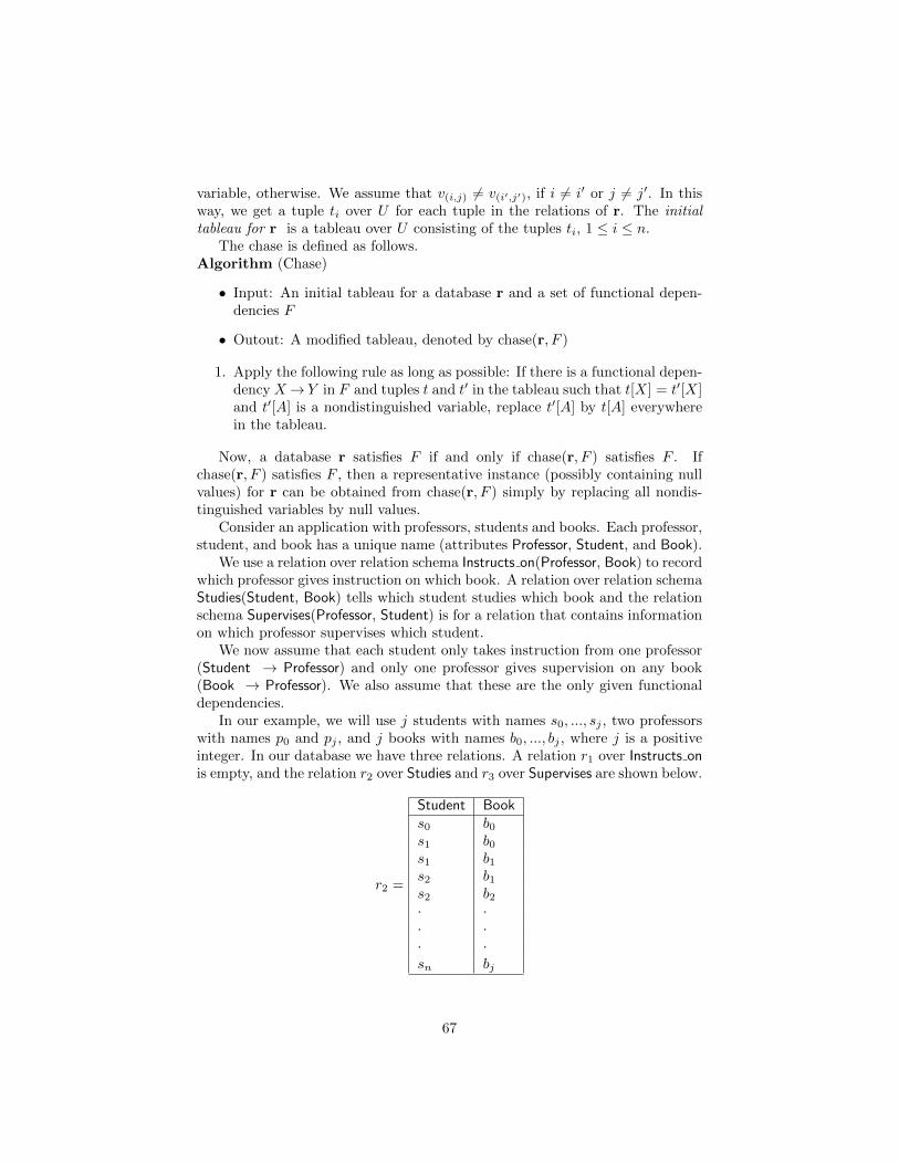
variable, otherwise. We assume that v(i,j) 6= v(i′,j′), if i 6= i′ or j 6= j′. In thisway, we get a tuple ti over U for each tuple in the relations of r. The initialtableau for r is a tableau over U consisting of the tuples ti, 1 ≤ i ≤ n.
The chase is defined as follows.Algorithm (Chase)
• Input: An initial tableau for a database r and a set of functional depen-dencies F
• Outout: A modified tableau, denoted by chase(r, F )
1. Apply the following rule as long as possible: If there is a functional depen-dency X→ Y in F and tuples t and t′ in the tableau such that t[X] = t′[X]and t′[A] is a nondistinguished variable, replace t′[A] by t[A] everywherein the tableau.
Now, a database r satisfies F if and only if chase(r, F ) satisfies F . Ifchase(r, F ) satisfies F , then a representative instance (possibly containing nullvalues) for r can be obtained from chase(r, F ) simply by replacing all nondis-tinguished variables by null values.
Consider an application with professors, students and books. Each professor,student, and book has a unique name (attributes Professor, Student, and Book).
We use a relation over relation schema Instructs on(Professor, Book) to recordwhich professor gives instruction on which book. A relation over relation schemaStudies(Student, Book) tells which student studies which book and the relationschema Supervises(Professor, Student) is for a relation that contains informationon which professor supervises which student.
We now assume that each student only takes instruction from one professor(Student → Professor) and only one professor gives supervision on any book(Book → Professor). We also assume that these are the only given functionaldependencies.
In our example, we will use j students with names s0, ..., sj , two professorswith names p0 and pj , and j books with names b0, ..., bj , where j is a positiveinteger. In our database we have three relations. A relation r1 over Instructs onis empty, and the relation r2 over Studies and r3 over Supervises are shown below.
r2 =
Student Books0 b0s1 b0s1 b1s2 b1s2 b2· ·· ·· ·sn bj
67
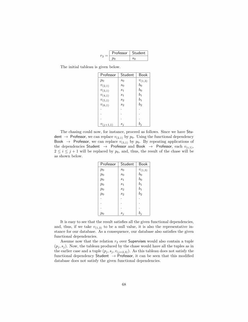
r3 =Professor Studentp0 s0
The initial tableau is given below.
Professor Student Bookp0 s0 v(1,3)v(2,1) s0 b0v(3,1) s1 b0v(4,1) s1 b1v(5,1) s2 b1v(6,1) s2 b2· · ·· · ·· · ·v(j+1,1) sj bj
The chasing could now, for instance, proceed as follows. Since we have Stu-dent → Professor, we can replace v(2,1) by p0. Using the functional dependencyBook → Professor, we can replace v(3,1) by p0. By repeating applications ofthe dependencies Student → Professor and Book → Professor, each v(i,1),2 ≤ i ≤ j + 1 will be replaced by p0, and, thus, the result of the chase will beas shown below.
Professor Student Bookp0 s0 v(1,3)p0 s0 b0p0 s1 b0p0 s1 b1p0 s2 b1p0 s2 b2· · ·· · ·· · ·p0 sj bj
It is easy to see that the result satisfies all the given functional dependencies,and, thus, if we take v(1,3) to be a null value, it is also the representative in-stance for our database. As a consequence, our database also satisfies the givenfunctional dependencies.
Assume now that the relation r2 over Supervises would also contain a tuple(pj , sj). Now, the tableau produced by the chase would have all the tuples as inthe earlier case and a tuple (pj , sj , v(j+2,3)). As this tableau does not satisfy thefunctional dependency Student → Professor, it can be seen that this modifieddatabase does not satisfy the given functional dependencies.
68

5.7 Design intuition*
To improve our intuition, let us first illustrate some examples of potentiallyproblematic designs. Consider, again, the table below on professor who teachstudents and on which course. Is this design problematic? This depends on thesemantic constraints, ie. the functional dependencies. Suppose, first, that
professor course studentRanta Compiler construction AndersRanta Compiler construction LenaKemp Data Science AndersNummenmaa Database systems Lena
Consider, first, splitting this table into two as follows. The first table tellswho is teaching which student and the second tells who is studying which course.
professor studentRanta AndersRanta LenaKemp AndersNummenmaa Lena
course studentCompiler construction AndersCompiler construction LenaData Science AndersDatabase systems Lena
If we join these table on students, we get the following table.
professor course studentRanta Compiler construction AndersRanta Compiler construction LenaRanta Data Science AndersRanta Database systems LenaKemp Data Science AndersKemp Compiler construction AndersNummenmaa Compile construction LenaNummenmaa Database systems Lena
This is obviously not what we want. The table includes rows that werenot in our original table. We say that the way to join the data is ”lossy” -however lossy does not mean losing data, which indeed did not happen, butlosing information on which pieces of data belonged together.
Our second attempt is to store the data with two tables, where the first tabletells who is teaching which course and the second tells who is studying whichcourse.
69

professor courseRanta Compiler constructionKemp Data ScienceNummenmaa Database systems
course studentCompiler construction AndersCompiler construction LenaData Science AndersDatabase systems Lena
If we join the tables on book, we get the original table back. In this case ourjoin is ”lossless” - no information was lost. In this case, though, the losslessnessis based on the fact that no course is being taught by two professors. If e.g.Nummenmaa starts to teach Data Science to Kati, then the situation withlosslessness changes. If, however, we know that each professor always onlyteaches one course, then we will be safe with joining on course and we alwaysget a lossless join. In this case our database design would have the lossless joinproperty.
Our initial design with just one table had - trivially - no problems with loss-lessness. Why would we not just stick with it? If we know that each professoronly teaches one course, then using just one table usually introduces redundantinformation that is repeated in different rows. Let’s assume, again, that eachcourse is only taught by one professor. If all data is stored in just one tableand the professors Ranta and Nummenmaa swap courses so that Nummenmaawill teach compile construction and Ranta will teach Database systesm, then wewould need to update a whole lot of rows in the tables (well, in our initial exam-ple just 3, but potentially). If the data is split into two tables with the losslessdesign, then only the two rows in (professor,course) table need to updated, nomatter how many students study these courses. So, the solution where the tableis split seems beneficial.
It seems, right enough, that the key structure plays a central role in solvingthese problems. But as a modeling construct, it is not enough. Suppose, now,that each student studies each course with one particular professor, and let ussuppose the following table, with (student, course) as the key.
professor course studentRanta Compiler construction AndersRanta Compiler construction LenaKemp Data Science AndersNummenmaa Database systems LenaNummenmaa Distributed systems Anders
This would mean that it is impossible to add a row where Anders studiesCompile construction under the instruction from Nummenmaa.
Let us make a further assumption that each course is only taught by at mostone professor. There is no way we can model this information with keys, since
70

course is and cannot be a key - e.g. Ranta would be a duplicate key value.\footnoteThis is example is better known as the (City, Street, Zip) example,where there is a unique Zip for each (City,Street) pair and a unique City foreach Zip. Also, in our table we have redundant information on who is teachingwhich course, since the course is always repeated with the professor.
We may try to get rid of the redundancy by splitting the table into two, asfollows.
professor courseRanta Compiler constructionKemp Data ScienceNummenmaa Database systems
professor studentRanta AndersRanta LenaKemp AndersNummenmaa Lena
We got rid of the redundant data, but other problems appeared. Joining thetables on professor we get e.g. a row (Kemp, Anders, Data Science)
Let us now consider a design where we have three tables
professor courseRanta Compiler constructionKemp Data ScienceNummenmaa Database systems
professor studentRanta AndersRanta LenaKemp AndersNummenmaa Lena
course studentCompiler construction AndersCompiler construction LenaData Science AndersDatabase systems Lena
This effectively eliminates redundant data. Let us suppose now that theonly key-like constraint is that each student studies each course with exactlyone professor. Then, when updates take place, we can only check this constraintby joining the tables. Besides, as the reader is urged to check, the joins are notlossless. Lossy joins follow from the fact that there are no foreign keys.
71
If no functional dependencies exist, then the three-table desing is lossless andthere is no constraint checking problem. However, then intuitive querying be-comes more problematic as there are multiple relationships between attributes.E.g. there is a relationship between course and student directly stored, but an-other one exists and it can be realized by joining the two other tables. Further,in some high-level query systems, as e.g. using natural language, the user maywant to just ask for professors and students. With two existing interpretations,there is some ambiguity.
5.8 More definitions and algorithms for database design*
Definition (dependency preservation). We call the database D dependencypreserving with respect to a set of functional dependencies FD, if D embeds acover of FD, that is, we can infer any given functional dependency in FD fromthe dependencies in the relations of D.
Definition (lossless join property). Let D= R 1, R 2, . . . , R n be a databaseschema over U . We say that D has the lossless join property if every relationr U over U decomposes losslessly onto R 1, ..., R n. If D has the lossless joinproperty, we also say that D is lossless. Otherwise, we say that D is lossy.
These two concepts are related: it is known that a dependency preservingdatabase D (i.e. set of relations) is lossless if and only if it contains a relationR such that closure of R contains all attributes in D.
Now, consider redundancy in the context of a single relation. We have seenabove that potential problems with redundancy appeared when there were otherfunctional dependencies than those describing a key. An example remedy wasBCNF decomposition, eliminating functional dependencies where the LHS is nota superkey. It can be shown that when we consider a single update (inserting ordeleting a tuple) in a single-relation database, then we cannot have an arbitrarynumber of required ”knock-on” updates if and only if that relation is in BCNF.This makes BCNF a strong required property.
The BCNF decomposition algorithm always produces databases in BCNF.There is a problem, though, that this may violate dependency preservation. Letus review, again, the City-Stree-Zip example, with dependencies City,Street ->Zip, Zip->City, and a relation (City,Street,Zip). If we decompose with Zip-City,then the database is no longer dependency preserving. If we do not decompose,then the database is not in BCNF. In such a case, we can achieve a weakerproperty, the third normal form (3NF).
Since the 3NF requirement is weaker than BCNF, it does not guaranteethe removal of all FD redundancies. But in many cases, the result is actuallythe same: the country-currency-value table is an example. The bad news with3NF is that potential knock-on updates happen on the key values, and as keysmay be used in foreign keys and indexes on data, this may be computationallyexpensive.
72
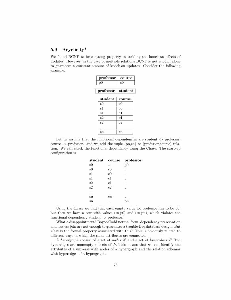
5.9 Acyclicity*
We found BCNF to be a strong property in tackling the knock-on effects ofupdates. However, in the case of multiple relations BCNF is not enough aloneto guarantee a constant amount of knock-on updates. Consider the followingexample.
professor coursep0 s0
professor student
student courses0 c0s1 c0s1 c1s2 c1s2 c2...sn cn
Let us assume that the functional dependencies are student -> professor,course -> professor. and we add the tuple (pn,cn) to (professor,course) rela-tion. We can check the functional dependency using the Chase. The start-upconfiguration is
student course professors0 p0s0 c0s1 c0s1 c1s2 c1s2 c2...sn cnsn pn
Using the Chase we find that each empty value for professor has to be p0,but then we have a row with values (sn,p0) and (sn,pn), which violates thefunctional dependency student -> professor.
What a disappointment! Boyce-Codd normal form, dependency preservationand lossless join are not enough to guarantee a trouble-free database design. Butwhat is the formal property associated with this? This is obviously related todifferent ways in which the same attributes are connected.
A hypergraph consist of a set of nodes N and a set of hyperedges E. Thehyperedges are nonempty subsets of N. This means that we can identify theattributes of a universe with nodes of a hypergraph and the relation schemaswith hyperedges of a hypergraph.
73
A suphypergraph of a hypergraph (N,E) is a pair (N,E’), where each hyper-edge in E’ is a subset of E.
There are different definitions of acyclicity of hypergraphs, but we are onlyinterested in so called γ-acyclicity, which we call simply acyclicity.
A γ-cycle in a hypergraph is a sequence R1, A1, ..., Rk, Ak, Rk+1 of alternat-ing edges and nodes such that
(i) A1, ..., Ak are distinct nodes,
(ii) R1, ..., Rk are distinct edges, and R1 = Rk+1,
(iii) k ≥ 3,
(iv) for each Ai, 1 ≤ i ≤ k, we have Ai ∈ Ri, Ai ∈ Ri+1, and,
(v) for each Ai, 1 ≤ i < k, we have Ai 6∈ Rj , if j 6= i, j 6= i+ 1.
Intuitively, one can ”walk” a round in the numbered order from the firstrelation schema by connecting nodes. Apart from Ak the connecting nodes arenot supposed to appear in other relation schemas apart from the two they arespecifically connecting.
A hypergraph (database) is γ-acyclic, if it contains no γ-cycles, otherwise itis γ-cyclic.
As an exercise, the reader is urged to check that (professor, student), (stu-dent,course),(course, professor) is γ-cyclic, whereas (professor,student,course),(course,book), (professor,course) is not.
Lossless dependency-preserving γ-acyclic BCNF databases have very strongproperties. First of all, there will only be a constant amount of knock-on updatesfor any insert or delete operation. Query processing is also known to be simpleand efficient. Further, it is known that for any pair of attributes in such anacyclic database, there is a unique minimal connection (simple semantics), whichcan be used e.g. in natural language query processing. When given a set ofattributes X, we can join the necessary relations and project them onto X withsimple relational algebra operations.
5.10 Optimal database design*
However, when and how are these nice properties achievable? The theory iscomplicated, but we will just some motivating examples and the results. Theproblematic sets of functional depdencies have two characteristic sets of prob-lems. The City, Street, Zip problem was caused because one functional depen-dency determined a proper subset of another functional dependency. This iscalled splitting. Another problematic situation is where the right hand sidesof functional dependencies have non-empty intersections, and, finally, the thirdproblematic situation may be where the left hand sides have non-empty inter-sections.
To cut a relatively long story very short, we just conclude that in practicewhen possible, that is, when the problematic situations do not exist or can be
74
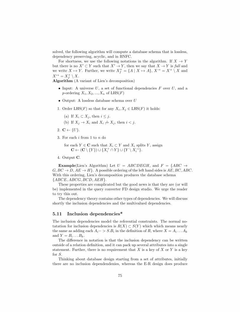
solved, the following algorithm will compute a database schema that is lossless,dependency preserving, acyclic, and in BNFC.
For shortness, we use the following notations in the algorithm. If X → Ybut there is no X ′ ⊂ Y such that X ′ → Y , then we say that X → Y is full andwe write X 7→ Y . Further, we write X+
f = A | X 7→ A, X→ = X+ \X and
X 7→ = X+f \X.
Algorithm (A variant of Lien’s decomposition)
• Input: A universe U , a set of functional dependencies F over U , and ap-ordering X1, X2, ..., Xn of LHS(F )
• Output: A lossless database schema over U
1. Order LHS(F ) so that for any Xi, Xj ∈ LHS(F ) it holds:
(a) If Xi ⊂ Xj , then i ≤ j.(b) If Xj → Xi and Xi 6→ Xj , then i < j.
2. C← U.
3. For each i from 1 to n do
for each Y ∈ C such that Xi ⊂ Y and Xi splits Y , assignC← (C \ Y ) ∪ X+
i ∩ Y ∪ Y \X→i .
4. Output C.
Example(Lien’s Algorithm) Let U = ABCDEGH, and F = ABC →G,BC → D, AE → H. A possible ordering of the left hand sides isAE,BC,ABC.With this ordering, Lien’s decomposition produces the database schemaABCE,ABCG,BCD,AEH.
These properties are complicated but the good news is that they are (or willbe) implemented in the query converter FD design studio. We urge the readerto try this out.
The dependency theory contains other types of dependencies. We will discussshortly the inclusion dependencies and the multivalued dependencies.
5.11 Inclusion dependencies*
The inclusion dependencies model the referential constraints. The normal no-tatation for inclusion dependencies is R(X) ⊂ S(Y ) which which means nearlythe same as adding each Ai− > S.Bi in the definition of R, where X = Ai . . . Ak
and Y = Bi . . . Bk.The difference in notation is that the inclusion dependency can be written
outside of a relation definition, and it can pack up several attributes into a singlestatement. Further, there is no requirement that X is a key of X or Y is a keyfor S.
Thinking about database design starting from a set of attributes, initiallythere are no inclusion dependendenies, whereas the E-R design does produce
75
them. However, decompositions produce them. Whenever we decompose arelation schema R with an FD X → Y where X ⊂ R, Y ⊂ R, producingrelation schemas S = X ∪ Y and R′ = R \ Y , then obviously X is a superkeyof S and the idea of the decomposition is to recover the decomposed data byjoining on X, and, consequently, an inclusion depdendency S.X ′ ⊆ R′.X wouldbe in order.
If there is no further FD to decompose R′, then X is a key and the inclusiondependecy can be used to create referential constraints. If there are further FDsto decompose R′, then the inclusion depdencies must be adapted accordingly.The details are left as an exercise to the interested reader. 5
5.12 Combining practice and theory in database design
Until now, we have introduced a basic method to produce database designs fromER diagrams and on the other hand we have characterized good designs and wehave given design algorithms based on the use of dependencies.
Dependency-based design is, in a way, more mechanical than E-R design.In E-R design, you have to decide many things: the ontological status of eachconcept (whether it is an entity, attribute, relationship, etc). You also have todecide the keys of the entities. In dependency analysis, you only have to decidethe basic dependencies. Lots of other dependencies are derived from these bymechanical rules. Also the possible keys - candidate keys - are mechanicallyderived. The decomposition to normal forms is mechanical as well. You justhave to decide what normal form (if any) you want to achieve. In addition, youhave to decide which of the candidate keys to declare as the primary key ofeach table.
Obviously, we need to consider how we can combine ER design and depen-dencies. First of all, some FDs can be directly derived from an ER diagram. Infact, we can use ER diagrams to produce all FDs, if we allow separate diagramsor parts of them to give additional information on dependencies, and the at-tributes naming is considered global. Thereby, we can separately construct anentity with City, Street, and Zip, and (City,Street) as key, and another entitywith the attributes Zip and City, with Zip as the key. Another alternative isjust to input additional FDs in a separate text file or similar.
A practical option, not based on the specific design theory above, is toproduce the relations from the ER diagram and then further decompose themusing the FDs. This solution is practical in the sense that designs producedfrom ER diagrams are most likely to avoid nontrivial MVDs and therefore onlyFD decomposition or similar is needed for the parts of the design where thereare additional FDs emerging from the additional ER diagram fragments.
You need to decide what decomposition you want. All normal forms havetheir pros and cons. At this point, you may want to compare the dependency-based design with the E-R design. This also depends on the application. Ifquery performance is crucial and one wants to avoid joins, and updates seldom
5Should we extend the details or give a reference to the book by Mannila and Raiha?
76

happen or are otherwise known to be feasible on pre-joined data, then you maydecompose less or store joins directly.
5.13 Relation analysis in the Query Converter*
The qconv command f reads a relation from a file and prints out relation info:• the closure of functional dependencies• superkeys• keys• normal form violations
The command n reads a relation from the same file format and prints out de-compositions in 3NF, BCNF, and 4NF.
The format of these files is as in the following example:
country capital popCountry popCapital currency value product exportTo
country -> capital popCountry currency
capital -> popCapital
currency -> value
country ->> product
The Haskell code in
https://github.com/GrammaticalFramework/gf-contrib/blob/master/query-converter/Fundep.hs
is a direct rendering of the mathematical definitions. There is a lot of room foroptimizations, but as long as the number of attributes is within the usual limitsof textbook exercises, the naive algorithms work perfectly well.
5.14 Further reading on normal forms and functional de-pendencies*
The following is a practical guide going through all the normal forms from 1NFto 5NF:
William Kent, ”A Simple Guide to Five Normal Forms in RelationalDatabase Theory”, Communications of the ACM 26(2), Feb. 1983,120-125. http://www.bkent.net/Doc/simple5.htm
77
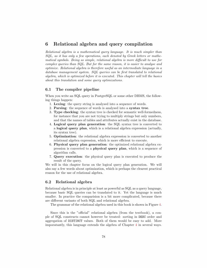
6 Relational algebra and query compilation
Relational algebra is a mathematical query language. It is much simpler thanSQL, as it has only a few operations, each denoted by Greek letters or mathe-matical symbols. Being so simple, relational algebra is more difficult to use forcomplex queries than SQL. But for the same reason, it is easier to analyse andoptimize. Relational algebra is therefore useful as an intermediate language in adatabase management system. SQL queries can be first translated to relationalalgebra, which is optimized before it is executed. This chapter will tell the basicsabout this translation and some query optimizations.
6.1 The compiler pipeline
When you write an SQL query in PostgreSQL or some other DBMS, the follow-ing things happen:
1. Lexing: the query string is analysed into a sequence of words.2. Parsing: the sequence of words is analysed into a syntax tree.3. Type checking: the syntax tree is checked for semantic well-formedness,
for instance that you are not trying to multiply strings but only numbers,and that the names of tables and attributes actually exist in the database.
4. Logical query plan generation: the SQL syntax tree is converted toa logical query plan, which is a relational algebra expression (actually,its syntax tree).
5. Optimization: the relational algebra expression is converted to anotherrelational algebra expression, which is more efficient to execute.
6. Physical query plan generation: the optimized relational algebra ex-pression is converted to a physical query plan, which is a sequence ofalgorithm calls.
7. Query execution: the physical query plan is executed to produce theresult of the query.
We will in this chapter focus on the logical query plan generation. We willalso say a few words about optimization, which is perhaps the clearest practicalreason for the use of relational algebra.
6.2 Relational algebra
Relational algebra is in principle at least as powerful as SQL as a query language,because basic SQL queries can be translated to it. Yet the language is muchsmaller. In practice the comparision is a bit more complicated, because thereare different variants of both SQL and relational algebra.
The grammar of the relational algebra used in this book is shown in Figure 4.
Since this is the ”official” relational algebra (from the textbook), a cou-ple of SQL constructs cannot however be treated: sorting in DESC order andaggregation of DISTINCT values. Both of them would be easy to add. Moreimporatantly, this language extends the algebra of Chapter 4 in several ways.
78
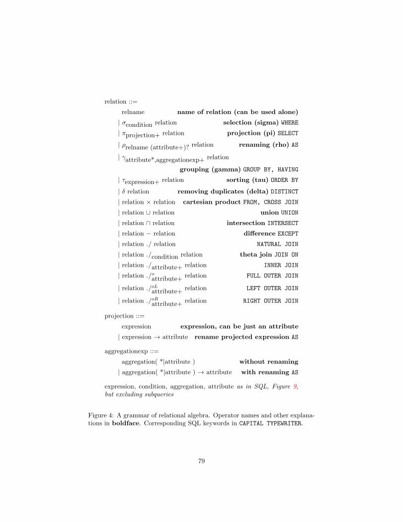
relation ::=
relname name of relation (can be used alone)
| σcondition relation selection (sigma) WHERE
| πprojection+ relation projection (pi) SELECT
| ρrelname (attribute+)? relation renaming (rho) AS
| γattribute*,aggregationexp+ relation
grouping (gamma) GROUP BY, HAVING
| τexpression+ relation sorting (tau) ORDER BY
| δ relation removing duplicates (delta) DISTINCT
| relation × relation cartesian product FROM, CROSS JOIN
| relation ∪ relation union UNION
| relation ∩ relation intersection INTERSECT
| relation − relation difference EXCEPT
| relation ./ relation NATURAL JOIN
| relation ./condition relation theta join JOIN ON
| relation ./attribute+ relation INNER JOIN
| relation ./oattribute+ relation FULL OUTER JOIN
| relation ./oLattribute+ relation LEFT OUTER JOIN
| relation ./oRattribute+ relation RIGHT OUTER JOIN
projection ::=
expression expression, can be just an attribute
| expression → attribute rename projected expression AS
aggregationexp ::=
aggregation( *|attribute ) without renaming
| aggregation( *|attribute ) → attribute with renaming AS
expression, condition, aggregation, attribute as in SQL, Figure 9,but excluding subqueries
Figure 4: A grammar of relational algebra. Operator names and other explana-tions in boldface. Corresponding SQL keywords in CAPITAL TYPEWRITER.
79
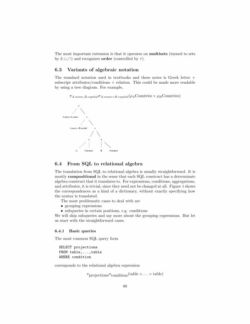
The most important extension is that it operates on multisets (turned to setsby δ,∪,∩) and recognizes order (controlled by τ).
6.3 Variants of algebraic notation
The standard notation used in textbooks and these notes is Greek letter +subscript attributes/conditions + relation. This could be made more readableby using a tree diagram. For example,
πA.name,B.capitalσA.name=B.capital(ρACountries× ρBCountries)
6.4 From SQL to relational algebra
The translation from SQL to relational algebra is usually straightforward. It ismostly compositional in the sense that each SQL construct has a determinatealgebra construct that it translates to. For expressions, conditions, aggregations,and attributes, it is trivial, since they need not be changed at all. Figure 4 showsthe correspondences as a kind of a dictionary, without exactly specifying howthe syntax is translated.
The most problematic cases to deal with are• grouping expressions• subqueries in certain positions, e.g. conditions
We will skip subqueries and say more about the grouping expressions. But letus start with the straightforward cases.
6.4.1 Basic queries
The most common SQL query form
SELECT projections
FROM table,...,table
WHERE condition
corresponds to the relational algebra expression
πprojectionsσcondition(table× . . .× table)
80

But notice, first of all, that names of relations can themselves be used as alge-braic queries. Thus we translate
SELECT * FROM Countries
=⇒ Countries
SELECT * FROM Countries WHERE name=’UK’
=⇒ σname=′UK′Countries
In general, SELECT * does not add anything to the algebra translation. However,there is a subtle exception with grouping queries, to be discussed later.
If the SELECT field contains attributes or expressions, these are copied intothe same expressions under the π operator. When the field is given anothername by AS, the arrow symbol is used in algebra:
SELECT capital, area/1000 FROM Countries WHERE name=’UK’
=⇒ πcapital,area/1000σname=′UK′Countries
SELECT name AS country, population/area AS density FROM Countries
=⇒ πname→country,population/area→densityCountries
The renaming of attributes could also be done with the ρ operator:
ρC(country,density)πname,population/areaCountries
is a more complicated and, in particular, less compositional solution, becausethe SELECT field is used in two different algebra operations. Moreover, it mustinvent C as a dummy name for the renamed table. However, ρ is the way to gowhen names are given to tables in the FROM field. This happens in particularwhen a cartesian product is made with two copies of the same table:
SELECT A.name, B.capital
FROM Countries AS A, Countries AS B
WHERE A.name = B.capital
=⇒πA.name,B.capitalσA.name=B.capital(ρACountries× ρBCountries)
No renaming of attributes takes place in this case.Set-theoretical operations and joins work in the same way as in SQL. No-
tice once again that the SQL distinction between ”queries” and ”tables” is notpresent in algebra, but everything is relations. This means that all operationswork with all kinds of relation arguments, unlike in SQL (see Section 2.16).
6.4.2 Grouping and aggregation
As we saw in Section 2.11, GROUP BY a (or any sequence of attributes) to atable R forms a new table, where a is the key. The other attributes can be foundin two places: the SELECT line above and the HAVING and ORDER BY linesbelow. All of these attributes must be aggregation function applications.
In relational algebra, the γ operator is an explicit name for this relation,collecting all information in one place. Thus
81
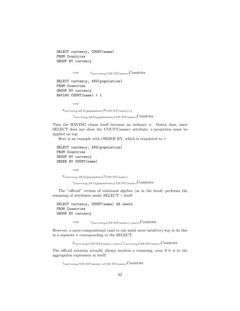
SELECT currency, COUNT(name)
FROM Countries
GROUP BY currency
=⇒ γcurrency,COUNT (name)Countries
SELECT currency, AVG(population)
FROM Countries
GROUP BY currency
HAVING COUNT(name) > 1
=⇒πcurrency,AV G(population)σCOUNT (name)>1
γcurrency,AV G(population),COUNT (name)Countries
Thus the HAVING clause itself becomes an ordinary σ. Notice that, sinceSELECT does not show the COUNT(name) attribute, a projection must beapplied on top.
Here is an example with ORDER BY, which is translated to τ :
SELECT currency, AVG(population)
FROM Countries
GROUP BY currency
ORDER BY COUNT(name)
=⇒πcurrency,AV G(population)τCOUNT (name)
γcurrency,AV G(population),COUNT (name)Countries
The ”official” version of relational algebra (as in the book) performs therenaming of attributes under SELECT γ itself:
SELECT currency, COUNT(name) AS users
FROM Countries
GROUP BY currency
=⇒ γcurrency,COUNT (name)→usersCountries
However, a more compositional (and to our mind more intuitive) way is do thisin a separate π corresponding to the SELECT:
πcurrency,COUNT (name)→usersγcurrency,COUNT (name)Countries
The official notation actually always involves a renaming, even if it is to theaggregation expression to itself:
γcurrency,COUNT (name)→COUNT (name)Countries
82
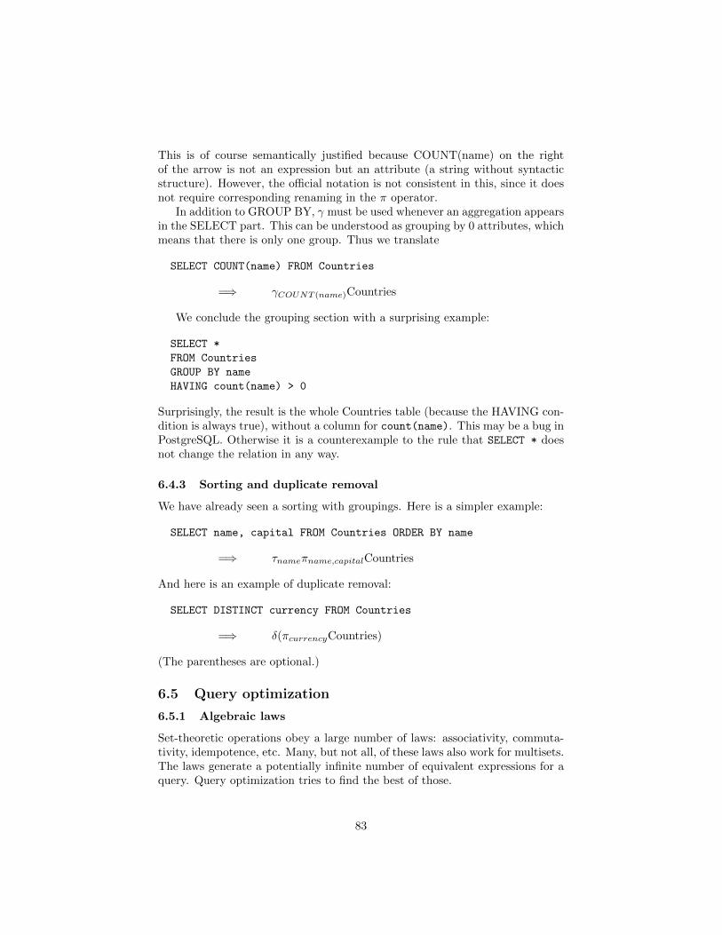
This is of course semantically justified because COUNT(name) on the rightof the arrow is not an expression but an attribute (a string without syntacticstructure). However, the official notation is not consistent in this, since it doesnot require corresponding renaming in the π operator.
In addition to GROUP BY, γ must be used whenever an aggregation appearsin the SELECT part. This can be understood as grouping by 0 attributes, whichmeans that there is only one group. Thus we translate
SELECT COUNT(name) FROM Countries
=⇒ γCOUNT (name)Countries
We conclude the grouping section with a surprising example:
SELECT *
FROM Countries
GROUP BY name
HAVING count(name) > 0
Surprisingly, the result is the whole Countries table (because the HAVING con-dition is always true), without a column for count(name). This may be a bug inPostgreSQL. Otherwise it is a counterexample to the rule that SELECT * doesnot change the relation in any way.
6.4.3 Sorting and duplicate removal
We have already seen a sorting with groupings. Here is a simpler example:
SELECT name, capital FROM Countries ORDER BY name
=⇒ τnameπname,capitalCountries
And here is an example of duplicate removal:
SELECT DISTINCT currency FROM Countries
=⇒ δ(πcurrencyCountries)
(The parentheses are optional.)
6.5 Query optimization
6.5.1 Algebraic laws
Set-theoretic operations obey a large number of laws: associativity, commuta-tivity, idempotence, etc. Many, but not all, of these laws also work for multisets.The laws generate a potentially infinite number of equivalent expressions for aquery. Query optimization tries to find the best of those.
83
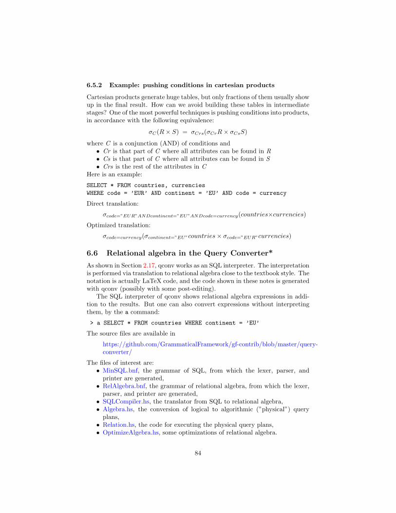
6.5.2 Example: pushing conditions in cartesian products
Cartesian products generate huge tables, but only fractions of them usually showup in the final result. How can we avoid building these tables in intermediatestages? One of the most powerful techniques is pushing conditions into products,in accordance with the following equivalence:
σC(R× S) = σCrs(σCrR× σCsS)
where C is a conjunction (AND) of conditions and• Cr is that part of C where all attributes can be found in R• Cs is that part of C where all attributes can be found in S• Crs is the rest of the attributes in C
Here is an example:
SELECT * FROM countries, currencies
WHERE code = ’EUR’ AND continent = ’EU’ AND code = currency
Direct translation:
σcode=”EUR”ANDcontinent=”EU”ANDcode=currency(countries×currencies)Optimized translation:
σcode=currency(σcontinent=”EU”countries× σcode=”EUR”currencies)
6.6 Relational algebra in the Query Converter*
As shown in Section 2.17, qconv works as an SQL interpreter. The interpretationis performed via translation to relational algebra close to the textbook style. Thenotation is actually LaTeX code, and the code shown in these notes is generatedwith qconv (possibly with some post-editing).
The SQL interpreter of qconv shows relational algebra expressions in addi-tion to the results. But one can also convert expressions without interpretingthem, by the a command:
> a SELECT * FROM countries WHERE continent = ’EU’
The source files are available in
https://github.com/GrammaticalFramework/gf-contrib/blob/master/query-converter/
The files of interest are:• MinSQL.bnf, the grammar of SQL, from which the lexer, parser, and
printer are generated,• RelAlgebra.bnf, the grammar of relational algebra, from which the lexer,
parser, and printer are generated,• SQLCompiler.hs, the translator from SQL to relational algebra,• Algebra.hs, the conversion of logical to algorithmic (”physical”) query
plans,• Relation.hs, the code for executing the physical query plans,• OptimizeAlgebra.hs, some optimizations of relational algebra.
84
6.7 Indexes
Indexes are another example of query optimization. An index is an efficientlookup table, making it fast to fetch information. A DBMS automatically cre-ates an index for the primary key of each table. One can manually create anddrop keys for other attributes by using the following SQL syntax:
statement ::=
CREATE INDEX indexname ON tablename (attribute+)?
| DROP INDEX indexname
Creating an index is a mixed blessing, since it• speeds up queries• makes modifications slower
An index obviously also takes extra space. To decide whether to create an indexon some attributes, one should estimate the cost of typical operations. The costis traditionally calculated by the following cost model:• The disk is divided to blocks.• Each tuple is in a block, which may contain many tuples.• A block access is the smallest unit of time.• Read 1 tuple = 1 block access.• Modify 1 tuple = 2 block accesses (read + write).• Every table is stored in some number n blocks. Hence,
– Reading all tuples of a table = n block accesses.– In particular, lookup all tuples matching an attibute without index
= n.– Similarly, modification without index = 2n– Insert new value without index = 2 (read one block and write it back)
• An index is stored in 1 block (idealizing assumption). Hence, for indexedattributes,
– Reading the whole index = 1 block access.– Lookup 1 tuple (i.e. to find where it is stored) = 1 block access– Fetch all tuples = 1 + k block accesses (where k << n is the number
of tuples per attribute)– In particular, fetching a tuple if the index is a key = 2 (1 + k with
k=1)– Modify (or insert) 1 tuple with index = 4 block accesses (read and
write both the tuple and the index)With this model, the decision goes as follows:
1. Generate some candidates for indexes: I1, . . . , Ik2. Identify the a set of typical SQL statements (for instance, the queries and
updates performed via the end user interface): S1, . . . , Sn
3. For each candidate index configuration, compute the costs of the typicalstatements: C(Ii, Sj)
4. Estimate the probabilities of each typical statement, e.g. as its relativefrequency: P (Sj)
85
5. Select the best index configuration, i.e. the one with the lowest expected
cost: argmini
n∑j=1
P (Sj)C(Ii)
Example. Consider a phone book, with the schema
PhoneNumbers(name,number)
Neither the name nor the number can be assumed to be a key, since one personcan have many numbers, and many persons can share a number. Assume that
• the table is stored in 100 blocks: n=100
• each name has on the average 2 numbers (k=2), whereas each number has1 person (k=1 ; actually, 1.01, but we round this down to 1)
• the following statement types occur with the following frequencies:
SELECT number FROM PhoneNumbers WHERE name=X -- 0.8
SELECT name FROM PhoneNumbers WHERE number=Y -- 0.05
INSERT INTO PhoneNumbers VALUES (X,Y) -- 0.15
Here are the costs with each indexing configuration, with ”index both” asthe winner:
no index index name index number index bothSELECT number 100 3 100 3SELECT name 100 100 2 2INSERT 2 4 4 6total cost 85.3 8.0 80.25 3.0why 80+5+0.3 2.4+5+0.6 80+0.05+0.2 2.4+0.1+0.9
86

7 SQL in software applications
SQL was designed to be a high-level query language, for direct query and ma-nipulation. However, direct access to SQL (e.g. via the PostgreSQL shell) canbe both too demanding and too powerful. Most database access by end usershence takes place via more high-level interfaces such as web forms. Most webservices such as bank transfers and booking train tickets access a database.
End user programs are often built by combining SQL and a general purposeprogramming language. This is called embedding, and the general purposelanguage is called a host language.
The host language in which SQL is embedded provides GUIs and othermeans that makes data access easier and safer. Databases are also accessed byprograms that analyse them, for instance to collect statistics. Then the hostlanguage provides computation methods that are more powerful than thoseavailable in SQL.
Our main objective is to embed SQL in Java programs. The supplementarymaterials of the book are intended to cover the same examples for more lan-guages, both object-oriented and not object-oriented. We will also cover somepitfalls in embedding.
First of all, there is a mismatch between the primitive data types of SQL andpractically all languages to which SQL is embedded. One has to be careful withstring lengths, integer sizes, etc. As a further problem, programming languagestypically do not implement NULL values similarly as SQL, and the possibilityof NULL values needs to be taken into account in application programming.
Secondly, there is a mismatch between object-oriented and relational higherlevel data types, that is, objects and tables. Object-oriented model uses pointersor references from one object to another for navigation. Relational databasesare based on values and queries for combining data. This gives flexibility andeven though there are databases to store objects directly as they are, the flexibledeclarative query facilities have maintained the success of relational databases.
Thirdly, there are security issues. For instance SQL injection is a securityhole where an end user can include SQL code in the data that she is asked togive. In one famous example, the name of a student includes a piece of codethat deletes all data from a student database. To round off, we will look at thehighest level of database access from the human point of view: natural languagequeries.
7.1 A minimal JDBC program*
Java is a verbose language, and accessing a database is just one of the casesthat requires a lot of wrapper code. Figure 5 is the smallest complete programwe could figure out that does something meaningful. The user writes a countryname and the program returns the capital. After this, a new prompt for a queryis displayed. For example:
> Sweden
87
Stockholm
>
The progam is very rough in the sense that it does not even recover from errorsor terminate gracefully. Thus the only way to terminate it is by ”control-C”.A more decent program is shown in the course material (Assignment 5) - atemplate from which Figure 5 is a stripped-down version.
The SQL-specific lines are marked *.• The first one loads the java.sql JDBC functionalities.• The second one, in the main method, loads a PostgreSQL driver class.• The next three ones define the database url, username, and password.• Then the connection is opened by these parameters. The rest of the main
method is setting the user inaction loop as a ”console”.• The method getCapital that sends a query and displays the results canthrow an exception (a better method would catch it). This exceptionhappens for instance when the SQL query has a syntax error.
• The actual work takes place in the body of getCapital:– The first thing is to create a Statement object, which has a method
for executing a query.– Executing the query returns a ResultSet, which is an iterator for all
the results.– We iterate through the rows with a while loop on rs.next(), which
returns False when all rows have been scanned.– For each row, we print column 2, which holds the capital.– The ResultSet object rs enables us to getString for the column.– At the end, we close the result set rs and the statement st nicely to
get ready for the next query.The rest of the code is ordinary Java. For the database-specific parts, excel-
lent Javadoc documentation can be found for googling for the APIs with classand method names. The only tricky thing is perhaps the concepts Connection,Statement, and ResultSet:• A connection is opened just in the beginning, with URL, username, and
password. This is much like starting the psql program in a Unix shell.• A statement is opened once for any SQL statement to be executed, be
it a query or an update, and insert, or a delete.• A result set is obtained when a query is executed. Other statements
don’t return result sets, but just modify the database.It is important to know that the result set is overwritten by each query, so youcannot collect many of them without ”saving” them e.g. with for loops.
7.2 Building queries and updates from input data
When building a query, it is obviously important to get the spaces and quotes inright positions! A safer way to build a query is to use a prepared statement.It has question marks for the arguments to be inserted, so we don’t need to careabout spaces and quotes. But we do need to select the type of each argument,with setString(Arg,Val), setInt(Arg,Val), etc.
88

import java.sql.*; // JDBC functionalities *
import java.io.*; // Reading user input
public class Capital
public static void main(String[] args) throws Exception
Class.forName("org.postgresql.Driver") ; // load the driver class *
String url = "jdbc:postgresql://ate.ita.chalmers.se/" ; // database url *
String username = "tda357_XXX" ; // your username *
String password = "XXXXXX" ; // your password *
Connection conn = DriverManager.getConnection(url, username, password);//connect to db *
Console console = System.console(); // create console for interaction
while(true) // loop forever
String country = console.readLine("> ") ; // print > as prompt and read query
getCapital(conn, country) ; // execute the query
static void getCapital(Connection conn, String country) throws SQLException // *
Statement st = conn.createStatement(); // start new statement *
ResultSet rs = // get the query results *
st.executeQuery("SELECT capital FROM Countries WHERE name = ’" + country + "’") ; *
while (rs.next()) // loop through all results *
System.out.println(rs.getString(2)) ; // print column 2 with newline *
rs.close(); // get ready for new query *
st.close(); // get ready for new statement *
Figure 5: A minimal JDBC program, answering questions ”what is the capitalof this country”. It prints a prompt > , reads a country name, prints its capital,and waits for the next query. It does not yet quit nicely or catch exceptionsproperly. The SQL-specific lines are marked with *.
89
static void getCapital(Connection conn, String country) throws SQLException
PreparedStatement st =
conn.prepareStatement("SELECT capital FROM Countries WHERE name = ?") ;
st.setString(1,country) ;
ResultSet rs = st.executeQuery() ;
if (rs.next())
System.out.println(rs.getString(1)) ;
rs.close() ;
st.close() ;
Modifications - inserts, updates, and deletes - are made with statements ina similar way as queries. In JDBC, they are all called updates. A Statementis needed for them as well. Here is an example of registering a mountain withits name, continent, and height.
// user input example: Kebnekaise Europe 2111
static void addMountain(Connection conn, String name, String continent, String height)
throws SQLException
PreparedStatement st =
conn.prepareStatement("INSERT INTO Mountains VALUES (?,?,?)") ;
st.setString(1,name) ;
st.setString(2,continent) ;
st.setInt(3,Integer.parseInt(height)) ;
st.executeUpdate() ;
st.close() ;
Now, how to divide the work between SQL and Java? As a guiding principle,
Put as much of your program in the SQL query as possible.
In a more complex program (as we will see shortly), one can send several queriesand collect their results from result sets, then combine the answer with some Javaprogramming. But this is not using SQL’s capacity to the full:
• You miss the optimizations that SQL provides, and have to reinvent them man-ually in your code.
• You increase the network traffic.Just think about the ”pushing conditions” example from Section 6.5.2.
SELECT * FROM countries, currencies
WHERE code = ’EUR’ AND continent = ’EU’ AND code = currency
If you just query the first line with SQL and do the WHERE part in Java, you mayhave to transfer thousands of times of more rows that you moreover have to inspectthan when doing everything in SQL.
90
7.3 Managing the primitive datatypes*
One needs to ensure that the host language datatypes can hold what comes from thedatabase and that the host program only trys to store to the database such informationthat the database can hold.
This way, it is beneficial to have Java datatypes that include information aboutthe characteristics of the database field. For instance, to avoid trying to insert toolong strings into the database, one needs to check the length. Even though there canbe a mismatch basically for all data types, particular care is needed with various dateand time variables, as they vary between SQL implementations and do not necessarilymatch the programming language types.
The NULL values need special treatment. JDBC has functions for testing if avalue is NULL and to set it NULL. However, if a value is NULL, then no matter howthe database software layer treats it, the application logic needs to take it into accountand how to do that is a decision by the application logic developer.
JDBC has functions to query the characteristics of data, but it will be cumbersometo use it always for all data values. Instead, one may generate such Java code from thedata description that includes the size parameters, and generates an error when dataof wrong size is used. Below is an example of such wrapping. It demonstrates variouscomplications that one needs to handle. Please note that things could be implementedin a different way and a number of design choices is already built into this code.However, constructing your software like this means you are being systematic aboutyour design choices.
First, the base class for all data types:
abstract class SqlDataType
/* status codes used instead of exceptions: */
public final static int attrValueOk = 0;
public final static int attrValueMissing = 1;
public final static int attrValueFormatNotOk = 2;
public final static int attrValueTooSmall = 3;
public final static int attrValueTooLarge = 4;
public final static int attrValueNotAllowed = 5;
private boolean isPrime; // means "is a part of primary key"
public SqlDataType() isPrime = false;
public void setPrime (boolean isPrime) this.isPrime = isPrime;
public boolean isPrime() return isPrime;
abstract void setString (String input);
public String toString() return "";
abstract boolean stringOk (String input); // for reading in
static boolean stringIsOk (String input) return true;
abstract int setAndCheck (String input, boolean notNull, String attributeName);
Then, the base class for all string types. This is really long, unfortunately.
package fi.uta.cs.sqldatatypes;
import fi.uta.cs.sqldatamodel.InvalidValueException;
import fi.uta.cs.sqldatamodel.NullNotAllowedException;
91
import fi.uta.cs.sqldatamodel.ValueTooLongException;
/**
* Concrete implementation of string-based SQL data types.
*
* Value data type is java.lang.String.
* JDBC data type is java.lang.String.
*/
public class SqlString extends SqlDataType
private String value;
private int maxLength;
public SqlString( int maxLength )
super();
value = null;
this.maxLength = maxLength;
// If -1 is given, the length is not limited.
public SqlString( int maxLength, String value )
this( maxLength );
try
fromString( value );
catch( InvalidValueException e )
// Ignored
// ======================================================================
// Bean property methods
// ======================================================================
public String getValue()
// String is immutable
return value;
public void setValue( String value ) throws NullNotAllowedException, ValueTooLongException
if( value==null && !isNullAllowed() )
throw new NullNotAllowedException();
if( value!=null && maxLength>=0 )
if( value.length()>maxLength ) throw new ValueTooLongException();
setValueUnchecked( value );
public void setValueUnchecked( String value )
if( value == null )
this.value = null;
92
else
// String is immutable
this.value = value;
public int getMaxLength()
if( maxLength<0 ) return Integer.MAX_VALUE;
return maxLength;
// ======================================================================
// JDBC property methods
// ======================================================================
public String jdbcGetValue()
return getValue();
public void jdbcSetValue( String value ) throws NullNotAllowedException, ValueTooLongException
setValue( value );
// ======================================================================
// SqlDataType methods
// ======================================================================
public String toString()
if( value == null ) return "";
return value;
public void fromString( String str ) throws NullNotAllowedException, ValueTooLongException
String newValue = null;
if( str!=null )
newValue = str;
setValue( newValue );
public boolean isValid()
if( (value==null) && (!isNullAllowed()) ) return false;
if( value!=null && maxLength>=0 )
if( value.length()>maxLength ) return false;
return true;
public boolean equals(Object obj)
if( !(obj instanceof SqlString) ) return false;
93
SqlString strObj = (SqlString)obj;
if( value==null || strObj.value==null )
if( value==null && strObj.value==null ) return true;
return false;
return value.equals( strObj.value );
public Object clone() throws CloneNotSupportedException
return super.clone();
public String getLongestString()
int stringLength = getMaxLength();
if( stringLength == Integer.MAX_VALUE )
// Use 64K for unlimited strings
stringLength = 65536;
StringBuffer sb = new StringBuffer(stringLength);
for(int i = 0; i < stringLength; i++)
sb.append("M");
return sb.toString();
After this, VARCHAR only needs the relevant constructors.
public class SqlVarchar extends SqlString
public SqlVarchar( int maxLength )
super( maxLength );
public SqlVarchar( int maxLength, String value )
super( maxLength, value );
7.4 Wrapping relations and views in classes*
The main observation to be made is that object oriented navigation proceeds throughreferences and making repeated calls to the database to get data row-by-row meansmisusing the SQL database. SQL databases are designed to manage queries whichretrieve a set of rows at once. The set can then be consumed in a one-by-one fashionin the host language software. Complicated queries executed from the host programcan be implemented using views, which takes the complications of the query closer tothe database system.
We will present one way, consistent to the primitive datatype management above,to wrap relations to classes. Wrapping of views can be done in a similar way apart
94
from the fact that one cannot by default update from views. These classes are actuallycreated by a tool, and they are arranged accordingly: the db class holds the databasefunctionality while the bean class offers standard setters and getters. The top levelclass is left for the application specific code. If the database changes, just the base andthe db class can be replaced, leaving the application specific code hopefully workingas before.
package fi.accounts; // only a part of the code is given here
import java.sql.*; // the supplementary materials have the rest
import java.util.Iterator;
import fi.uta.cs.sqldatamodel.*;
import fi.uta.cs.sqldatatypes.*;
//**
* Generated database access class for table Accounts.
*
*/
public class DbAccounts extends SqlAssignableObject implements Cloneable
private SqlVarchar numberData;
private SqlVarchar numberKC;
private SqlVarchar holderData;
private SqlVarchar typeData;
private SqlInteger balanceData;
// most methods cut out - insert given here:
/**
* Inserts this object to the database table Accounts.
* @param con Open and active connection to the database.
* @throws SQLException if the JDBC operation fails.
* @throws ObjectNotValidException if the attributes are invalid.
*/
public void insert(Connection con) throws SQLException, ObjectNotValidException
if( !numberData.isValid() ) throw new ObjectNotValidException("number");
if( !holderData.isValid() ) throw new ObjectNotValidException("holder");
if( !typeData.isValid() ) throw new ObjectNotValidException("type");
if( !balanceData.isValid() ) throw new ObjectNotValidException("balance");
String prepareString = "insert into Accounts (number, holder, type, balance) values (?, ?, ?, ?);";
PreparedStatement ps = con.prepareStatement(prepareString);
ps.setObject(1, numberData.jdbcGetValue());
ps.setObject(2, holderData.jdbcGetValue());
ps.setObject(3, typeData.jdbcGetValue());
ps.setObject(4, balanceData.jdbcGetValue());
int rows = ps.executeUpdate();
ps.close();
if( rows != 1 ) throw new SQLException("Insert did not return 1 row");
There is a class derived from the db class, offering setters and getters, in a fashionused in the so called beans in Java.
public class BeanAccounts extends DbAccounts
95

/**
* Default constructor.
*/
public BeanAccounts()
super();
/**
* Gets the value of the property number.
* @return Value as java.lang.String.
*/
public java.lang.String getNumber()
return getNumberData().getValue();
Finally, the top level class only inherits the previous ones and the applicationspecific code, if any, can be added here.
package fi.accounts;
/**
* Skeleton class for application-specific functionality.
*/
public class Accounts extends BeanAccounts
/**
* Default constructor.
*/
public Accounts()
super();
// @todo Insert your additional attributes and methods here.
7.5 SQL injection
An SQL injection is a hostile attack where the input data contains SQL statements.Such injections are possible if input data is pasted with SQL parts in a simple-mindedway. Here are two examples, modified from
https://www.owasp.org/index.php/SQL Injection
which is an excellent source on security attacks in general, and how to prevent them.The first injection is in a system where you can ask information about yourself by
entering your name. If you enter the name John, it builds and executes the query
SELECT * FROM Persons
WHERE name = ’John’
If you enter the name John’ OR 0=0-- it builds the query
96
SELECT * FROM Persons
WHERE name = ’John’ OR 0=0--’
which shows all information about all users!One can also change information by SQL injection. If you enter the name “John’;DROP
TABLE Persons– it builds the statements
SELECT * FROM Persons
WHERE name = ’John’;
DROP TABLE Persons--’
which deletes all person information.Now, if you use JDBC, the latter injection is not so easy, because you cannot
execute modifications with executeQuery(). But you can do the such a thing if thestatement asks you to insert your name.
A better help prpvided by JDBC is to use preparedStatement with ? variablesinstead of pasting in strings with Java’s +. The implementation of preparedStatementperforms a proper quoting of the values. Thus the first example becomes rather like
SELECT * FROM Persons
WHERE name = ’John’’ OR 0=0;--’
where the first single quote is escaped and the whole string is hence included in thename.
7.6 Three-tier architecture and connection pooling*
This chapter has mainly covered issues in organizing software to access the tables andviews in the database. In a normal web application, there can easily be hundreds ofthousands of client programs such as web pages sending service requests. However, thetime between a user’s actions is so long that a single server process can handle manyusers one-by-one. If the users connections are such that the users keep on identifyingthemselves and the information of the user activity history is sent with the request orstored in a place where it can be read, then the server program can switch betweendifferent users easily.
Several server programs, in turn, will connect the database, but only momentarily.Each database connection requires resources from the server contacting the databaseas well as from the database server itself. Since distributed databases are complicated,it would nice, if possible, to have just a single database server and use it’s resourcessparingly. For this reason, when the servers start, they open up the database con-nections and then recycle them between server processes. This is called connectionpooling. Some systems change dynamically the number of connections available forpooling.
The architecture, as described briefly above, has three tiers: the client tier, theapplication server tier, and the database tier. The database server on the databasetier typically only takes care of the database. If it takes care of some part of theapplication logic, it should be through triggers and functions in the database. Therest of the logic is spread between the client tier, typically run in a browser, and theserver tier, on the application servers.
97
Nowadays JDBC connection pooling is often build into the database systems, how-ever if not, ready made source code is easy to find. One should check how manyconnections are being used, though.
7.7 Authorization and grant diagrams
Typical database applications have multiple users. Typically, there is a need to controlwhat different users can see from the data. There are different ways to do this.
When a user creates an SQL object (table, view, trigger, function), she becomesthe owner of the object. She can grant privileges to other users, and also revokethem. Here is the SQL syntax for this:
statement ::=
GRANT privilege+ ON object TO user+ grantoption?
| REVOKE privilege+ ON object FROM user+ CASCADE?
| REVOKE GRANT OPTION FOR privilege ON object FROM user+ CASCADE?
| GRANT rolename TO username adminoption?
privilege ::=
SELECT | INSERT | DELETE | UPDATE | REFERENCES | ...
| ALL PRIVILEGES
object ::=
tablename (attribute+)+ | viewname (attribute+)+ | trigger | ...
user ::= username | rolename | PUBLIC
grantoption ::= WITH GRANT OPTION
adminoption ::= WITH ADMIN OPTION
Chains of granted privileges give rise to grant diagrams, which ultimatelylead to the owner. Each node consists of a username, privilege, and a tag forownership (**) or grant option (*). Granting a privilege creates a new node,with an arrow from the granting privilege.
A user who has granted privileges can also revoke them. The CASCADEoption makes this affect all the nodes that are reachable only via the revokedprivilege. The default is RESTRICT, which means that a REVOKE that wouldaffect other nodes is rejected.
Figure 6 shows an example of a grant diagram and its evolution.Users can be collected to roles, which can be granted and revoked privileges
together. The SQL privileges can be compared with the privileges in the Unixfile system, where• privileges are ”read”, ”write”, and ”execute”• objects are files and directories• roles are groups
The main difference is that the privileges and objects in SQL are more fine-grained.Example. What privileges are needed for the following? TODO
98
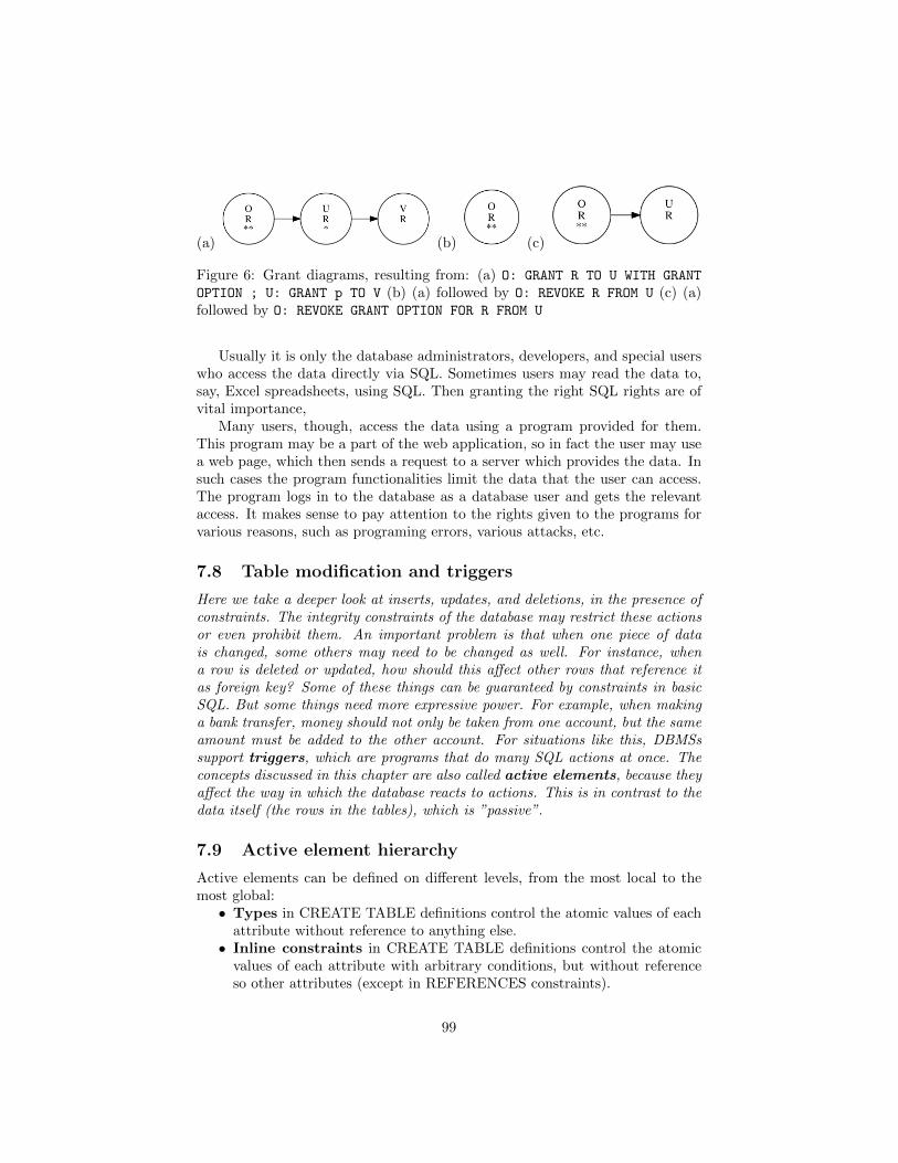
(a) (b) (c)
Figure 6: Grant diagrams, resulting from: (a) O: GRANT R TO U WITH GRANT
OPTION ; U: GRANT p TO V (b) (a) followed by O: REVOKE R FROM U (c) (a)followed by O: REVOKE GRANT OPTION FOR R FROM U
Usually it is only the database administrators, developers, and special userswho access the data directly via SQL. Sometimes users may read the data to,say, Excel spreadsheets, using SQL. Then granting the right SQL rights are ofvital importance,
Many users, though, access the data using a program provided for them.This program may be a part of the web application, so in fact the user may usea web page, which then sends a request to a server which provides the data. Insuch cases the program functionalities limit the data that the user can access.The program logs in to the database as a database user and gets the relevantaccess. It makes sense to pay attention to the rights given to the programs forvarious reasons, such as programing errors, various attacks, etc.
7.8 Table modification and triggers
Here we take a deeper look at inserts, updates, and deletions, in the presence ofconstraints. The integrity constraints of the database may restrict these actionsor even prohibit them. An important problem is that when one piece of datais changed, some others may need to be changed as well. For instance, whena row is deleted or updated, how should this affect other rows that reference itas foreign key? Some of these things can be guaranteed by constraints in basicSQL. But some things need more expressive power. For example, when makinga bank transfer, money should not only be taken from one account, but the sameamount must be added to the other account. For situations like this, DBMSssupport triggers, which are programs that do many SQL actions at once. Theconcepts discussed in this chapter are also called active elements, because theyaffect the way in which the database reacts to actions. This is in contrast to thedata itself (the rows in the tables), which is ”passive”.
7.9 Active element hierarchy
Active elements can be defined on different levels, from the most local to themost global:• Types in CREATE TABLE definitions control the atomic values of each
attribute without reference to anything else.• Inline constraints in CREATE TABLE definitions control the atomic
values of each attribute with arbitrary conditions, but without referenceso other attributes (except in REFERENCES constraints).
99
• Constraints in CREATE TABLE definitions control tuples or other setsof attribute, with conditions referring to things inside the table (exceptfor FOREIGN KEY).
• Assertions, which are top-level SQL statements, state conditions aboutthe whole database.
• Triggers, which are top-level SQL statements, can perform actions on thewhole database, using the DBMS.
• Host program code, in the embedded SQL case, can perform actionson the whole database, using both the DBMS and the host program.
It is often a good practice to state conditions on as local a level as possible,because they are then available in all wider contexts. However, there are threemajor exceptions:• Types such as CHAR(n) may seem to control the length of strings, but
they are not as accurate as CHECK constraints. For instance, CHAR(3)only checks the maximum length but not the exact length.
• Inline constraints cannot be changed afterwards by ALTER TABLE. Henceit can be better to use tuple-level named constraints.
• Assertions are disabled in many DBMSs (e.g. PostgreSQL, Oracle) be-cause they can be inefficient. Therefore one should use triggers to mimickassertions. This is what we do in this course.
Constraints that are marked DEFERRABLE in a CREATE TABLE statementare checked only at the end of each transaction (Section 9.2). This is useful,for instance, if one INSERT in a transaction involves a foreign key that is givenonly in a later statement.
7.10 Referential constraints and policies
A referential constraint (FOREIGN KEY ... REFERENCES) means that, whena value is used in the referring table, it must exist in the referenced table.But what happens if the value is deleted or changed in the referenced tableafterwards? This is what policies are for. The possible policies are CASCADEand SET NULL, to override the default behaviour which is to reject the change.
Assume we have a table of bank accounts:
CREATE TABLE Accounts (
number TEXT PRIMARY KEY,
holder TEXT,
type TEXT,
balance INT
)
The type attribute is supposed to hold the information of the bank accounttype: a savings account, a current account, etc. Let us then add a table withtransfers, with foreign keys referencing the first table:
CREATE TABLE Transfers (
sender TEXT REFERENCES Accounts(number),
100

recipient TEXT REFERENCES Accounts(number),
amount INT
)
What should we do with Transfers if a foreign key disappears i.e. if an accountnumber is removed from Accounts? There are three alternatives:• (default) reject the deletion from Accounts because of the reference in
Transfers,• CASCADE, i.e. also delete the transfers that reference the deleted ac-
count,• SET NULL, i.e. keep the transfers but set the sender or recipient number
to NULLOne of the last two actions can be defined to override the default, by using thefollowing syntax:
CREATE TABLE Transfers (
sender TEXT REFERENCES Accounts(number)
ON UPDATE CASCADE ON DELETE SET NULL,
recipient TEXT REFERENCES Accounts(number),
amount INT
)
ON UPDATE CASCADE means that if account number is changed in Accounts,it is also changed in Transfers. ON DELETE SET NULL means that if accountnumber is deleted from Accounts, it is changed to NULL in Transfers.
Finally, we have a table where we log the bank transfers. For each transferwe log the time, the user, the type of modification, and the data (new changeddata for insert and update, old removed data for delete).
Notice. This is a simplified example. These policies are probably not thebest way to handle accounts and transfers. It probably makes more sense tointroduce dates and times, so that rows referring to accounts existing at a certaintime need never be changed later.
7.11 CHECK constraints
CHECK constraints, which can be inlined or separate, are like invariants inprogramming. Here is a table definition with two attribute-level constraints,one inlined, the other named and separate:
-- specify a format for account numbers:
-- four characters,-, and at least two characters
-- more checks could be added to limit the characters to digits
CREATE TABLE Accounts (
number TEXT PRIMARY KEY CHECK (number LIKE ’____-%--’),
holder TEXT,
balance INT,
CONSTRAINT positive_balance CHECK (balance >= 0)
)
101
Here we have a table-level constraint referring to two attributes:
-- check that money may not be transferred from an account to itself
CREATE TABLE Transfers (
sender TEXT REFERENCES Accounts(number)
recipient TEXT REFERENCES Accounts(number),
amount INT,
CONSTRAINT not_to_self CHECK (recipient <> sender)
) ;
Here is a ”constraint” that is not possible in Transfers, trying to say thatthe balance cannot be exceeded in a transfer:
CONSTRAINT too_big_transfer CHECK (amount <= balance)
The reason is that the Transfers table cannot refer to the Accounts table (otherthan in FOREIGN KEY constraints). However, in this case, this is also un-necessary to state: because of the positive balance constraint in Accounts, atransfer exceeding the sender’s balance would be automatically blocked.
Here is another ”constraint” for Accounts, trying to set a maximum for themoney in the bank:
CONSTRAINT too_much_money_in_bank CHECK (sum(balance) < 1000000)
The problem is that constraints may not use aggregation functions (here, sum(balance)),because they are about tuples, not about whole tables. Such a constraint couldbe stated in an assertion, but these are not allowed in PostgreSQL even thoughthey are standard SQL. We will however be able to state this and many othertypes of contstraints using triggers, as we will see below.
7.12 ALTER TABLE
A table once created can be changed later with an ALTER TABLE statement. Themost important ways to alter a table are:• ADD COLUMN with the usual syntax (attribute, type, inline constraints).
The new column contains NULL values, unless some other default is speci-fied as DEFAULT.
• DROP COLUMN with the attribute name• ADD CONSTRAINT with the usual constraint syntax. Rejected if the already
existing table violates the constraint.• DROP CONSTRAINT with a named constraint
7.13 Triggers
Triggers in PostgreSQL are written in the language PL/PGSQL which is almoststandard SQL, with an exception:• the trigger body can only be a function call, and the function is written
separately
102
Here is the part of the syntax that we will need:
functiondefinition ::=
CREATE FUNCTION functionname() RETURNS TRIGGER AS $$
BEGIN
* statement
END
$$ LANGUAGE ’plpgsql’
;
triggerdefinition ::=
CREATE TRIGGER triggernane
whentriggered
FOR EACH ROW|STATEMENT
? WHEN ( condition )
EXECUTE PROCEDURE functionname
;
whentriggered ::=
BEFORE|AFTER events ON tablename
| INSTEAD OF events ON viewname
events ::= event | event OR events
event ::= INSERT | UPDATE | DELETE
statement ::=
IF ( condition ) THEN statement+ elsif* END IF ;
| RAISE EXCEPTION ’message’ ;
| sqlstatement ;
| RETURN NEW|OLD|NULL ;
elsif ::= ELSIF ( condition ) THEN statement+
Comments:• The statements may refer to NEW.attribute (in case of INSERT and UP-
DATE) and OLD.attribute (in case of UPDATE and DELETE).• FOR EACH ROW means that the trigger is executed for each new row
affected by an INSERT, UPDATE, or DELETE statement.• FOR EACH STATEMENT means that the trigger is executed once for
the whole statement.• A trigger is an atomic transaction, which either succeeds or fails totally
(see Chapter 9 for more details).• The PL/PGSQL functions have also access to further information, like
function now() telling the current time, and variables user telling the cur-rent database user, and TG OP telling the type of database operation(INSERT/UPDATE/DELETE).
Let us consider some examples.The first one is a check, that we could have also done when defining the
table:
103
CREATE OR REPLACE FUNCTION check_min_savings() RETURNS TRIGGER AS $$
BEGIN
IF NEW.type = ’savings’ AND NEW.balance < 100 THEN
RAISE EXCEPTION ’Balance too low for %’, NEW.Number ;
END IF;
RETURN NEW;
END
$$ LANGUAGE plpgsql ;
The related trigger:
CREATE TRIGGER minSavings
BEFORE INSERT OR UPDATE ON Accounts
FOR EACH ROW
EXECUTE PROCEDURE check_min_savings() ;
So, we can see that we can use triggers to check consistency. Since theactivities of functions are not limited, we could also here check the sum of thebalances of all accounts in the bank. The second example is doing exactlythat: limiting the maximum total balance of the bank. This trigger also doesn’tchange anything, and could therefore be defined as an ASSERTION, if theywere permitted.
CREATE OR REPLACE FUNCTION maxBalance() RETURNS TRIGGER AS $$
BEGIN
IF ((SELECT sum(balance) FROM Accounts) > 16000)
THEN RAISE EXCEPTION ’too much money in the bank’ ;
END IF ;
END
$$ LANGUAGE ’plpgsql’ ;
CREATE TRIGGER max_balance
AFTER INSERT OR UPDATE ON Accounts
FOR EACH STATEMENT
EXECUTE PROCEDURE maxBalance() ;
The third trigger introduces some application logic: it is a trigger that up-dates balances in Accounts after each inserted Transfer. In PostgreSQL, we firsthave to define a function that does the job by CREATE FUNCTION. After that, wecreate the trigger itself by CREATE TRIGGER.
CREATE FUNCTION make_transfer() RETURNS TRIGGER AS $$
BEGIN
UPDATE Accounts
SET balance = balance - NEW.amount
WHERE number = NEW.sender ;
UPDATE Accounts
104
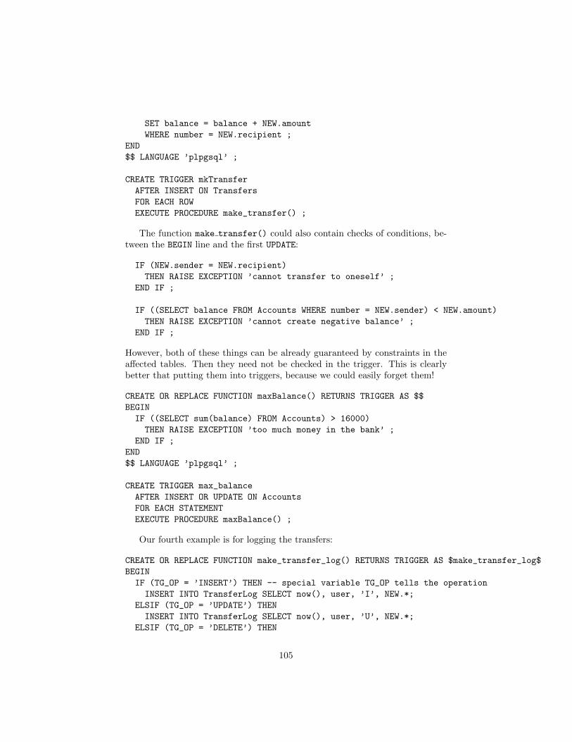
SET balance = balance + NEW.amount
WHERE number = NEW.recipient ;
END
$$ LANGUAGE ’plpgsql’ ;
CREATE TRIGGER mkTransfer
AFTER INSERT ON Transfers
FOR EACH ROW
EXECUTE PROCEDURE make_transfer() ;
The function make transfer() could also contain checks of conditions, be-tween the BEGIN line and the first UPDATE:
IF (NEW.sender = NEW.recipient)
THEN RAISE EXCEPTION ’cannot transfer to oneself’ ;
END IF ;
IF ((SELECT balance FROM Accounts WHERE number = NEW.sender) < NEW.amount)
THEN RAISE EXCEPTION ’cannot create negative balance’ ;
END IF ;
However, both of these things can be already guaranteed by constraints in theaffected tables. Then they need not be checked in the trigger. This is clearlybetter that putting them into triggers, because we could easily forget them!
CREATE OR REPLACE FUNCTION maxBalance() RETURNS TRIGGER AS $$
BEGIN
IF ((SELECT sum(balance) FROM Accounts) > 16000)
THEN RAISE EXCEPTION ’too much money in the bank’ ;
END IF ;
END
$$ LANGUAGE ’plpgsql’ ;
CREATE TRIGGER max_balance
AFTER INSERT OR UPDATE ON Accounts
FOR EACH STATEMENT
EXECUTE PROCEDURE maxBalance() ;
Our fourth example is for logging the transfers:
CREATE OR REPLACE FUNCTION make_transfer_log() RETURNS TRIGGER AS $make_transfer_log$
BEGIN
IF (TG_OP = ’INSERT’) THEN -- special variable TG_OP tells the operation
INSERT INTO TransferLog SELECT now(), user, ’I’, NEW.*;
ELSIF (TG_OP = ’UPDATE’) THEN
INSERT INTO TransferLog SELECT now(), user, ’U’, NEW.*;
ELSIF (TG_OP = ’DELETE’) THEN
105

INSERT INTO TransferLog SELECT now(), user, ’D’, OLD.*;
END IF;
RETURN NULL; -- no matter, as the update has already been done
END $make_transfer_log$
LANGUAGE plpgsql ;
CREATE TRIGGER mkLog
AFTER INSERT OR UPDATE OR DELETE ON Transfers
FOR EACH ROW
WHEN (pg_trigger_depth() < 1)
EXECUTE PROCEDURE make_transfer_log() ;
There is a particular risk with using triggers and functions: The functionexecutions may activate further triggers and in fact it is possible to create anon-terminating loop of trigger activations and function executions. A non-terminating execution is generally bad news, but additionally the functions maybe rapidly filling up the database as the execution is progressing. One safetyfeature is to use the pg trigger depth() function which returns a 0 if we are trig-gering the first function execution and when functions trigger further functions,each time the value of pg trigger depth() increases by 1.
The combinations of BEFORE/AFTER, OLD/NEW, and perhaps also ROW/STATEMENT,can be a bit tricky. The can be useful to test different combinations in Post-greSQL, monitor effects, and try to understand the error messages. When test-ing functions and triggers, it can be handy to write CREATE OR REPLACE insteadof just CREATE, so that a new version can be defined without a DROP of the oldversion.
Triggers can also be defined on views. Then the trigger is executed INSTEAD
OF updates, inserts, and deletions.
106
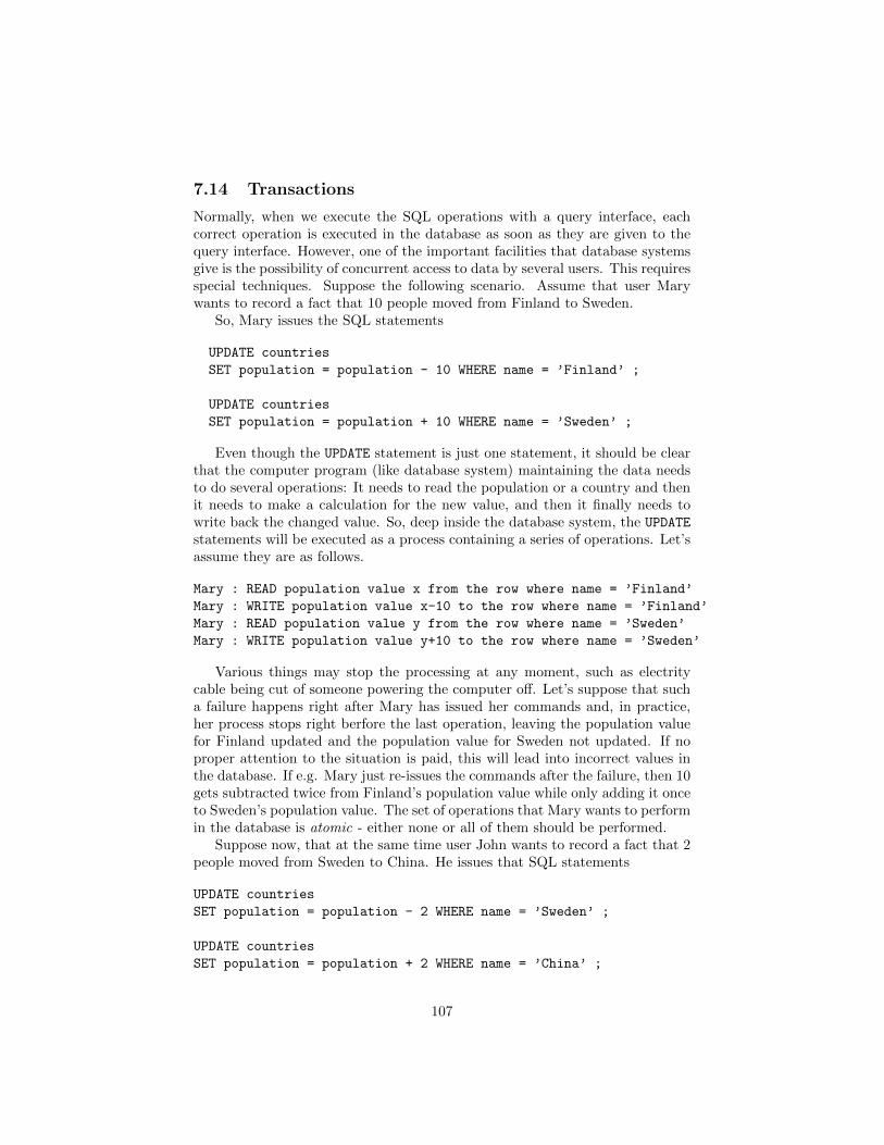
7.14 Transactions
Normally, when we execute the SQL operations with a query interface, eachcorrect operation is executed in the database as soon as they are given to thequery interface. However, one of the important facilities that database systemsgive is the possibility of concurrent access to data by several users. This requiresspecial techniques. Suppose the following scenario. Assume that user Marywants to record a fact that 10 people moved from Finland to Sweden.
So, Mary issues the SQL statements
UPDATE countries
SET population = population - 10 WHERE name = ’Finland’ ;
UPDATE countries
SET population = population + 10 WHERE name = ’Sweden’ ;
Even though the UPDATE statement is just one statement, it should be clearthat the computer program (like database system) maintaining the data needsto do several operations: It needs to read the population or a country and thenit needs to make a calculation for the new value, and then it finally needs towrite back the changed value. So, deep inside the database system, the UPDATE
statements will be executed as a process containing a series of operations. Let’sassume they are as follows.
Mary : READ population value x from the row where name = ’Finland’
Mary : WRITE population value x-10 to the row where name = ’Finland’
Mary : READ population value y from the row where name = ’Sweden’
Mary : WRITE population value y+10 to the row where name = ’Sweden’
Various things may stop the processing at any moment, such as electritycable being cut of someone powering the computer off. Let’s suppose that sucha failure happens right after Mary has issued her commands and, in practice,her process stops right berfore the last operation, leaving the population valuefor Finland updated and the population value for Sweden not updated. If noproper attention to the situation is paid, this will lead into incorrect values inthe database. If e.g. Mary just re-issues the commands after the failure, then 10gets subtracted twice from Finland’s population value while only adding it onceto Sweden’s population value. The set of operations that Mary wants to performin the database is atomic - either none or all of them should be performed.
Suppose now, that at the same time user John wants to record a fact that 2people moved from Sweden to China. He issues that SQL statements
UPDATE countries
SET population = population - 2 WHERE name = ’Sweden’ ;
UPDATE countries
SET population = population + 2 WHERE name = ’China’ ;
107
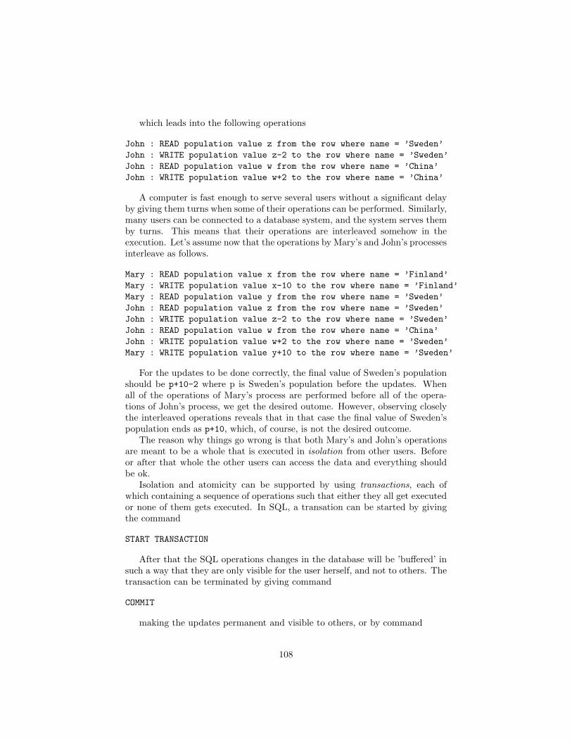
which leads into the following operations
John : READ population value z from the row where name = ’Sweden’
John : WRITE population value z-2 to the row where name = ’Sweden’
John : READ population value w from the row where name = ’China’
John : WRITE population value w+2 to the row where name = ’China’
A computer is fast enough to serve several users without a significant delayby giving them turns when some of their operations can be performed. Similarly,many users can be connected to a database system, and the system serves themby turns. This means that their operations are interleaved somehow in theexecution. Let’s assume now that the operations by Mary’s and John’s processesinterleave as follows.
Mary : READ population value x from the row where name = ’Finland’
Mary : WRITE population value x-10 to the row where name = ’Finland’
Mary : READ population value y from the row where name = ’Sweden’
John : READ population value z from the row where name = ’Sweden’
John : WRITE population value z-2 to the row where name = ’Sweden’
John : READ population value w from the row where name = ’China’
John : WRITE population value w+2 to the row where name = ’Sweden’
Mary : WRITE population value y+10 to the row where name = ’Sweden’
For the updates to be done correctly, the final value of Sweden’s populationshould be p+10-2 where p is Sweden’s population before the updates. Whenall of the operations of Mary’s process are performed before all of the opera-tions of John’s process, we get the desired outome. However, observing closelythe interleaved operations reveals that in that case the final value of Sweden’spopulation ends as p+10, which, of course, is not the desired outcome.
The reason why things go wrong is that both Mary’s and John’s operationsare meant to be a whole that is executed in isolation from other users. Beforeor after that whole the other users can access the data and everything shouldbe ok.
Isolation and atomicity can be supported by using transactions, each ofwhich containing a sequence of operations such that either they all get executedor none of them gets executed. In SQL, a transation can be started by givingthe command
START TRANSACTION
After that the SQL operations changes in the database will be ’buffered’ insuch a way that they are only visible for the user herself, and not to others. Thetransaction can be terminated by giving command
COMMIT
making the updates permanent and visible to others, or by command
108
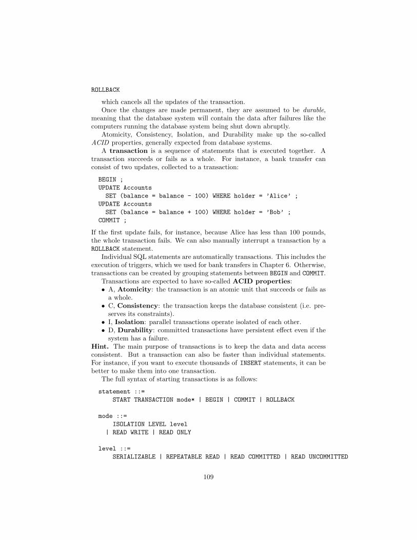
ROLLBACK
which cancels all the updates of the transaction.Once the changes are made permanent, they are assumed to be durable,
meaning that the database system will contain the data after failures like thecomputers running the database system being shut down abruptly.
Atomicity, Consistency, Isolation, and Durability make up the so-calledACID properties, generally expected from database systems.
A transaction is a sequence of statements that is executed together. Atransaction succeeds or fails as a whole. For instance, a bank transfer canconsist of two updates, collected to a transaction:
BEGIN ;
UPDATE Accounts
SET (balance = balance - 100) WHERE holder = ’Alice’ ;
UPDATE Accounts
SET (balance = balance + 100) WHERE holder = ’Bob’ ;
COMMIT ;
If the first update fails, for instance, because Alice has less than 100 pounds,the whole transaction fails. We can also manually interrupt a transaction by aROLLBACK statement.
Individual SQL statements are automatically transactions. This includes theexecution of triggers, which we used for bank transfers in Chapter 6. Otherwise,transactions can be created by grouping statements between BEGIN and COMMIT.
Transactions are expected to have so-called ACID properties:• A, Atomicity: the transaction is an atomic unit that succeeds or fails as
a whole.• C, Consistency: the transaction keeps the database consistent (i.e. pre-
serves its constraints).• I, Isolation: parallel transactions operate isolated of each other.• D, Durability: committed transactions have persistent effect even if the
system has a failure.Hint. The main purpose of transactions is to keep the data and data accessconsistent. But a transaction can also be faster than individual statements.For instance, if you want to execute thousands of INSERT statements, it can bebetter to make them into one transaction.
The full syntax of starting transactions is as follows:
statement ::=
START TRANSACTION mode* | BEGIN | COMMIT | ROLLBACK
mode ::=
ISOLATION LEVEL level
| READ WRITE | READ ONLY
level ::=
SERIALIZABLE | REPEATABLE READ | READ COMMITTED | READ UNCOMMITTED
109
The READ WRITE and READ ONLY modes indicate what interferences arepossible. This, as well as the effect of level, are discussed in more detail in thechapter on SQL in software applications.
7.15 Maintaining isolation*
The technicalities of how transactions are managed is not completely in the focusof this book. There are things, though, that a database user / programmershould understand, at least to trouble shoot problems appear. The need forisolation is motivated above. There are two main approaches for maintainingisolation: locking and multiversioning.
In locking, when a process needs access to a data item, it will ask for a lockon the item. There are two types of lockes: a Read lock (R-lock, shared lock),and a Read-Write lock (RW lock, exclusive lock). If a process needs to read anitem and has no previous lock on it, then it asks for an R-lock on the item. Ifsome other process holds an RW-lock to the item, then no lock is given and theprocess either rolls back or waits. If there are only R-locks or there are no lockson the item, then the R-lock is given to the process and the information of thelock is inserted into a lock table.
Similarly, if a process wants to write a data item, then it asks for an RW-lock on the item. IF some other process holds any kind of a lock, then the lockcannot be given and the requesting process either rolls back or waits. Otherwisethe lock is given and inserted to the lock table.
To maintain maximum isolation, the transaction only gives releases the locksat COMMIT or ROLLBACK. The waiting transactions may eventually get thelocks when other transactions terminate. Otherwise they may time out androll back. They may also stay on waiting, but there may be problems likedeadlock, where there is a cycle of processes each waiting for the locks that thenext process in the cycle holds. This can be detected by the system and some”random victim” can be sacrifised for the common good. Another problem isthat a process that rolls back and restarts might not get the locks even afterrepeated restart - this is called starvation. As a further problem with locking,transactions accessing large amounts of data will create a lot of entries in thelock tables, thus making the tables big.
Multiversioning is based on the idea that several versions of the data itemare stored. Transactions are given a number or a timestamp when they start.The basic idea is that a writing transaction updates the list of versions by writ-ing a new version along with its timestamp in the list. Reading transactionsselect from the list the value valid for their time. For instance, if the list, as-sumed here to be ordered, has<timestamp, value> pairs<100,5.0>, <104,2.0>,<109,11.0> for some data time A, then a transaction with timestamp 107 want-ing to read A would pick the value 2.0 as it is the last value written before time107.
We can remove such values from the list that there are no such transactionsanymore that would need those values. For instance, if all executing transactionshave at least timestamp 105, then we could remove <100,5.0> from the list.
110
If removal of old versions is done appropriately, then reads are always suc-cessful. However, to figure out if the writes can be executed, the reads have torecord the last timestamp when a data itme is read. Let’s suppose that the dataitem A above is read at time 112 and a transaction with timestamp 111 wantsto write a value for A. Now, to simulate a correct order of transactions, then thetransaction with timestamp 111 cannot write that value anymore, as the valueit wants to write should have been read by the transaction with timestamp 112,and, consequently, the transaction with timestamp 111 must be rolled back.This, however, may lead to a need to roll back other transactions that haveread data written with timestamp 111.
Even though reading transactions never block, this way they have to waitfor earlier transactions to commit or roll back before they can decide if they cancommit.
7.16 Interferences and isolation levels
If we maintain the transactions as in the previous section, then the effects ofthe execution are the same as if the transactions would be executed in a serialorder - thereby we such arrangements lead to serializable excutions (executionsthat could be re-arranged as serial).
However, big lock tables or waiting for other transactions to commit may beprohibiting for performance. For some applications we can have more flexiblerequirements for the concurrency, e.g. it may not be absolutely necessary thatthey read the last value, or it is not catastrophic if they read a value thatfinally was not stored permanently by the transaction. A bank might requireserializable executions to maintain the balances while in a social media platformwe may allow users to see comments that were not stored permanently or theuses may miss the most recent comments at some points.
Thus, sometimes Isolation requireent in the ACID properties is too rigid. Ifwe allow for multiversioning transactions to commit not waiting for others, thenthey might have read some value that did not become permanent (dirty data).Similarly, if locking transactions release their locks before commit/rollback andfinally roll back. In such cases also repeated reads of the data may bring differentresults.
In practice, a database system may allow weakening the Isolation conditionby using isolation levels. These levels are defined as follows:
• SERIALIZABLE: the transaction only sees data that was committed be-fore the transaction began.
• REPEATABLE READ: like READ COMMITTED, but previously readdata may not be changed.
• READ COMMITTED: the transaction can see data that is committedby other transactions during it is running, in addition to data committedbefore it started.
111
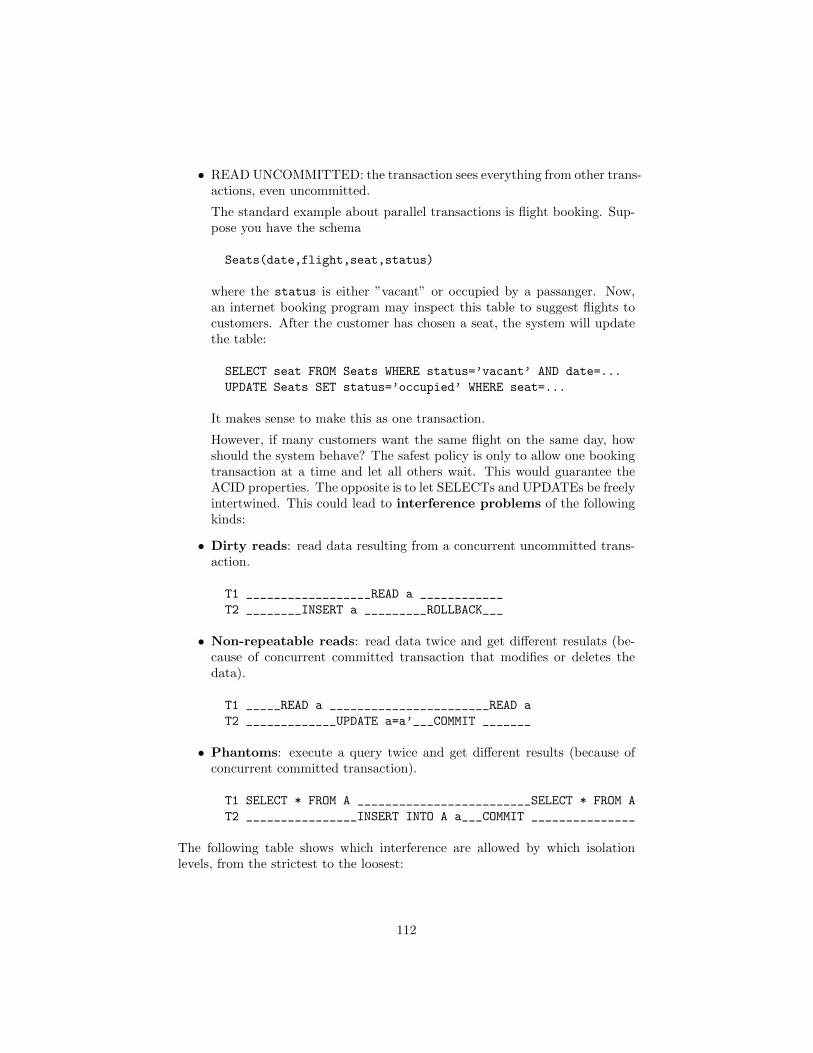
• READ UNCOMMITTED: the transaction sees everything from other trans-actions, even uncommitted.
The standard example about parallel transactions is flight booking. Sup-pose you have the schema
Seats(date,flight,seat,status)
where the status is either ”vacant” or occupied by a passanger. Now,an internet booking program may inspect this table to suggest flights tocustomers. After the customer has chosen a seat, the system will updatethe table:
SELECT seat FROM Seats WHERE status=’vacant’ AND date=...
UPDATE Seats SET status=’occupied’ WHERE seat=...
It makes sense to make this as one transaction.
However, if many customers want the same flight on the same day, howshould the system behave? The safest policy is only to allow one bookingtransaction at a time and let all others wait. This would guarantee theACID properties. The opposite is to let SELECTs and UPDATEs be freelyintertwined. This could lead to interference problems of the followingkinds:
• Dirty reads: read data resulting from a concurrent uncommitted trans-action.
T1 __________________READ a ____________
T2 ________INSERT a _________ROLLBACK___
• Non-repeatable reads: read data twice and get different resulats (be-cause of concurrent committed transaction that modifies or deletes thedata).
T1 _____READ a _______________________READ a
T2 _____________UPDATE a=a’___COMMIT _______
• Phantoms: execute a query twice and get different results (because ofconcurrent committed transaction).
T1 SELECT * FROM A _________________________SELECT * FROM A
T2 ________________INSERT INTO A a___COMMIT _______________
The following table shows which interference are allowed by which isolationlevels, from the strictest to the loosest:
112
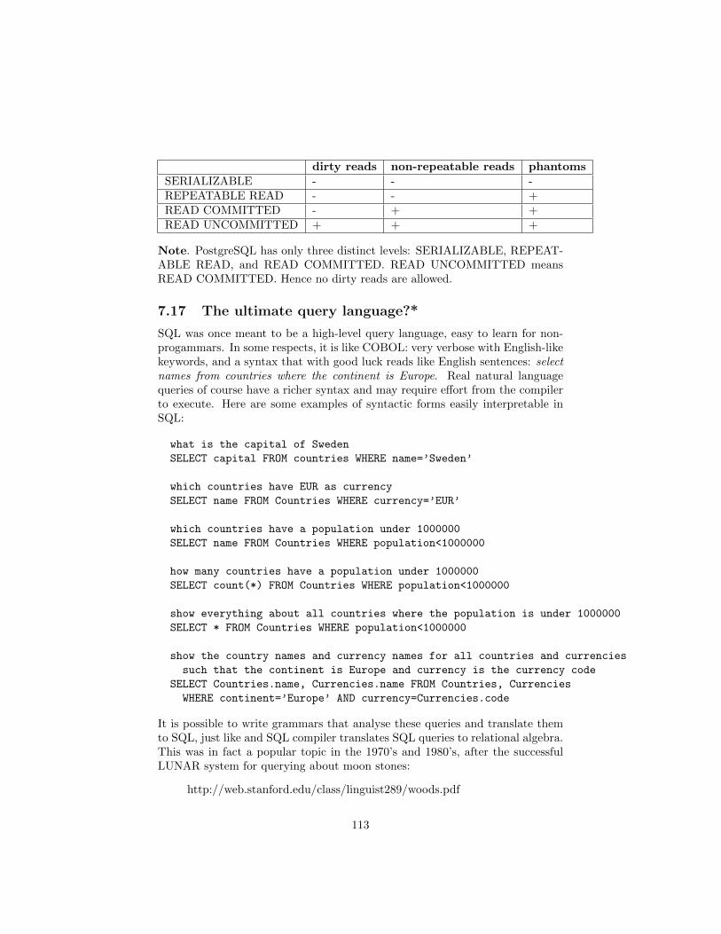
dirty reads non-repeatable reads phantomsSERIALIZABLE - - -REPEATABLE READ - - +READ COMMITTED - + +READ UNCOMMITTED + + +
Note. PostgreSQL has only three distinct levels: SERIALIZABLE, REPEAT-ABLE READ, and READ COMMITTED. READ UNCOMMITTED meansREAD COMMITTED. Hence no dirty reads are allowed.
7.17 The ultimate query language?*
SQL was once meant to be a high-level query language, easy to learn for non-progammars. In some respects, it is like COBOL: very verbose with English-likekeywords, and a syntax that with good luck reads like English sentences: selectnames from countries where the continent is Europe. Real natural languagequeries of course have a richer syntax and may require effort from the compilerto execute. Here are some examples of syntactic forms easily interpretable inSQL:
what is the capital of Sweden
SELECT capital FROM countries WHERE name=’Sweden’
which countries have EUR as currency
SELECT name FROM Countries WHERE currency=’EUR’
which countries have a population under 1000000
SELECT name FROM Countries WHERE population<1000000
how many countries have a population under 1000000
SELECT count(*) FROM Countries WHERE population<1000000
show everything about all countries where the population is under 1000000
SELECT * FROM Countries WHERE population<1000000
show the country names and currency names for all countries and currencies
such that the continent is Europe and currency is the currency code
SELECT Countries.name, Currencies.name FROM Countries, Currencies
WHERE continent=’Europe’ AND currency=Currencies.code
It is possible to write grammars that analyse these queries and translate themto SQL, just like and SQL compiler translates SQL queries to relational algebra.This was in fact a popular topic in the 1970’s and 1980’s, after the successfulLUNAR system for querying about moon stones:
http://web.stanford.edu/class/linguist289/woods.pdf
113
Natural language question answering is becoming popular again, in systems likeWolfram Alpha and IBM Watson. They are expected to give• more fine-grained search possibilities than plain string-based search• support for queries in speech, like in Google’s Voice Search and Apple’s
Siri.The main problems of natural language search are• precision: without a grammar comparable to e.g. SQL grammar, it is
difficult to interpret complex queries correctly• coverage: queries can be expressed in so many different ways that it is
difficult to have a complete grammar• ambiguity: a query can have different interpretations, which is sometimes
clear from context (but exactly how?), sometime not:– Please tell us quickly, Intelligent Defence System: Are the missiles
coming across the ocean or over the North Pole?– Calculating........ Yes.
Interestingly, once we can solve these problems for one language, other languagesfollow the same patterns:
vad ar Sveriges huvudstad
vilka lander har EUR som valuta
vilka lander har en befolkning under 1000000
hur manga lander har en befolkning under 1000000
visa allt om alla lander dar befolkningen ar under 1000000
visa landnamnen och valutanamnen for alla lander och valutor
dar kontinenten ar Europa och valutan ar valutakoden
Natural language queries are in the intersection of database technology andartificial intelligence. The problem can be approached incrementally, by accu-mulating technology and knowledge. Much of the research is on collecting theknowledge automatically, by for instance using machine learning. This is thecase in particular when the knowledge is in unstructured form such as text.However, when the knowledge is already in a database, the question becomesmuch more like query compilation.
114
8 Introduction to alternative data models
The relational data model has been dominating the database world for a longtime. But there are alternative models, some of which are gaining popularity.XML is an old model, often seen as a language for documents rather than data.In this perspective, it is a generalization of HTML. But it is a very powerfulgeneralization, which can be used for any structured data. XML data objectsneed not be just tuples, but they can be arbitrary trees. XML also has designatedquery languages, such as XPath and XQuery. This chapter introduces XMLand gives a summary of XPath. A more general approach is that of **docu-ment databases**, which are designed in particular textual structured or semi-structured data. One example of such systems is MongoDB, shortly also coveredin this chapter. A particular concern in document databases is a query lan-guage or facility, which has search structures more suitable for such documentsthan SQL. The chapter concludes with Big Data and ”NoSQL” approaches moregenerally, with Cassandra as example.
8.1 XML and its data model
XML (eXtensible Markup Language) is a notation for documents and data.For documents, it can be seen as a generalization of HTML (Hypertext MarkupLanguage): HTML is just one of the languages that can be defined in XML.If more structure is wanted for special kinds of documents, HTML can be ”ex-tended” with the help of XML. For instance, if we want to store an English-Swedish dictionary, we can build the following kind of XML objects:
<word>
<pos>Noun</pos>
<english>computer</english>
<swedish>dator</swedish>
</word>
(where pos = part of speech = ”ordklass”). When printing the dictionary, thisobject could be transformed into an HTML object,
<p>
<i>computer</i> (Noun)
dator
</p>
But the HTML format is less suitable when the dictionary is used as data, whereone can look up words. Therefore the original XML structure is better suitedfor storing the dictionary data.
The form of an XML data object is
<tag> ... </tag>
115
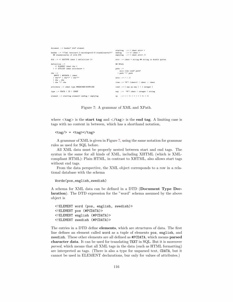
document ::= header? dtd? element
starttag ::= < ident attr* >
header ::= "<?xml version=1.0 encoding=utf-8 standalone=no?>" endtag ::= </ ident >
## standalone=no if with DTD emptytag ::= < ident attr* />
dtd ::= <! DOCTYPE ident [ definition* ]> attr ::= ident = string ## string in double quotes
definition ::= ## XPath
<! ELEMENT ident rhs >
| <! ATTLIST ident attribute* > path ::=
axis item cond? path?
rhs ::= | path "|" path
EMPTY | #PCDATA | ident
| rhs"*" | rhs"+" | rhs"?" axis ::= / | //
| rhs , rhs
| rhs "|" rhs item ::= "@"? (ident*) | ident :: ident
attribute ::= ident type #REQUIRED|#IMPLIED cond ::= [ exp op exp ] | [ integer ]
type ::= CDATA | ID | IDREF exp ::= "@"? ident | integer | string
element ::= starttag element* endtag | emptytag op ::= = | != | < | > | <= | >=
Figure 7: A grammar of XML and XPath.
where <tag> is the start tag and </tag> is the end tag. A limiting case istags with no content in between, which has a shorthand notation,
<tag/> = <tag></tag>
A grammar of XML is given in Figure 7, using the same notation for grammarrules as used for SQL before.
All XML data must be properly nested between start and end tags. Thesyntax is the same for all kinds of XML, including XHTML (which is XML-compliant HTML): Plain HTML, in contrast to XHTML, also allows start tagswithout end tags.
From the data perspective, the XML object corresponds to a row in a rela-tional database with the schema
Words(pos,english,swedish)
A schema for XML data can be defined in a DTD (Document Type Dec-laration). The DTD expression for the ”word” schema assumed by the aboveobject is
<!ELEMENT word (pos, english, swedish)>
<!ELEMENT pos (#PCDATA)>
<!ELEMENT english (#PCDATA)>
<!ELEMENT swedish (#PCDATA)>
The entries in a DTD define elements, which are structures of data. The firstline defines an element called word as a tuple of elements pos, english, andswedish. These other elements are all defined as #PCDATA, which means parsedcharacter data. It can be used for translating TEXT in SQL. But it is moreoverparsed, which means that all XML tags in the data (such as HTML formatting)are interpreted as tags. (There is also a type for unparsed text, CDATA, but itcannot be used in ELEMENT declarations, bur only for values of attributes.)
116
XML supports more data structures than the relational model. In the re-lational model, the only structure is the tuple, and all its elements must beatomic. In full XML, the elements of tuples can be structured elements them-selves. They are called daughter elements. In fact, XML supports algebraicdatatypes similar to Haskell’s data definitions:
• Elements can be defined as
tuples of elements: E, F
lists of elements: E*
nonempty lists of elements: E+
alternative elements: E | Foptional elements: E?
strings: #PCDATA
• Elements can be recursive, that is, a part of an element can be an instanceof the element itself. This enables elements of unlimited size.
• Thus the elements of XML are trees, not just tuples. (A tuple is a limitingcase, with just one branching node and leaves under it.)
The validation of an XML document checks its correctness with respect to aDTD. It corresponds to type checking in Haskell. Validation tools are availableon the web, for instance, http://validator.w3.org/
Figure 8 gives an example of a recursive type. It encodes a data type forarithmetic expression, and an element representing the expression 23 + 15 * x.It shows a complete XML document, which consists of a header, a DTD (startingwith the keyword DOCTYPE), and an element. It also shows a correspondingalgebraic datatype definition in Haskell and a Haskell expression correspondingto the XML element.
To encode SQL tuples, we only need the tuple type and the PCDATA type.However, this DTD encoding does not capture all parts of SQL’s table defini-tions:• basic types in XML are not so refined: basically only TEXT is available• constraints cannot be expressed in the DTD
Some of these problems can be solved by using attributes rather than elements.Here is an alternative representation of dictionary entries:
<!ELEMENT word EMPTY>
<!ATTLIST word
pos CDATA #REQUIRED
english CDATA #REQUIRED
swedish CDATA #REQUIRED
>
<word pos="Noun" english="Computer" swedish="Dator">
The #REQUIRED keyword is similar to a NOT NULL constraint in SQL. Optionalattributes have the keyword #IMPLIED.
Let us look at another example, which shows how to model referential con-straints:
117
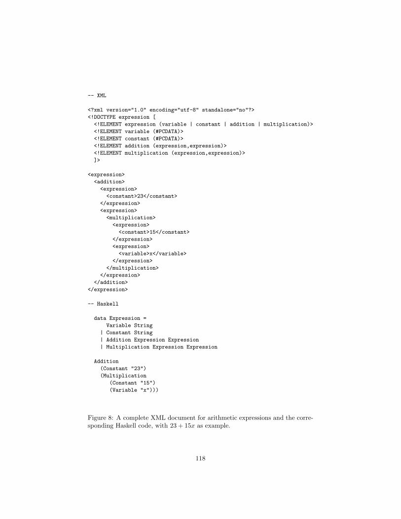
-- XML
<?xml version="1.0" encoding="utf-8" standalone="no"?>
<!DOCTYPE expression [
<!ELEMENT expression (variable | constant | addition | multiplication)>
<!ELEMENT variable (#PCDATA)>
<!ELEMENT constant (#PCDATA)>
<!ELEMENT addition (expression,expression)>
<!ELEMENT multiplication (expression,expression)>
]>
<expression>
<addition>
<expression>
<constant>23</constant>
</expression>
<expression>
<multiplication>
<expression>
<constant>15</constant>
</expression>
<expression>
<variable>x</variable>
</expression>
</multiplication>
</expression>
</addition>
</expression>
-- Haskell
data Expression =
Variable String
| Constant String
| Addition Expression Expression
| Multiplication Expression Expression
Addition
(Constant "23")
(Multiplication
(Constant "15")
(Variable "x")))
Figure 8: A complete XML document for arithmetic expressions and the corre-sponding Haskell code, with 23 + 15x as example.
118
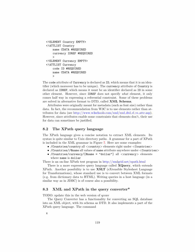
<!ELEMENT Country EMPTY>
<!ATTLIST Country
name CDATA #REQUIRED
currency IDREF #REQUIRED
>
<!ELEMENT Currency EMPTY>
<!ATTLIST Currency
code ID #REQUIRED
name CDATA #REQUIRED
>
The code attribute of Currency is declared as ID, which means that it is an iden-tifier (which moreover has to be unique). The currency attribute of Country isdeclared as IDREF, which means it must be an identifier declared as ID in someother element. However, since IDREF does not specify what element, it onlycomes half way in expressing a referential constraint. Some of these problemsare solved in alternative format to DTD, called XML Schema.
Attributes were originally meant for metadata (such as font size) rather thandata. In fact, the recommendation from W3C is to use elements rather than at-tributes for data (see http://www.w3schools.com/xml/xml dtd el vs attr.asp).However, since attributes enable some constraints that elements don’t, their usefor data can sometimes be justified.
8.2 The XPath query language
The XPath language gives a concise notation to extract XML elements. Itssyntax is quite similar to Unix directory paths. A grammar for a part of XPathis included in the XML grammar in Figure 7. Here are some examples:• /Countries/country all <country> elements right under <Countries>• /Countries//@name all values of name attribute anywhere under<Countries>• /Countries/currency/[@name = "dollar"] all <currency> elements
where name is dollar
There is an on-line XPath test program in http://xmlgrid.net/xpath.htmlThere is a more expressive query language called XQuery, which extends
XPath. Another possibility is to use XSLT (eXtensible Stylesheet Languagefor Transformations), whose standard use is to convert between XML formats(e.g. from dictionary data to HTML). Writing queries in a host language (in asimilar way as in JDBC) is of course also a possibility.
8.3 XML and XPath in the query converter*
TODO: update this in the web version of qconvThe Query Converter has a functionality for converting an SQL database
into an XML object, with its schema as DTD. It also implements a part of theXPath query language. The command
x
119
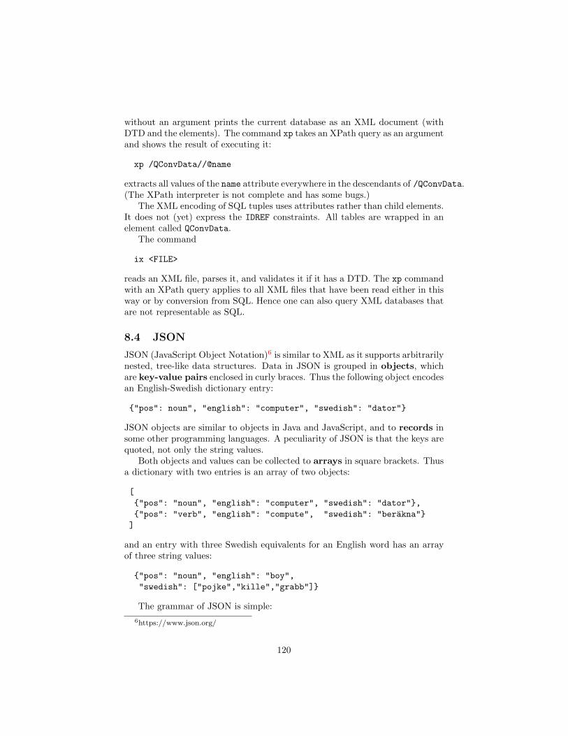
without an argument prints the current database as an XML document (withDTD and the elements). The command xp takes an XPath query as an argumentand shows the result of executing it:
xp /QConvData//@name
extracts all values of the name attribute everywhere in the descendants of /QConvData.(The XPath interpreter is not complete and has some bugs.)
The XML encoding of SQL tuples uses attributes rather than child elements.It does not (yet) express the IDREF constraints. All tables are wrapped in anelement called QConvData.
The command
ix <FILE>
reads an XML file, parses it, and validates it if it has a DTD. The xp commandwith an XPath query applies to all XML files that have been read either in thisway or by conversion from SQL. Hence one can also query XML databases thatare not representable as SQL.
8.4 JSON
JSON (JavaScript Object Notation)6 is similar to XML as it supports arbitrarilynested, tree-like data structures. Data in JSON is grouped in objects, whichare key-value pairs enclosed in curly braces. Thus the following object encodesan English-Swedish dictionary entry:
"pos": noun", "english": "computer", "swedish": "dator"
JSON objects are similar to objects in Java and JavaScript, and to records insome other programming languages. A peculiarity of JSON is that the keys arequoted, not only the string values.
Both objects and values can be collected to arrays in square brackets. Thusa dictionary with two entries is an array of two objects:
[
"pos": "noun", "english": "computer", "swedish": "dator",
"pos": "verb", "english": "compute", "swedish": "berakna"
]
and an entry with three Swedish equivalents for an English word has an arrayof three string values:
"pos": "noun", "english": "boy",
"swedish": ["pojke","kille","grabb"]
The grammar of JSON is simple:
6https://www.json.org/
120
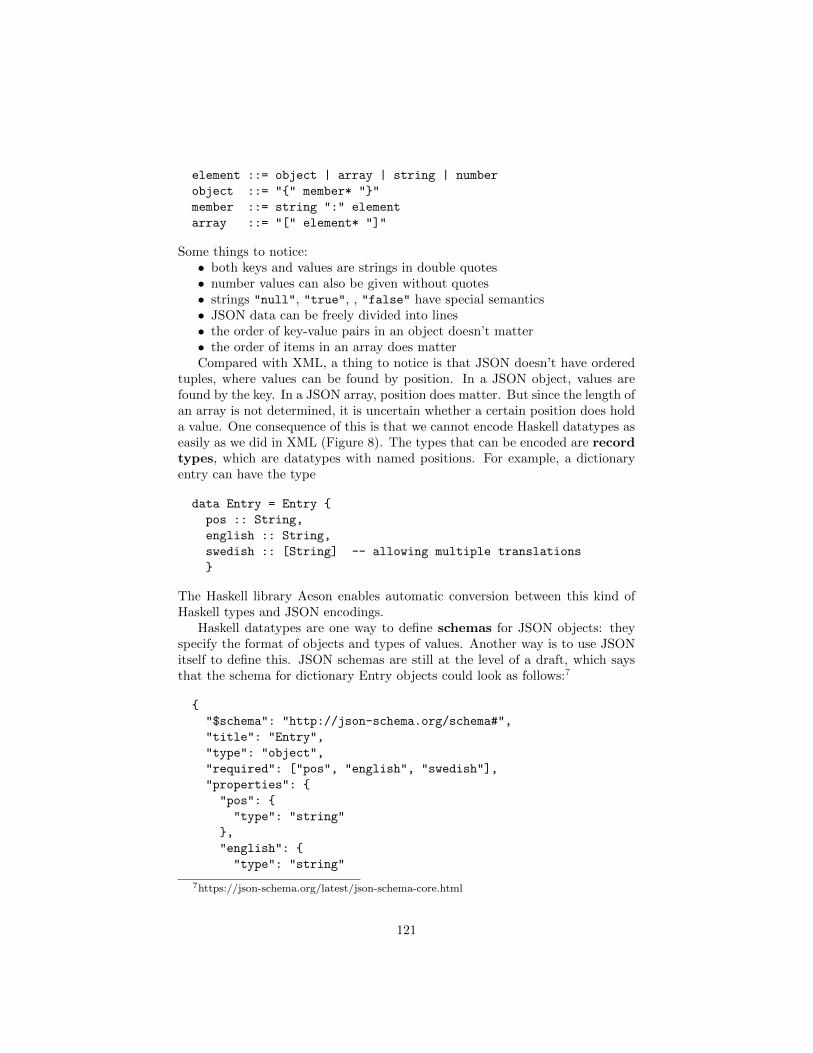
element ::= object | array | string | number
object ::= "" member* ""
member ::= string ":" element
array ::= "[" element* "]"
Some things to notice:• both keys and values are strings in double quotes• number values can also be given without quotes• strings "null", "true", , "false" have special semantics• JSON data can be freely divided into lines• the order of key-value pairs in an object doesn’t matter• the order of items in an array does matterCompared with XML, a thing to notice is that JSON doesn’t have ordered
tuples, where values can be found by position. In a JSON object, values arefound by the key. In a JSON array, position does matter. But since the length ofan array is not determined, it is uncertain whether a certain position does holda value. One consequence of this is that we cannot encode Haskell datatypes aseasily as we did in XML (Figure 8). The types that can be encoded are recordtypes, which are datatypes with named positions. For example, a dictionaryentry can have the type
data Entry = Entry
pos :: String,
english :: String,
swedish :: [String] -- allowing multiple translations
The Haskell library Aeson enables automatic conversion between this kind ofHaskell types and JSON encodings.
Haskell datatypes are one way to define schemas for JSON objects: theyspecify the format of objects and types of values. Another way is to use JSONitself to define this. JSON schemas are still at the level of a draft, which saysthat the schema for dictionary Entry objects could look as follows:7
"$schema": "http://json-schema.org/schema#",
"title": "Entry",
"type": "object",
"required": ["pos", "english", "swedish"],
"properties":
"pos":
"type": "string"
,
"english":
"type": "string"
7https://json-schema.org/latest/json-schema-core.html
121
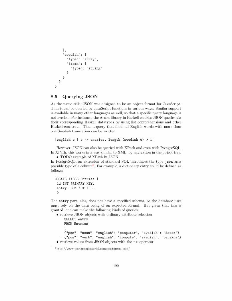
,
"swedish":
"type": "array",
"items":
"type": "string"
8.5 Querying JSON
As the name tells, JSON was designed to be an object format for JavaScript.Thus it can be queried by JavaScript functions in various ways. Similar supportis available in many other languages as well, so that a specific query language isnot needed. For instance, the Aeson library in Haskell enables JSON queries viatheir corresponding Haskell datatypes by using list comprehensions and otherHaskell construts. Thus a query that finds all English words with more thanone Swedish translation can be written
[english e | e <- entries, length (swedish e) > 1]
However, JSON can also be queried with XPath and even with PostgreSQL.In XPath, this works in a way similar to XML, by navigation in the object tree.• TODO example of XPath in JSON
In PostgreSQL, an extension of standard SQL introduces the type json as apossible type of a column8. For example, a dictionary entry could be defined asfollows:
CREATE TABLE Entries
id INT PRIMARY KEY,
entry JSON NOT NULL
The entry part, alas, does not have a specified schema, so the database usermust rely on the data being of an expected format. But given that this isgranted, one can make the following kinds of queries:• retrieve JSON objects with ordinary attribute selection
SELECT entry
FROM Entries
;
"pos": "noun", "english": "computer", "swedish": "dator"
‘ "pos": "verb", "english": "compute", "swedish": "berakna"
• retrieve values from JSON objects with the -> operator
8http://www.postgresqltutorial.com/postgresql-json/
122
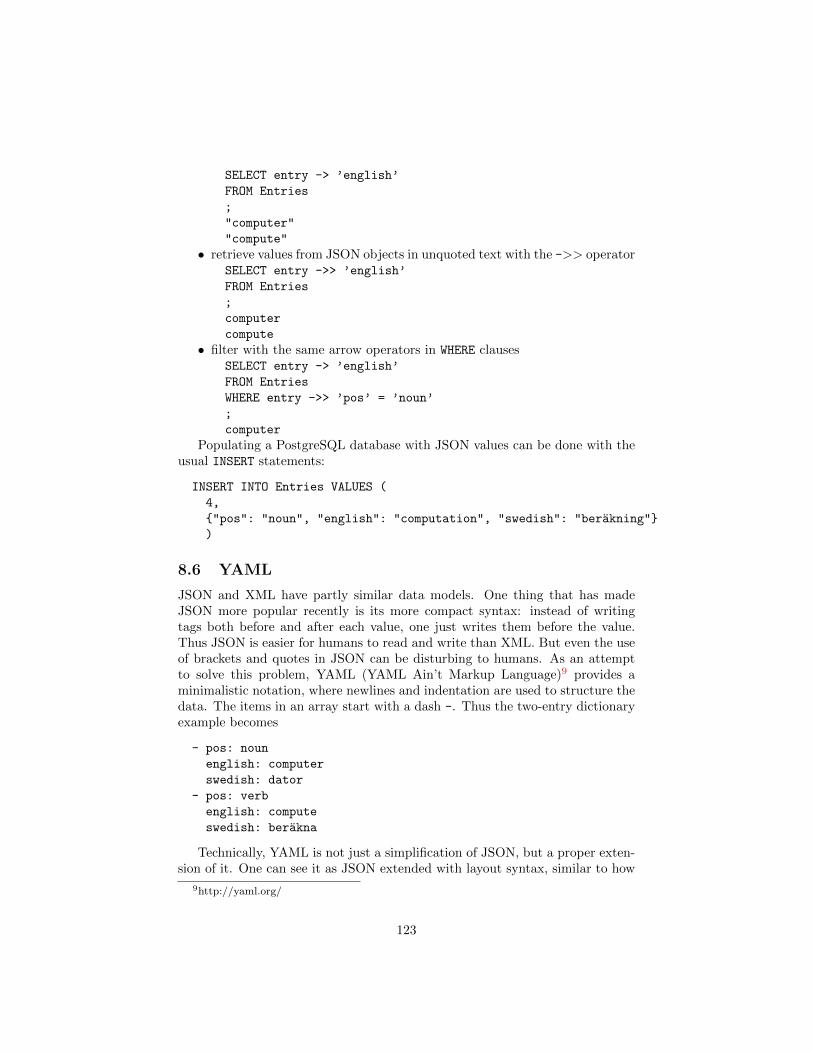
SELECT entry -> ’english’
FROM Entries
;
"computer"
"compute"
• retrieve values from JSON objects in unquoted text with the ->> operatorSELECT entry ->> ’english’
FROM Entries
;
computer
compute
• filter with the same arrow operators in WHERE clausesSELECT entry -> ’english’
FROM Entries
WHERE entry ->> ’pos’ = ’noun’
;
computer
Populating a PostgreSQL database with JSON values can be done with theusual INSERT statements:
INSERT INTO Entries VALUES (
4,
"pos": "noun", "english": "computation", "swedish": "berakning"
)
8.6 YAML
JSON and XML have partly similar data models. One thing that has madeJSON more popular recently is its more compact syntax: instead of writingtags both before and after each value, one just writes them before the value.Thus JSON is easier for humans to read and write than XML. But even the useof brackets and quotes in JSON can be disturbing to humans. As an attemptto solve this problem, YAML (YAML Ain’t Markup Language)9 provides aminimalistic notation, where newlines and indentation are used to structure thedata. The items in an array start with a dash -. Thus the two-entry dictionaryexample becomes
- pos: noun
english: computer
swedish: dator
- pos: verb
english: compute
swedish: berakna
Technically, YAML is not just a simplification of JSON, but a proper exten-sion of it. One can see it as JSON extended with layout syntax, similar to how
9http://yaml.org/
123

Python and Haskell avoid brackets by the use of line breaks and indentation.But JSON is included in YAML, so that a YAML element can contain parts thatare in ordinary JSON. This is sometimes more compact than ”pure” YAML, asa short array or object can be placed on a single line. In the following example,the left column shows a ”pure” YAML object and the right column uses inlinedJSON.
pos: noun pos: noun
english: boy english : boy
swedish: swedish: [pojke,kille,grabb]
- pojke
- kille
- grabb
YAML may look simple to the human eye, but its processing for a machineis much more complicated than JSON, because complicated rules are neededto deal with things like white space (as used for indentation and inside stringvalues) and escape characters (to know that belongs to the notation and whatis a part of a value). This can also, paradoxically, make it more difficult forhuman authors to write valid YAML without noticing it. We don’t even try toformulate a grammar of YAML here.
8.7 MongoDB*
MongoDB, another public open-source database product, uses the documentmetaphora for data storage. This makes it flexible and useful for TODO
8.8 Pivot tables and OLAP*
TODO
8.9 NoSQL data models*
Big Data is a word used for data whose mere size is a problem. What the sizeis depends on many things, such as available storage and computing power. Atthe time of writing, Big Data is often expected to be at least terabytes (1012
bytes), maybe even petabytes (1015).In relational databases, each table must usually reside in one computer. In
Big Data, data is usually distributed, maybe to thousands of computers (ormillions in the case of companies like Google). The computations must also beparallelizable as much as possible. This has implications for big data systems,which makes them different from relational databases:• simpler queries (e.g. no joins, search on indexed attributes only)• looser structures (e.g. no tables with rigid schemas)• less integrity guarantees (e.g. no checking of constraints, no transactions)• more redundancy (”denormalization” to keep together data that belongs
together)
124
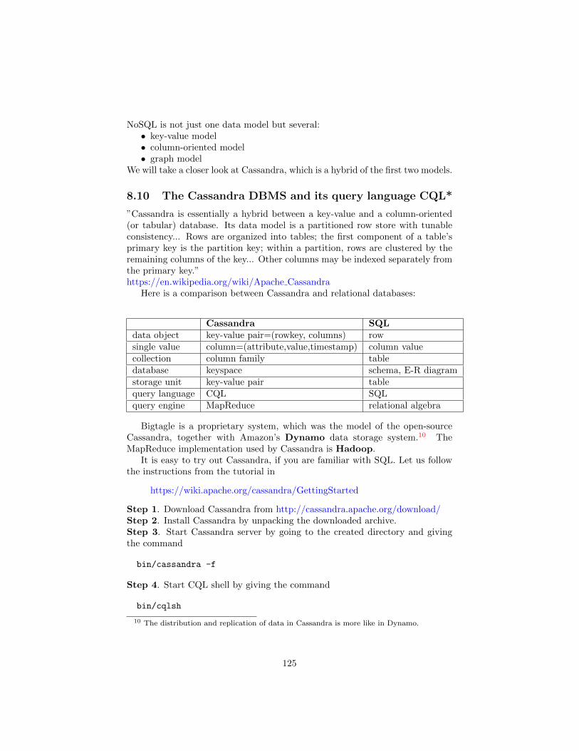
NoSQL is not just one data model but several:• key-value model• column-oriented model• graph model
We will take a closer look at Cassandra, which is a hybrid of the first two models.
8.10 The Cassandra DBMS and its query language CQL*
”Cassandra is essentially a hybrid between a key-value and a column-oriented(or tabular) database. Its data model is a partitioned row store with tunableconsistency... Rows are organized into tables; the first component of a table’sprimary key is the partition key; within a partition, rows are clustered by theremaining columns of the key... Other columns may be indexed separately fromthe primary key.”https://en.wikipedia.org/wiki/Apache Cassandra
Here is a comparison between Cassandra and relational databases:
Cassandra SQLdata object key-value pair=(rowkey, columns) rowsingle value column=(attribute,value,timestamp) column valuecollection column family tabledatabase keyspace schema, E-R diagramstorage unit key-value pair tablequery language CQL SQLquery engine MapReduce relational algebra
Bigtagle is a proprietary system, which was the model of the open-sourceCassandra, together with Amazon’s Dynamo data storage system.10 TheMapReduce implementation used by Cassandra is Hadoop.
It is easy to try out Cassandra, if you are familiar with SQL. Let us followthe instructions from the tutorial in
https://wiki.apache.org/cassandra/GettingStarted
Step 1. Download Cassandra from http://cassandra.apache.org/download/Step 2. Install Cassandra by unpacking the downloaded archive.Step 3. Start Cassandra server by going to the created directory and givingthe command
bin/cassandra -f
Step 4. Start CQL shell by giving the command
bin/cqlsh
10 The distribution and replication of data in Cassandra is more like in Dynamo.
125
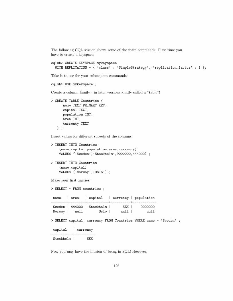
The following CQL session shows some of the main commands. First time youhave to create a keyspace:
cqlsh> CREATE KEYSPACE mykeyspace
WITH REPLICATION = ’class’ : ’SimpleStrategy’, ’replication_factor’ : 1 ;
Take it to use for your subsequent commands:
cqlsh> USE mykeyspace ;
Create a column family - in later versions kindly called a ”table”!
> CREATE TABLE Countries (
name TEXT PRIMARY KEY,
capital TEXT,
population INT,
area INT,
currency TEXT
) ;
Insert values for different subsets of the columns:
> INSERT INTO Countries
(name,capital,population,area,currency)
VALUES (’Sweden’,’Stockholm’,9000000,444000) ;
> INSERT INTO Countries
(name,capital)
VALUES (’Norway’,’Oslo’) ;
Make your first queries:
> SELECT * FROM countries ;
name | area | capital | currency | population
--------+--------+-----------+----------+------------
Sweden | 444000 | Stockholm | SEK | 9000000
Norway | null | Oslo | null | null
> SELECT capital, currency FROM Countries WHERE name = ’Sweden’ ;
capital | currency
-----------+----------
Stockholm | SEK
Now you may have the illusion of being in SQL! However,
126
> SELECT name FROM Countries WHERE capital = ’Oslo’ ;
InvalidRequest: code=2200 [Invalid query] message=
"No secondary indexes on the restricted columns support the provided operators: "
So you can only retrieve indexed values. PRIMARY KEY creates the primaryindex, but you can also create a secondary index:
> CREATE INDEX on Countries(capital) ;
> SELECT name FROM Countries WHERE capital = ’Oslo’ ;
name
--------
Norway
Most SQL constraints have no counterparts, but PRIMARY KEY does:
> INSERT INTO countries
(capital,population,area,currency)
VALUES (’Helsinki’,5000000, 337000,’EUR’) ;
InvalidRequest: code=2200 [Invalid query] message=
"Missing mandatory PRIMARY KEY part name"
A complete grammar of CQL can be found in
https://cassandra.apache.org/doc/cql/CQL.html
It is much simpler than the SQL grammar. But at least my version of CQLshell does not support the full set of queries.
8.11 Physical arrangement of data on disk*
HBase is another open-source commmunity-driven implementation based on theBigTable database. It provides a low-level access to the data: all data is storedas bytes and the application has to provide its own transformation functionsto interpret the data. Storing data is based on a primitive put function whilereading the data is based on a primitive get function.
Disk is still a slow component of computer systems. As a solution to this,Hbase organizes the data on disk physically sequentially to support fast retrievalbased on the primary key. This means that if an application needs large amountsof data, the system only needs to locate the data start position once, after whichit can read the data sequentially in order, which is relatively fast. As an example,suppose that we position timestamp first in the primary key, and know the timeinterval for which we need the data. This allows fast retrieval and storage.Building secondary indices does not give similar advantage, as the data is onlyorganized on the primary key.
127
The obvious general drawback is that there may be a need to reorganize thedata, and this can take a reasonably - or indeed unreasonably - long. This caneven result into a service break. Similar possibility exists with Cassandra.
The data is also replicated, in a configurable way. The data is stored usingthe Hadoop HDFS file system.
Further features include so called sharding where data placement on serversis defined based on the data values. In HBase the data can be split horizon-tally (using row sets e.g. placing data of customers on a particular continentphysically nearby) and vertically by using attribute families.
If avoiding downtime and service break is a priority, then key-value storessuch as Amazon’s key-value database or ??? There, the data is hashed on diskbased on key values. In ??? the data storage can dynamically be extended byintroducing new servers on-the-fly. As a result, the system will not encounterservice breaks due to data reorganization. However, data retrieval is harderthan in HBase - the basic choice to access the data is writing a MapReduceprogram.
A further complication due to distributed storage and parallel access lieswithin the reliability and transactional aspects. However, discussion of theserequires considerable knowledge of distributed system theory, and as such, it isskipped in this book.
8.12 NoSQL and MapReduce*
The precise definition of NoSQL is ”not only SQL”, which does not exclude SQLbut adds to it other ways to access that data. In practice, however, when talkingabout NoSQL databases, people often mean systems that do not support SQLat all. The main reason for such systems are computational needs that are hardto fulfill with SQL, and, in particular combined with large amounts of data.These models are often implemented to support distributed-parallel computingusing a computing cluster. There are also traditional database systems thatsupport distributed large data sets, but there are primarily two things thatdrive the users to the new systems. The first is money, as these systems areoften open-source community-developed software products, and participating inthe development even gives a possibility to support the features necessary for acompany, or alternatively just gives a cost-efficient solution. The other are theapplication needs, as there are needs to do perform such machine learning anddata mining tasks for which SQL is not a feasible option, and certain traditionaldatabase services may not be so important. In particular, the MapReducecomputational model is popular.
In MapReduce, a round of computations consists of first selecting the rele-vant data and mapping it by the values into suitable subsets, then followed bythe reduce step in which those subsets are used to compute some results. Theseresults may be intermediate and further MapReduce rounds may follow. TheMapReduce query engine is similar to map and fold in functinal program-ming. The computations can be made in parallel in different computers. It wasoriginally developed at Google, on top of the Bigtable data storage system.
128
TODO more details of MapReduceAlso, the traditional ACID properties may not be required by the new ap-
plications - it is not so fatal if sometimes some comment in the social media islost, some users see some dirty data which has been deleted, and so on.
The efficiency of Big Data databases often cricitally depends on the dataarrangement on disk. We will review some options for this in this chapter,along with some Big Data database products.
8.13 Further reading on NoSQL*
The course book covers XML, in chapters 11 and 12. The NoSQL approachis more recent, so we must refer to other material. I have found the followinguseful and readable:
• CQL Reference Manual https://docs.datastax.com/en/cql/3.1/index.htmlThe source used in this chapter.
• Martin Fowler, Introduction to NoSQLhttps://www.youtube.com/watch?v=qI g07C Q5I A very good overviewtalk without hype.
• ”Cassandra Essentials Tutorial”. http://www.datastax.com/resources/tutorialsRecommended by Oscar Soderlund in his Spotify guest talk.
• Kelley Reynolds, ”Understanding the Cassandra Data Model from a SQLPerspective”, 2010.http://rubyscale.com/blog/2010/09/13/understanding-the-cassandra-data-model-from-a-sql-perspective/
• Chang, Fay; Dean, Jeffrey; Ghemawat, Sanjay; Hsieh, Wilson C; Wallach,Deborah A; Burrows, Michael ‘Mike’; Chandra, Tushar; Fikes, Andrew;Gruber, Robert E, ”Bigtable: A Distributed Storage System for Struc-tured Data”, 2006.http://static.googleusercontent.com/media/research.google.com/en//archive/bigtable-osdi06.pdf
• Giuseppe DeCandia, Deniz Hastorun, Madan Jampani, Gunavardhan Kaku-lapati, Avinash Lakshman, Alex Pilchin, Swaminathan Sivasubramanian,Peter Vosshall and Werner Vogels, ”Dynamo: Amazon’s Highly AvailableKey-value Store”, 2007.http://www.allthingsdistributed.com/files/amazon-dynamo-sosp2007.pdf
• Jeffrey Dean and Sanjay Ghemawat, MapReduce: ”Simplified Data Pro-cessing on Large Clusters”, 2004.http://static.googleusercontent.com/media/research.google.com/en//archive/mapreduce-osdi04.pdf
• Ralf Lammel, ”Google’s MapReduce Programming Model - Revisited”,2008.http://userpages.uni-koblenz.de/˜laemmel/MapReduce/paper.pdf
129
A Appendix: SQL in a nutshell
Figure 9 shows a grammar of SQL. It is not full SQL, but it does contain all thoseconstructs that are used in this course for database definitions and queries. Thesyntax for triggers, indexes, authorizations, and transactions will be covered inlater chapters.
In addition to the standard constructs, different DBMSs contain their ownones, thus creating ”dialects” of SQL. They may even omit some standard con-structs. In this respect, PostgreSQL is closer to the standard than many othersystems.
The grammar notation is aimed for human readers. It is hence not com-pletely formal. A full formal grammar can be found e.g. in PostgreSQL refer-ences:
http://www.postgresql.org/docs/9.5/interactive/index.html
Another place to look is the Query Converter source file
https://github.com/GrammaticalFramework/gf-contrib/blob/master/query-converter/MinSQL.bnf
It is roughly equivalent to Figure 9, and hence incomplete. But it is completelyformal and is used for implementing an SQL parser.11
The grammar is BNF (Backus Naur form) with the following conventions:• CAPITAL words are SQL keywords, to take literally• small character words are names of syntactic categories, defined each in
their own rules• | separates alternatives• + means one or more, separated by commas• * means zero or more, separated by commas• ? means zero or one• in the beginning of a line, + * ? operate on the whole line; elsewhere,
they operate on the word just before• ## start comments, which explain unexpected notation or behaviour• text in double quotes means literal code, e.g. "*" means the operator *• other symbols, e.g. parentheses, also mean literal code (quotes are used
only in some cases, to separate code from grammar notation)• parentheses can be added to disambiguate the scopes of operators
Another important aspect of SQL syntax is case insensitivity:• keywords are usually written with capitals, but can be written by any
combinations of capital and small letters• the same concerns identifiers, i.e. names of tables, attributes, constraints• however, string literals in single quotes are case sensitive
11 The parser is generated by using the BNF Converter tool,http://bnfc.digitalgrammars.com/ which is also used for the relational algebra andXML parsers in qconv.
130
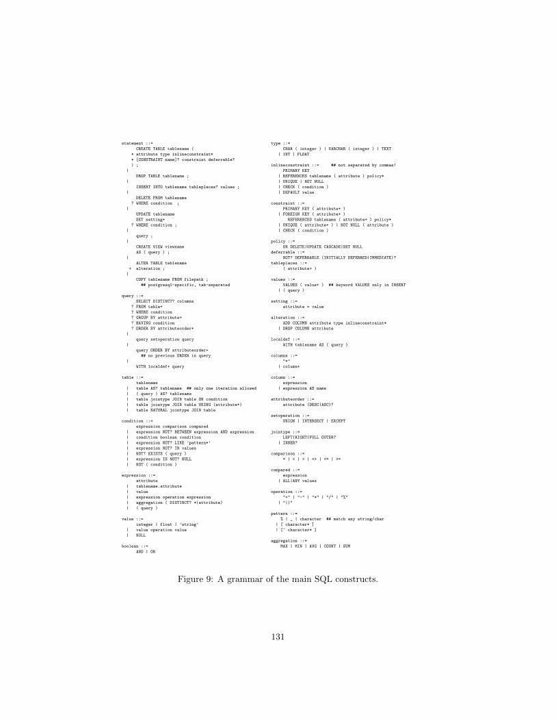
statement ::= type ::=
CREATE TABLE tablename ( CHAR ( integer ) | VARCHAR ( integer ) | TEXT
* attribute type inlineconstraint* | INT | FLOAT
* [CONSTRAINT name]? constraint deferrable?
) ; inlineconstraint ::= ## not separated by commas!
| PRIMARY KEY
DROP TABLE tablename ; | REFERENCES tablename ( attribute ) policy*
| | UNIQUE | NOT NULL
INSERT INTO tablename tableplaces? values ; | CHECK ( condition )
| | DEFAULT value
DELETE FROM tablename
? WHERE condition ; constraint ::=
| PRIMARY KEY ( attribute+ )
UPDATE tablename | FOREIGN KEY ( attribute+ )
SET setting+ REFERENCES tablename ( attribute+ ) policy*
? WHERE condition ; | UNIQUE ( attribute+ ) | NOT NULL ( attribute )
| | CHECK ( condition )
query ;
| policy ::=
CREATE VIEW viewname ON DELETE|UPDATE CASCADE|SET NULL
AS ( query ) ; deferrable ::=
| NOT? DEFERRABLE (INITIALLY DEFERRED|IMMEDIATE)?
ALTER TABLE tablename tableplaces ::=
+ alteration ; ( attribute+ )
|
COPY tablename FROM filepath ; values ::=
## postgresql-specific, tab-separated VALUES ( value+ ) ## keyword VALUES only in INSERT
| ( query )
query ::=
SELECT DISTINCT? columns setting ::=
? FROM table+ attribute = value
? WHERE condition
? GROUP BY attribute+ alteration ::=
? HAVING condition ADD COLUMN attribute type inlineconstraint*
? ORDER BY attributeorder+ | DROP COLUMN attribute
|
query setoperation query localdef ::=
| WITH tablename AS ( query )
query ORDER BY attributeorder+
## no previous ORDER in query columns ::=
| "*"
WITH localdef+ query | column+
table ::= column ::=
tablename expression
| table AS? tablename ## only one iteration allowed | expression AS name
| ( query ) AS? tablename
| table jointype JOIN table ON condition attributeorder ::=
| table jointype JOIN table USING (attribute+) attribute (DESC|ASC)?
| table NATURAL jointype JOIN table
setoperation ::=
condition ::= UNION | INTERSECT | EXCEPT
expression comparison compared
| expression NOT? BETWEEN expression AND expression jointype ::=
| condition boolean condition LEFT|RIGHT|FULL OUTER?
| expression NOT? LIKE ’pattern*’ | INNER?
| expression NOT? IN values
| NOT? EXISTS ( query ) comparison ::=
| expression IS NOT? NULL = | < | > | <> | <= | >=
| NOT ( condition )
compared ::=
expression ::= expression
attribute | ALL|ANY values
| tablename.attribute
| value operation ::=
| expression operation expression "+" | "-" | "*" | "/" | "%"
| aggregation ( DISTINCT? *|attribute) | "||"
| ( query )
pattern ::=
value ::= % | _ | character ## match any string/char
integer | float | ’string’ | [ character* ]
| value operation value | [^ character* ]
| NULL
aggregation ::=
boolean ::= MAX | MIN | AVG | COUNT | SUM
AND | OR
Figure 9: A grammar of the main SQL constructs.
131


