Article

Data-Driven Design of Intelligent Wireless Networks:An Overview and TutorialMerima Kulin ∗, Carolina Fortuna, Eli De Poorter, Dirk Deschrijver and Ingrid Moerman

Department of Information Technology, Ghent University-iMinds, Technologiepark-Zwijnaarde 15, Gent 9052,Belgium; carolina.fortuna@ijs.si (C.F.); eli.depoorter@intec.ugent.be (E.D.P.);dirk.deschrijver@intec.ugent.be (D.D.); ingrid.moerman@intec.ugent.be (I.M.)* Correspondence: merima.kulin@ugent.be; Tel.: +32-93-314-981

Academic Editor: Paolo BellavistaReceived: 29 March 2016; Accepted: 23 May 2016; Published: 1 June 2016

Abstract: Data science or “data-driven research” is a research approach that uses real-life data togain insight about the behavior of systems. It enables the analysis of small, simple as well as largeand more complex systems in order to assess whether they function according to the intendeddesign and as seen in simulation. Data science approaches have been successfully applied to analyzenetworked interactions in several research areas such as large-scale social networks, advancedbusiness and healthcare processes. Wireless networks can exhibit unpredictable interactions betweenalgorithms from multiple protocol layers, interactions between multiple devices, and hardwarespecific influences. These interactions can lead to a difference between real-world functioning anddesign time functioning. Data science methods can help to detect the actual behavior and possiblyhelp to correct it. Data science is increasingly used in wireless research. To support data-drivenresearch in wireless networks, this paper illustrates the step-by-step methodology that has to beapplied to extract knowledge from raw data traces. To this end, the paper (i) clarifies when, why andhow to use data science in wireless network research; (ii) provides a generic framework for applyingdata science in wireless networks; (iii) gives an overview of existing research papers that utilized datascience approaches in wireless networks; (iv) illustrates the overall knowledge discovery processthrough an extensive example in which device types are identified based on their traffic patterns;(v) provides the reader the necessary datasets and scripts to go through the tutorial steps themselves.

Keywords: wireless networks; data science; data-driven research; machine learning; knowledgediscovery; cognitive networking; intelligent systems

1. Introduction

1.1. What Is Data Science?

Data science, also referred to as data-driven research, is research that puts a strong emphasis onstarting from large datasets to solve a specific problem. The use of data science has gained popularitydue to its capability to better understand the behavior of complex systems that cannot easily bemodeled or simulated. For this reason, a possible definition of the term is provided by Dhar [1]and states that “data science is the study of the generalizable extraction of knowledge from data”.A simpler definition could be that data science enables discovering and extracting new knowledge fromdata. To this end, data-driven approaches start from datasets containing large amounts of experimentalreal-world data and utilize data science techniques to build statistical models that can be used to(i) better understand the behavior of the system and finally extract new knowledge; and (ii) generatesynthetic data from the statistical model which mimics (simulates) the original observed data. Ordersof magnitude larger than one are typically used in an analysis; often amounting to several gigabytes

Sensors 2016, 16, 790; doi:10.3390/s16060790 www.mdpi.com/journal/sensors

Sensors 2016, 16, 790 2 of 61

(possibly even terabytes) of traces. The use of data-driven research is increasing in various fields ofscience [2]. Example research areas in which data science was successfully applied include studyingthe human genome to predict the susceptibility of individual persons to specific diseases [3], analyzingconnections in social networks [4], predicting the interests of customers based on previously purchaseditems [5], cloud computing applications [6,7], analysis of traffic in mobile cellular networks [8], etc.

Due to their unpredictable nature, wireless networks are an interesting application area for datascience because they are influenced by both natural phenomena and man made artifacts. On onehand, they depend on electromagnetic propagation, which is a natural phenomenon, and on the otherhand, they depend on the network technology consisting of hardware and software elements thatwere built by humans. Whereas well-defined aspects of wireless systems such as algorithm behavior,propagation on a specific type of channel, etc., can be modeled in simulations, the functioning ofthe overall systems is difficult to simulate. Due to these limitations, a number of wireless systembehaviors cannot be identified and/or explained based on simulations alone. One such example is thefact that the inter-arrival time between wireless data packets depends on both protocol layer aspectsand hardware behavior, a fact which will be exploited in this paper to identify devices and devicetypes based on their traffic patterns. Other examples for the use of data science in wireless networksinclude the creation of complex system models, finding correlations and patterns between configurableparameters and network performance, predicting system behavior or identifying trade-offs such asPareto fronts.

1.2. Motivation

Recently, an increasing number of research works in the wireless domain that rely on large datasetsto prove their hypothesis can be seen [9–12]. While some of the "early adopters" of data-driven researchsuch as [11] follow by the book the methodology used in the communities that developed data sciencewithout explicitly mentioning some domain specific terminology, other more recent works clearly usea data science approach [9,10]. By carefully studying example works, later analyzed in Section 3.7,that rely on large datasets, we noticed that, in some cases, the methodology used for solving thedata science (data-driven) problem does not fully comply with the standard approaches (standardmethodology) developed and accepted by the data science community. This can be explained by thedifficulty of correctly grasping and understanding the knowledge discovery process, on which datascience relies, by newcomers to the field. However, as a result, this may raise questions regarding thevalidity of some of the results.

Furthermore, related work such as [13–16] provide a comprehensive overview of generic datamining techniques and/or research studies that successfully applied those techniques to wirelesssensor networks (WSN) and Internet of Things (IoT) networks. However, data mining is only a smallstep in the overall process of discovering knowledge from data. This means that just taking and usingexisting data mining algorithms, that seem best suited for a particular problem, is not always the mostadequate approach to the overall problem. Algorithm selection, implementation and evaluation ispossible and meaningful only after the problem is well defined and the data, including its statisticalproperties are analyzed and well understood. The formalization of the methodology for developingmodels based on empirical data in wireless networks is missing.

Similarly, related works such as [17] present an extensive survey of machine learning techniques,while [18] presents an extensive survey on computational intelligence algorithms (e.g., neural networks,evolutionary algorithms, swarm intelligence, reinforcement learning, etc.) that were used to addresscommon issues in WSNs. Ref. [19] reviews various machine learning techniques that have beenapplied to cognitive radios (CR), while in [20] novel cooperative spectrum sensing algorithms forcognitive radio networks (CRN) based on machine learning techniques were evaluated. These researchworks ([13–20]) focus on existing application examples of different data science approaches to specificwireless networks. We encourage the reader to refer to the reference papers in this section to gainmore insight on the algorithmic aspects of different data mining techniques and review a larger set

Sensors 2016, 16, 790 3 of 61

of examples of data science applications to the wireless domain. Hence, by focusing on a applicationarea, they narrow their context to the algorithms and approaches that are useful for that area ratherthan provide a generic methodology with the options and trade-offs available at each step.

Bulling et al. [21] present a comprehensive tutorial on human activity recognition (HAR) usingon-body inertial sensors. Although, this work provides the breadth of information expected from aneducational tutorial, it focuses on solving a particular data science problem (i.e., classification) for aparticular application domain (i.e., HAR) with regard to the challenges of a particular wireless networkscheme (i.e., body sensor networks). There is no single comprehensive tutorial on applying data scienceto various wireless networks, regardless on the application domain and type of problem that is to besolved, from an unified perspective (covering the overall process from the problem formulation, overdata analysis, to learning and evaluation).

The aforementioned facts motivated the present tutorial paper and its ultimate goal to explain theknowledge discovery process underlying data science, and show how it can be correctly applied forsolving wireless networking problems. This paper is provided at an opportune time, considering that:

• More and more data is generated by existing wireless deployments [22] and by the continuouslygrowing network of everyday objects (the IoT).

• Data-driven research has found applications in various schemes of wireless networks [13], diversefields of communication networks [6–8] and different fields of science in general [2].

Typically, wireless network researchers and experts are not (fully) aware of the potential that datascience methods and algorithms can offer. Rather than having wireless network experts dive intodata mining and machine learning literature, we provide the fundamental information in an easilyaccessible and understandable manner with examples of successful applications in the wireless domain.Hence, the main contribution of this paper is to offer a well-structured starting point for applying datascience in wireless networks with the goal of minimizing the effort required from wireless professionalsto start using data science methodology and tools to solve a domain specific problem. Ultimately,this knowledge will enable a better design of future wireless network systems such as the dense andheterogeneous wireless networks where humans, cars, homes, cities and factories will be monitoredand controlled by such networked devices (IoT networks).

To the best of our knowledge, this is the first attempt to formally explain the correct approach andmethodology for applying data science to the wireless domain. As such, we hope this tutorial paperwill help bridge the gap and foster collaboration between system experts, wireless network researchersand data science researchers.

1.3. Contributions and Organization of the Paper

The paper aims to give a comprehensive tutorial on applying data science to the wireless domainby providing:

1. An overview of types of problems in wireless network research that can be addressed usingdata science methods together with state-of-the-art algorithms that can solve each problem type.In this way, we provide a guide for researchers to help them formulate their wireless networkingproblem as a data science problem.

2. A brief survey on the on-going research in the area of data-driven wireless network research thatillustrates the diversity of problems that can be solved using data science techniques includingreferences to these research works.

3. A generic framework as a guideline for researchers wanting to solve their wireless networkingproblem as a data science problem using best practices developed by the data science community.

4. A comprehensive hands-on introduction for newcomers to data-driven wireless network research,which illustrates how each component of the generic framework can be instantiated for a specificwireless network problem. We demonstrate how to correctly apply the proposed methodology bysolving a timely problem on fingerprinting wireless devices, that was originally introduced

Sensors 2016, 16, 790 4 of 61

in [12]. Finally, we show benefits of using the proposed framework compared to taking acustom approach.

5. The necessary scripts to instantiate the proposed framework for the selected wireless networkingproblem [23], complemented with a publicly available datasets [24].

According to the aforementioned, the remainder of this paper is organized as follows: Section 2elaborates the use of data science in wireless networks. Section 3 introduces a generic frameworkfor applying the correct methodology for data-driven wireless network research. Section 4 detailshow each component of the framework can be executed in a time efficient manner using best practicedeveloped by the data science community. This process is extensively illustrated by a case studythat demonstrates how the proposed framework can be implemented to solve a wireless networksclassification problem. We underline the significance of the correct methodology by comparing theproposed solution against an existing work presented in [12]. Section 5 concludes the paper.

2. Introduction to Data Science in Wireless Networks

This section introduces the basic terminology used in data science in order to set up the necessaryfundamentals for the reader, and examines the applicability of recent advances in data science tothe wireless networking domain. Thus, this section (i) introduces the basic concepts of learning anddifferent learning paradigms used in data science; (ii) describes which categories of problems inwireless networks can be answered by data science approaches; (iii) describes a number of populardata science algorithms that can solve these categories of problems and state-of-the-art achievementsin applying these algorithms to various wireless network use cases.

With this in regard, this section is both, a brief survey on existing work in data-driven wirelessresearch and a starting guide for researchers wanting to apply data science to problems related towireless networks.

2.1. Types of Learning Paradigms

The ultimate goal of data science is to extract knowledge from data, i.e., turn data into realvalue [25]. At the heart of this process are severe algorithms that can learn from and make predictionson data. As such, these algorithms are referred to as learning algorithms and are part of the machinelearning and data mining fields of study (the differences between the two fields are detailed inSection 2.1.1).

In the context of wireless networks, learning is a mechanism that enables context awarenessand intelligence capabilities in different aspects of wireless communication. Over the last years, ithas gained popularity due to its success in enhancing network-wide performance (i.e., the Qualityof Service, QoS) [26], facilitating intelligent behavior by adapting to complex and dynamicallychanging (wireless) environments [27] and its ability to add automation for realizing conceptsof self-healing and self-optimization [28]. During the past years, different learning approacheshave been applied in various wireless networks schemes such as medium access control [29,30],routing [9,10], data aggregation and clustering [31,32], localization [33,34], energy harvestingcommunication [35], cognitive radio [36,37], etc. These schemes apply to a variety of wireless networkssuch as: mobile ad hoc networks [38], wireless sensor networks [18], wireless body area networks [39],cognitive radio networks [20,40] and cellular networks [41].

2.1.1. Data Mining vs. Machine Learning

In the literature, machine learning and data mining are terms used interchangeably. It is difficultto make a clear difference between the two, as they appear in the same context and very often relyon the same algorithms and techniques (e.g., decision trees, logistic regression, neural networks, etc.).Perhaps the best way to explain the difference is by looking at their scope.

Data mining aims to discover new, previously unseen knowledge in large datasets. It focuses onhelping humans understand complex relationships between data. For instance, it enables marketing

Sensors 2016, 16, 790 5 of 61

experts to segment customers based on previous shopping habits. Another example is applyinglearning algorithms to extract the shopping patterns of thousands of individuals over time; then beingpresented with a new individual, having a very short shopping history (e.g., five items), the learnedmodel is able to automatically tell to which of the segments discovered by the data mining processthe new individual belongs. Hence, data mining tends to be focused on solving actual problemsencountered in practice by exploiting algorithms developed by the machine learning community.

Machine learning on the other hand, aims to develop algorithms and techniques that givecomputers the ability to learn to recognize information or knowledge (i.e., patterns) automaticallywithout being explicitly programmed to do so. This is why machine learning algorithms are typicallyreferred to as learning algorithms. Machine learning experts focus on proving mathematical propertiesof new algorithms, while data mining experts focus on understanding empirical properties of existingalgorithms that they apply.

2.1.2. Supervised vs. Unsupervised vs. Semi-Supervised Learning

Learning can be categorized by the amount of knowledge or feedback that is given to the learneras either supervised or unsupervised.

Supervised Learning

Supervised learning utilizes predefined inputs and known outputs to build a system model.The set of inputs and outputs forms the labeled training dataset that is used to teach a learningalgorithm how to predict future outputs for new inputs that were not part of the training set.Supervised learning algorithms are suitable for wireless network problems where prior knowledgeabout the environment exists and data can be labeled. For example, predict the location of amobile node using an algorithm that is trained on signal propagation characteristics (inputs)at known locations (outputs). Various challenges in wireless networks have been addressedusing supervised learning such as: medium access control [29,42–44], routing [45], link qualityestimation [46,47], node clustering in WSN [48], localization [49–51], adding reasoning capabilities forcognitive radios [36,37,52–56], etc. Supervised learning has also been extensively applied to differenttypes of wireless networks application such as: human activity recognition [21,39,57–60], eventdetection [61–65], electricity load monitoring [66,67], security [68–70], etc. Some of these workswill be analyzed in more detail later.

Unsupervised Learning

In contrast, unsupervised learning algorithms try to find hidden structures in unlabeled data.The learner is provided only with inputs without known outputs, while learning is performed byfinding similarities in the input data. As such, these algorithms are suitable for wireless networkproblems where no prior knowledge about the outcomes exists, or annotating data (labelling) isdifficult to realize in practice. For instance, automatic grouping of wireless sensor nodes into clustersbased on their current sensed data values and geographical proximity (without knowing a priorithe group membership of each node) can be solved using unsupervised learning. In the context ofwireless networks, unsupervised learning algorithms are widely used for: data aggregation [31], nodeclustering for WSNs [31,71–73], data clustering [74–76], event detection [77] and several cognitiveradio applications [78,79].

Semi-Supervised Learning

Several mixes between the two learning methods exist and materialize into semi-supervisedlearning [80]. Semi-supervised learning is used in situations when a small amount of labeled datawith a large amount of unlabeled data exists. It has great practical value because it may alleviate thecost of rendering a fully labeled training set, especially in situations where it is infeasible to label allinstances. For instance, in human activity recognition systems where the activities change very fast so

Sensors 2016, 16, 790 6 of 61

that some activities stay unlabeled or the user is not willing to cooperate in the data collection process,supervised learning might be the best candidate to train a recognition model [81–83]. Other potentialuse cases in wireless networks might be localization systems where it can alleviate the tedious andtime-consuming process of collecting training data (calibration) in fingerprinting-based solutions [84]or semi-supervised traffic classification [85], etc.

2.1.3. Offline vs. Online vs. Active Learning

Learning can be categorized depending on the way the information is given to the learner aseither offline or online learning. In offline learning the learner is trained on the entire training data atonce, while in online learning the training data becomes available in a sequential order and is used toupdate the representation of the learner in each iteration.

Offline Learning

Offline learning is used when the system that is being modeled does not change its propertiesdynamically. Offline learned models are easy to implement because the models do not have to keepon learning constantly, and they can be easily retrained and redeployed in production. For example,in [9] a learning-based link quality estimator is implemented by deploying an offline trained modelinto the network stack of Tmote Sky wireless nodes. The model is trained based on measurementsabout the current status of the wireless channel that are obtained from extensive experiment setupsfrom a wireless testbed.

Another use cases are human activity recognition systems, where an offline trained classifier isdeployed to recognize actions from users. The classifier model can be trained based on informationextracted from raw measurements collected by sensors integrated in a smartphone, which is at thesame time the central processing unit that implements the offline learned model for online activityrecognition [86].

Online Learning

Online learning is useful for problems where training examples arrive one at a time or whendue to limited resources it is computationally infeasible to train over the entire dataset. For instance,in [87] a decentralized learning approach for anomaly detection in wireless sensor networks is proposed.The authors concentrate on detection methods that can be applied online (i.e., without the need ofan offline learning phase) and that are characterized by a limited computational footprint, so as toaccommodate the stringent hardware limitations of WSN nodes.

Another example can be found in [88], where the authors propose an online outlier detectiontechnique that can sequentially update the model and detect measurements that do not conform tothe normal behavioral pattern of the sensed data, while maintaining the resource consumption of thenetwork to a minimum.

Active Learning

A special form of online learning is active learning where the learner first reasons about whichexamples would be most useful for training (taking as few examples as possible) and then collectsthose examples. Active learning has proven to be useful in situations when it is expensive to obtainsamples from all variables of interest. Recently, the authors in [89] proposed a novel active learningapproach (for graphical model selection problems), where the goal is to optimize the total numberof scalar samples obtained by allowing the collection of samples from only subsets of the variables.This technique could for instance alleviate the need for synchronizing a large number of sensors toobtain samples from all the variables involved simultaneously.

Active learning has been a major topic in recent years in machine learning and an exhaustiveliterature survey is beyond the scope of this paper. We refer the reader to [90–92] for more details onstate-of-the-art and progress on active learning algorithms.

Sensors 2016, 16, 790 7 of 61

Table 1 summarizes the previously introduced learning paradigms.

Table 1. Summary of types of learning paradigms.

Categorization Criteria Learning Types Comment

Learning paradigms

Amount of feedback given to the learnerSupervised The learner knows all inputs/outputs

Unsupervised The learner knows only the inputs

Semi-supervised The learner knows only a few input/output pairs

Amount of information given to the learnerOffline The learner is trained on the entire dataset

Online The learner is trained sequentially as data becomes available

Active The learner selects the most useful training data

2.2. Types of Data Science Problems in Wireless Networks

As shown in previous section, data science has been successfully applied in different areas ofwireless networks. Prior to applying data science techniques to any wireless network problem, theproblem has to be first translated into an adequate data mining method. This section guides the readeron how to formulate the wireless networking problem as a data science problem, making a first steptowards the broader knowledge discovery process that will be formalized in Section 3. For each type ofproblem, the most popular learning algorithms and their relation to the previously introduced learningparadigms is identified.

2.2.1. Regression

Regression is a data mining method that is suitable for problems that aim to predict a real-valuedoutput variable. It is a supervised learning method, which models (i.e., fits) a set of knowninputs (i.e., explanatory or independent variables) and corresponding outputs (i.e., dependentvariable) with the most suitable mathematical representation (i.e., function or model). Dependingon the function representation, regression techniques can be categorized into linear and non-linearregression algorithms.

Linear Regression

Linear regression is a technique for modeling the relationship between the input (x) and outputvariable (y) so that the output is a linear combination of the input variables (dependent variable).

y(x) = θ0 + θ1x1 + ... + θnxn = θ0 +n

∑i=1

θixi (1)

where x = (x1, ...xn)T .A simple example is linear regression with one input variable (i.e., univariate linear regression),

which fits the data (inputs x and predictions y) with a linear function, e.g., f (x) = ax + b.This function, f (x), is supposed to predict future values, f (x), based on new inputs (i.e., x).

Linear regression use case in wireless networks. In the context of wireless networks, linearregression is frequently used to derive an empirical log-distance model for the radio propagationcharacteristics as a linear mathematical relationship between the Received Signal Strength Indication(RSSI), usually in dBm, and the distance. This model can be used in RSSI-based indoor localizationalgorithms to estimate the distance towards each fixed node (i.e., anchor node) in the ranging phase ofthe algorithm [33].

Nonlinear Regression

Nonlinear regression is a regression method which models the observed data by a function that isa nonlinear combination of the model parameters and one or more independent variables.

Sensors 2016, 16, 790 8 of 61

Nonlinear regression use case in wireless networks. For instance, in [93] non-linear regression isused to model the relationship between the SINR (Signal to Interference plus Noise Ratio) and PRR(Packet Reception Rate) that could improve the design and analysis of higher layer protocols. Similarly,non-linear regression techniques are extensively used for modeling the relation between the PRRand the RSSI, as well as between PRR and the Link Quality Indicator (LQI), to build a mechanism toestimate the link quality based on observations (RSSI, LQI) [94].

2.2.2. Classification

A classification problem tries to understand and predict discrete values or categories while aregression problem targets continuous valued problems. The term classification comes from the factthat it predicts the class membership of a particular input instance. Classification problems can besolved by supervised learning approaches, that aim to model boundaries between sets (i.e., classes) ofsimilar behaving instances, based on known and labeled (i.e., with defined class membership) inputvalues. The learned model is used to map future input instances (X) to a particular class (Y). A detailedexample will be given in Section 4 where devices and device types are classified based on the packetinter-arrival times from a publicly available dataset from wireless devices. Similarly, identifying theapplication layer protocol of a traffic flow can be solved as a classification problem: traffic classificationbased on the statistical properties of traffic traces [11]. There are many learning algorithms that can beused to classify data including decision trees, k-nearest neighbours, logistic regression, support vectormachines and neural networks.

Neural Networks

Neural Networks (NN) [95] or artificial neural networks (ANN) is a supervised learning algorithminspired on the working of the brain, that is typically used to derive complex, non-linear decisionboundaries for building a classification model, but are also suitable for training regression modelswhen the goal is to predict real-valued outputs (regression problems are explained in Section 2.2.1).Neural networks are known for their ability to identify complex trends and detect complex non-linearrelationships among the input variables at the cost of higher computational burden. A neural networkmodel consists of one input, a number of hidden layers and one output layer. The input layercorresponds to the input data variables. Each hidden layer consists of a number of processing elementscalled neurons that process its inputs (the data from the previous layer) using an activation or transferfunction that translates the input signals to an output signal. Commonly used activation functionsare: unit step function, linear function, sigmoid function and the hyperbolic tangent function. Theelements between each layer are highly connected by connections that have numeric weights that arelearned by the algorithm. The output layer outputs the prediction (i.e., the class) for the given inputsand according to the interconnection weights defined through the hidden layer. The algorithm is againgaining popularity in recent years because of new techniques and more powerful hardware that enabletraining complex models for solving complex tasks. In general, neural networks are said to be able toapproximate any function of interest when tuned well, which is why they are considered as universalapproximators [96].

Neural networks use case in wireless networks. In [97], the authors proposed a neural networkbased mechanism for dynamic channel selection in an IEEE 802.11 network. The neural networkis trained to identify how environmental measurements and the status of the network affect theperformance experienced on different channels. Based on this information it is possible to dynamicallyselect the channel which is expected to yield the best performance for the mobile users.

Deep Learning

Recently, it has been noticed that the same amount of complexity as modeled by a neural networkswith one hidden layer and several neurons can be gained with multiple hidden layers that have lessneurons in total. Such networks are known as deep neural networks and the learning process is known

Sensors 2016, 16, 790 9 of 61

as deep learning. Deep neural networks hold the potential to replace the process of manually extractingfeatures, which depends much on prior knowledge and domain expertise, with unsupervised orsemi-supervised feature learning techniques [98]. Various deep learning techniques such as deepneural networks (DNN), convolutional neural networks (CNN), recurrent neural networks (RNN)and deep belief networks (DBN) have shown success in various fields of science including computervision, automatic speech recognition, natural language processing, bioinformatics, etc. Although deepnetworks showed excellent performance in many challenging machine learning tasks, their applicationto wireless networks has not yet been widely explored. We present two recent advances applying deeplearning techniques to the wireless domain [99,100].

Deep learning use case in wireless networks. In [99], deep neural networks (DNN) have beenapplied to wireless sensor networks. The authors proposed a distributed learning model by dividingthe deep neural network into different layers and deploying them on several sensor nodes. Theproposed solution aims to reduce power consumption in WSNs by reducing the number of data thathas to be transmitted, by transmitting only data that is processed by the DNN layer locally at the nodeinstead of the full raw data.

In [100] a new intelligent communication systems is proposed called Cognition-Based Networks(COBANETS) whose main building blocks are (i) unsupervised deep learning networks as the enablerfor learning, modeling and optimization of networks, and (ii) software defined networking (SDN)as the enabler for reconfiguration of the network protocol stack and flexible network management,making it possible to actuate network-wide optimization strategies.

Decision Trees

Decision trees [101] is a supervised learning algorithm that creates a tree-like graph or model thatrepresents the possible outcomes or consequences of using certain input values. The tree consists ofone root node, internal nodes called decision nodes which test its input against a learned expression,and leaf nodes which correspond to a final class or decision. The learning tree can be used to derivesimple decision rules that can be used for decision problems or for classifying future instances bystarting at the root node and moving through the tree until a leaf node is reached where a class label isassigned. However, decision trees can achieve high accuracy only if the data is linearly separable, i.e.,if there exists a linear hyperplane between the classes. Hence, constructing an optimal decision tree isNP-complete [102].

There are many algorithms that can form a learning tree such as the simple Iterative Dichotomiser 3(ID3), its improved version C4.5, etc.

Decision trees use case in wireless networks. We consider the problem of designing an adaptiveMAC layer as an application example of decision trees in wireless networks. In [29] a self-adaptingMAC layer is proposed. It is composed of two parts: (i) a reconfigurable MAC architecture that canswitch between different MAC protocols at run time, and (ii) a trained MAC engine that selects themost suitable MAC protocol for the current network condition and application requirements. TheMAC engine is solved as a classification problem using a decision tree classifier which is learnedbased on: (i) two types of input variables which are (1) network conditions reflected through theRSSI statistics (i.e., mean and variance), and (2) the current traffic pattern monitored through theInter-Packet Interval statistics (i.e., mean and variance) and application requirements (i.e., reliability,energy consumption and latency), and (ii) the output which is the MAC protocol that is to be predictedand selected.

Logistic Regression

Logistic regression [103] is a simple supervised learning algorithm widely used for implementinglinear classification models, meaning that the models define smooth linear decision boundaries betweendifferent classes. At the core of the learning algorithm is the logistic function which is used to learn themodel and predict future instances.

Sensors 2016, 16, 790 10 of 61

Logistic regression use case in wireless networks. Liu et al. [9] improved multi-hop wirelessrouting by creating a data-driven learning-based radio link quality estimator. They investigatedwhether machine learning algorithms (e.g., logistic regression, neural networks) can perform betterthan traditional, manually-constructed, pre-defined estimators such as STLE (Short-Term LinkEstimator) [104] and 4Bit (Four-Bit) [105]. Finally, they selected logistic regression as the most promisingmodel for solving the following classification problem: predict whether the next packet will besuccessfully received, i.e., output class is 1, or lost, i.e., output class is 0, based on the current wirelesschannel conditions reflected by statistics of the PRR, RSSI, SNR and LQI.

While in [9] the authors used offline learning to do prediction, in their follow-up work [10], theywent a step further and both training and prediction were performed online by the nodes themselvesusing logistic regression with online learning (more specifically the stochastic gradient descent onlinelearning algorithm). The advantage of this approach is that the learning and thus the model, adapt tochanges in the wireless channel, that could otherwise be captured only by re-training the model offlineand updating the implementation on the node.

SVM

Support Vector Machine (SVM) [106] is a learning algorithm that solves classification problemsby first mapping the input data into a higher-dimensional feature space in which it becomes linearlyseparable by a hyperplane, which is used for classification. The mapping from the input space tothe high-dimensional feature space is non-linear, which is achieved using kernel functions. Differentkernel functions comply best for different application domains. There are three types of popular kernelfunctions: linear kernel, polynomial kernel and Gaussian radial basis kernel function (RBF).

SVM use case in wireless networks. SVMs have been extensively used in cognitive radioapplications to perform signal classification. For this purpose, typically flexible and reconfigurableSDR (software defined radio) platforms are used to sense the environment to obtain informationabout the wireless channel conditions and users’ requirements, while intelligent algorithms buildthe cognitive learning engine that can make decisions on those reconfigurable parameters on SDR(e.g., carrier frequency, transmission power, modulation scheme).

In [36,37,107] SVMs are used as the machine learning algorithm to classify signals among a givenset of possible modulation schemes. For instance, Huang et al. [37] identified four spectral correlationfeatures that can be extracted from signals for distinction of different modulation types. Their trainedSVM classifier was able to distinguish six modulation types with high accuracy: AM, ASK, FSK, PSK,MSK and QPSK.

k-NN

k nearest neighbors (k-NN) [108] is a learning algorithm that can solve classification and regressionproblems by looking into the distance (closeness) between input instances. It is called a non-parametriclearning algorithm because, unlike other supervised learning algorithms, it does not learn an explicitmodel function from the training data. Instead, the algorithm simply memorizes all previous instancesand then predicts the output by first searching the training set for the k closest instances and then:(i) for classification-predicts the majority class amongst those k nearest neighbors, while (ii) forregression-predicts the output value as the average of the values of its k nearest neighbors. Because ofthis approach, k-NN is considered a form of instance-based or memory-based learning.

In the context of this section, k-NN will be exemplified for solving a classification wireless problem.k-NN is widely used since it is one of the simplest forms of learning. It is also considered as lazylearning as the classifier is passive until a prediction has to be performed, hence no computation isrequired until performing classification.

k-NN use case in wireless networks. In [109] the goal of determining the activity of a humanwho is wearing attached sensor nodes is turned into a classification problem. The sensor nodes arecapturing and recording acceleration data, which is then sent via Bluetooth to the classifier. In [109],

Sensors 2016, 16, 790 11 of 61

k-NN was one of the candidates to solve the classification problem. Acceleration data (x, y, and zcoordinates) gathered from acceleration sensors is transformed into input data such as: step count, areabetween mean of local maxima and signal, crossing of mean value, mean value of local maxima andthe angle of each axis in relation to the gravity, and fed into the classifier. k-NN calculates the distancebetween each input instance to be classified and all the remaining training instances. Classification isperformed according to how many instances of a certain class are nearest.

2.2.3. Clustering

Clustering is a data mining method that can be used for problems where the goal is to group setsof similar instances into clusters. Opposed to classification, it uses unsupervised learning, which meansthat the input dataset instances used for training are not labeled, i.e., it is unknown to which groupthey belong. The clusters are determined by inspecting the data structure and grouping objects thatare similar according to some metric. Clustering algorithms are widely adopted in wireless sensornetworks, where they have found use for grouping sensor nodes into clusters to satisfy scalability andenergy efficiency objectives, and finally elect the head of each cluster. Recently, a large number of nodeclustering algorithms have been proposed for WSNs [110]. However, these node clustering algorithmstypically do not use the data science clustering techniques directly. Instead, they exploit data clusteringtechniques to find data correlations or similarities between data of neighboring nodes, that can be usedto partition sensor nodes into clusters.

Clustering can be used to solve other types of problems in wireless networks like anomalydetection, i.e., outliers detection, such as intrusion detection or event detection, for different datapre-processing tasks (data pre-processing is detailed in Section 3.3), cognitive radio application (e.g.,identifying wireless systems [79]), etc. There are many learning algorithms that can be used forclustering, but the most commonly used is k-Means.

k-Means

k-Means is an unsupervised learning clustering algorithm that simply partitions the input datainstances into k clusters, so that the resulting intra-cluster similarity is high, while the inter-clustersimilarity low. The similarity is measured with respect to the mean value of the instances in a cluster.

k-Means use case in wireless networks. In [74] a distributed version of the k-Means clusteringalgorithm was proposed for clustering data sensed by sensor nodes. The clustered data is summarizedand sent towards a sink node. Summarizing the data ensures to reduce the communicationtransmission, processing time and power consumption of the sensor nodes.

Other popular clustering algorithms include hierarchical clustering methods such assingle-linkage, complete-linkage, centroid-linkage; graph theory-based clustering such as highlyconnected subgraphs (HCS), cluster affinity search technique (CAST); kernel-based clustering as issupport vector clustering (SVC), etc. A novel two-level clustering algorithm, namely TW-k-means,has been introduced by Chen et al. [32]. For a more exhaustive list of clustering algorithms and theirexplanation we refer the reader to [111].

2.2.4. Anomaly Detection

Anomaly detection (changes and deviation detection) is used when the goal is to identify unusual,unexpected or abnormal system behavior. This type of problem can be solved by supervised orunsupervised learning depending on the amount of knowledge present in the data (i.e., whether itis labeled or unlabeled, respectively). Accordingly, classification and clustering algorithms can beused to solve anomaly detection problems. A wireless example is the detection of suddenly occurringphenomena, such as the identification of suddenly disconnected networks due to interference orincorrect transmission power settings. It is also widely used for outliers detection in the pre-processingphase [112]. Other use-case examples include intrusion detection, fraud detection, event detection insensor networks, etc.

Sensors 2016, 16, 790 12 of 61

Anomaly Detection use case in wireless networks. We consider an anomaly detection use casein the context of WSN security. Namely, WSNs have been target of many types of DoS attacks.The goal of DoS attacks in WSNs is to transmit as many packets as possible whenever the mediumis detected to be idle. This prevents a legitimate sensor node from transmitting their own packets.To combat a DoS attack, a secure MAC protocol based on neural networks has been proposed in [42].The NN model is trained to detect an attack by monitoring variations of following parameters:collision rate Rc, average waiting time of a packet in MAC buffer Tw, arrival rate of RTS packets RRTS.An anomaly, i.e., attack, is identified when the monitored traffic variations exceeds a preset threshold,after which the WSN node is switched off temporarily. The results is that flooding the network withuntrustworthy data is prevented by blocking only affected sensor nodes.

In [87] online learning techniques have been used to incrementally train a neural network forin-node anomaly detection in wireless sensor network. More specifically, the Extreme LearningMachine algorithm [113] has been used to implement classifiers that are trained online onresource-constrained sensor nodes for detecting anomalies such as: system failures, intrusion, orunanticipated behavior of the environment.

2.2.5. Summarization

Summarization is used in problems where the goal is to find a compact (summarized)representation of data. The method typically utilizes different summary statistics to find a reducedrepresentation of the data. It is frequently used in data analysis, data pre-processing, data visualizationand automated report generation tasks. Accordingly, this method can be rather seen as an optimizationproblem with the compaction gain and information loss as objective functions, whereas it is notsuitable to solve a prediction problem. As such, summarization does not conform to any of thelearning paradigms previously introduced, hence is not meant to solve a knowledge discoveryproblem. However, summarization techniques have been heavily used to address challenges that arecrucial for wireless communication systems and they can be realized by some of the aforementionedlearning-based data science methods. Thus, it is important to give a short overview of potentialsummarization techniques used in wireless networks. First, we would like to point the reader tosome of the recently emerging non-learning-based summarization techniques that are adopted inwireless networks including compressive sensing, expectation-maximization, non-negative matrixfactorization, etc.

Compressive sensing (CS) has shown great success in conjunction with principal componentanalysis for the design of efficient data aggregation schemes in wireless networks. In short, it replacesthe traditional “sample then compress” summarization scheme with “sample while compressing”.We refer the reader to [114] for more details on compressive sensing techniques. Some exampleworks that integrate compressive sensing techniques for reducing data transmission can be foundin [115,116], while [117] exploits CS for energy efficient vital signal telemonitoring in wireless bodyarea networks.

Expectation-maximization (EM) is an iterative method composed of two steps (i) expectation (E)where a cost function is defined while fixing the current expectation of the system parameters, and(ii) maximization (M) where the parameters are recomputed so that the cost function is minimized.EM is typically used in combination with principal component analysis to enhance data aggregationschemes in wireless networks.

Non-negative matrix factorization is a method for factorizing a matrix into two new matrices withthe property that all three matrices do not contain negative elements. In practice, this non-negativitymakes it easier to inspect matrices and has found many applications for designing clustering algorithmsand signal processing tasks.

Similarly as anomaly detection summarization can be realized by some of the previouslyintroduced methods, i.e., learning-based schemes, which is the focus of this paper. For example,several clustering approaches have shown promise for designing efficient data aggregation.

Sensors 2016, 16, 790 13 of 61

Summarization use case in wireless networks. Data summarization techniques are typically usedto design more efficient communication strategies in low power wireless sensor networks constrained.Given the fact that the most of the energy on the sensor nodes is consumed while the radio is turnedon, i.e., while sending and receiving data [118], data aggregation techniques can be used to reducetransmission and hence energy consumption. In [31] a data aggregation scheme is proposed forin-network data summarization to save energy and reduce computation in wireless sensor nodes. Theproposed algorithm first uses clustering as a method to form clusters of nodes sensing similar valueswithin a given threshold, and then only one sensor reading per cluster is transmitted which loweredextremely the number of transmissions in the wireless sensor network.

2.3. Summary

Although the main goal of all data science methods is to find useful information hidden in thedata, previous section showed that the original objectives are different. For example, classification isused to classify a set of patterns whereas regression is used to predict continuous outcomes. Thus,it is important to select the correct method for the target wireless networking problem. Severalresearches showed that the presented methods have the potential to extract useful knowledge that canbe exploited to solve a wide variety of problems in the wireless domain.

Table 2 presents a brief overview of the types of wireless problems that can be addressed with datascience techniques with regard to the application domain, including references to example applicationsthat were introduced in Section 2.2.

Table 2. Summary of various data science applications in wireless networks.

Problem Type Optimizing Wireless Network Performance Information Processing for Wireless Network Applications

MAC Routing Data Aggregation Cognitive Radio Activity Recognition Security Localization

Regression [94] [33]

Classification [29] [9,10] [99] [36,37,97,107] [109]

Clustering [74]

Anomaly Detection [42,87]

Summarization [31]

As it can be seen, data science methods can be applied to different facets of wireless networksproblems, that depending on the goal typically fall into one of the two categories: enhancing networkperformance and information processing for different wireless applications. A promising trend thatcan be found from these examples is that data science is able to optimize different aspects of wirelessnetworks or make even more intelligent.

3. A Generic Framework for Applying Data Science in Wireless Networks

There is a well established process used already for decades, that enables discovering newknowledge in large datasets—it is referred to as the Knowledge Discovery (KD) process [119]. Thereare many variations of the knowledge discovery process. Some authors describe a 9-step process, othersa 5- or 6-step process; however, the differences in opinion typically happen at the data pre-processingstep which is seen as one step with four sub-steps by some authors and as four different steps byothers [120].

Inspired by this process, this paper formalizes a six-step knowledge discovery framework forapplying data science to different aspects of wireless networks. Figure 1 depicts these six steps on thehorizontal axis, while the vertical axis summarizes the transformations happening within each step.

Sensors 2016, 16, 790 14 of 61

Classification!

1 2 1 12 3 4 12 4 9 33 2 5 6 3 9 5 12 1 4112 7 12 7 8 7 55 9 2

1 2 1112 3 7 9 4 2 8 3 2 5 19 4 14 5 12 5 8

11 2 712 7 34 7 55 3 73 26 1 8 9 2 4 23 7 5

3 26 1 8 71 2 4 23 4 7

features

class

ificat

ion

+ =

Features

F1 F2 F3 F4 ...Tr

ain i

ng

exam

ple s

trace 2

trace 1

...

T1T2

..

Training data

F1 F2 F3 F4 ...T1T2

..

Training data

Model

F1 F2 F3 F4 ...Test data

%0 100

def parseCssString(str):

rules = []

# first, split on } to get the rule chunks

chunks = str.split('}')

for chunk in chunks:

# second, split on { to get the selector and the list of properties

bits = chunk.split('{')

if len(bits) != 2: continue

rule = {}

rule['selector'] = bits[0].strip()

# third, split on ; to get the property declarations

bites = bits[1].strip().split(';')

if len(bites) < 1: continue

props = {}

for bite in bites:

# fourth, split on : to get the property name and value

nibbles = bite.strip().split(':')

if len(nibbles) != 2: continue

props[nibbles[0].strip()] = nibbles[1].strip()

rule['properties'] = props rules.append(rule)

return rules

def parseCssString(str):

rules = []

# first, split on } to get the rule chunks

chunks = str.split('}')

for chunk in chunks:

# second, split on { to get the selector and the list of properties

bits = chunk.split('{')

if len(bits) != 2: continue

rule = {}

rule['selector'] = bits[0].strip()

# third, split on ; to get the property declarations

bites = bits[1].strip().split(';')

if len(bites) < 1: continue

props = {}

for bite in bites:

# fourth, split on : to get the property name and value

nibbles = bite.strip().split(':')

if len(nibbles) != 2: continue

props[nibbles[0].strip()] = nibbles[1].strip()

rule['properties'] = props

rules.append(rule)

return rules

Program

Understanding the problem domain

Understanding the data

Data pre-processing

Data mining

Evaluation of the discovered knowledge

Using the discovered knowledge

Exe

cutio

n

Knowledge discovery steps

Performance

Sec. IV-BSec. IV-A Sec. IV-C Sec. IV-D Sec. IV-E Sec. IV-F

III-A-1)

a) b) c) d) e) f)

III-A-2) III-A-3) III-A-4) III-A-5) III-A-6)

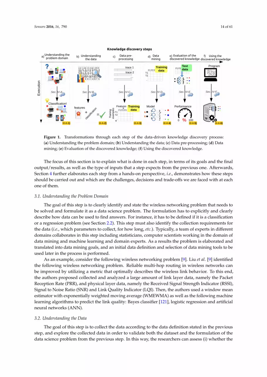
Figure 1. Transformations through each step of the data-driven knowledge discovery process:(a) Understanding the problem domain; (b) Understanding the data; (c) Data pre-processing; (d) Datamining; (e) Evaluation of the discovered knowledge; (f) Using the discovered knowledge.

The focus of this section is to explain what is done in each step, in terms of its goals and the finaloutput/results, as well as the type of inputs that a step expects from the previous one. Afterwards,Section 4 further elaborates each step from a hands-on perspective, i.e., demonstrates how these stepsshould be carried out and which are the challenges, decisions and trade-offs we are faced with at eachone of them.

3.1. Understanding the Problem Domain

The goal of this step is to clearly identify and state the wireless networking problem that needs tobe solved and formulate it as a data science problem. The formulation has to explicitly and clearlydescribe how data can be used to find answers. For instance, it has to be defined if it is a classificationor a regression problem (see Section 2.2). This step must also identify the collection requirements forthe data (i.e., which parameters to collect, for how long, etc.). Typically, a team of experts in differentdomains collaborates in this step including statisticians, computer scientists working in the domain ofdata mining and machine learning and domain experts. As a results the problem is elaborated andtranslated into data mining goals, and an initial data definition and selection of data mining tools to beused later in the process is performed.

As an example, consider the following wireless networking problem [9]. Liu et al. [9] identifiedthe following wireless networking problem. Reliable multi-hop routing in wireless networks canbe improved by utilizing a metric that optimally describes the wireless link behavior. To this end,the authors proposed collected and analyzed a large amount of link layer data, namely the PacketReception Rate (PRR), and physical layer data, namely the Received Signal Strength Indicator (RSSI),Signal to Noise Ratio (SNR) and Link Quality Indicator (LQI). Then, the authors used a window meanestimator with exponentially weighted moving average (WMEWMA) as well as the following machinelearning algorithms to predict the link quality: Bayes classifier [121], logistic regression and artificialneural networks (ANN).

3.2. Understanding the Data

The goal of this step is to collect the data according to the data definition stated in the previousstep, and explore the collected data in order to validate both the dataset and the formulation of thedata science problem from the previous step. In this way, the researchers can assess (i) whether the

Sensors 2016, 16, 790 15 of 61

selected data is a representative sample for solving the formulated problem, and (ii) whether thestated hypothesis is true and the selected data mining task is likely to prove it. For this purpose,data science experts often use simple visual representations of data, some simple statistics (i.e., avg,standard deviation, min, max, quartiles, etc.) and perhaps also some domain-specific metrics such asthe coefficient of determination R2, coefficient of correlation (Pearson’s product moment correlationcoefficient), etc. This helps them see whether one value, also referred to as the target value, label orclass can be predicted from or is in some way determined by the other available values, also referredto as dependent values, features or arguments. At the end, this step should indicate whether theresearcher can further proceed with the KD framework, i.e., with pre-processing the data, or shoulditerate back to the first step to revise the problem definition and/or collect new data.

To reuse the previous example, [9] states that the physical layer parameters (RSSI, SNR, LQI) aremeasurements that reflect the quality of the wireless channel. To test their hypothesis, they plottedthe PRR variation (estimation for the link quality) as a function of RSSI, SNR and LQI variation,respectively. Their results showed obvious correlations between the wireless link quality and thephysical layer data, and gave the indication that it is possible to model the dependency betweenthose variables by simply plotting the data (i.e., PRR = f (RSSI), PRR = f (SNR), PRR = f (LQI)).In this work, the values of the coefficient of determination R2 for SNR and LQI were 0.87 and 0.93,respectively. Obtaining high R2 values is often an indication of significant correlation with PRR. RSSIhad a much lower R2 value of 0.43. These results suggest that it is possible to leverage the SNR andLQI measurements to predict link quality with relatively high accuracy, while RSSI can only be used toa lesser extent. Hence, physical layer data could be used as a good input for the prediction process ofexpected PRR.

3.3. Data Pre-Processing

The goal of this step is to transform the collected data, also referred to as raw data, into a formatsuitable for feeding into data mining and machine learning algorithms, also referred to as trainingdata. The raw data may be unsuitable for direct use by the algorithms for several reasons, such as:

• raw data often contains values that do not reflect the real behavior of the target problem(e.g., faulty measurements);

• data is spread over multiple sources (e.g., across several databases);• data does not have the most optimal form for efficient training (e.g., parameters with

different scales);• data contains irrelevant or insignificant measurements/parameters (e.g., a system parameter that

is not likely to help solve the problem).

The term pre-processing emphasizes that the data has to be processed prior to training.The sub-steps used by the KD framework to transform the data from raw to training data are: datacleaning, integration, reduction and transformation.

Data cleaning is the step where abnormal observation points (i.e., measurements) are detected,and then corrected or removed from the dataset. Those observations are referred to as outliers. Variousoutlier detection techniques can be used at this stage. For instance, in [9] the PRR plotted as a functionof a physical layer parameter can be a graphical method of detecting outliers. The data plot for theLQI prediction parameter PRR = f (LQI) shows few points that are very distant from the remainingdataset. One reason for their occurrence comes from the fact that data derived from sensors is proneto measurement errors. Removing these values from the dataset can lead to a new more accurateprediction model.

Data integration is required when using multiple databases or files. This sub-step applies tolarger systems where objects are stored in (multiple) databases which often happens in complex webbased production systems, however it is less likely to be encountered in most problems concerningwireless networks.

Sensors 2016, 16, 790 16 of 61

Data transformation implies finding a new form of the data that is more suitable to train themining/learning algorithms. This process typically performs normalization. It has to be noted thatthe term normalization that is used in data pre-processing has also other connotations in statistics.on the input features by scaling them so as to fall within a smaller range. For instance, in [9] the physicallayer parameters (RSSI, SNR and LQI) range in the intervals: [55, 45], [0, 50] and [40, 110], respectively,while the PRR values fall within the range [0, 1]. Bringing the system parameters to the same scale bynormalizing the physical layer parameters to [0, 1] will often computationally speed-up the learningand prediction process the algorithms.

Data reduction is about removing irrelevant information with respect to the goal of the task. Inother words, we need to make sure that only relevant instances and system properties are selectedfor training. For this purpose different feature selection (finding useful features to represent the data)and extraction algorithms that reduce the datasets dimensionality are used. For instance, RSSI hasbeen shown in [9] to have a poor fit for the PRR function, only the SNR and LQI could be selected asrepresentative features to form the vector used as input for the link quality prediction model.

After completing the four sub-steps, the data will be available in a format suitable for training,often referred to as feature vectors. The feature vectors are a mathematical representation upon whichcalculations can be performed. For instance, one feature vector could be a collection of different wirelessnetwork parameters such as RSSI and SNR. In this case the feature vector would be [RSSI, SNR]T .There is an entire research branch concerned with feature engineering [122], however, such details arebeyond the scope of this paper.

3.4. Data Mining

The goal of this step is to train the data mining/machine learning algorithms to solve the KDproblem that was identified and formulated in step 1.

As elaborated in Section 2.1.2 , algorithms can be classified into two major subgroups: supervisedand unsupervised. Supervised methods require two input types: the feature vector and the label (ortarget) vector for training. The label vector represents the true class or value corresponding to thefeature vector and has been determined during the data collection process. The label vector is thetarget variable that needs to be predicted for future measurements. Each feature vector together withits corresponding label vector from the training set represents a training example. Hence, trainingexamples are vectors in a multidimensional feature space with corresponding labels. In contrast,unsupervised methods do not use labels and are more suitable for finding structure in unlabeled dataor for predicting the value of continuous parameters based on the feature vectors.

There is a trade-off between the length of the feature vector, the computational speed of thealgorithm and the accuracy of the prediction. The algorithm is supposed to build a model by calculatingthe model coefficients, based on pairs of known features and corresponding known predictions (i.e., thetraining set). Finding the optimal algorithm (see Section 2.2 for some examples) typically requires moreruns and iterations than the previous and next steps since each algorithm has a number of tunableparameters and the goal is to find the best performing configuration.

For instance, in the previously discussed example from [9] there are several combinations of inputfeature vectors that are used: [PRRi, RSSIi, SNRi, LQIi]

T , [PRRi, RSSIi]T , [PRRi, SNRi]

T , etc. The labelvector is binary, having the value 1 for successfully received packets and 0 for lost packets. Additionalsystem parameters that are tuned during this step are (1) the window size on which a prediction ismade, W (i.e., predict whether the next packet will be received based on the last 1, 10, 20, etc. packets),(2) the number of the considered links, L (i.e., all links in the network, a subset or a single link),(3) the number of packets used for generating the dataset, P, (4) the packet inter-arrival time, I, whichmodels different traffic behaviours and (5) model specific parameters such as the number and size ofthe hidden layers of the neural network. Altogether, in [9], 150 models were trained and analyzed.

Sensors 2016, 16, 790 17 of 61

3.5. Evaluation of the Discovered Knowledge

In this step, the performance of previously trained data mining/machine learning algorithms isevaluated and the best performing model is selected. There are two main approaches for modelevaluation: by reusing the previously collected dataset, or based on a newly collected dataset.The first approach assumes that separate data can be obtained for testing, which is only feasibleif the data collection process can easily be repeated [80]. In the second approach, the assumption isthat only one dataset for both testing and training is available which should be split into a trainingand a testing set. Generating the two sets may be done by simply selecting a random split of the data(e.g., 70% for training and 30% for testing). In most practical situations, the dataset is separated into anumber of equally sized chunks, so-called folds, of instances. The algorithm is then trained on all butone of the folds. The remaining fold is then used for testing. This process is repeated several timesso that each fold gets an opportunity to be left out and act as the test set for performance evaluation.Finally, the performance measures of the model are averaged across all folds. The process is known ask-fold cross validation.

The performance evaluation of a regression model is different from that of a classificationmodel. For evaluating the performance of a regression model, an error (or cost) function is typicallyused [123]. This function compares the actual values (targets) that are known with the values predictedby the algorithm and gives a measure of the prediction error (or the distance between the actual valuesand the predicted values). Often, this cost function is the same as the one used internally by thealgorithm for optimising the model coefficients/parameters during the training phase. Examples ofsuch functions that are commonly used are: Root Mean Squared Error, Relative Squared Error, MeanAbsolute Error, Relative Absolute Error, Coefficient of Determination, etc. [80].

For evaluating the performance of a classification model the prediction error is commonlycalculated based on the misclassification error metric, which gives a binary output by simply testingwhether each prediction was correct or not (i.e., 1 or 0). This binary output is used to compute aconfusion matrix that contains the true positives and true negatives (i.e., percentage of correctlypredicted instances), false positives and false negatives (i.e., percentage of instances that wereincorrectly labeled). Various performance metrics including precision/recall, F1 score, etc. (explainedlater in Section 4.6), are derived based on the confusion matrix.

Finally, the best performing model with respect to the considered performance metric is selectedfor both regression and classification—also referred to as model selection. When the performanceof the models is not satisfactory, the knowledge discovery process returns to the previous two stepswhere typically better feature engineering and model tuning are performed.

For instance, in [9] one dataset was used for training and testing: 60% of the total dataset instanceswere randomly selected for training, while the remaining 40% for testing. The mean square error (MSE)was used to reflect the average misclassification error and evaluate the performance of the followingalgorithms: Bayes classifier, logistic regression and artificial neural networks (ANN). They tuned thefeature space through feature engineering for: RSSI, SNR, LQI, PRR, and the system parameters bychanging values for: W, L, P and I as discussed in Section 3.4. For each feature/parameter combinationthe authors trained and evaluated every algorithm again in order to select the best model. The bestperforming model turned out to be logistic regression trained on the feature vector [PRR, LQI]T . Toshow the advantages of the model an evaluation against existing solutions such as 4Bit and STLE wasalso performed.

3.6. Using the Discovered Knowledge

A standalone offline machine learning system might not be a very useful tool. Therefore, in the lastKD step, the software development process of the selected model is considered. As in any traditionallysoftware development process, after the initial analysis that was performed through the previous steps,an appropriate design describing how the model should work is proposed, which may be visualizedby a simple block diagram or more detailed with several UML diagrams. Typically, it is also considered

Sensors 2016, 16, 790 18 of 61

how to integrate the proposed model with existing systems (e.g., into existing environment of the targetplatform, with existing database management system, with existing visualization tools, etc.). Then, aprototype program of the model is implemented on the target architecture, by means of coding usingadequate programming language which may depend on the target platform. The implementation isverified and validated through several tests. At the end, an implementation of the model is deployedat the target system.

For instance, after the initial analysis and several experiments performed based on offlinetrained models, Liu et al. [9] proposed a design for an (online) implementation of their logisticregression trained model, called 4C. Their target platform was a Tmote Sky mote running TinyOS [124].To this end, the authors had to consider how to integrate their model with the existing environment inTinyOS (e.g., with the forwarding engine, routing engine, link estimator etc.). Then, they implementedthe logistic regression-based link estimator as a module in nesC, which is the programming language inwhich the TinyOS system is written. At the end, they deployed the 4C module online on wireless sensormotes and tested through several experiments against existing link quality estimator implementationslike STLE and 4Bit and demonstrated superiority of their solution.

3.7. Examples of Using Data Science in Wireless Networks

In traditional wireless research, research often starts from theoretical models to design solutionswhich are then evaluated or validated using a simulator or experimental setup. For example, in [52], aspectrum usage prediction problem for cognitive radios is simulated in which neural networks are usedas the machine learning algorithm to predict which unlicensed channels are idle. In contrast to thesetraditional research approaches, the research works below [9,11,12] take a truly data-driven approach,i.e., starting from large, real-life wireless datasets to extract knowledge about wireless systems. Tothis end, this section provides an overview of selected applications of data science approaches inwireless networks by clearly identifying each step of the knowledge discovery in their methodologyand parts that do not follow best practices. We hope in this way to help the reader better understandhow to properly apply each step of the KD framework to existing problems originating from wirelessnetworks, and at the same time, motivate for new research ideas in the wireless domain.

Use Case 1: Link Quality Estimation

Liu et al. [9] improved multi-hop wireless routing by creating a better radio link quality estimator.They investigated whether machine learning algorithms (e.g., logistic regression, neural networks)can perform better than traditional, manually-constructed, pre-defined estimators such as STLE(Short-Term Link Estimator) [104] and 4 Bit (Four-Bit) [105]. The methodology employed in theirwork followed all the steps from the knowledge discovery process and we used examples fromthis work to show how the KD process steps can be successfully applied to wireless networks inprevious parts of this section. They clearly formulated the wireless networking problem and thecorresponding data mining/machine learning problem, then they collected a large amount of data,analyzed it and made sure it can solve the problem, pre-processed it and fed it to the machine learningalgorithms. Finally, they evaluated the way the algorithms performed at predicting the quality of thelink and implemented the most promising one (in this case logistic regression) on several testbeds.While in [9] the authors used an off-line trained model to do prediction, in their follow-up work [10],they went a step further and both the training and the prediction were performed online by the nodesthemselves. The advantage of this approach is that the learning and, thus the model adapt to changesin the wireless channel, that could otherwise be captured only by re-training the model offline andupdating the implementation on the node.

Use Case 2: Traffic Classification

Crotti et al. [11] proposed a new method for identifying the application layer protocol that hasgenerated a particular traffic flow. Their approach was motivated by the fact that standard techniques

Sensors 2016, 16, 790 19 of 61

at the time often failed to identify the application protocol (using transport layer ports) or scaledpoorly in high-capacity networks (detailed analysis of the payload of each packet). Their methodis based on the statistical properties of the traffic flows which allows discrimination between trafficclasses. While they do not seem to define their problem explicitly as a data mining/machine learningproblem, nor use well-known data mining/machine learning algorithms, they took a truly data-drivenapproach, they used methodologies and terminologies from data science and followed all the stepsof the KD process except the last one, i.e., system implementation. The authors clearly identified andformulated the application protocol identification problem as a (traffic) classification problem, wherethe classes are the application protocols learned by the classifier (e.g., HTTP, SMTP, SSH, etc.). Then,they collected data for training from their faculty’s campus network and created the feature vectors(pairs of {s, ∆t}, where s is the packet size, and ∆t the inter-arrival time between successive packets)and the training set, pre-processed it using a Gaussian filter to reduce the effects of noise and fed itinto their custom learning algorithm for training. The trained model consists of pairs of a matrix, Mp

and a vector Vp, for each protocol p, where Mp is the protocol mask that captures the main statisticalproperties of training flows produced by the same protocol, while Vp the protocol specific thresholdthat is used by the classifier to determine how close an unknown flow is to a fingerprinted protocolwith mask Mp. At each step they explained the rationale behind each action taken, which may be areplacement for the data analysis phase. At the end they evaluated their model with a separate test setcollected from the same network.

Use Case 3: Device Fingerprinting

In [12], the authors proposed a new solution for fingerprinting wireless devices that may helpexisting network access control (NAS) systems enhance network security by allowing access only forcertain devices or device types in accordance with a defined security policy. Unlike traditionalsecurity mechanisms that rely on device authentication based on public key cryptography and digitalcertificates, that can be simply transferred to another device, their approach relies on differentiatingdevices by looking into the statistical distribution of inter-arrival times between packets generatedby the same device and a particular application. Their assumption is that the physical particularitiesof devices such as processor, DMA controller, memory, clock skews, etc. reflect on how these devicessend packets over the air. By monitoring the inter-arrival times, it should be possible to distinguishindividual devices or devices of the same type (i.e., devices that have the same hardware configuration),thus they formulated a classification problem. They collected the necessary data to prove theirhypothesis from two testbeds: an isolated network environment and a live campus network. Theirfeature vectors consist of histograms constructed from inter-arrival times and their label or targetvalues consist of discrete classes (e.g., Dell Notebook). They selected an artificial neural network(ANN) model that was trained offline and then evaluated on the testing data. The best performingmodel turned out to be an ANN model with one hidden layer of 50 nodes. Even though this researchalso followed all the KD steps, some of the individual steps do not seem to conform with existing bestpractices. For instance, it is not clear how the feature vectors were generated in the data pre-processingstep. It is also unclear how many training examples were used in the data mining part and how thetraining and testing sets were separated. Finally, the evaluation is presented in a biased manner byonly showing an example of a well-performing case using only a subset of the relevant measures. Inthe following Case study section, we will use this publicly available dataset to provide an in-depthillustration of how the steps of the KD process should be performed.

Tumuluru et al. [52], as earlier mentioned, define a spectrum usage prediction problem.The authors follow some of the steps of the KD process. They used neural networks as the machinelearning/data mining algorithm, but they only use synthetic data produced with a simulator and noreal-world data. This means that the data understanding step is not relevant in their case since theyknow a-priori the statistical details of the synthetic data. This is in contradiction with the discussionin Section 3 regarding the KD process. Additionally, their evaluation is far from the best practices

Sensors 2016, 16, 790 20 of 61

used in the machine learning community. To remedy such cases, the next section aims to further closethe gap between wireless researchers and data science experts by giving very concrete examples andconsiderations for each of the knowledge discovery steps.

4. Case Study

This section details the implementation of each component of the general-purpose frameworkintroduced in Section 3. These implementations are used to demonstrated how a real-life wirelessnetworking problem can be solved using a data-driven approach. However, note that the presentedtechniques are generic, as such are not limited to the particular problem use case. The same genericalgorithms and techniques that are introduced in each step as well as the overall methodology can beapplied to a different type of problem. The main difference relies in the data mining step, where thepractitioner has to select specific algorithms that are suitable to solve the previously identified type ofproblem. Recall that Section 2 guides the reader how to properly formulate a specific wireless domainproblem into a data science problem with a list of suitable algorithms.

4.1. Solving a Classification Problem in Wireless Networks

For the case study, we chose a simple classification problem about wireless device fingerprintingwhich was introduced by Radhakrishnan et .al. [12] for which all the data (i.e., the GaTech dataset) ispublicly available on the CRAWDAD repository [24]. The dataset was also produced as part of thework presented in [12]. It can be downloaded by anyone who wishes to replicate the KD process stepsfurther detailed in the remainder of this tutorial. However, while the GaTech dataset was used in [12]to solve the wireless device fingerprinting problem using a custom approach, this tutorial paper reusesthe same dataset to demonstrate the correct methodology of applying data science techniques forsolving a wireless domain problem through a practical approach. Finally, a brief comparative study ofthe proposed methodology compared to their custom approach highlights the importance of applyingthe identified best practices developed by the data science community.

The scripts used during this tutorial for implementing the individual components of theframework can be downloaded from [23] together with all intermediary and processed datasets,thereby offering interested readers the opportunity to quickly learn how to apply these or similarsteps themselves.

Wireless Device Fingerprinting: A Brief Overview

Due to the broadcast nature of the wireless transmission medium, wireless networks arevulnerable to various network security attacks; in particular, they are easy to compromise in termsof their service availability (through Denial-of-Service attacks) as well as data confidentiality, dataintegrity and user/device authentication (wireless security protocols are known to have security holesthat can be easily exploited). The major security thread facing wireless networks is node forgery, wherean attacker obtains the credentials (cryptographic keys) of the legitimate user and impersonates thetrusted node. One promising approach to reduce the vulnerability of wireless networks to these attacksis device fingerprinting [125]. Device fingerprinting is the process of gathering device information(passively or actively) to extract unique device-specific signatures or fingerprints that can be used toreliably and robustly identify devices. A device identification system typically examines a three-stepprocess that consists of (i) identifying the relevant patterns; (ii) extracting patterns from raw data;(iii) creating a model for device identification. The extracted patterns from the raw observationsare also called features. Different approaches utilize different device-specific features, which can becategorized based on the layer of the protocol stack from which the information has been obtained.

1. PHY layer features: PHY features are derived from the RF waveform of the received signal.The most common PHY layer information for device fingerprinting are RSSI measures. However,the RSSI depends on the transmission power, propagation of the signal and attenuation

Sensors 2016, 16, 790 21 of 61

imposed by the channel. More fine-grained features are channel state information at thereceiver (CSIR) [126,127], channel frequency response (CFR) [128,129], channel impulse response(CIR) [126,130], carrier-frequency difference (CFD) [131], phase shift difference (PSD) [131],second-order cyclostationary feature (SOCF) [131], I/Q signal samples [132], etc.

2. MAC layer features: The motivation behind utilizing MAC layer features for device identificationis that some of the MAC layer implementation details are not specified in the standard and are leftto the vendors. Therefore, MAC layer features are usually vendor specific. Some example worksare: observing unique traffic patterns on the MAC layer to detect unauthorized users [133,134],observing the clock skew of an IEEE 802.11 access point from the Time Synchronization function(TSF) timestamps sent in the beacon/probe frames [135]; MAC features such as transmissionrate, frame size, medium access time (e.g., backoff), transmission time and frame inter-arrivaltime [136].

3. Network and upper layer features: Features at the network and upper layers typically look intouser’s traffic patterns or inter-arrival times calculated at the network and application layer. Forinstance, in [137] Gao et al. and in [12] Radhakrishnan et al. use inter-arrival times from TCP andUDP packets as features. Ahmed et al. [138] uses traffic patterns of digital TV broadcasting toidentify devices. On the other hand, in [139] Eckersley uses higher layer features by tracking theweb browser behaviour by analyzing the browser’s requests/replies.

Finally, multiple features can be combined to form a device fingerprint, leading to a cross-layeridentification approach. The case study example of this paper falls into the last category, whereinter-arrival times based features are used as is explained in next section.

4.2. Understanding the Problem Domain

One of the challenges of the knowledge discovery process is that the data scientists having the skillset and experience necessary for carrying out the process are not necessarily experts in the areas forwhich they apply these techniques. For instance, they will know what terminology such as supervisedand unsupervised methods, 10-fold cross-validation, etc. means and what techniques should be usedto execute them, but they will not know what packet inter-arrival time, TCP, UDP and SCP traffic arein detail. On the other hand, it requires quite some time and effort from a wireless networking expertwho is familiar with terminology such as SCP traffic, to carry out the knowledge discovery processbecause they will have to dive into and learn all the new data science terminology. This learning pathalso has many alleys and, for a novice, many aspects could turn out to be confusing.

As discussed in Section 3.7, there are several research works which seem to take a data scienceapproach in wireless networks while they miss some fundamental steps or parts of the KD process.

4.2.1. Understanding and Formulating the Device Fingerprinting Problem

The device fingerprinting problem defined in [12] is an actual problem related to the real-timedetection of malicious devices in wireless networks that aims to classify wireless devices based onseveral types of traces. It is based on the argumentation that each device exhibits some traits inherentwith its physical implementation. As a result, it is assumed that the packet creation process varies acrossdifferent device architectures and is influenced by the CPU, L1/L2 cache, DMA controller, physicalmemory, etc. At the same time, similar variations exist between individual devices with the samearchitecture, due to differences of clock skews. Thus, it might be feasible to differentiate individualdevices and also cohorts of devices with the same hardware characteristics (i.e., device types).

Furthermore, it should be possible to determine and learn the differences between the devices andtheir types by looking at packet inter-arrival times (IAT). This implies that, at capture time, for eachpacket it is known which device sent it (from IP address) and what transport and application layerprotocol sent it. To verify this hypothesis, the capture of IP traffic flows from several target devices isrequired. In the case of active device fingerprinting, where devices are queried, e.g., with ICMP echorequest packets (Ping), the captured packets may contain information about the MAC address of the

Sensors 2016, 16, 790 22 of 61

target device. However, it should be clear that the MAC address contains only the unique identifier ofthe manufacturer of the device, which is not sufficient to identify a particular device nor its type. Onthe other hand, MAC addresses can be easily spoofed.

Based on this argumentation, the following hypothesis can be constructed: "by building perdevice and per device type models based on packet IATs, it should be possible to classify devices anddevice types as well as their normal behaviour". Thus, the problem of fingerprinting wireless devicescan be translated into a data mining classification problem. To verify the stated hypothesis data has tobe collected to find out:

• How much can data from one device (e.g., a Dell Netbook) tell about the data from other similardevices (e.g., other Dell Notebooks)?

• How much can a certain type of device (e.g., Dell Netbooks) tell about other device types(e.g., iPhones)?

By answering such questions using the collected data, we should be able to anticipate whetherthe data can validate our hypothesis and further process with the KD process. If it turns out that thedata cannot be used to validate the hypothesis, we have to go into an iterative process that involves(1) tuning the hypothesis and (2) collecting different data.

4.2.2. Collecting the Data for Validating the Hypothesis

In order to validate their hypothesis, Radhakrishnan et al. [12] used three traces with packetinter-arrival times collected from several devices and several protocols in two different testbeds: anisolated testbed and a real testbed. For the purpose of this tutorial, we focus on the isolated testbeddata that contains 94 files containing IATs from 14 different devices and four different combinationsof tools and protocols as summarised in Table 3. Four different device types (Dell Netbook and iPad;iPhone and Nokia phone) were used in the testbed containing five pieces of Dell Netbook, three piecesof iPad, four pieces of iPhone and two pieces of Nokia Phone. The collected data consists of TCP, UDPand ICMP traffic generated using three tools: iPerf, Ping and SCP. The detailed device specification andother detailed information about the experimental settings under which the data has been collectedare available in Tables 1–3 in [12].

Table 3 presents a summary of IAT traces that were collected for each combination of device,protocol and tool. For instance, in the first line of the table it can be seen that five Dell Netbookswere used in the experiments as follows. First, five TCP traffic traces were generated using the iPerftool. These five traces had a minimum of 841.299 instances (i.e., IAT values) and a maximum of over3 million such instances. The average number of values in the dataset is 1.8 million with a standarddeviation of 948.900. Second, the UDP traffic was also generated using iPerf, but in this case, threedifferent packet size/rate settings were used (Case 1: 64 byte packets at 1 Mbps, Case 2: 1400 bytepacket at 1Mbps and Case 3: 64 byte packets at 8Mbps according to Table 1 in [12].), which is whythe table mentions three cases, and five traces for each case, totalling 15 traces with a minimum of298.956 items and a maximum of 5.702.776 items per file. Also Ping ICMP traces were collected, albeitonly for three of the five Dell Netbooks, and SCP TCP data as shown in the corresponding lines ofthe table.

It can be seen that the number of traces is consistent with the number of devices for each roundof the data collection. Except for the Dell Netbook, the same number of devices have been usedthroughout all the experiments. For the Dell Netbook, the Ping ICMP collection only used threedevices, while all the remaining campaigns used five. Furthermore, for some experiments, traces forseveral cases have been collected using various packet size and rates. Overall, the data is stored in94 files containing a total of 137,348,241 data points, with an average of 1,461,161 data points per file, amedian of 1,311,227 and a standard deviation of 1,315,710. The standard deviation is relatively high assome files contain several million data points (i.e., iPhone iPerf UDP case 3, trace 3 contains 4,057,490data points) while some other files contain several hundred thousands (i.e., Dell Netbook iPerf UDP

Sensors 2016, 16, 790 23 of 61

case 1, trace 1 contains 299,521 files). We can anticipate that having unbalanced traces in terms ofthe amount of data may lead to smaller training/testing sets for some devices and larger for others.In some cases, this may mean that the models where more training/testing data is available mightcapture the underlying process better than others [140].

Table 3. Isolated testbed data summary describing (i) the device types; (ii) the number of devicesfor each of these types; (iii) the traffic type and number of data traces for each traffic type and(iv) minimum, maximum, average and standard deviation of the number of data points per data trace.

Device Type Number of Devices Traffic Type Minimum Maximum Average Standard Deviation

Dell Netbook 5

iPerf TCP (1 case x 5 traces) 841,299 3,059,247 1,820,062 948,900

iPerf UDP (3 cases × 5 traces) 298,956 5,702,776 2,382,538 1,799,493

Ping ICMP (2 cases × 3 traces) 359,220 359,996 359,865 316

SCP TCP (1 case × 5 traces) 1,514,216 1,569,352 1,543,571 27,750

iPad 3

iPerf TCP (1 case × 3 traces) 1,305,673 1,780,640 1,527,179 239,090

iPerf UDP (3 cases × 3 traces) 297,957 2,181,618 1,305,483 769,987

Ping ICMP (2 cases × 3 traces) 301,966 322,124 309,749 7,991

SCP TCP (1 case × 3 traces) 1,598,030 1,847,037 1,749,059 132,710

iPhone 4

iPerf TCP (1 case × 4 traces) 440,623 4,162,438 2,357,540 2,072,695

iPerf UDP (3 cases × 4 traces) 306,413 4,094,728 1,791,755 1,378,019

Ping ICMP (2 cases × 4 traces) 314,176 673,590 494,099 190,049

SCP TCP (1 case × 4 traces) 599,460 1,599,098 1,348,888 499,619

Nokia Phone 2

iPerf TCP (1 case × 2 traces) 718,480 844,531 781,505 89,131

iPerf UDP (3 cases × 2 traces) 300,924 5,131,699 2,189,739 2,094,815

Ping ICMP (2 cases × 2 traces) 250,532 359,209 331,915 54,255

SCP TCP (1 case × 2 traces) 1,316,782 1,570,745 1,443,763 179,579

Practical Considerations for Understanding the Problem Domain

Once the wireless problem and its potential data-driven solution has been identified, a relevantbody of data has to be collected, processed, and understood to validate the stated hypothesis.

To facilitate the data collection process, readers can utilize repositories with existing datasets, orcollect new traces from publicly accessible wireless testbeds.

Repositories provide access to data from real-life wireless experiments. Examples areCRAWDAD [141], CONAN project [142], the "UC San Diego wireless measurements" whosedataset is available at [143], the University of Washington "Wireless Measurements Project" [144],EVARILOS [145], "UMass Trace Repository" [146], etc.

Wireless testbeds allow to setup a specific wireless scenario and collect the relevant datato evaluate a hypothesis. Several testbeds are part of the FIRE federations [147] including:w-iLab.t [148], TWIST [149], IRIS [150], LOG-A-TEC [151], NITOS [152], etc., and GENIfederations [153] such as: Motelab [154], ORBIT [155], Kansei [156], NetEye [157], etc.

4.3. Understanding the Data

As briefly discussed in Section 3.2, this second step of the KD process validates the data and thehypothesis. It verifies whether the data has the potential to lead to an accurate and meaningful model.It also verifies whether it makes sense to proceed further with the initial problem definition, or if thereis a need for a reformulation. Typically, this step also identifies whether data has to be pre-processed.

Sensors 2016, 16, 790 24 of 61

This step is sometimes referred to as Exploratory Data Analysis (EDA) and it consists of applyinganalytical/computational and graphical/visualization techniques on the data [158].

4.3.1. Generic EDA Techniques

Most EDA techniques rely on statistical methods, tools and techniques. For this reason, EDAis also known as the “statistics” part of the KD process. In contrast to the classical statisticalhypothesis testing that verifies certain a priori assumptions (e.g., correlations between differentattributes/variables, where there is some information concerning a possible dependency), EDA usesmore sophisticated techniques to identify systematic relations between attributes/variables aboutwhich no prior information exists. Data may be analyzed using computational or visual techniques.

• Computational techniques utilize statistical distributions, five-number summary, coefficient ofdetermination, advanced multivariate exploratory techniques (e.g., cluster analysis, principalcomponents and classification analysis, classification trees, self-organizing maps, etc.). In thistutorial, we use the five-number summary and the coefficient of determination to guide the readerthrough the process of understanding the data. More advanced techniques can be adopted fromthe domain specific literature [159].

The five-number summary consists of five reference values that summarize the behavior of adataset: min—the minimum value, Q1—first or lower quartile (the middle number betweenthe minimum value and the median), median—the “middle number” of the sorted dataset,Q3—third or upper quartile (the middle number between the median and the maximum value),and max—the maximum value.

The coefficient of determination (denoted by R2) is a simple statistic frequently used fordetermining relationships between system variables. It is defined as:

R2 = 1−∑

i(yi − fi)

2

∑i(yi − y)2 (2)

where yi is the target value, fi is the value modeled (predicted) by a linear function f , while thedenominator represents the total variation of the target variable’s instances.

In general, R2 describes how well some of the data can be approximated by a regression lineconstructed from some other data (i.e., one feature from the feature vector). High values of R2

scores will indicate that there is a high linear dependency between a particular feature and thetarget value, while low values of R2 may indicate the opposite.

• Visual techniques utilize histograms, box plots, scatter plots, contour plots (for functions oftwo variables), matrix plots, etc [160]. Histograms, also used throughout the rest of the tutorial,reflect the frequency density of events over discrete time intervals. They help understand andgraphically verify obtained results [161]. For instance, they display the distribution, the mean,skewness and range of the data. They are also a useful tool for identifying deviating points whichshould perhaps be removed from the dataset. A practical feature of histograms is their ability toreadily summarize and display large datasets.

A typical scenario for data exploration starts with computing simple statistics like thefive-number summary and getting more insight in the data using simple visualisation tools suchas histograms. These are simple but powerful techniques that help understand different dataproperties, find patterns in data, explore if there are instances out of compliance and suggest furthermodeling strategies.

Sensors 2016, 16, 790 25 of 61

4.3.2. Applying EDA Techniques to the GaTech Data

Validating the Fingerprinting Data

To exemplify this step of the KD process, we focus on the iPerf TCP traces from all devices anddevice types, but of course the same procedure may be applied to the remaining traces. Exhaustivelyconsidering all traces would lead to a very long paper with no significant added value. We observe14 iPerf TCP traces from: 5 Dell, 3 iPad, 4 iPhone (3G and 4G) and 2 Nokia devices. Table 4 presentsthe five-number summary for TCP IAT data. It can be noticed that the dataset from the iPad1 andiPad2 have significantly higher maximum values compared to the others. The iPad2 has a maximumIAT value (10.36 s) that is 100 times higher than the maximum IAT value of iPad3 (0.11 s). iPad1 hasthe next highest value of 5.2795 s, followed by iPhone3G1 with an IAT value of 2.95 s. The values formin, Q1, median and Q3 are more balanced, suggesting that only a few high-valued data points aredeviating from the rest of the dataset. Furthermore, the Q1, median and Q3 values are lying close toeach other for each dataset, while the max values are distant from Q3, suggesting that the majorityof the measurements and the relevant information lies in the IAT measurements with values lowerthan Q3. Consequently, all the points strongly deviating from Q3, i.e., close to the max points, might bepotential outliers. Those distant data points deviate from a normal IAT trace pattern for a particulardevice, and they may have occurred due to measurement errors.

Table 4. 5 number summary of the TCP inter-arrival times (IAT) data.

Device Type Device min[×10−6][s] Q1[×10−4][s] median[×10−4][s] Q3[×10−4][s] max[s]

Dell Netbook

DN1 5.96 6.91 8.24 13 0.1872

DN2 5.96 5.67 6.20 7.35 0.2845

DN3 5.96 5.72 6.18 7.70 0.1769

DN4 2.86 4.16 5.80 6.56 0.2017

DN5 2.86 3.82 4.72 6.22 0.6571

iPad

iPad1 1.91 5.46 6.20 12 5.2795

iPad2 1.91 5.80 7.83 13 10.3603

iPad3 2.86 16 19 34 0.1102

iPhone 3G and 4G

iPhone3G1 2.86 6.84 9.82 21 2.95

iPhone3G2 1.91 15 18 35 0.4726

iPhone4G1 3.81 9.55 13 25 0.1456

iPhone4G2 4.77 14 16 31 0.1487

Nokia Phone

NP1 1.91 5.39 6.43 11 0.1481

NP2 1.91 5.50 6.49 11 0.1486

Table 4 reveals large variations of min and max values between the datasets. In other words,the datasets span different ranges, which will result in histograms with nonconforming bin widths.Figure 2a illustrates this situations for histograms created from two datasets (DN1 and DN2) with afixed number of bins. Such histograms have to be adjusted in order to perform a correct prediction taskin the following steps. This can be done by adjusting the start and the ending points of the histograms,so that the bins for all histograms have the same width and can be compared against each other. Thishas to be done for all the 14 datasets from Table 4. We implemented a simple algorithm that looks atthe max point over all histograms, which according to Table 4 belongs to device iPad2, and aligns allhistograms with regard to that point, by padding the dataset with a new zero-count max value as aplace-holder. Figure 2b illustrates the same two histograms from Figure 2a after aligning.

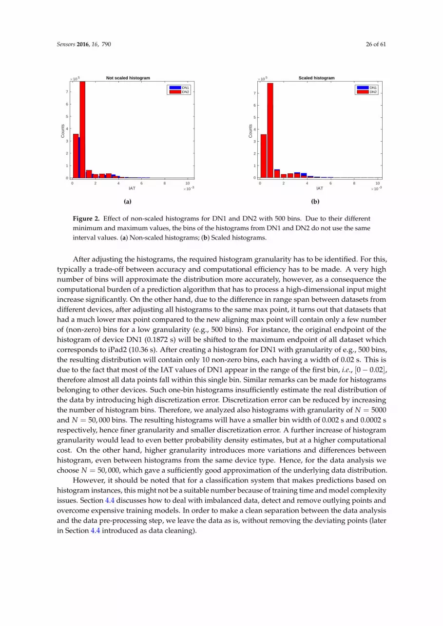
Sensors 2016, 16, 790 26 of 61

IAT #10 -30 2 4 6 8 10

Cou

nts

#10 5

0

1

2

3

4

5

6

7

Not scaled histogram

DN1DN2

(a)

IAT #10 -30 2 4 6 8 10

Cou

nts

#10 5

0

1

2

3

4

5

6

7

Scaled histogram

DN1DN2

(b)

Figure 2. Effect of non-scaled histograms for DN1 and DN2 with 500 bins. Due to their differentminimum and maximum values, the bins of the histograms from DN1 and DN2 do not use the sameinterval values. (a) Non-scaled histograms; (b) Scaled histograms.

After adjusting the histograms, the required histogram granularity has to be identified. For this,typically a trade-off between accuracy and computational efficiency has to be made. A very highnumber of bins will approximate the distribution more accurately, however, as a consequence thecomputational burden of a prediction algorithm that has to process a high-dimensional input mightincrease significantly. On the other hand, due to the difference in range span between datasets fromdifferent devices, after adjusting all histograms to the same max point, it turns out that datasets thathad a much lower max point compared to the new aligning max point will contain only a few numberof (non-zero) bins for a low granularity (e.g., 500 bins). For instance, the original endpoint of thehistogram of device DN1 (0.1872 s) will be shifted to the maximum endpoint of all dataset whichcorresponds to iPad2 (10.36 s). After creating a histogram for DN1 with granularity of e.g., 500 bins,the resulting distribution will contain only 10 non-zero bins, each having a width of 0.02 s. This isdue to the fact that most of the IAT values of DN1 appear in the range of the first bin, i.e., [0− 0.02],therefore almost all data points fall within this single bin. Similar remarks can be made for histogramsbelonging to other devices. Such one-bin histograms insufficiently estimate the real distribution ofthe data by introducing high discretization error. Discretization error can be reduced by increasingthe number of histogram bins. Therefore, we analyzed also histograms with granularity of N = 5000and N = 50, 000 bins. The resulting histograms will have a smaller bin width of 0.002 s and 0.0002 srespectively, hence finer granularity and smaller discretization error. A further increase of histogramgranularity would lead to even better probability density estimates, but at a higher computationalcost. On the other hand, higher granularity introduces more variations and differences betweenhistogram, even between histograms from the same device type. Hence, for the data analysis wechoose N = 50, 000, which gave a sufficiently good approximation of the underlying data distribution.

However, it should be noted that for a classification system that makes predictions based onhistogram instances, this might not be a suitable number because of training time and model complexityissues. Section 4.4 discusses how to deal with imbalanced data, detect and remove outlying points andovercome expensive training models. In order to make a clean separation between the data analysisand the data pre-processing step, we leave the data as is, without removing the deviating points (laterin Section 4.4 introduced as data cleaning).

Sensors 2016, 16, 790 27 of 61

Validating the Fingerprinting Hypothesis

In order to validate their hypothesis based on the collected data, Radhakrishnan et al. [12]performed an analysis by using simple visual techniques in which they show that: (1) the probabilitydistribution functions (PDF) that approximate the distribution of the empirically collected data vary fordevices with different internal hardware characteristics, which may enable device type classification;(2) the average IAT values vary between devices stemming from the same device type (e.g., Dellnetbooks with the same hardware configuration) because of clock skew, which should enable individualdevice classification. As a result of the above made observations, the data is considered suitable for thehypothesis and it seems that the distribution of the data rather than its shape (i.e., trend, periodicity,etc.) are relevant for the problem. An analysis of whether useful information is also contained in theshape of the data is missing in the original paper, possibly because it is not relevant for their study.However, generally speaking, analyzing such information may be useful for improving the overallperformance of the classifier [162].

In addition to visual techniques, used in [12], computational techniques are also very relevantto answer questions about the characteristics and relationships between the underlying data.In particular, when the aim is to find the predictive power of one trace with respect to others.

(i) How much can data from one Dell Notebook tell about the data from other Dell Notebooks?Table 3 has shown that there is quite some data about Dell Netbooks (DNs), therefore, we will first

try to understand how many IATs captured from one Dell Netbook can be used to predict the behaviorof other such netbooks. Table 5 presents the R2 coefficient for the iPerf TCP IATs with highlightedtraces from the five Dell Netbooks.

Table 5. R2 values for 50,000 bins histograms for iPerf TCP IATs for the traces from the 14 devicesdescribed in Table 3.

DN1 DN2 DN3 DN4 DN5 iPad1 iPad2 iPad3 iPhone1 iPhone2 iPhone3 iPhone4 Nokia1 Nokia2

DN1 1 0.2407 0.2213 0.1624 0.0968 0.1130 0.1326 0.0527 0.3364 0.0770 0.1858 0.0412 0.2390 0.1935DN2 0.2407 1 0.9981 0.8620 0.6961 0.9248 0.7738 0.0656 0.4497 0.1512 0.2688 0.0133 0.8659 0.8382DN3 0.2213 0.9981 1 0.8604 0.6950 0.9273 0.7702 0.0657 0.4633 0.1508 0.2694 0.0122 0.8656 0.8391DN4 0.1624 0.8620 0.8604 1 0.9581 0.8056 0.6613 0.0616 0.4238 0.1213 0.2278 0.0106 0.8212 0.7756DN5 0.0968 0.6961 0.6950 0.9581 1 0.6550 0.5230 0.0493 0.3408 0.0901 0.1667 0.0057 0.6870 0.6396iPad1 0.1130 0.9248 0.9273 0.8056 0.6550 1 0.9285 0.0818 0.3830 0.1646 0.3298 0.0626 0.8741 0.8724iPad2 0.1326 0.7738 0.7702 0.6613 0.5230 0.9285 1 0.1207 0.3734 0.2001 0.4456 0.1948 0.8286 0.8337iPad3 0.0527 0.0656 0.0657 0.0616 0.0493 0.0818 0.1207 1 0.1575 0.6292 0.2366 0.1978 0.1028 0.0986

iPhone1 0.3364 0.4497 0.4633 0.4238 0.3408 0.3830 0.3734 0.1575 1 0.1709 0.3572 0.0592 0.5170 0.4687iPhone2 0.0770 0.1512 0.1508 0.1213 0.0901 0.1646 0.2001 0.6292 0.1709 1 0.2353 0.4011 0.1837 0.1778iPhone3 0.1858 0.2688 0.2694 0.2278 0.1667 0.3298 0.4456 0.2366 0.3572 0.2353 1 0.1486 0.5019 0.5197iPhone4 0.0412 0.0133 0.0122 0.0106 0.0057 0.0626 0.1948 0.1978 0.0592 0.4011 0.1486 1 0.0460 0.0411Nokia1 0.2398 0.8659 0.8656 0.8212 0.6870 0.8741 0.8286 0.1028 0.5170 0.1837 0.5019 0.0460 1 0.9922Nokia2 0.1935 0.8382 0.8391 0.7756 0.6396 0.8724 0.8337 0.0986 0.4687 0.1778 0.5197 0.0411 0.9922 1

It can be seen that the traces from DN2 and DN3 have a very high determination coefficient of0.998, meaning that their distributions are very much alike. To illustrate the similarity of these traces,Figure 3a,b present the scale-adjusted histograms for DN2 and DN3. For a regression task, this is good,meaning that data from one of the two devices can be used to predict data from the second device.For a classification task, this may mean that data coming from these two devices are more likely to beconsidered as belonging to the same class. In this case, it means that classification methods might havetrouble differentiating between DN2 and DN3.

Sensors 2016, 16, 790 28 of 61

IAT #10 -31 2 3 4 5 6 7 8 9 10

coun

ts

#10 5

0

1

2

3

4

5

6

DN2

50.000 bins

(a)

IAT #10 -30 2 4 6 8 10

coun

ts

#10 5

0

1

2

3

4

5

6

DN3

50.000 bins

(b)

Figure 3. Comparing histograms for DN2 and DN3 for TCP case. (a) Histogram of DN2; (b) Histogramof DN3.

A high determination coefficient can also be found between data from DN4 and DN5 with an R2

value of 0.958. There is also a high determination between DN2 and DN4 and DN3 and DN4, followedby DN2 and DN5 and DN3 and DN5, thus similar conclusions can be drawn for these.

Table 5 also shows that the determination coefficient considered for DN device pairs that includeDN1 have a very low R2 value (first table row or column) with the lowest R2 value of 0.0967 forthe (DN1, DN5) pair and the and highest for the (DN1, DN2) pair with an R2 value of only 0.241.Figure 4a,b present histograms for DN1 and DN5 which had the lowest R2 score. It is clear that thehistograms differ much more than in the previous case, especially in the tails part, the shape and thepeak values.

IAT #10 -30 1 2 3 4 5 6 7 8 9 10

coun

ts

#10 5

0

0.5

1

1.5

2

2.5

3

3.5

4DN1

50.000 bins

(a)

IAT #10 -30 2 4 6 8 10

coun

ts

#10 5

0

2

4

6

8

10

12

DN5

50.000 bins

(b)

Figure 4. Comparing histograms for DN1 and DN5 for TCP case. (a) Histogram of DN1; (b) Histogramof DN5.

In conclusion, we expect that data coming from device DN1 will not be confused with data fromother devices for the classification task, however a regression task would perform poorly at predicting

Sensors 2016, 16, 790 29 of 61

the data generated by this particular device. R2 results for the other traffic cases can be obtained fromthis repository [163].

(ii) How much can iPerf TCP data from a set of similar devices tell about the same data from other devices?Next, instead of looking at individual devices, we look at TCP traces containing aggregated

data from multiple device types. Table 6 presents the R2 scores for data collected for sets of similardevices (i.e., from same device type) for the case of TCP traffic. This information can be used todetermine whether TCP data can be used to identify the type or device that transmitted the data.Dell Netbooks and Nokias have an R2 value of 0.8235, meaning that a regression task would performwell predicting IAT values for Nokia based on training values for Dells, however a classification taskmight be confusing the two classes, unless it can find a way to discriminate based on the training data.Similar conclusions are true for iPad and Nokia devices which have an R2 value of 0.7359, followed byiPad and iPhone with R2 = 0.6562, and Dell and iPad with R2 = 0.6254. R2 results for the remainingtraffic cases can be obtained from this repository [163].

Table 6. R2 values for 50.000 bin histograms for iPerf TCP IATs for traces concatenated by samedevice type.

DN iPad iPhone Nokia

DN 1 0.6254 0.4013 0.8235iPad 0.6254 1 0.6562 0.7359

iPhone 0.4013 0.6562 1 0.5188Nokia 0.8235 0.7359 0.5188 1

Practical Considerations for Understanding the Data

To understand the data gathered in previous step, the practitioner can make use of several existingdata mining toolboxes/libraries depending on the programming language of preference includingR [164], MATLAB [165], Octave, Weka [166], RapidMiner [167], Rattle GUI [168], and several Pythonlibraries such as Matplotlib, IPython, Pandas, NumPy/Scipy, scikit-learn, etc.

4.4. Data Pre-Processing

The goal of this step is to transform the collected data, also referred to as raw data, into a formatsuitable for feeding into data mining and machine learning algorithms, also referred to as training data.Section 3.3 introduced four pre-processing sub-steps that can be used to prepare data for training. Thissection clarifies how each sub-step should be performed, so as to improve the efficiency of the miningprocess and quality of the mining results. One of the most important aspects during this process isindisputably feature engineering. Feature engineering aims to find a representation of the data, usingdomain knowledge, that is most likely to solve the problem defined in the first step of the KD process.In this section of the tutorial, we exemplify the data cleaning, data transformation and data reductionmethods to guide the reader through the process of pre-processing and feature engineering.

4.4.1. Generic Data Pre-Processing Techniques

Figure 5 illustrates how each sub-step of data pre-processing should be performed.

Sensors 2016, 16, 790 30 of 61

F1 F2 F3 … F500

T1

…

Features

Trai

nin

g ex

ampl

es

T2

T1000

Data reductionData transformation

10 25 100 88 42

0.1 0.25 1 0.88 0.42

F1

Data integrationData cleaning

0 00 00

00

00 00 0

1 1

11 11 1111

1

111

ID

IDID

IDID

ID

Features

F1 F2 … F100

T1

…

T700

Trai

nin

g ex

ampl

es

F1

Figure 5. Data Pre-Processing Steps.

Data cleaning, as illustrated on Figure 5, fixes data by detecting/removing outliers, filling inmissing values or resolving inconsistencies [169]. Outliers may be detected using simple visualizationtechniques like boxplots and histograms, by simply ordering data and declaring all values above orbelow a user-defined threshold as outliers (requires domain knowledge), or some more sophisticatedtechniques such as clustering where similar values are organized into clusters, while the ones fallingoutside of the clusters may be considered as outliers. Missing values may be filled for numericalvalues by interpolation, while for nominal values by majority voting. Other options may be: fill themissing value for a given feature by the mean (or median) of all known values of that feature, or usea learning algorithm (e.g., decision trees, k-NN, etc.) to predict the missing value [170]. One of themost common and successful techniques for imputing missing values is to use the k nearest neighbors(k-NN) algorithm, where for each missing attribute the goal is to find the k nearest neighbor sampleshaving that attribute. Inconsistencies may be solved with the help of domain knowledge and deeperanalysis of the problem. In this tutorial, we will perform data cleaning by removing outliers above apre-determined threshold.

Data integration, as illustrated on Figure 5, combines data from several disparate sources.These sources usually include datasets stored in multiple databases. Typically, such datasets aremerged by matching based on some ID or database attribute. After merging, the data may be reducedin order to remove redundant information. For instance, one attribute may be redundant if it canbe somehow derived from or replaced by another attribute or set of attributes. Redundancy may bedetected by measuring how strongly one attribute implies the other, with some simple statistics likethe correlation coefficient for numerical data, and the χ2 (chi-square) test [171] for nominal data. In thistutorial, data integration is not further considered, because it is not applicable to the target problemand in general has found less use for problems concerning wireless networks.

Data transformation, as illustrated on Figure 5, is typically performed by either min-maxnormalization or zero-mean normalization (also known as standardization). Min-max normalization scalesthe features down to the unit range, i.e., [0,1], by the following transformation: (xi−Min)

Max−Min , where xidenotes the feature value, while Min and Max the minimum and maximum value of the feature, andMax−Min the range of the feature. Zero-mean normalization scales the features from original scaleto standard deviation scaling, by the following transformation: (xi−µi)

σ , where µi denotes the featuremean and σ the standard deviation of the feature. This transformation scales the features to have zeromean and unit standard deviation.

Sensors 2016, 16, 790 31 of 61

Transformed data can help improve the accuracy and the efficiency of the data mining algorithms.For instance, distance based algorithms such as k-NN (see Section 4.5) provide better results onnormalized data, because distance measurements taken on features with larger values are likelyto outweigh distance measurements taken on features with smaller values, which may worsenthe accuracy of the mining results [169]. For parametric algorithms, such as neural networks (seeSection 4.5), it may help speed up the converging process in the training phase [172]. In this tutorial,we will use min-max normalization for neural networks and k-NN.

Data reduction, as illustrated in Figure 5, can be done by replacing the original data with asmaller subset of data, also known as dimensionality reduction, or by replacing data by smaller datarepresentations, also known as numerosity reduction [169].

Dimensionality reduction typically refers to the process of selecting a subset of the original datafeatures by removing irrelevant, weakly relevant or redundant features. In machine learning anddata mining, this process is also known as feature selection [173]. Feature selection is consideredan art in the field and there are several ways of performing it, from manual to highly automatedby using simple of complex algorithms [174]. For instance, decision trees (see Section 4.5) can beused for selecting only the most relevant (informative) features. The algorithm forms a tree fromthe given data by selecting the most informative feature for partitioning the data at each node.The features that do not appear in the tree are assumed to be irrelevant and removed from the finalfeature set. For time-series data, dimensionality reduction can be achieved by applying the discretewavelet transform (DWT) or the fast Fourier transform (FFT), which summarize a series of data pointsby extracting Wavelet or Fourier coefficients that describe the time-series signal. Furthermore, the datacan be further reduces by also discarding features with high similarity as measured by the correlationcoefficient [175].

Numerosity reduction is a different data reduction method that transforms the dataset intoa compact representation (a model) of its main features. For instance, a parametric model mayrepresented by a regression model used to estimate the data, so that only the model parameters (slopeand y-intercept) need to be stored [176]. An example of a non-parametric model are histograms [177]which are used to reduce the representation of features, by storing only their approximate distribution(frequency count and bin width), rather than all individual data point values. In this tutorial,we will use histograms to represent the data, and form the training and testing sets for the datamining problem.

4.4.2. Pre-Processing the GaTech Dataset

Section 4.3 revealed some interesting characteristics of the dataset. In particular, Table 4 showedthat the datasets from several devices contain data points with values that are much larger than the restof the samples. For instance, iPad2 has a maximum IAT value of 10.36 s, while its Q3 is approximately104 times below the max. Because such data points considerably deviate from the rest of the samples,they may be as outliers. Another problem encountered in step 2 was related to model complexity.Namely, because of imbalanced datasets, high granularity histograms with N = 50.000 where used tostill be able to capture the distribution behavior. However, histograms with granularity 50.000 wouldrequire a very complex and inefficient training process and final prediction systems. In order to solveboth problems, existing outliers and model complexity, we use data cleaning techniques. The dataanalysis in Section 4.3 indicated that the main information that is necessary to correctly recognize adevice is contained in the histogram body, while negligible or less relevant information for solving thetarget problem is contained in the tail. Hence, removing some of the highest-value data points shouldnot negatively affect further mining results. Therefore, we perform data cleaning by first arrangingthe dataset values in ascending order, and then discarding values above a certain threshold (Th) toremove outliers.

In order to determine the optimal threshold, we perform the following test: we select severalcandidates for threshold (Th = 0.3, Th = 0.1 and Th = 0.01) and evaluate the performance of the

Sensors 2016, 16, 790 32 of 61

classifier trained on the resulting outlier-free data. We select the k-NN algorithm for the classifier trainedfor device type classification, cross-validation for performance evaluation and misclassification erroras a measure to evaluate the classifier’s performance (see Section 4.6). Other options for determiningthe optimal threshold may be to test the closeness of the resulting distribution of the cleaned data tothe distribution of the original data by means of statistical similarity measures such as coefficient ofcorrelation and covariance, or perform a Kolmogorov-Smirnov test.

Removing outlying data points allows to train simpler models, using histograms with lowergranularity. For instance, for Th = 0.1 new histograms with much lower granularity could be created,without loosing consistency with the data analysis. If selecting 500 bins, the resulting histogram binwidth will remain the same as it was in the data analysis for 50,000, i.e., 0.1

500 = 0.0002. For this reason,we selected first the value Th = 0.1 and use histograms with granularity 500. Using a smaller thresholdwill lead to histograms closer to the real underlying distribution at the cost of more data loss, while ahigher threshold will lead to histograms that loose important aspects of the real distribution for thebenefit of preserving more data points. To evaluate this trade-off we choose also a higher thresholdvalue Th = 0.3 and a lower Th = 0.01. Table 7 depicts results in terms of achieved performance for thek-NN classifier and the corresponding average data loss (calculated on cleaned data over all devices)for data cleaning with thresholds Th = 0.3, Th = 0.1 and Th = 0.01. It can be seen that selecting athreshold Th = 0.3 leaves most datasets unchanged, i.e., the average data loss is 0.0032%. Changesoccur only in datasets with high deviating points. By increasing the threshold more datasets becomeaffected, and more data points discarded. For instance, when using Th = 0.01 compared to Th = 0.1,approximately 10 times more data is lost. However, the misclassification error tends to increase withthe Th value, i.e., a smaller threshold may help improve the performance but at the cost of more dataloss. The results can be explained by the fact that typically most information about a distribution liesin the body of the distribution, rather than in the tail. As such, the histograms for lower thresholdstend to better reflect the original distribution of the data and hence lead to better trained models.

Table 7. Performance evaluation of k-NN trained on 500-bin histograms for device type classificationfor different values of data cleaning thresholds, and the corresponding data loss.

Threshold→ 0.3 0.1 0.01

Misclassification error 5.3% 3.4% 0.8%Average data loss 0.0032% 0.035% 0.387%

We select the value Th = 0.1 as a trade-off between data loss and performance gain.As an added benefit, this makes the forthcoming analysis consistent with the KD step 2 (Section 4.3).Since removing data above the threshold Th = 0.1 and using 500 bins leads to histograms with same binwidths as in step 2, the overall distribution until the point IAT = 0.1s from step 2 remains unaffected.

Table 8 shows the new R2 results for the TCP traffic case only for Dell devices with cleaned datausing Th = 0.1. The table presents only R2 for Dell devices because only those showed significantchanges, with increased R2, as can be anticipated when comparing to Table 5. This means thatafter data cleaning Dell Netbook devices show more similarities between each others histograms.R2 results for other devices, as well as the results for device type analysis had minor changes;therefore, we omit their full presentation, especially since they are consistent with the discussion inSection 4.3.2. All results are available at [178].

Sensors 2016, 16, 790 33 of 61

Table 8. R2 values for 500 bin histograms for iPerf TCP IATs for the traces from five Dell Netbookscleaned using Th = 0.1.

DN1 DN2 DN3 DN4 DN5

DN1 1 0.5915 0.6084 0.3660 0.1787DN2 0.5915 1 0.9991 0.8546 0.6394DN3 0.6084 0.9990 1 0.8516 0.6350DN4 0.3660 0.8546 0.8516 1 0.9356DN5 0.1787 0.6394 0.6350 0.9356 1

After data cleaning, data has to be prepared for training by defining the feature space and applyingdata transformation on the features. Figure 6 explains the feature design process. Histograms areturned into training instances, while the histogram bins into features. Note, representing data ashistograms in this stage is a form of data reduction, as was explained previously in Section 4.4.

We define the number of IAT values falling within a particular histogram bin, e.g., frequencycount (fc), as one feature. Thus, the first feature is the frequency count of the first bin ( f cbin1), thesecond feature is the frequency count of the second bin ( f cbin2), etc. In this way, we form the featurevectors, defined as:

XIAT =[

f cbin1 , f cbin2 , . . . , f cbinN

]T(3)

Figure 6 also shows that the training set consists of pairs (x(i), y(i)), where x(i) is a set of bins(features) from the same histogram (a feature vector), with y(i) the label for the associated classmembership. As described, we use 500 bins, thus N = 500 features. We use the Weka [166] data miningtoolbox for training. The label vector, Y, is formed so that it takes values from the nominal set of devicetypes {dell, ipad, iphone, nokia} and from the nominal set of devices {DN1, DN2, ...iPad1, iPad2, ...},respectively. These labels can be used for training supervised learning algorithms (see Section 2.1.2).

Feature vector Label vectorX

Y

+

0

10

20

30

40

50

60

0.17 0.18 0.19 0.2 0.21 0.22 0.23 0.24

1 IAT histogram = 1 training example

IAT frequency

Training example 1

Bin 1 Bin 2 Bin 3 Bin 4 Bin 5 Bin 6 Bin 7 Bin 8

26 27 42 39 23 19 0 12

. . . . . . . .

. . . . . . . .

. . . . . . . .

. . . . . . . .

. . . . . . . .

34 20 50 20 21 18 2 10

Class

1

.

.

.

.

.

4

Figure 6. Explanation for training data design.

After defining the feature vectors, we perform data transformation. We use the internal Wekaimplementation for min-max normalization for both neural networks and k-NN.

Sensors 2016, 16, 790 34 of 61

Practical Considerations for Pre-Processing

To facilitate the pre-processing step we refer the reader to some popular data miningtoolboxes/libraries including R, MATLAB, Octave, Weka, RapidMiner, Rattle GUI, NumPy/Scipy,scikit-learn, ELKI [179], etc.

4.5. Data Mining

Section 3.4 introduced the data mining step of the KD process. This section illustrates in moredetail how the data mining step of the KD process (see Section 3.4) should be performed.

4.5.1. Generic Data Mining Process

Figure 7 presents the data mining/machine learning process. On the left hand side of thefigure, the training phase is illustrated while on the right hand side, the classification/regression isperformed. Most systems perform the training offline on batch data (a static dataset that is availablerather than on streaming data) and are only afterwards used online (often on streams of data) for theclassification/regression task.

Training set

Data mining/Machine learning

algorithm

Hypothesis h(.)

X , Yfeatures, labels

model coefficients

h (x)

New input x

Predicted outputh(x)

m training examples

argmin J()

. .. .. ..

Training(offline)

Classification/Regression(online)

..

P, Sparameters

Figure 7. The supervised learning process: training phase (Left) and classification/regression (Right).

The training dataset consists of a set of feature vectors and label vectors. The mathematicalrepresentations of the feature vector and label vector are:

x =[

x0, x1, . . . , xn

]T∈ Rn+1 y ∈ R (4)

A pair (x, y) represents a training example or instance for the algorithm. Several such trainingexamples are used by the learning algorithm to build a model. The values of the features and labelscan be real-valued numbers, discrete-valued numbers or categorical.

Our hypothesis about the stochastic process f to be learned (approximated) is denoted by h [180].By hθ(x) in Figure 7 we refer to a hypothesis with coefficients θ learned using a set of tuning systemparameters, S, and model parameters (which can be internal or general parameters- explained below),M (e.g., S =[window size], M =[number of hidden layers in NN, size of the hidden layers, α, λ], etc.).The coefficients, θ, are learned through an iterative update process performed by an internaloptimization algorithm of the learning algorithm itself. During this process the coefficients θ areoptimized by minimizing a cost or error function with regard to θ, denoted as J(θ). This process can

Sensors 2016, 16, 790 35 of 61

be controlled by tuning internal parameters α and λ, where α- the learning rate, controls how fast thealgorithm converges to the optimal solution for θ, while λ- the regularization parameter, controls thecomplexity of the resulting model in order to avoid over-fitting (see Section 4.6). The process of learningthe coefficients θ can be additionally controlled by tuning the general model parameters such as thenumber of nodes in the hidden layer of the neural networks learning algorithm.

The learning algorithm picks the hypothesis, hθ(x), that is the best guess for f given the set oftuning parameters P and S. hθ(x), sometimes simply denoted as h(x), is computed based on a setof m training examples, called the training set, denoted as i.e., {(x(1), y(1)), (x(2), y(2)), ..., (x(m), y(m))}.Usually, there is a trade-off between the number of training examples needed for a learner to convergeto a highly accurate model, also considered as sample complexity, and the amount of resources itrequires to construct such model, also considered as computational complexity [181].

The learned hypothesis function is used to predict outcomes for new, previously unseen inputs,i.e., to map features x to values f(x). Section 2.2 already discussed a number of frequently used learningalgorithms. One major challenge is how to select the right learning algorithm that will solve a targetproblem? There are no rules of thumb for selecting a concrete learning/mining algorithm, but inpractice the following approach is used:

1. Start with a simple algorithm which is easy to understand and easy to implement.2. Train the algorithm and evaluate its performance.3. If the algorithm performs poorly, try to understand why:

• Diagnose if the model is too complex or too simple, i.e., whether it suffers from under-or over-fitting.

• Depending on the diagnosis tune appropriate parameters (system parameters, modelparameters, etc.).

• If necessary analyze manually where and why errors occur (i.e., error analysis). This helpsto get an intuition whether the features are representative.

4. If the algorithm still performs poor, select a new one and repeat all the steps.

According to [182], some of the most popular and influential data mining algorithms in theresearch community (able to solve problems like classification, clustering, etc.) are: C4.5, k-Means, SVM,Naive Bayes, k-NN, etc. Selecting the most suitable algorithm will require iterations with the next stepof the KD process, thus we leave the details about model selection and performance optimization forthe next section.

4.5.2. Mining the Device Fingerprinting Problem

For the device fingerprinting classification problem we selected the following four classificationtechniques: k-NN, decision trees, logistic regression and neural networks (see Section 2.2 for a briefdescription of each). We used the Weka data mining toolbox for training. The learning algorithmswe selected from the Weka GUI are the following: for k-NN the implementation from inside theclass of “lazy” algorithms called IBk (Instance Based learning with parameter k) with parameters:K = 1 neighbours; for decision trees the C4.5 implementation from inside the “trees” class called J48with parameters: con f idence f actor = 0.25 for pruning, M = 2 as minimum number of instances perleaf; for logistic regression the implementation from inside the "functions" category called Logisticwith parameters: λ = 10−8 and for neural networks the implementation from inside the “functions”category called MultilayerPerceptron with parameters: epochs = 500, hiddenlayer = 1, sigmoid nodesin hidden layer = 10, α = 0.3, momentum = 0.2. As such, it is clear that for the purpose of this tutorialwe selected very simple and basic algorithms containing few configurable parameters but also morecomplex ones such as neural networks with up to five configurable parameters.

Besides the model parameters, we need to decide on the target system parameters.More specifically, we need to decide on the number of IAT data points that will be used to createtraining examples (i.e., histogram instances with N feature bins). We introduce this system parameter

Sensors 2016, 16, 790 36 of 61

as the Window size, W. In order to select the optimal number for W, we perform the followingtest: we select several candidates for W (2000, 5000, 7000, 10,000, 12,000 and 15,000) and evaluatethe performance of each classifier (using cross-validation) for device type classification trained onthe resulting Size

W per device training examples, where Size is the total number of IAT data pointsper device trace. This resulted in having more training examples for each device. At the end, weselect the number of W that leads to the minimum prediction error. Best results showed W = 5000with 4933 adequately labeled training examples in total. This test is similar to the test performed inSection 4.4.2. Another option to determine the optimal Window size may be to calculate the closenessof the distributions of each training example (e.g., separately for all training examples derived fromDN1 trace) to the distribution of the corresponding original full data (e.g., full DN1 trace) by means ofstatistical similarity measures such as coefficient of correlation and covariance and take the average.Repeat the test for several values of W and select W that leads to the best closeness score.

We train the algorithms, separately for device and device type classification, with the datasetprepared in the pre-processing step of the KP process described in Section 4.4. The native file formatfor the input dataset is an ASCII text file called ARFF (Attribute-Relation File Format), whichwas developed for use in Weka. The file describes a list of instances that have a common set offeatures/attributes. However, Weka has also the capability to read flat CSV format files, where theconvention is as follows: first row contains feature/attribute names followed by the name for thelabel vectors (all separated by commas), each following row represents a training example withfeatures/label values listed in the same order (also separated by commas). We use the CSV formatfor the dataset, where the first row contains feature names having the format Bi, where i = [1, N]

corresponds to each of the N features (i.e., histogram bins), and the label vectors named simply as class.The resulting dataset can be seen as a m× (N + 1) matrix (without the first naming row).

Practical Considerations for Data Mining

Several data mining toolboxes/libraries provide implementations for the machine learningalgorithms introduced in Section 2 and beyond, such as: Weka, RapidMiner, Orange, KNIME, RattleGUI, ELKI, Java libraries such as Vowpal Wabbit, Shogun, Python libraries including scikit-learn,libsvm, Pybrain, TensorFlow for deep learning, etc.

4.6. Performance Evaluation

Section 3.5 introduced the performance evaluation step of the KD process. This section goes intomore details to clarify how this step should be performed.

4.6.1. Performance Evaluation Techniques

The overall performance evaluation process is summarized in Figure 8. For testing purposes, aseparate test set, to which the learning algorithm was not exposed at training time, is used to evaluatethe performance of the hypothesis, h(x), trained in the previous step. This is often done through k-foldcross-validation as illustrated in Figure 9 for the case of k = 5.

The general dataset is first permuted and split into five folds. Then, cross-validation is runthrough five rounds. In each round, one of the folds is kept for testing while the others are used fortraining. The test error, εi, is calculated and used as an estimate of the prediction error for that round.

At the end, the average error over all folds is computed as: ε = 1k

k

∑i=1

εi.

Sensors 2016, 16, 790 37 of 61

Test set

Error calculation

h(x)

. .. .. ..

Performance

xx

X , Y features, labels

t t

t t

(cross-validation) validat

validat

validat

validat

validat

training

training

trainingtraining

training

training

training

training Err (h(x ), y)

Figure 8. Testing the correctness of a model after the learning phase using a separate test dataset.

. . . . . . . . . . . . . . . . . . . . . . . . . . . . . . 1. Permute

2. Divide into K folds

Fold 1 Fold 2 Fold 3 Fold 4 Fold 5

3. Cross-validation

Validation

Validation

Validation

Validation

Validation

Training

TrainingTraining

TrainingTraining

Training

Round 1Round 2Round 3Round 4Round 5

d a t a s e t

1

2

3

4

5

^

^

^

^

^

Training Training

Figure 9. Illustration of a 5-fold cross validation process. The general dataset is permuted and splitinto five folds. Afterwards, cross-validation is run through five rounds. In each round, one of the foldsis kept for testing while the others are used for training.

In practical situations the case for k = 10, i.e., 10-fold cross-validation, has become the standardway of measuring the prediction error of a learning algorithm. Although, several tests and theoreticalevidence proved the number 10 to be the right choice for getting reliable prediction error estimates, datamining and machine learning circles still debate about the best choice for the number of k [183]. Formore reliable estimates of the prediction error, the author of [184] recommends to use stratified 10-foldcross validation, an approach where prior to cross validation the data needs to be arranged so thatin every fold, each class comprises approximately the same number of instances. Individual 10-foldcross-validation runs generate different results due to randomizing data instances before selecting thefolds. As such, another improvement proposed by [185] is to repeat 10-fold cross-validation 10 times,i.e., 10× 10 cross validation, and take the average over the individual results.

4.6.2. Performance Evaluation Metrics

Figure 8 also shows that an adequate error metric has to be selected to estimate the predictionor generalization error that the model will tend to make on future unseen examples. As mentioned inSection 3.5, for a classification task the confusion matrix and metrics derived based on it are commonlyused. Figure 10 depicts a typical confusion matrix where the rows indicate the actual class an instancebelongs to, while the columns indicate to which class it was assigned to by the prediction algorithm.For instance, it can be seen that items from class b have been correctly classified 486 times (i.e., TP—truepositives) and have been classified as class a and d 124 times (i.e., FN—false negatives). At the same

Sensors 2016, 16, 790 38 of 61

time, one instance of class a, four instances from class c and one instance from class d have beenclassified as belonging to class b, thus representing FP—false positives. All the other cells of the matrixrepresent the TN—true negatives.

1802 1 0 14

105 486 0 19

13 4 822 1

12 1 0 1646

a b c d

a = dell

b = ipad

c = iphone

d = nokia

Actual classPredicted class

TP for class b TP+FNTP+FP

TN

Figure 10. Confusion matrix interpretation for class b.

Four widely used metrics are computed based on the confusion matrix: accuracy, precision, recalland the F1 score.

• The accuracy of a classification system is defined as accuracy = TP+TNTP+TN+FP+FN , where TP, TN, FP

and FN are respectively the: true positives— instances that are correctly classified as the actual class,true negatives—instances that are correctly classified as not being the actual class, false positivesor Type I error—instances that are misclassified as the actual class, and false negatives or Type IIerror—instances from the actual class that are misclassified as another class [169]. In machinelearning and data mining literature the accuracy is also referred to as the overall recognition rateof the classifier [169] and gives information about the percentage of correctly classified instances.

• Precision, defined as precision = TPTP+FP represents the fraction of correctly classified instances

within all instances that were classified (correctly and incorrectly) as a particular class. In otherwords, it is the percentage of positive instances within all positive labeled instances. Hence, it canbe thought as the exactness of the classifier.

• Recall, sensitivity or the true positive rate, defined as recall = TPTP+FN is the fraction of correctly

classified instances of a particular class within all instances that belong to that class.• An alternative way of using precision and recall is to combine them into F1 or F-score defined as

the harmonic mean of precision and recall: F1 = 2×precision×recallprecision+recall .

In case of imbalanced classes, the last three metrics (precision, recall and the F1 score) give moreprecise results of a classifier’s performance. For instance, if we have 98% instances of class A, and only2% of class B, an accuracy rate of 98% is not an adequate measure, because it cannot indicate whetherthe classifier correctly classifies only the instances of class A and misclassifies all instances of B. Forthis purpose, precision and recall are used. In general, a good classifier should have high precision andhigh recall. For some applications it is important to be able to control the recall and precision values,for example when it is more important to reduce the false negatives rate (e.g., in predicting whether apatient has cancer) than the false positive rate. Such scenarios require a recall-precision trade-off.

The baseline any learning algorithm should be compared against is random guessing. If thealgorithm performs the same or worse than random guessing, then no learning has been realized.Similarly, algorithms that have 100% precision and recall most likely are the result of a fault in oneof the KD steps. When evaluating several algorithms at once, their performance should be rankedagainst the baseline and against each other.

4.6.3. Improving the Performance of a Learning Algorithm

The previous paragraphs discussed methods and metrics to evaluate the performance of a learningalgorithm. This section will discuss how to improve the performance of learning algorithms, which

Sensors 2016, 16, 790 39 of 61

in practice requires a two-step process (i) diagnose why a learning algorithm performs poor, and(ii) apply the correct set of actions to improve its performance. To be able to perform correct diagnosis,it is important to understand that one of the main reasons preventing a learning algorithm to performwell on new unseen examples is the bias-variance problem. In order to understand the bias-varianceproblem, first, it is important to note that in machine learning, more complex models are not alwaysbetter at predicting or classifying. Complex models tend to "over-fit" the training data (i.e., over-fittingoccurs), meaning that the model is trained to match the dataset too much, thereby modeling not onlythe underlying relationships but also the random error or noise that is present in the data. Modelsthat over-fit the data are said to have a high variance problem. Figure 11a shows an examples ofa model with high variance. Such models are too complex and it is to be expected that the modelwill appear to perform less well at predicting on new unseen data than on the original dataset usedfor training. In machine learning and data mining, this situation is known as that a model fails togeneralize well. In contrast, simple models, as one shown on Figure 11c, tend to "under-fit" the trainingdataset (i.e., under-fitting occurs), meaning that the statistical model is too simple with regards to thedata it is trying to model and as such fails to model crucial underlying particularities of the dataset.As indicated on Figure 11c, models that under-fit the data are said to have a high bias problem.

**

**

** * * *

f (x)

x

3

High variance

(a)

**

**

** * * *

f (x)

x

2

Just right

(b)

**

**

** * * *

x

f (x)1

High bias

(c)

Figure 11. Explanation of bias-variance problem (a) High variance; (b) Optimally trained model;(c) High bias.

How to know when a model has struck the right balance and is not under-fitting or over-fittingthe data it seeks to model? Figure 11b shows an examples of an optimally trained model, i.e., that isaccurate and expected to generalize well.

The generalization ability of a model can be tested by diagnosing whether it suffers from high biasor high variance. One approach to diagnose the bias-variance problem is using learning curves [180].The idea behind learning curves is to observe the test or cross-validation (CV) error and the trainingerror at the same time with respect to a parameter that represents a measure of varying amountsof learning effort [186]. The training error is the estimated error that the model makes against thesame dataset on which is was trained. As such, it will not be a reliable estimate of the predictionerror that the model will make on future unseen examples, but is a useful measure for diagnosing thebias-variance problem as is further explained.

Typically, learning curves are plots of the training and the cross-validation error as a function ofthe number of training examples or the number of iterations used for training. Figure 12 shows twocharacteristic learning curve shapes when plotting the training and the validation error as a functionof the training set size, m. The bias is highlighted with red, the variance with green, while the blueis the desired prediction error. In case of high bias (Figure 12a) the model is over-fitting and as suchincreasing the number of training examples causes the training and the validation error to converge toan unacceptably high error (above the desired error). In contrast, in case of high variance problems(Figure 12b) the training error stays below the acceptable value while the testing error tends to be

Sensors 2016, 16, 790 40 of 61

much higher. In this case, adding more training data can help to decrease the validation error closer tothe desired value. The intuition behind the phenomena in Figure 12 is that for small values of m it iseasy to fit the training data, which is why the training error Errtrain is small, but the produced modelwill not generalize well, which is why the test error ErrCV is high. By increasing the training set size m,it gets more difficult to fit the data perfectly but the model tends to generalize better to new instances,which is why the training error increases, while the test error decreases with m. However, for evenhigher values of m, in case of high bias both training and testing error do not satisfy the desired errorthreshold (blue line), while in case of over-fitting both errors seem to approach the desired value, andtypically a gap appears between them as illustrated on Figure 12b.

Er r

o r

Err train

Training set size, m

biasErr CV

(a)

Er r

or

Err train

Training set size, m

varianceErr CV

gap

(b)

Figure 12. Diagnosing the bias-variance problem (a) Learning curves indicating high bias; (b) Learningcurves indicating high variance.

Additionally, the bias-variance problem can also be solved by controlling the complexity of thetrained model through tweaking its internal and general parameters. Typically, the regularizationparameter λ [123] is controlled as an internal parameter for parametric models. Examples, of generalmodel parameters that can be tweaked are: the number of neighbours in k-NN classification, thenumber of hidden layers or the number of sigmoid nodes in the hidden layer of neural networks, etc.Choosing a simple model (e.g., a neural network with two nodes in the hidden layer) will increasethe risk of having high bias, because a simple model tends to under-fit the training data, leadingto high training and high validation error. Choosing a too complex model (e.g., a neural networkwith 100 nodes in the hidden layer) increases the risk of having a high variance problem, becausea complex model tends to fit the noise in the training data and does not generalize well, leading tohigh validation error but small training error. To decide on optimal configurations, it is helpful toplot the test and (cross)validation error with regard to the model parameters as shown in Figure 13.The optimal choice with the minimal validation error is denoted in dotted blue.

Sensors 2016, 16, 790 41 of 61

Er ro r

Parameter

Err

ErrCVCV

train

bias

variance

Figure 13. Tuning a learning algorithm.

Finally, another configuration parameter that can cause a learning algorithm to perform poorly isrelated to the convergence of the internal optimization algorithm used by the learning algorithm itselfduring the training phase, i.e., the rate with which the algorithm stabilizes. Typically, gradient descentis the internal algorithm integrated into a machine learning algorithm and is used for optimizingthe model coefficients. Often, the convergence can be achieved by increasing the number of trainingiterations, also known as epochs, that the algorithm is allowed to run. One epoch corresponds toone update step when calculating/optimizing the model coefficients during training phase. It is onecomplete sweep over the training data. Using too few epochs results in inaccurate models. Anothertunable parameter influencing the convergence rate is the learning rate α, that was introduced inSection 4.5.

To summarize, the goal of tuning a learning algorithm, also referred to as model selection,is to avoid bias and variance while keeping the test error (ErrCV) below the desired predictionerror. Table 9 summarizes the discussed actions one can take to improve the performance of learningalgorithms based on the diagnosed problem.

Table 9. Strategies for improving the performance of a learning algorithm. Adapted from [187].The asterisk (*) denotes solutions that are not applicable to non-parametric learning algorithms such ask nearest neighbors (k-NN) and decision trees.

Diagnosed Problem Solution

The model is suffering from high variance

Utilize more training dataTry a smaller set of features

Reduce the model complexityIncrease regularization (* for parametric models)

The model is suffering from high bias

Reduce the number of training instances (also increase speed)Obtain additional features

Increase the model complexityDecrease regularization (* for parametric models)

Convergence problem Use more training iterationsReduce the learning rate (* for parametric models)

4.6.4. Performance Evaluation for the Fingerprinting Problem

For the device fingerprinting classification problem we will evaluate the performance for thedata mining algorithms that were selected in the previous step: k-NN, decision trees, logisticregression and neural networks. We use the 10-fold cross-validation implementation available inthe Weka toolbox to obtain performance results of each model. As was anticipated in Section 4.2 theGaTech dataset is quite unbalanced and as such per-class performance evaluations should be used.Thus, we present results in form of a confusion matrix and derive per-class metrics such as precisionand recall from it. We start our discussion by presenting partial results for the device classificationproblem (i.e., identify the exact device ID), and then demonstrate detailed results, analysis andevaluation procedures for the device type classification problem (i.e., identify the device type).

Sensors 2016, 16, 790 42 of 61

By intention we select the default parameters for the neural networks algorithm in Weka,to demonstrate how the recommended actions proposed in Section 4.6.3 can be applied to improve alearning algorithms’ performance.

Table 10 presents the confusion matrix for the k-NN learning algorithm trained for deviceclassification. The model performs generally well, as the majority of the predictions are located inthe diagonal elements of the confusion matrix, which corresponds to correctly classified instances. Forinstance, for the dell1 class 164 instances were correctly classified as dell1, for dell2 190 instances werecorrectly classified as dell2, etc. By dividing the sum of the diagonal elements (i.e., 4033) with the totalnumber of instances (i.e., 4926) we obtain the rate of correctly classified instances of the model, i.e.,∼82%. It can be seen that the remaining ∼18% misclassified instances occurred mostly because ofconfusing dell2 with dell3, dell4 with dell5, ipad1 with ipad2 and dell2, and nokia1 with nokia2, which wasalready hinted at by high R2 scores in Table 5 of Section 4.3.

Table 10. k-NN performance for device classification.

dell1 dell2 dell3 dell4 dell5 ipad1 ipad2 ipad3 iphone1 iphone2 iphone3 iphone4 nokia1 nokia2 ← predicted

164 3 0 0 0 1 0 0 0 0 0 0 0 0 dell10 190 61 7 0 0 1 0 0 0 0 0 5 1 dell20 36 217 3 0 0 0 0 0 0 0 0 0 1 dell30 3 1 472 34 0 0 0 0 0 0 0 4 2 dell40 0 2 31 576 0 0 0 0 0 0 0 2 0 dell50 44 18 5 0 58 37 0 0 0 0 0 4 2 ipad10 27 12 1 1 7 82 0 0 0 0 0 8 5 ipad20 0 0 0 0 0 0 299 0 0 0 0 0 0 ipad33 3 2 2 0 1 0 0 342 0 0 0 2 0 iphone10 0 0 0 0 0 0 3 0 257 0 0 0 0 iphone20 0 0 0 0 0 0 0 0 0 137 0 0 0 iphone30 0 0 0 0 0 0 0 0 2 0 86 0 0 iphone40 3 0 7 1 0 1 0 0 0 0 0 536 284 nokia10 0 1 1 0 0 0 0 0 0 0 0 208 617 nokia2

Similar conclusions can be derived from the results of the remaining algorithms, availableat [188]. Decision trees demonstrated the best performance with 91% correctly classified instances,while logistic regression achieved 88%. Only neural networks demonstrated poor performance, i.e.,25%, which was not expected from the data analysis R2 results. However, it turned out that neuralnetworks showed similarly poor performance for the device type classification problem, hence, theperformance of neural networks will be discussed in more detail in the subsequent part of this section.The goal is to exemplify how to diagnose whether a algorithm can be improved or it should bediscarded in the model selection phase.

Table 11 presents the summarized confusion matrix, precision and recall and their weightedaverage values over all classes for: k-NN, decision trees, logistic regression and neural networkslearning algorithms that are trained for device type classification.

Table 11 shows that the k-NN trained model performs generally well, confusing mostly ipads withdells and dells with nokias, as anticipated by the high R2 scores, especially for dell and nokia, obtainedin Section 4.3. The highest precision is for the iphone class, i.e., 1, as no instance from other classeswere confused iphones (FP = 0), followed by ipad and nokia with a precision score of 0.98 and dell withprecision 0.935. The highest recall was obtained for nokia, i.e., 0.996, followed by dell, iphone and ipadwith scores 0.993, 0.979 and 0.784, respectively.

Sensors 2016, 16, 790 43 of 61

Table 11. Summarized classification performance for device type classification.

Algorithm Confusion Matrix Precision RecallDell Ipad Iphone Nokia ← Predicted

k-NN

1807 1 0 12 dell 0.935 0.993111 479 0 21 ipad 0.98 0.7848 9 824 1 iphone 1 0.9797 0 0 1653 nokia 0.98 0.996

weighted average [%]→ 96.7 96.6

Decision trees

1807 1 0 12 dell 0.99 1111 479 0 21 ipad 0.995 0.9928 9 824 1 iphone 0.998 0.9937 0 0 1653 nokia 0.997 0.998

weighted average [%]→ 99.7 99.7

Logistic regression

1807 1 0 12 dell 0.973 0.982111 479 0 21 ipad 0.916 0.848 9 824 1 iphone 0.966 0.8847 0 0 1653 nokia 0.939 0.999

weighted average [%]→ 95.3 95.3

Neural networks

1807 1 0 12 dell 0.443 0.699111 479 0 21 ipad 0.6 0.0058 9 824 1 iphone 0.627 0.67 0 0 1653 nokia 0.398 0.3

weighted average [%]→ 47.9 46.2

For decision trees, Table 11 shows also very good results, misclassifying only a few instances.As it can be seen, both precision and recall are above 0.99 for all classes, meaning that the model isresistant to false positive and false negative errors and this learning algorithm was able to capturedifferences between device type classes based on the training instances better then k-NN.

The logistic regression model performs slightly worse then k-NN and decision trees, havingmore classification errors and confusing also classes that had lower R2 scores like iphones with nokias.The precision and recall are slightly lower then in previous models, having average precision andrecall both of 95.3%, which is ∼4% lower then average precision and recall of decision trees, and ∼1%lower then in case of k-NN.

The performance of the neural networks is significantly poorer compared to the other models,confusing many more dells with nokias (and vice versa), and ipads with iphones as was anticipatedby high R2 scores obtained in Section 4.3, but also iphones with dells which had lower R2 scores.The precision and recall scores are drastically lower for each class, having an average precision scoresof 47.9% and recall scores of 46.2%, which is at least 48% lower then average precision and recall ofprevious models. This is suspicious as the performance of neural networks should be comparable orbetter than decision trees [189]. The main advantage that neural networks have over decision trees istheir flexibility to train simple to very complex models through tuning a large parameters space theyhave (recall that neural networks are known to be universal approximators!). As a result, we have tolook into the details of the mining algorithm and diagnose what is going wrong.

As discussed earlier, to gain insight in the behavior of an algorithm, besides the validation errorwe also need information about the training error. For this purpose, we run validation of neuralnetworks in Weka again using the training set instead of cross-validation for testing, to obtain thetraining error. The training error turned out to be as high as the cross-validation error. As discussed,high training errors in combination with high cross-validation errors might indicate the existenceof a high bias problem. According to the guidelines from Table 9, increasing the complexity of thealgorithm (in this case the number of sigmoid nodes in the hidden layer) might help decrease thecross validation error. Hence, an option is to calculate the training and cross-validation error again for

Sensors 2016, 16, 790 44 of 61

more complex models, e.g., 15, 20, 50 nodes and plot them similar to Figure 13. Unfortunately, theoutcomes showed that this is not likely to solve the problem, and that high error rates persist. Similarly,the classification errors are also unacceptably high for simpler models: 1, 2, 3, 5 and 6 nodes in thehidden layer. Returning to Table 9, a high bias problem can also be solved by either: reducing thenumber of training instances, adding more features or decreasing regularization. The first option didnot influence the accuracy of the model but it does improve the training speed, which is practical forcomputationally expensive algorithms. Adding more features might solve the problem. However,our model already considers a considerable number of features, i.e., the 500 bins of the histograms,therefore adding more features will likely not have a big influence on the performance. The last optionis also not a relevant candidate as no regularization was used.

Returning to Table 9, we see that there is a third issue that can prevent a model from performingwell, namely the convergence problem, which can be solved by using more training iterations or reducingthe learning rate. (i) To evaluate the influence of training iterations, we need to plot the learning curvescomparing the performance to the number of training iterations, i.e., epochs. For this purpose, wecalculate the training and validation error for several input values of number of epochs: 200, 500, 800,1000, etc. In order to keep the diagnosis process time-efficient, we selected a simpler model with onehidden layer with two sigmoid nodes, HLsigmoid = 2, whereas all remaining parameters are the same.Figure 14a shows the corresponding learning curves. As it can be seen, both the training and the testerror are relatively high for all cases, meaning that increasing the training iterations does not solve theproblem. (ii) Alternatively, a last possible issue could be the use of a learning rate α that is too highcausing the algorithm to fail to converge on the best solution. Namely, with a higher learning rate thealgorithm uses bigger steps during its convergence process. If the step is to big, the algorithm willlikely never approach the optimal solution. In order to verify this option, we recalculated the train andvalidation error for the same parameter set (HLsigmoid = 2, epochs = 500) but for the value of α = 0.1.The results showed that both training and validation error decreased below 20%. Hence, tuning thelearning rate solved the convergence problem.

Now that the convergence problem is solved, we can re-iterate the previous processes to furtherfine-tune the parameters of the learning algorithm. For this purpose, we calculated the training andvalidation error one last time with regard to the number of sigmoid nodes in the hidden layer ofneural networks, i.e., the model complexity. Figure 14b shows how the errors vary with the modelcomplexity (HLsigmoid = 1, 2, 3, 5, 6, 10). The best model was one with 6 hidden nodes. Increasing thecomplexity of the model further may introduce over-fitting, and makes no sense since the current 6sigmoid configuration has optimal training and validation errors.

Number of iterations500 1000 1500 2000 2500 3000

Cla

ssifi

catio

n er

ror

0

0.1

0.2

0.3

0.4

0.5

0.6

0.7

0.8

0.9

1

ErrCV

Errtrain

(a)

Number of nodes in hidden layer1 2 3 4 5 6 7 8 9 10

Cla

ssifi

catio

n er

ror

0

0.1

0.2

0.3

0.4

0.5

0.6

0.7

0.8

0.9

1

ErrCV

Errtrain

(b)

Figure 14. Tuning the performance of neural networks: solving the convergence problem. (a) Learningcurves, α = 0.3, HLsigmoid = 2; (b) Model selection, α = 0.1, 500 epochs.

Sensors 2016, 16, 790 45 of 61

Table 12 presents the confusion matrix for the new neural networks model. Although the neuralnetwork model initially seemed to perform worst out of all investigated algorithms, with the optimizedconfiguration settings the model now classifies correctly instances from all classes.

Table 12. Confusion matrix for neural networks using the optimized configuration settings, α = 0.1,500 epochs, HLsigmoid = 6.

dell ipad iphone nokia ← predicted

1820 0 0 0 dell0 611 0 0 ipad0 0 842 0 iphone0 0 0 1660 nokia

Practical Considerations for Performance Evaluation

The models trained in the previous KD step can be evaluated using some of the following datamining toolboxes/libraries: Weka, RapidMiner, Orange, KNIME, Rattle GUI, ELKI, Vowpal Wabbit,Shogun, scikit-learn, libsvm, Pybrain, etc.

4.7. Using the Discovered Knowledge

As discussed in Section 3.6, the last KD step deploys and integrates the learned models withinan operational system. Typically, the previous steps of the knowledge discovery framework wererealized using an available data mining toolbox offline which is not suited for a product environment.To translate this knowledge into a production solution, the experimenter needs to have moreunderstanding of the internal learning algorithm that was trained and implement the trained modelon the target system.

During this process, the programmer will have to investigate additional operational aspects suchas: how to collect the data, how to extract the features from the data, how much data has to be collectedas input for the prediction model, pre-processing of the data, etc.

However, in this paper we exemplified and implemented the first five steps of the knowledgediscovery framework. The sixth step requires developing specific algorithms which can use inferencesof the designed model within the target production environment. As there is no generic methodologyfor this step, it is out of scope of the purpose of a generic educational tutorial on designing data-drivenwireless communication solutions. Below, we attempt to formalize the steps that need to be takento implement the model that was designed through the previous five KD steps, towards having aproduction ready system for real-time detection of malicious devices.

Using the Discovered Knowledge for the Fingerprinting Problem

In order to implement the neural network model selected in previous step, we identify severalsteps that need to be realized.

1. Extract the model coefficients, i.e., the weights between each pair of neurons in the network,calculated by Weka. The trained neural networks model consists of three layers: the output,hidden and input layer. Each layer consists of a set of sigmoid nodes. The Weka GUI outputs:(i) the output layer sigmoid nodes (4 for device type classification or 14 nodes for deviceclassification), which are the output connections to each class, and their weights towards eachnode in the hidden layer, (ii) the hidden layer sigmoid nodes (6 nodes) and their weights towardseach node of the input layer. Those coefficients will act as parameters within a data mininglibrary. Because the target system for wireless device fingerprinting can be a general purposecomputer located in the corporate access network, Weka’s Java API may be a candidate for modelimplementation (the only prerequisite is the JVM installed).

Sensors 2016, 16, 790 46 of 61

2. Define how to collect data in the online system. Packets can be captured using tcpdump [190], orany other traffic-capture mechanism and packet analyzer.

3. Define how to extract the inter-arrival times (IAT), i.e., the difference between arrival timesof two successive packets, produced by the same device or device type class and the sameapplication running on top of that device. This may be achieved by processing the capturedtraffic flows, i.e., sequence of packets with same source and destination IP, source and destinationUDP/TCP ports.

4. Define how to pre-process the raw captured data. Histograms should be created similar to howthe training and testing data was pre-processed in Section 4.4.2.

5. Define how many packets (L) to collect to form the set of features needed to feed into theclassification model and perform a prediction task. This is defined by the previously establishedsystem parameter ‘window size’ W used to train the model. W determines the length of thetraffic flow, L, which is the number of packets that need to be collected to form the histogramwith 500 bins (features) and feed as a new instance into the classifier. The relation between Wand L is L = W + 1.

6. Deploy and start the classification engine on the target system.

4.8. Final Considerations: Future Recommendations and Implementation Challenges

Table 13 provides a structured overview of the knowledge discovery process that was exemplifiedin the Case study of Section 4. The first two columns of Table 13 present the knowledge discovery stepsand sub-steps, respectively; column “I: Custom approach” summarizes the approach per KD step thatwas taken to solve the wireless device fingerprinting problem in the work of Radhakrishnan et al. [12],while column “II: Proposed methodology” a solution to the same problem that utilizes best practicesfrom the data mining community. Finally, column “Recommendations” provides general conclusionsby comparing the custom approach, [12], with the approach that uses the proposed methodology. Thiscolumn summarizes general recommendations for a successful data science application to any problemin the field of wireless networks research. Below we discuss differences between both approaches foreach KD step, discuss pro/cons and give general recommendations.

Sensors 2016, 16, 790 47 of 61

Table 13. Comparative study of the proposed methodology in Section 3 vs. the custom approach in [12].

I: Custom Approach [12] II: Proposed Methodology 3 Recommendations.

Understanding the problem domain Problem formulation Stated classification problem X Stated classification problem X Use guidelines in Section 2

Data collection Collected Experimental data X Experimental data from Repository X Use real data

Understanding the data Data validation - 5 number summary X Use visual and

Hypothesis validation Visual techniques X Computational techniques X computational techniques

Data pre-processing

Data cleaning - Th-based cleaning X Ensure reliability of data

Data reduction Histograms Histograms with optimized granularity X Find optimal data representation

Data transformation - min-max normalization X Increase computational efficiency

Data mining NN X NN, k-NN, LR, DT X Select and evaluate the most suitable algorithms

Performance evaluation

Metrics Accuracy, Recall Precision, Recall X Exploit best

Model selection Custom approach Cross-validation X practices from the

Results representation Partial results Complete results—confusion matrix X data science community (Section 4.6)

Sensors 2016, 16, 790 48 of 61

Understanding the domain

In the first step, the problem was studied and the hypothesis was stated. While Section 4.2 gives abrief introduction on the selected problem, a more in depth study can be found in the original workof Radhakrishnan et al. [12]. Both approaches, I and II, correctly translated the problem into a datascience classification problem. In general, we recommend the novice to consult Section 2 to properlypursue this step. Then, the data collection requirements were identified using domain knowledge,which resulted in a set of IAT traces from several wireless devices. Generally, real (traces generatedfrom real wireless network deployments or experimental facilities) and synthetic data (data generatedthrough simulations) are used in practice to validate the hypothesis and design the prediction model.Due to the inherent characteristics of wireless networks that cannot be reflected through simulations ormathematical models, recommended is to collect experimental data from real-world wireless networks.This might be a complex, costly, and time consuming approach; however, real traces offer a morerealistic understanding of the actual system, compared to synthetic data which may have difficulties toaccurately capture the underlying particularities of wireless networks. Ultimately, data is at the centerof data-driven research, if the data is not of good quality nor sufficient, (valid) knowledge cannotbe extracted.

Understanding the Data

After the analysis in KD step 1, it should be known how the data can be used to verify the statedhypothesis and also validate if the selected dataset can solve the problem. The actual implementationof these validation techniques is done in the Understanding the data step. For this purpose, the customapproach exploited visualization techniques such as PDF and average IAT-values plots. Although thismight clarify whether the collected data can be used to classify devices based on their IAT patterns itdoes not give sufficient information about the data quality nor about the need for subsequent datacleaning. The proposed methodology suggests to complement visual techniques with computationaltechniques. Hence, the proposed methodology used the 5 number summary to get more insight in thedata and identify potential outliers and explore data transformation requirements; in general to identifydata pre-processing requirements. Finally, the R2 was used to reveal the predictive power of onetrace against others. In general, for this step it is recommended to combine visual and computationaltechniques, that were introduced in Section 4.3.

Data Pre-Processing

After the data pre-processing requirements have been identified, data has to be cleaned,transformed and/or reduced, through the Data pre-processing step. Both approaches used histogramsas a data reduction and feature extraction technique. However, the custom approach missed twoimportant steps: data cleaning and transformation. This can be explained by the absence of thedata validation step that should have been taken prior. In fact, it is not clear how the PDF plots instep 1 of approach I, [12], have been obtained without any additional pre-processing steps such as:histogram adjustment and outlier removal that have been applied in approach II. Furthermore, there isno clarification on the optimum number of selected histogram bins for training data representation.Recommended is to perform all three data pre-processing steps when needed, in order to obtain theoptimum training dataset that will enhance prediction accuracy and efficiency. The output of this stepshould be the optimal training set representation.

Data Mining

Finally, after the training set has been created Data mining is performed. Approach II used thecreated training dataset for training several machine learning algorithms including k-NN, NN, decisiontrees and logistic regression. Then the best model was selected as measured according to a performancemetric (i.e., precision and recall) and a model selection algorithm (i.e., cross-validation). The custom

Sensors 2016, 16, 790 49 of 61

approach I considered only one algorithm (NN) without justification on the algorithm selection. Takingonly one model is not in accordance with best practices in data science, as other models might performbetter in terms of accuracy and/or computational efficiency.

Performance Evaluation

The trained models are evaluated in the Performance evaluation step using a separate dataset.Typically, due to insufficient data resources, the original dataset is split into a test and training set,which can be automatised through the cross-validation algorithm. Finally, the performance is measuredby standard metrics such as: precision, recall, accuracy and F-score (for a classification task!), andpresented in a standard way using a confusion matrix. However, approach I uses a custom approach forextracting the test set and presents only partial performance results for a small number of devices. Alsoonly accuracy and precision were selected as the performance evaluation metrics. We recommend touse best practices established in the data mining community for the target problem type, as examinedin Section 4.6. For instance, the proposed approach II used the confusion matrix to show completeresults for all considered classes of devices. From this representation, all remaining performancemetrics can be extracted.

Using the Discovered Knowledge

In the final stage, when the best model has been found, it has to be elaborated how the modelwill perform within a real system, and what the practical limitations are towards its integration inan operational environment. Practical aspects about Using the discovered knowledge are discussed.As this step is problem specific it is not feasible to give general recommendations for it. However,in Section 4.7 we depicted the necessary steps towards a real-life model implementation taking intoaccount generic aspects that are common to most implementations such as: how to deploy the model,how to collect the data, how to extract features, how to pre-process data, etc. Such details were alsomissing in the original work in [12].

Implementation evaluation methods: In general, the most common approaches to evaluatethe proposed model in terms of implementation, i.e., to estimate its performance in a future fullyoperational system, are: analytical modeling, simulation and experimental validation.

Analytical modeling is a complex implementation technique that typically assumes certainapproximations and assumptions to obtain a mathematical closed form solutions to evaluate theperformance of the proposed scheme. However, analytical models may lead to imprecise results withlimited confidence especially in the context of real wireless networks.

Simulation is the most popular model implementation evaluation technique because of its lowcost and time of realization. In particular, first a certain wireless network scenario has to be simulated(e.g., generate a number of interference and traffic patterns, create a propagation model of the wirelessmedium, etc.), then the designed prediction model is added to the system to analyze and makepredictions on the target data (e.g., RSSI, LQI, PRR, etc.), and ultimately improve the performance ofthe wireless network (e.g., increase throughput, minimize latency, optimize energy consumption, etc.).In fact, most of the data science applications in wireless network research analyzed in Section 2 use realdata for modeling (i.e., KD steps 1-5), generated from a wireless test facility or obtained from an onlinerepository, while simulations for real-deployment evaluation (i.e., KD step 6). However, simulationshave its disadvantages and limitations compared to experimental evaluations due to (i) difficultiesto accurately model the underlying wireless transmission properties such as channel characteristicsand antenna diversity, and (ii) difficulties to simulate the hardware’s imperfections and dissimilaritiesbetween devices of the same type, which often have a considerable impact on the overall networkperformance [191]. Finally, results can vary when executing identical scenarios on different wirelessnetwork simulators.

Sensors 2016, 16, 790 50 of 61

Hence, for wireless networks research experimental validation is necessary to complement resultsfrom simulations. Experimental validation refers to the process of evaluating the performance of themodeled system behavior in a real system deployment. It has gained more attention recently due tothe (i) rise of available infrastructures with heterogeneous wireless devices and technologies providedfor experimentation purposes, and (ii) increased degree of automation for controlling and configuringthese devices. Finally, experimental model validation can provide the most dependable results.

Implementation challenges: Data science approaches have shown promising results andincreasingly intensive adoption for improving the performance and solving various problems ofwireless networks. However, there are a few challenges and limitations that should be consideredwhen implementing the extracted patterns in real wireless networks: (i) limitations due to resourceconstrained wireless devices, e.g., limited battery and computing power, little memory, etc.; and(ii) limitations due to constrained wireless networks, e.g., unreliable or lossy channels, limitedand unpredictable throughput, etc. These characteristics of wireless networks and wireless devicesimpose additional requirements when it comes to implementing data science models in a real system.Consequently, the key implementation challenges will depend on whether the data-driven predictiontask had to be executed on the wireless node or the wireless network. Basically, two system models canbe anticipated: Local models and Global models. Whether a local or a global model has to be deployedwill depend on the target scenario and wireless problem.

Local models Local models are models deployed directly on the wireless nodes. The keyimplementation challenges in this deployment scenario are related to the available processing powerand energy resources on the wireless nodes. All data processing and calculations for extractingknowledge, i.e., data pre-processing and predicting the accurate hypothesis need to be carried outlocally with regard to the available resources. In order to adjust to these limitations, a trade-offbetween model complexity and model accuracy should be considered. Model complexity refers tothe computational/processing and power consumption requirements on the hardware. The higherthe required model accuracy, the higher the computational and energy consumption requirementsare. In case the required accuracy or the model complexity cannot be satisfied by the node’s resources,the prediction task may be offloaded to a more powerful centralized point in the network. However,this comes at the cost of additional power consumption and network overhead as discussed in thenext paragraph.

Global models Global models are deployed at a central point in the network: a more powerfulwireless node, a dedicated server, or a dedicated cloud computing infrastructure. A global model canexecute a prediction task after obtaining a global view of the network using the information from allwireless nodes that are part of the considered scenario. The key implementation challenges of a globalmodel are related to the constraints of the wireless network (e.g., available bandwidth), as well as onthe available processing and power resources of the local nodes, as follows:

1. Transmission power consumption: Compared to the local model where the main limitation factorfor model implementation is the computing power consumption (i.e., power consumption due toheavy computations), in a global model deployment the processing tasks at the nodes need tobe optimized to reduce the transmitting power consumption (i.e., power consumption due toextensive transmission of information to the central node).

2. Network throughput consumption: A global model makes predictions based on data that is beingsampled by local nodes and sent over the wireless network to the target central point having theglobal model deployed. Forwarding each particular data sample, also called raw data, may resultin high bandwidth consumption as well as transmission power consumption on the local nodes.One way to prevent unnecessary communication overhead is to perform data pre-processingalready at the nodes locally, and send only aggregate reports to the central point. Advanceddeployments may consider also to distribute the processing load related to the data mining taskover several wireless nodes. In this way, each local node will contains partial event patterns

Sensors 2016, 16, 790 51 of 61

and transmit only reduced data amounts with partial mining results to the central point. Oneexample can be found in an earlier introduced work [99].

3. Large data volumes: Even after applying data aggregation and distributed data mining techniquesto reduce data transmissions, large-scale wireless networks with thousands of nodes mayproduce large volumes of data due to continuous transmissions by heterogeneous devices.The performance for processing and mining the data samples is limited by the central point’shardware resources, which are too expensive to be updated frequently. Several parallelprogramming models have been introduced to process large amounts of data in a fast andefficient way using distributed processing across clusters of computers. There is still openresearch in adapting some data mining algorithms for these parallel programming platforms(e.g., parallel k-means clustering).

5. Conclusions

Due to the recent successes of wireless testing facilities, more and more wireless data can beobtained from online repositories and/or wireless testbed facilities. In response to the need for efficientknowledge extraction from these large databases and large datasets,data mining has become a rapidlydeveloping technology for which specific standards are established over the past few years. Duringthis process it has evolved into a mature research and technology area becoming the heart of thebroader Knowledge Discovery Process and data science in general. As a result, data science has foundseveral applications in the domain of wireless communication and networks.

However, due to their very specialized expertises, the research gap between wireless expertsand experienced data science experts is still quite large. To remedy this situation, this paper gave anintroduction about the use of data science in the context of wireless networks. A high level overviewwas given about the categories of wireless problems in which data science techniques can be appliedand the uitability of a number of frequently used learning algorithms were discussed in the contextof wireless research problems. To further demonstrate the benefits of data science, an overview wasgiven of existing data-driven wireless research papers and the role of data science in these publicationswas further discussed.

Although an increasing number of research papers is based on data-driven research, not all of theseresearch papers utilize a methodology that fully complies with standard approaches developed andaccepted by the data science community. To remedy this, the paper introduced a high level frameworkfor knowledge extraction consisting of a 6-step methodology, and illustrated the methodology withwireless network research examples. It is important to note that data mining is just one step ofthe overall knowledge discovery process, but that additional steps such as problem definition, dataanalysis, pre-processing and performance analysis are an equally important part to successfully pursuea data-driven approach for knowledge discovery in wireless networks.

To further assist wireless engineers in the understanding of the concepts of data science and toshow fruitful ways of pursuing their research during each knowledge discovery step, the methodologywas then applied in the form of a wireless data science tutorial case study using an extensive real-worlddataset to identify devices and device types based on their traffic patterns. However, note that thepresented techniques, algorithms and the overall methodology are generic, as such are not limited tothe particular problem use case. In this tutorial, different knowledge discovery steps are re-evaluatedby considering real-life examples and examples are given for troubleshooting potential problemsin the context of wireless network research. All datasets and scripts used during the tutorial areavailable online for interested researchers and can be used for teaching or other educational purposes.Dataset: [24] and Scripts: [23].

In summary, the main purpose of this paper was to help engineers understand the concepts ofdata science by explaining various aspects and importance of each knowledge discovery step in detail,starting from a high level overview and theoretical concepts and then referring to practical examples.Providing such an overview and tutorial at this moment, at a time when more and more wireless data

Sensors 2016, 16, 790 52 of 61

can be found in online repositories and/or is generated by existing wireless deployments should havea positive impact in guiding wireless researchers and their work.

Acknowledgments: The research leading to these results has received funding from iMinds Strategic ResearchProgram on Internet of Things, the European Horizon 2020 Programmes under grant agreement n◦645274(WiSHFUL project) and number n◦88116 (eWINE project), and the SBO SAMURAI project (Software Architectureand Modules for Unified RAdIo control).

Author Contributions: The work was realized with the collaboration of all of the authors. Merima Kulincarried out the research study, contributed the main results and code implementation, and manuscript drafting.Carolina Fortuna, Eli de Poorter and Ingrid Moerman organized the work, provided the funding, defined andsupervised the research, were involved with structuring the paper. Dirk Deschrijver reviewed the draft of the paper.All authors discussed the results, approved the final version, and wrote the paper.

Conflicts of Interest: The authors declare no conflict of interest.

References

1. Dhar, V. Data science and prediction. Commun. ACM 2013, 56, 64–73.2. Liao, S.H.; Chu, P.H.; Hsiao, P.Y. Data mining techniques and applications—A decade review from 2000 to

2011. Expert Syst. Appl. 2012, 39, 11303–11311.3. Palaniappan, S.; Awang, R. Intelligent heart disease prediction system using data mining techniques.

In Proceedings of the 2008 IEEE/ACS International Conference on International Conference on ComputerSystems and Applications, Doha, Qatar, 31 March–4 April 2008; pp. 108–115.

4. Russell, M.A. Mining the Social Web: Data Mining Facebook, Twitter, LinkedIn, Google+, GitHub, and More;O’Reilly Media, Inc.: Sebastopol, CA, USA, 2013.

5. Adomavicius, G.; Tuzhilin, A. Using data mining methods to build customer profiles. Computer 2001, 34,74–82.

6. Chen H.; Turk, A.; Duri, S. S.; Isci, C.; Coskun, A. K.; Automated system change discovery and managementin the cloud. IBM J. Res. Dev. 2016, 60, 2:1–2:10.

7. Kartsakli, E.; Antonopoulos, A.; Alonso, L.; Verikoukis, C. A Cloud-Assisted Random Linear NetworkCoding Medium Access Control Protocol for Healthcare Applications. Sensors 2014, 14, 4806–4830.

8. Bastug, E.; Bennis, M.; Zeydan, E.; Kader, M.A.; Karatepe, A.; Er, A.S.; Debbah, M. Big data meets telcos:A proactive caching perspective. J. Commun. Netw. 2015, 17, 549–558.

9. Liu, T.; Cerpa, A.E. Foresee (4C): Wireless link prediction using link features. In Proceedings of the 201110th International Conference on Information Processing in Sensor Networks (IPSN), Chicago, IL, USA,12–14 April 2011; pp. 294–305.

10. Liu, T.; Cerpa, A.E. Temporal Adaptive Link Quality Prediction with Online Learning. ACM Trans. Sen. Netw.2014, 10, 1–41.

11. Crotti, M.; Dusi, M.; Gringoli, F.; Salgarelli, L. Traffic classification through simple statistical fingerprinting.ACM SIGCOMM Comput. Commun. Rev. 2007, 37, 5–16.

12. Radhakrishnan, S.V.; Uluagac, A.S.; Beyah, R. GTID: A Technique for Physical Device and Device TypeFingerprinting. IEEE Trans. Depend. Secur. Comput. 2014, 12, 519–532.

13. Tsai, C.W.; Lai, C.F.; Chiang, M.C.; Yang, L.T. Data mining for internet of things: A survey. IEEE Commun.Surv. Tutor. 2014, 16, 77–97.

14. Mahmood, A.; Shi, K.; Khatoon, S.; Xiao, M. Data mining techniques for wireless sensor networks: A survey.Int. J. Distrib. Sens. Netw. 2013, 2013, doi:10.1155/2013/406316.

15. Chen, F.; Deng, P.; Wan, J.; Zhang, D.; Vasilakos, A.V.; Rong, X. Data mining for the internet of things:Literature review and challenges. Int. J. Distrib. Sens. Netw. 2015, 501, doi:10.1155/2015/431047.

16. Di, M.; Joo, E.M. A survey of machine learning in wireless sensor netoworks from networking and applicationperspectives. In Proceedings of the 2007 6th International Conference on IEEE Information, Communications& Signal Processing, Singapore, 10–13 December 2007; pp. 1–5.

17. Abu Alsheikh, M.; Lin, S.; Niyato, D.; Tan, H.P. Machine learning in wireless sensor networks: Algorithms,strategies, and applications. IEEE Commun. Surv. Tutor. 2014, 16, 1996–2018.

18. Kulkarni, R.V.; Förster, A.; Venayagamoorthy, G.K. Computational intelligence in wireless sensor networks:A survey. IEEE Commun. Surv. Tutor. 2011, 13, 68–96.

Sensors 2016, 16, 790 53 of 61

19. Bkassiny, M.; Li, Y.; Jayaweera, S.K. A survey on machine-learning techniques in cognitive radios.IEEE Commun. Surv. Tutor. 2013, 15, 1136–1159.

20. Thilina, K.M.; Choi, K.W.; Saquib, N.; Hossain, E. Machine learning techniques for cooperative spectrumsensing in cognitive radio networks. IEEE J. Sel. Areas Commun. 2013, 31, 2209–2221.

21. Bulling, A.; Blanke, U.; Schiele, B. A tutorial on human activity recognition using body-worn inertial sensors.ACM Comput. Surv. (CSUR) 2014, 46, 33.

22. Gluhak, A.; Krco, S.; Nati, M.; Pfisterer, D.; Mitton, N.; Razafindralambo, T. A survey on facilities forexperimental internet of things research. IEEE Commun. Mag. 2011, 49, 58–67.

23. Kulin, M. An instance of the knowledge discovery framework for solving a wireless device fingerprintingproblem. Available online: http://crawdad.org/gatech/fingerprinting/ (accessed on 25 May 2016).

24. Uluagac, A.S. CRAWDAD Data Set Gatech/fingerprinting (v. 2014-06-09). Available online:http://crawdad.org/gatech/fingerprinting/ (accessed on 25 May 2016).

25. Fayyad, U.; Piatetsky-Shapiro, G.; Smyth, P. The KDD process for extracting useful knowledge from volumesof data. Commun. ACM 1996, 39, 27–34.

26. Yau, K.L.A.; Komisarczuk, P.; Teal, P.D. Reinforcement learning for context awareness and intelligence inwireless networks: Review, new features and open issues. J. Netw. Comput. Appl. 2012, 35, 253–267.

27. Venayagamoorthy, G.K.K. A successful interdisciplinary course on coputational intelligence. IEEE Comput.Intell. Mag. 2009, 4, 14–23.

28. Khatib, E.J.; Barco, R.; Munoz, P.; Bandera, L.; De, I.; Serrano, I. Self-healing in mobile networks with bigdata. IEEE Commun. Mag. 2016, 54, 114–120.

29. Sha, M.; Dor, R.; Hackmann, G.; Lu, C.; Kim, T.S.; Park, T. Self-adapting mac layer for wireless sensornetworks. In Proceedings of the 2013 IEEE 34th Real-Time Systems Symposium (RTSS), Vancouver, BC,Canada, 3–6 December 2013; pp. 192–201.

30. Esteves, V.; Antonopoulos, A.; Kartsakli, E.; Puig-Vidal, M.; Miribel-Català, P.; Verikoukis, C. Cooperativeenergy harvesting-adaptive MAC protocol for WBANs. Sensors 2015, 15, 12635–12650.

31. Yoon, S.; Shahabi, C. The Clustered AGgregation (CAG) technique leveraging spatial andtemporal correlations in wireless sensor networks. ACM Trans. Sens. Netw. (TOSN) 2007, 3,doi:10.1145/1210669.1210672.

32. Chen, X.; Xu, X.; Huang, J.Z.; Ye, Y. TW-k-means: Automated two-level variable weighting clusteringalgorithm for multiview data. IEEE Trans. Knowl. Data Eng. 2013, 25, 932–944.

33. Vanheel, F.; Verhaevert, J.; Laermans, E.; Moerman, I.; Demeester, P. Automated linear regression toolsimprove rssi wsn localization in multipath indoor environment. EURASIP J. Wirel. Commun. Netw. 2011,2011, 1–27.

34. Tennina, S.; Di Renzo, M.; Kartsakli, E.; Graziosi, F.; Lalos, A.S.; Antonopoulos, A.; Mekikis, P.V.;Alonso, L. WSN4QoL: A WSN-oriented healthcare system architecture. Int. J. Distrib. Sens. Netw. 2014, 2014,doi:10.1155/2014/503417.

35. Blasco, P.; Gunduz, D.; Dohler, M. A learning theoretic approach to energy harvesting communicationsystem optimization. IEEE Trans. Wirel. Commun. 2013, 12, 1872–1882.

36. Hu, H.; Song, J.; Wang, Y. Signal classification based on spectral correlation analysis and SVM in cognitiveradio. In Proceedings of 22nd International Conference on the Advanced Information Networking andApplications (AINA 2008), Okinawa, Janpan, 25–28 March 2008; pp. 883–887.

37. Huang, Y.; Jiang, H.; Hu, H.; Yao, Y. Design of learning engine based on support vector machine in cognitiveradio. In Proceedings of the International Conference on IEEE Computational Intelligence and SoftwareEngineering (CiSE 2009), Wuhan, China, 11–13 December 2009; pp. 1–4.

38. Förster, A. Machine learning techniques applied to wireless ad-hoc networks: Guide and survey.In Proceedings of the 3rd International Conference on ISSNIP 2007 IEEE Intelligent Sensors, Sensor Networksand Information, Melbourne, Australia, 3–6 December 2007; pp. 365–370.

39. Lara, O.D.; Labrador, M.A. A survey on human activity recognition using wearable sensors. IEEE Commun.Surv. Tutor. 2013, 15, 1192–1209.

40. Clancy, C.; Hecker, J.; Stuntebeck, E.; Shea, T.O. Applications of machine learning to cognitive radio networks.IEEE Wirel. Commun. 2007, 14, 47–52.

Sensors 2016, 16, 790 54 of 61

41. Anagnostopoulos, T.; Anagnostopoulos, C.; Hadjiefthymiades, S.; Kyriakakos, M.; Kalousis, A. Predicting thelocation of mobile users: A machine learning approach. In Proceedings of the 2009 International Conferenceon Pervasive Services, New York, NY, USA, 13 July 2009; pp. 65–72.

42. Kulkarni, R.V.; Venayagamoorthy, G.K. Neural network based secure media access control protocol forwireless sensor networks. In Proceedings of the 2009 International Joint Conference on Neural Networks,Atlanta, GA, USA, 14–19 June 2009; pp. 1680–1687.

43. Kim, M.H.; Park, M.G. Bayesian statistical modeling of system energy saving effectiveness for MAC protocolsof wireless sensor networks. In Software Engineering, Artificial Intelligence, Networking and Parallel/DistributedComputing; Springer: Heidelberg, Germany, 2009; pp. 233–245.

44. Shen, Y.J.; Wang, M.S. Broadcast scheduling in wireless sensor networks using fuzzy Hopfield neuralnetwork. Expert Syst. Appl. 2008, 34, 900–907.

45. Barbancho, J.; León, C.; Molina, J.; Barbancho, A. Giving neurons to sensors. QoS management in wirelesssensors networks. In Proceedings of the IEEE Conference on Emerging Technologies and Factory Automation(2006 ETFA’06), Prague, Czech Republic, 20–22 September, 2006; pp. 594–597.

46. Liu, T.; Cerpa, A.E. Data-driven link quality prediction using link features. ACM Trans. Sens. Netw. (TOSN)2014, 10, doi:10.1145/2530535.

47. Wang, Y.; Martonosi, M.; Peh, L.S. Predicting link quality using supervised learning in wireless sensornetworks. ACM SIGMOBILE Mobile Comput. Commun. Rev. 2007, 11, 71–83.

48. Ahmed, G.; Khan, N.M.; Khalid, Z.; Ramer, R. Cluster head selection using decision trees for wirelesssensor networks. In Proceedings of the ISSNIP 2008 International Conference on Intelligent Sensors, SensorNetworks and Information Processing, Sydney, Australia, 15–18 December 2008; pp. 173–178.

49. Shareef, A.; Zhu, Y.; Musavi, M. Localization using neural networks in wireless sensor networks.In Proceedings of the 1st International Conference on MOBILe Wireless MiddleWARE, Operating Systems,and Applications, ICST (Institute for Computer Sciences, Social-Informatics and TelecommunicationsEngineering), Brussels, Belgium, 13 February 2008.

50. Chagas, S.H.; Martins, J.B.; De Oliveira, L.L. An approach to localization scheme of wireless sensornetworks based on artificial neural networks and genetic algorithms. In Proceedings of the 2012 IEEE10th International New Circuits and systems Conference (NEWCAS), Montreal, QC, Canada, 2012;pp. 137–140.

51. Tran, D.A.; Nguyen, T. Localization in wireless sensor networks based on support vector machines.IEEE Trans. Parallel Distrib. Syst. 2008, 19, 981–994.

52. Tumuluru, V.K.; Wang, P.; Niyato, D. A neural network based spectrum prediction scheme for cognitiveradio. In Proceedings of the 2010 IEEE International Conference on IEEE Communications (ICC),Cape Town, South Africa, 23–27 May 2010; pp. 1–5.

53. Baldo, N.; Zorzi, M. Learning and adaptation in cognitive radios using neural networks. In Proceedingsof the 2008 5th IEEE Consumer Communications and Networking Conference, Las Vegas, NV, USA,10–12 January 2008; pp. 998–1003.

54. Tang, Y.J.; Zhang, Q.Y.; Lin, W. Artificial neural network based spectrum sensing method for cognitiveradio. In Proceedings of the 2010 6th International Conference on Wireless Communications Networkingand Mobile Computing (WiCOM), Chengdu, China, 23–25 September 2010; pp. 1–4.

55. Xu, G.; Lu, Y. Channel and modulation selection based on support vector machines for cognitive radio.In Proceedings of the 2006 International Conference on Wireless Communications, Networking and MobileComputing, Wuhan, China, 22–24 September 2006; pp. 1–4.

56. Petrova, M.; Mähönen, P.; Osuna, A. Multi-class classification of analog and digital signals in cognitiveradios using Support Vector Machines. In Proceedings of the 2010 7th International Symposium on WirelessCommunication Systems (ISWCS), York, UK, 19–22 September 2010; pp. 986–990.

57. Mannini, A.; Sabatini, A.M. Machine learning methods for classifying human physical activity from on-bodyaccelerometers. Sensors 2010, 10, 1154–1175.

Sensors 2016, 16, 790 55 of 61

58. Hong, J.H.; Kim, N.J.; Cha, E.J.; Lee, T.S. Classification technique of human motion context basedon wireless sensor network. In Proceedings of the 27th Annual International Conference of theEngineering in Medicine and Biology Society (IEEE-EMBS 2005), Shanghai, China, 17–18 January 2006;pp. 5201–5202.

59. Bao, L.; Intille, S.S. Activity Recognition from User-Annotated Acceleration Data. In Pervasive Computing;Springer: Heidelberg, Germany; 2004; pp. 1–17.

60. Bulling, A.; Ward, J.A.; Gellersen, H. Multimodal recognition of reading activity in transit using body-wornsensors. ACM Trans. Appl. Percept. 2012, 9, doi:10.1145/2134203.2134205.

61. Yu, L.; Wang, N.; Meng, X. Real-time forest fire detection with wireless sensor networks. In Proceedingsof the 2005 International Conference on Wireless Communications, Networking and Mobile Computing,Wuhan, China; 23–26 September 2005; pp. 1214–1217.

62. Bahrepour, M.; Meratnia, N.; Havinga, P.J. Use of AI techniques for residential fire detection in wireless sensornetworks. In Proceedings of the AIAI 2009 Workshop Proceedings; Thessaloniki, Greece, 23–25 April 2009;pp. 311–321.

63. Bahrepour, M.; Meratnia, N.; Poel, M.; Taghikhaki, Z.; Havinga, P.J. Distributed event detection in wirelesssensor networks for disaster management. In Proceedings of the 2010 2nd International Conference onIntelligent Networking and Collaborative Systems (INCOS), Thessaloniki, Greece, 24–26 November 2010;pp. 507–512.

64. Zoha, A.; Imran, A.; Abu-Dayya, A.; Saeed, A. A Machine Learning Framework for Detection of SleepingCells in LTE Network. In Proceedings of the Machine Learning and Data Analysis Symposium, Doha, Qatar,3–4 March 2014.

65. Khanafer, R.M.; Solana, B.; Triola, J.; Barco, R.; Moltsen, L.; Altman, Z.; Lazaro, P. Automated diagnosis forUMTS networks using Bayesian network approach. IEEE Trans. Veh. Technol. 2008, 57, 2451–2461.

66. Ridi, A.; Gisler, C.; Hennebert, J. A survey on intrusive load monitoring for appliance recognition.In Proceedings of the 2014 22nd International Conference on Pattern Recognition (ICPR), Stockholm, Sweden,24–28 August 2014; pp. 3702–3707.

67. Chang, H.H.; Yang, H.T.; Lin, C.L. Load identification in neural networks for a non-intrusive monitoringof industrial electrical loads. In Computer Supported Cooperative Work in Design IV; Springer: Melbourne,Australia, 2007; pp. 664–674.

68. Branch, J.W.; Giannella, C.; Szymanski, B.; Wolff, R.; Kargupta, H. In-network outlier detection in daawireless sensor networks. Knowl. Inf. Syst. 2013, 34, 23–54.

69. Kaplantzis, S.; Shilton, A.; Mani, N.; Sekercioglu, Y.A. Detecting selective forwarding attacks in wirelesssensor networks using support vector machines. In Proceedings of the 2007 3rd International Conferenceon IEEEIntelligent Sensors, Sensor Networks and Information (2007 ISSNIP), Melbourne, Australia,3–6 December 2007; pp. 335–340.

70. Kulkarni, R.V.; Venayagamoorthy, G.K.; Thakur, A.V.; Madria, S.K. Generalized neuron based secure mediaaccess control protocol for wireless sensor networks. In Proceedings of IEEE Symposium on ComputationalIntelligence in Miulti-Criteria Decision-Making (MCDM’09), Nashville, TN, USA, 30 March–2 April 2009;pp. 16–22.

71. He, H.; Zhu, Z.; Mäkinen, E. A neural network model to minimize the connected dominating set forself-configuration of wireless sensor networks. IEEE Trans. Neural Netw. 2009, 20, 973–982.

72. Kanungo, T.; Mount, D.M.; Netanyahu, N.S.; Piatko, C.D.; Silverman, R.; Wu, A.Y. An efficient k-meansclustering algorithm: Analysis and implementation. IEEE Trans. Pattern Anal. Mach. Intell. 2002, 24, 881–892.

73. Liu, C.; Wu, K.; Pei, J. A dynamic clustering and scheduling approach to energy saving in data collection fromwireless sensor networks. In Proceedings of the IEEE SECON, Santa Clara, CA, USA, 26–29 September 2005;pp. 374–385.

74. Taherkordi, A.; Mohammadi, R.; Eliassen, F. A communication-efficient distributed clusteringalgorithm for sensor networks. In Proceedings of the 22nd International Conference on AdvancedInformation Networking and Applications-Workshops (AINAW 2008), Okinawa, Japan, 25–28 March 2008;pp. 634–638.

75. Guo, L.; Ai, C.; Wang, X.; Cai, Z.; Li, Y. Real time clustering of sensory data in wireless sensornetworks. In Proceedings of the 2009 IEEE 28th International Performance Computing and CommunicationsConference (IPCCC), Scottsdale, AZ, USA, 14–16 December 2009; pp. 33–40.

Sensors 2016, 16, 790 56 of 61

76. Wang, K.; Ayyash, S.A.; Little, T.D.; Basu, P. Attribute-based clustering for information disseminationin wireless sensor networks. In Proceedings of the 2nd Annual IEEE Communications SocietyConference on Sensor and ad hoc Communications and Networks (SECON’05), Santa Clara, CA, USA,26–29 September 2005; pp. 498–509.

77. Ma, Y.; Peng, M.; Xue, W.; Ji, X. A dynamic affinity propagation clustering algorithm for cell outage detectionin self-healing networks. In Proceedings of the 2013 IEEE Wireless Communications and NetworkingConference (WCNC), Shanghai, China, 7–10 April 2013; pp. 2266–2270.

78. Clancy, T.C.; Khawar, A.; Newman, T.R. Robust signal classification using unsupervised learning. IEEE Trans.Wirel. Commun. 2011, 10, 1289–1299.

79. Shetty, N.; Pollin, S.; Pawełczak, P. Identifying spectrum usage by unknown systems using experiments inmachine learning. In Proceedings of the 2009 IEEE Wireless Communications and Networking Conference,Budapest, Hungary, 5–8 April 2009; pp. 1–6.

80. Witten, I.H.; Frank, E. Data Mining: Practical Machine Learning Tools and Techniques, Second Edition (MorganKaufmann Series in Data Management Systems); Morgan Kaufmann Publishers Inc.: San Francisco, CA,USA, 2005.

81. Guan, D.; Yuan, W.; Lee, Y.K.; Gavrilov, A.; Lee, S. Activity recognition based on semi-supervised learning.In Proceedings of the 13th IEEE International Conference on Embedded and Real-Time Computing Systemsand Applications, Daegu, Korea, 21–24, August, 2007; pp. 469–475.

82. Stikic, M.; Larlus, D.; Ebert, S.; Schiele, B. Weakly supervised recognition of daily life activities with wearablesensors. IEEE Trans. Pattern Anal. Mach. Intell. 2011, 33, 2521–2537.

83. Huynh, T.; Schiele, B. Towards less supervision in activity recognition from wearable sensors.In Proceedings of the 2006 10th IEEE International Symposium on Wearable Computers, Montreux,Switzerland, 11–14 October 2006; pp. 3–10.

84. Pulkkinen, T.; Roos, T.; Myllymäki, P. Semi-supervised learning for wlan positioning. In Artificial NeuralNetworks and Machine Learning–ICANN 2011; Springer: Espoo, Finland, 2011; pp. 355–362.

85. Erman, J.; Mahanti, A.; Arlitt, M.; Cohen, I.; Williamson, C. Offline/realtime traffic classification usingsemi-supervised learning. Perform. Eval. 2007, 64, 1194–1213.

86. bin Abdullah, M.F.A.; Negara, A.F.P.; Sayeed, M.S.; Choi, D.J.; Muthu, K.S. Classification algorithms inhuman activity recognition using smartphones. Int. J. Comput. Inf. Eng. 2012, 6, 77–84.

87. Bosman, H.H.; Iacca, G.; Tejada, A.; Wörtche, H.J.; Liotta, A. Ensembles of incremental learners to detectanomalies in ad hoc sensor networks. Ad Hoc Netw. 2015, 35, 14–36.

88. Zhang, Y.; Meratnia, N.; Havinga, P. Adaptive and online one-class support vector machine-basedoutlier detection techniques for wireless sensor networks. In Proceedings of the International Conferenceon Advanced Information Networking and Applications Workshops (WAINA’09), Bradford, UK,26–29 May 2009; pp. 990–995.

89. Dasarathy, G.; Singh, A.; Balcan, M.F.; Park, J.H. Active Learning Algorithms for Graphical Model Selection.J. Mach. Learn. Res. 2016, doi:arXiv1602.00354.

90. Castro, R.M.; Nowak, R.D. Minimax bounds for active learning. IEEE Trans. Inf. Theory 2008, 54, 2339–2353.91. Beygelzimer, A.; Langford, J.; Tong, Z.; Hsu, D.J. Agnostic active learning without constraints. In Proceedings

of the Advances in Neural Information Processing Systems; Vancouver, BC, Canada, 6–9 December 2010;pp. 199–207.

92. Hanneke, S. Theory of disagreement-based active learning. In Foundations and Trends R© in Machine Learning;Now Publishers Inc.: Hanover, MA, USA, 2014; pp. 131–309.

93. Son, D.; Krishnamachari, B.; Heidemann, J. Experimental study of concurrent transmission in wireless sensornetworks. In Proceedings of the 4th International Conference on Embedded Networked Sensor Systems;ACM: New York, NY, USA, 2006; pp. 237–250.

94. Levis, K. RSSI is under appreciated. In Proceedings of the Third Workshop on Embedded NetworkedSensors, Cambridge, MA, USA, 30–31 May 2006; pp. 239–242.

95. Haykin, S.S.; Haykin, S.S.; Haykin, S.S.; Haykin, S.S. Neural Networks and Learning Machines; PearsonEducation: Upper Saddle River, NJ, USA, 2009.

96. Hornik, K.; Stinchcombe, M.; White, H. Multilayer Feedforward Networks Are Universal Approximators.Neural Netw. 1989, 2, 359–366.

Sensors 2016, 16, 790 57 of 61

97. Baldo, N.; Tamma, B.R.; Manoj, B.; Rao, R.; Zorzi, M. A neural network based cognitive controller fordynamic channel selection. In Proceedings of the IEEE International Conference on Communications(ICC’09), Dresden, Germany, 14–18 June 2009; pp. 1–5.

98. Jia, F.; Lei, Y.; Lin, J.; Zhou, X.; Lu, N. Deep neural networks: A promising tool for fault characteristicmining and intelligent diagnosis of rotating machinery with massive data. Mech. Syst. Signal Process. 2016,72, 303–315.

99. Li, C.; Xie, X.; Huang, Y.; Wang, H.; Niu, C. Distributed data mining based on deep neural network forwireless sensor network. Int. J. Distrib. Sens. Netw. 2015, 2015, doi:10.1155/2015/157453.

100. Zorzi, M.; Zanella, A.; Testolin, A.; De Filippo De Grazia, M.; Zorzi, M. Cognition-Based Networks:A New Perspective on Network Optimization Using Learning and Distributed Intelligence. IEEE Access2015, 3, 1512–1530.

101. Rokach, L.; Maimon, O. Data Mining with Decision Trees: Theory and Applications; World Scientific PublishingCompany: Singapore, 2008.

102. Safavian, S.R.; Landgrebe, D. A survey of decision tree classifier methodology. IEEE Trans. Syst. Man Cybern.1990, 21, 660–674.

103. Freedman, D.A. Statistical Models: Theory and Practice; Cambridge University Press: New York, NY, USA, 2009.104. Alizai, M.H.; Landsiedel, O.; Link, J.Á.B.; Götz, S.; Wehrle, K. Bursty traffic over bursty links. In Proceedings

of the 7th ACM Conf on Embedded Networked Sensor Systems, New York, NY, USA, 14–17 March 2009;pp. 71–84.

105. Fonseca, R.; Gnawali, O.; Jamieson, K.; Levis, P. Four-Bit Wireless Link Estimation. In Peoceedings of theSixth Workshop on Hot Topics in Networks (HotNets), Atlanta, GA, USA, 14–15 November 2007.

106. Vapnik, V.N.; Vapnik, V. Statistical Learning Theory; Wiley: New York, NY, USA, 1998.107. Ramon, M.M.; Atwood, T.; Barbin, S.; Christodoulou, C.G. Signal classification with an SVM-FFT approach

for feature extraction in cognitive radio. In Proceedings of the 2009 SBMO/IEEE MTT-S InternationalMicrowave and Optoelectronics Conference (IMOC), Belem, Brazil, 3–6 November 2009; pp. 286–289.

108. Larose, D.T. k-Nearest Neighbor Algorithm. In Discovering Knowledge in Data: An Introduction to Data Mining;John Wiley & Sons, Inc.: New York, NJ, USA, 2005; pp. 90–106.

109. Jatoba, L.C.; Grossmann, U.; Kunze, C.; Ottenbacher, J.; Stork, W. Context-aware mobile health monitoring:Evaluation of different pattern recognition methods for classification of physical activity. In Proceedings ofthe 30th Annual International Conference of the IEEE Engineering in Medicine and Biology Society (EMBS2008), Vancouver, BC, Canada, 20–25 August 2008; pp. 5250–5253.

110. Abbasi, A.A.; Younis, M. A survey on clustering algorithms for wireless sensor networks. Comput. Commun.2007, 30, 2826–2841.

111. Xu, R.; Wunsch, D. Survey of clustering algorithms. IEEE Trans. Neural Netw. 2005, 16, 645–678.112. Zhang, Y.; Meratnia, N.; Havinga, P. Outlier detection techniques for wireless sensor networks: A survey.

Tutor. IEEE Commun. Surv. 2010, 12, 159–170.113. Huang, G.B.; Zhu, Q.Y.; Siew, C.K. Extreme learning machine: a new learning scheme of feedforward

neural networks. In Proceedings of the 2004 IEEE International Joint Conference on IEEE Neural Networks,Budapest, Hungary, 25–29 July 2004; pp. 985–990.

114. Duarte, M.F.; Eldar, Y.C. Structured compressed sensing: From theory to applications. IEEE Trans. SignalProcess. 2011, 59, 4053–4085.

115. Masiero, R.; Quer, G.; Munaretto, D.; Rossi, M.; Widmer, J.; Zorzi, M. Data acquisition through jointcompressive sensing and principal component analysis. In Proceedings of the Global TelecommunicationsConference (GLOBECOM), Honolulu, HI, USA, 30 November–4 December 2009; pp. 1–6.

116. Masiero, R.; Quer, G.; Rossi, M.; Zorzi, M. A Bayesian analysis of compressive sensing datarecovery in wireless sensor networks. In Proceedings of the International Conference on Ultra ModernTelecommunications & Workshops (ICUMT), Padova, Italy, 12–14 October 2009; pp. 1–6.

117. Lalos, A.S.; Antonopoulos, A.; Kartsakli, E.; Di Renzo, M.; Tennina, S.; Alonso, L.; Verikoukis, C.RLNC-Aided Cooperative Compressed Sensing for Energy Efficient Vital Signal Telemonitoring. IEEE Trans.Wirel. Commun. 2015, 14, 3685–3699.

118. Kimura, N.; Latifi, S. A survey on data compression in wireless sensor networks. In Proceedings ofthe International Conference on Information Technology: Coding and Computing, Las Vegas, NV, USA,4–6 April 2005; pp. 8–13.

Sensors 2016, 16, 790 58 of 61

119. Fayyad, U.; Fayyad, U.; Piatetsky-shapiro, G.; Piatetsky-shapiro, G.; Smyth, P.; Smyth, P. Knowledge Discoveryand Data Mining: Towards a Unifying Framework; AAAI Press: Portland, Oregon, 1996.

120. Klösgen, W.; Zytkow, J.M. The knowledge discovery process. In Handbook of Data Mining and KnowledgeDiscovery; Oxford University Press, Inc.: New York, NY, USA, 2002; pp. 10–21.

121. Lewis, D.D. Naive (Bayes) at forty: The independence assumption in information retrieval. In MachineLearning: ECML-98; Springer: Chemnitz, Germany, 1998; pp. 4–15.

122. Liu, H.; Motoda, H. Feature Extraction, Construction and Selection: A Data Mining Perspective; SpringerScience & Business Media: Norwell, MA, USA, 1998.

123. Bishop, C.M. Pattern Recognition and Machine Learning; Springer: New York, NY, USA, 2006.124. Levis, P.; Madden, S.; Polastre, J.; Szewczyk, R.; Whitehouse, K.; Woo, A.; Gay, D.; Hill, J.; Welsh, M.;

Brewer, E. Tinyos: An Operating System for Sensor Networks. In Ambient intelligence; Springer:Berlin/Heidelberg, Germany, 2005; pp. 115–148.

125. Xu, Q.; Zheng, R.; Saad, W.; Han, Z. Device Fingerprinting in Wireless Networks: Challenges andOpportunities. In Proceedings of the IEEE Communications Surveys & Tutorials, New York, NY, USA,27 January 2016; pp. 94–104.

126. Tugnait, J.K.; Kim, H. A channel-based hypothesis testing approach to enhance user authentication inwireless networks. In Proceedings of the 2010 Second International Conference on Communication Systemsand NETworks (COMSNETS), Bangalore, India, 5–9 January 2010; pp. 1–9.

127. Yu, P.L.; Sadler, B.M. Mimo authentication via deliberate fingerprinting at the physical layer. IEEE Trans.Inf. Forensics Secur. 2011, 6, 606–615.

128. Xiao, L.; Greenstein, L.; Mandayam, N.; Trappe, W. Fingerprints in the ether: Using the physical layer forwireless authentication. In Proceedings of the International Conference on Communications, Glasgow, UK,24–28 June 2007; pp. 4646–4651.

129. Xiao, L.; Greenstein, L.J.; Mandayam, N.B.; Trappe, W. Using the physical layer for wireless authenticationin time-variant channels. IEEE Trans. Wirel. Commun. 2008, 7, 2571–2579.

130. Liu, F.J.; Wang, X.; Primak, S.L. A two dimensional quantization algorithm for cir-based physical layerauthentication. In Proceedings of the 2013 IEEE International Conference on Communications (ICC),Budapest, Hungary, 9–13 June 2013; pp. 4724–4728.

131. Nguyen, N.T.; Zheng, G.; Han, Z.; Zheng, R. Device fingerprinting to enhance wireless security usingnonparametric Bayesian method. In Proceedings of the IEEE INFOCOM, Shanghai, China, 10–15 April 2011;pp. 1404–1412.

132. Brik, V.; Banerjee, S.; Gruteser, M.; Oh, S. Wireless device identification with radiometric signatures.In Proceedings of the 14th ACM International Conference on Mobile Computing and Networking, NewYork, NY, USA, 17 April 2008; pp. 116–127.

133. Corbett, C.L.; Beyah, R.A.; Copeland, J.A. Using active scanning to identify wireless NICs. In Proceedings ofthe Information Assurance Workshop, New York, NY, USA, 21–23 June 2006; pp. 239–246.

134. Corbett, C.L.; Beyah, R.A.; Copeland, J.A. Passive classification of wireless nics during rate switching.J. Wirel. Commun. Netw. 2007, 2008, 1–12.

135. Jana, S.; Kasera, S.K. On fast and accurate detection of unauthorized wireless access points using clockskews. IEEE Trans. Mob. Comput. 2010, 9, 449–462.

136. Neumann, C.; Heen, O.; Onno, S. An empirical study of passive 802.11 device fingerprinting. In Proceedingsof the 32nd International Conference on Distributed Computing Systems Workshops (ICDCSW), Macau,China, 18–21 June 2012; pp. 593–602.

137. Gao, K.; Corbett, C.; Beyah, R. A passive approach to wireless device fingerprinting. In Proceedings ofthe 2010 IEEE/IFIP International Conference on Dependable Systems&Networks (DSN), Chicago, IL, USA,28 June–1 July 2010; pp. 383–392.

138. Ahmed, M.E.; Song, J.B.; Han, Z.; Suh, D.Y. Sensing-transmission edifice using bayesian nonparametrictraffic clustering in cognitive radio networks. IEEE Trans. Mob. Comput. 2014, 13, 2141–2155.

139. Eckersley, P. How unique is your web browser? In Privacy Enhancing Technologies; Springer: Berlin, Germany,2010; pp. 1–18.

140. Zhu, X.; Vondrick, C.; Ramanan, D.; Fowlkes, C. Do We Need More Training Data or Better Modelsfor Object Detection? In Proceedings of the British Machine Vision Conference (BMVC), Surrey, England,3–7 September 2012.

Sensors 2016, 16, 790 59 of 61

141. Kotz, D.; Henderson, T. Crawdad: A community resource for archiving wireless data at dartmouth.IEEE Pervasive Comput. 2005, 4, 12–14.

142. CONAN Project. The CONAN (Congestion Analysis of Wireless Networks) Project. Available online:http://moment.cs.ucsb.edu/conan/ (accessed on 25 May 2016).

143. UC San Diego Measurements Repository. The UC San Diego wireless measurements. Available online:http://sysnet.ucsd.edu/pawn/sigcomm-trace/ (accessed on 25 May 2016).

144. University of Washington Measurements Repository. The University of Washington “WirelessMeasurements Project”. Available online: http://research.cs.washington.edu/networking/wireless/(accessed on 25 May 2016).

145. Van Haute, T.; De Poorter, E.; Rossey, J.; Moerman, I.; Handziski, V.; Behboodi, A.; Lemic, F.;Wolisz, A.; Wiström, N.; Voigt, T. The evarilos benchmarking handbook: Evaluation of rf-based indoorlocalization solutions. In Proceedings of the 2e International Workshop on Measurement-based ExperimentalResearch, Methodology and Tools (MERMAT), Dublin, Ireland, 7 May 2013; pp. 1–6.

146. UMass Measurements Repository. The UMass Trace Repository. Available online: http://traces.cs.umass.edu/index.php/Network/Network (accessed on 25 May 2016).

147. FIRE Project. The FIRE (Future Internet Research and Experimentation Initative) federations of EuropeanExperimental Facilities. Available online: http://cordis.europa.eu/fp7/ict/fire/ (accessed on 25 May 2016).

148. Bouckaert, S.; Vandenberghe, W.; Jooris, B.; Moerman, I.; Demeester, P. The w-iLab. t testbed. In Testbedsand Research Infrastructures. Development of Networks and Communities; Springer: Berlin, Germany, 2011;pp. 145–154.

149. Handziski, V.; Köpke, A.; Willig, A.; Wolisz, A. TWIST: A scalable and reconfigurable testbed for wirelessindoor experiments with sensor networks. In Proceedings of the 2nd International Workshop on Multi-Hopad hoc Networks: From Theory to Reality, Florence, Italy, 26 May 2006; pp. 63–70.

150. Sutton, P.; Lotze, J.; Lahlou, H.; Fahmy, S.; Nolan, K.; Ozgul, B.; Rondeau, T.W.; Noguera, J.; Doyle, L.E. Iris:An architecture for cognitive radio networking testbeds. IEEE Commun. Mag. 2010, 48, 114–122.

151. Šolc, T.; Fortuna, C.; Mohorcic, M. Low-cost testbed development and its applications in cognitiveradio prototyping. In Cognitive Radio and Networking for Heterogeneous Wireless Networks; Springer: Cham,Switzerland, 2015; pp. 361–405.

152. Giatsios, D.; Apostolaras, A.; Korakis, T.; Tassiulas, L. Methodology and Tools for Measurements onWireless Testbeds: The NITOS Approach. In Measurement Methodology and Tools; Springer: Berlin/Heidelberg,Germany, 2013; pp. 61–80.

153. GENI Project. The GENI (Global Environment for Network Innovations) federations of ExperimentalFacilities in the United States. Available online: http://www.geni.net/ (accessed on 25 May 2016).

154. Werner-Allen, G.; Swieskowski, P.; Welsh, M. Motelab: A wireless sensor network testbed. In Proceedingsof the 4th International Symposium on Information Processing in Sensor Networks, Boise, ID, USA,15 April 2005.

155. Raychaudhuri, D.; Seskar, I.; Ott, M.; Ganu, S.; Ramachandran, K.; Kremo, H.; Siracusa, R.; Liu, H.; Singh, M.Overview of the ORBIT radio grid testbed for evaluation of next-generation wireless network protocols.In Proceedings of the Wireless Communications and Networking Conference, New Orleans, LA, USA,13–17 March 2005; pp. 1664–1669.

156. Kansei Testbed. The Kansei testbed at the Ohio State University. Available online:http://kansei.cse.ohio-state.edu/ (accessed on 25 May 2016).

157. NetEye Testbed. The NetEye testbed at the State hall building at Wayne state University. Available online:http://neteye.cs.wayne.edu/neteye/home.php (accessed on 25 May 2016).

158. Gorunescu, F. Data Mining: Concepts, Models and Techniques; Springer Science & Business Media:Berlin/Heidelberg, Germany, 2011.

159. Tukey, J. Exploratory Data Analysis; Addison-Wesley series in behavioral science, Addison-Wesley PublishingCompany: Boston, MA, USA, 1977.

160. Tufte, E. Beautiful Evidence; Graphics Press: New York, NY, USA, 2006.161. Devore, J.; Peck, R. Statistics: The Exploration & Analysis of Data; Duxbury Press: Pacific Grove, CA, USA, 1997.162. Montgomery, D.C.; Jennings, C.L.; Kulahci, M. Introduction to Time Series Analysis and Forecasting; John

Wiley & Sons: Hoboken, NJ, USA, 2015.

Sensors 2016, 16, 790 60 of 61

163. Kulin, M. R2 results for several device types and for different traffic cases (ICMP, SCP, TCPand UDP). Available online: https://github.com/merimak/DataDrivenDesignWirelessNetworks/tree/master/Results/R%20squared%20results/Results%20in%20KDP%20step%202 (accessed on 25 May 2016).

164. Matloff, N. The art of R Programming: A Tour of Statistical Software Design; No Starch Press: San Francisco, CA,USA, 2011.

165. MATLAB. Version 8.4.0.150421 (R2014b); The MathWorks Inc.: Natick, MA, USA, 2014.166. Hall, M.; Frank, E.; Holmes, G.; Pfahringer, B.; Reutemann, P.; Witten, I.H. The WEKA Data Mining Software:

An Update. SIGKDD Explor. Newsl. 2009, 11, 10–18.167. Hofmann, M.; Klinkenberg, R. RapidMiner: Data Mining Use Cases and Business Analytics Applications;

CRC Press: Boca Raton, FL, USA, 2013.168. Williams, G. Data Mining with Rattle and R: The Art of Excavating Data for Knowledge Discovery; Springer

Science & Business Media: New York, NY, USA, 2011.169. Jiawei, H.; Kamber, M. Data Mining: Concepts and Techniques; Elsevier; Waltham, MA, USA, 2001.170. Acuna, E.; Rodriguez, C. The treatment of missing values and its effect on classifier accuracy. In Classification,

Clustering, and Data Mining Applications; Springer: Heidelberg, Germany, 2004; pp. 639–647.171. Agresti, A.; Kateri, M. Categorical Data Analysis; Springer: Heidelberg, Germany, 2011.172. Sola, J.; Sevilla, J. Importance of input data normalization for the application of neural networks to complex

industrial problems. IEEE Trans. Nucl. Sci. 1997, 44, 1464–1468.173. Guyon, I.; Elisseeff, A. An introduction to variable and feature selection. J. Mach. Learn. Res. 2003,

3, 1157–1182.174. Yu, L.; Liu, H. Efficient feature selection via analysis of relevance and redundancy. J. Mach. Learn. Res. 2004,

5, 1205–1224.175. Hall, M.A.; Smith, L.A. Feature Selection for Machine Learning: Comparing a Correlation-Based Filter

Approach to the Wrapper. In Proceedings of the Twelfth International Florida Artificial Intelligence ResearchSociety Conference, Orlando, FL, USA, 3 March 1999; pp. 235–239.

176. Chakrabarti, S.; Cox, E.; Frank, E.; Güting, R.H.; Han, J.; Jiang, X.; Kamber, M.; Lightstone, S.S.;Nadeau, T.P.; Neapolitan, R.E.; et al. Data Mining: Know It All: Know It All; Morgan Kaufmann: Burlington,MA, USA, 2008.

177. Gaber, M.M.; Zaslavsky, A.; Krishnaswamy, S. Mining Data Streams: A Review. ACM Sigmod Rec. 2005,34, 18–26.

178. Kulin, M. R2 Results after Dataset Pre-Processing for Several Device Types and for DifferentTraffic Cases (ICMP, SCP, TCP and UDP). Available online: https://github.com/merimak/DataDrivenDesignWirelessNetworks/tree/master/Results/R%20squared%20results/Results%20in%20KDP%20step%203 (accessed on 25 May 2016).

179. Achtert, E.; Kriegel, H.P.; Zimek, A. ELKI: A software system for evaluation of subspace clusteringalgorithms. In Scientific and Statistical Database Management; Springer: Heidelberg, Germany, 2008;pp. 580–585.

180. Abu-Mostafa, Y.S.; Magdon-Ismail, M.; Lin, H.T. Learning From Data: A Short Course; AMLBook: New York,NY, USA, 2012.

181. Mitchell, T.M. Machine Learning; McGraw-Hill Education: New York, NY, USA, 1997.182. Wu, X.; Kumar, V.; Quinlan, J.R.; Ghosh, J.; Yang, Q.; Motoda, H.; McLachlan, G.J.; Ng, A.; Liu, B.;

Philip, S.Y.; et al. Top 10 algorithms in data mining. Knowl. Inf. Syst. 2008, 14, 1–37.183. Refaeilzadeh, P.; Tang, L.; Liu, H. Cross-validation. In Encyclopedia of Database Systems; Springer Science

Business Media LLC: New York, NY, USA, 2009; pp. 532–538.184. Kohavi, R. A study of cross-validation and bootstrap for accuracy estimation and model selection.

In Proceedings of the 14th International Joint Conference on Artificial Intelligence (IJCAI’95); MorganKaufmann Publishers Inc.: San Francisco, CA, USA, 1995; pp. 1137–1145.

185. Bouckaert, R.R. Choosing between two learning algorithms based on calibrated tests. In Proceedings of the20th International Conference on Machine Learning (ICML-03), Washington, DC, USA, 21–24 August 2003;pp. 51–58.

186. Sammut, C.; Webb, G.I. Encyclopedia of machine learning; Springer Science & Business Media: New York, NY,USA, 2011.

Sensors 2016, 16, 790 61 of 61

187. Ng, A. Advice for Applying Machine Learning. Available online: http://cs229.stanford.edu/materials/ML-advice.pdf (accessed on 25 May 2016).

188. Kulin, M. Performance Evaluation Results for Several Data Mining Algorithms for the Wireless DeviceFingerprinting Problem. Available online: https://github.com/merimak/DataDrivenDesignWirelessNetworks/tree/master/Results/Performance%20results (accessed on 25 May 2016).

189. Caruana, R.; Niculescu-Mizil, A. An empirical comparison of supervised learning algorithms.In Proceedings of the 23rd International Conference on Machine Learning; Pittsburgh, PA, USA,25–29 June 2006; pp. 161–168.

190. Jacobson, V.; Leres, C.; McCanne, S. TCPDUMP Public Repository. Available online: http://www.tcpdump.org (accessed on 25 May 2016).

191. Mehari, M.T.; De Poorter, E.; Couckuyt, I.; Deschrijver, D.; Vanhie-Van Gerwen, J.; Pareit, D.;Dhaene, T.; Moerman, I. Efficient global optimization of multi-parameter network problems on wirelesstestbeds. Ad Hoc Netw. 2015, 29, 15–31.

c© 2016 by the authors; licensee MDPI, Basel, Switzerland. This article is an open accessarticle distributed under the terms and conditions of the Creative Commons Attribution(CC-BY) license (http://creativecommons.org/licenses/by/4.0/).