arX

iv:0

804.

2750

v1 [

nucl

-th]

17

Apr

200

8

Neutrino-induced pion production from nuclei at medium energies

C. Praet,∗ O. Lalakulich,† N. Jachowicz, and J. Ryckebusch

Department of Subatomic and Radiation Physics,

Ghent University,

Proeftuinstraat 86,

B-9000 Gent, Belgium.

(Dated: April 17, 2008)

Abstract

We present a fully relativistic formalism for describing neutrino-induced ∆-mediated single-pion

production from nuclei. We assess the ambiguities stemming from the ∆ interactions. Variations

in the cross sections of over 10% are observed, depending on whether or not magnetic-dipole

dominance is assumed to extract the vector form factors. These uncertainties have a direct impact

on the accuracy with which the axial-vector form factors can be extracted. Different predictions for

CA5 (Q2) induce up to 40-50% effects on the ∆-production cross sections. To describe the nucleus, we

turn to a relativistic plane-wave impulse approximation (RPWIA) using realistic bound-state wave

functions derived in the Hartree approximation to the σ-ω Walecka model. For neutrino energies

larger than 1 GeV, we show that a relativistic Fermi-gas model with appropriate binding-energy

correction produces comparable results as the RPWIA which naturally includes Fermi motion,

nuclear-binding effects and the Pauli exclusion principle. Including ∆ medium modifications yields

a 20 to 25% reduction of the RPWIA cross section. The model presented in this work can be

naturally extended to include the effect of final-state interactions in a relativistic and quantum-

mechanical way. Guided by recent neutrino-oscillation experiments, such as MiniBooNE and K2K,

and future efforts like MINERνA, we present Q2, W , and various semi-inclusive distributions, both

for a free nucleon and carbon, oxygen and iron targets.

PACS numbers: 13.15.+g, 21.60.-n, 24.10.Jv, 25.30.Pt

∗Electronic address: christophe.praet@ugent.be†Present address: Institut fur Theoretische Physik, Universitat Giessen, Germany.

1

I. INTRODUCTION

In the last few years, precision measurements of the neutrino-oscillation parameters have

driven the interest in medium-energy neutrino physics. The MiniBooNE [1] and K2K [2]

collaborations have recently collected a wealth of neutrino data in the 1-GeV energy range

[3], where the vast part of the strength can be attributed to quasi-elastic (QE) processes

and ∆-mediated one-pion production. A thorough understanding of these cross sections is

essential to reduce the systematic uncertainties. In turn, the high-statistics data from these

and future neutrino experiments like MINERνA [4] and SciBooNE [5] offer the opportunity

to address a variety of topics related to hadronic and nuclear weak physics.

Various theoretical models have been developed to study one-pion production on a free nu-

cleon [6, 7, 8, 9, 10]. These efforts chiefly focus on studying the vector and axial-vector form

factors that are introduced to parameterize the incomplete knowledge of the ∆-production

vertex. Whereas the vector form factors can be reasonably well determined from electro-

production data [7, 9], the axial-vector ones remain troublesome due to the large error flags

present in early bubble-chamber neutrino data and sizeable model dependencies in their anal-

yses [10, 11]. Besides, different theoretical calculations of the most important axial form

factor, CA5 (Q2), reveal highly divergent pictures [12, 13, 14]. Consequently, the Q2 evolution

of the axial form factors and the axial one-pion mass MA are rather poorly known. Concern-

ing the ∆-decay vertex, it has been established that the traditionally-used decay couplings

are not fully consistent with the Rarita-Schwinger field-theoretic description of the ∆ par-

ticle [15]. Instead, a consistent interaction can be constructed, which couples solely to the

physical spin-3/2 part of the ∆ propagator [15]. Since planned neutrino-scattering experi-

ments aim at putting further constraints on MA and the axial form factors, it is important

to assess the ambiguities related to the incomplete knowledge of the ∆ interactions.

Modeling is made even more challenging by the fact that nuclei are employed as detectors.

Thus, various nuclear effects need to be addressed in order to make realistic cross-section

predictions. Traditionally, the Fermi motion of the nucleons inside the nucleus is described

within the relativistic Fermi gas (RFG) [16, 17]. Owing to its relative simplicity, the RFG

model has been the preferred nuclear model in neutrino-event generators. Going beyond the

RFG, realistic bound-state wave functions can be calculated within a relativistic shell model

[17, 18], or by adopting spectral-function approaches that extend beyond the mean-field pic-

2

ture [19, 20, 21, 22]. A comparison of these models provides insight into the nuclear-model

dependence of the computed cross sections. Another nuclear effect stems from the fact that

the ∆ properties are modified in a medium [23], generally resulting in a shift of the peak

position and a collisional broadening of the width. Finally, one must consider the final-state

interactions (FSI) of the outgoing pion and nucleon. To study the effect of FSI, recent efforts

have resorted to a combination of semi-classical and Monte-Carlo techniques [24, 25]. Based

on these results, it is clear that FSI mechanisms produce by far the largest nuclear effect on

one-pion production computations.

In this work, we present a fully relativistic formalism that can serve as a starting point

to investigate ∆-mediated one-pion production from nuclei. Recognizing the ability of the

new generation of experiments to measure both inclusive and semi-inclusive observables,

we develop a framework that is geared towards a detailed study of various distributions,

like Q2, W , energy and scattering-angle dependences. To model nuclear effects, we turn

to the relativistic plane-wave impulse approximation, using relativistic bound-state wave

functions that are calculated in the Hartree approximation to the σ-ω Walecka model [26].

This approach was successfully applied in QE nucleon-knockout studies [18, 27, 28, 29], and

includes the effects of Fermi motion, nuclear binding and the Pauli exclusion principle in a

natural way. Medium modifications of the ∆ particle are taken into account along the lines

of Ref. [23]. We investigate the sensitivity of the cross section to uncertainties in the ∆

couplings. Then, we proceed with the nuclear-model dependence of our results, by compar-

ing with RFG calculations. Our findings in this regard are of great importance to neutrino

experiments that employ the RFG model in the event generators. The formalism outlined

in this work is an ideal starting ground to implement also FSI effects in a fully relativistic

and quantum-mechanical way. The discussion of FSI mechanisms, however, falls beyond the

scope of the present paper.

The paper is organized as follows. Section II introduces the formalism for the elementary

∆-mediated one-pion production process. The third section deals with the nuclear model

and discusses the framework for the description of neutrino-nucleus interactions. Numerical

results are presented in section IV. In section V, we summarize our conclusions.

3

II. CHARGED-CURRENT PION NEUTRINOPRODUCTION ON THE NU-

CLEON

A. Cross section

For a free proton target, the charged-current (CC) process under study is

νµ + p∆++

→ µ− + p+ π+. (1)

The corresponding reactions for a free neutron are

νµ+n∆+

→ µ− + p+ π0,

νµ+n∆+

→ µ− + n+ π+.(2)

Isospin considerations allow one to relate the strength of the above reactions

σ(W+p∆++

→ pπ+) = 9σ(W+n∆+

→ nπ+)

=9

2σ(W+n

∆+

→ pπ0),(3)

where W+ denotes the exchanged weak vector boson. In a laboratory frame of reference,

the corresponding differential cross section is given by [30]

d9σ =1

β

mν

Eν

ml

El

d3~kl

(2π)3

mN

EN

d3~kN

(2π)3

d3~kπ

2Eπ(2π)3

×∑

fi|M (free)

fi |2(2π)4δ(4)(kν + kN,i − kl − kπ − kN).

(4)

Figure 1 defines our conventions for the kinematical variables. The target nucleon has four-

momentum kN,i = (mN ,~0), with mN the nucleon’s mass. We write kν = (Eν , ~kν) for the

incoming neutrino, kl = (El, ~kl) for the outgoing muon, kπ = (Eπ, ~kπ) for the outgoing pion

and kN = (EN , ~kN) for the outgoing nucleon. The xyz coordinate system is chosen such that

the z axis lies along the momentum transfer ~q, the y axis along ~kν ×~kl, and the x axis in the

lepton-scattering plane. In Eq. (4), the incoming neutrino’s relative velocity β = |~kν|/Eν is

1. The neutrino mass mν will cancel with the neutrino normalization factor appearing in the

lepton tensor. The δ-function expresses energy-momentum conservation and∑

fi|M(free)fi |2

denotes the squared invariant matrix element, appropriately averaged over initial spins and

summed over final spins. Using the δ-function to integrate over the outgoing nucleon’s three-

momentum and the magnitude of the pion’s momentum, one arrives at the fivefold cross

4

z

y

θlθπ φN

φπ

kN(EN , ~kN)

kπ(Eπ, ~kπ)

θNq(ω, ~q)

kl(El, ~kl)

kν(Eν, ~kν)

FIG. 1: Kinematics for neutrino-induced charged-current one-pion production on the nucleon.

section

d5σ

dEldΩldΩπ

=mνml|~kl|mN |~kπ|

2(2π)5Eν |EN + Eπ(|~kπ|2 − ~q · ~kπ)/|~kπ|2|×

∑fi|M (free)

fi |2,(5)

where the solid angles Ωl and Ωπ define the direction of the outgoing muon and pion respec-

tively.

B. Matrix element for resonant one-pion production

Next to the kinematic phase-space factor, Eq. (5) contains the squared invariant matrix

element∑

fi|M (free)

fi |2 =1

2

∑

sν ;slsN,i;sN

[M

(free)fi

]†M

(free)fi . (6)

Here, the sum over final muon and nucleon spins is taken. Averaging over the initial nucleon’s

spin, sN,i , leads to a factor 1/2. An explicit expression for the invariant matrix element is

obtained by applying the Feynman rules in momentum space. Writing

M(free)fi = i

GF cos θc√2

< Jρ(free)had > SW,ρσ < Jσ

lep >, (7)

with GF the Fermi constant and θc the Cabibbo angle, one distinguishes the hadron current

< Jρ(free)had >= u(kN , sN)Γµ

∆πNS∆,µνΓνρWN∆u(kN,i, sN,i), (8)

5

the weak boson propagator

SW,ρσ =gρσM

2W

Q2 +M2W

; Q2 = −qµqµ, (9)

and the lepton current

< Jσlep >= u(kl, sl)γ

σ(1 − γ5)u(kν, sν). (10)

Clearly, the least-known physics is contained in the vertex functions of the matrix element

of Eq. (8). For the ∆-production vertex, we adopt the form [8]

ΓνρWN∆(k∆, q) =

[CV

3 (Q2)

mN(gνρ 6 q − qνγρ) +

CV4 (Q2)

m2N

(gνρq · k∆ − qνkρ∆) +

CV5 (Q2)

m2N

(gνρq · kN,i − qνkρN,i) + gνρC

+CA

3 (Q2)

mN

(gνρ 6 q − qνγρ) +CA

4 (Q2)

m2N

(gνρq · k∆ − qνkρ∆) + CA

5 (Q2)gνρ +CA

6 (Q2)

m2N

qνqρ,

(11)

where a set of vector (CVi , i = 3..6) and axial (CA

i , i = 3..6) form factors are introduced.

These form factors are constrained by physical principles and experimental data. Imposing

the conserved vector current (CVC) hypothesis leads to CV6 = 0. The partially-conserved

axial current (PCAC) hypothesis, together with the pion-pole dominance assumption, yields

the following relation between CA5 and the pseudoscalar form factor CA

6

CA6 = CA

5

m2N

Q2 +m2π

. (12)

At Q2 = 0, the off-diagonal Goldberger-Treiman relation gives CA5 = 1.2 [9]. Furthermore,

CVC entails that the weak vector current and the isovector part of the electromagnetic

current are components of the same isospin current. Consequently, after extracting the elec-

tromagnetic form factors from electroproduction data, the CVi , i = 3, 4, 5 follow immediately

by applying the appropriate transformations in isospin space. To extract the vector form

factors, it has been established that the magnetic-dipole (M1) dominance of the electromag-

netic N → ∆ transition amplitude is a reasonable assumption [31]. This M1 dominance

leads to the conditions [32]

CV4 = −CV

3

mN

W, CV

5 = 0, (13)

where W is the invariant mass, defined as W =√k2

∆. For CV3 , a modified-dipole parame-

terization is extracted [8, 24, 32]

CV3 =

1.95DV

1 +Q2/4M2V

, (14)

6

with DV = (1 + Q2/M2V )−2 the dipole function and MV = 0.84 GeV. In Eq. (14), the

faster-than-dipole fall-off reflects the fact that the ∆ is a more extended object than a

nucleon. Within this scheme, it is possible to relate all weak vector form factors to CV3 .

More recently, a direct analysis of the electroproduction helicity amplitudes from JLab and

Mainz experiments resulted in an alternative parameterization of the weak vector form

factors [9]

CV3 =

2.13DV

1 +Q2/4M2V

, CV4 =

−1.51

2.13CV

3 ,

CV5 =

0.48DV

1 +Q2/0.776M2V

,

(15)

attributing a non-zero strength to the weak vector form factor CV5 . The axial form factors

are even more difficult to determine, in the sense that they are only constrained by the

bubble-chamber neutrino data. A widely used parameterization is given by [8, 24, 32]

CA5 =

1.2

(1 +Q2/M2A)2

1

1 +Q2/3M2A

,

CA4 = − CA

5

4, CA

3 = 0,

(16)

where MA = 1.05 GeV. However, there still resides a great deal of uncertainty in the axial

form factors or, equivalently, in CA5 . The extracted axial-mass value, for example, is heavily

model-dependent [10, 11]. A re-analysis [10] of ANL data within a model that includes

background contributions next to the ∆-pole mechanism reveals a CA5 (0) value that is lower

than the one predicted by the Goldberger-Treiman relation. This result is corroborated by

some recent form-factor calculations, within a chiral constituent-quark (χCQ) model [12]

and lattice QCD framework [13, 14]. Figure 2 compares both theoretical calculations with

the phenomenological fit of Eq. (16). It can be clearly seen that all three approaches exhibit

highly divergent Q2 evolutions.

The Rarita-Schwinger spin-3/2 propagator for the ∆ reads

S∆,µν(k∆) =6 k∆ +M∆

k2∆ −M2

∆ + iM∆Γ

(gµν −

γµγν

3− 2k∆,µk∆,ν

3M2∆

− γµk∆,ν − γνk∆,µ

3M∆

), (17)

where M∆ = 1.232 GeV and Γ stands for the free decay width.

A common way of describing the ∆ decay is through the interaction Lagrangian

LπN∆ =fπN∆

mπψµ~T †(∂µ~φ)ψ + h.c, (18)

7

)2 (GeV2Q0 0.2 0.4 0.6 0.8 1 1.2 1.4 1.6 1.8 2

)2(Q

5AC

0

0.2

0.4

0.6

0.8

1

1.2 dominance fit∆

CQχ

lattice QCD

Graph

FIG. 2: Different results for the axial transition form factor CA5 (Q2). The full line represents a

phenomenological fit to ANL and BNL data within a ∆-dominance model (Eq. 16). The dashed

line shows a quenched lattice result, and is parameterized as CA5 (Q2) = CA

5 (0)(1 + Q2/M2A)−2,

CA5 (0) = 0.9 and MA = 1.5 GeV [14]. The dotted line corresponds to a χCQ result, and is taken

from Ref. [12].

where ψµ, ~φ and ψ denote the spin-3/2 Rarita-Schwinger field, the pion field and the nucleon

field respectively. The operator ~T is the isospin 1/2 → 3/2 transition operator. From (18),

one derives the simple vertex function

Γµ∆πN(kπ) =

fπN∆

mπkµ

π , (19)

and the corresponding energy-dependent width

Γ(W ) =1

12π

f 2πN∆

m2πW

|~qcm|3(mN + EN ), (20)

with

|~qcm| =

√(W 2 −m2

π −m2N )2 − 4m2

πm2N

2W. (21)

Requiring that Γ(M∆) equals the experimentally determined value of 120 MeV, one obtains

fπN∆ = 2.21. An alternative choice for the ∆πN interaction Lagrangian is provided by

LπN∆ =f ∗

πN∆

mπM∆ǫαβµνGβαγµγ5

~T †(∂ν~φ)ψ, (22)

where Gβα = ∂βψα−∂αψβ . This form has been proposed by Pascalutsa et al. [15], who point

out that many of the traditional couplings, like the one in Eq. (18), give rise to unwanted

8

spin-1/2 contributions to the cross section. The interaction of Eq. (22), however, couples

only to the physical, spin-3/2 part of the ∆ propagator. With the interaction Lagrangian

of Eq. (22) the vertex function becomes

Γµ∆πN(kπ, k∆) =

f ∗πN∆

mπM∆ǫµαβγkπ,αγβγ5k∆,γ. (23)

Calculating the decay width from Eq. (23) leads to the same expression as in Eq. (20),

implying f ∗πN∆ = fπN∆ = 2.21.

Combining formulas (6) to (10), the squared invariant matrix element can be cast in the

form∑

fi|M (free)

fi |2 =G2

F cos2 θcM4W

2(M2W +Q2)2

Hρσ(free)Lρσ, (24)

where the leptonic tensor is given by

Lρσ =2

mνml

(kν,ρkl,σ + kν,σkl,ρ − kν · klgρσ − iǫαρβσkαν k

βl ), (25)

with the definition ǫ0123 = +1. Introducing the shorthand notation Oσ = Γµ∆πNS∆,µνΓ

νσWN∆,

one arrives at the following expression for the hadronic tensor

Hρσ(free) =

1

8m2N

Tr(( 6 kN,i +mN )Oρ( 6 kN +mN )Oσ

), (26)

where Oρ = γ0(Oρ)†γ0.

III. CHARGED-CURRENT PION NEUTRINOPRODUCTION FROM A NU-

CLEUS

Turning to nuclear targets, a schematical representation of the reaction under study is

given by

νµ + A∆→ µ− + (A− 1) +N + π, (27)

where A denotes the mass number of the target nucleus. Compared to the free-nucleon case,

one now needs to consider the residual nucleus kA−1 = (EA−1, ~kA−1) as an extra particle in

the hadronic final state. Following the same line of reasoning as in section IIA, the lab-frame

9

cross section corresponding to the process of Eq. (27) becomes

d8σ

dEldΩldEπdΩπdΩN

=

mνml|~kl|mNmA−1|~kπ||~kN |2(2π)8Eν |EA−1 + EN + EN

~kN · (~kπ − ~q)/|~kN |2|×

∑fi|M (bound)

fi |2.

(28)

A. Relativistic bound-state wave functions

The invariant matrix element in (28) carries the tag bound and involves nuclear many-

body currents between initial and final nuclear wave functions. In medium-energy physics,

however, one usually resorts to a number of assumptions that allow a reduction of the

nuclear-current matrix elements to a form similar to Eq. (8). Here, we summarize the main

approximations that enable this simplification and refer to Ref. [33] for the more detailed

and analytic considerations. First, we only consider processes where the residual (A − 1)

system is left with an excitation energy not exceeding a few tens of MeV. The major fraction

of the transferred energy is carried by the outgoing pion and nucleon. Further, we adopt the

impulse approximation (IA): the nuclear many-body current is replaced by a sum of one-

body current operators, exempt from medium effects. Assuming an independent-particle

model (IPM) for the initial and final nuclear wave functions, the hadronic current matrix

elements can be written in the form of Eq. (8), whereby the initial-nucleon free Dirac spinor

is replaced by a bound-state spinor [33]. This approach, where the outgoing nucleon and

pion remain unaffected by the nuclear medium, is generally referred to as the relativistic

plane-wave impulse approximation (RPWIA).

The single-particle wave functions used in this work are determined in the Hartree approx-

imation to the σ-ω Walecka model, using the W1 parameterization for the different field

strengths [26]. They are written as

Ψα,m(~r) =

iG(r)

rY+κ,m(~r)

−F (r)rY−κ,m(~r)

, (29)

where m is the magnetic quantum number and α stands for all other quantum numbers that

specify a single-particle orbital. In the definition of the spherical two-spinors, a generalized

10

angular momentum κ is introduced. The momentum wave functions are obtained from

Uα,m(~p) =1

(2π)3/2

∫Ψα,m(~r)e−i~p·~rd~r. (30)

The result is

Uα,m(~p) = i(1−l)

√2

π

1

p

g(p)Y+κ,m(~p)

−f(p)Y−κ,m(~p)

, (31)

with

g(p) =

∫ ∞

0

G(r)l(pr)dr, (32)

and

f(p) = sgn(κ)

∫ ∞

0

F (r)l(pr)dr, l =

l + 1, κ < 0

l − 1, κ > 0

. (33)

In (32) and (33), l(x) = x jl(x) is the Ricatti-Bessel function.

Returning to the calculation of the squared invariant matrix element in (28), the following

factor appears

Sα(~p) =1

2j + 1

∑

m

Uα,m(~p)Uα,m(~p). (34)

This expression, referred to as the bound-state propagator, can be cast in a form which is

similar to the free-nucleon projection operator [34]. One finds

Sα(~p) = (6 kα +Mα), (35)

with the definitions

Mα =1

(2π)3

π

p2

(g2(p) − f 2(p)

),

Eα =1

(2π)3

π

p2

(g2(p) + f 2(p)

),

~kα =1

(2π)3

π

p2

(2g(p)f(p)~p

).

(36)

In other words, the hadronic tensor for scattering off a bound nucleon is readily found from

the free-nucleon one in Eq. (26) by making the replacement

1

2

( 6 kN,i +mN)

2mN−→ (2π)3( 6 kα +Mα). (37)

Figure 3 shows the momentum wave functions of Eqs. (32) and (33) for a proton belonging

to a specified carbon shell. Owing to the small contribution of the lower wave-function

component, the quantities Mα and Eα are almost equal in strength.

11

p (MeV)0 100 200 300 400

) -1

/2g(

p), f

(p)

(MeV

0

0.02

0.04

0.06

0.08

0.1

Graph

p (MeV)0 100 200 300 400

)-3

(MeV

0

1

2

3

4

5

6

7-910×

α M

α E

|αk |

Graph

FIG. 3: The left panel shows the momentum wave functions for the carbon nucleus. The full

(dashed) line corresponds to g(p) (f(p)) for a 1s1/2 proton, the dotted (dash-dotted) line represents

g(p) (f(p)) for a 1p3/2 proton. In the right panel, the quantities defined in Eq. (36) are shown for

a 1p3/2-shell 12C proton.

B. Medium modifications of ∆ properties

In a nuclear environment, the ∆ mass and width will be modified with respect to its

free values. These medium modifications can be estimated by calculating the in-medium ∆

self-energy, as was e.g. done in Ref. [23]. The real part of the ∆ self-energy causes a shift of

the resonance position, whereas the imaginary part is related to the decay width. Medium

modifications for the width result from the competition between a Pauli-blocking correc-

tion, reducing the free decay width, and a term proportional to the imaginary part of the

∆ self-energy, including various meson and baryon interaction mechanisms and, therefore,

enhancing the free decay width. A convenient parameterization for the medium-modified

mass and width of the ∆ is given in Ref. [23], in terms of the nuclear density ρ. For our

purposes, we shall adopt an average nuclear density ρ = 0.75ρ0, with ρ0 the equilibrium

density. Then, at the ∆ peak, we calculate the following shifts

M∆ −→M∆ + 30 MeV,

Γ −→ Γ + 40 MeV.(38)

12

In Ref. [35], a similar recipe was used to accommodate medium modifications in the calcula-

tion of 12C(γ, pn) and 12C(γ, pp) cross sections. There, the computations proved to compare

favorably with the data in an energy regime where the reaction is dominated by ∆ creation.

IV. RESULTS AND DISCUSSION

In this section, we present computations for the process

νµ + p∆++

→ µ− + p+ π+, (39)

the strength of which can be straightforwardly related to the other channels listed in Eq. (2)

by applying the isospin relations of Eq. (3). Throughout this work, the cross sections are

shown per nucleon, meaning that the RPWIA results are scaled to the number of protons

in the target nucleus. Unless otherwise stated, we use the vector form factors derived in

the M1-dominance model (Eqs. (13) and (14)), the axial form factors of Eq. (16) with

MA = 1.05 GeV, and the traditional ∆πN coupling defined in Eq. (18). For the RFG

calculations, we adopt kF = 225 MeV and an average binding energy of EB = 20 MeV. The

latter value can be considered as a good estimate for the weighted average of the centroids

of the single-particle strength distributions in typical even-even nuclei near the closed shells

[36].

A. WN∆ and ∆πN couplings

Before discussing the nuclear effects described in section III, we address some topics

related to the elementary ∆ couplings introduced in section IIB. Figure 4 appraises the

sensitivity of the Q2 distribution to uncertainties residing in the vector and axial-vector form

factors. The left-hand panel contrasts the widely used M1-dominance parameterization for

the vector form factors with a more recent fit to electroproduction helicity amplitudes, which

extends beyond magnetic-dipole dominance [9]. With the Lalakulich fit of Eq. (15) one finds

cross sections which are about 10% higher than those obtained with the M1-dominance

form factors of Eqs. (13) and (14). The discrepancy between both parameterizations is

significant, as vector form factors are usually regarded as well-known when they are used

as input to extract the far less known axial form factors from neutrino-scattering data.

13

)2 (GeV2Q0 0.2 0.4 0.6 0.8 1 1.2

)-2

GeV

2 (

cm2

dQσd

0

1

2

3

4

5

6

7

8

9

10-3910×

1/2C 1s12

= 1 GeVνE

M1 dominance

Lalakulich fit

Graph

)2 (GeV2Q0 0.2 0.4 0.6 0.8 1 1.2

)-2

GeV

2 (

cm2

dQσd

0

1

2

3

4

5

6

7

8

9-3910×

dominance fit∆

lattice QCD

CQχ

Graph

FIG. 4: Q2 evolution of the ∆++-production cross sections for a 1s1/212C proton and an incoming

neutrino energy of 1 GeV. In the left panel, the full (dashed) line corresponds to the vector form-

factor parameterization of Eqs. (13) and (14) (Eq. (15)). The right panel studies the sensitivity of

the cross sections to the various parameterizations for CA5 (Q2), contained in Fig. 2.

As pointed out in section IIB, the current situation for the axial-vector form factors is

somewhat more dramatic. To see how uncertainties in CA5 (Q2) affect the cross section, we

have performed computations with both the phenomenological result of Eq. (16) and the

theoretical calculations shown in Fig. 2. The right-hand panel of Fig. 4 shows what this

implies for the Q2 distribution. Clearly, the Q2 evolution of the ∆-production cross section

exhibits a strong sensitivity to the adopted CA5 (Q2) parameterization. Near Q2 = 0, cross

sections using the χCQ- and QCD-model results are about 40% lower than the calculation

with the ∆-dominance fit. This is almost entirely due to the difference in CA5 (0) values,

which yields a ratio of (0.9)2/(1.2)2 ≈ 0.56 for the dominant cross-section contribution.

The rapid fall-off predicted by the χCQ model results in cross-section values that are much

lower over the whole Q2 range. On the other hand, the QCD calculation foretells a less

steep dipole dependence, leading to more strength towards higher Q2 values. The χCQ

result for CA5 halves the integrated cross section with respect to the calculation with the ∆-

dominance fit. To investigate the impact of different ∆-decay couplings, we have computed

W -distributions using both the traditional coupling of Eq. (18) and the Pascalutsa coupling

14

W (MeV)1000 1100 1200 1300 1400 1500 1600

)-1

MeV

2 (

cmdW

σd

0

5

10

15

20

-4210×

traditional

Pascalutsa

= 1 GeVνE1/2C 1s12

Graph

FIG. 5: Invariant-mass dependence of the ∆++-production cross sections for a 1s1/212C proton

and an incoming neutrino energy of 1 GeV. The hadronic invariant mass is defined as W =√

(kπ + kN )2. The full (dashed) line uses the ∆πN coupling of Eq. (18) (Eq. (22)).

of Eq. (22). The results are shown in Fig. 5, where it can be seen that differences between

the two approaches are small. Although the Pascalutsa coupling yields higher values in the

tail of the W -distribution, we infer an overall effect that does not exceed the 2% level.

B. Nuclear-model effects

In this subsection, the results of section IVA will be put in a more general perspective.

To this end, we will compare neutrino-nucleus with neutrino-nucleon cross sections. Figure 6

shows how the total strength for the process in Eq. (39) varies with the incoming neutrino

energy. Under the same kinematical conditions and with similar input for the ∆ couplings,

our results for the elementary process compare very well with the predictions published in

Ref. [10]. Turning to the predictions for target nuclei, Fig. 6 shows how the elementary

cross section is halved near threshold. For higher incoming energies, the effect dwindles to

20% at Eν = 800 MeV and 8% at Eν = 2 GeV. Most strikingly, the RFG calculations are

in good to excellent agreement with both the carbon and iron RPWIA results. The only

discernable feature of Fig. 6 is that the iron curve exceeds the carbon and RFG ones by

roughly 15% just beyond threshold. This can be understood after recognizing that the iron

result is largely due to outer-shell protons, which are less bound than the corresponding

15

(MeV)νE500 1000 1500 2000

)2 (

cmσ

0

1

2

3

4

5

6

7

8

9-3910×

free proton RFG carbon iron

Graph

(MeV)νE300 400 500 600

)2 (

cmσ

0

0.5

1

1.5-3910×

Graph

FIG. 6: Total cross sections per nucleon for νµ + p∆++

→ µ− + p + π+. The full line represents the

elementary process, for scattering from a free proton. The dash-dotted line stands for the RFG

calculations, whereas the dashed (dotted) line corresponds to scattering from a carbon (iron) target

nucleus. The right panel focusses on the threshold region.

carbon ones. Clearly, the nuclear-target cross sections are very sensitive to binding-energy

differences at lower incoming energies. These effects, however, vanish at higher neutrino

energies and fall to a 1% correction level at Eν = 1 GeV. As a matter of fact, at sufficiently

high energies RFG calculations with a well-chosen binding-energy correction are almost

indiscernible from the corresponding RPWIA results. These findings are more detailedly

assessed in Figs. 7, 8 and 9. Figures 7 and 8 compare RFG and RPWIA computations.

The former considers scattering from a carbon target at Eν = 800 MeV, which corresponds

to the mean energy of the neutrino beam used by the MiniBooNE experiment. As can be

appreciated from Fig. 7, the RFG and RPWIA models produce almost identical results. In

Fig. 8, we present the ratio of RFG to carbon RPWIA results for the twofold cross section

d2σ/dTπd cos θ∗π, where Tπ is the outgoing pion’s kinetic energy and θ∗π its scattering angle

relative to the neutrino-beam direction. Apart from the threshold region, where numerical

instabilities induce large fluctuations, it is observed that differences between the RFG and

RPWIA result do not exceed the 5% level over the whole (Tπ, θ∗π) range. In addition, the

largest deviations occur where the cross section has hardly any strength. Consequently,

16

)2 (GeV2Q0 0.1 0.2 0.3 0.4 0.5 0.6 0.7 0.8

)-2

GeV

2 (

cm2

dQσd

0

2

4

6

8

10-3910×

C12

= 800 MeVνE

free proton

RFG

RPWIA

Graph

FIG. 7: Cross section per nucleon for νµ + p∆++

→ µ− + p + π+ on carbon at an incoming neutrino

energy of 800 MeV. The full line represents the elementary process, whereas the short-dashed

(long-dashed) line stands for the RFG (RPWIA) calculation.

(MeV)π

T0

200400

600800

(degrees)

π*

θ

020406080100120140160180

0.8

0.9

1

1.1

1.2

0.8

0.85

0.9

0.95

1

1.05

1.1

1.15

1.2

= 1 GeVνERFG/RPWIA

FIG. 8: Ratio of RFG to RPWIA computations for the d2σ/dTπd cos θ∗π cross section of the process

νµ +p∆++

→ µ−+p+π+. A carbon target and an incoming neutrino energy of 1 GeV are considered.

upon integrating over Tπ and θ∗π, we find that the total RFG cross section exceeds the

RPWIA one by about 2%. Figure 9 compares the cross section for a carbon nucleus with

the one for an iron nucleus at Eν = 1.5 GeV. Although the total strength, integrated over

the outgoing muon energy El, is the same for both nuclei, it is interesting to note that the

17

(MeV)lE200 400 600 800 1000 1200 1400

)-1

MeV

2 (

cml

dEσd

0

2

4

6

8

10

12

14-4210×

free proton

carbon

iron

= 1.5 GeVνE

Graph

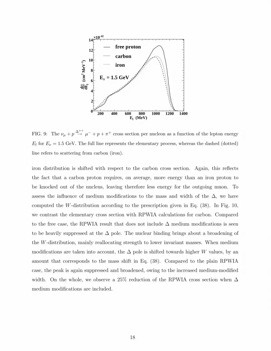
FIG. 9: The νµ + p∆++

→ µ− + p + π+ cross section per nucleon as a function of the lepton energy

El for Eν = 1.5 GeV. The full line represents the elementary process, whereas the dashed (dotted)

line refers to scattering from carbon (iron).

iron distribution is shifted with respect to the carbon cross section. Again, this reflects

the fact that a carbon proton requires, on average, more energy than an iron proton to

be knocked out of the nucleus, leaving therefore less energy for the outgoing muon. To

assess the influence of medium modifications to the mass and width of the ∆, we have

computed the W -distribution according to the prescription given in Eq. (38). In Fig. 10,

we contrast the elementary cross section with RPWIA calculations for carbon. Compared

to the free case, the RPWIA result that does not include ∆ medium modifications is seen

to be heavily suppressed at the ∆ pole. The nuclear binding brings about a broadening of

the W -distribution, mainly reallocating strength to lower invariant masses. When medium

modifications are taken into account, the ∆ pole is shifted towards higher W values, by an

amount that corresponds to the mass shift in Eq. (38). Compared to the plain RPWIA

case, the peak is again suppressed and broadened, owing to the increased medium-modified

width. On the whole, we observe a 25% reduction of the RPWIA cross section when ∆

medium modifications are included.

18

W (MeV)1000 1100 1200 1300 1400 1500 1600

)-1

MeV

2 (

cmdW

σd

0

10

20

30

40-4210×

free proton

RPWIA

med mod∆ +

= 1 GeVνE1/2C 1s12

Graph

FIG. 10: Invariant-mass distribution for νµ + p∆++

→ µ− + p + π+ on a 1s1/212C proton at an

incoming neutrino energy of 1 GeV. The full (dashed) line represents the calculation for a free

(bound) proton. The dotted curve adds the effect of ∆ medium modifications to the RPWIA

result.

C. Results under MiniBooNE and K2K kinematics

In view of recent results presented by the MiniBooNE and K2K collaborations [3], we

conclude this section with some computations for the specific neutrino energies and target

nuclei employed by these experiments. From an experimental viewpoint, the most accessible

distributions are the ones with respect to outgoing-muon variables. Fig. 11 depicts an

RPWIA calculation for a two-fold differential cross section against the outgoing-muon energy

and scattering angle with respect to the neutrino beam. The incoming neutrino energy is

fixed at 800 MeV, corresponding to MiniBooNE’s mean beam energy. Since MiniBooNE has

carbon as target material, this calculation was performed on a carbon nucleus. The result

shown in Fig. 11 can be integrated over θl or El to yield the one-fold cross sections displayed

in Fig. 12. Relative to the free cross section, the angular distribution for a carbon target is

evenly reduced by about 20%. In general, the outgoing muon prefers a forward direction,

although a minor shift seems to take place between the free and the bound case. This effect

relates to the change in the muon-energy distribution, depicted in the right-hand panel of

Fig. 12. Indeed, for scattering off bound protons, one observes a shift of the El distribution

towards lower values. Recognizing the correlation between high muon energies and forward

19

(MeV)l

E

200300

400500

600700

(degrees)lθ

0 20 40 60 80 100 120 140 160 180

0

5

10

15

20

-4210×

0

5

10

15

-4210×)-1 MeV2 (cm lθdcosl dE

σ2 d

FIG. 11: Cross section per nucleon for νµ + p∆++

→ µ− + p + π+ against outgoing-muon energy and

scattering angle. The incoming neutrino energy is 800 MeV, the target nucleus is carbon.

scattering angles, as can be appreciated in Fig. 11, the bound case will correspondingly

yield a larger number of events at slightly higher scattering angles. We also note that the

RPWIA result fades out sooner than the elementary cross section, because a certain amount

of energy is needed to knock the carbon proton out of its shell. Planned experiments like

MINERνA endeavor to have a good energy resolution for both the muon and the hadronic

final state. The ability to detect the outgoing pion or nucleon or even both would allow

a detailed study of different nuclear effects. In Figs. 13 and 14 we present cross sections

versus the pion kinetic energy Tπ and pion scattering angle relative to the beam direction

θ∗π. This time, we adopted K2K settings, namely an oxygen target hit by neutrinos with an

energy of 1.3 GeV. From the left-hand panel of Fig. 14, one infers that, within the RPWIA

model, the outgoing pion prefereably leaves the nucleus along the beam direction. As for

the kinetic-energy distribution, we observe a comparable reduction and shift of the strength

as in the muon-energy distribution.

V. CONCLUSION AND OUTLOOK

We have developed a relativistic framework to study ∆-mediated one-pion production

from nuclei at medium energies. The proposed formalism offers great flexibility in calcu-

lating various observables both for the free process and for scattering from nuclear targets.

20

(degrees)lθ0 20 40 60 80 100 120 140 160 180

)2 (

cmlθ

dcosσd

0

1

2

3

4

5

-3910×

= 800 MeVνEC12

Graph

(MeV)lE200 300 400 500 600 700

)-1

MeV

2 (

cml

dEσd

0

2

4

6

8

10

12

14-4210×

free proton

RPWIA

Graph

FIG. 12: Cross sections per nucleon for νµ + p∆++

→ µ− + p + π+, for 800 MeV neutrinos scattering

from a carbon target. The left (right) panel shows the cross section as a function of the outgoing-

muon scattering angle (energy). Each of the panels contrasts the elementary cross section (full

line) with the RPWIA result, without ∆ medium modifications (dashed line).

Motivated by operational and planned experiments, we have conducted a systematic study

by addressing the impact of ∆-coupling ambiguities on the Q2 and W distributions. Cross

sections are found to vary by as much as 10% depending on whether or not the M1-dominance

assumption is used to extract the vector form factors. This is very significant, as the ex-

tracted value for the axial mass MA depends heavily on the model applied in the analysis of

the neutrino-scattering data and, therefore, on a reliable input for the vector form factors.

Uncertainties in the dominant axial form factor, CA5 (Q2), have a dramatic effect on the

∆-production cross sections. At low Q2, a 25% reduction of the off-diagonal Goldberger-

Treiman value CA5 (0) = 1.2 leads to cross sections that are smaller by 40%. In the case of a

Q2 dependence that is steeper than a modified-dipole form, the effect increases to almost 50%

over the whole Q2 range. In the W distribution, we observe 2%-level deviations between the

traditional ∆-decay coupling choice and a consistent one, which effects a decoupling from the

spin-1/2 terms. To investigate the influence of nuclear effects, we have computed RPWIA

neutrino-nucleus cross sections for carbon, oxygen and iron nuclei. We have briefly touched

on the topic of ∆ medium modifications. Using a prescription that gives good results in

21

(MeV)πT

0200

400600

8001000

(degrees)

π*

θ

020406080100120140160180

05

101520253035

-4210×

0

5

10

15

20

25

30

-4210×)-1 MeV2 (cm π

*θdcosπ dT σ2 d

FIG. 13: Cross section per nucleon for νµ+p∆++

→ µ−+p+π+ against outgoing-pion kinetic energy

and scattering angle. The incoming neutrino energy is 1.3 GeV, the target nucleus is oxygen.

photo-induced two-nucleon knockout and electron-scattering studies, we infer a 20-25% sup-

pression of the RPWIA cross sections due to medium effects. The nuclear responses are

very sensitive to binding-energy differences at lower neutrino energies. From Eν = 1 GeV

onwards, the cross sections per nucleon for different nuclear targets are seen to agree at the

1% level. To assess the nuclear-model uncertainty in our description of ∆-mediated one-pion

production, we have also contrasted the RPWIA results with calculations performed within

an RFG model with a well-considered binding-energy correction. At 1-GeV neutrino ener-

gies, differences between one- and two-fold distributions computed within both models do

not exceed the 5% level. The agreement is better for total cross sections, where deviations

between the RFG and RPWIA model dwindle to 1-2%. Hence, for sufficiently high incom-

ing neutrino energies, the influence of Fermi motion, nuclear binding and the Paul exclusion

principle can be well described by adopting an RFG model with binding-energy correction.

The RFG model, however, just as the RPWIA approach, falls short in implementing FSI

and nuclear correlations of the short and long-range type. Contrary to the RFG, the model

proposed in this work has the important advantage that it can serve as a starting point for

a relativistic and quantum-mechanical study of FSI mechanisms. As a matter of fact, the

inclusion of FSI for the ejected pions and nucleons is currently under study. To this end,

we closely follow the lines of Ref. [33], where use is made of a relativistic Glauber model for

22

(degrees)π*θ

0 20 40 60 80 100 120 140 160 180

)2 (

cmπ* θ

dcosσd

0

2

4

6

8

10

12

14

-3910×

= 1.3 GeVνEO16

Graph

(MeV)πT0 200 400 600 800 1000

)-1

MeV

2 (

cmπ

dTσd

0

5

10

15

20

25-4210×

free proton

RPWIA

Graph

FIG. 14: Cross sections per nucleon for νµ + p∆++

→ µ− + p + π+, for 1.3 GeV neutrinos scattering

from an oxygen target. The left (right) panel shows the cross section as a function of the outgoing-

pion scattering angle (kinetic energy). Each of the panels contrasts the elementary cross section

(full line) with the RPWIA result, without ∆ medium modifications (dashed line).

fast ejectiles and an optical-potential approach for lower ejectile energies.

Acknowledgments

The authors acknowledge financial support from the Research Foundation - Flanders

(FWO), and the Research Council of Ghent University.

[1] BooNE Collaboration home page http://www-boone.fnal.gov/.

[2] K2K Collaboration home page http://neutrino.kek.jp/.

[3] R. Tayloe (MiniBooNE collaboration), in Proceedings of NuInt07: the 5th international

workshop on neutrino-nucleus interactions in the few-GeV region, Batavia, 2007, edited by

G. P. Zeller, J. G. Morfin and F. Cavanna (Melville, New York, 2007), p. 39; L. Whitehead

and A. Rodriguez (K2K collaboration), ibid. p. 169.

[4] S. Boyd (MINERνA), Nucl. Phys. Proc. Suppl. 139, 311 (2005).

23

[5] SciBooNE Collaboration home page http://www-sciboone.fnal.gov/.

[6] D. Rein and L. M. Sehgal, Ann. Phys. (N.Y.) 133, 79 (1981).

[7] K. M. Graczyk and J. T. Sobczyk, Phys. Rev. D 77, 053001 (2008).

[8] O. Lalakulich and E. A. Paschos, Phys. Rev. D 71, 074003 (2005).

[9] O. Lalakulich, E. A. Paschos and G. Piranishvili, Phys. Rev. D 74, 014009 (2006).

[10] E. Hernandez, J. Nieves and M. Valverde, Phys. Rev. D 76, 033005 (2007).

[11] K. S. Kuzmin, V. V. Lyubushkin and V. A. Naumov, Acta Phys. Pol. B 37, 2337 (2006).

[12] D. Barquilla-Cano, A. J. Buchmann and E. Hernandez, Phys. Rev. C 75, 065203 (2007).

[13] C. Alexandrou, Th. Leontiou, J. W. Negele and A. Tsapalis, Phys. Rev. Lett. 98, 052003

(2007).

[14] C. Alexandrou, G. Koutsou, Th. Leontiou, J. W. Negele and A. Tsapalis, Phys. Rev. D 76,

094511 (2007).

[15] V. Pascalutsa and R. Timmermans, Phys. Rev. C 60, 042201 (1999).

[16] C. J. Horowitz, H. Kim, D. P. Murdock and S. Pollock, Phys. Rev. C 48, 3078 (1993).

[17] W. M. Alberico, M. B. Barbaro, S. M. Bilenky, J. A. Caballero, C. Giunti, C. Maieron,

E. Moya de Guerra and J. M. Udıas, Nucl. Phys. A623, 471 (1997).

[18] M. C. Martınez, P. Lava, N. Jachowicz, J. Ryckebusch, K. Vantournhout and J. M. Udıas,

Phys. Rev. C 73, 024607 (2006).

[19] O. Benhar, A. Fabrocini, S. Fantoni and I. Sick, Nucl. Phys. A579, 493 (1994).

[20] O. Benhar, N. Farina, H. Nakamura, M. Sakuda and R. Seki, Phys. Rev. D 72, 053005 (2005).

[21] O. Benhar and D. Meloni, Nucl. Phys. A789, 379 (2007).

[22] A. M. Ankowski and J. T. Sobczyk, arXiv:0711.2031 [nucl-th].

[23] E. Oset and L. L. Salcedo, Nucl. Phys. A468, 631 (1987).

[24] T. Leitner, L. Alvarez-Ruso and U. Mosel, Phys. Rev. C 73, 065502 (2006).

[25] S. Ahmad, M. S. Athar and S. K. Singh, Phys. Rev. D 74, 073008 (2006).

[26] R. J. Furnstahl, B. D. Serot and H.-B. Tang, Nucl. Phys. A615, 441 (1997).

[27] P. Lava, N. Jachowicz, M. C. Martınez and J. Ryckebusch, Phys. Rev. C 73, 064605 (2006).

[28] C. Praet, N. Jachowicz, J. Ryckebusch, P. Vancraeyveld and K. Vantournhout, Phys. Rev. C

74, 065501 (2006).

[29] N. Jachowicz, P. Vancraeyveld, P. Lava, C. Praet and J. Ryckebusch, Phys. Rev. C 76, 055501

(2007).

24

[30] J. Bjorken and S. Drell, Relativistic Quantum Mechanics, (McGraw-Hill, N.Y. 1964).

[31] P. Stoler, Phys. Rept. 226, 103 (1993).

[32] E. A. Paschos, J.-Y. Yu and M. Sakuda, Phys. Rev. D 69, 014013 (2004).

[33] W. Cosyn, M. C. Martınez and J. Ryckebusch, Phys. Rev. C 77, 034602 (2008).

[34] S. Gardner and J. Piekarewicz, Phys. Rev. C 50, 2822 (1994).

[35] I. J. D. MacGregor et al., Phys. Rev. Lett. 80, 245 (1998).

[36] K. L. G. Heyde, The Nuclear Shell Model (Springer-Verlag, Berlin, 1994).

25