COUPLED DRIVES 1: Basics

www.control-systems-principles.co.uk. Coupled Drives 1: Basics

COUPLED DRIVES 1: Basics

Hilde Hagadoorn and Mark Readman, control systems principles.co.uk

ABSTRACT: This is one of a series of white papers on systems modelling, analysis and control, prepared by Control Systems Principles.co.uk to give insights into important principles and processes in control. In control systems there are a number of generic systems and methods which are encountered in all areas of industry and technology. These white papers aim to explain these important systems and methods in straightforward terms. The white papers describe what makes a particular type of system/method important, how it works and then demonstrates how to control it. The control demonstrations are performed using models of real systems we designed, and which are manufactured by TQ Education and Training Ltd in their CE range of equipment. Where possible results from the real system are shown. This white paper is about how to model and control two or more electric drives that are coupled together through the system. It will introduce readers to interacting dynamical systems and multivariable control.

1. Why Are Coupled Electric Drives Systems Important?

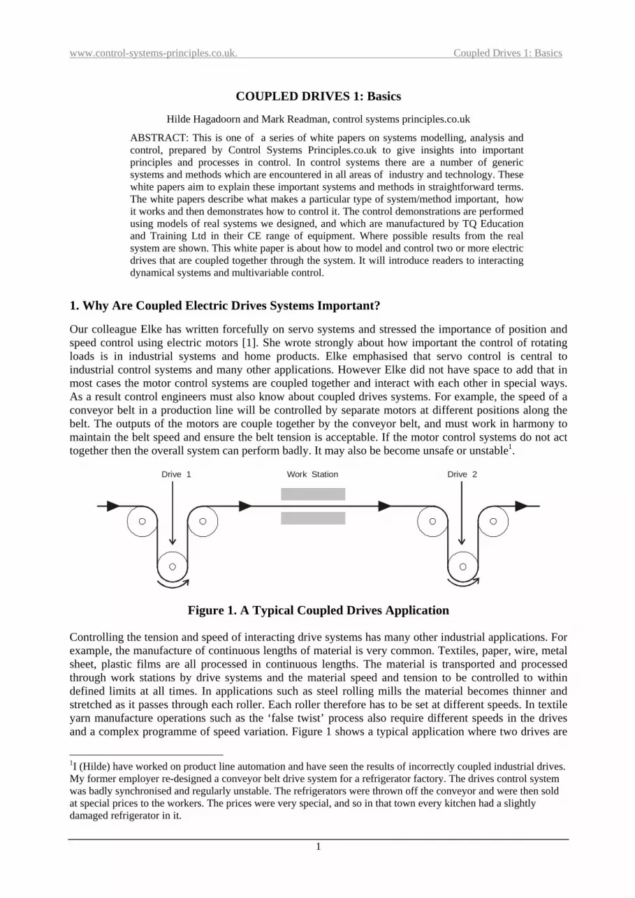
Our colleague Elke has written forcefully on servo systems and stressed the importance of position and speed control using electric motors [1]. She wrote strongly about how important the control of rotating loads is in industrial systems and home products. Elke emphasised that servo control is central to industrial control systems and many other applications. However Elke did not have space to add that in most cases the motor control systems are coupled together and interact with each other in special ways. As a result control engineers must also know about coupled drives systems. For example, the speed of a conveyor belt in a production line will be controlled by separate motors at different positions along the belt. The outputs of the motors are couple together by the conveyor belt, and must work in harmony to maintain the belt speed and ensure the belt tension is acceptable. If the motor control systems do not act together then the overall system can perform badly. It may also be become unsafe or unstable1.

Drive 1 Drive 2Work Station

Figure 1. A Typical Coupled Drives Application

Controlling the tension and speed of interacting drive systems has many other industrial applications. For example, the manufacture of continuous lengths of material is very common. Textiles, paper, wire, metal sheet, plastic films are all processed in continuous lengths. The material is transported and processed through work stations by drive systems and the material speed and tension to be controlled to within defined limits at all times. In applications such as steel rolling mills the material becomes thinner and stretched as it passes through each roller. Each roller therefore has to be set at different speeds. In textile yarn manufacture operations such as the ‘false twist’ process also require different speeds in the drives and a complex programme of speed variation. Figure 1 shows a typical application where two drives are

1I (Hilde) have worked on product line automation and have seen the results of incorrectly coupled industrial drives. My former employer re-designed a conveyor belt drive system for a refrigerator factory. The drives control system was badly synchronised and regularly unstable. The refrigerators were thrown off the conveyor and were then sold at special prices to the workers. The prices were very special, and so in that town every kitchen had a slightly damaged refrigerator in it.

1


used to transport a continuous sheet through a work-station. The job of the drive control system is to regulate the material speed and tension. If it does not regulate well, then the material sheet can be damaged or even break.

Coupled drive control is particularly vital in the paper industry. To see a paper break incident in a paper factory is an unforgettable experience. The paper sheet moves with frightening speed on the paper machine, so a break will produce very large quantities of paper very quickly. To visit a steel strip rolling mill is even more impressive and daunting. Huge motors are used to move a steel sheet backward and forward while it is pressed between rollers to a required thickness– the forces required are huge and the drives must be controlled in a way which deals with their coupling and interaction.

These examples illustrate the importance of drive systems (usually electrical drives) and their control. Coupled industrial drive systems are a very basic component of a modern continuous production line. Products are transported by conveyor systems, and many materials are produced in continuous strips or sheets. There are examples to in the home and in military systems, but the main application that the control systems engineer should know about is in manufacturing. In general terms the idea of interaction and multivariable control systems are central to many, many applications.

2. A Standard Coupled Drives System

Electrical drives can be coupled together in many ways. The details of the connection depend upon the use and application of the drive system. We will look at a standard coupled drives system. It contains the important components of electric coupled drives and will be our theme for this white paper. The standard coupled drive system is designed to have the characteristics seen in industrial drives, but it is not any particular industrial application. It is a prototype for all industrial coupled drive applications. The Figure 2 shows a diagram of the standard system.

Jockey Armfor Tension

Measurement

Pivot

DriveMotor 2

DriveMotor 1

ContinuousFlexible Belt

JockeyPulley

SimulatedWork Station

Figure 2. A Standard Coupled Drives System

2


Arm Tensioning Spring

JockeyPulleyF F

L

θ

FlexibleBelt

Pivot

α α

aFx ,

Arm

Pivot

Figure 3. Jockey Pulley and Arm in Detail

The standard system in Figure 2 has two drive motors (Motor 1 and Motor 2). These drives operate together to control the speed of a continuous flexible belt that goes round pulleys on the drive motor shafts and a so-called ‘jockey pulley’2. The jockey pulley is mounted on a swinging arm that is supported by a spring. The deflection of the arm is a measure of the tension in the drive belt. The pulley and arm assembly represents a ‘work station’ where material that the belt represents can be processed. It is the job of the two drives to regulate the tension and speed of the belt at the work-station. The work-station analogy is appropriate to material processing applications. In a conveyor belt system, the pulley and arm would represent the belt speed and tension sensors needed to ensure safe operation of a conveyor belt. (remember those falling refrigerators!). The Figure 3 shows the set up for the pulley and arm in more detail. The tensions in the belt sections, F, are related to the force in the arm tensioning spring, , by the equation:

aF

αcos2aF

F = (1)

The tensioning spring is linear with stiffness, , so that force and change in tensioning spring length ak Fx are related by:

xk

F aαcos2

= (2)

The continuous flexible belt in Figure 2 couples the actions of Motor 1 and Motor 2. For example, if we apply a drive voltage to Motor 1 drive input, then the speed and tension in the belt will be changed, and the Motor 2 will be rotated by the drag from Motor 1. Similar things happen if a drive voltage is applied to Motor 2 drive input. This is the coupling that we have been talking about. Both motors change both

2 Footnote from Hilde – the terminology jockey pulley was new to me when I came to work in English speaking factories. I had to look for it in an engineering dictionary. It means a pulley that ‘rides’ on a belt with taking energy from the belt.

3


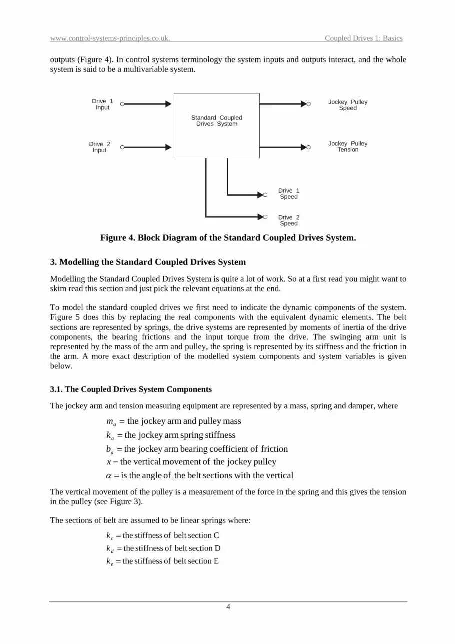
outputs (Figure 4). In control systems terminology the system inputs and outputs interact, and the whole system is said to be a multivariable system.

Standard CoupledDrives System

Drive 1Input

Drive 2Input

Jockey PulleySpeed

Jockey PulleyTension

Drive 1Speed

Drive 2Speed

Figure 4. Block Diagram of the Standard Coupled Drives System.

3. Modelling the Standard Coupled Drives System

Modelling the Standard Coupled Drives System is quite a lot of work. So at a first read you might want to skim read this section and just pick the relevant equations at the end.

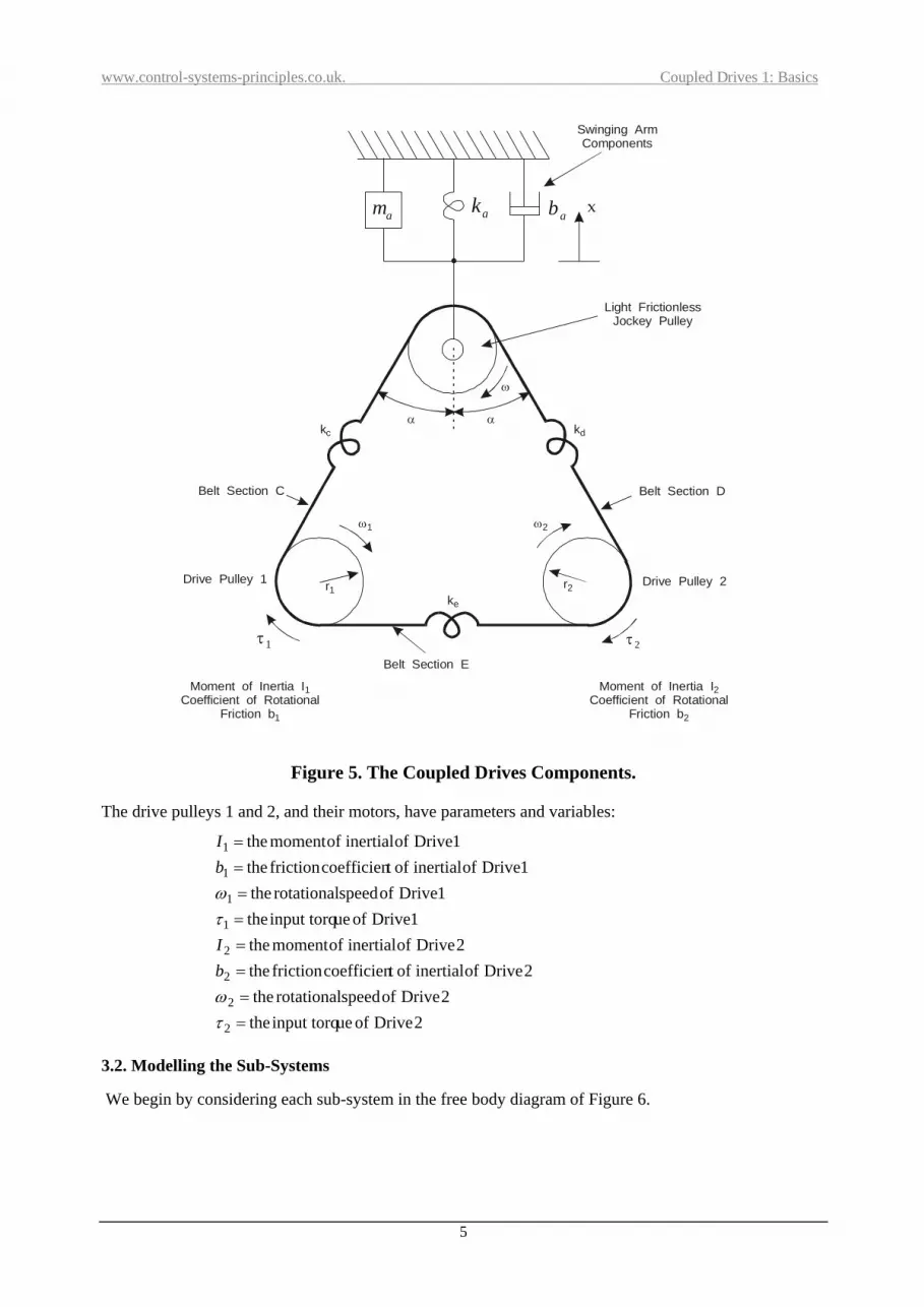
To model the standard coupled drives we first need to indicate the dynamic components of the system. Figure 5 does this by replacing the real components with the equivalent dynamic elements. The belt sections are represented by springs, the drive systems are represented by moments of inertia of the drive components, the bearing frictions and the input torque from the drive. The swinging arm unit is represented by the mass of the arm and pulley, the spring is represented by its stiffness and the friction in the arm. A more exact description of the modelled system components and system variables is given below.

3.1. The Coupled Drives System Components

The jockey arm and tension measuring equipment are represented by a mass, spring and damper, where

friction oft coefficien bearing armjockey thestiffness spring armjockey the

masspulley and armjockey the

===

a

a

a

bkm

vertical with thesectionsbelt theof angle theis pulleyjockey theofmovement vertical the

==

αx

The vertical movement of the pulley is a measurement of the force in the spring and this gives the tension in the pulley (see Figure 3).

The sections of belt are assumed to be linear springs where:

Esection belt of stiffness theDsection belt of stiffness theCsection belt of stiffness the

===

e

d

c

kkk

4


kc

r1 r2ke

kd

x

α α

ω

Belt Section C Belt Section D

Belt Section E

Swinging ArmComponents

Light FrictionlessJockey Pulley

Drive Pulley 1 Drive Pulley 2

ω2ω1

Moment of Inertia ICoefficient of Rotational

Friction b

1

1

Moment of Inertia ICoefficient of Rotational

Friction b

2

2

1τ 2τ

am ak ab

Figure 5. The Coupled Drives Components.

The drive pulleys 1 and 2, and their motors, have parameters and variables:

2 Drive of ueinput torq the2 Drive of speed rotational the

2 Drive of inertial oft coefficienfriction the2 Drive of inertial ofmoment the

1 Drive of ueinput torq the1 Drive of speed rotational the

1 Drive of inertial oft coefficienfriction the1 Drive of inertial ofmoment the

2

2

2

2

1

1

1

1

========

τω

τω

bI

bI

3.2. Modelling the Sub-Systems

We begin by considering each sub-system in the free body diagram of Figure 6.

5


v2

vd

v4

ve

F5 F5 F6 F6

r2r1

v3

ω2ω1

F2

F2

F4

F 1

F 3

F2

F2

F4

F 1

F 3

v1

vcα α

ω

1τ 2τ

am ak ab

Figure 6. Free Body Diagram of Couple Drives System

3.2.1 The Belt Sections

If are the extensions of the belt section C, D, and D respectively (see Figure 6), then a force balance on each belt section gives,

and edc x, xx

ddcc xkxkF == (3a)

ee xkF =′ (3b)

where,

65 FFF ==′

and

4321 FFFFF ====

3.2.2 The Jockey Pulley Assembly

The pulley is light and rotates without friction, so that,

FFF == 21

Resolving forces vertically gives,

αcos2FFa = (4)

6


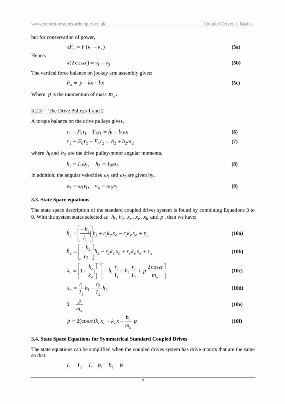
but for conservation of power,

)( 21 vvFFx a −=& (5a) Hence,

21)cos2( vvx −=α& (5b)

The vertical force balance on jockey arm assembly gives:

xbkxpFa && ++= (5c)

Where p is the momentum of mass . am

3.2.3 The Drive Pulleys 1 and 2

A torque balance on the drive pulleys gives,

11115131 ωτ bhrFrF +=−+ & (6)

22224262 ωτ bhrFrF +=−+ & (7)

where and are the drive pulley/motor angular momenta. 1h 2h

222111 , ωω IhIh == (8)

In addition, the angular velocities 1ω and 2ω are given by,

224113 , rvrv ωω == (9)

3.3. State Space equations

The state space description of the standard coupled drives system is found by combining Equations 3 to 9. With the system states selected as , then we have: p, x, x, x, hh ec and k21

11111

11 τ+−+⎥

⎦

⎤⎢⎣

⎡−= eecc xkrxkrh

Ib

h& (10a)

22222

22 τ++−⎥

⎦

⎤⎢⎣

⎡−= eecc xkrxkrh

Ib

h& (10b)

⎥⎦

⎤⎢⎣

⎡++−⎥

⎦

⎤⎢⎣

⎡+=

−

ad

cc m

pIrh

Irh

kk

x αcos212

22

1

11

1

& (10c)

22

21

1

1 hIrh

Irxe −=& (10d)

ampx =& (10e)

pmb

xkxkpa

aacc −−= )(cos2 α& (10f)

3.4. State Space Equations for Symmetrical Standard Coupled Drives

The state equations can be simplified when the coupled drives system has drive motors that are the same so that:

bbbIII ==== 2121 ,

7


Drive pulleys all have the same radius and the belt sections have the same length:

kkkkrrr edc ===== ,21

This gives the simplified state equations:

111 τ+−+⎥⎦⎤

⎢⎣⎡−

= ec rkxrkxhIbh& (11a)

222 τ++−⎥⎦⎤

⎢⎣⎡−

= ec rkxrkxhIbh& (11b)

⎥⎦

⎤⎢⎣

⎡++−=

ac m

pIrh

Irhx αcos2

21

21& (11c)

21 hIrh

Irxe −=& (11d)

ampx =& (11e)

pmb

xkkxpa

aac −−= )(cos2 α& (11f)

4. Transfer Functions for the Standard Coupled Drives System

4.1. The Important Transfer Functions

The job of a control system for the Coupled Drives is to regulate the belt tension and speed at the jockey arm pulley using the torques ( 21 ,ττ ) applied to the drive pulleys. The pulley speed (ω ) is measured directly. The tension in the belt at the arm pulley is found by measuring the extension of the arm spring ( x ).

From the state equations the two transfer functions for the standard coupled drives are:

[ ])(2

)()()( 21

bsIss

s+

+=

ττω (12)

( ))(cos2)))(cos2()(3(

)()()cos()( 222222212

ααττα

rkkksbsmkrbIssskrsx

aaa −+++++−

= (13)

4.2. Including Actuators and Transducers

The motor torques ),( 21 ττ are controlled by the control input signals to the drive amplifer. In the simplest case the actuator characteristic is linear so that:

),( 21 uu

222

111

ugug

==

ττ

The true system output variables ))(( )( sxandsω are measured by a speed sensor (with output ) on the jockey wheel pulley, and angle sensor on the pivot of the arm. The arm angle

ωyθ and x are related

approximately by

Lx

=θ

8


The jockey arm deflection θ is measured by a sensor with output . These signals are related by constants:

xy

xgygy

xx == ωωω

5. Uses of the Models and Transfer Functions.

The system state space model of the standard coupled drives is in the form of model used in detail simulation and design studies of drive systems. Extra details would be added to describe the drive electronics. We have missed this out because we want to show the dynamics which couple the system and make it highly interacting. For controller design both the state space model and the transfer function models are interesting. The transfer functions of Equations 12 and 13 are especially useful. They tell the control designer that it is possible to treat the control of speed and tension separately by applying the control signal for speed ( ) plus the control signal for tension ( ) to Drive input 1 ( ) and the control signal for speed minus the control signal for tension to Drive input 2 ( ). So that:

)(suω )(sux )(1 su)(2 su

x

x

uuuuuu

−=+=

ω

ω

2

1

In multivariable control theory this is called de-coupling the control problem into two, single input/single output control problems. This looks easy but there are some things that need to be done to make this form of control work well. We will not do any more control in this white paper – that will come later, so keep checking the web site for control white paper for the coupled drives.

6. Example of a Coupled Drives System

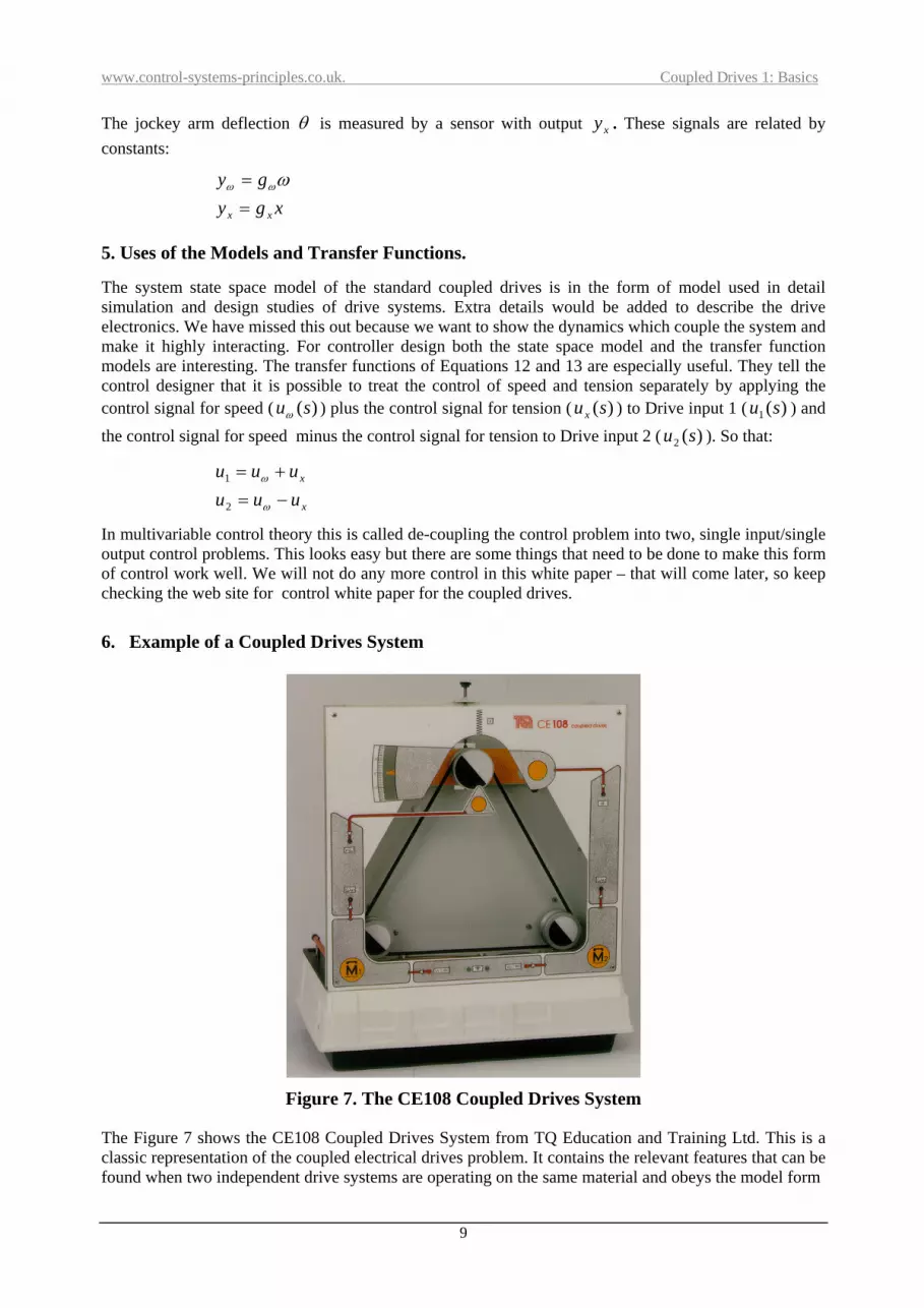
Figure 7. The CE108 Coupled Drives System

The Figure 7 shows the CE108 Coupled Drives System from TQ Education and Training Ltd. This is a classic representation of the coupled electrical drives problem. It contains the relevant features that can be found when two independent drive systems are operating on the same material and obeys the model form

9


derived in this white paper.

The CE108 system follows the layout of a standard coupled drives system very closely. At the bottom corners the two drive pulleys can be seen. At the top centre is the jockey and arm with a calibrated plate so that the angle deflection of the arm can be read off directly. The belt is seen as the continuous black ribbon around the three pulleys. On the front panel are input and output sockets with which to connect to the sensors and drive actuators.

We have not included any control at this stage – the white paper is long enough already. We plan a second white paper which just deals with the control of the Coupled Drives System and multivariable and interacting processes. The Coupled Drives System is in fact a good example of an interacting system. For some technical background on interacting control and an up-to-date perspective on multivariable control see, [2]. There are many other books on this subject, but the father of multivariable control is Professor Howard Rosenbrock and his books on multivariable design [3] set the pattern for a generation of researchers. For good modern information on electric drives we recommend you use the lastest information from manufacturers and practical handbooks from trade journals, we use the handbook by Richmond, [4] from the Drives and Controls Magazine.

6. A Final Word from Hilde

I am told by the Control Systems Principles team that I am an ersatz-Elke. I hope this is not true, because she is so aggressive and hard on the boys in the office. I have tried to write with a more gentle tone. The dynamics of coupled drives can be quite difficult for beginners, and even professionals make mistakes. In fact many university professors have commented on the modelling of the Coupled Drives and corrected the original equations derived by Peter Wellstead. The equations in this white paper are (we think!) correct thanks to the help of Professor Peter Willett from University of Connecticut and Professor David Clarke of Oxford University.

Bis nachste Mal!

Hilde

7. The Final Word

We get lots of email with pleas for technical help from students and engineers. We am sorry to say that Control Systems Principles can not answer inquiries and questions about the detail contents of our white papers unless we have a contract with your organisation. For more information about the CE108 Coupled Drives Systems go to the TQ Education and Training web site, use the links on our web site (control-systems-principles.co.uk) or use the email [email protected].

8. References 1. Laubwald, E, Servo Control Systems White Paper, (downloadable at www.control-systems-principles.co.uk) 2. Goodwin, G, Gräbe. S. and Salgado, M. Control Systems Design, Prentice Hall, 2001. 3. Rosenbrock, H.H. State Space and Multivariable Theory, Nelson, 1970. 4. Richmond,A.W. Servos and Steppers: A Practical Engineers’s Handbook, Kamtech Publishing, 1999, (this

book is hard to get so try the address of the publisher – Airport House, Purley Way, Croydon, Surrey, CR0 0XZ, UK.)

10

mailto:[email protected]

http://www.control-systems-principles.co.uk/

Documents

COUPLED DRIVES 1: Basics