Correction of finite element estimates for Sturm-Liouville eigenvalues

Numer. Math. 50, 205-215 (1986) Numerische MathemaUk �9 Springer-Verlag 1986

Correction of Finite Element Estimates for Sturm-Liouville Eigenvalues

Alan L. Andrew 1 and John W. Paine 2

1 Mathematics Department, La Trobe University, Bundoora, Victoria 3083, Australia 2 Department of Geology and Geophysics, University of Adelaide, Adelaide, S.A. 5001, Australia

Summary. It is shown that a simple asymptotic correction technique of Paine, de Hoog and Anderssen reduces the error in the estimate of the kth eigenvalue of a regular Sturm-Liouville problem obtained by the finite element method, with linear hat functions and mesh length h, from O(k 4 h 2) to O(kh2). The result still holds when the matrix elements are evaluated by Simpson's rule, but if the trapezoidal rule is used the error is O(k zh2). Numerical results demonstrate the usefulness of the correction even for low values of k.

Subject Classifications: AMS(MOS): 65L15; CR: G1.7.

I. Introduction

When finite element or finite difference methods are used to approximate the eigenvalues 21 < 2 2 < 2 3 < . . . of the regular Sturm-Liouville problem

-y" +qy=2y ( la)

y(0) = y(~) = 0, (1 b)

the error in the approximation to 2 k is known to increase rapidly with k. Paine, de Hoog and Anderssen [9] showed that, in the case of the second order centred finite difference method with uniform mesh, the error when q = 0 (which is known in closed form) has the same asymptotic form as k ~ oe as the error for general q. They showed that the accuracy of the estimates obtained for high eigenvalues could be dramatically improved at negligible extra cost by using the known error for q - -0 to correct the estimates obtained for general q. Their numerical results indicate that this correction generally improves the accuracy of all computed eigenvalues, not just the higher ones.

It was suggested in [9] that a similar correction might prove useful for the finite element method. However, although there has been considerable sub-

206 A.L. Andrew and J.W. Paine

sequent deve lopment of this asymptot ic correct ion technique in conjunct ion with finite difference methods [1, 2, 4, 81, its use with the finite element me thod has not been studied either theoretically or numerically.

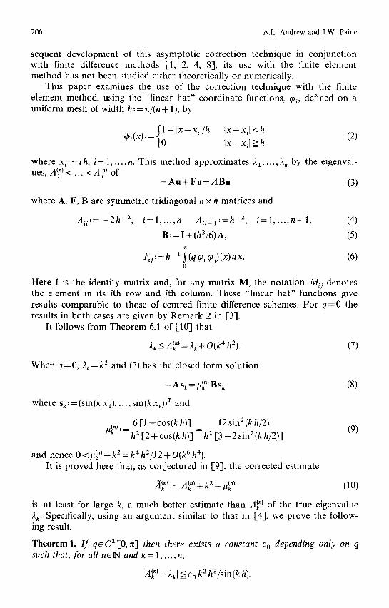
This paper examines the use of the correct ion technique with the finite element method, using the " l inear ha t " coordinate functions, qSi, defined on a uniform mesh of width h." = n/(n + 1), by

4 ) i ( x ) : = { ; - , x - x ~ , / h I x - x~[<h I x - xi] > h (2)

where x~:=ih, i = 1 , . . . ,n. This me thod approx imates 21 . . . . . 2,. by the eigenvalues, A] "1 < "(") ... <z~, of

- A u + F u = A B u (3)

where A, F, B are symmetr ic t r idiagonat n x n matr ices and

Aii:= - 2 h -2 , i = 1 . . . . . n Aii+a:=h -2, i = l , . . . , n - 1 , (4)

B : = I + ( h 2 / 6 ) A , (5)

Fij, = h-1 ~ (q c~ i c/) j)(x) dx. (6) 0

Here I is the identity matr ix and, for any matr ix M, the no ta t ion M~j denotes the element in its ith row and j th column. These " l inear ha t" functions give results comparab le to those of centred finite difference schemes. Fo r q = 0 the results in bo th cases are given by R e m a r k 2 in [,31.

It follows f rom T h e o r e m 6.1 of [101 that

2k =< ~k~(") ---- 2 k + O(k 4 h2). (7)

When q = 0, 2 k = k z and (3) has the closed form solution

- Ask = ~") Bsk (8)

where Sk: = (sin(k x 1) . . . . , sin(k x,)) r and

/~,) : = 6 [ 1 - c o s ( k h ) ] 12sin2(kh/2) h 2 [2 + cos(k h)] - h 2 [3 - 2 sinZ(k h/2)] (9)

and hence 0 < #~") - k 2 = k 4 h2/12 + O(k 6 h4). It is p roved here that, as conjectured in [,9], the corrected est imate

ffl~'):= Akm + k2-1t(k") (lO)

is, at least for large k, a much better es t imate than A~ ") of the true eigenvalue 2 k. Specifically, using an a rgument similar to that in [4J, we prove the following result.

Theorem 1. I f qe C 2 [,0, TcI then there exists a constant c o depending only on q such that, for all n e N and k= 1 . . . . . n,

[/1~") - 2kl =< C o k 2 ha/sin (k h).

Correction of Finite Element Eigenvalues 207

Since kh/sin(kh) increases only slowly with k when kh<rc/2, Theorem 1 shows that for k <n/2 the error in the corrected finite element eigenvalues, At") is essentially O(kh 2) compared with the O(k4h 2) error in the uncorrected estimate. Although the improvement produced by the correction (10) is greatest for large k, our numerical results, summarised in Sect. 4, demonstrate the usefulness of the correction for all k. Note that, in order to reduce roundoff error in numerical calculations, the second form given for /t~ ") in (9) should always be used.

The effect of approximating the integrals in F by various quadrature rules is examined in Sect. 3.

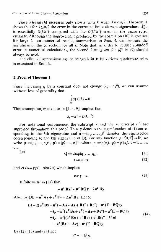
2. Proof of Theorem 1

Since increasing q by a constant does not change (2k--Atkm), we can assume without loss of generality that

r~

S q(x) dx = O. 0

This assumption, made also in [1, 4, 9], implies that

2 k = k 2 + O(k- 2).

For notational convenience, the subscript k and the superscript (n) are supressed throughout this proof. Thus y denotes the eigenfunction of (1) corresponding to the kth eigenvalue and u :=(u I . . . . . u,) r denotes the eigenvector corresponding to the kth eigenvalue of (3). For any function p: [0, rc]--,N, we write P:=(PI . . . . . p,)r, p, =(p, . . . . . p,)r where pi:=p(xi), p'i:=p'(xl), i = l . . . . ,n, etc.

Let Q"= diag(ql . . . . . qn), (11)

~ . ' = u - s (12)

and e(x): = y ( x ) - sin(k x) which implies

e = y - s . (13)

It follows from (1 a) that

- u r B y " + u r B Q y = 2 u r B y .

Also, by (3), - u r A y + u r F y = A u r B y . Hence

( A - 2) ur By = u r ( - A s - A e + B s " + Be") + u r ( F - BQ) y

= ( # - k 2 ) u r B s + u r ( - A e + B e " ) + u r ( F - B Q ) y (14)

= (# - k 2) (u r B s + s r Be) + s r B(e" + k 2 e)

+ er (Be" - Ae) + ur(F - BQ) y

by (12), (13) and (8) since s "= - k 2 s.


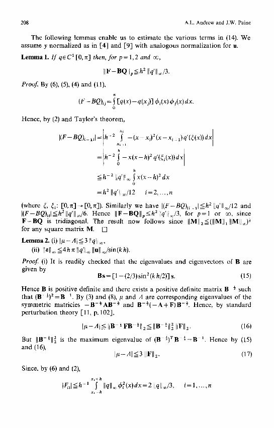
The following lemmas enable us to estimate the various terms in (14). We assume y normalized as in I-4] and [9] with analogous normalization for u.

L e m m a 1. If qe C ~ 1-0, n] then, for p = 1, 2 and oo,

I IF-BOl lp<h 2 Ilq'll o~/3.

Proof. By (6), (5), (4) and (11),

(F - BQ)ij = i 1-q (x) - q (x j)] qbi(x ) q~j(x) dx. 0

Hence, by (2) and Taylor's theorem,

I(F-nQ)i_li[= h -2 ~,-,~' _(x_xi)2(x_xi_ 1)q'(~(x))dx

= h-2 i - x ( x - h ) 2 q ' ( r

h < h - 2 Ilq'll~ ~ x ( x - h ) 2 dX

0

--h 2 [[q'll oo/12 i = 2 . . . . . n

(where 4, r [0,n] ~ [0,hi). Similarly we have I(F-BQ)ii_ d<h2 ][q'l[o~/12 and [(F-BQ).l<=h21lq'][~/6. Hence I[F-BQIIp<__h2I{q'[{~/3, for p = l or ~ , since F - B Q is tridiagonal. The result now follows since tIMII2<(llMIIltlMIl~) ~ for any square matrix M. []

L e m m a 2. (i) I ~ t - A [ _<_3 Ilql[ o~,

(ii) Ilnll~ <4hn Ilql[o~ IlullJsin(kh).

Proof (i) It is readily checked that the eigenvalues and eigenvectors of B are given by

B s = E1 - (2/3) sin 2 (k h/2)] s. (15)

Hence B is positive definite and there exists a positive definite matrix B- * such that (B-�89 -1. By (3) and (8),/~ and A are corresponding eigenvalues of the symmetric matricies - B - � 8 9 -~ and B - � 8 9 -�89 Hence, by standard perturbation theory [11, p. 102],

I # - a [ < liB -~ FB-�89 < IIB-~lt 2 IIFII2. (16)

But IIB-~II~ is the maximum eigenvalue of ( B - ~ ) r B - ~ = B -1. Hence by (15) and (16),

1#-51 <3 IIFII2. (17)

Since, by (6) and (2),

xi+h IF, l<h -1 ~ Ilqllo~ ga2(x)dx=2 Ilqllo~/3,

xi-h i=l , . . . ,n


and Jci

IF/i-1 [ ~ h - 1 S Ilqllo~(~iO,-1)(x)dx=llqll~o/6, i = 2 . . . . . n x i h

and F is symmetric tridiagonal, it follows that

IIFLI 1 = IIFII ~o < IIq[I ~ (18)

and hence IIFII2 < Ilqll~o. The result now follows from (17). (ii) Subtracting p B u + F u from both sides of (3) and multiplying by - [ 2

+ cos(k h)] h2/3 yields

[2 + cos(k h)] h 2 u~-l -2c~ 3 [ (# - A)Bu + Fu]~, j = l . . . . . n.

An argument analogous to that used in the proof of Lemma 1 of 1-4] now shows that

I~1 _-< h2( j - 1)(Ip - A[ + II Fll o~)Ilull ~/sin (k h).

The result now follows from (18) and Lemma 2(i) since h(j-1)<~z. []

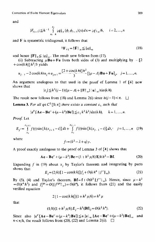
Lemma 3. For all qe C 2 [0, 7z] there exists a constant c 1 such that

Ier[Ae-Be"+(p-k2)Be][<clk2h2/sin(kh), k = l . . . . . n.

Proof. Let

X j + I X j - 1

E~:= S f ( t ) s in[k(x j+l - t ) ]d t+ ~ f( t)sin[k(xj_l- t)]dt ,~ j = l , . . . , n (19) X j X 2

where f :=(k2 -2+q)y .

A proof exactly analogous to the proof of Lemma 3 of 1"4] shows that

A e - B e" + (/~ - k 2) B e = (1 + h 2 /~ /6 ) Elk h 2 _ g f . ( 2 0 )

Expanding f in (19) about xj by Taylor's theorem and integrating by parts shows that

Ej = (2/k) [1 - cos (k h)]fj + O(k h 4 II f " [I ~). (21)

By (5), (4) and Taylor's theorem, Bf=f+O(h211f"lL~). Hence, since g - k 2 =O(k4h 2) and fff~=O(llf~P~llo~)=O(kP), it follows from (21) and the easily verified equation

that

2 [1 - cos(k h)] (1 + h 2 #/6) = h 2

Since also n < n/h, the result follows from (20), (22) and Lemma 2(ii).

(l/k) (1 + h 2 #/6) E j - h2 (Bf)j = O(k 2 h4). (22)

[ ~ r [ A e - B e " + ( # - k 2 ) B e ] l < n IIsIL~ [LAe-Be"+(#-k2)Be[Io~ and []


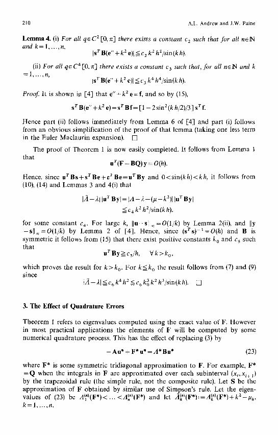
L e m m a 4. (i) For all q~ C 2 [0, ~] there exists a constant c 2 such that for all n ~ N and k = 1 . . . . . n,

Is r B(e" + k 2 e)l < CE k 2 hE/sin(k h).

(ii) For all qe C 4 [0, 7z] there exists a constant c 3 such that, for all n~]N and k

Is r B(e" + k E e)l < c3 k 4 h4/sin(k h).

Proof. It is shown in [4] that e " + k z e=f , and so by (15),

s r B(e" + k 2 e) = s T B f = [1 - 2 sin E (k h/2)/3] s r f.

Hence part (ii) follows immediately from Lemma 6 of [4] and part (i) follows from an obvious simplification of the proof of that lemma (taking one less term in the Euler Maclaurin expansion). []

The proof of Theorem 1 is now easily completed. It follows from Lemma 1 that

a t ( F - BQ) y = O(h).

Hence, since u r B s + s r B e + ~ r B e = u r B y and O < s i n ( k h ) < k h , it follows from (10), (14) and Lemmas 3 and 4(i) that

IA-21 lur Byl =IA- -2 - - (# - - kE) I lUT Byl

< c 4 k 2 hZ/sin(k h),

for some constant c4. For large k, I In - s [ l~=O(1 /k ) by Lemma 2(ii), and IlY - s t [ ~ = O ( 1 / k ) by Lemma 2 of [4]. Hence, since ( s r s ) - l = O ( h ) and B is symmetric it follows from (15) that there exist positive constants k o and c 5 such that

uTBy>=cJh, V k > k o,

which proves the result for k > k 0. For k < k o the result follows from (7) and (9) since

Ifl-El<=c6k4hZ<=c6k3kZh3/sin(kh). []

3. The Effect of Quadrature Errors

Theorem 1 refers to eigenvalues computed using the exact value of F. However in most practical applications the elements of F will be computed by some numerical quadrature process. This has the effect of replacing (3) by

- Au* + F* u* = A* Bu* (23)

where F* is some symmetric tridiagonal approximation to F. For example, F* = Q when the integrals in F are approximated over each subinterval (xi,xi+ 1) by the trapezoidal rule (the simple rule, not the composite rule). Let S be the approximation of F obtained by similar use of Simpson's rule. Let the eigenvalues of (23) be A~")(F*)< ... <A~)(F *) and let ft~")(F*):=a~k")(F*)+kE-I~ k, k = l .. . . ,n.


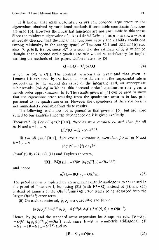
It is known that small quadrature errors can produce large errors in the eigenvalues obtained by variational methods if unsuitable coordinate functions are used [6]. However the linear hat functions are not unsuitable in this sense. Since the minimum eigenvalue o f - A is 4s in2(h /2) /h2~ 1 as n ~ oo (i.e. h ~0), it is readily checked that the linear hat functions satisfy the stability conditions (strong minimality in the energy space) of Theorem 52.1 and 52.2 of [6] (see also [7, p. 36]). Hence, since Ark ") is a second order estimate of 2 k it might be thought that a second order quadrature rule would be satisfactory for imple- menting the methods of this paper. Unfortunately, by (5)

O - B Q = (h2/6) AQ (24)

which, by (4), is O(1). The contrast between this result and that given in Lemma 1 is explained by the fact that, since the error in the trapezoidal rule is proportional to the second derivative of the integrand and, on appropriate subintervals, (q4)ic~j)"=O(h-2), this "second order" quadrature rule gives a zeroth order approximation to F. The results given in [5] can be used to show that the eigenvalue error resulting from the quadrature error is in fact proportional to the quadrature error. However the dependence of the error on k is not immediately available from these results.

The following results are not as general as that given in [5], but are more suited to our analysis since the dependence on k is given explicitly.

Theorem 2. (i) For all q 6 C 2 [0, 7z], there exists a constant c: such that, Jot all n ~ N and k = 1 . . . . . n,

L z ] ~ ' ) ( Q ) - ;~kl < c7 k 2 h 2.

(ii) For all qsC4[0,~], there exists a constant c s such that, Jbr all n e N and k = l, . . . ,n,

[ Z](k") (S) - A~k")I < c 8 h 2.

Proof (i) By (24), (4), (11) and Taylor's theorem,

II (Q - B Q ) Yk II oo = O( h2 Ll(q Yk)" II ~ )= O(k 2 h2)

and hence

u [ ( Q - B Q ) Yk---- O( k2 h). (25)

The proof is now completed by an argument exactly analogous to that used in the proof of Theorem 1, but using (23) (with F * = Q ) instead of (3), and (25) instead of Lemma 1, the O(k2h3/sin(kh)) error terms being absorbed into the larger O(k 2 h 2) error term.

(ii) On each subinterval, thi q~j is a quadratic and hence

(q ~b i q~ j)(4) = q(4) thi ~bj + 4 q(3)(~)i ~)j)' 4- 6 q"(dp i dp~)" = 0 (h - 2).

Hence, by (6) and the standard error expression for Simpson's rule, [(F-S)i j l =O(h4[l(q(ai(aj)(4~lloo)=O(h2 ) and, since F - S is symmetric tridiagonal, IIF - - S ] l 1 = IIF-Sll ~ ---O(h 2) and so

[IF- SN2 = O(h2). (26)


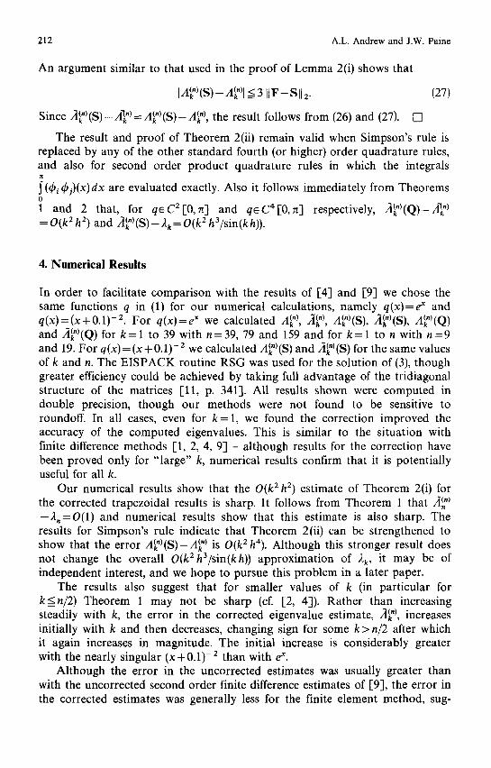
An argument similar to that used in the proof of Lemma 2(i) shows that

[A(k ") (S) - A(k")[ < 3 II F - S 112. (27)

Since "'k2(")t~--Xt")--A(")tr ~'k -- ' 'k ~.b...~! the result follows from (26) and (27). []

The result and proof of Theorem 2(ii) remain valid when Simpson's rule is replaced by any of the other standard fourth (or higher) order quadrature rules, and also for second order product quadrature rules in which the integrals 7t

(c~i c~j)(x)dx are evaluated exactly. Also it follows immediately from Theorems 0

1 and 2 that, for qeC2[O,n] and q~C4[O,n] respectively, A~k")(Q)--A~k ") = O(k 2 h 2) and ,'irk") (S) - 2 k = O(k 2 ha/sin(kh)).

4. Numerical Results

In order to facilitate comparison with the results of [4] and I-9] we chose the same functions q in (1) for our numerical calculations, namely q(x)=e ~' and q(x)=(x+O.1) -2. For q(x)=e x we calculated A~ "), Ak"), A~")(S), /]~")(S), Atk")(Q) and ,4~k")(Q) for k = l to 39 with n=39, 79 and 159 and for k = l to n with n = 9 and 19. For q(x)= (x + O. 1)-2 we calculated A~k ") (S) and l]~k ") (S) for the same values of k and n. The EISPACK routine RSG was used for the solution of (3), though greater efficiency could be achieved by taking full advantage of the tridiagonal structure of the matrices [11, p. 341]. All results shown were computed in double precision, though our methods were not found to be sensitive to roundoff. In all cases, even for k= 1, we found the correction improved the accuracy of the computed eigenvalues. This is similar to the situation with finite difference methods [1, 2, 4, 9] - although results for the correction have been proved only for "large" k, numerical results confirm that it is potentially useful for all k.

Our numerical results show that the O(k 2 h 2) estimate of Theorem 2(i) for the corrected trapezoidal results is sharp. It follows from Theorem 1 that A~) - 2 , = O ( 1 ) and numerical results show that this estimate is also sharp. The results for Simpson's rule indicate that Theorem 2(ii) can be strengthened to show that the error Atk")(S)--Atk") is O(k2h4). Although this stronger result does not change the overall O(k2h3/sin(kh)) approximation of ~L k, it may be of independent interest, and we hope to pursue this problem in a later paper.

The results also suggest that for smaller values of k (in particular for k<n/2) Theorem 1 may not be sharp (cf. [2, 4]). Rather than increasing steadily with k, the error in the corrected eigenvalue estimate, ,'](k "), increases initially with k and then decreases, changing sign for some k> n/2 after which it again increases in magnitude. The initial increase is considerably greater with the nearly singular (x+0.1) -2 than with e x.

Although the error in the uncorrected estimates was usually greater than with the uncorrected second order finite difference estimates of [9], the error in the corrected estimates was generally less for the finite element method, sug-

Correction of Finite Element Eigenvalues

Table 1. Errors in eigenvalue estimates for q(x)= e x with n = 39

213

k )~k A(k39'-- ~k 1](k39~-- 2~ h~39~(Q)- 2~ A~39'(S)- 2k

1 4.89667 0.00288 0.00236 0.00593 0.00236 2 10.04519 0.01721 0.00898 0.02518 0.00899 3 16.01927 0.05452 0,01280 0.05647 0.01281 4 23.26627 0.14386 0.01184 0.10380 0.01186 5 32.26371 0,33310 0.01019 0,16931 0,01022 6 43.22002 0.68023 0.00922 0.25159 0.00925 7 56.18159 1.25487 0.00862 0,35008 0.00868 8 71.15300 2.14020 0.00817 0.46516 0.00824 9 88.13212 3.43344 0.00776 0.59751 0.00785

10 107.11668 5.24604 0.00735 0.74796 0.00747 12 151.09604 10.94763 0.00648 1.1069l 0.00665 14 203.08337 20.42619 0.00548 1.55058 0.00572 16 263.07507 35.08393 0.00436 2.08902 0.00468 18 331~6934 56,50253 0.00306 2.73344 0.00348 20 407~6525 86,34322 0.00154 3.49551 0,00209 25 632.05890 206.56667 -0.00409 5.97366 -0.00316 30 907.05548 384.29062 -0.01835 9.18381 -0.01693 35 1232.05334 513.86316 -0.09237 12.11917 -0.09047 39 1528.05225 414,39124 - 1.00775 13.61001 - 1.00577

Table 2. Scaled errors,(h~)(S)-2k)sin(kh)/k2h3for q(x)=e ~

n

k 9 19 39 79 159

I 0.37463 0.38104 0.38262 0.38289 0,38288 2 0.65325 0.71054 0.72531 0.72912 0,73012 3 0.51126 0.64830 0.68588 0.69542 0.69798 4 0.24344 0.41881 0.47260 0.48678 0.49042 9 -0.09961 0.04707 0.12998 0.15755 0.16480

14 -0~3667 0.05371 0.09103 0.10208 19 -0.10801 0.01604 0.05828 0.07269 24 -0.00611 0.03803 0.05504 29 -0.02356 0.02413 0.04313 34 -0.04947 0,01406 0.03446 39 -0.10709 0.00652 0.02783

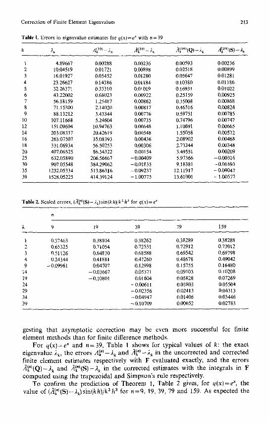
gesting that asymptotic correction may be even more successful for finite element methods than for finite difference methods.

For q (x )=e x and n=39, Table 1 shows for typical values of k: the exact eigenvalue 2k, the errors A~k " ) - 2, and -/]Ck")--2 k in the uncorrected and corrected finite element estimates respectively with F evaluated exactly, and the errors A(k")(Q)--2k a n d A~n)(s)-)~ k in the corrected estimates with the integrals in F computed using the trapezoidal and Simpson's rule respectively.

To confirm the prediction of Theorem 1, Table 2 gives, for q(x)=@, the value of (Tl~"~(S)-;~k)sin(kh)/kZh 3 for n=9, 19, 39, 79 and 159. As expected the


Table 3. Errors in corrected estimates ./]_~k"~(S) with q(x)= (x + O. 1)-2

k 2k A~"~(S)- Ak

n = 1 9 n = 3 9 n = 7 9 n = 159

1 1.51987 0.00124 0.00029 0.00007 0.00002 2 4.94331 0.00638 0.00150 0.00036 0.00009 3 10.28466 0.01539 0.00361 0.00087 0.00021 4 17.55996 0.02675 0.00631 0.00150 0.00037 6 37.96443 0.04885 0.01223 0.00289 0.00071 8 66.23645 0.05737 0.01756 0.00413 0.00100

10 102.42499 0.03345 0.02161 0.00512 0.00123 12 146.55961 -0 .05548 0.02408 0.00588 0.00140 14 198.65838 -0 .26990 0.02469 0.00643 0.00153 16 258.73262 -0 .71029 0.02285 0.00684 0.00162 18 326.78963 -1.51288 0.01750 0.00714 0.00168 20 402.83424 0.00690 0.00734 0.00173 25 627.91064 -0.06453 0.00743 0.00180 30 902.95734 -0.29019 0.00678 0.00184 35 1227.98778 -0 .93816 0.00478 0.00186 39 1524.00503 -2 .34012 0.00144 0.00187

value of this ratio remains bounded as n increases, but its decrease as a function of k for k= 3 to n/2 (while not inconsistent with Theorem 1) remains unexplained.

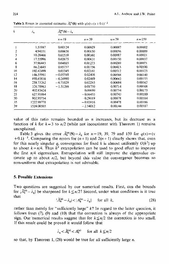
Table3 gives the e r r o r /](kn)(S)--,~k for n=19, 39, 79 and 159 for q(x)=(x +0.1) -z. Comparing the errors for (n+ l ) and 2(n+ 1) clearly shows that, even for this nearly singular q, convergence for fixed k is almost uniformly O(h 2) up to about k=n/4. Thus h 2 extrapolation can be used to good effect to improve the first n/4 eigenvalues. Extrapolation will still improve the eigenvalue estimate up to about n/2, but beyond this value the convergence becomes so non-uniform that extrapolation is not advisable.

5. Possible Extensions

Two questions are suggested by our numerical results. First, can the bounds for [A~,")-2kl be sharpened for k < n/2? Second, under what conditions is it true that

Ifl~k")--2kl<[A~k")--2kl for all k, (28)

rather than merely for "sufficiently large" k? In regard to the latter question, it follows from (7), (9) and (10) that the correction is always of the appropriate sign. Our numerical results suggest that for k<n/2 the correction is too small. If this result could be proved it would follow that

2k < ,lk3~"/ --- l,k/A~n~ for all k < n/2

so that, by Theorem 1, (28) would be true for all sufficiently large n.


A common feature of all numerical methods for which the asymptotic correction technique for (1) has been justified so far is that, when q=0 , the eigenvectors coincide with the exact eigenfunctions at the mesh points. Certain higher order finite element methods for Sturm-Liouville problems also have this property [10, p. 227], which suggests that asymptotic correction may also be useful for these methods. In view of the general superiority of the corrected Numerov estimates 1-4] over the corrected second order finite difference estimates and the well-known advantages of high order finite element methods for low eigenvalues El0], this is an obvious field for further investigation. However the results of Sect. 3 suggest that if the correction can be extended to a finite element method of order p, unless a suitable product rule is used, it will probably be necessary to use a quadrature rule of order at least 2p to gain the full benefit of the correction and that a stronger smoothness condition on q will be required.

Another possible extension is to more general problems than (1), at least to more general boundary conditions as in [1], and perhaps also to more general differential equations. Some related suggestions for further investigation of asymptotic correction for finite difference methods are made in [2] where, in particular, results are presented which suggest that asymptotic correction may be useful for computation of eigenvalues of partial differential equations.

References

1. Anderssen, R.S., de Hoog, F.R.: On the correction of finite difference eigenvalue approximations for Sturm-Liouville problems with general boundary conditions. BIT 24, 401-412 (1984)

2. Andrew, A.L.: Asymptotic correction of finite difference eigenvalues. In: Computational tech- niques and applications: CTAC-85 (J. Noye, R. May, eds.), pp. 333-341. Amsterdam: North- Holland 1986

3. Andrew, A.L.: The accuracy of Numerov's method for eigenvalues. BIT 26, 251-253 (1986) 4. Andrew, A.L., Paine, J.W.: Correction of Numerov's eigenvalue estimates. Numer. Math. 47,

289-300 (1985) 5. Fix, G.J.: Effects of quadrature errors in finite element approximation of steady state, eigenval-

ue and parabolic problems. In: The mathematical foundations of the finite element method with applications to partial differential equations (A.K. Aziz, ed.), pp. 525-556. New York: Academic Press 1972

6. Mikhlin, S.G.: The numerical performance of variational methods. Nauka Press, Moscow, 1968; English translation, Wolters-Noordhoff, Groningen, 1971

7. Omodei, B.J., Anderssen, R.S.: Stability of the Rayleigh-Ritz procedure for non-linear two- point boundary value problems. Numer. Math. 24, 27-38 (1975)

8. Paine, J.: A numerical method for the inverse Sturm-Liouville problem. SIAM J. Sci. Stat. Comput. 5, 149-156 (1984)

9. Paine, J.W., de Hoog, F.R., Anderssen, R.S.: On the correction of finite difference eigenvalue approximations for Sturm-Liouville problems. Computing 26, 123-139 (1981)

10. Strang, G., Fix, G.J.: An analysis of the finite element method. Englewood Cliffs: Prentice-Hall 1973

11. Wilkinson, J.H.: The algebraic eigenvalue problem. Oxford: Clarendon Press 1965

Received December 16, 1985 / June 1, 1986

Documents

Correction of finite element estimates for Sturm-Liouville eigenvalues