Embed Size (px)
Citation preview

1 / 25
Core-Periphery Model in Urban Economic Growth:
An Analysis Based on
Chinese City-Level Panel Data
1990-2006
Ming LU
Zhao CHEN
Zheng XU
Fudan University, Shanghai 200433, People’s Republic of China
Abstract: This paper uses Chinese city- level panel data from 1990 to 2006 to estimate
the impact of inter-city spatial agglomeration on urban economic growth. Our results
show a ∽-shaped correlation between the distance to the nearest major ports in China
and urban economic growth, which verifies the Core-Periphery Model in the new
economic geography theory. We also find that a city which locates near the regional
central city has a higher economic growth rate. Besides, our results suggest that due to
the market segmentation between Chinese provinces, the ―border effect‖ of Chinese
provinces is equivalent to adding as much as 260 kilometers, which prevents cities
from being absorbed by regional central cities in other provinces.
Key Words: Spatial agglomeration, market segmentation, urban economic growth,
Core-Periphery Model
Corresponding author. E-mail address: [email protected] (G. Wan).

2 / 25
I. Introduction
China has been experiencing rapid economic growth during the past thirty-years,
while global capital and China’s inland cheap labor keep combining in China’s eastern
coastal area. This spatial agglomeration of economic activities has brought
tremendous changes in spatial distribution of China’s economy, as well as the basis
for empirical testing the "core-periphery" theory in the new economic geography. But
no literature has used econometric modesl to describe the Chinese urban Systems.
Given that the new economic geography theory has successfully interpreted spatial
agglomeration and urban, regional economic development (Neary, 2001), this paper
will use Chinese city- level panel data from 1990 to 2006, based on the new economic
geography theory, research the effect of geography factors to China's urban economic
growth, and show the process of spatial agglomeration in city level.
Our research will focus on the two following questions: First, how does the
inter-city spatial agglomeration affect urban economic growth in China? Second, does
Chinese inter-province market segmentation add actual distance between cities in
different provinces, while limiting the inter-city agglomeration effect, as well as
distorting the allocation of resources?
The new economic geography finds that the effects of spatial agglomeration on
urban economy include both centripetal forces (Krugman, 1991) and centrifugal
forces (Helpman, 1999; Tabuchi, 1998). Centripetal forces mean the power to
promote economic concentration, while centrifugal forces refer to the contrary with
such power. Centripetal forces derive primarily from related industries, knowledge
spillovers and other external economies; centrifugal forces are due to poor mobility of
production factors, transport costs, congestion and other external diseconomies.
Fujita et al. (1996, 1999a, 1999b) simulated a ∽-shaped curve between
distance and urban market potential which reflects the economic scale of urban in a
single-core urban system. This curve shows that with the distance to regional central
cities increases, the market potential declines first, and later rises, then declines again,
which reflects the interaction of spatial agglomeration between the centripetal force
3 / 25
and centrifugal force. On one hand, the regions nearer to regional central cities are
more attractive; on the other hand, the cities far away from central cities avoid from
fierce competitions with central cities and surrounding regions, of which the impetus
encourage manufacturers to stay away from central cities. Fujita et al. (1996a, 1999b)
also draws a ∽-shaped market potential curve in a single-core urban system by
numerical simulation, when describing the impact of the transport hubs, such as ports,
on the city location.
But empirical studies of the new economic geography lag far behind the theory.
―Buttressing the approach with empirical work‖ and ―quantified models‖ are two
important directions for the new economic geography future researches by Fujita and
Krugman (2004). However, ―Due to the highly nonlinear nature of geographical
phenomena‖, it’s not easy ―to make the models consistent with the data‖. At the same
time, economic geography, in particular the role of spatial agglomeration factors
require a wide range of space, long time of accumulation and development, while
national boundaries, geographical boundaries, war and other factors often limit the
free flow of resources, it is difficult to use the empirical econometric model and
real-world data to clearly portray the spatial agglomeration effects. Therefore, it’s
studies on stably-developing large countries that seem particularly important for the
empirical researches of the new economic geography.
Hanson(2005), by constructing the market potential function, with the U.S.
counties data, finds a significant negative non- line correlation between distance and
market potential, and the impact decreases as distance increases, which almost
disappears 200-300 km away. But Hanson doesn’t find any evidence for "centrifugal
forces".
Dobkins and Ioannides (2000, 2001), Ioannides and Overman (2004) and so on
use the 1900-1990 U.S. metropolitan-area panel data to find no significant
correlation between the distance to the nearest higher-level city and the population
growth or wages, and there is no non-linear relationship, which may be because the
links between wages or population and urban market potential are too complicated.
None of the above researches have given convincing empirical evidences for the

4 / 25
impact of spatial agglomeration on urban economy.
Researches using China data may contribute to the empirical studies of the new
economic geography, mainly based on the following reasons: 1) China has a vast
territory, as well as a large population. The vast territory provides not only space
required by agglomeration effects, but also plenty of samples for empirical studies.
Meanwhile, a large population provides sufficient market potentials. 2) Compared
with the United States, China has a larger interregional geographical diversity and
more obvious geographical heterogeneity, because of the concentration of the ports
distribution, which leads to a bigger variance within cross-section samples. 3) China
has a rapid economic development in the last thirty years with observably temporal
changes of the spatial distribution of economic activities, which allow us to observe
the impact of spatial agglomeration on urban economy in long term with the data of
recent years.
Bao et al. (2002) find the economies in coastal areas developed faster by
absorbing more FDI and labor, using Chinese province- level data. Chen et al. (2008)
find that the coastal areas have the geographical advantages in industrial
concentration. Other studies also find "spatial-concentration" or "spatial-dependence"
in China's regional economic development, that is, coastal provinces and cities
develop faster (Ho and Li, 2008). Nevertheless, such studies only use coastal- inland
dummy or east-middle-west dummy to measure the factors of geographical location,
so there are at least two deficiencies: First, they can’t explain whether the observed
"spatial-concentration" or "spatial-dependence" stems from the policy or geographic
location; Second, it’s unable to clearly characterize the non-linear effect of spatial
agglomeration or verify centripetal forces and centrifugal forces.
Based on the above problems, we use Chinese city- level panel data from 1990 to
2006 to estimate the impact of spatial agglomeration of the regional central cities as
well as the major ports on urban economic growth. In this paper, there are two main
indicators measuring geographical factors: the distance to the nearest regional central
city, and the distance to the nearest major port. Because we use the continuous
distance indicators, we can simulate the effect of agglomeration as distance changes,
5 / 25
and identify centrifugal forces and centripetal forces.
Policy is an important variable which impacts spatial agglomeration in the new
economic geography. But when it comes to studies on Chinese urban system, an
important policy variable which affects regional economic development often be
overlooked, which is market segmentation. Studies have suggested that among
Chinese provinces there is serious market segmentation (Young, 2000; Ponect, 2005).
This division is likely to add the actual distance between cities in different provinces,
and limit the inter-city agglomeration effects, thus, lead to distortions in resource
allocation. This article will examine the effects of China's inter-province market
segmentation on spatial agglomeration, and compare the agglomeration effects
between capitals and regional central cities, thus, explore the effects of market
segmentation and ―border effect‖ on Chinese urban economic growth.
In addition, we will compare the effects of the geographic factors with other
traditional factors, such as investment, labor, FDI, government expenditure in short-
and long-term, respectively. Thus, we might find long-term economic growth factors
and explore a sustainable developing way for urban economy.
Section II of this paper will introduce the research method and data used in this
paper. Section III presents the the empirical results. Section IV would try to expand
the primary model to find long-term economic growth factors. And the last section
offers conclusions of this paper.
II、Method and Data
Although we use Chinese city- level panel data, we focus on the effects of
inter-city spatial agglomeration in long-term. So we use the cross-section OLS
regression as our basic method, which is based on the economic growth model of
Barro (2000). The model specification is as follows:
0 0 0 0 0 0 0 0(ln ,int , , , , ; ; ...)it i i i i i i i iDgdp f gdp e lab edu gov fdi con geo
In this paper, we used Chinese city- level panel data (1990-2006) based on
Chinese cities Statistical Yearbook, including 286 cities from 30 provinces of
6 / 25
mainland China.
The dependent variable itDgdp is the the annual growth rate of real per capita
GDP deflated by provincial urban CPIs, respectively, for the city i year t. The
theoretical assumptions of the new economic geography emphasize the agglomeration
effect of industrial and service, so we removed the first industrial output out of the
GDP indicators and the agricultural population out of the population indicators. For
details on data sources and data construction, see Appendix (To be filled).
In the right of equation, following the traditional economic growth literatures
(Barro, 2000), we add the initial level of per capita GDP 0ln igdp to observe whether
Chinese economy conditional converges at city level; we control the ratios of
investment to GDP (0int ie ), of employee population to total population (
0ilab ), and of
teachers to students (0iedu ) to observe the effects of investment, labor and education.
And the government expenditure proportion and foreign direct investment proportion
of GDP, are also usually controlled by economic growth literatures, which are
0igov and 0ifdi in this paper.
0icon represents some other control variables related to Chinese urban
economic growth, including: the ratio of the non-agricultural population to the total
population (urb) accounting for the level of urbanization; the population density
(density) and its square (den_2) accounting for internal population agglomeration in
urban. In order to alleviate the endogeneity bias of this model, we use the initial
situation of all explanatory variables in 1990, so that the estimated results would
represent the long-term impact of the explanatory variables above on urban economic
growth.
Based on this long-term economic growth model, we add the geographical
variables of our concern, including: 1) the shorter straight- line distance to Shanghai
and Hong Kong disport, which are two major ports of China, its square disport_2 and
cubic disport_3, which in order to observe the impact of distance to major port on
urban economic growth; 2) the shortest straight-line distance to the regional central
7 / 25
cities distbig, its square distbig_2 and cubic distbig_3, which in order to observe the
impact of distance to the regional central city on urban economic growth; 3) the GDP
level of the nearest regional central city in the initial year gdpofbig0; 4) dummy
samepro, represents whether the city is in the same province with the the nearest
regional central city; 5) dummy seaport and riverport, to show whether a city has a
seaport or river port; 6) following the studies on Chinese economic growth, we also
put the capital- or municipality- dummy (capital), as well as central-(mid) and
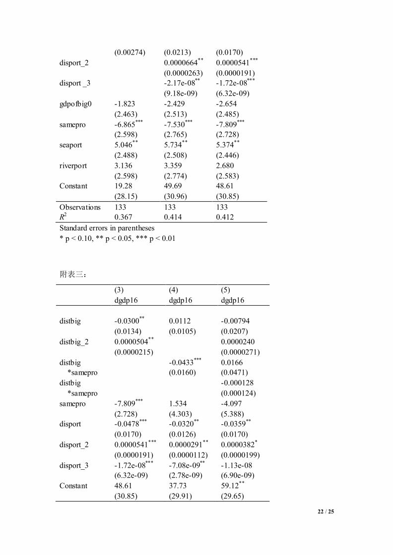
western- (west) dummy. Statistical distribution of distance variables is in Table 1.
In particular, we use straight- line distance instead of road or railway distance as
our measure of distance, because it’s not only available, but also exogenous, which
avoids some potential estimated bias brought by the endogeneity of traffic distance.
III、Results
Estimated results of the model are in Table II. In addition to the traditional
economic growth factors, we add the geographical variables we are concerned in the
equation (1), including the first item of the distance to the central city and the major
port, both of which are insignificant. It may be because, as Fujita et al. (1996, 1999a,
1999b), that there is a ―∽‖shaped relationship between the distances to the central
city or major port and economic activities. So we add the square and cube of distances
to the equation (2).
Equation (2) shows that distance to major ports and its square and cube are all
significant, while neither of the distance to central cities or its square or cube is
significant. This is most likely due to the effects of three items need a broader scope,
but the reality of distance to regional central city is not large enough. So we removed
the cube of the distance to central city from the equation (3). Obviously, all distance
variables are significant: the distance to central cities is negative, its second item is
positive; the distance to major ports is negative, while the second item is positive and
the third item negative. Based on estimated results, we draw the relationships between
distance to the major port or central city and urban economic growth rate, respectively,
in Figure I and II in appendix, of which the horizontal axis means the distance, and

8 / 25
the longitudinal axis means the impact on economic growth.
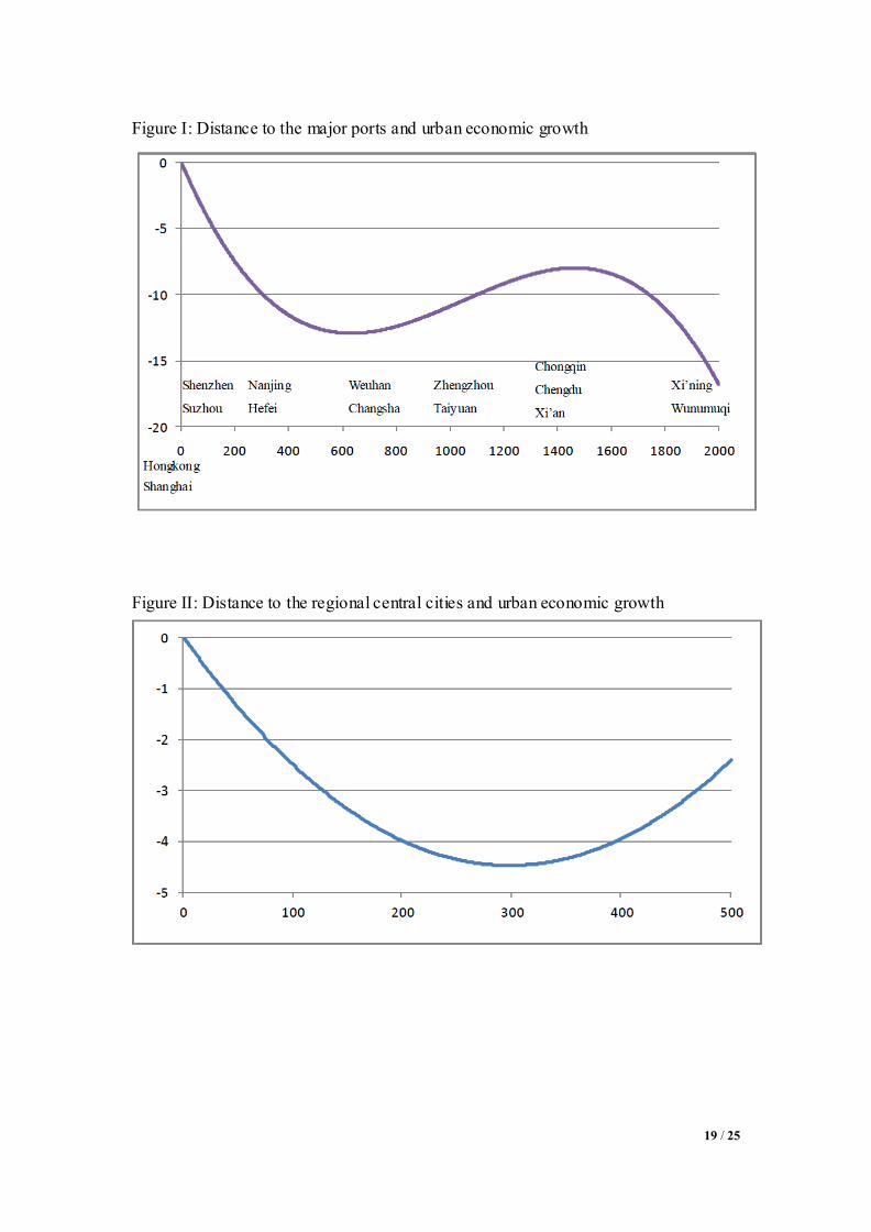
Figure I suggests that the impact of the distance to the major port on urban
economic growth has basically the same shape with the market potential curve in new
economic geography (Fujita et al., 1996, 1999b). While a city located closer to ports,
it’s closer to foreign markets, thus has a larger market potential and a higher
economic growth rate. While the distance is longer than a certain extent, foreign
markets are no longer that important. Therefore, a location far away from ports might
promote the accumulation of regional and domestic market potentials, as well as the
the development of local economy. While the distance is long enough, the city far
way from both domestic and foreign markets would suffer from both low market
potential and economic growth rate.
In Figure 1, we marked major cities in China in accordance with the distance to
the major port as followed. We can see that it’s Chongqing, Chengdu, Xi'an that
locate at the distance from 1200 to 1600 km – which is the protruding part of the ―∽‖
shaped curve. And the above three cities are nearly most developed in the western and
central China. At the same time, the absolute value of the slope of decreasing-parts in
this curve is much larger than that of the increasing-part, which means if the spatial
distance can be shortened, it would improve the growth of the whole economy. Of
course, physically, the distance can’t be shortened, but the transport costs represented
by distance could be reduced by improving transport conditions, loosening restrictions
on interregional migration and reducing the provincial market segmentation in China.
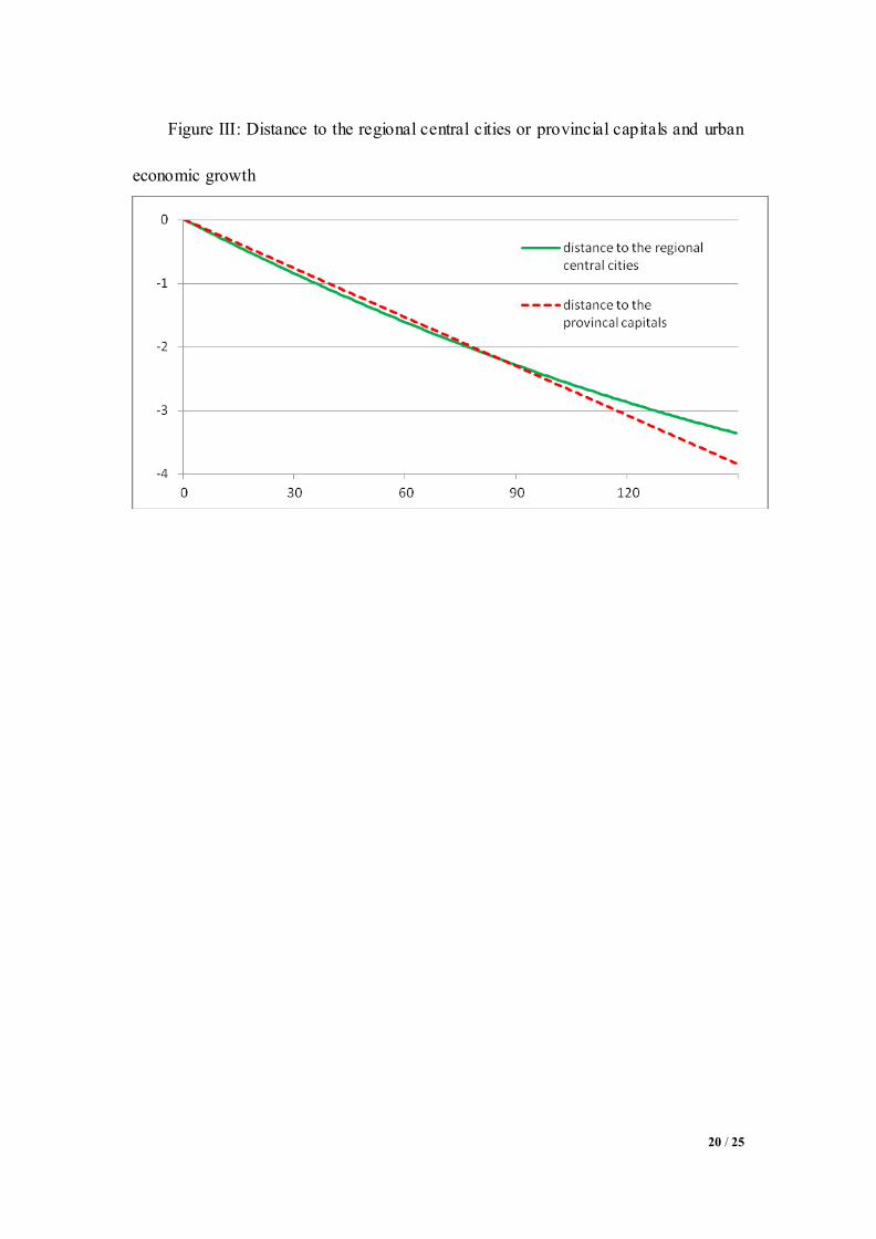
As shown in figure II, when it’s close to the regional central cities, scale effect
and other external economies brought by spatial agglomeration promote the central
city to absorb economic resources from surroundings, which is the significant
centripetal force. So the closer to the central cities, the faster it grows. But when it’s
far away from the regional central city, instead of the centripetal force, the centrifugal
force plays a major role. So the farther the distance, the faster it grows. Our estimated
result shows the turning point is about 300 kilometers, which means in less than 300
kilometers, inter-city spatial agglomeration shows a strong role of the centripetal force,
which is similar with Hanson (2005). The difference is that we also find that when the
9 / 25
distance is greater than 300 kilometers around, because of transportation cost and
other other external diseconomies, the inter-city spatial agglomeration performs as the
centrifugal force.
What needs to be emphasized is that, in Figure 2, the curve is U-shaped rather
than ―∽‖-shaped, which is not surprising. By comparing Figure I and II, we might
find that to see the complete ―∽‖-shaped curve, it required at least 1,400-km distance,
while the real distance to the regional central city is not long enough. Therefore, it’s
definitely possible that Figure 2 shows the left part of the whole ―∽‖-shaped curve.
We also notice that in the equation (1) - (3), the central-western dummy is almost
always no significant, which is because the spatial distance variables have captured
the weakness of the central and western area in geographical location. The
same-province dummy is always significantly negative, which seems the spatial
agglomeration of the regional central cities differs whether or not small cities are in
the same province with the central cites. If a city is in the same province with the
nearest regional central city, the absorption effect from the central cities will be larger,
therefore, the city will grow slower. On the contrary, this means that the "border
effect" similar to Parsley and Wei (2001) exists in Chinese provincial borders, which
increases the actual distances between cities in different provinces. Preliminary
estimating, China's inter-province "border effect" is equivalent to adding as much as
260 km①.
The "border effect" in this paper presents as the distortion of the spatial
concentration. We think it’s relevant with Chinese province- level market
segmentation. Young (2000), Ponect (2005) prove that China has serious
province- level market segmentation. This inter-province market segmentation may be
not conducive to agglomeration effects of the regional central cities, but to economic
growth of small and medium cities in the different province.
To observe the relationship between the inter-province market segmentation and
the spatial agglomeration more clearly, we add in the equation (4) the interaction of
① We estimate the average ―border effect‖ by dividing the coefficient of the same-province dummy by that of
the distance to the nearest regional central city in the equation (3).
10 / 25
the same-province dummy with the distance to the central cities, and in the equation
(5) the interactions of the same-province dummy with both the distance to the central
city and its square item. Results are in table III.
In the equation (4), both the distance to central city and the same-province
dummy are not significant, but the interaction is significantly negative. This means at
the same distance, the absorption effects are stronger to the small cities within the
same province. In the equation (5), neither of the distance, the same-province dummy
nor the interaction is significant, perhaps because the distance to the regional central
city and the same-province dummy have a strong colinearity while there’s not enough
samples.
Chen et al. (2007) believe that government intervention has a strong role in
promoting market segmentation in the Chinese province level. Obviously, the
provincial governments segregate the market to restrict the agglomeration effects
from big cities in other provinces, so as to protect their own economic development.
Although for the cities of the province, such market segmentation can prevent them
from the absorption effect of other provinces large cities, but for the regional
economy or even the national economy, it brings a loss of resource allocation
efficiency, thus a lower growth rate of the whole economy, resulting in smaller
Chinese cities (Au and Henderson, 2006), and smeller variance among Chinese cities
(Fujita et al., 2004).
When the inter-province market segmentation exists, the provincial governments
have incentives to limit the agglomeration effects of the regional central cities in other
provinces, strengthen the economic concentration of the province capital by
administrative orders, in order to promote the province economic development. To
understand this effect better, we replace "the distance to the nearest regional central
city"(distbig) in the original model with " the distance to the provincial capital"
(distcap) to compare the agglomeration effects between regional central cities and
provincial capitals, and observe the restriction of inter-province market segmentation
to the agglomeration effects of regional central cities, as well as the resultant
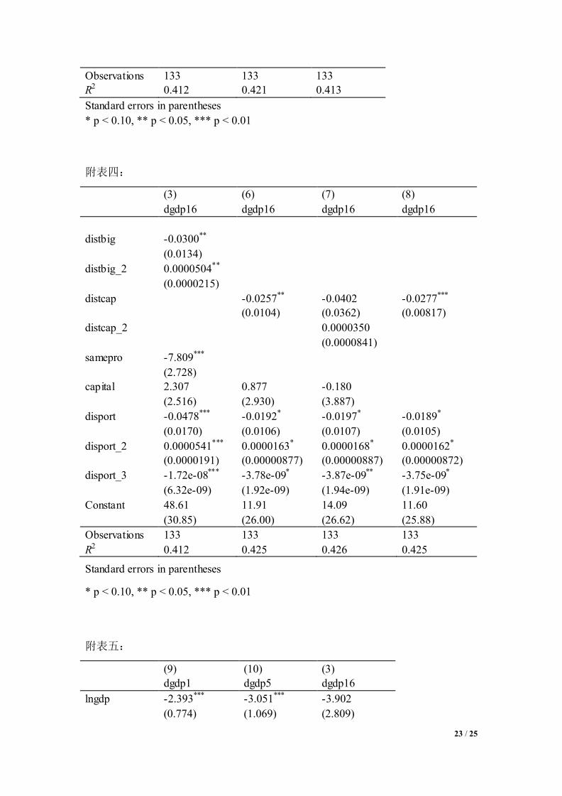
distortion of resources. See Table IV.

11 / 25
As can be seen from Table IV, in Equation (6) we only add the distance to the
provincial capital, which is significantly negative, showing the provincial capitals
have strong absorption effects on the the surrounding cities. In the equation (7), we
add both the distance to the provincial capital and its square, both of which are not
significant. So provincial capitals have only significant centripetal forces, which is not
conducive to the economic growth of the remote cities. Considering that the distance
to the capital and the capital dummy may have a strong correlation, we remove the
capital dummy in the equation (8). The results have no significant changes.
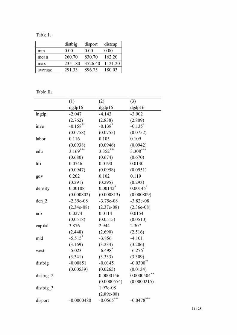
We draw Figure III simulating the relationship between urban economic growth
and the distance to the central city or the provincial capital. As can be seen from
Figure III, at distance less than 90 kilometers, the concentrated effects of regional
central cities are stronger than those of the provincial capitals; while at distances more
than 90 kilometers or so, provincial capitals have stronger centripetal forces. So even
in the presence of the inter-province market segmentation, the agglomeration effects
of the regional central cities in other provinces still have important impacts on the
provincial small cities. Market segmentation, not only in theory is not conducive to
the promotion of inter-regional division, but also difficult to truly reverse the
inter-regional agglomeration.
IV、Model Development: Do geographical factors affect urban economic growth in
long or short term?
As asserted by Forbes (2000), the relationship between economic growth and
growth factors maybe change by the difference in the time horizon considered, which
has been proved by Wan et al.(2006) with Chinese data. We have confirmed the
impact of geography on urban economic growth with the time horizon of sixteen
years, but we do not know whether this effect also exists in a shorter term. To this end,
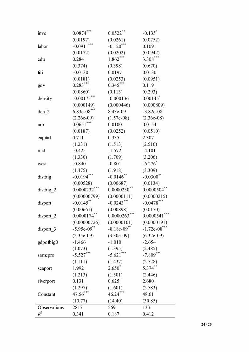
we use panel data to estimate the equation (9), (10), and compare with the equation
(3). The explanatory variables of the equation (9), (10) are the same with the equation
(3). Because the geographical variables do not changed across time, we use the
Generalized Least Squares (GLS) to estimate the random effects model instead of the
12 / 25
fixed effects model. The results are in Table 5.
Forbes (2000) uses data averaged over a 5-year interval in a growth regression
and claims that this is a medium- or short-run relationship. Meanwhile, Barro (2000)
relies on averages over a 10-year interval to estimate long-run relationships. Though
no consensus exists regarding what time horizon constitutes or defines the short-,
medium-, or long-run concepts (Wan et al., 2006), we may use the same regression
model with different time horizons to compare the coefficients of the explanatory
variables in short-, medium-, or long-run in one model.
In equation (9), we lag the explanatory variables by 1 year using the Chinese
city 1990-2006 annual panel data, in fact, to find the short-term urban economic
growth factors. Regression results show that the distance to the central cities and to
the major ports and their respective square or three items are significant. In the
equation (10), we use the Chinese city 1990,1995,2000,2005 panel data, with the
five-year average per capita real GDP growth rate as the dependent variable, the
initial situation of all explanatory variables in each five-year period as their values.
Regression results also show a significant relationship between geographical distance
and economic growth. Compare equation (9), (10) with (3), the geographical distance
variables and the seaport dummy are almost all more significant with bigger absolute
values of coefficients in the long-term. Thus, the impact of geographical factor on
economic growth is more significant in a longer term.
We also compared the impact of other factors influencing urban economic
growth in different time horizons. Regression results imply that, the impact of
investment on economic growth is significant positive in short term while not so
significant negative in long term This may be due to the level of investment is a
short-term factors of economic growth, which means, regions with a high investment
level maybe have no obvious economic advantages, on the contrary, may suffer from
low efficiency spawned by over-investment.(Zhang, 2003). Labor force has a negative
impact on economic growth, which may be related to China's overall labor surplus
(Wan et al., 2006). However, the impact of labor force isn’t significant in long term.
Education is a positive factor of economic growth and even more significant in long
13 / 25
term. On one hand, this can be explained by long-term economic growth factor, on the
other hand, it can be related with the measurement of education variable. Considering
the availability of data, this paper chose the ratio of teachers and students in primary
and junior schools as a city- level education measure, which is actually a proxy
variable of educational resources. Human capital, as well as economic growth lags
behind education resource investment, which can partly explain why education is so
significant in long term. Government expenditure impacts on economic growth
positively in short term whereas not significant in long term, which may be because
the current governmental expenditure would instantly improve local investment and
consume in short term, however, in the long term, high government expenditure will
distort the resource collocation of market with the low efficiency of its own.(Barro,
2000; Clarke, 1995; Partridge, 1997). FDI has no significant relationship with urban
economic growth in either short-or long- term which explained by Luo (2006) is that
FDI as a kind of investment does not have significant impact on economic growth
directly, but it can play a positive role in economic growth indirectly by productivity
improvement and squeezing into domestic investment.
As to the structural variables related with Chinese economic characteristics, the
relationship between population density and economic growth implies U-shaped in
short term, which is opposite to Au and Henderson (2006). Meanwhile, in long term,
this relationship seems to have an inconspicuous coherency with inversed-U Shaped
of Au and Henderson. It can be explained by that population density is an endogenetic
variable of geographic location and some other urban characteristics which, if be
controlled by the model, the impact of population density on economic growth is not
conspicuous. The positive impact of urbanization only happens in short term. The
capital dummy and the west-central dummy are not positively, which obviously differ
with former researches, such as Bao et al. (2002), Chen et al.(2008), Ho and Li
(2008), which is because with the inter-city distances controlled in the paper no
obvious growth disadvantages exist in western or central regions ,and no advantages
in provincial capitals. In other words, spatial agglomeration factors contribute most in
the interregional economic disparities in China. Finally, the initial level of per capita
14 / 25
GDP has a significant negative impact on Chinese urban economic growth, which
performs as the China economy conditional converges at the city level, but this kind
of "convergence" is not significant in long term.
We simplify the model further by making the independent variables only
include exogenous geographical distances and initial economic level while the
dependent variables remain the lagged one-year GDP per capita growth rate, the
average GDP per capita growth rate of five years and the sixteen years. Regression
results are in Table VI, which suggest all geographical distances are significant, and
with time passing by, almost all coefficients and significances of the geographic
factors increase as well as the R-square of the regression models, indicating that the
impact of geographical factors on the urban economic growth are more significant in
long term.
Regression results also suggest that conditional convergence exists at the
city- level of Chinese economy when only geographical distances controlled, and the
speed of which increases in longer term.
V. Conclusions
The most important finding of this paper is to verify the ―∽‖-shaped non- linear
relationship between the geographical distance and urban economic growth, based on
the spatial agglomeration effects and the Core-Periphery model in the new economic
geography theory. We find that the Core-Periphery model is well proved in the
Chinese urban economic growth model: 1) There is a significant ―∽‖-shaped
relationship between the distance to major port and Chinese urban economic growth,
which is negative first, then positive, negative at last. 2) There is a significant
U-shaped relationship between the distance to regional central city and Chinese urban
economic growth, based on which the inter-city spatial agglomeration effects present
the trend of centripetal forces within the distance of 300 kilometers, while the trend of
centrifugal forces out of the distance of 300 kilometers. 3) The "border effect" caused
by Chinese inter-province market segmentation is equivalent to an increase of about
260 kilometers of the actual distance. While this market segmentation limits the
15 / 25
spatial agglomeration of the regional central cities in other provinces, it protects the
economic growth of small cities in the province. Nevertheless, this protection for
small cities in the province suggests the efficiency losses of the interregional resource
allocation.
This article also studies other urban economic growth factors. Our main findings
include the following: (1) Education promotes long-term urban economic growth. (2)
Investment, government spending, FDI though may promote economic growth in
short term, but there’s no significant impact in long term. (3) There is "conditional
convergence" in Chinese urban economic growth.
Our research suggests that the inter-city agglomeration effect must be made full
use of to achieve the goal of sustainable growth of urban economy, which is also the primary impetus behind Chinese sustainable economic growth. However, the
inter-province market segmentation limit the agglomeration effects, thus is not
conducive to interregional allocation of resources. Therefore, we should reduce the
restrictions on the inter-province transportation of production factors (especially labor)
and goods, promote market integration and rational distribution of resources.
As to economic policy-making, the urban economic long-term sustainable growth
depends on making full use of the spatial agglomeration effects and the improvement
of education. In contrast, investment, government expenditure, FDI may contribute to
short-term growth of the local economy, but it will not promote the economic growth
in long term. As to western and central areas in China, the key to urban and regional
economic growth is the improvement of transportation and the development of the
domestic market. To improve the transportation, it will shorten the transport distance
and cost among central, western and coastal areas, as well as the small cities and
regional central cities, which is conducive to the effects of spatial agglomeration and
regional economic development. The development of the domestic market suggests
that compared with the eastern coast facing a broader international market, the
western areas should make full use of regional and domestic markets with the
effects of regional agglomeration, and promote regional economic growth with the
development of regional central cities.
16 / 25
References:
[1] Au, Chun-Chung and J. Vernon Henderson, 2006, ―Are Chinese Cities Too Small?‖ Review
of Economic Studies, Vol. 73, No. 3, 549-576.
[2] Bao, Shuming, Gene Hsin Chang, Jeffrey D.Sachs, Wing Thye Woo, 2002, ―Geographic
factors and China’s regional development under market reforms, 1978–1998,‖ China
Economic Review, 13, 89–111.
[3] Barro, Robert J., 2000, ―Inequality and Growth in a Panel of Countries,‖ Journal of
Economic Growth, 5, 1, March, 87-120.
[4] Clarke, G. R. G., 1995, ―More Evidence on Income Distribution and Growth,‖ Journal of
Development Economics, 47, 2, 403-427.
[5] Chen, Min, Qihan Gui, Ming Lu and Zhao Chen, 2007, ―Economic Opening and Domestic
Market Integration,‖ in Ross Garnaut and Ligang Song (eds.), China: Linking Markets for
Growth, Asia Pacific Press, 369-393.
[6] Chen, Zhao, Yu Jin and Ming Lu, 2008, ―Economic Opening and Industrial Agglomeration in
China,‖ in M. Fujita, S. Kumagai and K. Nishikimi (eds.), Economic Integration in East Asia,
Perspectives from Spatial and Neoclassical Economics, Edward Elgar Publishing, 276-31.
[7] Dobkins, L. and Y., Ioannides, 2000, ―Dynamic Evolution of the Size Distribution of U.S.
Cities," in J. M. Huriot and J.-F. Thisse (eds.), Economics of Cities, Cambridge: Cambridge
University Press, 217-260.
[8] Dobkins, L. and Y., Ioannides, 2001, ―Spatial Interactions among U.S. Cities: 1900–1990,‖
Regional Science and Urban Economics, 31, 701–731
[9] Forbes, Kristin J., 2000, ―A Reassessment of the Relationship between Inequality and
Growth,‖ American Economic Review, 90, 4, 869-887.
[10] Fujita, M., Henderson, V., Kanemoto Y., and T., Mori, 2004, ―Spatial Distribution of
Economic Activities in Japan and China,‖ in V. Henderson and J.-F. Thisse (eds), Handbook
of Urban and Regional Economics, vol.4, North-Holland, 2911-2977.
[11] Fujita, M. and P.R., Krugman, 1995, ―When is the Economy Monocentric? von Thünen and
Chamberlin Unified,‖ Regional Science and Urban Economics, 25, 505-528.
[12] Fujita, M. and P.R., Krugman, 2004, ―The New Economic Geography: Past, Present and the
17 / 25
Future,‖ Regional Science, 83, 139-164.
[13] Fujita, M., P.R., Krugman, and T., Mori, 1999a, ―On the Evolution of Hierarchical Urban
Systems,‖ European Economic Review, 43, 209-251.
[14] Fujita, M., P.R., Krugman, and A.J., Venables, 1999b, The Spatial Economy: Cities, Regions
and International Trade, Cambridge, Massachusetts: The MIT Press.
[15] Fujita, M. and T., Mori, 1996, ―The Role of Ports in the Making of Major Cities:
Selfagglomeration and Hub-effect.‖ Journal of Development Economics, 49, 93-120.
[16] Fujita, M. and T., Mori, 1997, ―Structural Stability and Evolution of Urban System,‖
Regional Science and Urban Economics, 27, 299-442.
[17] Hanson, G., 2005, ―Market Potential, Increasing Returns, and Geographic Concentration.‖
Journal of International Economics, 67 , 1 –24
[18] Helpman, Elhanan, 1999, ―R&D Spillover and Global Growth‖, Journal of International
Economics, 47, 399-428.
[19] Ho, Chunyu and Dan Li, 2008, ―Spatial Dependence and Divergence across Chinese Cities‖,
working paper.
[20] Ioannides, Y.M. and Overman, H.G., 2004, ―Spatial Evolution of the US Urban System‖.
Journal of Economic Geography, 4, 131-156.
[21] Luo,Changyuan, 2006,―FDI, Domestic Capital and Economic Growth: an Analys is Based
on Chinese Province Panel Data, 1987-2001,‖ World Economy Papers, 4, 27-43.
[22] Parsley, D., and S. Wei, 2001a, ―Explaining the Border Effect: The Role of Exchange Rate
Variability, Shipping Cost, and Geography,‖ Journal of International Economics, 55 (1), 87
-105.
[23] Patridge, D., Mark, 1997, ―Is Inequality Harmful for Growth? Comment,‖ American
Economic Review, 87, 1019-1032.
[24] Poncet, S., 2005, ―A Fragmented China: Measure and Determinants of Chinese Domestic
Market Disintegration,‖ Review of International Economics, 13 (3), 409 —430.
[25] Tabuchi, T., 1998, ―Unban Agglomeration and Dispersion: A Synthesis of Alonso and
Krugman,‖ Journal of Unban Economics, 44, 333-351.
[26] Wan, Guanghua, Ming Lu and Zhao Chen, 2006, ―The Inequality–Growth Nexus in the Short
and Long Runs: Empirical Evidence from China,‖ Journal of Comparative Economics, 34(4),

18 / 25
654-667.
[27] Young, A., 2000, ―The Razor’s Edge: Distortions and Incremental Reform in t he People’s
Republic of China,‖ Quarterl y Journal of Economics, 115 (4), 1091 —1135.
[28] Zhang, Jun, 2003, ―Investment, Investment Efficiency, and Economic Growth in China,‖
Journal of Asian Economics, 14, 5, 713-734.
19 / 25
Figure I: Distance to the major ports and urban economic growth
Figure II: Distance to the regional central cities and urban economic growth
20 / 25
Figure III: Distance to the regional central cities or provincial capitals and urban
economic growth
21 / 25
Table I:
distbig disport distcap
min 0.00 0.00 0.00
mean 260.70 830.70 162.20
max 2351.80 3526.40 1121.20
average 291.33 896.75 180.03
Table II:
(1) (2) (3)
dgdp16 dgdp16 dgdp16
lngdp -2.047 -4.143 -3.902
(2.762) (2.838) (2.809)
inve -0.158** -0.138* -0.135*
(0.0758) (0.0755) (0.0752)
labor 0.116 0.105 0.109
(0.0938) (0.0946) (0.0942)
edu 3.169*** 3.352*** 3.308***
(0.680) (0.674) (0.670)
fdi 0.0746 0.0190 0.0130
(0.0947) (0.0958) (0.0951)
gov 0.202 0.102 0.119
(0.291) (0.295) (0.293)
density 0.00108 0.00142* 0.00145*
(0.000802) (0.000813) (0.000809)
den_2 -2.39e-08 -3.75e-08 -3.82e-08
(2.34e-08) (2.37e-08) (2.36e-08)
urb 0.0274 0.0114 0.0154
(0.0518) (0.0515) (0.0510)
capital 3.876 2.944 2.307
(2.448) (2.690) (2.516)
mid -5.515* -3.856 -4.101
(3.169) (3.234) (3.206)
west -5.023 -6.498* -6.276*
(3.341) (3.333) (3.309)
distbig -0.00851 -0.0145 -0.0300**
(0.00539) (0.0265) (0.0134)
distbig_2 0.0000156 0.0000504**
(0.0000554) (0.0000215)
distbig_3 1.97e-08
(2.89e-08)
disport -0.0000480 -0.0565*** -0.0478***
22 / 25
(0.00274) (0.0213) (0.0170)
disport_2 0.0000664** 0.0000541***
(0.0000263) (0.0000191)
disport _3 -2.17e-08** -1.72e-08***
(9.18e-09) (6.32e-09)
gdpofbig0 -1.823 -2.429 -2.654
(2.463) (2.513) (2.485)
samepro -6.865*** -7.530*** -7.809***
(2.598) (2.765) (2.728)
seaport 5.046** 5.734** 5.374**
(2.488) (2.508) (2.446)
riverport 3.136 3.359 2.680
(2.598) (2.774) (2.583)
Constant 19.28 49.69 48.61
(28.15) (30.96) (30.85)
Observations 133 133 133
R2 0.367 0.414 0.412
Standard errors in parentheses
* p < 0.10, ** p < 0.05, *** p < 0.01
附表三:
(3) (4) (5)
dgdp16 dgdp16 dgdp16
distbig -0.0300** 0.0112 -0.00794
(0.0134) (0.0105) (0.0207)
distbig_2 0.0000504** 0.0000240
(0.0000215) (0.0000271)
distbig -0.0433*** 0.0166
*samepro (0.0160) (0.0471)
distbig -0.000128
*samepro (0.000124)
samepro -7.809*** 1.534 -4.097
(2.728) (4.303) (5.388)
disport -0.0478*** -0.0320** -0.0359**
(0.0170) (0.0126) (0.0170)
disport_2 0.0000541*** 0.0000291** 0.0000382*
(0.0000191) (0.0000112) (0.0000199)
disport_3 -1.72e-08*** -7.08e-09** -1.13e-08
(6.32e-09) (2.78e-09) (6.90e-09)
Constant 48.61 37.73 59.12**
(30.85) (29.91) (29.65)
23 / 25
Observations 133 133 133
R2 0.412 0.421 0.413
Standard errors in parentheses
* p < 0.10, ** p < 0.05, *** p < 0.01
附表四:
(3) (6) (7) (8)
dgdp16 dgdp16 dgdp16 dgdp16
distbig -0.0300**
(0.0134)
distbig_2 0.0000504**
(0.0000215)
distcap -0.0257** -0.0402 -0.0277***
(0.0104) (0.0362) (0.00817)
distcap_2 0.0000350
(0.0000841)
samepro -7.809***
(2.728)
capital 2.307 0.877 -0.180
(2.516) (2.930) (3.887)
disport -0.0478*** -0.0192* -0.0197* -0.0189*
(0.0170) (0.0106) (0.0107) (0.0105)
disport_2 0.0000541*** 0.0000163* 0.0000168* 0.0000162*
(0.0000191) (0.00000877) (0.00000887) (0.00000872)
disport_3 -1.72e-08*** -3.78e-09* -3.87e-09** -3.75e-09*
(6.32e-09) (1.92e-09) (1.94e-09) (1.91e-09)
Constant 48.61 11.91 14.09 11.60
(30.85) (26.00) (26.62) (25.88)
Observations 133 133 133 133
R2 0.412 0.425 0.426 0.425
Standard errors in parentheses
* p < 0.10, ** p < 0.05, *** p < 0.01
附表五:
(9) (10) (3)
dgdp1 dgdp5 dgdp16
lngdp -2.393*** -3.051*** -3.902
(0.774) (1.069) (2.809)
24 / 25
inve 0.0874*** 0.0522** -0.135*
(0.0197) (0.0261) (0.0752)
labor -0.0911*** -0.120*** 0.109
(0.0172) (0.0202) (0.0942)
edu 0.284 1.862*** 3.308***
(0.374) (0.398) (0.670)
fdi -0.0130 0.0197 0.0130
(0.0181) (0.0253) (0.0951)
gov 0.283*** 0.345*** 0.119
(0.0860) (0.113) (0.293)
density -0.00175*** -0.000136 0.00145*
(0.000149) (0.000446) (0.000809)
den_2 6.83e-08*** 8.43e-09 -3.82e-08
(2.26e-09) (1.57e-08) (2.36e-08)
urb 0.0651*** 0.0100 0.0154
(0.0187) (0.0252) (0.0510)
capital 0.711 0.335 2.307
(1.231) (1.513) (2.516)
mid -0.425 -1.572 -4.101
(1.330) (1.709) (3.206)
west -0.840 -0.801 -6.276*
(1.475) (1.918) (3.309)
distbig -0.0194*** -0.0146** -0.0300**
(0.00528) (0.00687) (0.0134)
distbig_2 0.0000232*** 0.0000230** 0.0000504**
(0.00000799) (0.0000111) (0.0000215)
disport -0.0145** -0.0243*** -0.0478***
(0.00661) (0.00898) (0.0170)
disport_2 0.0000174** 0.0000263*** 0.0000541***
(0.00000726) (0.0000101) (0.0000191)
disport_3 -5.95e-09** -8.18e-09** -1.72e-08***
(2.35e-09) (3.30e-09) (6.32e-09)
gdpofbig0 -1.466 -1.010 -2.654
(1.073) (1.395) (2.485)
samepro -5.527*** -5.621*** -7.809***
(1.111) (1.437) (2.728)
seaport 1.992 2.650* 5.374**
(1.213) (1.501) (2.446)
riverport 0.131 0.625 2.680
(1.297) (1.601) (2.583)
Constant 47.56*** 46.24*** 48.61
(10.77) (14.40) (30.85)
Observations 2817 569 133
R2 0.341 0.187 0.412

25 / 25
Standard errors in parentheses
* p < 0.10, ** p < 0.05, *** p < 0.01
附表六:
(11) (12) (13)
dgdp1 dgdp5 dgdp16
lngdp -2.664*** -5.056*** -7.407***
(0.755) (0.875) (-3.99)
distbig -0.0106** -0.0113** -0.0254***
(0.00494) (0.00539) (-2.88)
distbig_2 0.0000191*** 0.0000271*** 0.0000552***
(0.00000737) (0.00000839) (3.90)
disport -0.0168*** -0.0175*** -0.0398***
(0.00590) (0.00658) (-3.62)
disport _2 0.0000175*** 0.0000198*** 0.0000429***
(0.00000614) (0.00000701) (3.59)
disport _3 -5.51e-09*** -7.02e-09*** -1.46e-08***
(1.99e-09) (2.30e-09) (-3.70)
Constant 38.09*** 58.79*** 90.47***
(7.420) (8.320) (5.49)
Observations 3224 718 208
R2 0.0054 0.0518 0.129
Standard errors in parentheses
* p < 0.10, ** p < 0.05, *** p < 0.01


