Embed Size (px)
Citation preview
Houston Journal of Mathematicsc© 2002 University of Houston
Volume 28, No. 2, 2002
CONTROL SYNTHESIS IN HYBRID SYSTEMS WITH FINSLERDYNAMICS
WOLF KOHN, VLADIMIR BRAYMAN, AND ANIL NERODE
Abstract. This paper is concerned with a symbolic-based synthesis of feed-
back control policies for hybrid and continuous dynamic systems. A key step
in our synthesis procedure is a new method to solve the following dynamic
programming problem:
∂V
∂t(z, t) = min
v
∂V
∂z(z, t)ρv(z, v)v
z = ρ(z, v), t ∈ [0, T ](1)
V (z, T ) = Ψ(z, T )(2)
Here V (z, t) is the cost-to-go function associated with a certain type of ho-
mogeneous calculus of variations problem on a Finsler manifold and (z, v)
is a positive homogeneous function of degree one in v. This optimization
problem is at the core of the control synthesis procedure for many hybrid
control problems [1], [2].
1. Dedication
We dedicate this paper to Professor Chern with gratitude, and for good reason.Nerode learned his differential geometry from Chern’s classes at the University ofChicago in 1951. As a lifelong mathematical logician, Nerode never expected touse this knowledge, especially knowledge of Finsler Geometry, which he had lateracquired from his friend and fellow student of Chern’s, Louis Auslander. Whendeveloping feedback policies for optimal control systems, we discovered that thesecan be modeled as Finsler geodesic fields and connections. One never knows inadvance what mathematics one may need, and it is nice to be in a position torecognize what is needed. A great virtue of the University of Chicago program,of which Chern was one of its founders, was that general knowledge of broadfields was an explicit aim. Kohn learned differential geometry at MIT and foundits tremendous potential in control applications. He has been an avid student
353

354 WOLF KOHN, VLADIMIR BRAYMAN, AND ANIL NERODE
of Professor Chern’s work. Vladimir Brayman who is completing his PhD inElectrical Engineering is working on the application of the differential geometricmethods to enterprise control problems.
2. Introduction
The discipline of hybrid systems emerged in the decade 1990-2000 as an impor-tant science at the interface of control theory, electrical engineering, and computerscience. Hybrid systems are systems that incorporate (discrete) logical controlprograms that interact with continuous physical plants in a changing environ-ment. In this context, a plant is thought of as an evolving vector field of plantstates. Before the Hybrid System approach, the standard models for such systemstended to ignore either the continuous or the discrete aspects of the system. Thereare many cases where non-hybrid approaches are not adequate to develop optimalcontrol laws. An enterprise control system is an example. The discipline of hybridsystems attempts to build and analyze models in which both the continuous anddiscrete aspects of the control problem are taken into account in a combined con-tinuous field encoding both the discrete (event driven) and continuous dynamicsof the system, with a transformation to the discrete domain when needed. Agood place to see examples of these systems, is in the four volumes of hybridsystems which have appeared in the Lecture Notes in Computer Science series bySpringer-Verlag, see references [1], [2]. There have been many conferences on thissubject worldwide since the publication of these seminal volumes.
We design logical control laws for hybrid systems to force the evolution of theplant states to satisfy a performance specification, even when subjected to dis-turbances in the environment, and in the presence of unmodeled plant dynamics.A control law is implemented by a real time control architecture. The way acontrol architecture module operates is as follows: when the plant enters a cer-tain prescribed region of the state manifold, the event is sensed by the controlarchitecture, which triggers the control program to change the control parame-ters for the plant actuators, thereby changing the plant evolution vector field toa new vector field. The plant state trajectory is thus a piecewise differentiablepath. Therefore, the discontinuities in the direction of the trajectory take placeat the times of the control law intervention. In other words, the hybrid controlprograms are event-driven finite automata, switching the plant from one vectorfield evolution to another for the purpose of enforcing plant performance specifi-cations. The use of hybrid control programs extends the range of applications of

CONTROL SYNTHESIS IN HYBRID SYSTEMS WITH FINSLER DYNAMICS 355
conventional continuous control theory to complex non-linear non-homogeneoussystems. The problem is, how does one develop such a program?
The fundamental problem of hybrid systems is to produce control algorithmsand control implementation architectures that enforce the performance specifica-tion for the system, given the plant state models. In our approach, we introducea manifold on which evolution of plant state trajectory y(t) take place. Themanifold is determined by the constraints. The control policies are formulated asfunctions γ(y(t), y(t)) that determine the direction y(t) = ρ(y(t), u(t)) at time t
when the plant state is y(t). In practice, the control effort should depend on thecurrent state y and rate y, and not on the current time, because the unknown dis-turbances and inaccuracies in the modelling parameters may lead to timing andpositional inaccuracies. We introduce a suitable non-negative Lagrangian L(y, u, t)and a goal set G on the manifold. We rephrase the performance specification sothat the requirement on the control policy can be chosen such that the plant statetrajectory y(t) remains on the manifold. The trajectory y(t) leads from currentstate to the goal set G, and minimizes
∫
L(y, γ(y, y), t)dt among all trajectoriesy(t) arising from admissible control policies.
The discussion is confined to the case when the goal is a single point. Therefore,a control policy indicates, given the current state, the optimal direction to goin order to end at the goal point. We allow the tangent field along the optimalstate trajectory to be measure-valued. This is done to ensure that mathematicallyoptimal trajectories exist. Furthermore, this implies that we allow control policiesthat are generalized curves u(t) in the sense of L.C. Young [7]. Measure-valuedoptimal control policies are generally not physically realizable, but there are closeapproximations that are realizable. Given a positive ε, we can generate algorithmsthat allow one to compute a piecewise constant approximation to γ(y, y) to anoptimal control policy which brings
∫
L(y, γ(y, y), t)dt within ε of its minimumamong all admissible trajectories. If the states y and the directions y are thendiscretized, the approximate control policy can be implemented as a logical controlprogram that is a hybrid control automaton [4]. Unlike the true optimal controlpolicy, this approximate control policy can be implemented in such a way as toguarantee the ε-optimality. This automaton is easily realizable in a generic formwith Horn clauses [6], [5].
The Pontryagin School of optimal control was based on necessary, not sufficient,conditions. In this approach, one solves the necessary conditions, and amongthe feasible solutions to the plant equations one finds candidates to an optimal
356 WOLF KOHN, VLADIMIR BRAYMAN, AND ANIL NERODE
solution. In our Young-based sufficiency approach, we approximate to an optimalweak solution already known to exist by the convexity properties of Finsler spaces.
Finsler manifolds enter through the Caratheodory-Cartan reformulation of aHamiltonian variational problem as a feedback control extraction problem. Fol-lowing the example of Weierstrass for ordinary differential equations and vari-ational calculus, time is introduced as an additional explicit variable, replacingy by x = (y, t). With the transformed variables and Finsler Lagrangian, thepositive homogeneity condition that L(x, λx) = λL(x, x) for positive λ is pro-duced. An optimal control policy yields a path from the present position x tothe goal point minimizing the cost-to-go function
∫
L(x, x)dt. When (gij(x, x)) =(
∂2(L2(x,x)∂xi∂xj
)
is positive definite, the Finsler interpretation of the cost-to-go func-
tion∫
L(x, x)dx measures the ”Finsler length” of the curve x(t). The Finslerfundamental ground form Σijgij(x, x)dxidxj represents infinitesimal length as afunction of position x and velocity x. Integrating this quantity along curves givesits Finsler length. Thus the optimal plant state trajectories are Finsler geodesics.One may take as admissible control policies functions u(t) = γ(x, x), giving thevelocity x = ρ(x, γ(x, x)) at each position x, with ρ a positive homogeneous func-tion of degree one in the second argument. ρ is the Euler-Lagrange form of theLagrangian L. The generalized control policies γ(x, x) may be interpreted as hav-ing probability measures on sets of values of x and x. These generalized controlpolicies yield a Lebesgue measurable plant state trajectory on which the expectedvalue of x(t) is almost always the velocity of the actual plant state trajectory x(t).
When the apparently artificial homogeneity in x is introduced, where no homo-geneity was originally present, the Finsler manifold structure introduced allowsone to compute these control policies explicitly. But one only sees the controlpolicies as geodesic fields or connections when this transformation is carried out.Reading the introduction to Cartan’s book and Finsler’s thesis, the transforma-tion of variational problems to Finsler form seems to have been the inspirationfor developing Finsler geometry in the first place. It is fitting that this source ofFinsler spaces is now found to be very powerful for computing optimal controlpolicies. Another inspiration for Finsler’s thesis was undoubtedly Caratheodory’sfamous ”Golden Path” to the calculus of variations, which was an axiomatictreatment of the relation between a geodesic field and its family of wave front hy-persurfaces. Finsler’s work made this Caratheodory relation arise automaticallyfrom Lagrangian problems recast in Finsler form. Now much of the structure ofcontrol policies can be seen clearly through the duality between the finite dimen-sional tangent space unit sphere and its cotangent space.
CONTROL SYNTHESIS IN HYBRID SYSTEMS WITH FINSLER DYNAMICS 357
The process for extracting digital programs to control continuous physical sys-tems breaks into several stages. First, the control problem is reinterpreted as anoptimal control problem, by the inverse problem method of the calculus of varia-tions, and then the optimal control problems are translated to the correspondingFinsler Manifold. On the Finsler manifold, the control problem becomes one ofcomputing a geodesic field. This amounts to finding the connection matrix inthe Cartan sense. Connections or geodesic fields are the required control poli-cies. They often exist only as weak limits of sectionally smooth geodesic fieldsif one uses the sufficient conditions of the calculus of variations attributed to L.C. Young. Weak limits are usually not physically realizable, but they can be ap-proximated by digital control programs that are real-time finite automata. Thusfor any ε, a sectionally smooth trajectory that will produce a result within ε ofthe minimum for the Lagrangian involved, and a discrete real time digital controlprogram that issues control orders to achieve such a trajectory can be generated.The digital control program arises by decomposing the Finsler tangent manifoldinto a finite number of regions, and when a new region is entered, the systemcommunicates this fact to the control automaton, which issues the appropriatecontrol to the actuators, usually a chattering control. Digital control programscan achieve near optimal behavior when they arise from continuous models bydiscretization. In this paper, we do not delve into the discretization process. Itis more appropriate for this volume to describe the classical differential geometrytools used to compute the needed control policies. These are in the tradition ofCartan, and we use his notation. At the Hynomics corporation, the needed algo-rithms have been implemented in symbolic software. The first commercializationof this software is for agent based supply chain programming. Included here aresome of the tools used.
3. An Approach to Control Synthesis
Our approach for designing adaptive feedback control laws is not the usual one.We begin by describing the desired behavior of the intended closed-loop system.This desired behavior is a trajectory on a suitable constructed manifold, calledthe carrier manifold, generated by a variational formulation
(3) minα
T∫
0
L(α(t))dt, where L : TM → R,
with α(t) = ((x(t), x(t)), α(0) = α0) given and α(T ) ∈ G. We shall call such anL a closed-loop Lagrangian. L is constructed from the equations of motion of the

358 WOLF KOHN, VLADIMIR BRAYMAN, AND ANIL NERODE
system and isoperimetric constraints. The necessary conditions for the extremaltrajectory (Euler-Lagrange equations, Noether invariants) represent the desireddynamics of the closed-loop system.
We first construct a constraint manifold by incorporating the geometric andlogical constraints imposed on the system, and then embed the constraint mani-fold into a ”carrier manifold”. Such an embedding is often not possible withoutrelaxing the problem. Physically reasonable changes in the model, the closed-loop Lagrangian and the carrier manifold can be made to get this embedding.In applications, such modifications are made iteratively on-line as an adaptivemechanism for altering the controller to meet performance specifications.
Think of a large building as the result of two final blueprints which agree atthe end of the design process. One is the architect’s blueprint the other is thestructural engineer’s blueprint. Blueprints are handed from one to the other untilone gets a final common blueprint. This is a feedback loop. The conventionalsynthesis procedure is that the architect presents his current blueprint to thestructural engineer, who dictates the modifications she thinks are required andreturns her blueprint to the architect, who then modifies his blueprint to conformmore closely, et al... The feedback proceeds till the blueprints agree.
But the feedback can be in the opposite direction. This is the paradigm wefollow. In this paradigm, the structural engineer hands her blueprint to the ar-chitect, who makes an architecture blueprint which approximately matches thestructural engineer’s blueprint. This blueprint is then handed back to the struc-tural engineer, and this continues till the blueprints agree. That is, the architectformulates a blueprint containing the desired livability conditions, the construc-tion industry analogue to our choice of constraints, manifold, and Lagrangian.The structural engineer then attempts to design a physical system approximatelymatching the architect’s blueprint. This is iterated until the blueprints corre-spond. In the process, the architect may well have to relaxed constraints if theycannot be met, including cost constraints.
In this paper we concentrate on the Euclidean connections of Cartan. Otherconnections can be equally useful. A great variety of geodesic fields appear to beuseful when one is doing control by chattering between different geodesic fields inthe course of the evolution.
4. Cartan Absolute Differentiation
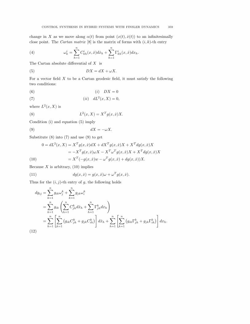
Let X be a vector field on a section of TM in a neighborhood of a given trajec-tory α(t) = (x(t), x(t)). The absolute Cartan differential of X measures the local
CONTROL SYNTHESIS IN HYBRID SYSTEMS WITH FINSLER DYNAMICS 359
change in X as we move along α(t) from point (x(t), x(t)) to an infinitesimallyclose point. The Cartan matrix [8] is the matrix of forms with (i, k)-th entry
(4) ωik =
n∑
h=1
Cikh(x, x)dxh +
n∑
h=1
Γikh(x, x)dxh.
The Cartan absolute differential of X is
(5) DX = dX + ωX.
For a vector field X to be a Cartan geodesic field, it must satisfy the followingtwo conditions:
(i) DX = 0(6)
(ii) dL2(x, X) = 0,(7)
where L2(x, X) is
(8) L2(x, X) = XT g(x, x)X.
Condition (i) and equation (5) imply
(9) dX = −ωX.
Substitute (8) into (7) and use (9) to get
0 = dL2(x, X) = XT g(x, x)dX + dXT g(x, x)X + XT dg(x, x)X
= −XT g(x, x)ωX −XT ωT g(x, x)X + XT dg(x, x)X
= XT (−g(x, x)w − ωT g(x, x) + dg(x, x))X.(10)
Because X is arbitrary, (10) implies
(11) dg(x, x) = g(x, x)ω + ωT g(x, x).
Thus for the (i, j)-th entry of g, the following holds
dgij =n
∑
k=1
gikωkj +
n∑
k=1
gjkωki
=n
∑
k=1
gik
(
n∑
h=1
Ckjhdxh +
n∑
h=1
Γkjhdxh
)
=n
∑
h=1
[
n∑
k=1
(
gikCkjh + gjkCk
ih
)
]
dxh +n
∑
h=1
[
n∑
k=1
(
gikΓkjh + gjkΓk
ih
)
]
dxh.
(12)
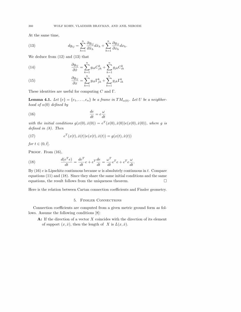
360 WOLF KOHN, VLADIMIR BRAYMAN, AND ANIL NERODE
At the same time,
(13) dgij =n
∑
h=1
∂gij
∂xhdxh +
n∑
h=1
∂gij
∂xhdxh.
We deduce from (12) and (13) that
∂gij
∂x=
n∑
k=1
gikCkjh +
n∑
k=1
gjkCkih(14)
∂gij
∂x=
n∑
k=1
gikΓkjh +
n∑
k=1
gjkΓkih(15)
These identities are useful for computing C and Γ.
Lemma 4.1. Let {e} = {e1, . . . , en} be a frame in TMα(0). Let U be a neighbor-hood of α(0) defined by
(16)de
dt= e
ω
dt
with the initial conditions g(x(0), x(0)) = eT (x(0), x(0))e(x(0), x(0)), where g isdefined in (8). Then
(17) eT (x(t), x(t))e(x(t), x(t)) = g(x(t), x(t))
for t ∈ (0, t].
Proof. From (16),
(18)d(eT e)
dt=
deT
dte + eT de
dt=
ωT
dteT e + eT e
ω
dt.
By (16) e is Lipschitz continuous because w is absolutely continuous in t. Compareequations (11) and (18). Since they share the same initial conditions and the sameequations, the result follows from the uniqueness theorem. £
Here is the relation between Cartan connection coefficients and Finsler geometry.
5. Finsler Connections
Connection coefficients are computed from a given metric ground form as fol-lows. Assume the following conditions [8]:
A: If the direction of a vector X coincides with the direction of its elementof support (x, x), then the length of X is L(x, x).
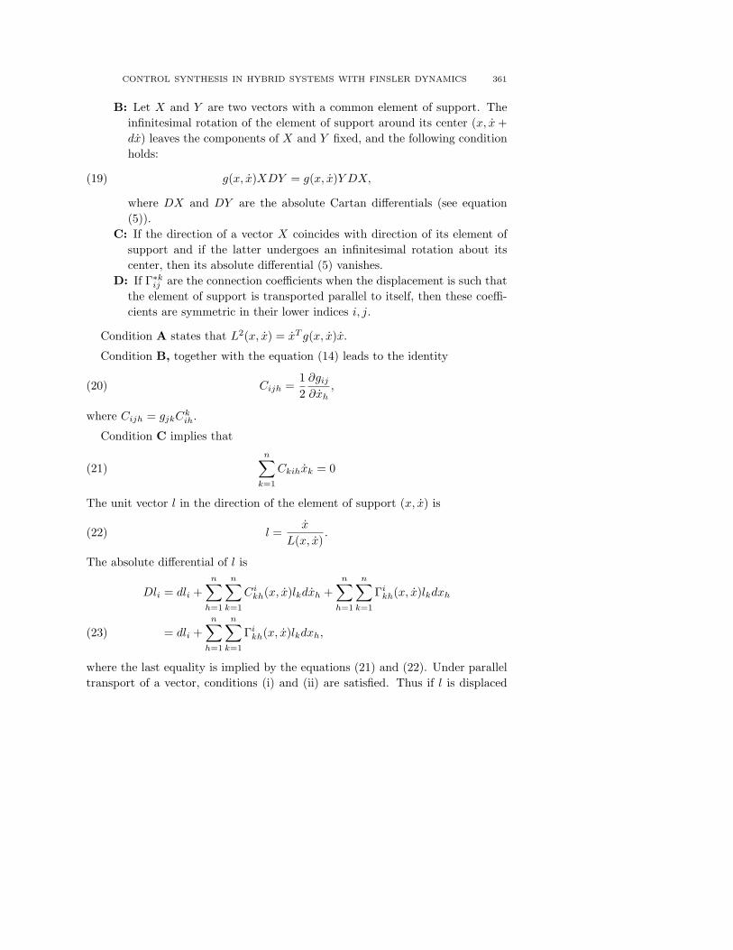
CONTROL SYNTHESIS IN HYBRID SYSTEMS WITH FINSLER DYNAMICS 361
B: Let X and Y are two vectors with a common element of support. Theinfinitesimal rotation of the element of support around its center (x, x +dx) leaves the components of X and Y fixed, and the following conditionholds:
(19) g(x, x)XDY = g(x, x)Y DX,
where DX and DY are the absolute Cartan differentials (see equation(5)).
C: If the direction of a vector X coincides with direction of its element ofsupport and if the latter undergoes an infinitesimal rotation about itscenter, then its absolute differential (5) vanishes.
D: If Γ∗kij are the connection coefficients when the displacement is such thatthe element of support is transported parallel to itself, then these coeffi-cients are symmetric in their lower indices i, j.
Condition A states that L2(x, x) = xT g(x, x)x.
Condition B, together with the equation (14) leads to the identity
(20) Cijh =12
∂gij
∂xh,
where Cijh = gjkCkih.
Condition C implies that
(21)n
∑
k=1
Ckihxk = 0
The unit vector l in the direction of the element of support (x, x) is
(22) l =x
L(x, x).
The absolute differential of l is
Dli = dli +n
∑
h=1
n∑
k=1
Cikh(x, x)lkdxh +
n∑
h=1
n∑
k=1
Γikh(x, x)lkdxh
= dli +n
∑
h=1
n∑
k=1
Γikh(x, x)lkdxh,(23)
where the last equality is implied by the equations (21) and (22). Under paralleltransport of a vector, conditions (i) and (ii) are satisfied. Thus if l is displaced
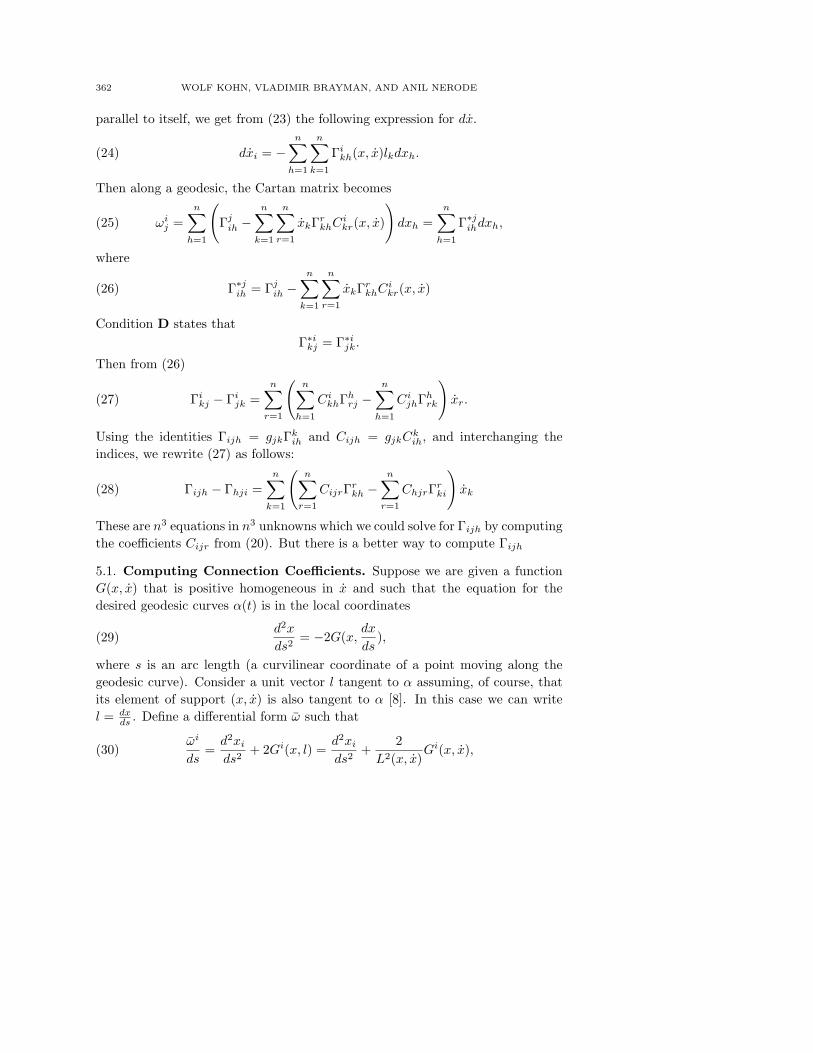
362 WOLF KOHN, VLADIMIR BRAYMAN, AND ANIL NERODE
parallel to itself, we get from (23) the following expression for dx.
(24) dxi = −n
∑
h=1
n∑
k=1
Γikh(x, x)lkdxh.
Then along a geodesic, the Cartan matrix becomes
(25) ωij =
n∑
h=1
(
Γjih −
n∑
k=1
n∑
r=1
xkΓrkhCi
kr(x, x)
)
dxh =n
∑
h=1
Γ∗jihdxh,
where
(26) Γ∗jih = Γjih −
n∑
k=1
n∑
r=1
xkΓrkhCi
kr(x, x)
Condition D states thatΓ∗ikj = Γ∗ijk.
Then from (26)
(27) Γikj − Γi
jk =n
∑
r=1
(
n∑
h=1
CikhΓh
rj −n
∑
h=1
CijhΓh
rk
)
xr.
Using the identities Γijh = gjkΓkih and Cijh = gjkCk
ih, and interchanging theindices, we rewrite (27) as follows:
(28) Γijh − Γhji =n
∑
k=1
(
n∑
r=1
CijrΓrkh −
n∑
r=1
ChjrΓrki
)
xk
These are n3 equations in n3 unknowns which we could solve for Γijh by computingthe coefficients Cijr from (20). But there is a better way to compute Γijh
5.1. Computing Connection Coefficients. Suppose we are given a functionG(x, x) that is positive homogeneous in x and such that the equation for thedesired geodesic curves α(t) is in the local coordinates
(29)d2x
ds2= −2G(x,
dx
ds),
where s is an arc length (a curvilinear coordinate of a point moving along thegeodesic curve). Consider a unit vector l tangent to α assuming, of course, thatits element of support (x, x) is also tangent to α [8]. In this case we can writel = dx
ds . Define a differential form ω such that
(30)ωi
ds=
d2xi
ds2+ 2Gi(x, l) =
d2xi
ds2+
2L2(x, x)
Gi(x, x),
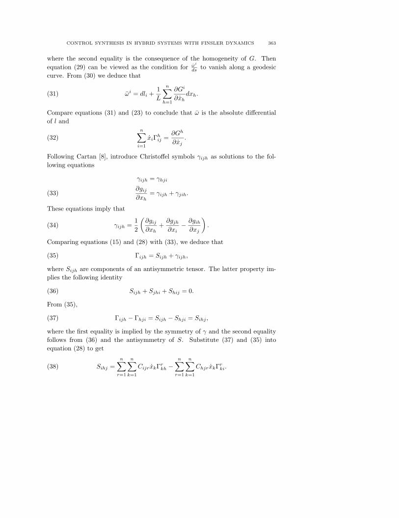
CONTROL SYNTHESIS IN HYBRID SYSTEMS WITH FINSLER DYNAMICS 363
where the second equality is the consequence of the homogeneity of G. Thenequation (29) can be viewed as the condition for ωi
ds to vanish along a geodesiccurve. From (30) we deduce that
(31) ωi = dli +1L
n∑
h=1
∂Gi
∂xhdxh.
Compare equations (31) and (23) to conclude that ω is the absolute differentialof l and
(32)n
∑
i=1
xiΓhij =
∂Gh
∂xj.
Following Cartan [8], introduce Christoffel symbols γijh as solutions to the fol-lowing equations
γijh = γhji
∂gij
∂xh= γijh + γjih.(33)
These equations imply that
(34) γijh =12
(
∂gij
∂xh+
∂gjh
∂xi− ∂gih
∂xj
)
.
Comparing equations (15) and (28) with (33), we deduce that
(35) Γijh = Sijh + γijh,
where Sijh are components of an antisymmetric tensor. The latter property im-plies the following identity
(36) Sijh + Sjhi + Shij = 0.
From (35),
(37) Γijh − Γhji = Sijh − Shji = Sihj ,
where the first equality is implied by the symmetry of γ and the second equalityfollows from (36) and the antisymmetry of S. Substitute (37) and (35) intoequation (28) to get
(38) Sihj =n
∑
r=1
n∑
k=1
CijrxkΓrkh −
n∑
r=1
n∑
k=1
ChjrxkΓrki.

364 WOLF KOHN, VLADIMIR BRAYMAN, AND ANIL NERODE
Using (32) in (38), we get
(39) Sihj =n
∑
r=1
n∑
k=1
Cijr∂Gr
∂xh−
n∑
r=1
n∑
k=1
Chjr∂Gr
∂xi.
Equations (35) and (39) give the desired result
(40) Γihj = γihj +n
∑
r=1
n∑
k=1
Cijr∂Gr
∂xh−
n∑
r=1
n∑
k=1
Chjr∂Gr
∂xi,
where γihj can be found from (34) and Cijr can be found from (20).
6. Bellman’s Blueprint In Finsler Spaces
We now show how Bellman equation is a blueprint in the Finsler context forthe extraction of control policies and the implementation of control loops. Asecond, subtler, use for the Bellman equation is to extract feedback correction torevise control polices when additional information about the environment facedand the inadequacies of the system model become available on line during theoperation of the system. This is a form of adaptation. The Bellman equationhere arises from a dynamic programming formulation of the variational problemon the associated Finsler manifold. Solutions are implemented by a differentialinclusion procedure. Bellman’s equation plays a role here similar to the role ofHamilton-Jacobi equations in classical mechanical systems.
Below are the necessary and sufficient conditions for optimal solutions of theFinsler variational problem assuming that Bellman’s Principle of Optimality holdsfor the problem [3].
Let L be a constrained Finsler Lagrangian over TM (see Section 4). We for-mulate the desired behavior of the system as solution trajectories of the followingvariational problem
Problem 1.
(41) minimize
T∫
0
L(x(t), x(t))dt,
over a family of curves α(t) on an open set U of a constraint manifold M , with theprescribed boundary condition α(T ) ∈ G and subject to (α(t), α(t)) = (x(t), v(t)),v(t) ∈ TMx(t).
CONTROL SYNTHESIS IN HYBRID SYSTEMS WITH FINSLER DYNAMICS 365
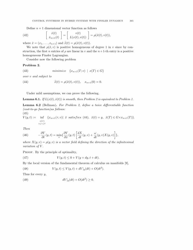
Define n + 1 dimensional vector function as follows
(42)[
x(t)xn+1(t)
]
=[
v(t)L(x(t), v(t))
]
= ρ(x(t), v(t)),
where x = (x1, . . . , xn+1) and ˙x(t) = ρ(x(t), v(t)).We note that ρ(x, v) is positive homogeneous of degree 1 in v since by con-
struction, the first n entries of ρ are linear in v and the n+1-th entry is a positivehomogeneous Finsler Lagrangian.
Consider now the following problem
Problem 2.
(43) minimize {xn+1(T ; v) | x(T ) ∈ G}
over v and subject to
(44) ˙x(t) = ρ(x(t), v(t)), xn+1(0) = 0.
Under mild assumptions, we can prove the following.
Lemma 6.1. If L(x(t), x(t)) is smooth, then Problem 2 is equivalent to Problem 1.
Lemma 6.2 (Bellman). For Problem 2, define a twice differentiable function(cost-to-go function)as follows:(45)V (y, t) := inf
v(τ)t≤τ≤T
{xn+1(τ, v)| x satisfies (44), x(t) = y, x(T ) ∈ G×xn+1(T )}.
Then
(46) −∂V
∂t(y, t) = min
v{∂V
∂x(y, t)
[
dX
dt(y, v) +
ω
dt(y, v)X(y, v)
]
},
where X(y, v) = ρ(y, v) is a vector field defining the direction of the infinitesimalvariation of V .
Proof. By the principle of optimality,
(47) V (y, t) ≤ 0 + V (y + dy, t + dt).
By the local version of the fundamental theorem of calculus on manifolds [9],
(48) V (y, t) ≤ V (y, t) + dV |y(dt) + O(dt2).
Thus for every y,
(49) dV |y(dt) + O(dt2) ≥ 0.

366 WOLF KOHN, VLADIMIR BRAYMAN, AND ANIL NERODE
Expanding dV , we get
(50) 0 ≤ ∂V
∂t(y, t)dt +
∂V
∂x(y, t)DX + O(dt2),
where DX is the absolute differential of X (see equation (5)). Then we canrewrite (50) as follows
(51) 0 ≤ ∂V
∂t(y, t)dt +
∂V
∂x(y, t)
[
dX
dt+
ω
dtX
]
dt + O(dt2)
Dividing by dt and taking the limit as dt → 0,
(52) −∂V
∂t(y, t) = min
v{∂V
∂x(y, t)
[
dX
dt+
ω
dtX
]
},
where X and ω depend on y and v. £
Equation (52) is a necessary condition for optimality in Problem 2 and henceProblem 1. Let α(t) be an optimal solution of Problem 1.
Theorem 6.3. The Solution of Problem 2 is a Cartan geodesic field.
Proof. Observe that the only term in (52) that depends on v is[
dXdt (y, v) + ω
dt (y, v)X(y, v)]
. Since V (·, ·) is constant along optimal solutions,
(53)∂V
∂t(y, t) = 0.
Since this is true along a Cartan geodesic field (see equation (9)), the resultfollows. £
We showed that V (·, ·) is constant along optimal solutions and non-decreasingalong solutions of (44). These properties together with the final value V (·, T ) =xn+1(T ) characterize this function [10].
Later on in Section 7, we will consider a mechanism that will construct a Cartangeodesic using the mathematical machinery developed in the present section.
7. The Control Loop
7.1. Active Geometric Constraints. Consider a gradient of the constraintvector KT
z evaluated at a certain state (z, z). Let (v1, . . . , vm) be column vectorsof KT
z . Then we define (v1, . . . , vm) to be an orthonormal basis obtained fromv’s using the KVD procedure. Define also (e1, . . . , en) to be the canonical or-thonormal basis of Rn. Introduce a transformation (e1, . . . , en) → (e′1, . . . , e
′n) as
CONTROL SYNTHESIS IN HYBRID SYSTEMS WITH FINSLER DYNAMICS 367
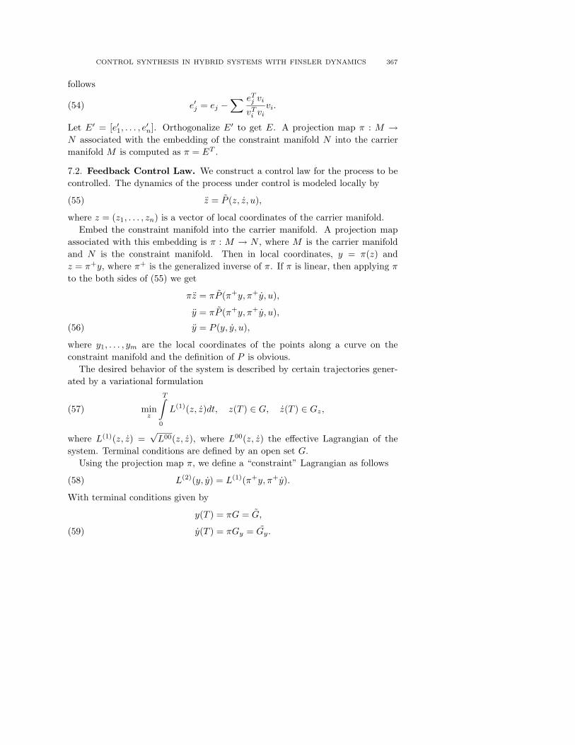
follows
(54) e′j = ej −∑ eT
j vi
vTi vi
vi.
Let E′ = [e′1, . . . , e′n]. Orthogonalize E′ to get E. A projection map π : M →
N associated with the embedding of the constraint manifold N into the carriermanifold M is computed as π = ET .
7.2. Feedback Control Law. We construct a control law for the process to becontrolled. The dynamics of the process under control is modeled locally by
(55) z = P (z, z, u),
where z = (z1, . . . , zn) is a vector of local coordinates of the carrier manifold.Embed the constraint manifold into the carrier manifold. A projection map
associated with this embedding is π : M → N , where M is the carrier manifoldand N is the constraint manifold. Then in local coordinates, y = π(z) andz = π+y, where π+ is the generalized inverse of π. If π is linear, then applying π
to the both sides of (55) we get
πz = πP (π+y, π+y, u),
y = πP (π+y, π+y, u),
y = P (y, y, u),(56)
where y1, . . . , ym are the local coordinates of the points along a curve on theconstraint manifold and the definition of P is obvious.
The desired behavior of the system is described by certain trajectories gener-ated by a variational formulation
(57) minz
T∫
0
L(1)(z, z)dt, z(T ) ∈ G, z(T ) ∈ Gz,
where L(1)(z, z) =√
L00(z, z), where L00(z, z) the effective Lagrangian of thesystem. Terminal conditions are defined by an open set G.
Using the projection map π, we define a “constraint” Lagrangian as follows
(58) L(2)(y, y) = L(1)(π+y, π+y).
With terminal conditions given by
y(T ) = πG = G,
y(T ) = πGy = Gy.(59)
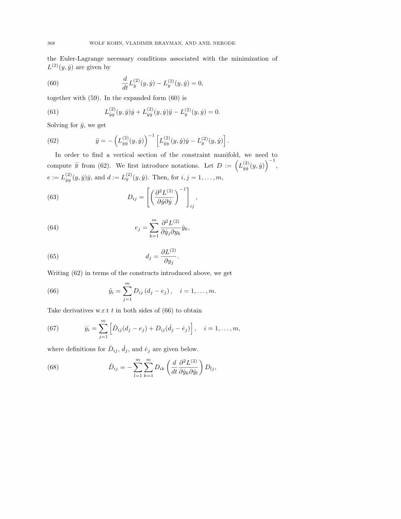
368 WOLF KOHN, VLADIMIR BRAYMAN, AND ANIL NERODE
the Euler-Lagrange necessary conditions associated with the minimization ofL(2)(y, y) are given by
(60)d
dtL
(2)y (y, y)− L(2)
y (y, y) = 0,
together with (59). In the expanded form (60) is
(61) L(2)yy (y, y)y + L
(2)yy (y, y)y − L(2)
y (y, y) = 0.
Solving for y, we get
(62) y = −(
L(2)yy (y, y)
)−1 [
L(2)yy (y, y)y − L(2)
y (y, y)]
.
In order to find a vertical section of the constraint manifold, we need to
compute...y from (62). We first introduce notations. Let D :=
(
L(2)yy (y, y)
)−1
,
e := L(2)yy (y, y)y, and d := L
(2)y (y, y). Then, for i, j = 1, . . . , m,
(63) Dij =
[
(
∂2L(2)
∂y∂y
)−1]
ij
,
(64) ej =m
∑
k=1
∂2L(2)
∂yj∂ykyk,
(65) dj =∂L(2)
∂yj.
Writing (62) in terms of the constructs introduced above, we get
(66) yi =m
∑
j=1
Dij (dj − ej) , i = 1, . . . , m.
Take derivatives w.r.t t in both sides of (66) to obtain
(67)...yi =
m∑
j=1
[
Dij(dj − ej) + Dij(dj − ej)]
, i = 1, . . . , m,
where definitions for Dij , dj , and ej are given below.
(68) Dij = −m
∑
l=1
m∑
k=1
Dik
(
d
dt
∂2L(2)
∂yk∂yl
)
Dlj ,
CONTROL SYNTHESIS IN HYBRID SYSTEMS WITH FINSLER DYNAMICS 369
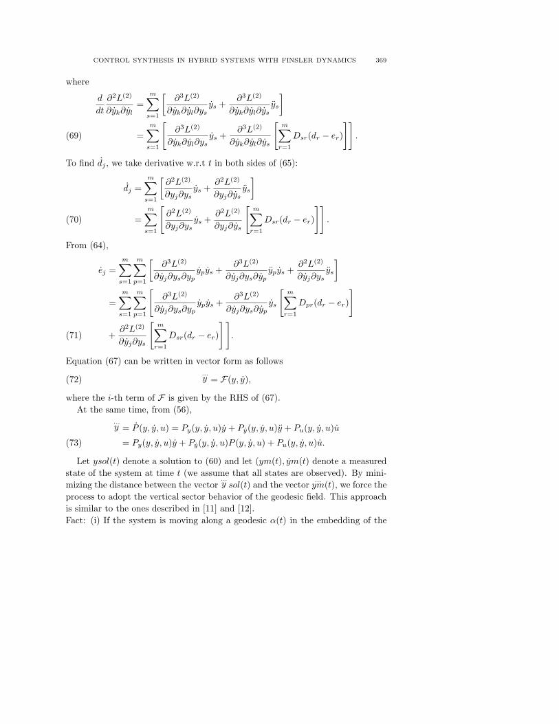
where
d
dt
∂2L(2)
∂yk∂yl=
m∑
s=1
[
∂3L(2)
∂yk∂yl∂ysys +
∂3L(2)
∂yk∂yl∂ysys
]
=m
∑
s=1
[
∂3L(2)
∂yk∂yl∂ysys +
∂3L(2)
∂yk∂yl∂ys
[
m∑
r=1
Dsr(dr − er)
]]
.(69)
To find dj , we take derivative w.r.t t in both sides of (65):
dj =m
∑
s=1
[
∂2L(2)
∂yj∂ysys +
∂2L(2)
∂yj∂ysys
]
=m
∑
s=1
[
∂2L(2)
∂yj∂ysys +
∂2L(2)
∂yj∂ys
[
m∑
r=1
Dsr(dr − er)
]]
.(70)
From (64),
ej =m
∑
s=1
m∑
p=1
[
∂3L(2)
∂yj∂ys∂ypypys +
∂3L(2)
∂yj∂ys∂ypypys +
∂2L(2)
∂yj∂ysys
]
=m
∑
s=1
m∑
p=1
[
∂3L(2)
∂yj∂ys∂ypypys +
∂3L(2)
∂yj∂ys∂ypys
[
m∑
r=1
Dpr(dr − er)
]
+∂2L(2)
∂yj∂ys
[
m∑
r=1
Dsr(dr − er)
] ]
.(71)
Equation (67) can be written in vector form as follows
(72)...y = F(y, y),
where the i-th term of F is given by the RHS of (67).At the same time, from (56),
...y = P (y, y, u) = Py(y, y, u)y + Py(y, y, u)y + Pu(y, y, u)u
= Py(y, y, u)y + Py(y, y, u)P (y, y, u) + Pu(y, y, u)u.(73)
Let ysol(t) denote a solution to (60) and let (ym(t), ym(t) denote a measuredstate of the system at time t (we assume that all states are observed). By mini-mizing the distance between the vector
...y sol(t) and the vector
...ym(t), we force the
process to adopt the vertical sector behavior of the geodesic field. This approachis similar to the ones described in [11] and [12].Fact: (i) If the system is moving along a geodesic α(t) in the embedding of the
370 WOLF KOHN, VLADIMIR BRAYMAN, AND ANIL NERODE
constraint manifold in the carrier manifold, no correction control is needed. Thusγ∗(α(t)) = 0, where γ∗(y(t)) := u(t) is the differential of the map γ(y(t)) := u(t)
(ii) If the invariant condition is not satisfied but the quasi-geodesic condition[13] is satisfied, then the process is following a curve β(t) (quasi-geodesic) satis-fying the following condition.
(74) |α(t)− β(τ)| ≤ κ|t− τ |,
where κ, a Lipschitz-like constant, defines the range of curves close enough tothe geodesic pipe so that the control law proposed below maintains a boundeddistance between α and β. The control law, u(t) = γ(y(t)) must be applied tothe process to achieve this condition. Then we formulate a control problem asfollows. Find u such that the distance between ysol(t) and ym(t) is minimal incurvature, i.e.
(75) minu
{
(F − P )T (F − P )}
.
Theorem 7.1. If P (y, y, u) and F(y, y) satisfy sufficient smoothness conditionsand there exists a differentiable optimal feedback control law, then the rate of thiscontrol law is given by
u(t) = γ∗(ysol(t), ysol(t), ym(t), ym(t))
=(
PTu (ym(t), ym(t), u(t))Pu(ym(t), ym(t), u(t))
)−1PT
u (ym(t), ym(t), u(t))(
F(ysol(t), ysol(t))− Py(ym(t), ym(t), u(t))ym
− Py(ym(t), ym(t), u(t))P (ym(t), ym(t), u(t)))
(76)
Proof. The existence of the optimal u is assured by the convexity of the objectivefunction in (75). Necessary condition for optimality (without constraints) can bewritten as
(77)d
du
(
FTF − FT P − PTF + PT P
)
= 0.
CONTROL SYNTHESIS IN HYBRID SYSTEMS WITH FINSLER DYNAMICS 371
Substitute for P from (73) and simplify to get
F(ysol(t), ysol(t))− Py(ym(t), ym(t), u(t))ym
− Py(ym(t), ym(t), u(t))P (ym(t), ym(t), u(t))
= Pu(ym(t), ym(t), u(t))u(t).(78)
Using the right pseudo-inverse of Pu, the result follows immediately. £
Note that, according to Theorem 7.1, if two curvatures match exactly, u(t) = 0and thus no change in control is needed.
7.3. The Inverse Variational Problem. This subsection is devoted to theconstruction of a non-negative Lagrangian L on the carrier manifold of the system,the traditional ”inverse variational problem” when the problem starts withouta Lagrangian. Given a second order differential equation, we construct a non-negative Lagrangian such that the extremals which minimize this Lagrangian arethe solutions of the original differential equation. These extremals might or mightnot be physically realizable. We use approximation techniques to find a physicallyrealizable approximations to them.
Consider a vector second order differential equation
(79) x = F (x, x, t)
Consider also the Euler-Lagrange equations
(80)d
dtLxi(x, x)− Lxi(x, x) = 0, i = 1, . . . , n
Write (80) as
(81) ∂Lx(x, x)
x
x
1
− Lx(x, x) = 0,
where ∂Lx =[
(Lxixj ) (Lxixj ) Lxt
]
, i, j = 1, . . . , n.Substitute for x from the equation (79):
(82) ∂Lx(x, x)
x
F
1
− Lx(x, x) = 0,
372 WOLF KOHN, VLADIMIR BRAYMAN, AND ANIL NERODE
Take the derivative with respect to x from the both sides of this equation:
[
∂Lxx1(x, x) ∂Lxx2(x, x) . . . ∂Lxxn(x, x)]
x
F
1
+ ∂Lx(x, x)
I
Fx
0
−Lxx(x, x) = 0.
(83)
where I is the identity matrix and Fx =[
∂F∂x1
∂F∂x2
. . . ∂F∂xn
]
. With the
assumptions that L is in C3 and the mixed partials are continuous, the followingrelations hold: Lxxx = Lxxx, and Lxtx = Lxxt. Thus the equation (83) can berewritten as
(84)d
dtLxx(x, x) + Lxx(x, x) + Lxx(x, x)Fx(x, x, t)− Lxx(x, x) = 0.
Take the transpose of (84) using the fact that(
ddtLxx
)T= d
dtLxx
(85)d
dtLxx(x, x) + Lxx(x, x) + (Fx)T (x, x, t)Lxx(x, x)− Lxx(x, x) = 0.
Add (84) and (85) and divide by 2 to get the Lyapunov equation
(86) − d
dtΨ =
12FT
x Ψ +12ΨFx
where Ψ(x, x) = Lxx. The solution of this equation will give the desired Lxx.
7.4. Bellman’s Inverse Problem. Here is the Bellman inverse problem [3].Given a local control law x = v(y, t) that determines V (y, t), we would like tofind a function L(x, x) such that
(87) V (y, t) = minx
T∫
t
L(x, x)dt, x(t) = y.
Note that the cost-to-go function V (y, t) is constant along a geodesic line givenby v(y, t) and the boundary condition is V (y, T ) = 0. Under the conditions forBellman’s principle of optimality,
(88) V (y, t) = minv
[L(y, v)∆ + V (exp(∆v)y, t + ∆)] + O(∆2).
CONTROL SYNTHESIS IN HYBRID SYSTEMS WITH FINSLER DYNAMICS 373
Expand V (exp(∆v)y, t + ∆) in the Lie-Taylor series [14], page 31.
V (exp(∆v)y, t + ∆) = V (y, t) + ∆v(V )(y, t) + ∆∂V
∂t(y, t) + O(∆2)
= V (y, t) + ∆n
∑
i=1
ξi(y, t)∂V
∂yi(y, t) + ∆
∂V
∂t(y, t) + O(∆2),
(89)
where (y1, . . . , yn) are local coordinates of the point y and v(y, t) =n∑
i=1
ξi(y, t) ∂∂yi
.
If we denote v(y, t) = [ξ1(y, t), . . . , ξn(y, t)]T and ∂V∂y = [ ∂V
∂y1, . . . , ∂V
∂yn], then (89)
can be rewritten in a vector form as
(90) V (exp(∆v)y, t + ∆) = V (y, t) + ∆∂V
∂y(y, t)v(y, t) + ∆
∂V
∂t(y, t) + O(∆2).
Substitute (90) into (88) and simplify, to get
(91) −∆∂V
∂t(y, t) = min
v
[
L(y, v)∆ + ∆∂V
∂y(y, t)v(y, t)
]
+ O(∆2).
Divide by ∆ and let ∆ → 0, to get the Hamilton-Jacobi-Bellman equation:
(92) −∂V
∂t(y, t) = min
v
[
L(y, v) +∂V
∂y(y, t)v(y, t)
]
, V (y, T ) = 0.
Now assume that L is twice differentiable and convex in x. Then for the given(optimal) v, Lx(y, v) + ∂V
∂y (y, t) = 0. Then (92) can be rewritten as
∂V
∂t(y, t) = Lx(y, v)v(y, t)− L(y, v)(93)
∂V
∂y(y, t) = −Lx(y, v).(94)
The differential of V (y, t) is given by
dV =∂V
∂y(y, t)dy +
∂V
∂t(y, t)dt(95)
= −Lx(y, v)dy + (Lx(y, v)v(y, t)− L(y, v)) dt.(96)
Along a geodesic, V is constant and thus dV = 0. Then
(97) Lx(y, v)v = L(y, v),
(98) Lx = 0.
Equation (97) shows that L(y, v) is positive homogeneous of degree one in x.We also can show that the optimal control can be written in the form [15]
374 WOLF KOHN, VLADIMIR BRAYMAN, AND ANIL NERODE
(99) γ(y) = exp(γy y)εγ(0).
8. Conclusion
This paper illustrated some tools from Finsler geometry used to extract controlpolicies, mostly by symbolic computation. These have all been implemented.
There are many other areas of science in which the Caratheodory-Finsler-Cartan translation of variational problems, and these same tools, may prove tobe of equal value. The strategy that physicists have used for 25 years in designingconnections, gauge fields, for a given problem is valuable here too. We are cur-rently investigating algorithms for constructing connections to meet given systemgoals without using an explicit variational formulation or the inverse variationalmethod. Much of the algebra of linear connections and gauge fields has alreadybeen used in particle physics for similar purposes. We believe this algebra isequally useful here for boutique control program design. We see useful Finslerspaces now all around us.
References
[1] R. L. Grossman, A. Nerode, A. Ravn, and H.Rischel, eds., Hybrid Systems, Lecture Notes
in Computer Science 736, Springer-Verlag, 1993.
[2] P. Antsaklis, W. Kohn, A. Nerode, S. Sastry, eds., Hybrid Systems II, Lecture Notes in
Computer Science vol. 999, Springer-Verlag, 1995.
[3] R. Bellman, Dynamic Programming, Princeton University Press, Princeton, NJ, 1957.
[4] W. Kohn, A Declarative Theory for Rational Controllers, Proc. 27th IEEE CDC, 1988,
130-136.
[5] W. Kohn, Declarative Multiplexed Rational Controllers, Proceedings of the 5th IEEE
International Symposium on Intelligent Control, Philadelphia, PA, 1990.
[6] W. Kohn, Declarative Hierarchical Controllers, Proceedings of the Workshop on Software
Tools for Distributed Intelligent Control Systems, Pacifica, CA., 1990, 141-163.
[7] L. C. Young, Lectures on the Calculus of Variations and Optimal Control Theory, Chelsea
Publishing Company, New York, N.Y., 1980.
[8] E. Cartan, Exposes de geometrie, Hermann, Paris, 1971.
[9] R. W. Sharpe, Differential Geometry. Cartan’s Generalization of Klein’s Erlangen Prob-
lem, Springer, New York, 1997.
[10] Helene Frankowska, Lower Semicontinuous Solutions of Hamilton-Jacobi-Bellman Equa-
tions, SIAM J. Control and Optimization, v.31(1), 1993, 257-272.
[11] D. Bao and S. S. Chern, On a notable connection in Finsler geometry, Houston J. math.,
v.19, 1993, 135-180
[12] Patrick Foulon, Geometrie des equations defferentielles du second ordre, Ann. Inst. Henri
Poincare, v.45(1), 1986, 1-28.
CONTROL SYNTHESIS IN HYBRID SYSTEMS WITH FINSLER DYNAMICS 375
[13] Shlomo Sternberg, Lectures on Differential Geometry, Chelsea Publishing Company, New
York, N.Y., 1983.
[14] Peter J. Olver, Applications of Lie Groups to Differential Equations, second edition,
Springer-Verlag, 1993.
[15] Wolf Kohn, Vladimir Brayman, and Jeffrey Remmel, Hybrid Systems Approach to Optimal
Enterprise Control, to be published by Kluwer Academic Publishers, 2002.
Received November 26, 2001
Hynomics Corporation,Kirkland, WA 98033-7921
E-mail address: [email protected]
Hynomics Corporation,Kirkland, WA 98033-7921
E-mail address: [email protected]
Department of Mathematics, Cornell University, Ithaca, New York 14853
E-mail address: [email protected]


