arX

iv:m

ath/

0303

246v

1 [

mat

h.Q

A]

20

Mar

200

3

CONSTRUCTING r−MATRICES ON SIMPLE LIE

SUPERALGEBRAS

GIZEM KARAALI

Abstract. We construct r−matrices for simple Lie superalgebras with non-degenerate Killing forms using Belavin-Drinfeld type triples. This constructiongives us the standard r−matrices and some nonstandard ones.

1. Introduction

Let g be a Lie algebra with a non-degenerate g−invariant bilinear form ( , ).Denote by Ω the element of (g ⊗ g)g that corresponds to the quadratic Casimirelement in Ug of g. Then the classical Yang-Baxter equation (CYBE) for anelement r ∈ g ⊗ g is:

[r12, r13] + [r12, r23] + [r13, r23] = 0.

A solution r to the classical Yang-Baxter equation is called a classical r−matrix(or simply an r−matrix). An r−matrix r is called non-degenerate if it satisfies:

r12 + r21 = Ω.

In [1] and [2] Belavin and Drinfeld classified such r−matrices. The solutions in thisclassification are parametrized by triples (Γ1,Γ2, τ) (called admissible triples)where the Γi are certain subsets of the set Γ of simple roots of g, and τ : Γ1 → Γ2 isan isometric bijection. They proved that for each admissible triple and some fixedr0 ∈ g ⊗ g there exists a unique non-degenerate classical r−matrix, and converselythat each non-degenerate classical r−matrix can be associated with such data.

In this paper we construct classical r−matrices using analogs of the Belavin-Drinfeld data for simple Lie superalgebras with non-degenerate Killing form. Wefirst start with a review of the situation in the Lie algebra case. Thus in Section 2we give an overview of the Belavin-Drinfeld result for simple Lie algebras. Next, inSection 3, we recall some basic definitions and results about simple Lie superalge-bras. Then after developing the necessary ingredients we state our main theorem.The next three sections of the paper are devoted to the proof of this theorem. Thenin Section 7 we construct various r−matrices for the Lie superalgebra sl(2, 1) usingthe main theorem.

This theorem is very much in the spirit of the Belavin-Drinfeld result. It tellsus that, given a Belavin-Drinfeld type triple, one can construct a non-degenerater−matrix in a way similar to the construction in the Lie algebra case. One shouldpoint out, however, that this is not a complete classification result. The theoremgives us r−matrices, but does not tell us whether we can always extract a Belavin-Drinfeld type triple from a given r−matrix. We discuss this briefly in the lastsection of the paper.

1

2 GIZEM KARAALI

Acknowledgments. I would like to thank Nicolai Reshetikhin for fruitful discus-sions, Vera Serganova for her close attention and useful suggestions, and MilenYakimov for introducing me to the Belavin-Drinfeld result. This work was sup-ported by the NSF grant DMS−0070931.

2. Classification Theorem for Lie Algebras

Here we recall briefly the main result of [1] and [2] for Lie algebras. Let g bea simple Lie algebra. Fixing a positive Borel subalgebra b+ determines a Cartansubalgebra h for g, and we can talk about positive roots, simple roots etc. Hencewe can define Γ = α1, α2, · · · , αr to be the set of all simple roots of g. We willbe interested in admissible triples, i.e. triples (Γ1,Γ2, τ) where Γi ⊂ Γ andτ : Γ1 → Γ2 is a bijection such that

(1) for any α, β ∈ Γ1, (τ(α), τ(β)) = (α, β);(2) for any α ∈ Γ1 there exists a k ∈ N such that τk(α) 6∈ Γ1.

1

We will also need a continuous parameter r0, an element of h⊗ h which satisfiesthe following equations:

r012 + r0

21 = Ω0 (1)

(τ(α) ⊗ 1)(r0) + (1 ⊗ α)(r0) = 0 for all α ∈ Γ1 (2)

where Ω0 ∈ h ⊗ h is the h−component of the quadratic Casimir element Ω of g.Fix a system of Weyl-Chevalley generators Xα, Yα, Hα for α ∈ Γ. Recall that

these elements generate the Lie algebra g with the defining relations: [Xαi, Yαj

] =δi,jHαj

, [Hαi, Xαj

] = ai,jXαjand [Hαi

, Yαj] = −ai,jYαj

for all αi, αj ∈ Γ, where

ai,j = αj(Hαi) =

2(αi,αj)(αi,αi)

, along with the well-known Serre relations.

Denote by gi the subalgebra of g generated by the elements Xα, Yα, Hα for allα ∈ Γi. We define a map ϕ by:

ϕ(Xα) = Xτ(α) ϕ(Yα) = Yτ(α) ϕ(Hα) = Hτ(α)

for all α ∈ Γ1. Then this can be extended to an isomorphism ϕ : g1 → g2 becausethe relations between Xα, Yα, Hα for α ∈ Γ1 will be the same as the relationsbetween Xτ(α), Yτ(α), Hτ(α) for α ∈ Γ1. Note that this requires the first property of

τ , namely that it is an isometry. Next extend τ to a bijection between the Γi, whereΓi is the set of those roots which can be written as a nonnegative integral linearcombination of the elements of Γi. In each root space gα, we choose an element eαsuch that (eα, e−α) = 1 for any α and ϕ(eα) = eτ(α) for all α ∈ Γ1

2. Finally wedefine a partial order on the set of all positive roots:

α < β if and only if there exists a k ∈ N such that β = τk(α)

1The expression τk(α) has a meaning only if the expressions τj(α) for all j < k are elementsof Γ1. So this condition actually may be translated as saying that τk(α) does not make sense forlarge enough k.

2Such eα can always be chosen consistently if “there are no cycles ”, i.e. if τ satisfies thesecond property. Otherwise, if there is a cycle of simple roots α1, · · · , αk such that τ(αi) = αi+1

for i = 1, 2, · · · , k−1 and τ(αk) = α1 and τ is an isometry, then we must have that (αi, αi+1) = 0

for all i = 1, 2, · · · , k−1, since no cycles are allowed in Dynkin diagrams. Then if s is the smallestinteger such that (α1, α1+s) 6= 0, then s > 1 and s|k. So our cycle must have s disconnectedsubgraphs of length k/s. Then we can still choose eα consistently, provided we allow only cyclesas above.

CONSTRUCTING r−MATRICES ON SIMPLE LIE SUPERALGEBRAS 3

Note that in this case we will have α ∈ Γ1, β ∈ Γ2. Clearly one needs property 2for a partial order; no cycles are allowed in partial orders.

Now we can state the Belavin-Drinfeld theorem:

Theorem 1. (1) Let r0 ∈ h ⊗ h satisfy Equations 1 and 2. Then the element r ofg ⊗ g defined by:

r = r0 +∑

α>0

e−α ⊗ eα +∑

α,β>0,α<β

(e−α ⊗ eβ − eβ ⊗ e−α)

is a solution to the system:r12 + r21 = Ω (3)

[r12, r13] + [r12, r23] + [r13, r23] = 0 (4)

(2) Any solution (up to isomorphism) to the above system can be obtained as aboveby a suitable choice of an admissible triple (Γ1,Γ2, τ) and some r0 ∈ h ⊗ h thatsatisfies Equations 1 and 2.

The proof of this theorem provided in [2] is actually quite clear; one can alsolook at [3] for another exposition.

3. The Construction Theorem for Lie Superalgebras

Now our aim is to develop a similar theory for super structures. Let g be asimple Lie superalgebra with a non-degenerate Killing form 3.

3.1. The Quadratic Casimir Element: Let Iα be a homogeneous basis for g

and denote by Iα∗ the dual basis of g with respect to the non-degenerate (Killing)

form. Thus we have:(Iα, Iβ

∗) = δαβ

If we denote the parity of a homogeneous element x ∈ g by |x|, then we also havethat

|Iα| = |Iα∗|

since the supertrace form is consistent [Recall that a bilinear form ( , ) is consistentif for any homogeneous x, y ∈ g of different parities, (x, y) = 0].

We can write the quadratic Casimir element of g as follows:

Ω =∑

α

(−1)|Iα||Iα∗|Iα ⊗ Iα

∗ =∑

α

(−1)|Iα|Iα ⊗ Iα∗

Example 1. For the special case g = gl(m,n) with basis ei,j |1 ≤ i, j ≤ m+ n,we use the supertrace form to find the dual basis:

ei,j∗ = (−1)[i]ej,i

where

[j] =

0 if j ≤ m1 if j > m

Then this gives us:

Ω =∑

α

(−1)|Iα|Iα ⊗ Iα∗ =

∑

i,j

(−1)|ei,j |ei,j ⊗ (−1)[i]ej,i =∑

i,j

(−1)[j]ei,j ⊗ ej,i

3This implies that g is isomorphic to a simple Lie algebra or to one of the following classicalLie superalgebras: A(m, n) with m 6= n, B(m, n), C(n), D(m, n) with m − n 6= 1, F (4), or G(3).See [4] for details.

4 GIZEM KARAALI

3.2. Borel subsuperalgebras and Dynkin diagrams: Let h be a Cartan sub-algebra. By definition, h ⊂ g0 is a Cartan subalgebra of the even part of our Liesuperalgebra. Let ∆ = ∆0 + ∆1 be the set of all roots of g associated with theCartan subalgebra h 4, where ∆0 and ∆1 are the even and odd roots respectively.Fix a Borel subsuperalgebra b containing h. Recall that a Lie subsuperalgebrab of a Lie superalgebra g is a Borel subsuperalgebra if there is some Cartansubsuperalgebra h of g and some base Γ for ∆, such that

b = h ⊕⊕

α∈∆+

gα

where ∆+ consists of all nonnegative integral combinations of the elements of Γthat are in ∆.

In the Lie algebra case subalgebras given by this definition turn out to be max-imally solvable, and all maximally solvable subalgebras of a simple Lie algebra areof this type. Thus this definition agrees with the usual definition of a Borel sub-algebra as a maximally solvable subalgebra. However Borel subsuperalgebras asdefined above are not necessarily maximally solvable.

Example 2. Let g be a Lie superalgebra, fix some set ∆+ of positive roots, and letα be a positive isotropic root. Define b as the sum of all the positive root spaces.Then b is a Borel subsuperalgebra but is not maximally solvable. The (parabolic 5)subsuperalgebra p = b ⊕ g−α is also solvable.

In fact maximally solvable subsuperalgebras may be even more complicated. [See[6] for a study of maximally solvable subsuperalgebras of gl(m,n) and sl(m,n).]Therefore we choose to define Borels as above instead of using the more traditionalcharacterization by maximal solvability.

Thus Borel subsuperalgebras determine simple roots, and different Borel sub-superalgebras may correspond to different Dynkin diagrams and Cartan matrices.Let us then fix some Borel subsuperalgebra b, or equivalently some set Γ of simpleroots, and the associated Dynkin diagram D. Note that Γ may contain even andodd roots. Another significant difference from the theory of Lie algebras is to benoted here; two Dynkin diagrams of a given Lie superalgebra are not necessarilyisomorphic, but can be obtained from one another via a chain of odd reflections.

3.3. The Data for the Theorem: In this setup, let ∆+ (resp. ∆−) be the set ofall positive (resp. negative) roots, with respect to the chosen Γ = α1, α2, · · · , αr.

Now let Γ1,Γ2 ⊂ Γ be two subsets, and τ : Γ1 → Γ2 be a bijection. We will saythat the triple (Γ1,Γ2, τ) is admissible if:

(1) for any α, β ∈ Γ1, (τ(α), τ(β)) = (α, β);(2) for any α ∈ Γ1 there exists a k ∈ N such that τk(α) 6∈ Γ1;(3) τ preserves grading, i.e. it maps even roots to even ones, and odd roots to

odd ones.

For a given admissible triple (Γ1,Γ2, τ), we define Γi for i = 1, 2 as in the Liealgebra case: Γi is the set of those roots which can be written as a nonnegative

4In fact ∆ is independent of the choice of h5As in the Lie algebra case, a Lie subsuperalgebra p is a parabolic subsuperalgebra if p

contains a Borel.

CONSTRUCTING r−MATRICES ON SIMPLE LIE SUPERALGEBRAS 5

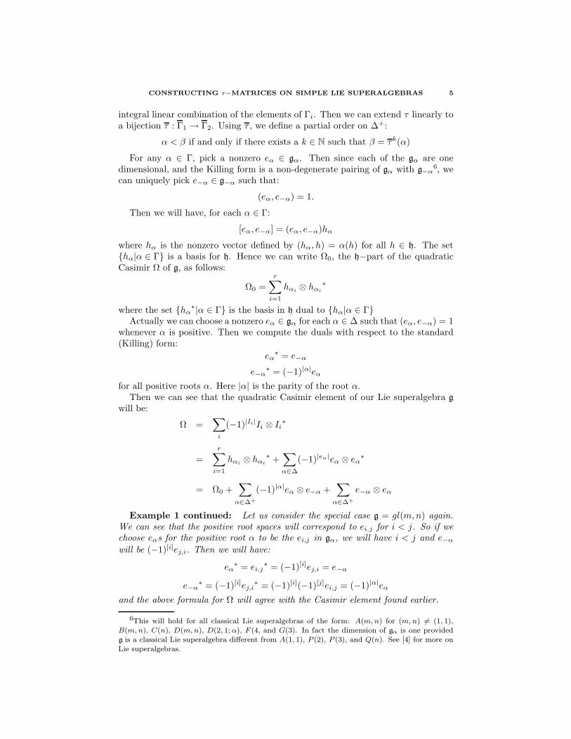
integral linear combination of the elements of Γi. Then we can extend τ linearly toa bijection τ : Γ1 → Γ2. Using τ , we define a partial order on ∆+:

α < β if and only if there exists a k ∈ N such that β = τk(α)

For any α ∈ Γ, pick a nonzero eα ∈ gα. Then since each of the gα are onedimensional, and the Killing form is a non-degenerate pairing of gα with g−α

6, wecan uniquely pick e−α ∈ g−α such that:

(eα, e−α) = 1.

Then we will have, for each α ∈ Γ:

[eα, e−α] = (eα, e−α)hα

where hα is the nonzero vector defined by (hα, h) = α(h) for all h ∈ h. The sethα|α ∈ Γ is a basis for h. Hence we can write Ω0, the h−part of the quadraticCasimir Ω of g, as follows:

Ω0 =r∑

i=1

hαi⊗ hαi

∗

where the set hα∗|α ∈ Γ is the basis in h dual to hα|α ∈ Γ

Actually we can choose a nonzero eα ∈ gα for each α ∈ ∆ such that (eα, e−α) = 1whenever α is positive. Then we compute the duals with respect to the standard(Killing) form:

eα∗ = e−α

e−α∗ = (−1)|α|eα

for all positive roots α. Here |α| is the parity of the root α.Then we can see that the quadratic Casimir element of our Lie superalgebra g

will be:

Ω =∑

i

(−1)|Ii|Ii ⊗ Ii∗

=

r∑

i=1

hαi⊗ hαi

∗ +∑

α∈∆

(−1)|eα|eα ⊗ eα∗

= Ω0 +∑

α∈∆+

(−1)|α|eα ⊗ e−α +∑

α∈∆+

e−α ⊗ eα

Example 1 continued: Let us consider the special case g = gl(m,n) again.We can see that the positive root spaces will correspond to ei.j for i < j. So if wechoose eαs for the positive root α to be the ei,j in gα, we will have i < j and e−αwill be (−1)[i]ej,i. Then we will have:

eα∗ = ei.j

∗ = (−1)[i]ej,i = e−α

e−α∗ = (−1)[i]ej,i

∗ = (−1)[i](−1)[j]ei,j = (−1)|α|eα

and the above formula for Ω will agree with the Casimir element found earlier.

6This will hold for all classical Lie superalgebras of the form: A(m, n) for (m, n) 6= (1, 1),B(m, n), C(n), D(m, n), D(2, 1; α), F (4, and G(3). In fact the dimension of gα is one providedg is a classical Lie superalgebra different from A(1, 1), P (2), P (3), and Q(n). See [4] for more onLie superalgebras.

6 GIZEM KARAALI

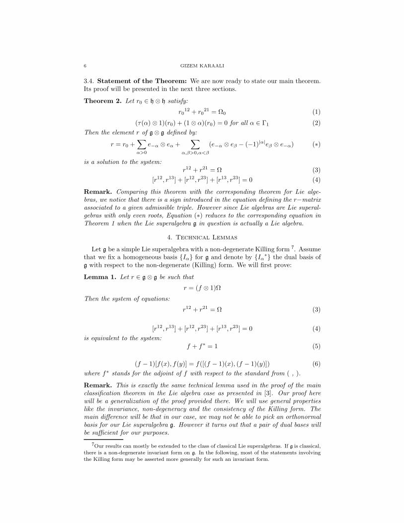
3.4. Statement of the Theorem: We are now ready to state our main theorem.Its proof will be presented in the next three sections.

Theorem 2. Let r0 ∈ h ⊗ h satisfy:

r012 + r0

21 = Ω0 (1)

(τ(α) ⊗ 1)(r0) + (1 ⊗ α)(r0) = 0 for all α ∈ Γ1 (2)

Then the element r of g ⊗ g defined by:

r = r0 +∑

α>0

e−α ⊗ eα +∑

α,β>0,α<β

(e−α ⊗ eβ − (−1)|α|eβ ⊗ e−α) (∗)

is a solution to the system:r12 + r21 = Ω (3)

[r12, r13] + [r12, r23] + [r13, r23] = 0 (4)

Remark. Comparing this theorem with the corresponding theorem for Lie alge-bras, we notice that there is a sign introduced in the equation defining the r−matrixassociated to a given admissible triple. However since Lie algebras are Lie superal-gebras with only even roots, Equation (∗) reduces to the corresponding equation inTheorem 1 when the Lie superalgebra g in question is actually a Lie algebra.

4. Technical Lemmas

Let g be a simple Lie superalgebra with a non-degenerate Killing form 7. Assumethat we fix a homogeneous basis Iα for g and denote by Iα

∗ the dual basis ofg with respect to the non-degenerate (Killing) form. We will first prove:

Lemma 1. Let r ∈ g ⊗ g be such that

r = (f ⊗ 1)Ω

Then the system of equations:

r12 + r21 = Ω (3)

[r12, r13] + [r12, r23] + [r13, r23] = 0 (4)

is equivalent to the system:f + f∗ = 1 (5)

(f − 1)[f(x), f(y)] = f([(f − 1)(x), (f − 1)(y)]) (6)

where f∗ stands for the adjoint of f with respect to the standard from ( , ).

Remark. This is exactly the same technical lemma used in the proof of the mainclassification theorem in the Lie algebra case as presented in [3]. Our proof herewill be a generalization of the proof provided there. We will use general propertieslike the invariance, non-degeneracy and the consistency of the Killing form. Themain difference will be that in our case, we may not be able to pick an orthonormalbasis for our Lie superalgebra g. However it turns out that a pair of dual bases willbe sufficient for our purposes.

7Our results can mostly be extended to the class of classical Lie superalgebras. If g is classical,there is a non-degenerate invariant form on g. In the following, most of the statements involvingthe Killing form may be asserted more generally for such an invariant form.

CONSTRUCTING r−MATRICES ON SIMPLE LIE SUPERALGEBRAS 7

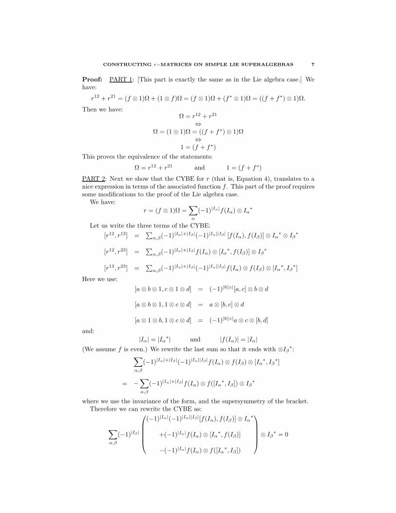
Proof: PART 1: [This part is exactly the same as in the Lie algebra case.] Wehave:

r12 + r21 = (f ⊗ 1)Ω + (1 ⊗ f)Ω = (f ⊗ 1)Ω + (f∗ ⊗ 1)Ω = ((f + f∗) ⊗ 1)Ω.

Then we have:Ω = r12 + r21

⇔Ω = (1 ⊗ 1)Ω = ((f + f∗) ⊗ 1)Ω

⇔1 = (f + f∗)

This proves the equivalence of the statements:

Ω = r12 + r21 and 1 = (f + f∗)

PART 2: Next we show that the CYBE for r (that is, Equation 4), translates to anice expression in terms of the associated function f . This part of the proof requiressome modifications to the proof of the Lie algebra case.

We have:

r = (f ⊗ 1)Ω =∑

α

(−1)|Iα|f(Iα) ⊗ Iα∗

Let us write the three terms of the CYBE:

[r12, r13] =∑

α,β(−1)|Iα|+|Iβ |(−1)|Iα||Iβ | [f(Iα), f(Iβ)] ⊗ Iα∗ ⊗ Iβ

∗

[r12, r23] =∑

α,β(−1)|Iα|+|Iβ |f(Iα) ⊗ [Iα∗, f(Iβ)] ⊗ Iβ

∗

[r13, r23] =∑

α,β(−1)|Iα|+|Iβ |(−1)|Iα||Iβ |f(Iα) ⊗ f(Iβ) ⊗ [Iα∗, Iβ

∗]

Here we use:

[a⊗ b⊗ 1, c⊗ 1 ⊗ d] = (−1)|b||c|[a, c] ⊗ b⊗ d

[a⊗ b⊗ 1, 1 ⊗ c⊗ d] = a⊗ [b, c] ⊗ d

[a⊗ 1 ⊗ b, 1 ⊗ c⊗ d] = (−1)|b||c|a⊗ c⊗ [b, d]

and:

|Iα| = |Iα∗| and |f(Iα)| = |Iα|

(We assume f is even.) We rewrite the last sum so that it ends with ⊗Iβ∗:

∑

α,β

(−1)|Iα|+|Iβ |(−1)|Iα||Iβ |f(Iα) ⊗ f(Iβ) ⊗ [Iα∗, Iβ

∗]

= −∑

α,β

(−1)|Iα|+|Iβ |f(Iα) ⊗ f([Iα∗, Iβ ]) ⊗ Iβ

∗

where we use the invariance of the form, and the supersymmetry of the bracket.Therefore we can rewrite the CYBE as:

∑

α,β

(−1)|Iβ |

(−1)|Iα|(−1)|Iα||Iβ |[f(Iα), f(Iβ)] ⊗ Iα∗

+(−1)|Iα|f(Iα) ⊗ [Iα∗, f(Iβ)]

−(−1)|Iα|f(Iα) ⊗ f([Iα∗, Iβ ])

⊗ Iβ∗ = 0

8 GIZEM KARAALI

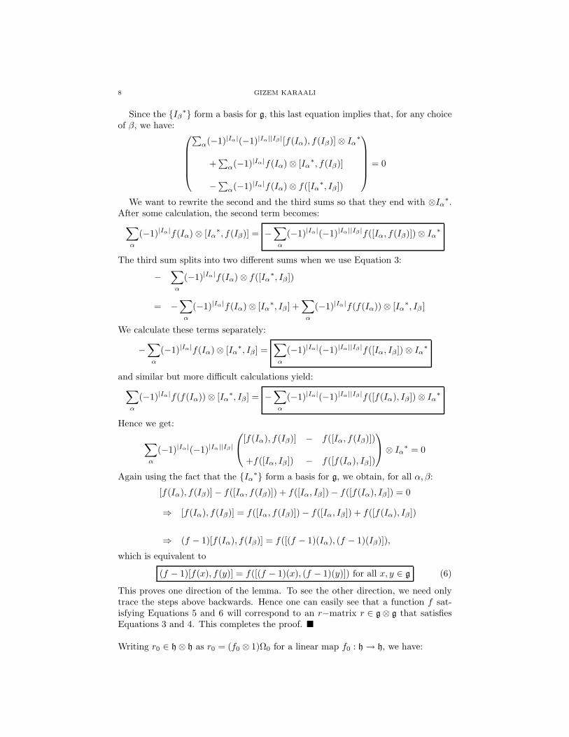
Since the Iβ∗ form a basis for g, this last equation implies that, for any choice

of β, we have:

∑

α(−1)|Iα|(−1)|Iα||Iβ |[f(Iα), f(Iβ)] ⊗ Iα∗

+∑

α(−1)|Iα|f(Iα) ⊗ [Iα∗, f(Iβ)]

−∑

α(−1)|Iα|f(Iα) ⊗ f([Iα∗, Iβ ])

= 0

We want to rewrite the second and the third sums so that they end with ⊗Iα∗.

After some calculation, the second term becomes:∑

α

(−1)|Iα|f(Iα) ⊗ [Iα∗, f(Iβ)] = −

∑

α

(−1)|Iα|(−1)|Iα||Iβ |f([Iα, f(Iβ)]) ⊗ Iα∗

The third sum splits into two different sums when we use Equation 3:

−∑

α

(−1)|Iα|f(Iα) ⊗ f([Iα∗, Iβ ])

= −∑

α

(−1)|Iα|f(Iα) ⊗ [Iα∗, Iβ ] +

∑

α

(−1)|Iα|f(f(Iα)) ⊗ [Iα∗, Iβ ]

We calculate these terms separately:

−∑

α

(−1)|Iα|f(Iα) ⊗ [Iα∗, Iβ ] =

∑

α

(−1)|Iα|(−1)|Iα||Iβ |f([Iα, Iβ ]) ⊗ Iα∗

and similar but more difficult calculations yield:∑

α

(−1)|Iα|f(f(Iα)) ⊗ [Iα∗, Iβ ] = −

∑

α

(−1)|Iα|(−1)|Iα||Iβ |f([f(Iα), Iβ ]) ⊗ Iα∗

Hence we get:

∑

α

(−1)|Iα|(−1)|Iα||Iβ |

[f(Iα), f(Iβ)] − f([Iα, f(Iβ)])

+f([Iα, Iβ ]) − f([f(Iα), Iβ ])

⊗ Iα∗ = 0

Again using the fact that the Iα∗ form a basis for g, we obtain, for all α, β:

[f(Iα), f(Iβ)] − f([Iα, f(Iβ)]) + f([Iα, Iβ ]) − f([f(Iα), Iβ ]) = 0

⇒ [f(Iα), f(Iβ)] = f([Iα, f(Iβ)]) − f([Iα, Iβ ]) + f([f(Iα), Iβ ])

⇒ (f − 1)[f(Iα), f(Iβ)] = f([(f − 1)(Iα), (f − 1)(Iβ)]),

which is equivalent to

(f − 1)[f(x), f(y)] = f([(f − 1)(x), (f − 1)(y)]) for all x, y ∈ g (6)

This proves one direction of the lemma. To see the other direction, we need onlytrace the steps above backwards. Hence one can easily see that a function f sat-isfying Equations 5 and 6 will correspond to an r−matrix r ∈ g ⊗ g that satisfiesEquations 3 and 4. This completes the proof.

Writing r0 ∈ h ⊗ h as r0 = (f0 ⊗ 1)Ω0 for a linear map f0 : h → h, we have:

CONSTRUCTING r−MATRICES ON SIMPLE LIE SUPERALGEBRAS 9

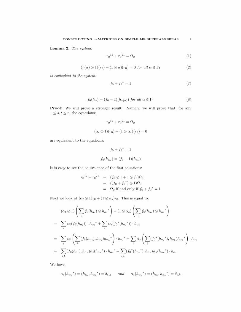
Lemma 2. The system:

r012 + r0

21 = Ω0 (1)

(τ(α) ⊗ 1)(r0) + (1 ⊗ α)(r0) = 0 for all α ∈ Γ1 (2)

is equivalent to the system:

f0 + f0∗ = 1 (7)

f0(hα) = (f0 − 1)(hτ(α)) for all α ∈ Γ1 (8)

Proof: We will prove a stronger result. Namely, we will prove that, for any1 ≤ s, t ≤ r, the equations:

r012 + r0

21 = Ω0

(αt ⊗ 1)(r0) + (1 ⊗ αs)(r0) = 0

are equivalent to the equations:

f0 + f0∗ = 1

f0(hαs) = (f0 − 1)(hαt

)

It is easy to see the equivalence of the first equations:

r012 + r0

21 = (f0 ⊗ 1 + 1 ⊗ f0)Ω0

= ((f0 + f0∗) ⊗ 1)Ω0

= Ω0 if and only if f0 + f0∗ = 1

Next we look at (αt ⊗ 1)r0 + (1 ⊗ αs)r0. This is equal to:

(αt ⊗ 1)

(

∑

i

f0(hαi) ⊗ hαi

∗

)

+ (1 ⊗ αs)

(

∑

i

f0(hαi) ⊗ hαi

∗

)

=∑

i

αt(f0(hαi)) · hαi

∗ +∑

i

αs(f0∗(hαi

∗)) · hαi

=∑

i

αt

(

∑

k

(f0(hαi), hαk

)hαk

∗

)

· hαi

∗ +∑

i

αs

(

∑

k

(f0∗(hαi

∗), hαk)hαk

∗

)

· hαi

=∑

i,k

(f0(hαi), hαk

)αt(hαk

∗) · hαi

∗ +∑

i,k

(f0∗(hαi

∗), hαk)αs(hαk

∗) · hαi

We have:

αs(hαk

∗) = (hαs, hαk

∗) = δs,k and αt(hαk

∗) = (hαt, hαk

∗) = δt,k

10 GIZEM KARAALI

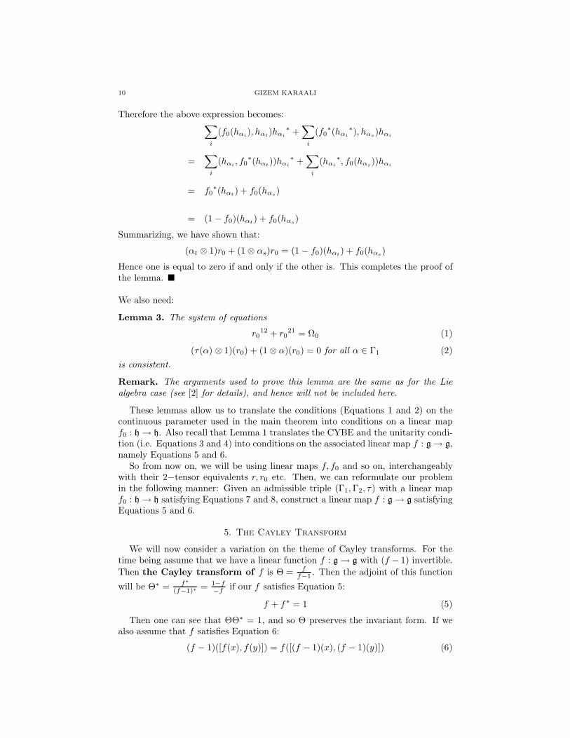
Therefore the above expression becomes:∑

i

(f0(hαi), hαt

)hαi

∗ +∑

i

(f0∗(hαi

∗), hαs)hαi

=∑

i

(hαi, f0

∗(hαt))hαi

∗ +∑

i

(hαi

∗, f0(hαs))hαi

= f0∗(hαt

) + f0(hαs)

= (1 − f0)(hαt) + f0(hαs

)

Summarizing, we have shown that:

(αt ⊗ 1)r0 + (1 ⊗ αs)r0 = (1 − f0)(hαt) + f0(hαs

)

Hence one is equal to zero if and only if the other is. This completes the proof ofthe lemma.

We also need:

Lemma 3. The system of equations

r012 + r0

21 = Ω0 (1)

(τ(α) ⊗ 1)(r0) + (1 ⊗ α)(r0) = 0 for all α ∈ Γ1 (2)

is consistent.

Remark. The arguments used to prove this lemma are the same as for the Liealgebra case (see [2] for details), and hence will not be included here.

These lemmas allow us to translate the conditions (Equations 1 and 2) on thecontinuous parameter used in the main theorem into conditions on a linear mapf0 : h → h. Also recall that Lemma 1 translates the CYBE and the unitarity condi-tion (i.e. Equations 3 and 4) into conditions on the associated linear map f : g → g,namely Equations 5 and 6.

So from now on, we will be using linear maps f, f0 and so on, interchangeablywith their 2−tensor equivalents r, r0 etc. Then, we can reformulate our problemin the following manner: Given an admissible triple (Γ1,Γ2, τ) with a linear mapf0 : h → h satisfying Equations 7 and 8, construct a linear map f : g → g satisfyingEquations 5 and 6.

5. The Cayley Transform

We will now consider a variation on the theme of Cayley transforms. For thetime being assume that we have a linear function f : g → g with (f − 1) invertible.

Then the Cayley transform of f is Θ = ff−1 . Then the adjoint of this function

will be Θ∗ = f∗

(f−1)∗ = 1−f−f if our f satisfies Equation 5:

f + f∗ = 1 (5)

Then one can see that ΘΘ∗ = 1, and so Θ preserves the invariant form. If wealso assume that f satisfies Equation 6:

(f − 1)([f(x), f(y)]) = f([(f − 1)(x), (f − 1)(y)]) (6)

CONSTRUCTING r−MATRICES ON SIMPLE LIE SUPERALGEBRAS 11

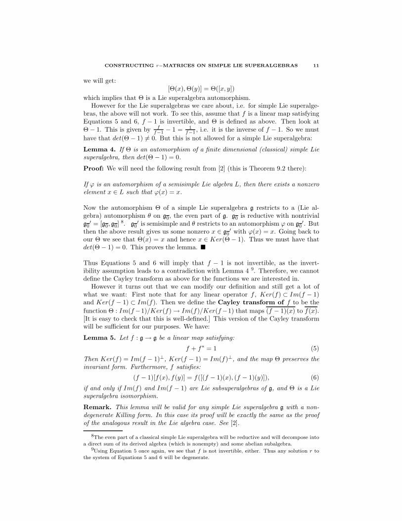
we will get:[Θ(x),Θ(y)] = Θ([x, y])

which implies that Θ is a Lie superalgebra automorphism.However for the Lie superalgebras we care about, i.e. for simple Lie superalge-

bras, the above will not work. To see this, assume that f is a linear map satisfyingEquations 5 and 6, f − 1 is invertible, and Θ is defined as above. Then look atΘ − 1. This is given by f

f−1 − 1 = 1f−1 , i.e. it is the inverse of f − 1. So we must

have that det(Θ − 1) 6= 0. But this is not allowed for a simple Lie superalgebra:

Lemma 4. If Θ is an automorphism of a finite dimensional (classical) simple Liesuperalgebra, then det(Θ − 1) = 0.

Proof: We will need the following result from [2] (this is Theorem 9.2 there):

If ϕ is an automorphism of a semisimple Lie algebra L, then there exists a nonzeroelement x ∈ L such that ϕ(x) = x.

Now the automorphism Θ of a simple Lie superalgebra g restricts to a (Lie al-gebra) automorphism θ on g0, the even part of g. g0 is reductive with nontrivialg0

′ = [g0, g0]8. g0

′ is semisimple and θ restricts to an automorphism ϕ on g0′. But

then the above result gives us some nonzero x ∈ g0′ with ϕ(x) = x. Going back to

our Θ we see that Θ(x) = x and hence x ∈ Ker(Θ − 1). Thus we must have thatdet(Θ − 1) = 0. This proves the lemma.

Thus Equations 5 and 6 will imply that f − 1 is not invertible, as the invert-ibility assumption leads to a contradiction with Lemma 4 9. Therefore, we cannotdefine the Cayley transform as above for the functions we are interested in.

However it turns out that we can modify our definition and still get a lot ofwhat we want: First note that for any linear operator f , Ker(f) ⊂ Im(f − 1)and Ker(f − 1) ⊂ Im(f). Then we define the Cayley transform of f to be the

function Θ : Im(f−1)/Ker(f) → Im(f)/Ker(f−1) that maps (f − 1)(x) to f(x).[It is easy to check that this is well-defined.] This version of the Cayley transformwill be sufficient for our purposes. We have:

Lemma 5. Let f : g → g be a linear map satisfying:

f + f∗ = 1 (5)

Then Ker(f) = Im(f − 1)⊥, Ker(f − 1) = Im(f)⊥, and the map Θ preserves theinvariant form. Furthermore, f satisfies:

(f − 1)[f(x), f(y)] = f([(f − 1)(x), (f − 1)(y)]), (6)

if and only if Im(f) and Im(f − 1) are Lie subsuperalgebras of g, and Θ is a Liesuperalgebra isomorphism.

Remark. This lemma will be valid for any simple Lie superalgebra g with a non-degenerate Killing form. In this case its proof will be exactly the same as the proofof the analogous result in the Lie algebra case. See [2].

8The even part of a classical simple Lie superalgebra will be reductive and will decompose intoa direct sum of its derived algebra (which is nonempty) and some abelian subalgebra.

9Using Equation 5 once again, we see that f is not invertible, either. Thus any solution r tothe system of Equations 5 and 6 will be degenerate.

12 GIZEM KARAALI

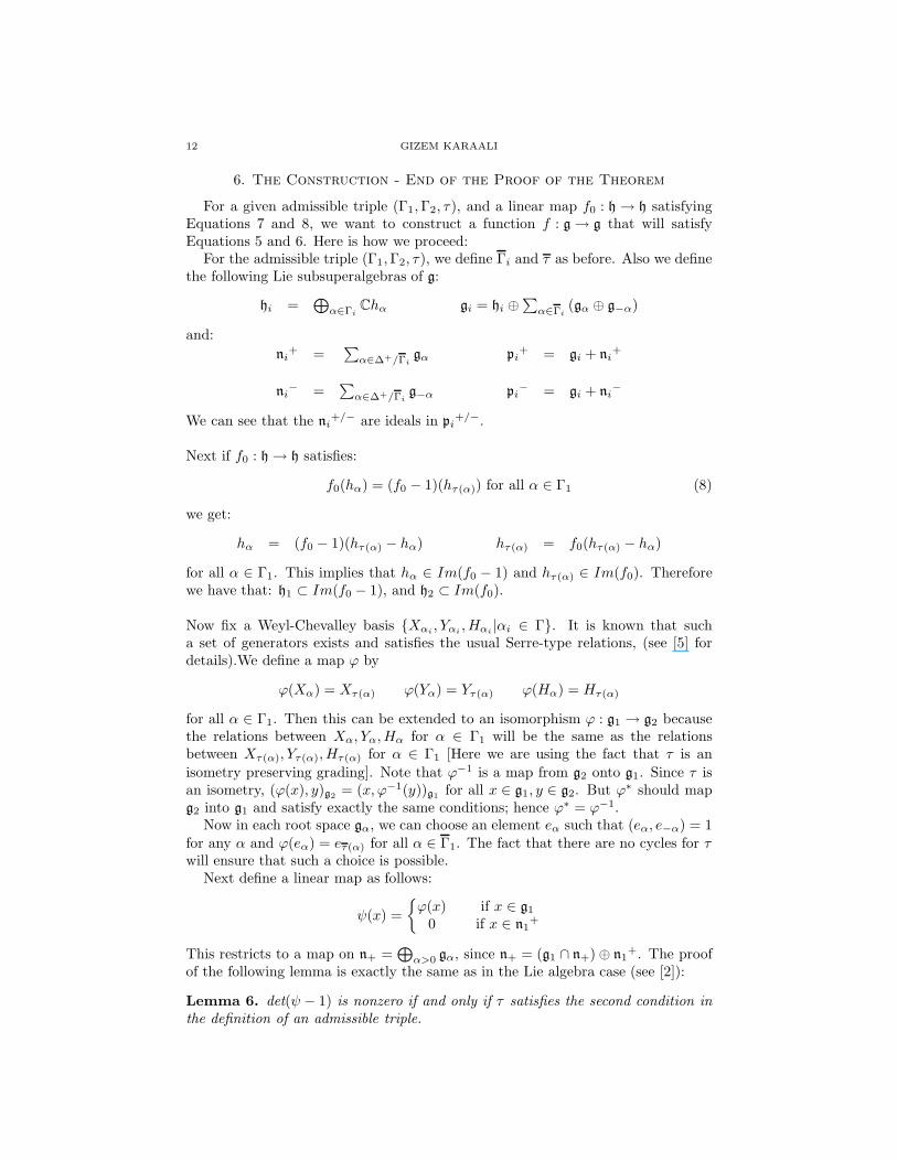
6. The Construction - End of the Proof of the Theorem

For a given admissible triple (Γ1,Γ2, τ), and a linear map f0 : h → h satisfyingEquations 7 and 8, we want to construct a function f : g → g that will satisfyEquations 5 and 6. Here is how we proceed:

For the admissible triple (Γ1,Γ2, τ), we define Γi and τ as before. Also we definethe following Lie subsuperalgebras of g:

hi =⊕

α∈ΓiChα gi = hi ⊕

∑

α∈Γi(gα ⊕ g−α)

and:

ni+ =

∑

α∈∆+/Γigα pi

+ = gi + ni+

ni− =

∑

α∈∆+/Γig−α pi

− = gi + ni−

We can see that the ni+/− are ideals in pi

+/−.

Next if f0 : h → h satisfies:

f0(hα) = (f0 − 1)(hτ(α)) for all α ∈ Γ1 (8)

we get:

hα = (f0 − 1)(hτ(α) − hα) hτ(α) = f0(hτ(α) − hα)

for all α ∈ Γ1. This implies that hα ∈ Im(f0 − 1) and hτ(α) ∈ Im(f0). Thereforewe have that: h1 ⊂ Im(f0 − 1), and h2 ⊂ Im(f0).

Now fix a Weyl-Chevalley basis Xαi, Yαi

, Hαi|αi ∈ Γ. It is known that such

a set of generators exists and satisfies the usual Serre-type relations, (see [5] fordetails).We define a map ϕ by

ϕ(Xα) = Xτ(α) ϕ(Yα) = Yτ(α) ϕ(Hα) = Hτ(α)

for all α ∈ Γ1. Then this can be extended to an isomorphism ϕ : g1 → g2 becausethe relations between Xα, Yα, Hα for α ∈ Γ1 will be the same as the relationsbetween Xτ(α), Yτ(α), Hτ(α) for α ∈ Γ1 [Here we are using the fact that τ is an

isometry preserving grading]. Note that ϕ−1 is a map from g2 onto g1. Since τ isan isometry, (ϕ(x), y)g2

= (x, ϕ−1(y))g1for all x ∈ g1, y ∈ g2. But ϕ∗ should map

g2 into g1 and satisfy exactly the same conditions; hence ϕ∗ = ϕ−1.Now in each root space gα, we can choose an element eα such that (eα, e−α) = 1

for any α and ϕ(eα) = eτ(α) for all α ∈ Γ1. The fact that there are no cycles for τwill ensure that such a choice is possible.

Next define a linear map as follows:

ψ(x) =

ϕ(x) if x ∈ g1

0 if x ∈ n1+

This restricts to a map on n+ =⊕

α>0 gα, since n+ = (g1 ∩ n+) ⊕ n1+. The proof

of the following lemma is exactly the same as in the Lie algebra case (see [2]):

Lemma 6. det(ψ − 1) is nonzero if and only if τ satisfies the second condition inthe definition of an admissible triple.

CONSTRUCTING r−MATRICES ON SIMPLE LIE SUPERALGEBRAS 13

Recall that we started with an admissible triple. The above lemma then saysthat ψ − 1 is invertible. Therefore we can define a function on n+ by:

f+ =ψ

ψ − 1= −(ψ + ψ2 + · · · )

Clearly the sum on the right hand side is finite as ψ is nilpotent. Notice that ψ∗ andso f+

∗ are maps on n− =⊕

α<0 gα, since the Killing form induces a non-degeneratepairing of n+ with n−.

Now define a linear map on n− by:

f− = 1 − f+∗ = 1 + ψ∗ + ψ∗2 + · · ·

Then define f to be the function whose restriction to h, n+, n− is f0, f+, f−,respectively. We have:

f + f∗ = (f0 + f+ + f−) + (f0 + f+ + f−)∗

= (f0 + f0∗) + (f+ + f−

∗) + (f+∗ + f−)

= 1h + 1n++ 1n−

= 1g

To see that f satisfies Equation 6, we will use Lemma 5. Recall that for a linearmap f : g → g, we defined the Cayley transform to be the function

Θ : Im(f − 1)/Ker(f) → Im(f)/Ker(f − 1)

that maps (f − 1)(x) to f(x). Then we have seen before that if f satisfies Equation 5i.e. f + f∗ = 1, then Ker(f) = Im(f − 1)⊥, Ker(f − 1) = Im(f)⊥, and ΘΘ∗ = 1.Furthermore, f satisfies Equation 6 if and only if Im(f) and Im(f − 1) are Liesubsuperalgebras of g, and Θ is a Lie superalgebra isomorphism.

Thus our problem now reduces to showing that C1 = Im(f − 1) and C2 = Im(f)are Lie subsuperalgebras of g, and that the Cayley transform Θ of f is a Liesuperalgebra isomorphism.

We have

C1 = Im(f − 1) = Im(f0 − 1) ∪ Im(f+ − 1) ∪ Im(f− − 1)

C2 = Im(f) = Im(f0) ∪ Im(f+) ∪ Im(f−)

We have seen that Im(f0 − 1) ⊃ h1 and Im(f0) ⊃ h2. We will therefore define V1,V2 as (vector) subspaces of h such that Im(f0 − 1) = h1 ⊕ V1 and Im(f0) = h2 ⊕ V2.

In the Lie algebra case, the Killing form restricts to a positive definite non-degenerate form on (the real subspace generated by Hα|α ∈ Γ of) h. So we candefine the orthogonal complements of h1 and h2 with respect to this form; call theseh1c and h2

c; then we have: h = h1 ⊕ h1c = h2 ⊕ h2

c. Then for a fixed f0, the twosubspaces V1 and V2 are uniquely determined if we add the condition that Vi ⊂ hi

c.In the super case, this is no longer possible; the Cartan subalgebra h may have

isotropic elements and subspaces of h may intersect their orthogonal complementsnontrivially. However in our case we still can define hi

c as follows:

hic =

⊕

α∈Γ\Γi

Chα

Thus we still can write h = hi ⊕ hic, and still can demand that Vi ⊂ hi

c. This choiceof the Vi is then again well-defined, but clearly depends on our choice for Γ.

14 GIZEM KARAALI

Next we compute:

Im(f+ − 1) = Im( 1ψ−1 ) = n+

Im(f− − 1) = Im( ψ∗

1−ψ∗ ) = Im(ψ∗) = g1 ∩ n−

Im(f+) = Im( ψ1−ψ ) = Im(ψ) = g2 ∩ n+

Im(f−) = Im( 11−ψ∗ ) = n−

where we use the fact that ψ − 1 is invertible. The above then yields:

C1 = p1+ ⊕ V1 C2 = p2

− ⊕ V2

It is now easy to check that C1 and C2 are both closed under the bracket and henceare Lie subsuperalgebras of g.

Finally we need to see that the Cayley transform Θ is a Lie superalgebra iso-morphism. Now we note that by the last lemma above, Ci ⊃ Ci

⊥. So we have:

C1⊥ = (p1

+ ⊕ V1)⊥ = n1

+ ⊕ (h1 ⊕ V1)⊥ = n1

+ ⊕ (h1⊥ ∩ V1

⊥) ⊂ p1+ ⊕ V1

and similarly:

C2⊥ = (p2

− ⊕ V2)⊥ = n2

− ⊕ (h2 ⊕ V2)⊥ = n2

− ⊕ (h2⊥ ∩ V2

⊥) ⊂ p2− ⊕ V2

Hence we have:hi

⊥ ∩ Vi⊥ ⊂ hi ⊕ Vi

which gives us:

C1/C1⊥ =

p1+ ⊕ V1

(p1+ ⊕ V1)⊥

=

⊕

α∈Γ1

gα ⊕ g−α

⊕h1 ⊕ V1

h1⊥ ∩ V1

⊥

and similarly:

C2/C2⊥ =

p2− ⊕ V2

(p2− ⊕ V2)⊥

=

⊕

α∈Γ2

gα ⊕ g−α

⊕h2 ⊕ V2

h2⊥ ∩ V2

⊥

We have already seen that the Ci are Lie subsuperalgebras. Since Ci⊥ is an ideal,

we have a Lie superalgebra structure on Ci/Ci⊥. But [gα, g−α] = CHα, therefore

we must have a complete copy of hi and so a copy of gi in Ci/Ci⊥. This implies

that hi⊥ ∩ Vi

⊥ lies in Vi, and we have:

Ci/Ci⊥ = gi ⊕

Vi

hi⊥ ∩ Vi

⊥

So we need to show that:

Θ : g1 ⊕V1

h1⊥ ∩ V1

⊥→ g2 ⊕

V2

h2⊥ ∩ V2

⊥

is a Lie superalgebra isomorphism.We first note that Θ(x) = ϕ(x) for all x ∈ g1. Indeed if α ∈ Γ1, we have:

Xα = (f+ − 1)(Xτ(α) −Xα)

and so is mapped via Θ to:

f+(Xτ(α) −Xα) = Xτ(α)

CONSTRUCTING r−MATRICES ON SIMPLE LIE SUPERALGEBRAS 15

And similarly:

Yα = (f− − 1)(Yτ(α) − Yα)

is mapped via Θ to:

f−(Yτ(α) − Yα) = Yτ(α)

Also it is easy to see that since Hα = (f0 − 1)(Hτ(α) −Hα) for each α ∈ Γ1, Θsends Hα to f0(Hτ(α) −Hα) = Hτ(α). Hence the restriction of Θ to g1 is exactlythe Lie superalgebra isomorphism ϕ.

Next we look at what Θ does on the Cartan part of the Ci/Ci⊥. We have that:

Ci/Ci⊥ =

⊕

α∈Γi

gα ⊕ g−α

⊕hi ⊕ Vi

hi⊥ ∩ Vi

⊥

i.e. we can rewriteCi/Ci⊥ as the direct sum of a Cartan part and a non-Cartan part.

Then the previous arguments show that Θ maps the non-Cartan part of C1/C1⊥

into the non-Cartan part of C2/C2⊥ like ϕ does. And then since Θ preserves the

invariant form, it maps the Cartan part of C1/C1⊥ to the Cartan part of C2/C2

⊥:

Θ(

(non-Cartan of C1/C1⊥)⊥

)

= (non-Cartan of C2/C2⊥)⊥

In other words:

Θ

(

h1 ⊕ V1

h1⊥ ∩ V1

⊥

)

=

(

h2 ⊕ V2

h2⊥ ∩ V2

⊥

)

Since hi⊕Vi

hi⊥∩Vi

⊥ are abelian, Θ restricts to an isomorphism there as well. Therefore Θ

is an isomorphism. This then will imply that the associated linear map f satisfiesEquations 5 and 6 and so corresponds to an r− matrix satisfying Equations 3 and4.

At this point one needs to check if the function f constructed in this way willyield the tensor r of Equation (∗). This is reasonably straightforward. Hence wehave proved our theorem.

7. Examples: r−matrices on sl(2, 1)

Recall that two Dynkin diagrams of a given Lie superalgebra are not necessarilyisomorphic, but one can be obtained from the other via a chain of odd reflections.Therefore while listing all possible admissible triples for a given Lie superalgebra,we need to take into consideration all possible Dynkin diagrams. This raises a newquestion as to how r-matrices obtained from two nonisomorphic Dynkin diagramsare related, if at all. We will see that at least in the case of sl(2, 1), if r is thestandard r-matrix associated to a fixed Dynkin diagram D, and D′ is the Dynkindiagram obtained from D by the odd reflection σα, then r′, the standard r-matrixassociated to D′, will be the image of r under the same reflection σα.

7.1. Dynkin Diagrams of sl(2,1). The roots of sl(2, 1) are

∆0 = ǫ1 − ǫ2, ǫ2 − ǫ1 ∆1 = ǫ1 − λ1, ǫ2 − λ1, λ1 − ǫ1, λ1 − ǫ2

where ǫi is the (restriction to the Cartan subalgebra of sl(2, 1) of the) standardbasis: ǫi(Ejk) = δi,jδi,k, and λ1 = ǫ3. We will denote the set of simple roots by Γ.

There are six possible Dynkin diagrams:

16 GIZEM KARAALI

(1) Γ(D1) = ǫ1−ǫ2, ǫ2−λ1. We will set α1 = ǫ1 − ǫ2 and α2 = ǫ2 − λ1. α1 iseven, while α2 is odd. The third positive root in this case is α1 + α2 whichis odd.

(2) Γ(D2) = ǫ1 − λ1, λ1 − ǫ2. Note that these two roots are actually α1 + α2

and −α2, and it is easy to see that D2 is obtained from D1 via the oddreflection σα2

associated to the root α2. We can obtain D1 back from D2

by σ−α2. Note also that the third positive root in this case will be α1 which

is even.(3) Γ(D3) = λ1 − ǫ1, ǫ1 − ǫ2 = −α1 −α2, α1. We note that D3 is obtained

from D2 via the odd reflection σα1+α2. Applying σ−α1−α2

to D3 will returnD2 as expected. Note also that the third positive root will be −α2 whichis odd.

(4) Γ(D4) = −Γ(D1) = −α1,−α2. The third positive root in this case willbe −α1 − α2 which is odd.

(5) Γ(D5) = −Γ(D2) = −α1 − α2, α2. The third positive root in this casewill be −α1 which is even. Note that D5 is obtained from D4 via σ−α2

,and that applying σα2

to D5 will yield D4 as expected.(6) Γ(D6) = −Γ(D3) = α1 + α2,−α1. The third positive root will be α2

which is odd. The odd reflections σ−α1−α2and σα1+α2

will map D5 andD6 into one another.

Hence, up to sign, there are three Dynkin diagrams, and these can be obtainedfrom one another via a chain of odd reflections (which change the signs of some ofthe odd roots but a positive even root stays positive). Also note that except forthe two Dynkin diagrams D2 and D5, the diagrams consist of one white circle andone gray circle (standing for two roots of different parities), and so these diagramswill not allow any nontrivial admissible triples. Therefore the construction of ourtheorem will only yield standard r-matrices for these cases. In D2 and D5, bothsimple roots are odd, and we can actually consider a nontrivial admissible triplein these cases. Therefore the theorem will give us one standard r-matrix and twononstandard r-matrices for each of the diagrams D2 and D5.

7.2. The Standard r-matrices. By construction, given r0 ∈ h ⊗ h satisfyingr0 + r0

21 = Ω010, the standard r-matrix for a fixed Dynkin diagram is

r = r0 +∑

α>0

e−α ⊗ eα.

So fixing r0 we write down the standard r-matrices for the above diagrams:

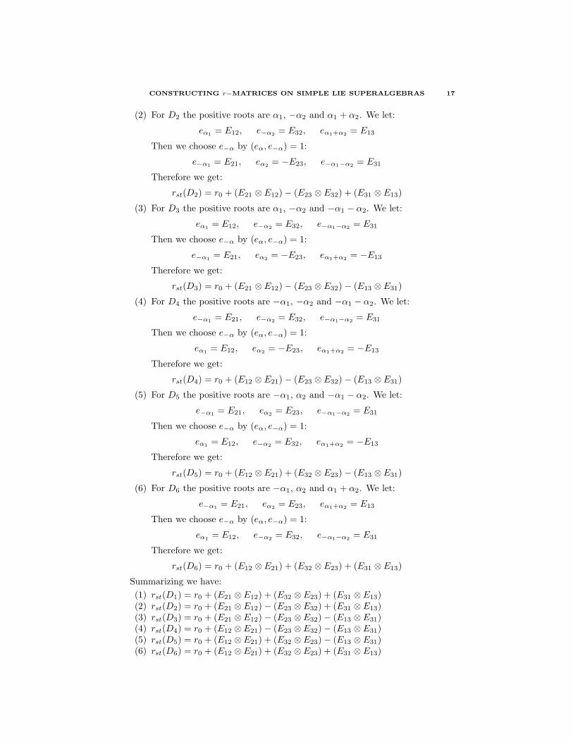
(1) For D1 the positive roots are α1, α2 and α1 + α2. We let:

eα1= E12, eα2

= E23, eα1+α2= E13

Then we choose e−α by (eα, e−α) = 1:

e−α1= E21, e−α2

= E32, e−α1−α2= E31

Therefore we get:

rst(D1) = r0 + (E21 ⊗ E12) + (E32 ⊗ E23) + (E31 ⊗ E13)

10Ω0 is the Cartan part of the quadratic Casimir element Ω of g.

CONSTRUCTING r−MATRICES ON SIMPLE LIE SUPERALGEBRAS 17

(2) For D2 the positive roots are α1, −α2 and α1 + α2. We let:

eα1= E12, e−α2

= E32, eα1+α2= E13

Then we choose e−α by (eα, e−α) = 1:

e−α1= E21, eα2

= −E23, e−α1−α2= E31

Therefore we get:

rst(D2) = r0 + (E21 ⊗ E12) − (E23 ⊗ E32) + (E31 ⊗ E13)

(3) For D3 the positive roots are α1, −α2 and −α1 − α2. We let:

eα1= E12, e−α2

= E32, e−α1−α2= E31

Then we choose e−α by (eα, e−α) = 1:

e−α1= E21, eα2

= −E23, eα1+α2= −E13

Therefore we get:

rst(D3) = r0 + (E21 ⊗ E12) − (E23 ⊗ E32) − (E13 ⊗ E31)

(4) For D4 the positive roots are −α1, −α2 and −α1 − α2. We let:

e−α1= E21, e−α2

= E32, e−α1−α2= E31

Then we choose e−α by (eα, e−α) = 1:

eα1= E12, eα2

= −E23, eα1+α2= −E13

Therefore we get:

rst(D4) = r0 + (E12 ⊗ E21) − (E23 ⊗ E32) − (E13 ⊗ E31)

(5) For D5 the positive roots are −α1, α2 and −α1 − α2. We let:

e−α1= E21, eα2

= E23, e−α1−α2= E31

Then we choose e−α by (eα, e−α) = 1:

eα1= E12, e−α2

= E32, eα1+α2= −E13

Therefore we get:

rst(D5) = r0 + (E12 ⊗ E21) + (E32 ⊗ E23) − (E13 ⊗ E31)

(6) For D6 the positive roots are −α1, α2 and α1 + α2. We let:

e−α1= E21, eα2

= E23, eα1+α2= E13

Then we choose e−α by (eα, e−α) = 1:

eα1= E12, e−α2

= E32, e−α1−α2= E31

Therefore we get:

rst(D6) = r0 + (E12 ⊗ E21) + (E32 ⊗ E23) + (E31 ⊗ E13)

Summarizing we have:

(1) rst(D1) = r0 + (E21 ⊗ E12) + (E32 ⊗ E23) + (E31 ⊗ E13)(2) rst(D2) = r0 + (E21 ⊗ E12) − (E23 ⊗ E32) + (E31 ⊗ E13)(3) rst(D3) = r0 + (E21 ⊗ E12) − (E23 ⊗ E32) − (E13 ⊗ E31)(4) rst(D4) = r0 + (E12 ⊗ E21) − (E23 ⊗ E32) − (E13 ⊗ E31)(5) rst(D5) = r0 + (E12 ⊗ E21) + (E32 ⊗ E23) − (E13 ⊗ E31)(6) rst(D6) = r0 + (E12 ⊗ E21) + (E32 ⊗ E23) + (E31 ⊗ E13)

18 GIZEM KARAALI

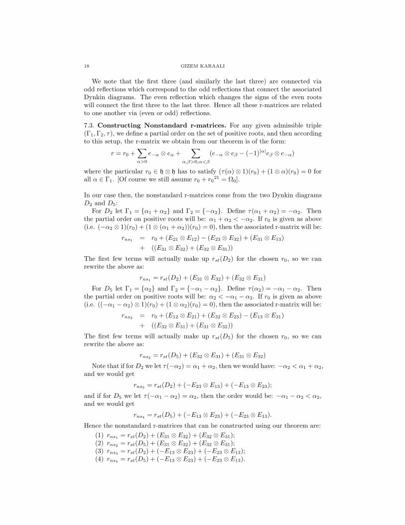
We note that the first three (and similarly the last three) are connected viaodd reflections which correspond to the odd reflections that connect the associatedDynkin diagrams. The even reflection which changes the signs of the even rootswill connect the first three to the last three. Hence all these r-matrices are relatedto one another via (even or odd) reflections.

7.3. Constructing Nonstandard r-matrices. For any given admissible triple(Γ1,Γ2, τ), we define a partial order on the set of positive roots, and then accordingto this setup, the r-matrix we obtain from our theorem is of the form:

r = r0 +∑

α>0

e−α ⊗ eα +∑

α,β>0,α<β

(e−α ⊗ eβ − (−1)|α|eβ ⊗ e−α)

where the particular r0 ∈ h ⊗ h has to satisfy (τ(α) ⊗ 1)(r0) + (1 ⊗ α)(r0) = 0 forall α ∈ Γ1. [Of course we still assume r0 + r0

21 = Ω0].

In our case then, the nonstandard r-matrices come from the two Dynkin diagramsD2 and D5:

For D2 let Γ1 = α1 + α2 and Γ2 = −α2. Define τ(α1 + α2) = −α2. Thenthe partial order on positive roots will be: α1 + α2 < −α2. If r0 is given as above(i.e. (−α2 ⊗ 1)(r0) + (1 ⊗ (α1 + α2))(r0) = 0), then the associated r-matrix will be:

rns1 = r0 + (E21 ⊗ E12) − (E23 ⊗ E32) + (E31 ⊗ E13)

+ ((E31 ⊗ E32) + (E32 ⊗ E31))

The first few terms will actually make up rst(D2) for the chosen r0, so we canrewrite the above as:

rns1 = rst(D2) + (E31 ⊗ E32) + (E32 ⊗ E31)

For D5 let Γ1 = α2 and Γ2 = −α1 − α2. Define τ(α2) = −α1 − α2. Thenthe partial order on positive roots will be: α2 < −α1 − α2. If r0 is given as above(i.e. ((−α1 − α2) ⊗ 1)(r0) + (1 ⊗ α2)(r0) = 0), then the associated r-matrix will be:

rns2 = r0 + (E12 ⊗ E21) + (E32 ⊗ E23) − (E13 ⊗ E31)

+ ((E32 ⊗ E31) + (E31 ⊗ E32))

The first few terms will actually make up rst(D5) for the chosen r0, so we canrewrite the above as:

rns2 = rst(D5) + (E32 ⊗ E31) + (E31 ⊗ E32)

Note that if forD2 we let τ(−α2) = α1 + α2, then we would have: −α2 < α1 + α2,and we would get

rns3 = rst(D2) + (−E23 ⊗ E13) + (−E13 ⊗ E23);

and if for D5 we let τ(−α1 − α2) = α2, then the order would be: −α1 − α2 < α2,and we would get

rns4 = rst(D5) + (−E13 ⊗ E23) + (−E23 ⊗ E13).

Hence the nonstandard r-matrices that can be constructed using our theorem are:

(1) rns1 = rst(D2) + (E31 ⊗ E32) + (E32 ⊗ E31);(2) rns2 = rst(D5) + (E31 ⊗ E32) + (E32 ⊗ E31);(3) rns3 = rst(D2) + (−E13 ⊗ E23) + (−E23 ⊗ E13);(4) rns4 = rst(D5) + (−E13 ⊗ E23) + (−E23 ⊗ E13).

CONSTRUCTING r−MATRICES ON SIMPLE LIE SUPERALGEBRAS 19

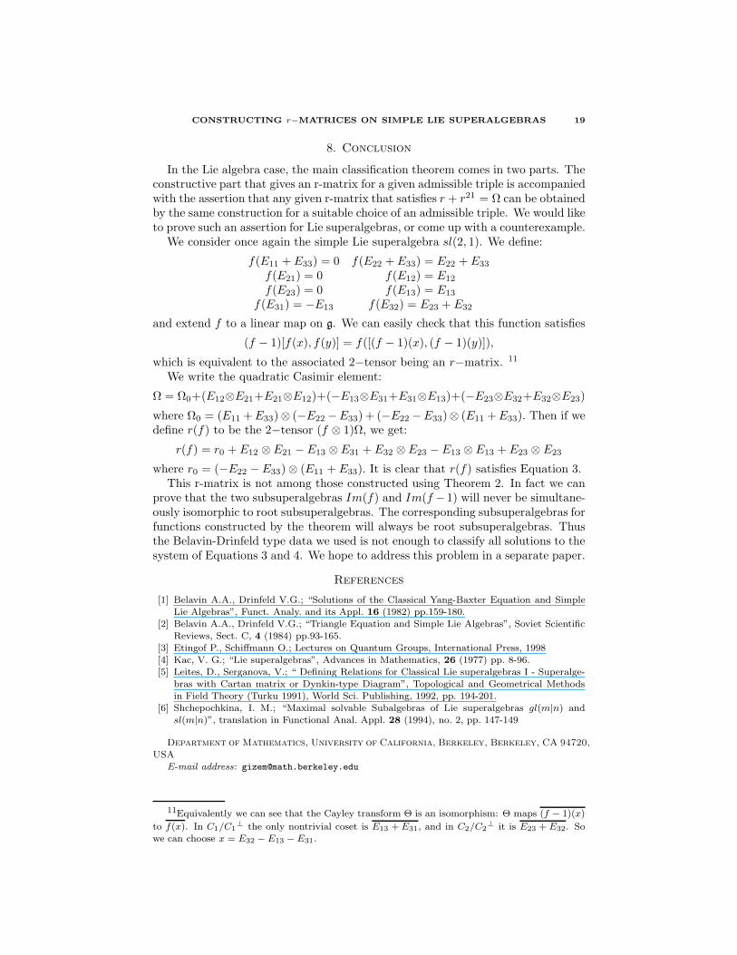
8. Conclusion

In the Lie algebra case, the main classification theorem comes in two parts. Theconstructive part that gives an r-matrix for a given admissible triple is accompaniedwith the assertion that any given r-matrix that satisfies r + r21 = Ω can be obtainedby the same construction for a suitable choice of an admissible triple. We would liketo prove such an assertion for Lie superalgebras, or come up with a counterexample.

We consider once again the simple Lie superalgebra sl(2, 1). We define:

f(E11 + E33) = 0 f(E22 + E33) = E22 + E33

f(E21) = 0 f(E12) = E12

f(E23) = 0 f(E13) = E13

f(E31) = −E13 f(E32) = E23 + E32

and extend f to a linear map on g. We can easily check that this function satisfies

(f − 1)[f(x), f(y)] = f([(f − 1)(x), (f − 1)(y)]),

which is equivalent to the associated 2−tensor being an r−matrix. 11

We write the quadratic Casimir element:

Ω = Ω0+(E12⊗E21+E21⊗E12)+(−E13⊗E31+E31⊗E13)+(−E23⊗E32+E32⊗E23)

where Ω0 = (E11 +E33)⊗ (−E22 −E33) + (−E22 −E33)⊗ (E11 +E33). Then if wedefine r(f) to be the 2−tensor (f ⊗ 1)Ω, we get:

r(f) = r0 + E12 ⊗ E21 − E13 ⊗ E31 + E32 ⊗ E23 − E13 ⊗ E13 + E23 ⊗ E23

where r0 = (−E22 − E33) ⊗ (E11 + E33). It is clear that r(f) satisfies Equation 3.This r-matrix is not among those constructed using Theorem 2. In fact we can

prove that the two subsuperalgebras Im(f) and Im(f −1) will never be simultane-ously isomorphic to root subsuperalgebras. The corresponding subsuperalgebras forfunctions constructed by the theorem will always be root subsuperalgebras. Thusthe Belavin-Drinfeld type data we used is not enough to classify all solutions to thesystem of Equations 3 and 4. We hope to address this problem in a separate paper.

References

[1] Belavin A.A., Drinfeld V.G.; “Solutions of the Classical Yang-Baxter Equation and SimpleLie Algebras”, Funct. Analy. and its Appl. 16 (1982) pp.159-180.

[2] Belavin A.A., Drinfeld V.G.; “Triangle Equation and Simple Lie Algebras”, Soviet ScientificReviews, Sect. C, 4 (1984) pp.93-165.

[3] Etingof P., Schiffmann O.; Lectures on Quantum Groups, International Press, 1998[4] Kac, V. G.; “Lie superalgebras”, Advances in Mathematics, 26 (1977) pp. 8-96.[5] Leites, D., Serganova, V.; “ Defining Relations for Classical Lie superalgebras I - Superalge-

bras with Cartan matrix or Dynkin-type Diagram”, Topological and Geometrical Methodsin Field Theory (Turku 1991), World Sci. Publishing, 1992, pp. 194-201.

[6] Shchepochkina, I. M.; “Maximal solvable Subalgebras of Lie superalgebras gl(m|n) andsl(m|n)”, translation in Functional Anal. Appl. 28 (1994), no. 2, pp. 147-149

Department of Mathematics, University of California, Berkeley, Berkeley, CA 94720,

USA

E-mail address: gizem@math.berkeley.edu

11Equivalently we can see that the Cayley transform Θ is an isomorphism: Θ maps (f − 1)(x)

to f(x). In C1/C1⊥ the only nontrivial coset is E13 + E31, and in C2/C2

⊥ it is E23 + E32. Sowe can choose x = E32 − E13 − E31.