Consortium

for

Small-Scale Modelling

Technical Report No. 38

The COSMO Priority Project CORSO-A

Final Report

April 2019

DOI: 10.5676/DWD pub/nwv/cosmo-tr 38

Deutscher Wetterdienst

MeteoSwiss

Ufficio Generale Spazio Aereo e Meteorologia

EΘNIKH METEΩPOΛOΓIKH ΥΠHPEΣIA

Instytucie Meteorogii i Gospodarki Wodnej

Administratia Nationala de Meteorologie

ROSHYDROMET

Agenzia Regionale Protezione Ambiente Piemonte

Agenzia Regionale Prevenzione Ambiente Energia Emilia Romagna

Centro Italiano Ricerche Aerospaziali

Amt fur GeoInformationswesen der Bundeswehr

Israel Meteorological Service

www.cosmo-model.org

Editor: Massimo Milelli, ARPA Piemonte

The COSMO Priority Project CORSO-A

Final Report

Project participants:

G. Rivin1‡, I. Rozinkina1‡, E. Astakhova1, A. Montani2,

J-M. Bettems3, D. Alferov1, D. Blinov1,

P. Eckert3, A. Euripides4, J. Helmert5, M.Shatunova1.

‡ Task LeadersFederal Service for Hydrometeorology and Environmental Monitoring, Russia (Roshydromet)Hydrometeorological Research Centre of Russian Federation (Hydrometcentre of Russia)11-13, B. Predtechensky per., Moscow, 123242, Russia

1 RHM

2 ARPAE

3 MCH

4 HNMS

5 DWD

Contents 2

Contents

1 Introduction 4

1.1 The goal of PT . . . . . . . . . . . . . . . . . . . . . . . . . . . . . . . . . . . 4

2 SubTasks, brief description 5

2.1 SubTask 1 The guidance of the optimal domain’s size selection for 1.1 kmresolution of nested COSMO models for the regions with complex mountainrelief (STL G. Rivin) . . . . . . . . . . . . . . . . . . . . . . . . . . . . . . . . 5

2.1.1 Motivation . . . . . . . . . . . . . . . . . . . . . . . . . . . . . . . . . 5

2.1.2 Goal . . . . . . . . . . . . . . . . . . . . . . . . . . . . . . . . . . . . . 5

2.2 SubTask 2 Development of algorithm of subgrid h-correction of T2m (due tothe differences between models and real heights) based on COSMO- forecastsof vertical T-gradient (STL I. Rozinkina) . . . . . . . . . . . . . . . . . . . . 5

2.2.1 Motivation . . . . . . . . . . . . . . . . . . . . . . . . . . . . . . . . . 5

2.2.2 Goal . . . . . . . . . . . . . . . . . . . . . . . . . . . . . . . . . . . . . 6

2.3 SubTask 3 Preparing of archives of 7 km and 2.2 km EPSs forecasts for theSochi-2014 modelling area applicable for research aimed at improving COSMOEPS systems and available for community (TL E. Astakhova, A. Montani) . . 6

2.3.1 Motivation . . . . . . . . . . . . . . . . . . . . . . . . . . . . . . . . . 6

2.3.2 Goal . . . . . . . . . . . . . . . . . . . . . . . . . . . . . . . . . . . . . 7

2.4 SubTask 4. Preparing of recommendations for forecasters The features ofusing and interpretation of the results of limited- area meso-scale modeling(TL I. Rozinkina) . . . . . . . . . . . . . . . . . . . . . . . . . . . . . . . . . . 7

2.4.1 Motivation . . . . . . . . . . . . . . . . . . . . . . . . . . . . . . . . . 7

2.4.2 Goal . . . . . . . . . . . . . . . . . . . . . . . . . . . . . . . . . . . . . 7

3 The guidance of the optimal domain’s size selection for 1.1 km resolutionof nested COSMO models for the regions with complex mountain relief(G. Rivin, M. Shatunova, J. Helmert) 8

3.1 Introduction . . . . . . . . . . . . . . . . . . . . . . . . . . . . . . . . . . . . . 8

3.2 Simulation domains . . . . . . . . . . . . . . . . . . . . . . . . . . . . . . . . 8

3.3 VERSUS verification results . . . . . . . . . . . . . . . . . . . . . . . . . . . . 10

3.4 Verification of heavy precipitation event forecast (case studies) . . . . . . . . 13

3.5 Conclusions . . . . . . . . . . . . . . . . . . . . . . . . . . . . . . . . . . . . . 21

4 Development of algorithm of subgrid h-correction of T2m for mountainsbased on COSMO forecasts of local lapse rate (h-correction) (I. Rozinkina,J-M. Bettems, D. Blinov, A. Euripides) 22

2

Contents 3

5 COSMO-BASED ENSEMBLE FORECASTING FOR SOCHI-2014 OLYMPICS:ARCHIVING THE RESULTS (E. Astakhova, A. Montani, D. Kiktev, D.Alferov, A. Smirnov) 23

5.1 Introduction . . . . . . . . . . . . . . . . . . . . . . . . . . . . . . . . . . . . . 23

5.2 Ensemble prediction systems developed in CORSO . . . . . . . . . . . . . . . 23

5.3 CORSO-A necessity and goal . . . . . . . . . . . . . . . . . . . . . . . . . . . 24

5.4 A Unified Sochi archive . . . . . . . . . . . . . . . . . . . . . . . . . . . . . . 24

5.5 Conclusions . . . . . . . . . . . . . . . . . . . . . . . . . . . . . . . . . . . . . 27

6 PREPARING OF RECOMMENDATIONS FOR FORECASTERS ABOUTFEATURES OF INTERPRETATION OF THE RESULTS OF MESO-SCALE MODELING (How to use the LAM mesoscale NWP results formountain terrain) (I. Rozinkina, P. Eckert, G. S. Rivin) 28

6.1 Introduction . . . . . . . . . . . . . . . . . . . . . . . . . . . . . . . . . . . . . 28

6.2 Key definitions . . . . . . . . . . . . . . . . . . . . . . . . . . . . . . . . . . . 28

6.3 Main statements of use of products of global / Limited area NWP Productsfor short-range and very-short range forecasting . . . . . . . . . . . . . . . . . 29

6.4 Stages of analysis of NWP products for local short- range forecasting . . . . . 31

6.4.1 Common recommends . . . . . . . . . . . . . . . . . . . . . . . . . . . 31

6.4.2 Experience of large-scale weather types before the analyze of HR prod-ucts . . . . . . . . . . . . . . . . . . . . . . . . . . . . . . . . . . . . . 32

6.4.3 Recommended sequence of analysis, design and content of forecastersmaps . . . . . . . . . . . . . . . . . . . . . . . . . . . . . . . . . . . . . 34

6.5 Analysis of Meteograms of deterministic LAM HR NWP . . . . . . . . . . . . 39

6.5.1 Definitions and goals . . . . . . . . . . . . . . . . . . . . . . . . . . . . 39

6.5.2 Key principles for technology of meteogram forming . . . . . . . . . . 40

6.5.3 Forecasters analysis based on meteograms . . . . . . . . . . . . . . . . 41

6.6 Conclusion . . . . . . . . . . . . . . . . . . . . . . . . . . . . . . . . . . . . . 43

7 Acknowledgements 43

A Appendix 44

3

1 Introduction

The PP CORSO (Consolidation of Operation and Research results for the Sochi Olympics)dedicated to development of high-resolution NWP meteosupport of Sochi2014 Olympics heldin 2011-2014. PP CORSO was adopted with a goal to enhance and demonstrate the capa-bilities of COSMO-based systems of NWP in winter conditions for mountainous terrain andto assess the effect of practical use of this information during Sochi-2014 Olympic Games.There were 3 directions of activities concerning the development and implementation of:

a) high-resolution forecasting system (Task1),

b) the means of practical forecasting and down-scaling post-processing (Task2),

c) mesoscale EPS (Task3).

PP CORSO obtained the successful results. The main result of FDP part of PP CORSOwas the implementation of high quality NWP system, which the forecasters of OrganizingCommittee and of sport venues have used as a basic. The COSMO experience and itspossibilities were concentrated for obtain the renovated NWP system for SOCHI-2014 regionwith complex geographical terrain. Due to the cooperation of FDP and RDP activities ofPP CORSO, the new level of modeling and of interpretation of results were obtained (Thenew COSMO-version with step 1.1km, the some down-scaling postprocessing algorithms,knowledge of feed-back from forecasters, the implementation of High-resolution EPS-system2.2. km for mountain area). Some aspects obtained results could be further researched andcould be useful for implementation and investigations in whole COSMO community. Theobtained experience, accumulated data of measurements and of forecasts and new numericexperiments permit to adapt & develop and test of the proposed algorithms and technicalsolutions. The new PT CORSO-After (CORSO-A) should meet these developed challengesfor implementation in COSMO technologies and investigations.

1.1 The goal of PT

To prepare the new COSMO tools and practical instructions for be available for COSMO-community related to:

• the implementation of versions COSMO-1km (SubTask1 The guidance of the optimaldomain’s size selection for 1.1 km resolution of nested COSMO models for the regionswith complex mountain relief, TL G.Rivin),

• the realization of down-scaling postprocessing tools for mountain area, (SubTask2, De-velopment of algorithm of subgrid h-correction of T2m (due to the differences betweenmodels and real heights) based on COSMO- forecasts of vertical T-gradient , STLI.Rozinkina),

• the development of archive for development of convective-resolution EPS (SubTask3Preparing of archives of 7 km and 2.2 km EPS forecasts for the Sochi- 2014 model-ing area applicable for research aimed at improving COSMO EPS systems and avail-able for community. Their compliance with FROST2014 archives, STL E.Astakhova,A.Montani),

4

• the preparing of instructions for forecasters for use the results of meso-scale determin-istic and EPS results (SubTask4 Preparing of recommendations for forecasters Thefeatures of using and interpretation of the results of limited- area meso-scale modelingSTL I.Rozinkina).

2 SubTasks, brief description

2.1 SubTask 1 The guidance of the optimal domain’s size selection for 1.1km resolution of nested COSMO models for the regions with complexmountain relief (STL G. Rivin)

2.1.1 Motivation

The development and implementation of COSMO1 were obtained as result of RDP part of PPCORSO. As addition the participants managed to organize the operational runs of COSMO1for Sochi2014 area during the Olympics 2014, and the positive experience of use of COSMO1 for Sochi area was gained. The modeling with grid step about 1 km is significantly morerealistic for mountain area and as sequence permit to provide for forecasters the additionalimportant products as, e.g. flows of wind in bottom level, that determines the weather in hillsand valleys. During the CORSO PP were obtained results shown the strong dependence ofthe predicted precipitation amount and spatial distribution on the models domain size. Thisproblem need the more attentive examination, because the runs of COSMO1 as part of nestedtechnologies are very expensive in point of view of computing time. The computing resourcesand the technological requirements of providing forecast by a certain time determine themodel run timing. On the other hand it exists the requirements for the quality of theforecasts.

2.1.2 Goal

To formulate and to prove the selection of models domain size for COSMO1 model runs fordisseminate this experience for create the similar technologies for detailed calculations onmountain domains in condition of limited computing resources.

2.2 SubTask 2 Development of algorithm of subgrid h-correction of T2m(due to the differences between models and real heights) based onCOSMO- forecasts of vertical T-gradient (STL I. Rozinkina)

2.2.1 Motivation

In framework of PP CORSO were realized some approaches for subgrid correction of T2m,as the direct forecasts from COSMO-model of T2m for mountain region were not convenient.There are some causes because it. One of principal causes of this fact for mountain areais the simple discrepancy of local real and averaged of grid cells height. As traditional,T2m can be corrected by use standard adiabatic gradient, but in Sochi2014 region thereal temperature profiles can be significantly different including inversions. Because of thevariability of the vertical temperature profile depending on a large-scale weather forecaststhe implementation of KF or MOS in lot of cases is inefficiently because there are nonsystematic errors. The CORSO participants proposed the algorithm of correction of local

5

values of T2m for mountains based the COSMO- models forecasts of T-profile of bottomslevels (H-corection). The implementation of this algorithm in meteogram tables permit toobtain the more realistic T2m forecasts for points before the possible subsequent correctiontools (KF or MOS), due to improve the limitations of parameterization schemes. Thisproposed algorithm can be disseminate in two direction of implementation: a) by modifiedtechnology of forming of meteograms by including into FieldExtra for calculate the fields ofsubgrid variations of T2m (for min and max real height of cells).

2.2.2 Goal

To realize the updated software of Fieldextra with including of calculations of subgrid valuesof T2m based the forecasts of vertical T gradient. To provide the software of 1-D correctionof T2m forecasts based the forecasts of vertical T gradient (h-correction).

2.3 SubTask 3 Preparing of archives of 7 km and 2.2 km EPSs forecastsfor the Sochi-2014 modelling area applicable for research aimed atimproving COSMO EPS systems and available for community (TL E.Astakhova, A. Montani)

2.3.1 Motivation

The two ensemble prediction systems were developed within the PP CORSO: COSMO-S14-EPS with a 7-km resolution and COSMO-Ru2-EPS with a 2.2 km resolution. The resultsof both ensembles were provided to Sochi forecasters during the Olympics and proved togive a valuable support to them. COSMO-S14-EPS (S14 stands for Sochi-2014) is a relo-cation of COSMO-LEPS to the area of Olympic Games and was generated rather similarlyto COSMO-LEPS but with some changes introduced because of computer-time constraintsand the interest towards the short-range. Initial and boundary conditions for COSMO-S14-EPS were taken from ECMWF EPS. The initial ensemble size was reduced to 10 membersselected by a clustering procedure (Montani et al., 2011). The lower boundary condition forall COSMO-S14-EPS members was taken from COSMO model run in hindcast mode (short-range forecast nested on ECMWF analyses). COSMO-S14-EPS ran on a regular basis since19 December 2011 on ECMWF supercomputers. COSMO-S14-EPS generated a set of stan-dard probabilistic products (including probability of surpassing a threshold, ensemble mean,ensemble standard deviation, and ensemble meteograms for several surface and upper-airvariables) which were delivered to Sochi forecasters in operational mode. COSMO-Ru2-EPSis a convective-permitting ensemble, based on initial and boundary conditions provided byCOSMO-S14-EPS. The system ran on Roshydromet computers. The first winter of its regu-lar runs (2012-2013) and case studies (2011-2013) showed that COSMO-Ru2-EPS gave ratherprecise and detailed forecasts and therefore could be useful for Sochi forecasters. Followingthis conclusion, COSMO-Ru2-EPS operationally ran twice a day (00 and 12 UTC) sinceNovember 2013 and during the Olympics. In course of CORSO project, the output resultsof the two EPSs were archived on Roshydromet computers. In total, the results of nearly sixmonths of runs of the COSMO EPSs (both 7 and 2.2 km) are available (November 2013-April2014). These are forecasts for a very specific area, where mountains with very steep slopesare in close vicinity to the sea and where high-resolution forecasting of high-impact eventsis a real challenge. The available COSMO-EPS forecasts can be also considered as a partof the FROST2014 archive. Roshydromet suggested that the FROST2014 archive be freelyaccessible to the entire meteorological community. In addition to the forecasts, available inthe FROST2014 archive, the initial and boundary conditions generated by COSMO-S14-EPS

6

were stored at Roshydromet as well. The entire dataset available (COSMO EPSs forecasts+ initial and boundary conditions for COSMO high-resolution EPS + FROST forecasts andobservations) can be very useful for the international community and especially for COSMOcommunity. Re-forecasts using a modified high-resolution EPS can be done to estimatethe influence of different aspects of ensemble generation (e.g. model-related perturbations,soil perturbations, etc.) However, at present there are still some obstacles for using theCOSMO-related data:

• there are some gaps in the data;

• the COSMO-Ru2-EPS forecasts are stored on different computers to which there is noexternal access;

• the entire outputs of COSMO models are stored for COSMO-Ru2-EPS while only apre-specified set of variables should be archived according to the FROST rules;

• there is no manual;

• the data should be completed by a list of severe events and periods that are worth toexamine.

2.3.2 Goal

To prepare an archive of COSMO ensemble forecasts (with 7 and 2.2 km resolutions) for theSochi area accompanied by initial and boundary conditions for high-resolution ensemblesand by a list of important weather events during the period considered. The archive must beprovided according to TIGGE-LAM archiving standards, easily accessible and have a clearmanual to provide COSMO-community a possibility of experiments over an area where steepmountains are in close vicinity to the sea and high-resolution forecasts of severe events area challenge.

2.4 SubTask 4. Preparing of recommendations for forecasters The fea-tures of using and interpretation of the results of limited- area meso-scale modeling (TL I. Rozinkina)

2.4.1 Motivation

Due to the COSMO PP CORSO and the WMO DP Frost2014 the forecasters of Sochi2014 region obtained the cascade of model outputs form deterministic and ensemble modernmesoscale NWP technologies at large window of spatial resolutions. The some synopticaltrainings for understanding of possible limitations of models are realized d at 2011-2014.Sometime there are not evident forecasting rules for correct interpretation of it output. Thestudy of experience of feedback form forecasters permitted to obtain the experience, usefulfor disseminate among the forecasters. This practical rules must be based the knowledge oftechnology and limitations of algorithms for more effective interpretation the main correction.

2.4.2 Goal

To prepare the recommendations for forecasters to formulate and disseminate the experienceof feedback and trainings of period before and during the Sochi-2014 concerning the featuresof interpretation of limited- area mesoscale NWP Systems (based COSMO-Ru technologies).

7

3 The guidance of the optimal domain’s size selection for 1.1km resolution of nested COSMO models for the regionswith complex mountain relief (G. Rivin, M. Shatunova, J.Helmert)

3.1 Introduction

The development and implementation of COSMO model with 1.1 km resolution for theSochi region was a part of RDP works within the Priority Project CORSO (Consolidationof Operation and Research results for the Sochi Olympics). The RDP results shown thestrong dependence of the predicted precipitation amount and its spatial distribution onthe models domain size. This problem need the more attentive examination, because therun of COSMO-Ru1 as part of nested technologies is rather expensive in point of viewof computational time. The computing resources and the technological requirements ofproviding forecast by a certain time determine the model run timing. On the other hand,there are requirements for the quality of the forecasts. Factors determining the weather inthe region, e.g., predominant direction of air mass transfer, and regional orography definepossible location and size of the simulation domain. Forecasts assessment for the area oninterest, area of the Sochi Olympics 2014 in our case, allow designate preferable domain.We used data from the observation sites located for the most part near the sports venues intwo clusters coastal and mountainous, for verification. Sites of the first cluster are locatedon the coastline of 95 km and at distance up to 12 km, at an altitude from 2 to 660 m.Mountainous sites are located within the Mzymta river valley and adjoined highlands at analtitude from 560 to 2225 m. Forecast verification was made for the whole region and formountain valley separately considering distribution of the observation sites.

3.2 Simulation domains

Selection of the simulation domains size and location was made using the results of Subtask2.2 of PP CORSO Compilation of significant weather climatology for the Sochi region, basedon automated weather classification and taking into consideration influence of regional orog-raphy. Area of Sochi Olympics and surroundings presented on Fig. 1, where red rectangleindicates location of the Sochi2014 sport venues. Air masses coming from WSW and ENdetermined weather conditions in the area of Sochi2014 during the winter. Local cycloneformed over the eastern Black Sea basin affects weather also. While western (NW or SW)direction prevails in a large-scale air transport, warm and moisture air mass moves along thelocal cyclone periphery and along the coast in NE direction, shifts over land and inflows intothe mountain valleys. Two mountain ridges Main Caucasian Ridge and East Pontic Moun-tains are a kind of natural border, preventing the penetration of air masses in the Sochi2014area from the northeast and southeast. It seems reasonable that simulation domain coveredthe eastern Black Sea basin and be limited by mentioned mountain ridges. The followingthree variants were suggested: domain 1 (D1) has 300x300 grid points, domain 2 (D2) has450x450 and domain 3 (D3) has 450x650, and grid points (see Fig. 2). The results obtainedfor these three domains were verified by VERSUS. An effect of the simulation domain sizeand location on precipitation forecast was investigated also for several cases of heavy pre-cipitation. Additional simulations were performed for the one more domain D4 (750x750grid points) for case studies. COSMO-Ru7 model (7 km grid spacing) provided initial andboundary conditions for COSMO-Ru1.

8

Figure 1: Geographical location of Sochi2014 region (red rectangle).

Figure 2: Simulation domains: D1 (blue rectangle) 300 x 300 grid points, D2 (green rectangle)450 x 450 grid points, D3 (yellow rectangle) 450 x 650 grid points, D4 (red rectangle) 750 x750 grid points.

9

3.3 VERSUS verification results

By means of VERSUS, 24 h forecasts for air temperature at 2 m, dew point temperature at2 m, wind speed at 10 m and 3 h precipitation sum were verified. Two kind of VERSUSstratification were used. The first, Sochi39, includes 56 stations of which half is in thecoastal zone and half is in the mountains. The second stratification, Sochi Mount, includes25 stations located in the mountain cluster of Sochi2014 within the upper and middle partof the Mzymta river valley. Nearest point 3D optimized method was chosen for verification.During February and March, 2014 local time was equivalent to UTC + 04 h. Verificationresults mean error (ME) and root mean square error (RMSE) of the 24 h forecast for thedifferent domains are presented on Fig. 3. The results for all domains and two variant ofstratification look rather similar but have some features:

• RMSE is less for the D1 for the daytime (04 14 UTC) for air temperature and windspeed forecasts. RMSE difference reaches 0.8 for T2m forecast and 0.3 for wind speedforecast;

• dew point temperature was predicted better for D1 for the most, difference betweenresults for D1 and D2 and D3 became greater after 18 h and at 24 h lead time amounts0.7-0.9 for mean error.

The difference between results for D2 and D3 is negligible. Thus, the expansion of thesimulation domain in the NW direction has not given effect. Average difference betweenresults for D1, D2 and D3 for air temperature is less 0.1 (for ME) and 0.1-0.2 (for RMSE),for dew point temperature is less 0.4 (for ME) and 0.4-0.6 (for RMSE), for wind speed isless 0.1 (for ME) and about 0.1 (for RMSE). Analysis of the results for two stratificationsshows that wind speed is slightly better predicted for the mountain cluster, whereas airtemperature and dew point temperature forecasts for mountain cluster have lesser scorethan for the whole assessment area. To assess accumulated precipitation several verificationscores described below were calculated using 2x2 contingency table (Table 8) for differentthresholds. These scores were calculated for 3h precipitation forecast and for all lead-time(Tables 9-13).

Bias is used to detect whether model overestimated precipitation event or underestimatedit (Schirmer, Jamieson, 2015), bias = (A+B)/(A+ C).

Critical success index (CSI), also called the threat score (TS), CSI = A/(A+ B + C).This score indicates the relative worth of different forecasting techniques (Schaefer, 1990).

True skill statistic (TSS), TSS = (A · D − B · C)/[(A + C)(B + D)]; also known asHanssen-Kuiper skill score is a verification measure of categorical forecast.

Heidke skill score (HSS), HSS = (A +D − E)/(A + B + C +D − E), where E is thecorrect random forecasts. HSS score used for evaluating rare event forecast is suitable forheavy precipitation forecast assessment.

Equitable Threat Score (ETS), also called Gilbert skill score (GS), ETS = (A −CH)/(A + B + C − CH), where CH = (A + B)(A + C)/(A + B + C + D) is hit due tochance. ETS is commonly used for precipitation verification, in particular because correctno-event forecasts are not considered in this score.

Extremal Dependency Index (EDI), EDI = (logF − logH)/(logF + logH), whereF = B/(B +D) is false alarm rate and H = A/(A + C) is hit rate. EDI is an innovative

10

categorical measured, being independent from base rate (A+C)/(A+B+C +D), used forrare dichotomic events verification.

Figure 3: Mean error and RMSE of the air temperature at 2 m, dew point temperature at 2 mand wind speed at 10 m forecasts obtained for three domains.

Precipitation on February and March 2014 in Sochi2014 region usually occurred duringdaytime, 7-15 h local time (total number of cases indicated at the bottom of the column onFig. 4). The most cases of heavy precipitation were observed within the 10-16 h local time.Secondary maximum of heavy precipitation (>5 mm/3h) was registered at 22-01 h local time.Bias values for precipitation threshold 0.1 mm/3h for different lead-time (Fig. 5a) show thatmodel overestimates precipitation event for all lead-time regardless of the domain size. Formoderate and heavy precipitation (1-5 mm/3h) there is a temporal shift shown on Fig. 5b:while precipitation for the period 9-12 UTC is overestimated, there is underestimation of theevent for the previous 3 hours (6-9 UTC). Evaluation of the precipitation with the threshold3, 5 and 10 mm/3h was made using sample large enough to obtain statistically significantscores.

11

Figure 4: Number of observed precipitation cases for different threshold for 3-hour periods duringthe day.

Figure 5: Bias for precipitation threshold 0.1 mm/3h for different lead-time (a) and for differentthresholds for lead-time 9 and 12 h (b) for different simulation domains.

Analysis of the scores presented in Tables 9-12 shows that for the first 3 hours period for alldomains forecast may be considered no more than satisfactory. Assessment increases for thenext periods and for the 9-12 h period forecast has the highest scores for all domains andprecipitation thresholds from 0.1 to 5 mm/3h. It is noted that model has rather high scoresfor forecast precipitation more 10 mm/3h with lead-time 21 h, when secondary maximumof heavy precipitation observed. Comparison of the results for different domains shows thatscores for precipitation event forecast (0.1 mm/3h threshold) for D1 are slightly worse thanthat for D2 and D3. Based on ETS and HSS values that are most suitable for rare eventassessment it can be conclude that D1 and D3 have some advantages in heavy precipitationforecasting. It is interesting to note that precipitation forecast for 10 mm/3h threshold isbetter for D1 for 12 h lead-time, while D3 has some advantages for longer lead-time 21 h.This is also confirmed by the EDI values. Verification by VERSUS shows that small domaincan be used for precipitation simulation for the lead-time until 18 h, for greater lead-time itis better to make simulation for larger domain.

12

3.4 Verification of heavy precipitation event forecast (case studies)

Analysis of the several cases of heavy precipitation was performed to assess the effect of thedomain size on the forecast of precipitation amount, its spatial and temporal distribution.The analysis was performed for 12 sites located in the central part of the Sochi2014 area(Fig. 6). Solokh-Aul, Lazarevskoe and Imeretinka are in the coastal cluster, but only thelast two are on the seashore. Solokh-Aul is located in the hills at a distance of 12 km fromthe sea.

Figure 6: Location of the observation sites used in case studies.

Predicted precipitation daily amount for all domains in comparison with the observations arepresented in Tables 1-5. The maximum difference between forecasts was nearly 10 mm/24h.Comparison of the results detects various situations, e.g.:

• results for all domains could be very close to each other and to observation (see Table3 for G.Karusel-1500);

• difference between forecast and observation could be much greater than differencebetween forecasts for various domains (see Table 2 for Solokh-Aul);

• for the one domain predicted amount could have good agreement with observationswhile the difference between forecasts for various domains could be significant (seeTable 1 for Kepsha).

13

Site Obs.Forecast

750x750 450x650 450x450 300x300

Coastal cluster

Solokh-Aul 23.0 27.5 28.9 30.5 31.7

Lazarevskoe 19.7 10.8 14.5 7.8 14.2

Imeretinka 9.0 17.0 14.0 17.3 13.3

Mountain cluster (h<1000 m)

Kepsha 33.5 33.7 29.3 28.6 24.1

Kr. Polyana 29.4 40.0 39.3 38.9 37.1

K. Laura 37.5 41.4 42.4 40.6 40.9

Sledge-700 24.1 28.4 26.8 27.4 25.1

Rosa Khutor-7 32.7 24.6 23.3 26.3 23.1

Sledge-830 24.1 22.8 21.0 22.7 18.4

Mountain cluster (h>1000 m)

Rosa Khutor-4 38.4 25.9 24.4 26.2 23.1

Biathlon Std. 34.7 30.4 31.2 28.8 30.3

G. Karusel-1500 26.0 22.3 21.0 22.3 19.1

Table 1: Observed and forecasted accumulated precipitation for 24 h on February 18, 2014.

Precipitation temporal distribution presented on Fig. 7 for several sites allows detect domainsize influence on the forecast. Variation of the hourly precipitation amount depending ondomain could be estimated also. The precipitation on March 17 was caused by convectiondeveloped on the cold front and occurred in the morning with peak at 6-7 UTC on coastalsites and at 8-10 UTC on mountainous sites. Maximum hourly amount equal to 12.7 mmwas observed at Kepsha. On March 18 precipitation was accompanied by the passage of therather weak warm front and continued throughout the day. On coastal sites two peaks wereobserved at 7 and 12 UTC, while within the mountain valley precipitation was more evenlydistributed in time. The same forecasted temporal distribution of the precipitation wasobtained for all simulation domains. There is shift of the event start time that is about 1-2hours, predicted precipitation starts earlier than observed. The difference between forecastsfor D1-D4 is small for the first 3-5 hours of the forecast. Later it could reach 2-3 mm forhourly-accumulated amount and this was noted both for coastal and mountains sites.

14

Site Obs.Forecast

750x750 450x650 450x450 300x300

Coastal cluster

Solokh-Aul 74.7 37.4 41.5 38.9 41.1

Lazarevskoe 39.0 24.4 26.7 24.6 24.5

Imeretinka 22.7 33.4 31.4 31.8 35.7

Mountain cluster (h<1000 m)

Kepsha 28.9 31.5 34.4 34.0 35.8

Kr. Polyana 15.1 17.9 20.6 20.7 21.8

K. Laura 17.0 15.3 17.8 17.4 17.2

Sledge-700 15.8 14.2 17.2 16.6 15.3

Rosa Khutor-7 13.8 14.0 16.9 17.0 17.4

Sledge-830 18.8 15.7 16.9 18.8 17.3

Mountain cluster (h>1000 m)

Rosa Khutor-4 13.9 16.7 19.2 18.9 20.0

Biathlon Std. 11.1 15.0 16.9 16.4 11.6

G. Karusel-1500 20.9 17.0 21.4 21.1 20.3

Table 2: Observed and forecasted accumulated precipitation for 24 h on March 11, 2014

Site Obs.Forecast

750x750 450x650 450x450 300x300

Coastal cluster

Solokh-Aul 32.9 26.3 26.2 25.9 26.0

Lazarevskoe 24.2 13.8 15.6 14.7 14.6

Imeretinka 13.4 18.5 19.1 18.3 19.1

Mountain cluster (h<1000 m)

Kepsha 26.4 17.8 18.3 18.7 18.7

Kr. Polyana 10.4 8.9 9.6 9.7 9.8

K. Laura 15.1 7.6 7.9 7.9 8.4

Sledge-700 12.9 10.6 10.9 10.8 11.5

Rosa Khutor-7 11.7 8.9 9.1 9.0 10.2

Sledge-830 14.2 10.3 10.7 10.6 11.5

Mountain cluster (h>1000 m)

Rosa Khutor-4 13.8 9.9 10.0 10.1 11.2

Biathlon Std. 15.1 9.4 9.4 9.4 10.1

G. Karusel-1500 15.3 13.5 13.5 13.6 14.5

Table 3: Observed and forecasted accumulated precipitation for 24 h on March 12, 2014

15

Site Obs.Forecast

750x750 450x650 450x450 300x300

Coastal cluster

Solokh-Aul 4.9 14.0 14.8 11.9 12.9

Lazarevskoe 9.2 3.6 3.3 2.5 3.5

Imeretinka 6.6 4.9 5.2 5.1 3.6

Mountain cluster (h<1000 m)

Kepsha 34.3 29.8 30.4 29.6 31.3

Kr. Polyana 22.5 17.2 17.8 19.6 18.7

K. Laura 18.5 21.5 21.5 23.7 21.7

Sledge-700 14.3 26.8 25.7 25.1 25.3

Rosa Khutor-7 17.3 29.1 27.3 27.7 26.9

Sledge-830 16.7 27.8 26.6 26.8 26.9

Mountain cluster (h>1000 m)

Rosa Khutor-4 22.2 34.8 32.8 33.3 32.2

Biathlon Std. 9.1 22.6 21.4 20.4 21.5

G. Karusel-1500 22.4 28.8 27.6 26.7 28.8

Table 4: Observed and forecasted accumulated precipitation for 24 h on March 17, 2014

Site Obs.Forecast

750x750 450x650 450x450 300x300

Coastal cluster

Solokh-Aul 13.0 10.1 15.8 16.8 19.8

Lazarevskoe 21.3 7.0 15.6 10.3 15.5

Imeretinka 1.2 0.6 19.1 1.4 1.2

Mountain cluster (h<1000 m)

Kepsha 13.9 4.2 5.5 6.0 7.4

Kr. Polyana 20.8 12.9 14.2 13.1 14.5

K. Laura 24.5 16.4 17.5 17.2 19.7

Sledge-700 15.3 11.0 11.7 11.3 13.6

Rosa Khutor-7 24.8 11.4 12.2 12.2 14.0

Sledge-830 14.3 11.0 11.4 11.0 13.6

Mountain cluster (h>1000 m)

Rosa Khutor-4 25.6 15.1 16.2 15.7 18.5

Biathlon Std. 16.2 13.9 14.7 14.2 17.1

G. Karusel-1500 19.6 12.1 12.6 11.9 14.4

Table 5: Observed and forecasted accumulated precipitation for 24 h on March 18, 2014

16

Figure 7: Hourly accumulated precipitation forecasts simulated for various domains in comparisonwith observation.

The most evident effect of the domain size in precipitation spatial distribution reveals nearthe domains boundary (Fig. 8 and 10). The difference between forecasts for two domains canreach 10 mm/day. Looking closer on the results for D1-D4 (Fig. 9 and 11), it is noted thatthe main structure of the precipitation spatial distribution is the same, but there are somevariations. In particular, on March 17 precipitation amount increases within the Mzymtariver valley (where the Olympic competition took place) with increasing domain size (Fig.11). Comparison the results for different events shows that changes of the precipitationmaximum location and amount could occurred in different direction. The interrelation ofthe direction of the air mass movement and local orography plays its role here.

17

Figure 8: 24 hours accumulated precipitation predicted for various domains: D1 (a), D2 (b), D3(c), D4 (d). Forecast start 18.02.2014, 00 UTC.

18

Figure 9: The same as Fig. 8 but for the Sochi region with model orography (isolines).

19

Figure 10: Accumulated precipitation for the period 06-12 UTC predicted for various domains:D1 (a), D2 (b), D3 (c), D4 (d). Forecast start from 17.03.2014, 00 UTC.

20

Figure 11: The same as Fig. 10 but for the Sochi region with model orography (isolines).

3.5 Conclusions

COSMO-Ru1 model simulations performed for different domains allow evaluate influence ofdomain size on the weather elements forecast. A large number of observations provided anassessment period from February 3 to March 31, 2014 for Sochi2014 region. Verification byVERSUS of the forecasts for air temperature at 2 m, dew point temperature at 2 m, windspeed at 10 m shown insignificant variations of the results for chosen domains. Verificationshown that model overestimates precipitation event for all lead-time regardless of the domainsize and indicated the presence of temporal shift in the forecast of the moderate and heavyprecipitation. The difference between forecasts of heavy precipitation amount for variousdomains can reach 10 mm for daily amount and 2-3 mm for hourly-accumulated precipitation.Verification scores used traditionally for precipitation assessment demonstrate possibility touse rather small simulation domain (300x300 grid points) for the forecasts with lead-timeuntil 18 h without loss of forecast quality.

21

4 Development of algorithm of subgrid h-correction of T2mfor mountains based on COSMO forecasts of local lapse rate(h-correction) (I. Rozinkina, J-M. Bettems, D. Blinov, A.Euripides)

The mail idea of proposed technique is to forecast the lapse-rate of T and Td for the pointsand make the T2m and TD2m correction based these values. This could be useful in inversia-situations via hight- resolution modeling. In the framework of CORSO-A the proposedalgorithm should to be included into FieldExtra.

Figure 12: The description of tests and results is given in PP CORSO report.

The description of algorithm and proposals for FieldExtra extension are obtained. Therealization of algorithm of FieldEextra (calculation of orography differences for points inFieldExtra and extension of software) + additional testing of 1-D version have been includedThe algorithm was formulated and included into FieldExtra Software (since 2016, FieldExtra12.2.0, J-M Bettems).

22

5 COSMO-BASED ENSEMBLE FORECASTING FOR SOCHI-2014 OLYMPICS: ARCHIVING THE RESULTS (E. As-takhova, A. Montani, D. Kiktev, D. Alferov, A. Smirnov)

5.1 Introduction

The last winter Olympic/Paralympic Games were held in February-March 2014 in Sochi,Russia. The Russian Meteorological Service (Roshydromet) initiated a special internationalproject FROST-2014 (FROST - Forecast and Research in the Olympic Sochi Testbed) relatedto these Games; it got a status of WMO World Weather Research Programme (WWRP)blended Forecast Demonstration and Research and Development Project (Kiktev et al.,2015a; Kiktev et al., 2015b) . The COSMO activity in FROST-2014 was integrated withina consortium priority project Consolidation of Operation and Research results for the SochiOlympic Games (PP CORSO) (Rivin and Rozinkina, 2013). PP CORSO finished in 2014.Its results included a successful experience of high-resolution modeling in mountainous areas,improved downscaling/postprocessing procedures for the Sochi region, regular provision ofprobabilistic forecasts during the Games as well as research in ensemble modeling withdifferent resolutions. It was realized in 2014 that some additional work was necessary toimplement CORSO achievements to COSMO practice and to enable their better usage. Thatis why the priority task CORSO-A followed PP CORSO. Here only the ensemble componentof CORSO and CORSO-A activity will be considered. We shall briefly remind CORSOresults, overview the goal of CORSO-A, and summarize its results.

5.2 Ensemble prediction systems developed in CORSO

Two ensemble prediction systems (EPS) were developed within PP CORSO: COSMO-S14-EPS with a 7-km resolution and COSMO-Ru2-EPS with a 2.2 km resolution (Montani etal, 2013, 2014, 2015). COSMO-S14-EPS (S14 stands for Sochi2014) was created at ARPA-SIMC (Montani et al, 2013) and was a version of COSMO-LEPS system (Montani et al,2011) displaced from the European area to the Sochi region. The system was driven by theECMWF EPS, namely, by its most representative prognostic realizations which were selectedby a clustering procedure. The lower boundary condition was a result of COSMO modelrun in hindcast mode (a short-range forecast nested on ECMWF analyses). The model-related uncertainties were taken into account in COSMO-S14-EPS by using two differentconvection parameterization schemes (Tiedtke or Kain-Fritsch, random choice) in differentmembers and also by varying tuning coefficients in parameterizations of sub-grid scale pro-cesses (in particular, turbulent). The most essential differences between COSMO-S14-EPSand COSMO-LEPS systems were integration domains (Sochi region or Europe) and ensemblesizes (10 or 16 members, respectively). The system with a 2.2-km grid size named COSMO-Ru2-EPS ran at Roshydromet and performed a dynamical downscaling of COSMO-S14-EPSincreasing the forecast resolution both in horizontal (from 7 to 2.2 km) and in vertical (from40 to 50 levels). No additional perturbations were introduced neither to initial and boundaryconditions nor to the model. The ensemble has the same size as in COSMO-S14-EPS and wascomposed of 10 perturbed members with no control. Both EPSs ran operationally during theOlympics/Paralympics, their results were provided to Sochi forecasters and proved to give avaluable support to them. In fact, the entire length of parallel runs of COSMO-S14-EPS andCOSMO-Ru2-EPS was longer than the period of the Games and covered December 2013-April 2014. The forecast results were archived on Roshydromet servers along with initial andboundary conditions generated by COSMO-S14-EPS and later used by COSMO-Ru2-EPS.

23

5.3 CORSO-A necessity and goal

It is worth to note here that COSMO ensemble forecasts can be considered a part of a moreextensive FROST-2014 archive that included the results of four more ensemble predictionsystems (Kiktev et al, 2015; Astakhova et al, 2015). The two systems, GLAMEPS andHarmonEPS, were presented to FROST-2014 by the Norwegian Meteorological Institute,while ALADIN-LAEF and NMMB-EPS came from the Central Institution for Meteorologyand Geodynamics (ZAMG), Austria, and the National Centers for Environmental Prediction(NCEP), USA, respectively. The EPS resolution was 7 to 11 km except for the convectionpermitting HarmonEPS with its 2.5 km horizontal step; the ensemble size varied from 7 to54. Additionally, deterministic forecasts by 9 different systems, nowcasts from 6 systems,and a variety of observational data of different types, including station, radar, profiler data,operational meteorological bulletins, camera snapshots, etc., were aggregated at the FROST-2014 server and available via the project web-site http://frost2014.meteoinfo.ru. By nodoubt, this huge amount of forecast and observation data could be very useful for research inthe field of short-range limited-area deterministic and ensemble prediction. Remember thatthe Sochi area is a very complex region with steep mountains lying near the warm Black Seaand forecasting in mountainous regions is still a challenge for numerical weather predictionmodels. However, it became clear after the Olympic Games, that in research tasks it wouldbe quite difficult and problematic to use the forecast data in the form presented on theFROST-2014 server because of different coding and organization of data files transferred toRoshydromet by various data providers. The application of the archive would be much easierif the forecast data were organized following some standard rules. A good idea is to followTIGGE-LAM project and to prepare a Sochi unified archive using the coding standards anduser interfaces adopted in TIGGE-LAM (Paccagnella et al., 2012). TIGGE and TIGGE-LAM data portals are well known and very popular in scientific community and a lot ofresearch has been done using the data presented there. That is why one of CORSO-Agoals was to implement a unified archive of COSMO ensemble forecasts (with 7 and 2.2 kmresolutions) for the Sochi area. The archive was expected to be accompanied by the dataon initial and boundary conditions for high-resolution ensembles and by a list of importantweather events during Olympics and Paralympics.

5.4 A Unified Sochi archive

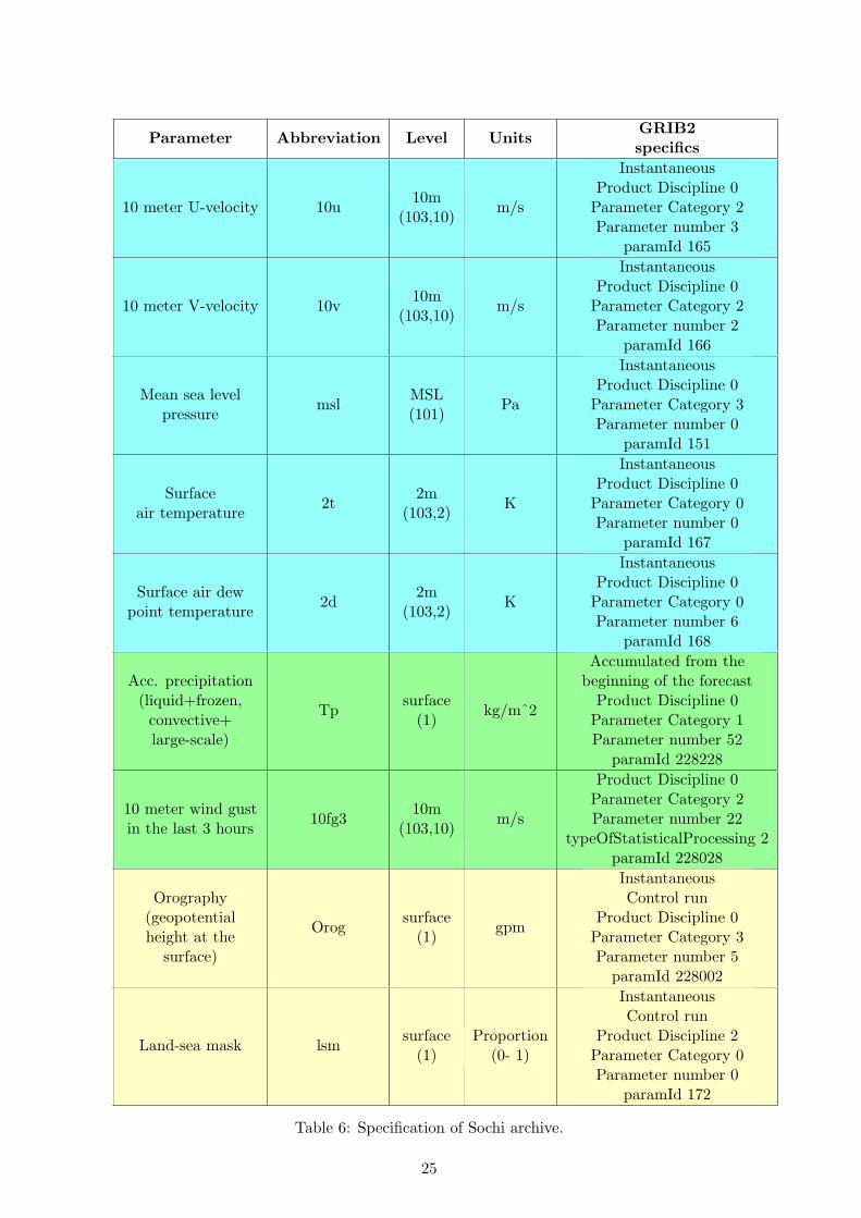
The Sochi unified archive covers the period from January 15, 2014 to March 16, 2014. Thistime interval coincides with the period adopted for verification in FROST-2014 (January 15- March 15, 2014). The archive contains the ensemble forecasts by COSMO-S14-EPS andCOSMO-Ru2-EPS starting at 00 UTC and 12 UTC on the dates within the above-mentionedtwo-month interval. The prognostic fields for all members are presented with a 3h timefrequency on the original COSMO-model rotated latitude-longitude grid with resolutions 7and 2.2 km for COSMO-S14-EPS and COSMO-Ru2-EPS, respectively. The accumulatedparameters (precipitation and wind gusts at 10 m) are not archived at zero time step. Thedata are in WMO-GRIB2 format. The archived parameters and the corresponding codinginformation are listed in Table 6. The parameter set is slightly different from the TIGGE-LAM high-priority parameters. The Sochi archive does not contain large-scale precipitation,convective inhibition, and convective available potential energy. As static fields (land-seamask and orography) did not change during the period, they were written to the archiveonly once.

24

Parameter Abbreviation Level UnitsGRIB2specifics

10 meter U-velocity 10u10m

(103,10)m/s

InstantaneousProduct Discipline 0Parameter Category 2Parameter number 3

paramId 165

10 meter V-velocity 10v10m

(103,10)m/s

InstantaneousProduct Discipline 0Parameter Category 2Parameter number 2

paramId 166

Mean sea levelpressure

mslMSL(101)

Pa

InstantaneousProduct Discipline 0Parameter Category 3Parameter number 0

paramId 151

Surfaceair temperature

2t2m

(103,2)K

InstantaneousProduct Discipline 0Parameter Category 0Parameter number 0

paramId 167

Surface air dewpoint temperature

2d2m

(103,2)K

InstantaneousProduct Discipline 0Parameter Category 0Parameter number 6

paramId 168

Acc. precipitation(liquid+frozen,convective+large-scale)

Tpsurface(1)

kg/mˆ2

Accumulated from thebeginning of the forecastProduct Discipline 0Parameter Category 1Parameter number 52

paramId 228228

10 meter wind gustin the last 3 hours

10fg310m

(103,10)m/s

Product Discipline 0Parameter Category 2Parameter number 22

typeOfStatisticalProcessing 2paramId 228028

Orography(geopotentialheight at the

surface)

Orogsurface(1)

gpm

InstantaneousControl run

Product Discipline 0Parameter Category 3Parameter number 5paramId 228002

Land-sea mask lsmsurface(1)

Proportion(0- 1)

InstantaneousControl run

Product Discipline 2Parameter Category 0Parameter number 0

paramId 172

Table 6: Specification of Sochi archive.

25

CaseMeteorological

process/phenomenon

Models behaviorImpact on

competitions

07.02 Foehn

Poor temperature forecast(underestimated by

1.4 ... 3.7 )by most models atBiathlon Stadium

10-11.02Dissipated

precipitation

Precipitation in the MountainCluster predicted by themajority of systems,

but not observed actually

15.02

Poor forecast of maximumwind speed by most models

at Krasnaya Polyana(underestimated by

3.5 ... 7 m/s)

16.02Low

visibility

Postponed competitionsat Laura andExtreme Park

18.02 Cold frontGood precipitation forecast

by most models

22.02 Foehn

Poor temperature forecastby most models

(negative forecast errors:-2.4 ... -4.4 ,

mostly at 1500 m)

11.03Cold front.

Low visibility

Bad description of the behaviorof maximum temperature(Tmax) by most models

(Tmax forecasted at noon,whereas in reality it wasobserved in the morning)

Postponed skiingcompetitions

at Roza Khutor

13.03Poor precipitation forecast bymost models above 1500 m

17.03 Cold frontUnderestimation of maximumwind speed by most models

above 1500 m

Table 7: The most interesting cases during the Olympics/Paralympics.

The following ensemble meta-data information is included to the GRIB files:

• the ensemble size (GRIB key numberOfForecastsInEnsemble);

• the number of ensemble member (GRIB key perturbationNumber);

• the forecast type (GRIB key dataType = pf/cf, i.e. perturbed/control).

No data for mean sea level pressure is available for COSMO-S14-EPS. Initial and boundaryconditions for high-resolution COSMO EPS are available on demand. All other FROST-2014 forecast data (both deterministic and ensemble) in the Sochi unified archive are coded

26

in the same way. The archive is available at http://frost2014.meteoinfo.ru (authorizationrequired). To download the forecasts, you must switch to Forecasts (upper panel) -Exportof gridded ensemble forecasts (right panel), and then select the necessary data using theinterface similar to that of TIGGE-LAM data portal (Fig. 13). The necessary data will beprepared in compressed form, the corresponding reference will be sent by e-mail, and thenthe data can be downloaded. In addition to the prognostic fields, point forecasts (mean forensembles) can be exported in csv format for more than 30 stations in the Sochi region.During the Olympics these forecasts were regularly presented at the multi-system page ofthe FROST-2014 site along with observation data and were considered very useful both byforecasters and researchers. To prepare these forecasts, the nearest grid-point approach wasapplied. A Web-tool to export observation data was also developed. For more details, pleasevisit http:/frost2014.meteoinfo.ru, where you will also find a short description of all FROST-2014 numerical weather prediction systems. When research deals with the investigation ofthe skill of different weather prediction systems and of new ways to improve the forecast,it is important to have information about the synoptic situation in the analyzed domainand to select really essential events for case studies. To facilitate research in the field ofshort-range forecasting, Sochi forecasters prepared a list of cases recommended for detailedconsideration. This list supplements the unified archive and is given in Table 7.

Figure 13: The FROST-2014 Web-interface used to download forecasts from the unified Sochiarchive.

5.5 Conclusions

The unified Sochi archive containing forecasts for the area of Olympic Games 2014 forthe period from January 15, 2014 to March 16, 2014 was prepared. The forecasts of twoCOSMO-based ensemble prediction systems, COSMO-S14-EPS and COSMO-Ru2-EPS with

27

resolutions 7 and 2.2 km respectively, are stored in the archive. The Web-tool to down-load the forecasts and observations as well as the list of interesting cases for research sup-plement the archive. The archive is organized in TIGGE-LAM style and is available athttp://frost2014.meteoinfo.ru.

6 PREPARING OF RECOMMENDATIONS FOR FORE-CASTERS ABOUT FEATURES OF INTERPRETATIONOF THE RESULTS OF MESO- SCALE MODELING (Howto use the LAM mesoscale NWP results for mountain ter-rain) (I. Rozinkina, P. Eckert, G. S. Rivin)

The feed-back from forecasters of Sochi-team in domain of experience of use of numeric meso-scale products was studied. The Some recommendations for improving the further trainingswere obtained.

6.1 Introduction

This document summarizes the lessons from experience of meteorological support of SochiTrials 2011, 2012, 2014), Olympics and Paraolympics (2014), matters of trainings for fore-casters team for Sochi2014 meteosupport (2011-2014) in part of use of High resolution NWPproducts based on COSMO-Ru output, the discussions of experts of the COSMO WG4sessions during and after period of Sochi-2014 meteosupport and learning exercise. Someexamples of NWP output of named learning period were upgraded. The complexity of theSochi region (steep mountains located in close proximity to the wide warm Black Sea area)justifies the application of the high resolution for short-term numerical weather forecasting.Weather forecast for the “Sochi-2014” is yet a big challenge. This document is focused on thefeatures of using Mesoscale NWP products for mountain terrain on example of COSMO-Rumodel with resolution 2.2 km with 1.2 km nested domains. This document is prepared inframework of COSMO PT “CORSO-A” which had the goal to summarize the experience ofusing results obtained during the realization of Sochi meteosupport for dissemination amongthe COSMO participating countries. As part, it consists of fixation of certain experienceobtained using the products of High-resolution mesoscale model.

6.2 Key definitions

• Mesoscale atmospheric circulations - in context of this document it is determinedas the atmospheric processes of the spatial scale from several (first tens kilometers) to100 - 500 km (as distinct from synoptic scale processes - from 100 - 500 to 5000 km). Itshould be considered that no defined distinction between these scales could be statedas absolute truth. All scales are cross-related and could be determined only specificallyin context of specific synoptic situation. In terms of time scale the mesoscale processescould last from minutes to several hours. However these phenomena can generate thesynoptic scale events, which could be viable for several days. The cyclones, includingtropical cyclones are defined as synoptic objects. The earlier classifications (1970-th)limit the synoptic processes with much more rough scale 2000 km, latter (1980-th) -several hundred km, which partially was related to possibility identifying the circulationobjects according the density of observation data.

28

• Model grid step - horizontal distance between the centers of adjacent grids. Size ofatmospheric model grid step limits the lower edge of the synoptic objects, which couldbe identified by the certain model.

• Resolution of modelled processes - determines the dimension of reliably circum-scribed by the model circulation objects. Normally these objects are of the size of 7 -10 model grid sells. Accuracy of forecast of atmospheric phenomena related to theseobjects is of the same scale. For meteorological parameters near the surface, especiallyat the mountains, the accuracy of the detailed model results could be significantlycloser to the size of grid sell due to local limited land surface forcing.

• Mesoscale atmospheric models - global or limited area models (LAM) with thegrids allowing describe the different atmospheric processes of defined spatial and timeintervals (1, 3).

• Non-hydrostatic atmospheric models are the models with such spatial resolutionwhen the hydro-static approximation is non-correct, and is required the explicit con-sideration of vertical motion acceleration (based on vertical component of wind speed),where the hydrostatic approximation can not be used. Non-hydrostatic effects shouldbe taken into account for the grids with the step lesser than 9 - 10 km. This is thetypical characteristic of the contemporary models for the limited areas. At the sametime, the non-hydrostatic approach is evolved in global modeling aspect.

• Convective-resolving atmospheric models - models of the atmosphere allowing(not using parameterizations) describe the large convective systems. Such models havethe horizontal grid step of less than 3 km. However, a certain part of convectiveprocesses (depending on grid step) will remain in the under-grid scale and shouldbe parameterized. The algorithms of remaining share of convective processes shouldadequately describe their scale.

6.3 Main statements of use of products of global / Limited area NWPProducts for short-range and very-short range forecasting

For short-range weather prediction a forecaster should analyze the output of both kinds ofNWP technologies: global and systems of the limited area modeling. The advance of LAMsagainst the global models is determined by combination of two factors: higher resolution /considering non-hydrostatic effects and the list of available output for forecasters of Nationalmeteorological centers, which develop LAM technology. The following statements explainthe above.

Purposes for the use of the output of:

a) Global modeling

To determine the large-scale weather patterns of atmospheric processes, analyzing andforecasting of generation, evolution and trajectories of the cyclones and anticyclonesin short- and medium-range forecasting (in medium-range forecasting the forecasts arebased usually on global ensemble modeling). Grid resolution of advances operationalglobal models allows reasonably accurately reproduce the baroclinic zones, jet streamsin upper troposphere and stratosphere, processes of cyclones generation, forming anddegradation of atmospheric fronts. The grid resolution of global models has a tendencyto more and more increasing, and the new generation of Global NWP are usually usenon-hydrostatic approach. However, frequently some limitations exist for providing the

29

full sets of products of Global NWP to local users - this is one of serious reasons whythe LAM technologies become more and more popular in the National MeteorologicalServices.

b) Limited-area modeling

For forecasting of large variety of phenomena from synoptic to local (depending ofdimension of calculation area and dimension/resolution of grid cells. Operational non-hydrostatic LAMmight have a large range of grid dimensions - from hundreds meters toseveral or even first tens of kilometers. They can reasonably adequately reproduce thewide range of meteorological processes in different LAM, often, by “nested” technolo-gies: from large-scale processes (generation, evolution and trajectories of the cyclones)to events of convective nature and/or hazard of appearance of local phenomena (windgusts, heavy showers, blizzards), fogs, circulation in the mountains and in the coastalareas, influence of the urbanized territories on meteorological characteristics, genesisand development of small-scale, but extremely dangerous polar-lows, etc. Possibilityof description of the processes of certain scales is limited to the dimension of LAMgrid resolution and form one side and from another - to the dimension of calculationarea. Products of LAM operating in the spacious areas of calculation could be usedby forecasters along with the products of global systems in analysis of synoptic objectsdynamics.

Centers operating the models:

a) Global NWP models

Global NWP systems are developed on their own in relatively small number of centers.These global centers have sufficient computational, technological and communicationalresources, as well as a proper personnel skills. An important component of the globalNWP producing is the development of comprehensive technologies of data assimilationand processing.

b) Limited-area NWP systems

The LAM systems are developing in more than 70 National meteorological centers ofWMO. LAM systems are developing as a role, both in the centers of global modelling,and in the National meteorological centers, and in some local forecasting centers. LAM“cascade” technologies produce more and more detailed products from initial globalmodel, using the more rough version to LAM versions with each step increasing res-olution 3-4 times to hundreds meters comparing with the models, which are used forproducing the initial and boundary conditions for LAMs normally having more roughresolution. These systems could be developed for weather forecasting in relatively smallareas within the region of responsibility of National (district) meteorological services.Many NGMSs are using LAM models developed in other countries, which relates es-pecially to international consortiums. The LAM systems are based on the operationalaccess to the sets of initial data and boundary conditions for calculation area providedby centers of global NWP via Internet.

Features of Dissemination of NWP products for NHMS WMO weather forecasters

a) Global NWP products:

30

1 Information is provided via WMOWIS in standard code formats on the net - gridsin correspondence with WMO regulations (if other is not envisaged by agreementof the country with producers of global forecasts). WMO WIS regulations areoriented on φ/λ grids and standard vertical levels. In the Global models grids ofdisseminated products are naturally more rough than computational grids. There-fore a part of information of the surface weather produced by global models areoften additionally smoothed in the process of transmission of digital information.

2 Via specialized meteorological Internet sites as graphical products. At the sametime, lists of the placed products are limited and it is practically impossible tosatisfy all requirements connected with detailed visualization and maps design forzone of responsibility of each NHMS.

b) LAM NWP products:

Each NHMS can use maximally the LAM output with required details both in compu-tational aspect and visualization for certain region via Internet-technologies.

6.4 Stages of analysis of NWP products for local short- range forecasting

6.4.1 Common recommends

The forecaster analysis of NWP products should have certain stages.

The main idea: To understand the genesis of meteorological processes (following, theirproperties and potential conditions for severe weather) for identified areas based on combi-nation of synoptic analysis with more detailed data.

The daily operational forecaster discussions (briefing):

The discussion (synoptic briefing) have to be organized to coordinate forecasts for all venuesof area of responsibility creating unified concept of understanding of different forecastersand forecasters groups of current and future weather processes. These briefings should beorganized firstly in the each forecasters group (e.g. concrete venue or region) and after thatvia video-conference arranging participation of representatives of all groups at least once aday, but preferably - twice a day, before the issue of morning official forecast and in theevening. The main responsibility takes the main forecaster group, which issues the dailybulletin and controls the Web-site information The discussion have to contain the followingitems:

1 Analysis of processes from large to local space - scales

2 Proposals for 4-5 Day weather trends based on NWP of large-scale processes for abouthalf/third of Hemisphere

3 Analysis of weather of previous day/night

4 Knowledge of current NWP forecast quality (typical errors for the last several days)

5 Proposals for short-range (from 12 until 72h: tomorrow, after-tomorrow) and veryshort-range (from 2 until 12 hours: today/tonight)

6 Threat assessment of severe weather events for each forecasting interval.

31

6.4.2 Experience of large-scale weather types before the analyze of HR products

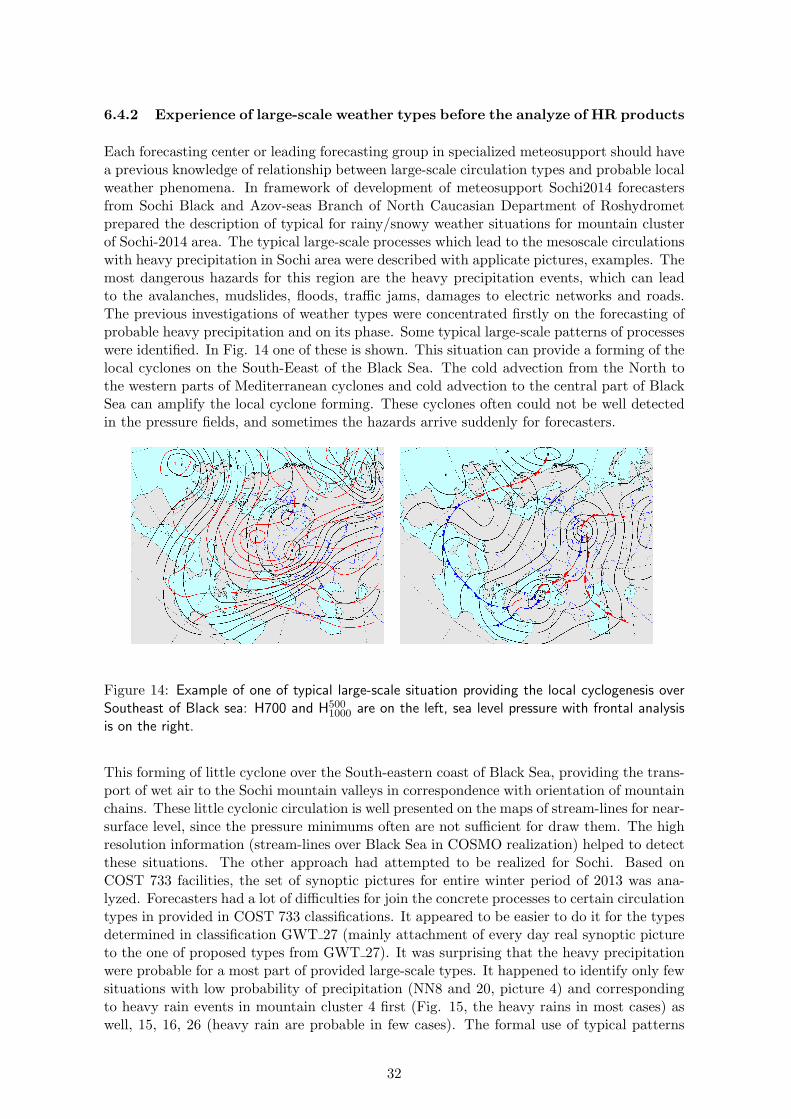
Each forecasting center or leading forecasting group in specialized meteosupport should havea previous knowledge of relationship between large-scale circulation types and probable localweather phenomena. In framework of development of meteosupport Sochi2014 forecastersfrom Sochi Black and Azov-seas Branch of North Caucasian Department of Roshydrometprepared the description of typical for rainy/snowy weather situations for mountain clusterof Sochi-2014 area. The typical large-scale processes which lead to the mesoscale circulationswith heavy precipitation in Sochi area were described with applicate pictures, examples. Themost dangerous hazards for this region are the heavy precipitation events, which can leadto the avalanches, mudslides, floods, traffic jams, damages to electric networks and roads.The previous investigations of weather types were concentrated firstly on the forecasting ofprobable heavy precipitation and on its phase. Some typical large-scale patterns of processeswere identified. In Fig. 14 one of these is shown. This situation can provide a forming of thelocal cyclones on the South-Eeast of the Black Sea. The cold advection from the North tothe western parts of Mediterranean cyclones and cold advection to the central part of BlackSea can amplify the local cyclone forming. These cyclones often could not be well detectedin the pressure fields, and sometimes the hazards arrive suddenly for forecasters.

Figure 14: Example of one of typical large-scale situation providing the local cyclogenesis overSoutheast of Black sea: H700 and H500

1000 are on the left, sea level pressure with frontal analysisis on the right.

This forming of little cyclone over the South-eastern coast of Black Sea, providing the trans-port of wet air to the Sochi mountain valleys in correspondence with orientation of mountainchains. These little cyclonic circulation is well presented on the maps of stream-lines for near-surface level, since the pressure minimums often are not sufficient for draw them. The highresolution information (stream-lines over Black Sea in COSMO realization) helped to detectthese situations. The other approach had attempted to be realized for Sochi. Based onCOST 733 facilities, the set of synoptic pictures for entire winter period of 2013 was ana-lyzed. Forecasters had a lot of difficulties for join the concrete processes to certain circulationtypes in provided in COST 733 classifications. It appeared to be easier to do it for the typesdetermined in classification GWT 27 (mainly attachment of every day real synoptic pictureto the one of proposed types from GWT 27). It was surprising that the heavy precipitationwere probable for a most part of provided large-scale types. It happened to identify only fewsituations with low probability of precipitation (NN8 and 20, picture 4) and correspondingto heavy rain events in mountain cluster 4 first (Fig. 15, the heavy rains in most cases) aswell, 15, 16, 26 (heavy rain are probable in few cases). The formal use of typical patterns

32

from GWT 27, type 4 showed a good correspondence with process shown in Fig. 14, selectedin independent mode via only forecasters experience.

Figure 15: The Pattern N4 from GWT-27. (“wet” with lot of cases of heavy precipitations).

Figure 16: The Pattern N4 (left) and 20 (right) from GWT-27. (“dry” without precipitation).

Note, these “dry” cases are not depended form Ps values, but in both cases the advection ofcold air to the middle Black sea is blocked. This below illustrates following conclusions:

• A large scale synoptic analysis for this region has to establish the factors(cold advection from North or North-East, high humidity flows) to front

33

forming near and over the area of forecasters responsibility. For certaindays cold advection to the Black Sea has to be detected.

• The combination with HR results is necessary for notify the forming of theregional circulation or to notify the large-scale synoptic circulation withpassing of active fronts with additional advection from North-West.

6.4.3 Recommended sequence of analysis, design and content of forecastersmaps

A view of some - days forecast row of H500 pictures in parallel with P for further3-4 days

A goal to detect the main atmospheric flow forming advection on area of responsibility, thevelocity of processes moving and development, the lapse rates and resemblance to the typicallarge-scale patterns. The combining of H500 with T2m (or T850) and of P with Middle levelclouds and 3-h precipitation amounts is recommended. The printing of these rows of maps isrecommended for forecasters for compare the next day old and new forecast rows to discovertendencies of model errors in movement of synoptic objects and front development. Theinitial part of such forecast row (until 48 hours) by COSMO-Ru7 (step 7 km) is shown atFig. 17). Figs 18 and 19 present more detailed an example of H500+T2m forecast mapdesign.

Some remarks:

• The time step for quick large- scale analysis can be 12 hours.

• The grid- step of modelling of 15 km is sufficient (If global products with similar grid-step are available, they can be used in similar visualization).

34

Figure 17: A row of forecasts: H500 and T2m on the left, PMSL, 3h accumulated precipitationand midlevel cloud on the right.

35

Figure 18: An example map design with H500 and T2m forecast. (Inscription in Russian: (Top)Forecast time and date, forecasted parameters; (Bottom) lead time and forecast start time, modeland grid spacing; map legend: color scale for temperature, lines: black- , white: PMSL).

Figure 19: An example map design with PMSL, 3h accumulated precipitation and mid-levelcloudiness forecast. (Inscription in Russian: (Top) Forecast time and date, forecasted parameters;(Bottom) lead time and forecast start time, model and grid spacing; map legend: color scale of3h Precipitation, color scale of Clouds, lines: black: PMSL).

36

Analysis of maps series of PMSL, Cloudiness, Precipitation with 3h-temporal resolution until78-84 hours lead time is recommended additionally. This permits to understand the genesisof cyclones and related precipitation. The Mid-level clouds correlate with the frontal area.

Analysis of map series of high- resolution output: COSMO-Ru2 (2.2.km)

Temporal resolution 1 hour, until 48 hours lead time, for entire Caucasian and Eastern BlackSea area:

• Low clouds

• PMSL+ Mid-level Clouds + 3h Precipitation /1h Precipitation (recommended timestep of view maps is 3 hours)

• V10m and wing gusts

• T2m + T850

• Fresh snow accumulated for 3 hours and for 24 hours

• Stream lines + Relative humidity at the 900, 800, 750 hPa

• Stream lines + Relative humidity at the 900, 800, 750 hPa

Some design examples are shown in Figs. 20-22.

Figure 20: Design of COSMO-Ru2 forecast maps: PMSL, mid-level clouds, 1h precipitation(left) and 12 h accumulated precipitation (right).

37

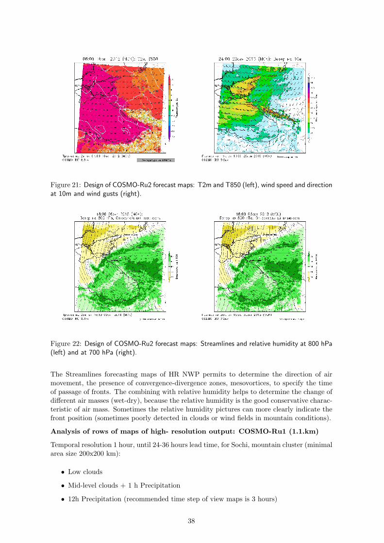
Figure 21: Design of COSMO-Ru2 forecast maps: T2m and T850 (left), wind speed and directionat 10m and wind gusts (right).

Figure 22: Design of COSMO-Ru2 forecast maps: Streamlines and relative humidity at 800 hPa(left) and at 700 hPa (right).

The Streamlines forecasting maps of HR NWP permits to determine the direction of airmovement, the presence of convergence-divergence zones, mesovortices, to specify the timeof passage of fronts. The combining with relative humidity helps to determine the change ofdifferent air masses (wet-dry), because the relative humidity is the good conservative charac-teristic of air mass. Sometimes the relative humidity pictures can more clearly indicate thefront position (sometimes poorly detected in clouds or wind fields in mountain conditions).

Analysis of rows of maps of high- resolution output: COSMO-Ru1 (1.1.km)

Temporal resolution 1 hour, until 24-36 hours lead time, for Sochi, mountain cluster (minimalarea size 200x200 km):

• Low clouds

• Mid-level clouds + 1 h Precipitation

• 12h Precipitation (recommended time step of view maps is 3 hours)

38

• V10m and wing gusts

• T2m + T850

• Fresh snow accumulated for 3 hours and for 24 hours

• Stream lines + Relative air humidity at the 900, 800, 750 hPa

The products of NWP technology with 1km grid step are the most important kind of NWPinformation for weather forecasting in the mountains. The most important forecast elementsvia NWP-1 km are wind and fresh snow fields. The forecasts reflect mountain chains andvalleys most accurately (see Fig. 23).

Figure 23: Design of COSMO-Ru1 forecast maps: Streamlines and relative humidity at 800 hPa(left) and fresh snow (right).

6.5 Analysis of Meteograms of deterministic LAM HR NWP

6.5.1 Definitions and goals

Definitions. Meteograms are the graphs, which combine model output (deterministic or en-semble) with form of time evaluation graphics of selected meteorological parameters. Incase of ensemble forecasting ones are named Ensemble Prediction System meteograms (EPS-grammes). The information of this section relates to the deterministic high-resolution(HR) model output. Goals and applications. Meteograms permit to observe timeevaluation of key meteorological parameters for selected vertical levels for concrete points.The 1-h (or less) time steps of presenting information (as a rule lesser than for forecastingcharts) permits to notify a time of fronts passing, of star-end of weather phenomena, as wellof daily temperature extrem time. Another application of meteograms (Fig. 24) is a veryquick forecasters complication of meteorological data for big number of points for not largeregion to receive an information about spatial differences and uncertainties of some param-eters. The analysis of NWP matters by forecasters can start by watching of meteograms, aswell, it is useful to look at them after analysis of all forecasting maps, after understanding offorecasted synoptic and mesoscale processes. Fig. 24 shows the Meteograms design, whichwas realized as a result of feed-back from forecasters of Sochi / Hydrometcenter of Russiabased on adaptation of DWD variant of COSMO software. The color and placing of picturefor forecasts of different parameters are important.

39

Figure 24: Example of deterministic meteogram for points of Sochi mountain.

6.5.2 Key principles for technology of meteogram forming

• Meteograms are presented in some sections of graphics for one point with unifiedtime axe of selected elements adapted to the forecasters expert analysis, e.g. wind,temperature, clouds on several levels, precipitation, etc. The levels for pictures fordifferent elements can be different. A feedback from forecasters for realizing the mostefficient pictures design (icluding fast loading of pictures for big number of points onthe monitor) is strongly recommended.

• Meteograms technology has to provide for quick forecasting analysis the picturesof few-days changes for nominated points of maximal number of important parameterswith timestep no more than 1 hour.

• A severe meteograms around nominated point or inside an area (a city, acluster of competitions, etc.) is recommended for more reliable forecasting of randomprecipitation and of probably hazards.

• The volume of pictures should be minimal. This requirement was set up: firstly,to necessity of quick forecasters analysis and comparison of large number of meteogramsfor different points for one region, secondly, by possible limitations of Internet channelsavailable to forecasters outside on large forecaster centers.

• Lists of points for meteogram visualization should be prepared by forecast-ers/users with indication of Lat/Lon (as rules, there are points of meteostations,towns/cities, important objects, venues of competitions) in stage of forming of meteogram-technology. Systems of forming of meteograms of high resolution modeling such COSMOdo not interpolate from the gridded model results to nominated points, and as rules,

40

a nearest model grid-point is automatically selected. In cases of high spatial vari-ability of geographical properties grid- points have to be manually selected based anexpert analysis of geographical properties. As an example, Fig. 25 shows grid-pointsof COSMO-Ru7 (blue) and COSMO-Ru2 (yellow). In the red are shown the pointsof venues / observing stations. COSMO-Ru2 grid- nodes nearest to the venues havea good concordance with the 2 nominated points (chance coincidence), but a mostrepresentative grid-point for the point Krasnaya Polyana should be chosen manually(which has a close high is preferable from 4 nearest grid-nodes).

Figure 25: Grid-nodes of COSMO-Ru7 (blue circles) and COSMO-Ru2 (yellow circles) over Earthmap for mountain cluster of Sochi region. Red balloons and blue snowflakes indicate the venueslocations.

6.5.3 Forecasters analysis based on meteograms

Forecasters should take account that:

• Coordinates of nominated by forecasters points are not same as ones of meteograms(nearest corresponding model grid- points) (see above the previous section) Coordinatevalues of model meteograms points have be indicated at the top of the picture pages.Forecasters have to compare indicated values with coordinates of real nominated point.In cases of complicate geographical conditions it can lead to the completely wrongforecasts for selected points of local weather conditions (e.g. a land point can beautomatically corresponded to a maritime nearest grid point, a point in the valley - tothe point at the top of mountain, etc.). In the Fig. 26 grid-point coordinates longitude40.2E, latitude=43.7N are indicated by red oval. The coordinates of nominated pointare 40.1E, 43.6N).

• The real high of nominated point is not same as high of corresponding model grid point(important especially for the mountain cases) High of model grid points is indicated atthe top of the picture pages (Fig. 26 at the green oval - 1544m). Forecasters have to

41

compare these values with ones of real nominated points and to analyze a difference.Some postprocessing technologies calculate the corrected values of T2m and of Td2mbased on assumptions of temperature lapse rate. In our example, the real high is only576m. The results of correction of T2m is shown on the meteogram by violet line,parallel to the red line, corresponding a T2m forecasts from direct model output.

Figure 26: Example of meteogram for Cordon Laura. The coordinates and high of grid- box arecircled in ovals (red and green).

There are some features of analysis, important for forecasters:

• Pressure section: pressure values and its tendencies, the time interval of minimum dueto the rapid cyclone passage

• Temperature section:

– Temperature values and their tendencies at 2, 850 hPa, 700 hPa and 500 hPa canbe important for mountain area. Note the inversion state (e.g. if T2m less thanT850, in mountains T850 less than T700). (Following special requests, the levelscan be other).

– T850 In mountains regions can be close to the T2m (or underground)

– An additional T2m values as postprocessing result can be added. Be careful withits analysis.

– The close and equal values of TD2m and of T2m can indicate the high probabilityof fog.

• Precipitation section:

– Additional to the vertical columns (1-hour sums) the 3-h sums are written.

42

– If the T2m is corrected by postprocessing techniques, the additional control ofphase of precipitation is useful. In our case (Fig. 26) after T2m lapse rate correc-tion it was warmer than 0 degrees. So, the predicted snow should be not snow,but in case of continuous heavy rain, forecaster could make a decision himself.

– In case of short precipitation and/or precipitation of convective origin. It is use-ful to analyze meteograms for other close grid- points. The radius of probableprecipitation is about 3-4 grid- cells!

• Cloud section:

– Middle level clouds are the most important and indicate with high clear-sky orovercast conditions.

– Low level clouds have a lowest forecasting skill. This is feasible to control basedon synoptic knowledge.

– Convection existing or not can help to understand the origin of clouds.

– Maximum convection height (yellow columns at the bottom of the page) canindicate the dangerous convective situations in case of extremely high (more than10 km) of convection level. In these cases the weather hazards of convective originhave a high probability not only for the point of meteogram, but also around thisplace.

• Wind section:

– Wind direction and speed at 10 m, 500 m, 850, 700, 500 hPa levels are presented.For specialized forecasts the other levels can be required by users.

– Sharp changes in wind direction at the lower levels can indicate the time of frontpassage (in our case- at the first hours of forecast and at 3-rd forecast day).

– Wind speed more than 25 m/s at 500 m altitude can indicate as a threat of squallat the near-surface level.

6.6 Conclusion

In the current document we shoved the key positions of experience of trainings for forecastersfor Sochi forecaster team in 2012-2014 years. This experience could be useful for furthertrainings from one hand, and from other hand should be developed in further.

7 Acknowledgements

This work was carried out within the COSMO PT CORSO-A and WWRP FDP/RDPFROST-2014. The authors are grateful to Tatiana Dmitrieva (Roshydromet) for provid-ing the information on weather cases during the winter 2014 and to Tiziana Paccagnella(ARPAE) for supporting the work.

43

A Appendix

Event ObservedYES NO

Event ForecastedYES A BNO C D

Table 8: 2x2 Contingency Table.

Threshold (mm/3h)Forecast lead time (h)

3 6 9 12 15 18 21 24

Domain 300 x 300 g.p.

0.1 0.42 0.62 0.63 0.72 0.58 0.39 0.36 0.49

0.5 0.43 0.66 0.68 0.73 0.62 0.46 0.37 0.42

1 0.35 0.49 0.70 0.77 0.55 0.42 0.33 0.34

2 0.28 0.28 0.59 0.68 0.31 0.38 0.29 0.21

3 0.22 0.44 0.64 0.31 0.51 0.32

5 0.32 0.55 0.53

10 0.27 0.26 0.60

Domain 450 x 450 g.p.

0.1 0.42 0.57 0.62 0.66 0.56 0.38 0.38 0.49

0.5 0.43 0.58 0.59 0.70 0.57 0.44 0.37 0.42

1 0.35 0.43 0.62 0.74 0.55 0.39 0.35 0.35

2 0.27 0.25 0.57 0.71 0.39 0.40 0.31 0.18

3 0.20 0.48 0.65 0.34 0.48 0.40

5 0.32 0.55 0.47

10 0.26 0.16 0.63

Domain 450x 650 g.p.

0.1 0.42 0.57 0.62 0.66 0.56 0.38 0.38 0.49

0.5 0.43 0.58 0.59 0.70 0.57 0.44 0.37 0.42

1 0.35 0.43 0.62 0.74 0.55 0.39 0.35 0.35

2 0.27 0.25 0.57 0.71 0.39 0.40 0.31 0.18

3 0.20 0.48 0.65 0.34 0.48 0.40

5 0.32 0.55 0.47

10 0.26 0.16 0.63

Table 9: CSI values.

44

Threshold (mm/3h)Forecast lead time (h)

3 6 9 12 15 18 21 24

Domain 300 x 300 g.p.

0.1 0.28 0.51 0.53 0.64 0.50 0.29 0.25 0.38

0.5 0.34 0.59 0.61 0.67 0.56 0.40 0.29 0.33

1 0.29 0.42 0.64 0.72 0.49 0.37 0.27 0.27

2 0.25 0.23 0.53 0.62 0.27 0.35 0.25 0.17

3 0.19 0.39 0.60 0.29 0.49 0.29

5 0.29 0.52 0.52

10 0.25 0.24 0.59

Domain 450 x 450 g.p.

0.1 0.29 0.45 0.51 0.58 0.47 0.27 0.27 0.38

0.5 0.34 0.51 0.50 0.63 0.51 0.37 0.29 0.34

1 0.29 0.36 0.55 0.68 0.50 0.33 0.30 0.28

2 0.24 0.21 0.51 0.67 0.36 0.37 0.27 0.14

3 0.17 0.43 0.61 0.32 0.46 0.38

5 0.29 0.52 0.46

10 0.25 0.15 0.63

Domain 450x 650 g.p.

0.1 0.29 0.45 0.48 0.59 0.52 0.29 0.27 0.36

0.5 0.34 0.50 0.51 0.62 0.53 0.37 0.28 0.34

1 0.29 0.36 0.58 0.65 0.50 0.33 0.31 0.27

2 0.24 0.22 0.51 0.59 0.38 0.34 0.27 0.15

3 0.20 0.42 0.53 0.37 0.44 0.40

5 0.28 0.55 0.52

10 0.24 0.17 0.63

Table 10: ETS values.

45

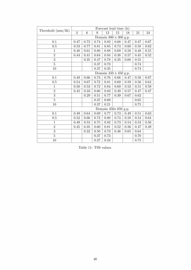
Threshold (mm/3h)Forecast lead time (h)

3 6 9 12 15 18 21 24

Domain 300 x 300 g.p.

0.1 0.47 0.72 0.74 0.82 0.68 0.47 0.47 0.67

0.5 0.53 0.77 0.81 0.85 0.74 0.60 0.58 0.62

1 0.48 0.61 0.80 0.88 0.69 0.58 0.48 0.55

2 0.44 0.41 0.64 0.84 0.38 0.57 0.45 0.52

3 0.35 0.47 0.78 0.35 0.68 0.55

5 0.37 0.73 0.74

10 0.37 0.35 0.74

Domain 450 x 450 g.p.

0.1 0.49 0.66 0.73 0.76 0.66 0.47 0.50 0.67

0.5 0.54 0.67 0.72 0.81 0.69 0.59 0.56 0.64

1 0.50 0.53 0.72 0.84 0.69 0.53 0.51 0.59

2 0.45 0.33 0.60 0.83 0.49 0.57 0.47 0.47

3 0.29 0.51 0.77 0.39 0.67 0.62

5 0.37 0.69 0.65

10 0.37 0.21 0.75

Domain 450x 650 g.p.

0.1 0.49 0.64 0.69 0.77 0.73 0.49 0.51 0.63

0.5 0.52 0.66 0.72 0.80 0.74 0.58 0.54 0.64

1 0.49 0.53 0.75 0.82 0.73 0.54 0.53 0.56

2 0.45 0.35 0.60 0.81 0.52 0.56 0.47 0.49

3 0.32 0.50 0.73 0.46 0.65 0.64

5 0.37 0.73 0.70

10 0.37 0.24 0.75

Table 11: TSS values.

46

Threshold (mm/3h)Forecast lead time (h)

3 6 9 12 15 18 21 24

Domain 300 x 300 g.p.

0.1 0.43 0.68 0.69 0.78 0.67 0.44 0.40 0.55

0.5 0.51 0.74 0.76 0.80 0.72 0.57 0.45 0.49

1 0.45 0.59 0.78 0.84 0.66 0.54 0.42 0.42

2 0.40 0.38 0.69 0.77 0.42 0.51 0.40 0.29

3 0.32 0.56 0.75 0.45 0.66 0.45

5 0.44 0.69 0.68

10 0.41 0.39 0.74

Domain 450 x 450 g.p.

0.1 0.45 0.62 0.68 0.73 0.64 0.43 0.43 0.55

0.5 0.51 0.67 0.67 0.77 0.67 0.54 0.45 0.51

1 0.45 0.53 0.71 0.81 0.66 0.49 0.46 0.44

2 0.39 0.35 0.68 0.80 0.53 0.54 0.43 0.25

3 0.29 0.60 0.76 0.48 0.63 0.55

5 0.45 0.69 0.63

10 0.40 0.25 0.77

Domain 450x 650 g.p.

0.1 0.45 0.62 0.65 0.74 0.69 0.45 0.43 0.53

0.5 0.50 0.66 0.68 0.76 0.69 0.54 0.44 0.51

1 0.45 0.53 0.74 0.79 0.67 0.49 0.48 0.43

2 0.39 0.36 0.67 0.75 0.55 0.51 0.43 0.25

3 0.33 0.59 0.69 0.54 0.61 0.57

5 0.44 0.71 0.68

10 0.38 0.29 0.77

Table 12: HSS values.

Threshold (mm/3h)Forecast lead time (h)

6 9 12 15 18 21

Domain 300 x 300 g.p.

3 0.50 0.70 0.89 0.62 0.83 0.71

5 0.61 0.85 0.87

10 0.64 0.61 0.90

Domain 450 x 450 g.p.

3 0.49 0.72 0.88 0.65 0.83 0.78

5 0.62 0.83 0.83

10 0.64 0.48 0.90

Domain 450x 650 g.p.

3 0.53 0.71 0.84 0.69 0.81 0.80

5 0.60 0.86 0.89

10 0.63 0.52 0.90

Table 13: EDI values.

47

Threshold (mm/3h)Time interval (h)

0-3 3-6 6-9 9-12 12-15 15-18 18-21 21-24

0.1 201 201 188 185 166 157 148 145

0.5 143 153 159 164 129 116 105 111

1 98 129 152 152 112 94 89 82

2 50 76 140 116 75 51 61 39

3 22 45 119 96 57 36 40 27

5 5 17 64 62 21 19 24 19

10 0 2 21 27 2 4 16 3

Table 14: Number of precipitation events of different thresholds for 3-hour intervals.

48

References

Astakhova, E. D., Montani, A., Alferov and Yu, D., 2015: Ensemble forecasts for theSochi-2014 Olympic Games. Russian meteorology and hydrology, 40, 8, 531–539, DOI10.3103/S1068373915080051

Kiktev, D. B., Astakhova, E. D., Zaripov, R. B., Muravev, A. V., Smirnov, A. V. and Tsyrul-nikov, M. D., 2015a: FROST-2014 project and meteorological support of the Sochi-2014Olympics. Russian Meteorology and Hydrology, 40, 8, 504–512, DOI 10.3103/S1068373915080026

Kiktev, D. B., Astakhova, E. D., Zaripov, R. B., Muravev, A. V, Smirnov, A. V. andTsyrulnikov, M. D., 2015b: Erratum to “FROST-2014 project and meteorological supportof the Sochi-2014 Olympics”, Russian Meteorology and Hydrology, 40, 12, 844–845, DOI10.3103/S1068373915120109

Montani, A., Cesari, D., Marsigli, C. and Paccagnella, T., 2011: Seven years of activity inthe field of mesoscale ensemble forecasting by the COSMO-LEPS system: main achievementsand open challenges. Tellus A, 63, 605–624, DOI: 10.1111/j.1600-0870.2010.00499

Montani, A., Marsigli, C. and Paccagnella, T., 2013: Development of a COSMO-basedlimited-area ensemble system for the 2014 Winter Olympic Games. COSMO Newsletter, 13,93–99, available athttp://cosmo-model.org/content/model/documentation/newsLetters/newsLetter13/cnl13 12.pdf

Montani, A., Alferov, D., Astakhova, E., Marsigli, C. and Paccagnella, T., 2014: Ensem-ble forecasting for Sochi-2014 Olympics: the COSMO-based ensemble prediction systems.COSMO Newsletter, 14, 88–94, available athttp://cosmo-model.org/content/model/documentation/newsLetters/newsLetter14/cnl14 10.pdf

Montani, A., Alferov, D., Astakhova, E., Marsigli, C. and Paccagnella, T., 2015: Perfor-mance of the COSMO-based ensemble systems during Sochi-2014 pre-Olympics. COSMONewsletter, 15, 77–82, available athttp://cosmo-model.org/content/model/documentation/newsLetters/newsLetter15/cnl15 10.pdf

Paccagnella, T., Hacker, J., Marsigli, C., Montani, A., Pappenberger, F., Parsons, D., Swin-bank, R. and Toth, Z., 2012: THORPEX Interactive Research Grand Global Ensemble -Limited Area Model Plan. WMO publications, 17, available athttp://www.wmo.int/pages/prog/arep/wwrp/new/wwrp publications.html

Rivin, G. and Rozinkina, I., 2013: Priority Project CORSO: Consolidation of Operation andResearch results for the Sochi Olympic Games, available athttp://cosmo-model.org/content/tasks/priorityProjects/corso/default.htm

Schaefer, J. T., 1990: The critical success index as an indicator of waring skill. Weather andforecasting, 5, 570–575

Schirmer, M. and B. Jamieson, 2015: Verification of forecasted winter precipitation in com-plex terrain. The Cryosphere, 3, 9(2), 587–601, DOI 10.5194/tc-9-587

Shatunova, M. V., Rivin, G. S. and Rozinkina, I. A., 2015: Visibility forecasting for February1618 2014 for the region of the Sochi-2014 Olympic Games using the high-resolution COSMO-Ru1 model. Russian Meteorology and Hydrology, 40, 8, 523–530, DOI 10.3103/S106837391508004X

49

List of COSMO Newsletters and Technical Reports

(available for download from the COSMO Website: www.cosmo-model.org)

COSMO Newsletters

No. 1: February 2001.

No. 2: February 2002.

No. 3: February 2003.

No. 4: February 2004.

No. 5: April 2005.

No. 6: July 2006.

No. 7: April 2008; Proceedings from the 8th COSMO General Meeting in Bucharest, 2006.

No. 8: September 2008; Proceedings from the 9th COSMO General Meeting in Athens, 2007.

No. 9: December 2008.

No. 10: March 2010.

No. 11: April 2011.

No. 12: April 2012.

No. 13: April 2013.

No. 14: April 2014.

No. 15: July 2015.

No. 16: July 2016.

No. 17: July 2017.

No. 18: November 2018.

COSMO Technical Reports

No. 1: Dmitrii Mironov and Matthias Raschendorfer (2001):Evaluation of Empirical Parameters of the New LM Surface-Layer ParameterizationScheme. Results from Numerical Experiments Including the Soil Moisture Analysis.

No. 2: Reinhold Schrodin and Erdmann Heise (2001):The Multi-Layer Version of the DWD Soil Model TERRA LM.

No. 3: Gunther Doms (2001):A Scheme for Monotonic Numerical Diffusion in the LM.

50

No. 4: Hans-Joachim Herzog, Ursula Schubert, Gerd Vogel, Adelheid Fiedler and RoswithaKirchner (2002):LLM ¯ the High-Resolving Nonhydrostatic Simulation Model in the DWD-Project LIT-FASS.Part I: Modelling Technique and Simulation Method.

No. 5: Jean-Marie Bettems (2002):EUCOS Impact Study Using the Limited-Area Non-Hydrostatic NWP Model in Oper-ational Use at MeteoSwiss.

No. 6: Heinz-Werner Bitzer and Jurgen Steppeler (2004):Documentation of the Z-Coordinate Dynamical Core of LM.

No. 7: Hans-Joachim Herzog, Almut Gassmann (2005):Lorenz- and Charney-Phillips vertical grid experimentation using a compressible non-hydrostatic toy-model relevant to the fast-mode part of the ’Lokal-Modell’.

No. 8: Chiara Marsigli, Andrea Montani, Tiziana Paccagnella, Davide Sacchetti, Andre Walser,Marco Arpagaus, Thomas Schumann (2005):Evaluation of the Performance of the COSMO-LEPS System.

No. 9: Erdmann Heise, Bodo Ritter, Reinhold Schrodin (2006):Operational Implementation of the Multilayer Soil Model.

No. 10: M.D. Tsyrulnikov (2007):Is the particle filtering approach appropriate for meso-scale data assimilation ?

No. 11: Dmitrii V. Mironov (2008):Parameterization of Lakes in Numerical Weather Prediction. Description of a LakeModel.

No. 12: Adriano Raspanti (2009):COSMO Priority Project ”VERification System Unified Survey” (VERSUS): Final Re-port.

No. 13: Chiara Marsigli (2009):COSMO Priority Project ”Short Range Ensemble Prediction System” (SREPS): FinalReport.

No. 14: Michael Baldauf (2009):COSMO Priority Project ”Further Developments of the Runge-Kutta Time IntegrationScheme” (RK): Final Report.

No. 15: Silke Dierer (2009):COSMO Priority Project ”Tackle deficiencies in quantitative precipitation forecast”(QPF): Final Report.

No. 16: Pierre Eckert (2009):COSMO Priority Project ”INTERP”: Final Report.

No. 17: D. Leuenberger, M. Stoll and A. Roches (2010):Description of some convective indices implemented in the COSMO model.

No. 18: Daniel Leuenberger (2010):Statistical analysis of high-resolution COSMO Ensemble forecasts in view of Data As-similation.

51

No. 19: A. Montani, D. Cesari, C. Marsigli, T. Paccagnella (2010):Seven years of activity in the field of mesoscale ensemble forecasting by the COSMO–LEPS system: main achievements and open challenges.

No. 20: A. Roches, O. Fuhrer (2012):Tracer module in the COSMO model.

No. 21: Michael Baldauf (2013):A new fast-waves solver for the Runge-Kutta dynamical core.

No. 22: C. Marsigli, T. Diomede, A. Montani, T. Paccagnella, P. Louka, F. Gofa, A. Corigliano(2013):The CONSENS Priority Project.

No. 23: M. Baldauf, O. Fuhrer, M. J. Kurowski, G. de Morsier, M. Mullner, Z. P. Piotrowski,B. Rosa, P. L. Vitagliano, D. Wojcik, M. Ziemianski (2013):The COSMO Priority Project ’Conservative Dynamical Core’ Final Report.

No. 24: A. K. Miltenberger, A. Roches, S. Pfahl, H. Wernli (2014):Online Trajectory Module in COSMO: a short user guide.

No. 25: P. Khain, I. Carmona, A. Voudouri, E. Avgoustoglou, J.-M. Bettems, F. Grazzini(2015):The Proof of the Parameters Calibration Method: CALMO Progress Report.

No. 26: D. Mironov, E. Machulskaya, B. Szintai, M. Raschendorfer, V. Perov, M. Chumakov,E. Avgoustoglou (2015):The COSMO Priority Project ’UTCS’ Final Report.

No. 27: J-M. Bettems (2015):The COSMO Priority Project ’COLOBOC’: Final Report.

No. 28: Ulrich Blahak (2016):RADAR MIE LM and RADAR MIELIB - Calculation of Radar Reflectivity from ModelOutput.

No. 29: M. Tsyrulnikov and D. Gayfulin (2016):A Stochastic Pattern Generator for ensemble applications.

No. 30: D. Mironov and E. Machulskaya (2017):A Turbulence Kinetic Energy – Scalar Variance Turbulence Parameterization Scheme.

No. 31: P. Khain, I. Carmona, A. Voudouri, E. Avgoustoglou, J.-M. Bettems, F. Grazzini, P.Kaufmann (2017):CALMO - Progress Report.

No. 32: A. Voudouri, P. Khain, I. Carmona, E. Avgoustoglou, J.M. Bettems, F. Grazzini, O.Bellprat, P. Kaufmann and E. Bucchignani (2017):Calibration of COSMO Model, Priority Project CALMO Final report

No. 33: N. Vela (2017):VAST 2.0 - User Manual.

No. 34: C. Marsigli, D. Alferov, M. Arpagaus, E. Astakhova, R. Bonanno, G. Duniec, C.Gebhardt, W. Interewicz, N. Loglisci, A. Mazur, V. Maurer, A. Montani, A. Walser(2018):COsmo Towards Ensembles at the Km-scale IN Our countries (COTEKINO), PriorityProject final report.

52

No. 35: G. Rivin, I. Rozinkina, E. Astakhova, A. Montani, D. Alferov, M. Arpagaus, D. Blinov,A. Bundel, M. Chumakov, P. Eckert, A. Euripides, J. Forstner, J. Helmert, E. Kaza-kova, A. Kirsanov, V. Kopeikin, E. Kukanova, D. Majewski, C. Marsigli, G. de Morsier,A. Muravev, T. Paccagnella, U. Schattler, C. Schraff, M. Shatunova, A. Shcherbakov,P. Steiner, M. Zaichenko (2018):The COSMO Priority Project CORSO Final Report.

No. 36: A. Raspanti, A. Celozzi, A. Troisi, A. Vocino, R. Bove, F. Batignani (2018):The COSMO Priority Project VERSUS2 Final Report.

No. 37: A. Bundel, F. Gofa, D. Alferov, E. Astakhova, P. Baumann, D. Boucouvala, U. Dam-rath, P. Eckert, A. Kirsanov, X. Lapillonne, J. Linkowska, C. Marsigli, A. Montani, A.Muraviev, E. Oberto, M.S. Tesini, N. Vela, A. Wyszogrodzki, M. Zaichenko, A. Walser(2019):The COSMO Priority Project INSPECT Final Report.

53

COSMO Technical Reports

Issues of the COSMO Technical Reports series are published by the COnsortium for Small-scale MOdelling at non-regular intervals. COSMO is a European group for numerical weatherprediction with participating meteorological services from Germany (DWD, AWGeophys),Greece (HNMS), Italy (USAM, ARPA-SIMC, ARPA Piemonte), Switzerland (MeteoSwiss),Poland (IMGW), Romania (NMA) and Russia (RHM). The general goal is to develop, im-prove and maintain a non-hydrostatic limited area modelling system to be used for bothoperational and research applications by the members of COSMO. This system is initiallybased on the COSMO-Model (previously known as LM) of DWD with its corresponding dataassimilation system.

The Technical Reports are intended

• for scientific contributions and a documentation of research activities,

• to present and discuss results obtained from the model system,

• to present and discuss verification results and interpretation methods,

• for a documentation of technical changes to the model system,

• to give an overview of new components of the model system.

The purpose of these reports is to communicate results, changes and progress related to theLM model system relatively fast within the COSMO consortium, and also to inform otherNWP groups on our current research activities. In this way the discussion on a specifictopic can be stimulated at an early stage. In order to publish a report very soon after thecompletion of the manuscript, we have decided to omit a thorough reviewing procedure andonly a rough check is done by the editors and a third reviewer. We apologize for typographicaland other errors or inconsistencies which may still be present.

At present, the Technical Reports are available for download from the COSMO web site(www.cosmo-model.org). If required, the member meteorological centres can produce hard-copies by their own for distribution within their service. All members of the consortium willbe informed about new issues by email.

For any comments and questions, please contact the editor:

Massimo MilelliMassimo.Milelli@arpa.piemonte.it

54