HAL Id: hal-01492977https://hal.archives-ouvertes.fr/hal-01492977v3

Submitted on 29 Dec 2017

HAL is a multi-disciplinary open accessarchive for the deposit and dissemination of sci-entific research documents, whether they are pub-lished or not. The documents may come fromteaching and research institutions in France orabroad, or from public or private research centers.

L’archive ouverte pluridisciplinaire HAL, estdestinée au dépôt et à la diffusion de documentsscientifiques de niveau recherche, publiés ou non,émanant des établissements d’enseignement et derecherche français ou étrangers, des laboratoirespublics ou privés.

Copyright

Connectionist Economics - An Outline.H. Georg Schulze

To cite this version:

H. Georg Schulze. Connectionist Economics - An Outline. . 2010, 978-1-4269-4851-0. �hal-01492977v3�

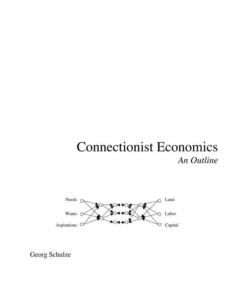
Connectionist Economics

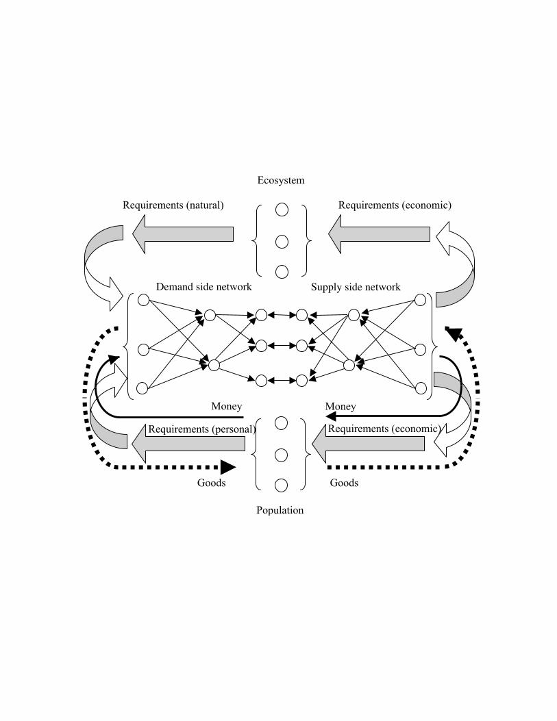
ii

Money

Population

Goods Goods

Money

Requirements (personal) Requirements (economic)

Ecosystem

Requirements (natural) Requirements (economic)

Demand side network Supply side network

iii

Connectionist Economics An Outline

Introductory Section: Chapters 1 to 4

Georg Schulze

Land

Capital Aspirations

Needs

Wants Labor

vi

To my parents, who, each on their own, and between them, managed to balance

many things

vii

Contents

ACRONYMS AND ABBREVIATIONS xiv EQUATIONS xv

PREFACE

xvii

Introduction

1 INTRODUCTION 3 Summary Introduction General overview Demand- and supply-side networks Local descriptions Global descriptions Interacting networks Interacting systems A closer look at the objectives Some remaining difficulties APPENDIX 11 Neurons Networks of neurons Artificial neural networks Worked example

viii Network computations Local perspective

Global perspective

Basic Concepts

2 THE SUPPLY-SIDE NETWORK 22 Summary Introduction The formal structure of the supply-side network The flow of resources, goods and services Money flows Aggregate quantities Network representations Discussion and conclusions

3 THE DEMAND-SIDE NETWORK 34 Summary Introduction The formal structure of the demand-side network The flow of requirements and money The flow of goods and services Aggregate quantities Network representations Discussion and conclusions

4 THE CORE SYSTEM 46 Summary Introduction Integration of demand- and supply-side networks Qualitative applications Markets Prices Remunerations Rents Wages

ix Interest Earnings Rewards Recompenses Equilibria Supply inflation Cost inflation Demand inflation Income inflation Elasticities Discussion and conclusions

Refinements

5 THE QUANTIFICATION OF RESOURCES AND REQUIREMENTS 59 Summary Introduction Resources Land Labor Capital Appearing and disappearing resources Requirements Needs Wants Aspirations Appearing and disappearing requirements Discussion and conclusions

6 THE QUANTIFICATION OF ECONOMIC TRANSFORMATION UNITS 73 Summary Introduction The identities of economic transformation units The number of economic transformation units Speed Efficiency Quality Robustness Discussion and conclusions

x

7 THE QUANTIFICATION OF PRODUCTS 82 Summary Introduction Products supplied Resolution Identification Products demanded Resolution Identification Product optimality Discussion and conclusions

8 REFINEMENTS AT THE LOCAL LEVEL 91 Summary Introduction Local connections Connection weights Transfer functions Node dynamics Innovation Maturation Market entry and exit Profits Losses Discussion and conclusions

9 REFINEMENTS AT THE GLOBAL LEVEL 104 Summary Introduction Number of layers Partitioning of layers Non-local connections

Direct connections Reentrant connections Lateral connections

Variable connections: monopolies and competition Fixed connections: exigencies Discussion and conclusions

xi

Expansions

10 THE PUBLIC ECONOMY AND GOVERNMENT 115 Summary Introduction Government: supply-side Government: demand-side Interactions between public and private systems Taxes Regulation Discussion and conclusions

11 COMPLETING THE SYSTEM WITH CIRCULAR FLOWS 129 Summary Introduction Populations Circular flows Money Goods Requirements Ecosystems Wages, rents, and interest Discussion and conclusions

12 MONEY AND BANKS: GETTING THE SYSTEM GOING 147 Summary Introduction Money as expression of requirements Money should reflect a variety of aspects of requirements Other functions of money Money supply

Creation and distribution Volumes Excessive levels

Deficient levels Velocity Capital Credit

xii Discussion and conclusions

Advanced Topics

13 INTERACTIONS BETWEEN NETWORKS PRODUCE ECONOMIC CYCLES 168 Summary Introduction Disequilibrium causes network errors Network error Network oscillations Profits and losses are error signals Simple and complex disequilibria Simple disequilibria Complex disequilibria Indirect interactions Discussion and conclusions

14 INTERNATIONAL TRADE AND THE INTERACTIONS BETWEEN SYSTEMS 181 Summary Introduction The causes of international trade One-way trade Bidirectional trade Trade policy considerations

Comparable and compatible systems Systems with different environments Systems with different populations Systems with unequal public and private sectors

Discussion and conclusions

Implications

15 IMPLICATIONS OF THE CONNECTIONIST THEORY OF ECONOMICS 196 Summary Introduction Full Employment

Full employment

xiii Education Economic growth The growth of enterprises

Price stability Price stability Economic cycles

Discussion and conclusions Capital and credit creation Credit growth Interest rates Taxation

Simulations 16 BASIC SIMULATIONS 212 Summary Introduction Supply and demand curves Fluctuations and equilibria Discussion and conclusions

References 236

Index 241

xiv ACRONYMS AND ABBREVIATIONS

ANN Artificial neural networks ADP Aggregate demand of a given product ASP Aggregate supply of a given product CTE Connectionist theory of economics DGPD Domestic gross product demand DGPS Domestic gross product supply DSN Demand-side network EE Equilibrium error ETU Economic transformation unit GMD Gross money demand GMS Gross money supply GDP Gross domestic product GPD Gross product demand GPS Gross product supply PMD Product monetary demand PMS Product monetary supply SE Systemic error SSN Supply-side network TPP Total physical product

xv EQUATIONS

Equation Description Page Eq. 2.1 Qj: The total input quantity to hidden node j 24 Eq. 2.2 Pj: The dependence of the total volume of goods produced by

enterprise j on the production transfer function 24

Eq. 2.3 sjk: The amount of ‘Product K’ supplied by enterprise j 24 Eq. 2.4 Productk: The total amount of ‘Product K’ supplied to market 24 Eq. 2.5 Productk: Network equation for ‘Product K’ 26 Eq. 2.6 Cj: The dependence of the goods unit cost for enterprise j on

the cost transfer function 27

Eq. 3.1 Lj: The sum of all requirement input levels to hidden node j 35 Eq. 3.2 Hj: The dependence of the total volume of goods predicted by

enterprise j to be in demand on the production transfer function 36

Eq. 3.3 djk: The amount of ‘Product K’ estimated by enterprise j 36 Eq. 3.4 Demandk: The total estimated market demand of ‘Product K’ 36 Eq. 3.5 Demandk: Network equation for ‘Product K’ 36 Eq. 3.6 MV = PT: The equation of exchange 37 Eq. 6.1 ηsj: The connection-specific nodal resource efficiency of

production 65

Eq. 6.2 ηdj: The connection-specific nodal requirement efficiency of production

65

Eq. 6.3 ζsj: The overall nodal resource efficiency of production 65 Eq. 6.4 ζdj: The overall nodal requirement efficiency of production 65 Eq. 6.5 υj: The efficiency of utilization of output from node j 65 Eq. 6.6 The May-Wigner stability theorem 66 Eq. 6.7 N: The number of nodes in a network 66 Eq. 6.8 C: The number of connections in a (fully connected) network 66 Eq. 6.9 N: The number of hidden nodes in a network 66 Eq. 8.1 Utilizationk: Weights from a node approximately sum to unity 80 Eq. 8.2 pjk: Production function of product k generated by enterprise j 81 Eq. 8.3 y: Hyperbolic independent one-factor production function 82 Eq. 8.4 Pj: The dependence of the total volume of goods produced by

enterprise j on the production transfer function in general form 82

Eq. 8.5 pjk: The volume of product k produced by enterprise j modeled by a transfer function

82

Eq. 8.6

pjk: The volume of product k produced by enterprise j modeled by a power series or polynomial transfer function

82

Eq. 8.7 Qj: Vandermonde matrix of input quantities to enterprise (node) j

83

Eq. 8.8 bnk: Matrix equation to solve for model function coefficients 83 Eq. 8.9 P: Aggregate production function with output P 83 Eq. 8.10 pjk: Time-dependent production function 85 Eq. 11.1 M: Quantity of money in a system 120 Eq. 11.2 Vj: Local velocity of circulation 120

119119

Eq. 8.6

Eq. 8.8

xvi Eq. 11.3 MV: Money in circulation 120 Eq. 11.4 V: Velocity of circulation in a simple serial circuit 120 Eq. 11.5 DP: Population demand 120 Eq. 11.6 V: Velocity of circulation as function of effective demand 122 Eq. 11.7 M': Composition of money not in circulation 123 Eq. 11.8 MV: Composition of money in circulation 123 Eq. 11.9 V: Velocity as a function of the quantity of money 123 Eq. 11.10 V: Velocity of circulation in a simple parallel circuit 123 Eq. 11.11 dP/dt: Price as a function of money supply changes and

capacity utilization 124

Eq. 12.1 M: Money supply as subdivisions based on requirements 133 Eq. 13.1 E: Network error stated in the general terms of network target

and network output 148

Eq. 13.2 E: Network error rephrased in the general terms for economic networks of supply and demand

148

Eq. 13.3 E: Network error stated for the DSN 148 Eq. 13.4 E: Network error stated for the SSN 148 Eq. 13.5 r: The rate of profit 155 Eq. 15.1 gY: Fundamental equation of growth 172 Eq. 15.2 gs(Y): Fundamental supply-side equation of growth 172 Eq. 15.3 gd(Y): Fundamental demand-side equation of growth 172 Eq. 15.4 Overall growth equilibration between demand and supply 175 Eq. 15.5 Individual growth equilibration between demand and supply 175 Eqs. 16 Simulation examples, not separately listed 187

119119119121122122122122

123131

144

144144144151167167167170170180

xvii PREFACE

In September 2006 I was on vacation, and instead of hiking through pristine wilderness, I was sitting at my campsite, swatting at wayward mosquitoes, and reading a stack of books that I had brought along. This, of course, got me into trouble.

One of those that I read was a book on Thorstein Veblen, the great American sociologist, (Seckler 1975). I no longer remember the thread that lead me to this topic – whether it was the lure of idle curiosity resonating with years of studying psychology or whether it was the lure of the, to me, still unknown realms of sociology. Either way, it confronted me with economics and the realization that I had no more than the flimsiest acquaintance with this important field. Besides, there were occasional rumblings in the main stream media about the “new economy”, “subprime mortgages”, “the Japanese carry trade”, “sophisticated financial instruments”, and so on. I understood none of these, and decided that it was time to educate myself.

So I got a book on economics (Galbraith 1994), read it, and realized that I should have started with the basics. That, too, created problems. No sooner did I read about the utilization of limited resources to produce goods to satisfy unlimited wants (Ison 2000: 2) than I was reminded of an artificial neural network – also known as a connectionist model. I came across them through my interests in psychology and again later through work in signal processing. Thus it appeared to me that if the inputs to the economic system were resources and they were allocated to production units that delivered goods for consumption as output, then one was dealing with a three-layered network. This network had as input nodes land, labor, and capital and combinations of these inputs were fed forward to hidden nodes, thus resembling resource allocation. Hidden nodes, in turn, generated the different output products represented by the different nodes of the output layer. This seemed to work well, even if only as metaphor, until I encountered the demand side. How could I account for demand? The ubiquitous textbook graphs of economic supply and demand seemed to suggest that supply and demand were independent matters, implying that the demand side must be represented independently. Could the demand side therefore be represented as a network too? The unlimited wants, mentioned above, must then somehow be the inputs of the demand side network and demands, characterized as demands for specific products, must be the output? And was there an implicit symmetry between the networks? In that case the output products from the supply side would mirror the products required by the demand side. This lead me to think that, to minimize stresses in the system, it would be desirable to match products supplied with products demanded. That, in turn, meant that the target for the supply side network was the output from the demand side network and that the output from the supply side network would, perhaps to a lesser degree, be the target of the demand side. Clearly, here was an adaptive setup carrying seeds of volatility.

I started elaborating on these ideas then, finding that they became more and more compelling as they developed. This happened against a backdrop of ever louder rumblings occurring in the media. Rumblings that became so intense and frequent that they came to dominate much of the news. They were also accompanied by increasingly frequent laments on forums of economists, analysts, traders, and other agents active in and observant of the economy, that the economy was not understood by anyone.

Pure coincidence, then, brought this book about at this particular point in time. It could not have been more unfortunate: with the profession of economics perceived to be in

xviii a state of malady, disorder, or outright upheaval, copious analyses are being devoted to these discontents, their origins, and their potential remedies. It also could not have been more fortunate: those practitioners most willing to entertain a new look at the fundamentals of their field may be the very ones in dismay about the state of their discipline.

1

Introduction

3

1

Introduction

4

Introduction

Summary

Artificial neural networks or connectionist models play a key conceptual role in this theory. I provide a short description of the rationale behind the linkage of artificial neural networks and economics and why the linkage has this specific structure. It is followed by an overview of the organization of the work and the various topics covered in each of the chapters. After that I give a more detailed discussion of the objectives I had in mind and conclude with what I see as some of the key structural difficulties that remain. I cover artificial neural networks in a brief tutorial that constitutes the appendix to this chapter.

5 Introduction

In simple form, the Anima Motrix model (Schulze 1995; Schulze and Mariano 2003; Schulze 2004a) claims that the physiological integrity of a person is maintained by homeostatic mechanisms. When these mechanisms by themselves are insufficient to maintain physiological integrity, the hedonic states of pain and pleasure are generated to recruit behaviors to aid them. Recruited behaviors, then, are auxiliary means to maintain physiological homeostasis and can be modified by learning. Thus, at the most basic or primitive level, every adult engages in autarky - various behaviors to provide for his/her own requirements.

An economy arises when internal decoupling occurs between requirements and provisioning and a looser external coupling arises such that one person contributes towards the satisfaction of another’s requirements in exchange for a similar consideration. When these exchanges occur within set parameters (be they formal or informal) an economic system emerges. The term “an economy” is thus used here in its most general sense, namely any social system where exchange interactions occur between members of the social system. “Economic system” is a narrowing of this definition to account for the parameters governing these exchange interactions: whether they be free, limited, proscribed, or coerced; what the medium of exchange is; what the temporal characteristics of exchange are; and so on.

The basic thesis advanced in this work is that an economic system can be modeled as an assemblage of interacting artificial neural networks (ANNs). Specifically, it is an attempt to use ANNs to develop a universal model that can adequately represent the details of micro- and macroeconomics in the same framework. This would then provide the basis of explanatory, interpretative, and predictive considerations of economic phenomena. Macro- and microeconomics are to be described by this general model by taking the appropriate perspective; converting between these views should be easy and intuitive given the model, and changing the perspective should not affect the underlying structure, function, or assumptions of the model. Thus, what I’m proposing here is not financial engineering – the use of ANNs as (function) estimators of financial time series (e.g. Levine 2000: 369) – but something more fundamental and encompassing that may eventually inform or influence economic thinking at large.

Why use ANNs? ANNs consist of a number of independent computational units, called nodes, that are often arranged in layers, and that are in communication with one another through connections. ANNs are particularly interesting. First, one can describe the operation of the very same ANN at a local (e.g. Tsoi and Back 1997: 186) or global level (e.g. Tsoi and Back 1997: 193) and the quantitative descriptions at these different levels are fully commensurate. Second, ANNs combine inputs, transform these combined inputs and produce desired outputs in ways that are suggestive of economic production processes. Third, they are adaptive systems that can be constructed to respond to changing input conditions and output expectations and in this respect too are suggestive of an economic system. Fourth, visual representations of ANNs are common (e.g. Lippmann 1987; Hush and Horne 1993) and I believe that visual representations of economic systems that are tightly coupled to their quantitative representations will be highly valuable: any change to the visual model will have an immediate quantitative effect. Finally, ANNs are quite flexible from a design point of view and there are many types of ANNs (e.g. Harvey 1994: 3; Lippmann 1987: 5; Hush and Horne 1993: 8, 9; Tsoi and Back 1997: 207). They offer thus plenty of scope for visual and quantitative economic modeling.

The best known type of ANN is perhaps the perceptron (e.g. Harvey 1994: 86; Levine 2000: 18) and the three-layer (i.e. one hidden-layer) perceptron is used as a point of departure. Because the core economic system is here represented by two counterpoised three-layer perceptrons, it is reasonable to consider collapsing them into one structure with feedforward (money) and feedback (goods and services) connections such that an (modified) adaptive resonance theory network (e.g. Harvey 1994: 64; Levine 2000: 226) can be used as a model. I have not pursued this possibility, but confined my thinking to perceptrons.

6 A short description of how perceptron ANNs function is provided in the Appendix to this chapter.

The reader already familiar with ANNs may wish to skip the Appendix and proceed to Chapter 2. In the remainder of this section, I present the key ingredients of the model and a brief description of each.

General overview

Demand- and supply-side networks. Two ANNs form the foundation of the connectionist theory of economics (CTE). These two networks are in resonance with each other in various ways, but pertinently so regarding their outputs. The first, in a broad sense of causality and importance, is the demand-side network (DSN) that represents the demand-side of an economic system. The second is the supply-side network (SSN). The second has resources as inputs and an array of products as outputs. The supply-side is more intuitively represented as an ANN and is described first (Chapter 2). The demand-side, described thereafter, has as inputs physiological, psychological, and sociological requirements arising from individuals - these combine to produce an array of demands as outputs (Chapter 3).

The inputs of both networks are transformed into product-related outputs (i.e. product demand and product supply, respectively) by economic transformation units (ETUs). At the most simple level, the demand-side ETU is conceptually an individual market analysis enterprise (and functionally a retailer) while the supply-side ETU is conceptually an individual market supplying enterprise (and functionally a manufacturer). Thus, linking back to Veblen, the DSN is more related to the humanistic processes of ‘sufficient reason’ and the SSN more to the scientific ones of ‘sufficient cause’ (Seckler 1975: 8).

A balanced system requires a matching of supply outputs with demand outputs as set out in Chapter 4. Although the demand-side output is conceptually key in terms of shaping the supply-side output, mutual interactions do occur at a secondary level. The primary determinants of individual demand (physiological, psychological) and secondary determinants of demand (psychological, sociological) and their susceptibility to modification by the supply-side are addressed in depth in Chapter 5. This is followed by an examination of the factors that affect the number of enterprises (Chapter 6) and the array of products demanded and supplied (Chapter 7). The issues covered in the latter three chapters arise as a consequence of the need to create a quantitative model.

Local descriptions. The computations performed at every node in a network are dependent on that node’s transfer function. Transfer functions govern the relationship between inputs and outputs at a local level and they can be used to model the specifics of demand and supply at a more detailed level. This is done in Chapter 8 where the production function is furthermore shown to be the economic counterpart of the transfer function.

Global descriptions. On a more global level the partitioning of demand input nodes to reflect social strata, the number of nodes per layer, as well as the connections that are established between them, is considered in Chapter 9. Parallel systems such as the public sector are described in Chapter 10. Chapter 11 deals with source/sink considerations such as the population (i.e., households) and the environment and their roles in the generation of circular flows of money on one hand and circular flows of goods and services on the other. In simple form, goods flow from the supply side input to the supply side output and then continue ‘backward’ from the demand side output to the demand side input – demands, thus money, flow in the opposite direction. As I explain in Chapter 12, money is the formalized and standardized (and often tangible) tokens used to represent demands. Therefore money is in counterflow with goods and services. Consequently, every network connection is seen to sustain two types of flows: money and goods and services. Here an interesting symmetry emerges because the product supply network (i.e. SSN) can now be seen as a (money) demand network, and likewise, the product demand network (i.e. DSN) can be seen as a (money) supply network. Again, I consider product demand to be primal and it should exist before trade can exist. In fact, as mentioned above, where demand can be supplied sufficiently and efficiently at its origin (i.e. self-supplied), trade will not emerge.

7 Interacting networks. The interactions that occur between output-coupled networks generate

oscillations. Because the output of one network is the target of the other (and vice versa), a change in the output of one network induces both networks to compensate for the discrepancy, but in opposite directions. This can easily lead to over- or undershooting of the equilibrium level and it is considered to be one of the causes of economic cycles (Chapter 13). The actions of powerful fiscal and monetary agents may inadvertently synchronize and amplify such oscillations. Furthermore, credit can be expanded far more rapidly than production can be ramped up, making temporary mismatches in demand and supply, and the resulting oscillations, all but unavoidable. As a result, systemic credit expansion is particularly disruptive, especially when inadvertently coordinated by policies.

Interacting systems. International trade also arises from interactions, but from those that occur between systems (Chapter 14). Where extensive trade occurs between two similar systems, a single system with two currencies is approximated. Ultimately, environments determine the types of economic systems in existence and the types of economic systems constrain the extent to which they can interact or merge. This conclusion derives from the idea that some behaviors, thus by extension some cultures, are sustainable in some environments but not others - keeping in mind that technological advances may blur some of these constraints.

Finally, in Chapter 15, I discuss some implications of the connectionist theory of economics for topics that I think others may find of interest (price stability and full employment) and that I find of interest (taxation). Specifically, I consider (supernormal) profit, inflation, and economic growth to be closely related. Profit is a signal of a relatively localized supply-demand imbalance and serves to adjust supply and demand over a limited number of connections. This I deem self-correcting if the local profits are applied to fund the changes needed to adjust supply and demand where the imbalance arises. An increase, not justified by productivity and education, in the monetary base or in credit allows demands to expand system-wide generating, at first, profit signals along multiple connections and along with it economic growth and higher employment. However, these are false profits because the ‘profits’ expected by some are now eroded due to the ‘profits’ accruing to others. In order to pay for commitments made, turnover or prices have to be increased. At some point, increasing production capacity becomes too cumbersome, slow, and uncertain, and increasing prices remains the only alternative.

Regarding taxation, I think that it should be used as a monetary instrument, specifically, income and other taxes (not user fees) should be abolished and a transaction tax, applied to all monetary transactions, instituted. Not a penny should be able to change hands or accounts without exciting a tax. Interest rates could be said to accomplish something similar, but is it effective? A transaction tax would provide greater monetary control of the economy, since along with the money supply, its velocity can be managed better. This arises from adjusting the ‘friction’ in all monetary conduits by way of the tax. An economy that is stable, all the more so when noticed to be stable due to good stewardship, will encourage agents to participate constructively.

This outline is concluded with Chapter 16 where I show the results of some simple simulations and discuss their implications along with suggestions on how to move to more advanced simulations.

A closer look at the objectives

My ultimate aim is to create a sufficiently robust and functionally meaningful general model of any economic system to permit quantitative modeling in toto or in part. Cameron and Neal (2003: 3) claim that “…scholars and scientists have not yet produced a theory of economic development that is operationally useful and generally applicable.” In my view, this applies to economics in general, and this view has been reinforced by the global economic distress that emerged around 2007.

One might wonder why I chose such a big bite. The answer is that I think I can make more progress in creating a coherent and articulated framework by taking an overarching view rather than starting with

8 smaller bites and generating micro-theories that ultimately turn out to be disjointed, mutually incompatible, and collectively uninformative. By taking an overarching view, the different parts can be made first to relate closely and functionally to one another and second to develop in detail themselves. Thus the whole can be allowed to grow organically – arborizations that hopefully develop from a solid root system. In this vein, I have attempted to indicate points of intersection between the framework developed here and the various subdisciplines of economics.

A second aim, and the one more readily attainable perhaps, is to provide a conceptual framework of sufficient cogency to guide formal thinking about economics. The trivial often becomes more profound when systematically examined. The reader may perhaps recognize herein the observation by the protagonist in The curious incident of the dog in the nighttime that something was interesting because it was being thought about, not because it was new (Haddon 2003). Formal definition would contribute to clarity, and greatly so, if the formal definitions are mutually compatible, globally coherent, and internally consistent. This will be more difficult to achieve in a piecemeal approach, therefore again my preference for the larger framework.

Clarity of concepts in turn will promote insight. Having defined “price” for example as the ratio of demand for a given product along a specific connection to the flow of that product along the same connection, it becomes easier to explain the relative levels of prices and how they are determined. Thus the statics and dynamics of requirements and how they translate into demands and the statics and dynamics of resources and how they translate into goods and services need to be considered – tractable because the concepts ‘requirements’ and ‘resources’ also have been defined and elaborated on. Furthermore, since the aggregate size of monetary flows through a given node can be used to define the size of a firm, and since the aggregate size of monetary flows through that node depends on the connections it has to other nodes, its transfer functions, and the relative pressure of supplies and demands pertaining to its inputs and outputs, respectively, the spread of firm sizes in an economic system can be assessed. An understanding of the hierarchical nature of requirements and the relative elasticities of these requirements also provides insight into consumption since ‘needs’ (i.e. physiologically determined requirements) are inelastic and varies little from person to person. However, status desires are elastic, and capital accumulation may reflect these. Thus, capital could be accumulated to gain status, but will not necessarily lead to an increase in per capita consumption of inelastic ‘needs’ that are already satisfied.

Some problems, however, may have to be addressed indirectly. Capital accumulation is often seen as being in tension with labor wages because high wages impede capital accumulation while high levels of capital accumulation may drive up labor costs (Levine 2005: 13-14). From my current perspective, however, capital accumulation should not be seen as a major objective – instead capital accumulation is viewed as the accumulation of reserves and these do not arise in a system in equilibrium, but in one experiencing stress. For example, along a connection where demand stress occurs, prices are likely to increase resulting in (supernormal) profit, this profit provides the reserves needed for production expansion and it should occur in the general absence of concomitant wage increases. Save for natural disasters and perhaps unique conditions of population growth, economies where system-wide stresses occur are not managed well. Even so, for some, this may still leave unresolved the issue of relative if not “fair” wages. Thus one could model a number of identical economic systems but each with a different level of wages and seek to determine which is the most robust under different internal and external perturbations and which provides the most consistent and efficient long-term matching of supply and demand. I make here the underlying assumption that the long-term survival of the population is paramount.

In general, therefore, this modeling could shed light on some of the central issues of economics such as the allocation, distribution, and utilization of resources (Ison 2000: 2). I hope then, that with the aid of a coherent model a response to Kalecki can emerge: that theoretical laws can be derived that are verifiable and that for empirical laws can be found explanations.

9 Some remaining difficulties

Yes, there are remaining difficulties. Most of them can be fixed if the model has “good bones”. But if the bones themselves are a problem, it is a different matter. Here are some of the bothersome bones that come to mind. The first, enterprises on the demand side are thought of as being, in practice, retailers. Conceptually, they are thought of as enterprises that utilize combinations of requirements to create or formalize demands for specific products. It is rarely the consumer that produces detailed specifications for running shoes, but someone close to her and with an understanding of her needs and wishes, that does this. The manufacturer produces according to the product’s specifications, but does not generally consider himself to be in the business of product design. Thus “retailers” conceive of a product that they anticipate their customers would want and these are the products that the demand-side network has as outputs. These, of course, are also the products that the supply-side network aims to provide. At first I considered the demand-side’s hidden nodes to be individuals that fashion conceptually, from the amorphous sea of requirements that arise from a population, the individual products that they wished for consumption. This, however, did not seem to work very well or fit comfortably with my views of how things may be in reality. It prompted me to adopt the current embodiment, though it too, may yet reveal problems.

Furthermore, the approach that I adopted created the second cause for concern. If these enterprises were like retailers, then they would need access to at least some resources such as land, labor, and capital. But this casts them in the light of supply-side units. Perhaps they are somewhat hybrid in nature, with qualities of both demand-side and supply-side enterprises, but with the former dominating. In reality therefore, demand-side and supply-side networks are not as neatly separated as I have portrayed them throughout this work. They most definitely have hard wired connections between them, but perhaps not as many nor as extensively as within a given network. Thus the networks are coupled by virtue of taking each other’s outputs as targets or goals for their own outputs and joined with some direct connections between some nodes of one network and some nodes of the other. Taken together, there appears to be some scope for conceptual reorganization here. It is also true that the demarcation between demand-side and supply-side networks may be convenient rather than realistic, but the present demarcation nevertheless should serve sufficiently the exposition of the theory. In the final analysis, only time will tell how serious these difficulties may be and how many others emerge.

Another problem arises due to the circularity inherent in the model and the need to use it to simulate an economic system. Monetary flows in the system are largely circular and the model shows that the flows of goods and services must be too, even though transformed. In addition, there is the public economy and other national economies. I have not attempted to model this complexity although I believe it can be done because the components of the overall structure, and how they articulate, have been outlined.

Also, the performance of some network components such as some nodes will depend in part on the people that administer them. They, in turn, have needs, wants, and aspirations. I have not attempted formally to account for this nestedness of requirements within other components of the system. Whether these requirements are best seen as attributes inherent to network components or as contributions to aggregate demand, will require more thought.

Finally, this theory is built from the ground up. It lacks the sheen of many years of refinement, experience, and accumulated topical knowledge. Readers, especially economists, may find the work naïve and unpolished. This is so: there will be misconceptions and concepts crudely expressed. However, if the foundations are sound, both cosmetic changes and further developments are readily accommodated.

20

Basic Concepts

20

2

The Supply-side Network

21

The Supply-side Network

Summary

The most basic model of the supply-side of the economy is provided here by a three-layered network. The input nodes represent land, labor, and capital. Hidden nodes represent economic enterprises such as manufacturers. Manufacturers convert the inputs into products which are subsequently delivered to distributors. The output nodes of the network represent these distributors and they supply the products received from the manufacturers to the market. Therefore, the network has as inputs quantities of land, labor, and capital and as outputs quantities of specific products. Goods, first as resources and after conversion as products, flow from input nodes to output nodes. Money flows in the opposite direction. The network’s operation is illustrated with a simple example and different possible network representations, for instance, in terms of fractional utilization or prices, are described.

22 Introduction

The supply side of the economy is far easier to understand, and intuitively far more plausible to represent as a network, than the demand side is. The demand side requires the creation of more extensive underpinnings in order to represent as a network. Nevertheless, once the reader has grasped the basic idea, the conceptual transitions to the demand side will be facilitated. The supply-side network is therefore the logical candidate to discuss first.

The formal structure of the supply-side network

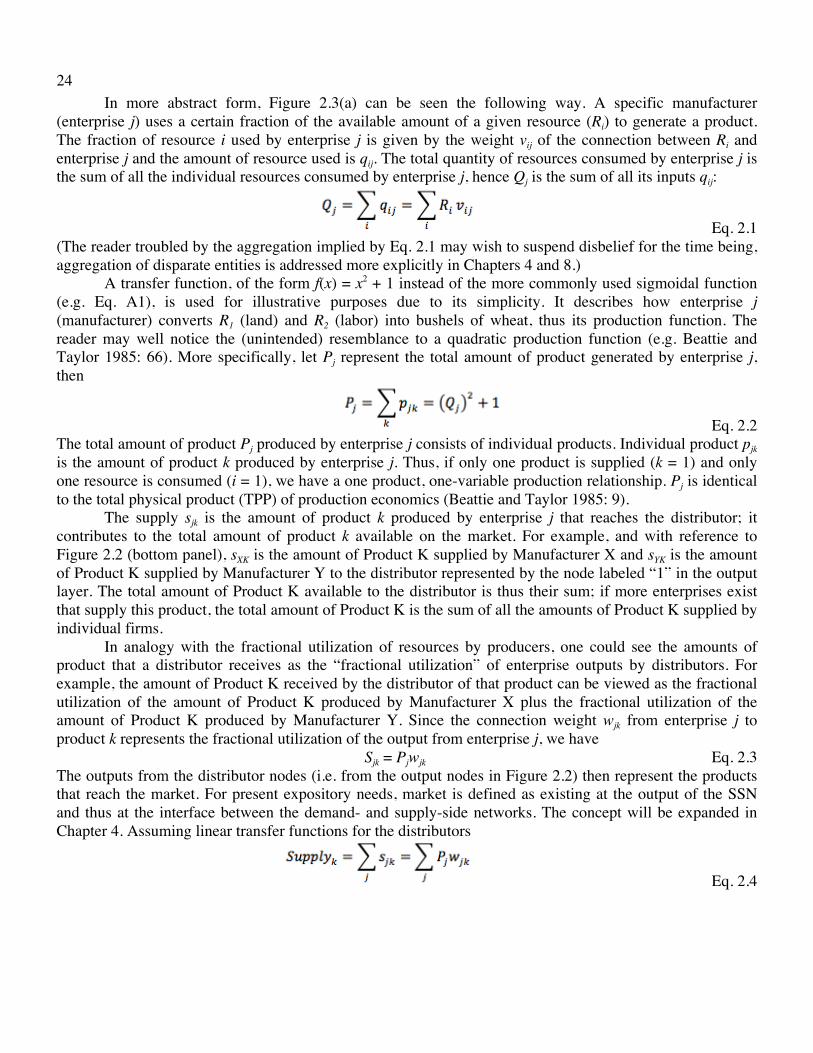
The basic structure of a supply-side connectionist model is shown in Figure 2.1. This model takes as inputs the economic resources of land and labor and these are represented by the input nodes. An economic transformation unit or enterprise, represented by the hidden node which employs a transfer function f, converts these resources into a product that is delivered to a supplier. The supplier is represented by the output node using the transfer function g. The supplier distributes the product to the market and this product is represented by the network output. The network connection weights indicate the volume fractions of goods that are distributed from one node to the next along the connection between them. Furthermore, note that the product is subscripted with “supply” to distinguish it from the similar product demanded by the demand side - products supplied and products demanded are not taken to be identical, but are taken to be matched to a degree that is good enough. Intuitively, one might think of better matches as producing better flows through the system. Here, “good enough” is taken to mean that the match is sufficient to permit economic exchanges to occur.

Figure 2.1 is intended to lay the foundations for some of the basic concepts involved. Clearly, the

network of Figure 2.1 is highly simplified and basic model. Although, land, labor, and capital are the standard resources of economic systems, this example network takes as input only the two resources of land and labor. However, capital is easily accommodated in a manner analogous to accommodating additional enterprises and additional products (see below), i.e. by adding an input node to account for it. More products,

quantity available

Labor

Land

Manufacturers

Productsupply fraction utilized

fraction utilized fraction utilized

Figure 2.1 A simple supply-side economic network is shown in this figure. The network takes as

inputs the economic resources of land and labor (input nodes). An economic manufacturing enterprise (hidden node with transfer function f) converts these

resources into a product that is supplied to market via a distributor (output node with transfer function g). The network connections indicate the fractions of these

goods used by (or distributed to) the next layer. In this example, there are two nodes in the input layer, and one each in the hidden and output layers.

f g

1

2

1 1

Distributors

quantity available

quantity available

Resources

23 more enterprises, more resources, or all of them, can be accommodated as shown in Figure 2.2. In passing, note that panel (a) in Figure 2.2 represents a basic monopoly while panel (b) implies competition.

The flow of resources, goods and services

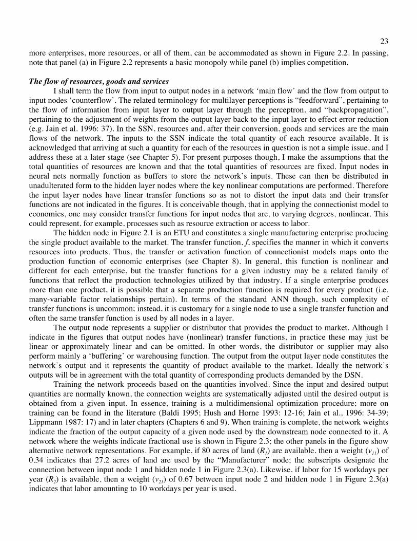
I shall term the flow from input to output nodes in a network ‘main flow’ and the flow from output to input nodes ‘counterflow’. The related terminology for multilayer perceptions is “feedforward”, pertaining to the flow of information from input layer to output layer through the perceptron, and “backpropagation”, pertaining to the adjustment of weights from the output layer back to the input layer to effect error reduction (e.g. Jain et al. 1996: 37). In the SSN, resources and, after their conversion, goods and services are the main flows of the network. The inputs to the SSN indicate the total quantity of each resource available. It is acknowledged that arriving at such a quantity for each of the resources in question is not a simple issue, and I address these at a later stage (see Chapter 5). For present purposes though, I make the assumptions that the total quantities of resources are known and that the total quantities of resources are fixed. Input nodes in neural nets normally function as buffers to store the network’s inputs. These can then be distributed in unadulterated form to the hidden layer nodes where the key nonlinear computations are performed. Therefore the input layer nodes have linear transfer functions so as not to distort the input data and their transfer functions are not indicated in the figures. It is conceivable though, that in applying the connectionist model to economics, one may consider transfer functions for input nodes that are, to varying degrees, nonlinear. This could represent, for example, processes such as resource extraction or access to labor.

The hidden node in Figure 2.1 is an ETU and constitutes a single manufacturing enterprise producing the single product available to the market. The transfer function, f, specifies the manner in which it converts resources into products. Thus, the transfer or activation function of connectionist models maps onto the production function of economic enterprises (see Chapter 8). In general, this function is nonlinear and different for each enterprise, but the transfer functions for a given industry may be a related family of functions that reflect the production technologies utilized by that industry. If a single enterprise produces more than one product, it is possible that a separate production function is required for every product (i.e. many-variable factor relationships pertain). In terms of the standard ANN though, such complexity of transfer functions is uncommon; instead, it is customary for a single node to use a single transfer function and often the same transfer function is used by all nodes in a layer.

The output node represents a supplier or distributor that provides the product to market. Although I indicate in the figures that output nodes have (nonlinear) transfer functions, in practice these may just be linear or approximately linear and can be omitted. In other words, the distributor or supplier may also perform mainly a ‘buffering’ or warehousing function. The output from the output layer node constitutes the network’s output and it represents the quantity of product available to the market. Ideally the network’s outputs will be in agreement with the total quantity of corresponding products demanded by the DSN.

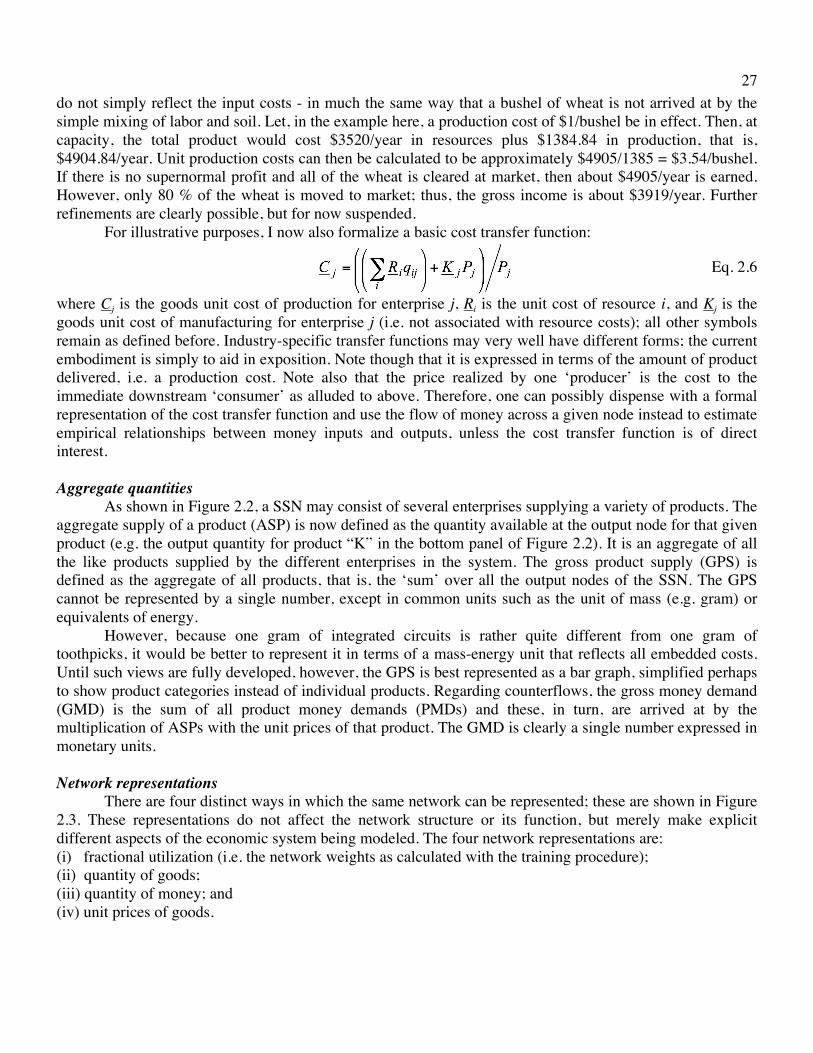
Training the network proceeds based on the quantities involved. Since the input and desired output quantities are normally known, the connection weights are systematically adjusted until the desired output is obtained from a given input. In essence, training is a multidimensional optimization procedure; more on training can be found in the literature (Baldi 1995; Hush and Horne 1993: 12-16; Jain et al., 1996: 34-39; Lippmann 1987: 17) and in later chapters (Chapters 6 and 9). When training is complete, the network weights indicate the fraction of the output capacity of a given node used by the downstream node connected to it. A network where the weights indicate fractional use is shown in Figure 2.3; the other panels in the figure show alternative network representations. For example, if 80 acres of land (R1) are available, then a weight (v11) of 0.34 indicates that 27.2 acres of land are used by the “Manufacturer” node; the subscripts designate the connection between input node 1 and hidden node 1 in Figure 2.3(a). Likewise, if labor for 15 workdays per year (R2) is available, then a weight (v21) of 0.67 between input node 2 and hidden node 1 in Figure 2.3(a) indicates that labor amounting to 10 workdays per year is used.

24 In more abstract form, Figure 2.3(a) can be seen the following way. A specific manufacturer

(enterprise j) uses a certain fraction of the available amount of a given resource (Ri) to generate a product. The fraction of resource i used by enterprise j is given by the weight vij of the connection between Ri and enterprise j and the amount of resource used is qij. The total quantity of resources consumed by enterprise j is the sum of all the individual resources consumed by enterprise j, hence Qj is the sum of all its inputs qij:

Eq. 2.1 (The reader troubled by the aggregation implied by Eq. 2.1 may wish to suspend disbelief for the time being, aggregation of disparate entities is addressed more explicitly in Chapters 4 and 8.)

A transfer function, of the form f(x) = x2 + 1 instead of the more commonly used sigmoidal function (e.g. Eq. A1), is used for illustrative purposes due to its simplicity. It describes how enterprise j (manufacturer) converts R1 (land) and R2 (labor) into bushels of wheat, thus its production function. The reader may well notice the (unintended) resemblance to a quadratic production function (e.g. Beattie and Taylor 1985: 66). More specifically, let Pj represent the total amount of product generated by enterprise j, then

Eq. 2.2 The total amount of product Pj produced by enterprise j consists of individual products. Individual product pjk is the amount of product k produced by enterprise j. Thus, if only one product is supplied (k = 1) and only one resource is consumed (i = 1), we have a one product, one-variable production relationship. Pj is identical to the total physical product (TPP) of production economics (Beattie and Taylor 1985: 9).

The supply sjk is the amount of product k produced by enterprise j that reaches the distributor; it contributes to the total amount of product k available on the market. For example, and with reference to Figure 2.2 (bottom panel), sXK is the amount of Product K supplied by Manufacturer X and sYK is the amount of Product K supplied by Manufacturer Y to the distributor represented by the node labeled “1” in the output layer. The total amount of Product K available to the distributor is thus their sum; if more enterprises exist that supply this product, the total amount of Product K is the sum of all the amounts of Product K supplied by individual firms.

In analogy with the fractional utilization of resources by producers, one could see the amounts of product that a distributor receives as the “fractional utilization” of enterprise outputs by distributors. For example, the amount of Product K received by the distributor of that product can be viewed as the fractional utilization of the amount of Product K produced by Manufacturer X plus the fractional utilization of the amount of Product K produced by Manufacturer Y. Since the connection weight wjk from enterprise j to product k represents the fractional utilization of the output from enterprise j, we have

Sjk = Pjwjk Eq. 2.3 The outputs from the distributor nodes (i.e. from the output nodes in Figure 2.2) then represent the products that reach the market. For present expository needs, market is defined as existing at the output of the SSN and thus at the interface between the demand- and supply-side networks. The concept will be expanded in Chapter 4. Assuming linear transfer functions for the distributors

Eq. 2.4

25

panels to enhance readability.

Figure 2.2 The basic supply-side economic network shown in Figure 2.1 can be expanded to show, from top to bottom: a network with a single enterprise producing two different products;

a network with two enterprises producing a single product; a network with two enterprises producing several products; and a network incorporating multiple

resources, enterprises, and products. Some labels are simplified or omitted in the lower panels to enhance readability.

X

K

Labor

Land 1

2

1

1 Y 2

D

(b)

Labor

Land 1

2

1

2

2 3

K 1

L

M

X

Y

D

E

F

(c)

Labor

Land 1

2

1

2

2 3

1

Capital 3

K

L

M

X

Y

D

E

F

(d)

Labor

Land

Manufacturer X

Product Ksupply

f

g 1

2

1

1

Product Lsupply

g 2

Distributor D

Distributor E

(a)

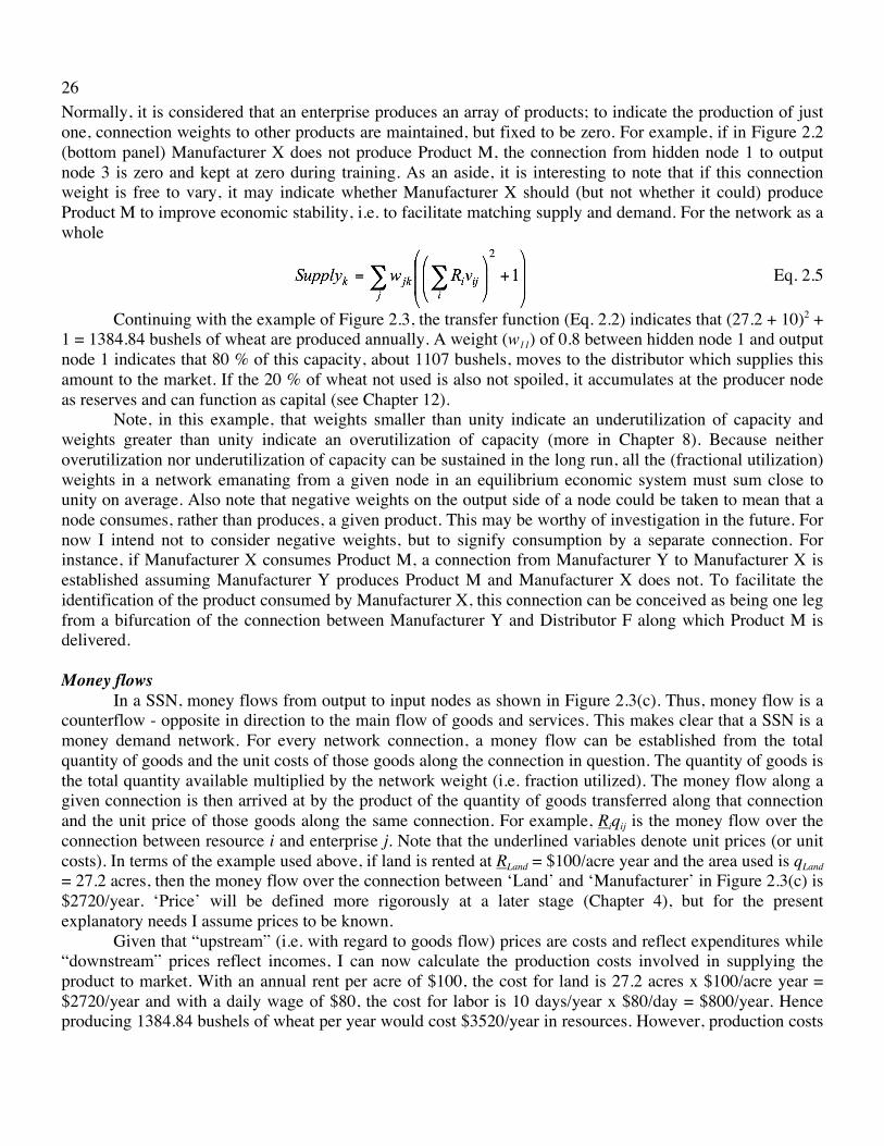
26 Normally, it is considered that an enterprise produces an array of products; to indicate the production of just one, connection weights to other products are maintained, but fixed to be zero. For example, if in Figure 2.2 (bottom panel) Manufacturer X does not produce Product M, the connection from hidden node 1 to output node 3 is zero and kept at zero during training. As an aside, it is interesting to note that if this connection weight is free to vary, it may indicate whether Manufacturer X should (but not whether it could) produce Product M to improve economic stability, i.e. to facilitate matching supply and demand. For the network as a whole

Eq. 2.5

Continuing with the example of Figure 2.3, the transfer function (Eq. 2.2) indicates that (27.2 + 10)2 + 1 = 1384.84 bushels of wheat are produced annually. A weight (w11) of 0.8 between hidden node 1 and output node 1 indicates that 80 % of this capacity, about 1107 bushels, moves to the distributor which supplies this amount to the market. If the 20 % of wheat not used is also not spoiled, it accumulates at the producer node as reserves and can function as capital (see Chapter 12).

Note, in this example, that weights smaller than unity indicate an underutilization of capacity and weights greater than unity indicate an overutilization of capacity (more in Chapter 8). Because neither overutilization nor underutilization of capacity can be sustained in the long run, all the (fractional utilization) weights in a network emanating from a given node in an equilibrium economic system must sum close to unity on average. Also note that negative weights on the output side of a node could be taken to mean that a node consumes, rather than produces, a given product. This may be worthy of investigation in the future. For now I intend not to consider negative weights, but to signify consumption by a separate connection. For instance, if Manufacturer X consumes Product M, a connection from Manufacturer Y to Manufacturer X is established assuming Manufacturer Y produces Product M and Manufacturer X does not. To facilitate the identification of the product consumed by Manufacturer X, this connection can be conceived as being one leg from a bifurcation of the connection between Manufacturer Y and Distributor F along which Product M is delivered.

Money flows

In a SSN, money flows from output to input nodes as shown in Figure 2.3(c). Thus, money flow is a counterflow - opposite in direction to the main flow of goods and services. This makes clear that a SSN is a money demand network. For every network connection, a money flow can be established from the total quantity of goods and the unit costs of those goods along the connection in question. The quantity of goods is the total quantity available multiplied by the network weight (i.e. fraction utilized). The money flow along a given connection is then arrived at by the product of the quantity of goods transferred along that connection and the unit price of those goods along the same connection. For example, Riqij is the money flow over the connection between resource i and enterprise j. Note that the underlined variables denote unit prices (or unit costs). In terms of the example used above, if land is rented at RLand = $100/acre year and the area used is qLand = 27.2 acres, then the money flow over the connection between ‘Land’ and ‘Manufacturer’ in Figure 2.3(c) is $2720/year. ‘Price’ will be defined more rigorously at a later stage (Chapter 4), but for the present explanatory needs I assume prices to be known.

Given that “upstream” (i.e. with regard to goods flow) prices are costs and reflect expenditures while “downstream” prices reflect incomes, I can now calculate the production costs involved in supplying the product to market. With an annual rent per acre of $100, the cost for land is 27.2 acres x $100/acre year = $2720/year and with a daily wage of $80, the cost for labor is 10 days/year x $80/day = $800/year. Hence producing 1384.84 bushels of wheat per year would cost $3520/year in resources. However, production costs

27 do not simply reflect the input costs - in much the same way that a bushel of wheat is not arrived at by the simple mixing of labor and soil. Let, in the example here, a production cost of $1/bushel be in effect. Then, at capacity, the total product would cost $3520/year in resources plus $1384.84 in production, that is, $4904.84/year. Unit production costs can then be calculated to be approximately $4905/1385 = $3.54/bushel. If there is no supernormal profit and all of the wheat is cleared at market, then about $4905/year is earned. However, only 80 % of the wheat is moved to market; thus, the gross income is about $3919/year. Further refinements are clearly possible, but for now suspended.

For illustrative purposes, I now also formalize a basic cost transfer function:

Eq. 2.6

where Cj is the goods unit cost of production for enterprise j, Ri is the unit cost of resource i, and Kj is the goods unit cost of manufacturing for enterprise j (i.e. not associated with resource costs); all other symbols remain as defined before. Industry-specific transfer functions may very well have different forms; the current embodiment is simply to aid in exposition. Note though that it is expressed in terms of the amount of product delivered, i.e. a production cost. Note also that the price realized by one ‘producer’ is the cost to the immediate downstream ‘consumer’ as alluded to above. Therefore, one can possibly dispense with a formal representation of the cost transfer function and use the flow of money across a given node instead to estimate empirical relationships between money inputs and outputs, unless the cost transfer function is of direct interest.

Aggregate quantities

As shown in Figure 2.2, a SSN may consist of several enterprises supplying a variety of products. The aggregate supply of a product (ASP) is now defined as the quantity available at the output node for that given product (e.g. the output quantity for product “K” in the bottom panel of Figure 2.2). It is an aggregate of all the like products supplied by the different enterprises in the system. The gross product supply (GPS) is defined as the aggregate of all products, that is, the ‘sum’ over all the output nodes of the SSN. The GPS cannot be represented by a single number, except in common units such as the unit of mass (e.g. gram) or equivalents of energy.

However, because one gram of integrated circuits is rather quite different from one gram of toothpicks, it would be better to represent it in terms of a mass-energy unit that reflects all embedded costs. Until such views are fully developed, however, the GPS is best represented as a bar graph, simplified perhaps to show product categories instead of individual products. Regarding counterflows, the gross money demand (GMD) is the sum of all product money demands (PMDs) and these, in turn, are arrived at by the multiplication of ASPs with the unit prices of that product. The GMD is clearly a single number expressed in monetary units.

Network representations

There are four distinct ways in which the same network can be represented; these are shown in Figure 2.3. These representations do not affect the network structure or its function, but merely make explicit different aspects of the economic system being modeled. The four network representations are: (i) fractional utilization (i.e. the network weights as calculated with the training procedure); (ii) quantity of goods; (iii) quantity of money; and (iv) unit prices of goods.

28

(a)

(b)

(c)

(d)

Figure 2.3 The four representations of a simple supply-side economic network: a) connections

between nodes represent utilization; b) connections represent goods flows; c) connections represent money flows; and d) connections represent unit prices. The

arrows are in keeping with the convention of connectionist models originally meant to indicate a flow of information from input to output layers – in the case of money flows

and prices, the direction reverses as illustrated.

$2720

$800

$3924

1

2

1 1

$100/acre

$80/workday

$3.54/bushel

1

2

1 1

15 workdays

27.2 acres

10 workdays

1107 bushels of wheat

1

2

1 1

80 acres 1107 bushels of wheat

15 workdays

Productsupply

0.34

0.67

.80

1

2

1 1

Distributor Manufacturer 80 acres

Resources

29 It is also possible to incorporate all of these aspects in the same network representation, but at the risk

of sacrificing clarity. All the network presentations in Figure 2.3 are based on the preceding example where 80 acres of land and 15 workdays are available and utilization of these resources results in the production of 1385 bushels of wheat per year of which 1107 are taken by the distributor (and presumably reach the market).

From the foregoing, it is also evident that these representations are interrelated, but it seems that at least two components are relatively independent: the supply of resources and the supply of requirements (see Chapter 3). Requirements are here represented by money (i.e. tokens of demand). It may be convenient therefore to use quantity of goods and quantity of money as the basic modes of representation. Whichever representation is preferred is likely to depend on the discipline involved and the task at hand; for example, the representation showing money flows may be of most interest from a financial point of view. However, representation (i) is used in the computational literature and the one adopted as standard here. Discussion and conclusions

I have given here a representation of the supply-side of an economic system in terms of a neural network or connectionist model. This model has resources as input nodes, enterprises as hidden nodes, and distributors as output nodes. The network outputs, that is, the outputs from the output nodes, represent the products available to the market. The transfer functions of the nodes map onto the production functions of economic concerns. Furthermore, aggregate measures appear broadly analogous to those of macroeconomics. Consequently, my first conclusion is that, at both local and global levels, there is a natural and easy transfer of connectionist concepts to economics. In later chapters I will continue to map concepts from connectionist models onto economics, and where such transfer is not possible, attempt to develop the economic models independently.

The second conclusion I come to is that the SSN is a money demand network. This is inferred from the fact that money flows in opposition to goods and services. The implication is that when money (or other reusable tokens of demand) is not available, the system slows or halts. Slowing or halting must be basically a quantization effect, and not dependent on the number of tokens in the system per se. In other words, if there are too few tokens in the system to permit the acquisition of individual products at practical quantities, slowing will start to take effect. Prior to that, simple price deflation will appear.

The last conclusion is that the flow volumes of goods and services across the SSN must be preserved. When more goods enter the system than leave it, the excesses accumulate somewhere and can be thought of as reserves, and by extension, capital. These excesses thus contribute to the resource node ‘Capital’ in Figure 2.2 (d). Thus the principles of physics are seen to affect economics as they should. Applying the principle of conservation also to monetary flows, one conjectures that money entering the network, but not leaving it, must accumulate somewhere as either internal reserves (at the node) or are deposited as external reserves giving rise to financial capital.

30

3

The Demand-side Network

31

The Demand-side Network Summary

The origins of economic demand are formed by a set of ‘requirements’ - needs, wants, and aspirations – derived from human motivational attributes. Analogous to the way in which the supply-side network is modeled with resources as inputs, the demand-side is now modeled using requirements as inputs. In the demand-side network, hidden nodes perform the task of devising and designing products that are expected to meet the postulated requirements. Therefore, they convert requirements into products deemed desirable (and to some extent deliverable by the supply side). By way of conceptual simplification, retailers are here taken to perform this role. Their products are product specifications and orders for those products that are provided to the output nodes that represent purchasers or wholesalers. In turn, purchasers or wholesalers canvas or put out tenders or solicit submissions for these products from the market–the demand for specific products thus represents the demand-side model’s output. The model shows how requirements, originating as physiological, psychological, and sociological variables, become transmuted into demands for more refined and concrete entities, i.e. demands for specific products. An example is used to illustrate the network’s operation and a description of various network representations is given. Like the supply-side network, this model also has counterflows. In the demand-side network, demand flow is the main flow, going from input to output nodes, while goods flow is the counterflow. When the demand-side network flows are compared to those of the supply-side network, the flows of demands and those of money appear to be coincident. This comparison suggests that money flows are indices of human demands.

32 Introduction

In the previous chapter the supply side of an economic system was modeled in terms of a connectionist model. Because the supply side was relatively easily and intuitively modeled in connectionist terms, the reader may have found such a model at least plausible. In this chapter, the concept is extended to the demand side. Thus, I proceed from the assumption that the demand-side model may be similar to the supply-side one when formulating network inputs and outputs. Consequently, the demand-side network emerges largely as a mirror image of the supply-side network. Although this may not be accurate in its fine structure, as will become explicit in later chapters, I consider it conceptually sufficient for present purposes.

Unfortunately, unlike the supply side, the demand side is not as well characterized in terms of inputs and outputs. This is especially true regarding inputs; therefore some initial attention will be devoted to outlining them.

The formal structure of the demand-side network

It could be argued that any economic system arises by virtue of a set of reciprocal actions that individuals engage in. These actions spring from drives or urges that individuals experience and the drives result from hedonic states that themselves arise from physiological, psychological, and social factors modified by learning. Hedonic states are additive, giving rise to a net drive state (Schulze 1995: 275; Schulze and Mariano 2003: 11-4; Schulze, 2004a: 53). Although the overall drive state is different from person to person, and within a person over the course of a lifespan, it is useful to classify drives according to their natures and hence get an inkling of the objects that may be suitable to modify these drive states. In an economic context, the origins of these drive states are termed ‘requirements’, the drive states themselves are closely related to the concept of ‘utility’, and they become manifest as demands. The classification used here partitions requirements into ‘needs’, ‘wants’, and ‘aspirations’, ranked by elasticity, and they are described in more detail next.

Needs are hard requirements and have an inelastic quality. Needs refer to physiological survival-related variables and the impact they have on behavior. The hard nature of needs means that they do not accommodate shortages or excesses easily: once essential levels are met, increased consumption is unlikely – it is in fact undesirable. For example, although we absolutely need to ingest a certain amount of water regularly, excessive consumption is unlikely and could be fatal due to water intoxication. Thus, violation of their boundaries causes death. There is no wide variation between individuals based on need. Absolute levels are important in satisfying needs. The relationship between these survival-related needs and how they govern behavior has been extensively developed in earlier work (Schulze 1995; Schulze and Mariano 2003; Schulze 2004a).

Wants’ are ‘softer’ and more elastic requirements. Wants refer to physiological and psychological procreation-related variables and their impact on behavior. Both shortages and/or excesses can be accommodated. If wants are unmet, death will generally not result but distress may. In my view wants are closely related to sex and procreation but may become manifest through secondary or more distal variables such as status (e.g. Wong 2000: 38-42). Not having a pool and hence not consuming water under the ‘wants’ rubric is not fatal, but may limit a male’s ability to attract mates; conversely, having a larger pool and a larger still pool, hence consuming ‘excessive’ amounts of water, may increase the number and quality of mates attracted. Wide variations can exist between individuals regarding wants. The levels at which wants are met, relative to other individuals, become significant determinants of satisfaction. This has important economic consequences because wants can be manipulated to increase consumption in ways that needs cannot be.

Aspirations’ are the softest and most elastic of requirement categories. It refers to psychological and sociological variables that only have diffuse and mostly longer-term effects on survival and procreation. Under ‘aspirations’ would be considered issues such as health care, education, justice, governance structures, and so on. These are clearly important issues, but lack the immediacy of needs and wants. Building a

33 communal pool for recreation, instruction, and competition represents water demand under the ‘aspirations’ rubric: its absence is not disastrous and its upper limits are unbounded. Variations between individuals may be extremely wide and reflect levels of imagination, intelligence, and education.

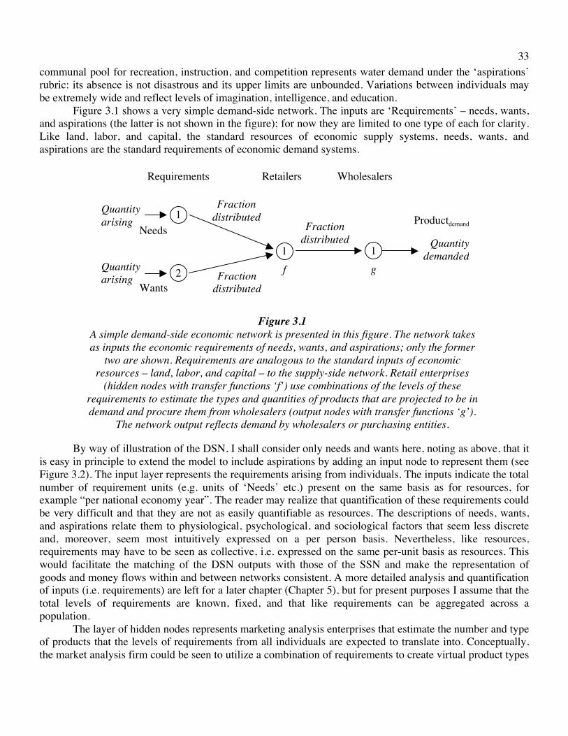
Figure 3.1 shows a very simple demand-side network. The inputs are ‘Requirements’ – needs, wants, and aspirations (the latter is not shown in the figure); for now they are limited to one type of each for clarity. Like land, labor, and capital, the standard resources of economic supply systems, needs, wants, and aspirations are the standard requirements of economic demand systems.

By way of illustration of the DSN, I shall consider only needs and wants here, noting as above, that it

is easy in principle to extend the model to include aspirations by adding an input node to represent them (see Figure 3.2). The input layer represents the requirements arising from individuals. The inputs indicate the total number of requirement units (e.g. units of ‘Needs’ etc.) present on the same basis as for resources, for example “per national economy year”. The reader may realize that quantification of these requirements could be very difficult and that they are not as easily quantifiable as resources. The descriptions of needs, wants, and aspirations relate them to physiological, psychological, and sociological factors that seem less discrete and, moreover, seem most intuitively expressed on a per person basis. Nevertheless, like resources, requirements may have to be seen as collective, i.e. expressed on the same per-unit basis as resources. This would facilitate the matching of the DSN outputs with those of the SSN and make the representation of goods and money flows within and between networks consistent. A more detailed analysis and quantification of inputs (i.e. requirements) are left for a later chapter (Chapter 5), but for present purposes I assume that the total levels of requirements are known, fixed, and that like requirements can be aggregated across a population.

The layer of hidden nodes represents marketing analysis enterprises that estimate the number and type of products that the levels of requirements from all individuals are expected to translate into. Conceptually, the market analysis firm could be seen to utilize a combination of requirements to create virtual product types

Quantity demanded

Wants

Needs

Retailers

Productdemand Fraction

distributed

Fraction distributed

Fraction distributed

Figure 3.1 A simple demand-side economic network is presented in this figure. The network takes as inputs the economic requirements of needs, wants, and aspirations; only the former

two are shown. Requirements are analogous to the standard inputs of economic resources – land, labor, and capital – to the supply-side network. Retail enterprises

(hidden nodes with transfer functions ‘f’) use combinations of the levels of these requirements to estimate the types and quantities of products that are projected to be in demand and procure them from wholesalers (output nodes with transfer functions ‘g’).

The network output reflects demand by wholesalers or purchasing entities.

f

Quantity arising

Quantity arising

1

Requirements Wholesalers

2

1 g

1

34 and their respective quantities – these virtual products then represent the products eventually demanded of the market. The market analysis enterprise is therefore rather analogous to a manufacturing enterprise; however, instead of utilizing different economic resources to generate products supplied to the market, it is an ETU that utilizes different requirements to design products sought on the market. Although marketing analysis enterprises may be hard to identify in a formal sense, I assume here that they do exist as discrete concerns and that retailers are closely related or perform similar functions. Therefore retailers are taken to be these concerns in Figure 3.1. This at least, may enable me to delineate the structure and symmetry of the DSN, to contrast it with the SSN, and to show what an ideal system may look and function like.

The transfer functions specify the manner in which inputs to a node are converted into outputs from that node. For example, the transfer function governs how needs, wants, and aspirations at the hidden node combine into a given product sought by the retailer – i.e. the proper (main flow-related) production function of the retailer.

Output nodes represent agents that ‘supply’ demands from retailers to the supply-side network. For the sake of exposition, the output node is here taken to resemble a wholesale concern. The outputs of output nodes constitute the network’s output. As output the network produces the total quantity of product demanded of the market. Since the ultimate aim is to match supply and demand, the output of the SSN needs to be matched with that of the DSN. The DSN output provides therefore a target for the SSN output, and does so in two respects: it specifies in a general sense the types of products demanded and the quantities of each. Given that in this case only one product is demanded, the quantity of product demanded constitutes the full market demand for this product. It is, as before, very easy to extend the basic network of Figure 3.1 to accommodate either more products demanded, or to incorporate conceptually more requirements, or both as shown in Figure 3.2.

The flow of requirements and money

For the SSN it has been established that money flows occur over every network connection and that they are in counterflow to those of goods. In the DSN, in contrast, the main flows are demand flows while goods and services are counterflows. Demands arise from requirements and, after transmutation, become product designs and then products sought on the market.

Getting down to numbers, let, for example and with reference to Figure 3.2, a given person, Individual X, experience a net general yearly drive state of 6,000 “drive units”. Let one third of these be classifiable as needs, one third as wants, and one third as aspirations. Let likewise Individual Y experience a net yearly drive state of 4,000 “drive units” and let one half represent needs and one half wants. Then, assuming the aggregation of like requirements, both contribute drive states of 2,000 “drive units” per year to needs. Taken together, these numbers lead to needs at 4,000, wants at 4,000, and aspirations at a level of 2,000 units per year.

The enterprises Retailer M and Retailer N use requirements to design types of products deemed demanded by consumers and to estimate their quantities. These products exist in a virtual form in DSN main flows, i.e. as product design concepts and product specifications, and as real products in DSN counterflows. In order to maintain consistency, the DSN that matches the trained SSN discussed above uses fractional incorporation as weights. For example, Retailer M uses 0.75 (i.e. 75 %) of all needs, 0.2 of wants and 0.1 of aspirations, to generate 5,657 overall products (see below) consisting of two types, Product K and Product L. Retailer N uses 0.25 of all needs, 0.8 of wants and 0.9 of aspirations to generate the same two products, Product K and Product L, as well as an additional one, Product M at a level of 8,486 products per year in total. Even though these are virtual products, the two enterprises, between them, should not use more requirements than exist. For example, they both should not use 0.75 of needs since 0.75 + 0.75 = 1.5 or 50 % more needs than exist. The reason is simply that an overall ‘overincorporation’ would generate a degree of fictitious demand that would lead to inefficiencies in the system. A transfer function of the form

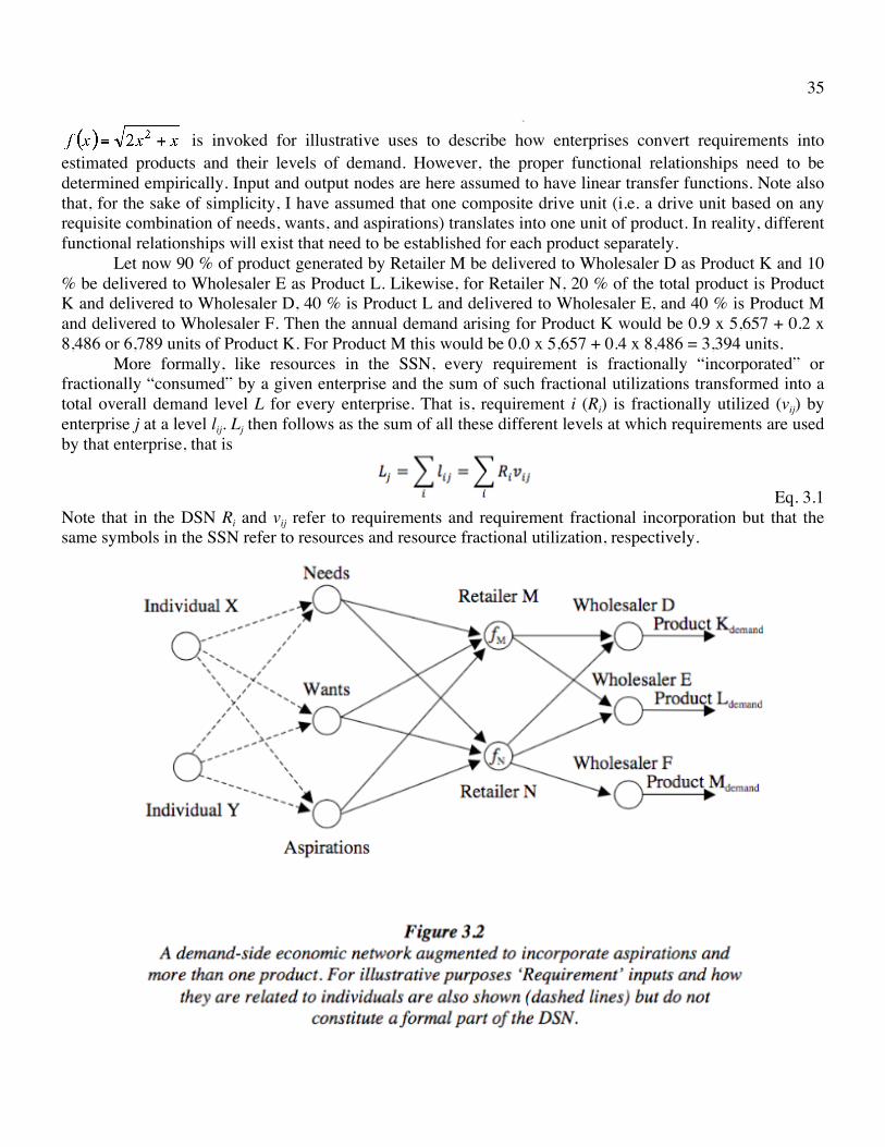
35 fictitious demand that would lead to inefficiencies in the system. A transfer function of the form

is invoked for illustrative uses to describe how enterprises convert requirements into estimated products and their levels of demand. However, the proper functional relationships need to be determined empirically. Input and output nodes are here assumed to have linear transfer functions. Note also that, for the sake of simplicity, I have assumed that one composite drive unit (i.e. a drive unit based on any requisite combination of needs, wants, and aspirations) translates into one unit of product. In reality, different functional relationships will exist that need to be established for each product separately.

Let now 90 % of product generated by Retailer M be delivered to Wholesaler D as Product K and 10 % be delivered to Wholesaler E as Product L. Likewise, for Retailer N, 20 % of the total product is Product K and delivered to Wholesaler D, 40 % is Product L and delivered to Wholesaler E, and 40 % is Product M and delivered to Wholesaler F. Then the annual demand arising for Product K would be 0.9 x 5,657 + 0.2 x 8,486 or 6,789 units of Product K. For Product M this would be 0.0 x 5,657 + 0.4 x 8,486 = 3,394 units.

More formally, like resources in the SSN, every requirement is fractionally “incorporated” or fractionally “consumed” by a given enterprise and the sum of such fractional utilizations transformed into a total overall demand level L for every enterprise. That is, requirement i (Ri) is fractionally utilized (vij) by enterprise j at a level lij. Lj then follows as the sum of all these different levels at which requirements are used by that enterprise, that is

Eq. 3.1 Note that in the DSN Ri and vij refer to requirements and requirement fractional incorporation but that the same symbols in the SSN refer to resources and resource fractional utilization, respectively.

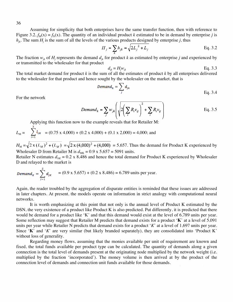
36 Assuming for simplicity that both enterprises have the same transfer function, then with reference to

Figure 3.2, fM(x) = fN(x). The quantity of an individual product k estimated to be in demand by enterprise j is hjk. The sum Hj is the sum of all the levels of the various products designed by enterprise j, thus

Eq. 3.2

The fraction wjk of Hj represents the demand djk for product k as estimated by enterprise j and experienced by or transmitted to the wholesaler for that product

djk = Hjwjk Eq. 3.3 The total market demand for product k is the sum of all the estimates of product k by all enterprises delivered to the wholesaler for that product and hence sought by the wholesaler on the market, that is

Eq. 3.4 For the network

Eq. 3.5

Applying this function now to the example reveals that for Retailer M:

LM = = (0.75 x 4,000) + (0.2 x 4,000) + (0.1 x 2,000) = 4,000; and

HM = = = 5,657. Thus the demand for Product K experienced by Wholesaler D from Retailer M is dMK = 0.9 x 5,657 = 5091 units. Retailer N estimates dNK = 0.2 x 8,486 and hence the total demand for Product K experienced by Wholesaler D and relayed to the market is

= (0.9 x 5,657) + (0.2 x 8,486) = 6,789 units per year.

Again, the reader troubled by the aggregation of disparate entities is reminded that these issues are addressed in later chapters. At present, the models operate on information in strict analogy with computational neural networks.

It is worth emphasizing at this point that not only is the annual level of Product K estimated by the DSN, the very existence of a product like Product K is also predicted. Put differently, it is predicted that there would be demand for a product like ‘K’ and that this demand would exist at the level of 6,789 units per year. Some reflection may suggest that Retailer M predicts that demand exists for a product ‘K’ at a level of 5,091 units per year while Retailer N predicts that demand exists for a product ‘K’ at a level of 1,697 units per year. Since ‘K’ and ‘K’ are very similar (but likely branded separately), they are consolidated into ‘Product K’ without loss of generality.

Regarding money flows, assuming that the monies available per unit of requirement are known and fixed, the total funds available per product type can be calculated. The quantity of demands along a given connection is the total level of demands present at the originating node multiplied by the network weight (i.e. multiplied by the fraction ‘incorporated’). The money volume is then arrived at by the product of the connection level of demands and connection unit funds available for those demands.

For example, if individuals are willing and able to expend $10 per unit of needs, $4 per unit of wants, and $1 per unit of aspirations, the funds available for distribution across all products are $10 x 4,000 (needs),

37 For example, if individuals are willing and able to expend $10 per unit of needs, $4 per unit of wants,

and $1 per unit of aspirations, the funds available for distribution across all products are $10 x 4,000 (needs), $4 x 4,000 (wants) and $1 x 2,000 (aspirations) for a total of $58,000 per year. Note that this example is meant to illustrate the concepts involved; it is not meant to imply that establishing the funding amounts allocated to requirements is trivial or easy. Further, Retailer M now estimates that 75 % of funds available for needs (0.75 x $40,000), 20 % of funds available for wants (0.2 x $16,000), and 10 % of funds available for aspirations (0.10 x $2,000) will constitute a demand of $33,400 for products of all types. Of this amount, 90 %, or $30,060, would be available for Product K. Likewise Retailer N estimates that 25 % of funds available for needs (0.25 x $40,000), 80 % of funds available for wants (0.8 x $16,000), and 90 % of funds available for aspirations (0.9 x $2,000) will constitute a demand of $24,600 for products of all types. Of the latter amount 20 %, or $4,920, is available for Product K giving a total level of funds available of $34,980. Since the total demand for Product K is known, the funds available for the acquisition of Product K are $5.15 per item.

The flow of goods and services

Goods and services are the counterflows of the DSN. Assuming an economy in equilibrium, the number and type of products demanded are more-or-less met by the number and type of products supplied. The (real) products supplied to wholesalers are then delivered to retailers and these to consumers. Consumption of goods and services must therefore ultimately meet or satisfy the requirements of consumers. As for main flows above, counterflow volumes can be calculated and these should match, given the condition of equilibrium, the main flow volumes across the same connections.

Aggregate quantities

As shown in Figure 3.2, a demand-side connectionist model may consist of several enterprises projecting a variety of product demands. The aggregate demand of a product (ADP) can now be defined as the level present at the output node for that given product (e.g. the output level for “ProductKdemand” in Figure 3.2). It is an aggregate of all the like products projected to be in demand by the different demand enterprises in the system. The gross product demand (GPD) is defined as the aggregate demand of all products, that is, the ‘sum’ over all the output nodes of the DSN. Like the GPS, the GPD cannot be represented by a single number, except in common units of requirements such as a unit of “drive” or hedonic tension, but such a unit is still largely undefined. The gross money supply (GMS) is the sum of all funds available for a given product (PMSs) and these, in turn, is arrived at by the multiplication of ADP with the unit funds available for that product. Like the GMD, the GMS is clearly a single number. With the numbers used above, the GMS can be calculated:

GMS = 6,789 units of Product K transacted at $5.15/unit + 3,960 units of Product L transacted at $3.33/unit + 3,394 units of Product M transacted at $2.90/unit = $57,990, within round-off error of the $58,000 per year deemed available. GMS is arrived at as the sum of all products between goods quantities and their prices. It is equal to

PT in Fisher’s form of the equation of exchange MV = PT Eq. 3.6

where M denotes “money supply”, V is the velocity of circulation of money, P is the average price of all transactions concluded in the economy and T is the total number of transactions (Ison 2000: 207; Jackson 1986: 45; Vaggi and Groenewegen 2003: 260). The concept of the DSN, introduced here, suggests however that velocity and prices do not fluctuate in some arbitrary fashion, but that velocity and price changes are likely to be closely related to individual requirement categories. In other words, care must be exercised in utilizing central descriptors of velocity and prices lest they obscure more than they reveal. For example, it is

38 conceivable, based on the foregoing, that in a system with an increasing population and fixed monetary base, velocity increases may predominantly be driven by needs rather than other requirements.

Network representations

There are six distinct ways in which the same DSN network can be represented - analogous to that shown in Figure 2.3. As for the SSN, these representations do not affect the network structure or its function, but make explicit different aspects of the system. For reasons stated previously (i.e. for the SSN) and for reasons of symmetry and comparison, the fractional incorporation of requirements into products is taken as the basic representation of the network (Figure 3.3). The network representations are: (i) fractional incorporation of demands (i.e. the network weights as estimated initially or subsequently calculated with the training procedure); (ii) level of demands; (iii) quantities of goods and services; (iv) demand expressed per unit goods and services; (v) money flows; and (vi) “price” per unit demand.

In Figure 3.3, fractional incorporation is meant to indicate that certain fractions of requirements, i.e. a certain fraction of needs plus a certain fraction of wants plus a certain fraction of aspirations, are incorporated into the formulation of a given product by an enterprise as explained above. Since the total amount of a given product (e.g. Product K) estimated to be in demand (and hence “ordered”, thus demanded) could also be seen as fractional incorporations of the outputs of the different ETUs, I chose to use “fractional incorporation” to denote the weights of connections in the basic representation of the DSN in contrast to “fractional utilization” for the basic SSN representation.

Note that some discrepancies may exist between demands and tokens of demands (money). Nevertheless, if a universal ‘unit of requirement’ can be determined, there ought to exist a fixed ratio between ‘unit of requirement’ and unit token of demand in a stable economic system. Thus an equivalence exists between money and demands and this equivalence is more narrowly maintained than the equivalence between demands on one hand and goods and services on the other (in an economic system at stable equilibrium, however, they are all in narrow equivalence). Therefore, the representation of the level of demands may also represent, and be represented by, the flow of money. One may though, for theoretical or practical reasons, prefer to use one or the other.

Discussion and conclusions

In this chapter, I attempted to generate a connectionist model of the demand-side economy. To accomplish this, the concept of ‘requirements’ had to be formulated. This concept firmly anchors the DSN in a humanistic bedrock. The position of requirements as input nodes, and their derivation from individuals, should make it immediately clear that humans are pivotal in economic systems since their requirements (co-)determine economic demand. This is rather consistent with what one might expect. The DSN makes explicit and, I hope, more tractable the social nature of economics. It does so in a way that specifies the relationship of physiological, psychological, and social variables to other economic variables in a consistent and transparent manner. The ‘Individuals’ “layer” and a corresponding ‘Environment’ layer play pivotal roles in the whole system; they will be formally introduced, and their relationships to the networks will be specified, in a later chapter (Chapter 11).

This model uses the SSN as template, thus a close general correspondence and symmetry between the DSN and the SSN emerges. The demand-side network also functionally mirrors the supply-side network. Although the number of nodes in a given layer may not necessarily be equal, the layers perform qualitatively similar functions. My first conclusion, therefore, is that the modeling of the demand-side economy with a

39 connectionist model is at least plausible, but also meaningful by virtue of having links between human attributes and economic demands.

Because goods and services are in counterflow to demands in the DSN, a problem may arise in the

ultimate distribution of a good or service to a given requirement. This should not be viewed as insurmountable since hidden nodes by their very nature transform their inputs (e.g. land, labor, and capital) into something different (e.g. bushels of wheat). Thus a raincoat could be seen as being transformed into a need (e.g. protection) and a want (e.g. status, appeal). However, it does raise an intriguing question – whether one should or could stick with a given unit of product and conceive one raincoat to consist of a certain amount of land, a certain amount of labor, and a certain amount of capital, just like fractions of the same raincoat meet the requirement of needs and wants. Potentially then, both resources and requirements could be represented in terms of raincoats (and all the other products on the market). Such an attempt at consistent representation may make an analysis of demand/supply ratio changes across a network interesting. It is reminiscent or Ricardo’s corn model (e.g. Vaggi and Groenewegen 2003: 144). For my present purposes, however, I wish to point out that the DSN inputs (i.e. needs, wants, and aspirations) are less tangible than those of the SSN (i.e. land, labor, capital). Consequently, when one considers that the “demands” of the DSN flow in the opposite direction to goods and in the same direction as funds, it becomes clear that money can be viewed as tangible manifestations of demands. This is my second conclusion.

Figure 3.3 The figure shows a basic representation of a demand-side economic network in terms of connection weights as fractional incorporation of requirements and demands. It is also augmented to show annual flows of demands through the nodes. The numbers differ slightly from those in the text due to round-off error. The requirements are in

units of drive and other demands are in units of product.

Needs (4,000 units)

Enterprise M (5,657 units)

Product Kdemand

Wants (4,000 units)

Aspirations (2,000 units)

Enterprise N (8,486 units)

Product Ldemand

Product Mdemand

0.75

.25 .20

.10

.80 .40

.90 .10

.40

.20

.90

.00

Wholesaler D (6,788 units)

Wholesaler E (3,960 units)

Wholesaler F (3,394 units)

40

4

The Core System

41

The Core System Summary

The reconciliation of demand and supply lies at the heart of the economic process. The core of the connectionist theory of economics is therefore created by integrating the demand-side and supply-side networks by interfacing them along their output nodes. This core system is then used to define concepts of interest and examine them qualitatively. Markets are defined as the interfaces between layers: here products are transferred from one set of economic entities to another while money is exchanged in the opposite direction. Prices are defined as the ratio of the flow of money to the flow of goods along a specific connection at such an interface. Inflation and deflation are viewed as changes in price due either to changes in quantities of goods or to changes in the levels of funds available for those goods. Semi-inelasticities in the system result from fixed requirements (most often needs) or fixed supplies (most often limited resources). Full inelasticities occur when a given requirement and its corresponding resource are both fixed – a potentially dangerous combination. Finally, these concepts are discussed with brief reference to the historical context.

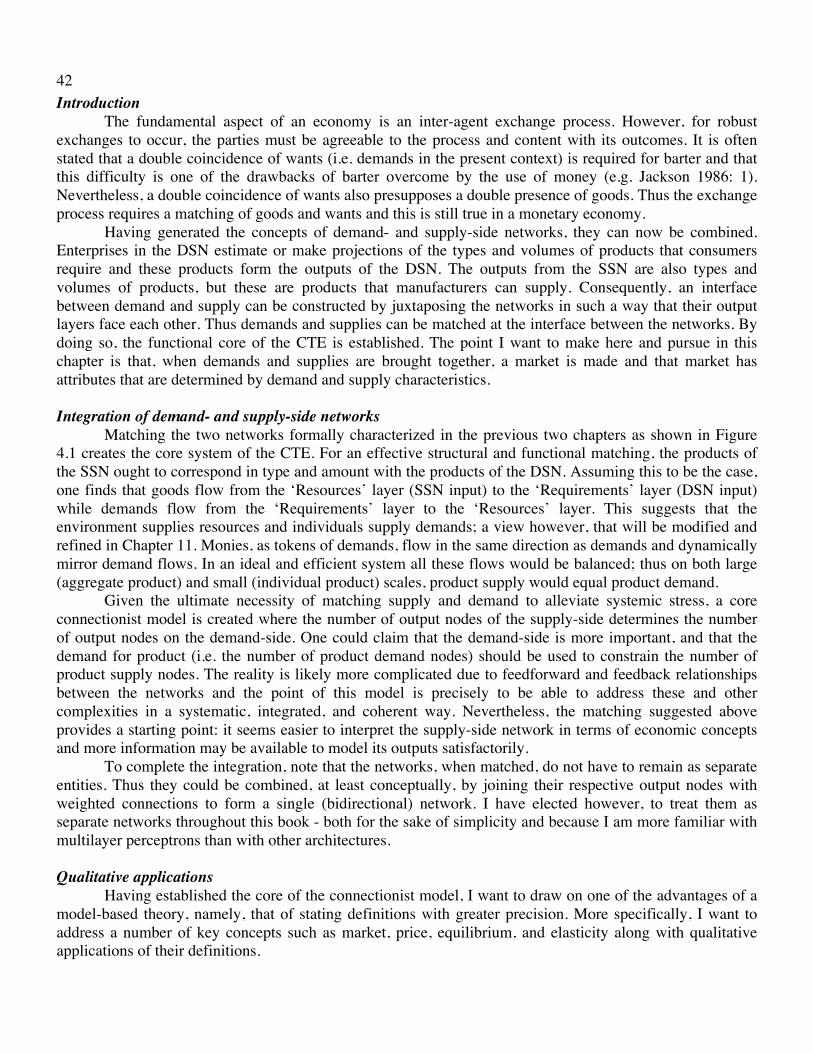
42 Introduction

The fundamental aspect of an economy is an inter-agent exchange process. However, for robust exchanges to occur, the parties must be agreeable to the process and content with its outcomes. It is often stated that a double coincidence of wants (i.e. demands in the present context) is required for barter and that this difficulty is one of the drawbacks of barter overcome by the use of money (e.g. Jackson 1986: 1). Nevertheless, a double coincidence of wants also presupposes a double presence of goods. Thus the exchange process requires a matching of goods and wants and this is still true in a monetary economy.

Having generated the concepts of demand- and supply-side networks, they can now be combined. Enterprises in the DSN estimate or make projections of the types and volumes of products that consumers require and these products form the outputs of the DSN. The outputs from the SSN are also types and volumes of products, but these are products that manufacturers can supply. Consequently, an interface between demand and supply can be constructed by juxtaposing the networks in such a way that their output layers face each other. Thus demands and supplies can be matched at the interface between the networks. By doing so, the functional core of the CTE is established. The point I want to make here and pursue in this chapter is that, when demands and supplies are brought together, a market is made and that market has attributes that are determined by demand and supply characteristics.

Integration of demand- and supply-side networks

Matching the two networks formally characterized in the previous two chapters as shown in Figure 4.1 creates the core system of the CTE. For an effective structural and functional matching, the products of the SSN ought to correspond in type and amount with the products of the DSN. Assuming this to be the case, one finds that goods flow from the ‘Resources’ layer (SSN input) to the ‘Requirements’ layer (DSN input) while demands flow from the ‘Requirements’ layer to the ‘Resources’ layer. This suggests that the environment supplies resources and individuals supply demands; a view however, that will be modified and refined in Chapter 11. Monies, as tokens of demands, flow in the same direction as demands and dynamically mirror demand flows. In an ideal and efficient system all these flows would be balanced; thus on both large (aggregate product) and small (individual product) scales, product supply would equal product demand.

Given the ultimate necessity of matching supply and demand to alleviate systemic stress, a core connectionist model is created where the number of output nodes of the supply-side determines the number of output nodes on the demand-side. One could claim that the demand-side is more important, and that the demand for product (i.e. the number of product demand nodes) should be used to constrain the number of product supply nodes. The reality is likely more complicated due to feedforward and feedback relationships between the networks and the point of this model is precisely to be able to address these and other complexities in a systematic, integrated, and coherent way. Nevertheless, the matching suggested above provides a starting point: it seems easier to interpret the supply-side network in terms of economic concepts and more information may be available to model its outputs satisfactorily.

To complete the integration, note that the networks, when matched, do not have to remain as separate entities. Thus they could be combined, at least conceptually, by joining their respective output nodes with weighted connections to form a single (bidirectional) network. I have elected however, to treat them as separate networks throughout this book - both for the sake of simplicity and because I am more familiar with multilayer perceptrons than with other architectures.

Qualitative applications

Having established the core of the connectionist model, I want to draw on one of the advantages of a model-based theory, namely, that of stating definitions with greater precision. More specifically, I want to address a number of key concepts such as market, price, equilibrium, and elasticity along with qualitative applications of their definitions.

43

Markets: Although in preceding chapters ‘market’ was defined as existing at the output of the DSN and SSN, thus at the interface between the demand- and supply-side networks, conjoining the juxtaposed networks in Figure 4.1 suggests that the definition of market can be expanded to include any interface where transactions occur, i.e. where the exchange of an agreed upon level of services or goods for an agreed upon amount of money takes place.

When the definition is expanded to include interfaces between any two layers of any network as shown in Figure 4.2, different aggregate markets can be delineated. Between resources and enterprises is found the market for resources (primary supply market, resource market, commodities market), between enterprises and products the market for enterprise output (secondary supply market, manufactured goods market), and between products supplied and products demanded the wholesale market (tertiary supply market, common to both supply and demand systems). Likewise, between requirements and enterprises is found the market for requirements (primary demand market, consumer market), between enterprises and products the market for enterprise demands (secondary demand market, retailers’ market), and between products demanded and products supplied again the wholesale (tertiary demand) market common to both systems.

When the definition is expanded even further to include any interface between any two connected nodes of any network, different individual product markets can be delineated, for example, a wholesale or tertiary market for Product K.

44 Prices: Figure 4.1 shows the flow of demands from the requirements layer to the resources layer and

the counterflow of goods and services. Therefore, along every connection of the core system, a ratio of demands to supplies can be established. For a system in balance, where supplies equal demands, this ratio is approximately one (approximately because dynamic and adaptive systems will experience fluctuations).

‘Enterprises’.

Because money flows occur in the same direction as demand flows, a ratio of money volume to

product volume can also be determined along every such connection. This ratio however, will not necessarily approximate one, but will depend, ceteris paribus, on the number of tokens in the system. For example, if nothing changes except for an increase or decrease in the number of tokens, they will become redistributed, after accounting for transient effects, across all connections in the same proportions as before. It is this ratio, of money to goods along a specific connection at a given moment, which is defined as price. Since this ratio may fluctuate considerably, taking an average over a suitable time period may be more useful for some applications than instantaneous values. Thus price is demand expressed in terms of the monetary unit relative to supply.

As a reminder, recall that, for any given node, money flows on the demand downstream side are expenditures and on the demand upstream side are incomes. Price is equal to expenditures (e.g. the price of a given resource contributes to the expenditures to a supply side manufacturer) and equal to incomes (e.g. the price of a given product contributes to the incomes of a supply side manufacturer) given a specific connection. Thus “price” is the more generic and neutral term, while expenditures and incomes indicate how price affects the balance sheet. Furthermore, price neither refers to bid nor offer, but to what happens when an exchange is effected.

45 Since price is the ratio of tokens to supplies pertaining to a given connection, and by implication in a

given market, it follows that prices can be classified along like lines. Tertiary prices obtain in tertiary markets and perhaps are the easiest to illustrate. Thus, assuming for illustrative use and with respective reference to Figure 2.2(d) and Figure 3.2 that Product Ksupply is 6,789 units per year and that Product Kdemand is equivalent to $34,980 per year then Price K = Product Kdemand/Product Ksupply = $34,980/6,789 units = $5.15 per unit. Primary and secondary prices are determined as defined and exactly as for tertiary prices.

If the supplier makes an offer higher than the bid of the buyer, a transaction does not occur and the market is at an impasse. The stalemate will only be resolved if adjustments have been made in the levels of demands and/or the amounts of goods and services such that transactions do occur. An inherent tension is therefore present that plays out along two dimensions: (i) the relative levels of supply and demand - if the level of funds stays constant and the supply drops, the price will increase; similar qualitative outcomes can be divined for other permutations and all are consistent with common consensus; and (ii) the elasticities of supply and demand – how do supplies and demands change if they cannot be satisfied at their current levels?

The foregoing dynamic also hints at how relative prices are established. Since price is defined as the ratio of funds flows to goods flows along a given connection, prices may vary within a connection over time and between connections at a given time. Given that some requirements are “hard” and inelastic (e.g. needs) and that some resources are limited and inelastic (e.g. land), relative prices must reflect this reality. Relative prices are further influenced by enterprises, specifically their production functions, which determine how requirements and resources are transmuted into products. In the final analysis, prices must reflect the ratio of requirements to resources and this will differ over time as populations and environments change; this will also differ by region due to extant differential populations and environments. More on this in Chapter 6.

Remunerations. Economic activities produce a circulating flow of funds in the system (Chapter 11). When these funds accrue to owners of specific supply-side economic entities, they constitute the retained earnings of such owners. Four of the six types of remuneration can be associated with nodes that are primarily in the supply-side network. The other two are mentioned here for the sake of completeness and are associated with the introduction of new nodes or the modification of existing nodes and the deletion of existing nodes. These funds are not meant to include profits, but do include a level of compensation sufficient to induce the economic agent to engage in and/or remain engaged in the given economic activity. The funds to accrue as earnings are labeled as follows.

Rents. Rents are funds, net of expenditures, which accrue to owners of “land”. Wages. Wages are funds, net of expenditures, which accrue to laborers. Interest. Funds net of expenditures, which accrue to owners of capital, are denoted ‘interest’. Earnings. Earnings are funds, net of expenditures, which accrue to proprietors of enterprises. Rewards. Rewards are funds, net of expenditures, which accrue to entrepreneurs for creating or

modifying enterprises. Recompenses. These are the fees, net of expenditures, paid to entrepreneurs that liquidate enterprises. Equilibria. Due to the output layer-output layer interface between the networks, some equilibrium

flow has to be established if money flows in the two networks are not initially the same across their output layers. In other words, not all markets have to be active simultaneously, but if any given market is prevented from functioning freely for a prolonged period of time, activities in the entire system will progressively become constrained and stressed.. Put differently, there is some sense in which all markets are in ‘harmony’ when the system functions as an entity. For example, transactions concluded in a primary market that are not ultimately compatible with transactions concluded in all markets will cause a disruption of systemic activity. However, because an aggregate market consists of many connections, i.e. all those connections between two adjacent layers of nodes, a lack of activity along a given connection may not be systemically catastrophic except in the very unusual case where an aggregate market consists of a single, or very few, connections.

46 Consider now, as a condition of reference, a core system as shown in Figure 4.1 that is in equilibrium,

i.e. demands and supplies are matched in type and volume and stable over time. Inflation is defined here with regard to the CTE, but is consistent with the general notion of “price inflation” as opposed to inflation of the money supply. Any perturbation to this system that causes prices to increase produces inflation and a perturbation that causes prices to decrease causes deflation. Changes in the supply side always produce push-inflation or push-deflation and changes in the demand side pull-inflation or pull-deflation. Note that such changes can have an origin either in the absolute/relative quantities of goods or the absolute/relative quantities of money; hence I characterize four types of inflation (and four types of deflation) as described below. Because inflation reflects changes in prices, inflation is also layer-dependent like prices and markets, hence one can distinguish between primary, secondary, and tertiary inflation/deflation along the same lines as discussed above for markets and prices. Inflation can also occur along a given connection or subset of connections.

In the following, note that three rather independent factors are operational – the first two relate to changes in supply and demand per se, the third relates to the number of tokens in the system and their differential allocation to requirements.

Supply inflation. When, in a reference system, a perturbation occurs such that the aggregate supply of the number of units of a given product drops but the number of tokens allocated in aggregate to that product remains stable, supply inflation will result. A supply shortfall may occur due to exhaustion of a resource, a bottleneck in or departure of an enterprise from the system, or for some other reason. If the supply shortfall is of short duration, the problem will become manifest mostly as one of empty shelves and warehouses and some hoarding may ensue; if there is a supply shortfall of sufficient duration, competition for product may force up the price of product since the level of funds (i.e. the number of tokens) available for that product has not changed. In other words, the price for a product, e.g. Product K, increases because the same number of tokens is now spent on fewer units of product. Because the product costs have not increased, (supernormal) profit arises. Profit, in turn, may induce new/other enterprises to supply additional product and/or can be invested to expand the supply of product. Thus profit that arises in this fashion constitutes an adaptive response to supply shortfalls.

Cost inflation. When a reference system suffers a perturbation such that the aggregate supply of the number of units of a given product remains stable but the aggregate number of tokens required to maintain the supply of product at existing levels increases, cost inflation will occur. Since there is no change in the initial level of funds available for this product, the price has, technically speaking, not changed. However, the product, e.g. Product K, is not sold at the old price or available at the old price, therefore the net effect is that of a reduction in supply. In this case the supply drops in a relative rather than absolute sense. This relative drop in supply will lead to an increase in price as people start to allocate additional funds to Product K to ensure that requirements satisfied by Product K can be met, especially so if they relate to needs. Opportunities for profit generally do not arise. However, in a variant of cost inflation, profit could occur where a monopolist tries to extract it from the market by restricting supply at the formerly prevailing price.

Demand inflation. Consider a reference core system suffering a perturbation such that the aggregate number of units of Product K demanded increases while the aggregate number of tokens available for acquisition of that product remains at prior levels, demand inflation may occur. Increases in the aggregate number of units of product demanded are most easily seen in the context of a population expansion, but could also occur in a stable population due to stressors (e.g. an epidemic creating increased demand for a given medication) or in a healthy, unstressed population where wants and aspirations have changed (e.g. a shift in demand occurs due to advertisement or education). Some of the effects are similar to those of supply inflation, but the causes are different due to their origins in the demand side of the system.

If the money supply does not increase proportionately, consumers will reallocate funds away from other products, mostly from aspirations, and to a lesser extent, wants. Hence the prices of some “cultural”

47 and “luxury” goods will decline. If the money supply does increase, the prices of cultural and luxury goods may not change, but more tokens will be allocated to the product with increased demand, thus the price of the latter will increase.

Income inflation. When a reference system suffers a perturbation such that the aggregate demand of the number of units of a given product remains stable but the aggregate number of tokens allocated to the supply of product at existing levels increases, income inflation will occur.

When extra funds are injected into an economic system without an accompanying increase in absolute demand levels, these surplus funds will be allocated to products that serve wants and aspirations since needs are assumed to be mostly met and consuming more essentials provide little benefit to consumers. However, consuming more wants or aspirations may satisfy sexual competition or social desires and therefore, in the absence of sustained increases in supplies of luxury and cultural goods, their prices will rise. In societies where wants and aspirations, like needs, show little interpersonal variation, across-the-board increases in prices due to a simple redistribution of tokens, allocated in the same proportions as before to needs, wants, and aspirations, will occur. Otherwise, the injection of funds in the absence of productivity increases will lead to an uneven distribution of price increases.

In both cases, initial increases in expenditures will be perceived at the local level as profits, thus spurring economic growth and subsequent increases in supply. This is further discussed in Chapters 13 and 15.

Elasticities. Elasticities relate to limitations. Thus, elasticities in demands occur when they are free to vary within broad boundaries and inelasticities occur when demands are constrained by narrow boundaries. Needs-related products are likely to be demand-inelastic because needs are related to physiological variables that are maintained within strict limits to support life. Therefore, if a product, say Product K, primarily satisfies needs, the demand for Product K is inelastic in proportion to the extent to which Product K satisfies needs; demand is more elastic dependent on the extent to which Product K satisfies wants, and most elastic for the satisfaction of aspirations. Consequently, if Product K satisfies mostly needs and Product L satisfies some needs, but less than Product K, Product L cannot readily be substituted for Product K. Even if Product L is now, after the cost increase of Product K, available at the same price as Product K, the ratio of funds to number of need units satisfied is higher for Product L. For example, at the old price, a dollar spent on Product K satisfied 2.5 units of needs (and none of the other requirements). After the cost increase, a dollar spent on Product K satisfies 2 units of needs but the same dollar spent on Product L satisfies only 1 unit of needs (and one unit of wants). Given the precedence of needs over wants, Product K is still cost-effective, substitution will not be observed, and demand will be inelastic. If a product similar to Product K is available at a price lower than that of Product K, a substitution effect will occur.

Now, if for lack of Product K or a substitute product, some demands, especially needs, go unmet, the demand for other (but dissimilar) products will increase and do so proportional to the extent that they conserve funds while meeting those requirements now unsatisfied due to the absence of Product K. That is, other products such as Product L will be bought in an attempt to make up for the shortfalls in supplies of Product K. This is not a substitution effect. This is an augmentation effect and occurs when only partial substitution is possible by any given other product. Therefore, if a similar product is not available, the unmet requirements must be satisfied by consuming a range of other products, each of which may satisfy only a fraction of the requirements met by the original. Consequently, more in total will be consumed since those parts of the products that do not meet the requirements satisfied by the original (i.e. the product in short supply), must also be consumed. For example, if one wishes to consume plain yoghurt, but only yoghurt with fruit is available, the fruit will also be consumed even if at the time there is no requirement for fruit, only for plain yoghurt. A substitution effect only occurs if another brand of plain yoghurt is available.

Consequently, a simple case is the following: if Product K primarily satisfies needs and a substitute product meeting the same needs is not available, a higher price will be accommodated; if neither Product K

48 nor a substitute is available (even at high prices), an augmentation effect will occur. In reality, some combination of substitution, augmentation, and price accommodation will ensue to optimize the satisfaction of needs at the lowest expenditure of tokens. Thus, Engel’s law - the poorer a family the larger the share of its income spent on food (e.g. Clark 2007: 52) - reflects inelasticities because needs must be accommodated first.

Likewise, supplies are elastic if they can vary within wide boundaries and inelastic if they are narrowly constrained. For example, water supplies in an arid land-locked country may be finite and renewal of the resource through rainfall and runoff strictly limited. Therefore, irrespective of price, a limited quantity of the resource is available.

An interesting consequence of this analysis of elasticities is the implication that an inelasticity, limited to either the supply-side or the demand-side is systemically a semi-inelasticity. This is because either supplies could eventually be ramped up to meet demands (due to increased manufacturing, extraction, etc.) or demands may fall off (e.g. due to consumption changes) to equilibrate with supplies. A full inelasticity on the other hand occurs when there is inelasticity of a given requirement coupled with inelasticity of the corresponding supply necessary to meet this inelastic requirement. Note that full inelasticities are more probable for needs, related resources (i.e. resources that are required for the satisfaction of needs and that are, purely by coincidence, also limited), and their corresponding products, but could conceivably also happen for other requirements such as those related to cultural goods. Full inelasticities harbor the potential for catastrophe when demands outstrip supplies because either resource collapse or population declines or both become likely. Narrowly constrained resources that serve to satisfy needs are rate limiting to population growth. Discussion and conclusions

The core of the connectionist economic model is created by interfacing the demand-side and supply-side networks at their output layers. The model then makes explicit the flow of goods and services from resources to requirements (supply source to supply sink) and the counterflow of demands from requirements to resources (money source to money sink). This system is in equilibrium if demands and supplies are matched and stable flows of goods and funds occur. Although derived differently, the reader may not find the core system all too foreign on account of it being reminiscent of Quesnay’s tableau économique wherein the flow of expenditures between different economic agents is traced (Vaggi and Groenewegen 2003: 64).

An analysis of core system functionality reveals the dynamics that arise due to changes in requirements and/or resources and, if these are not system-wide, the transient adjustments along local interfaces that can occur. Decreases in supplies of a given good will lead to increases in price according to the definition of price, provide an opportunity for profit, and entice producers to augment the quantities produced of that good. Hence transient changes or fluctuations in price will reflect the adaptive aspects of the system. In contrast, permanent or unidirectional changes in price reflect inelastic components of the system. Inelasticities may occur in either the SSN or the DSN and may be surmountable, but when matched inelasticities occur, there is a potential for systemic collapse.

Based on the core system, a number of definitions can be made. Although that of price emerges logically from the present connectionist context, it has been formulated similarly already in the eighteenth century (Groenewegen 2003: 45). However, the ratio was often reversed. For example, Smith defined market price as a relationship of supply to demand (Vaggi and Groenewegen 2003: 110). Mill also defined price as a relationship between quantities supplied and those demanded, but as it occurs at equilibrium (Vaggi and Groenewegen 2003: 194). Furthermore, the relation here of price to the market wherein a transaction occurs, although it reflects in the present context the proximity to the resource, is compatible with the spirit of Quesnay’s differentiation between ‘first hand prices’ that reflect the proximity to the production process or

49 creation step and subsequent prices that merely reflect exchanges rather than new production (Vaggi and Groenewegen 2003: 61).

The definitions of remunerations have some interesting consequences that merit mention. They indicate that certain portions of the money stream are diverted to the owners of economic entities. These owners, to the extent that they are human beings (either proximally or distally), will have requirements. By implication then, they will also have wants and aspirations with wants predominating in the reproductive years and aspirations predominating perhaps in later years (see also Chapter 5). Especially in the case where wants predominate, competitive forces will operate and these will provide pressure on owners to maximize their remuneration. Thus wants-derived competitive forces will seek the maximization of rents by landowners, wages by laborers, interest by capitalists, and so on. Given that requirements are already related to human requisites, the definitions of remuneration in effect reveal the entire core system to be animated.

50

Refinements

51

5 The Quantification of Resources

and Requirements

52

The Quantification of Resources and Requirements Summary

The core economic system, sketched in the preceding chapters, can now be modeled more quantitatively. Modeling requires first a decision on whether an extant or hypothetical economy is to be researched and at what resolution this needs to be done. Once the level of resolution has been determined, it becomes necessary to quantify economic entities at this resolution, starting with the input entities. Economic resources are generally more tangible entities and are relatively easy to quantify from economic data and are dealt with first. In contrast, all requirements originate ultimately from persons as needs, wants, and aspirations. This makes requirements more difficult to quantify and dependent on physiological, psychological, and sociological research. Needs are rooted in the physiologies of persons and are the easiest requirements to quantify, with wants and aspirations more difficult to determine due to their sociological aspects. The quantification of requirements highlights the correspondence between the demand-side input layer and behavioral economics while the quantification of both requirements and resources implies that certain fundamental quantitative relationships must exist between demands and supplies that affect value.

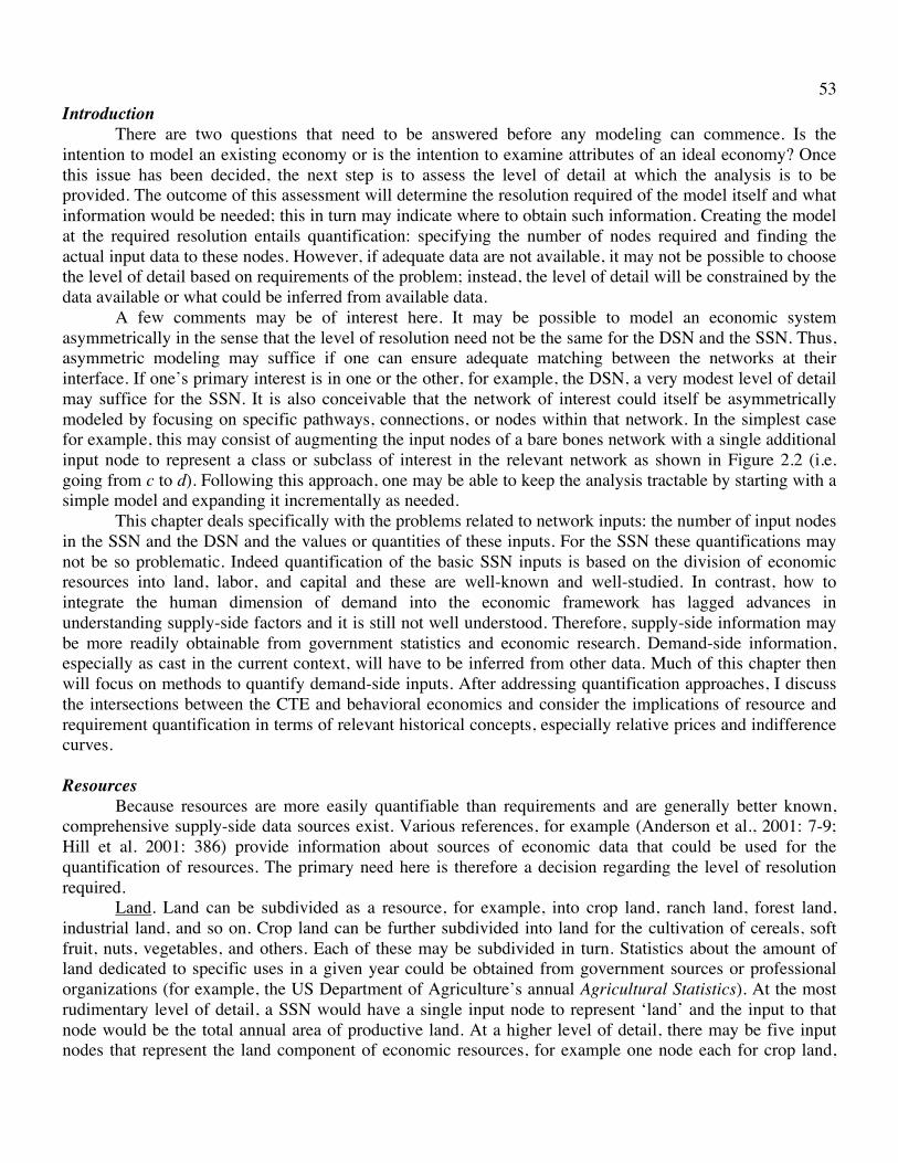
53 Introduction

There are two questions that need to be answered before any modeling can commence. Is the intention to model an existing economy or is the intention to examine attributes of an ideal economy? Once this issue has been decided, the next step is to assess the level of detail at which the analysis is to be provided. The outcome of this assessment will determine the resolution required of the model itself and what information would be needed; this in turn may indicate where to obtain such information. Creating the model at the required resolution entails quantification: specifying the number of nodes required and finding the actual input data to these nodes. However, if adequate data are not available, it may not be possible to choose the level of detail based on requirements of the problem; instead, the level of detail will be constrained by the data available or what could be inferred from available data.

A few comments may be of interest here. It may be possible to model an economic system asymmetrically in the sense that the level of resolution need not be the same for the DSN and the SSN. Thus, asymmetric modeling may suffice if one can ensure adequate matching between the networks at their interface. If one’s primary interest is in one or the other, for example, the DSN, a very modest level of detail may suffice for the SSN. It is also conceivable that the network of interest could itself be asymmetrically modeled by focusing on specific pathways, connections, or nodes within that network. In the simplest case for example, this may consist of augmenting the input nodes of a bare bones network with a single additional input node to represent a class or subclass of interest in the relevant network as shown in Figure 2.2 (i.e. going from c to d). Following this approach, one may be able to keep the analysis tractable by starting with a simple model and expanding it incrementally as needed.

This chapter deals specifically with the problems related to network inputs: the number of input nodes in the SSN and the DSN and the values or quantities of these inputs. For the SSN these quantifications may not be so problematic. Indeed quantification of the basic SSN inputs is based on the division of economic resources into land, labor, and capital and these are well-known and well-studied. In contrast, how to integrate the human dimension of demand into the economic framework has lagged advances in understanding supply-side factors and it is still not well understood. Therefore, supply-side information may be more readily obtainable from government statistics and economic research. Demand-side information, especially as cast in the current context, will have to be inferred from other data. Much of this chapter then will focus on methods to quantify demand-side inputs. After addressing quantification approaches, I discuss the intersections between the CTE and behavioral economics and consider the implications of resource and requirement quantification in terms of relevant historical concepts, especially relative prices and indifference curves.

Resources

Because resources are more easily quantifiable than requirements and are generally better known, comprehensive supply-side data sources exist. Various references, for example (Anderson et al., 2001: 7-9; Hill et al. 2001: 386) provide information about sources of economic data that could be used for the quantification of resources. The primary need here is therefore a decision regarding the level of resolution required.

Land. Land can be subdivided as a resource, for example, into crop land, ranch land, forest land, industrial land, and so on. Crop land can be further subdivided into land for the cultivation of cereals, soft fruit, nuts, vegetables, and others. Each of these may be subdivided in turn. Statistics about the amount of land dedicated to specific uses in a given year could be obtained from government sources or professional organizations (for example, the US Department of Agriculture’s annual Agricultural Statistics). At the most rudimentary level of detail, a SSN would have a single input node to represent ‘land’ and the input to that node would be the total annual area of productive land. At a higher level of detail, there may be five input nodes that represent the land component of economic resources, for example one node each for crop land,

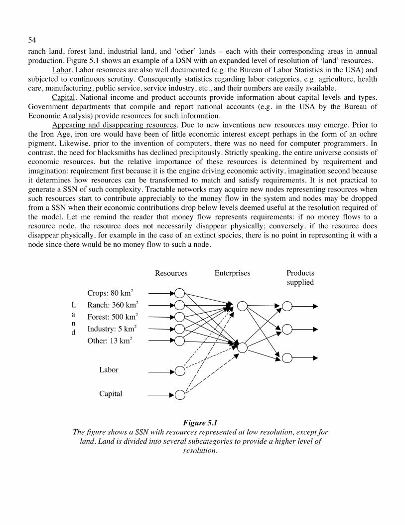
54 ranch land, forest land, industrial land, and ‘other’ lands – each with their corresponding areas in annual production. Figure 5.1 shows an example of a DSN with an expanded level of resolution of ‘land’ resources.

Labor. Labor resources are also well documented (e.g. the Bureau of Labor Statistics in the USA) and subjected to continuous scrutiny. Consequently statistics regarding labor categories, e.g. agriculture, health care, manufacturing, public service, service industry, etc., and their numbers are easily available.

Capital. National income and product accounts provide information about capital levels and types. Government departments that compile and report national accounts (e.g. in the USA by the Bureau of Economic Analysis) provide resources for such information.

Appearing and disappearing resources. Due to new inventions new resources may emerge. Prior to the Iron Age, iron ore would have been of little economic interest except perhaps in the form of an ochre pigment. Likewise, prior to the invention of computers, there was no need for computer programmers. In contrast, the need for blacksmiths has declined precipitously. Strictly speaking, the entire universe consists of economic resources, but the relative importance of these resources is determined by requirement and imagination: requirement first because it is the engine driving economic activity, imagination second because it determines how resources can be transformed to match and satisfy requirements. It is not practical to generate a SSN of such complexity. Tractable networks may acquire new nodes representing resources when such resources start to contribute appreciably to the money flow in the system and nodes may be dropped from a SSN when their economic contributions drop below levels deemed useful at the resolution required of the model. Let me remind the reader that money flow represents requirements: if no money flows to a resource node, the resource does not necessarily disappear physically; conversely, if the resource does disappear physically, for example in the case of an extinct species, there is no point in representing it with a node since there would be no money flow to such a node.

Figure 5.1 The figure shows a SSN with resources represented at low resolution, except for

land. Land is divided into several subcategories to provide a higher level of resolution.

Resources Enterprises Products supplied

Crops: 80 km2 Ranch: 360 km2 Forest: 500 km2 Industry: 5 km2 Other: 13 km2

L a n d

Labor

Capital

55 Requirements

Requirements bring us to the essential social aspects of economics. If we view economic activities as resulting from the expression of human motives, and if we see demands as corollaries of human motives, then the nature of the demand process must be understood first before the supply process can be understood fully. In very basic terms, thirst fundamentally precedes the search for and consumption of water even if, due to learning, one could avoid thirst by searching for water first.

Demand has fixed, variable, and inducible components that contribute to the dynamic complexities of economics. These components correspond loosely to the requirement categories of needs, wants, and aspirations. But how are the levels of needs determined? How are wants determined? How are aspirations determined? Without a quantitative determination of their levels, the quantitative nature of the entire model is in jeopardy. A secondary problem is how different mixes of needs, wants, and aspirations cluster together to generate demands for specific products. I have pointed out before that some enterprises overtly or covertly perform this task, but there is a related problem: given that a certain product is available, how does a consumer assess whether this product would meet their requirements in the most cost-effective way? Perhaps this works by a process of product selection, where some products are found to be suitable by consumers and consequently these products achieve higher levels of sustained demand than others. But with finite resources, an infinite array of possible products cannot be supplied for such a process selection to operate on.

Since the advent of macroeconomics and marginalism in the mid-nineteenth century, demand-side factors have not received as much attention as supply side factors until the resurgence of interest following the publication of Prospect Theory (Kahneman and Tversky 1979). This renewed attention has given rise to subdisciplines such as behavioral economics and experimental economics, aimed at understanding the motives of ‘rational economic man’ and measuring the behavioral outcomes of these motives (Lewis 2008: 4). It has also given rise to neuroeconomics, aimed at elucidating the neural circuitry underpinning economic behaviors (Lohrenz and Montague 2008: 457). Interestingly, the problem of the quantification of requirements therefore intersects the subdisciplines of behavioral economics, experimental economics, and neuroeconomics.

Needs. All behaviors can be seen as attempts to meet a person’s requirements. When these behaviors derive directly from homeostatic processes, needs are in question and they are the most easily quantified requirements. The Anima Motrix model is a quantitative model of motivated behaviors showing how behaviors arise, along with the physiological processes and neural circuitry upon which they depend, to maintain homeostasis (Schulze 1995: 278; Schulze and Mariano 2003: 10-3; Schulze 2004a: 6).

Briefly, for every individual, homeostatic processes regulate a host of physiological variables within certain ranges, each bracketing a set point, to support life. Set points, and the ranges within which regulated variables can deviate from them, are dependent on the metabolism and thus on activity level, health, and the environment. In stable situations (e.g. in peacetime, pandemic-free, and stable environments), these variables vary within generally narrow limits. When these autonomous and subconscious processes fail to maintain homeostasis, they need to recruit supporting behaviors. Behaviors are recruited by the generation of growing distress as the regulated variable deviates increasingly from the set point and they are guided by the generation of pleasure when they succeed in moving the regulated variable back to the set point.

For the sake of continuity, a slight further elaboration is necessary. Because the hedonic urges arising from physiological regulation produce (economic) demands, the intensity of a demand derives from the intensity of an urge, not the actual physiological deficit (i.e. not the physical amount of a commodity needed). Although there is a relationship between the two, this relationship is non-linear (e.g. Schulze 1995: 275-279; Schulze 2004a: 18) implying that marginal utility would be nonlinear. Furthermore, the behavioral expression of the urge becomes subject to modification through learning and experience; specifically, intertemporal compensation occurs permitting better maintenance, thus optimization, of physiological conditions over longer time horizons (Schulze 2004a: 42-53; Schulze and Mariano 2003: 16-1, 22-5). The

56 intensity of an urge may be taken to represent utility as used historically – the psychological benefit that a given good confers upon consumption.

Thus, arguments from requirement microfoundations suggest that the demand curves pertaining to needs (except for the very young) are not zero at zero physiological deficits in experienced persons. Indeed, rational persons become aware, through learning, of the average amount of a given commodity they need to consume and any excess that they need to keep on hand to guard against the unforeseen. Greater uncertainties will likely mean that a larger buffer is preferred. Nevertheless, irrespective of how purchasing decisions are traded off and distributed over time, the consumption of a certain level of a commodity per unit time is essential and determined by the metabolism. Consequently, for every needs node, there exists a production or transfer function that is generally non-linear (in contrast to previous simplifying assumptions about the transfer functions of input nodes) and that changes with experience. An example is given in the chapter on simulations (Chapter 16).

The following small example illustrates the quantification of needs. The average person has an energy requirement of about 2,000 calories per day. Because I used 15 work days for the SSN in Figure 2.3, the needs tally of a simple DSN to complement that SSN must reflect a single person’s caloric requirements for an entire year (even if only 15 days are spent working). This would be 365 x 2,000 = 730,000 calories per year. Therefore, let this be the input to the ‘Needs’ node of such a DSN. If the system includes more persons and their requirements have to be met, the needs level should be adjusted correspondingly. This is clearly an oversimplification, but illustrates the point. In reality, more than calories are needed: water, other nutrients, heat (including basic clothing and basic shelter), and so on. Still, our understanding of physiology may go a long way towards assessments of needs.

Wants. I have pointed out that wants are related to procreation. Specifically, wants may be strongly related to mating and other implicit and explicit sexual activities – these undoubtedly include competition for mates and sometimes competition to position one’s offspring favorably in the contest for mates. Because competition carries with it implications of relative social position (i.e. status), wants are variable in nature. It is not adequate to have enough – one must have more than one’s competitors to obtain a selection advantage. Competition, moreover, would affect both the quality and the quantity of wanted items. All else being equal, wants are constrained by physical prowess, intellectual ability, and general health. Therefore, unlike needs, generally similar for all adults, wants can vary more widely. This is where true quantification difficulties arise.

As before, it is necessary to determine the level of resolution desired for wants. This includes the problem of determining or identifying these wants. Next, one has to assess their qualities and quantities. Perhaps the earliest manifestation of wants is as a simple extension of some needs beyond what are needed for personal survival. Thus, those portions “in excess” should be counted as wants. Further refinements may come from studies on human motives such as Maslow’s hierarchy of human needs (Maslow 1943). This hierarchy ranges, in order of precedence, from physiological needs through safety and security, love and belongingness, and esteem, to self-actualization needs. Note that ‘needs’ as I have defined them in terms of this connectionist model corresponds only with the “physiological needs” (and possibly with some “safety and security needs”) of Maslow’s hierarchy. “Self-actualization” is more congruent with aspirations. This means that wants correspond broadly to Maslow’s “love”, “belongingness”, and “esteem”. The latter may serve then as a starting point from which to examine, identify, enumerate, and quantify wants.

On a practical level, law and regulation may specify many requirements and one has to decide whether to class them as needs or wants or how to proportionate them between these two requirements. My own bias is in favor of a separation of elastic and inelastic demands; it may render some of the dynamics of economic systems more transparent. Consider for example living space. Building regulations generally specify minimum levels of insulation (heat, a need) and floor area per occupant (shelter, a need). Levels exceeding these should be considered as wants. For the sake of argument, let the average value for needs-

57 related living space be 1,000 square foot per person per year. Then, assuming a single input node for wants, consisting of living space only, the presence of 4,000 square foot of living space represents a want of 3,000 square foot. Consequently, when modeling an existing economy, wants may have to be inferred from requirement levels after correcting for needs. Nevertheless, wants could vary from zero to an arbitrarily large number.

Aspirations. Aspirations derive from community-related behaviors. To put them in context again: needs relate to the self irrespective of others; wants reflect the relative standing of self to others; and aspirations involve the interests of all. It may be useful to partition aspirations into either benefit-seeking or harm-avoiding groups because these groups may have asymmetric demands. Voting patterns, volunteer work, and charitable contributions all give clues about the prevalence and intensities of aspirations. Indeed, US Census Bureau numbers suggest that charitable contributions as a proportion of income increases with age, that is, as the reproductive years pass and sexual drives abate, relatively less is spent on wants and more is spent on aspirations. Although one may expect older persons to be better off and hence more likely to make charitable donations, a somewhat inverse relationship holds to income - the poor give relatively more. Hence, I contend that a shift from wants to aspirations occurs, with needs being relatively constant.

Quantification of aspirations may proceed along two routes. The first is to asses the fraction of the population that displays non-negligible levels of aspirations. This may fluctuate over time, but national voter turnout in national elections may provide a clue about normal levels of aspirations in a population. In the USA, the number of people participating in non-presidential elections comprises (a minimum of) about one third of voting-age persons. Next, one needs to determine what the average levels for aspirations are, relative to other requirements, in this portion of the population. Consider, for example, a single representative person of this part of the population. Let this person experience a net general yearly drive state of 10,000 ‘drive units’. These drive units represent units of motivational drive irrespective of whether they arise from needs, wants, or aspirations. Let, for example, one half of these be classifiable as needs, one quarter as wants, and one quarter as aspirations. For others, not voting in non-presidential elections, let one half of the 10,000 drive units represent needs and one half wants. Then the total level of aspiration drive units for the population would be 10,000 (drive units) times one third (of the population) times one quarter (of drive units being due to aspirations). This gives an average of about 8 % of drive states per person attributable to aspirations. The difficulty is to asses the relative strengths of such drive states. Hedonic states, that is, the intensities of the pains or pleasures experienced in response to actions and inactions, provide a means to determine at any point in time, or on average, what these relative weights are (e.g. Hess et al. 2006; Schulze and Mariano 2003: 11-4). Should one consume salt or suede or sovereignty? Equal marginal hedonic utility answers this question.

The second route is by way of an analysis of expenditures. Estimates of benefit-seeking aspirations can be arrived at from examining households’ monetary and in-kind contributions to charities. For the USA, this is about 2.5 % of income (Independent Sector 2000). Assuming a zero percent savings rate, 100 % of income must be distributed across all requirements. If approximately 3 % is assigned to aspirations, then the remaining 97 % must be distributed between needs and wants. According to the US Census Bureau, the 2008 per capita income was $26,964 and the poverty threshold $10,991 or about 41 % of per capita income. Because the poverty threshold would be closely related to needs, the numbers above suggest that 40 % of drive units represent needs, 57.5 % wants, and 2.5 % aspirations. Because the drive units for aspirations are based on those voting in non-presidential elections and those contributing to charity, one could plausibly combine them to get a value for aspirations of about 5 % (in an A.D. 2000 North American society). Thus, taken together, a rough estimate is that about 40 % of requirements pertain to needs, 55 % to wants, and 5 % to aspirations.

Appearing and disappearing requirements. Nodes representing new requirements may be introduced into a DSN and those representing disappearing requirements may be dropped. Emergent and disappearing

58 requirements will be of the wants or aspirations type because needs, in general, will be fixed in a physiological, hence physical sense. As with resources, all potential requirements can be modeled, but not all will exist at economically appreciable levels, that is involve an appreciable money flow. Therefore, the nodes included in demand- and supply-side networks depend on existing requirements, resources known to be necessary for their satisfaction, and the level of resolution desired of the model. As I shall discuss later, the situation with hidden nodes is somewhat more complex.

Discussion and conclusions

Resources, the inputs to the SSN, are relatively easily quantified. A wealth of sources and statistics are available to determine, estimate, and infer the levels of resources. Requirements, the causal factors in economic exchanges, are rather more problematic though needs, by virtue of being rooted in physiology, are most easily addressed. Regardless, both the subdivision of resources and requirements and the quantification of resources and requirements have consequences. The former, for example, because it enables investigations regarding the roles played by different aspects of demand and supply hence relating it to behavioral economics. The latter, for example, because fundamental ratios of demand to supply can then be established permitting relative values, upon which utility is further imposed, to be examined.

Requirements instigate requirement-satisfying behaviors; therefore, they are the ultimate causal factors in economic exchanges. The view here, simply put, posits that requirements activate hedonic states that trigger behaviors to satisfy these requirements. In the case of needs, a strong linkage can be drawn between homeostatic mechanisms that function to minimize physiological stresses and the neural pathways that generate hedonic states and subsequently activate behaviors (e.g. Schulze 2004a: 6). Both the role of requirements as economic causal factors and the roles of hedonic states, especially, in driving behaviors have historical parallels. For example: Bentham was of the opinion that the actions of man were ruled by pain and pleasure; Say thought that utility or desire was the true origin of the exchange value of a commodity; and Senior saw demand to depend on the intensity of pleasure and pain derived from commodity consumption (Vaggi and Groenewegen 2003: 118, 120, 155). The most extensive overlap perhaps occurs with the work of Jevons who believed that a true theory of economics depended on elucidating the drivers of human action (Vaggi and Groenewegen 2003: 204-209). In contrast to Jevons, though, I do not see diminishing returns to necessarily occur for the consumption of all goods. Specifically, diminishing returns must hold for the consumption of goods that satisfy needs, will not hold for the consumption of goods that satisfy wants (i.e., status goods, in the absence of a stable status hierarchy), and may not hold at all for the consumption of goods that satisfy aspirations (e.g. education).

Requirements are subdivided into needs, wants, and aspirations. This subdivision is also reminiscent of earlier thought. Thus Steuart’s distinction between strong demand and strong competition (Vaggi and Groenewegen 2003: 89) seems to delineate between needs and wants, respectively. The reader may also recognize in Menger’s ‘goods of the first order’, required for life itself, a resemblance with needs, while ‘goods of a higher order’ are more closely related to wants and aspirations (Vaggi and Groenewegen 2003: 212). Finally, Pareto’s concerns about utility and commodity quantities (Vaggi and Groenewegen 2003: 289) are addressed here by formulating a relationship between the urge to consume, the quantity of a corresponding commodity consumed, and the quantity of that commodity available. This relationship is based on the distinction between the urge to consume and the quantity to be consumed (e.g. mentioned above as “hedonic states” and “physiological stresses”, respectively) and relative values that arise from the quantity of a commodity to be consumed and its availability (mentioned below in terms of relative prices).

Interestingly, the specific partitioning of requirements into needs, wants, and aspirations also have implications for Say’s law (in the long run, there can be no general glut in the market, e.g. Vaggi and Groenewegen 2003: 139). Neglecting a Malthusian effect (i.e. an increase in the population brought about by prosperity), needs are limited, thus a glut can arise with regards to needs. On the other hand, wants, unless a

59 stable status hierarchy can be established, are potentially unlimited; in this regard, there can be no general glut of (some) wants-related goods in the market. Similar considerations hold for aspirations and how the lack or presence of education affects them. Say, however, formulated his view based on the circular flow of revenues (Vaggi and Groenewegen 2003: 121), therefore, the number of tokens available for the expression of requirements will also affect demand. Moreover, the model developed here consists of adaptive systems, thus any excess in supplies will be curtailed. The penultimate (unlimited wants) and, especially, the last consideration (supplies adapted to demands) seem to support the long-run validity of Say’s law.

Considering next the quantification of resources and requirements, they have a bearing on the explanation of relative prices which has been a major problem for classical theories of the market (Levine 2005: 11). Many economists have considered intrinsic values, relative values, values in exchange, and concepts of utility to address how relative prices arise. Locke, for example, denied the existence of intrinsic value and differentiated between use value and exchange value (e.g. Vaggi and Gronenwegen 2003: 26). In contrast Cantillon believed that the intrinsic value of something depended on the amounts of land and labor required to produce it (Vaggi and Gronenwegen 2003: 48). Having quantified resources and requirements, some important conclusions can now be drawn about values and prices.

Given that needs are determined within narrow limits by the demands of physiological processes and given that resources are finite, it is immediately obvious that some fundamental ratio of needs to corresponding resources must exist. Furthermore, this ratio must depend on the population and hence will change as the population changes. If the population increases, resources become scarcer. This ratio will not be the same for all needs because their physiological magnitudes differ with respect to one another and the relative abundances of their corresponding resources are also not the same. Specified in this fundamental way, the ratio therefore represents an intrinsic value. This intrinsic or natural value is modified by other factors such as a person’s and/or a population’s state (i.e. health, level of nourishment, etc.) as well as the accessibility of resources. Thus, something can never be worth less than its intrinsic value, but may very well be worth more due to the factors of modification. Such modification will determine the eventual exchange value. The intrinsic value is therefore not independent from the exchange value, but is a subcomponent of the exchange value.

For example, salt is absolutely essential in the diet, but at modest quantities. Moreover, the amount of salt in the world is finite and rather large. A fundamental ratio can therefore be determined that relates the lifetime requirement of salt per person multiplied by the total number of people to the total amount of salt available. This is the intrinsic value of salt. Because salt can be extracted from the available total amount only at a certain rate and a person does not consume their lifetime requirement of salt all at once, but does so instead at a certain rate, a secondary or effective intrinsic ratio arises. The effective intrinsic ratio relates the (planet-wide) rate of consumption to the (planet-wide) rate of extraction. Now, some amino acids are also essential in the diet, and in larger quantities than salt. Their availability may also be rather more circumscribed than that of salt. Thus a different intrinsic value and a different effective intrinsic value will arise for the essential amino acids compared to those of salt. We have here then the emergence of relative intrinsic and relative effective intrinsic values. Relative effective intrinsic value appears to be related to Locke’s ‘exchange value’.

Furthermore, if one is in need of ingesting salt, this need is communicated by the body to the mind via the generation of hedonic states or urges (Schulze 2004a: 18, 51-53). If more salt is needed, a stronger urge is created than when less is needed, but disproportionately so. Thus a unit quantity of salt obtained when the urge is weak will have less utility than the same unit of salt would have when the urge is stronger. This demonstrates the physiological basis of diminishing marginal utility. It is also more likely that one would part with a unit of salt if one currently has no or little urge to consume it oneself, than when one has a great urge to do so. Conversely, one is at a disadvantage when attempting to acquire salt if a strong salt hunger is present. It should not be lost sight of that the party on the other side of the trade is subject to the same

60 considerations with regard to what they wish to obtain and what they wish to offer in exchange for that. Prices are established when these exchanges finally happen, whether in barter or via a standardized medium of exchange.

For a want, a less tightly constrained relationship exists with its corresponding resources. Gold, for example, is not required in the diet. It is a noble metal, meaning that it does not tarnish readily and retains its reflective properties. These reflective properties interact with the visual system, for example, the peripheral visual system, to capture attention. The primitive possessor of gold would therefore have had an edge, compared to those dependent on their natural charms or dependent on alternative ornaments, in the competition for mates. This explains its enduring role in human affairs. Thus for gold an intrinsic value exists: one determined by its natural abundance, the intensity of competition, and its ability to attract attention hence mediate in competition. For as long as humans retain vision and remain competitive sexual beings, gold will have an intrinsic value.

I think it is altogether more difficult to estimate the intrinsic value of a want than it is to do the same for a need, but if a want can be quantified along with its corresponding resource(s), it could be done in principle. Resources that exclusively serve to meet aspirations may also have intrinsic values and these may depend on innate cognitive and emotional abilities. Here the quantification of aspirations also implies that their intrinsic values can be determined. Where a resource has multiple uses, for example, where it satisfies both needs and wants, an intrinsic value still exists and can be determined, but it will be difficult to do so.

To summarize, relative intrinsic values are dependent on the ratios of the absolute levels of requirements to the absolute levels of their respective resources. These ratios are modified by the efficiencies of requirement expression and resource utilization to produce relative effective intrinsic values. In the case of needs, average annual physiological deficits determine average annual consumption needs, which, when expressed relative to their respective available annual supplies, produce use values. Exchange values are modifications of use values and are dependent on the intensities of psychological urges produced by short term fluctuations in physiological deficits, as opposed to their longer term average values. Note the differences vis-à-vis ‘utility’ as commonly encountered and Locke’s usage of ‘exchange value’.

Both the subdivision and quantification of requirements have implications that pertain to Pareto’s indifference curves. Where nutrients are concerned, indifference curves can only extend until that point where a unique nutrient in one or the other commodity becomes rate limiting and puts a floor under the amount of that commodity consumed: anything less will lead to demise. Furthermore, indifference curves for needs may be quite distinct from those of wants and these, in turn, from those of aspirations. Given the essential nature of needs and the discretionary nature of aspirations, indifference curves between needs and aspirations probably do not exist. Likewise, the different attributes of needs, wants, and aspirations imply that indifference curves between needs and wants and those between wants and aspirations may be restricted.

Finally, the subdivision and quantification of requirements is interesting because of its intersections with behavioral and experimental economics. On the one hand, experimental economics could prove valuable to determine the levels of wants and aspirations. Existing models of behavior could be used to flesh out the input region of the DSN because models of consumer behavior relate to the ‘Requirements’ layer, its transfer functions, and its efferent connections. A number of behavioral models are compared by Antonides (2008).

On the other hand, the specific partitioning of requirements into needs, wants, and aspirations may cast experimental economics and behavioral models in a different light. For example, the Theory of Demand, which is based on the maximization of utility or pleasure, posits the decreasing marginal utility of consumption (Antonides 2008:230). This I deem to hold for needs because consumption will first produce diminished pleasure and overconsumption will produce displeasure. Wants, however, relate to relative standing and the marginal utility of consumption may increase rather than decrease. The same may apply to aspirations – more schooling is not necessarily less valued. A different perspective is also provided on Modigliani’s Life Cycle Model. This model suggests that borrowing is based on the life cycle and aims to

61 even out expenditures over the life cycle (Antonides 2008:231). But because wants are tied to competition and reproduction, and the reproductive years peak in the early middle to middle part of the life cycle, this part of the life cycle may involve more borrowing if it will enhance one’s relative standing. My view is that the relative levels of needs, wants, and aspirations change over the life cycle and will affect expenditure patterns, thus a tendency to equalize spending will be moderated by these effects.

62

6 The Quantification of Economic

Transformation Units

63

The Quantification of Economic Transformation Units

Summary

Extending the quantification process to economic transformation units requires, as before, a decision on whether to model an extant or hypothetical economy. If an existing economy is modeled, it is necessary to identify economic transformation units by industry and type such as builders and retailers. Then estimates of their numbers can be made from official statistics for such industries and enterprises. For a hypothetical system, the number of economic transformation units can be varied at will. Nevertheless, assessing the ideal number and size of economic transformation units required for an economic system to function optimally is of great interest. Research on artificial neural networks has shown that networks with many hidden nodes adjust quickly to external changes but suffer from suboptimal efficiencies. In contrast, neural networks with few hidden nodes may not be able to produce the outputs needed and may experience catastrophic failure if one or more nodes fail. Analyses suggest that intermediate numbers of nodes, tending to the high side, could be good options for economic models. It is concluded that the number of economic transformation units in an ideal economy should be of the same order of magnitude as the number of products on the market and that these units should all be of similar size.

64 Introduction

In the previous chapter, the task of developing some of the quantitative aspects of the connectionist model was commenced by considering the quantification of inputs to the model. This task is here extended to address the quantification of the hidden layers of the demand- and supply-side networks that represent ETUs as well as to address the level of resolution at which to model the hidden layers. On the supply-side, ETUs function to transform economic resources into products delivered to the market. On the demand-side, they function to transform economic requirements into products demanded on the market. For conceptual simplicity, we have previously characterized the supply-side enterprises as manufacturers and demand-side enterprises as retailers and we will retain this characterization here.

As before, quantification requires a decision on whether an existing economy is to be modeled or whether theoretical issues are to be investigated. Unlike inputs, however, ETUs may be harder to quantify because, in the case of an existing economy, their identities may be unclear and, in the case of theoretical work, their optimal number is generally not known. Thus, one of the problems of quantification in the former case is the identification of ETUs in terms of industries, manufacturers, suppliers, wholesalers, distributors, retailers, and so on. In the latter case, the problems of quantification are the assessment of the optimal number of hidden nodes and the dynamics according to which these entities are created and deleted. These dynamics have implications for the market entry and exit of firms.

The identities of economic transformation units

Because knowledge about the identities of ETUs will facilitate their quantification based on statistical sources, it is necessary to know these identities. As a general rule, enterprises that are primarily engaged in creating products should be on the supply-side while those that primarily specify, distribute, or provide products should be on the demand-side. Thus the steel maker and aircraft builder are supply-side enterprises while the airline and the travel agent are demand-side enterprises. Likewise, the automaker and car dealership are on opposite sides of the tertiary market divide. It is not necessary for the partition into demand- and supply-side units to be perfect at this point; an approximation will suffice to convey the concepts involved.

The number of economic transformation units

Because one could either model an existing system or a hypothetical one, the number of ETUs should be considered in those two respects. Thus, one could ask, when modeling an existing system, how many nodes it has in the hidden layer. Once the identities of hidden nodes are established, as suggested above, their numbers can be estimated from the relevant data sources.

One could also ask, for a hypothetical (or a real) system with specified inputs and outputs, how many hidden nodes it should have to perform optimally. Now optimality itself needs to be defined. Moreover, optimality may change for various reasons. For the purposes of this outline, I will discuss the putative components of optimality in terms of processing speed, efficiency, quality, and robustness without trying to pin down the sizes of their relative contributions to an optimal system.

Speed. For classification tasks, perceptrons require no more than two hidden layers (Harvey 1994: 89). However, more layers are possible and in terms of economic systems, probably occur. Because a network consists of successive layers, nodes are connected serially. Having more layers implies that more nodes are connected serially and that processing times will increase. In economic terms, processing times refers to the time taken to convert a combination of resources into products and get these products to the point where they actually satisfy a combination or requirements, thus it has a bearing on production speed. In contrast, a greater number of nodes, irrespective of the number of layers they are organized into, implies that there are more connections in total; this decreases the overall training time of the network (e.g. Levine 2000: 215). Thus it takes less time for a network to respond adaptively (i.e. with an adjustment in weights) if a change in either input or target or both occurs. The SSN, for example, will adjust its outputs more quickly to

65 the necessary levels if a change in resources or demand makes this necessary. In more simple terms, I mean here that scaling production up or down engenders less of a lag if there are more ETUs in the SSN to contribute. This refers to an adjustment of production capacity; it is different from the case above that refers to (cumulative) production speed.

The foregoing considerations indicate that it is of considerable interest to know (i) how many hidden layers a network has, and (ii) how many nodes (per hidden layer) there are. In the context of optimality, as we discuss here, knowledge of these two factors may guide legislation, regulation, and stewardship of the economy.

Designers of ANNs often take half of the sum of input and output nodes as a first estimate for the number of hidden nodes required. If the network fails to converge, that is, it gets trapped in a local minimum, a hidden node is added. If it converges initially, a hidden node is removed. In general, the number of nodes has to be determined empirically and this number is much dependent on the application (Levine 2000: 215). However, the range of possible solutions can be narrowed perhaps by taking into consideration other constraints such as those imposed by network stability.

Efficiency. I shall define efficiency in terms of nodal (i.e. local) efficiency, in terms of network efficiency, and in terms of system efficiency. The connection-specific nodal resource efficiency (ηs) is the level of a specified output connection divided by the level of a specified input connection to a given node; if there is zero input, the input is not consumed and efficiency is undefined. Thus, for a given ETUj, and using Eq. 2.1 and Eq. 2.2:

Eq. 6.1

Likewise, a connection-specific nodal requirement efficiency (ηd) can be defined using Eq. 3.1 and Eq. 3.2:

Eq. 6.2

Because resources and requirements flow in opposite directions, the use of these terms defines directionality, hence how ‘input’ and ‘output’ to a node should be considered. Likewise, overall nodal efficiencies (ζ) are specified as:

Eq. 6.3

Eq. 6.4

The efficiencies η and ζ can be seen as production efficiencies. It is also possible to define an efficiency of utilization (υj) for the output of a given ETUj. This is the

ratio of outputs from ETUj consumed by other nodes to the total outputs produced by ETUj. The efficiency of utilization is easily stated in terms of fractional utilization (see Figure 2.3); using Eq. 2.3 the efficiency of utilization is:

Eq. 6.5

66 which simplifies to the sum of the weights of all the connections emanating from a node (see also Eq. 8.1).

Uniformly low efficiencies therefore could mean that the resource or requirement signal is being attenuated as it traverses the core system, thus the system is inefficient. Resources are inefficiently converted into products and requirements are inefficiently expressed as product demands. Further below, system efficiencies specifically are addressed.

Quality. The number of nodes in an information processing network has a direct effect on the quality of the output. If there are too few nodes, the network cannot be trained to produce acceptable outputs. If there are too many nodes, the network overlearns and cannot generalize to similar but new samples that it has not been exposed to before (e.g. Levine 2000: 219; Schoner 1992). From the perspective of a core economic system, if a network is too small, it cannot produce an acceptable array of products (SSN) or ‘specify’ a workable array of products (DSN). It is unclear what the problem is when a network is too large, i.e. when it has too many ETUs. The ‘boutique’ phenomenon may well be the analogue of overtraining and the presence of too many nodes in a network. Nevertheless, the implication drawn is that such a network may tend to become overspecialized and resistant to adaptation.

Consistent with the point made above regarding production efficiencies, low utilization efficiencies imply small weights, thus the network’s weights have a small standard deviation σ. A small σ attenuates network signals (Buckley and Bullock 2008: 6), thus the quality of output could also be affected. In contrast, the probability of stability of a network increases with decreasing σ or decreasing C (see below).

Robustness. Under ‘robustness’ one could consider the stability of a network’s output with regard to a perturbation of its input or the stability of the output with regard to a perturbation of the network’s architecture. Because inputs are propagated to outputs via weighted connections, the May-Wigner threshold can be used for examining the dependence of input-output stabilities on weights. Assuming that the weights in a network are normally distributed around a mean of zero and with a variance of σ2, a system with a number of nodes much larger than 1 is stable when:

Eq. 6.6 where N is the number of nodes in a network, C the number of connections in that network, and β is a small value subtracted from each weight to stabilize the system (Buckley and Bullock 2008: 4). Because, in terms of economic networks, a negative connection implies a reversal of flow and at present I do not favor using negative weights to indicate such flows (but rather separate connections), the weights in economic networks are likely to have positive, but small means. This should not significantly affect Eq. 6.6.

The May-Wigner threshold (Eq. 6.6) also provides some information on the size of a network and its effects on output stability. Let a network have I input nodes, H hidden nodes, and O output nodes. Then, for a fully connected network:

Eq. 6.7 and

Eq. 6.8 Substituting Eq. 6.7 and Eq. 6.8 in Eq. 6.6 gives

and rearranging

Taking H to be of the same order of magnitude as I + O, one arrives at the approximate solution

Eq. 6.9

67 Thus, feasible and stable solutions seem to exist only for very small σ, (i.e. for small enough σ such that

) but as explained above, at the cost of attenuating network output or compromising the quality of the output.

Regarding the dependence of output stability on network architecture, one may consider how the output of a network changes with a gain or loss of nodes and/or connections. As mentioned above, a network with too many hidden nodes is prone to overtraining, thus adding nodes creates this risk. However, in the case of the economic core system model, the networks are on-line and are being trained continuously which may ameliorate overtraining. Furthermore, adding nodes facilitates on-line training (Levine 2000: 216), thus some trade-off exists here between overtraining and the ability to respond rapidly to changing input and output conditions.

In contrast, for a given network, deleting nodes makes training more difficult (Levine 2000: 216) and degrades the quality of the output. This latter quality is termed “graceful degradation” since deleting a node does not generally lead to an abrupt failure of network performance, but a gradual deterioration as more nodes are deleted (e.g. Rumelhart and McClelland 1986: 134). At some point, however, training will become difficult if not prohibitive. At this point, deleting a node may cause systemic failure (i.e. a failure to train). If, at this point, all hidden nodes are of the ‘same size’, one could argue that this represents the size at which a node is too big to fail. A network needs more nodes than those that would exist at this limit, and if it has more nodes, no node should be allowed to have larger flows of either demands or resources across it than established by the too-big-to-fail limit. Although I cannot say what this size limit should be, or is, in any given economic system, it is clearly a question that can be investigated theoretically.

Discussion and conclusions

Here, in passing, I have dealt with the issue of determining the number of economic transformation units of core system networks that are used to model extant economies. I have simply pointed out the need to identify ETUs and then to determine their numbers from sources of economic statistics such as those from government departments. I have dealt at much greater length with the question of determining the optimal number of ETUs for a core system given its prevailing input and output contexts. From analyses of network stability, a number of conflicting interpretations arise. It seems that a large number of hidden nodes could make a network unstable and that a small number could expose the network to catastrophic failure should one or more of the hidden nodes fail. Likewise, a large variance in network weights may produce instability, while a small variance may compromise output quality. My conclusion is that a relatively large number of nodes with a small variance of weights is the best choice. This would ensure network stability, rapid training, and avoid catastrophic failure, but could come at the cost of reduced efficiency, output quality, and increased specialization.

Addressing now specifically systemic efficiencies, one could ask what the consequences of an incorrect number of hidden nodes would be. Four types of malady may be posited to arise, even in equilibrated systems: (i) an inability to estimate demands; (ii) an inability to supply demands; (iii) an overspecialization and inflexibility of demand; and (iv) an overspecialization and inflexibility of supply. Inflexibility here refers to the inability of the network(s) to adjust smoothly to small changes in input patterns.

Regarding the symptoms, an inability to estimate demands would lead to stresses in the population: when needs are not met, medical conditions are likely to dominate; when wants are not met, social ills may be more dominant; and when aspirations cannot be met, discontent may surface predominantly at the level of politics. In addition, at least some products are likely to be in chronic short supply. An inability to supply real demands would also lead to at least some products being in chronic short supply and this would be coupled with capacity ceilings being reached in at least those cases.

68 Inflexibility or specialization of demand is not of itself problematic, but it is so in an unstable or variable

environment – because the environmental context in which an economic system is embedded would affect both resources and requirements, and in different ways, fostering or allowing inflexibility incommensurate with contextual variability is unwise. Inflexibility or specialization of supply leading to unmet demands is more problematic because it would ultimately result in the medical, social, and/or political ills mentioned above, but if this is not the case, the inflexibility of supply is nevertheless vulnerable to environmental instabilities. In the case of demand, inflexibility will be observed as a lag in the types and levels of product demanded; in the case of supply, there will be a lag in what is supplied even if demand tracks environmental contexts adequately. Remember that “inflexibility” here refers to the inability of a network to accommodate small variations in its input and this “inflexibility” will be expressed not as a rigidity in output (i.e. the same output regardless of small changes in input), but as an instability in output as explained above.

Regarding the remedies, the following can be advanced in terms of network modifications. For malady (i)—an inability to estimate real demands—one or more nodes should be added to the hidden layer of the DSN; for (ii)—an inability to supply real demands—one or more nodes should be added to the hidden layer of the SSN; for (iii)—an overspecialization and erratic demand—one or more nodes should be deleted from the hidden layer of the DSN; and for (iv)—an overspecialization and erratic supply—one or more nodes should be deleted from the hidden layer of the SSN.

These network modification remedies have specific economic analogs. Thus, in the case of an improper estimate of products demanded (i.e. a demand-side malady), some products would be supplied that are consumed at much lower levels than the levels of available supply while others may be supplied at levels much lower than the levels of desired consumption. In the latter case, supply inflation and profits will arise that may entice existing SSN enterprises to increase production levels or DSN enterprises to increase or modify estimates and new enterprises on either side to enter the market. In the case of an inadequate supply of some products (i.e. a supply-side malady), supply inflation will also occur, but will not be accompanied by instances of oversupply of some products unless there is also a simultaneous error in product demand estimates. Note, in more concrete terms, that in this case there is not enough product because not enough product can be manufactured to meet that ordered. This is not the same as erroneously ordering less product than actually required.

In the case of model building it is easy to add and delete nodes from networks, but in a real economic system addition of nodes correspond to market entry of enterprises and deletion of nodes correspond to market exit of enterprises. One has to ask, therefore, what the conditions are for market entry and market exit in the respective sides of an economic system and whether these are consistent with the concepts discussed above regarding optimality. Alternatively, if the mechanisms and causes of market entry and market exit are not well understood, one has to ask whether the CTE could provide insight into the matter. Demonstrating that the need for market entry and market exit arises does not elucidate the actual mechanisms whereby these processes occur. These mechanisms involve the generation of profits and losses and they are briefly discussed in Chapter 4 and, in more detail, in Chapter 13.

69

7

The Quantification of Products

70

The Quantification of Products Summary

The quantification process is brought to a close by looking at the quantification of products. As before, when modeling an extant system, a decision is required on the level of detail at which the modeling is to be performed. Thus, the number of product categories should be decided upon along with establishing their identities and volumes. Because the quantification of products is in many respects similar to the quantification of the gross domestic product, economic and population statistics available from government bodies and other sources of data can be used to estimate the types and volumes of products demanded and supplied. Regarding theoretical work, the optimal number of product categories required for a given economic system can be investigated. Results from computational models suggest that at least a few product categories may be needed for the system to function, but that too many categories will make it inefficient. Due to the semblance between the quantification of products and GDP calculations, theoretical investigations also raise questions about the methodology and purpose of the GDP. It is concluded that other measures or a different way to calculate GDP may be more beneficial to determine whether an economic system is effective in meeting population requirements, because the latter, not economic growth, is the ultimate economic objective.

71 Introduction

This chapter deals with the problems related to network outputs: the number of output nodes in the SSN and the DSN and the levels or quantities of these outputs. By design, the number of output nodes for both the SSN and the DSN are matched, but their volumes may not be. For example, there may be a product available (SSN) but no demand for it (DSN). This situation cannot endure indefinitely, thus the number of output nodes for both networks may be dynamic. More generally, the output levels for both networks fluctuate due to independent factors (changes in population and environment) and dependent factors (adaptation by one network to the output of the other and vice versa). For practical reasons though, one may assume that these are fixed initially and then proceed to quantify them based on the level of resolution or detail required. Because the outputs for the SSN are closely related to the entities that figure in calculations of gross domestic product, quantification may be relatively easy.

With resources and requirements, thus with input nodes, the question of how many there should be does not generally arise: the number of input nodes reflects the realities of population (requirements) and environment (resources) as explained in more detail in Chapters 2, 3, and 11. Thus, in some absolute sense, they are fixed save for the resolution that one wants to model. With hidden and output nodes, but especially so for hidden nodes, the question of optimality arises. In contrast to hidden nodes, where the optimal number could be decided upon when the network is created or maintained (i.e. by legislation), more freedom is required for establishing the number of output nodes. In particular, the demand-side nodes are important and it is unclear how one could regulate or decree what products should be in demand. Narcotics and firearms may be exceptions, but the consumption of water or bread is not easily decreed. Therefore much freedom is needed to allow for the expression of requirements in terms of products demanded. Likewise, freedom to allow for product supplied also follows, otherwise stresses arise in the population because, even though it may demand certain products, these cannot be obtained. Thus, for both SSN and DSN the number of output nodes should be self-determined, keeping in mind that these networks are matched, thus they constrain each other in terms of output nodes. Nevertheless, some theoretical considerations may also exist that may impact on the performances of the networks. The chapter will therefore be devoted to the consideration of both practical and theoretical considerations affecting the number of output nodes in the networks of the core economic system.

A technical issue needs to be clarified at this point. In the introductory chapters, I described the output nodes of the SSN as “distributors” and those of the DSN as “wholesalers”. In the description of the core system, they are sometimes simply described as “products supplied” and “products demanded”, respectively. A good compromise may be to think of output nodes as being distributors or wholesalers of a single product. One is not particularly interested in matching distributors with wholesalers, but it is important, from the economic perspective, to match the products of the supply side with products demanded on the demand side. When considering distributors and wholesalers as purveyors of single products, matching like ones would automatically ensure a matching of the same types of product (although the levels of these products may not match). They key point throughout is that resources are to be matched with requirements. This matching proceeds through intermediate stages and the most recognizable of these is ‘products’. When the reader is sufficiently comfortable with the concepts, s/he may proceed to model multi product distributors and wholesalers, although the products of the supply side, irrespective of how distributed, must still be matched with the products in demand, irrespective of how the demand is mediated. Ultimately, the outputs of the SSN are products supplied and the outputs of the DSN are products demanded and these must be matched.

Products supplied

The GPS is defined as the aggregate of all products, that is, the sum of all the output nodes of the SSN (Chapter 2). Similarly, the GMD is defined as the sum of all product money demands arrived at by the multiplication of aggregate supply of a given product with the unit price of that product. Therefore, GPS is in

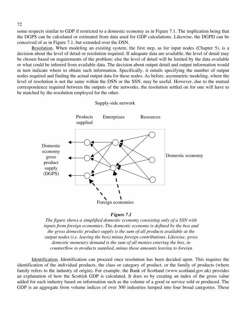
72 some respects similar to GDP if restricted to a domestic economy as in Figure 7.1. The implication being that the DGPS can be calculated or estimated from data used for GDP calculations. Likewise, the DGPD can be conceived of as in Figure 7.1, but extended over the DSN.

Resolution. When modeling an existing system, the first step, as for input nodes (Chapter 5), is a decision about the level of detail or resolution required. If adequate data are available, the level of detail may be chosen based on requirements of the problem; else the level of detail will be limited by the data available or what could be inferred from available data. The decision about output detail and output information would in turn indicate where to obtain such information. Specifically, it entails specifying the number of output nodes required and finding the actual output data for these nodes. As before, asymmetric modeling, where the level of resolution is not the same within the DSN or the SSN, may be useful. However, due to the mutual correspondence required between the outputs of the networks, the resolution settled on for one will have to be matched by the resolution employed for the other.

Identification. Identification can proceed once resolution has been decided upon. This requires the

identification of the individual products, the class or category of product, or the family of products (where family refers to the industry of origin). For example, the Bank of Scotland (www.scotland.gov.uk) provides an explanation of how the Scottish GDP is calculated. It does so by creating an index of the gross value added for each industry based on information such as the volume of a good or service sold or produced. The GDP is an aggregate from volume indices of over 300 industries lumped into four broad categories. These

Figure 7.1 The figure shows a simplified domestic economy consisting only of a SSN with

inputs from foreign economies. The domestic economy is defined by the box and the gross domestic product supply is the sum of all products available at the

output nodes (i.e. leaving the box) minus foreign contributions. Likewise, gross domestic monetary demand is the sum of all monies entering the box, in

counterflow to products supplied, minus those amounts leaving to foreign economies.

Resources Enterprises Products supplied

Supply-side network

Foreign economies

Domestic economy

Domestic economy

gross product supply

(DGPS)

73 are agriculture, hunting, forestry, and fishing, production, construction, and services. Production is further subdivided into mining, energy and water, and manufacturing. Manufacturing, in its turn, consists of metal and metal products, food, drink, and tobacco, textiles, footwear, leather, and clothing, and several others. This approach makes clear both the issue of resolution (such as the levels of broad categories, the level of sub-categories, or the level of sub sub-categories) as well as identities within a level of resolution (such as production, or manufacturing, or textiles, respectively) as shown in Figure 7.2. Estimates of the cash values at current prices of the gross value added are estimated differently and by a different government department, the Office of National Statistics.

It is of interest to consider the differences between GDP and DGPS or GDP and DGPD. By approximation, the GDP can be considered as the summation of gross money outputs (or goods and services equivalents) from all nodes in a core system except resources and requirements. Note that, because the DSN and the SSN are matched with regard to their output nodes, the summation should be only across one set (of the two sets) of output nodes. Thus, the GDP is the sum of the gross money flows from every node in the box in Figure 7.3.

Figure 7.3 and, by extension, Figure 4.1 raise the question of whether the way in which the GDP is calculated is meaningful. By summing gross output from each node, some multiple counting appears to occur. Perhaps a better way is to estimate, separately, the money flows at the DSN output nodes (i.e. products demanded) and those at the SSN output nodes (i.e. products supplied). Alternatively, one can try to estimate money flows across the network at the DSN primary market, i.e. directly following requirements as indicated by the dashed line in Figure 7.3.

Products demanded

The GPD is defined as the aggregate of all products, that is, the sum of all the output nodes of the DSN (Chapter 3). Similarly, the GMS is defined as the sum of all product money supplies arrived at by the multiplication of aggregate demand of a given product with the unit price of that product. Because the network outputs are matched and are dynamically mutually adapting, their levels, that is products supplied and products demanded, will tend to track each other. This implies that the DGPD can provide an independent estimate of the DGPS, and by extension, of the GDP.

Resolution. The first step, as above, is a decision about the level of detail or resolution required. The same further considerations as for the SSN apply.

Identification. Once the question of resolution is settled (jointly with that of the SSN), one has to identify the individual products, the class or category of product, or the family of products, as applicable.

Product optimality

The reader is now be well aware of the fact that modeling can be considered with regard to an existing economy in order to understand its past performances and predict its future outcomes or a hypothetical one in order to investigate fundamental questions such as the attributes of an ideal system. Thus, an interesting question that arises concerns the optimal number of output nodes required for core system networks. ANNs are often used as pattern classification networks. Technically speaking, they learn an arbitrary nonlinear mapping of patterns in an n-dimensional space to patterns in an m-dimensional space. In this economic application, one can think of the SSN as mapping resources onto products supplied. Likewise, the DSN maps requirements onto products demanded. Thus, how many output patterns or product patterns are there? How many should there be? In other words, what is the optimal number (and what are the optimal types) of products that should be demanded and produced in a well-functioning economic system?

74

Another question therefore is this: to what extent is the economic mapping arbitrary? Resources are

non-arbitrary in the sense of being (environmentally) given, requirements are non-arbitrary in the sense of being (population-wise) given as well (and by implication being the result of adaptation to the environment, thus to resources), so to what extent can mappings of resources and requirements via products supplied and products demanded be arbitrary? It would seem that the more arbitrary these mappings are, the more nodes would be needed and the less efficient the system would be.

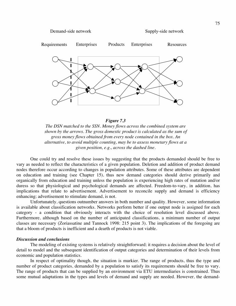
75

One could try and resolve these issues by suggesting that the products demanded should be free to

vary as needed to reflect the characteristics of a given population. Deletion and addition of product demand nodes therefore occur according to changes in population attributes. Some of these attributes are dependent on education and training (see Chapter 15), thus new demand categories should derive primarily and organically from education and training unless the population is experiencing high rates of mutation and/or duress so that physiological and psychological demands are affected. Freedom-to-vary, in addition, has implications that relate to advertisement. Advertisement to reconcile supply and demand is efficiency enhancing; advertisement to stimulate demand, is not.

Unfortunately, questions outnumber answers in both number and quality. However, some information is available about classification networks. Networks perform better if one output node is assigned for each category - a condition that obviously interacts with the choice of resolution level discussed above. Furthermore, although based on the number of anticipated classifications, a minimum number of output classes are necessary (Zoriassatine and Tannock 1998: 215 point 3). The implications of the foregoing are that a bloom of products is inefficient and a dearth of products is not viable.

Discussion and conclusions

The modeling of existing systems is relatively straightforward; it requires a decision about the level of detail to model and the subsequent identification of output categories and determination of their levels from economic and population statistics.

In respect of optimality though, the situation is murkier. The range of products, thus the type and number of product categories, demanded by a population to satisfy its requirements should be free to vary. The range of products that can be supplied by an environment via ETU intermediaries is constrained. Thus some mutual adaptations in the types and levels of demand and supply are needed. However, the demand-

Requirements Enterprises Resources Enterprises Products

Demand-side network Supply-side network

Figure 7.3 The DSN matched to the SSN. Money flows across the combined system are shown by the arrows. The gross domestic product is calculated as the sum of

gross money flows obtained from every node contained in the box. An alternative, to avoid multiple counting, may be to assess monetary flows at a

given position, e.g., across the dashed line.

76 side is, in my view, the leading side. Yet, questions about the optimal number of product categories are hard to answer and the available answers seem to be trite: enough are needed for the system to function but too many categories cause the system to become inefficient.

It is interesting to consider what policies could be pursued to achieve a near-optimal number and level of products. Education and training policies are discussed in Chapter 15. Taxation policies are discussed in Chapter 15 too, but I wish to mention here that a good tax policy may facilitate the formation of a proper number of outputs, thus of product categories. Maddison (2001: 80) points out that the Dutch Republic in the seventeenth century levied high taxes, not on income, but on expenditure. Thus savings, frugality, and hard work were promoted. In my view, due diligence will also be promoted. Taken together, I would expect that such an approach would result in fewer products demanded, those demanded would be necessary and appropriate, and an overall more efficient economy would arise.

Modeling supply output is in some respects reminiscent of calculating the GDP. Considering the GDP in the context of the core system makes one question both its methodology and its purpose. Why is the GDP estimated? The reflexive answer is likely to be that it gives an indication of economic growth and by extension economic health. But why is economic growth needed? This question would hopefully give pause for reflection: the economy has as its sole, ultimate purpose the meeting of population requirements, not the generation of growth. Growth may help with the former, but it is not a given. Therefore, perhaps a better measure of effectiveness is needed and some measure other than the GDP should be defined and estimated to aid in economic stewardship. The definition of wealth as the fraction of requirements that can be satisfied may help to formulate a more meaningful indicator of economic health.

77

8

Refinements at the Local Level

78

Refinements at the Local Level Summary

After determining the number of nodes in a network, addressed in the previous chapters on quantification, further refinements can be made to these nodes and their connections. The connections of a node, the weights of these connections, and the transfer function(s) employed by a node are the local level components of the network. Therefore, when modeling desired network attributes at the local level, important considerations are the number and targets of locally originated connections, their weights, and the extent to which they are or should be constrained. Recurrent connections can be employed to model fixed capital and parallel connections to model joint production. Constraining connection weights can be used to ensure adherence to the physical laws of conservation. Consideration should likewise be given to the selection of proper transfer functions to model the physical and temporal performance of individual nodes. Individual transfer functions can be used to model the output of individual products where joint production occurs. The modeling of innovation and economic development can be included by incorporating time dependencies in transfer functions. All these choices will be influenced, as before, by the objectives – whether to model existing systems or to investigate the general characteristics of economic systems.

79 Introduction

A neural network can be represented both globally and locally. Furthermore, such representation has both structural and computational aspects. At the global level, the structural representation occurs in terms of a network’s architecture: the number of layers, the number of nodes per layer, and the connections between the layers. The computational representation occurs as a sequence of matrix operations (e.g. Schulze and Mariano 2004: 18-5; see also the Appendix to Chapter 1). At the local level, a network is structurally seen as consisting of individual nodes and their transfer functions, as well as connections leading to and connections leading away from each node. Computation is effected locally by the summation of the information arriving along all connections leading to a node. This information is then transformed by the node, by way of a transfer function, before passing the transformed information along via exiting connections.

Because the number of nodes has been addressed in the preceding chapters on quantification, the connective and functional attributes of individual nodes can now be considered and refined as needed. Nodes are inherently dynamic entities whose attributes may change over time. Including such time dependencies in the refinements makes possible the modeling of innovation, growth, and decay. In this chapter, local level refinements of the SSN and DSN are examined.

Local connections

To effect flows between nodes, a connection between them needs to be established. Fully connected layers have been introduced before (Figure A3) and two further modifications will be discussed here. The first deals with connections that permit modeling of fixed capital and the second with connections that apply to instances of joint production.

Flows are often distinguished from funds in production theory (e.g. Kurz and Salvadori 2003: 488) and this distinction appears to be compatible with the connectionist model if flows are mapped to connections and funds to nodes. However, the difference between funds and flows may be merely one of timescales. On long timescales, one is dealing with funds, alternatively, one is dealing with flows. Thus funds are ‘slow’ flows. Because alterations of connectivity will affect flows and connections can be devised for the flows one wishes to model, the preceding view suggests that funds can be modeled with connections.

In some cases it is useful to connect a node with itself. The technical term for such connections is ‘recurrent connections’. Recurrent connections can be used to model flows within a functioning economic concern. In particular, recurrent connections can be used to model funds or fixed capital. Thus, a t-year old tractor could be modeled as a joint output of corn produced by means of a t-1 year old tractor (Kurz and Salvadori 2003: 494). The recurrent connections thus allow longer sojourn times for some inputs. The weight of the recurrent connection determines its ongoing contribution to the output (i.e. wear and tear) while money counterflows determine the associated costs (i.e. depreciation). The extent to which the weights of these recurrent connections are less than unity reflects the extent to which fixed capital wear out and, by implication, their money counterflows will reflect their depreciation. Figure 8.1 shows an ETU in a SSN with two recurrent connections that could model fixed capital (e.g. warehouse, loom) used in the production of textiles. Tapped delay lines can be used to specify whether a weight is turned on or off during a given network updating cycle, thus allow a further refinement to encompass patterns of utilization.

In cases of joint production, distinct products are generated. However, the standard, fully-connected node projects the same output to those downstream nodes that it is connected to. Joint production is equivalent to having multiple parallel connections between two nodes with each connection representing a different product. Figure 8.2 shows parallel connections between nodes to accommodate two distinct products. Every connection has its own individually adjustable weight and every product may be associated with its own transfer function (see further below). Because the concept can be extended to every other node, every instance of joint production can be modeled.

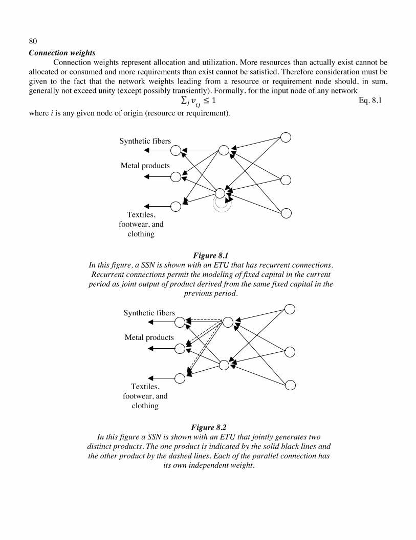
80 Connection weights

Connection weights represent allocation and utilization. More resources than actually exist cannot be allocated or consumed and more requirements than exist cannot be satisfied. Therefore consideration must be given to the fact that the network weights leading from a resource or requirement node should, in sum, generally not exceed unity (except possibly transiently). Formally, for the input node of any network

!" #" ≤ 1 Eq. 8.1 where i is any given node of origin (resource or requirement).

Synthetic fibers

Textiles, footwear, and

clothing

Metal products

Figure 8.1 In this figure, a SSN is shown with an ETU that has recurrent connections. Recurrent connections permit the modeling of fixed capital in the current

period as joint output of product derived from the same fixed capital in the previous period.

Synthetic fibers

Textiles, footwear, and

clothing

Metal products

Figure 8.2 In this figure a SSN is shown with an ETU that jointly generates two

distinct products. The one product is indicated by the solid black lines and the other product by the dashed lines. Each of the parallel connection has

its own independent weight.

81 In the case of a hidden node (i.e. an enterprise) that generates a single product, there would be but a

single efferent connection and its weight also should not exceed unity. In the case of an output node that distributes or purveys a single product, there also would be a single efferent connection and its weight should not exceed unity. Moreover, the sum of afferent connections should not exceed unity. In the more general case where a given enterprise may generate several products, the same consideration should be given to the conservation laws of mass and energy. Thus the modeling of economic networks can be aligned with the physical laws of conservation by invoking realistic constraints on some model parameters.

Money flows are opposite in direction to the flows of goods and services and the same conservation constraints can be applied to monetary flows. Reconciling moneys flowing in with moneys flowing out of an enterprise constitutes a basic form of accounting. Highly effective accounting procedures should furthermore include balancing the flow of goods in and out of an enterprise. In the latter case, one devises a material and energy balance over the enterprise—procedures well-established in some engineering disciplines (Perry and Chilton 1973: 4-23). Any instance of material or energy leaving the node without a compensating monetary flow represents either waste or an illegal activity such as dumping or pollution. Proper accounting procedures should reckon with materials and energy consumed and distributed equally as much as with debits and credits. If accountancy is indeed the basis of financial systems (Gardiner 2006: 22), highly effective accounting procedures must reconcile between and across all of these.

Transfer functions

Transfer functions govern the relationship between inputs and outputs at a local level and they can be used to model the specifics of demand and supply at a more detailed and individual level. In general, the selection of an appropriate transfer function can have a significant effect on a classification network’s performance (e.g. Hush and Horne 1993: 9, 12, 23; Lippmann 1987: 14; Rumelhart et al.: 1988: 48) where its main purpose is to map the linearly non-separable input data space onto a linearly separable space (Mao and Jain 1995), thus increasing the linear independence of the data (Chen 1996: 1222). Specifically, the choice of transfer function affects the complexity of the mapping that can be performed (Lee 1992: 193) and hence the quality of performance (Bakshi and Stephanopoulos 1993). Nevertheless, relatively little is known about the complexity of learning in neural nets with non-linear activation functions (Hush 1999: 1251), making their selection difficult.

When the connectionist concept is applied to economics, it becomes clear that the transfer function for a node specifies the quantity of product as a function of resources consumed. It is the ‘production function’ of economic entities (e.g. Ison 2000: 68) where the quantity of product x is a function of land, labor, and capital and is commonly stated as

( ) ( ) ( )( ) ( ) ( )

( ) ( ) ( )

h h hh h h

h h h

J

J

lp lp lp

J

110

111

11

120

121

12

0 1

...

: :...

!

"

#####

$

%

&&&&&

. The production function is paraphrased below to be consistent with the preceding connectionist terminology, i.e. pjk (product k generated by enterprise j) is a function of land, labor, and capital which collectively constitute the input Qj to enterprise j

!"# = %('()*, '(,-., /(!01(') thus !"# = %('")

where Eq. 8.2 and where, as a reminder, vij is the fractional utilization of resource i (Ri) by enterprise j.

In traditional pattern classification networks, transfer functions are single variable functions, i.e. functions that take as argument the sum of inputs to a node. The reader may realize that two successive functions are in fact used: the first (Eq. 2.1 restated below) is a summation function and the second (e.g. Eq. A1 also restated below) is the transfer or activation function that takes the output of the summation function

Q = f(land, labor, capital)x

82 as argument. In the special case of a linear second function with unity slope, an outcome identical to that of a linear production function is obtained. This is because the summation function in an ANN is already equivalent to a linear production function in an economic entity and the ANN transfer function with unit slope that operates on the output of the summation function will not further alter the output. Regarding the second function, fortunately, the most commonly used non-linear transfer function in ANNs is the sigmoidal transfer function and it is easily recognized as a production function. Thus, the transfer function stated in the appendix to Chapter 1

y = (1 + tanh(10x - 5))/2 Eq. A1 is equivalent to the hyperbolic one-factor production function for technically independent factors (e.g. Beattie and Talor 1985: 71)

y = β0 + β1tanh(β2 - β3x) Eq. 8.3 Nevertheless, in economic networks a greater diversity of transfer functions occurs, consequently they will differ from those used in pattern classification networks. In the majority of cases, the identities of these transfer functions are likely to be unknown, but could be estimated from sufficient data (e.g. Aigner and Chu 1968; Levinsohn and Petrin 2003).

The preceding analysis suggests that the connectionist approach can be refined in at least two respects. First, the summation function can be altered. Recall from an earlier chapter that the total quantity Qj of resources consumed by enterprise j is the sum of all the individual resources consumed by enterprise j, hence the sum of all its inputs qij:

Eq. 2.1 When the summation function is replaced with a product function, for example, something like a Cobb-Douglas function may result. I say “may result”, because the ultimate outcome depends on two serially applied functions, thus the form of the second function will also have an effect and at this point only the first has been considered.

The output from the first function is passed as argument to a second function f, hitherto known as the ‘transfer function’, to give the total volume of product k produced by enterprise j:

!"# = %('") Eq. 8.4 Second, therefore, the transfer function (i.e. the second function in the sequence outlined above) can be altered. One option is to present a collection of functions that will specify a relationship between the output of the previous function and quantities of individual products produced, thus a modification that could improve the modeling of joint production. This approach is sketched out below.

Consider the amount of product pjk obtained as a function of total input quantity Qj. Generally it can be modeled as

Eq. 8.5 where the sn are model functions, the bn their coefficients, and N is the number of model functions used. For example, where the model functions are elements of a power series, one gets

= b0jQj

0 + b1jQj1 + b2jQj

2 + .....+ bNjQjN Eq. 8.6

Let now for any hidden node j producing K products the matrix Q be a Vandermonde matrix of powers of Qj :

83

Eq. 8.7 then

Eq. 8.8 The matrix B of model function coefficients b can now be solved by singular value decomposition (SVD; e.g. Press et al. 1994: 59-70) to yield the coefficients of the power series-modeled transfer functions for each of the K different products generated by enterprise j. Hence knowing the quantities of resources consumed and products generated permits one to estimate the transfer function on a given unit time basis. Note that the shape of the transfer function may drift over time or fluctuate seasonally and that one may wish to take temporal variations into account, an issue addressed below.

The two modifications discussed above may also be of interest in modeling the aggregate production function of neoclassical economics. When doing this, it is necessary to aggregate over the whole SSN instead of over a single individual ETU, thus to use all resources (at the desired resolution) as inputs and all products (at the desired resolution) as outputs. It is not necessarily true that the aggregate function has to be similar to the functional forms being aggregated (see also Mishra 2007: 13). Indeed, the aggregate production function is often represented as

P = Ka1Ra2La3 Eq. 8.9 where the output P is dependent on the stock of capital K, natural resources R and labor L (e.g. Daly 1997: 262). However, empirical data may show that the true functional form, as estimated with Eq. 8.8, does not resemble Eq. 8.9 and that Eq. 8.9 is therefore not the best descriptor of aggregate production.

Node dynamics

Due to the adaptive nature of economic systems, the fluctuations in resource availability, the volatility in requirement levels, and the inherent qualities of nodes, the performance of nodes change over time. These changes are either due to temporally stable inherent nodal attributes that permit the use of input-output relationships to analyze the different stages of production (e.g. Beattie 1985: 13-15) or to inherent nodal attributes that are temporally dynamic. These latter attributes may depend primarily on production functions. Consequently, the time-dependence of production functions should be examined and introduced into the model. Time dependencies may involve changes in the coefficients of the production functions, or, more profoundly, in their functional forms. Two types of change are addressed here: those arising from innovation and those arising from maturation.

Innovation. Technological advances (or losses!) may modify the functional forms of production functions. Innovations, mediated via research and development efforts, can play a big role in economics (Sengupta 2007: 48). Indeed, Schumpeter considered innovation to be a key aspect of economic development (Vaggi and Groenewegen 2003: 266). Production functions can include innovation and thus have implicit time-dependencies as discussed by Mishra (2007: 9). One of these is Sato’s (1975: 1002) production function that attempts to account for innovation by presenting a constant elasticity of substitution production function that incorporates a technical progress factor, T, which is implicitly time-dependent (Mishra 2007: 7). Therefore, the use of similar production functions offer scope for refining the model to include innovation and, by implication, aspects of economic development.

Nevertheless, quantifying innovation presents problems. An approximation could perhaps be made by considering it to be a random process, initially with zero mean and a given standard deviation. Samples drawn from the distribution that are positive represent innovations, while negative ones represent the loss of

84 knowledge or skills. Social factors such as education may induce an elevation in the mean of the distribution. A consideration of the dynamics of, and factors contributing to, the growth of knowledge may be of use here (Schulze 2004b).

Maturation. Time may also enter into node dynamics in a guise different from that presented by innovation. Maturation, such as aging, is one way in which such a different time dependence arises. When establishing an enterprise, there are overheads to set up, resources are being consumed (most likely different ones compared to the ones being consumed under steady state or operating conditions), special taxes are being paid, no product is being supplied. When in steady state, (different compared to start-up) resources are being consumed, ongoing taxes are being paid, and products are being delivered. When being liquidated, resource consumption declines, product delivery declines, special products (i.e. liquidation products) are supplied, and special taxes may be due. Furthermore, entry and exit, thus the birth and death of economic units, are two key aspects of maturation. Maturation and viability are thus closely linked, and, in order to assess viability, accounting is required.

Profits. Considering all the physical and monetary flows to and from a node, in accordance with the material and energy balance approach to accounting mentioned above, and monetizing each of these streams, a profit accrues when the sum of monetary inflows to a node exceeds the sum of monetary outflows from that node, over a given unit of time. Hence all implicit and explicit expenses must be accounted for (e.g. Ison, 2000: 79), including reasonable levels of remuneration (e.g. rents, wages, interest, earnings, etc. as defined in Chapter 4). ‘Reasonable’ may be definable in terms of the long-run stability of the system, that is, everyone must benefit on a sustainable basis. The definition of profit in this work rules out the use of profit in the sense of ‘accounting profit’ and brings its use closer to the concept of ‘supernormal profit’. Note that this usage of ‘profit’ implies that the term ‘profitability’ will have a meaning somewhat different from that commonly intended.

Losses. A loss accrues when the sum of monetary outflows from a node exceeds the sum of monetary inflows to that node, over a given unit of time. Thus one can step methodically through the combinations of inputs, outputs, and production functions to examine their contributions to long term monetary balances.

Market entry and exit. Given, for the sake of simplicity, an economic system where the networks have an optimal number of ETUs or a model of such a system with an optimal number of hidden nodes, one must consider those factors that will permit or induce new ETUs to enter the system or existing ones to exit it. Clearly, if the system is optimal, the entry or exit of ETUs will render it suboptimal. Thus, some changes must occur in order to maintain optimality in response to internal or external events that destabilize the system.

Neurons atrophy if they are starved of nutrients and deprived of stimulation. Metaphorically speaking, economic entities atrophy if they are starved of resources or deprived of demands. A change in resources may cause the exit of an ETU if it no longer has sufficient resources to maintain income neutrality over a long period of time. Incomes will also be impacted negatively if demand drops beyond a certain level. ETUs experiencing sustained inadequate demand will exit the system. In contrast, profit in a system provides an incentive for the creation of new ETUs (or modification of existing, ETUs) along the pathway(s) where such profit arises. Thus population changes, environmental changes, resource discovery, resource depletion, technological changes, legislation, and competitive practices are factors that would affect participation profitability and hence govern the entry and exit of nodes, including those that are not ETUs. Nevertheless, some nodes may cease to exist for reasons that are totally internal and idiosyncratic such as the death of a proprietor.

Because money is the tangible form of requirements (see Chapter 12), that is, of demands, the development of profit across a node means that more demands are being made on that node than it makes in its turn on the remainder of the system. Where a loss occurs, it means that a node makes greater demands on the system than the system makes on it. If few demands are made by the system on a given node, it is

85 superfluous and should be eliminated; if it furthermore makes demands on the system, it is a liability. Note that in a system in equilibrium the demands made on the node should be balanced by the demands made by the node. The balancing of demands made by and on a node can be assessed and monitored in monetary terms.

Profits and losses are therefore indicators of stresses in the system. Fortunately, in truly organic form, these stresses are potentially self-correcting. Profits represent a ready source of capital that accrues at a node, thus demand stresses cause liquidity to arise locally. Funds are therefore available for investments in a demand-stressed node to expand its production capacity or efficiency. Likewise, supply stresses cause liquidity to diminish locally and losses should eventually lead to cessation of nodal functioning, nodal elimination, and supply reduction.

This organic self-maintaining capability can be lost. Normally, there exists at the local level a tight coupling between profits and losses and associated relevant information. This coupling between monetary balances and information is lost when profits or losses are distributed distally independently from the associated information. If the profits are not reinvested in local expansion, but made generally available through higher wages, higher dividends, deposits at intermediaries, and so on, the probability arises that such excess funds, that now constitute capital, could be invested in the creation of another node in parallel with the demand-stressed one. This would mean competition and may occur on a scale that is not well-calibrated relative to the original stresses; consequently, an inadequate reduction in demand stress and/or the generation of supply stress can occur. With distal distribution, the even greater probability arises that such excess funds could be allocated to meet requirements other than those related to the condition of stress, hence constituting an even more detrimental malinvestment. Not reinvesting in the stressed nodes to alleviate their stresses therefore entails the creation of risk and additional stresses through inappropriate market entry and/or exit.

Innovation and maturation changes can also run together. For example, a similar situation to start-up occurs when new technologies are implemented: some conversion expenses may be incurred; some temporary disruption of production may occur; some temporary changes in resource utilization may take place; but most importantly, the way in which resources are being converted into products changes, i.e. the transfer function(s) of a given node changes. This is partly congruent with Schumpeter’s contention that the introduction of a new method of production leads to a shift in the production function, rather than movement along it (Vaggi and Groenewegen 2002: 267). It is perhaps, however, stronger because it states that the functional form of the production function itself could potentially change. Due to maturation, therefore, the stages of production will, in general, differ for each of the maturation phases of a node. Detailed analyses of internal economies relating to the growth and life cycle of the firm have been provided, for example, by Marshall (Vaggi and Groenewegen 2002: 233). In the context of connectionist economics, generalized maturation or node dynamics can be represented as:

Eq. 8.10

where, as before, pjk is the total volume of product k produced by enterprise j from the input Qj it receives during the periods demarcated by the subscripted times ti when the production functions fi are operational. Discussion and conclusions

The local refinement of networks can proceed by alterations in connectivity, by imposing limits on the connection weights, and by selecting suitable transfer functions. Furthermore, time dependencies can be

86 incorporated in the alterations. Refinements therefore entail a number of practical and conceptual implications, some of which I address below.

Connections represent flows between nodes while nodes themselves represent sinks or sources. The connections formed between a node and its upstream neighbors indicate the origins of its inputs. Their weights are the fractional volumes of the inputs consumed in the production process. Connection weights therefore pertain to allocative efficiency and the sum of the weights of connections emanating from a node pertain utilization efficiency (e.g. Eq. 6.5). The transfer function, in contrast, indicates how the output from a node (i.e. source) varies as a function of the allocated inputs. Thus the attributes of transfer functions should reflect technical efficiencies. Furthermore, because both flows and funds can be modeled with connections, it appears that the distinction between them is a minor one pertaining to aspects of connectivity, while a more significant distinction occurs between processes of transformation (nodes) and processes of distribution (connections). Because of the distinction between nodes and connections (e.g. Chapter 1, Appendix), allocative and technical efficiencies are separable in the connectionist model. Therefore, one could, for a given selection of transfer functions (e.g. one for every joint product of a node), optimize the connections and their weights, thus examine allocative efficiencies. Likewise, for a given set of nodal connections and weights, one could optimize its transfer functions and thus examine technical efficiencies.

Connectionist modeling can also be applied in a manner that is commensurate with the conservation laws of physics. Where the network is used to represent the flows of goods, for example, the sum of the weights of all the connections emanating from a given node, and with regard to a single product, should not exceed unity. A weight (or sum of weights) exceeding unity implies that additional goods are created by the connection. In addition, the flow of mass and energy across a node should balance. Because something different (e.g. raw material) enters the node than that (products) leaving it, an accounting process must be applied at the more fundamental level of matter (i.e. mass and energy) by performing a mass and energy balance across a node. In my view, the laws of conservation tie directly into the matter of accounting. Proper accounting practices therefore should be applied simultaneously to flows of materials and flows of funds. Although they can be accounted for independently, appropriate accounting should establish strong correlations or mappings between funds and materials throughout every stage of production to ensure that the transformation processes and their distribution outcomes are transparent. Errors of neglect that often plague economic discourse (e.g. Daly 1997: 261; Kurz and Salvadori 2003: 489; Mayumi et al. 1998: 115) could be mitigated with application of the connectionist model because of its ability to make processes of distribution and transformation very explicit.

Connectivity modifications can be used to model joint production and the modeling can be refined further with implementing individual production functions. Additionally, technological changes can be accounted for by incorporating time dependencies in the connections via delay lines and in the production functions via time-dependent trends or changes in functional form. Thus, the core system can be modified from a Walrasian-like system, where the dynamics are dynamics of equilibration, to a more Schumpeterian-like system that incorporates developmental dynamics, hence making the core system a system of compound dynamics. Consequently, the modifications introduced in this chapter allow more accurate temporal and structural modeling.

On a further note of interest, some aspects of the Cambridge controversies (e.g. Daly 1997; Kurz and Salvadori 2003) may be shown in a different perspective by neural networks. Neural networks do combine incommensurable components, that is, inputs from different connections are combined in downstream nodes. For example, Karim and coworkers (1997: 6) trained a neural network to predict bioreactor state variables such as biomass, ethanol, and glucose concentrations (output, i.e. ‘products’) from on-line measured variables such as temperature, carbon dioxide concentration, optical density, and redox potential (input, i.e. ‘resources’). Here, temperature, carbon dioxide concentration, optical density, and redox potential have different units of measurement and they are added at the hidden nodes which should be problematic. I am not

87 aware of aggregation of neural network inputs, in the neoclassical aggregate production function sense (e.g. Daly 1997), in an attempt to reduce the dimensionality of the input data set. Typically, other methods, such as principal component analysis, are used to select the most informative subset of data. Nevertheless, in neural nets, inputs are summed at the hidden node(s) before processing with a transfer function. Although this summation occurs after multiplication with connection weights (i.e., after weighting), it still amounts to an aggregation of disparate entities.

Traditionally, neural networks have been used as pattern classifiers or as function estimators and aggregation of inputs needs to be seen in this context. Conceptually, the network performs a classification based on an input pattern or performs an association between input and output patterns (McClelland et al. 1986: 33). Therefore, if the data are viewed as patterns of relative amounts of physical entities or variables, then the inputs to the network consist of patterns (of information). The outputs are also patterns and they reflect responses to the input patterns. I prefer to think of the process as one of transforming an input pattern into an output pattern. This view lends itself better to the modeling of economic systems since it makes more intuitive sense to consider an economy as one where inputs (resources) are transformed into outputs (products) as opposed to one where inputs are associated with outputs. Furthermore, scaling or normalization of the input data is generally advised (Sumpter and Noid 196: 237; Zoriassatine and Tannock 1998: 216), rendering them dimensionless. Consequently, diverse inputs to production functions, in terms of the present conceptualization of economic systems, ought to be no more problematic than diverse inputs to the transfer functions of ANNs.

The modeling of node dynamics in this chapter lead to the definitions of profits and losses. Profits and losses are not exclusive of remuneration, that is, they fully account for remuneration (wages, rent, interest, rewards, etc.). Thus the various types of remuneration become consolidated with price as Steuart (Vaggi and Groenewegen 2003: 152) thought to be appropriate (except that ‘profit’ as used by Steuart has been relabeled ‘reward’ here).

A more important consequence of the present view of profits and losses is that they represented stresses – at the node where the profits or losses occur, specifically, and in the system more generally. Furthermore, increased volumes are likely to be the first signals of stress in the system. Consequently, profits arise first from increased volumes, then from increased prices. In this respect, they resemble Turgot’s (Vaggi and Groenewegen 2003: 95) secondary profits (due to higher volumes) and primary profits (due to higher prices) to some extent. Even if profits arise from technical innovations, they still could reflect demand-stresses. For example, consider a node of interest in a system originally at equilibrium. Due to an innovation money outflows are reduced and a profit arises. Because requirements are in principle infinite and in practice depend on the degree to which cultures and their members have wants and aspirations, the latter are in general not completely satisfied. There would consequently be a continuous driving force to allocate funds to these requirements, and any avenue that would permit existing requirements to be met at lower cost would result in the reallocation of funds to those still unmet requirements. Put differently, in cultures where higher-order requirements are feeble, profits may occur rarely, be smaller, and be of little interest. Thus, profits occurring in response to innovation still represent stresses in the system , but stresses that are now actionable.

The view of profits and losses portrayed here is an impersonal view and reflects system dynamics. The dynamic consequences of profits and losses mean that they are, de facto, transient. It aligns with Schumpeter’s characterization of profits as temporary phenomena that are competed away (Vaggi and Groenewegen 2003: 268). Taken together, the implication is that attempts to manipulate the system to generate profits stress the system and, where technical innovation-related profits persist, they also prevent the resolution of higher-order systemic stresses. Clearly, approaches to induce perpetual profits are not in the collective interest.

88 An interesting question now arises regarding the best way to dispose of profits. Hoarding (i.e. no

reinvestment) would mean that some requirements will change status from being met to being unmet. Where needs are involved, this could have serious consequences. Where other requirements are involved, it would have serious consequences if reproduction is adversely affected such that population levels decline. Alternatively, where profits are generated and reinvested to such an extent that requirements are satisfied to an excessive and frivolous degree, it could be disadvantageous by degrading the environment. This would lead to resource depletion and collapse, hence essential requirements may now not be satisfied and consequences will be equally deleterious. The optimal economic system must be one where a careful and sustained balance can be maintained between requirements and resources.

89

9 Refinements at the Global Level

90

Refinements at the Global Level Summary

In addition to making refinements at the local level, they can also be made at the global level. The global level components of a network are network layers and their connections. Global refinements can be implemented by altering the number of layers in a network, by partitioning of layers, and by modification or augmentation of the connections between layers. Increasing the number of layers in a network means that more processing stages are being accommodated, thus, an economy with greater depth can be modeled. Partitioning of layers permits the grouping of like nodes, for example, to reflect specific industries or stratified populations. Direct connections can be used to model the distribution of products from earlier stages of production to entities engaged in later stages of production. Reentrant connections are useful to model the distribution of output from later stages of production back to entities involved earlier stages of production. Finally, lateral connections can be used to model interactions between entities in the same industry.

91 Introduction

Neural networks are represented globally in terms of their architectures: the number of layers, the number of nodes per layer, and the connections between the layers. In contrast to the local level, where the attributes of individual nodes are considered, the global view is predominantly a consideration of supra-nodal or layer attributes. Therefore, refinements of the SSN and DSN at the global level will involve modifications of network architecture. The number of nodes per layer has been addressed previously (Chapters 5-7) in the context of quantification. Presently, the focus will be on the number of layers, the partitioning of layers, and interlayer connections.

Number of layers

Traditionally a backpropagation network has only three layers - input, hidden, and output layers (e.g. Hush and Horne 1993: 11). In the engineering literature, the input layer is considered to be simply an input buffer and the network is viewed as a two-layer network (Hush and Horne 1993: 10, 11; Lippmann 1987: 16). Although multiple hidden layers can be used and often permit improved performance, it has been shown that the same performance can be obtained with a single hidden layer but with more nodes added to the hidden layer (e.g. Hush and Horne 1993: 11).

In the present context, the number of hidden layers added to a network depends on whether one wants to model a real economy or whether one wants to analyze different models from a theoretical perspective. In the former case, one needs to add as many hidden layers as there are aggregate markets in an economy because an “aggregate market” was defined in Chapter 4 as the interface between two layers. Alternatively, one could consider a layer a representing a processing stage. Thus, more layers could be used to model an economy with greater depth, i.e. one with more highly processed or advanced products. In the latter case, one may wish to consider the effects of multiple markets on economic resilience and flexibility, efficiency, price, profit, innovation, and a host of other factors by examining the performance of systems with different numbers of hidden layers compared to systems with single, but larger, hidden layers.

Regardless of how layers are viewed, adding more layers to a network is not, in principle, problematic. More computations will be required and the time lag between input an output will be increased, but otherwise the considerations are the level of detail that one wishes to model and whether the model is intended for empirical or theoretical purposes.

Partitioning of layers

The reader may have inferred from an earlier chapter (Chapter 5) on the quantification of resources and requirements that these inputs could be partitioned to reflect similar groupings. For example, the layer of resources could be partitioned into renewable and non-renewable resources, each potentially with its land, labor, and capital subdivisions; the layer of enterprises could be partitioned to group manufacturers by industry; and the output layer could be partitioned to group products as durable or consumer goods.

Similar considerations apply to the DSN. Of particular interest is the partitioning of demand-side inputs to reflect the differential contributions of different social strata to requirements. Here, a layer could be partitioned, for example, into the customary three social strata of the upper, lower, and middle classes. Each stratum will have needs, wants, and aspirations, but the relative proportions of these requirements to one another will be unique for each stratum. Moreover, each stratum’s contribution to requirements in the aggregate may differ. For example, all three strata are likely to have similar levels of needs when population adjusted, but very dissimilar levels of other requirements. Thus it is likely that, overall, the upper class is responsible for the bulk of requirements and hence demand-related money flows.

The ability to incorporate social stratification into the economic theory provides and important link to other social sciences and to social theory. This link complements the links established via requirements to physiology and psychology. Taken together, they emphasize that the source of economic activity derives

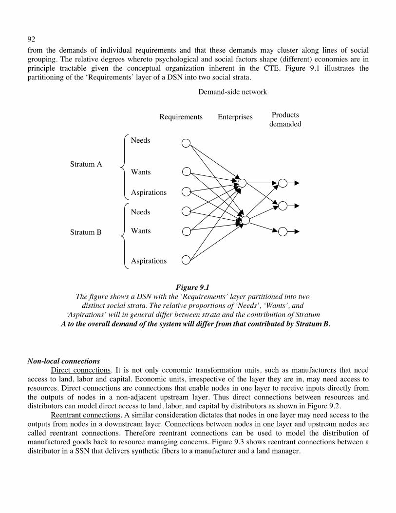
92 from the demands of individual requirements and that these demands may cluster along lines of social grouping. The relative degrees whereto psychological and social factors shape (different) economies are in principle tractable given the conceptual organization inherent in the CTE. Figure 9.1 illustrates the partitioning of the ‘Requirements’ layer of a DSN into two social strata.

Non-local connections Direct connections. It is not only economic transformation units, such as manufacturers that need

access to land, labor and capital. Economic units, irrespective of the layer they are in, may need access to resources. Direct connections are connections that enable nodes in one layer to receive inputs directly from the outputs of nodes in a non-adjacent upstream layer. Thus direct connections between resources and distributors can model direct access to land, labor, and capital by distributors as shown in Figure 9.2.

Reentrant connections. A similar consideration dictates that nodes in one layer may need access to the outputs from nodes in a downstream layer. Connections between nodes in one layer and upstream nodes are called reentrant connections. Therefore reentrant connections can be used to model the distribution of manufactured goods back to resource managing concerns. Figure 9.3 shows reentrant connections between a distributor in a SSN that delivers synthetic fibers to a manufacturer and a land manager.

Figure 9.1 The figure shows a DSN with the ‘Requirements’ layer partitioned into two

distinct social strata. The relative proportions of ‘Needs’, ‘Wants’, and ‘Aspirations’ will in general differ between strata and the contribution of Stratum

Requirements Enterprises Products demanded

Demand-side network

Needs

Wants

Aspirations

Needs

Wants

Aspirations

Stratum A

Stratum B

A to the overall demand of the system will differ from that contributed by Stratum B.

93

Lateral connections. In neural networks, competition and support are often modeled by inhibitory and

excitatory lateral connections, respectively (e.g. Levine 2000: 96). Lateral inhibition occurs where a node in a given layer inhibits other nodes in the same layer via inhibitory lateral connections. Thus, if a node is strongly activated, it could depress activation in neighboring nodes via inhibitory lateral connections; this can be viewed as an anticompetitive practice that sharpens the contrast between the successfully activated node and its neighbors. In the visual system, lateral inhibition gives rise to the Mach effect. The Mach effect can be noticed when uniformly tinted bands of different tones of the same color are juxtaposed to one another. Each band will appear to have edges of varying tone: for a given band, the tone appears lighter on the inside edge of the same band where it borders the band with the darker tone when in fact there is no difference.

In addition to direct and reentrant connections, lateral connections can be established to represent interactions between adjacent and non-adjacent nodes in the same layer. Thus, inhibitory lateral connections have the potential to model restrictive competitive practices such as patenting and copyrighting, for example. However, I will use lateral connections here in the normal (or excitatory) sense exclusively used so far. Other restrictive competitive practices such as exclusive arrangements with suppliers or merchants and preferential treatments are better modeled with normal, non-inhibitory connections. This can be done by fixing to zero or capping the weights of connections to non-preferred partners, respectively (more below). Reciprocal lateral connections between adjacent nodes are shown in Figure 9.4, however, lateral connections can be non-reciprocal and connect non-adjacent nodes.

Variable connections: monopolies and competition

The term “fully-connected network” is used to denote a network where every node in one layer is connected to every node in the next (i.e. downstream) layer. The modifications discussed in the preceding chapters show that network connectivity can be even further increased by parallel connections, recurrent

Land

Labor

Capital

Synthetic fibers

Textiles, footwear, and

clothing

Metal products

Figure 9.2 The figure shows a SSN with a node that has direct connections which enable it to receive inputs directly from the outputs of nodes in a non-adjacent upstream layer. Thus direct connections between resources and distributors can model

direct access to land, labor, and capital by distributors as shown.

Resources Enterprises Products supplied

Supply-side network

94 connections, direct connections, reentrant connections, and lateral connections. A high degree of connectivity generally means that a network can operate with minimal deterioration in performance when a single node in the network or a single connection in the network becomes dysfunctional, a phenomenon termed “graceful degradation” in the literature (McClelland et al. 1986: 29). In other words, extensive connections provide some robustness to the network.

Under normal circumstances some pruning or effective pruning of connections may occur simply

because some enterprises may not make use of some resources or some consumers may not avail themselves of some products. For example, health services enterprises may not have a direct need for forest lands, consequently no connection between the two is formed, but the freedom to develop such connections must remain. Likewise, connections become established if sufficient exchange pressures arise. For example, increased demand is likely to produce demand inflation, increased profits, and eventually increased capacity via the reinvestment of profits as explained previously. Thus, without manipulation, connections can vary according to need.

Nevertheless, when it happens that a given product or type of resource can only be traced through a single node, a sole supplier exists. If provenance of a resource or product can be traced to more than one node, some degree of market competition exists. Where a sole supplier also manipulates connections or nodes in order to attain or protect its status as sole supplier, a monopoly comes into existence. Numerous connections, free to form and with variable weights, will facilitate competition while limited connections and fixed weights may restrict it. Hence, one may come to the view that legislation should make any reasonable demand on a node legal. Differential access, e.g. exclusive product distribution, limits on product volume, and temporal constraints on product availability, should be discouraged or prohibited.

Figure 9.3 A SSN where recurrent connections exist from the output layer back to product

upstream layers is shown in the figure. Reentrant connections permit the modeling of situations where final products are supplied back to economic

entities involved in earlier stages of production.

Synthetic fibers

Textiles, footwear, and

clothing

Metal products

Land

Labor

Capital

Resources Enterprises Products supplied

Supply-side network

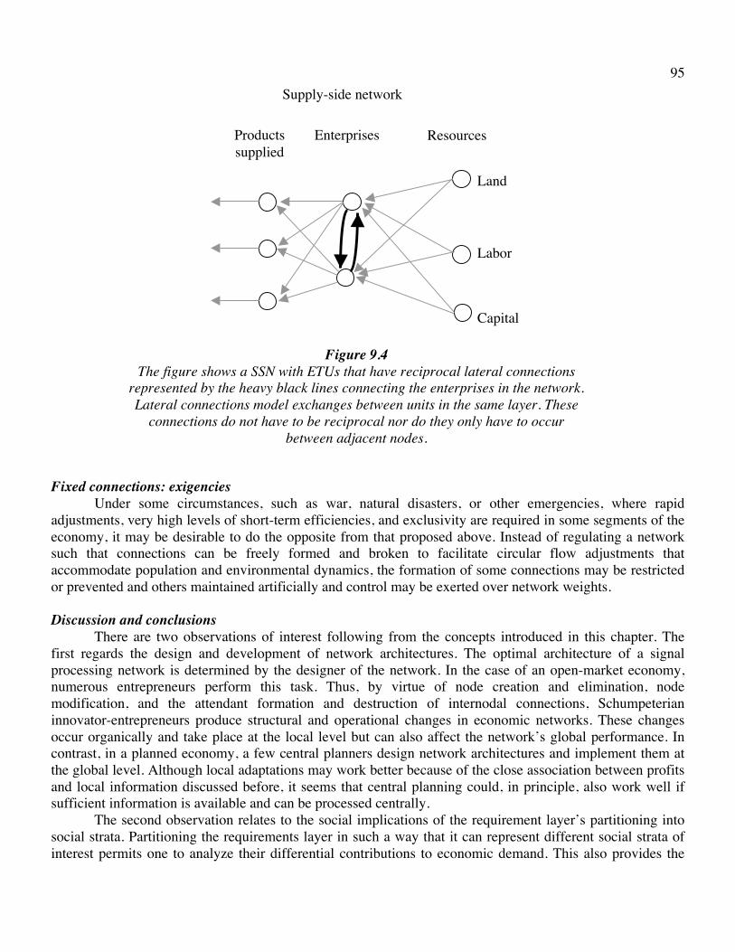
95

Fixed connections: exigencies

Under some circumstances, such as war, natural disasters, or other emergencies, where rapid adjustments, very high levels of short-term efficiencies, and exclusivity are required in some segments of the economy, it may be desirable to do the opposite from that proposed above. Instead of regulating a network such that connections can be freely formed and broken to facilitate circular flow adjustments that accommodate population and environmental dynamics, the formation of some connections may be restricted or prevented and others maintained artificially and control may be exerted over network weights.

Discussion and conclusions

There are two observations of interest following from the concepts introduced in this chapter. The first regards the design and development of network architectures. The optimal architecture of a signal processing network is determined by the designer of the network. In the case of an open-market economy, numerous entrepreneurs perform this task. Thus, by virtue of node creation and elimination, node modification, and the attendant formation and destruction of internodal connections, Schumpeterian innovator-entrepreneurs produce structural and operational changes in economic networks. These changes occur organically and take place at the local level but can also affect the network’s global performance. In contrast, in a planned economy, a few central planners design network architectures and implement them at the global level. Although local adaptations may work better because of the close association between profits and local information discussed before, it seems that central planning could, in principle, also work well if sufficient information is available and can be processed centrally.

The second observation relates to the social implications of the requirement layer’s partitioning into social strata. Partitioning the requirements layer in such a way that it can represent different social strata of interest permits one to analyze their differential contributions to economic demand. This also provides the

Figure 9.4 The figure shows a SSN with ETUs that have reciprocal lateral connections

represented by the heavy black lines connecting the enterprises in the network. Lateral connections model exchanges between units in the same layer. These

connections do not have to be reciprocal nor do they only have to occur between adjacent nodes.

Resources Enterprises Products supplied

Supply-side network

Land

Labor

Capital

96 potential to asses the extent to which the requirements of different groups are being satisfied in a given economic system. Therefore, if the requirements for different strata can be quantified, along with their degrees of satisfaction, an idea can be formed about which groups are deprived of satisfaction and which requirements are not being satisfied. Such analyses may prove informative for the creation and operation of public systems if the latter are, at least in part, meant to address questions of inequity.

97

Expansions

98

10

The Public Economy and Government

99

The Public Economy and Government Summary

The existence of a government introduces a public component into the economy. Because this public component can include public resources as well as public requirements, the public component can form an entirely parallel economic system that deals with itself when it uses public resources to satisfy public requirements. It is therefore possible to model the public component with a public core system in parallel to the private core system. The public and private systems, often termed public and private sectors of the economy, respectively, generally interact. These interactions can be represented with connections between the two systems. In the private sector, money and product flows are always roughly in balance, but exchanges between public and private sectors often mean that money is garnered (taxation) from sources whereto products are not supplied while products (infrastructure, social services, etc.) can be supplied to recipients from whom money is not collected. This redistribution of resources by the public system can be seen, in the abstract, as a means to promote the potential of the social entity, while the private system functions to promote its efficiency. Redistribution will affect economic growth and redistribution efficiency depends on whether the mode of redistribution is governed by criteria arising from needs, wants, or aspirations.

100 Introduction

Although the existence of public economics and the government’s role therein has been addressed explicitly at least since the appearance of Smith’s The Wealth of Nations in 1776, a significant problem that remains for the social sciences is how institutions, given their importance, arise without a common purpose (Seckler 1975: 80). A common purpose, however, may not be anymore preexisting than it is preexisting for the division of labor. Natural conditions provide the driving forces for these specialization processes and when, in due course, they are discerned, they can be exploited, refined, or imitated. The partitioning of the demand-side input layer to reflect the requirements of different economic strata, introduced previously (Chapter 9), suggests that a gradual separation of an existing economic system can occur. This separation may lead to, or be accompanied with, increased specialization, resulting in a ‘speciation’ event. The speciation process eventually facilitates the recognition of institutions and parallel economies.

Regardless of how governments develop, however, they are recognized as important actors in the economic theater and any credible modeling effort will require their incorporation. Fortunately, this digression about the partitioning of a network also has the benefit of suggesting that a government or public economy can be modeled with a fully partitioned core system, like the core system described in Chapter 4, and in parallel with it. The earlier core system then comes to represent a private economy. How, from the entire base of available resources and requirements to all economies, the partitioning of resources and requirements into public and private domains occurs, or should occur, falls outside the immediate scope of the present discussion, but I admit its intriguing nature.

The newly-created parallel core system is not a duplicate private economy, although it can conceivably become such given adequate pressures, but it is a system that serves to meet a different purpose and hence may have structural and operational differences from that of a private system. In the present chapter, I will therefore introduce and develop a parallel core system to represent a public economy and proceed to describe the structure and attributes of the public economy. Although non-governmental public systems may exist, I shall for the present use ‘public system’, ‘government’, and ‘state’ (in an economic sense) somewhat interchangeably.

Once a model that includes both public and private sectors and interfaces between them is created, considerations about the optimal purposes and designs of the model components, and how to construct the best interface between them, arise. At this point the role of the state, types of states and governments, welfare economics and Pareto efficiency, and government finances are some of the issues that may gain tractability from a model with both visual and quantitative attributes.

Government: supply-side

The creation of a parallel core system implies that both a supply side and a demand side exists, each with its input, hidden, and output layers. Like the private system, the public system uses resources such as land, labor, and capital. Where public systems exist, resources often have a public character and public resource categories can be recognized in such things as national parks, state lands, military areas, military personnel, public service personnel, government buildings, infrastructure, and military equipment. Public resources are often utilized by government. Government departments are the counterparts to private enterprises and are the ETUs of the public supply-side economy. The goods and services that a government provides are the outputs of the public supply-side system. For example, Smith ascribed to government a number of tasks (Vaggi and Groenewegen 2003: 114) loosely characterizable as defense, justice, and education. Thus government departments provide goods such as infrastructure, services such as defense, health care, education, and justice, and consumables such as passports, permits, and other documents. These outputs are often made available through dedicated outlets and are consumed by either the private economy or by other government entities as described for the demand side below.

101 Resources in the public economy are collective resources from the point of view of the citizenry,

rather than an aggregate of individually owned or exploited resources as in the private system. At least in principle then, everyone should have equal access to, or an equal stake in, public resources. In practice, public economy components (e.g. government departments) may have preferred or exclusive access, and, in some instances, public resources may also be accessible directly to components of the private economy. Nevertheless, access to public resources is normally thought to be to the benefit of all citizens in contrast to the private system where a strong sense of equitability is not present.

In the public system, money flows may also be fundamentally different from those in the private economy. Specifically, money flows are less tightly coupled to the flow of products supplied than they are in the private sector. Money streams are generally composed of user fees and taxes. Except in the case of user fees, there is not necessarily a match or balance between the goods and services delivered along a given connection and the money stream along that same connection. Thus, seen from the supply side, government effects a redistribution of resources and these resources are not necessarily public resources. This may be especially clear in the case of welfare. Pigou, for example, argued that revenues obtained from taxing the affluent should be spend on goods and services that primarily aided the poor, but without reducing the national dividend (Vaggi and Groenewegen 2003: 275). The reader will realize that the mismatch between goods and monetary flows and the redistribution of resources create a rather peculiar situation vulnerable to problems of accounting and thus accountability.

Government: demand-side

It is often clear that government manages and spends large sums of money. Government spending constitutes public demand. Like resources, there is an implicit partitioning of the entire base of requirements into public and private domains. For example, health care requirements could be private or public requirements. Spending originating from other sources such as education, social services, the military and so on, also reflect, at least partly, public requirements. In some cases, requirements are not related directly to the citizenry and are clearly government requirements, the military being an example. Requirements that are exclusive to the government form the input nodes of the public demand side; these requirements still consist of needs, wants, and aspirations. Hidden nodes in the public sector represent those government agencies most directly involved in providing services or goods, thus taking delivery of the outputs of the supply-side and to some degree, shaping the nature of public sector demands.

The military comes perhaps the closest to exemplifying the parallel nature of the public economy. Here public resources may be used by government corporations and departments to produce goods and services such as weaponry, transportation, and food to the military. This is the supply side. These goods and services in turn are delivered to specific branches of and units within the military from where they proceed as ordnance to individual military personnel or as materiel to units of personnel such as tank crews. This reflects the demand side. Stated this way, the parallel system appears rather independent or isolated from the private system. In practice, unless resources are partitioned such that those ending up in the public domain are fully equal to and can be made to meet public requirements, some cross-talk between public and private systems will be necessary. Broadly speaking, cross-talk between public and private systems will permit compensation for shortfalls on either demand or supply side. The integration between public and private systems is discussed further below.

Interactions between public and private systems

As pointed out above, the private and public sectors are generally not completely non-interacting parallel economic systems. Some mutual tapping of resources by the different systems occur as well as the cross-delivery of economic products—goods and services—from one system to the other. This may occur

102 irrespective of whether public-private cross-talk is necessary due to unbalanced requirement and resource partitioning.

Integration between private and public systems on the supply side can occur in a number of ways. Symmetry considerations suggest that cross-talk can occur between public and private system supply sides, between public and private system demand sides, between the supply side of one system and the demand side of the other system and vice versa. The reader keeping count will realize that there are four major routes of integration possible between the two systems. Not all the routes may be used to the same extent and their relative use may also fluctuate over time reflecting changing economic necessities and reigning philosophies. Full integration would mean that every node of one layer of one system is fully connected to every node of the next layer in the other system. In the case of full integration, it will nevertheless still hold true that public system nodes and public system connections may function differently from their private system counterparts. Specifically, production functions and monetary/product flow relationships may be quite different between public and private sectors.

Supply side-supply side integration may occur, for example, when entities such as government departments utilize resources from the private sector such as renting office space. Likewise, private enterprises can have legal access to public resources such as exploration, mining, or logging on public lands. Demand side integration occurs when some government agencies, instead of providing services to members of the government or to government units such as the military, provide services to members of the citizenry eligible for these services; the term ‘entitlement’ comes to mind. Integration can also occur when public requirements are satisfied by obtaining needed goods and services from the private sector, a process known as ‘outsourcing’.

Cross-talk between the supply side of one system and the demand side of the other system occurs when products generated by the private sector are acquired by the public sector and vice versa. For example, automobiles identical to those available in the private sector may be acquired by government agencies for their own use. Outputs from government departments, that is, wholesale goods produced by the government, could also be acquired by the private sector. This is perhaps unusual but may occur when surplus military or other equipment are auctioned off or made available to the private sector.

Finally, note that an indirect and transient integration may occur between public and private systems through an exchange of nodes. This exchange is termed ‘privatization’ when a government department changes its position from the public to the private sector and ‘nationalization’ when a private enterprise changes ambit to the public sector.

The parallel economic systems of the public and private sectors are shown in Figure 10.1 along with some illustrative integration pathways between the two systems.

Taxes

Where government makes demands on the private sector, money flows are usually commensurate with the flows of goods and services. However, where the private sector makes demands on the government, money flows are not necessarily commensurate with the delivery of goods and services in a direct fashion. This is because the delivery of goods (such as infrastructure) and services (such as social services) are paid for from taxation. Resources are often taxed specifically: taxes on land (e.g. property taxes); taxes on labor (e.g. income taxes); and taxes on capital (e.g. capital gains taxes). On the other side, requirements too can be taxed via consumption taxes such as sales or value added taxes. Remittance of taxes is shown conceptually and in simplified form in Figure 10.2. Note that only monetary flows occur across the connections, thus indicating the remittance of taxes; the goods and services procured with taxes typically flow along other connections.

103

come from those receiving the education, and if they do, may do so in a delayed and/or incommensurate fashion.

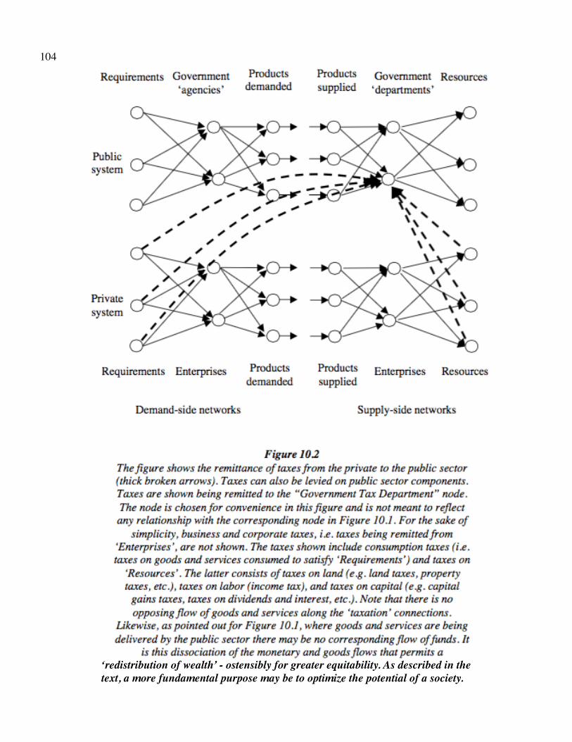
104

‘redistribution of wealth’ - ostensibly for greater equitability. As described in the text, a more fundamental purpose may be to optimize the potential of a society.

105 A primary reason d’etre of the public system may be precisely to generate a mismatch between

monetary flows and flows of goods and services. Otherwise, why duplicate the private system? In the public system, goods and services are often delivered to those who do not deserve them in terms of private sector criteria (otherwise they would be paid for in full).

Seen from an idealistic perspective, it appears that the public system exists to maintain a potential while the private system responds to actualities. During times of stability and success, it may be important to build up stores of potential; in times of distress, it may be beneficial to conserve resources. The public system therefore supplies or functions to maintain the range of options from which competitors in the private system can emerge. If the environment were to change, those that were efficient formerly may no longer be so. If the public system fulfilled its function of nurturing and maintaining a reservoir of potentialities, new competitors, that are more efficient under the changed circumstances, may emerge from this reservoir. Those that win in competition are the more efficient agents in a given environment. Hence the private sector is more closely associated with economic efficiency while the public system is more likely to be associated with economic inefficiency. On the other hand, the public system may be more efficient in maintaining potential than the private system.

Education is an example of this process: not everyone goes on to make extensive use of calculus, but if everyone gets a solid schooling, a larger reservoir exists from which engineers could emerge, and emerge more quickly, if the need should arise.

Regulation

In addition to the hotly-debated role of the state as a participant in the economy, whether as competitor for wealth or redistributor of wealth, it is widely accepted that a state can, does, and perhaps should play a role as regulator of private sector activity (e.g. Mookherjee 2003: 140). Wherever regulation occurs, another form of interaction between public and private economies takes place. Given the importance of the regulatory function of the state, it is quite reasonable to ask whether it can be modeled.

The answer is that at least some regulatory functions can be modeled and that depends on the regulations at issue. Where exchanges between nodes are forbidden, connections between said nodes should have fixed weights, i.e. weights that do not adjust during the training process (e.g. Rumelhart et al. 1988: 327), and the weights should be set to zero. Environmental regulations may require that different production processes be used, thus the choice of transfer or production function will be limited or proscribed. The size of a node may be regulated such that the total volume of its consumption of raw materials or its share of market supply may not exceed a fixed value or a proportion of industrial sector inputs or outputs, thus limits should be placed on the aggregate values of flows to and/or from a node.

Because regulations impose limits and restrictions, they represent opportunity costs in the sense that some opportunities are made unavailable. Regulations can also have direct monetary costs. For example, building regulations may require foundations and insulation that increase capital costs, while other regulations may impose operating costs. Where the regulations impact operating costs in the nature of fees and duties remitted to government entities, they can be modeled along the lines of Figure 10.2. Where they impact operating costs in the nature of sunk expenses instead, a threshold is effectively created. These thresholds have to be overcome to avoid operating losses. A bias node is used to model thresholds in ANNs (e.g. Hush and Horne 1993: 9) and can be used to model the monetary effects of regulations as shown in Figure 10.3. A bias can be thought of as a monetary sink in the sense that very few goods and services meaningful to a concern may be received in return, or as a threshold in the sense that expenditures have to be increased and/or incomes reduced before profitability (in the sense of common usage) becomes possible.

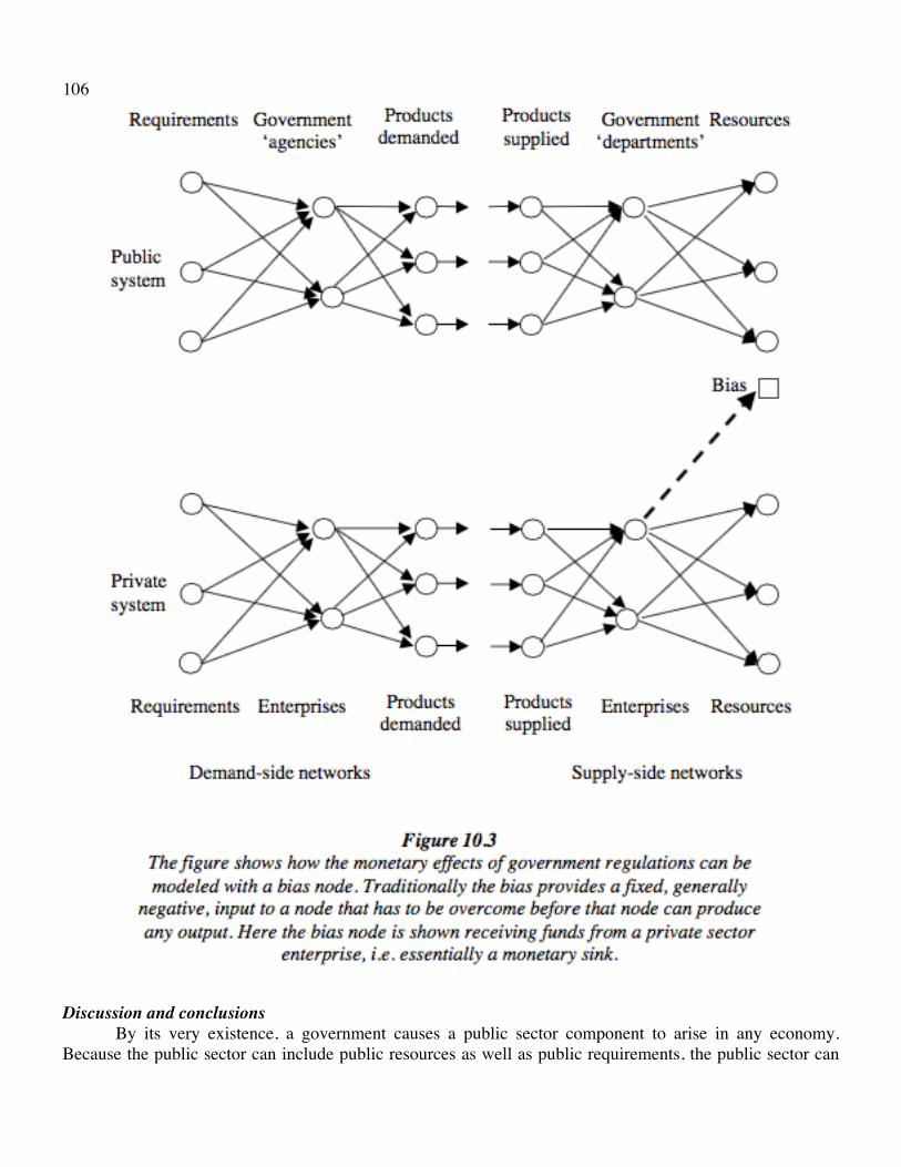
106

Discussion and conclusions By its very existence, a government causes a public sector component to arise in any economy.

Because the public sector can include public resources as well as public requirements, the public sector can

107 comprise an entirely parallel economic system when it deals with itself, that is, when it uses public resources to satisfy public requirements. However, the public and private systems are generally integrated, thus they influence each other. In the private sector, money and product flows are always roughly in balance, but in the public sector money is often garnered (taxation) from sources whereto products are not supplied while products (infrastructure, social services, etc.) can be supplied to recipients from whom money is not collected. The public system therefore has effects akin to those of externalities as defined by Pigou (Vaggi and Groenewegen 2003: 276), but without the attribute of being incidental. From the perspective of private sector concerns though, they could, on aggregate, have similar short-term consequences as externalities.

When public and private economies are allowed to exist side-by-side, flexibility in the overall economic system is created. In a volatile environment, with high risks, resources need to be conserved, thus resources need to be directed to the most successful. In a stable environment, growth needs to be maximized, thus resources need to be widely distributed to generate the diversity that can hopefully provide successful entities during high-risk periods. The relative importance of public and private sector economies can be adjusted by adjusting the size of government. In socialist systems, the public system becomes dominant and in capitalist systems, the private sector is dominant. ‘Dominance’ remains to be defined, but can be expected to take volumes of money and product flows into account. If this interpretation has validity, it implies broadly that under stable, favorable conditions, the mix of economic systems should lean toward socialism (to increase potential and scope for adaptation) and under unfavorable conditions, toward capitalism (to increase efficiency and the likelihood of survival). Cullis and Jones (2008: 300) suggest that, in order to provide an answer to the question of how big a government should be, information should first be sought about the nature and capabilities of individuals and about the causes of their happiness. The conclusion here is different. The size of government should be a function of overall long-term economic stability within its corresponding fluctuating environmental and population contexts.

Regarding taxation, it can be examined in the context provided by Figure 10.2. For example, when taxation exceeds spending, it will have the net effect of withdrawing money from the system (i.e. an inadequate counterflow of goods and services), thus reducing economic activity. Spending that exceeds taxation (deficit spending) means that an increased demand arises. If public resources cannot be converted to meet the increased public demands, the excess demands will be directed to the private system. Thus extra demand is injected into the private system. This extra demand will create demand stress as explained above, thus profits and growth signals are generated (see Chapters 8, 13). Thus, deficit spending is likely to inject extra demand into the private system, cause economic growth, and lead in the short term to resource transfer from the private to the public system. Properly invested profits that arise from deficit spending will lead to amelioration of the demand stresses and a reduction of growth unless the amount of deficit spending is further increased. A reduction of taxes will have a similar effect, but the demands that arise will be dictated by the private sector, not the public sector. If needs are mostly met, the extra funds made available from reduced taxation will be allocated to wants and aspirations. Extra funds that are primarily allocated to wants will have different consequences from those primarily allocated to aspirations; these issues are taken up again in Chapters 13 and 15.

Taxes levied by the state purportedly have the social aim of promoting fairness by way of the regulation of private system activities (broadly speaking, by promoting equal access to resources) and/or by way of redistribution of private system products (similarly broadly speaking, by promoting equal sharing in the collective product). For example, Cameron and Neal (2003: 402) contend that “The inequality in the distribution of resources – among individuals, social groups, and nations – is at the very heart of the problem of economic development...” and Nayak (2003: 246) points out in his examination of Schumpeter’s tax state that Schumpeter was pessimistic about the future of the capitalist state because he thought that people would simply escalate, until the point of failure, their demands to share in the aggregate product via the state. Either way, pressures for equal access are generally evaluated on the criterion of Pareto efficiency (e.g. Fairris and

108 Pattanaik 2003: 90; Mookherjee 2003: 115): a Pareto efficient outcome would make somebody better off without making anybody else worse off. It is therefore relevant to ask whether this is possible, at least in principle.

Fairris and Pattanaik (2003: 91) address the question of Pareto optimality in welfare economics by formulating a choice problem. Here an economic agent has to make a choice given

(i)! a universal set X = {x, y, z, …} of all conceivable but mutually exclusive options that has (ii)! a non-empty subset A of feasible options at the moment of choice where the latter options are (iii)! ranked, in the ordering Ht, according to a criterion t (from a set consisting of m criteria). If x is

at least as good as y in terms of criterion t, it is denoted xHty. When there is no criterion for which a better feasible option than x exists, x is undominated.

An efficient choice is thus made when an agent chooses an undominated feasible option. When applied to welfare economics, the economic agent is the (enfranchised) society, the set of

options is all conceivable forms of governments of which some are feasible at the time when the choice is made, and every individual of the n individuals constituting the society can provide an ordering of the feasible options ranked according to that individual’s preference. A Pareto optimal state or government is therefore an undominated feasible option – at least as good as any other feasible option, but not worse.

Given that Pareto efficiency is dependent on rankings of types of governments by individuals according to criteria of their choosing, one might inquire about the nature of these criteria. Fairris and Pattanaik (2003: 105) observe that welfare economics has not always paid adequate attention to the fact that the same individual may have different types of preferences. In doing so, it seems reasonable to surmise that preferences governing selection criteria will be based on requirements, specifically, that selection criteria will reflect the aim to maximize the satisfaction of individual requirements (e.g. “desire fulfillment” in Fairris and Pattanaik 2003: 104). The subcategories of requirements, namely, needs, wants, and aspirations, imply that one could potentially distinguish between at least three different categories of state options. In poor societies, the satisfaction of needs will predominate and the rankings of feasible state options will favor states that are viewed as most likely to satisfy needs. In other societies, wants may predominate and states perceived to enhance the individual’s competitive advantage(s) will be the undominated options amongst those of feasible states. In highly egalitarian and/or advanced societies, the ordering of feasible options will be based on the satisfaction of aspirations.

What are the consequences of this interpretation? Mostly, that strife will arise. In societies functioning near subsistence levels, needs are by definition not readily satisfied. Moreover, among requirements, needs dominate in importance and must be satisfied first. Needs will dominate selection criteria. Thus in needy societies, needs-related demand exceeds needs-related supply and the implication is that a zero sum condition prevails. Unless redistribution is effective in inducing an increase in aggregate output adequate to improve the satisfaction of needs-related requirements for everyone, redistribution under zero-sum conditions will simply make some better off at the expense of others. Despite their contention that the inequality in the distribution of resources is a fundamental problem of economic development, Cameron and Neal (2003: 249, 245, 246, 266, 267) provide strong evidence that it is very much the distribution of human, not natural resources, that is fundamental to economic development. Countries with high levels of literacy, like the Netherlands, Denmark, Norway, Sweden, Switzerland, and Japan, achieved high levels of economic development despite poor endowments of natural resources. Thus, it is unclear how Pareto optimality could be achieved in a society without the human resources to effect the required increase in aggregate output.

Yet, there is a further problem. Assuming that an adequate aggregate output could be generated or externally supplied, it must be sustainable through technological advancement or continued aid to avoid the Malthusian trap. When the trap is sprung, the society falls back into zero sum conditions and the same option that was formerly Pareto efficient will no longer be so. Consequently, whether the redistribution of wealth in

109 needy societies is from internal or external sources, finding an enduring solution in this manner will be difficult. Internal redistributions will flounder on the rocks of zero-sum shores and external redistribution only aimed at needs-relief must be maintained indefinitely. Indeed, international aid has had little effect in societies where human resources were lacking (Galbraith 1994: 162), but, in contrast, there is no place in the world where well-educated people are really poor (Galbraith 1994: 181).

In better-off societies, where needs are routinely met, but where a strong egalitarian sense or high levels of social obligation are not moderating influences, wants will predominate as state selection criteria. Wants, however, have a strong procreative component and consequently a competitive nature (see Chapter 5). Competition, by its very essence, serves to establish rank. Someone wins the race and someone looses; competition is impotent if it merely establishes equality between all competitors – all win or all loose. Indeed, establishing relative advantage is the raison d’être of competition. Therefore, in principle, achieving Pareto efficiency under such circumstances is impossible because improving the situation of one member of society comes specifically at the detriment of everyone else. Furthermore, from an entitlement point of view, competition means that resources must eventually be exhausted or a stable status hierarchy must be established, because having enough is insufficient if the neighbors have more. In addition, due to the procreative component of wants, they are subject to humoral influences and these fluctuate in both men and women: in women on a monthly basis, in men on a diurnal and annual basis, and for both across the lifespan. Thus wants are inherently unstable because they have large dynamic ranges of consumption and fluctuating temporal dynamics that will play out on a demographic level.

Ironically, the above analysis seems to indicate that Pareto efficient choices can only be made in societies that are already egalitarian and affluent, may not need welfare, and where Pareto-efficient choices will have scant impact. Put differently, if a welfare state is to be created, it is not likely to occur by choice in those societies that need it most; it will have to be imposed. At the very least, ‘wants’ must be disallowed as subcomponents of criteria by which individuals rank their preferences of feasible social state options. Note the intriguing implication above that a (benign) autocratic state may have utility as a transitional or parenting state, that is, to effect the conversion of a society from a needy one to an affluent one.

The extensions outlined here, although just briefly touched upon, suggest ways to model the role of a state or government in an overall economy. Modeling the state will affect decisions about the size of the public economy relative to that of the private economy, the degree of parallelism of the public economy, and the architecture of the public economy. Modeling a government may not affect the model of the state much unless a fundamental shift has occurred (e.g. a change occurred from a capitalist to a socialist state). Thus, modeling a government will only involve minor changes to the state model but more extensive changes to the interface between public and private sectors.

In conclusion, the ability to model the public sector may make possible a principled understanding of the causes and effects of public sector demands (i.e. government spending) and the conception of a more consistent, efficient, and targeted delivery of governmental goods and services. The ability to model the public sector may also permit the evaluation of a given public sector to assess its performance and may furthermore enable a reconsideration and restructuring of taxation and regulatory systems to implement the its mandate more efficiently.

110

11

Completing the System With Circular Flows

111

Completing the System With Circular Flows

Summary

The role of humans in determining economic demands as well as supplying economic resources in the form of labor has been delineated in preceding chapters. Circular flows in the overall economic system therefore arise naturally by postulating a human population and interposing it outside the demand- and supply-side networks. Thus money can flow from the owners and suppliers of resources to the human population as incomes. These incomes are proportioned as desired between the requirements of needs, wants, and aspirations and are used to fund them. Money then flows from requirements in the DSN to resources in the SSN where it arrives as incomes, hence completing the circuit. Circular flows for money also imply that goods and services, in some mutable form at least, must experience circular flows. Every individual, if s/he is to participate in the economy, thus must receive a sufficient income to purchase a sufficient level of goods and services to maintain at least their ability to participate. Circular flows make this possible in principle. An ecosystem is also postulated to exist, analogous to the human population. The ecosystem potentially permits circular flows between non-human economic resources and the DSN requirements. Humans must administer money and care on behalf of the ecosystem. This incorporation of circular flows into the model reveals that the factors that govern circulation fall into two groups – drivers of circulation and friction forces that inhibit circulation. These factors are used to develop an equation for the velocity of circulation.

112

Introduction Circular flows are well-entrenched concepts of standard economics (e.g. Ison 2000: 158). Here,

factor services flow from households to firms and goods and services flow from firms to households, all in the same direction. In the opposite direction, money flows from firms to households as wages and from households to firms as expenditures. The notion of a circular flow of money is already clearly expressed by early writers such as Hume and Petty (Wood 1995: 104) and that of the circular flow of income in particular seems to have first gained importance in the eighteenth century with Law’s monetary and macroeconomic analyses (Vaggi and Groenewegen 2003: 41). Later, in Quesnay’s Tableau Économique, circular monetary flows became tightly integrated with the circulation and reproduction of commodities (Vaggi and Groenewegen 2003: 63-67). The rate of circulation of money is termed the ‘velocity of circulation’ and played and important role in Wicksell’s analysis of price levels (Vaggi and Groenewegen 2003: 256). It is most familiar in the quantity theory of money in the form used by Fisher (e.g. Jackson 1986: 45) and given in Eq. 3.6.

I have established in earlier chapters that requirements issue from individuals. Knowing that economic resources include labor and capital, and that the former definitely and the latter potentially include individuals, it becomes clear that another interface exists between the DSN and SSN. This interface arises between these two networks’ respective input layers (as opposed to between their output layers as shown in Figure 4.1) and occurs via human intermediaries. I have elected to refer to the stage of the CTE containing the first interface as a “core” version of the model. The expanded skeleton of the model requires that the second interface also be developed. The introduction of this second interface permits the circular flows of money and commodities and it is the objective of this chapter. This will structurally complete the basic economic system.

Populations

Although it has been established that goods and services counterflow money, one has to ask what finally happens when goods and services and money, respectively, reach their destinations. The macroeconomic notion of circular flows of money and goods (e.g. Ison 2000: 158) suggests that once money reaches its ultimate destination (i.e. ‘Resources’), it should be returned to its origins (i.e. to ‘Requirements’). The most obvious way to complete the circuit is to exploit the connection that exists between labor and requirements. Labor constitutes human labor while requirements are derived from human attributes (see Chapters 2, 3, and 5). Thus, a new connection between labor and requirements can be established. It would allow funds of money that reach the labor component of economic resources to be recycled back to the requirements of, at least, these laborers. Clearly, we are dealing here with the issue of wages.

Fortunately, Figure 3.2 suggests a way to proceed. The figure makes explicit that requirements originate from different individuals and some of these individuals, it is reasonable to assume, also provide labor. Therefore a population of individuals is created such that all the members of the population contribute to the sum total of requirements and some of these individuals receive compensation for labor. In addition, land and capital ultimately belong to individuals, whether individually or collectively, and incomes deriving from these resources also flow to the population.

Figure 11.1 shows this circular connection of the core networks. The familiar SSN and DSN remain as juxtaposed previously, but their input layers are now connected ‘backward’ via the population of individuals. Whether these backward connections via the population can also be, or should also be, represented as networks, i.e., similar to the DSN and SSN, may be a worthwhile future question to pursue.

Circular flows

In order to maintain flows, the system must operate to circulate money and reproduce commodities.

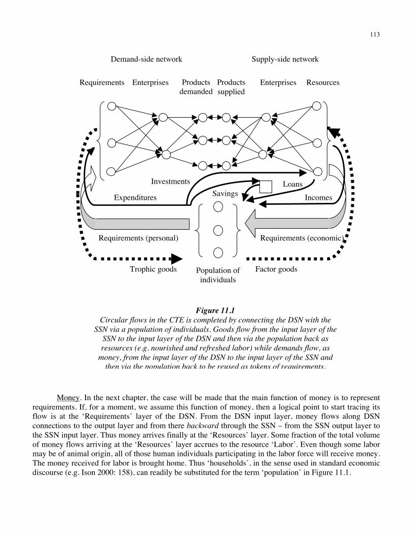
113

Money. In the next chapter, the case will be made that the main function of money is to represent

requirements. If, for a moment, we assume this function of money, then a logical point to start tracing its flow is at the ‘Requirements’ layer of the DSN. From the DSN input layer, money flows along DSN connections to the output layer and from there backward through the SSN – from the SSN output layer to the SSN input layer. Thus money arrives finally at the ‘Resources’ layer. Some fraction of the total volume of money flows arriving at the ‘Resources’ layer accrues to the resource ‘Labor’. Even though some labor may be of animal origin, all of those human individuals participating in the labor force will receive money. The money received for labor is brought home. Thus ‘households’, in the sense used in standard economic discourse (e.g. Ison 2000: 158), can readily be substituted for the term ‘population’ in Figure 11.1.

Figure 11.1 Circular flows in the CTE is completed by connecting the DSN with the

SSN via a population of individuals. Goods flow from the input layer of the SSN to the input layer of the DSN and then via the population back as resources (e.g. nourished and refreshed labor) while demands flow, as

money, from the input layer of the DSN to the input layer of the SSN and then via the population back to be reused as tokens of requirements.

Requirements Enterprises Products demanded

Resources Enterprises Products supplied

Demand-side network Supply-side network

Incomes

Population of individuals

Factor goods Trophic goods

Expenditures

Requirements (personal) Requirements (economic)

Savings Investments Loans

114

In the simplest case, a single individual retains his/her total income. In more complex cases, the laborer forms part of a larger household and some fraction of his/her income goes toward the household income while the remainder may be retained by the earner. Household income may be distributed, directly or in trust, to individuals that are not receiving any income (e.g. children). In any case, all individuals that receive money, directly or by proxy, contribute to the generation of economic requirements. Clearly, those individuals that receive no money cannot generate economic requirements even though they do have personal requirements just like those who do receive money. They can become connected to the private economy by virtue of income received through the public economy (e.g. through social assistance or unemployment insurance) or must remain outside the economy and fend for themselves, depend on informal care, or perish.

Income is not only derived from labor, but from other sources as well (listed in Chapter 4). All these income streams then join those obtained from labor to constitute a population income. The population allocates income according to its requirements. As discussed before, some of these requirements are fairly inelastic (e.g. needs) and have to be given allocation priority while others are more elastic (e.g. aspirations) and thus discretionary. All income allocated to requirements constitute expenditures. Any income that is not allocated to requirements, in the elementary case, is retained locally as ‘savings’ or made available as ‘investments’, i.e. becomes a resource through recirculation directly to the ‘Capital’ node of the SSN.

Goods and services. Taking as starting point for the flow of goods and services the ‘Resource’ layer of the SSN, goods and services flow to the SSN output layer, to the DSN output layer, then backwards through the DSN to the DSN input layer. At that point, human requirements are being met or being satisfied, in whole or in part. However, the process does not stop there. When requirements are being met, the resources, that is, the goods being consumed, are being transformed into a different essence. The consumption of goods affects a population in such a way that, ideally, the population is maintained and/or strengthened. Because individuals in the population are nourished, rested, and recuperated following consumption of these goods, they are termed ‘trophic’ goods in Figure 11.1. Trophic goods have physiological, psychological, and social impacts that enable the population to provide factor goods to the economy, for example, in the form of labor. For example, the consumption of resources serves to maintain, improve, and expand the labor resource itself.

Requirements. Money, being tokens of requirements as described in the next chapter, must always flow in parallel with those requirements that they represent. Thus, in parallel with the circulation of money, there is a complete circulation of requirements. At the starting position, the DSN ‘Requirements’ layer, they are requirements of consumer goods and services, once the SSN is entered, they become production requirements, and when about to leave the SSN, they become requirements for factor goods. ‘Factor goods’ are here meant to indicate SSN requirements of labor, amongst others, placed upon the population. In turn, the population has requirements for nourishment and maintenance and these, made upon the DSN, constitute the input layer of the DSN. Thus one arrives back at the starting position.

Ecosystems

The example above of requirement flows that are completed via the labor resource may prompt one to ask what role the resources land and capital play. The issue of capital is postponed for a later chapter; that of land is considered here. Like human resources, one would surmise that circular flows pertaining to natural resources must also be completed. Thus, as in the case where a population of humans individuals was posited to exist, a ‘population’ of natural resources must exist. This ‘population of natural resources’ is now formally defined as the ‘ecosystem’.

Augmenting Figure 11.1 with an ecosystem, along with circular flows analogous to those described for and involving the population, produces Figure 11.2. There is however, an important practical aspect in

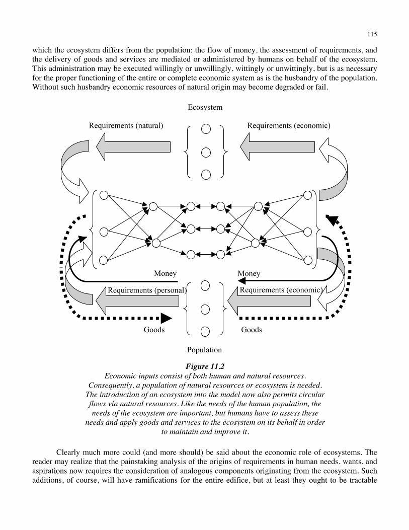
115

which the ecosystem differs from the population: the flow of money, the assessment of requirements, and the delivery of goods and services are mediated or administered by humans on behalf of the ecosystem. This administration may be executed willingly or unwillingly, wittingly or unwittingly, but is as necessary for the proper functioning of the entire or complete economic system as is the husbandry of the population. Without such husbandry economic resources of natural origin may become degraded or fail.

Clearly much more could (and more should) be said about the economic role of ecosystems. The

reader may realize that the painstaking analysis of the origins of requirements in human needs, wants, and aspirations now requires the consideration of analogous components originating from the ecosystem. Such additions, of course, will have ramifications for the entire edifice, but at least they ought to be tractable

Figure 11.2 Economic inputs consist of both human and natural resources.

Consequently, a population of natural resources or ecosystem is needed. The introduction of an ecosystem into the model now also permits circular flows via natural resources. Like the needs of the human population, the needs of the ecosystem are important, but humans have to assess these

needs and apply goods and services to the ecosystem on its behalf in order to maintain and improve it.

Money

Population

Goods Goods

Money

Requirements (personal) Requirements (economic)

Ecosystem

Requirements (natural) Requirements (economic)

116

given the existing framework. Ecological requirements are, for present purposes, deemed to be subsumed by the requirements expressed by the human population.

Velocities of circulation

Given the importance of the velocity of circulation (of money) in quantity theory and monetarism (e.g. Ison 2000: 207; Jackson 1986: 45; Vaggi and Groenewegen 2003: 256, 319; Woods 1995: 104-106) it is of interest to consider it in the augmented model shown in Figure 11.1 where circular flows can now occur. This consideration has two major components: the first requires an analysis of the paths of circulation and the second requires and analysis of the factors determining the velocity of circulation. In a public economy with redistributive operations and in the interface of such a public economy with a private economy, money does not necessarily flow along all connections or flow in a manner more-or-less counterbalanced with the flow of products of economic activity within a connection. However, in the private economy, this is generally the case and it serves as a good point of departure to analyze both the routes of circulation and the factors driving circulation along those routes.

Routes of circulation. Given the multitude of connections that exist in a private economy and the level of resolution that one may wish to use in modeling them, it may be tempting to section the core system across its central interface or at some other perceived convenient position such as the ‘Resources’ or ‘Requirements’ layers in order to assess the velocity of circulation. The question is whether this is well-advised. Recall from the refinements introduced in Chapters 8 and 9 that a number of local connections can exist. These may thus complicate the circulation of money and hence affect its velocity. Therefore, a distinction needs to be drawn between local circulation(s) and global circulation and the question of velocity considered in more nuanced form, even if local and global circulations are ultimately aggregated. Figure 11.3 shows an example of a local circuit being completed with a reentrant connection as well as the global circuit that consists of flows through both networks redirected to them via the population.

Local circulation. It is worth taking stock of those connections that may enable or affect local circulation. These are recurrent (Figure 8.1), parallel (Figure 8.2), direct (Figure 9.2), reentrant, (Figure 9.3) and lateral (Figure 9.4) connections. Recurrent, reentrant, and lateral connections can clearly sustain local money flows that are quite different from more global flows. On the other hand, parallel and direct connections are more likely to affect local money flows, but not likely to sustain them because they do not create complete local circuits. Recurrent connections form complete local circuits, while reentrant connections complement normal feedforward connections to form more extensive local circuits than those formed by recurrent connections. Lateral connections, such as bilateral connections between the same pair of nodes, can also create local circuits. Local circuits furthermore include flows along the savings and investment routes (Figure 11.1). The volumes and velocities of monetary flows over local connections may differ by type, size, and position of these local circuits, and also depend on global monetary flows, that is overall economic activity.

Global circulation. The global route of circulation has been described in detail above – from the DSN requirements layer to the SSN resource layer circulating back to the DSN via the population. The existence of local circuits suggests that changes in global velocity in one part of the global system may not result in an equivalent change of global velocity in another part of the system because local circuits may transiently affect such changes. In other words, local circuits could accommodate increased money flows from one part of the global system via increased local velocities or volumes thus limiting any pass-through global effects. Thus it may happen that only when local capacities reach saturation, or when increases in global flows outstrip response times in local circuits, pass-through effects will become evident.

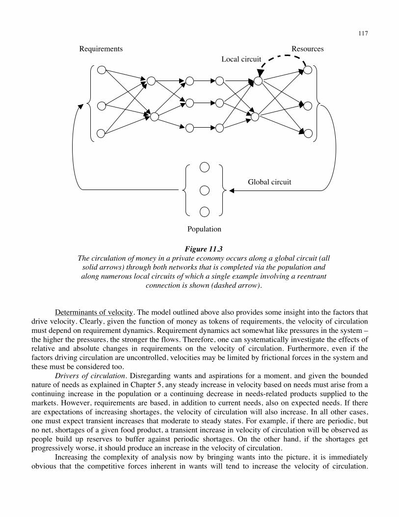
117

Determinants of velocity. The model outlined above also provides some insight into the factors that drive velocity. Clearly, given the function of money as tokens of requirements, the velocity of circulation must depend on requirement dynamics. Requirement dynamics act somewhat like pressures in the system – the higher the pressures, the stronger the flows. Therefore, one can systematically investigate the effects of relative and absolute changes in requirements on the velocity of circulation. Furthermore, even if the factors driving circulation are uncontrolled, velocities may be limited by frictional forces in the system and these must be considered too.

Drivers of circulation. Disregarding wants and aspirations for a moment, and given the bounded nature of needs as explained in Chapter 5, any steady increase in velocity based on needs must arise from a continuing increase in the population or a continuing decrease in needs-related products supplied to the markets. However, requirements are based, in addition to current needs, also on expected needs. If there are expectations of increasing shortages, the velocity of circulation will also increase. In all other cases, one must expect transient increases that moderate to steady states. For example, if there are periodic, but no net, shortages of a given food product, a transient increase in velocity of circulation will be observed as people build up reserves to buffer against periodic shortages. On the other hand, if the shortages get progressively worse, it should produce an increase in the velocity of circulation.

Increasing the complexity of analysis now by bringing wants into the picture, it is immediately obvious that the competitive forces inherent in wants will tend to increase the velocity of circulation.

Figure 11.3 The circulation of money in a private economy occurs along a global circuit (all

solid arrows) through both networks that is completed via the population and along numerous local circuits of which a single example involving a reentrant

connection is shown (dashed arrow).

Population

Global circuit

Local circuit Requirements Resources

118

Unless the number of tokens in the system is limited, numbers in excess of what are required to satisfy needs will be allocated mostly to wants. Moreover, keen competition may result in the unrestrained procurement of tokens through credit facilities unless counterbalancing costs arise. Thus, conditions that permit or favor competition will promote circulation while those that inhibit competition will reduce circulation. Aspirations will also affect the velocity of circulation, but do so based on actions deemed in the collective benefit.

Besides requirements, there are other drivers of circulation. As alluded to above, the supply of goods and services is one. High levels of supply relative to demand imply capacity underutilization and reduced pressures on circulation. Hence velocity will be reduced. Also drivers of circulation are on-hand savings, investments, and loans. Both savings and investments remove tokens from circulation, thus reduce effective demands and velocities, while drawing on savings and obtaining loans will add tokens and hence increase effective demands and velocities.

Nevertheless, drivers of circulation, regardless of their origins, may be sufficient only to increase velocities of circulation up to a point before the velocities get moderated by friction forces.

Friction forces. Velocities are limited by capacities in the system and by the ease with which exchanges can occur. These conditions do not drive circulation, but come into play once circulation commences. Regulation, taxation, and other factors are constraints on circulation because accommodating them takes a finite amount of time and a finite number of tokens and thus exchange processes can be speeded up only to a certain extent. Likewise, manufacturing, distribution, wholesale, and retail capacities, processing speeds, and rates of obsolescence are also finite. Moreover, these processes have associated costs and approaching or exceeding the foregoing limits will lead to quick escalations of cost. Thus friction forces exist in the system and they will tend to inhibit circulation and moderate its velocities.

Discussion and conclusions

Completing the system by introducing a population and an environment that permit circular flows of demands and supplies, brings one into contact with the quantity theory of money and monetarist policy. Considerable interest therefore arises from an analysis of the model and its implications for the quantity theory and monetarism.

The quantity theory is somewhat imperfectly captured by the equation of exchange MV = PT Eq. 3.6

with symbols standing for money, velocity, price, and transaction volume, from left to right respectively. The quantity theory of money is a theory about the general price level and its dependence on the quantity of money in a system. The theory is often used to formulate price stabilization policies, thus giving rise to monetarism. Paraphrasing Blaug (1995: 29) slightly, the quantity theory is seen to consist of three propositions: that causality runs from money to prices via specific transmission mechanisms; that the velocity of circulation is stable and independent of the money supply; and that the volume of transactions is independent of the quantity of money or the general level of prices. Thus a number of questions arise from these propositions: what governs the quantity of money in the system? Does the quantity of money indeed affect prices? By which mechanisms are prices affected? Is the velocity of money stable? Is the velocity of circulation independent of the quantity of money? What governs the velocity of circulation? Do prices affect the money supply? Are transactions independent of the quantity of money? Are transactions independent of price levels? What governs the volume of transactions? These questions are important, specifically, because their answers may indicate, first, whether monetarism is a feasible policy and, second, how to proceed with monetarist policies. It is therefore instructive to analyze monetary flows, starting with an analysis of a simplified circuit based on Figure 11.3 and to gradually augment it as illustrated in the consecutive panels of Figure 11.4.

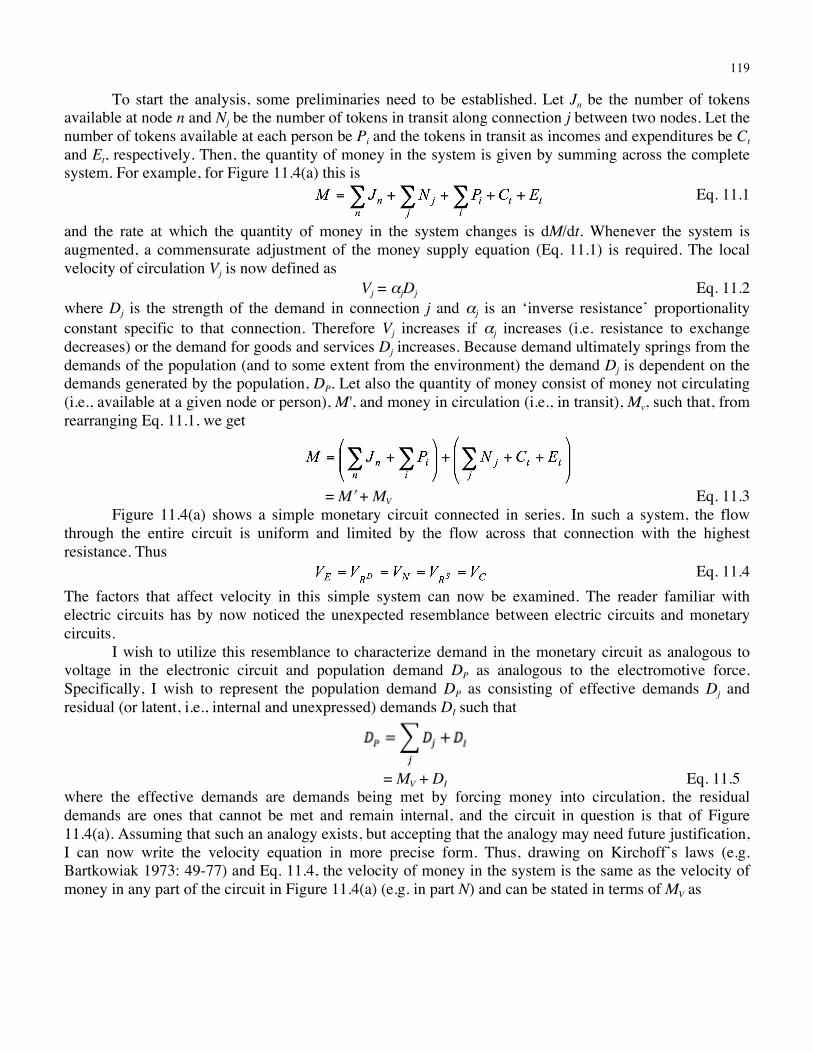
119

To start the analysis, some preliminaries need to be established. Let Jn be the number of tokens available at node n and Nj be the number of tokens in transit along connection j between two nodes. Let the number of tokens available at each person be Pi and the tokens in transit as incomes and expenditures be Ct and Et, respectively. Then, the quantity of money in the system is given by summing across the complete system. For example, for Figure 11.4(a) this is

Eq. 11.1

and the rate at which the quantity of money in the system changes is dM/dt. Whenever the system is augmented, a commensurate adjustment of the money supply equation (Eq. 11.1) is required. The local velocity of circulation Vj is now defined as

Vj = αjDj Eq. 11.2 where Dj is the strength of the demand in connection j and αj is an ‘inverse resistance’ proportionality constant specific to that connection. Therefore Vj increases if αj increases (i.e. resistance to exchange decreases) or the demand for goods and services Dj increases. Because demand ultimately springs from the demands of the population (and to some extent from the environment) the demand Dj is dependent on the demands generated by the population, DP. Let also the quantity of money consist of money not circulating (i.e., available at a given node or person), M', and money in circulation (i.e., in transit), Mv, such that, from rearranging Eq. 11.1, we get

= M" + MV Eq. 11.3 Figure 11.4(a) shows a simple monetary circuit connected in series. In such a system, the flow

through the entire circuit is uniform and limited by the flow across that connection with the highest resistance. Thus

Eq. 11.4 The factors that affect velocity in this simple system can now be examined. The reader familiar with electric circuits has by now noticed the unexpected resemblance between electric circuits and monetary circuits.

I wish to utilize this resemblance to characterize demand in the monetary circuit as analogous to voltage in the electronic circuit and population demand DP as analogous to the electromotive force. Specifically, I wish to represent the population demand DP as consisting of effective demands Dj and residual (or latent, i.e., internal and unexpressed) demands DI such that

= MV + DI Eq. 11.5

where the effective demands are demands being met by forcing money into circulation, the residual demands are ones that cannot be met and remain internal, and the circuit in question is that of Figure 11.4(a). Assuming that such an analogy exists, but accepting that the analogy may need future justification, I can now write the velocity equation in more precise form. Thus, drawing on Kirchoff’s laws (e.g. Bartkowiak 1973: 49-77) and Eq. 11.4, the velocity of money in the system is the same as the velocity of money in any part of the circuit in Figure 11.4(a) (e.g. in part N) and can be stated in terms of MV as

120

Figure 11.4 The circulation of money in a private economy is shown in progressively

more complex global monetary circuits: (a) along a simple circuit, (b) along a circuit expanded to include savings and withdrawals as well as

investments and loans, and (c) along a circuit further augmented with parallel paths and local loops.

N

Population

Requirements Resources

RD RS

N

C E

(a)

N

Population

Requirements Resources

RD RS

C E

I L

S W

(b)

Population

Requirements Resources

RD RS

C E

I L

S W

B F1

(c)

F2

121

Eq. 11.6

One must now enquire as to the effect of an increase in M on V, P and T. Eq. 11.5 and Eq. 11.6 indicate that changes in effective demand will affect the velocity of circulation. Consequently, changes in the money supply, because they are likely to affect effective demand, will affect the velocity of circulation. These changes are considered next with reference to needs, wants, and aspirations.

In a population where needs are only partially satisfied and other requirements are non-existent or negligible, all money would be in circulation (M' = 0). Conditions where needs are partially satisfied endanger the survival of the population. Thus one could expect the velocity of circulation to increase. However, because the supply of tokens is inadequate to represent requirements at a proper fine-grained level, individual tokens would be highly valuable, hence reducing the propensity to put them into circulation. The most likely outcome under the partial satisfaction of needs is an increase of the demand for tokens. If more tokens are available, more needs can be effectively represented and MV increases. Eq. 11.6 suggests this would bring about an increase in the velocity of circulation. In the absence of an increase in the money supply, the velocity of circulation can also increase if barriers to circulation such as transaction costs and transaction times are reduced. If velocities increase until supplies become limited, prices will rise (accepting that the transition between these conditions is not discontinuous). Price increases, when local rather than widespread, produce profits that are error or stress signals (more in Chapter 13) that would elicit production increases. If the supply of goods and services can be increased to permit some stock to be carried, price pressures will abate. Further build-up of stocks would produce a reduction in velocity after which would follow a reduction in prices.

The scenarios above play out because needs, by their nature, must be satisfied and cannot be oversatisfied. The reader may recall that the consumption of a certain amount of water is essential for life, but that physically consuming greater than essential quantities quickly becomes detrimental. Thus needs as a driver of velocity is bounded. When needs can be satisfied, effective demand does not increase (and hence the money in circulation is not increased) unless demand is expanded, by virtue of newly available tokens, to include wants and aspirations.

In contrast to needs, wants are unbounded drivers of velocity due to their inherent aspects of competitive display (keep in mind that competitiveness differs between individuals and within an individual over the lifespan). When money is injected into a system where population needs are fully

satisfied and wants exist, it will tend to be put into circulation, thus and . The velocity of circulation will increase until it becomes transaction- and/or supply-limited and prices rise, or until competition moderates because a stable status hierarchy is established. Regardless, velocity and price effects will occur predominantly along those pathways that satisfy wants. Aspirations, because they too are unbounded drivers of velocity, are likely to have similar effects, but are more likely to be moderated if their implementation is perceived to produce adverse social outcomes.

Although I have drawn a distinction above between money in circulation and money not in circulation, Figure 11.4(a) does not offer opportunities for saving. This is rectified with the augmented circuit shown in Figure 11.4(b) permitting savings S and withdrawals W. In addition, investments I can be made and loans L can be had. Investment returns accrue via the income stream C along with other incomes. Interest expenses are remitted via E along with all other expenditures. Let now V0 be a base velocity such that DP is satisfied (i.e. needs satisfied and a stable dominance hierarchy established) and let M0 be the smallest quantity of tokens sufficient to enable this condition to arise and persist. Any increase in M such that M > M0 will favor an increase in savings, thus an increase in M'. Socio-economic stability will

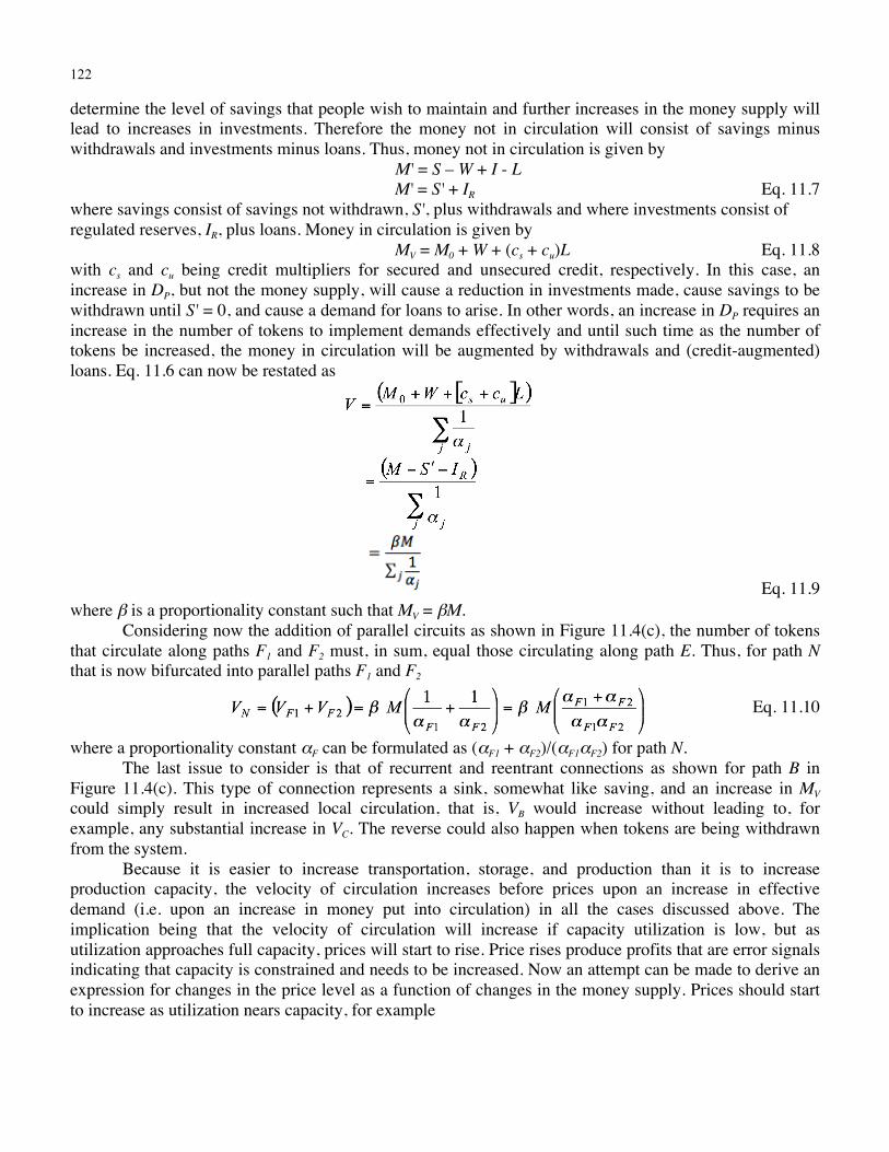
122

determine the level of savings that people wish to maintain and further increases in the money supply will lead to increases in investments. Therefore the money not in circulation will consist of savings minus withdrawals and investments minus loans. Thus, money not in circulation is given by

M' = S – W + I - L M' = S' + IR Eq. 11.7

where savings consist of savings not withdrawn, S', plus withdrawals and where investments consist of regulated reserves, IR, plus loans. Money in circulation is given by

MV = M0 + W + (cs + cu)L Eq. 11.8 with cs and cu being credit multipliers for secured and unsecured credit, respectively. In this case, an increase in DP, but not the money supply, will cause a reduction in investments made, cause savings to be withdrawn until S' = 0, and cause a demand for loans to arise. In other words, an increase in DP requires an increase in the number of tokens to implement demands effectively and until such time as the number of tokens be increased, the money in circulation will be augmented by withdrawals and (credit-augmented) loans. Eq. 11.6 can now be restated as

Eq. 11.9 where β is a proportionality constant such that MV = βM.

Considering now the addition of parallel circuits as shown in Figure 11.4(c), the number of tokens that circulate along paths F1 and F2 must, in sum, equal those circulating along path E. Thus, for path N that is now bifurcated into parallel paths F1 and F2

Eq. 11.10

where a proportionality constant αF can be formulated as (αF1 + αF2)/(αF1αF2) for path N. The last issue to consider is that of recurrent and reentrant connections as shown for path B in

Figure 11.4(c). This type of connection represents a sink, somewhat like saving, and an increase in MV could simply result in increased local circulation, that is, VB would increase without leading to, for example, any substantial increase in VC. The reverse could also happen when tokens are being withdrawn from the system.

Because it is easier to increase transportation, storage, and production than it is to increase production capacity, the velocity of circulation increases before prices upon an increase in effective demand (i.e. upon an increase in money put into circulation) in all the cases discussed above. The implication being that the velocity of circulation will increase if capacity utilization is low, but as utilization approaches full capacity, prices will start to rise. Price rises produce profits that are error signals indicating that capacity is constrained and needs to be increased. Now an attempt can be made to derive an expression for changes in the price level as a function of changes in the money supply. Prices should start to increase as utilization nears capacity, for example

123

Eq. 11.11 where the gammas are proportionality constants and Y is an index of capacity utilization.

Reconsidering the quantity theory in light of the foregoing, what can now be said about its central propositions (e.g. Blaug 1995: 29)? The first proposition is that causality runs from money to prices via specific transmission mechanisms. This proposition must be true in all cases except where all requirements are met. Because wants have a competitive aspect, it is in general difficult to meet all wants. Requirements generate demands and demands are implemented with money. An increase in the money supply means that more demands can be implemented and, because available supplies are limited, prices need to increase to foster supply augmentation. Thus, the primary chain of causality runs from money to prices (more below also). However, due to the nature of circular flows, prices could in turn affect demands causing a reallocation of expenditures, the secondary chain of causality. The second proposition is that the velocity of circulation is stable and independent of the money supply. This proposition must generally be false for the same reasons that the first one must generally be true. An increase in the money supply means that more demands, especially wants, can be expressed, hence effective demand increases and more money is brought into circulation. This is captured, for example, by Eq. 11.9. The third proposition is that the volume of transactions is independent of the quantity of money or the general level of prices. The third proposition can only be true, within reason, of needs, but cannot be true for wants. If more money is available, more wants can be expressed and, provided that the demand can be met, the volume of transactions will increase.

A critical factor in all of the foregoing is how population demands become expressed as effective demands. This conversion is dependent on both current and anticipated requirements and provisions. The velocity of circulation will increase if, relative to demand, the supply of one or more products is expected to become constrained. Conversely, velocity will decrease if the relative supply is expected to increase. Thus, in an inflationary environment, and given that money represents demands, the supply of goods at a given price are expected to become scarce relative to the demand for them at that price. Waiting produces a loss of the opportunity to procure supplies at a given price and consumers will be tempted to spend sooner, while the opportunities still may exist, rather than later, when they may be gone. This is perhaps best illustrated by the experience of German hyperinflation after World War I when the velocity of circulation increased enormously (e.g. Davies 2002: 575). In a deflationary environment, waiting produces a gain since procuring requirements could take place at a later stage when supplies are available at a reduced price. In the latter case, velocity drops. Note again that velocity fluctuations cannot pertain to needs, because the satisfaction of needs must occur at a constant rate, i.e., the rate of satisfaction must be commensurate with physiological requirements. Velocity fluctuations must therefore primarily reflect elasticities of wants and aspirations.

Finally, addressing short-run and long-run effects on the economy caused by increases in the money supply appears problematic and controversial given the difficulties of specifying these time periods (e.g. Patinkin 1995: 121). Instead, one must consider characterizing periods of velocity-governed effects and supply-governed effects. Velocity-governed effects are dominant at low capacity utilization (note that we are shifting parts of the problem now to capacity utilization) and supply-governed effects otherwise. In a growing economy, capacity utilization is likely to be high and remain high and velocity-governed effects may be of short duration. Hence, increases in expressed demand will quickly lead to price increases. Thus, effects of changes in the money supply are entirely dependent on the level of requirements relative to the levels of supplies. This is captured by Eq. 11.11 which shows that increases in the money supply will be

124

more effective in causing price increases if capacity utilization is high, but not otherwise. Price increases, of course, provided they are modest, will cause economic expansion as explained elsewhere.

The major insights arrived at in this chapter are that the fundamental purpose of economic activities is the effective husbandry of a human population and the environment (ecosystem) wherein it is embedded. When the DSN and the SSN are in balance, existing population and ecosystem requirements are reconciled with existing resources without exceeding the natural constraints of the latter. Analyses of these circular flows show that economic functioning is fundamentally driven by the relationships between demands and supplies and the channels through which they are reconciled. Thus, in a self-correcting economy, the successes and failures of ongoing population and ecological husbandry will cause adaptive fluctuations that can become manifest as changes in economic variables such as the velocity of circulation, prices, transaction volumes, and output.

125

12

Money and Banks: Getting the System Going

126

Money and Banks: Getting the System Going

Summary

At the most elementary level, money is a request made by someone for some resource that they lack in order to satisfy a requirement. If the requestor is deemed likely to reciprocate in the future, the requestor’s ‘creditworthiness’ is high. The creditworthiness of the requestor therefore determines the quality of the request. Requests from the creditworthy are likely to be granted. Effective currencies are portable and provide either instant reciprocation or proof of creditworthiness. More complex, temporally and spatially distributed exchanges are mediated by the banking system. Thus, money is requests that have gained traction through natural or fabricated association with reciprocity. Because requests arise from requirements, money is the way in which requirements are expressed and prioritized. Money must be present in adequate volumes and of sufficient flexibility and versatility to fulfill this role.

127 Introduction

Requirements are an integral part of the connectionist economic model, but it has yet to be specified how they are expressed within the system, that is, how they become ‘tangible’. I argue in this chapter that requirements are expressed with money. This does not mean that money preexisted and has found, in addition to other uses, utility as an expression of requirements. Indeed, the thesis here is singular: money exists because it is used to express requirements.

A consensus definition of money and its role in the economy are notoriously difficult to achieve (e.g. Spahn 2007: 150). Martin (2003), for example, considers genuine money to be based on taxation, and that, in turn, on the State and its power. Often, money is defined as anything acceptable to pay debt (Jackson 1986: 1). This, of course, requires debt to be defined. Gardiner (2006: 38) makes the connection between money and debt very explicit by pointing out that money is created when money is borrowed, that is when debt is created. He formally defines money as negotiable claims on value (Gardiner 2006: 8). This definition is readily related to the view of money espoused here: claims can be seen to be demands, thus requirements, while value ultimately must reside in resources. Hence this formal definition defines money as negotiable requirements of resources. Since requirements already imply ‘requirements of resources’, money is negotiable requirements. However, there is a difference between the view presented here and Gardiner’s definition. Gardiner considers money as debt, thus reciprocal demand, as opposed to the view here where money is considered the original demand with reciprocity implied. Importantly, though, negotiability means that money can express the requirements of different agents.

It is my view that the earliest money served to satisfy needs, hence was perishable and consumable. Indeed, like chimpanzees (e.g. Alexander and Noonan 1979; de Waal 1987; Kuroda 1984; Stanford 1999), our very first ancestors may have traded sex for food; with sex performing the role of money. The history of banking provides further evidence that money initially addressed needs. In Sumer (around 3000 BC) banking developed independently of coin and was based on the taking of deposits transferable to third parties; deposits were mainly grain, but other types of crops were also accepted, as were implements, and metals (Davies 2002: 50). Grain-based banking was also highly developed in Ptolemaic Egypt (around 100 BC) in parallel with metal-based banking (Davies 2002: 52). The fact that different types of crops were accepted as banking deposits suggests that the convertibility of the satisfaction of needs was useful; thus the satisfaction of one ‘need’ could be traded for the satisfaction of another.

Subsequently, the expression of one type of requirement in terms of another evolved formally. The origins of this exchange are already present in the sex-for-food example above where the satisfaction of a want is traded for the satisfaction of a need. Formal conversion emerged in Babylonian times (Gardiner 2006: 4) when one shekel of silver (ornament, a want) was decreed equivalent to one gur (~ 300 L) of barley (food, a need). Thus, with increasing sophistication, ornament became tradable for food and it is the superior attributes of some types of ornament – in terms of durability, countability, uniformity – that became valued in addition to their intrinsic value as ornaments. These attributes therefore promoted the use of some ornaments as a medium of exchange. The earliest money, pre-metallic money, often had ornamental value and when metals became available they were then fashioned to resemble existing non-metallic money; for example, some of the earliest quasi-coinage was metallic cowry imitations produced in China at the end of the Stone Age (e.g. Davies 2002: 45-47).

Metals, especially noble metals, due to the persistence of their luster, had ornamental value since they could be used to attract the attention of potential mates. Metals also had utilitarian value since they could be fashioned into implements. Furthermore, metals were relatively durable, but unlike cowries or cattle, did not appear in uniform and easily countable amounts. However, by virtue of being malleable, metals were susceptible to standardization. The earliest origins of coin in Lydia in Asia Minor reflected a progressive standardization of metal passed in trade. During the period 690 BC to 630 BC, lumps of metal became

128 increasingly standardized, then stamped to reflect that standardization, until a fairly high level of standardization was reached with proper double-struck coins (Davies 2002: 64).

Convertibility was again extended with the introduction of paper money. Around 800 AD, a severe shortage of copper for the manufacture of small coin resulted in the introduction of paper money in China (Davies 2002: 181). Initially the use of paper money was meant to represent the value of existing metals or produce, but by the end of the first millennium, quantities of paper money had become excessive, creating inflation. The original introduction of paper money therefore may have been of the form of a note promising the bearer a certain quantity of copper coin when supplies were restored, but later may have also served as ‘bill of exchange’. In Europe, paper money derived from the activities of goldsmiths in England in the seventeenth century. Goldsmiths were often, associated with their trade, dealers in foreign and domestic coin; they had strong boxes for safekeeping and members of the public began to make use of these facilities, especially during times of unrest and uncertainty. When given jewelry, bullion, and coins, receipts were issued for these demand deposits. Deposits were also lent out, and at some point in the seventeenth century, London goldsmith bankers provided, instead of coins or bullion, promissory notes to those borrowing. Hence the banknote was born, augmenting the money supply (Davies 2002: 252), and making cumbersome transfers of bullion and coins between parties unnecessary.

It is important to realize that paper notes were evidence of stores of value held in deposit. It should also be clear that, provided paper notes were negotiable, fungible, uniform, and dependable as guarantees of reciprocity, they could serve as evidence of stores of value held in general, i.e. as claims on the social product. Furthermore, the serial conversion of paper notes to metallic currency to requirements would be unnecessary. Any uniform, standardized, and widely acceptable item could serve as unit of account provided that the supply of the unit of account could be controlled, either naturally or by design, to prevent leakages into and out of the system since such leakages, were they to be substantial, would render accounting problematic and participants in the system cautious or unwilling to engage. Thus, the historical record suggests that, whether of paper or electronic or other form, provided they carried standardized reciprocal heft as further explained below, tokens that served multidirectionally as indicators of requirements would function as money. Money as expression of requirements

Although the foregoing examination of the historical record is plausibly consistent with the role of money as an expression of requirements, it does not reflect how I arrived at this interpretation of money. The structure of the model lead me to a hypothesis about the origins of money: it is an organic hypothesis and meant to indicate the human-based origins - and their evolution - of the close relationships between requirements and resources, and to provide a point of departure for further examination and discussion. The following explains how the role of money as an expression of requirements rests conformably on the model’s structure.

If one had ready access to sufficient resources to satisfy all one’s requirements, money would not be needed. The need for money arises indirectly when self-sufficiency becomes fragmented either physically or temporally or both; this is because trade or exchange is now necessary to achieve sufficiency along all the requirement dimensions. Specialization, or the division of labor, whether this be biological as in childbirth or based on custom, will no doubt accelerate this process. Specialization means that more attention is paid to selected tasks, with the implication that less attention is available for other tasks. The fruits of those tasks being neglected must therefore be made up through other means, exchange being one of these. Moreover, there are benefits to advertising one’s specialization and one’s success at the specialized task because it will be beneficial in the exchange process.

In pre-historic foraging societies, the successful forager had direct access not only to the immediate object of the foraging, e.g. meat or melons, but also to more durable parts associated therewith: teeth,

129 feathers, horns, fur, shells, seeds, gourds, and so on. Originally, display of these items may then have advertised the skills of the possessor. It may not have gone unnoticed that the display of such items brought additional attention to the owner thereof, thus enhancing their success in the competition for mates. Both foraging prowess and mating success would have translated into higher status. If the display of such items, originally dependent on foraging, subsequently became associated with status, they would have gained purchase independently of their derivation. Hence I see a natural social connection and progression from needs to wants to aspirations.

The ultimate object of a requirement, via derivative products, is a resource and the extent to which resources are required is related to the amounts consumed. If direct satisfaction is not possible and mediation is required, the requirements have to be indicated. Where barter is engaged in, excess resources are traded for resources lacking. However, ‘excess’ and ‘scarcity’ are defined, not in absolute terms or relative to other products, but only in terms of what is required. This is addressed in earlier chapters. Thus even when barter is used and even when resource products are traded to satisfy needs, they are specified in terms of what is needed, and perhaps, in a more sophisticated exchange, also in terms of anticipated needs. The traded excess resources (or resource products) reflect extant requirements. When I trade relatively (to me) abundant apples for relatively (to me) scarce eggs, the apples do not represent apples to me, nor eggs, but my requirement for eggs. The apples available for exchange are then the tangible form of my requirements. In this case, the apples are in the strict sense of the definition ‘money’ since they are expressions of my requirements. Specifically, they represent needs. They may also be resource products that are needed by others; thus they will carry instant reciprocity. If so, they will generally be consumed rather than further traded, i.e. they have a limited lifetime and limited circulation as money. The apples could also be used to trade for ornament - whale’s tooth, cowry shell, wampum - and ornament may make one attractive to prospective mates. Thus apples again would indicate requirements, but this time wants, and apples as expression of wants constitute money. Furthermore, where apples represent the need for eggs to one party, to the other, eggs represent the need for apples; of equal importance though, to the former party eggs, and the latter party apples, represent a resource. When an exchange occurs, a requirement is transferred in one direction and a resource in the other relieving the imbalances that arose with the initial specializations and producing for both parties a state of greater satisfaction than existed prior to the specialization.

Juxtaposed to the short historical analysis above, and paraphrased somewhat, there is clearly a progression on one side but not the other: apples, as money represented a requirement (e.g. the requirement for eggs); then cowry shells came to represent a requirement; then metal came to represent a requirement; then paper currency came to represent a requirement; finally, electronic tallies came to represent a requirement. In contrast, the requirement (for eggs) has not changed. Thus various things can represent a requirement, leading to the idea of expressing requirements with tokens.

Finally, and most significantly, money counterflows resources and this is a practical demonstration of its function as an expression of requirements.

Money should reflect a variety of aspects of requirements

For individuals, requirements obviously change over the course of a lifetime. ‘Requirements’ as conceived in terms of the present system, specifically as inputs to the DSN, are aggregates of the individual requirements in a population. Even so, these aggregates can vary over time, and needs, wants, and aspirations take on different proportions relative to one another. For example, their relative proportions will be different in times of peace, stability, and prosperity, compared to times of peace and famine or times of peace, plenty, and oppressive social circumstances. Therefore, money must be allowed to reflect all the concrete, abstract, and temporal aspect of requirements. Failure to allow this freedom will simply lead to the build-up of pressures and tensions within the system – impediments will eventually be circumvented or destroyed by mounting pressures.

130

Other functions of money When several parties can conspire to exploit a given resource more effectively, consideration should

be given to, at least, the distribution of the marginal increase in resource availability that the cooperative venture is likely to bring about. Hence prediction, planning, and negotiation are skills called upon. If one or more of these fails, then the cooperative venture may fail, and no-one is better off. Duping others cannot work in the long term if they take notice or if they fail in health and energies to the point where they cannot contribute effort. Thus, given a specific distribution of requirements, money allows resource fluctuations that occur between individuals, regions, and time periods to be smoothed out to the general advantage of all. A simple request already accomplishes some of this.

In principle, therefore, a simple request for food constitutes money and the memory of this request the record of the requirement. Likewise, an individual can use special tokens to indicate his/her requirements. If money is durable, it will also be a record of such requirements. If money is negotiable, the constraints of bilateral exchanges are lifted because more parties can now be involved as the need arises. Money then is a representation of what is required; when money changes hands in one direction and goods in the opposite direction, it also becomes a record of the transaction. Why should these balance? Requirements must be in balance with resources, they cannot exceed resources without creating stresses. However, provided the stresses are not too severe, pressures for adjustment arise permitting the system to self-correct giving rise to dynamic equilibria.

Money supply

At its root, an economy depends on the relationship between consumption and ability: the lone forager can only consume what he/she has gathered through effort and skill. This relationship is progressively loosened through the use of barter, metallic money, and convertible currencies. However, because we live in a physical world where the conservation laws of matter and energy are in effect, the relationship between consumption and ability can be modified but cannot be severed. Thus, even when fiat tokens are introduced, this relationship emerges as a need to administer the availability of tokens to retain a balance between consumption and ability, hence between demands and supplies. Thus, even though it may stand to reason that the creation of tokens to express requirements and mandating their acceptance entails standardization and specification of their parameters of use, it is necessary to determine how to create and distribute the tokens as well as how to ensure that a working balance between resources and requirements is maintained by creating the proper volume of tokens.

Creation and distribution. The most basic, informal, and perhaps frequent way that money is created is simply by asking – it often suffices to obtain the required resources. However, the one receiving resources incurs an obligation to reciprocate, not necessarily immediately or even in the short term or even in kind or even in value, but some reciprocation is implicitly expected. If someone continues to ask, but is unable to or refuses to reciprocate when able to and asked to, their ‘creditworthiness’ suffers. Therefore the likelihood that someone’s request will have purchase as money is proportional to their likelihood of giving back at some point. Specifically, someone’s requests (i.e. ‘currency’) will be valued according to the likelihood that they will and could reciprocate. If it is less likely that they can or would reciprocate, their ‘currency’ becomes correspondingly devalued. Expectations of reciprocation are normally governed by cultural norms and custom; and they function all the more effectively in small groups with efficient information diffusion where a refusal to reciprocate will rapidly lead to ‘personal currency’ devaluation. Requests from strangers and transients are less likely to be honored and when so, will be yielded to in a more altruistic fashion, that is, without the expectation of return, and perhaps also at levels below those that could fulfill adequately the requests. Thus ‘creditworthiness’, a specialization of ‘trustworthiness’, is an intuitive way to maintain the balance of demand and supply in a system with exchange.

131 In ancient times, the kings owned mineral resources (Davies 2002: 82) hence they could barter with

metals. Thus money was introduced into the system because it was not consumed as a resource, but rather used as ornament, display, or implement, and was durable so that others could use it for the same purposes repeatedly. In medieval times, the owner of gold or silver could deliver it to the mint where the metal would be coined in exchange for a small fee, the seigniorage; after 1666, this service was provided free of charge in England (Chown 1994: 10). This again shows that money enters the system because it is owned on a prior basis as a resource. Having a liquid resource, i.e. one that is immediately available for trade, establishes creditworthiness instantaneously and creditworthiness gives money its purchase.

In the case of barter, creditworthiness is established near effectively and near instantaneously (one does not need to wait for the harvest or the hunt to conclude). Clearly, if the creditworthiness of every person could be established and be available universally, freely, and easily, asking for required resources could suffice without recourse to more tangible or formal forms of money. Of course, asking (for money) is precisely what happens when one approaches the bank for a loan and determining one’s creditworthiness is exactly what the bank does (or should do) before granting the request. Intermediation, e.g. banking, brings economic agents together in the abstract and in a way that permits time-shifting and product-shifting. Banking standardizes and facilitates the process of establishing creditworthiness such that the amount asked for can be regulated by the amount that could be delivered reciprocally. Thus, money with a certified quality is established. It makes sense, then, to permit banks to create money provided the standards of creation are even, evenly applied, and subject to macroeconomic constraints.

The reader should note that I draw a distinction here between creditworthiness based on collateral and creditworthiness based on expectation. The former is money and the latter is a product of the banking system, namely credit, that functions as money as described further below.

Volumes. It is clearly the case that there should be enough money in the system to reflect requirements at a well-grained level. If not, resolution-related problems, known as quantization problems, will occur. But what is well-grained? My guess is that well-grained could be expressed in terms of basic needs, such as the need to consume 2,000 calories per person per day. Let such an amount of calories be constituted from a variety of food sources providing the most basic, but balanced and nutritious, diet. Let such a supply of calories be worth one unit of currency, e.g. $1.00.

The problem is not solved however, since both wants and aspirations are not accounted for and both, especially aspirations, are unbounded. Thus the estimate of the money supply as suggested here is at best a minimum. Realistically, some multiple of this estimate is required and one may wish to determine how to establish this multiple. I suggest that two multiples be considered; one to determine the money supply needed exclusively for wants and one to determine the money supply exclusively for aspirations. This allows one to express the money supply, M, in terms of requirements as:

M = mNeeds + mWants + mAspirations = mNeeds + kWants mNeeds + kAspiration mNeeds

= mNeeds(1 + kWants + kAspiration) Eq. 12.1

where the subscripted m indicates a subdivision of the money supply - sufficient to allow representation of the subscripted requirement, and where the subscripted k represents a multiple of the needs-related subdivision of the money supply.

Wants is considered to be related to competition for mates; more intense competition may therefore bring about a reduction in birth rate since more intense competition will lead to the consumption and display of resources instead of procreation. The birth rate, in terms of the average number of children per woman, may therefore serve as an index of this multiple (in the absence of disease or starvartion). Specifically, kWants is determined as the ratio of potential to actual number of children per woman. For example, if the average child-bearing potential per woman is 7, and the actual average number of children borne is 2, then kWants = 7/2 or 3.5. Likewise, aspirations is related to education and kAspirations could be taken as that fraction of the

132 population (τ) that completes tertiary education divided by that fraction that does not (1 - τ), hence kAspirations = τ/(1 - τ). For example, with 25 % of the population completing a tertiary education, kAspirations = 0.25/(0.75) or 0.33. Substituting these numbers in Eq. 12.1 gives M = mNeeds(1.00 + 3.50 + 0.33) or 4.83 x mNeeds and since mNeeds can be determined based on daily caloric intake as described above, M can be calculated.

This is perhaps the most meaningful basic level at which to operate, but certainly, it could stand a more elegant formulation and further elaboration. And, yes, a transistor may cost less than the atomic monetary unit resulting from this approach, but it is typically not consumed individually. Furthermore, the production of food will reflect the availability of energy, thus be in some relationship to the production of most other requirements and fluctuate, in broad measure, along with them. Also, it would be possible to relate the money supply in an easy and intuitive way to the population level.

Excessive levels. Assuming a money supply suitably well-grained to permit the effective expression of current requirements, consider now the consequences of increasing this money supply to excessive levels. ‘Excessive’ obviously can refer to one of four cases given the present perspective: (i) a system-wide money supply that is in excess of what is required for a well-grained representation of aggregate requirements; (ii) an individual-based money supply that is in excess of what is required for a well-grained representation of individual requirements; (iii) a system-wide money supply that is in excess of what can be reciprocated in aggregate; and (iv) an individual-based money supply that is in excess of what can be reciprocated individually. I will leave aside the issue of excessive levels pertaining to individuals, but note in passing that aggregating individual effects could produce systemic effects.

A system-wide supply in excess of what is required for a well-grained representation of aggregate requirements would lead to an increase in the expression of wants and a related increase in consumption. Therefore, it would destabilize the balance between some requirements and their corresponding resources, it would cause price increases in those resources and produce profits along some of the connections between these requirements and their corresponding resources, and it would foster increases in the output of the currently limiting entities. An increase in consumption would occur because the consumption of wants and aspirations are not hard-limited like those of needs; furthermore, wants have a competitive character and are likely to expand until some stable status-hierarchy is eventually established. These dynamics have been addressed in previous chapters.

If creditworthiness is good, the process of reciprocating will likely contribute eventually to the general increase in the supply of products because creditworthiness, in its broader sense, implies that the basic conditions exist to permit the expansion of production. The ability to reciprocate can be tied to efficiency and that, in turn, to education (see Chapter 15). Thus, in simple form, this type of excess money will create a transient increase in demand, followed by a rebalancing increase in supply. The increased level of production could in turn sustain demand capable of expanding further: the creation of new money is feasible because new collateral is available. Obviously, if all demands are being met with the now increased levels of the money supply, no new demands arise and money creation is superfluous. Thus, in order for growth to continue, additional demands need to arise – an issue discussed further in Chapter 15.

A system-wide money supply in excess of what can reasonably be reciprocated will also lead to an increase in consumption as above, destabilize the balance between requirements and resources, cause price increases in those resources favored/scarce, produce profit along some connections, and foster an increase in the output of the currently limiting resources. Because creditworthiness is poor, effective reciprocation may be minimal and a rebalancing of demand by increased production will not occur, leading at first to a rather sharper increase in prices along some or all connections. The lack of reciprocation will eventually lead to a drop in demand as creditworthiness declines and further money creation is curtailed. It is important to note that two losses occur – both assets and creditworthiness are lost. The first occurs because of the loss of asset values due to failing demand and the second because of the demonstrated inability to reciprocate. The first

133 makes it impossible for the original lender to create more money and extend it to a more creditworthy party, because of the loss of misallocated assets. The second makes it impossible for the borrower to obtain money due to a lack of collateral. Thus both supply and demand shrink. Keep in mind that various factors would affect creditworthiness: these may include personality attributes, technological advances, climate changes, and so on, and they may become manifest randomly or in synchronized fashion after created money has been distributed. The foregoing mechanisms are rather interesting; they suggest the generation of economic cycles as will be explained in the next chapter: excess demand stimulates an increase in production; excess product stimulates a reduction in production.

It is also interesting to consider why money increases would first lead to economic growth and then to more adverse conditions such as economic stagnation with inflation (stagflation). Price inflation along a single connection or a few connections will signify, relative to demand, a shortfall in supply. Hence a profit could be had by increasing the supply. This may require some capital outlay and an increase in production capacity in order to meet the higher demand. Thus in this limited sense, there would be increased investment and productivity – thus ‘local’ (i.e. pertaining to the connections involved) economic growth. When more connections are involved, commensurately more growth would occur, but the profits gained are also now more likely to be consumed by the inflation occurring along other connections. At some point, if too many connections experience inflation, profits are generally lost. More explicitly, the investor contributing to the expansion of production capacity relating to one product finds that the profits generated by his investments are lost due to inflation in the prices of other requirements. At this point, the only feasible option is to increase prices rather than production, thus economic expansion comes to a halt, but inflation is perpetuated.

Deficient levels. Considering in turn the consequences of deficient levels of the money supply, the same four cases obtain, but relative to a money supply deficit: (i) a system-wide money supply that is less than what is required for a well-grained representation of aggregate requirements; (ii) an individual-based money supply that is less than what is required for a well-grained representation of individual requirements; (iii) a system-wide money supply that is less than what can be reciprocated in aggregate; and (iv) an individual-based money supply that is less than what can be reciprocated individually. Once again, I will deal only with the systemic effects.

In the first systemic case, a systemic money deficit implies that aggregate requirements cannot be adequately expressed. This is the quantization problem writ large because it implies that some common necessity like a garment costs far less than what an atomic token is worth. In a manner of speaking, the penny has to be cut or quartered. The transaction has to be postponed until four garments are needed or just enough items additional to the garment to put into circulation the penny. Hence, in this case, a lack of tokens will stifle economic development.

In the second systemic case, if the token supply is less than what could be reciprocated in aggregate, economic potential goes unused because requirements cannot be expressed and supplies cannot be targeted effectively. Moreover, because requirements cannot be adequately expressed, they cannot be met easily. Requirements left poorly satisfied would lead to considerable frustration, a frustration that can be partly overcome by increasing the velocity of circulation.

Velocity

The velocity of circulation has been extensively discussed in the previous chapter, but needs some reference here. If the demand increases, but the number of tokens in the system is fixed, the demand for tokens will increase. Nevertheless, if the token supply is not increased, demands must be met with higher velocities and by drawing on reserves, where these exist. In the above context of a fixed money supply, an increased velocity of circulation may be indicative of an inaccurate estimate of the required level of tokens.

134 Capital

What is capital? The standard inputs of economic systems are land, labor, and capital. It seems that, conceptually speaking, land and labor reduce to matter and energy, respectively, hence capital must be something different. However, any reflection suggests that capital can only be either mass or energy or both, hence it looks like some form of reserve (i.e. stores of land and labor or combinations thereof that could be used on a temporary basis, either directly as goods or by proxy, as money or credit). Therefore, I prefer to look in a general sense on capital as reserves and consider, vice versa, any reserves, monetary or non-monetary, as being able to function as capital.

Above money was characterized as having its origins in simple (verbal) requests. When money is used for paying, it represents a concrete rather than verbal method of expressing a demand for requirements. When bartering is used, each party uses his/her own currency (i.e. the goods being exchanged). In ancient times when kings controlled mines and used metals for payment, the metals, because they were durable and could be used as ornament and implement, came to circulate as money. It is important to note here the pervasive implication of existing or anticipated reserves. In the simplest case, where requirements are sought verbally, a request is much more likely to be granted if the goods in question are available as reserves than when they are in short supply. If reserves of the goods in question are expected to arise in the future, a request for access to the future reserves is also more likely to be granted (perhaps conditionally) than if a future shortage is anticipated. In the case of bartering, reserves rather than operational supplies are likely to be bartered. When active exchanges arise in an economy and it moves away from subsistence activities with occasional exchange, a proximal economic objective that arises is the generation of reserves for exchange purposes. Even in subsistence an economy, reserves may arise. Reserves constitute capital.

Capital, therefore, should be defined with respect to a surplus of resources and resource products (i.e. when the supply of goods exceeds requirements). These surpluses, when sufficiently durable, constitute reserves and become available for use by others or in the future. Throughout history grain and produce, durable ornaments, and metallic money have served as reserves and hence as capital. Because money is inherently more liquid than goods, there may be a bias in economic systems to favor monetary reserves over product and resource reserves. However, a surfeit of tokens is a surfeit of demands, not a surplus of goods and services. An excess of tokens in the absence of resource or resource product reserves cannot function as capital. On the other hand, creating tokens to represent existing (resource or resource product) reserves can function as capital.

The primary purpose of reserves is to permit intertemporal links in an economic system. When existing reserves are being used, a link between past economic activities and present ones comes into being. More formally, when current activities draw on existing reserves, a link is established from reserves generated in the past, thus from the past. When reserves are being accumulated currently for future use, the link is being forged from the present to the future. This schema of linking is shown in Figure 12.1.

Figure 12.1 shows that in (a) a near-perfect link can be established between reserves created in the past and present economic activities, that is, present activities can be matched to known reserves. This link should have the least risk. In (b), present economic activities can be used to generate reserves for future use, but with future needs uncertain, it entails some risk. However, future activities can be adjusted to align them with the then available reserves. In (c), past economic activities have drawn on reserves that must now be made up with present economic activities while in (d) anticipated future reserves are being utilized for present economic activities. Both the latter involve more risk. For example, it may be less risky to plan future activities based on current reserves (b) than predicating current activity upon future reserves (d) since future activities can be modified if needed, but if future reserves do not materialize, it will be too late to modify current activities since these would then be in the past. Therefore, the utilization of reserves (i.e. the forging of links or intertemporal conduits) may require particular skill, especially in those cases where known entities are linked with unknown entities. Indeed, care should be exercised with token creation, because reserves

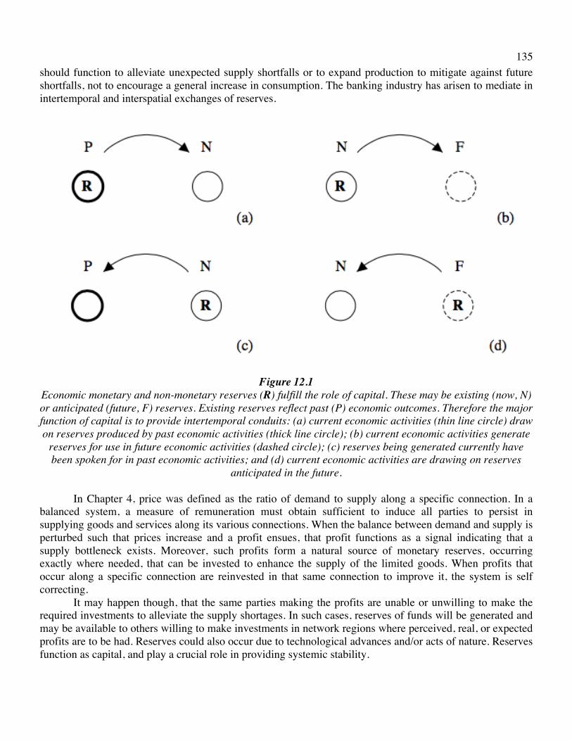
135 should function to alleviate unexpected supply shortfalls or to expand production to mitigate against future shortfalls, not to encourage a general increase in consumption. The banking industry has arisen to mediate in intertemporal and interspatial exchanges of reserves.

Figure 12.1

Economic monetary and non-monetary reserves (R) fulfill the role of capital. These may be existing (now, N) or anticipated (future, F) reserves. Existing reserves reflect past (P) economic outcomes. Therefore the major function of capital is to provide intertemporal conduits: (a) current economic activities (thin line circle) draw on reserves produced by past economic activities (thick line circle); (b) current economic activities generate

reserves for use in future economic activities (dashed circle); (c) reserves being generated currently have been spoken for in past economic activities; and (d) current economic activities are drawing on reserves

anticipated in the future.

In Chapter 4, price was defined as the ratio of demand to supply along a specific connection. In a balanced system, a measure of remuneration must obtain sufficient to induce all parties to persist in supplying goods and services along its various connections. When the balance between demand and supply is perturbed such that prices increase and a profit ensues, that profit functions as a signal indicating that a supply bottleneck exists. Moreover, such profits form a natural source of monetary reserves, occurring exactly where needed, that can be invested to enhance the supply of the limited goods. When profits that occur along a specific connection are reinvested in that same connection to improve it, the system is self correcting.

It may happen though, that the same parties making the profits are unable or unwilling to make the required investments to alleviate the supply shortages. In such cases, reserves of funds will be generated and may be available to others willing to make investments in network regions where perceived, real, or expected profits are to be had. Reserves could also occur due to technological advances and/or acts of nature. Reserves function as capital, and play a crucial role in providing systemic stability.

136 Credit

Banks, other financial institutions, and exchanges are enterprises that draw primarily on reserves. In the case of lending institutions, credit is created and offered as a product (like textiles, footwear, or metal products) to consumers. Numerous forms of credit exist and the distinction between credit and capital often seems unclear. Here, I suggest the following interpretation. Reserves constitute capital and the tokens created to monetize this capital exactly represent financial capital. Possessions that are in use are not reserves. When tokens are created to monetize such possessions, credit is generated. In some cases, tokens are created against anticipated reserves and/or possessions and these also constitute credit. Thus, the generation of more tokens than can be accounted for by extant reserves, whether as multiples of existing reserves, as monetization of possessions, or in anticipation of future reserves, or a combination of thereof, creates credit. Credit is a product with no existing reserves to back it up, but can nevertheless be a product (loosely) derived from current or future reserves. All types of token creation create money to the extent that they are all perceived to carry reciprocity. However, capital is more solid money. Regardless of how they were created, the tokens themselves will be indistinguishable, fungible, and have the same effects when pressed into use in the system. Therefore, credit must be included in estimates of the money supply. However, because of differential provenance, the consequences of credit generation, as opposed to capital generation, will be different.

Discussion and conclusions

This chapter gave a brief outline of the history of money, emphasizing the role of money in serving as tokens of requirements; it also addressed the need to reciprocate in order to give any request traction, hence to give tokens ‘validity’ when the validity is not built-in. Tokens for use by an economic agent are created by an intermediary and their number is determined through an assessment by the intermediary about the likelihood that the agent receiving the tokens would reciprocate. The likelihood that the agents receiving the tokens would reciprocate is dependent on their possession of current reserves or the likelihood of their possession of future reserves. It is recommended that tokens fully backed by existing reserves be called ‘capital’ and tokens be considered ‘credit’ otherwise. In general, requests and reciprocation enter the intertemporal domain.

Because credit can be backed to a greater or lesser extent by anticipated reserves, credit can, to that extent, sidestep reciprocity and harbor special risks. Standardization of tokens is therefore a problem, and to some extent this is alleviated by making tokens convertible. However, the inappropriate creation and allocation of tokens could hamper economic activities or improperly stimulate them.

The account of money exposed here has much in common with Spahn’s (2007: 150) view of money as a social bookkeeping device. Tracing it through the works of Galiani, Marx, Schumpeter and others, he asserts that money: “… records the value of market agents’ contributions to the national product and, at the same time, documents the ‘justification’ of its bearer to demand goods and services.” However, there may be some points of difference between Spahn’s views and my own. First, Spahn appears to emphasize reciprocity - it’s a priori existence would induce the asking and granting of requests. However, I view asking as the primal act and reciprocation as following. When reciprocation is forthcoming, subsequent requests are fortified. Thus, once established, reciprocation facilitates further exchanges in the way Spahn seems to conceptualize it. Second, Spahn (2007: 161) considers the basic flaw of money as bookkeeping device to reside in the required centralized bookkeeping process. I think that bookkeeping can be performed locally by intermediaries, but this creates the need for bookkeeping standardization and standard enforcement. Admittedly, the problem is shifted from centralized bookkeeping to centralized standard-setting and enforcement, but this trade-off may be useful. Third, Spahn (2007: 161) is also troubled by the acceptance of tokens based on backward-looking to the bearer having earned them as opposed to the acceptance of tokens based on trust, thus forward-looking to the bearer providing payment. I think both of these occur – when

137 tokens are created on the basis of reserves (i.e., capital) it is backward-looking and when based on future reserves or unsecured (i.e., credit), it is forward-looking.

The use of existing reserves for token creation is less problematic than the use of anticipated future reserves. It therefore could be questioned whether the use of anticipated reserves should be permitted at all or only where sufficient skill can be demonstrated. Nevertheless, if money is created from asking, and then only if the applicant already has sufficient reserves to serve as security, one may ask how any reserves arise to begin with – how do the first funds enter the system? If some reserves are accepted to pre-exist naturally (i.e. they existed before humans and economic systems came into being) and others are accepted to arise fortuitously from natural events, then mere asking is sufficient, but not efficient, in getting the system going and keeping it going. The system gains in efficiency when lending institutions provide tokens to represent reserves that a borrower has or shares of reserves that a borrower may use. This is not because bartering is sidestepped, but because most components (i.e. ‘players’) in the system are freed from the necessity to continually assess the creditworthiness of partners, customers, and clients, and to furnish proof of their own.

At this point, it also becomes possible to provide an answer to the question of why capital is scarce (e.g. Spahn 2001: 34). Products and reserves are scarce relative to requirements, especially non-needs requirements, which are in principle infinite. Products and reserves are scarce because they are also finite in extent, or can be exploited only at a finite rate, or are subject to decay and loss (or all of these) while requirements are less constrained in growth. Furthermore, monetary reserves can only accrue along connections where supply constraints have arisen and profit is to be had. As pointed out above, system-wide supply constraints will only lead to inflation or a change in the absolute price levels (see below). System-wide increases in price levels will consume any profits that may otherwise exist so that monetary reserves cannot accumulate except if the relative rise in prices along one connection exceeds the rise in prices on average over other connections (i.e. exceeds the general or overall inflation rate). Thus the question of why capital is scarce becomes clear when reserves are seen as capital: population increases will keep reserves low and requirements high, but, conversely, population decreases may free assets up to serve as reserves.

Relatedly, one could also ask why money is scarce. This question may be all the more baffling if money, in essence, is a request for products or reserves. However, if such requests are granted based on the existence of the perceived reserves or the anticipated reserves of the requestor, money availability will also be limited compared to requirements and money will be scarce. Hence money is an accounting device in aggregate as well. If the money supply is not limited and increases system-wide, money will be neutral if apportioned between requirements in the same manner as before because neither requirements nor the supply of products and the existing reserves would have changed materially (excepting transient effects). Thus relative prices will not change, but absolute prices will change and do so in the absence, excepting transient effects, of growth. If money is apportioned between requirements in a different manner than before, subsequent to a system-wide increase in the money supply, money will not be neutral. This is because, for example, some money is now allocated to wants or aspirations that received no allocations before. If existing resources have not changed materially, relative prices will change because the expression of relative demands via tokens has changed and stimulate relative growth. Thus, care should be taken to differentiate the condition where the money supply increases systemically without changes in requirement allocations from the situation where the money supply increases systemically with changes in requirement allocations.

An interesting observation here is that the determination of the volume of tokens needed, based on caloric intake, is reminiscent of Ricardo’s corn model. Assigning 100 atomic tokens to represent average adult daily needs (e.g. based on a daily intake of 2000 calories) and estimating the level of other requirements in terms of needs allows one to calculate how many tokens to permit in the economy. Assuming token creation occurs this way, one could analyze wages and labor based on token flows, tokens being defined in terms of calories (i.e. Ricardo’s corn counterpart). Furthermore, the effects of wage redirection could be analyzed in terms of asymmetric flows between different population strata as shown in Figure 12.2. This

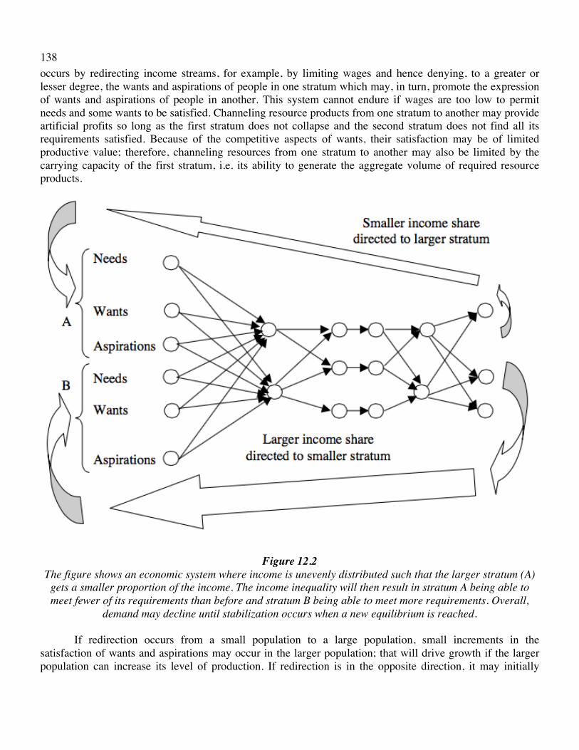
138 occurs by redirecting income streams, for example, by limiting wages and hence denying, to a greater or lesser degree, the wants and aspirations of people in one stratum which may, in turn, promote the expression of wants and aspirations of people in another. This system cannot endure if wages are too low to permit needs and some wants to be satisfied. Channeling resource products from one stratum to another may provide artificial profits so long as the first stratum does not collapse and the second stratum does not find all its requirements satisfied. Because of the competitive aspects of wants, their satisfaction may be of limited productive value; therefore, channeling resources from one stratum to another may also be limited by the carrying capacity of the first stratum, i.e. its ability to generate the aggregate volume of required resource products.

Figure 12.2 The figure shows an economic system where income is unevenly distributed such that the larger stratum (A)

gets a smaller proportion of the income. The income inequality will then result in stratum A being able to meet fewer of its requirements than before and stratum B being able to meet more requirements. Overall,

demand may decline until stabilization occurs when a new equilibrium is reached.

If redirection occurs from a small population to a large population, small increments in the satisfaction of wants and aspirations may occur in the larger population; that will drive growth if the larger population can increase its level of production. If redirection is in the opposite direction, it may initially

139 generate very high profits that saturate at some level and then start to decline. This happens because redirection from a large to a small population will first cause reserve depletion and then lead to a reduction of tokens available to express all the requirements of the larger population (i.e. a loss of demand) that cannot be compensated for by the commensurate increase in tokens in the smaller population because its requirements cannot increase sufficiently. Thus, depending on the sizes of the inequalities and the populations involved, income inequalities may stifle growth by causing insufficient demand as claimed by Sismondi (see Vaggi and Groenewegen 2003: 122). Furthermore, the levels of income inequalities that different economic systems can sustain, may vary. Extracting profits from the system through income redirection may therefore be ultimately self-defeating because it could cause changes in demand and hence precipitate economic instabilities as discussed in the next chapter. Marx’s view (e.g. Vaggi and Groenewegen 2003: 168) that the capitalist system has a built-in conflict appears consistent with the preceding analysis if one admits profit seeking by means of income redirection to the definition of capitalism.

140

Advanced Topics

141

13

Interactions Between Networks Produce Economic Cycles

142

Interactions Between Networks Produce Economic Cycles

Summary

Interactions at a global level can occur directly between the demand- and supply-side networks because the output of one network serves as a target for the output of the opposing network. Therefore, any environmental, population, or internal factor causing a change in the output of one network will require the complementary network to adjust. However, the output of the complementary network, before and during its adjustment, will still serve as target for the network experiencing the initiating change. It will therefore also try to adapt to regain its previous level of output. This implies that two networks, initially at equilibrium, will adjust in opposite directions after the occurrence of a disturbance - setting into motion an oscillation. The generation of such oscillations provides some insight into the nature of economic cycles. Global imbalances can also be traced back along the individual connections of both networks. Therefore, at a local level, mismatches must occur between demands and supplies along some connections. Where a mismatch occurs along a particular connection, profits and losses arise. Consequently, profits and losses are to be seen as local error signals and indicators of stressed connections. Profits are also a natural source of investment capital arising precisely where it is needed in a system; conversely, losses drain capital from connections where too much exists. Finally, interactions at a global level can occur indirectly between the demand- and supply-side networks when effects are propagated to the other network via either the population or the environment, or both. Because of direct and indirect interactions between complementary networks, as well as connections with other (e.g. public) systems, the interactions between networks can assume a considerable range of complexities.

143 Introduction

Up until now, I have been discussing the basic components of a model of an economic system, refining them, and adding to them. This has created a fairly sophisticated and comprehensive visual model that is very rich in its implications. The model is backed by enough mathematical pointers to permit, with some knowledge, insight, and creativity, the generation of a mathematical equivalent. Indeed, an ANN can be described by a mathematical equation (for examples, see Tsoi and Back 1997: 193-199); thus the two networks of a private sector and the two networks of a public sector can be represented mathematically. To this one needs to add a mathematical description of the interface between private and public sectors and a mathematical description of the circular flows pertaining to each of the private and public sectors. Finally, one needs to show how the two networks comprising a core system interact. I start this chapter with a description and analysis of the latter interface, but in this section of the book, I also want to address systemic effects and how they arise from interactions between networks. The first chapter in this section, because it addresses the interface between the two networks of a core system, will also consider the dynamics of their interactions via this interface. Here questions about economic cycles arise. The second chapter deals with interactions between two notionally independent economic systems, thus permits one to consider aspects of international trade.

Moving now to the topic of this chapter, let us consider interactions between the two networks of a core system. Ideally, some equilibrium is reached between the SSN and the DSN. This search for equilibrium is not an emergent economic imperative, but derives from a psychological one. Basically, it is an attempt to satisfy requirements with resources. Some of the latter derive from the environment and some from the individual. At a primal level, the forager uses self-supplied labor to search the environment for other resources that would satisfy his/her requirements. Because the labor is self-supplied, it is costly in terms of effort, hence in terms of discomfort. Likewise, requirements derive from the self and are costly in terms of discomfort if they go unsatisfied. Thus an optimum exists where a sufficient amount of labor must be expended to meet the most pressing requirements. Even with plentiful energy and semi-automated labor, some effort is required to meet one’s requirements. The search for equilibrium also derives from the environment. Careless exploitation of the environment may cause resource depletion and increase the level of discomfort when the desired resources are no longer available. At the very least, the environment cannot be overexploited; more likely, it requires husbandry. Here too, a balance is necessary. The balance therefore becomes manifest as one between what the ongoing population requirements are and what the population and environment can deliver on an ongoing basis as resources.

Thus, both the DSN and SSN are dynamic systems that respond to input and target changes. Such changes can arise, broadly, from the environment, from the population, from other networks (e.g. public sector networks), and from the complementary network. But, if input and/or target changes cause the two networks to become disequilibrated, how do they restore balance? Which network should make all or most of the adjustment(s)? Attempts to answer these questions allow us to address the causes of economic cycles and economic growth.

Disequilibrium causes network errors

Network error. Consider now, for example, a stimulus originating from the environment that triggers an adaptation response. Imagine this adaptation stimulus to be the result of an environmental change, such as a drought, that causes a failure of the wheat harvest. Wheat and derivative products now become, relative to previously balanced levels, scarce. Hence the demand for wheat-based products will now exceed the supply of such products. This difference between products demanded and products supplied constitutes an error where the size of the error is the size of the difference between demand and supply. Because both networks experience an error in their output, they will attempt to reduce the error through adjusting their various

144 network weights. This constitutes the primary adjustment process (with the secondary adjustment process consisting of node addition or deletion).

The overall error for any network (e.g. Levine 2000: 83; Sumpter and Noid 1996: 232) is generally defined as

Eq. 13.1

The actual amount by which the weight of a given connection in a network is adjusted depends on the negative of the rate of change, that is, the negative of the derivative of the error with respect to the local activation of the network. This adjustment amount can further be weighted by a ‘learning rate’ to make the adjustments smaller and less violent, or larger and faster. Additionally, short-term fluctuations that may otherwise destabilize the adaptation process can be counteracted by including a ‘momentum’ term in the current adjustment (i.e., a fraction of the adjustment made to a given weight previously is added to the newly calculated weight). The interested reader is referred to the literature for details on backpropagation and other optimization methods for neural networks (e.g. Baldi 1995: 184-188; Rumelhart et al. 1988: 330).

The network error, stated here in terms of the economic networks, is the squared difference between the demand for a given product and the supply for that product, summed for all products. That is

Eq. 13.2

Thus, for the DSN

Eq. 13.3

where ‘demand’ is calculated as explained in Chapter 3. For the SSN

Eq. 13.4

where ‘product’ is calculated as explained in Chapter 2. Note that the calculated values of the errors would be identical for both networks because of the squared term, but that the inner terms are reversed. Thus, the output of one network serves as the target for the complementary network and vice versa. In terms of the model, Eq. 13.2 defines the equilibrium error (EE) of the economy and it can be specified with regard to both the private and public sectors. In other words, an economy with both public and private sectors has two EEs that could be consolidated into a single systemic error (SE) for that system.

Network oscillations. It is now clear that if one network has an error the other network also has an error: identical in size, but opposite in direction. For example, for one network, demand is too high, for the complementary network, supply is too low. Because the EE applies to both networks equally, both networks would adjust to this error, but not necessarily in synchrony. In other words, due to different network sizes, different learning rates, and different momentum terms, the rate of adjustment in one network may be faster than that of the other.

However, it is instructive to consider what would happen if both complementary networks were nearly identical and the system had a high degree of symmetry. In such cases, the adjustments should occur nearly synchronously. Because one network experiences too high a demand, it will reduce demand to meet available supplies. The other network, because it generates too low a level of supplies, will increase production. If both networks are successful in making rapid adjustments, the system will overshoot the new equilibrium position. This happens because both networks adjusted to the full error rather than to half the

145 error. Consequently, there will now be too low a demand, and too high a level of production. More concretely, if there is a shortfall of one unit between supply and demand for a given product, the SSN will adjust to increase the supply of the given product by one unit while the DSN will adjust to reduce the demand for the given product by one unit. Had only the SSN adjusted, the shortfall of one unit of the given product would have been eliminated. Because the DSN also adjusted, there is now an oversupply of the product that was previously in short supply.

From a technical perspective, the origin of the oscillations that affect the coupled system, consisting of the two networks, can be seen from Eq. 13.3 and Eq. 13.4: the output of one network is the target for the other and vice versa. Thus, when one network adjusts its output, it actually changes the target that the other network is trying to hit. The other network will then adjust its output to meet the new target, but in so doing, changes the target for the first network.

The important outcome of this analysis is that it reveals inherent instabilities in core systems comprised of adaptive subsystems. Therefore, irrespective of how well a network could adjust to the size of the error, even if it adjusted perfectly in a certain amount of time, one must reckon on the occurrence of core system oscillations. It is interesting to consider the consequences of this chaotic system, why it should have evolved this way, what the benefits of these oscillations may be in terms of survival of the system, and ways to mitigate extreme oscillations. Specifically, it is interesting to consider whether these oscillations contribute, at least in part, to economic cycles. If so, it would also be of interest to consider those factors that may constitute and determine the learning rates and momentum terms of the networks and how they could be used to moderate oscillations.

Profits and losses are error signals. In the adaptive process of traditional (i.e. backpropagation) ANNs, the network error is backpropagated through the network in order to adjust the weights of the different connections. Because, the network error becomes manifest at a given connection in some form (e.g. Rumelhart et al. 1988: 327), the weight of that connection can be changed in such a manner that the network’s subsequent performance is improved, that is, the network error is reduced. This local manifestation of the backpropagated error appears in the economic realm, depending on the nature of the error, as either a profit or loss (as seen from the supply-side) and, correspondingly, as either a rip-off or bargain (as seen from the demand-side). Thus when profits or losses arise at nodes along some connections due to demand and supply being out of balance, they are backpropagated errors that provide information about the way in which the connections of an economic network should be adjusted to restore balance.

For example, if the demand is greater than the supply, there is a profit that will occur along one or more connections from the demand origin (e.g. from needs, wants, or aspirations or a combination of them) to the supply origins (land, labor, or capital or a combination of them). That is, at some nodes situated along these connections funds will begin to accumulate (see below). From the point of view of supply-side entities (e.g. manufacturers), profits may occur. From the point of view of demand-side entities (e.g. consumers), there will be a loss of funds. Of course, when supply exceeds demand, the situation in general is reversed, and enterprises along some connections that carry excess supplies stand to incur losses while consumers are likely to find bargains (i.e. ‘gain’ funds). Moreover, when demand of a given product exceeds supply and prices rise, consumers will tend to curtail spending on that product to preserve their funds while enterprises will tend to expand the production of that product (and when both happen more or less simultaneously, the system will overshoot the point of equilibrium). Therefore, just as connection weights in ANNs are adjusted locally or individually, profits and losses can lead organically to local adjustments with global outcomes.

However, there is a detail pertaining to economic networks that differs from those of traditional computational neural networks. In traditional ANNs, nodes are considered fixed entities, and if not, they exhibit discontinuous attributes in the sense that they can be added (appear) or pruned (disappear) but generally do not change their characteristics over time. In contrast, each individual node in an economic network is also a dynamic entity that can decay through obsolescence or improve its performance through

146 technical innovations. Where a decay occurs and performance is compromised, a local excess in demand will occur leading to profit arising where the stress is present in the system. It has been pointed out before, but bears repetition, that this is a natural adaptive response – capital, in the form of profits, arise exactly where capital needs to be invested to relieve the stress. It is also likely that a change in local network performance will affect the network’s output, and hence, as explained above, change the target of the opposing network with consequent triggering of oscillations.

Simple and complex disequilibria

Noting that interactions between networks can produce disequilibrium, one may wish to examine the nature of such disequilibria. Here I want to draw a distinction between disequilibria that occur as a result of the interactions of free or unconstrained networks and those that occur as a result of interactions between networks where at least one of them is constrained.

Simple disequilibria. Simple disequilibria involve two or more networks that are free to adjust in any manner to minimize their EEs. The preceding example explained disequilibrium in terms of a private sector system, isolated from other systems, thus interactions involved two free and autonomous networks. This is probably the simplest type of disequilibrium. When two such systems interact, as might be the case with international trade, a bigger, but essentially similar, system is created (as explained in the following chapter). Hence disequilibria that occur between these interacting systems, although they now include four or more networks, are still to be seen as simple disequilibria.

Complex disequilibria. Complex disequilibria occur where at least one of the interacting networks is constrained by environmental or population factors (e.g. governance, customs, climate, etc.). For example, the most elementary complex disequilibrium arises in an economy that consists entirely of an isolated public sector system. In such a case the forces of supply and demand are not free to adjust to equilibrium values, but are affected by social factors leading to market intervention and/or legislation. Thus a layer is added to the system, increasing its complexity. Furthermore, this layer may be difficult to model or predict because political factors and intervention characteristics need to be understood and specified. The resulting complexity will, in general, require more adjustments between more interacting components, leading to chronic, prolonged, or amplified disequilibria.

For example, two general problems arise with public systems and public interventions: those making decisions need to be well-versed in divining economic signals of disequilibrium that are not communicated by the relatively effective forces of the marketplace; and those making decisions need to be well-versed in divining economic remedies for disequilibria that cannot be righted by the relatively effective forces of the marketplace. Furthermore, it is unclear how frequent and/or abrupt changes of policy and/or implementation procedures will contribute to stability. Like social factors, environmental factors too would have constraining and unpredictable components, but perhaps qualitatively different from social ones. The complexity of disequilibria are further enriched in a national economy where private and public sectors interact, and even more so where multiple national economies with different natural and social environments are mutually engaged.

Indirect interactions

By virtue of circular flows (see Chapter 11), interactions between all of the networks involved in an economic system can also occur indirectly. The easiest way to gain an appreciation of indirect influences, but not the only route whereby indirect interactions between networks can occur, is to consider interactions by way of the population, specifically, the wage-earning component of the population. This component of the population may have some independence and act in a concerted fashion, for example by way of trade unions, to demand higher wages. In a system or along connections where profit does not arise, one of two consequences, or a combination of them, must obtain if such demands are granted: (i) the increase in costs

147 must be passed on to the consumer, or (ii) or wages must be redistributed by reducing those of some wage earners to compensate for the increases of others. In the event of profit, a third option, namely that of depleting the profit becomes available. Note the implication that the economy will then be deprived of new investments to compensate for demand-supply imbalances that are giving rise to the profit in the first place.

In every one of these cases, other networks will be affected. In the first case, a direct effect ensues as a result of the price increase because it amounts to an effective reduction in supply of the same goods (at the previous price). In the second case, income streams are redirected and will affect other networks. This effect was pointed out in the preceding chapter: changed incomes for different groups may force changed token allocation to requirements thus causing changes in effective demand. This is an indirect effect. In the third case, pertaining to profit siphoning, adaptation in the network experiencing stress is prevented, and the adaptation is forced, in whole or in part, on to other networks.

Indirect effects can therefore be characterized as those that do not occur along the interface between the two complementary networks of a core system (the locus of the ‘tertiary market’), but along those other pathways where flows occur from one network to the other via an environment or a population (e.g. Figure 13.1).

Discussion and conclusions

Numerous factors such as government actions, credit creation, environmental shocks, population dynamics, and others, can disturb a network. Because networks are individual, largely autonomous, but adaptive systems, interactions between them, triggered by a disturbance in one network, could be complex and give rise to economic dislocations. Furthermore, in order to overcome these dislocations, modifications to internal network components will be necessary to adapt network outputs to present conditions. Profits and losses occur where these modifications are required while their sizes indicate the degrees of stress, thus the urgencies and extents of the required adjustments.

Regarding the adaptation process, one must first ask what could affect a network’s output. The output is generally dependent on three things: the input, the internal processing by the network, and the target for the output. Thus, for the DSN, the output is a function of requirements, the availability of tokens and the conversion of requirements into demands, and the levels of available supply-side products; for the SSN, the output is a function of resources, production processes, and demand. Requirements, to the extent of their dependence on demographics, and resources, to the extent of their dependence on the environment (weather, metallic deposits, etc.), are to some extent independent. In other respects, requirements and resources are indirectly dependent because they influence each other indirectly through wages and rents and consumed goods and services. Furthermore, internal processing by the networks is independent; token creation via credit and token allocation to express requirements can occur far more rapidly than production and production capacity can be expanded. Differential inertia for networks also derives from the momentum of error adjustment (analogous to the momentum term), the number of connections that have to be adjusted, and the rate at which processing at a node can be changed. Consequently, the DSN and SSN may adjust their outputs at different rates: “…it is recognized that the economic dislocation resulting from the fact that goods markets adjust more slowly than financial markets will result in real dislocation” (discussion of monetary control policies, original emphasis, O’Brien 1995: 63). Finally, demands and supplies are directly related because the level of one is a target output for the other, thus a change in one would affect the other.

The foregoing indicates that economic disturbances could occur due to any change of input, processing, or target. However, it does not matter through which route a particular network’s output is affected; other networks in the system will attempt to adjust to the change. A second question that now arises is whether these disturbances have an inherent frequency or whether they are erratic. In my view, small changes in output may be of the erratic sort, that is, they do not precipitate oscillations. Clearly, if an imbalance arises with regard to a relatively small subset of supplied products or a relatively small subset of

148 demanded products, any tendency to an oscillation will get dampened by adjustments that occur along other connections. Therefore, if the requirement is an adjustment in production, but not production capacity, oscillations are not likely.

In contrast, when a large enough imbalance occurs, system-wide oscillations are set in motion. Assuming that a sudden increase in demand occurs for a specific high-value product, entrepreneurs will perceive that supplies of that good are constrained locally and that investments to generate new production capacity will be profitable. Entrepreneurs may therefore request credit and put this to use to increase production capacity to meet this primary demand increase. Therefore, tokens are injected into the economy. The tokens eventually make their way to the SSN input nodes as wages and rents. These incomes circulate back to the input nodes of the DSN via the population. Importantly, however, redistribution of tokens to the DSN input layer is likely to involve a reallocation of requirements. In other words, the recirculated tokens are not used exclusively to obtain more of the original high-value product, but may now be allocated to other products, giving rise to secondary increases in demand. Thus, a second round of investments, but now to increase production capacity of other products as well, is triggered. This process is illustrated in Figure 13.1.

Because production capacity increases take substantial time to implement, they will lag demand increases. In this intervening period, demand my change. Furthermore, unless production capacity increases are accurately estimated, a mismatch between demand and supply will result. This is very likely if several entrepreneurs, acting on the same of data, but without sufficient local knowledge and coordination, attempt to expand production capacity to meet the same demand increase. The augmented production capacity will therefore potentially exceed the increased demand several-fold. Thus while demand is potentially being adjusted downward (due to shifting priorities, reallocation to substitutes, loss of interest, etc.), increased production capacity comes on-line leading to a large, near step-wise increase in supplies of the erstwhile limited-availability high-value product. The adjustment process now reverses. Because production exceeds demands by a substantial margin, prices fall, enterprises go bankrupt, debts cannot be serviced and have to be written off thus withdrawing tokens from circulation. Incomes are reduced, and the reduced incomes are reallocated according to new priorities.

A follow-up question that arises is how severe these oscillations could be, that is, are there extremes or limits to them? I suggest that there are two types: hard limits and ‘levels of resistance’, to borrow a technical trading term. The hard limits pertain, on the downside, to wholesale destruction of one or both of the environment or population, and, on the upside, to a condition where all requirements are fully satisfied. The levels of resistance pertain to those cases where demand is compressed from aspirations to wants, with a stronger resistance occurring when compressed from wants to needs. Finally, the compression of needs (food, shelter, utilities) should be the most difficult because it puts the survival of the population at risk. Clearly, cyclical contractions are first likely to affect aspirations, then wants, and last needs. These levels of resistance may determine, therefore, how far any contraction proceeds. I suspect a similar argument holds for resources in that capital (i.e. reserves) losses would tend to occur before labor reductions and that labor reductions would tend to occur before ‘land’ dispositions.

Taken together, oscillations will be triggered when central authorities act system-wide to enact policies or when a sudden availability or loss of substantial resources (e.g. gold and silver, land, oil, credit, etc.) occurs. Likewise, when market agents adjust simultaneously (but unaware of each other or in competition with each other) to changes, attention is focused on some products or resources. Consequently, they may suddenly change to much higher or much lower levels, precipitating oscillations potentially augmented by secondary effects due to the shifting and reallocation of incomes.

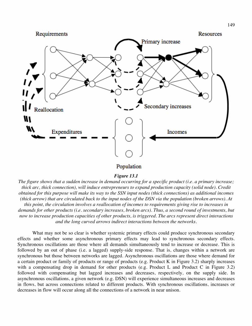
149

Figure 13.1

The figure shows that a sudden increase in demand occurring for a specific product (i.e. a primary increase; thick arc, thick connection), will induce entrepreneurs to expand production capacity (solid node). Credit

obtained for this purpose will make its way to the SSN input nodes (thick connections) as additional incomes (thick arrow) that are circulated back to the input nodes of the DSN via the population (broken arrows). At

this point, the circulation involves a reallocation of incomes to requirements giving rise to increases in demands for other products (i.e. secondary increases, broken arcs). Thus, a second round of investments, but now to increase production capacities of other products, is triggered. The arcs represent direct interactions

and the long curved arrows indirect interactions between the networks. What may not be so clear is whether systemic primary effects could produce synchronous secondary

effects and whether some asynchronous primary effects may lead to synchronous secondary effects. Synchronous oscillations are those where all demands simultaneously tend to increase or decrease. This is followed by an out of phase (i.e. a lagged) supply-side response. That is, changes within a network are synchronous but those between networks are lagged. Asynchronous oscillations are those where demand for a certain product or family of products or range of products (e.g. Product K in Figure 3.2) sharply increases with a compensating drop in demand for other products (e.g. Product L and Product C in Figure 3.2) followed with compensating but lagged increases and decreases, respectively, on the supply side. In asynchronous oscillations, a given network (e.g. DSN) will experience simultaneous increases and decreases in flows, but across connections related to different products. With synchronous oscillations, increases or decreases in flow will occur along all the connections of a network in near unison.

150 Reallocation of incomes in conjunction with credit expansion suggests follow-on effects will tend to

be synchronous while reallocation of incomes in conjunction with no credit expansion suggests follow-on effects could be asynchronous. The first occurs because enough new tokens are available for allocation to additional requirements; the last occurs because the same number of tokens has to be reallocated and thus may actually involve the expression of fewer requirements (i.e. because one with a high priority is now more costly to satisfy, thus others have to be foregone). Either way, an important conclusion to draw here is that economic dislocations can follow from either a large network-wide disturbance, or from a sufficiently large localized disturbance that spreads systemically through the induction of secondary effects.

Means to overcome economic dislocations can also involve internal modifications and these are apt to occur along connections that were put under stress as a result of the dislocations. Profits and losses are symptoms of explicit stresses and indicate where modifications should occur. Specifically, profits are indications of supply deficits and investments constitute responses to profit generation. Losses, by and large, are indications of supply surfeits and production cutbacks constitute responses to losses. This interpretation suggests that the application of profits arising in one part of a system to effect modifications in another (i.e. unrelated) part constitutes an investment misallocation. Technical innovations, too, are responses to stresses and will contribute to internal modifications.

Either local or system-wide increases in money supply will engender internal modifications whether demand shifting occurs or not. I have pointed out before that inflation, in its early stages, will generate economic growth. This is because it will appear initially as if local opportunities for profit exist. That is, it will appear to local entrepreneurial agents that supplies are constrained locally and that investments to generate new production capacity will be profitable. Entrepreneurs may therefore request credit, a demand for money different from money demand for trading purposes, and put this to use to increase production capacity. However, since these supply constraints are not local, but widespread, widespread investments will occur, hence a system-wide phenomenon of growth. If growth is widespread due to increased demands, price rises may also be widespread and will reduce the returns on investments. At some point, if prices rise too rapidly, economic agents will perceive that it is more advantageous to increase prices than to expand production. This is because rapid rises in prices increase their costs, reduce their relative advantage, and erode their returns before their investments can be recovered. Thus money neutrality increases when the returns on investments decrease until, at the point where investments cease, money neutrality is reached. At this point, increases in the money supply will simply lead to proportional increases in prices.

Traditionally, the question about the neutrality of money was framed in terms of its short-run or long-runs effects (e.g. Blaug 1995: 30, 41-44). An important consequence of internal modifications arising from profits is that money is not neutral if the money supply increases at a rate slower than supply-side adjustments can occur. If the money supply increases at faster rates, money is neutral. Given that inflationary pressures typically build up over time from low levels, money would appear not to be neutral in the short run. In contrast, rapid inflation does not typically occur de novo overnight, thus the neutrality associated with high rates of growth in the money supply would likewise appear in the long run. Nevertheless, it should be clear here that it is not the short run or long run that demarcates the neutrality of money, but the rate of increase in the money supply relative to the rate(s) of supply-side capacity increases (modulated to some extent by demand shifting).

It is possible, at this point, to also address the rate of profit in incipient form. Because all participants in the economy are entitled to their remuneration, the latter determined by levels that promote optimal stability in the system, extracting profits by income redirection or resource depletion is here considered aberrant. Therefore, the rate of profit as seen here deviates from that as defined by Ricardo (e.g. Vaggi and Groenewegen 2003: 139) and Marx (e.g. Vaggi and Groenewegen 2003: 168), although, as observed before, concerns about exploitation-generated instabilities are shared with Marx.

151 The rate of profit, r, is the net aggregate demand (D - S) expressed as a fraction of total aggregate

demand, D. Specifically

Eq. 13.5 where S is the aggregate supply and rf is the rate of inflation. In practical terms, demand is taken to be effective demand, which is demand expressed by way of tokens. Therefore, demand is a function of population (affecting mostly the number of requirements), education (affecting mostly the types and distribution of requirements), and, as explained above, money supply (i.e. non-neutral conditions). Supply, on the other hand, is a function of obsolescence (this includes innovation) and resource quality (e.g. growth, discovery, depletion, and so on). Note that if equilibrium can be established and all the factors contributing to net aggregate demand are stable, the rate of profit will be zero. Because the contributing factors vary, the rate of profit will therefore depend on their natural fluctuations, hence a natural rate of profit arises as an average of these fluctuations. The natural rate of interest, furthermore, is seen as being constrained by an upper boundary set by the natural rate of profit. General uncertainty and capital scarcity may cause the natural rate of interest to vary within the range set by the upper and lower bounds of the rate of profit. Interestingly, rising prices imply an increase of demand relative to supply, and, by extension, an increase in net aggregate demand. Consequently it follows via Eq. 13.5 that rising prices under non-neutral money supply conditions will be associated with rising rates of profit. Thus, rising prices could very well provide scope for rising natural interest rates by expanding their upper boundary, but also by creating uncertainty and capital scarcity.

Some of the other inherent dynamic aspects of networks are also of interest. Because economic entities are administered by humans, internal modifications are complicated by a running together of individual and administrative dictates. What this means is that local economic adjustments may be influenced, despite ethical and regulatory requirements, by individual requirements independently of the contributions of these requirements to aggregate demand (i.e. via the requirements layer of the DSN). Specifically, at the individual level, wants may be unsatisfied because of unstable status hierarchies. Therefore, profits may be spent to support individual wants, but at the corporate level. The latter condition occurs because the newly generated profits, especially if distally distributed, may be entrusted to persons who are inclined to use them in a manner that satisfies their own wants (i.e. status) due to the loss of fiduciary focus. Barnes (2009: 43) points out that risk-protection can lead to a separation between the interests of management and owners. Managers make the operational decisions. Except under unusual conditions, risk-taking does not enter into needs (these are too personal and too important) or aspirations (these generally are too civil-minded), but are related to competition for mates, or more proximally, status. Managers taking risks to satisfy their wants are not dissimilar to bus drivers engaging in competitive racing while carrying passengers. Where important components of the system are at risk, such competition should be absent. Therefore, especially under conditions where adverse personal outcomes are muted, the status-conscious high-achiever is not the right person for positions that are of structural importance, even if their interests can perhaps be aligned with those of society at large. This Minskian fragility (e.g. Tse 2001: 80) results from the wrong persons having stewardship of critical components of the economic system. Whether a system can be designed to align interests and harness energies much better, is an open question.

In conclusion and taken together, networks are adaptive systems, constantly adjusting to each other in the core system’s attempts to reach equilibrium. That notions of equilibrium or the existence of natural levels of economic variables arose in economic discourse (e.g. Turgot, Smith, Walras, Marshall, Wicksell, Pareto) are therefore to be expected. However, networks are adaptive systems also embedded in dynamic environmental and population contexts, thus fluctuations and disturbances that upset equilibrium are frequent. Moreover, attempts to restore that equilibrium may itself generate economic oscillations. That disaffection with notions of equilibrium arose (e.g. Sismondi, Marx, Menger, Pigou) is therefore not

152 surprising. Finally, networks are also dynamic systems capable of organic change, leading to innovation, obsolescence, growth, and decay. Thus the range of views accommodated here can be rounded out with those views emphasizing economic phenomena of an organic nature as well (e.g. Schumpeter, Keynes).

153

14

International Trade and the Interactions Between Systems

154

International Trade and the Interactions Between Systems

Summary

International trade rests on domestic economies and cannot be considered in isolation from them. Because international trade involves different systems, more than just an interaction between the complementary networks of a domestic core system occurs. Due to this interconnectedness, a perturbation in one network may cause reactions in all the interacting networks. Furthermore, initiating trade may itself induce such perturbations, especially if the exchange of goods and currencies is unbalanced. More specifically, trade causes modifications of relative demands which lead to altered income streams; they, in turn, feed through to a reallocation of requirements that become expressed as shifted demands. These have secondary effects resulting from circular flows, further altering trade and modifying relative demands. The patterns of trade and growth that emerge from international exchanges therefore depend in the main on differential requirements, technologies, and resource endowments, but also on circular flows and network oscillations.

155 Introduction

Modern economics germinated from problems that were brought into focus by bullionism and mercantilism. Bullionism was the view that precious metals represented wealth and provided the state with the ability to dispense of its executive functions. Bullionists aimed to increase the national stock of bullion with measures designed to influence capital movements and current account balances (e.g. Vaggi and Groenewegen 2003: 17). Mercantilism was the tactic used to obtain bullion through trade. Mercantilists therefore viewed the manufacture and export of goods and the provisioning of services to be necessary to engender a surplus in foreign trade and hence the inflow of precious metals in exchange. Mercantilist thought, by focusing not exclusively on bullion, but on the means to obtain bullion by trade, caused the emphasis to shift to production and exchange. By the end of the seventeenth century, bullion was no longer seen as the sole determinant of wealth, but production and production potential were gaining in relative importance (e.g. Vaggi and Groenewegen 2003: 27). Thus international trade came into view and along with it an interest in the causes and patterns of trade and the effects of trade practices and policies on national wealth.

The orthodoxy of international trade consists of three main models, each aiming to explain the determinants of international trade. The comparative advantage theory, developed independently by Ricardo and Torrens in the early nineteenth century (Gandolfo 1998: 3), attributed the emergence of international trade to the existence of trade goods with differential comparative advantages of production in the trading countries (Gandolfo 1998: 11; Vaggi and Groenewegen 2003: 145) and terms of trade strictly between their comparative costs of production (Gandolfo 1998: 11). Thus the classical theory of international trade is one that emphasizes the technological aspects of the supply-side. In present terms, it emphasizes activities performed by the hidden layer of the SSN. In contrast, the Heckscher-Ohlin model attributes the emergence of international trade to the existence of different factor endowments between countries. Countries export commodities which use that country’s differentially abundant factor(s) more intensively (Gandolfo 1998: 65). In this case, the major emphasis is on the input layer of the SSN, or resources. The neoclassical model, which can be traced back to J. S. Mill, acknowledges the importance of both comparative production and factor endowment advantages in international trade, but adds to these the presence of differential tastes in consumer goods between trading countries (Gandolfo 1998: 3). The neoclassical theory is therefore the only one of the three models that also includes aspects of the DSN because tastes become manifest as genetically- and/or culturally-determined patterns of requirement expression.

New theories of international trade relax or dispense with some of the assumptions that the orthodox models rely on; specifically, they do not require perfect competition and/or product homogeneity. In addition, they purport to explain the presence of intra-industry trade and increasing returns to scale. In light of the current context, the orthodox theories can be differentiated from the new models by virtue of their greater dependence on the more global organization of networks such as the relative influence of their layers while new theories rely more on local aspects of networks such as production functions, connection patterns, and number of nodes (i.e. competition, product array).

In contrast to the emergence of modern economics from concerns raised by trade, the sequence is here reversed and international trade can only be considered now that the modeling of domestic economic systems is relatively complete. Market interactions that occur between one or more such domestic systems constitute international trade and it represents an extension to the interactions between individual networks considered in the previous chapter. In my view, therefore, international trade is an outgrowth of domestic economies or a superstructure resting on domestic economies that cannot be considered in isolation. Having affirmed the order between domestic economies and international trade, one can now address the causes and patterns of trade and the effects of trade practices and policies on national wealth.

156 The causes of international trade

Let us start with the simplest possible case, arrived at by considering two economic systems, Systems A and B (or equivalently, Country A and Country B), which consist of only private sectors as shown in Figure 14.1. This avoids complications arising from interactions between private and public economies; these interactions can later be explicitly examined once interactions between the private economies are understood.

Figure 14.1 The figure shows monetary (i.e. demand) flows in two parallel and independent private sector-only economic

systems, System A and System B. These two systems are engaged in foreign trade. Shown in the figure is a limited degree of trade where System A uses Currency A to obtain a given product from System B. If no

reciprocal trade occurs, System A is eventually depleted of currency and System B may become depleted of resources. The transfer of currency from System A to System B will cause a slowdown in economic activity in

System A since the money supply will be dwindling and may become inadequate. If Currency A has purchasing power in System B, growth will be stimulated in System B in the short run and inflation possibly

in the long run.

157 When considered in the abstract, foreign trade appears rather similar, if not identical, to exchanges

between individual persons using barter. As pointed out in Chapter 12, barter involves the exchange of excess resources for resources lacking. Clearly, then, it is a precondition that requirements must exist in one system and resources, capable of addressing these requirements, in the other. However, for any given functioning system, existing requirements generally must be satisfied with existing resources. Therefore, where System A is identical to System B, absent barriers of distance and custom, this precondition must already exist by virtue of the identity. In other words, the requirements of System A can as easily be met with the resources of System B as with the resources of System A by virtue of the equivalence of resources (and likewise for the requirements of System B). Extensive trade, leading to eventual full integration, must therefore be possible because, in essence, one merely has a doubling of population and a doubling of resources. Any deviation from the existing patterns must consequently come primarily as a result of altered returns to scale or altered scope for increased returns to scale that can be exploited. Leaving aside differential rates of change (i.e. caused by amalgamation as opposed to endogenous expansion), these are the same changes that would occur to any of the two systems in isolation if it were to experience population growth and resource augmentation. Thus a comparative advantage and beneficial terms of trade in the aggregate are not necessary; because these always exist at the micro-level within any one system to propel economic activity, they will also suffice for barrierless international trade.

Where barriers do arise between identical systems, they will completely curtail any trade if they are sufficient to overcome all micro-level comparative advantages and all potential benefits from augmentation effects. In order to create comparative advantages sufficient to ignite international trade in the presence of such barriers, one must therefore look to cases where the two countries have similar population numbers but differential requirements, or where the two countries have similar resource wealth but differential endowments, or a combination of both. In such instances, a product that is in low demand in one country and in higher demand in the other can profitably be exported if increased returns to scale can be realized (both countries are assumed to posses identical technologies). The trade patterns that emerge will tend to reflect a matching of a high relative demand in one country with a high relative supply in the other country. Furthermore, the firms that benefit from trade are those that can best utilize the potential offered by larger markets. Hence those firms already operating near full capacity are at a relative disadvantage while those with spare capacity can ramp up production, increase productivity, and hence benefit from increased returns to scale.

The foregoing analysis suggest that one can, in like manner, step through all the other variables in the model to examine their first-impact and iterative effects on international trade, whether they generate barriers to trade or imbalances (i.e. comparative advantages) that could overcome any barriers. In fact, these effects could be examined with the help of a model possessing the desired level of resolution; for example, qualitatively, by inspection of a visual model such as that in Figure 14.1, or, quantitatively, by doing simulations using its equivalent mathematical description. Some of these variables are briefly touched upon next in the context of factors that may affect trade policies; first however, a look at the monetary consequences of international trade.

One-way trade

To consider the monetary effects of trade, let us start again with the simple system outlined above, modified as shown in Figure 14.1 such that the only interaction involves System A acquiring a single product from System B at a constant rate of supply and providing in “exchange” a fiat money, Currency A. It is necessary to assume here a fiduciary currency, for any non-fiduciary currency will turn a one-way “exchange” into a proper exchange with full compensation. For example, if a metallic money or specie is

158 used, the metal itself could constitute the counterflow of goods that makes foreign trade in this regard similar to bartering. Now we consider the following cases.

Currency A has no purchasing power in Country B. If the money supply is adequate as defined in Chapter 12 and new money is not created, money will bleed from Country A to Country B, eventually dropping to levels too low to sustain viable economic activity in Country A. Money will of course accumulate in Country B, but will have no effect since it has no purchase in that economy. Country B in turn may gradually be bled of its resources, these being transferred to Country A. This arrangement is not sustainable.

Currency A has purchasing power in Country B. If the money supply is adequate as defined in Chapter 12 and new money is not created, money will bleed, as before, from Country A to Country B, eventually dropping to levels too low to sustain viable economic activity in Country A. In addition, as the money supply dwindles in Country A, products in Country A will become cheaper in nominal terms of Currency A. In contrast, the money accumulating in Country B will have the ability to stimulate growth. If sufficient demand arises from Country A then growth will be targeted initially to those connections along which the trade-related demands have arisen. Thereafter, or if demand is weak but persistent, early inflation-like growth will occur because the accumulating funds will be reallocated upon circulation in Country B, leading to demand-shifting and the generation of more system-wide demands. A related problem here is how Currency A can maintain purchasing power in Country B in the absence of counter trade.

Thus, under these conditions, exports tend to stimulate and imports tend to depress growth. However, these conditions do not normally prevail since trade generally involves the bidirectional exchange of goods and currencies. At best, these conditions can be approximated only at the initial stages of trading or when sudden, system-wide, changes in trading activity occur. It is erroneous to believe that export-driven growth can be maintained in the long term, but it may have beneficial short term utility. Unfortunately, attempts may be made to extend the short term indefinitely thus leading to the buildup of tensions in the trading system.

Bidirectional trade

Before considering full bidirectional trade, let us consider first the case where Currency A, whether or not it has purchase in Country B, is returned to or ‘reinvested’ in Country A. In this case, Country A will experience no loss of currency, it will maintain an adequate money supply, price levels will be maintained in nominal terms, and Country A will maintain its economic activity save for the extent to which the inflow of goods from Country B may modify the latter (e.g. through demand shifting). Country A will experience the situation as the transfer of ‘free’ goods from Country B to Country A at the aggregate level. The provision of free goods will foster dependence in Country A (i.e. weak industries or weakened abilities to provide the goods that are obtained from Country B since they cannot be provided at the same price). In the longer run, resentment arises in Country B when it becomes apparent that the reinvestments of Currency A in Country A have no benefits for Country B and that Country B provides for Country A without reciprocation.

The solution appears to be full and fully compensated bidirectional trade: Country B must use Currency A to obtain products from Country A. When there is no net flow of one currency to the other system, the interactions are balanced. Note that if many such interactions occur, the systems essentially combine into a single larger system with more products and more requirements and two currencies as shown in Figure 14.2. The use of two currencies may therefore be inefficient.

If trade is not balanced, the ills of one-directional trade arise, but perhaps in more muted form. A complication is that it may take longer and be more difficult to ascertain whether a trade imbalance is emerging. If large amounts of Currency A accumulate in Country B, two consequences (or a combination) arise where free trade is permitted. (i) Large amounts of Currency A accumulating in Country B imply that large volumes of product are obtained from Country B. The increased demand may lead to a price increase of those products in high demand. The price increase should serve to reduce, in the short term, the demand for

159 products from Country B. The price increase will also affect the DSN of Country B, thus an interaction between the networks of Country B will be precipitated. (ii) Currency A can be used to purchase amounts of Currency B that are available in System A. This would drive up the price of Currency B (i.e. the exchange rate). This should make Currency B less attractive, therefore the export of goods to Country A in order to obtain Currency A, less attractive by implication. Note that the requirement to purchase Currency B with Currency A in order to use Currency B to purchase goods from Country B leads, along a more tortuous route, to the same outcome – an accumulation of Currency A in Country B if trade is not balanced (or, obviously, vice versa).

Figure 14.2

The figure shows monetary (i.e. demand) flows in two parallel and independent private sector-only economic systems, System A and System B. These two systems are engaged in fully bidirectional and balanced foreign trade. When numerous products are traded in substantial quantities, a single system with a wider array of

products and two currencies emerges. One could argue that the use of two currencies under such circumstances is inefficient.

160 Clearly, trade imbalances can be generated or countered in a variety of formal or explicit ways. (i)

The first is via price manipulation executed through the imposition of tariffs. The importing country may impose tariffs on imports to protect local industries, or to generate revenue, or both. The exporting country may impose tariffs on exports to protect local resources, or to generate revenue, or both. The importing country may subsidize imports to benefit local populations, or to generate favor, or both. The exporting country may subsidize exports to benefit local industries, or to generate favor, or both. The preceding conditions are primarily aimed at objectives that are not directly related to the correction of overall trade imbalances. It is possible though, but perhaps not common, to redress trade imbalances by the imposition of tariffs on imported or exported goods or the provision of subsidies for imported or exported goods. (ii) The second is via currency manipulation executed through devaluations and revaluations. Currency devaluation makes products paid for in the devalued currency cheaper and promotes exports. It makes products denominated in other currencies more expensive and inhibits imports. Thus devaluation can correct a trade imbalance where a currency is lost to another system, i.e. when too much is imported from another system. Currency revaluation can correct the opposite problem.

As above, simulations should also be useful to examine monetary flows and the effects of trade policies on goods and currency flows.

Trade policy considerations

Disregarding complications arising from nationalistic tendencies, it seems to me that tariffs and subsidies, as they pertain to international trade, are essentially no different from selective taxes and government grants within a country. Therefore the basic questions relating to trade ought not to be different from those relating to endogenous growth, save perhaps the issue of national independence,. First, one should foster the local ability to produce goods to satisfy local requirements. Second, one should foster the ability to produce export goods in order to import those goods that would lead, overall, to a further improvement of local requirements. The best possible husbandry of the population and its environment should be the ultimate objectives, not the accumulation of trade surpluses or specie. Nevertheless, some consideration should be made to allow for the accumulation of reserves in order to fund anticipated expenditures or to serve as a buffer against the unforeseen.

So, what are the considerations that could affect or guide general trade policies? This depends on a number of factors that one can address nevertheless systematically. These are trade occurring between (i) comparable and compatible systems; (ii) systems unequal with regard to their environments; and (iii) systems unequal with regard to their populations. The reader may believe that a fourth case exists, namely that of systems with different proportions of private and public sectors. For example, in System A the public sector may comprise 10 % of the overall economy and in System B (measured the same way) the public sector may comprise 50 % of the overall economy. Where any particular proportion of private and public sectors arise within a given economy due to (relatively immutable) environmental or population characteristics, cases (ii) and (iii) apply, respectively, because the proportion of public and private sectors are likely to reflect a systemic adaptation to such characteristics. Where a particular arbitrary proportion of private and public sectors arises within a given economy, I tend to view it as aberrant, irrational, and transitory. However, I concede that such cases exist (although I tend to think they are mostly transitional phenomena on an adaptation trajectory), thus I will add: (iv) systems with unequal proportions of public and private sectors.

Comparable and compatible systems. This is essentially the trading system discussed above that has as logical endpoint a merger of domestic systems and currencies into one larger unit. When trade is commenced initially, it may be worthwhile taking gradual steps to avoid triggering oscillations. When trade becomes extensive, fluctuations in exchange rates may become similar to, or less than, fluctuations produced by other factors and a single currency may become feasible at that point.

161 I have pointed out above that it was more efficient for a single economy to have a single currency,

rather than two currencies. I think it interesting to repeat a paraphrased version of this statement as a question: what is the point of one economy and two political systems?

Systems with different environments. Systems with different environments will require different forms of husbandry. The reader may be aware that even in single, unified, national economies there are regional differences due to different environments – for example, the ‘sub-economies’ of arctic and temperate regions within a national economy may differ and these differences may even be formally accommodated in terms of tax incentives, subsidies, development preferences, and so on. Clearly, trade can exist, and makes a fortiori sense between economies with different environments, but where one environment is more fragile than another, this must be addressed. It will either be addressed via trade restrictions, or could be addressed via harmonized environmental legislation in the trading countries. The former, of course, being unilateral, may be easier to achieve and more effective in the short term. Significant differences in environmental attributes may therefore require extensive differences in administration and a partitioning of economies may make sense in this regard.

Systems with different populations. Here, I mean systems with populations that have different genetic attributes. That is, population characteristics (not individual characteristics) of genetic origin that govern how a population interacts with itself, with other (i.e. genetically different) populations, and with its environment; and that predispose the responses (i.e. that determine the susceptibility) of this population to these three factors. My intent is not to prove or disprove the existence of population differences - that falls outside the scope of this work. However, given the central importance of a population in any economic system (see Chapter 11, Figure 11.1), this case must be examined even if only for theoretical reasons. As for environments above, clearly trade can exist, and makes a fortiori sense, between economies with different populations. Like differences in environments, differences in populations can be expected to provide different arrays of products that can be traded. Like environments, populations may be differentially vulnerable, and some protection may be appropriate and indeed desirable. But must all vulnerabilities be protected or must some be allowed to remain unprotected? Again, answering this question falls outside the scope of this work, but it is indeed appropriate to raise it. As above with environments, if some populations are to be protected, one essentially has two systems. Thus, the partitioning of economies along boundaries demarcated by population (characteristics) does make sense. This leads me to the conclusion that environmental boundaries are probably fundamental since populations must adapt to environments, hence population characteristics will reflect these adaptations (e.g. Schulze and Mariano 2003: 1-2). Thus one is back, on a more principled basis perhaps, with national economies as they may originally have developed. Now, should national economies engage in trade in a manner that is Pareto-optimal or does it merely return us to the issues raised in Chapter 10?

Systems with unequal public and private sectors. These may be some of the most interesting and intractable systems. Compositional disparities may arise where one or both (or several if multilateral trade is considered) systems are going through a process of adaptation. For example, an environment may be changing, requiring its population to adapt. One could argue that in a given environment and for a given population, there is an optimal composition (public-to-private sector ratio) for an economic system. But it is not clear how this could be known in advance, except possibly by inference from historical data. Thus, some merit resides in the pursuit and evaluation of alternatives – accounting for systems that may be aberrant and transient.

Discussion and conclusions

The preceding considerations can be related back to bartering to gain a gut-level sense of the consequences of international trade under the circumstances specified. Where two persons are engaged in bartering, and apples are exchanged for free (analogous to Currency A being without purchase in System B)

162 or for ‘goodwill’ (analogous to Currency A having purchase in System B), the person providing apples will have to increase his/her activity level in order consistently to meet the new demand. However, if that person never receives anything practical in return, it is unlikely that he/she would persist with this type of bartering, unless ‘keeping busy’ is desirable for some specific reasons. One could conceive of ‘keeping busy’ as a pathological condition, and may ask why its analogue, full employment, is not pathological as well.

When full bartering ensues, an economic system arises and the need for money along with it. Note that the use of different currencies amounts to a somewhat complicated bartering system. I have apples and pears and keep them in baskets; you have eggs and cheeses and keep them in pots. You want apples and I want eggs. You provide me with eggs in exchange for baskets. You can then obtain apples (or pears) in exchange for the baskets. If you initiate the exchanges, I provide you with apples in exchange for pots and may use the pots later to obtain eggs (or cheeses). Clearly, the need for money arises here in the same sense, but perhaps to a lesser degree, than it arises in a simple system based on barter. This leads to the conclusion that a universal single currency may be appropriate. However, differences do exist between economies. These differences may have as distal origin differences in environments. Differences in environments may force populations to adapt leading in turn to more proximal differences in populations. Thus, if a universal currency is adopted, environmental and population differences may have to be accommodated by legislation.

The major conclusion in this chapter is that the specific patterns of trade and growth that emerge from international trade depend in the main on environments and populations – these produce differential resource endowments, technologies, and requirements giving rise to differential relative demands. Furthermore, trade causes a modification of relative demands which leads to altered income streams; they, in turn, feed through to a reallocation of requirements that become expressed as shifted demands. This has secondary effects, further altering trade and modifying relative demands, and so on.

Within resource endowments, technologies, and requirements, changes occur according to their different inherent attributes. For example, an increase in the population of one country will cause a proportionate increase in needs, but increases in wants and aspirations may be disproportionate depending on the genetic and cultural (including education-modulated) characteristics of the home population. Thus, indifference curves may be the same for different countries at some initial stage, but diverge thereafter, primarily for wants and aspirations, according to their different human potentials. Because trade involves altered income streams and reallocated requirements, ultimately producing demand shifting, any analysis of trade effects requires in my view an understanding of demand shifting. As discussed in the next chapter, education can have significant effects on the generation of requirements, thus on the available ‘room’ for demand shifting within the different requirements. Demand-shifting moreover occurs as technology-modified requirements expressed in the context of technology-modified resources. Leontieff’s paradox (Gandolfo 1998: 86-92), where the USA, which was considered capital-abundant relative to its trade partners in 1947, nevertheless imported capital-intensive commodities and exported labor-intensive ones in aggregate, therefore cannot be explained in terms of the present model without considering demand shifting (i.e. to wants and aspirations and the more capital-intensive nature of their respective supplies). This conclusion is largely consistent with that of the neoclassical view as pointed out by Gandolfo (1998: 92): different factor endowments are not sufficient to explain international trade, but both technology and demand patterns (cf. demand shifting) also need to be considered.

163

Implications

164

15 Implications of the Connectionist

Theory of Economics

165

Implications of the Connectionist Theory of Economics

Summary

Price stability and full employment are two of the prime economic objectives of monetary policy. The connectionist theory suggests that any policy resulting in the intentional or inadvertent uneven stimulation of an economic system will induce economic oscillations. That is, irrespective of whether the supply side or the demand side is predominantly affected, adaptive adjustments will be triggered in both sides of the economy leading to instability. Moreover, stimulation carries the inherent risk of synchronizing large sectors of the economy, making adaptive fluctuations potentially more violent. Consequently, one must consider, first, that a system requiring periodic stimulation is not well-designed or well-managed and, second, that stimulation of the system should have balancing spatial and temporal effects. System design improvements should therefore focus on preventing imbalances from arising (between demand and supply) and on ways to moderate them should they occur. These objectives can be effected, for example, by limiting credit growth nominally to economic growth and by applying a small transaction tax universally to all transactions (while abolishing other taxes to remove the potentially destabilizing effects of taxation). Likewise, stimulation, if it must be applied, should not throw demand and supply out of kilter. Continual improvements in education and training are seen as the most organic, beneficial, and long-run effective method to improve the economy specifically, with concomitant benefits for society and environment.

166 Introduction

Spahn (2001: 39) characterizes the tasks of central banking as maintaining the solvency of the banking system, safeguarding the value of the currency, and providing some interest income to obtain investors. Explicitly, however, the mandates for two of the largest central banks in the world, the European Central Bank (ECB) and the Federal Reserve Bank of the United States of America (Fed), are price stability and both price stability and full employment, respectively. Because these mandates determine monetary policies (e.g. Fontana 2006: 437-438), it is of interest to consider whether they can be met and what policies should be pursued to meet them.

Full Employment

Full employment. Innovation tends to make new things, but also old things in better or more efficient ways. Thus, prices should decline as efficiencies increase. However, if there is a parallel increase in consumer sophistication, brought about by increased education and training, resources saved can be redirected to meet the novel demands of a more sophisticated population. This may prevent, moderate, or modify the decline in prices of the originally extant goods that may otherwise occur. For example, Davies (2002: 216) points out that increased specialization in sixteenth century London meant that fewer people produced their own food and that food prices consequently rose in the city.

Consider the simple case of a population engaged in economic activities where some members provide labor. Assume an environment and population with the respective attributes of environment and population matched such that 95 % of available labor is employed on a full-time basis to meet needs. Let this constitute “full employment”. Now an accidental discovery leads to a technological advance such that only 80 % of available labor can be employed on a full-time basis to meet needs. In order to regain full employment, some of the labor objectives therefore have to shift to unmet wants and aspirations. This may be possible with the same labor force (i.e. available labor with inherent resources and levels of development), but, if productivity advances that facilitate the meeting of needs continue, it may no longer be possible to maintain full employment at some point. Then both new innovations and changes in the characteristics of the labor force will be needed to provide further satisfaction of wants and aspirations in order to restore full employment. Both will require training and education.

The good news is that wants and aspirations are potentially unlimited requirements and if they can be exploited, may provide full employment indefinitely. The bad news is that, in the absence of training and education to drive the required innovations, technological advances, and their skillful execution, full employment can only be achieved through “make work” projects (i.e. inefficient or useless projects).

Thus, in societies where needs are satisfied, where wants are moderated by stable status structures, and where aspirations are limited by imagination and understanding, economic stimulation in order to achieve full employment is ill advised because neither supply-side nor demand-side stimulation is meaningful. The stimulation of demand will be ineffective because needs cannot be stimulated due to their inelastic nature, wants cannot be stimulated if no motivation to compete exists, and aspirations cannot be stimulated if they cannot be imagined or envisioned. Likewise, the stimulation of supply with limited technologies and skill sets will simply generate an oversupply of currently available goods and services.

Education to provide technologies and skills ought to be the first, and perhaps only, order of business regarding full employment. Likewise, demands for job security are meaningless, but demands for high quality training are eminently practical and the best form of security. In other words, given two economies and all other things equal, the one with the better education system will experience the highest rates of employment and the greatest degree of requirement satisfaction. Indeed, there are number of examples where countries achieved high living standards, despite being poor in natural resources, by virtue of being well-endowed with human capital and having high literacy rates (e.g. Cameron and Neal 2004: 246, 249, 266).

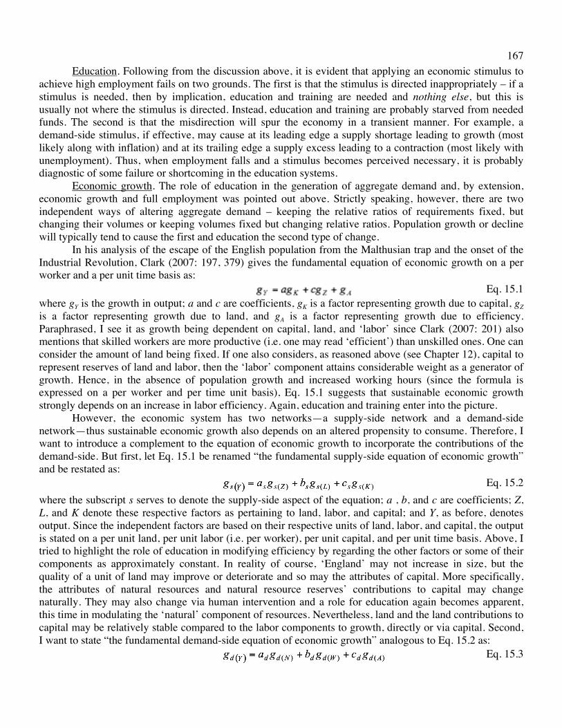
167 Education. Following from the discussion above, it is evident that applying an economic stimulus to

achieve high employment fails on two grounds. The first is that the stimulus is directed inappropriately – if a stimulus is needed, then by implication, education and training are needed and nothing else, but this is usually not where the stimulus is directed. Instead, education and training are probably starved from needed funds. The second is that the misdirection will spur the economy in a transient manner. For example, a demand-side stimulus, if effective, may cause at its leading edge a supply shortage leading to growth (most likely along with inflation) and at its trailing edge a supply excess leading to a contraction (most likely with unemployment). Thus, when employment falls and a stimulus becomes perceived necessary, it is probably diagnostic of some failure or shortcoming in the education systems.

Economic growth. The role of education in the generation of aggregate demand and, by extension, economic growth and full employment was pointed out above. Strictly speaking, however, there are two independent ways of altering aggregate demand – keeping the relative ratios of requirements fixed, but changing their volumes or keeping volumes fixed but changing relative ratios. Population growth or decline will typically tend to cause the first and education the second type of change.

In his analysis of the escape of the English population from the Malthusian trap and the onset of the Industrial Revolution, Clark (2007: 197, 379) gives the fundamental equation of economic growth on a per worker and a per unit time basis as:

Eq. 15.1 where gY is the growth in output; a and c are coefficients, gK is a factor representing growth due to capital, gZ is a factor representing growth due to land, and gA is a factor representing growth due to efficiency. Paraphrased, I see it as growth being dependent on capital, land, and ‘labor’ since Clark (2007: 201) also mentions that skilled workers are more productive (i.e. one may read ‘efficient’) than unskilled ones. One can consider the amount of land being fixed. If one also considers, as reasoned above (see Chapter 12), capital to represent reserves of land and labor, then the ‘labor’ component attains considerable weight as a generator of growth. Hence, in the absence of population growth and increased working hours (since the formula is expressed on a per worker and per time unit basis), Eq. 15.1 suggests that sustainable economic growth strongly depends on an increase in labor efficiency. Again, education and training enter into the picture.

However, the economic system has two networks—a supply-side network and a demand-side network—thus sustainable economic growth also depends on an altered propensity to consume. Therefore, I want to introduce a complement to the equation of economic growth to incorporate the contributions of the demand-side. But first, let Eq. 15.1 be renamed “the fundamental supply-side equation of economic growth” and be restated as:

Eq. 15.2 where the subscript s serves to denote the supply-side aspect of the equation; a , b, and c are coefficients; Z, L, and K denote these respective factors as pertaining to land, labor, and capital; and Y, as before, denotes output. Since the independent factors are based on their respective units of land, labor, and capital, the output is stated on a per unit land, per unit labor (i.e. per worker), per unit capital, and per unit time basis. Above, I tried to highlight the role of education in modifying efficiency by regarding the other factors or some of their components as approximately constant. In reality of course, ‘England’ may not increase in size, but the quality of a unit of land may improve or deteriorate and so may the attributes of capital. More specifically, the attributes of natural resources and natural resource reserves’ contributions to capital may change naturally. They may also change via human intervention and a role for education again becomes apparent, this time in modulating the ‘natural’ component of resources. Nevertheless, land and the land contributions to capital may be relatively stable compared to the labor components to growth, directly or via capital. Second, I want to state “the fundamental demand-side equation of economic growth” analogous to Eq. 15.2 as:

Eq. 15.3

168 where the subscript d serves to denote the demand-side aspect of the equation; a , b, and c are coefficients; N, W, and A denote these factors as being based on needs, wants, and aspirations, respectively; and Y denotes output (now of products demanded rather than products supplied). The independent factors are based again on their respective units of needs, wants, and aspirations. Physiology determines to a large extent awareness of needs and, less so, wants. Psychological factors determine some aspects of needs, mostly those of wants, and perhaps some of aspirations. Finally, social factors conveyed via education serve to generate an awareness of aspirations and to facilitate the generation of new aspirations. Here the novel demands of a more sophisticated population, alluded to above, are made explicit. Provided that education elucidates all the alternatives and their potential outcomes, but does not advance a recommendation, adaptation can proceed unimpeded.

The growth of enterprises. The spread of firm sizes within an economy cannot be explained by classical theory (Bloch 2005: 34). Because firms have differential relative growth rates due to differential competitive strengths (Bloch 2005: 25), they can respond to fluctuating demand and supply pressures. Fluctuating changes in the flow of goods, money, or both must affect the growth of enterprises. Four conditions can be discerned:

(i)! changed flows of existing demands affect a node (i.e. a firm); (ii)! changed flows of existing products affect a node; (iii)! new demands or disappearing demands affect a node; and (iv)! new products or disappearing products affect a node. It should be evident from previous discussions that an increase in the levels of existing demands or a

more efficient utilization of resources would lead to the accumulation of reserves (i.e. profit) at entities under demand stress while draining reserves from entities under supply stress. Where reserves are being accumulated, they can then be put to use to expand production capacity. If, due to a shift in consumer propensities to higher order requirements such as wants and aspirations, a new demand emerges, existing enterprises have to adapt or new ones have to come into existence to meet the new demand. If the emerging demands are very different from existing ones, adaptation of existing production facilities may not be feasible and this would favor the emergence of new firms. Therefore, if the demands cannot be met, growth will either occur at an enterprise or a new enterprise is likely to come into existence.

The analysis here suggests that the distribution of firm sizes within an economy will reflect the changes in consumption propensities of a population as they relate to the proportions of needs, wants, and aspirations involved. Thus, given the absence of extraneous constraints, firm sizes in a mature and healthy industry are probably normally distributed reflecting the fact that the different attributes of an unstressed population generally have normal distributions. In the case of emerging demands and new industries, firm sizes are probably distributed normally but skewed to smaller firms. In contrast, where demands are declining and an industry is aging, the distribution is likely skewed to larger firms. The presence of skewed distributions of firm sizes should therefore be indicative of changing (i.e., stressed) systems.

Price stability

Price stability. Fluctuations occur in economic systems. Prices, because they are signals of the relationships between demands and supplies, are means to adjust to these fluctuations; indeed, they are part of the adaptive process. Generally, price fluctuations are local and reflect components of the economic system under stress much like sore muscles reflect those specific parts of the musculature that have been challenged. Some prices will increase where shortages occur, while others may decrease due to increased supplies. Prices may also increase or decrease systemically. What exactly is price stability? Why is it needed? What causes price fluctuations?

First, demand should be free to vary as needed and supply should be free to respond accordingly. This allows prices to perform their signaling role in the system. When prices are constrained or distorted via

169 intervention or manipulation, information transmission is compromised and adaptation along with it. It is preferable by far to design a system such that it would operate naturally without the need for intervention. Thus, in a well-designed system, funneling or constraining demand or supply to a given node or a given pathway should not be needed and should not occur. Second, if prices fluctuate or change on a scale that is too fast to permit articulated responses by the system, a malfunction occurs as well. Here, ample information may be conveyed, but due to the rapid refresh rate of the information, response options may be limited or nonexistent. In other words, responses that are formulated based on current information may be outdated before these responses can be implemented. Note that in both cases, the flow of information is of such a nature as to interfere with the requisite adaptive responses of the system: in the first case because it has lost its integrity; and in the second case because it is changing too fast. Thus it appears that some price fluctuations are necessary and should be permitted, while others are pathological and should be countered. However, these conclusions may not hold up when economic cycles are considered.

Economic cycles. Economic cycles strongly affect both full employment and price stability. Their origins can be classified into one of two groups. Either they are events that have natural cycles themselves and entrain the economic system, or they are single dislocating events that set into motion adaptive responses that are oscillating in nature. Figuratively speaking, one could say that the boat rocks because of continuous wave motion or because a sudden shock provoked righting responses. An inspection of Figure 11.2 shows that natural cycles could derive from the environment and the population, and factors (in part) dependent on them such as reserve growth (hence attendant capital formation and credit creation) and technological change. In principle, natural cycles could be countered to some extent by adaptive responses. Dislocations, on the other hand, can originate from any source whether environment, population, SSN, DSN, government networks, or foreign trading partners. Dislocations have the potential to create network errors and trigger oscillations as described in Chapter 13. Consequently, after such dislocating events one should expect reversions to the mean to occur, often with overshoots due to the triggering of systemic adaptive responses.

Seasonal fluctuations in employment are a well-known example of entrainment of the economy by natural cycles in the environment. However, environmental entrainment can have more complex effects. For example, 5-year El Niño cycles can affect the economy. Over the past 15,000 years, El Niño periods in coastal Ecuador and Peru have gradually increased in frequency from one about every 55 years to one about every 5 years (Rodbell et al., 1999). Furthermore, a study of the 1997-1998 El Niño event concluded that it was associated with a $19 billion economic gain and a $4 billion loss (Changnon 1999: 1819). Larger-than-normal gains will produce reserves and savings. Because credit creation is a product that is ultimately based on existing or anticipated reserves, and these, in turn, derive from land and labor, economic cycles may derive from natural fluctuations amplified by the credit multiplier. With a 10 % cash ratio, an existing $100 reserve can very quickly be expanded several-fold. Due to the general presence of latent demand (i.e. in the form of wants), such rapid credit creation is easily converted into effective demand (i.e. latent demands are tokenized to become effective demands). This will provide a strong jolt to economic activity. However, in non El Niño years, reserve buildup may be slowed or reserves may be depleted to compensate for weak gains or for losses. The demand-generation process then stops after having given a spur to the supply side. Because the supply side has a greater inertia than the demand side, demand may start to falter when supply is gearing up. The balance between supply and demand is then disrupted and network oscillations are engendered. If the oscillations subside before the next event, the process will simply repeat itself. If not, the oscillations could be mitigated or amplified, depending on the nature of the overlap between the ongoing oscillations and the new El Niño event. Thus, staggered, lagged, and/or layered effects may counter or amplify some of these cycles.

Oscillations can also arise from high-impact dislocating events that cause a change in supply or demand, precipitating a mismatch between the supplies available in a system and the supplies required. Thus prices either rise or fall, depending on supply shortage or surplus, respectively. However, if prices rise then

170 demand is moderated (by consumers) and supply is increased (by producers) and due to a reduced demand and increased supply, an excess of supplies result (and vice versa for falling prices). Hence a change in supply or demand without a commensurate change in demand or supply (accounting for the necessary time lags between DSN and SSN), respectively, will generate oscillations in the adaptive process of matching supply and demand. For example, an event that causes collateral destruction or prevents the buildup of collateral after an extensive period of secured or unsecured credit extension will produce a loss of reserves for the lender and a loss of creditworthiness for the borrower (see Chapter 12). Consequently, a demand is generated first by credit extension, followed by an increase in supply to meet the increased demand, followed by a loss of demand due to the dislocating event and hence excess supply, followed by impediment of economic growth due to the loss of capital on one hand and the loss of creditworthiness on the other.

More troublesome cases of cycle-induction may be attributed to monetary and fiscal policies because of their wide-spread effects. Ironically, these are the very policies aimed at promoting full employment or price stability. A systemic economic stimulus is likely to either stimulate demand or stimulate production depending on how the stimulus was applied (primarily demand-side or primarily supply-side). As explained above, such an action disrupts the balance between supply and demand and triggers a series of oscillations.

Importantly, precisely because it is system-wide, a systemic economic stimulus could be especially damaging as a result of amplifying the mismatches that are generated. This amplification occurs because a stimulus is likely to synchronize demands or synchronize production capacity, e.g. synchronize capital equipment replacements at a given level of technology. The former will lead to an increase in demand and may initiate the latter. Thus, in both cases, a stimulus tends to realign enterprise growth rates and capital equipment life cycles, and so network-network oscillations can become entrenched, requiring repeated episodes of stimulation. This induction of long-term oscillations may hold true even if only some enterprises, such as Category I firms that are held to respond best to Keynesian measures (Toporowski 2005: 113), are entrained.

It is worth to consider again, in this context, Eq. 15.2 and Eq. 15.3. In an adaptive system, growth in product supplied generally should track growth in product demanded, thus, when equilibrated

Eq. 15.4 and, by implication,

Eq. 15.5 I do not mean to imply that there is a strict equality, this is not realistic in an adaptive and dynamic system, but I do hold that it applies more-or-less in an adapted and healthy system, even one that experiences low growth. Now, an economic stimulus, if it were to be applied, to which one of the six terms of Eq. 15.5 would it be applied? If not aimed at one in particular, which one would (unintentionally) be stimulated primarily? Clearly, a stimulus applied to the system, if it affects one side of the equation to a larger extent than the other, throws the whole system out of kilter and will induce, to a greater or lesser extent, oscillations when the system tries to right itself.

Education, as far as I see it, affects both the fundamental equations of growth (i.e., Eq. 15.2 and Eq. 15.3) and is likely to be the best way to stimulate growth in a manner that does not generate disparities between supply and demand. Put differently, the educated person, as soon as s/he conceives of a new requirement, is also likely to consider the means by which this new requirement is to be supplied – hence both supply and demand receive attention. It is true that such a tightly coupled coincidence may occur only for a very few persons. But, in general, the educated laborer can make more sophisticated demands of the economy in one area while simultaneously furnishing it with more highly skilled labor in another. Thus my statement seems to be plausible on an aggregate, if not an individual, basis. A stimulus directed at changing the attributes of the population or the environment is fundamentally different from one directed at one or the other network of the economy (or a component of these networks), as an inspection of Figure 11.1 will

171 reveal, and offers the best scope to achieve full employment and price stability. Note also, at a very rudimentary level, that better training (i.e. an improvement in labor performance) without better education (i.e. an improvement in ‘demand performance’ or an improvement in the generation of demands) is likely to lead to production efficiencies but not necessarily to increased demands. Thus unemployment will gradually rise as it should – if one figures out a more expedient way to dispense of some chore, one has more leisure time in consequence. In contrast, continuous and wide-spread quality education is likely to increase higher-order demands such that the roles of economic growth and full employment could become reversed – indeed, full employment (due to its implication of a labor shortage) may become a limiting factor to economic growth under these circumstances.

Discussion and conclusions

Based on the preceding considerations, one could argue that some price fluctuations are necessary and should be permitted, while others are pathological and should be countered. Nevertheless, one could reasonably ask whether price stability is to be pursued through policy or through system design. However, given the adaptive nature of economic systems, one must conclude that if a stimulus is needed then the system is malfunctioning. This implies that there is a design flaw and design flaws should not be addressed with interventions, but with better designs. Therefore price stability and full employment should not be the objectives of central bank policies – alternatively, they can only be the objectives of central bank policies in flawed systems. But this still leaves one pondering some design questions and operational parameters. Given the role of credit creation in economic growth, and its potential to destabilize the system, it is an important factor to consider. Taxation is another way to modulate the number of tokens in the system and thereby to affect economic growth, price stability, and employment. Even though the former is considered a monetary and the latter a fiscal instrument, there is no reason why taxation cannot be made a monetary instrument in a redesigned system. Moreover, interest rate policies, credit creation, and taxation appear to have temporal complementarity. For example, interest rate adjustments can take some time to affect the real economy, while the effects of taxation adjustments may have a more rapid onset. The issues of credit, interest, and taxation are considered next.

Capital and credit creation. Increased product yields relative to product consumption produces reserves and these contribute directly to the formation of capital. This view has points of intersection with those of Smith who saw capital as arising from savings out of (mostly profit) surpluses, Torrens who saw it as consisting of previously produced commodities, and Böhm-Bawerk’s view of capital as an intermediate good derived from land and labor (e.g. Vaggi and Groenewegen 2003: 111, 151, 249). Financial enterprises use capital as a resource to create a variety of credit products that can amount to many multiples of the original reserves. Credit, when in the hands of the consumer, is indistinguishable from money and is used like money to indicate consumer demands; this is precisely the point of credit creation. To extrapolate from Quesnay (Vaggi and Groenewegen 2003: 60), capital is reserves transmuted into forms that can be advanced to others to promote their endeavors. However, because credit creation can be very destabilizing, it is important to consider how appropriate credit levels should be determined.

I do not want to suggest an injunction against the creation of credit as a product, but I do want to draw attention to the capricious nature of fractional reserve requirements. Because of arbitrary regulations, credit, which is used and functions as money, bears little relationship to the purpose of money as reciprocity-based tokens for representing requirements. It is better to base credit creation on aggregate requirements as explained in Chapter 12 and given in Eq. 12.1. In addition, credit creation should be based on needs, wants, and aspirations separately to ensure that some individuals do not usurp all the credit at the expense of others. This does not mean every individual is entitled to the same overall credit – this is only true for needs-related credit. The levels of credit that potentially could be extended for wants and aspirations may vary significantly between individuals based on their education levels, experience, and personal histories. Whether any credit is

172 extended at all, however, depends on creditworthiness. Thus two considerations come into play when extending credit: the credit requirements of the applicant based on principled considerations of individual merits within aggregate limits and due diligence regarding the creditworthiness of the applicant given the amount being extended. A tighter relationship between the amount of money in the system and the aggregate levels of requirements that need expression within the system should promote price stability without impeding the price dynamism associated with adaptive processes.

Credit growth. The effect of the credit multiplier can be modeled with a recurrent connection, i.e. a connection that goes from a given financial unit node back to itself (e.g. Figure 8.1) with the credit multiplier being the weight of the recurrent connection. However, the feed from the recurrent connection cannot be distinguished from other inputs to the same node. If capital is seen as reserves that have accrued from past production or are expected to accrue from future production, it becomes transparent that phantom reserves are being created. This is an important point. Current reserves are real and extant. Anticipated reserves are also in a sense real if the estimates on which they are based are well-grounded. Phantom reserves, in contrast, are not well anchored in the economic system and generate a potential for disconnect between SSN and DSN. It is true that borrowers may ask for credit, and in this sense it may reflect a reality of the economic system. However, if credit is extended purely on the basis of the cash ratio with little regard for the extant or anticipated reserves of the system, stresses can arise due to mismatched demand and supply. Clearly, opportunities exist to expand credit considerably depending on the credit multiplier.

The reader should not take this analysis to be an argument for the prohibition of fractional reserve lending. Instead, it is an argument for a principled determination of the cash ratio and its frequent revision. Basing the level of the cash ratio on what seems to work, or on what has worked in the past, is not appropriate. A principled approach may proceed along the following lines. Since the initial stimulus or kernel is provided by existing reserves in the form of the first deposit, the fraction kept in reserve must reflect both the size of the existing reserves and the rate of growth of the existing reserves. If, for example, over the course of a year a capital reserve of $100 arises which is then deposited, it is unrealistic to create credit up to 9 times that amount in the following year. An economy growing at 3 % per year is not likely to generate reserves up to 900 % per year. If the economic growth rate were 3 % per annum, then the cash ratio should be in the order of (100 - 3) % during the following year. Some would argue that a cash ratio of around 97 %, instead of 10 % or less, would stifle growth. In my view however, growth should be a consequence of education and training (see below), this would increase existing real reserves due to technological advancement and improved skills, and this increase should fuel further expansion. Moreover, as expansion (economic growth) then increases, the cash ratio will decrease. All this happens then in an orderly manner, keeping the demand and supply sides of the economy tightly coupled. This, in turn, is the best way to promote price stability. It stands to reason that the same insight should apply to all manners of credit creation. A balance must be struck between demands for credit products and stores of existing and potential reserves (i.e., available capital). After all, this holds true for other goods and services too. Seed corn, before it can be advanced and applied, must first of all exist. Creating credit without regard to existing reserves and reserve growth rates practically amounts to the counterfeiting of money (even though perfectly legal). Consider that any counterfeit money that passes as money should also successfully stimulate the economy.

Interest rates. When the complementary economic networks (i.e. SSN and DSN) were introduced, it was generally assumed that every transaction consisted of a simultaneous exchange of goods and tokens. But sometimes asynchronous flows occur when part or all of the tokens involved are handed over first and the goods are only taken possession of later (e.g. investments, advance purchases, deposits on a house or car or yacht, etc.). Alternatively, the goods are handed over first and the receipt of funds is delayed until later such as when something is bought on credit. Thus the party not receiving the counter-balancing items typically demands some form of compensation. This is either thought of as compensation for delayed consumption or compensation for the risk of missed opportunities (e.g. Jackson 1986: 37; Spahn 2001: 27, 34). The greater

173 the time lags between delivery and counter-delivery, the greater the risks involved due to a loss of liquidity and the greater the distress, discomfort, and disappointment involved due to delayed consumption. This should be reflected in the interest premium payable for delayed counter-delivery. When the same practice occurs on an industry- or system-wide basis, interest premiums should change because risks are changed. If interventions of some kind are or can be expected, interest calculus and exchange practices become distorted. Asynchronous flows with large time lags are not advisable, not because more risk and distress is involved, but because risk and distress assessment is more difficult for more distal times and a secondary risk of inaccurate assessment arises. Awareness of these secondary risks may make them eventually tractable, but awareness is needed.

Manipulating interest rates is often the method of choice employed by central banks. Given the possible causes of economic cycles discussed above, it is quite unclear how the steering of interest rates could be a meaningful way to stimulate an economy. Maintaining a high cash ratio as suggested above is not only likely to reduce the contribution of rapid credit creation to economic cycles, but may also lead to generally higher interest rates and favor innovation and technological progress over speculation. This can only have long-term benefits.

Taxation. Taxation is rather interesting when seen from the perspective of Chapter 10, namely, as a means to transfer demand (i.e. money) from the private to the public sector. Indeed, moral hazard abounds when engaging in such transfers with ‘needed’ and ‘earned’ being the two poles of the matter. Thus one has to consider the context within which such transfers occur. If the ground ethic is seen as achieving and maintaining the best health and greatest robustness of the social system over as long a time horizon as possible, individual concerns can be left for individual interactions. Clearly, transfers should not occur if:

(i)! the ability of the social system to expand is undermined; (ii)! the ability of the social system to maintain itself is undermined; and (iii)! the quality of the social system becomes compromised.

A second reason why I find taxation interesting is because the tax collection process is enormously wasteful. Countless resources are spent by individuals, enterprises, and governments on the simple and very unproductive process of extracting demands from one system and moving them to the other or avoiding the same. Rather than tying those resources up with complex calculations, tedious collection and monitoring efforts, and costly administration, why can’t they be freed up to better effect? Far better ways of taxation must exist.

Taxation may also be, in addition to the manipulation of interest rates, a monetary means of maintaining stability in the system. If one finds oneself unexpectedly on wet ice, one may come to regard friction as an advantage. Similarly, a transaction tax, applied to all connections in all networks, may function as a stabilizing factor. It could be used to inhibit rapid and damaging, especially speculative, monetary flows. The idea is known as the “Tobin tax”, is not new, (Davies 2002: 675), but should be extended in scope! Taxation as a monetary policy instrument is the third reason why I find it interesting.

The question now is how to create a more efficient tax system and one that meets the triple mandate of maintaining the viability of the economic system, promoting its growth, and benefiting all members of society.

First, it seems necessary to establish a publicly-owned, accountable, and politically independent monetary authority analogous to the judicial system (accountable and independent seem incompatible – a problem that also arises with the judiciary). The national or central bank would be subsumed by this monetary authority. Taxation will be the sole domain of the monetary authority, not the government. Taxes must be collected uniformly in a manner that is consistent with economic health. I would argue that the collection of taxes be tied to economic growth. A portion of the taxes collected must be kept in reserve to buffer the system against unexpected adverse events. The remainder is made available to the government to allocate against spending priorities decided in a debated budgeting process. The government has no authority

174 to borrow or lend. The sole income for the monetary authority (capital and operating funds) must be included in this budget. Thus I argue for a complete depolitization of the tax system - whomever collects taxes cannot spend it and whomever spends it cannot collect it.

Second, it is the task of the government to reallocate resources in accordance with the expressed priorities of the voting public. It is not the task of the monetary authority to tax some more and others less. Taxes must be collected evenly and at the same rate, no exceptions. If some individuals, some groups, some enterprises, and/or some industries are to receive special considerations, it should be via the giving arm, not the taking arm. Thus, a transaction tax as mentioned above, applied as a small percentage of the amount involved to every transaction, could fulfill this requirement. I suggest that financial institutions be given this task since they are already central players in the monetary flow circuits. Money flows through banks. Every time money enters an account; a fraction should be withheld as tax. For example, for every dollar moved from any one account to any other account (regardless of whether the transaction occurs for the same or a different entity and in the same or a different financial institution) one thousandth could be withheld as tax. Cash should be taxed at a different and much higher rate based on the average number of times that cash changes hands before being returned to a bank. All other taxes should be abolished. Note that the more economically active a person or entity, the more times money would be transferred from one account to another, the more taxes they would pay. Generally speaking, as the velocity of money increases, so will taxes. Thus taxation is not based on wealth, but on activity, hence the utility of taxation as a means of economic stabilization. Consider too that a transaction tax is highly egalitarian – everyone pays exactly the same rate. Large amounts of money sitting in a mattress are no more useful to the owner than a pea sitting in the same mattress. The only advantage over a pea is the potential that money may embody, but potential never realized is empty potential. Since everyone has the same needs and must spend similar amounts of money to satisfy these needs, everyone is taxed equally on the basis of essentials. My main point, however, is that this argument should not enter the debate on taxation, but the dictates of social structure belong to the domain of politics and should be expressed in budgeting.

Third, the monetary authority governs the supply of money and controls the mint as well. This creates another possibility of ‘taxation’, namely that a certain percentage of the money brought into circulation (minted, printed, or otherwise created) be directed to the government. Thus, the tokens used as money are taxed at their ultimate origin rather than at distal points (consumption taxes, income taxes) or via conduit taxation (transaction tax).

175

Simulations

176

16

Simulations

177

Simulations Summary

Because computations that occur at individual nodes represent the activities of individual economic agents such as firms and because demands are derived from the population, thus ‘households’, local network computations and requirement generation pertain to microeconomic phenomena even though these microeconomic phenomena are differently embedded within the system. The outcomes of these micro-level activities, in aggregate, produce macroeconomic phenomena. The dependence of macroeconomic phenomena on micro-foundations was here examined by creating simple complementary core networks to simulate the demand- and supply-side of a private economy. These networks were allowed to interact via their output layers. First a supply-side network with a hyperbolic tangent ETU production function was created. The output obtained from this network produced a supply curve. Second, a demand-side network was created that incorporated physiological, psychological, and social requirement factors. These requirements were fed forward to an ETU with either a hyperbolic tangent or a Cobb-Douglas production functions to obtain a demand curve. Slightly larger networks were then combined to create a core system and the core system’s behavior was simulated. The simulations suggested that with such systems, market equilibria could be established. Demand and/or supply shocks disrupted these equilibria and induced oscillatory adaptations that, in many cases, lead to new market equilibria or even to stability with mismatched demands and supplies. Thus, the simulations provide proof-of-principle that the model is able to generate macroeconomic phenomena from microeconomic foundations.

178 Introduction

I hope that the preceding chapters accomplished the exposition of the model sufficiently well to convey its major aspects qualitatively, especially visually, and in an intuitively plausible manner. Throughout, I have also provided quantitative aspects of the model. In this chapter, I want to focus on some of these quantitative aspects and attempt to synthesize them into a larger entity. Specifically, I will seek to synthesize a quantitative model of the core system of the theory: two complementary networks, yoked to each other via their outputs and drawing, each in its characteristic way, upon their shared environment. This will allow me to lay the groundwork for, and point the way to, an eventual complete quantitative synthesis and evaluation of the model.

I will proceed in the following manner. First, I will create a supply-side network and examine its output. This is followed by an analogous synthesis for the demand-side, the more challenging task because of the need to convert human motives into economic observables. It is of particular interest to me to examine whether macro trends can be derived from microfoundations with the core system. Being one of its primary objectives, this is a critical test of the model.

Second, I will combine the networks generated above to simulate and examine the basic behavior of a core system. It has been my contention that two or more coupled adaptive systems will generate oscillations when one or more of their inputs are disturbed in such a way as to cause mismatched outputs. This has, in principle, important consequences for some of the most fundamental of economic concepts - equilibrium and economic cycles - and may indicate promising avenues of future investigation.

Although I pursue the prior objectives with very simple networks and with reference to the tertiary market, once the application of the concepts is grasped and the organization of the model is understood, augmentation of the core system is readily achieved because the mathematics of ANNs are well-developed (e.g. Tsoi and Back 1997: 193-199). Proceeding beyond the core system will require the addition of mathematical descriptions of the circular flows pertaining to the core system, as well as mathematical descriptions for the interfaces between private and public sectors and between different national economies, depending on what one wishes to model. However, at the end of this chapter, the reader would have been exposed to the outline of the entire model and those interested should be in a position to proceed on their own.

Developing a quantitative model of the core system

The core system is described in Chapter 4; the top panel in Figure 16.1 is a modification of Figure 4.1 showing the simplified SSN modeled here. I start with the SSN again because it is the most intuitive to grasp. From there, the transition to the DSN follows more easily.

Supply side. I shall consider now a network with one input node, one hidden node, and one output node, that part of the SSN of the core system as bolded in Figure 16.1. I also assume for the present example that the input node has a linear transfer function, the hidden node has a sigmoidal transfer function (e.g. a hyperbolic tangent such as Eq. A1), and the output node also has a linear transfer function. Note that the transfer function of the hidden node is consistent with a hyperbolic tangent production function for technically independent factors (Beattie and Taylor 1985: 71). In what follows, I furthermore use production functions in the way transfer functions are used in ANNs, that is, I apply the production function to the sum of (production factor) inputs. Production functions as the analogs of transfer functions are discussed in Chapter 8 along with modifications that would make them more similar to their usage in economics and refinements that would permit more accurate modeling of production functions.

Without loss of generality then, the output of the one product single factor-based SSN on the tertiary market can be calculated for any given input volume. This output is calculated using a modification of Eq. 2.5 to accommodate a hyperbolic tangent production function

179

Requirements Enterprises Products demanded

Resources Enterprises Products supplied

Demand-side network Supply-side network

Supplyk v w

R

Figure 16.1 Top: adaptation of Figure 4.1 showing, in bold, the simplified SSN simulated here. Bottom: the output on the tertiary market of the bolded network, thus at

the end of the production path from resources to product (i.e. from input nodes through hidden nodes to output nodes), as a function of normalized

resource use. For a given product in a SSN where many products are supplied from many input factors, the ultimate shape of the curve for that

product will depend on the individual contributions of all the nodes along all the parallel production paths leading to it, thus on their connection weights

and individual transfer (i.e. production) functions.

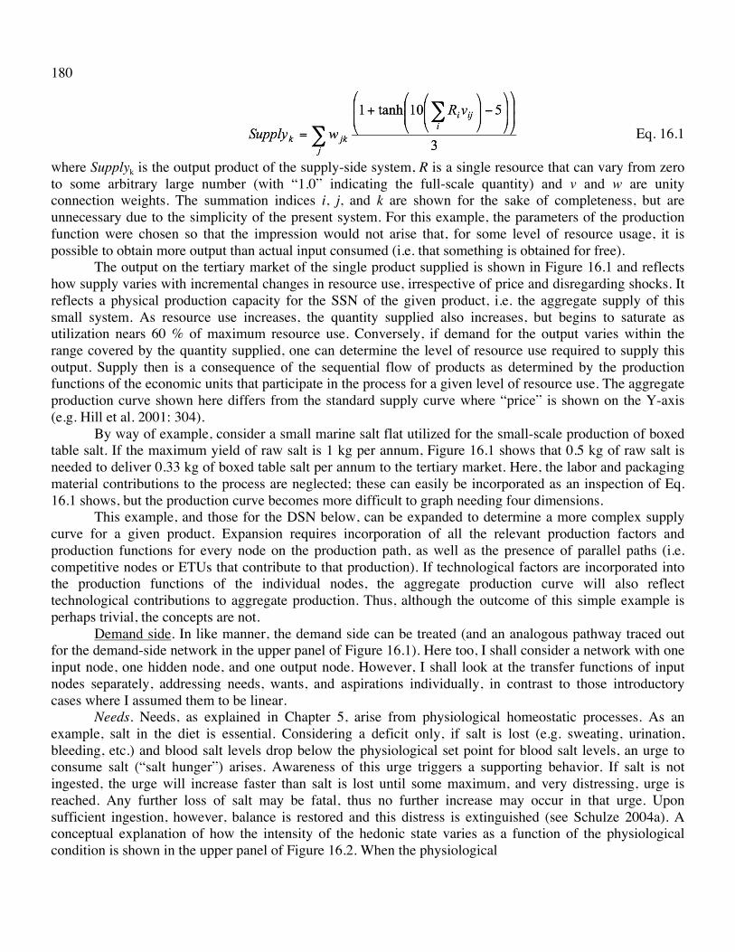
180

Eq. 16.1

where Supplyk is the output product of the supply-side system, R is a single resource that can vary from zero to some arbitrary large number (with “1.0” indicating the full-scale quantity) and v and w are unity connection weights. The summation indices i, j, and k are shown for the sake of completeness, but are unnecessary due to the simplicity of the present system. For this example, the parameters of the production function were chosen so that the impression would not arise that, for some level of resource usage, it is possible to obtain more output than actual input consumed (i.e. that something is obtained for free).

The output on the tertiary market of the single product supplied is shown in Figure 16.1 and reflects how supply varies with incremental changes in resource use, irrespective of price and disregarding shocks. It reflects a physical production capacity for the SSN of the given product, i.e. the aggregate supply of this small system. As resource use increases, the quantity supplied also increases, but begins to saturate as utilization nears 60 % of maximum resource use. Conversely, if demand for the output varies within the range covered by the quantity supplied, one can determine the level of resource use required to supply this output. Supply then is a consequence of the sequential flow of products as determined by the production functions of the economic units that participate in the process for a given level of resource use. The aggregate production curve shown here differs from the standard supply curve where “price” is shown on the Y-axis (e.g. Hill et al. 2001: 304).

By way of example, consider a small marine salt flat utilized for the small-scale production of boxed table salt. If the maximum yield of raw salt is 1 kg per annum, Figure 16.1 shows that 0.5 kg of raw salt is needed to deliver 0.33 kg of boxed table salt per annum to the tertiary market. Here, the labor and packaging material contributions to the process are neglected; these can easily be incorporated as an inspection of Eq. 16.1 shows, but the production curve becomes more difficult to graph needing four dimensions.

This example, and those for the DSN below, can be expanded to determine a more complex supply curve for a given product. Expansion requires incorporation of all the relevant production factors and production functions for every node on the production path, as well as the presence of parallel paths (i.e. competitive nodes or ETUs that contribute to that production). If technological factors are incorporated into the production functions of the individual nodes, the aggregate production curve will also reflect technological contributions to aggregate production. Thus, although the outcome of this simple example is perhaps trivial, the concepts are not.

Demand side. In like manner, the demand side can be treated (and an analogous pathway traced out for the demand-side network in the upper panel of Figure 16.1). Here too, I shall consider a network with one input node, one hidden node, and one output node. However, I shall look at the transfer functions of input nodes separately, addressing needs, wants, and aspirations individually, in contrast to those introductory cases where I assumed them to be linear.

Needs. Needs, as explained in Chapter 5, arise from physiological homeostatic processes. As an example, salt in the diet is essential. Considering a deficit only, if salt is lost (e.g. sweating, urination, bleeding, etc.) and blood salt levels drop below the physiological set point for blood salt levels, an urge to consume salt (“salt hunger”) arises. Awareness of this urge triggers a supporting behavior. If salt is not ingested, the urge will increase faster than salt is lost until some maximum, and very distressing, urge is reached. Any further loss of salt may be fatal, thus no further increase may occur in that urge. Upon sufficient ingestion, however, balance is restored and this distress is extinguished (see Schulze 2004a). A conceptual explanation of how the intensity of the hedonic state varies as a function of the physiological condition is shown in the upper panel of Figure 16.2. When the physiological

181

Figure 16.2 The top panel shows conceptually the intensity of a need as a function of the size of the need, i.e. the

psychological urge arising from a physiological imbalance (here a deficit) in a given regulated variable like blood sodium (i.e. salt concentration in blood). If salt is lost through sweating or urination, and blood salt

levels become too low, an urge to consume salt arises. When there is an excess of salt in the blood (not shown), an urge to avoid ingesting salt will arise. Thus, the absolute intensity of the urge is at its lowest if there is no imbalance. The practical example in the bottom panel shows that an average deficit of 0.35 %

from the set point (0.87 % NaCl by weight) for blood salt will induce the urge to consume (2.5 g) salt (solid arrows) and that a slightly larger deficit will induce a much larger urge to consume salt leading to the

consumption of more salt (dashed arrows).

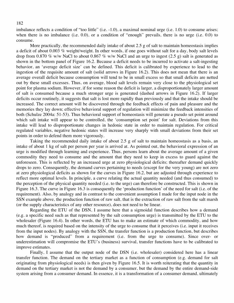
182 imbalance reflects a condition of “too little” (i.e. -1.0), a maximal nominal urge (i.e. 1.0) to consume arises; when there is no imbalance (i.e. 0.0), or a condition of “enough” prevails, there is no urge (i.e. 0.0) to consume.

More practically, the recommended daily intake of about 2.5 g of salt to maintain homeostasis implies a deficit of about 0.003 % weight/weight. In other words, if one goes without salt for a day, body salt levels drop from 0.870 % w/w NaCl to about 0.867 % w/w NaCl and an urge to ingest (2.5 g) salt is generated as shown in the bottom panel of Figure 16.2. Because a deficit needs to be incurred to activate a salt-ingesting behavior, an ‘average deficit size’ can be defined. This deficit is calibrated by experience to lead to the ingestion of the requisite amount of salt (solid arrows in Figure 16.2). This does not mean that there is an average overall deficit because consumption will tend to be in small excess so that small deficits are netted out by these small excesses. Thus, on average, blood salt levels remain very close to the physiological set point for plasma sodium. However, if for some reason the deficit is larger, a disproportionately larger amount of salt is consumed because a much stronger urge is generated (dashed arrows in Figure 16.2). If larger deficits occur routinely, it suggests that salt is lost more rapidly than previously and that the intake should be increased. The correct amount will be discovered through the feedback effects of pain and pleasure and the memories they lay down; effective behavioral support of regulation will minimize the feedback intensities of both (Schulze 2004a: 51-53). Thus behavioral support of homeostasis will generate a pseudo set point around which salt intake will appear to be controlled, the ‘consumption set point’ for salt. Deviations from this intake will lead to disproportionate changes in hedonic state in order to maintain regulation. For critical regulated variables, negative hedonic states will increase very sharply with small deviations from their set points in order to defend them more vigorously.

Taking the recommended daily intake of about 2.5 g of salt to maintain homeostasis as a basis, an intake of about 1 kg of salt per person per year is arrived at. As pointed out, the behavioral expression of an urge is modified through learning and experience. Thus, persons learn about the average amount of a given commodity they need to consume and the amount that they need to keep in excess to guard against the unforeseen. This is reflected by an increased urge at zero physiological deficits; thereafter demand quickly drops to zero. Consequently, the demand curves pertaining to needs (except for the very young) are not zero at zero physiological deficits as shown for the curves in Figure 16.2, but are adjusted through experience to reflect more optimal levels. In principle, a curve relating the actual quantity needed (and thus consumed) to the perception of the physical quantity needed (i.e. to the urge) can therefore be constructed. This is shown in Figure 16.3. The curve in Figure 16.3 is consequently the ‘production function’ of the need for salt (i.e. of the requirement). Also, by analogy and in contrast to the convenient assumption I made for the input node in the SSN example above, the production function of raw salt, that is the extraction of raw salt from the salt marsh (or the supply characteristics of any other resource), does not need to be linear.

Regarding the ETU of the DSN, I assume here that a sigmoidal function describes how a demand (e.g. a specific need such as that represented by the salt consumption urge) is transmitted by the ETU to the wholesaler (Figure 16.4). In other words, the ETU has to make an estimate of which commodity, and how much thereof, is required based on the intensity of the urge to consume that it perceives (i.e. input it receives from the input nodes). By analogy with the SSN, the transfer function is a production function, but describes how demand is “produced” from a requirement (i.e. from the urge to consume). Since over- or underestimation will compromise the ETU’s (business) survival, transfer functions have to be calibrated to improve estimates.

Finally, I assume that the output node of the DSN (i.e. wholesaler) considered here has a linear transfer function. The demand on the tertiary market as a function of consumption (e.g. demand for salt originating from physiological needs) is then given by Figure 16.5. It is worth reiterating that the quantity in demand on the tertiary market is not the demand by a consumer, but the demand by the entire demand-side system arising from a consumer demand. In essence, it is a transformation of a consumer demand, ultimately

183 based on a physiological set point, into a market demand. Thus Figure 16.5 indicates that, although the real physiological need is 1 kg of salt per year, a demand of about 1.6 kg of salt per year prevails on the tertiary market given the assumptions made for the example.

Figure 16.3 The annual quantity of a commodity (table salt) perceived necessary as a function of the actual amount

consumed is shown in the figure by the solid line. The dashed line indicates the annual amount of consumption that is physiologically necessary plotted with respect to the consumption urge. Experience leads to a small excess perceived necessary even if adequate amounts are consumed. If an excess is consumed, the

amount perceived necessary will rapidly decline, while, conversely, it will rapidly increase when consumption is inadequate.

Demand and supply can now be plotted on the same graph as a function of physical quantity consumed or physical quantity of resource extracted, respectively, as shown in Figure 16.6 (i.e., “Quantity” on the abscissa). For the purpose of creating Figure 16.6, I assumed the existence of a population of 500 persons in an environment with a resource yielding 1,000 kg of raw salt per year. Figure 16.6 shows that the needs curve (dashed trace) varies from very high to very low over a small increment in quantity, consistent with a highly inelastic demand. Put differently, if a shortage of salt were to arise, a massive demand will emerge (and people would be willing to pay astronomical prices for it); conversely, if supplies are adequate, inducing significant excess consumption will be very, very difficult. In contrast, the supply curve (solid trace) is less constrained.

Figure 16.6 also shows the point where demand is in equilibrium, i.e. where the amount consumed equals the amount perceived needed. This point occurs where the diagonal crosses the demand curve. The demand prevailing at this point is furthermore one that the SSN can meet by using some finite amount of resource. Note that the supply curve indicates that the supply side is unable to meet much higher demands, even when consuming (implied) infinite amounts of resource.

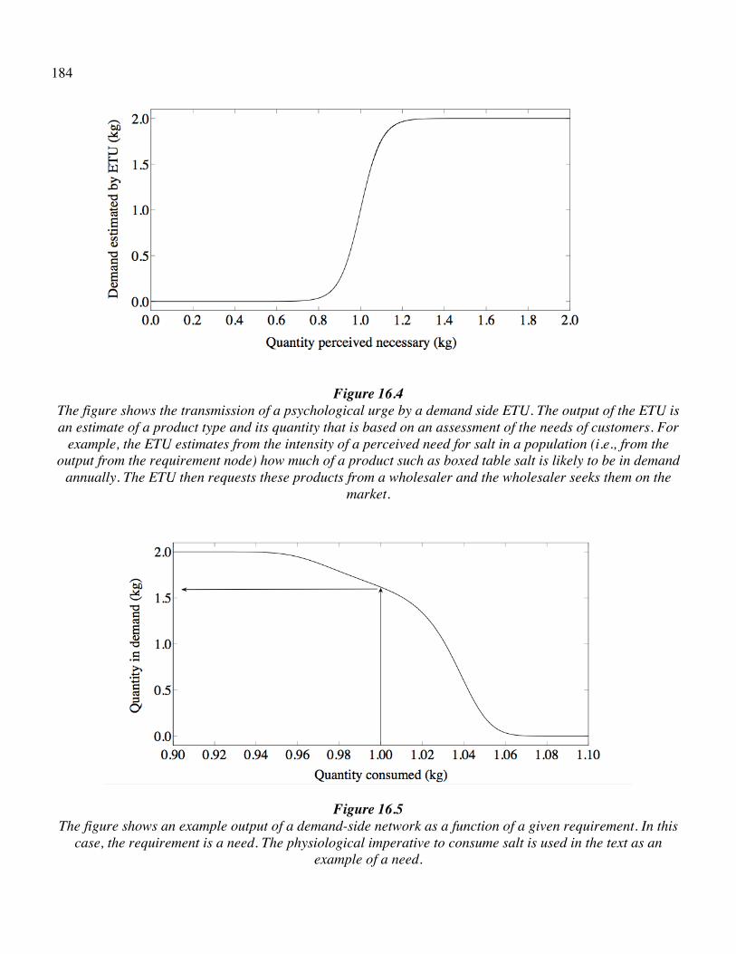
184

Figure 16.4 The figure shows the transmission of a psychological urge by a demand side ETU. The output of the ETU is an estimate of a product type and its quantity that is based on an assessment of the needs of customers. For

example, the ETU estimates from the intensity of a perceived need for salt in a population (i.e., from the output from the requirement node) how much of a product such as boxed table salt is likely to be in demand

annually. The ETU then requests these products from a wholesaler and the wholesaler seeks them on the market.

Figure 16.5 The figure shows an example output of a demand-side network as a function of a given requirement. In this

case, the requirement is a need. The physiological imperative to consume salt is used in the text as an example of a need.

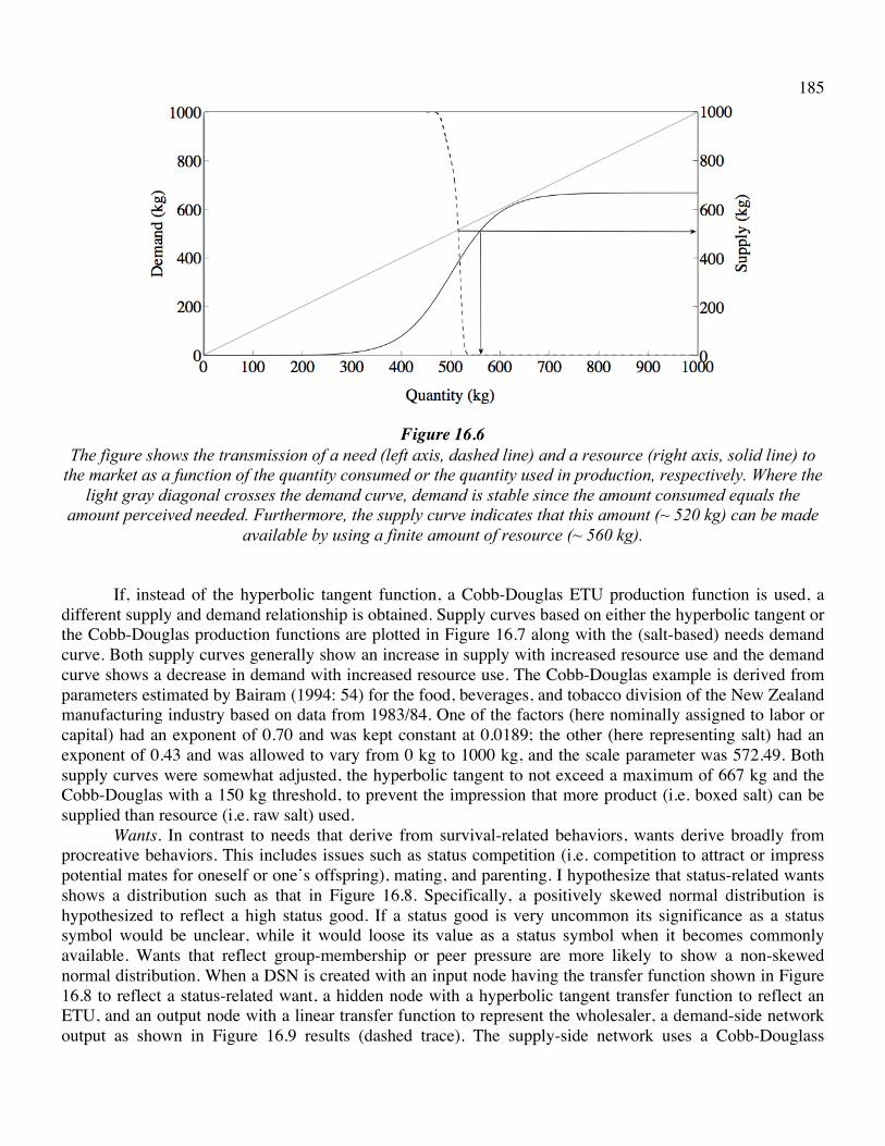
185

Figure 16.6 The figure shows the transmission of a need (left axis, dashed line) and a resource (right axis, solid line) to

the market as a function of the quantity consumed or the quantity used in production, respectively. Where the light gray diagonal crosses the demand curve, demand is stable since the amount consumed equals the

amount perceived needed. Furthermore, the supply curve indicates that this amount (~ 520 kg) can be made available by using a finite amount of resource (~ 560 kg).

If, instead of the hyperbolic tangent function, a Cobb-Douglas ETU production function is used, a different supply and demand relationship is obtained. Supply curves based on either the hyperbolic tangent or the Cobb-Douglas production functions are plotted in Figure 16.7 along with the (salt-based) needs demand curve. Both supply curves generally show an increase in supply with increased resource use and the demand curve shows a decrease in demand with increased resource use. The Cobb-Douglas example is derived from parameters estimated by Bairam (1994: 54) for the food, beverages, and tobacco division of the New Zealand manufacturing industry based on data from 1983/84. One of the factors (here nominally assigned to labor or capital) had an exponent of 0.70 and was kept constant at 0.0189; the other (here representing salt) had an exponent of 0.43 and was allowed to vary from 0 kg to 1000 kg, and the scale parameter was 572.49. Both supply curves were somewhat adjusted, the hyperbolic tangent to not exceed a maximum of 667 kg and the Cobb-Douglas with a 150 kg threshold, to prevent the impression that more product (i.e. boxed salt) can be supplied than resource (i.e. raw salt) used.

Wants. In contrast to needs that derive from survival-related behaviors, wants derive broadly from procreative behaviors. This includes issues such as status competition (i.e. competition to attract or impress potential mates for oneself or one’s offspring), mating, and parenting. I hypothesize that status-related wants shows a distribution such as that in Figure 16.8. Specifically, a positively skewed normal distribution is hypothesized to reflect a high status good. If a status good is very uncommon its significance as a status symbol would be unclear, while it would loose its value as a status symbol when it becomes commonly available. Wants that reflect group-membership or peer pressure are more likely to show a non-skewed normal distribution. When a DSN is created with an input node having the transfer function shown in Figure 16.8 to reflect a status-related want, a hidden node with a hyperbolic tangent transfer function to reflect an ETU, and an output node with a linear transfer function to represent the wholesaler, a demand-side network output as shown in Figure 16.9 results (dashed trace). The supply-side network uses a Cobb-Douglass

186 production function for the ETU and linear production functions for the other nodes; its output is also plotted in Figure 16.9 (solid trace).

Figure 16.7 The transmission of a need (left axis, dashed line) and a resource (right axis, solid and dotted lines) to the market as a function of the quantity required or supplied, respectively, are shown in the figure. The supply

functions illustrate the use of two different ETU production functions – a hyperbolic tangent (solid line) and a Cobb-Douglas with one factor fixed (dotted line). Both supply curves show that supplies increase with

increasing resource use and the demand curve shows that demand decreases with increased resource use (i.e. decreases with increased consumption).

Figure 16.9, although exclusively conceptual, has several interesting implications. The left side of the

demand curve shows that an increase in supplies, i.e., an increase in the frequency of occurrence in the population is accompanied with an increase in demand. Although I have yet to address the issue of price in the current context, this behavior has the essence of a Veblen good. On the right side of the demand curve, a ‘normal’ demand condition seems to apply. In my opinion, it is not accurate to consider this as a normal condition since it still pertains to a Veblen good. A distinction is therefore called for, not on the basis of demand phenomenology, but on the basis of demand ontology. Thus I am inclined to view demand curves as reflecting “needs goods”, “wants goods” and “aspirations goods”. The Veblen good is then an instance (status consumption, snob effect) of “wants goods”.

The Giffen good, in contrast, is a special case of “needs goods” but is somewhat of a mystery. One would expect that an increase in the price of one essential good leading to a compensatory increase in the consumption thereof because supplementary goods, even at unaltered prices, can no longer be afforded, would simply lead to physiological distress. Where dietary goods are in question, malnutrition will occur in the long term since the required nutrients cannot be consumed in their necessary proportions. Thus the presence of a Giffen good may be indicative of pathological socio-economic conditions in marginalized segments of the population or, when under extreme stress, the population at large. The prevalence of Giffen goods should therefore be relatively rare and rather more transient compared to other needs goods.

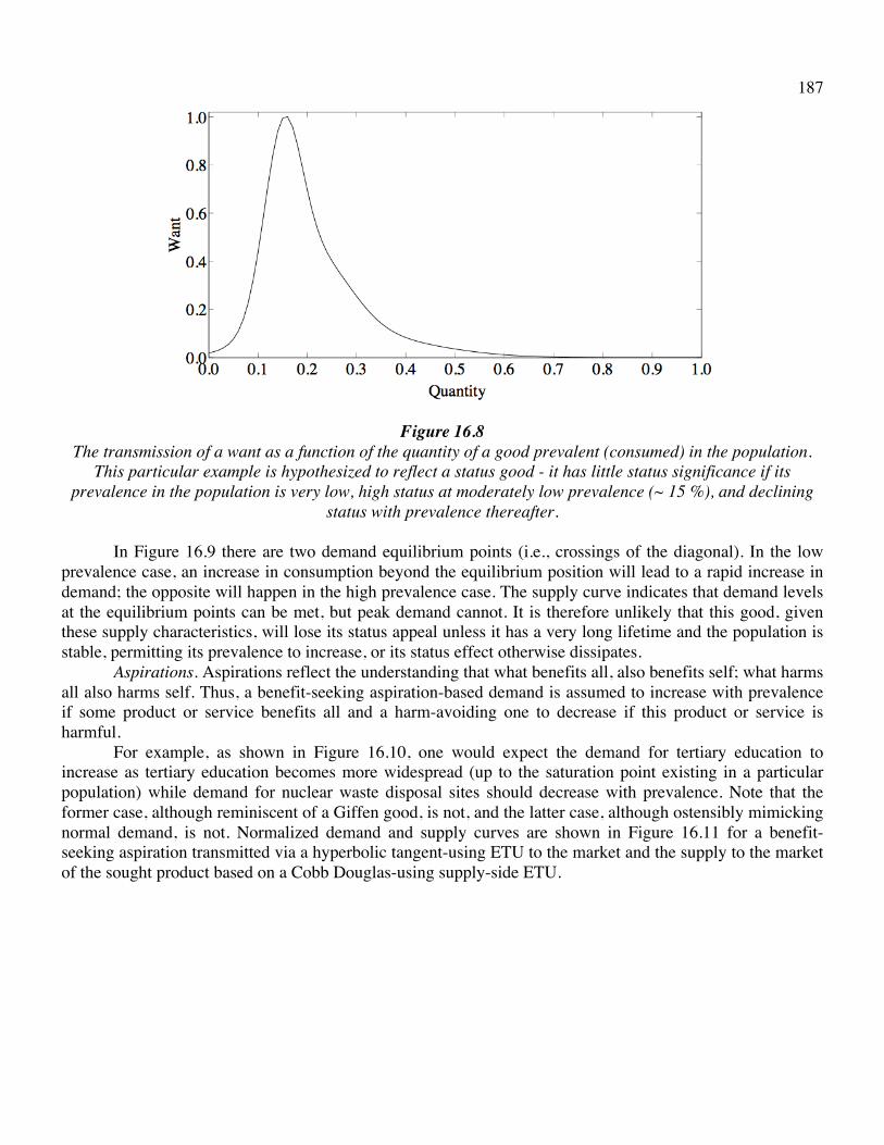
187

Figure 16.8 The transmission of a want as a function of the quantity of a good prevalent (consumed) in the population.

This particular example is hypothesized to reflect a status good - it has little status significance if its prevalence in the population is very low, high status at moderately low prevalence (~ 15 %), and declining

status with prevalence thereafter.

In Figure 16.9 there are two demand equilibrium points (i.e., crossings of the diagonal). In the low prevalence case, an increase in consumption beyond the equilibrium position will lead to a rapid increase in demand; the opposite will happen in the high prevalence case. The supply curve indicates that demand levels at the equilibrium points can be met, but peak demand cannot. It is therefore unlikely that this good, given these supply characteristics, will lose its status appeal unless it has a very long lifetime and the population is stable, permitting its prevalence to increase, or its status effect otherwise dissipates.

Aspirations. Aspirations reflect the understanding that what benefits all, also benefits self; what harms all also harms self. Thus, a benefit-seeking aspiration-based demand is assumed to increase with prevalence if some product or service benefits all and a harm-avoiding one to decrease if this product or service is harmful.

For example, as shown in Figure 16.10, one would expect the demand for tertiary education to increase as tertiary education becomes more widespread (up to the saturation point existing in a particular population) while demand for nuclear waste disposal sites should decrease with prevalence. Note that the former case, although reminiscent of a Giffen good, is not, and the latter case, although ostensibly mimicking normal demand, is not. Normalized demand and supply curves are shown in Figure 16.11 for a benefit-seeking aspiration transmitted via a hyperbolic tangent-using ETU to the market and the supply to the market of the sought product based on a Cobb Douglas-using supply-side ETU.

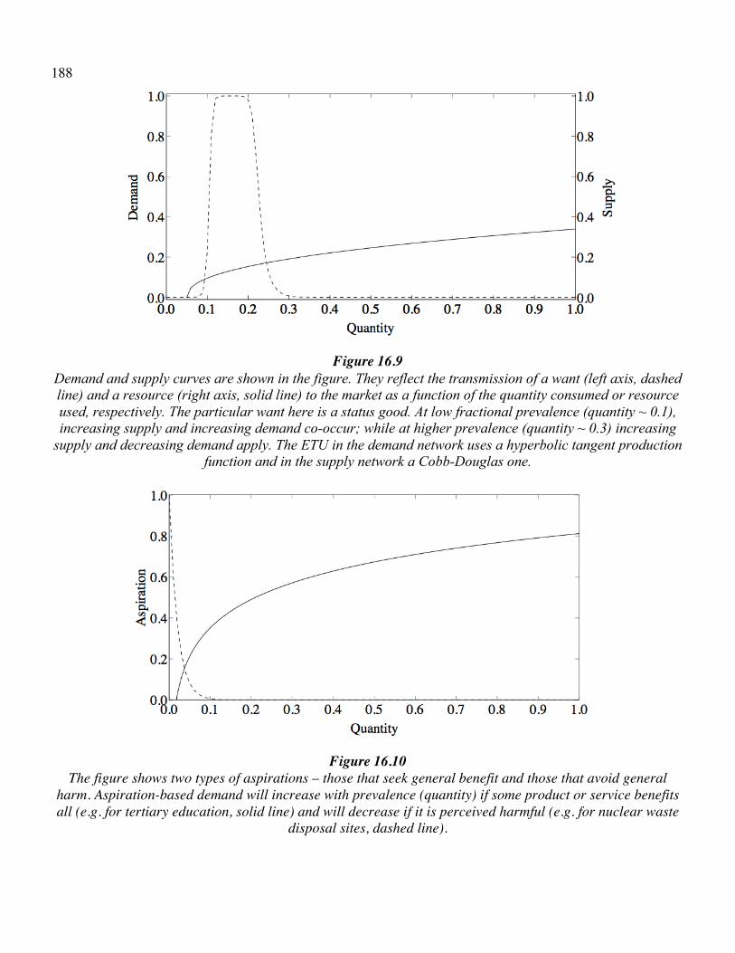
188

Figure 16.9 Demand and supply curves are shown in the figure. They reflect the transmission of a want (left axis, dashed line) and a resource (right axis, solid line) to the market as a function of the quantity consumed or resource used, respectively. The particular want here is a status good. At low fractional prevalence (quantity ~ 0.1), increasing supply and increasing demand co-occur; while at higher prevalence (quantity ~ 0.3) increasing

supply and decreasing demand apply. The ETU in the demand network uses a hyperbolic tangent production function and in the supply network a Cobb-Douglas one.

Figure 16.10 The figure shows two types of aspirations – those that seek general benefit and those that avoid general

harm. Aspiration-based demand will increase with prevalence (quantity) if some product or service benefits all (e.g. for tertiary education, solid line) and will decrease if it is perceived harmful (e.g. for nuclear waste

disposal sites, dashed line).

189

Prices. I have defined “price” before as the ratio of money to goods along a specific connection at a

given moment. This can only be effectively addressed where the demand and supply patterns as well as the number of tokens in the system and the allocation of tokens to different requirements are known. Nevertheless, a few points can be made here.

Price curves cannot be derived from ratios of demand to supply as shown in figures with demand and supply curves, even when the same quantity is plotted on the abscissa (e.g. Figure 16.11). This is because the amount of resource used is not the same as the amount of resource consumed. Resource use is generally more than resource consumption due to losses in the system. Looking at demand relative to supply at a given quantity is therefore not meaningful except by chance.

What these curves do tell us is whether the physical production of supplies is capable of meeting the physiological generation of demands as shown in Figure 16.6. The supply side in Figure 16.6 is unable to meet demand in excess of 667 kg per annum for a boxed table salt product, even when the available resource is fully utilized. As demand approaches this level demand inflation pressures should arise. Furthermore, the discrepancy between the actual demand and the available supply expressed relative to the available supply would provide some indication of such price pressures.

To obtain prices from the model, simulations are required. This would yield the levels of demand and supply that occur along every connection, thus their ratios can be determined. Still missing, though, before nominal prices can be derived, are the numbers of tokens allocated to express a unit of demand along a given connection. Figure 11.1 shows how physiological, psychological, and social requirements are distributed from a population to the input nodes of the DSN and how expenditures are also allocated to these nodes.

Figure 16.11 A demand curve reflecting the transmission of an aspiration (left axis, dashed line) and a

supply curve reflecting the transmission of resource (right axis, solid line) to the market as a function of the requirement or resource used, respectively. The aspiration is a benefit-seeking aspiration, thus increased consumption is deemed beneficial to all and leads to

further increased consumption. The ETU in the demand network uses a hyperbolic tangent production function and in the supply network a Cobb-Douglas one.

190 Consequently, the tokens that constitute these expenditures can be thought of as a means to prioritize or weight the different requirements. The more important a requirement, the more tokens are allocated to that requirement. In addition, because the number of tokens are limited (and must be limited to make possible some sort of stable mapping between tokens and finite product supplies) the very allocation process will involve a trade-off between requirements that are also, at least in part, dependent on price and price expectations. This is of interest because an understanding of how expectations (which are a function of experience and education, amongst others) influence prioritizing may facilitate the evaluation of policy alternatives (Lucas 1976: 41). Modeling this part of the system would require information about prices to reach the population (i.e. connections between the population and points where price information can be obtained). Nevertheless, simulations of the core system, assuming that inputs to the DSN and SSN already incorporate all the required information, will give an indication of the stability of the core system and how prices, due to fluctuations in demand relative to supply, will be affected.

Simulations of the core system

Above, I have shown how to implement demand- and supply-side networks by way of simple illustrative examples. These examples can readily be extended, for example, along the lines discussed in previous chapters on model refinements. Nevertheless, with a simple SSN and a simple DSN, in part based on the examples above, a core system can now be simulated and its output behavior examined. My major objective with this work is to sketch out a model-based theory; unfortunately, it is impossible here to evaluate by simulation the surfeit of points of interest that arise from it. Therefore, a few simple simulations must suffice and they are aimed at addressing the critical concept of market equilibrium. These simulations look at EEs that arise from two networks in a private economy, hence instances of simple disequilibria.

Parameters. Demand- and supply-side networks were created with three input nodes, two hidden nodes, and two output nodes each (unless otherwise specified). The input and output layers employed linear transfer functions while the hidden layer used the hyperbolic tangent function given by Eq. A1. The inputs for both networks had time horizons of 7 time points, thus one 7 by 3 input matrix was generated for each network using random numbers drawn from a normal distribution with mean 0.5 and standard deviation 0.1.

All the weights in both networks were given values drawn from a uniform distribution with limits 0.01 to 0.99. These weights were then further subjected to constraints. In the DSN, the first set of weights (i.e. from the input to hidden layers) was scaled so that their sum fell between the limits 0.8 to 1.0 to indicate the relative inelasticity of needs. Connections originating from node 2 of the input layer were scaled to sum within the limits 0.3 to 0.8 to indicate the relative elasticity of wants while those originating from node 3 of the input layer were scaled to sum within the limits 0.0 to 0.3 to indicate the high elasticity of aspirations. The second set of weights (i.e. from the hidden to output layers) were scaled to sum within the limits 0.9 to 1.0 to reflect the fact that not all demands are adequately relayed to the market by enterprises. All of the weights in the first set of weights for the SSN were scaled to sum between the limits 0.9 and 1.0 to reflect a relatively high level of resource utilization. Weights in the second set were scaled similarly to reflect the fact that most, but not all, products reach the market.

Once inputs and weights were assigned, the initial output of each network was calculated. The initial output of the DSN was then used as target to train the SSN. Thereafter, the initial output of the SSN was used to train the DSN. After training, the output for each network was calculated and assigned as the next ‘initial’ output. The networks were thus trained on their successive outputs up to 99 trials or convergence, whichever came first, using only a few iterations per trial and a conjugate gradient optimization method. The training was performed in batch mode rather than on-line mode and the inputs were kept constant except where otherwise noted. Graphs show the evolution of the EE over trials as well as the evolution over trials of one output from each network to provide qualitative information about the ratio of demand to supply, hence of prices on the tertiary market, for that product (output node 1).

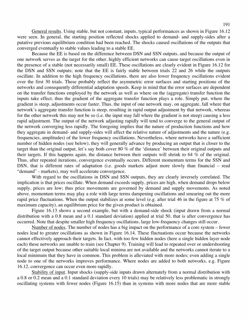
191 General results. Using stable, but not constant, inputs, typical performances as shown in Figure 16.12

were seen. In general, the starting position reflected shocks applied to demand- and supply-sides after a putative previous equilibrium condition had been reached. The shocks caused oscillations of the outputs that converged eventually to stable values leading to a stable EE.

Because the EE is based on the difference between DSN and SSN outputs, and because the output of one network serves as the target for the other, highly efficient networks can cause target oscillations even in the presence of a stable (not necessarily small) EE. These oscillations are clearly evident in Figure 16.12 for the DSN and SSN outputs; note that the EE is fairly stable between trials 22 and 26 while the outputs oscillate. In addition to the high frequency oscillations, there are also lower frequency oscillations evident over the first 30 trials. These probably reflect the asymmetric error surfaces and starting positions of the networks and consequently differential adaptation speeds. Keep in mind that the error surfaces are dependent on the transfer functions employed by the network as well as where on the (aggregate) transfer function the inputs take effect, thus the gradient of the aggregate transfer function plays a role. Simply put, where the gradient is steep, adjustments occur faster. Thus, the input of one network may, on aggregate, fall where that network’s aggregate transfer function is steep, resulting in rapid output adjustment by that network, whereas for the other network this may not be so (i.e. the input may fall where the gradient is not steep) causing a less rapid adjustment. The output of the network adjusting rapidly will tend to converge to the general output of the network converging less rapidly. The foregoing implies that the nature of production functions and how they aggregate in demand- and supply-sides will affect the relative nature of adjustments and the nature (e.g. frequencies, amplitudes) of the lower frequency oscillations. Nevertheless, where networks have a sufficient number of hidden nodes (see below), they will generally advance by producing an output that is closer to the target than the original output, let’s say both cover 80 % of the ‘distance’ between their original outputs and their targets. If this happens again, the distance between their outputs will shrink to 64 % of the original. Thus, after repeated iterations, convergence eventually occurs. Different momentum terms for the SSN and DSN, that is different rates of adaptation (i.e. goods markets adjust more slowly than financial – read “demand” - markets), may well accelerate convergence.

With regard to the oscillations in DSN and SSN outputs, they are clearly inversely correlated. The implication is that prices oscillate. When demand exceeds supply, prices are high, when demand drops below supply, prices are low; thus price movements are governed by demand and supply movements. As noted above, momentum terms may play a role with large terms dampening oscillations and smearing out the more rapid price fluctuations. When the output stabilizes at some level (e.g. after trial 46 in the figure at 75 % of maximum capacity), an equilibrium price for the given product is obtained.

Figure 16.13 shows a second example, but with a demand-side shock (input drawn from a normal distribution with a 0.8 mean and a 0.1 standard deviation) applied at trial 50, that is after convergence has occurred. Note that despite smaller high frequency oscillations, large low-frequency changes still occur.

Number of nodes. The number of nodes has a big impact on the performance of a core system – fewer nodes lead to greater oscillations as shown in Figure 16.14. These fluctuations occur because the networks cannot effectively approach their targets. In fact, with too few hidden nodes (here a single hidden layer node each) these networks are unable to train (see Chapter 9). Training will lead to repeated over or undershooting of the target output because other suitable local minima are not available and the networks cannot iterate to a local minimum that they have in common. This problem is alleviated with more nodes; even adding a single node to one of the networks improves performance. Where nodes are added to both networks, e.g. Figure 16.12, convergence can occur even more rapidly.

Stability of input. Input shocks (supply-side inputs drawn alternately from a normal distribution with a 0.8 or 0.2 mean and a 0.1 standard deviation every 10 trials) may be relatively less problematic in strongly oscillating systems with fewer nodes (Figure 16.15) than in systems with more nodes that are more stable

192 (Figure 16.16). However, systems with more nodes are capable of converging rapidly after such shocks, i.e. they adapt fast.

Figure 16.12

A simulation of a simple private core system economy (see text for details) shows that the equilibrium error fluctuates after an initial shock (in both demand and supply sides; trial 0) but tends to converge. Oscillations

are evident in the output values from the networks because the output of one network is used as a target to train the other network and vice versa.

Figure 16.13 A simulation of a simple private core system economy shows that the equilibrium error fluctuates after an

initial shock (in both demand and supply sides; trial 0) and also when, after convergence, a second (demand-side) shock was applied (trial 50).

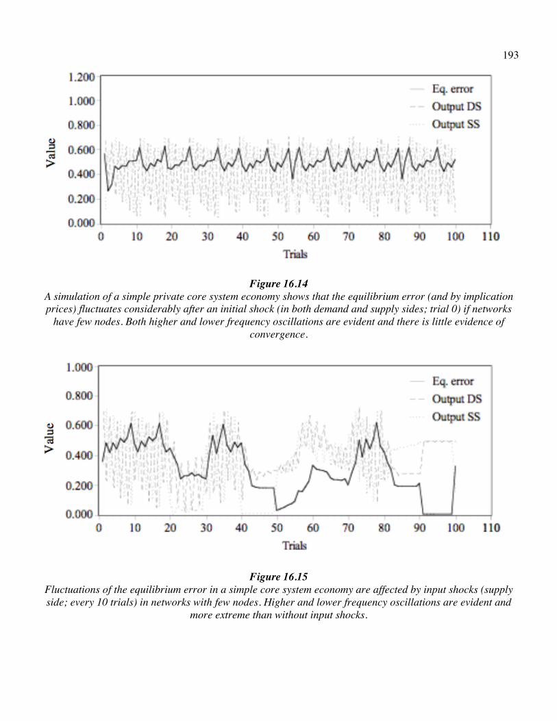
193

Figure 16.14 A simulation of a simple private core system economy shows that the equilibrium error (and by implication prices) fluctuates considerably after an initial shock (in both demand and supply sides; trial 0) if networks

have few nodes. Both higher and lower frequency oscillations are evident and there is little evidence of convergence.

Figure 16.15 Fluctuations of the equilibrium error in a simple core system economy are affected by input shocks (supply side; every 10 trials) in networks with few nodes. Higher and lower frequency oscillations are evident and

more extreme than without input shocks.

194

Figure 16.16 Fluctuations of the equilibrium error in a simple core system economy are notably affected by input shocks (supply side; every 10 trials) in networks with more nodes. However, after each shock convergence rapidly

occurs.

With regard to Figure 16.16, two further observations can be made. The first is that periods of stability appear possible even though supply and demand are not matched. For example, between trials 20 and 30, demand appears to be consistently higher than supply while the opposite is true between trials 40 and 50. The former period should be characterized by high prices and the latter by low prices. Second, there is an apparent tendency for the aggregate output of both demand and supply to decrease with repeated shocks. This could indicate that repeated shocks are damaging to the core system, but the validity of this interpretation is unclear presently and the persistence, thus significance, of the trend should await more extensive and comprehensive simulations.

Discussion and conclusions

Demand- and supply-side networks were created here and combined into a core economic system. The output functions from the networks, which depend on demand and supply production functions, constitute demand and supply curves. On the supply side, where resources are comparatively passive, an ETU could possibly use more arbitrary fractions of any given resource to provide one or more products to the market. On the demand side, in contrast, fractions of requirements (especially needs) cannot be used in an arbitrary manner since some needs may then go unsatisfied leading to a sharp increase in demand to which a capable and unconstrained ETU will respond. For this reason, I have taken pains to formulate and incorporate the dynamics with which requirements are transmitted to ETUs in the DSN. Strictly speaking though, such dynamics also occur for resources; these are not as passive as one might suspect and resource utilization could affect resource availability in an equally dynamic, but perhaps less vociferous, manner.

From these analyses of simple examples, supply and demand trends are obtained and their relationships can be examined. In particular, these trends reveal regions where product can be supplied at levels that meet demands and regions where supply will be inadequate. Thus regions can be identified where price pressures will be strong (i.e. supply is inadequate), regions where price pressures will be mild (i.e.

195 supply is adequate), and regions where price pressures could be negative (i.e. supply is excessive). However, these relationships do not reveal prices because neither the number of tokens (i.e. money) in the system nor their prioritized allocation to different requirements has been specified.

It is also interesting to consider how adaptation in a real economy occurs. In these simulations, networks were trained with a conjugate gradient method. This is essentially a gradient descent method meaning that adaptations occur in the direction that reduces the output error (here the EE). But does it happen this way in the real world? Does economic adaptation bear any semblance to gradient descent? Possibly. I suspect that profits and losses are local error signals that permit adaptation in the manner of error backpropagation where the adjustment step size is given by the size of the error. Once the system is in equilibrium, there are no (supernormal) profits or losses to be had since there are no gradients. This suggests that the pursuit of profit in a system at equilibrium is either pointless or destabilizing. The adaptation process also raises the question of how to define “efficient markets” in terms of network attributes – the rate and/or the extent of EE reduction? A formal analysis assessing whether economic systems adjust in a manner analogous to error backpropagation, the commonly used learning algorithm in multilayer perceptron networks (e.g. Hush and Horne 1993: 12), would be of interest.

With these simulations, I hope to have put into practice some of the conceptual aspects of the CTE by illustrating how to convert human attributes (physiology, psychology, sociology) into economic demands by way of demand-side neural networks and how to combine demand- and supply-side neural networks into a an operating core system. It concludes the largely qualitative conceptual framework outlined in the preceding chapters with a quantitative implementation of a key segment of the model. This part of the connectionist model therefore provides proof-of-principle that microfoundations can be used to obtain macroeconomic trends.

196

References Aigner, D. J. ; Chu, S. F. 1968. On estimating the industry production function. The American Economic

Review 58: 826-839. Alexander, R. D.; Noonan, K. M. 1979. Concealment of ovulation, parental care, and human social

evolution. In Chagnon, N.; Irons, W. (eds.) Evolutionary biology and human social behavior, pp. 436-53. North Scituate, MA: Duxbury.

Anderson, D. R.; Sweeney, D. J.; Williams, T. A. 2001. Contemporary business statistics with Microsoft excel. Cincinnati, OH: South-Western.

Antonides, G. 2008. Comparing models of consumer behavior. In Lewis, A. (ed.) Psychology and economic behavior, pp. 227-252. Cambridge, UK: Cambridge.

Bairam, E. I. 1994. Homogeneous and nonhomogeneous production functions: theory and applications. Aldershot, UK: Avebury.

Bakshi, R. B.; Stephanopoulos, G. 1993. Wave-net: a multiresolution, hierarchical neural network with localized learning. AIChE Journal 39: 57-81.

Baldi, P. 1995. Gradient descent learning algorithm overview: a general dynamical systems perspective. IEEE Transactions on Neural Networks 6: 182-195.

Barnes, P. 2007. Minsky’s financial instability hypothesis, information asymmetry and accounting information: the UK financial crises of 1866 and 19897. Accounting History 12: 29-53.

Bartkowiak, R. A. 1973. Electric circuits. New York, NY: Intext Educational Publishers. Beattie, B. R.; Taylor, C. R. 1985. The economics of production. New York, NY: Wiley. Blaug, M. Why is the quantity theory of money the oldest surviving theory in economics? In Blaug, M. et

al., (authors), The quantity theory of money, pp. 27-49. Hants, UK: Edward Elgar. Bloch, H. 2005. Steindl’s analysis of firm growth and the tendency toward industry concentration. In T.

Mott and N Shapiro (eds.), Rethinking capitalist development: essays on the economics of Josef Steindl, pp. 23-36. London: Routledge.

Cameron, R; Neal, L. 2003. A concise economic history of the world. Oxford, UK: Oxford University Press.

Changnon, S. A. 1999. Impacts of the 1997-98 El Niño-generated weather in the United States. Bulletin of the American Meteorological Society 80: 1819-1827.

Chen, C. L. P. 1996. A rapid supervised learning neural network for function interpolation and approximation. IEEE Transactions on Neural Networks 7: 1220-1229.

Chown, J. F. 1994. A history of money: from AD 800. New York, NY: Routledge. Cichocki, A; Unbehauen, R. 1993. Neural networks for optimization and signal processing. New York,

NY: Wiley and Sons. Cullis, J. G.; Jones, P. R. 2008. How big should government be? In Lewis, A. (ed.) Psychology and

economic behavior, pp. 281-303. Cambridge, UK: Cambridge. Davies, G 2002. A history of money: from ancient times to the present day. Cardiff, UK: University of

Wales Press. Daly, H. E. 1997. Georgescu-Roegen versus Solow/Stiglitz. Ecological Economics 22: 261-266. de Waal, F. B. M. 1987. Tension regulation and nonreproductive functions of sex among captive bonobos.

National Geographic Research 3: 3180-335. Fairris, D.; Pattanaik, P. K. 2003. On the notion of optimality in welfare economics. In K. Basu; P. B.

Nayak; R. Ray (eds.), Markets and Governments, pp. 90-109. New Delhi: Oxford University Press. Fontana, G. 2006. The Federal Reserve and the European Central Bank: a theoretical comparison of their

legislative mandates. Journal of Post Keynesian Economics 28: 433-450.

197 Gandolfo, G. 1998. International trade theory and policy. Berlin, Germany: Springer. Gardiner, G. 2006. The evolution of creditary structures and controls. New York, NY: Palgrave McMillan. Galbraith, J. K. 1994. A journey through economic time. Boston, MA: Houghton Mifflin. Groenewegen, P. 2003. Classics and moderns in economics (Volume I). New York, NY: Routledge. Haddon, M. 2003. The curious incident of the dog in the nighttime. London, UK: Jonathan Cape. Harvey, R. L. 1994. Neural network principles. Englewood Cliffs, NJ: Prentice-Hall. Hess, J. D.; Kacen, J. J.; Kim, J. 2006. Mood-management dynamics: the interrelationship between moods

and behaviours. British Journal of Mathematical and Statistical Psychology 59: 347-378. Hill, R. C.; Griffiths, W. E.; Judge, G. G. 2001. Undergraduate Econometrics. Hoboken, NJ: Wiley. Hush, D. R. 1999. Training a sigmoidal node is hard. Neural Computation 11: 1249-1260. Hush, D.R.; Horne, B. G. 1993. Progress in supervised neural networks. IEEE Signal processing 10: 8-39. Independent Sector. 2000. Giving and volunteering in the United States: 1999 Edition. Washington, DC:

Independent Sector. Ison, S. 2000. Economics. New York, NY: Prentice Hall. Jackson, T. M. 1986. Basic concepts in monetary economics. London, UK: Checkmate. Jain, A. K.; Mao, J.; Mohiuddin, K. M. 1996. Artificial neural networks: a tutorial. IEEE Computer March:

31-44. Kahneman D.; Tversky, A. 1979. Prospect theory: an analysis of decision under risk. Econometrica XLVII

263-291. Karhunen J.; Joutsensalo, J. 1995. Representation and separation of signals using non-linear PCA type

learning. Neural Networks 7: 113-127. Karim, M. N.; Yoshida, T.; Rivera, S. L.; Saucedo, V. M. ; Eikens, B.; Oh, G.-S. 1997. Global and local

neural network models in biotechnology: application to different cultivation processes. Journal of Fermentation and Bioengineering 83: 1-11.

Kelly, J. P. 1985a. Anatomy of the central visual pathways. In E. R. Kandel; J. H. Schwartz (eds.), Principles of neural science (2nd Ed.), pp. 356-365. Amsterdam: Elsevier.

Kelly, J. P. 1985b. Anatomical basis of sensory perception and motor coordination. In E. R. Kandel; J. H. Schwartz (eds.), Principles of neural science (2nd Ed.), pp. 222-243. Amsterdam: Elsevier.

Kuroda, S. 1984. Interactions over food among pygmy chimpanzees. In Susman, S. (1984) The pygmy chimpanzee, pp. 301-24. New York: Plenum.

Kurz, H. D.; Salvadori, N. 2003. Fund-flow versus flow-flow in production theory: reflections on Georgescu-Roegen’s contribution. Journal of Economic Behavior and Organization 51: 487-505.

Lee, S. 1992. Supervised learning with Gaussian potentials. In: B. Kosko (ed.), Neural networks for signal processing (pp. 189-223), Englewood Cliffs, NJ: Prentice Hall.

Lewis, A. 2008. Introduction. In: A. Lewis (ed.), Psychology and economic behavior, pp. 3-8. Cambridge: Cambridge University Press.

Levine, D. P. 2005. Reproduction and transformation in the theory of the market: observations on Josef Steindl’s theory of capitalist dynamics. In T. Mott and N Shapiro (eds.), Rethinking capitalist development: essays on the economics of Josef Steindl, pp. 11-22. London: Routledge.

Levine, D. S. 2000. Introduction to neural and cognitive modeling. Mahwah, NJ: Lawrence Erlbaum. Levinsohn, J.; Petrin, A. 2003. Estimating production functions using inputs to control for unobservables.

Review of Economic Studies 70: 317-341. Lippmann, R. P. 1987. An introduction to computing with neural nets. IEEE Acoustics, Speech and Signal

Processing Magazine 4: 4-22. Lohrenz, T.; Montague, P. R. 2008. Neuroeconomics: what neuroscience can learn from economics. In:

A. Lewis (ed.), Psychology and economic behavior, pp. 457-492. Cambridge: Cambridge University Press.

198 Lucas, R. E. 1976. Econometric policy evaluation: a critique. Carnegie-Rochester Conference Series on

Public Policy 1: 19-46. Maddison, A. 2001. The world economy: a millennial perspective. OECD: Paris, France. Mao, J.; Jain, A. K. 1995. Artificial neural networks for feature extraction and multivariate data projection.

IEEE Transactions on Neural Networks 6: 296-317. Martin, P. C. 2003 (November). Power, the state, and the institution of property. Paper presented at the

international symposium Genuine Money, Good Securities and the Foundations of the Economy: A New Look at Property Rights at the Universität Bremen (IKSF), Germany.

Maslow, A. H.. 1943. A theory of human motivation. Psychological Review 50: 370-396. Mayumi, K; Giampietro, M.; Gowdy, J. M. 1998. Georgescu-Roegen/Daly versus Solow/Stiglitz revisited.

Ecological Economics 27: 115-117. McClelland, J. L.; Rumelhart, D. E. 1986. A distributed model of human learning and memory. In D. E.

Rumelhart; J. L. McClelland (eds.), Parallel distributed processing, pp. 171-215. Cambridge, MA: MIT.

McClelland, J. L.; Rumelhart, D. E.; Hinton, G. E. 1986. The appeal of parallel distributed processing. In D. E. Rumelhart, J. L. McClelland (eds.) Parallel distributed processing, pp. 3-43. Cambridge, MA: MIT.

Mishra, S. K. 2007. A brief history of production functions. Accessed online at http://mpra.ub.uni-muenchen.de/5254 in April 2009.

Mookherjee, D. 2003. Markets versus state: a sterile controversy? In K. Basu; P. B. Nayak; R. Ray (eds.), Markets and Governments, pp. 110-143. New Delhi: Oxford University Press.

Nayak, P. B. 2003. An examination of Schumpeter’s tax state. In K. Basu; P. B. Nayak; R. Ray (eds.), Markets and Governments, pp. 243-258. New Delhi: Oxford University Press.

O’Brien, D. 1995. Long-run equilibrium and cyclical disturbances: the currency and banking controversy over monetary control. In Blaug, M. et al., (authors), The quantity theory of money, pp. 50-79. Hants, UK: Edward Elgar.

Patinkin, D. 1995. Concluding comments on the quantity theory. In Blaug, M. et al., (authors), The quantity theory of money, pp. 120-133. Hants, UK: Edward Elgar.

Perry, R. H.; Chilton, C. H. 1973. Chemical engineer’s handbook, pp. 4-23 to 4 -24. Tokyo: McGraw-Hill Kogakusha.

Press, W. H.; Teukolsky, S. A.; Vetterling, W. T.; Flannery, B. P. 1994. Numerical recipes in C. Cambridge, U.K. Cambridge University Press.

Rodbell, D. T.; Seltzer, G. O.; Anderson, D. M.; Abbott, M. B.; Enfield, D. B.; Newman, J. H. 1999. An ~15,000-year record of El Niño-driven alluviation in southwestern Ecuador. Science 283: 516-520.

Rumelhart, D. E.; Hinton, G. E.; McClelland, J. L. 1988. A general framework for parallel distributed processing. In: D. E. Rumelhart; J. L. McClelland (eds.), Parallel distributed processing, pp. 46-76. Cambridge, MA: MIT.

Rumelhart, D. E.; Hinton, G. E.; McClelland, J. L. 1988. PDP models and general issues in cognitive science. In: D. E. Rumelhart; J. L. McClelland (eds.), Parallel distributed processing, pp. 110-146. Cambridge, MA: MIT.

Rumelhart, D. E.; Hinton, G. E.; Williams, R. J. 1988. Learning internal representations by error propagation. In: D. E. Rumelhart; J. L. McClelland (eds.), Parallel distributed processing, pp. 318-362. Cambridge, MA: MIT.

Sato, R, 1975. The most general class of CES functions. Econometrica 43: 999-1003. Schoner, 1992. Reaching the generalization maximum of backpropagation networks. In I. Aleksandr; J.

Taylor (eds.), Artificial neural networks, 2, pp. 91-94. Amsterdam: Elsevier.

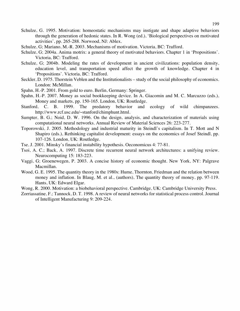
199 Schulze, G. 1995. Motivation: homeostatic mechanisms may instigate and shape adaptive behaviors

through the generation of hedonic states. In R. Wong (ed.), ‘Biological perspectives on motivated activities’, pp. 265-288. Norwood, NJ: Ablex.

Schulze, G; Mariano, M.-R. 2003. Mechanisms of motivation. Victoria, BC: Trafford. Schulze, G; 2004a. Anima motrix: a general theory of motivated behaviors. Chapter 1 in ‘Propositions’.

Victoria, BC: Trafford. Schulze, G; 2004b. Modeling the rates of development in ancient civilizations: population density,

education level, and transportation speed affect the growth of knowledge. Chapter 4 in ‘Propositions’. Victoria, BC: Trafford.

Seckler, D. 1975. Thorstein Veblen and the Institutionalists – study of the social philosophy of economics. London: McMillan.

Spahn, H.-P. 2001. From gold to euro. Berlin, Germany: Springer. Spahn, H.-P. 2007. Money as social bookkeeping device. In A. Giacomin and M. C. Marcuzzo (eds.),

Money and markets, pp. 150-165. London, UK: Routledge. Stanford, C. B. 1999. The predatory behavior and ecology of wild chimpanzees.

http://www.rcf.usc.edu/~stanford/chimphunt.html. Sumpter, B. G.; Noid, D. W. 1996. On the design, analysis, and characterization of materials using

computational neural networks. Annual Review of Material Sciences 26: 223-277. Toporowski, J. 2005. Methodology and industrial maturity in Steindl’s capitalism. In T. Mott and N

Shapiro (eds.), Rethinking capitalist development: essays on the economics of Josef Steindl, pp. 107-126. London, UK: Routledge.

Tse, J. 2001. Minsky’s financial instability hypothesis. Oeconomicus 4: 77-81. Tsoi, A. C.; Back, A. 1997. Discrete time recurrent neural network architectures: a unifying review.

Neurocomputing 15: 183-223. Vaggi, G; Groenewegen, P. 2003. A concise history of economic thought. New York, NY: Palgrave

Macmillan. Wood, G. E. 1995. The quantity theory in the 1980s: Hume, Thornton, Friedman and the relation between

money and inflation. In Blaug, M. et al., (authors), The quantity theory of money, pp. 97-119. Hants, UK: Edward Elgar.

Wong, R. 2000. Motivation: a biobehavioral perspective. Cambridge, UK: Cambridge University Press. Zorriassatine, F.; Tannock, D. T. 1998. A review of neural networks for statistical process control. Journal

of Intelligent Manufacturing 9: 209-224.