Embed Size (px)
Citation preview
209
Chapter 9
Computers
ARMAND B. CACHELIN, JOHN DEMPSTER andPETER T. A. GRAY
Hardware is the parts of a computer you can kick.Computers don’t save time, they redistribute it.
This chapter is a short introduction to computers and their use in the laboratory. Notsurprisingly, this chapter has become far more outdated than others in the six yearssince the publication of the first edition of Microelectrode Techniques - ThePlymouth Workshop Handbook. The potential role of desktop computers was justbeginning to emerge in 1987. Six years on, two computer generations later, thepersonal computer reigns undisputed in the office and in the lab. Thus the aim of thischapter is not so much to familiarise readers with PCs than to draw their attention toimportant points when choosing a computer or commercially available software fortheir lab. The chapter starts with a brief outline of some of the most important issuesto consider when selecting a system. This is followed by sections which provide amore detailed consideration, firstly, of the basic hardware issues relating to theacquisition and storage of signals on a computer system and, secondly, of thefunctional requirements for software used for the analysis of electrophysiologicaldata.
1. Selecting a system
Selection of a computer system when starting from scratch requires balancing a largenumber of factors. In general a guide-line widely accepted when specifyingcommercial systems, which applies as well here, is that the first thing to choose is thesoftware. Choose software that will do what you want, then select hardware that willrun it. In many cases, of course, the hardware choice may already be constrained bythe existence, for example, of a PC of a particular type that must be used for costreasons. However even in these cases the rule above should be applied to selection ofother parts of the hardware, such as laboratory interfaces.
When selecting software it is essential to bear in mind likely future requirements as
A. B. CACHELIN, Pharmacology Department, University of Berne, 3010 Berne,SwitzerlandJ. DEMPSTER, Department of Physiology and Pharmacology, University of Strathclyde,Glasgow G1 1XW, UKP. T. A. GRAY, 52 Sudbourne Road, London SW2 5AH, UK
well as current requirements. This can be very hard to do in any environment, as theintroduction of a computer system always changes working patterns in ways that arehard to predict in advance. In a scientific laboratory, where the nature of futureexperiments is hard to predict anyway, this is doubly true. This is one reason for tryingto select an adaptable system if at all possible. Maximum flexibility is obtained bywriting your own software, but the cost in terms of time is high, and cannot generallybe justified where off-the-shelf packages are available. However, if you are developingnovel techniques it may be essential to have total control over your software. For mostusers applying established techniques, the choice is best limited to off-the-shelfsystems, but the flexibility of the system should be a primary factor in the decision.
Flexibility in an off-the-shelf system can be assessed in many ways. For example,at the level of data acquisition are maximum sample rates, sample sizes, availablecomplexity of output control pulses (e.g. for controlling voltage jump protocols)likely to match future requirements. At the next stage, factors such as the forms ofdata analysis available must be considered. How flexible are they? In many systemsinflexibility here can often be partially overcome by exporting data to an externalanalysis package, provided that the software selected allows for data export in asuitable form. At the highest level of flexibility, can the system be used to control,sample and analyse data from completely new types of experiment? In most cases theanswer, unsurprisingly, will be no. In this case, one must simply wait for off-the-shelfsoftware to become available unless one writes the program oneself.
P A R T O N E : H A R D W A R E
2. Of bytes and men
Before going further it is worth introducing some basic concepts and terms which arewidely used in computer-related discussions. Decimal numbers are a natural form ofrepresentation for ten-fingered humans. According to this system, numbers arecomposed of digits which take values between 0 and 9. Digital computers makeextensive use of a different, so called binary number system. The elementary piece ofinformation used in the computer is the bit which can take only two values (0 or 1).This binary system fits the ON-OFF nature of the computer’s digital logic circuits. Anumber expressed in binary form consists of a string of ‘1’s and ‘0’s. For instance, thedecimal number 23 (2×101+3×100) has the binary form 10111 which is equal to1×24+0×23+1×22+1×21+1×20.
Computers use a ‘language’ in which all words have the same length. Thus bothoperands (data) and operations (instructions) used by computer systems are encodedas fixed length binary numbers. Common word lengths are 16, 32 and more recently64 bits. An 8 bit word is known as a byte and the term is often used as a unit of datastorage capacity. One kilobyte (KB) is equivalent to 1024 bytes (210 bytes)1, a MB to1048576 (220) bytes. The address bus width sets the limits to the address space. The
210 A. B. CACHELIN, J. DEMPSTER AND P. T. A. GRAY
1By convention, we shall use “K” as abbreviation for 1024 and “k” for 1000.
wordsize sets the width of data that a processor can manage conveniently. Forexample, 216 (64 KB) is the largest number of memory locations that can beaddressed directly by a 16 bit wide address bus. Additional bits must be used to storeand fetch data from larger RAM. Of course 32 bit processors are much less limitedbeing able to address up to 4 GB of RAM.
A further consequence of the use of a fixed length binary number system is that, atthe most fundamental level, a digital computer can only store and manipulate integernumbers (0, 1, 2,...), so the highest integer number that could be stored within 16 bitsis 216. The computer reserves one bit to represent the sign of a integer. Thus wholenumbers in the range ±215 can be stored within 2 bytes. Although almost any kind ofdata can be stored and processed by a computer system, some forms of data are easierto handle than others. Large numbers (>215) and real numbers (i.e. with fractionalparts, e.g. 1.23) cannot be directly stored in memory locations. How this and otherproblems are solved is the subject of the next section.
3. Computer systems
The digital computer forms the core of the data acquisition system, providing thefollowing three basic functions: data input, processing and output. In the context of alaboratory these functions could be for example:
Input: acquisition of signal(s) (analogue to digital conversion) reading back data filesinput of commands by keyboard or mouse
Processing: qualitative signal analysis (preparation of ‘idealised’ data)quantitative signal analysis (statistics, curve fitting, estimation of
parameters of models)Output: command signals (digital to analogue conversion)
visual display of stored datastorage to data files on disk or tapeproduction of hard copies on paperconnection to other computer systems via a network
The advances in computer technology are such that most readily available personalcomputers within the IBM personal computer (‘PC’2) and Macintosh families aremore than adequate for the above tasks, in terms of computing speed and graphicaldisplay quality. Given the pace of change in computer technology, it is futile toprovide particular specifications as they must become rapidly obsolete. In thefollowing, we present certain general observations which should be borne in mindwhen choosing a computer.
Central processor unit
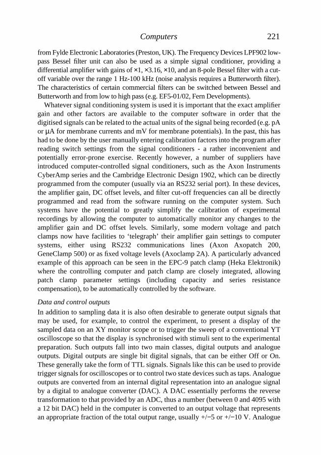
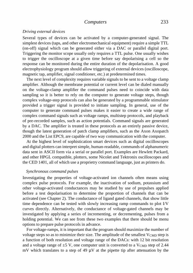
As can be seen from Fig.1, the central processing unit (CPU) forms the core of the
211Computers
2From now on and throughout this chapter we will use the term ‘PC’ to designate acomputer that is compatible with the IBM PC family of computers regardless of the model(PC/XT/286, 386...) or manufacturer (IBM, Compaq, Hewlett-Packard etc.).
computer system. It is, essentially, a machine for processing binary numerical data,according to the instructions contained in a binary program. The operation of the CPU isgoverned by a master clock which times the execution of instructions, the higher theclock rate the faster the CPU3. The performance of a CPU also depends upon the size ofthe data that a single instruction can handle, calculations being more efficient if they canbe performed by a single instruction rather than a group of instructions. Typical personalcomputer CPUs (c. 1993) can handle 32 bit numbers in a single instruction and operate atclock rates of 25-66 MHz. The two major personal computer families (PCs and AppleMacintosh) are based upon different CPU designs, PCs use the 80×86 family of Intelprocessors (or clones by AMD or Cyrix) while the Macintosh uses the Motorola 680×0family. Over the years, each CPU family has evolved with the introduction of newer andfaster CPUs, while retaining essential compatibility with earlier models. Currently usedmembers of the Intel CPU family include the 80386, 80486 and the recently introducedPentium (‘80586’). Macintosh computers are built around the Motorola 68030 and68040 processors. The first computers built around the PowerPC 601/603 chips (seeBYTE article) will be available by the time this book is printed. The clear trend towardsgraphical user interfaces makes it advisable to chose a computer system which uses atleast an 80486 processor. Modern CPUs have more than enough power for most PCapplications. However, certain tasks, such as program development, lengthy numericalanalysis, such as curve fitting, and graphics intensive applications, do benefit from thefastest possible processor.
Floating point unit
The arithmetic operations within the instruction set of most CPUs are designed tohandle integer numbers of a fixed size. Scientific calculations, however, require amore flexible number system capable of representing a much wider range of numbersincluding the complete set of real numbers as well as handling trigonometric,transcendental and other mathematical functions. For this purpose, computers use aninternal notation convention called ‘floating point’ in which real numbers areapproximated as product of a power of 2 times a normalised fraction. Thus:
R = 2k × f,
where k is the exponent and f is the mantissa. The most common laboratorycomputers, PCs and Macintoshes, both represent these numbers internally followingthe IEEE standard 754. In both cases, ignoring details of ordering of bytes in memory,these are stored internally as follows:
The sign bit S is set if the number is negative. The exponent may be either positiveor negative (see Table 1), however, it is internally stored as a number in the range
212 A. B. CACHELIN, J. DEMPSTER AND P. T. A. GRAY
3This is of course only true when comparing identical CPUs. Different CPUs runningidentical clock rates need not perform the same operations at the same speed.
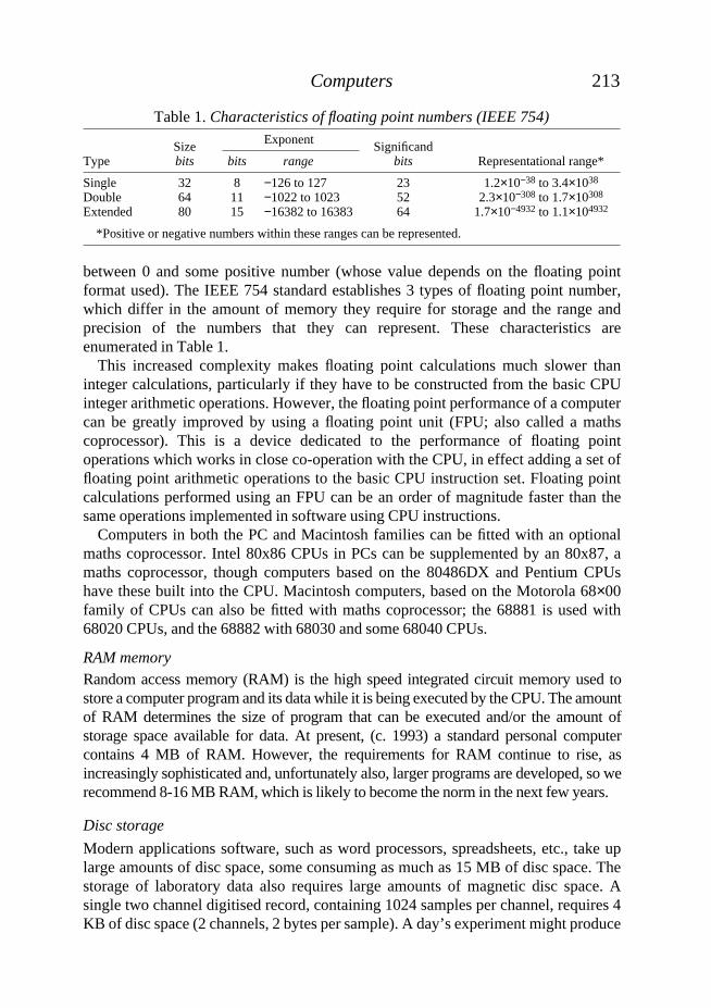
between 0 and some positive number (whose value depends on the floating pointformat used). The IEEE 754 standard establishes 3 types of floating point number,which differ in the amount of memory they require for storage and the range andprecision of the numbers that they can represent. These characteristics areenumerated in Table 1.
This increased complexity makes floating point calculations much slower thaninteger calculations, particularly if they have to be constructed from the basic CPUinteger arithmetic operations. However, the floating point performance of a computercan be greatly improved by using a floating point unit (FPU; also called a mathscoprocessor). This is a device dedicated to the performance of floating pointoperations which works in close co-operation with the CPU, in effect adding a set offloating point arithmetic operations to the basic CPU instruction set. Floating pointcalculations performed using an FPU can be an order of magnitude faster than thesame operations implemented in software using CPU instructions.
Computers in both the PC and Macintosh families can be fitted with an optionalmaths coprocessor. Intel 80x86 CPUs in PCs can be supplemented by an 80x87, amaths coprocessor, though computers based on the 80486DX and Pentium CPUshave these built into the CPU. Macintosh computers, based on the Motorola 68×00family of CPUs can also be fitted with maths coprocessor; the 68881 is used with68020 CPUs, and the 68882 with 68030 and some 68040 CPUs.
RAM memoryRandom access memory (RAM) is the high speed integrated circuit memory used tostore a computer program and its data while it is being executed by the CPU. The amountof RAM determines the size of program that can be executed and/or the amount ofstorage space available for data. At present, (c. 1993) a standard personal computercontains 4 MB of RAM. However, the requirements for RAM continue to rise, asincreasingly sophisticated and, unfortunately also, larger programs are developed, so werecommend 8-16 MB RAM, which is likely to become the norm in the next few years.
Disc storage
Modern applications software, such as word processors, spreadsheets, etc., take uplarge amounts of disc space, some consuming as much as 15 MB of disc space. Thestorage of laboratory data also requires large amounts of magnetic disc space. Asingle two channel digitised record, containing 1024 samples per channel, requires 4KB of disc space (2 channels, 2 bytes per sample). A day’s experiment might produce
213Computers
Table 1. Characteristics of floating point numbers (IEEE 754)
Size Exponent SignificandType bits bits range bits Representational range*
Single 32 8 −126 to 127 23 1.2×10−38 to 3.4×1038
Double 64 11 −1022 to 1023 52 2.3×10−308 to 1.7×10308
Extended 80 15 −16382 to 16383 64 1.7×10−4932 to 1.1×104932
*Positive or negative numbers within these ranges can be represented.
1000 of such records, occupying up 4 MB of disc space. The same amount of discspace will be taken up by less than 2 minutes of continuous sampling at 20 kHz onone channel. It is important, therefore, to ensure that there is sufficient disc storagespace to comfortably accommodate the quantity of experimental work envisaged,particularly when the computer is being used as the only storage device forexperimental signals. Overall, 200-300 MB of disc capacity should be available andfor the more demanding laboratory applications, 1000 MB might be preferable.
The hard disk system should also allow rapid access. Software disk caches, whichuse some of the system’s RAM are effective in speeding system response, but it isbetter, when buying new hardware, to ensure that the disk performance is as good as
214 A. B. CACHELIN, J. DEMPSTER AND P. T. A. GRAY
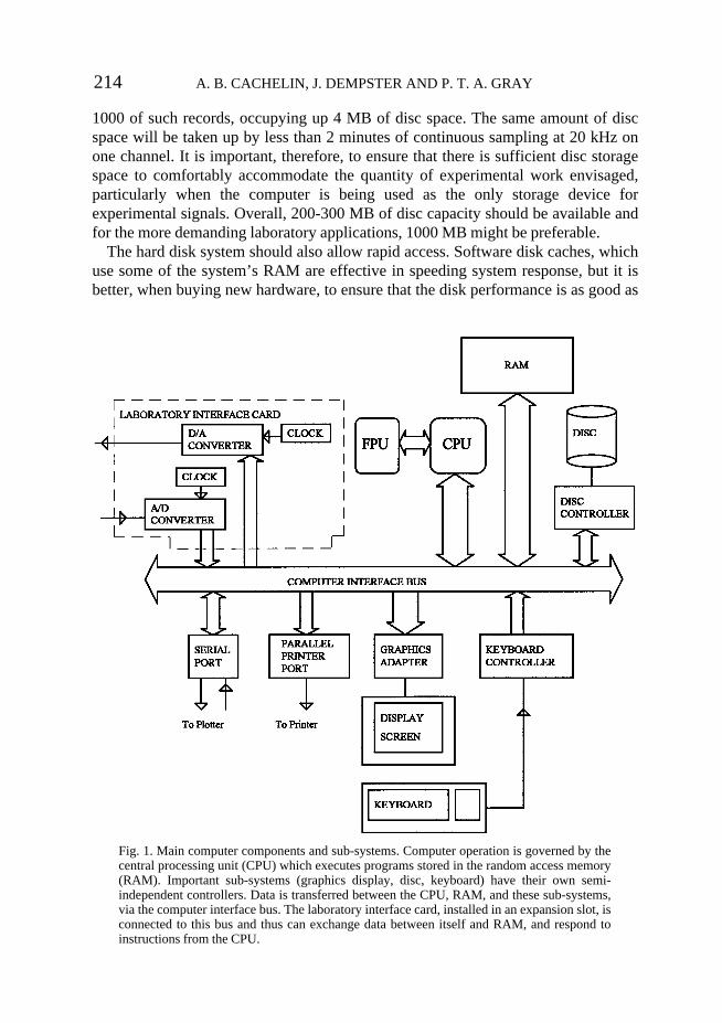
Fig. 1. Main computer components and sub-systems. Computer operation is governed by thecentral processing unit (CPU) which executes programs stored in the random access memory(RAM). Important sub-systems (graphics display, disc, keyboard) have their own semi-independent controllers. Data is transferred between the CPU, RAM, and these sub-systems,via the computer interface bus. The laboratory interface card, installed in an expansion slot, isconnected to this bus and thus can exchange data between itself and RAM, and respond toinstructions from the CPU.
can be afforded. A fast disk speeds up many applications more than a fasterprocessor. On PCs a range of disk drives is available. The choice of disk interfacemay play a significant role in determining disk drive performance. The most commonform is the IDE interface which is standard on many systems. SCSI drive interfacesgenerally offer better performance than other types, in particular for large drives.Performance may also be enhanced by using interfaces which have on-boardmemory, which is used to cache recently accessed data. Better performance still canbe achieved on modern PCs with a local bus version of these cached interfaces, whichpass data to the processor by a direct high speed link, instead of using the muchslower general purpose interface bus that older models do.
Archive storage
Although it is convenient to store experimental data on the computer’s internal harddisc, even the largest discs cannot accommodate more than a small number ofexperiments. Some form of removable data storage medium is therefore required forarchival storage of the data. The secure storage of experimental data is an importantissue. Experimental recordings are extremely valuable, if one takes into account thecost of person-hours required to design and perform the experiments. At least one‘back up’ copy of the recorded data should be made on a different medium, in casethe hard disc fails. It may also be necessary to preserve this archive data for manyyears, for scientific audit purposes or to allow future re-evaluation of results.
A variety of removable computer tape and disc media are available for archivestorage. This is one area where rapid improvements in technology (and the consequentobsolescence of the old) does not help since it becomes difficult to determine whichmedia are going to remain in widespread use. However, at present there are a numberof choices. A number of tape forms exist, using cartridges of varieties of sizes andcapacities (DC300, 45 MB; DC600, 65 MB; DAT (Digital Audio Tape) 1200 MB).Removable magnetic discs exist (e.g. the Bernoulli disc) but these are relativelyexpensive and have small capacities (40-80 MB) compared to alternatives.
In general, high capacity removable disc media use one of a number of optical datastorage technologies. WORM (Write Once Read Many) discs, for instance, use alaser beam to vaporise tiny pits in the reflective surface of a metal-coated disc, whichcan be read by detecting the reflections of a lower-power laser light trained on thesurface. As the name suggests, data can be written to a WORM disc only once, butread as many times as necessary. Rewritable optical discs are also available, whichuse the laser beam to effect a reversible phase change in the disc surface rather than apermanent pit. Two sizes of optical disc are available, 5.25 inch with a capacity of640 MB (e.g. Panasonic LF-7010), and 3.5 inch supporting 128 MB (e.g. Sony S350or Panasonic LF3000). The 3.5 inch discs are rewritable while the 5.25 inch drivessupport either WORM or rewritable discs.
A strong argument can also be made for storing a complete recording of theoriginal experimental signals on some form of instrumentation tape recorder,designed for storing analogue signals. FM (Frequency Modulation) tape recorders,such as the Racal Store 4, with a DC-5 kHz recording bandwidth (at 7.5 inches per
215Computers
second tape speed) have been used for many years. Analogue signals can also bestored on standard video cassette recorders, using a PCM (pulse code modulation)encoder to convert the signals into pseudo-video format. The Instrutech VR10B, forinstance, can be used to store two DC-22.5 kHz analogue channels (or 1, and 4 digitalmarker channels) on a standard VHS video tape. These devices may gradually bereplaced by modified DAT (Digital Audio Tape) recorders, such as the BiologicDTR1200 or DTR1600 which provide a similar capacity and performance to thePCM/video systems. DAT tape recorders are simple to operate compared to mostcomputer systems and have a high effective storage capacity (a single 60 min DATtape is equivalent to over 600 MB of digital storage)4. They provide additionalsecurity in case of loss of the digitised data, and allow the data to be stored in aneconomical and accessible form (compared to the non-standard data storage formatsof most electrophysiology software). They thus provide the opportunity for thesignals to be replayed and processed by different computer systems. An additionaladvantage is that a voice track can often be added during the experiment, offering avaluable form of notation. It MUST be borne in mind that ALL forms of magnetictape (i.e. also DAT recorders) have a limited bandwidth though the reason for thislimited bandwidth differs from one type of tape recorder to the other.
Networks
Laboratory computer systems are often connected to local area networks which allow datato be transferred between computers systems at high speed, permitting shared access tohigh capacity storage discs and printers. Often, the network can also be used to exchangeelectronic mail, both locally and, if connected to a campus network, internationally.Networks can be categorised both by the nature of the hardware connecting computers(e.g. Ethernet) and the software protocols (Novell Netware, Windows, NetBios) used tocontrol the flow of data5. Within the PC family, the most commonly used networkhardware is Ethernet followed by Token Ring. Ethernet permits data to be transferred at amaximum rate of 10 Mbps (bit per second). An Ethernet adapter card is required toconnect a PC to an Ethernet network. Low end Macintosh computers are fitted with aLocalTalk network connector as a standard feature. However, LocalTalk, with a transferrate of 230 kbps, is noticeably slower than Ethernet. On the other hand, high end Applecomputers (Quadra family) and printers (Laser Writer IIg, Laser Writer Pro 630) arefactory-equipped with serial, LocalTalk and Ethernet ports.
A wide variety of network software is available from a number of competingsuppliers, the most commonly used being Novell Netware, PC-NFS (a system whichallows PCs to use discs and printers on UNIX workstations), Windows forWorkgroups on PCs or Asanté (and other programs) on Apple networks. Netware andPC-NFS are server-based systems where a dedicated file server is required to provide
216 A. B. CACHELIN, J. DEMPSTER AND P. T. A. GRAY
4Two types of DAT recorders are currently available: “straight” data recorders and file-oriented back up devices. The data format and hence the access mode and time to the data isdifferent.
5This is a little oversimplified since for example Ethernet is also a data transfer protocol(IEEE 802.3).
shared discs and printers. Windows for Workgroups, can act as a peer-to-peernetwork where any computer on the network can allow its discs and printers to beshared by any other. Macintosh computers also use a peer-to-peer system. In general,peer-to-peer systems are easier to set up, and are well-suited to the needs of a smallgroup of 4-10 users within a single laboratory. Server-based systems, on the otherhand, are better suited to the needs of large groups (10-100) on a departmental orinstitutional scale. They are complex to set up and administer, but have many featuresneeded to handle electronic mail, archiving procedures, security, and remote printerswhich the simple peer-to-peer systems lack. Such networks require professionalmanagement, and large academic and research institutions may provide centralsupport, particularly for Netware and PC-NFS. Differences between client/server andpeer-to-peer are becoming blurred as time passes. Windows for Workgroups, forexample, can access data on Novell file servers and can coexist with PC-NFS.
One final issue concerning networks is that there is often a potential conflict betweenthe needs of the network adapter card and the laboratory interface unit. Particular caremust be taken to ensure that the boards do not attempt to use the same DMA channel orinterrupt request (IRQ) line. A more difficult problem, with running network softwareon a PC, is the 50-100 KB of RAM memory taken up by the network access software.The program has to be resident in the memory all the time leaving only 400-500 KBfree memory (DOS limits the amount of memory for running programs to the lower640 KB) which may not be sufficient to load some of the more memory-demandingdata acquisition programs currently in use. DOS 5.xx (and above) by allowing loadingof devices drivers and short programs in the so-called ‘high’ memory (i.e. the addressrange between 640 KB and 1 MB) frees room in the ‘low’ memory for running otherprograms. These memory limitations problems are not known to Macintosh computerusers because directly addressable memory is not limited by the operating system.Furthermore (slow) local network support for up to 32 users is provided from System7.xx on. On PCs memory limitations are likely to become a thing of the past for goodwith the introduction of ‘Windows 4’ (currently code-named Chicago, which could bethe end of DOS) or are already abolished by Windows NT.
However, while it may be advantageous to have a laboratory computer linked to anetwork (for example, to allow for exchange of data, text and figures between PCs), ingeneral, timing constraints mean that it is not possible for a PC to act as a server duringdata acquisition or experimental control.
4. Data acquisition
Acquisition is the most important operation performed on the experimental data. Ittransforms the original analogue experimental signal into a data form (binary digits) thatcan be handled by a computer. Some of the relevant steps are discussed below. A generalintroduction to data acquisition and analysis can be found in Bendat and Piersol (1986).
Analogue to digital conversionThe outputs from most laboratory recording apparatus are analogue electrical signals,
217Computers
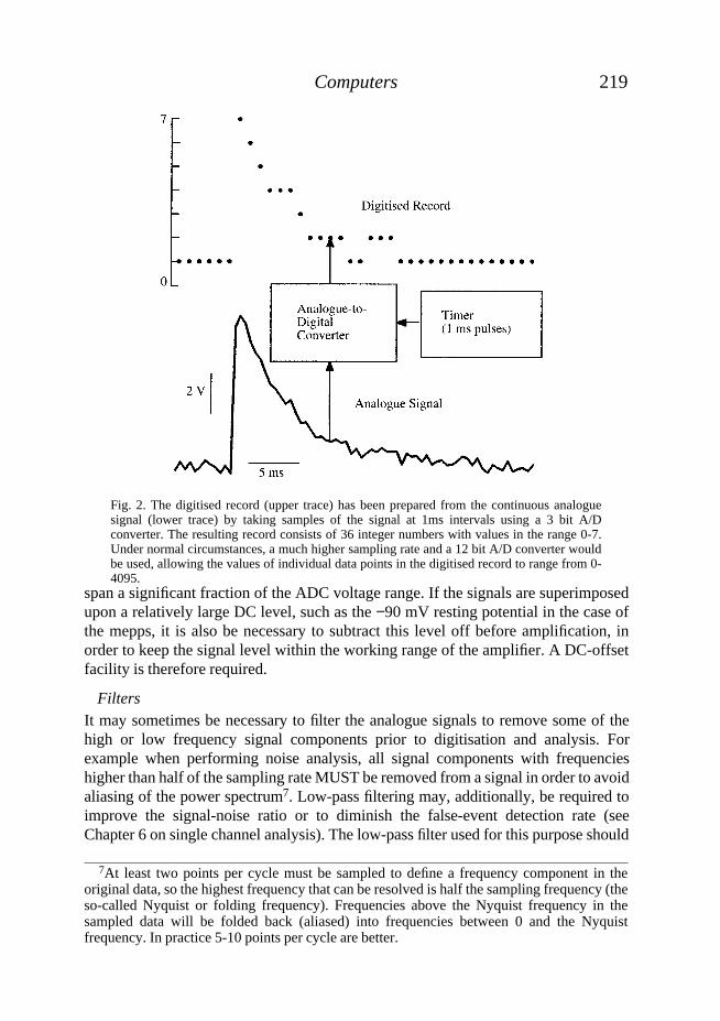
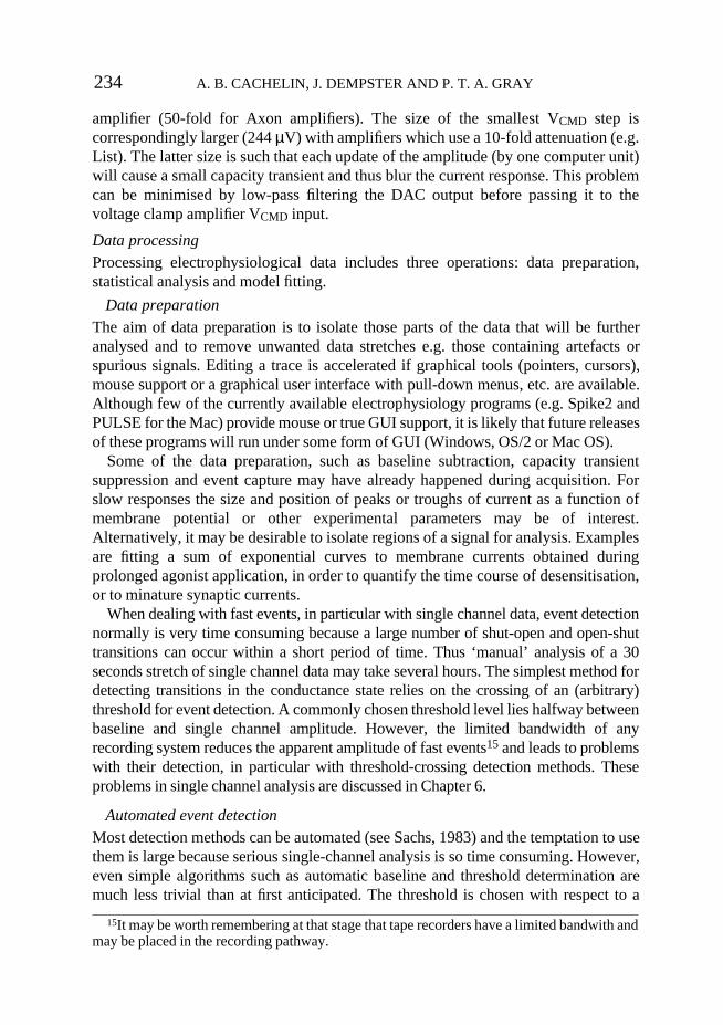
i.e. continuous time-varying voltages. Before this analogue signal can be processedby a computer system it must be brought into a computer-readable form. A digitisedapproximation must be made, by using an analogue to digital converter (ADC) whichtakes samples (i.e. measurements) of the continuous voltage signal at fixed timeintervals and quantifies them, i.e. produces a binary number proportional to thevoltage level, as shown in Fig. 2. The frequency resolution of the digitised recordingdepends upon the rate at which samples are taken. The signal to noise ratio andamplitude resolution depend on the number of quantization levels available(machine-dependent) and actually used (signal preparation!). The choice of theoptimal sampling frequency and the importance of the resolution are discussed inChapter 6 (see also Colquhoun and Sigworth, 1983; Bendat and Piersol, 1986).
The choice of commercially available ADC performances is very broad withresolutions available between 8-20 bits and sampling rates as high as 1 MHz (1 Hz =1 sec−1). However, for general use within the laboratory, an ADC with a samplingrate of 100 kHz and 12 bit resolution, allowing the measurement of 212=4096 discretevoltage levels, with ±5 volts input range6 is quite sufficient (though ±10 V mightbetter match the output range of certain voltage-clamp amplifiers, see Table A1).
ADC facilities can be added to most personal computers by installing a specialisedelectronic device. This is either an internal circuit card or a specialised externallaboratory interface unit. Either form supplies the ADC, digital-analogue converter(DAC) and timing hardware necessary to allow the computer to interact withlaboratory data and equipment. The circuit card is usually installed in one of the slotsof the computer expansion bus (see Fig. 1). A data ‘bus’ is actually more a datahighway with multiple lanes used to transfer data between CPU and computerperipherals. An external laboratory interface unit is connected to the computer via aspecialised interface card which sits in the expansion bus. Software running on thepersonal computer can thus both control the operation of the laboratory interface anddata transfers to and from computer memory.
Analogue signal conditioning
Matching the data to the ADC
It is important to ensure that the voltage levels of the analogue signal are suitablymatched to the input voltage range of the ADC. A number of ADCs are designed tohandle voltage ranges of ±5 V. With 12 bits of resolution, the minimum voltagedifference that can be measured is 2.44 mV (10000 mV/4096). However, manylaboratory recording devices supply signals of quite small amplitude. For instance, amicroelectrode amplifier (e.g. World Precision Instruments WPI 705) recordingminiature synaptic potentials from skeletal muscle might provide signals no morethan 1-2 mV in amplitude at its output. If such signals are to be measured accurately,additional amplification (e.g. ×1000) is required to scale up the signals so that they
218 A. B. CACHELIN, J. DEMPSTER AND P. T. A. GRAY
6Signal input can is either be single-ended (se) or differential (di). The signal of a single-ended input is measured relative to ground. Alternatively using-differential inputs thedifference between two inputs is measured.
span a significant fraction of the ADC voltage range. If the signals are superimposedupon a relatively large DC level, such as the −90 mV resting potential in the case ofthe mepps, it is also be necessary to subtract this level off before amplification, inorder to keep the signal level within the working range of the amplifier. A DC-offsetfacility is therefore required.
FiltersIt may sometimes be necessary to filter the analogue signals to remove some of thehigh or low frequency signal components prior to digitisation and analysis. Forexample when performing noise analysis, all signal components with frequencieshigher than half of the sampling rate MUST be removed from a signal in order to avoidaliasing of the power spectrum7. Low-pass filtering may, additionally, be required toimprove the signal-noise ratio or to diminish the false-event detection rate (seeChapter 6 on single channel analysis). The low-pass filter used for this purpose should
219Computers
Fig. 2. The digitised record (upper trace) has been prepared from the continuous analoguesignal (lower trace) by taking samples of the signal at 1ms intervals using a 3 bit A/Dconverter. The resulting record consists of 36 integer numbers with values in the range 0-7.Under normal circumstances, a much higher sampling rate and a 12 bit A/D converter wouldbe used, allowing the values of individual data points in the digitised record to range from 0-4095.
7At least two points per cycle must be sampled to define a frequency component in theoriginal data, so the highest frequency that can be resolved is half the sampling frequency (theso-called Nyquist or folding frequency). Frequencies above the Nyquist frequency in thesampled data will be folded back (aliased) into frequencies between 0 and the Nyquistfrequency. In practice 5-10 points per cycle are better.
be of a design which provides a frequency response with as sharp a roll-off as possibleabove the cut-off frequency8, but without producing peaking or ringing in the signal.High-pass filters are less frequently needed, but are used when performing noiseanalysis to eliminate frequencies below those of interest. The roll-off characteristics offilters vary e.g. Bessel, used for single channel data and Butterworth, used for noiseanalysis. Tchebychev filters are not used for analysis but are found in FM taperecorders (e.g. RACAL) to remove carrier frequencies (see ‘Filters’ in Chapter 16).
Event detectionFor some types of experiments, particularly those including random events, theremay also be need for an event discriminator. This is a device which detects theoccurrence of large amplitude waveforms within the incoming analogue signal.Typical uses include the detection of the signals associated with the spontaneousrelease of quantal transmitter packets (miniature synaptic currents or miniaturesynaptic potentials) at central and peripheral synapses or the opening of ion channelsduring agonist application. The detection of events by the software is discussedbelow. A hardware discriminator monitors the incoming analogue signal level andgenerates a digital TTL (transistor-transistor logic) pulse each time the signal crossesan adjustable threshold. TTL signals represent binary ON / OFF states by two voltagelevels, 0 V (LOW) and about 5 V (HIGH). The TTL output of a discriminator is oftenheld at 5 V, with a short pulse step to 0 V signifying that an event has been detected.
The TTL signal can be used to initiate an A/D conversion sweep by the laboratoryinterface to capture the event. In practice, it is not as simple as this since there is oftena requirement for obtaining ‘pre-trigger’ data samples so that the leading edge of thewaveform is not lost. Discriminators are also useful for matching trigger pulses froma variety of devices (e.g. Grass stimulators, Racal FM tape recorders) which producesignals incompatible with the TTL trigger input requirements of most laboratoryinterfaces. Suitable event discriminators include the World Precision InstrumentsModel 121, Axon Instruments AI2020A, Neurolog NL201 module or CED 1401-18add-on card for the 1401.
All-in-one signal conditioner
In summary, a flexible signal conditioning system should provide one or more amplifierswith gains variable over the range 1-1000, facilities to offset DC levels over a ±10 Vrange, a low/high pass filter with cut-off frequencies variable over the range 1 Hz-20 kHzand an event discriminator. Such systems can be constructed in-house with operationalamplifier circuits (Discussed in Chapter 16). However, it is often more convenient topurchase one of the modular signal conditioning systems, available from a number ofsuppliers. Digitimer’s (Welwyn, UK) Neurolog system, for instance, consists of a 19inch rack mountable mains-powered housing, into which an number of differentialamplifiers, filters and other modules can be inserted. Similar systems can be obtained
220 A. B. CACHELIN, J. DEMPSTER AND P. T. A. GRAY
8The frequency at which the ratio of the output to the input voltage signal amplitudes is 0.7(−3dB). 1 dB (decibel) = 20 × log (output amplitude / input amplitude), see Chapter 16.
from Fylde Electronic Laboratories (Preston, UK). The Frequency Devices LPF902 low-pass Bessel filter unit can also be used as a simple signal conditioner, providing adifferential amplifier with gains of ×1, ×3.16, ×10, and an 8-pole Bessel filter with a cut-off variable over the range 1 Hz-100 kHz (noise analysis requires a Butterworth filter).The characteristics of certain commercial filters can be switched between Bessel andButterworth and from low to high pass (e.g. EF5-01/02, Fern Developments).
Whatever signal conditioning system is used it is important that the exact amplifiergain and other factors are available to the computer software in order that thedigitised signals can be related to the actual units of the signal being recorded (e.g. pAor µA for membrane currents and mV for membrane potentials). In the past, this hashad to be done by the user manually entering calibration factors into the program afterreading switch settings from the signal conditioners - a rather inconvenient andpotentially error-prone exercise. Recently however, a number of suppliers haveintroduced computer-controlled signal conditioners, such as the Axon InstrumentsCyberAmp series and the Cambridge Electronic Design 1902, which can be directlyprogrammed from the computer (usually via an RS232 serial port). In these devices,the amplifier gain, DC offset levels, and filter cut-off frequencies can all be directlyprogrammed and read from the software running on the computer system. Suchsystems have the potential to greatly simplify the calibration of experimentalrecordings by allowing the computer to automatically monitor any changes to theamplifier gain and DC offset levels. Similarly, some modern voltage and patchclamps now have facilities to ‘telegraph’ their amplifier gain settings to computersystems, either using RS232 communications lines (Axon Axopatch 200,GeneClamp 500) or as fixed voltage levels (Axoclamp 2A). A particularly advancedexample of this approach can be seen in the EPC-9 patch clamp (Heka Elektronik)where the controlling computer and patch clamp are closely integrated, allowingpatch clamp parameter settings (including capacity and series resistancecompensation), to be automatically controlled by the software.
Data and control outputs
In addition to sampling data it is also often desirable to generate output signals thatmay be used, for example, to control the experiment, to present a display of thesampled data on an XY monitor scope or to trigger the sweep of a conventional YToscilloscope so that the display is synchronised with stimuli sent to the experimentalpreparation. Such outputs fall into two main classes, digital outputs and analogueoutputs. Digital outputs are single bit digital signals, that can be either Off or On.These generally take the form of TTL signals. Signals like this can be used to providetrigger signals for oscilloscopes or to control two state devices such as taps. Analogueoutputs are converted from an internal digital representation into an analogue signalby a digital to analogue converter (DAC). A DAC essentially performs the reversetransformation to that provided by an ADC, thus a number (between 0 and 4095 witha 12 bit DAC) held in the computer is converted to an output voltage that representsan appropriate fraction of the total output range, usually +/−5 or +/−10 V. Analogue
221Computers
signals can be used, for example, to control the holding potential of a voltage clampamplifier, or to plot a hard copy of the incoming data to a chart recorder.
The laboratory interfaceA laboratory interface used for electrophysiological data acquisition should have atleast the following specification:
• 8 analogue input channels• 12 bit resolution• 100 kHz sampling rate (with hardware provision to enable sampling to disk)• direct memory access (DMA) data transfer• 2 analogue output channels (3 if a scope is to be driven by DACs)• independent timing of analogue to digital conversion and digital to analogue
waveform generation• 4 digital inputs and 4 digital outputs9
• interrupt-driven operation10
A wide range of laboratory interfaces, meeting most of these specifications, are
222 A. B. CACHELIN, J. DEMPSTER AND P. T. A. GRAY
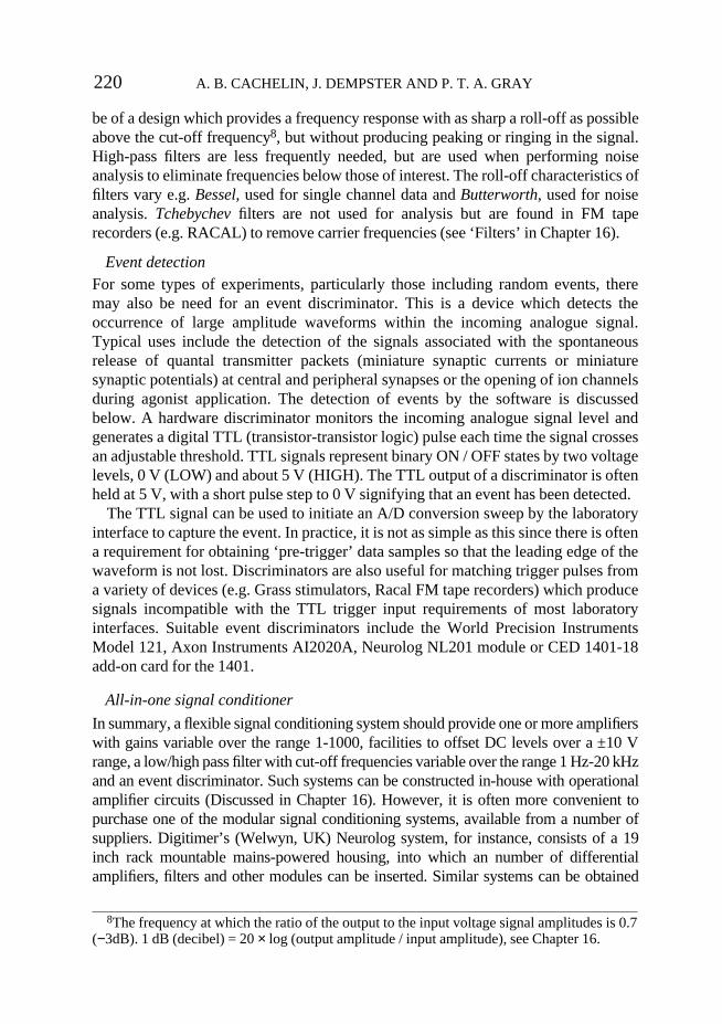
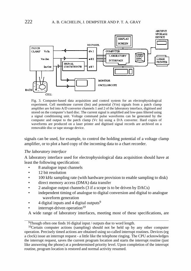
Fig. 3. Computer-based data acquisition and control system for an electrophysiologicalexperiment. Cell membrane current (Im) and potential (Vm) signals from a patch clampamplifier are fed into A/D converter channels 1 and 2 of the laboratory interface, digitised andstored on the computer’s hard disc. The current signal is amplified and low-pass filtered usinga signal conditioning unit. Voltage command pulse waveforms can be generated by thecomputer and output to the patch clamp (Vc In) using a D/A converter. Hard copies ofwaveforms are produced on a laser printer and digitised signal records are archived on aremovable disc or tape storage device.
9Though often one finds 16 digital input / outputs due to word length.10Certain computer actions (sampling) should not be held up by any other computer
operation. Precisely timed actions are obtained using so-called interrupt routines. Devices (ega clock) issue an interrupt request - a little like the telephone ringing. The CPU acknowledgesthe interrupt request, saves the current program location and starts the interrupt routine (justlike answering the phone) at a predetermined priority level. Upon completion of the interruptroutine, program location is restored and normal activity resumed.
available for both PC and Apple Macintosh families of computers. In theelectrophysiology laboratory, the devices most commonly used in combination withPCs are the Scientific Solutions Labmaster DMA card, the Cambridge ElectronicsDesign 1401plus interface (also for Mac) and - to a lesser extent - the DataTranslation DT2801A card (Table A1 contains information on a more recent DTcard). On the Apple Macintosh, the Instrutech ITC-16 is quite widely used.
The Labmaster card was one of the first laboratory interfaces to become availablefor PCs and has been in use for more than 10 years. Its popularity stems from its usewith the pCLAMP software supplied by Axon Instruments. However, its old designlimits its future even though it was updated in 1988 to support DMA - direct memoryaccess, a hardware technique for transferring digitised data into the computermemory, essential for high speed data acquisition operations (Table A1 containsdocumentation on the follow up card, the Labmaster AD). Axon Instruments has nowreplaced it with an interface of their own design, the Digidata 1200.
The CED 1401 interface has also been in use for a number of years, particularly inEurope. It is a quite different design from the Labmaster card, being more a specialpurpose data acquisition computer in its own right, with an on-board CPU and RAMmemory capable of executing programs and storing data independently of the hostcomputer. The 1401 has recently been superseded by the much higher performanceCED 1401plus which uses a 32 bit CPU rather than the original 8 bit 6502. Anunusual feature of the CED 1401 is that it can be connected to a wide range ofdifferent types of computer system, including not only PC and Macintosh families,but also minicomputers such as the VAX and Sun workstations, via an IEEE 488standard connection (a specialised parallel port).
Quite often the choice of laboratory interface is determined more by the choice ofelectrophysiological analysis software, rather than basic specifications. However,these specifications can be critical when writing one’s own software. Unlike manyother computer system components (e.g. disc drives, video displays), there arecurrently no hardware standards for the design and operation of laboratory interfaces.Each device has its own unique set of I/O ports and operating commands. Since mostcommercially available software packages work with only one particular interfacecard (usually manufactured by the supplier), it is not normally possible to substituteone type for another (an exception here is the Strathclyde Electrophysiology Softwarewhich supports several of the commonly available devices). The availability ofsuitable software has been one of the reasons for the widespread use of the CED 1401and the Labmaster in electrophysiology labs.
5. Examining and exporting data
Once the data has been sampled, it must be examined and analysed. A video displayunit is the minimum peripheral required for visual inspection. Permanentdocumentation requires some sort of hard copy device.
223Computers
Video graphics displayDue to the lack of cheap high-resolution graphical display facilities in earlier computersystems (e.g. minicomputers in the 1980s), it was necessary to display digitised signalson an oscilloscope screen driven through DACs. Most modern personal computers arenow capable of displaying data on the computer screen itself with enough resolution.Images are created on these screens by generating a bit map array in special videoRAM in which each element determines whether a point on the screen is illuminated,in which colour (Red / Green / Blue) and at which intensity. The quality of the image isdetermined by the display resolution, measured as the number of independent pixels(picture elements) that can be illuminated. A typical screen display (c.1993) has ascreen resolution of 640 (horizontal) × 480 (vertical) pixels each pixel capable of beingilluminated in 16 colours from a palette of 64. A resolution of 800×600 is gettingcommon and is more convenient for running Windows. Higher resolutions (up to1024×768 pixels, or more, and up to 16 million colours) are available but not usable byall software. In general a trade off must be made between higher resolution or morecolours on one hand and both the speed and cost of the graphic display on the other.
With the increasing use of graphical user interfaces, the performance of the graphicsdisplay hardware has become at least as important as that of the main processor. In orderto maintain adequate display rates, an increasing degree of intelligence has been builtinto video graphics cards, allowing basic operations such as the filling of areas of thescreen with blocks of colour and drawing of lines, to be done by the display hardwarerather than the CPU (see BYTE reference). The updating of a high resolution displayalso requires large amounts of data to be transferred from the main RAM into videoRAM, making great demands on the interface over which data passes. In particular, thestandard ISA (Industry Standard Architecture) interface bus found in most PCs, with its8 MHz 16 bit data path, has become inadequate to support modern video displays. Thisproblem has been overcome using special ‘local bus’ connectors, such as the VL or PCIbuses, allowing data to be transferred to the video card over 32 bit paths and at muchhigher speeds. Many PCs now come equipped with both ISA interface slots and one ormore local bus slots. The PCI bus is currently gaining acceptance for wider uses with itsendorsement by IBM and Apple for use in their Power-PC based computers.
Static data display Overall, the ability to combine text and graphics in colour, and its convenience, makethe use of the bit mapped computer display preferable to using a separate oscilloscopescreen, but important limitations should be noted. The 480 pixel vertical resolution ofmost screens is not sufficient to fully represent the 4096 levels of a 12 bit ADCsample. Similarly, the 640 pixel horizontal resolution limits the number of samplesthat can displayed at one time, e.g. with a 20 kHz sampling rate, the screen is a mere32 ms ‘wide’. The displayed image is thus of much lower resolution than the digitisedsignal and does not contain (by far) as much information as is contained in the dataitself. Brief/transient signals may be missed on a slow time scale. However, the lackof resolution can be partially overcome by using software with the ability toselectively magnify sections of the displayed signal.
224 A. B. CACHELIN, J. DEMPSTER AND P. T. A. GRAY
Dynamic data display
The transient nature of the oscilloscope image, which persists only for a fraction of asecond without refreshment, is well suited to the scrolling of signals across the screen,since only the new trace needs to be written. Images written to bit map, on the otherhand, remain on the screen once written, supported by the graphics adapter displaysub-system. This in turns means that to create a moving display the old trace must beerased (usually pixel by pixel because the fast screen erase erases ALL informationfrom the screen) before a new trace can be drawn. Thus, implementing a fast scrollingdisplay on a graphics display requires considerable handling of data and proves to be adifficult programming task. At present, few electrophysiological analysis programshave succeeded in implementing a scrolling display of the same dynamic quality ascan be achieved using an oscilloscope. The problem is not insoluble, however, and it islikely that with the current rate of improvement in graphic display technology goodscrolling signal displays will soon be realised on a computer screen. It is possible togenerate scrolling displays using some existing hardware if the interface card is used togenerate the X, Y and intensity (‘Z’) signals needed to generate such a display on anXY oscilloscope. For example, the support library supplied with the CED 1401interface provides a command which allows programmers to generate such a display.
Hard copy graphicsThe production of hard copies of stored signals, of sufficient quality for reproductionin a journal, is at least as important as the dynamic display of signals on screen. Hardcopy devices fall into two main categories: printers which generate an image using abit-map, like display screen graphics, and digital plotters which create the image bydrawing lines (vectors) with a pen.
Until recently, the digital plotter was the most commonly used device for producinghigh quality plots of digitised signals. These devices, typical examples being theHewlett Packard 7470A or 7475, are fitted with a number of coloured pens and candraw lines and simple alphanumeric characters on an A4 sheet of paper. Data is sent tothe plotter in the form of a simple graph plotting language HPGL (Hewlett PackardGraphics Language) which contains instructions for selecting, raising and loweringpens, drawing lines etc. Although digital plotters can address over a thousand pointsper inch (1016 plotter units per inch) they position their pens to within a much largerfraction of a millimetre due to mechanical and other limitations (pens and penwidth).They can fully reproduce a 12 bit digitised record on an A4 page (10900×7650addressable points). Plotters, however, are slow devices taking several minutes toproduce a single trace with 1-2000 points. Also, the text produced by plotters was notquite of publication quality. Using HPGL has however the advantage that such filescan be imported by a number of graphics programs (as will be discussed later).
Several laser printers can also emulate HPGL plotters11, in particular the HP LaserjetIII and IV series. Others can also do so provided they have been equipped with the
225Computers
11Availability of line thickness adjustment is an important prerequisite for publication-quality figures.
appropriate hardware or using emulation software running on the PC. This is aparticularly useful feature since some (older) software packages only provide graphicaloutput in HPGL form. To a large extent, plotters are being replaced by printers that canproduce hard copy graphics of a similar quality to the plotter, and also very high qualitytext. The laser printer is ideally suited for general laboratory work, being fast, capableof producing high quality text in a wide variety of typefaces. Laser printers are alsoreliable and easy to maintain in operation.. The latest printers, with 600 dpi resolution,are capable of fully reproducing a 12 bit digitised record without loss of precision(7002×5100 dots for an A4 page). Ink jet printers (e.g. Hewlett Packard Deskjet, CanonStylewriter/Bubblejet, Epson Stylus) provide a similar quality of text and graphics (300DPI) but a lower cost. The most recent members of the HP Deskjet family make colouraccessible at a low (Deskjet 550C incl. PostScript for just less than US$ 1000.0) tomoderate price (Deskjet 1200C incl. PostScript). They are still very slow (up to severalminutes per page) and their use is recommended for final copies only.
As in many other areas of the computer industry, competitive pressures have leadto the creation of de facto standards. The most important emulations are PCL5 (HPLaserjet III), PCL5e (HP Laserjet 4) and Postscript Level I or II (see BYTENovember 1993 p. 276 ff). Other frequent emulations include ESC-P (EPSONLQ/FX), IBM Proprinter and HPGL. The various emulations are differentiated by thecodes used to transmit formatting and graphics instructions to the printer. Postscript isa specialised Page Description Language (PDL) licenced from Adobe Inc. designedfor the precise description of the shape and location of text characters and graphics onthe printed page. One of its prime advantages is its portability. A Postscriptdescription of a page of text should be printable on any printing device supportingPostScript PDL (not just a laser printer). It is in widespread use within the publishingand printing industry. The main practical difference between the Postscript and othergraphic images is that Postscript’s images are defined using vectors which are be sentdirectly to the printing device while PCL graphics must be first created as bit-mapswithin host computer memory (a more complicated process) then sent to the printer.
In practice, there is little to choose between either type of laser printer. Postscriptprinters, perhaps, have the edge in terms of variety of type styles, while PCL printersare usually faster at printing bit mapped images. However, both of these families arewidely supported by applications software such as word processors, spreadsheets andgraph plotting programs. In addition, many printers now have both PCL andPostscript capabilities (e.g. HP Laserjet 4MP), while Postscript facilities can be easilyadded to older HP Laserjet printers using an expansion cartridge (e.g. PacificPagePostscript Emulator).
P A R T T W O : S O F T W A R E
6. Operating systems
The operating system is a collection of interlinked programs which perform the basicoperations necessary to make a computer system usable; reading data from the keyboard,creating, erasing, copying disc files, displaying data on the screen. The operating system
226 A. B. CACHELIN, J. DEMPSTER AND P. T. A. GRAY
acts as a environment from which to invoke applications programs. It defines thecharacteristics of the computer system at least as much as the hardware does.
The operating system appears to the user as the set of commands and menus usedto operate the computer. It acts as an interface between hardware and the user, hencethe term ‘user interface’. From the point of view of the programmer, the operatingsystem is the set of subroutines and conventions used to call upon operating systemsservices - the applications programmer interface (API). The debate about the relativemerits of different computer families (e.g. Macintosh vs. PC) is very much adiscussion about the nature of the operating system and what features it shouldprovide to the user, rather than about the hardware, which is essentially similar inperformance.
Although this chapter is primarily concerned with the applications of the computerto data acquisition in the context of electrophysiology, a brief consideration of thedevelopment of operating systems for personal computers is worthwhile since theyprovide the basic environment within which our software has to function.
Character-based OSMost electrophysiology software runs on PCs, and uses MS-DOS (Microsoft DiscOperating System). MS-DOS is a relatively basic, single task system; primarilydesigned for running only one program at a time. This simplicity of design, comparedto more complex systems like the Macintosh OS or UNIX, has made it relatively easyto develop efficient data acquisition software for PCs. However, the simple nature ofMS-DOS, which was well matched to the performance of computers of the 1980’s, isincreasingly becoming a major limitation in making effective use of the modernprocessors which are 100 times more powerful12.
MS-DOS, like its ancestor CP/M, uses a command line interface (CLI), i.e. the useroperates the system by typing series of somewhat terse commands (e.g. DIR C: to listthe directory of files on disc drive C:). This approach, though simple to implement,requires the user to memorise large numbers of command names and use them in verysyntactically precise ways. A number of utility programs (e.g. PCTools, NortonCommander, Xtree) simplify often used file operations (e.g. copy, move, delete) andlaunching of programs, as well as providing a simple, mouse-driven graphical userinterface (GUI). A very primitive GUI called DOSSHELL is also present in DOS(since version 4). It enables starting several programs which can be run alternatively(but not simultaneously)13. Modern operating systems are expected to be able to runseveral programs at the same time and provide a GUI. Windows 4 (‘Chicago’) willeventually replace DOS (but emulate it).
227Computers
12Most PC users have confronted, at least once, the 640KB limit on memory dictated byDOS and the architecture of the first PCs. Most PCs, with 386 and above processors,overcome this problem by using 32 bit memory addressing to support up to 4GB of memory.This feature (32 bit memory addressing) is supported by recent versions of Windows. Thoughthis is also supported by so-called DOS extenders, we do not recommend this practice is it islikely to cause compatibility problems.
13It is of limited practical use. Windows (3.1 and above) is a much better alternative.
Graphical user interfacesThe major external difference between character-based and graphical user interfaces isthe way the user interacts with the computer. Within a GUI, the user uses a hand-heldpointing device (the mouse) linked to a cursor on the screen in order to point to pictorialobjects (icons) on the screen, which represent programs or data files, or to choose fromvarious menu options. The first widespread implementation of a GUI was on the AppleMacintosh family, and contributed markedly to the success of that machine. The concepthas now been widely accepted and, with the introduction of the Microsoft Windows andIBM OS/2 for PCs, most personal computers are now supplied with a GUI.
Windows, OS/2 and Macintosh System 7 provide very similar facilities, beingmouse-driven, with pull-down menus, ‘simultaneous’ execution of multipleprograms linked to movable resizable windows. The main difference between thesethree systems is that on the Macintosh and in OS/2, the GUI is closely integrated withthe rest of the operating system whereas the Windows GUI is separate from, butmakes use of, MS-DOS. Apple, IBM and Microsoft are in close competition witheach other to develop newer and more powerful operating systems for the 1990’s.Microsoft, has recently released Windows NT, a new operating system whichintegrates the Windows GUI with a new underlying operating system, better able tosupport multi-tasking and without many of MS-DOS’s limitations.
These newer operating systems also all provide some support for 32 bit applications,that is programs that can directly access the full 4GB of memory that the CPU canaccess. The degree of integration of this support varies, OS/2 and Windows NTproviding full support, Windows 3.xx only partial support. The additional overheadsinvolved in supporting the graphical user interface do, however, mean that there is a costboth in terms of performance and memory requirement in using these operating systems.The entry level requirements for hardware to run these operating systems (in terms ofmemory size and processor power) are greater than those for a basic DOS system: e.g. aDOS based system running on a 80286 processor and with 640 KB of memory wouldprovide adequate performance for most tasks. In contrast the minimum possible systemto take full advantage of the current version of Windows (3.1) is an 80386 processor and2MB of memory. In fact even this configuration would quickly be found to be severelylimiting if any use was made of the multitasking capabilities of Windows.
7. Electrophysiology software
Electrophysiology covers a wide range of experiments and produces many differenttypes of data. The electrical signal produced by biological preparations in suchexperiments has mainly two components: time and amplitude. Thus, analysis ofelectrophysiological records is primarily concerned with monitoring the amplitudeof a signal as a function of time, or the time spent at a given amplitude. Mostelectrophysiology programs are like a ‘Swiss army knife’: although they can dealwith a lot of experimental situations, they usually fall short when the properinstrument is needed. The ‘perfect program’, which incorporates only the bestsubroutines to deal with each type of data obviously does not exist. This is usually
228 A. B. CACHELIN, J. DEMPSTER AND P. T. A. GRAY
the reason why some expertise in programming is important. Writing one’s ownsoftware may sometimes be essential to allow those experiments to be done thatshould be done and not those dictated by the software. It is the aim of the presentsection to mention which options should be present in a good electrophysiologyprogram (see also Table A3-A5).
Most widely used electrophysiology packages for PCs (e.g. pCLAMP, CED EPSuite, Strathclyde Software) currently run under DOS. GUI based multitaskingoperating systems for PCs, such as Windows and OS/2 are gradually replacing DOS,though it may some time before character based OSs disappear altogether. This shift isreflected in a migration towards GUI versions of data acquisition programs: e.g. AxonInstruments’ Axodata or Instrutech’s PULSE for the Macintosh OS or CED’s Spike2for Macintosh, Windows 3.1 and Windows NT. Many standard applications (e.g. wordprocessors, spreadsheets, graphic packages) are now available in a GUI-based version(e.g. for Windows, OS/2; Macintosh). How far electrophysiology packages follow thetrend towards being GUI based depends to some extent upon the continued availabilityof character-based shells within future GUI OSs, such as the ‘DOS box’ within currentversions of Windows and OS/2. There are undoubtedly great advantages that comealong with GUIs, e.g. consistency of the user interface, ability to exchange data withother programs, multi-tasking14. Unfortunately, there is also a price to pay for theincreased functionality of GUIs. It proves to be more difficult to develop programs fora graphical, multi-tasking environment than for a character-based OS. Fortunately,software publishers (e.g. CED) already provide direct-link libraries (DLLs) whichgreatly simplify communication with data acquisition hardware (e.g. 1401) or accessto data files using proprietary file formats under Windows.
Different programs for different experiments
In the real world, most electrophysiology programs originate from teams which havedesigned their software to perform optimally with one type of experiment.Electrophysiology software has evolved in mainly two directions. Some programswere written to analyse short stretches of data often sampled in a repetitive way. Suchprograms were originally written to investigate the properties of voltage activatedchannels (e.g. sodium, potassium or calcium channels) in response to polarisations,such as voltage steps, applied by the experimenter. For example the AxoBASIC set ofsubroutines was uniquely tailored to perform repetitive tasks on a small number ofdata points.
Other programs have been designed to deal with random data at equilibrium; forexample programs specifically conceived to sample and analyse long stretches of dataobtained from agonist-activated ion channels. As already mentioned, the type ofexperiments that are likely to be done may often determine the choice of the program
229Computers
14True multi-tasking, allowing several different programs to be active at once, by timesharing the CPU, is available in Windows enhanced mode. However, real time laboratoryapplications, such as sampling and experimental control, should normally be run exclusively,or there may be problems such as missed data points or timing errors.
and as a consequence the hardware e.g. requirements for interrupt driven dataacquisition and large capacity data storage. It is important that experimentalrequirements determine software, and not vice versa; in early voltage-jumpexperiments hardware limitations in sample rates and durations had a profound effecton the information extracted from the data produced.
Fig. 3 shows the major components of a typical computer-based data acquisitionsystem, as it would be applied to the recording of electrophysiological signals from avoltage or patch clamp experiment. The membrane current and potential signals from thevoltage clamp are amplified and/or filtered via a signal conditioning sub-system and fedinto the analogue inputs of the laboratory interface unit. Computer-synthesised voltagepulses and other waveforms can be output via DACs and applied to the commandvoltage input of the voltage clamp in order to stimulate the cell. On completion of theexperiment, the digitised signals stored on disc can be displayed on the computer screenand analysed using signal analysis software. Hard copies of the signal waveforms andanalysis results can be produced on a laser printer or digital plotter. As digitised signalsaccumulate, filling up the hard disc, they are removed from the system and stored on aarchival storage device such as digital magnetic tape or optical disc.
Short events
The currents produced by voltage-operated channels during membrane depolarisationare typical short events lasting a few hundreds of milliseconds, though steady statemay be reached only after much longer periods of time. It is important that theduration of each sample should be long enough for the relaxation of the properties ofthe channels to a new equilibrium to be complete during the sampling period.Essential program options are simple menus to adjust sample frequency and duration.Advanced program options include the ability to sample during several intervalswithin a repetitive pattern. The optimal sample frequency is determined by severalparameters such as the required time resolution, and the filter-cut-off frequency isadjusted accordingly e.g. Chapter 6, Colquhoun and Sigworth (1983). Typically suchexperiments require sampling on two channels, e.g. voltage and current. Sometimesone may wish to monitor an additional signal such as the output of a photomultipliertube, which allows measurement of the intracellular concentration of various mono-and divalent ions when used with appropriate indicators. It should be borne in mindthat the maximum sample frequency (fmax) quoted for a laboratory interface applies tosampling on a single channel. The maximum frequency per channel when samplingon multiple channels is usually equal to fmax divided by the number of channels.
Watching the data on-line
One should always monitor the original, unmodified data on a scope. Duringrepetitive sampling, this requires the software to keep triggering the scope evenduring episodes in which no data is being sampled (or manually switching the scopeto a self-triggered mode). Also, it is often useful and sometimes essential to be able towatch the conditioned, sampled data on-line during acquisition.
Watching large amplitude signals such as whole-cell response to an agonist on-line
230 A. B. CACHELIN, J. DEMPSTER AND P. T. A. GRAY
should not be problem provided the data has been correctly amplified prior to theacquisition (see Signal Conditioning above). The situation is entirely different if therelative amplitude of the data is small compared to the underlying signal. This is thecase for single channel openings of voltage-activated channels. Rapid changes of themembrane potential are accompanied by capacity transients which can be muchlarger than the actual single channel amplitude. The amplitude of capacity transientscan be at least partially reduced by adjusting appropriate compensatory circuits in thevoltage or patch clamp amplifier.
The channel openings are also superimposed on a holding current whose size maybe much larger than the amplitude of a single channel opening. Before details can beobserved, it is necessary to subtract such offsets, usually due to (unspecific) leakcurrents and capacity transients, from the original data. If this cannot performed byexternal hardware prior to or during acquisition, it is necessary to prepare a leak tracewithout openings to be subtracted from the sampled data. A good electrophysiologyprogram should include options to do this on-line leak and capacity transientsubtraction.
Leak current and capacity transient subtraction
A method often used for leak subtraction is the following. Let us assume that thechannel is activated by stepping from a holding potential of −100 mV to a potential of−10 mV, a protocol often used to activate sodium channels. The individual channelopenings will be much smaller than holding current and capacity transients. Acorrection signal is obtained by averaging N traces measured while inverting thecommand pulse thus hyperpolarising the membrane potential from −100 mV to −190mV, a procedure which does not activate ion channels but allows measurement of thepassive membrane properties, the silent assumption of this protocol being that thesepassive electrical membrane properties are purely ohmic, i.e. symmetrical and linearover a wide range of potentials. When the step potential is large, for example to −240mV in order to compensate a step from −100 to +40 mV, a fraction of the voltage stepis used instead (e.g. from −100 mV to −120 mV) and a linear extrapolation made.
Assuming that the leak current is linear, the sampled response is then scaled (in ourexample by a factor of 7) and may be used for correction of multiple voltage-stepamplitudes (‘scalable’ leak in Table A3). This method was originally introduced byArmstrong and Bezanilla (1974) and called ‘P/4’ because the pulse amplitude wasdivided by 4. More generally the method is called P/N to indicate that an arbitraryfraction of the pulse is used. However, the assumption of linear leak is not alwayscorrect and the leak trace many need arbitrary adjustment (‘adjustable’ leak in TableA3). Most procedures for leak and capacity transient subtraction are not perfect so itis good practice to store both the original, unaltered data, as well as the leaksubtraction and capacity compensation signal, so that a later, better or more detailedanalysis can be performed as required. Another method of signal correction which,however, does not work on-line, consists in marking and averaging traces which donot contain single channel openings (‘nulls’) to prepare the leak and capacity
231Computers
transient subtraction signal. This method has been used to analyse data obtained fromvoltage-dependent calcium channels.
It is important that the method used for preparation of leak and capacity transientcompensation signals used by a software package should be clearly explained in theprogram documentation. Ideally, it should be possible for the user to modify themethod used (for example by having access to the code).
Long samplesSome types of data require sampling for long periods of time. These are for examplethe slow responses of a cell following application of an agonist, or random data, suchas the single channel openings or membrane current noise during agonist applicationor spontaneous minature synaptic events.
Triggered eventsPredictable events, such as evoked synaptic currents, are easy to deal with providedthey have undergone adequate conditioning (e.g. amplification) prior to sampling. Anumber of programs exist which turn the computer into a smart chart recorder. Theseprograms can record at moderate sampling frequencies on up to 16 and morechannels. They include options for entering single character markers. These programscan usually play back the data but their analysis options are normally limited whenthey exist at all. Examples of such programs are CED’s CHART, AXON’sAXOTAPE or Labtech’s Notebook programs. Their limited analysis capabilitiesmake it essential that programs can export data in various formats for analysis byother software (see below).
Random eventsRandom events are more difficult to deal with. An important question is to decidewhether all of the data should be recorded on-line as well as on an analogue recorder.The considerable amount of disk storage space required to store all of an experimentmakes it worth considering detection hardware and algorithms in order to sampleonly the data which is actually relevant. Obviously, the event detector must becapable of keeping track of time between meaningful events (such as minaturesynaptic events or single channel openings), as time intervals are one of the variablesin the data. The event detector may be implemented in hardware, as described brieflyabove, or in software. Software event detectors sample data into an ‘endless’,circular, buffer. The size of the buffer determines how much data prior to thetriggering event will be available.
A problem with the use of event detectors is that the experimental record betweenevents is not seen. Signal properties, such as the noise levels, or the size of the eventthat fires the trigger, may change during an experiment. In the latter case, the eventdetector may fail to trigger and data will be lost. It is therefore essential if using thistechnique to record all original data to tape, so that re-analysis with, for example,different trigger parameters may be carried out if needed. In addition, the voice trackon a tape recorder can contain far more useful information than a few commentstyped quickly in a file.
232 A. B. CACHELIN, J. DEMPSTER AND P. T. A. GRAY
Driving external devices
Several types of devices can be activated by a computer-generated signal. Thesimplest devices (taps, and other electromechanical equipment) require a simple TTL(on-off) signal which can be generated either via a DAC or parallel digital port.Triggering the monitor scope usually only requires a TTL pulse. One usually wishesto trigger the oscilloscope at a given time before say depolarising a cell so theresponse can be monitored during the entire duration of the depolarisation. A goodelectrophysiology program should allow triggering of external devices (oscilloscope,magnetic tap, amplifier, signal conditioner, etc.) at predetermined times.
The next level of complexity requires variable signals to be sent to a voltage clampamplifier. Although the membrane potential or current level can be dialed manuallyon the voltage-clamp amplifier the command pulses need to coincide with datasampling so it is better to rely on the computer to generate voltage steps, thoughcomplex voltage-step protocols can also be generated by a programmable stimulatorprovided a trigger signal is provided to initiate sampling. In general, use of thecomputer to generate command pulses makes it easier to create a wide range ofcomplex command signals such as voltage ramps, multistep protocols, and playbackof pre-recorded samples, such as action potentials. Command signals are generatedby a DAC. The amplifier is treated in these protocols as an entirely passive device,though the latest generation of patch clamp amplifiers, such as the Axon Axopatch2000 and the List EPC9, are capable of two way communication with the computer.
At the highest level of sophistication smart devices such as digital oscilloscopesand digital plotters can interpret simple, human-readable, commands of alphanumericdata sent in ASCII form via a serial or parallel port. Examples are Hewlett Packard,and other HPGL compatible, plotters, some Nicolet and Tektronix oscilloscopes andthe CED 1401, all of which use a proprietry command language, just as printers do.
Synchronous command pulses
Investigating the properties of voltage-activated ion channels often means usingcomplex pulse protocols. For example, the inactivation of sodium, potassium andother voltage-activated conductances may be studied by use of prepulses appliedbefore a test depolarisation to determine the proportion of channels that can beactivated (see Chapter 2). The conductance of ligand gated channels, that show littletime dependence can be tested with slowly increasing ramp commands to plot I/Vcurves directly. Alternatively, the conductance of voltage-gated channels may beinvestigated by applying a series of incrementing, or decrementing, pulses from aholding potential. We can see from these two examples that there should be menuoptions to prepare pulse protocols in advance.
For voltage-ramps, it is important that the program should maximize the number ofvoltage steps so as to minimize their size. The amplitude of the smallest VCMD step isa function of both resolution and voltage range of the DACs: with 12 bit resolutionand a voltage range of ±5 V, one computer unit is converted to a VCMD step of 2.44mV which translates to a step of 49 µV at the pipette tip after attenuation by the
233Computers
amplifier (50-fold for Axon amplifiers). The size of the smallest VCMD step iscorrespondingly larger (244 µV) with amplifiers which use a 10-fold attenuation (e.g.List). The latter size is such that each update of the amplitude (by one computer unit)will cause a small capacity transient and thus blur the current response. This problemcan be minimised by low-pass filtering the DAC output before passing it to thevoltage clamp amplifier VCMD input.
Data processingProcessing electrophysiological data includes three operations: data preparation,statistical analysis and model fitting.
Data preparationThe aim of data preparation is to isolate those parts of the data that will be furtheranalysed and to remove unwanted data stretches e.g. those containing artefacts orspurious signals. Editing a trace is accelerated if graphical tools (pointers, cursors),mouse support or a graphical user interface with pull-down menus, etc. are available.Although few of the currently available electrophysiology programs (e.g. Spike2 andPULSE for the Mac) provide mouse or true GUI support, it is likely that future releasesof these programs will run under some form of GUI (Windows, OS/2 or Mac OS).
Some of the data preparation, such as baseline subtraction, capacity transientsuppression and event capture may have already happened during acquisition. Forslow responses the size and position of peaks or troughs of current as a function ofmembrane potential or other experimental parameters may be of interest.Alternatively, it may be desirable to isolate regions of a signal for analysis. Examplesare fitting a sum of exponential curves to membrane currents obtained duringprolonged agonist application, in order to quantify the time course of desensitisation,or to minature synaptic currents.
When dealing with fast events, in particular with single channel data, event detectionnormally is very time consuming because a large number of shut-open and open-shuttransitions can occur within a short period of time. Thus ‘manual’ analysis of a 30seconds stretch of single channel data may take several hours. The simplest method fordetecting transitions in the conductance state relies on the crossing of an (arbitrary)threshold for event detection. A commonly chosen threshold level lies halfway betweenbaseline and single channel amplitude. However, the limited bandwidth of anyrecording system reduces the apparent amplitude of fast events15 and leads to problemswith their detection, in particular with threshold-crossing detection methods. Theseproblems in single channel analysis are discussed in Chapter 6.
Automated event detectionMost detection methods can be automated (see Sachs, 1983) and the temptation to usethem is large because serious single-channel analysis is so time consuming. However,even simple algorithms such as automatic baseline and threshold determination aremuch less trivial than at first anticipated. The threshold is chosen with respect to a
234 A. B. CACHELIN, J. DEMPSTER AND P. T. A. GRAY
15It may be worth remembering at that stage that tape recorders have a limited bandwith andmay be placed in the recording pathway.
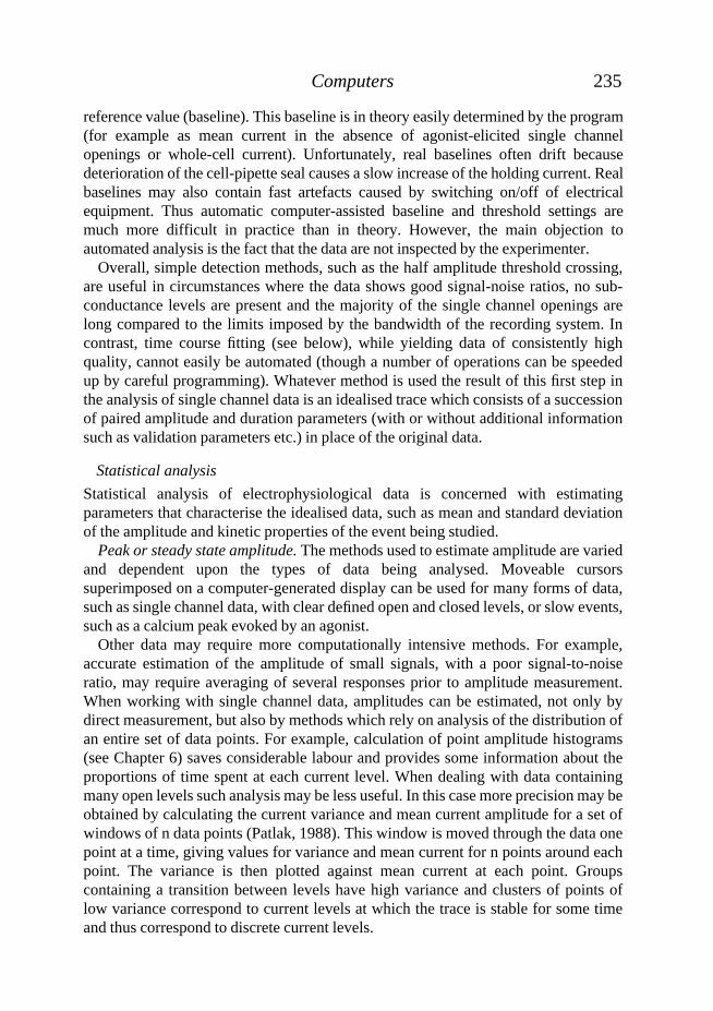
reference value (baseline). This baseline is in theory easily determined by the program(for example as mean current in the absence of agonist-elicited single channelopenings or whole-cell current). Unfortunately, real baselines often drift becausedeterioration of the cell-pipette seal causes a slow increase of the holding current. Realbaselines may also contain fast artefacts caused by switching on/off of electricalequipment. Thus automatic computer-assisted baseline and threshold settings aremuch more difficult in practice than in theory. However, the main objection toautomated analysis is the fact that the data are not inspected by the experimenter.
Overall, simple detection methods, such as the half amplitude threshold crossing,are useful in circumstances where the data shows good signal-noise ratios, no sub-conductance levels are present and the majority of the single channel openings arelong compared to the limits imposed by the bandwidth of the recording system. Incontrast, time course fitting (see below), while yielding data of consistently highquality, cannot easily be automated (though a number of operations can be speededup by careful programming). Whatever method is used the result of this first step inthe analysis of single channel data is an idealised trace which consists of a successionof paired amplitude and duration parameters (with or without additional informationsuch as validation parameters etc.) in place of the original data.
Statistical analysis
Statistical analysis of electrophysiological data is concerned with estimatingparameters that characterise the idealised data, such as mean and standard deviationof the amplitude and kinetic properties of the event being studied.
Peak or steady state amplitude. The methods used to estimate amplitude are variedand dependent upon the types of data being analysed. Moveable cursorssuperimposed on a computer-generated display can be used for many forms of data,such as single channel data, with clear defined open and closed levels, or slow events,such as a calcium peak evoked by an agonist.
Other data may require more computationally intensive methods. For example,accurate estimation of the amplitude of small signals, with a poor signal-to-noiseratio, may require averaging of several responses prior to amplitude measurement.When working with single channel data, amplitudes can be estimated, not only bydirect measurement, but also by methods which rely on analysis of the distribution ofan entire set of data points. For example, calculation of point amplitude histograms(see Chapter 6) saves considerable labour and provides some information about theproportions of time spent at each current level. When dealing with data containingmany open levels such analysis may be less useful. In this case more precision may beobtained by calculating the current variance and mean current amplitude for a set ofwindows of n data points (Patlak, 1988). This window is moved through the data onepoint at a time, giving values for variance and mean current for n points around eachpoint. The variance is then plotted against mean current at each point. Groupscontaining a transition between levels have high variance and clusters of points oflow variance correspond to current levels at which the trace is stable for some timeand thus correspond to discrete current levels.
235Computers
Time course. As with amplitude measurements, much data can be dealt with bytaking measurements with superimposed cursors on a computer-generated display,e.g. the latency of responses to applied agonist. However, in many cases, this methodwill either be too slow in dealing with large amounts of data, will be unable toproduce the information required or will fail to achieve the degree of precisionrequired. In these cases, methods that make greater use of the power of the computercan be used. In the case of synaptic currents, the kinetic information can generallyonly be obtained by fitting exponential curves to the data (see Chapter 8). In the caseof single channel data greater temporal precision can be obtained by fitting the timecourse of each transition, whereas greater speed but less precision may be achievedwith the threshold-crossing method. The relative advantages and disadvantages ofthese methods are discussed in Chapter 6.
Noise analysis. The unitary events, such as channel gating or receptor potentials,underlying a response occur as random events of characteristic amplitude, lifetime andfrequency. The statistical noise they introduce can be analysed to provide informationabout the amplitude and kinetics of underlying events in signals in which theindividual events themselves cannot be resolved (see Chapter 8). Analysis of noise,beyond the most basic studies is impossible without the use of a computer. Therequired resolution determines the sample rate and length required. The lowestfrequency point that can be analysed is given by inverse of the sample length, while thehighest possible frequency is half the sample rate to avoid aliasing (Chapter 16).Kinetic analysis of noise requires calculation of the Fourier transform of the signal.This is always done using a Fast Fourier Transform (FFT) algorithm (see Press et al.,1986). Such algorithms impose a limitation upon the way the data is transformed inthat they will only operate on arrays whose size is a power of 2, so data can only beprocessed in blocks of 2n points. In the past the size of available memory could imposetight limits upon the size of the array that could be transformed. Thus, if each numberis represented by a 4 byte floating point number, a sample of 2 seconds at 4069Hz,allowing analysis from 0.5Hz to 2KHz, would take up 32 KB. Using compilers thatallow access to the full addressable memory of an 80386 or 80486 processoreffectively removes this limitation as arrays much larger than this can be handled.
A second issue concerns the use of integer or floating point numbers to represent theindividual data points. Integer FFTs were much faster than floating point FFTs, asCPUs can perform integer arithmetic more rapidly. However, the drawback is that thepower spectrum produced, the plot of the signal power vs frequency, is distorted at thebottom end by the limited numerical resolution, the points being clustered at discretelevels. In practice, in a recent computer fitted with a FPU the difference in performanceof integer over floating point FFTs is minimal, and not worth the loss of resolution.
In general, analysis of noise requires sampling on two channels, one channelrecords a low gain, low pass filtered record, for calculation of mean current levels.The second channel records the noise at high gain, after removal of DC componentsby high pass filtering, and removal of all frequencies above the folding (Nyquist)frequency by low pass filtering. Calculation of spectrum and variance of the noise
236 A. B. CACHELIN, J. DEMPSTER AND P. T. A. GRAY
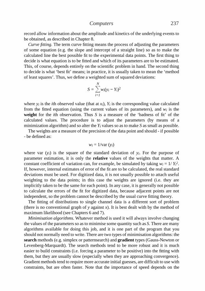
record allow information about the amplitude and kinetics of the underlying events tobe obtained, as described in Chapter 8.
Curve fitting. The term curve fitting means the process of adjusting the parametersof some equation (e.g. the slope and intercept of a straight line) so as to make thecalculated line the best possible fit to the experimental data points. The first thing todecide is what equation is to be fitted and which of its parameters are to be estimated.This, of course, depends entirely on the scientific problem in hand. The second thingto decide is what ‘best fit’ means; in practice, it is usually taken to mean the ‘methodof least squares’. Thus, we define a weighted sum of squared deviations:
where yi is the ith observed value (that at xi), Yi is the corresponding value calculatedfrom the fitted equation (using the current values of its parameters), and wi is theweight for the ith observation. Thus S is a measure of the ‘badness of fit’ of thecalculated values. The procedure is to adjust the parameters (by means of aminimization algorithm) and so alter the Yi values so as to make S as small as possible.
The weights are a measure of the precision of the data point and should - if possible- be defined as:
wi = 1/var (yi)
where var (yi) is the square of the standard deviation of yi. For the purpose ofparameter estimation, it is only the relative values of the weights that matter. Aconstant coefficient of variation can, for example, be simulated by taking wi = 1/ Yi2.If, however, internal estimates of error of the fit are to be calculated, the real standarddeviations must be used. For digitized data, it is not usually possible to attach usefulweighting to the data points; in this case the weights are ignored (i.e. they areimplicitly taken to be the same for each point). In any case, it is generally not possibleto calculate the errors of the fit for digitized data, because adjacent points are notindependent, so the problem cannot be described by the usual curve fitting theory.
The fitting of distributions to single channel data is a different sort of problem(there is no conventional graph of y against x). It is best dealt with by the method ofmaximum likelihood (see Chapters 6 and 7).
Minimisation algorithms. Whatever method is used it will always involve changingthe values of the parameters so as to minimise some quantity such as S. There are manyalgorithms available for doing this job, and it is one part of the program that youshould not normally need to write. There are two types of minimisation algorithms: thesearch methods (e.g. simplex or patternsearch) and gradient types (Gauss-Newton orLevenberg-Marquardt). The search methods tend to be more robust and it is mucheasier to build constraints (i.e. forcing a parameter to be positive) into the fitting withthem, but they are usually slow (especially when they are approaching convergence).Gradient methods tend to require more accurate initial guesses, are difficult to use withconstraints, but are often faster. Note that the importance of speed depends on the
S = ^wi(yi − Yi)2N
i=1
237Computers
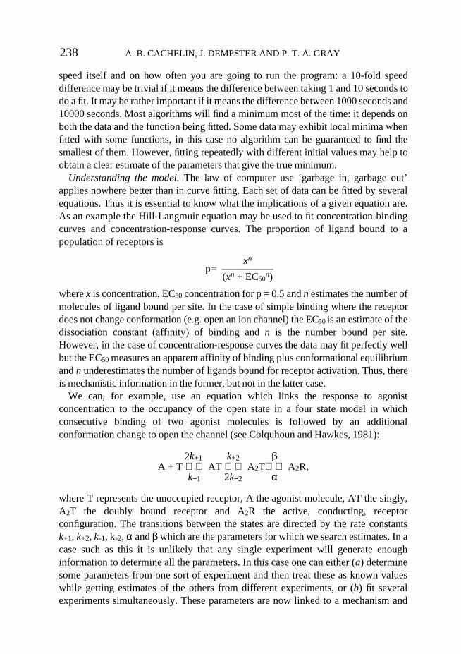
speed itself and on how often you are going to run the program: a 10-fold speeddifference may be trivial if it means the difference between taking 1 and 10 seconds todo a fit. It may be rather important if it means the difference between 1000 seconds and10000 seconds. Most algorithms will find a minimum most of the time: it depends onboth the data and the function being fitted. Some data may exhibit local minima whenfitted with some functions, in this case no algorithm can be guaranteed to find thesmallest of them. However, fitting repeatedly with different initial values may help toobtain a clear estimate of the parameters that give the true minimum.
Understanding the model. The law of computer use ‘garbage in, garbage out’applies nowhere better than in curve fitting. Each set of data can be fitted by severalequations. Thus it is essential to know what the implications of a given equation are.As an example the Hill-Langmuir equation may be used to fit concentration-bindingcurves and concentration-response curves. The proportion of ligand bound to apopulation of receptors is
xn
p= ––––––––––(xn + EC50
n)
where x is concentration, EC50 concentration for p = 0.5 and n estimates the number ofmolecules of ligand bound per site. In the case of simple binding where the receptordoes not change conformation (e.g. open an ion channel) the EC50 is an estimate of thedissociation constant (affinity) of binding and n is the number bound per site.However, in the case of concentration-response curves the data may fit perfectly wellbut the EC50 measures an apparent affinity of binding plus conformational equilibriumand n underestimates the number of ligands bound for receptor activation. Thus, thereis mechanistic information in the former, but not in the latter case.
We can, for example, use an equation which links the response to agonistconcentration to the occupancy of the open state in a four state model in whichconsecutive binding of two agonist molecules is followed by an additionalconformation change to open the channel (see Colquhoun and Hawkes, 1981):
2k+1 k+2 βA + T ⇐⇒ AT ⇐⇒ A2T⇐⇒ A2R,
k−1 2k−2 α
where T represents the unoccupied receptor, A the agonist molecule, AT the singly,A2T the doubly bound receptor and A2R the active, conducting, receptorconfiguration. The transitions between the states are directed by the rate constantsk+1, k+2, k-1, k-2, α and β which are the parameters for which we search estimates. In acase such as this it is unlikely that any single experiment will generate enoughinformation to determine all the parameters. In this case one can either (a) determinesome parameters from one sort of experiment and then treat these as known valueswhile getting estimates of the others from different experiments, or (b) fit severalexperiments simultaneously. These parameters are now linked to a mechanism and
238 A. B. CACHELIN, J. DEMPSTER AND P. T. A. GRAY
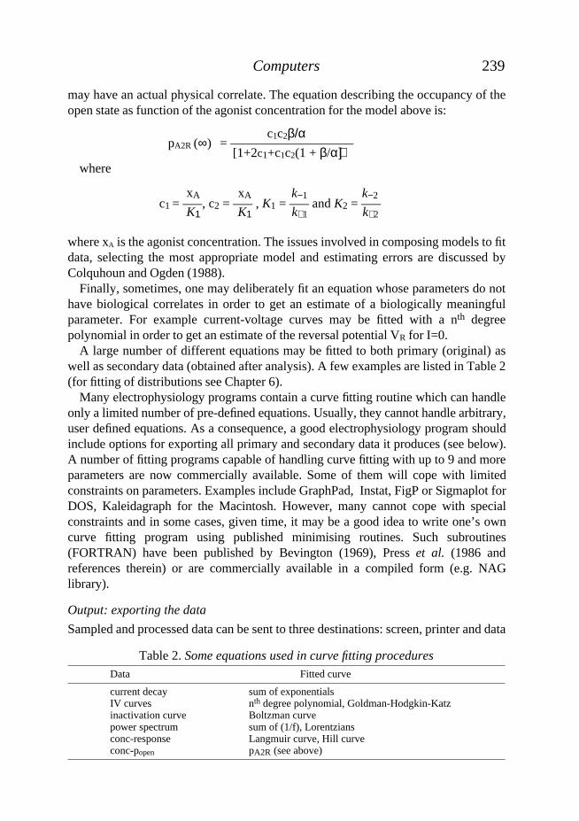
may have an actual physical correlate. The equation describing the occupancy of theopen state as function of the agonist concentration for the model above is:
c1c2β/αpA2R (∞) = –––––––––––––––––––
[1+2c1+c1c2(1 + β/α)]where
where xA is the agonist concentration. The issues involved in composing models to fitdata, selecting the most appropriate model and estimating errors are discussed byColquhoun and Ogden (1988).
Finally, sometimes, one may deliberately fit an equation whose parameters do nothave biological correlates in order to get an estimate of a biologically meaningfulparameter. For example current-voltage curves may be fitted with a nth degreepolynomial in order to get an estimate of the reversal potential VR for I=0.
A large number of different equations may be fitted to both primary (original) aswell as secondary data (obtained after analysis). A few examples are listed in Table 2(for fitting of distributions see Chapter 6).
Many electrophysiology programs contain a curve fitting routine which can handleonly a limited number of pre-defined equations. Usually, they cannot handle arbitrary,user defined equations. As a consequence, a good electrophysiology program shouldinclude options for exporting all primary and secondary data it produces (see below).A number of fitting programs capable of handling curve fitting with up to 9 and moreparameters are now commercially available. Some of them will cope with limitedconstraints on parameters. Examples include GraphPad, Instat, FigP or Sigmaplot forDOS, Kaleidagraph for the Macintosh. However, many cannot cope with specialconstraints and in some cases, given time, it may be a good idea to write one’s owncurve fitting program using published minimising routines. Such subroutines(FORTRAN) have been published by Bevington (1969), Press et al. (1986 andreferences therein) or are commercially available in a compiled form (e.g. NAGlibrary).
Output: exporting the data
Sampled and processed data can be sent to three destinations: screen, printer and data
c1 = –––, c2 = ––– , K1 = ––– and K2 = –––xA xA k−1 k−2
k+1 k+2K1 K1
239Computers
Table 2. Some equations used in curve fitting proceduresData Fitted curve
current decay sum of exponentialsIV curves nth degree polynomial, Goldman-Hodgkin-Katzinactivation curve Boltzman curvepower spectrum sum of (1/f), Lorentziansconc-response Langmuir curve, Hill curveconc-popen pA2R (see above)
files. Hardware aspects of graphic displays and printers have been discussed in thefirst part of this chapter. The necessity to export data to data files arises from at leastthree reasons: the need for detailed statistics or specialised analysis (e.g. noiseanalysis), the possibility to fit arbitrary, user-defined curves to the data and finally thenecessity to produce publication-quality figures. In the following, we shall discussvarious ways to export data and present specific advantages / disadvantages of a fewdata file formats (see also Table A5).
Text (ASCII ) files
The simplest format used to export data consists in transforming all information intouser-readable text using the ASCII code. This format is universally readable evenacross various computer types (DOS, OS/2, Macintosh OS). Most if not allcommercially available programs (spreadsheets, statistics, graphics) can read ASCIIfiles. ASCII export / import routines are easily implemented in user-written programs.Finally, ASCII files can easily be read or modified using simple text editors (DOS edit,Windows Notepad, etc.). ASCII files are unfortunately quite uneconomic in terms ofstorage space: Numbers are no longer encoded in a fixed number of bytes but require abyte per digit. It is worth checking how the various programs interpret ASCII filessince some programs (e.g. Lotus 1-2-3) cannot directly handle ASCII files containingboth text and numbers. Additional data parsing may be required to restore the originalappearance of the data. Other programs (e.g. Kaleidagraph) cannot contain text andnumbers within the same column. If the exported data consists of several columns ofnumbers or text, they must be separated by a character that is recognised as such by thereading program. Commonly used separators are space, comma and tab characters.
Lotus (*.WK%) file format
This format is a custom binary file format used by Lotus Development to encode datawithin its Lotus 1-2-3 spreadsheet program. Lotus 1-2-3 is a widespread programwhich runs on multiple platforms (DOS, Windows, OS/2, Macintosh). Furthermore itcan be read by several other spreadsheet programs such as MS-Excel or BorlandQuattro Pro. Several graphics programs (Lotus Freelance, Harvard Graphics) also canread Lotus 1-2-3 (*.WK%) files. These files can contain text, numbers and graphicsinformation for plots. The disadvantage is that it is not as universally recognised asASCII files. Determined programmers can incorporate code to read and write Lotus1-2-3 files into their programs (see Lotus reference).
Proprietary file formatsA recent and promising development is the use of standardised file formats fordigitised signals by commercially available software. Both CED and AXON usestructured binary data files so the user may extract whatever information he or sherequires. CED (and others) have gone a step further by writing and distributing a set ofsubroutines written in Pascal or C which can read and write standard CED FilingSystem (‘CFS’) files (and other files using proprietary file formats). An immediateadvantage of standardisation is that data can be easily exchanged between programs
240 A. B. CACHELIN, J. DEMPSTER AND P. T. A. GRAY
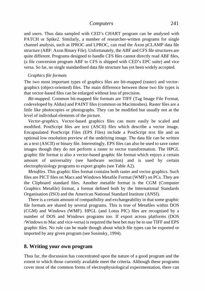
and users. Thus data sampled with CED’s CHART program can be analysed withPATCH or Spike2. Similarly, a number of researcher-written programs for singlechannel analysis, such as IPROC and LPROC, can read the Axon pCLAMP data filestructure (ABF: Axon Binary File). Unfortunately, the ABF and CFS file structures arequite different. Programs designed to handle CFS files cannot directly read ABF files,(a file conversion program ABF to CFS is shipped with CED’s EPC suite) and viceversa. So far, no single standardised data file structure has yet been widely accepted.
Graphics file formats
The two most important types of graphics files are bit-mapped (raster) and vector-graphics (object-oriented) files. The main difference between those two file types isthat vector-based files can be enlarged without loss of precision.
Bit-mapped. Common bit-mapped file formats are TIFF (Tag Image File Format,codeveloped by Aldus) and PAINT files (common on Macintoshes). Raster files are alittle like photocopies or photographs. They can be modified but usually not at thelevel of individual elements of the picture.
Vector-graphics. Vector-based graphics files can more easily be scaled andmodified. PostScript files are text (ASCII) files which describe a vector image.Encapsulated PostScript Files (EPS Files) include a PostScript text file and anoptional low resolution preview of the undelying image. The data file can be writtenas a text (ASCII) or binary file. Interestingly, EPS files can also be used to save rasterimages though they do not perform a raster to vector transformation. The HPGLgraphic file format is also a vector-based graphic file format which enjoys a certainamount of universality (see hardware section) and is used by certainelectrophysiology programs to export graphs (see Table A2).
Metafiles. This graphic files format contains both raster and vector graphics. Suchfiles are PICT files on Macs and Windows Metafile Format (WMF) on PCs. They arethe Clipboard standard files. Another metafile format is the CGM (ComputerGraphics Metafile) format, a format defined both by the International StandardsOrganisation (ISO) and the American National Standard Institute (ANSI).
There is a certain amount of compatibility and exchangeability in that some graphicfile formats are shared by several programs. This is true of Metafiles within DOS(CGM) and Windows (WMF). HPGL (and Lotus PIC) files are recognised by anumber of DOS and Windows programs too. If export across platforms (DOS/Windows to Mac and vice-versa) is required the best bet may be to use TIFF and EPSgraphic files. No rule can be made though about which file types can be exported orimported by any given program (see Sosinsky, 1994).
8. Writing your own program
Thus far, the discussion has concentrated upon the nature of a good program and theextent to which those currently available meet the criteria. Although these programscover most of the common forms of electrophysiological experimentation, there can
241Computers
be no doubt that occasions still exist where it is necessary for the experimenter towrite his/her own program.
One language does not fit all
Computer programming can be done at three levels: Low level language(Assembler) programming is for the experts. Assembler reaches parts of thecomputer other languages cannot reach. It is hardest to write, but fastest inexecution time. At a moderate level of programming expertise, ‘high level’programming languages (BASIC, FORTRAN, Pascal, C, Modula etc.) enable all(arithmetic) data manipulation usually required in a lab. Solving givenmathematical problems requires for example, understanding of the mathematical /statistical background behind the data manipulation. The reader should be awarethat knowing that solving a given problem requires inverting a matrix is only thefirst part of the solution of this problem. It is usually just as important to haveaccess to specialised literature on so-called ‘numerical recipes’ (e.g. Press et al.,1986) to perform given mathematical tasks (e.g. matrix inversion). Specialisedapplications such as writing software to convert binary file formats requireadditional knowledge on proprietary file formats which is usually provided by thesoftware companies (as manuals) or published (e.g. Lotus File Formats). Mostcommercially available programs were written in one these high level languages.At the highest (language) level, some commercial programs enable the user tosimplify repetitive tasks in data manipulation so they can run in a predetermined,‘programmed’ way, using so-called macros (e.g. Lotus 1-2-3). Recently, a numberof programs have appeared which can perform analytical mathematics (as opposedto numerical). Such programs include Wolfram Research’s Mathematica,MathSoft’s Mathcad or Waterloo Maple Software’s Maple.
It is striking how many of the existing commercial programs originated in researchlaboratories (e.g. Axon’s pCLAMP and Axograph, Instrutech PULSE software orCED PATCH & VCLAMP modules). A case can therefore be made for the need toretain programming skills within at least some electrophysiological laboratories. Newforms of signals such as those obtained from fluorescent dyes often require therecording of signals from new classes of devices (e.g. photomultipliers or videocameras) and different analysis algorithms.
A number of programming languages are available for both the DOS and Macintoshplatforms. They include numerous brands of BASIC, Pascal, FORTRAN, Modula 2,Assembler and C, to name but the most important. Programs in a high level languagecan be pepped up with low-level subroutines: this so called mixed languageprogramming may be an excellent approach for solving certain problems. A programwritten in a ‘high level’ language makes use of compiled subroutines written in ‘lowerlevel’ languages (Assembler, C) which run very fast. This removes the task of writingand checking specialised subroutines from the occasional programmer while givinghim/her access to high powered software. The reader is referred to specialised literaturefor this sort of programming (e.g. Microsoft mixed language programming guide).
One critical application of this approach to anyone writing data acquisition or
242 A. B. CACHELIN, J. DEMPSTER AND P. T. A. GRAY
experimental control software is the provision of libraries of low level procedures thathandle communication with the interface. Programming these aspects generallyinvolves lengthy Assembler programming. Most laboratory interfaces are suppliedwith libraries of user callable procedures (e.g. Axon’s set of subroutines for theDigidata 1200 or the LabPac set of subroutines for the Labmaster DMA card), or othersupport mechanisms, that handle those low level aspects. When selecting an interfacewith the intention of writing one’s own software, the quality and functionality of theprogrammer support is a major factor to consider. Other examples of user callablesubroutine packages (libraries) are: the CFS set of subroutines to access CFS files, thescientific NAG (National Algorithms Group) library (state of the art statistics andmathematics package), or the MetaWindows set of graphic subroutines.
The widespread adoption of GUI based systems, such as Microsoft Windows and theMacintosh OS calls for programming languages adapted to these new environments.Several programming languages are available for the Windows platform and theMacintosh OS. Microsoft’s Visual Basic, Borland’s Turbo Pascal for Windows (andother similar tools) are fairly easily learnt languages which enable writing of trueWindows applications (if somewhat slower than applications written in C). Theseprogramming environments, together with the latest versions of Microsoft and BorlandC++, all support a visual programming metaphor for the construction of the Windowsuser interface. This removes from the programmer a major part of the load ofdeveloping a Windows application, allowing the programmer to concentrate on codingthe underlying functionality in a traditional programming language. Mixed languageprogramming with all its advantages is possible (also from Visual Basic) by calling so-called direct link libraries (DLLs) which perform specialised tasks (e.g. data acquisitionor display). Some of the laboratory interfaces presented in Table A1 are supported byDLLs. However, as discussed earlier, the development of such programs is moredifficult than writing straight DOS programs. This may become unavoidable whenmulti-tasking systems such as Windows NT become standard. Using the Macintoshtoolbox is already now a difficult task for non-professional programmers. Anotherapproach may be to use DOS compilers which take advantage of the protected (true 32bit) processor mode. With the exception of the latest generation of C++ programmingenvironments, these may have the disadvantage of not being mainstream.
A further solution to the problem of developing customised laboratory softwarewithin the new GUI environments is to make use of a specialised softwaredevelopment system which provides the basic software components necessary for theacquisition, display and analysis of analogue signals. One of the most advancedexamples of this approach is the National Instruments LabView package whichallows the development of data acquisition software for both Windows and theMacintosh. With this package, ‘virtual instruments’ can be created by graphically‘wiring up’ acquisition, analysis and display icons on the screen. NationalInstruments also produce the Lab-Windows package which allows the developmentof similar systems (for PCs only), but with a more conventional programmingapproach, using enhanced versions of the C and QuickBasic programming languages.
In each case, the merits of developing a new program in-house should be carefully
243Computers
weighed, with consideration given to whether there might be better uses for one’stime. Software development, even with the assistance of a good developmentenvironment, is a skilled and time consuming activity. There is little value inproducing a poor and unreliable imitation of an existing program. On the other hand,the existing software that is widely available is far from perfect, and there is always aplace for faster, more versatile, easier to use, software.
9. Concluding remarks
The preceding sections are intended to provide sufficient basic information andguidance to allow a suitable laboratory computer system to be selected. However, it iswithout doubt a good idea to take additional advice, where possible, from colleaguesin your own field who have experience of performing experiments and analysissimilar to those that you intend to undertake, with one or more of the packages underconsideration. In addition, it is crucial that before making a selection, a specificationof requirements should be drawn up which details what functionality is needed suchas the number of signals to be recorded in parallel, maximum sample rates (whichwill be determined by signal bandwidth), signal length, short and long term storagerequirements (which will be related to the sample rate and length), provision ofcontrol signals and data or trigger outputs to monitor scopes, forms of analysisrequired, forms of hard copy needed. Other factors such as cost limitations orconstraints imposed by existing hardware must also be considered.
The field of personal computers is moving fast. It is quite obvious that by the timethis chapter is published or soon after, new, better and faster processors will beavailable. This may be important to satisfy the increasing demands of numbercrunching applications and of graphical user interfaces. The ease of use andaffordability of personal computers has created a trend for people to buy ready to use‘turn-key’ systems. This is a clear change from the time of mini-computers such asthe PDP-11 when all software had to be custom made. There is a danger thatelectrophysiologists do only those experiments that can be done with commercialsoftware instead of doing those experiments necessary to answer a (biological)question. The clear trend towards GUIs may aggravate this situation by furtherdecreasing the number of people both willing and able16 to write their own software.
This means that electrophysiologists have to rely on programs written by peoplewho are not necessarily familiar with the biology behind the numbers.Electrophysiologists using such programs should be aware of this fact and criticalabout what computers tell them. To those who have not got access to the programsource, the hardware and software should be treated as a black-box whose behaviourshould be carefully assessed and critically analysed to be sure its limitations areappreciated. Numbers need not be correct just because they appear on a terminal or acomputer print out. Users should never forget that while computers are infinitely
244 A. B. CACHELIN, J. DEMPSTER AND P. T. A. GRAY
16 The limits often being set by time, budget and publishing considerations.
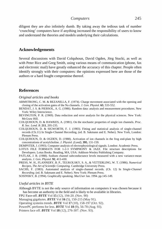
diligent they are also infinitely dumb. By taking away the tedious task of number‘crunching’ computers have if anything increased the responsibility of users to knowand understand the theories and models underlying their calculations.
Acknowledgements
Several discussions with David Colquhoun, David Ogden, Jörg Stucki, as well aswith Peter Rice and Greg Smith, using various means of communication (phone, faxand electronic mail) have greatly enhanced the accuracy of this chapter. People oftenidentify strongly with their computers: the opinions expressed here are those of theauthors or a hard fought compromise thereof.
References
Original articles and booksARMSTRONG, C. M. & BEZANILLA, F. (1974). Charge movement associated with the opening and
closing of the activation gates of the Na channels. J. Gen. Physiol. 63, 533-552.BENDAT, J. S. & PIERSOL, A. G. (1986). Random data: analysis and measurement procedures. New
York: Wiley Interscience. BEVINGTON, P. R. (1969). Data reduction and error analysis for the physical sciences. New York:
McGraw Hill. COLQUHOUN, D. & HAWKES, A. (1981). On the stochastic properties of single ion channels. Proc.
R. Soc. Lond. B. 211, 205-235.COLQUHOUN, D. & SIGWORTH, F. J. (1983). Fitting and statistical analysis of single-channel
records (Ch.11) In Single-Channel Recording, (ed. B. Sakmann and E. Neher). New York, London:Plenum Press.
COLQUHOUN, D. & OGDEN, D. (1988). Activation of ion channels in the frog end-plate by highconcentrations of acetylcholine. J. Physiol. (Lond), 395, 131-159.
DEMPSTER, J. (1993). Computer analysis of electrophysiological signals. London: Academic Press. LOTUS FILE FORMATS FOR 1-2-3 SYMPHONY & JAZZ. File structure descriptions for
Developers. Lotus Books. Reading, MA, USA: Addison-Wesley Publishing Company. PATLAK, J. B. (1988). Sodium channel subconductance levels measured with a new variance-mean
analysis. J. Gen. Physiol. 92, 413-430.PRESS, W. H., FLANNERY, B. P., TEUKOLSKY, S. A., & VETTERLING, W. T. (1986). Numerical
Recipes, The Art of Scientific Computing. Cambridge University Press. SACHS, F. (1983). Automated analysis of single-channel records. (Ch. 12) In Single-Channel
Recording. (ed. B. Sakmann and E. Neher). New York: Plenum Press. SOSINSKY, B. (1994). Graphically speaking. MacUser Jan. 1994. pp.145-149.
Useful articles in BYTE Although BYTE is not the only source of information on computers it was chosen because it
has become an authority in the field and is likely to be available in libraries.FPU Face-off. BYTE Vol 15 (12), 194-20. (Nov. 90)Managing gigabytes. BYTE Vol 16 (5), 150-215 (May 91).Operating systems trends. BYTE Vol 17 (10), 158-197 (Oct. 92).PowerPC performs for less. BYTE Vol 18 (9), 56-78 (Aug. 93).Printers face off. BYTE Vol 18 (12), 276-307. (Nov. 93).
245Computers
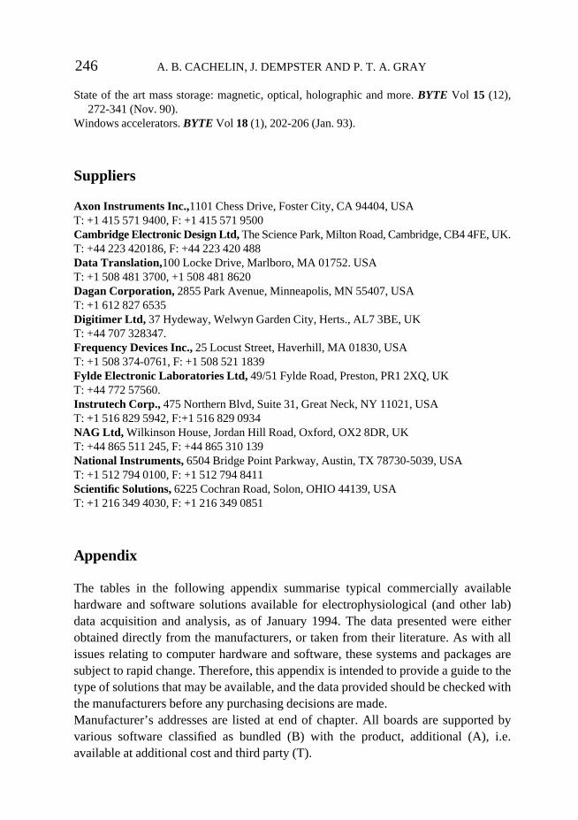
State of the art mass storage: magnetic, optical, holographic and more. BYTE Vol 15 (12),272-341 (Nov. 90).
Windows accelerators. BYTE Vol 18 (1), 202-206 (Jan. 93).
Suppliers
Axon Instruments Inc.,1101 Chess Drive, Foster City, CA 94404, USA T: +1 415 571 9400, F: +1 415 571 9500 Cambridge Electronic Design Ltd, The Science Park, Milton Road, Cambridge, CB4 4FE, UK.T: +44 223 420186, F: +44 223 420 488Data Translation,100 Locke Drive, Marlboro, MA 01752. USA T: +1 508 481 3700, +1 508 481 8620Dagan Corporation, 2855 Park Avenue, Minneapolis, MN 55407, USAT: +1 612 827 6535Digitimer Ltd, 37 Hydeway, Welwyn Garden City, Herts., AL7 3BE, UKT: +44 707 328347.Frequency Devices Inc., 25 Locust Street, Haverhill, MA 01830, USAT: +1 508 374-0761, F: +1 508 521 1839Fylde Electronic Laboratories Ltd, 49/51 Fylde Road, Preston, PR1 2XQ, UKT: +44 772 57560.Instrutech Corp., 475 Northern Blvd, Suite 31, Great Neck, NY 11021, USAT: +1 516 829 5942, F:+1 516 829 0934NAG Ltd, Wilkinson House, Jordan Hill Road, Oxford, OX2 8DR, UKT: +44 865 511 245, F: +44 865 310 139National Instruments, 6504 Bridge Point Parkway, Austin, TX 78730-5039, USAT: +1 512 794 0100, F: +1 512 794 8411Scientific Solutions, 6225 Cochran Road, Solon, OHIO 44139, USAT: +1 216 349 4030, F: +1 216 349 0851
Appendix
The tables in the following appendix summarise typical commercially availablehardware and software solutions available for electrophysiological (and other lab)data acquisition and analysis, as of January 1994. The data presented were eitherobtained directly from the manufacturers, or taken from their literature. As with allissues relating to computer hardware and software, these systems and packages aresubject to rapid change. Therefore, this appendix is intended to provide a guide to thetype of solutions that may be available, and the data provided should be checked withthe manufacturers before any purchasing decisions are made.Manufacturer’s addresses are listed at end of chapter. All boards are supported byvarious software classified as bundled (B) with the product, additional (A), i.e.available at additional cost and third party (T).
246 A. B. CACHELIN, J. DEMPSTER AND P. T. A. GRAY
247C
omputers
Table A1. Comparison of commonly used laboratory interfacesInterface CED 1401plus Digidata 1200 ITC-16 DT 2839 Labmaster AD AT/NB1-MIO-16
Supported by yes yes yes no2 no3 noelectrophysiologysoftware
Computer type PC, PS/2, MacIntosh PC PC, MacIntosh, Atari PC PC PC, PS/2, MacIntoshAnalog input(s) 16 SE 4 32 option 32 pseudo DI 8 DI 5 16 expandable 16 SE / 8 DI 16 SE / 8 DI
to 224 expandable to 64 se or 32 di
ADC range (s) ±5 V standard ±10.24 V ±10.24 V 0-1.25,0-2.5, ±10 V 0-10 V, ±5 V, ±10 V±10 V option 0-5, 0-10 V,
±1.25, ±2.5,±5, ±10 V
AD converter 12 bit 333 kHz 12 bit 333 kHz 16 bit 100 kHz / 12 bit 224 kHz 12 bit 330 kHz 12 bit 200 kHz 6
12 bit 200 kHz (1 MHz 1 ch)Programmable input gain option 7 1, 2, 4, 8 no 1, 2, 4, 8 PGH: 1,2,4,8 or 0.5, 1, 2, 5, 10, 20,
PGL: 1, 10, 50,100100,1000
DA converters 4× 12 bit 444 kHz 2× 12 bit 333 kHz 4 × 16 bit 200 kHz 2 × 12 bit 2× 12 bit 2× 12 bit 250 kHz 8
130 kHz; 260 kHz 130 kHz full scaleaggregate max 500 kHz
DAC range(s) ±5 V standard ±10.24 V ±10.24 V 0-5 V, 0-10 V, ±10 V (5 mA) 0-10 V, ±10 V ±10 V option ±2.5 V, ±5 V,
±10 VAsynchronous digital 16× TTL 8× TTL 16× TTL 16× TTL 8× TTL 8× TTL
input(s)Asynchronous digital 16× 24 mA 8× 24 mA 16× 24 mA 16× 24 mA 16× 24 mA 8× 24 mA
output(s) (or 4 sync.)Clock(s) 4× 32 bit 250 ns 48 bit 250 ns 250 ns 2× 16 bit 250 ns 16 bit 250 ns 16 bit 200 ns
1× 48 bit 1 µs programmable programmableCounter/timer 2 channels 9513A no 9513A 9513A 9513A
5 channels 5 channels 5 channels 5 channels
1AT indicates PC cards, NB (NuBus) Mac cards. 2Older board (DT2801A) is supported by Strathclyde software and other packages. 3Older board (Labmaster DMA)is supported by Strathclyde software and other packages. 4SE: single-ended, DI: differential. See section 4 for definition. 5Optically isolated. 6NB-MIO: 100 kHz.7Gains: 1, 2, 5, 10, 20, 50, 100. 8Option 64 F5: 1 MHz.
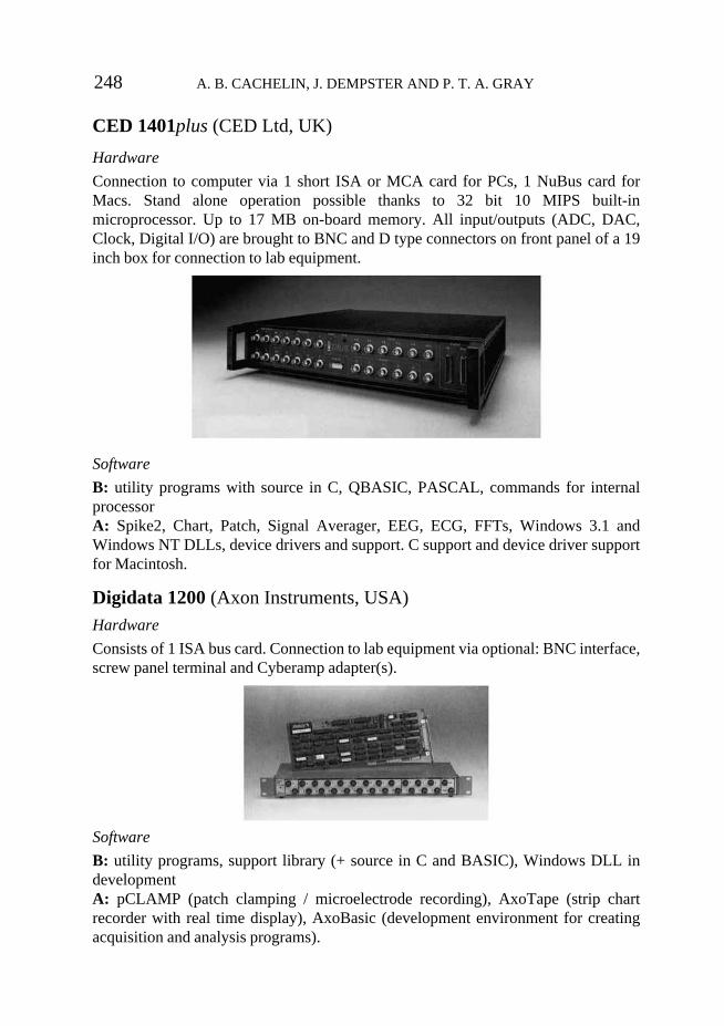
CED 1401plus (CED Ltd, UK)
Hardware
Connection to computer via 1 short ISA or MCA card for PCs, 1 NuBus card forMacs. Stand alone operation possible thanks to 32 bit 10 MIPS built-inmicroprocessor. Up to 17 MB on-board memory. All input/outputs (ADC, DAC,Clock, Digital I/O) are brought to BNC and D type connectors on front panel of a 19inch box for connection to lab equipment.
Software
B: utility programs with source in C, QBASIC, PASCAL, commands for internalprocessorA: Spike2, Chart, Patch, Signal Averager, EEG, ECG, FFTs, Windows 3.1 andWindows NT DLLs, device drivers and support. C support and device driver supportfor Macintosh.
Digidata 1200 (Axon Instruments, USA)Hardware
Consists of 1 ISA bus card. Connection to lab equipment via optional: BNC interface,screw panel terminal and Cyberamp adapter(s).
Software
B: utility programs, support library (+ source in C and BASIC), Windows DLL indevelopmentA: pCLAMP (patch clamping / microelectrode recording), AxoTape (strip chartrecorder with real time display), AxoBasic (development environment for creatingacquisition and analysis programs).
248 A. B. CACHELIN, J. DEMPSTER AND P. T. A. GRAY
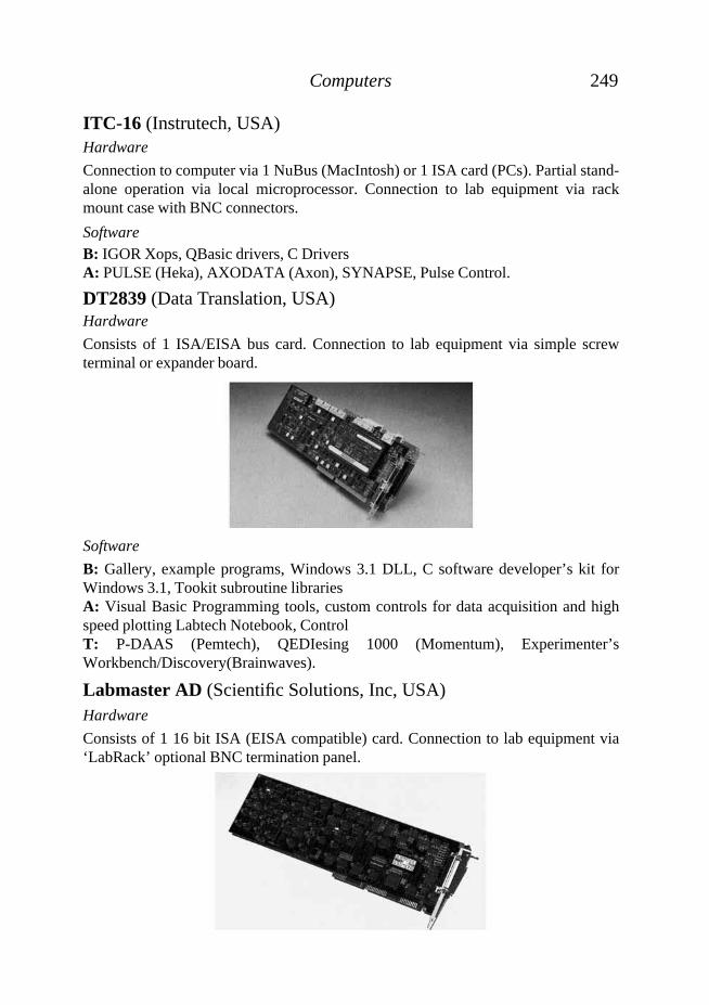
ITC-16 (Instrutech, USA)Hardware
Connection to computer via 1 NuBus (MacIntosh) or 1 ISA card (PCs). Partial stand-alone operation via local microprocessor. Connection to lab equipment via rackmount case with BNC connectors.
SoftwareB: IGOR Xops, QBasic drivers, C DriversA: PULSE (Heka), AXODATA (Axon), SYNAPSE, Pulse Control.
DT2839 (Data Translation, USA)Hardware
Consists of 1 ISA/EISA bus card. Connection to lab equipment via simple screwterminal or expander board.
Software
B: Gallery, example programs, Windows 3.1 DLL, C software developer’s kit forWindows 3.1, Tookit subroutine librariesA: Visual Basic Programming tools, custom controls for data acquisition and highspeed plotting Labtech Notebook, Control T: P-DAAS (Pemtech), QEDIesing 1000 (Momentum), Experimenter’sWorkbench/Discovery(Brainwaves).
Labmaster AD (Scientific Solutions, Inc, USA)Hardware
Consists of 1 16 bit ISA (EISA compatible) card. Connection to lab equipment via‘LabRack’ optional BNC termination panel.
249Computers
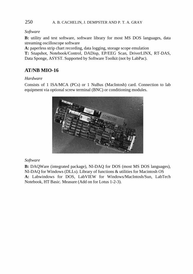
Software
B: utility and test software, software library for most MS DOS languages, datastreaming oscilloscope softwareA: paperless strip chart recording, data logging, storage scope emulationT: Snapshot, Notebook/Control, DADisp, EP/EEG Scan, DriverLINX, RT-DAS,Data Sponge, ASYST. Supported by Software Toolkit (not by LabPac).
AT/NB MIO-16
Hardware
Consists of 1 ISA/MCA (PCs) or 1 NuBus (MacIntosh) card. Connection to labequipment via optional screw terminal (BNC) or conditioning modules.
Software
B: DAQWare (integrated package), NI-DAQ for DOS (most MS DOS languages),NI-DAQ for Windows (DLLs). Library of functions & utilities for Macintosh OSA: Labwindows for DOS, LabVIEW for Windows/MacIntosh/Sun, LabTechNotebook, HT Basic. Measure (Add on for Lotus 1-2-3).
250 A. B. CACHELIN, J. DEMPSTER AND P. T. A. GRAY
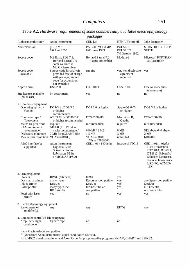
251Computers
Table A2. Hardware requirements of some commercially available electrophysiologypackages
Author/manufacturer Axon Instruments CED Ltd HEKA Elektronik John Dempster
Name/Version pCLAMP PATCH+VCLAMP PULSE + STRATHCLYDE EP6.0 June 1993 6.03 June 1993 PULSEFIT SUITE
7.0 October 1992Source code MS Basic PDS 7.1, Borland Pascal 7.0 Modula-2 Microsoft FORTRAN
Borland Pascal, 7.0 + some Assembler & Assemblersome routines inMS C / Assembler
Source code Source code for analysis enquire yes, non disclosure yesavailable provided free of charge agreement
with package, source requiredcode for acquisitionnot available
Approx price US$ 2000. UK£ 1000. US$ 1500.- Free to academics(shareware)
Site licence available by department yes no no(multi-user)
1. Computer equipmentOperating system / DOS-3.1 , DOS 5.0 DOS 2.0 or higher Apple OS 6.03 DOS 3.3 or higher
Version or higher or higherrecommended
Computer type / AT 33 MHz 80386 DX PC/AT 80×86 Macintosh II, PC/AT 80×86(Processor) or higher recommended Quadra
Maths co-processor required recommended required recommendedRAM minimum / 640 kB (+ 1 MB disk
recommended cache recommended) 640 kB / 1 MB 8 MB 512 kbyte/640 kbyteDiskspace minimum 7 MB for pCLAMP files 1.5 MB 3 MB 2 MBMax screen resolution VGA (640×480) VGA 640×480 unlimited 640×480
Wyse 1280×800ADC interface(s) Axon Instruments CED1401 / 1401plus Instrutech ITC16 CED 1401/1401plus,
supported Digidata 1200, Data TranslationScientific Soltns DT2801A, DT2821,Labmaster DMA DT2812, Scientificor MC/DAS (PS/2) Solutions Labmaster,
National InstrumentsLAB-PC, ATMIO-16X.
2. Printers/plottersPlotters HPGL (≤ 6 pens) HPGL yes1
Dot matrix printer many types Epson or -compatible yes1 any Epson compatibleInkjet printer DeskJet DeskJet yes1 DeskJetLaser printer many types incl. HP-LaserJet or yes1 HP LaserJet
HP LaserJet compatible or compatiblesPostScript laser yes no yes1 yes
printer
3. Electrophysiology equipmentRecommended any any EPC-9 any
amplifier(s)
4. Computer controlled lab equipmentAmplifier / signal CyberAmp2 no3 no
conditioner
1any Macintosh OS compatible.2CyberAmp: Axon Instruments’ signal conditioner. See text.3CED1902 signal conditioner and Axon CyberAmp supported by programs SIGAV, CHART and SPIKE2.
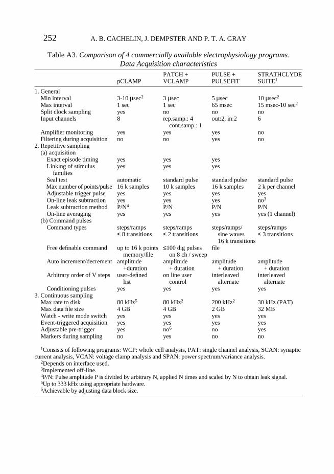
252 A. B. CACHELIN, J. DEMPSTER AND P. T. A. GRAY
Table A3. Comparison of 4 commercially available electrophysiology programs.Data Acquisition characteristics
PATCH + PULSE + STRATHCLYDE pCLAMP VCLAMP PULSEFIT SUITE1
1. GeneralMin interval 3-10 µsec2 3 µsec 5 µsec 10 µsec2
Max interval 1 sec 1 sec 65 msec 15 msec-10 sec2
Split clock sampling yes no no noInput channels 8 rep.samp.: 4 out:2, in:2 6
cont.samp.: 1Amplifier monitoring yes yes yes noFiltering during acquisition no no yes no
2. Repetitive sampling(a) acquisition
Exact episode timing yes yes yesLinking of stimulus yes yes yes
familiesSeal test automatic standard pulse standard pulse standard pulseMax number of points/pulse 16 k samples 10 k samples 16 k samples 2 k per channelAdjustable trigger pulse yes yes yes yesOn-line leak subtraction yes yes yes no3
Leak subtraction method P/N4 P/N P/N P/NOn-line averaging yes yes yes yes (1 channel)
(b) Command pulsesCommand types steps/ramps steps/ramps steps/ramps/ steps/ramps
≤ 8 transitions ≤ 2 transitions sine waves ≤ 3 transitions16 k transitions
Free definable command up to 16 k points ≤100 dig pulses filememory/file on 8 ch / sweep
Auto increment/decrement amplitude amplitude amplitude amplitude +duration + duration + duration + duration
Arbitrary order of V steps user-defined on line user interleaved interleavedlist control alternate alternate
Conditioning pulses yes yes yes yes3. Continuous sampling
Max rate to disk 80 kHz5 80 kHz2 200 kHz2 30 kHz (PAT)Max data file size 4 GB 4 GB 2 GB 32 MBWatch - write mode switch yes yes yes yesEvent-triggered acquisition yes yes yes yesAdjustable pre-trigger yes no6 no yesMarkers during sampling no yes no no
1Consists of following programs: WCP: whole cell analysis, PAT: single channel analysis, SCAN: synapticcurrent analysis, VCAN: voltage clamp analysis and SPAN: power spectrum/variance analysis.
2Depends on interface used.3Implemented off-line.4P/N: Pulse amplitude P is divided by arbitrary N, applied N times and scaled by N to obtain leak signal.5Up to 333 kHz using appropriate hardware.6Achievable by adjusting data block size.
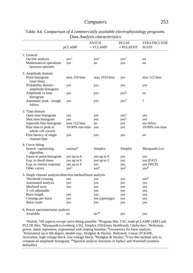
253Computers
Table A4. Comparison of 4 commercially available electrophysiology programs.Data Analysis characteristics
PATCH PULSE STRATHCLYDE pCLAMP + VCLAMP + PULSEFIT SUITE
1. General On-line analysis yes1 yes1 yes2 noMathematical operations yes no yes no
between episodes
2. Amplitude domainPoint histogram max 256 bins max 1024 bins yes max 512 bins
(max bins)Probability density- yes yes yes yes
amplitude histogramAmplitude vs time yes yes yes3 no
histogramAutomatic peak - trough yes yes yes3 ?
follow
3. Time domainOpen time histogram yes yes yes3 yesShut time histogram yes yes yes3 yesSigworth Sine histogram max 512 bins no yes see belowRise time to peak in 10-90% rise time yes yes 10-90% rise time
whole cell currentFirst latency of single yes yes yes no
channel data
4. Curve fittingSearch / optimizing various4 Simplex Simplex Marquardt-Lev.
algorithm Gauss to point histogram yes up to 6 yes up to 6 yes yesExp. to dwell times yes up to 6 yes up to 2 yes yes (PAT)Exp. to current response yes up to 6 yes yes yes (WCP)Other curves yes5 yes6 yes7 yes8
5. Single channel analysis/detection method/burst analysisThreshold crossing yes yes yes yes9
Automated analysis yes yes yes yesIdealized trace yes yes yes yesT-crit adjustable yes yes yesBurst length yes yes yes yesClosings per burst yes yes (openings) yes yesBurst count yes yes yes yes
6. Power spectrum/noise analysisAvailable no no10 yes yes
1Partial; 2All aspects except curve-fitting possible; 3Program Mac TAC reads pCLAMP (ABF) andPULSE files; 4Marquardt-Levenberg, LSQ, Simplex (SSQ/max likelihood), Chebychev; 5Boltzman,power, linear regression, exponential with sloping baseline; 6Geometrics for burst analysis;7Polynomial up to 9th degree, double exp., Hodgkin & Huxley, Boltzman, Linear (IV)GHK,Activation, high voltage block, low-voltage block; 8Hodgkin & Huxley; 9Uses this method only tocompute an amplitude histogram; 10Spectral analysis functions in Spike2 and Waterfall (windowdefinable).
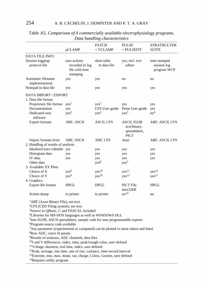
254 A. B. CACHELIN, J. DEMPSTER AND P. T. A. GRAY
Table A5. Comparison of 4 commercially available electrophysiology programs.Data handling characteristics
PATCH PULSE STRATHCLYDEpCLAMP + VCLAMP + PULSEFIT SUITE
DATA FILE INFOSession logging/ user actions short table yes, incl. text time stamped
protocol file recorded in log in data file editor session logfile with time program WCPstamping
Automatic filename yes yes no noimplementation
Notepad in data file yes yes yes yes
DATA IMPORT / EXPORT1. Data file format
Proprietary file format yes1 yes2 yes yesDocumentation yes CFS User guide Pulse User guide yesDedicated user yes3 yes4 yes5 no6
softwareExport formats ABF, ASCII ASCII, CFS ASCII, IGOR ABF, ASCII, CFS
text/binary,spreadsheet,PICT
Import formats from ABF, ASCII ABF, CFS Atari ABF, ASCII, CFS2. Handling of results of analysis
Idealised trace editable yes yes yes yesHistogram data yes yes yes yesIV data yes yes yes yesOther data yes8 yes7
3. Available XY PlotsChoice of X yes9 yes10 yes11 yes12
Choice of Y yes9 yes10 yes13 yes12
4. GraphicsExport file format HPGL HPGL PICT File HPGL
max32kBScreen dump to printer to printer no14 no
1ABF (Axon Binary File), see text2CFS (CED Filing system), see text3Source in QBasic, C and PASCAL included4Libraries for MS-DOS languages as well as WINDOWS DLL5Into IGOR, ASCII spreadsheet, sample code for user programmable exports6Program source code available7Any parameter (experimental or computed) can be plotted vs most others and fitted8Raw ADC, curve fit param.9Results of analyses, ADC channels, data files10I and V differences, index, time, peak/trough value, user defined11Voltage, duration, real time, index, user defined12Peak, average, rise time, rate of rise, variance, inter-record interval13Extreme, min, max, mean, var, charge, Cslow, Gseries, user defined14Requires utility program


