Computational modeling of bone and bone remodeling

Woodh

ead P

ublis

hing L

imite

d

© 2014 Woodhead Publishing Limited

244

8 Computational modeling of bone

and bone remodeling

H. GONG and L. WANG , Beihang University, People’s

Republic of China , M. ZHANG , The Hong Kong

Polytechnic University, Hong Kong and Y. FAN ,

Beihang University, People’s Republic of China

DOI : 10.1533/9780857096739.2.244

Abstract : Computational modeling is an important technique to better understand bone mechanical properties and the relationship between bone structure and its mechanical, as well as its biological, environment. The chapter fi rst introduces three distinct computational modeling examples for different bone mechanical properties: subject-specifi c, image-based nonlinear fi nite element modeling of proximal femur; trabecular bone yield behaviors at the tissue level; and dynamic mechanical behaviors of trabecular bone for the intertrochanteric fracture fi xation. It then describes computational simulations of bone remodeling and adaptation of trabecular bone to mechanical and biological factors.

Key words : fi nite element modeling, trabecular bone, mechanical property, strength, functional adaptation.

8.1 Introduction

The determinants of whole bone strength include geometry, architecture,

and material properties. Bone mineral density (BMD) in clinics cannot

predict bone fracture risks accurately. With new imaging techniques and

increasing computing power, it is possible to obtain three-dimensional

(3D) geometric morphology, and build computational models to predict

bone strength and the related fracture risk. In this chapter, three distinct

computational modeling examples for different bone mechanical proper-

ties are introduced and the modeling techniques are described in detail;

these are subject-specifi c, image-based nonlinear fi nite element model-

ing of proximal femur; trabecular bone yield behaviors at the tissue level;

and dynamic mechanical behaviors of trabecular bone for intertrochan-

teric fracture fi xation. Bone is a living organ with the ability to adapt to

mechanical usage or other biophysical stimuli in terms of its mass and

architecture. This phenomenon is known as functional adaptation in the

08_p244-267.indd 24408_p244-267.indd 244 1/17/2014 7:48:08 PM1/17/2014 7:48:08 PM

Woodh

ead P

ublis

hing L

imite

d

Computational modeling of bone and bone remodeling 245

forms of modeling and remodeling. Computational simulations of bone

remodeling and the adaptation of trabecular bone to mechanical and bio-

logical factors are described in this chapter. A brief discussion of chal-

lenges, applications, and future developments are presented at the end of

the chapter.

8.2 Computational modeling examples of bone mechanical properties and bone remodeling

In this section, four computational examples of bone mechanical proper-

ties and bone remodeling were introduced, i.e. subject-specifi c image-based

nonlinear fi nite element modeling of proximal femur, computational model-

ing of trabecular bone yield behaviors at the tissue level, dynamic mechan-

ical behaviors of trabecular bone, and computational simulation of bone

remodeling.

8.2.1 Subject-specifi c, image-based nonlinear fi nite element modeling of proximal femur

The development of subject-specifi c fi nite element models from Quantitative

Computed Tomography (QCT) data was termed Biomechanical CT (BCT),

and became the most technologically advanced method currently available

for in vivo assessment of bone strength (Keaveny et al ., 2010).

Quantitative computed tomography (QCT) scanning

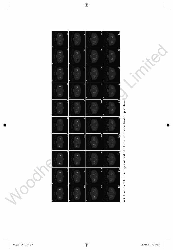
QCT scans were made at the hip region using a QCT scanner with a slice

width of 2.5 mm and an in-plane voxel size of 0.9375 mm (GE Medical

Systems/lightspeed 16, Wakesha, WI, USA) (Gong et al ., 2012). A calibration

phantom containing known hydroxyapatite concentrations was scanned

together with the subject to calibrate the x-ray absorptions of different

materials. Figure 8.1 shows a series of QCT images of part of a femur with

a calibration phantom.

Three-dimensional modeling of the proximal femur

Three-dimensional reconstruction and meshing of the proximal femur was

performed in Mimics software (Materialise Inc., Belgium) from the femoral

head to 1 cm below the lesser trochanter. To account for bone tissue het-

erogeneity, bone material property in the whole proximal femur was repre-

sented by approximately 170 discrete sets of material properties so that the

modulus of each material increased by an increment of 5% over the modu-

lus of the previous material (Keyak et al ., 1998; Perillo-Marcone et al ., 2003).

08_p244-267.indd 24508_p244-267.indd 245 1/17/2014 7:48:09 PM1/17/2014 7:48:09 PM

Woodh

ead P

ublis

hing L

imite

d

8.1

A s

eri

es o

f Q

CT

im

ag

es o

f p

art

of

a f

em

ur

wit

h a

ca

lib

rati

on

ph

an

tom

.

08_p244-267.indd 24608_p244-267.indd 246 1/17/2014 7:48:09 PM1/17/2014 7:48:09 PM

Woodh

ead P

ublis

hing L

imite

d


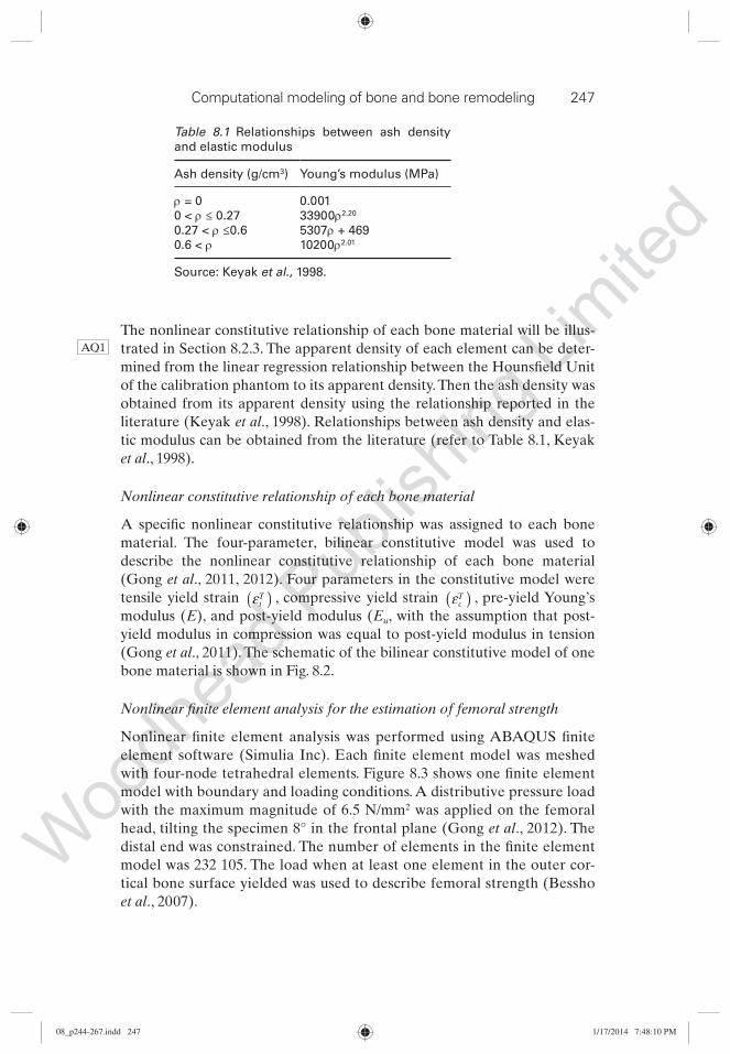
The nonlinear constitutive relationship of each bone material will be illus-

trated in Section 8.2.3 . The apparent density of each element can be deter-

mined from the linear regression relationship between the Hounsfi eld Unit

of the calibration phantom to its apparent density. Then the ash density was

obtained from its apparent density using the relationship reported in the

literature (Keyak et al ., 1998). Relationships between ash density and elas-

tic modulus can be obtained from the literature (refer to Table 8.1, Keyak

et al ., 1998).

Nonlinear constitutive relationship of each bone material

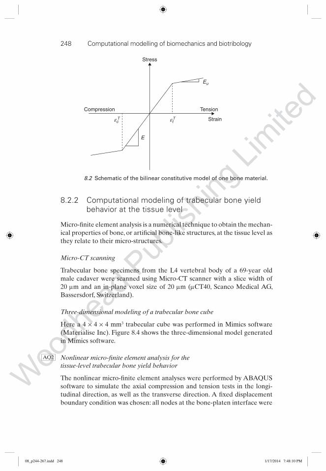
A specifi c nonlinear constitutive relationship was assigned to each bone

material. The four-parameter, bilinear constitutive model was used to

describe the nonlinear constitutive relationship of each bone material

(Gong et al ., 2011, 2012). Four parameters in the constitutive model were

tensile yield strain εtTε( ) , compressive yield strain εc

Tε( ) , pre-yield Young’s

modulus ( E ), and post-yield modulus ( E u , with the assumption that post-

yield modulus in compression was equal to post-yield modulus in tension

(Gong et al ., 2011). The schematic of the bilinear constitutive model of one

bone material is shown in Fig. 8.2.

Nonlinear fi nite element analysis for the estimation of femoral strength

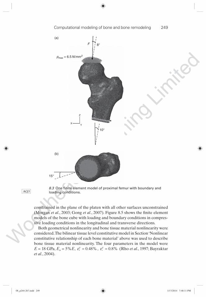
Nonlinear fi nite element analysis was performed using ABAQUS fi nite

element software (Simulia Inc). Each fi nite element model was meshed

with four-node tetrahedral elements. Figure 8.3 shows one fi nite element

model with boundary and loading conditions. A distributive pressure load

with the maximum magnitude of 6.5 N/mm 2 was applied on the femoral

head, tilting the specimen 8° in the frontal plane (Gong et al ., 2012). The

distal end was constrained. The number of elements in the fi nite element

model was 232 105. The load when at least one element in the outer cor-

tical bone surface yielded was used to describe femoral strength (Bessho

et al ., 2007).

AQ1

Table 8.1 Relationships between ash density

and elastic modulus

Ash density (g/cm 3 ) Young’s modulus (MPa)

ρ = 0 0.001

0 < ρ ≤ 0.27 33900 ρ 2.20

0.27 < ρ ≤0.6 5307 ρ + 469

0.6 < ρ 10200 ρ 2.01

Source: Keyak et al ., 1998.

08_p244-267.indd 24708_p244-267.indd 247 1/17/2014 7:48:10 PM1/17/2014 7:48:10 PM

Woodh

ead P

ublis

hing L

imite

d

248 Computational modelling of biomechanics and biotribology

8.2.2 Computational modeling of trabecular bone yield behavior at the tissue level

Micro-fi nite element analysis is a numerical technique to obtain the mechan-

ical properties of bone, or artifi cial bone-like structures, at the tissue level as

they relate to their micro-structures.

Micro-CT scanning

Trabecular bone specimens from the L4 vertebral body of a 69-year old

male cadaver were scanned using Micro-CT scanner with a slice width of

20 μ m and an in-plane voxel size of 20 μ m ( μ CT40, Scanco Medical AG,

Bassersdorf, Switzerland).

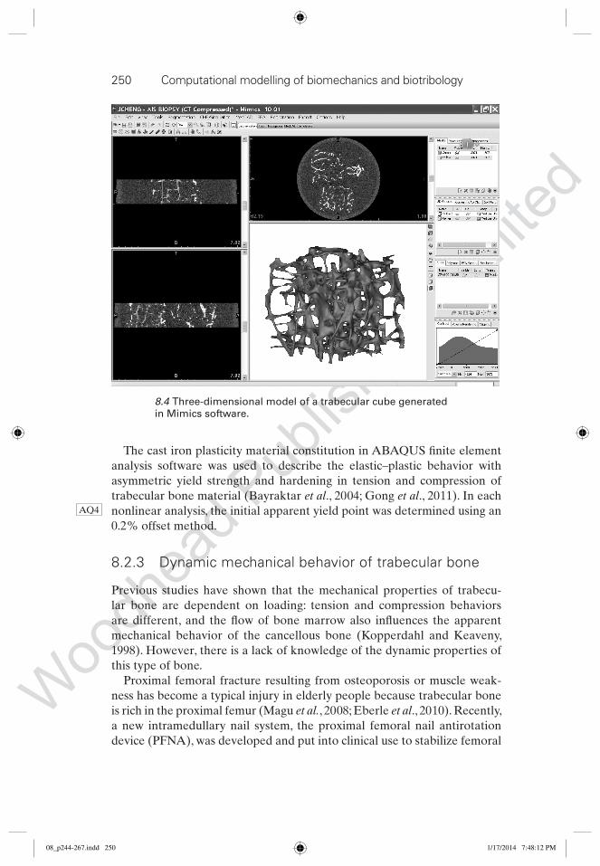
Three-dimensional modeling of a trabecular bone cube

Here a 4 × 4 × 4 mm 3 trabecular cube was performed in Mimics software

(Materialise Inc). Figure 8.4 shows the three-dimensional model generated

in Mimics software.

Nonlinear micro-fi nite element analysis for the tissue-level trabecular bone yield behavior

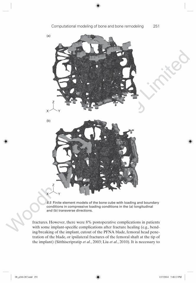
The nonlinear micro-fi nite element analyses were performed by ABAQUS

software to simulate the axial compression and tension tests in the longi-

tudinal direction, as well as the transverse direction. A fi xed displacement

boundary condition was chosen: all nodes at the bone-platen interface were

AQ2

Strain

Tension

Stress

Compression

E

Eu

εcT εt

T

8.2 Schematic of the bilinear constitutive model of one bone material.

08_p244-267.indd 24808_p244-267.indd 248 1/17/2014 7:48:10 PM1/17/2014 7:48:10 PM

Woodh

ead P

ublis

hing L

imite

d


F 8°

(a)

(b)

10°

15°

X

Z

Y

pmax = 6.5 N/mm2

8.3 One fi nite element model of proximal femur with boundary and

loading conditions. AQ3

constrained in the plane of the platen with all other surfaces unconstrained

(Morgan et al ., 2003; Gong et al ., 2007). Figure 8.5 shows the fi nite element

models of the bone cube with loading and boundary conditions in compres-

sive loading conditions in the longitudinal and transverse directions.

Both geometrical nonlinearity and bone tissue material nonlinearity were

considered. The bilinear tissue level constitutive model in Section ‘Nonlinear

constitutive relationship of each bone material’ above was used to describe

bone tissue material nonlinearity. The four parameters in the model were

E = 18 GPa, E u = 5% E , εtTε = 0 4. %48 , εc

Tε = 0 8. %8 (Rho et al ., 1997; Bayraktar

et al ., 2004).

08_p244-267.indd 24908_p244-267.indd 249 1/17/2014 7:48:11 PM1/17/2014 7:48:11 PM

Woodh

ead P

ublis

hing L

imite

d


The cast iron plasticity material constitution in ABAQUS fi nite element

analysis software was used to describe the elastic–plastic behavior with

asymmetric yield strength and hardening in tension and compression of

trabecular bone material (Bayraktar et al ., 2004; Gong et al ., 2011). In each

nonlinear analysis, the initial apparent yield point was determined using an

0.2% offset method.

8.2.3 Dynamic mechanical behavior of trabecular bone

Previous studies have shown that the mechanical properties of trabecu-

lar bone are dependent on loading: tension and compression behaviors

are different, and the fl ow of bone marrow also infl uences the apparent

mechanical behavior of the cancellous bone (Kopperdahl and Keaveny,

1998). However, there is a lack of knowledge of the dynamic properties of

this type of bone.

Proximal femoral fracture resulting from osteoporosis or muscle weak-

ness has become a typical injury in elderly people because trabecular bone

is rich in the proximal femur (Magu et al. , 2008; Eberle et al ., 2010). Recently,

a new intramedullary nail system, the proximal femoral nail antirotation

device (PFNA), was developed and put into clinical use to stabilize femoral

AQ4

8.4 Three-dimensional model of a trabecular cube generated

in Mimics software.

08_p244-267.indd 25008_p244-267.indd 250 1/17/2014 7:48:12 PM1/17/2014 7:48:12 PM

Woodh

ead P

ublis

hing L

imite

d


(a)

(b)

X Y

Z

X Y

Z

8.5 Finite element models of the bone cube with loading and boundary

conditions in compressive loading conditions in the (a) longitudinal

and (b) transverse directions.

fractures. However, there were 8% postoperative complications in patients

with some implant-specifi c complications after fracture healing (e.g., bend-

ing/breaking of the implant, cutout of the PFNA blade, femoral head pene-

tration of the blade, or ipsilateral fractures of the femoral shaft at the tip of

the implant) (Sitthiseripratip et al ., 2003; Liu et al ., 2010). It is necessary to

08_p244-267.indd 25108_p244-267.indd 251 1/17/2014 7:48:13 PM1/17/2014 7:48:13 PM

Woodh

ead P

ublis

hing L

imite

d


analyze the stress/strain distribution during intertrochanteric fracture heal-

ing, which may be altered consistently .

Dynamic simulation of the intertrochanteric fracture fi xation

To simulate the dynamic behavior of the proximal femur with intertrochan-

teric fracture fi xation in the process of healing, three-dimensional models

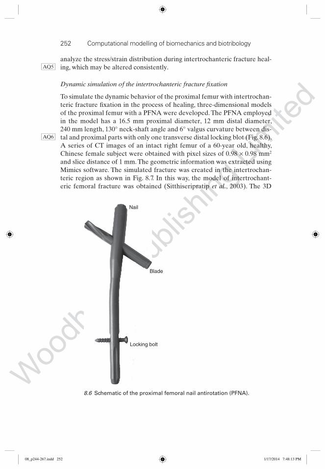
of the proximal femur with a PFNA were developed. The PFNA employed

in the model has a 16.5 mm proximal diameter, 12 mm distal diameter,

240 mm length, 130° neck-shaft angle and 6° valgus curvature between dis-

tal and proximal parts with only one transverse distal locking blot (Fig. 8.6).

A series of CT images of an intact right femur of a 60-year old, healthy,

Chinese female subject were obtained with pixel sizes of 0.98 × 0.98 mm 2

and slice distance of 1 mm. The geometric information was extracted using

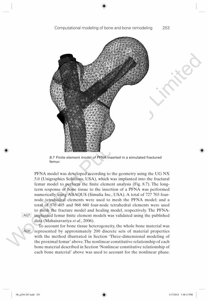
Mimics software. The simulated fracture was created in the intertrochan-

teric region as shown in Fig. 8.7. In this way, the model of intertrochant-

eric femoral fracture was obtained (Sitthiseripratip et al ., 2003). The 3D

AQ5

AQ6

Blade

Locking bolt

Nail

8.6 Schematic of the proximal femoral nail antirotation (PFNA).

08_p244-267.indd 25208_p244-267.indd 252 1/17/2014 7:48:13 PM1/17/2014 7:48:13 PM

Woodh

ead P

ublis

hing L

imite

d


PFNA model was developed according to the geometry using the UG NX

5.0 (Unigraphics Solutions, USA), which was implanted into the fractural

femur model to perform the fi nite element analysis (Fig. 8.7). The long-

term response of bone tissue to the insertion of a PFNA was performed

numerically using ABAQUS (Simulia Inc., USA). A total of 727 703 four-

node tetrahedral elements were used to mesh the PFNA model; and a

total of 976 405 and 968 660 four-node tetrahedral elements were used

to mesh the fracture model and healing model, respectively. The PFNA-

implanted femur fi nite element models was validated using the published

data (Mahaisavariya et al ., 2006).

To account for bone tissue heterogeneity, the whole bone material was

represented by approximately 200 discrete sets of material properties

with the method illustrated in Section ‘Three-dimensional modeling of

the proximal femur’ above. The nonlinear constitutive relationship of each

bone material described in Section ‘Nonlinear constitutive relationship of

each bone material’ above was used to account for the nonlinear phase.

AQ7

AQ8

8.7 Finite element model of PFNA inserted in a simulated fractured

femur.

08_p244-267.indd 25308_p244-267.indd 253 1/17/2014 7:48:13 PM1/17/2014 7:48:13 PM

Woodh

ead P

ublis

hing L

imite

d


The isotropic Poisson’s ratio of each bone material was 0.3 (Homminga

et al ., 2002). For the PFNA, titanium alloy was assigned to be a linear

elastic and isotropic material with an elastic modulus of 113.8 GPa and

a Poisson’s ratio of 0.34 (Sitthiseripratip et al. , 2003; Ramakrishnan et al ., 2009).

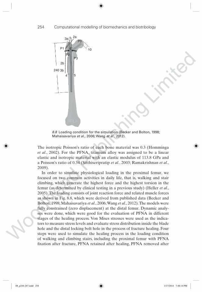
In order to simulate physiological loading in the proximal femur, we

focused on two common activities in daily life, that is, walking and stair

climbing, which generate the highest force and the highest torsion in the

femur (as determined by clinical testing in a previous study) (Heller et al ., 2005). The loading consists of joint reaction force and related muscle forces

as shown in Fig. 8.8, which were derived from published data (Becker and

Bolton, 1998; Mahaisavariya et al ., 2006; Wang et al ., 2012). The models were

fully constrained (zero displacement) at the distal femur. Dynamic analy-

ses were done, which were good for the evaluation of PFNA in different

stages of the healing process. Von Mises stresses were used as the indica-

tors to measure stress levels and evaluate stress distribution inside the blade

hole and the distal locking bolt hole in the process of fracture healing. Four

steps were used to simulate the healing process in the loading condition

of walking and climbing stairs, including the proximal femur with PFNA

fi xation after fracture, PFNA retained after healing, PFNA removed after

54

3b

2b

P1

P03a 2a

P3P2

106°

1

240

8.8 Loading condition for the simulation (Becker and Bolton, 1998;

Mahaisavariya et al ., 2006; Wang et al ., 2012).

08_p244-267.indd 25408_p244-267.indd 254 1/17/2014 7:48:14 PM1/17/2014 7:48:14 PM

Woodh

ead P

ublis

hing L

imite

d


healing, and intact femur after new bone tissue has been formed (Wang

et al ., 2012).

8.2.4 Computational simulation of bone remodeling

Bone remodeling is performed by groups of osteoclasts and osteoblasts

organized into basic multicellular units (BMUs). Remodeling by BMUs

includes biologically coupled BMU activation, bone resorption by osteo-

clasts, and bone formation by osteoblasts.

Bone remodeling algorithm

The bone remodeling process is controlled by mechanical usage and biolog-

ical factors. Osteocytes act as sensors of mechanoreceptors and regulators

of bone mass by mediating osteoblasts for bone formation and osteoclasts

for bone resorption (Cowin et al ., 1991; Lanyon, 1993). The computational

model of bone remodeling we developed is shown here as an example

(Gong et al ., 2010). The total mechanical stimulus at location x on the tra-

becular surface ( P ( x , t )) is the contribution of all the osteocytes in the forms

of strain energy density (SED), relative to their distance from x (Mullender

and Huiskes, 1995; Gong et al ., 2010):

t f x R ti iff x ii

N

,( ) ( ) ( )=∑ μ

1

[8.1]

where μ i is the mechanosensitivity of the osteocyte i , R i ( t ) is the SED of the

osteocyte i , and f i ( x ) is the spatial infl uence function describing the infl uence

of osteocyte i on the osteoblasts and osteoclasts at location x (Mullender

et al ., 1994; Gong et al ., 2010).

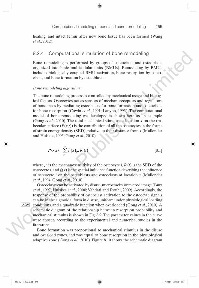
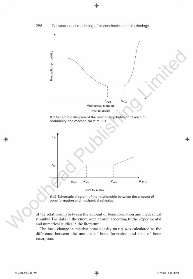
Osteoclasts can be activated by disuse, microcracks, or microdamage (Burr

et al ., 1997; Huiskes et al ., 2000; Vahdati and Rouhi, 2009). Accordingly, the

response of the probability of osteoclast activation to the osteocyte signals

can be in the sigmoidal form in disuse, uniform under physiological loading

conditions, and a quadratic function when overloaded (Gong et al ., 2010). A

schematic diagram of the relationship between resorption probability and

mechanical stimulus is shown in Fig. 8.9. The parameter values in the curve

were chosen according to the experimental and numerical studies in the

literature.

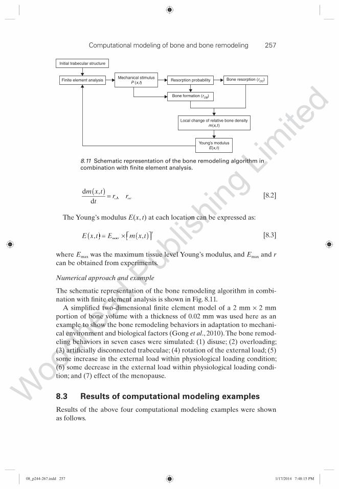
Bone formation was proportional to mechanical stimulus in the disuse

and overload zones, and was equal to bone resorption in the physiological

adaptive zone (Gong et al ., 2010). Figure 8.10 shows the schematic diagram

AQ9

08_p244-267.indd 25508_p244-267.indd 255 1/17/2014 7:48:14 PM1/17/2014 7:48:14 PM

Woodh

ead P

ublis

hing L

imite

d


of the relationship between the amount of bone formation and mechanical

stimulus. The data in the curve were chosen according to the experimental

and numerical studies in the literature.

The local change in relative bone density m ( x , t ) was calculated as the

difference between the amount of bone formation and that of bone

resorption:

(Not to scale)

KAD1 KAD2 P (x,t)KOB

roc

rob

8.10 Schematic diagram of the relationship between the amount of

bone formation and mechanical stimulus.

Mechanical stimulus

(Not to scale)

Res

orpt

ion

prob

abili

ty

KAD1 KAD2

8.9 Schematic diagram of the relationship between resorption

probability and mechanical stimulus.

08_p244-267.indd 25608_p244-267.indd 256 1/17/2014 7:48:14 PM1/17/2014 7:48:14 PM

Woodh

ead P

ublis

hing L

imite

d


d

d

m x t

tr robrr ocrr

,( ) = rr [8.2]

The Young’s modulus E ( x , t ) at each location can be expressed as:

E x t E m x tr

, ,t E m xmax( ) ×EE ( )⎡⎣⎡⎡ ⎤⎦⎤⎤ [8.3]

where E max was the maximum tissue level Young’s modulus, and E max and r

can be obtained from experiments.

Numerical approach and example

The schematic representation of the bone remodeling algorithm in combi-

nation with fi nite element analysis is shown in Fig. 8.11.

A simplifi ed two-dimensional fi nite element model of a 2 mm × 2 mm

portion of bone volume with a thickness of 0.02 mm was used here as an

example to show the bone remodeling behaviors in adaptation to mechani-

cal environment and biological factors (Gong et al ., 2010). The bone remod-

eling behaviors in seven cases were simulated: (1) disuse; (2) overloading;

(3) artifi cially disconnected trabeculae; (4) rotation of the external load; (5)

some increase in the external load within physiological loading condition;

(6) some decrease in the external load within physiological loading condi-

tion; and (7) effect of the menopause.

8.3 Results of computational modeling examples

Results of the above four computational modeling examples were shown

as follows.

Initial trabecular structure

Resorption probability

Bone formation (rOB)

Local change of relative bone densitym(x,t )

Young’s modulusE(x,t )

Bone resorption (rOC)Finite element analysisMechanical stimulus

P (x,t)

8.11 Schematic representation of the bone remodeling algorithm in

combination with fi nite element analysis.

08_p244-267.indd 25708_p244-267.indd 257 1/17/2014 7:48:15 PM1/17/2014 7:48:15 PM

Woodh

ead P

ublis

hing L

imite

d


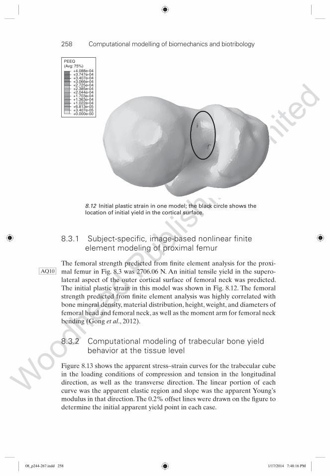
8.3.1 Subject-specifi c, image-based nonlinear fi nite element modeling of proximal femur

The femoral strength predicted from fi nite element analysis for the proxi-

mal femur in Fig. 8.3 was 2706.06 N. An initial tensile yield in the supero-

lateral aspect of the outer cortical surface of femoral neck was predicted.

The initial plastic strain in this model was shown in Fig. 8.12. The femoral

strength predicted from fi nite element analysis was highly correlated with

bone mineral density, material distribution, height, weight, and diameters of

femoral head and femoral neck, as well as the moment arm for femoral neck

bending (Gong et al ., 2012).

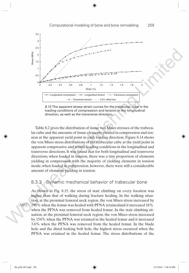
8.3.2 Computational modeling of trabecular bone yield behavior at the tissue level

Figure 8.13 shows the apparent stress–strain curves for the trabecular cube

in the loading conditions of compression and tension in the longitudinal

direction, as well as the transverse direction. The linear portion of each

curve was the apparent elastic region and slope was the apparent Young’s

modulus in that direction. The 0.2% offset lines were drawn on the fi gure to

determine the initial apparent yield point in each case.

AQ10

+4.088e-04

PEEQ(Avg: 75%)

+3.747e-04+3.407e-04+3.066e-04+2.725e-04+2.385e-04+2.044e-04+1.703e-04+1.363e-04+1.022e-04+6.813e-05+3.407e-05+0.000e-00

8.12 Initial plastic strain in one model; the black circle shows the

location of initial yield in the cortical surface.

08_p244-267.indd 25808_p244-267.indd 258 1/17/2014 7:48:16 PM1/17/2014 7:48:16 PM

Woodh

ead P

ublis

hing L

imite

d


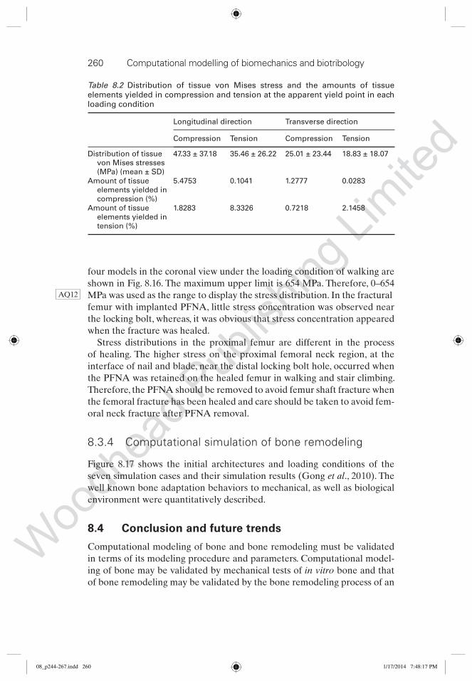
Table 8.2 gives the distribution of tissue von Mises stresses of the trabecu-

lar cube and the amounts of tissue elements yielded in compression and ten-

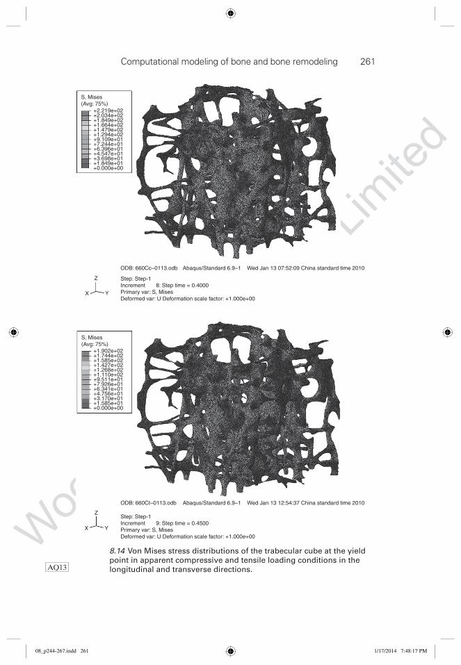
sion at the apparent yield point in each loading direction. Figure 8.14 shows

the von Mises stress distributions of the trabecular cube at the yield point in

apparent compressive and tensile loading conditions in the longitudinal and

transverse directions. It was found that for both longitudinal and transverse

directions, when loaded in tension, there was a tiny proportion of elements

yielding in compression with the majority of yielding elements in tension

mode; when loaded in compression, however, there were still a considerable

amount of elements yielding in tension.

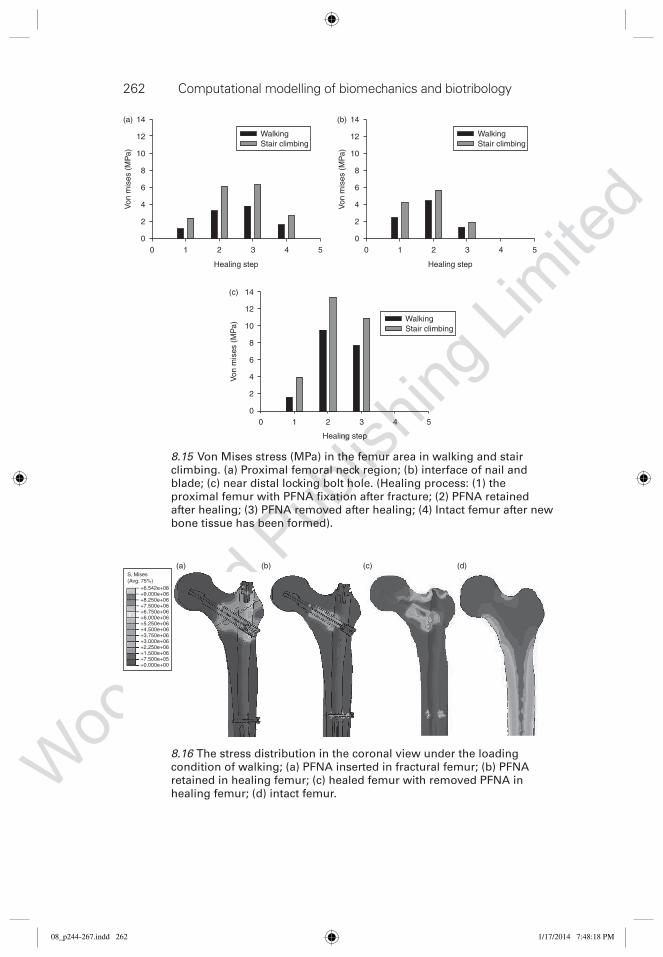
8.3.3 Dynamic mechanical behavior of trabecular bone

As shown in Fig. 8.15, the stress of stair climbing on every location was

higher than that of walking during fracture healing. In the walking situa-

tion, at the proximal femoral neck region, the von Mises stress increased by

196% when the femur was healed with PFNA retainedand it increased 16%

when the PFNA was removed from healed femur. In the stair climbing sit-

uation, at the proximal femoral neck region, the von Mises stress increased

by 154% when the PFNA was retained in the healed femur and it increased

3.6% when the PFNA was removed from the healed femur. In the blade

hole and the distal locking bolt hole, the highest stress occurred when the

PFNA was retained in the healed femur. The stress distributions of the

AQ11

3.5

3

2.5

2

1.5

0.5

00 0.2 0.4 0.6 0.8 1 1.2

Strain (%)

Str

ess

(MP

a)

1.4 1.6 1.8 2

1

Longitudinal compression Longitudinal tension Transverse compression

Transverse tension 0.2% offset line

8.13 The apparent stress–strain curves for the trabecular cube in the

loading conditions of compression and tension in the longitudinal

direction, as well as the transverse direction,.

08_p244-267.indd 25908_p244-267.indd 259 1/17/2014 7:48:16 PM1/17/2014 7:48:16 PM

Woodh

ead P

ublis

hing L

imite

d


four models in the coronal view under the loading condition of walking are

shown in Fig. 8.16. The maximum upper limit is 654 MPa. Therefore, 0–654

MPa was used as the range to display the stress distribution. In the fractural

femur with implanted PFNA, little stress concentration was observed near

the locking bolt, whereas, it was obvious that stress concentration appeared

when the fracture was healed.

Stress distributions in the proximal femur are different in the process

of healing. The higher stress on the proximal femoral neck region, at the

interface of nail and blade, near the distal locking bolt hole, occurred when

the PFNA was retained on the healed femur in walking and stair climbing.

Therefore, the PFNA should be removed to avoid femur shaft fracture when

the femoral fracture has been healed and care should be taken to avoid fem-

oral neck fracture after PFNA removal.

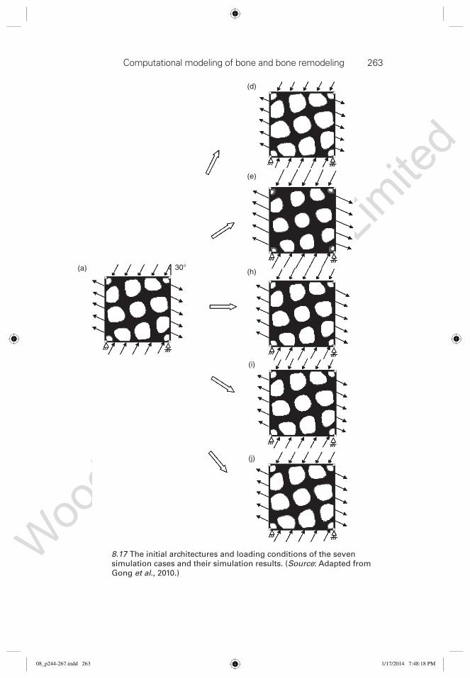
8.3.4 Computational simulation of bone remodeling

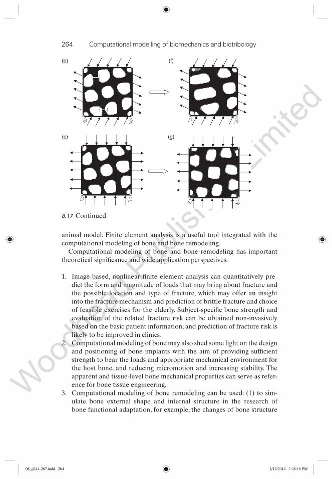
Figure 8.17 shows the initial architectures and loading conditions of the

seven simulation cases and their simulation results (Gong et al ., 2010). The

well known bone adaptation behaviors to mechanical, as well as biological

environment were quantitatively described.

8.4 Conclusion and future trends

Computational modeling of bone and bone remodeling must be validated

in terms of its modeling procedure and parameters. Computational model-

ing of bone may be validated by mechanical tests of in vitro bone and that

of bone remodeling may be validated by the bone remodeling process of an

AQ12

Table 8.2 Distribution of tissue von Mises stress and the amounts of tissue

elements yielded in compression and tension at the apparent yield point in each

loading condition

Longitudinal direction Transverse direction

Compression Tension Compression Tension

Distribution of tissue

von Mises stresses

(MPa) (mean ± SD)

47.33 ± 37.18 35.46 ± 26.22 25.01 ± 23.44 18.83 ± 18.07

Amount of tissue

elements yielded in

compression (%)

5.4753 0.1041 1.2777 0.0283

Amount of tissue

elements yielded in

tension (%)

1.8283 8.3326 0.7218 2.1458

08_p244-267.indd 26008_p244-267.indd 260 1/17/2014 7:48:17 PM1/17/2014 7:48:17 PM

Woodh

ead P

ublis

hing L

imite

d


Step: Step-1Increment 8: Step time = 0.4000Primary var: S, MisesDeformed var: U Deformation scale factor: +1.000e+00

ODB: 660Cc–0113.odb

Z

X

S, Mises(Avg: 75%)

+1.902e+02+1.744e+02+1.585e+02+1.427e+02+1.268e+02+1.110e+02+9.511e+01+7.926e+01+6.341e+01+4.756e+01+3.170e+01+1.585e+01+0.000e+00

S, Mises(Avg: 75%)

+2.219e+02+2.034e+02+1.849e+02+1.664e+02+1.479e+02+1.294e+02+9.109e+01+7.244e+01+6.396e+01+4.547e+01+3.698e+01+1.849e+01+0.000e+00

Y

Z

X Y

Abaqus/Standard 6.9–1 Wed Jan 13 07:52:09 China standard time 2010

Step: Step-1Increment 9: Step time = 0.4500Primary var: S, MisesDeformed var: U Deformation scale factor: +1.000e+00

ODB: 660Ct–0113.odb Abaqus/Standard 6.9–1 Wed Jan 13 12:54:37 China standard time 2010

8.14 Von Mises stress distributions of the trabecular cube at the yield

point in apparent compressive and tensile loading conditions in the

longitudinal and transverse directions. AQ13

08_p244-267.indd 26108_p244-267.indd 261 1/17/2014 7:48:17 PM1/17/2014 7:48:17 PM

Woodh

ead P

ublis

hing L

imite

d


4 532

Healing step

WalkingStair climbing

100

2

4

6

Von

mis

es (

MP

a)

8

10

12

14

4 532

Healing step

100

2

4

6

Von

mis

es (

MP

a)

8

10

12

14

4 532

Healing step

100

2

4

6

Von

mis

es (

MP

a)

8

10

12

14(c)

(a) (b)



8.15 Von Mises stress (MPa) in the femur area in walking and stair

climbing. (a) Proximal femoral neck region; (b) interface of nail and

blade; (c) near distal locking bolt hole. (Healing process: (1) the

proximal femur with PFNA fi xation after fracture; (2) PFNA retained

after healing; (3) PFNA removed after healing; (4) Intact femur after new

bone tissue has been formed).

+3.750e+06

+5.250e+06+6.000e+06+6.750e+06+7.500e+06+8.250e+06+9.000e+06+6.542e+08

S, Mises(Avg: 75%)

(a) (b) (c) (d)

+4.500e+06

+2.250e+06+3.000e+06

+1.500e+06+7.500e+05+0.000e+00

8.16 The stress distribution in the coronal view under the loading

condition of walking; (a) PFNA inserted in fractural femur; (b) PFNA

retained in healing femur; (c) healed femur with removed PFNA in

healing femur; (d) intact femur.

08_p244-267.indd 26208_p244-267.indd 262 1/17/2014 7:48:18 PM1/17/2014 7:48:18 PM

Woodh

ead P

ublis

hing L

imite

d


8.17 The initial architectures and loading conditions of the seven

simulation cases and their simulation results. ( Source : Adapted from

Gong et al ., 2010.)

30°(a)

(d)

(e)

(h)

(i)

(j)

08_p244-267.indd 26308_p244-267.indd 263 1/17/2014 7:48:18 PM1/17/2014 7:48:18 PM

Woodh

ead P

ublis

hing L

imite

d


animal model. Finite element analysis is a useful tool integrated with the

computational modeling of bone and bone remodeling.

Computational modeling of bone and bone remodeling has important

theoretical signifi cance and wide application perspectives.

Image-based, nonlinear fi nite element analysis can quantitatively pre-1.

dict the form and magnitude of loads that may bring about fracture and

the possible location and type of fracture, which may offer an insight

into the fracture mechanism and prediction of brittle fracture and choice

of feasible exercises for the elderly. Subject-specifi c bone strength and

evaluation of the related fracture risk can be obtained non-invasively

based on the basic patient information, and prediction of fracture risk is

likely to be improved in clinics.

Computational modeling of bone may also shed some light on the design 2.

and positioning of bone implants with the aim of providing suffi cient

strength to bear the loads and appropriate mechanical environment for

the host bone, and reducing micromotion and increasing stability. The

apparent and tissue-level bone mechanical properties can serve as refer-

ence for bone tissue engineering.

Computational modeling of bone remodeling can be used: (1) to sim-3.

ulate bone external shape and internal structure in the research of

bone functional adaptation, for example, the changes of bone structure

8.17 Continued

(b)

(c)

(f)

(g)

08_p244-267.indd 26408_p244-267.indd 264 1/17/2014 7:48:18 PM1/17/2014 7:48:18 PM

Woodh

ead P

ublis

hing L

imite

d


following the changes of exercise and pose, and traumatic bone atrophy

and related prevention and treatment; (2) to study the mechanisms of

osteoporosis and osteophyte; (3) to simulate bone structure and inves-

tigate stress shielding following implantation (internal/external fi xa-

tion, artifi cial joint, etc.), as well as design the implants; (4) to simulate

changes of bone structure caused by orthopedic surgery and choose the

optimal scenario. In general, it can provide some theoretical basis for

fundamentally understanding the relationship between bone structure

and its mechanical environment. Moreover, it also serves as an impor-

tant guideline for bone culture in tissue engineering.

8.5 Sources of further information and advice

For more information about computational modeling of bone and bone

remodeling, readers are encouraged to consult the societies of biomechan-

ics such as the International Society of Biomechanics (ISB), European

Society of Biomechanics (ESB), etc., and also the International Chinese

Hard Tissue Society (http://www.ichts.org/), American Society for Bone

and Mineral Research, Biomedical Engineering Society, and International

Bone and Mineral Society, etc. The journals that readers may consult

include Journal of Biomechanics , Journal of Bone and Mineral Research, Bone , Annals of Biomedical Engineering , Journal of Bone and Mineral Metabolism , etc.

8.6 Acknowledgements

This work is supported by the grant from National Natural Science Foundation

of China (Nos. 11120101001, 11322223, 11202017) and the Program for New

Century Excellent Talents in University (NCET-12–0024).

8.7 References Bayraktar, H. H., Morgan, E. F., Niebur, G. L., Morris, G. E., Wong, E. K. and Keaveny,

T. M. (2004) ‘Comparison of the elastic and yield properties of human femoral

trabecular and cortical bone tissue’, J Biomech , 37 , 27–35.

Becker, B. S. and Bolton, J. D. (1998). ‘Properties of sintered Ti-6Al-4V alloys

designed for use as implantable medical devices’, Processing and Fabrication of Advanced Materials VI , 1&2 , 1671–1682.

Bessho, M., Ohnishi, I., Matsuyama, J., Matsumoto, T., Imai, K. and Nakamura, K.

(2007) ‘Prediction of strength and strain of the proximal femur by a CT-based

fi nite element method’, J Biomech , 40 , 1745–1753.

Burr, D. B., Forwood, M., Fyhrie, D. P., Martin, R. B. and Turner, C. H. (1997) ‘Bone

microdamage and skeletal fragility in osteoporosis and stress fractures’, J Bone Miner Res , 16 , 6–15.

08_p244-267.indd 26508_p244-267.indd 265 1/17/2014 7:48:19 PM1/17/2014 7:48:19 PM

Woodh

ead P

ublis

hing L

imite

d


Cowin, S. C., Moss-Salentijn, L. and Moss, M. L. (1991) ‘Candidates for the mecha-

nosensory system in bone’, J Biomech Eng , 113 , 191–197.

Eberle, S., Gerber, C., von Oldenburg, G., H o gel, F. and Augat, P. (2010) ‘A bio-

mechanical evaluation of orthopaedic implants for hip fractures by fi nite ele-

ment analysis and in-vitro tests’, Proc Inst Mech Eng H , 224 , 1141–1152.

Gong, H., Zhang, M. and Fan, Y. (2011) ‘Micro-fi nite element analysis of trabecu-

lar bone yield behavior-effects of tissue non-linear material properties’, J Mech Med Biol , 11 , 563–580.

Gong, H., Zhang, M., Qin, L. and Hou, Y. (2007) ‘Regional variations in the apparent

and tissue-level mechanical parameters of vertebral trabecular bone with aging

using micro-fi nite element analysis’, Ann Biomed Eng , 35 , 1622–1631.

Gong, H., Zhang, M., Fan, Y., Kwok, W. L. and Leung, P. C. (2012) ‘Relationships

between femoral strength evaluated by nonlinear fi nite element analysis and

BMD, material distribution and geometric morphology’, Ann Biomed Eng , 40 ,

1575–1585.

Gong, H., Zhu, D., Gao, J., Lv, L. and Zhang, X. (2010) ‘An adaptation model for

trabecular bone at different mechanical levels’, Biomed Eng Online , 9 , 32.

Heller, M. O., Bergmann, G., Kassi J. P., Claes, L., Haas, N. P. and Duda, G. N. (2005)

‘Determination of muscle loading at the hip joint for use in pre-clinical testing’,

J Biomech , 38 , 1155–1163.

Homminga, J., McCreadie, B. R., Ciarelli, T. E., Weinans, H., Goldstein, S. A. and

Huiskes, R. (2002) ‘Cancellous bone mechanical properties from normals and

patients with hip fractures differ on the structure level, not on the bone hard

tissue level’, Bone , 30 , 759–764.

Huiskes, R., Ruimerman, R., van Lenthe, G. H. and Janssen, J. D. (2000) ‘Effects of

mechanical forces on maintenance and adaptation of form in trabecular bone’,

Nature , 404 , 704–706.

Keaveny, T. M., Kopperdahl, D. L., Melton, L. J. III, Hoffmann, P. F., Amin, S., Riggs, B.

L. and Khosla, S. (2010) ‘Age-dependence of femoral strength in white women

and men’, J Bone Miner Res , 25 , 994–1001.

Keyak, J. H., Rossi, S. A., Jones, K. A. and Skinner, H. B. (1998) ‘Prediction of fem-

oral fracture load using automated fi nite element modelling’, J Biomech , 31 ,

125–133.

Kopperdahl, D. L. and Keaveny, T. M. (1998) ‘Yield strain behavior of trabecular

bone’, J Biomech , 31 , 601–608.

Lanyon, L. E. (1993) ‘Osteocytes, strain detection, bone modeling and remodeling’,

Calcif Tissue Int , 53 , S102–S106.

Liu, Y. K., Tao, R., Liu, F., Wang, Y., Zhou, Z., Cao, Y. and Wang, H. (2010) ‘Mid-term

outcomes after intramedullary fi xation of peritrochanteric femoral fractures

using the new proximal femoral nail antirotation (PFNA)’, Injury , 41 , 810–817.

Magu, N. K., Tater, R., Rohilla, R., Gulia, A., Singh, R. and Kamboj, P. (2008)

‘Functional outcome of modifi ed Pauwels intertrochanteric osteotomy and

total hip arthroplasty in femoral neck fractures in elderly patients’, Indian J Orthop , 42 , 49–55.

Mahaisavariya, B., Sitthiseripratip, K. and Suwanprateeb, J. (2006) ‘Finite element

study of the proximal femur with retained trochanteric gamma nail and after

removal of nail’, Injury , 37 , 778–785.

08_p244-267.indd 26608_p244-267.indd 266 1/17/2014 7:48:19 PM1/17/2014 7:48:19 PM

Woodh

ead P

ublis

hing L

imite

d


Morgan, E. F., Bayraktar, H. H. and Keaveny, T. M. (2003) ‘Trabecular bone modu-

lus-density relationships depend on anatomic site’, J Biomech , 36 , 897–904.

Mullender, M. G. and Huiskes, R. (1995) ‘Proposal for the regulatory mechanism of

Wolff’s law’, J Orthop Res , 13 , 503–512.

Mullender, M. G., Huiskes, R. and Weinans, H. (1994) ‘A physiological approach to

the simulation of bone remodeling as a self-organizational control process’, J Biomech , 27 , 1389–1394.

Perillo-Marcone, A., Alonso-Wazquez, A. and Taylor, M. (2003) ‘Assessment of the

effect of mesh density on the material property discretisation within QCT based

FE models: a practical example using the implanted proximal tibia’, Comput Meth Biomech Biomed Eng , 6 , 17–26.

Ramakrishnan, S., Asaithambi, M. and Christopher, J. J. (2009) ‘Qualitative assess-

ment of tensile strength components of human femur trabecular bone using

radiographic imaging and spectral analysis’, J Mech Med Biol , 9 , 21–29.

Rho, J. Y., Tsui, T. Y. and Pharr, G. M. (1997) ‘Elastic properties of human cortical

and trabecular lamellar bone measured by nanoindentation’, Biomaterials , 18 ,

1325–1330.

Sitthiseripratip, K., Van Oosterwyck, H., Vander Sloten, J., Mahaisavariya, B., Bohez,

E. L., Suwanprateeb, J., Van Audekercke, R. and Oris, P. (2003) ‘Finite element

study of trochanteric gamma nail for trochanteric fracture’, Med Eng Phys , 25 ,

99–106.

Vahdati, A. and Rouhi, G. (2009) ‘A model for mechanical adaptation of trabecular

bone incorporating cellular accommodation and effects of microdamage and

disuse’, Mech Res Commun , 36 , 284–293.

Wang, L., Zhao, F., Han, J., Wang, C. and Fan Y. (2012). ‘Biomechanical study on

proximal femoral nail antirotation (PFNA) for intertrochanteric fracture’, J Mech Med Biol , 12 , 1250075, doi:10.1142/S0219519412500753

AQ1 Please confi rm cross-reference of Section 8.2.3 is correct.

AQ2 Are the subheadings necessary here? Can the text be combined into one

longer paragraph at 8.2.2?

AQ3 Please provide explanations for part fi gures a and b.

AQ4 Please check insertionthe insertion of the article ‘an’ in the sentence ‘In each

nonlinear ...’.

AQ5 Please check the sentence ‘It is necessary ...’, since it is unclear.

AQ6 Please clarify whether the term ‘blot’ can be changed to ‘bolt’ in the sen-

tence ‘The PFNA employed ’.

AQ7 Please clarify whethet the phrase ‘models was’ should be changed as ‘mod-

els were’ or ‘model was’ in the sentence ‘The PFNA-implanted ...’.

AQ8 Please confi rm whether the edits made to the sentence ‘To account for bone

...’ are appropriate.

AQ9 Please confi rm whether the edits made to the sentence ‘Accordingly, the re-

sponse ...’ are appropraite.

AQ10 Are these values are signifi cant fi gures?

AQ11 Please note that the the phrase ‘...increased 16%; is not clear. Please confi rm

whetehr it could be changed as ‘a further 16%’.

AQ12 Please clarify whether the word ‘fractural’ should be changed as ‘fractured’

in the sentence ‘In the fractural femur ...’.

AQ13 Please provide explanations for part fi gures a and b.

08_p244-267.indd 26708_p244-267.indd 267 1/17/2014 7:48:19 PM1/17/2014 7:48:19 PM

Documents

Computational modeling of bone and bone remodeling