Computational FluidDynamics on AWS

AWS Whitepaper

Computational Fluid Dynamics on AWS AWS Whitepaper

Computational Fluid Dynamics on AWS: AWS WhitepaperCopyright © Amazon Web Services, Inc. and/or its affiliates. All rights reserved.

Amazon's trademarks and trade dress may not be used in connection with any product or service that is notAmazon's, in any manner that is likely to cause confusion among customers, or in any manner that disparages ordiscredits Amazon. All other trademarks not owned by Amazon are the property of their respective owners, who mayor may not be affiliated with, connected to, or sponsored by Amazon.

Computational Fluid Dynamics on AWS AWS Whitepaper

Table of ContentsAbstract and introduction .... . . . . . . . . . . . . . . . . . . . . . . . . . . . . . . . . . . . . . . . . . . . . . . . . . . . . . . . . . . . . . . . . . . . . . . . . . . . . . . . . . . . . . . . . . . . . . . . . . . . . . . . . . . . . . . . . i

Abstract ... . . . . . . . . . . . . . . . . . . . . . . . . . . . . . . . . . . . . . . . . . . . . . . . . . . . . . . . . . . . . . . . . . . . . . . . . . . . . . . . . . . . . . . . . . . . . . . . . . . . . . . . . . . . . . . . . . . . . . . . . . . . . . . . . . 1Introduction .... . . . . . . . . . . . . . . . . . . . . . . . . . . . . . . . . . . . . . . . . . . . . . . . . . . . . . . . . . . . . . . . . . . . . . . . . . . . . . . . . . . . . . . . . . . . . . . . . . . . . . . . . . . . . . . . . . . . . . . . . . . 1

Are you Well-Architected? .... . . . . . . . . . . . . . . . . . . . . . . . . . . . . . . . . . . . . . . . . . . . . . . . . . . . . . . . . . . . . . . . . . . . . . . . . . . . . . . . . . . . . . . . . . . . . . . . . . . . . . . . . . . . . . . . 4Why CFD on AWS? .... . . . . . . . . . . . . . . . . . . . . . . . . . . . . . . . . . . . . . . . . . . . . . . . . . . . . . . . . . . . . . . . . . . . . . . . . . . . . . . . . . . . . . . . . . . . . . . . . . . . . . . . . . . . . . . . . . . . . . . . . . 5Getting started with AWS ..... . . . . . . . . . . . . . . . . . . . . . . . . . . . . . . . . . . . . . . . . . . . . . . . . . . . . . . . . . . . . . . . . . . . . . . . . . . . . . . . . . . . . . . . . . . . . . . . . . . . . . . . . . . . . . . 6CFD approaches on AWS ..... . . . . . . . . . . . . . . . . . . . . . . . . . . . . . . . . . . . . . . . . . . . . . . . . . . . . . . . . . . . . . . . . . . . . . . . . . . . . . . . . . . . . . . . . . . . . . . . . . . . . . . . . . . . . . . . . 8

Architectures .... . . . . . . . . . . . . . . . . . . . . . . . . . . . . . . . . . . . . . . . . . . . . . . . . . . . . . . . . . . . . . . . . . . . . . . . . . . . . . . . . . . . . . . . . . . . . . . . . . . . . . . . . . . . . . . . . . . . . . . . . . 8Traditional cluster environments .... . . . . . . . . . . . . . . . . . . . . . . . . . . . . . . . . . . . . . . . . . . . . . . . . . . . . . . . . . . . . . . . . . . . . . . . . . . . . . . . . . . . . . . 8Cloud native environments .... . . . . . . . . . . . . . . . . . . . . . . . . . . . . . . . . . . . . . . . . . . . . . . . . . . . . . . . . . . . . . . . . . . . . . . . . . . . . . . . . . . . . . . . . . . . . . . 9

Software .... . . . . . . . . . . . . . . . . . . . . . . . . . . . . . . . . . . . . . . . . . . . . . . . . . . . . . . . . . . . . . . . . . . . . . . . . . . . . . . . . . . . . . . . . . . . . . . . . . . . . . . . . . . . . . . . . . . . . . . . . . . . . . . . 9Installation .... . . . . . . . . . . . . . . . . . . . . . . . . . . . . . . . . . . . . . . . . . . . . . . . . . . . . . . . . . . . . . . . . . . . . . . . . . . . . . . . . . . . . . . . . . . . . . . . . . . . . . . . . . . . . . . . . . . . . 9Licensing .... . . . . . . . . . . . . . . . . . . . . . . . . . . . . . . . . . . . . . . . . . . . . . . . . . . . . . . . . . . . . . . . . . . . . . . . . . . . . . . . . . . . . . . . . . . . . . . . . . . . . . . . . . . . . . . . . . . . . . 10Setup .... . . . . . . . . . . . . . . . . . . . . . . . . . . . . . . . . . . . . . . . . . . . . . . . . . . . . . . . . . . . . . . . . . . . . . . . . . . . . . . . . . . . . . . . . . . . . . . . . . . . . . . . . . . . . . . . . . . . . . . . . . . 10Maintenance .... . . . . . . . . . . . . . . . . . . . . . . . . . . . . . . . . . . . . . . . . . . . . . . . . . . . . . . . . . . . . . . . . . . . . . . . . . . . . . . . . . . . . . . . . . . . . . . . . . . . . . . . . . . . . . . . . 11

Cluster lifecycle .... . . . . . . . . . . . . . . . . . . . . . . . . . . . . . . . . . . . . . . . . . . . . . . . . . . . . . . . . . . . . . . . . . . . . . . . . . . . . . . . . . . . . . . . . . . . . . . . . . . . . . . . . . . . . . . . . . . . . 11CFD case scalability ... . . . . . . . . . . . . . . . . . . . . . . . . . . . . . . . . . . . . . . . . . . . . . . . . . . . . . . . . . . . . . . . . . . . . . . . . . . . . . . . . . . . . . . . . . . . . . . . . . . . . . . . . . . . . . . . 12

Strong scaling vs. weak scaling .... . . . . . . . . . . . . . . . . . . . . . . . . . . . . . . . . . . . . . . . . . . . . . . . . . . . . . . . . . . . . . . . . . . . . . . . . . . . . . . . . . . . . . . 13Running efficiency .... . . . . . . . . . . . . . . . . . . . . . . . . . . . . . . . . . . . . . . . . . . . . . . . . . . . . . . . . . . . . . . . . . . . . . . . . . . . . . . . . . . . . . . . . . . . . . . . . . . . . . . . . 14Turn-around time and cost ... . . . . . . . . . . . . . . . . . . . . . . . . . . . . . . . . . . . . . . . . . . . . . . . . . . . . . . . . . . . . . . . . . . . . . . . . . . . . . . . . . . . . . . . . . . . . . 15

Optimizing HPC components .... . . . . . . . . . . . . . . . . . . . . . . . . . . . . . . . . . . . . . . . . . . . . . . . . . . . . . . . . . . . . . . . . . . . . . . . . . . . . . . . . . . . . . . . . . . . . . . . . . . . . . . . . . 17Compute .... . . . . . . . . . . . . . . . . . . . . . . . . . . . . . . . . . . . . . . . . . . . . . . . . . . . . . . . . . . . . . . . . . . . . . . . . . . . . . . . . . . . . . . . . . . . . . . . . . . . . . . . . . . . . . . . . . . . . . . . . . . . . . 17Network .... . . . . . . . . . . . . . . . . . . . . . . . . . . . . . . . . . . . . . . . . . . . . . . . . . . . . . . . . . . . . . . . . . . . . . . . . . . . . . . . . . . . . . . . . . . . . . . . . . . . . . . . . . . . . . . . . . . . . . . . . . . . . . . 18Storage .... . . . . . . . . . . . . . . . . . . . . . . . . . . . . . . . . . . . . . . . . . . . . . . . . . . . . . . . . . . . . . . . . . . . . . . . . . . . . . . . . . . . . . . . . . . . . . . . . . . . . . . . . . . . . . . . . . . . . . . . . . . . . . . . 18

Transferring input data .... . . . . . . . . . . . . . . . . . . . . . . . . . . . . . . . . . . . . . . . . . . . . . . . . . . . . . . . . . . . . . . . . . . . . . . . . . . . . . . . . . . . . . . . . . . . . . . . . . 19Running your CFD simulation .... . . . . . . . . . . . . . . . . . . . . . . . . . . . . . . . . . . . . . . . . . . . . . . . . . . . . . . . . . . . . . . . . . . . . . . . . . . . . . . . . . . . . . . . . . 19Storing output data .... . . . . . . . . . . . . . . . . . . . . . . . . . . . . . . . . . . . . . . . . . . . . . . . . . . . . . . . . . . . . . . . . . . . . . . . . . . . . . . . . . . . . . . . . . . . . . . . . . . . . . . 20Archiving inactive data .... . . . . . . . . . . . . . . . . . . . . . . . . . . . . . . . . . . . . . . . . . . . . . . . . . . . . . . . . . . . . . . . . . . . . . . . . . . . . . . . . . . . . . . . . . . . . . . . . . . 20Storage summary .... . . . . . . . . . . . . . . . . . . . . . . . . . . . . . . . . . . . . . . . . . . . . . . . . . . . . . . . . . . . . . . . . . . . . . . . . . . . . . . . . . . . . . . . . . . . . . . . . . . . . . . . . . 20

Visualization .... . . . . . . . . . . . . . . . . . . . . . . . . . . . . . . . . . . . . . . . . . . . . . . . . . . . . . . . . . . . . . . . . . . . . . . . . . . . . . . . . . . . . . . . . . . . . . . . . . . . . . . . . . . . . . . . . . . . . . . . . 20Costs ... . . . . . . . . . . . . . . . . . . . . . . . . . . . . . . . . . . . . . . . . . . . . . . . . . . . . . . . . . . . . . . . . . . . . . . . . . . . . . . . . . . . . . . . . . . . . . . . . . . . . . . . . . . . . . . . . . . . . . . . . . . . . . . . . . . . . . . . . . . . 22Conclusion .... . . . . . . . . . . . . . . . . . . . . . . . . . . . . . . . . . . . . . . . . . . . . . . . . . . . . . . . . . . . . . . . . . . . . . . . . . . . . . . . . . . . . . . . . . . . . . . . . . . . . . . . . . . . . . . . . . . . . . . . . . . . . . . . . . . . 24Contributors ... . . . . . . . . . . . . . . . . . . . . . . . . . . . . . . . . . . . . . . . . . . . . . . . . . . . . . . . . . . . . . . . . . . . . . . . . . . . . . . . . . . . . . . . . . . . . . . . . . . . . . . . . . . . . . . . . . . . . . . . . . . . . . . . . . 25Further reading .... . . . . . . . . . . . . . . . . . . . . . . . . . . . . . . . . . . . . . . . . . . . . . . . . . . . . . . . . . . . . . . . . . . . . . . . . . . . . . . . . . . . . . . . . . . . . . . . . . . . . . . . . . . . . . . . . . . . . . . . . . . . . 26Document revisions .... . . . . . . . . . . . . . . . . . . . . . . . . . . . . . . . . . . . . . . . . . . . . . . . . . . . . . . . . . . . . . . . . . . . . . . . . . . . . . . . . . . . . . . . . . . . . . . . . . . . . . . . . . . . . . . . . . . . . . . 27Notices .... . . . . . . . . . . . . . . . . . . . . . . . . . . . . . . . . . . . . . . . . . . . . . . . . . . . . . . . . . . . . . . . . . . . . . . . . . . . . . . . . . . . . . . . . . . . . . . . . . . . . . . . . . . . . . . . . . . . . . . . . . . . . . . . . . . . . . . . . 28AWS glossary .... . . . . . . . . . . . . . . . . . . . . . . . . . . . . . . . . . . . . . . . . . . . . . . . . . . . . . . . . . . . . . . . . . . . . . . . . . . . . . . . . . . . . . . . . . . . . . . . . . . . . . . . . . . . . . . . . . . . . . . . . . . . . . . . 29

iii

Computational Fluid Dynamics on AWS AWS WhitepaperAbstract

Computational Fluid Dynamics onAWS

Publication date: March 24, 2022 (Document revisions (p. 27))

AbstractThe scalable nature and variable demand of computational fluid dynamics (CFD) workloads makes themwell suited for a cloud computing environment. This whitepaper describes best practices for running CFDworkloads on Amazon Web Services (AWS). Use this document to learn more about AWS services, andthe related quick start tools that simplify getting started with running CFD cases on AWS.

IntroductionFluid dynamics is the study of the motion of fluids, usually in the presence of an object. Typical fluidflows of interest to engineers and scientist include flow in pipes, through engines, and around objects,such as buildings, automobiles, and airplanes. Computational fluid dynamics (CFD) is the study ofthese flows using a numerical approach. CFD involves the solution of conservation equations (mass,momentum, energy, and others) in a finite domain.

Many CFD tools are currently available, including specialized and in-house tools. This variety is theresult of the broad domain of physical problems solved with CFD. There is not a universal code forall applications, although there are packages that offer great capabilities. Broad CFD capabilities areavailable in commercial packages, such as ANSYS Fluent, Siemens Simcenter STAR-CCM+, MetacompTechnologies CFD++, and open-source packages, such as OpenFOAM and SU2.

A typical CFD simulation involves the following four steps:

• Define the geometry — In some cases, this step is simple, such as modeling flow in a duct. In othercases, this step involves complex components and moving parts, such as modeling a gas turbineengine. For many cases, the geometry creation is extremely time-consuming. The geometry step isgraphics intensive and requires a capable graphics workstation, preferably with a Graphics ProcessingUnit (GPU). Often, the geometry is provided by a designer, but the CFD engineer must “clean” thegeometry for input into the flow solver or mesh generation tool. This can be a tedious and time-consuming step and can sometimes require a large amount of system memory (RAM) depending onthe complexity of the geometry.

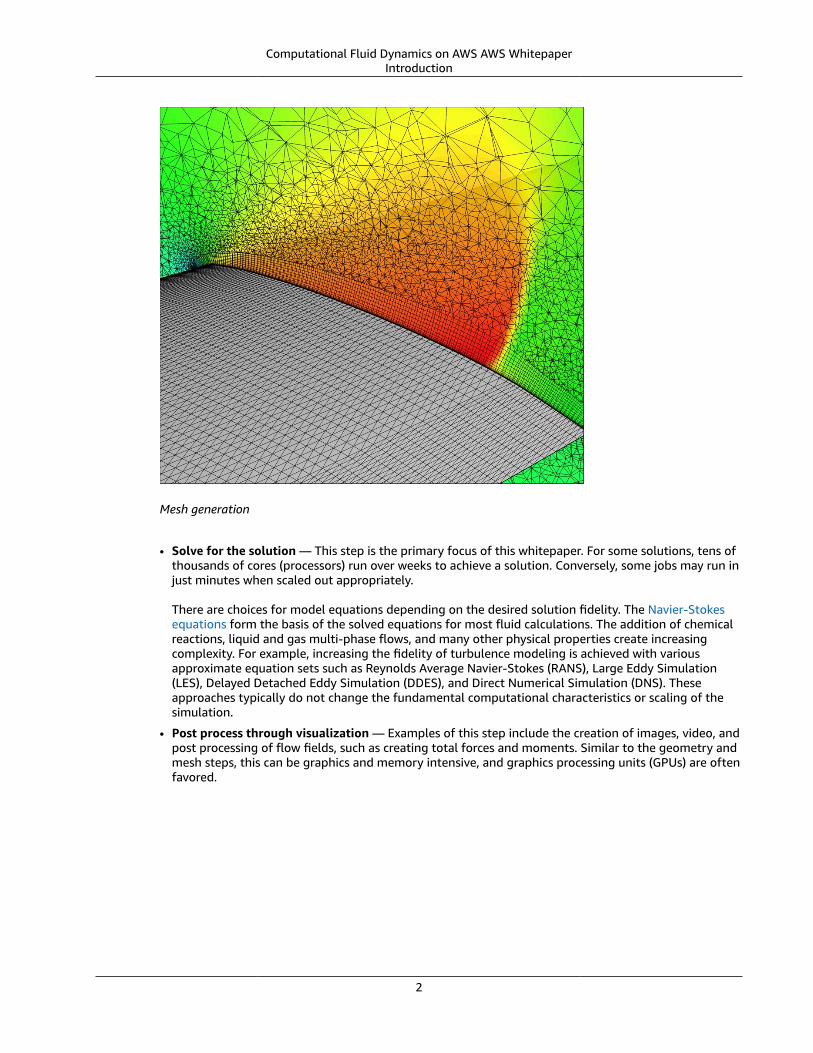
• Generate the mesh or grid — Mesh generation is a critical step because computational accuracy isdependent on the size, cell location, and skewness or orthogonality of the cells. In the following figure,a hybrid mesh is shown on a slice through an aircraft wing. Mesh generation can be iterative with thesolution, where fixes to the mesh are driven by an understanding of flow features and gradients inthe solution. Meshing is frequently an interactive process and its elliptical nature generally requiresa substantial amount of memory. Like geometry definition, generating a single mesh can take hours,days, weeks, and sometimes months. Many mesh generation codes are still limited to a single node,so general-purpose Amazon Elastic Compute Cloud (Amazon EC2) instances, such as the M family, ormemory-optimized instances, such as the R family, are often used.

1

Computational Fluid Dynamics on AWS AWS WhitepaperIntroduction

Mesh generation

• Solve for the solution — This step is the primary focus of this whitepaper. For some solutions, tens ofthousands of cores (processors) run over weeks to achieve a solution. Conversely, some jobs may run injust minutes when scaled out appropriately.

There are choices for model equations depending on the desired solution fidelity. The Navier-Stokesequations form the basis of the solved equations for most fluid calculations. The addition of chemicalreactions, liquid and gas multi-phase flows, and many other physical properties create increasingcomplexity. For example, increasing the fidelity of turbulence modeling is achieved with variousapproximate equation sets such as Reynolds Average Navier-Stokes (RANS), Large Eddy Simulation(LES), Delayed Detached Eddy Simulation (DDES), and Direct Numerical Simulation (DNS). Theseapproaches typically do not change the fundamental computational characteristics or scaling of thesimulation.

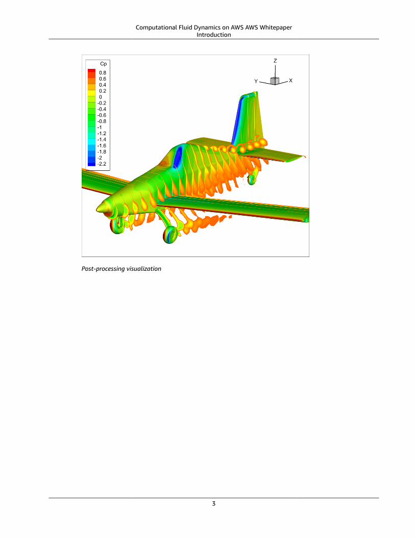
• Post process through visualization — Examples of this step include the creation of images, video, andpost processing of flow fields, such as creating total forces and moments. Similar to the geometry andmesh steps, this can be graphics and memory intensive, and graphics processing units (GPUs) are oftenfavored.

2

Computational Fluid Dynamics on AWS AWS WhitepaperIntroduction

Post-processing visualization

3

Computational Fluid Dynamics on AWS AWS Whitepaper

Are you Well-Architected?The AWS Well-Architected Framework helps you understand the pros and cons of the decisions you makewhen building systems in the cloud. The six pillars of the Framework allow you to learn architectural bestpractices for designing and operating reliable, secure, efficient, cost-effective, and sustainable systems.Using the AWS Well-Architected Tool, available at no charge in the AWS Management Console, you canreview your workloads against these best practices by answering a set of questions for each pillar.

For more expert guidance and best practices for your cloud architecture—reference architecturedeployments, diagrams, and whitepapers—refer to the AWS Architecture Center.

4

Computational Fluid Dynamics on AWS AWS Whitepaper

Why CFD on AWS?AWS is a great place to run CFD cases. CFD workloads are typically tightly coupled workloads using aMessage Passing Interface (MPI) implementation and relying on a large number of cores across manynodes. Many of the AWS instance types, such as the compute family instance types, are designed toinclude support for this type of workload. AWS has network options that support extreme scalability andshort turn-around time as necessary.

CFD workloads typically scale well on the cloud. Most codes rely on domain decomposition to distributeportions of the calculation to the compute nodes. A case can be run highly parallel to receive resultsin minutes. Additionally, large numbers of cases can run simultaneously as efficiently and cheaply aspossible to allow the timely completion of all cases.

The cloud offers a quick way to deploy and turn around CFD workloads at any scale without the needto own your own infrastructure. You can run jobs that once were in the realm of national labs or largeindustry. In just an hour or two, you can deploy CFD software, upload input files, launch compute nodes,and complete jobs on a large number of cores. When your job completes, results can be visualized anddownloaded, and then all resources can be ended – so you only pay for what you use. If preferred, yourresults can be securely archived on AWS using a storage service, such as Amazon Simple Storage Service(Amazon S3). Due to cloud scalability, you have the option to run multiple cases simultaneously with adedicated cluster for each case.

The cloud accommodates the variable demand of CFD. Often, there is a need to run a large number ofcases as quickly as possible. Situations can require a sudden burst of tens, hundreds, or thousands ofcalculations immediately, and then perhaps no runs until the next cycle. The need to run a large numberof cases could be for a preliminary design review, or perhaps a sweep of cases for the creation of asolution database. On the cloud, the cost is the same to run many jobs simultaneously, in parallel, as itis to run them serially, so you can get your data more quickly and at no extra cost. The cost savings inengineering time is an often-forgotten part of cost analysis. Running in parallel can be an ideal solutionfor design optimization.

Cloud computing is a strong choice for other CFD steps. You can easily change the underlying hardwareconfiguration to handle the geometry, meshing, and post-processing. With remote visualization softwareavailable to handle the display, you can manage the GPU instance running your post-processingvisualization from any screen (laptop, desktop, web browser) as though you were working on a largeworkstation.

5

Computational Fluid Dynamics on AWS AWS Whitepaper

Getting started with AWSTo begin, you must create an AWS account and an AWS Identity and Access Management (IAM) user.An IAM user is a user within your AWS account. The IAM user allows authentication and authorizationto AWS resources. Multiple IAM users can be created if multiple people need access to the same AWSaccount.

During the first year after account activation, many AWS services are available for free with the AWS FreeTier. The free-tier program provides an opportunity to learn about AWS without incurring significantcharges. It provides an offset to charges incurred while training on AWS. However, the compute-heavynature of CFD means that charges are regularly not covered by the free tier. Training helps limit mistakesresulting in unnecessary charges. You can also set up AWS billing alarms to alert you of estimatedcharges.

After creating an AWS account, you are provided with what is referred to as your root user. It isrecommended that you do not use this root user for anything other than billing. Instead, set upprivileged users (through IAM) for day-to-day usage of AWS. IAM users are useful because they help yousecurely control access to AWS resources within your account. Use IAM to control authentication andauthorization for resources. Create IAM users for everyone, including yourself, and preserve the root userfor the required account and service management tasks.

By default, your account is limited on the number of instances that you can launch in a Region, whichis a physical location around the world where AWS clusters data centers. These limits are initially setlow to prevent unnecessary charges, but you can raise them to preferred values. CFD applications oftenrequire a large number of compute instances simultaneously. The ability and advantages of scalinghorizontally are highly desirable for high performance computing (HPC) workloads. However, you mayneed to request an increase to the Amazon EC2 service limits before deploying a large workload to eitherone large cluster, or too many smaller clusters at once.

If you want to understand more about the underlying services, a few foundational tutorials can behelpful to get started on AWS:

• Amazon EC2 is the Amazon Web Service you use to create and run compute nodes in the cloud. AWScalls these compute nodes “instances”. This Launch a Linux Virtual Machine with Amazon Lightsailtutorial will help you successfully launch a Linux compute node on Amazon EC2 within our AWS FreeTier.

• Amazon S3 is a service that enables you to store your data (referred to as objects) at massive scale.This Store and Retrieve a File with Amazon S3 tutorial will help you store your files in the cloud usingAmazon S3 by creating an Amazon S3 bucket, uploading a file, retrieving the file, and deleting the file.

• AWS Command Line Interface (AWS CLI) is a common programmatic tool for automating AWSresources. For example, you can use it to deploy AWS infrastructure or manage data in S3. In this AWSCommand Line Interface tutorial, you learn how to use the AWS CLI to access Amazon S3. You can theneasily build your own scripts for moving your files to the cloud and easily retrieving them as needed.

• AWS Budgets gives you the ability to set custom budgets that alert you when your costs or usageexceed (or are forecasted to exceed) your budgeted amount. In the Control your AWS costs with theAWS Free Tier and AWS Budgets tutorial, you learn how to control your costs while exploring AWSservice offerings using the AWS Free Tier, then using AWS Budgets to set up a cost budget to monitorany costs associated with your usage.

A dedicated Running CFD on AWS workshop has been created to guide you through the process ofrunning your CFD codes on AWS. This workshop has step-by-step instructions for common codes likeSimcenter STAR-CCM+, OpenFOAM, and ANSYS Fluent.

6

Computational Fluid Dynamics on AWS AWS Whitepaper

Additionally, the AWS Well-Architected Framework High Performance Computing (HPC) Lens coverscommon HPC scenarios and identifies key elements to ensure that your workloads are architectedaccording to best practices. It focuses on how to design, deploy, and architect your HPC workloads on theAWS Cloud.

7

Computational Fluid Dynamics on AWS AWS WhitepaperArchitectures

CFD approaches on AWSMost CFD solvers have locality of data and use sparse matrix solvers. Once properly organized(application dependent), a well-configured job exhibits good strong and weak scaling on simple AWScluster architectures. “Structured” and “Unstructured” codes are commonly run on AWS. Spectral andpseudo-spectral methods involve fast Fourier transforms (FFTs), and while less common than traditionalCFD algorithms, they also scale well on AWS. Your architectural decisions have tradeoffs, and AWS makesit quick and easy to try different architectures to optimize for cost and performance.

ArchitecturesThere are two primary design patterns to consider when choosing an AWS architecture for CFDapplications: the traditional cluster and the cloud native cluster. Customers choose their preferredarchitecture based on the use case and the CFD users’ needs. For example, use cases that requirefrequent involvement and monitoring, such as when you need to start and stop the CFD case severaltimes on the way to convergence, often prefer a traditional style cluster.

Conversely, cases that are easily automated often prefer a cloud native setup, which enables you to easilysubmit large numbers of cases simultaneously or automate your run for a complete end-to-end solution.Cloud native is useful when cases require special pre- or post-processing steps which benefit fromautomation. Whether choosing traditional or cloud native architectures, the cloud offers the advantageof elastic scalability — enabling you to only consume and pay for resources when you need them.

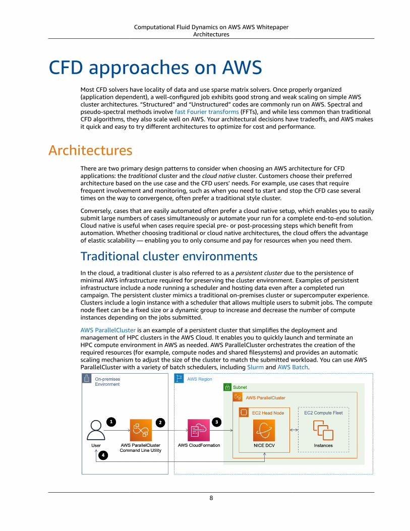
Traditional cluster environmentsIn the cloud, a traditional cluster is also referred to as a persistent cluster due to the persistence ofminimal AWS infrastructure required for preserving the cluster environment. Examples of persistentinfrastructure include a node running a scheduler and hosting data even after a completed runcampaign. The persistent cluster mimics a traditional on-premises cluster or supercomputer experience.Clusters include a login instance with a scheduler that allows multiple users to submit jobs. The computenode fleet can be a fixed size or a dynamic group to increase and decrease the number of computeinstances depending on the jobs submitted.

AWS ParallelCluster is an example of a persistent cluster that simplifies the deployment andmanagement of HPC clusters in the AWS Cloud. It enables you to quickly launch and terminate anHPC compute environment in AWS as needed. AWS ParallelCluster orchestrates the creation of therequired resources (for example, compute nodes and shared filesystems) and provides an automaticscaling mechanism to adjust the size of the cluster to match the submitted workload. You can use AWSParallelCluster with a variety of batch schedulers, including Slurm and AWS Batch.

8

Computational Fluid Dynamics on AWS AWS WhitepaperCloud native environments

Example AWS ParallelCluster architecture

An AWS ParallelCluster architecture enables the following workflow:

• Creating a desired configuration through a text file• Launching a cluster through the AWS ParallelCluster Command Line Utility (CLI)• Orchestrating AWS services automatically through AWS CloudFormation• Accessing the cluster through the command line with Secure Shell Protocol (SSH) or graphically with

NICE DCV

Cloud native environmentsA cloud native cluster is also called an ephemeral cluster due to its relatively short lifetime. A cloudnative approach to tightly coupled HPC ties each run, or sweep of runs, to its own cluster. For eachcase, resources are provisioned and launched, data is placed on the instances, jobs run across multipleinstances, and case output is retrieved automatically or sent to Amazon S3. Upon job completion, theinfrastructure is ended. Clusters designed this way are ephemeral, treat infrastructure as code, and allowfor complete version control of infrastructure changes. Login nodes and job schedulers are less criticaland often not used at all with an ephemeral cluster. The following are a few frequently used methods toimplement such a design:

• Scripted approach — A common quick-start approach for CFD users getting started with AWS is tocombine a custom Amazon Machine Image (AMI) with the AWS CLI and a bash script. After launchingan Amazon EC2 instance, software can be added to the instance and an AMI is created to be usedas the starting point for all compute nodes. It is typical to set up the SSH files and the .bashrc filebefore creating the custom AMI or “golden image.” Although many CFD solvers do not require a sharedfile location, one can easily be created with an exported network file system (NFS) volume, or withAmazon FSx for Lustre, an AWS managed Lustre file system.

• API based — If preferred, an automated deployment can be developed with one of the SoftwareDevelopment Kits (SDKs), such as Python, available for programming an end-to-end solution.

• CloudFormation templates — AWS CloudFormation is an AWS Cloud native approach to provisioningAWS resources based on a JSON or YAML template. AWS CloudFormation offers an easily version-controlled cluster provisioning capability.

• AWS Batch — AWS Batch is a cloud-native, container-based approach that enables CFD users toefficiently run hundreds of thousands of batch computing jobs in containers on AWS. AWS Batchdynamically provisions the optimal quantity and type of compute resources (for example, compute ormemory-optimized instances) based on the volume and specific resource requirements of the batchjobs submitted.

With AWS Batch, there is no need to install and manage batch computing software or serverinfrastructure that you use to run your jobs — enabling you to focus on analyzing results and solvingproblems. AWS Batch plans, schedules, and runs your batch computing workloads across the full rangeof AWS compute services and features, such as Amazon EC2 and Spot Instances. AWS Batch can alsobe used as a job scheduler with AWS ParallelCluster.

SoftwareInstallationCFD software can either be installed into a base AMI, or it can be used from prebuilt AMIs from the AWSMarketplace. If installing into a base AMI, a custom AMI can be created to launch new instances with the

9

Computational Fluid Dynamics on AWS AWS WhitepaperLicensing

software already installed. The AWS Marketplace offers a listing of software from individual softwarevendors, which offer software included with AWS services. Finally, you can also add the installation to thecluster deployment scripts and run them at cluster creation.

LicensingMany commercial CFD solvers are licensed and may require access to a license server, such as FlexNetPublisher. Licensing software in the cloud is much like licensing with any other cluster. If a license serveris necessary, you can configure your networking to use an existing on-premises server, or you can hostthe license server on the cloud.

If hosting the license server on AWS, burstable general-purpose T instances in small sizes, such as micro,can be used for cost-effective hosting. A Reserved Instance purchase for the license server providesfurther cost savings.

The FlexNet Publisher license relies on the network interface’s MAC address. The easiest way to retrievethe new MAC address for your license is to launch the instance and retrieve the MAC address before thelicense is issued. You can preserve the MAC address by changing the ending behavior to prevent deletionof the network interface if the instance is ever terminated. When hosting your own license server,confirm that the security group for the license-server instance allows connectivity on the appropriateports required by the software package.

If accessing an on-premises license server, create an AWS Site-to-Site VPN for your Virtual Private Cloud(VPC), or alternatively, if on-premises firewalls allow, you may be able to access the on-premises licenseserver through SSH tunneling.

Cloud-friendly licensing through power-on-demand licensing keys is also growing in popularity and relieson submitting a job with a key provided by the software provider.

SetupThere are multiple strategies for setting up software in clusters. The most widely used examples arebelow:

Create a custom AMIThis method features the shortest application startup time and avoids potential bottlenecks whenaccessing a single shared resource. This is the preferred means of distribution for large-scale runs (tens ofthousands of MPI ranks) or applications that must load a large number of shared libraries. A drawback isthe larger AMI size, which incurs more cost for Amazon Elastic Block Store (Amazon EBS).

Share an Amazon EBS volume via NFSThis method installs the necessary software into a single Amazon EBS volume, creates an NFS exporton a single instance, and mounts the NFS share on all of the compute instances. This approach reducesthe Amazon EBS footprint because only one Amazon EBS volume must be created for the software. Thismethod is useful for large software packages and moderate scale runs (up to thousands of MPI ranks).

To optimize input/output (I/O) performance, different EBS volume types are available offering differentperformance characteristics. A tradeoff with this method is a small amount of added network traffic anda potential bottleneck with a single instance hosting the NFS share. Ensuring a larger NFS host instancewith additional network capabilities mitigates these concerns.

To make this approach repeatable, the exported NFS directory can be decoupled from the root volume,stored on a separate Amazon EBS volume, and created from an Amazon EBS snapshot. This approach is

10

Computational Fluid Dynamics on AWS AWS WhitepaperMaintenance

similar to the custom AMI method, but instead it isolates software from the root volume. An additionalAmazon EBS volume is created from an Amazon EBS snapshot at instance launch and is mounted as anadditional disk to the compute instance. The snapshot used to create the volume contains the softwareinstallation. Decoupling the user software from operating system updates that are necessary on the rootvolume reduces the complexity of maintenance. Furthermore, the user can rely on the latest AMI releasesfor the compute instances, which provide an up-to-date system without maintaining a custom AMI.

Use a managed shared file systemThis approach installs the CFD software into an AWS managed file system service, such as Amazon FSxfor Lustre or Amazon Elastic File System (Amazon EFS), and mounts the shared file system on all of thecompute instances. Amazon FSx for Lustre provides a high-performance, parallel file system optimizedfor HPC workloads. Lustre is optimized for simultaneous access, and its performance can be scaledindependently from any single instance size.

FSx for Lustre works natively with Amazon S3 and can be automatically populated with data residingin S3, which enables users to have a Lustre file system running only while compute jobs are active andeasily discard it afterwards.

Amazon EFS provides a simple, scalable, fully managed elastic NFS file system that can be used as alocation for home directories. However, EFS is not recommended for other aspects of a CFD cluster, suchas hosting simulation data or compiling a solver, due to performance considerations.

MaintenanceNew feature releases and patches to existing software are a frequent need in the CFD applicationworkflow. All distribution strategies can be fully automated. When using the AMI or Amazon EBSsnapshot strategy, the software update cycle can be isolated from the application runs. Once a newAMI or snapshot has been created and tested, the cluster is reconfigured to pick up the latest version.Software updates cycles in the strategies using file sharing via NFS or FSx for Lustre must be coordinatedwith application runs because a live system is being altered.

In general, automating CFD application installation with scripting tools is recommended and isusually referred to as a Continuous Integration/Continuous Deployment (CI/CD) pipeline on AWS. Theautomation process reduces the manual processes required to build and deploy new software andsecurity patches to HPC systems. This is useful if you want to use the latest features in software packageswith fast update cycles. You can read more about CI/CD pipelines in the AWS Continuous Deliverydocumentation.

Cluster lifecycleAWS offers a variety of unique ways to design architectures that deploy HPC workloads. Your choice ofdeployment method for a particular workload depends on a number of factors, including your desireduser experience, degree of automation, experience with AWS, preferred scripting languages, size andnumber of cases, and the lifecycle of your data. The High Performance Computing Lens whitepapercovers additional best practices for architectures beyond what is discussed in this paper.

While the architecture for a cluster is typically unique and tailored for the workload, all HPC clustersbenefit from lifecycle planning and management of the cluster and the data produced — allowing foroptimized performance, reliability, and cost.

It is not unusual for an on-premises cluster to run for many years, perhaps without significant operatingsystem (OS) update or modification, until the hardware is obsolete thus rendering it useless. In contrast,AWS regularly releases new services and updates to improve performance and lower costs. The easiest

11

Computational Fluid Dynamics on AWS AWS WhitepaperCFD case scalability

way to take advantage of new AWS capabilities, such as new instances, is by maintaining the cluster asa script or template. AWS refers to this as “Infrastructure as Code” because it allows for the creation ofclusters quickly, provides repeatable automation, and maintains reliable version control.

Examples of “cluster as code” are the AWS ParallelCluster configuration file, deployment scripts, orCloudFormation templates. These text-based configurations are easy to modify for a new capability orworkload.

A view of the cluster lifecycle includes infrastructure as code that starts before the cluster is deployedwith the maintenance of the deployment scripts. Elements of a cluster maintained as code include:

• Base AMI to build your cluster

• Automated software installation scripts

• Configuration files, such as scheduler configs, MPI configurations, and .bashrc

• Text description of the infrastructure, such as a CloudFormation template, or an AWS ParallelClusterconfiguration file

• Script to initiate cluster deployment and subsequent software installation

While the nature of a cluster changes depending on the type of workload, the most cost-effectiveclusters are those that are deployed only when they are actively being used.

The cluster lifecycle can have a significant impact on costs. For example, it is common with manytraditional on-premises clusters to maintain a large storage volume. This is not necessary in the cloudbecause data can be easily moved to S3 where it is reliably and cheaply stored. Maintaining a cluster ascode allows you to place a cluster under version control and repeatedly deploy replicas if needed.

Each cluster maintained as code can be instantiated multiple times if multiple clusters are required fortesting, onboarding new users, or running a large number of cases in parallel. If set up correctly, youavoid idle infrastructure when jobs are not running.

CFD case scalabilityCFD cases that cross multiple nodes raise the question, “How will my application scale on AWS?”CFD solvers depend heavily on the solver algorithm’s ability to scale compute tasks efficiently inparallel across multiple compute resources. Parallel performance is often evaluated by determining anapplication’s scale-up. Scale-up is a function of the number of processors used and is defined as the timeit takes to complete a run on one processor, divided by the time it takes to complete the same run on thenumber of processors used for the parallel run.

Scale-up equation

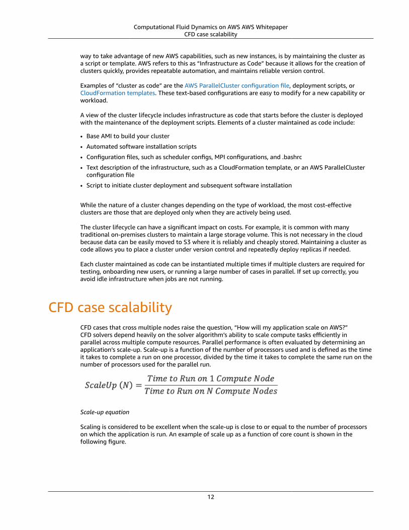
Scaling is considered to be excellent when the scale-up is close to or equal to the number of processorson which the application is run. An example of scale up as a function of core count is shown in thefollowing figure.

12

Computational Fluid Dynamics on AWS AWS WhitepaperStrong scaling vs. weak scaling

Strong scaling demonstrated for a 14M cell external aerodynamics use case

The example case in preceding figure is a 14 million cell external aerodynamics calculation using a cell-centered unstructured solver. The mesh is composed largely of hexahedra. The black line shows the idealor perfect scalability. The blue diamond-based curve shows the actual scale-up for this case as a functionof increasing processor count. Excellent scaling is seen to almost 1000 cores for this small-sized case.This example was run on Amazon EC2 c5n.18xlarge instances, with Elastic Fabric Adapter (EFA), andusing a fully loaded compute node.

Fourteen million cells is a relatively small CFD case by today’s standards. A small case was purposelychosen for the discussion on scalability because small cases are more difficult to scale. The idea thatsmall cases are harder than large cases to scale may seem counter intuitive, but smaller cases have lesstotal compute to spread over a large number of cores. An understanding of strong scaling vs. weakscaling offers more insight.

Strong scaling vs. weak scalingCase scalability can be characterized two ways: strong scaling or weak scaling. Weak does not meaninadequate — it is a technical term facilitating the description of the type of scaling.

Strong scaling, as demonstrated in the following figure, is a traditional view of scaling, where aproblem size is fixed and spread over an increasing number of processors. As more processors are addedto the calculation, good strong scaling means that the time to complete the calculation decreasesproportionally with increasing processor count.

In comparison, weak scaling does not fix the problem size used in the evaluation, but purposely increasesthe problem size as the number of processors also increases. The ratio of the problem size to the number

13

Computational Fluid Dynamics on AWS AWS WhitepaperRunning efficiency

of processors on which the case is run is constant. For a CFD calculation, problem size most often refersto the number of cells or nodes in the mesh for a similar configuration.

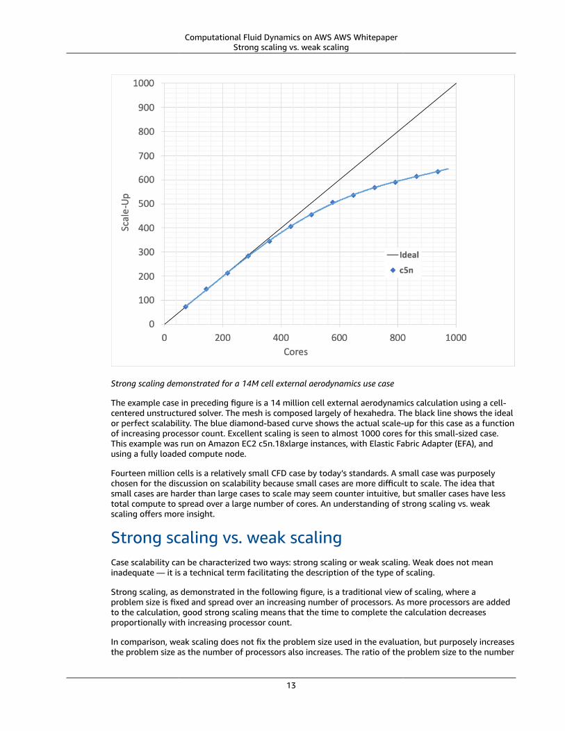
An application demonstrates good weak scaling when the time to complete the calculation remainsconstant as the ratio of compute effort to the number of processors is held constant. Weak scalingoffers insight into how an application behaves with varying case size. Well-written CFD solvers offerexcellent weak scaling capability allowing for more cores to be used when running bigger applications.The scalability of CFD cases can then be determined by looking at a normalized plot of scale-up based onthe number of mesh cells per core (cells/core). An example plot is shown in the following figure.

Scale-up and efficiency as a function of cells per processor

Running efficiencyEfficiency is defined as the scale-up divided by the number of processors used in the calculation. Scale-up and efficiency as a function of cells/core is shown in the preceding figure. In this figure, the cells percore are on the horizontal axis. The blue diamond-based line shows scale-up as a function of mesh cellsper processor. The vertical axis for scale-up is on the left-hand side of the graph as indicated by thelower blue arrow. The orange circle-based line shows efficiency as a function of mesh cells per core. Thevertical axis for efficiency is shown on the right side of the graph and is indicated by the upper orangearrow.

Running efficiency and scale-up equation

14

Computational Fluid Dynamics on AWS AWS WhitepaperTurn-around time and cost

For similar case types, running with similar solver settings, a plot like the one in this figure can help youchoose the desired efficiency and number of cores running for a given case.

Efficiency remains at about 100% between approximately 200,000 mesh cells per core and 100,000mesh cells per core. Efficiency starts to fall off at about 50,000 mesh cells per core. An efficiency ofat least 80% is maintained until 20,000 mesh cells per core, for this case. Decreasing mesh cells percore leads to decreased efficiency because the total computational effort per core is reduced. Theinefficiencies that show up at higher core counts come from a variety of sources and are caused by“serial” work. Serial work is the work that cannot be effectively parallelized. Serial work comes fromsolver inefficiencies, I/O inefficiencies, unequal domain decomposition, additional physical modelingsuch as radiative effects, additional user-defined functions, and eventually, from the network as corecount continues to increase.

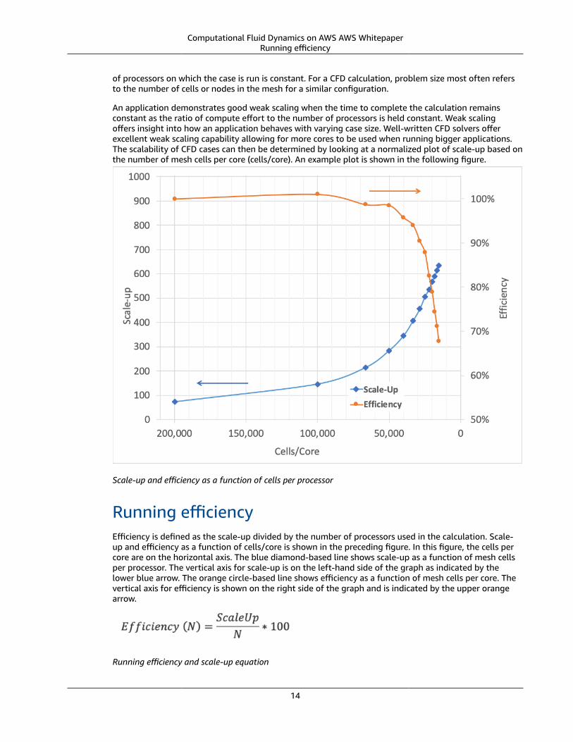
Turn-around time and costPlots of scale-up and efficiency offer an understanding about how a case or application scales. However,what matters most HPC users is case turn-around time and cost. A plot of turn-around time versus CPUcost for this case is shown in the following figure. As the number of cores increases, the inefficiency alsoincreases, which leads to increased costs.

Cost for per run based on on-demand pricing for the c5n.18xlarge instance as a function of turn-aroundtime

In the preceding figure, the turn-around time is shown on the horizontal axis. The cost is shown on thevertical axis. The price is based on the “on-demand” price of a c5n.18xlarge for 1000 iterations, andonly includes the computational costs. Small costs are also incurred for data storage. Minimum cost wasobtained at approximately 50,000 cells per core or more. As the efficiency is 100% over a range of core

15

Computational Fluid Dynamics on AWS AWS WhitepaperTurn-around time and cost

counts, the price is the same regardless of the number of cores. Many users choose a cell count per coreto achieve the lowest possible cost.

As core count goes up, inefficiencies start to show up, but turn-around time continues to drop. When afast turn-around is needed, users may choose a large number of cores to accelerate the time to solution.For this case, a turn-around time of about five minutes can be obtained by running on about 20,000cells per core. When considering total cost, the inclusion of license costs may make the fastest run thecheapest run.

16

Computational Fluid Dynamics on AWS AWS WhitepaperCompute

Optimizing HPC componentsThe AWS Cloud provides a broad range of scalable, flexible infrastructure services that you select tomatch your workloads and tasks. This gives you the ability to choose the most appropriate mix ofresources for your specific applications. Cloud computing makes it easy to experiment with infrastructurecomponents and architecture design. The HPC solution components listed below are a great startingpoint to set up and manage your HPC cluster. Always test various solution configurations to find the bestperformance at the lowest cost.

ComputeThe optimal compute solution for a particular HPC architecture depends on the workload deploymentmethod, degree of automation, usage patterns, and configuration. Different compute solutions may bechosen for each step of a process. Selecting the appropriate compute solution for an architecture canlead to higher performance efficiency and lower cost.

There are multiple compute options available on AWS, and at a high level, they are separated into threecategories: instances, containers, and functions. Amazon EC2 instances, or servers, are resizable computecapacity in the cloud. Containers provide operating system virtualization for applications that sharean underlying operating system installed on a server. Functions are a serverless computing model thatallows you to run code without thinking about provisioning and managing the underlying servers. ForCFD workloads, EC2 instances are the primary compute choice.

Amazon EC2 lets you choose from a variety of compute instance types that can be configured tosuit your needs. Instances come in different families and sizes to offer a wide variety of capabilities.Some instance families target specific workloads, for example, compute-, memory-, or GPU-intensiveworkloads, while others are general purpose. Both the targeted-workload and general-purpose instancefamilies are useful for CFD applications based on the step in the CFD process.

When considering CFD steps, different instance types can be targeted for pre-processing, solving, andpost-processing. In pre-processing, the geometry step can benefit from an instance with a GPU, while themesh generation stage may require a higher memory-to-core ratio, such as general-purpose or memory-optimized instances. When solving CFD cases, evaluate your case size and cluster size.

If the case is spread across multiple instances, the memory requirements are low per core, and compute-optimized instances are recommended as the most cost-effective and performant choice. If a single-instance calculation is desired, it may require more memory per core and benefit from a general-purpose,or memory-optimized instance.

Optimal performance is typically obtained with compute-optimized instances (Intel, AMD, or Graviton),and when using multiple instances with cells per core below 100,000, instances with higher networkthroughput and packet rate performance are preferred. Refer to the Instance Type Matrix for instancedetails.

AWS enables simultaneous multithreading (SMT), or hyper-threading technology for Intel processors,commonly referred to as “hyperthreading” by default for supported processors. Hyperthreadingimproves performance for some systems by allowing multiple threads to be run simultaneously on asingle core. Most CFD applications do not benefit from hyperthreading, and therefore, disabling it tendsto be the preferred environment. Hyperthreading is easily disabled in Amazon EC2. Unless an applicationhas been tested with hyperthreading enabled, it is recommended that hyperthreading be disabled andthat processes are launched and pinned to individual cores.

There are many compute options available to optimize your compute environment. Cloud deploymentallows for experimentation on every level from operating system to instance type to bare-metal

17

Computational Fluid Dynamics on AWS AWS WhitepaperNetwork

deployments. Time spent experimenting with cloud-based clusters is vital to achieving the desiredperformance.

NetworkMost CFD workloads exceed the capacity of a single compute node and require a cluster-based solution.A crucial factor in achieving application performance with a multi-node cluster is optimizing theperformance of the network connecting the compute nodes.

Launching instances within a cluster placement group provides consistent, low latency within a cluster.Instances launched within a cluster placement group are also launched to the same Availability Zone.

To further improve the network performance between EC2 instances, you can use an Elastic FabricAdapter (EFA) on select instance types. EFA is designed for tightly coupled HPC workloads by providingan operating system (OS)-bypass capability and hardware-designed reliability to take advantage of theEC2 network. It works well with CFD solvers. OS-bypass is an access model that allows an applicationto bypass the operating system’s TCP/IP stack and communicate directly with the network device. Thisprovides lower and more consistent latency and higher throughput than the TCP transport traditionallyused. When using EFA, your normal IP traffic remains routable and can communicate with other networkresources.

CFD applications use EFA through a message passing interface (MPI) implementation using the LibfabricAPI. EFA usage can be confirmed with the MPI runtime debugging output. Each MPI implementationhas environment variables or command-line flags for verbose debugging output or explicitly settingthe fabric provider. These options vary by MPI implementation, and access to these options vary by CFDapplication. Refer to Getting Started with EFA and MPI documentation for additional details.

StorageAWS provides many storage options for CFD, including object storage with Amazon S3, block storagewith Amazon EBS, temporary block-level storage with Amazon EC2 instance store, and file storage withAmazon FSx for Lustre. You can utilize all these storage types for certain aspects of your CFD workload.

A vital part of working with CFD solvers on AWS is the management of case data, which includesfiles such as CAD, meshes, input files, and output figures. In general, all CFD users want to maintainavailability of the data when it is in use and to archive a subset of the data if it’s needed at some point inthe future.

An efficient data lifecycle uses a combination of storage types and tiers to minimize costs. Data isdescribed as hot, warm, and cold, depending on the immediate need of the data.

• Hot data is data that you need immediately, such as a case or sweep of cases about to be deployed.• Warm data is your data, which is not needed at the moment, but it may be used sometime in the near

future; perhaps within the next six months.• Cold data is data that may not ever be used again, but it is stored for archival purposes.

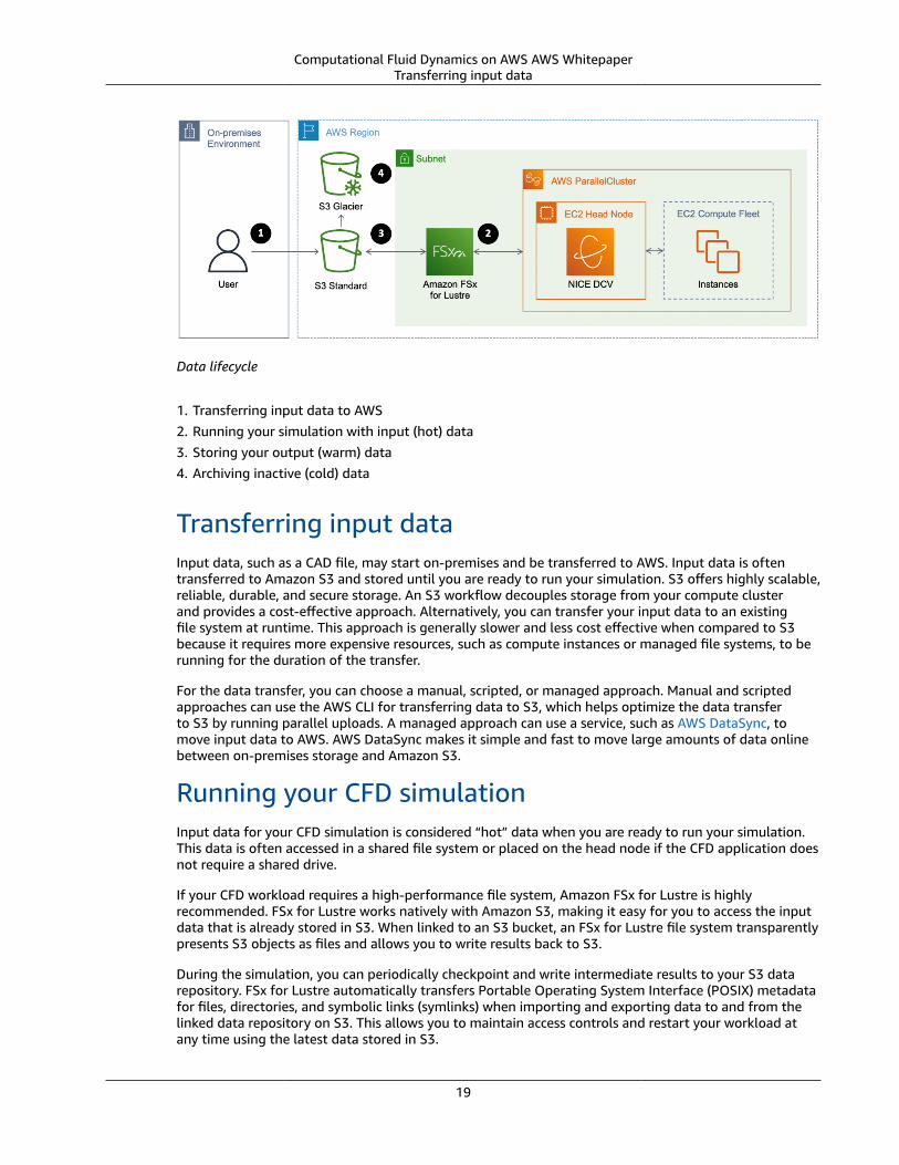
Your data lifecycle can occur only within AWS, or it can be combined with an on-premises workflow. Forexample, you may move case data, such as a case file, from your local computing facilities, to AmazonS3, and then to an EC2 cluster. Completed runs can traverse the same path in reverse back to your on-premises environment or to Amazon S3 where they can remain in the S3 Standard or S3 InfrequentAccess storage class, or transitioned to Amazon S3 Glacier through a lifecycle rule for archiving. AmazonS3 Glacier and S3 Glacier Deep Archive are S3 storage tiers that offer deep discounts on storage forarchival data. The following figure is an example data lifecycle for CFD.

18

Computational Fluid Dynamics on AWS AWS WhitepaperTransferring input data

Data lifecycle

1. Transferring input data to AWS2. Running your simulation with input (hot) data3. Storing your output (warm) data4. Archiving inactive (cold) data

Transferring input dataInput data, such as a CAD file, may start on-premises and be transferred to AWS. Input data is oftentransferred to Amazon S3 and stored until you are ready to run your simulation. S3 offers highly scalable,reliable, durable, and secure storage. An S3 workflow decouples storage from your compute clusterand provides a cost-effective approach. Alternatively, you can transfer your input data to an existingfile system at runtime. This approach is generally slower and less cost effective when compared to S3because it requires more expensive resources, such as compute instances or managed file systems, to berunning for the duration of the transfer.

For the data transfer, you can choose a manual, scripted, or managed approach. Manual and scriptedapproaches can use the AWS CLI for transferring data to S3, which helps optimize the data transferto S3 by running parallel uploads. A managed approach can use a service, such as AWS DataSync, tomove input data to AWS. AWS DataSync makes it simple and fast to move large amounts of data onlinebetween on-premises storage and Amazon S3.

Running your CFD simulationInput data for your CFD simulation is considered “hot” data when you are ready to run your simulation.This data is often accessed in a shared file system or placed on the head node if the CFD application doesnot require a shared drive.

If your CFD workload requires a high-performance file system, Amazon FSx for Lustre is highlyrecommended. FSx for Lustre works natively with Amazon S3, making it easy for you to access the inputdata that is already stored in S3. When linked to an S3 bucket, an FSx for Lustre file system transparentlypresents S3 objects as files and allows you to write results back to S3.

During the simulation, you can periodically checkpoint and write intermediate results to your S3 datarepository. FSx for Lustre automatically transfers Portable Operating System Interface (POSIX) metadatafor files, directories, and symbolic links (symlinks) when importing and exporting data to and from thelinked data repository on S3. This allows you to maintain access controls and restart your workload atany time using the latest data stored in S3.

19

Computational Fluid Dynamics on AWS AWS WhitepaperStoring output data

When your workload is done, you can write final results from your file system to your S3 data repositoryand delete your file system.

Storing output dataOutput data from your simulation is considered “warm” data after the simulation finishes. For a cost-effective workflow, transfer the output data off of your cluster and terminate the more expensivecompute and storage resources. If you stored your data in an Amazon EBS volume, transfer your outputdata to S3 with the AWS CLI. If you used FSx for Lustre, create a data repository task to manage thetransfer of output data and metadata to S3 or export your files with HSM commands. You can alsoperiodically push the output data to S3 with a data repository task.

Archiving inactive dataAfter your output data is stored in S3 and is considered cold or inactive, transition it to a more cost-effective storage class, such as Amazon S3 Glacier and S3 Glacier Deep Archive. These storage classesallow you to archive older data more affordably than with the S3 Standard storage class. Objects inS3 Glacier and S3 Glacier Deep Archive are not available for real-time access and must be restored ifneeded. Restoring objects incurs a cost, and to keep costs low yet suitable for varying needs, S3 Glacierand S3 Glacier Deep Archive provide multiple retrieval options.

Storage summaryUse the following table to select the best storage solution for your workload:

Table 1 — Storage services and their uses

Service Description Use

Amazon EBS Block storage Block storage or export as aNetwork File System (NFS) share

Amazon FSx for Lustre Managed Lustre Fast parallel high-performancefile system optimized for HPCworkloads

Amazon S3 Object storage Store case files, input, andoutput data

Amazon S3 Glacier Archival storage Long-term storage of archivaldata

Amazon EFS Managed NFS Network File System (NFS) toshare files across multipleinstances. Occasionally used forhome directories. Not generallyrecommended for CFD cases.

VisualizationA graphical interface is useful throughout the CFD solution process, from building meshes, debuggingflow-solution errors, and visualizing the flow field. Many CFD solvers include visualization packagesas part of their installation. As an example, ParaView is packaged with OpenFOAM. In addition to

20

Computational Fluid Dynamics on AWS AWS WhitepaperVisualization

visualization tools within the CFD suites, there are third-party visualization tools, which can be morepowerful, adaptable, and general.

Post processing in AWS can reduce manual extractions, lower time to results, and decrease data transfercosts. Visualization is often performed remotely with either an application that supports client-servermode or with remote visualization of the server desktop. Client-server mode works well on AWS and canbe implemented in the same way as other remote desktop set-ups. When using client-server mode foran application, it is important to connect to the server using the public IP address and not the private IPaddress, unless you have private network connectivity configured, such as a Site-to-Site VPN.

AWS offers NICE DCV for local display of remote desktops. NICE DCV is easy to implement and is free touse with EC2. There are a variety of ways to add NICE DCV to your HPC cluster. The simplest approachis to launch AWS ParallelCluster. If you are using AWS ParallelCluster, you can enable NICE DCV onthe head node when launching the cluster with a short addition in the configuration file. A graphics-intensive instance can be easily launched running a Linux or Windows NICE DCV AMI to have NICE DCVpre-installed. Refer to Getting Started with NICE DCV on Amazon EC2 for more information.

AWS also offers managed desktop and application streaming services, such as Amazon WorkSpacesor Amazon AppStream 2.0. Amazon WorkSpaces is a Desktop-as-a-Service solution providing Linux orWindows desktops while Amazon AppStream 2.0 is a non-persistent application and desktop streamingservice for Windows environments.

In general, visualizing CFD results on AWS reduces the need to download large data back to on-premisesstorage, and it helps reduce cost and increase productivity.

21

Computational Fluid Dynamics on AWS AWS Whitepaper

CostsAWS offers a pay-as-you-go approach for pricing for cloud services. You pay only for the individualservices you need, for as long as you use them, without long-term contracts or complex licensing. Someservices and tools incur no charge, such as AWS ParallelCluster, AWS Batch, and AWS CloudFormation;however, the underlying AWS components used to run cases incur charges.

AWS charges arise primarily from the compute resources required for the CFD solution. Storage anddata transfer also incur charges. Depending on your implementation, you may use additional services inyour architecture, such as AWS Lambda, Amazon Simple Notification Service (Amazon SNS), or AmazonCloudWatch, but cost accumulated by usage of these services is rarely significant when compared to thecompute costs for CFD.

It is common to stand up a cluster for only the time period in which it is needed. In a simple scenario,costs are associated with EC2 instances and Amazon EBS volumes. Costs incurred after shut down of thecluster include any snapshots taken of Amazon EBS volumes and any data stored on Amazon S3.

While data transfer into Amazon EC2 from the internet is free, data transfer out of AWS can incurmodest charges. Many users choose to leave their data in S3 and only move the smaller post-processeddata out of AWS. Data can also be transitioned to Amazon S3 Glacier for archival storage to reduce long-term storage costs.

When AWS ParallelCluster is maintained for an extended period of time, the login node and AmazonEBS volumes continue to incur costs. The compute nodes scale up and down as needed, which minimizescosts to only reflect the times when the cluster is being used.

When developing an architecture, you must monitor your workload (automatically through monitoringsolutions or manually through the console) and ensure that your resources scale up and down asexpected. Occasionally, hung jobs or other factors can prevent your resources from scaling properly.Logging on to the compute node and checking processes with a tool, such as top or htop, can help debugissues.

AWS provides four different ways to pay for EC2 instances:

• On-Demand Instances• Reserved Instances• Savings Plans• Spot Instances

Amazon EC2 instance costs can be minimized by using Spot Instances, Savings Plans, and ReservedInstances.

• On-Demand Instances — With On-Demand Instances, you pay for compute capacity by the houror the second, depending on which you run. No long-term commitments or upfront payments areneeded. You can increase or decrease your compute capacity depending on the demands of yourapplication and only pay the specified per-hour rates for the instance you use.

On-Demand Instances are the highest cost model for computing and require no upfront commitment.Cost saving is gained because costs are only incurred while the instances are in a running state. Fora dynamic workload, the savings can be large. Savings occur because you can select the newestprocessor types, which may speed up the computations significantly.

• Reserved Instances — Reserved Instances (RIs) provide you with a significant discount (up to 75%)compared to On-Demand Instance pricing. For customers that have steady state or predictable usage

22

Computational Fluid Dynamics on AWS AWS Whitepaper

and can commit to using EC2 over a 1- or 3-year term, Reserved Instances provide significant savingscompared to using On-Demand Instances.

• Savings Plans — Savings Plans are a flexible pricing model that provides savings of up to 72% on yourAWS compute usage. This pricing model offers lower prices on Amazon EC2 instances usage, regardlessof instance family, size, OS, tenancy or AWS Region, and also applies to AWS Fargate usage.

Savings Plans offer significant savings over On-Demand Instances, just like EC2 Reserved Instances, inexchange for a commitment to use a specific amount of compute power (measured in $/hour) for aone- or three-year period. You can sign up for Savings Plans for a one- or three-year term and easilymanage your plans by taking advantage of recommendations, performance reporting, and budgetalerts in the AWS Cost Explorer.

• Spot Instances — Amazon EC2 Spot Instances let you take advantage of unused EC2 capacity at upto a 90% discount compared to On-Demand prices. However, Spot Instances can be interrupted whenEC2 needs to reclaim the capacity. Spot Instances are frequently the most cost-effective resource forflexible or fault-tolerant workloads and can also be used for CFD cases. Spot availability varies by spotpool (for example, Region, Availability Zone, and instance type). Consider your deployment strategyand interruption impact when determining the most cost-effective resources for your case.

When a Spot Instance is interrupted, your case is interrupted. The interruption impact to your casedepends on how your CFD application handles the interruption, and you can minimize this impact bycheckpointing your simulation if supported. In addition, you can minimize the risk of Spot Instanceinterruption by working with the Spot Advisor, being flexible on instance type and Availability Zone,and using advanced features, such as the capacity-optimized allocation strategy in EC2 Fleet, to launchyour Spot Instances. Overall, the need to occasionally restart a workload can be offset by the costsavings of Spot Instances.

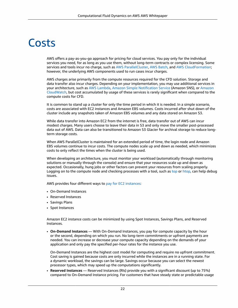
• Combined approach — You can easily combine Spot Instances with On-Demand and RIs to furtheroptimize workload cost with performance. For example, in the following figure, you could useReserved Instances for your daily workloads, Spot Instances for component exploration, and On-Demand Instances for design review.

EC2 cost optimization for CFD cases

23

Computational Fluid Dynamics on AWS AWS Whitepaper

ConclusionThis whitepaper describes best practices for using AWS for computational fluid dynamics (CFD). Thepaper presents the advantages of using AWS for CFD workloads, covers the getting started process,discusses AWS approaches for CFD, and addresses the options for optimizing the HPC components forCFD workloads. Following the best practices presented in this paper allows you to architect and optimizeyour environment for CFD workloads.

24

Computational Fluid Dynamics on AWS AWS Whitepaper

ContributorsThe following individuals and organizations contributed to this document:

• Aaron Bucher, HPC Specialist Solutions Architect, AWS• Scott Eberhardt, Tech Lead for Aerospace, AWS• Lewis Foti, HPC Specialist Solutions Architect, AWS• Linda Hedges, HPC Application Engineer, AWS• Stephen Sachs, HPC Application Engineer, AWS• Anh Tran, HPC Specialist Solutions Architect, AWS• Neil Ashton, CFD Specialist Solutions Architect, AWS

25

Computational Fluid Dynamics on AWS AWS Whitepaper

Further readingFor additional information, refer to:

• CFD Workshop• CFD on AWS• HPC on AWS• AWS Well-Architected Framework• Introduction to HPC on AWS

26

Computational Fluid Dynamics on AWS AWS Whitepaper

Document revisionsTo be notified about updates to this whitepaper, subscribe to the RSS feed.

update-history-change update-history-description update-history-date

Document updated (p. 27) Minor updates. March 24, 2022

Document updated (p. 27) Minor updates. July 1, 2021

Initial publication (p. 27) Whitepaper published. March 1, 2020

27

Computational Fluid Dynamics on AWS AWS Whitepaper

NoticesCustomers are responsible for making their own independent assessment of the information in thisdocument. This document: (a) is for informational purposes only, (b) represents current AWS productofferings and practices, which are subject to change without notice, and (c) does not create anycommitments or assurances from AWS and its affiliates, suppliers or licensors. AWS products or servicesare provided “as is” without warranties, representations, or conditions of any kind, whether express orimplied. The responsibilities and liabilities of AWS to its customers are controlled by AWS agreements,and this document is not part of, nor does it modify, any agreement between AWS and its customers.

© 2022, Amazon Web Services, Inc. or its affiliates. All rights reserved.

28

Computational Fluid Dynamics on AWS AWS Whitepaper

AWS glossaryFor the latest AWS terminology, see the AWS glossary in the AWS General Reference.

29