Abstract—This paper deals with efficient computation of

probability coefficients which offers computational simplicity as compared to spectral coefficients. It eliminates the need of inner product evaluations in determination of signature of a combinational circuit realizing given Boolean function. The method for computation of probability coefficients using transform matrix, fast transform method and using BDD is given. Theoretical relations for achievable computational advantage in terms of required additions in computing all 2n probability coefficients of n variable function have been developed. It is shown that for n ≥ 5, only 50% additions are needed to compute all probability coefficients as compared to spectral coefficients. The fault detection techniques based on spectral signature can be used with probability signature also to offer computational advantage.

Keywords—Binary Decision Diagrams, Spectral Coefficients, Fault detection

I. INTRODUCTION INCE last three decades spectral techniques has been widely adopted in field of VLSI CAD, testing, quantum computing [2, 6, 9, 13, 14, 16] etc. Due to exponential

increase in numbers of transistors in a single chip the problem of synthesizing and testing are becoming more complex. This is necessitating consideration of testing issues right in the design phase rather than post design practice [10, 17] leading to on-chip incorporation of both test hardware and software routines in the design of self-testing, fault tolerant, fail-safe and/or self-repairing digital devices and systems [11, 15]. Spectral techniques of fault detection provide an attractive solution to the problem of testing complex digital circuits by offering global information about the target circuit realizing the function. One of the major drawback of spectral techniques is their computational complexity in calculation of spectral coefficients; making them impractical for testing complex circuits. The phenomenal increase in operating speed of digital devices and systems during 1990s has created resurgence of interest for exploring faster testing techniques to perform time efficient testing. This is more so because even

Ashutosh Kumar Singh is with Department of ECEC, School of

Engineering and Science, Curtin University of Technology, Miri, Sarawak. Malaysia (email: ashutosh.s@ curtin.edu.my)

Anand Mohan is with Department of Electronics Engineering, Institute of Science and Technology, Banaras Hindu University, Varanasi, India (e-mail: amohan@ bhu.ac.in)

fastest available spectral methods using fast transform techniques don’t perform efficiently due to their inherent computational constrains [6, 7].

This paper addresses the problem of computational complexities and describes the efficient method to generate probability coefficient obtained from the output probability [1, 9] of a Boolean function. We use Rademacher-Walsh (R-W) transform for conversion between Boolean to Probability domain as shown in Figure 1.

Fig. 1: Block Diagram for conversation between Boolean to probability domain

We propose three methods to compute these coefficients (1)

Matrix method (2) FFT method (3) BDD method. The value of Probability coefficients varies between (-1) to (+1). Mathematical expression for determination of probability coefficients of a function is developed and theoretical plot illustrating computational advantage offered by probability coefficients is achieved. These coefficients are used to obtain a probability signature using linearisation technique [14, 19] which is then used for fault detection by comparing the probability signatures of the fault free and faulty circuits. A set of rules [14] for selecting spectral coefficients constituting spectral signature have been similarly applied to linearisation technique for obtaining probability signature. Test results obtained using probability signatures are compared with those of spectral signature technique and have been found same; validating the use of probability signature for fault detection applications.

The paper is organized as follows: section 2 includes the basics definition and mathematical background for Binary Decision Diagrams and spectral techniques. Probability coefficient and their computation using different methods definition is discussed in section 3 with basic definitions and theorems. Section 4 describes about the test vector generation for fault detection using linearisation techniques. In section 5 we discuss about the results and their comparison with spectral coefficient’s computation. Finally concluding remarks and future work is given in section 6.

Computation of Probability Coefficients using Binary Decision Diagram and their Application

in Test Vector Generation Ashutosh Kumar Singh, Anand Mohan

S

Boolean Domain (0, 1)

Probability Domain (-1 to +1)

R-W Matrix of order of 2n × 2n

International Journal of Computer Science and Engineering 3:1 2009

33

II. PRELIMINARIES

A. Binary Decision Diagram Binary Decision Diagrams (BDDs) is based on Shannon

expansion [8, 12, 20]: 10'iiii fxfxf += (1)

Where f ∈ Bn be a Boolean function defined over the variable set Xn = {x1, …, xn) for all i = {x1, …, xn). It represents a Boolean functions as a rooted, directed acyclic graph with a vertex set containing two types of vertices, non-terminal and terminal vertices. A non-terminal vertex v has two attributes i.e. (i) an argument index (v) ∈ {x1,….., xn} and (ii) two children indicated by dashed and solid lines for low (v) and high (v) respectively. A terminal vertex v has an attribute value (v) ∈ {0, 1} and has no outgoing edge.

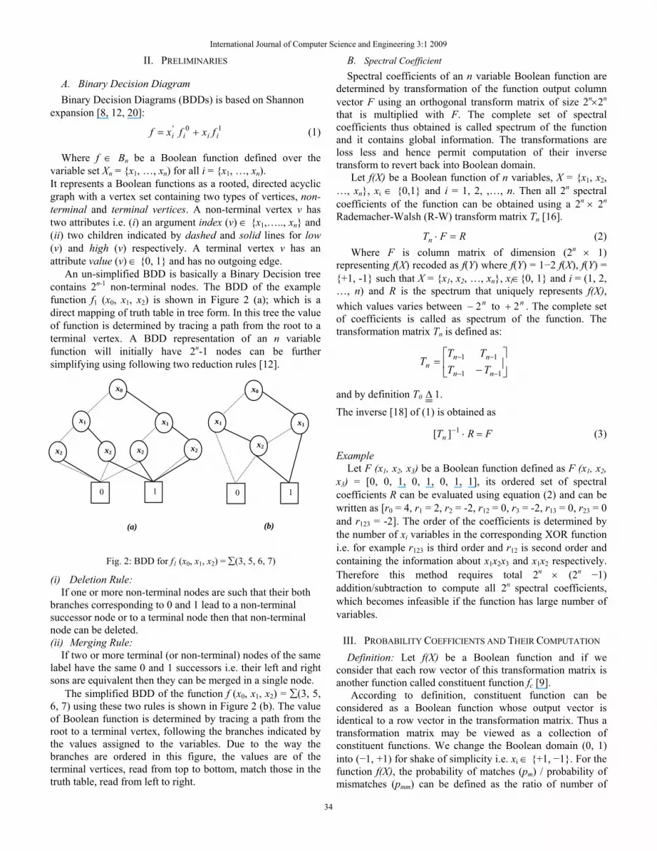
An un-simplified BDD is basically a Binary Decision tree contains 2n-1 non-terminal nodes. The BDD of the example function f1 (x0, x1, x2) is shown in Figure 2 (a); which is a direct mapping of truth table in tree form. In this tree the value of function is determined by tracing a path from the root to a terminal vertex. A BDD representation of an n variable function will initially have 2n-1 nodes can be further simplifying using following two reduction rules [12].

Fig. 2: BDD for f1 (x0, x1, x2) = ∑(3, 5, 6, 7)

(i) Deletion Rule: If one or more non-terminal nodes are such that their both

branches corresponding to 0 and 1 lead to a non-terminal successor node or to a terminal node then that non-terminal node can be deleted. (ii) Merging Rule:

If two or more terminal (or non-terminal) nodes of the same label have the same 0 and 1 successors i.e. their left and right sons are equivalent then they can be merged in a single node.

The simplified BDD of the function f (x0, x1, x2) = ∑(3, 5, 6, 7) using these two rules is shown in Figure 2 (b). The value of Boolean function is determined by tracing a path from the root to a terminal vertex, following the branches indicated by the values assigned to the variables. Due to the way the branches are ordered in this figure, the values are of the terminal vertices, read from top to bottom, match those in the truth table, read from left to right.

B. Spectral Coefficient Spectral coefficients of an n variable Boolean function are

determined by transformation of the function output column vector F using an orthogonal transform matrix of size 2n×2n that is multiplied with F. The complete set of spectral coefficients thus obtained is called spectrum of the function and it contains global information. The transformations are loss less and hence permit computation of their inverse transform to revert back into Boolean domain.

Let f(X) be a Boolean function of n variables, X = {x1, x2, …, xn}, xi ∈ {0,1} and i = 1, 2, ,…, n. Then all 2n spectral coefficients of the function can be obtained using a 2n × 2n Rademacher-Walsh (R-W) transform matrix Tn [16].

RFTn =⋅ (2) Where F is column matrix of dimension (2n × 1)

representing f(X) recoded as f(Y) where f(Y) = 1−2 f(X), f(Y) = {+1, -1} such that X = {x1, x2, …, xn}, xi∈{0, 1} and i = (1, 2, …, n) and R is the spectrum that uniquely represents f(X), which values varies between n2− to n2+ . The complete set of coefficients is called as spectrum of the function. The transformation matrix Tn is defined as:

⎥⎦

⎤⎢⎣

⎡−

=−−

−−

11

11

nn

nnn TT

TTT

and by definition T0 Δ 1.

The inverse [18] of (1) is obtained as

FRTn =⋅−1][ (3)

Example Let F (x1, x2, x3) be a Boolean function defined as F (x1, x2,

x3) = [0, 0, 1, 0, 1, 0, 1, 1], its ordered set of spectral coefficients R can be evaluated using equation (2) and can be written as [r0 = 4, r1 = 2, r2 = -2, r12 = 0, r3 = -2, r13 = 0, r23 = 0 and r123 = -2]. The order of the coefficients is determined by the number of xi variables in the corresponding XOR function i.e. for example r123 is third order and r12 is second order and containing the information about x1x2x3 and x1x2 respectively. Therefore this method requires total 2n × (2n −1) addition/subtraction to compute all 2n spectral coefficients, which becomes infeasible if the function has large number of variables.

III. PROBABILITY COEFFICIENTS AND THEIR COMPUTATION Definition: Let f(X) be a Boolean function and if we

consider that each row vector of this transformation matrix is another function called constituent function fc [9].

According to definition, constituent function can be considered as a Boolean function whose output vector is identical to a row vector in the transformation matrix. Thus a transformation matrix may be viewed as a collection of constituent functions. We change the Boolean domain (0, 1) into (−1, +1) for shake of simplicity i.e. xi ∈ {+1, −1}. For the function f(X), the probability of matches (pm) / probability of mismatches (pmm) can be defined as the ratio of number of

0

x0

x1 x1

x2 x2 x2 x2

1

x1

0

x0

x1

x2

1

(a) (b)

International Journal of Computer Science and Engineering 3:1 2009

34

matches / mismatches between f(X) and fc to 2n. The number of matches “pm(i)” corresponding to any probability coefficient Pi is obtained from bit by bit Ex-NOR between f(X) and the ith constituent function fc(i) of transformation matrix “T” of order 2n × 2n followed by summation.

nc

imfandXfbetweenmatchesofNumberTotal

p2

)()( = (4)

Mathematically this can be expressed as:

∑ ⊕= )(21

)()( Xffp icnim (5)

Similarly the number of mismatches “pmm(i)” corresponding to probability coefficient Pi is obtained from bit by bit Ex-OR between f(X) and fc(i) of transformation matrix “T” followed by summation as:

nc

immfandXfbetweenmismatchesofNumberTotal

p2

)()( = (6)

∑ ⊕= )(21

)( Xff icn (7)

Definition: Probability coefficient of f(X) is the difference between probability of matches and probability of mismatches i.e. (pmi−pmmi).

Theorem: The probability coefficient (Pi) of any Boolean function corresponding to the ith row vector of transformation matrix “T” can be given as:

Pi=2pm(i)-1=1-2pmm(i) , where i=1, 2, …, 2n (8)

Proof: Since the ith probability coefficient of any Boolean function f(X) is defined as the difference between the probability of matches “pm(i)” and mismatches “pmm(i)”, therefore

Pi = pm(i) – pmm(i) = pm(i) – (1– pm(i))=2pm(i) – 1 (9)

Similarly substituting the value of pm(i) in terms of pmm(i) we get

Pi = pm(i) – pmm(i)= (1 – pmm(i)) – pmm(i)= 1 – 2 pmm(i) (10)

From equations (9) & (10) Pi=2pm(i) –1=1 – 2pmm(i) (11)

A. Matrix Method For an “n” variable Boolean function f(X), all the 2n

probability coefficients can be computed using R-W transform matrix of order 2n× 2n

nT ][ # F =P=(2 pm –1)=1–2 pmm (12)

Where F is vector representing the function, P is the set of probability coefficients and “#” denotes either (Ex-NOR) or (Ex-OR) operators but not both simultaneously.

Therefore all the 2n probability coefficients (P) of a given Boolean function f(X) can be determined using equations (5) or (7) and (12). The procedure for finding probability coefficients of an “n” variable Boolean function with output vector “F” of order 2n × 1 can be stated as:

(i) Initialize C (counter) = 0.

(ii) Select first row of the transformation matrix. (iii) Compare the corresponding elements of selected row and

output vector (iv) Increment C by “1” for each match (mismatch) until all in

the row vector have been compared. (v) Calculate probability of matches (mismatches) using pm

(pmm) = C/2n and determine probability coefficients as Pi=2pm(i) – 1=1 – 2pm m(i) for i=1, 2, …, 2n

Using R-W transform for the example function F (x1, x2, x3) and changing Boolean variables “0” and “1” to +1 and –1 respectively, its probability coefficients can be computed. For the first probability coefficient (p0)

5.0]1,1,11,1,1,1,1[]1,1,1,1,1,1,1,1[213

=−−−−⊕= ∑mp

Now using equation (12) we get p0=0 Similarly for second probability coefficient (p1)

25.0]1,1,11,1,1,1,1[]1,1,1,1,1,1,1,1[213

=−−−−⊕−−−−= ∑mp

and equation (12) gives p1=−0.5.

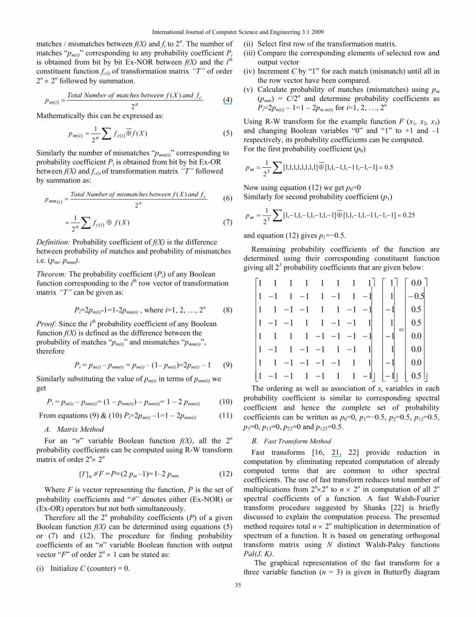
Remaining probability coefficients of the function are determined using their corresponding constituent function giving all 23 probability coefficients that are given below:

⎥⎥⎥⎥⎥⎥⎥⎥⎥⎥⎥

⎦

⎤

⎢⎢⎢⎢⎢⎢⎢⎢⎢⎢⎢

⎣

⎡−

=

⎥⎥⎥⎥⎥⎥⎥⎥⎥⎥⎥

⎦

⎤

⎢⎢⎢⎢⎢⎢⎢⎢⎢⎢⎢

⎣

⎡

−−

−

−

⎥⎥⎥⎥⎥⎥⎥⎥⎥⎥⎥

⎦

⎤

⎢⎢⎢⎢⎢⎢⎢⎢⎢⎢⎢

⎣

⎡

−−−−−−−−

−−−−−−−−

−−−−−−−−−−−−

5.00.00.00.05.05.05.0

0.0

11111111

1111111111111111111111111111111111111111111111111111111111111111

The ordering as well as association of xi variables in each probability coefficient is similar to corresponding spectral coefficient and hence the complete set of probability coefficients can be written as p0=0, p1=−0.5, p2=0.5, p12=0.5, p3=0, p13=0, p23=0 and p123=0.5.

B. Fast Transform Method Fast transforms [16, 21, 22] provide reduction in

computation by eliminating repeated computation of already computed terms that are common to other spectral coefficients. The use of fast transform reduces total number of multiplications from 2n×2n to n × 2n in computation of all 2n spectral coefficients of a function. A fast Walsh-Fourier transform procedure suggested by Shanks [22] is briefly discussed to explain the computation process. The presented method requires total n × 2n multiplication in determination of spectrum of a function. It is based on generating orthogonal transform matrix using N distinct Walsh-Paley functions Pal(J, K).

The graphical representation of the fast transform for a three variable function (n = 3) is given in Butterfly diagram

International Journal of Computer Science and Engineering 3:1 2009

35

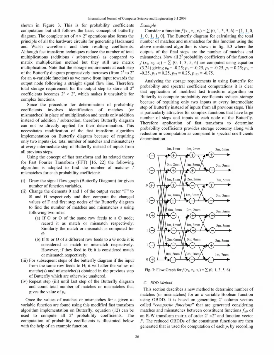
shown in Figure 3. This is for probability coefficients computation but still follows the basic concept of butterfly diagram. The complete set of n × 2n operations also forms the principle of all the hardware circuits for generating Hadamard and Walsh waveforms and their resulting coefficients. Although fast transform techniques reduce the number of total multiplications (additions / subtractions) as compared to matrix multiplication method but they still use matrix multiplication. Note that the storage requirements at each step of the Butterfly diagram progressively increases (from 21 to 2n for an n-variable function) as we move from input towards the output node following a straight signal flow line. Therefore total storage requirement for the output step to store all 2n coefficients becomes 2n × 2n, which makes it unsuitable for complex functions.

Since the procedure for determination of probability coefficients involves identification of matches (or mismatches) in place of multiplication and needs only addition instead of addition / subtraction, therefore Butterfly diagram can not be directly applied for their determination. This necessitates modification of the fast transform algorithm implementation on Butterfly diagram because of requiring only two inputs (i.e. total number of matches and mismatches) at every intermediate step of Butterfly instead of inputs from all previous steps.

Using the concept of fast transform and its related theory for Fast Fourier Transform (FFT) [16, 22] the following algorithm is adopted to find the number of matches / mismatches for each probability coefficient:

(i) Draw the signal flow graph (Butterfly Diagram) for given number of function variables.

(ii) Change the elements 0 and 1 of the output vector “F” to ⊕ and Ө respectively and then compare the changed values of F and first step nodes of the Butterfly diagram to find the number of matches and mismatches s using following two rules:

(a) If ⊕ or Ө of the same row feeds to a ⊕ node; record it as match or mismatch respectively. Similarly the match or mismatch is computed for Ө.

(b) If ⊕ or Ө of a different row feeds to a ⊕ node it is considered as match or mismatch respectively. However, if they feed to Ө; it is considered match or mismatch respectively.

(iii) For subsequent steps of the butterfly diagram if the input from the same row feeds to Ө; it will alter the values of matche(s) and mismatche(s) obtained in the previous step of Butterfly which are otherwise unaltered.

(iv) Repeat step (iii) until last step of the Butterfly diagram and count total number of matches or mismatches that gives the value of pi.

Once the values of matches or mismatches for a given n-variable function are found using this modified fast transform algorithm implementation on Butterfly, equation (12) can be used to compute all 2n probability coefficients. The computation of probability coefficients is illustrated below with the help of an example function.

Example Consider a function f (x1, x2, x3) = ∑ (0, 1, 3, 5, 6) = [1, 1, 0,

1, 0, 1, 1, 0]. The Butterfly diagram for calculating the total number of matches and mismatches for this function using the above mentioned algorithm is shown in fig. 3.3 where the outputs of the final steps are the number of matches and mismatches. Now all 23 probability coefficients of the function f (x1, x2, x3) = ∑ (0, 1, 3, 5, 6) are computed using equation (3.24) giving p0 = -0.25; p1 = -0.25, p2 = -0.25, p3 = 0.25; p12 = -0.25, p13 = 0.25, p23 = 0.25, p123 = -0.75.

Analyzing the storage requirements in using Butterfly for probability and spectral coefficient computations it is clear that application of modified fast transform algorithm on Butterfly to compute probability coefficients reduces storage because of requiring only two inputs at every intermediate step of Butterfly instead of inputs from all previous steps. This is particularly attractive for complex functions that have large number of steps and inputs at each node of the Butterfly. Therefore application of fast transform to determine probability coefficients provides storage economy along with reduction in computation as compared to spectral coefficients determination.

Fig. 3: Flow Graph for f (x1, x2, x3) = ∑ (0, 1, 3, 5, 6)

C. BDD Method This section describes a new method to determine number of

matches (or mismatches) for an n variable Boolean function using OBDD. It is based on generating 2n column vectors called “composite functions” that are generated considering matches and mismatches between constituent functions fc(i) of an R-W transform matrix of order 2n ×2n and function vector F. The reduced OBDDs of the constituent functions are then generated that is used for computation of each pi by recording

-

1

1m, 1mm 2m, 2mm 3m, 5mm

0m, 2mm 1m, 3mm 5m, 3mm1

1m, 1mm 2m, 2mm 3m, 5mm

0m, 2mm 2m, 2mm 3m, 5mm

0

1 1m, 1mm 1m, 3mm 5m, 3mm

0

1 1m, 1mm 1m, 3mm 5m, 3mm

1 2m, 0mm 0m, 4mm 3m, 3mm

0 0m, 2mm 3m, 1mm 1m, 7mm

International Journal of Computer Science and Engineering 3:1 2009

36

the number of one and zero terminating paths for matches and mismatches respectively. Once the total number of matches and mismatches are found, equation (12) is used to compute probability coefficients. However, counting of the total number of terminating paths on terminal nodes “1” and “0” of an OBDD can be difficult for complex constituent functions but this can be simplified using probability assignment algorithm [9] that is briefly discussed below:

Probability assignment algorithm (i) Assign probability = 1 for the input node (ii) If the probability of node j = pj, assign a probability of 1/2

pj to each of the outgoing arcs from j. (iii) The probability pk, of node k is the sum of the

probabilities of the incoming arcs.

The application of above algorithm for counting 1s and 0s in graphical representation of a function is demonstrated below taking an example function.

An important limitation of this method of finding t1 and t0 is that it requires computation of output probability at each node that becomes tedious for complex BDDs. The unreduced OBDDs of a function have all paths allowing direct determination of t1 and t0, however, direct counting can not be done for reduced OBDDs because some nodes are merged or deleted. The contribution of deleted and / or merged nodes to the total number of 1s and 0s is therefore necessary for correct determination of t1 and t0 in an OBDD.

We propose following new rules for direct calculation of t1 and t0 of reduced OBDDs without calculating output probability of nodes: (i) If reduced OBDD of a function has only one node then

the number of 1s / 0s will be 2n/2. (ii) If “k” variables are missing in a path terminating at node

“1” or “0” then “t1” and “t0” will be 2k, where k=0, 1, 2 …., (n-1).

(iii) If more than one paths are terminating at node “1” or “0” then “t1” and “t0” will be the sum of number of 1s and 0s respectively in each path calculated by applying rule (ii).

The step wise algorithm for computing probability coefficients of a n-variable Boolean function using OBDD can be stated as below:

(1) Select a constituent function of R-W matrix of order 2n × 2n.

(2) Perform bit-by-bit comparison between elements of selected constituent function and output vector F. Record 1 for match or 0 for mismatch at the corresponding positions in the composite function.

(3) Repeat steps (1) and (2) until all 2n composite functions have been generated.

(4) Generate reduced OBDD for each composite function and calculate t1 and t0 for all 2n OBDDs using rules (i) to (iii) as mentioned above.

(5) Calculate all the 2n probability coefficients using equation (12).

If the function having large number of variables (n ≥5) we select optimal ordering for generating OBBDs of composite function which provides significant reduction in computation

as well as storage and time requirement. The computation of probability coefficients using above procedure is illustrated below with the help of an example.

IV. SELECTION OF TEST VECTORS FOR FAULT DETECTION A subset of all 2n probability coefficients which is sufficient

to cover all stuck-at and bridging faults in the circuit is defined as probability signature. Probability signature of a circuit realizing given Boolean function can be obtained using linearisation technique [14, 18]. Their use in detection of permanent faults allows further simplification of testing by reducing the number of probability coefficients that are to be stored and compared with their corresponding values of fault free and faulty circuits. Realization of Boolean functions using linearisation technique is based on partitioning of the function into two sub-functions i.e. linear and a canonic function. Determination of probability signature using linearisation technique is achieved through following steps:

(i) Let B be a matrix of n × n which is initially empty (ii) Select probability coefficients excluding p0 as follows:

(a) The largest magnitude coefficient (s) (b) If more than one coefficient satisfy (a), select the one

(s) with lowest order (c) If all the coefficients selected in (b) have same order,

select the one with the highest decimal subscript. (iii) Insert the binary representation of the decimal subscript

of the selected coefficient as a new column of B, with the bit corresponding to xj as the jth entry. Delete the selected probability from the list.

(iv) Delete all probability coefficients whose decimal subscripts have binary representation which are equal to the bit by bit mod-2 sum of any subsets of existing columns of B matrix.

(v) Repeat step (ii) through (iv) ignoring coefficients that have been deleted.

The probability coefficients in B matrix constitute the probability signature of linear sub-function and any ith column of B matrix defines the EX-OR operation in spectral domain involving those xj (j=1, 2, …, n) variables for which the jth entry in the ith column of B matrix is 1. The validity of probability signature generated using B matrix can be proved by considering an arbitrary Boolean function and computing it’s spectral as well as probability signatures. If the two signatures exhibit similar magnitude profile while also involving same xi variables for their corresponding coefficients; it verifies the correctness of the obtained probability signature and implies that linearisation technique can be extended for determination of probability signature. Considering the example function [14] F(x1, x2, x3, x4,) = ∑(2, 3, 4, 7, 8, 11, 13, 14), its coefficients constituting spectral signature will be:

r4321 = -6, r3 = -2, r43 = 2, r32 = -2

The probability coefficients of the function obtained using equation (9) are:

International Journal of Computer Science and Engineering 3:1 2009

37

p0=0.0, p4=0.0, p3=0.25, p2=0.0, p1=0.0; p43=−0.25, p42=0.0, p32=0.25, p41=0.0, p31=0.25, p21=0.0; p432=−0.25, p431=−0.25, p421=0.0, p321=0.25; p4321=0.75.

The above iterative procedure can be used to obtain B matrix as:

⎥⎥⎥⎥

⎦

⎤

⎢⎢⎢⎢

⎣

⎡

=

0101111110010001

B

This matrix is same as obtained in [14] for deriving the spectral signature. Therefore the probability signature of the function can be obtained from above B matrix consisting of probability coefficients p4321, p3, p43 and p32. Comparing the corresponding magnitudes and association of variables in spectral and probability domains, it is evident that the two signatures are identical and have exactly same order. This proves that probability signature technique can be used to eliminate the need of spectral signature determination for fault detection purposes while also reducing the computational requirements. Due to space constraints we are omitting the fault detection subsection.

V. RESULT AND COMPARISON The determination of probability coefficients involves

finding only total number of matches (or mismatches) and also that only addition is required instead of multiplication and addition / subtraction as in spectral coefficient determination therefore it offers significant reduction in computational efforts. However, since the number of matches (or mismatches) depends not only on the transform matrix but also the output function vector F hence it will not be possible to find the total number of required additions without knowing F. However, an upper bound of the total number of required additions to determine all 2n probability coefficients can be evaluated.

The upper bound of total number of additions required to compute complete set of probability coefficients of an n variable function using R-W transform matrix can be determined by expressing maximum number of required additions in terms of n. For any R-W transform matrix of 2n×2n, total number of +1s and –1s shall be {2n–1 (2n+1)} and {2n–1 (2n−1)} respectively and therefore the number of maximum additions can be found by comparing +1s in the matrix with F containing all +1s. Under this situation the maximum value of matches corresponding to maximum additions shall be {2n–1×(2n+1)}, however, in actual practice +1 or –1 can be chosen depending upon output function to further minimize the number of additions. Therefore the ratio of maximum number of additions in probability coefficient determination and additions/subtractions in spectral coefficient computation can be expressed as:

)12(2)12(

)/(

)(

+×−

= n

n

sa

a

RP

(13)

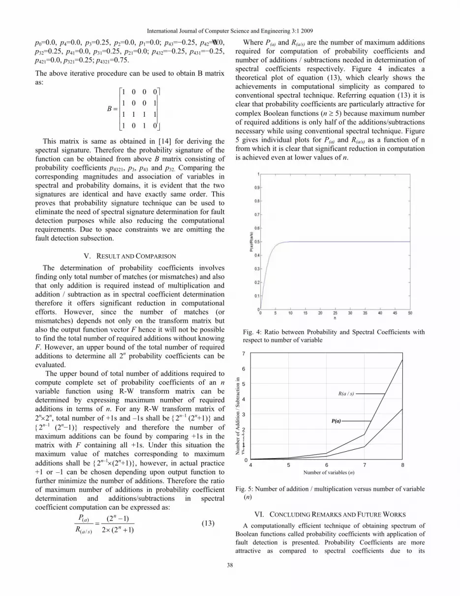
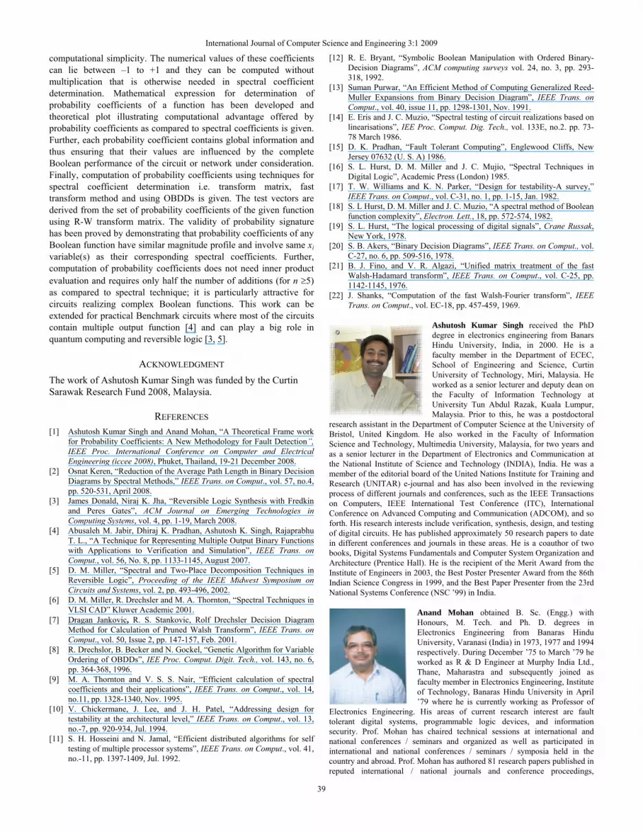
W Where P(a) and R(a/s) are the number of maximum additions required for computation of probability coefficients and number of additions / subtractions needed in determination of spectral coefficients respectively. Figure 4 indicates a theoretical plot of equation (13), which clearly shows the achievements in computational simplicity as compared to conventional spectral technique. Referring equation (13) it is clear that probability coefficients are particularly attractive for complex Boolean functions (n ≥ 5) because maximum number of required additions is only half of the additions/subtractions necessary while using conventional spectral technique. Figure 5 gives individual plots for P(a) and R(a/s) as a function of n from which it is clear that significant reduction in computation is achieved even at lower values of n.

Fig. 4: Ratio between Probability and Spectral Coefficients with respect to number of variable

Fig. 5: Number of addition / multiplication versus number of variable

(n)

VI. CONCLUDING REMARKS AND FUTURE WORKS A computationally efficient technique of obtaining spectrum of

Boolean functions called probability coefficients with application of fault detection is presented. Probability Coefficients are more attractive as compared to spectral coefficients due to its

4 5 6 7 8Number of variables (n)

0

1

2

3

4

5

6

7

P(a)

R(a / s)

Num

ber o

f Add

ition

/ Su

btra

ctio

n in

Th

ousa

nds

International Journal of Computer Science and Engineering 3:1 2009

38

computational simplicity. The numerical values of these coefficients can lie between –1 to +1 and they can be computed without multiplication that is otherwise needed in spectral coefficient determination. Mathematical expression for determination of probability coefficients of a function has been developed and theoretical plot illustrating computational advantage offered by probability coefficients as compared to spectral coefficients is given. Further, each probability coefficient contains global information and thus ensuring that their values are influenced by the complete Boolean performance of the circuit or network under consideration. Finally, computation of probability coefficients using techniques for spectral coefficient determination i.e. transform matrix, fast transform method and using OBDDs is given. The test vectors are derived from the set of probability coefficients of the given function using R-W transform matrix. The validity of probability signature has been proved by demonstrating that probability coefficients of any Boolean function have similar magnitude profile and involve same xi variable(s) as their corresponding spectral coefficients. Further, computation of probability coefficients does not need inner product evaluation and requires only half the number of additions (for n ≥5) as compared to spectral technique; it is particularly attractive for circuits realizing complex Boolean functions. This work can be extended for practical Benchmark circuits where most of the circuits contain multiple output function [4] and can play a big role in quantum computing and reversible logic [3, 5].

ACKNOWLEDGMENT The work of Ashutosh Kumar Singh was funded by the Curtin Sarawak Research Fund 2008, Malaysia.

REFERENCES [1] Ashutosh Kumar Singh and Anand Mohan, “A Theoretical Frame work

for Probability Coefficients: A New Methodology for Fault Detection”, IEEE Proc. International Conference on Computer and Electrical Engineering (iccee 2008), Phuket, Thailand, 19-21 December 2008.

[2] Osnat Keren, “Reduction of the Average Path Length in Binary Decision Diagrams by Spectral Methods,” IEEE Trans. on Comput., vol. 57, no.4, pp. 520-531, April 2008.

[3] James Donald, Niraj K. Jha, “Reversible Logic Synthesis with Fredkin and Peres Gates”, ACM Journal on Emerging Technologies in Computing Systems, vol. 4, pp. 1-19, March 2008.

[4] Abusaleh M. Jabir, Dhiraj K. Pradhan, Ashutosh K. Singh, Rajaprabhu T. L., “A Technique for Representing Multiple Output Binary Functions with Applications to Verification and Simulation”, IEEE Trans. on Comput., vol. 56, No. 8, pp. 1133-1145, August 2007.

[5] D. M. Miller, “Spectral and Two-Place Decomposition Techniques in Reversible Logic”, Proceeding of the IEEE Midwest Symposium on Circuits and Systems, vol. 2, pp. 493-496, 2002.

[6] D. M. Miller, R. Drechsler and M. A. Thornton, “Spectral Techniques in VLSI CAD” Kluwer Academic 2001.

[7] Dragan Jankovic, R. S. Stankovic, Rolf Drechsler Decision Diagram Method for Calculation of Pruned Walsh Transform”, IEEE Trans. on Comput., vol. 50, Issue 2, pp. 147-157, Feb. 2001.

[8] R. Drechslor, B. Becker and N. Gockel, “Genetic Algorithm for Variable Ordering of OBDDs”, IEE Proc. Comput. Digit. Tech., vol. 143, no. 6, pp. 364-368, 1996.

[9] M. A. Thornton and V. S. S. Nair, “Efficient calculation of spectral coefficients and their applications”, IEEE Trans. on Comput., vol. 14, no.11, pp. 1328-1340, Nov. 1995.

[10] V. Chickermane, J. Lee, and J. H. Patel, “Addressing design for testability at the architectural level,” IEEE Trans. on Comput., vol. 13, no.-7, pp. 920-934, Jul. 1994.

[11] S. H. Hosseini and N. Jamal, “Efficient distributed algorithms for self testing of multiple processor systems”, IEEE Trans. on Comput., vol. 41, no.-11, pp. 1397-1409, Jul. 1992.

[12] R. E. Bryant, “Symbolic Boolean Manipulation with Ordered Binary-Decision Diagrams”, ACM computing surveys vol. 24, no. 3, pp. 293-318, 1992.

[13] Suman Purwar, “An Efficient Method of Computing Generalized Reed-Muller Expansions from Binary Decision Diagram”, IEEE Trans. on Comput., vol. 40, issue 11, pp. 1298-1301, Nov. 1991.

[14] E. Eris and J. C. Muzio, “Spectral testing of circuit realizations based on linearisations”, IEE Proc. Comput. Dig. Tech., vol. 133E, no.2. pp. 73-78 March 1986.

[15] D. K. Pradhan, “Fault Tolerant Computing”, Englewood Cliffs, New Jersey 07632 (U. S. A) 1986.

[16] S. L. Hurst, D. M. Miller and J. C. Mujio, “Spectral Techniques in Digital Logic”, Academic Press (London) 1985.

[17] T. W. Williams and K. N. Parker, “Design for testability-A survey,” IEEE Trans. on Comput., vol. C-31, no. 1, pp. 1-15, Jan. 1982.

[18] S. L Hurst, D. M. Miller and J. C. Muzio, “A spectral method of Boolean function complexity”, Electron. Lett., 18, pp. 572-574, 1982.

[19] S. L. Hurst, “The logical processing of digital signals”, Crane Russak, New York, 1978.

[20] S. B. Akers, “Binary Decision Diagrams”, IEEE Trans. on Comput., vol. C-27, no. 6, pp. 509-516, 1978.

[21] B. J. Fino, and V. R. Algazi, “Unified matrix treatment of the fast Walsh-Hadamard transform”, IEEE Trans. on Comput., vol. C-25, pp. 1142-1145, 1976.

[22] J. Shanks, “Computation of the fast Walsh-Fourier transform”, IEEE Trans. on Comput., vol. EC-18, pp. 457-459, 1969.

Ashutosh Kumar Singh received the PhD degree in electronics engineering from Banars Hindu University, India, in 2000. He is a faculty member in the Department of ECEC, School of Engineering and Science, Curtin University of Technology, Miri, Malaysia. He worked as a senior lecturer and deputy dean on the Faculty of Information Technology at University Tun Abdul Razak, Kuala Lumpur, Malaysia. Prior to this, he was a postdoctoral

research assistant in the Department of Computer Science at the University of Bristol, United Kingdom. He also worked in the Faculty of Information Science and Technology, Multimedia University, Malaysia, for two years and as a senior lecturer in the Department of Electronics and Communication at the National Institute of Science and Technology (INDIA), India. He was a member of the editorial board of the United Nations Institute for Training and Research (UNITAR) e-journal and has also been involved in the reviewing process of different journals and conferences, such as the IEEE Transactions on Computers, IEEE International Test Conference (ITC), International Conference on Advanced Computing and Communication (ADCOM), and so forth. His research interests include verification, synthesis, design, and testing of digital circuits. He has published approximately 50 research papers to date in different conferences and journals in these areas. He is a coauthor of two books, Digital Systems Fundamentals and Computer System Organization and Architecture (Prentice Hall). He is the recipient of the Merit Award from the Institute of Engineers in 2003, the Best Poster Presenter Award from the 86th Indian Science Congress in 1999, and the Best Paper Presenter from the 23rd National Systems Conference (NSC ’99) in India.

Anand Mohan obtained B. Sc. (Engg.) with Honours, M. Tech. and Ph. D. degrees in Electronics Engineering from Banaras Hindu University, Varanasi (India) in 1973, 1977 and 1994 respectively. During December ’75 to March ’79 he worked as R & D Engineer at Murphy India Ltd., Thane, Maharastra and subsequently joined as faculty member in Electronics Engineering, Institute of Technology, Banaras Hindu University in April ’79 where he is currently working as Professor of

Electronics Engineering. His areas of current research interest are fault tolerant digital systems, programmable logic devices, and information security. Prof. Mohan has chaired technical sessions at international and national conferences / seminars and organized as well as participated in international and national conferences / seminars / symposia held in the country and abroad. Prof. Mohan has authored 81 research papers published in reputed international / national journals and conference proceedings,

International Journal of Computer Science and Engineering 3:1 2009

39

supervised 47 M. Tech. dissertations and good number of Ph. D. theses. He has been reviewer of research papers for publication in IEEE Transactions on Computer (USA), Journal of Computer and Information Science (Canada), and Institution of Engineers, (India) and has also reviewed book on Microcontrollers for Tata-MacGraw Hill and learning material for ISTE, New Delhi. His coauthored papers have received awards of International Union of Radio Science (URSI), Belgium, Institution of Engineers, (India) and Indian Science Congress. Prof. Mohan is Fellow of Institution of Electronics and Telecommunication Engineers, (India) and Institution of Engineers (India) and Life Member of Indian Society for Technical Education (ISTE), New Delhi. Anand Mohan is Chairman of research panel on Armament Sensors & Electronics, DRDO, Ministry of Defence, Govt. of India, worked as Chairman of NBA Ad-hoc Committees of AICTE, New Delhi, and chaired project review committee of HAL, Korwa. He has been Member of several national committees of UGC, CSIR, DST, DRDO and reputed academic institutions of the country. Prof. Mohan was also Member of Executive Council, Banaras Hindu University, Governor’s Nominee, Rajasthan Technical University, Kota, and presently he is Member of Governing Councils of HBTI, Kanpur, IET, Lucknow, and many other reputed institutions of Engineering & Technology.

International Journal of Computer Science and Engineering 3:1 2009

40