Embed Size (px)
Citation preview

Comparison of two commonly used
Hydrofoils and their Propensity to Cavitation and
Ventilation
by
James Robert Mackenzie
B.ENG (Naval Architecture)
National Centre for Maritime Engineering and Hydrodynamics
Submitted in fulfilment of the requirements for the Master of Philosophy
(Maritime Engineering)
University of Tasmania June 2021

i
Declaration
I hereby declare that the whole of this submission is my own work and the result of my own
investigation and that, to the best of my knowledge and belief, it contains no material previously
published or written by another person, except where due reference is made in the text of the
project.
I further declare that the work embodied in this project has not been accepted for the award of any
other degree or diploma in any institution, college or university, and is not being concurrently
submitted for any other degree or diploma award.
This thesis may be made available for loan and limited copying and communication in accordance
with the Copyright Act 1968.
…………………………………………..
James Mackenzie
December 2020

ii
Acknowledgements
I acknowledge the patience of all parties with interest in this project. I thank the professional
support given by my supervisor Prof Jonathan Binns and Co-Supervisor Dr Jonathan Duffy.
Personally, thank you to my family and friends for all your support and encouragement you have
given me over the years.
iii
Table of Contents
Declaration ............................................................................................................................................ i
Acknowledgements .............................................................................................................................. ii
List of Tables ...................................................................................................................................... vi
List of Figures .................................................................................................................................... vii
Table of Acronyms............................................................................................................................ xiv
Abstract ................................................................................................................................................ 1
1 Introduction ................................................................................................................................ 2
1.1 Background ....................................................................................................................... 2
1.2 Problem Definition/Hypothesis ......................................................................................... 3
1.3 Literature Review .............................................................................................................. 4
1.4 Novel Components of Work ............................................................................................. 6
1.4.1 CFD Numerical Analysis to Research Cavitation Phenomena ............................. 6
1.4.2 Full Scale Testing to Research Ventilation Phenomena ....................................... 6
1.4.3 CFD Numerical Analysis and Full-Scale Testing Results .................................... 7
1.5 Effect of Ventilation on Hydrofoil Efficiency .................................................................. 7
1.6 The International Moth Class ............................................................................................ 7
2 CFD Numerical Analysis............................................................................................................ 9
2.1 CFD Numerical Analysis Methods ................................................................................... 9
2.1.1 CAD/Rhino 6 Modelling Details ........................................................................... 9
2.1.2 Design Modeller Details ...................................................................................... 10
2.1.3 Meshing ............................................................................................................... 10
2.1.4 Mesh Accuracy .................................................................................................... 12
2.1.5 Selection of URANS CFD Analysis ................................................................... 12
2.1.6 Courant Number Convergence Study ................................................................. 13
2.1.7 Richardson Extrapolation Mesh Study ................................................................ 14
2.1.8 Y+ Selection ........................................................................................................ 17
2.1.9 Skewness and Orthogonal Quality ...................................................................... 18
2.1.10 CFD Simulation Setup ........................................................................................ 19
2.1.11 Boundary Conditions Applied in CFX Pre-Processor ......................................... 19
2.1.12 CEL Expressions and Additional Variables ........................................................ 20
2.2 CFD Numerical Analysis Results ................................................................................... 21
2.2.1 General ................................................................................................................ 21
2.2.2 Negative Ten Degrees Flap Deflection – Cavitation Number and Cavity Length
as a Function of Depth of Submergence ........................................................... 22
2.2.3 Negative Ten Degrees Flap Deflection – Lift, Drag and Torque Coefficients ... 26
2.2.4 Zero Degrees Flap Deflection – Cavitation Number and Cavity Length as a
Function of Depth of Submergence .................................................................. 27
2.2.5 Zero Degrees Flap Deflection – Lift, Drag and Torque Coefficients ................. 30
2.2.6 Positive Fifteen Degrees Flap Deflection – Cavitation Number and Cavity
Length as a Function of Depth of Submergence ............................................... 32
2.2.7 Positive Fifteen Degrees Flap Deflection – Lift, Drag and Torque Coefficients 35

iv
2.2.8 Conclusions and Recommendations for CFD Numerical Analysis .................... 37
3 Full Scale Testing ..................................................................................................................... 39
3.1 Full Scale Testing Methods ............................................................................................. 39
3.1.1 General ................................................................................................................ 39
3.1.2 Design of Hydrofoils ........................................................................................... 39
3.1.3 Building of Hydrofoils ........................................................................................ 40
3.1.4 Experiment Setup ................................................................................................ 41
3.1.5 Test Program ....................................................................................................... 41
3.1.6 Instrumentation Used for Full Scale Testing ....................................................... 43
3.1.7 Full Scale Testing Data Analysis ........................................................................ 44
3.1.8 Experiment Uncertainty ...................................................................................... 45
3.2 Full Scale Testing Results ............................................................................................... 46
3.2.1 General ................................................................................................................ 46
3.2.2 Ventilated Cavity Attachment Propensity of Each Hydrofoil ............................. 47
3.2.3 Average Period of Ventilation Events Over Varied Depth of Submergence ...... 50
3.2.4 Average Speed of Hydrofoil Over Varied Depth of Submergence ..................... 51
3.2.5 Percentage Flap Angle Occurrences Over Varied Depth of Submergence ......... 52
3.2.6 Conclusions and Recommendations for Full Scale Testing ................................ 54
4 Conclusion and Recommendations .......................................................................................... 56
4.1 Summary ......................................................................................................................... 56
4.2 Conclusion....................................................................................................................... 56
4.3 Recomendations .............................................................................................................. 59
Appendix A ........................................................................................................................................ 60
Trial of Data Logger for Full Scale Experiment ....................................................................... 60
Appendix B ........................................................................................................................................ 61
ANSYS Geometry and Meshing Details .................................................................................. 61
CEL and Additional Variables for ANSYS CFX Solver ......................................................... 62
Appendix C ........................................................................................................................................ 63
Appendix D ........................................................................................................................................ 65
ANSYS Screenshots of the NACA-0012 CFD Analysis ......................................................... 65
ANSYS Screenshots of The Mach 2 CFD Analysis................................................................. 85
Appendix E ...................................................................................................................................... 100
Mach 2 Analysis Used for Thesis Dated (28/08/2020) .......................................................... 100
NACA-0012 Analysis Used for Thesis Dated (19/09/2020) .................................................. 101
Mach 2 Supplementary Analysis not used in Main Body of Thesis ...................................... 102
NACA-0012 Supplementary Analysis not used in Main Body of Thesis .............................. 103
Appendix F ....................................................................................................................................... 105
NACA-0012 Sail Dated on the 19/09/2020 at (12:39:31 Pm)................................................ 105
Mach 2 Sailed on Date (28/08/2020) ...................................................................................... 124
NACA-0012 Secondary Test Sailed on Date (7/11/2020) ..................................................... 159
Mach 2 Secondary Test Sailed on Date (5/07/2020) .............................................................. 188
Appendix G ...................................................................................................................................... 192
Geometric Properties of Hydrofoils Analysed ....................................................................... 192

v
MACH 2 Geometrical Offsets ................................................................................................ 192
NACA-0012 Geometrical Offsets .......................................................................................... 193
Hydrofoil Planform Shape for Both Sections ......................................................................... 194
Appendix H ...................................................................................................................................... 195
Construction Methods for the NACA-0012 Hydrofoil........................................................... 195
Appendix I........................................................................................................................................ 200
Background to Selection of Hydrofoil Sections for Research Project ................................... 200
Effect of Hinge Junction on Hydrofoil Performance .............................................................. 200
Appendix J ....................................................................................................................................... 202
Additional Information ........................................................................................................... 202
References ........................................................................................................................................ 204

vi
List of Tables
Table 2-1 Percentage error for hydrofoil surface area between Cad and ANSYS. ........................... 12
Table 2-2 Mesh metric spectrum analysis results. ............................................................................. 19
Table 2-3 List of graphs used in the CFD Results section, which defines their relevance in
determining the cavitation propensity of each hydrofoil over all three flap deflections and foil
depths analysed......................................................................................................................... 21
Table B-1 List of CEL expressions and additional variables defined in CFX Pre-Processor and used
to define key temporal and spatial parameters used to solve the CFD model. ........................ 62
Table G-1 Table of offsets for the Mach 2 hydrofoil section, with upper and lower surfaces listed as
a function of percentage chord length referenced from nose to trailing edge of foil. ..................... 192
Table G-2 Table of offsets for the NACA-0012 hydrofoil section, with upper and lower surfaces
listed as a function of percentage chord length referenced from nose to trailing edge of foil.
................................................................................................................................................ 193
vii
List of Figures
Figure 2-1 Dimensions of the two-dimensional fluid domain that was used in the CFD analysis. The fluid domain was 1
mm thick and required remodelling in Rhino 6 for every design condition analysed. This included altering flap
angle, foil AOA and foil section type (NACA-0012 or Mach 2). ........................................................................... 10
Figure 2-2 ANSYS meshing refinement example on the leading edge of the foil where the element size, growth rate and
curvature normal were altered to increase the quality of meshing around areas where there is an abrupt change
in geometry. The reduced quality of a coarse mesh is shown (top), while a finer mesh with higher accuracy is
shown (bottom). Both screen shots are of the NACA-0012 at 15 degrees flap deflection and negative 6 degrees
AOA. ...................................................................................................................................................................... 11
Figure 2-3 Histogram for the period of all ventilation events for the NACA-0012 and Mach 2 hydrofoils analysed in
full-scale testing. The period of 2-2.5 seconds had over 30% of all total events, with an average period of 1.82
seconds. The complete tabulated results for the full-scale testing are shown in Appendix E ................................ 13
Figure 2-4 Courant number and (lift/drag) coefficients plotted against timestep (seconds). ........................................... 14
Figure 2-5 Drag coefficient variation and Richardson extrapolation plotted against total mesh elements. .................... 16
Figure 2-6 Relative error of drag coefficient plotted against total mesh elements........................................................... 16
Figure 2-7 First node distance and number of layers for the NACA-0012 hydrofoil section set at four degrees angle of
attack and zero degrees flap deflection. ................................................................................................................ 17
Figure 2-8 Results for Y+ study, for the NACA-0012 hydrofoil section drag coefficient when set at four degrees angle of
attack and zero degrees flap deflection. ................................................................................................................ 18
Figure 2-9 ANSYS mesh metric spectrums ANSYS (2020)................................................................................................ 18
Figure 2-10 Screenshot of boundary conditions applied to the fluid domain in ANSYS Pre Processor for the NACA-0012
hydrofoil at -10 degrees flap and +8 degrees angle of attack. The domain utilised a constant mass flow rate
which entered through the inlet and exited though the outlet. The top of the domain was an opening which
allowed fluid to exit and re-enter prior to leaving the domain through the outlet. These boundary conditions
ensured continuity of the flow to meet the required mass flow rate. The free stream velocity was set at 10 m/s and
ran along the X-axis and can be seen running from left to right in the figure above. ........................................... 20
Figure 2-11 Hydrofoil angle of attack as a function of depth for a negative ten degrees flap deflection (Mach 2 &
NACA-0012). The NACA-0012 foil needed a greater AOA to generate the same lift coefficient of the Mach 2.
This was also the flap deflection where the NACA-0012 had a vapour cavity and cavitation on the surface of the
foil near its leading edge. ...................................................................................................................................... 22
Figure 2-12 CFD results of both foils for a -10 degrees flap deflection, where the cavitation number and cavity length
are plotted as a function of depth. The NACA-0012 had both cavitation and vapour cavity formation on its
surface over all depths analysed. .......................................................................................................................... 23
Figure 2-13 Contour plot of Absolute Pressure for the NACA-0012 hydrofoil at -10 degrees flap deflection and 25 mm
depth of submergence. There are two regions of low pressure present on the foil surface, with the region on the
upper surface near the leading edge containing cavitation and a vapour cavity. ................................................. 24
Figure 2-14 Contour plot of volume fraction for the NACA-0012 foil at negative ten degrees flap for selected range of
foil depths. The contour plots are ordered with the shallowest depth 6 mm (top), 25 mm (middle) and 100 mm
(bottom). All regions of cavity formation coincided with areas of minimum absolute pressure on the surface of
the foil. The largest cavity length was 8.03 mm at a depth of 25 mm on the upper foil surface near the leading
edge. ...................................................................................................................................................................... 25
Figure 2-15 Results of both foils for a negative ten degrees flap deflection, where the CL/CD coefficients are plotted
against foil depth. The Mach 2 foil had a higher CL/CD coefficient values over all depths. The two foils both
have a reduction of CL/CD as the depth is reduced. ............................................................................................. 26
Figure 2-16 Results of both foils for a negative ten degrees flap deflection, where the torque coefficients (CT) are
plotted against foil depth. The Mach 2 foil had a higher torque coefficient value over all depths. ...................... 27
Figure 2-17 Hydrofoil angle of attack as a function of depth for a zero degrees flap deflection (Mach 2 & NACA-0012).
The NACA-0012 was set at positive AOA, while the Mach 2 was set at negative AOA. This shows the difference
in setup to reach the baseline lift coefficient. The AOA needed to be adjusted with a greater positive incidence
with reduced proximity to the free surface, this phenomenon occurred with both foil sections. ........................... 28
Figure 2-18 CFD results of both foils for a zero degrees flap deflection, where the cavitation number is graphed as a
function of foil depth. At depths less than 25 mm the NACA-0012 had an overall reduction in cavitation number,
while the Mach 2 experienced an overall increase in cavitation number. ............................................................ 29
Figure 2-19 ANSYS contour plot of non-clipped absolute pressure for the NACA-0012 foil at 0 degrees flap deflection, 4
degrees AOA and (6 mm) depth. The NACA-0012 when set at 0 degrees flap deflection only experienced one
region of low pressure around its surface on the suction side near the leading edge. .......................................... 30
viii
Figure 2-20 CFD results of both foils for a zero degrees flap deflection, where the CL/CD coefficients are plotted
against foil depth. The Mach 2 once again had a higher value of CL/CD coefficients, as replicated with the -10
degrees flap deflection. .......................................................................................................................................... 31
Figure 2-21 CFD results of both foils for a zero degrees flap deflection, where the CT coefficients are plotted against
foil depth. The Mach 2 once again had a greater positive magnitude of torque coefficient, as replicated with the -
10 degrees flap deflection. ..................................................................................................................................... 31
Figure 2-22 Hydrofoil angle of attack as a function of depth for a positive fifteen degrees flap deflection (Mach 2 &
NACA-0012). The Mach 2 was inclined at a greater AOA to generate the same baseline CL, due to the
geometrical properties of the foil (asymmetric) and the NACA-0012 was (symmetrical). .................................... 32
Figure 2-23 CFD results of both foils for a positive fifteen degrees flap deflection, where the cavitation number is
graphed as a function of foil depth. The Mach 2 at this design condition had absolute pressures below the
vapour pressure of saltwater though did not have vapour cavity propagation on its surface. This phenomenon
will require further CFD to be confirmed and could lead to a design condition where the Mach 2 has a high
propensity to cavitation. ........................................................................................................................................ 33
Figure 2-24 ANSYS contour plot of non-clipped absolute pressure for the Mach 2 foil at 15 degrees flap deflection, -12
degrees AOA. The order of depth for the images are 6 mm (top), 50 mm (middle) and 100 mm (bottom). Both foil
sections at 15 degrees flap had an increase in cavitation number as the depth was reduced, this means as the
depth is increased both foils have a higher propensity for cavitation. The Mach 2 also has two regions of low
absolute pressure on its surface, being on its lower surface near the leading edge (which had lowest magnitude)
and the other on the upper surface at the junction of the hydrofoil and flap. ....................................................... 34
Figure 2-25 CFD results of both foils for a positive fifteen degrees flap deflection, where the CL/CD coefficients are
plotted against foil depth. The Mach 2 had a lower CL/CD value over all depths, which shows it operated at a
lower efficiency than the NACA-0012. The flap deflection of 15 degrees was where the NACA-0012
outperformed the Mach 2 in terms of cavitation propensity. ................................................................................. 36
Figure 2-26 CFD results of both foils for a positive fifteen degrees flap deflection, where the CT are plotted against foil
depth. The Mach 2 has a lower CT at 15 degrees flap deflection over all depths when compared to the NACA-
0012. The lower value shows a correlation between reduced CL/CD, higher CT and lower cavitation number. The
NACA-00012 experienced the same trends when operating at -10 and 0 degrees flap deflections. ...................... 36
Figure 3-1 Geometry that was duplicated from the Mach 2 foil to create the NACA-0012 hydrofoil. The plan form
shape, flap size and strut shape were all duplicated. The only variation was the hydrofoil cross section, which
formed the basis for this analysis. ......................................................................................................................... 40
Figure 3-2 The real time graphical plot of two full scale test sessions with the NACA-0012 left and Mach 2 on the right.
The red line defines the course travelled by the moth in each session. The setup of equipment required over ten
test sessions to get a setup that could record data efficiently. ............................................................................... 42
Figure 3-3 Images of full-scale testing capturing ventilated tip vortex forming on NACA-0012 hydrofoil (top and bottom
left). These two images also show the wand angle (which is a function of flap deflection) and foil depth as
referenced by markings on the foil’s vertical strut. The Mach 2 hydrofoil is shown bottom right and in this design
condition the foil is operating with a 15 degrees flap deflection to raise the hull above the free surface and into
the hydro foiling regime. The two angles at which the cameras were set were synced with the data logger to both
graphically and numerically capture unique parameters that define ventilation events for each hydrofoil. ........ 42
Figure 3-43-5 Axis orientation in all six degrees of freedom for the moth used in both CFD and full scale testing (Hull,
2011), along axis orientation used on the iPhone APP Sensor Play for experimental data collection (Broder,
2018) to the right. The iPhone was setup to be securely mounted to the moth with both moth and iPhone aligned
in the same axis orientation. .................................................................................................................................. 43
Figure 3-6 Setup of instrumentation used in full scale testing incorporating two GoPro cameras, one fitted on the
transom looking forward and the other fitted off the front right wing bar to capture the side profile of the moth
including (wand, strut and foil). The data logger was fitted on deck in line with the aft wing bar and cantered on
vessel centreline with moth and data logger having their axis orientations aligned. ............................................ 44
Figure 3-7 Ventilated cavity attachment to the NACA-0012 hydrofoil in full scale testing. Refer Appendix D (NACA-
0012 Supplementary Analysis not used in Main Body of Thesis) event 23. The four images sequenced from top
left, top right, bottom left, and bottom right show hydrofoil tip break the free surface and allowing tip vortices to
induce ventilated cavities to attach to the leading edge of the hydrofoil, which lead to the moth having a
catastrophic crash off its foils. .............................................................................................................................. 48
Figure 3-8 Ventilation event for the Mach 2 Refer Appendix E (Mach 2 Analysis Used for Thesis Dated (28/08/2020)
event 12, which resulted in no cavity attachment to the hydrofoil surface or catastrophic crashing off the foils.
The sequence starts from top left to right, then bottom left to right. The vapour cavity once again propagates due
to the hydrofoil tip breaking the free surface. The vapour cavity reaches the trailing of foil as shown on the
bottom left image, though fails to stick to the hydrofoil surface as shown on the bottom right image. ................. 48
ix
Figure 3-9 Full scale testing results for the Mach 2 hydrofoil, where the percentage of attached ventilated cavities are
compared to the total number of ventilation events. The events are plotted as a function of foil depth on the X-
axis and an orange trend line has been added to show the effect of foil submergence. The Mach 2 had 29 % of all
ventilation events result in cavity attachment to the foil surface of which 11 % resulted in catastrophic crashing
off foils. .................................................................................................................................................................. 49
Figure 3-10 Full scale testing results for the NACA-0012 hydrofoil, where the percentage of attached ventilated cavities
are compared to the total number of ventilation events. The events are plotted as a function of foil depth on the
X-axis and an orange trend line has been added to show the effect of foil submergence. The NACA-0012 had 90
% of all ventilation events result in cavity attachment to the foil surface and catastrophic crashing off foils. ..... 49
Figure 3-11 Results for Mach 2, average period of ventilation event over varied depth of submergence. The period of
ventilation events was categorized as either less or greater than 1.5 seconds, then percentage occurrence plotted
as function of depth. The Mach 2 had higher percentage of periods greater than 1.5 seconds at a depth greater
than 75 mm. ........................................................................................................................................................... 50
Figure 3-12 Results for NACA-0012, average period of ventilation event over varied depth of submergence. The period
of ventilation events was categorized as either less or greater than 1.5 seconds, then percentage occurrence
plotted as function of depth. The NACA-0012 had 50 % of all ventilation events occur at 50mm depth and with a
period greater than 1.5 seconds. This show a design condition where there is a high occurrence of ventilated
cavity attachment for the NACA-0012. .................................................................................................................. 51
Figure 3-13 Average speed of both (Mach 2 and NACA-0012) over varied depth of submergence. ................................ 52
Figure 3-14 Results for percentage total of flap deflections for the Mach 2 hydrofoil as a function of depth of
submergence. The Mach 2 operated with a higher percentage of positive flap deflections in the depth range of 12
mm to 100 mm, with a higher percentage of negative deflections when depth was reduced to 6 mm. .................. 53
Figure 3-15 The percentage total of flap deflections for the NACA-0012 hydrofoil as a function of depth of
submergence. ......................................................................................................................................................... 53
Figure A-1 Arduino Uno data logger built by author. This item was not used in experiments as it never functioned
correctly. ............................................................................................................................................................... 60
Figure B-1 Details of ANSYS meshing algorithm used for the CFD analysis. ................................................................. 61
Figure C-1 The derivation of the three- and two-dimensional lift coefficients used in the CFD Numerical Analysis ..... 64
Figure D-1 ANSYS screen shot of the NACA-0012 hydrofoil absolute pressure at -10 degrees flap deflection and 6 mm
foil depth. ............................................................................................................................................................... 65
Figure D-2 ANSYS screen shot of the NACA-0012 hydrofoil sea water volume fraction at -10 degrees flap deflection
and 6 mm foil depth. .............................................................................................................................................. 66
Figure D-3 ANSYS screen shot of the NACA-0012 hydrofoil absolute pressure at -10 degrees flap deflection and 12 mm
foil depth. ............................................................................................................................................................... 67
Figure D-4 ANSYS screen shot of the NACA-0012 hydrofoil sea water volume fraction at -10 degrees flap deflection
and 12 mm foil depth. ............................................................................................................................................ 68
Figure D-5 ANSYS screen shot of the NACA-0012 hydrofoil absolute pressure at -10 degrees flap deflection and 25 mm
foil depth. ............................................................................................................................................................... 69
Figure D-6 ANSYS screen shot of the NACA-0012 hydrofoil sea water volume fraction at -10 degrees flap deflection
and 25 mm foil depth. ............................................................................................................................................ 70
Figure D-7 ANSYS screen shot of the NACA-0012 hydrofoil absolute pressure at -10 degrees flap deflection and 50 mm
foil depth. ............................................................................................................................................................... 71
Figure D-8 ANSYS screen shot of the NACA-0012 hydrofoil sea water volume fraction at -10 degrees flap deflection
and 50 mm foil depth. ............................................................................................................................................ 72
Figure D-9 ANSYS screen shot of the NACA-0012 hydrofoil absolute pressure at -10 degrees flap deflection and 100
mm foil depth. ........................................................................................................................................................ 73
Figure D-10 ANSYS screen shot of the NACA-0012 hydrofoil sea water volume fraction at -10 degrees flap deflection
and 100 mm foil depth. .......................................................................................................................................... 74
Figure D-11 ANSYS screen shot of the NACA-0012 hydrofoil absolute pressure at 0 degrees flap deflection and 6 mm
foil depth. ............................................................................................................................................................... 75
Figure D-12 ANSYS screen shot of the NACA-0012 hydrofoil absolute pressure at 0 degrees flap deflection and 12 mm
foil depth. ............................................................................................................................................................... 76
Figure D-13 ANSYS screen shot of the NACA-0012 hydrofoil absolute pressure at 0 degrees flap deflection and 25 mm
foil depth. ............................................................................................................................................................... 77
Figure D-14 ANSYS screen shot of the NACA-0012 hydrofoil absolute pressure at 0 degrees flap deflection and 50 mm
foil depth. ............................................................................................................................................................... 78
x
Figure D-15 ANSYS screen shot of the NACA-0012 hydrofoil absolute pressure at 0 degrees flap deflection and 100 mm
foil depth. ............................................................................................................................................................... 79
Figure D-16 ANSYS screen shot of the NACA-0012 hydrofoil absolute pressure at 15 degrees flap deflection and 6 mm
foil depth. ............................................................................................................................................................... 80
Figure D-17 ANSYS screen shot of the NACA-0012 hydrofoil absolute pressure at 15 degrees flap deflection and 12 mm
foil depth. ............................................................................................................................................................... 81
Figure D-18 ANSYS screen shot of the NACA-0012 hydrofoil absolute pressure at 15 degrees flap deflection and 25 mm
foil depth. ............................................................................................................................................................... 82
Figure D-19 ANSYS screen shot of the NACA-0012 hydrofoil absolute pressure at 15 degrees flap deflection and 50 mm
foil depth. ............................................................................................................................................................... 83
Figure D-20 ANSYS screen shot of the NACA-0012 hydrofoil absolute pressure at 15 degrees flap deflection and 100
mm foil depth. ........................................................................................................................................................ 84
Figure D-21 ANSYS screen shot of the Mach 2 hydrofoil absolute pressure at -10 degrees flap deflection and 6 mm foil
depth. ..................................................................................................................................................................... 85
Figure D-22 ANSYS screen shot of the Mach 2 hydrofoil absolute pressure at -10 degrees flap deflection and 12 mm foil
depth. ..................................................................................................................................................................... 86
Figure D-23 ANSYS screen shot of the Mach 2 hydrofoil absolute pressure at -10 degrees flap deflection and 25 mm foil
depth. ..................................................................................................................................................................... 87
Figure D-24 ANSYS screen shot of the Mach 2 hydrofoil absolute pressure at -10 degrees flap deflection and 50 mm foil
depth. ..................................................................................................................................................................... 88
Figure D-25 ANSYS screen shot of the Mach 2 hydrofoil absolute pressure at -10 degrees flap deflection and 100 mm
foil depth. ............................................................................................................................................................... 89
Figure D-26 ANSYS screen shot of the Mach 2 hydrofoil absolute pressure at 0 degrees flap deflection and 6 mm foil
depth. ..................................................................................................................................................................... 90
Figure D-27 ANSYS screen shot of the Mach 2 hydrofoil absolute pressure at 0 degrees flap deflection and 12 mm foil
depth. ..................................................................................................................................................................... 91
Figure D-28 ANSYS screen shot of the Mach 2 hydrofoil absolute pressure at 0 degrees flap deflection and 25 mm foil
depth. ..................................................................................................................................................................... 92
Figure D-29 ANSYS screen shot of the Mach 2 hydrofoil absolute pressure at 0 degrees flap deflection and 50 mm foil
depth. ..................................................................................................................................................................... 93
Figure D-30 ANSYS screen shot of the Mach 2 hydrofoil absolute pressure at 0 degrees flap deflection and 100 mm foil
depth. ..................................................................................................................................................................... 94
Figure D-31 ANSYS screen shot of the Mach 2 hydrofoil absolute pressure at 15 degrees flap deflection and 6 mm foil
depth. ..................................................................................................................................................................... 95
Figure D-32 ANSYS screen shot of the Mach 2 hydrofoil absolute pressure at 15 degrees flap deflection and 12 mm foil
depth. ..................................................................................................................................................................... 96
Figure D-33 ANSYS screen shot of the Mach 2 hydrofoil absolute pressure at 15 degrees flap deflection and 25 mm foil
depth. ..................................................................................................................................................................... 97
Figure D-34 ANSYS screen shot of the Mach 2 hydrofoil absolute pressure at 15 degrees flap deflection and 50 mm foil
depth. ..................................................................................................................................................................... 98
Figure D-35 ANSYS screen shot of the Mach 2 hydrofoil absolute pressure at 15 degrees flap deflection and 100 mm
foil depth. ............................................................................................................................................................... 99
Figure F-1 Full Scale Test Image of NACA-0012 (19/09/2020) – Event 1. .................................................................... 105
Figure F-2 Full Scale Test Image of NACA-0012 (19/09/2020) – Event 2. .................................................................... 106
Figure F-3 Full Scale Test Image of NACA-0012 (19/09/2020) – Event 3. .................................................................... 107
Figure F-4 Full Scale Test Image of NACA-0012 (19/09/2020) – Event 4. .................................................................... 108
Figure F-5 Full Scale Test Image of NACA-0012 (19/09/2020) – Event 5. .................................................................... 109
Figure F-6 Full Scale Test Image of NACA-0012 (19/09/2020) – Event 6. .................................................................... 110
Figure F-7 Full Scale Test Image of NACA-0012 (19/09/2020) – Event 7. .................................................................... 111
Figure F-8 Full Scale Test Image of NACA-0012 (19/09/2020) – Event 8. .................................................................... 112
Figure F-9 Full Scale Test Image of NACA-0012 (19/09/2020) – Event 9. .................................................................... 113
Figure F-10 Full Scale Test Image of NACA-0012 (19/09/2020) – Event 10. ................................................................ 114
Figure F-11 Full Scale Test Image of NACA-0012 (19/09/2020) – Event 11. ................................................................ 115
Figure F-12 Full Scale Test Image of NACA-0012 (19/09/2020) – Event 12. ................................................................ 116
xi
Figure F-13 Full Scale Test Image of NACA-0012 (19/09/2020) – Event 13. ................................................................ 117
Figure F-14 Full Scale Test Image of NACA-0012 (19/09/2020) – Event 14. ................................................................ 118
Figure F-15 Full Scale Test Image of NACA-0012 (19/09/2020) – Event 15. ................................................................ 119
Figure F-16 Full Scale Test Image of NACA-0012 (19/09/2020) – Event 16. ................................................................ 120
Figure F-17 Full Scale Test Image of NACA-0012 (19/09/2020) – Event 17. ................................................................ 121
Figure F-18 Full Scale Test Image of NACA-0012 (19/09/2020) – Event 18. ................................................................ 122
Figure F-19 Full Scale Test Image of NACA-0012 (19/09/2020) – Event 19. ................................................................ 123
Figure F-20 Full Scale Test Image of Mach 2 (28/08/2020) – Event 1. ......................................................................... 124
Figure F-21 Full Scale Test Image of Mach 2 (28/08/2020) – Event 2. ......................................................................... 125
Figure F-22 Full Scale Test Image of Mach 2 (28/08/2020) – Event 3. ......................................................................... 126
Figure F-23 Full Scale Test Image of Mach 2 (28/08/2020) – Event 4. ......................................................................... 127
Figure F-24 Full Scale Test Image of Mach 2 (28/08/2020) – Event 5. ......................................................................... 128
Figure F-25 Full Scale Test Image of Mach 2 (28/08/2020) – Event 6. ......................................................................... 129
Figure F-26 Full Scale Test Image of Mach 2 (28/08/2020) – Event 7. ......................................................................... 130
Figure F-27 Full Scale Test Image of Mach 2 (28/08/2020) – Event 8. ......................................................................... 131
Figure F-28 Full Scale Test Image of Mach 2 (28/08/2020) – Event 9. ......................................................................... 132
Figure F-29 Full Scale Test Image of Mach 2 (28/08/2020) – Event 10. ....................................................................... 133
Figure F-30 Full Scale Test Image of Mach 2 (28/08/2020) – Event 11. ....................................................................... 134
Figure F-31 Full Scale Test Image of Mach 2 (28/08/2020) – Event 12. ....................................................................... 135
Figure F-32 Full Scale Test Image of Mach 2 (28/08/2020) – Event 13. ....................................................................... 136
Figure F-33 Full Scale Test Image of Mach 2 (28/08/2020) – Event 14. ....................................................................... 137
Figure F-34 Full Scale Test Image of Mach 2 (28/08/2020) – Event 15. ....................................................................... 138
Figure F-35 Full Scale Test Image of Mach 2 (28/08/2020) – Event 16. ....................................................................... 139
Figure F-36 Full Scale Test Image of Mach 2 (28/08/2020) – Event 17. ....................................................................... 140
Figure F-37 Full Scale Test Image of Mach 2 (28/08/2020) – Event 18. ....................................................................... 141
Figure F-38 Full Scale Test Image of Mach 2 (28/08/2020) – Event 19. ....................................................................... 142
Figure F-39 Full Scale Test Image of Mach 2 (28/08/2020) – Event 20. ....................................................................... 143
Figure F-40 Full Scale Test Image of Mach 2 (28/08/2020) – Event 21. ....................................................................... 144
Figure F-41 Full Scale Test Image of Mach 2 (28/08/2020) – Event 22. ....................................................................... 145
Figure F-42 Full Scale Test Image of Mach 2 (28/08/2020) – Event 23. ....................................................................... 146
Figure F-43 Full Scale Test Image of Mach 2 (28/08/2020) – Event 24. ....................................................................... 147
Figure F-44 Full Scale Test Image of Mach 2 (28/08/2020) – Event 25. ....................................................................... 148
Figure F-45 Full Scale Test Image of Mach 2 (28/08/2020) – Event 26. ....................................................................... 149
Figure F-46 Full Scale Test Image of Mach 2 (28/08/2020) – Event 27. ....................................................................... 150
Figure F-47 Full Scale Test Image of Mach 2 (28/08/2020) – Event 28. ....................................................................... 151
Figure F-48 Full Scale Test Image of Mach 2 (28/08/2020) – Event 29. ....................................................................... 152
Figure F-49 Full Scale Test Image of Mach 2 (28/08/2020) – Event 30. ....................................................................... 153
Figure F-50 Full Scale Test Image of Mach 2 (28/08/2020) – Event 31. ....................................................................... 154
Figure F-51 Full Scale Test Image of Mach 2 (28/08/2020) – Event 32. ....................................................................... 155
Figure F-52 Full Scale Test Image of Mach 2 (28/08/2020) – Event 33. ....................................................................... 156
Figure F-53 Full Scale Test I Mach 2 (28/08/202mage of0) – Event 34. ....................................................................... 157
Figure F-54 Full Scale Test Image of Mach 2 (28/08/2020) – Event 35. ....................................................................... 158
Figure F-55 Secondary Full Scale Test Image only of NACA-0012 (07/11/2020) – Event 1. ........................................ 159
Figure F-56 Secondary Full Scale Test Image only of NACA-0012 (07/11/2020) – Event 2. ........................................ 160
Figure F-57 Secondary Full Scale Test Image only of NACA-0012 (07/11/2020) – Event 3. ........................................ 161
Figure F-58 Secondary Full Scale Test Image only of NACA-0012 (07/11/2020) – Event 4. ........................................ 162
Figure F-59 Secondary Full Scale Test Image only of NACA-0012 (07/11/2020) – Event 5. ........................................ 163
Figure F-60 Secondary Full Scale Test Image only of NACA-0012 (07/11/2020) – Event 6. ........................................ 164
Figure F-61 Secondary Full Scale Test Image only of NACA-0012 (07/11/2020) – Event 7. ........................................ 165
Figure F-62 Secondary Full Scale Test Image only of NACA-0012 (07/11/2020) – Event 8. ........................................ 166
xii
Figure F-63 Secondary Full Scale Test Image only of NACA-0012 (07/11/2020) – Event 9. ........................................ 167
Figure F-64 Secondary Full Scale Test Image only of NACA-0012 (07/11/2020) – Event 10. ...................................... 168
Figure F-65 Secondary Full Scale Test Image only of NACA-0012 (07/11/2020) – Event 11. ...................................... 169
Figure F-66 Secondary Full Scale Test Image only of NACA-0012 (07/11/2020) – Event 12. ...................................... 170
Figure F-67 Secondary Full Scale Test Image only of NACA-0012 (07/11/2020) – Event 13. ...................................... 171
Figure F-68 Secondary Full Scale Test Image only of NACA-0012 (07/11/2020) – Event 14. ...................................... 172
Figure F-69 Secondary Full Scale Test Image only of NACA-0012 (07/11/2020) – Event 15. ...................................... 173
Figure F-70 Secondary Full Scale Test Image only of NACA-0012 (07/11/2020) – Event 16. ...................................... 174
Figure F-71 Secondary Full Scale Test Image only of NACA-0012 (07/11/2020) – Event 17. ...................................... 175
Figure F-72 Secondary Full Scale Test Image only of NACA-0012 (07/11/2020) – Event 18. ...................................... 176
Figure F-73 Secondary Full Scale Test Image only of NACA-0012 (07/11/2020) – Event 19. ...................................... 177
Figure F-74 Secondary Full Scale Test Image only of NACA-0012 (07/11/2020) – Event 20. ...................................... 178
Figure F-75 Secondary Full Scale Test Image only of NACA-0012 (07/11/2020) – Event 21. ...................................... 179
Figure F-76 Secondary Full Scale Test Image only of NACA-0012 (07/11/2020) – Event 22. ...................................... 180
Figure F-77 Secondary Full Scale Test Image only of NACA-0012 (07/11/2020) – Event 23. ...................................... 181
Figure F-78 Secondary Full Scale Test Image only of NACA-0012 (07/11/2020) – Event 24 ....................................... 182
Figure F-79 Secondary Full Scale Test Image only of NACA-0012 (07/11/2020) – Event 25. ...................................... 183
Figure F-80 Secondary Full Scale Test Image only of NACA-0012 (07/11/2020) – Event 26. ...................................... 183
Figure F-81 Secondary Full Scale Test Image only of NACA-0012 (07/11/2020) – Event 27. ...................................... 184
Figure F-82 Secondary Full Scale Test Image only of NACA-0012 (07/11/2020) – Event 28. ...................................... 184
Figure F-83 Secondary Full Scale Test Image only of NACA-0012 (07/11/2020) – Event 29. ...................................... 185
Figure F-84 Secondary Full Scale Test Image only of NACA-0012 (07/11/2020) – Event 30. ...................................... 185
Figure F-85 Secondary Full Scale Test Image only of NACA-0012 (07/11/2020) – Event 31. ...................................... 186
Figure F-86 Secondary Full Scale Test Image only of NACA-0012 (07/11/2020) – Event 32. ...................................... 186
Figure F-87 Secondary Full Scale Test Image only of NACA-0012 (07/11/2020) – Event 33. ...................................... 187
Figure F-88 Secondary Full Scale Test Image only of NACA-0012 (07/11/2020) – Event 34. ...................................... 187
Figure F-89 Secondary Full Scale Test Image only of Mach 2 (05/07/2020) – Event 1................................................. 188
Figure F-90 Secondary Full Scale Test Image only of Mach 2 (05/07/2020) – Event 2................................................. 188
Figure F-91 Secondary Full Scale Test Image only of Mach 2 (05/07/2020) – Event 3................................................. 189
Figure F-92 Secondary Full Scale Test Image only of Mach 2 (05/07/2020) – Event 4................................................. 189
Figure F-93 Figure 160 Secondary Full Scale Test Image only of Mach 2 (05/07/2020) – Event 5. ............................. 190
Figure F-94 Secondary Full Scale Test Image only of Mach 2 (05/07/2020) – Event 6................................................. 190
Figure F-95 Secondary Full Scale Test Image only of Mach 2 (05/07/2020) – Event 7................................................. 191
Figure G-1 Cross section of Mach 2 foil with horizontal reference line (x axis) and vertical stations (y axis) used as a
graphical representation of the table of offsets show directly below…………………………………………………192
Figure G-2 Cross section of NACA-0012 foil with horizontal reference line (x axis) and vertical stations (y axis) used as
a graphical representation of the table of offsets show directly below……………………………………………….193
Figure G-3 Hydrofoil planform shape for both sections used in the research project. The geometry below has a NACA-
0012 section modelled. The hydrofoil sections can be lofted onto the planform shape to generate the three-
dimensional surfaces………………………………………………………………………………………………….…….194
Figure H-1 CNC routing of NACA-0012 hydrofoil moulds, which were made in two halves and joined at line of
symmetry of the leading and trailing edges. ........................................................................................................ 196
Figure H-2 Top CNC milled MDF sealed with polyurethane paint. Bottom left the two halves of the NACA-0012
hydrofoil are laid up with carbon fibre and epoxy resin. The two mould halves were then glued and clamped
together prior to the epoxy curing. Bottom right is male plug at the bottom of the vertical for which is slotted into
a female rebate on the upper surface of the NACA-0012 hydrofoil and connected with an 8 mm bolt through a
hole in the hydrofoil into the threaded male plug. ............................................................................................... 197
Figure H-3 NACA-0012 hydrofoil prior to sanding and application of polyurethane paint coating to seal and smoothen
the hydrofoil and vertical strut. ........................................................................................................................... 198
Figure H-4 Setting up of the NACA-0012 hydrofoil into the moth with predefined angle of attack of 4 degrees as
obtained from CFD analysis. The bottom image shows a digital level which was used with a contour pitch gauge
to set the angle of attack related to a set horizontal axis aligned with moth’s centreline and zero degrees pitch.
............................................................................................................................................................................. 199
xiii
Figure I-1 The cross section profile of two styles of hinge connections for trailing edge flaps used on the moth dinghy
Beaver and Zseleczky
(2009)………………………………….………………………………………………………………….…………………201
Figure J-1 Example of calculations to define Y+ values for the CFD analysis .............................................................. 202
Figure J-2 Simplified diagram of the fluid domain used in the CFD analysis. .............................................................. 202
Figure J-3 Diagram of the moths control system and its operation which was used in full scale testing. ..................... 203
Figure J-4 Trailing edge flat created in CAD model to allow mesh cell formation within the boundary layer around the
hydrofoil surface. The dimensions are in millimetres. ......................................................................................... 203

xiv
Table of Acronyms
ACRONYMS DESCRIPTION
ANSYS Analysis System, Inc
AOA Angle of Attack
APP Application
CAD Computer Aided Design
CAM Computer Aided Modelling
CD Drag Coefficient
CCD Charge-Coupled Device
CEL ANSYS CFX Expression Language
CFD Computational Fluid Dynamics
CFL Courant-Friedrichs-Levy
CL Lift Coefficient
CL/CD Lift / Drag Coefficient
CNC Computerized Numerical Control
CP min Minimum Pressure Coefficient
CSV Comma-Separated Values
CT Torque Coefficient
D Depth (referenced from free surface to mean chord of foil)
D/C Depth to Chord Ratio
deg Degrees
GoPro Camera
GPS Global Positioning System
iPhone Apple Mobile Phone
ITTC International Towing Tank Conference
MDF Medium Density Fibreboard
m Meter (unit of measure)
mm Millimetre (unit of measure)
m/s Meters/Second (unit of measure)
NACA National Advisory Committee for Aeronautics
n/m2 Newton/Meter Squared (unit of measure)
PC Critical Pressure
RANS Reynolds Average Navier-Stokes
URANS Unsteady Reynold Average Navier-Stokes
1
Abstract
Cavitation occurs when vapour pockets form in a liquid flow because of local pressure reductions.
This kind of phenomena can occur on hydrofoils operating in a liquid domain near a free surface
(seawater and air) this boundary induces persistent ventilated cavities to form and attach to the
hydrofoil surface. As a result, ventilation and cavitation can coexist to reduce the efficiency of a
hydrofoil operating in a liquid domain near a boundary (free surface) with air.
The objective of the research project is to determine if the same trends can be seen in both
cavitation and ventilation propensity for two commonly used hydrofoil sections (NACA-0012 &
Mach 2) whilst using realisable design methodologies. The hydrofoils were configured around a
typical main foil fitted to a moth sailing dinghy.
The cavitation propensity of the hydrofoil sections was analysed numerically by using
Computational Fluid Dynamics (CFD) to determine design conditions where cavitation is likely to
occur when operating near a free surface. The two-dimensional CFD analysis was performed purely
to determine the effect of cross-sectional shape to cause cavitation propensity at certain design
conditions. The CFD analysis showed that both hydrofoils had a high reduction in lift and increase
in drag when operating at Depth to Chord Ratio (D/C) of one. The proximity relationship with the
free surface also showed that cavity length increased as submergence was decreased. The NACA-
0012 had a greater propensity to cavitation over the design conditions analysed.
The ventilation propensity of the hydrofoils was analysed by conducting a full-scale experiment
where the number of ventilation events were analysed over a set period. The full-scale experiment
showed the existence of ventilation caused by the hydrofoil tip breaking the free surface which
allowed a tip vortex to propagate from behind the trailing edge and attached to regions on the upper
surface of the hydrofoil. The NACA-0012 experienced this phenomenon on more occasions than
the Mach 2 and more importantly had greater period of persistent ventilated cavity attachment on
the leading edge. This location of persistent ventilated cavity attachment also coincided to be the
same region of maximum cavitation propagation as verified in the CFD results, this is where the
NACA-0012 hydrofoil had a higher propensity to operate with cavitation where pressure regions
below free surface reached cavitation critical pressure due to cross-sectional shape.
The research project has shown that there is a correlation between ventilation and cavitation on a
hydrofoil operating near a free surface. The primary focus was to determine common trends and
explain the commonality of both phenomena. With such information a designer can use a relatively
simple measure of two-dimensional cavitation propensity to help reduce the probability of complex
three-dimensional persistent ventilated cavities.
2
1 Introduction
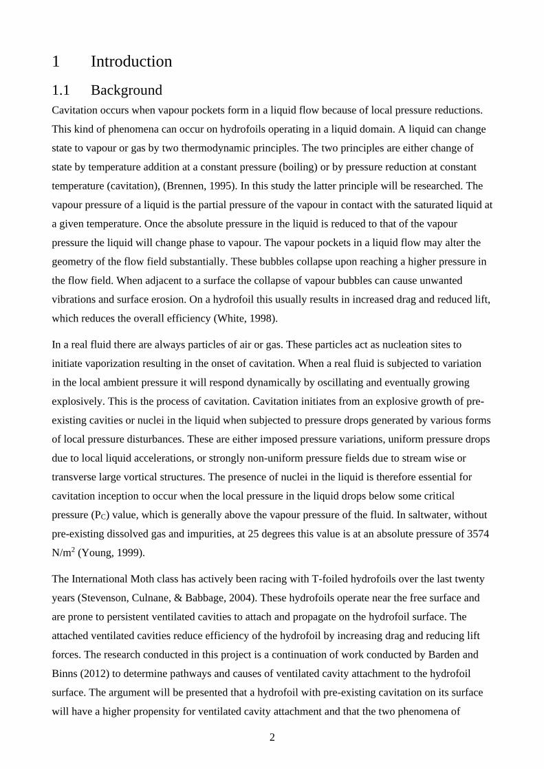
1.1 Background
Cavitation occurs when vapour pockets form in a liquid flow because of local pressure reductions.
This kind of phenomena can occur on hydrofoils operating in a liquid domain. A liquid can change
state to vapour or gas by two thermodynamic principles. The two principles are either change of
state by temperature addition at a constant pressure (boiling) or by pressure reduction at constant
temperature (cavitation), (Brennen, 1995). In this study the latter principle will be researched. The
vapour pressure of a liquid is the partial pressure of the vapour in contact with the saturated liquid at
a given temperature. Once the absolute pressure in the liquid is reduced to that of the vapour
pressure the liquid will change phase to vapour. The vapour pockets in a liquid flow may alter the
geometry of the flow field substantially. These bubbles collapse upon reaching a higher pressure in
the flow field. When adjacent to a surface the collapse of vapour bubbles can cause unwanted
vibrations and surface erosion. On a hydrofoil this usually results in increased drag and reduced lift,
which reduces the overall efficiency (White, 1998).
In a real fluid there are always particles of air or gas. These particles act as nucleation sites to
initiate vaporization resulting in the onset of cavitation. When a real fluid is subjected to variation
in the local ambient pressure it will respond dynamically by oscillating and eventually growing
explosively. This is the process of cavitation. Cavitation initiates from an explosive growth of pre-
existing cavities or nuclei in the liquid when subjected to pressure drops generated by various forms
of local pressure disturbances. These are either imposed pressure variations, uniform pressure drops
due to local liquid accelerations, or strongly non-uniform pressure fields due to stream wise or
transverse large vortical structures. The presence of nuclei in the liquid is therefore essential for
cavitation inception to occur when the local pressure in the liquid drops below some critical
pressure (PC) value, which is generally above the vapour pressure of the fluid. In saltwater, without
pre-existing dissolved gas and impurities, at 25 degrees this value is at an absolute pressure of 3574
N/m2 (Young, 1999).
The International Moth class has actively been racing with T-foiled hydrofoils over the last twenty
years (Stevenson, Culnane, & Babbage, 2004). These hydrofoils operate near the free surface and
are prone to persistent ventilated cavities to attach and propagate on the hydrofoil surface. The
attached ventilated cavities reduce efficiency of the hydrofoil by increasing drag and reducing lift
forces. The research conducted in this project is a continuation of work conducted by Barden and
Binns (2012) to determine pathways and causes of ventilated cavity attachment to the hydrofoil
surface. The argument will be presented that a hydrofoil with pre-existing cavitation on its surface
will have a higher propensity for ventilated cavity attachment and that the two phenomena of
3
cavitation and ventilation propagate in the same low-pressure regions of the hydrofoil as verified in
full scale testing.
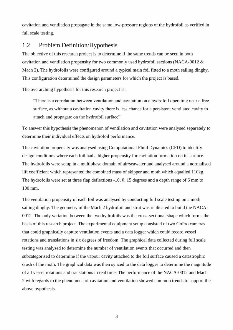
1.2 Problem Definition/Hypothesis
The objective of this research project is to determine if the same trends can be seen in both
cavitation and ventilation propensity for two commonly used hydrofoil sections (NACA-0012 &
Mach 2). The hydrofoils were configured around a typical main foil fitted to a moth sailing dinghy.
This configuration determined the design parameters for which the project is based.
The overarching hypothesis for this research project is:
“There is a correlation between ventilation and cavitation on a hydrofoil operating near a free
surface, as without a cavitation cavity there is less chance for a persistent ventilated cavity to
attach and propagate on the hydrofoil surface”
To answer this hypothesis the phenomenon of ventilation and cavitation were analysed separately to
determine their individual effects on hydrofoil performance.
The cavitation propensity was analysed using Computational Fluid Dynamics (CFD) to identify
design conditions where each foil had a higher propensity for cavitation formation on its surface.
The hydrofoils were setup in a multiphase domain of air/seawater and analysed around a normalised
lift coefficient which represented the combined mass of skipper and moth which equalled 110kg.
The hydrofoils were set at three flap deflections -10, 0, 15 degrees and a depth range of 6 mm to
100 mm.
The ventilation propensity of each foil was analysed by conducting full scale testing on a moth
sailing dinghy. The geometry of the Mach 2 hydrofoil and strut was replicated to build the NACA-
0012. The only variation between the two hydrofoils was the cross-sectional shape which forms the
basis of this research project. The experimental equipment setup consisted of two GoPro cameras
that could graphically capture ventilation events and a data logger which could record vessel
rotations and translations in six degrees of freedom. The graphical data collected during full scale
testing was analysed to determine the number of ventilation events that occurred and then
subcategorised to determine if the vapour cavity attached to the foil surface caused a catastrophic
crash of the moth. The graphical data was then synced to the data logger to determine the magnitude
of all vessel rotations and translations in real time. The performance of the NACA-0012 and Mach
2 with regards to the phenomena of cavitation and ventilation showed common trends to support the
above hypothesis.
4
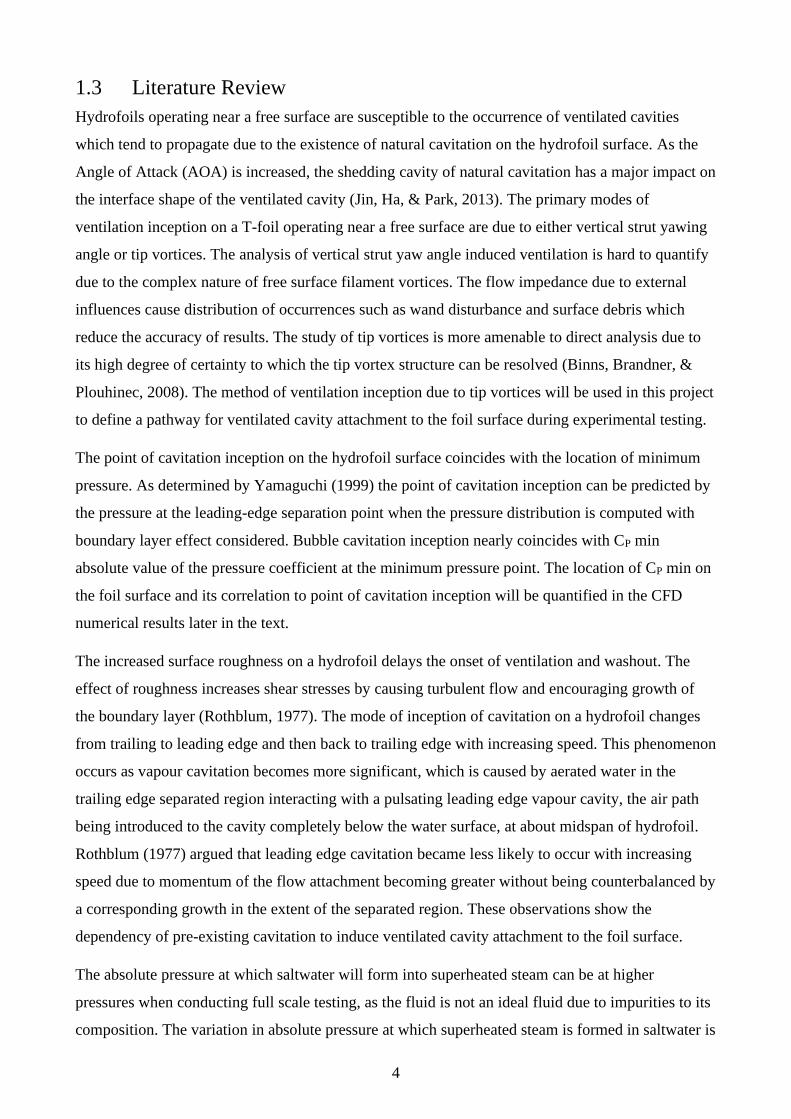
1.3 Literature Review
Hydrofoils operating near a free surface are susceptible to the occurrence of ventilated cavities
which tend to propagate due to the existence of natural cavitation on the hydrofoil surface. As the
Angle of Attack (AOA) is increased, the shedding cavity of natural cavitation has a major impact on
the interface shape of the ventilated cavity (Jin, Ha, & Park, 2013). The primary modes of
ventilation inception on a T-foil operating near a free surface are due to either vertical strut yawing
angle or tip vortices. The analysis of vertical strut yaw angle induced ventilation is hard to quantify
due to the complex nature of free surface filament vortices. The flow impedance due to external
influences cause distribution of occurrences such as wand disturbance and surface debris which
reduce the accuracy of results. The study of tip vortices is more amenable to direct analysis due to
its high degree of certainty to which the tip vortex structure can be resolved (Binns, Brandner, &
Plouhinec, 2008). The method of ventilation inception due to tip vortices will be used in this project
to define a pathway for ventilated cavity attachment to the foil surface during experimental testing.
The point of cavitation inception on the hydrofoil surface coincides with the location of minimum
pressure. As determined by Yamaguchi (1999) the point of cavitation inception can be predicted by
the pressure at the leading-edge separation point when the pressure distribution is computed with
boundary layer effect considered. Bubble cavitation inception nearly coincides with CP min
absolute value of the pressure coefficient at the minimum pressure point. The location of CP min on
the foil surface and its correlation to point of cavitation inception will be quantified in the CFD
numerical results later in the text.
The increased surface roughness on a hydrofoil delays the onset of ventilation and washout. The
effect of roughness increases shear stresses by causing turbulent flow and encouraging growth of
the boundary layer (Rothblum, 1977). The mode of inception of cavitation on a hydrofoil changes
from trailing to leading edge and then back to trailing edge with increasing speed. This phenomenon
occurs as vapour cavitation becomes more significant, which is caused by aerated water in the
trailing edge separated region interacting with a pulsating leading edge vapour cavity, the air path
being introduced to the cavity completely below the water surface, at about midspan of hydrofoil.
Rothblum (1977) argued that leading edge cavitation became less likely to occur with increasing
speed due to momentum of the flow attachment becoming greater without being counterbalanced by
a corresponding growth in the extent of the separated region. These observations show the
dependency of pre-existing cavitation to induce ventilated cavity attachment to the foil surface.
The absolute pressure at which saltwater will form into superheated steam can be at higher
pressures when conducting full scale testing, as the fluid is not an ideal fluid due to impurities to its
composition. The variation in absolute pressure at which superheated steam is formed in saltwater is
5
due to bubble dynamics. The mechanism of bubble/nuclei formation is a major contributor to
inception of cavitation. Chahine (2004) argued that bubble inception has to start from the
observation that, any real liquid contains nuclei which when subjected to variations in the local
ambient pressure will respond dynamically by oscillating and eventually growing explosively
(cavitation). The inclusion of nuclei and nuclei dynamics must be considered when comparing
numerical and experimental results. This research showed that cavitation inception could form at
higher absolute pressures in full scale testing than in the numerical analysis, due to bubble dynamics
and the presence of pre-exiting bubble/nuclei in fluid which changes the chemical composition and
material properties of saltwater. The analysis of foil cavitation propensity must consider numerical
models that show absolute pressures in the region slightly above the pressure at which saltwater
forms superheated steam. The implications of this research will form the basis to link the
phenomenon of ventilated cavity attachment to foil in full scale testing and results for absolute
pressure taken from the numerical analysis.
The results obtained from numerical analysis need to be qualified and quantified through
conducting full scale testing. Erney (2008) analysed compressible CFD cavitation solvers using a
K-Epsilon turbulence model and a NACA-66 foil section. The results were validated against
experimental work produced by Rouse and McNown (1948). The comparison found that leading
edge and mid chord cavitation obtained in numerical results were in good agreement with
experimental data in terms of surface pressure and cavity lengths. The major variation between
numerical and experimental results was due to increased foil incidence and lowering of cavitation
number. The numerical analysis seemed to under predict leading edge cavitation and size of vapour
cavity. The variation was attributed to increased pressure gradient over the suction side of the foil.
This research showed numerical results will under predict cavitation and cavity length, with
increased foil incidence and lowered cavitation number. This observation supports the hypothesis
that foils which show vapour cavity attachment in full scale testing have a higher cavitation
propensity, even though the foil did not have either cavitation or a vapour cavity in the numerical
analysis.
The existence during full scale testing of ventilation, cavitation, or a combination of both is a topic
which has been regularly discussed. Emonson (2009) researched the possibility of identifying a
cavitation number at which cavitation would occur on a T-foil. Chen and Wu (2009) provided
significant insight into physical symptoms that would be observed in the case of cavitation, though
provided no definitive point at which cavitation was predicted to occur. The literature presented
with regards to propellor and duct cavitation showed that at cavitation numbers less than 0.4,
cavitation should occur. Full scale experiments were conducted by Emonson (2009) to verify this
6
hypothesis, which were performed on a T-foil at cavitation numbers less than 0.4. The conclusion
was that cavitation was not present or was not easily observable from the experiments carried out.
The research showed the complexities of defining the existence of either cavitation or ventilation in
full scale testing. This showed the significance of using tools such as CFD to determine design
conditions where the hydrofoil is operating at low absolute pressure close or near to the vapor
pressure. The use of a pressure sensor on the upper surface of the foil near the leading edge was also
considered for this project to get a localised pressure value, though was abandoned due to the
complex construction techniques required to incorporate the sensor inside the hydrofoil laminate.
These two previous mentioned methods would aid the identification of either cavitation, ventilation,
or a combination of both on the surface of the hydrofoil.
1.4 Novel Components of Work
The phenomena of cavitation and ventilation were analysed separately to determine if the same
trends can be seen for two commonly used hydrofoil sections (NACA-0012 & Mach 2). The two
primary methods used to research the problem definition/hypothesis are summarised in this section.
1.4.1 CFD Numerical Analysis to Research Cavitation Phenomena
The cavitation propensity of the two hydrofoils was analysed using software from ANSYS (2020).
The software applies the Rayleigh-Plesset model to describe the interphase mass transformation in
the framework of a homogenous multiphase model. The two-phase system is solved for the vapour
and the liquid with a non-condensable gas. The CFD model was a two-dimensional multiphase
domain which included seawater and air. The foil depth was defined by varying the height of the
free surface above the hydrofoil which was a function of hydrostatic pressure, buoyancy, gravity,
and seawater/air volume fractions. The CFD analysis was solved using the transient model which
encompasses the Unsteady Reynold Average Navier-Stokes (URANS) equations resolved at a given
timestep as selected in the Courant number convergence study. The CFD analysis was setup to be a
simplified two-dimensional model that identifies design conditions where each foil had a high
propensity for cavitation formation on its surface.
1.4.2 Full Scale Testing to Research Ventilation Phenomena
The ventilation phenomena over the two hydrofoils was analysed in full scale testing. The NACA-
0012 and Mach 2 were setup to replicate design conditions used in the CFD analysis. The
experimental equipment consisted of two GoPro cameras to graphically collect data, along with a
data logger to record all vessel rotations and translations in six degrees of freedom. The full-scale
graphical data was analysed with the number of ventilation events defined and then sub-categorised
as either attached or non-attached cavity to the hydrofoil surface. The graphical data was then
synced to the data logger to determine all vessel rotations and translations.
7
1.4.3 CFD Numerical Analysis and Full-Scale Testing Results
The separate analysis of cavitation with CFD and ventilation in full-scale testing shows their
individual characteristics and defines design conditions where they are likely to occur. The analysis
results will show that pre-existing cavitation on the hydrofoil surface can increase the propensity of
a ventilated cavity tracking from the free surface and attaching to the hydrofoil in regions already
habited by pre-existing cavitation.
The data collection in full scale testing and two-dimensional CFD analysis provide two separate
design tools to study the individual effects of ventilation and cavitation, respectively. This is
required as the existence of both phenomena cannot be determined concurrently when conducting
full scale testing. The research results will show that vapour cavity attachment and cavitation both
occurred in regions around the foil’s leading edge where the absolute pressure was below the PC for
saltwater. The analysis methods used in this project could be used to analyse other forms of cavity
attachment to hydrofoils including strut induced ventilation and interference due to external
influences (wand or disturbed wake over rudder T-Foil).
1.5 Effect of Ventilation on Hydrofoil Efficiency
The existence of ventilated cavities on the surface of the hydrofoil reduces it’s efficiency by
displacing seawater in the effected region and lowering the pressure differential between the high-
and low-pressure surfaces. The lower pressure differential causes reduced fluid circulation around
the hydrofoil surface. The two pathways for ventilated cavity attachment to the surface of a T-Foil
hydrofoil configuration are by either trailing edge tip vortices or propagation along surface of the
vertical strut, as shown by Barden and Binns (2012). The determination of expected design
conditions for which the hydrofoil operates can reduce ventilation occurrences by understanding the
magnitude of the Cavitation and Reynolds numbers Emonson (2009). The design techniques
adopted in the International Moth Class to reduce ventilation propagation along the surface of the
vertical strut have involved either adding a fence on the forward edge of the vertical strut
immediately below the waterline and increasing surface roughness of the vertical strut, while
reduction of tip vortices disturbance has been done by fitting of wing tips to the hydrofoil. The
analysis of hydrofoil cross sectional shape and it’s propensity to ventilation has not received much
attention and is evident due to negligible change in hydrofoil cross section used over the last ten
years as shown by Beaver and Zseleczky (2009).
1.6 The International Moth Class
The International Moth is a single-handed development class boat that has its origins from 1928
when Len Morris built a hard chined scow to sail on Lake Inverloch in Victoria. The ethos of the
8
moth class is to allow an open development platform with limited rules which encourage innovative
design and has laid the way for some innovative development in dinghy sailing since the class
inception in 1928. The primary rules which dictate the moth class are as follows:
• Maximum overall length of 3.355m
• Maximum width of 2.25m
• Maximum sail area of 8.25m2.
• No catamarans or windsurfers
• Maximum of one crew per boat
• No restrictions on materials, construction methods and no minimum weight limit.
The moth class has continually evolved and in the year 2000 hydrofoils were successfully
introduced at a world titles and showed the potential speed increase by operating the vessel on
hydrofoils. The original configuration of surface piercing struts fitted to the outer wing bars was out
lawed as it was deemed to resemble a catamaran. The design was evolved in 2001 by John Illett
who fitted two centreline T-Foils, one to the centreboard case and the other to where the rudder is
fitted (Stevenson et al., 2004). This configuration has formed the basis for the design and
development of the modern-day moth dinghy. The operation of the hydrofoil system fitted to the
moth dinghy is shown in Figure J-3.
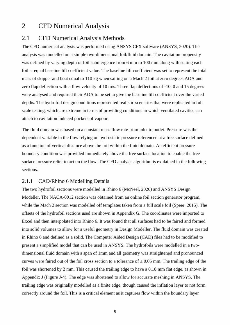
9
2 CFD Numerical Analysis
2.1 CFD Numerical Analysis Methods
The CFD numerical analysis was performed using ANSYS CFX software (ANSYS, 2020). The
analysis was modelled on a simple two-dimensional foil/fluid domain. The cavitation propensity
was defined by varying depth of foil submergence from 6 mm to 100 mm along with setting each
foil at equal baseline lift coefficient value. The baseline lift coefficient was set to represent the total
mass of skipper and boat equal to 110 kg when sailing on a Mach 2 foil at zero degrees AOA and
zero flap deflection with a flow velocity of 10 m/s. Three flap deflections of -10, 0 and 15 degrees
were analysed and required their AOA to be set to give the baseline lift coefficient over the varied
depths. The hydrofoil design conditions represented realistic scenarios that were replicated in full
scale testing, which are extreme in terms of providing conditions in which ventilated cavities can
attach to cavitation induced pockets of vapour.
The fluid domain was based on a constant mass flow rate from inlet to outlet. Pressure was the
dependent variable in the flow relying on hydrostatic pressure referenced at a free surface defined
as a function of vertical distance above the foil within the fluid domain. An efficient pressure
boundary condition was provided immediately above the free surface location to enable the free
surface pressure relief to act on the flow. The CFD analysis algorithm is explained in the following
sections.
2.1.1 CAD/Rhino 6 Modelling Details
The two hydrofoil sections were modelled in Rhino 6 (McNeel, 2020) and ANSYS Design
Modeller. The NACA-0012 section was obtained from an online foil section generator program,
while the Mach 2 section was modelled off templates taken from a full scale foil (Speer, 2015). The
offsets of the hydrofoil sections used are shown in Appendix G. The coordinates were imported to
Excel and then interpolated into Rhino 6. It was found that all surfaces had to be faired and formed
into solid volumes to allow for a useful geometry in Design Modeller. The fluid domain was created
in Rhino 6 and defined as a solid. The Computer Aided Design (CAD) files had to be modified to
present a simplified model that can be used in ANSYS. The hydrofoils were modelled in a two-
dimensional fluid domain with a span of 1mm and all geometry was straightened and pronounced
curves were faired out of the foil cross section to a tolerance of ± 0.05 mm. The trailing edge of the
foil was shortened by 2 mm. This caused the trailing edge to have a 0.18 mm flat edge, as shown in
Appendix J (Figure J-4). The edge was shortened to allow for accurate meshing in ANSYS. The
trailing edge was originally modelled as a finite edge, though caused the inflation layer to not form
correctly around the foil. This is a critical element as it captures flow within the boundary layer
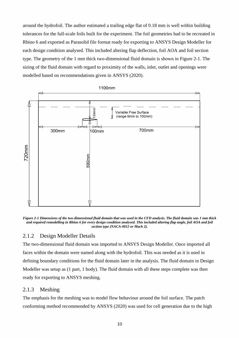
10
around the hydrofoil. The author estimated a trailing edge flat of 0.18 mm is well within building
tolerances for the full-scale foils built for the experiment. The foil geometries had to be recreated in
Rhino 6 and exported as Parasolid file format ready for exporting to ANSYS Design Modeller for
each design condition analysed. This included altering flap deflection, foil AOA and foil section
type. The geometry of the 1 mm thick two-dimensional fluid domain is shown in Figure 2-1. The
sizing of the fluid domain with regard to proximity of the walls, inlet, outlet and openings were
modelled based on recommendations given in ANSYS (2020).
Figure 2-1 Dimensions of the two-dimensional fluid domain that was used in the CFD analysis. The fluid domain was 1 mm thick
and required remodelling in Rhino 6 for every design condition analysed. This included altering flap angle, foil AOA and foil
section type (NACA-0012 or Mach 2).
2.1.2 Design Modeller Details
The two-dimensional fluid domain was imported to ANSYS Design Modeller. Once imported all
faces within the domain were named along with the hydrofoil. This was needed as it is used in
defining boundary conditions for the fluid domain later in the analysis. The fluid domain in Design
Modeller was setup as (1 part, 1 body). The fluid domain with all these steps complete was then
ready for exporting to ANSYS meshing.
2.1.3 Meshing
The emphasis for the meshing was to model flow behaviour around the foil surface. The patch
conforming method recommended by ANSYS (2020) was used for cell generation due to the high
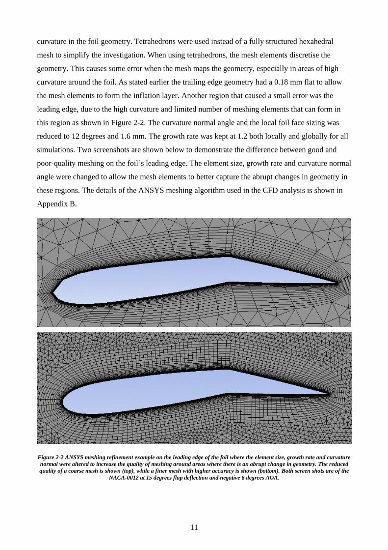
11
curvature in the foil geometry. Tetrahedrons were used instead of a fully structured hexahedral
mesh to simplify the investigation. When using tetrahedrons, the mesh elements discretise the
geometry. This causes some error when the mesh maps the geometry, especially in areas of high
curvature around the foil. As stated earlier the trailing edge geometry had a 0.18 mm flat to allow
the mesh elements to form the inflation layer. Another region that caused a small error was the
leading edge, due to the high curvature and limited number of meshing elements that can form in
this region as shown in Figure 2-2. The curvature normal angle and the local foil face sizing was
reduced to 12 degrees and 1.6 mm. The growth rate was kept at 1.2 both locally and globally for all
simulations. Two screenshots are shown below to demonstrate the difference between good and
poor-quality meshing on the foil’s leading edge. The element size, growth rate and curvature normal
angle were changed to allow the mesh elements to better capture the abrupt changes in geometry in
these regions. The details of the ANSYS meshing algorithm used in the CFD analysis is shown in
Appendix B.
Figure 2-2 ANSYS meshing refinement example on the leading edge of the foil where the element size, growth rate and curvature
normal were altered to increase the quality of meshing around areas where there is an abrupt change in geometry. The reduced
quality of a coarse mesh is shown (top), while a finer mesh with higher accuracy is shown (bottom). Both screen shots are of the
NACA-0012 at 15 degrees flap deflection and negative 6 degrees AOA.
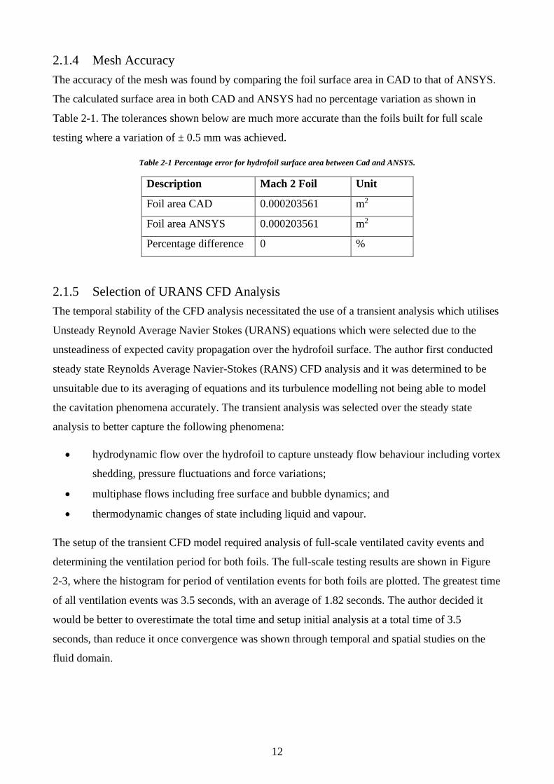
12
2.1.4 Mesh Accuracy
The accuracy of the mesh was found by comparing the foil surface area in CAD to that of ANSYS.
The calculated surface area in both CAD and ANSYS had no percentage variation as shown in
Table 2-1. The tolerances shown below are much more accurate than the foils built for full scale
testing where a variation of ± 0.5 mm was achieved.
Table 2-1 Percentage error for hydrofoil surface area between Cad and ANSYS.
Description Mach 2 Foil Unit
Foil area CAD 0.000203561 m2
Foil area ANSYS 0.000203561 m2
Percentage difference 0 %
2.1.5 Selection of URANS CFD Analysis
The temporal stability of the CFD analysis necessitated the use of a transient analysis which utilises
Unsteady Reynold Average Navier Stokes (URANS) equations which were selected due to the
unsteadiness of expected cavity propagation over the hydrofoil surface. The author first conducted
steady state Reynolds Average Navier-Stokes (RANS) CFD analysis and it was determined to be
unsuitable due to its averaging of equations and its turbulence modelling not being able to model
the cavitation phenomena accurately. The transient analysis was selected over the steady state
analysis to better capture the following phenomena:
• hydrodynamic flow over the hydrofoil to capture unsteady flow behaviour including vortex
shedding, pressure fluctuations and force variations;
• multiphase flows including free surface and bubble dynamics; and
• thermodynamic changes of state including liquid and vapour.
The setup of the transient CFD model required analysis of full-scale ventilated cavity events and
determining the ventilation period for both foils. The full-scale testing results are shown in Figure
2-3, where the histogram for period of ventilation events for both foils are plotted. The greatest time
of all ventilation events was 3.5 seconds, with an average of 1.82 seconds. The author decided it
would be better to overestimate the total time and setup initial analysis at a total time of 3.5
seconds, than reduce it once convergence was shown through temporal and spatial studies on the
fluid domain.
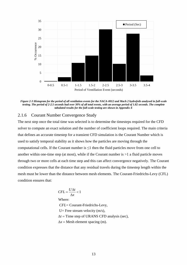
13
Figure 2-3 Histogram for the period of all ventilation events for the NACA-0012 and Mach 2 hydrofoils analysed in full-scale
testing. The period of 2-2.5 seconds had over 30% of all total events, with an average period of 1.82 seconds. The complete
tabulated results for the full-scale testing are shown in Appendix E
2.1.6 Courant Number Convergence Study
The next step once the total time was selected is to determine the timesteps required for the CFD
solver to compute an exact solution and the number of coefficient loops required. The main criteria
that defines an accurate timestep for a transient CFD simulation is the Courant Number which is
used to satisfy temporal stability as it shows how the particles are moving through the
computational cells. If the Courant number is ≤1 then the fluid particles move from one cell to
another within one-time step (at most), while if the Courant number is >1 a fluid particle moves
through two or more cells at each time step and this can affect convergence negatively. The Courant
condition expresses that the distance that any residual travels during the timestep length within the
mesh must be lower than the distance between mesh elements. The Courant-Friedrichs-Levy (CFL)
condition ensures that:
1
Where:
= Courant-Friedrichs-Levy,
U= Free stream velocity (m/s),
Time step of URANS CFD analysis (sec),
Mesh element spacing (m).
U tCFL
x
CFL
t
x
=
=
=
0
5
10
15
20
25
30
35
0-0.5 0.5-1 1-1.5 1.5-2 2-2.5 2.5-3 3-3.5 3.5-4
% O
ccurr
ence
Period of Ventillation Event (seconds)
Period (Sec)
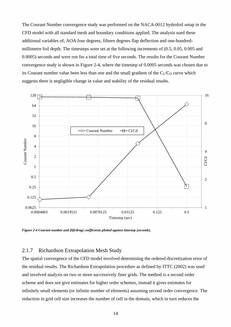
14
The Courant Number convergence study was performed on the NACA-0012 hydrofoil setup in the
CFD model with all standard mesh and boundary conditions applied. The analysis used these
additional variables of; AOA four degrees, fifteen degrees flap deflection and one-hundred-
millimetre foil depth. The timesteps were set at the following increments of (0.5, 0.05, 0.005 and
0.0005) seconds and were run for a total time of five seconds. The results for the Courant Number
convergence study is shown in Figure 2-4, where the timestep of 0.0005 seconds was chosen due to
its Courant number value been less than one and the small gradient of the CL/CD curve which
suggests there is negligible change in value and stability of the residual results.
Figure 2-4 Courant number and (lift/drag) coefficients plotted against timestep (seconds).
2.1.7 Richardson Extrapolation Mesh Study
The spatial convergence of the CFD model involved determining the ordered discretization error of
the residual results. The Richardson Extrapolation procedure as defined by ITTC (2002) was used
and involved analysis on two or more successively finer grids. The method is a second order
scheme and does not give estimates for higher order schemes, instead it gives estimates for
infinitely small elements (or infinite number of elements) assuming second order convergence. The
reduction in grid cell size increases the number of cell in the domain, which in turn reduces the
1
2
4
8
16
0.0625
0.125
0.25
0.5
1
2
4
8
16
32
64
128
0.0004883 0.0019531 0.0078125 0.03125 0.125 0.5
Cl/
Cd
Co
ura
nt
Num
ber
Timestep (sec)
Courant Number Cl/Cd
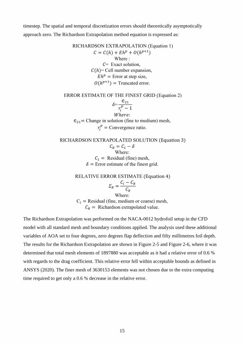
15
timestep. The spatial and temporal discretization errors should theoretically asymptotically
approach zero. The Richardson Extrapolation method equation is expressed as:
RICHARDSON EXTRAPOLATION (Equation 1)
𝐶 = 𝐶(ℎ) + 𝐸ℎ𝑝 + 𝑂(ℎ𝑝+1)Where :
𝐶= Exact solution,
𝐶(ℎ)= Cell number expansion,
𝐸ℎ𝑝 = Error at step size,
𝑂(ℎ𝑝+1) = Truncated error.
ERROR ESTIMATE OF THE FINEST GRID (Equation 2)
𝛿=∈21
𝑟𝑖𝑝 − 1
𝑊ℎ𝑒𝑟𝑒:∈21= Change in solution (fine to medium) mesh,
𝑟𝑖𝑝 = Convergence ratio.
RICHARDSON EXTRAPOLATED SOLUTION (Equation 3)𝐶𝑅 = 𝐶1 − 𝛿
Where:
𝐶1 = Residual (fine) mesh,
𝛿 = Error estimate of the finest grid.
RELATIVE ERROR ESTIMATE (Equation 4)
𝛴𝑅 =𝐶𝑖 − 𝐶𝑅
𝐶𝑅
Where:
C𝑖 = Residual (fine, medium or coarse) mesh,
𝐶𝑅 = Richardson extrapolated value.
The Richardson Extrapolation was performed on the NACA-0012 hydrofoil setup in the CFD
model with all standard mesh and boundary conditions applied. The analysis used these additional
variables of AOA set to four degrees, zero degrees flap deflection and fifty millimetres foil depth.
The results for the Richardson Extrapolation are shown in Figure 2-5 and Figure 2-6, where it was
determined that total mesh elements of 1897880 was acceptable as it had a relative error of 0.6 %
with regards to the drag coefficient. This relative error fell within acceptable bounds as defined in
ANSYS (2020). The finer mesh of 3630153 elements was not chosen due to the extra computing
time required to get only a 0.6 % decrease in the relative error.
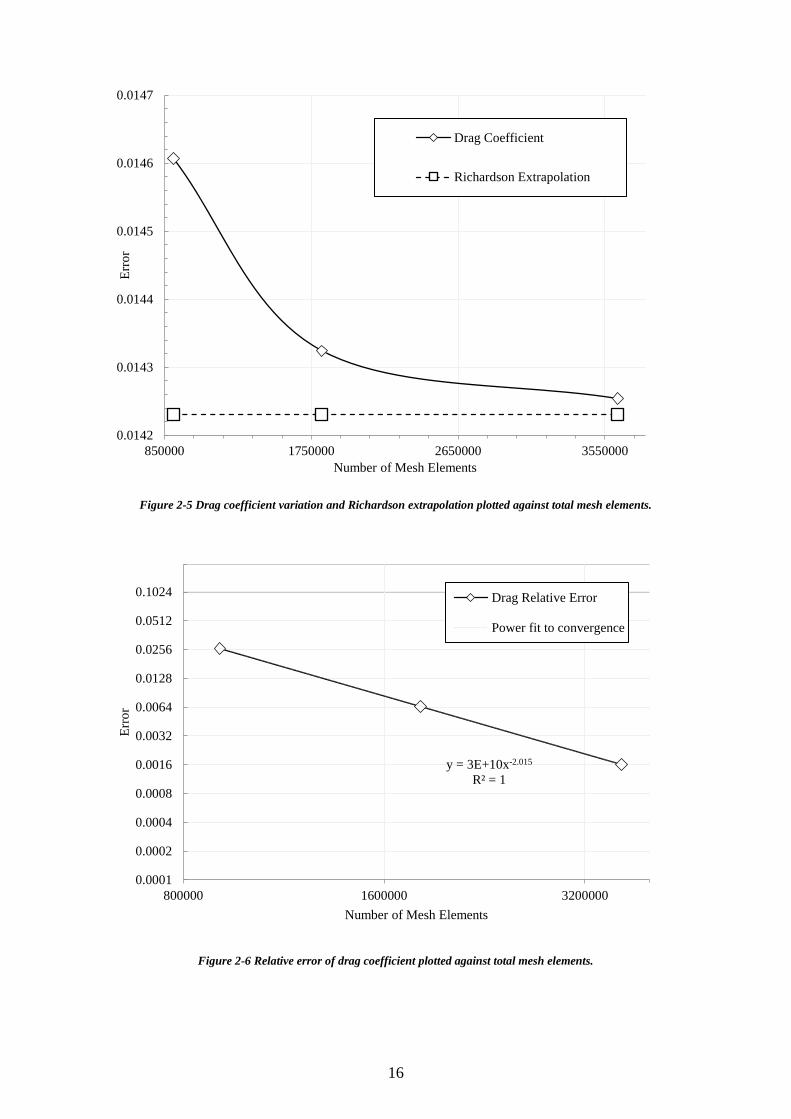
16
Figure 2-5 Drag coefficient variation and Richardson extrapolation plotted against total mesh elements.
Figure 2-6 Relative error of drag coefficient plotted against total mesh elements.
0.0142
0.0143
0.0144
0.0145
0.0146
0.0147
850000 1750000 2650000 3550000
Err
or
Number of Mesh Elements
Drag Coefficient
Richardson Extrapolation
y = 3E+10x-2.015
R² = 1
0.0001
0.0002
0.0004
0.0008
0.0016
0.0032
0.0064
0.0128
0.0256
0.0512
0.1024
800000 1600000 3200000
Err
or
Number of Mesh Elements
Drag Relative Error
Power fit to convergence
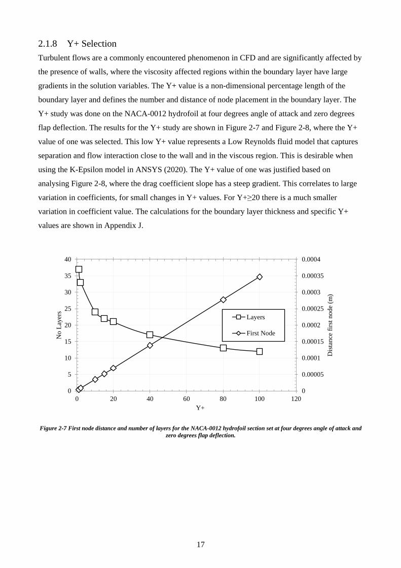
17
2.1.8 Y+ Selection
Turbulent flows are a commonly encountered phenomenon in CFD and are significantly affected by
the presence of walls, where the viscosity affected regions within the boundary layer have large
gradients in the solution variables. The Y+ value is a non-dimensional percentage length of the
boundary layer and defines the number and distance of node placement in the boundary layer. The
Y+ study was done on the NACA-0012 hydrofoil at four degrees angle of attack and zero degrees
flap deflection. The results for the Y+ study are shown in Figure 2-7 and Figure 2-8, where the Y+
value of one was selected. This low Y+ value represents a Low Reynolds fluid model that captures
separation and flow interaction close to the wall and in the viscous region. This is desirable when
using the K-Epsilon model in ANSYS (2020). The Y+ value of one was justified based on
analysing Figure 2-8, where the drag coefficient slope has a steep gradient. This correlates to large
variation in coefficients, for small changes in Y+ values. For Y+≥20 there is a much smaller
variation in coefficient value. The calculations for the boundary layer thickness and specific Y+
values are shown in Appendix J.
Figure 2-7 First node distance and number of layers for the NACA-0012 hydrofoil section set at four degrees angle of attack and
zero degrees flap deflection.
0
0.00005
0.0001
0.00015
0.0002
0.00025
0.0003
0.00035
0.0004
0
5
10
15
20
25
30
35
40
0 20 40 60 80 100 120
Y+
Dis
tance
fir
st n
od
e (m
)
No
Lay
ers
Layers
First Node
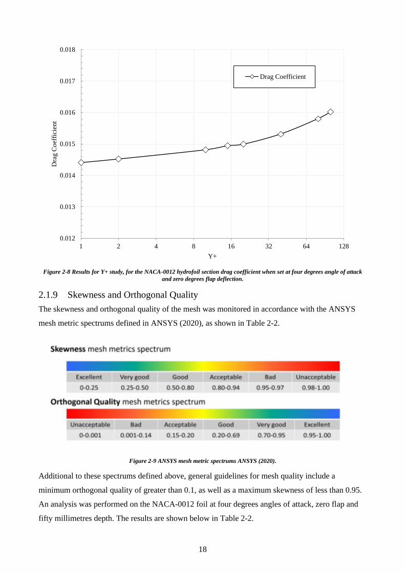
18
Figure 2-8 Results for Y+ study, for the NACA-0012 hydrofoil section drag coefficient when set at four degrees angle of attack
and zero degrees flap deflection.
2.1.9 Skewness and Orthogonal Quality
The skewness and orthogonal quality of the mesh was monitored in accordance with the ANSYS
mesh metric spectrums defined in ANSYS (2020), as shown in Table 2-2.
Figure 2-9 ANSYS mesh metric spectrums ANSYS (2020).
Additional to these spectrums defined above, general guidelines for mesh quality include a
minimum orthogonal quality of greater than 0.1, as well as a maximum skewness of less than 0.95.
An analysis was performed on the NACA-0012 foil at four degrees angles of attack, zero flap and
fifty millimetres depth. The results are shown below in Table 2-2.
0.012
0.013
0.014
0.015
0.016
0.017
0.018
1 2 4 8 16 32 64 128
Dra
g C
oef
fici
ent
Y+
Drag Coefficient
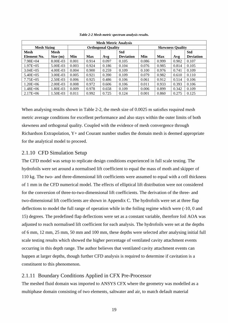
19
Table 2-2 Mesh metric spectrum analysis results.
Mesh Metric Analysis
Mesh Sizing Orthogonal Quality Skewness Quality
Mesh
Element No.
Mesh
Size (m) Min Max Avg
Std
Deviation Min Max Avg
Std
Deviation
7.98E+04 8.00E-03 0.001 0.914 0.097 0.105 0.086 0.999 0.902 0.107
1.97E+05 5.00E-03 0.003 0.924 0.186 0.104 0.076 0.985 0.814 0.105
3.04E+05 4.00E-03 0.004 0.900 0.259 0.109 0.100 0.976 0.741 0.109
5.40E+05 3.00E-03 0.005 0.921 0.390 0.109 0.079 0.982 0.610 0.110
7.75E+05 2.50E-03 0.006 0.925 0.486 0.106 0.061 0.912 0.514 0.106
1.20E+06 2.00E-03 0.008 0.972 0.606 0.106 0.011 0.933 0.393 0.106
1.48E+06 1.80E-03 0.009 0.978 0.658 0.109 0.006 0.899 0.342 0.109
2.17E+06 1.50E-03 0.011 0.992 0.725 0.124 0.001 0.860 0.275 0.125
When analysing results shown in Table 2-2, the mesh size of 0.0025 m satisfies required mesh
metric average conditions for excellent performance and also stays within the outer limits of both
skewness and orthogonal quality. Coupled with the evidence of mesh convergence through
Richardson Extrapolation, Y+ and Courant number studies the domain mesh is deemed appropriate
for the analytical model to proceed.
2.1.10 CFD Simulation Setup
The CFD model was setup to replicate design conditions experienced in full scale testing. The
hydrofoils were set around a normalised lift coefficient to equal the mass of moth and skipper of
110 kg. The two- and three-dimensional lift coefficients were assumed to equal with a cell thickness
of 1 mm in the CFD numerical model. The effects of elliptical lift distribution were not considered
for the conversion of three-to-two-dimensional lift coefficients. The derivation of the three- and
two-dimensional lift coefficients are shown in Appendix C. The hydrofoils were set at three flap
deflections to model the full range of operation while in the foiling regime which were (-10, 0 and
15) degrees. The predefined flap deflections were set as a constant variable, therefore foil AOA was
adjusted to reach normalised lift coefficient for each analysis. The hydrofoils were set at the depths
of 6 mm, 12 mm, 25 mm, 50 mm and 100 mm, these depths were selected after analysing initial full
scale testing results which showed the higher percentage of ventilated cavity attachment events
occurring in this depth range. The author believes that ventilated cavity attachment events can
happen at larger depths, though further CFD analysis is required to determine if cavitation is a
constituent to this phenomenon.
2.1.11 Boundary Conditions Applied in CFX Pre-Processor
The meshed fluid domain was imported to ANSYS CFX where the geometry was modelled as a
multiphase domain consisting of two elements, saltwater and air, to match default material
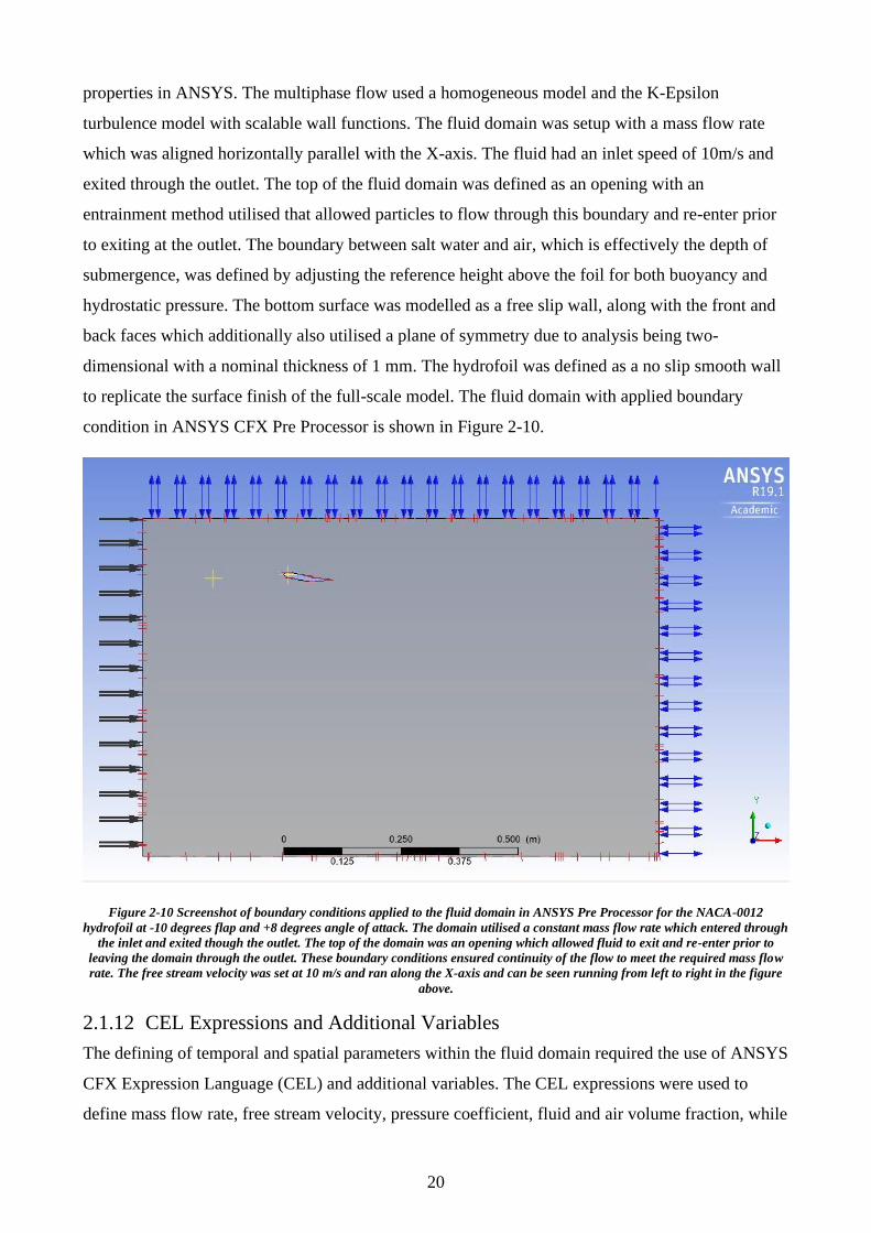
20
properties in ANSYS. The multiphase flow used a homogeneous model and the K-Epsilon
turbulence model with scalable wall functions. The fluid domain was setup with a mass flow rate
which was aligned horizontally parallel with the X-axis. The fluid had an inlet speed of 10m/s and
exited through the outlet. The top of the fluid domain was defined as an opening with an
entrainment method utilised that allowed particles to flow through this boundary and re-enter prior
to exiting at the outlet. The boundary between salt water and air, which is effectively the depth of
submergence, was defined by adjusting the reference height above the foil for both buoyancy and
hydrostatic pressure. The bottom surface was modelled as a free slip wall, along with the front and
back faces which additionally also utilised a plane of symmetry due to analysis being two-
dimensional with a nominal thickness of 1 mm. The hydrofoil was defined as a no slip smooth wall
to replicate the surface finish of the full-scale model. The fluid domain with applied boundary
condition in ANSYS CFX Pre Processor is shown in Figure 2-10.
Figure 2-10 Screenshot of boundary conditions applied to the fluid domain in ANSYS Pre Processor for the NACA-0012
hydrofoil at -10 degrees flap and +8 degrees angle of attack. The domain utilised a constant mass flow rate which entered through
the inlet and exited though the outlet. The top of the domain was an opening which allowed fluid to exit and re-enter prior to
leaving the domain through the outlet. These boundary conditions ensured continuity of the flow to meet the required mass flow
rate. The free stream velocity was set at 10 m/s and ran along the X-axis and can be seen running from left to right in the figure
above.
2.1.12 CEL Expressions and Additional Variables
The defining of temporal and spatial parameters within the fluid domain required the use of ANSYS
CFX Expression Language (CEL) and additional variables. The CEL expressions were used to
define mass flow rate, free stream velocity, pressure coefficient, fluid and air volume fraction, while
21
the additional variables were used to geometrically define vapour cavity formation on the surface of
the hydrofoil. The list of CEL expressions and additional variables used in ANSYS solver are
shown in Appendix B.
2.2 CFD Numerical Analysis Results
2.2.1 General
The post processing of the CFD results required the analysis of three flap deflections analysed (-10,
0 and +15 degrees). The selections of these design conditions were to replicate the maximum range
of positive and negative movement of the flap along with its optimum design condition of 0 degrees
flap deflection and the AOA of the whole section adjusted to provide the lift required for foiling.
The analysis was limited to a depth range of 6 mm to 100 mm, this was chosen after analysing
original experimental data where it was shown that most ventilation events happened in this depth
range. There is a possibility of cavitation occurring at depths greater than 100 mm, however this
would require further CFD analysis to determine each foil’s propensity at certain design conditions.
The graphs presented in the following section are common to all three flap deflections analysed and
their relevance in determining foil performance and cavitation propensity are shown in Table 2-3.
Table 2-3 List of graphs used in the CFD Results section, which defines their relevance in determining the cavitation propensity
of each hydrofoil over all three flap deflections and foil depths analysed.
Graph Title Parameter to Determine Hydrofoil Performance
Angle of Attack / Foil Depth Defines the angle of incidence at which each foil is
to be set for each flap deflection to generate the
baseline lift coefficient.
Cavitation Number & Cavity Length / Foil
Depth
Defines the foils propensity to cavitation and length
of cavity attachment on the foil’s surface.
(Lift / Drag Coefficients) / Foil Depth The lift/drag coefficient ratio (CL/CD) defines the
efficiency of a hydrofoil. In the case of constant lift
coefficient for the CFD analysis, a higher value
determines the hydrofoil to be more efficient with
greater lift and smaller drag for the same lift
coefficient.
Torque Coefficient / Foil Depth Defines the orientation of torque moment acting
around the hydrofoil’s transverse axis, which
influences the centre of pressure and fluid
circulation around the hydrofoil.
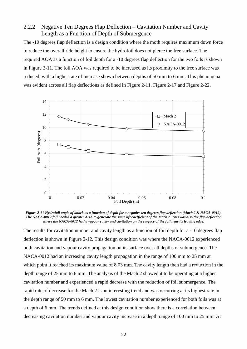
22
2.2.2 Negative Ten Degrees Flap Deflection – Cavitation Number and Cavity
Length as a Function of Depth of Submergence
The -10 degrees flap deflection is a design condition where the moth requires maximum down force
to reduce the overall ride height to ensure the hydrofoil does not pierce the free surface. The
required AOA as a function of foil depth for a -10 degrees flap deflection for the two foils is shown
in Figure 2-11. The foil AOA was required to be increased as its proximity to the free surface was
reduced, with a higher rate of increase shown between depths of 50 mm to 6 mm. This phenomena
was evident across all flap deflections as defined in Figure 2-11, Figure 2-17 and Figure 2-22.
Figure 2-11 Hydrofoil angle of attack as a function of depth for a negative ten degrees flap deflection (Mach 2 & NACA-0012).
The NACA-0012 foil needed a greater AOA to generate the same lift coefficient of the Mach 2. This was also the flap deflection
where the NACA-0012 had a vapour cavity and cavitation on the surface of the foil near its leading edge.
The results for cavitation number and cavity length as a function of foil depth for a -10 degrees flap
deflection is shown in Figure 2-12. This design condition was where the NACA-0012 experienced
both cavitation and vapour cavity propagation on its surface over all depths of submergence. The
NACA-0012 had an increasing cavity length propagation in the range of 100 mm to 25 mm at
which point it reached its maximum value of 8.03 mm. The cavity length then had a reduction in the
depth range of 25 mm to 6 mm. The analysis of the Mach 2 showed it to be operating at a higher
cavitation number and experienced a rapid decrease with the reduction of foil submergence. The
rapid rate of decrease for the Mach 2 is an interesting trend and was occurring at its highest rate in
the depth range of 50 mm to 6 mm. The lowest cavitation number experienced for both foils was at
a depth of 6 mm. The trends defined at this design condition show there is a correlation between
decreasing cavitation number and vapour cavity increase in a depth range of 100 mm to 25 mm. At
0
2
4
6
8
10
12
14
0 0.02 0.04 0.06 0.08 0.1
Fo
il A
oA
(d
egre
es)
Foil Depth (m)
Mach 2
NACA-0012
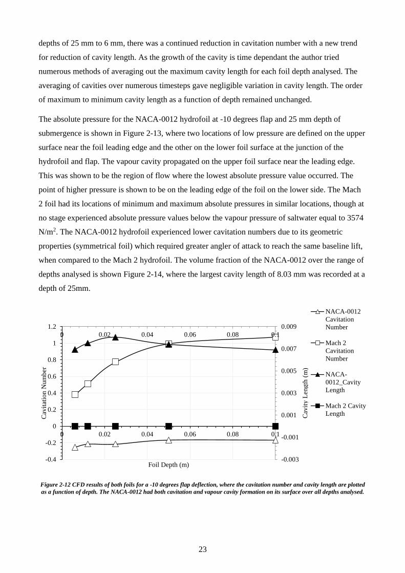
23
depths of 25 mm to 6 mm, there was a continued reduction in cavitation number with a new trend
for reduction of cavity length. As the growth of the cavity is time dependant the author tried
numerous methods of averaging out the maximum cavity length for each foil depth analysed. The
averaging of cavities over numerous timesteps gave negligible variation in cavity length. The order
of maximum to minimum cavity length as a function of depth remained unchanged.
The absolute pressure for the NACA-0012 hydrofoil at -10 degrees flap and 25 mm depth of
submergence is shown in Figure 2-13, where two locations of low pressure are defined on the upper
surface near the foil leading edge and the other on the lower foil surface at the junction of the
hydrofoil and flap. The vapour cavity propagated on the upper foil surface near the leading edge.
This was shown to be the region of flow where the lowest absolute pressure value occurred. The
point of higher pressure is shown to be on the leading edge of the foil on the lower side. The Mach
2 foil had its locations of minimum and maximum absolute pressures in similar locations, though at
no stage experienced absolute pressure values below the vapour pressure of saltwater equal to 3574
N/m2. The NACA-0012 hydrofoil experienced lower cavitation numbers due to its geometric
properties (symmetrical foil) which required greater angler of attack to reach the same baseline lift,
when compared to the Mach 2 hydrofoil. The volume fraction of the NACA-0012 over the range of
depths analysed is shown Figure 2-14, where the largest cavity length of 8.03 mm was recorded at a
depth of 25mm.
Figure 2-12 CFD results of both foils for a -10 degrees flap deflection, where the cavitation number and cavity length are plotted
as a function of depth. The NACA-0012 had both cavitation and vapour cavity formation on its surface over all depths analysed.
0 0.02 0.04 0.06 0.08 0.1
-0.003
-0.001
0.001
0.003
0.005
0.007
0.009
-0.4
-0.2
0
0.2
0.4
0.6
0.8
1
1.2
0 0.02 0.04 0.06 0.08 0.1
Foil Depth (m)
Cav
ity L
ength
(m
)
Cav
itat
ion N
um
ber
NACA-0012
Cavitation
Number
Mach 2
Cavitation
Number
NACA-
0012_Cavity
Length
Mach 2 Cavity
Length
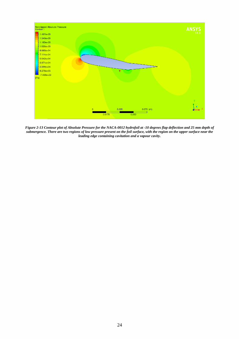
24
Figure 2-13 Contour plot of Absolute Pressure for the NACA-0012 hydrofoil at -10 degrees flap deflection and 25 mm depth of
submergence. There are two regions of low pressure present on the foil surface, with the region on the upper surface near the
leading edge containing cavitation and a vapour cavity.
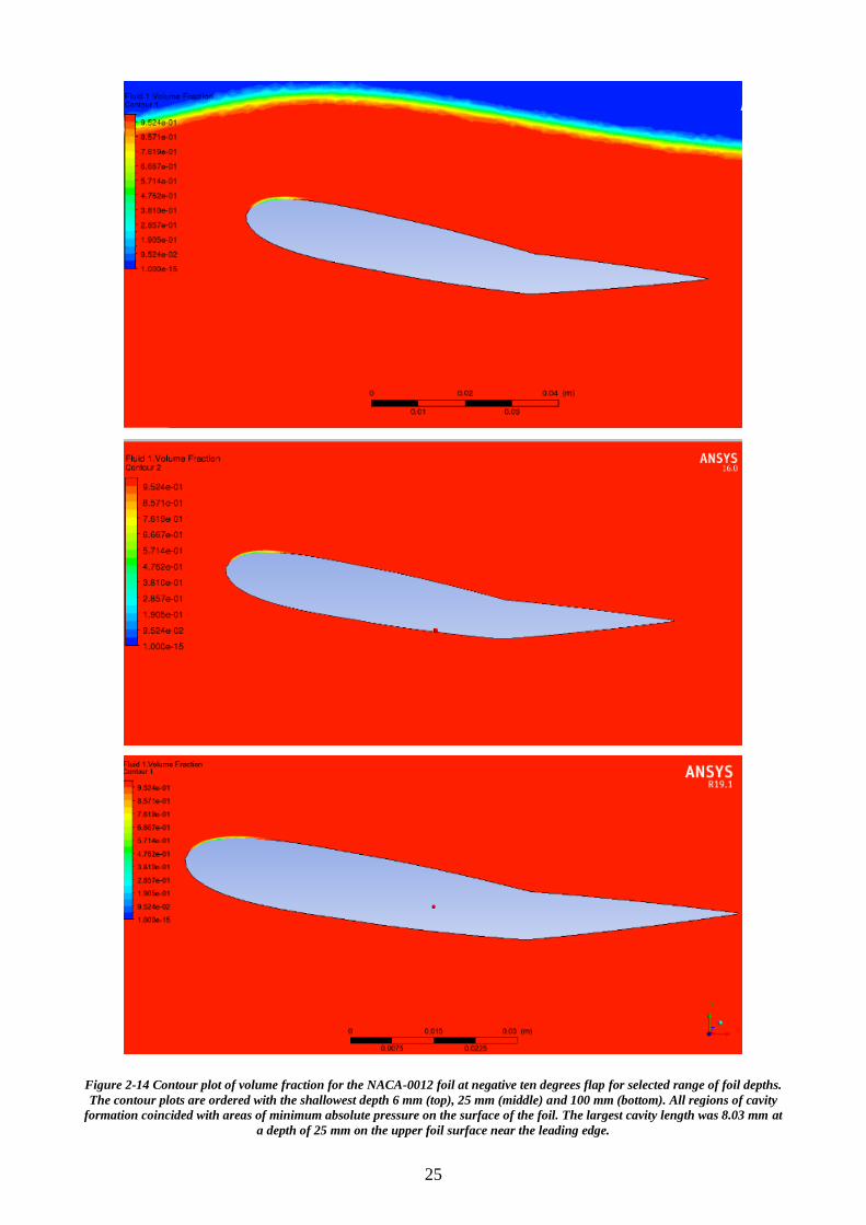
25
Figure 2-14 Contour plot of volume fraction for the NACA-0012 foil at negative ten degrees flap for selected range of foil depths.
The contour plots are ordered with the shallowest depth 6 mm (top), 25 mm (middle) and 100 mm (bottom). All regions of cavity
formation coincided with areas of minimum absolute pressure on the surface of the foil. The largest cavity length was 8.03 mm at
a depth of 25 mm on the upper foil surface near the leading edge.
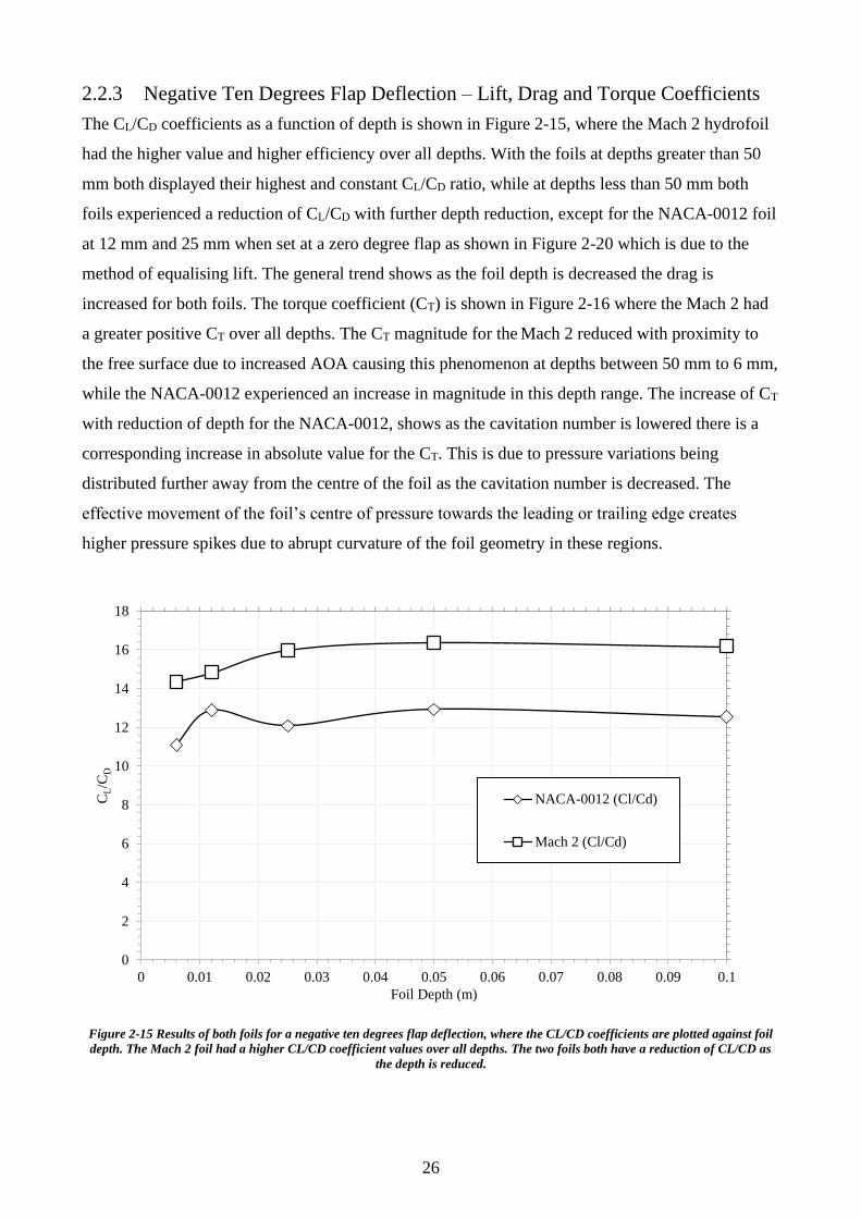
26
2.2.3 Negative Ten Degrees Flap Deflection – Lift, Drag and Torque Coefficients
The CL/CD coefficients as a function of depth is shown in Figure 2-15, where the Mach 2 hydrofoil
had the higher value and higher efficiency over all depths. With the foils at depths greater than 50
mm both displayed their highest and constant CL/CD ratio, while at depths less than 50 mm both
foils experienced a reduction of CL/CD with further depth reduction, except for the NACA-0012 foil
at 12 mm and 25 mm when set at a zero degree flap as shown in Figure 2-20 which is due to the
method of equalising lift. The general trend shows as the foil depth is decreased the drag is
increased for both foils. The torque coefficient (CT) is shown in Figure 2-16 where the Mach 2 had
a greater positive CT over all depths. The CT magnitude for the Mach 2 reduced with proximity to
the free surface due to increased AOA causing this phenomenon at depths between 50 mm to 6 mm,
while the NACA-0012 experienced an increase in magnitude in this depth range. The increase of CT
with reduction of depth for the NACA-0012, shows as the cavitation number is lowered there is a
corresponding increase in absolute value for the CT. This is due to pressure variations being
distributed further away from the centre of the foil as the cavitation number is decreased. The
effective movement of the foil’s centre of pressure towards the leading or trailing edge creates
higher pressure spikes due to abrupt curvature of the foil geometry in these regions.
Figure 2-15 Results of both foils for a negative ten degrees flap deflection, where the CL/CD coefficients are plotted against foil
depth. The Mach 2 foil had a higher CL/CD coefficient values over all depths. The two foils both have a reduction of CL/CD as
the depth is reduced.
0
2
4
6
8
10
12
14
16
18
0 0.01 0.02 0.03 0.04 0.05 0.06 0.07 0.08 0.09 0.1
CL/C
D
Foil Depth (m)
NACA-0012 (Cl/Cd)
Mach 2 (Cl/Cd)
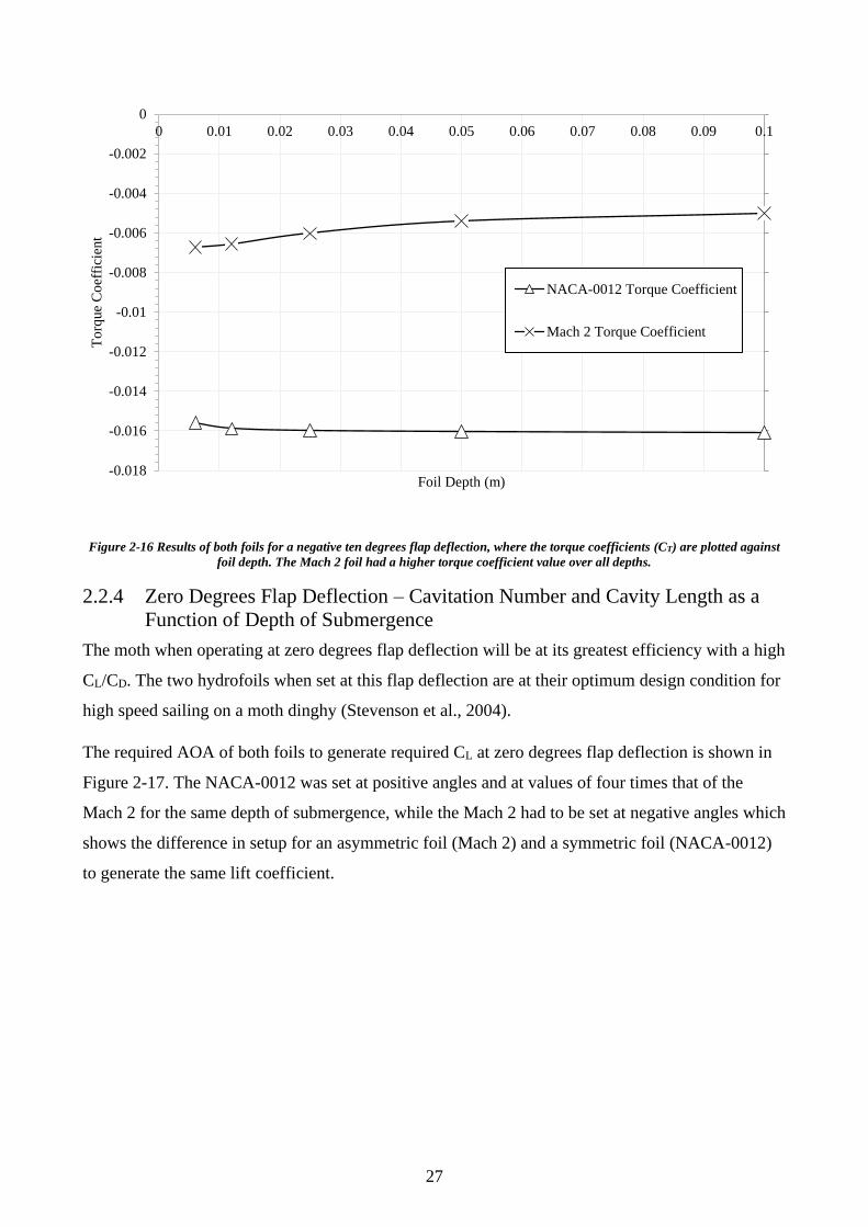
27
Figure 2-16 Results of both foils for a negative ten degrees flap deflection, where the torque coefficients (CT) are plotted against
foil depth. The Mach 2 foil had a higher torque coefficient value over all depths.
2.2.4 Zero Degrees Flap Deflection – Cavitation Number and Cavity Length as a
Function of Depth of Submergence
The moth when operating at zero degrees flap deflection will be at its greatest efficiency with a high
CL/CD. The two hydrofoils when set at this flap deflection are at their optimum design condition for
high speed sailing on a moth dinghy (Stevenson et al., 2004).
The required AOA of both foils to generate required CL at zero degrees flap deflection is shown in
Figure 2-17. The NACA-0012 was set at positive angles and at values of four times that of the
Mach 2 for the same depth of submergence, while the Mach 2 had to be set at negative angles which
shows the difference in setup for an asymmetric foil (Mach 2) and a symmetric foil (NACA-0012)
to generate the same lift coefficient.
-0.018
-0.016
-0.014
-0.012
-0.01
-0.008
-0.006
-0.004
-0.002
0
0 0.01 0.02 0.03 0.04 0.05 0.06 0.07 0.08 0.09 0.1
To
rque
Co
effi
cien
t
Foil Depth (m)
NACA-0012 Torque Coefficient
Mach 2 Torque Coefficient
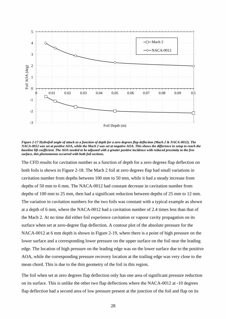
28
Figure 2-17 Hydrofoil angle of attack as a function of depth for a zero degrees flap deflection (Mach 2 & NACA-0012). The
NACA-0012 was set at positive AOA, while the Mach 2 was set at negative AOA. This shows the difference in setup to reach the
baseline lift coefficient. The AOA needed to be adjusted with a greater positive incidence with reduced proximity to the free
surface, this phenomenon occurred with both foil sections.
The CFD results for cavitation number as a function of depth for a zero degrees flap deflection on
both foils is shown in Figure 2-18. The Mach 2 foil at zero degrees flap had small variations in
cavitation number from depths between 100 mm to 50 mm, while it had a steady increase from
depths of 50 mm to 6 mm. The NACA-0012 had constant decrease in cavitation number from
depths of 100 mm to 25 mm, then had a significant reduction between depths of 25 mm to 12 mm.
The variation in cavitation numbers for the two foils was constant with a typical example as shown
at a depth of 6 mm, where the NACA-0012 had a cavitation number of 2.4 times less than that of
the Mach 2. At no time did either foil experience cavitation or vapour cavity propagation on its
surface when set at zero-degree flap deflection. A contour plot of the absolute pressure for the
NACA-0012 at 6 mm depth is shown in Figure 2-19, where there is a point of high pressure on the
lower surface and a corresponding lower pressure on the upper surface on the foil near the leading
edge. The location of high pressure on the leading edge was on the lower surface due to the positive
AOA, while the corresponding pressure recovery location at the trailing edge was very close to the
mean chord. This is due to the thin geometry of the foil in this region.
The foil when set at zero degrees flap deflection only has one area of significant pressure reduction
on its surface. This is unlike the other two flap deflections where the NACA-0012 at -10 degrees
flap deflection had a second area of low pressure present at the junction of the foil and flap on its
-3
-2
-1
0
1
2
3
4
5
0 0.01 0.02 0.03 0.04 0.05 0.06 0.07 0.08 0.09 0.1
Fo
il A
OA
(d
eg)
Foil Depth (m)
Mach 2
NACA-0012
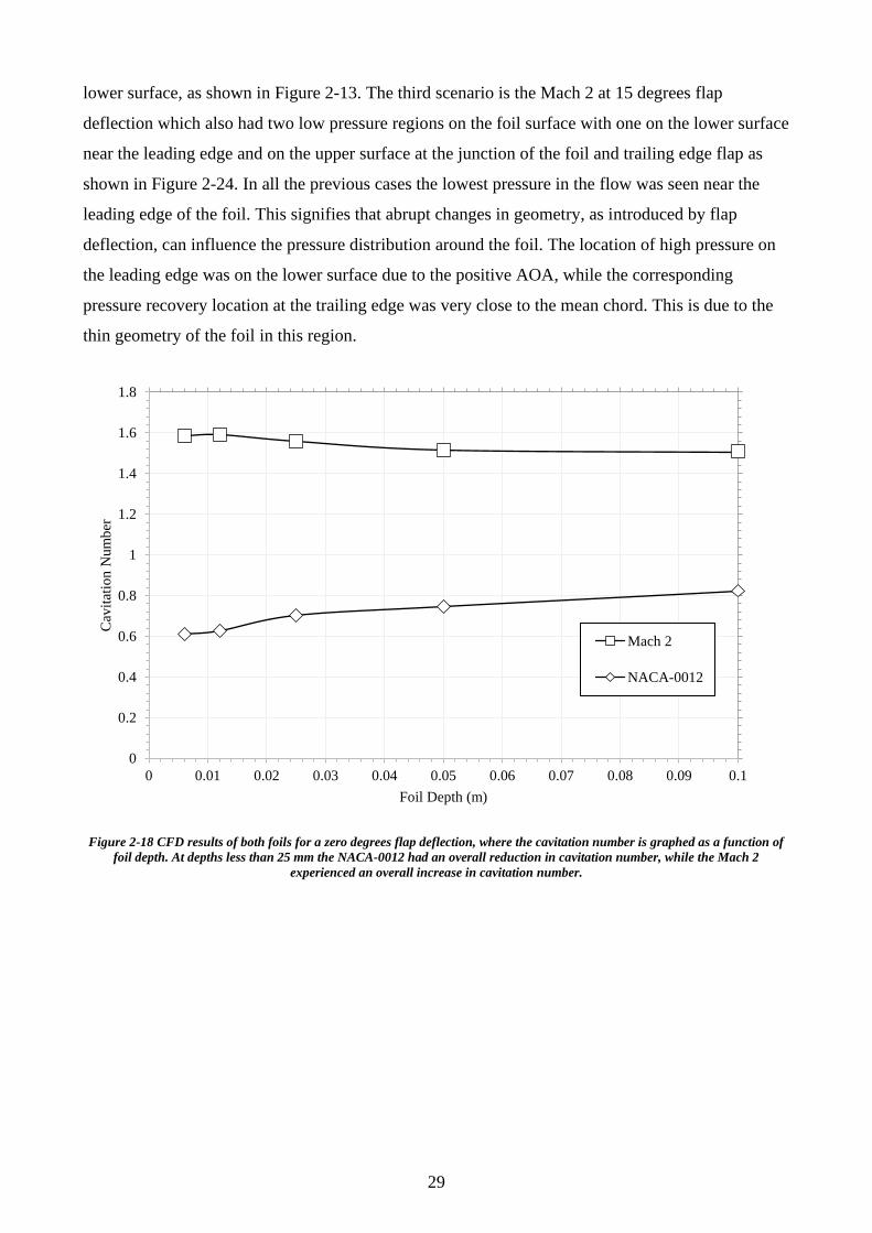
29
lower surface, as shown in Figure 2-13. The third scenario is the Mach 2 at 15 degrees flap
deflection which also had two low pressure regions on the foil surface with one on the lower surface
near the leading edge and on the upper surface at the junction of the foil and trailing edge flap as
shown in Figure 2-24. In all the previous cases the lowest pressure in the flow was seen near the
leading edge of the foil. This signifies that abrupt changes in geometry, as introduced by flap
deflection, can influence the pressure distribution around the foil. The location of high pressure on
the leading edge was on the lower surface due to the positive AOA, while the corresponding
pressure recovery location at the trailing edge was very close to the mean chord. This is due to the
thin geometry of the foil in this region.
Figure 2-18 CFD results of both foils for a zero degrees flap deflection, where the cavitation number is graphed as a function of
foil depth. At depths less than 25 mm the NACA-0012 had an overall reduction in cavitation number, while the Mach 2
experienced an overall increase in cavitation number.
0
0.2
0.4
0.6
0.8
1
1.2
1.4
1.6
1.8
0 0.01 0.02 0.03 0.04 0.05 0.06 0.07 0.08 0.09 0.1
Cav
itat
ion N
um
ber
Foil Depth (m)
Mach 2
NACA-0012
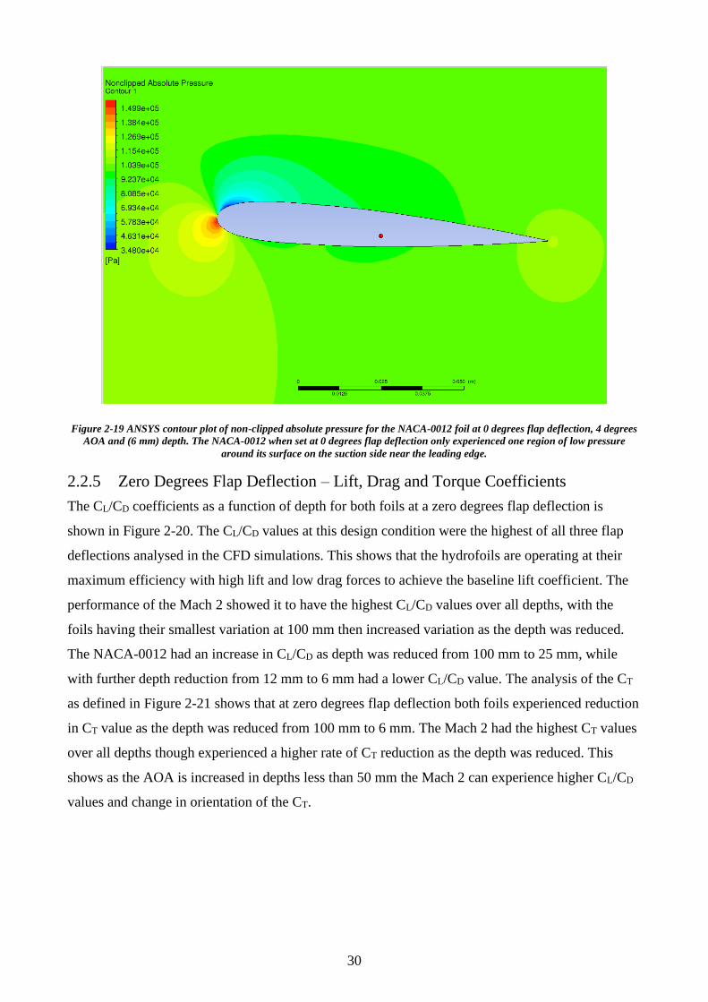
30
Figure 2-19 ANSYS contour plot of non-clipped absolute pressure for the NACA-0012 foil at 0 degrees flap deflection, 4 degrees
AOA and (6 mm) depth. The NACA-0012 when set at 0 degrees flap deflection only experienced one region of low pressure
around its surface on the suction side near the leading edge.
2.2.5 Zero Degrees Flap Deflection – Lift, Drag and Torque Coefficients
The CL/CD coefficients as a function of depth for both foils at a zero degrees flap deflection is
shown in Figure 2-20. The CL/CD values at this design condition were the highest of all three flap
deflections analysed in the CFD simulations. This shows that the hydrofoils are operating at their
maximum efficiency with high lift and low drag forces to achieve the baseline lift coefficient. The
performance of the Mach 2 showed it to have the highest CL/CD values over all depths, with the
foils having their smallest variation at 100 mm then increased variation as the depth was reduced.
The NACA-0012 had an increase in CL/CD as depth was reduced from 100 mm to 25 mm, while
with further depth reduction from 12 mm to 6 mm had a lower CL/CD value. The analysis of the CT
as defined in Figure 2-21 shows that at zero degrees flap deflection both foils experienced reduction
in CT value as the depth was reduced from 100 mm to 6 mm. The Mach 2 had the highest CT values
over all depths though experienced a higher rate of CT reduction as the depth was reduced. This
shows as the AOA is increased in depths less than 50 mm the Mach 2 can experience higher CL/CD
values and change in orientation of the CT.
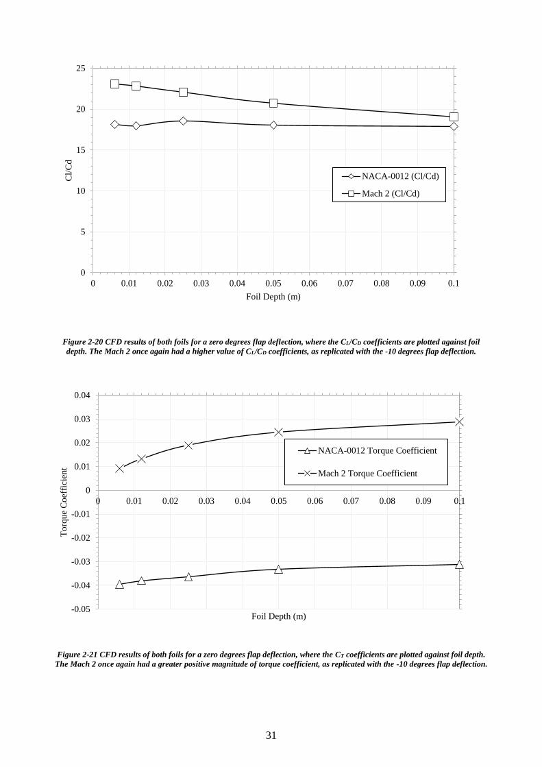
31
Figure 2-20 CFD results of both foils for a zero degrees flap deflection, where the CL/CD coefficients are plotted against foil
depth. The Mach 2 once again had a higher value of CL/CD coefficients, as replicated with the -10 degrees flap deflection.
Figure 2-21 CFD results of both foils for a zero degrees flap deflection, where the CT coefficients are plotted against foil depth.
The Mach 2 once again had a greater positive magnitude of torque coefficient, as replicated with the -10 degrees flap deflection.
0
5
10
15
20
25
0 0.01 0.02 0.03 0.04 0.05 0.06 0.07 0.08 0.09 0.1
Cl/
Cd
Foil Depth (m)
NACA-0012 (Cl/Cd)
Mach 2 (Cl/Cd)
-0.05
-0.04
-0.03
-0.02
-0.01
0
0.01
0.02
0.03
0.04
0 0.01 0.02 0.03 0.04 0.05 0.06 0.07 0.08 0.09 0.1
To
rque
Co
effi
cien
t
Foil Depth (m)
NACA-0012 Torque Coefficient
Mach 2 Torque Coefficient
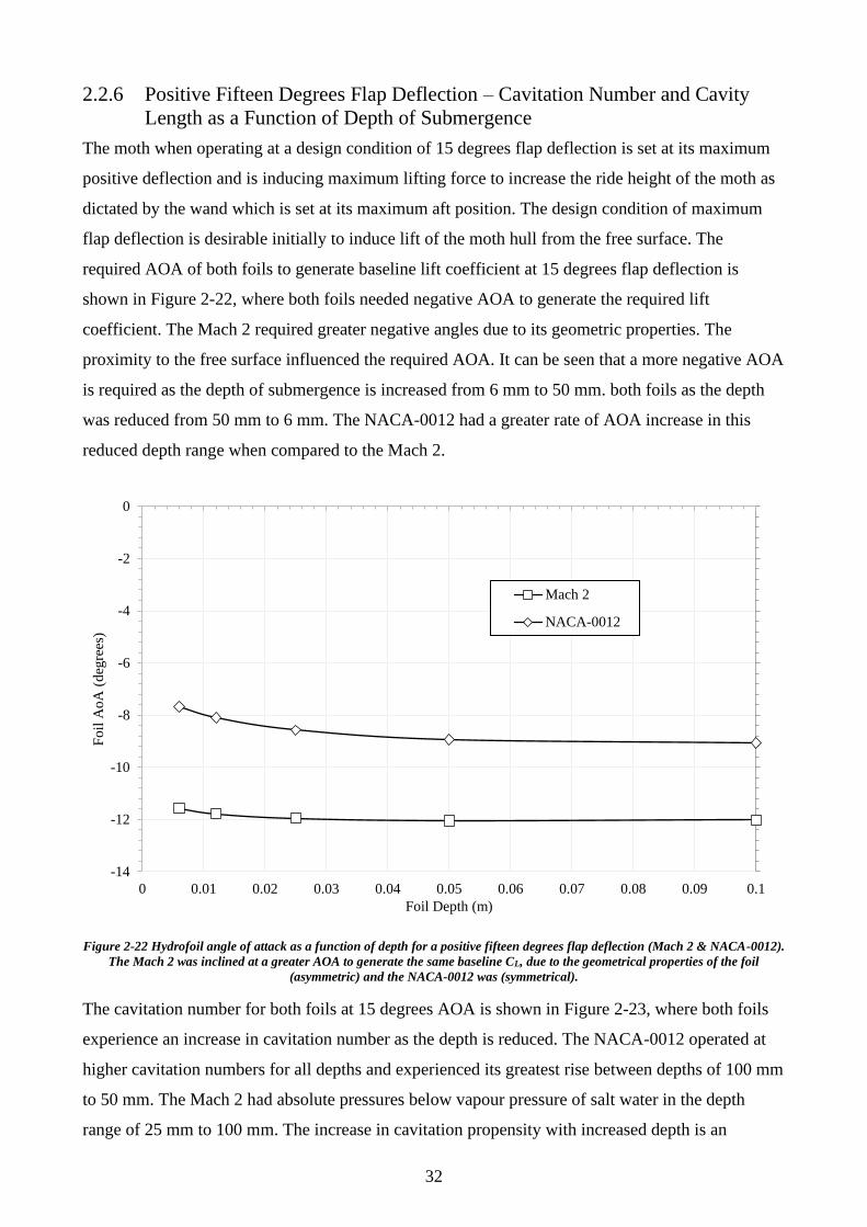
32
2.2.6 Positive Fifteen Degrees Flap Deflection – Cavitation Number and Cavity
Length as a Function of Depth of Submergence
The moth when operating at a design condition of 15 degrees flap deflection is set at its maximum
positive deflection and is inducing maximum lifting force to increase the ride height of the moth as
dictated by the wand which is set at its maximum aft position. The design condition of maximum
flap deflection is desirable initially to induce lift of the moth hull from the free surface. The
required AOA of both foils to generate baseline lift coefficient at 15 degrees flap deflection is
shown in Figure 2-22, where both foils needed negative AOA to generate the required lift
coefficient. The Mach 2 required greater negative angles due to its geometric properties. The
proximity to the free surface influenced the required AOA. It can be seen that a more negative AOA
is required as the depth of submergence is increased from 6 mm to 50 mm. both foils as the depth
was reduced from 50 mm to 6 mm. The NACA-0012 had a greater rate of AOA increase in this
reduced depth range when compared to the Mach 2.
Figure 2-22 Hydrofoil angle of attack as a function of depth for a positive fifteen degrees flap deflection (Mach 2 & NACA-0012).
The Mach 2 was inclined at a greater AOA to generate the same baseline CL, due to the geometrical properties of the foil
(asymmetric) and the NACA-0012 was (symmetrical).
The cavitation number for both foils at 15 degrees AOA is shown in Figure 2-23, where both foils
experience an increase in cavitation number as the depth is reduced. The NACA-0012 operated at
higher cavitation numbers for all depths and experienced its greatest rise between depths of 100 mm
to 50 mm. The Mach 2 had absolute pressures below vapour pressure of salt water in the depth
range of 25 mm to 100 mm. The increase in cavitation propensity with increased depth is an
-14
-12
-10
-8
-6
-4
-2
0
0 0.01 0.02 0.03 0.04 0.05 0.06 0.07 0.08 0.09 0.1
Fo
il A
oA
(d
egre
es)
Foil Depth (m)
Mach 2
NACA-0012
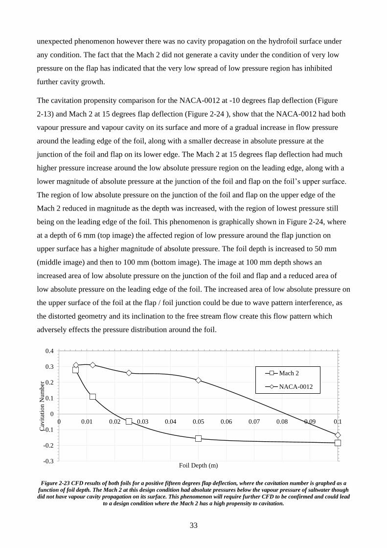
33
unexpected phenomenon however there was no cavity propagation on the hydrofoil surface under
any condition. The fact that the Mach 2 did not generate a cavity under the condition of very low
pressure on the flap has indicated that the very low spread of low pressure region has inhibited
further cavity growth.
The cavitation propensity comparison for the NACA-0012 at -10 degrees flap deflection (Figure
2-13) and Mach 2 at 15 degrees flap deflection (Figure 2-24 ), show that the NACA-0012 had both
vapour pressure and vapour cavity on its surface and more of a gradual increase in flow pressure
around the leading edge of the foil, along with a smaller decrease in absolute pressure at the
junction of the foil and flap on its lower edge. The Mach 2 at 15 degrees flap deflection had much
higher pressure increase around the low absolute pressure region on the leading edge, along with a
lower magnitude of absolute pressure at the junction of the foil and flap on the foil’s upper surface.
The region of low absolute pressure on the junction of the foil and flap on the upper edge of the
Mach 2 reduced in magnitude as the depth was increased, with the region of lowest pressure still
being on the leading edge of the foil. This phenomenon is graphically shown in Figure 2-24, where
at a depth of 6 mm (top image) the affected region of low pressure around the flap junction on
upper surface has a higher magnitude of absolute pressure. The foil depth is increased to 50 mm
(middle image) and then to 100 mm (bottom image). The image at 100 mm depth shows an
increased area of low absolute pressure on the junction of the foil and flap and a reduced area of
low absolute pressure on the leading edge of the foil. The increased area of low absolute pressure on
the upper surface of the foil at the flap / foil junction could be due to wave pattern interference, as
the distorted geometry and its inclination to the free stream flow create this flow pattern which
adversely effects the pressure distribution around the foil.
Figure 2-23 CFD results of both foils for a positive fifteen degrees flap deflection, where the cavitation number is graphed as a
function of foil depth. The Mach 2 at this design condition had absolute pressures below the vapour pressure of saltwater though
did not have vapour cavity propagation on its surface. This phenomenon will require further CFD to be confirmed and could lead
to a design condition where the Mach 2 has a high propensity to cavitation.
-0.3
-0.2
-0.1
0
0.1
0.2
0.3
0.4
0 0.01 0.02 0.03 0.04 0.05 0.06 0.07 0.08 0.09 0.1
Cav
itat
ion N
um
ber
Foil Depth (m)
Mach 2
NACA-0012

34
Figure 2-24 ANSYS contour plot of non-clipped absolute pressure for the Mach 2 foil at 15 degrees flap deflection, -12 degrees
AOA. The order of depth for the images are 6 mm (top), 50 mm (middle) and 100 mm (bottom). Both foil sections at 15 degrees
flap had an increase in cavitation number as the depth was reduced, this means as the depth is increased both foils have a higher
propensity for cavitation. The Mach 2 also has two regions of low absolute pressure on its surface, being on its lower surface near
the leading edge (which had lowest magnitude) and the other on the upper surface at the junction of the hydrofoil and flap.
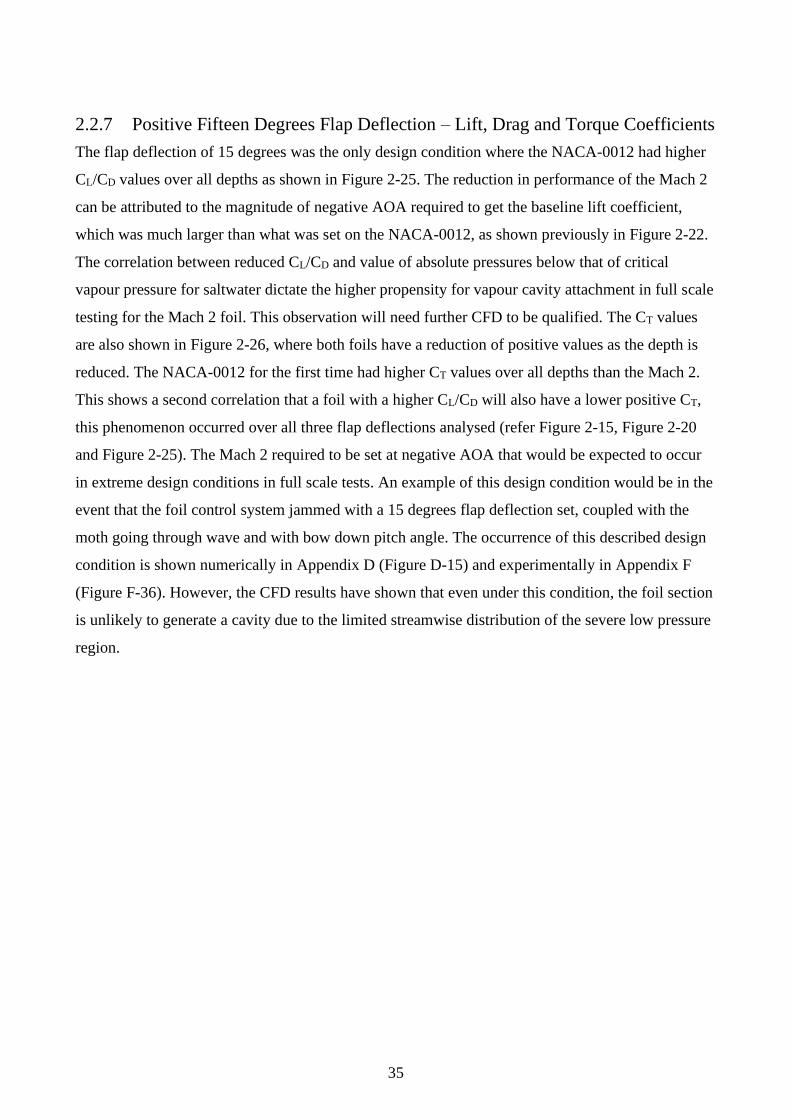
35
2.2.7 Positive Fifteen Degrees Flap Deflection – Lift, Drag and Torque Coefficients
The flap deflection of 15 degrees was the only design condition where the NACA-0012 had higher
CL/CD values over all depths as shown in Figure 2-25. The reduction in performance of the Mach 2
can be attributed to the magnitude of negative AOA required to get the baseline lift coefficient,
which was much larger than what was set on the NACA-0012, as shown previously in Figure 2-22.
The correlation between reduced CL/CD and value of absolute pressures below that of critical
vapour pressure for saltwater dictate the higher propensity for vapour cavity attachment in full scale
testing for the Mach 2 foil. This observation will need further CFD to be qualified. The CT values
are also shown in Figure 2-26, where both foils have a reduction of positive values as the depth is
reduced. The NACA-0012 for the first time had higher CT values over all depths than the Mach 2.
This shows a second correlation that a foil with a higher CL/CD will also have a lower positive CT,
this phenomenon occurred over all three flap deflections analysed (refer Figure 2-15, Figure 2-20
and Figure 2-25). The Mach 2 required to be set at negative AOA that would be expected to occur
in extreme design conditions in full scale tests. An example of this design condition would be in the
event that the foil control system jammed with a 15 degrees flap deflection set, coupled with the
moth going through wave and with bow down pitch angle. The occurrence of this described design
condition is shown numerically in Appendix D (Figure D-15) and experimentally in Appendix F
(Figure F-36). However, the CFD results have shown that even under this condition, the foil section
is unlikely to generate a cavity due to the limited streamwise distribution of the severe low pressure
region.
36
Figure 2-25 CFD results of both foils for a positive fifteen degrees flap deflection, where the CL/CD coefficients are plotted against
foil depth. The Mach 2 had a lower CL/CD value over all depths, which shows it operated at a lower efficiency than the NACA-
0012. The flap deflection of 15 degrees was where the NACA-0012 outperformed the Mach 2 in terms of cavitation propensity.
Figure 2-26 CFD results of both foils for a positive fifteen degrees flap deflection, where the CT are plotted against foil depth. The
Mach 2 has a lower CT at 15 degrees flap deflection over all depths when compared to the NACA-0012. The lower value shows a
correlation between reduced CL/CD, higher CT and lower cavitation number. The NACA-00012 experienced the same trends when
operating at -10 and 0 degrees flap deflections.
0
5
10
15
20
25
0 0.01 0.02 0.03 0.04 0.05 0.06 0.07 0.08 0.09 0.1
CL/C
D
Foil Depth (m)
Mach 2 (Cl/Cd)
NACA-0012 (Cl/Cd)
0
0.002
0.004
0.006
0.008
0.01
0 0.01 0.02 0.03 0.04 0.05 0.06 0.07 0.08 0.09 0.1
To
rque
Co
effi
cien
t
Foil Depth (m)
Mach 2
NACA-0012
37
2.2.8 Conclusions and Recommendations for CFD Numerical Analysis
The CFD analysis was conducted to determine the cavitation propensity of the NACA-0012 and
Mach 2 hydrofoil sections. The hydrofoils were analysed over a range of deflections which were
selected to represent the extremities of operation. The three flap deflections of -10, 0 and 15 degrees
represent the maximum negative, efficient (neutral) and positive flap deflections set on the main
hydrofoil and used in this research project. The foils were setup at these flap deflections then had
their AOA adjusted to give a normalised lift coefficient to represent the mass of skipper and moth
which equalled 110 kg. The analysis was limited to a maximum depth of 100mm due to high
percentage of ventilation events occurring in initial full-scale testing. The NACA-0012 had a higher
propensity to cavitation when set at -10 and 0 degrees flap deflections. The NACA-0012 was the
only hydrofoil to have both absolute pressures below the critical vapour pressure of saltwater and
vapour cavity propagation on its surface. This occurred when the NACA-0012 was set at a -10
degrees flap deflection. The region of vapour cavity attachment coincided with the area of
minimum absolute pressure on the foil surface, which was on the upper foil surface near the leading
edge. The vapour cavity had an increasing cavity length as the depth was reduced from 100 mm to
25 mm. The cavity length of 8.03 mm was the largest estimated on the NACA-0012 at a depth of 25
mm. The cavity length then decreased with further depth reduction from 25 mm to 6 mm. The
hydrofoils set at either a -10 or 15 degrees flap deflection had two regions of low absolute pressure
present on its surface, which were near the leading edge on the suction side of the foil and the
second location at the junction of the hydrofoil and flap. The exact location depended on flap
deflection and whether the foil was set at a positive or negative AOA. The CFD results showed a
correlation in the behaviour of residuals that lead to increased cavitation propensity which are: (a)
decreased absolute pressure and CL/CD and (b) increased absolute value of the CT. This was shown
for the NACA-0012 at -10 degrees flap deflection and the Mach 2 at 15 degrees flap deflection. The
Mach 2 when set at a 15 degrees flap deflection could potentially experience cavitation, as it
experienced absolute pressure values below the vapor pressure, though did not have cavity
propagation on its surface. The cavitation propensity for both foils at 15 degrees flap deflection
increased when operating at larger depth of submergence, this is due to reduced absolute pressure at
the junction of the foil and flap which creates wave pattern interference and a greater region of low
absolute pressure on the upper surface of the hydrofoil. Further CFD analysis is required to
determine whether it is possible for vapour cavity propagation on the Mach 2 when setup with a 15
degrees flap deflection and AOA normalised to a baseline lift coefficient to lift a mass of 110kg.
The NACA-0012 when set at a 15 degrees flap deflection had a greater efficiency due to its higher
CL/CD over all depths.
38
It is recommended that future CFD numerical analysis consider three-dimensional effects on
cavitation and vapour cavity formation as they are time dependent phenomena that interact along
the full span of the hydrofoil. The second recommendation is to define all variables that are
pertinent to determining cavitation propensity in the CFD analysis. The replication of the CFD
analysis through full scale experiments should include the use of an Arduino data logger to
incorporate localised pressure sensors on the foil surface and an angle sensor attached to bell crank
of the main hydrofoil to determine the angle of flap deflection. The identification of pre-existing
cavitation on the hydrofoil in full scale testing prior to the introduction of ventilated cavities
propagating from the free surface would confirm the observation from full scale testing where the
NACA-0012 had a 60 % higher propensity for vapour cavity attachment due to pre-existing
cavitation on the foil surface as shown in the CFD analysis. The verification of CFD results through
full scale testing may not be any easy task. This is due to the time dependent cavity propagation that
had a maximum size of 8.03 mm and lasted for at least 1.5 seconds replicated on a moth would
require considerable expense and may be easier to perform in a controlled environment such as a
cavitation tunnel.
39
3 Full Scale Testing
3.1 Full Scale Testing Methods
3.1.1 General
The full-scale testing was conducted to verify CFD results for cavitation propensity for both the
Mach 2 and NACA-0012 hydrofoils. The two hydrofoils share exact geometric properties with the
only variation being the hydrofoil cross-section shape, which forms the basis for this analysis. The
hydrofoils were setup on an International Moth Dinghy built by the author. The full-scale testing
was conducted on Sydney Harbour over a six-month period. Each ventilation event was captured
with GoPro cameras and all vessel rotations and translations were collected with an iPhone Data
logger APP. The results presented later in the text show that the NACA-0012 had a greater
percentage of events with ventilated cavity attachment to its foil surface in full scale testing when
compared to the Mach 2.
3.1.2 Design of Hydrofoils
The two foil sections used in analysis (NACA-0012 and Mach 2) were modelled to the same
geometric properties with the only difference being the cross-sectional shape of the hydrofoil. The
standard Mach 2 hydrofoil and strut were used as the baseline for the construction of the NACA-
0012 hydrofoil. The construction process for the NACA-0012 involved numerous methods to
replicate the Mach 2 geometrical features. The hydrofoil and strut were modelled using a
planometer and a contour gauge to ensure the correct area and cross-sectional shapes were defined.
The sketches were then modelled in the Rhino 6 three-dimensional surface modelling program. The
full-scale sections were then printed on A3 paper and compared to original sketches to verify the
accuracy of the CAD model and were within an allowable tolerance of ±0.5mm. The Mach 2 model
was then ready to have the NACA-0012 section profile transferred onto the planform shape of the
Mach 2 geometry. The primary geometrical features that were used in the creation of the NACA-
0012 foil are shown below in Figure 3-1.
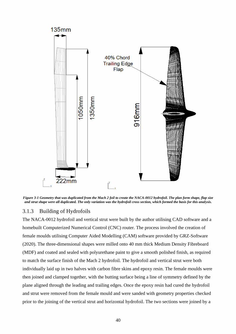
40
Figure 3-1 Geometry that was duplicated from the Mach 2 foil to create the NACA-0012 hydrofoil. The plan form shape, flap size
and strut shape were all duplicated. The only variation was the hydrofoil cross section, which formed the basis for this analysis.
3.1.3 Building of Hydrofoils
The NACA-0012 hydrofoil and vertical strut were built by the author utilising CAD software and a
homebuilt Computerized Numerical Control (CNC) router. The process involved the creation of
female moulds utilising Computer Aided Modelling (CAM) software provided by GRZ-Software
(2020). The three-dimensional shapes were milled onto 40 mm thick Medium Density Fibreboard
(MDF) and coated and sealed with polyurethane paint to give a smooth polished finish, as required
to match the surface finish of the Mach 2 hydrofoil. The hydrofoil and vertical strut were both
individually laid up in two halves with carbon fibre skins and epoxy resin. The female moulds were
then joined and clamped together, with the butting surface being a line of symmetry defined by the
plane aligned through the leading and trailing edges. Once the epoxy resin had cured the hydrofoil
and strut were removed from the female mould and were sanded with geometry properties checked
prior to the joining of the vertical strut and horizontal hydrofoil. The two sections were joined by a
41
female to male plug with the female rebate being in the upper surface of the horizontal hydrofoil.
The fastening of the two sections was achieved by using an 8 mm bolt which was threaded from the
bottom surface of the hydrofoil and tapped into the male plug of the vertical hydrofoil. This method
of attachment is used on both the Mach 2 and NACA-0012 hydrofoils. The control system setup
was replicated to that of the Mach 2 with a vertical push rod running through the trailing edge of the
vertical strut and attaching to the hydrofoil flap. The push rod provides automation and control of
the flap deflection. The moth required no changes as the foil geometry for both foils were replicated
and fitted straight into the centreboard case and ready for full scale testing. Further details on the
NACA-0012 foil construction process are provided in Appendix H.
3.1.4 Experiment Setup
The full-scale experiment was setup to capture ventilation events for both the NACA-0012 and
Mach 2 hydrofoils. Both hydrofoils were setup to replicate baseline conditions defined in the CFD
analysis which included foil AOA, flap range of deflection and foil depth of submergence. The
collection of experiment data required the use of both graphical and numerical methods to be
incorporated. The moth was fitted with two GoPro cameras to graphically capture ventilation events
and a data logger to record the magnitude of all vessel rotations and translations in six degrees of
freedom. The graphical and numerical data were then synced to define unique parameters around
each ventilation event that occurred during full scale testing.
3.1.5 Test Program
The full-scale testing consisted of two by one-hour sessions where the moth was fitted with either
the NACA-0012 or Mach 2 hydrofoil and the ventilation events were captured. The wind range for
all test was between 5 to 10 m/s with average wind strength of 7.5 m/s in the test area. These
conditions were desirable as at this wind strength the moth was able to operate in the hydro-foiling
regime. The real time plot of two full scale test sessions are shown in Figure 3-2, where the red line
defines the course travelled by the moth in each session. The flow regime over the NACA-0012
hydrofoil with the early stages of a ventilated tip vortex formation is shown below in Figure 3-3
along with a view from aft of the Mach 2 foil operating at a design condition where the moth is with
a 15 degrees flap deflection to raise the hull above the free surface and into the hydro-foiling
regime.

42
Figure 3-2 The real time graphical plot of two full scale test sessions with the NACA-0012 left and Mach 2 on the right. The red
line defines the course travelled by the moth in each session. The setup of equipment required over ten test sessions to get a setup
that could record data efficiently.
Figure 3-3 Images of full-scale testing capturing ventilated tip vortex forming on NACA-0012 hydrofoil (top and bottom left).
These two images also show the wand angle (which is a function of flap deflection) and foil depth as referenced by markings on
the foil’s vertical strut. The Mach 2 hydrofoil is shown bottom right and in this design condition the foil is operating with a 15
degrees flap deflection to raise the hull above the free surface and into the hydro foiling regime. The two angles at which the
cameras were set were synced with the data logger to both graphically and numerically capture unique parameters that define
ventilation events for each hydrofoil.
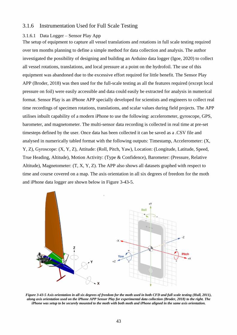
43
3.1.6 Instrumentation Used for Full Scale Testing
3.1.6.1 Data Logger – Sensor Play App
The setup of equipment to capture all vessel translations and rotations in full scale testing required
over ten months planning to define a simple method for data collection and analysis. The author
investigated the possibility of designing and building an Arduino data logger (Igoe, 2020) to collect
all vessel rotations, translations, and local pressure at a point on the hydrofoil. The use of this
equipment was abandoned due to the excessive effort required for little benefit. The Sensor Play
APP (Broder, 2018) was then used for the full-scale testing as all the features required (except local
pressure on foil) were easily accessible and data could easily be extracted for analysis in numerical
format. Sensor Play is an iPhone APP specially developed for scientists and engineers to collect real
time recordings of specimen rotations, translations, and scalar values during field projects. The APP
utilises inbuilt capability of a modern iPhone to use the following: accelerometer, gyroscope, GPS,
barometer, and magnetometer. The multi-sensor data recording is collected in real time at pre-set
timesteps defined by the user. Once data has been collected it can be saved as a .CSV file and
analysed in numerically tabled format with the following outputs: Timestamp, Accelerometer: (X,
Y, Z), Gyroscope: (X, Y, Z), Attitude: (Roll, Pitch, Yaw), Location: (Longitude, Latitude, Speed,
True Heading, Altitude), Motion Activity: (Type & Confidence), Barometer: (Pressure, Relative
Altitude), Magnetometer: (T, X, Y, Z). The APP also shows all datasets graphed with respect to
time and course covered on a map. The axis orientation in all six degrees of freedom for the moth
and iPhone data logger are shown below in Figure 3-43-5.
Figure 3-43-5 Axis orientation in all six degrees of freedom for the moth used in both CFD and full scale testing (Hull, 2011),
along axis orientation used on the iPhone APP Sensor Play for experimental data collection (Broder, 2018) to the right. The
iPhone was setup to be securely mounted to the moth with both moth and iPhone aligned in the same axis orientation.
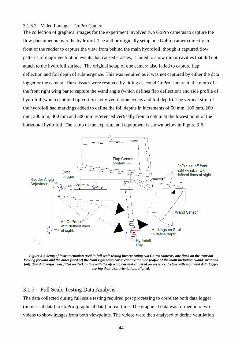
44
3.1.6.2 Video Footage – GoPro Camera
The collection of graphical images for the experiment involved two GoPro cameras to capture the
flow phenomenon over the hydrofoil. The author originally setup one GoPro camera directly in
front of the rudder to capture the view from behind the main hydrofoil, though it captured flow
patterns of major ventilation events that caused crashes, it failed to show minor cavities that did not
attach to the hydrofoil surface. The original setup of one camera also failed to capture flap
deflection and foil depth of submergence. This was required as it was not captured by either the data
logger or the camera. These issues were resolved by fitting a second GoPro camera to the moth off
the front right wing bar to capture the wand angle (which defines flap deflection) and side profile of
hydrofoil (which captured tip vortex cavity ventilation events and foil depth). The vertical strut of
the hydrofoil had markings added to define the foil depths in increments of 50 mm, 100 mm, 200
mm, 300 mm, 400 mm and 500 mm referenced vertically from a datum at the lowest point of the
horizontal hydrofoil. The setup of the experimental equipment is shown below in Figure 3-6.
Figure 3-6 Setup of instrumentation used in full scale testing incorporating two GoPro cameras, one fitted on the transom
looking forward and the other fitted off the front right wing bar to capture the side profile of the moth including (wand, strut and
foil). The data logger was fitted on deck in line with the aft wing bar and cantered on vessel centreline with moth and data logger
having their axis orientations aligned.
3.1.7 Full Scale Testing Data Analysis
The data collected during full scale testing required post processing to correlate both data logger
(numerical data) to GoPro (graphical data) in real time. The graphical data was formed into two
videos to show images from both viewpoints. The videos were then analysed to define ventilation
45
events and their severity. The videos were able to capture images from two angles of the same event
in synchronised real time. The wand angle was also used to determine flap angle with reference to
markings on the moth hull. The foil depth of submergence was defined by analysing markings on
the vertical strut which was affected by heel angle and as a result needed trigonometry to determine
foil tip depth. The Sensor Play numerical data gave data at a sampling frequency of 10 hertz which
was synched to the graphical data by timestep, latitude, longitude, moth velocity and verified by
time of ventilation event in video. The numerical results were verified against graphical data to
ensure they have similar correlation with regards to translations, rotations and vessel velocity. This
was required as the moth could have considerable change in all degrees of freedom over a small
amount of timesteps. As a result, the readings in some instances were averaged to give results that
replicate what was shown graphically in the videos.
The quality of the full-scale results required constant monitoring and had an inbuilt redundancy
utilising both graphical and motion sensing equipment. The post processing of results shown in
Appendix E and Appendix F, required over 20 hours analysing of video footage to identify
ventilation events and then synching with motion sensing data. The ventilation events were
categorized as either cavity or non-cavity attachment to the foil surface.
3.1.8 Experiment Uncertainty
The accuracy of results taken from full scale testing required constant review with multiple
iterations of equipment setup required to ensure the accuracy of the data collected. As the two
primary methods of data collection were graphical (camera) and motion sensing (data logger)
identifying methods to align the data in real time was required. The data logger gave real time
information which qualified the exact location at any given time. The data logger results were
quantified against graphical images that showed visually the rotations and translations recorded in
real time. The collection of experimental data will always have a degree of uncertainty and
examples of possible sources of error in full scale testing could be attributed to the following:
• Pixilation error caused by distortion of image due to sunlight, sea spray on camera causing
lens blurring of the image, misalignment of camera due to a knock, fogging of GoPro
camera in its case due to condensation.
• Sensor Play data logger numerical errors due to inaccurate readings. This was justified
after analysis of early experiments that showed three-metre variations in the vessel heave
magnitude. This was verified upon contacting the creator of the APP Broder (2018) who
advised heave and barometric pressure were not accurate over the range covered in full
scale testing. The author believes this was justified with the greatest variation expected to
be less than 1000 mm based on the span of the foils vertical strut. The graphical data
46
supports this argument. The iPhone could possibly move in its waterproof case which
would have negligible affects as it was securely fastened to the vessel. The final error
related to the data logger could be due to accuracy of GPS location settings which on at
least one experiment run failed to record vessel latitude and longitude.
• Parallax error due to change in the apparent position of the hydrofoil due to the viewing
angle of the camera not set perpendicular with respect to the hydrofoil. The cause of this
error is due to the image collected not in the centre of the image Charge-Coupled Device
(CCD). The Parallax error did not have an impact on the experiment result as the foil
measurement gradations were located at the site of the water height being measured.
• Uncontrolled environment due to test conditions not been the same for all experiment
sessions. To reduce the error there were seven separate sessions conducted for each foil,
with the most consistent two chosen based on weather conditions, sea state and quality of
data collected.
• Alignment of the iPhone axis to moth axis which would give inaccurate results in all six
degrees of freedom.
The above errors in data collection were minimised as much as possible and having both numerical
and graphical data collection provided two forms of redundancy to ensure a reasonable level of
accuracy in the results.
3.2 Full Scale Testing Results
3.2.1 General
The full-scale testing was conducted utilising the NACA-0012 and Mach 2 hydrofoil sections to
capture ventilation events and the propensity for vapor cavity attachment to the hydrofoil surface.
The two hydrofoils were setup on the moth to replicate baseline conditions defined in the CFD
analysis which included foil angle of attack, flap range of deflection and foil depth of submergence.
The testing equipment consisted of two GoPro cameras to record the flow phenomena over the foils
and an iPhone data logger to capture vessel rotations and translations in all six degrees of freedom.
The full-scale testing consisted of seven trials to get equipment setup that could accurately record
data in real time. The results of two sessions per hydrofoil are shown in Appendix E and Appendix
F, where one session per foil was selected to be used in this analysis. This was required due to
results from some sessions being disregarded due to inaccurate data collection or adverse weather
conditions during the session. The tabled results for the best two sessions per foil are shown in
Appendix E, while in Appendix F screenshots of the associated ventilation event is shown. The full
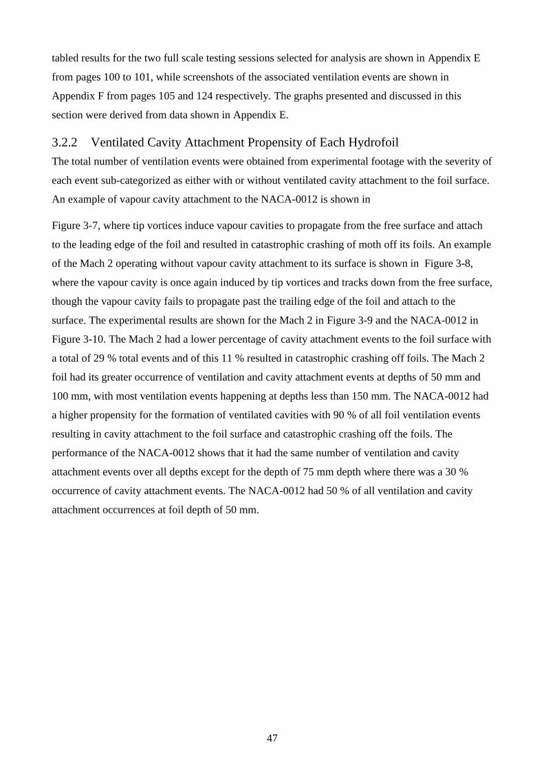
47
tabled results for the two full scale testing sessions selected for analysis are shown in Appendix E
from pages 100 to 101, while screenshots of the associated ventilation events are shown in
Appendix F from pages 105 and 124 respectively. The graphs presented and discussed in this
section were derived from data shown in Appendix E.
3.2.2 Ventilated Cavity Attachment Propensity of Each Hydrofoil
The total number of ventilation events were obtained from experimental footage with the severity of
each event sub-categorized as either with or without ventilated cavity attachment to the foil surface.
An example of vapour cavity attachment to the NACA-0012 is shown in
Figure 3-7, where tip vortices induce vapour cavities to propagate from the free surface and attach
to the leading edge of the foil and resulted in catastrophic crashing of moth off its foils. An example
of the Mach 2 operating without vapour cavity attachment to its surface is shown in Figure 3-8,
where the vapour cavity is once again induced by tip vortices and tracks down from the free surface,
though the vapour cavity fails to propagate past the trailing edge of the foil and attach to the
surface. The experimental results are shown for the Mach 2 in Figure 3-9 and the NACA-0012 in
Figure 3-10. The Mach 2 had a lower percentage of cavity attachment events to the foil surface with
a total of 29 % total events and of this 11 % resulted in catastrophic crashing off foils. The Mach 2
foil had its greater occurrence of ventilation and cavity attachment events at depths of 50 mm and
100 mm, with most ventilation events happening at depths less than 150 mm. The NACA-0012 had
a higher propensity for the formation of ventilated cavities with 90 % of all foil ventilation events
resulting in cavity attachment to the foil surface and catastrophic crashing off the foils. The
performance of the NACA-0012 shows that it had the same number of ventilation and cavity
attachment events over all depths except for the depth of 75 mm depth where there was a 30 %
occurrence of cavity attachment events. The NACA-0012 had 50 % of all ventilation and cavity
attachment occurrences at foil depth of 50 mm.
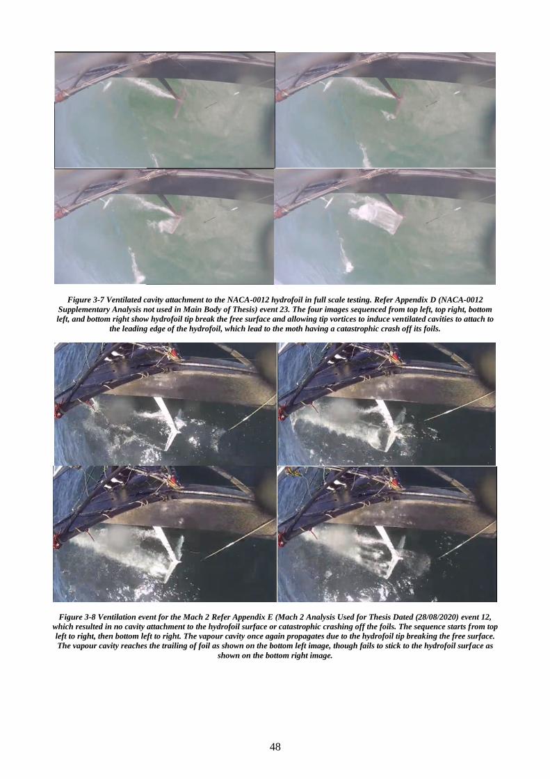
48
Figure 3-7 Ventilated cavity attachment to the NACA-0012 hydrofoil in full scale testing. Refer Appendix D (NACA-0012
Supplementary Analysis not used in Main Body of Thesis) event 23. The four images sequenced from top left, top right, bottom
left, and bottom right show hydrofoil tip break the free surface and allowing tip vortices to induce ventilated cavities to attach to
the leading edge of the hydrofoil, which lead to the moth having a catastrophic crash off its foils.
Figure 3-8 Ventilation event for the Mach 2 Refer Appendix E (Mach 2 Analysis Used for Thesis Dated (28/08/2020) event 12,
which resulted in no cavity attachment to the hydrofoil surface or catastrophic crashing off the foils. The sequence starts from top
left to right, then bottom left to right. The vapour cavity once again propagates due to the hydrofoil tip breaking the free surface.
The vapour cavity reaches the trailing of foil as shown on the bottom left image, though fails to stick to the hydrofoil surface as
shown on the bottom right image.
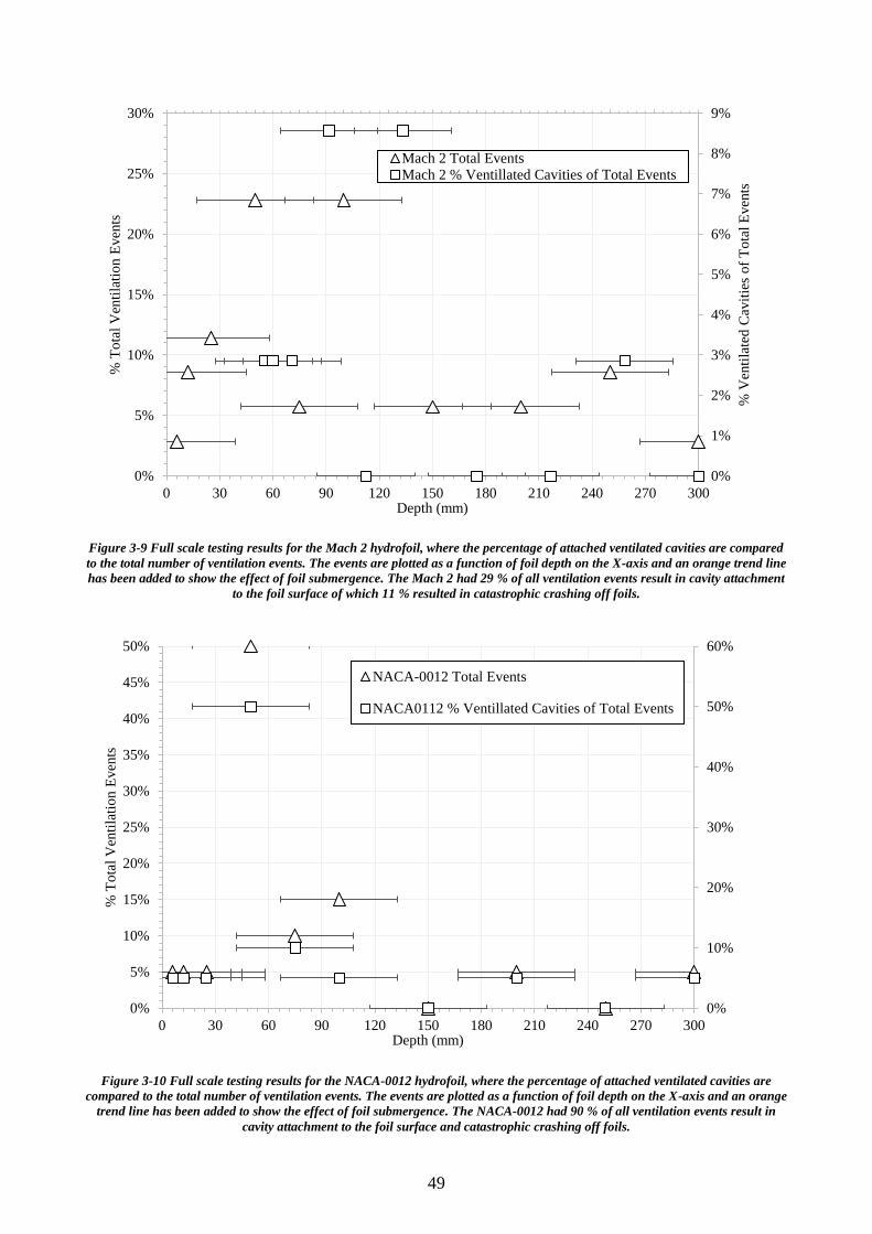
49
Figure 3-9 Full scale testing results for the Mach 2 hydrofoil, where the percentage of attached ventilated cavities are compared
to the total number of ventilation events. The events are plotted as a function of foil depth on the X-axis and an orange trend line
has been added to show the effect of foil submergence. The Mach 2 had 29 % of all ventilation events result in cavity attachment
to the foil surface of which 11 % resulted in catastrophic crashing off foils.
Figure 3-10 Full scale testing results for the NACA-0012 hydrofoil, where the percentage of attached ventilated cavities are
compared to the total number of ventilation events. The events are plotted as a function of foil depth on the X-axis and an orange
trend line has been added to show the effect of foil submergence. The NACA-0012 had 90 % of all ventilation events result in
cavity attachment to the foil surface and catastrophic crashing off foils.
0%
1%
2%
3%
4%
5%
6%
7%
8%
9%
0%
5%
10%
15%
20%
25%
30%
0 30 60 90 120 150 180 210 240 270 300
% V
enti
late
d C
avit
ies
of
To
tal
Even
ts
% T
ota
l V
enti
lati
on E
ven
ts
Depth (mm)
Mach 2 Total EventsMach 2 % Ventillated Cavities of Total Events
0%
10%
20%
30%
40%
50%
60%
0%
5%
10%
15%
20%
25%
30%
35%
40%
45%
50%
0 30 60 90 120 150 180 210 240 270 300
% T
ota
l V
enti
lati
on E
ven
ts
Depth (mm)
NACA-0012 Total Events
NACA0112 % Ventillated Cavities of Total Events
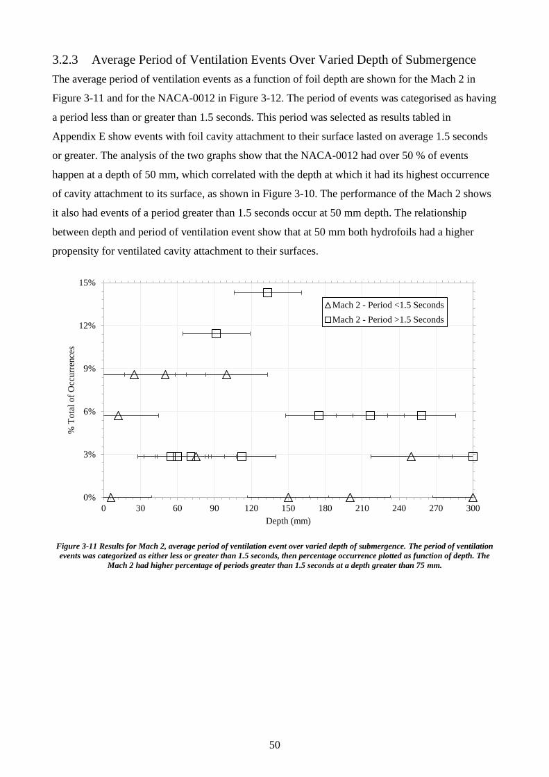
50
3.2.3 Average Period of Ventilation Events Over Varied Depth of Submergence
The average period of ventilation events as a function of foil depth are shown for the Mach 2 in
Figure 3-11 and for the NACA-0012 in Figure 3-12. The period of events was categorised as having
a period less than or greater than 1.5 seconds. This period was selected as results tabled in
Appendix E show events with foil cavity attachment to their surface lasted on average 1.5 seconds
or greater. The analysis of the two graphs show that the NACA-0012 had over 50 % of events
happen at a depth of 50 mm, which correlated with the depth at which it had its highest occurrence
of cavity attachment to its surface, as shown in Figure 3-10. The performance of the Mach 2 shows
it also had events of a period greater than 1.5 seconds occur at 50 mm depth. The relationship
between depth and period of ventilation event show that at 50 mm both hydrofoils had a higher
propensity for ventilated cavity attachment to their surfaces.
Figure 3-11 Results for Mach 2, average period of ventilation event over varied depth of submergence. The period of ventilation
events was categorized as either less or greater than 1.5 seconds, then percentage occurrence plotted as function of depth. The
Mach 2 had higher percentage of periods greater than 1.5 seconds at a depth greater than 75 mm.
0%
3%
6%
9%
12%
15%
0 30 60 90 120 150 180 210 240 270 300
% T
ota
l o
f O
ccurr
ence
s
Depth (mm)
Mach 2 - Period <1.5 Seconds
Mach 2 - Period >1.5 Seconds
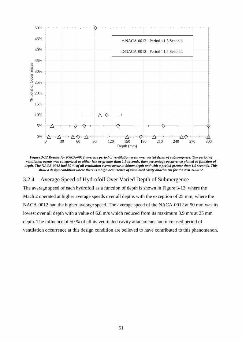
51
Figure 3-12 Results for NACA-0012, average period of ventilation event over varied depth of submergence. The period of
ventilation events was categorized as either less or greater than 1.5 seconds, then percentage occurrence plotted as function of
depth. The NACA-0012 had 50 % of all ventilation events occur at 50mm depth and with a period greater than 1.5 seconds. This
show a design condition where there is a high occurrence of ventilated cavity attachment for the NACA-0012.
3.2.4 Average Speed of Hydrofoil Over Varied Depth of Submergence
The average speed of each hydrofoil as a function of depth is shown in Figure 3-13, where the
Mach 2 operated at higher average speeds over all depths with the exception of 25 mm, where the
NACA-0012 had the higher average speed. The average speed of the NACA-0012 at 50 mm was its
lowest over all depth with a value of 6.8 m/s which reduced from its maximum 8.9 m/s at 25 mm
depth. The influence of 50 % of all its ventilated cavity attachments and increased period of
ventilation occurrence at this design condition are believed to have contributed to this phenomenon.
0%
5%
10%
15%
20%
25%
30%
35%
40%
45%
50%
0 30 60 90 120 150 180 210 240 270 300
% T
ota
l o
f O
ccurr
ence
s
Depth (mm)
NACA-0012 - Period <1.5 Seconds
NACA-0012 - Period >1.5 Seconds
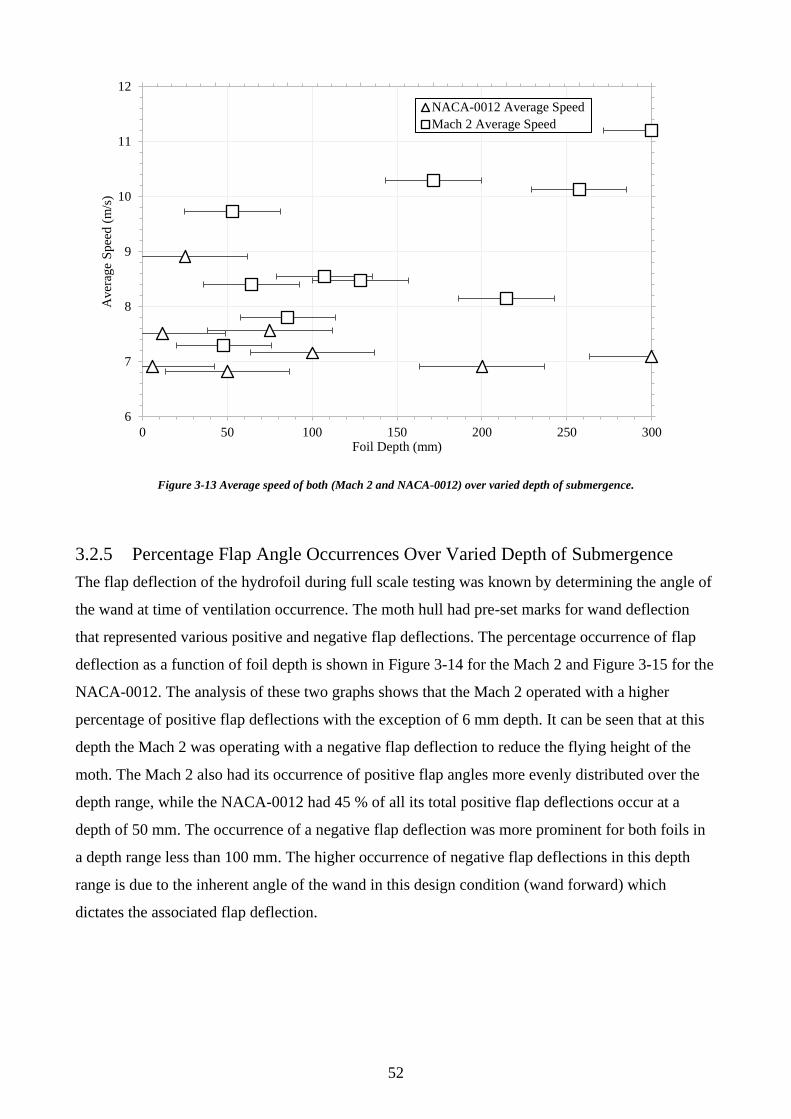
52
Figure 3-13 Average speed of both (Mach 2 and NACA-0012) over varied depth of submergence.
3.2.5 Percentage Flap Angle Occurrences Over Varied Depth of Submergence
The flap deflection of the hydrofoil during full scale testing was known by determining the angle of
the wand at time of ventilation occurrence. The moth hull had pre-set marks for wand deflection
that represented various positive and negative flap deflections. The percentage occurrence of flap
deflection as a function of foil depth is shown in Figure 3-14 for the Mach 2 and Figure 3-15 for the
NACA-0012. The analysis of these two graphs shows that the Mach 2 operated with a higher
percentage of positive flap deflections with the exception of 6 mm depth. It can be seen that at this
depth the Mach 2 was operating with a negative flap deflection to reduce the flying height of the
moth. The Mach 2 also had its occurrence of positive flap angles more evenly distributed over the
depth range, while the NACA-0012 had 45 % of all its total positive flap deflections occur at a
depth of 50 mm. The occurrence of a negative flap deflection was more prominent for both foils in
a depth range less than 100 mm. The higher occurrence of negative flap deflections in this depth
range is due to the inherent angle of the wand in this design condition (wand forward) which
dictates the associated flap deflection.
6
7
8
9
10
11
12
0 50 100 150 200 250 300
Aver
age
Sp
eed
(m
/s)
Foil Depth (mm)
NACA-0012 Average Speed
Mach 2 Average Speed
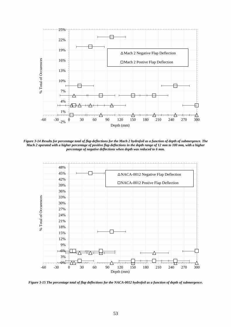
53
Figure 3-14 Results for percentage total of flap deflections for the Mach 2 hydrofoil as a function of depth of submergence. The
Mach 2 operated with a higher percentage of positive flap deflections in the depth range of 12 mm to 100 mm, with a higher
percentage of negative deflections when depth was reduced to 6 mm.
Figure 3-15 The percentage total of flap deflections for the NACA-0012 hydrofoil as a function of depth of submergence.
-2%
1%
4%
7%
10%
13%
16%
19%
22%
25%
-60 -30 0 30 60 90 120 150 180 210 240 270 300
% T
ota
l o
f O
ccure
nce
s
Depth (mm)
Mach 2 Negative Flap Deflection
Mach 2 Postive Flap Deflection
0%
3%
6%
9%
12%
15%
18%
21%
24%
27%
30%
33%
36%
39%
42%
45%
48%
-60 -30 0 30 60 90 120 150 180 210 240 270 300
% T
ota
l o
f O
ccure
nce
s
Depth (mm)
NACA-0012 Negative Flap Deflection
NACA-0012 Postive Flap Deflection
54
3.2.6 Conclusions and Recommendations for Full Scale Testing
The full-scale testing was performed to determine the propensity for ventilated cavity attachment to
the surface of the Mach 2 and NACA-0012 hydrofoils. The two hydrofoils were analysed and setup
to replicate design conditions simulated in the CFD analysis. The experimental data was captured
graphically with two GoPro cameras and an iPhone data logger to record the magnitude and
orientation of all rotations and translations in all six degrees of freedom. The ventilation events
were categorised as either attached or not attached to the surface of the hydrofoil. The complete set
of tabled and graphical results are shown in Appendix E and Appendix F, respectively. The analysis
shows that the NACA-0012 had a higher propensity for ventilated cavity attachment resulting in
catastrophic crashing off the foils which occurred 90 % out of all ventilation events recorded, while
the Mach 2 had 29 % of total events with ventilated cavity attachment to foil surface and 11 % of
which resulted in catastrophic crashing off the foils. The NACA-0012 had one unique design
condition where vapour cavity attachment had its highest occurrence at a depth of 50mm. The
NACA-0012 had 50 % of all its total cavity attachment events occur at this depth. The higher
occurrence of cavity attachment at this design condition shows an interesting correlation with
experimental data collected, where at 50 mm depth the NACA-0012 had an average period of
ventilation greater than 1.5 seconds, operated at its lowest average speed of 6.8 m/s along with
operating at 50 % of its total positive flap deflections at this depth. The occurrence of negative flap
deflection was more prominent for both foils in a depth range less than 100 mm, which is expected
to occur as the moth in this area of operation requires a reduction in lift to stop the foil piercing the
free surface. The Mach 2 operated at a higher efficiency as determined by its reduced propensity for
vapour cavity attachment, higher average speed overall design conditions (except for a depth of 25
mm), and reduced percentage of ventilation periods greater than 1.5 seconds (period increased upon
cavity attachment).
It is recommended that future testing should involve the inbuilt capability provided by the Arduino
data logger (Igoe, 2020) which is justified as instructions regarding design and manufacture are
easily accessible on the internet. The Arduino data logger can be built to incorporate all features
available on the Sensor Play APP, along with additional variables such as pressure sensors located
on the upper and lower surface of the hydrofoil to determine the local pressure in the flow. The
localised pressure could then be compared to CFD numerical results to ensure the accuracy of both
data sets. The second addition to the Arduino data logger is an angle sensor to determine the angle
of flap deflection which could be attached to the rotating bell crank on the main hydrofoil strut.
Capturing the exact angle of flap deflection would increase the accuracy of full-scale data
collection. The current project could only identify positive or negative flap deflations based on
graphical data which showed wand position. The graphical data was prone to uncertainty due to
55
reasons shown in Section 3.1.8. The utilisation of pressure and angle sensors would define
additional key variables that are required to determine the propensity for ventilated cavity
attachment to the hydrofoil surface, which can be compared to CFD numerical results to determine
the association of pre-existing cavitation on the hydrofoil surface and its effects on inducing vapour
cavity to the surface of the foil. The areas of the hydrofoil identified in the CFD analysis where the
absolute pressure operates at its lowest pressures were the leading edge and at the junction of the
hydrofoil and flap. The leading edge of the hydrofoil experienced the lowest magnitude of absolute
pressure of all regions in CFD results in this project.
56
4 Conclusion and Recommendations
4.1 Summary
A method was developed for the analysis of two common hydrofoil sections (NACA-0012 and
Mach 2) to show that there is a correlation between ventilation and cavitation on a hydrofoil
operating near a free surface, as without a pre-existing cavitation cavity there is less chance for a
persistent ventilated cavity to attach and propagate on the hydrofoil surface. The cavitation
propensity of each hydrofoil section was analysed numerically by using CFD to identify design
conditions where this phenomenon will occur. The analysis of ventilation and cavity attachment to
the foil was undertaken through full scale testing. The hydrofoils and strut shared common
geometric properties with the only variation being the hydrofoil cross-section, which formed the
basis of this research project. The NACA-0012 was the only hydrofoil to experience cavitation
vapour cavity formation in the CFD analysis when set at a -10 degrees flap deflection and a
normalised lift coefficient to lift 110 kg. The full-scale testing showed the NACA-0012 had a higher
percentage of ventilated cavities attach and propagate on the hydrofoil surface, with this occurring
90 % out of all ventilation events. The Mach 2 had a lower percentage of attached cavities with only
29 % of total ventilation events.
4.2 Conclusion
The NACA-0012 and Mach 2 hydrofoils sections were analysed using CFD to define their
cavitation propensity with three flap deflections of -10, 0 and 15 degrees to represent the maximum
negative, efficient (neutral) and positive flap deflections set on the main hydrofoil and used in this
research project. The foils were setup at these flap deflections before adjusting their AOA to give a
normalised lift coefficient to represent the combined mass of skipper and moth equal to 110 kg. The
analysis was limited to a depth of 100 mm due to high percentage of ventilation events occurring in
initial full-scale testing. The design condition of -10 degrees flap deflection is an area of operation
where the moth requires maximum down force to reduce the overall ride height to ensure the
hydrofoil does not pierce the free surface. The NACA-0012 experienced both cavitation and vapour
cavity propagation on its surface over all depths of submergence. The NACA-0012 had an
increasing cavity length propagation in the range of 100 mm to 25 mm at which point it reached its
maximum value of 8.2 mm. The cavity length then had a reduction in the depth range of 25 mm to 6
mm. The region of low absolute pressure and cavity formation occurred in the area on the upper
surface of the NACA-0012 near the leading edge, there was also a region of low pressure on the
junction between foil and flap on the lower surface of the foil though had a higher magnitude of
absolute pressure compared to the region on the leading edge. The NACA-0012 at -10 degrees flap
deflection experienced an increase of CT with reduction in depth of submergence, which shows as
57
the cavitation number is lowered there is a corresponding increase in absolute value for the CT. This
is due to pressure variations being distributed further away from the centre of the foil as the
cavitation number is decreased. The effective movement of the foil’s centre of pressure towards the
leading or trailing edge creates higher pressure spikes due to abrupt curvature of the foil geometry
in these regions. The analysis of the Mach 2 at -10 degrees flap deflection showed it to be operating
at a higher cavitation number and experienced a rapid decrease with the reduction of foil
submergence, while operating at higher CT, CL/CD values and lower AOA due to its geometric
properties (asymmetric cross-section).
The foils when set at zero degrees flap deflection had their highest CL/CD of all three design
conditions with the Mach 2 having the highest magnitude over all depths. The NACA-0012 was set
at positive AOA and at values of four times that of the Mach 2 for the same depth of submergence,
while the Mach 2 had to be set at negative angles which shows the difference in setup for an
asymmetric foil (Mach 2) and a symmetric foil (NACA-0012) to generate the same lift coefficient.
The NACA-0012 experienced reduction in cavitation number with reduced depth, while the Mach 2
experienced an increase in cavitation number with reduced depth. The hydrofoils when set at zero
degrees flap deflection only had one location of low absolute pressure around the hydrofoil surface.
This is due to the foils having no flap deflection and operating at their highest efficiency as
determined by magnitude of the CL/CD values. The pressure distribution around the NACA-0012
had a high-pressure location on the lower surface of foil near the leading edge and a low-pressure
region on the upper surface near the leading edge, along with a pressure recovery region at the
trailing edge of the foil as shown earlier in Figure 2-19. This was the only design condition that had
one region of low absolute pressure on the foil surface, which was due to the flap being set at zero
degrees deflection.
The moth when operating at a design condition of 15 degrees flap deflection is set at its maximum
positive deflection and is inducing maximum lifting force to increase the ride height of the moth as
dictated by the wand which is set at its maximum aft position. The hydrofoils required to be set at a
negative AOA to generate the required lift coefficient, with the Mach 2 requiring a greater negative
AOA due to its asymmetrical cross-sectional shape. As was the case with all other flap deflections
the AOA needed a greater positive angle with reduced proximity to the free surface. When set at a
15 degrees flap deflection both foils experienced an increase in cavitation number as the depth was
reduced. The NACA-0012 operated at higher cavitation numbers for all depths and experienced its
greatest rise between depths of 100 mm to 50 mm. The Mach 2 had absolute pressures below
vapour pressure of salt water in the depth range of 25 mm to 100 mm. The increase in cavitation
propensity with increased depth is an unexpected phenomenon as there was no cavity propagation
58
on the hydrofoil surface. This behaviour could be due to the pressure distribution around the Mach
2 at 15 degrees flap deflection, which had two regions of low pressure on its surface with the first
located on the lower surface near the leading edge and the second at the junction of the foil and flap
on the upper surface. The magnitude of absolute low pressures changed at these two locations as the
depth increased, with the low-pressure region at the flap junction on the upper surface experiencing
a greater reduction of low absolute pressure. The reduction of absolute pressure at the junction of
the foil and flap could be due to wave pattern interference, as the distorted geometry and its
inclination to the free stream flow creates an obstruction that adversely effects the pressure gradient
on the suction side of the foil. The flap deflection of 15 degrees was the only design condition
where the NACA-0012 had higher CL/CD value over all depths. The reduction in performance of the
Mach 2 can be attributed to the magnitude of negative AOA required to get the baseline lift
coefficient, which was much larger than what was set on the NACA-0012. The Mach 2 had the
lowest CT values over all depths and experienced an increase in magnitude as the submergence was
increased, which occurred concurrently with a reduction of minimum pressure around the foil
surface. To operate at the above design condition of 15 degrees flap deflection the Mach 2 foil
would need to be set at negative AOA that would be expected to occur in extreme design conditions
in full scale tests. An example of this design condition would be in the event the foil control system
jammed with a 15 degrees flap set, coupled with moth going through wave with a bow down pitch
angle. The occurrence of this described design condition is shown numerically in Appendix D
(Figure D-15) and experimentally in Appendix F (Figure F-36).
The CFD results showed a correlation in the behaviour of residuals that lead to increased cavitation
propensity which are (a) decreased absolute pressure and CL/CD and (b) increased absolute value of
the CT. This was shown for the NACA-0012 at -10 degrees flap and the Mach 2 at 15 degrees flap
deflection.
The full-scale testing was conducted utilising the NACA-0012 and Mach 2 hydrofoil sections to
capture ventilation events and the propensity for vapor cavity attachment to the hydrofoil surface.
The two hydrofoils were setup on the moth to replicate baseline conditions defined in the CFD
analysis which included foil angle of attack, flap range of deflection and foil depth of submergence.
The analysis showed that the NACA-0012 had a higher propensity for ventilated cavity attachment
resulting in catastrophic crashing off the foils which occurred 90 % out of all ventilation events
recorded, while the Mach 2 had 29 % of total events with ventilated cavity attachment to foil
surface and 11 % of which resulted in catastrophic crashing off the foils. The NACA-0012 had 50
% of its cavity attachment events occur at a depth of 50 mm. The analysis of the NACA-0012 at this
design condition showed a trend in experimental data where the average period of ventilation events
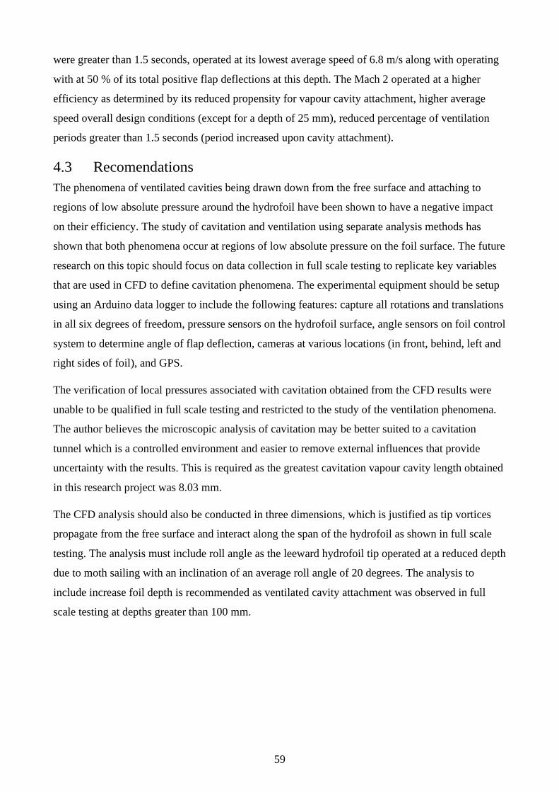
59
were greater than 1.5 seconds, operated at its lowest average speed of 6.8 m/s along with operating
with at 50 % of its total positive flap deflections at this depth. The Mach 2 operated at a higher
efficiency as determined by its reduced propensity for vapour cavity attachment, higher average
speed overall design conditions (except for a depth of 25 mm), reduced percentage of ventilation
periods greater than 1.5 seconds (period increased upon cavity attachment).
4.3 Recomendations
The phenomena of ventilated cavities being drawn down from the free surface and attaching to
regions of low absolute pressure around the hydrofoil have been shown to have a negative impact
on their efficiency. The study of cavitation and ventilation using separate analysis methods has
shown that both phenomena occur at regions of low absolute pressure on the foil surface. The future
research on this topic should focus on data collection in full scale testing to replicate key variables
that are used in CFD to define cavitation phenomena. The experimental equipment should be setup
using an Arduino data logger to include the following features: capture all rotations and translations
in all six degrees of freedom, pressure sensors on the hydrofoil surface, angle sensors on foil control
system to determine angle of flap deflection, cameras at various locations (in front, behind, left and
right sides of foil), and GPS.
The verification of local pressures associated with cavitation obtained from the CFD results were
unable to be qualified in full scale testing and restricted to the study of the ventilation phenomena.
The author believes the microscopic analysis of cavitation may be better suited to a cavitation
tunnel which is a controlled environment and easier to remove external influences that provide
uncertainty with the results. This is required as the greatest cavitation vapour cavity length obtained
in this research project was 8.03 mm.
The CFD analysis should also be conducted in three dimensions, which is justified as tip vortices
propagate from the free surface and interact along the span of the hydrofoil as shown in full scale
testing. The analysis must include roll angle as the leeward hydrofoil tip operated at a reduced depth
due to moth sailing with an inclination of an average roll angle of 20 degrees. The analysis to
include increase foil depth is recommended as ventilated cavity attachment was observed in full
scale testing at depths greater than 100 mm.
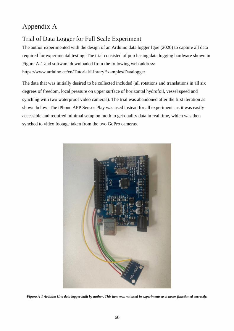
60
Trial of Data Logger for Full Scale Experiment
The author experimented with the design of an Arduino data logger Igoe (2020) to capture all data
required for experimental testing. The trial consisted of purchasing data logging hardware shown in
Figure A-1 and software downloaded from the following web address:
https://www.arduino.cc/en/Tutorial/LibraryExamples/Datalogger
The data that was initially desired to be collected included (all rotations and translations in all six
degrees of freedom, local pressure on upper surface of horizontal hydrofoil, vessel speed and
synching with two waterproof video cameras). The trial was abandoned after the first iteration as
shown below. The iPhone APP Sensor Play was used instead for all experiments as it was easily
accessible and required minimal setup on moth to get quality data in real time, which was then
synched to video footage taken from the two GoPro cameras.
Figure A-1 Arduino Uno data logger built by author. This item was not used in experiments as it never functioned correctly.
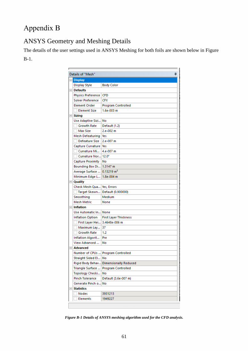
61
ANSYS Geometry and Meshing Details
The details of the user settings used in ANSYS Meshing for both foils are shown below in Figure
B-1.
Figure B-1 Details of ANSYS meshing algorithm used for the CFD analysis.
62
CEL and Additional Variables for ANSYS CFX Solver
The CEL and additional variables used for the ANSYS-CFX solver are shown below in Table B-1.
Table B-1 List of CEL expressions and additional variables defined in CFX Pre-Processor and used to define key temporal and
spatial parameters used to solve the CFD model.
CEL EXPRESSIONS
CEL Expression
Name Definition
MassFlow = 1025[kg/m^3]*area()@REGION:inlet*SetVel
MaxX = max(MaxXCylFront , MaxXFront )
MaxXCylFront = maxVal(Fluid 1.XExtentCavity ) @ REGION:front
MaxXFront = maxVal(Fluid 1.XExtentCavity ) @ REGION:front
Press Coeff = (Pressure)/(.5*(1025[kg/m^3])*((10[m/s])^2))
SetVel = 10[m/s]
freeSurfaceAir = 1-step((0.0377[m]-y)/1[m])
hydroPressure = (0.0377[m]-y)*g*1025[kg/m^3]
xlocation =
(x+0.05[m])*step(0.52-(Vapour.Volume Fraction\))*step((Vapour.Volume
Fraction)-0.48)
ADDITIONAL VARIABLES
Additional Variable 1
XExtentCavity
Option = Definition
Tensor Type = SCALAR
Units = [ m]
Variable Type = Specific
Additional Variable 2
Name: Xlcn
Option = Definition
Tensor Type = SCALAR
Units = [m ]
Variable Type = Volumetric
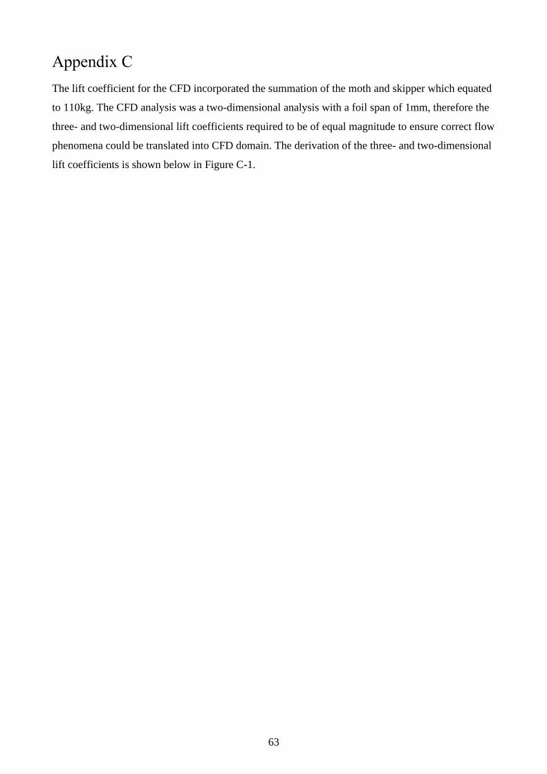
63
The lift coefficient for the CFD incorporated the summation of the moth and skipper which equated
to 110kg. The CFD analysis was a two-dimensional analysis with a foil span of 1mm, therefore the
three- and two-dimensional lift coefficients required to be of equal magnitude to ensure correct flow
phenomena could be translated into CFD domain. The derivation of the three- and two-dimensional
lift coefficients is shown below in Figure C-1.
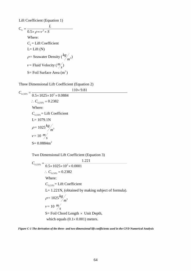
64
2
3
2
Lift Coefficient (Equation 1)
C0.5
Where:
= Lift Coefficient
L= Lift (N)
= Seawater Density ( )
= Fluid Velocity ( )
S= Foil Surface Area (m )
Three Dimensional Lift Coefficient (Equation 2)
L
L
L
S
C
kgm
ms
=
(3 ) 2
(3 )
(3 )
3
2
(2 ) 2
(3
110 9.81
0.5 1025 10 0.0884
0.2382
Where:
= Lift Coefficient
L= 1079.1N
= 1025
= 10
S= 0.0884m
Two Dimensional Lift Coefficient (Equation 3)
1.221
0.5 1025 10 0.0001
L D
L D
L D
L D
L D
C
C
C
kgm
ms
C
C
=
=
=
)
(2 )
3
0.2382
Where:
= Lift Coefficient
L= 1.221N, (obtained by making subject of formula).
= 1025
= 10
S= Foil Chord Length Unit Depth,
which equals (0.1 0.001) meters.
L DC
kgm
ms
=
Figure C-1 The derivation of the three- and two-dimensional lift coefficients used in the CFD Numerical Analysis
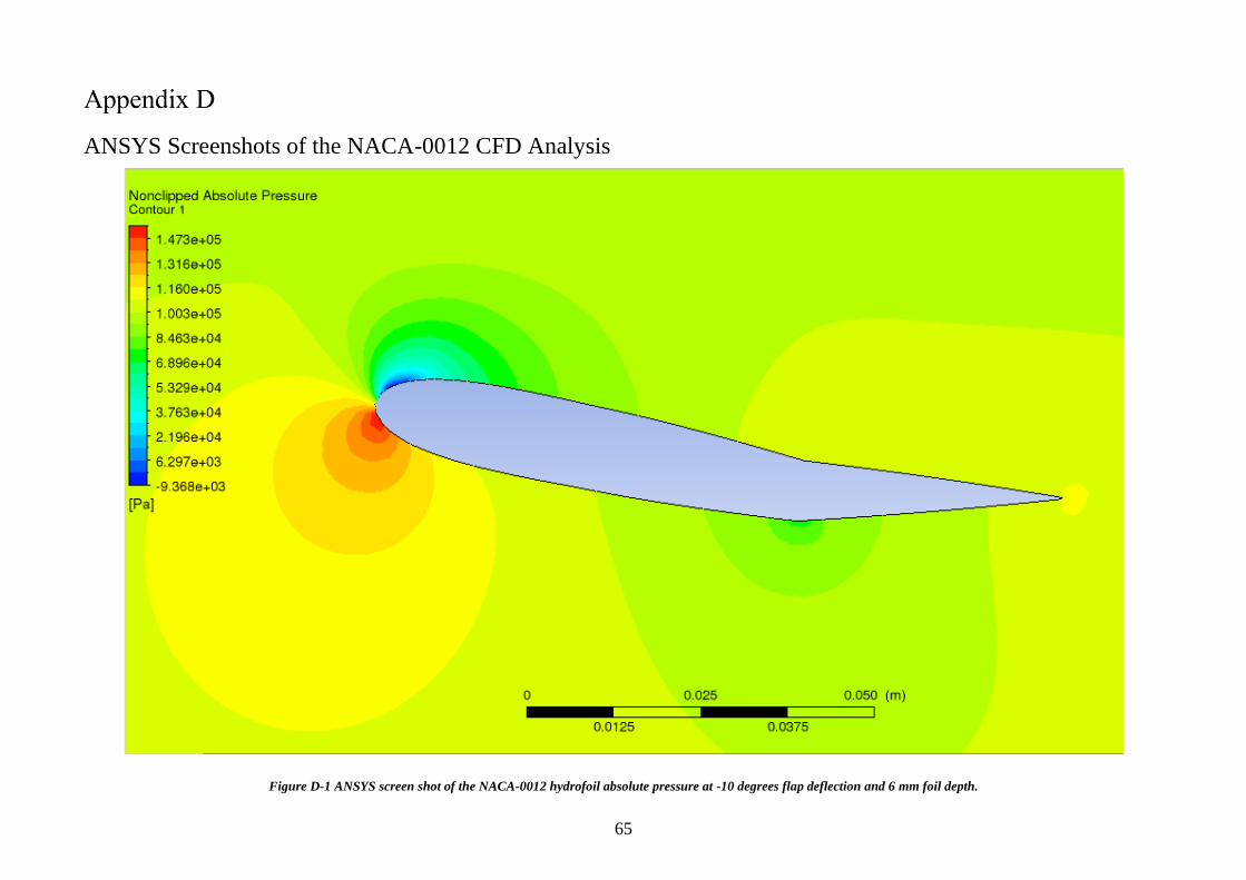
65
ANSYS Screenshots of the NACA-0012 CFD Analysis
Figure D-1 ANSYS screen shot of the NACA-0012 hydrofoil absolute pressure at -10 degrees flap deflection and 6 mm foil depth.
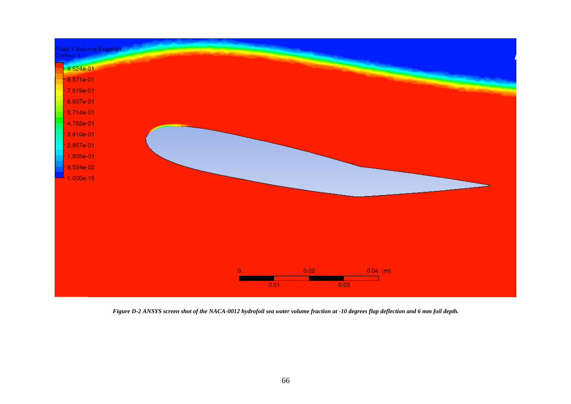
66
Figure D-2 ANSYS screen shot of the NACA-0012 hydrofoil sea water volume fraction at -10 degrees flap deflection and 6 mm foil depth.
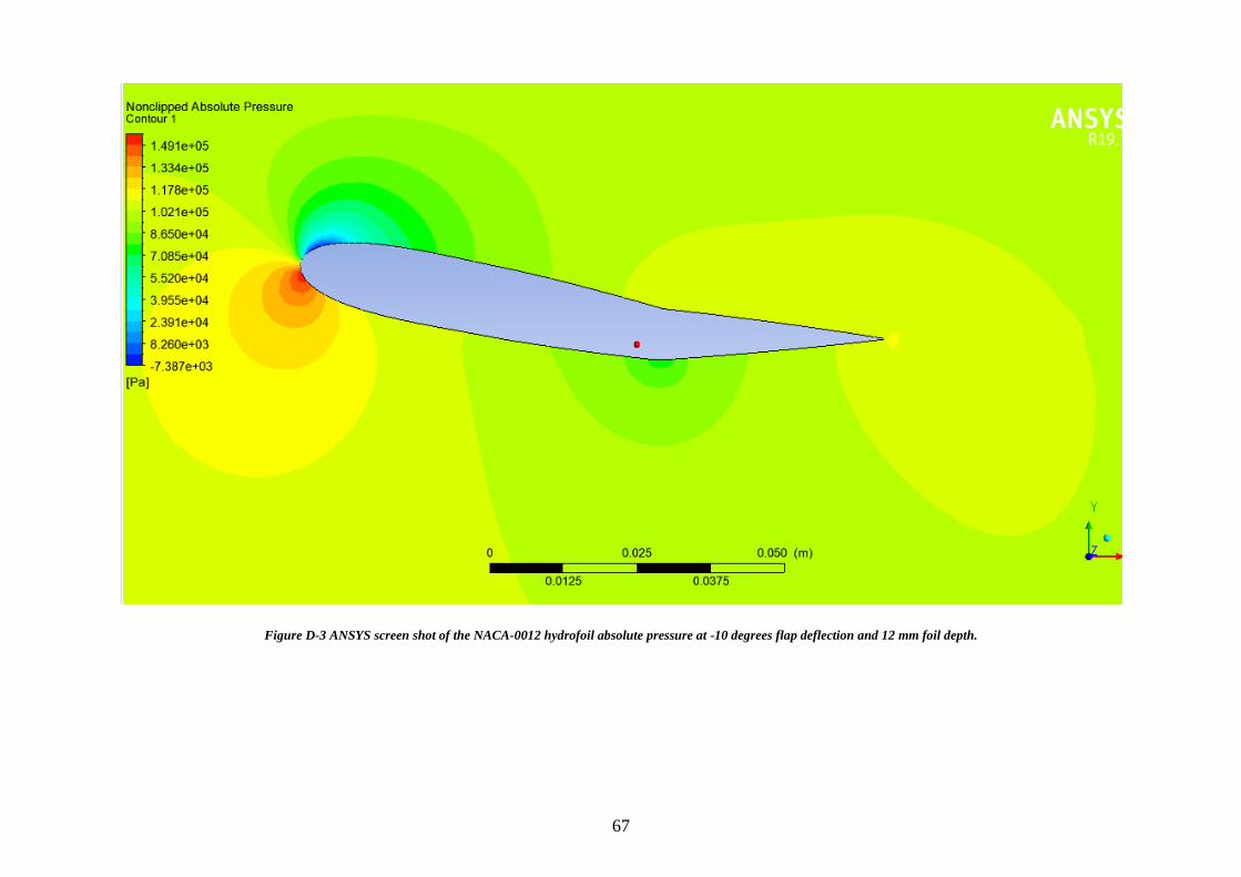
67
Figure D-3 ANSYS screen shot of the NACA-0012 hydrofoil absolute pressure at -10 degrees flap deflection and 12 mm foil depth.
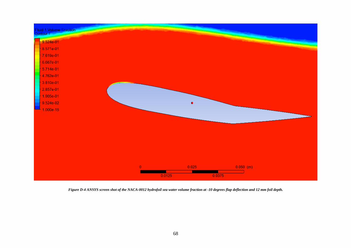
68
Figure D-4 ANSYS screen shot of the NACA-0012 hydrofoil sea water volume fraction at -10 degrees flap deflection and 12 mm foil depth.
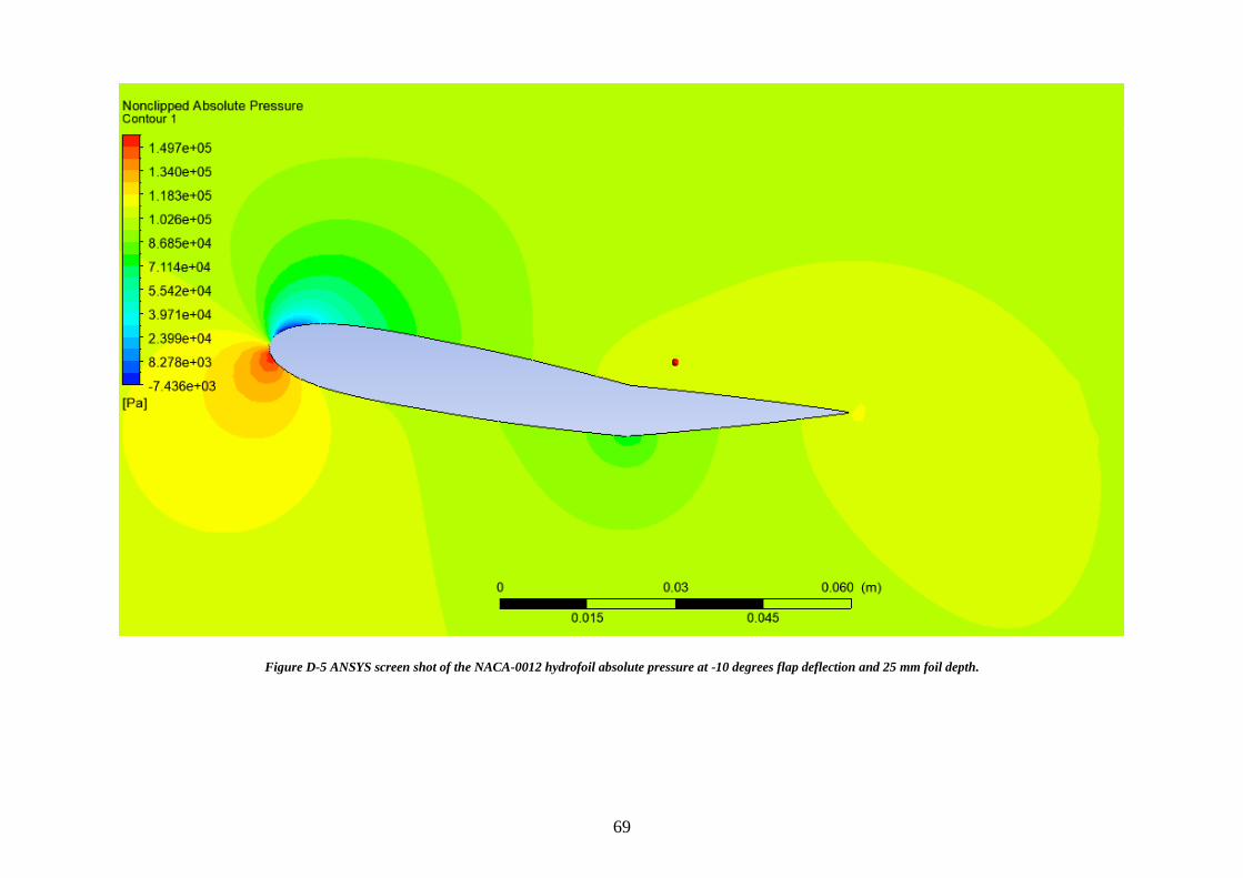
69
Figure D-5 ANSYS screen shot of the NACA-0012 hydrofoil absolute pressure at -10 degrees flap deflection and 25 mm foil depth.
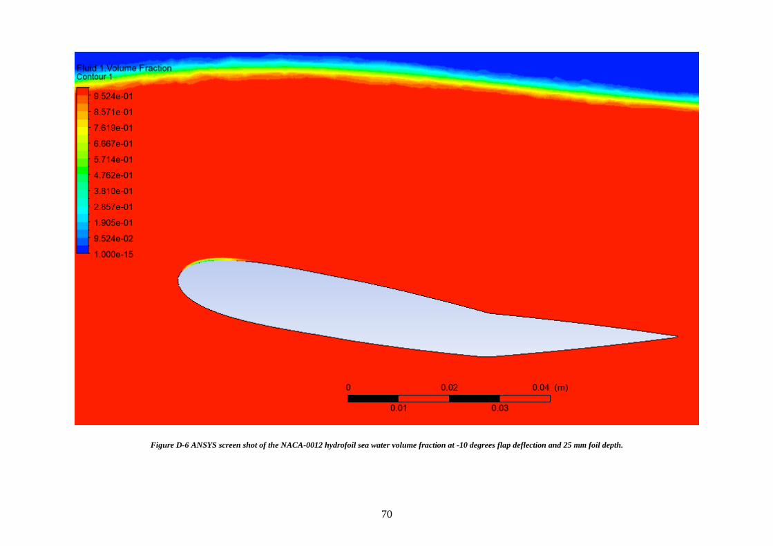
70
Figure D-6 ANSYS screen shot of the NACA-0012 hydrofoil sea water volume fraction at -10 degrees flap deflection and 25 mm foil depth.
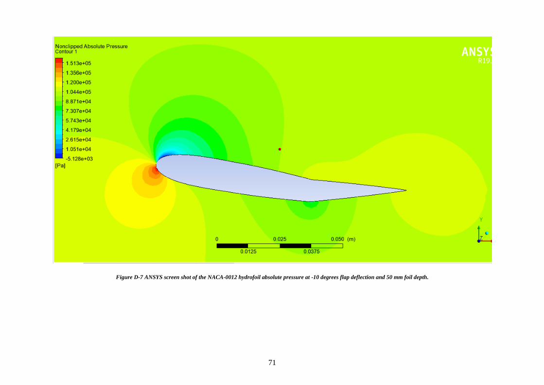
71
Figure D-7 ANSYS screen shot of the NACA-0012 hydrofoil absolute pressure at -10 degrees flap deflection and 50 mm foil depth.
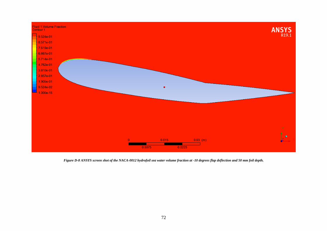
72
Figure D-8 ANSYS screen shot of the NACA-0012 hydrofoil sea water volume fraction at -10 degrees flap deflection and 50 mm foil depth.
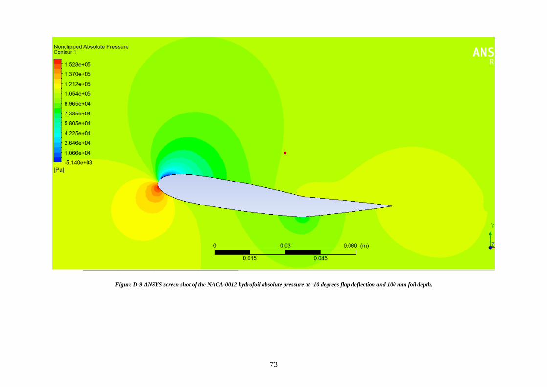
73
Figure D-9 ANSYS screen shot of the NACA-0012 hydrofoil absolute pressure at -10 degrees flap deflection and 100 mm foil depth.
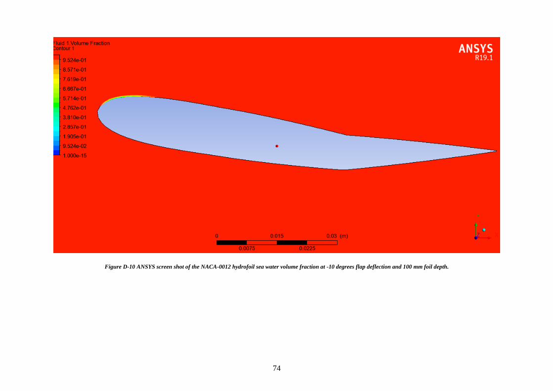
74
Figure D-10 ANSYS screen shot of the NACA-0012 hydrofoil sea water volume fraction at -10 degrees flap deflection and 100 mm foil depth.
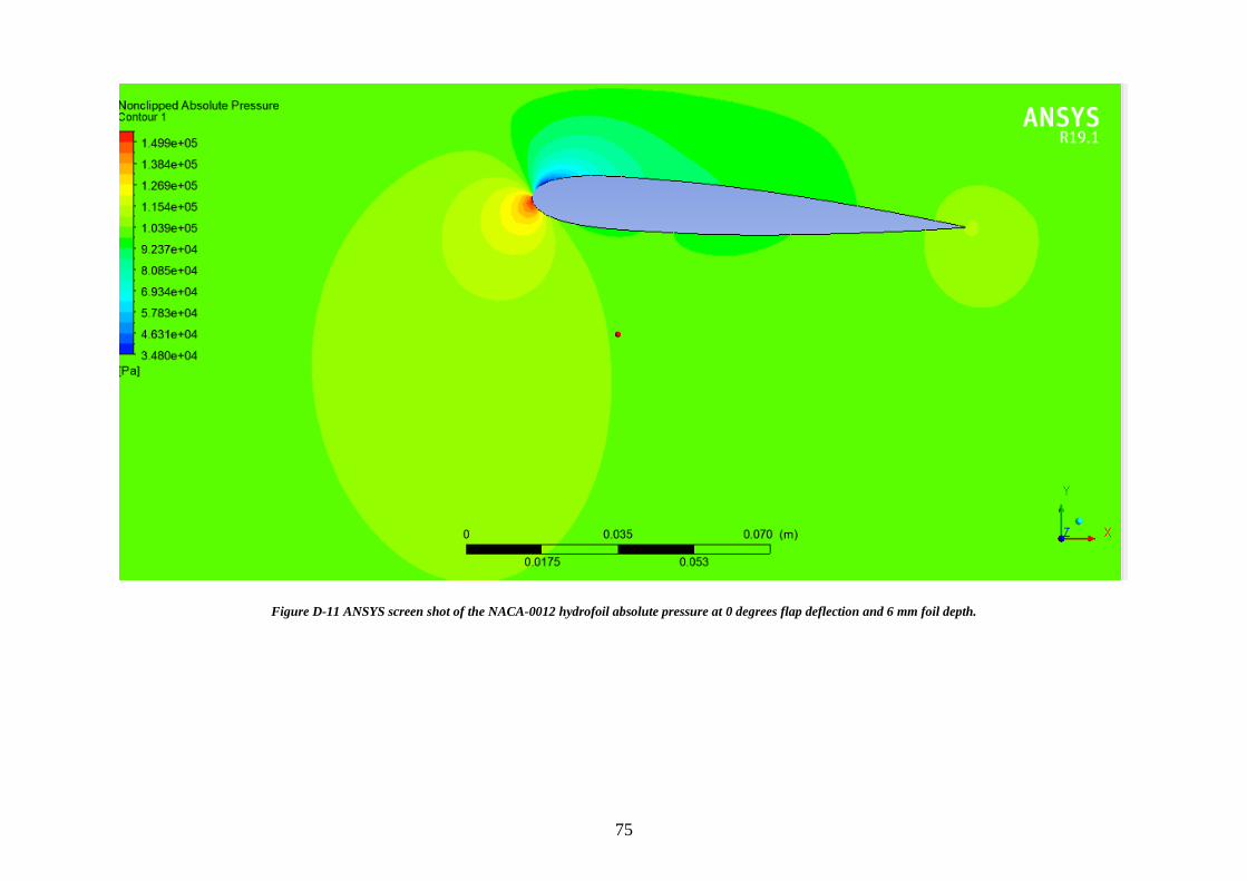
75
Figure D-11 ANSYS screen shot of the NACA-0012 hydrofoil absolute pressure at 0 degrees flap deflection and 6 mm foil depth.
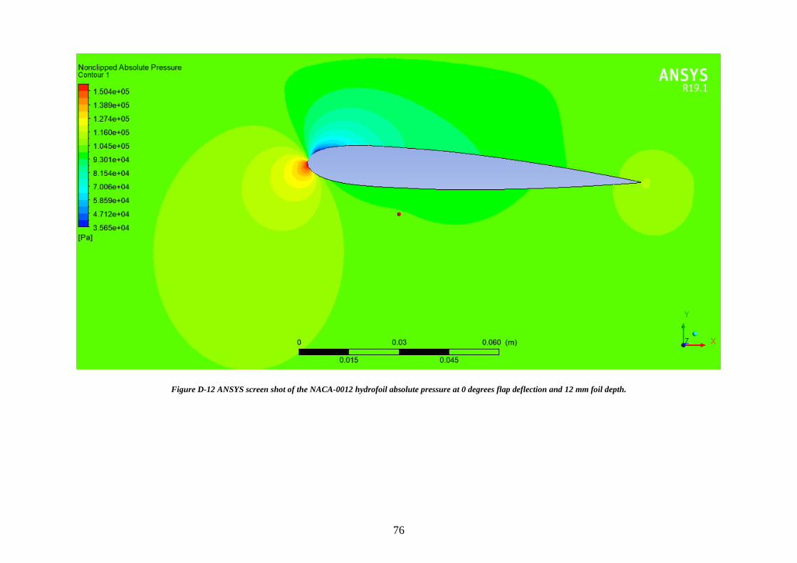
76
Figure D-12 ANSYS screen shot of the NACA-0012 hydrofoil absolute pressure at 0 degrees flap deflection and 12 mm foil depth.
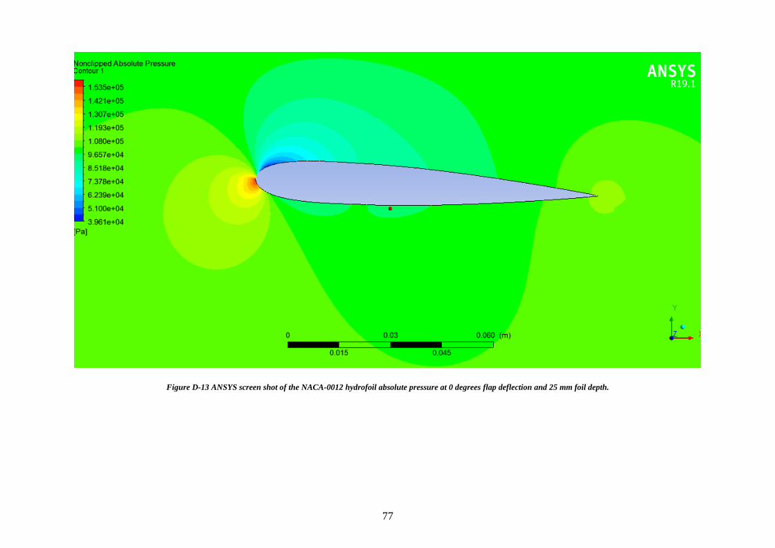
77
Figure D-13 ANSYS screen shot of the NACA-0012 hydrofoil absolute pressure at 0 degrees flap deflection and 25 mm foil depth.
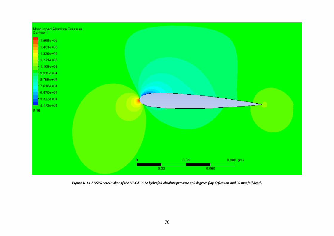
78
Figure D-14 ANSYS screen shot of the NACA-0012 hydrofoil absolute pressure at 0 degrees flap deflection and 50 mm foil depth.
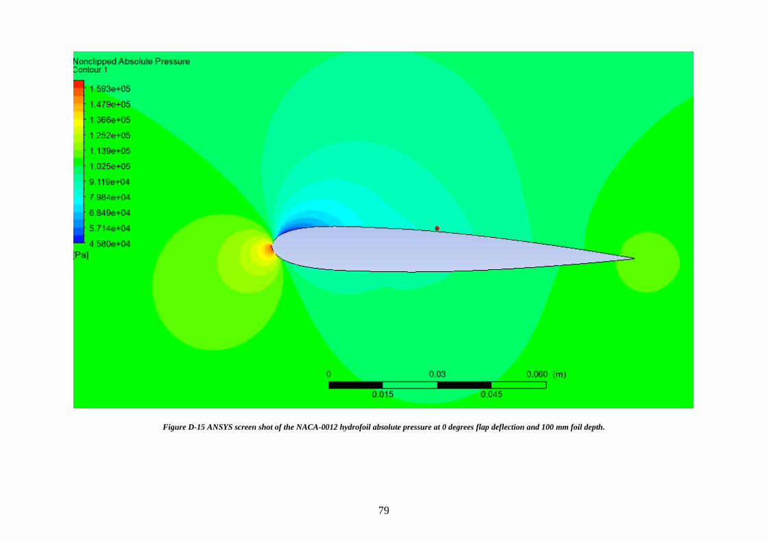
79
Figure D-15 ANSYS screen shot of the NACA-0012 hydrofoil absolute pressure at 0 degrees flap deflection and 100 mm foil depth.
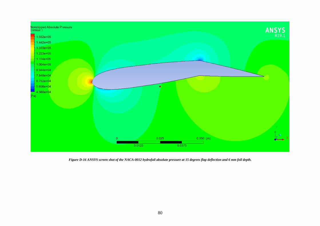
80
Figure D-16 ANSYS screen shot of the NACA-0012 hydrofoil absolute pressure at 15 degrees flap deflection and 6 mm foil depth.
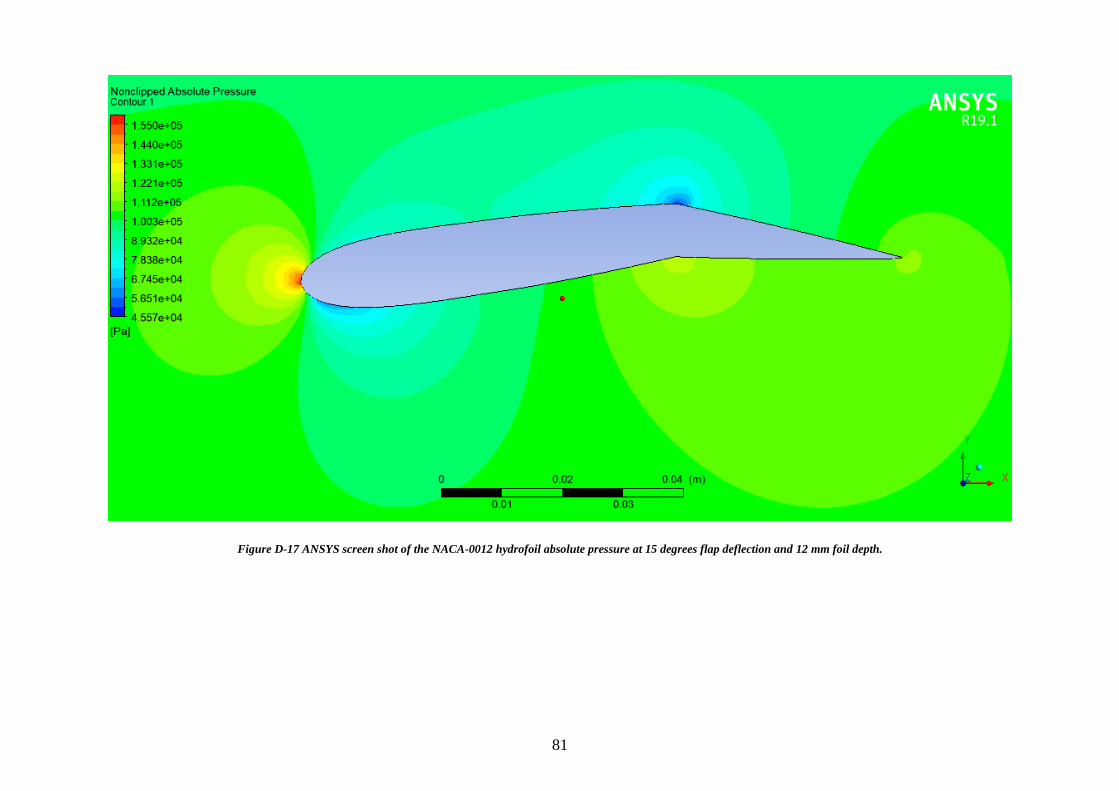
81
Figure D-17 ANSYS screen shot of the NACA-0012 hydrofoil absolute pressure at 15 degrees flap deflection and 12 mm foil depth.
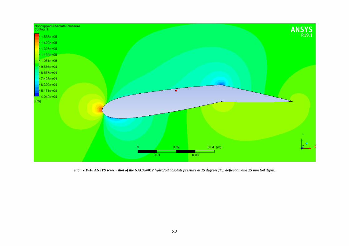
82
Figure D-18 ANSYS screen shot of the NACA-0012 hydrofoil absolute pressure at 15 degrees flap deflection and 25 mm foil depth.
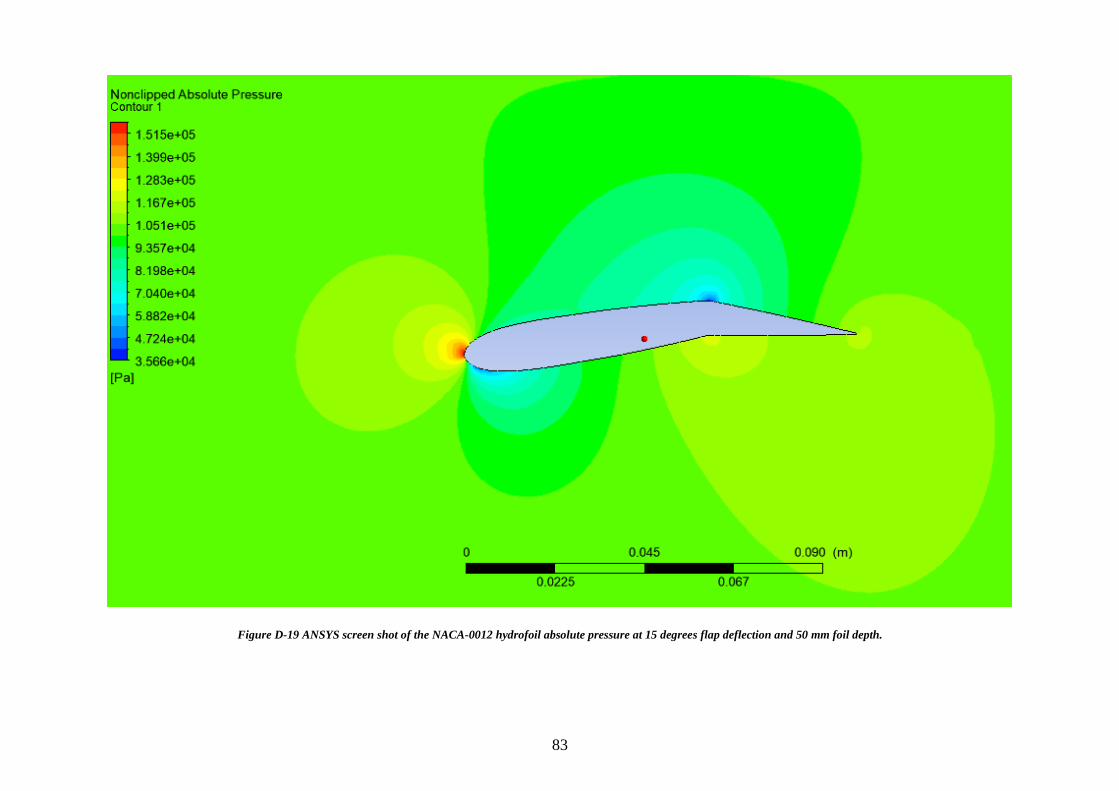
83
Figure D-19 ANSYS screen shot of the NACA-0012 hydrofoil absolute pressure at 15 degrees flap deflection and 50 mm foil depth.
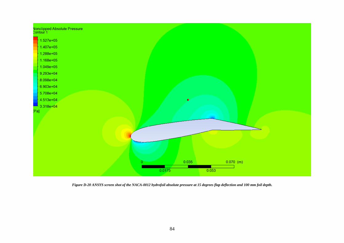
84
Figure D-20 ANSYS screen shot of the NACA-0012 hydrofoil absolute pressure at 15 degrees flap deflection and 100 mm foil depth.
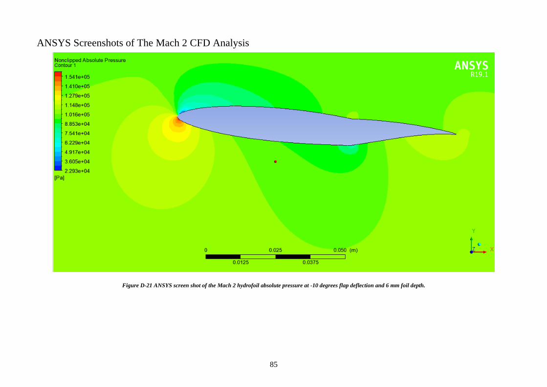
85
ANSYS Screenshots of The Mach 2 CFD Analysis
Figure D-21 ANSYS screen shot of the Mach 2 hydrofoil absolute pressure at -10 degrees flap deflection and 6 mm foil depth.
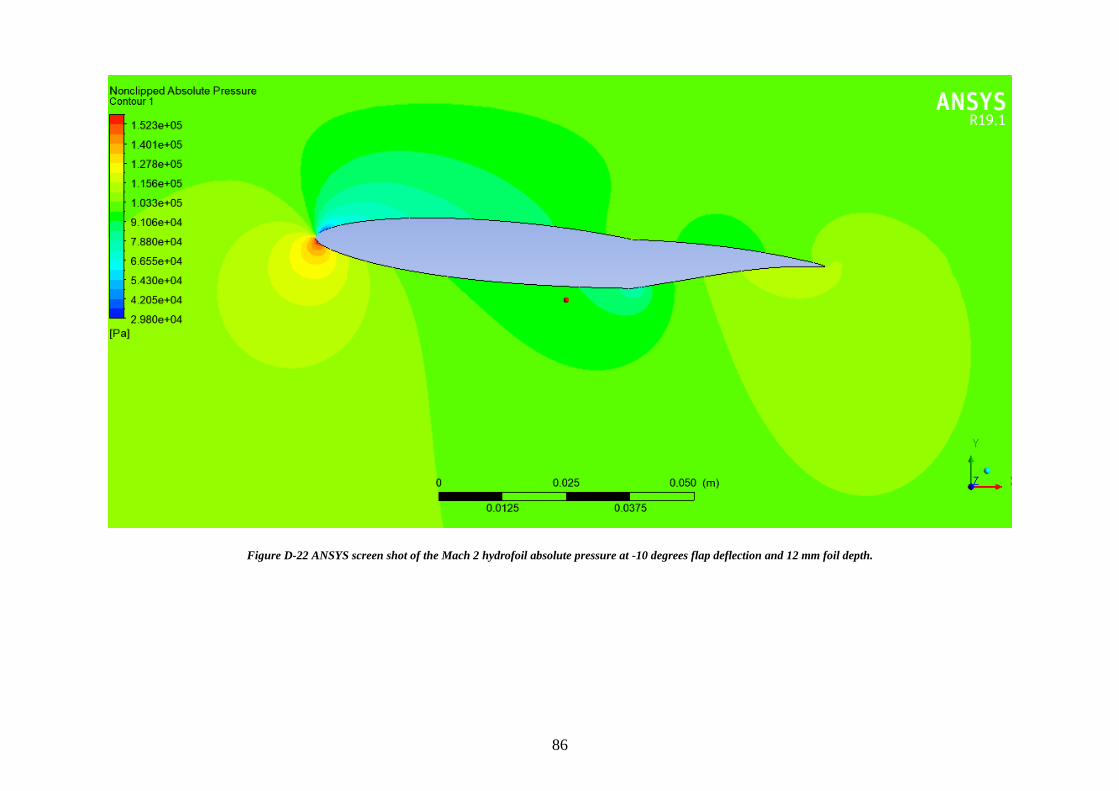
86
Figure D-22 ANSYS screen shot of the Mach 2 hydrofoil absolute pressure at -10 degrees flap deflection and 12 mm foil depth.
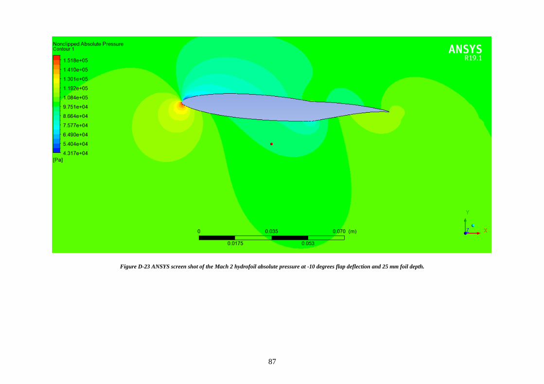
87
Figure D-23 ANSYS screen shot of the Mach 2 hydrofoil absolute pressure at -10 degrees flap deflection and 25 mm foil depth.
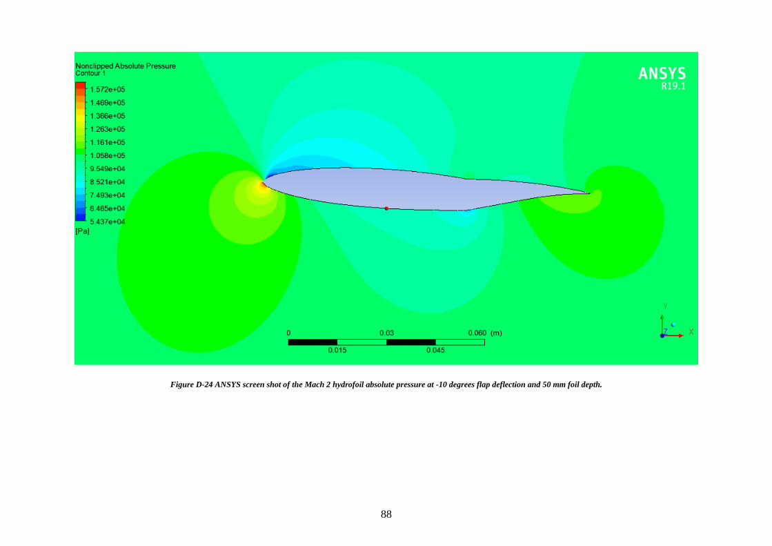
88
Figure D-24 ANSYS screen shot of the Mach 2 hydrofoil absolute pressure at -10 degrees flap deflection and 50 mm foil depth.
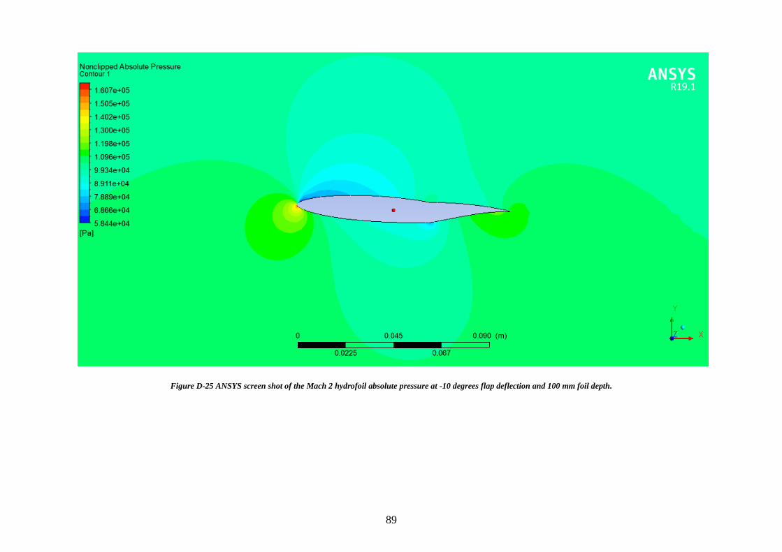
89
Figure D-25 ANSYS screen shot of the Mach 2 hydrofoil absolute pressure at -10 degrees flap deflection and 100 mm foil depth.
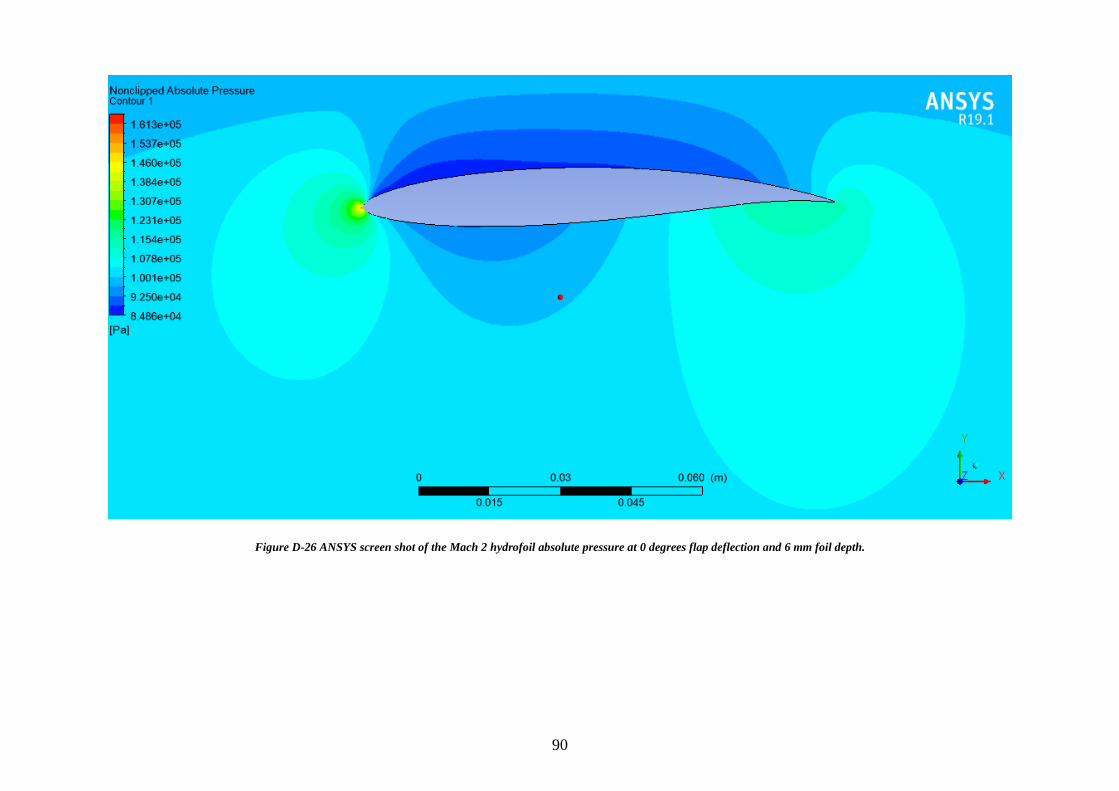
90
Figure D-26 ANSYS screen shot of the Mach 2 hydrofoil absolute pressure at 0 degrees flap deflection and 6 mm foil depth.

91
Figure D-27 ANSYS screen shot of the Mach 2 hydrofoil absolute pressure at 0 degrees flap deflection and 12 mm foil depth.
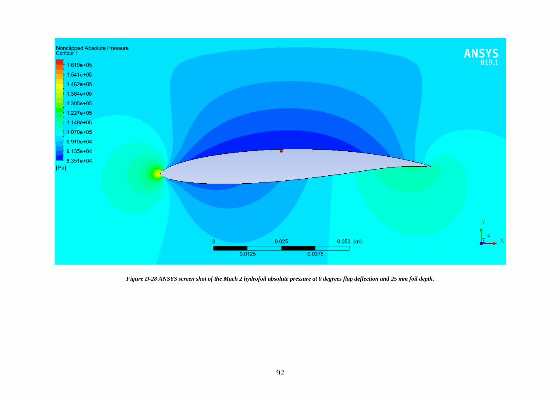
92
Figure D-28 ANSYS screen shot of the Mach 2 hydrofoil absolute pressure at 0 degrees flap deflection and 25 mm foil depth.
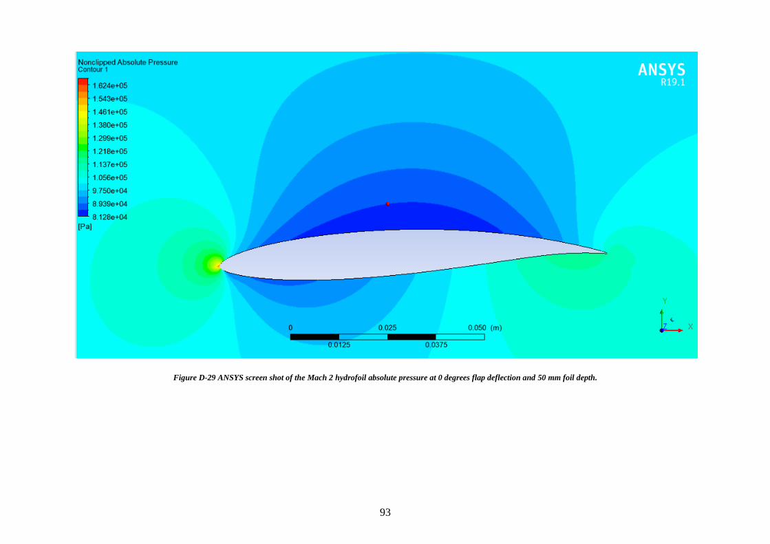
93
Figure D-29 ANSYS screen shot of the Mach 2 hydrofoil absolute pressure at 0 degrees flap deflection and 50 mm foil depth.
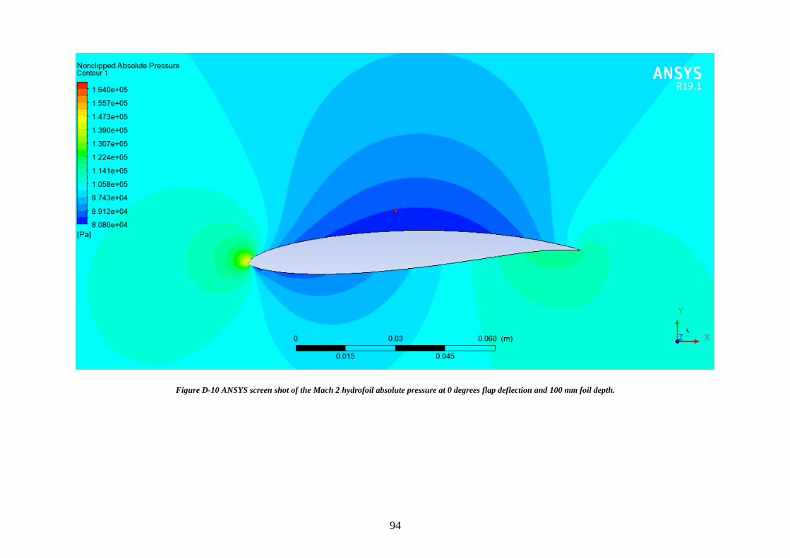
94
Figure D-10 ANSYS screen shot of the Mach 2 hydrofoil absolute pressure at 0 degrees flap deflection and 100 mm foil depth.
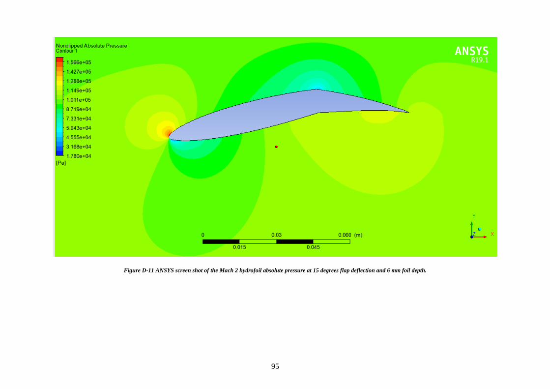
95
Figure D-11 ANSYS screen shot of the Mach 2 hydrofoil absolute pressure at 15 degrees flap deflection and 6 mm foil depth.
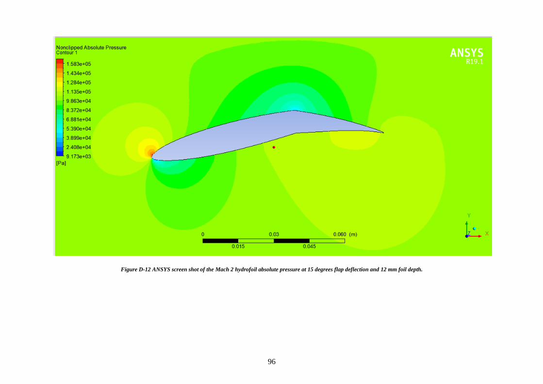
96
Figure D-12 ANSYS screen shot of the Mach 2 hydrofoil absolute pressure at 15 degrees flap deflection and 12 mm foil depth.
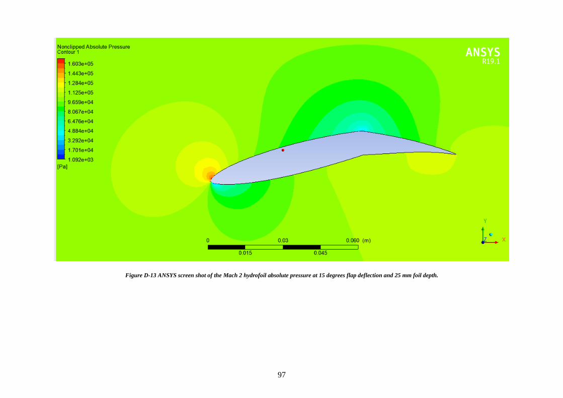
97
Figure D-13 ANSYS screen shot of the Mach 2 hydrofoil absolute pressure at 15 degrees flap deflection and 25 mm foil depth.

98
Figure D-14 ANSYS screen shot of the Mach 2 hydrofoil absolute pressure at 15 degrees flap deflection and 50 mm foil depth.
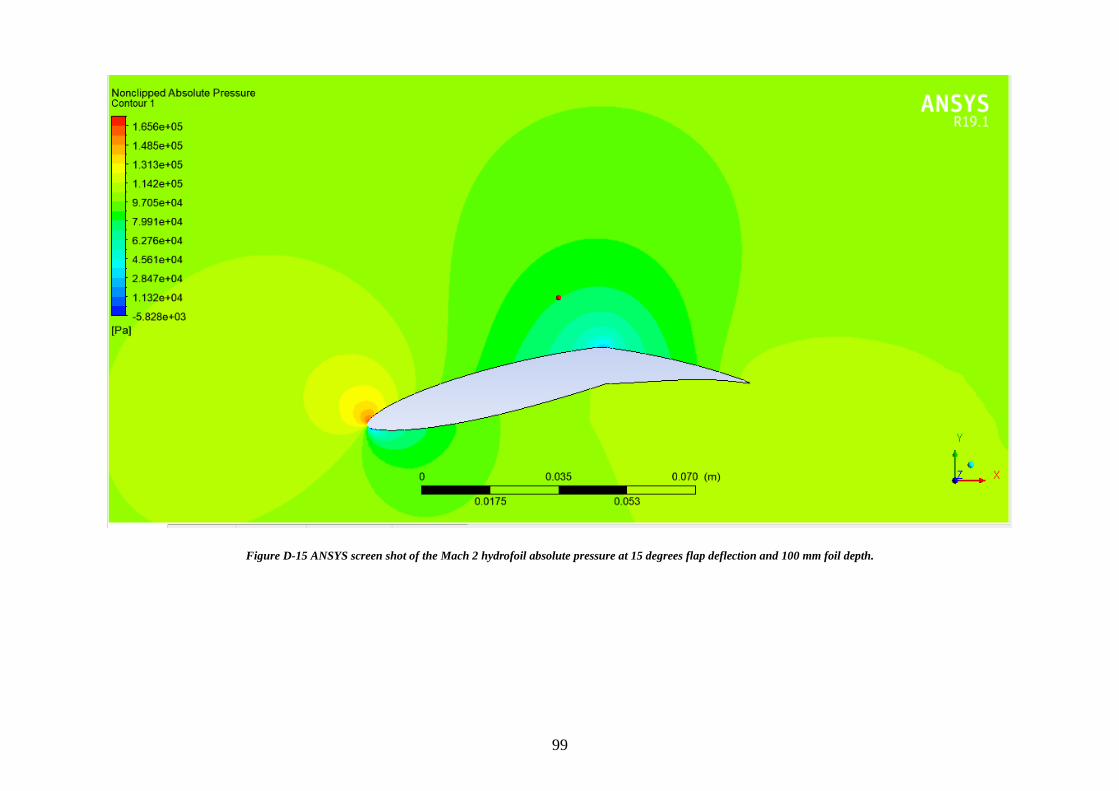
99
Figure D-15 ANSYS screen shot of the Mach 2 hydrofoil absolute pressure at 15 degrees flap deflection and 100 mm foil depth.

100
Mach 2 Analysis Used for Thesis Dated (28/08/2020)
Mach 2
Event
Number
Time in
Video
(mins.sec)
Occurrences
(date/time)
Period of
Event
(sec)
Depth
(mm)
Pitch/AOA
(deg)
Flap
Deflection
(deg)
Speed
(m/s)
Roll
(deg
Ventilated
Cavitation
Cavity (Y or N)
Crash or
Recovery
(C or R)
Event 1 13.06 28/08/2020 0.50 50 5.0 15.0 8.40 -20 N R
Event 2 15.14 28/08/2020 0.50 25 5.0 5.0 7.30 -30 N R
Event 3 15.20 28/08/2020 0.25 25 5.0 0.0 10.40 20 N R
Event 4 16.17 28/08/2020 1.50 6 5.0 -10.0 7.30 -15 Y C
Event 5 17.34 28/08/2020 1.50 200 5.0 15.0 6.40 -20 N R
Event 6 20.04 28/08/2020 1.50 50 5.0 0.0 5.60 20 N R
Event 7 20.25 28/08/2020 2.50 100 5.0 5.0 8.00 20 Y R
Event 8 20.44 28/08/2020 2.00 75 5.0 10.0 9.60 20 N R
Event 9 21.00 28/08/2020 0.50 25 5.0 0.0 7.80 18 N R
Event 10 21.22 28/08/2020 1.20 100 5.0 5.0 9.50 20 N R
Event 11 27.27 28/08/2020 1.00 12 0.0 -10.0 7.80 -20 Y C
Event 12 29.25 28/08/2020 3.00 50 5.0 5.0 7.40 30 Y R
Event 13 29.44 28/08/2020 1.50 100 5.0 5.0 8.00 20 N R
Event 14 29.53 28/08/2020 2.20 100 5.0 10.0 9.00 20 Y C
Event 15 38.29 28/08/2020 1.50 250 5.0 5.0 9.75 -20 N R
Event 16 41.20 28/08/2020 1.00 12 3.0 -10.0 8.40 20 N R
Event 17 48.51 28/08/2020 1.50 150 5.0 10.0 11.10 22 N R
Event 18 52.41 28/08/2020 1.50 300 5.0 0.0 11.20 -20 N R
Event 19 53.03 28/08/2020 0.50 50 5.0 0.0 8.50 -18 N R
Event 20 53.15 28/08/2020 0.50 75 3.0 0.0 7.50 -20 N R
Event 21 56.05 28/08/2020 2.00 50 5.0 -10.0 9.60 -20 N C
Event 22 57.12 28/08/2020 2.00 200 5.0 0.0 9.90 -15 N R
Event 23 58.38 28/08/2020 1.20 250 4.0 5.0 12.05 -20 Y R
Event 24 101.02 28/08/2020 2.00 12 5.0 5.0 13.00 20 N R
Event 25 101.05 28/08/2020 2.50 50 5.0 10.0 8.50 20 Y R
Event 26 101.26 28/08/2020 2.00 100 4.0 5.0 9.60 20 N R
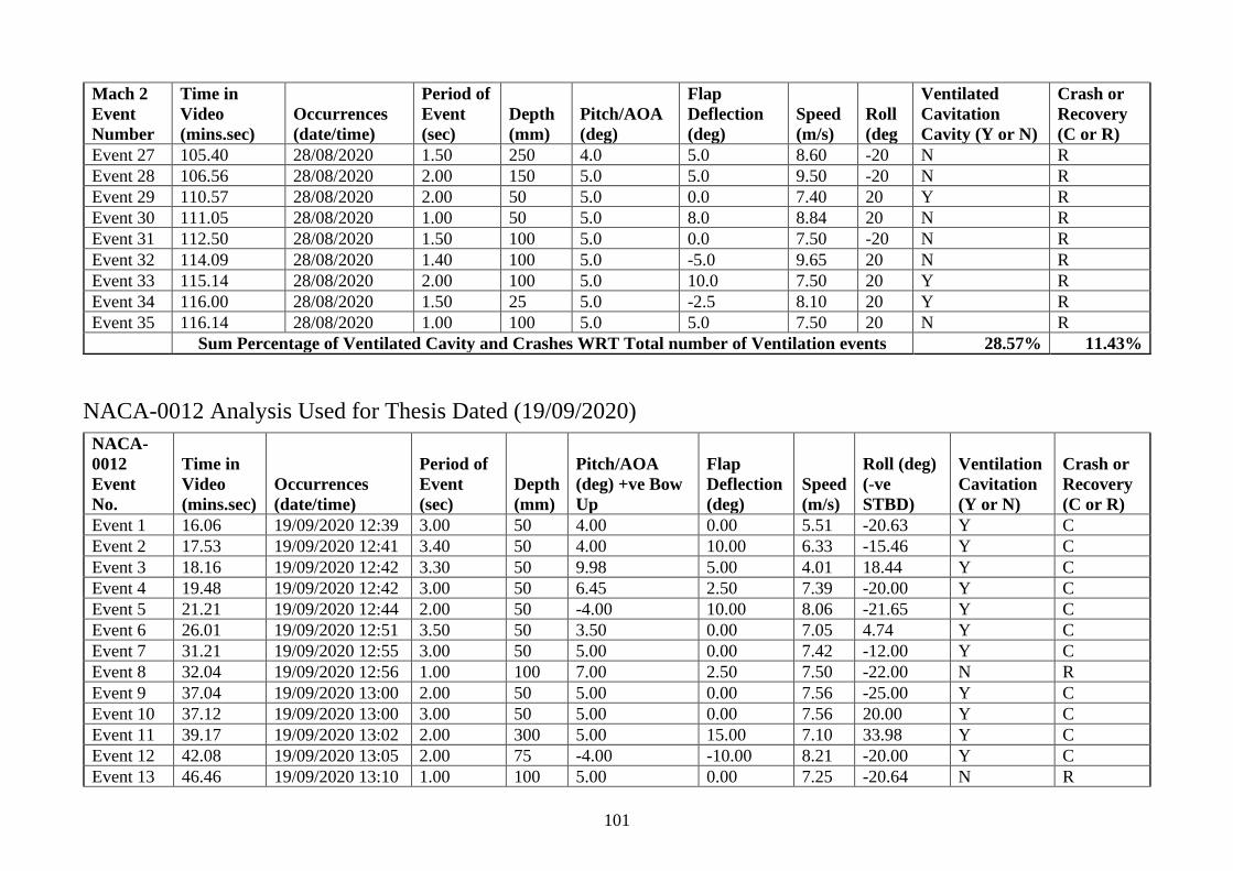
101
Mach 2
Event
Number
Time in
Video
(mins.sec)
Occurrences
(date/time)
Period of
Event
(sec)
Depth
(mm)
Pitch/AOA
(deg)
Flap
Deflection
(deg)
Speed
(m/s)
Roll
(deg
Ventilated
Cavitation
Cavity (Y or N)
Crash or
Recovery
(C or R)
Event 27 105.40 28/08/2020 1.50 250 4.0 5.0 8.60 -20 N R
Event 28 106.56 28/08/2020 2.00 150 5.0 5.0 9.50 -20 N R
Event 29 110.57 28/08/2020 2.00 50 5.0 0.0 7.40 20 Y R
Event 30 111.05 28/08/2020 1.00 50 5.0 8.0 8.84 20 N R
Event 31 112.50 28/08/2020 1.50 100 5.0 0.0 7.50 -20 N R
Event 32 114.09 28/08/2020 1.40 100 5.0 -5.0 9.65 20 N R
Event 33 115.14 28/08/2020 2.00 100 5.0 10.0 7.50 20 Y R
Event 34 116.00 28/08/2020 1.50 25 5.0 -2.5 8.10 20 Y R
Event 35 116.14 28/08/2020 1.00 100 5.0 5.0 7.50 20 N R
Sum Percentage of Ventilated Cavity and Crashes WRT Total number of Ventilation events 28.57% 11.43%
NACA-0012 Analysis Used for Thesis Dated (19/09/2020)
NACA-
0012
Event
No.
Time in
Video
(mins.sec)
Occurrences
(date/time)
Period of
Event
(sec)
Depth
(mm)
Pitch/AOA
(deg) +ve Bow
Up
Flap
Deflection
(deg)
Speed
(m/s)
Roll (deg)
(-ve
STBD)
Ventilation
Cavitation
(Y or N)
Crash or
Recovery
(C or R)
Event 1 16.06 19/09/2020 12:39 3.00 50 4.00 0.00 5.51 -20.63 Y C
Event 2 17.53 19/09/2020 12:41 3.40 50 4.00 10.00 6.33 -15.46 Y C
Event 3 18.16 19/09/2020 12:42 3.30 50 9.98 5.00 4.01 18.44 Y C
Event 4 19.48 19/09/2020 12:42 3.00 50 6.45 2.50 7.39 -20.00 Y C
Event 5 21.21 19/09/2020 12:44 2.00 50 -4.00 10.00 8.06 -21.65 Y C
Event 6 26.01 19/09/2020 12:51 3.50 50 3.50 0.00 7.05 4.74 Y C
Event 7 31.21 19/09/2020 12:55 3.00 50 5.00 0.00 7.42 -12.00 Y C
Event 8 32.04 19/09/2020 12:56 1.00 100 7.00 2.50 7.50 -22.00 N R
Event 9 37.04 19/09/2020 13:00 2.00 50 5.00 0.00 7.56 -25.00 Y C
Event 10 37.12 19/09/2020 13:00 3.00 50 5.00 0.00 7.56 20.00 Y C
Event 11 39.17 19/09/2020 13:02 2.00 300 5.00 15.00 7.10 33.98 Y C
Event 12 42.08 19/09/2020 13:05 2.00 75 -4.00 -10.00 8.21 -20.00 Y C
Event 13 46.46 19/09/2020 13:10 1.00 100 5.00 0.00 7.25 -20.64 N R
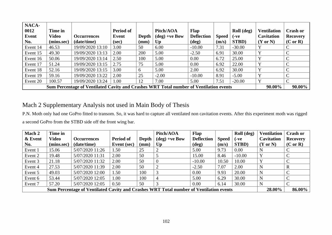
102
NACA-
0012
Event
No.
Time in
Video
(mins.sec)
Occurrences
(date/time)
Period of
Event
(sec)
Depth
(mm)
Pitch/AOA
(deg) +ve Bow
Up
Flap
Deflection
(deg)
Speed
(m/s)
Roll (deg)
(-ve
STBD)
Ventilation
Cavitation
(Y or N)
Crash or
Recovery
(C or R)
Event 14 46.53 19/09/2020 13:10 3.00 50 6.00 -10.00 7.31 -30.00 Y C
Event 15 49.30 19/09/2020 13:13 2.00 200 5.00 -2.50 6.91 30.00 Y C
Event 16 50.06 19/09/2020 13:14 2.50 100 5.00 0.00 6.72 25.00 Y C
Event 17 51.24 19/09/2020 13:15 2.75 75 5.00 0.00 6.92 22.00 Y C
Event 18 52.16 19/09/2020 13:15 3.00 6 5.00 2.00 6.92 30.00 Y C
Event 19 59.16 19/09/2020 13:22 2.00 25 -2.00 -10.00 8.91 -5.00 Y C
Event 20 100.57 19/09/2020 13:24 1.00 12 7.00 5.00 7.51 -20.00 Y C
Sum Percentage of Ventilated Cavity and Crashes WRT Total number of Ventilation events 90.00% 90.00%
Mach 2 Supplementary Analysis not used in Main Body of Thesis
P.N. Moth only had one GoPro fitted to transom. So, it was hard to capture all ventilated non cavitation events. After this experiment moth was rigged
a second GoPro from the STBD side off the front wing bar.
Mach 2
& Event
No.
Time in
Video
(mins.sec)
Occurrences
(date/time)
Period of
Event (sec)
Depth
(mm)
Pitch/AOA
(deg) +ve Bow
Up
Flap
Deflection
(deg)
Speed
(m/s)
Roll (deg)
(-ve
STBD)
Ventilation
Cavitation
(Y or N)
Crash or
Recovery
(C or R)
Event 1 15.06 5/07/2020 11:26 1.50 25 2 5.00 9.73 0.00 N C
Event 2 19.48 5/07/2020 11:31 2.00 50 5 15.00 8.46 -10.00 Y C
Event 3 21.18 5/07/2020 11:32 2.00 50 0 -10.00 10.50 10.00 Y C
Event 4 27.53 5/07/2020 11:39 2.00 50 2 -2.50 7.07 2.00 N R
Event 5 49.03 5/07/2020 12:00 1.50 100 3 0.00 9.93 20.00 N C
Event 6 53.44 5/07/2020 12:05 1.00 100 4 5.00 6.29 30.00 N C
Event 7 57.20 5/07/2020 12:05 0.50 50 3 0.00 6.14 30.00 N C
Sum Percentage of Ventilated Cavity and Crashes WRT Total number of Ventilation events 28.00% 86.00%
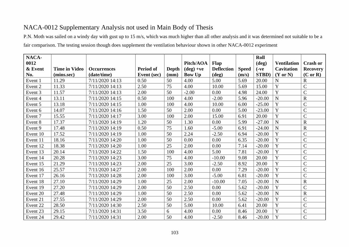
103
NACA-0012 Supplementary Analysis not used in Main Body of Thesis
P.N. Moth was sailed on a windy day with gust up to 15 m/s, which was much higher than all other analysis and it was determined not suitable to be a
fair comparison. The testing session though does supplement the ventilation behaviour shown in other NACA-0012 experiment
NACA-
0012
& Event
No.
Time in Video
(mins.sec)
Occurrences
(date/time)
Period of
Event (sec)
Depth
(mm)
Pitch/AOA
(deg) +ve
Bow Up
Flap
Deflection
(deg)
Speed
(m/s)
Roll
(deg)
(-ve
STBD)
Ventilation
Cavitation
(Y or N)
Crash or
Recovery
(C or R)
Event 1 11.29 7/11/2020 14:13 0.50 50 4.00 5.00 5.69 20.00 N R
Event 2 11.33 7/11/2020 14:13 2.50 75 4.00 10.00 5.69 15.00 Y C
Event 3 11.57 7/11/2020 14:13 2.00 50 -2.00 0.00 4.98 24.00 Y C
Event 4 13.11 7/11/2020 14:15 0.50 100 4.00 -2.00 5.96 -20.00 N R
Event 5 13.18 7/11/2020 14:15 1.00 100 4.00 10.00 6.00 -25.00 Y C
Event 6 14.07 7/11/2020 14:16 1.50 50 2.00 0.00 5.00 -23.00 Y C
Event 7 15.55 7/11/2020 14:17 3.00 100 2.00 15.00 6.91 20.00 Y C
Event 8 17.37 7/11/2020 14:19 1.20 50 1.30 0.00 5.99 -27.00 N R
Event 9 17.48 7/11/2020 14:19 0.50 75 1.60 -5.00 6.91 -24.00 N R
Event 10 17.52 7/11/2020 14:19 1.00 50 2.24 -2.50 6.94 -20.00 Y C
Event 11 18.16 7/11/2020 14:20 1.00 50 0.00 0.00 6.35 -20.00 Y C
Event 12 18.38 7/11/2020 14:20 1.00 25 2.00 0.00 7.14 -20.00 Y C
Event 13 20.14 7/11/2020 14:22 1.50 100 4.00 5.00 7.81 -20.00 Y C
Event 14 20.28 7/11/2020 14:23 3.00 75 4.00 -10.00 9.08 20.00 Y C
Event 15 21.29 7/11/2020 14:23 2.00 25 3.00 -2.50 8.92 20.00 Y C
Event 16 25.57 7/11/2020 14:27 2.00 100 2.00 0.00 7.29 -20.00 Y C
Event 17 26.16 7/11/2020 14:28 2.00 100 3.00 -5.00 6.81 -20.00 Y C
Event 18 27.10 7/11/2020 14:29 1.00 25 2.00 -10.00 7.05 -20.00 N R
Event 19 27.20 7/11/2020 14:29 2.00 50 2.50 0.00 5.62 -20.00 Y C
Event 20 27.48 7/11/2020 14:29 1.00 50 2.50 0.00 5.62 -20.00 N R
Event 21 27.55 7/11/2020 14:29 2.00 50 2.50 0.00 5.62 -20.00 Y C
Event 22 28.50 7/11/2020 14:30 2.50 50 5.00 10.00 6.41 20.00 Y C
Event 23 29.15 7/11/2020 14:31 3.50 6 4.00 0.00 8.46 20.00 Y C
Event 24 29.42 7/11/2020 14:31 2.00 50 4.00 -2.50 8.46 -20.00 Y C
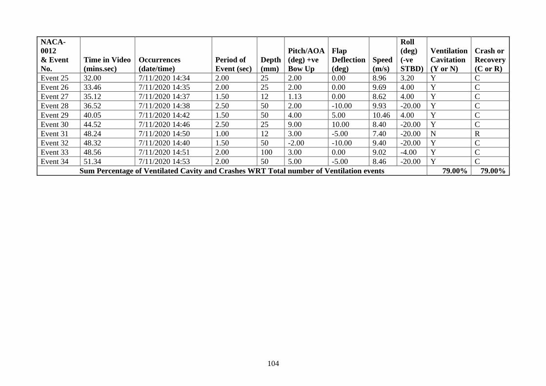
104
NACA-
0012
& Event
No.
Time in Video
(mins.sec)
Occurrences
(date/time)
Period of
Event (sec)
Depth
(mm)
Pitch/AOA
(deg) +ve
Bow Up
Flap
Deflection
(deg)
Speed
(m/s)
Roll
(deg)
(-ve
STBD)
Ventilation
Cavitation
(Y or N)
Crash or
Recovery
(C or R)
Event 25 32.00 7/11/2020 14:34 2.00 25 2.00 0.00 8.96 3.20 Y C
Event 26 33.46 7/11/2020 14:35 2.00 25 2.00 0.00 9.69 4.00 Y C
Event 27 35.12 7/11/2020 14:37 1.50 12 1.13 0.00 8.62 4.00 Y C
Event 28 36.52 7/11/2020 14:38 2.50 50 2.00 -10.00 9.93 -20.00 Y C
Event 29 40.05 7/11/2020 14:42 1.50 50 4.00 5.00 10.46 4.00 Y C
Event 30 44.52 7/11/2020 14:46 2.50 25 9.00 10.00 8.40 -20.00 Y C
Event 31 48.24 7/11/2020 14:50 1.00 12 3.00 -5.00 7.40 -20.00 N R
Event 32 48.32 7/11/2020 14:40 1.50 50 -2.00 -10.00 9.40 -20.00 Y C
Event 33 48.56 7/11/2020 14:51 2.00 100 3.00 0.00 9.02 -4.00 Y C
Event 34 51.34 7/11/2020 14:53 2.00 50 5.00 -5.00 8.46 -20.00 Y C
Sum Percentage of Ventilated Cavity and Crashes WRT Total number of Ventilation events 79.00% 79.00%
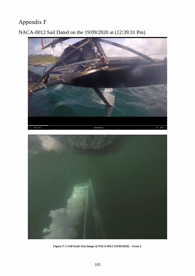
105
NACA-0012 Sail Dated on the 19/09/2020 at (12:39:31 Pm)
Figure F-1 Full Scale Test Image of NACA-0012 (19/09/2020) – Event 1.
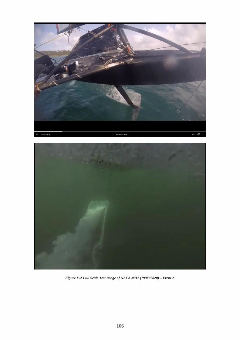
106
Figure F-2 Full Scale Test Image of NACA-0012 (19/09/2020) – Event 2.
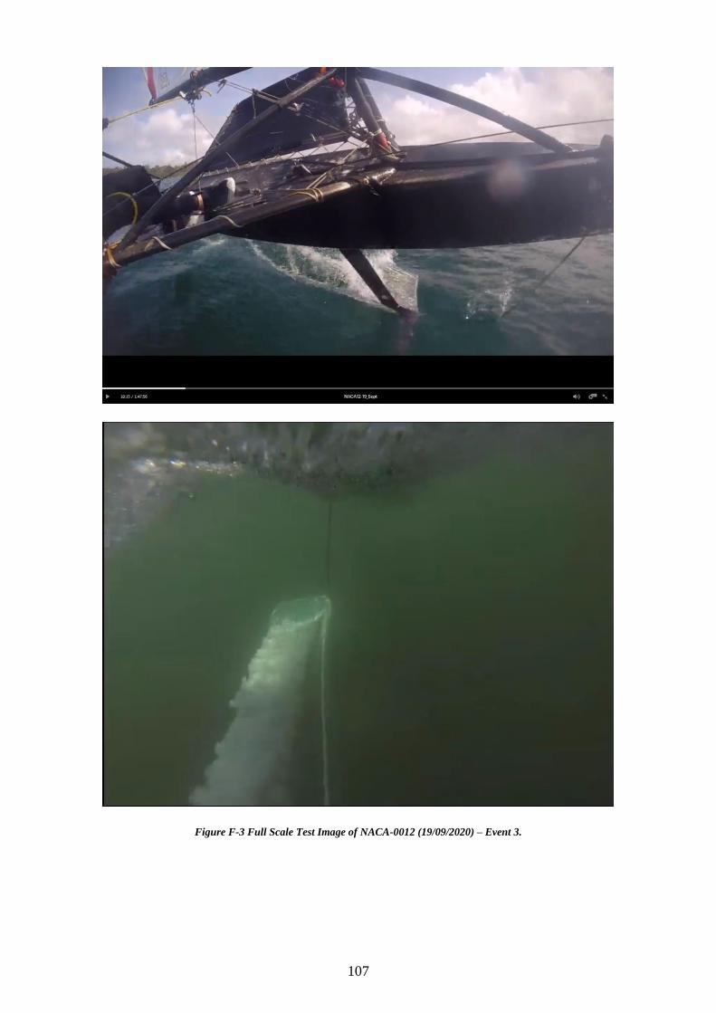
107
Figure F-3 Full Scale Test Image of NACA-0012 (19/09/2020) – Event 3.
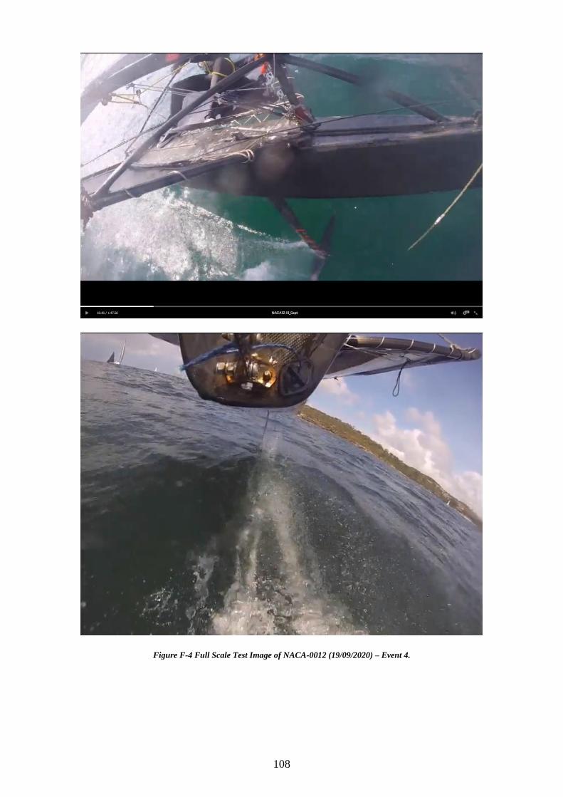
108
Figure F-4 Full Scale Test Image of NACA-0012 (19/09/2020) – Event 4.
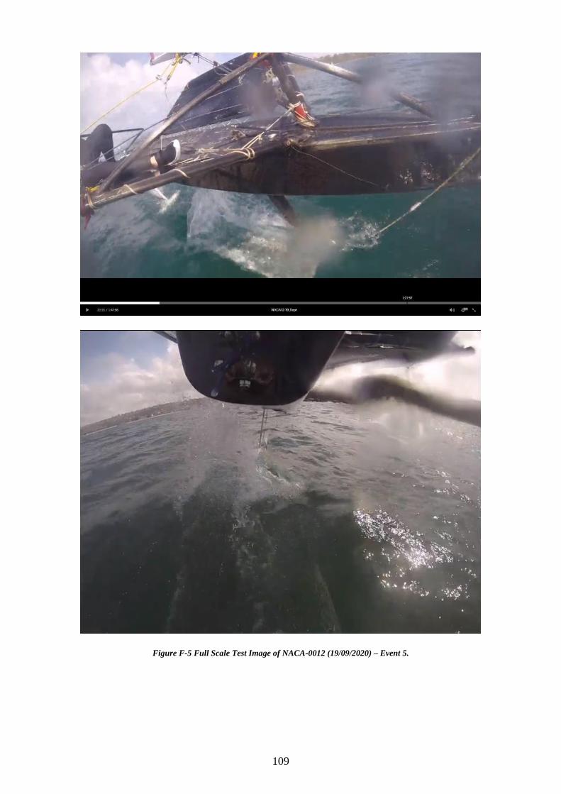
109
Figure F-5 Full Scale Test Image of NACA-0012 (19/09/2020) – Event 5.
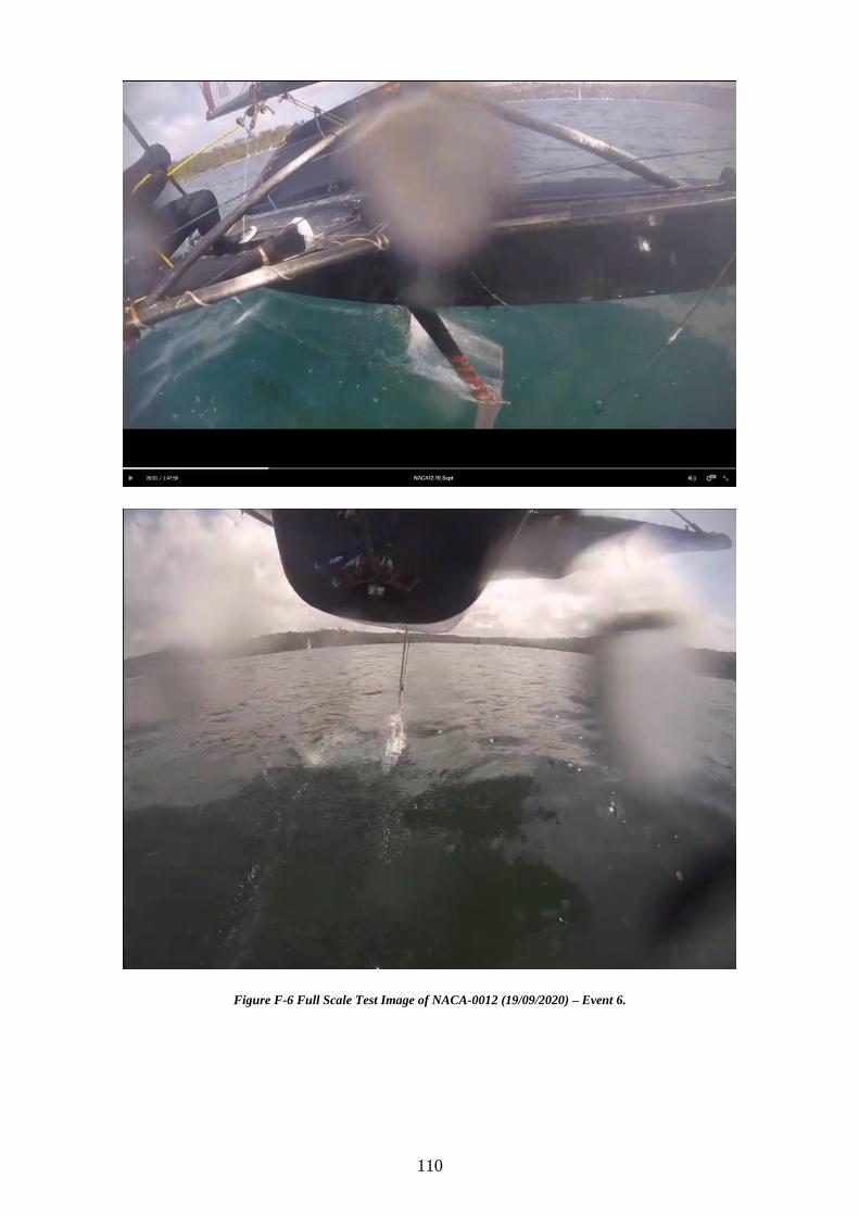
110
Figure F-6 Full Scale Test Image of NACA-0012 (19/09/2020) – Event 6.
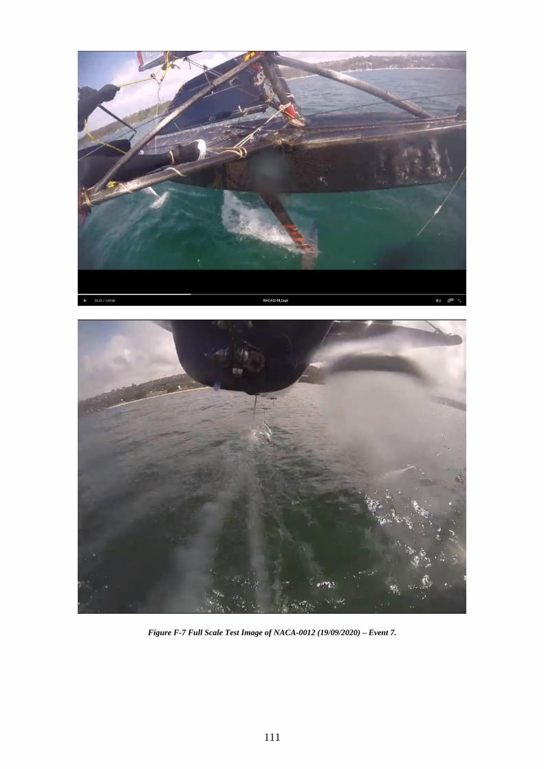
111
Figure F-7 Full Scale Test Image of NACA-0012 (19/09/2020) – Event 7.
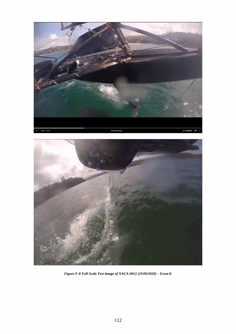
112
Figure F-8 Full Scale Test Image of NACA-0012 (19/09/2020) – Event 8.
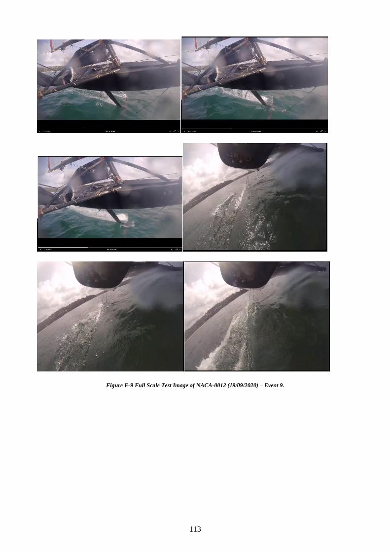
113
Figure F-9 Full Scale Test Image of NACA-0012 (19/09/2020) – Event 9.
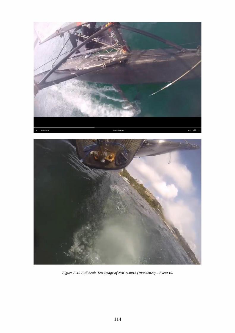
114
Figure F-10 Full Scale Test Image of NACA-0012 (19/09/2020) – Event 10.
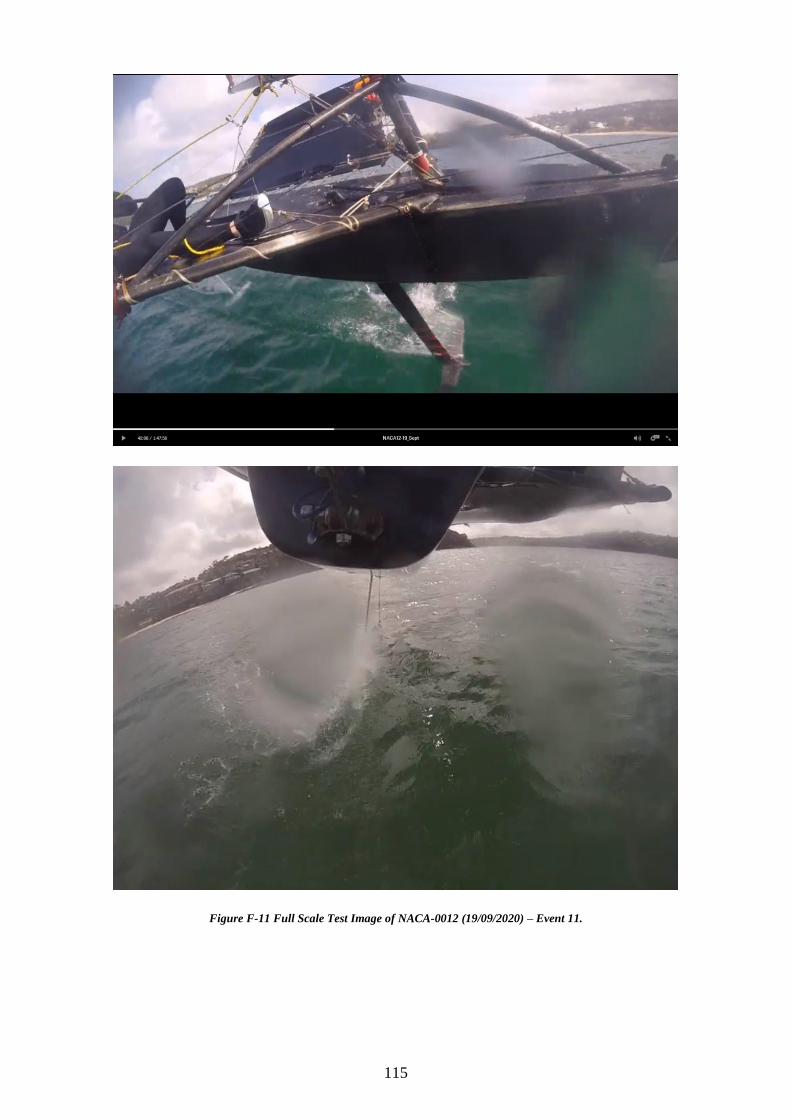
115
Figure F-11 Full Scale Test Image of NACA-0012 (19/09/2020) – Event 11.
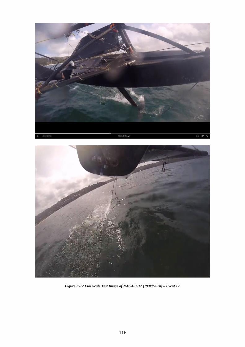
116
Figure F-12 Full Scale Test Image of NACA-0012 (19/09/2020) – Event 12.
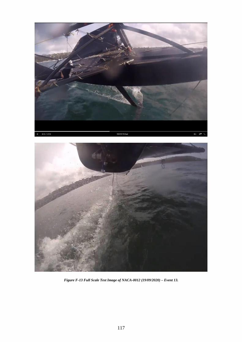
117
Figure F-13 Full Scale Test Image of NACA-0012 (19/09/2020) – Event 13.
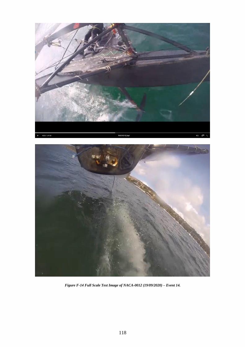
118
Figure F-14 Full Scale Test Image of NACA-0012 (19/09/2020) – Event 14.
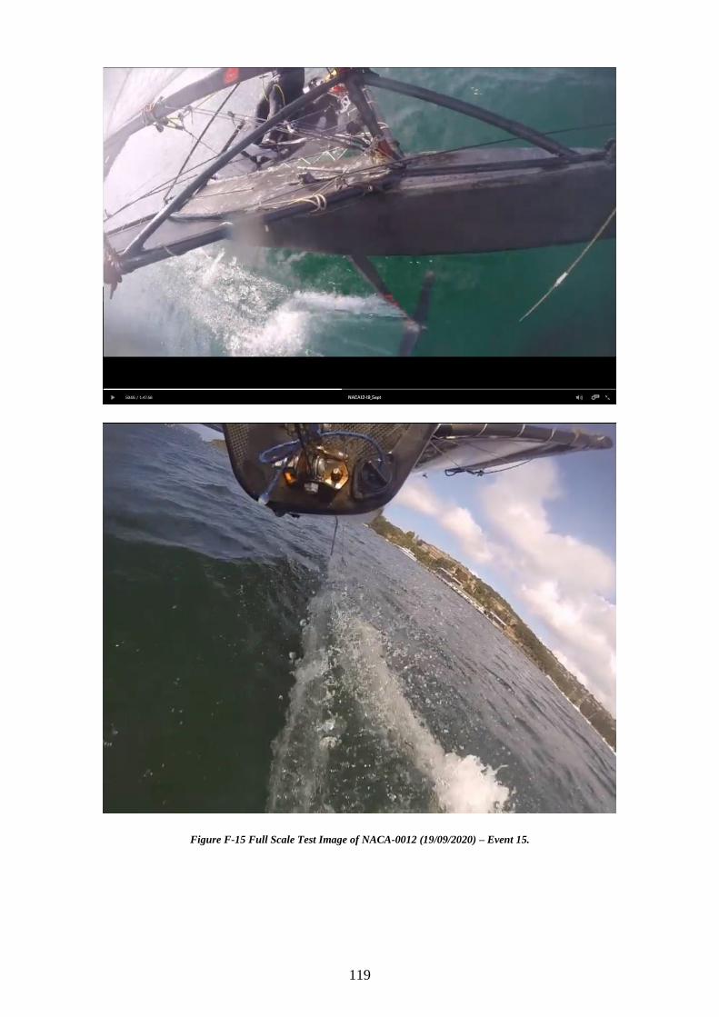
119
Figure F-15 Full Scale Test Image of NACA-0012 (19/09/2020) – Event 15.
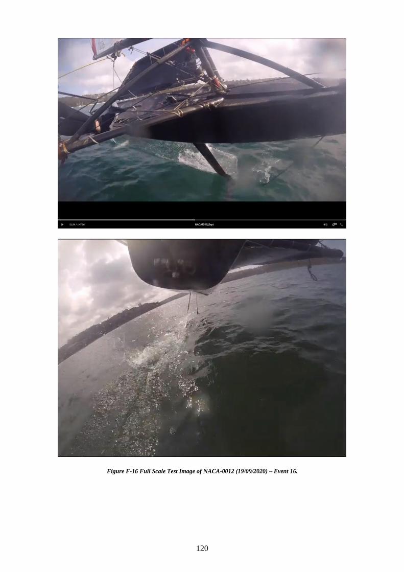
120
Figure F-16 Full Scale Test Image of NACA-0012 (19/09/2020) – Event 16.
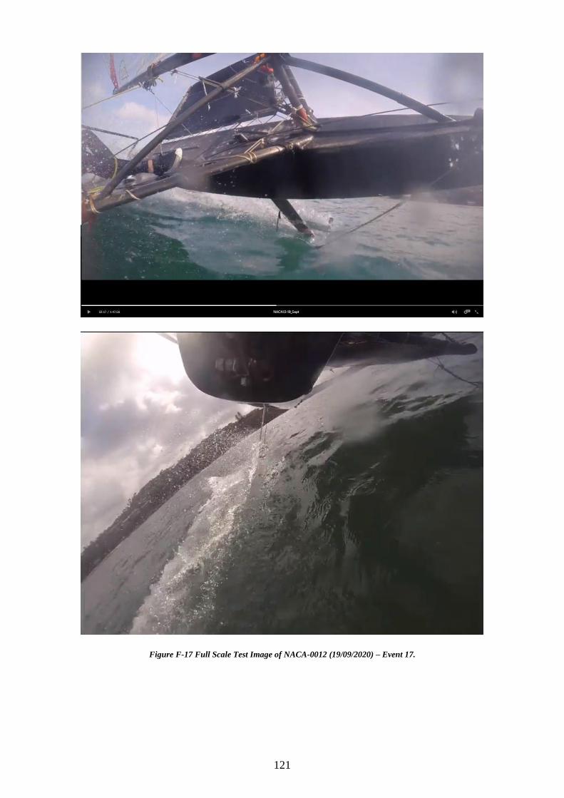
121
Figure F-17 Full Scale Test Image of NACA-0012 (19/09/2020) – Event 17.
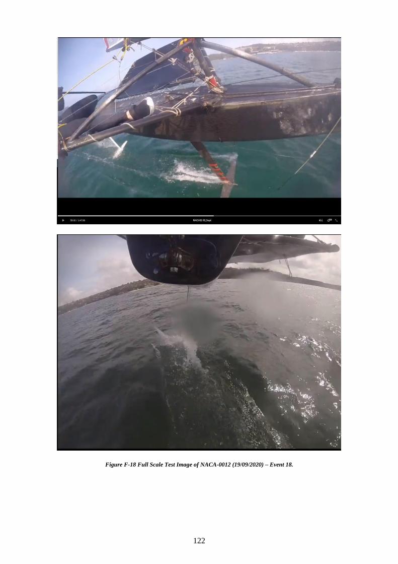
122
Figure F-18 Full Scale Test Image of NACA-0012 (19/09/2020) – Event 18.
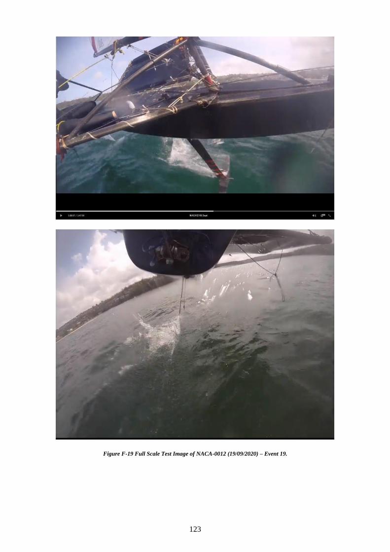
123
Figure F-19 Full Scale Test Image of NACA-0012 (19/09/2020) – Event 19.
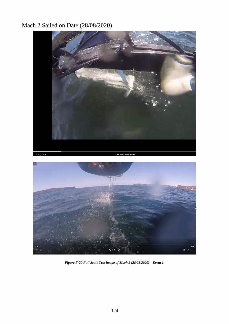
124
Mach 2 Sailed on Date (28/08/2020)
Figure F-20 Full Scale Test Image of Mach 2 (28/08/2020) – Event 1.
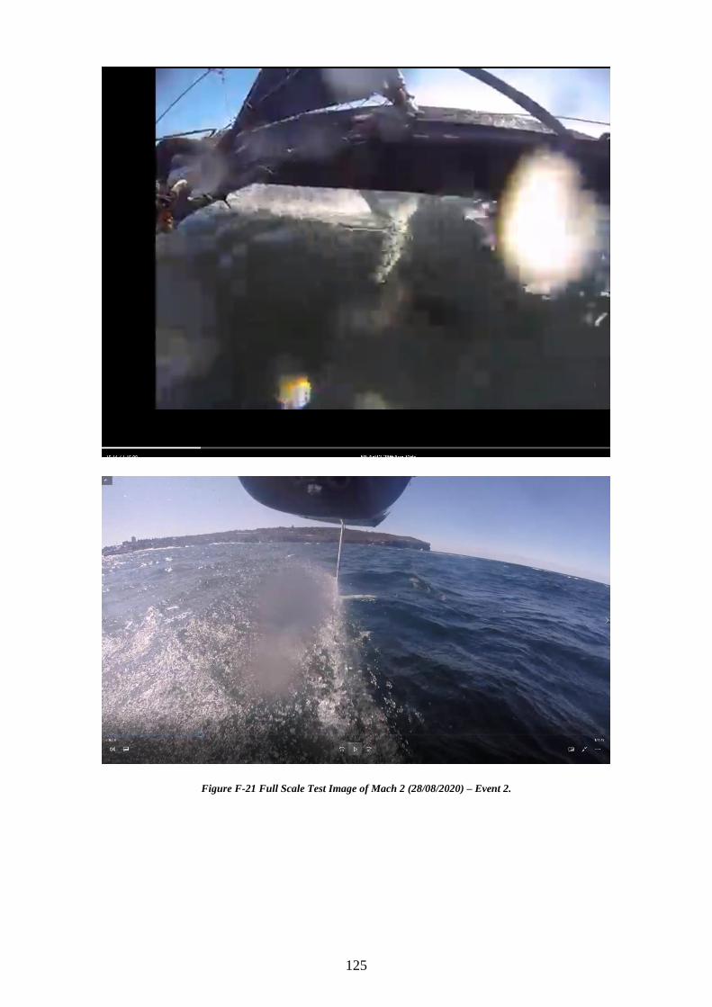
125
Figure F-21 Full Scale Test Image of Mach 2 (28/08/2020) – Event 2.
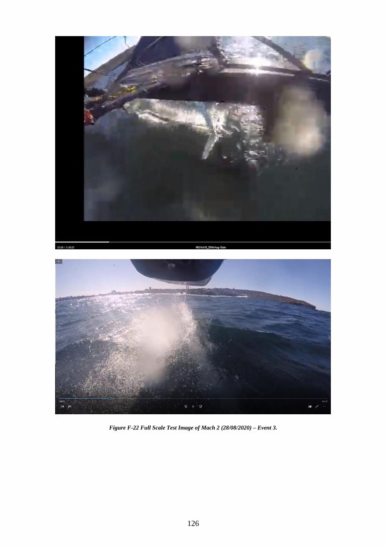
126
Figure F-22 Full Scale Test Image of Mach 2 (28/08/2020) – Event 3.
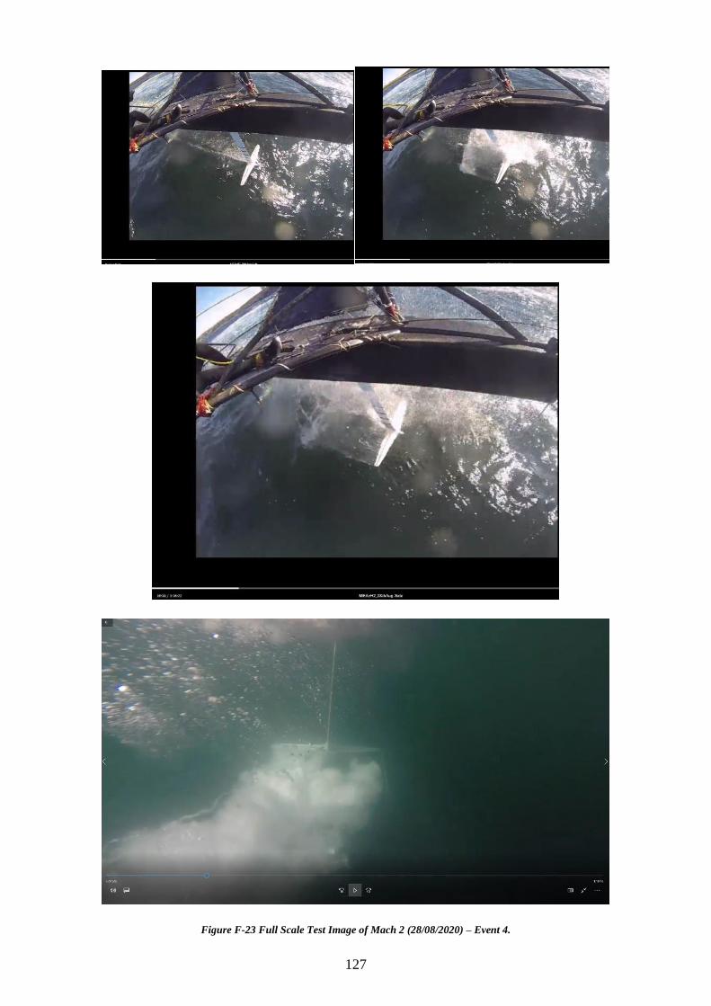
127
Figure F-23 Full Scale Test Image of Mach 2 (28/08/2020) – Event 4.
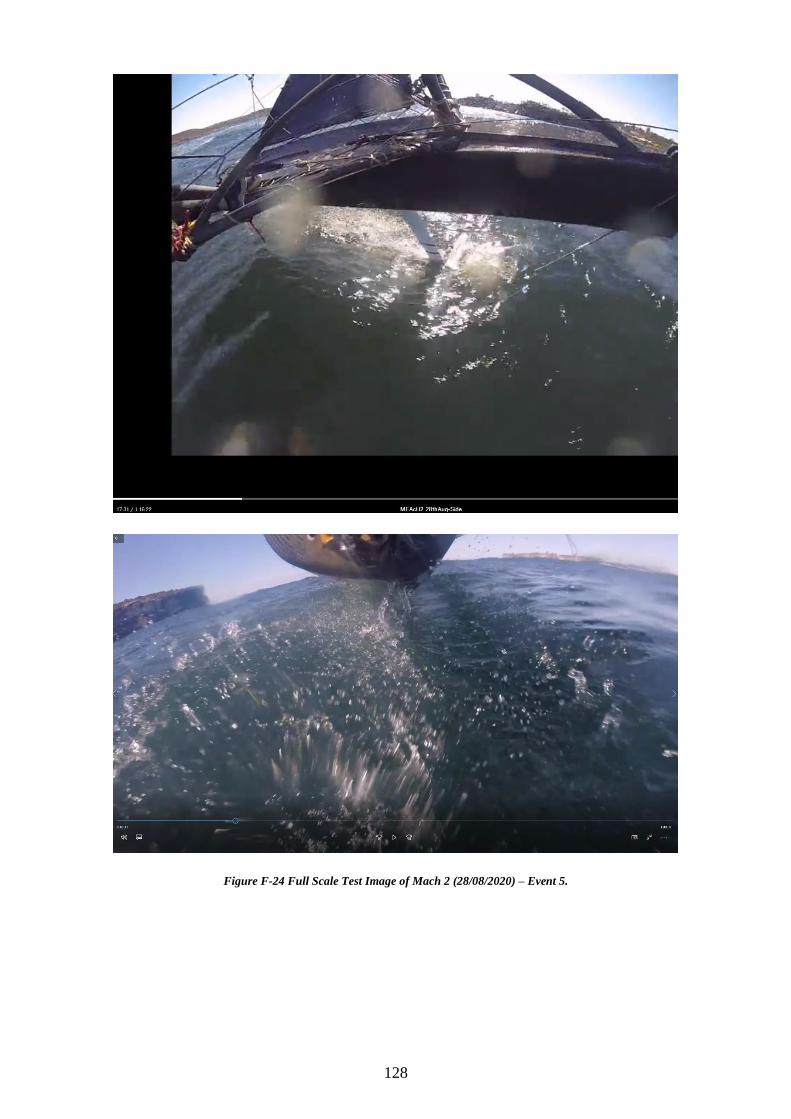
128
Figure F-24 Full Scale Test Image of Mach 2 (28/08/2020) – Event 5.
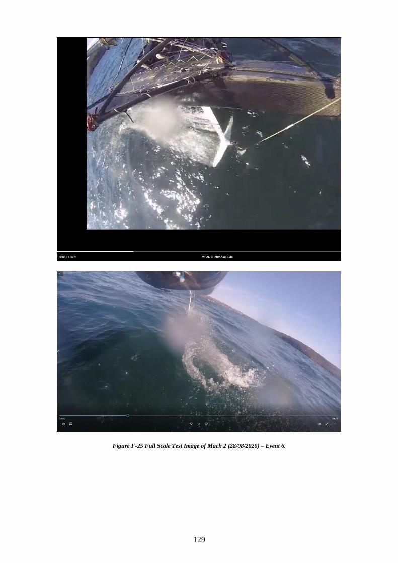
129
Figure F-25 Full Scale Test Image of Mach 2 (28/08/2020) – Event 6.
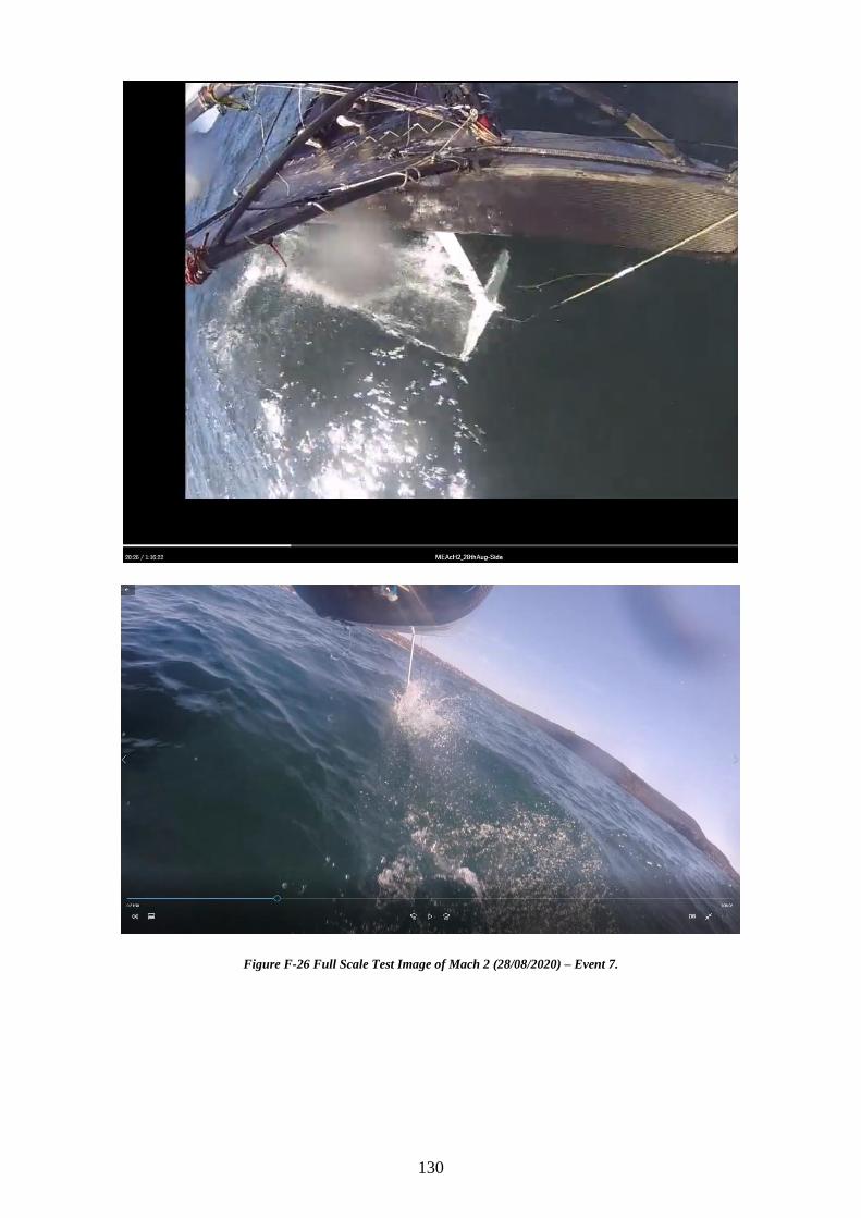
130
Figure F-26 Full Scale Test Image of Mach 2 (28/08/2020) – Event 7.
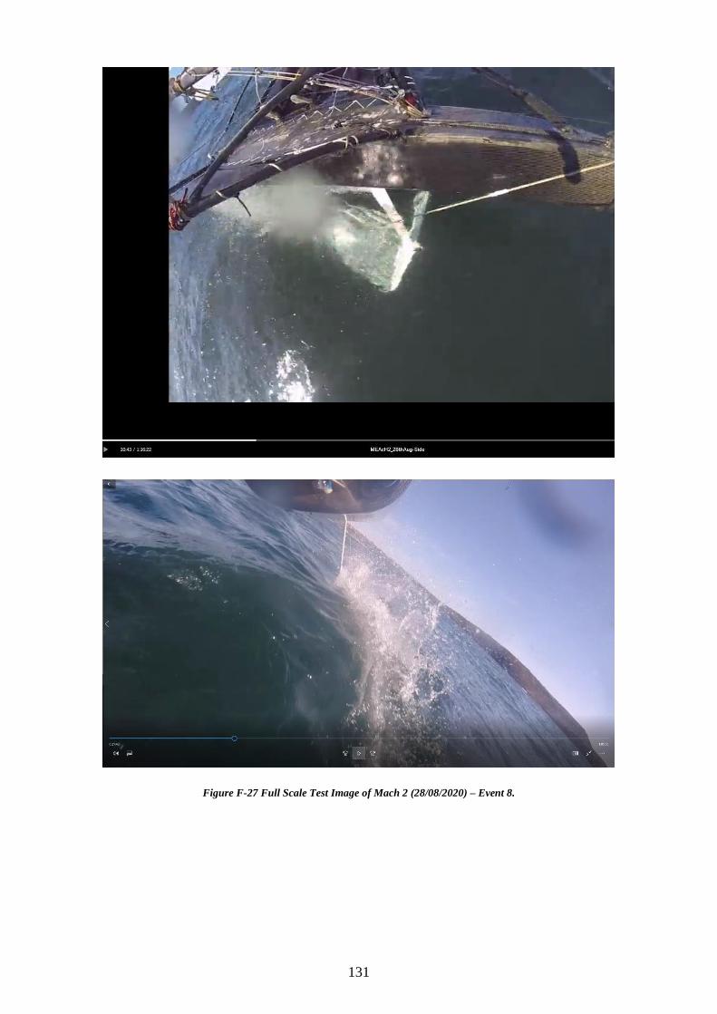
131
Figure F-27 Full Scale Test Image of Mach 2 (28/08/2020) – Event 8.
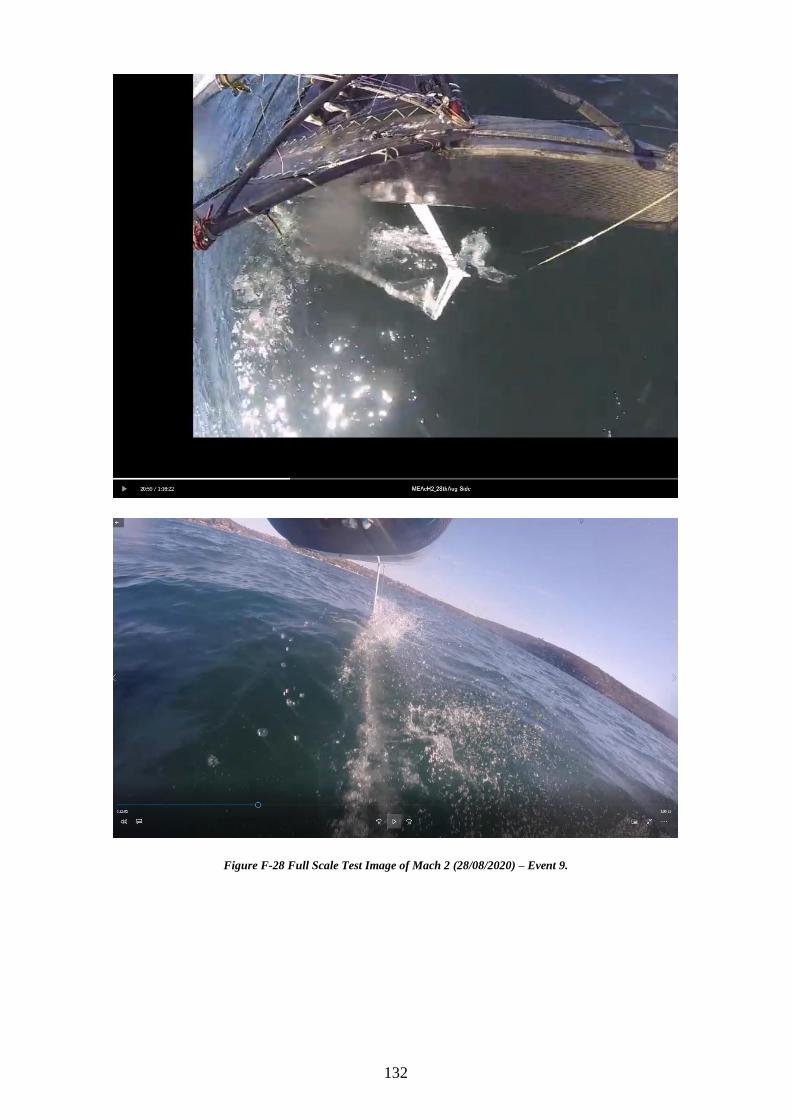
132
Figure F-28 Full Scale Test Image of Mach 2 (28/08/2020) – Event 9.
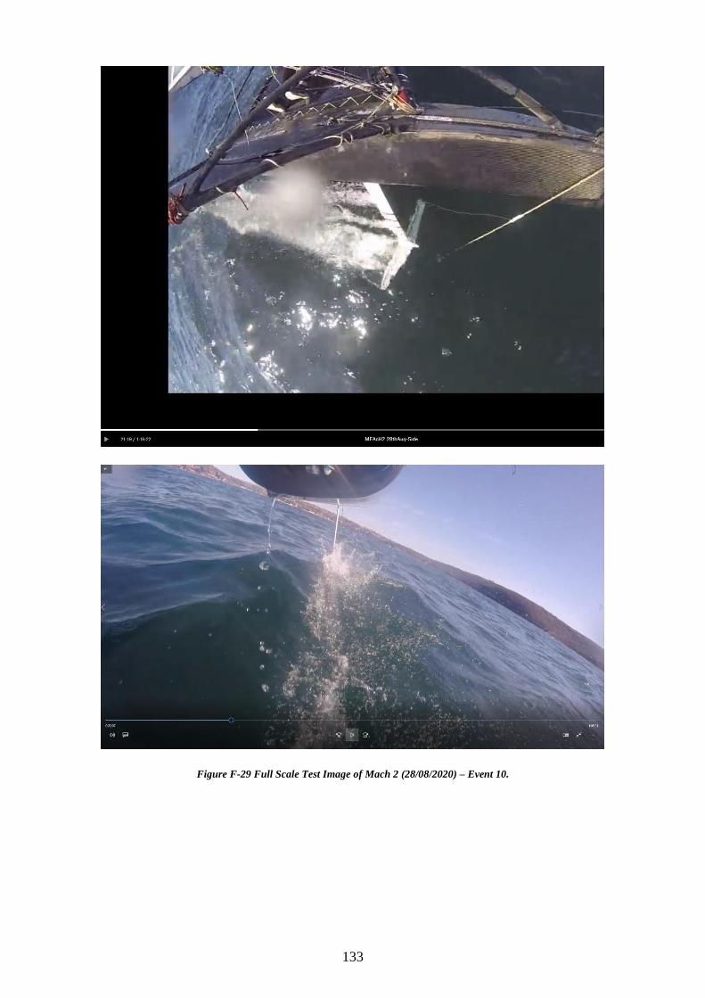
133
Figure F-29 Full Scale Test Image of Mach 2 (28/08/2020) – Event 10.
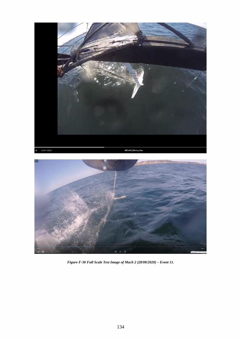
134
Figure F-30 Full Scale Test Image of Mach 2 (28/08/2020) – Event 11.
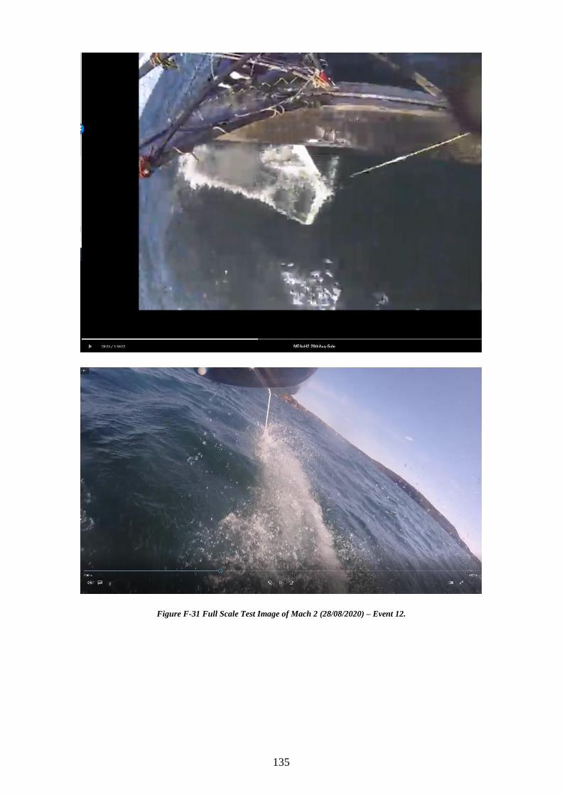
135
Figure F-31 Full Scale Test Image of Mach 2 (28/08/2020) – Event 12.
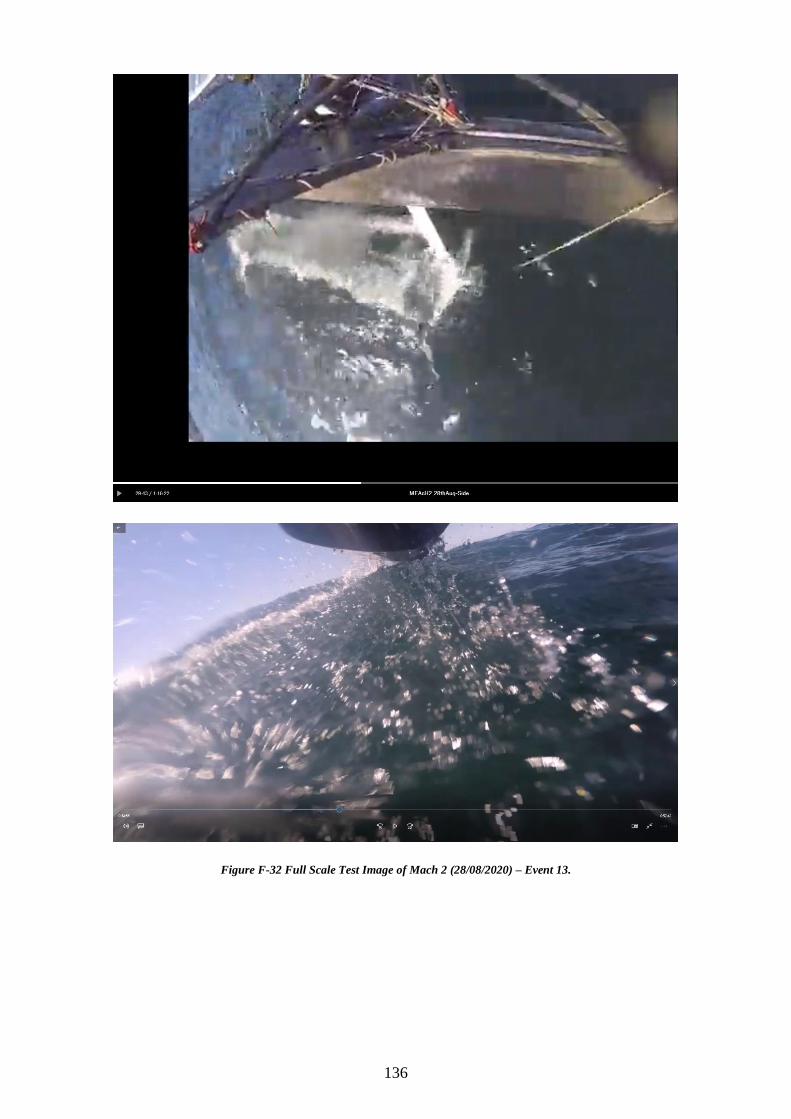
136
Figure F-32 Full Scale Test Image of Mach 2 (28/08/2020) – Event 13.
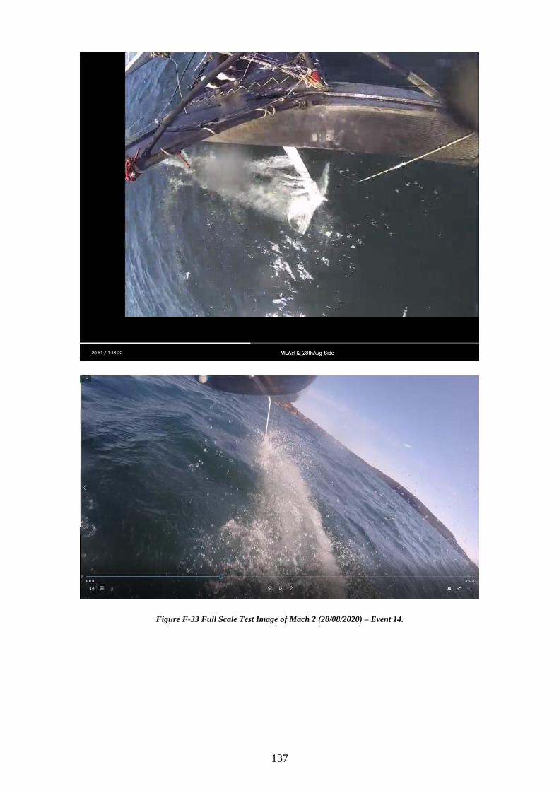
137
Figure F-33 Full Scale Test Image of Mach 2 (28/08/2020) – Event 14.
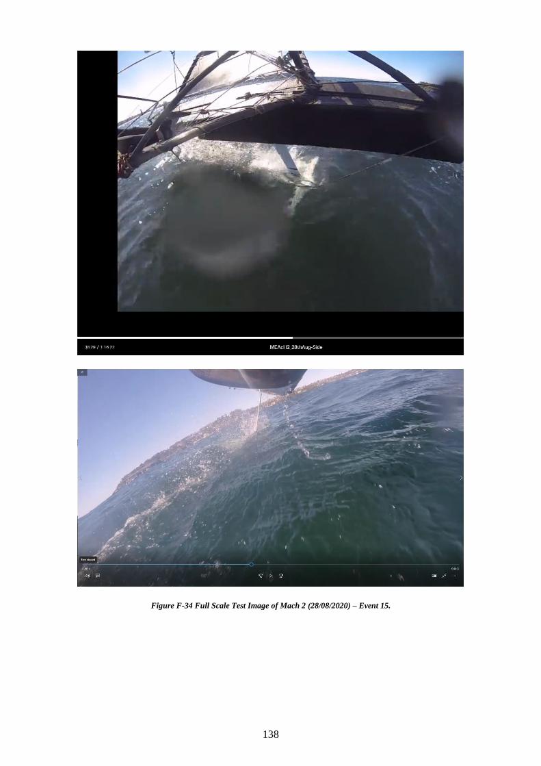
138
Figure F-34 Full Scale Test Image of Mach 2 (28/08/2020) – Event 15.
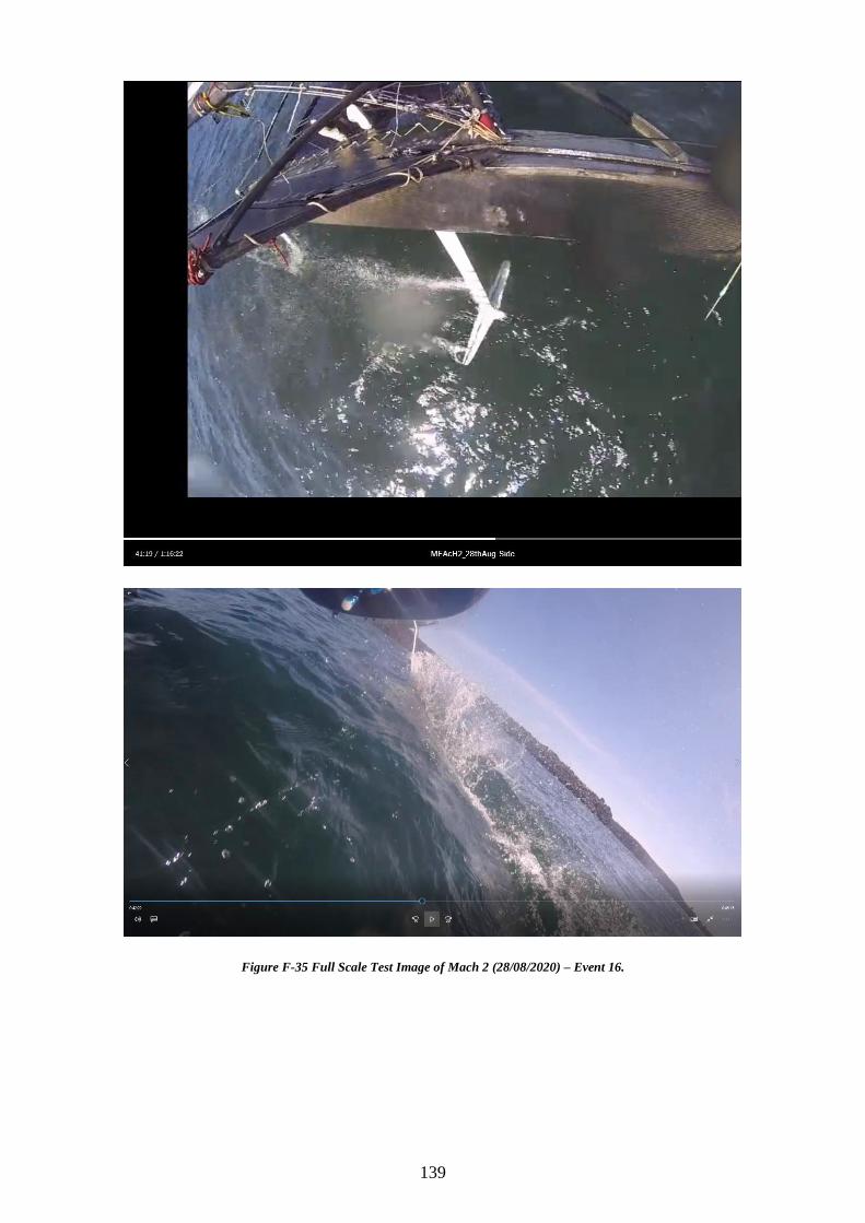
139
Figure F-35 Full Scale Test Image of Mach 2 (28/08/2020) – Event 16.
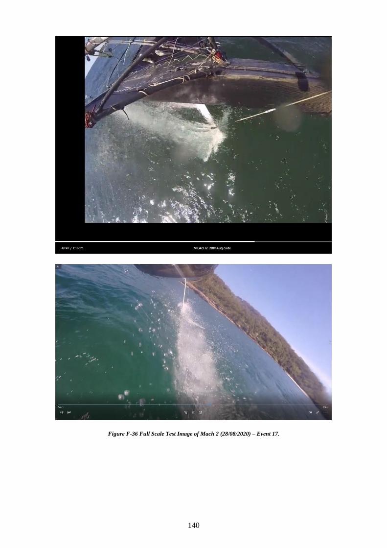
140
Figure F-36 Full Scale Test Image of Mach 2 (28/08/2020) – Event 17.
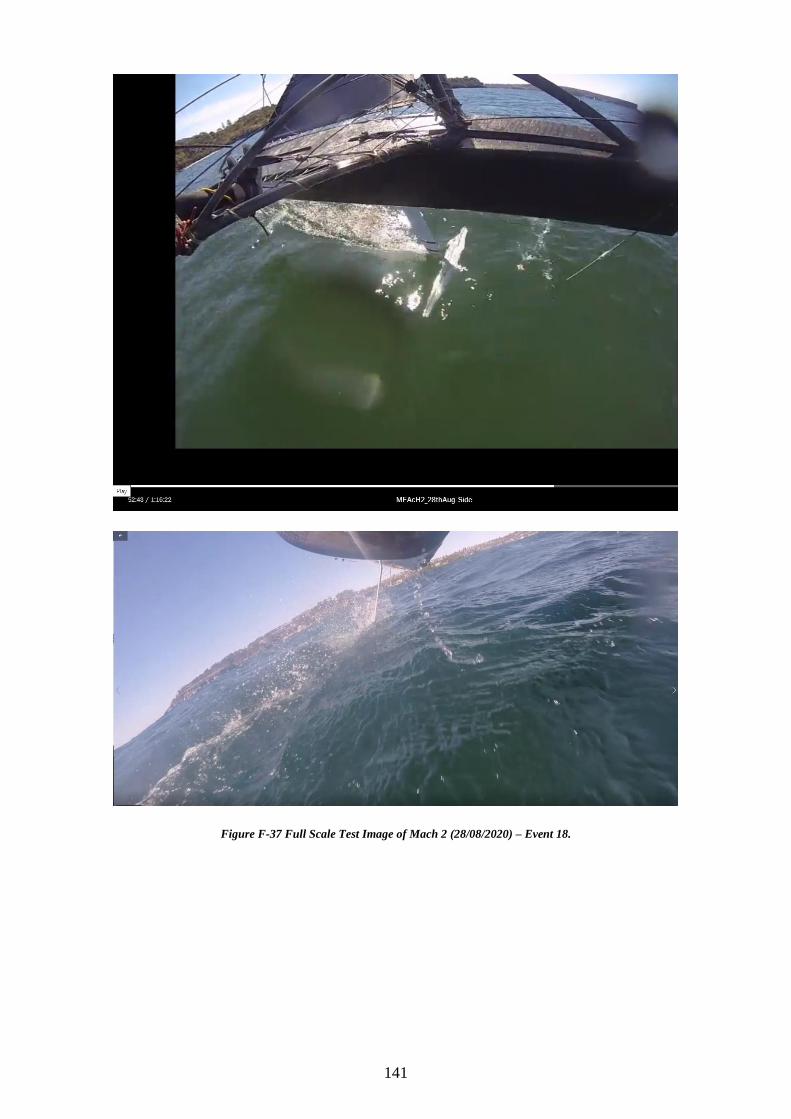
141
Figure F-37 Full Scale Test Image of Mach 2 (28/08/2020) – Event 18.
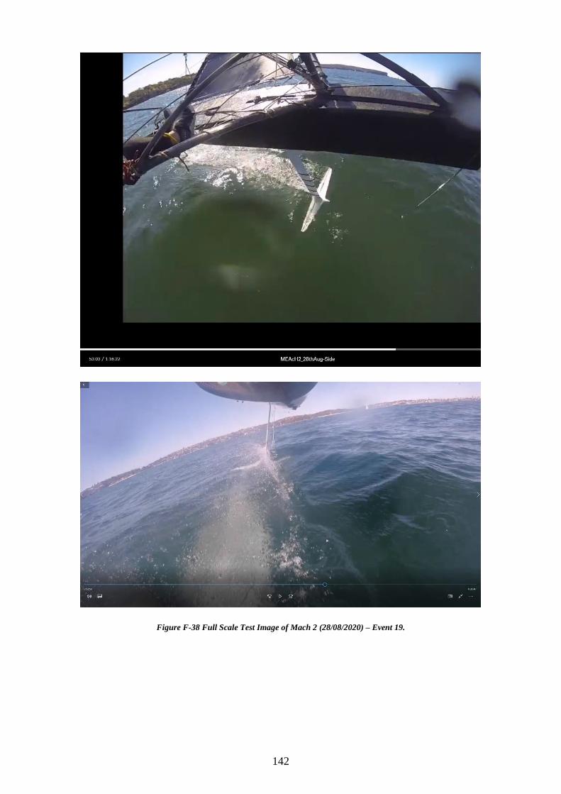
142
Figure F-38 Full Scale Test Image of Mach 2 (28/08/2020) – Event 19.
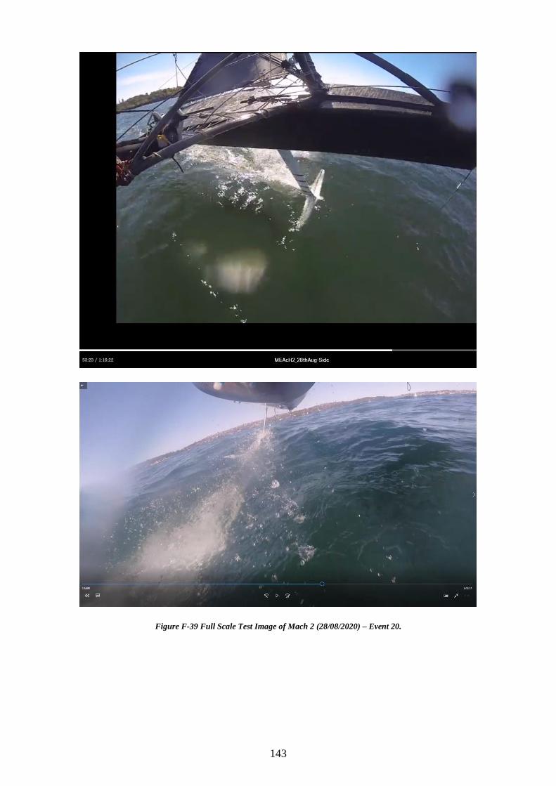
143
Figure F-39 Full Scale Test Image of Mach 2 (28/08/2020) – Event 20.
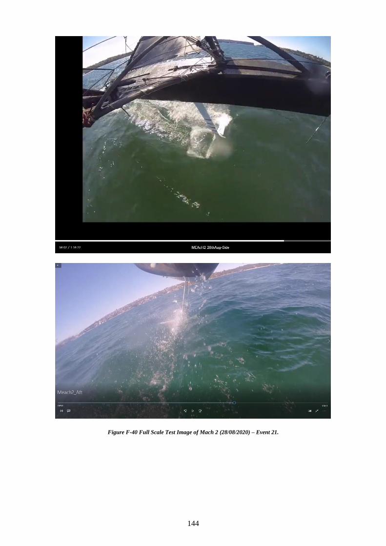
144
Figure F-40 Full Scale Test Image of Mach 2 (28/08/2020) – Event 21.
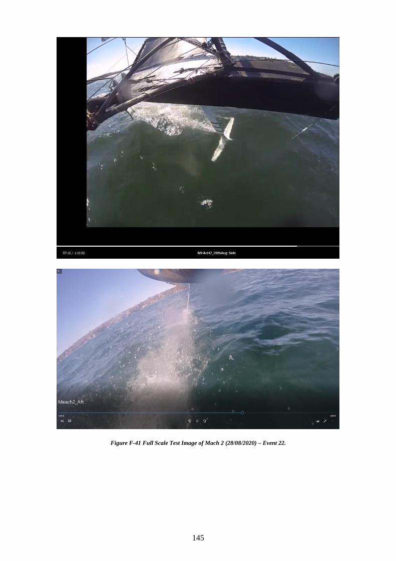
145
Figure F-41 Full Scale Test Image of Mach 2 (28/08/2020) – Event 22.
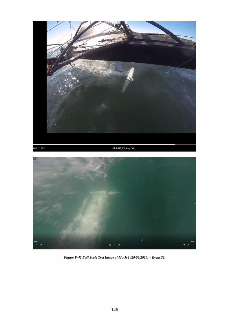
146
Figure F-42 Full Scale Test Image of Mach 2 (28/08/2020) – Event 23.
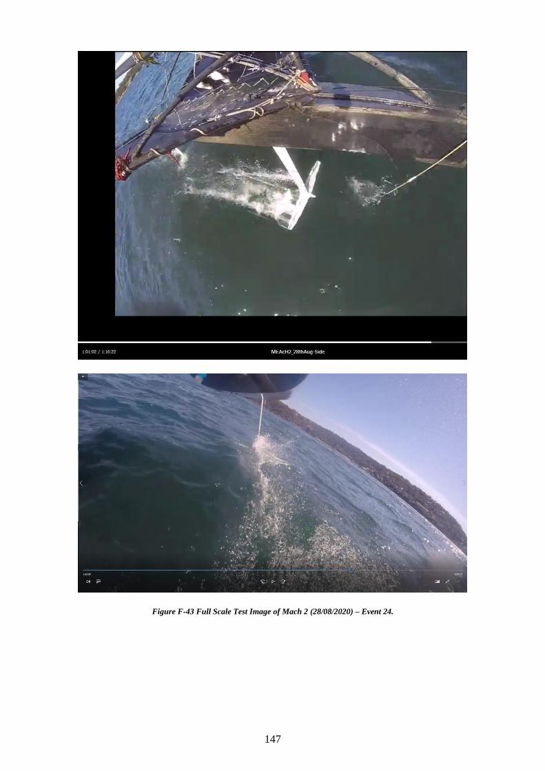
147
Figure F-43 Full Scale Test Image of Mach 2 (28/08/2020) – Event 24.
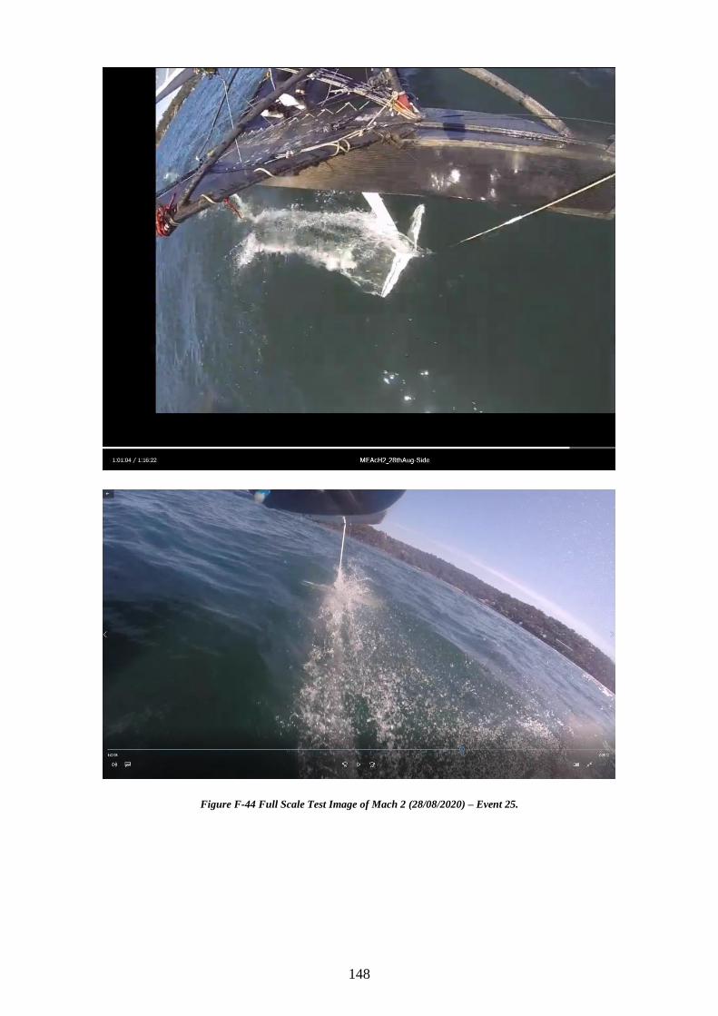
148
Figure F-44 Full Scale Test Image of Mach 2 (28/08/2020) – Event 25.
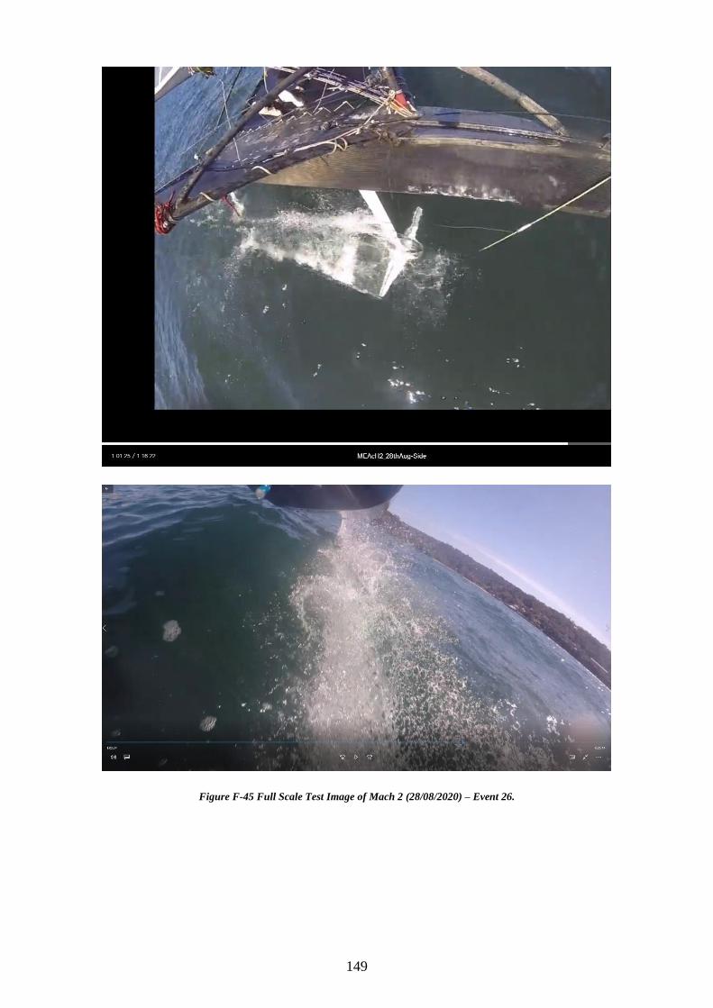
149
Figure F-45 Full Scale Test Image of Mach 2 (28/08/2020) – Event 26.
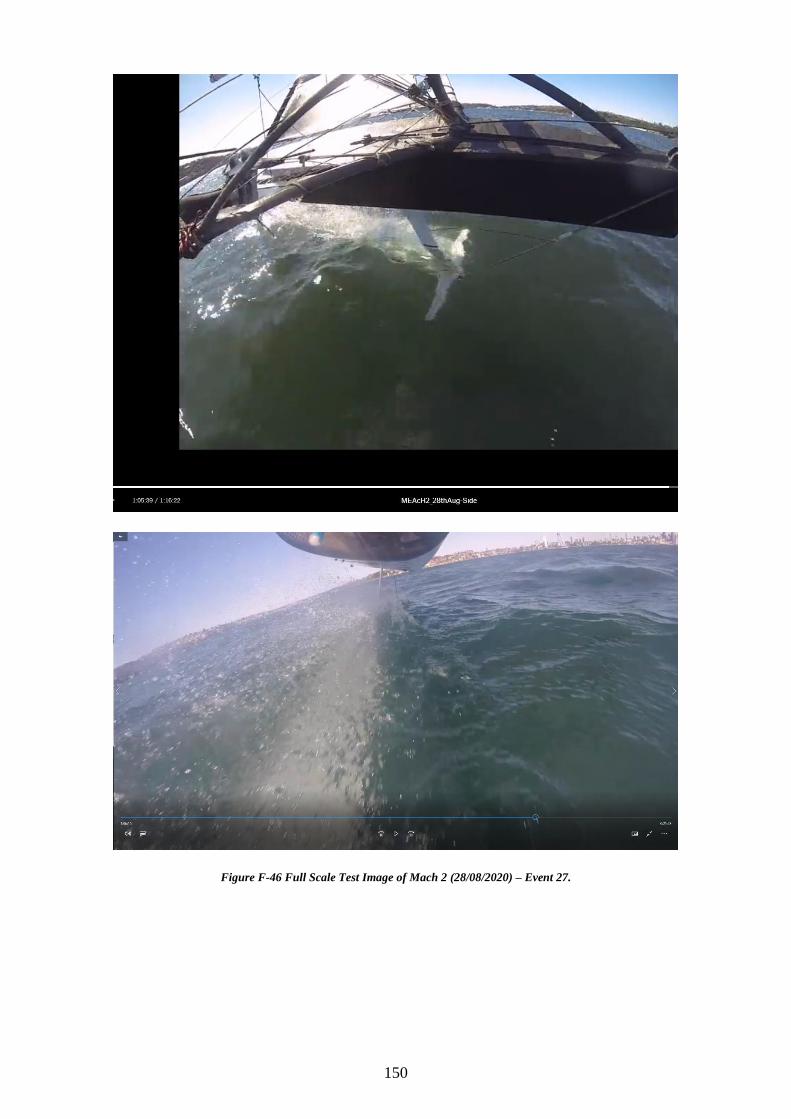
150
Figure F-46 Full Scale Test Image of Mach 2 (28/08/2020) – Event 27.
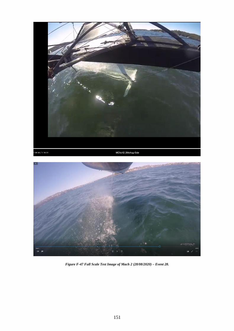
151
Figure F-47 Full Scale Test Image of Mach 2 (28/08/2020) – Event 28.
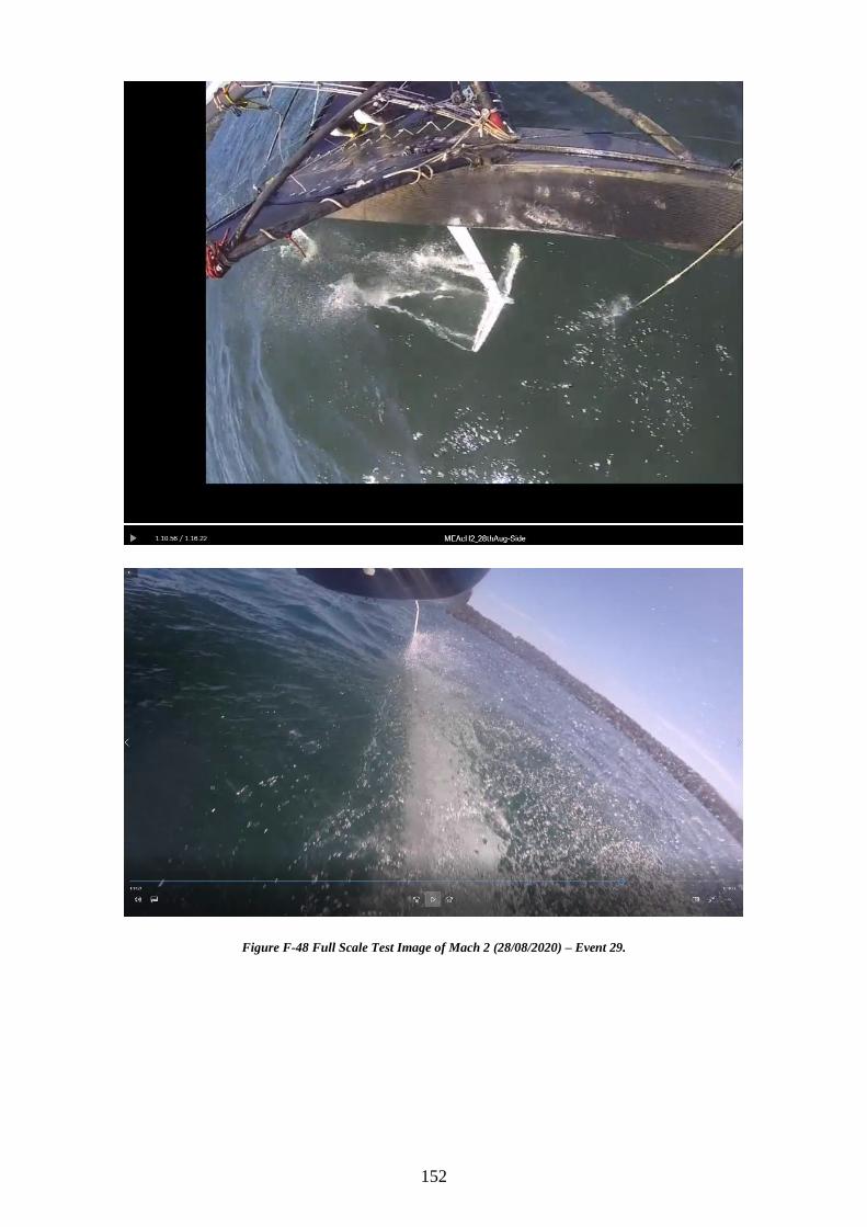
152
Figure F-48 Full Scale Test Image of Mach 2 (28/08/2020) – Event 29.
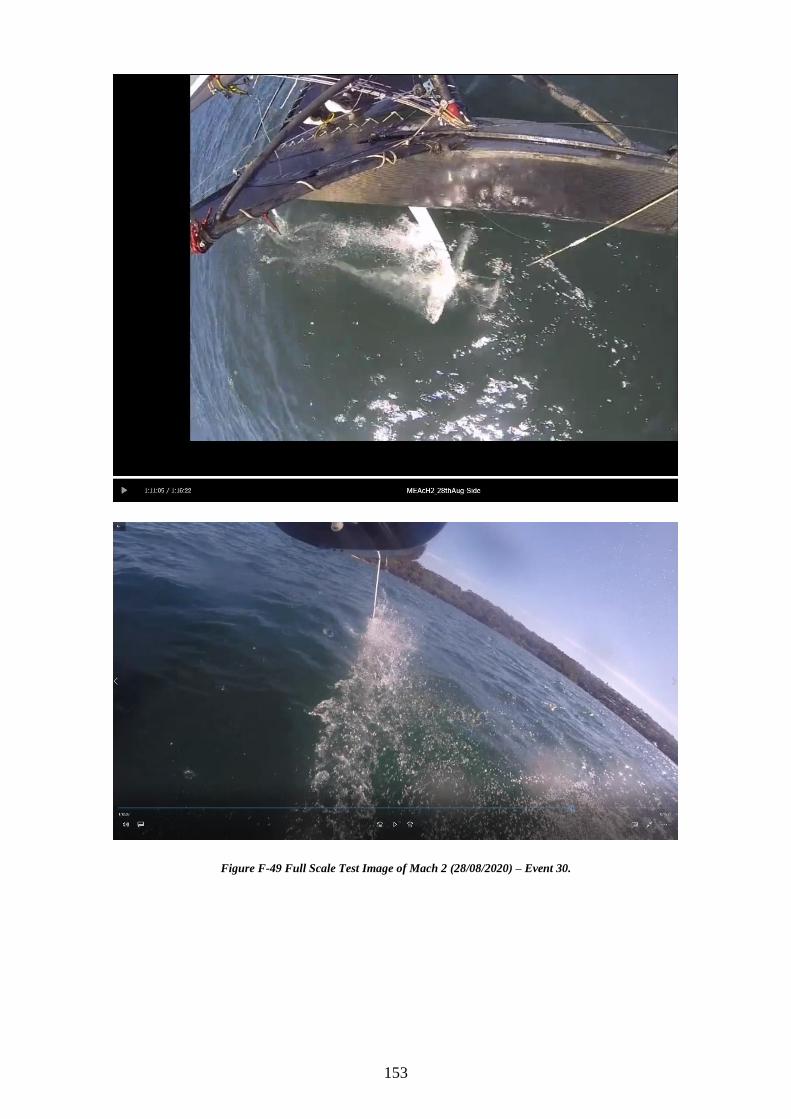
153
Figure F-49 Full Scale Test Image of Mach 2 (28/08/2020) – Event 30.
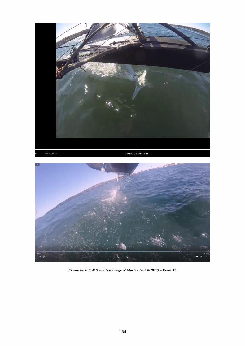
154
Figure F-50 Full Scale Test Image of Mach 2 (28/08/2020) – Event 31.
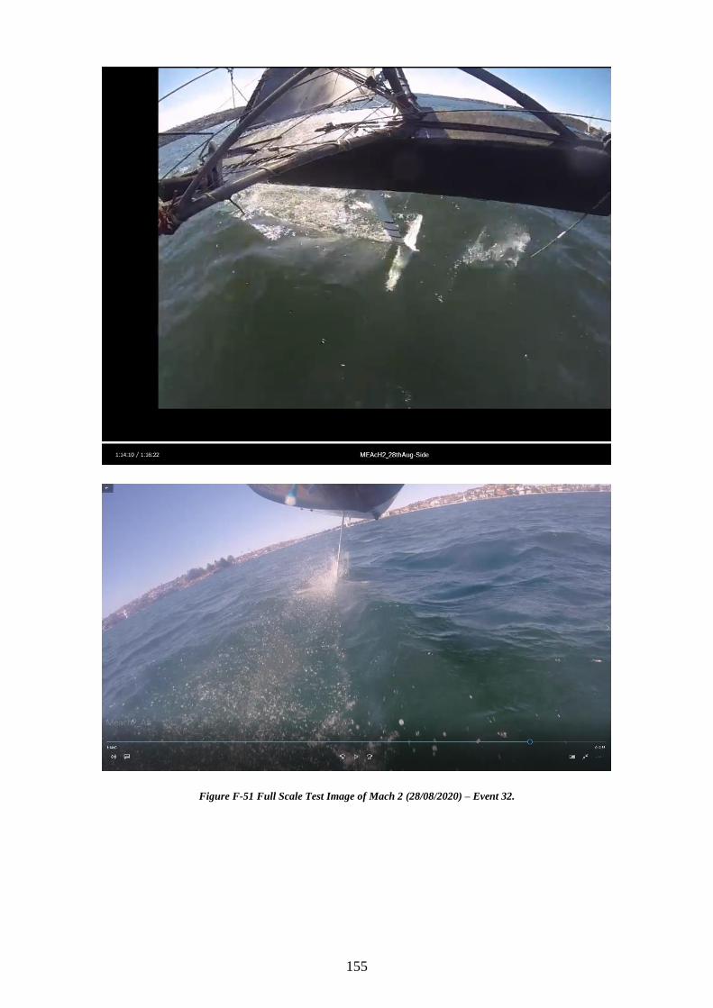
155
Figure F-51 Full Scale Test Image of Mach 2 (28/08/2020) – Event 32.
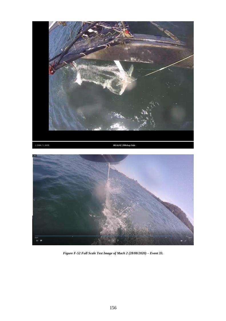
156
Figure F-52 Full Scale Test Image of Mach 2 (28/08/2020) – Event 33.
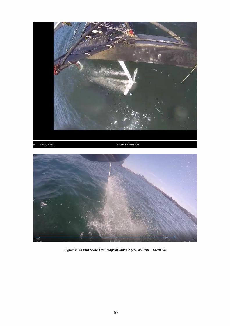
157
Figure F-53 Full Scale Test Image of Mach 2 (28/08/2020) – Event 34.
158
Figure F-54 Full Scale Test Image of Mach 2 (28/08/2020) – Event 35.
159
NACA-0012 Secondary Test Sailed on Date (7/11/2020)
Figure F-55 Secondary Full Scale Test Image only of NACA-0012 (07/11/2020) – Event 1.
160
Figure F-56 Secondary Full Scale Test Image only of NACA-0012 (07/11/2020) – Event 2.
161
Figure F-57 Secondary Full Scale Test Image only of NACA-0012 (07/11/2020) – Event 3.
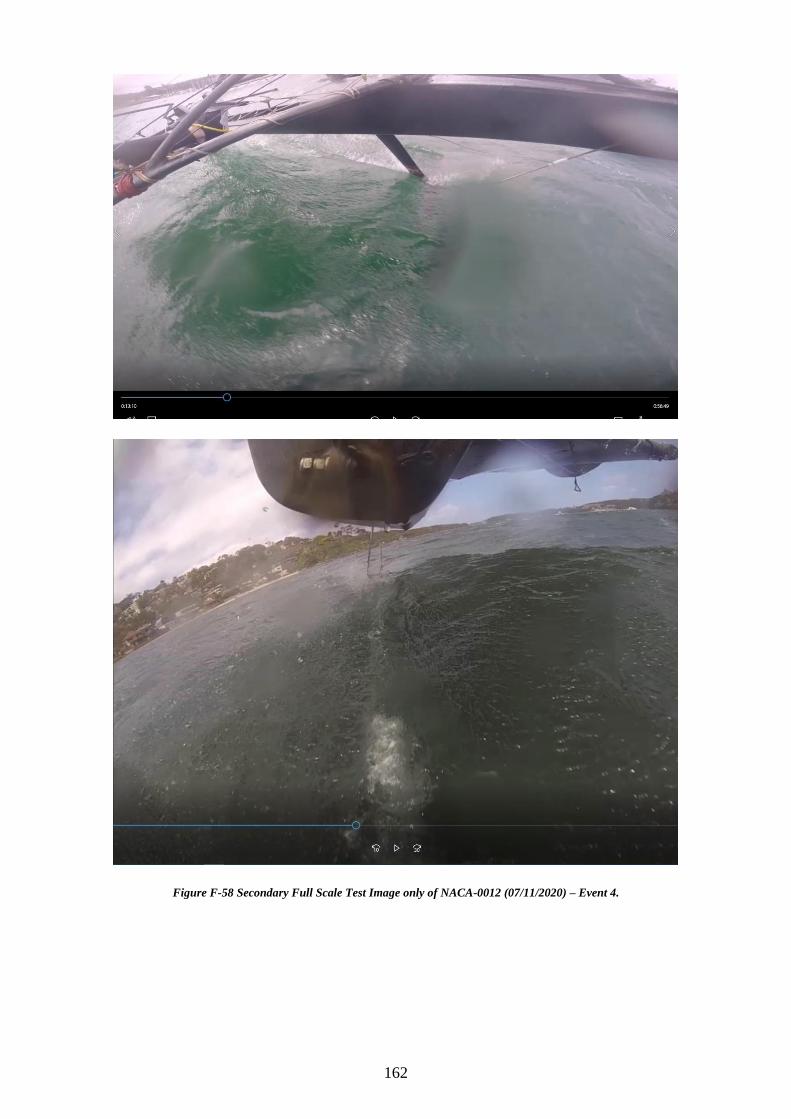
162
Figure F-58 Secondary Full Scale Test Image only of NACA-0012 (07/11/2020) – Event 4.

163
Figure F-59 Secondary Full Scale Test Image only of NACA-0012 (07/11/2020) – Event 5.
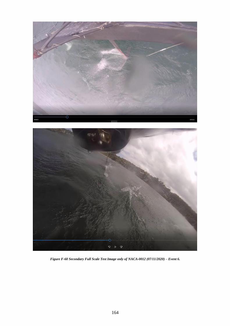
164
Figure F-60 Secondary Full Scale Test Image only of NACA-0012 (07/11/2020) – Event 6.
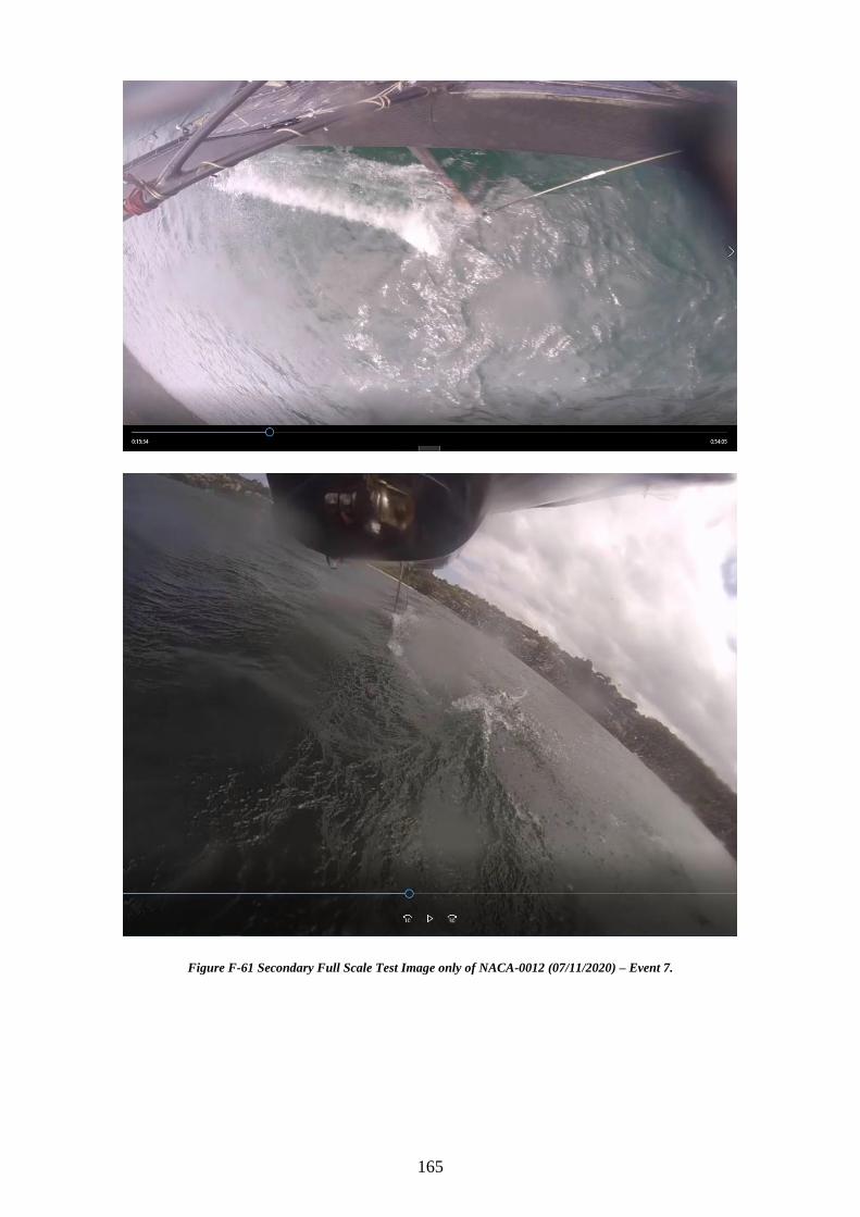
165
Figure F-61 Secondary Full Scale Test Image only of NACA-0012 (07/11/2020) – Event 7.
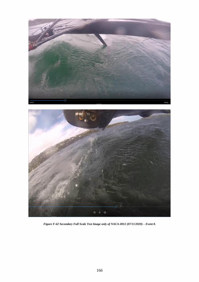
166
Figure F-62 Secondary Full Scale Test Image only of NACA-0012 (07/11/2020) – Event 8.
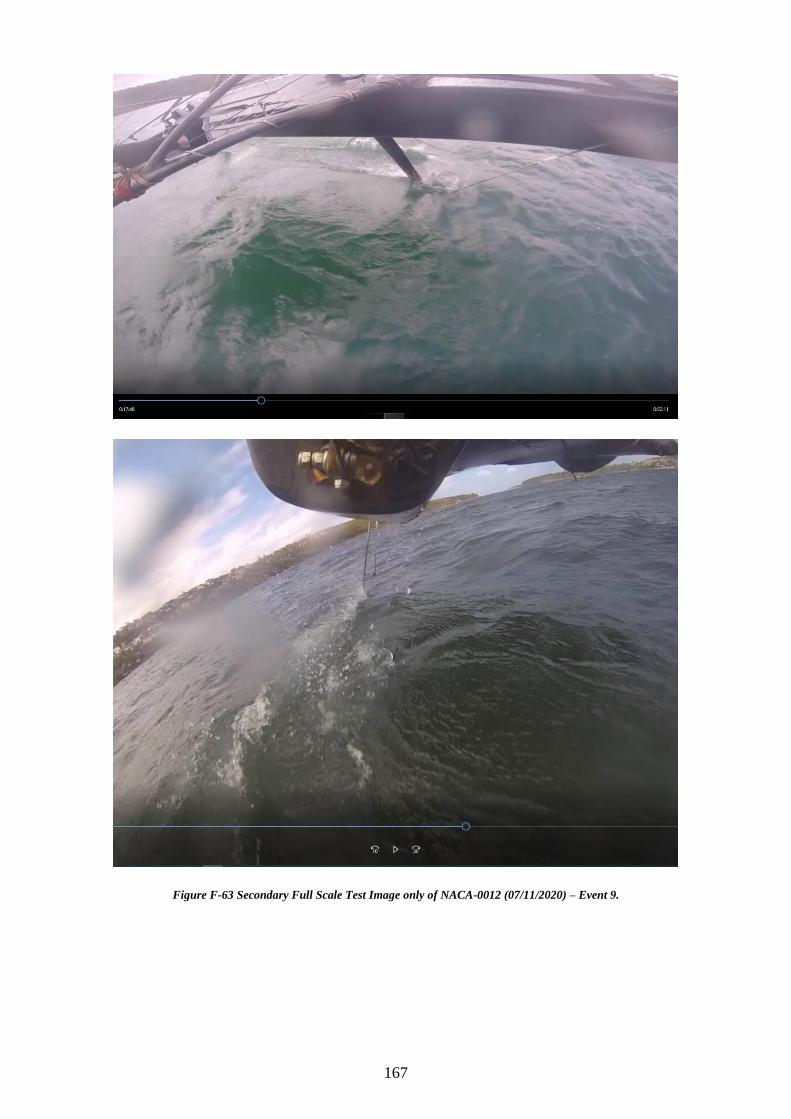
167
Figure F-63 Secondary Full Scale Test Image only of NACA-0012 (07/11/2020) – Event 9.
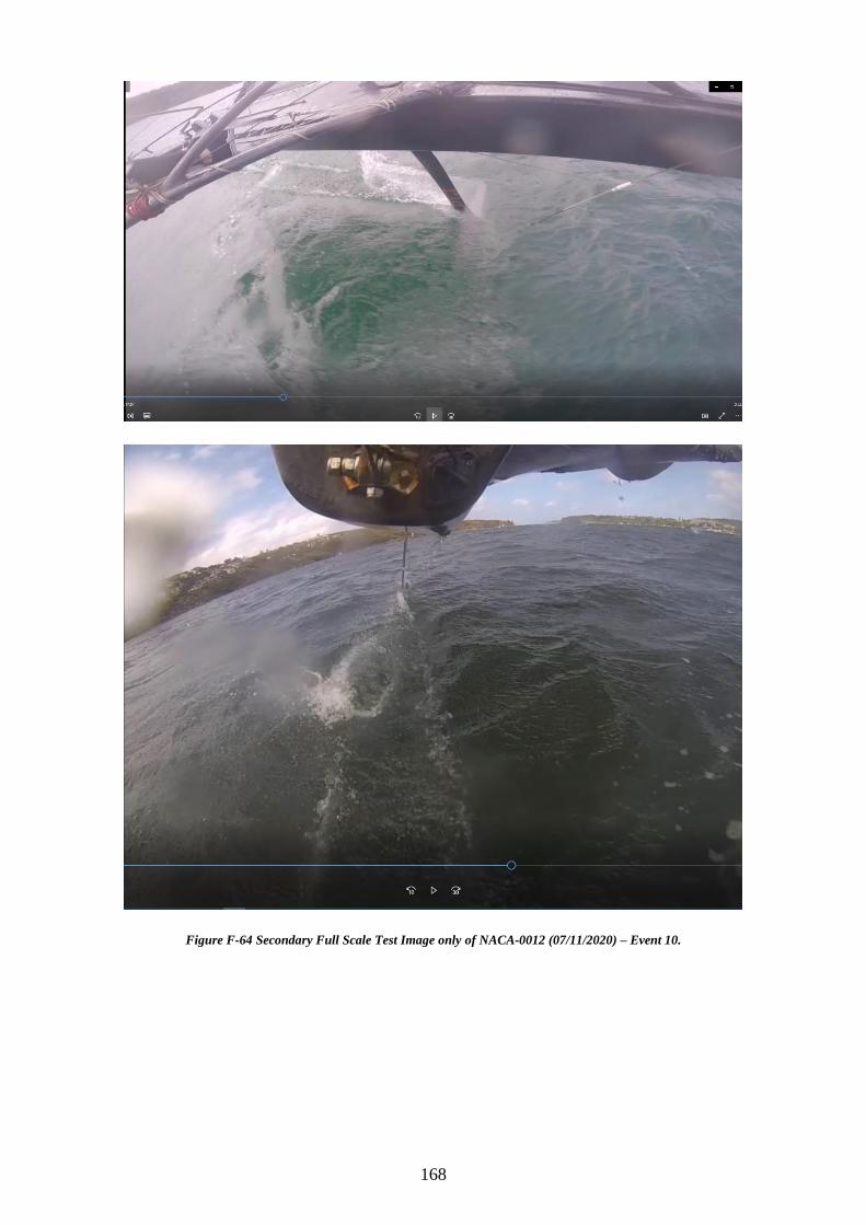
168
Figure F-64 Secondary Full Scale Test Image only of NACA-0012 (07/11/2020) – Event 10.
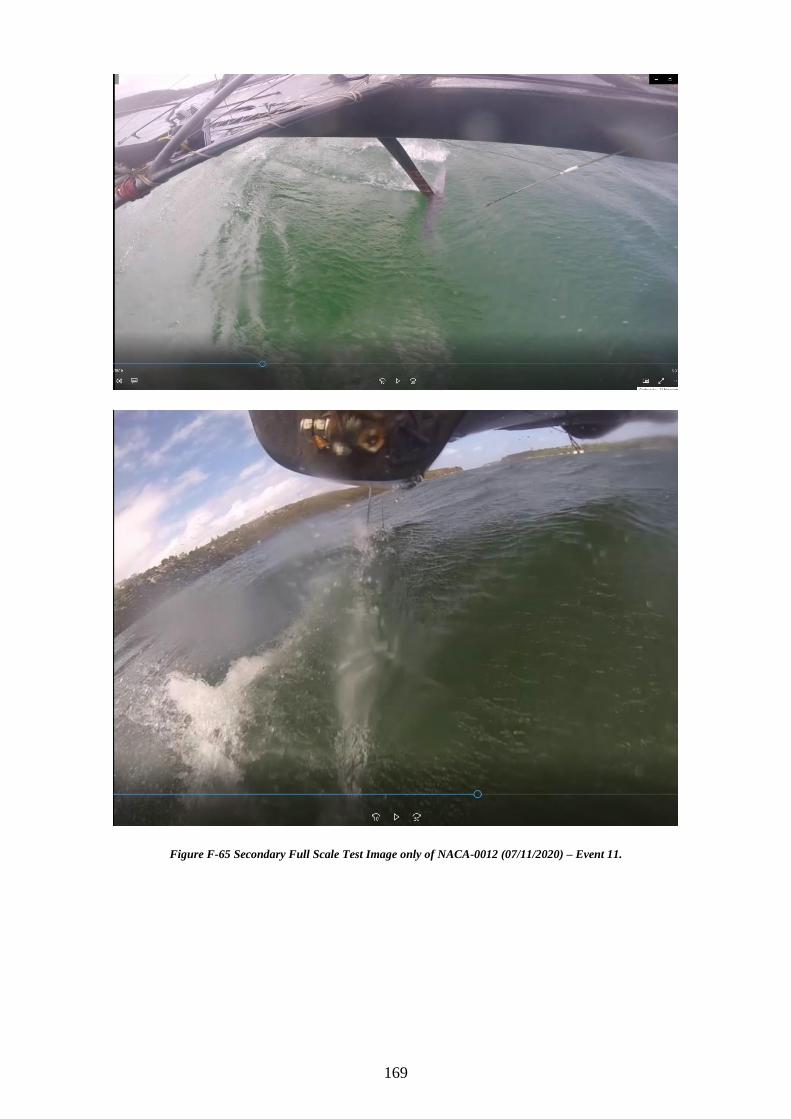
169
Figure F-65 Secondary Full Scale Test Image only of NACA-0012 (07/11/2020) – Event 11.

170
Figure F-66 Secondary Full Scale Test Image only of NACA-0012 (07/11/2020) – Event 12.

171
Figure F-67 Secondary Full Scale Test Image only of NACA-0012 (07/11/2020) – Event 13.
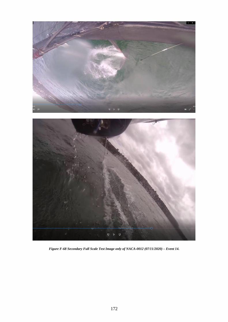
172
Figure F-68 Secondary Full Scale Test Image only of NACA-0012 (07/11/2020) – Event 14.
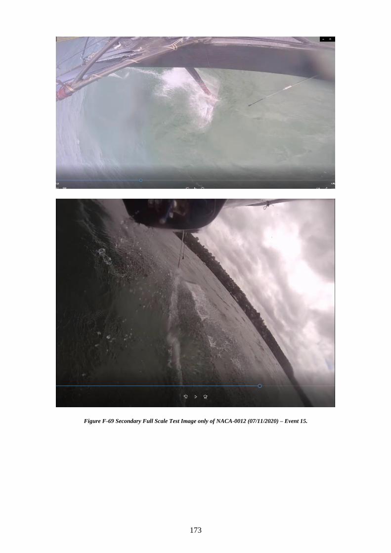
173
Figure F-69 Secondary Full Scale Test Image only of NACA-0012 (07/11/2020) – Event 15.
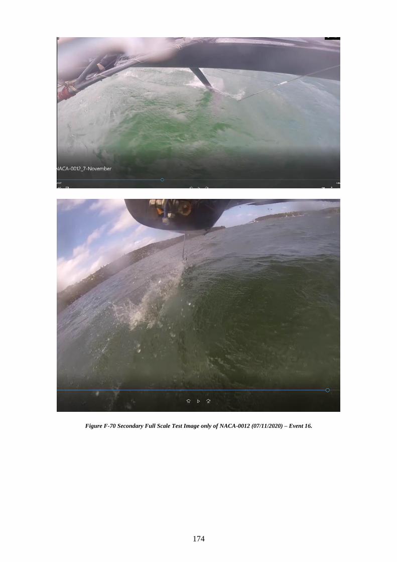
174
Figure F-70 Secondary Full Scale Test Image only of NACA-0012 (07/11/2020) – Event 16.
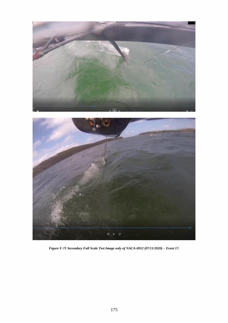
175
Figure F-71 Secondary Full Scale Test Image only of NACA-0012 (07/11/2020) – Event 17.
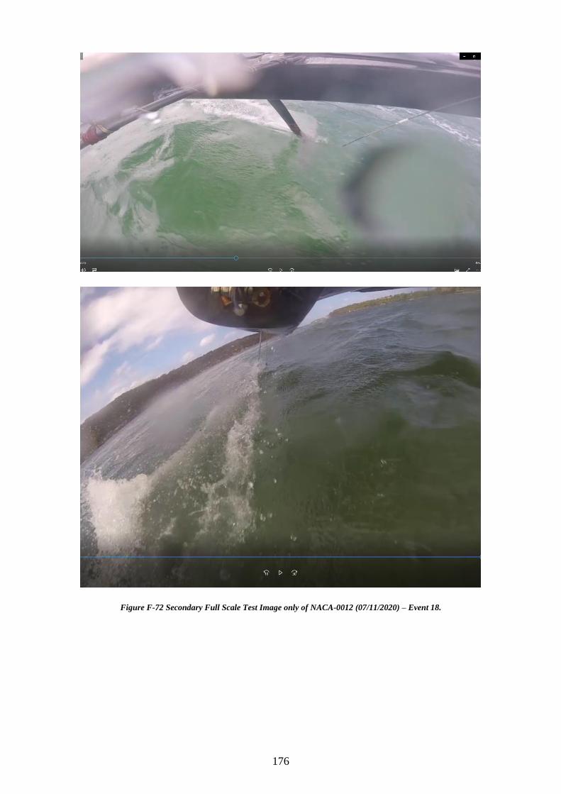
176
Figure F-72 Secondary Full Scale Test Image only of NACA-0012 (07/11/2020) – Event 18.
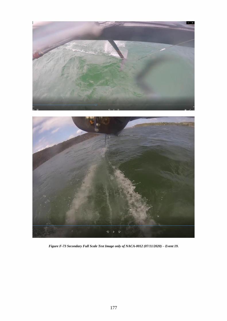
177
Figure F-73 Secondary Full Scale Test Image only of NACA-0012 (07/11/2020) – Event 19.
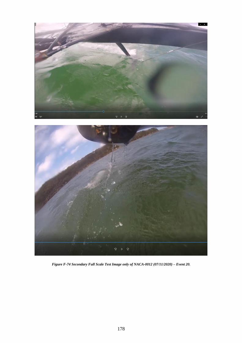
178
Figure F-74 Secondary Full Scale Test Image only of NACA-0012 (07/11/2020) – Event 20.
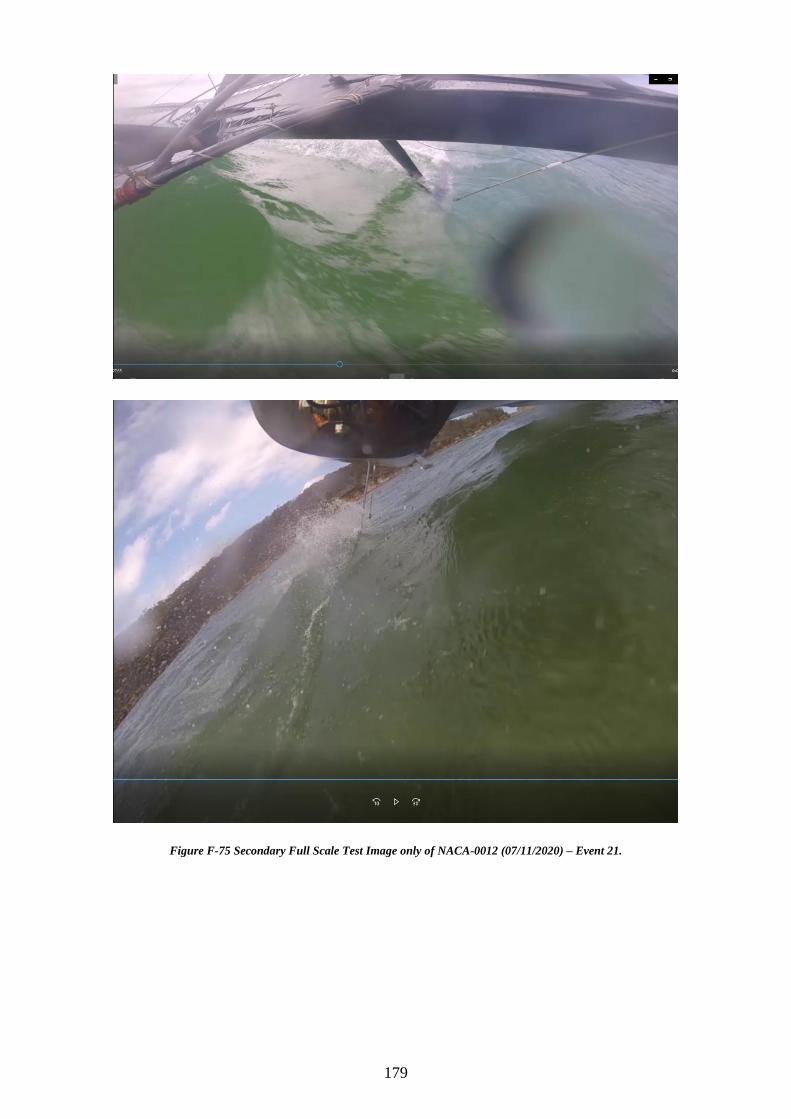
179
Figure F-75 Secondary Full Scale Test Image only of NACA-0012 (07/11/2020) – Event 21.

180
Figure F-76 Secondary Full Scale Test Image only of NACA-0012 (07/11/2020) – Event 22.
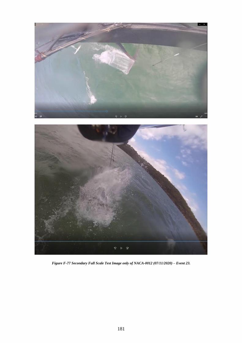
181
Figure F-77 Secondary Full Scale Test Image only of NACA-0012 (07/11/2020) – Event 23.
182
Figure F-78 Secondary Full Scale Test Image only of NACA-0012 (07/11/2020) – Event 24
183
Figure F-79 Secondary Full Scale Test Image only of NACA-0012 (07/11/2020) – Event 25.
Figure F-80 Secondary Full Scale Test Image only of NACA-0012 (07/11/2020) – Event 26.
184
Figure F-81 Secondary Full Scale Test Image only of NACA-0012 (07/11/2020) – Event 27.
Figure F-82 Secondary Full Scale Test Image only of NACA-0012 (07/11/2020) – Event 28.

185
Figure F-83 Secondary Full Scale Test Image only of NACA-0012 (07/11/2020) – Event 29.
Figure F-84 Secondary Full Scale Test Image only of NACA-0012 (07/11/2020) – Event 30.
186
Figure F-85 Secondary Full Scale Test Image only of NACA-0012 (07/11/2020) – Event 31.
Figure F-86 Secondary Full Scale Test Image only of NACA-0012 (07/11/2020) – Event 32.
187
Figure F-87 Secondary Full Scale Test Image only of NACA-0012 (07/11/2020) – Event 33.
Figure F-88 Secondary Full Scale Test Image only of NACA-0012 (07/11/2020) – Event 34.
188
Mach 2 Secondary Test Sailed on Date (5/07/2020)
Figure F-89 Secondary Full Scale Test Image only of Mach 2 (05/07/2020) – Event 1.
Figure F-90 Secondary Full Scale Test Image only of Mach 2 (05/07/2020) – Event 2.
189
Figure F-91 Secondary Full Scale Test Image only of Mach 2 (05/07/2020) – Event 3.
Figure F-92 Secondary Full Scale Test Image only of Mach 2 (05/07/2020) – Event 4.
190
Figure F-93 Secondary Full Scale Test Image only of Mach 2 (05/07/2020) – Event 5.
Figure F-94 Secondary Full Scale Test Image only of Mach 2 (05/07/2020) – Event 6.
191
Figure F-95 Secondary Full Scale Test Image only of Mach 2 (05/07/2020) – Event 7.
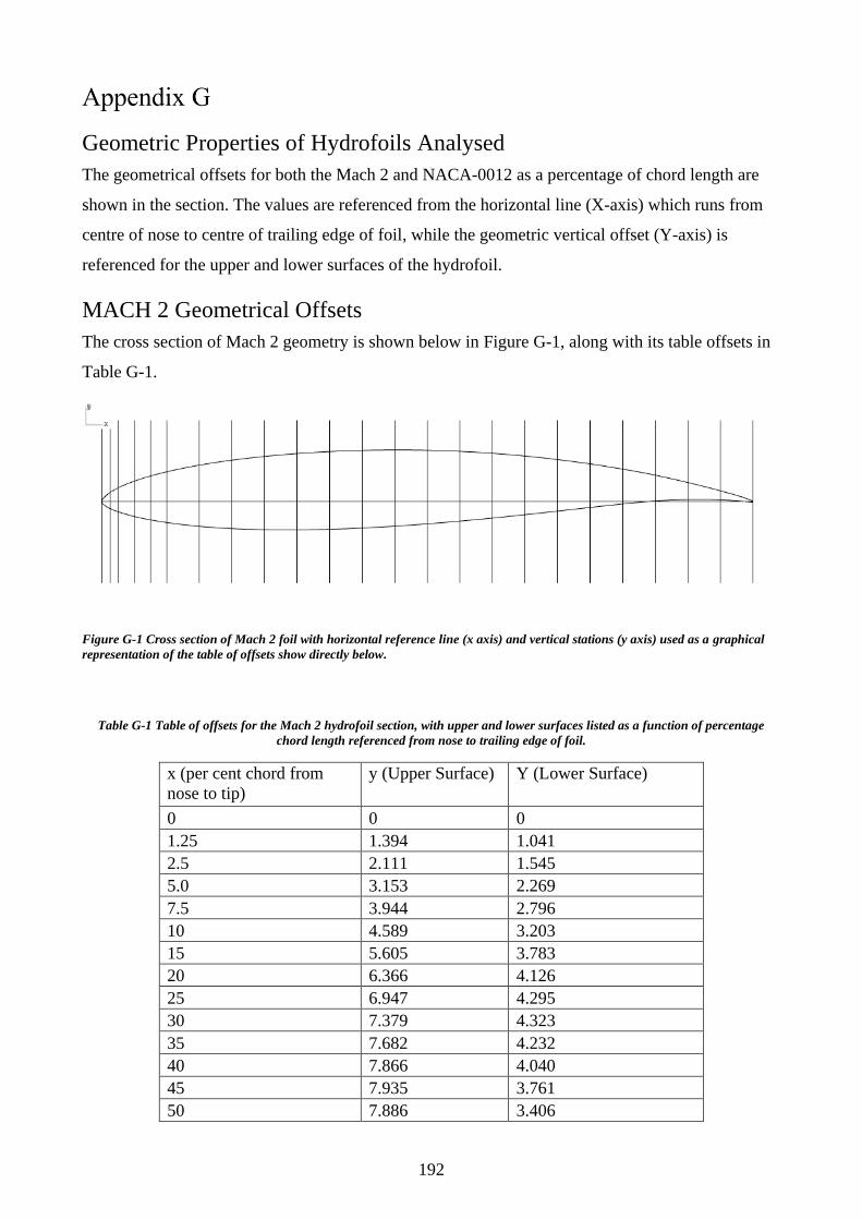
192
Geometric Properties of Hydrofoils Analysed
The geometrical offsets for both the Mach 2 and NACA-0012 as a percentage of chord length are
shown in the section. The values are referenced from the horizontal line (X-axis) which runs from
centre of nose to centre of trailing edge of foil, while the geometric vertical offset (Y-axis) is
referenced for the upper and lower surfaces of the hydrofoil.
MACH 2 Geometrical Offsets
The cross section of Mach 2 geometry is shown below in Figure G-1, along with its table offsets in
Table G-1.
Figure G-1 Cross section of Mach 2 foil with horizontal reference line (x axis) and vertical stations (y axis) used as a graphical
representation of the table of offsets show directly below.
Table G-1 Table of offsets for the Mach 2 hydrofoil section, with upper and lower surfaces listed as a function of percentage
chord length referenced from nose to trailing edge of foil.
x (per cent chord from
nose to tip)
y (Upper Surface) Y (Lower Surface)
0 0 0
1.25 1.394 1.041
2.5 2.111 1.545
5.0 3.153 2.269
7.5 3.944 2.796
10 4.589 3.203
15 5.605 3.783
20 6.366 4.126
25 6.947 4.295
30 7.379 4.323
35 7.682 4.232
40 7.866 4.040
45 7.935 3.761
50 7.886 3.406
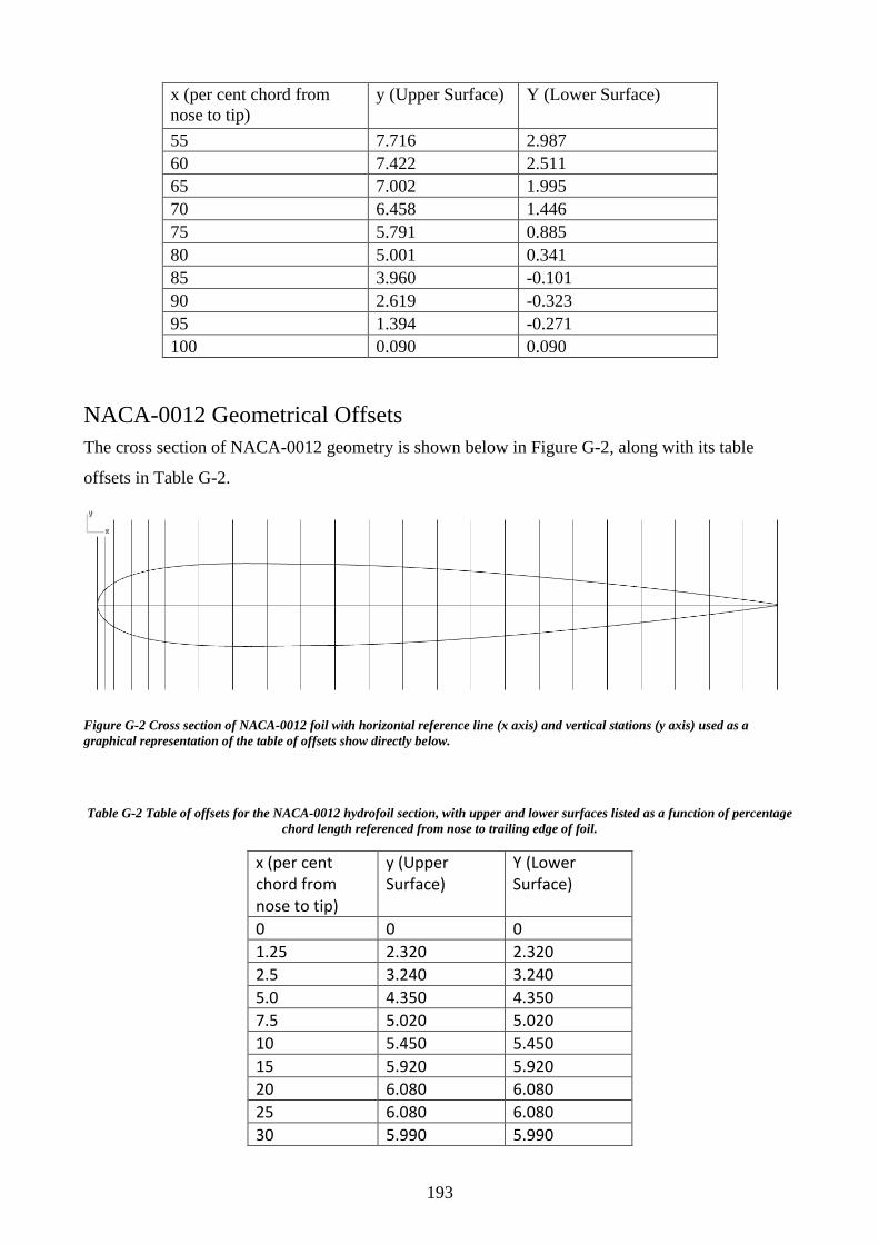
193
x (per cent chord from
nose to tip)
y (Upper Surface) Y (Lower Surface)
55 7.716 2.987
60 7.422 2.511
65 7.002 1.995
70 6.458 1.446
75 5.791 0.885
80 5.001 0.341
85 3.960 -0.101
90 2.619 -0.323
95 1.394 -0.271
100 0.090 0.090
NACA-0012 Geometrical Offsets
The cross section of NACA-0012 geometry is shown below in Figure G-2, along with its table
offsets in Table G-2.
Figure G-2 Cross section of NACA-0012 foil with horizontal reference line (x axis) and vertical stations (y axis) used as a
graphical representation of the table of offsets show directly below.
Table G-2 Table of offsets for the NACA-0012 hydrofoil section, with upper and lower surfaces listed as a function of percentage
chord length referenced from nose to trailing edge of foil.
x (per cent chord from nose to tip)
y (Upper Surface)
Y (Lower Surface)
0 0 0
1.25 2.320 2.320
2.5 3.240 3.240
5.0 4.350 4.350
7.5 5.020 5.020
10 5.450 5.450
15 5.920 5.920
20 6.080 6.080
25 6.080 6.080
30 5.990 5.990
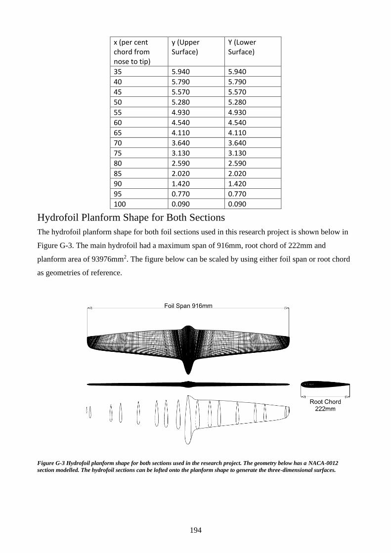
194
x (per cent chord from nose to tip)
y (Upper Surface)
Y (Lower Surface)
35 5.940 5.940
40 5.790 5.790
45 5.570 5.570
50 5.280 5.280
55 4.930 4.930
60 4.540 4.540
65 4.110 4.110
70 3.640 3.640
75 3.130 3.130
80 2.590 2.590
85 2.020 2.020
90 1.420 1.420
95 0.770 0.770
100 0.090 0.090
Hydrofoil Planform Shape for Both Sections
The hydrofoil planform shape for both foil sections used in this research project is shown below in
Figure G-3. The main hydrofoil had a maximum span of 916mm, root chord of 222mm and
planform area of 93976mm2. The figure below can be scaled by using either foil span or root chord
as geometries of reference.
Figure G-3 Hydrofoil planform shape for both sections used in the research project. The geometry below has a NACA-0012
section modelled. The hydrofoil sections can be lofted onto the planform shape to generate the three-dimensional surfaces.
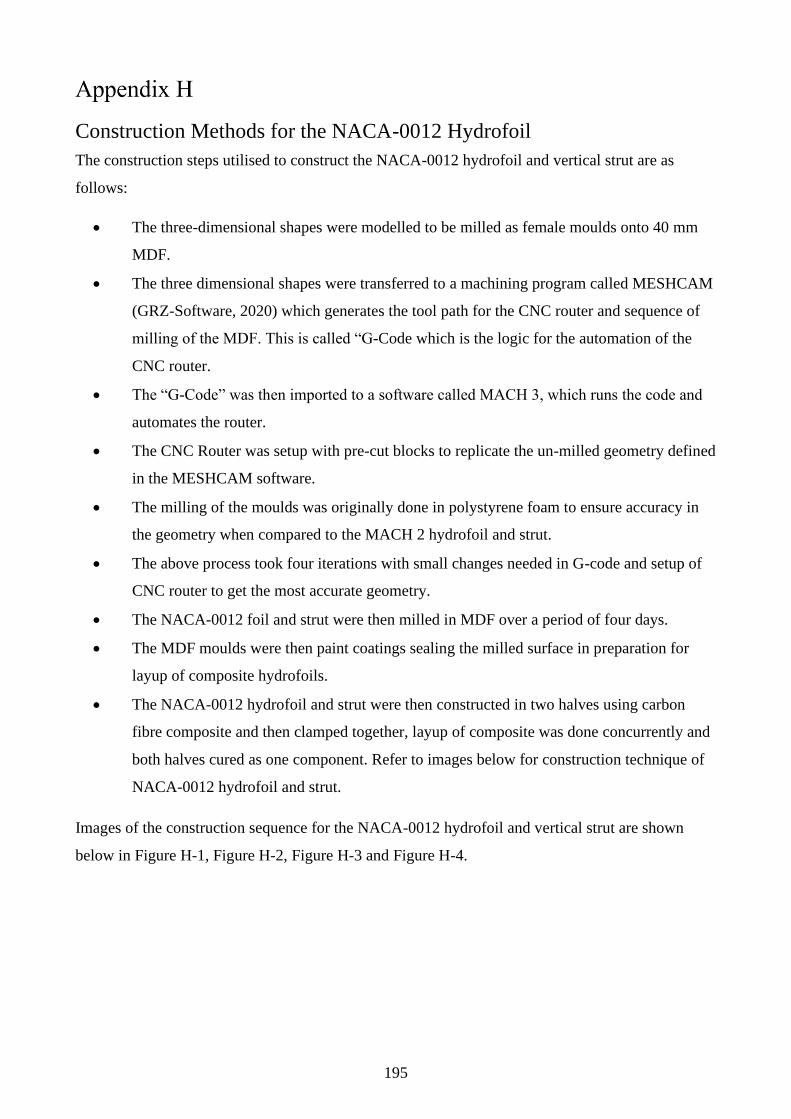
195
Construction Methods for the NACA-0012 Hydrofoil
The construction steps utilised to construct the NACA-0012 hydrofoil and vertical strut are as
follows:
• The three-dimensional shapes were modelled to be milled as female moulds onto 40 mm
MDF.
• The three dimensional shapes were transferred to a machining program called MESHCAM
(GRZ-Software, 2020) which generates the tool path for the CNC router and sequence of
milling of the MDF. This is called “G-Code which is the logic for the automation of the
CNC router.
• The “G-Code” was then imported to a software called MACH 3, which runs the code and
automates the router.
• The CNC Router was setup with pre-cut blocks to replicate the un-milled geometry defined
in the MESHCAM software.
• The milling of the moulds was originally done in polystyrene foam to ensure accuracy in
the geometry when compared to the MACH 2 hydrofoil and strut.
• The above process took four iterations with small changes needed in G-code and setup of
CNC router to get the most accurate geometry.
• The NACA-0012 foil and strut were then milled in MDF over a period of four days.
• The MDF moulds were then paint coatings sealing the milled surface in preparation for
layup of composite hydrofoils.
• The NACA-0012 hydrofoil and strut were then constructed in two halves using carbon
fibre composite and then clamped together, layup of composite was done concurrently and
both halves cured as one component. Refer to images below for construction technique of
NACA-0012 hydrofoil and strut.
Images of the construction sequence for the NACA-0012 hydrofoil and vertical strut are shown
below in Figure H-1, Figure H-2, Figure H-3 and Figure H-4.
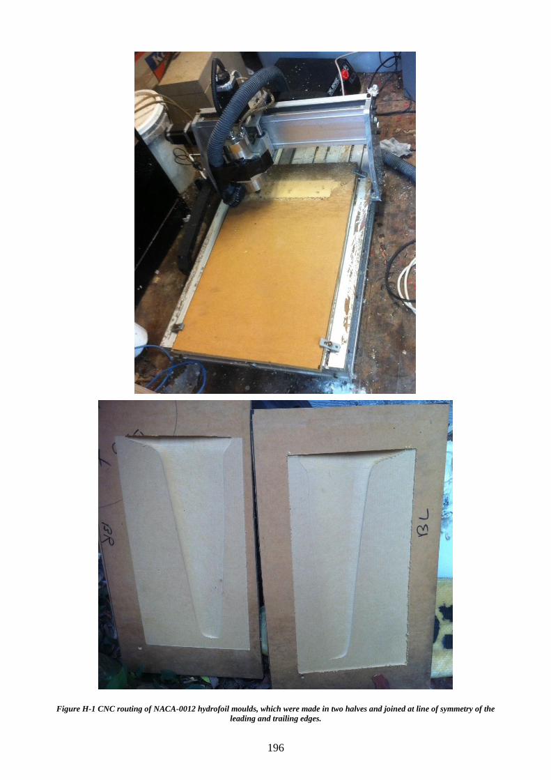
196
Figure H-1 CNC routing of NACA-0012 hydrofoil moulds, which were made in two halves and joined at line of symmetry of the
leading and trailing edges.
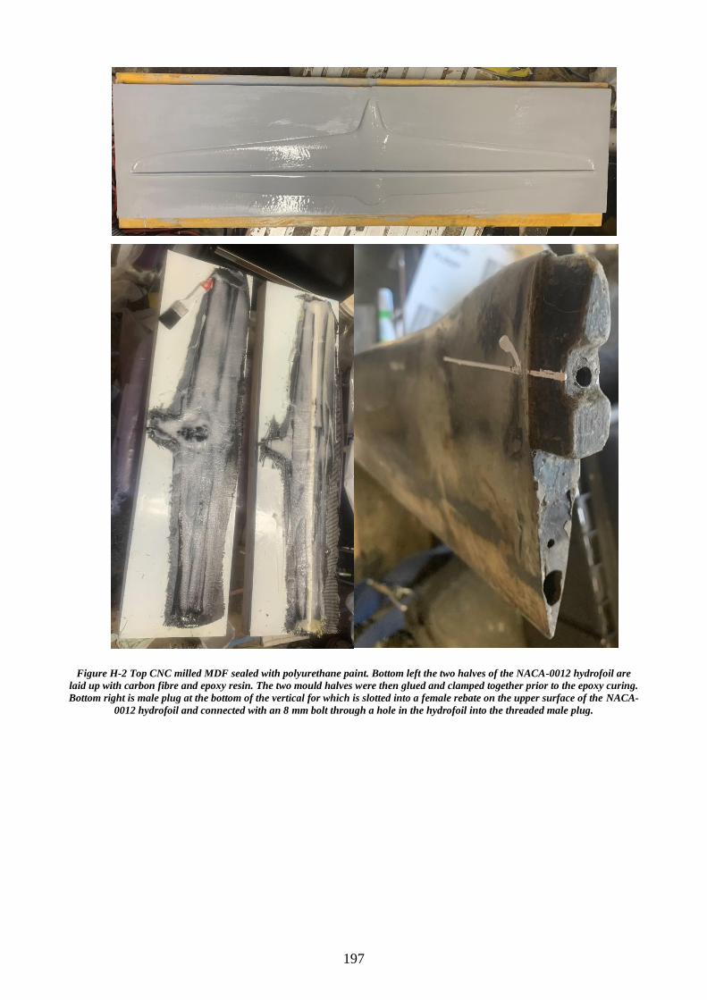
197
Figure H-2 Top CNC milled MDF sealed with polyurethane paint. Bottom left the two halves of the NACA-0012 hydrofoil are
laid up with carbon fibre and epoxy resin. The two mould halves were then glued and clamped together prior to the epoxy curing.
Bottom right is male plug at the bottom of the vertical for which is slotted into a female rebate on the upper surface of the NACA-
0012 hydrofoil and connected with an 8 mm bolt through a hole in the hydrofoil into the threaded male plug.
198
Figure H-3 NACA-0012 hydrofoil prior to sanding and application of polyurethane paint coating to seal and smoothen the
hydrofoil and vertical strut.
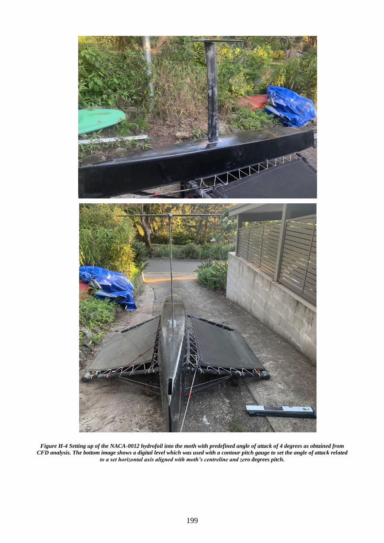
199
Figure H-4 Setting up of the NACA-0012 hydrofoil into the moth with predefined angle of attack of 4 degrees as obtained from
CFD analysis. The bottom image shows a digital level which was used with a contour pitch gauge to set the angle of attack related
to a set horizontal axis aligned with moth’s centreline and zero degrees pitch.

200
Background to Selection of Hydrofoil Sections for Research Project
The selection of an symmetrical and asymmetrical hydrofoil sections for this project was done as a
continuation of work done by Binns, Brandner, & Plouhinec, (2008) and Emonson (2009) where the
ventilation and cavitation behaviour of the NACA-0012 (symmetrical) foil was analysed. The Mach
2 (asymmetrical) foil was selected as it has become the most common section used on the moth
dinghy to date (Stevenson, Culnane, & Babbage, 2004). The foils operated in the same range of flap
deflection though required varied angle of attack to achieve the same baseline lift. The use of
symmetrical foil sections in the moth class has been restricted to the vertical strut which operates at
low yawing and leeway angles. As shown in this work at low angles of attack the symmetrical foil
operates at lower drag forces than the asymmetrical foil. The geometric variances of the two
sections with respect to camber affects the pressure distribution on the foil surface, as a result
induces vapour attachment in low pressure regions on the upper surface of the foil.
Effect of Hinge Junction on Hydrofoil Performance
The hinge geometry at the connection of the trailing edge flap to the main hydrofoil body has an
abrupt change in shape due to structural requirements needed to allow the flap to articulate through
the full angles of operation. The flap junction has a transverse hollow on the lower surface of the
hydrofoil. The hollow is placed on the lower surface to align with the high-pressure side of the foil,
this has a reduced impact on pressure gradients when compared to upper (low pressure) side of the
foil. The existence of this hollow at flap junction can increase the induced drag of the foil section as
found by Beaver and Zseleczky (2009). The hydrofoil cross section profile of two styles of hinge
connections is shown below in Figure I-1 where the upper image of the cross-section represents the
hinge attachment used on both foils in this research project.
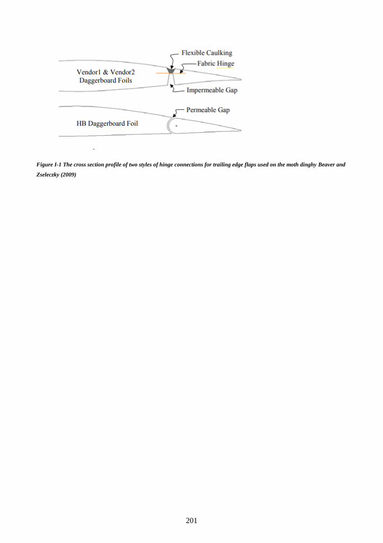
201
Figure I-1 The cross section profile of two styles of hinge connections for trailing edge flaps used on the moth dinghy Beaver and
Zseleczky (2009)
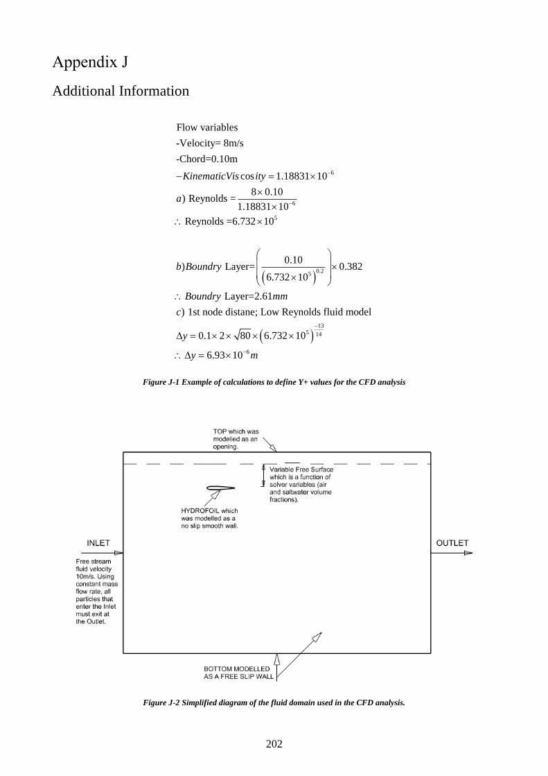
202
Additional Information
( )
6
6
5
0.25
Flow variables
-Velocity= 8m/s
-Chord=0.10m
cos 1.18831 10
8 0.10) Reynolds =
1.18831 10
Reynolds =6.732 10
0.10) Layer= 0.382
6.732 10
Layer=2.61
) 1st no
KinematicVis ity
a
b Boundry
Boundry mm
c
−
−
− =
( )13
5 14
6
de distane; Low Reynolds fluid model
0.1 2 80 6.732 10
6.93 10
y
y m
−
−
=
=
Figure J-1 Example of calculations to define Y+ values for the CFD analysis
Figure J-2 Simplified diagram of the fluid domain used in the CFD analysis.
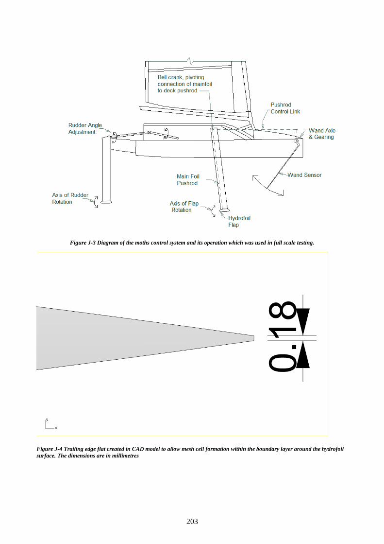
203
Figure J-3 Diagram of the moths control system and its operation which was used in full scale testing.
Figure J-4 Trailing edge flat created in CAD model to allow mesh cell formation within the boundary layer around the hydrofoil
surface. The dimensions are in millimetres
204
References
ANSYS. (2020). ANSYS. Retrieved from https://www.ansys.com/
Barden, T., & Binns, J. (2012). On the road to establishing ventilation probability for Moth sailing dinghies.
Paper presented at the 18th Australasian Fluid Mechanics Conference.
Beaver, B., & Zseleczky, J. (2009). Full scale measurements on a hydrofoil international moth. Paper
presented at the 19th Chesapeake Sailing Yacht Symposium, Annapolis, Maryland.
Binns, J., Brandner, P., & Plouhinec, J. (2008). The effect of heel angle and free surface proximity on the
performance and strut wake of a moth sailing dinghy rudder t-foil. Paper presented at the High performance
yacht design conference.
Brennen, C. E. C. E. (1995). Cavitation and bubble dynamics. New York: Oxford University Press.
Broder, P. (2018). Sensor Play Data Recorder. Retrieved from https://apps.apple.com/us/app/sensor-play-data-recorder/id921385514
Chahine, G. L. (2004). Nuclei effects on cavitation inception and noise. Paper presented at the Keynote
presentation, 25th Symposium on Naval Hydrodynamics, St. John’s, Newfoundland and Labrador,
Canada.
Emonson, J. A. (2009). An investigation into the effect of froude, weber and cavitation numbers on
ventilation of surface-piercing t-foils. (Bachelor of Engineering (Naval Architecture) An
investigation into the effect of froude, weber and cavitation numbers on ventilation of surface-
piercing t-foils). Australian Maritime College, Launceston.
Erney, R. W. (2008). Verification And Validation Of Single Phase and Cavitating Flows Using An Open
Source CFD Tool The Pennsylvania State University,
GRZ-Software. (2020). MeshCAM. Retrieved from http://www.grzsoftware.com/
Hajime Yamaguchi, H. K., Masatsugu Maeda and Makoto Toyoda. (1999). High Performance Foil Sections
with Delayed Cavitation Inception. Proceedings of the 3rd ASME/JSME Joint Fluids Engineering
Conference July 18-22, 1999, San Francisco, California,, FEDSM99-7294. Retrieved from
https://www.semanticscholar.org/paper/HIGH-PEFORMANCE-FOIL-SECTIONS-WITH-DELAYED-Yamaguchi-Kato/ec19df70a8b690c46292e9bc5bb5f00f79955760
Hull, D. (2011). Speed sailing design and velocity prediction program. (Bachelor of Engineering (Naval
Architecture)). Australian Maritime College, Launceston.
Igoe, T. (2020). Arduino Tutorial - Using the SD library to log data. Retrieved from
https://www.arduino.cc/en/Tutorial/LibraryExamples/Datalogger ITTC. (2002). ITTC – Recommended Procedures - Testing and Extrapolation Methods Resistance Resistance
Test. Paper presented at the Specialist Committee: Procedures for Resistance, Propulsion and
Propeller Open Water
Tests of 23rd ITTC 2002 https://ittc.info/media/2019/75-02-02-01.pdf Jin, M.-S., Ha, C.-T., & Park, W.-G. (2013). Numerical study of ventilated cavitating flows with free surface
effects. Journal of Mechanical Science and Technology, 27(12), 3683-3691. doi:10.1007/s12206-
013-0914-0
McNeel, R. (2020). Rhino 6. Retrieved from https://www.rhino3d.com/6/
Rothblum, R. S. (1977). Investigation of Methods of Delaying Or Controlling Ventilation On Surface
Piercing Struts. Retrieved from http://etheses.whiterose.ac.uk/11335/1/646388.pdf Rouse, H., & McNown, J. S. (1948). Cavitation and pressure distribution: head forms at zero angle of yaw.
Speer, T. (2015, 16/11/2015). [Moth Hydrofoil Section, H105].
Stevenson, P., Culnane, D., & Babbage, S. (2004). Moth web forum. Retrieved from http://moth-sailing.org/imca/faces/news.jsp
White, F. M. (1998). Fluid Mechanics. 4th. In: McGraw-Hill.
Wu, J.-H. C. a. P. (2009). A computational study of a two-dimensional viscous cavitating foil near a free
surface. Paper presented at the 10th International Conference on Fluid Control, Measurement and
Visualisation, Moscow.
Young, F. R. (1999). Cavitation: McGraw-Hill.


