Embed Size (px)
Citation preview
RESEARCH ARTICLE
Comparative landscape genetic analysis of three Pacific salmonspecies from subarctic North America
Jeffrey B. Olsen • Penelope A. Crane •
Blair G. Flannery • Karen Dunmall •
William D. Templin • John K. Wenburg
Received: 21 February 2010 / Accepted: 7 September 2010
� US Government 2010
Abstract We examined the assumption that landscape
heterogeneity similarly influences the spatial distribution of
genetic diversity in closely related and geographically
overlapping species. Accordingly, we evaluated the influ-
ence of watershed affiliation and nine habitat variables from
four categories (spatial isolation, habitat size, climate, and
ecology) on population divergence in three species of Pacific
salmon (Oncorhynchus tshawytscha, O. kisutch, and O.
keta) from three contiguous watersheds in subarctic North
America. By incorporating spatial data we found that the
three watersheds did not form the first level of hierarchical
population structure as predicted. Instead, each species
exhibited a broadly similar spatial pattern: a single coastal
group with populations from all watersheds and one or more
inland groups primarily in the largest watershed. These
results imply that the spatial scale of conservation should
extend across watersheds rather than at the watershed level
which is the scale for fishery management. Three indepen-
dent methods of multivariate analysis identified two vari-
ables as having influence on population divergence across
all watersheds: precipitation in all species and subbasin area
(SBA) in Chinook. Although we found general broad-scale
congruence in the spatial patterns of population divergence
and evidence that precipitation may influence population
divergence in each species, we also found differences in the
level of population divergence (coho [ Chinook and chum)
and evidence that SBA may influence population divergence
only in Chinook. These differences among species support a
species-specific approach to evaluating and planning for the
influence of broad-scale impacts such as climate change.
Keywords Landscape genetics � Pacific salmon �Population structure � Subarctic
Introduction
Identifying the landscape factors influencing population
structure is important for understanding how populations
evolve and for predicting how they may change in the face of
environmental perturbations. Multi-species analysis using
landscape genetics methods (Manel et al. 2003; Storfer et al.
2006) can provide important insights in this regard. For
example, common patterns of population structure among co-
occurring species that exhibit different life histories have
revealed landscape features (and evidence of historical pro-
cesses) that have broad taxonomic influence (e.g., Petren et al.
2005; Gagnon and Angers 2006). On the other hand, con-
trasting patterns of population structure among species from
the same landscape have shown the importance of species
ecology and life history and demonstrate the danger in gen-
eralizing the role of habitat heterogeneity on genetic diversity
(e.g., Whiteley et al. 2004; Short and Caterino 2009). Multi-
species analyses are particularly relevant for conservation of
closely related and geographically overlapping species for
Electronic supplementary material The online version of thisarticle (doi:10.1007/s10592-010-0135-3) contains supplementarymaterial, which is available to authorized users.
J. B. Olsen (&) � P. A. Crane � B. G. Flannery � J. K. Wenburg
Conservation Genetics Laboratory, U.S. Fish & Wildlife Service,
1011 East Tudor Road, Anchorage, AK 99503, USA
e-mail: [email protected]
K. Dunmall
Fisheries Department, Kawerak, Inc., PO Box 948, Nome,
AK 99762, USA
W. D. Templin
Alaska Department of Fish and Game, Division of Commercial
Fisheries, Gene Conservation Laboratory, 333 Raspberry Road,
Anchorage, AK 99518, USA
123
Conserv Genet
DOI 10.1007/s10592-010-0135-3
which it may seem reasonable to assume that landscape
heterogeneity similarly influences the spatial distribution of
genetic diversity (Marten et al. 2006). Here we question this
assumption by examining the role of habitat features on the
spatial patterns and level of population divergence in three
species of Pacific Salmon (Oncorhynchus spp.) in a pristine
subarctic environment in North America.
Pacific salmon are found in most river systems on the west
coast of North America between 40�N and 68�N (Groot and
Margolis 1991). Five species are anadromous, philopatric and
semelparous. Along the west coast of Alaska above 60�N,
three species, Chinook (O. tshawytscha), coho (O. kisutch),
and chum (O. keta) salmon, are sufficiently abundant to
support commercial, subsistence, and sport fisheries. These
three species broadly overlap across three contiguous water-
sheds (Norton Sound, Yukon River, Kuskokwim River)
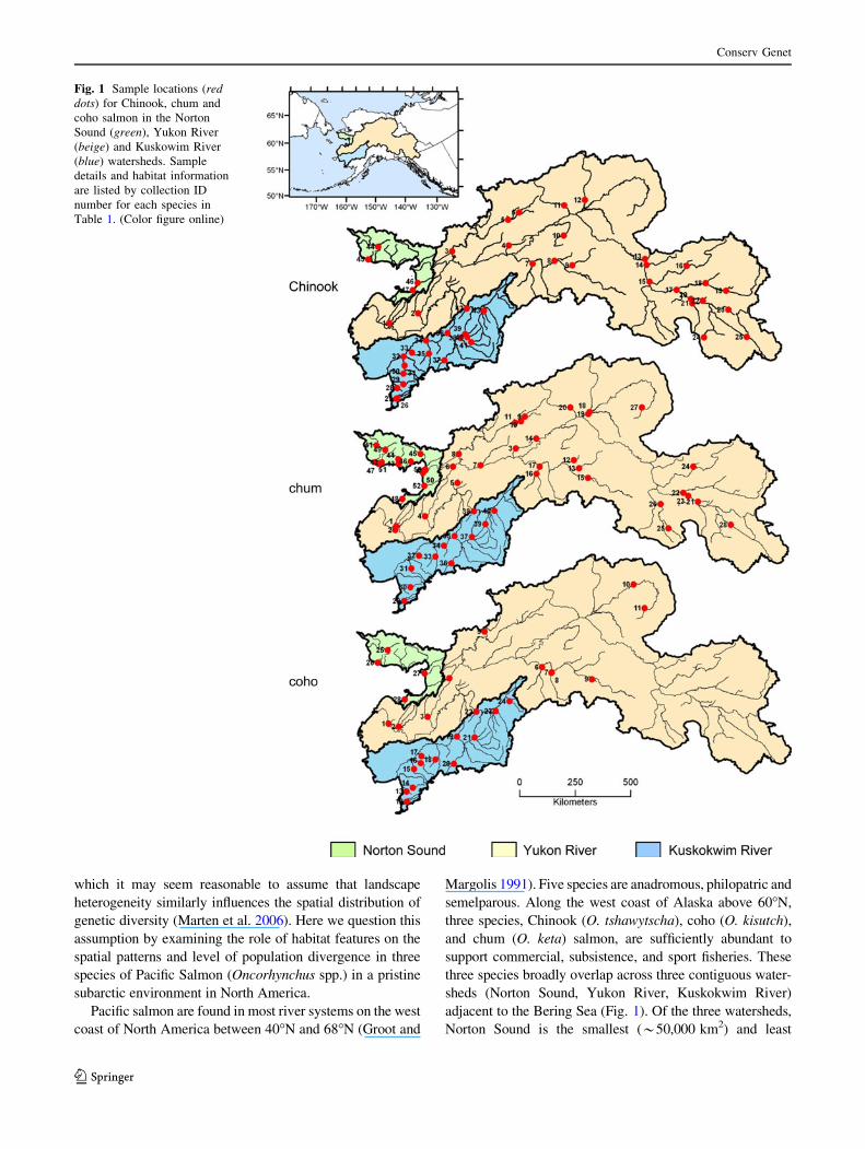
adjacent to the Bering Sea (Fig. 1). Of the three watersheds,
Norton Sound is the smallest (*50,000 km2) and least
Fig. 1 Sample locations (reddots) for Chinook, chum and
coho salmon in the Norton
Sound (green), Yukon River
(beige) and Kuskowim River
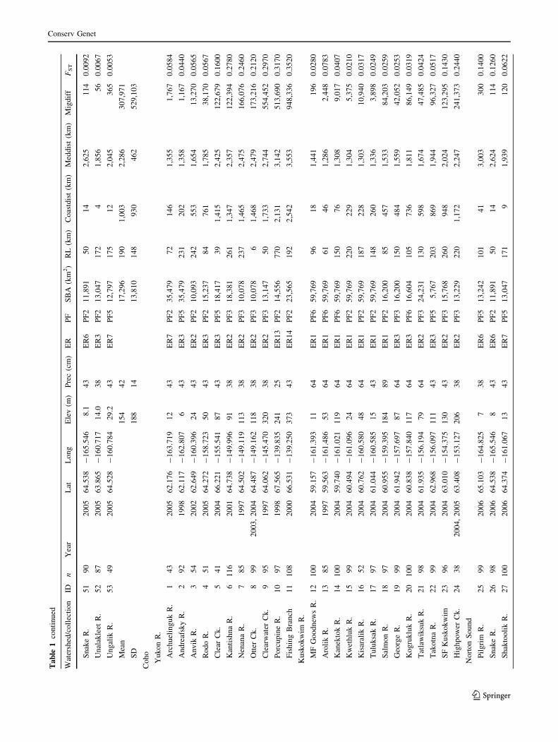
(blue) watersheds. Sample
details and habitat information
are listed by collection ID
number for each species in
Table 1. (Color figure online)
Conserv Genet
123

complex (four ecoregions), consisting of many unconnected
and relatively short (mean length *110 km) coastal rivers.
The Kuskokwim River watershed is larger (*151,000 km2)
and more complex (six ecoregions) than Norton Sound,
extending into the interior of Alaska over 1,500 rkm from the
mouth. The Yukon River watershed is the largest
(858,000 km2) and most complex (22 ecoregions) of the
three, traversing Alaska with headwaters in British Columbia
over 3,000 rkm from the mouth. The three watersheds
encompass over 1 million km2 and 24 ecoregions. Based on
the broad physical and ecological differences among water-
sheds, we predict that they will form the first level of hier-
archical population structure of each species.
The goal of landscape genetics is to identify and quantify
the effects of landscape heterogeneity on genetic variation
(Storfer et al. 2006). Recent studies have begun to address
this goal for species in the aquatic realm. Results from these
studies show that habitat features associated with genetic
diversity may include indicators of spatial isolation or geo-
graphic distance (e.g., waterway and coastline distance),
climate features (e.g., temperature), habitat size (e.g., lake
area), and environmental gradients (e.g., salinity) (Dionne
et al. 2008; Dillane et al. 2008; Jørgensen et al. 2005). Some
studies also show the importance of spatial scale as some
factors (e.g., temperature) may vary over broad spatial scales
and influence genetic diversity at a regional level but not at
the level of watersheds or individual rivers (e.g., Dionne et al.
2008). Few studies, however have examined and compared
the influence of landscape heterogeneity on genetic diversity
in co-occurring and closely related aquatic species.
Here, we used landscape genetics methods to determine if
habitat heterogeneity similarly influences the spatial distri-
bution of genetic diversity in subarctic populations of Chi-
nook, chum and coho salmon. Our objectives were twofold.
First, we assessed if the three watersheds form the first level
of hierarchical population structure in each species. More
generally, we assessed if the patterns of hierarchical popu-
lation structure in each species were congruent. Second, we
evaluated and compared the extent to which habitat features
from four general categories (spatial isolation, habitat size,
climate, and ecology) explained population divergence in
each species. The results were evaluated in the context of
current management and conservation efforts with an
emphasis on broad-scale environmental perturbations from
factors such as climate change.
Materials and methods
Genetic data
The genetic data consisted of microsatellite genotypes
drawn mostly from genetic baselines developed for mixed-
stock analysis and to describe population structure (e.g.,
Flannery et al. 2006; Crane et al. 2007; Olsen et al. 2008).
For the present study, we added genotypes for coho and
Chinook from Norton Sound following the protocol of
Crane et al. (2007) and Seeb et al. (2007). The genotypes
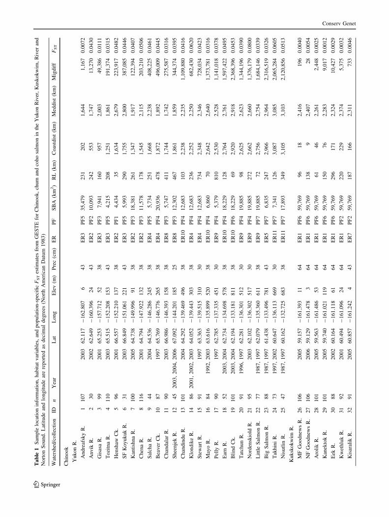
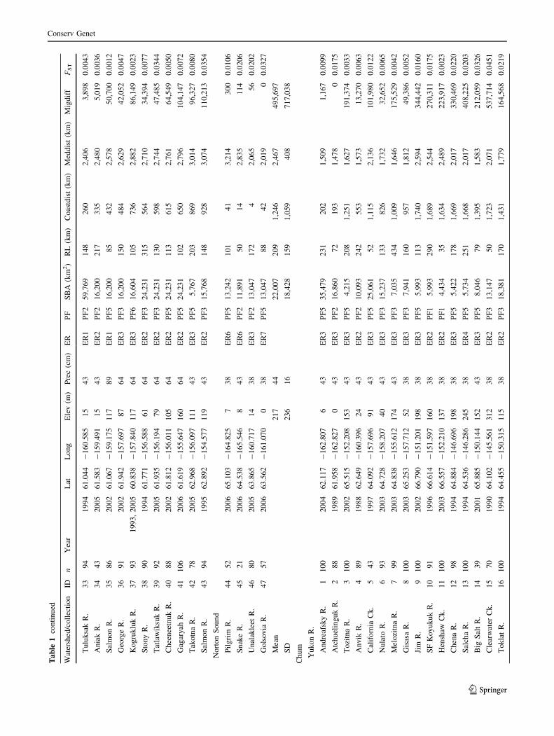
represented 13, 12, and eight loci for Chinook (47 collec-
tions), chum (53 collections), and coho (28 collections),
respectively (Table 1; Fig. 1, Appendices S1–S3 in Sup-
plementary materials). The sample sizes ranged from 21 to
116 per location and averaged approximately 85 for each
species. A geographic information system (GIS) data layer
of sample locations was created using latitude and longi-
tude (North American Datum 1983) from a GPS or a
physical description of the location. No data was available
for coho from the upper Yukon River. There is little evi-
dence of coho spawning in that area. All samples were
collected from mature adults except for juvenile coho
salmon from Clear Creek and the Fishing Branch River in
the Yukon River watershed. Although some Chinook and
chum samples were collected as much as 19 years apart,
previous studies using many of these samples (e.g., Bea-
cham et al. 2006; Olsen et al. 2008) show that differences
at this temporal scale contribute little to the overall esti-
mates of population divergence.
Habitat data
Habitat data in the form of GIS data layers were obtained
from the Alaska geospatial data clearing house (http://agdc.
usgs.gov/) and the Canadian GeoBase (http://www.geo
base.ca/geobase/en/index.html). We examined nine vari-
ables associated with the watershed environment (Table 7
in Appendix). These variables reflected four general cate-
gories (spatial isolation, habitat size, climate, and ecology)
that may affect population divergence by influencing gene
flow or genetic drift or both. Increasing spatial isolation is
expected to decrease gene flow in migratory and philop-
atric species. Spatial isolation was evaluated using four
indictors: waterway distance to the coast, median pairwise
waterway distance from each location to all other locations
(similar to connectivity, Kittlein and Gaggiotti 2008),
elevation, and migration difficulty (waterway distance to
the coast 9 elevation, see Quinn 2005). All estimates of
waterway distance were computed in ArcGISTM (ESRI)
version 9.2 using National Hydrologic Dataset (NHD)
flowlines. Increasing habitat size may correspond with
larger population size which should result in lower genetic
drift. Habitat size was evaluated using two indicators: the
length of the home river for each sample and the U.S.
Geological Service (USGS) Hydrologic Unit Code (HUC)
level four subbasin area (SBA) (and the equivalent from
the Canadian GeoBase). Although finer scale HUC units
are available, we chose level four because it is equivalent
Conserv Genet
123
Ta
ble
1S
amp
lelo
cati
on
info
rmat
ion
,h
abit
atv
aria
ble
s,an
dp
op
ula
tio
n-s
pec
ific
FS
Tes
tim
ates
fro
mG
ES
TE
for
Ch
ino
ok
,ch
um
and
coh
osa
lmo
nin
the
Yu
ko
nR
iver
,K
usk
ok
wim
,R
iver
and
No
rto
nS
ou
nd
.L
atit
ud
ean
dlo
ng
itu
de
are
rep
ort
edas
dec
imal
deg
rees
(No
rth
Am
eric
anD
atu
m1
98
3)
Wat
ersh
ed/c
oll
ecti
on
IDn
Yea
rL
atL
on
gE
lev
(m)
Pre
c(c
m)
ER
PF
SB
A(k
m2)
RL
(km
)C
oas
tdis
t(k
m)
Med
dis
t(k
m)
Mig
dif
fF
ST
Ch
ino
ok
Yu
ko
nR
.
An
dre
afsk
yR
.1
10
72
00
36
2.1
17
-1
62
.80
76
43
ER
3P
F5
35
,47
92
31
20
21
,64
41
,16
70
.00
72
An
vik
R.
23
02
00
26
2.6
49
-1
60
.39
62
44
3E
R2
PF
21
0,0
93
24
25
53
1,7
47
13
,27
00
.04
30
Gis
asa
R.
39
92
00
16
5.2
53
-1
57
.71
25
23
8E
R3
PF
37
,94
11
60
95
72
,00
34
9,3
86
0.0
11
1
To
zitn
aR
.4
11
02
00
36
5.5
15
-1
52
.20
81
53
43
ER
3P
F5
4,2
15
20
81
,25
11
,86
11
91
,37
40
.03
15
Hen
shaw
Ck
.5
96
20
01
66
.55
7-
15
2.2
10
13
73
8E
R2
PF
14
,43
43
51
,63
42
,67
92
23
,91
70
.04
82
SF
Ko
yu
ku
kR
.6
31
20
03
66
.84
9-
15
1.0
61
22
14
3E
R3
PF
55
,99
32
90
1,7
55
2,8
00
38
7,0
85
0.0
44
6
Kan
tish
na
R.
71
00
20
05
64
.73
8-
14
9.9
96
91
38
ER
2P
F3
18
,38
12
61
1,3
47
1,9
17
12
2,3
94
0.0
40
7
Ch
ena
R.
81
16
20
01
64
.79
4-
14
7.9
22
13
23
8E
R2
PF
31
1,5
78
17
81
,54
52
,11
52
03
,21
00
.05
06
Sal
cha
R.
94
42
00
46
4.5
36
-1
46
.28
62
45
38
ER
4P
F5
5,7
34
25
11
,66
82
,23
84
08
,22
50
.04
61
Bea
ver
Ck
.1
08
71
99
76
5.7
69
-1
46
.77
62
65
38
ER
4P
F4
20
,93
64
78
1,8
72
1,8
92
49
6,0
09
0.0
44
5
Ch
and
alar
R.
11
90
20
03
66
.98
6-
14
6.3
93
15
83
8E
R8
PF
35
,74
74
11
1,7
44
1,7
42
27
5,5
87
0.0
31
6
Sh
een
jek
R.
12
45
20
03
,2
00
4,
20
06
67
.09
2-
14
4.2
01
18
52
5E
R8
PF
31
2,3
02
46
71
,86
11
,85
93
44
,37
40
.03
95
Ch
and
ind
uR
.1
31
01
20
04
64
.29
2-
13
9.4
69
49
63
8E
R1
0P
F4
12
,68
31
03
2,2
38
2,2
35
1,1
09
,88
00
.04
16
Klo
nd
ike
R.
14
86
20
01
,2
00
2,
20
03
64
.05
2-
13
9.4
43
30
33
8E
R4
PF
41
2,6
83
23
62
,25
22
,25
06
82
,43
00
.06
20
Ste
war
tR
.1
59
11
99
76
3.3
63
-1
39
.51
53
10
30
ER
4P
F4
12
,68
37
34
2,3
48
2,3
46
72
8,0
34
0.0
42
3
May
oR
.1
68
41
99
2,
20
03
63
.61
6-
13
5.8
99
52
03
8E
R1
0P
F4
6,8
60
70
2,6
42
2,6
40
1,3
73
,78
10
.03
16
Pel
lyR
.1
79
01
99
76
2.7
85
-1
37
.33
54
51
30
ER
9P
F4
5,3
79
81
02
,53
02
,52
81
,14
1,0
18
0.0
37
8
Ear
nR
.1
85
22
00
3,
20
04
62
.73
4-
13
4.6
98
57
83
8E
R1
0P
F4
18
,22
91
28
2,7
64
2,7
61
1,5
97
,42
20
.04
95
Bli
nd
Ck
.1
91
01
20
03
,2
00
46
2.1
94
-1
33
.18
18
11
38
ER
10
PF
61
8,2
29
69
2,9
20
2,9
18
2,3
68
,39
60
.04
53
Tat
chu
nR
.2
09
11
99
6,
19
97
62
.28
1-
13
6.3
01
51
23
0E
R9
PF
41
9,8
85
98
2,6
25
2,6
23
1,3
44
,19
60
.03
90
No
rden
skio
ldR
.2
19
52
00
36
2.1
02
-1
36
.30
25
17
30
ER
9P
F4
19
,88
52
72
2,6
62
2,6
60
1,3
76
,17
90
.08
00
Lit
tle
Sal
mo
nR
.2
27
71
98
7,
19
97
62
.07
9-
13
5.3
60
61
13
8E
R9
PF
71
9,8
85
72
2,7
56
2,7
54
1,6
84
,14
60
.03
39
Big
Sal
mo
nR
.2
38
81
98
7,
19
97
61
.43
8-
13
3.4
96
78
14
3E
R5
PF
76
,83
52
47
2,9
66
2,9
64
2,3
16
,51
90
.03
26
Tak
hin
iR
.2
47
31
99
7,
20
02
60
.64
7-
13
6.1
13
66
93
0E
R1
1P
F7
7,3
41
12
63
,08
73
,08
52
,06
5,2
84
0.0
60
5
Nis
utl
inR
.2
54
71
98
7,
19
97
60
.16
2-
13
2.7
25
68
33
8E
R1
1P
F7
17
,89
33
49
3,1
05
3,1
03
2,1
20
,85
60
.05
13
Ku
ksk
ok
wim
R.
MF
Go
od
new
sR
.2
61
06
20
05
59
.15
7-
16
1.3
93
11
64
ER
1P
F6
59
,76
99
61
82
,41
61
96
0.0
04
0
NF
Go
od
new
sR
.2
71
06
20
06
59
.12
9-
16
1.4
78
36
4E
R1
PF
65
9,7
69
13
89
2,4
07
28
0.0
05
4
Aro
lik
R.
28
10
12
00
55
9.5
63
-1
61
.48
65
36
4E
R1
PF
65
9,7
69
61
46
2,2
61
2,4
48
0.0
02
5
Kan
ekto
kR
.2
91
01
20
05
59
.74
0-
16
1.0
21
11
96
4E
R1
PF
65
9,7
69
15
07
62
,28
39
,01
70
.00
12
Eek
R.
30
88
20
02
60
.16
4-
16
1.1
18
61
64
ER
1P
F6
59
,76
92
96
17
12
,32
41
0,4
27
0.0
02
9
Kw
eth
luk
R.
31
92
20
01
60
.49
4-
16
1.0
96
24
64
ER
1P
F2
59
,76
92
20
22
92
,37
45
,37
50
.00
32
Kis
aral
ikR
.3
29
12
00
56
0.8
57
-1
61
.24
24
43
ER
7P
F2
59
,76
91
87
16
62
,31
17
33
0.0
04
6
Conserv Genet
123
Ta
ble
1co
nti
nu
ed
Wat
ersh
ed/c
oll
ecti
on
IDn
Yea
rL
atL
on
gE
lev
(m)
Pre
c(c
m)
ER
PF
SB
A(k
m2)
RL
(km
)C
oas
tdis
t(k
m)
Med
dis
t(k
m)
Mig
dif
fF
ST
Tu
luk
sak
R.
33
94
19
94
61
.04
4-
16
0.5
85
15
43
ER
1P
F2
59
,76
91
48
26
02
,40
63
,89
80
.00
43
An
iak
R.
34
43
20
05
61
.58
3-
15
9.4
91
15
43
ER
2P
F2
16
,20
02
17
33
52
,48
05
,01
90
.00
36
Sal
mo
nR
.3
58
62
00
26
1.0
67
-1
59
.17
51
17
89
ER
1P
F5
16
,20
08
54
32
2,5
78
50
,70
00
.00
12
Geo
rge
R.
36
91
20
02
61
.94
2-
15
7.6
97
87
64
ER
3P
F3
16
,20
01
50
48
42
,62
94
2,0
52
0.0
04
7
Ko
gru
klu
kR
.3
79
31
99
3,
20
05
60
.83
8-
15
7.8
40
11
76
4E
R3
PF
61
6,6
04
10
57
36
2,8
82
86
,14
90
.00
23
Sto
ny
R.
38
90
19
94
61
.77
1-
15
6.5
88
61
64
ER
2P
F3
24
,23
13
15
56
42
,71
03
4,3
94
0.0
07
7
Tat
law
iksu
kR
.3
99
22
00
56
1.9
35
-1
56
.19
47
96
4E
R2
PF
32
4,2
31
13
05
98
2,7
44
47
,48
50
.03
44
Ch
een
eetn
uk
R.
40
88
20
02
61
.81
2-
15
6.0
11
10
56
4E
R2
PF
52
4,2
31
11
36
15
2,7
61
64
,54
90
.00
50
Gag
ary
ahR
.4
11
06
20
06
61
.61
9-
15
5.6
47
16
06
4E
R2
PF
52
4,2
31
10
26
50
2,7
96
10
4,1
47
0.0
07
2
Tak
otn
aR
.4
27
82
00
56
2.9
68
-1
56
.09
71
11
43
ER
3P
F5
5,7
67
20
38
69
3,0
14
96
,32
70
.00
80
Sal
mo
nR
.4
39
41
99
56
2.8
92
-1
54
.57
71
19
43
ER
2P
F3
15
,76
81
48
92
83
,07
41
10
,21
30
.03
54
No
rto
nS
ou
nd
Pil
gri
mR
.4
45
22
00
66
5.1
03
-1
64
.82
57
38
ER
6P
F5
13
,24
21
01
41
3,2
14
30
00
.01
06
Sn
ake
R.
45
21
20
06
64
.53
8-
16
5.5
46
84
3E
R6
PF
21
1,8
91
50
14
2,8
35
11
40
.02
06
Un
alak
leet
R.
46
80
20
05
63
.86
5-
16
0.7
17
14
38
ER
3P
F2
13
,04
71
72
42
,06
55
60
.02
02
Go
lso
via
R.
47
57
20
06
63
.56
2-
16
1.0
70
03
8E
R7
PF
51
3,0
47
88
42
2,0
19
00
.03
27
Mea
n2
17
44
22
,00
72
09
1,2
46
2,4
67
49
5,6
97
SD
23
61
61
8,4
28
15
91
,05
94
08
71
7,0
38
Ch
um
Yu
ko
nR
.
An
dre
afsk
yR
.1
10
02
00
46
2.1
17
-1
62
.80
76
43
ER
3P
F5
35
,47
92
31
20
21
,50
91
,16
70
.00
99
Atc
hu
elin
gu
kR
.2
88
19
89
61
.95
8-
16
2.8
27
04
3E
R3
PF
21
6,8
60
72
19
31
,47
80
0.0
17
5
To
zitn
aR
.3
10
02
00
26
5.5
15
-1
52
.20
81
53
43
ER
3P
F5
4,2
15
20
81
,25
11
,62
71
91
,37
40
.00
33
An
vik
R.
48
91
98
86
2.6
49
-1
60
.39
62
44
3E
R2
PF
21
0,0
93
24
25
53
1,5
73
13
,27
00
.00
63
Cal
ifo
rnia
Ck
.5
43
19
97
64
.09
2-
15
7.6
96
91
43
ER
3P
F5
25
,06
15
21
,11
52
,13
61
01
,98
00
.01
22
Nu
lato
R.
69
32
00
36
4.7
28
-1
58
.20
74
04
3E
R3
PF
31
5,2
37
13
38
26
1,7
32
32
,65
20
.00
65
Mel
ozi
tna
R.
79
92
00
36
4.8
38
-1
55
.61
21
74
43
ER
3P
F3
7,0
35
43
41
,00
91
,64
61
75
,52
90
.00
42
Gis
asa
R.
81
00
20
03
65
.25
3-
15
7.7
12
52
38
ER
3P
F3
7,9
41
16
09
57
1,8
12
49
,38
60
.00
52
Jim
R.
91
00
20
02
66
.79
0-
15
1.2
01
19
83
8E
R3
PF
55
,99
31
13
1,7
40
2,5
94
34
4,4
42
0.0
16
0
SF
Ko
yu
ku
kR
.1
09
11
99
66
6.6
14
-1
51
.59
71
60
38
ER
2P
F1
5,9
93
29
01
,68
92
,54
42
70
,31
10
.01
75
Hen
shaw
Ck
.1
11
00
20
03
66
.55
7-
15
2.2
10
13
73
8E
R2
PF
14
,43
43
51
,63
42
,48
92
23
,91
70
.00
23
Ch
ena
R.
12
98
19
94
64
.88
4-
14
6.6
96
19
83
8E
R3
PF
55
,42
21
78
1,6
69
2,0
17
33
0,4
69
0.0
22
0
Sal
cha
R.
13
10
01
99
46
4.5
36
-1
46
.28
62
45
38
ER
4P
F5
5,7
34
25
11
,66
82
,01
74
08
,22
50
.02
03
Big
Sal
tR
.1
43
92
00
16
5.8
85
-1
50
.14
41
52
43
ER
3P
F5
8,0
46
79
1,3
95
1,5
83
21
2,0
59
0.0
32
6
Cle
arw
ater
Ck
.1
57
01
99
06
4.1
02
-1
45
.56
13
12
38
ER
2P
F3
13
,14
75
01
,72
32
,07
15
37
,71
40
.04
51
To
kla
tR
.1
61
00
19
94
64
.45
5-
15
0.3
15
11
53
8E
R2
PF
31
8,3
81
17
01
,43
11
,77
91
64
,56
80
.02
19
Conserv Genet
123

Ta
ble
1co
nti
nu
ed
Wat
ersh
ed/c
oll
ecti
on
IDn
Yea
rL
atL
on
gE
lev
(m)
Pre
c(c
m)
ER
PF
SB
A(k
m2)
RL
(km
)C
oas
tdis
t(k
m)
Med
dis
t(k
m)
Mig
dif
fF
ST
Kan
tish
na
R.
17
10
02
00
16
4.7
38
-1
49
.99
69
13
8E
R2
PF
31
8,3
81
26
11
,34
71
,69
51
22
,39
40
.03
10
Sh
een
jek
R.
18
10
01
98
96
6.7
40
-1
44
.56
91
36
25
ER
8P
F3
14
,55
64
67
1,7
60
1,8
71
23
9,3
65
0.0
29
7
Bla
ckR
.1
91
00
19
95
66
.66
4-
14
4.7
31
13
42
5E
R8
PF
31
4,5
56
53
81
,74
31
,85
52
33
,56
10
.02
98
Ch
and
alar
R.
20
10
02
00
16
7.0
18
-1
46
.46
51
69
38
ER
8P
F3
5,7
47
41
11
,75
01
,86
22
95
,79
10
.01
97
Tat
chu
nR
.2
18
91
99
26
2.2
81
-1
36
.30
15
12
30
ER
9P
F4
19
,88
59
82
,62
52
,73
71
,34
4,1
96
0.0
33
9
Pel
lyR
.2
25
01
99
36
2.7
85
-1
37
.33
54
51
30
ER
9P
F4
18
,22
98
10
2,5
30
2,6
42
1,1
41
,01
80
.08
44
Big
Ck
.2
38
91
99
56
2.6
14
-1
36
.98
24
64
30
ER
9P
F4
19
,88
51
22
2,5
61
2,6
73
1,1
88
,42
10
.04
27
Min
toC
k.
24
86
19
89
63
.70
2-
13
5.8
67
59
13
8E
R1
0P
F4
6,8
60
22
2,6
59
2,7
71
1,5
71
,45
70
.04
18
Klu
ane
R.
25
99
20
01
61
.53
0-
13
9.3
17
74
23
8E
R1
2P
F6
25
,82
11
65
2,7
59
2,8
70
2,0
46
,87
30
.06
37
Do
nje
kR
.2
65
71
99
46
2.5
53
-1
39
.51
75
18
38
ER
4P
F4
25
,82
13
22
2,5
44
2,6
56
1,3
17
,82
00
.08
41
Fis
hin
gB
ran
ch2
71
00
19
97
66
.53
1-
13
9.2
50
37
34
3E
R1
4P
F2
23
,56
51
92
2,5
42
2,6
54
94
8,3
36
0.0
34
1
Tes
lin
R.
28
97
19
92
61
.02
2-
13
4.1
54
72
13
8E
R1
1P
F7
5,0
40
50
82
,94
63
,05
82
,12
4,2
69
0.0
70
9
Ku
sko
kw
imR
.
MF
Go
od
new
sR
.2
98
82
00
75
9.1
57
-1
61
.39
31
16
4E
R1
PF
65
9,7
69
96
18
2,3
12
19
60
.00
67
Kan
ekto
kR
.3
08
22
00
75
9.7
40
-1
61
.02
11
19
64
ER
1P
F6
59
,76
91
50
76
2,1
79
9,0
17
0.0
05
9
Kw
eth
luk
R.
31
92
20
07
60
.49
4-
16
1.0
96
24
64
ER
1P
F2
59
,76
92
20
22
92
,27
15
,37
50
.00
38
Tu
luk
sak
R.
32
90
20
07
61
.04
4-
16
0.5
85
15
43
ER
1P
F2
59
,76
91
48
26
02
,30
23
,89
80
.00
39
Sal
mo
nR
.3
38
72
00
76
1.0
63
-1
59
.19
41
29
89
ER
1P
F5
16
,20
08
54
33
2,4
75
55
,90
00
.00
37
Ho
lok
uk
R.
34
47
20
07
61
.52
5-
15
8.5
42
36
64
ER
2P
F5
16
,20
08
63
93
2,4
35
14
,15
90
.00
41
Geo
rge
R.
35
95
20
07
61
.94
2-
15
7.6
97
87
64
ER
3P
F3
16
,20
01
50
48
42
,52
64
2,0
52
0.0
03
6
Ko
gru
klu
kR
.3
69
02
00
76
0.8
38
-1
57
.84
01
17
64
ER
3P
F6
16
,60
41
05
73
62
,77
88
6,1
49
0.0
05
2
Tat
law
iksu
kR
.3
79
02
00
76
1.9
35
-1
56
.19
47
96
4E
R2
PF
32
4,2
31
13
05
98
2,6
40
47
,48
50
.00
58
Tak
otn
aR
.3
88
22
00
76
2.9
68
-1
56
.09
71
11
43
ER
3P
F5
5,7
67
20
38
69
2,9
11
96
,32
70
.00
57
Big
R.
39
82
20
08
62
.46
7-
15
5.0
50
20
64
3E
R3
PF
31
5,7
68
22
19
77
3,0
19
20
1,3
07
0.0
35
9
SF
Ku
sko
kw
im4
09
32
00
86
3.0
04
-1
54
.27
31
32
43
ER
2P
F3
15
,76
82
60
95
93
,00
11
26
,49
40
.03
04
No
rto
nS
ou
nd
Ag
iap
uk
R.
41
96
20
05
65
.22
3-
16
5.7
29
7.4
38
ER
6P
F5
13
,24
21
20
21
2,9
47
15
60
.02
00
Eld
ora
do
R.
42
93
20
05
64
.57
3-
16
4.9
37
7.2
51
ER
6P
F2
11
,89
15
41
02
,55
47
30
.00
66
Fis
hR
.4
34
82
00
56
4.6
24
-1
63
.35
41
.34
3E
R6
PF
21
1,8
91
14
64
2,3
49
50
.00
75
Niu
klu
kR
.4
47
72
00
56
4.8
03
-1
63
.45
07
.64
3E
R3
PF
51
1,8
91
97
38
2,3
83
28
70
.01
29
Ko
yu
kR
.4
54
32
00
56
5.1
39
-1
61
.39
08
.74
3E
R3
PF
51
2,7
97
25
98
52
,17
97
40
0.0
18
0
Kw
iniu
kR
.4
68
82
00
56
4.7
84
-1
62
.23
82
8.9
43
ER
3P
F5
12
,79
78
93
32
,23
29
53
0.0
10
0
No
me
R.
47
90
20
05
64
.49
7-
16
5.2
18
13
.94
3E
R6
PF
21
1,8
91
65
62
,61
28
60
.00
59
Pik
mik
tali
kR
.4
89
22
00
56
3.2
37
-1
62
.58
26
.03
8E
R7
PF
21
3,0
47
79
51
,62
92
90
.00
66
Pil
gri
mR
.4
99
12
00
56
5.1
03
-1
64
.82
57
.33
8E
R6
PF
51
3,2
42
10
14
13
,00
53
00
0.0
05
9
Sh
akto
oli
kR
.5
09
42
00
56
4.3
82
-1
60
.96
32
2.3
43
ER
7P
F5
13
,04
71
71
17
1,9
49
39
00
.00
79
Conserv Genet
123
Ta
ble
1co
nti
nu
ed
Wat
ersh
ed/c
oll
ecti
on
IDn
Yea
rL
atL
on
gE
lev
(m)
Pre
c(c
m)
ER
PF
SB
A(k
m2)
RL
(km
)C
oas
tdis
t(k
m)
Med
dis
t(k
m)
Mig
dif
fF
ST
Sn
ake
R.
51
90
20
05
64
.53
8-
16
5.5
46
8.1
43
ER
6P
F2
11
,89
15
01
42
,62
51
14
0.0
09
2
Un
alak
leet
R.
52
87
20
05
63
.86
5-
16
0.7
17
14
.03
8E
R3
PF
21
3,0
47
17
24
1,8
56
56
0.0
06
7
Un
gal
ikR
.5
34
92
00
56
4.5
28
-1
60
.78
42
9.2
43
ER
7P
F5
12
,79
71
75
12
2,0
45
36
50
.00
53
Mea
n1
54
42
17
,29
61
90
1,0
03
2,2
86
30
7,9
71
SD
18
81
41
3,8
10
14
89
30
46
25
29
,10
3
Co
ho
Yu
ko
nR
.
Arc
hu
elin
gu
kR
.1
43
20
05
62
.17
6-
16
3.7
19
12
43
ER
7P
F2
35
,47
97
21
46
1,3
55
1,7
67
0.0
58
4
An
dre
afsk
yR
.2
92
19
98
62
.11
7-
16
2.8
07
64
3E
R3
PF
53
5,4
79
23
12
02
1,3
58
1,1
67
0.0
44
0
An
vik
R.
35
42
00
26
2.6
49
-1
60
.39
62
44
3E
R2
PF
21
0,0
93
24
25
53
1,6
54
13
,27
00
.05
65
Ro
do
R.
45
12
00
56
4.2
72
-1
58
.72
35
04
3E
R3
PF
21
5,2
37
84
76
11
,78
53
8,1
70
0.0
56
7
Cle
arC
k.
54
12
00
46
6.2
21
-1
55
.54
18
74
3E
R3
PF
51
8,4
17
39
1,4
15
2,4
25
12
2,6
79
0.1
60
0
Kan
tish
na
R.
61
16
20
01
64
.73
8-
14
9.9
96
91
38
ER
2P
F3
18
,38
12
61
1,3
47
2,3
57
12
2,3
94
0.2
78
0
Nen
ana
R.
78
51
99
76
4.5
02
-1
49
.11
91
13
38
ER
2P
F3
10
,07
82
37
1,4
65
2,4
75
16
6,0
76
0.2
46
0
Ott
erC
k.
89
92
00
3,
20
04
64
.48
7-
14
9.1
62
11
83
8E
R2
PF
31
0,0
78
61
,46
82
,47
91
73
,21
60
.21
20
Cle
arw
ater
Ck
.9
95
19
97
64
.06
2-
14
5.4
70
32
03
8E
R2
PF
31
3,1
47
50
1,7
33
2,7
44
55
4,4
52
0.2
97
0
Po
rcu
pin
eR
.1
09
71
99
86
7.5
65
-1
39
.83
52
41
25
ER
13
PF
21
4,5
56
77
02
,13
13
,14
25
13
,69
00
.31
70
Fis
hin
gB
ran
ch1
11
08
20
00
66
.53
1-
13
9.2
50
37
34
3E
R1
4P
F2
23
,56
51
92
2,5
42
3,5
53
94
8,3
36
0.3
52
0
Ku
sko
kw
imR
.
MF
Go
od
new
sR
.1
21
00
20
04
59
.15
7-
16
1.3
93
11
64
ER
1P
F6
59
,76
99
61
81
,44
11
96
0.0
28
0
Aro
lik
R.
13
85
19
97
59
.56
3-
16
1.4
86
53
64
ER
1P
F6
59
,76
96
14
61
,28
62
,44
80
.07
83
Kan
ekto
kR
.1
41
00
20
04
59
.74
0-
16
1.0
21
11
96
4E
R1
PF
65
9,7
69
15
07
61
,30
89
,01
70
.04
07
Kw
eth
luk
R.
15
99
20
04
60
.49
4-
16
1.0
96
24
64
ER
1P
F2
59
,76
92
20
22
91
,30
45
,37
50
.02
10
Kis
aral
ikR
.1
65
22
00
46
0.7
62
-1
60
.58
04
86
4E
R1
PF
25
9,7
69
18
72
28
1,3
03
10
,94
00
.03
17
Tu
luk
sak
R.
17
97
20
04
61
.04
4-
16
0.5
85
15
43
ER
1P
F2
59
,76
91
48
26
01
,33
63
,89
80
.02
49
Sal
mo
nR
.1
89
72
00
46
0.9
55
-1
59
.39
51
84
89
ER
1P
F2
16
,20
08
54
57
1,5
33
84
,20
30
.02
59
Geo
rge
R.
19
99
20
04
61
.94
2-
15
7.6
97
87
64
ER
3P
F3
16
,20
01
50
48
41
,55
94
2,0
52
0.0
25
3
Ko
gru
klu
kR
.2
01
00
20
04
60
.83
8-
15
7.8
40
11
76
4E
R3
PF
61
6,6
04
10
57
36
1,8
11
86
,14
90
.03
19
Tat
law
iksu
kR
.2
19
82
00
46
1.9
35
-1
56
.19
47
96
4E
R2
PF
32
4,2
31
13
05
98
1,6
74
47
,48
50
.04
24
Tak
otn
aR
.2
29
92
00
46
2.9
68
-1
56
.09
71
11
43
ER
3P
F5
5,7
67
20
38
69
1,9
44
96
,32
70
.05
17
SF
Ku
sko
kw
im2
39
62
00
46
3.0
10
-1
54
.37
51
30
43
ER
2P
F3
15
,76
82
60
94
82
,02
41
23
,29
50
.14
30
Hig
hp
ow
erC
k.
24
38
20
04
,2
00
56
3.4
08
-1
53
.12
72
06
38
ER
2P
F3
13
,22
92
20
1,1
72
2,2
47
24
1,3
73
0.2
44
0
No
rto
nS
ou
nd
Pil
gri
mR
.2
59
92
00
66
5.1
03
-1
64
.82
57
38
ER
6P
F5
13
,24
21
01
41
3,0
03
30
00
.14
00
Sn
ake
R.
26
98
20
06
64
.53
8-
16
5.5
46
84
3E
R6
PF
21
1,8
91
50
14
2,6
24
11
40
.12
60
Sh
akto
oli
kR
.2
71
00
20
06
64
.37
4-
16
1.0
67
13
43
ER
7P
F5
13
,04
71
71
91
,93
91
20
0.0
62
2
Conserv Genet
123
to the finest scale freely available from the Canadian
GeoBase. Climate was evaluated using regional estimates
of mean annual precipitation for areas in Alaska and
northwest Canada. The amount of precipitation in this area
is positively correlated to the magnitude and frequency of
flooding (Jones and Fahl 1994) which decreases river sta-
bility. Less stable rivers are hypothesized to promote
higher gene flow (Quinn 2005). Ecology was evaluated
using two categorical indicators: ecoregion and permafrost
region. Ecoregions are spatial zones in which biotic and
abiotic features such a vegetation, geology, minerals,
physiography, and land cover are relatively homogeneous.
Permafrost regions are spatial zones with varying vertical
and horizontal distribution of permafrost, the extent of
which can influence stream biogeochemistry (MacLean
et al. 1999). Recent landscape genetic studies show that
patterns of population structure at neutral loci in marine
and freshwater fishes can be associated with regional-scale
variation in environmental factors (e.g., temperature and
salinity), suggesting these factors constrain gene flow and
may be involved in local adaptation (e.g., Jørgensen et al.
2005; Dionne et al. 2008). In this context we suggest
ecoregions and permafrost regions may reflect one or more
environmental factors that constrain gene flow and perhaps
make possible local adaptation. We used ecoregions
defined by Gallant et al. (1995) and the Ecological Strati-
fication Working Group (1996) because the two data sets
represent Alaska and the Yukon Territory, respectively,
and are based on the same habitat criteria. Our collections
represented permafrost regions from the circum-arctic
permafrost and ground ice data layer (Heginbottom et al.
1993). We converted the categorical indicators of ecology
into measures of ecological connectivity for each collec-
tion relative to all other collections. We did this by com-
puting the mean pairwise distance from each collection to
all other collections (similar to median waterway distance
above), except that in this case values of 0 and 1 were used
for collections from the same and from different regions,
respectively. Metadata describing the data layers above can
be found at http://alaska.fws.gov/fisheries/genetics/CGL_
googlemap.html.
Intra-population diversity
Estimates of allele frequency, allelic richness (Ar), and
observed and expected heterozygosity (Ho, He) were
computed for each locus and collection using the computer
program FSTAT version 2.9.3 (Goudet 2001). Estimates of
private allele richness (pAr) were computed for each locus
in each collection using the computer program HP-RARE
version 1.0 (Kalinowski 2005). Randomization tests were
used to test for conformity to Hardy–Weinberg equilibrium
(HWE) for each locus and collection combination and toTa
ble
1co
nti
nu
ed
Wat
ersh
ed/c
oll
ecti
on
IDn
Yea
rL
atL
on
gE
lev
(m)
Pre
c(c
m)
ER
PF
SB
A(k
m2)
RL
(km
)C
oas
tdis
t(k
m)
Med
dis
t(k
m)
Mig
dif
fF
ST
Pik
mik
tali
kR
.2
81
00
20
06
63
.23
7-
16
2.5
82
63
8E
R7
PF
21
3,0
47
79
51
,62
72
90
.05
92
Mea
n9
54
52
5,7
98
16
47
13
1,9
75
12
1,7
33
SD
96
18
19
,21
81
40
70
56
35
21
4,8
63
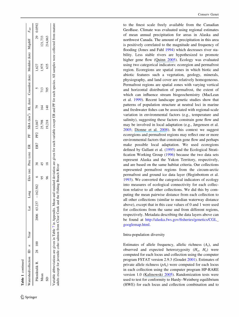
Var
iab
leab
bre
via
tio
ns
are
giv
enin
Tab
le7
inA
pp
end
ix.
Mea
nan
dst
and
ard
dev
iati
on
are
giv
enfo
rea
chv
aria
ble
exce
pt
ER
and
PF
for
each
spec
ies.
All
sam
ple
sw
ere
coll
ecte
dfr
om
mat
ure
adu
lts
exce
pt
for
juv
enil
eco
ho
salm
on
fro
mC
lear
Cre
ekan
dth
eF
ish
ing
Bra
nch
Riv
er
Conserv Genet
123
test for genotypic disequilibrium among locus pairs over all
collections. These tests were performed using FSTAT and
GenePop version 4.0.7 (Rousset 2008), respectively, and
the threshold for statistical significance (a = 0.05) was
corrected (a/k) for k-simultaneous tests using the sequential
Bonferroni method (Rice 1989). Two values of k were used
for the HWE test to evaluate each collection over all k-loci
and each locus over k-collections.
Population divergence
The level of population divergence in each species was first
estimated using FST (Wright 1943), which was computed
over all collections and for each pair of collections, over all
loci, according to Weir and Cockerham (1984) using
FSTAT. The null hypothesis (global FST not greater than
zero) was tested by bootstrap sampling of loci.
Landscape genetic analysis
We used hierarchical Analysis of Molecular Variance
(AMOVA, Excoffier et al. 2005) to evaluate the spatial
patterns of population structure for each species. First, we
grouped collections by watershed and used the program
ARLEQUIN version 3.01 (Excoffier et al. 2005) to esti-
mate how much variation exists within (FSC) and among
(FCT) the three groups of collections. The level of group
differentiation, FCT, should be maximized under this
grouping strategy if the three watersheds form the first
level of hierarchical population structure. Next, we used
the program SAMOVA (Spatial Analysis of Molecular
Variance, Dupanloup et al. 2002) version 1.0 that incor-
porates spatial data (x and y coordinates) for each collec-
tion. SAMOVA performs a series of AMOVA analyses in
which groups are defined through a simulated annealing
procedure that identifies geographically homogeneous
groups which are maximally differentiated. The number of
groups (k) is a user defined variable so we began with
k = 2 and increased k until FCT was maximized and FSC
was minimized. Because latitude and longitude data do not
reflect the true spatial relationships in a riverine system, we
derived surrogate x and y coordinates by using the pairwise
waterway distance matrix to project the position of the
collections on a multidimensional scaling (MDS) plot and
then spatially reference collections using MDS axes one
and two values (Manni et al. 2004).
We used the program BARRIER version 2.2 (Manni
et al. 2004) to complement the SAMOVA results. Our
interests here were twofold: assess if population divergence
associated with the watersheds was significant enough to be
consistent with a genetic barrier, and assess if putative
genetic barriers for each species were congruent. Simula-
tions suggest the Monmonier’s approach is better than
SAMOVA for identifying barriers, particularly when pop-
ulation divergence follows an isolation-by-distance pattern
(Dupanloup et al. 2002; Manni et al. 2004). We used the
values from the MDS axes one and two as described above
for the x and y coordinates for each location. To account for
isolation by distance in each species we used a matrix of
residuals rather than FST as suggested by Manni et al.
(2004). In order to determine the robustness of each barrier,
we generated 100 matrices of residuals by bootstrap sam-
pling of loci. The pairwise FST values, bootstrap sampling,
and computation of residuals used in the BARRIER anal-
yses were derived using R-scripts (R 2.8.1, http://www.
r-project.org/) written by J. Olsen (USFWS Anchorage
Alaska) and J. Bromaghin (USGS, Anchorage Alaska).
We conducted a post-hoc test for differences in esti-
mates of Ar, He, FST, and pAr among coastal and inland
groups of collections revealed by SAMOVA. We used a
pairwise randomization test in FSTAT to evaluate the first
four variables and a Mann–Whitney test in R 2.8.1 to
evaluate pAr using each locus as an observation.
Balkenhol et al. (2009) showed there is presently no
optimal approach to multivariate analysis of landscape
genetic data and recommended using multiple methods to
avoid drawing conclusions from method-dependent results.
Therefore, we employed two statistical methods that do not
assume an explicit linear model and have been used in
recent studies. The main assumption of both methods is
that the influence of the landscape features is best evaluated
as location (patch) specific data rather than pairwise
(landscape resistance) data. First, we used the hierarchical
Bayesian method implemented in GESTE version 2.0 (Foll
and Gaggiotti 2006; Kittlein and Gaggiotti 2008) to relate
estimates of population-specific FST to location-specific
estimates of environmental attributes under a generalized
linear model. This method also assumes two demographic
models when computing the likelihood function: a fission
model where all populations are descendent from a single
ancestral population and an island model. All combinations
of habitat variables were considered and evaluated using
estimates of posterior probability, the 95% highest proba-
bility density interval (HPDI), and the estimate of unex-
plained variance (r2, Foll and Gaggiotti 2006). As
suggested by the authors, we used 10 pilot runs of 5,000
iterations to obtain the parameters of the proposal distri-
butions. We also used an additional burn in of 50,000
iterations and a thinning interval of 20. All estimates were
derived from a sample size of 10,000.
Second, we used distance-based multivariate multiple
regression with forward selection as implemented in
DISTLM forward (Anderson 2003; Carmichael et al.
2007). Marginal tests were first performed to estimate the
proportion of the total sum of squares explained by each
location-specific explanatory variable when related to
Conserv Genet
123
pairwise estimates of genetic divergence [FST/(1 - FST)]
computed from FSTAT. Then conditional tests were per-
formed using a step-wise forward selection procedure that
identifies the most informative subset of variables
sequentially and conditional on the variables already
selected. This step-wise procedure accounts for correlation
among the variables. A pseudo F-statistic was computed
for each variable (or subset of variables) and a P-value was
determined by recalculating F for 9,999 random re-order-
ings of the genetic distance matrix to assess statistical
significance (Anderson 2003). For both GESTE and
DISTLM forward the variables Coastdist, Meddist, Elev,
Migdiff, RL, SA, Prec were log-transformed (Ln) to reduce
the influence of extreme values.
To complement the two methods above, we used a
partial Mantel test (Smouse et al. 1986). This test is more
commonly used than GESTE and DISTLM forward (Bal-
kenhol et al. 2009) however a single test is limited to three
pairwise distance matrices (one dependant and two inde-
pendent variables) and the test evaluates landscape features
as pairwise rather than location-specific data. We con-
ducted a series of tests where we controlled for the influ-
ence of pairwise waterway distance while testing the
influence of the other habitat features (and vice versa) on
estimates of pairwise genetic divergence [FST/(1 - FST)].
We converted the location-specific habitat data into pair-
wise estimates by computing pairwise differences for dis-
tance to the coast, elevation, and migration difficulty and
pairwise averages for precipitation, SBA, and river length
(RL). Ecoregion and permafrost region were treated as
binary variables in which pairs of collections from the
same and different regions were assigned values of 0 and 1,
respectively. The tests were performed using the program
IBD version 1.52 (Bohonak 2002).
Results
Intra-population genetic diversity
Mean heterozygosity (He) was 0.75, 0.85, 0.37 and mean
allelic richness (Ar) was 10.1, 11.1, 2.9 for Chinook, chum,
and coho, respectively (Appendices S1–S3 in Supplemen-
tary materials). A total of 50 (8.1%, Chinook), 53 (8.3%
chum), and 10 (4.5%, coho) collection 9 locus combina-
tions deviated from HWE at a = 0.05 (Appendices S1–S3
in Supplementary materials). When the a-level was
adjusted for multiple tests, the number of significant tests
declined to 12 (Chinook), 19 (chum), and one (coho) for
multiple loci, and eight (Chinook), 14 (chum), and one
(coho) for multiple collections. Significant tests were not
indicative of deviations of HWE at any specific locus or
collection.
Population divergence
The overall estimates of FST for Chinook, chum and coho
were 0.027, 0.016, and 0.092, respectively. The 95% con-
fidence intervals were 0.02–0.036 (Chinook), 0.011–0.024
(chum), 0.051–0.153 (coho), suggesting all estimates are
significantly greater than zero and population divergence in
coho is significantly greater than in Chinook and chum.
Landscape genetic analysis
The genetic variation among groups (FCT) was not maxi-
mized when collections were grouped by watershed
(Table 2). In fact, FCT was actually lower than FSC (within-
group variation) for Chinook and chum. The SAMOVA
analysis showed that the largest estimates of FCT were
derived assuming k = 2 groups for each species. However,
for both Chinook and chum, one group contained no more
than two collections, and the estimates of FSC were similar
to the watershed groupings. Therefore, we increased k until
the estimate of FSC exhibited a substantial incremental
decline (50% or more relative to FSC for k - 1). This
occurred at k = 6 for both Chinook and chum and k = 2
for coho (Table 2; Fig. 2). The results suggested a single
coastal group with collections from all watersheds and one
(coho) or more (Chinook and chum) inland groups con-
sisting of one or more collections. The inland groups also
revealed some spatial inconsistencies. For example, Chi-
nook collections 5 and 6, and chum collections 9 and 10,
are part of inland groups despite being closer by waterway
to coastal groups. Coho collections 23 and 24 in the upper
Kuskokwim River appear to be more closely related to an
inland Yukon River group.
The BARRIER results were transferred from the Dela-
unay triangulation to approximate locations on area maps
for each species (Fig. 2). No barriers were found separating
the three watersheds, but barriers were identified among
most collection groups revealed by SAMOVA. Most bar-
riers were strongly supported by bootstrap sampling. Of the
100 bootstrap replicates, twelve of the 15 barriers (all
species) occurred at least 80 times, and all 15 barriers
occurred at least 50 times. The strongest barriers (i.e., those
identified first and having the highest bootstrap support) for
Chinook and chum encapsulated collections furthest from
the ocean in the upper Yukon and Kuskokwim rivers,
whereas for coho the strongest barrier separated the coastal
collections from collections in the middle-upper Yukon
River. Barrier 6 for Chinook and chum supported the rel-
ative isolation of collections 5 and 6 (Chinook) and 9 and
10 (chum) from the geographically closest coastal collec-
tions. Similarly, barrier 2 for coho supported the isolation
of collections 23 and 24 in the upper Kuskokwim River
from adjacent lower river collections.
Conserv Genet
123

The estimates of He, Ar, and mean private allele richness
over loci (pAr) differed significantly (P \ 0.05) between
the coastal and inland collections and were larger for the
coastal collections (Table 3). The values of FST were larger
for the inland collections compared to the coastal collec-
tions; however, the differences were only significant
(P \ 0.05) for Chinook and chum.
The results from GESTE and DISTLM forward sug-
gested multiple habitat variables may influence population
divergence in each species but only one variable, precipi-
tation (Prec), was identified by both programs and was
common to all species (Tables 4, 5; Table 7 in Appendix).
The variable SBA was identified for Chinook by both
programs. Different indicators of spatial isolation were
selected by both methods. DISTLM forward identified
migration difficulty (Migdiff) as the first variable in the
forward selection process for each species and added the
indicator of connectivity (Meddist) as the third variable for
Chinook. GESTE identified elevation (Elev) for chum and
Meddist for coho. DISTLM forward identified more vari-
ables than GESTE for Chinook and chum, including the
measures of ecological connectivity ecoregion (EroR) for
both species and permafrost region (PermR) for chum. The
variables coastal distance (Coastdist) and RL were not
identified by either method. The posterior probabilities for
the HP models identified by GESTE were relatively low,
ranging from 0.15 (Chinook) to 0.30 (coho). Nevertheless,
the HP models fit the data reasonable well as indicated by the
moderate estimates of unexplained variance (r2,
range = 0.43–0.60) and the fact that the upper bounds of the
95% HPDIs were less than one (Foll and Gaggiotti 2006).
The results of the partial Mantel tests indicated each
habitat variable was significantly correlated with popula-
tion divergence in at least one species when controlling for
the influence of pairwise waterway distance (Table 6). The
tests for five variables (Elev, Prec, Coastdist, Migdiff,
EcoR) were significant in all species.
The results from DISTLM forward showed most variable
pairs were only weakly to moderately correlated (Table 8 in
Appendix). As expected, Migdiff which is a product of Elev
and Coastdist was highly correlated with both variables.
Elev and Coastdist were also highly correlated.
Discussion
Hierarchical population structure
Contrary to our prediction, the SAMOVA and BARRIER
results suggest that the three watersheds do not form the
first level of hierarchical population structure. Rather, the
results show that hierarchical population structure for each
Table 2 AMOVA results for collections when grouped by watershed (3w) using Arlequin version 3.01 and when grouped to maximize FCT
(among-group variation) using SAMOVA version 1.0
Species Groups Group composition FST FCT FSC
Chinook 3w [1–25] [26–43] [44–47] 0.032 0.012 0.020
2 [1–20,22–47] [21] 0.053 0.031 0.023
3 [1–20,22–23,25–47] [21] [24] 0.049 0.027 0.022
4 [1–20,22–23,25–44,46–47] [21] [24] [45] 0.047 0.025 0.022
5 [1–20,22–23,25–38,40–44,46–47] [21] [24] [39] [45] 0.044 0.024 0.021
6 [1–4,26–38,40–47] [5–12] [13–14] [15–20,22–25] [21] [39] 0.033 0.024 0.009
7 [1–4,26–38,40–47] [5–12] [13–14] [15–20,22–23,25] [21] [24] [39] 0.033 0.025 0.008
8 [1–4,26–38,40–47] [5–9] [10–12] [13–14] [15–20,22–23,25] [21] [24] [39] 0.033 0.026 0.007
Chum 3w [1–28] [29–40] [41–53] 0.019 0.009 0.011
2 [1–24,27–53] [25–26] 0.039 0.030 0.009
3 [1–24,27–53] [25] [26] 0.037 0.027 0.009
4 [1–24,27–38,40–53] [25] [26] [39] 0.031 0.023 0.009
5 [1–24,27,29–38,40–53] [25] [26] [28] [39] 0.028 0.020 0.008
6 [1–8,11,29–38,41–53] [9–10,14–24,27] [12–13] [25–26] [28] [39–40] 0.020 0.020 0.000
7 [1–8,11,29–38,41–53] [9–10,14,18–24,27] [12–13] [15–17] [25–26] [28] [39–40] 0.019 0.020 -0.001
8 [1–8,11,29–38,41–53] [9–10,14,15,18–24,27] [12–13] [16] [17] [25–26] [28] [39–40] 0.019 0.020 -0.001
Coho 3w [1–11] [12–24] [25–28] 0.112 0.062 0.054
2 [1–5,12–22,25–28] [6–11,23–24] 0.162 0.141 0.025
3 [1–5,12–22,25–28] [6–11,23] [24] 0.159 0.138 0.025
4 [1–5,12–22,25–28] [6,9–11,23] [7–8] [24] 0.154 0.135 0.022
The bold values indicate the grouping strategy when FSC (within-group variation) exhibits a substantial incremental decline (50% or more). The
numbers in each group indicate collection ID in Table 1
Conserv Genet
123
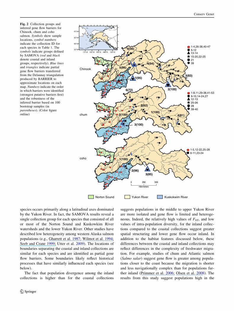
species occurs primarily along a latitudinal axes dominated
by the Yukon River. In fact, the SAMOVA results reveal a
single collection group for each species that consisted of all
or most of the Norton Sound and Kuskowkim River
watersheds and the lower Yukon River. Other studies have
described low heterogeneity among western Alaska salmon
populations (e.g., Gharrett et al. 1987; Wilmot et al. 1994;
Seeb and Crane 1999; Utter et al. 2009). The locations of
boundaries separating the coastal and inland collections are
similar for each species and are identified as partial gene
flow barriers. Some boundaries likely reflect historical
processes that have similarly influenced each species (see
below).
The fact that population divergence among the inland
collections is higher than for the coastal collections
suggests populations in the middle to upper Yukon River
are more isolated and gene flow is limited and heteroge-
neous. Indeed, the relatively high values of FST, and low
values of intra-population diversity, for the inland collec-
tions compared to the coastal collections suggest greater
spatial structuring and lower gene flow occur inland. In
addition to the habitat features discussed below, these
differences between the coastal and inland collections may
reflect differences in the complexity of freshwater migra-
tion. For example, studies of chum and Atlantic salmon
(Salmo salar) suggest gene flow is greater among popula-
tions closer to the coast because the migration is shorter
and less navigationally complex than for populations fur-
ther inland (Primmer et al. 2006; Olsen et al. 2008). The
results from this study suggest populations high in the
1(95)
2(100)
4(94) 5(86)
6(56)
3(83)
1(100)
3(100)
2(100) 4(81)
5(62)
6(72)
1(100)
2(96) 3(85)
Chinook
chum
coho
Norton Sound Yukon River Kuskokwim River
1-4,26-38,40-47 5-12 13-14 15-20,22-25 21 39
1-8,11,29-38,41-539-10,14-24,27 12-13 25-26 28 39-40
1-5,12-22,25-28 6-11,23-24
Fig. 2 Collection groups and
inferred gene flow barriers for
Chinook, chum and coho
salmon. Symbols show sample
locations, symbol numbersindicate the collection ID for
each species in Table 1. The
symbols indicate groups defined
by SAMOVA (red and blackdenote coastal and inland
groups, respectively). Blue linesand triangles indicate partial
gene flow barriers transferred
from the Delaunay triangulation
produced by BARRIER to
approximate locations on each
map. Numbers indicate the order
in which barriers were identified
(strongest putative barriers first)
and the robustness of the
inferred barrier based on 100
bootstrap samples (in
parentheses). (Color figure
online)
Conserv Genet
123
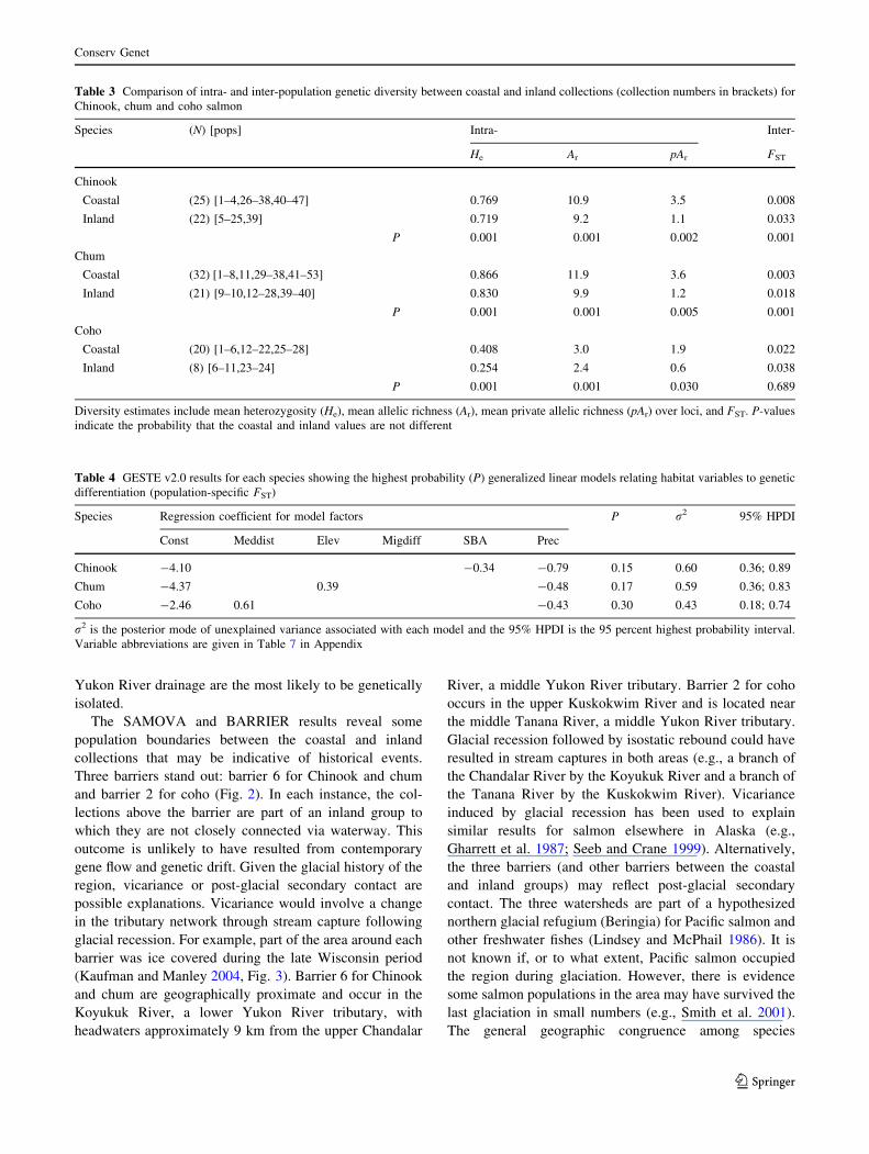
Yukon River drainage are the most likely to be genetically
isolated.
The SAMOVA and BARRIER results reveal some
population boundaries between the coastal and inland
collections that may be indicative of historical events.
Three barriers stand out: barrier 6 for Chinook and chum
and barrier 2 for coho (Fig. 2). In each instance, the col-
lections above the barrier are part of an inland group to
which they are not closely connected via waterway. This
outcome is unlikely to have resulted from contemporary
gene flow and genetic drift. Given the glacial history of the
region, vicariance or post-glacial secondary contact are
possible explanations. Vicariance would involve a change
in the tributary network through stream capture following
glacial recession. For example, part of the area around each
barrier was ice covered during the late Wisconsin period
(Kaufman and Manley 2004, Fig. 3). Barrier 6 for Chinook
and chum are geographically proximate and occur in the
Koyukuk River, a lower Yukon River tributary, with
headwaters approximately 9 km from the upper Chandalar
River, a middle Yukon River tributary. Barrier 2 for coho
occurs in the upper Kuskokwim River and is located near
the middle Tanana River, a middle Yukon River tributary.
Glacial recession followed by isostatic rebound could have
resulted in stream captures in both areas (e.g., a branch of
the Chandalar River by the Koyukuk River and a branch of
the Tanana River by the Kuskokwim River). Vicariance
induced by glacial recession has been used to explain
similar results for salmon elsewhere in Alaska (e.g.,
Gharrett et al. 1987; Seeb and Crane 1999). Alternatively,
the three barriers (and other barriers between the coastal
and inland groups) may reflect post-glacial secondary
contact. The three watersheds are part of a hypothesized
northern glacial refugium (Beringia) for Pacific salmon and
other freshwater fishes (Lindsey and McPhail 1986). It is
not known if, or to what extent, Pacific salmon occupied
the region during glaciation. However, there is evidence
some salmon populations in the area may have survived the
last glaciation in small numbers (e.g., Smith et al. 2001).
The general geographic congruence among species
Table 3 Comparison of intra- and inter-population genetic diversity between coastal and inland collections (collection numbers in brackets) for
Chinook, chum and coho salmon
Species (N) [pops] Intra- Inter-
He Ar pAr FST
Chinook
Coastal (25) [1–4,26–38,40–47] 0.769 10.9 3.5 0.008
Inland (22) [5–25,39] 0.719 9.2 1.1 0.033
P 0.001 0.001 0.002 0.001
Chum
Coastal (32) [1–8,11,29–38,41–53] 0.866 11.9 3.6 0.003
Inland (21) [9–10,12–28,39–40] 0.830 9.9 1.2 0.018
P 0.001 0.001 0.005 0.001
Coho
Coastal (20) [1–6,12–22,25–28] 0.408 3.0 1.9 0.022
Inland (8) [6–11,23–24] 0.254 2.4 0.6 0.038
P 0.001 0.001 0.030 0.689
Diversity estimates include mean heterozygosity (He), mean allelic richness (Ar), mean private allelic richness (pAr) over loci, and FST. P-values
indicate the probability that the coastal and inland values are not different
Table 4 GESTE v2.0 results for each species showing the highest probability (P) generalized linear models relating habitat variables to genetic
differentiation (population-specific FST)
Species Regression coefficient for model factors P r2 95% HPDI
Const Meddist Elev Migdiff SBA Prec
Chinook -4.10 -0.34 -0.79 0.15 0.60 0.36; 0.89
Chum -4.37 0.39 -0.48 0.17 0.59 0.36; 0.83
Coho -2.46 0.61 -0.43 0.30 0.43 0.18; 0.74
r2 is the posterior mode of unexplained variance associated with each model and the 95% HPDI is the 95 percent highest probability interval.
Variable abbreviations are given in Table 7 in Appendix
Conserv Genet
123
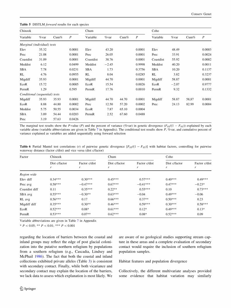
regarding the location of barriers between the coastal and
inland groups may reflect the edge of post glacial coloni-
zation into the putative northern refugium by populations
from a southern refugium (e.g., Cascadia, Lindsey and
McPhail 1986). The fact that both the coastal and inland
collections exhibited private alleles (Table 3) is consistent
with secondary contact. Finally, while both vicariance and
secondary contact may explain the location of the barriers,
we lack data to assess which explanation is most likely. We
are aware of no geological studies supporting stream cap-
ture in these areas and a complete evaluation of secondary
contact would require the inclusion of southern refugium
population samples.
Habitat features and population divergence
Collectively, the different multivariate analyses provided
some evidence that habitat variation may similarly
Table 5 DISTLM forward results for each species
Chinook Chum Coho
Variable %var Cum% P Variable %var Cum% P Variable %var Cum% P
Marginal (individual) tests
Elev 35.32 0.0001 Elev 43.20 0.0001 Elev 48.49 0.0003
Prec 21.08 0.0001 Prec 26.05 0.0001 Prec 33.91 0.0024
Coastdist 31.09 0.0001 Coastdist 38.76 0.0001 Coastdist 55.92 0.0002
Meddist 6.12 0.0499 Meddist -2.45 0.9998 Meddist 40.20 0.0011
SBA 7.78 0.0231 SBA 1.73 0.3756 SBA 10.20 0.1137
RL 4.76 0.0955 RL 8.04 0.0285 RL 3.82 0.3237
Migdiff 35.93 0.0001 Migdiff 44.70 0.0001 Migdiff 58.87 0.0001
EcoR 15.72 0.0005 EcoR 15.54 0.0026 EcoR -2.07 0.9777
PermR 1.29 0.595 PermR 17.76 0.0010 PermR 9.32 0.1332
Conditional (sequential) tests
Migdiff 35.93 35.93 0.0001 Migdiff 44.70 44.70 0.0001 Migdiff 58.87 58,87 0.0001
EcoR 8.88 44.80 0.0002 Prec 12.50 57.20 0.0002 Prec 24.13 82.99 0.0004
Meddist 5.75 50.55 0.0034 EcoR 7.87 65.10 0.0004
SBA 3.89 54.44 0.0203 PermR 2.52 67.60 0.0488
Prec 3.19 57.63 0.0426
The marginal test results show the P-value (P) and the percent of variance (%var) in genetic divergence (FST/(1 - FST)) explained by each
variable alone (variable abbreviations are given in Table 7 in Appendix). The conditional test results show P, %var, and cumulative percent of
variance explained as variables are added sequentially using forward selection
Table 6 Partial Mantel test correlations (r) of pairwise genetic divergence [FST/(1 - FST)] with habitat factors, controlling for pairwise
waterway distance (factor c/dist) and vice versa (dist c/factor)
Factor Chinook Chum Coho
Dist c/factor Factor c/dist Dist c/factor Factor c/dist Dist c/factor Factor c/dist
r r r r r r
Region wide
Elev diff 0.34*** 0.30*** 0.45*** 0.57*** 0.40*** 0.49***
Prec avg 0.58*** -0.47*** 0.67*** -0.41*** 0.47*** -0.23*
Coastdist diff 0.11 0.35*** 0.22** 0.55*** 0.10 0.73***
SBA avg 0.55*** -0.30** 0.63*** -0.04 0.49*** -0.06
RL avg 0.56*** 0.17 0.66*** 0.37** 0.50*** 0.23
Migdiff diff 0.35*** 0.30** 0.46*** 0.59*** 0.30*** 0.58***
EcoR 0.52*** 0.08* 0.61*** 0.12* 0.49*** 0.13*
PermR 0.53*** 0.07** 0.62*** 0.08* 0.52*** 0.09
Variable abbreviations are given in Table 7 in Appendix
* P \ 0.05; ** P \ 0.01; *** P \ 0.001
Conserv Genet
123
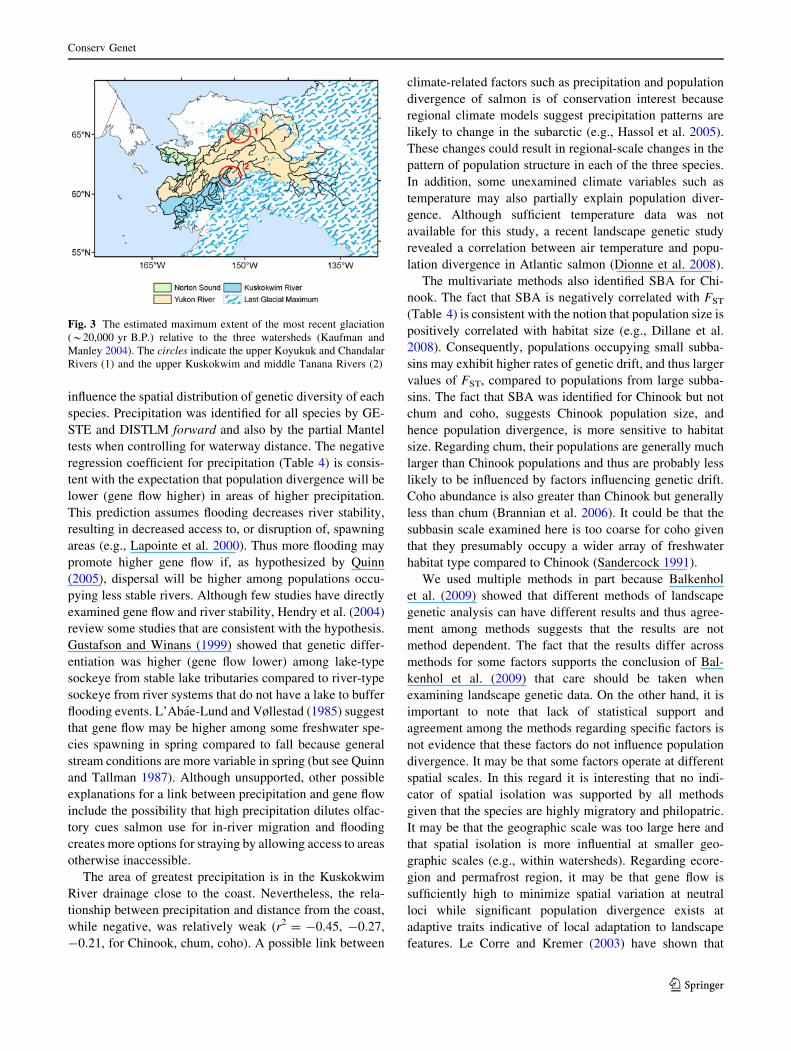
influence the spatial distribution of genetic diversity of each
species. Precipitation was identified for all species by GE-
STE and DISTLM forward and also by the partial Mantel
tests when controlling for waterway distance. The negative
regression coefficient for precipitation (Table 4) is consis-
tent with the expectation that population divergence will be
lower (gene flow higher) in areas of higher precipitation.
This prediction assumes flooding decreases river stability,
resulting in decreased access to, or disruption of, spawning
areas (e.g., Lapointe et al. 2000). Thus more flooding may
promote higher gene flow if, as hypothesized by Quinn
(2005), dispersal will be higher among populations occu-
pying less stable rivers. Although few studies have directly
examined gene flow and river stability, Hendry et al. (2004)
review some studies that are consistent with the hypothesis.
Gustafson and Winans (1999) showed that genetic differ-
entiation was higher (gene flow lower) among lake-type
sockeye from stable lake tributaries compared to river-type
sockeye from river systems that do not have a lake to buffer
flooding events. L’Abae-Lund and Vøllestad (1985) suggest
that gene flow may be higher among some freshwater spe-
cies spawning in spring compared to fall because general
stream conditions are more variable in spring (but see Quinn
and Tallman 1987). Although unsupported, other possible
explanations for a link between precipitation and gene flow
include the possibility that high precipitation dilutes olfac-
tory cues salmon use for in-river migration and flooding
creates more options for straying by allowing access to areas
otherwise inaccessible.
The area of greatest precipitation is in the Kuskokwim
River drainage close to the coast. Nevertheless, the rela-
tionship between precipitation and distance from the coast,
while negative, was relatively weak (r2 = -0.45, -0.27,
-0.21, for Chinook, chum, coho). A possible link between
climate-related factors such as precipitation and population
divergence of salmon is of conservation interest because
regional climate models suggest precipitation patterns are
likely to change in the subarctic (e.g., Hassol et al. 2005).
These changes could result in regional-scale changes in the
pattern of population structure in each of the three species.
In addition, some unexamined climate variables such as
temperature may also partially explain population diver-
gence. Although sufficient temperature data was not
available for this study, a recent landscape genetic study
revealed a correlation between air temperature and popu-
lation divergence in Atlantic salmon (Dionne et al. 2008).
The multivariate methods also identified SBA for Chi-
nook. The fact that SBA is negatively correlated with FST
(Table 4) is consistent with the notion that population size is
positively correlated with habitat size (e.g., Dillane et al.
2008). Consequently, populations occupying small subba-
sins may exhibit higher rates of genetic drift, and thus larger
values of FST, compared to populations from large subba-
sins. The fact that SBA was identified for Chinook but not
chum and coho, suggests Chinook population size, and
hence population divergence, is more sensitive to habitat
size. Regarding chum, their populations are generally much
larger than Chinook populations and thus are probably less
likely to be influenced by factors influencing genetic drift.
Coho abundance is also greater than Chinook but generally
less than chum (Brannian et al. 2006). It could be that the
subbasin scale examined here is too coarse for coho given
that they presumably occupy a wider array of freshwater
habitat type compared to Chinook (Sandercock 1991).
We used multiple methods in part because Balkenhol
et al. (2009) showed that different methods of landscape
genetic analysis can have different results and thus agree-
ment among methods suggests that the results are not
method dependent. The fact that the results differ across
methods for some factors supports the conclusion of Bal-
kenhol et al. (2009) that care should be taken when
examining landscape genetic data. On the other hand, it is
important to note that lack of statistical support and
agreement among the methods regarding specific factors is
not evidence that these factors do not influence population
divergence. It may be that some factors operate at different
spatial scales. In this regard it is interesting that no indi-
cator of spatial isolation was supported by all methods
given that the species are highly migratory and philopatric.
It may be that the geographic scale was too large here and
that spatial isolation is more influential at smaller geo-
graphic scales (e.g., within watersheds). Regarding ecore-
gion and permafrost region, it may be that gene flow is
sufficiently high to minimize spatial variation at neutral
loci while significant population divergence exists at
adaptive traits indicative of local adaptation to landscape
features. Le Corre and Kremer (2003) have shown that
Fig. 3 The estimated maximum extent of the most recent glaciation
(*20,000 yr B.P.) relative to the three watersheds (Kaufman and
Manley 2004). The circles indicate the upper Koyukuk and Chandalar
Rivers (1) and the upper Kuskokwim and middle Tanana Rivers (2)
Conserv Genet
123
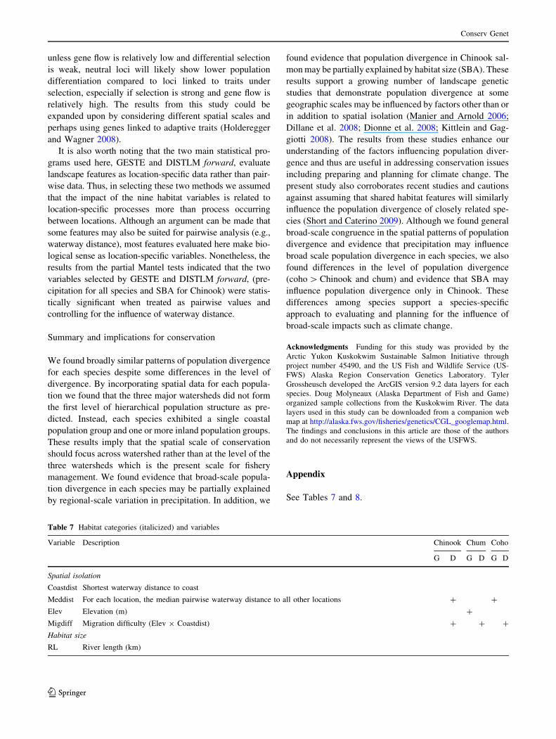
unless gene flow is relatively low and differential selection
is weak, neutral loci will likely show lower population
differentiation compared to loci linked to traits under
selection, especially if selection is strong and gene flow is
relatively high. The results from this study could be
expanded upon by considering different spatial scales and
perhaps using genes linked to adaptive traits (Holderegger
and Wagner 2008).
It is also worth noting that the two main statistical pro-
grams used here, GESTE and DISTLM forward, evaluate
landscape features as location-specific data rather than pair-
wise data. Thus, in selecting these two methods we assumed
that the impact of the nine habitat variables is related to
location-specific processes more than process occurring
between locations. Although an argument can be made that
some features may also be suited for pairwise analysis (e.g.,
waterway distance), most features evaluated here make bio-
logical sense as location-specific variables. Nonetheless, the
results from the partial Mantel tests indicated that the two
variables selected by GESTE and DISTLM forward, (pre-
cipitation for all species and SBA for Chinook) were statis-
tically significant when treated as pairwise values and
controlling for the influence of waterway distance.
Summary and implications for conservation
We found broadly similar patterns of population divergence
for each species despite some differences in the level of
divergence. By incorporating spatial data for each popula-
tion we found that the three major watersheds did not form
the first level of hierarchical population structure as pre-
dicted. Instead, each species exhibited a single coastal
population group and one or more inland population groups.
These results imply that the spatial scale of conservation
should focus across watershed rather than at the level of the
three watersheds which is the present scale for fishery
management. We found evidence that broad-scale popula-
tion divergence in each species may be partially explained
by regional-scale variation in precipitation. In addition, we
found evidence that population divergence in Chinook sal-
mon may be partially explained by habitat size (SBA). These
results support a growing number of landscape genetic
studies that demonstrate population divergence at some
geographic scales may be influenced by factors other than or
in addition to spatial isolation (Manier and Arnold 2006;
Dillane et al. 2008; Dionne et al. 2008; Kittlein and Gag-
giotti 2008). The results from these studies enhance our
understanding of the factors influencing population diver-
gence and thus are useful in addressing conservation issues
including preparing and planning for climate change. The
present study also corroborates recent studies and cautions
against assuming that shared habitat features will similarly
influence the population divergence of closely related spe-
cies (Short and Caterino 2009). Although we found general
broad-scale congruence in the spatial patterns of population
divergence and evidence that precipitation may influence
broad scale population divergence in each species, we also
found differences in the level of population divergence
(coho [ Chinook and chum) and evidence that SBA may
influence population divergence only in Chinook. These
differences among species support a species-specific
approach to evaluating and planning for the influence of
broad-scale impacts such as climate change.
Acknowledgments Funding for this study was provided by the
Arctic Yukon Kuskokwim Sustainable Salmon Initiative through
project number 45490, and the US Fish and Wildlife Service (US-
FWS) Alaska Region Conservation Genetics Laboratory. Tyler
Grossheusch developed the ArcGIS version 9.2 data layers for each
species. Doug Molyneaux (Alaska Department of Fish and Game)
organized sample collections from the Kuskokwim River. The data
layers used in this study can be downloaded from a companion web
map at http://alaska.fws.gov/fisheries/genetics/CGL_googlemap.html.
The findings and conclusions in this article are those of the authors
and do not necessarily represent the views of the USFWS.
Appendix
See Tables 7 and 8.
Table 7 Habitat categories (italicized) and variables
Variable Description Chinook Chum Coho
G D G D G D
Spatial isolation
Coastdist Shortest waterway distance to coast
Meddist For each location, the median pairwise waterway distance to all other locations ? ?
Elev Elevation (m) ?
Migdiff Migration difficulty (Elev 9 Coastdist) ? ? ?
Habitat size
RL River length (km)
Conserv Genet
123

Table 8 Correlations (r2) among habitat variables for each species estimated using DISTLM forward
Variable 1 Variable 2 Chinook Chum Coho
Elev Prec -0.317 -0.231 0.008
Elev Coastdist 0.839 0.826 0.792
Elev Meddist 0.292 0.268 0.409
Elev SBA -0.415 -0.195 -0.238
Elev RL 0.172 0.259 0.087
Elev Miggdiff 0.957 0.944 0.928
Elev EcoR 0.222 0.203 -0.288
Elev PermR 0.101 0.331 -0.016
Prec Coastdist -0.446 -0.265 -0.207
Prec Meddist 0.148 0.121 -0.536
Prec SBA 0.522 0.328 0.494
Prec RL -0.299 -0.297 -0.122
Prec Miggdiff -0.400 -0.263 -0.124
Prec EcoR -0.574 -0.182 -0.361
Prec PermR -0.045 -0.096 0.174
Coastdist Meddist 0.123 0.054 0.337
Coastdist SBA -0.497 -0.182 -0.273
Coastdist RL 0.296 0.300 0.143
Coastdist Miggdiff 0.961 0.965 0.963
Coastdist EcoR 0.202 -0.003 -0.346
Coastdist PermR -0.013 0.213 -0.173
Meddist SBA -0.030 0.063 -0.507
Meddist RL -0.352 -0.143 0.010
Meddist Miggdiff 0.216 0.157 0.390
Meddist EcoR 0.095 0.306 0.426
Table 7 continued
Variable Description Chinook Chum Coho
G D G D G D
SBA Subbasin area (km2)—the USGS hydrologic unit level 4 and equivalent for the Canadian section of the
Yukon River.
? ?
Climate
Prec Annual precipitation (cm) ? ? ? ? ? ?
Ecology
EcoR Ecoregion: ER1—Ahklun and Kilbuck Mountains, ER2—Interior Bottomlands, ER3—Interior Forested
Lowlands and Uplands, ER4—Interior Highlands, ER5—Pelly Mountains, ER6—Seward Peninsula,
ER7—Subarctic Coastal Plains, ER8—Yukon Flats, ER9—Yukon Plateau Central, ER10—Yukon Plateau
North, ER11—Yukon Southern Lakes, ER12—Ruby Range, ER13—Old Crow Range, ER14—Ogilvie
Mountains
? ?
PermR Permafrost region: PF1—Continuous permafrost extent with high ground ice content and thick overburden,
PF2—Continuous permafrost extent with medium ground ice content and thick overburden, PF3—
Discontinuous permafrost extent with low ground ice content and thick overburden, PF4—Discontinuous
permafrost extent with low ground ice content and thin overburden and exposed bedrock, PF5—
Discontinuous permafrost extent with medium ground ice content and thick overburden, PF6—Sporadic
permafrost extent with low ground ice content and thick overburden, PF7—Sporadic permafrost extent
with low ground ice content and thin overburden and exposed bedrock
?
Habitat variables selected by GESTE v2.0 (G) and DISTLM forward (D) are indicated with a ? for each species. See text and Tables 4 and 5 for
further detail
Conserv Genet
123

References
Anderson MJ (2003) DISTLM forward: a FORTRAN computer
program to calculate a distance-based multivariate analysis for a
linear model using forward selection. Department of Statistics,
University of Auckland, New Zealand. http://www.stat.auckland.
ac.nz/*mja/Programs.htm
Balkenhol N, Waits LP, Dezzani RJ (2009) Statistical approaches in
landscape genetics: an evaluation of methods for linking
landscape and genetic data. Ecography 32:818–830
Beacham TD, Jonsen KL, Supernault J, Wetklo M, Deng L,
Varnavskaya N (2006) Pacific Rim population structure of
Chinook salmon as determined from microsatellite analysis.
Trans Am Fish Soc 135:1604–1621
Bohonak AJ (2002) IBD (isolation by distance); a program for
analysis of isolation by distance. J Hered 93:153–154
Brannian LK, Evenson MJ, Hilsinger JR (2006) Escapement goal
recommendations for select Arctic-Yukon-Kuskokwim region
salmon stocks, 2007. Alaska Department of Fish and Game,
Fishery Manuscript No. 06-07, Anchorage. http://www.sf.adfg.
state.ak.us/FedAidPDFs/fm06-07.pdf
Carmichael LE, Krizan J, Nagy JA, Fuglei E, Dumond M, Johnson D,
Veitch A, Berteaux D, Strobeck C (2007) Historical and
ecological determinants of genetic structure in arctic canids.
Mol Ecol 16:3466–3483
Crane P, Molyneaux D, Lewis C, Wenburg J (2007) Genetic variation
among coho salmon populations from the Kuskokwim Region and
application to stock-specific harvest estimation. Alaska Fisheries
Technical Report No. 96, U.S. Fish and Wildlife Service,
Anchorage. http://alaska.fws.gov/fisheries/genetics/reports.htm
Dillane E, McGinnity P, Coughlan JP, Cross MC, Eyto ED,
Kenchington E, Prodohl P, Cross TF (2008) Demographics and
landscape features determine intrariver population structure in
Atlantic salmon (Salmo salar L.): the case of the River Moy in
Ireland. Mol Ecol 17:4786–4800
Dionne M, Caron F, Dodson JJ, Bernatchez L (2008) Landscape
genetics and hierarchical genetic structure in Atlantic salmon:
the interaction of gene flow and local adaptation. Mol Ecol
17:2382–2396
Dupanloup I, Schneider S, Excoffier L (2002) A simulated annealing
approach to define the genetic structure of populations. Mol Ecol
11:2571–2581
Ecological Stratification Working Group (1996) A National Ecolog-
ical Framework for Canada. Agriculture and Agri-Food Canada,
Research Branch, Centre for Land and Biological Resources
Research and Environment Canada, State of Environment
Directorate, Ottawa/Hull, 125 pp. http://sis.agr.gc.ca/cansis/
publications/ecostrat/intro.html
Excoffier L, Laval G, Schneider S (2005) Arlequin ver. 3.0: an
integrated software program for population genetic data analysis.
Evol Bioinform Online 1:47–50
Flannery B, Beacham T, Wetklo M, Smith C, Templin B, Antonovich
A, Seeb L, Miller S, Schlei O, Wenburg JK (2006) Run timing,
migratory patterns, and harvest information of Chinook salmon
stocks within the Yukon River. Alaska Fisheries Technical
Report No. 92, U.S. Fish and Wildlife Service. http://alaska.fws.
gov/fisheries/genetics/reports.htm
Foll M, Gaggiotti O (2006) Identifying the environmental factors that
determine the genetic structure of populations. Genetics 174:
875–891
Gagnon M, Angers B (2006) The determinant role of temporary
proglacial drainages on the genetic structure of fishes. Mol Ecol
15:1051–1065
Gallant AL, Binnian EF, Omernik JM, Shasby MB (1995) Ecoregions
of Alaska US Geological Survey Professional Paper 1567, 73 pp.
http://pubs.er.usgs.gov/usgspubs/pp/pp1567
Gharrett AJ, Shirley SM, Tromble GR (1987) Genetic relationships
among populations of Alaskan chinook salmon (Oncorhynchustshawytscha). Can J Fish Aquat Sci 44:765–774
Goudet J (2001) FSTAT, a program to estimate and test gene
diversities and fixation indices (version 2.9.3). http://www.unil.
ch/izea/softwares/fstat.html
Groot C, Margolis L (1991) Pacific salmon life histories. University
of British Columbia Press, Vancouver, BC
Gustafson RG, Winans GA (1999) Distribution and population
genetic structure of river- and sea-type sockeye salmon in
western North America. Ecol Freshw Fish 8:181–193
Hassol SJ, Berner J, Callaghan TV, Fox S, Furgal C, Hoel AH et al
(2005) Arctic climate impact assessment. Cambridge University
Press, Cambridge. http://www.acia.uaf.edu/
Heginbottom JA, Brown J, Melnikov ES, Ferrians OJ Jr (1993)
Circum-arctic map of permafrost and ground ice conditions. In:
Proceedings of the sixth international conference on Permafrost,
Wushan, vol 2. South China University Press, Guangzhou,
China, pp 1132–1136. http://nsidc.org/data/docs/fgdc/ggd318_
map_circumarctic/brown.html
Hendry AP, Castric V, Kinnison MT, Quinn TP (2004) The evolution
of philopatry and dispersal: homing versus straying in salmonids.
In: Hendry AP, Stearns S (eds) Evolution illuminated: Salmon
and their relatives. Oxford University Press, Oxford, pp 52–91
Table 8 continued
Variable 1 Variable 2 Chinook Chum Coho
Meddist PermR 0.267 0.337 -0.002
SBA RL -0.120 -0.005 0.083
SBA Miggdiff -0.476 -0.198 -0.274
SBA EcoR -0.231 0.220 -0.134
SBA PermR 0.070 0.169 0.057
RL Miggdiff 0.246 0.296 0.126
RL EcoR 0.127 0.095 0.107
RL PermR -0.278 0.010 -0.119
Miggdiff EcoR 0.223 0.095 -0.338
Miggdiff PermR 0.045 0.278 -0.113
EcoR PermR 0.106 0.430 -0.187
Conserv Genet
123

Holderegger R, Wagner HH (2008) Landscape genetics. Bioscience
58:199–207
Jones SH, Fahl CB (1994) Magnitude and frequency of floods in
Alaska and conterminous basins of Canada. US Geological
Survey Water-Resources Investigations Report, 93-4197, 122 pp.
http://pubs.er.usgs.gov/usgspubs/wri/wri934179
Jørgensen HBH, Hansen MM, Bekkevold D, Ruzzante DE, Loes-
chcke V (2005) Marine landscapes and population genetic
structure of herring (Clupea harengus L.) in the Baltic Sea. Mol
Ecol 14:3219–3234
Kalinowski ST (2005) HP-RARE 1.0: a computer program for
performing rarefaction on measures of allelic richness. Mol Ecol
Notes 5:187–189
Kaufman DS, Manley WF (2004) Pleistocene maximum and late
Wisconsin glacier extents across Alaska, U.S.A. In: Ehlers J,
Gibbard PL (eds) Quarternary glaciations extent and chronology,
part II: North America. Elsevier, Amsterdam, 440 pp
Kittlein MJ, Gaggiotti OE (2008) Interactions between environmental
factors can hide isolation by distance patterns: a case study of
Ctenomys rionegrensis in Uruguay. Proc R Soc Lond B
275:2633–2638
L’Abae-Lund JH, Vøllestad LA (1985) Homing precision of roach
Rutilus rutilus in Lake Arungen, Norway. Environ Biol Fish
13:235–239
Lapointe M, Eaton B, Driscol S, Latulippe C (2000) Modeling the
probability of salmonid egg pocket scour due to floods. Can J
Fish Aquat Sci 57:1120–1130
Le Corre V, Kremer A (2003) Genetic variability at neutral markers,
quantitative trait loci and trait in a subdivided population under
selection. Genetics 164:1205–1219
Lindsey CC, McPhail JD (1986) Zoogeography of fishes of the Yukon
and Mackenzie basins. In: Hocutt CH, Wiley EO (eds) The
zoogeography of North American freshwater fishes. Wiley, New
York, pp 639–674
MacLean R, Oswood MW, Irons JG, McDowell WH (1999) The
effect of permafrost on stream biogeochemistry: a case study of
two streams in the Alaskan (U.S.A.) taiga. Biogeochemistry
47:239–267
Manel S, Schwartz MK, Luikart G, Taberlet P (2003) Landscape
genetics: combining landscape ecology and population genetics.
TREE 18:189–197
Manier MK, Arnold SJ (2006) Ecological correlates of population
genetic structure: a comparative approach using a vertebrate
metacommunity. Proc R Soc Lond B 273:3001–3009
Manni F, Guerard E, Heyer E (2004) Geographic patterns of (genetic,
morphologic, linguistic) variation: how barriers can be detected
by using Monmonier’s algorithm. Hum Biol 76:173–190
Marten A, Brandle M, Brandl R (2006) Habitat type predicts genetic
population differentiation in freshwater invertebrates. Mol Ecol
15:2643–2651
Olsen JB, Flannery BG, Beacham TD, Bromaghin JF, Crane PA,
Lean CF, Dunmall KM, Wenburg JK (2008) The influence of
hydrographic structure and seasonal run timing on genetic
diversity and isolation-by-distance in chum salmon (Oncorhyn-chus keta). Can J Fish Aquat Sci 65:2026–2042
Petren K, Grant PR, Grant BR, Keller L (2005) Comparative
landscape genetics and the adaptive radiation of Darwin’s
finches: the role of peripheral isolation. Mol Ecol 14:2943–2957
Primmer CR, Veselov AJ, Zubchenko A, Poututkin A, Bakhmet I,
Koskinen MT (2006) Isolation by distance within a river system:
genetic population structuring of Atlantic salmon, Salmo salar,
in tributaries of the Varzuga River in northwest Russia. Mol Ecol
15:653–666
Quinn TP (2005) The behavior and ecology of Pacific salmon and
trout. University of Washington Press, Seattle, WA
Quinn T, Tallman R (1987) Seasonal environmental predictability and
homing in riverine fishes. Environ Biol Fish 18:155–159
Rice WR (1989) Analyzing tables of statistical tests. Evolution
43:223–225
Rousset F (2008) Genepop’007: a complete re-implementation of the
genepop software for Windows and Linux. Mol Ecol Res
8:103–106
Sandercock FK (1991) Life history of coho salmon. In: Groot C,
Margolis L (eds) Pacific salmon life histories. University of
British Columbia Press, Vancouver, BC, pp 392–446
Seeb LW, Crane PA (1999) High genetic heterogeneity in chum
salmon in western Alaska, the contact zone between northern
and southern lineages. Trans Am Fish Soc 128:58–87
Seeb LW, Antonovich A, Banks MA, Beacham TD, Bellinger MR,
Blankenship SM et al (2007) Development of a standardized
DNA database for Chinook salmon. Fisheries 32:540–552
Short AEZ, Caterino MS (2009) On the validity of habitat as a
predictor of genetic structure in aquatic systems: a comparative
study using California water beetles. Mol Ecol 18:403–414
Smith CT, Nelson RJ, Wood CC, Koop BF (2001) Glacial biogeog-
raphy of North American coho salmon (Oncorhynchus kisutch).
Mol Ecol 10:2775–2785
Smouse PE, Long JC, Sokal RR (1986) Multiple regression and
correlation extensions of the Mantel test matrix correspondence.
Syst Zool 35:627–632
Storfer A, Murphy MA, Evans JS et al (2006) Putting the ‘landscape’
in landscape genetics. Heredity 98:128–142
Utter FM, McPhee MV, Allendorf FW (2009) Population genetics
and the management of Arctic-Yukon-Kuskokwim salmon
populations. In: Krueger CC, Zimmerman CE (eds) Pacific
salmon: ecology and management of western Alaska’s popula-
tions. American Fisheries Society, Symposium 70, Bethesda,
MD, pp 97–123
Weir BS, Cockerham CC (1984) Estimating F-statistics for the
analysis of population structure. Evolution 38:1358–1370
Whiteley AR, Spruell P, Allendorf F (2004) Ecological and life
history characteristics predict population genetic divergence of
two salmonids in the same landscape. Mol Ecol 13:3675–3688
Wilmot RL, Everett RJ, Spearman WJ, Baccus R, Varnavskaya NV,
Putivkin SV (1994) Genetic stock structure of Western Alaska
chum salmon and a comparison with Russian far east stocks. Can
J Fish Aquat Sci 51:84–94
Wright S (1943) Isolation by distance. Genetics 28:114–138
Conserv Genet
123