Embed Size (px)
Citation preview
Collaborative Statistics Using Spreadsheets
Collection Editors:Irene Mary Duranczyk
Suzanne LochJanet Stottlemyer

Collaborative Statistics Using Spreadsheets
Collection Editors:Irene Mary Duranczyk
Suzanne LochJanet Stottlemyer
Authors:Susan Dean
Irene Mary DuranczykBarbara Illowsky, Ph.D.
Suzanne LochJanet Stottlemyer
Online:< http://cnx.org/content/col11521/1.19/ >
C O N N E X I O N S
Rice University, Houston, Texas

This selection and arrangement of content as a collection is copyrighted by Irene Mary Duranczyk, Suzanne Loch,
Janet Stottlemyer. It is licensed under the Creative Commons Attribution License 3.0 (http://creativecommons.org/licenses/by/3.0/).
Collection structure revised: January 8, 2014
PDF generated: January 8, 2014
For copyright and attribution information for the modules contained in this collection, see p. 631.
Table of Contents
1 Sampling and Data
1.1 Sampling and Data: Introduction . . . . . . . . . . . . . . . . . . . . . . . . . . . . . . . . . . . . . . . . . . . . . . . . . . . . . . . . . . . . 11.2 Sampling and Data: Statistics . . . . . . . . . . . . . . . . . . . . . . . . . . . . . . . . . . . . . . . . . . . . . . . . . . . . . . . . . . . . . . . 11.3 Sampling and Data: Probability . . . . . . . . . . . . . . . . . . . . . . . . . . . . . . . . . . . . . . . . . . . . . . . . . . . . . . . . . . . . . 41.4 Sampling and Data: Key Terms . . . . . . . . . . . . . . . . . . . . . . . . . . . . . . . . . . . . . . . . . . . . . . . . . . . . . . . . . . . . . 41.5 Sampling and Data: Data . . . . . . . . . . . . . . . . . . . . . . . . . . . . . . . . . . . . . . . . . . . . . . . . . . . . . . . . . . . . . . . . . . . 61.6 The 5W's . . . . . . . . . . . . . . . . . . . . . . . . . . . . . . . . . . . . . . . . . . . . . . . . . . . . . . . . . . . . . . . . . . . . . . . . . . . . . . . . . . 121.7 Sampling and Data: Sampling . . . . . . . . . . . . . . . . . . . . . . . . . . . . . . . . . . . . . . . . . . . . . . . . . . . . . . . . . . . . . . 131.8 Sampling and Data: Variation and Critical Evaluation . . . . . . . . . . . . . . . . . . . . . . . . . . . . . . . . . . . . . . 181.9 Sampling and Data: Answers and Rounding O� . . . . . . . . . . . . . . . . . . . . . . . . . . . . . . . . . . . . . . . . . . . . 211.10 Sampling and Data: Frequency, Relative Frequency, and Cumulative Frequency . . . . . . . . . . . . . 211.11 Sampling and Data: Using Spreadsheets to View and Summarize Data . . . . . . . . . . . . . . . . . . . . 251.12 Sampling and Data: Summary . . . . . . . . . . . . . . . . . . . . . . . . . . . . . . . . . . . . . . . . . . . . . . . . . . . . . . . . . . . . 391.13 Sampling and Data: Practice 1 . . . . . . . . . . . . . . . . . . . . . . . . . . . . . . . . . . . . . . . . . . . . . . . . . . . . . . . . . . . . 421.14 Sampling and Data: Homework . . . . . . . . . . . . . . . . . . . . . . . . . . . . . . . . . . . . . . . . . . . . . . . . . . . . . . . . . . . 451.15 Sampling and Data: Data Collection Lab I . . . . . . . . . . . . . . . . . . . . . . . . . . . . . . . . . . . . . . . . . . . . . . . . 531.16 Sampling and Data: Sampling Experiment Lab II . . . . . . . . . . . . . . . . . . . . . . . . . . . . . . . . . . . . . . . . . 55Solutions . . . . . . . . . . . . . . . . . . . . . . . . . . . . . . . . . . . . . . . . . . . . . . . . . . . . . . . . . . . . . . . . . . . . . . . . . . . . . . . . . . . . . . . . 59
2 Univariate Descriptive Statistics
2.1 Descriptive Statistics: Introduction . . . . . . . . . . . . . . . . . . . . . . . . . . . . . . . . . . . . . . . . . . . . . . . . . . . . . . . . . 632.2 Descriptive Statistics: Displaying Data . . . . . . . . . . . . . . . . . . . . . . . . . . . . . . . . . . . . . . . . . . . . . . . . . . . . . 632.3 Descriptive Statistics: Stem and Leaf Graphs (Stemplots), Line Graphs and Bar
Graphs . . . . . . . . . . . . . . . . . . . . . . . . . . . . . . . . . . . . . . . . . . . . . . . . . . . . . . . . . . . . . . . . . . . . . . . . . . . . . . . . . . . . . 642.4 Descriptive Statistics: Histogram . . . . . . . . . . . . . . . . . . . . . . . . . . . . . . . . . . . . . . . . . . . . . . . . . . . . . . . . . . . 672.5 Descriptive Statistics: Box Plot . . . . . . . . . . . . . . . . . . . . . . . . . . . . . . . . . . . . . . . . . . . . . . . . . . . . . . . . . . . . . 712.6 Box Plots with Outliers . . . . . . . . . . . . . . . . . . . . . . . . . . . . . . . . . . . . . . . . . . . . . . . . . . . . . . . . . . . . . . . . . . . . 742.7 Descriptive Statistics: Measuring the Location of the Data . . . . . . . . . . . . . . . . . . . . . . . . . . . . . . . . . . 762.8 Descriptive Statistics: Measuring the Center of the Data . . . . . . . . . . . . . . . . . . . . . . . . . . . . . . . . . . . . 802.9 Descriptive Statistics: Skewness and the Mean, Median, and Mode . . . . . . . . . . . . . . . . . . . . . . . . . . 832.10 Descriptive Statistics: Measuring the Spread of the Data . . . . . . . . . . . . . . . . . . . . . . . . . . . . . . . . . . 842.11 Univariate Descriptive Statistics Using Spreadsheets to View and Summarize
Data . . . . . . . . . . . . . . . . . . . . . . . . . . . . . . . . . . . . . . . . . . . . . . . . . . . . . . . . . . . . . . . . . . . . . . . . . . . . . . . . . . . . . . . 932.12 Univariate Descriptive Statistics: Summary of Formulas . . . . . . . . . . . . . . . . . . . . . . . . . . . . . . . . . . 1062.13 Univariate Descriptive Statistics: Practice 1 . . . . . . . . . . . . . . . . . . . . . . . . . . . . . . . . . . . . . . . . . . . . . . 1082.14 Descriptive Statistics: Practice 2 . . . . . . . . . . . . . . . . . . . . . . . . . . . . . . . . . . . . . . . . . . . . . . . . . . . . . . . . . 1112.15 Univariate Descriptive Statistics: Homework . . . . . . . . . . . . . . . . . . . . . . . . . . . . . . . . . . . . . . . . . . . . . 1132.16 Descriptive Statistics: Descriptive Statistics Lab . . . . . . . . . . . . . . . . . . . . . . . . . . . . . .. . . . . . . . . . . . 124Solutions . . . . . . . . . . . . . . . . . . . . . . . . . . . . . . . . . . . . . . . . . . . . . . . . . . . . . . . . . . . . . . . . . . . . . . . . . . . . . . . . . . . . . . . 126
3 Bivariate Descriptive Statistics
3.1 Bivariate Descriptive Statistics: Introduction . . . . . . . . . . . . . . . . . . . . . . . . . . . . . . . . . . . . . . . . . . . . . . 1353.2 Linear Regression and Correlation: Linear Equations . . . . . . . . . . . . . . . . . . . . . . . . . . . . . . . . . . . . . . 1413.3 Linear Regression and Correlation: Slope and Y-Intercept of a Linear Equation . . . . . . . . . . . . 1423.4 Bivariate Descriptive Statistics: Linear Regression and Correlation: Scatter Plots . . . . . . . . . . . . 1433.5 Bivariate Descriptive Statistics: Correlation Coe�cient and Coe�cient of Deter-
mination . . . . . . . . . . . . . . . . . . . . . . . . . . . . . . . . . . . . . . . . . . . . . . . . . . . . . . . . . . . . . . . . . . . . . . .. . . . . . . . . . . . 1463.6 Bivariate Descriptive Statistics: The Regression Equation . . . . . . . . . . . . . . . . . . . . . .. . . . . . . . . . . . 1483.7 Linear Regression and Correlation: Prediction . . . . . . . . . . . . . . . . . . . . . . . . . . . . . . . . . . . . . . . . . . . . . 1523.8 Bivariate Descriptive Statistics: Using Spreadsheets to View and Summarize Data . . . . . . . . . . . . 153
iv
3.9 Bivariate Descriptive Statistics: Summary . . . . . . . . . . . . . . . . . . . . . . . . . . . . . . . . . . . . . . . . . . . . . . . . . 1683.10 Linear Regression and Correlation: Practice . . . . . . . . . . . . . . . . . . . . . . . . . . . . . . . . . . . . . . . . . . . . . . 1693.11 Bivariate Descriptive Statistics: Homework . . . . . . . . . . . . . . . . . . . . . . . . . . . . . . . . . . . . . . . . . . . . . . . 1723.12 Bivariate Descriptive Statistics: Regression Lab I . . . . . . . . . . . . . . . . . . . . . . . . . . . . .. . . . . . . . . . . . 2003.13 Bivariate Descriptive Statistics: Linear Regression and Correlation: Regression
Lab II . . . . . . . . . . . . . . . . . . . . . . . . . . . . . . . . . . . . . . . . . . . . . . . . . . . . . . . . . . . . . . . . . . . . . . . . . . . . . . . . . . . . . 2033.14 Bivariate Descriptive Statistics: Linear Regression and Correlation: Regression
Lab III . . . . . . . . . . . . . . . . . . . . . . . . . . . . . . . . . . . . . . . . . . . . . . . . . . . . . . . . . . . . . . . . . . . . . . . . . . . . . . . . . . . . 205Solutions . . . . . . . . . . . . . . . . . . . . . . . . . . . . . . . . . . . . . . . . . . . . . . . . . . . . . . . . . . . . . . . . . . . . . . . . . . . . . . . . . . . . . . . 209
4 Probability Topics
4.1 Probability Topics: Introduction . . . . . . . . . . . . . . . . . . . . . . . . . . . . . . . . . . . . . . . . . . . . . . . . . . . . . . . . . . . 2154.2 Probability Topics: Terminology . . . . . . . . . . . . . . . . . . . . . . . . . . . . . . . . . . . . . . . . . . . . . . . . . . . . . . . . . . . 2164.3 Probability Topics: Independent & Mutually Exclusive Events . . . . . . . . . . . . . . . . . . . . . . . . . . . . . 2184.4 Probability Topics: Two Basic Rules of Probability . . . . . . . . . . . . . . . . . . . . . . . . . . . . . . . . . . . . . . . . 2214.5 Probability Topics: Contingency Tables . . . . . . . . . . . . . . . . . . . . . . . . . . . . . . . . . . . . . . . .. . . . . . . . . . . . 2254.6 Probability Topics: Venn Diagrams (optional) . . . . . . . . . . . . . . . . . . . . . . . . . . . . . . . . . . . . . . . . . . . . . 2284.7 Probability Topics: Tree Diagrams (optional) . . . . . . . . . . . . . . . . . . . . . . . . . . . . . . . . . . . . . . . . . . . . . . 2294.8 Probability Topics: Using Spreadsheets to Explore Probability Topics . . . . . . . . . . . . . . . . . . . . . . 2334.9 Probability Topics: Summary of Formulas . . . . . . . . . . . . . . . . . . . . . . . . . . . . . . . . . . . . . . . . . . . . . . . . . 2374.10 Probability Topics: Practice . . . . . . . . . . . . . . . . . . . . . . . . . . . . . . . . . . . . . . . . . . . . . . . . . . . . . . . . . . . . . . 2394.11 Probability Topics: Practice II . . . . . . . . . . . . . . . . . . . . . . . . . . . . . . . . . . . . . . . . . . . . . . . . . . . . . . . . . . . 2414.12 Probability Topics: Homework . . . . . . . . . . . . . . . . . . . . . . . . . . . . . . . . . . . . . . . . . . . . . . . . . . . . . . . . . . . 2424.13 Probability Topics: Review . . . . . . . . . . . . . . . . . . . . . . . . . . . . . . . . . . . . . . . . . . . . . . . . . . .. . . . . . . . . . . . 2534.14 Probability Topics: Probability Lab . . . . . . . . . . . . . . . . . . . . . . . . . . . . . . . . . . . . . . . . . . . . . . . . . . . . . . 255Solutions . . . . . . . . . . . . . . . . . . . . . . . . . . . . . . . . . . . . . . . . . . . . . . . . . . . . . . . . . . . . . . . . . . . . . . . . . . . . . . . . . . . . . . . 258
5 Discrete and Continuous Random Variables5.1 Discrete and Continuous Random Variables: Introduction to Discrete Random
Variables . . . . . . . . . . . . . . . . . . . . . . . . . . . . . . . . . . . . . . . . . . . . . . . . . . . . . . . . . . . . . . . . . . . . . . . . . . . . . . . . . . 2655.2 Discrete Random Variables: Probability Distribution Function (PDF) for a Dis-
crete Random Variable . . . . . . . . . . . . . . . . . . . . . . . . . . . . . . . . . . . . . . . . . . . . . . . . . . . . . . . . . . . . . . . . . . . . 2665.3 Discrete Random Variables: Mean or Expected Value and Standard Deviation . . . . . . . . . . . . . 2675.4 Discrete Random Variables: Common Discrete Probability Distribution Func-
tions . . . . . . . . . . . . . . . . . . . . . . . . . . . . . . . . . . . . . . . . . . . . . . . . . . . . . . . . . . . . . . . . . . . . . . . . . . .. . . . . . . . . . . . 2705.5 Discrete Random Variables: Binomial . . . . . . . . . . . . . . . . . . . . . . . . . . . . . . . . . . . . . . . . . . . . . . . . . . . . . 2705.6 Continuous Random Variables: Introduction . . . . . . . . . . . . . . . . . . . . . . . . . . . . . . . . . . . . . . . . . . . . . . . 2735.7 Continuous Random Variables: Continuous Probability Functions . . . . . . . . . . . . . .. . . . . . . . . . . . 2755.8 Continuous Random Variables: The Uniform Distribution . . . . . . . . . . . . . . . . . . . . . . . . . . . . . . . . . 2775.9 Discrete and Continuous Random Variables: Using Spreadsheets to Explore Dis-
tributions . . . . . . . . . . . . . . . . . . . . . . . . . . . . . . . . . . . . . . . . . . . . . . . . . . . . . . . . . . . . . . . . . . . . . .. . . . . . . . . . . . 2855.10 Discrete and Continuous Random Variables: Summary of the Discrete and Con-
tinuous Probability Functions . . . . . . . . . . . . . . . . . . . . . . . . . . . . . . . . . . . . . . . . . . . . . . . . . . . . . . . . . . . . . . 2935.11 Discrete Random Variables: Practice 1: Discrete Distributions . . . . . . . . . . . . . . . .. . . . . . . . . . . . 2965.12 Discrete Random Variables: Practice 2: Binomial Distribution . . . . . . . . . . . . . . . .. . . . . . . . . . . . 2975.13 Continuous Random Variables: Practice 1 . . . . . . . . . . . . . . . . . . . . . . . . . . . . . . . . . . . . . . . . . . . . . . . . 2995.14 Discrete and Continuous Random Variables: Homework . . . . . . . . . . . . . . . . . . . . . . . . . . . . . . . . . . 3025.15 Discrete Random Variables: Review . . . . . . . . . . . . . . . . . . . . . . . . . . . . . . . . . . . . . . . . . . . . . . . . . . . . . . 3115.16 Continuous Random Variables: Review . . . . . . . . . . . . . . . . . . . . . . . . . . . . . . . . . . . . . . . . . . . . . . . . . . . 3145.17 Discrete Random Variables: Lab I . . . . . . . . . . . . . . . . . . . . . . . . . . . . . . . . . . . . . . . . . . . .. . . . . . . . . . . . 3175.18 Discrete Random Variables: Lab II . . . . . . . . . . . . . . . . . . . . . . . . . . . . . . . . . . . . . . . . . . . . . . . . . . . . . . . 3215.19 Continuous Random Variables: Lab I . . . . . . . . . . . . . . . . . . . . . . . . . . . . . . . . . . . . . . . . . . . . . . . . . . . . 325Solutions . . . . . . . . . . . . . . . . . . . . . . . . . . . . . . . . . . . . . . . . . . . . . . . . . . . . . . . . . . . . . . . . . . . . . . . . . . . . . . . . . . . . . . . 328
Available for free at Connexions <http://cnx.org/content/col11521/1.19>
v
6 The Normal Distribution6.1 Normal Distribution: Introduction . . . . . . . . . . . . . . . . . . . . . . . . . . . . . . . . . . . . . . . . . . . . . . . . . . . . . . . . . 3356.2 Normal Distribution: Standard Normal Distribution . . . . . . . . . . . . . . . . . . . . . . . . . . . . . . . . . . . . . . . 3376.3 Normal Distribution: Z-scores . . . . . . . . . . . . . . . . . . . . . . . . . . . . . . . . . . . . . . . . . . . . . . . . . . . . . . . . . . . . . 3376.4 Normal Distribution: Calculations of Probabilities . . . . . . . . . . . . . . . . . . . . . . . . . . . . . . . . . . . . . . . . . 3396.5 The Normal Distribution: Using Spreadsheets to Explore the Normal Distribution . . . . . . . . . . . . 3446.6 Normal Distribution: Summary of Formulas . . . . . . . . . . . . . . . . . . . . . . . . . . . . . . . . . . . . . . . . . . . . . . . 3476.7 Normal Distribution: Practice . . . . . . . . . . . . . . . . . . . . . . . . . . . . . . . . . . . . . . . . . . . . . . . . . . . . . . . . . . . . . 3486.8 Normal Distribution: Homework . . . . . . . . . . . . . . . . . . . . . . . . . . . . . . . . . . . . . . . . . . . . . . .. . . . . . . . . . . . 3506.9 Normal Distribution: Review . . . . . . . . . . . . . . . . . . . . . . . . . . . . . . . . . . . . . . . . . . . . . . . . . . . . . . . . . . . . . . 3556.10 Normal Distribution: Normal Distribution Lab I . . . . . . . . . . . . . . . . . . . . . . . . . . . . . . . . . . . . . . . . . 3576.11 Normal Distribution: Normal Distribution Lab II . . . . . . . . . . . . . . . . . . . . . . . . . . . . .. . . . . . . . . . . . 360Solutions . . . . . . . . . . . . . . . . . . . . . . . . . . . . . . . . . . . . . . . . . . . . . . . . . . . . . . . . . . . . . . . . . . . . . . . . . . . . . . . . . . . . . . . 362
7 The Central Limit Theorem7.1 Central Limit Theorem: Introduction . . . . . . . . . . . . . . . . . . . . . . . . . . . . . . . . . . . . . . . . . . . . . . . . . . . . . . 3657.2 Central Limit Theorem: Assumptions and Conditions . . . . . . . . . . . . . . . . . . . . . . . . . .. . . . . . . . . . . . 3667.3 Central Limit Theorem: Central Limit Theorem for Sample Means . . . . . . . . . . . . . . . . . . . . . . . . 3667.4 Central Limit Theorem: Central Limit Theorem for Sums . . . . . . . . . . . . . . . . . . . . . . . . . . . . . . . . . 3687.5 Two Column Model Step by Step Example of a Sampling Distribution for Sums . . . . . . . . . . . . 3707.6 Central Limit Theorem: Using the Central Limit Theorem . . . . . . . . . . . . . . . . . . . . . . . . . . . . . . . . . 3727.7 Central Limit Theorem: Two Column Model Step by Step Example of a Sampling
Distribution for a Mean . . . . . . . . . . . . . . . . . . . . . . . . . . . . . . . . . . . . . . . . . . . . . . . . . . . . . . . .. . . . . . . . . . . . 3757.8 Central Limit Theorem: Two Column Model Step by Step Example of a Sampling
Distribution for a Binomial . . . . . . . . . . . . . . . . . . . . . . . . . . . . . . . . . . . . . . . . . . . . . . . . . . . . . . . . . . . . . . . . 3777.9 Central Limit Theorem: Summary of Formulas . . . . . . . . . . . . . . . . . . . . . . . . . . . . . . . . . . . . . . . . . . . . 3797.10 Central Limit Theorem: Practice . . . . . . . . . . . . . . . . . . . . . . . . . . . . . . . . . . . . . . . . . . . . . . . . . . . . . . . . . 3807.11 Central Limit Theorem: Homework . . . . . . . . . . . . . . . . . . . . . . . . . . . . . . . . . . . . . . . . . . . . . . . . . . . . . . 3827.12 Central Limit Theorem: Review . . . . . . . . . . . . . . . . . . . . . . . . . . . . . . . . . . . . . . . . . . . . . . . . . . . . . . . . . . 3887.13 Central Limit Theorem: Central Limit Theorem Lab I . . . . . . . . . . . . . . . . . . . . . . . .. . . . . . . . . . . . 3907.14 Central Limit Theorem: Central Limit Theorem Lab II . . . . . . . . . . . . . . . . . . . . . . .. . . . . . . . . . . . 394Solutions . . . . . . . . . . . . . . . . . . . . . . . . . . . . . . . . . . . . . . . . . . . . . . . . . . . . . . . . . . . . . . . . . . . . . . . . . . . . . . . . . . . . . . . 399
8 Con�dence Intervals8.1 Con�dence Intervals: Introduction . . . . . . . . . . . . . . . . . . . . . . . . . . . . . . . . . . . . . . . . . . . . . . . . . . . . . . . . . 4038.2 Con�dence Interval: Assumptions and Conditions . . . . . . . . . . . . . . . . . . . . . . . . . . . . . . . . . . . . . . . . . 4058.3 Con�dence Intervals: Con�dence Interval, Single Population Mean, Population
Standard Deviation Known, Normal . . . . . . . . . . . . . . . . . . . . . . . . . . . . . . . . . . . . . . . . . . . . . . . . . . . . . . . 4058.4 Con�dence Interval: Two Column Model Step by Step Example of a Con�dence
Interval for a Mean, Sigma Known . . . . . . . . . . . . . . . . . . . . . . . . . . . . . . . . . . . . . . . . . . . . . . . . . . . . . . . . . 4118.5 Con�dence Intervals: Con�dence Interval, Single Population Mean, Standard De-
viation Unknown, Student's-t . . . . . . . . . . . . . . . . . . . . . . . . . . . . . . . . . . . . . . . . . . . . . . . . . . . . . . . . . . . . . . 4128.6 Con�dence Interval: Two Column Model Step by Step Example of a Con�dence
Interval for a Mean, Sigma Unknown . . . . . . . . . . . . . . . . . . . . . . . . . . . . . . . . . . . . . . . . . . .. . . . . . . . . . . . 4168.7 Con�dence Intervals: Con�dence Interval for a Population Proportion . . . . . . . . . . . . . . . . . . . . . 4188.8 Con�dence Interval: Two Column Model Step by Step Example of a Con�dence
Intervals for a Proportion . . . . . . . . . . . . . . . . . . . . . . . . . . . . . . . . . . . . . . . . . . . . . . . . . . . . . . . . . . . . . . . . . . 4228.9 Con�dence Intervals: Using Spreadsheets to Explore and Display Con�dence In-
tervals . . . . . . . . . . . . . . . . . . . . . . . . . . . . . . . . . . . . . . . . . . . . . . . . . . . . . . . . . . . . . . . . . . . . . . . . . . . . . . . . . . . . . 4248.10 Con�dence Intervals: Summary of Formulas . . . . . . . . . . . . . . . . . . . . . . . . . . . . . . . . . . . . . . . . . . . . . . 4278.11 Con�dence Intervals: Practice 1 . . . . . . . . . . . . . . . . . . . . . . . . . . . . . . . . . . . . . . . . . . . . . . . . . . . . . . . . . . 4298.12 Con�dence Intervals: Practice 2 . . . . . . . . . . . . . . . . . . . . . . . . . . . . . . . . . . . . . . . . . . . . . . . . . . . . . . . . . . 4318.13 Con�dence Intervals: Practice 3 . . . . . . . . . . . . . . . . . . . . . . . . . . . . . . . . . . . . . . . . . . . . . . . . . . . . . . . . . . 4338.14 Con�dence Intervals: Homework . . . . . . . . . . . . . . . . . . . . . . . . . . . . . . . . . . . . . . . . . . . . . . . . . . . . . . . . . 435
Available for free at Connexions <http://cnx.org/content/col11521/1.19>
vi
8.15 Con�dence Intervals: Review . . . . . . . . . . . . . . . . . . . . . . . . . . . . . . . . . . . . . . . . . . . . . . . . . . . . . . . . . . . . . 4458.16 Con�dence Intervals: Con�dence Interval Lab I . . . . . . . . . . . . . . . . . . . . . . . . . . . . . . .. . . . . . . . . . . . 4488.17 Con�dence Intervals: Con�dence Interval Lab II . . . . . . . . . . . . . . . . . . . . . . . . . . . . . .. . . . . . . . . . . . 4508.18 Con�dence Intervals: Con�dence Interval Lab III . . . . . . . . . . . . . . . . . . . . . . . . . . . . . . . . . . . . . . . . . 452Solutions . . . . . . . . . . . . . . . . . . . . . . . . . . . . . . . . . . . . . . . . . . . . . . . . . . . . . . . . . . . . . . . . . . . . . . . . . . . . . . . . . . . . . . . 454
9 Hypothesis Testing: Single Mean, Single Proportion
9.1 Hypothesis Testing of Single Mean and Single Proportion: Introduction . . . . . . . . . . . . . . . . . . . . 4599.2 Hypothesis Testing of Single Mean and Single Proportion: Null and Alternate
Hypotheses . . . . . . . . . . . . . . . . . . . . . . . . . . . . . . . . . . . . . . . . . . . . . . . . . . . . . . . . . . . . . . . . . . . . . . . . . . . . . . . . 4609.3 Hypothesis Testing of Single Mean and Single Proportion: Outcomes and the
Type I and Type II Errors . . . . . . . . . . . . . . . . . . . . . . . . . . . . . . . . . . . . . . . . . . . . . . . . . . . . . . . . . . . . . . . . . 4619.4 Hypothesis Testing of Single Mean and Single Proportion: Distribution Needed
for Hypothesis Testing . . . . . . . . . . . . . . . . . . . . . . . . . . . . . . . . . . . . . . . . . . . . . . . . . . . . . . . . . . . . . . . . . . . . . 4629.5 Hypothesis Testing of Single Mean and Single Proportion: Assumptions . . . . . . . . . . . . . . . . . . . 4639.6 Hypothesis Testing of Single Mean and Single Proportion: Rare Events . . . . . . . . . . . . . . . . . . . . 4649.7 Hypothesis Testing of Single Mean and Single Proportion: Using the Sample to
Test the Null Hypothesis . . . . . . . . . . . . . . . . . . . . . . . . . . . . . . . . . . . . . . . . . . . . . . . . . . . . . . .. . . . . . . . . . . . 4649.8 Hypothesis Testing: Two Column Model Step by Step Example of a Hypothesis
Test for a Single Mean, Sigma Known . . . . . . . . . . . . . . . . . . . . . . . . . . . . . . . . . . . . . . . . . .. . . . . . . . . . . . 4659.9 Hypothesis Testing of Single Mean and Single Proportion: Decision and Conclu-
sion . . . . . . . . . . . . . . . . . . . . . . . . . . . . . . . . . . . . . . . . . . . . . . . . . . . . . . . . . . . . . . . . . . . . . . . . . . . . . . . . . . . . . . . 4699.10 Hypothesis Testing of Single Mean and Single Proportion: Additional Informa-
tion . . . . . . . . . . . . . . . . . . . . . . . . . . . . . . . . . . . . . . . . . . . . . . . . . . . . . . . . . . . . . . . . . . . . . . . . . . . . . . . . . . . . . . . 4699.11 Hypothesis Testing of Single Mean and Single Proportion: Summary of the
Hypothesis Test . . . . . . . . . . . . . . . . . . . . . . . . . . . . . . . . . . . . . . . . . . . . . . . . . . . . . . . . . . . . . . . . . . . . . . . . . . . 4719.12 Hypothesis Testing of Single Mean and Single Proportion: Examples Alternate
Title . . . . . . . . . . . . . . . . . . . . . . . . . . . . . . . . . . . . . . . . . . . . . . . . . . . . . . . . . . . . . . . . . . . . . . . . . . .. . . . . . . . . . . . 4719.13 Hypothesis Testing: Two Column Model Step by Step Example of a Hypothesis
Test for a Single Mean, Sigma Unknown . . . . . . . . . . . . . . . . . . . . . . . . . . . . . . . . . . . . . . . . . . . . . . . . . . . 4779.14 Hypothesis Testing: Two Column Model Step by Step Example of a Hypothesis
Test for a Single Proportion . . . . . . . . . . . . . . . . . . . . . . . . . . . . . . . . . . . . . . . . . . . . . . . . . . . . . . . . . . . . . . . 4819.15 Single Mean, Single Proportion Hypothesis Testing: Using Spreadsheets for Cal-
culations and Display . . . . . . . . . . . . . . . . . . . . . . . . . . . . . . . . . . . . . . . . . . . . . . . . . . . . . . . . . . . . . . . . . . . . . . 4849.16 Hypothesis Testing of Single Mean and Single Proportion: Summary of Formulas . . . . . . . . . . . . 4909.17 Hypothesis Testing of Single Mean and Single Proportion: Practice 2 . . . . . . . . . . . . . . . . . . . . . 4929.18 Hypothesis Testing of Single Mean and Single Proportion: Practice 3 . . . . . . . . . . . . . . . . . . . . . 4949.19 Hypothesis Testing: Hypothesis Testing of Single Mean and Single Proportion:
Homework . . . . . . . . . . . . . . . . . . . . . . . . . . . . . . . . . . . . . . . . . . . . . . . . . . . . . . . . . . . . . . . . . . . . . . . . . . . . . . . . . 4969.20 Hypothesis Testing of Single Mean and Single Proportion: Review . . . . . . . . . . . . . . . . . . . . . . . . 508Solutions . . . . . . . . . . . . . . . . . . . . . . . . . . . . . . . . . . . . . . . . . . . . . . . . . . . . . . . . . . . . . . . . . . . . . . . . . . . . . . . . . . . . . . . 511
10 Hypothesis Testing: Two Means, Two Proportions
10.1 Hypothesis Testing: Two Population Means and Two Population Proportions:Introduction . . . . . . . . . . . . . . . . . . . . . . . . . . . . . . . . . . . . . . . . . . . . . . . . . . . . . . . . . . . . . . . . . . . . . . . . . . . . . . . 517
10.2 Hypothesis Testing: Two Population Means and Two Population Proportions:Comparing Two Independent Population Means with Unknown Population Stan-dard Deviations . . . . . . . . . . . . . . . . . . . . . . . . . . . . . . . . . . . . . . . . . . . . . . . . . . . . . . . . . . . . . . . .. . . . . . . . . . . . 518
10.3 Two Column Model Step by Step Example of a Hypothesis Test for Two Means,Sigma Unknown . . . . . . . . . . . . . . . . . . . . . . . . . . . . . . . . . . . . . . . . . . . . . . . . . . . . . . . . . . . . . . . . . . . . . . . . . . . 521
10.4 Hypothesis Testing: Two Population Means and Two Population Proportions:Comparing Two Independent Population Proportions . . . . . . . . . . . . . . . . . . . . . . . . . . . . . . . . . . . . . . 526
10.5 Two Column Model Step by Step Example of a Hypotheses Test for a TwoPopulation Proportion . . . . . . . . . . . . . . . . . . . . . . . . . . . . . . . . . . . . . . . . . . . . . . . . . . . . . . . . . . . . . . . . . . . . . 528
Available for free at Connexions <http://cnx.org/content/col11521/1.19>
vii
10.6 TwoMean, Two Proportion Hypothesis Testing: Using Spreadsheets to Calculateand Display Hypothesis Tests . . . . . . . . . . . . . . . . . . . . . . . . . . . . . . . . . . . . . . . . . . . . . . . . . . . . . . . . . . . . . . 531
10.7 Hypothesis Testing: Two Population Means and Two Population Proportions:Summary of Types of Hypothesis Tests . . . . . . . . . . . . . . . . . . . . . . . . . . . . . . . . . . . . . . . . . . . . . . . . . . . . 537
10.8 Hypothesis Testing of Two Means and Two Proportions: Homework . . . . . . . . . . . . . . . . . . . . . . 53810.9 Hypothesis Testing: Two Population Means and Two Population Proportions:
Practice 1 . . . . . . . . . . . . . . . . . . . . . . . . . . . . . . . . . . . . . . . . . . . . . . . . . . . . . . . . . . . . . . . . . . . . . . . . . . . . . . . . . 54410.10 Hypothesis Testing: Two Population Means and Two Population Proportions:
Practice 2 . . . . . . . . . . . . . . . . . . . . . . . . . . . . . . . . . . . . . . . . . . . . . . . . . . . . . . . . . . . . . . . . . . . . . . . . . . . . . . . . . 54610.11 Hypothesis Testing of Two Means and Two Proportions: Lab I . . . . . . . . . . . . . . . . . . . . . . . . . . 548Solutions . . . . . . . . . . . . . . . . . . . . . . . . . . . . . . . . . . . . . . . . . . . . . . . . . . . . . . . . . . . . . . . . . . . . . . . . . . . . . . . . . . . . . . . 553
11 The Chi-Square Distribution
11.1 The Chi-Square Distribution: Introduction . . . . . . . . . . . . . . . . . . . . . . . . . . . . . . . . . . . . . . . . . . . . . . . 55711.2 The Chi-Square Distribution: Facts About The Chi-Square Distribution . . . . . . . . . . . . . . . . . . 55711.3 The Chi-Square Distribution: Test of Independence . . . . . . . . . . . . . . . . . . . . . . . . . . . . . . . . . . . . . . 55911.4 The Chi-Square Distribution Using Spreadsheets to Calculate and Display Re-
sults . . . . . . . . . . . . . . . . . . . . . . . . . . . . . . . . . . . . . . . . . . . . . . . . . . . . . . . . . . . . . . . . . . . . . . . . . . . . . . . . . . . . . . . 56411.5 The Chi-Square Distribution: Summary of Formulas . . . . . . . . . . . . . . . . . . . . . . . . . .. . . . . . . . . . . . 56911.6 The Chi-Square Distribution: Practice 2 . . . . . . . . . . . . . . . . . . . . . . . . . . . . . . . . . . . . . . . . . . . . . . . . . 57011.7 The Chi-Square Distribution: Homework . . . . . . . . . . . . . . . . . . . . . . . . . . . . . . . . . . . . . . . . . . . . . . . . . 57211.8 The Chi-Square Distribution: Review . . . . . . . . . . . . . . . . . . . . . . . . . . . . . . . . . . . . . . . . . . . . . . . . . . . . 57611.9 The Chi-Square Distribution: Lab II . . . . . . . . . . . . . . . . . . . . . . . . . . . . . . . . . . . . . . . . . . . . . . . . . . . . . 580Solutions . . . . . . . . . . . . . . . . . . . . . . . . . . . . . . . . . . . . . . . . . . . . . . . . . . . . . . . . . . . . . . . . . . . . . . . . . . . . . . . . . . . . . . . 582
12 Testing the Signi�cance of the Correlation Coe�cient
12.1 Inferencial Statistics: Testing the Signi�cance of the Correlation Coe�cient . . .. . . . . . . . . . . . 58712.2 Linear Regression and Correlation: 95% Critical Values of the Sample Correla-
tion Coe�cient Table . . . . . . . . . . . . . . . . . . . . . . . . . . . . . . . . . . . . . . . . . . . . . . . . . . . . . . . . . . . . . . . . . . . . . . 591
13 Appendixes
13.1 Tables . . . . . . . . . . . . . . . . . . . . . . . . . . . . . . . . . . . . . . . . . . . . . . . . . . . . . . . . . . . . . . . . . . . . . . . . . . . . . . . . . . . 59313.2 Collaborative Statistics: English Phrases Written Mathematically . . . . . . . . . . . . . . . . . . . . . . . . 60313.3 Collaborative Statistics: Symbols and their Meanings . . . . . . . . . . . . . . . . . . . . . . . . .. . . . . . . . . . . . 60413.4 Collaborative Statistics: Formulas . . . . . . . . . . . . . . . . . . . . . . . . . . . . . . . . . . . . . . . . . . . . . . . . . . . . . . . . 60913.5 Solutions Sheets / Two Column Step by Step Models . . . . . . . . . . . . . . . . . . . . . . . . . . . . . . . . . . . . . 61113.6 Data Analysis Flowcharts . . . . . . . . . . . . . . . . . . . . . . . . . . . . . . . . . . . . . . . . . . . . . . . . . . . . . . . . . . . . . . . . 616
Glossary . . . . . . . . . . . . . . . . . . . . . . . . . . . . . . . . . . . . . . . . . . . . . . . . . . . . . . . . . . . . . . . . . . . . . . . . . . . . . . . . . . . . . . . . . . . . 619Index . . . . . . . . . . . . . . . . . . . . . . . . . . . . . . . . . . . . . . . . . . . . . . . . . . . . . . . . . . . . . . . . . . . . . . . . . . . . . . . . . . . . . . . . . . . . . . . 626Attributions . . . . . . . . . . . . . . . . . . . . . . . . . . . . . . . . . . . . . . . . . . . . . . . . . . . . . . . . . . . . . . . . . . . . . . . . . . . . . . . . . . . . . . . .631
Available for free at Connexions <http://cnx.org/content/col11521/1.19>

viii
Available for free at Connexions <http://cnx.org/content/col11521/1.19>
Chapter 1
Sampling and Data
1.1 Sampling and Data: Introduction1
1.1.1 Student Learning Outcomes
By the end of this chapter, the student should be able to:
• Recognize and di�erentiate between key terms.• Identify the 5 W's and H of research studies.• Apply various types of sampling methods to data collection.• Create and interpret frequency tables.
1.1.2 Introduction
You are probably asking yourself the question, "When and where will I use statistics?". If you read anynewspaper or watch television, or use the Internet, you will see statistical information. There are statisticsabout crime, sports, education, politics, and real estate. Typically, when you read a newspaper article orwatch a news program on television, you are given sample information. With this information, you maymake a decision about the correctness of a statement, claim, or "fact." Statistical methods can help youmake the "best educated guess."
Since you will undoubtedly be given statistical information at some point in your life, you need to knowsome techniques to analyze the information thoughtfully. Think about buying a house or managing a budget.Think about your chosen profession. The �elds of economics, business, psychology, education, biology, law,computer science, police science, and early childhood development require at least one course in statistics.
Included in this chapter are the basic ideas and words of probability and statistics. You will soonunderstand that statistics and probability work together. You will also learn how data are gathered andwhat "good" data are.
1.2 Sampling and Data: Statistics2
The science of statistics deals with the collection, analysis, interpretation, and presentation of data. Wesee and use data in our everyday lives.
1This content is available online at <http://cnx.org/content/m46121/1.1/>.2This content is available online at <http://cnx.org/content/m16020/1.16/>.
Available for free at Connexions <http://cnx.org/content/col11521/1.19>
1
2 CHAPTER 1. SAMPLING AND DATA
1.2.1 Optional Collaborative Classroom Exercise
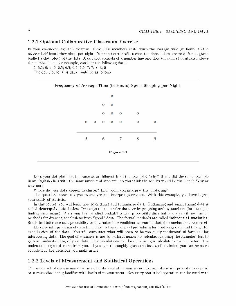
In your classroom, try this exercise. Have class members write down the average time (in hours, to thenearest half-hour) they sleep per night. Your instructor will record the data. Then create a simple graph(called a dot plot) of the data. A dot plot consists of a number line and dots (or points) positioned abovethe number line. For example, consider the following data:
5; 5.5; 6; 6; 6; 6.5; 6.5; 6.5; 6.5; 7; 7; 8; 8; 9The dot plot for this data would be as follows:
Frequency of Average Time (in Hours) Spent Sleeping per Night
Figure 1.1
Does your dot plot look the same as or di�erent from the example? Why? If you did the same examplein an English class with the same number of students, do you think the results would be the same? Why orwhy not?
Where do your data appear to cluster? How could you interpret the clustering?The questions above ask you to analyze and interpret your data. With this example, you have begun
your study of statistics.In this course, you will learn how to organize and summarize data. Organizing and summarizing data is
called descriptive statistics. Two ways to summarize data are by graphing and by numbers (for example,�nding an average). After you have studied probability and probability distributions, you will use formalmethods for drawing conclusions from "good" data. The formal methods are called inferential statistics.Statistical inference uses probability to determine how con�dent we can be that the conclusions are correct.
E�ective interpretation of data (inference) is based on good procedures for producing data and thoughtfulexamination of the data. You will encounter what will seem to be too many mathematical formulas forinterpreting data. The goal of statistics is not to perform numerous calculations using the formulas, but togain an understanding of your data. The calculations can be done using a calculator or a computer. Theunderstanding must come from you. If you can thoroughly grasp the basics of statistics, you can be morecon�dent in the decisions you make in life.
1.2.2 Levels of Measurement and Statistical Operations
The way a set of data is measured is called its level of measurement. Correct statistical procedures dependon a researcher being familiar with levels of measurement. Not every statistical operation can be used with
Available for free at Connexions <http://cnx.org/content/col11521/1.19>
3
every set of data. Data can be classi�ed into four levels of measurement. They are (from lowest to highestlevel):
• Nominal scale level• Ordinal scale level• Interval scale level• Ratio scale level
Data that is measured using a nominal scale is qualitative. Categories, colors, names, labels and favoritefoods along with yes or no responses are examples of nominal level data. Nominal scale data are not ordered.For example, trying to classify people according to their favorite food does not make any sense. Puttingpizza �rst and sushi second is not meaningful.
Smartphone companies are another example of nominal scale data. Some examples are Sony, Mo-torola, Nokia, Samsung and Apple. This is just a list and there is no agreed upon order. Some people mayfavor Apple but that is a matter of opinion. Nominal scale data cannot be used in calculations.
Data that is measured using an ordinal scale is similar to nominal scale data but there is a bigdi�erence. The ordinal scale data can be ordered. An example of ordinal scale data is a list of the top �venational parks in the United States. The top �ve national parks in the United States can be ranked fromone to �ve but we cannot measure di�erences between the data.
Another example using the ordinal scale is a cruise survey where the responses to questions aboutthe cruise are �excellent,� �good,� �satisfactory� and �unsatisfactory.� These responses are ordered from themost desired response by the cruise lines to the least desired. But the di�erences between two pieces of datacannot be measured. Like the nominal scale data, ordinal scale data cannot be used in calculations.
Data that is measured using the interval scale is similar to ordinal level data because it has a def-inite ordering but there is a di�erence between data. The di�erences between interval scale data can bemeasured though the data does not have a starting point.
Temperature scales like Celsius (C) and Fahrenheit (F) are measured by using the interval scale. Inboth temperature measurements, 40 degrees is equal to 100 degrees minus 60 degrees. Di�erences makesense. But 0 degrees does not because, in both scales, 0 is not the absolute lowest temperature. Tempera-tures like -10o F and -15o C exist and are colder than 0.
Interval level data can be used in calculations but one type of comparison cannot be done. Eightydegrees C is not 4 times as hot as 20o C (nor is 80o F 4 times as hot as 20o F). There is no meaning to theratio of 80 to 20 (or 4 to 1).
Data that is measured using the ratio scale takes care of the ratio problem and gives you the mostinformation. Ratio scale data is like interval scale data but, in addition, it has a 0 point and ratios can becalculated. For example, four multiple choice statistics �nal exam scores are 80, 68, 20 and 92 (out of apossible 100 points). The exams were machine-graded.
The data can be put in order from lowest to highest: 20, 68, 80, 92.
The di�erences between the data have meaning. The score 92 is more than the score 68 by 24points.
Ratios can be calculated. The smallest score for ratio data is 0. So 80 is 4 times 20. The score of80 is 4 times better than the score of 20.
Available for free at Connexions <http://cnx.org/content/col11521/1.19>
4 CHAPTER 1. SAMPLING AND DATA
Exercises
What type of measure scale is being used? Nominal, Ordinal, Interval or Ratio.
1. High school men soccer players classi�ed by their athletic ability: Superior, Average, Above average.2. Baking temperatures for various main dishes: 350, 400, 325, 250, 3003. The colors of crayons in a 24-crayon box.4. Social security numbers.5. Incomes measured in dollars6. A satisfaction survey of a social website by number: 1 = very satis�ed, 2 = somewhat satis�ed, 3 =
not satis�ed.7. Political outlook: extreme left, left-of-center, right-of-center, extreme right.8. Time of day on an analog watch.9. The distance in miles to the closest grocery store.10. The dates 1066, 1492, 1644, 1947, 1944.11. The heights of 21 � 65 year-old women.12. Common letter grades A, B, C, D, F.
Answers 1. ordinal, 2. interval, 3. nominal, 4. nominal, 5. ratio, 6. ordinal, 7. nominal, 8. interval, 9. ratio,10. interval, 11. ratio, 12. ordinal
1.3 Sampling and Data: Probability3
Probability is a mathematical tool used to study randomness. It deals with the chance (the likelihood) ofan event occurring. For example, if you toss a fair coin 4 times, the outcomes may not be 2 heads and 2tails. However, if you toss the same coin 4,000 times, the outcomes will be close to half heads and half tails.The expected theoretical probability of heads in any one toss is 1
2 or 0.5. Even though the outcomes of afew repetitions are uncertain, there is a regular pattern of outcomes when there are many repetitions. Afterreading about the English statistician Karl Pearson who tossed a coin 24,000 times with a result of 12,012heads, one of the authors tossed a coin 2,000 times. The results were 996 heads. The fraction 996
2000 is equalto 0.498 which is very close to 0.5, the expected probability.
The theory of probability began with the study of games of chance such as poker. Predictions take theform of probabilities. To predict the likelihood of an earthquake, of rain, or whether you will get an A inthis course, we use probabilities. Doctors use probability to determine the chance of a vaccination causingthe disease the vaccination is supposed to prevent. A stockbroker uses probability to determine the rate ofreturn on a client's investments. You might use probability to decide to buy a lottery ticket or not. In yourstudy of statistics, you will use the power of mathematics through probability calculations to analyze andinterpret your data.
1.4 Sampling and Data: Key Terms4
In statistics, we generally want to study a population. You can think of a population as an entire collectionof persons, things, or objects under study. To study the larger population, we select a sample. The idea ofsampling is to select a portion (or subset) of the larger population and study that portion (the sample) togain information about the population. Data are the result of sampling from a population.
Because it takes a lot of time and money to examine an entire population, sampling is a very practicaltechnique. If you wished to compute the overall grade point average at your school, it would make sense toselect a sample of students who attend the school. The data collected from the sample would be the students'grade point averages. In presidential elections, opinion poll samples of 1,000 to 2,000 people are taken. The
3This content is available online at <http://cnx.org/content/m16015/1.11/>.4This content is available online at <http://cnx.org/content/m46249/1.3/>.
Available for free at Connexions <http://cnx.org/content/col11521/1.19>
5
opinion poll is supposed to represent the views of the people in the entire country. Manufacturers of cannedcarbonated drinks take samples to determine if a 16 ounce can contains 16 ounces of carbonated drink.
From the sample data, we can calculate a statistic. A statistic is a number that is a property of thesample. For example, if we consider one math class to be a sample of the population of all math classes,then the average number of points earned by students in that one math class at the end of the term is anexample of a statistic. The statistic is an estimate of a population parameter. A parameter is a numberthat is a property of the population. Since we considered all math classes to be the population, then theaverage number of points earned per student over all the math classes is an example of a parameter.
One of the main concerns in the �eld of statistics is how accurately a statistic estimates a parameter.The accuracy really depends on how well the sample represents the population. The sample must containthe characteristics of the population in order to be a representative sample. We are interested in boththe sample statistic and the population parameter in inferential statistics. In a later chapter, we will use thesample statistic to test the validity of the established population parameter.
A variable, notated by capital letters like X and Y , is a characteristic of interest for each person orthing in a population. Variables may be numerical or categorical. Numerical variables take on valueswith equal units such as weight in pounds and time in hours. Categorical variables place the person orthing into a category. If we let X equal the number of points earned by one math student at the end of aterm, then X is a numerical variable. If we let Y be a person's party a�liation, then examples of Y includeRepublican, Democrat, and Independent. Y is a categorical variable. We could do some math with valuesof X (calculate the average number of points earned, for example), but it makes no sense to do math withvalues of Y (calculating an average party a�liation makes no sense).
Data are the actual values of the variable. They may be numbers or they may be words. Datum is asingle value.
Two words that come up often in statistics are mean and proportion. If you were to take three examsin your math classes and obtained scores of 86, 75, and 92, you calculate your mean score by adding thethree exam scores and dividing by three (your mean score would be 84.3 to one decimal place). If, in yourmath class, there are 40 students and 22 are men and 18 are women, then the proportion of men students is2240 and the proportion of women students is 18
40 . Mean and proportion are discussed in more detail in laterchapters.
note: The words "mean" and "average" are often used interchangeably. The substitution of oneword for the other is common practice. The technical term is "arithmetic mean" and "average" istechnically a center location. However, in practice among non-statisticians, "average" is commonlyaccepted for "arithmetic mean."
Example 1.1De�ne the key terms from the following study: We want to know the average (mean) amount
of money �rst year college students spend at ABC College on school supplies that do not includebooks. We randomly survey 100 �rst year students at the college. Three of those students spent$150, $200, and $225, respectively.
SolutionThe population is all �rst year students attending ABC College this term.
The sample could be all students enrolled in one section of a beginning statistics course atABC College (although this sample may not represent the entire population).
The parameter is the average (mean) amount of money spent (excluding books) by �rst yearcollege students at ABC College this term.
The statistic is the average (mean) amount of money spent (excluding books) by �rst yearcollege students in the sample.
The variable could be the amount of money spent (excluding books) by one �rst year student.Let X = the amount of money spent (excluding books) by one �rst year student attending ABCCollege.
Available for free at Connexions <http://cnx.org/content/col11521/1.19>
6 CHAPTER 1. SAMPLING AND DATA
The data are the dollar amounts spent by the �rst year students. Examples of the data are$150, $200, and $225.
1.4.1 Optional Collaborative Classroom Exercise
Do the following exercise collaboratively with up to four people per group. Find a population, a sample, theparameter, the statistic, a variable, and data for the following study: You want to determine the average(mean) number of glasses of milk college students drink per day. Suppose yesterday, in your English class,you asked �ve students how many glasses of milk they drank the day before. The answers were 1, 0, 1, 3,and 4 glasses of milk.
1.5 Sampling and Data: Data5
Data may come from a population or from a sample. Small letters like x or y generally are used to representdata values. Most data can be put into the following categories:
• Qualitative• Quantitative
Qualitative data are the result of categorizing or describing attributes of a population. Hair color, bloodtype, ethnic group, the car a person drives, and the street a person lives on are examples of qualitative data.Qualitative data are generally described by words or letters. For instance, hair color might be black, darkbrown, light brown, blonde, gray, or red. Blood type might be AB+, O-, or B+. Researchers often prefer touse quantitative data over qualitative data because it lends itself more easily to mathematical analysis. Forexample, it does not make sense to �nd an average hair color or blood type.
Quantitative data are always numbers. Quantitative data are the result of counting or measuringattributes of a population. Amount of money, pulse rate, weight, number of people living in your town, andthe number of students who take statistics are examples of quantitative data. Quantitative data may beeither discrete or continuous.
All data that are the result of counting are called quantitative discrete data. These data take on onlycertain numerical values. If you count the number of phone calls you receive for each day of the week, youmight get 0, 1, 2, 3, etc.
All data that are the result of measuring are quantitative continuous data assuming that we canmeasure accurately. Measuring angles in radians might result in the numbers π
6 ,π3 ,π2 , π , 3π
4 , etc. If youand your friends carry backpacks with books in them to school, the numbers of books in the backpacks arediscrete data and the weights of the backpacks are continuous data.
note: In this course, the data used is mainly quantitative. It is easy to calculate statistics (like themean or proportion) from numbers. In the chapter Descriptive Statistics, you will be introducedto stem plots, histograms and box plots all of which display quantitative data. Qualitative data isdiscussed at the end of this section through graphs.
Example 1.2: Data Sample of Quantitative Discrete DataThe data are the number of books students carry in their backpacks. You sample �ve students.Two students carry 3 books, one student carries 4 books, one student carries 2 books, and onestudent carries 1 book. The numbers of books (3, 4, 2, and 1) are the quantitative discrete data.
5This content is available online at <http://cnx.org/content/m16005/1.18/>.
Available for free at Connexions <http://cnx.org/content/col11521/1.19>
7
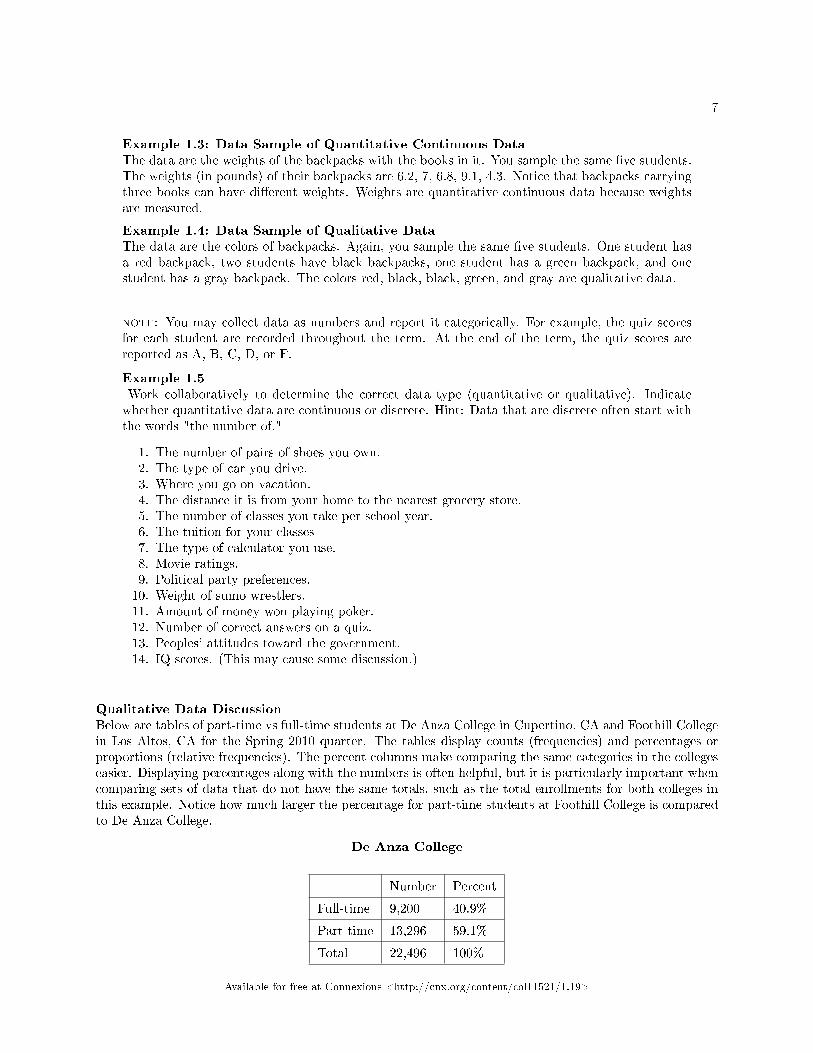
Example 1.3: Data Sample of Quantitative Continuous DataThe data are the weights of the backpacks with the books in it. You sample the same �ve students.The weights (in pounds) of their backpacks are 6.2, 7, 6.8, 9.1, 4.3. Notice that backpacks carryingthree books can have di�erent weights. Weights are quantitative continuous data because weightsare measured.
Example 1.4: Data Sample of Qualitative DataThe data are the colors of backpacks. Again, you sample the same �ve students. One student hasa red backpack, two students have black backpacks, one student has a green backpack, and onestudent has a gray backpack. The colors red, black, black, green, and gray are qualitative data.
note: You may collect data as numbers and report it categorically. For example, the quiz scoresfor each student are recorded throughout the term. At the end of the term, the quiz scores arereported as A, B, C, D, or F.
Example 1.5Work collaboratively to determine the correct data type (quantitative or qualitative). Indicatewhether quantitative data are continuous or discrete. Hint: Data that are discrete often start withthe words "the number of."
1. The number of pairs of shoes you own.2. The type of car you drive.3. Where you go on vacation.4. The distance it is from your home to the nearest grocery store.5. The number of classes you take per school year.6. The tuition for your classes7. The type of calculator you use.8. Movie ratings.9. Political party preferences.10. Weight of sumo wrestlers.11. Amount of money won playing poker.12. Number of correct answers on a quiz.13. Peoples' attitudes toward the government.14. IQ scores. (This may cause some discussion.)
Qualitative Data DiscussionBelow are tables of part-time vs full-time students at De Anza College in Cupertino, CA and Foothill Collegein Los Altos, CA for the Spring 2010 quarter. The tables display counts (frequencies) and percentages orproportions (relative frequencies). The percent columns make comparing the same categories in the collegeseasier. Displaying percentages along with the numbers is often helpful, but it is particularly important whencomparing sets of data that do not have the same totals, such as the total enrollments for both colleges inthis example. Notice how much larger the percentage for part-time students at Foothill College is comparedto De Anza College.
De Anza College
Number Percent
Full-time 9,200 40.9%
Part-time 13,296 59.1%
Total 22,496 100%
Available for free at Connexions <http://cnx.org/content/col11521/1.19>
8 CHAPTER 1. SAMPLING AND DATA
Table 1.1
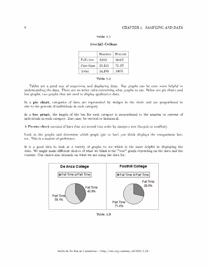
Foothill College
Number Percent
Full-time 4,059 28.6%
Part-time 10,124 71.4%
Total 14,183 100%
Table 1.2
Tables are a good way of organizing and displaying data. But graphs can be even more helpful inunderstanding the data. There are no strict rules concerning what graphs to use. Below are pie charts andbar graphs, two graphs that are used to display qualitative data.
In a pie chart, categories of data are represented by wedges in the circle and are proportional insize to the percent of individuals in each category.
In a bar graph, the length of the bar for each category is proportional to the number or percent ofindividuals in each category. Bars may be vertical or horizontal.
A Pareto chart consists of bars that are sorted into order by category size (largest to smallest).
Look at the graphs and determine which graph (pie or bar) you think displays the comparisons bet-ter. This is a matter of preference.
It is a good idea to look at a variety of graphs to see which is the most helpful in displaying thedata. We might make di�erent choices of what we think is the "best" graph depending on the data and thecontext. Our choice also depends on what we are using the data for.
Table 1.3
Available for free at Connexions <http://cnx.org/content/col11521/1.19>
9
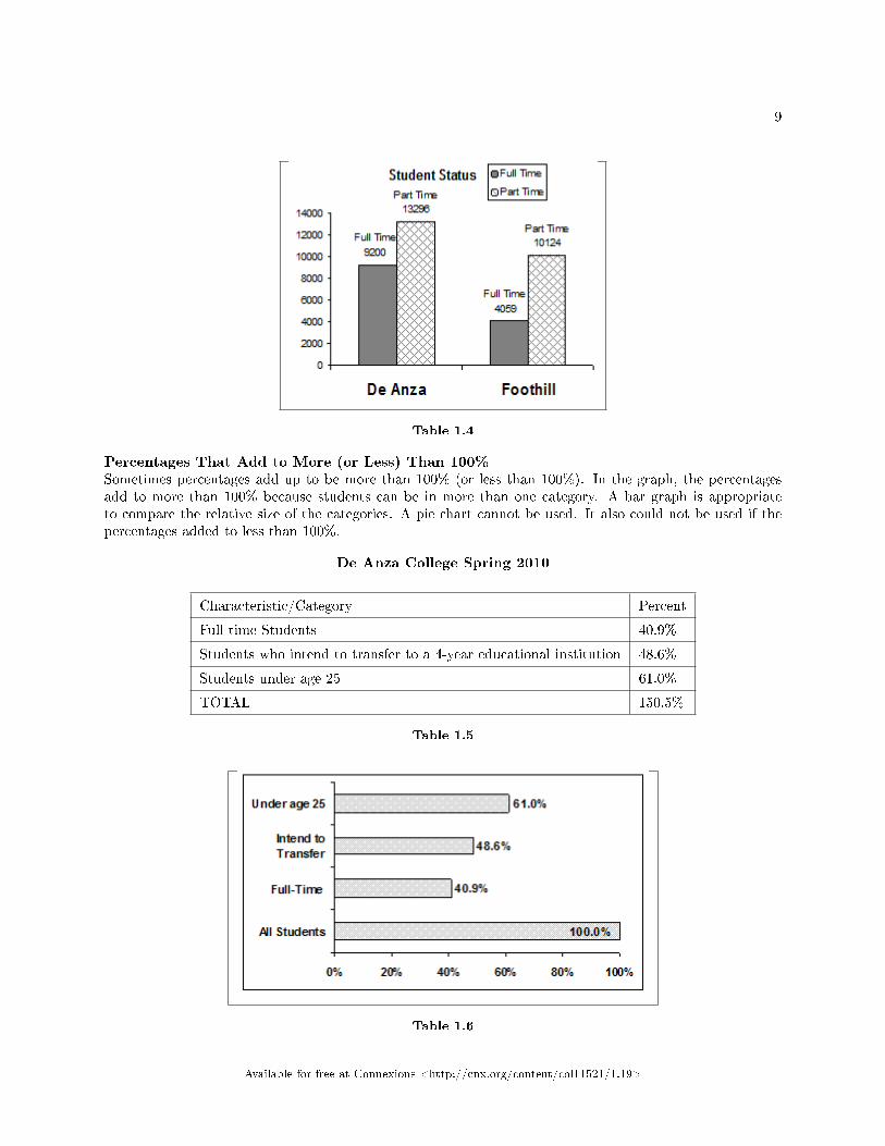
Table 1.4
Percentages That Add to More (or Less) Than 100%Sometimes percentages add up to be more than 100% (or less than 100%). In the graph, the percentagesadd to more than 100% because students can be in more than one category. A bar graph is appropriateto compare the relative size of the categories. A pie chart cannot be used. It also could not be used if thepercentages added to less than 100%.
De Anza College Spring 2010
Characteristic/Category Percent
Full-time Students 40.9%
Students who intend to transfer to a 4-year educational institution 48.6%
Students under age 25 61.0%
TOTAL 150.5%
Table 1.5
Table 1.6
Available for free at Connexions <http://cnx.org/content/col11521/1.19>
10 CHAPTER 1. SAMPLING AND DATA
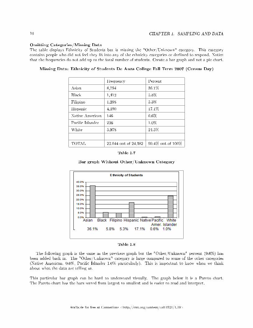
Omitting Categories/Missing DataThe table displays Ethnicity of Students but is missing the "Other/Unknown" category. This categorycontains people who did not feel they �t into any of the ethnicity categories or declined to respond. Noticethat the frequencies do not add up to the total number of students. Create a bar graph and not a pie chart.
Missing Data: Ethnicity of Students De Anza College Fall Term 2007 (Census Day)
Frequency Percent
Asian 8,794 36.1%
Black 1,412 5.8%
Filipino 1,298 5.3%
Hispanic 4,180 17.1%
Native American 146 0.6%
Paci�c Islander 236 1.0%
White 5,978 24.5%
TOTAL 22,044 out of 24,382 90.4% out of 100%
Table 1.7
Bar graph Without Other/Unknown Category
Table 1.8
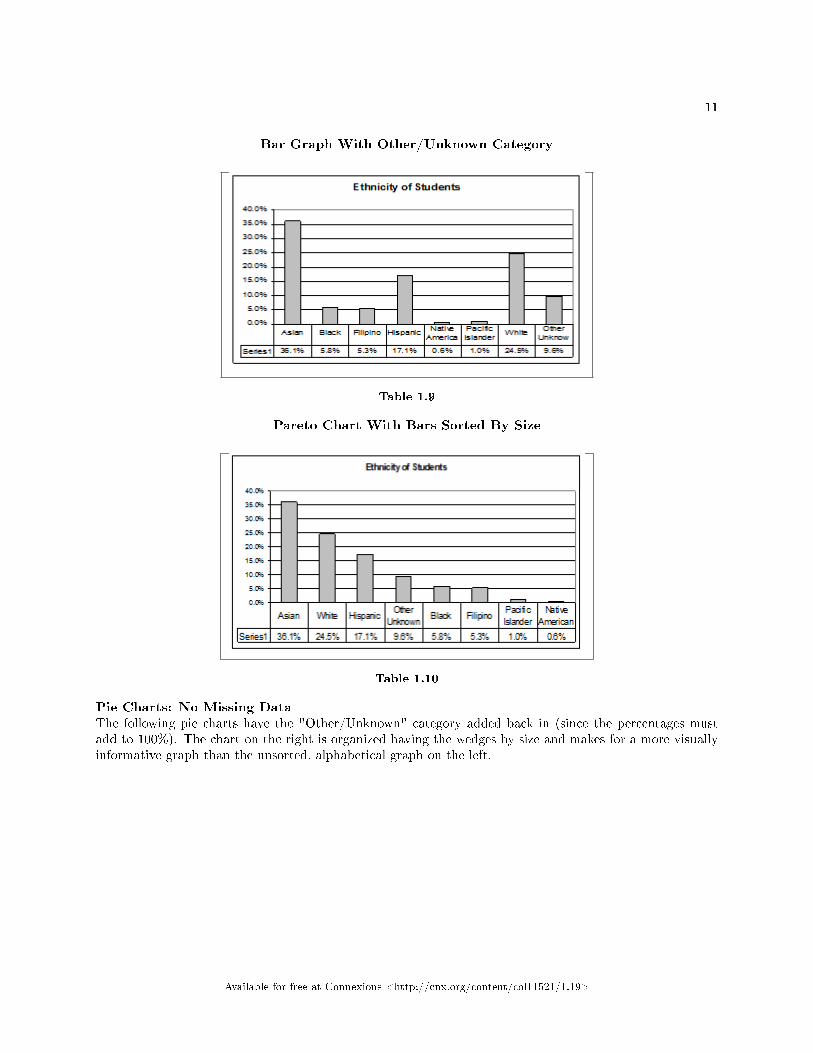
The following graph is the same as the previous graph but the "Other/Unknown" percent (9.6%) hasbeen added back in. The "Other/Unknown" category is large compared to some of the other categories(Native American, 0.6%, Paci�c Islander 1.0% particularly). This is important to know when we thinkabout what the data are telling us.
This particular bar graph can be hard to understand visually. The graph below it is a Pareto chart.The Pareto chart has the bars sorted from largest to smallest and is easier to read and interpret.
Available for free at Connexions <http://cnx.org/content/col11521/1.19>
11
Bar Graph With Other/Unknown Category
Table 1.9
Pareto Chart With Bars Sorted By Size
Table 1.10
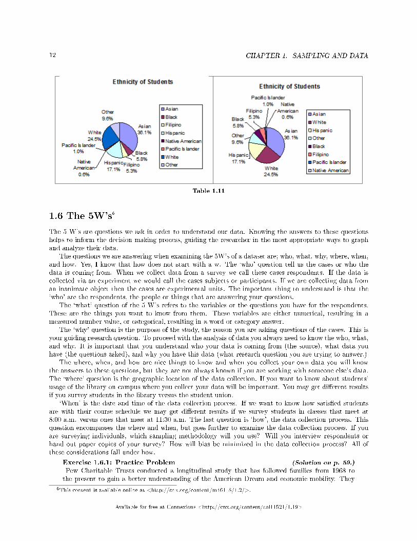
Pie Charts: No Missing DataThe following pie charts have the "Other/Unknown" category added back in (since the percentages mustadd to 100%). The chart on the right is organized having the wedges by size and makes for a more visuallyinformative graph than the unsorted, alphabetical graph on the left.
Available for free at Connexions <http://cnx.org/content/col11521/1.19>
12 CHAPTER 1. SAMPLING AND DATA
Table 1.11
1.6 The 5W's6
The 5 W's are questions we ask in order to understand our data. Knowing the answers to these questionshelps to inform the decision making process, guiding the researcher in the most appropriate ways to graphand analyze their data.
The questions we are answering when examining the 5W's of a dataset are; who, what, why, where, when,and how. Yes, I know that how does not start with a w. The `who' question tell us the cases or who thedata is coming from. When we collect data from a survey we call these cases respondents. If the data iscollected via an experiment we would call the cases subjects or participants. If we are collecting data froman inanimate object then the cases are experimental units. The important thing to understand is that the`who' are the respondents, the people or things that are answering your questions.
The `what' question of the 5 W's refers to the variables or the questions you have for the respondents.These are the things you want to know from them. These variables are either numerical, resulting in ameasured number value, or categorical, resulting in a word or category answer.
The `why' question is the purpose of the study, the reason you are asking questions of the cases. This isyour guiding research question. To proceed with the analysis of data you always need to know the who, what,and why. It is important that you understand who your data is coming from (the source), what data youhave (the questions asked), and why you have this data (what research question you are trying to answer.)
The where, when, and how are nice things to know and when you collect your own data you will knowthe answers to these questions, but they are not always known if you are working with someone else's data.The `where' question is the geographic location of the data collection. If you want to know about students'usage of the library on campus where you collect your data will be important. You may get di�erent resultsif you survey students in the library versus the student union.
`When' is the date and time of the data collection process. If we want to know how satis�ed studentsare with their course schedule we may get di�erent results if we survey students in classes that meet at8:00 a.m. versus ones that meet at 11:30 a.m. The last question is `how', the data collection process. Thisquestion encompasses the where and when, but goes further to examine the data collection process. If youare surveying individuals, which sampling methodology will you use? Will you interview respondents orhand out paper copies of your survey? How will bias be minimized in the data collection process? All ofthese considerations fall under how.
Exercise 1.6.1: Practice Problem (Solution on p. 59.)
Pew Charitable Trusts conducted a longitudinal study that has followed families from 1968 tothe present to gain a better understanding of the American Dream and economic mobility. They
6This content is available online at <http://cnx.org/content/m46118/1.2/>.
Available for free at Connexions <http://cnx.org/content/col11521/1.19>
13
surveyed 2227 American families asking, �What is your �Family income� including all taxable income(such as earnings, interest, and dividends) and cash transfers (such as Social Security and welfare)of all family members?� Identify the 5W's of this example.
1.7 Sampling and Data: Sampling7
Gathering information about an entire population often costs too much or is virtually impossible. Instead,we use a sample of the population. A sample should have the same characteristics as the populationit is representing. Most statisticians use various methods of random sampling in an attempt to achievethis goal. This section will describe a few of the most common methods.
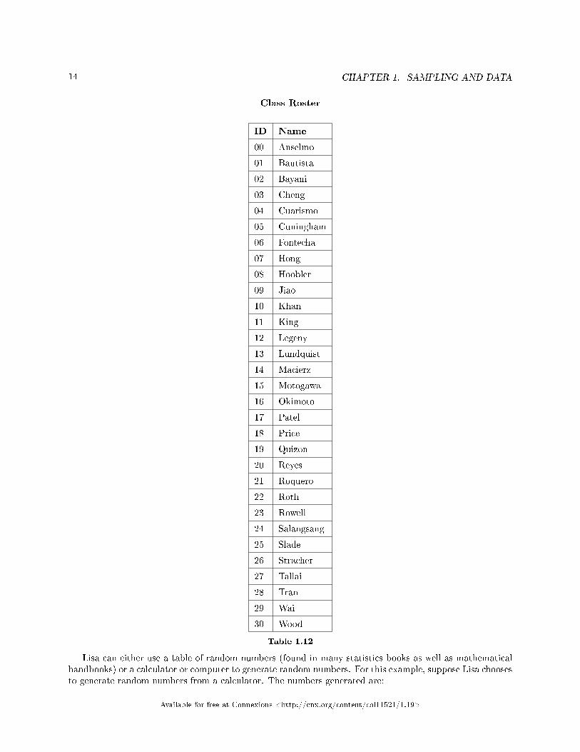
There are several di�erent methods of random sampling. In each form of random sampling, eachmember of a population initially has an equal chance of being selected for the sample. Each method has prosand cons. The easiest method to describe is called a simple random sample. Any group of n individualsis equally as likely to be chosen as any other group of n individuals if the simple random sampling techniqueis used. In other words, each sample of the same size has an equal chance of being selected. For example,suppose Lisa wants to form a four-person study group (herself and three other people) from her pre-calculusclass, which has 31 members not including Lisa. To choose a simple random sample of size 3 from the othermembers of her class, Lisa could put all 31 names in a hat, shake the hat, close her eyes, and pick out 3names. A more technological way is for Lisa to �rst list the last names of the members of her class togetherwith a two-digit number as shown below.
7This content is available online at <http://cnx.org/content/m46800/1.1/>.
Available for free at Connexions <http://cnx.org/content/col11521/1.19>
14 CHAPTER 1. SAMPLING AND DATA
Class Roster
ID Name
00 Anselmo
01 Bautista
02 Bayani
03 Cheng
04 Cuarismo
05 Cuningham
06 Fontecha
07 Hong
08 Hoobler
09 Jiao
10 Khan
11 King
12 Legeny
13 Lundquist
14 Macierz
15 Motogawa
16 Okimoto
17 Patel
18 Price
19 Quizon
20 Reyes
21 Roquero
22 Roth
23 Rowell
24 Salangsang
25 Slade
26 Stracher
27 Tallai
28 Tran
29 Wai
30 Wood
Table 1.12
Lisa can either use a table of random numbers (found in many statistics books as well as mathematicalhandbooks) or a calculator or computer to generate random numbers. For this example, suppose Lisa choosesto generate random numbers from a calculator. The numbers generated are:
Available for free at Connexions <http://cnx.org/content/col11521/1.19>
15
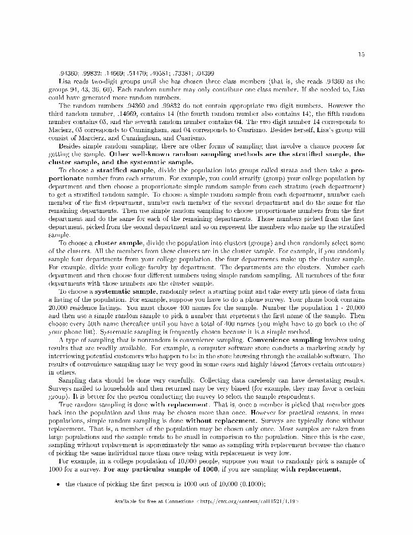
.94360; .99832; .14669; .51470; .40581; .73381; .04399Lisa reads two-digit groups until she has chosen three class members (that is, she reads .94360 as the
groups 94, 43, 36, 60). Each random number may only contribute one class member. If she needed to, Lisacould have generated more random numbers.
The random numbers .94360 and .99832 do not contain appropriate two digit numbers. However thethird random number, .14669, contains 14 (the fourth random number also contains 14), the �fth randomnumber contains 05, and the seventh random number contains 04. The two-digit number 14 corresponds toMacierz, 05 corresponds to Cunningham, and 04 corresponds to Cuarismo. Besides herself, Lisa's group willconsist of Marcierz, and Cunningham, and Cuarismo.
Besides simple random sampling, there are other forms of sampling that involve a chance process forgetting the sample. Other well-known random sampling methods are the strati�ed sample, thecluster sample, and the systematic sample.
To choose a strati�ed sample, divide the population into groups called strata and then take a pro-portionate number from each stratum. For example, you could stratify (group) your college population bydepartment and then choose a proportionate simple random sample from each stratum (each department)to get a strati�ed random sample. To choose a simple random sample from each department, number eachmember of the �rst department, number each member of the second department and do the same for theremaining departments. Then use simple random sampling to choose proportionate numbers from the �rstdepartment and do the same for each of the remaining departments. Those numbers picked from the �rstdepartment, picked from the second department and so on represent the members who make up the strati�edsample.
To choose a cluster sample, divide the population into clusters (groups) and then randomly select someof the clusters. All the members from these clusters are in the cluster sample. For example, if you randomlysample four departments from your college population, the four departments make up the cluster sample.For example, divide your college faculty by department. The departments are the clusters. Number eachdepartment and then choose four di�erent numbers using simple random sampling. All members of the fourdepartments with those numbers are the cluster sample.
To choose a systematic sample, randomly select a starting point and take every nth piece of data froma listing of the population. For example, suppose you have to do a phone survey. Your phone book contains20,000 residence listings. You must choose 400 names for the sample. Number the population 1 - 20,000and then use a simple random sample to pick a number that represents the �rst name of the sample. Thenchoose every 50th name thereafter until you have a total of 400 names (you might have to go back to the ofyour phone list). Systematic sampling is frequently chosen because it is a simple method.
A type of sampling that is nonrandom is convenience sampling. Convenience sampling involves usingresults that are readily available. For example, a computer software store conducts a marketing study byinterviewing potential customers who happen to be in the store browsing through the available software. Theresults of convenience sampling may be very good in some cases and highly biased (favors certain outcomes)in others.
Sampling data should be done very carefully. Collecting data carelessly can have devastating results.Surveys mailed to households and then returned may be very biased (for example, they may favor a certaingroup). It is better for the person conducting the survey to select the sample respondents.
True random sampling is done with replacement. That is, once a member is picked that member goesback into the population and thus may be chosen more than once. However for practical reasons, in mostpopulations, simple random sampling is done without replacement. Surveys are typically done withoutreplacement. That is, a member of the population may be chosen only once. Most samples are taken fromlarge populations and the sample tends to be small in comparison to the population. Since this is the case,sampling without replacement is approximately the same as sampling with replacement because the chanceof picking the same individual more than once using with replacement is very low.
For example, in a college population of 10,000 people, suppose you want to randomly pick a sample of1000 for a survey. For any particular sample of 1000, if you are sampling with replacement,
• the chance of picking the �rst person is 1000 out of 10,000 (0.1000);
Available for free at Connexions <http://cnx.org/content/col11521/1.19>
16 CHAPTER 1. SAMPLING AND DATA
• the chance of picking a di�erent second person for this sample is 999 out of 10,000 (0.0999);• the chance of picking the same person again is 1 out of 10,000 (very low).
If you are sampling without replacement,
• the chance of picking the �rst person for any particular sample is 1000 out of 10,000 (0.1000);• the chance of picking a di�erent second person is 999 out of 9,999 (0.0999);• you do not replace the �rst person before picking the next person.
Compare the fractions 999/10,000 and 999/9,999. For accuracy, carry the decimal answers to 4 place deci-mals. To 4 decimal places, these numbers are equivalent (0.0999).
Sampling without replacement instead of sampling with replacement only becomes a mathematics issuewhen the population is small which is not that common. For example, if the population is 25 people, thesample is 10 and you are sampling with replacement for any particular sample,
• the chance of picking the �rst person is 10 out of 25 and a di�erent second person is 9 out of 25 (youreplace the �rst person).
If you sample without replacement,
• the chance of picking the �rst person is 10 out of 25 and then the second person (which is di�erent) is9 out of 24 (you do not replace the �rst person).
Compare the fractions 9/25 and 9/24. To 4 decimal places, 9/25 = 0.3600 and 9/24 = 0.3750. To 4 decimalplaces, these numbers are not equivalent.
When you analyze data, it is important to be aware of sampling errors and nonsampling errors. Theactual process of sampling causes sampling errors. For example, the sample may not be large enough.Factors not related to the sampling process cause nonsampling errors. A defective counting device cancause a nonsampling error.
In reality, a sample will never be exactly representative of the population so there will always besome sampling error. As a rule, the larger the sample, the smaller the sampling error.
In statistics, a sampling bias is created when a sample is collected from a population and somemembers of the population are not as likely to be chosen as others (remember, each member of thepopulation should have an equally likely chance of being chosen). When a sampling bias happens, there canbe incorrect conclusions drawn about the population that is being studied.
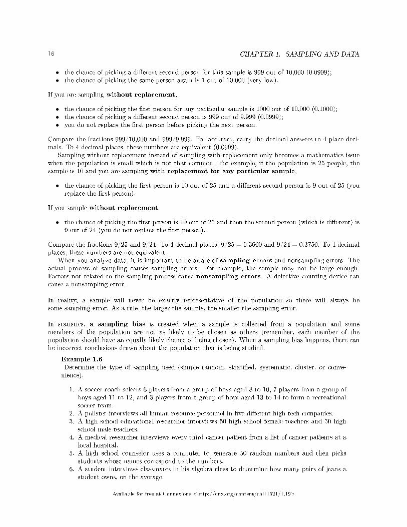
Example 1.6Determine the type of sampling used (simple random, strati�ed, systematic, cluster, or conve-nience).
1. A soccer coach selects 6 players from a group of boys aged 8 to 10, 7 players from a group ofboys aged 11 to 12, and 3 players from a group of boys aged 13 to 14 to form a recreationalsoccer team.
2. A pollster interviews all human resource personnel in �ve di�erent high tech companies.3. A high school educational researcher interviews 50 high school female teachers and 50 high
school male teachers.4. A medical researcher interviews every third cancer patient from a list of cancer patients at a
local hospital.5. A high school counselor uses a computer to generate 50 random numbers and then picks
students whose names correspond to the numbers.6. A student interviews classmates in his algebra class to determine how many pairs of jeans a
student owns, on the average.
Available for free at Connexions <http://cnx.org/content/col11521/1.19>
17
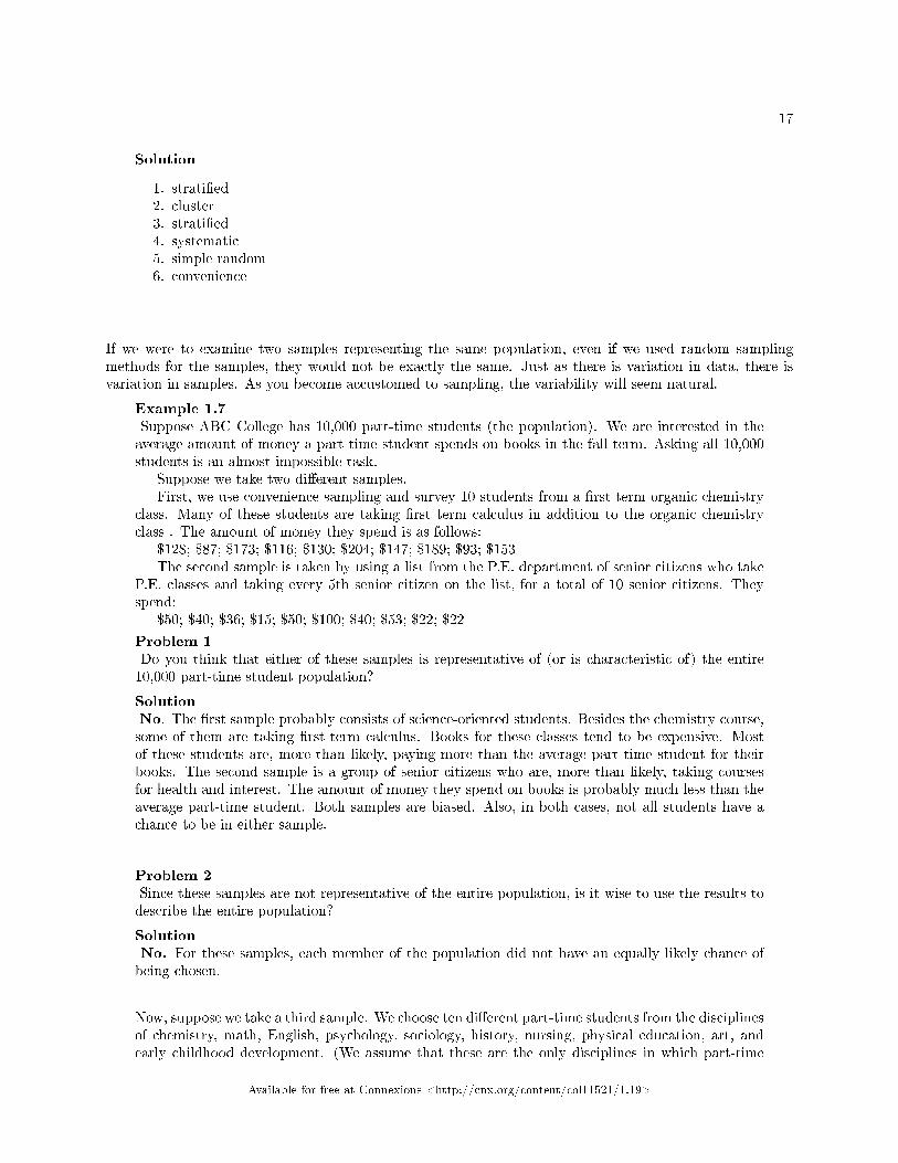
Solution
1. strati�ed2. cluster3. strati�ed4. systematic5. simple random6. convenience
If we were to examine two samples representing the same population, even if we used random samplingmethods for the samples, they would not be exactly the same. Just as there is variation in data, there isvariation in samples. As you become accustomed to sampling, the variability will seem natural.
Example 1.7Suppose ABC College has 10,000 part-time students (the population). We are interested in theaverage amount of money a part-time student spends on books in the fall term. Asking all 10,000students is an almost impossible task.
Suppose we take two di�erent samples.First, we use convenience sampling and survey 10 students from a �rst term organic chemistry
class. Many of these students are taking �rst term calculus in addition to the organic chemistryclass . The amount of money they spend is as follows:
$128; $87; $173; $116; $130; $204; $147; $189; $93; $153The second sample is taken by using a list from the P.E. department of senior citizens who take
P.E. classes and taking every 5th senior citizen on the list, for a total of 10 senior citizens. Theyspend:
$50; $40; $36; $15; $50; $100; $40; $53; $22; $22
Problem 1Do you think that either of these samples is representative of (or is characteristic of) the entire10,000 part-time student population?
SolutionNo. The �rst sample probably consists of science-oriented students. Besides the chemistry course,some of them are taking �rst-term calculus. Books for these classes tend to be expensive. Mostof these students are, more than likely, paying more than the average part-time student for theirbooks. The second sample is a group of senior citizens who are, more than likely, taking coursesfor health and interest. The amount of money they spend on books is probably much less than theaverage part-time student. Both samples are biased. Also, in both cases, not all students have achance to be in either sample.
Problem 2Since these samples are not representative of the entire population, is it wise to use the results todescribe the entire population?
SolutionNo. For these samples, each member of the population did not have an equally likely chance ofbeing chosen.
Now, suppose we take a third sample. We choose ten di�erent part-time students from the disciplinesof chemistry, math, English, psychology, sociology, history, nursing, physical education, art, andearly childhood development. (We assume that these are the only disciplines in which part-time
Available for free at Connexions <http://cnx.org/content/col11521/1.19>
18 CHAPTER 1. SAMPLING AND DATA
students at ABC College are enrolled and that an equal number of part-time students are enrolled ineach of the disciplines.) Each student is chosen using simple random sampling. Using a calculator,random numbers are generated and a student from a particular discipline is selected if he/she hasa corresponding number. The students spend:
$180; $50; $150; $85; $260; $75; $180; $200; $200; $150
Problem 3Is the sample biased?
SolutionThe sample is unbiased, but a larger sample would be recommended to increase the likelihoodthat the sample will be close to representative of the population. However, for a biased samplingtechnique, even a large sample runs the risk of not being representative of the population.
Students often ask if it is "good enough" to take a sample, instead of surveying the entire population.If the survey is done well, the answer is yes.
1.7.1 Optional Collaborative Classroom Exercise
Exercise 1.7.1As a class, determine whether or not the following samples are representative. If they are not,discuss the reasons.
1. To �nd the average GPA of all students in a university, use all honor students at the universityas the sample.
2. To �nd out the most popular cereal among young people under the age of 10, stand outside alarge supermarket for three hours and speak to every 20th child under age 10 who enters thesupermarket.
3. To �nd the average annual income of all adults in the United States, sample U.S. congressmen.Create a cluster sample by considering each state as a stratum (group). By using simplerandom sampling, select states to be part of the cluster. Then survey every U.S. congressmanin the cluster.
4. To determine the proportion of people taking public transportation to work, survey 20 peoplein New York City. Conduct the survey by sitting in Central Park on a bench and interviewingevery person who sits next to you.
5. To determine the average cost of a two day stay in a hospital in Massachusetts, survey 100hospitals across the state using simple random sampling.
1.8 Sampling and Data: Variation and Critical Evaluation8
1.8.1 Variation in Data
Variation is present in any set of data. For example, 16-ounce cans of beverage may contain more or less than16 ounces of liquid. In one study, eight 16 ounce cans were measured and produced the following amount(in ounces) of beverage:
15.8; 16.1; 15.2; 14.8; 15.8; 15.9; 16.0; 15.5
8This content is available online at <http://cnx.org/content/m16021/1.15/>.
Available for free at Connexions <http://cnx.org/content/col11521/1.19>
19
Measurements of the amount of beverage in a 16-ounce can may vary because di�erent people make themeasurements or because the exact amount, 16 ounces of liquid, was not put into the cans. Manufacturersregularly run tests to determine if the amount of beverage in a 16-ounce can falls within the desired range.
Be aware that as you take data, your data may vary somewhat from the data someone else is taking forthe same purpose. This is completely natural. However, if two or more of you are taking the same data andget very di�erent results, it is time for you and the others to reevaluate your data-taking methods and youraccuracy.
1.8.2 Variation in Samples
It was mentioned previously that two or more samples from the same population, taken randomly, andhaving close to the same characteristics of the population are di�erent from each other. Suppose Doreen andJung both decide to study the average amount of time students at their college sleep each night. Doreen andJung each take samples of 500 students. Doreen uses systematic sampling and Jung uses cluster sampling.Doreen's sample will be di�erent from Jung's sample. Even if Doreen and Jung used the same samplingmethod, in all likelihood their samples would be di�erent. Neither would be wrong, however.
Think about what contributes to making Doreen's and Jung's samples di�erent.If Doreen and Jung took larger samples (i.e. the number of data values is increased), their sample results
(the average amount of time a student sleeps) might be closer to the actual population average. But still,their samples would be, in all likelihood, di�erent from each other. This variability in samples cannot bestressed enough.
1.8.2.1 Size of a Sample
The size of a sample (often called the number of observations) is important. The examples you have seen inthis book so far have been small. Samples of only a few hundred observations, or even smaller, are su�cientfor many purposes. In polling, samples that are from 1200 to 1500 observations are considered large enoughand good enough if the survey is random and is well done. You will learn why when you study con�denceintervals.
Be aware that many large samples are biased. For example, call-in surveys are invariable biasedbecause people choose to respond or not.
1.8.2.2 Optional Collaborative Classroom Exercise
Exercise 1.8.1Divide into groups of two, three, or four. Your instructor will give each group one 6-sided die. Trythis experiment twice. Roll one fair die (6-sided) 20 times. Record the number of ones, twos,threes, fours, �ves, and sixes you get below ("frequency" is the number of times a particular faceof the die occurs):
First Experiment (20 rolls)
Face on Die Frequency
1
2
3
4
5
6
Available for free at Connexions <http://cnx.org/content/col11521/1.19>
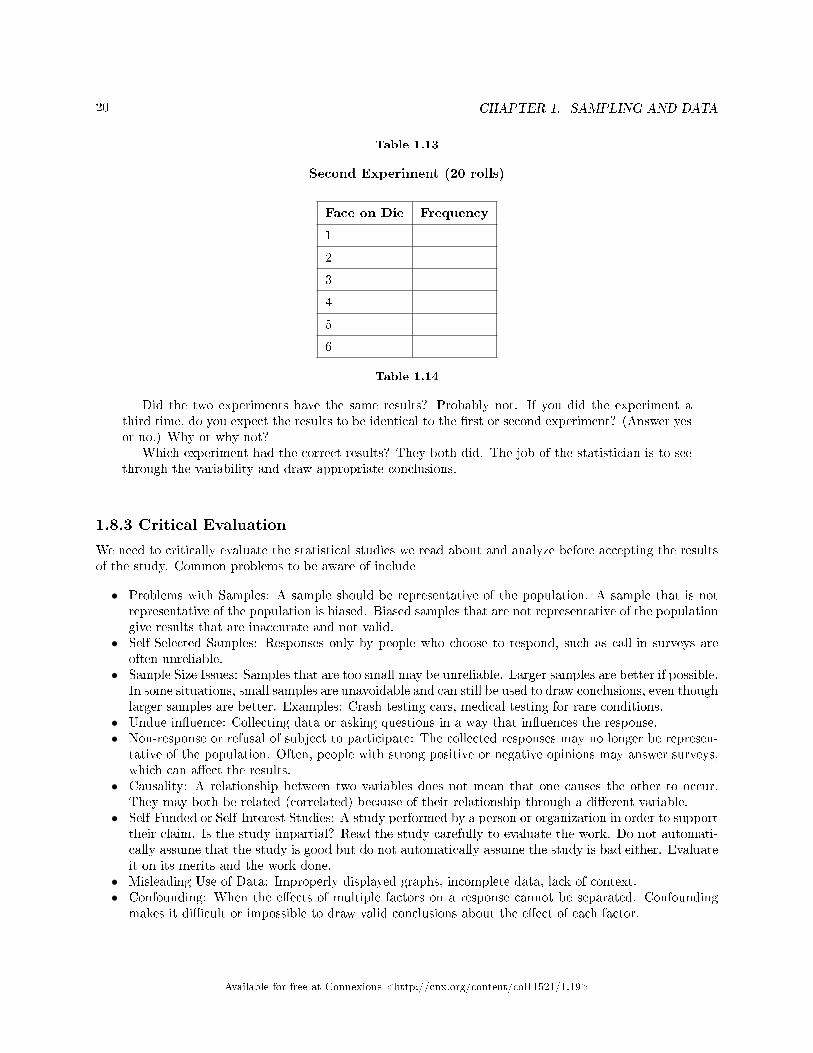
20 CHAPTER 1. SAMPLING AND DATA
Table 1.13
Second Experiment (20 rolls)
Face on Die Frequency
1
2
3
4
5
6
Table 1.14
Did the two experiments have the same results? Probably not. If you did the experiment athird time, do you expect the results to be identical to the �rst or second experiment? (Answer yesor no.) Why or why not?
Which experiment had the correct results? They both did. The job of the statistician is to seethrough the variability and draw appropriate conclusions.
1.8.3 Critical Evaluation
We need to critically evaluate the statistical studies we read about and analyze before accepting the resultsof the study. Common problems to be aware of include
• Problems with Samples: A sample should be representative of the population. A sample that is notrepresentative of the population is biased. Biased samples that are not representative of the populationgive results that are inaccurate and not valid.
• Self-Selected Samples: Responses only by people who choose to respond, such as call-in surveys areoften unreliable.
• Sample Size Issues: Samples that are too small may be unreliable. Larger samples are better if possible.In some situations, small samples are unavoidable and can still be used to draw conclusions, even thoughlarger samples are better. Examples: Crash testing cars, medical testing for rare conditions.
• Undue in�uence: Collecting data or asking questions in a way that in�uences the response.• Non-response or refusal of subject to participate: The collected responses may no longer be represen-
tative of the population. Often, people with strong positive or negative opinions may answer surveys,which can a�ect the results.
• Causality: A relationship between two variables does not mean that one causes the other to occur.They may both be related (correlated) because of their relationship through a di�erent variable.
• Self-Funded or Self-Interest Studies: A study performed by a person or organization in order to supporttheir claim. Is the study impartial? Read the study carefully to evaluate the work. Do not automati-cally assume that the study is good but do not automatically assume the study is bad either. Evaluateit on its merits and the work done.
• Misleading Use of Data: Improperly displayed graphs, incomplete data, lack of context.• Confounding: When the e�ects of multiple factors on a response cannot be separated. Confounding
makes it di�cult or impossible to draw valid conclusions about the e�ect of each factor.
Available for free at Connexions <http://cnx.org/content/col11521/1.19>
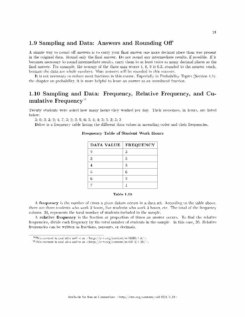
21
1.9 Sampling and Data: Answers and Rounding O�9
A simple way to round o� answers is to carry your �nal answer one more decimal place than was presentin the original data. Round only the �nal answer. Do not round any intermediate results, if possible. If itbecomes necessary to round intermediate results, carry them to at least twice as many decimal places as the�nal answer. For example, the average of the three quiz scores 4, 6, 9 is 6.3, rounded to the nearest tenth,because the data are whole numbers. Most answers will be rounded in this manner.
It is not necessary to reduce most fractions in this course. Especially in Probability Topics (Section 4.1),the chapter on probability, it is more helpful to leave an answer as an unreduced fraction.
1.10 Sampling and Data: Frequency, Relative Frequency, and Cu-mulative Frequency10
Twenty students were asked how many hours they worked per day. Their responses, in hours, are listedbelow:
5; 6; 3; 3; 2; 4; 7; 5; 2; 3; 5; 6; 5; 4; 4; 3; 5; 2; 5; 3Below is a frequency table listing the di�erent data values in ascending order and their frequencies.
Frequency Table of Student Work Hours
DATA VALUE FREQUENCY
2 3
3 5
4 3
5 6
6 2
7 1
Table 1.15
A frequency is the number of times a given datum occurs in a data set. According to the table above,there are three students who work 2 hours, �ve students who work 3 hours, etc. The total of the frequencycolumn, 20, represents the total number of students included in the sample.
A relative frequency is the fraction or proportion of times an answer occurs. To �nd the relativefrequencies, divide each frequency by the total number of students in the sample - in this case, 20. Relativefrequencies can be written as fractions, percents, or decimals.
9This content is available online at <http://cnx.org/content/m16006/1.8/>.10This content is available online at <http://cnx.org/content/m16012/1.20/>.
Available for free at Connexions <http://cnx.org/content/col11521/1.19>
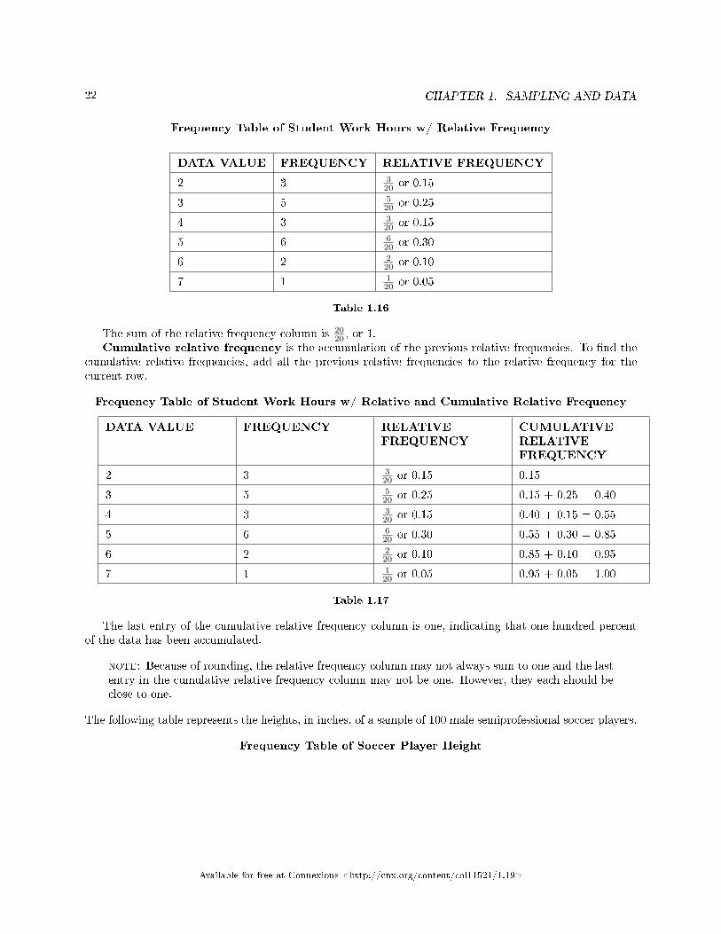
22 CHAPTER 1. SAMPLING AND DATA
Frequency Table of Student Work Hours w/ Relative Frequency
DATA VALUE FREQUENCY RELATIVE FREQUENCY
2 3 320 or 0.15
3 5 520 or 0.25
4 3 320 or 0.15
5 6 620 or 0.30
6 2 220 or 0.10
7 1 120 or 0.05
Table 1.16
The sum of the relative frequency column is 2020 , or 1.
Cumulative relative frequency is the accumulation of the previous relative frequencies. To �nd thecumulative relative frequencies, add all the previous relative frequencies to the relative frequency for thecurrent row.
Frequency Table of Student Work Hours w/ Relative and Cumulative Relative Frequency
DATA VALUE FREQUENCY RELATIVEFREQUENCY
CUMULATIVERELATIVEFREQUENCY
2 3 320 or 0.15 0.15
3 5 520 or 0.25 0.15 + 0.25 = 0.40
4 3 320 or 0.15 0.40 + 0.15 = 0.55
5 6 620 or 0.30 0.55 + 0.30 = 0.85
6 2 220 or 0.10 0.85 + 0.10 = 0.95
7 1 120 or 0.05 0.95 + 0.05 = 1.00
Table 1.17
The last entry of the cumulative relative frequency column is one, indicating that one hundred percentof the data has been accumulated.
note: Because of rounding, the relative frequency column may not always sum to one and the lastentry in the cumulative relative frequency column may not be one. However, they each should beclose to one.
The following table represents the heights, in inches, of a sample of 100 male semiprofessional soccer players.
Frequency Table of Soccer Player Height
Available for free at Connexions <http://cnx.org/content/col11521/1.19>
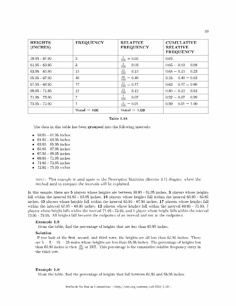
23
HEIGHTS(INCHES)
FREQUENCY RELATIVEFREQUENCY
CUMULATIVERELATIVEFREQUENCY
59.95 - 61.95 5 5100 = 0.05 0.05
61.95 - 63.95 3 3100 = 0.03 0.05 + 0.03 = 0.08
63.95 - 65.95 15 15100 = 0.15 0.08 + 0.15 = 0.23
65.95 - 67.95 40 40100 = 0.40 0.23 + 0.40 = 0.63
67.95 - 69.95 17 17100 = 0.17 0.63 + 0.17 = 0.80
69.95 - 71.95 12 12100 = 0.12 0.80 + 0.12 = 0.92
71.95 - 73.95 7 7100 = 0.07 0.92 + 0.07 = 0.99
73.95 - 75.95 1 1100 = 0.01 0.99 + 0.01 = 1.00
Total = 100 Total = 1.00
Table 1.18
The data in this table has been grouped into the following intervals:
• 59.95 - 61.95 inches• 61.95 - 63.95 inches• 63.95 - 65.95 inches• 65.95 - 67.95 inches• 67.95 - 69.95 inches• 69.95 - 71.95 inches• 71.95 - 73.95 inches• 73.95 - 75.95 inches
note: This example is used again in the Descriptive Statistics (Section 2.1) chapter, where themethod used to compute the intervals will be explained.
In this sample, there are 5 players whose heights are between 59.95 - 61.95 inches, 3 players whose heightsfall within the interval 61.95 - 63.95 inches, 15 players whose heights fall within the interval 63.95 - 65.95inches, 40 players whose heights fall within the interval 65.95 - 67.95 inches, 17 players whose heights fallwithin the interval 67.95 - 69.95 inches, 12 players whose heights fall within the interval 69.95 - 71.95, 7players whose height falls within the interval 71.95 - 73.95, and 1 player whose height falls within the interval73.95 - 75.95. All heights fall between the endpoints of an interval and not at the endpoints.
Example 1.8From the table, �nd the percentage of heights that are less than 65.95 inches.
SolutionIf you look at the �rst, second, and third rows, the heights are all less than 65.95 inches. Thereare 5 + 3 + 15 = 23 males whose heights are less than 65.95 inches. The percentage of heights lessthan 65.95 inches is then 23
100 or 23%. This percentage is the cumulative relative frequency entry inthe third row.
Example 1.9From the table, �nd the percentage of heights that fall between 61.95 and 65.95 inches.
Available for free at Connexions <http://cnx.org/content/col11521/1.19>
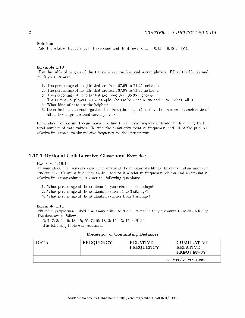
24 CHAPTER 1. SAMPLING AND DATA
SolutionAdd the relative frequencies in the second and third rows: 0.03 + 0.15 = 0.18 or 18%.
Example 1.10Use the table of heights of the 100 male semiprofessional soccer players. Fill in the blanks andcheck your answers.
1. The percentage of heights that are from 67.95 to 71.95 inches is:2. The percentage of heights that are from 67.95 to 73.95 inches is:3. The percentage of heights that are more than 65.95 inches is:4. The number of players in the sample who are between 61.95 and 71.95 inches tall is:5. What kind of data are the heights?6. Describe how you could gather this data (the heights) so that the data are characteristic of
all male semiprofessional soccer players.
Remember, you count frequencies. To �nd the relative frequency, divide the frequency by thetotal number of data values. To �nd the cumulative relative frequency, add all of the previousrelative frequencies to the relative frequency for the current row.
1.10.1 Optional Collaborative Classroom Exercise
Exercise 1.10.1In your class, have someone conduct a survey of the number of siblings (brothers and sisters) eachstudent has. Create a frequency table. Add to it a relative frequency column and a cumulativerelative frequency column. Answer the following questions:
1. What percentage of the students in your class has 0 siblings?2. What percentage of the students has from 1 to 3 siblings?3. What percentage of the students has fewer than 3 siblings?
Example 1.11Nineteen people were asked how many miles, to the nearest mile they commute to work each day.The data are as follows:
2; 5; 7; 3; 2; 10; 18; 15; 20; 7; 10; 18; 5; 12; 13; 12; 4; 5; 10The following table was produced:
Frequency of Commuting Distances
DATA FREQUENCY RELATIVEFREQUENCY
CUMULATIVERELATIVEFREQUENCY
continued on next page
Available for free at Connexions <http://cnx.org/content/col11521/1.19>
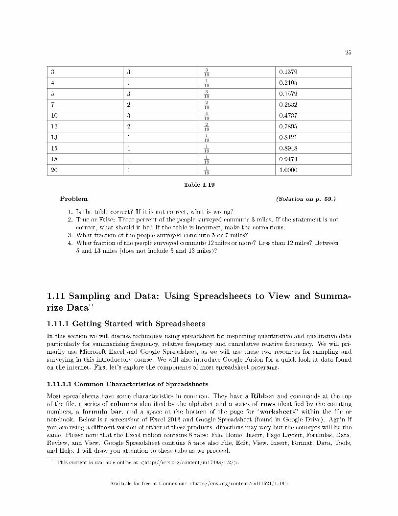
25
3 3 319 0.1579
4 1 119 0.2105
5 3 319 0.1579
7 2 219 0.2632
10 3 419 0.4737
12 2 219 0.7895
13 1 119 0.8421
15 1 119 0.8948
18 1 119 0.9474
20 1 119 1.0000
Table 1.19
Problem (Solution on p. 59.)
1. Is the table correct? If it is not correct, what is wrong?2. True or False: Three percent of the people surveyed commute 3 miles. If the statement is not
correct, what should it be? If the table is incorrect, make the corrections.3. What fraction of the people surveyed commute 5 or 7 miles?4. What fraction of the people surveyed commute 12 miles or more? Less than 12 miles? Between
5 and 13 miles (does not include 5 and 13 miles)?
1.11 Sampling and Data: Using Spreadsheets to View and Summa-rize Data11
1.11.1 Getting Started with Spreadsheets
In this section we will discuss techniques using spreadsheet for inspecting quantitative and qualitative dataparticularly for summarizing frequency, relative frequency and cumulative relative frequency. We will pri-marily use Microsoft Excel and Google Spreadsheet, as we will use these two resources for sampling andsurveying in this introductory course. We will also introduce Google Fusion for a quick look at data foundon the internet. First let's explore the components of most spreadsheet programs.
1.11.1.1 Common Characteristics of Spreadsheets
Most spreadsheets have some characteristics in common. They have a Ribbon and commands at the topof the �le, a series of columns identi�ed by the alphabet and a series of rows identi�ed by the countingnumbers, a formula bar, and a space at the bottom of the page for �worksheets� within the �le ornotebook. Below is a screenshot of Excel 2013 and Google Spreadsheet (found in Google Drive). Again ifyou are using a di�erent version of either of these products, directions may vary but the concepts will be thesame. Please note that the Excel ribbon contains 8 tabs: File, Home, Insert, Page Layout, Formulas, Data,Review, and View. Google Spreadsheet contains 8 tabs also File, Edit, View, Insert, Format, Data, Tools,and Help. I will draw you attention to these tabs as we proceed.
11This content is available online at <http://cnx.org/content/m47493/1.2/>.
Available for free at Connexions <http://cnx.org/content/col11521/1.19>
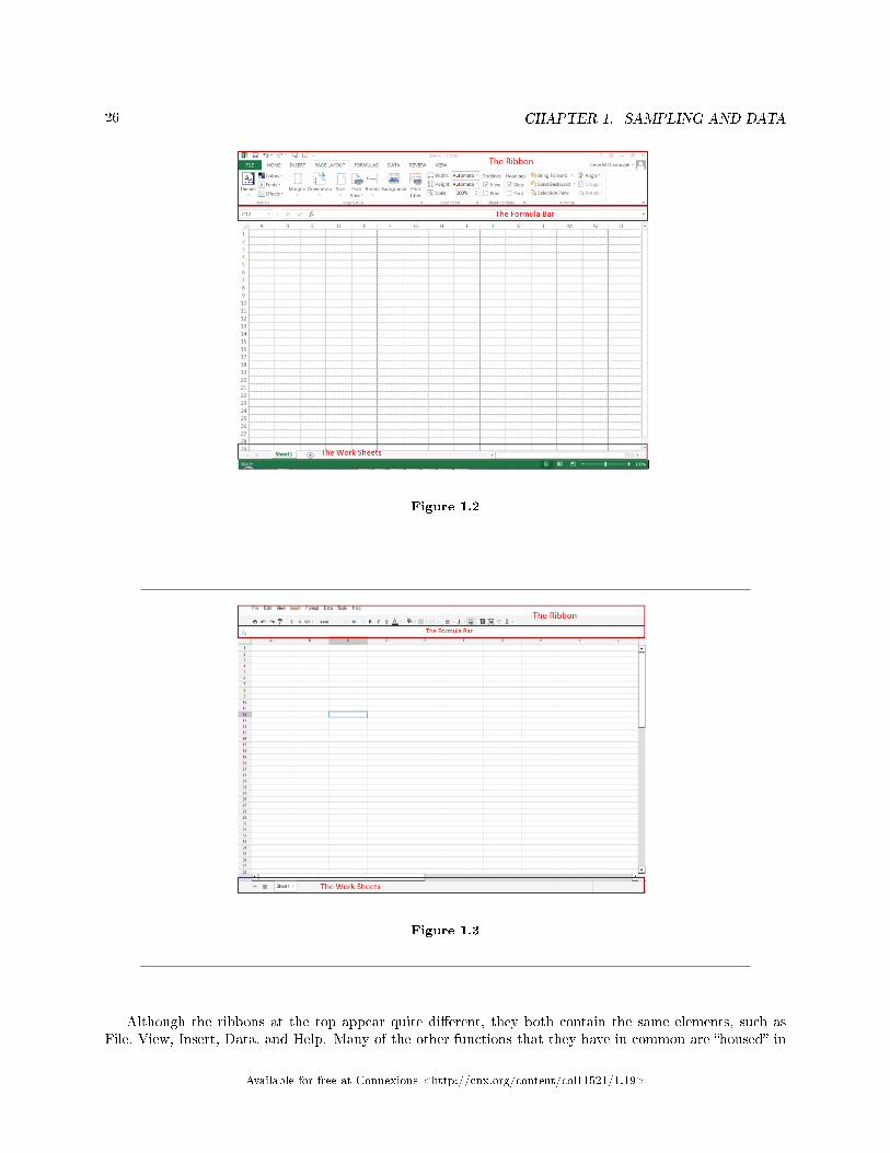
26 CHAPTER 1. SAMPLING AND DATA
Figure 1.2
Figure 1.3
Although the ribbons at the top appear quite di�erent, they both contain the same elements, such asFile, View, Insert, Data, and Help. Many of the other functions that they have in common are �housed� in
Available for free at Connexions <http://cnx.org/content/col11521/1.19>
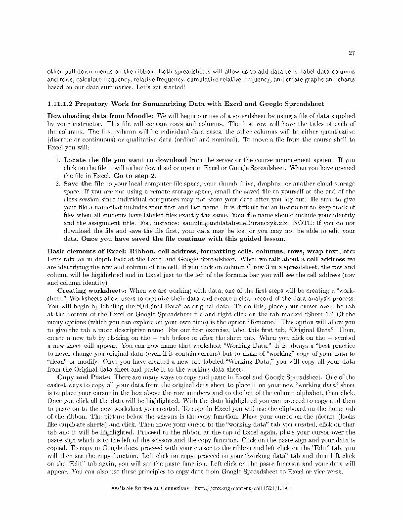
27
other pull down menus on the ribbon. Both spreadsheets will allow us to add data cells, label data columnsand rows, calculate frequency, relative frequency, cumulative relative frequency, and create graphs and chartsbased on our data summaries. Let's get started!
1.11.1.2 Prepatory Work for Summarizing Data with Excel and Google Spreadsheet
Downloading data from Moodle: We will begin our use of a spreadsheet by using a �le of data suppliedby your instructor. This �le will contain rows and columns. The �rst row will have the titles of each ofthe columns. The �rst column will be individual data cases, the other columns will be either quantitative(discrete or continuous) or qualitative data (ordinal and nominal). To move a �le from the course shell toExcel you will:
1. Locate the �le you want to download from the server or the course management system. If youclick on the �le it will either download or open in Excel or Google Spreadsheet. When you have openedthe �le in Excel. Go to step 2.
2. Save the �le to your local computer �le space, your thumb drive, dropbox, or another cloud storagespace. If you are not using a remote storage space, email the saved �le to yourself at the end of theclass session since individual computers may not store your data after you log out. Be sure to giveyour �le a namethat includes your �rst and last name. It is di�cult for an instructor to keep track of�les when all students have labeled �les exactly the same. Your �le name should include your identityand the assignment title. For, instance: samplinganddataIreneDuranczyk.xlx. NOTE: If you do notdownload the �le and save the �le �rst, your data may be lost or you may not be able to edit yourdata. Once you have saved the �le continue with this guided lesson.
Basic elements of Excel: Ribbon, cell address, formatting cells, columns, rows, wrap text, etc:Let's take an in depth look at the Excel and Google Spreadsheet. When we talk about a cell address weare identifying the row and column of the cell. If you click on column C row 3 in a spreadsheet, the row andcolumn will be highlighted and in Excel just to the left of the formula bar you will see the cell address (rowand column identity)
Creating worksheets: When we are working with data, one of the �rst steps will be creating a �work-sheet.� Worksheets allow users to organize their data and create a clear record of the data analysis process.You will begin by labeling the �Original Data� as original data. To do this, place your curser over the tabat the bottom of the Excel or Google Spreadsheet �le and right click on the tab marked �Sheet 1.� Of themany options (which you can explore on your own time) is the option �Rename.� This option will allow youto give the tab a more descriptive name. For our �rst exercise, label this �rst tab, �Original Data�. Then,create a new tab by clicking on the + tab before or after the sheet tab. When you click on the + symbola new sheet will appear. You can now name that worksheet �Working Data.� It is always a �best practiceto never change you original data (even if it contains errors) but to make of �working� copy of your data to�clean� or modify. Once you have created a new tab labeled �Working Data,� you will copy all your datafrom the Original data sheet and paste it to the working data sheet.
Copy and Paste: There are many ways to copy and paste in Excel and Google Spreadsheet. One of theeasiest ways to copy all your data from the original data sheet to place it on your new �working data� sheetis to place your cursor in the box above the row numbers and to the left of the column alphabet, then click.Once you click all the data will be highlighted. With the data highlighted you can proceed to copy and thento paste on to the new worksheet you created. To copy in Excel you will use the clipboard on the home tabof the ribbon. The picture below the scissors is the copy function. Place your cursor on the picture (lookslike duplicate sheets) and click. Then move your cursor to the �working data� tab you created, click on thattab and it will be highlighted. Proceed to the ribbon at the top of Excel again, place your cursor over thepaste sign which is to the left of the scissors and the copy function. Click on the paste sign and your data iscopied. To copy in Google docs, proceed with your cursor to the ribbon and left click on the �Edit� tab, youwill then see the copy function. Left click on copy, proceed to your �working data� tab and then left clickon the �Edit� tab again, you will see the paste function. Left click on the paste function and your data willappear. You can also use these principles to copy data from Google Spreadsheet to Excel or vice versa.
Available for free at Connexions <http://cnx.org/content/col11521/1.19>
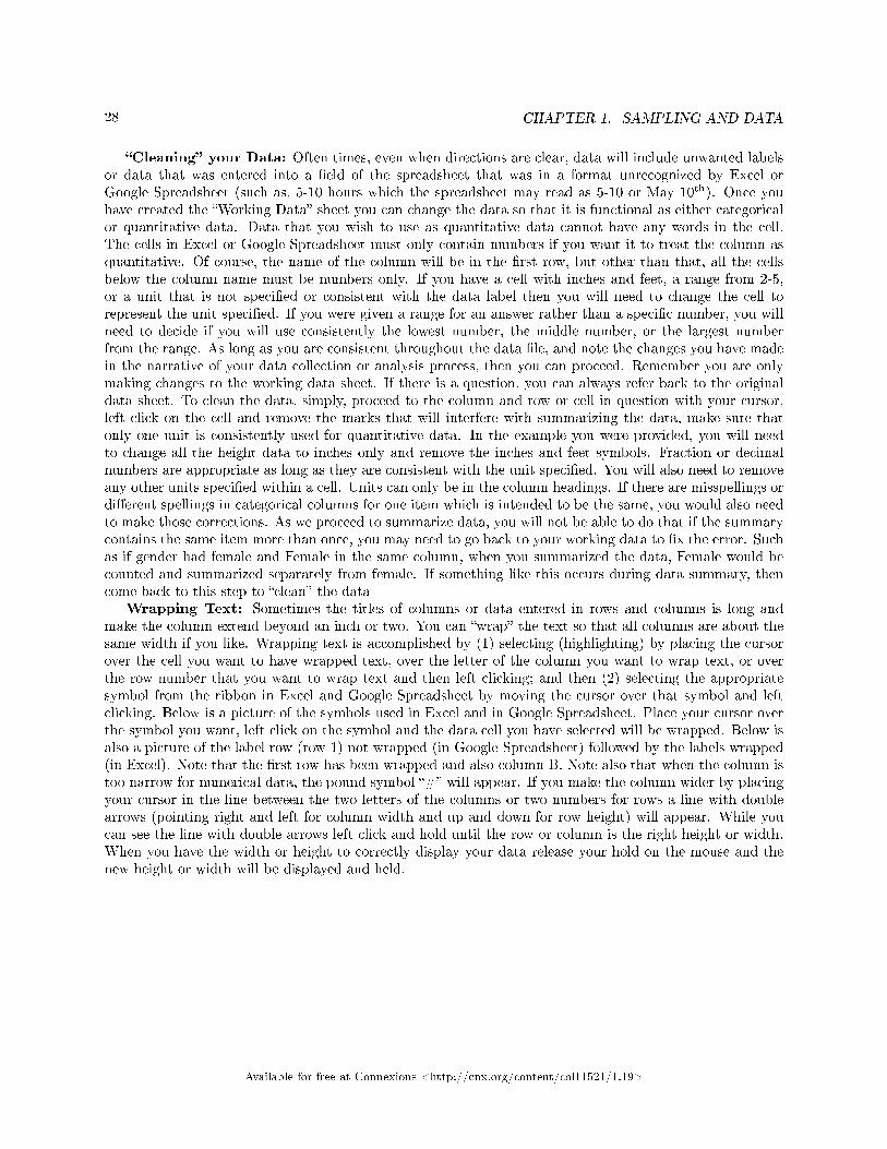
28 CHAPTER 1. SAMPLING AND DATA
�Cleaning� your Data: Often times, even when directions are clear, data will include unwanted labelsor data that was entered into a �eld of the spreadsheet that was in a format unrecognized by Excel orGoogle Spreadsheet (such as, 5-10 hours which the spreadsheet may read as 5-10 or May 10th). Once youhave created the �Working Data� sheet you can change the data so that it is functional as either categoricalor quantitative data. Data that you wish to use as quantitative data cannot have any words in the cell.The cells in Excel or Google Spreadsheet must only contain numbers if you want it to treat the column asquantitative. Of course, the name of the column will be in the �rst row, but other than that, all the cellsbelow the column name must be numbers only. If you have a cell with inches and feet, a range from 2-5,or a unit that is not speci�ed or consistent with the data label then you will need to change the cell torepresent the unit speci�ed. If you were given a range for an answer rather than a speci�c number, you willneed to decide if you will use consistently the lowest number, the middle number, or the largest numberfrom the range. As long as you are consistent throughout the data �le, and note the changes you have madein the narrative of your data collection or analysis process, then you can proceed. Remember you are onlymaking changes to the working data sheet. If there is a question, you can always refer back to the originaldata sheet. To clean the data, simply, proceed to the column and row or cell in question with your cursor,left click on the cell and remove the marks that will interfere with summarizing the data, make sure thatonly one unit is consistently used for quantitative data. In the example you were provided, you will needto change all the height data to inches only and remove the inches and feet symbols. Fraction or decimalnumbers are appropriate as long as they are consistent with the unit speci�ed. You will also need to removeany other units speci�ed within a cell. Units can only be in the column headings. If there are misspellings ordi�erent spellings in categorical columns for one item which is intended to be the same, you would also needto make those corrections. As we proceed to summarize data, you will not be able to do that if the summarycontains the same item more than once, you may need to go back to your working data to �x the error. Suchas if gender had female and Female in the same column, when you summarized the data, Female would becounted and summarized separately from female. If something like this occurs during data summary, thencome back to this step to �clean� the data
Wrapping Text: Sometimes the titles of columns or data entered in rows and columns is long andmake the column extend beyond an inch or two. You can �wrap� the text so that all columns are about thesame width if you like. Wrapping text is accomplished by (1) selecting (highlighting) by placing the cursorover the cell you want to have wrapped text, over the letter of the column you want to wrap text, or overthe row number that you want to wrap text and then left clicking; and then (2) selecting the appropriatesymbol from the ribbon in Excel and Google Spreadsheet by moving the cursor over that symbol and leftclicking. Below is a picture of the symbols used in Excel and in Google Spreadsheet. Place your cursor overthe symbol you want, left click on the symbol and the data cell you have selected will be wrapped. Below isalso a picture of the label row (row 1) not wrapped (in Google Spreadsheet) followed by the labels wrapped(in Excel). Note that the �rst row has been wrapped and also column B. Note also that when the column istoo narrow for numerical data, the pound symbol �#� will appear. If you make the column wider by placingyour cursor in the line between the two letters of the columns or two numbers for rows a line with doublearrows (pointing right and left for column width and up and down for row height) will appear. While youcan see the line with double arrows left click and hold until the row or column is the right height or width.When you have the width or height to correctly display your data release your hold on the mouse and thenew height or width will be displayed and held.
Available for free at Connexions <http://cnx.org/content/col11521/1.19>
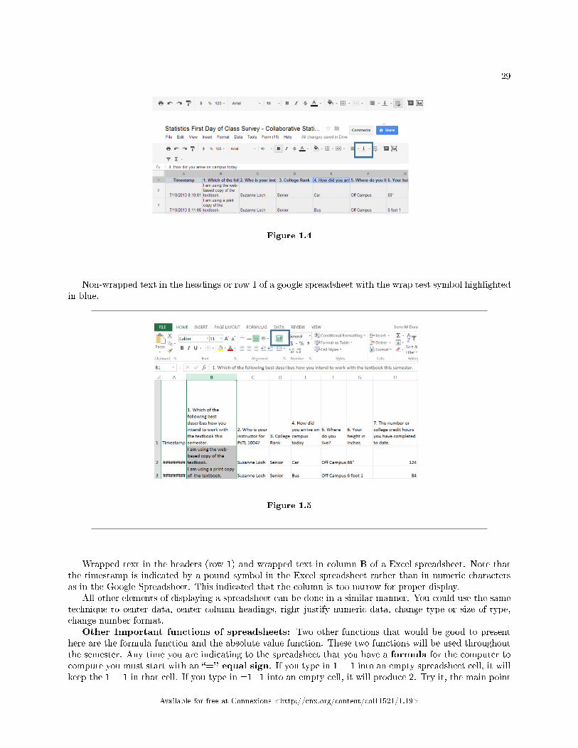
29
Figure 1.4
Non-wrapped text in the headings or row 1 of a google spreadsheet with the wrap test symbol highlightedin blue.
Figure 1.5
Wrapped text in the headers (row 1) and wrapped text in column B of a Excel spreadsheet. Note thatthe timestamp is indicated by a pound symbol in the Excel spreadsheet rather than in numeric charactersas in the Google Spreadsheet. This indicated that the column is too narrow for proper display.
All other elements of displaying a spreadsheet can be done in a similar manner. You could use the sametechnique to center data, center column headings, right justify numeric data, change type or size of type,change number format.
Other Important functions of spreadsheets: Two other functions that would be good to presenthere are the formula function and the absolute value function. These two functions will be used throughoutthe semester. Any time you are indicating to the spreadsheet that you have a formula for the computer tocompute you must start with an �=� equal sign. If you type in 1 + 1 into an empty spreadsheet cell, it willkeep the 1 + 1 in that cell. If you type in =1+1 into an empty cell, it will produce 2. Try it, the main point
Available for free at Connexions <http://cnx.org/content/col11521/1.19>
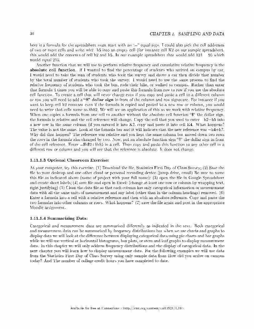
30 CHAPTER 1. SAMPLING AND DATA
here is a formula for the spreadsheet must start with an �=� equal sign. I could also pick the cell addressesof two or more cells and write =h2+h5 into an empty cell (for instance cell K2 on our sample spreadsheet,this would add the contents of cell h2 and h5. In our example spreadsheet that would add 124 + 95 whichwould equal 215.
Another function that we will use to perform relative frequency and cumulative relative frequency is theabsolute cell function. If I wanted to �nd the percentage of students who arrived on campus by car,I would need to take the sum of students who took the survey and drove a car then divide that numberby the total number of students who took the survey. I would need to use the same process to �nd therelative frequency of students who took the bus, rode their bike, or walked to campus. Rather than enterthat formula 4 times you will be able to copy and paste this formula from row to row if you use the absolutecell function. To create a cell that will never change even if you copy and paste a cell to a di�erent columnor row you will need to add a �$� dollar sign in front of the column and row signature. For instance if youwant to keep cell h2 constant even if the formula is copied and pasted to a new row or column, you wouldneed to write that cells name as $h$2, We will see an application of this as we work with relative frequency.When one copies a formula from one cell to another without the absolute cell function �$� the dollar sign,the formula is relative and the cell reference will change. Copy the cell that you used to enter =h2+h5 intoa new row in the same column (if you entered it into K2, copy and paste it into cell K4. What happens?The value is not the same. Look at the formula bar and it will indicate that the new reference was +h4+h7.Why did that happen? The reference was relative and you kept the same column but moved down two rowsthe rows in the formula also changed by two. Now, put an absolute function sign �$� the dollar sign in frontof the cell reference. Enter =$h$2+$h$5 in a cell. Then copy and paste this function to any other cell in adi�erent row or column and you will see that the reference is absolute. It does not change.
1.11.1.3 Optional Classroom Exercise:
At your computer, try this exercise: (1) Download the �le, Statistics First Day of Class Survey; (2) Save the�le to your desktop and one other cloud or personal recording device (jump drive, email) Be sure to namethis �le as indicated above (name of project with your full name); (3) open the �le in Google Spreadsheetand create sheet labels; (4) save �le and open in Excel; (change at least one row or column by wrapping text,right justifying) (5) Clean the data �le so that each column has only categorical information or measurementdata with all the same units of measurement and any label (other than in the column headings) removed. (6)Enter a formula into a cell with a relative reference and then with an absolute reference. Copy and paste thetwo formulas into other columns or rows. What happens? (7) save the �le again and post in the appropriateMoodle assignment.
1.11.1.4 Summarizing Data:
Categorical and measurement data are summarized di�erently as indicated in the text. Both categoricaland measurement data can be summarized by frequency distributions but when we use charts and graphs todisplay data we will look at the di�erence between displaying categorical data using pie charts and bar graphswhile we will use vertical or horizontal histograms, box plots, or stem and leaf graphs to display measurementdata. In this chapter we will only address frequency distributions and the display of categorical data. In thenext chapter you will learn how to display measurement data. For the following examples we will use datafrom the Statistics First Day of Class Survey using only sample data from How did you arrive on campustoday? And The number of college credit hours you have completed to date.
Available for free at Connexions <http://cnx.org/content/col11521/1.19>
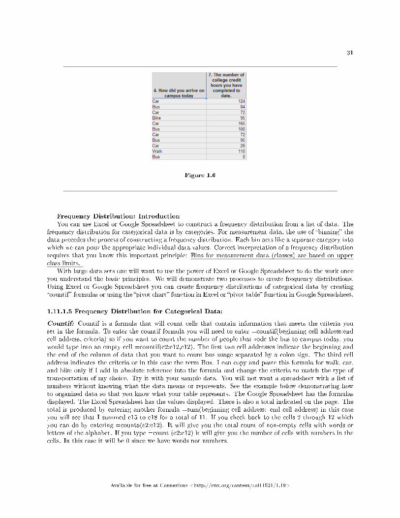
31
Figure 1.6
Frequency Distribution: IntroductionYou can use Excel or Google Spreadsheet to construct a frequency distribution from a list of data. The
frequency distribution for categorical data is by categories. For measurement data, the use of �binning� thedata precedes the process of constructing a frequency distribution. Each bin acts like a separate category intowhich we can pour the appropriate individual data values. Correct interpretation of a frequency distributionrequires that you know this important principle: Bins for measurement data (classes) are based on upperclass limits.
With large data sets one will want to use the power of Excel or Google Spreadsheet to do the work onceyou understand the basic principles. We will demonstrate two processes to create frequency distributions.Using Excel or Google Spreadsheet you can create frequency distributions of categorical data by creating�countif� formulas or using the �pivot chart� function in Excel or �pivot table� function in Google Spreadsheet.
1.11.1.5 Frequency Distribution for Categorical Data:
Countif: Countif is a formula that will count cells that contain information that meets the criteria youset in the formula. To enter the countif formula you will need to enter =countif(beginning cell address:endcell address, criteria) so if you want to count the number of people that rode the bus to campus today, youwould type into an empty cell =countif(e2:e12,e12). The �rst two cell addresses indicate the beginning andthe end of the column of data that you want to count bus usage separated by a colon sign. The third celladdress indicates the criteria or in this case the term Bus. I can copy and paste this formula for walk, car,and bike only if I add in absolute reference into the formula and change the criteria to match the type oftransportation of my choice. Try it with your sample data. You will not want a spreadsheet with a list ofnumbers without knowing what the data means or represents. See the example below demonstrating howto organized data so that you know what your table represents. The Google Spreadsheet has the formulasdisplayed. The Excel Spreadsheet has the values displayed. There is also a total indicated on the page. Thetotal is produced by entering another formula =sum(beginning cell address: end cell address) in this caseyou will see that I summed e15 to e18 for a total of 11. If you check back to the cells 2 through 12 whichyou can do by entering =counta(e2:e12). It will give you the total count of non-empty cells with words orletters of the alphabet. If you type =count (e2:e12) it will give you the number of cells with numbers in thecells. In this case it will be 0 since we have words not numbers.
Available for free at Connexions <http://cnx.org/content/col11521/1.19>
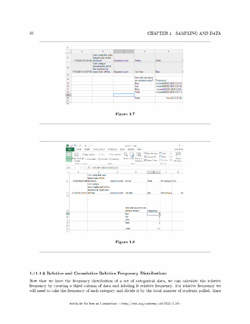
32 CHAPTER 1. SAMPLING AND DATA
Figure 1.7
Figure 1.8
1.11.1.6 Relative and Cumulative Relative Frequency Distribution:
Now that we have the frequency distribution of a set of categorical data, we can calculate the relativefrequency by creating a third column of data and labeling it relative frequency. For relative frequency wewill need to take the frequency of each category and divide it by the total number of students polled. Here
Available for free at Connexions <http://cnx.org/content/col11521/1.19>
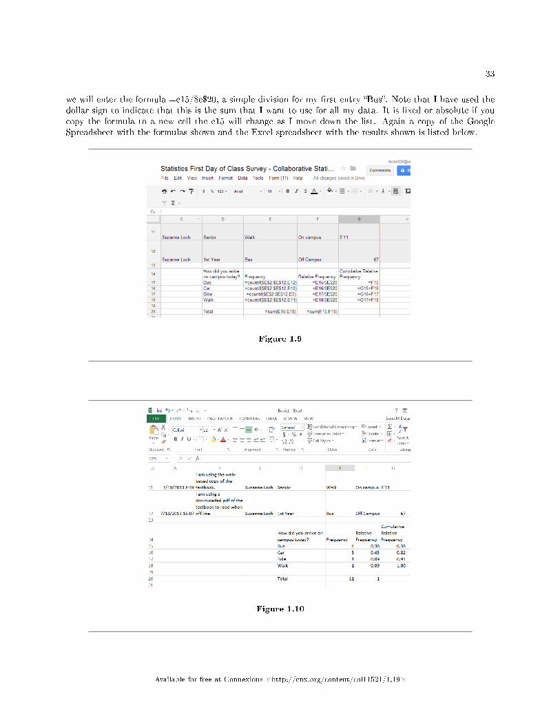
33
we will enter the formula =e15/$e$20, a simple division for my �rst entry �Bus�. Note that I have used thedollar sign to indicate that this is the sum that I want to use for all my data. It is �xed or absolute if youcopy the formula to a new cell the e15 will change as I move down the list. Again a copy of the GoogleSpreadsheet with the formulas shown and the Excel spreadsheet with the results shown is listed below.
Figure 1.9
Figure 1.10
Available for free at Connexions <http://cnx.org/content/col11521/1.19>
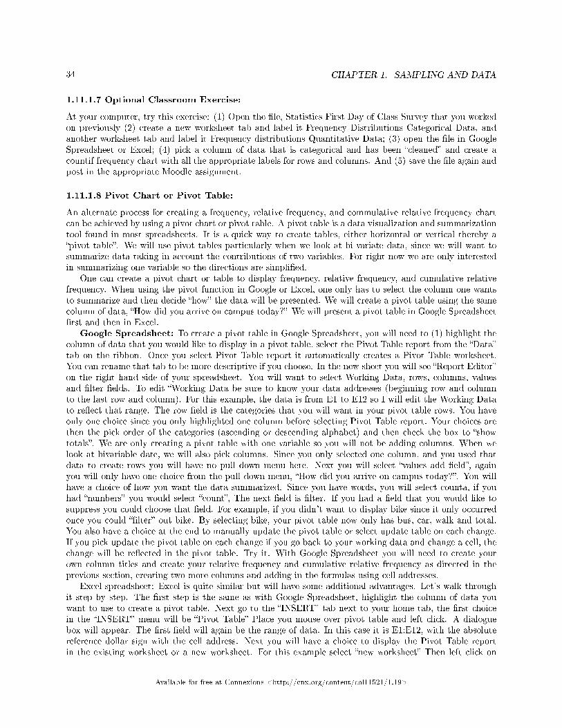
34 CHAPTER 1. SAMPLING AND DATA
1.11.1.7 Optional Classroom Exercise:
At your computer, try this exercise: (1) Open the �le, Statistics First Day of Class Survey that you workedon previously (2) create a new worksheet tab and label it Frequency Distributions Categorical Data, andanother worksheet tab and label it Frequency distributions Quantitative Data; (3) open the �le in GoogleSpreadsheet or Excel; (4) pick a column of data that is categorical and has been �cleaned� and create acountif frequency chart with all the appropriate labels for rows and columns. And (5) save the �le again andpost in the appropriate Moodle assignment.
1.11.1.8 Pivot Chart or Pivot Table:
An alternate process for creating a frequency, relative frequency, and commulative relative frequency chartcan be achieved by using a pivot chart or pivot table. A pivot table is a data visualization and summarizationtool found in most spreadsheets. It is a quick way to create tables, either horizontal or vertical thereby a�pivot table�. We will use pivot tables particularly when we look at bi-variate data, since we will want tosummarize data taking in account the contributions of two variables. For right now we are only interestedin summarizing one variable so the directions are simpli�ed.
One can create a pivot chart or table to display frequency, relative frequency, and cumulative relativefrequency. When using the pivot function in Google or Excel, one only has to select the column one wantsto summarize and then decide �how� the data will be presented. We will create a pivot table using the samecolumn of data, �How did you arrive on campus today?� We will present a pivot table in Google Spreadsheet�rst and then in Excel.
Google Spreadsheet: To create a pivot table in Google Spreadsheet, you will need to (1) highlight thecolumn of data that you would like to display in a pivot table, select the Pivot Table report from the �Data�tab on the ribbon. Once you select Pivot Table report it automatically creates a Pivot Table worksheet.You can rename that tab to be more descriptive if you choose. In the new sheet you will see �Report Editor�on the right hand side of your spreadsheet. You will want to select Working Data, rows, columns, valuesand �lter �elds. To edit �Working Data be sure to know your data addresses (beginning row and columnto the last row and column). For this example, the data is from E1 to E12 so I will edit the Working Datato re�ect that range. The row �eld is the categories that you will want in your pivot table rows. You haveonly one choice since you only highlighted one column before selecting Pivot Table report. Your choices arethen the pick order of the categories (ascending or descending alphabet) and then check the box to �showtotals�. We are only creating a pivot table with one variable so you will not be adding columns. When welook at bivariable date, we will also pick columns. Since you only selected one column, and you used thatdata to create rows you will have no pull down menu here. Next you will select �values add �eld�, againyou will only have one choice from the pull down menu, �How did you arrive on campus today?�. You willhave a choice of how you want the data summarized. Since you have words, you will select counta, if youhad �numbers� you would select �count�, The next �eld is �lter. If you had a �eld that you would like tosuppress you could choose that �eld. For example, if you didn't want to display bike since it only occurredonce you could ��lter� out bike. By selecting bike, your pivot table now only has bus, car, walk and total.You also have a choice at the end to manually update the pivot table or select update table on each change.If you pick update the pivot table on each change if you go back to your working data and change a cell, thechange will be re�ected in the pivot table. Try it. With Google Spreadsheet you will need to create yourown column titles and create your relative frequency and cumulative relative frequency as directed in theprevious section, creating two more columns and adding in the formulas using cell addresses.
Excel spreadsheet: Excel is quite similar but will have some additional advantages. Let's walk throughit step by step. The �rst step is the same as with Google Spreadsheet, highlight the column of data youwant to use to create a pivot table. Next go to the �INSERT� tab next to your home tab, the �rst choicein the �INSERT� menu will be �Pivot Table� Place you mouse over pivot table and left click. A dialoguebox will appear. The �rst �eld will again be the range of data. In this case it is E1:E12, with the absolutereference dollar sign with the cell address. Next you will have a choice to display the Pivot Table reportin the existing worksheet or a new worksheet. For this example select �new worksheet� Then left click on
Available for free at Connexions <http://cnx.org/content/col11521/1.19>
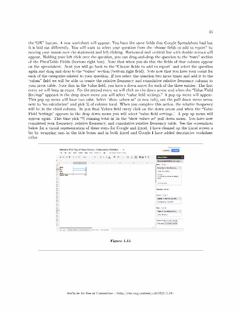
35
the �OK� button. A new worksheet will appear. You have the same �elds that Google Spreadsheet had butit is laid out di�erently. You will want to select your question from the �choose �elds to add to report� bymoving your mouse over the statement and left clicking. Horizontal and vertical line with double arrows willappear. Holding your left click over the question, you can drag-and-drop the question to the �rows� sectionof the PivotTable Fields (bottom right box). Note that when you do this the �elds of that column appearon the spreadsheet. Next you will go back to the �Choose �elds to add to report� and select the questionagain and drag-and-drop to the �values� section (bottom right �eld). Note now that you have your count foreach of the categories related to your question. If you select the question two more times and add it to the�values� �eld we will be able to create the relative frequency and cumulative relative frequency column toyour pivot table. Note that in the Value �eld, you have a down arrow for each of the three entries. The �rstentry we will keep as count. For the second entry we will click on the down arrow and when the �Value FieldSettings� appears in the drop down menu you will select �value �eld settings.� A pop up menu will appear.This pop up menu will have two tabs. Select �show values as� (a new tab), use the pull down menu arrownext to �no calculation� and pick % of column total. When you complete this action, the relative frequencywill be in the third column. In you �nal Values �eld entry click on the down arrow and when the �ValueField Settings� appears in the drop down menu you will select �value �eld settings.� A pop up menu willappear again. This time pick �% running total in�.in the �show values as� pull down menu. You have nowcompleted your frequency, relative frequency, and cumulative relative frequency table. See the screenshotsbelow for a visual representation of these steps for Google and Excel. I have cleaned up the Excel screen abit by wrapping text in the title boxes and in both Excel and Google I have added descriptive worksheettitles.
Figure 1.11
Available for free at Connexions <http://cnx.org/content/col11521/1.19>
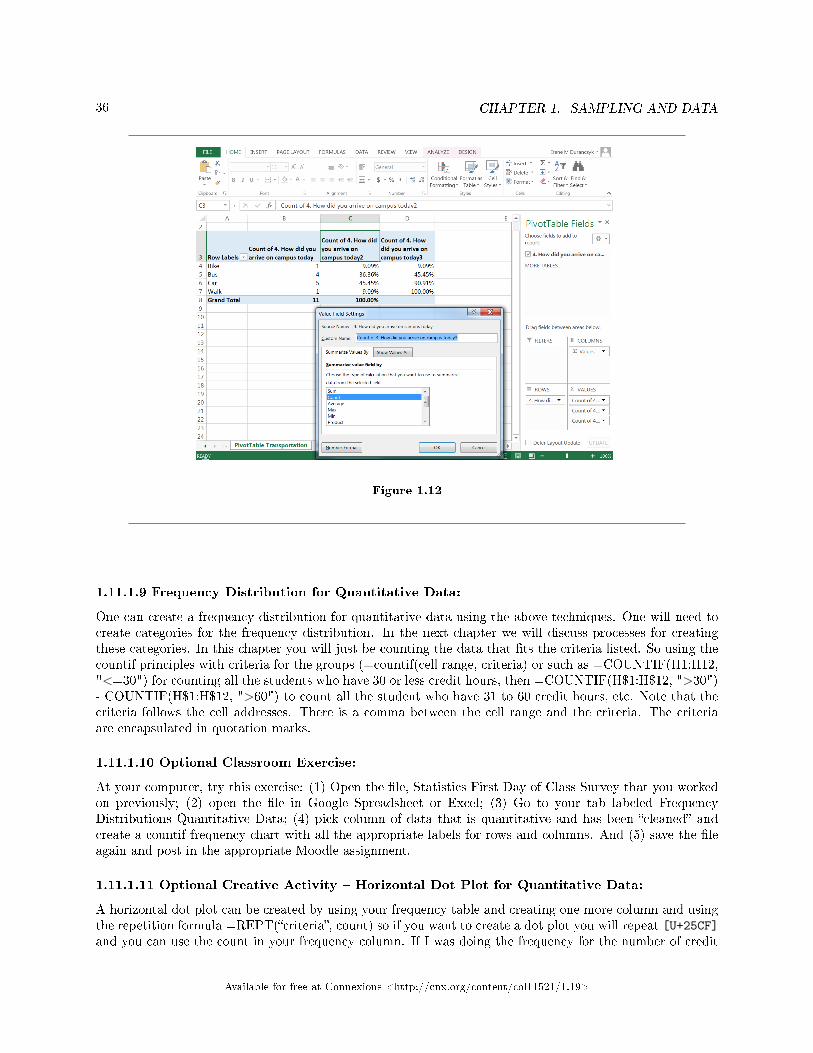
36 CHAPTER 1. SAMPLING AND DATA
Figure 1.12
1.11.1.9 Frequency Distribution for Quantitative Data:
One can create a frequency distribution for quantitative data using the above techniques. One will need tocreate categories for the frequency distribution. In the next chapter we will discuss processes for creatingthese categories. In this chapter you will just be counting the data that �ts the criteria listed. So using thecountif principles with criteria for the groups (=countif(cell range, criteria) or such as =COUNTIF(H1:H12,"<=30") for counting all the students who have 30 or less credit hours, then =COUNTIF(H$1:H$12, ">30")- COUNTIF(H$1:H$12, ">60") to count all the student who have 31 to 60 credit hours, etc. Note that thecriteria follows the cell addresses. There is a comma between the cell range and the criteria. The criteriaare encapsulated in quotation marks.
1.11.1.10 Optional Classroom Exercise:
At your computer, try this exercise: (1) Open the �le, Statistics First Day of Class Survey that you workedon previously; (2) open the �le in Google Spreadsheet or Excel; (3) Go to your tab labeled FrequencyDistributions Quantitative Data; (4) pick column of data that is quantitative and has been �cleaned� andcreate a countif frequency chart with all the appropriate labels for rows and columns. And (5) save the �leagain and post in the appropriate Moodle assignment.
1.11.1.11 Optional Creative Activity � Horizontal Dot Plot for Quantitative Data:
A horizontal dot plot can be created by using your frequency table and creating one more column and usingthe repetition formula =REPT(�criteria�, count) so if you want to create a dot plot you will repeat [U+25CF]and you can use the count in your frequency column. If I was doing the frequency for the number of credit
Available for free at Connexions <http://cnx.org/content/col11521/1.19>
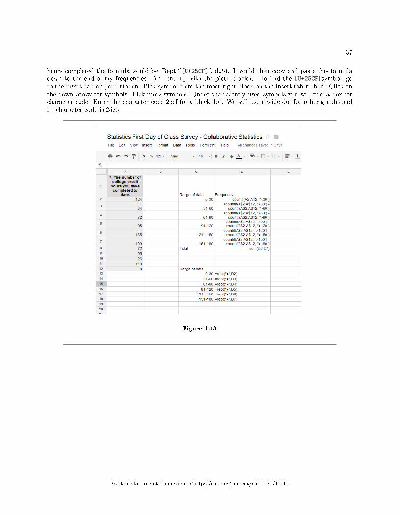
37
hours completed the formula would be `Rept(�[U+25CF]�, d25). I would then copy and paste this formuladown to the end of my frequencies. And end up with the picture below. To �nd the [U+25CF]symbol, goto the insert tab on your ribbon. Pick symbol from the most right block on the insert tab ribbon. Click onthe down arrow for symbols. Pick more symbols. Under the recently used symbols you will �nd a box forcharacter code. Enter the character code 25cf for a black dot. We will use a wide dot for other graphs andits character code is 25cb
Figure 1.13
Available for free at Connexions <http://cnx.org/content/col11521/1.19>
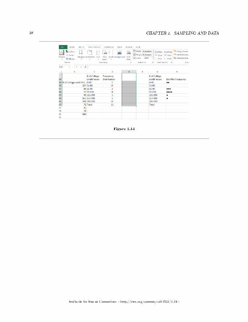
38 CHAPTER 1. SAMPLING AND DATA
Figure 1.14
Available for free at Connexions <http://cnx.org/content/col11521/1.19>
39
1.12 Sampling and Data: Summary12
Average
• A number that describes the central tendency of the data. There are a number of specialized averages,including the arithmetic mean, weighted mean, median, mode, and geometric mean.
Continuous Random Variable
• A random variable (RV) whose outcomes are measured. Example: The height of trees in the forest isa continuous RV
Cumulative Relative Frequency (cum. rel. freq. or cum RF)
• An accumulation of the previous relative frequencies. The Cumulative Relative Frequency is the sumof the relative frequencies for all values that are less than or equal to the given value.
Data
• A set of observations (a set of possible outcomes). Most data can be put into two groups: qualitative(hair color, ethnic groups and other attributes of the population) and quantitative (distance traveled tocollege, number of children in a family, etc.). Quantitative data can be separated into two subgroups:discrete and continuous. Data is discrete if it is the result of counting (the number of students of agiven ethnic group in a class, the number of books on a shelf, etc.). Data is continuous if it is the resultof measuring (distance traveled, weight of luggage, etc.)
• Quantitative Data (a number)
· Discrete (You count it.)· Continuous (You measure it.)
• Qualitative Data (a category, words)
Discrete Random Variable
• A random variable (RV) whose outcomes are counted.
Frequency (freq. or f)
• The number of times an answer occurs
Parameter
• A number that is a property of the population.
Population
• The collection, or set, of all individuals, objects, or measurements whose properties are being studied.
Probability
• Mathematical tool used to study randomness. A number between 0 and 1, inclusive, that gives thelikelihood that a speci�c event will occur.
Proportion
• As a number: A proportion is the number of successes divided by the total number in the sample.
12This content is available online at <http://cnx.org/content/m46128/1.2/>.
Available for free at Connexions <http://cnx.org/content/col11521/1.19>
40 CHAPTER 1. SAMPLING AND DATA
• As a probability distribution: Given a binomial random variable (RV), X ∼ B(n,p), consider the ratioof the number X of successes in n Bernouli trials to the number n of trials.
• p = x/n
Random Sampling
• Each member of the population has an equal chance of being selected
Relative Frequency (rel. freq. or RF)
• The proportion of times an answer occurs• Can be interpreted as a fraction, decimal, or percent
Sample
• A portion of the population understudy. A sample is representative if it characterizes the populationbeing studied.
Sampling
• With Replacement: A member of the population may be chosen more than once• Without Replacement: A member of the population may be chosen only once
Sampling Methods
• Random
· Simple random sample· Strati�ed sample· Cluster sample· Systematic sample
• Not Random
· Convenience sample
Statistic
• A numerical characteristic of the sample. A statistic estimates the corresponding population parameter.For example, the average number of full-time students in a 7:30 a.m. class for this term (statistic) isan estimate for the average number of full-time students in any class this term (parameter).
Statistics
• Deals with the collection, analysis, interpretation, and presentation of data
The 5 W's
• Who• What• Why• Where• When• How
Variable
• A characteristics of interest for each person or thing in a population. Variables may be numerical orcategorical.
Available for free at Connexions <http://cnx.org/content/col11521/1.19>
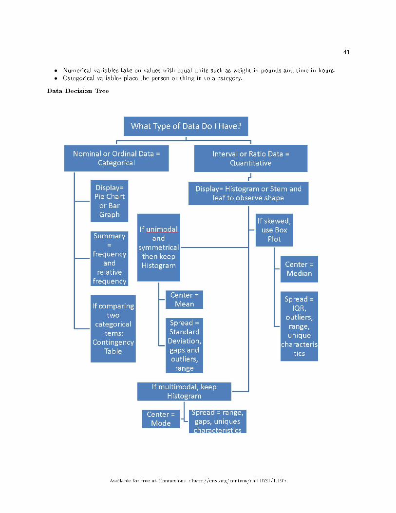
41
• Numerical variables take on values with equal units such as weight in pounds and time in hours.• Categorical variables place the person or thing in to a category.
Data Decision Tree
Available for free at Connexions <http://cnx.org/content/col11521/1.19>
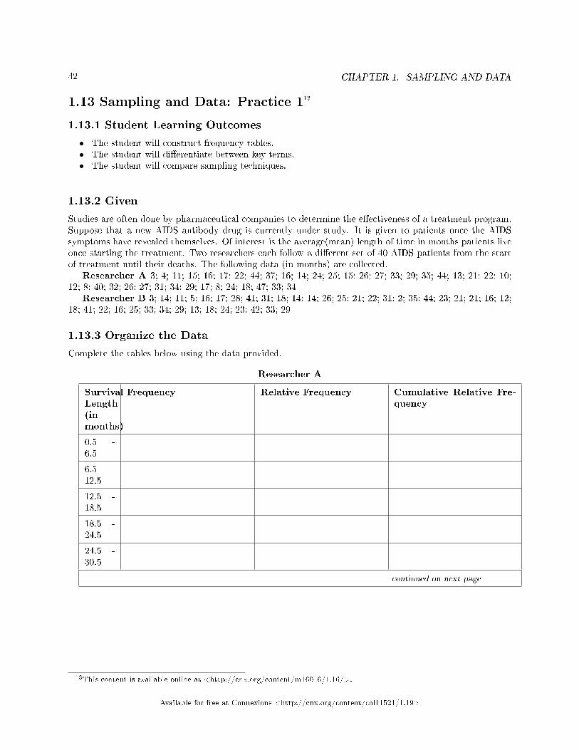
42 CHAPTER 1. SAMPLING AND DATA
1.13 Sampling and Data: Practice 113
1.13.1 Student Learning Outcomes
• The student will construct frequency tables.• The student will di�erentiate between key terms.• The student will compare sampling techniques.
1.13.2 Given
Studies are often done by pharmaceutical companies to determine the e�ectiveness of a treatment program.Suppose that a new AIDS antibody drug is currently under study. It is given to patients once the AIDSsymptoms have revealed themselves. Of interest is the average(mean) length of time in months patients liveonce starting the treatment. Two researchers each follow a di�erent set of 40 AIDS patients from the startof treatment until their deaths. The following data (in months) are collected.
Researcher A 3; 4; 11; 15; 16; 17; 22; 44; 37; 16; 14; 24; 25; 15; 26; 27; 33; 29; 35; 44; 13; 21; 22; 10;12; 8; 40; 32; 26; 27; 31; 34; 29; 17; 8; 24; 18; 47; 33; 34
Researcher B 3; 14; 11; 5; 16; 17; 28; 41; 31; 18; 14; 14; 26; 25; 21; 22; 31; 2; 35; 44; 23; 21; 21; 16; 12;18; 41; 22; 16; 25; 33; 34; 29; 13; 18; 24; 23; 42; 33; 29
1.13.3 Organize the Data
Complete the tables below using the data provided.
Researcher A
SurvivalLength(inmonths)
Frequency Relative Frequency Cumulative Relative Fre-quency
0.5 -6.5
6.5 -12.5
12.5 -18.5
18.5 -24.5
24.5 -30.5
continued on next page
13This content is available online at <http://cnx.org/content/m16016/1.16/>.
Available for free at Connexions <http://cnx.org/content/col11521/1.19>
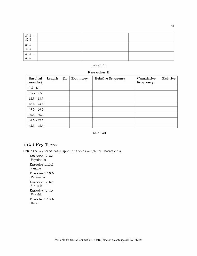
43
30.5 -36.5
36.5 -42.5
42.5 -48.5
Table 1.20
Researcher B
Survival Length (inmonths)
Frequency Relative Frequency Cumulative RelativeFrequency
0.5 - 6.5
6.5 - 12.5
12.5 - 18.5
18.5 - 24.5
24.5 - 30.5
30.5 - 36.5
36.5 - 42.5
42.5 - 48.5
Table 1.21
1.13.4 Key Terms
De�ne the key terms based upon the above example for Researcher A.
Exercise 1.13.1Population
Exercise 1.13.2Sample
Exercise 1.13.3Parameter
Exercise 1.13.4Statistic
Exercise 1.13.5Variable
Exercise 1.13.6Data
Available for free at Connexions <http://cnx.org/content/col11521/1.19>
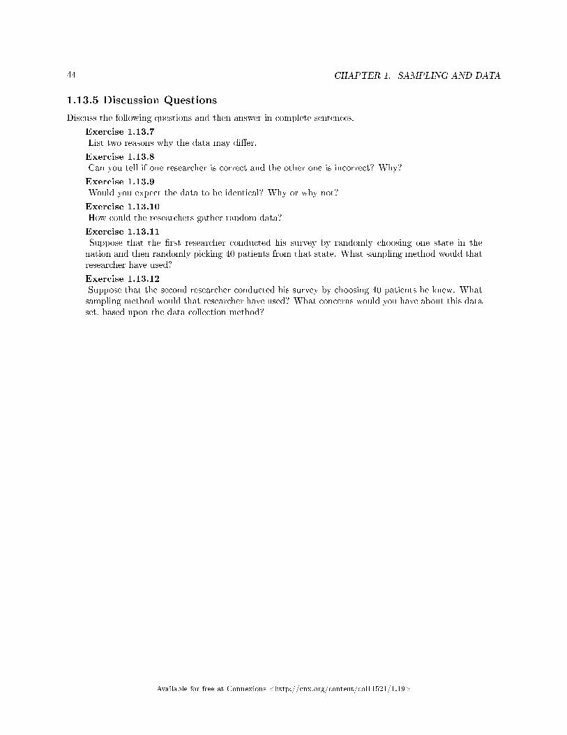
44 CHAPTER 1. SAMPLING AND DATA
1.13.5 Discussion Questions
Discuss the following questions and then answer in complete sentences.
Exercise 1.13.7List two reasons why the data may di�er.
Exercise 1.13.8Can you tell if one researcher is correct and the other one is incorrect? Why?
Exercise 1.13.9Would you expect the data to be identical? Why or why not?
Exercise 1.13.10How could the researchers gather random data?
Exercise 1.13.11Suppose that the �rst researcher conducted his survey by randomly choosing one state in thenation and then randomly picking 40 patients from that state. What sampling method would thatresearcher have used?
Exercise 1.13.12Suppose that the second researcher conducted his survey by choosing 40 patients he knew. Whatsampling method would that researcher have used? What concerns would you have about this dataset, based upon the data collection method?
Available for free at Connexions <http://cnx.org/content/col11521/1.19>
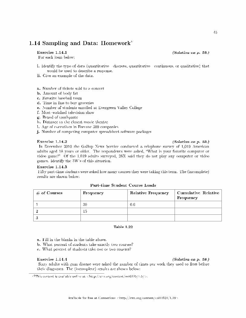
45
1.14 Sampling and Data: Homework14
Exercise 1.14.1 (Solution on p. 59.)
For each item below:
i. Identify the type of data (quantitative - discrete, quantitative - continuous, or qualitative) thatwould be used to describe a response.
ii. Give an example of the data.
a. Number of tickets sold to a concertb. Amount of body fatc. Favorite baseball teamd. Time in line to buy groceriese. Number of students enrolled at Evergreen Valley Collegef. Most�watched television showg. Brand of toothpasteh. Distance to the closest movie theatrei. Age of executives in Fortune 500 companiesj. Number of competing computer spreadsheet software packages
Exercise 1.14.2 (Solution on p. 59.)
In December 2010 the Gallup News Service conducted a telephone survey of 1,019 Americanadults aged 18 years or older. The respondents were asked, �What is your favorite computer orvideo game?� Of the 1,019 adults surveyed, 25% said they do not play any computer or videogames. Identify the 5W's of this situation.
Exercise 1.14.3Fifty part-time students were asked how many courses they were taking this term. The (incomplete)results are shown below:
Part-time Student Course Loads
# of Courses Frequency Relative Frequency Cumulative RelativeFrequency
1 30 0.6
2 15
3
Table 1.22
a. Fill in the blanks in the table above.b. What percent of students take exactly two courses?c. What percent of students take one or two courses?
Exercise 1.14.4 (Solution on p. 59.)
Sixty adults with gum disease were asked the number of times per week they used to �oss beforetheir diagnoses. The (incomplete) results are shown below:
14This content is available online at <http://cnx.org/content/m46125/1.5/>.
Available for free at Connexions <http://cnx.org/content/col11521/1.19>
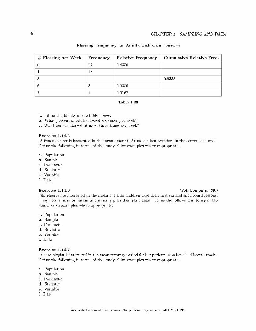
46 CHAPTER 1. SAMPLING AND DATA
Flossing Frequency for Adults with Gum Disease
# Flossing per Week Frequency Relative Frequency Cumulative Relative Freq.
0 27 0.4500
1 18
3 0.9333
6 3 0.0500
7 1 0.0167
Table 1.23
a. Fill in the blanks in the table above.b. What percent of adults �ossed six times per week?c. What percent �ossed at most three times per week?
Exercise 1.14.5A �tness center is interested in the mean amount of time a client exercises in the center each week.De�ne the following in terms of the study. Give examples where appropriate.
a. Populationb. Samplec. Parameterd. Statistice. Variablef. Data
Exercise 1.14.6 (Solution on p. 59.)
Ski resorts are interested in the mean age that children take their �rst ski and snowboard lessons.They need this information to optimally plan their ski classes. De�ne the following in terms of thestudy. Give examples where appropriate.
a. Populationb. Samplec. Parameterd. Statistice. Variablef. Data
Exercise 1.14.7A cardiologist is interested in the mean recovery period for her patients who have had heart attacks.De�ne the following in terms of the study. Give examples where appropriate.
a. Populationb. Samplec. Parameterd. Statistice. Variablef. Data
Available for free at Connexions <http://cnx.org/content/col11521/1.19>
47
Exercise 1.14.8 (Solution on p. 60.)
Insurance companies are interested in the mean health costs each year for their clients, so thatthey can determine the costs of health insurance. De�ne the following in terms of the study. Giveexamples where appropriate.
a. Populationb. Samplec. Parameterd. Statistice. Variablef. Data
Exercise 1.14.9A politician is interested in the proportion of voters in his district that think he is doing a goodjob. De�ne the following in terms of the study. Give examples where appropriate.
a. Populationb. Samplec. Parameterd. Statistice. Variablef. Data
Exercise 1.14.10 (Solution on p. 60.)
A marriage counselor is interested in the proportion the clients she counsels that stay married.De�ne the following in terms of the study. Give examples where appropriate.
a. Populationb. Samplec. Parameterd. Statistice. Variablef. Data
Exercise 1.14.11Political pollsters may be interested in the proportion of people that will vote for a particularcause. De�ne the following in terms of the study. Give examples where appropriate.
a. Populationb. Samplec. Parameterd. Statistice. Variablef. Data
Exercise 1.14.12 (Solution on p. 60.)
A marketing company is interested in the proportion of people that will buy a particular product.De�ne the following in terms of the study. Give examples where appropriate.
a. Populationb. Samplec. Parameterd. Statistic
Available for free at Connexions <http://cnx.org/content/col11521/1.19>
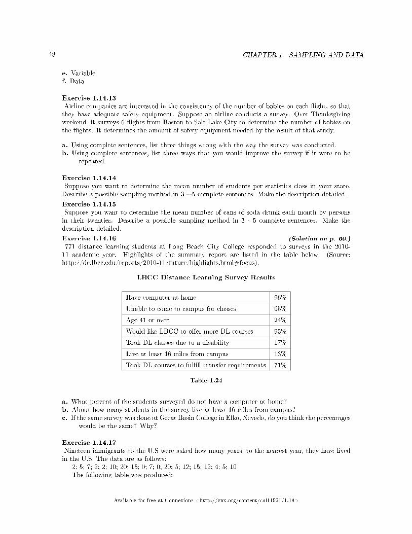
48 CHAPTER 1. SAMPLING AND DATA
e. Variablef. Data
Exercise 1.14.13Airline companies are interested in the consistency of the number of babies on each �ight, so thatthey have adequate safety equipment. Suppose an airline conducts a survey. Over Thanksgivingweekend, it surveys 6 �ights from Boston to Salt Lake City to determine the number of babies onthe �ights. It determines the amount of safety equipment needed by the result of that study.
a. Using complete sentences, list three things wrong with the way the survey was conducted.b. Using complete sentences, list three ways that you would improve the survey if it were to be
repeated.
Exercise 1.14.14Suppose you want to determine the mean number of students per statistics class in your state.Describe a possible sampling method in 3 � 5 complete sentences. Make the description detailed.
Exercise 1.14.15Suppose you want to determine the mean number of cans of soda drunk each month by personsin their twenties. Describe a possible sampling method in 3 - 5 complete sentences. Make thedescription detailed.
Exercise 1.14.16 (Solution on p. 60.)
771 distance learning students at Long Beach City College responded to surveys in the 2010-11 academic year. Highlights of the summary report are listed in the table below. (Source:http://de.lbcc.edu/reports/2010-11/future/highlights.html#focus).
LBCC Distance Learning Survey Results
Have computer at home 96%
Unable to come to campus for classes 65%
Age 41 or over 24%
Would like LBCC to o�er more DL courses 95%
Took DL classes due to a disability 17%
Live at least 16 miles from campus 13%
Took DL courses to ful�ll transfer requirements 71%
Table 1.24
a. What percent of the students surveyed do not have a computer at home?b. About how many students in the survey live at least 16 miles from campus?c. If the same survey was done at Great Basin College in Elko, Nevada, do you think the percentages
would be the same? Why?
Exercise 1.14.17Nineteen immigrants to the U.S were asked how many years, to the nearest year, they have livedin the U.S. The data are as follows:
2; 5; 7; 2; 2; 10; 20; 15; 0; 7; 0; 20; 5; 12; 15; 12; 4; 5; 10The following table was produced:
Available for free at Connexions <http://cnx.org/content/col11521/1.19>
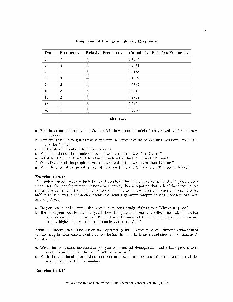
49
Frequency of Immigrant Survey Responses
Data Frequency Relative Frequency Cumulative Relative Frequency
0 2 219 0.1053
2 3 319 0.2632
4 1 119 0.3158
5 3 319 0.1579
7 2 219 0.5789
10 2 219 0.6842
12 2 219 0.7895
15 1 119 0.8421
20 1 119 1.0000
Table 1.25
a. Fix the errors on the table. Also, explain how someone might have arrived at the incorrectnumber(s).
b. Explain what is wrong with this statement: �47 percent of the people surveyed have lived in theU.S. for 5 years.�
c. Fix the statement above to make it correct.d. What fraction of the people surveyed have lived in the U.S. 5 or 7 years?e. What fraction of the people surveyed have lived in the U.S. at most 12 years?f. What fraction of the people surveyed have lived in the U.S. fewer than 12 years?g. What fraction of the people surveyed have lived in the U.S. from 5 to 20 years, inclusive?
Exercise 1.14.18A �random survey� was conducted of 3274 people of the �microprocessor generation� (people bornsince 1971, the year the microprocessor was invented). It was reported that 48% of those individualssurveyed stated that if they had $2000 to spend, they would use it for computer equipment. Also,66% of those surveyed considered themselves relatively savvy computer users. (Source: San JoseMercury News)
a. Do you consider the sample size large enough for a study of this type? Why or why not?b. Based on your �gut feeling,� do you believe the percents accurately re�ect the U.S. population
for those individuals born since 1971? If not, do you think the percents of the population areactually higher or lower than the sample statistics? Why?
Additional information: The survey was reported by Intel Corporation of individuals who visitedthe Los Angeles Convention Center to see the Smithsonian Institure's road show called �America'sSmithsonian.�
c. With this additional information, do you feel that all demographic and ethnic groups wereequally represented at the event? Why or why not?
d. With the additional information, comment on how accurately you think the sample statisticsre�ect the population parameters.
Exercise 1.14.19
Available for free at Connexions <http://cnx.org/content/col11521/1.19>
50 CHAPTER 1. SAMPLING AND DATA
a. List some practical di�culties involved in getting accurate results from a telephone survey.b. List some practical di�culties involved in getting accurate results from a mailed survey.c. With your classmates, brainstorm some ways to overcome these problems if you needed to
conduct a phone or mail survey.
1.14.1 Try these multiple choice questions
The next four questions refer to the following: A Lake Tahoe Community College instructor isinterested in the mean number of days Lake Tahoe Community College math students are absent from classduring a quarter.
Exercise 1.14.20 (Solution on p. 60.)
What is the population she is interested in?
A. All Lake Tahoe Community College studentsB. All Lake Tahoe Community College English studentsC. All Lake Tahoe Community College students in her classesD. All Lake Tahoe Community College math students
Exercise 1.14.21 (Solution on p. 60.)
Consider the following:X = number of days a Lake Tahoe Community College math student is absentIn this case, X is an example of a:
A. VariableB. PopulationC. StatisticD. Data
Exercise 1.14.22 (Solution on p. 60.)
The instructor takes her sample by gathering data on 5 randomly selected students from each LakeTahoe Community College math class. The type of sampling she used is
A. Cluster samplingB. Strati�ed samplingC. Simple random samplingD. Convenience sampling
Exercise 1.14.23 (Solution on p. 60.)
The instructor's sample produces an mean number of days absent of 3.5 days. This value is anexample of a
A. ParameterB. DataC. StatisticD. Variable
The next two questions refer to the following relative frequency table on hurricanes that have madedirect hits on the U.S between 1851 and 2004. Hurricanes are given a strength category rating based on theminimum wind speed generated by the storm. (http://www.nhc.noaa.gov/gifs/table5.gif 15)
15http://www.nhc.noaa.gov/gifs/table5.gif
Available for free at Connexions <http://cnx.org/content/col11521/1.19>
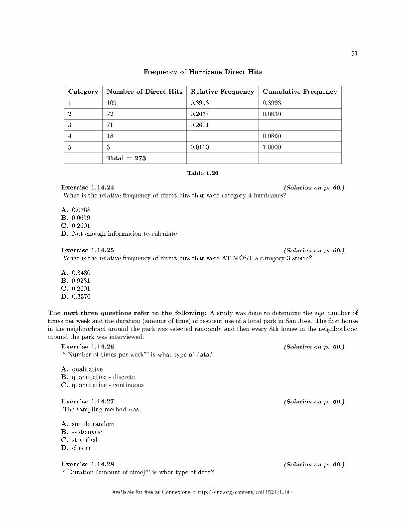
51
Frequency of Hurricane Direct Hits
Category Number of Direct Hits Relative Frequency Cumulative Frequency
1 109 0.3993 0.3993
2 72 0.2637 0.6630
3 71 0.2601
4 18 0.9890
5 3 0.0110 1.0000
Total = 273
Table 1.26
Exercise 1.14.24 (Solution on p. 60.)
What is the relative frequency of direct hits that were category 4 hurricanes?
A. 0.0768B. 0.0659C. 0.2601D. Not enough information to calculate
Exercise 1.14.25 (Solution on p. 60.)
What is the relative frequency of direct hits that were AT MOST a category 3 storm?
A. 0.3480B. 0.9231C. 0.2601D. 0.3370
The next three questions refer to the following: A study was done to determine the age, number oftimes per week and the duration (amount of time) of resident use of a local park in San Jose. The �rst housein the neighborhood around the park was selected randomly and then every 8th house in the neighborhoodaround the park was interviewed.
Exercise 1.14.26 (Solution on p. 60.)
� `Number of times per week� ' is what type of data?
A. qualitativeB. quantitative - discreteC. quantitative - continuous
Exercise 1.14.27 (Solution on p. 60.)
The sampling method was:
A. simple randomB. systematicC. strati�edD. cluster
Exercise 1.14.28 (Solution on p. 60.)
� `Duration (amount of time)� ' is what type of data?
Available for free at Connexions <http://cnx.org/content/col11521/1.19>
52 CHAPTER 1. SAMPLING AND DATA
A. qualitativeB. quantitative - discreteC. quantitative - continuous
Exercises 28 and 29 are not multiple choice exercises.
Exercise 1.14.29 (Solution on p. 61.)
Name the sampling method used in each of the following situations:
A. A woman in the airport is handing out questionnaires to travelers asking them to evaluate theairport's service. She does not ask travelers who are hurrying through the airport with theirhands full of luggage, but instead asks all travelers sitting near gates and who are not takingnaps while they wait.
B. A teacher wants to know if her students are doing homework so she randomly selects rows 2and 5, and then calls on all students in row 2 and all students in row 5 to present the solutionto homework problems to the class.
C. The marketing manager for an electronics chain store wants information about the ages of itscustomers. Over the next two weeks, at each store location, 100 randomly selected customersare given questionnaires to �ll out which asks for information about age, as well as aboutother variables of interest.
D. The librarian at a public library wants to determine what proportion of the library users arechildren. The librarian has a tally sheet on which she marks whether the books are checkedout by an adult or a child. She records this data for every 4th patron who checks out books.
E. A political party wants to know the reaction of voters to a debate between the candidates. Theday after the debate, the party's polling sta� calls 1200 randomly selected phone numbers.If a registered voter answers the phone or is available to come to the phone, that registeredvoter is asked who he/she intends to vote for and whether the debate changed his/her opinionof the candidates.
** Contributed by Roberta Bloom
Exercise 1.14.30 (Solution on p. 61.)
Several online textbook retailers advertise that they have lower prices than on-campus bookstores.However, an important factor is whether the internet retailers actually have the textbooks thatstudents need in stock. Students need to be able to get textbooks promptly at the beginning ofthe college term. If the book is not available, then a student would not be able to get the textbookat all, or might get a delayed delivery if the book is back ordered.
A college newspaper reporter is investigating textbook availability at online retailers. Hedecides to investigate one textbook for each of the following 7 subjects: calculus, biology,chemistry, physics, statistics, geology, and general engineering. He consults textbook industrysales data and selects the most popular nationally used textbook in each of these subjects. Hevisits websites for a random sample of major online textbook sellers and looks up each of these 7textbooks to see if they are available in stock for quick delivery through these retailers. Based onhis investigation, he writes an article in which he draws conclusions about the overall availabilityof all college textbooks through online textbook retailers.
Write an analysis of his study that addresses the following issues: Is his sample representa-tive of the population of all college textbooks? Explain why or why not. Describe some possiblesources of bias in this study, and how it might a�ect the results of the study. Give some suggestionsabout what could be done to improve the study.
** Contributed by Roberta Bloom
Available for free at Connexions <http://cnx.org/content/col11521/1.19>
53
1.15 Sampling and Data: Data Collection Lab I16
Class Time:Names:
1.15.1 Student Learning Outcomes
• The student will demonstrate the systematic sampling technique.• The student will construct Relative Frequency Tables.• The student will interpret results and their di�erences from di�erent data groupings.
1.15.2 Movie Survey
Ask �ve classmates from a di�erent class how many movies they saw last month at the theater. Do notinclude rented movies.
1. Record the data2. In class, randomly pick one person. On the class list, mark that person's name. Move down four
people's names on the class list. Mark that person's name. Continue doing this until you have marked12 people's names. You may need to go back to the start of the list. For each marked name recordbelow the �ve data values. You now have a total of 60 data values.
3. For each name marked, record the data:
____________________________________________________________
____________________________________________________________
____________________________________________________________
____________________________________________________________
____________________________________________________________
____________________________________________________________
Table 1.27
1.15.3 Order the Data
Complete the two relative frequency tables below using your class data.
16This content is available online at <http://cnx.org/content/m16004/1.11/>.
Available for free at Connexions <http://cnx.org/content/col11521/1.19>
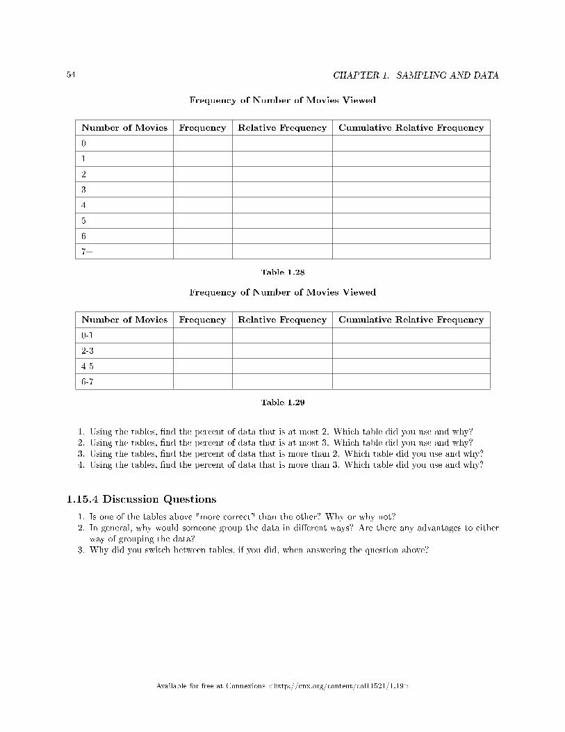
54 CHAPTER 1. SAMPLING AND DATA
Frequency of Number of Movies Viewed
Number of Movies Frequency Relative Frequency Cumulative Relative Frequency
0
1
2
3
4
5
6
7+
Table 1.28
Frequency of Number of Movies Viewed
Number of Movies Frequency Relative Frequency Cumulative Relative Frequency
0-1
2-3
4-5
6-7+
Table 1.29
1. Using the tables, �nd the percent of data that is at most 2. Which table did you use and why?2. Using the tables, �nd the percent of data that is at most 3. Which table did you use and why?3. Using the tables, �nd the percent of data that is more than 2. Which table did you use and why?4. Using the tables, �nd the percent of data that is more than 3. Which table did you use and why?
1.15.4 Discussion Questions
1. Is one of the tables above "more correct" than the other? Why or why not?2. In general, why would someone group the data in di�erent ways? Are there any advantages to either
way of grouping the data?3. Why did you switch between tables, if you did, when answering the question above?
Available for free at Connexions <http://cnx.org/content/col11521/1.19>
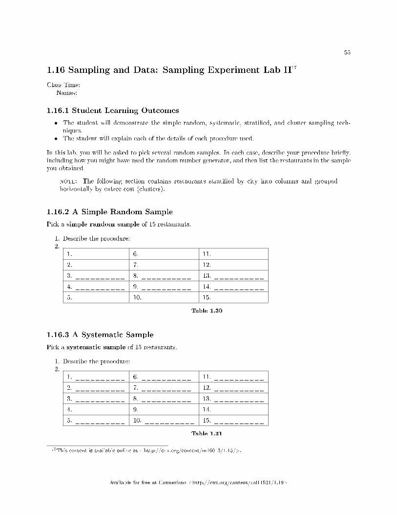
55
1.16 Sampling and Data: Sampling Experiment Lab II17
Class Time:Names:
1.16.1 Student Learning Outcomes
• The student will demonstrate the simple random, systematic, strati�ed, and cluster sampling tech-niques.
• The student will explain each of the details of each procedure used.
In this lab, you will be asked to pick several random samples. In each case, describe your procedure brie�y,including how you might have used the random number generator, and then list the restaurants in the sampleyou obtained
note: The following section contains restaurants strati�ed by city into columns and groupedhorizontally by entree cost (clusters).
1.16.2 A Simple Random Sample
Pick a simple random sample of 15 restaurants.
1. Describe the procedure:2.
1. __________ 6. __________ 11. __________
2. __________ 7. __________ 12. __________
3. __________ 8. __________ 13. __________
4. __________ 9. __________ 14. __________
5. __________ 10. __________ 15. __________
Table 1.30
1.16.3 A Systematic Sample
Pick a systematic sample of 15 restaurants.
1. Describe the procedure:2.
1. __________ 6. __________ 11. __________
2. __________ 7. __________ 12. __________
3. __________ 8. __________ 13. __________
4. __________ 9. __________ 14. __________
5. __________ 10. __________ 15. __________
Table 1.31
17This content is available online at <http://cnx.org/content/m16013/1.15/>.
Available for free at Connexions <http://cnx.org/content/col11521/1.19>
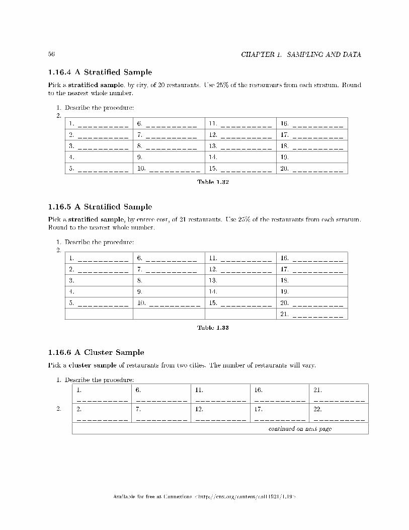
56 CHAPTER 1. SAMPLING AND DATA
1.16.4 A Strati�ed Sample
Pick a strati�ed sample, by city, of 20 restaurants. Use 25% of the restaurants from each stratum. Roundto the nearest whole number.
1. Describe the procedure:2.
1. __________ 6. __________ 11. __________ 16. __________
2. __________ 7. __________ 12. __________ 17. __________
3. __________ 8. __________ 13. __________ 18. __________
4. __________ 9. __________ 14. __________ 19. __________
5. __________ 10. __________ 15. __________ 20. __________
Table 1.32
1.16.5 A Strati�ed Sample
Pick a strati�ed sample, by entree cost, of 21 restaurants. Use 25% of the restaurants from each stratum.Round to the nearest whole number.
1. Describe the procedure:2.
1. __________ 6. __________ 11. __________ 16. __________
2. __________ 7. __________ 12. __________ 17. __________
3. __________ 8. __________ 13. __________ 18. __________
4. __________ 9. __________ 14. __________ 19. __________
5. __________ 10. __________ 15. __________ 20. __________
21. __________
Table 1.33
1.16.6 A Cluster Sample
Pick a cluster sample of restaurants from two cities. The number of restaurants will vary.
1. Describe the procedure:
2.
1.__________
6.__________
11.__________
16.__________
21.__________
2.__________
7.__________
12.__________
17.__________
22.__________
continued on next page
Available for free at Connexions <http://cnx.org/content/col11521/1.19>
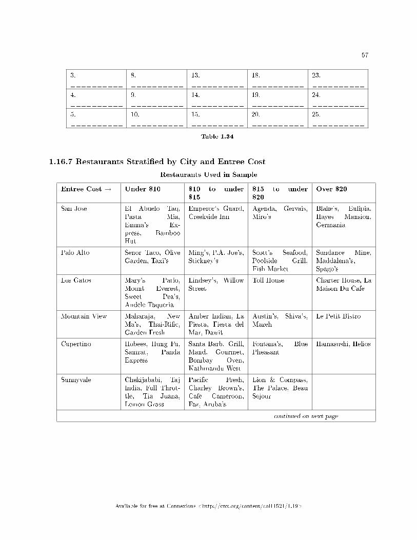
57
3.__________
8.__________
13.__________
18.__________
23.__________
4.__________
9.__________
14.__________
19.__________
24.__________
5.__________
10.__________
15.__________
20.__________
25.__________
Table 1.34
1.16.7 Restaurants Strati�ed by City and Entree Cost
Restaurants Used in Sample
Entree Cost → Under $10 $10 to under$15
$15 to under$20
Over $20
San Jose El Abuelo Taq,Pasta Mia,Emma's Ex-press, BambooHut
Emperor's Guard,Creekside Inn
Agenda, Gervais,Miro's
Blake's, Eulipia,Hayes Mansion,Germania
Palo Alto Senor Taco, OliveGarden, Taxi's
Ming's, P.A. Joe's,Stickney's
Scott's Seafood,Poolside Grill,Fish Market
Sundance Mine,Maddalena's,Spago's
Los Gatos Mary's Patio,Mount Everest,Sweet Pea's,Andele Taqueria
Lindsey's, WillowStreet
Toll House Charter House, LaMaison Du Cafe
Mountain View Maharaja, NewMa's, Thai-Ri�c,Garden Fresh
Amber Indian, LaFiesta, Fiesta delMar, Dawit
Austin's, Shiva's,Mazeh
Le Petit Bistro
Cupertino Hobees, Hung Fu,Samrat, PandaExpress
Santa Barb. Grill,Mand. Gourmet,Bombay Oven,Kathmandu West
Fontana's, BluePheasant
Hamasushi, Helios
Sunnyvale Chekijababi, TajIndia, Full Throt-tle, Tia Juana,Lemon Grass
Paci�c Fresh,Charley Brown's,Cafe Cameroon,Faz, Aruba's
Lion & Compass,The Palace, BeauSejour
continued on next page
Available for free at Connexions <http://cnx.org/content/col11521/1.19>

58 CHAPTER 1. SAMPLING AND DATA
Santa Clara Rangoli, Ar-madillo Willy's,Thai Pepper,Pasand
Arthur's, Katie'sCafe, Pedro's, LaGalleria
Birk's, TruyaSushi, ValleyPlaza
Lakeside, Mari-ani's
Table 1.35
note: The original lab was designed and contributed by Carol Olmstead.
Available for free at Connexions <http://cnx.org/content/col11521/1.19>
59
Solutions to Exercises in Chapter 1
Solution to Example 1.5, Problem (p. 7)Items 1, 5, 11, and 12 are quantitative discrete; items 4, 6, 10, and 14 are quantitative continuous; anditems 2, 3, 7, 8, 9, and 13 are qualitative.Solution to Exercise 1.6.1 (p. 12)Who: 2227 American families What: Family income Why: To understand the relationship between theAmerican Dream and economic mobility. Where: United States of America When: 1968 to present How:Longitudinal studySolution to Example 1.10, Problem (p. 24)
1. 29%2. 36%3. 77%4. 875. quantitative continuous6. get rosters from each team and choose a simple random sample from each
Solution to Example 1.11, Problem (p. 25)
1. No. Frequency column sums to 18, not 19. Not all cumulative relative frequencies are correct.2. False. Frequency for 3 miles should be 1; for 2 miles (left out), 2. Cumulative relative frequency column
should read: 0.1052, 0.1579, 0.2105, 0.3684, 0.4737, 0.6316, 0.7368, 0.7895, 0.8421, 0.9474, 1.3. 5
194. 7
19 ,1219 ,
719
Solutions to Sampling and Data: Homework
Solution to Exercise 1.14.1 (p. 45)
a. quantitative - discreteb. quantitative - continuousc. qualitatived. quantitative - continuouse. quantitative - discretef. qualitativeg. qualitativeh. quantitative - continuousi. quantitative - continuousj. quantitative - discrete
Solution to Exercise 1.14.2 (p. 45)Who: 1,019 American Adults aged 18 years and older What: Survey Question, "What is your favoritecomputer or video game?" Why: not stated Where: not stated When: Dec. 2010 How: a telephone surveySolution to Exercise 1.14.4 (p. 45)
a. Cum. Rel. Freq. for 0 is 0.4500Rel. Freq. for 1 is 0.3000 and Cum. Rel. Freq. for 1 or less is 0.7500Freq. for 3 is 11 and Rel. Freq. is 0.1833Cum. Rel. Freq. for 6 or less is 0.9833Cum. Rel. Freq. for 7 or less is 1
b. 5.00%c. 93.33%
Solution to Exercise 1.14.6 (p. 46)
Available for free at Connexions <http://cnx.org/content/col11521/1.19>
60 CHAPTER 1. SAMPLING AND DATA
a. Children who take ski or snowboard lessonsb. A group of these childrenc. The population meand. The sample meane. X = the age of one child who takes the �rst ski or snowboard lessonf. Values for X, such as 3, 7, etc.
Solution to Exercise 1.14.8 (p. 47)
a. The clients of the insurance companiesb. A group of the clientsc. The mean health costs of the clientsd. The mean health costs of the samplee. X = the health costs of one clientf. Values for X, such as 34, 9, 82, etc.
Solution to Exercise 1.14.10 (p. 47)
a. All the clients of the counselorb. A group of the clientsc. The proportion of all her clients who stay marriedd. The proportion of the sample who stay marriede. X = the number of couples who stay marriedf. yes, no
Solution to Exercise 1.14.12 (p. 47)
a. All people (maybe in a certain geographic area, such as the United States)b. A group of the peoplec. The proportion of all people who will buy the productd. The proportion of the sample who will buy the producte. X = the number of people who will buy itf. buy, not buy
Solution to Exercise 1.14.16 (p. 48)
a: 4%b: 100
Solution to Exercise 1.14.20 (p. 50)DSolution to Exercise 1.14.21 (p. 50)ASolution to Exercise 1.14.22 (p. 50)BSolution to Exercise 1.14.23 (p. 50)CSolution to Exercise 1.14.24 (p. 51)BSolution to Exercise 1.14.25 (p. 51)BSolution to Exercise 1.14.26 (p. 51)BSolution to Exercise 1.14.27 (p. 51)B
Available for free at Connexions <http://cnx.org/content/col11521/1.19>
61
Solution to Exercise 1.14.28 (p. 51)CSolution to Exercise 1.14.29 (p. 52)
A. ConvenienceB. ClusterC. Strati�edD. SystematicE. Simple Random
Solution to Exercise 1.14.30 (p. 52)The answer below contains some of the issues that students might discuss for this problem. Individualstudent's answers may also identify other issues that pertain to this problem that are not included in theanswer below.
The sample is not representative of the population of all college textbooks. Two reasons why it isnot representative are that he only sampled 7 subjects and he only investigated one textbook in eachsubject. There are several possible sources of bias in the study. The 7 subjects that he investigated areall in mathematics and the sciences; there are many subjects in the humanities, social sciences, and manyother subject areas, (for example: literature, art, history, psychology, sociology, business) that he did notinvestigate at all. It may be that di�erent subject areas exhibit di�erent patterns of textbook availability,but his sample would not detect such results.
He also only looked at the most popular textbook in each of the subjects he investigated. Theavailability of the most popular textbooks may di�er from the availability of other textbooks in one of twoways:
• the most popular textbooks may be more readily available online, because more new copies are printedand more students nationwide selling back their used copies OR
• the most popular textbooks may be harder to �nd available online, because more student demandexhausts the supply more quickly.
In reality, many college students do not use the most popular textbook in their subject, and this study givesno useful information about the situation for those less popular textbooks.
He could improve this study by
• expanding the selection of subjects he investigates so that it is more representative of all subjectsstudied by college students and
• expanding the selection of textbooks he investigates within each subject to include a mixed represen-tation of both the popular and less popular textbooks.
Available for free at Connexions <http://cnx.org/content/col11521/1.19>

62 CHAPTER 1. SAMPLING AND DATA
Available for free at Connexions <http://cnx.org/content/col11521/1.19>
Chapter 2
Univariate Descriptive Statistics
2.1 Descriptive Statistics: Introduction1
2.1.1 Student Learning Outcomes
By the end of this chapter, the student should be able to:
• Display data graphically and interpret graphs: stemplots, histograms and boxplots.• Recognize, describe, and calculate the measures of location of data: quartiles and percentiles.• Recognize, describe, and calculate the measures of the center of data: mean, median, and mode.• Recognize, describe, and calculate the measures of the spread of data: variance, standard deviation,
and range.
2.1.2 Introduction
Once you have collected data, what will you do with it? Data can be described and presented in manydi�erent formats. For example, suppose you are interested in buying a house in a particular area. You mayhave no clue about the house prices, so you might ask your real estate agent to give you a sample data set ofprices. Looking at all the prices in the sample often is overwhelming. A better way might be to look at themedian price and the variation of prices. The median and variation are just two ways that you will learn todescribe data. Your agent might also provide you with a graph of the data.
In this chapter, you will study numerical and graphical ways to describe and display your data. This areaof statistics is called "Descriptive Statistics". You will learn to calculate, and even more importantly, tointerpret these measurements and graphs.
2.2 Descriptive Statistics: Displaying Data2
A statistical graph is a tool that helps you learn about the shape or distribution of a sample. The graph canbe a more e�ective way of presenting data than a mass of numbers because we can see where data clustersand where there are only a few data values. Newspapers and the Internet use graphs to show trends and toenable readers to compare facts and �gures quickly.
Statisticians often graph data �rst to get a picture of the data. Then, more formal tools may be applied.Some of the types of graphs that are used to summarize and organize data are the dot plot, the bar chart,
the histogram, the stem-and-leaf plot, the frequency polygon (a type of broken line graph), pie charts, and
1This content is available online at <http://cnx.org/content/m16300/1.9/>.2This content is available online at <http://cnx.org/content/m16297/1.9/>.
Available for free at Connexions <http://cnx.org/content/col11521/1.19>
63
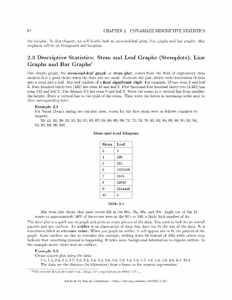
64 CHAPTER 2. UNIVARIATE DESCRIPTIVE STATISTICS
the boxplot. In this chapter, we will brie�y look at stem-and-leaf plots, line graphs and bar graphs. Ouremphasis will be on histograms and boxplots.
2.3 Descriptive Statistics: Stem and Leaf Graphs (Stemplots), LineGraphs and Bar Graphs3
One simple graph, the stem-and-leaf graph or stem plot, comes from the �eld of exploratory dataanalysis.It is a good choice when the data sets are small. To create the plot, divide each observation of datainto a stem and a leaf. The leaf consists of a �nal signi�cant digit. For example, 23 has stem 2 and leaf3. Four hundred thirty-two (432) has stem 43 and leaf 2. Five thousand four hundred thirty-two (5,432) hasstem 543 and leaf 2. The decimal 9.3 has stem 9 and leaf 3. Write the stems in a vertical line from smallestthe largest. Draw a vertical line to the right of the stems. Then write the leaves in increasing order next totheir corresponding stem.
Example 2.1For Susan Dean's spring pre-calculus class, scores for the �rst exam were as follows (smallest tolargest):
33; 42; 49; 49; 53; 55; 55; 61; 63; 67; 68; 68; 69; 69; 72; 73; 74; 78; 80; 83; 88; 88; 88; 90; 92; 94;94; 94; 94; 96; 100
Stem-and-Leaf Diagram
Stem Leaf
3 3
4 299
5 355
6 1378899
7 2348
8 03888
9 0244446
10 0
Table 2.1
The stem plot shows that most scores fell in the 60s, 70s, 80s, and 90s. Eight out of the 31scores or approximately 26% of the scores were in the 90's or 100, a fairly high number of As.
The stem plot is a quick way to graph and gives an exact picture of the data. You want to look for an overallpattern and any outliers. An outlier is an observation of data that does not �t the rest of the data. It issometimes called an extreme value. When you graph an outlier, it will appear not to �t the pattern of thegraph. Some outliers are due to mistakes (for example, writing down 50 instead of 500) while others mayindicate that something unusual is happening. It takes some background information to explain outliers. Inthe example above, there were no outliers.
Example 2.2Create a stem plot using the data:
1.1; 1.5; 2.3; 2.5; 2.7; 3.2; 3.3; 3.3; 3.5; 3.8; 4.0; 4.2; 4.5; 4.5; 4.7; 4.8; 5.5; 5.6; 6.5; 6.7; 12.3The data are the distance (in kilometers) from a home to the nearest supermarket.
3This content is available online at <http://cnx.org/content/m16849/1.17/>.
Available for free at Connexions <http://cnx.org/content/col11521/1.19>
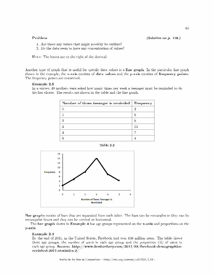
65
Problem (Solution on p. 126.)
1. Are there any values that might possibly be outliers?2. Do the data seem to have any concentration of values?
Hint: The leaves are to the right of the decimal.
Another type of graph that is useful for speci�c data values is a line graph. In the particular line graphshown in the example, the x-axis consists of data values and the y-axis consists of frequency points.The frequency points are connected.
Example 2.3In a survey, 40 mothers were asked how many times per week a teenager must be reminded to dohis/her chores. The results are shown in the table and the line graph.
Number of times teenager is reminded Frequency
0 2
1 5
2 8
3 14
4 7
5 4
Table 2.2
Bar graphs consist of bars that are separated from each other. The bars can be rectangles or they can berectangular boxes and they can be vertical or horizontal.
The bar graph shown in Example 4 has age groups represented on the x-axis and proportions on they-axis.
Example 2.4By the end of 2011, in the United States, Facebook had over 146 million users. The table showsthree age groups, the number of users in each age group and the proportion (%) of users ineach age group. Source: http://www.kenburbary.com/2011/03/facebook-demographics-revisited-2011-statistics-2/
Available for free at Connexions <http://cnx.org/content/col11521/1.19>
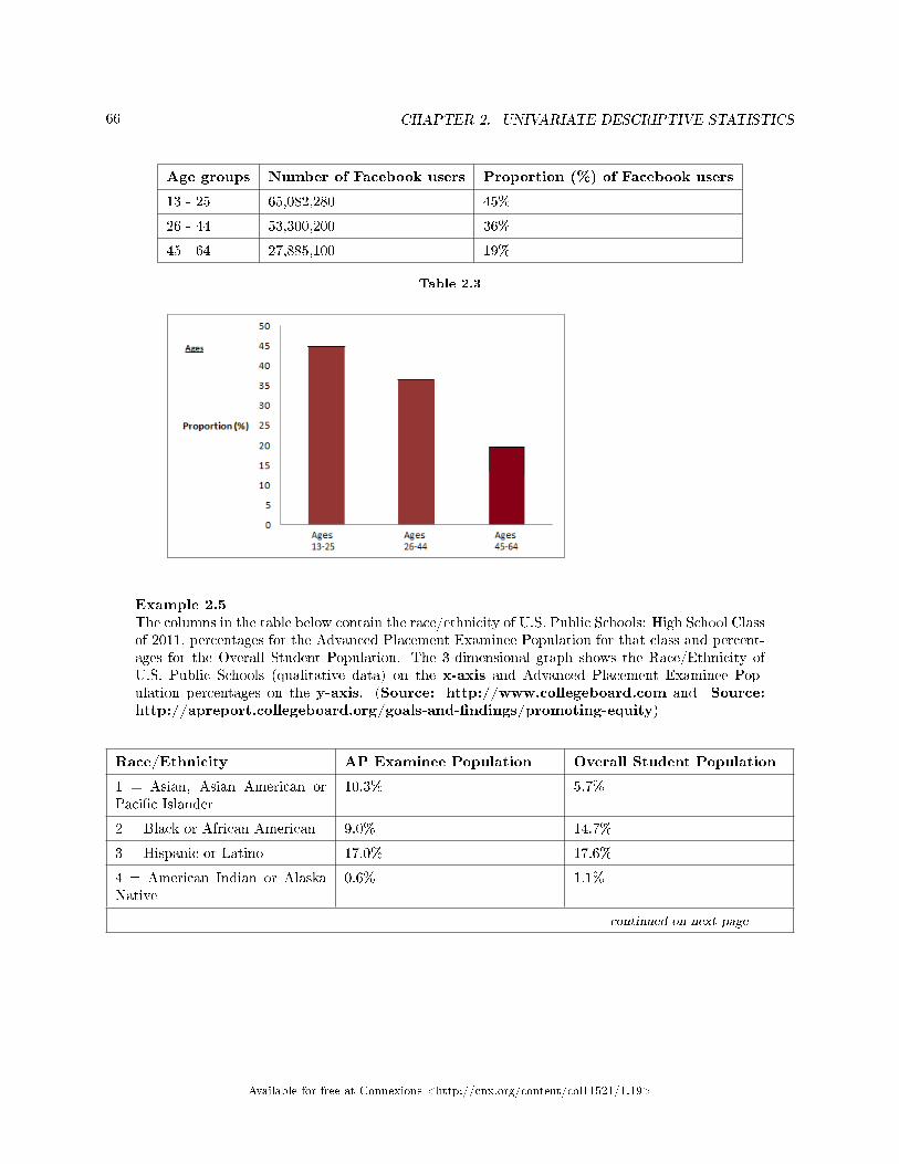
66 CHAPTER 2. UNIVARIATE DESCRIPTIVE STATISTICS
Age groups Number of Facebook users Proportion (%) of Facebook users
13 - 25 65,082,280 45%
26 - 44 53,300,200 36%
45 - 64 27,885,100 19%
Table 2.3
Example 2.5The columns in the table below contain the race/ethnicity of U.S. Public Schools: High School Classof 2011, percentages for the Advanced Placement Examinee Population for that class and percent-ages for the Overall Student Population. The 3-dimensional graph shows the Race/Ethnicity ofU.S. Public Schools (qualitative data) on the x-axis and Advanced Placement Examinee Pop-ulation percentages on the y-axis. (Source: http://www.collegeboard.com and Source:http://apreport.collegeboard.org/goals-and-�ndings/promoting-equity)
Race/Ethnicity AP Examinee Population Overall Student Population
1 = Asian, Asian American orPaci�c Islander
10.3% 5.7%
2 = Black or African American 9.0% 14.7%
3 = Hispanic or Latino 17.0% 17.6%
4 = American Indian or AlaskaNative
0.6% 1.1%
continued on next page
Available for free at Connexions <http://cnx.org/content/col11521/1.19>
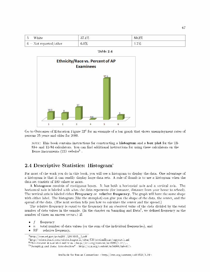
67
5 = White 57.1% 59.2%
6 = Not reported/other 6.0% 1.7%
Table 2.4
Go to Outcomes of Education Figure 224 for an example of a bar graph that shows unemployment rates ofpersons 25 years and older for 2009.
note: This book contains instructions for constructing a histogram and a box plot for the TI-83+ and TI-84 calculators. You can �nd additional instructions for using these calculators on theTexas Instruments (TI) website5 .
2.4 Descriptive Statistics: Histogram6
For most of the work you do in this book, you will use a histogram to display the data. One advantage ofa histogram is that it can readily display large data sets. A rule of thumb is to use a histogram when thedata set consists of 100 values or more.
A histogram consists of contiguous boxes. It has both a horizontal axis and a vertical axis. Thehorizontal axis is labeled with what the data represents (for instance, distance from your home to school).The vertical axis is labeled either Frequency or relative frequency. The graph will have the same shapewith either label. The histogram (like the stemplot) can give you the shape of the data, the center, and thespread of the data. (The next section tells you how to calculate the center and the spread.)
The relative frequency is equal to the frequency for an observed value of the data divided by the totalnumber of data values in the sample. (In the chapter on Sampling and Data7, we de�ned frequency as thenumber of times an answer occurs.) If:
• f = frequency• n = total number of data values (or the sum of the individual frequencies), and• RF = relative frequency,
4http://nces.ed.gov/pubs2011/2011015_5.pdf5http://education.ti.com/educationportal/sites/US/sectionHome/support.html6This content is available online at <http://cnx.org/content/m16298/1.14/>.7"Sampling and Data: Introduction" <http://cnx.org/content/m16008/latest/>
Available for free at Connexions <http://cnx.org/content/col11521/1.19>
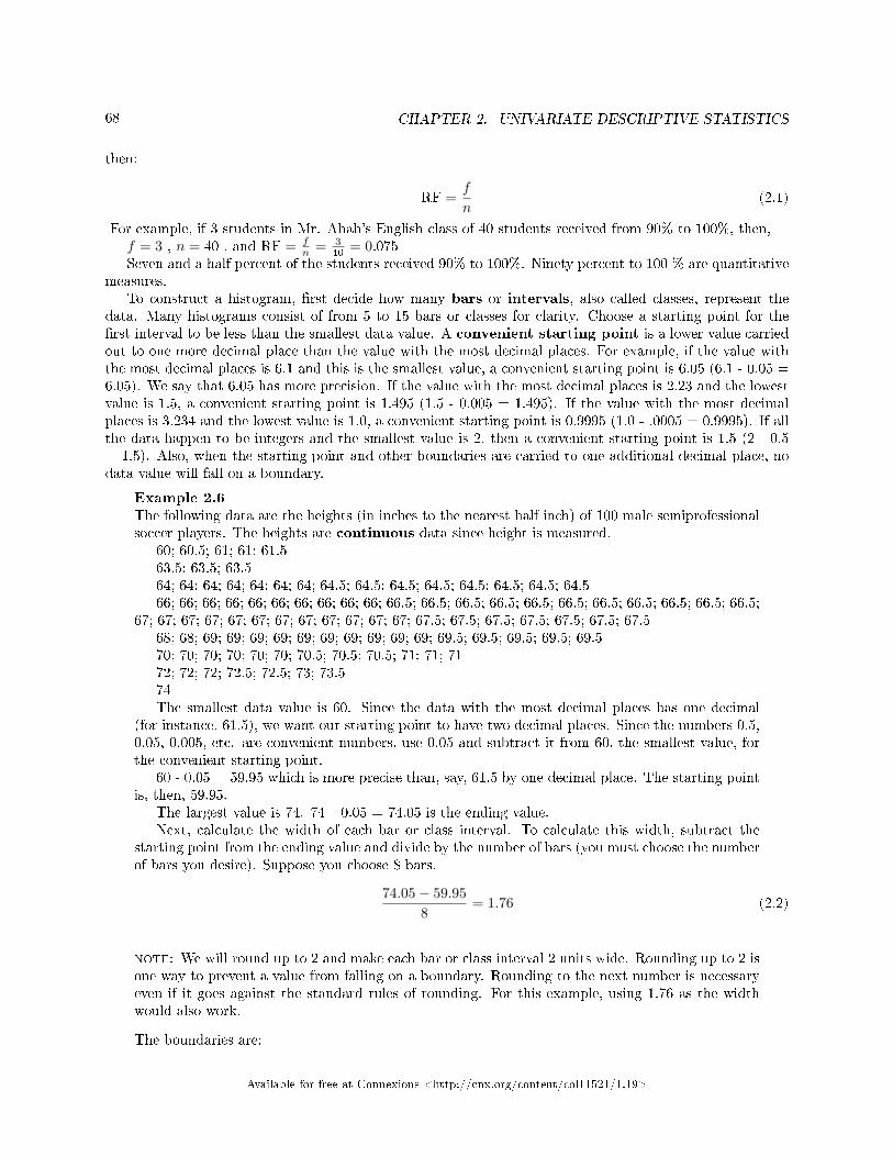
68 CHAPTER 2. UNIVARIATE DESCRIPTIVE STATISTICS
then:
RF =f
n(2.1)
For example, if 3 students in Mr. Ahab's English class of 40 students received from 90% to 100%, then,f = 3 , n = 40 , and RF = f
n = 340 = 0.075
Seven and a half percent of the students received 90% to 100%. Ninety percent to 100 % are quantitativemeasures.
To construct a histogram, �rst decide how many bars or intervals, also called classes, represent thedata. Many histograms consist of from 5 to 15 bars or classes for clarity. Choose a starting point for the�rst interval to be less than the smallest data value. A convenient starting point is a lower value carriedout to one more decimal place than the value with the most decimal places. For example, if the value withthe most decimal places is 6.1 and this is the smallest value, a convenient starting point is 6.05 (6.1 - 0.05 =6.05). We say that 6.05 has more precision. If the value with the most decimal places is 2.23 and the lowestvalue is 1.5, a convenient starting point is 1.495 (1.5 - 0.005 = 1.495). If the value with the most decimalplaces is 3.234 and the lowest value is 1.0, a convenient starting point is 0.9995 (1.0 - .0005 = 0.9995). If allthe data happen to be integers and the smallest value is 2, then a convenient starting point is 1.5 (2 - 0.5= 1.5). Also, when the starting point and other boundaries are carried to one additional decimal place, nodata value will fall on a boundary.
Example 2.6The following data are the heights (in inches to the nearest half inch) of 100 male semiprofessionalsoccer players. The heights are continuous data since height is measured.
60; 60.5; 61; 61; 61.563.5; 63.5; 63.564; 64; 64; 64; 64; 64; 64; 64.5; 64.5; 64.5; 64.5; 64.5; 64.5; 64.5; 64.566; 66; 66; 66; 66; 66; 66; 66; 66; 66; 66.5; 66.5; 66.5; 66.5; 66.5; 66.5; 66.5; 66.5; 66.5; 66.5; 66.5;
67; 67; 67; 67; 67; 67; 67; 67; 67; 67; 67; 67; 67.5; 67.5; 67.5; 67.5; 67.5; 67.5; 67.568; 68; 69; 69; 69; 69; 69; 69; 69; 69; 69; 69; 69.5; 69.5; 69.5; 69.5; 69.570; 70; 70; 70; 70; 70; 70.5; 70.5; 70.5; 71; 71; 7172; 72; 72; 72.5; 72.5; 73; 73.574The smallest data value is 60. Since the data with the most decimal places has one decimal
(for instance, 61.5), we want our starting point to have two decimal places. Since the numbers 0.5,0.05, 0.005, etc. are convenient numbers, use 0.05 and subtract it from 60, the smallest value, forthe convenient starting point.
60 - 0.05 = 59.95 which is more precise than, say, 61.5 by one decimal place. The starting pointis, then, 59.95.
The largest value is 74. 74+ 0.05 = 74.05 is the ending value.Next, calculate the width of each bar or class interval. To calculate this width, subtract the
starting point from the ending value and divide by the number of bars (you must choose the numberof bars you desire). Suppose you choose 8 bars.
74.05− 59.958
= 1.76 (2.2)
note: We will round up to 2 and make each bar or class interval 2 units wide. Rounding up to 2 isone way to prevent a value from falling on a boundary. Rounding to the next number is necessaryeven if it goes against the standard rules of rounding. For this example, using 1.76 as the widthwould also work.
The boundaries are:
Available for free at Connexions <http://cnx.org/content/col11521/1.19>
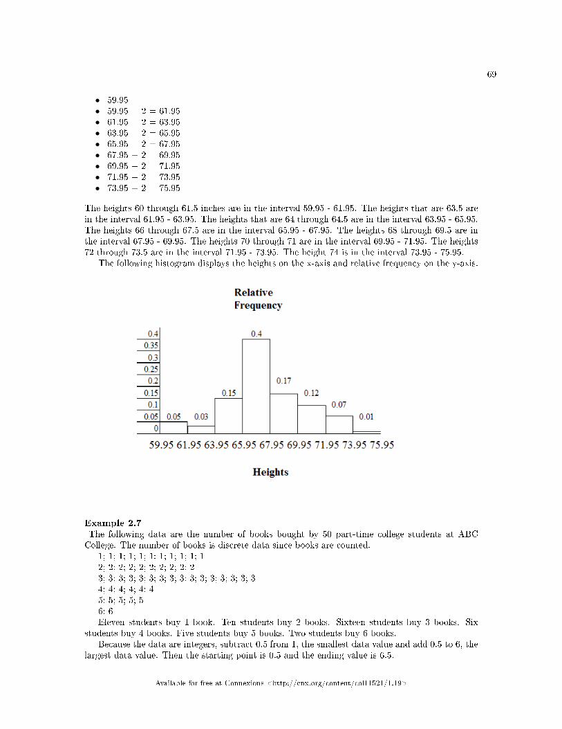
69
• 59.95• 59.95 + 2 = 61.95• 61.95 + 2 = 63.95• 63.95 + 2 = 65.95• 65.95 + 2 = 67.95• 67.95 + 2 = 69.95• 69.95 + 2 = 71.95• 71.95 + 2 = 73.95• 73.95 + 2 = 75.95
The heights 60 through 61.5 inches are in the interval 59.95 - 61.95. The heights that are 63.5 arein the interval 61.95 - 63.95. The heights that are 64 through 64.5 are in the interval 63.95 - 65.95.The heights 66 through 67.5 are in the interval 65.95 - 67.95. The heights 68 through 69.5 are inthe interval 67.95 - 69.95. The heights 70 through 71 are in the interval 69.95 - 71.95. The heights72 through 73.5 are in the interval 71.95 - 73.95. The height 74 is in the interval 73.95 - 75.95.
The following histogram displays the heights on the x-axis and relative frequency on the y-axis.
Example 2.7The following data are the number of books bought by 50 part-time college students at ABCCollege. The number of books is discrete data since books are counted.
1; 1; 1; 1; 1; 1; 1; 1; 1; 1; 12; 2; 2; 2; 2; 2; 2; 2; 2; 23; 3; 3; 3; 3; 3; 3; 3; 3; 3; 3; 3; 3; 3; 3; 34; 4; 4; 4; 4; 45; 5; 5; 5; 56; 6Eleven students buy 1 book. Ten students buy 2 books. Sixteen students buy 3 books. Six
students buy 4 books. Five students buy 5 books. Two students buy 6 books.Because the data are integers, subtract 0.5 from 1, the smallest data value and add 0.5 to 6, the
largest data value. Then the starting point is 0.5 and the ending value is 6.5.
Available for free at Connexions <http://cnx.org/content/col11521/1.19>
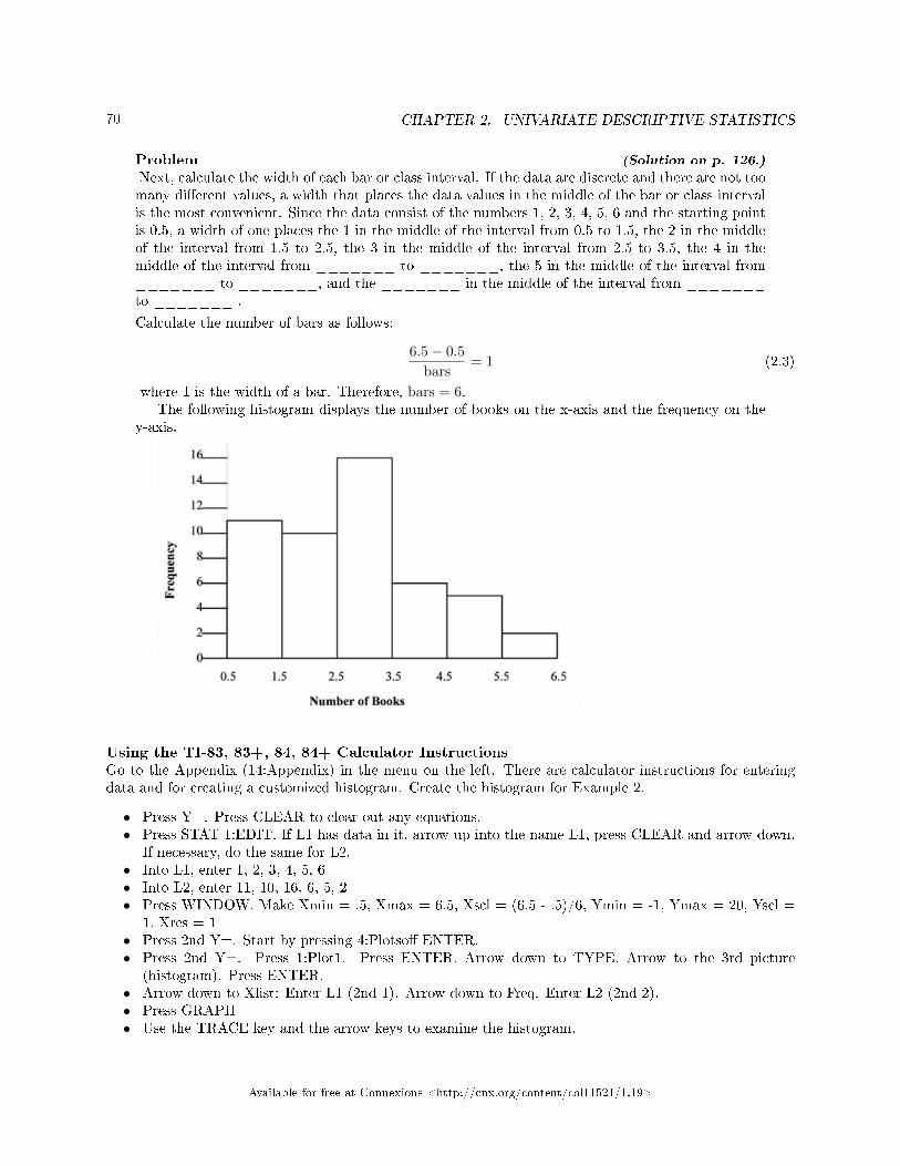
70 CHAPTER 2. UNIVARIATE DESCRIPTIVE STATISTICS
Problem (Solution on p. 126.)
Next, calculate the width of each bar or class interval. If the data are discrete and there are not toomany di�erent values, a width that places the data values in the middle of the bar or class intervalis the most convenient. Since the data consist of the numbers 1, 2, 3, 4, 5, 6 and the starting pointis 0.5, a width of one places the 1 in the middle of the interval from 0.5 to 1.5, the 2 in the middleof the interval from 1.5 to 2.5, the 3 in the middle of the interval from 2.5 to 3.5, the 4 in themiddle of the interval from _______ to _______, the 5 in the middle of the interval from_______ to _______, and the _______ in the middle of the interval from _______to _______ .
Calculate the number of bars as follows:
6.5− 0.5bars
= 1 (2.3)
where 1 is the width of a bar. Therefore, bars = 6.The following histogram displays the number of books on the x-axis and the frequency on the
y-axis.
Using the TI-83, 83+, 84, 84+ Calculator InstructionsGo to the Appendix (14:Appendix) in the menu on the left. There are calculator instructions for enteringdata and for creating a customized histogram. Create the histogram for Example 2.
• Press Y=. Press CLEAR to clear out any equations.• Press STAT 1:EDIT. If L1 has data in it, arrow up into the name L1, press CLEAR and arrow down.
If necessary, do the same for L2.• Into L1, enter 1, 2, 3, 4, 5, 6• Into L2, enter 11, 10, 16, 6, 5, 2• Press WINDOW. Make Xmin = .5, Xmax = 6.5, Xscl = (6.5 - .5)/6, Ymin = -1, Ymax = 20, Yscl =
1, Xres = 1• Press 2nd Y=. Start by pressing 4:Plotso� ENTER.• Press 2nd Y=. Press 1:Plot1. Press ENTER. Arrow down to TYPE. Arrow to the 3rd picture
(histogram). Press ENTER.• Arrow down to Xlist: Enter L1 (2nd 1). Arrow down to Freq. Enter L2 (2nd 2).• Press GRAPH• Use the TRACE key and the arrow keys to examine the histogram.
Available for free at Connexions <http://cnx.org/content/col11521/1.19>
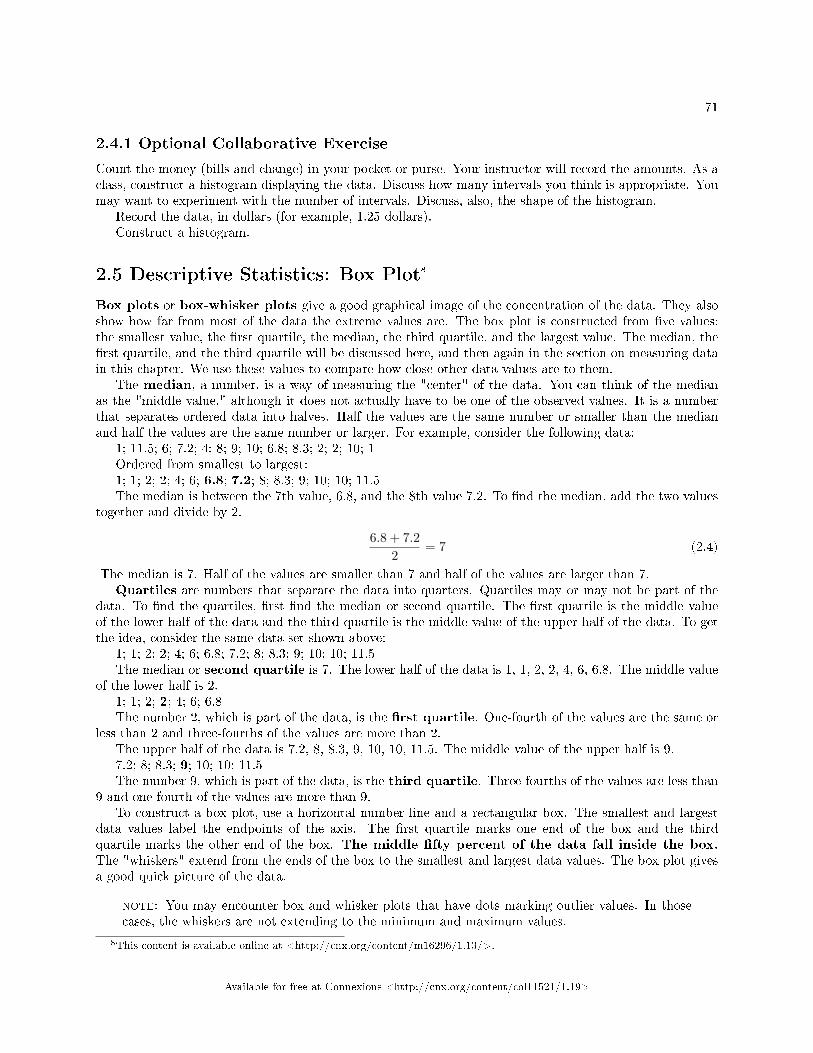
71
2.4.1 Optional Collaborative Exercise
Count the money (bills and change) in your pocket or purse. Your instructor will record the amounts. As aclass, construct a histogram displaying the data. Discuss how many intervals you think is appropriate. Youmay want to experiment with the number of intervals. Discuss, also, the shape of the histogram.
Record the data, in dollars (for example, 1.25 dollars).Construct a histogram.
2.5 Descriptive Statistics: Box Plot8
Box plots or box-whisker plots give a good graphical image of the concentration of the data. They alsoshow how far from most of the data the extreme values are. The box plot is constructed from �ve values:the smallest value, the �rst quartile, the median, the third quartile, and the largest value. The median, the�rst quartile, and the third quartile will be discussed here, and then again in the section on measuring datain this chapter. We use these values to compare how close other data values are to them.
The median, a number, is a way of measuring the "center" of the data. You can think of the medianas the "middle value," although it does not actually have to be one of the observed values. It is a numberthat separates ordered data into halves. Half the values are the same number or smaller than the medianand half the values are the same number or larger. For example, consider the following data:
1; 11.5; 6; 7.2; 4; 8; 9; 10; 6.8; 8.3; 2; 2; 10; 1Ordered from smallest to largest:1; 1; 2; 2; 4; 6; 6.8; 7.2; 8; 8.3; 9; 10; 10; 11.5The median is between the 7th value, 6.8, and the 8th value 7.2. To �nd the median, add the two values
together and divide by 2.
6.8 + 7.22
= 7 (2.4)
The median is 7. Half of the values are smaller than 7 and half of the values are larger than 7.Quartiles are numbers that separate the data into quarters. Quartiles may or may not be part of the
data. To �nd the quartiles, �rst �nd the median or second quartile. The �rst quartile is the middle valueof the lower half of the data and the third quartile is the middle value of the upper half of the data. To getthe idea, consider the same data set shown above:
1; 1; 2; 2; 4; 6; 6.8; 7.2; 8; 8.3; 9; 10; 10; 11.5The median or second quartile is 7. The lower half of the data is 1, 1, 2, 2, 4, 6, 6.8. The middle value
of the lower half is 2.1; 1; 2; 2; 4; 6; 6.8The number 2, which is part of the data, is the �rst quartile. One-fourth of the values are the same or
less than 2 and three-fourths of the values are more than 2.The upper half of the data is 7.2, 8, 8.3, 9, 10, 10, 11.5. The middle value of the upper half is 9.7.2; 8; 8.3; 9; 10; 10; 11.5The number 9, which is part of the data, is the third quartile. Three-fourths of the values are less than
9 and one-fourth of the values are more than 9.To construct a box plot, use a horizontal number line and a rectangular box. The smallest and largest
data values label the endpoints of the axis. The �rst quartile marks one end of the box and the thirdquartile marks the other end of the box. The middle �fty percent of the data fall inside the box.The "whiskers" extend from the ends of the box to the smallest and largest data values. The box plot givesa good quick picture of the data.
note: You may encounter box and whisker plots that have dots marking outlier values. In thosecases, the whiskers are not extending to the minimum and maximum values.
8This content is available online at <http://cnx.org/content/m16296/1.13/>.
Available for free at Connexions <http://cnx.org/content/col11521/1.19>
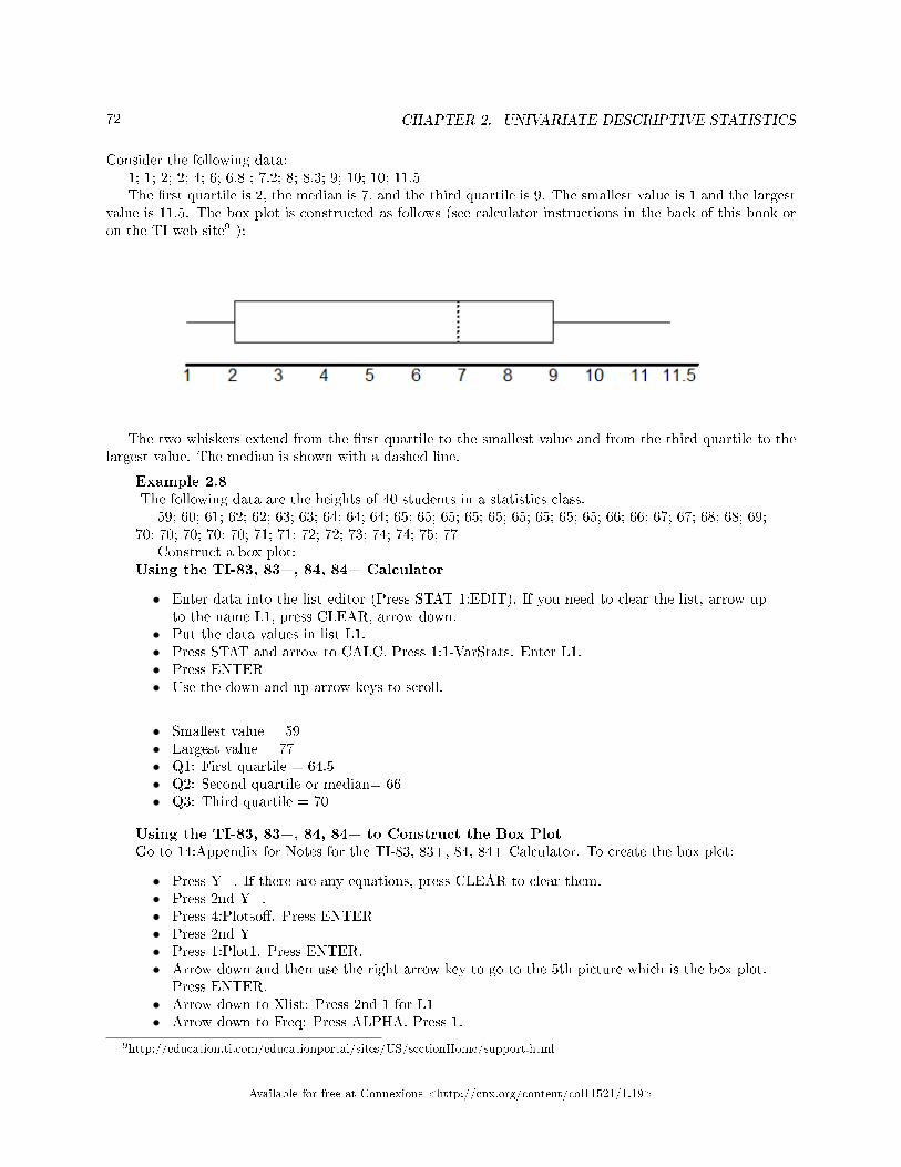
72 CHAPTER 2. UNIVARIATE DESCRIPTIVE STATISTICS
Consider the following data:1; 1; 2; 2; 4; 6; 6.8 ; 7.2; 8; 8.3; 9; 10; 10; 11.5The �rst quartile is 2, the median is 7, and the third quartile is 9. The smallest value is 1 and the largest
value is 11.5. The box plot is constructed as follows (see calculator instructions in the back of this book oron the TI web site9 ):
The two whiskers extend from the �rst quartile to the smallest value and from the third quartile to thelargest value. The median is shown with a dashed line.
Example 2.8The following data are the heights of 40 students in a statistics class.
59; 60; 61; 62; 62; 63; 63; 64; 64; 64; 65; 65; 65; 65; 65; 65; 65; 65; 65; 66; 66; 67; 67; 68; 68; 69;70; 70; 70; 70; 70; 71; 71; 72; 72; 73; 74; 74; 75; 77
Construct a box plot:Using the TI-83, 83+, 84, 84+ Calculator
• Enter data into the list editor (Press STAT 1:EDIT). If you need to clear the list, arrow upto the name L1, press CLEAR, arrow down.
• Put the data values in list L1.• Press STAT and arrow to CALC. Press 1:1-VarStats. Enter L1.• Press ENTER• Use the down and up arrow keys to scroll.
• Smallest value = 59• Largest value = 77• Q1: First quartile = 64.5• Q2: Second quartile or median= 66• Q3: Third quartile = 70
Using the TI-83, 83+, 84, 84+ to Construct the Box PlotGo to 14:Appendix for Notes for the TI-83, 83+, 84, 84+ Calculator. To create the box plot:
• Press Y=. If there are any equations, press CLEAR to clear them.• Press 2nd Y=.• Press 4:Plotso�. Press ENTER• Press 2nd Y=• Press 1:Plot1. Press ENTER.• Arrow down and then use the right arrow key to go to the 5th picture which is the box plot.
Press ENTER.• Arrow down to Xlist: Press 2nd 1 for L1• Arrow down to Freq: Press ALPHA. Press 1.
9http://education.ti.com/educationportal/sites/US/sectionHome/support.html
Available for free at Connexions <http://cnx.org/content/col11521/1.19>
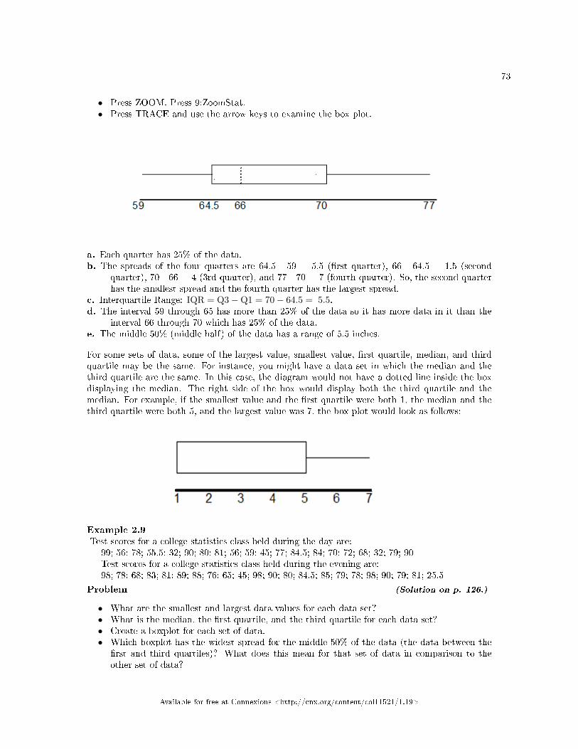
73
• Press ZOOM. Press 9:ZoomStat.• Press TRACE and use the arrow keys to examine the box plot.
a. Each quarter has 25% of the data.b. The spreads of the four quarters are 64.5 - 59 = 5.5 (�rst quarter), 66 - 64.5 = 1.5 (second
quarter), 70 - 66 = 4 (3rd quarter), and 77 - 70 = 7 (fourth quarter). So, the second quarterhas the smallest spread and the fourth quarter has the largest spread.
c. Interquartile Range: IQR = Q3−Q1 = 70− 64.5 = 5.5.d. The interval 59 through 65 has more than 25% of the data so it has more data in it than the
interval 66 through 70 which has 25% of the data.e. The middle 50% (middle half) of the data has a range of 5.5 inches.
For some sets of data, some of the largest value, smallest value, �rst quartile, median, and thirdquartile may be the same. For instance, you might have a data set in which the median and thethird quartile are the same. In this case, the diagram would not have a dotted line inside the boxdisplaying the median. The right side of the box would display both the third quartile and themedian. For example, if the smallest value and the �rst quartile were both 1, the median and thethird quartile were both 5, and the largest value was 7, the box plot would look as follows:
Example 2.9Test scores for a college statistics class held during the day are:
99; 56; 78; 55.5; 32; 90; 80; 81; 56; 59; 45; 77; 84.5; 84; 70; 72; 68; 32; 79; 90Test scores for a college statistics class held during the evening are:98; 78; 68; 83; 81; 89; 88; 76; 65; 45; 98; 90; 80; 84.5; 85; 79; 78; 98; 90; 79; 81; 25.5
Problem (Solution on p. 126.)
• What are the smallest and largest data values for each data set?• What is the median, the �rst quartile, and the third quartile for each data set?• Create a boxplot for each set of data.• Which boxplot has the widest spread for the middle 50% of the data (the data between the
�rst and third quartiles)? What does this mean for that set of data in comparison to theother set of data?
Available for free at Connexions <http://cnx.org/content/col11521/1.19>
74 CHAPTER 2. UNIVARIATE DESCRIPTIVE STATISTICS
• For each data set, what percent of the data is between the smallest value and the �rst quartile?(Answer: 25%) the �rst quartile and the median? (Answer: 25%) the median and the thirdquartile? the third quartile and the largest value? What percent of the data is between the�rst quartile and the largest value? (Answer: 75%)
The �rst data set (the top box plot) has the widest spread for the middle 50% of the data. IQR =Q3 − Q1 is 82.5 − 56 = 26.5 for the �rst data set and 89 − 78 = 11 for the second data set.So, the �rst set of data has its middle 50% of scores more spread out.
25% of the data is between M and Q3 and 25% is between Q3 and Xmax.
2.6 Box Plots with Outliers10
Now that you know how to �nd a quick box plot, one made up of the minimum value, �rst quartile, median,third quartile and maximum value we are going to go a step further and do the mathematics for an outlierbox plot. So instead of looking at the data and saying well that value looks di�erent or far away from therest of data so it must be an outlier we will have a concrete way of determining if data values are outliers.
An outlier is a data value that is well separated from most of the other data in a distribution. Judgingwhether or not a value �ts this de�nition relies on qualitative judgment. What is needed is a more preciserule for identifying outliers. Such a rule has been described by a statistician named John W. Tukey.
2.6.1 Finding Outliers
Tukey uses the following procedure for identifying outliers.
1. De�ne the location of a FENCE as the value that is 1.5 times the interquartile range below the lowerquartile, or above the upper quartile.
2. De�ne the UPPER FENCE as the upper quartile plus one step. UPPER FENCE = Q3 + 1.5 (IQR)3. De�ne the LOWER FENCE as the lower quartile minus one step. LOWER FENCE = Q1 - 1.5 (IQR)4. Any value that is less than the Lower Fence or that is greater than the Upper Fence is declared an
OUTLIER
2.6.2 The Outlier Box Plot
In order to draw an outlier box plot, you need to �nd two additional values, sometimes called the ADJACENTvalues. The Lower Adjacent value is the actual value in the distribution that is closest to the Lower Fence,but which is not less than the Lower Fence. Similarly, the Upper Adjacent Value is the actual value in thedistribution that comes closest to the Upper Fence, but that is not greater than the Upper Fence.
Let's go through an example to understand the process of constructing an outlier box plot. This exampleuses data on the number of hysterectomies performed by male doctors.
The data for the male doctors are given as follows:20 25 25 27 28 31 33 34 36 37 44 50 59 85 86The �rst step is to determine the �ve number summary (a short hand for listing out some of your
statistics). The �ve number summary starts with the sample size (minimum, �rst quartile, median, thirdquartile, maximum value). For this data the �ve number summary is 15(20, 27, 34, 50, 86).
A quick box plot based on this �ve number summary would look like the graph below:
10This content is available online at <http://cnx.org/content/m46129/1.1/>.
Available for free at Connexions <http://cnx.org/content/col11521/1.19>
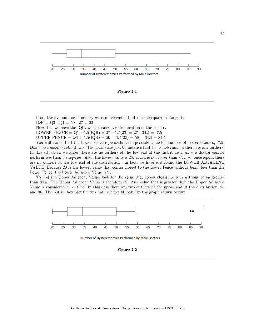
75
Figure 2.1
From the �ve number summary we can determine that the Interquartile Range isIQR = Q3 - Q1 = 50 - 27 = 23Now that we have the IQR, we can calculate the location of the Fences.LOWER FENCE = Q1 � 1.5(IQR) = 27 � 1.5(23) = 27 - 34.5 = -7.5UPPER FENCE = Q3 + 1.5(IQR) = 50 + 1.5(23) = 50 + 34.5 = 84.5You will notice that the Lower Fence represents an impossible value for number of hysterectomies, -7.5.
Don't be concerned about this. The fences are just boundaries that let us determine if there are any outliers.In this situation, we know there are no outliers at the low end of the distribution since a doctor cannotperform less than 0 surgeries. Also, the lowest value is 20, which is not lower than -7.5, so, once again, thereare no outliers at the low end of the distribution. In fact, we have just found the LOWER ADJACENTVALUE. Because 20 is the lowest value that comes closest to the Lower Fence without being less than theLower Fence, the Lower Adjacent Value is 20.
To �nd the Upper Adjacent Value, look for the value that comes closest to 84.5 without being greaterthan 84.5. The Upper Adjacent Value is therefore 59. Any value that is greater than the Upper AdjacentValue is considered an outlier. In this case there are two outliers at the upper end of the distribution, 85and 86. The outlier box plot for this data set would look like the graph shown below:
Figure 2.2
Available for free at Connexions <http://cnx.org/content/col11521/1.19>
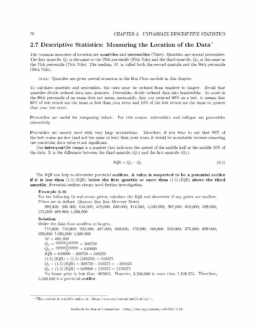
76 CHAPTER 2. UNIVARIATE DESCRIPTIVE STATISTICS
2.7 Descriptive Statistics: Measuring the Location of the Data11
The common measures of location are quartiles and percentiles (%iles). Quartiles are special percentiles.The �rst quartile, Q1 is the same as the 25th percentile (25th %ile) and the third quartile, Q3, is the same asthe 75th percentile (75th %ile). The median, M , is called both the second quartile and the 50th percentile(50th %ile).
note: Quartiles are given special attention in the Box Plots module in this chapter.
To calculate quartiles and percentiles, the data must be ordered from smallest to largest. Recall thatquartiles divide ordered data into quarters. Percentiles divide ordered data into hundredths. To score inthe 90th percentile of an exam does not mean, necessarily, that you received 90% on a test. It means that90% of test scores are the same or less than your score and 10% of the test scores are the same or greaterthan your test score.
Percentiles are useful for comparing values. For this reason, universities and colleges use percentilesextensively.
Percentiles are mostly used with very large populations. Therefore, if you were to say that 90% ofthe test scores are less (and not the same or less) than your score, it would be acceptable because removingone particular data value is not signi�cant.
The interquartile range is a number that indicates the spread of the middle half or the middle 50% ofthe data. It is the di�erence between the third quartile (Q3) and the �rst quartile (Q1).
IQR = Q3 −Q1 (2.5)
The IQR can help to determine potential outliers. A value is suspected to be a potential outlierif it is less than (1.5) (IQR) below the �rst quartile or more than (1.5) (IQR) above the thirdquartile. Potential outliers always need further investigation.
Example 2.10For the following 13 real estate prices, calculate the IQR and determine if any prices are outliers.Prices are in dollars. (Source: San Jose Mercury News)
389,950; 230,500; 158,000; 479,000; 639,000; 114,950; 5,500,000; 387,000; 659,000; 529,000;575,000; 488,800; 1,095,000
SolutionOrder the data from smallest to largest.
114,950; 158,000; 230,500; 387,000; 389,950; 479,000; 488,800; 529,000; 575,000; 639,000;659,000; 1,095,000; 5,500,000
M = 488, 800Q1 = 230500+387000
2 = 308750Q3 = 639000+659000
2 = 649000IQR = 649000− 308750 = 340250(1.5) (IQR) = (1.5) (340250) = 510375Q1 − (1.5) (IQR) = 308750− 510375 = −201625Q3 + (1.5) (IQR) = 649000 + 510375 = 1159375No house price is less than -201625. However, 5,500,000 is more than 1,159,375. Therefore,
5,500,000 is a potential outlier.
11This content is available online at <http://cnx.org/content/m47514/1.1/>.
Available for free at Connexions <http://cnx.org/content/col11521/1.19>
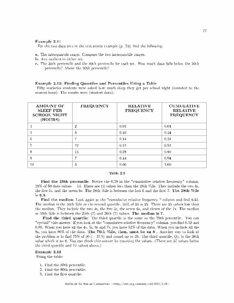
77
Example 2.11For the two data sets in the test scores example (p. 73), �nd the following:
a. The interquartile range. Compare the two interquartile ranges.b. Any outliers in either set.c. The 30th percentile and the 80th percentile for each set. How much data falls below the 30th
percentile? Above the 80th percentile?
Example 2.12: Finding Quartiles and Percentiles Using a TableFifty statistics students were asked how much sleep they get per school night (rounded to thenearest hour). The results were (student data):
AMOUNT OFSLEEP PER
SCHOOL NIGHT(HOURS)
FREQUENCY RELATIVEFREQUENCY
CUMULATIVERELATIVE
FREQUENCY
4 2 0.04 0.04
5 5 0.10 0.14
6 7 0.14 0.28
7 12 0.24 0.52
8 14 0.28 0.80
9 7 0.14 0.94
10 3 0.06 1.00
Table 2.5
Find the 28th percentile: Notice the 0.28 in the "cumulative relative frequency" column.28% of 50 data values = 14. There are 14 values less than the 28th %ile. They include the two 4s,the �ve 5s, and the seven 6s. The 28th %ile is between the last 6 and the �rst 7. The 28th %ileis 6.5.
Find the median: Look again at the "cumulative relative frequency " column and �nd 0.52.The median is the 50th %ile or the second quartile. 50% of 50 = 25. There are 25 values less thanthe median. They include the two 4s, the �ve 5s, the seven 6s, and eleven of the 7s. The medianor 50th %ile is between the 25th (7) and 26th (7) values. The median is 7.
Find the third quartile: The third quartile is the same as the 75th percentile. You can"eyeball" this answer. If you look at the "cumulative relative frequency" column, you �nd 0.52 and0.80. When you have all the 4s, 5s, 6s and 7s, you have 52% of the data. When you include all the8s, you have 80% of the data. The 75th %ile, then, must be an 8 . Another way to look atthe problem is to �nd 75% of 50 (= 37.5) and round up to 38. The third quartile, Q3, is the 38thvalue which is an 8. You can check this answer by counting the values. (There are 37 values belowthe third quartile and 12 values above.)
Example 2.13Using the table:
1. Find the 80th percentile.2. Find the 90th percentile.3. Find the �rst quartile.
Available for free at Connexions <http://cnx.org/content/col11521/1.19>
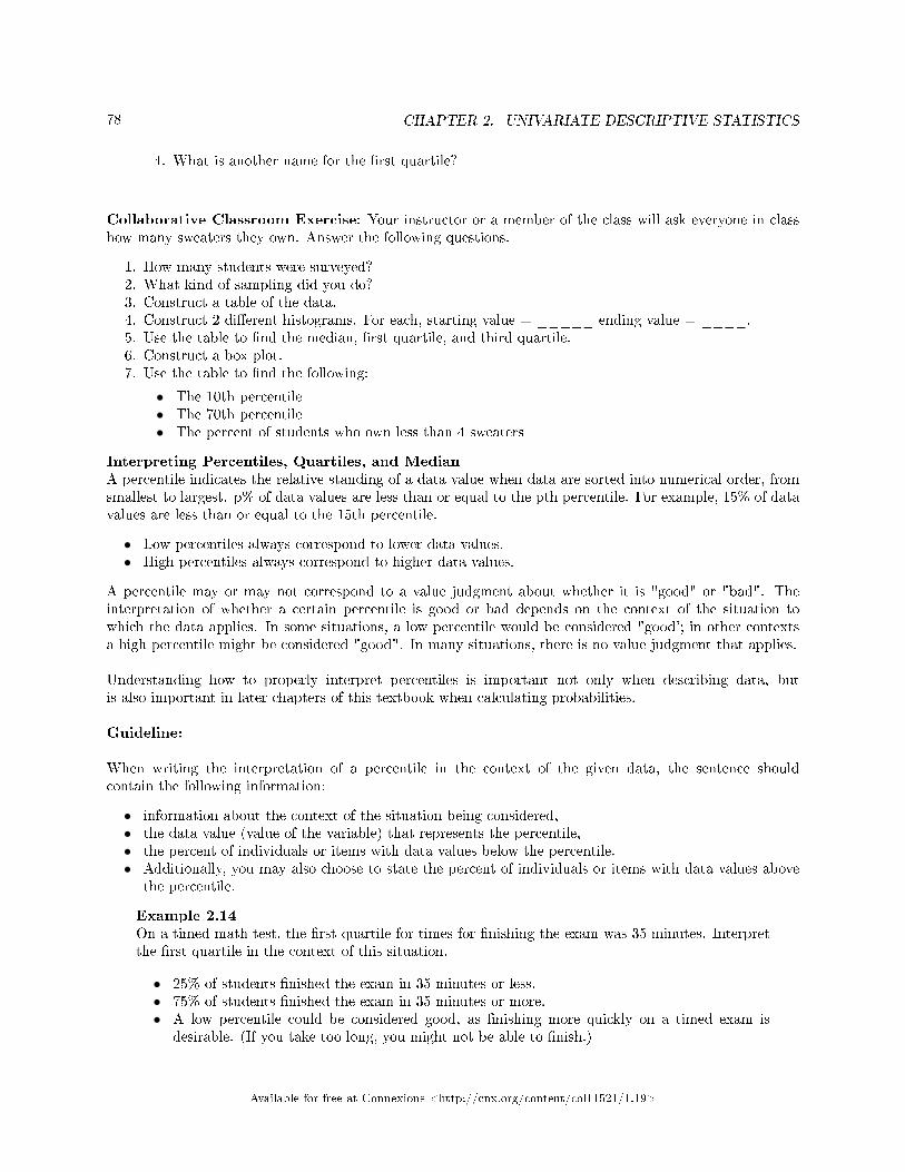
78 CHAPTER 2. UNIVARIATE DESCRIPTIVE STATISTICS
4. What is another name for the �rst quartile?
Collaborative Classroom Exercise: Your instructor or a member of the class will ask everyone in classhow many sweaters they own. Answer the following questions.
1. How many students were surveyed?2. What kind of sampling did you do?3. Construct a table of the data.4. Construct 2 di�erent histograms. For each, starting value = _____ ending value = ____.5. Use the table to �nd the median, �rst quartile, and third quartile.6. Construct a box plot.7. Use the table to �nd the following:
• The 10th percentile• The 70th percentile• The percent of students who own less than 4 sweaters
Interpreting Percentiles, Quartiles, and MedianA percentile indicates the relative standing of a data value when data are sorted into numerical order, fromsmallest to largest. p% of data values are less than or equal to the pth percentile. For example, 15% of datavalues are less than or equal to the 15th percentile.
• Low percentiles always correspond to lower data values.• High percentiles always correspond to higher data values.
A percentile may or may not correspond to a value judgment about whether it is "good" or "bad". Theinterpretation of whether a certain percentile is good or bad depends on the context of the situation towhich the data applies. In some situations, a low percentile would be considered "good'; in other contextsa high percentile might be considered "good". In many situations, there is no value judgment that applies.
Understanding how to properly interpret percentiles is important not only when describing data, butis also important in later chapters of this textbook when calculating probabilities.
Guideline:
When writing the interpretation of a percentile in the context of the given data, the sentence shouldcontain the following information:
• information about the context of the situation being considered,• the data value (value of the variable) that represents the percentile,• the percent of individuals or items with data values below the percentile.• Additionally, you may also choose to state the percent of individuals or items with data values above
the percentile.
Example 2.14On a timed math test, the �rst quartile for times for �nishing the exam was 35 minutes. Interpretthe �rst quartile in the context of this situation.
• 25% of students �nished the exam in 35 minutes or less.• 75% of students �nished the exam in 35 minutes or more.• A low percentile could be considered good, as �nishing more quickly on a timed exam is
desirable. (If you take too long, you might not be able to �nish.)
Available for free at Connexions <http://cnx.org/content/col11521/1.19>
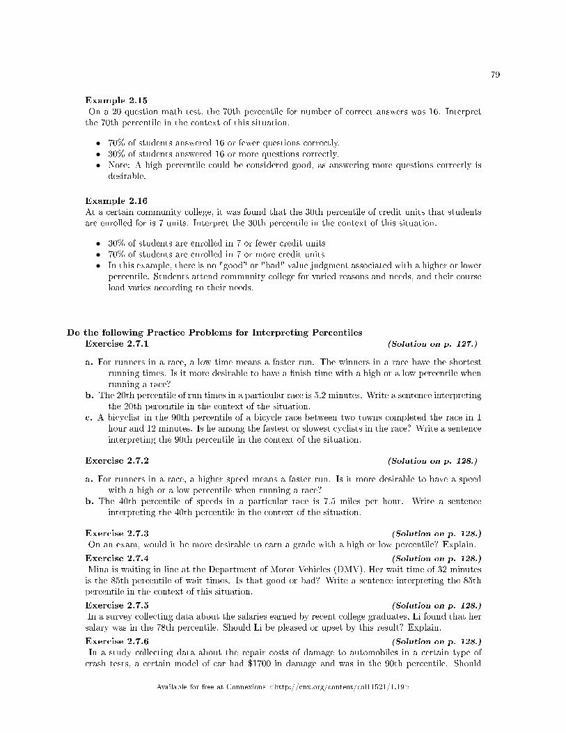
79
Example 2.15On a 20 question math test, the 70th percentile for number of correct answers was 16. Interpretthe 70th percentile in the context of this situation.
• 70% of students answered 16 or fewer questions correctly.• 30% of students answered 16 or more questions correctly.• Note: A high percentile could be considered good, as answering more questions correctly is
desirable.
Example 2.16At a certain community college, it was found that the 30th percentile of credit units that studentsare enrolled for is 7 units. Interpret the 30th percentile in the context of this situation.
• 30% of students are enrolled in 7 or fewer credit units• 70% of students are enrolled in 7 or more credit units• In this example, there is no "good" or "bad" value judgment associated with a higher or lower
percentile. Students attend community college for varied reasons and needs, and their courseload varies according to their needs.
Do the following Practice Problems for Interpreting PercentilesExercise 2.7.1 (Solution on p. 127.)
a. For runners in a race, a low time means a faster run. The winners in a race have the shortestrunning times. Is it more desirable to have a �nish time with a high or a low percentile whenrunning a race?
b. The 20th percentile of run times in a particular race is 5.2 minutes. Write a sentence interpretingthe 20th percentile in the context of the situation.
c. A bicyclist in the 90th percentile of a bicycle race between two towns completed the race in 1hour and 12 minutes. Is he among the fastest or slowest cyclists in the race? Write a sentenceinterpreting the 90th percentile in the context of the situation.
Exercise 2.7.2 (Solution on p. 128.)
a. For runners in a race, a higher speed means a faster run. Is it more desirable to have a speedwith a high or a low percentile when running a race?
b. The 40th percentile of speeds in a particular race is 7.5 miles per hour. Write a sentenceinterpreting the 40th percentile in the context of the situation.
Exercise 2.7.3 (Solution on p. 128.)
On an exam, would it be more desirable to earn a grade with a high or low percentile? Explain.
Exercise 2.7.4 (Solution on p. 128.)
Mina is waiting in line at the Department of Motor Vehicles (DMV). Her wait time of 32 minutesis the 85th percentile of wait times. Is that good or bad? Write a sentence interpreting the 85thpercentile in the context of this situation.
Exercise 2.7.5 (Solution on p. 128.)
In a survey collecting data about the salaries earned by recent college graduates, Li found that hersalary was in the 78th percentile. Should Li be pleased or upset by this result? Explain.
Exercise 2.7.6 (Solution on p. 128.)
In a study collecting data about the repair costs of damage to automobiles in a certain type ofcrash tests, a certain model of car had $1700 in damage and was in the 90th percentile. Should
Available for free at Connexions <http://cnx.org/content/col11521/1.19>
80 CHAPTER 2. UNIVARIATE DESCRIPTIVE STATISTICS
the manufacturer and/or a consumer be pleased or upset by this result? Explain. Write a sentencethat interprets the 90th percentile in the context of this problem.
Exercise 2.7.7 (Solution on p. 128.)
The University of California has two criteria used to set admission standards for freshman to beadmitted to a college in the UC system:
a. Students' GPAs and scores on standardized tests (SATs and ACTs) are entered into a formulathat calculates an "admissions index" score. The admissions index score is used to set eligi-bility standards intended to meet the goal of admitting the top 12% of high school studentsin the state. In this context, what percentile does the top 12% represent?
b. Students whose GPAs are at or above the 96th percentile of all students at their high schoolare eligible (called eligible in the local context), even if they are not in the top 12% of allstudents in the state. What percent of students from each high school are "eligible in thelocal context"?
Exercise 2.7.8 (Solution on p. 128.)
Suppose that you are buying a house. You and your realtor have determined that the mostexpensive house you can a�ord is the 34th percentile. The 34th percentile of housing prices is$240,000 in the town you want to move to. In this town, can you a�ord 34% of the houses or 66%of the houses?
**With contributions from Roberta Bloom
2.8 Descriptive Statistics: Measuring the Center of the Data12
The "center" of a data set is also a way of describing location. The two most widely used measures of the"center" of the data are the mean (average) and the median. To calculate the mean weight of 50 people,add the 50 weights together and divide by 50. To �nd the median weight of the 50 people, order the dataand �nd the number that splits the data into two equal parts (previously discussed under box plots in thischapter). The median is generally a better measure of the center when there are extreme values or outliersbecause it is not a�ected by the precise numerical values of the outliers. The mean is the most commonmeasure of the center.
note: The words "mean" and "average" are often used interchangeably. The substitution of oneword for the other is common practice. The technical term is "arithmetic mean" and "average" istechnically a center location. However, in practice among non-statisticians, "average" is commonlyaccepted for "arithmetic mean."
The mean can also be calculated by multiplying each distinct value by its frequency and then dividing thesum by the total number of data values. The letter used to represent the sample mean is an x with a barover it (pronounced "x bar"): x.
The Greek letter µ (pronounced "mew") represents the population mean. One of the requirements forthe sample mean to be a good estimate of the population mean is for the sample taken to be truly random.
To see that both ways of calculating the mean are the same, consider the sample:1; 1; 1; 2; 2; 3; 4; 4; 4; 4; 4
x =1 + 1 + 1 + 2 + 2 + 3 + 4 + 4 + 4 + 4 + 4
11= 2.7 (2.6)
x =3× 1 + 2× 2 + 1× 3 + 5× 4
11= 2.7 (2.7)
12This content is available online at <http://cnx.org/content/m17102/1.13/>.
Available for free at Connexions <http://cnx.org/content/col11521/1.19>
81
In the second calculation for the sample mean, the frequencies are 3, 2, 1, and 5.You can quickly �nd the location of the median by using the expression n+1
2 .The letter n is the total number of data values in the sample. If n is an odd number, the median is the
middle value of the ordered data (ordered smallest to largest). If n is an even number, the median is equal tothe two middle values added together and divided by 2 after the data has been ordered. For example, if thetotal number of data values is 97, then n+1
2 = 97+12 = 49. The median is the 49th value in the ordered data.
If the total number of data values is 100, then n+12 = 100+1
2 = 50.5. The median occurs midway between the50th and 51st values. The location of the median and the value of the median are not the same. The uppercase letter M is often used to represent the median. The next example illustrates the location of the medianand the value of the median.
Example 2.17AIDS data indicating the number of months an AIDS patient lives after taking a new antibodydrug are as follows (smallest to largest):
3; 4; 8; 8; 10; 11; 12; 13; 14; 15; 15; 16; 16; 17; 17; 18; 21; 22; 22; 24; 24; 25; 26; 26; 27; 27; 29;29; 31; 32; 33; 33; 34; 34; 35; 37; 40; 44; 44; 47
Calculate the mean and the median.
SolutionThe calculation for the mean is:
x = [3+4+(8)(2)+10+11+12+13+14+(15)(2)+(16)(2)+...+35+37+40+(44)(2)+47]40 = 23.6
To �nd the median, M, �rst use the formula for the location. The location is:n+1
2 = 40+12 = 20.5
Starting at the smallest value, the median is located between the 20th and 21st values (the two24s):
3; 4; 8; 8; 10; 11; 12; 13; 14; 15; 15; 16; 16; 17; 17; 18; 21; 22; 22; 24; 24; 25; 26; 26; 27; 27; 29;29; 31; 32; 33; 33; 34; 34; 35; 37; 40; 44; 44; 47
M = 24+242 = 24
The median is 24.
Using the TI-83,83+,84, 84+ CalculatorsCalculator Instructions are located in the menu item 14:Appendix (Notes for the TI-83, 83+, 84,84+ Calculators).
• Enter data into the list editor. Press STAT 1:EDIT• Put the data values in list L1.• Press STAT and arrow to CALC. Press 1:1-VarStats. Press 2nd 1 for L1 and ENTER.• Press the down and up arrow keys to scroll.
x = 23.6, M = 24
Example 2.18Suppose that, in a small town of 50 people, one person earns $5,000,000 per year and the other
49 each earn $30,000. Which is the better measure of the "center," the mean or the median?
Solutionx = 5000000+49×30000
50 = 129400M = 30000(There are 49 people who earn $30,000 and one person who earns $5,000,000.)The median is a better measure of the "center" than the mean because 49 of the values are
30,000 and one is 5,000,000. The 5,000,000 is an outlier. The 30,000 gives us a better sense of themiddle of the data.
Available for free at Connexions <http://cnx.org/content/col11521/1.19>
82 CHAPTER 2. UNIVARIATE DESCRIPTIVE STATISTICS
Another measure of the center is the mode. The mode is the most frequent value. If a data set has twovalues that occur the same number of times, then the set is bimodal.
Example 2.19: Statistics exam scores for 20 students are as followsStatistics exam scores for 20 students are as follows:
50 ; 53 ; 59 ; 59 ; 63 ; 63 ; 72 ; 72 ; 72 ; 72 ; 72 ; 76 ; 78 ; 81 ; 83 ; 84 ; 84 ; 84 ; 90 ; 93
ProblemFind the mode.
SolutionThe most frequent score is 72, which occurs �ve times. Mode = 72.
Example 2.20Five real estate exam scores are 430, 430, 480, 480, 495. The data set is bimodal because the scores430 and 480 each occur twice.
When is the mode the best measure of the "center"? Consider a weight loss program thatadvertises a mean weight loss of six pounds the �rst week of the program. The mode might indicatethat most people lose two pounds the �rst week, making the program less appealing.
note: The mode can be calculated for qualitative data as well as for quantitative data.
Statistical software will easily calculate the mean, the median, and the mode. Some graphingcalculators can also make these calculations. In the real world, people make these calculationsusing software.
2.8.1 The Law of Large Numbers and the Mean
The Law of Large Numbers says that if you take samples of larger and larger size from any population, thenthe mean x of the sample is very likely to get closer and closer to µ. This is discussed in more detail in TheCentral Limit Theorem.
note: The formula for the mean is located in the Summary of Formulas13 section course.
2.8.2 Sampling Distributions and Statistic of a Sampling Distribution
You can think of a sampling distribution as a relative frequency distribution with a great manysamples. (See Sampling and Data for a review of relative frequency). Suppose thirty randomly selectedstudents were asked the number of movies they watched the previous week. The results are in the relativefrequency table shown below.
# of movies Relative Frequency
0 5/30
1 15/30
2 6/30
3 4/30
4 1/30
13"Descriptive Statistics: Summary of Formulas" <http://cnx.org/content/m16310/latest/>
Available for free at Connexions <http://cnx.org/content/col11521/1.19>
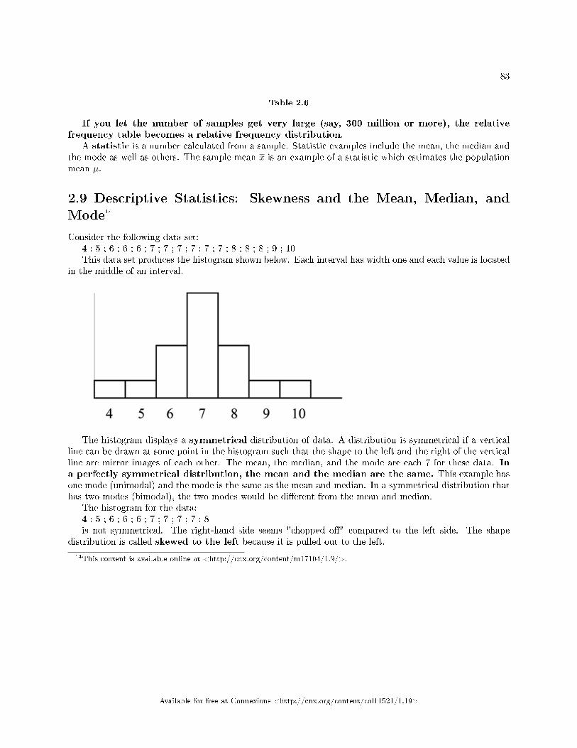
83
Table 2.6
If you let the number of samples get very large (say, 300 million or more), the relativefrequency table becomes a relative frequency distribution.
A statistic is a number calculated from a sample. Statistic examples include the mean, the median andthe mode as well as others. The sample mean x is an example of a statistic which estimates the populationmean µ.
2.9 Descriptive Statistics: Skewness and the Mean, Median, andMode14
Consider the following data set:4 ; 5 ; 6 ; 6 ; 6 ; 7 ; 7 ; 7 ; 7 ; 7 ; 7 ; 8 ; 8 ; 8 ; 9 ; 10This data set produces the histogram shown below. Each interval has width one and each value is located
in the middle of an interval.
The histogram displays a symmetrical distribution of data. A distribution is symmetrical if a verticalline can be drawn at some point in the histogram such that the shape to the left and the right of the verticalline are mirror images of each other. The mean, the median, and the mode are each 7 for these data. Ina perfectly symmetrical distribution, the mean and the median are the same. This example hasone mode (unimodal) and the mode is the same as the mean and median. In a symmetrical distribution thathas two modes (bimodal), the two modes would be di�erent from the mean and median.
The histogram for the data:4 ; 5 ; 6 ; 6 ; 6 ; 7 ; 7 ; 7 ; 7 ; 8is not symmetrical. The right-hand side seems "chopped o�" compared to the left side. The shape
distribution is called skewed to the left because it is pulled out to the left.
14This content is available online at <http://cnx.org/content/m17104/1.9/>.
Available for free at Connexions <http://cnx.org/content/col11521/1.19>
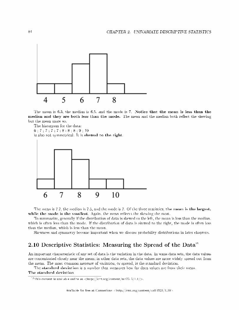
84 CHAPTER 2. UNIVARIATE DESCRIPTIVE STATISTICS
The mean is 6.3, the median is 6.5, and the mode is 7. Notice that the mean is less than themedian and they are both less than the mode. The mean and the median both re�ect the skewingbut the mean more so.
The histogram for the data:6 ; 7 ; 7 ; 7 ; 7 ; 8 ; 8 ; 8 ; 9 ; 10is also not symmetrical. It is skewed to the right.
The mean is 7.7, the median is 7.5, and the mode is 7. Of the three statistics, the mean is the largest,while the mode is the smallest. Again, the mean re�ects the skewing the most.
To summarize, generally if the distribution of data is skewed to the left, the mean is less than the median,which is often less than the mode. If the distribution of data is skewed to the right, the mode is often lessthan the median, which is less than the mean.
Skewness and symmetry become important when we discuss probability distributions in later chapters.
2.10 Descriptive Statistics: Measuring the Spread of the Data15
An important characteristic of any set of data is the variation in the data. In some data sets, the data valuesare concentrated closely near the mean; in other data sets, the data values are more widely spread out fromthe mean. The most common measure of variation, or spread, is the standard deviation.
The standard deviation is a number that measures how far data values are from their mean.The standard deviation
15This content is available online at <http://cnx.org/content/m47515/1.1/>.
Available for free at Connexions <http://cnx.org/content/col11521/1.19>
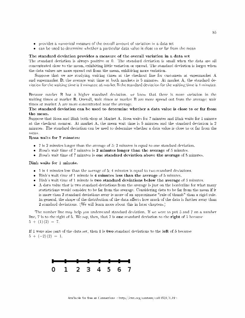
85
• provides a numerical measure of the overall amount of variation in a data set• can be used to determine whether a particular data value is close to or far from the mean
The standard deviation provides a measure of the overall variation in a data setThe standard deviation is always positive or 0. The standard deviation is small when the data are allconcentrated close to the mean, exhibiting little variation or spread. The standard deviation is larger whenthe data values are more spread out from the mean, exhibiting more variation.
Suppose that we are studying waiting times at the checkout line for customers at supermarket Aand supermarket B; the average wait time at both markets is 5 minutes. At market A, the standard de-viation for the waiting time is 2 minutes; at market B the standard deviation for the waiting time is 4 minutes.
Because market B has a higher standard deviation, we know that there is more variation in thewaiting times at market B. Overall, wait times at market B are more spread out from the average; waittimes at market A are more concentrated near the average.The standard deviation can be used to determine whether a data value is close to or far fromthe mean.Suppose that Rosa and Binh both shop at Market A. Rosa waits for 7 minutes and Binh waits for 1 minuteat the checkout counter. At market A, the mean wait time is 5 minutes and the standard deviation is 2minutes. The standard deviation can be used to determine whether a data value is close to or far from themean.Rosa waits for 7 minutes:
• 7 is 2 minutes longer than the average of 5; 2 minutes is equal to one standard deviation.• Rosa's wait time of 7 minutes is 2 minutes longer than the average of 5 minutes.• Rosa's wait time of 7 minutes is one standard deviation above the average of 5 minutes.
Binh waits for 1 minute.
• 1 is 4 minutes less than the average of 5; 4 minutes is equal to two standard deviations.• Binh's wait time of 1 minute is 4 minutes less than the average of 5 minutes.• Binh's wait time of 1 minute is two standard deviations below the average of 5 minutes.• A data value that is two standard deviations from the average is just on the borderline for what many
statisticians would consider to be far from the average. Considering data to be far from the mean if itis more than 2 standard deviations away is more of an approximate "rule of thumb" than a rigid rule.In general, the shape of the distribution of the data a�ects how much of the data is further away than2 standard deviations. (We will learn more about this in later chapters.)
The number line may help you understand standard deviation. If we were to put 5 and 7 on a numberline, 7 is to the right of 5. We say, then, that 7 is one standard deviation to the right of 5 because5 + (1) (2) = 7.
If 1 were also part of the data set, then 1 is two standard deviations to the left of 5 because5 + (−2) (2) = 1.
Available for free at Connexions <http://cnx.org/content/col11521/1.19>
86 CHAPTER 2. UNIVARIATE DESCRIPTIVE STATISTICS
• In general, a value = mean + (#ofSTDEV)(standard deviation)• where #ofSTDEVs = the number of standard deviations• 7 is one standard deviation more than the mean of 5 because: 7=5+(1)(2)• 1 is two standard deviations less than the mean of 5 because: 1=5+(−2)(2)
The equation value = mean + (#ofSTDEVs)(standard deviation) can be expressed for a sampleand for a population:
• sample: x = x+ (#ofSTDEV) (s)• Population: x = µ+ (#ofSTDEV) (σ)
The lower case letter s represents the sample standard deviation and the Greek letter σ (sigma, lower case)represents the population standard deviation.
The symbol x is the sample mean and the Greek symbol µ is the population mean.Calculating the Standard DeviationIf x is a number, then the di�erence "x - mean" is called its deviation. In a data set, there are as manydeviations as there are items in the data set. The deviations are used to calculate the standard deviation.If the numbers belong to a population, in symbols a deviation is x − µ . For sample data, in symbols adeviation is x− x .
The procedure to calculate the standard deviation depends on whether the numbers are the entire pop-ulation or are data from a sample. The calculations are similar, but not identical. Therefore the symbolused to represent the standard deviation depends on whether it is calculated from a population or a sample.The lower case letter s represents the sample standard deviation and the Greek letter σ (sigma, lower case)represents the population standard deviation. If the sample has the same characteristics as the population,then s should be a good estimate of σ.
To calculate the standard deviation, we need to calculate the variance �rst. The variance is an averageof the squares of the deviations (the x− x values for a sample, or the x − µ values for a population).The symbol σ2 represents the population variance; the population standard deviation σ is the square rootof the population variance. The symbol s2 represents the sample variance; the sample standard deviation sis the square root of the sample variance. You can think of the standard deviation as a special average ofthe deviations.
If the numbers come from a census of the entire population and not a sample, when we calculatethe average of the squared deviations to �nd the variance, we divide by N, the number of items in thepopulation. If the data are from a sample rather than a population, when we calculate the average of thesquared deviations, we divide by n-1, one less than the number of items in the sample. You can see that inthe formulas below.Formulas for the Sample Standard Deviation
• s =√
Σ(x−x)2
n−1 or s =√
Σf ·(x−x)2
n−1
• For the sample standard deviation, the denominator is n-1, that is the sample size MINUS 1.
Formulas for the Population Standard Deviation
• σ =√
Σ(x−µ)2
N or σ =√
Σf ·(x−µ)2
N• For the population standard deviation, the denominator is N, the number of items in the population.
In these formulas, f represents the frequency with which a value appears. For example, if a value appearsonce, f is 1. If a value appears three times in the data set or population, f is 3.Sampling Variability of a StatisticThe statistic of a sampling distribution was discussed in Descriptive Statistics: Measuring the Centerof the Data. How much the statistic varies from one sample to another is known as the sampling vari-ability of a statistic. You typically measure the sampling variability of a statistic by its standard error.
Available for free at Connexions <http://cnx.org/content/col11521/1.19>
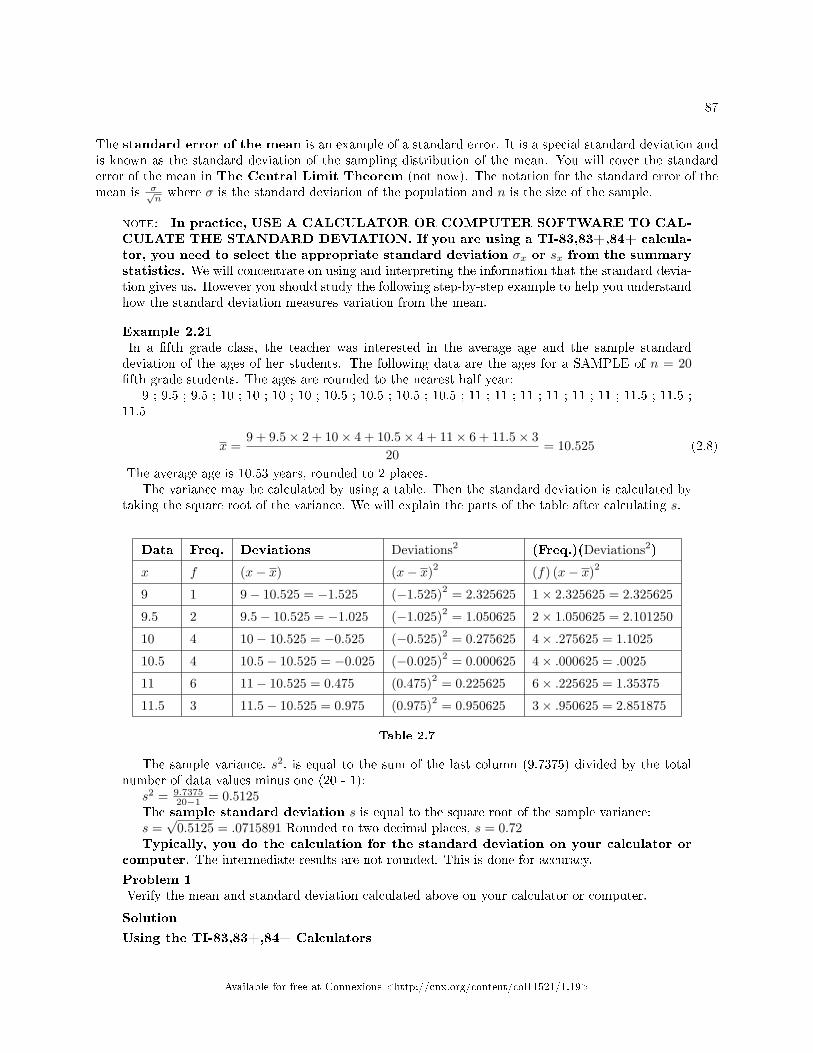
87
The standard error of the mean is an example of a standard error. It is a special standard deviation andis known as the standard deviation of the sampling distribution of the mean. You will cover the standarderror of the mean in The Central Limit Theorem (not now). The notation for the standard error of themean is σ√
nwhere σ is the standard deviation of the population and n is the size of the sample.
note: In practice, USE A CALCULATOR OR COMPUTER SOFTWARE TO CAL-CULATE THE STANDARD DEVIATION. If you are using a TI-83,83+,84+ calcula-tor, you need to select the appropriate standard deviation σx or sx from the summarystatistics. We will concentrate on using and interpreting the information that the standard devia-tion gives us. However you should study the following step-by-step example to help you understandhow the standard deviation measures variation from the mean.
Example 2.21In a �fth grade class, the teacher was interested in the average age and the sample standarddeviation of the ages of her students. The following data are the ages for a SAMPLE of n = 20�fth grade students. The ages are rounded to the nearest half year:
9 ; 9.5 ; 9.5 ; 10 ; 10 ; 10 ; 10 ; 10.5 ; 10.5 ; 10.5 ; 10.5 ; 11 ; 11 ; 11 ; 11 ; 11 ; 11 ; 11.5 ; 11.5 ;11.5
x =9 + 9.5× 2 + 10× 4 + 10.5× 4 + 11× 6 + 11.5× 3
20= 10.525 (2.8)
The average age is 10.53 years, rounded to 2 places.The variance may be calculated by using a table. Then the standard deviation is calculated by
taking the square root of the variance. We will explain the parts of the table after calculating s.
Data Freq. Deviations Deviations2 (Freq.)(Deviations2)
x f (x− x) (x− x)2 (f) (x− x)2
9 1 9− 10.525 = −1.525 (−1.525)2 = 2.325625 1× 2.325625 = 2.325625
9.5 2 9.5− 10.525 = −1.025 (−1.025)2 = 1.050625 2× 1.050625 = 2.101250
10 4 10− 10.525 = −0.525 (−0.525)2 = 0.275625 4× .275625 = 1.1025
10.5 4 10.5− 10.525 = −0.025 (−0.025)2 = 0.000625 4× .000625 = .0025
11 6 11− 10.525 = 0.475 (0.475)2 = 0.225625 6× .225625 = 1.35375
11.5 3 11.5− 10.525 = 0.975 (0.975)2 = 0.950625 3× .950625 = 2.851875
Table 2.7
The sample variance, s2, is equal to the sum of the last column (9.7375) divided by the totalnumber of data values minus one (20 - 1):
s2 = 9.737520−1 = 0.5125
The sample standard deviation s is equal to the square root of the sample variance:s =√
0.5125 = .0715891 Rounded to two decimal places, s = 0.72Typically, you do the calculation for the standard deviation on your calculator or
computer. The intermediate results are not rounded. This is done for accuracy.
Problem 1Verify the mean and standard deviation calculated above on your calculator or computer.
Solution
Using the TI-83,83+,84+ Calculators
Available for free at Connexions <http://cnx.org/content/col11521/1.19>
88 CHAPTER 2. UNIVARIATE DESCRIPTIVE STATISTICS
� Enter data into the list editor. Press STAT 1:EDIT. If necessary, clear the lists by arrowingup into the name. Press CLEAR and arrow down.
� Put the data values (9, 9.5, 10, 10.5, 11, 11.5) into list L1 and the frequencies (1, 2, 4, 4, 6,3) into list L2. Use the arrow keys to move around.
� Press STAT and arrow to CALC. Press 1:1-VarStats and enter L1 (2nd 1), L2 (2nd 2). Donot forget the comma. Press ENTER.
� x=10.525� Use Sx because this is sample data (not a population): Sx=0.715891
• For the following problems, recall that value = mean + (#ofSTDEVs)(standard devi-ation)
• For a sample: x = x + (#ofSTDEVs)(s)• For a population: x = µ + (#ofSTDEVs)( σ)• For this example, use x = x + (#ofSTDEVs)(s) because the data is from a sample
Problem 2Find the value that is 1 standard deviation above the mean. Find (x+ 1s).
Solution(x+ 1s) = 10.53 + (1) (0.72) = 11.25
Problem 3Find the value that is two standard deviations below the mean. Find (x− 2s).
Solution(x− 2s) = 10.53− (2) (0.72) = 9.09
Problem 4Find the values that are 1.5 standard deviations from (below and above) the mean.
Solution
• (x− 1.5s) = 10.53− (1.5) (0.72) = 9.45• (x+ 1.5s) = 10.53 + (1.5) (0.72) = 11.61
Explanation of the standard deviation calculation shown in the tableThe deviations show how spread out the data are about the mean. The data value 11.5 is farther from themean than is the data value 11. The deviations 0.97 and 0.47 indicate that. A positive deviation occurswhen the data value is greater than the mean. A negative deviation occurs when the data value is less thanthe mean; the deviation is -1.525 for the data value 9. If you add the deviations, the sum is alwayszero. (For this example, there are n=20 deviations.) So you cannot simply add the deviations to get thespread of the data. By squaring the deviations, you make them positive numbers, and the sum will also bepositive. The variance, then, is the average squared deviation.
The variance is a squared measure and does not have the same units as the data. Taking the square rootsolves the problem. The standard deviation measures the spread in the same units as the data.
Notice that instead of dividing by n=20, the calculation divided by n-1=20-1=19 because the data is asample. For the sample variance, we divide by the sample size minus one (n− 1). Why not divide by
Available for free at Connexions <http://cnx.org/content/col11521/1.19>
89
n? The answer has to do with the population variance. The sample variance is an estimate of thepopulation variance. Based on the theoretical mathematics that lies behind these calculations, dividingby (n− 1) gives a better estimate of the population variance.
note: Your concentration should be on what the standard deviation tells us about the data. Thestandard deviation is a number which measures how far the data are spread from the mean. Let acalculator or computer do the arithmetic.
The standard deviation, s or σ, is either zero or larger than zero. When the standard deviation is 0, there isno spread; that is, the all the data values are equal to each other. The standard deviation is small when thedata are all concentrated close to the mean, and is larger when the data values show more variation fromthe mean. When the standard deviation is a lot larger than zero, the data values are very spread out aboutthe mean; outliers can make s or σ very large.
The standard deviation, when �rst presented, can seem unclear. By graphing your data, you can get abetter "feel" for the deviations and the standard deviation. You will �nd that in symmetrical distributions,the standard deviation can be very helpful but in skewed distributions, the standard deviation may not bemuch help. The reason is that the two sides of a skewed distribution have di�erent spreads. In a skeweddistribution, it is better to look at the �rst quartile, the median, the third quartile, the smallest value, andthe largest value. Because numbers can be confusing, always graph your data.
note: The formula for the standard deviation is at the end of the chapter.
Example 2.22Use the following data (�rst exam scores) from Susan Dean's spring pre-calculus class:
33; 42; 49; 49; 53; 55; 55; 61; 63; 67; 68; 68; 69; 69; 72; 73; 74; 78; 80; 83; 88; 88; 88; 90; 92; 94;94; 94; 94; 96; 100
a. Create a chart containing the data, frequencies, relative frequencies, and cumulative relativefrequencies to three decimal places.
b. Calculate the following to one decimal place using a TI-83+ or TI-84 calculator:
i. The sample meanii. The sample standard deviationiii. The medianiv. The �rst quartilev. The third quartilevi. IQR
c. Construct a box plot and a histogram on the same set of axes. Make comments about the boxplot, the histogram, and the chart.
Solution
Available for free at Connexions <http://cnx.org/content/col11521/1.19>
90 CHAPTER 2. UNIVARIATE DESCRIPTIVE STATISTICS
a.Data Frequency Relative Frequency Cumulative Relative Frequency
33 1 0.032 0.032
42 1 0.032 0.064
49 2 0.065 0.129
53 1 0.032 0.161
55 2 0.065 0.226
61 1 0.032 0.258
63 1 0.032 0.29
67 1 0.032 0.322
68 2 0.065 0.387
69 2 0.065 0.452
72 1 0.032 0.484
73 1 0.032 0.516
74 1 0.032 0.548
78 1 0.032 0.580
80 1 0.032 0.612
83 1 0.032 0.644
88 3 0.097 0.741
90 1 0.032 0.773
92 1 0.032 0.805
94 4 0.129 0.934
96 1 0.032 0.966
100 1 0.032 0.998 (Why isn't this value 1?)
Table 2.8
b. i. The sample mean = 73.5ii. The sample standard deviation = 17.9iii. The median = 73iv. The �rst quartile = 61v. The third quartile = 90vi. IQR = 90 - 61 = 29
c. The x-axis goes from 32.5 to 100.5; y-axis goes from -2.4 to 15 for the histogram; number ofintervals is 5 for the histogram so the width of an interval is (100.5 - 32.5) divided by 5 which isequal to 13.6. Endpoints of the intervals: starting point is 32.5, 32.5+13.6 = 46.1, 46.1+13.6= 59.7, 59.7+13.6 = 73.3, 73.3+13.6 = 86.9, 86.9+13.6 = 100.5 = the ending value; No datavalues fall on an interval boundary.
Available for free at Connexions <http://cnx.org/content/col11521/1.19>
91
Figure 2.3
The long left whisker in the box plot is re�ected in the left side of the histogram. The spread ofthe exam scores in the lower 50% is greater (73 - 33 = 40) than the spread in the upper 50% (100- 73 = 27). The histogram, box plot, and chart all re�ect this. There are a substantial number ofA and B grades (80s, 90s, and 100). The histogram clearly shows this. The box plot shows us thatthe middle 50% of the exam scores (IQR = 29) are Ds, Cs, and Bs. The box plot also shows usthat the lower 25% of the exam scores are Ds and Fs.
Comparing Values from Di�erent Data SetsThe standard deviation is useful when comparing data values that come from di�erent data sets. If the datasets have di�erent means and standard deviations, it can be misleading to compare the data values directly.
• For each data value, calculate how many standard deviations the value is away from its mean.• Use the formula: value = mean + (#ofSTDEVs)(standard deviation); solve for #ofSTDEVs.• #ofSTDEVs = value−mean
standard deviation• Compare the results of this calculation.
#ofSTDEVs is often called a "z-score"; we can use the symbol z. In symbols, the formulas become:
Sample x = x + z s z = x−xs
Population x = µ + z σ z = x−µσ
Table 2.9
Available for free at Connexions <http://cnx.org/content/col11521/1.19>
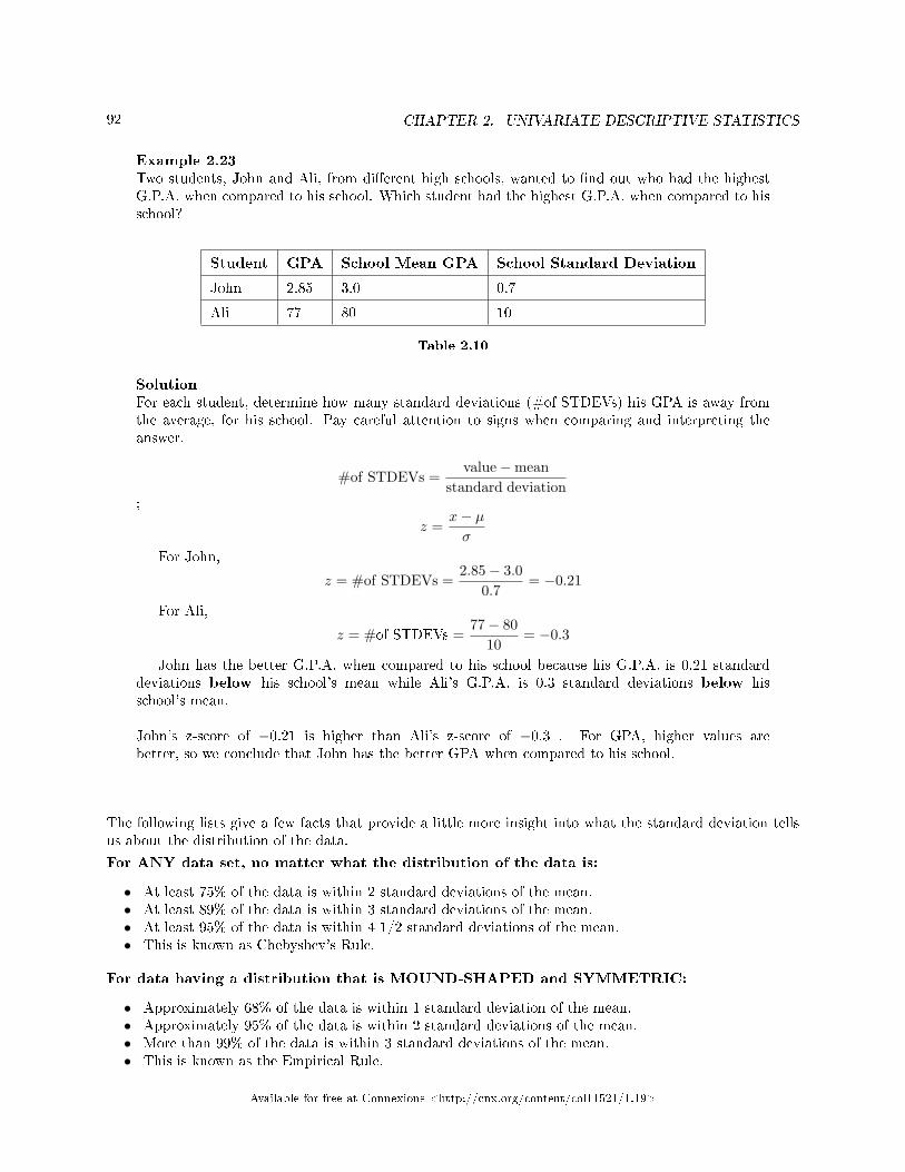
92 CHAPTER 2. UNIVARIATE DESCRIPTIVE STATISTICS
Example 2.23Two students, John and Ali, from di�erent high schools, wanted to �nd out who had the highestG.P.A. when compared to his school. Which student had the highest G.P.A. when compared to hisschool?
Student GPA School Mean GPA School Standard Deviation
John 2.85 3.0 0.7
Ali 77 80 10
Table 2.10
SolutionFor each student, determine how many standard deviations (#of STDEVs) his GPA is away fromthe average, for his school. Pay careful attention to signs when comparing and interpreting theanswer.
#of STDEVs =value−mean
standard deviation;
z =x− µσ
For John,
z = #of STDEVs =2.85− 3.0
0.7= −0.21
For Ali,
z = #of STDEVs =77− 80
10= −0.3
John has the better G.P.A. when compared to his school because his G.P.A. is 0.21 standarddeviations below his school's mean while Ali's G.P.A. is 0.3 standard deviations below hisschool's mean.
John's z-score of −0.21 is higher than Ali's z-score of −0.3 . For GPA, higher values arebetter, so we conclude that John has the better GPA when compared to his school.
The following lists give a few facts that provide a little more insight into what the standard deviation tellsus about the distribution of the data.
For ANY data set, no matter what the distribution of the data is:
• At least 75% of the data is within 2 standard deviations of the mean.• At least 89% of the data is within 3 standard deviations of the mean.• At least 95% of the data is within 4 1/2 standard deviations of the mean.• This is known as Chebyshev's Rule.
For data having a distribution that is MOUND-SHAPED and SYMMETRIC:
• Approximately 68% of the data is within 1 standard deviation of the mean.• Approximately 95% of the data is within 2 standard deviations of the mean.• More than 99% of the data is within 3 standard deviations of the mean.• This is known as the Empirical Rule.
Available for free at Connexions <http://cnx.org/content/col11521/1.19>
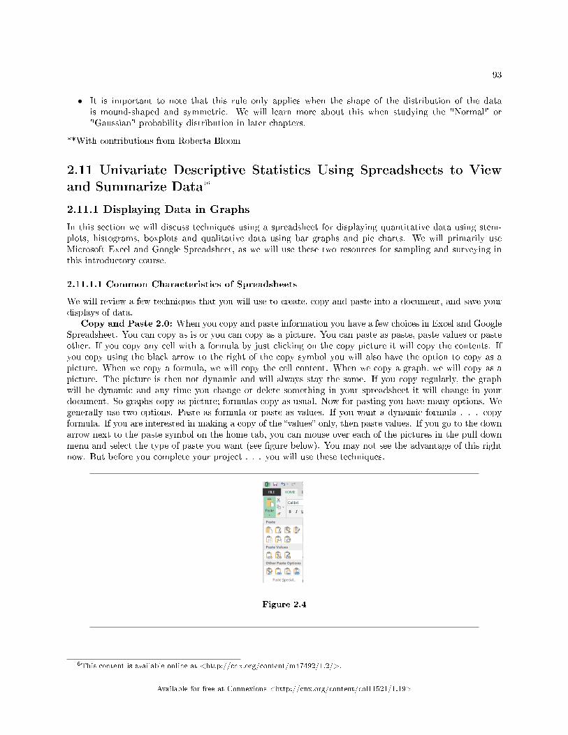
93
• It is important to note that this rule only applies when the shape of the distribution of the datais mound-shaped and symmetric. We will learn more about this when studying the "Normal" or"Gaussian" probability distribution in later chapters.
**With contributions from Roberta Bloom
2.11 Univariate Descriptive Statistics Using Spreadsheets to Viewand Summarize Data16
2.11.1 Displaying Data in Graphs
In this section we will discuss techniques using a spreadsheet for displaying quantitative data using stem-plots, histograms, boxplots and qualitative data using bar graphs and pie charts. We will primarily useMicrosoft Excel and Google Spreadsheet, as we will use these two resources for sampling and surveying inthis introductory course.
2.11.1.1 Common Characteristics of Spreadsheets
We will review a few techniques that you will use to create, copy and paste into a document, and save yourdisplays of data.
Copy and Paste 2.0: When you copy and paste information you have a few choices in Excel and GoogleSpreadsheet. You can copy as is or you can copy as a picture. You can paste as paste, paste values or pasteother. If you copy any cell with a formula by just clicking on the copy picture it will copy the contents. Ifyou copy using the black arrow to the right of the copy symbol you will also have the option to copy as apicture. When we copy a formula, we will copy the cell content. When we copy a graph, we will copy as apicture. The picture is then not dynamic and will always stay the same. If you copy regularly, the graphwill be dynamic and any time you change or delete something in your spreadsheet it will change in yourdocument. So graphs copy as picture; formulas copy as usual. Now for pasting you have many options. Wegenerally use two options. Paste as formula or paste as values. If you want a dynamic formula . . . copyformula. If you are interested in making a copy of the �values� only, then paste values. If you go to the downarrow next to the paste symbol on the home tab, you can mouse over each of the pictures in the pull downmenu and select the type of paste you want (see �gure below). You may not see the advantage of this rightnow. But before you complete your project . . . you will use these techniques.
Figure 2.4
16This content is available online at <http://cnx.org/content/m47492/1.2/>.
Available for free at Connexions <http://cnx.org/content/col11521/1.19>
94 CHAPTER 2. UNIVARIATE DESCRIPTIVE STATISTICS
2.11.1.2 Common Characteristics of Bar Graphs and Histograms
Both bar graphs for qualitative data and histograms for quantitative data involve using frequency distribu-tions of the data. For qualitative data each bar will represent one category of data. Since the data is discreteor nominal in nature, we will be sure to represent the data with each category having its own bar. The orderof the bars does not matter, but what does matter is that the bars are separated by space so that it is clearthat each bar is a di�erent category. When we work with quantitative data, we will make sure that the barsare touching (connected) since we will be working with continuous data and there is no space between themeasurement-level data.
2.11.1.3 Creating Bar Graphs
To create a bar graph using Excel, highlight the column of qualitative date that you would like to represent.Open the �Insert� tab on the ribbon and choose �Chart� in google spreadsheet or mouse over recommendedcharts in excel and click. A popup window with a bar chart will appear with categories and the counts ineach of the categories. If it looks like you intended, then mouse over to the OK button and click (bottomright of the popup screen). Excel will create a new spreadsheet for you. Again you will want to give theworksheet tab a descriptive name. You may even want to change the counts to percent of total. If so you willuse the sum of values box in the pivot chart �elds, use the downward pointing arrow to bring up another pulldown menu and select �Value Field Settings� (sound familiar), show values as, instead of no calculation pickpercent of total, then click on the ok button. You now have a bar chart with relative frequency. Note thatthis was a quick way to create a pivot table and a bar chart at the same time. While you are on this pageyou can select the categories of your data (in the example below college rank categories) and the relativefrequency column (highlight them with your mouse, next go to the insert tab in your ribbon and selectrecommended charts, Pie and then mouse over your OK button and you will have a pie chart on your Excelspreadsheet. You can mouse over the space provided for a title and give your pie chart a more descriptivetitle.
Available for free at Connexions <http://cnx.org/content/col11521/1.19>
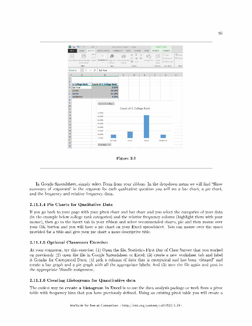
95
Figure 2.5
In Google Spreadsheet, simply select Form from your ribbon. In the dropdown menu we will �nd �Showsummary of responses� in the response for each qualitative question you will see a bar chart, a pie chart,and the frequency and relative frequency data.
2.11.1.4 Pie Charts for Qualitative Data
If you go back to your page with your pivot chart and bar chart and you select the categories of your data(in the example below college rank categories) and the relative frequency column (highlight them with yourmouse), then go to the insert tab in your ribbon and select recommended charts, pie and then mouse overyour OK button and you will have a pie chart on your Excel spreadsheet. You can mouse over the spaceprovided for a title and give your pie chart a more descriptive title.
2.11.1.5 Optional Classroom Exercise:
At your computer, try this exercise: (1) Open the �le, Statistics First Day of Class Survey that you workedon previously (2) open the �le in Google Spreadsheet or Excel; (3) create a new worksheet tab and labelit Graphs for Categorical Data; (4) pick a column of data that is categorical and has been �cleaned� andcreate a bar graph and a pie graph with all the appropriate labels; And (5) save the �le again and post inthe appropriate Moodle assignment.
2.11.1.6 Creating Histograms for Quantitative data
The easiest way to create a histogram in Excel is to use the data analysis package or work from a pivottable with frequency bins that you have previously de�ned. Using an existing pivot table you will create a
Available for free at Connexions <http://cnx.org/content/col11521/1.19>
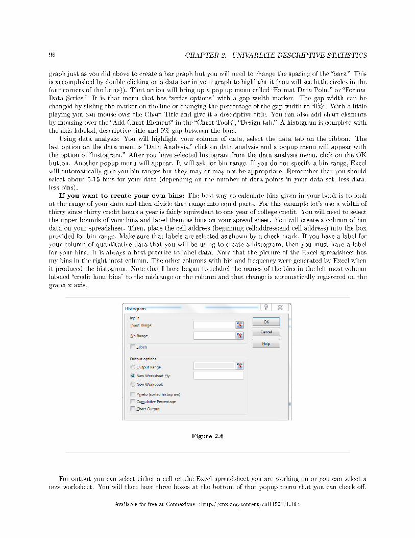
96 CHAPTER 2. UNIVARIATE DESCRIPTIVE STATISTICS
graph just as you did above to create a bar graph but you will need to change the spacing of the �bars.� Thisis accomplished by double clicking on a data bar in your graph to highlight it (you will see little circles in thefour corners of the bar(s)). That action will bring up a pop up menu called �Format Data Point� or �FormatData Series.� It is that menu that has �series options� with a gap width marker. The gap width can bechanged by sliding the marker on the line or changing the percentage of the gap width to �0%�. With a littleplaying you can mouse over the Chart Title and give it a descriptive title. You can also add chart elementsby mousing over the �Add Chart Element� in the �Chart Tools�, �Design tab.� A histogram is complete withthe axis labeled, descriptive title and 0% gap between the bars.
Using data analysis: You will highlight your column of data, select the data tab on the ribbon. Thelast option on the data menu is �Data Analysis,� click on data analysis and a popup menu will appear withthe option of �histogram.� After you have selected histogram from the data analysis menu, click on the OKbutton. Another popup menu will appear. It will ask for bin range. If you do not specify a bin range, Excelwill automatically give you bin ranges but they may or may not be appropriate. Remember that you shouldselect about 5-15 bins for your data (depending on the number of data points in your data set, less data,less bins).
If you want to create your own bins: The best way to calculate bins given in your book is to lookat the range of your data and then divide that range into equal parts. For this example let's use a width ofthirty since thirty credit hours a year is fairly equivalent to one year of college credit. You will need to selectthe upper bounds of your bins and label them as bins on your spread sheet. You will create a column of bindata on your spreadsheet. Then, place the cell address (beginning celladdress:end cell address) into the boxprovided for bin range. Make sure that labels are selected as shown by a check mark. If you have a label foryour column of quantitative data that you will be using to create a histogram, then you must have a labelfor your bins. It is always a best practice to label data. Note that the picture of the Excel spreadsheet hasmy bins in the right most column. The other columns with bin and frequency were generated by Excel whenit produced the histogram. Note that I have begun to relabel the names of the bins in the left most columnlabeled �credit hour bins� to the midrange or the column and that change is automatically registered on thegraph x-axis.
Figure 2.6
For output you can select either a cell on the Excel spreadsheet you are working on or you can select anew worksheet. You will then have three boxes at the bottom of that popup menu that you can check o�.
Available for free at Connexions <http://cnx.org/content/col11521/1.19>
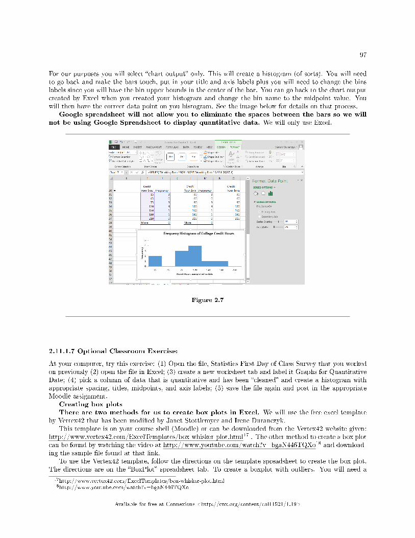
97
For our purposes you will select �chart output� only. This will create a histogram (of sorts). You will needto go back and make the bars touch, put in your title and axis labels plus you will need to change the binslabels since you will have the bin upper bounds in the center of the bar. You can go back to the chart outputcreated by Excel when you created your histogram and change the bin name to the midpoint value. Youwill then have the correct data point on you histogram. See the image below for details on that process.
Google spreadsheet will not allow you to eliminate the spaces between the bars so we willnot be using Google Spreadsheet to display quantitative data. We will only use Excel.
Figure 2.7
2.11.1.7 Optional Classroom Exercise:
At your computer, try this exercise: (1) Open the �le, Statistics First Day of Class Survey that you workedon previously (2) open the �le in Excel; (3) create a new worksheet tab and label it Graphs for QuantitativeDate; (4) pick a column of data that is quantitative and has been �cleaned� and create a histogram withappropriate spacing, titles, midpoints, and axis labels; (5) save the �le again and post in the appropriateMoodle assignment.
Creating box plotsThere are two methods for us to create box plots in Excel. We will use the free excel template
by Vertex42 that has been modi�ed by Janet Stottlemyer and Irene Duranczyk.This template is on your course shell (Moodle) or can be downloaded from the Vertex42 website given:
http://www.vertex42.com/ExcelTemplates/box-whisker-plot.html17 . The other method to create a box plotcan be found by watching the video at http://www.youtube.com/watch?v=bgaN446TQXo18 and download-ing the sample �le found at that link.
To use the Vertex42 template, follow the directions on the template spreadsheet to create the box plot.The directions are on the �BoxPlot� spreadsheet tab. To create a boxplot with outliers. You will need a
17http://www.vertex42.com/ExcelTemplates/box-whisker-plot.html18http://www.youtube.com/watch?v=bgaN446TQXo
Available for free at Connexions <http://cnx.org/content/col11521/1.19>
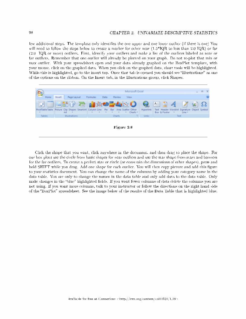
98 CHAPTER 2. UNIVARIATE DESCRIPTIVE STATISTICS
few additional steps. The template only identi�es the one upper and one lower outlier (if there is one) Youwill need to follow the steps below to create a marker for other near (1.5*IQR to less than 2.0 IQR) or far(2.0+IQR or more) outliers. First, identify your outliers and make a list of the outliers labeled as near orfar outliers. Remember that one outlier will already be plotted on your graph. Do not re-plot that min ormax outlier. With your spreadsheet open and your data already graphed on the BoxPlot template, withyour mouse, click on the graphed data. When you click on the graphed data, chart tools will be highlighted.While this is highlighted, go to the insert tap. Once that tab is opened you should see �Illustrations" as oneof the options on the ribbon. On the Insert tab, in the Illustrations group, click Shapes.
Figure 2.8
Click the shape that you want, click anywhere in the document, and then drag to place the shape. Forour box plots use the circle from basic shapes for near outliers and use the star shape from stars and bannersfor the far outliers. To create a perfect star or circle (or constrain the dimensions of other shapes), press andhold SHIFT while you drag. Add one shape for each outlier. You will then copy picture and add this �gureto your statistics document. You can change the name of the columns by adding your category name in thedata table. You are only to change the names in the data table and only add data to the data table. Onlymake changes in the �blue� highlighted �elds. If you want fewer columns of data delete the columns you arenot using. If you want more columns, talk to your instructor or follow the directions on the right hand sideof the �BoxPlot� spreadsheet. See the image below of the results of the Data Table that is highlighted blue.
Available for free at Connexions <http://cnx.org/content/col11521/1.19>
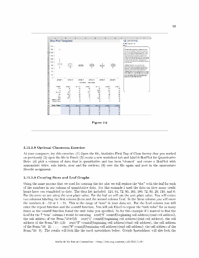
99
Figure 2.9
2.11.1.8 Optional Classroom Exercise:
At your computer, try this exercise: (1) Open the �le, Statistics First Day of Class Survey that you workedon previously (2) open the �le in Excel; (3) create a new worksheet tab and label it BoxPlot for QuantitativeDate; (4) pick a column of data that is quantitative and has been �cleaned� and create a BoxPlot withappropriate titles, axis labels, near and far outliers; (5) save the �le again and post in the appropriateMoodle assignment.
2.11.1.9 Creating Stem and Leaf Graphs
Using the same process that we used for creating the dot plot we will replace the �dot� with the leaf for eachof the numbers in our column of quantitative data. For this example I used the data on How many credithours have you completed to date. The data list included: 124, 84, 72, 95, 165, 100, 72, 95, 26, 110, and 0.For the stem we are using the tens place value. For the leaf we will use the unit place value. You will createtwo columns labeling the �rst column Stem and the second column Leaf. In the Stem column you will enterthe numbers 0 � 12 or 1 � 11. This is the range of �tens� in your data set. For the Leaf column you willenter the repeat function and the countif function. You will ask Excel to repeat the �unit value� for as manytimes as the countif function found the unit value you speci�ed. So for this example if I wanted to �nd theLeaf for the 7 �tens� column I would be entering =rept(�0� countif(beginning cell address):(end cell address),the cell address of the Stem,*10+0)& =rept(�1� countif(beginning cell address):(end cell address), the celladdress of the Stem,*10+1)& =rept(�2� countif(beginning cell address):(end cell address), the cell addressof the Stem,*10+2). . . . =rept(�9� countif(beginning cell address):(end cell address), the cell address of theStem,*10+9). The results will look like the excel spreadsheet below. Google Spreadsheet will also look the
Available for free at Connexions <http://cnx.org/content/col11521/1.19>
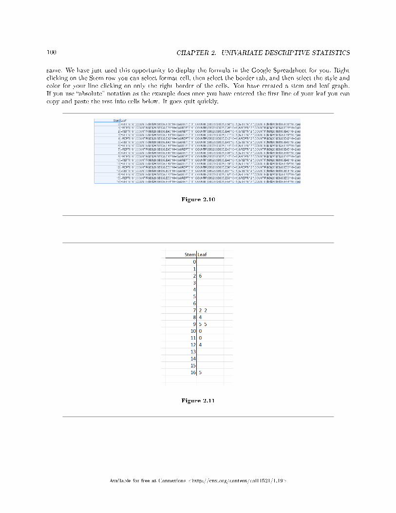
100 CHAPTER 2. UNIVARIATE DESCRIPTIVE STATISTICS
same. We have just used this opportunity to display the formula in the Google Spreadsheet for you. Rightclicking on the Stem row you can select format cell, then select the border tab, and then select the style andcolor for your line clicking on only the right border of the cells. You have created a stem and leaf graph.If you use �absolute� notation as the example does once you have entered the �rst line of your leaf you cancopy and paste the rest into cells below. It goes quit quickly.
Figure 2.10
Figure 2.11
Available for free at Connexions <http://cnx.org/content/col11521/1.19>
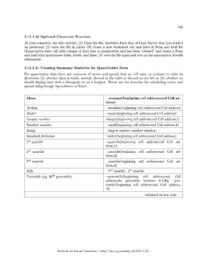
101
2.11.1.10 Optional Classroom Exercise:
At your computer, try this exercise: (1) Open the �le, Statistics First Day of Class Survey that you workedon previously (2) open the �le in Excel; (3) create a new worksheet tab and label it Stem and Leaf forQuantitative Date; (4) pick column of data that is quantitative and has been �cleaned� and create a Stemand Leaf with appropriate titles, labels, and lines; (5) save the �le again and post in the appropriate Moodleassignment.
2.11.1.11 Creating Summary Statistics for Quantitative Data
For quantitative data there are measures of center and spread that we will want to evaluate in order todetermine (1) whether data is nearly normal, skewed to the right or skewed to the left or (2) whether weshould display data with a histogram or on a boxplot. Below are the formulas for calculating center andspread using Google Spreadsheet or Excel.
Mean =average(beginning cell address:end Cell ad-dress)
Median =meadian(beginning cell address:end Cell address)
Mode* =mode(beginning cell address:end Cell address)
Largest number =large((beginning cell address:end Cell address,1)
Smallest number =small(beginning cell address:end Cell address,1)
Range =largest number-smallest number
Standard deviation =stdev(beginning cell address:end Cell address)
1st quartile =quartile(beginning cell address:end Cell ad-dress,1)
2nd quartile =quartile(beginning cell address:end Cell ad-dress,2)
3rd quartile =quartile(beginning cell address:end Cell ad-dress,3)
IQR =3rd quartile=1st quartile
Percentile (eg. 90th percentile) =percentile(beginning cell address:end Celladdress,the percentile between 0-1)Eg =per-centile(beginning cell address:end Cell address,.9)
continued on next page
Available for free at Connexions <http://cnx.org/content/col11521/1.19>
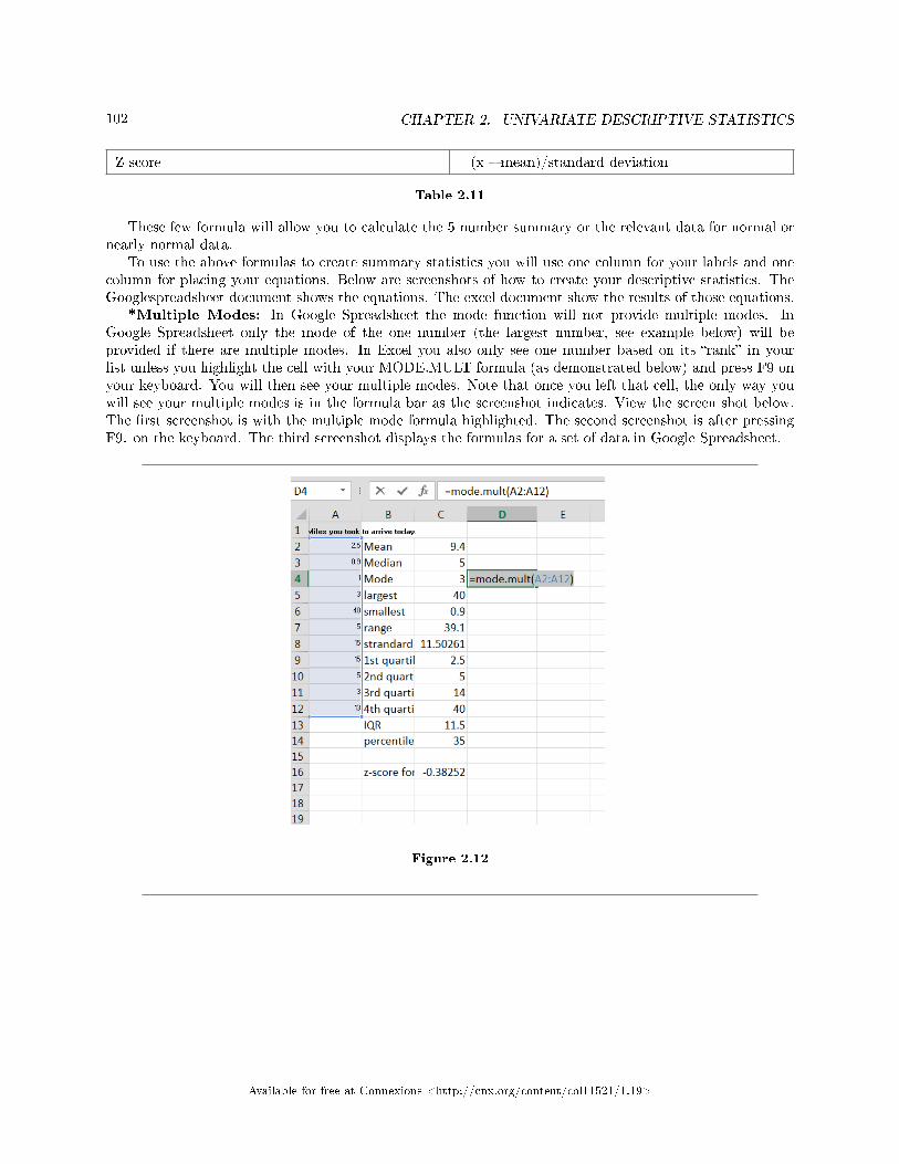
102 CHAPTER 2. UNIVARIATE DESCRIPTIVE STATISTICS
Z score =(x � mean)/standard deviation
Table 2.11
These few formula will allow you to calculate the 5 number summary or the relevant data for normal ornearly normal data.
To use the above formulas to create summary statistics you will use one column for your labels and onecolumn for placing your equations. Below are screenshots of how to create your descriptive statistics. TheGooglespreadsheet document shows the equations. The excel document show the results of those equations.
*Multiple Modes: In Google Spreadsheet the mode function will not provide multiple modes. InGoogle Spreadsheet only the mode of the one number (the largest number, see example below) will beprovided if there are multiple modes. In Excel you also only see one number based on its �rank� in yourlist unless you highlight the cell with your MODE.MULT formula (as demonstrated below) and press F9 onyour keyboard. You will then see your multiple modes. Note that once you left that cell, the only way youwill see your multiple modes is in the formula bar as the screenshot indicates. View the screen shot below.The �rst screenshot is with the multiple mode formula highlighted. The second screenshot is after pressingF9. on the keyboard. The third screenshot displays the formulas for a set of data in Google Spreadsheet.
Figure 2.12
Available for free at Connexions <http://cnx.org/content/col11521/1.19>
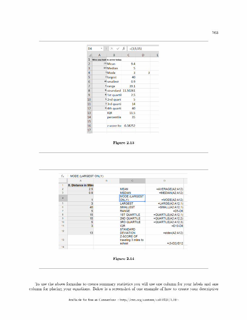
103
Figure 2.13
Figure 2.14
To use the above formulas to create summary statistics you will use one column for your labels and onecolumn for placing your equations. Below is a screenshot of one example of how to create your descriptive
Available for free at Connexions <http://cnx.org/content/col11521/1.19>
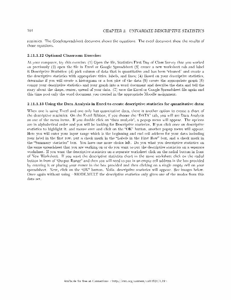
104 CHAPTER 2. UNIVARIATE DESCRIPTIVE STATISTICS
statistics. The Googlespreadsheet document shows the equations. The excel document show the results ofthose equations.
2.11.1.12 Optional Classroom Exercise:
At your computer, try this exercise: (1) Open the �le, Statistics First Day of Class Survey that you workedon previously (2) open the �le in Excel or Google Spreadsheet (3) create a new worksheet tab and labelit Descriptive Statistics; (4) pick column of data that is quantitative and has been �cleaned� and create athe descriptive statistics with appropriate titles, labels, and lines; (4) Based on your descriptive statistics,determine if you will create a historgram or a box plot of the data (5) create the appropriate graph (6)compy your descriptive statistics and your graph into a word document and describe the data and tell thestory about the shape, center, spread of your data. (7) save the Excel or Google Spreadsheet �le again andthis time post only the word document you created in the appropriate Moodle assignment.
2.11.1.13 Using the Data Analysis in Excel to create descriptive statistics for quantitative data:
When one is using Excel and one only has quantitative data, there is another option to create a chart ofthe descriptive statistics. On the Excel Ribbon, if you choose the �DATA� tab, you will see Data Analysisas one of the menu items. If you double click on �data analysis�, a popup menu will appear. The optionsare in alphabetical order and you will be looking for Descriptive statistics. If you click once on descriptivestatistics to highlight it, and mouse over and click on the �OK� button, another popup menu will appear.Here you will enter your input range which is the beginning and end cell address for your data includingyour label in the �rst row, put a check mark in the �Labels in the First Row� box, and a check mark inthe �Summary statistics� box. You have one more choice left. Do you what you descriptive statistics onthe same spreadsheet that you are working on or do you want to put the descriptive statistics on a separateworksheet. If you want the descriptive statistics on a separate worksheet click on the radial button in frontof New Worksheet. If you want the descriptive statistics chart in the same worksheet click on the radialbutton in from of �Output Range� and then you will need to put in an empty cell address in the box providedby entering it or placing your curser in the box provided and then clicking on a single empty cell on yourspreadsheet. Next, click on the �OK� button. Voila, descriptive statistics will appear. See images below.Once again without using =MODE.MULT the descriptive statistics only gives one of the modes from thisdata set.
Available for free at Connexions <http://cnx.org/content/col11521/1.19>
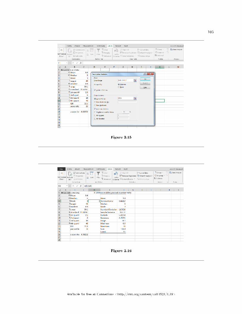
105
Figure 2.15
Figure 2.16
Available for free at Connexions <http://cnx.org/content/col11521/1.19>
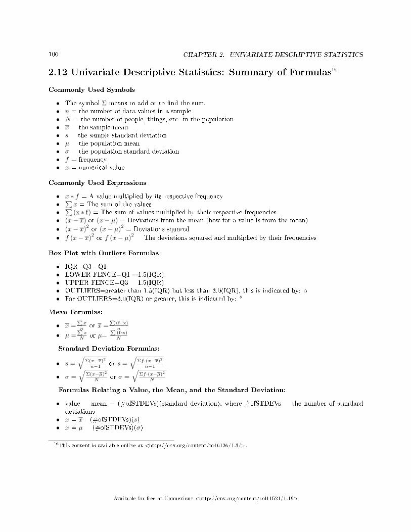
106 CHAPTER 2. UNIVARIATE DESCRIPTIVE STATISTICS
2.12 Univariate Descriptive Statistics: Summary of Formulas19
Commonly Used Symbols
• The symbol Σ means to add or to �nd the sum.• n = the number of data values in a sample• N = the number of people, things, etc. in the population• x = the sample mean• s = the sample standard deviation• µ = the population mean• σ = the population standard deviation• f = frequency• x = numerical value
Commonly Used Expressions
• x ∗ f = A value multiplied by its respective frequency•∑x = The sum of the values
•∑
(x ∗ f) = The sum of values multiplied by their respective frequencies• (x− x) or (x− µ) = Deviations from the mean (how far a value is from the mean)
• (x− x)2or (x− µ)2
= Deviations squared
• f (x− x)2or f (x− µ)2
= The deviations squared and multiplied by their frequencies
Box Plot with Outliers Formulas
• IQR=Q3 - Q1• LOWER FENCE=Q1 � 1.5(IQR)• UPPER FENCE=Q3 + 1.5(IQR)• OUTLIERS=greater than 1.5(IQR) but less than 3.0(IQR), this is indicated by: o• Far OUTLIERS=3.0(IQR) or greater, this is indicated by: *
Mean Formulas:
• x =Pxn or x =
P(f· x)n
• µ =Px
N or µ=P
(f·x)N
Standard Deviation Formulas:
• s =√
Σ(x−x)2
n−1 or s =√
Σf ·(x−x)2
n−1
• σ =√
Σ(x−µ)2
N or σ =√
Σf ·(x−µ)2
N
Formulas Relating a Value, the Mean, and the Standard Deviation:
• value = mean + (#ofSTDEVs)(standard deviation), where #ofSTDEVs = the number of standarddeviations
• x = x+ (#ofSTDEVs)(s)• x = µ + (#ofSTDEVs)(σ)
19This content is available online at <http://cnx.org/content/m46126/1.3/>.
Available for free at Connexions <http://cnx.org/content/col11521/1.19>
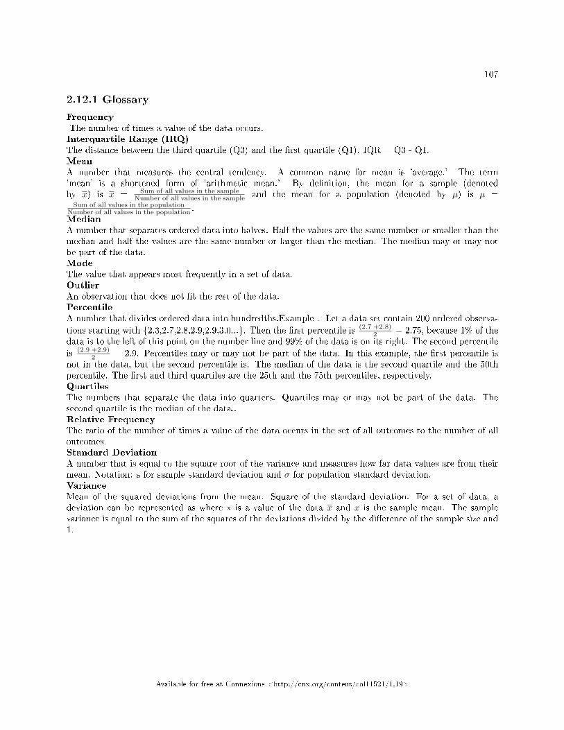
107
2.12.1 Glossary
FrequencyThe number of times a value of the data occurs.Interquartile Range (IRQ)The distance between the third quartile (Q3) and the �rst quartile (Q1). IQR = Q3 - Q1.MeanA number that measures the central tendency. A common name for mean is 'average.' The term'mean' is a shortened form of 'arithmetic mean.' By de�nition, the mean for a sample (denotedby x) is x = Sum of all values in the sample
Number of all values in the sample and the mean for a population (denoted by µ) is µ =Sum of all values in the population
Number of all values in the population .MedianA number that separates ordered data into halves. Half the values are the same number or smaller than themedian and half the values are the same number or larger than the median. The median may or may notbe part of the data.ModeThe value that appears most frequently in a set of data.OutlierAn observation that does not �t the rest of the data.PercentileA number that divides ordered data into hundredths.Example . Let a data set contain 200 ordered observa-
tions starting with {2.3,2.7,2.8,2.9,2.9,3.0...}. Then the �rst percentile is (2.7 +2.8)2 = 2.75, because 1% of the
data is to the left of this point on the number line and 99% of the data is on its right. The second percentile
is (2.9 +2.9)2 = 2.9. Percentiles may or may not be part of the data. In this example, the �rst percentile is
not in the data, but the second percentile is. The median of the data is the second quartile and the 50thpercentile. The �rst and third quartiles are the 25th and the 75th percentiles, respectively.QuartilesThe numbers that separate the data into quarters. Quartiles may or may not be part of the data. Thesecond quartile is the median of the data..Relative FrequencyThe ratio of the number of times a value of the data occurs in the set of all outcomes to the number of alloutcomes.Standard DeviationA number that is equal to the square root of the variance and measures how far data values are from theirmean. Notation: s for sample standard deviation and σ for population standard deviation.VarianceMean of the squared deviations from the mean. Square of the standard deviation. For a set of data, adeviation can be represented as where x is a value of the data x and x is the sample mean. The samplevariance is equal to the sum of the squares of the deviations divided by the di�erence of the sample size and1.
Available for free at Connexions <http://cnx.org/content/col11521/1.19>
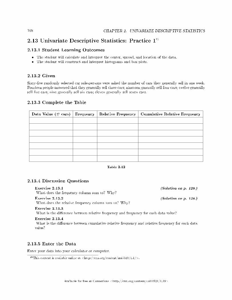
108 CHAPTER 2. UNIVARIATE DESCRIPTIVE STATISTICS
2.13 Univariate Descriptive Statistics: Practice 120
2.13.1 Student Learning Outcomes
• The student will calculate and interpret the center, spread, and location of the data.• The student will construct and interpret histograms and box plots.
2.13.2 Given
Sixty-�ve randomly selected car salespersons were asked the number of cars they generally sell in one week.Fourteen people answered that they generally sell three cars; nineteen generally sell four cars; twelve generallysell �ve cars; nine generally sell six cars; eleven generally sell seven cars.
2.13.3 Complete the Table
Data Value (# cars) Frequency Relative Frequency Cumulative Relative Frequency
Table 2.12
2.13.4 Discussion Questions
Exercise 2.13.1 (Solution on p. 128.)
What does the frequency column sum to? Why?
Exercise 2.13.2 (Solution on p. 128.)
What does the relative frequency column sum to? Why?
Exercise 2.13.3What is the di�erence between relative frequency and frequency for each data value?
Exercise 2.13.4What is the di�erence between cumulative relative frequency and relative frequency for each datavalue?
2.13.5 Enter the Data
Enter your data into your calculator or computer.
20This content is available online at <http://cnx.org/content/m47525/1.1/>.
Available for free at Connexions <http://cnx.org/content/col11521/1.19>
109
2.13.6 Construct a Histogram
Determine appropriate minimum and maximum x and y values and the scaling. Sketch the histogram below.Label the horizontal and vertical axes with words. Include numerical scaling.
2.13.7 Data Statistics
Calculate the following values:
Exercise 2.13.5 (Solution on p. 128.)
Sample mean = x =
Exercise 2.13.6 (Solution on p. 128.)
Sample standard deviation = sx =
Exercise 2.13.7 (Solution on p. 128.)
Sample size = n =
2.13.8 Calculations
Use the table in section 2.11.3 to calculate the following values:
Exercise 2.13.8 (Solution on p. 128.)
Median =
Exercise 2.13.9 (Solution on p. 128.)
Mode =
Exercise 2.13.10 (Solution on p. 128.)
First quartile =
Exercise 2.13.11 (Solution on p. 128.)
Second quartile = median = 50th percentile =
Exercise 2.13.12 (Solution on p. 129.)
Third quartile =
Exercise 2.13.13 (Solution on p. 129.)
Interquartile range (IQR) = _____ - _____ = _____
Exercise 2.13.14 (Solution on p. 129.)
10th percentile =
Exercise 2.13.15 (Solution on p. 129.)
70th percentile =
Available for free at Connexions <http://cnx.org/content/col11521/1.19>
110 CHAPTER 2. UNIVARIATE DESCRIPTIVE STATISTICS
Exercise 2.13.16 (Solution on p. 129.)
Find the value that is 3 standard deviations:
a. Above the meanb. Below the mean
2.13.9 Box Plot
Construct a box plot below. Use a ruler to measure and scale accurately.
2.13.10 Interpretation
Looking at your box plot, does it appear that the data are concentrated together, spread out evenly, orconcentrated in some areas, but not in others? How can you tell?
Available for free at Connexions <http://cnx.org/content/col11521/1.19>
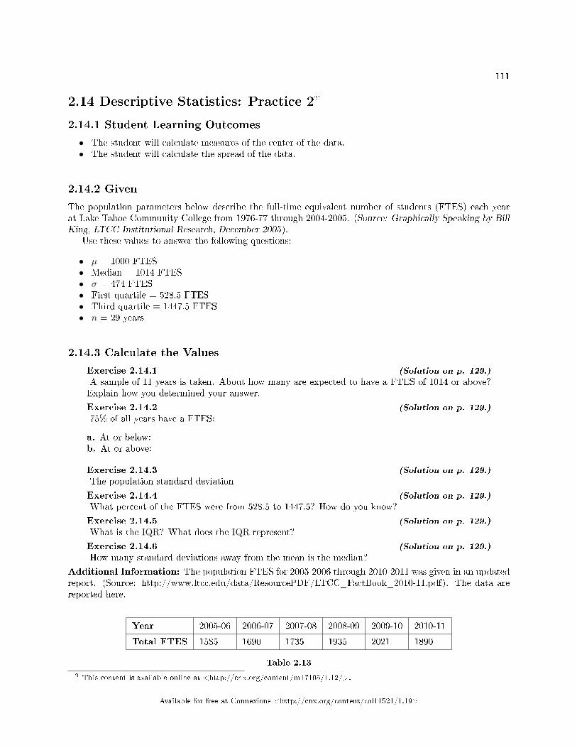
111
2.14 Descriptive Statistics: Practice 221
2.14.1 Student Learning Outcomes
• The student will calculate measures of the center of the data.• The student will calculate the spread of the data.
2.14.2 Given
The population parameters below describe the full-time equivalent number of students (FTES) each yearat Lake Tahoe Community College from 1976-77 through 2004-2005. (Source: Graphically Speaking by BillKing, LTCC Institutional Research, December 2005).
Use these values to answer the following questions:
• µ = 1000 FTES• Median = 1014 FTES• σ = 474 FTES• First quartile = 528.5 FTES• Third quartile = 1447.5 FTES• n = 29 years
2.14.3 Calculate the Values
Exercise 2.14.1 (Solution on p. 129.)
A sample of 11 years is taken. About how many are expected to have a FTES of 1014 or above?Explain how you determined your answer.
Exercise 2.14.2 (Solution on p. 129.)
75% of all years have a FTES:
a. At or below:b. At or above:
Exercise 2.14.3 (Solution on p. 129.)
The population standard deviation =
Exercise 2.14.4 (Solution on p. 129.)
What percent of the FTES were from 528.5 to 1447.5? How do you know?
Exercise 2.14.5 (Solution on p. 129.)
What is the IQR? What does the IQR represent?
Exercise 2.14.6 (Solution on p. 129.)
How many standard deviations away from the mean is the median?
Additional Information: The population FTES for 2005-2006 through 2010-2011 was given in an updatedreport. (Source: http://www.ltcc.edu/data/ResourcePDF/LTCC_FactBook_2010-11.pdf). The data arereported here.
Year 2005-06 2006-07 2007-08 2008-09 2009-10 2010-11
Total FTES 1585 1690 1735 1935 2021 1890
Table 2.13
21This content is available online at <http://cnx.org/content/m17105/1.12/>.
Available for free at Connexions <http://cnx.org/content/col11521/1.19>
112 CHAPTER 2. UNIVARIATE DESCRIPTIVE STATISTICS
Exercise 2.14.7 (Solution on p. 129.)
Calculate the mean, median, standard deviation, �rst quartile, the third quartile and the IQR.Round to one decimal place.
Exercise 2.14.8Construct a boxplot for the FTES for 2005-2006 through 2010-2011 and a boxplot for the FTESfor 1976-1977 through 2004-2005.
Exercise 2.14.9 (Solution on p. 129.)
Compare the IQR for the FTES for 1976-77 through 2004-2005 with the IQR for the FTES for2005-2006 through 2010-2011. Why do you suppose the IQRs are so di�erent?
Available for free at Connexions <http://cnx.org/content/col11521/1.19>
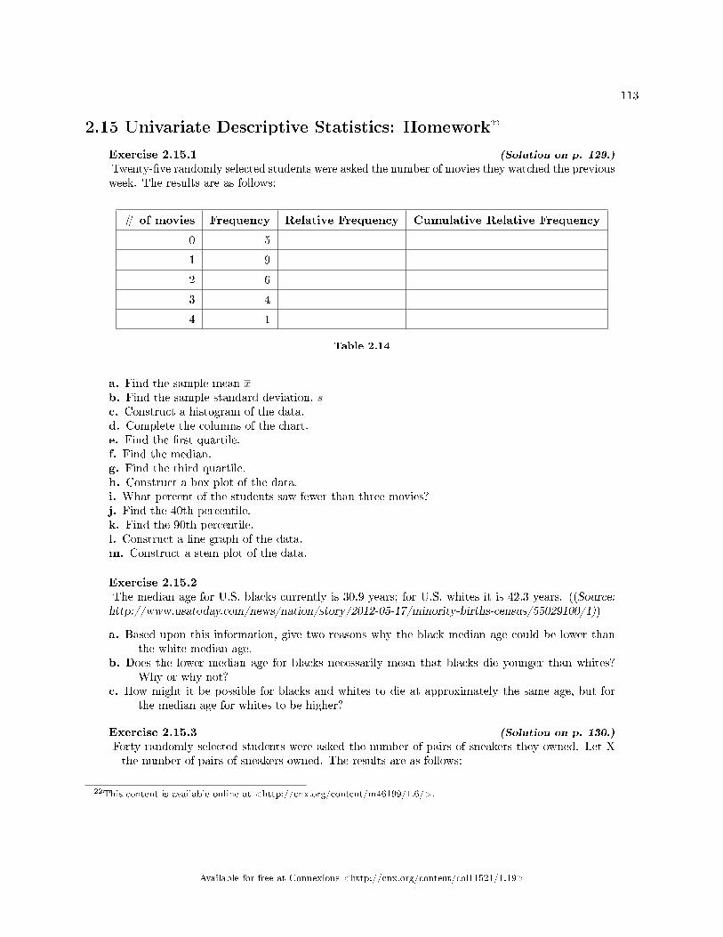
113
2.15 Univariate Descriptive Statistics: Homework22
Exercise 2.15.1 (Solution on p. 129.)
Twenty-�ve randomly selected students were asked the number of movies they watched the previousweek. The results are as follows:
# of movies Frequency Relative Frequency Cumulative Relative Frequency
0 5
1 9
2 6
3 4
4 1
Table 2.14
a. Find the sample mean xb. Find the sample standard deviation, sc. Construct a histogram of the data.d. Complete the columns of the chart.e. Find the �rst quartile.f. Find the median.g. Find the third quartile.h. Construct a box plot of the data.i. What percent of the students saw fewer than three movies?j. Find the 40th percentile.k. Find the 90th percentile.l. Construct a line graph of the data.m. Construct a stem plot of the data.
Exercise 2.15.2The median age for U.S. blacks currently is 30.9 years; for U.S. whites it is 42.3 years. ((Source:http://www.usatoday.com/news/nation/story/2012-05-17/minority-births-census/55029100/1))
a. Based upon this information, give two reasons why the black median age could be lower thanthe white median age.
b. Does the lower median age for blacks necessarily mean that blacks die younger than whites?Why or why not?
c. How might it be possible for blacks and whites to die at approximately the same age, but forthe median age for whites to be higher?
Exercise 2.15.3 (Solution on p. 130.)
Forty randomly selected students were asked the number of pairs of sneakers they owned. Let X= the number of pairs of sneakers owned. The results are as follows:
22This content is available online at <http://cnx.org/content/m46199/1.6/>.
Available for free at Connexions <http://cnx.org/content/col11521/1.19>
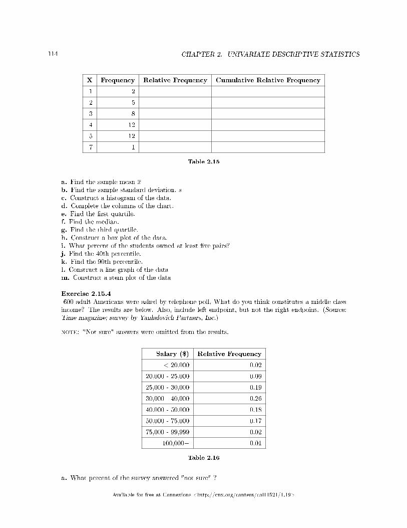
114 CHAPTER 2. UNIVARIATE DESCRIPTIVE STATISTICS
X Frequency Relative Frequency Cumulative Relative Frequency
1 2
2 5
3 8
4 12
5 12
7 1
Table 2.15
a. Find the sample mean xb. Find the sample standard deviation, sc. Construct a histogram of the data.d. Complete the columns of the chart.e. Find the �rst quartile.f. Find the median.g. Find the third quartile.h. Construct a box plot of the data.i. What percent of the students owned at least �ve pairs?j. Find the 40th percentile.k. Find the 90th percentile.l. Construct a line graph of the datam. Construct a stem plot of the data
Exercise 2.15.4600 adult Americans were asked by telephone poll, What do you think constitutes a middle-classincome? The results are below. Also, include left endpoint, but not the right endpoint. (Source:Time magazine; survey by Yankelovich Partners, Inc.)
note: "Not sure" answers were omitted from the results.
Salary ($) Relative Frequency
< 20,000 0.02
20,000 - 25,000 0.09
25,000 - 30,000 0.19
30,000 - 40,000 0.26
40,000 - 50,000 0.18
50,000 - 75,000 0.17
75,000 - 99,999 0.02
100,000+ 0.01
Table 2.16
a. What percent of the survey answered "not sure" ?
Available for free at Connexions <http://cnx.org/content/col11521/1.19>
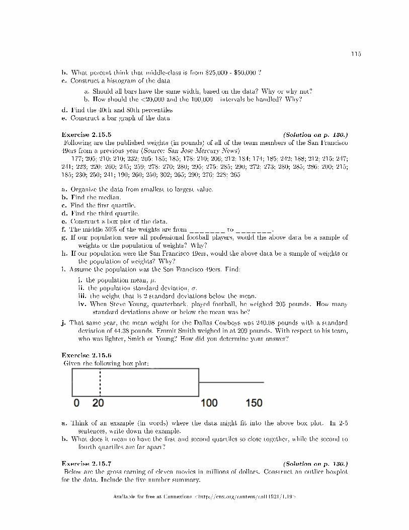
115
b. What percent think that middle-class is from $25,000 - $50,000 ?c. Construct a histogram of the data
a. Should all bars have the same width, based on the data? Why or why not?b. How should the <20,000 and the 100,000+ intervals be handled? Why?
d. Find the 40th and 80th percentilese. Construct a bar graph of the data
Exercise 2.15.5 (Solution on p. 130.)
Following are the published weights (in pounds) of all of the team members of the San Francisco49ers from a previous year (Source: San Jose Mercury News)
177; 205; 210; 210; 232; 205; 185; 185; 178; 210; 206; 212; 184; 174; 185; 242; 188; 212; 215; 247;241; 223; 220; 260; 245; 259; 278; 270; 280; 295; 275; 285; 290; 272; 273; 280; 285; 286; 200; 215;185; 230; 250; 241; 190; 260; 250; 302; 265; 290; 276; 228; 265
a. Organize the data from smallest to largest value.b. Find the median.c. Find the �rst quartile.d. Find the third quartile.e. Construct a box plot of the data.f. The middle 50% of the weights are from _______ to _______.g. If our population were all professional football players, would the above data be a sample of
weights or the population of weights? Why?h. If our population were the San Francisco 49ers, would the above data be a sample of weights or
the population of weights? Why?i. Assume the population was the San Francisco 49ers. Find:
i. the population mean, µ.ii. the population standard deviation, σ.iii. the weight that is 2 standard deviations below the mean.iv. When Steve Young, quarterback, played football, he weighed 205 pounds. How many
standard deviations above or below the mean was he?
j. That same year, the mean weight for the Dallas Cowboys was 240.08 pounds with a standarddeviation of 44.38 pounds. Emmit Smith weighed in at 209 pounds. With respect to his team,who was lighter, Smith or Young? How did you determine your answer?
Exercise 2.15.6Given the following box plot:
a. Think of an example (in words) where the data might �t into the above box plot. In 2-5sentences, write down the example.
b. What does it mean to have the �rst and second quartiles so close together, while the second tofourth quartiles are far apart?
Exercise 2.15.7 (Solution on p. 130.)
Below are the gross earning of eleven movies in millions of dollars. Construct an outlier boxplotfor the data. Include the �ve number summary.
Available for free at Connexions <http://cnx.org/content/col11521/1.19>
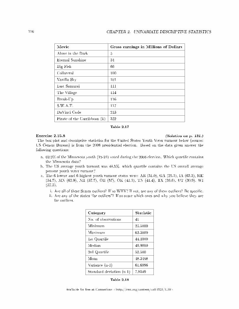
116 CHAPTER 2. UNIVARIATE DESCRIPTIVE STATISTICS
Movie Gross earnings in Millions of Dollars
Alone in the Dark 5
Eternal Sunshine 34
Big Fish 66
Collateral 100
Vanilla Sky 101
Last Samurai 111
The Village 114
Break-Up 116
S.W.A.T. 117
DaVinci Code 213
Pirate of the Carribbean (ii) 322
Table 2.17
Exercise 2.15.8 (Solution on p. 131.)
The box plot and descriptive statistics for the United States Youth Voter turnout below (source:US Census Bureau) is from the 2008 presidential election. Based on the data given answer thefollowing questions:
a. 62.9% of the Minnesota youth (18-24) voted during the 2008 election. Which quartile containsthe Minnesota data?
b. The US average youth turnout was 48.5%, which quartile contains the US overall averagepercent youth voter turnout?
c. The 6 lowest and 6 highest youth turnout states were: AR (31.0), GA (25.5), IA (63.5), ME(54.7), MN (62.9), NH (57.7), OH (57), OK (41.5), TN (41.4), TX (36.6), UT (30.9), WI(57.5).
i. Are all of these States outliers? If so WHY? If not, are any of them outliers? Be speci�c.ii. Are any of the states �far outliers�? If so state which ones and why you believe they are
far outliers.
Category Statistic
No. of observations 41
Minimum 25.5000
Maximum 63.5000
1st Quartile 44.1000
Median 49.9000
3rd Quartile 52.500
Mean 48.3488
Variance (n-1) 61.6996
Standard deviation (n-1) 7.8549
Table 2.18
Available for free at Connexions <http://cnx.org/content/col11521/1.19>
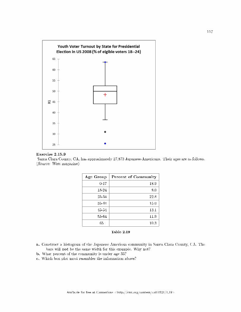
117
Exercise 2.15.9Santa Clara County, CA, has approximately 27,873 Japanese-Americans. Their ages are as follows.(Source: West magazine)
Age Group Percent of Community
0-17 18.9
18-24 8.0
25-34 22.8
35-44 15.0
45-54 13.1
55-64 11.9
65+ 10.3
Table 2.19
a. Construct a histogram of the Japanese-American community in Santa Clara County, CA. Thebars will not be the same width for this example. Why not?
b. What percent of the community is under age 35?c. Which box plot most resembles the information above?
Available for free at Connexions <http://cnx.org/content/col11521/1.19>
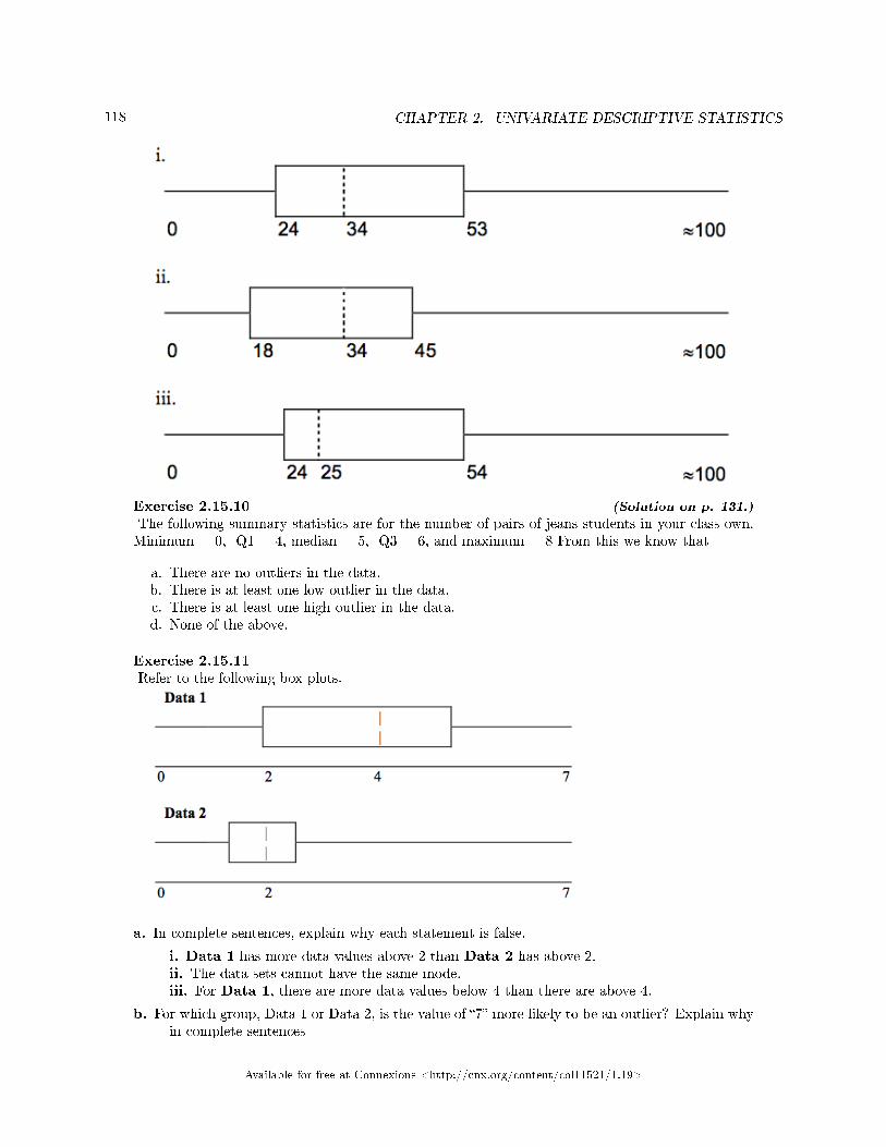
118 CHAPTER 2. UNIVARIATE DESCRIPTIVE STATISTICS
Exercise 2.15.10 (Solution on p. 131.)
The following summary statistics are for the number of pairs of jeans students in your class own.Minimum = 0, Q1 = 4, median = 5, Q3 = 6, and maximum = 8 From this we know that
a. There are no outliers in the data.b. There is at least one low outlier in the data.c. There is at least one high outlier in the data.d. None of the above.
Exercise 2.15.11Refer to the following box plots.
a. In complete sentences, explain why each statement is false.
i. Data 1 has more data values above 2 than Data 2 has above 2.ii. The data sets cannot have the same mode.iii. For Data 1, there are more data values below 4 than there are above 4.
b. For which group, Data 1 or Data 2, is the value of �7� more likely to be an outlier? Explain whyin complete sentences
Available for free at Connexions <http://cnx.org/content/col11521/1.19>
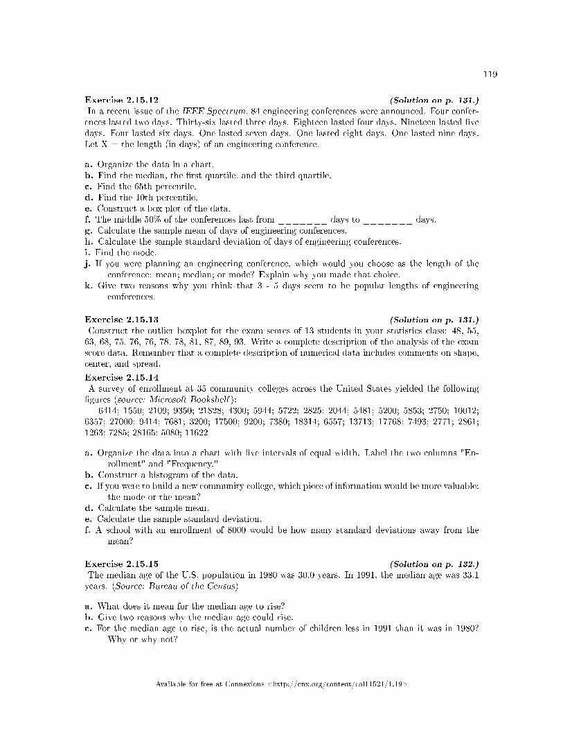
119
Exercise 2.15.12 (Solution on p. 131.)
In a recent issue of the IEEE Spectrum, 84 engineering conferences were announced. Four confer-ences lasted two days. Thirty-six lasted three days. Eighteen lasted four days. Nineteen lasted �vedays. Four lasted six days. One lasted seven days. One lasted eight days. One lasted nine days.Let X = the length (in days) of an engineering conference.
a. Organize the data in a chart.b. Find the median, the �rst quartile, and the third quartile.c. Find the 65th percentile.d. Find the 10th percentile.e. Construct a box plot of the data.f. The middle 50% of the conferences last from _______ days to _______ days.g. Calculate the sample mean of days of engineering conferences.h. Calculate the sample standard deviation of days of engineering conferences.i. Find the mode.j. If you were planning an engineering conference, which would you choose as the length of the
conference: mean; median; or mode? Explain why you made that choice.k. Give two reasons why you think that 3 - 5 days seem to be popular lengths of engineering
conferences.
Exercise 2.15.13 (Solution on p. 131.)
Construct the outlier boxplot for the exam scores of 13 students in your statistics class: 48, 55,63, 68, 75, 76, 76, 78, 78, 81, 87, 89, 93. Write a complete description of the analysis of the examscore data. Remember that a complete description of numerical data includes comments on shape,center, and spread.
Exercise 2.15.14A survey of enrollment at 35 community colleges across the United States yielded the following�gures (source: Microsoft Bookshelf ):
6414; 1550; 2109; 9350; 21828; 4300; 5944; 5722; 2825; 2044; 5481; 5200; 5853; 2750; 10012;6357; 27000; 9414; 7681; 3200; 17500; 9200; 7380; 18314; 6557; 13713; 17768; 7493; 2771; 2861;1263; 7285; 28165; 5080; 11622
a. Organize the data into a chart with �ve intervals of equal width. Label the two columns "En-rollment" and "Frequency."
b. Construct a histogram of the data.c. If you were to build a new community college, which piece of information would be more valuable:
the mode or the mean?d. Calculate the sample mean.e. Calculate the sample standard deviation.f. A school with an enrollment of 8000 would be how many standard deviations away from the
mean?
Exercise 2.15.15 (Solution on p. 132.)
The median age of the U.S. population in 1980 was 30.0 years. In 1991, the median age was 33.1years. (Source: Bureau of the Census)
a. What does it mean for the median age to rise?b. Give two reasons why the median age could rise.c. For the median age to rise, is the actual number of children less in 1991 than it was in 1980?
Why or why not?
Available for free at Connexions <http://cnx.org/content/col11521/1.19>
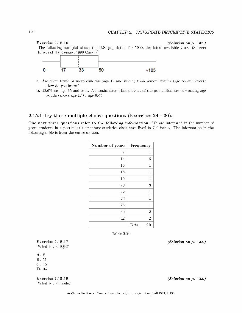
120 CHAPTER 2. UNIVARIATE DESCRIPTIVE STATISTICS
Exercise 2.15.16 (Solution on p. 132.)
The following box plot shows the U.S. population for 1990, the latest available year. (Source:Bureau of the Census, 1990 Census)
a. Are there fewer or more children (age 17 and under) than senior citizens (age 65 and over)?How do you know?
b. 12.6% are age 65 and over. Approximately what percent of the population are of working ageadults (above age 17 to age 65)?
2.15.1 Try these multiple choice questions (Exercises 24 - 30).
The next three questions refer to the following information. We are interested in the number ofyears students in a particular elementary statistics class have lived in California. The information in thefollowing table is from the entire section.
Number of years Frequency
7 1
14 3
15 1
18 1
19 4
20 3
22 1
23 1
26 1
40 2
42 2
Total = 20
Table 2.20
Exercise 2.15.17 (Solution on p. 132.)
What is the IQR?
A. 8B. 11C. 15D. 35
Exercise 2.15.18 (Solution on p. 132.)
What is the mode?
Available for free at Connexions <http://cnx.org/content/col11521/1.19>
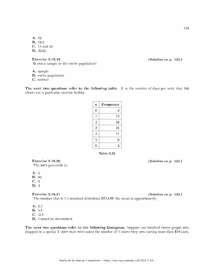
121
A. 19B. 19.5C. 14 and 20D. 22.65
Exercise 2.15.19 (Solution on p. 132.)
Is this a sample or the entire population?
A. sampleB. entire populationC. neither
The next two questions refer to the following table. X = the number of days per week that 100clients use a particular exercise facility.
x Frequency
0 3
1 12
2 33
3 28
4 11
5 9
6 4
Table 2.21
Exercise 2.15.20 (Solution on p. 132.)
The 80th percentile is:
A. 5B. 80C. 3D. 4
Exercise 2.15.21 (Solution on p. 132.)
The number that is 1.5 standard deviations BELOW the mean is approximately:
A. 0.7B. 4.8C. -2.8D. Cannot be determined
The next two questions refer to the following histogram. Suppose one hundred eleven people whoshopped in a special T-shirt store were asked the number of T-shirts they own costing more than $19 each.
Available for free at Connexions <http://cnx.org/content/col11521/1.19>
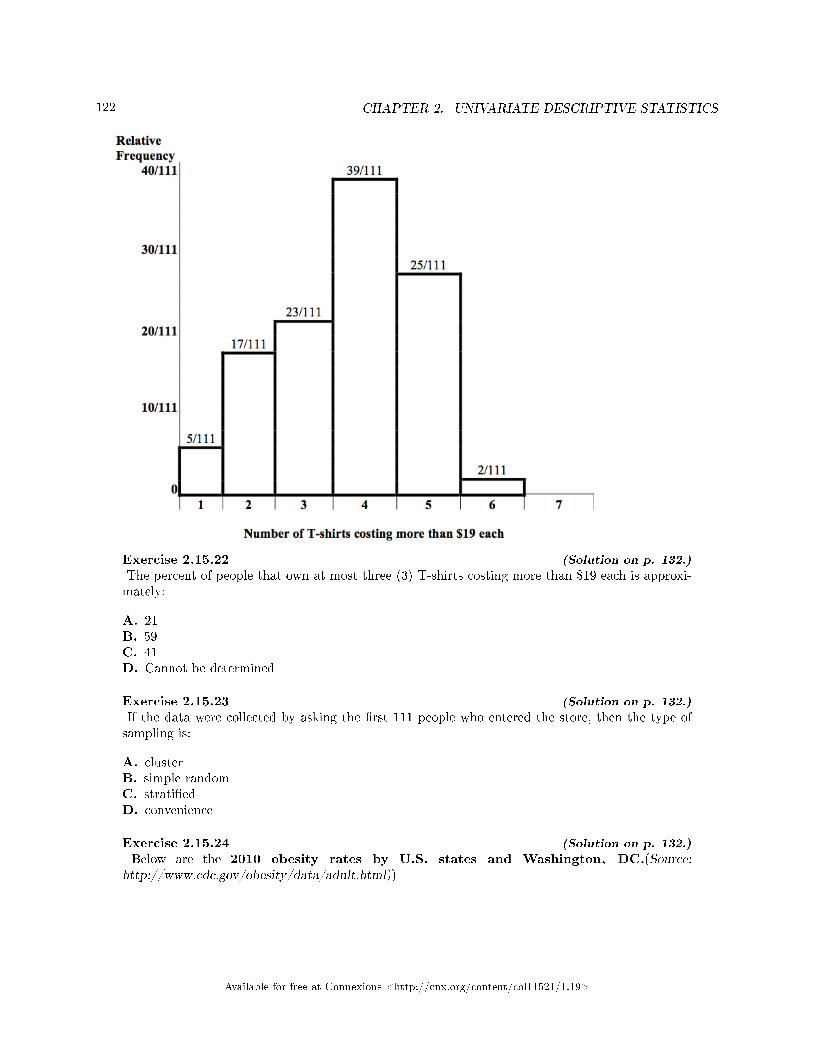
122 CHAPTER 2. UNIVARIATE DESCRIPTIVE STATISTICS
Exercise 2.15.22 (Solution on p. 132.)
The percent of people that own at most three (3) T-shirts costing more than $19 each is approxi-mately:
A. 21B. 59C. 41D. Cannot be determined
Exercise 2.15.23 (Solution on p. 132.)
If the data were collected by asking the �rst 111 people who entered the store, then the type ofsampling is:
A. clusterB. simple randomC. strati�edD. convenience
Exercise 2.15.24 (Solution on p. 132.)
Below are the 2010 obesity rates by U.S. states and Washington, DC.(Source:http://www.cdc.gov/obesity/data/adult.html))
Available for free at Connexions <http://cnx.org/content/col11521/1.19>
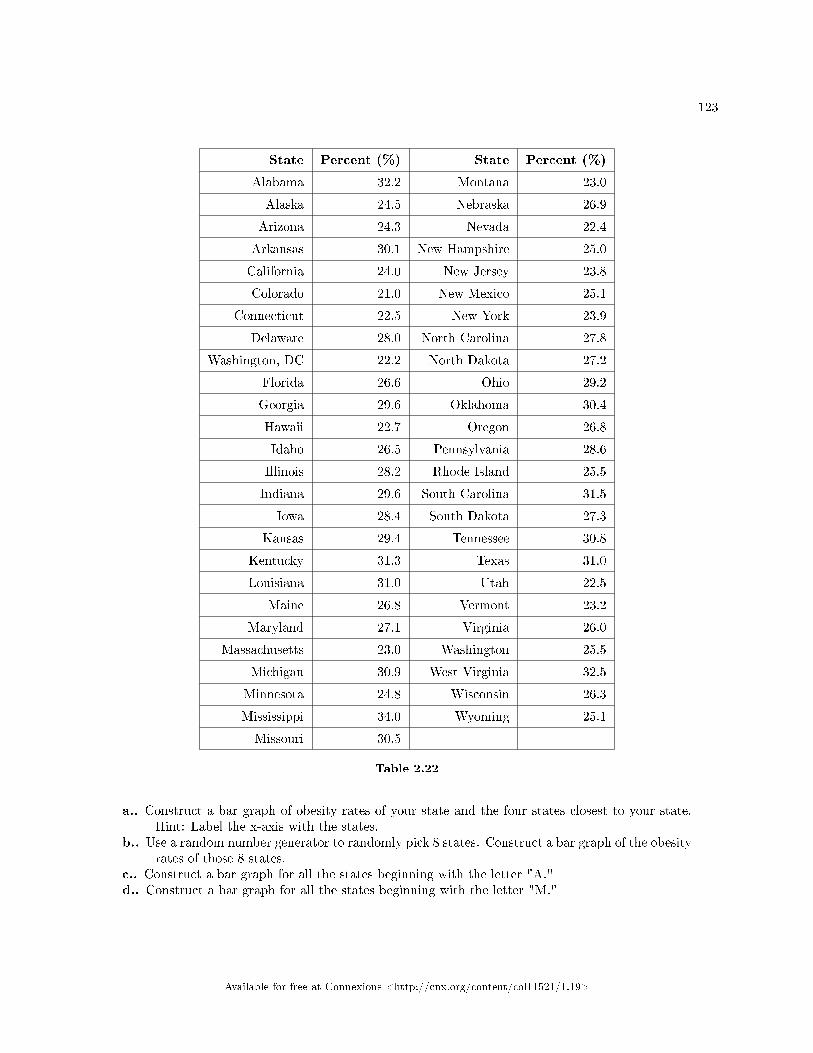
123
State Percent (%) State Percent (%)
Alabama 32.2 Montana 23.0
Alaska 24.5 Nebraska 26.9
Arizona 24.3 Nevada 22.4
Arkansas 30.1 New Hampshire 25.0
California 24.0 New Jersey 23.8
Colorado 21.0 New Mexico 25.1
Connecticut 22.5 New York 23.9
Delaware 28.0 North Carolina 27.8
Washington, DC 22.2 North Dakota 27.2
Florida 26.6 Ohio 29.2
Georgia 29.6 Oklahoma 30.4
Hawaii 22.7 Oregon 26.8
Idaho 26.5 Pennsylvania 28.6
Illinois 28.2 Rhode Island 25.5
Indiana 29.6 South Carolina 31.5
Iowa 28.4 South Dakota 27.3
Kansas 29.4 Tennessee 30.8
Kentucky 31.3 Texas 31.0
Louisiana 31.0 Utah 22.5
Maine 26.8 Vermont 23.2
Maryland 27.1 Virginia 26.0
Massachusetts 23.0 Washington 25.5
Michigan 30.9 West Virginia 32.5
Minnesota 24.8 Wisconsin 26.3
Mississippi 34.0 Wyoming 25.1
Missouri 30.5
Table 2.22
a.. Construct a bar graph of obesity rates of your state and the four states closest to your state.Hint: Label the x-axis with the states.
b.. Use a random number generator to randomly pick 8 states. Construct a bar graph of the obesityrates of those 8 states.
c.. Construct a bar graph for all the states beginning with the letter "A."d.. Construct a bar graph for all the states beginning with the letter "M."
Available for free at Connexions <http://cnx.org/content/col11521/1.19>
124 CHAPTER 2. UNIVARIATE DESCRIPTIVE STATISTICS
2.16 Descriptive Statistics: Descriptive Statistics Lab23
Class Time:Names:
2.16.1 Student Learning Outcomes
• The student will construct a histogram and a box plot.• The student will calculate univariate statistics.• The student will examine the graphs to interpret what the data implies.
2.16.2 Collect the Data
Record the number of pairs of shoes you own:
1. Randomly survey 30 classmates. Record their values.
Survey Results
_____ _____ _____ _____ _____
_____ _____ _____ _____ _____
_____ _____ _____ _____ _____
_____ _____ _____ _____ _____
_____ _____ _____ _____ _____
_____ _____ _____ _____ _____
Table 2.23
2. Construct a histogram. Make 5-6 intervals. Sketch the graph using a ruler and pencil. Scale the axes.
23This content is available online at <http://cnx.org/content/m16299/1.13/>.
Available for free at Connexions <http://cnx.org/content/col11521/1.19>
125
Figure 2.17
3. Calculate the following:
• x =• s =
4. Are the data discrete or continuous? How do you know?5. Describe the shape of the histogram. Use complete sentences.6. Are there any potential outliers? Which value(s) is (are) it (they)? Use a formula to check the end
values to determine if they are potential outliers.
2.16.3 Analyze the Data
1. Determine the following:
• Minimum value =• Median =• Maximum value =• First quartile =• Third quartile =• IQR =
2. Construct a box plot of data3. What does the shape of the box plot imply about the concentration of data? Use complete sentences.4. Using the box plot, how can you determine if there are potential outliers?5. How does the standard deviation help you to determine concentration of the data and whether or not
there are potential outliers?6. What does the IQR represent in this problem?7. Show your work to �nd the value that is 1.5 standard deviations:
a. Above the mean:b. Below the mean:
Available for free at Connexions <http://cnx.org/content/col11521/1.19>
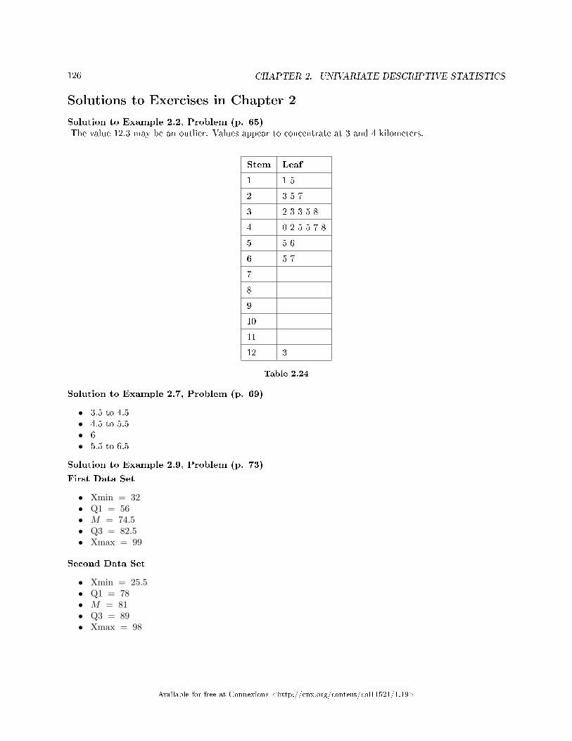
126 CHAPTER 2. UNIVARIATE DESCRIPTIVE STATISTICS
Solutions to Exercises in Chapter 2
Solution to Example 2.2, Problem (p. 65)The value 12.3 may be an outlier. Values appear to concentrate at 3 and 4 kilometers.
Stem Leaf
1 1 5
2 3 5 7
3 2 3 3 5 8
4 0 2 5 5 7 8
5 5 6
6 5 7
7
8
9
10
11
12 3
Table 2.24
Solution to Example 2.7, Problem (p. 69)
• 3.5 to 4.5• 4.5 to 5.5• 6• 5.5 to 6.5
Solution to Example 2.9, Problem (p. 73)
First Data Set
• Xmin = 32• Q1 = 56• M = 74.5• Q3 = 82.5• Xmax = 99
Second Data Set
• Xmin = 25.5• Q1 = 78• M = 81• Q3 = 89• Xmax = 98
Available for free at Connexions <http://cnx.org/content/col11521/1.19>
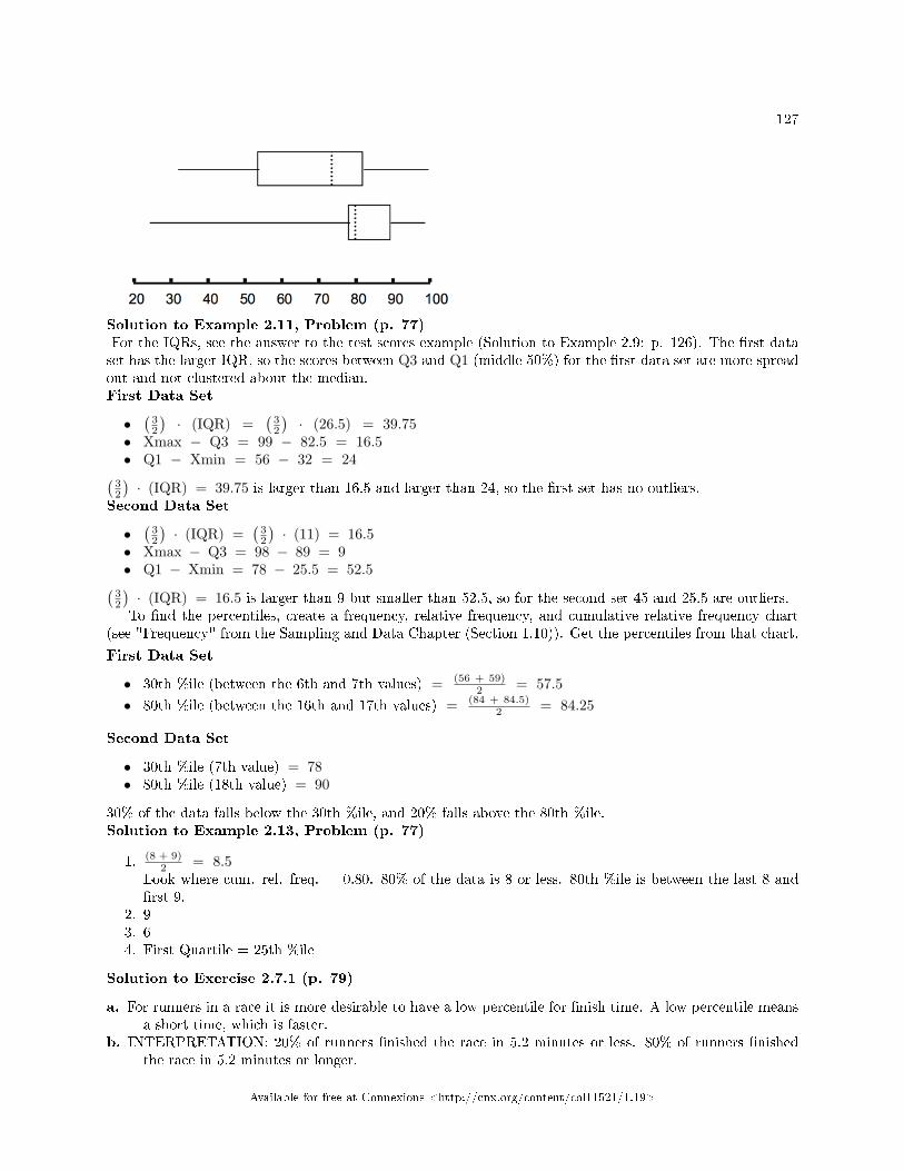
127
Solution to Example 2.11, Problem (p. 77)For the IQRs, see the answer to the test scores example (Solution to Example 2.9: p. 126). The �rst dataset has the larger IQR, so the scores between Q3 and Q1 (middle 50%) for the �rst data set are more spreadout and not clustered about the median.First Data Set
•(
32
)· (IQR) =
(32
)· (26.5) = 39.75
• Xmax − Q3 = 99 − 82.5 = 16.5• Q1 − Xmin = 56 − 32 = 24(
32
)· (IQR) = 39.75 is larger than 16.5 and larger than 24, so the �rst set has no outliers.
Second Data Set
•(
32
)· (IQR) =
(32
)· (11) = 16.5
• Xmax − Q3 = 98 − 89 = 9• Q1 − Xmin = 78 − 25.5 = 52.5(
32
)· (IQR) = 16.5 is larger than 9 but smaller than 52.5, so for the second set 45 and 25.5 are outliers.
To �nd the percentiles, create a frequency, relative frequency, and cumulative relative frequency chart(see "Frequency" from the Sampling and Data Chapter (Section 1.10)). Get the percentiles from that chart.
First Data Set
• 30th %ile (between the 6th and 7th values) = (56 + 59)2 = 57.5
• 80th %ile (between the 16th and 17th values) = (84 + 84.5)2 = 84.25
Second Data Set
• 30th %ile (7th value) = 78• 80th %ile (18th value) = 90
30% of the data falls below the 30th %ile, and 20% falls above the 80th %ile.Solution to Example 2.13, Problem (p. 77)
1. (8 + 9)2 = 8.5
Look where cum. rel. freq. = 0.80. 80% of the data is 8 or less. 80th %ile is between the last 8 and�rst 9.
2. 93. 64. First Quartile = 25th %ile
Solution to Exercise 2.7.1 (p. 79)
a. For runners in a race it is more desirable to have a low percentile for �nish time. A low percentile meansa short time, which is faster.
b. INTERPRETATION: 20% of runners �nished the race in 5.2 minutes or less. 80% of runners �nishedthe race in 5.2 minutes or longer.
Available for free at Connexions <http://cnx.org/content/col11521/1.19>
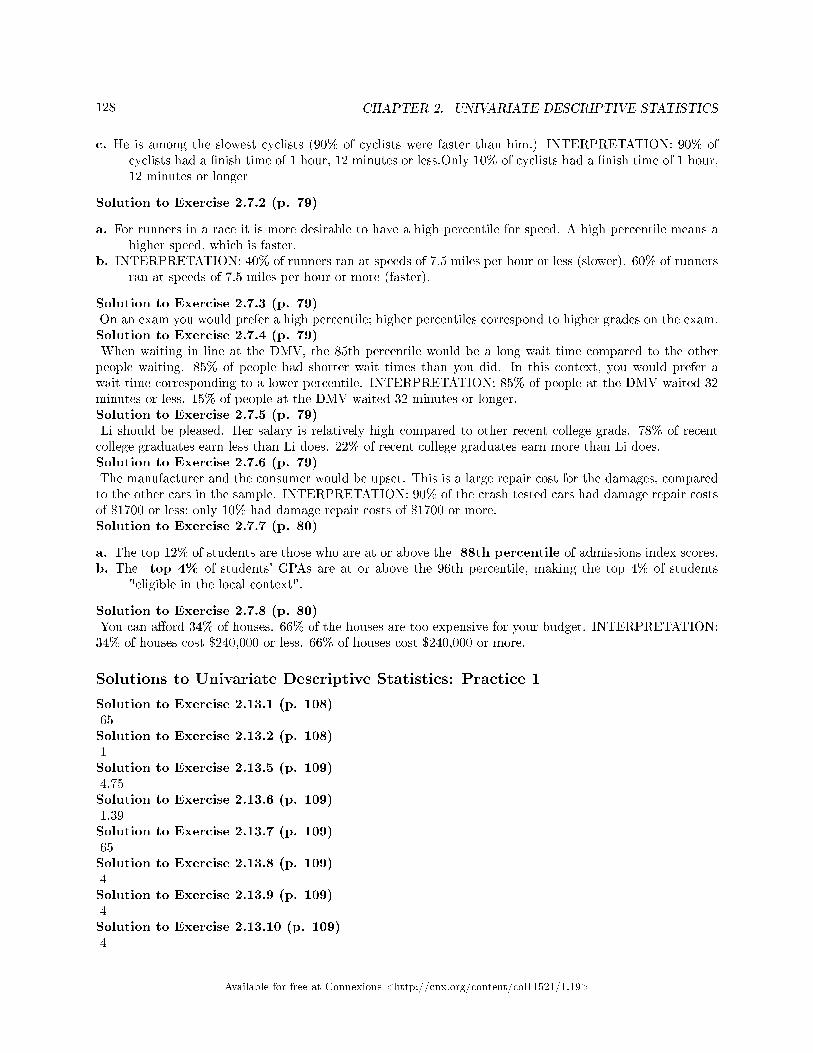
128 CHAPTER 2. UNIVARIATE DESCRIPTIVE STATISTICS
c. He is among the slowest cyclists (90% of cyclists were faster than him.) INTERPRETATION: 90% ofcyclists had a �nish time of 1 hour, 12 minutes or less.Only 10% of cyclists had a �nish time of 1 hour,12 minutes or longer
Solution to Exercise 2.7.2 (p. 79)
a. For runners in a race it is more desirable to have a high percentile for speed. A high percentile means ahigher speed, which is faster.
b. INTERPRETATION: 40% of runners ran at speeds of 7.5 miles per hour or less (slower). 60% of runnersran at speeds of 7.5 miles per hour or more (faster).
Solution to Exercise 2.7.3 (p. 79)On an exam you would prefer a high percentile; higher percentiles correspond to higher grades on the exam.Solution to Exercise 2.7.4 (p. 79)When waiting in line at the DMV, the 85th percentile would be a long wait time compared to the otherpeople waiting. 85% of people had shorter wait times than you did. In this context, you would prefer await time corresponding to a lower percentile. INTERPRETATION: 85% of people at the DMV waited 32minutes or less. 15% of people at the DMV waited 32 minutes or longer.Solution to Exercise 2.7.5 (p. 79)Li should be pleased. Her salary is relatively high compared to other recent college grads. 78% of recentcollege graduates earn less than Li does. 22% of recent college graduates earn more than Li does.Solution to Exercise 2.7.6 (p. 79)The manufacturer and the consumer would be upset. This is a large repair cost for the damages, comparedto the other cars in the sample. INTERPRETATION: 90% of the crash tested cars had damage repair costsof $1700 or less; only 10% had damage repair costs of $1700 or more.Solution to Exercise 2.7.7 (p. 80)
a. The top 12% of students are those who are at or above the 88th percentile of admissions index scores.b. The top 4% of students' GPAs are at or above the 96th percentile, making the top 4% of students
"eligible in the local context".
Solution to Exercise 2.7.8 (p. 80)You can a�ord 34% of houses. 66% of the houses are too expensive for your budget. INTERPRETATION:34% of houses cost $240,000 or less. 66% of houses cost $240,000 or more.
Solutions to Univariate Descriptive Statistics: Practice 1
Solution to Exercise 2.13.1 (p. 108)65Solution to Exercise 2.13.2 (p. 108)1Solution to Exercise 2.13.5 (p. 109)4.75Solution to Exercise 2.13.6 (p. 109)1.39Solution to Exercise 2.13.7 (p. 109)65Solution to Exercise 2.13.8 (p. 109)4Solution to Exercise 2.13.9 (p. 109)4Solution to Exercise 2.13.10 (p. 109)4
Available for free at Connexions <http://cnx.org/content/col11521/1.19>
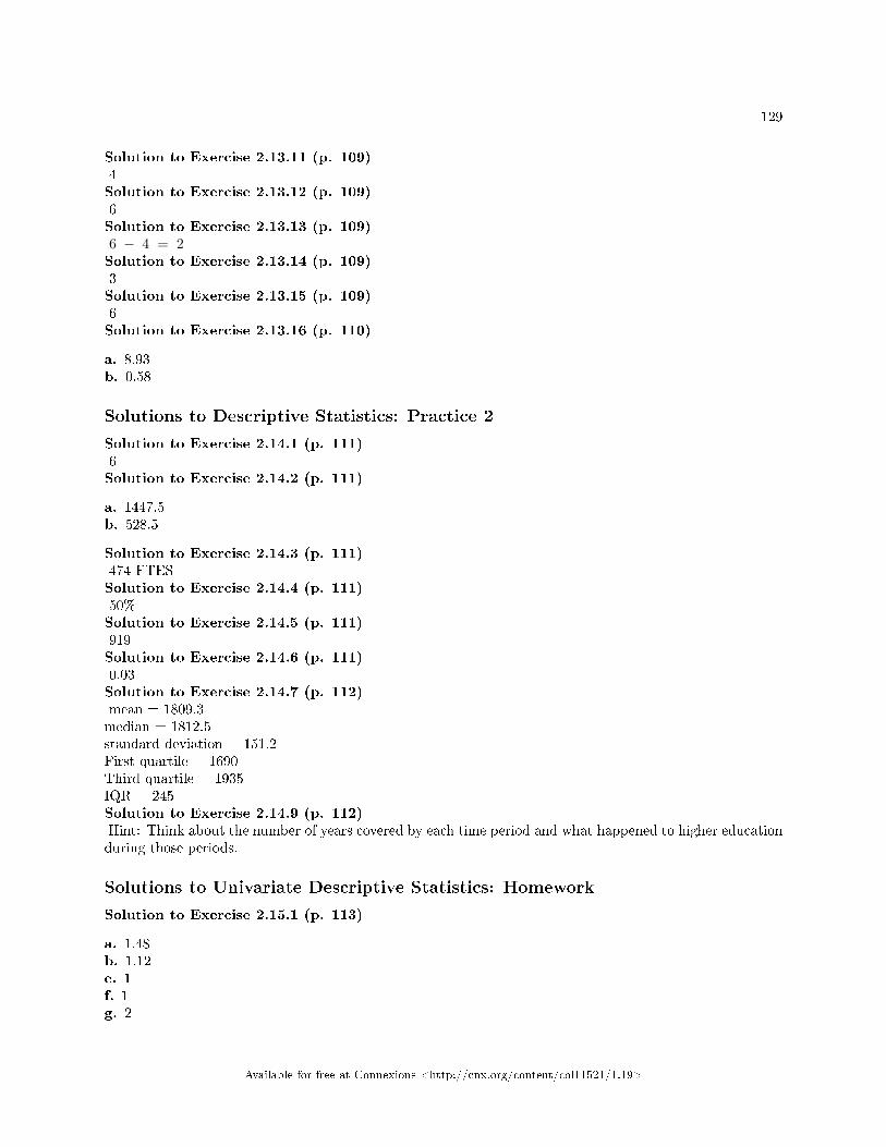
129
Solution to Exercise 2.13.11 (p. 109)4Solution to Exercise 2.13.12 (p. 109)6Solution to Exercise 2.13.13 (p. 109)6 − 4 = 2Solution to Exercise 2.13.14 (p. 109)3Solution to Exercise 2.13.15 (p. 109)6Solution to Exercise 2.13.16 (p. 110)
a. 8.93b. 0.58
Solutions to Descriptive Statistics: Practice 2
Solution to Exercise 2.14.1 (p. 111)6Solution to Exercise 2.14.2 (p. 111)
a. 1447.5b. 528.5
Solution to Exercise 2.14.3 (p. 111)474 FTESSolution to Exercise 2.14.4 (p. 111)50%Solution to Exercise 2.14.5 (p. 111)919Solution to Exercise 2.14.6 (p. 111)0.03Solution to Exercise 2.14.7 (p. 112)mean = 1809.3median = 1812.5standard deviation = 151.2First quartile = 1690Third quartile = 1935IQR = 245Solution to Exercise 2.14.9 (p. 112)Hint: Think about the number of years covered by each time period and what happened to higher educationduring those periods.
Solutions to Univariate Descriptive Statistics: Homework
Solution to Exercise 2.15.1 (p. 113)
a. 1.48b. 1.12e. 1f. 1g. 2
Available for free at Connexions <http://cnx.org/content/col11521/1.19>
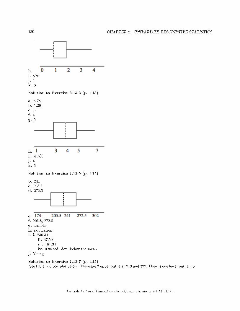
130 CHAPTER 2. UNIVARIATE DESCRIPTIVE STATISTICS
h.i. 80%j. 1k. 3
Solution to Exercise 2.15.3 (p. 113)
a. 3.78b. 1.29e. 3f. 4g. 5
h.i. 32.5%j. 4k. 5
Solution to Exercise 2.15.5 (p. 115)
b. 241c. 205.5d. 272.5
e.f. 205.5, 272.5g. sampleh. populationi. i. 236.34
ii. 37.50iii. 161.34iv. 0.84 std. dev. below the mean
j. Young
Solution to Exercise 2.15.7 (p. 115)See table and box plot below. There are 2 upper outliers: 213 and 322; Their is one lower outlier: 5
Available for free at Connexions <http://cnx.org/content/col11521/1.19>
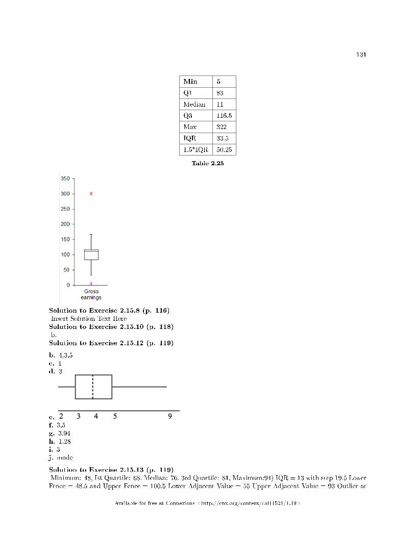
131
Min 5
Q1 83
Median 11
Q3 116.5
Max 322
IQR 33.5
1.5*IQR 50.25
Table 2.25
Solution to Exercise 2.15.8 (p. 116)Insert Solution Text HereSolution to Exercise 2.15.10 (p. 118)b.Solution to Exercise 2.15.12 (p. 119)
b. 4,3,5c. 4d. 3
e.f. 3,5g. 3.94h. 1.28i. 3j. mode
Solution to Exercise 2.15.13 (p. 119)Minimum: 48, Ist Quartile: 68, Median: 76, 3rd Quartile: 81, Maximum:94) IQR = 13 with step 19.5 LowerFence = 48.5 and Upper Fence = 100.5 Lower Adjacent Value = 55 Upper Adjacent Value = 93 Outlier at
Available for free at Connexions <http://cnx.org/content/col11521/1.19>
132 CHAPTER 2. UNIVARIATE DESCRIPTIVE STATISTICS
48 *The distribution of statistics student's exam scores is slightly skewed left or to the low values. A typicalscore on the test was 76 points, the median. The overall variability of the exam scores is 45 points with themiddle half of the data having a spread of 13 points. These is one outlier at the low end of 48 points.Solution to Exercise 2.15.15 (p. 119)
c. Maybe
Solution to Exercise 2.15.16 (p. 120)
a. more childrenb. 62.4%
Solution to Exercise 2.15.17 (p. 120)ASolution to Exercise 2.15.18 (p. 120)ASolution to Exercise 2.15.19 (p. 121)BSolution to Exercise 2.15.20 (p. 121)DSolution to Exercise 2.15.21 (p. 121)ASolution to Exercise 2.15.22 (p. 122)CSolution to Exercise 2.15.23 (p. 122)DSolution to Exercise 2.15.24 (p. 122)Example solution for b using the random number generator for the Ti-84 Plus to generate a simple randomsample of 8 states. Instructions are below.
Number the entries in the table 1 - 51 (Includes Washington, DC; Numbered vertically)Press MATHArrow over to PRBPress 5:randInt(Enter 51,1,8)
Eight numbers are generated (use the right arrow key to scroll through the numbers). The num-bers correspond to the numbered states (for this example: {47 21 9 23 51 13 25 4}. Ifany numbers are repeated, generate a di�erent number by using 5:randInt(51,1)). Here, thestates (and Washington DC) are {Arkansas, Washington DC, Idaho, Maryland, Michigan, Missis-sippi, Virginia, Wyoming}. Corresponding percents are {28.7 21.8 24.5 26 28.9 32.8 25 24.6}.
Available for free at Connexions <http://cnx.org/content/col11521/1.19>
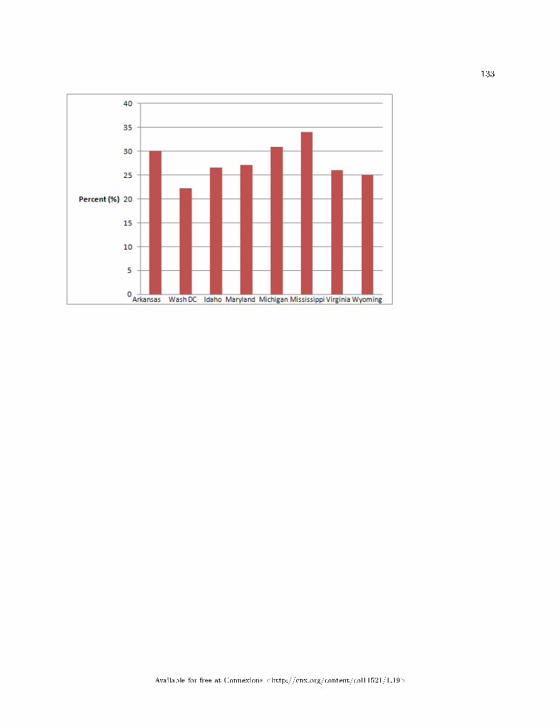
133
Available for free at Connexions <http://cnx.org/content/col11521/1.19>

134 CHAPTER 2. UNIVARIATE DESCRIPTIVE STATISTICS
Available for free at Connexions <http://cnx.org/content/col11521/1.19>
Chapter 3
Bivariate Descriptive Statistics
3.1 Bivariate Descriptive Statistics: Introduction1
3.1.1 Descriptive Statistics for Bivariate Data: Introduction
3.1.1.1 Student Learning Outcomes
By the end of this chapter, the student should be able to:
• Identify di�erent types of relationships between variables: categorical-categorical, categorical-numerical, and numerical-numerical
Categorical - Categorical
• Know how to make and summarize a contingency table between two categorical variables• Discuss and describe patterns in contingency tables and supporting graphic summaries
Categorical - Numerical
• Be able to build side-by-side histograms, back-to-back stemplots, and multiple box-plots between acategorical and a numeric variable.
• Compare and contrast multiple groups based on their shape, center, and spread.
Numerical - Numerical
• Discuss basic ideas of the relationship between two numeric variables including scatter plots, linearregression and correlation
• Create and interpret a line of best �t• Calculate and interpret the correlation coe�cient
3.1.1.2 Introduction
In the previous chapters you have explored how to organize, summarize, and discuss both univariate cat-egorical and numerical variables. Usually more interesting questions are to examine relationships betweensets of variables. For example, are men or women more likely to purchase co�ee at a co�ee shop or do stu-dents that spend more time studying for an exam really do better? We can start to answer these questionsby examining the relationship between the variables: categorical and categorical variables, categorical andnumerical variables, or numerical and numerical variables. We will do this by producing graphs, calculatingsummary statistics, and making comparisons.
1This content is available online at <http://cnx.org/content/m46177/1.2/>.
Available for free at Connexions <http://cnx.org/content/col11521/1.19>
135
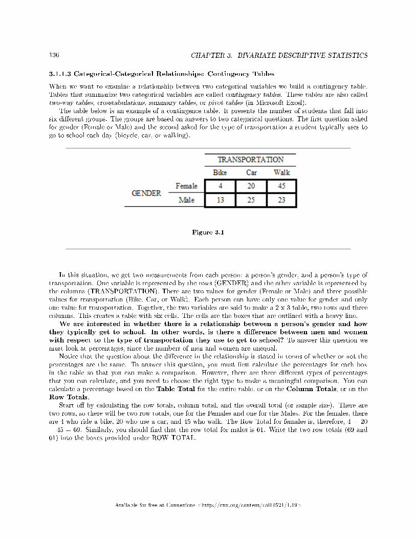
136 CHAPTER 3. BIVARIATE DESCRIPTIVE STATISTICS
3.1.1.3 Categorical-Categorical Relationships: Contingency Tables
When we want to examine a relationship between two categorical variables we build a contingency table.Tables that summarize two categorical variables are called contingency tables. These tables are also calledtwo-way tables, crosstabulations, summary tables, or pivot tables (in Microsoft Excel).
The table below is an example of a contingence table. It presents the number of students that fall intosix di�erent groups. The groups are based on answers to two categorical questions. The �rst question askedfor gender (Female or Male) and the second asked for the type of transportation a student typically uses togo to school each day (bicycle, car, or walking).
Figure 3.1
In this situation, we get two measurements from each person: a person's gender, and a person's type oftransportation. One variable is represented by the rows (GENDER) and the other variable is represented bythe columns (TRANSPORTATION). There are two values for gender (Female or Male) and three possiblevalues for transportation (Bike, Car, or Walk). Each person can have only one value for gender and onlyone value for transportation. Together, the two variables are said to make a 2 x 3 table, two rows and threecolumns. This creates a table with six cells. The cells are the boxes that are outlined with a heavy line.
We are interested in whether there is a relationship between a person's gender and howthey typically get to school. In other words, is there a di�erence between men and womenwith respect to the type of transportation they use to get to school? To answer this question wemust look at percentages, since the numbers of men and women are unequal.
Notice that the question about the di�erence in the relationship is stated in terms of whether or not thepercentages are the same. To answer this question, you must �rst calculate the percentages for each boxin the table so that you can make a comparison. However, there are three di�erent types of percentagesthat you can calculate, and you need to choose the right type to make a meaningful comparison. You cancalculate a percentage based on the Table Total for the entire table, or on the Column Totals, or on theRow Totals.
Start o� by calculating the row totals, column total, and the overall total (or sample size). There aretwo rows, so there will be two row totals, one for the Females and one for the Males. For the females, thereare 4 who ride a bike, 20 who use a car, and 45 who walk. The Row Total for females is, therefore, 4 + 20+ 45 = 69. Similarly, you should �nd that the row total for males is 61. Write the two row totals (69 and61) into the boxes provided under ROW TOTAL.
Available for free at Connexions <http://cnx.org/content/col11521/1.19>
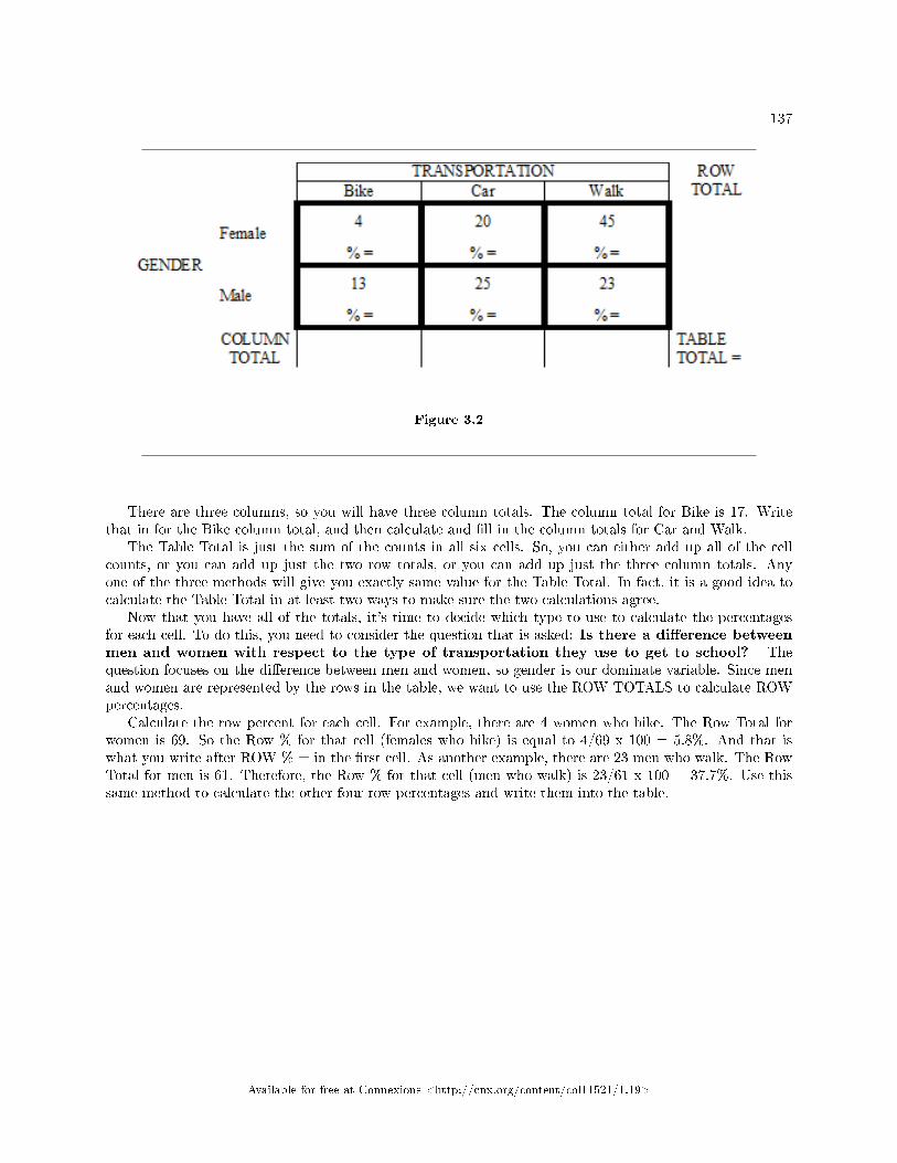
137
Figure 3.2
There are three columns, so you will have three column totals. The column total for Bike is 17. Writethat in for the Bike column total, and then calculate and �ll in the column totals for Car and Walk.
The Table Total is just the sum of the counts in all six cells. So, you can either add up all of the cellcounts, or you can add up just the two row totals, or you can add up just the three column totals. Anyone of the three methods will give you exactly same value for the Table Total. In fact, it is a good idea tocalculate the Table Total in at least two ways to make sure the two calculations agree.
Now that you have all of the totals, it's time to decide which type to use to calculate the percentagesfor each cell. To do this, you need to consider the question that is asked: Is there a di�erence betweenmen and women with respect to the type of transportation they use to get to school? Thequestion focuses on the di�erence between men and women, so gender is our dominate variable. Since menand women are represented by the rows in the table, we want to use the ROW TOTALS to calculate ROWpercentages.
Calculate the row percent for each cell. For example, there are 4 women who bike. The Row Total forwomen is 69. So the Row % for that cell (females who bike) is equal to 4/69 x 100 = 5.8%. And that iswhat you write after ROW % = in the �rst cell. As another example, there are 23 men who walk. The RowTotal for men is 61. Therefore, the Row % for that cell (men who walk) is 23/61 x 100 = 37.7%. Use thissame method to calculate the other four row percentages and write them into the table.
Available for free at Connexions <http://cnx.org/content/col11521/1.19>
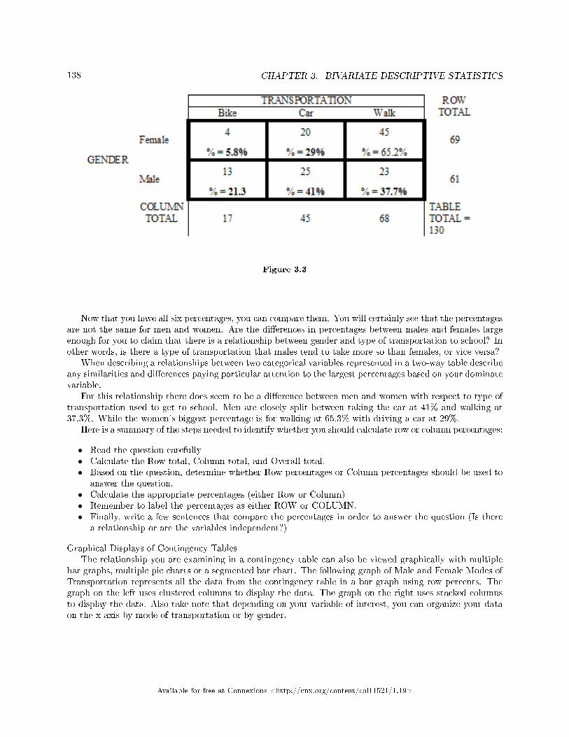
138 CHAPTER 3. BIVARIATE DESCRIPTIVE STATISTICS
Figure 3.3
Now that you have all six percentages, you can compare them. You will certainly see that the percentagesare not the same for men and women. Are the di�erences in percentages between males and females largeenough for you to claim that there is a relationship between gender and type of transportation to school? Inother words, is there a type of transportation that males tend to take more so than females, or vice versa?
When describing a relationships between two categorical variables represented in a two-way table describeany similarities and di�erences paying particular attention to the largest percentages based on your dominatevariable.
For this relationship there does seem to be a di�erence between men and women with respect to type oftransportation used to get to school. Men are closely split between taking the car at 41% and walking at37.3%. While the women's biggest percentage is for walking at 65.3% with driving a car at 29%.
Here is a summary of the steps needed to identify whether you should calculate row or column percentages:
• Read the question carefully• Calculate the Row total, Column total, and Overall total.• Based on the question, determine whether Row percentages or Column percentages should be used to
answer the question.• Calculate the appropriate percentages (either Row or Column)• Remember to label the percentages as either ROW or COLUMN.• Finally, write a few sentences that compare the percentages in order to answer the question (Is there
a relationship or are the variables independent?)
Graphical Displays of Contingency TablesThe relationship you are examining in a contingency table can also be viewed graphically with multiple
bar graphs, multiple pie charts or a segmented bar chart. The following graph of Male and Female Modes ofTransportation represents all the data from the contingency table in a bar graph using row percents. Thegraph on the left uses clustered columns to display the data. The graph on the right uses stacked columnsto display the data. Also take note that depending on your variable of interest, you can organize your dataon the x-axis by mode of transportation or by gender.
Available for free at Connexions <http://cnx.org/content/col11521/1.19>
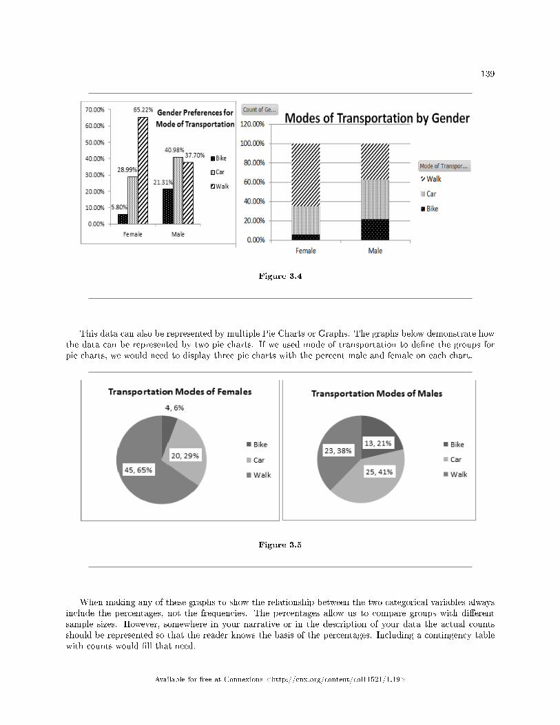
139
Figure 3.4
This data can also be represented by multiple Pie Charts or Graphs. The graphs below demonstrate howthe data can be represented by two pie charts. If we used mode of transportation to de�ne the groups forpie charts, we would need to display three pie charts with the percent male and female on each chart.
Figure 3.5
When making any of these graphs to show the relationship between the two categorical variables alwaysinclude the percentages, not the frequencies. The percentages allow us to compare groups with di�erentsample sizes. However, somewhere in your narrative or in the description of your data the actual countsshould be represented so that the reader knows the basis of the percentages. Including a contingency tablewith counts would �ll that need.
Available for free at Connexions <http://cnx.org/content/col11521/1.19>
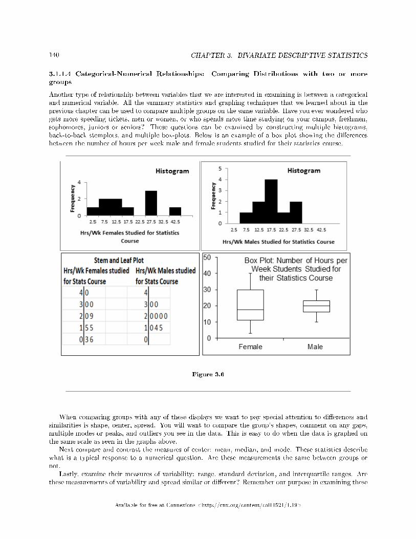
140 CHAPTER 3. BIVARIATE DESCRIPTIVE STATISTICS
3.1.1.4 Categorical-Numerical Relationships: Comparing Distributions with two or moregroups
Another type of relationship between variables that we are interested in examining is between a categoricaland numerical variable. All the summary statistics and graphing techniques that we learned about in theprevious chapter can be used to compare multiple groups on the same variable. Have you ever wondered whogets more speeding tickets, men or women, or who spends more time studying on your campus, freshmen,sophomores, juniors or seniors? These questions can be examined by constructing multiple histograms,back-to-back stemplots, and multiple box-plots. Below is an example of a box plot showing the di�erencesbetween the number of hours per week male and female students studied for their statistics course.
Figure 3.6
When comparing groups with any of these displays we want to pay special attention to di�erences andsimilarities is shape, center, spread. You will want to compare the group's shapes, comment on any gaps,multiple modes or peaks, and outliers you see in the data. This is easy to do when the data is graphed onthe same scale as seen in the graphs above.
Next compare and contrast the measures of center: mean, median, and mode. These statistics describewhat is a typical response to a numerical question. Are these measurements the same between groups ornot.
Lastly, examine their measures of variability: range, standard deviation, and interquartile ranges. Arethese measurements of variability and spread similar or di�erent? Remember our purpose in examining these
Available for free at Connexions <http://cnx.org/content/col11521/1.19>
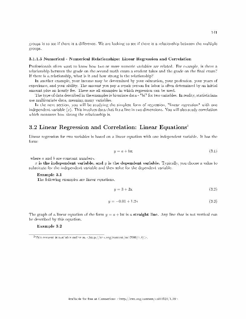
141
groups is to see if there is a di�erence. We are looking to see if there is a relationship between the multiplegroups.
3.1.1.5 Numerical - Numerical Relationships: Linear Regression and Correlation
Professionals often want to know how two or more numeric variables are related. For example, is there arelationship between the grade on the second math exam a student takes and the grade on the �nal exam?If there is a relationship, what is it and how strong is the relationship?
In another example, your income may be determined by your education, your profession, your years ofexperience, and your ability. The amount you pay a repair person for labor is often determined by an initialamount plus an hourly fee. These are all examples in which regression can be used.
The type of data described in the examples is bivariate data - "bi" for two variables. In reality, statisticiansuse multivariate data, meaning many variables.
In the next section, you will be studying the simplest form of regression, "linear regression" with oneindependent variable (x). This involves data that �ts a line in two dimensions. You will also study correlationwhich measures how strong the relationship is.
3.2 Linear Regression and Correlation: Linear Equations2
Linear regression for two variables is based on a linear equation with one independent variable. It has theform:
y = a+ bx (3.1)
where a and b are constant numbers.x is the independent variable, and y is the dependent variable. Typically, you choose a value to
substitute for the independent variable and then solve for the dependent variable.
Example 3.1The following examples are linear equations.
y = 3 + 2x (3.2)
y = −0.01 + 1.2x (3.3)
The graph of a linear equation of the form y = a+ bx is a straight line. Any line that is not vertical canbe described by this equation.
Example 3.2
2This content is available online at <http://cnx.org/content/m17086/1.4/>.
Available for free at Connexions <http://cnx.org/content/col11521/1.19>
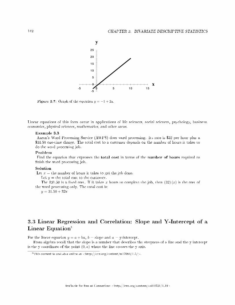
142 CHAPTER 3. BIVARIATE DESCRIPTIVE STATISTICS
Figure 3.7: Graph of the equation y = −1 + 2x.
Linear equations of this form occur in applications of life sciences, social sciences, psychology, business,economics, physical sciences, mathematics, and other areas.
Example 3.3Aaron's Word Processing Service (AWPS) does word processing. Its rate is $32 per hour plus a$31.50 one-time charge. The total cost to a customer depends on the number of hours it takes todo the word processing job.
ProblemFind the equation that expresses the total cost in terms of the number of hours required to�nish the word processing job.
SolutionLet x = the number of hours it takes to get the job done.
Let y = the total cost to the customer.The $31.50 is a �xed cost. If it takes x hours to complete the job, then (32) (x) is the cost of
the word processing only. The total cost is:y = 31.50 + 32x
3.3 Linear Regression and Correlation: Slope and Y-Intercept of aLinear Equation3
For the linear equation y = a+ bx, b = slope and a = y-intercept.From algebra recall that the slope is a number that describes the steepness of a line and the y-intercept
is the y coordinate of the point (0, a) where the line crosses the y-axis.
3This content is available online at <http://cnx.org/content/m17083/1.5/>.
Available for free at Connexions <http://cnx.org/content/col11521/1.19>
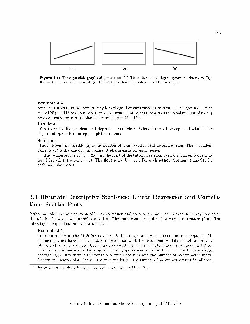
143
(a) (b) (c)
Figure 3.8: Three possible graphs of y = a + bx. (a) If b > 0, the line slopes upward to the right. (b)If b = 0, the line is horizontal. (c) If b < 0, the line slopes downward to the right.
Example 3.4Svetlana tutors to make extra money for college. For each tutoring session, she charges a one timefee of $25 plus $15 per hour of tutoring. A linear equation that expresses the total amount of moneySvetlana earns for each session she tutors is y = 25 + 15x.
ProblemWhat are the independent and dependent variables? What is the y-intercept and what is theslope? Interpret them using complete sentences.
SolutionThe independent variable (x) is the number of hours Svetlana tutors each session. The dependentvariable (y) is the amount, in dollars, Svetlana earns for each session.
The y-intercept is 25 (a = 25). At the start of the tutoring session, Svetlana charges a one-timefee of $25 (this is when x = 0). The slope is 15 (b = 15). For each session, Svetlana earns $15 foreach hour she tutors.
3.4 Bivariate Descriptive Statistics: Linear Regression and Correla-tion: Scatter Plots4
Before we take up the discussion of linear regression and correlation, we need to examine a way to displaythe relation between two variables x and y. The most common and easiest way is a scatter plot. Thefollowing example illustrates a scatter plot.
Example 3.5From an article in the Wall Street Journal: In Europe and Asia, m-commerce is popular. M-commerce users have special mobile phones that work like electronic wallets as well as providephone and Internet services. Users can do everything from paying for parking to buying a TV setor soda from a machine to banking to checking sports scores on the Internet. For the years 2000through 2004, was there a relationship between the year and the number of m-commerce users?Construct a scatter plot. Let x = the year and let y = the number of m-commerce users, in millions.
4This content is available online at <http://cnx.org/content/m46171/1.2/>.
Available for free at Connexions <http://cnx.org/content/col11521/1.19>
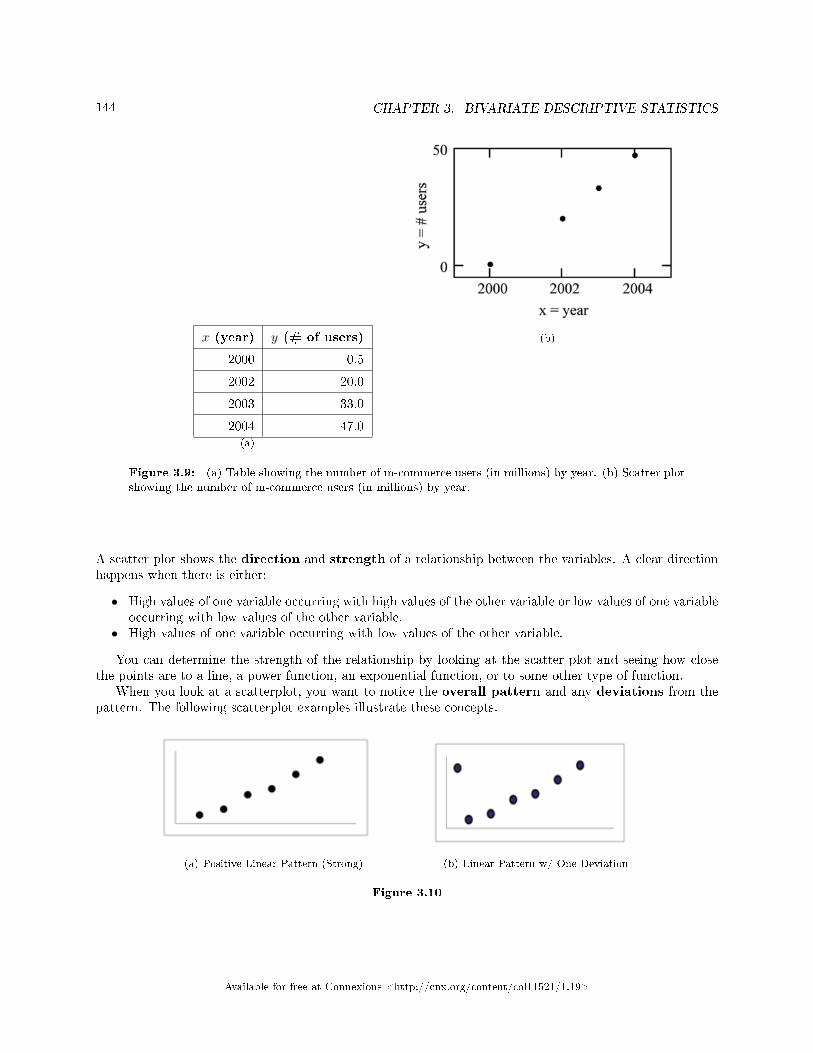
144 CHAPTER 3. BIVARIATE DESCRIPTIVE STATISTICS
x (year) y (# of users)
2000 0.5
2002 20.0
2003 33.0
2004 47.0(a)
(b)
Figure 3.9: (a) Table showing the number of m-commerce users (in millions) by year. (b) Scatter plotshowing the number of m-commerce users (in millions) by year.
A scatter plot shows the direction and strength of a relationship between the variables. A clear directionhappens when there is either:
• High values of one variable occurring with high values of the other variable or low values of one variableoccurring with low values of the other variable.
• High values of one variable occurring with low values of the other variable.
You can determine the strength of the relationship by looking at the scatter plot and seeing how closethe points are to a line, a power function, an exponential function, or to some other type of function.
When you look at a scatterplot, you want to notice the overall pattern and any deviations from thepattern. The following scatterplot examples illustrate these concepts.
(a) Positive Linear Pattern (Strong) (b) Linear Pattern w/ One Deviation
Figure 3.10
Available for free at Connexions <http://cnx.org/content/col11521/1.19>
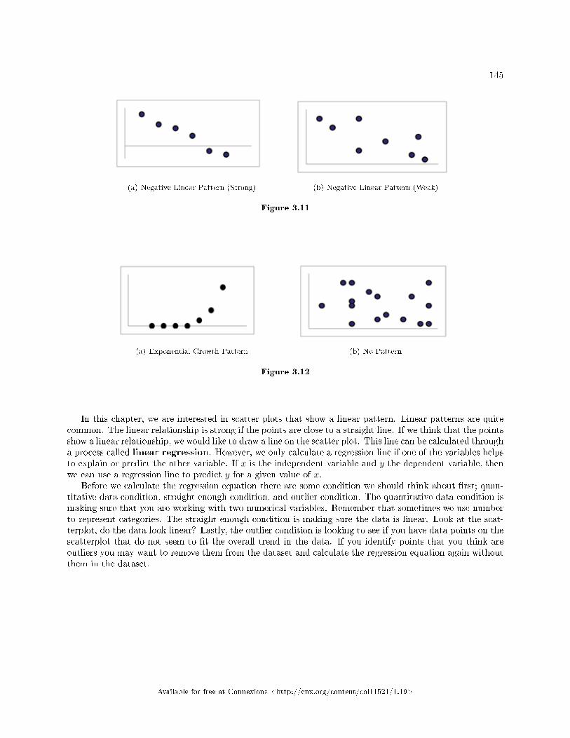
145
(a) Negative Linear Pattern (Strong) (b) Negative Linear Pattern (Weak)
Figure 3.11
(a) Exponential Growth Pattern (b) No Pattern
Figure 3.12
In this chapter, we are interested in scatter plots that show a linear pattern. Linear patterns are quitecommon. The linear relationship is strong if the points are close to a straight line. If we think that the pointsshow a linear relationship, we would like to draw a line on the scatter plot. This line can be calculated througha process called linear regression. However, we only calculate a regression line if one of the variables helpsto explain or predict the other variable. If x is the independent variable and y the dependent variable, thenwe can use a regression line to predict y for a given value of x.
Before we calculate the regression equation there are some condition we should think about �rst; quan-titative data condition, straight enough condition, and outlier condition. The quantitative data condition ismaking sure that you are working with two numerical variables. Remember that sometimes we use numberto represent categories. The straight enough condition is making sure the data is linear. Look at the scat-terplot, do the data look linear? Lastly, the outlier condition is looking to see if you have data points on thescatterplot that do not seem to �t the overall trend in the data. If you identify points that you think areoutliers you may want to remove them from the dataset and calculate the regression equation again withoutthem in the dataset.
Available for free at Connexions <http://cnx.org/content/col11521/1.19>
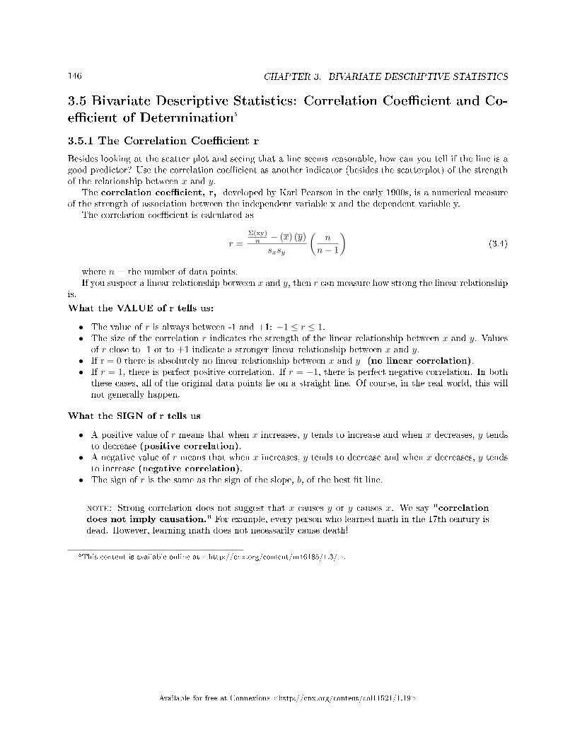
146 CHAPTER 3. BIVARIATE DESCRIPTIVE STATISTICS
3.5 Bivariate Descriptive Statistics: Correlation Coe�cient and Co-e�cient of Determination5
3.5.1 The Correlation Coe�cient r
Besides looking at the scatter plot and seeing that a line seems reasonable, how can you tell if the line is agood predictor? Use the correlation coe�cient as another indicator (besides the scatterplot) of the strengthof the relationship between x and y.
The correlation coe�cient, r, developed by Karl Pearson in the early 1900s, is a numerical measureof the strength of association between the independent variable x and the dependent variable y.
The correlation coe�cient is calculated as
r =Σ(xy)n − (x) (y)
sxsy
(n
n− 1
)(3.4)
where n = the number of data points.If you suspect a linear relationship between x and y, then r can measure how strong the linear relationship
is.
What the VALUE of r tells us:
• The value of r is always between -1 and +1: −1 ≤ r ≤ 1.• The size of the correlation r indicates the strength of the linear relationship between x and y. Values
of r close to -1 or to +1 indicate a stronger linear relationship between x and y.• If r = 0 there is absolutely no linear relationship between x and y (no linear correlation).• If r = 1, there is perfect positive correlation. If r = −1, there is perfect negative correlation. In both
these cases, all of the original data points lie on a straight line. Of course, in the real world, this willnot generally happen.
What the SIGN of r tells us
• A positive value of r means that when x increases, y tends to increase and when x decreases, y tendsto decrease (positive correlation).
• A negative value of r means that when x increases, y tends to decrease and when x decreases, y tendsto increase (negative correlation).
• The sign of r is the same as the sign of the slope, b, of the best �t line.
note: Strong correlation does not suggest that x causes y or y causes x. We say "correlationdoes not imply causation." For example, every person who learned math in the 17th century isdead. However, learning math does not necessarily cause death!
5This content is available online at <http://cnx.org/content/m46185/1.3/>.
Available for free at Connexions <http://cnx.org/content/col11521/1.19>
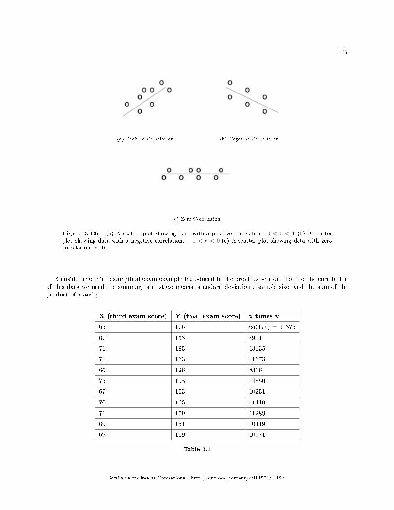
147
(a) Positive Correlation (b) Negative Correlation
(c) Zero Correlation
Figure 3.13: (a) A scatter plot showing data with a positive correlation. 0 < r < 1 (b) A scatterplot showing data with a negative correlation. −1 < r < 0 (c) A scatter plot showing data with zerocorrelation. r=0
Consider the third exam/�nal exam example introduced in the previous section. To �nd the correlationof this data we need the summary statistics; means, standard deviations, sample size, and the sum of theproduct of x and y.
X (third exam score) Y (�nal exam score) x times y
65 175 65(175) = 11375
67 133 8911
71 185 13135
71 163 11573
66 126 8316
75 198 14850
67 153 10251
70 163 11410
71 159 11289
69 151 10419
69 159 10971
Table 3.1
Available for free at Connexions <http://cnx.org/content/col11521/1.19>
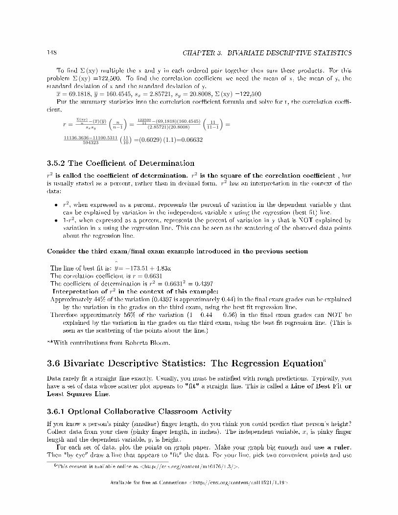
148 CHAPTER 3. BIVARIATE DESCRIPTIVE STATISTICS
To �nd Σ (xy) multiple the x and y in each ordered pair together then sum these products. For thisproblem Σ (xy) =122,500. To �nd the correlation coe�cient we need the mean of x, the mean of y, thestandard deviation of x and the standard deviation of y.
x = 69.1818, y = 160.4545, sx = 2.85721, sy = 20.8008, Σ (xy) =122,500Put the summary statistics into the correlation coe�cient formula and solve for r, the correlation coe�-
cient.
r =Σ(xy)n −(x)(y)
sxsy
(nn−1
)=
12250011 −(69,1818)(160.4545)
(2.85721)(20.8008)
(11
11−1
)=
11136.3636−11100.5311594323
(1110
)=(0.6029) (1.1)=0.06632
3.5.2 The Coe�cient of Determination
r2 is called the coe�cient of determination. r2 is the square of the correlation coe�cient , butis usually stated as a percent, rather than in decimal form. r2 has an interpretation in the context of thedata:
• r2, when expressed as a percent, represents the percent of variation in the dependent variable y thatcan be explained by variation in the independent variable x using the regression (best �t) line.
• 1-r2, when expressed as a percent, represents the percent of variation in y that is NOT explained byvariation in x using the regression line. This can be seen as the scattering of the observed data pointsabout the regression line.
Consider the third exam/�nal exam example introduced in the previous section
The line of best �t is:^y= −173.51 + 4.83x
The correlation coe�cient is r = 0.6631The coe�cient of determination is r2 = 0.66312 = 0.4397Interpretation of r2 in the context of this example:Approximately 44% of the variation (0.4397 is approximately 0.44) in the �nal exam grades can be explained
by the variation in the grades on the third exam, using the best �t regression line.Therefore approximately 56% of the variation (1 - 0.44 = 0.56) in the �nal exam grades can NOT be
explained by the variation in the grades on the third exam, using the best �t regression line. (This isseen as the scattering of the points about the line.)
**With contributions from Roberta Bloom.
3.6 Bivariate Descriptive Statistics: The Regression Equation6
Data rarely �t a straight line exactly. Usually, you must be satis�ed with rough predictions. Typically, youhave a set of data whose scatter plot appears to "�t" a straight line. This is called a Line of Best Fit orLeast Squares Line.
3.6.1 Optional Collaborative Classroom Activity
If you know a person's pinky (smallest) �nger length, do you think you could predict that person's height?Collect data from your class (pinky �nger length, in inches). The independent variable, x, is pinky �ngerlength and the dependent variable, y, is height.
For each set of data, plot the points on graph paper. Make your graph big enough and use a ruler.Then "by eye" draw a line that appears to "�t" the data. For your line, pick two convenient points and use
6This content is available online at <http://cnx.org/content/m46176/1.3/>.
Available for free at Connexions <http://cnx.org/content/col11521/1.19>
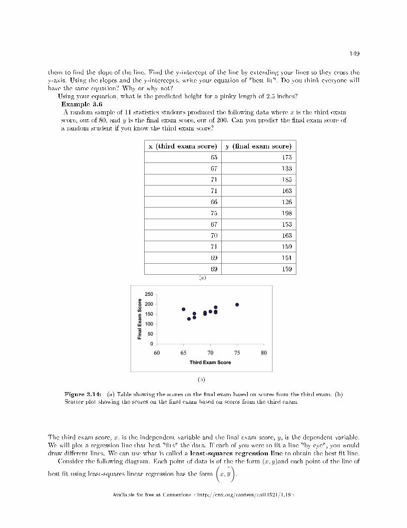
149
them to �nd the slope of the line. Find the y-intercept of the line by extending your lines so they cross they-axis. Using the slopes and the y-intercepts, write your equation of "best �t". Do you think everyone willhave the same equation? Why or why not?
Using your equation, what is the predicted height for a pinky length of 2.5 inches?Example 3.6A random sample of 11 statistics students produced the following data where x is the third examscore, out of 80, and y is the �nal exam score, out of 200. Can you predict the �nal exam score ofa random student if you know the third exam score?
x (third exam score) y (�nal exam score)
65 175
67 133
71 185
71 163
66 126
75 198
67 153
70 163
71 159
69 151
69 159(a)
(b)
Figure 3.14: (a) Table showing the scores on the �nal exam based on scores from the third exam. (b)Scatter plot showing the scores on the �nal exam based on scores from the third exam.
The third exam score, x, is the independent variable and the �nal exam score, y, is the dependent variable.We will plot a regression line that best "�ts" the data. If each of you were to �t a line "by eye", you woulddraw di�erent lines. We can use what is called a least-squares regression line to obtain the best �t line.
Consider the following diagram. Each point of data is of the the form (x, y)and each point of the line of
best �t using least-squares linear regression has the form
(x,^y
).
Available for free at Connexions <http://cnx.org/content/col11521/1.19>
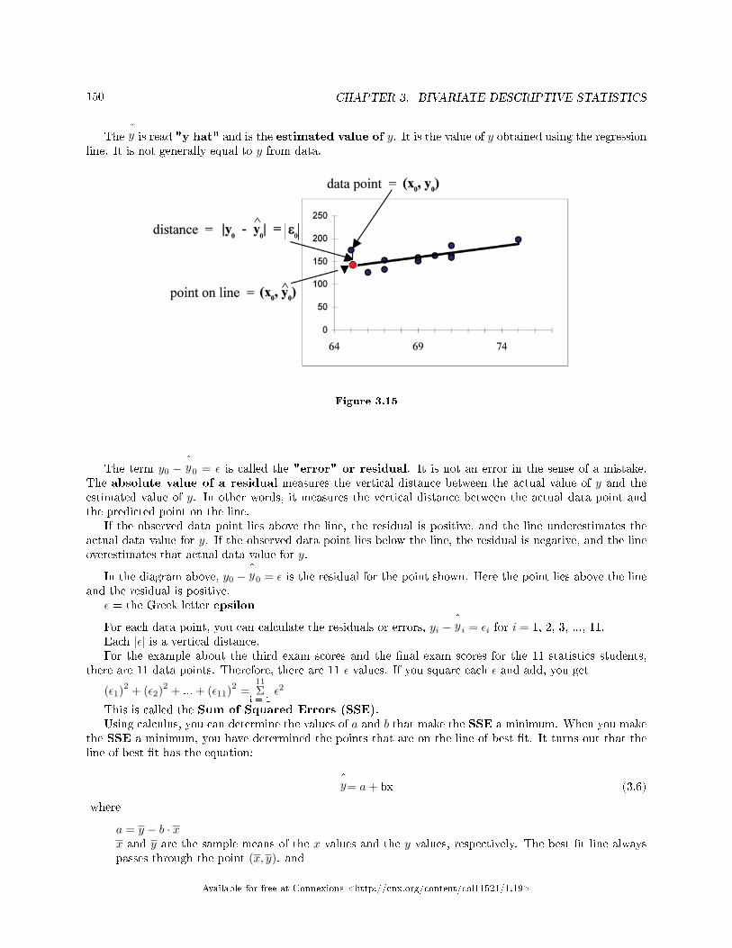
150 CHAPTER 3. BIVARIATE DESCRIPTIVE STATISTICS
The^y is read "y hat" and is the estimated value of y. It is the value of y obtained using the regression
line. It is not generally equal to y from data.
Figure 3.15
The term y0 −^y0 = ε is called the "error" or residual. It is not an error in the sense of a mistake.
The absolute value of a residual measures the vertical distance between the actual value of y and theestimated value of y. In other words, it measures the vertical distance between the actual data point andthe predicted point on the line.
If the observed data point lies above the line, the residual is positive, and the line underestimates theactual data value for y. If the observed data point lies below the line, the residual is negative, and the lineoverestimates that actual data value for y.
In the diagram above, y0 −^y0 = ε is the residual for the point shown. Here the point lies above the line
and the residual is positive.ε = the Greek letter epsilon
For each data point, you can calculate the residuals or errors, yi −^yi = εi for i = 1, 2, 3, ..., 11.
Each |ε| is a vertical distance.For the example about the third exam scores and the �nal exam scores for the 11 statistics students,
there are 11 data points. Therefore, there are 11 ε values. If you square each ε and add, you get
(ε1)2 + (ε2)2 + ... + (ε11)2 =11
Σi = 1
ε2
This is called the Sum of Squared Errors (SSE).Using calculus, you can determine the values of a and b that make the SSE a minimum. When you make
the SSE a minimum, you have determined the points that are on the line of best �t. It turns out that theline of best �t has the equation:
^y= a+ bx (3.6)
where
a = y − b · xx and y are the sample means of the x values and the y values, respectively. The best �t line alwayspasses through the point (x, y). and
Available for free at Connexions <http://cnx.org/content/col11521/1.19>
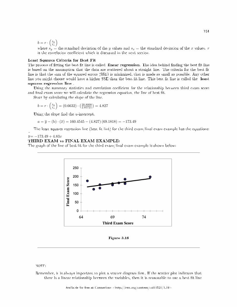
151
b = r ·(sysx
)where sy = the standard deviation of the y values and sx = the standard deviation of the x values. ris the correlation coe�cient which is discussed in the next section.
Least Squares Criteria for Best FitThe process of �tting the best �t line is called linear regression. The idea behind �nding the best �t lineis based on the assumption that the data are scattered about a straight line. The criteria for the best �tline is that the sum of the squared errors (SSE) is minimized, that is made as small as possible. Any otherline you might choose would have a higher SSE than the best �t line. This best �t line is called the leastsquares regression line .
Using the summary statistics and correlation coe�cient for the relationship between third exam scoreand �nal exam score we will calculate the regression equation, the line of best �t.
Start by calculating the slope of the line.
b = r ·(sysx
)= (0.6632) ·
(20.80082.85721
)= 4.827
Using the slope �nd the u-intercept.
a = y − (b) · (x) = 160.4545− (4.827) (69.1818) = −173.49
The least squares regression line (best �t lint) for the third exam/�nal exam example has the equations:^y= −173.49 + 4.83xTHIRD EXAM vs FINAL EXAM EXAMPLE:The graph of the line of best �t for the third exam/�nal exam example is shown below:
Figure 3.16
note:
Remember, it is always important to plot a scatter diagram �rst. If the scatter plot indicates thatthere is a linear relationship between the variables, then it is reasonable to use a best �t line
Available for free at Connexions <http://cnx.org/content/col11521/1.19>
152 CHAPTER 3. BIVARIATE DESCRIPTIVE STATISTICS
to make predictions for y given x within the domain of x-values in the sample data, but notnecessarily for x-values outside that domain.
You could use the line to predict the �nal exam score for a student who earned a grade of 73 onthe third exam.
You should NOT use the line to predict the �nal exam score for a student who earned a grade of50 on the third exam, because 50 is not within the domain of the x-values in the sample data,which are between 65 and 75.
UNDERSTANDING SLOPEThe slope of the line, b, describes how changes in the variables are related. It is important to interpretthe slope of the line in the context of the situation represented by the data. You should be able to write asentence interpreting the slope in plain English.
INTERPRETATION OF THE SLOPE: The slope of the best �t line tells us how the dependentvariable (y) changes for every one unit increase in the independent (x) variable, on average.
THIRD EXAM vs FINAL EXAM EXAMPLE
Slope: The slope of the line is b = 4.83.Interpretation: For a one point increase in the score on the third exam, the �nal exam score increases by
4.83 points, on average.
3.7 Linear Regression and Correlation: Prediction7
Recall the third exam/�nal exam example.We examined the scatterplot and showed that the correlation coe�cient is signi�cant. We found the
equation of the best �t line for the �nal exam grade as a function of the grade on the third exam. We cannow use the least squares regression line for prediction.
Suppose you want to estimate, or predict, the �nal exam score of statistics students who received 73 onthe third exam. The exam scores (x-values) range from 65 to 75. Since 73 is between the x-values65 and 75, substitute x = 73 into the equation. Then:
^y= −173.51 + 4.83 (73) = 179.08 (3.7)
We predict that statistic students who earn a grade of 73 on the third exam will earn a grade of 179.08 onthe �nal exam, on average.
Example 3.7Recall the third exam/�nal exam example.
Problem 1What would you predict the �nal exam score to be for a student who scored a 66 on the third
exam?
Solution145.27
Problem 2 (Solution on p. 209.)
What would you predict the �nal exam score to be for a student who scored a 90 on the thirdexam?
**With contributions from Roberta Bloom
7This content is available online at <http://cnx.org/content/m17095/1.8/>.
Available for free at Connexions <http://cnx.org/content/col11521/1.19>
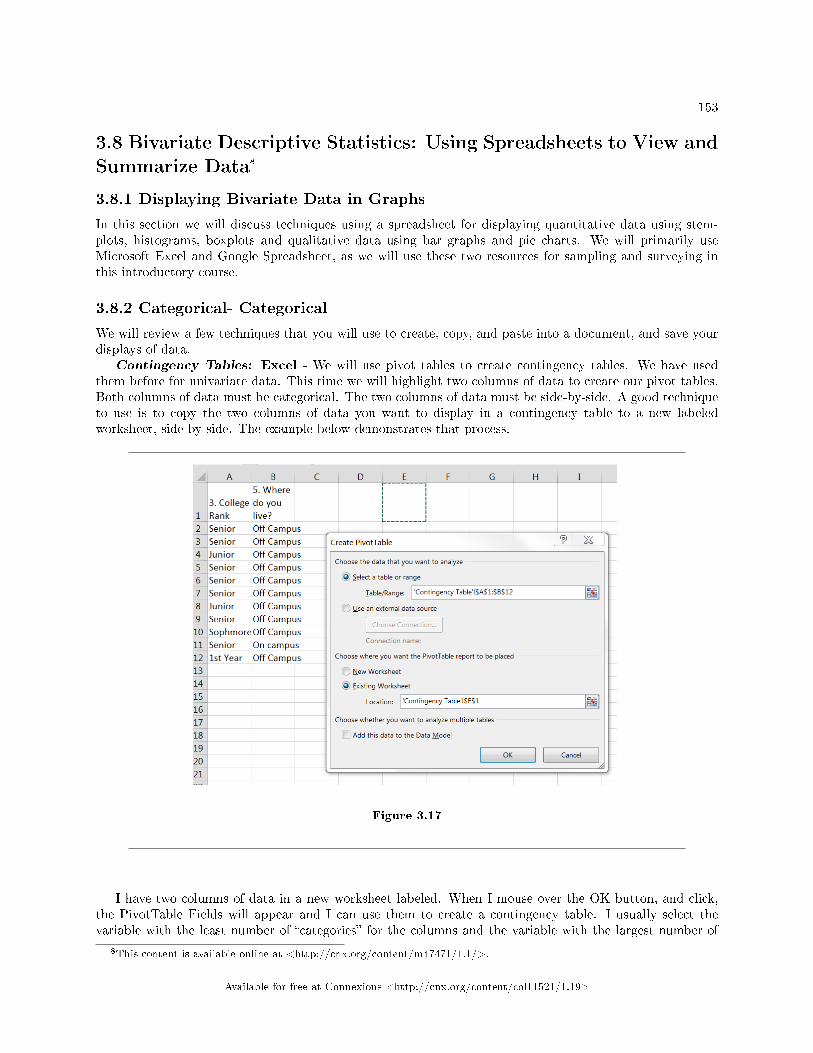
153
3.8 Bivariate Descriptive Statistics: Using Spreadsheets to View andSummarize Data8
3.8.1 Displaying Bivariate Data in Graphs
In this section we will discuss techniques using a spreadsheet for displaying quantitative data using stem-plots, histograms, boxplots and qualitative data using bar graphs and pie charts. We will primarily useMicrosoft Excel and Google Spreadsheet, as we will use these two resources for sampling and surveying inthis introductory course.
3.8.2 Categorical- Categorical
We will review a few techniques that you will use to create, copy, and paste into a document, and save yourdisplays of data.
Contingency Tables: Excel - We will use pivot tables to create contingency tables. We have usedthem before for univariate data. This time we will highlight two columns of data to create our pivot tables.Both columns of data must be categorical. The two columns of data must be side-by-side. A good techniqueto use is to copy the two columns of data you want to display in a contingency table to a new labeledworksheet, side by side. The example below demonstrates that process.
Figure 3.17
I have two columns of data in a new worksheet labeled. When I mouse over the OK button, and click,the PivotTable Fields will appear and I can use them to create a contingency table. I usually select thevariable with the least number of �categories� for the columns and the variable with the largest number of
8This content is available online at <http://cnx.org/content/m47471/1.1/>.
Available for free at Connexions <http://cnx.org/content/col11521/1.19>
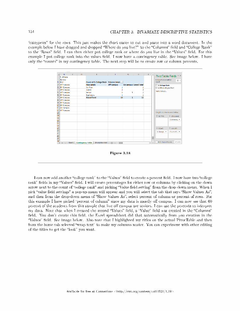
154 CHAPTER 3. BIVARIATE DESCRIPTIVE STATISTICS
�categories� for the rows. This just makes the chart easier to cut and paste into a word document. In theexample below I have dragged and dropped �Where do you live?� to the �Columns� �eld and �College Rank�to the �Rows� �eld. I can then either put college rank or where do you live in the �Values� �eld. For thisexample I put college rank into the values �eld. I now have a contingency table. See image below. I haveonly the �counts� in my contingency table. The next step will be to create row or column percents.
Figure 3.18
I can now add another �college rank� to the �Values� �eld to create a percent �eld. I now have two �collegerank� �elds in my �Values� �eld. I will create percentages for either row or columns by clicking on the downarrow next to the count of �college rank� and picking �Value �eld setting� from the drop-down menu. When Ipick �value �eld settings� a pop-up menu will appear and you will select the tab that says �Show Values As�,and then from the drop-down menu of �Show Values As�, select percent of column or percent of rows. Forthis example I have picked �percent of column� since my data is mostly o� campus. I can now see that 60percent of the students from this sample that live o� campus are seniors. I can use the percents to interpretmy data. Note that when I created the second �Values� �eld, a �Value� �eld was created in the �Columns��eld. You don't create this �eld, the Excel spreadsheet did that automatically from you creation in the�Values� �eld. See image below. Also note that I highlighted my titles on the actual PivotTable and thenfrom the home tab selected �wrap text� to make my columns neater. You can experiment with other editingof the titles to get the �look� you want.
Available for free at Connexions <http://cnx.org/content/col11521/1.19>
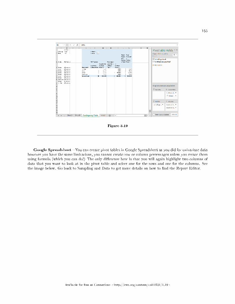
155
Figure 3.19
Google Spreadsheet � You can create pivot tables in Google Spreadsheet as you did for univariate datahowever you have the same limitations, you cannot create row or column percentages unless you create themusing formula (which you can do!) The only di�erence here is that you will again highlight two columns ofdata that you want to look at in the pivot table and select one for the rows and one for the columns. Seethe image below. Go back to Sampling and Data to get more details on how to �nd the Report Editor.
Available for free at Connexions <http://cnx.org/content/col11521/1.19>
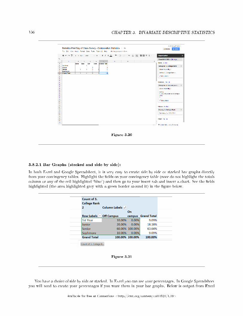
156 CHAPTER 3. BIVARIATE DESCRIPTIVE STATISTICS
Figure 3.20
3.8.2.1 Bar Graphs (stacked and side by side):
In both Excel and Google Spreadsheet, it is very easy to create side by side or stacked bar graphs directlyfrom your contingency tables. Highlight the �elds on your contingency table (note do not highlight the totalscolumn or any of the cell highlighted �blue�) and then go to your insert tab and insert a chart. See the �eldshighlighted (the area highlighted grey with a green border around it) in the �gure below.
Figure 3.21
You have a choice of side by side or stacked. In Excel you can use your percentages. In Google Spreadsheetyou will need to create your percentages if you want them in your bar graphs. Below is output from Excel
Available for free at Connexions <http://cnx.org/content/col11521/1.19>

157
and Google Spreadsheet. Both spreadsheet programs give you many options in the design and format modes.In Excel you can access the design you want from the Change Chart Type �eld on the Design Tab. In GoogleSpreadsheet you change chart types in the Chart editor under the start tab or the charts tab. Explore . . .it's fun.
Figure 3.22
Available for free at Connexions <http://cnx.org/content/col11521/1.19>
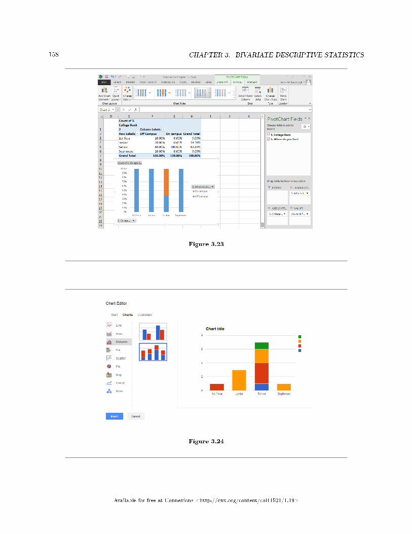
158 CHAPTER 3. BIVARIATE DESCRIPTIVE STATISTICS
Figure 3.23
Figure 3.24
Available for free at Connexions <http://cnx.org/content/col11521/1.19>
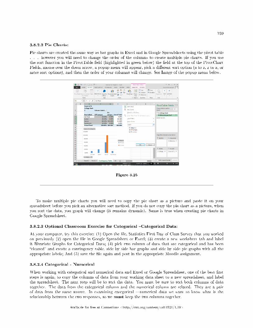
159
3.8.2.2 Pie Charts:
Pie charts are created the same way as bar graphs in Excel and in Google Spreadsheets using the pivot table. . . however you will need to change the order of the columns to create multiple pie charts. If you usethe sort function in the PivotTable �eld (highlighted in green below) the �eld at the top of the PivotChartFields, mouse over the down arrow, a popup menu will appear, pick a di�erent sort option (a to z, z to a, ormore sort options), and then the order of your columns will change. See Image of the popup menu below.
Figure 3.25
To make multiple pie charts you will need to copy the pie chart as a picture and paste it on yourspreadsheet before you pick an alternative sort method. If you do not copy the pie chart as a picture, whenyou sort the data, you graph will change (it remains dynamic). Same is true when creating pie charts inGoogle Spreadsheet.
3.8.2.3 Optional Classroom Exercise for Categorical �Categorical Data:
At your computer, try this exercise: (1) Open the �le, Statistics First Day of Class Survey that you workedon previously (2) open the �le in Google Spreadsheet or Excel; (3) create a new worksheet tab and labelit Bivariate Graphs for Categorical Data; (4) pick two column of data that are categorical and has been�cleaned� and create a contingency table, side by side bar graphs and side by side pie graphs with all theappropriate labels; And (5) save the �le again and post in the appropriate Moodle assignment.
3.8.2.4 Categorical - Numerical
When working with categorical and numerical data and Excel or Google Spreadsheet, one of the best �rststeps is again, to copy the columns of data from your working data sheet to a new spreadsheet, and labelthe spreadsheet. The next step will be to sort the data. You must be sure to sort both columns of datatogether. The data from the categorical column and the numerical column are related. They are a pairof data from the same source. In examining categorical � numerical data we want to know what is therelationship between the two responses, so we must keep the two columns together.
Available for free at Connexions <http://cnx.org/content/col11521/1.19>
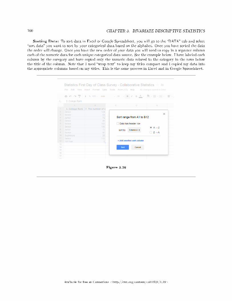
160 CHAPTER 3. BIVARIATE DESCRIPTIVE STATISTICS
Sorting Data: To sort data in Excel or Google Spreadsheet, you will go to the �DATA� tab and select�sort data� you want to sort by your categorical data based on the alphabet. Once you have sorted the datathe order will change. Once you have the new order of your data you will need to copy in a separate columneach of the numeric data for each unique categorical data source. See the example below. I have labeled eachcolumn by the category and have copied only the numeric data related to the category in the rows belowthe title of the column. Note that I used �wrap text� to keep my titles compact and I copied my data intothe appropriate columns based on my titles. This is the same process in Excel and in Google Spreadsheet.
Figure 3.26
Available for free at Connexions <http://cnx.org/content/col11521/1.19>
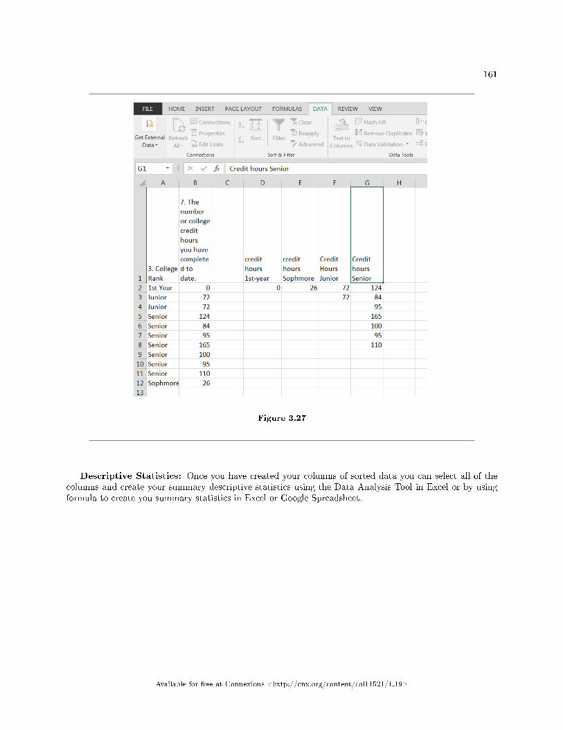
161
Figure 3.27
Descriptive Statistics: Once you have created your columns of sorted data you can select all of thecolumns and create your summary descriptive statistics using the Data Analysis Tool in Excel or by usingformula to create you summary statistics in Excel or Google Spreadsheet.
Available for free at Connexions <http://cnx.org/content/col11521/1.19>
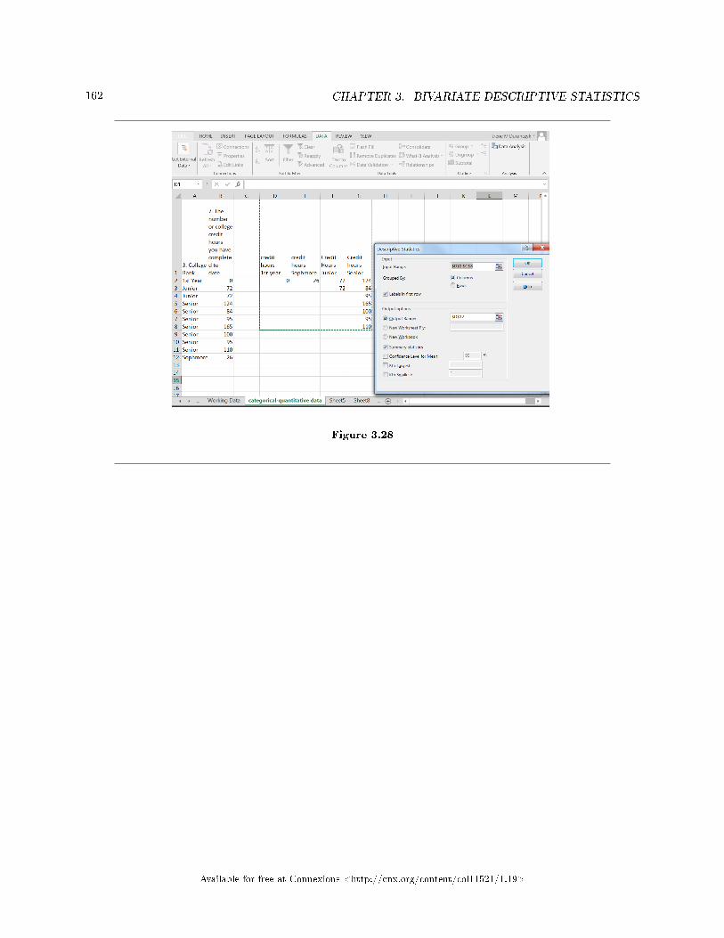
162 CHAPTER 3. BIVARIATE DESCRIPTIVE STATISTICS
Figure 3.28
Available for free at Connexions <http://cnx.org/content/col11521/1.19>
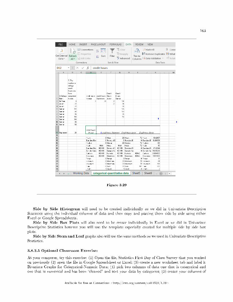
163
Figure 3.29
Side by Side Histogram will need to be created individually as we did in Univariate DescriptiveStatistics using the individual columns of data and then copy and pasting them side by side using eitherExcel or Google Spreadsheets.
Side by Side Box Plots will also need to be create individually in Excel as we did in UnivariateDescriptive Statistics however you will use the template especially created for multiple side by side boxplots.
Side by Side Stem and Leaf graphs also will use the same methods as we used in Univariate DescriptiveStatistics.
3.8.2.5 Optional Classroom Exercise:
At your computer, try this exercise: (1) Open the �le, Statistics First Day of Class Survey that you workedon previously (2) open the �le in Google Spreadsheet or Excel; (3) create a new worksheet tab and label itBivariate Graphs for Categorical-Numeric Data; (4) pick two columns of data one that is categorical andone that is numerical and has been �cleaned� and sort your data by categories; (5) create your columns of
Available for free at Connexions <http://cnx.org/content/col11521/1.19>
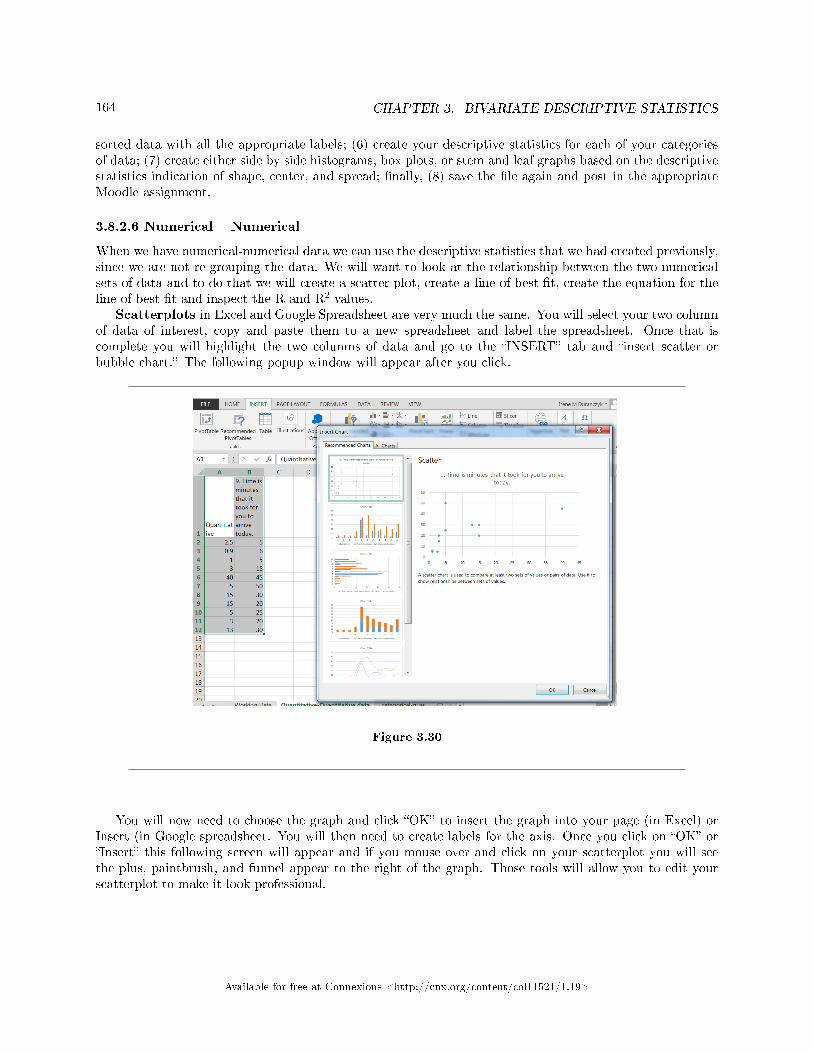
164 CHAPTER 3. BIVARIATE DESCRIPTIVE STATISTICS
sorted data with all the appropriate labels; (6) create your descriptive statistics for each of your categoriesof data; (7) create either side by side histograms, box plots, or stem and leaf graphs based on the descriptivestatistics indication of shape, center, and spread; �nally, (8) save the �le again and post in the appropriateMoodle assignment.
3.8.2.6 Numerical � Numerical
When we have numerical-numerical data we can use the descriptive statistics that we had created previously,since we are not re-grouping the data. We will want to look at the relationship between the two numericalsets of data and to do that we will create a scatter plot, create a line of best �t, create the equation for theline of best �t and inspect the R and R2 values.
Scatterplots in Excel and Google Spreadsheet are very much the same. You will select your two columnof data of interest, copy and paste them to a new spreadsheet and label the spreadsheet. Once that iscomplete you will highlight the two columns of data and go to the �INSERT� tab and �insert scatter orbubble chart.� The following popup window will appear after you click.
Figure 3.30
You will now need to choose the graph and click �OK� to insert the graph into your page (in Excel) orInsert (in Google spreadsheet. You will then need to create labels for the axis. Once you click on �OK� or�Insert� this following screen will appear and if you mouse over and click on your scatterplot you will seethe plus, paintbrush, and funnel appear to the right of the graph. Those tools will allow you to edit yourscatterplot to make it look professional.
Available for free at Connexions <http://cnx.org/content/col11521/1.19>
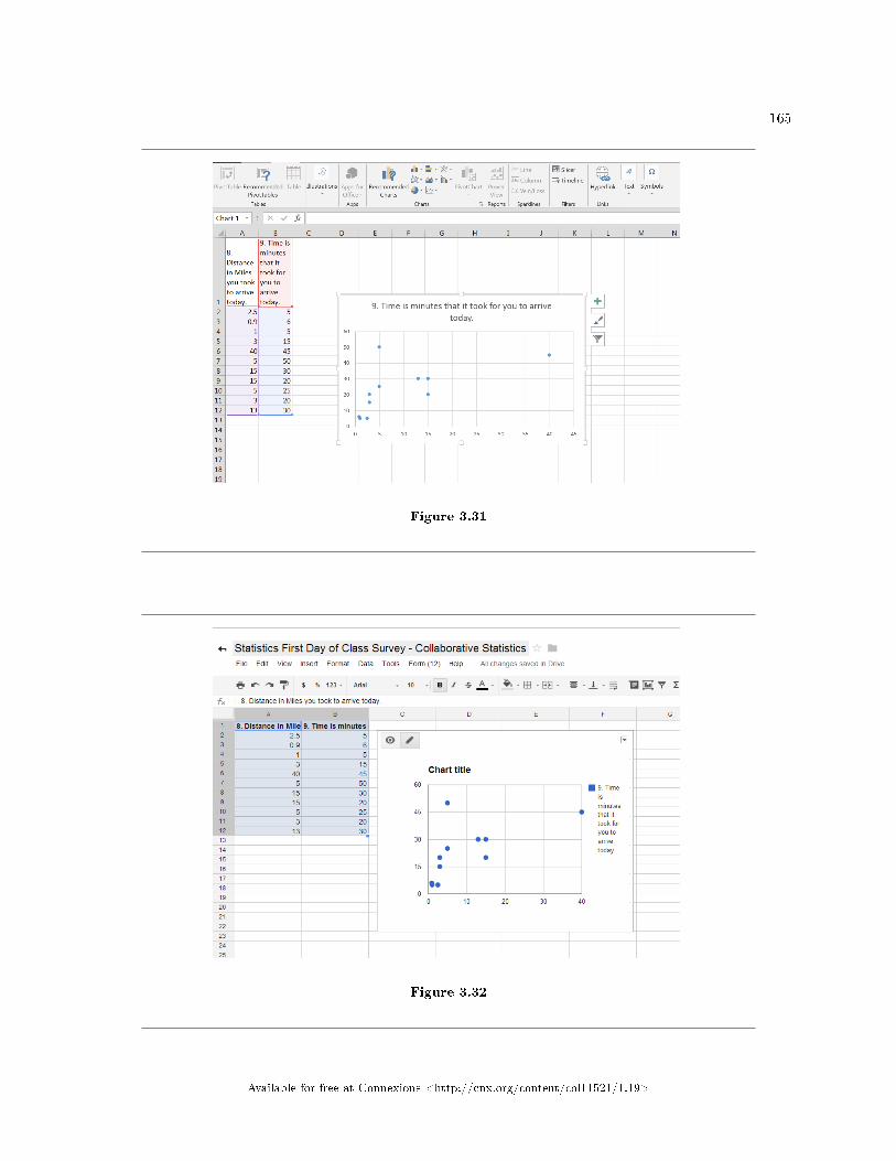
165
Figure 3.31
Figure 3.32
Available for free at Connexions <http://cnx.org/content/col11521/1.19>
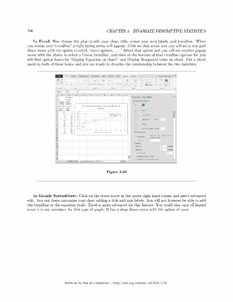
166 CHAPTER 3. BIVARIATE DESCRIPTIVE STATISTICS
In Excel: Now choose the plus to edit your chart title, create your axis labels, and trendline. Whenyou mouse over �trendline� a right facing arrow will appear. Click on that arrow and you will see a new pulldown menu with the option to select, �more options. . . � Select that option and you will see another popupmenu with the choice to select a Linear trendline, and then at the bottom of that trendline options list youwill �nd option boxes for �Display Equation on chart�, and Display R-squared value on chart. Put a checkmark in both of these boxes and you are ready to describe the relationship between the two variables.
Figure 3.33
In Google Spreadsheet: Click on the down arrow in the upper right hand corner and select advancededit. You can there customize your chart adding a title and axis labels. You will not however be able to addthe trendline or the equation easily. Excel is more advanced for this feature. You could also turn o� legendsince it is not necessary for this type of graph. It has a drop down menu with the option of none.
Available for free at Connexions <http://cnx.org/content/col11521/1.19>
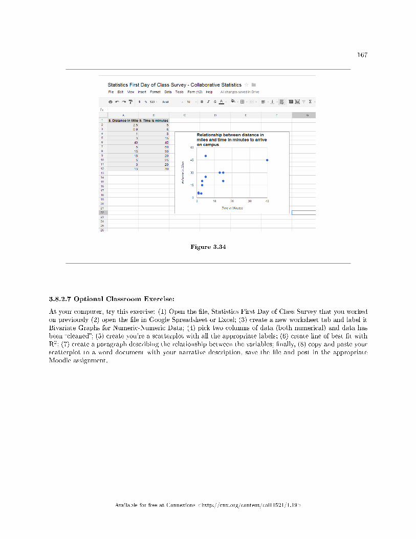
167
Figure 3.34
3.8.2.7 Optional Classroom Exercise:
At your computer, try this exercise: (1) Open the �le, Statistics First Day of Class Survey that you workedon previously (2) open the �le in Google Spreadsheet or Excel; (3) create a new worksheet tab and label itBivariate Graphs for Numeric-Numeric Data; (4) pick two columns of data (both numerical) and data hasbeen �cleaned�; (5) create you're a scatterplot with all the appropriate labels; (6) create line of best �t withR2; (7) create a paragraph describing the relationship between the variables; �nally, (8) copy and paste yourscatterplot to a word document with your narrative description, save the �le and post in the appropriateMoodle assignment.
Available for free at Connexions <http://cnx.org/content/col11521/1.19>
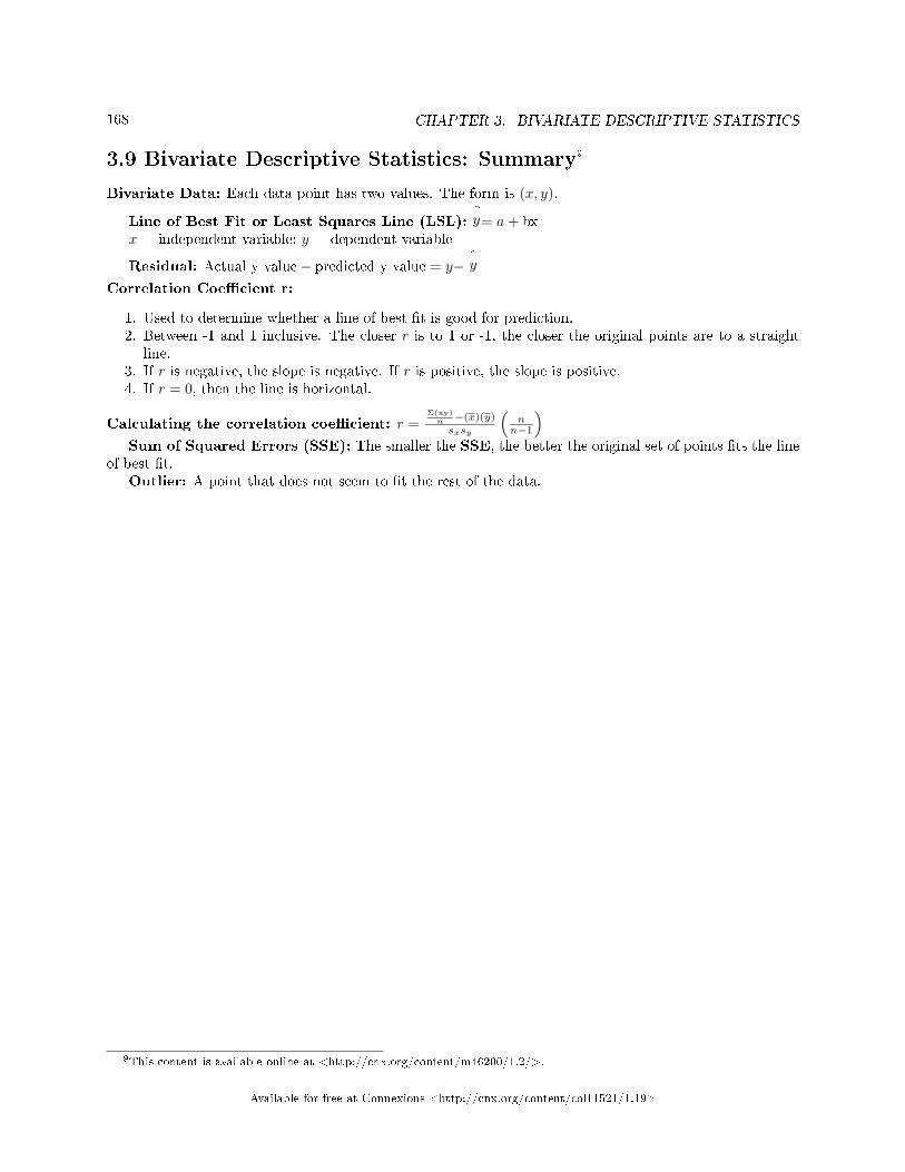
168 CHAPTER 3. BIVARIATE DESCRIPTIVE STATISTICS
3.9 Bivariate Descriptive Statistics: Summary9
Bivariate Data: Each data point has two values. The form is (x, y).
Line of Best Fit or Least Squares Line (LSL):^y= a+ bx
x = independent variable; y = dependent variable
Residual: Actual y value− predicted y value = y−^y
Correlation Coe�cient r:
1. Used to determine whether a line of best �t is good for prediction.2. Between -1 and 1 inclusive. The closer r is to 1 or -1, the closer the original points are to a straight
line.3. If r is negative, the slope is negative. If r is positive, the slope is positive.4. If r = 0, then the line is horizontal.
Calculating the correlation coe�cient: r =Σ(xy)n −(x)(y)
sxsy
(nn−1
)Sum of Squared Errors (SSE): The smaller the SSE, the better the original set of points �ts the line
of best �t.Outlier: A point that does not seem to �t the rest of the data.
9This content is available online at <http://cnx.org/content/m46200/1.2/>.
Available for free at Connexions <http://cnx.org/content/col11521/1.19>
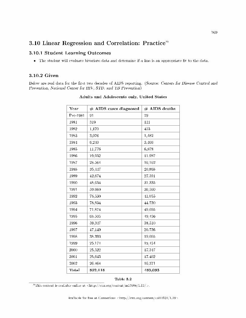
169
3.10 Linear Regression and Correlation: Practice10
3.10.1 Student Learning Outcomes
• The student will evaluate bivariate data and determine if a line is an appropriate �t to the data.
3.10.2 Given
Below are real data for the �rst two decades of AIDS reporting. (Source: Centers for Disease Control andPrevention, National Center for HIV, STD, and TB Prevention)
Adults and Adolescents only, United States
Year # AIDS cases diagnosed # AIDS deaths
Pre-1981 91 29
1981 319 121
1982 1,170 453
1983 3,076 1,482
1984 6,240 3,466
1985 11,776 6,878
1986 19,032 11,987
1987 28,564 16,162
1988 35,447 20,868
1989 42,674 27,591
1990 48,634 31,335
1991 59,660 36,560
1992 78,530 41,055
1993 78,834 44,730
1994 71,874 49,095
1995 68,505 49,456
1996 59,347 38,510
1997 47,149 20,736
1998 38,393 19,005
1999 25,174 18,454
2000 25,522 17,347
2001 25,643 17,402
2002 26,464 16,371
Total 802,118 489,093
Table 3.2
10This content is available online at <http://cnx.org/content/m17088/1.12/>.
Available for free at Connexions <http://cnx.org/content/col11521/1.19>
170 CHAPTER 3. BIVARIATE DESCRIPTIVE STATISTICS
note: We will use the columns �year� and �# AIDS cases diagnosed� for all questions unlessotherwise stated.
3.10.3 Graphing
Graph �year� vs. �# AIDS cases diagnosed.� Plot the points on the graph located below in thesection titled "Plot" . Do not include pre-1981. Label both axes with words. Scale both axes.
3.10.4 Data
Exercise 3.10.1Enter your data into your calculator or computer. The pre-1981 data should not be included. Whyis that so?
3.10.5 Linear Equation
Write the linear equation below, rounding to 4 decimal places:
note: For any prediction questions, the answers are calculated using the least squares (best �t)line equation cited in the solution.
Exercise 3.10.2 (Solution on p. 209.)
Calculate the following:
a. a =b. b =c. corr. =d. n =(# of pairs)
Exercise 3.10.3 (Solution on p. 209.)
equation:^y=
3.10.6 Solve
Exercise 3.10.4 (Solution on p. 209.)
Solve.
a. When x = 1985,^y=
b. When x = 1990,^y=
Available for free at Connexions <http://cnx.org/content/col11521/1.19>
171
3.10.7 Plot
Plot the 2 above points on the graph below. Then, connect the 2 points to form the regression line.
Obtain the graph on your calculator or computer.
3.10.8 Discussion Questions
Look at the graph above.
Exercise 3.10.5Does the line seem to �t the data? Why or why not?
Exercise 3.10.6Do you think a linear �t is best? Why or why not?
Exercise 3.10.7Hand draw a smooth curve on the graph above that shows the �ow of the data.
Exercise 3.10.8What does the correlation imply about the relationship between time (years) and the number ofdiagnosed AIDS cases reported in the U.S.?
Exercise 3.10.9Why is �year� the independent variable and �# AIDS cases diagnosed.� the dependent variable(instead of the reverse)?
Exercise 3.10.10 (Solution on p. 209.)
Solve.
a. When x = 1970,^y=:
b. Why doesn't this answer make sense?
Available for free at Connexions <http://cnx.org/content/col11521/1.19>
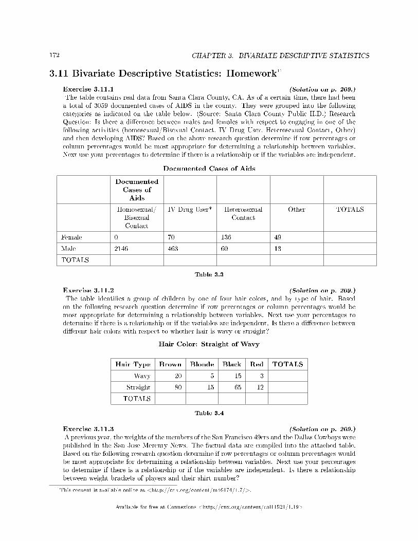
172 CHAPTER 3. BIVARIATE DESCRIPTIVE STATISTICS
3.11 Bivariate Descriptive Statistics: Homework11
Exercise 3.11.1 (Solution on p. 209.)
The table contains real data from Santa Clara County, CA. As of a certain time, there had beena total of 3059 documented cases of AIDS in the county. They were grouped into the followingcategories as indicated on the table below. (Source: Santa Clara County Public H.D.) ResearchQuestion: Is there a di�erence between males and females with respect to engaging in one of thefollowing activities (homosexual/Bisexual Contact, IV Drug User, Heterosexual Contact, Other)and then developing AIDS? Based on the above research question determine if row percentages orcolumn percentages would be most appropriate for determining a relationship between variables.Next use your percentages to determine if there is a relationship or if the variables are independent.
Documented Cases of Aids
DocumentedCases ofAids
Homosexual/BisexualContact
IV Drug User* HeterosexualContact
Other TOTALS
Female 0 70 136 49
Male 2146 463 60 13
TOTALS
Table 3.3
Exercise 3.11.2 (Solution on p. 209.)
The table identi�es a group of children by one of four hair colors, and by type of hair. Basedon the following research question determine if row percentages or column percentages would bemost appropriate for determining a relationship between variables. Next use your percentages todetermine if there is a relationship or if the variables are independent. Is there a di�erence betweendi�erent hair colors with respect to whether hair is wavy or straight?
Hair Color: Straight of Wavy
Hair Type Brown Blonde Black Red TOTALS
Wavy 20 5 15 3
Straight 80 15 65 12
TOTALS
Table 3.4
Exercise 3.11.3 (Solution on p. 209.)
A previous year, the weights of the members of the San Francisco 49ers and the Dallas Cowboys werepublished in the San Jose Mercury News. The factual data are compiled into the attached table.Based on the following research question determine if row percentages or column percentages wouldbe most appropriate for determining a relationship between variables. Next use your percentagesto determine if there is a relationship or if the variables are independent. Is there a relationshipbetween weight brackets of players and their shirt number?
11This content is available online at <http://cnx.org/content/m46174/1.7/>.
Available for free at Connexions <http://cnx.org/content/col11521/1.19>
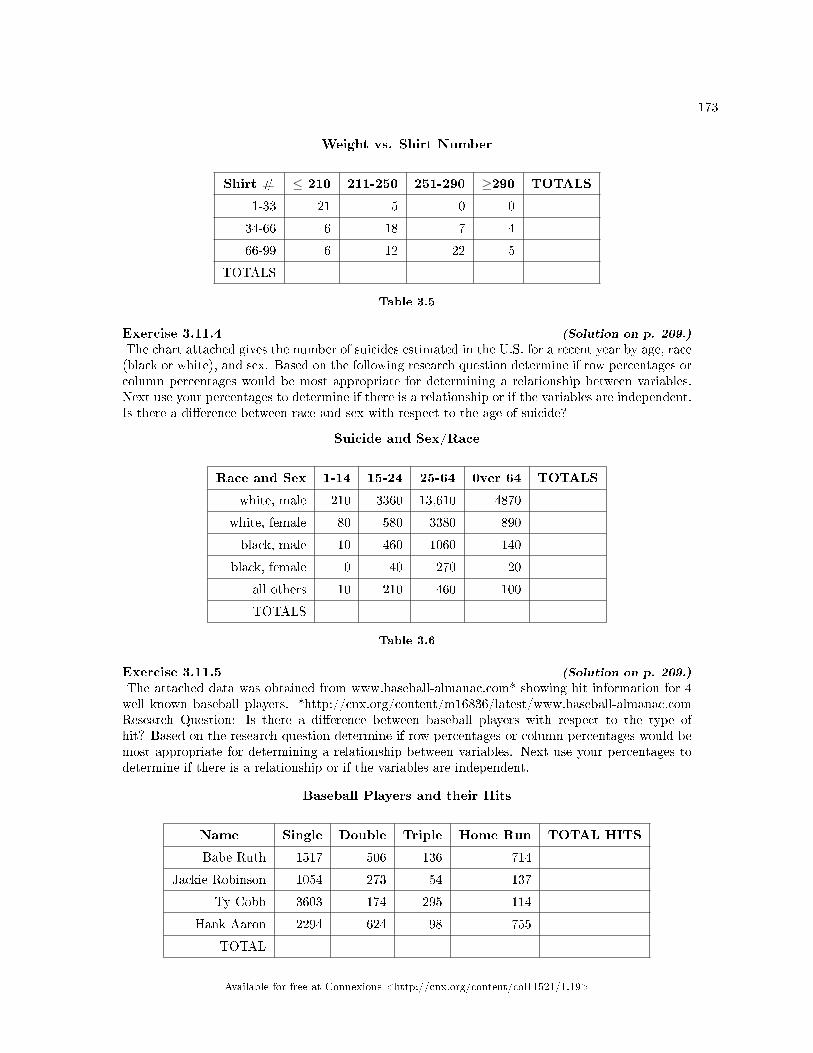
173
Weight vs. Shirt Number
Shirt # ≤ 210 211-250 251-290 ≥290 TOTALS
1-33 21 5 0 0
34-66 6 18 7 4
66-99 6 12 22 5
TOTALS
Table 3.5
Exercise 3.11.4 (Solution on p. 209.)
The chart attached gives the number of suicides estimated in the U.S. for a recent year by age, race(black or white), and sex. Based on the following research question determine if row percentages orcolumn percentages would be most appropriate for determining a relationship between variables.Next use your percentages to determine if there is a relationship or if the variables are independent.Is there a di�erence between race and sex with respect to the age of suicide?
Suicide and Sex/Race
Race and Sex 1-14 15-24 25-64 0ver 64 TOTALS
white, male 210 3360 13,610 4870
white, female 80 580 3380 890
black, male 10 460 1060 140
black, female 0 40 270 20
all others 10 210 460 100
TOTALS
Table 3.6
Exercise 3.11.5 (Solution on p. 209.)
The attached data was obtained from www.baseball-almanac.com* showing hit information for 4well known baseball players. *http://cnx.org/content/m16836/latest/www.baseball-almanac.comResearch Question: Is there a di�erence between baseball players with respect to the type ofhit? Based on the research question determine if row percentages or column percentages would bemost appropriate for determining a relationship between variables. Next use your percentages todetermine if there is a relationship or if the variables are independent.
Baseball Players and their Hits
Name Single Double Triple Home Run TOTAL HITS
Babe Ruth 1517 506 136 714
Jackie Robinson 1054 273 54 137
Ty Cobb 3603 174 295 114
Hank Aaron 2294 624 98 755
TOTAL
Available for free at Connexions <http://cnx.org/content/col11521/1.19>
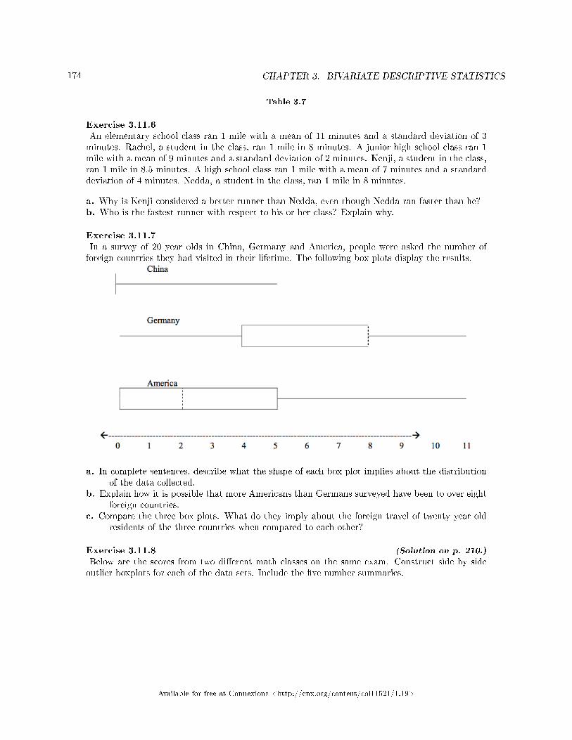
174 CHAPTER 3. BIVARIATE DESCRIPTIVE STATISTICS
Table 3.7
Exercise 3.11.6An elementary school class ran 1 mile with a mean of 11 minutes and a standard deviation of 3minutes. Rachel, a student in the class, ran 1 mile in 8 minutes. A junior high school class ran 1mile with a mean of 9 minutes and a standard deviation of 2 minutes. Kenji, a student in the class,ran 1 mile in 8.5 minutes. A high school class ran 1 mile with a mean of 7 minutes and a standarddeviation of 4 minutes. Nedda, a student in the class, ran 1 mile in 8 minutes.
a. Why is Kenji considered a better runner than Nedda, even though Nedda ran faster than he?b. Who is the fastest runner with respect to his or her class? Explain why.
Exercise 3.11.7In a survey of 20 year olds in China, Germany and America, people were asked the number offoreign countries they had visited in their lifetime. The following box plots display the results.
a. In complete sentences, describe what the shape of each box plot implies about the distributionof the data collected.
b. Explain how it is possible that more Americans than Germans surveyed have been to over eightforeign countries.
c. Compare the three box plots. What do they imply about the foreign travel of twenty year oldresidents of the three countries when compared to each other?
Exercise 3.11.8 (Solution on p. 210.)
Below are the scores from two di�erent math classes on the same exam. Construct side by sideoutlier boxplots for each of the data sets. Include the �ve number summaries.
Available for free at Connexions <http://cnx.org/content/col11521/1.19>
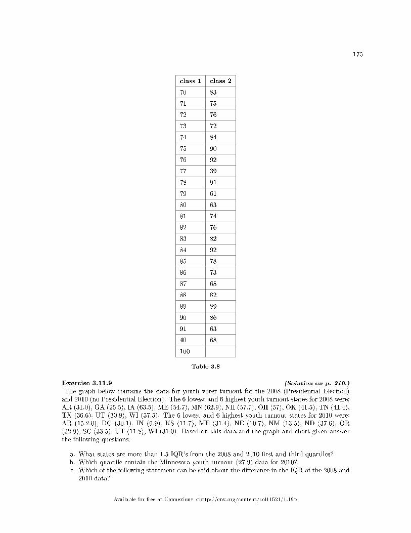
175
class 1 class 2
70 83
71 75
72 76
73 72
74 84
75 90
76 92
77 39
78 91
79 61
80 63
81 74
82 76
83 82
84 92
85 78
86 73
87 68
88 82
89 89
90 86
91 63
40 68
100
Table 3.8
Exercise 3.11.9 (Solution on p. 210.)
The graph below contains the data for youth voter turnout for the 2008 (Presidential Election)and 2010 (no Presidential Election). The 6 lowest and 6 highest youth turnout states for 2008 were:AR (31.0), GA (25.5), IA (63.5), ME (54.7), MN (62.9), NH (57.7), OH (57), OK (41.5), TN (41.4),TX (36.6), UT (30.9), WI (57.5). The 6 lowest and 6 highest youth turnout states for 2010 were:AR (15.2.0), DC (30.1), IN (9.9), KS (11.7), ME (31.4), NE (10.7), NM (13.5), ND (37.6), OR(32.9), SC (33.5), UT (11.8), WI (31.0). Based on this data and the graph and chart given answerthe following questions.
a. What states are more than 1.5 IQR's from the 2008 and 2010 �rst and third quartiles?b. Which quartile contain the Minnesota youth turnout (27.9) data for 2010?c. Which of the following statement can be said about the di�erence in the IQR of the 2008 and
2010 data?
Available for free at Connexions <http://cnx.org/content/col11521/1.19>
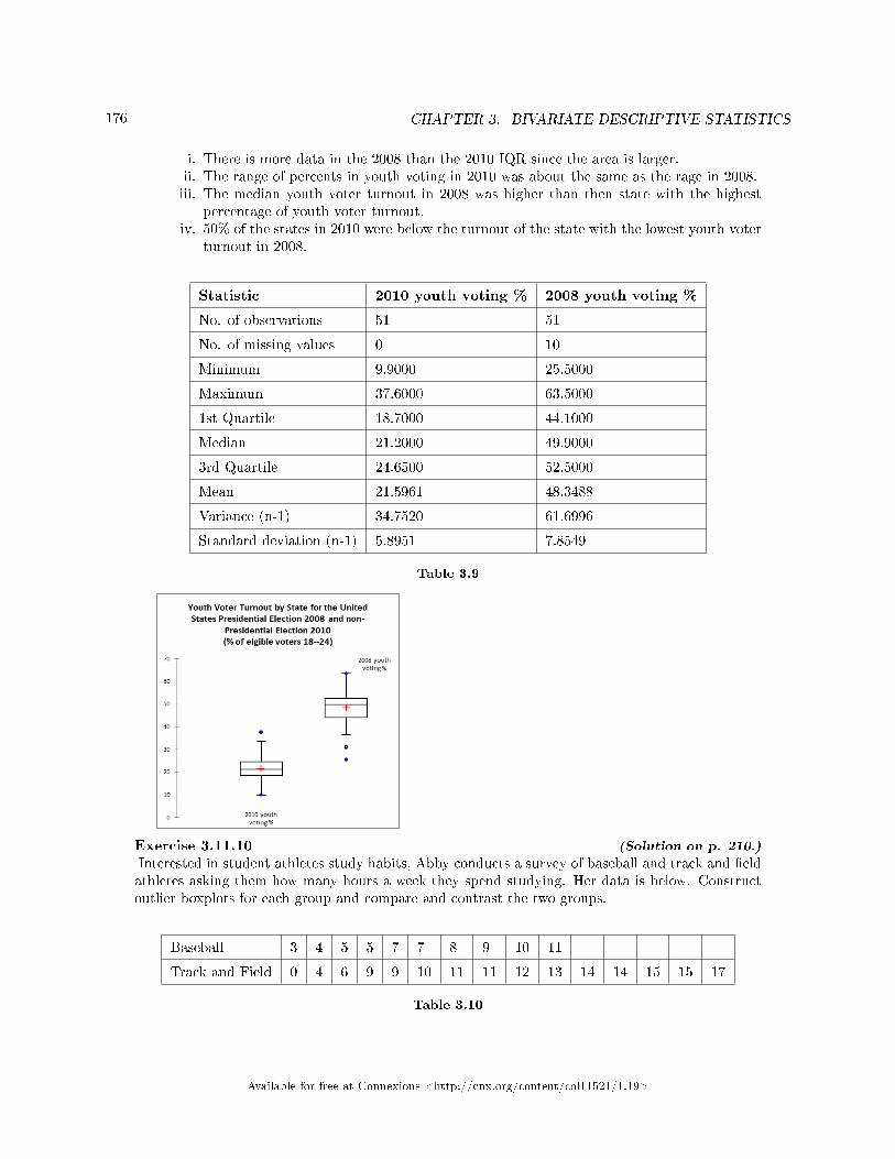
176 CHAPTER 3. BIVARIATE DESCRIPTIVE STATISTICS
i. There is more data in the 2008 than the 2010 IQR since the area is larger.ii. The range of percents in youth voting in 2010 was about the same as the rage in 2008.iii. The median youth voter turnout in 2008 was higher than then state with the highest
percentage of youth voter turnout.iv. 50% of the states in 2010 were below the turnout of the state with the lowest youth voter
turnout in 2008.
Statistic 2010 youth voting % 2008 youth voting %
No. of observations 51 51
No. of missing values 0 10
Minimum 9.9000 25.5000
Maximum 37.6000 63.5000
1st Quartile 18.7000 44.1000
Median 21.2000 49.9000
3rd Quartile 24.6500 52.5000
Mean 21.5961 48.3488
Variance (n-1) 34.7520 61.6996
Standard deviation (n-1) 5.8951 7.8549
Table 3.9
Exercise 3.11.10 (Solution on p. 210.)
Interested in student athletes study habits, Abby conducts a survey of baseball and track and �eldathletes asking them how many hours a week they spend studying. Her data is below. Constructoutlier boxplots for each group and compare and contrast the two groups.
Baseball 3 4 5 5 7 7 8 9 10 11
Track and Field 0 4 6 9 9 10 11 11 12 13 14 14 15 15 17
Table 3.10
Available for free at Connexions <http://cnx.org/content/col11521/1.19>
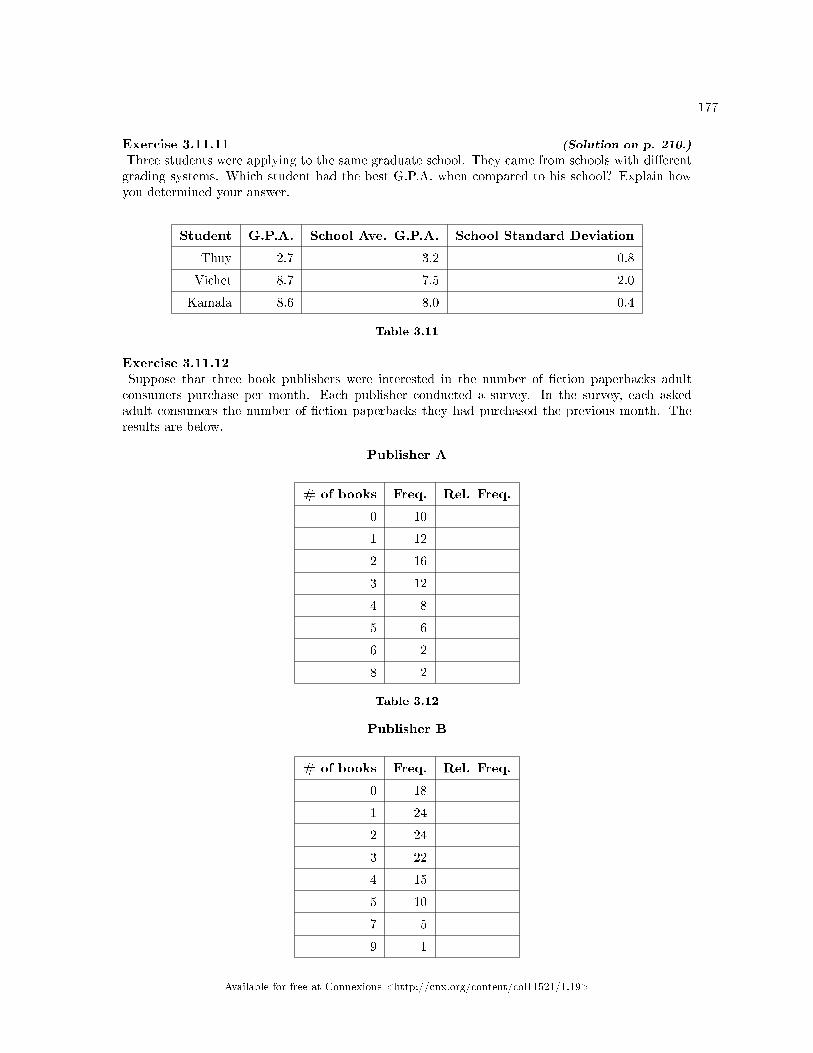
177
Exercise 3.11.11 (Solution on p. 210.)
Three students were applying to the same graduate school. They came from schools with di�erentgrading systems. Which student had the best G.P.A. when compared to his school? Explain howyou determined your answer.
Student G.P.A. School Ave. G.P.A. School Standard Deviation
Thuy 2.7 3.2 0.8
Vichet 8.7 7.5 2.0
Kamala 8.6 8.0 0.4
Table 3.11
Exercise 3.11.12Suppose that three book publishers were interested in the number of �ction paperbacks adultconsumers purchase per month. Each publisher conducted a survey. In the survey, each askedadult consumers the number of �ction paperbacks they had purchased the previous month. Theresults are below.
Publisher A
# of books Freq. Rel. Freq.
0 10
1 12
2 16
3 12
4 8
5 6
6 2
8 2
Table 3.12
Publisher B
# of books Freq. Rel. Freq.
0 18
1 24
2 24
3 22
4 15
5 10
7 5
9 1
Available for free at Connexions <http://cnx.org/content/col11521/1.19>
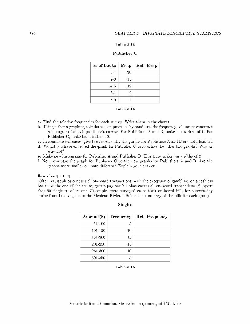
178 CHAPTER 3. BIVARIATE DESCRIPTIVE STATISTICS
Table 3.13
Publisher C
# of books Freq. Rel. Freq.
0-1 20
2-3 35
4-5 12
6-7 2
8-9 1
Table 3.14
a. Find the relative frequencies for each survey. Write them in the charts.b. Using either a graphing calculator, computer, or by hand, use the frequency column to construct
a histogram for each publisher's survey. For Publishers A and B, make bar widths of 1. ForPublisher C, make bar widths of 2.
c. In complete sentences, give two reasons why the graphs for Publishers A and B are not identical.d. Would you have expected the graph for Publisher C to look like the other two graphs? Why or
why not?e. Make new histograms for Publisher A and Publisher B. This time, make bar widths of 2.f. Now, compare the graph for Publisher C to the new graphs for Publishers A and B. Are the
graphs more similar or more di�erent? Explain your answer.
Exercise 3.11.13Often, cruise ships conduct all on-board transactions, with the exception of gambling, on a cashlessbasis. At the end of the cruise, guests pay one bill that covers all on-board transactions. Supposethat 60 single travelers and 70 couples were surveyed as to their on-board bills for a seven-daycruise from Los Angeles to the Mexican Riviera. Below is a summary of the bills for each group.
Singles
Amount($) Frequency Rel. Frequency
51-100 5
101-150 10
151-200 15
201-250 15
251-300 10
301-350 5
Table 3.15
Available for free at Connexions <http://cnx.org/content/col11521/1.19>
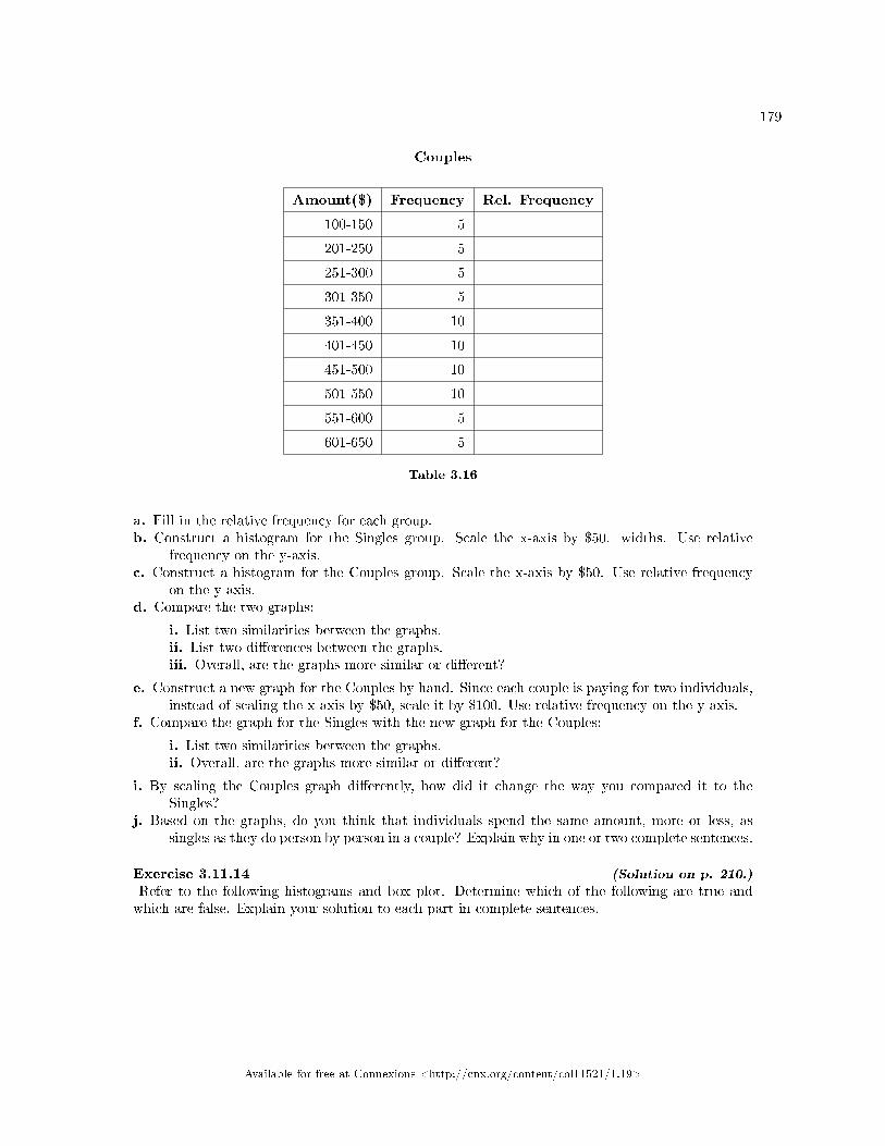
179
Couples
Amount($) Frequency Rel. Frequency
100-150 5
201-250 5
251-300 5
301-350 5
351-400 10
401-450 10
451-500 10
501-550 10
551-600 5
601-650 5
Table 3.16
a. Fill in the relative frequency for each group.b. Construct a histogram for the Singles group. Scale the x-axis by $50. widths. Use relative
frequency on the y-axis.c. Construct a histogram for the Couples group. Scale the x-axis by $50. Use relative frequency
on the y-axis.d. Compare the two graphs:
i. List two similarities between the graphs.ii. List two di�erences between the graphs.iii. Overall, are the graphs more similar or di�erent?
e. Construct a new graph for the Couples by hand. Since each couple is paying for two individuals,instead of scaling the x-axis by $50, scale it by $100. Use relative frequency on the y-axis.
f. Compare the graph for the Singles with the new graph for the Couples:
i. List two similarities between the graphs.ii. Overall, are the graphs more similar or di�erent?
i. By scaling the Couples graph di�erently, how did it change the way you compared it to theSingles?
j. Based on the graphs, do you think that individuals spend the same amount, more or less, assingles as they do person by person in a couple? Explain why in one or two complete sentences.
Exercise 3.11.14 (Solution on p. 210.)
Refer to the following histograms and box plot. Determine which of the following are true andwhich are false. Explain your solution to each part in complete sentences.
Available for free at Connexions <http://cnx.org/content/col11521/1.19>
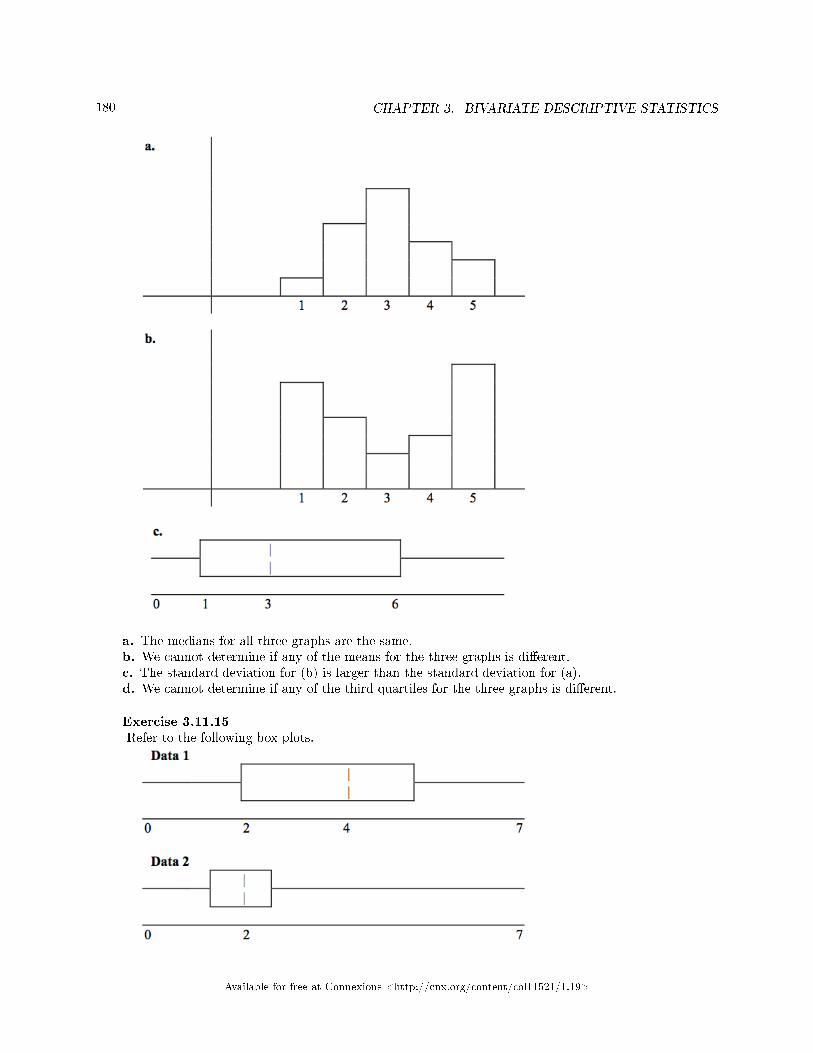
180 CHAPTER 3. BIVARIATE DESCRIPTIVE STATISTICS
a. The medians for all three graphs are the same.b. We cannot determine if any of the means for the three graphs is di�erent.c. The standard deviation for (b) is larger than the standard deviation for (a).d. We cannot determine if any of the third quartiles for the three graphs is di�erent.
Exercise 3.11.15Refer to the following box plots.
Available for free at Connexions <http://cnx.org/content/col11521/1.19>
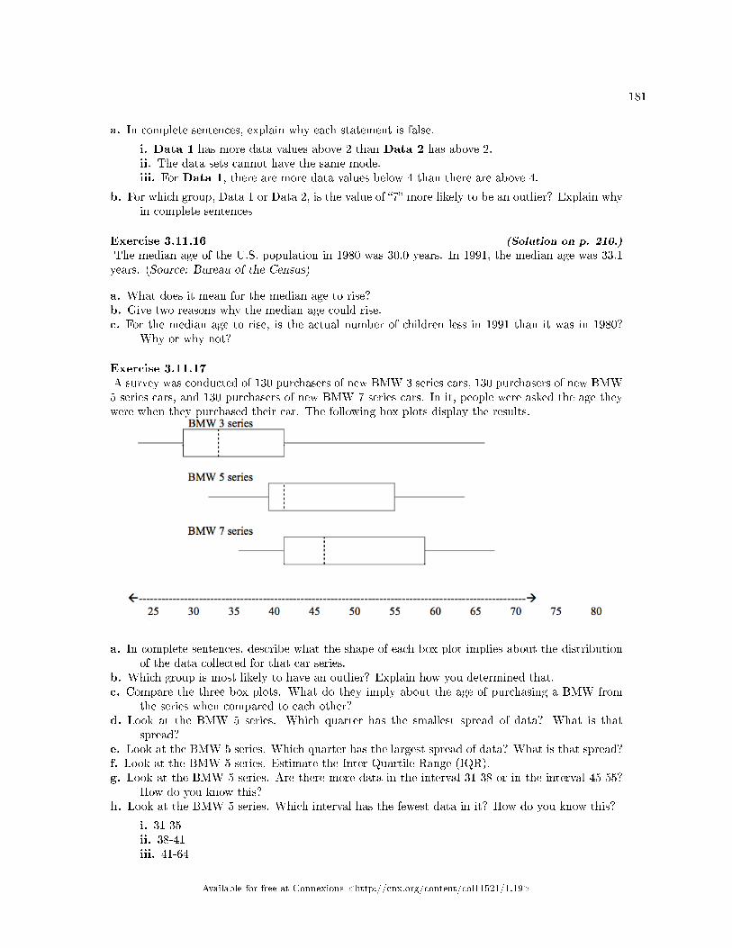
181
a. In complete sentences, explain why each statement is false.
i. Data 1 has more data values above 2 than Data 2 has above 2.ii. The data sets cannot have the same mode.iii. For Data 1, there are more data values below 4 than there are above 4.
b. For which group, Data 1 or Data 2, is the value of �7� more likely to be an outlier? Explain whyin complete sentences
Exercise 3.11.16 (Solution on p. 210.)
The median age of the U.S. population in 1980 was 30.0 years. In 1991, the median age was 33.1years. (Source: Bureau of the Census)
a. What does it mean for the median age to rise?b. Give two reasons why the median age could rise.c. For the median age to rise, is the actual number of children less in 1991 than it was in 1980?
Why or why not?
Exercise 3.11.17A survey was conducted of 130 purchasers of new BMW 3 series cars, 130 purchasers of new BMW5 series cars, and 130 purchasers of new BMW 7 series cars. In it, people were asked the age theywere when they purchased their car. The following box plots display the results.
a. In complete sentences, describe what the shape of each box plot implies about the distributionof the data collected for that car series.
b. Which group is most likely to have an outlier? Explain how you determined that.c. Compare the three box plots. What do they imply about the age of purchasing a BMW from
the series when compared to each other?d. Look at the BMW 5 series. Which quarter has the smallest spread of data? What is that
spread?e. Look at the BMW 5 series. Which quarter has the largest spread of data? What is that spread?f. Look at the BMW 5 series. Estimate the Inter Quartile Range (IQR).g. Look at the BMW 5 series. Are there more data in the interval 31-38 or in the interval 45-55?
How do you know this?h. Look at the BMW 5 series. Which interval has the fewest data in it? How do you know this?
i. 31-35ii. 38-41iii. 41-64
Available for free at Connexions <http://cnx.org/content/col11521/1.19>
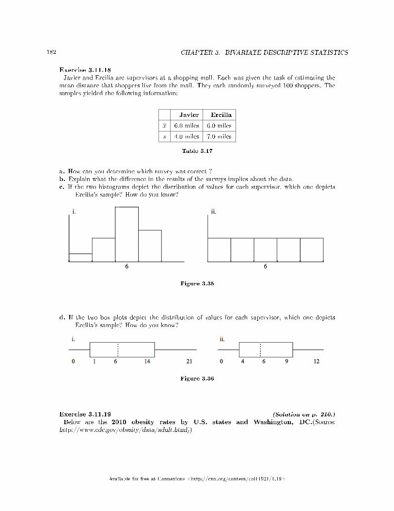
182 CHAPTER 3. BIVARIATE DESCRIPTIVE STATISTICS
Exercise 3.11.18Javier and Ercilia are supervisors at a shopping mall. Each was given the task of estimating the
mean distance that shoppers live from the mall. They each randomly surveyed 100 shoppers. Thesamples yielded the following information:
Javier Ercilla
x 6.0 miles 6.0 miles
s 4.0 miles 7.0 miles
Table 3.17
a. How can you determine which survey was correct ?b. Explain what the di�erence in the results of the surveys implies about the data.c. If the two histograms depict the distribution of values for each supervisor, which one depicts
Ercilia's sample? How do you know?
Figure 3.35
d. If the two box plots depict the distribution of values for each supervisor, which one depictsErcilia's sample? How do you know?
Figure 3.36
Exercise 3.11.19 (Solution on p. 210.)
Below are the 2010 obesity rates by U.S. states and Washington, DC.(Source:http://www.cdc.gov/obesity/data/adult.html))
Available for free at Connexions <http://cnx.org/content/col11521/1.19>
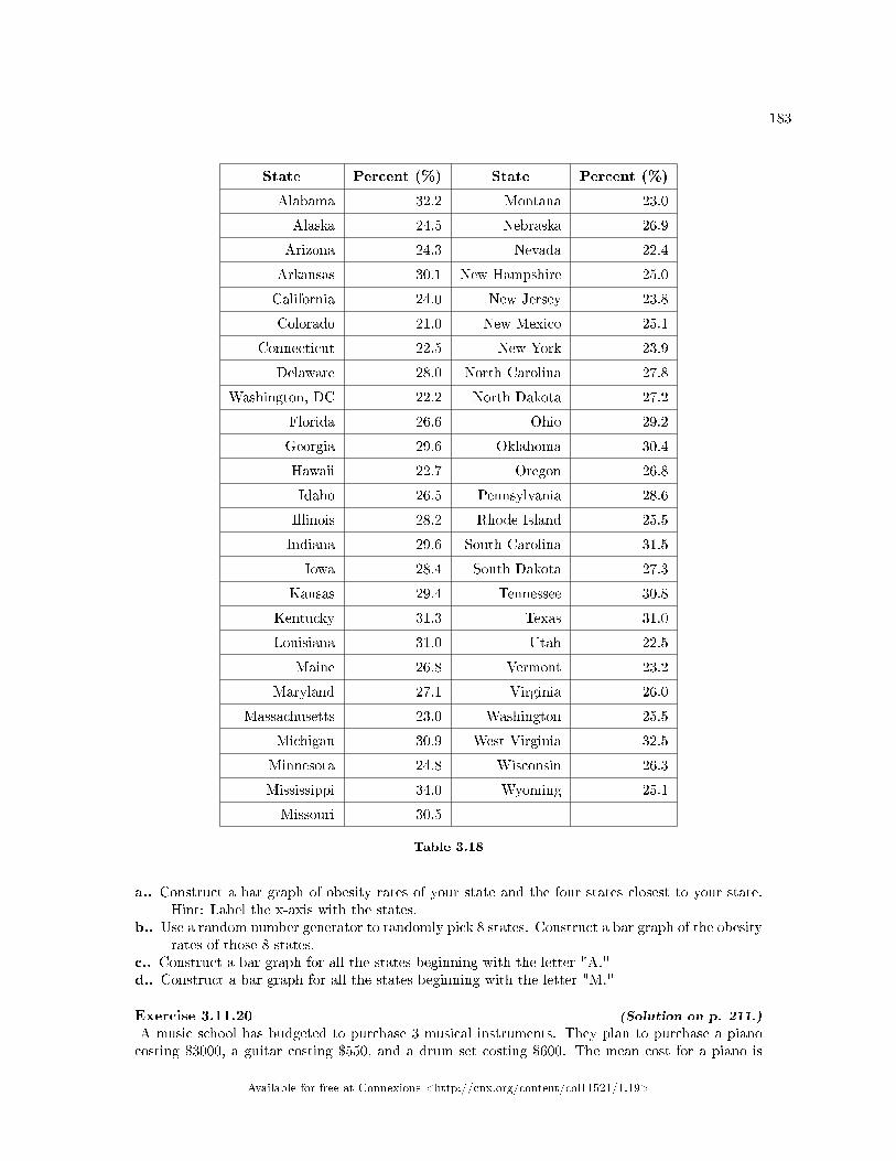
183
State Percent (%) State Percent (%)
Alabama 32.2 Montana 23.0
Alaska 24.5 Nebraska 26.9
Arizona 24.3 Nevada 22.4
Arkansas 30.1 New Hampshire 25.0
California 24.0 New Jersey 23.8
Colorado 21.0 New Mexico 25.1
Connecticut 22.5 New York 23.9
Delaware 28.0 North Carolina 27.8
Washington, DC 22.2 North Dakota 27.2
Florida 26.6 Ohio 29.2
Georgia 29.6 Oklahoma 30.4
Hawaii 22.7 Oregon 26.8
Idaho 26.5 Pennsylvania 28.6
Illinois 28.2 Rhode Island 25.5
Indiana 29.6 South Carolina 31.5
Iowa 28.4 South Dakota 27.3
Kansas 29.4 Tennessee 30.8
Kentucky 31.3 Texas 31.0
Louisiana 31.0 Utah 22.5
Maine 26.8 Vermont 23.2
Maryland 27.1 Virginia 26.0
Massachusetts 23.0 Washington 25.5
Michigan 30.9 West Virginia 32.5
Minnesota 24.8 Wisconsin 26.3
Mississippi 34.0 Wyoming 25.1
Missouri 30.5
Table 3.18
a.. Construct a bar graph of obesity rates of your state and the four states closest to your state.Hint: Label the x-axis with the states.
b.. Use a random number generator to randomly pick 8 states. Construct a bar graph of the obesityrates of those 8 states.
c.. Construct a bar graph for all the states beginning with the letter "A."d.. Construct a bar graph for all the states beginning with the letter "M."
Exercise 3.11.20 (Solution on p. 211.)
A music school has budgeted to purchase 3 musical instruments. They plan to purchase a pianocosting $3000, a guitar costing $550, and a drum set costing $600. The mean cost for a piano is
Available for free at Connexions <http://cnx.org/content/col11521/1.19>
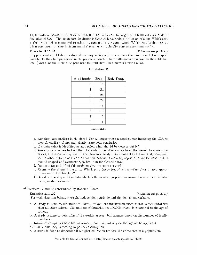
184 CHAPTER 3. BIVARIATE DESCRIPTIVE STATISTICS
$4,000 with a standard deviation of $2,500. The mean cost for a guitar is $500 with a standarddeviation of $200. The mean cost for drums is $700 with a standard deviation of $100. Which costis the lowest, when compared to other instruments of the same type? Which cost is the highestwhen compared to other instruments of the same type. Justify your answer numerically.
Exercise 3.11.21 (Solution on p. 211.)
Suppose that a publisher conducted a survey asking adult consumers the number of �ction paper-back books they had purchased in the previous month. The results are summarized in the table be-low. (Note that this is the data presented for publisher B in homework exercise 13).
Publisher B
# of books Freq. Rel. Freq.
0 18
1 24
2 24
3 22
4 15
5 10
7 5
9 1
Table 3.19
a. Are there any outliers in the data? Use an appropriate numerical test involving the IQR toidentify outliers, if any, and clearly state your conclusion.
b. If a data value is identi�ed as an outlier, what should be done about it?c. Are any data values further than 2 standard deviations away from the mean? In some situ-
ations, statisticians may use this criteria to identify data values that are unusual, comparedto the other data values. (Note that this criteria is most appropriate to use for data that ismound-shaped and symmetric, rather than for skewed data.)
d. Do parts (a) and (c) of this problem give the same answer?e. Examine the shape of the data. Which part, (a) or (c), of this question gives a more appro-
priate result for this data?f. Based on the shape of the data which is the most appropriate measure of center for this data:mean, median or mode?
**Exercises 17 and 18 contributed by Roberta Bloom
Exercise 3.11.22 (Solution on p. 212.)
For each situation below, state the independent variable and the dependent variable.
a. A study is done to determine if elderly drivers are involved in more motor vehicle fatalitiesthan all other drivers. The number of fatalities per 100,000 drivers is compared to the age ofdrivers.
b. A study is done to determine if the weekly grocery bill changes based on the number of familymembers.
c. Insurance companies base life insurance premiums partially on the age of the applicant.d. Utility bills vary according to power consumption.e. A study is done to determine if a higher education reduces the crime rate in a population.
Available for free at Connexions <http://cnx.org/content/col11521/1.19>
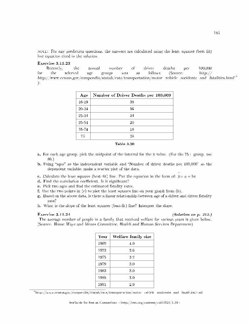
185
note: For any prediction questions, the answers are calculated using the least squares (best �t)line equation cited in the solution.
Exercise 3.11.23Recently, the annual number of driver deaths per 100,000
for the selected age groups was as follows (Source: http://http://www.census.gov/compendia/statab/cats/transportation/motor_vehicle_accidents_and_fatalities.html12
):
Age Number of Driver Deaths per 100,000
16-19 38
20-24 36
25-34 24
35-54 20
55-74 18
75+ 28
Table 3.20
a. For each age group, pick the midpoint of the interval for the x value. (For the 75+ group, use80.)
b. Using �ages� as the independent variable and �Number of driver deaths per 100,000� as thedependent variable, make a scatter plot of the data.
c. Calculate the least squares (best��t) line. Put the equation in the form of:^y= a+ bx
d. Find the correlation coe�cient. Is it signi�cant?e. Pick two ages and �nd the estimated fatality rates.f. Use the two points in (e) to plot the least squares line on your graph from (b).g. Based on the above data, is there a linear relationship between age of a driver and driver fatality
rate?h. What is the slope of the least squares (best-�t) line? Interpret the slope.
Exercise 3.11.24 (Solution on p. 212.)
The average number of people in a family that received welfare for various years is given below.(Source: House Ways and Means Committee, Health and Human Services Department)
Year Welfare family size
1969 4.0
1973 3.6
1975 3.2
1979 3.0
1983 3.0
1988 3.0
1991 2.9
12http://www.census.gov/compendia/statab/cats/transportation/motor_vehicle_accidents_and_fatalities.html
Available for free at Connexions <http://cnx.org/content/col11521/1.19>
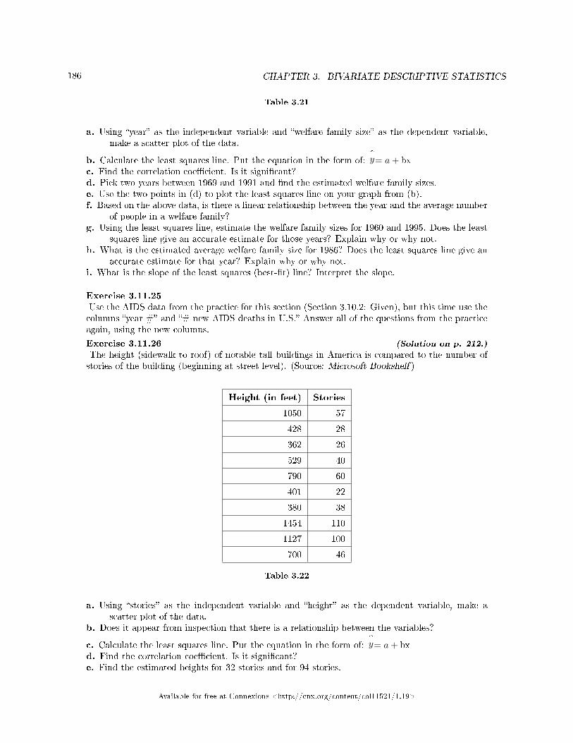
186 CHAPTER 3. BIVARIATE DESCRIPTIVE STATISTICS
Table 3.21
a. Using �year� as the independent variable and �welfare family size� as the dependent variable,make a scatter plot of the data.
b. Calculate the least squares line. Put the equation in the form of:^y= a+ bx
c. Find the correlation coe�cient. Is it signi�cant?d. Pick two years between 1969 and 1991 and �nd the estimated welfare family sizes.e. Use the two points in (d) to plot the least squares line on your graph from (b).f. Based on the above data, is there a linear relationship between the year and the average number
of people in a welfare family?g. Using the least squares line, estimate the welfare family sizes for 1960 and 1995. Does the least
squares line give an accurate estimate for those years? Explain why or why not.h. What is the estimated average welfare family size for 1986? Does the least squares line give an
accurate estimate for that year? Explain why or why not.i. What is the slope of the least squares (best-�t) line? Interpret the slope.
Exercise 3.11.25Use the AIDS data from the practice for this section (Section 3.10.2: Given), but this time use thecolumns �year #� and �# new AIDS deaths in U.S.� Answer all of the questions from the practiceagain, using the new columns.
Exercise 3.11.26 (Solution on p. 212.)
The height (sidewalk to roof) of notable tall buildings in America is compared to the number ofstories of the building (beginning at street level). (Source: Microsoft Bookshelf )
Height (in feet) Stories
1050 57
428 28
362 26
529 40
790 60
401 22
380 38
1454 110
1127 100
700 46
Table 3.22
a. Using �stories� as the independent variable and �height� as the dependent variable, make ascatter plot of the data.
b. Does it appear from inspection that there is a relationship between the variables?
c. Calculate the least squares line. Put the equation in the form of:^y= a+ bx
d. Find the correlation coe�cient. Is it signi�cant?e. Find the estimated heights for 32 stories and for 94 stories.
Available for free at Connexions <http://cnx.org/content/col11521/1.19>
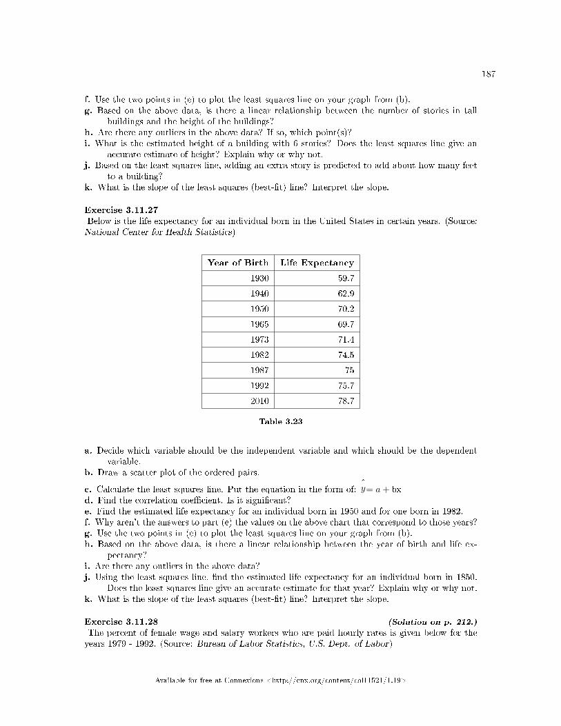
187
f. Use the two points in (e) to plot the least squares line on your graph from (b).g. Based on the above data, is there a linear relationship between the number of stories in tall
buildings and the height of the buildings?h. Are there any outliers in the above data? If so, which point(s)?i. What is the estimated height of a building with 6 stories? Does the least squares line give an
accurate estimate of height? Explain why or why not.j. Based on the least squares line, adding an extra story is predicted to add about how many feet
to a building?k. What is the slope of the least squares (best-�t) line? Interpret the slope.
Exercise 3.11.27Below is the life expectancy for an individual born in the United States in certain years. (Source:National Center for Health Statistics)
Year of Birth Life Expectancy
1930 59.7
1940 62.9
1950 70.2
1965 69.7
1973 71.4
1982 74.5
1987 75
1992 75.7
2010 78.7
Table 3.23
a. Decide which variable should be the independent variable and which should be the dependentvariable.
b. Draw a scatter plot of the ordered pairs.
c. Calculate the least squares line. Put the equation in the form of:^y= a+ bx
d. Find the correlation coe�cient. Is it signi�cant?e. Find the estimated life expectancy for an individual born in 1950 and for one born in 1982.f. Why aren't the answers to part (e) the values on the above chart that correspond to those years?g. Use the two points in (e) to plot the least squares line on your graph from (b).h. Based on the above data, is there a linear relationship between the year of birth and life ex-
pectancy?i. Are there any outliers in the above data?j. Using the least squares line, �nd the estimated life expectancy for an individual born in 1850.
Does the least squares line give an accurate estimate for that year? Explain why or why not.k. What is the slope of the least squares (best-�t) line? Interpret the slope.
Exercise 3.11.28 (Solution on p. 212.)
The percent of female wage and salary workers who are paid hourly rates is given below for theyears 1979 - 1992. (Source: Bureau of Labor Statistics, U.S. Dept. of Labor)
Available for free at Connexions <http://cnx.org/content/col11521/1.19>
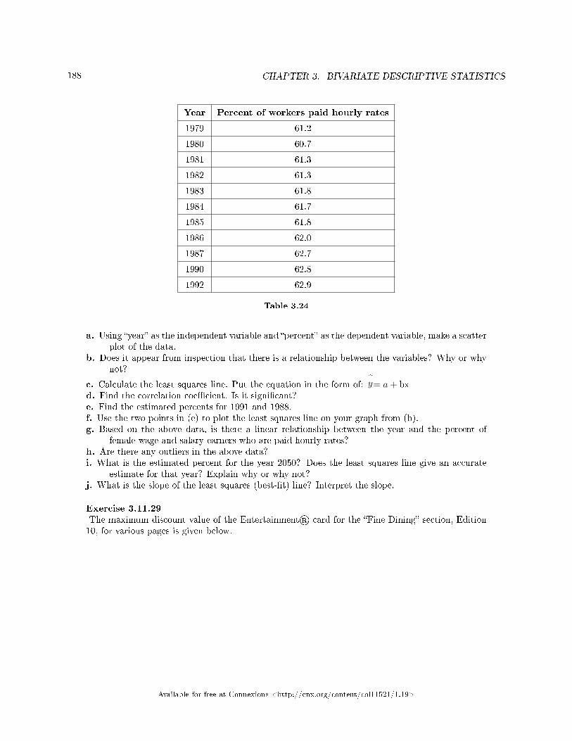
188 CHAPTER 3. BIVARIATE DESCRIPTIVE STATISTICS
Year Percent of workers paid hourly rates
1979 61.2
1980 60.7
1981 61.3
1982 61.3
1983 61.8
1984 61.7
1985 61.8
1986 62.0
1987 62.7
1990 62.8
1992 62.9
Table 3.24
a. Using �year� as the independent variable and �percent� as the dependent variable, make a scatterplot of the data.
b. Does it appear from inspection that there is a relationship between the variables? Why or whynot?
c. Calculate the least squares line. Put the equation in the form of:^y= a+ bx
d. Find the correlation coe�cient. Is it signi�cant?e. Find the estimated percents for 1991 and 1988.f. Use the two points in (e) to plot the least squares line on your graph from (b).g. Based on the above data, is there a linear relationship between the year and the percent of
female wage and salary earners who are paid hourly rates?h. Are there any outliers in the above data?i. What is the estimated percent for the year 2050? Does the least squares line give an accurate
estimate for that year? Explain why or why not?j. What is the slope of the least squares (best-�t) line? Interpret the slope.
Exercise 3.11.29The maximum discount value of the Entertainment® card for the �Fine Dining� section, Edition10, for various pages is given below.
Available for free at Connexions <http://cnx.org/content/col11521/1.19>
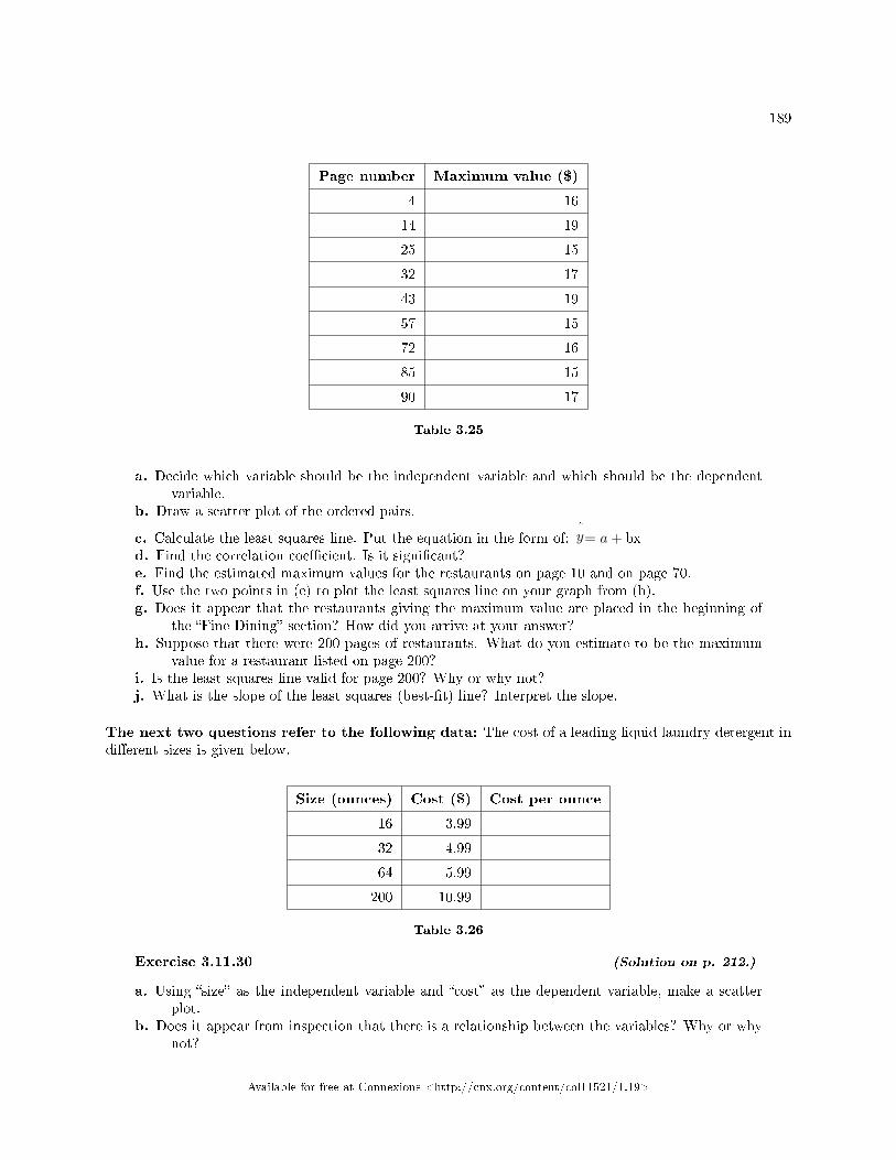
189
Page number Maximum value ($)
4 16
14 19
25 15
32 17
43 19
57 15
72 16
85 15
90 17
Table 3.25
a. Decide which variable should be the independent variable and which should be the dependentvariable.
b. Draw a scatter plot of the ordered pairs.
c. Calculate the least squares line. Put the equation in the form of:^y= a+ bx
d. Find the correlation coe�cient. Is it signi�cant?e. Find the estimated maximum values for the restaurants on page 10 and on page 70.f. Use the two points in (e) to plot the least squares line on your graph from (b).g. Does it appear that the restaurants giving the maximum value are placed in the beginning of
the �Fine Dining� section? How did you arrive at your answer?h. Suppose that there were 200 pages of restaurants. What do you estimate to be the maximum
value for a restaurant listed on page 200?i. Is the least squares line valid for page 200? Why or why not?j. What is the slope of the least squares (best-�t) line? Interpret the slope.
The next two questions refer to the following data: The cost of a leading liquid laundry detergent indi�erent sizes is given below.
Size (ounces) Cost ($) Cost per ounce
16 3.99
32 4.99
64 5.99
200 10.99
Table 3.26
Exercise 3.11.30 (Solution on p. 212.)
a. Using �size� as the independent variable and �cost� as the dependent variable, make a scatterplot.
b. Does it appear from inspection that there is a relationship between the variables? Why or whynot?
Available for free at Connexions <http://cnx.org/content/col11521/1.19>
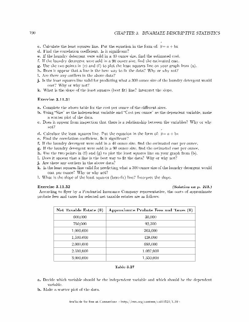
190 CHAPTER 3. BIVARIATE DESCRIPTIVE STATISTICS
c. Calculate the least squares line. Put the equation in the form of:^y= a+ bx
d. Find the correlation coe�cient. Is it signi�cant?e. If the laundry detergent were sold in a 40 ounce size, �nd the estimated cost.f. If the laundry detergent were sold in a 90 ounce size, �nd the estimated cost.g. Use the two points in (e) and (f) to plot the least squares line on your graph from (a).h. Does it appear that a line is the best way to �t the data? Why or why not?i. Are there any outliers in the above data?j. Is the least squares line valid for predicting what a 300 ounce size of the laundry detergent would
cost? Why or why not?k. What is the slope of the least squares (best-�t) line? Interpret the slope.
Exercise 3.11.31
a. Complete the above table for the cost per ounce of the di�erent sizes.b. Using �Size� as the independent variable and �Cost per ounce� as the dependent variable, make
a scatter plot of the data.c. Does it appear from inspection that there is a relationship between the variables? Why or why
not?
d. Calculate the least squares line. Put the equation in the form of:^y= a+ bx
e. Find the correlation coe�cient. Is it signi�cant?f. If the laundry detergent were sold in a 40 ounce size, �nd the estimated cost per ounce.g. If the laundry detergent were sold in a 90 ounce size, �nd the estimated cost per ounce.h. Use the two points in (f) and (g) to plot the least squares line on your graph from (b).i. Does it appear that a line is the best way to �t the data? Why or why not?j. Are there any outliers in the above data?k. Is the least squares line valid for predicting what a 300 ounce size of the laundry detergent would
cost per ounce? Why or why not?l. What is the slope of the least squares (best-�t) line? Interpret the slope.
Exercise 3.11.32 (Solution on p. 213.)
According to �yer by a Prudential Insurance Company representative, the costs of approximateprobate fees and taxes for selected net taxable estates are as follows:
Net Taxable Estate ($) Approximate Probate Fees and Taxes ($)
600,000 30,000
750,000 92,500
1,000,000 203,000
1,500,000 438,000
2,000,000 688,000
2,500,000 1,037,000
3,000,000 1,350,000
Table 3.27
a. Decide which variable should be the independent variable and which should be the dependentvariable.
b. Make a scatter plot of the data.
Available for free at Connexions <http://cnx.org/content/col11521/1.19>
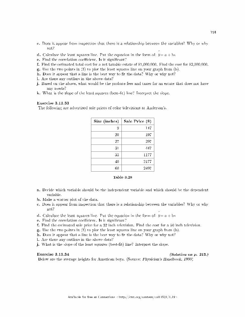
191
c. Does it appear from inspection that there is a relationship between the variables? Why or whynot?
d. Calculate the least squares line. Put the equation in the form of:^y= a+ bx
e. Find the correlation coe�cient. Is it signi�cant?f. Find the estimated total cost for a net taxable estate of $1,000,000. Find the cost for $2,500,000.g. Use the two points in (f) to plot the least squares line on your graph from (b).h. Does it appear that a line is the best way to �t the data? Why or why not?i. Are there any outliers in the above data?j. Based on the above, what would be the probate fees and taxes for an estate that does not have
any assets?k. What is the slope of the least squares (best-�t) line? Interpret the slope.
Exercise 3.11.33The following are advertised sale prices of color televisions at Anderson's.
Size (inches) Sale Price ($)
9 147
20 197
27 297
31 447
35 1177
40 2177
60 2497
Table 3.28
a. Decide which variable should be the independent variable and which should be the dependentvariable.
b. Make a scatter plot of the data.c. Does it appear from inspection that there is a relationship between the variables? Why or why
not?
d. Calculate the least squares line. Put the equation in the form of:^y= a+ bx
e. Find the correlation coe�cient. Is it signi�cant?f. Find the estimated sale price for a 32 inch television. Find the cost for a 50 inch television.g. Use the two points in (f) to plot the least squares line on your graph from (b).h. Does it appear that a line is the best way to �t the data? Why or why not?i. Are there any outliers in the above data?j. What is the slope of the least squares (best-�t) line? Interpret the slope.
Exercise 3.11.34 (Solution on p. 213.)
Below are the average heights for American boys. (Source: Physician's Handbook, 1990)
Available for free at Connexions <http://cnx.org/content/col11521/1.19>
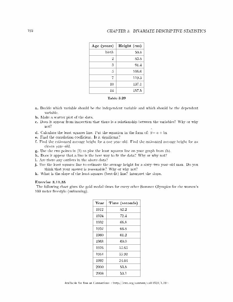
192 CHAPTER 3. BIVARIATE DESCRIPTIVE STATISTICS
Age (years) Height (cm)
birth 50.8
2 83.8
3 91.4
5 106.6
7 119.3
10 137.1
14 157.5
Table 3.29
a. Decide which variable should be the independent variable and which should be the dependentvariable.
b. Make a scatter plot of the data.c. Does it appear from inspection that there is a relationship between the variables? Why or why
not?
d. Calculate the least squares line. Put the equation in the form of:^y= a+ bx
e. Find the correlation coe�cient. Is it signi�cant?f. Find the estimated average height for a one year�old. Find the estimated average height for an
eleven year�old.g. Use the two points in (f) to plot the least squares line on your graph from (b).h. Does it appear that a line is the best way to �t the data? Why or why not?i. Are there any outliers in the above data?j. Use the least squares line to estimate the average height for a sixty�two year�old man. Do you
think that your answer is reasonable? Why or why not?k. What is the slope of the least squares (best-�t) line? Interpret the slope.
Exercise 3.11.35The following chart gives the gold medal times for every other Summer Olympics for the women's100 meter freestyle (swimming).
Year Time (seconds)
1912 82.2
1924 72.4
1932 66.8
1952 66.8
1960 61.2
1968 60.0
1976 55.65
1984 55.92
1992 54.64
2000 53.8
2008 53.1
Available for free at Connexions <http://cnx.org/content/col11521/1.19>
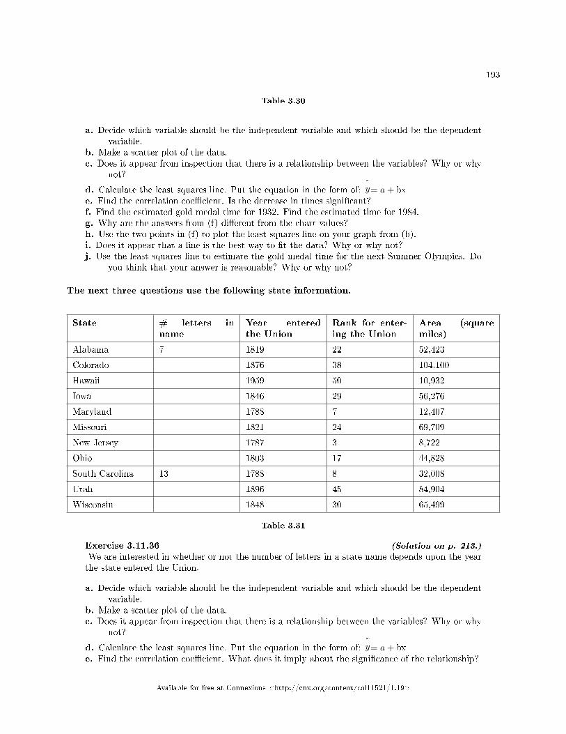
193
Table 3.30
a. Decide which variable should be the independent variable and which should be the dependentvariable.
b. Make a scatter plot of the data.c. Does it appear from inspection that there is a relationship between the variables? Why or why
not?
d. Calculate the least squares line. Put the equation in the form of:^y= a+ bx
e. Find the correlation coe�cient. Is the decrease in times signi�cant?f. Find the estimated gold medal time for 1932. Find the estimated time for 1984.g. Why are the answers from (f) di�erent from the chart values?h. Use the two points in (f) to plot the least squares line on your graph from (b).i. Does it appear that a line is the best way to �t the data? Why or why not?j. Use the least squares line to estimate the gold medal time for the next Summer Olympics. Do
you think that your answer is reasonable? Why or why not?
The next three questions use the following state information.
State # letters inname
Year enteredthe Union
Rank for enter-ing the Union
Area (squaremiles)
Alabama 7 1819 22 52,423
Colorado 1876 38 104,100
Hawaii 1959 50 10,932
Iowa 1846 29 56,276
Maryland 1788 7 12,407
Missouri 1821 24 69,709
New Jersey 1787 3 8,722
Ohio 1803 17 44,828
South Carolina 13 1788 8 32,008
Utah 1896 45 84,904
Wisconsin 1848 30 65,499
Table 3.31
Exercise 3.11.36 (Solution on p. 213.)
We are interested in whether or not the number of letters in a state name depends upon the yearthe state entered the Union.
a. Decide which variable should be the independent variable and which should be the dependentvariable.
b. Make a scatter plot of the data.c. Does it appear from inspection that there is a relationship between the variables? Why or why
not?
d. Calculate the least squares line. Put the equation in the form of:^y= a+ bx
e. Find the correlation coe�cient. What does it imply about the signi�cance of the relationship?
Available for free at Connexions <http://cnx.org/content/col11521/1.19>
194 CHAPTER 3. BIVARIATE DESCRIPTIVE STATISTICS
f. Find the estimated number of letters (to the nearest integer) a state would have if it enteredthe Union in 1900. Find the estimated number of letters a state would have if it entered theUnion in 1940.
g. Use the two points in (f) to plot the least squares line on your graph from (b).h. Does it appear that a line is the best way to �t the data? Why or why not?i. Use the least squares line to estimate the number of letters a new state that enters the Union
this year would have. Can the least squares line be used to predict it? Why or why not?
Exercise 3.11.37We are interested in whether there is a relationship between the ranking of a state and the area ofthe state.
a. Let rank be the independent variable and area be the dependent variable.b. What do you think the scatter plot will look like? Make a scatter plot of the data.c. Does it appear from inspection that there is a relationship between the variables? Why or why
not?
d. Calculate the least squares line. Put the equation in the form of:^y= a+ bx
e. Find the correlation coe�cient. What does it imply about the signi�cance of the relationship?f. Find the estimated areas for Alabama and for Colorado. Are they close to the actual areas?g. Use the two points in (f) to plot the least squares line on your graph from (b).h. Does it appear that a line is the best way to �t the data? Why or why not?i. Are there any outliers?j. Use the least squares line to estimate the area of a new state that enters the Union. Can the
least squares line be used to predict it? Why or why not?k. Delete �Hawaii� and substitute �Alaska� for it. Alaska is the fortieth state with an area of 656,424
square miles.l. Calculate the new least squares line.m. Find the estimated area for Alabama. Is it closer to the actual area with this new least squares
line or with the previous one that included Hawaii? Why do you think that's the case?n. Do you think that, in general, newer states are larger than the original states?
Exercise 3.11.38 (Solution on p. 213.)
We are interested in whether there is a relationship between the rank of a state and the year itentered the Union.
a. Let year be the independent variable and rank be the dependent variable.b. What do you think the scatter plot will look like? Make a scatter plot of the data.c. Why must the relationship be positive between the variables?
d. Calculate the least squares line. Put the equation in the form of:^y= a+ bx
e. Find the correlation coe�cient. What does it imply about the signi�cance of the relationship?f. Let's say a �fty-�rst state entered the union. Based upon the least squares line, when should
that have occurred?g. Using the least squares line, how many states do we currently have?h. Why isn't the least squares line a good estimator for this year?
Exercise 3.11.39Below are the percents of the U.S. labor force (excluding self-employed and unemployed ) that aremembers of a union. We are interested in whether the decrease is signi�cant. (Source: Bureau ofLabor Statistics, U.S. Dept. of Labor)
Available for free at Connexions <http://cnx.org/content/col11521/1.19>
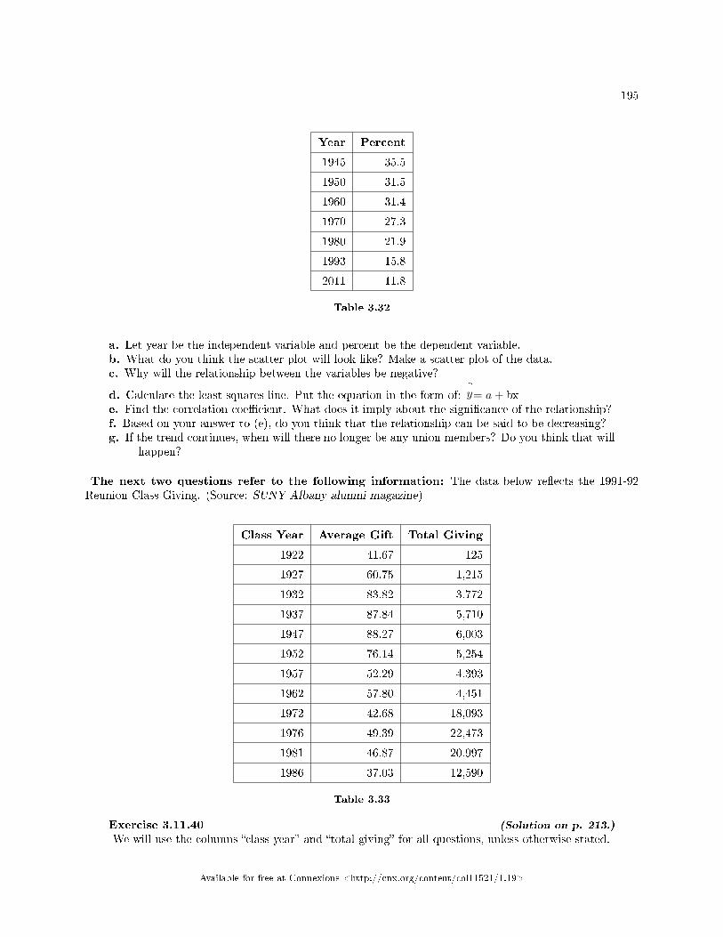
195
Year Percent
1945 35.5
1950 31.5
1960 31.4
1970 27.3
1980 21.9
1993 15.8
2011 11.8
Table 3.32
a. Let year be the independent variable and percent be the dependent variable.b. What do you think the scatter plot will look like? Make a scatter plot of the data.c. Why will the relationship between the variables be negative?
d. Calculate the least squares line. Put the equation in the form of:^y= a+ bx
e. Find the correlation coe�cient. What does it imply about the signi�cance of the relationship?f. Based on your answer to (e), do you think that the relationship can be said to be decreasing?g. If the trend continues, when will there no longer be any union members? Do you think that will
happen?
The next two questions refer to the following information: The data below re�ects the 1991-92Reunion Class Giving. (Source: SUNY Albany alumni magazine)
Class Year Average Gift Total Giving
1922 41.67 125
1927 60.75 1,215
1932 83.82 3,772
1937 87.84 5,710
1947 88.27 6,003
1952 76.14 5,254
1957 52.29 4,393
1962 57.80 4,451
1972 42.68 18,093
1976 49.39 22,473
1981 46.87 20,997
1986 37.03 12,590
Table 3.33
Exercise 3.11.40 (Solution on p. 213.)
We will use the columns �class year� and �total giving� for all questions, unless otherwise stated.
Available for free at Connexions <http://cnx.org/content/col11521/1.19>
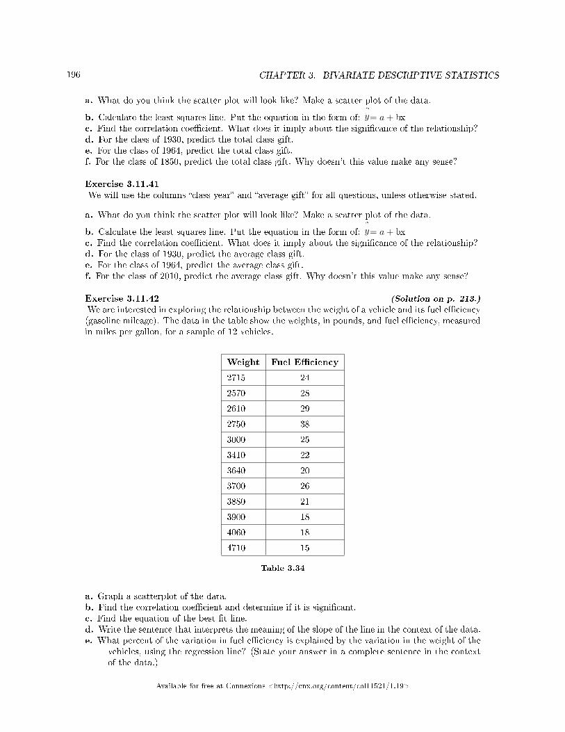
196 CHAPTER 3. BIVARIATE DESCRIPTIVE STATISTICS
a. What do you think the scatter plot will look like? Make a scatter plot of the data.
b. Calculate the least squares line. Put the equation in the form of:^y= a+ bx
c. Find the correlation coe�cient. What does it imply about the signi�cance of the relationship?d. For the class of 1930, predict the total class gift.e. For the class of 1964, predict the total class gift.f. For the class of 1850, predict the total class gift. Why doesn't this value make any sense?
Exercise 3.11.41We will use the columns �class year� and �average gift� for all questions, unless otherwise stated.
a. What do you think the scatter plot will look like? Make a scatter plot of the data.
b. Calculate the least squares line. Put the equation in the form of:^y= a+ bx
c. Find the correlation coe�cient. What does it imply about the signi�cance of the relationship?d. For the class of 1930, predict the average class gift.e. For the class of 1964, predict the average class gift.f. For the class of 2010, predict the average class gift. Why doesn't this value make any sense?
Exercise 3.11.42 (Solution on p. 213.)
We are interested in exploring the relationship between the weight of a vehicle and its fuel e�ciency(gasoline mileage). The data in the table show the weights, in pounds, and fuel e�ciency, measuredin miles per gallon, for a sample of 12 vehicles.
Weight Fuel E�ciency
2715 24
2570 28
2610 29
2750 38
3000 25
3410 22
3640 20
3700 26
3880 21
3900 18
4060 18
4710 15
Table 3.34
a. Graph a scatterplot of the data.b. Find the correlation coe�cient and determine if it is signi�cant.c. Find the equation of the best �t line.d. Write the sentence that interprets the meaning of the slope of the line in the context of the data.e. What percent of the variation in fuel e�ciency is explained by the variation in the weight of the
vehicles, using the regression line? (State your answer in a complete sentence in the contextof the data.)
Available for free at Connexions <http://cnx.org/content/col11521/1.19>
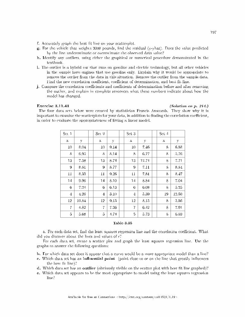
197
f. Accurately graph the best �t line on your scatterplot.g. For the vehicle that weights 3000 pounds, �nd the residual (y-yhat). Does the value predicted
by the line underestimate or overestimate the observed data value?h. Identify any outliers, using either the graphical or numerical procedure demonstrated in the
textbook.i. The outlier is a hybrid car that runs on gasoline and electric technology, but all other vehicles
in the sample have engines that use gasoline only. Explain why it would be appropriate toremove the outlier from the data in this situation. Remove the outlier from the sample data.Find the new correlation coe�cient, coe�cient of determination, and best �t line.
j. Compare the correlation coe�cients and coe�cients of determination before and after removingthe outlier, and explain in complete sentences what these numbers indicate about how themodel has changed.
Exercise 3.11.43 (Solution on p. 214.)
The four data sets below were created by statistician Francis Anscomb. They show why it isimportant to examine the scatterplots for your data, in addition to �nding the correlation coe�cient,in order to evaluate the appropriateness of �tting a linear model.
Set 1 Set 2 Set 3 Set 4
x y x y x y x y
10 8.04 10 9.14 10 7.46 8 6.58
8 6.95 8 8.14 8 6.77 8 5.76
13 7.58 13 8.74 13 12.74 8 7.71
9 8.81 9 8.77 9 7.11 8 8.84
11 8.33 11 9.26 11 7.81 8 8.47
14 9.96 14 8.10 14 8.84 8 7.04
6 7.24 6 6.13 6 6.08 8 5.25
4 4.26 4 3.10 4 5.39 19 12.50
12 10.84 12 9.13 12 8.15 8 5.56
7 4.82 7 7.26 7 6.42 8 7.91
5 5.68 5 4.74 5 5.73 8 6.89
Table 3.35
a. For each data set, �nd the least squares regression line and the correlation coe�cient. Whatdid you discover about the lines and values of r?
For each data set, create a scatter plot and graph the least squares regression line. Use thegraphs to answer the following questions:
b. For which data set does it appear that a curve would be a more appropriate model than a line?c. Which data set has an in�uential point (point close to or on the line that greatly in�uences
the best �t line)?d. Which data set has an outlier (obviously visible on the scatter plot with best �t line graphed)?e. Which data set appears to be the most appropriate to model using the least squares regression
line?
Available for free at Connexions <http://cnx.org/content/col11521/1.19>
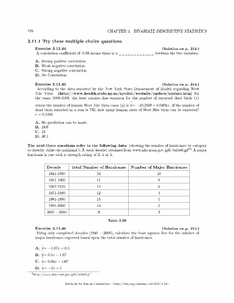
198 CHAPTER 3. BIVARIATE DESCRIPTIVE STATISTICS
3.11.1 Try these multiple choice questions
Exercise 3.11.44 (Solution on p. 214.)
A correlation coe�cient of -0.95 means there is a ____________ between the two variables.
A. Strong positive correlationB. Weak negative correlationC. Strong negative correlationD. No Correlation
Exercise 3.11.45 (Solution on p. 214.)
According to the data reported by the New York State Department of Health regarding WestNile Virus (http://www.health.state.ny.us/nysdoh/westnile/update/update.htm) forthe years 2000-2008, the least squares line equation for the number of reported dead birds (x)
versus the number of human West Nile virus cases (y) is^y= −10.2638+ 0.0491x. If the number of
dead birds reported in a year is 732, how many human cases of West Nile virus can be expected?r = 0.5490
A. No prediction can be made.B. 19.6C. 15D. 38.1
The next three questions refer to the following data: (showing the number of hurricanes by categoryto directly strike the mainland U.S. each decade) obtained from www.nhc.noaa.gov/gifs/table6.gif 13 A majorhurricane is one with a strength rating of 3, 4 or 5.
Decade Total Number of Hurricanes Number of Major Hurricanes
1941-1950 24 10
1951-1960 17 8
1961-1970 14 6
1971-1980 12 4
1981-1990 15 5
1991-2000 14 5
2001 � 2004 9 3
Table 3.36
Exercise 3.11.46 (Solution on p. 214.)
Using only completed decades (1941 � 2000), calculate the least squares line for the number ofmajor hurricanes expected based upon the total number of hurricanes.
A.^y= −1.67x+ 0.5
B.^y= 0.5x− 1.67
C.^y= 0.94x− 1.67
D.^y= −2x+ 1
13http://www.nhc.noaa.gov/gifs/table6.gif
Available for free at Connexions <http://cnx.org/content/col11521/1.19>
199
Exercise 3.11.47 (Solution on p. 214.)
The data for 2001-2004 show 9 hurricanes have hit the mainland United States. The line of best�t predicts 2.83 major hurricanes to hit mainland U.S. Can the least squares line be used to makethis prediction?
A. No, because 9 lies outside the independent variable valuesB. Yes, because, in fact, there have been 3 major hurricanes this decadeC. No, because 2.83 lies outside the dependent variable valuesD. Yes, because how else could we predict what is going to happen this decade.
**Exercises 42 and 43 contributed by Roberta Bloom
Available for free at Connexions <http://cnx.org/content/col11521/1.19>
200 CHAPTER 3. BIVARIATE DESCRIPTIVE STATISTICS
3.12 Bivariate Descriptive Statistics: Regression Lab I14
Class Time:Names:
3.12.1 Student Learning Outcomes:
• The student will calculate and construct the line of best �t between two variables.
3.12.2 Collect the Data
Use 8 members of your class for the sample. Collect bivariate data (distance an individual lives from school,the cost of supplies for the current term).
1. Complete the table.
Distance from school Cost of supplies this term
Table 3.37
2. Which variable should be the dependent variable and which should be the independent variable? Why?3. Graph �distance� vs. �cost.� Plot the points on the graph. Label both axes with words. Scale both
axes.
14This content is available online at <http://cnx.org/content/m46172/1.1/>.
Available for free at Connexions <http://cnx.org/content/col11521/1.19>
201
Figure 3.37
3.12.3 Analyze the Data
Enter your data into your calculator or computer. Write the linear equation below, rounding to 4 decimalplaces.
1. Calculate the following:
a. a =b. b=c. correlation =d. n =
e. equation:^y =
2. Supply an answer for the following senarios:
a. For a person who lives 8 miles from campus, predict the total cost of supplies this term:b. For a person who lives 80 miles from campus, predict the total cost of supplies this term:
3. Obtain the graph on your calculator or computer. Sketch the regression line below.
Available for free at Connexions <http://cnx.org/content/col11521/1.19>
202 CHAPTER 3. BIVARIATE DESCRIPTIVE STATISTICS
Figure 3.38
3.12.4 Discussion Questions
1. Answer each with 1-3 complete sentences.
a. Does the line seem to �t the data? Why?b. What does the correlation imply about the relationship between the distance and the cost?
2. Are there any outliers? If so, which point is an outlier?3. Should the outlier, if it exists, be removed? Why or why not?
Available for free at Connexions <http://cnx.org/content/col11521/1.19>
203
3.13 Bivariate Descriptive Statistics: Linear Regression and Corre-lation: Regression Lab II15
Class Time:Names:
3.13.1 Student Learning Outcomes:
• The student will calculate and construct the line of best �t between two variables.• The student will evaluate the relationship between two variables to determine if that relationship is
signi�cant.
3.13.2 Collect the Data
Survey 10 textbooks. Collect bivariate data (number of pages in a textbook, the cost of the textbook).
1. Complete the table.
Number of pages Cost of textbook
Table 3.38
2. Which variable should be the dependent variable and which should be the independent variable? Why?3. Graph �distance� vs. �cost.� Plot the points on the graph in "Analyze the Data". Label both axes
with words. Scale both axes.
3.13.3 Analyze the Data
Enter your data into your calculator or computer. Write the linear equation below, rounding to 4 decimalplaces.
1. Calculate the following:
a. a =b. b =c. correlation =d. n =e. equation: y =
15This content is available online at <http://cnx.org/content/m46201/1.1/>.
Available for free at Connexions <http://cnx.org/content/col11521/1.19>
204 CHAPTER 3. BIVARIATE DESCRIPTIVE STATISTICS
2. Supply an answer for the following senarios:
a. For a textbook with 400 pages, predict the cost:b. For a textbook with 600 pages, predict the cost:
3. Obtain the graph on your calculator or computer. Sketch the regression line below.
Figure 3.39
3.13.4 Discussion Questions
1. Answer each with 1-3 complete sentences.
a. Does the line seem to �t the data? Why?b. What does the correlation imply about the relationship between the number of pages and the cost?
2. Are there any outliers? If so, which point(s) is an outlier?3. Should the outlier, if it exists, be removed? Why or why not?
Available for free at Connexions <http://cnx.org/content/col11521/1.19>
205
3.14 Bivariate Descriptive Statistics: Linear Regression and Corre-lation: Regression Lab III16
Class Time:Names:
3.14.1 Student Learning Outcomes:
• The student will calculate and construct the line of best �t between two variables.• The student will evaluate the relationship between two variables to determine if that relationship is
signi�cant.
3.14.2 Collect the Data
Use the most recent April issue of Consumer Reports. It will give the total fuel e�ciency (in miles pergallon) and weight (in pounds) of new model cars with automatic transmissions. We will use this data todetermine the relationship, if any, between the fuel e�ciency of a car and its weight.
1. Which variable should be the independent variable and which should be the dependent variable?Explain your answer in one or two complete sentences.
2. Using your random number generator, randomly select 20 cars from the list and record their weightsand fuel e�ciency into the table below.
16This content is available online at <http://cnx.org/content/m46202/1.1/>.
Available for free at Connexions <http://cnx.org/content/col11521/1.19>
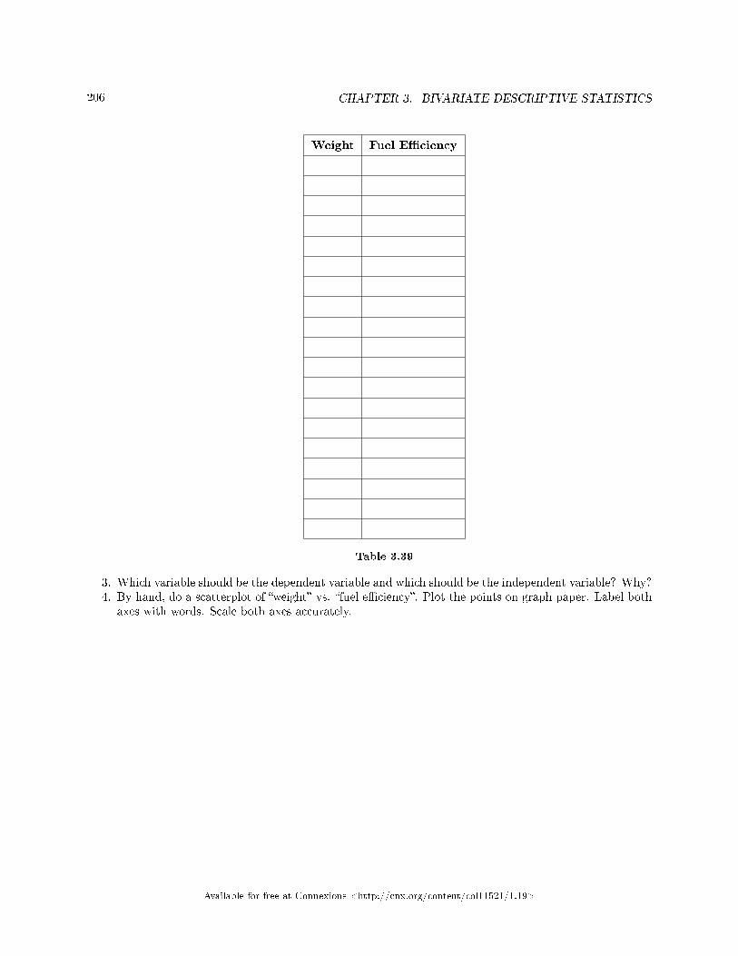
206 CHAPTER 3. BIVARIATE DESCRIPTIVE STATISTICS
Weight Fuel E�ciency
Table 3.39
3. Which variable should be the dependent variable and which should be the independent variable? Why?4. By hand, do a scatterplot of �weight� vs. �fuel e�ciency�. Plot the points on graph paper. Label both
axes with words. Scale both axes accurately.
Available for free at Connexions <http://cnx.org/content/col11521/1.19>
207
Figure 3.40
3.14.3 Analyze the Data
Enter your data into your calculator or computer. Write the linear equation below, rounding to 4 decimalplaces.
1. Calculate the following:
a. a =b. b =c. correlation =d. n =
e. equation:^y =
2. Obtain the graph of the regression line on your calculator. Sketch the regression line on the same axesas your scatterplot.
3.14.4 Discussion Questions
1. Is the correlation signi�cant? Explain how you determined this in complete sentences.
Available for free at Connexions <http://cnx.org/content/col11521/1.19>
208 CHAPTER 3. BIVARIATE DESCRIPTIVE STATISTICS
2. Is the relationship a positive one or a negative one? Explain how you can tell and what this means interms of weight and fuel e�ciency.
3. In one or two complete sentences, what is the practical interpretation of the slope of the least squaresline in terms of fuel e�ciency and weight?
4. For a car that weighs 4000 pounds, predict its fuel e�ciency. Include units.5. Can we predict the fuel e�ciency of a car that weighs 10000 pounds using the least squares line?
Explain why or why not.6. Questions. Answer each in 1 to 3 complete sentences.
a. Does the line seem to �t the data? Why or why not?b. What does the correlation imply about the relationship between fuel e�ciency and weight of a car?
Is this what you expected?
7. Are there any outliers? If so, which point is an outlier?
** This lab was designed and contributed by Diane Mathios.
Available for free at Connexions <http://cnx.org/content/col11521/1.19>
209
Solutions to Exercises in Chapter 3
Solution to Example 3.7, Problem 2 (p. 152)The x values in the data are between 65 and 75. 90 is outside of the domain of the observed x
values in the data (independent variable), so you cannot reliably predict the �nal exam score for thisstudent. (Even though it is possible to enter x into the equation and calculate a y value, you should not do so!)
To really understand how unreliable the prediction can be outside of the observed x values in thedata, make the substitution x = 90 into the equation.
^y= −173.51 + 4.83 (90) = 261.19
The �nal exam score is predicted to be 261.19. The largest the �nal exam score can be is 200.
note: The process of predicting inside of the observed x values in the data is called interpolation.The process of predicting outside of the observed x values in the data is called extrapolation.
Solutions to Linear Regression and Correlation: Practice
Solution to Exercise 3.10.2 (p. 170)
a. a = -3,448,225b. b = 1750c. corr. = 0.4526d. n = 22
Solution to Exercise 3.10.3 (p. 170)^y= -3,448,225 +1750xSolution to Exercise 3.10.4 (p. 170)
a. 25,525b. 34,275
Solution to Exercise 3.10.10 (p. 171)
a. -725
Solutions to Bivariate Descriptive Statistics: Homework
Solution to Exercise 3.11.1 (p. 172)Row percentages, and yes, there is a relationship between gender and the particular behaviors related toAIDS.Solution to Exercise 3.11.2 (p. 172)Column percentages and based on this chart there is a independent relationship between hair color and typeof hair.Solution to Exercise 3.11.3 (p. 172)Column percentages and based on the chart, there is a dependent relationship between shirt numbers andweight brackets.Solution to Exercise 3.11.4 (p. 173)Row percentages and yes there is a dependent relationship between age of suicide when looking at race andsex.
Available for free at Connexions <http://cnx.org/content/col11521/1.19>
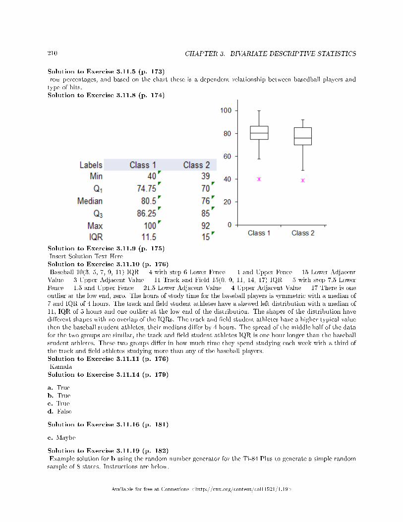
210 CHAPTER 3. BIVARIATE DESCRIPTIVE STATISTICS
Solution to Exercise 3.11.5 (p. 173)row percentages, and based on the chart these is a dependent relationship between basedball players andtype of hits.Solution to Exercise 3.11.8 (p. 174)
Solution to Exercise 3.11.9 (p. 175)Insert Solution Text HereSolution to Exercise 3.11.10 (p. 176)Baseball 10(3, 5, 7, 9, 11) IQR = 4 with step 6 Lower Fence = -1 and Upper Fence = 15 Lower AdjacentValue = 3 Upper Adjacent Value = 11 Track and Field 15(0, 9, 11, 14, 17) IQR = 5 with step 7.5 LowerFence = 1.5 and Upper Fence = 21.5 Lower Adjacent Value = 4 Upper Adjacent Value = 17 There is oneoutlier at the low end, zero. The hours of study time for the baseball players is symmetric with a median of7 and IQR of 4 hours. The track and �eld student athletes have a skewed left distribution with a median of11, IQR of 5 hours and one outlier at the low end of the distribution. The shapes of the distribution havedi�erent shapes with no overlap of the IQRs. The track and �eld student athletes have a higher typical valuethen the baseball student athletes, their medians di�er by 4 hours. The spread of the middle half of the datafor the two groups are similar, the track and �eld student athletes IQR is one hour longer than the baseballstudent athletes. These two groups di�er in how much time they spend studying each week with a third ofthe track and �eld athletes studying more than any of the baseball players.Solution to Exercise 3.11.11 (p. 176)KamalaSolution to Exercise 3.11.14 (p. 179)
a. Trueb. Truec. Trued. False
Solution to Exercise 3.11.16 (p. 181)
c. Maybe
Solution to Exercise 3.11.19 (p. 182)Example solution for b using the random number generator for the Ti-84 Plus to generate a simple randomsample of 8 states. Instructions are below.
Available for free at Connexions <http://cnx.org/content/col11521/1.19>
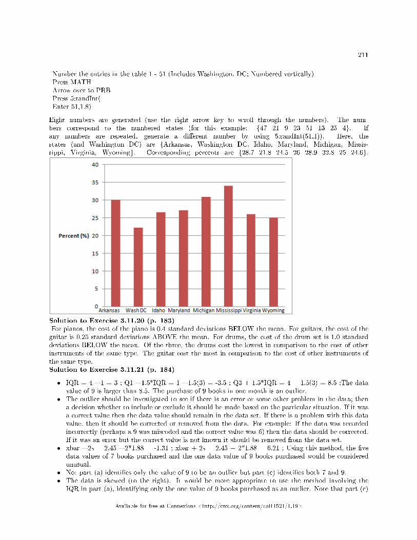
211
Number the entries in the table 1 - 51 (Includes Washington, DC; Numbered vertically)Press MATHArrow over to PRBPress 5:randInt(Enter 51,1,8)
Eight numbers are generated (use the right arrow key to scroll through the numbers). The num-bers correspond to the numbered states (for this example: {47 21 9 23 51 13 25 4}. Ifany numbers are repeated, generate a di�erent number by using 5:randInt(51,1)). Here, thestates (and Washington DC) are {Arkansas, Washington DC, Idaho, Maryland, Michigan, Missis-sippi, Virginia, Wyoming}. Corresponding percents are {28.7 21.8 24.5 26 28.9 32.8 25 24.6}.
Solution to Exercise 3.11.20 (p. 183)For pianos, the cost of the piano is 0.4 standard deviations BELOW the mean. For guitars, the cost of theguitar is 0.25 standard deviations ABOVE the mean. For drums, the cost of the drum set is 1.0 standarddeviations BELOW the mean. Of the three, the drums cost the lowest in comparison to the cost of otherinstruments of the same type. The guitar cost the most in comparison to the cost of other instruments ofthe same type.Solution to Exercise 3.11.21 (p. 184)
• IQR = 4 � 1 = 3 ; Q1 � 1.5*IQR = 1 � 1.5(3) = -3.5 ; Q3 + 1.5*IQR = 4 + 1.5(3) = 8.5 ;The datavalue of 9 is larger than 8.5. The purchase of 9 books in one month is an outlier.
• The outlier should be investigated to see if there is an error or some other problem in the data; thena decision whether to include or exclude it should be made based on the particular situation. If it wasa correct value then the data value should remain in the data set. If there is a problem with this datavalue, then it should be corrected or removed from the data. For example: If the data was recordedincorrectly (perhaps a 9 was miscoded and the correct value was 6) then the data should be corrected.If it was an error but the correct value is not known it should be removed from the data set.
• xbar � 2s = 2.45 � 2*1.88 = -1.31 ; xbar + 2s = 2.45 + 2*1.88 = 6.21 ; Using this method, the �vedata values of 7 books purchased and the one data value of 9 books purchased would be consideredunusual.
• No: part (a) identi�es only the value of 9 to be an outlier but part (c) identi�es both 7 and 9.• The data is skewed (to the right). It would be more appropriate to use the method involving the
IQR in part (a), identifying only the one value of 9 books purchased as an outlier. Note that part (c)
Available for free at Connexions <http://cnx.org/content/col11521/1.19>
212 CHAPTER 3. BIVARIATE DESCRIPTIVE STATISTICS
remarks that identifying unusual data values by using the criteria of being further than 2 standarddeviations away from the mean is most appropriate when the data are mound-shaped and symmetric.
• The data are skewed to the right. For skewed data it is more appropriate to use the median as ameasure of center.
Solution to Exercise 3.11.22 (p. 184)
a. Independent: Age; Dependent: Fatalitiesd. Independent: Power Consumption; Dependent: Utility
Solution to Exercise 3.11.24 (p. 185)
b.^y= 88.7206− 0.0432x
c. -0.8533, Yesg. Noh. 2.93, Yesi. slope = -0.0432. As the year increases by one, the welfare family size tends to decrease by 0.0432 people.
Solution to Exercise 3.11.26 (p. 186)
b. Yes
c.^y= 102.4287 + 11.7585x
d. 0.9436; yese. 478.70 feet; 1207.73 feetg. Yesh. Yes; (57, 1050)i. 172.98; Noj. 11.7585 feetk. slope = 11.7585. As the number of stories increases by one, the height of the building tends to increase
by 11.7585 feet.
Solution to Exercise 3.11.28 (p. 187)
b. Yes
c.^y= −266.8863 + 0.1656x
d. 0.9448; Yese. 62.8233; 62.3265h. yes; (1987, 62.7)i. 72.5937; Noj. slope = 0.1656. As the year increases by one, the percent of workers paid hourly rates tends to increase
by 0.1656.
Solution to Exercise 3.11.30 (p. 189)
b. Yes
c.^y= 3.5984 + 0.0371x
d. 0.9986; Yese. $5.08f. $6.93i. Noj. Not validk. slope = 0.0371. As the number of ounces increases by one, the cost of liquid detergent tends to increase
by $0.0371 or is predicted to increase by $0.0371 (about 4 cents).
Available for free at Connexions <http://cnx.org/content/col11521/1.19>
213
Solution to Exercise 3.11.32 (p. 190)
c. Yes
d.^y= −337, 424.6478 + 0.5463x
e. 0.9964; Yesf. $208,875.35; $1,028,325.35h. Yesi. Nok. slope = 0.5463. As the net taxable estate increases by one dollar, the approximate probate fees and taxes
tend to increase by 0.5463 dollars (about 55 cents).
Solution to Exercise 3.11.34 (p. 191)
c. Yes
d.^y= 65.0876 + 7.0948x
e. 0.9761; yesf. 72.2 cm; 143.13 cmh. Yesi. Noj. 505.0 cm; Nok. slope = 7.0948. As the age of an American boy increases by one year, the average height tends to increase
by 7.0948 cm.
Solution to Exercise 3.11.36 (p. 193)
c. No
d.^y= 47.03− 0.0216x
e. -0.4280f. 6; 5
Solution to Exercise 3.11.38 (p. 194)
d.^y= −480.5845 + 0.2748x
e. 0.9553f. 1934
Solution to Exercise 3.11.40 (p. 195)
b.^y= −569, 770.2796 + 296.0351x
c. 0.8302d. $1577.46e. $11,642.66f. -$22,105.34
Solution to Exercise 3.11.42 (p. 196)
b. r = -0.8, signi�cantc. yhat = 48.4-0.00725xd. For every one pound increase in weight, the fuel e�ciency tends to decrease (or is predicted to decrease)
by 0.00725 miles per gallon. (For every one thousand pounds increase in weight, the fuel e�ciencytends to decrease by 7.25 miles per gallon.)
e. 64% of the variation in fuel e�ciency is explained by the variation in weight using the regression line.g. yhat=48.4-0.00725(3000)=26.65 mpg. y-yhat=25-26.65=-1.65. Because yhat=26.5 is greater than y=25,
the line overestimates the observed fuel e�ciency.
Available for free at Connexions <http://cnx.org/content/col11521/1.19>
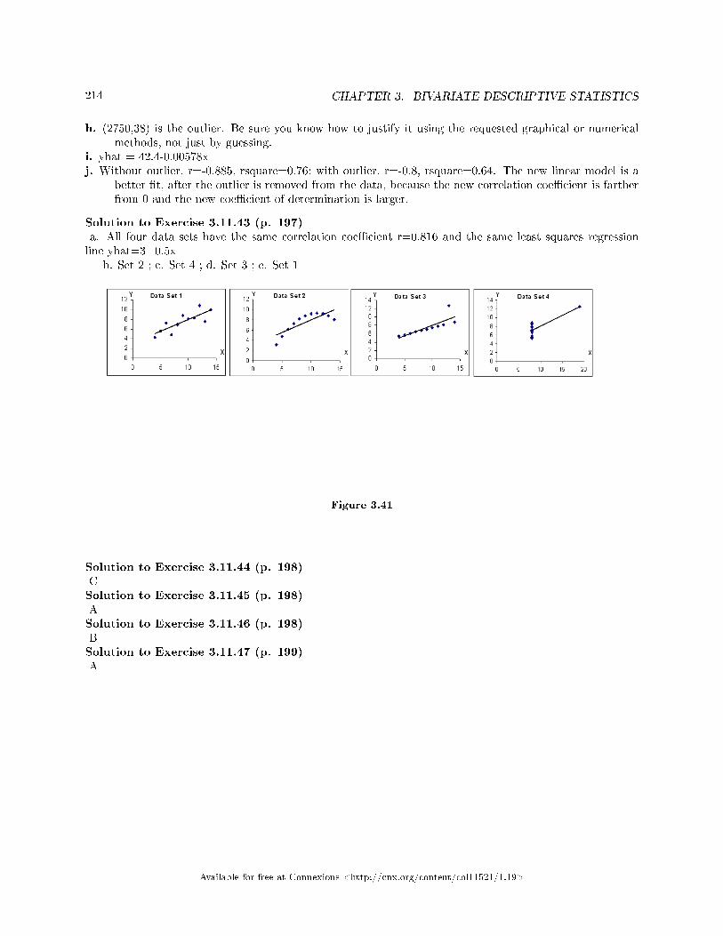
214 CHAPTER 3. BIVARIATE DESCRIPTIVE STATISTICS
h. (2750,38) is the outlier. Be sure you know how to justify it using the requested graphical or numericalmethods, not just by guessing.
i. yhat = 42.4-0.00578xj. Without outlier, r=-0.885, rsquare=0.76; with outlier, r=-0.8, rsquare=0.64. The new linear model is a
better �t, after the outlier is removed from the data, because the new correlation coe�cient is fartherfrom 0 and the new coe�cient of determination is larger.
Solution to Exercise 3.11.43 (p. 197)a. All four data sets have the same correlation coe�cient r=0.816 and the same least squares regressionline yhat=3+0.5x
b. Set 2 ; c. Set 4 ; d. Set 3 ; e. Set 1
Figure 3.41
Solution to Exercise 3.11.44 (p. 198)CSolution to Exercise 3.11.45 (p. 198)ASolution to Exercise 3.11.46 (p. 198)BSolution to Exercise 3.11.47 (p. 199)A
Available for free at Connexions <http://cnx.org/content/col11521/1.19>
Chapter 4
Probability Topics
4.1 Probability Topics: Introduction1
4.1.1 Student Learning Outcomes
By the end of this chapter, the student should be able to:
• Understand and use the terminology of probability.• Determine whether two events are mutually exclusive and whether two events are independent.• Calculate probabilities using the Addition Rules and Multiplication Rules.• Construct and interpret Contingency Tables.• Construct and interpret Venn Diagrams (optional).• Construct and interpret Tree Diagrams (optional).
4.1.2 Introduction
It is often necessary to "guess" about the outcome of an event in order to make a decision. Politicians studypolls to guess their likelihood of winning an election. Teachers choose a particular course of study based onwhat they think students can comprehend. Doctors choose the treatments needed for various diseases basedon their assessment of likely results. You may have visited a casino where people play games chosen becauseof the belief that the likelihood of winning is good. You may have chosen your course of study based on theprobable availability of jobs.
You have, more than likely, used probability. In fact, you probably have an intuitive sense of probability.Probability deals with the chance of an event occurring. Whenever you weigh the odds of whether or notto do your homework or to study for an exam, you are using probability. In this chapter, you will learn tosolve probability problems using a systematic approach.
4.1.3 Optional Collaborative Classroom Exercise
Your instructor will survey your class. Count the number of students in the class today.
• Raise your hand if you have any change in your pocket or purse. Record the number of raised hands.• Raise your hand if you rode a bus within the past month. Record the number of raised hands.• Raise your hand if you answered "yes" to BOTH of the �rst two questions. Record the number of
raised hands.
1This content is available online at <http://cnx.org/content/m16838/1.11/>.
Available for free at Connexions <http://cnx.org/content/col11521/1.19>
215
216 CHAPTER 4. PROBABILITY TOPICS
Use the class data as estimates of the following probabilities. P(change) means the probability that arandomly chosen person in your class has change in his/her pocket or purse. P(bus) means the probabilitythat a randomly chosen person in your class rode a bus within the last month and so on. Discuss youranswers.
• Find P(change).• Find P(bus).• Find P(change and bus) Find the probability that a randomly chosen student in your class has change
in his/her pocket or purse and rode a bus within the last month.• Find P(change| bus) Find the probability that a randomly chosen student has change given that he/she
rode a bus within the last month. Count all the students that rode a bus. From the group of studentswho rode a bus, count those who have change. The probability is equal to those who have change androde a bus divided by those who rode a bus.
4.2 Probability Topics: Terminology2
Probability is a measure that is associated with how certain we are of outcomes of a particular experimentor activity. An experiment is a planned operation carried out under controlled conditions. If the result isnot predetermined, then the experiment is said to be a chance experiment. Flipping one fair coin twice isan example of an experiment.
The result of an experiment is called an outcome. A sample space is a set of all possible outcomes.Three ways to represent a sample space are to list the possible outcomes, to create a tree diagram, or tocreate a Venn diagram. The uppercase letter S is used to denote the sample space. For example, if you �ipone fair coin, S = {H, T} where H = heads and T = tails are the outcomes.
An event is any combination of outcomes. Upper case letters like A and B represent events. For example,if the experiment is to �ip one fair coin, event A might be getting at most one head. The probability of anevent A is written P (A).
The probability of any outcome is the long-term relative frequency of that outcome. Probabilitiesare between 0 and 1, inclusive (includes 0 and 1 and all numbers between these values). P (A) = 0means the event A can never happen. P (A) = 1 means the event A always happens. P (A) = 0.5 meansthe event A is equally likely to occur or not to occur. For example, if you �ip one fair coin repeatedly (from20 to 2,000 to 20,000 times) the relative fequency of heads approaches 0.5 (the probability of heads).
Equally likely means that each outcome of an experiment occurs with equal probability. For example,if you toss a fair, six-sided die, each face (1, 2, 3, 4, 5, or 6) is as likely to occur as any other face. If youtoss a fair coin, a Head(H) and a Tail(T) are equally likely to occur. If you randomly guess the answer to atrue/false question on an exam, you are equally likely to select a correct answer or an incorrect answer.
To calculate the probability of an event A when all outcomes in the sample space are equallylikely, count the number of outcomes for event A and divide by the total number of outcomes in the samplespace. For example, if you toss a fair dime and a fair nickel, the sample space is {HH, TH, HT, TT} whereT = tails and H = heads. The sample space has four outcomes. A = getting one head. There are twooutcomes {HT, TH}. P (A) = 2
4 .Suppose you roll one fair six-sided die, with the numbers {1,2,3,4,5,6} on its faces. Let event E = rolling
a number that is at least 5. There are two outcomes {5, 6}. P (E) = 26 . If you were to roll the die only a
few times, you would not be surprised if your observed results did not match the probability. If you were toroll the die a very large number of times, you would expect that, overall, 2/6 of the rolls would result in anoutcome of "at least 5". You would not expect exactly 2/6. The long-term relative frequency of obtainingthis result would approach the theoretical probability of 2/6 as the number of repetitions grows larger andlarger.
2This content is available online at <http://cnx.org/content/m47517/1.1/>.
Available for free at Connexions <http://cnx.org/content/col11521/1.19>
217
This important characteristic of probability experiments is the known as the Law of Large Numbers:as the number of repetitions of an experiment is increased, the relative frequency obtained in the experimenttends to become closer and closer to the theoretical probability. Even though the outcomes don't happenaccording to any set pattern or order, overall, the long-term observed relative frequency will approach thetheoretical probability. (The word empirical is often used instead of the word observed.) The Law ofLarge Numbers will be discussed again in Chapter 7.
It is important to realize that in many situations, the outcomes are not equally likely. A coin or die maybe unfair, or biased . Two math professors in Europe had their statistics students test the Belgian 1 Eurocoin and discovered that in 250 trials, a head was obtained 56% of the time and a tail was obtained 44%of the time. The data seem to show that the coin is not a fair coin; more repetitions would be helpful todraw a more accurate conclusion about such bias. Some dice may be biased. Look at the dice in a game youhave at home; the spots on each face are usually small holes carved out and then painted to make the spotsvisible. Your dice may or may not be biased; it is possible that the outcomes may be a�ected by the slightweight di�erences due to the di�erent numbers of holes in the faces. Gambling casinos have a lot of moneydepending on outcomes from rolling dice, so casino dice are made di�erently to eliminate bias. Casino dicehave �at faces; the holes are completely �lled with paint having the same density as the material that thedice are made out of so that each face is equally likely to occur. Later in this chapter we will learn techniquesto use to work with probabilities for events that are not equally likely."OR" Event:An outcome is in the event A OR B if the outcome is in A or is in B or is in both A and B. For example,let A = {1, 2, 3, 4, 5} and B = {4, 5, 6, 7, 8}. A OR B = {1, 2, 3, 4, 5, 6, 7, 8}. Notice that 4 and5 are NOT listed twice."AND" Event:An outcome is in the event A AND B if the outcome is in both A and B at the same time. For example, letA and B be {1, 2, 3, 4, 5} and {4, 5, 6, 7, 8}, respectively. Then A AND B = {4, 5}.
The complement of event A is denoted A' (read "A prime"). A' consists of all outcomes that are NOTin A. Notice that P (A) + P (A') = 1. For example, let S = {1, 2, 3, 4, 5, 6} and let A = {1, 2, 3, 4}.Then, A' = {5, 6}. P (A) = 4
6 , P (A') =26 , and P (A) + P (A') =4
6 + 26= 1
The conditional probability of A given B is written P (A|B). P (A|B) is the probability that event Awill occur given that the event B has already occurred. A conditional reduces the sample space. Wecalculate the probability of A from the reduced sample space B. The formula to calculate P (A|B) is
P (A|B) = P (AandB)P (B)
where P (B) is greater than 0.For example, suppose we toss one fair, six-sided die. The sample space S = {1, 2, 3, 4, 5, 6}. Let A =
face is 2 or 3 and B = face is even (2, 4, 6). To calculate P (A|B), we count the number of outcomes 2 or 3in the sample space B = {2, 4, 6}. Then we divide that by the number of outcomes in B (and not S).
We get the same result by using the formula. Remember that S has 6 outcomes.
P (A|B) = P(A and B)P(B) = (the number of outcomes that are 2 or 3 and even in S) / 6
(the number of outcomes that are even in S) / 6 = 1/63/6 = 1
3
Understanding Terminology and SymbolsIt is important to read each problem carefully to think about and understand what the events are. Under-standing the wording is the �rst very important step in solving probability problems. Reread the problemseveral times if necessary. Clearly identify the event of interest. Determine whether there is a conditionstated in the wording that would indicate that the probability is conditional; carefully identify the condition,if any.
Exercise 4.2.1 (Solution on p. 258.)
In a particular college class, there are male and female students. Some students have long hair andsome students have short hair. Write the symbols for the probabilities of the events for parts (a)through (j) below. (Note that you can't �nd numerical answers here. You were not given enoughinformation to �nd any probability values yet; concentrate on understanding the symbols.)
• Let F be the event that a student is female.
Available for free at Connexions <http://cnx.org/content/col11521/1.19>
218 CHAPTER 4. PROBABILITY TOPICS
• Let M be the event that a student is male.• Let S be the event that a student has short hair.• Let L be the event that a student has long hair.
a. The probability that a student does not have long hair.b. The probability that a student is male or has short hair.c. The probability that a student is a female and has long hair.d. The probability that a student is male, given that the student has long hair.e. The probability that a student has long hair, given that the student is male.f. Of all the female students, the probability that a student has short hair.g. Of all students with long hair, the probability that a student is female.h. The probability that a student is female or has long hair.i. The probability that a randomly selected student is a male student with short hair.j. The probability that a student is female.
**With contributions from Roberta Bloom
4.3 Probability Topics: Independent & Mutually Exclusive Events3
Independent and mutually exclusive do not mean the same thing.
4.3.1 Independent Events
Two events are independent if the following are true:
• P (A|B) = P (A)• P (B|A) = P (B)• P (A AND B) = P (A) · P (B)
Two events A and B are independent if the knowledge that one occurred does not a�ect the chance theother occurs. For example, the outcomes of two roles of a fair die are independent events. The outcome ofthe �rst roll does not change the probability for the outcome of the second roll. To show two events areindependent, you must show only one of the above conditions. If two events are NOT independent, thenwe say that they are dependent.
Sampling may be done with replacement or without replacement.
• With replacement: If each member of a population is replaced after it is picked, then that memberhas the possibility of being chosen more than once. When sampling is done with replacement, thenevents are considered to be independent, meaning the result of the �rst pick will not change theprobabilities for the second pick.
• Without replacement:: When sampling is done without replacement, then each member of a pop-ulation may be chosen only once. In this case, the probabilities for the second pick are a�ected by theresult of the �rst pick. The events are considered to be dependent or not independent.
If it is not known whether A and B are independent or dependent, assume they are dependent untilyou can show otherwise.
3This content is available online at <http://cnx.org/content/m16837/1.14/>.
Available for free at Connexions <http://cnx.org/content/col11521/1.19>
219
4.3.2 Mutually Exclusive Events
A and B are mutually exclusive events if they cannot occur at the same time. This means that A and Bdo not share any outcomes and P(A AND B) = 0.
For example, suppose the sample space S = {1, 2, 3, 4, 5, 6, 7, 8, 9, 10}. LetA = {1, 2, 3, 4, 5}, B = {4, 5, 6, 7, 8}, and C = {7, 9}. A AND B = {4, 5}. P(A AND B) =210and is not equal to zero. Therefore, A and B are not mutually exclusive. A and C do not have anynumbers in common so P(A AND C) = 0. Therefore, A and C are mutually exclusive.
If it is not known whether A and B are mutually exclusive, assume they are not until you can showotherwise.
The following examples illustrate these de�nitions and terms.
Example 4.1Flip two fair coins. (This is an experiment.)
The sample space is {HH, HT, TH, TT} where T = tails and H = heads. The outcomes areHH, HT, TH, and TT. The outcomes HT and TH are di�erent. The HT means that the �rst coinshowed heads and the second coin showed tails. The TH means that the �rst coin showed tails andthe second coin showed heads.
• Let A = the event of getting at most one tail. (At most one tail means 0 or 1 tail.) ThenA can be written as {HH, HT, TH}. The outcome HH shows 0 tails. HT and TH each show1 tail.
• Let B = the event of getting all tails. B can be written as {TT}. B is the complement ofA. So, B = A'. Also, P (A) + P (B) = P (A) + P (A') = 1.
• The probabilities for A and for B are P (A) = 34 and P (B) = 1
4 .• Let C = the event of getting all heads. C = {HH}. Since B = {TT}, P (B AND C) = 0.
B and C are mutually exclusive. (B and C have no members in common because you cannothave all tails and all heads at the same time.)
• Let D = event of getting more than one tail. D = {TT}. P (D) = 14 .
• Let E = event of getting a head on the �rst roll. (This implies you can get either a head ortail on the second roll.) E = {HT,HH}. P (E) = 2
4 .• Find the probability of getting at least one (1 or 2) tail in two �ips. Let F = event of getting
at least one tail in two �ips. F = {HT,TH,TT}. P(F) = 34
Example 4.2Roll one fair 6-sided die. The sample space is {1, 2, 3, 4, 5, 6}. Let event A = a face is odd. ThenA = {1, 3, 5}. Let event B = a face is even. Then B = {2, 4, 6}.
• Find the complement of A, A'. The complement of A, A', is B because A and B together makeup the sample space. P(A) + P(B) = P(A) + P(A') = 1. Also, P(A) = 3
6 and P(B) = 36
• Let event C = odd faces larger than 2. Then C = {3, 5}. Let event D = all even faces smallerthan 5. Then D = {2, 4}. P(C and D) = 0 because you cannot have an odd and even faceat the same time. Therefore, C and D are mutually exclusive events.
• Let event E = all faces less than 5. E = {1, 2, 3, 4}.Problem (Solution on p. 258.)
Are C and E mutually exclusive events? (Answer yes or no.) Why or why not?
• Find P(C|A). This is a conditional. Recall that the event C is {3, 5} and event A is {1, 3, 5}.To �nd P(C|A), �nd the probability of C using the sample space A. You have reduced thesample space from the original sample space {1, 2, 3, 4, 5, 6} to {1, 3, 5}. So, P(C|A) = 2
3
Available for free at Connexions <http://cnx.org/content/col11521/1.19>
220 CHAPTER 4. PROBABILITY TOPICS
Example 4.3Let event G = taking a math class. Let event H = taking a science class. Then, G AND H = takinga math class and a science class. Suppose P(G) = 0.6, P(H) = 0.5, and P(G AND H) = 0.3. AreG and H independent?
If G and H are independent, then you must show ONE of the following:
• P(G|H) = P(G)• P(H|G) = P(H)• P(G AND H) = P(G) · P(H)
note: The choice you make depends on the information you have. You could choose anyof the methods here because you have the necessary information.
Problem 1Show that P(G|H) = P(G).
SolutionP(G|H) = P(G AND H)
P(H) = 0.30.5 = 0.6 = P(G)
Problem 2Show P(G AND H) = P(G) · P(H).SolutionP (G) · P (H) = 0.6 · 0.5 = 0.3 = P(G AND H)
Since G and H are independent, then, knowing that a person is taking a science class does notchange the chance that he/she is taking math. If the two events had not been independent (thatis, they are dependent) then knowing that a person is taking a science class would change thechance he/she is taking math. For practice, show that P(H|G) = P(H) to show that G and H areindependent events.
Example 4.4In a box there are 3 red cards and 5 blue cards. The red cards are marked with the numbers 1, 2,and 3, and the blue cards are marked with the numbers 1, 2, 3, 4, and 5. The cards are well-shu�ed.You reach into the box (you cannot see into it) and draw one card.
Let R = red card is drawn, B = blue card is drawn, E = even-numbered card is drawn.The sample space S = R1, R2, R3, B1, B2, B3, B4, B5. S has 8 outcomes.
• P(R) = 38 . P(B) = 5
8 . P(R AND B) = 0. (You cannot draw one card that is both red andblue.)
• P(E) = 38 . (There are 3 even-numbered cards, R2, B2, and B4.)
• P(E|B) = 25 . (There are 5 blue cards: B1, B2, B3, B4, and B5. Out of the blue cards, there
are 2 even cards: B2 and B4.)• P(B|E) = 2
3 . (There are 3 even-numbered cards: R2, B2, and B4. Out of the even-numberedcards, 2 are blue: B2 and B4.)
• The events R and B are mutually exclusive because P(R AND B) = 0.• Let G = card with a number greater than 3. G = {B4,B5}. P(G) = 2
8 . Let H = blue cardnumbered between 1 and 4, inclusive. H = {B1,B2,B3,B4}. P(G|H) = 1
4 . (The only cardin H that has a number greater than 3 is B4.) Since 2
8 = 14 , P(G) = P(G|H) which means
that G and H are independent.
Available for free at Connexions <http://cnx.org/content/col11521/1.19>
221
Example 4.5In a particular college class, 60% of the students are female. 50 % of all students in the class havelong hair. 45% of the students are female and have long hair. Of the female students, 75% havelong hair. Let F be the event that the student is female. Let L be the event that the student haslong hair. One student is picked randomly. Are the events of being female and having long hairindependent?
• The following probabilities are given in this example:• P(F ) = 0.60 ; P(L ) = 0.50• P(F AND L) = 0.45• P(L|F) = 0.75
note: The choice you make depends on the information you have. You could use the �rstor last condition on the list for this example. You do not know P(F|L) yet, so you can not use thesecond condition.
Solution 1Check whether P(F and L) = P(F)P(L): We are given that P(F and L) = 0.45 ; but P(F)P(L) =(0.60)(0.50)= 0.30 The events of being female and having long hair are not independent becauseP(F and L) does not equal P(F)P(L).Solution 2check whether P(L|F) equals P(L): We are given that P(L|F) = 0.75 but P(L) = 0.50; they are notequal. The events of being female and having long hair are not independent.Interpretation of ResultsThe events of being female and having long hair are not independent; knowing that a student isfemale changes the probability that a student has long hair.
**Example 5 contributed by Roberta Bloom
4.4 Probability Topics: Two Basic Rules of Probability4
4.4.1 The Multiplication Rule
If A and B are two events de�ned on a sample space, then: P(A AND B) = P(B) · P(A|B).This rule may also be written as : P (A|B) = P (A AND B)
P (B)
(The probability of A given B equals the probability of A and B divided by the probability of B.)If A and B are independent, then P(A|B) = P(A). Then P(A AND B) = P(A|B) P(B) becomes
P(A AND B) = P(A) P(B).
4.4.2 The Addition Rule
If A and B are de�ned on a sample space, then: P(A OR B) = P(A) + P(B)− P(A AND B).If A and B are mutually exclusive, then P(A AND B) = 0. Then P(A OR B) = P(A) + P(B) −
P(A AND B) becomes P(A OR B) = P(A) + P(B).Example 4.6Klaus is trying to choose where to go on vacation. His two choices are: A = New Zealand and B= Alaska
• Klaus can only a�ord one vacation. The probability that he chooses A is P(A) = 0.6 and theprobability that he chooses B is P(B) = 0.35.
4This content is available online at <http://cnx.org/content/m16847/1.11/>.
Available for free at Connexions <http://cnx.org/content/col11521/1.19>
222 CHAPTER 4. PROBABILITY TOPICS
• P(A and B) = 0 because Klaus can only a�ord to take one vacation• Therefore, the probability that he chooses either New Zealand or Alaska is P(A OR B) =
P(A) + P(B) = 0.6 + 0.35 = 0.95. Note that the probability that he does not choose to goanywhere on vacation must be 0.05.
Example 4.7Carlos plays college soccer. He makes a goal 65% of the time he shoots. Carlos is going to attempttwo goals in a row in the next game.
A = the event Carlos is successful on his �rst attempt. P(A) = 0.65. B = the event Carlos issuccessful on his second attempt. P(B) = 0.65. Carlos tends to shoot in streaks. The probabilitythat he makes the second goal GIVEN that he made the �rst goal is 0.90.
Problem 1What is the probability that he makes both goals?
SolutionThe problem is asking you to �nd P(A AND B) = P(B AND A). Since P(B|A) = 0.90:
P(B AND A) = P(B|A) P(A) = 0.90 ∗ 0.65 = 0.585 (4.1)
Carlos makes the �rst and second goals with probability 0.585.
Problem 2What is the probability that Carlos makes either the �rst goal or the second goal?
SolutionThe problem is asking you to �nd P(A OR B).
P(A OR B) = P(A) + P(B) − P(A AND B) = 0.65 + 0.65− 0.585 = 0.715 (4.2)
Carlos makes either the �rst goal or the second goal with probability 0.715.
Problem 3Are A and B independent?
SolutionNo, they are not, because P(B AND A) = 0.585.
P(B) · P(A) = (0.65) · (0.65) = 0.423 (4.3)
0.423 6= 0.585 = P(B AND A) (4.4)
So, P(B AND A) is not equal to P(B) · P(A).
Problem 4Are A and B mutually exclusive?
SolutionNo, they are not because P(A and B) = 0.585.
To be mutually exclusive, P(A AND B) must equal 0.
Available for free at Connexions <http://cnx.org/content/col11521/1.19>
223
Example 4.8A community swim team has 150members. Seventy-�ve of the members are advanced swimmers.Forty-seven of the members are intermediate swimmers. The remainder are novice swimmers.Forty of the advanced swimmers practice 4 times a week. Thirty of the intermediate swimmerspractice 4 times a week. Ten of the novice swimmers practice 4 times a week. Suppose one memberof the swim team is randomly chosen. Answer the questions (Verify the answers):
Problem 1What is the probability that the member is a novice swimmer?
Solution28150
Problem 2What is the probability that the member practices 4 times a week?
Solution80150
Problem 3What is the probability that the member is an advanced swimmer and practices 4 times a week?
Solution40150
Problem 4What is the probability that a member is an advanced swimmer and an intermediate swimmer?
Are being an advanced swimmer and an intermediate swimmer mutually exclusive? Why or whynot?
SolutionP(advanced AND intermediate) = 0, so these are mutually exclusive events. A swimmer cannotbe an advanced swimmer and an intermediate swimmer at the same time.
Problem 5Are being a novice swimmer and practicing 4 times a week independent events? Why or why not?
SolutionNo, these are not independent events.
P(novice AND practices 4 times per week) = 0.0667 (4.5)
P(novice) · P(practices 4 times per week) = 0.0996 (4.6)
0.0667 6= 0.0996 (4.7)
Available for free at Connexions <http://cnx.org/content/col11521/1.19>
224 CHAPTER 4. PROBABILITY TOPICS
Example 4.9Studies show that, if she lives to be 90, about 1 woman in 7 (approximately 14.3%) will developbreast cancer. Suppose that of those women who develop breast cancer, a test is negative 2% of thetime. Also suppose that in the general population of women, the test for breast cancer is negativeabout 85% of the time. Let B = woman develops breast cancer and let N = tests negative. Supposeone woman is selected at random.
Problem 1What is the probability that the woman develops breast cancer? What is the probability thatwoman tests negative?
SolutionP(B) = 0.143 ; P(N) = 0.85
Problem 2Given that the woman has breast cancer, what is the probability that she tests negative?
SolutionP(N|B) = 0.02
Problem 3What is the probability that the woman has breast cancer AND tests negative?
SolutionP(B AND N) = P(B) · P(N|B) = (0.143) · (0.02) = 0.0029
Problem 4What is the probability that the woman has breast cancer or tests negative?
SolutionP(B OR N) = P(B) + P(N) − P(B AND N) = 0.143 + 0.85− 0.0029 = 0.9901
Problem 5Are having breast cancer and testing negative independent events?
SolutionNo. P(N) = 0.85; P(N|B) = 0.02. So, P(N|B) does not equal P(N)
Problem 6Are having breast cancer and testing negative mutually exclusive?
SolutionNo. P(B AND N) = 0.0029. For B and N to be mutually exclusive, P(B AND N) must be 0.
Available for free at Connexions <http://cnx.org/content/col11521/1.19>
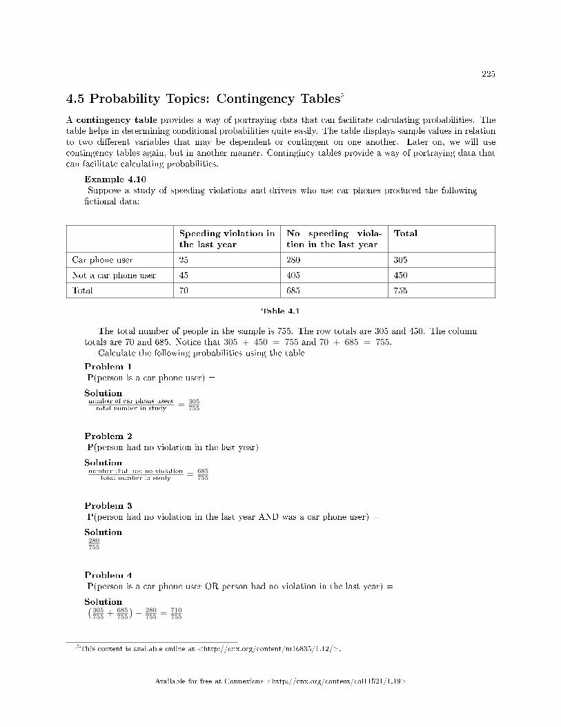
225
4.5 Probability Topics: Contingency Tables5
A contingency table provides a way of portraying data that can facilitate calculating probabilities. Thetable helps in determining conditional probabilities quite easily. The table displays sample values in relationto two di�erent variables that may be dependent or contingent on one another. Later on, we will usecontingency tables again, but in another manner. Contingincy tables provide a way of portraying data thatcan facilitate calculating probabilities.
Example 4.10Suppose a study of speeding violations and drivers who use car phones produced the following�ctional data:
Speeding violation inthe last year
No speeding viola-tion in the last year
Total
Car phone user 25 280 305
Not a car phone user 45 405 450
Total 70 685 755
Table 4.1
The total number of people in the sample is 755. The row totals are 305 and 450. The columntotals are 70 and 685. Notice that 305 + 450 = 755 and 70 + 685 = 755.
Calculate the following probabilities using the table
Problem 1P(person is a car phone user) =
Solutionnumber of car phone userstotal number in study = 305
755
Problem 2P(person had no violation in the last year) =
Solutionnumber that had no violation
total number in study = 685755
Problem 3P(person had no violation in the last year AND was a car phone user) =
Solution280755
Problem 4P(person is a car phone user OR person had no violation in the last year) =
Solution(305755 + 685
755
)− 280
755 = 710755
5This content is available online at <http://cnx.org/content/m16835/1.12/>.
Available for free at Connexions <http://cnx.org/content/col11521/1.19>
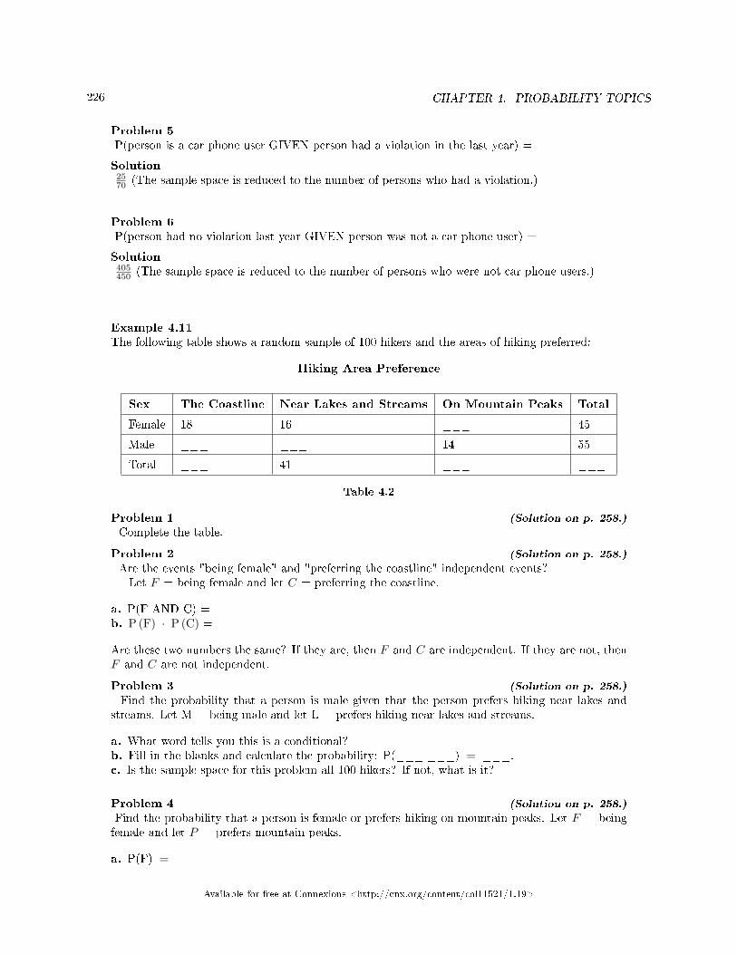
226 CHAPTER 4. PROBABILITY TOPICS
Problem 5P(person is a car phone user GIVEN person had a violation in the last year) =
Solution2570 (The sample space is reduced to the number of persons who had a violation.)
Problem 6P(person had no violation last year GIVEN person was not a car phone user) =
Solution405450 (The sample space is reduced to the number of persons who were not car phone users.)
Example 4.11The following table shows a random sample of 100 hikers and the areas of hiking preferred:
Hiking Area Preference
Sex The Coastline Near Lakes and Streams On Mountain Peaks Total
Female 18 16 ___ 45
Male ___ ___ 14 55
Total ___ 41 ___ ___
Table 4.2
Problem 1 (Solution on p. 258.)
Complete the table.
Problem 2 (Solution on p. 258.)
Are the events "being female" and "preferring the coastline" independent events?Let F = being female and let C = preferring the coastline.
a. P(F AND C) =b. P (F) · P (C) =
Are these two numbers the same? If they are, then F and C are independent. If they are not, thenF and C are not independent.
Problem 3 (Solution on p. 258.)
Find the probability that a person is male given that the person prefers hiking near lakes andstreams. Let M = being male and let L = prefers hiking near lakes and streams.
a. What word tells you this is a conditional?b. Fill in the blanks and calculate the probability: P(___|___) = ___.c. Is the sample space for this problem all 100 hikers? If not, what is it?
Problem 4 (Solution on p. 258.)
Find the probability that a person is female or prefers hiking on mountain peaks. Let F = beingfemale and let P = prefers mountain peaks.
a. P(F) =
Available for free at Connexions <http://cnx.org/content/col11521/1.19>
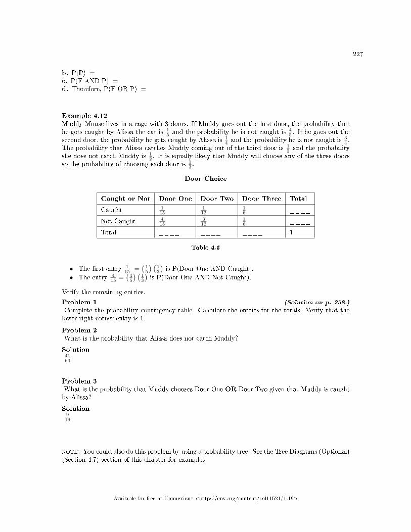
227
b. P(P) =c. P(F AND P) =d. Therefore, P(F OR P) =
Example 4.12Muddy Mouse lives in a cage with 3 doors. If Muddy goes out the �rst door, the probability thathe gets caught by Alissa the cat is 1
5 and the probability he is not caught is 45 . If he goes out the
second door, the probability he gets caught by Alissa is 14 and the probability he is not caught is 3
4 .The probability that Alissa catches Muddy coming out of the third door is 1
2 and the probabilityshe does not catch Muddy is 1
2 . It is equally likely that Muddy will choose any of the three doorsso the probability of choosing each door is 1
3 .
Door Choice
Caught or Not Door One Door Two Door Three Total
Caught 115
112
16 ____
Not Caught 415
312
16 ____
Total ____ ____ ____ 1
Table 4.3
• The �rst entry 115 =
(15
) (13
)is P(Door One AND Caught).
• The entry 415 =
(45
) (13
)is P(Door One AND Not Caught).
Verify the remaining entries.
Problem 1 (Solution on p. 258.)
Complete the probability contingency table. Calculate the entries for the totals. Verify that thelower-right corner entry is 1.
Problem 2What is the probability that Alissa does not catch Muddy?
Solution4160
Problem 3What is the probability that Muddy chooses Door One OR Door Two given that Muddy is caughtby Alissa?
Solution919
note: You could also do this problem by using a probability tree. See the Tree Diagrams (Optional)(Section 4.7) section of this chapter for examples.
Available for free at Connexions <http://cnx.org/content/col11521/1.19>
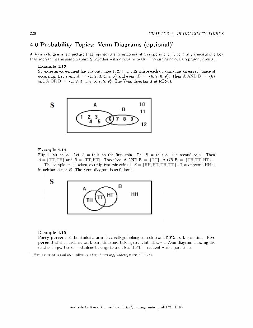
228 CHAPTER 4. PROBABILITY TOPICS
4.6 Probability Topics: Venn Diagrams (optional)6
A Venn diagram is a picture that represents the outcomes of an experiment. It generally consists of a boxthat represents the sample space S together with circles or ovals. The circles or ovals represent events.
Example 4.13Suppose an experiment has the outcomes 1, 2, 3, ... , 12 where each outcome has an equal chance ofoccurring. Let event A = {1, 2, 3, 4, 5, 6} and event B = {6, 7, 8, 9}. Then A AND B = {6}and A OR B = {1, 2, 3, 4, 5, 6, 7, 8, 9}. The Venn diagram is as follows:
Example 4.14Flip 2 fair coins. Let A = tails on the �rst coin. Let B = tails on the second coin. ThenA = {TT,TH} and B = {TT,HT}. Therefore, A AND B = {TT}. A OR B = {TH,TT,HT}.
The sample space when you �ip two fair coins is S = {HH,HT,TH,TT}. The outcome HH isin neither A nor B. The Venn diagram is as follows:
Example 4.15Forty percent of the students at a local college belong to a club and 50% work part time. Fivepercent of the students work part time and belong to a club. Draw a Venn diagram showing therelationships. Let C = student belongs to a club and PT = student works part time.
6This content is available online at <http://cnx.org/content/m16848/1.12/>.
Available for free at Connexions <http://cnx.org/content/col11521/1.19>
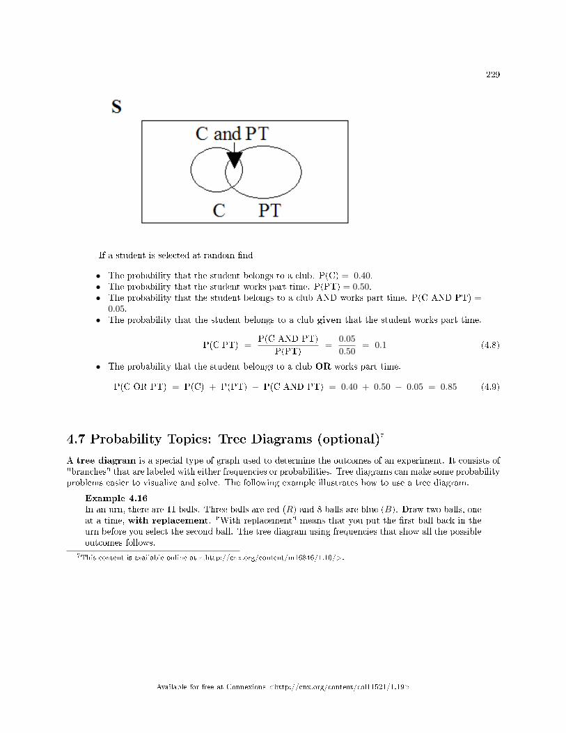
229
If a student is selected at random �nd
• The probability that the student belongs to a club. P(C) = 0.40.• The probability that the student works part time. P(PT) = 0.50.• The probability that the student belongs to a club AND works part time. P(C AND PT) =
0.05.• The probability that the student belongs to a club given that the student works part time.
P(C|PT) =P(C AND PT)
P(PT)=
0.050.50
= 0.1 (4.8)
• The probability that the student belongs to a club OR works part time.
P(C OR PT) = P(C) + P(PT) − P(C AND PT) = 0.40 + 0.50 − 0.05 = 0.85 (4.9)
4.7 Probability Topics: Tree Diagrams (optional)7
A tree diagram is a special type of graph used to determine the outcomes of an experiment. It consists of"branches" that are labeled with either frequencies or probabilities. Tree diagrams can make some probabilityproblems easier to visualize and solve. The following example illustrates how to use a tree diagram.
Example 4.16In an urn, there are 11 balls. Three balls are red (R) and 8 balls are blue (B). Draw two balls, oneat a time, with replacement. "With replacement" means that you put the �rst ball back in theurn before you select the second ball. The tree diagram using frequencies that show all the possibleoutcomes follows.
7This content is available online at <http://cnx.org/content/m16846/1.10/>.
Available for free at Connexions <http://cnx.org/content/col11521/1.19>
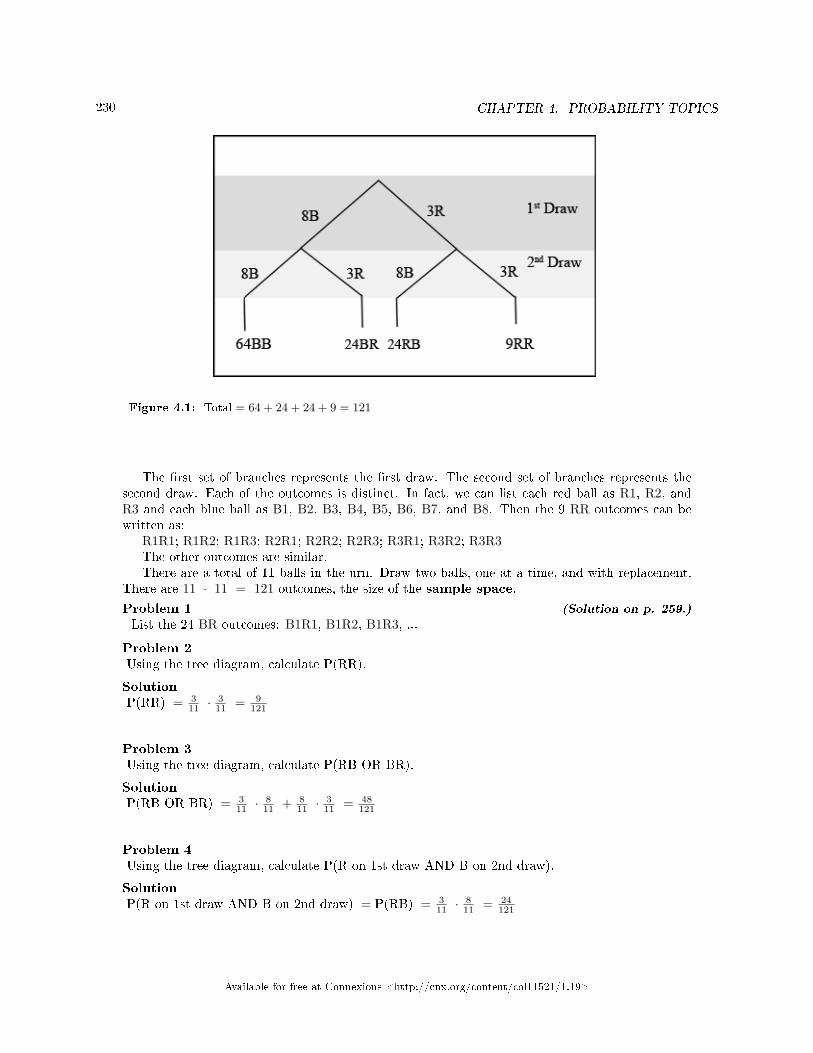
230 CHAPTER 4. PROBABILITY TOPICS
Figure 4.1: Total = 64 + 24 + 24 + 9 = 121
The �rst set of branches represents the �rst draw. The second set of branches represents thesecond draw. Each of the outcomes is distinct. In fact, we can list each red ball as R1, R2, andR3 and each blue ball as B1, B2, B3, B4, B5, B6, B7, and B8. Then the 9 RR outcomes can bewritten as:
R1R1; R1R2; R1R3; R2R1; R2R2; R2R3; R3R1; R3R2; R3R3The other outcomes are similar.There are a total of 11 balls in the urn. Draw two balls, one at a time, and with replacement.
There are 11 · 11 = 121 outcomes, the size of the sample space.
Problem 1 (Solution on p. 259.)
List the 24 BR outcomes: B1R1, B1R2, B1R3, ...
Problem 2Using the tree diagram, calculate P(RR).
SolutionP(RR) = 3
11 ·311 = 9
121
Problem 3Using the tree diagram, calculate P(RB OR BR).
SolutionP(RB OR BR) = 3
11 ·811 + 8
11 ·311 = 48
121
Problem 4Using the tree diagram, calculate P(R on 1st draw AND B on 2nd draw).
SolutionP(R on 1st draw AND B on 2nd draw) = P(RB) = 3
11 ·811 = 24
121
Available for free at Connexions <http://cnx.org/content/col11521/1.19>
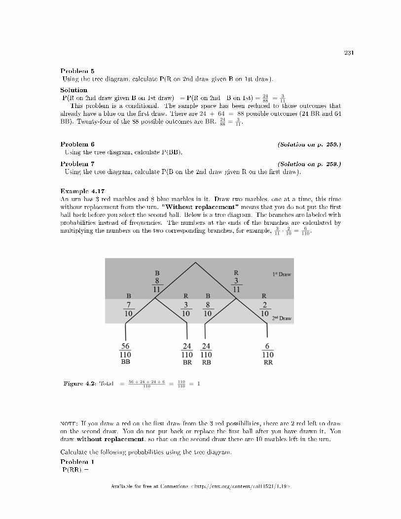
231
Problem 5Using the tree diagram, calculate P(R on 2nd draw given B on 1st draw).
SolutionP(R on 2nd draw given B on 1st draw) = P(R on 2nd | B on 1st) = 24
88 = 311
This problem is a conditional. The sample space has been reduced to those outcomes thatalready have a blue on the �rst draw. There are 24 + 64 = 88 possible outcomes (24 BR and 64BB). Twenty-four of the 88 possible outcomes are BR. 24
88 = 311 .
Problem 6 (Solution on p. 259.)
Using the tree diagram, calculate P(BB).
Problem 7 (Solution on p. 259.)
Using the tree diagram, calculate P(B on the 2nd draw given R on the �rst draw).
Example 4.17An urn has 3 red marbles and 8 blue marbles in it. Draw two marbles, one at a time, this timewithout replacement from the urn. "Without replacement" means that you do not put the �rstball back before you select the second ball. Below is a tree diagram. The branches are labeled withprobabilities instead of frequencies. The numbers at the ends of the branches are calculated bymultiplying the numbers on the two corresponding branches, for example, 3
11 ·210 = 6
110 .
Figure 4.2: Total = 56 + 24 + 24 + 6110
= 110110
= 1
note: If you draw a red on the �rst draw from the 3 red possibilities, there are 2 red left to drawon the second draw. You do not put back or replace the �rst ball after you have drawn it. Youdraw without replacement, so that on the second draw there are 10 marbles left in the urn.
Calculate the following probabilities using the tree diagram.
Problem 1P(RR) =
Available for free at Connexions <http://cnx.org/content/col11521/1.19>
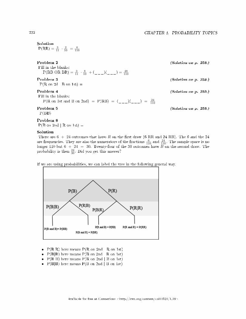
232 CHAPTER 4. PROBABILITY TOPICS
SolutionP(RR) = 3
11 ·210 = 6
110
Problem 2 (Solution on p. 259.)
Fill in the blanks:P(RB OR BR) = 3
11 ·810 + (___)(___) = 48
110
Problem 3 (Solution on p. 259.)
P(R on 2d | B on 1st) =
Problem 4 (Solution on p. 259.)
Fill in the blanks:P(R on 1st and B on 2nd) = P(RB) = (___)(___) = 24
110
Problem 5 (Solution on p. 259.)
P(BB) =
Problem 6P(B on 2nd | R on 1st) =
SolutionThere are 6 + 24 outcomes that have R on the �rst draw (6 RR and 24 RB). The 6 and the 24are frequencies. They are also the numerators of the fractions 6
110 and 24110 . The sample space is no
longer 110 but 6 + 24 = 30. Twenty-four of the 30 outcomes have B on the second draw. Theprobability is then 24
30 . Did you get this answer?
If we are using probabilities, we can label the tree in the following general way.
• P(R|R) here means P(R on 2nd | R on 1st)• P(B|R) here means P(B on 2nd | R on 1st)• P(R|B) here means P(R on 2nd | B on 1st)• P(B|B) here means P(B on 2nd | B on 1st)
Available for free at Connexions <http://cnx.org/content/col11521/1.19>
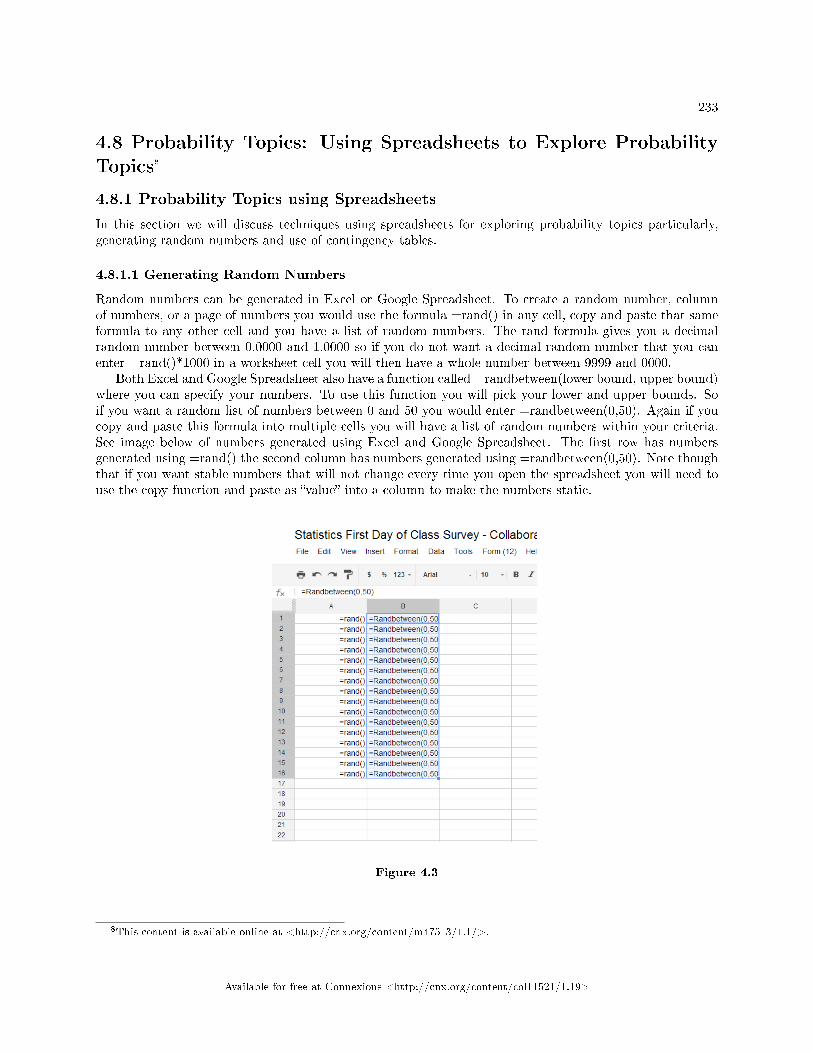
233
4.8 Probability Topics: Using Spreadsheets to Explore ProbabilityTopics8
4.8.1 Probability Topics using Spreadsheets
In this section we will discuss techniques using spreadsheets for exploring probability topics particularly,generating random numbers and use of contingency tables.
4.8.1.1 Generating Random Numbers
Random numbers can be generated in Excel or Google Spreadsheet. To create a random number, columnof numbers, or a page of numbers you would use the formula =rand() in any cell, copy and paste that sameformula to any other cell and you have a list of random numbers. The rand formula gives you a decimalrandom number between 0.0000 and 1.0000 so if you do not want a decimal random number that you canenter =rand()*1000 in a worksheet cell you will then have a whole number between 9999 and 0000.
Both Excel and Google Spreadsheet also have a function called =randbetween(lower bound, upper bound)where you can specify your numbers. To use this function you will pick your lower and upper bounds. Soif you want a random list of numbers between 0 and 50 you would enter =randbetween(0,50). Again if youcopy and paste this formula into multiple cells you will have a list of random numbers within your criteria.See image below of numbers generated using Excel and Google Spreadsheet. The �rst row has numbersgenerated using =rand() the second column has numbers generated using =randbetween(0,50). Note thoughthat if you want stable numbers that will not change every time you open the spreadsheet you will need touse the copy function and paste as �value� into a column to make the numbers static.
Figure 4.3
8This content is available online at <http://cnx.org/content/m47513/1.1/>.
Available for free at Connexions <http://cnx.org/content/col11521/1.19>
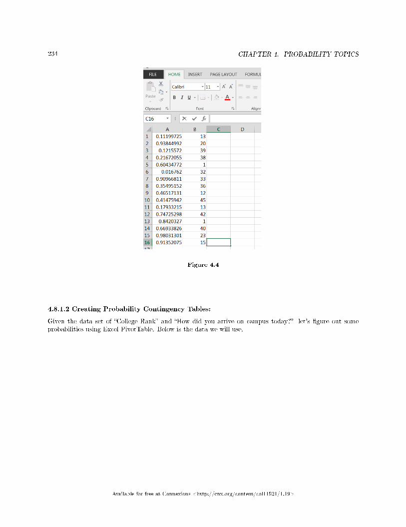
234 CHAPTER 4. PROBABILITY TOPICS
Figure 4.4
4.8.1.2 Creating Probability Contingency Tables:
Given the data set of �College Rank� and �How did you arrive on campus today?� let's �gure out someprobabilities using Excel PivotTable. Below is the data we will use.
Available for free at Connexions <http://cnx.org/content/col11521/1.19>
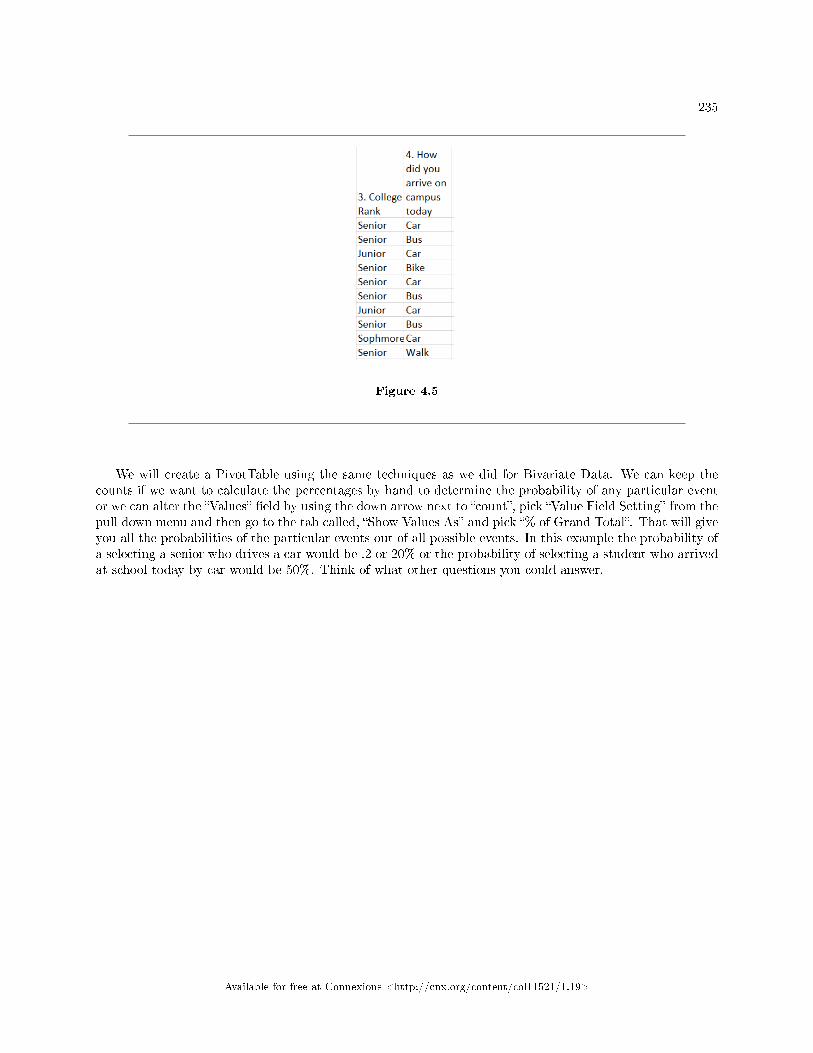
235
Figure 4.5
We will create a PivotTable using the same techniques as we did for Bivariate Data. We can keep thecounts if we want to calculate the percentages by hand to determine the probability of any particular eventor we can alter the �Values� �eld by using the down arrow next to �count�, pick �Value Field Setting� from thepull down menu and then go to the tab called, �Show Values As� and pick �% of Grand Total�. That will giveyou all the probabilities of the particular events out of all possible events. In this example the probability ofa selecting a senior who drives a car would be .2 or 20% or the probability of selecting a student who arrivedat school today by car would be 50%. Think of what other questions you could answer.
Available for free at Connexions <http://cnx.org/content/col11521/1.19>
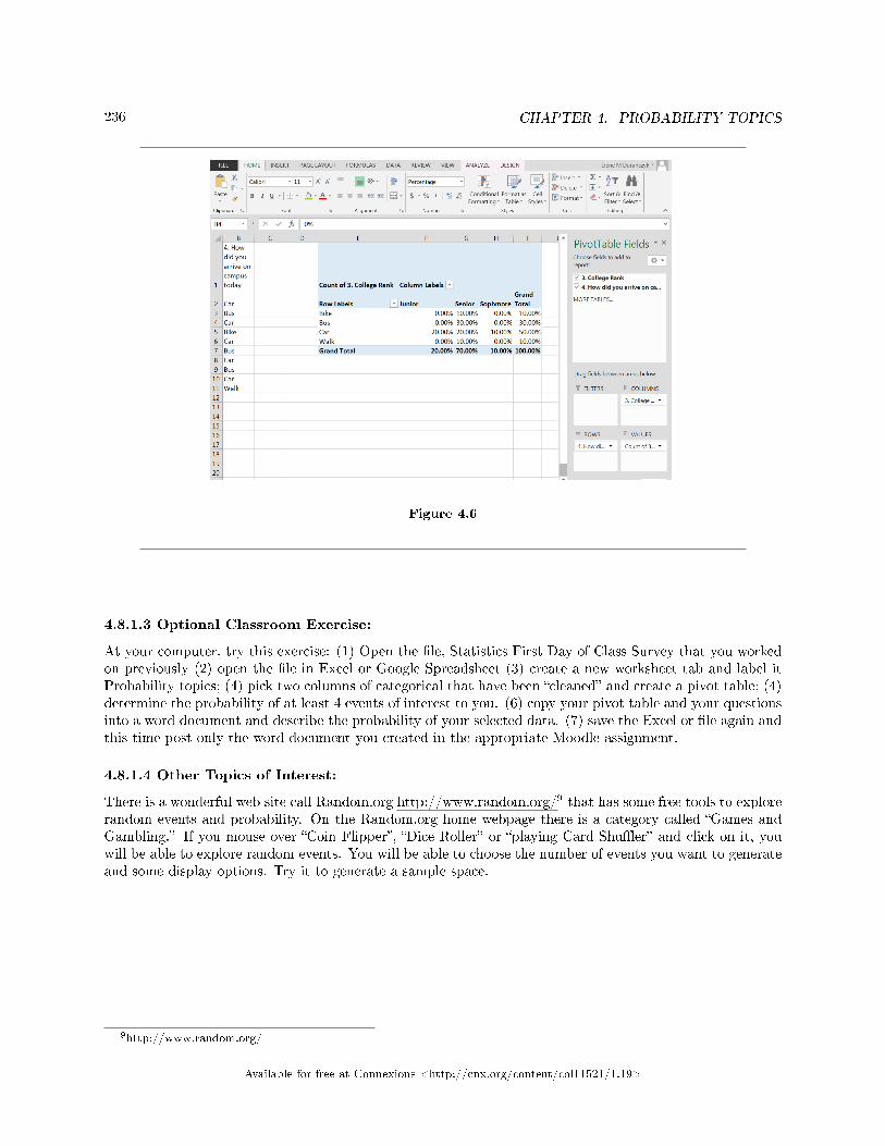
236 CHAPTER 4. PROBABILITY TOPICS
Figure 4.6
4.8.1.3 Optional Classroom Exercise:
At your computer, try this exercise: (1) Open the �le, Statistics First Day of Class Survey that you workedon previously (2) open the �le in Excel or Google Spreadsheet (3) create a new worksheet tab and label itProbability topics; (4) pick two columns of categorical that have been �cleaned� and create a pivot table; (4)determine the probability of at least 4 events of interest to you. (6) copy your pivot table and your questionsinto a word document and describe the probability of your selected data. (7) save the Excel or �le again andthis time post only the word document you created in the appropriate Moodle assignment.
4.8.1.4 Other Topics of Interest:
There is a wonderful web site call Random.org http://www.random.org/9 that has some free tools to explorerandom events and probability. On the Random.org home webpage there is a category called �Games andGambling.� If you mouse over �Coin Flipper�, �Dice Roller� or �playing Card Shu�er� and click on it, youwill be able to explore random events. You will be able to choose the number of events you want to generateand some display options. Try it to generate a sample space.
9http://www.random.org/
Available for free at Connexions <http://cnx.org/content/col11521/1.19>
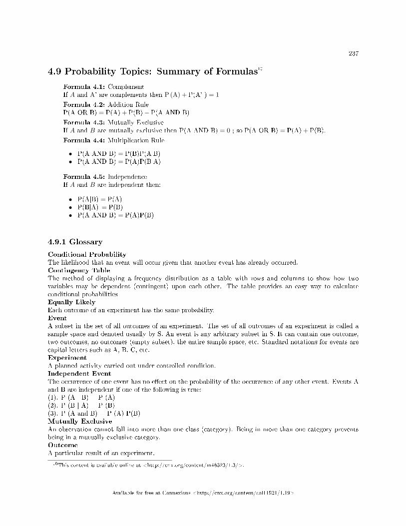
237
4.9 Probability Topics: Summary of Formulas10
Formula 4.1: ComplementIf A and A' are complements then P (A) + P(A' ) = 1Formula 4.2: Addition RuleP(A OR B) = P(A) + P(B)− P(A AND B)
Formula 4.3: Mutually ExclusiveIf A and B are mutually exclusive then P(A AND B) = 0 ; so P(A OR B) = P(A) + P(B).
Formula 4.4: Multiplication Rule
• P(A AND B) = P(B)P(A|B)• P(A AND B) = P(A)P(B|A)
Formula 4.5: IndependenceIf A and B are independent then:
• P(A|B) = P(A)• P(B|A) = P(B)• P(A AND B) = P(A)P(B)
4.9.1 Glossary
Conditional ProbabilityThe likelihood that an event will occur given that another event has already occurred.Contingency TableThe method of displaying a frequency distribution as a table with rows and columns to show how twovariables may be dependent (contingent) upon each other. The table provides an easy way to calculateconditional probabilitiesEqually LikelyEach outcome of an experiment has the same probability.EventA subset in the set of all outcomes of an experiment. The set of all outcomes of an experiment is called asample space and denoted usually by S. An event is any arbitrary subset in S. It can contain one outcome,two outcomes, no outcomes (empty subset), the entire sample space, etc. Standard notations for events arecapital letters such as A, B, C, etc.ExperimentA planned activity carried out under controlled condition.Independent EventThe occurrence of one event has no e�ect on the probability of the occurrence of any other event. Events Aand B are independent if one of the following is true:(1). P (A | B) = P (A)(2). P (B | A) = P (B)(3). P (A and B) = P (A) P(B)Mutually ExclusiveAn observation cannot fall into more than one class (category). Being in more than one category preventsbeing in a mutually exclusive category.OutcomeA particular result of an experiment.
10This content is available online at <http://cnx.org/content/m48323/1.3/>.
Available for free at Connexions <http://cnx.org/content/col11521/1.19>
238 CHAPTER 4. PROBABILITY TOPICS
ProbabilityA number between 0 and 1, inclusive, that gives the likelihood that a speci�c event will occur. The foundationof statistics is given by the following 3 axioms (by A. N. Kolmogorov, 1930's): Let S denote the sample spaceand A and B are two events in S . Then:(1). 0≤P(A)≤1(2). If A and B are any two mutually exclusive events, then P(A or B)= P(A)+P(B)(3). P(S)=1Sample SpaceThe set of all possible outcomes of an experiment.Tree DiagramThe useful visual representation of a sample space and events in the form of a �tree� with branches markedby possible outcomes simultaneously with associated probabilities (frequencies, relative frequencies).Venn DiagramThe visual representation of a sample space and events in the form of circles or ovals showing their intersec-tion.
Available for free at Connexions <http://cnx.org/content/col11521/1.19>
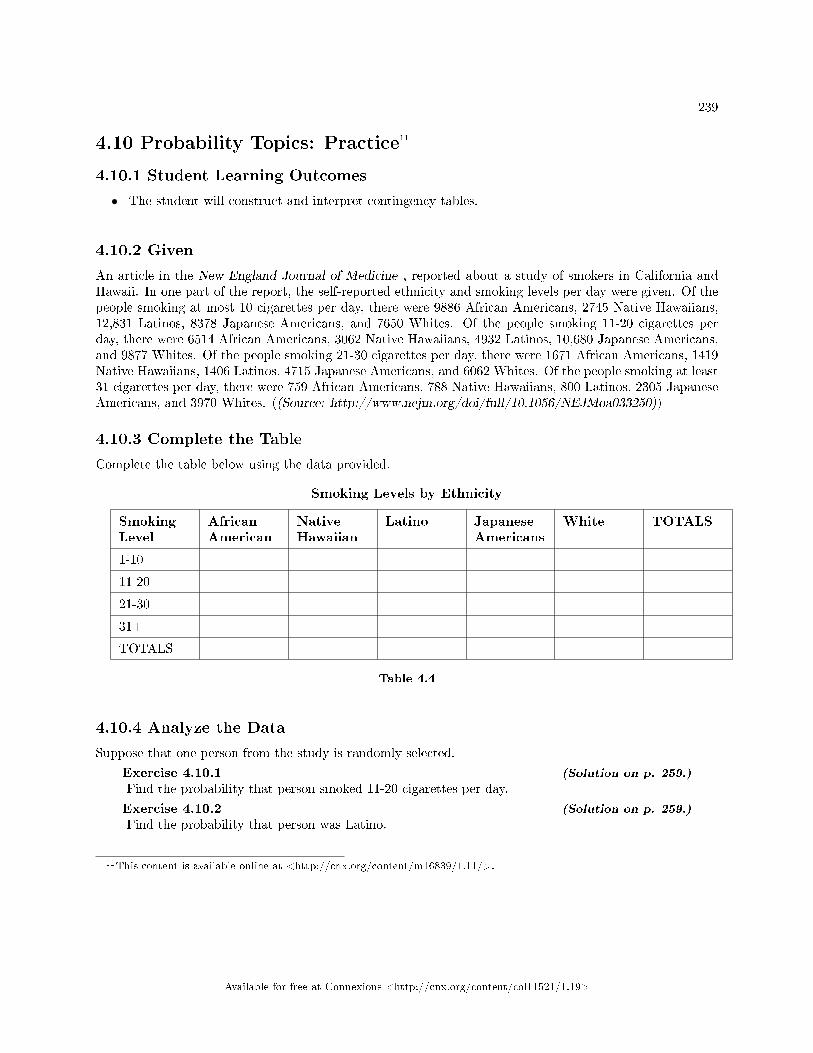
239
4.10 Probability Topics: Practice11
4.10.1 Student Learning Outcomes
• The student will construct and interpret contingency tables.
4.10.2 Given
An article in the New England Journal of Medicine , reported about a study of smokers in California andHawaii. In one part of the report, the self-reported ethnicity and smoking levels per day were given. Of thepeople smoking at most 10 cigarettes per day, there were 9886 African Americans, 2745 Native Hawaiians,12,831 Latinos, 8378 Japanese Americans, and 7650 Whites. Of the people smoking 11-20 cigarettes perday, there were 6514 African Americans, 3062 Native Hawaiians, 4932 Latinos, 10,680 Japanese Americans,and 9877 Whites. Of the people smoking 21-30 cigarettes per day, there were 1671 African Americans, 1419Native Hawaiians, 1406 Latinos, 4715 Japanese Americans, and 6062 Whites. Of the people smoking at least31 cigarettes per day, there were 759 African Americans, 788 Native Hawaiians, 800 Latinos, 2305 JapaneseAmericans, and 3970 Whites. ((Source: http://www.nejm.org/doi/full/10.1056/NEJMoa033250))
4.10.3 Complete the Table
Complete the table below using the data provided.
Smoking Levels by Ethnicity
SmokingLevel
AfricanAmerican
NativeHawaiian
Latino JapaneseAmericans
White TOTALS
1-10
11-20
21-30
31+
TOTALS
Table 4.4
4.10.4 Analyze the Data
Suppose that one person from the study is randomly selected.
Exercise 4.10.1 (Solution on p. 259.)
Find the probability that person smoked 11-20 cigarettes per day.
Exercise 4.10.2 (Solution on p. 259.)
Find the probability that person was Latino.
11This content is available online at <http://cnx.org/content/m16839/1.11/>.
Available for free at Connexions <http://cnx.org/content/col11521/1.19>
240 CHAPTER 4. PROBABILITY TOPICS
4.10.5 Discussion Questions
Exercise 4.10.3 (Solution on p. 259.)
In words, explain what it means to pick one person from the study and that person is �JapaneseAmerican AND smokes 21-30 cigarettes per day.� Also, �nd the probability.
Exercise 4.10.4 (Solution on p. 259.)
In words, explain what it means to pick one person from the study and that person is �JapaneseAmerican OR smokes 21-30 cigarettes per day.� Also, �nd the probability.
Exercise 4.10.5 (Solution on p. 259.)
In words, explain what it means to pick one person from the study and that person is �JapaneseAmerican GIVEN that person smokes 21-30 cigarettes per day.� Also, �nd the probability.
Exercise 4.10.6Prove that smoking level/day and ethnicity are dependent events.
Available for free at Connexions <http://cnx.org/content/col11521/1.19>
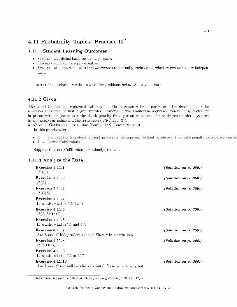
241
4.11 Probability Topics: Practice II12
4.11.1 Student Learning Outcomes
• Students will de�ne basic probability terms.• Students will calculate probabilities.• Students will determine whether two events are mutually exclusive or whether two events are indepen-
dent.
note: Use probability rules to solve the problems below. Show your work.
4.11.2 Given
48% of all Californians registered voters prefer life in prison without parole over the death penalty fora person convicted of �rst degree murder. Among Latino California registered voters, 55% prefer lifein prison without parole over the death penalty for a person convicted of �rst degree murder. (Source:http://�eld.com/�eldpollonline/subscribers/Rls2393.pdf ).37.6% of all Californians are Latino (Source: U.S. Census Bureau).
In this problem, let:
• C = Californians (registered voters) preferring life in prison without parole over the death penalty for a person convicted of first degree murder• L = Latino Californians
Suppose that one Californian is randomly selected.
4.11.3 Analyze the Data
Exercise 4.11.1 (Solution on p. 259.)
P (C) =Exercise 4.11.2 (Solution on p. 259.)
P (L) =Exercise 4.11.3 (Solution on p. 259.)
P (C|L) =Exercise 4.11.4In words, what is " C | L"?Exercise 4.11.5 (Solution on p. 259.)
P (L AND C) =Exercise 4.11.6In words, what is �L and C�?
Exercise 4.11.7 (Solution on p. 259.)
Are L and C independent events? Show why or why not.
Exercise 4.11.8 (Solution on p. 260.)
P (L OR C) =Exercise 4.11.9In words, what is �L or C�?
Exercise 4.11.10 (Solution on p. 260.)
Are L and C mutually exclusive events? Show why or why not.
12This content is available online at <http://cnx.org/content/m16840/1.12/>.
Available for free at Connexions <http://cnx.org/content/col11521/1.19>
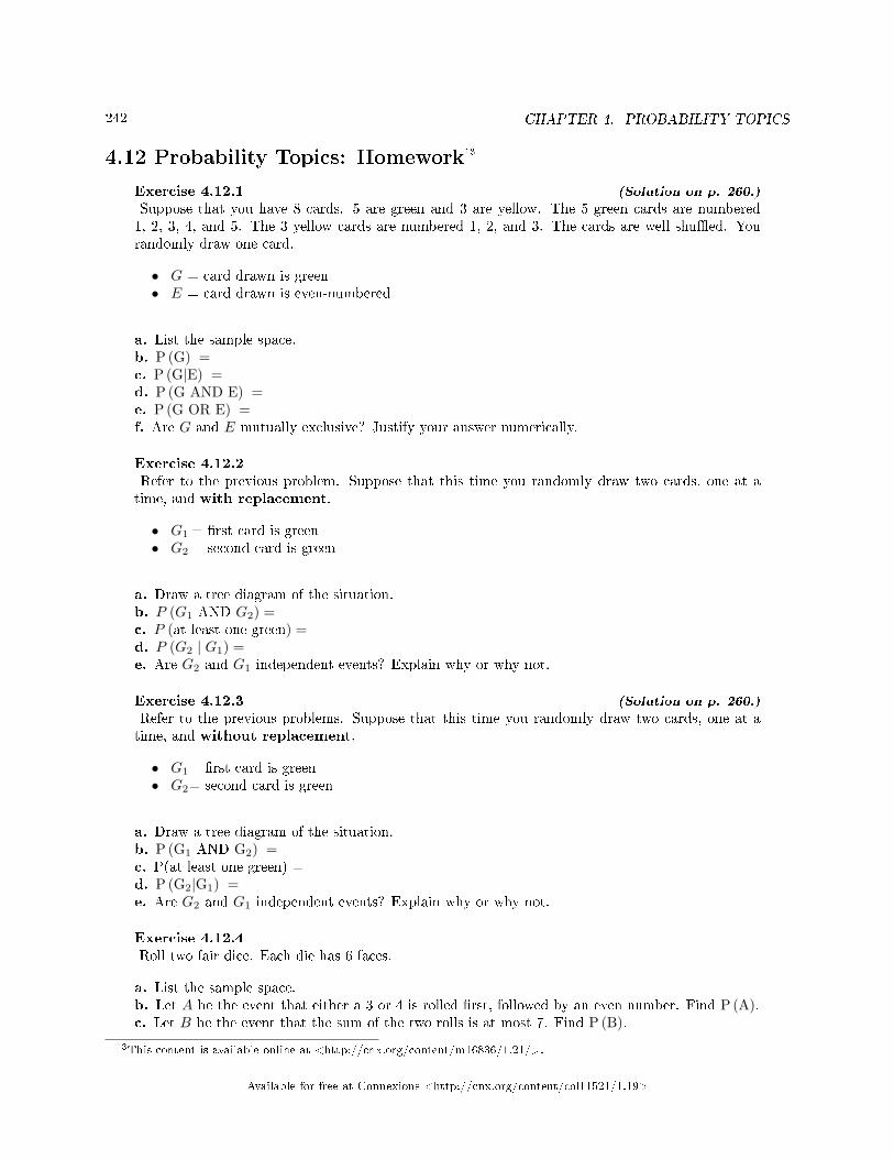
242 CHAPTER 4. PROBABILITY TOPICS
4.12 Probability Topics: Homework13
Exercise 4.12.1 (Solution on p. 260.)
Suppose that you have 8 cards. 5 are green and 3 are yellow. The 5 green cards are numbered1, 2, 3, 4, and 5. The 3 yellow cards are numbered 1, 2, and 3. The cards are well shu�ed. Yourandomly draw one card.
• G = card drawn is green• E = card drawn is even-numbered
a. List the sample space.b. P (G) =c. P (G|E) =d. P (G AND E) =e. P (G OR E) =f. Are G and E mutually exclusive? Justify your answer numerically.
Exercise 4.12.2Refer to the previous problem. Suppose that this time you randomly draw two cards, one at atime, and with replacement.
• G1 = �rst card is green• G2 = second card is green
a. Draw a tree diagram of the situation.b. P (G1 AND G2) =c. P (at least one green) =d. P (G2 | G1) =e. Are G2 and G1 independent events? Explain why or why not.
Exercise 4.12.3 (Solution on p. 260.)
Refer to the previous problems. Suppose that this time you randomly draw two cards, one at atime, and without replacement.
• G1= �rst card is green• G2= second card is green
a. Draw a tree diagram of the situation.b. P (G1 AND G2) =c. P(at least one green) =d. P (G2|G1) =e. Are G2 and G1 independent events? Explain why or why not.
Exercise 4.12.4Roll two fair dice. Each die has 6 faces.
a. List the sample space.b. Let A be the event that either a 3 or 4 is rolled �rst, followed by an even number. Find P (A).c. Let B be the event that the sum of the two rolls is at most 7. Find P (B).
13This content is available online at <http://cnx.org/content/m16836/1.21/>.
Available for free at Connexions <http://cnx.org/content/col11521/1.19>
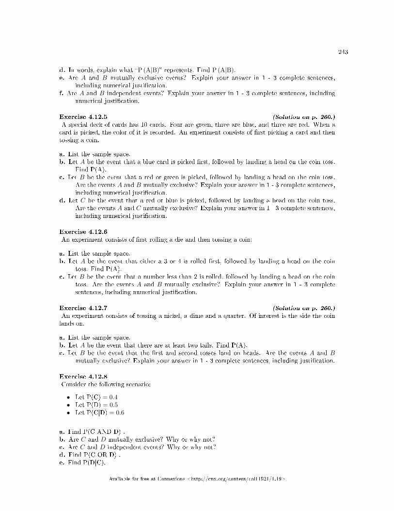
243
d. In words, explain what �P (A|B)� represents. Find P (A|B).e. Are A and B mutually exclusive events? Explain your answer in 1 - 3 complete sentences,
including numerical justi�cation.f. Are A and B independent events? Explain your answer in 1 - 3 complete sentences, including
numerical justi�cation.
Exercise 4.12.5 (Solution on p. 260.)
A special deck of cards has 10 cards. Four are green, three are blue, and three are red. When acard is picked, the color of it is recorded. An experiment consists of �rst picking a card and thentossing a coin.
a. List the sample space.b. Let A be the event that a blue card is picked �rst, followed by landing a head on the coin toss.
Find P(A).c. Let B be the event that a red or green is picked, followed by landing a head on the coin toss.
Are the events A and B mutually exclusive? Explain your answer in 1 - 3 complete sentences,including numerical justi�cation.
d. Let C be the event that a red or blue is picked, followed by landing a head on the coin toss.Are the events A and C mutually exclusive? Explain your answer in 1 - 3 complete sentences,including numerical justi�cation.
Exercise 4.12.6An experiment consists of �rst rolling a die and then tossing a coin:
a. List the sample space.b. Let A be the event that either a 3 or 4 is rolled �rst, followed by landing a head on the coin
toss. Find P(A).c. Let B be the event that a number less than 2 is rolled, followed by landing a head on the coin
toss. Are the events A and B mutually exclusive? Explain your answer in 1 - 3 completesentences, including numerical justi�cation.
Exercise 4.12.7 (Solution on p. 260.)
An experiment consists of tossing a nickel, a dime and a quarter. Of interest is the side the coinlands on.
a. List the sample space.b. Let A be the event that there are at least two tails. Find P(A).c. Let B be the event that the �rst and second tosses land on heads. Are the events A and B
mutually exclusive? Explain your answer in 1 - 3 complete sentences, including justi�cation.
Exercise 4.12.8Consider the following scenario:
• Let P(C) = 0.4• Let P(D) = 0.5• Let P(C|D) = 0.6
a. Find P(C AND D) .b. Are C and D mutually exclusive? Why or why not?c. Are C and D independent events? Why or why not?d. Find P(C OR D) .e. Find P(D|C).
Available for free at Connexions <http://cnx.org/content/col11521/1.19>
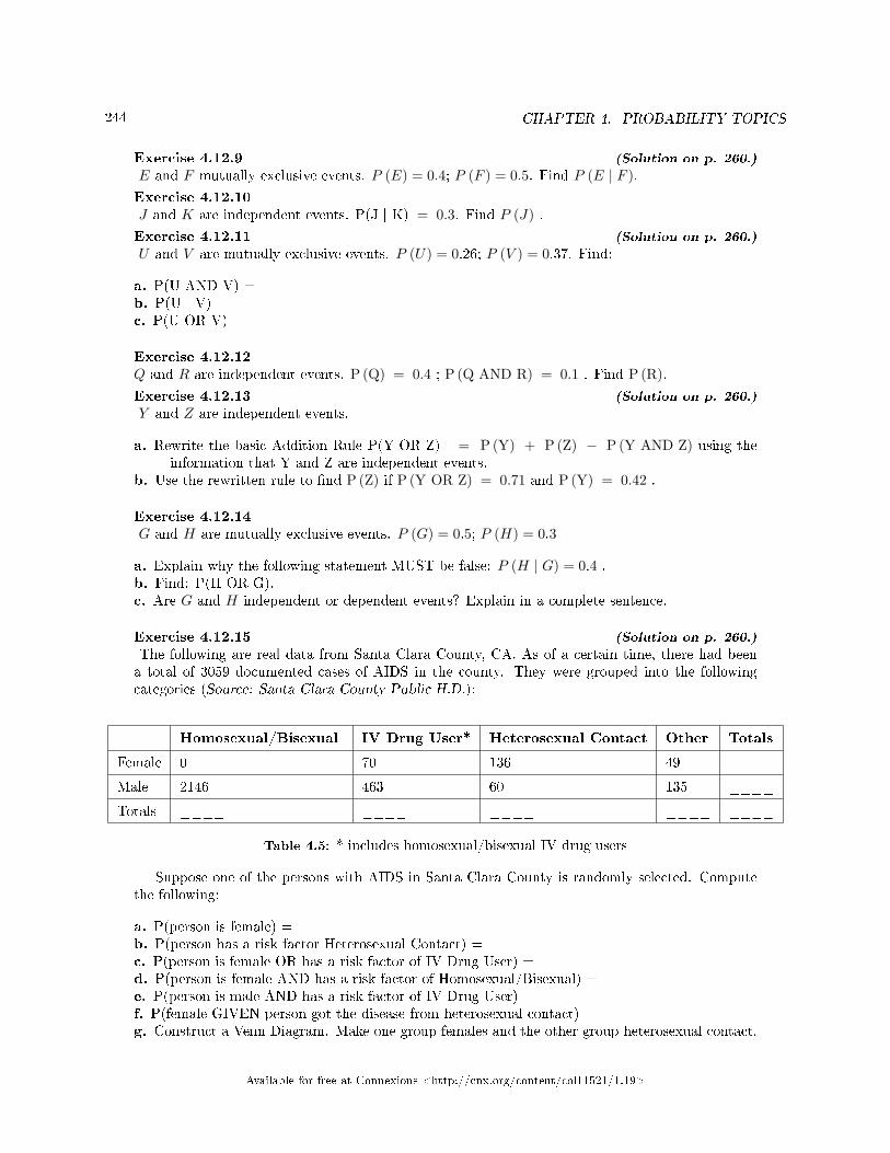
244 CHAPTER 4. PROBABILITY TOPICS
Exercise 4.12.9 (Solution on p. 260.)
E and F mutually exclusive events. P (E) = 0.4; P (F ) = 0.5. Find P (E | F ).Exercise 4.12.10J and K are independent events. P(J | K) = 0.3. Find P (J) .Exercise 4.12.11 (Solution on p. 260.)
U and V are mutually exclusive events. P (U) = 0.26; P (V ) = 0.37. Find:
a. P(U AND V) =b. P(U | V) =c. P(U OR V) =
Exercise 4.12.12Q and R are independent events. P (Q) = 0.4 ; P (Q AND R) = 0.1 . Find P (R).Exercise 4.12.13 (Solution on p. 260.)
Y and Z are independent events.
a. Rewrite the basic Addition Rule P(Y OR Z) = P (Y) + P (Z) − P (Y AND Z) using theinformation that Y and Z are independent events.
b. Use the rewritten rule to �nd P (Z) if P (Y OR Z) = 0.71 and P (Y) = 0.42 .
Exercise 4.12.14G and H are mutually exclusive events. P (G) = 0.5; P (H) = 0.3
a. Explain why the following statement MUST be false: P (H | G) = 0.4 .b. Find: P(H OR G).c. Are G and H independent or dependent events? Explain in a complete sentence.
Exercise 4.12.15 (Solution on p. 260.)
The following are real data from Santa Clara County, CA. As of a certain time, there had beena total of 3059 documented cases of AIDS in the county. They were grouped into the followingcategories (Source: Santa Clara County Public H.D.):
Homosexual/Bisexual IV Drug User* Heterosexual Contact Other Totals
Female 0 70 136 49 ____
Male 2146 463 60 135 ____
Totals ____ ____ ____ ____ ____
Table 4.5: * includes homosexual/bisexual IV drug users
Suppose one of the persons with AIDS in Santa Clara County is randomly selected. Computethe following:
a. P(person is female) =b. P(person has a risk factor Heterosexual Contact) =c. P(person is female OR has a risk factor of IV Drug User) =d. P(person is female AND has a risk factor of Homosexual/Bisexual) =e. P(person is male AND has a risk factor of IV Drug User) =f. P(female GIVEN person got the disease from heterosexual contact) =g. Construct a Venn Diagram. Make one group females and the other group heterosexual contact.
Available for free at Connexions <http://cnx.org/content/col11521/1.19>
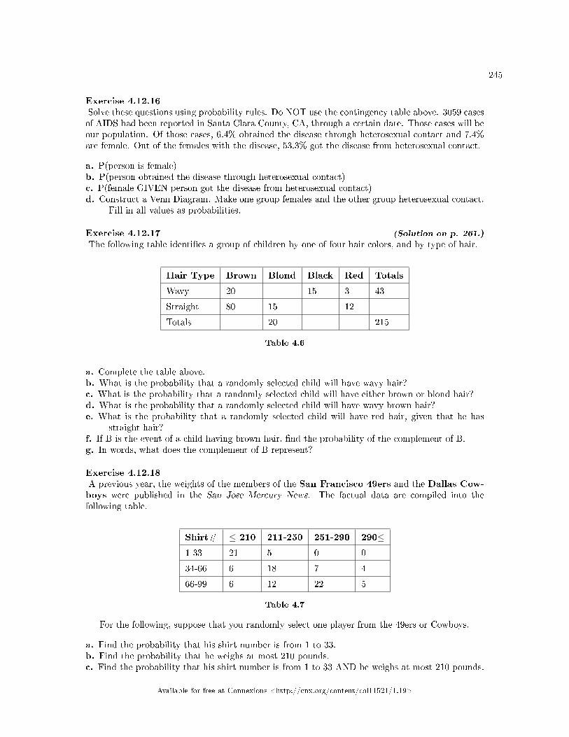
245
Exercise 4.12.16Solve these questions using probability rules. Do NOT use the contingency table above. 3059 casesof AIDS had been reported in Santa Clara County, CA, through a certain date. Those cases will beour population. Of those cases, 6.4% obtained the disease through heterosexual contact and 7.4%are female. Out of the females with the disease, 53.3% got the disease from heterosexual contact.
a. P(person is female) =b. P(person obtained the disease through heterosexual contact) =c. P(female GIVEN person got the disease from heterosexual contact) =d. Construct a Venn Diagram. Make one group females and the other group heterosexual contact.
Fill in all values as probabilities.
Exercise 4.12.17 (Solution on p. 261.)
The following table identi�es a group of children by one of four hair colors, and by type of hair.
Hair Type Brown Blond Black Red Totals
Wavy 20 15 3 43
Straight 80 15 12
Totals 20 215
Table 4.6
a. Complete the table above.b. What is the probability that a randomly selected child will have wavy hair?c. What is the probability that a randomly selected child will have either brown or blond hair?d. What is the probability that a randomly selected child will have wavy brown hair?e. What is the probability that a randomly selected child will have red hair, given that he has
straight hair?f. If B is the event of a child having brown hair, �nd the probability of the complement of B.g. In words, what does the complement of B represent?
Exercise 4.12.18A previous year, the weights of the members of the San Francisco 49ers and the Dallas Cow-boys were published in the San Jose Mercury News. The factual data are compiled into thefollowing table.
Shirt# ≤ 210 211-250 251-290 290≤1-33 21 5 0 0
34-66 6 18 7 4
66-99 6 12 22 5
Table 4.7
For the following, suppose that you randomly select one player from the 49ers or Cowboys.
a. Find the probability that his shirt number is from 1 to 33.b. Find the probability that he weighs at most 210 pounds.c. Find the probability that his shirt number is from 1 to 33 AND he weighs at most 210 pounds.
Available for free at Connexions <http://cnx.org/content/col11521/1.19>
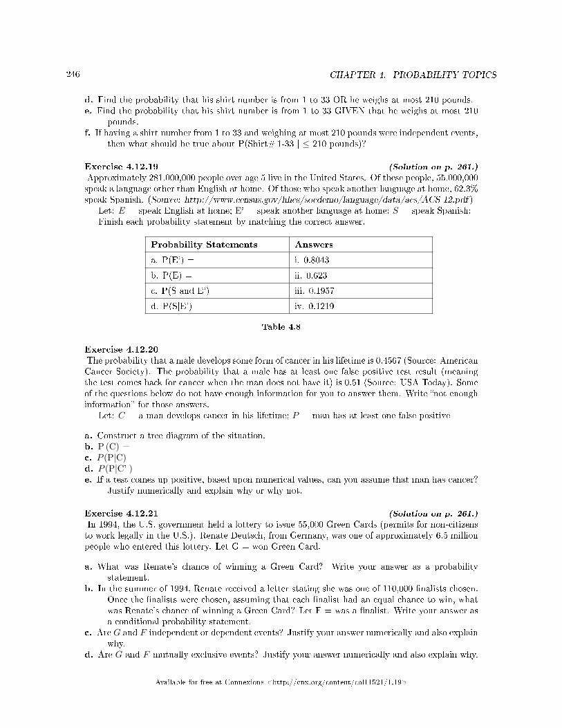
246 CHAPTER 4. PROBABILITY TOPICS
d. Find the probability that his shirt number is from 1 to 33 OR he weighs at most 210 pounds.e. Find the probability that his shirt number is from 1 to 33 GIVEN that he weighs at most 210
pounds.f. If having a shirt number from 1 to 33 and weighing at most 210 pounds were independent events,
then what should be true about P(Shirt# 1-33 | ≤ 210 pounds)?
Exercise 4.12.19 (Solution on p. 261.)
Approximately 281,000,000 people over age 5 live in the United States. Of these people, 55,000,000speak a language other than English at home. Of those who speak another language at home, 62.3%speak Spanish. (Source: http://www.census.gov/hhes/socdemo/language/data/acs/ACS-12.pdf )
Let: E = speak English at home; E' = speak another language at home; S = speak Spanish;Finish each probability statement by matching the correct answer.
Probability Statements Answers
a. P(E') = i. 0.8043
b. P(E) = ii. 0.623
c. P(S and E') = iii. 0.1957
d. P(S|E') = iv. 0.1219
Table 4.8
Exercise 4.12.20The probability that a male develops some form of cancer in his lifetime is 0.4567 (Source: AmericanCancer Society). The probability that a male has at least one false positive test result (meaningthe test comes back for cancer when the man does not have it) is 0.51 (Source: USA Today). Someof the questions below do not have enough information for you to answer them. Write �not enoughinformation� for those answers.
Let: C = a man develops cancer in his lifetime; P = man has at least one false positive
a. Construct a tree diagram of the situation.b. P (C) =c. P (P|C) =d. P (P|C' ) =e. If a test comes up positive, based upon numerical values, can you assume that man has cancer?
Justify numerically and explain why or why not.
Exercise 4.12.21 (Solution on p. 261.)
In 1994, the U.S. government held a lottery to issue 55,000 Green Cards (permits for non-citizensto work legally in the U.S.). Renate Deutsch, from Germany, was one of approximately 6.5 millionpeople who entered this lottery. Let G = won Green Card.
a. What was Renate's chance of winning a Green Card? Write your answer as a probabilitystatement.
b. In the summer of 1994, Renate received a letter stating she was one of 110,000 �nalists chosen.Once the �nalists were chosen, assuming that each �nalist had an equal chance to win, whatwas Renate's chance of winning a Green Card? Let F = was a �nalist. Write your answer asa conditional probability statement.
c. Are G and F independent or dependent events? Justify your answer numerically and also explainwhy.
d. Are G and F mutually exclusive events? Justify your answer numerically and also explain why.
Available for free at Connexions <http://cnx.org/content/col11521/1.19>
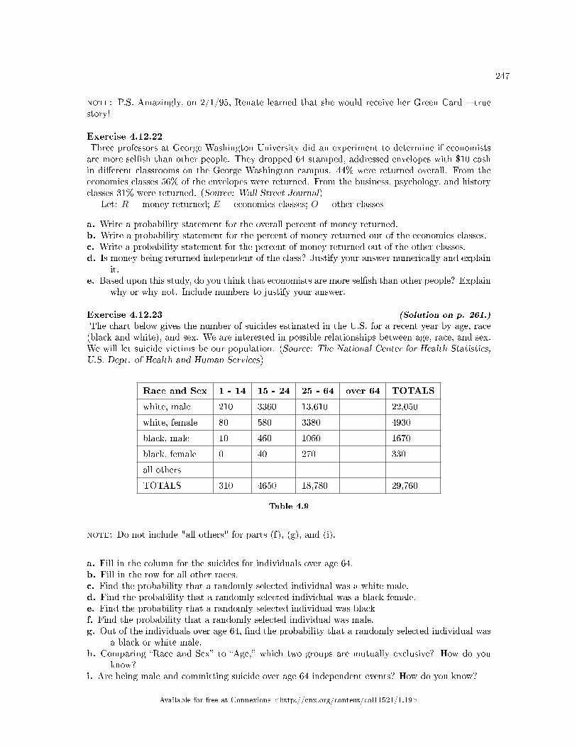
247
note: P.S. Amazingly, on 2/1/95, Renate learned that she would receive her Green Card � truestory!
Exercise 4.12.22Three professors at George Washington University did an experiment to determine if economistsare more sel�sh than other people. They dropped 64 stamped, addressed envelopes with $10 cashin di�erent classrooms on the George Washington campus. 44% were returned overall. From theeconomics classes 56% of the envelopes were returned. From the business, psychology, and historyclasses 31% were returned. (Source: Wall Street Journal)
Let: R = money returned; E = economics classes; O = other classes
a. Write a probability statement for the overall percent of money returned.b. Write a probability statement for the percent of money returned out of the economics classes.c. Write a probability statement for the percent of money returned out of the other classes.d. Is money being returned independent of the class? Justify your answer numerically and explain
it.e. Based upon this study, do you think that economists are more sel�sh than other people? Explain
why or why not. Include numbers to justify your answer.
Exercise 4.12.23 (Solution on p. 261.)
The chart below gives the number of suicides estimated in the U.S. for a recent year by age, race(black and white), and sex. We are interested in possible relationships between age, race, and sex.We will let suicide victims be our population. (Source: The National Center for Health Statistics,U.S. Dept. of Health and Human Services)
Race and Sex 1 - 14 15 - 24 25 - 64 over 64 TOTALS
white, male 210 3360 13,610 22,050
white, female 80 580 3380 4930
black, male 10 460 1060 1670
black, female 0 40 270 330
all others
TOTALS 310 4650 18,780 29,760
Table 4.9
note: Do not include "all others" for parts (f), (g), and (i).
a. Fill in the column for the suicides for individuals over age 64.b. Fill in the row for all other races.c. Find the probability that a randomly selected individual was a white male.d. Find the probability that a randomly selected individual was a black female.e. Find the probability that a randomly selected individual was blackf. Find the probability that a randomly selected individual was male.g. Out of the individuals over age 64, �nd the probability that a randomly selected individual was
a black or white male.h. Comparing �Race and Sex� to �Age,� which two groups are mutually exclusive? How do you
know?i. Are being male and committing suicide over age 64 independent events? How do you know?
Available for free at Connexions <http://cnx.org/content/col11521/1.19>
248 CHAPTER 4. PROBABILITY TOPICS
The next two questions refer to the following: The percent of licensed U.S. drivers (from a recentyear) that are female is 48.60. Of the females, 5.03% are age 19 and under; 81.36% are age 20 - 64; 13.61%are age 65 or over. Of the licensed U.S. male drivers, 5.04% are age 19 and under; 81.43% are age 20 - 64;13.53% are age 65 or over. (Source: Federal Highway Administration, U.S. Dept. of Transportation)
Exercise 4.12.24Complete the following:
a. Construct a table or a tree diagram of the situation.b. P(driver is female) =c. P(driver is age 65 or over | driver is female) =d. P(driver is age 65 or over AND female) =e. In words, explain the di�erence between the probabilities in part (c) and part (d).f. P(driver is age 65 or over) =g. Are being age 65 or over and being female mutually exclusive events? How do you know
Exercise 4.12.25 (Solution on p. 261.)
Suppose that 10,000 U.S. licensed drivers are randomly selected.
a. How many would you expect to be male?b. Using the table or tree diagram from the previous exercise, construct a contingency table of
gender versus age group.c. Using the contingency table, �nd the probability that out of the age 20 - 64 group, a randomly
selected driver is female.
Exercise 4.12.26Approximately 86.5% of Americans commute to work by car, truck or van. Out of that group, 84.6%drive alone and 15.4% drive in a carpool. Approximately 3.9% walk to work and approximately 5.3%take public transportation. (Source: Bureau of the Census, U.S. Dept. of Commerce. Disregardrounding approximations.)
a. Construct a table or a tree diagram of the situation. Include a branch for all other modes oftransportation to work.
b. Assuming that the walkers walk alone, what percent of all commuters travel alone to work?c. Suppose that 1000 workers are randomly selected. How many would you expect to travel alone
to work?d. Suppose that 1000 workers are randomly selected. How many would you expect to drive in a
carpool?
Exercise 4.12.27Explain what is wrong with the following statements. Use complete sentences.
a. If there's a 60% chance of rain on Saturday and a 70% chance of rain on Sunday, then there's a130% chance of rain over the weekend.
b. The probability that a baseball player hits a home run is greater than the probability that hegets a successful hit.
Available for free at Connexions <http://cnx.org/content/col11521/1.19>
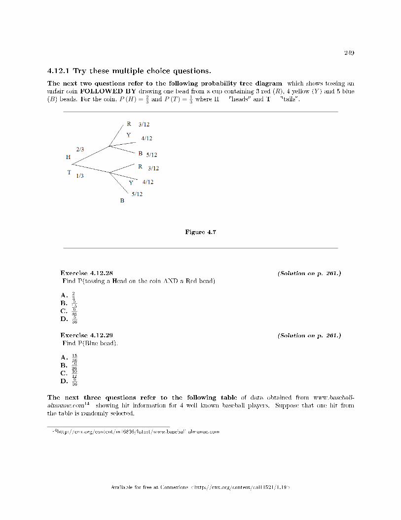
249
4.12.1 Try these multiple choice questions.
The next two questions refer to the following probability tree diagram which shows tossing anunfair coin FOLLOWED BY drawing one bead from a cup containing 3 red (R), 4 yellow (Y ) and 5 blue(B) beads. For the coin, P (H) = 2
3 and P (T ) = 13 where H = "heads" and T = "tails�.
Figure 4.7
Exercise 4.12.28 (Solution on p. 261.)
Find P(tossing a Head on the coin AND a Red bead)
A. 23
B. 515
C. 636
D. 536
Exercise 4.12.29 (Solution on p. 261.)
Find P(Blue bead).
A. 1536
B. 1036
C. 1012
D. 636
The next three questions refer to the following table of data obtained from www.baseball-almanac.com14 showing hit information for 4 well known baseball players. Suppose that one hit fromthe table is randomly selected.
14http://cnx.org/content/m16836/latest/www.baseball-almanac.com
Available for free at Connexions <http://cnx.org/content/col11521/1.19>
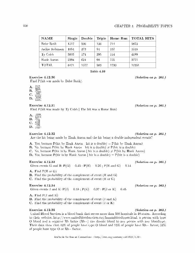
250 CHAPTER 4. PROBABILITY TOPICS
NAME Single Double Triple Home Run TOTAL HITS
Babe Ruth 1517 506 136 714 2873
Jackie Robinson 1054 273 54 137 1518
Ty Cobb 3603 174 295 114 4189
Hank Aaron 2294 624 98 755 3771
TOTAL 8471 1577 583 1720 12351
Table 4.10
Exercise 4.12.30 (Solution on p. 261.)
Find P(hit was made by Babe Ruth).
A. 15182873
B. 287312351
C. 58312351
D. 418912351
Exercise 4.12.31 (Solution on p. 261.)
Find P(hit was made by Ty Cobb | The hit was a Home Run)
A. 418912351
B. 1141720
C. 17204189
D. 11412351
Exercise 4.12.32 (Solution on p. 261.)
Are the hit being made by Hank Aaron and the hit being a double independent events?
A. Yes, because P(hit by Hank Aaron | hit is a double) = P(hit by Hank Aaron)B. No, because P(hit by Hank Aaron | hit is a double) 6= P(hit is a double)C. No, because P(hit is by Hank Aaron | hit is a double) 6= P(hit by Hank Aaron)D. Yes, because P(hit is by Hank Aaron | hit is a double) = P(hit is a double)
Exercise 4.12.33 (Solution on p. 261.)
Given events G and H: P(G) = 0.43 ; P(H) = 0.26 ; P(H and G) = 0.14
A. Find P(H or G)B. Find the probability of the complement of event (H and G)C. Find the probability of the complement of event (H or G)
Exercise 4.12.34 (Solution on p. 262.)
Given events J and K: P(J) = 0.18 ; P(K) = 0.37 ; P(J or K) = 0.45
A. Find P(J and K)B. Find the probability of the complement of event (J and K)C. Find the probability of the complement of event (J or K)
Exercise 4.12.35 (Solution on p. 262.)
United Blood Services is a blood bank that serves more than 500 hospitals in 18 states. Accordingto their website, http://www.unitedbloodservices.org/humanbloodtypes.html, a person with typeO blood and a negative Rh factor (Rh−) can donate blood to any person with any bloodtype.Their data show that 43% of people have type O blood and 15% of people have Rh− factor; 52%of people have type O or Rh− factor.
Available for free at Connexions <http://cnx.org/content/col11521/1.19>
251
A. Find the probability that a person has both type O blood and the Rh− factorB. Find the probability that a person does NOT have both type O blood and the Rh− factor.
Exercise 4.12.36 (Solution on p. 262.)
At a college, 72% of courses have �nal exams and 46% of courses require research papers. Supposethat 32% of courses have a research paper and a �nal exam. Let F be the event that a course hasa �nal exam. Let R be the event that a course requires a research paper.
A. Find the probability that a course has a �nal exam or a research project.B. Find the probability that a course has NEITHER of these two requirements.
Exercise 4.12.37 (Solution on p. 262.)
In a box of assorted cookies, 36% contain chocolate and 12% contain nuts. Of those, 8% containboth chocolate and nuts. Sean is allergic to both chocolate and nuts.
A. Find the probability that a cookie contains chocolate or nuts (he can't eat it).B. Find the probability that a cookie does not contain chocolate or nuts (he can eat it).
Exercise 4.12.38 (Solution on p. 262.)
A college �nds that 10% of students have taken a distance learning class and that 40% of studentsare part time students. Of the part time students, 20% have taken a distance learning class. Let D= event that a student takes a distance learning class and E = event that a student is a part timestudent
A. Find P(D and E)B. Find P(E | D)C. Find P(D or E)D. Using an appropriate test, show whether D and E are independent.E. Using an appropriate test, show whether D and E are mutually exclusive.
Exercise 4.12.39 (Solution on p. 262.)
When the Euro coin was introduced in 2002, two math professors had their statistics students testwhether the Belgian 1 Euro coin was a fair coin. They spun the coin rather than tossing it, and itwas found that out of 250 spins, 140 showed a head (event H) while 110 showed a tail (event T).Therefore, they claim that this is not a fair coin.
A. Based on the data above, �nd P(H) and P(T).B. Use a tree to �nd the probabilities of each possible outcome for the experiment of tossing the
coin twice.C. Use the tree to �nd the probability of obtaining exactly one head in two tosses of the coin.D. Use the tree to �nd the probability of obtaining at least one head.
Exercise 4.12.40A box of cookies contains 3 chocolate and 7 butter cookies. Miguel randomly selects a cookie andeats it. Then he randomly selects another cookie and eats it also. (How many cookies did he take?)
A. Draw the tree that represents the possibilities for the cookie selections. Write the probabilitiesalong each branch of the tree.
B. Are the probabilities for the �avor of the SECOND cookie that Miguel selects independent ofhis �rst selection? Explain.
C. For each complete path through the tree, write the event it represents and �nd the probabilities.D. Let S be the event that both cookies selected were the same �avor. Find P(S).
Available for free at Connexions <http://cnx.org/content/col11521/1.19>
252 CHAPTER 4. PROBABILITY TOPICS
E. Let T be the event that both cookies selected were di�erent �avors. Find P(T) by two di�erentmethods: by using the complement rule and by using the branches of the tree. Your answersshould be the same with both methods.
F. Let U be the event that the second cookie selected is a butter cookie. Find P(U).
**Exercises 33 - 40 contributed by Roberta Bloom
Available for free at Connexions <http://cnx.org/content/col11521/1.19>
253
4.13 Probability Topics: Review15
The �rst six exercises refer to the following study: In a survey of 100 stocks on NASDAQ, the averagepercent increase for the past year was 9% for NASDAQ stocks. Answer the following:
Exercise 4.13.1 (Solution on p. 262.)
The �average increase� for all NASDAQ stocks is the:
A. PopulationB. StatisticC. ParameterD. SampleE. Variable
Exercise 4.13.2 (Solution on p. 262.)
All of the NASDAQ stocks are the:
A. PopulationB. StatisticC. ParameterD. SampleE. Variable
Exercise 4.13.3 (Solution on p. 262.)
9% is the:
A. PopulationB. StatisticC. ParameterD. SampleE. Variable
Exercise 4.13.4 (Solution on p. 263.)
The 100 NASDAQ stocks in the survey are the:
A. PopulationB. StatisticC. ParameterD. SampleE. Variable
Exercise 4.13.5 (Solution on p. 263.)
The percent increase for one stock in the survey is the:
A. PopulationB. StatisticC. ParameterD. SampleE. Variable
15This content is available online at <http://cnx.org/content/m16842/1.9/>.
Available for free at Connexions <http://cnx.org/content/col11521/1.19>
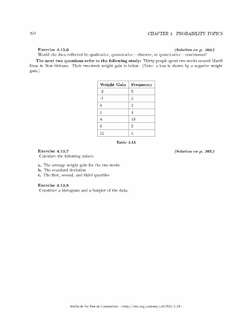
254 CHAPTER 4. PROBABILITY TOPICS
Exercise 4.13.6 (Solution on p. 263.)
Would the data collected be qualitative, quantitative � discrete, or quantitative � continuous?
The next two questions refer to the following study: Thirty people spent two weeks around MardiGras in New Orleans. Their two-week weight gain is below. (Note: a loss is shown by a negative weightgain.)
Weight Gain Frequency
-2 3
-1 5
0 2
1 4
4 13
6 2
11 1
Table 4.11
Exercise 4.13.7 (Solution on p. 263.)
Calculate the following values:
a. The average weight gain for the two weeksb. The standard deviationc. The �rst, second, and third quartiles
Exercise 4.13.8Construct a histogram and a boxplot of the data.
Available for free at Connexions <http://cnx.org/content/col11521/1.19>
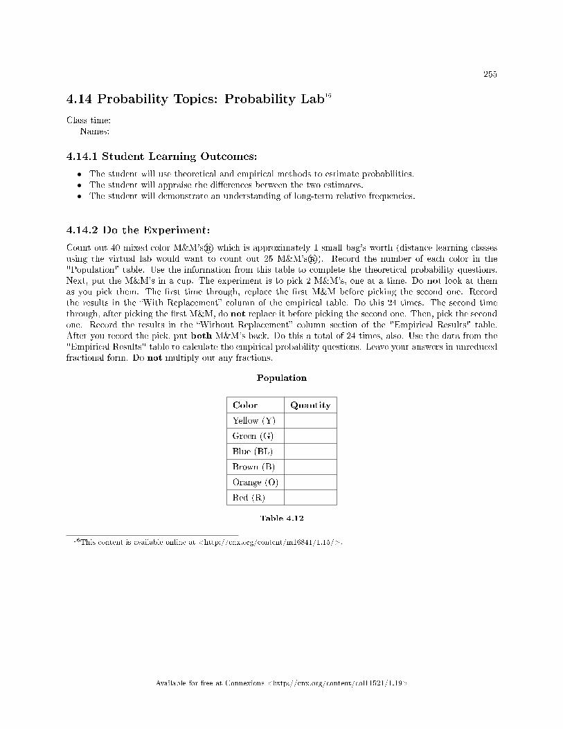
255
4.14 Probability Topics: Probability Lab16
Class time:Names:
4.14.1 Student Learning Outcomes:
• The student will use theoretical and empirical methods to estimate probabilities.• The student will appraise the di�erences between the two estimates.• The student will demonstrate an understanding of long-term relative frequencies.
4.14.2 Do the Experiment:
Count out 40 mixed-color M&M's® which is approximately 1 small bag's worth (distance learning classesusing the virtual lab would want to count out 25 M&M's®). Record the number of each color in the"Population" table. Use the information from this table to complete the theoretical probability questions.Next, put the M&M's in a cup. The experiment is to pick 2 M&M's, one at a time. Do not look at themas you pick them. The �rst time through, replace the �rst M&M before picking the second one. Recordthe results in the �With Replacement� column of the empirical table. Do this 24 times. The second timethrough, after picking the �rst M&M, do not replace it before picking the second one. Then, pick the secondone. Record the results in the �Without Replacement� column section of the "Empirical Results" table.After you record the pick, put both M&M's back. Do this a total of 24 times, also. Use the data from the"Empirical Results" table to calculate the empirical probability questions. Leave your answers in unreducedfractional form. Do not multiply out any fractions.
Population
Color Quantity
Yellow (Y)
Green (G)
Blue (BL)
Brown (B)
Orange (O)
Red (R)
Table 4.12
16This content is available online at <http://cnx.org/content/m16841/1.15/>.
Available for free at Connexions <http://cnx.org/content/col11521/1.19>
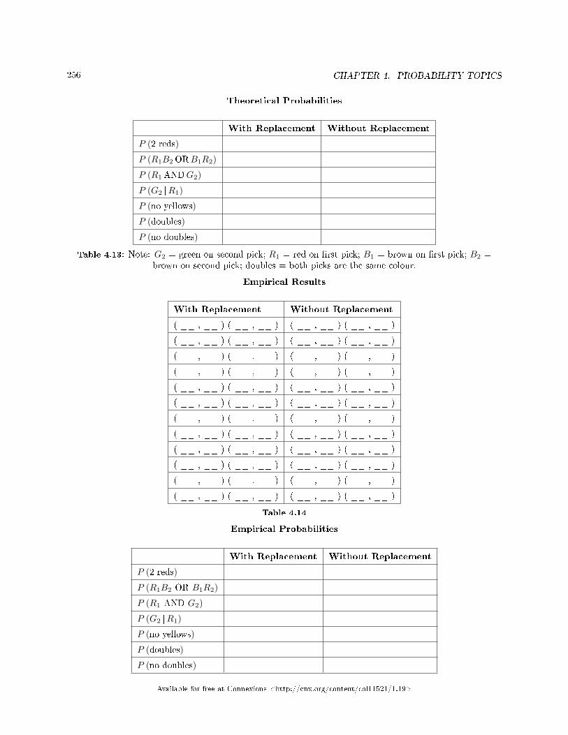
256 CHAPTER 4. PROBABILITY TOPICS
Theoretical Probabilities
With Replacement Without Replacement
P (2 reds)
P (R1B2 ORB1R2)
P (R1 ANDG2)
P (G2 |R1)
P (no yellows)
P (doubles)
P (no doubles)
Table 4.13: Note: G2 = green on second pick; R1 = red on �rst pick; B1 = brown on �rst pick; B2 =brown on second pick; doubles = both picks are the same colour.
Empirical Results
With Replacement Without Replacement
( __ , __ ) ( __ , __ ) ( __ , __ ) ( __ , __ )
( __ , __ ) ( __ , __ ) ( __ , __ ) ( __ , __ )
( __ , __ ) ( __ , __ ) ( __ , __ ) ( __ , __ )
( __ , __ ) ( __ , __ ) ( __ , __ ) ( __ , __ )
( __ , __ ) ( __ , __ ) ( __ , __ ) ( __ , __ )
( __ , __ ) ( __ , __ ) ( __ , __ ) ( __ , __ )
( __ , __ ) ( __ , __ ) ( __ , __ ) ( __ , __ )
( __ , __ ) ( __ , __ ) ( __ , __ ) ( __ , __ )
( __ , __ ) ( __ , __ ) ( __ , __ ) ( __ , __ )
( __ , __ ) ( __ , __ ) ( __ , __ ) ( __ , __ )
( __ , __ ) ( __ , __ ) ( __ , __ ) ( __ , __ )
( __ , __ ) ( __ , __ ) ( __ , __ ) ( __ , __ )
Table 4.14
Empirical Probabilities
With Replacement Without Replacement
P (2 reds)
P (R1B2 OR B1R2)
P (R1 AND G2)
P (G2 |R1)
P (no yellows)
P (doubles)
P (no doubles)
Available for free at Connexions <http://cnx.org/content/col11521/1.19>
257
Table 4.15: Note:
4.14.3 Discussion Questions
1. Why are the �With Replacement� and �Without Replacement� probabilities di�erent?2. Convert P(no yellows) to decimal format for both Theoretical �With Replacement� and for Empirical
�With Replacement�. Round to 4 decimal places.
a. Theoretical �With Replacement�: P(no yellows) =b. Empirical �With Replacement�: P(no yellows) =c. Are the decimal values �close�? Did you expect them to be closer together or farther apart? Why?
3. If you increased the number of times you picked 2 M&M's to 240 times, why would empirical probabilityvalues change?
4. Would this change (see (3) above) cause the empirical probabilities and theoretical probabilities to becloser together or farther apart? How do you know?
5. Explain the di�erences in what P (G1 AND R2) and P (R1 |G2) represent. Hint: Think about thesample space for each probability.
Available for free at Connexions <http://cnx.org/content/col11521/1.19>
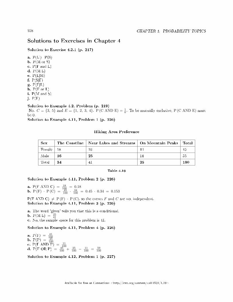
258 CHAPTER 4. PROBABILITY TOPICS
Solutions to Exercises in Chapter 4
Solution to Exercise 4.2.1 (p. 217)
a. P(L')=P(S)b. P(M or S)c. P(F and L)d. P(M|L)e. P(L|M)f. P(S|F)g. P(F|L)h. P(F or L)i. P(M and S)j. P(F)
Solution to Example 4.2, Problem (p. 219)No. C = {3, 5} and E = {1, 2, 3, 4}. P (C AND E) = 1
6 . To be mutually exclusive, P (C AND E) mustbe 0.Solution to Example 4.11, Problem 1 (p. 226)
Hiking Area Preference
Sex The Coastline Near Lakes and Streams On Mountain Peaks Total
Female 18 16 11 45
Male 16 25 14 55
Total 34 41 25 100
Table 4.16
Solution to Example 4.11, Problem 2 (p. 226)
a. P(F AND C) = 18100 = 0.18
b. P (F) · P (C) = 45100 ·
34100 = 0.45 · 0.34 = 0.153
P(F AND C) 6= P (F) · P (C), so the events F and C are not independent.Solution to Example 4.11, Problem 3 (p. 226)
a. The word 'given' tells you that this is a conditional.b. P(M|L) = 25
41c. No, the sample space for this problem is 41.
Solution to Example 4.11, Problem 4 (p. 226)
a. P(F) = 45100
b. P(P) = 25100
c. P(F AND P) = 11100
d. P(F OR P) = 45100 + 25
100 −11100 = 59
100
Solution to Example 4.12, Problem 1 (p. 227)
Available for free at Connexions <http://cnx.org/content/col11521/1.19>
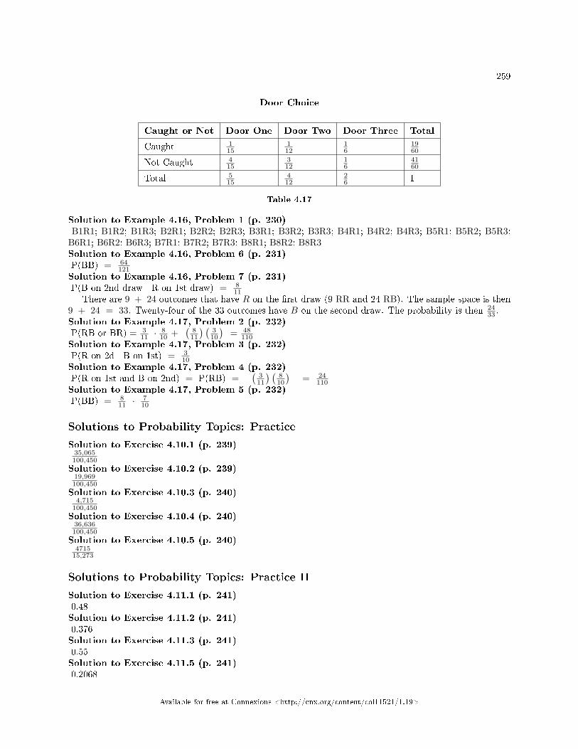
259
Door Choice
Caught or Not Door One Door Two Door Three Total
Caught 115
112
16
1960
Not Caught 415
312
16
4160
Total 515
412
26 1
Table 4.17
Solution to Example 4.16, Problem 1 (p. 230)B1R1; B1R2; B1R3; B2R1; B2R2; B2R3; B3R1; B3R2; B3R3; B4R1; B4R2; B4R3; B5R1; B5R2; B5R3;
B6R1; B6R2; B6R3; B7R1; B7R2; B7R3; B8R1; B8R2; B8R3Solution to Example 4.16, Problem 6 (p. 231)P(BB) = 64
121Solution to Example 4.16, Problem 7 (p. 231)P(B on 2nd draw | R on 1st draw) = 8
11There are 9 + 24 outcomes that have R on the �rst draw (9 RR and 24 RB). The sample space is then
9 + 24 = 33. Twenty-four of the 33 outcomes have B on the second draw. The probability is then 2433 .
Solution to Example 4.17, Problem 2 (p. 232)P(RB or BR) = 3
11 ·810 +
(811
) (310
)= 48
110Solution to Example 4.17, Problem 3 (p. 232)P(R on 2d | B on 1st) = 3
10Solution to Example 4.17, Problem 4 (p. 232)P(R on 1st and B on 2nd) = P(RB) =
(311
) (810
)= 24
110Solution to Example 4.17, Problem 5 (p. 232)P(BB) = 8
11 ·710
Solutions to Probability Topics: Practice
Solution to Exercise 4.10.1 (p. 239)35,065100,450
Solution to Exercise 4.10.2 (p. 239)19,969100,450
Solution to Exercise 4.10.3 (p. 240)4,715
100,450
Solution to Exercise 4.10.4 (p. 240)36,636100,450
Solution to Exercise 4.10.5 (p. 240)4715
15,273
Solutions to Probability Topics: Practice II
Solution to Exercise 4.11.1 (p. 241)0.48Solution to Exercise 4.11.2 (p. 241)0.376Solution to Exercise 4.11.3 (p. 241)0.55Solution to Exercise 4.11.5 (p. 241)0.2068
Available for free at Connexions <http://cnx.org/content/col11521/1.19>
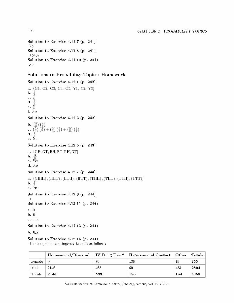
260 CHAPTER 4. PROBABILITY TOPICS
Solution to Exercise 4.11.7 (p. 241)NoSolution to Exercise 4.11.8 (p. 241)0.6492Solution to Exercise 4.11.10 (p. 241)No
Solutions to Probability Topics: Homework
Solution to Exercise 4.12.1 (p. 242)
a. {G1, G2, G3, G4, G5, Y1, Y2, Y3}b. 5
8c. 2
3d. 2
8e. 6
8f. No
Solution to Exercise 4.12.3 (p. 242)
b.(
58
) (47
)c.(
58
) (37
)+(
38
) (57
)+(
58
) (47
)d. 4
7e. No
Solution to Exercise 4.12.5 (p. 243)
a. {GH,GT,BH,BT,RH,RT}b. 3
20c. Yesd. No
Solution to Exercise 4.12.7 (p. 243)
a. {(HHH) , (HHT) , (HTH) , (HTT) , (THH) , (THT) , (TTH) , (TTT)}b. 4
8c. Yes
Solution to Exercise 4.12.9 (p. 244)0Solution to Exercise 4.12.11 (p. 244)
a. 0b. 0c. 0.63
Solution to Exercise 4.12.13 (p. 244)
b. 0.5
Solution to Exercise 4.12.15 (p. 244)The completed contingency table is as follows:
Homosexual/Bisexual IV Drug User* Heterosexual Contact Other Totals
Female 0 70 136 49 255
Male 2146 463 60 135 2804
Totals 2146 533 196 184 3059
Available for free at Connexions <http://cnx.org/content/col11521/1.19>
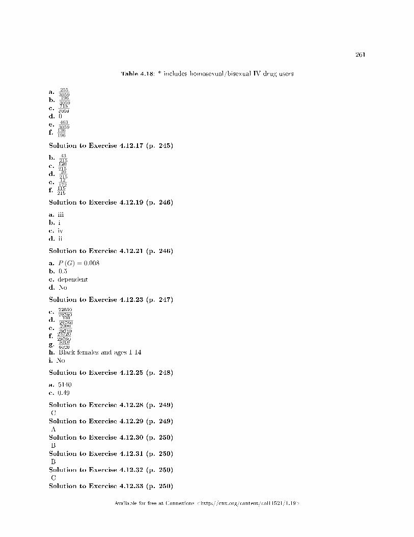
261
Table 4.18: * includes homosexual/bisexual IV drug users
a. 2553059
b. 1963059
c. 7183059
d. 0e. 463
3059f. 136
196
Solution to Exercise 4.12.17 (p. 245)
b. 43215
c. 120215
d. 20215
e. 12172
f. 115215
Solution to Exercise 4.12.19 (p. 246)
a. iiib. ic. ivd. ii
Solution to Exercise 4.12.21 (p. 246)
a. P (G) = 0.008b. 0.5c. dependentd. No
Solution to Exercise 4.12.23 (p. 247)
c. 2205029760
d. 33029760
e. 200029760
f. 2372029760
g. 50106020
h. Black females and ages 1-14i. No
Solution to Exercise 4.12.25 (p. 248)
a. 5140c. 0.49
Solution to Exercise 4.12.28 (p. 249)CSolution to Exercise 4.12.29 (p. 249)ASolution to Exercise 4.12.30 (p. 250)BSolution to Exercise 4.12.31 (p. 250)BSolution to Exercise 4.12.32 (p. 250)CSolution to Exercise 4.12.33 (p. 250)
Available for free at Connexions <http://cnx.org/content/col11521/1.19>
262 CHAPTER 4. PROBABILITY TOPICS
A. P(H or G) = P(H) + P(G) − P(H and G) = 0.26 + 0.43 − 0.14 = 0.55B. P( NOT (H and G) ) = 1 − P(H and G) = 1 − 0.14 = 0.86C. P( NOT (H or G) ) = 1 − P(H or G) = 1 − 0.55 = 0.45
Solution to Exercise 4.12.34 (p. 250)
A. P(J or K) = P(J) + P(K) − P(J and K); 0.45 = 0.18 + 0.37 − P(J and K) ; solve to �nd P(J and K)= 0.10
B. P( NOT (J and K) ) = 1 − P(J and K) = 1 − 0.10 = 0.90C. P( NOT (J or K) ) = 1 − P(J or K) = 1 − 0.45 = 0.55
Solution to Exercise 4.12.35 (p. 250)
A. P(Type O or Rh−) = P(Type O) + P(Rh−) − P(Type O and Rh−)0.52 = 0.43 + 0.15 − P(Type O and Rh−); solve to �nd P(Type O and Rh−) = 0.066% of people have type O Rh− blood
B. P( NOT (Type O and Rh−) ) = 1 − P(Type O and Rh−) = 1 − 0.06 = 0.9494% of people do not have type O Rh− blood
Solution to Exercise 4.12.36 (p. 251)
A. P(R or F) = P(R) + P(F) − P(R and F) = 0.72 + 0.46 − 0.32 = 0.86B. P( Neither R nor F ) = 1 − P(R or F) = 1 − 0.86 = 0.14
Solution to Exercise 4.12.37 (p. 251)
Let C be the event that the cookie contains chocolate. Let N be the event that the cookie contains nuts.A. P(C or N) = P(C) + P(N) − P(C and N) = 0.36 + 0.12 − 0.08 = 0.40B. P( neither chocolate nor nuts) = 1 − P(C or N) = 1 − 0.40 = 0.60
Solution to Exercise 4.12.38 (p. 251)
A. P(D and E) = P(D|E)P(E) = (0.20)(0.40) = 0.08B. P(E|D) = P(D and E) / P(D) = 0.08/0.10 = 0.80C. P(D or E) = P(D) + P(E) − P(D and E) = 0.10 + 0.40 − 0.08 = 0.42D. Not Independent: P(D|E) = 0.20 which does not equal P(D) = .10E. Not Mutually Exclusive: P(D and E) = 0.08 ; if they were mutually exclusive then we would need to
have P(D and E) = 0, which is not true here.
Solution to Exercise 4.12.39 (p. 251)
A. P(H) = 140/250; P(T) = 110/250C. 308/625D. 504/625
Solutions to Probability Topics: Review
Solution to Exercise 4.13.1 (p. 253)
C. Parameter
Solution to Exercise 4.13.2 (p. 253)
A. Population
Solution to Exercise 4.13.3 (p. 253)
B. Statistic
Available for free at Connexions <http://cnx.org/content/col11521/1.19>
263
Solution to Exercise 4.13.4 (p. 253)
D. Sample
Solution to Exercise 4.13.5 (p. 253)
E. Variable
Solution to Exercise 4.13.6 (p. 254)quantitative - continuousSolution to Exercise 4.13.7 (p. 254)
a. 2.27b. 3.04c. -1, 4, 4
Available for free at Connexions <http://cnx.org/content/col11521/1.19>

264 CHAPTER 4. PROBABILITY TOPICS
Available for free at Connexions <http://cnx.org/content/col11521/1.19>
Chapter 5
Discrete and Continuous Random
Variables
5.1 Discrete and Continuous Random Variables: Introduction to Dis-crete Random Variables1
5.1.1 Student Learning Outcomes
By the end of this chapter, the student should be able to:
• Recognize and understand discrete and continuous probability distribution functions, in general.• Calculate and interpret expected values.• Recognize the binomial probability distribution and apply it appropriately.• Recognize the uniform probability distribution and apply it appropriately.• Classify discrete and continuous word problems by their distributions.
5.1.2 Introduction to Discrete Random Variables
A student takes a 10 question true-false quiz. Because the student had such a busy schedule, he or she couldnot study and randomly guesses at each answer. What is the probability of the student passing the test withat least a 70%?
Small companies might be interested in the number of long distance phone calls their employees makeduring the peak time of the day. Suppose the average is 20 calls. What is the probability that the employeesmake more than 20 long distance phone calls during the peak time?
These two examples illustrate two di�erent types of probability problems involving discrete randomvariables. Recall that discrete data are data that you can count. A random variable describes theoutcomes of a statistical experiment in words. The values of a random variable can vary with each repetitionof an experiment.
In this chapter, you will study probability problems involving discrete random distributions. You willalso study long-term averages associated with them.
5.1.3 Random Variable Notation
Upper case letters like X or Y denote a random variable. Lower case letters like x or y denote the valueof a random variable. If X is a random variable, then X is written in words. and x is given as anumber.
1This content is available online at <http://cnx.org/content/m46207/1.1/>.
Available for free at Connexions <http://cnx.org/content/col11521/1.19>
265
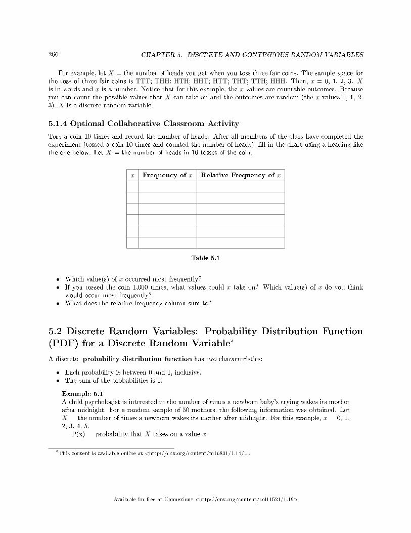
266 CHAPTER 5. DISCRETE AND CONTINUOUS RANDOM VARIABLES
For example, let X = the number of heads you get when you toss three fair coins. The sample space forthe toss of three fair coins is TTT; THH; HTH; HHT; HTT; THT; TTH; HHH. Then, x = 0, 1, 2, 3. Xis in words and x is a number. Notice that for this example, the x values are countable outcomes. Becauseyou can count the possible values that X can take on and the outcomes are random (the x values 0, 1, 2,3), X is a discrete random variable.
5.1.4 Optional Collaborative Classroom Activity
Toss a coin 10 times and record the number of heads. After all members of the class have completed theexperiment (tossed a coin 10 times and counted the number of heads), �ll in the chart using a heading likethe one below. Let X = the number of heads in 10 tosses of the coin.
x Frequency of x Relative Frequency of x
Table 5.1
• Which value(s) of x occurred most frequently?• If you tossed the coin 1,000 times, what values could x take on? Which value(s) of x do you think
would occur most frequently?• What does the relative frequency column sum to?
5.2 Discrete Random Variables: Probability Distribution Function(PDF) for a Discrete Random Variable2
A discrete probability distribution function has two characteristics:
• Each probability is between 0 and 1, inclusive.• The sum of the probabilities is 1.
Example 5.1A child psychologist is interested in the number of times a newborn baby's crying wakes its motherafter midnight. For a random sample of 50 mothers, the following information was obtained. LetX = the number of times a newborn wakes its mother after midnight. For this example, x = 0, 1,2, 3, 4, 5.
P(x) = probability that X takes on a value x.
2This content is available online at <http://cnx.org/content/m16831/1.14/>.
Available for free at Connexions <http://cnx.org/content/col11521/1.19>
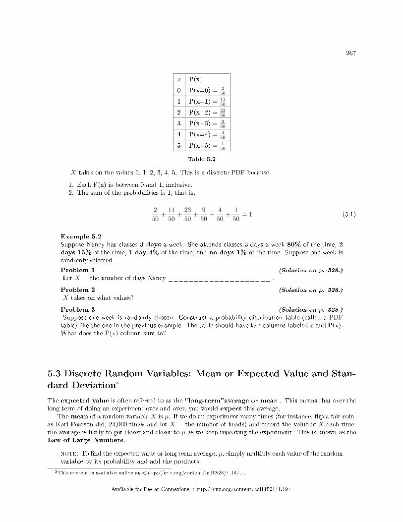
267
x P(x)
0 P(x=0) = 250
1 P(x=1) = 1150
2 P(x=2) = 2350
3 P(x=3) = 950
4 P(x=4) = 450
5 P(x=5) = 150
Table 5.2
X takes on the values 0, 1, 2, 3, 4, 5. This is a discrete PDF because
1. Each P(x) is between 0 and 1, inclusive.2. The sum of the probabilities is 1, that is,
250
+1150
+2350
+950
+450
+150
= 1 (5.1)
Example 5.2Suppose Nancy has classes 3 days a week. She attends classes 3 days a week 80% of the time, 2days 15% of the time, 1 day 4% of the time, and no days 1% of the time. Suppose one week israndomly selected.
Problem 1 (Solution on p. 328.)
Let X = the number of days Nancy ____________________ .
Problem 2 (Solution on p. 328.)
X takes on what values?
Problem 3 (Solution on p. 328.)
Suppose one week is randomly chosen. Construct a probability distribution table (called a PDFtable) like the one in the previous example. The table should have two columns labeled x and P(x).What does the P(x) column sum to?
5.3 Discrete Random Variables: Mean or Expected Value and Stan-dard Deviation3
The expected value is often referred to as the "long-term"average or mean . This means that over thelong term of doing an experiment over and over, you would expect this average.
The mean of a random variable X is µ. If we do an experiment many times (for instance, �ip a fair coin,as Karl Pearson did, 24,000 times and let X = the number of heads) and record the value of X each time,the average is likely to get closer and closer to µ as we keep repeating the experiment. This is known as theLaw of Large Numbers.
note: To �nd the expected value or long term average, µ, simply multiply each value of the randomvariable by its probability and add the products.
3This content is available online at <http://cnx.org/content/m16828/1.16/>.
Available for free at Connexions <http://cnx.org/content/col11521/1.19>
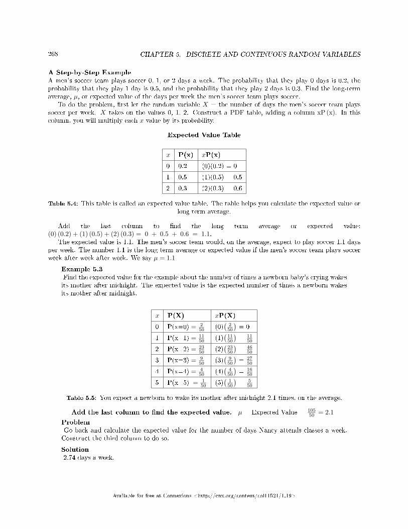
268 CHAPTER 5. DISCRETE AND CONTINUOUS RANDOM VARIABLES
A Step-by-Step ExampleA men's soccer team plays soccer 0, 1, or 2 days a week. The probability that they play 0 days is 0.2, theprobability that they play 1 day is 0.5, and the probability that they play 2 days is 0.3. Find the long-termaverage, µ, or expected value of the days per week the men's soccer team plays soccer.
To do the problem, �rst let the random variable X = the number of days the men's soccer team playssoccer per week. X takes on the values 0, 1, 2. Construct a PDF table, adding a column xP (x). In thiscolumn, you will multiply each x value by its probability.
Expected Value Table
x P(x) xP(x)
0 0.2 (0)(0.2) = 0
1 0.5 (1)(0.5) = 0.5
2 0.3 (2)(0.3) = 0.6
Table 5.4: This table is called an expected value table. The table helps you calculate the expected value orlong-term average.
Add the last column to �nd the long term average or expected value:(0) (0.2) + (1) (0.5) + (2) (0.3) = 0 + 0.5 + 0.6 = 1.1.
The expected value is 1.1. The men's soccer team would, on the average, expect to play soccer 1.1 daysper week. The number 1.1 is the long term average or expected value if the men's soccer team plays soccerweek after week after week. We say µ = 1.1
Example 5.3Find the expected value for the example about the number of times a newborn baby's crying wakesits mother after midnight. The expected value is the expected number of times a newborn wakesits mother after midnight.
x P(X) xP(X)
0 P(x=0) = 250 (0)
(250
)= 0
1 P(x=1) = 1150 (1)
(1150
)= 11
50
2 P(x=2) = 2350 (2)
(2350
)= 46
50
3 P(x=3) = 950 (3)
(950
)= 27
50
4 P(x=4) = 450 (4)
(450
)= 16
50
5 P(x=5) = 150 (5)
(150
)= 5
50
Table 5.5: You expect a newborn to wake its mother after midnight 2.1 times, on the average.
Add the last column to �nd the expected value. µ = Expected Value = 10550 = 2.1
ProblemGo back and calculate the expected value for the number of days Nancy attends classes a week.Construct the third column to do so.
Solution2.74 days a week.
Available for free at Connexions <http://cnx.org/content/col11521/1.19>
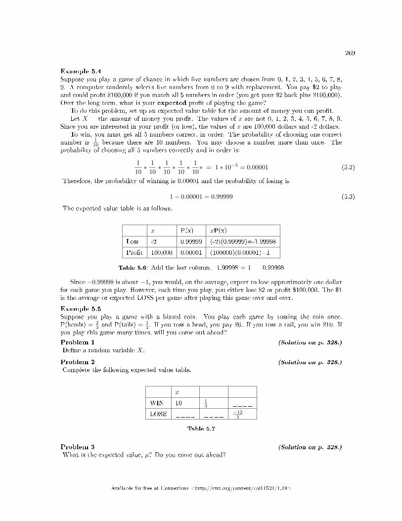
269
Example 5.4Suppose you play a game of chance in which �ve numbers are chosen from 0, 1, 2, 3, 4, 5, 6, 7, 8,9. A computer randomly selects �ve numbers from 0 to 9 with replacement. You pay $2 to playand could pro�t $100,000 if you match all 5 numbers in order (you get your $2 back plus $100,000).Over the long term, what is your expected pro�t of playing the game?
To do this problem, set up an expected value table for the amount of money you can pro�t.Let X = the amount of money you pro�t. The values of x are not 0, 1, 2, 3, 4, 5, 6, 7, 8, 9.
Since you are interested in your pro�t (or loss), the values of x are 100,000 dollars and -2 dollars.To win, you must get all 5 numbers correct, in order. The probability of choosing one correct
number is 110 because there are 10 numbers. You may choose a number more than once. The
probability of choosing all 5 numbers correctly and in order is:
110∗ 1
10∗ 1
10∗ 1
10∗ 1
10∗ = 1 ∗ 10−5 = 0.00001 (5.2)
Therefore, the probability of winning is 0.00001 and the probability of losing is
1− 0.00001 = 0.99999 (5.3)
The expected value table is as follows.
x P(x) xP(x)
Loss -2 0.99999 (-2)(0.99999)=-1.99998
Pro�t 100,000 0.00001 (100000)(0.00001)=1
Table 5.6: Add the last column. -1.99998 + 1 = -0.99998
Since −0.99998 is about −1, you would, on the average, expect to lose approximately one dollarfor each game you play. However, each time you play, you either lose $2 or pro�t $100,000. The $1is the average or expected LOSS per game after playing this game over and over.
Example 5.5Suppose you play a game with a biased coin. You play each game by tossing the coin once.P(heads) = 2
3 and P(tails) = 13 . If you toss a head, you pay $6. If you toss a tail, you win $10. If
you play this game many times, will you come out ahead?
Problem 1 (Solution on p. 328.)
De�ne a random variable X.
Problem 2 (Solution on p. 328.)
Complete the following expected value table.
x ____ ____
WIN 10 13 ____
LOSE ____ ____ −123
Table 5.7
Problem 3 (Solution on p. 328.)
What is the expected value, µ? Do you come out ahead?
Available for free at Connexions <http://cnx.org/content/col11521/1.19>
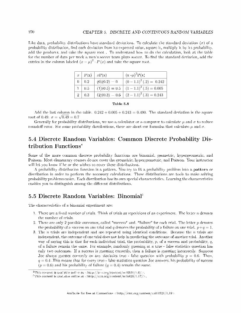
270 CHAPTER 5. DISCRETE AND CONTINUOUS RANDOM VARIABLES
Like data, probability distributions have standard deviations. To calculate the standard deviation (σ) of aprobability distribution, �nd each deviation from its expected value, square it, multiply it by its probability,add the products, and take the square root . To understand how to do the calculation, look at the tablefor the number of days per week a men's soccer team plays soccer. To �nd the standard deviation, add theentries in the column labeled (x− µ)2 · P (x) and take the square root.
x P(x) xP(x) (x -µ)2P(x)
0 0.2 (0)(0.2) = 0 (0− 1.1)2 (.2) = 0.242
1 0.5 (1)(0.5) = 0.5 (1− 1.1)2 (.5) = 0.005
2 0.3 (2)(0.3) = 0.6 (2− 1.1)2 (.3) = 0.243
Table 5.8
Add the last column in the table. 0.242 + 0.005 + 0.243 = 0.490. The standard deviation is the squareroot of 0.49. σ =
√0.49 = 0.7
Generally for probability distributions, we use a calculator or a computer to calculate µ and σ to reduceroundo� error. For some probability distributions, there are short-cut formulas that calculate µ and σ.
5.4 Discrete Random Variables: Common Discrete Probability Dis-tribution Functions4
Some of the more common discrete probability functions are binomial, geometric, hypergeometric, andPoisson. Most elementary courses do not cover the geometric, hypergeometric, and Poisson. Your instructorwill let you know if he or she wishes to cover these distributions.
A probability distribution function is a pattern. You try to �t a probability problem into a pattern ordistribution in order to perform the necessary calculations. These distributions are tools to make solvingprobability problems easier. Each distribution has its own special characteristics. Learning the characteristicsenables you to distinguish among the di�erent distributions.
5.5 Discrete Random Variables: Binomial5
The characteristics of a binomial experiment are:
1. There are a �xed number of trials. Think of trials as repetitions of an experiment. The letter n denotesthe number of trials.
2. There are only 2 possible outcomes, called "success" and, "failure" for each trial. The letter p denotesthe probability of a success on one trial and q denotes the probability of a failure on one trial. p+q = 1.
3. The n trials are independent and are repeated using identical conditions. Because the n trials areindependent, the outcome of one trial does not help in predicting the outcome of another trial. Anotherway of saying this is that for each individual trial, the probability, p, of a success and probability, q,of a failure remain the same. For example, randomly guessing at a true - false statistics question hasonly two outcomes. If a success is guessing correctly, then a failure is guessing incorrectly. SupposeJoe always guesses correctly on any statistics true - false question with probability p = 0.6. Then,q = 0.4 .This means that for every true - false statistics question Joe answers, his probability of success(p = 0.6) and his probability of failure (q = 0.4) remain the same.
4This content is available online at <http://cnx.org/content/m16821/1.6/>.5This content is available online at <http://cnx.org/content/m16820/1.17/>.
Available for free at Connexions <http://cnx.org/content/col11521/1.19>
271
The outcomes of a binomial experiment �t a binomial probability distribution. The random variableX = the number of successes obtained in the n independent trials.
The mean, µ, and variance, σ2, for the binomial probability distribution is µ = np and σ2 = npq. Thestandard deviation, σ, is then σ =
√npq.
Any experiment that has characteristics 2 and 3 and where n = 1 is called a Bernoulli Trial (namedafter Jacob Bernoulli who, in the late 1600s, studied them extensively). A binomial experiment takes placewhen the number of successes is counted in one or more Bernoulli Trials.
Example 5.6At ABC College, the withdrawal rate from an elementary physics course is 30% for any given term.This implies that, for any given term, 70% of the students stay in the class for the entire term. A"success" could be de�ned as an individual who withdrew. The random variable is X = the numberof students who withdraw from the randomly selected elementary physics class.
Example 5.7Suppose you play a game that you can only either win or lose. The probability that you win anygame is 55% and the probability that you lose is 45%. Each game you play is independent. If youplay the game 20 times, what is the probability that you win 15 of the 20 games? Here, if youde�ne X = the number of wins, then X takes on the values 0, 1, 2, 3, ..., 20. The probability of asuccess is p = 0.55. The probability of a failure is q = 0.45. The number of trials is n = 20. Theprobability question can be stated mathematically as P (x = 15).
Example 5.8A fair coin is �ipped 15 times. Each �ip is independent. What is the probability of getting morethan 10 heads? Let X = the number of heads in 15 �ips of the fair coin. X takes on the values0, 1, 2, 3, ..., 15. Since the coin is fair, p = 0.5 and q = 0.5. The number of trials is n = 15. Theprobability question can be stated mathematically as P (x > 10).
Example 5.9Approximately 70% of statistics students do their homework in time for it to be collected andgraded. Each student does homework independently. In a statistics class of 50 students, what isthe probability that at least 40 will do their homework on time? Students are selected randomly.
Problem 1 (Solution on p. 328.)
This is a binomial problem because there is only a success or a __________, there are ade�nite number of trials, and the probability of a success is 0.70 for each trial.
Problem 2 (Solution on p. 328.)
If we are interested in the number of students who do their homework, then how do we de�ne X?
Problem 3 (Solution on p. 328.)
What values does x take on?
Problem 4 (Solution on p. 328.)
What is a "failure", in words?
The probability of a success is p = 0.70. The number of trial is n = 50.
Problem 5 (Solution on p. 328.)
If p+ q = 1, then what is q?
Problem 6 (Solution on p. 328.)
The words "at least" translate as what kind of inequality for the probability questionP (x____40).The probability question is P (x ≥ 40).
Available for free at Connexions <http://cnx.org/content/col11521/1.19>
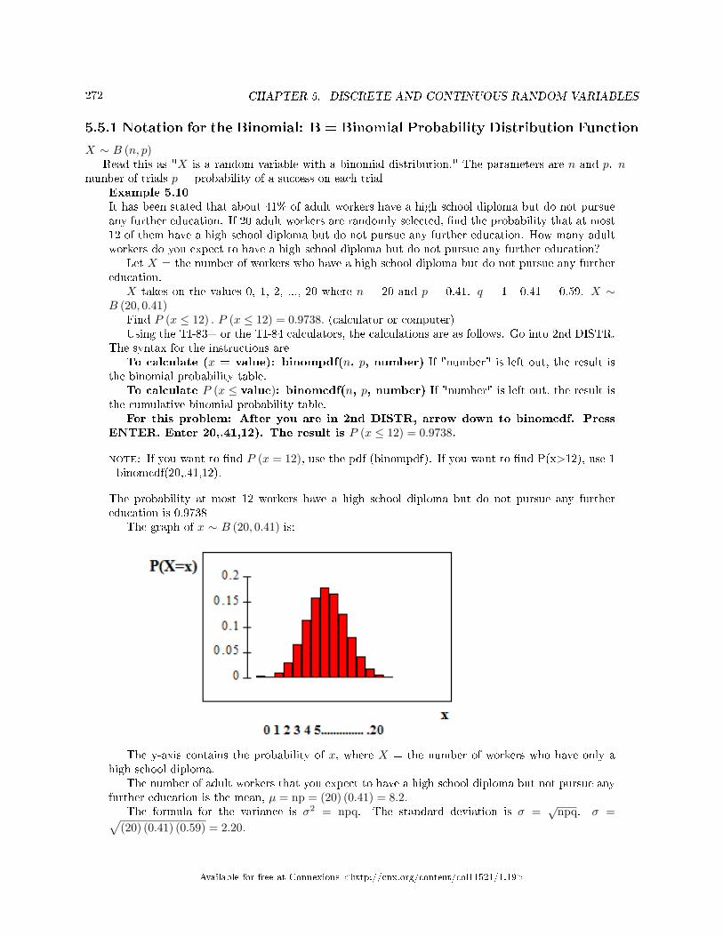
272 CHAPTER 5. DISCRETE AND CONTINUOUS RANDOM VARIABLES
5.5.1 Notation for the Binomial: B = Binomial Probability Distribution Function
X ∼ B (n, p)Read this as "X is a random variable with a binomial distribution." The parameters are n and p. n =
number of trials p = probability of a success on each trialExample 5.10It has been stated that about 41% of adult workers have a high school diploma but do not pursueany further education. If 20 adult workers are randomly selected, �nd the probability that at most12 of them have a high school diploma but do not pursue any further education. How many adultworkers do you expect to have a high school diploma but do not pursue any further education?
Let X = the number of workers who have a high school diploma but do not pursue any furthereducation.
X takes on the values 0, 1, 2, ..., 20 where n = 20 and p = 0.41. q = 1 - 0.41 = 0.59. X ∼B (20, 0.41)
Find P (x ≤ 12) . P (x ≤ 12) = 0.9738. (calculator or computer)Using the TI-83+ or the TI-84 calculators, the calculations are as follows. Go into 2nd DISTR.
The syntax for the instructions areTo calculate (x = value): binompdf(n, p, number) If "number" is left out, the result is
the binomial probability table.To calculate P (x ≤ value): binomcdf(n, p, number) If "number" is left out, the result is
the cumulative binomial probability table.For this problem: After you are in 2nd DISTR, arrow down to binomcdf. Press
ENTER. Enter 20,.41,12). The result is P (x ≤ 12) = 0.9738.
note: If you want to �nd P (x = 12), use the pdf (binompdf). If you want to �nd P(x>12), use 1- binomcdf(20,.41,12).
The probability at most 12 workers have a high school diploma but do not pursue any furthereducation is 0.9738
The graph of x ∼ B (20, 0.41) is:
The y-axis contains the probability of x, where X = the number of workers who have only ahigh school diploma.
The number of adult workers that you expect to have a high school diploma but not pursue anyfurther education is the mean, µ = np = (20) (0.41) = 8.2.
The formula for the variance is σ2 = npq. The standard deviation is σ =√
npq. σ =√(20) (0.41) (0.59) = 2.20.
Available for free at Connexions <http://cnx.org/content/col11521/1.19>
273
Example 5.11The following example illustrates a problem that is not binomial. It violates the condition ofindependence. ABC College has a student advisory committee made up of 10 sta� members and 6students. The committee wishes to choose a chairperson and a recorder. What is the probabilitythat the chairperson and recorder are both students? All names of the committee are put intoa box and two names are drawn without replacement. The �rst name drawn determines thechairperson and the second name the recorder. There are two trials. However, the trials are notindependent because the outcome of the �rst trial a�ects the outcome of the second trial. Theprobability of a student on the �rst draw is 6
16 . The probability of a student on the second drawis 5
15 , when the �rst draw produces a student. The probability is 615 when the �rst draw produces
a sta� member. The probability of drawing a student's name changes for each of the trials and,therefore, violates the condition of independence.
5.6 Continuous Random Variables: Introduction6
5.6.1 Student Learning Outcomes
By the end of this chapter, the student should be able to:
• Recognize and understand continuous probability density functions in general.• Recognize the uniform probability distribution and apply it appropriately.• Recognize the exponential probability distribution and apply it appropriately.
5.6.2 Introduction
Continuous random variables have many applications. Baseball batting averages, IQ scores, the length oftime a long distance telephone call lasts, the amount of money a person carries, the length of time a computerchip lasts, and SAT scores are just a few. The �eld of reliability depends on a variety of continuous randomvariables.
This chapter gives an introduction to continuous random variables and the many continuous distributions.We will be studying these continuous distributions for several chapters.
NOTE: The values of discrete and continuous random variables can be ambiguous. For example,if X is equal to the number of miles (to the nearest mile) you drive to work, then X is a discreterandom variable. You count the miles. If X is the distance you drive to work, then you measurevalues of X and X is a continuous random variable. How the random variable is de�ned is veryimportant.
5.6.3 Properties of Continuous Probability Distributions
The graph of a continuous probability distribution is a curve. Probability is represented by area under thecurve.
The curve is called the probability density function (abbreviated: pdf). We use the symbol f (x)to represent the curve. f (x) is the function that corresponds to the graph; we use the density function f (x)to draw the graph of the probability distribution.
Area under the curve is given by a di�erent function called the cumulative distribution function(abbreviated: cdf). The cumulative distribution function is used to evaluate probability as area.
6This content is available online at <http://cnx.org/content/m16808/1.12/>.
Available for free at Connexions <http://cnx.org/content/col11521/1.19>
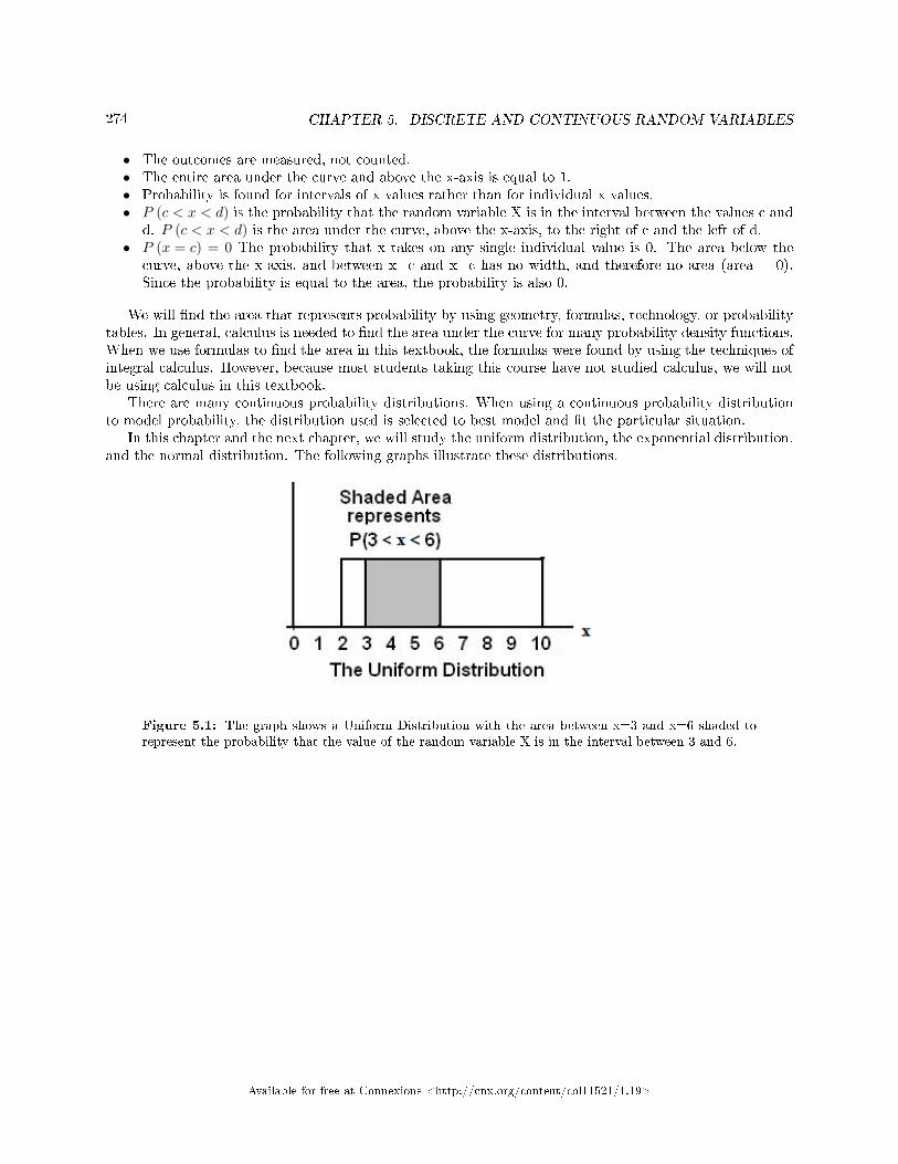
274 CHAPTER 5. DISCRETE AND CONTINUOUS RANDOM VARIABLES
• The outcomes are measured, not counted.• The entire area under the curve and above the x-axis is equal to 1.• Probability is found for intervals of x values rather than for individual x values.• P (c < x < d) is the probability that the random variable X is in the interval between the values c and
d. P (c < x < d) is the area under the curve, above the x-axis, to the right of c and the left of d.• P (x = c) = 0 The probability that x takes on any single individual value is 0. The area below the
curve, above the x-axis, and between x=c and x=c has no width, and therefore no area (area = 0).Since the probability is equal to the area, the probability is also 0.
We will �nd the area that represents probability by using geometry, formulas, technology, or probabilitytables. In general, calculus is needed to �nd the area under the curve for many probability density functions.When we use formulas to �nd the area in this textbook, the formulas were found by using the techniques ofintegral calculus. However, because most students taking this course have not studied calculus, we will notbe using calculus in this textbook.
There are many continuous probability distributions. When using a continuous probability distributionto model probability, the distribution used is selected to best model and �t the particular situation.
In this chapter and the next chapter, we will study the uniform distribution, the exponential distribution,and the normal distribution. The following graphs illustrate these distributions.
Figure 5.1: The graph shows a Uniform Distribution with the area between x=3 and x=6 shaded torepresent the probability that the value of the random variable X is in the interval between 3 and 6.
Available for free at Connexions <http://cnx.org/content/col11521/1.19>
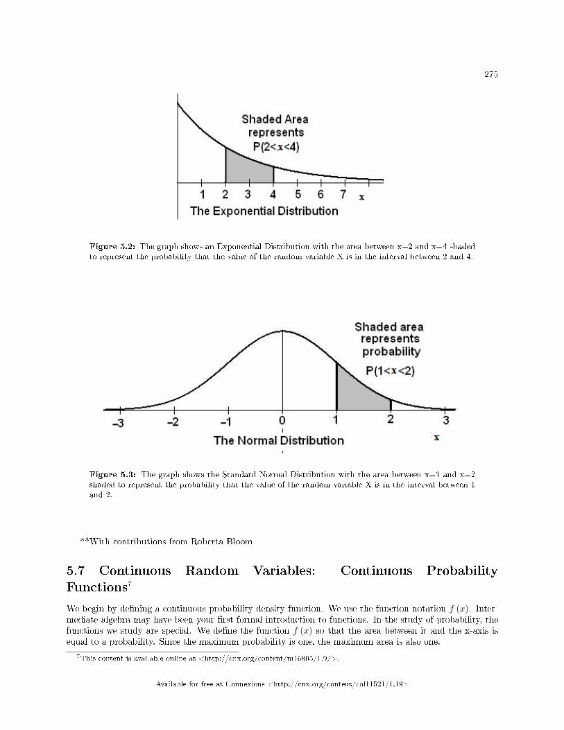
275
Figure 5.2: The graph shows an Exponential Distribution with the area between x=2 and x=4 shadedto represent the probability that the value of the random variable X is in the interval between 2 and 4.
Figure 5.3: The graph shows the Standard Normal Distribution with the area between x=1 and x=2shaded to represent the probability that the value of the random variable X is in the interval between 1and 2.
**With contributions from Roberta Bloom
5.7 Continuous Random Variables: Continuous ProbabilityFunctions7
We begin by de�ning a continuous probability density function. We use the function notation f (x). Inter-mediate algebra may have been your �rst formal introduction to functions. In the study of probability, thefunctions we study are special. We de�ne the function f (x) so that the area between it and the x-axis isequal to a probability. Since the maximum probability is one, the maximum area is also one.
7This content is available online at <http://cnx.org/content/m16805/1.9/>.
Available for free at Connexions <http://cnx.org/content/col11521/1.19>
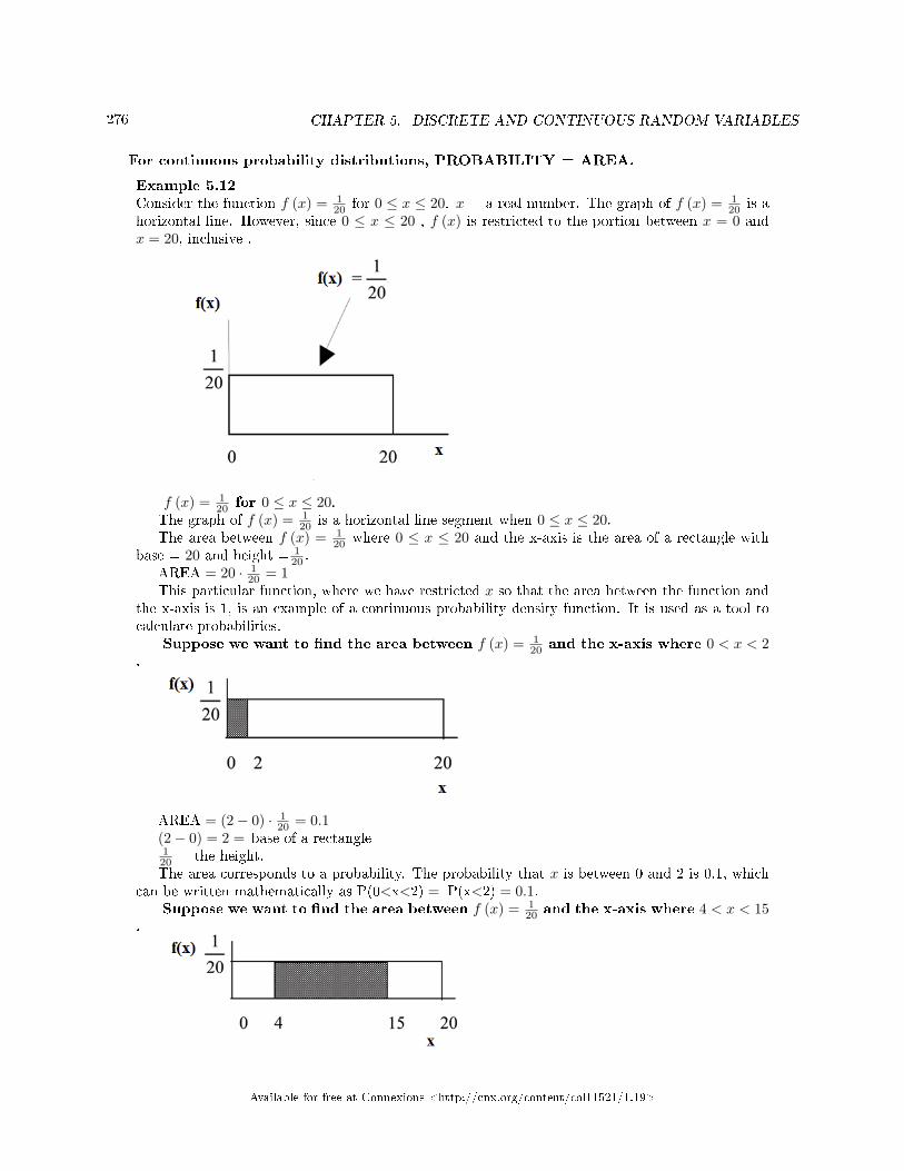
276 CHAPTER 5. DISCRETE AND CONTINUOUS RANDOM VARIABLES
For continuous probability distributions, PROBABILITY = AREA.
Example 5.12Consider the function f (x) = 1
20 for 0 ≤ x ≤ 20. x = a real number. The graph of f (x) = 120 is a
horizontal line. However, since 0 ≤ x ≤ 20 , f (x) is restricted to the portion between x = 0 andx = 20, inclusive .
f (x) = 120 for 0 ≤ x ≤ 20.
The graph of f (x) = 120 is a horizontal line segment when 0 ≤ x ≤ 20.
The area between f (x) = 120 where 0 ≤ x ≤ 20 and the x-axis is the area of a rectangle with
base = 20 and height = 120 .
AREA = 20 · 120 = 1
This particular function, where we have restricted x so that the area between the function andthe x-axis is 1, is an example of a continuous probability density function. It is used as a tool tocalculate probabilities.
Suppose we want to �nd the area between f (x) = 120 and the x-axis where 0 < x < 2
.
AREA = (2− 0) · 120 = 0.1
(2− 0) = 2 = base of a rectangle120 = the height.The area corresponds to a probability. The probability that x is between 0 and 2 is 0.1, which
can be written mathematically as P(0<x<2) = P(x<2) = 0.1.Suppose we want to �nd the area between f (x) = 1
20 and the x-axis where 4 < x < 15.
Available for free at Connexions <http://cnx.org/content/col11521/1.19>
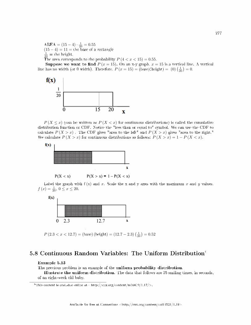
277
AREA = (15− 4) · 120 = 0.55
(15− 4) = 11 = the base of a rectangle120 = the height.The area corresponds to the probability P (4 < x < 15) = 0.55.Suppose we want to �nd P (x = 15). On an x-y graph, x = 15 is a vertical line. A vertical
line has no width (or 0 width). Therefore, P (x = 15) = (base)(height) = (0)(
120
)= 0.
P (X ≤ x) (can be written as P (X < x) for continuous distributions) is called the cumulativedistribution function or CDF. Notice the "less than or equal to" symbol. We can use the CDF tocalculate P (X > x) . The CDF gives "area to the left" and P (X > x) gives "area to the right."We calculate P (X > x) for continuous distributions as follows: P (X > x) = 1− P (X < x).
Label the graph with f (x) and x. Scale the x and y axes with the maximum x and y values.f (x) = 1
20 , 0 ≤ x ≤ 20.
P (2.3 < x < 12.7) = (base) (height) = (12.7− 2.3)(
120
)= 0.52
5.8 Continuous Random Variables: The Uniform Distribution8
Example 5.13The previous problem is an example of the uniform probability distribution.
Illustrate the uniform distribution. The data that follows are 55 smiling times, in seconds,of an eight-week old baby.
8This content is available online at <http://cnx.org/content/m16819/1.17/>.
Available for free at Connexions <http://cnx.org/content/col11521/1.19>
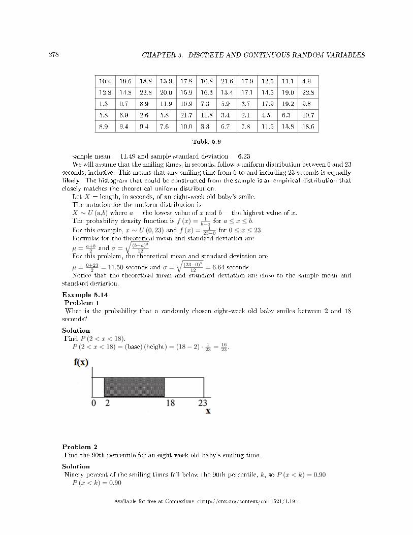
278 CHAPTER 5. DISCRETE AND CONTINUOUS RANDOM VARIABLES
10.4 19.6 18.8 13.9 17.8 16.8 21.6 17.9 12.5 11.1 4.9
12.8 14.8 22.8 20.0 15.9 16.3 13.4 17.1 14.5 19.0 22.8
1.3 0.7 8.9 11.9 10.9 7.3 5.9 3.7 17.9 19.2 9.8
5.8 6.9 2.6 5.8 21.7 11.8 3.4 2.1 4.5 6.3 10.7
8.9 9.4 9.4 7.6 10.0 3.3 6.7 7.8 11.6 13.8 18.6
Table 5.9
sample mean = 11.49 and sample standard deviation = 6.23We will assume that the smiling times, in seconds, follow a uniform distribution between 0 and 23
seconds, inclusive. This means that any smiling time from 0 to and including 23 seconds is equallylikely. The histogram that could be constructed from the sample is an empirical distribution thatclosely matches the theoretical uniform distribution.
Let X = length, in seconds, of an eight-week old baby's smile.The notation for the uniform distribution isX ∼ U (a,b) where a = the lowest value of x and b = the highest value of x.The probability density function is f (x) = 1
b−a for a ≤ x ≤ b.For this example, x ∼ U (0, 23) and f (x) = 1
23−0 for 0 ≤ x ≤ 23.Formulas for the theoretical mean and standard deviation are
µ = a+b2 and σ =
√(b−a)2
12For this problem, the theoretical mean and standard deviation are
µ = 0+232 = 11.50 seconds and σ =
√(23−0)2
12 = 6.64 secondsNotice that the theoretical mean and standard deviation are close to the sample mean and
standard deviation.
Example 5.14Problem 1What is the probability that a randomly chosen eight-week old baby smiles between 2 and 18seconds?
SolutionFind P (2 < x < 18).P (2 < x < 18) = (base) (height) = (18− 2) · 1
23 = 1623 .
Problem 2Find the 90th percentile for an eight week old baby's smiling time.
SolutionNinety percent of the smiling times fall below the 90th percentile, k, so P (x < k) = 0.90P (x < k) = 0.90
Available for free at Connexions <http://cnx.org/content/col11521/1.19>
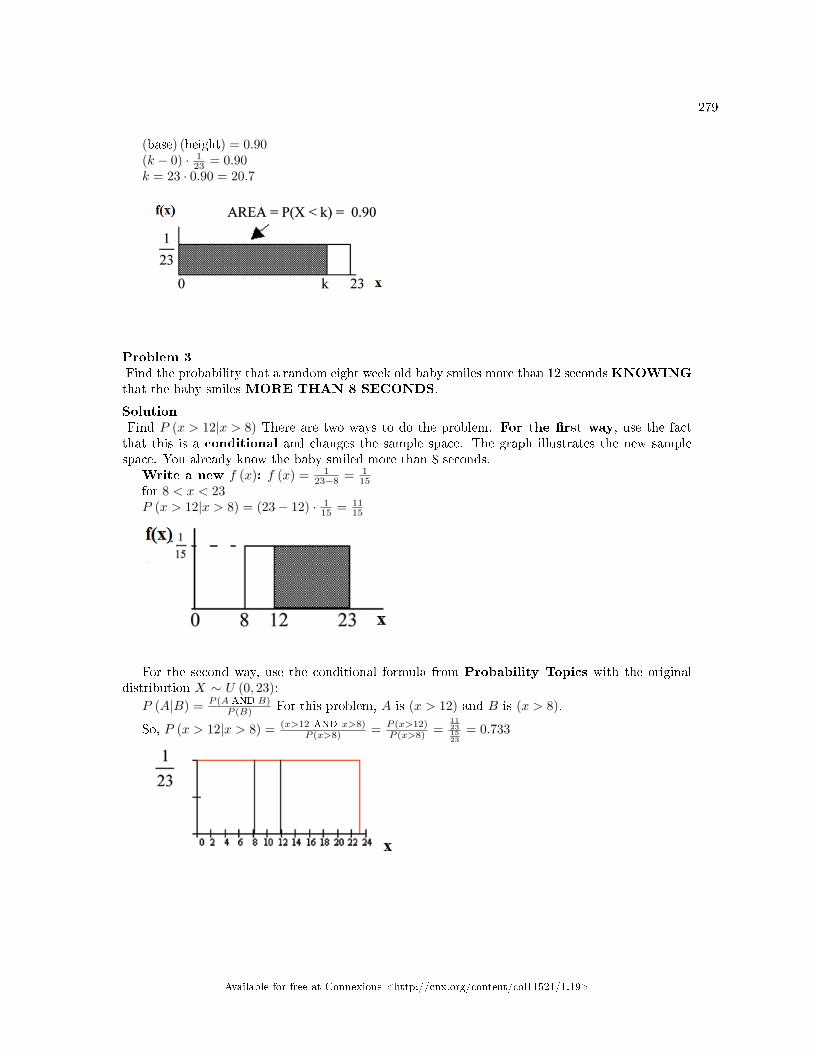
279
(base) (height) = 0.90(k − 0) · 1
23 = 0.90k = 23 · 0.90 = 20.7
Problem 3Find the probability that a random eight week old baby smiles more than 12 secondsKNOWINGthat the baby smiles MORE THAN 8 SECONDS.
SolutionFind P (x > 12|x > 8) There are two ways to do the problem. For the �rst way, use the factthat this is a conditional and changes the sample space. The graph illustrates the new samplespace. You already know the baby smiled more than 8 seconds.
Write a new f (x): f (x) = 123−8 = 1
15for 8 < x < 23P (x > 12|x > 8) = (23− 12) · 1
15 = 1115
For the second way, use the conditional formula from Probability Topics with the originaldistribution X ∼ U (0, 23):
P (A|B) = P (A AND B)P (B) For this problem, A is (x > 12) and B is (x > 8).
So, P (x > 12|x > 8) = (x>12 AND x>8)P (x>8) = P (x>12)
P (x>8) =11231523
= 0.733
Available for free at Connexions <http://cnx.org/content/col11521/1.19>
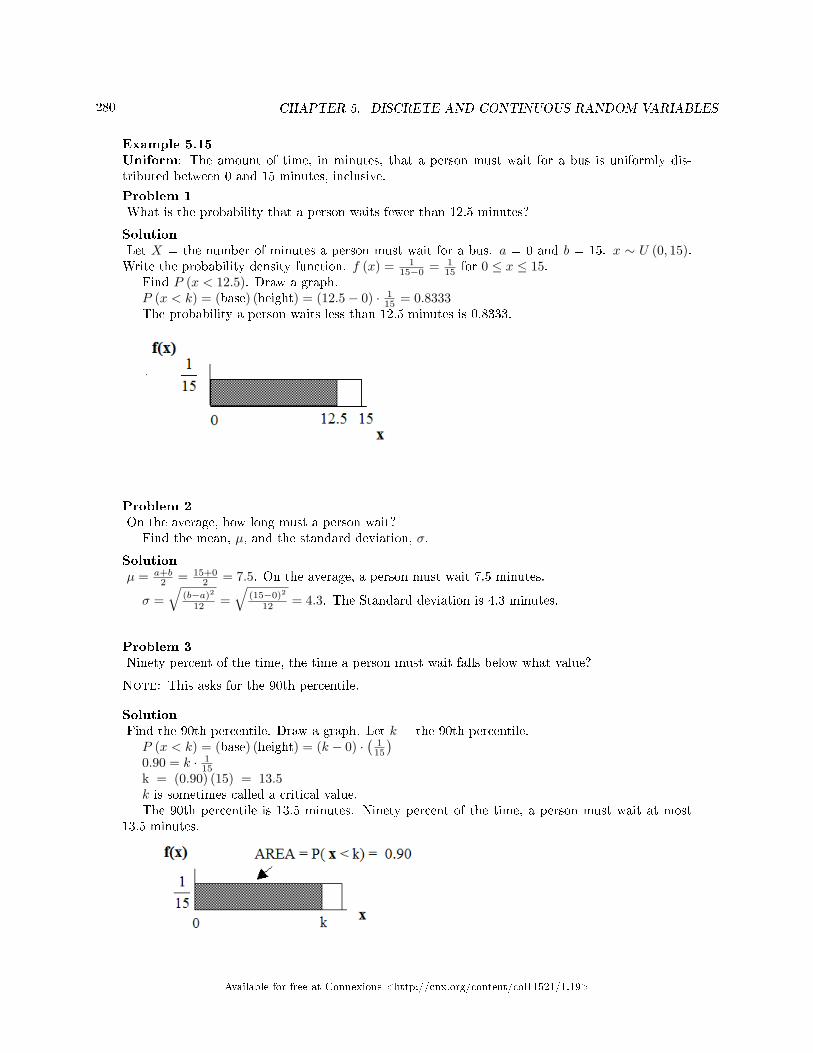
280 CHAPTER 5. DISCRETE AND CONTINUOUS RANDOM VARIABLES
Example 5.15Uniform: The amount of time, in minutes, that a person must wait for a bus is uniformly dis-tributed between 0 and 15 minutes, inclusive.
Problem 1What is the probability that a person waits fewer than 12.5 minutes?
SolutionLet X = the number of minutes a person must wait for a bus. a = 0 and b = 15. x ∼ U (0, 15).Write the probability density function. f (x) = 1
15−0 = 115 for 0 ≤ x ≤ 15.
Find P (x < 12.5). Draw a graph.P (x < k) = (base) (height) = (12.5− 0) · 1
15 = 0.8333The probability a person waits less than 12.5 minutes is 0.8333.
Problem 2On the average, how long must a person wait?
Find the mean, µ, and the standard deviation, σ.
Solutionµ = a+b
2 = 15+02 = 7.5. On the average, a person must wait 7.5 minutes.
σ =√
(b−a)2
12 =√
(15−0)2
12 = 4.3. The Standard deviation is 4.3 minutes.
Problem 3Ninety percent of the time, the time a person must wait falls below what value?
Note: This asks for the 90th percentile.
SolutionFind the 90th percentile. Draw a graph. Let k = the 90th percentile.P (x < k) = (base) (height) = (k − 0) ·
(115
)0.90 = k · 1
15k = (0.90) (15) = 13.5k is sometimes called a critical value.The 90th percentile is 13.5 minutes. Ninety percent of the time, a person must wait at most
13.5 minutes.
Available for free at Connexions <http://cnx.org/content/col11521/1.19>
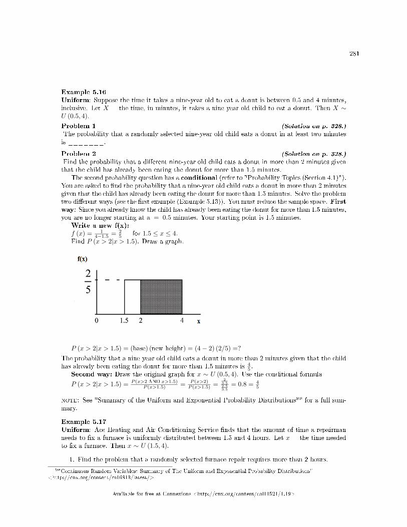
281
Example 5.16Uniform: Suppose the time it takes a nine-year old to eat a donut is between 0.5 and 4 minutes,inclusive. Let X = the time, in minutes, it takes a nine-year old child to eat a donut. Then X ∼U (0.5, 4).Problem 1 (Solution on p. 328.)
The probability that a randomly selected nine-year old child eats a donut in at least two minutesis _______.
Problem 2 (Solution on p. 328.)
Find the probability that a di�erent nine-year old child eats a donut in more than 2 minutes giventhat the child has already been eating the donut for more than 1.5 minutes.
The second probability question has a conditional (refer to "Probability Topics (Section 4.1)").You are asked to �nd the probability that a nine-year old child eats a donut in more than 2 minutesgiven that the child has already been eating the donut for more than 1.5 minutes. Solve the problemtwo di�erent ways (see the �rst example (Example 5.13)). You must reduce the sample space. Firstway: Since you already know the child has already been eating the donut for more than 1.5 minutes,you are no longer starting at a = 0.5 minutes. Your starting point is 1.5 minutes.
Write a new f(x):f (x) = 1
4−1.5 = 25 for 1.5 ≤ x ≤ 4.
Find P (x > 2|x > 1.5). Draw a graph.
P (x > 2|x > 1.5) = (base) (new height) = (4− 2) (2/5) =?The probability that a nine-year old child eats a donut in more than 2 minutes given that the childhas already been eating the donut for more than 1.5 minutes is 4
5 .Second way: Draw the original graph for x ∼ U (0.5, 4). Use the conditional formulaP (x > 2|x > 1.5) = P (x>2 AND x>1.5)
P (x>1.5) = P (x>2)P (x>1.5) =
23.52.53.5
= 0.8 = 45
note: See "Summary of the Uniform and Exponential Probability Distributions9" for a full sum-mary.
Example 5.17Uniform: Ace Heating and Air Conditioning Service �nds that the amount of time a repairmanneeds to �x a furnace is uniformly distributed between 1.5 and 4 hours. Let x = the time neededto �x a furnace. Then x ∼ U (1.5, 4).
1. Find the problem that a randomly selected furnace repair requires more than 2 hours.
9"Continuous Random Variables: Summary of The Uniform and Exponential Probability Distributions"<http://cnx.org/content/m16813/latest/>
Available for free at Connexions <http://cnx.org/content/col11521/1.19>
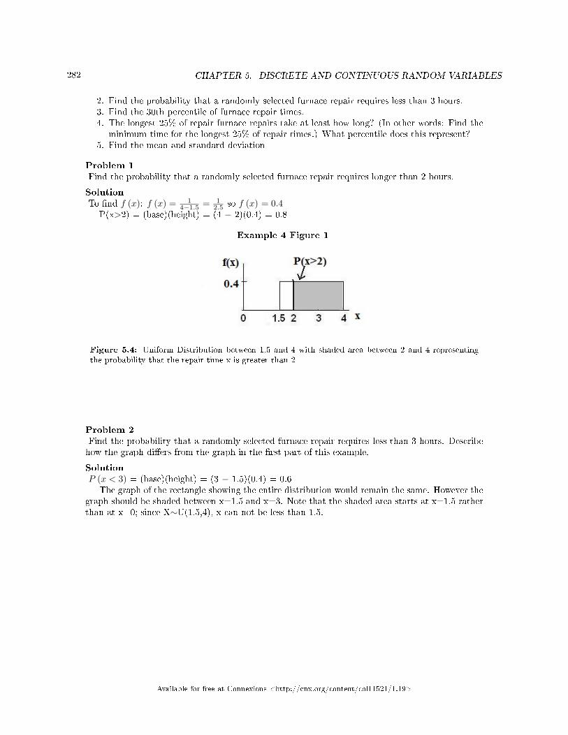
282 CHAPTER 5. DISCRETE AND CONTINUOUS RANDOM VARIABLES
2. Find the probability that a randomly selected furnace repair requires less than 3 hours.3. Find the 30th percentile of furnace repair times.4. The longest 25% of repair furnace repairs take at least how long? (In other words: Find the
minimum time for the longest 25% of repair times.) What percentile does this represent?5. Find the mean and standard deviation
Problem 1Find the probability that a randomly selected furnace repair requires longer than 2 hours.
SolutionTo �nd f (x): f (x) = 1
4−1.5 = 12.5 so f (x) = 0.4
P(x>2) = (base)(height) = (4 − 2)(0.4) = 0.8
Example 4 Figure 1
Figure 5.4: Uniform Distribution between 1.5 and 4 with shaded area between 2 and 4 representingthe probability that the repair time x is greater than 2
Problem 2Find the probability that a randomly selected furnace repair requires less than 3 hours. Describehow the graph di�ers from the graph in the �rst part of this example.
SolutionP (x < 3) = (base)(height) = (3 − 1.5)(0.4) = 0.6
The graph of the rectangle showing the entire distribution would remain the same. However thegraph should be shaded between x=1.5 and x=3. Note that the shaded area starts at x=1.5 ratherthan at x=0; since X∼U(1.5,4), x can not be less than 1.5.
Available for free at Connexions <http://cnx.org/content/col11521/1.19>
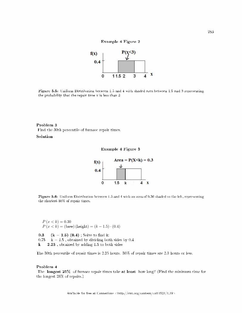
283
Example 4 Figure 2
Figure 5.5: Uniform Distribution between 1.5 and 4 with shaded area between 1.5 and 3 representingthe probability that the repair time x is less than 3
Problem 3Find the 30th percentile of furnace repair times.
Solution
Example 4 Figure 3
Figure 5.6: Uniform Distribution between 1.5 and 4 with an area of 0.30 shaded to the left, representingthe shortest 30% of repair times.
P (x < k) = 0.30P (x < k) = (base) (height) = (k − 1.5) · (0.4)
0.3 = (k − 1.5) (0.4) ; Solve to �nd k:0.75 = k − 1.5 , obtained by dividing both sides by 0.4k = 2.25 , obtained by adding 1.5 to both sides
The 30th percentile of repair times is 2.25 hours. 30% of repair times are 2.5 hours or less.
Problem 4The longest 25% of furnace repair times take at least how long? (Find the minimum time forthe longest 25% of repairs.)
Available for free at Connexions <http://cnx.org/content/col11521/1.19>
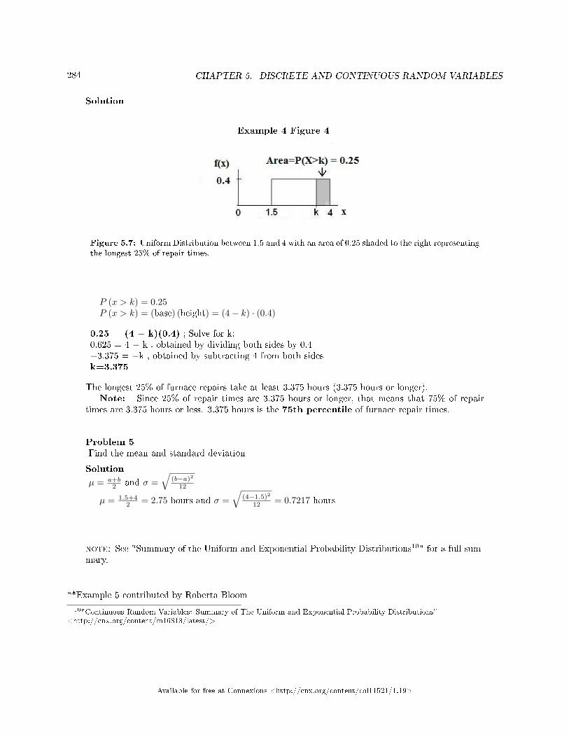
284 CHAPTER 5. DISCRETE AND CONTINUOUS RANDOM VARIABLES
Solution
Example 4 Figure 4
Figure 5.7: Uniform Distribution between 1.5 and 4 with an area of 0.25 shaded to the right representingthe longest 25% of repair times.
P (x > k) = 0.25P (x > k) = (base) (height) = (4− k) · (0.4)
0.25 = (4 − k)(0.4) ; Solve for k:0.625 = 4 − k , obtained by dividing both sides by 0.4−3.375 = −k , obtained by subtracting 4 from both sidesk=3.375
The longest 25% of furnace repairs take at least 3.375 hours (3.375 hours or longer).Note: Since 25% of repair times are 3.375 hours or longer, that means that 75% of repair
times are 3.375 hours or less. 3.375 hours is the 75th percentile of furnace repair times.
Problem 5Find the mean and standard deviation
Solution
µ = a+b2 and σ =
√(b−a)2
12
µ = 1.5+42 = 2.75 hours and σ =
√(4−1.5)2
12 = 0.7217 hours
note: See "Summary of the Uniform and Exponential Probability Distributions10" for a full sum-mary.
**Example 5 contributed by Roberta Bloom
10"Continuous Random Variables: Summary of The Uniform and Exponential Probability Distributions"<http://cnx.org/content/m16813/latest/>
Available for free at Connexions <http://cnx.org/content/col11521/1.19>
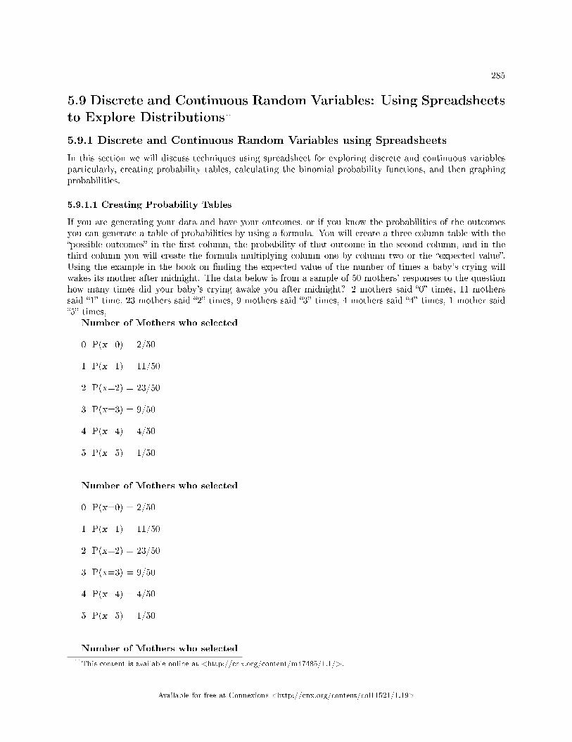
285
5.9 Discrete and Continuous Random Variables: Using Spreadsheetsto Explore Distributions11
5.9.1 Discrete and Continuous Random Variables using Spreadsheets
In this section we will discuss techniques using spreadsheet for exploring discrete and continuous variablesparticularly, creating probability tables, calculating the binomial probability functions, and then graphingprobabilities.
5.9.1.1 Creating Probability Tables
If you are generating your data and have your outcomes, or if you know the probabilities of the outcomesyou can generate a table of probabilities by using a formula. You will create a three column table with the�possible outcomes� in the �rst column, the probability of that outcome in the second column, and in thethird column you will create the formula multiplying column one by column two or the �expected value�.Using the example in the book on �nding the expected value of the number of times a baby's crying willwakes its mother after midnight. The data below is from a sample of 50 mothers' responses to the questionhow many times did your baby's crying awake you after midnight? 2 mothers said �0� times, 11 motherssaid �1� time, 23 mothers said �2� times, 9 mothers said �3� times, 4 mothers said �4� times, 1 mother said�5� times,
Number of Mothers who selected
0 P(x=0) = 2/50
1 P(x=1) = 11/50
2 P(x=2) = 23/50
3 P(x=3) = 9/50
4 P(x=4) = 4/50
5 P(x=5) = 1/50
Number of Mothers who selected
0 P(x=0) = 2/50
1 P(x=1) = 11/50
2 P(x=2) = 23/50
3 P(x=3) = 9/50
4 P(x=4) = 4/50
5 P(x=5) = 1/50
Number of Mothers who selected11This content is available online at <http://cnx.org/content/m47485/1.1/>.
Available for free at Connexions <http://cnx.org/content/col11521/1.19>
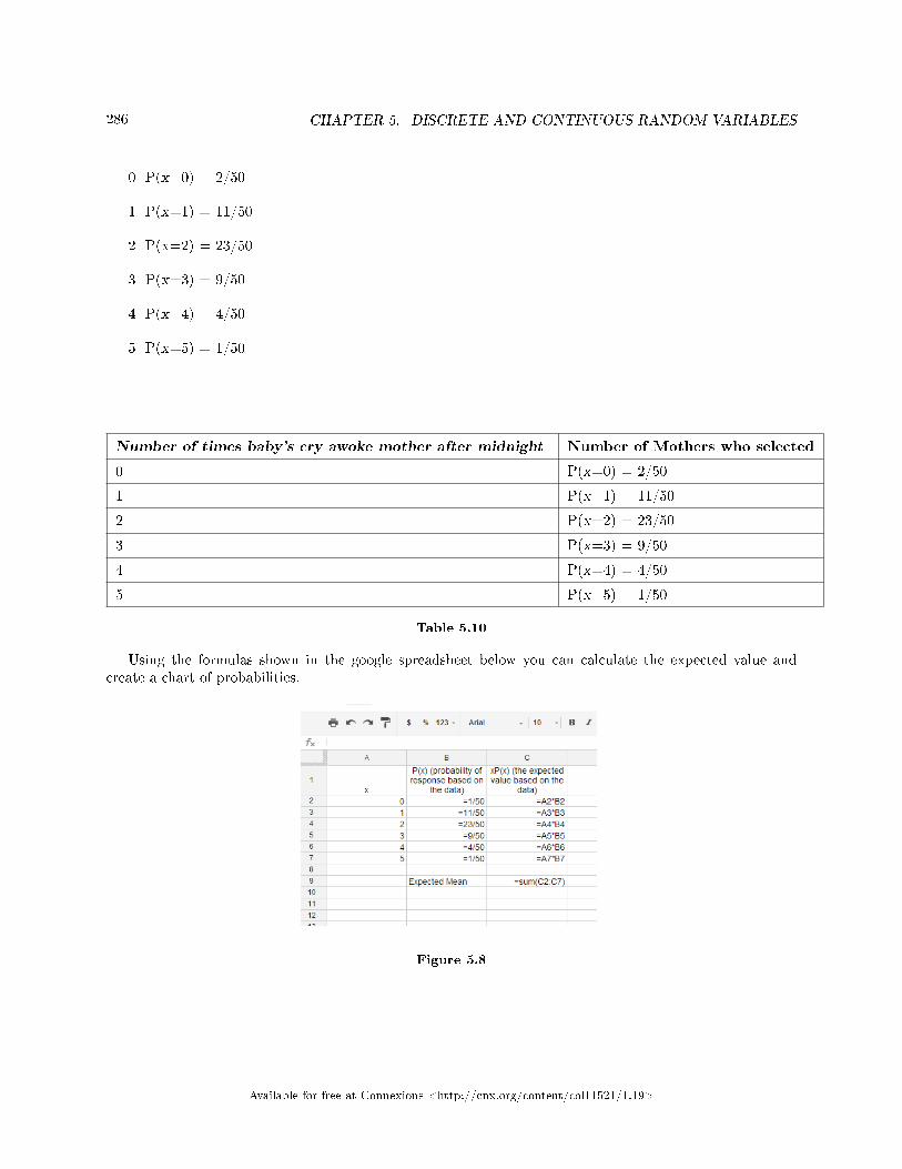
286 CHAPTER 5. DISCRETE AND CONTINUOUS RANDOM VARIABLES
0 P(x=0) = 2/50
1 P(x=1) = 11/50
2 P(x=2) = 23/50
3 P(x=3) = 9/50
4 P(x=4) = 4/50
5 P(x=5) = 1/50
Number of times baby's cry awoke mother after midnight Number of Mothers who selected
0 P(x=0) = 2/50
1 P(x=1) = 11/50
2 P(x=2) = 23/50
3 P(x=3) = 9/50
4 P(x=4) = 4/50
5 P(x=5) = 1/50
Table 5.10
Using the formulas shown in the google spreadsheet below you can calculate the expected value andcreate a chart of probabilities.
Figure 5.8
Available for free at Connexions <http://cnx.org/content/col11521/1.19>
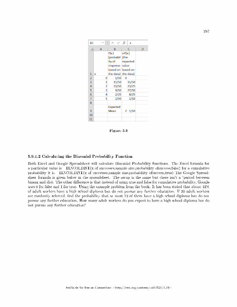
287
Figure 5.9
5.9.1.2 Calculating the Binomial Probability Function
Both Excel and Google Spreadsheet will calculate Binomial Probability functions. The Excel formula fora particular value is =BINOM.DIST(x of successes,sample size,probability ofsuccess,false) for a cumulativeprobability it is =BINOM.DIST(x of successes,sample size,probability ofsuccess,true) The Google Spread-sheet formula is given below in the spreadsheet. The setup is the same but there isn't a �period betweenbinom and dist. The other di�erence is that instead of using true and false for cumulative probability, Googleuses 0 for false and 1 for true. Using the example problem from the book: It has been stated that about 41%of adult workers have a high school diploma but do not pursue any further education. If 20 adult workersare randomly selected, �nd the probability that at most 12 of them have a high school diploma but do notpursue any further education. How many adult workers do you expect to have a high school diploma but donot pursue any further education?
Available for free at Connexions <http://cnx.org/content/col11521/1.19>
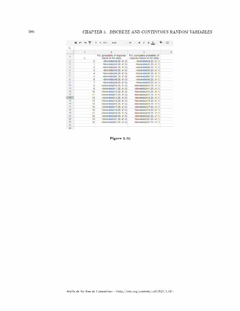
288 CHAPTER 5. DISCRETE AND CONTINUOUS RANDOM VARIABLES
Figure 5.10
Available for free at Connexions <http://cnx.org/content/col11521/1.19>
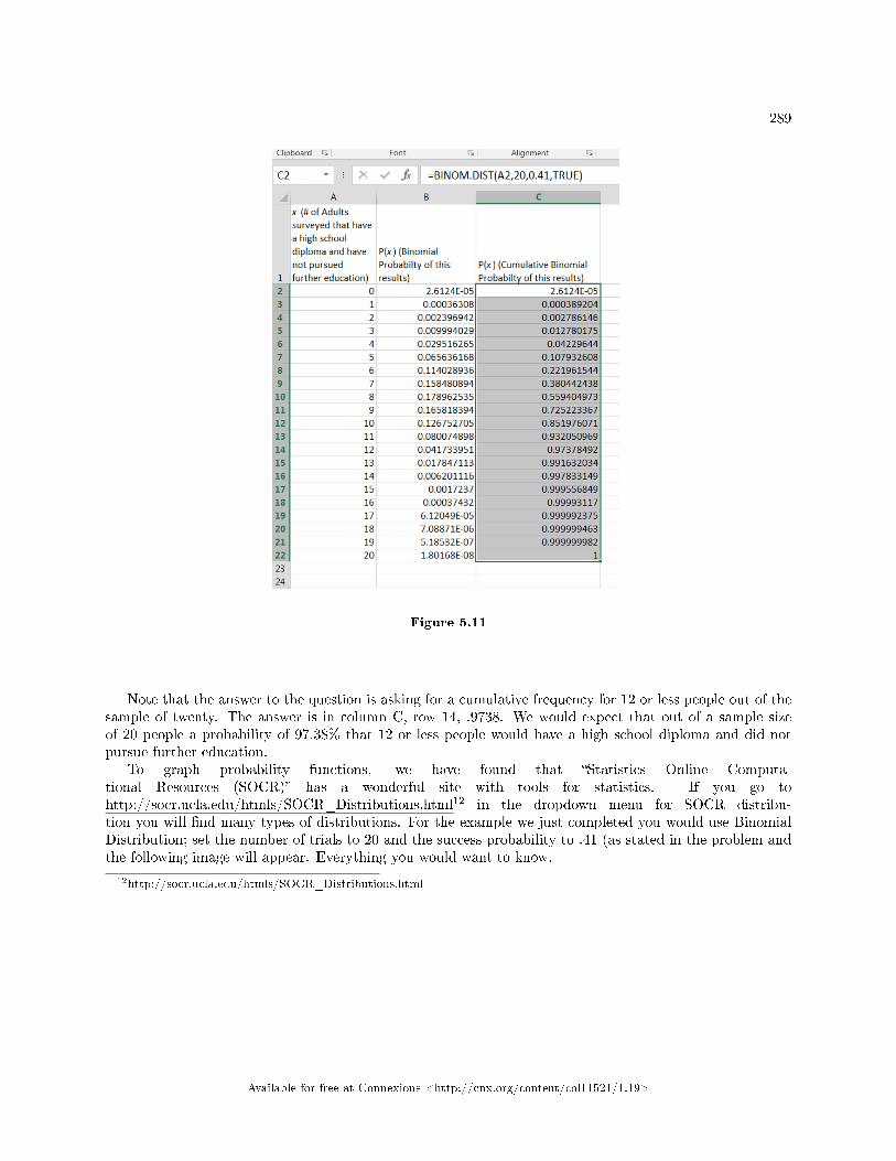
289
Figure 5.11
Note that the answer to the question is asking for a cumulative frequency for 12 or less people out of thesample of twenty. The answer is in column C, row 14, .9738. We would expect that out of a sample sizeof 20 people a probability of 97.38% that 12 or less people would have a high school diploma and did notpursue further education.
To graph probability functions, we have found that �Statistics Online Computa-tional Resources (SOCR)� has a wonderful site with tools for statistics. If you go tohttp://socr.ucla.edu/htmls/SOCR_Distributions.html12 in the dropdown menu for SOCR distribu-tion you will �nd many types of distributions. For the example we just completed you would use BinomialDistribution; set the number of trials to 20 and the success probability to .41 (as stated in the problem andthe following image will appear. Everything you would want to know.
12http://socr.ucla.edu/htmls/SOCR_Distributions.html
Available for free at Connexions <http://cnx.org/content/col11521/1.19>
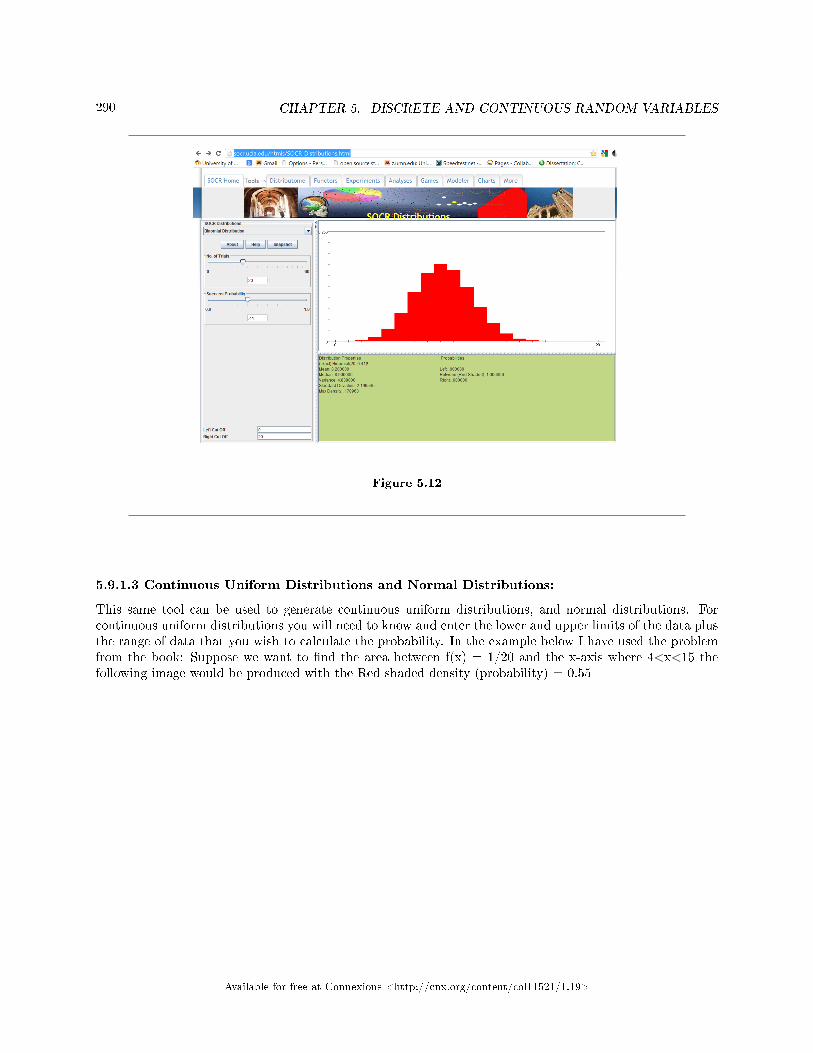
290 CHAPTER 5. DISCRETE AND CONTINUOUS RANDOM VARIABLES
Figure 5.12
5.9.1.3 Continuous Uniform Distributions and Normal Distributions:
This same tool can be used to generate continuous uniform distributions, and normal distributions. Forcontinuous uniform distributions you will need to know and enter the lower and upper limits of the data plusthe range of data that you wish to calculate the probability. In the example below I have used the problemfrom the book: Suppose we want to �nd the area between f(x) = 1/20 and the x-axis where 4<x<15 thefollowing image would be produced with the Red shaded density (probability) = 0.55
Available for free at Connexions <http://cnx.org/content/col11521/1.19>
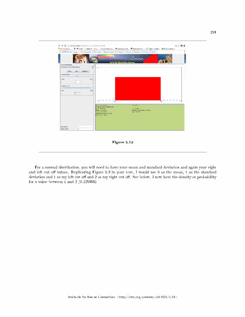
291
Figure 5.13
For a normal distribution, you will need to have your mean and standard deviation and again your rightand left cut o� values. Replicating Figure 5.3 in your text, I would use 0 as the mean, 1 as the standarddeviation and 1 as my left cut o� and 2 as my right cut o�. See below. I now have the density or probabilityfor a value between 1 and 2 (0.125905)
Available for free at Connexions <http://cnx.org/content/col11521/1.19>
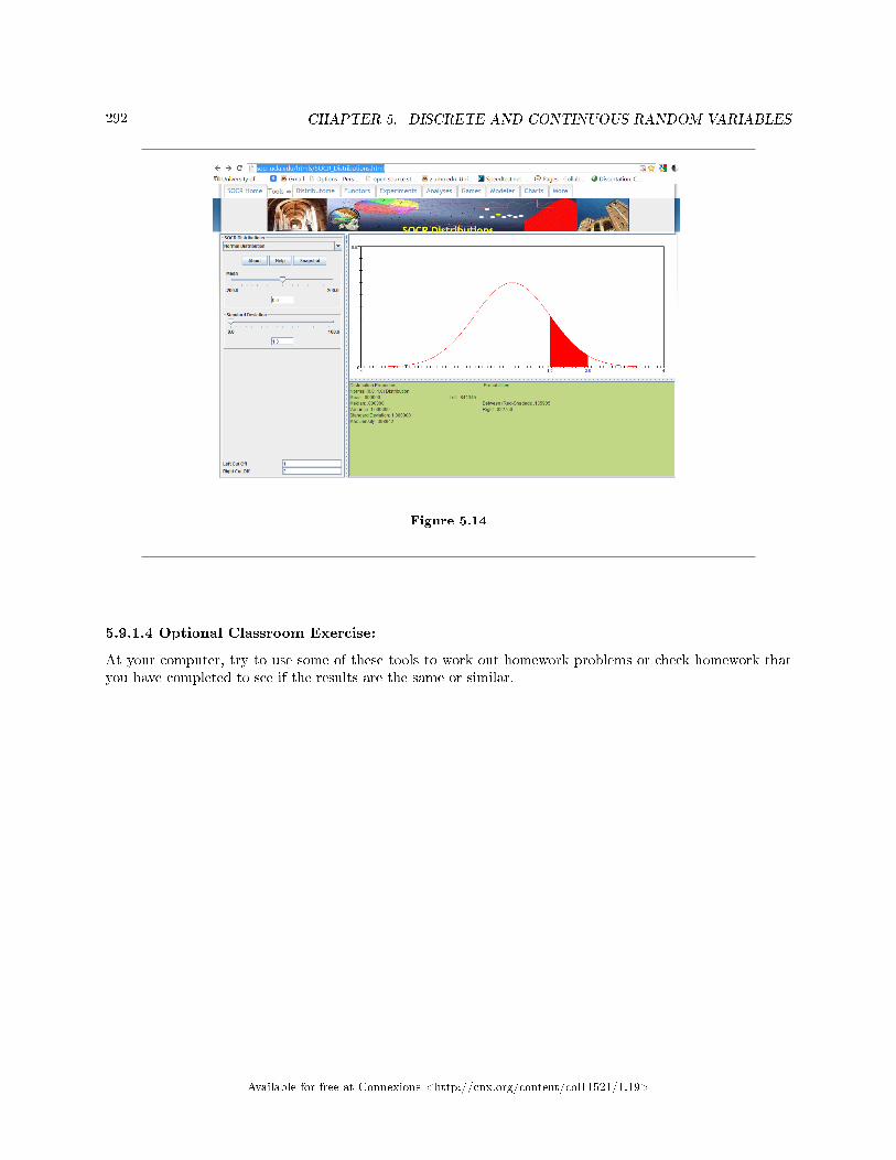
292 CHAPTER 5. DISCRETE AND CONTINUOUS RANDOM VARIABLES
Figure 5.14
5.9.1.4 Optional Classroom Exercise:
At your computer, try to use some of these tools to work out homework problems or check homework thatyou have completed to see if the results are the same or similar.
Available for free at Connexions <http://cnx.org/content/col11521/1.19>
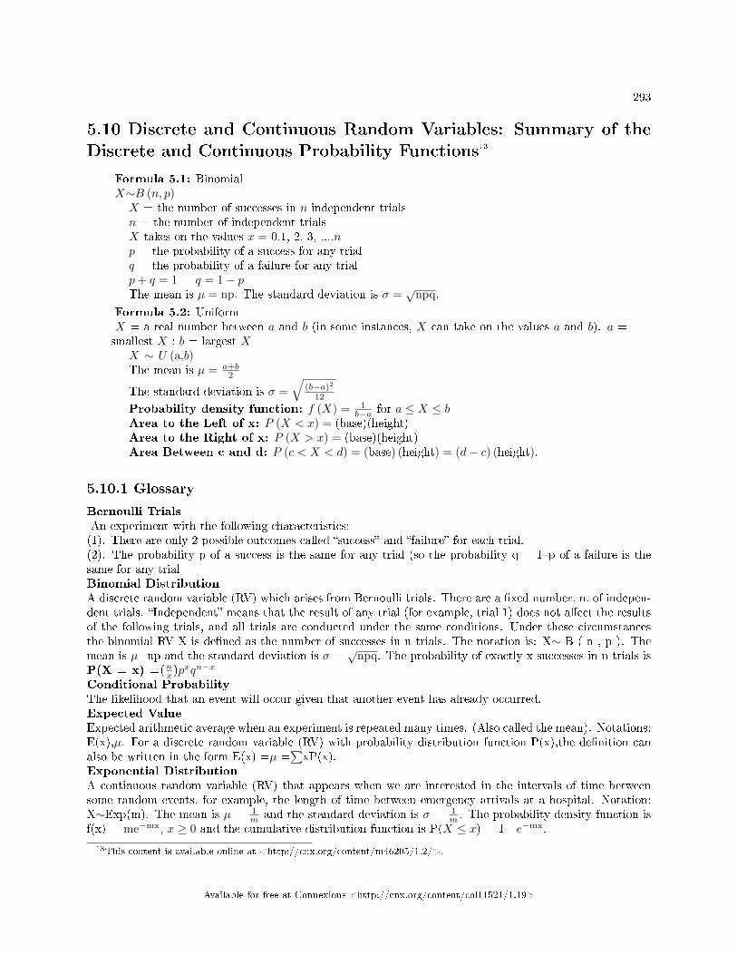
293
5.10 Discrete and Continuous Random Variables: Summary of theDiscrete and Continuous Probability Functions13
Formula 5.1: BinomialX∼B (n, p)X = the number of successes in n independent trialsn = the number of independent trialsX takes on the values x = 0,1, 2, 3, ...,np = the probability of a success for any trialq = the probability of a failure for any trialp+ q = 1 q = 1− pThe mean is µ = np. The standard deviation is σ =
√npq.
Formula 5.2: UniformX = a real number between a and b (in some instances, X can take on the values a and b). a =smallest X ; b = largest X
X ∼ U (a,b)The mean is µ = a+b
2
The standard deviation is σ =√
(b−a)2
12
Probability density function: f (X) = 1b−a for a ≤ X ≤ b
Area to the Left of x: P (X < x) = (base)(height)Area to the Right of x: P (X > x) = (base)(height)Area Between c and d: P (c < X < d) = (base) (height) = (d− c) (height).
5.10.1 Glossary
Bernoulli TrialsAn experiment with the following characteristics:(1). There are only 2 possible outcomes called �success� and �failure� for each trial.(2). The probability p of a success is the same for any trial (so the probability q = 1�p of a failure is thesame for any trialBinomial DistributionA discrete random variable (RV) which arises from Bernoulli trials. There are a �xed number, n, of indepen-dent trials. �Independent� means that the result of any trial (for example, trial 1) does not a�ect the resultsof the following trials, and all trials are conducted under the same conditions. Under these circumstancesthe binomial RV X is de�ned as the number of successes in n trials. The notation is: X∼ B ( n , p ). Themean is µ=np and the standard deviation is σ =
√npq. The probability of exactly x successes in n trials is
P(X = x) =(nx )pxqn−x
Conditional ProbabilityThe likelihood that an event will occur given that another event has already occurred.Expected ValueExpected arithmetic average when an experiment is repeated many times. (Also called the mean). Notations:E(x),µ. For a discrete random variable (RV) with probability distribution function P(x),the de�nition canalso be written in the form E(x) =µ =
∑xP(x).
Exponential DistributionA continuous random variable (RV) that appears when we are interested in the intervals of time betweensome random events, for example, the length of time between emergency arrivals at a hospital. Notation:X∼Exp(m). The mean is µ = 1
m and the standard deviation is σ = 1m . The probability density function is
�(x) = me−mx, x ≥ 0 and the cumulative distribution function is P(X ≤ x) = 1 - e−mx.
13This content is available online at <http://cnx.org/content/m46205/1.2/>.
Available for free at Connexions <http://cnx.org/content/col11521/1.19>
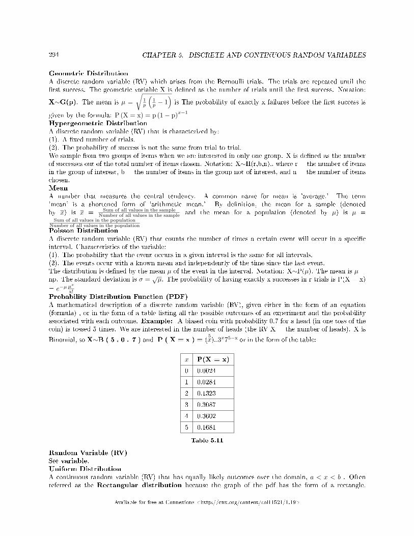
294 CHAPTER 5. DISCRETE AND CONTINUOUS RANDOM VARIABLES
Geometric DistributionA discrete random variable (RV) which arises from the Bernoulli trials. The trials are repeated until the�rst success. The geometric variable X is de�ned as the number of trials until the �rst success. Notation:
X∼G(p). The mean is µ =
√1p
(1p − 1
)is The probability of exactly x failures before the �rst success is
given by the formula: P (X = x) = p (1− p)x−1
Hypergeometric DistributionA discrete random variable (RV) that is characterized by:(1). A �xed number of trials.(2). The probability of success is not the same from trial to trial.We sample from two groups of items when we are interested in only one group. X is de�ned as the numberof successes out of the total number of items chosen. Notation: X∼H(r,b,n)., where r = the number of itemsin the group of interest, b = the number of items in the group not of interest, and n = the number of itemschosen.MeanA number that measures the central tendency. A common name for mean is 'average.' The term'mean' is a shortened form of 'arithmetic mean.' By de�nition, the mean for a sample (denotedby x) is x = Sum of all values in the sample
Number of all values in the sample and the mean for a population (denoted by µ) is µ =Sum of all values in the population
Number of all values in the populationPoisson DistributionA discrete random variable (RV) that counts the number of times a certain event will occur in a speci�cinterval. Characteristics of the variable:(1). The probability that the event occurs in a given interval is the same for all intervals.(2). The events occur with a known mean and independently of the time since the last event.The distribution is de�ned by the mean µ of the event in the interval. Notation: X∼P(µ). The mean is µ =np. The standard deviation is σ =
õ. The probability of having exactly x successes in r trials is P(X = x)
= e−µ µx
x!Probability Distribution Function (PDF)A mathematical description of a discrete random variable (RV), given either in the form of an equation(formula) , or in the form of a table listing all the possible outcomes of an experiment and the probabilityassociated with each outcome. Example: A biased coin with probability 0.7 for a head (in one toss of thecoin) is tossed 5 times. We are interested in the number of heads (the RV X = the number of heads). X is
Binomial, so X∼B ( 5 , 0 . 7 ) and P ( X = x ) = (5x)..3x75−x or in the form of the table:
x P(X = x)
0 0.0024
1 0.0284
2 0.1323
3 0.3087
4 0.3602
5 0.1681
Table 5.11
Random Variable (RV)See variable.Uniform DistributionA continuous random variable (RV) that has equally likely outcomes over the domain, a < x < b . Oftenreferred as the Rectangular distribution because the graph of the pdf has the form of a rectangle.
Available for free at Connexions <http://cnx.org/content/col11521/1.19>
295
Notation: X∼U(a,b). The mean is µ = a + b2 and the standard deviation is
√(b−a)2
12 . The probability
density function is �(x) = 1b − a for a < x < b or a ≤ x ≤ b. The cumalative distribution is P(X ≤ x) =
x − ab − a .Variable (Random Variable)A characteristic of interest in a population being studied. Common notation for variables are upper caseLatin letters X, Y, Z,...; common notation for a speci�c value from the domain (set of all possible values ofa variable) are lower case Latin letters x, y, z,.... For example, if X is the number of children in a family,then x represents a speci�c integer 0, 1, 2, 3, .... Variables in statistics di�er from variables in intermediatealgebra in two following ways.(1). The domain of the random variable (RV) is not necessarily a numerical set; the domain may be expressedin words; for example, if X = hair color then the domain is {black, blond, gray, green, orange}.(2.) We can tell what speci�c value x of the Random Variable X takes only after performing the experiment.
Available for free at Connexions <http://cnx.org/content/col11521/1.19>
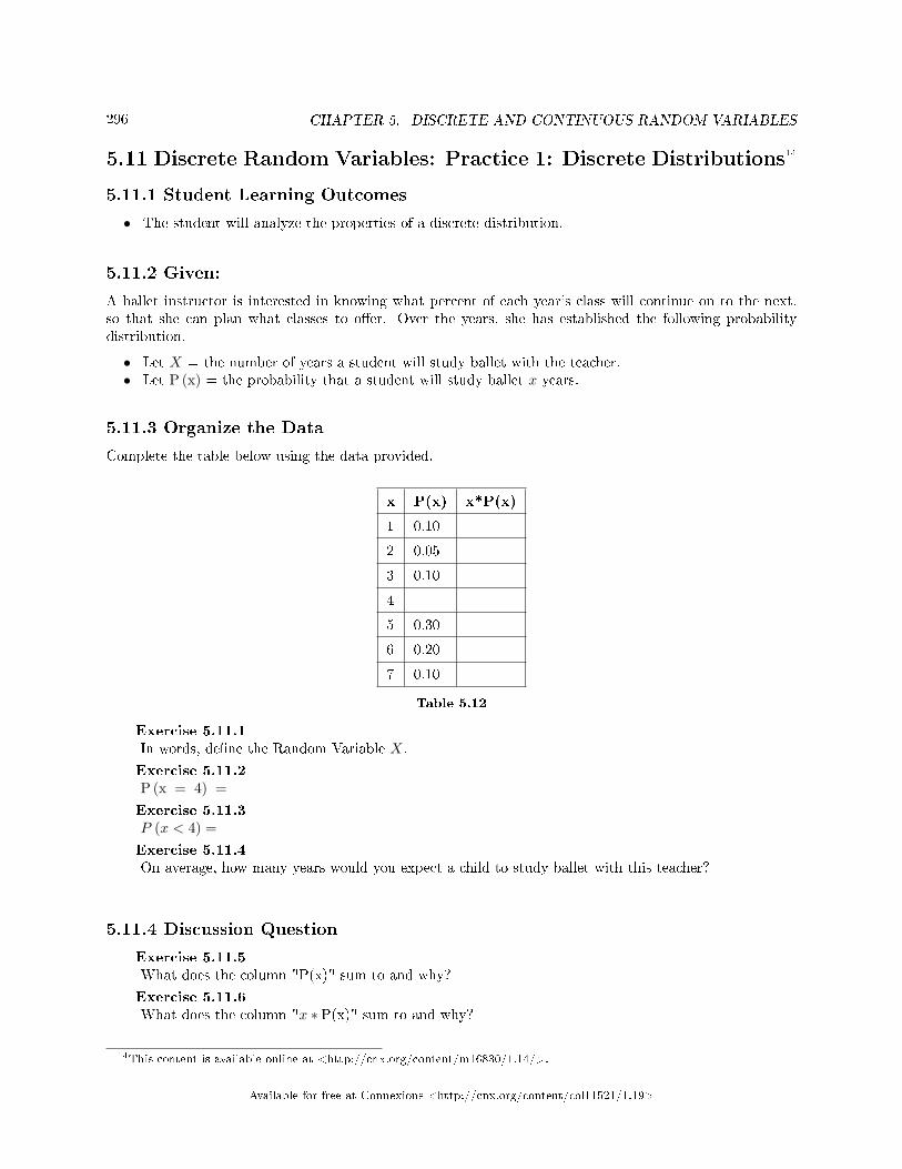
296 CHAPTER 5. DISCRETE AND CONTINUOUS RANDOM VARIABLES
5.11 Discrete Random Variables: Practice 1: Discrete Distributions14
5.11.1 Student Learning Outcomes
• The student will analyze the properties of a discrete distribution.
5.11.2 Given:
A ballet instructor is interested in knowing what percent of each year's class will continue on to the next,so that she can plan what classes to o�er. Over the years, she has established the following probabilitydistribution.
• Let X = the number of years a student will study ballet with the teacher.• Let P (x) = the probability that a student will study ballet x years.
5.11.3 Organize the Data
Complete the table below using the data provided.
x P(x) x*P(x)
1 0.10
2 0.05
3 0.10
4
5 0.30
6 0.20
7 0.10
Table 5.12
Exercise 5.11.1In words, de�ne the Random Variable X.
Exercise 5.11.2P (x = 4) =Exercise 5.11.3P (x < 4) =Exercise 5.11.4On average, how many years would you expect a child to study ballet with this teacher?
5.11.4 Discussion Question
Exercise 5.11.5What does the column "P(x)" sum to and why?
Exercise 5.11.6What does the column "x ∗ P(x)" sum to and why?
14This content is available online at <http://cnx.org/content/m16830/1.14/>.
Available for free at Connexions <http://cnx.org/content/col11521/1.19>
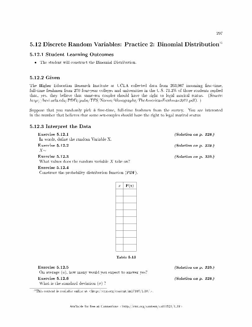
297
5.12 Discrete Random Variables: Practice 2: Binomial Distribution15
5.12.1 Student Learning Outcomes
• The student will construct the Binomial Distribution.
5.12.2 Given
The Higher Education Research Institute at UCLA collected data from 203,967 incoming �rst-time,full-time freshmen from 270 four-year colleges and universities in the U.S. 71.3% of those students repliedthat, yes, they believe that same-sex couples should have the right to legal marital status. (Source:http://heri.ucla.edu/PDFs/pubs/TFS/Norms/Monographs/TheAmericanFreshman2011.pdf). )
Suppose that you randomly pick 8 �rst-time, full-time freshmen from the survey. You are interestedin the number that believes that same sex-couples should have the right to legal marital status
5.12.3 Interpret the Data
Exercise 5.12.1 (Solution on p. 329.)
In words, de�ne the random Variable X.
Exercise 5.12.2 (Solution on p. 329.)
X∼___________Exercise 5.12.3 (Solution on p. 329.)
What values does the random variable X take on?
Exercise 5.12.4Construct the probability distribution function (PDF).
x P(x)
Table 5.13
Exercise 5.12.5 (Solution on p. 329.)
On average (u), how many would you expect to answer yes?
Exercise 5.12.6 (Solution on p. 329.)
What is the standard deviation (σ) ?
15This content is available online at <http://cnx.org/content/m17107/1.18/>.
Available for free at Connexions <http://cnx.org/content/col11521/1.19>
298 CHAPTER 5. DISCRETE AND CONTINUOUS RANDOM VARIABLES
Exercise 5.12.7 (Solution on p. 329.)
What is the probability that at most 5 of the freshmen reply �yes�?
Exercise 5.12.8 (Solution on p. 329.)
What is the probability that at least 2 of the freshmen reply �yes�?
Exercise 5.12.9Construct a histogram or plot a line graph. Label the horizontal and vertical axes with words.Include numerical scaling.
Available for free at Connexions <http://cnx.org/content/col11521/1.19>
299
5.13 Continuous Random Variables: Practice 116
5.13.1 Student Learning Outcomes
• The student will analyze data following a uniform distribution.
5.13.2 Given
The age of cars in the sta� parking lot of a suburban college is uniformly distributed from six months (0.5years) to 9.5 years.
5.13.3 Describe the Data
Exercise 5.13.1 (Solution on p. 329.)
What is being measured here?
Exercise 5.13.2 (Solution on p. 329.)
In words, de�ne the Random Variable X.
Exercise 5.13.3 (Solution on p. 329.)
Are the data discrete or continuous?
Exercise 5.13.4 (Solution on p. 329.)
The interval of values for x is:
Exercise 5.13.5 (Solution on p. 329.)
The distribution for X is:
5.13.4 Probability Distribution
Exercise 5.13.6 (Solution on p. 329.)
Write the probability density function.
Exercise 5.13.7 (Solution on p. 329.)
Graph the probability distribution.
a. Sketch the graph of the probability distribution.
Figure 5.15
16This content is available online at <http://cnx.org/content/m16812/1.14/>.
Available for free at Connexions <http://cnx.org/content/col11521/1.19>
300 CHAPTER 5. DISCRETE AND CONTINUOUS RANDOM VARIABLES
b. Identify the following values:
i. Lowest value for x:ii. Highest value for x:iii. Height of the rectangle:iv. Label for x-axis (words):v. Label for y-axis (words):
5.13.5 Random Probability
Exercise 5.13.8 (Solution on p. 329.)
Find the probability that a randomly chosen car in the lot was less than 4 years old.
a. Sketch the graph. Shade the area of interest.
Figure 5.16
b. Find the probability. P (x < 4) =
Exercise 5.13.9 (Solution on p. 329.)
Out of just the cars less than 7.5 years old, �nd the probability that a randomly chosen car in thelot was less than 4 years old.
a. Sketch the graph. Shade the area of interest.
Available for free at Connexions <http://cnx.org/content/col11521/1.19>
301
Figure 5.17
b. Find the probability. P (x < 4 | x < 7.5) =
Exercise 5.13.10: Discussion QuestionWhat has changed in the previous two problems that made the solutions di�erent?
5.13.6 Quartiles
Exercise 5.13.11 (Solution on p. 329.)
Find the average age of the cars in the lot.
Exercise 5.13.12 (Solution on p. 329.)
Find the third quartile of ages of cars in the lot. This means you will have to �nd the value suchthat 3
4 , or 75%, of the cars are at most (less than or equal to) that age.
a. Sketch the graph. Shade the area of interest.
Figure 5.18
b. Find the value k such that P (x < k) = 0.75.c. The third quartile is:
Available for free at Connexions <http://cnx.org/content/col11521/1.19>
302 CHAPTER 5. DISCRETE AND CONTINUOUS RANDOM VARIABLES
5.14 Discrete and Continuous Random Variables: Homework17
Exercise 5.14.1 (Solution on p. 330.)
1. Complete the PDF and answer the questions.
x P (X = x) x · P (X = x)
0 0.3
1 0.2
2
3 0.4
Table 5.14
a. Find the probability that x = 2.b. Find the expected value.
Exercise 5.14.2Suppose that you are o�ered the following �deal.� You roll a die. If you roll a 6, you win $10. Ifyou roll a 4 or 5, you win $5. If you roll a 1, 2, or 3, you pay $6.
a. What are you ultimately interested in here (the value of the roll or the money you win)?b. In words, de�ne the Random Variable X.c. List the values that X may take on.d. Construct a PDF.e. Over the long run of playing this game, what are your expected average winnings per game?f. Based on numerical values, should you take the deal? Explain your decision in complete sen-
tences.
Exercise 5.14.3 (Solution on p. 330.)
A venture capitalist, willing to invest $1,000,000, has three investments to choose from. The �rstinvestment, a software company, has a 10% chance of returning $5,000,000 pro�t, a 30% chance ofreturning $1,000,000 pro�t, and a 60% chance of losing the million dollars. The second company,a hardware company, has a 20% chance of returning $3,000,000 pro�t, a 40% chance of returning$1,000,000 pro�t, and a 40% chance of losing the million dollars. The third company, a biotech�rm, has a 10% chance of returning $6,000,000 pro�t, a 70% of no pro�t or loss, and a 20% chanceof losing the million dollars.
a. Construct a PDF for each investment.b. Find the expected value for each investment.c. Which is the safest investment? Why do you think so?d. Which is the riskiest investment? Why do you think so?e. Which investment has the highest expected return, on average?
Exercise 5.14.4A theater group holds a fund-raiser. It sells 100 ra�e tickets for $5 apiece. Suppose you purchase4 tickets. The prize is 2 passes to a Broadway show, worth a total of $150.
a. What are you interested in here?
17This content is available online at <http://cnx.org/content/m46206/1.2/>.
Available for free at Connexions <http://cnx.org/content/col11521/1.19>
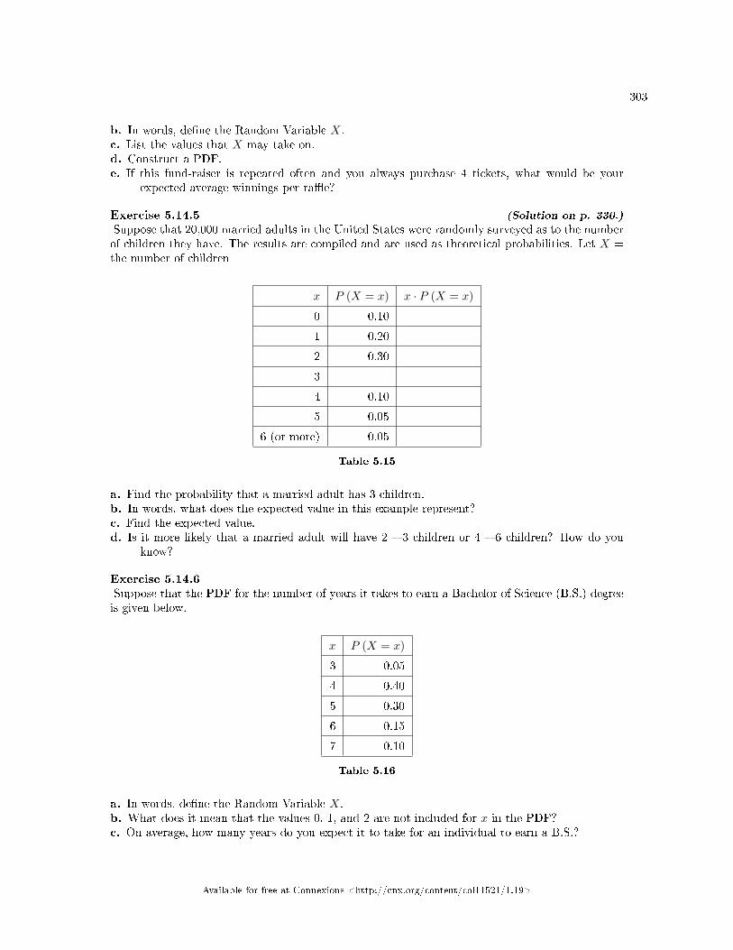
303
b. In words, de�ne the Random Variable X.c. List the values that X may take on.d. Construct a PDF.e. If this fund-raiser is repeated often and you always purchase 4 tickets, what would be your
expected average winnings per ra�e?
Exercise 5.14.5 (Solution on p. 330.)
Suppose that 20,000 married adults in the United States were randomly surveyed as to the numberof children they have. The results are compiled and are used as theoretical probabilities. Let X =the number of children
x P (X = x) x · P (X = x)
0 0.10
1 0.20
2 0.30
3
4 0.10
5 0.05
6 (or more) 0.05
Table 5.15
a. Find the probability that a married adult has 3 children.b. In words, what does the expected value in this example represent?c. Find the expected value.d. Is it more likely that a married adult will have 2 � 3 children or 4 � 6 children? How do you
know?
Exercise 5.14.6Suppose that the PDF for the number of years it takes to earn a Bachelor of Science (B.S.) degreeis given below.
x P (X = x)
3 0.05
4 0.40
5 0.30
6 0.15
7 0.10
Table 5.16
a. In words, de�ne the Random Variable X.b. What does it mean that the values 0, 1, and 2 are not included for x in the PDF?c. On average, how many years do you expect it to take for an individual to earn a B.S.?
Available for free at Connexions <http://cnx.org/content/col11521/1.19>
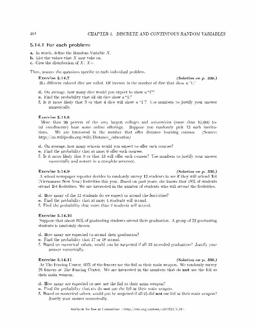
304 CHAPTER 5. DISCRETE AND CONTINUOUS RANDOM VARIABLES
5.14.1 For each problem:
a. In words, de�ne the Random Variable X.b. List the values that X may take on.c. Give the distribution of X. X∼
Then, answer the questions speci�c to each individual problem.
Exercise 5.14.7 (Solution on p. 330.)
Six di�erent colored dice are rolled. Of interest is the number of dice that show a �1.�
d. On average, how many dice would you expect to show a �1�?e. Find the probability that all six dice show a �1.�f. Is it more likely that 3 or that 4 dice will show a �1�? Use numbers to justify your answer
numerically.
Exercise 5.14.8More than 96 percent of the very largest colleges and universities (more than 15,000 to-
tal enrollments) have some online o�erings. Suppose you randomly pick 13 such institu-tions. We are interested in the number that o�er distance learning courses. (Source:http://en.wikipedia.org/wiki/Distance_education)
d. On average, how many schools would you expect to o�er such courses?e. Find the probability that at most 6 o�er such courses.f. Is it more likely that 0 or that 13 will o�er such courses? Use numbers to justify your answer
numerically and answer in a complete sentence.
Exercise 5.14.9 (Solution on p. 330.)
A school newspaper reporter decides to randomly survey 12 students to see if they will attend Tet(Vietnamese New Year) festivities this year. Based on past years, she knows that 18% of studentsattend Tet festivities. We are interested in the number of students who will attend the festivities.
d. How many of the 12 students do we expect to attend the festivities?e. Find the probability that at most 4 students will attend.f. Find the probability that more than 2 students will attend.
Exercise 5.14.10Suppose that about 85% of graduating students attend their graduation. A group of 22 graduatingstudents is randomly chosen.
d. How many are expected to attend their graduation?e. Find the probability that 17 or 18 attend.f. Based on numerical values, would you be surprised if all 22 attended graduation? Justify your
answer numerically.
Exercise 5.14.11 (Solution on p. 330.)
At The Fencing Center, 60% of the fencers use the foil as their main weapon. We randomly survey25 fencers at The Fencing Center. We are interested in the numbers that do not use the foil astheir main weapon.
d. How many are expected to not use the foil as their main weapon?e. Find the probability that six do not use the foil as their main weapon.f. Based on numerical values, would you be surprised if all 25 did not use foil as their main weapon?
Justify your answer numerically.
Available for free at Connexions <http://cnx.org/content/col11521/1.19>
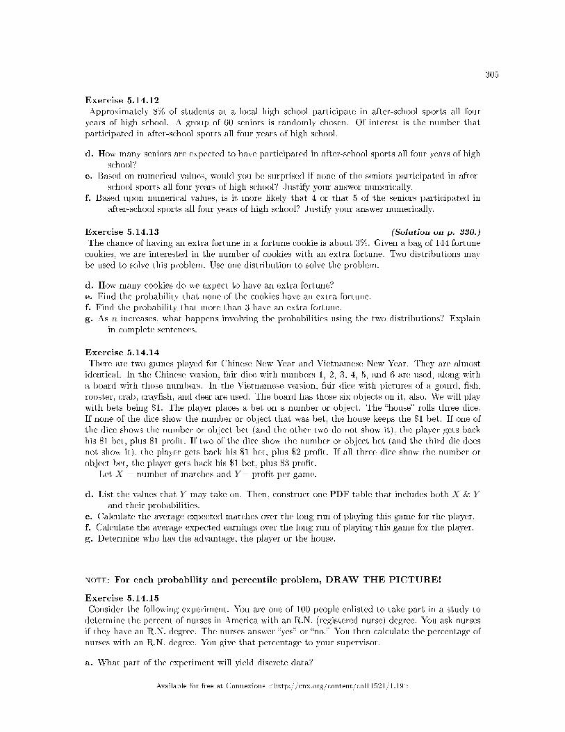
305
Exercise 5.14.12Approximately 8% of students at a local high school participate in after-school sports all fouryears of high school. A group of 60 seniors is randomly chosen. Of interest is the number thatparticipated in after-school sports all four years of high school.
d. How many seniors are expected to have participated in after-school sports all four years of highschool?
e. Based on numerical values, would you be surprised if none of the seniors participated in after-school sports all four years of high school? Justify your answer numerically.
f. Based upon numerical values, is it more likely that 4 or that 5 of the seniors participated inafter-school sports all four years of high school? Justify your answer numerically.
Exercise 5.14.13 (Solution on p. 330.)
The chance of having an extra fortune in a fortune cookie is about 3%. Given a bag of 144 fortunecookies, we are interested in the number of cookies with an extra fortune. Two distributions maybe used to solve this problem. Use one distribution to solve the problem.
d. How many cookies do we expect to have an extra fortune?e. Find the probability that none of the cookies have an extra fortune.f. Find the probability that more than 3 have an extra fortune.g. As n increases, what happens involving the probabilities using the two distributions? Explain
in complete sentences.
Exercise 5.14.14There are two games played for Chinese New Year and Vietnamese New Year. They are almostidentical. In the Chinese version, fair dice with numbers 1, 2, 3, 4, 5, and 6 are used, along witha board with those numbers. In the Vietnamese version, fair dice with pictures of a gourd, �sh,rooster, crab, cray�sh, and deer are used. The board has those six objects on it, also. We will playwith bets being $1. The player places a bet on a number or object. The �house� rolls three dice.If none of the dice show the number or object that was bet, the house keeps the $1 bet. If one ofthe dice shows the number or object bet (and the other two do not show it), the player gets backhis $1 bet, plus $1 pro�t. If two of the dice show the number or object bet (and the third die doesnot show it), the player gets back his $1 bet, plus $2 pro�t. If all three dice show the number orobject bet, the player gets back his $1 bet, plus $3 pro�t.
Let X = number of matches and Y= pro�t per game.
d. List the values that Y may take on. Then, construct one PDF table that includes both X & Yand their probabilities.
e. Calculate the average expected matches over the long run of playing this game for the player.f. Calculate the average expected earnings over the long run of playing this game for the player.g. Determine who has the advantage, the player or the house.
note: For each probability and percentile problem, DRAW THE PICTURE!
Exercise 5.14.15Consider the following experiment. You are one of 100 people enlisted to take part in a study todetermine the percent of nurses in America with an R.N. (registered nurse) degree. You ask nursesif they have an R.N. degree. The nurses answer �yes� or �no.� You then calculate the percentage ofnurses with an R.N. degree. You give that percentage to your supervisor.
a. What part of the experiment will yield discrete data?
Available for free at Connexions <http://cnx.org/content/col11521/1.19>
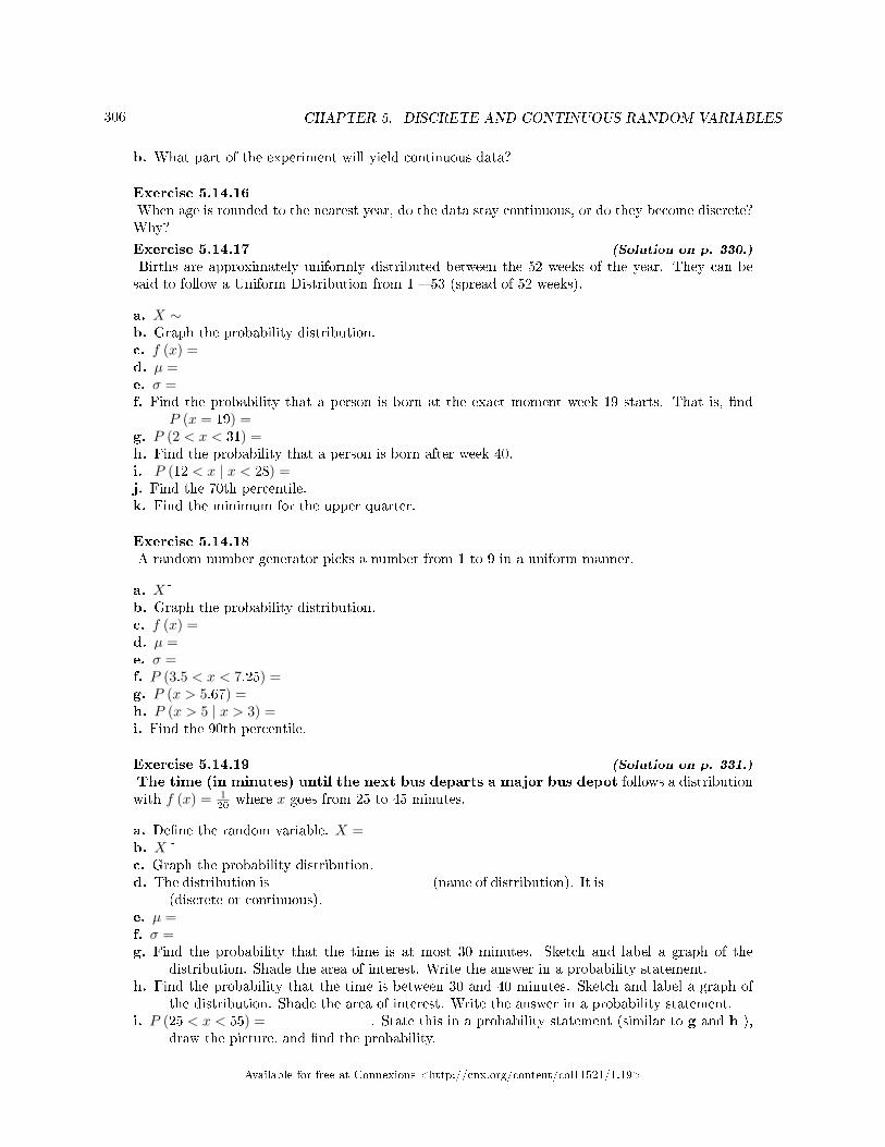
306 CHAPTER 5. DISCRETE AND CONTINUOUS RANDOM VARIABLES
b. What part of the experiment will yield continuous data?
Exercise 5.14.16When age is rounded to the nearest year, do the data stay continuous, or do they become discrete?Why?
Exercise 5.14.17 (Solution on p. 330.)
Births are approximately uniformly distributed between the 52 weeks of the year. They can besaid to follow a Uniform Distribution from 1 � 53 (spread of 52 weeks).
a. X ∼b. Graph the probability distribution.c. f (x) =d. µ =e. σ =f. Find the probability that a person is born at the exact moment week 19 starts. That is, �nd
P (x = 19) =g. P (2 < x < 31) =h. Find the probability that a person is born after week 40.i. P (12 < x | x < 28) =j. Find the 70th percentile.k. Find the minimum for the upper quarter.
Exercise 5.14.18A random number generator picks a number from 1 to 9 in a uniform manner.
a. X~b. Graph the probability distribution.c. f (x) =d. µ =e. σ =f. P (3.5 < x < 7.25) =g. P (x > 5.67) =h. P (x > 5 | x > 3) =i. Find the 90th percentile.
Exercise 5.14.19 (Solution on p. 331.)
The time (in minutes) until the next bus departs a major bus depot follows a distributionwith f (x) = 1
20 where x goes from 25 to 45 minutes.
a. De�ne the random variable. X =b. X~c. Graph the probability distribution.d. The distribution is ______________ (name of distribution). It is _____________
(discrete or continuous).e. µ =f. σ =g. Find the probability that the time is at most 30 minutes. Sketch and label a graph of the
distribution. Shade the area of interest. Write the answer in a probability statement.h. Find the probability that the time is between 30 and 40 minutes. Sketch and label a graph of
the distribution. Shade the area of interest. Write the answer in a probability statement.i. P (25 < x < 55) = _________. State this in a probability statement (similar to g and h ),
draw the picture, and �nd the probability.
Available for free at Connexions <http://cnx.org/content/col11521/1.19>
307
j. Find the 90th percentile. This means that 90% of the time, the time is less than _____minutes.
k. Find the 75th percentile. In a complete sentence, state what this means. (See j.)l. Find the probability that the time is more than 40 minutes given (or knowing that) it is at least
30 minutes.
Exercise 5.14.20According to a study by Dr. John McDougall of his live-in weight loss program at St. HelenaHospital, the people who follow his program lose between 6 and 15 pounds a month until theyapproach trim body weight. Let's suppose that the weight loss is uniformly distributed. We areinterested in the weight loss of a randomly selected individual following the program for one month.(Source: The McDougall Program for Maximum Weight Loss by John A. McDougall,M.D.)
a. De�ne the random variable. X =b. X~c. Graph the probability distribution.d. f (x) =e. µ =f. σ =g. Find the probability that the individual lost more than 10 pounds in a month.h. Suppose it is known that the individual lost more than 10 pounds in a month. Find the proba-
bility that he lost less than 12 pounds in the month.i. P (7 < x < 13 | x > 9) = __________. State this in a probability question (similar to g
and h), draw the picture, and �nd the probability.
Exercise 5.14.21 (Solution on p. 331.)
A subway train on the Red Line arrives every 8 minutes during rush hour. We are interested in thelength of time a commuter must wait for a train to arrive. The time follows a uniform distribution.
a. De�ne the random variable. X =b. X~c. Graph the probability distribution.d. f (x) =e. µ =f. σ =g. Find the probability that the commuter waits less than one minute.h. Find the probability that the commuter waits between three and four minutes.i. 60% of commuters wait more than how long for the train? State this in a probability question
(similar to g and h), draw the picture, and �nd the probability.
Exercise 5.14.22The age of a �rst grader on September 1 at Garden Elementary School is uniformly distributedfrom 5.8 to 6.8 years. We randomly select one �rst grader from the class.
a. De�ne the random variable. X =b. X~c. Graph the probability distribution.d. f (x) =e. µ =f. σ =g. Find the probability that she is over 6.5 years.
Available for free at Connexions <http://cnx.org/content/col11521/1.19>
308 CHAPTER 5. DISCRETE AND CONTINUOUS RANDOM VARIABLES
h. Find the probability that she is between 4 and 6 years.i. Find the 70th percentile for the age of �rst graders on September 1 at Garden Elementary School.
5.14.2 Try these multiple choice problems.
For the next three problems: The probability that the San Jose Sharks will win any given game is 0.3694based on a 13 year win history of 382 wins out of 1034 games played (as of a certain date). An upcomingmonthly schedule contains 12 games.Let X = the number of games won in that upcoming month.
Exercise 5.14.23 (Solution on p. 331.)
The expected number of wins for that upcoming month is:
A. 1.67B. 12C. 382
1043D. 4.43
Exercise 5.14.24 (Solution on p. 331.)
What is the probability that the San Jose Sharks win 6 games in that upcoming month?
A. 0.1476B. 0.2336C. 0.7664D. 0.8903
Exercise 5.14.25 (Solution on p. 331.)
What is the probability that the San Jose Sharks win at least 5 games in that upcoming month
A. 0.3694B. 0.5266C. 0.4734D. 0.2305
For the next two questions: The average number of times per week that Mrs. Plum's cats wake her upat night because they want to play is 10. We are interested in the number of times her cats wake her upeach week.
Exercise 5.14.26 (Solution on p. 331.)
In words, the random variable X =
A. The number of times Mrs. Plum's cats wake her up each weekB. The number of times Mrs. Plum's cats wake her up each hourC. The number of times Mrs. Plum's cats wake her up each nightD. The number of times Mrs. Plum's cats wake her up
Exercise 5.14.27 (Solution on p. 331.)
Find the probability that her cats will wake her up no more than 5 times next week.
A. 0.5000B. 0.9329C. 0.0378
Available for free at Connexions <http://cnx.org/content/col11521/1.19>
309
D. 0.0671
The next three questions refer to the following information. The Sky Train from the terminal tothe rental car and long term parking center is supposed to arrive every 8 minutes. The waiting times for thetrain are known to follow a uniform distribution.
Exercise 5.14.28 (Solution on p. 331.)
What is the average waiting time (in minutes)?
A. 0.0000B. 2.0000C. 3.0000D. 4.0000
Exercise 5.14.29 (Solution on p. 331.)
Find the 30th percentile for the waiting times (in minutes).
A. 2.0000B. 2.4000C. 2.750D. 3.000
Exercise 5.14.30 (Solution on p. 331.)
The probability of waiting more than 7 minutes given a person has waited more than 4 minutesis?
A. 0.1250B. 0.2500C. 0.500D. 0.7500
Exercise 5.14.31 (Solution on p. 331.)
People visiting video rental stores often rent more than one DVD at a time. The probabilitydistribution for DVD rentals per customer at Video To Go is given below. There is 5 video limitper customer at this store, so nobody ever rents more than 5 DVDs.
x 0 1 2 3 4 5
P(X=x) 0.03 0.50 0.24 ? 0.07 0.04
Table 5.17
A. Describe the random variable X in words.B. Find the probability that a customer rents three DVDs.C. Find the probability that a customer rents at least 4 DVDs.D. Find the probability that a customer rents at most 2 DVDs.
Another shop, Entertainment Headquarters, rents DVDs and videogames. The probability distri-bution for DVD rentals per customer at this shop is given below. They also have a 5 DVD limitper customer.
x 0 1 2 3 4 5
P(X=x) 0.35 0.25 0.20 0.10 0.05 0.05
Available for free at Connexions <http://cnx.org/content/col11521/1.19>
310 CHAPTER 5. DISCRETE AND CONTINUOUS RANDOM VARIABLES
Table 5.18
E. At which store is the expected number of DVDs rented per customer higher?F. If Video to Go estimates that they will have 300 customers next week, how many DVDs do they
expect to rent next week? Answer in sentence form.G. If Video to Go expects 300 customers next week and Entertainment HQ projects that they will
have 420 customers, for which store is the expected number of DVD rentals for next weekhigher? Explain.
H. Which of the two video stores experiences more variation in the number of DVD rentals percustomer? How do you know that?
Exercise 5.14.32 (Solution on p. 332.)
A game involves selecting a card from a deck of cards and tossing a coin. The deck has 52 cardsand 12 cards are "face cards" (Jack, Queen, or King) The coin is a fair coin and is equally likely toland on Heads or Tails
• If the card is a face card and the coin lands on Heads, you win $6• If the card is a face card and the coin lands on Tails, you win $2• If the card is not a face card, you lose $2, no matter what the coin shows.
A. Find the expected value for this game (expected net gain or loss).B. Explain what your calculations indicate about your long-term average pro�ts and losses on this
game.C. Should you play this game to win money?
Exercise 5.14.33 (Solution on p. 332.)
You buy a lottery ticket to a lottery that costs $10 per ticket. There are only 100 tickets availablebe sold in this lottery. In this lottery there is one $500 prize, 2 $100 prizes and 4 $25 prizes. Findyour expected gain or loss.
Exercise 5.14.34 (Solution on p. 332.)
A student takes a 10 question true-false quiz, but did not study and randomly guesses each answer.Find the probability that the student passes the quiz with a grade of at least 70% of the questionscorrect.
Exercise 5.14.35 (Solution on p. 332.)
A student takes a 32 question multiple choice exam, but did not study and randomly guesses eachanswer. Each question has 3 possible choices for the answer. Find the probability that the studentguesses more than 75% of the questions correctly.
Exercise 5.14.36 (Solution on p. 333.)
Suppose that you are perfoming the probability experiment of rolling one fair six-sided die. Let Fbe the event of rolling a "4" or a "5". You are interested in how many times you need to roll thedie in order to obtain the �rst �4 or 5� as the outcome.
• p = probability of success (event F occurs)• q = probability of failure (event F does not occur)
A. Write the description of the random variable X. What are the values that X can take on? Findthe values of p and q.
B. Find the probability that the �rst occurrence of event F (rolling a �4� or �5�) is on the secondtrial.
C. How many trials would you expect until you roll a �4� or �5�?
**Exercises 38 - 43 contributed by Roberta Bloom
Available for free at Connexions <http://cnx.org/content/col11521/1.19>
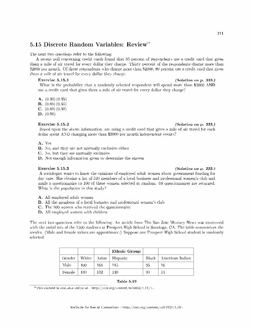
311
5.15 Discrete Random Variables: Review18
The next two questions refer to the following:A recent poll concerning credit cards found that 35 percent of respondents use a credit card that gives
them a mile of air travel for every dollar they charge. Thirty percent of the respondents charge more than$2000 per month. Of those respondents who charge more than $2000, 80 percent use a credit card that givesthem a mile of air travel for every dollar they charge.
Exercise 5.15.1 (Solution on p. 333.)
What is the probability that a randomly selected respondent will spend more than $2000 ANDuse a credit card that gives them a mile of air travel for every dollar they charge?
A. (0.30) (0.35)B. (0.80) (0.35)C. (0.80) (0.30)D. (0.80)
Exercise 5.15.2 (Solution on p. 333.)
Based upon the above information, are using a credit card that gives a mile of air travel for eachdollar spent AND charging more than $2000 per month independent events?
A. YesB. No, and they are not mutually exclusive eitherC. No, but they are mutually exclusiveD. Not enough information given to determine the answer
Exercise 5.15.3 (Solution on p. 333.)
A sociologist wants to know the opinions of employed adult women about government funding forday care. She obtains a list of 520 members of a local business and professional women's club andmails a questionnaire to 100 of these women selected at random. 68 questionnaires are returned.What is the population in this study?
A. All employed adult womenB. All the members of a local business and professional women's clubC. The 100 women who received the questionnaireD. All employed women with children
The next two questions refer to the following: An article from The San Jose Mercury News was concernedwith the racial mix of the 1500 students at Prospect High School in Saratoga, CA. The table summarizes theresults. (Male and female values are approximate.) Suppose one Prospect High School student is randomlyselected.
Ethnic Group
Gender White Asian Hispanic Black American Indian
Male 400 168 115 35 16
Female 440 132 140 40 14
Table 5.19
18This content is available online at <http://cnx.org/content/m16832/1.11/>.
Available for free at Connexions <http://cnx.org/content/col11521/1.19>
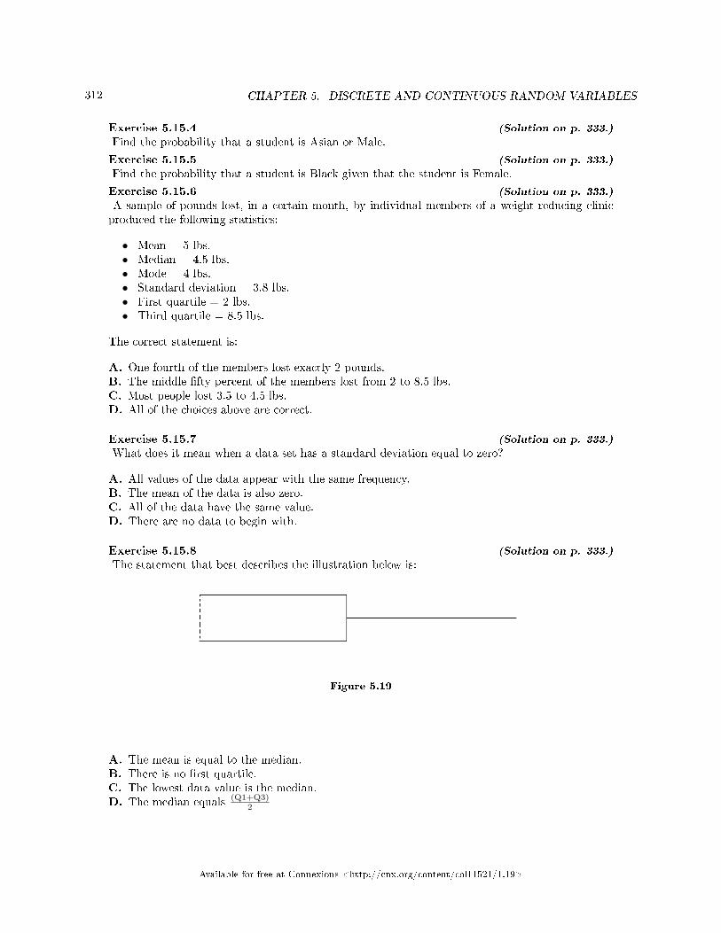
312 CHAPTER 5. DISCRETE AND CONTINUOUS RANDOM VARIABLES
Exercise 5.15.4 (Solution on p. 333.)
Find the probability that a student is Asian or Male.
Exercise 5.15.5 (Solution on p. 333.)
Find the probability that a student is Black given that the student is Female.
Exercise 5.15.6 (Solution on p. 333.)
A sample of pounds lost, in a certain month, by individual members of a weight reducing clinicproduced the following statistics:
• Mean = 5 lbs.• Median = 4.5 lbs.• Mode = 4 lbs.• Standard deviation = 3.8 lbs.• First quartile = 2 lbs.• Third quartile = 8.5 lbs.
The correct statement is:
A. One fourth of the members lost exactly 2 pounds.B. The middle �fty percent of the members lost from 2 to 8.5 lbs.C. Most people lost 3.5 to 4.5 lbs.D. All of the choices above are correct.
Exercise 5.15.7 (Solution on p. 333.)
What does it mean when a data set has a standard deviation equal to zero?
A. All values of the data appear with the same frequency.B. The mean of the data is also zero.C. All of the data have the same value.D. There are no data to begin with.
Exercise 5.15.8 (Solution on p. 333.)
The statement that best describes the illustration below is:
Figure 5.19
A. The mean is equal to the median.B. There is no �rst quartile.C. The lowest data value is the median.D. The median equals (Q1+Q3)
2
Available for free at Connexions <http://cnx.org/content/col11521/1.19>
313
Exercise 5.15.9 (Solution on p. 333.)
According to a recent article (San Jose Mercury News) the average number of babies born withsigni�cant hearing loss (deafness) is approximately 2 per 1000 babies in a healthy baby nursery.The number climbs to an average of 30 per 1000 babies in an intensive care nursery.
Suppose that 1000 babies from healthy baby nurseries were randomly surveyed. Find the prob-ability that exactly 2 babies were born deaf.
Exercise 5.15.10 (Solution on p. 333.)
A �friend� o�ers you the following �deal.� For a $10 fee, you may pick an envelope from a boxcontaining 100 seemingly identical envelopes. However, each envelope contains a coupon for a freegift.
• 10 of the coupons are for a free gift worth $6.• 80 of the coupons are for a free gift worth $8.• 6 of the coupons are for a free gift worth $12.• 4 of the coupons are for a free gift worth $40.
Based upon the �nancial gain or loss over the long run, should you play the game?
A. Yes, I expect to come out ahead in money.B. No, I expect to come out behind in money.C. It doesn't matter. I expect to break even.
The next four questions refer to the following: Recently, a nurse commented that when a patient calls themedical advice line claiming to have the �u, the chance that he/she truly has the �u (and not just a nastycold) is only about 4%. Of the next 25 patients calling in claiming to have the �u, we are interested in howmany actually have the �u.
Exercise 5.15.11 (Solution on p. 333.)
De�ne the Random Variable and list its possible values.
Exercise 5.15.12 (Solution on p. 333.)
State the distribution of X .
Exercise 5.15.13 (Solution on p. 333.)
Find the probability that at least 4 of the 25 patients actually have the �u.
Exercise 5.15.14 (Solution on p. 333.)
On average, for every 25 patients calling in, how many do you expect to have the �u?
The next two questions refer to the following: Di�erent types of writing can sometimes be distinguished bythe number of letters in the words used. A student interested in this fact wants to study the number ofletters of words used by Tom Clancy in his novels. She opens a Clancy novel at random and records thenumber of letters of the �rst 250 words on the page.
Exercise 5.15.15 (Solution on p. 333.)
What kind of data was collected?
A. qualitativeB. quantitative - continuousC. quantitative � discrete
Exercise 5.15.16 (Solution on p. 333.)
What is the population under study?
Available for free at Connexions <http://cnx.org/content/col11521/1.19>
314 CHAPTER 5. DISCRETE AND CONTINUOUS RANDOM VARIABLES
5.16 Continuous Random Variables: Review19
Exercise 5.16.1 � Exercise 5.16.7 refer to the following study: A recent study of mothers of juniorhigh school children in Santa Clara County reported that 76% of the mothers are employed in paid positions.Of those mothers who are employed, 64% work full-time (over 35 hours per week), and 36% work part-time.However, out of all of the mothers in the population, 49% work full-time. The population under study ismade up of mothers of junior high school children in Santa Clara County.
Let E =employed, Let F =full-time employment
Exercise 5.16.1 (Solution on p. 334.)
a. Find the percent of all mothers in the population that NOT employed.b. Find the percent of mothers in the population that are employed part-time.
Exercise 5.16.2 (Solution on p. 334.)
The type of employment is considered to be what type of data?
Exercise 5.16.3 (Solution on p. 334.)
Find the probability that a randomly selected mother works part-time given that she is employed.
Exercise 5.16.4 (Solution on p. 334.)
Find the probability that a randomly selected person from the population will be employed ORwork full-time.
Exercise 5.16.5 (Solution on p. 334.)
Based upon the above information, are being employed AND working part-time:
a. mutually exclusive events? Why or why not?b. independent events? Why or why not?
Exercise 5.16.6 - Exercise 5.16.7 refer to the following: We randomly pick 10 mothers from the abovepopulation. We are interested in the number of the mothers that are employed. Let X =number of mothersthat are employed.
Exercise 5.16.6 (Solution on p. 334.)
State the distribution for X.
Exercise 5.16.7 (Solution on p. 334.)
Find the probability that at least 6 are employed.
Exercise 5.16.8 (Solution on p. 334.)
We expect the Statistics Discussion Board to have, on average, 14 questions posted to it per week.We are interested in the number of questions posted to it per day.
a. De�ne X.b. What are the values that the random variable may take on?c. State the distribution for X.d. Find the probability that from 10 to 14 (inclusive) questions are posted to the Listserv on a
randomly picked day.
Exercise 5.16.9 (Solution on p. 334.)
A person invests $1000 in stock of a company that hopes to go public in 1 year.
• The probability that the person will lose all his money after 1 year (i.e. his stock will beworthless) is 35%.
• The probability that the person's stock will still have a value of $1000 after 1 year (i.e. nopro�t and no loss) is 60%.
19This content is available online at <http://cnx.org/content/m16810/1.11/>.
Available for free at Connexions <http://cnx.org/content/col11521/1.19>
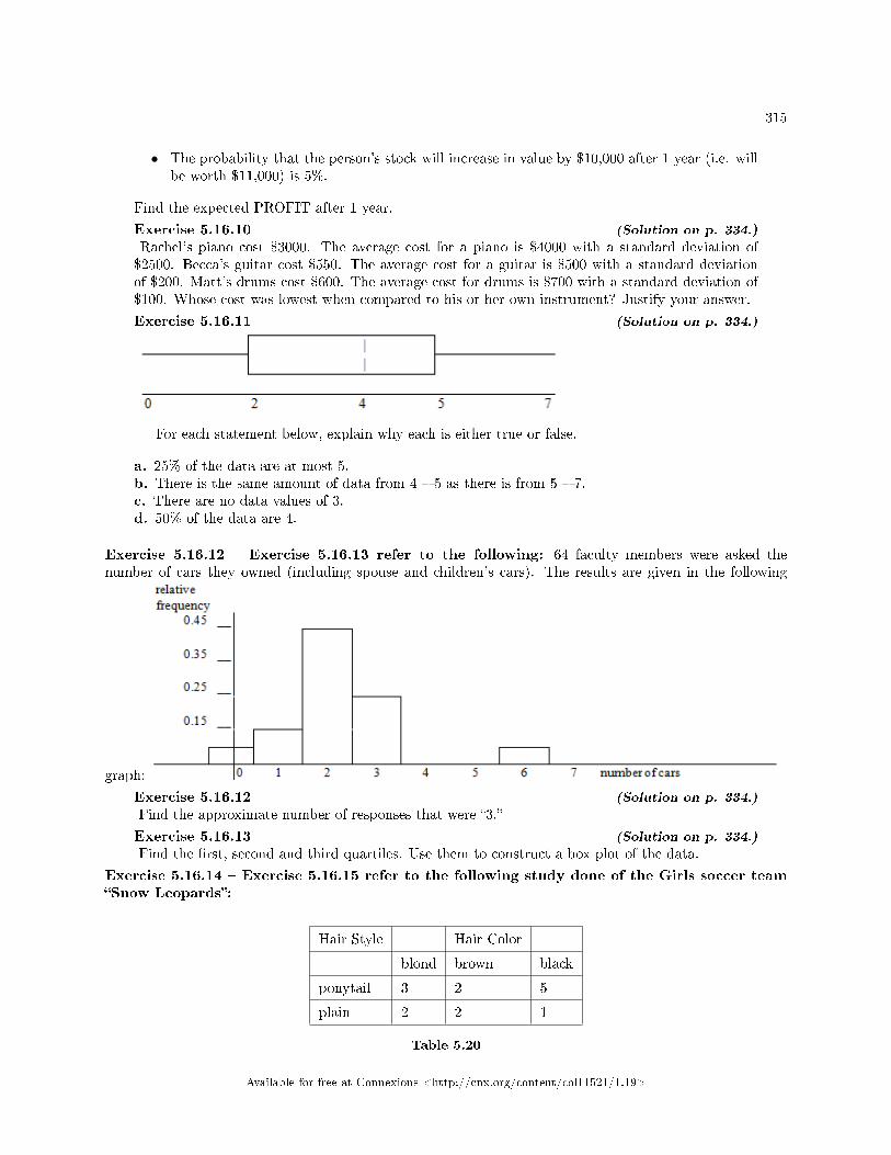
315
• The probability that the person's stock will increase in value by $10,000 after 1 year (i.e. willbe worth $11,000) is 5%.
Find the expected PROFIT after 1 year.
Exercise 5.16.10 (Solution on p. 334.)
Rachel's piano cost $3000. The average cost for a piano is $4000 with a standard deviation of$2500. Becca's guitar cost $550. The average cost for a guitar is $500 with a standard deviationof $200. Matt's drums cost $600. The average cost for drums is $700 with a standard deviation of$100. Whose cost was lowest when compared to his or her own instrument? Justify your answer.
Exercise 5.16.11 (Solution on p. 334.)
For each statement below, explain why each is either true or false.
a. 25% of the data are at most 5.b. There is the same amount of data from 4 � 5 as there is from 5 � 7.c. There are no data values of 3.d. 50% of the data are 4.
Exercise 5.16.12 � Exercise 5.16.13 refer to the following: 64 faculty members were asked thenumber of cars they owned (including spouse and children's cars). The results are given in the following
graph:
Exercise 5.16.12 (Solution on p. 334.)
Find the approximate number of responses that were �3.�
Exercise 5.16.13 (Solution on p. 334.)
Find the �rst, second and third quartiles. Use them to construct a box plot of the data.
Exercise 5.16.14 � Exercise 5.16.15 refer to the following study done of the Girls soccer team�Snow Leopards�:
Hair Style Hair Color
blond brown black
ponytail 3 2 5
plain 2 2 1
Table 5.20
Available for free at Connexions <http://cnx.org/content/col11521/1.19>
316 CHAPTER 5. DISCRETE AND CONTINUOUS RANDOM VARIABLES
Suppose that one girl from the Snow Leopards is randomly selected.
Exercise 5.16.14 (Solution on p. 334.)
Find the probability that the girl has black hair GIVEN that she wears a ponytail.
Exercise 5.16.15 (Solution on p. 334.)
Find the probability that the girl wears her hair plain OR has brown hair.
Exercise 5.16.16 (Solution on p. 334.)
Find the probability that the girl has blond hair AND that she wears her hair plain.
Available for free at Connexions <http://cnx.org/content/col11521/1.19>
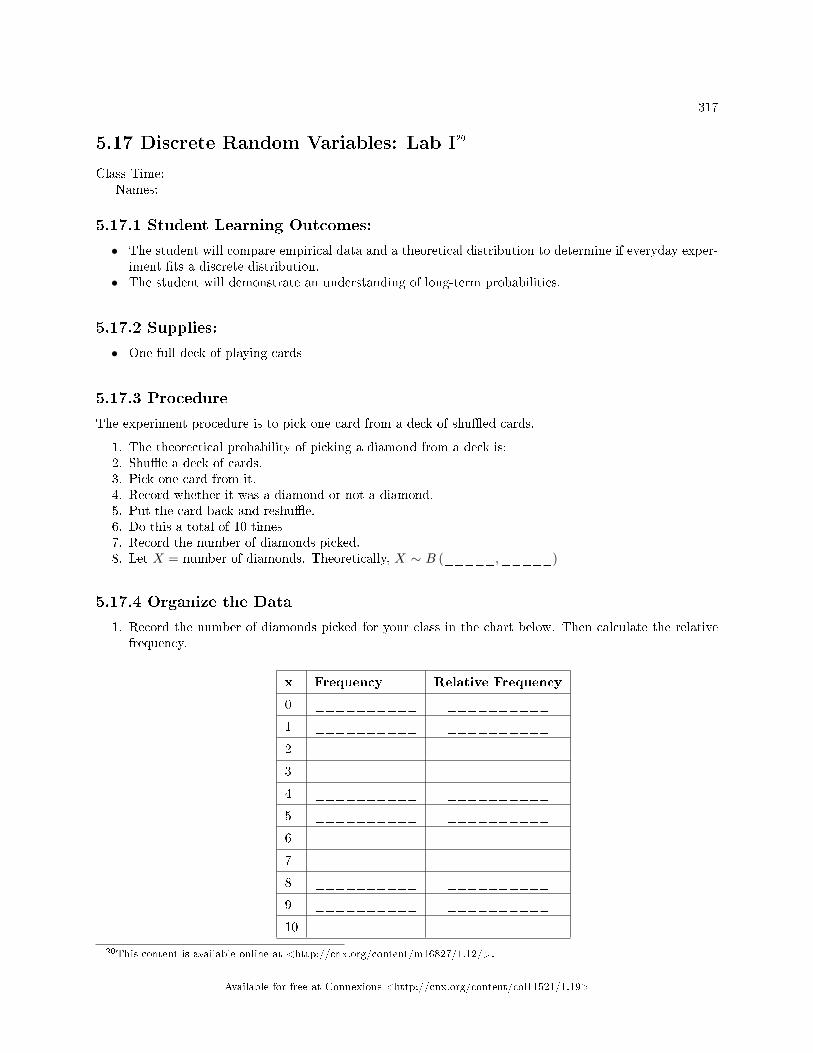
317
5.17 Discrete Random Variables: Lab I20
Class Time:Names:
5.17.1 Student Learning Outcomes:
• The student will compare empirical data and a theoretical distribution to determine if everyday exper-iment �ts a discrete distribution.
• The student will demonstrate an understanding of long-term probabilities.
5.17.2 Supplies:
• One full deck of playing cards
5.17.3 Procedure
The experiment procedure is to pick one card from a deck of shu�ed cards.
1. The theorectical probability of picking a diamond from a deck is: _________2. Shu�e a deck of cards.3. Pick one card from it.4. Record whether it was a diamond or not a diamond.5. Put the card back and reshu�e.6. Do this a total of 10 times7. Record the number of diamonds picked.8. Let X = number of diamonds. Theoretically, X ∼ B (_____,_____)
5.17.4 Organize the Data
1. Record the number of diamonds picked for your class in the chart below. Then calculate the relativefrequency.
x Frequency Relative Frequency
0 __________ __________
1 __________ __________
2 __________ __________
3 __________ __________
4 __________ __________
5 __________ __________
6 __________ __________
7 __________ __________
8 __________ __________
9 __________ __________
10 __________ __________
20This content is available online at <http://cnx.org/content/m16827/1.12/>.
Available for free at Connexions <http://cnx.org/content/col11521/1.19>
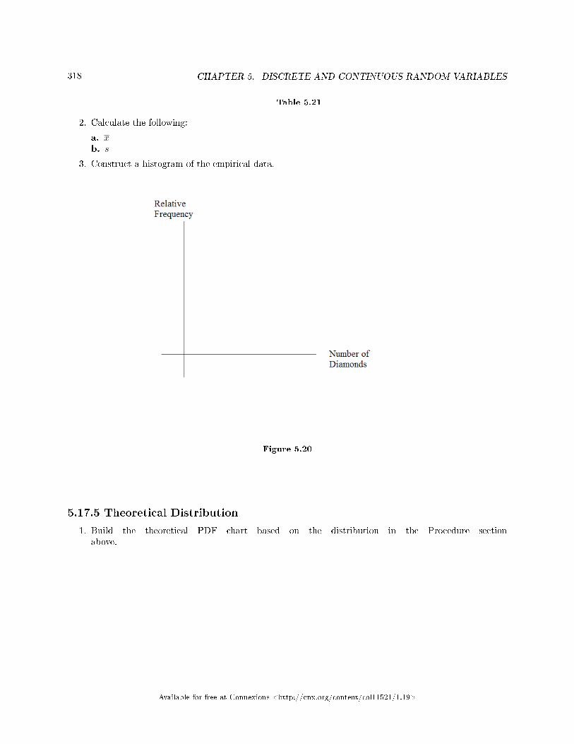
318 CHAPTER 5. DISCRETE AND CONTINUOUS RANDOM VARIABLES
Table 5.21
2. Calculate the following:
a. x =b. s =
3. Construct a histogram of the empirical data.
Figure 5.20
5.17.5 Theoretical Distribution
1. Build the theoretical PDF chart based on the distribution in the Procedure sectionabove.
Available for free at Connexions <http://cnx.org/content/col11521/1.19>
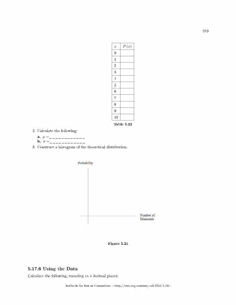
319
x P (x)
0
1
2
3
4
5
6
7
8
9
10
Table 5.22
2. Calculate the following:
a. µ =____________b. σ =____________
3. Construct a histogram of the theoretical distribution.
Figure 5.21
5.17.6 Using the Data
Calculate the following, rounding to 4 decimal places:
Available for free at Connexions <http://cnx.org/content/col11521/1.19>
320 CHAPTER 5. DISCRETE AND CONTINUOUS RANDOM VARIABLES
note: RF = relative frequency
Use the table from the section titled "Theoretical Distribution" here:
• P (x = 3) =• P (1 < x < 4) =• P (x ≥ 8) =
Use the data from the section titled "Organize the Data" here:
• RF (x = 3) =• RF (1 < x < 4) =• RF (x ≥ 8) =
5.17.7 Discussion Questions
For questions 1. and 2., think about the shapes of the two graphs, the probabilities and the relativefrequencies, the means, and the standard deviations.
1. Knowing that data vary, describe three similarities between the graphs and distributions of the theo-retical and empirical distributions. Use complete sentences. (Note: These answers may vary and stillbe correct.)
2. Describe the three most signi�cant di�erences between the graphs or distributions of the theoreticaland empirical distributions. (Note: These answers may vary and still be correct.)
3. Using your answers from the two previous questions, does it appear that the data �t the theoreticaldistribution? In 1 - 3 complete sentences, explain why or why not.
4. Suppose that the experiment had been repeated 500 times. Which table (from "Organize the data"and "Theoretical Distributions") would you expect to change (and how would it change)? Why? Whywouldn't the other table change?
Available for free at Connexions <http://cnx.org/content/col11521/1.19>
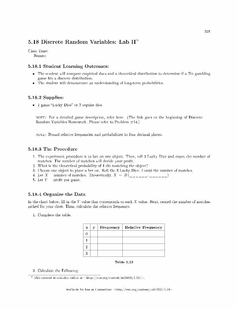
321
5.18 Discrete Random Variables: Lab II21
Class Time:Names:
5.18.1 Student Learning Outcomes:
• The student will compare empirical data and a theoretical distribution to determine if a Tet gamblinggame �ts a discrete distribution.
• The student will demonstrate an understanding of long-term probabilities.
5.18.2 Supplies:
• 1 game �Lucky Dice� or 3 regular dice
note: For a detailed game description, refer here. (The link goes to the beginning of DiscreteRandom Variables Homework. Please refer to Problem #14.)
note: Round relative frequencies and probabilities to four decimal places.
5.18.3 The Procedure
1. The experiment procedure is to bet on one object. Then, roll 3 Lucky Dice and count the number ofmatches. The number of matches will decide your pro�t.
2. What is the theoretical probability of 1 die matching the object? _________3. Choose one object to place a bet on. Roll the 3 Lucky Dice. Count the number of matches.4. Let X = number of matches. Theoretically, X ∼ B (______,______)5. Let Y = pro�t per game.
5.18.4 Organize the Data
In the chart below, �ll in the Y value that corresponds to each X value. Next, record the number of matchespicked for your class. Then, calculate the relative frequency.
1. Complete the table.
x y Frequency Relative Frequency
0
1
2
3
Table 5.23
2. Calculate the Following:
21This content is available online at <http://cnx.org/content/m16826/1.12/>.
Available for free at Connexions <http://cnx.org/content/col11521/1.19>
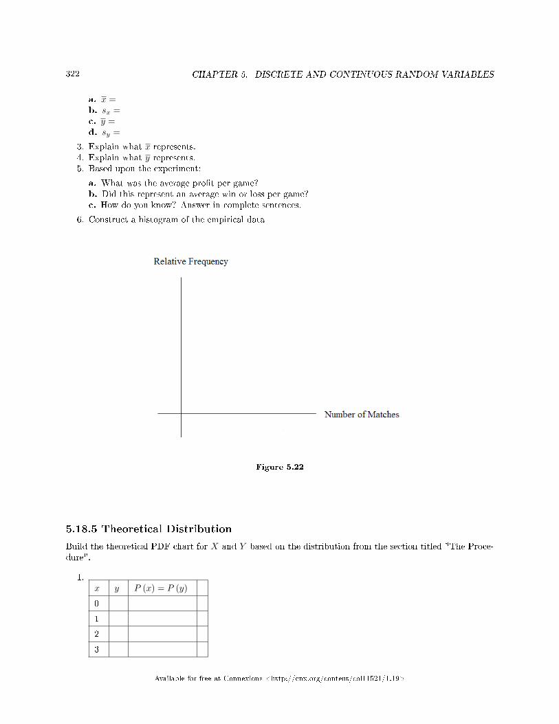
322 CHAPTER 5. DISCRETE AND CONTINUOUS RANDOM VARIABLES
a. x =b. sx =c. y =d. sy =
3. Explain what x represents.4. Explain what y represents.5. Based upon the experiment:
a. What was the average pro�t per game?b. Did this represent an average win or loss per game?c. How do you know? Answer in complete sentences.
6. Construct a histogram of the empirical data
Figure 5.22
5.18.5 Theoretical Distribution
Build the theoretical PDF chart for X and Y based on the distribution from the section titled "The Proce-dure".
1.x y P (x) = P (y)
0
1
2
3
Available for free at Connexions <http://cnx.org/content/col11521/1.19>
323
Table 5.24
2. Calculate the following
a. µx =b. σx =c. µy =
3. Explain what µx represents.4. Explain what µy represents.5. Based upon theory:
a. What was the expected pro�t per game?b. Did the expected pro�t represent an average win or loss per game?c. How do you know? Answer in complete sentences.
6. Construct a histogram of the theoretical distribution.
Figure 5.23
5.18.6 Use the Data
Calculate the following (rounded to 4 decimal places):
note: RF = relative frequency
Use the data from the section titled "Theoretical Distribution" here:
1. P (x = 3) =____________2. P (0 < x < 3) =____________3. P (x ≥ 2) =____________
Available for free at Connexions <http://cnx.org/content/col11521/1.19>
324 CHAPTER 5. DISCRETE AND CONTINUOUS RANDOM VARIABLES
Use the data from the section titled "Organize the Data" here:
1. RF (x = 3) =____________2. RF (0 < x < 3) =____________3. RF (x ≥ 2) = ____________
5.18.7 Discussion Question
For questions 1. and 2., consider the graphs, the probabilities and relative frequencies, the means and thestandard deviations.
1. Knowing that data vary, describe three similarities between the graphs and distributions of the theo-retical and empirical distributions. Use complete sentences. (Note: these answers may vary and stillbe correct.)
2. Describe the three most signi�cant di�erences between the graphs or distributions of the theoreticaland empirical distributions. (Note: these answers may vary and still be correct.)
3. Thinking about your answers to 1. and 2.,does it appear that the data �t the theoretical distribution?In 1 - 3 complete sentences, explain why or why not.
4. Suppose that the experiment had been repeated 500 times. Which table (from "Organize the Data"or "Theoretical Distribution") would you expect to change? Why? How might the table change?
Available for free at Connexions <http://cnx.org/content/col11521/1.19>
325
5.19 Continuous Random Variables: Lab I22
Class Time:Names:
5.19.1 Student Learning Outcomes:
• The student will compare and contrast empirical data from a random number generator with theUniform Distribution.
5.19.2 Collect the Data
Use a random number generator to generate 50 values between 0 and 1 (inclusive). List them below. Roundthe numbers to 4 decimal places or set the calculator MODE to 4 places.
1. Complete the table:
__________ __________ __________ __________ __________
__________ __________ __________ __________ __________
__________ __________ __________ __________ __________
__________ __________ __________ __________ __________
__________ __________ __________ __________ __________
__________ __________ __________ __________ __________
__________ __________ __________ __________ __________
__________ __________ __________ __________ __________
__________ __________ __________ __________ __________
__________ __________ __________ __________ __________
Table 5.25
2. Calculate the following:
a. x =b. s =c. 1st quartile =d. 3rd quartile =e. Median =
5.19.3 Organize the Data
1. Construct a histogram of the empirical data. Make 8 bars.
22This content is available online at <http://cnx.org/content/m16803/1.13/>.
Available for free at Connexions <http://cnx.org/content/col11521/1.19>
326 CHAPTER 5. DISCRETE AND CONTINUOUS RANDOM VARIABLES
Figure 5.24
2. Construct a histogram of the empirical data. Make 5 bars.
Figure 5.25
Available for free at Connexions <http://cnx.org/content/col11521/1.19>
327
5.19.4 Describe the Data
1. Describe the shape of each graph. Use 2 � 3 complete sentences. (Keep it simple. Does the graph gostraight across, does it have a V shape, does it have a hump in the middle or at either end, etc.? Oneway to help you determine a shape, is to roughly draw a smooth curve through the top of the bars.)
2. Describe how changing the number of bars might change the shape.
5.19.5 Theoretical Distribution
1. In words, X =2. The theoretical distribution of X is X ∼ U (0, 1). Use it for this part.3. In theory, based upon the distribution X ∼ U (0, 1), complete the following.
a. µ =b. σ =c. 1st quartile =d. 3rd quartile =e. median = __________
4. Are the empirical values (the data) in the section titled "Collect the Data" close to the correspondingtheoretical values above? Why or why not?
5.19.6 Plot the Data
1. Construct a box plot of the data. Be sure to use a ruler to scale accurately and draw straight edges.2. Do you notice any potential outliers? If so, which values are they? Either way, numerically justify your
answer. (Recall that any DATA are less than Q1 � 1.5*IQR or more than Q3 + 1.5*IQR are potentialoutliers. IQR means interquartile range.)
5.19.7 Compare the Data
1. For each part below, use a complete sentence to comment on how the value obtained from the datacompares to the theoretical value you expected from the distribution in the section titled "TheoreticalDistribution."
a. minimum value:b. 1st quartile:c. median:d. third quartile:e. maximum value:f. width of IQR:g. overall shape:
2. Based on your comments in the section titled "Collect the Data", how does the box plot �t or not �twhat you would expect of the distribution in the section titled "Theoretical Distribution?"
5.19.8 Discussion Question
1. Suppose that the number of values generated was 500, not 50. How would that a�ect what you wouldexpect the empirical data to be and the shape of its graph to look like?
Available for free at Connexions <http://cnx.org/content/col11521/1.19>
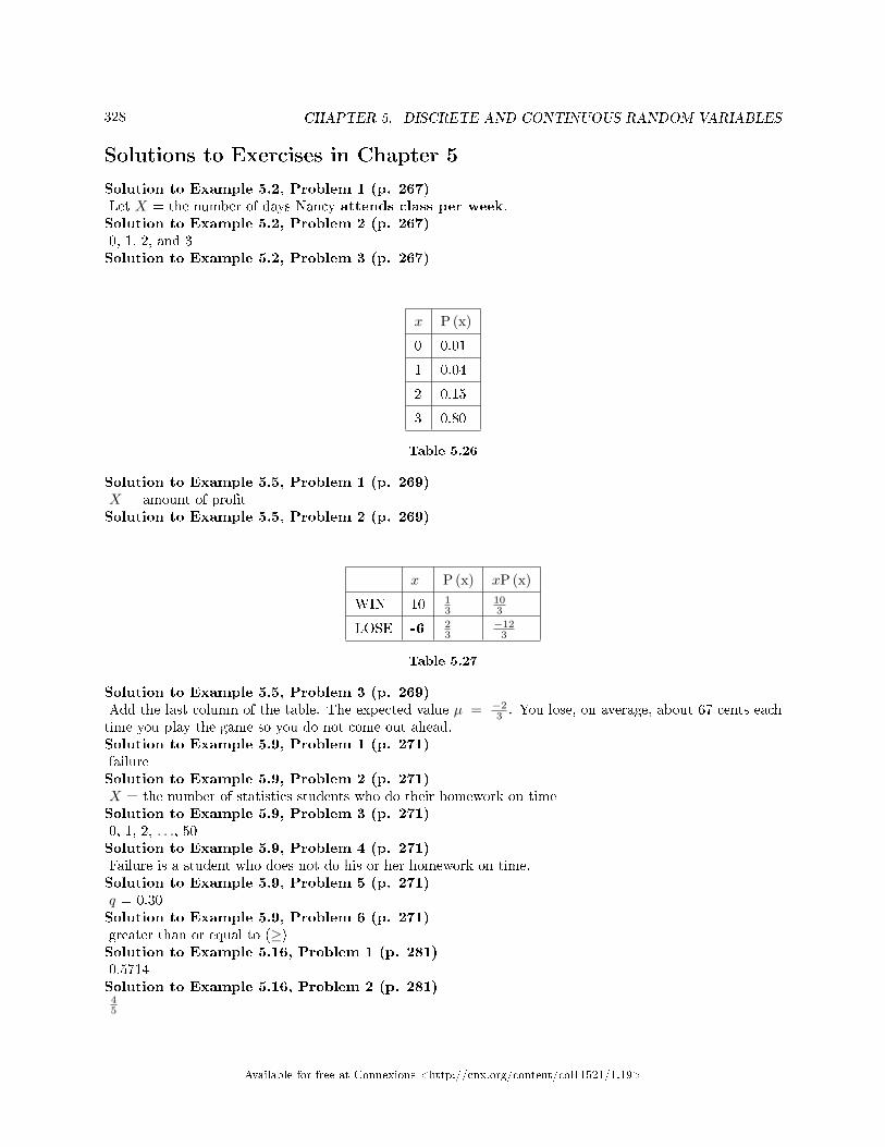
328 CHAPTER 5. DISCRETE AND CONTINUOUS RANDOM VARIABLES
Solutions to Exercises in Chapter 5
Solution to Example 5.2, Problem 1 (p. 267)Let X = the number of days Nancy attends class per week.Solution to Example 5.2, Problem 2 (p. 267)0, 1, 2, and 3Solution to Example 5.2, Problem 3 (p. 267)
x P (x)
0 0.01
1 0.04
2 0.15
3 0.80
Table 5.26
Solution to Example 5.5, Problem 1 (p. 269)X = amount of pro�tSolution to Example 5.5, Problem 2 (p. 269)
x P (x) xP (x)
WIN 10 13
103
LOSE -6 23
−123
Table 5.27
Solution to Example 5.5, Problem 3 (p. 269)Add the last column of the table. The expected value µ = −2
3 . You lose, on average, about 67 cents eachtime you play the game so you do not come out ahead.Solution to Example 5.9, Problem 1 (p. 271)failureSolution to Example 5.9, Problem 2 (p. 271)X = the number of statistics students who do their homework on timeSolution to Example 5.9, Problem 3 (p. 271)0, 1, 2, . . ., 50Solution to Example 5.9, Problem 4 (p. 271)Failure is a student who does not do his or her homework on time.Solution to Example 5.9, Problem 5 (p. 271)q = 0.30Solution to Example 5.9, Problem 6 (p. 271)greater than or equal to (≥)Solution to Example 5.16, Problem 1 (p. 281)0.5714Solution to Example 5.16, Problem 2 (p. 281)
45
Available for free at Connexions <http://cnx.org/content/col11521/1.19>
329
Solutions to Discrete Random Variables: Practice 2: Binomial Distribution
Solution to Exercise 5.12.1 (p. 297)X= the number that reply �yes�Solution to Exercise 5.12.2 (p. 297)B(8,0.713)Solution to Exercise 5.12.3 (p. 297)0,1,2,3,4,5,6,7,8Solution to Exercise 5.12.5 (p. 297)5.7Solution to Exercise 5.12.6 (p. 297)1.28Solution to Exercise 5.12.7 (p. 298)0.4151Solution to Exercise 5.12.8 (p. 298)0.9990
Solutions to Continuous Random Variables: Practice 1
Solution to Exercise 5.13.1 (p. 299)The age of cars in the sta� parking lotSolution to Exercise 5.13.2 (p. 299)X = The age (in years) of cars in the sta� parking lotSolution to Exercise 5.13.3 (p. 299)ContinuousSolution to Exercise 5.13.4 (p. 299)0.5 - 9.5Solution to Exercise 5.13.5 (p. 299)X ∼ U (0.5, 9.5)Solution to Exercise 5.13.6 (p. 299)f (x) = 1
9Solution to Exercise 5.13.7 (p. 299)
b.i. 0.5b.ii. 9.5b.iii. 1
9b.iv. Age of Carsb.v. f (x)
Solution to Exercise 5.13.8 (p. 300)
b.: 3.59
Solution to Exercise 5.13.9 (p. 300)
b: 3.57
Solution to Exercise 5.13.11 (p. 301)µ = 5Solution to Exercise 5.13.12 (p. 301)
b. k = 7.25
Available for free at Connexions <http://cnx.org/content/col11521/1.19>
330 CHAPTER 5. DISCRETE AND CONTINUOUS RANDOM VARIABLES
Solutions to Discrete and Continuous Random Variables: Homework
Solution to Exercise 5.14.1 (p. 302)
a. 0.1b. 1.6
Solution to Exercise 5.14.3 (p. 302)
b. $200,000;$600,000;$400,000c. third investmentd. �rst investmente. second investment
Solution to Exercise 5.14.5 (p. 303)
a. 0.2c. 2.35d. 2-3 children
Solution to Exercise 5.14.7 (p. 304)
a. X = the number of dice that show a 1b. 0,1,2,3,4,5,6c. X∼B
(6, 1
6
)d. 1e. 0.00002f. 3 dice
Solution to Exercise 5.14.9 (p. 304)
a. X = the number of students that will attend Tet.b. 0, 1, 2, 3, 4, 5, 6, 7, 8, 9, 10, 11, 12c. X∼B(12,0.18)d. 2.16e. 0.9511f. 0.3702
Solution to Exercise 5.14.11 (p. 304)
a. X = the number of fencers that do not use foil as their main weaponb. 0, 1, 2, 3,... 25c. X∼B(25,0.40)d. 10e. 0.0442f. Yes
Solution to Exercise 5.14.13 (p. 305)
a. X = the number of fortune cookies that have an extra fortuneb. 0, 1, 2, 3,... 144c. X∼B(144, 0.03) or P(4.32)d. 4.32e. 0.0124 or 0.0133f. 0.6300 or 0.6264
Solution to Exercise 5.14.17 (p. 306)
Available for free at Connexions <http://cnx.org/content/col11521/1.19>
331
a. X~U (1, 53)c. f (x) = 1
52 where 1 ≤ x ≤ 53d. 27e. 15.01f. 0g. 29
52h. 13
52i. 16
27j. 37.4k. 40
Solution to Exercise 5.14.19 (p. 306)
b. X~U (25, 45)d. uniform; continuouse. 35 minutesf. 5.8 minutesg. 0.25h. 0.5i. 1j. 43 minutesk. 40 minutesl. 0.3333
Solution to Exercise 5.14.21 (p. 307)
b. X~U (0, 8)d. f (x) = 1
8 where 0 ≤ x ≤ 8e. 4f. 2.31g. 1
8h. 1
8i. 3.2
Solution to Exercise 5.14.23 (p. 308)D: 4.43Solution to Exercise 5.14.24 (p. 308)A: 0.1476Solution to Exercise 5.14.25 (p. 308)C: 0.4734Solution to Exercise 5.14.26 (p. 308)A: The number of times Mrs. Plum's cats wake her up each weekSolution to Exercise 5.14.27 (p. 308)D: 0.0671Solution to Exercise 5.14.28 (p. 309)DSolution to Exercise 5.14.29 (p. 309)BSolution to Exercise 5.14.30 (p. 309)BSolution to Exercise 5.14.31 (p. 309)Partial Answer:A: X = the number of DVDs a Video to Go customer rents
Available for free at Connexions <http://cnx.org/content/col11521/1.19>
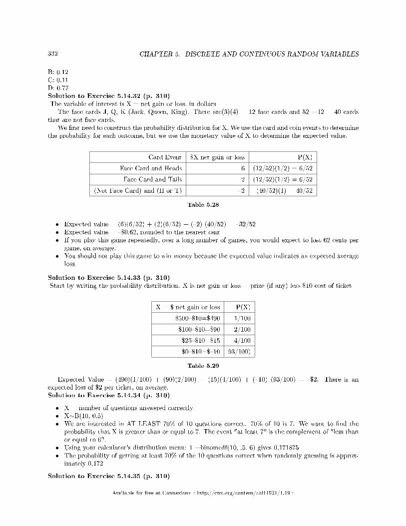
332 CHAPTER 5. DISCRETE AND CONTINUOUS RANDOM VARIABLES
B: 0.12C: 0.11D: 0.77Solution to Exercise 5.14.32 (p. 310)The variable of interest is X = net gain or loss, in dollars
The face cards J, Q, K (Jack, Queen, King). There are(3)(4) = 12 face cards and 52 � 12 = 40 cardsthat are not face cards.
We �rst need to construct the probability distribution for X. We use the card and coin events to determinethe probability for each outcome, but we use the monetary value of X to determine the expected value.
Card Event $X net gain or loss P(X)
Face Card and Heads 6 (12/52)(1/2) = 6/52
Face Card and Tails 2 (12/52)(1/2) = 6/52
(Not Face Card) and (H or T) �2 (40/52)(1) = 40/52
Table 5.28
• Expected value = (6)(6/52) + (2)(6/52) + (�2) (40/52) = �32/52• Expected value = �$0.62, rounded to the nearest cent• If you play this game repeatedly, over a long number of games, you would expect to lost 62 cents per
game, on average.• You should not play this game to win money because the expected value indicates an expected average
loss.
Solution to Exercise 5.14.33 (p. 310)Start by writing the probability distribution. X is net gain or loss = prize (if any) less $10 cost of ticket
X = $ net gain or loss P(X)
$500�$10=$490 1/100
$100�$10=$90 2/100
$25�$10=$15 4/100
$0�$10=$�10 93/100)
Table 5.29
Expected Value = (490)(1/100) + (90)(2/100) + (15)(4/100) + (�10) (93/100) = �$2. There is anexpected loss of $2 per ticket, on average.Solution to Exercise 5.14.34 (p. 310)
• X = number of questions answered correctly• X∼B(10, 0.5)• We are interested in AT LEAST 70% of 10 questions correct. 70% of 10 is 7. We want to �nd the
probability that X is greater than or equal to 7. The event "at least 7" is the complement of "less thanor equal to 6".
• Using your calculator's distribution menu: 1 � binomcdf(10, .5, 6) gives 0.171875• The probability of getting at least 70% of the 10 questions correct when randomly guessing is approx-
imately 0.172
Solution to Exercise 5.14.35 (p. 310)
Available for free at Connexions <http://cnx.org/content/col11521/1.19>
333
• X = number of questions answered correctly• X∼B(32, 1/3)• We are interested in MORE THAN 75% of 32 questions correct. 75% of 32 is 24. We want to �nd
P(x>24). The event "more than 24" is the complement of "less than or equal to 24".• Using your calculator's distribution menu: 1 - binomcdf(32, 1/3, 24)• P(x>24) = 0.00000026761• The probability of getting more than 75% of the 32 questions correct when randomly guessing is very
small and practically zero.
Solution to Exercise 5.14.36 (p. 310)A: X can take on the values 1, 2, 3, .... p = 2/6, q = 4/6B: 0.2222C: 3
Solutions to Discrete Random Variables: Review
Solution to Exercise 5.15.1 (p. 311)CSolution to Exercise 5.15.2 (p. 311)BSolution to Exercise 5.15.3 (p. 311)ASolution to Exercise 5.15.4 (p. 312)0.5773Solution to Exercise 5.15.5 (p. 312)0.0522Solution to Exercise 5.15.6 (p. 312)BSolution to Exercise 5.15.7 (p. 312)CSolution to Exercise 5.15.8 (p. 312)CSolution to Exercise 5.15.9 (p. 313)0.2709Solution to Exercise 5.15.10 (p. 313)BSolution to Exercise 5.15.11 (p. 313)X = the number of patients calling in claiming to have the �u, who actually have the �u. X = 0, 1, 2,...25Solution to Exercise 5.15.12 (p. 313)B (25, 0.04)Solution to Exercise 5.15.13 (p. 313)0.0165Solution to Exercise 5.15.14 (p. 313)1Solution to Exercise 5.15.15 (p. 313)CSolution to Exercise 5.15.16 (p. 313)All words used by Tom Clancy in his novels
Available for free at Connexions <http://cnx.org/content/col11521/1.19>
334 CHAPTER 5. DISCRETE AND CONTINUOUS RANDOM VARIABLES
Solutions to Continuous Random Variables: Review
Solution to Exercise 5.16.1 (p. 314)
a. 24%b. 27%
Solution to Exercise 5.16.2 (p. 314)QualitativeSolution to Exercise 5.16.3 (p. 314)0.36Solution to Exercise 5.16.4 (p. 314)0.7636Solution to Exercise 5.16.5 (p. 314)
a. No,b. No,
Solution to Exercise 5.16.6 (p. 314)B (10, 0.76)Solution to Exercise 5.16.7 (p. 314)0.9330Solution to Exercise 5.16.8 (p. 314)
a. X = the number of questions posted to the Statistics Listserv per dayb. x = 0, 1, 2, ...c. X~P (2)d. 0
Solution to Exercise 5.16.9 (p. 314)$150Solution to Exercise 5.16.10 (p. 315)MattSolution to Exercise 5.16.11 (p. 315)
a. Falseb. Truec. Falsed. False
Solution to Exercise 5.16.12 (p. 315)16Solution to Exercise 5.16.13 (p. 315)2, 2, 3Solution to Exercise 5.16.14 (p. 316)
510 = 0.5Solution to Exercise 5.16.15 (p. 316)
715Solution to Exercise 5.16.16 (p. 316)
215
Available for free at Connexions <http://cnx.org/content/col11521/1.19>
Chapter 6
The Normal Distribution
6.1 Normal Distribution: Introduction1
6.1.1 Student Learning Outcomes
By the end of this chapter, the student should be able to:
• Recognize the normal probability distribution and apply it appropriately.• Recognize the standard normal probability distribution and apply it appropriately.• Compare normal probabilities by converting to the standard normal distribution.
6.1.2 Introduction
The normal, a continuous distribution, is the most important of all the distributions. It is widely usedand even more widely abused. Its graph is bell-shaped. You see the bell curve in almost all disciplines.Some of these include psychology, business, economics, the sciences, nursing, and, of course, mathematics.Some of your instructors may use the normal distribution to help determine your grade. Most IQ scores arenormally distributed. Often real estate prices �t a normal distribution. The normal distribution is extremelyimportant but it cannot be applied to everything in the real world.
In this chapter, you will study the normal distribution, the standard normal, and applications associatedwith them.
6.1.3 Optional Collaborative Classroom Activity
Your instructor will record the heights of both men and women in your class, separately. Draw histogramsof your data. Then draw a smooth curve through each histogram. Is each curve somewhat bell-shaped?Do you think that if you had recorded 200 data values for men and 200 for women that the curves wouldlook bell-shaped? Calculate the mean for each data set. Write the means on the x-axis of the appropriategraph below the peak. Shade the approximate area that represents the probability that one randomly chosenmale is taller than 72 inches. Shade the approximate area that represents the probability that one randomlychosen female is shorter than 60 inches. If the total area under each curve is one, does either probabilityappear to be more than 0.5?
The normal distribution has two parameters (two numerical descriptive measures), the mean (µ) and thestandard deviation (σ). If X is a quantity to be measured that has a normal distribution with mean (µ) andthe standard deviation (σ), we designate this by writing
NORMAL:X∼N (µ, σ)
1This content is available online at <http://cnx.org/content/m46211/1.2/>.
Available for free at Connexions <http://cnx.org/content/col11521/1.19>
335
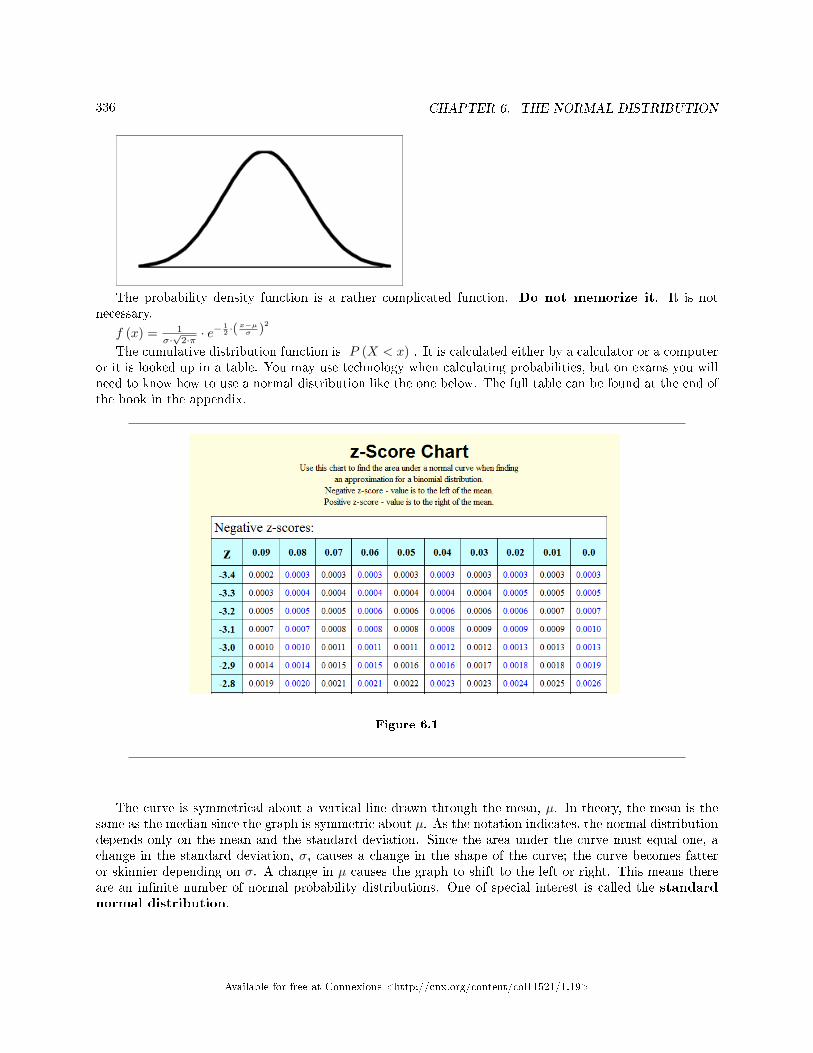
336 CHAPTER 6. THE NORMAL DISTRIBUTION
The probability density function is a rather complicated function. Do not memorize it. It is notnecessary.
f (x) = 1σ·√
2·π · e− 1
2 ·( x−µσ )2
The cumulative distribution function is P (X < x) . It is calculated either by a calculator or a computeror it is looked up in a table. You may use technology when calculating probabilities, but on exams you willneed to know how to use a normal distribution like the one below. The full table can be found at the end ofthe book in the appendix.
Figure 6.1
The curve is symmetrical about a vertical line drawn through the mean, µ. In theory, the mean is thesame as the median since the graph is symmetric about µ. As the notation indicates, the normal distributiondepends only on the mean and the standard deviation. Since the area under the curve must equal one, achange in the standard deviation, σ, causes a change in the shape of the curve; the curve becomes fatteror skinnier depending on σ. A change in µ causes the graph to shift to the left or right. This means thereare an in�nite number of normal probability distributions. One of special interest is called the standardnormal distribution.
Available for free at Connexions <http://cnx.org/content/col11521/1.19>
337
6.2 Normal Distribution: Standard Normal Distribution2
The standard normal distribution is a normal distribution of standardized values called z-scores.A z-score is measured in units of the standard deviation. For example, if the mean of a normaldistribution is 5 and the standard deviation is 2, the value 11 is 3 standard deviations above (or to the rightof) the mean. The calculation is:
x = µ + (z)σ = 5 + (3) (2) = 11 (6.1)
The z-score is 3.The mean for the standard normal distribution is 0 and the standard deviation is 1. The transformationz = x−µ
σ produces the distribution Z∼ N (0, 1) . The value x comes from a normal distributionwith mean µ and standard deviation σ.
6.3 Normal Distribution: Z-scores3
If X is a normally distributed random variable and X∼N (µ, σ), then the z-score is:
z =x− µσ
(6.2)
The z-score tells you how many standard deviations that the value x is above (to the right of)or below (to the left of) the mean, µ. Values of x that are larger than the mean have positive z-scoresand values of x that are smaller than the mean have negative z-scores. If x equals the mean, then x has az-score of 0.
Example 6.1Suppose X ∼ N (5, 6). This says that X is a normally distributed random variable with meanµ = 5 and standard deviation σ = 6. Suppose x = 17. Then:
z =x− µσ
=17− 5
6= 2 (6.3)
This means that x = 17 is 2 standard deviations (2σ) above or to the right of the mean µ = 5.The standard deviation is σ = 6.
Notice that:
5 + 2 · 6 = 17 (The pattern is µ+ zσ = x.) (6.4)
Now suppose x = 1. Then:
z =x− µσ
=1− 5
6= −0.67 (rounded to two decimal places) (6.5)
This means that x = 1 is 0.67 standard deviations (− 0.67σ) below or to the left ofthe mean µ = 5. Notice that:
5 + (−0.67) (6) is approximately equal to 1 (This has the pattern µ+ (−0.67)σ = 1 )Summarizing, when z is positive, x is above or to the right of µ and when z is negative, x is to
the left of or below µ.
Example 6.2Some doctors believe that a person can lose 5 pounds, on the average, in a month by reducinghis/her fat intake and by exercising consistently. Suppose weight loss has a normal distribution.
2This content is available online at <http://cnx.org/content/m16986/1.7/>.3This content is available online at <http://cnx.org/content/m16991/1.10/>.
Available for free at Connexions <http://cnx.org/content/col11521/1.19>
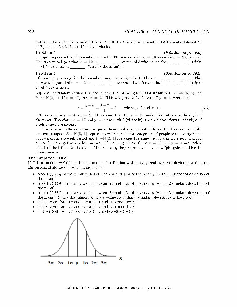
338 CHAPTER 6. THE NORMAL DISTRIBUTION
Let X = the amount of weight lost (in pounds) by a person in a month. Use a standard deviationof 2 pounds. X∼N (5, 2). Fill in the blanks.
Problem 1 (Solution on p. 362.)
Suppose a person lost 10 pounds in a month. The z-score when x = 10 pounds is z = 2.5 (verify).This z-score tells you that x = 10 is ________ standard deviations to the ________ (rightor left) of the mean _____ (What is the mean?).
Problem 2 (Solution on p. 362.)
Suppose a person gained 3 pounds (a negative weight loss). Then z = __________. Thisz-score tells you that x = −3 is ________ standard deviations to the __________ (rightor left) of the mean.
Suppose the random variables X and Y have the following normal distributions: X ∼N (5, 6) andY ∼ N (2, 1). If x = 17, then z = 2. (This was previously shown.) If y = 4, what is z?
z =y − µσ
=4− 2
1= 2 where µ=2 and σ=1. (6.6)
The z-score for y = 4 is z = 2. This means that 4 is z = 2 standard deviations to the right ofthe mean. Therefore, x = 17 and y = 4 are both 2 (of their) standard deviations to the right oftheir respective means.
The z-score allows us to compare data that are scaled di�erently. To understand theconcept, suppose X ∼N (5, 6) represents weight gains for one group of people who are trying togain weight in a 6 week period and Y ∼N (2, 1) measures the same weight gain for a second groupof people. A negative weight gain would be a weight loss. Since x = 17 and y = 4 are each 2standard deviations to the right of their means, they represent the same weight gain relative totheir means.
The Empirical RuleIf X is a random variable and has a normal distribution with mean µ and standard deviation σ then theEmpirical Rule says (See the �gure below)
• About 68.27% of the x values lie between -1σ and +1σ of the mean µ (within 1 standard deviation ofthe mean).
• About 95.45% of the x values lie between -2σ and +2σ of the mean µ (within 2 standard deviations ofthe mean).
• About 99.73% of the x values lie between -3σ and +3σ of the mean µ (within 3 standard deviations ofthe mean). Notice that almost all the x values lie within 3 standard deviations of the mean.
• The z-scores for +1σ and �1σ are +1 and -1, respectively.• The z-scores for +2σ and �2σ are +2 and -2, respectively.• The z-scores for +3σ and �3σ are +3 and -3 respectively.
Available for free at Connexions <http://cnx.org/content/col11521/1.19>
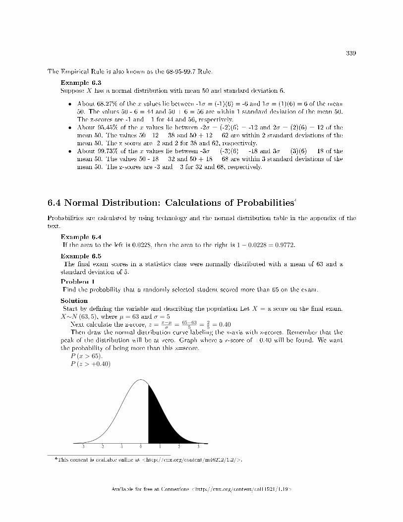
339
The Empirical Rule is also known as the 68-95-99.7 Rule.
Example 6.3Suppose X has a normal distribution with mean 50 and standard deviation 6.
• About 68.27% of the x values lie between -1σ = (-1)(6) = -6 and 1σ = (1)(6) = 6 of the mean50. The values 50 - 6 = 44 and 50 + 6 = 56 are within 1 standard deviation of the mean 50.The z-scores are -1 and +1 for 44 and 56, respectively.
• About 95.45% of the x values lie between -2σ = (-2)(6) = -12 and 2σ = (2)(6) = 12 of themean 50. The values 50 - 12 = 38 and 50 + 12 = 62 are within 2 standard deviations of themean 50. The z-scores are -2 and 2 for 38 and 62, respectively.
• About 99.73% of the x values lie between -3σ = (-3)(6) = -18 and 3σ = (3)(6) = 18 of themean 50. The values 50 - 18 = 32 and 50 + 18 = 68 are within 3 standard deviations of themean 50. The z-scores are -3 and +3 for 32 and 68, respectively.
6.4 Normal Distribution: Calculations of Probabilities4
Probabilities are calculated by using technology and the normal distribution table in the appendix of thetext.
Example 6.4If the area to the left is 0.0228, then the area to the right is 1− 0.0228 = 0.9772.
Example 6.5The �nal exam scores in a statistics class were normally distributed with a mean of 63 and astandard deviation of 5.
Problem 1Find the probability that a randomly selected student scored more than 65 on the exam.
SolutionStart by de�ning the variable and describing the population Let X = a score on the �nal exam.X∼N (63, 5), where µ = 63 and σ = 5
Next calculate the z-score, z = x−µσ = 65−63
5 = 25 = 0.40
Then draw the normal distribution curve labeling the x-axis with z-scores. Remember that thepeak of the distribution will be at zero. Graph where a z-score of +0.40 will be found. We wantthe probability of being more than this z=score.
P (x > 65).P (z > +0.40)
4This content is available online at <http://cnx.org/content/m46212/1.2/>.
Available for free at Connexions <http://cnx.org/content/col11521/1.19>
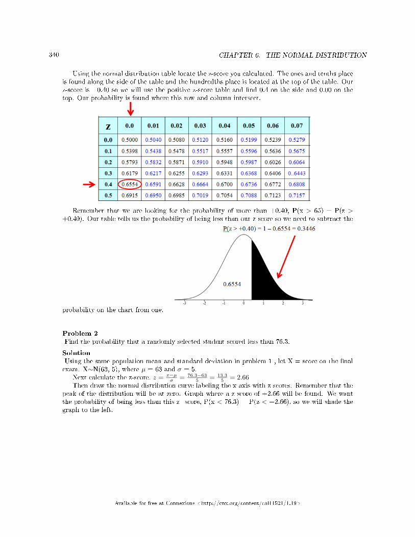
340 CHAPTER 6. THE NORMAL DISTRIBUTION
Using the normal distribution table locate the z-score you calculated. The ones and tenths placeis found along the side of the table and the hundredths place is located at the top of the table. Ourz-score is +0.40 so we will use the positive z-score table and �nd 0.4 on the side and 0.00 on thetop. Our probability is found where this row and column intersect.
Remember that we are looking for the probability of more than +0.40, P(x > 65) = P(z >+0.40). Our table tells us the probability of being less than our z-score so we need to subtract the
probability on the chart from one.
Problem 2Find the probability that a randomly selected student scored less than 76.3.
SolutionUsing the same population mean and standard deviation in problem 1 , let X = score on the �nalexam. X∼N(63, 5), where µ = 63 and σ = 5.
Next calculate the z-score, z = x−µσ = 76.3−63
5 = 13.35 = 2.66
Then draw the normal distribution curve labeling the x-axis with z-scores. Remember that thepeak of the distribution will be at zero. Graph where a z-score of +2.66 will be found. We wantthe probability of being less than this z=score, P(x < 76.3) = P(z < +2.66), so we will shade thegraph to the left.
Available for free at Connexions <http://cnx.org/content/col11521/1.19>
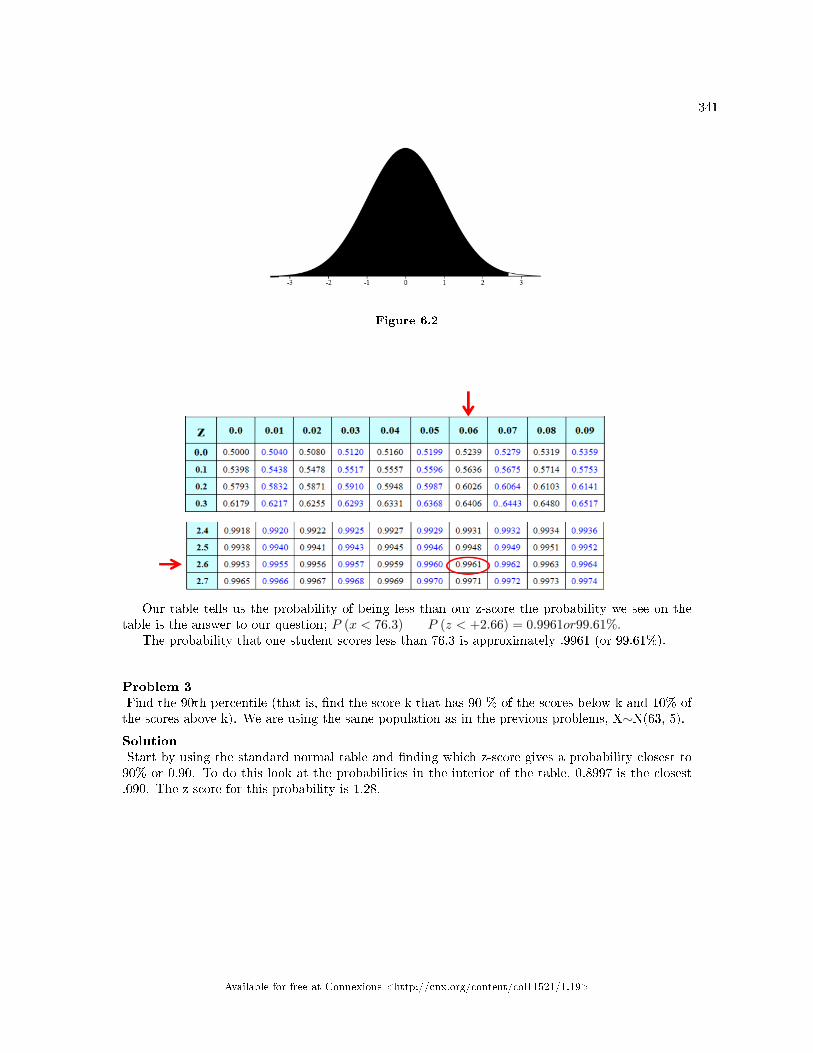
341
Figure 6.2
Our table tells us the probability of being less than our z-score the probability we see on thetable is the answer to our question; P (x < 76.3) = P (z < +2.66) = 0.9961or99.61%.
The probability that one student scores less than 76.3 is approximately .9961 (or 99.61%).
Problem 3Find the 90th percentile (that is, �nd the score k that has 90 % of the scores below k and 10% ofthe scores above k). We are using the same population as in the previous problems, X∼N(63, 5).SolutionStart by using the standard normal table and �nding which z-score gives a probability closest to90% or 0.90. To do this look at the probabilities in the interior of the table, 0.8997 is the closest.090. The z-score for this probability is 1.28.
Available for free at Connexions <http://cnx.org/content/col11521/1.19>
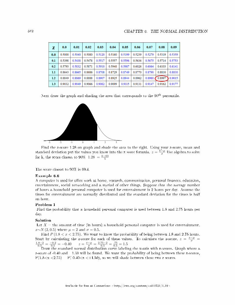
342 CHAPTER 6. THE NORMAL DISTRIBUTION
Next draw the graph and shading the area that corresponds to the 90th percentile.
Find the z-score 1.28 on graph and shade the area to the right. Using your z-score, mean andstandard deviation put the values you know into the z-score formula. z = k−µ
σ Use algebra to solve
for k, the score closest to 90% 1.28 = k−635
The score closest to 90% is 69.4.
Example 6.6A computer is used for o�ce work at home, research, communication, personal �nances, education,entertainment, social networking and a myriad of other things. Suppose that the average numberof hours a household personal computer is used for entertainment is 2 hours per day. Assume thetimes for entertainment are normally distributed and the standard deviation for the times is halfan hour.
Problem 1Find the probability that a household personal computer is used between 1.8 and 2.75 hours perday.
SolutionLet X = the amount of time (in hours) a household personal computer is used for entertainment.x∼N (2, 0.5) where µ = 2 and σ = 0.5.
Find P (1.8 < x < 2.75). We want to know the probability of being between 1.8 and 2.75 hours.Start by calculating the z-score for each of these values. To calculate the z-score, z = x−µ
σ =1.8−2
0.5 = −0.20.5 = −0.40 z = x−µ
σ = 2.75−20.5 = .75
0.5 = 1.5Draw the standard normal distribution curve labeling the x-axis with z-scores. Graph where a
z-score of -0.40 and +1.50 will be found. We want the probability of being between these z-scores,P(1.8<x <2.75) = P(-0.40<z <+1.50), so we will shade between these two z-scores.
Available for free at Connexions <http://cnx.org/content/col11521/1.19>
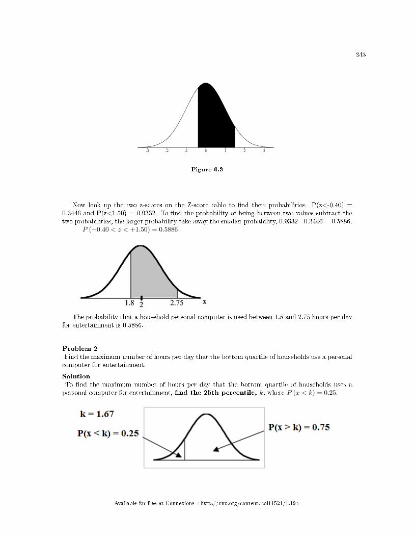
343
Figure 6.3
Now look up the two z-scores on the Z-score table to �nd their probabilities. P(z<-0.40) =0.3446 and P(z<1.50) = 0.9332. To �nd the probability of being between two values subtract thetwo probabilities, the larger probability take away the smaller probability, 0.9332 - 0.3446 = 0.5886.
P (−0.40 < z < +1.50) = 0.5886
The probability that a household personal computer is used between 1.8 and 2.75 hours per dayfor entertainment is 0.5886.
Problem 2Find the maximum number of hours per day that the bottom quartile of households use a personalcomputer for entertainment.
SolutionTo �nd the maximum number of hours per day that the bottom quartile of households uses apersonal computer for entertainment, �nd the 25th percentile, k, where P (x < k) = 0.25.
Available for free at Connexions <http://cnx.org/content/col11521/1.19>
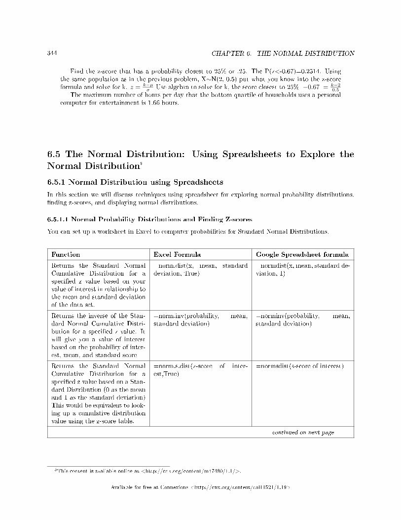
344 CHAPTER 6. THE NORMAL DISTRIBUTION
Find the z-score that has a probability closest to 25% or .25. The P(z<-0.67)=0.2514. Usingthe same population as in the previous problem, X∼N(2, 0.5) put what you know into the z-scoreformula and solve for k. z = k−µ
σ Use algebra to solve for k, the score closest to 25% −0.67 = k−20.5
The maximum number of hours per day that the bottom quartile of households uses a personalcomputer for entertainment is 1.66 hours.
6.5 The Normal Distribution: Using Spreadsheets to Explore theNormal Distribution5
6.5.1 Normal Distribution using Spreadsheets
In this section we will discuss techniques using spreadsheet for exploring normal probability distributions,�nding z-scores, and displaying normal distributions.
6.5.1.1 Normal Probability Distributions and Finding Z-scores
You can set up a worksheet in Excel to computer probabilities for Standard Normal Distributions.
Function Excel Formula Google Spreadsheet formula
Returns the Standard NormalCumulative Distribution for aspeci�ed z value based on yourvalue of interest in relationship tothe mean and standard deviationof the data set.
=norm.dist(x, mean, standarddeviation, True)
=normdist(x, mean, standard de-viation, 1)
Returns the inverse of the Stan-dard Normal Cumulative Distri-bution for a speci�ed z value. Itwill give you a value of interestbased on the probability of inter-est, mean, and standard score
=norm.inv(probability, mean,standard deviation)
=norminv(probability, mean,standard deviation)
Returns the Standard NormalCumulative Distribution for aspeci�ed z value based on a Stan-dard Distribution (0 as the meanand 1 as the standard deviation)This would be equivalent to look-ing up a cumulative distributionvalue using the z-score table.
=norm.s.dist(z-score of inter-est,True)
=normsdist(s-score of interest)
continued on next page
5This content is available online at <http://cnx.org/content/m47480/1.1/>.
Available for free at Connexions <http://cnx.org/content/col11521/1.19>
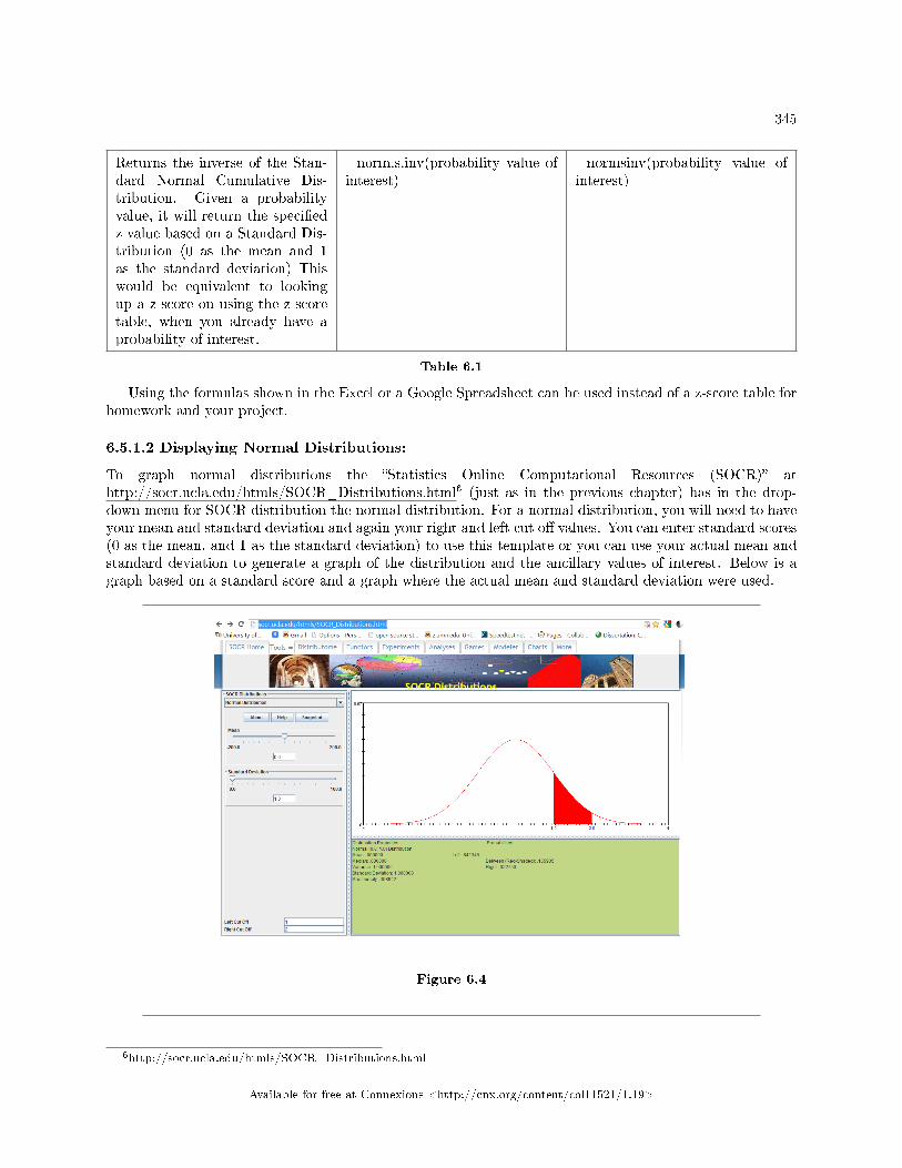
345
Returns the inverse of the Stan-dard Normal Cumulative Dis-tribution. Given a probabilityvalue, it will return the speci�edz value based on a Standard Dis-tribution (0 as the mean and 1as the standard deviation) Thiswould be equivalent to lookingup a z-score on using the z-scoretable, when you already have aprobability of interest.
=norm.s.inv(probability value ofinterest)
=normsinv(probability value ofinterest)
Table 6.1
Using the formulas shown in the Excel or a Google Spreadsheet can be used instead of a z-score table forhomework and your project.
6.5.1.2 Displaying Normal Distributions:
To graph normal distributions the �Statistics Online Computational Resources (SOCR)� athttp://socr.ucla.edu/htmls/SOCR_Distributions.html6 (just as in the previous chapter) has in the drop-down menu for SOCR distribution the normal distribution. For a normal distribution, you will need to haveyour mean and standard deviation and again your right and left cut o� values. You can enter standard scores(0 as the mean, and 1 as the standard deviation) to use this template or you can use your actual mean andstandard deviation to generate a graph of the distribution and the ancillary values of interest. Below is agraph based on a standard score and a graph where the actual mean and standard deviation were used.
Figure 6.4
6http://socr.ucla.edu/htmls/SOCR_Distributions.html
Available for free at Connexions <http://cnx.org/content/col11521/1.19>
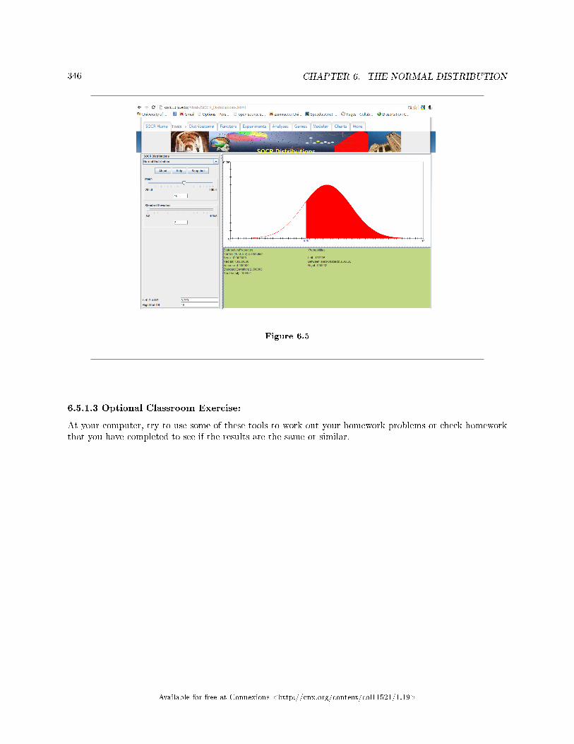
346 CHAPTER 6. THE NORMAL DISTRIBUTION
Figure 6.5
6.5.1.3 Optional Classroom Exercise:
At your computer, try to use some of these tools to work out your homework problems or check homeworkthat you have completed to see if the results are the same or similar.
Available for free at Connexions <http://cnx.org/content/col11521/1.19>
347
6.6 Normal Distribution: Summary of Formulas7
Formula 6.1: Normal Probability DistributionX∼N (µ, σ)µ = the mean σ = the standard deviation
Formula 6.2: Standard Normal Probability DistributionZ∼N (0, 1)z = a standardized value (z-score)mean = 0 standard deviation = 1
Formula 6.3: Finding the kth PercentileTo �nd the kth percentile when the z-score is known: k = µ+ (z)σFormula 6.4: z-scorez = x−µ
σ
Formula 6.5: Finding the area to the leftThe area to the left: P (X < x)Formula 6.6: Finding the area to the rightThe area to the right: P (X > x) = 1− P (X < x)
6.6.1 De�nitions
Normal Distribution
• A continuous Random Variable (RV) with Probability Density Function (PDF) f (x) = 1σ·√
2·π ·
e−12 ·( x−µσ )2
, where µ is the mean of the distribution and σ is the standard deviation.• Notation: X ∼ N(µ, σ). If µ=0 and σ=1, the RV is called the standard normal distribution.
Standard Normal Distribution
• A continuous random variable (RV) X∼N(0,1). When X follows the standard normal distribution, itis often noted as Z∼N(0,1).
z-score
• The linear transformation of the form z = x−µσ . If this transformation is applied to any normal
distribution X∼N(µ,σ), the result is the standard normal distribution Z∼N(0,1). If this transformationis applied to any speci�c value x of the RV with mean µ and standard deviation σ , the result is calledthe z-score of x. Z-scores allow us to compare data that are normally distributed but scaled di�erently
7This content is available online at <http://cnx.org/content/m48355/1.2/>.
Available for free at Connexions <http://cnx.org/content/col11521/1.19>
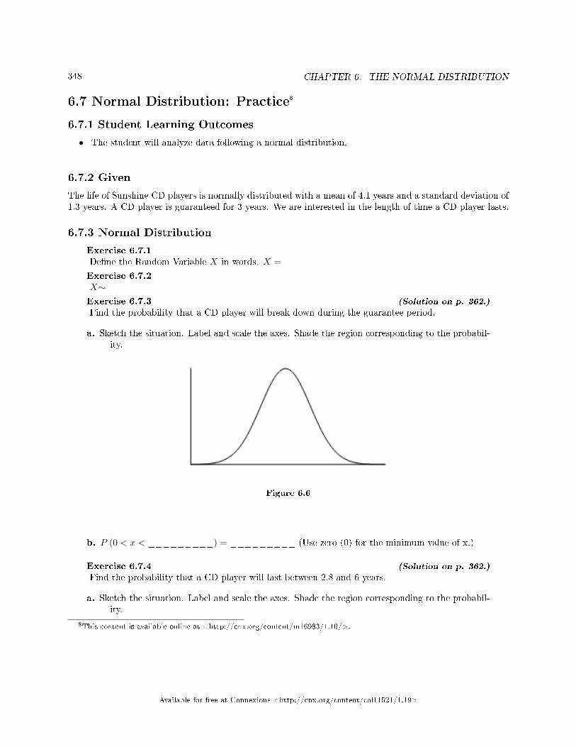
348 CHAPTER 6. THE NORMAL DISTRIBUTION
6.7 Normal Distribution: Practice8
6.7.1 Student Learning Outcomes
• The student will analyze data following a normal distribution.
6.7.2 Given
The life of Sunshine CD players is normally distributed with a mean of 4.1 years and a standard deviation of1.3 years. A CD player is guaranteed for 3 years. We are interested in the length of time a CD player lasts.
6.7.3 Normal Distribution
Exercise 6.7.1De�ne the Random Variable X in words. X =Exercise 6.7.2X∼Exercise 6.7.3 (Solution on p. 362.)
Find the probability that a CD player will break down during the guarantee period.
a. Sketch the situation. Label and scale the axes. Shade the region corresponding to the probabil-ity.
Figure 6.6
b. P (0 < x < _________) = _________ (Use zero (0) for the minimum value of x.)
Exercise 6.7.4 (Solution on p. 362.)
Find the probability that a CD player will last between 2.8 and 6 years.
a. Sketch the situation. Label and scale the axes. Shade the region corresponding to the probabil-ity.
8This content is available online at <http://cnx.org/content/m16983/1.10/>.
Available for free at Connexions <http://cnx.org/content/col11521/1.19>
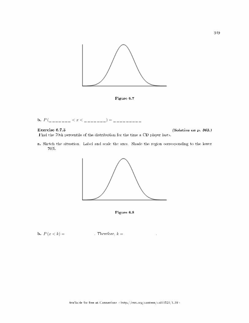
349
Figure 6.7
b. P (_______ < x < _______) = _________
Exercise 6.7.5 (Solution on p. 362.)
Find the 70th percentile of the distribution for the time a CD player lasts.
a. Sketch the situation. Label and scale the axes. Shade the region corresponding to the lower70%.
Figure 6.8
b. P (x < k) = _________. Therefore, k = __________.
Available for free at Connexions <http://cnx.org/content/col11521/1.19>
350 CHAPTER 6. THE NORMAL DISTRIBUTION
6.8 Normal Distribution: Homework9
Exercise 6.8.1 (Solution on p. 362.)
According to a study done by De Anza students, the height for Asian adult males is normallydistributed with an average of 66 inches and a standard deviation of 2.5 inches. Suppose one Asianadult male is randomly chosen. Let X =height of the individual.
a. X∼_______(_______,_______)b. Find the probability that the person is between 65 and 69 inches. Include a sketch of the graph
and write a probability statement.c. Would you expect to meet many Asian adult males over 72 inches? Explain why or why not,
and justify your answer numerically.d. The middle 40% of heights fall between what two values? Sketch the graph and write the
probability statement.
Exercise 6.8.2IQ is normally distributed with a mean of 100 and a standard deviation of 15. Suppose oneindividual is randomly chosen. Let X =IQ of an individual.
a. X∼_______(_______,_______)b. Find the probability that the person has an IQ greater than 120. Include a sketch of the graph
and write a probability statement.c. Mensa is an organization whose members have the top 2% of all IQs. Find the minimum IQ
needed to qualify for the Mensa organization. Sketch the graph and write the probabilitystatement.
d. The middle 50% of IQs fall between what two values? Sketch the graph and write the probabilitystatement.
Exercise 6.8.3 (Solution on p. 362.)
The percent of fat calories that a person in America consumes each day is normally distributedwith a mean of about 36 and a standard deviation of 10. Suppose that one individual is randomlychosen. Let X =percent of fat calories.
a. X∼_______(_______,_______)b. Find the probability that the percent of fat calories a person consumes is more than 40. Graph
the situation. Shade in the area to be determined.c. Find the maximum number for the lower quarter of percent of fat calories. Sketch the graph
and write the probability statement.
Exercise 6.8.4Suppose that the distance of �y balls hit to the out�eld (in baseball) is normally distributed witha mean of 250 feet and a standard deviation of 50 feet.
a. If X = distance in feet for a �y ball, then X∼_______(_______,_______)b. If one �y ball is randomly chosen from this distribution, what is the probability that this ball
traveled fewer than 220 feet? Sketch the graph. Scale the horizontal axis X. Shade the regioncorresponding to the probability. Find the probability.
c. Find the 80th percentile of the distribution of �y balls. Sketch the graph and write the probabilitystatement.
9This content is available online at <http://cnx.org/content/m46210/1.2/>.
Available for free at Connexions <http://cnx.org/content/col11521/1.19>
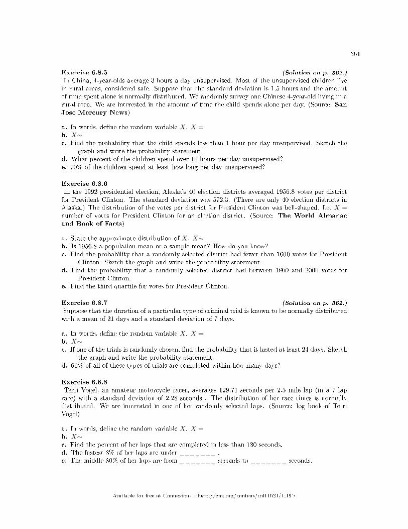
351
Exercise 6.8.5 (Solution on p. 362.)
In China, 4-year-olds average 3 hours a day unsupervised. Most of the unsupervised children livein rural areas, considered safe. Suppose that the standard deviation is 1.5 hours and the amountof time spent alone is normally distributed. We randomly survey one Chinese 4-year-old living in arural area. We are interested in the amount of time the child spends alone per day. (Source: SanJose Mercury News)
a. In words, de�ne the random variable X. X =b. X∼c. Find the probability that the child spends less than 1 hour per day unsupervised. Sketch the
graph and write the probability statement.d. What percent of the children spend over 10 hours per day unsupervised?e. 70% of the children spend at least how long per day unsupervised?
Exercise 6.8.6In the 1992 presidential election, Alaska's 40 election districts averaged 1956.8 votes per districtfor President Clinton. The standard deviation was 572.3. (There are only 40 election districts inAlaska.) The distribution of the votes per district for President Clinton was bell-shaped. Let X =number of votes for President Clinton for an election district. (Source: The World Almanacand Book of Facts)
a. State the approximate distribution of X. X∼b. Is 1956.8 a population mean or a sample mean? How do you know?c. Find the probability that a randomly selected district had fewer than 1600 votes for President
Clinton. Sketch the graph and write the probability statement.d. Find the probability that a randomly selected district had between 1800 and 2000 votes for
President Clinton.e. Find the third quartile for votes for President Clinton.
Exercise 6.8.7 (Solution on p. 362.)
Suppose that the duration of a particular type of criminal trial is known to be normally distributedwith a mean of 21 days and a standard deviation of 7 days.
a. In words, de�ne the random variable X. X =b. X∼c. If one of the trials is randomly chosen, �nd the probability that it lasted at least 24 days. Sketch
the graph and write the probability statement.d. 60% of all of these types of trials are completed within how many days?
Exercise 6.8.8Terri Vogel, an amateur motorcycle racer, averages 129.71 seconds per 2.5 mile lap (in a 7 laprace) with a standard deviation of 2.28 seconds . The distribution of her race times is normallydistributed. We are interested in one of her randomly selected laps. (Source: log book of TerriVogel)
a. In words, de�ne the random variable X. X =b. X∼c. Find the percent of her laps that are completed in less than 130 seconds.d. The fastest 3% of her laps are under _______ .e. The middle 80% of her laps are from _______ seconds to _______ seconds.
Available for free at Connexions <http://cnx.org/content/col11521/1.19>
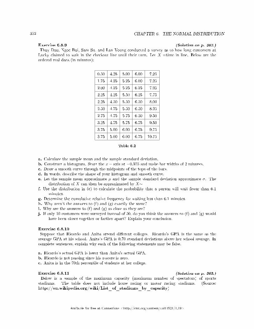
352 CHAPTER 6. THE NORMAL DISTRIBUTION
Exercise 6.8.9 (Solution on p. 362.)
Thuy Dau, Ngoc Bui, Sam Su, and Lan Voung conducted a survey as to how long customers atLucky claimed to wait in the checkout line until their turn. Let X =time in line. Below are theordered real data (in minutes):
0.50 4.25 5.00 6.00 7.25
1.75 4.25 5.25 6.00 7.25
2.00 4.25 5.25 6.25 7.25
2.25 4.25 5.50 6.25 7.75
2.25 4.50 5.50 6.50 8.00
2.50 4.75 5.50 6.50 8.25
2.75 4.75 5.75 6.50 9.50
3.25 4.75 5.75 6.75 9.50
3.75 5.00 6.00 6.75 9.75
3.75 5.00 6.00 6.75 10.75
Table 6.2
a. Calculate the sample mean and the sample standard deviation.b. Construct a histogram. Start the x− axis at −0.375 and make bar widths of 2 minutes.c. Draw a smooth curve through the midpoints of the tops of the bars.d. In words, describe the shape of your histogram and smooth curve.e. Let the sample mean approximate µ and the sample standard deviation approximate σ. The
distribution of X can then be approximated by X∼f. Use the distribution in (e) to calculate the probability that a person will wait fewer than 6.1
minutes.g. Determine the cumulative relative frequency for waiting less than 6.1 minutes.h. Why aren't the answers to (f) and (g) exactly the same?i. Why are the answers to (f) and (g) as close as they are?j. If only 10 customers were surveyed instead of 50, do you think the answers to (f) and (g) would
have been closer together or farther apart? Explain your conclusion.
Exercise 6.8.10Suppose that Ricardo and Anita attend di�erent colleges. Ricardo's GPA is the same as theaverage GPA at his school. Anita's GPA is 0.70 standard deviations above her school average. Incomplete sentences, explain why each of the following statements may be false.
a. Ricardo's actual GPA is lower than Anita's actual GPA.b. Ricardo is not passing since his z-score is zero.c. Anita is in the 70th percentile of students at her college.
Exercise 6.8.11 (Solution on p. 363.)
Below is a sample of the maximum capacity (maximum number of spectators) of sportsstadiums. The table does not include horse racing or motor racing stadiums. (Source:http://en.wikipedia.org/wiki/List_of_stadiums_by_capacity)
Available for free at Connexions <http://cnx.org/content/col11521/1.19>
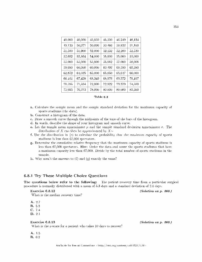
353
40,000 40,000 45,050 45,500 46,249 48,134
49,133 50,071 50,096 50,466 50,832 51,100
51,500 51,900 52,000 52,132 52,200 52,530
52,692 53,864 54,000 55,000 55,000 55,000
55,000 55,000 55,000 55,082 57,000 58,008
59,680 60,000 60,000 60,492 60,580 62,380
62,872 64,035 65,000 65,050 65,647 66,000
66,161 67,428 68,349 68,976 69,372 70,107
70,585 71,594 72,000 72,922 73,379 74,500
75,025 76,212 78,000 80,000 80,000 82,300
Table 6.3
a. Calculate the sample mean and the sample standard deviation for the maximum capacity ofsports stadiums (the data).
b. Construct a histogram of the data.c. Draw a smooth curve through the midpoints of the tops of the bars of the histogram.d. In words, describe the shape of your histogram and smooth curve.e. Let the sample mean approximate µ and the sample standard deviation approximate σ. The
distribution of X can then be approximated by X∼f. Use the distribution in (e) to calculate the probability that the maximum capacity of sports
stadiums is less than 67,000 spectators.g. Determine the cumulative relative frequency that the maximum capacity of sports stadiums is
less than 67,000 spectators. Hint: Order the data and count the sports stadiums that havea maximum capacity less than 67,000. Divide by the total number of sports stadiums in thesample.
h. Why aren't the answers to (f) and (g) exactly the same?
6.8.1 Try These Multiple Choice Questions
The questions below refer to the following: The patient recovery time from a particular surgicalprocedure is normally distributed with a mean of 5.3 days and a standard deviation of 2.1 days.
Exercise 6.8.12 (Solution on p. 363.)
What is the median recovery time?
A. 2.7B. 5.3C. 7.4D. 2.1
Exercise 6.8.13 (Solution on p. 363.)
What is the z-score for a patient who takes 10 days to recover?
A. 1.5B. 0.2
Available for free at Connexions <http://cnx.org/content/col11521/1.19>
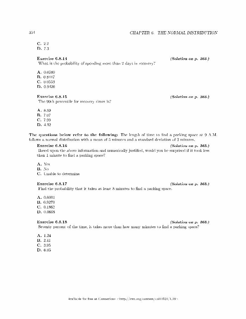
354 CHAPTER 6. THE NORMAL DISTRIBUTION
C. 2.2D. 7.3
Exercise 6.8.14 (Solution on p. 363.)
What is the probability of spending more than 2 days in recovery?
A. 0.0580B. 0.8447C. 0.0553D. 0.9420
Exercise 6.8.15 (Solution on p. 363.)
The 90th percentile for recovery times is?
A. 8.89B. 7.07C. 7.99D. 4.32
The questions below refer to the following: The length of time to �nd a parking space at 9 A.M.follows a normal distribution with a mean of 5 minutes and a standard deviation of 2 minutes.
Exercise 6.8.16 (Solution on p. 363.)
Based upon the above information and numerically justi�ed, would you be surprised if it took lessthan 1 minute to �nd a parking space?
A. YesB. NoC. Unable to determine
Exercise 6.8.17 (Solution on p. 363.)
Find the probability that it takes at least 8 minutes to �nd a parking space.
A. 0.0001B. 0.9270C. 0.1862D. 0.0668
Exercise 6.8.18 (Solution on p. 363.)
Seventy percent of the time, it takes more than how many minutes to �nd a parking space?
A. 1.24B. 2.41C. 3.95D. 6.05
Available for free at Connexions <http://cnx.org/content/col11521/1.19>
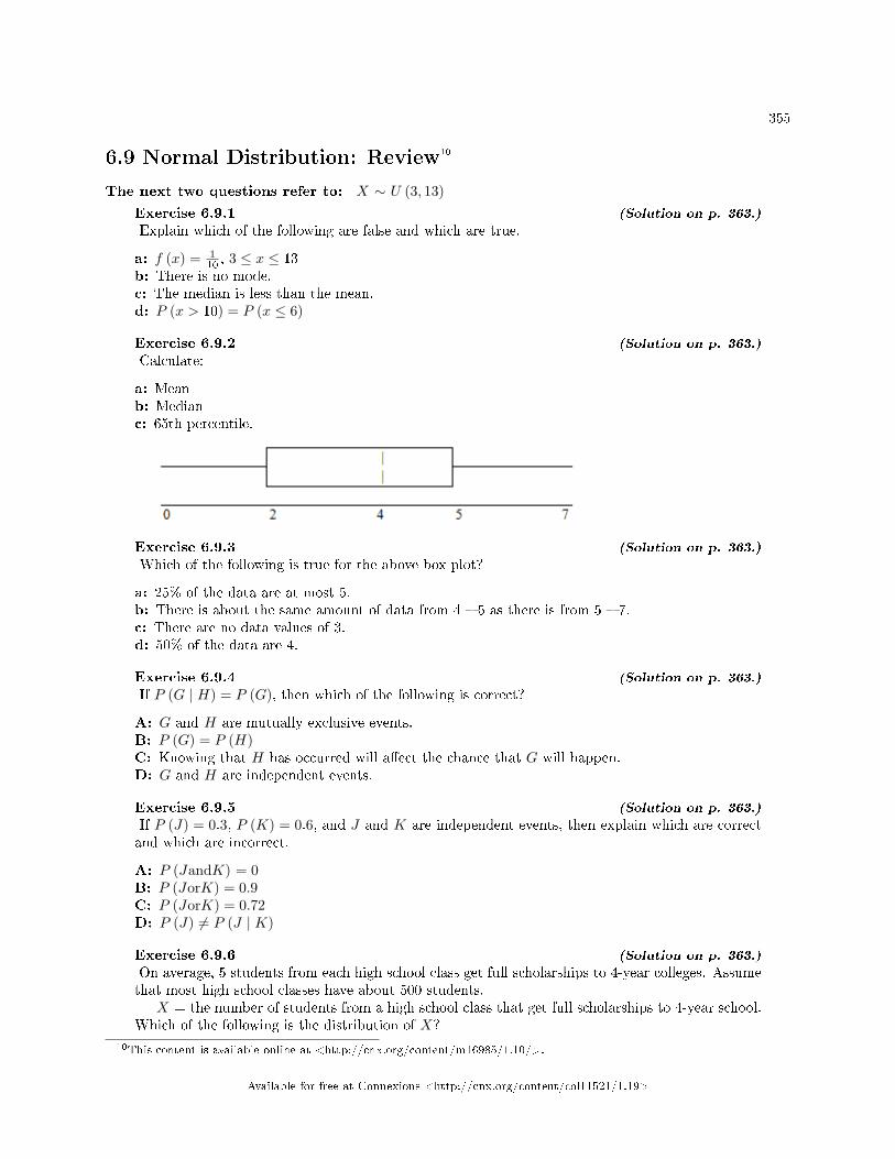
355
6.9 Normal Distribution: Review10
The next two questions refer to: X ∼ U (3, 13)Exercise 6.9.1 (Solution on p. 363.)
Explain which of the following are false and which are true.
a: f (x) = 110 , 3 ≤ x ≤ 13
b: There is no mode.c: The median is less than the mean.d: P (x > 10) = P (x ≤ 6)
Exercise 6.9.2 (Solution on p. 363.)
Calculate:
a: Meanb: Medianc: 65th percentile.
Exercise 6.9.3 (Solution on p. 363.)
Which of the following is true for the above box plot?
a: 25% of the data are at most 5.b: There is about the same amount of data from 4 � 5 as there is from 5 � 7.c: There are no data values of 3.d: 50% of the data are 4.
Exercise 6.9.4 (Solution on p. 363.)
If P (G | H) = P (G), then which of the following is correct?
A: G and H are mutually exclusive events.B: P (G) = P (H)C: Knowing that H has occurred will a�ect the chance that G will happen.D: G and H are independent events.
Exercise 6.9.5 (Solution on p. 363.)
If P (J) = 0.3, P (K) = 0.6, and J and K are independent events, then explain which are correctand which are incorrect.
A: P (JandK) = 0B: P (JorK) = 0.9C: P (JorK) = 0.72D: P (J) 6= P (J | K)
Exercise 6.9.6 (Solution on p. 363.)
On average, 5 students from each high school class get full scholarships to 4-year colleges. Assumethat most high school classes have about 500 students.
X = the number of students from a high school class that get full scholarships to 4-year school.Which of the following is the distribution of X?
10This content is available online at <http://cnx.org/content/m16985/1.10/>.
Available for free at Connexions <http://cnx.org/content/col11521/1.19>

356 CHAPTER 6. THE NORMAL DISTRIBUTION
A. P(5)B. B(500,5)C. Exp(1/5)D. N(5, (0.01)(0.99)/500)
Available for free at Connexions <http://cnx.org/content/col11521/1.19>

357
6.10 Normal Distribution: Normal Distribution Lab I11
Class Time:Names:
6.10.1 Student Learning Outcome:
• The student will compare and contrast empirical data and a theoretical distribution to determine ifTerry Vogel's lap times �t a continuous distribution.
6.10.2 Directions:
Round the relative frequencies and probabilities to 4 decimal places. Carry all other decimal answers to 2places.
6.10.3 Collect the Data
1. Use the data from Terri Vogel's Log Book12. Use a Strati�ed Sampling Method by Lap (Races 1 � 20)and a random number generator to pick 6 lap times from each stratum. Record the lap times belowfor Laps 2 � 7.
_______ _______ _______ _______ _______ _______
_______ _______ _______ _______ _______ _______
_______ _______ _______ _______ _______ _______
_______ _______ _______ _______ _______ _______
_______ _______ _______ _______ _______ _______
_______ _______ _______ _______ _______ _______
Table 6.4
2. Construct a histogram. Make 5 - 6 intervals. Sketch the graph using a ruler and pencil. Scale theaxes.
11This content is available online at <http://cnx.org/content/m16981/1.18/>.12"Collaborative Statistics: Data Sets": Section Lap Times <http://cnx.org/content/m17132/latest/#element-244>
Available for free at Connexions <http://cnx.org/content/col11521/1.19>
358 CHAPTER 6. THE NORMAL DISTRIBUTION
Figure 6.9
3. Calculate the following.
a. x =b. s =
4. Draw a smooth curve through the tops of the bars of the histogram. Use 1 � 2 complete sentences todescribe the general shape of the curve. (Keep it simple. Does the graph go straight across, does ithave a V-shape, does it have a hump in the middle or at either end, etc.?)
6.10.4 Analyze the Distribution
Using your sample mean, sample standard deviation, and histogram to help, what was the approximatetheoretical distribution of the data?
• X ∼• How does the histogram help you arrive at the approximate distribution?
6.10.5 Describe the Data
Use the Data from the section titled "Collect the Data" to complete the following statements.
• The IQR goes from __________ to __________.• IQR = __________. (IQR=Q3-Q1)• The 15th percentile is:• The 85th percentile is:• The median is:• The empirical probability that a randomly chosen lap time is more than 130 seconds =• Explain the meaning of the 85th percentile of this data.
Available for free at Connexions <http://cnx.org/content/col11521/1.19>
359
6.10.6 Theoretical Distribution
Using the theoretical distribution from the section titled "Analyse the Distribution" complete the followingstatements:
• The IQR goes from __________ to __________.• IQR =• The 15th percentile is:• The 85th percentile is:• The median is:• The probability that a randomly chosen lap time is more than 130 seconds =• Explain the meaning of the 85th percentile of this distribution.
6.10.7 Discussion Questions
• Do the data from the section titled "Collect the Data" give a close approximation to the theoreticaldistibution in the section titled "Analyze the Distribution"? In complete sentences and comparing theresult in the sections titled "Describe the Data" and "Theoretical Distribution", explain why or whynot.
Available for free at Connexions <http://cnx.org/content/col11521/1.19>
360 CHAPTER 6. THE NORMAL DISTRIBUTION
6.11 Normal Distribution: Normal Distribution Lab II13
Class Time:Names:
6.11.1 Student Learning Outcomes:
• The student will compare empirical data and a theoretical distribution to determine if data from theexperiment follow a continuous distribution.
6.11.2 Collect the Data
Measure the length of your pinkie �nger (in cm.)
1. Randomly survey 30 adults. Round to the nearest 0.5 cm.
_______ _______ _______ _______ _______
_______ _______ _______ _______ _______
_______ _______ _______ _______ _______
_______ _______ _______ _______ _______
_______ _______ _______ _______ _______
_______ _______ _______ _______ _______
Table 6.5
2. Construct a histogram. Make 5-6 intervals. Sketch the graph using a ruler and pencil. Scale the axes.
3. Calculate the Following
a. x =13This content is available online at <http://cnx.org/content/m16980/1.16/>.
Available for free at Connexions <http://cnx.org/content/col11521/1.19>
361
b. s =
4. Draw a smooth curve through the top of the bars of the histogram. Use 1-2 complete sentences todescribe the general shape of the curve. (Keep it simple. Does the graph go straight across, does ithave a V-shape, does it have a hump in the middle or at either end, etc.?)
6.11.3 Analyze the Distribution
Using your sample mean, sample standard deviation, and histogram to help, what was the approximatetheoretical distribution of the data from the section titled "Collect the Data"?
• X ∼• How does the histogram help you arrive at the approximate distribution?
6.11.4 Describe the Data
Using the data in the section titled "Collect the Data" complete the following statements. (Hint: order thedata)
Remember: (IQR = Q3−Q1)
• IQR =• 15th percentile is:• 85th percentile is:• Median is:• What is the empirical probability that a randomly chosen pinkie length is more than 6.5 cm?• Explain the meaning the 85th percentile of this data.
6.11.5 Theoretical Distribution
Using the Theoretical Distribution in the section titled "Analyze the Distribution"
• IQR =• 15th percentile is:• 85th percentile is:• Median is:• What is the theoretical probability that a randomly chosen pinkie length is more than 6.5 cm?• Explain the meaning of the 85th percentile of this data.
6.11.6 Discussion Questions
• Do the data from the section entitled "Collect the Data" give a close approximation to the theoreticaldistribution in "Analyze the Distribution." In complete sentences and comparing the results in thesections titled "Describe the Data" and "Theoretical Distribution", explain why or why not.
Available for free at Connexions <http://cnx.org/content/col11521/1.19>
362 CHAPTER 6. THE NORMAL DISTRIBUTION
Solutions to Exercises in Chapter 6
Solution to Example 6.2, Problem 1 (p. 338)This z-score tells you that x = 10 is 2.5 standard deviations to the right of the mean 5.Solution to Example 6.2, Problem 2 (p. 338)z = -4. This z-score tells you that x = −3 is 4 standard deviations to the left of the mean.
Solutions to Normal Distribution: Practice
Solution to Exercise 6.7.3 (p. 348)
b. 3, 0.1979
Solution to Exercise 6.7.4 (p. 348)
b. 2.8, 6, 0.7694
Solution to Exercise 6.7.5 (p. 349)
b. 0.70, 4.78years
Solutions to Normal Distribution: Homework
Solution to Exercise 6.8.1 (p. 350)
a. N (66, 2.5)b. 0.5404c. Nod. Between 64.7 and 67.3 inches
Solution to Exercise 6.8.3 (p. 350)
a. N (36,10)b. 0.3446c. 29.3
Solution to Exercise 6.8.5 (p. 351)
a. the time (in hours) a 4-year-old in China spends unsupervised per dayb. N (3, 1.5)c. 0.0912d. 0e. 2.21 hours
Solution to Exercise 6.8.7 (p. 351)
a. The duration of a criminal trialb. N (21, 7)c. 0.3341d. 22.77
Solution to Exercise 6.8.9 (p. 352)
a. The sample mean is 5.51 and the sample standard deviation is 2.15e. N (5.51, 2.15)f. 0.6081g. 0.64
Available for free at Connexions <http://cnx.org/content/col11521/1.19>
363
Solution to Exercise 6.8.11 (p. 352)
a. The sample mean is 60,136.4 and the sample standard deviation is 10,468.1.e. N (60136.4, 10468.1)f. 0.7440g. 0.7167
Solution to Exercise 6.8.12 (p. 353)BSolution to Exercise 6.8.13 (p. 353)CSolution to Exercise 6.8.14 (p. 354)DSolution to Exercise 6.8.15 (p. 354)CSolution to Exercise 6.8.16 (p. 354)ASolution to Exercise 6.8.17 (p. 354)DSolution to Exercise 6.8.18 (p. 354)C
Solutions to Normal Distribution: Review
Solution to Exercise 6.9.1 (p. 355)
a: Trueb: Truec: False � the median and the mean are the same for this symmetric distributiond: True
Solution to Exercise 6.9.2 (p. 355)
a: 8b: 8c: P (x < k) = 0.65 = (k − 3) ∗
(110
). k = 9.5
Solution to Exercise 6.9.3 (p. 355)
a: False � 34 of the data are at most 5
b: True � each quartile has 25% of the datac: False � that is unknownd: False � 50% of the data are 4 or less
Solution to Exercise 6.9.4 (p. 355)DSolution to Exercise 6.9.5 (p. 355)
A: False - J and K are independent so they are not mutually exclusive which would imply dependency(meaning P(J and K) is not 0).
B: False - see answer C.C: True - P(J or K) = P(J) + P(K) - P(J and K) = P(J) + P(K) - P(J)P(K) = 0.3 + 0.6 - (0.3)(0.6) =
0.72. Note that P(J and K) = P(J)P(K) because J and K are independent.D: False - J and K are independent so P(J) = P(J|K).
Solution to Exercise 6.9.6 (p. 355)A
Available for free at Connexions <http://cnx.org/content/col11521/1.19>

364 CHAPTER 6. THE NORMAL DISTRIBUTION
Available for free at Connexions <http://cnx.org/content/col11521/1.19>
Chapter 7
The Central Limit Theorem
7.1 Central Limit Theorem: Introduction1
7.1.1 Student Learning Outcomes
By the end of this chapter, the student should be able to:
• Recognize the Central Limit Theorem problems.• Classify continuous word problems by their distributions.• Apply and interpret the Central Limit Theorem for Means.• Apply and interpret the Central Limit Theorem for Sums.
7.1.2 Introduction
Why are we so concerned with means? Two reasons are that they give us a middle ground for comparisonand they are easy to calculate. In this chapter, you will study means and the Central Limit Theorem.
The Central Limit Theorem (CLT for short) is one of the most powerful and useful ideas in all ofstatistics. Both alternatives are concerned with drawing �nite samples of size n from a population with aknown mean, µ, and a known standard deviation, σ. The �rst alternative says that if we collect samplesof size n and n is "large enough," calculate each sample's mean, and create a histogram of those means,then the resulting histogram will tend to have an approximate normal bell shape. The second alternativesays that if we again collect samples of size n that are "large enough," calculate the sum of each sample andcreate a histogram, then the resulting histogram will again tend to have a normal bell-shape.
In either case, it does not matter what the distribution of the original population is, orwhether you even need to know it. The important fact is that the sample means and the sumstend to follow the normal distribution. And, the rest you will learn in this chapter.
The size of the sample, n, that is required in order to be to be 'large enough' depends on the originalpopulation from which the samples are drawn. If the original population is far from normal then moreobservations are needed for the sample means or the sample sums to be normal. Sampling is done withreplacement.Optional Collaborative Classroom Activity
Do the following example in class: Suppose 8 of you roll 1 fair die 10 times, 7 of you roll 2 fair dice10 times, 9 of you roll 5 fair dice 10 times, and 11 of you roll 10 fair dice 10 times.
Each time a person rolls more than one die, he/she calculates the sample mean of the faces showing.For example, one person might roll 5 fair dice and get a 2, 2, 3, 4, 6 on one roll.
1This content is available online at <http://cnx.org/content/m16953/1.17/>.
Available for free at Connexions <http://cnx.org/content/col11521/1.19>
365
366 CHAPTER 7. THE CENTRAL LIMIT THEOREM
The mean is 2+2+3+4+65 = 3.4. The 3.4 is one mean when 5 fair dice are rolled. This same person
would roll the 5 dice 9 more times and calculate 9 more means for a total of 10 means.Your instructor will pass out the dice to several people as described above. Roll your dice 10 times. For
each roll, record the faces and �nd the mean. Round to the nearest 0.5.Your instructor (and possibly you) will produce one graph (it might be a histogram) for 1 die, one graph
for 2 dice, one graph for 5 dice, and one graph for 10 dice. Since the "mean" when you roll one die, is justthe face on the die, what distribution do these means appear to be representing?
Draw the graph for the means using 2 dice. Do the sample means show any kind of pattern?Draw the graph for the means using 5 dice. Do you see any pattern emerging?Finally, draw the graph for the means using 10 dice. Do you see any pattern to the graph? What
can you conclude as you increase the number of dice?As the number of dice rolled increases from 1 to 2 to 5 to 10, the following is happening:
1. The mean of the sample means remains approximately the same.2. The spread of the sample means (the standard deviation of the sample means) gets smaller.3. The graph appears steeper and thinner.
You have just demonstrated the Central Limit Theorem (CLT).The Central Limit Theorem tells you that as you increase the number of dice, the sample means tend
toward a normal distribution (the sampling distribution).
7.2 Central Limit Theorem: Assumptions and Conditions2
7.2.1 Assumptions and Conditions
To use the normal model, we must meet some assumptions and conditions. The Central Limit Theoremassumes the following:
Randomization Condition: The data must be sampled randomly. Is one of the good sampling method-ologies discussed in the chapter �Sampling and Data� being used?
Independence Assumption: The sample values must be independent of each other. This means thatthe occurrence of one event has no in�uence on the next event. Usually, if we know that people or itemswere selected randomly we can assume that the independence assumption is met.
10% Condition: When the sample is drawn without replacement (usually the case), the sample size,n, should be no more than 10% of the population.
Sample Size Assumption: The sample size must be su�ciently large. Although the Central LimitTheorem tells us that we can use a Normal model to think about the behavior of sample means when thesample size is large enough, it does not tell us how large that should be. If the population is very skewed, youwill need a pretty large sample size to use the CLT, however if the population is unimodal and symmetric,even small samples are acceptable. So think about your sample size in terms of what you know about thepopulation and decide whether the sample is large enough. In general a sample size of 30 is consideredsu�cient if the sample is unimodal (and meets the 10% condition).
7.3 Central Limit Theorem: Central Limit Theorem for SampleMeans3
Suppose X is a random variable with a distribution that may be known or unknown (it can be any distri-bution). Using a subscript that matches the random variable, suppose:
a. µX = the mean of X
2This content is available online at <http://cnx.org/content/m46217/1.1/>.3This content is available online at <http://cnx.org/content/m16947/1.23/>.
Available for free at Connexions <http://cnx.org/content/col11521/1.19>
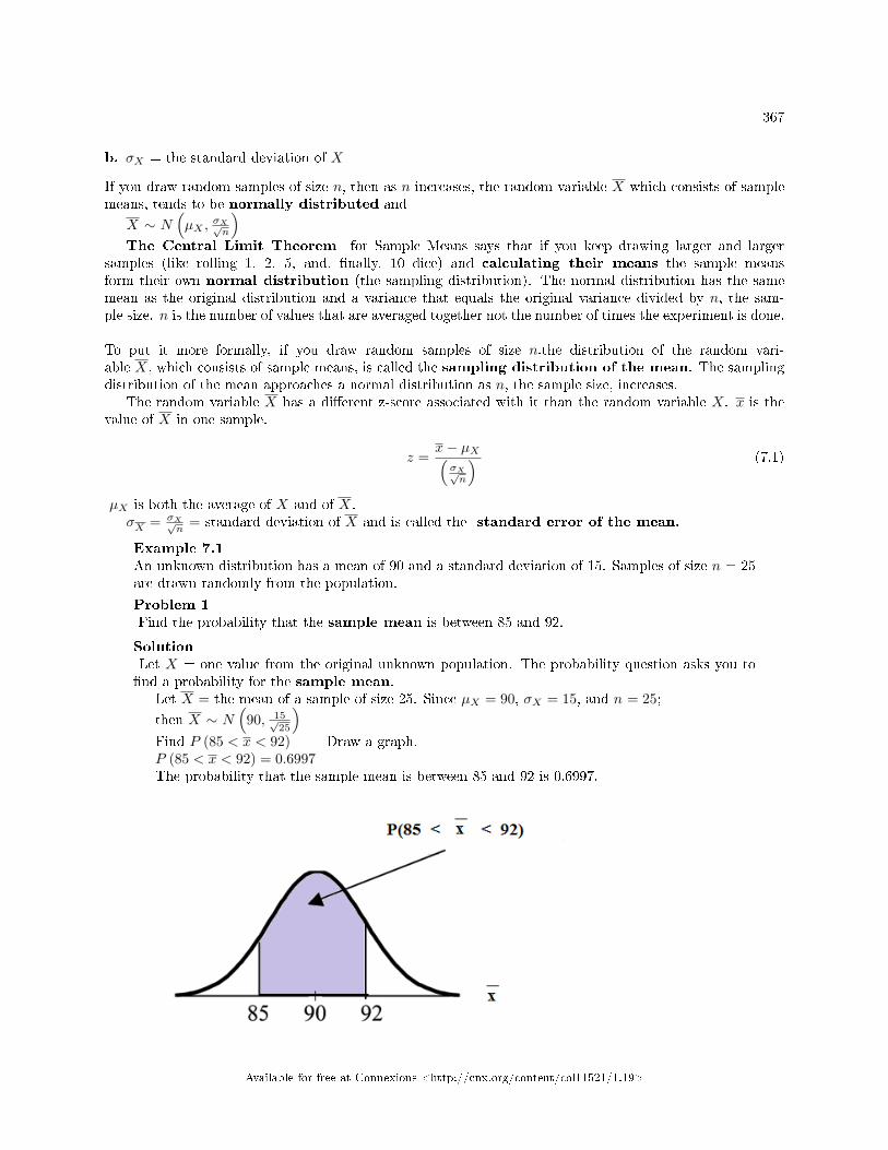
367
b. σX = the standard deviation of X
If you draw random samples of size n, then as n increases, the random variable X which consists of samplemeans, tends to be normally distributed and
X ∼ N(µX ,
σX√n
)The Central Limit Theorem for Sample Means says that if you keep drawing larger and larger
samples (like rolling 1, 2, 5, and, �nally, 10 dice) and calculating their means the sample meansform their own normal distribution (the sampling distribution). The normal distribution has the samemean as the original distribution and a variance that equals the original variance divided by n, the sam-ple size. n is the number of values that are averaged together not the number of times the experiment is done.
To put it more formally, if you draw random samples of size n,the distribution of the random vari-able X, which consists of sample means, is called the sampling distribution of the mean. The samplingdistribution of the mean approaches a normal distribution as n, the sample size, increases.
The random variable X has a di�erent z-score associated with it than the random variable X. x is thevalue of X in one sample.
z =x− µX(σX√n
) (7.1)
µX is both the average of X and of X.σX = σX√
n= standard deviation of X and is called the standard error of the mean.
Example 7.1An unknown distribution has a mean of 90 and a standard deviation of 15. Samples of size n = 25are drawn randomly from the population.
Problem 1Find the probability that the sample mean is between 85 and 92.
SolutionLet X = one value from the original unknown population. The probability question asks you to�nd a probability for the sample mean.
Let X = the mean of a sample of size 25. Since µX = 90, σX = 15, and n = 25;then X ∼ N
(90, 15√
25
)Find P (85 < x < 92) Draw a graph.P (85 < x < 92) = 0.6997The probability that the sample mean is between 85 and 92 is 0.6997.
Available for free at Connexions <http://cnx.org/content/col11521/1.19>
368 CHAPTER 7. THE CENTRAL LIMIT THEOREM
TI-83 or 84: normalcdf(lower value, upper value, mean, standard error of the mean)The parameter list is abbreviated (lower value, upper value, µ, σ√
n)
normalcdf(
85, 92, 90, 15√25
)= 0.6997
Problem 2Find the value that is 2 standard deviations above the expected value (it is 90) of the sample mean.
SolutionTo �nd the value that is 2 standard deviations above the expected value 90, use the formula
value = µX + (#ofSTDEVs)(σX√n
)value = 90 + 2 · 15√
25= 96
So, the value that is 2 standard deviations above the expected value is 96.
Example 7.2The length of time, in hours, it takes an "over 40" group of people to play one soccer match isnormally distributed with a mean of 2 hours and a standard deviation of 0.5 hours. Asample of size n = 50 is drawn randomly from the population.
ProblemFind the probability that the sample mean is between 1.8 hours and 2.3 hours.
SolutionLet X = the time, in hours, it takes to play one soccer match.
The probability question asks you to �nd a probability for the sample mean time, in hours,it takes to play one soccer match.
Let X = the mean time, in hours, it takes to play one soccer match.
If µX = _________, σX = __________, and n = ___________, thenX ∼ N(______, ______) by the Central Limit Theorem for Means.
µX = 2, σX = 0.5, n = 50, and X ∼ N(
2 , 0.5√50
)Find P (1.8 < x < 2.3). Draw a graph.P (1.8 < x < 2.3) = 0.9977normalcdf
(1.8, 2.3, 2, .5√
50
)= 0.9977
The probability that the mean time is between 1.8 hours and 2.3 hours is ______.
7.4 Central Limit Theorem: Central Limit Theorem for Sums4
Suppose X is a random variable with a distribution that may be known or unknown (it can be anydistribution) and suppose:
a. µX = the mean of Xb. σX = the standard deviation of X
4This content is available online at <http://cnx.org/content/m16948/1.16/>.
Available for free at Connexions <http://cnx.org/content/col11521/1.19>
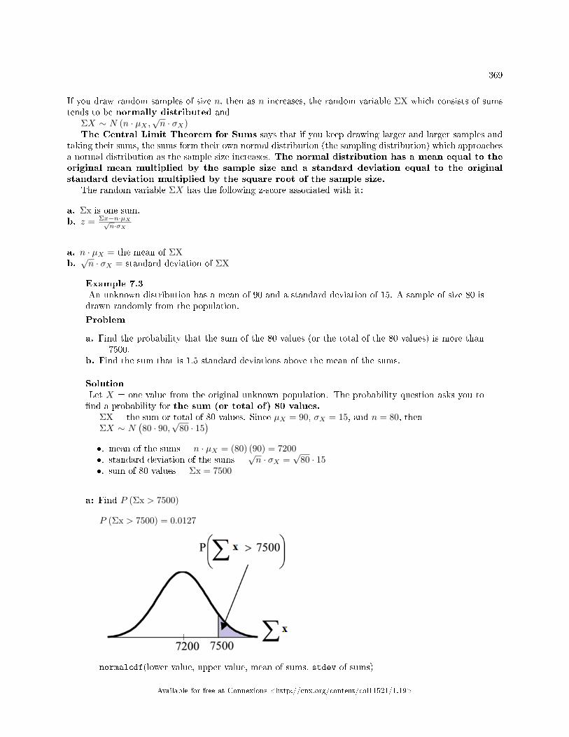
369
If you draw random samples of size n, then as n increases, the random variable ΣX which consists of sumstends to be normally distributed and
ΣX ∼ N (n · µX ,√n · σX)
The Central Limit Theorem for Sums says that if you keep drawing larger and larger samples andtaking their sums, the sums form their own normal distribution (the sampling distribution) which approachesa normal distribution as the sample size increases. The normal distribution has a mean equal to theoriginal mean multiplied by the sample size and a standard deviation equal to the originalstandard deviation multiplied by the square root of the sample size.
The random variable ΣX has the following z-score associated with it:
a. Σx is one sum.b. z = Σx−n·µX√
n·σX
a. n · µX = the mean of ΣXb.√n · σX = standard deviation of ΣX
Example 7.3An unknown distribution has a mean of 90 and a standard deviation of 15. A sample of size 80 isdrawn randomly from the population.
Problem
a. Find the probability that the sum of the 80 values (or the total of the 80 values) is more than7500.
b. Find the sum that is 1.5 standard deviations above the mean of the sums.
SolutionLet X = one value from the original unknown population. The probability question asks you to�nd a probability for the sum (or total of) 80 values.
ΣX = the sum or total of 80 values. Since µX = 90, σX = 15, and n = 80, thenΣX ∼ N
(80 · 90,
√80 · 15
)�. mean of the sums = n · µX = (80) (90) = 7200�. standard deviation of the sums =
√n · σX =
√80 · 15
�. sum of 80 values = Σx = 7500
a: Find P (Σx > 7500)
P (Σx > 7500) = 0.0127
normalcdf(lower value, upper value, mean of sums, stdev of sums)
Available for free at Connexions <http://cnx.org/content/col11521/1.19>
370 CHAPTER 7. THE CENTRAL LIMIT THEOREM
The parameter list is abbreviated (lower, upper, n · µX ,√n · σX)
normalcdf(7500,1E99, 80 · 90,√
80 · 15 = 0.0127Reminder: 1E99 = 1099. Press the EE key for E.
b: Find Σx where z = 1.5:
Σx = n · µX + z ·√n · σX = (80)(90) + (1.5)(
√80) (15) = 7401.2
7.5 Two Column Model Step by Step Example of a Sampling Distri-bution for Sums5
Step-By-Step Example of the Sampling Distribution Model for Sums (Ex 7.3)An unknown distribution has a mean of 90 and a standard deviation of 15. A sample of size 80 is drawn
randomly from the population.Find the probability that the sum of the 80 values (or the total of the 80 values) is more than 7500.
5This content is available online at <http://cnx.org/content/m46257/1.4/>.
Available for free at Connexions <http://cnx.org/content/col11521/1.19>
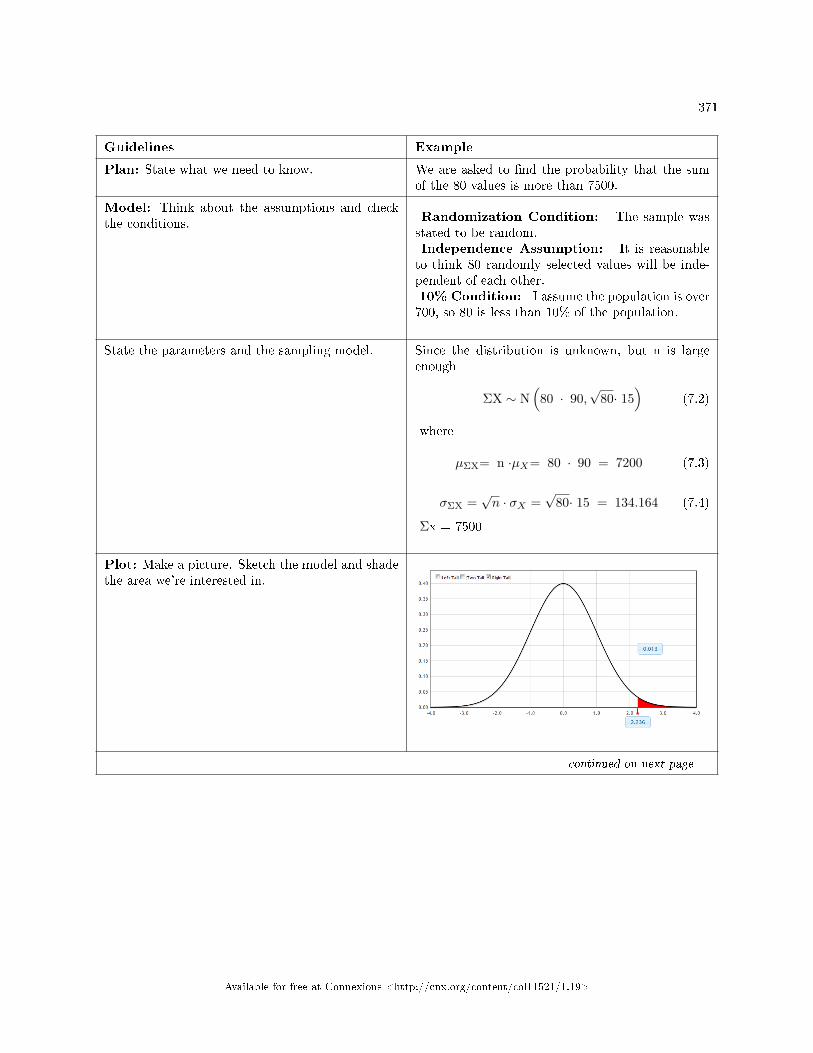
371
Guidelines Example
Plan: State what we need to know. We are asked to �nd the probability that the sumof the 80 values is more than 7500.
Model: Think about the assumptions and checkthe conditions.
Randomization Condition: The sample wasstated to be random.Independence Assumption: It is reasonableto think 80 randomly selected values will be inde-pendent of each other.10% Condition: I assume the population is over700, so 80 is less than 10% of the population.
State the parameters and the sampling model. Since the distribution is unknown, but n is largeenough
ΣX ∼ N(
80 · 90,√
80· 15)
(7.2)
where
µΣX= n ·µX= 80 · 90 = 7200 (7.3)
σΣX =√n · σX =
√80· 15 = 134.164 (7.4)
Σx = 7500
Plot: Make a picture. Sketch the model and shadethe area we're interested in.
continued on next page
Available for free at Connexions <http://cnx.org/content/col11521/1.19>
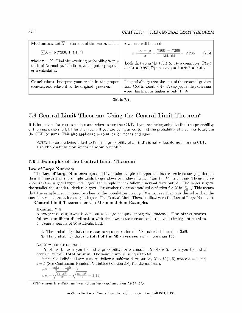
372 CHAPTER 7. THE CENTRAL LIMIT THEOREM
Mechanics: Let X = the sum of the scores. Then,∑X ∼ N(7200, 134.165)
where n = 80. Find the resulting probability from atable of Normal probabilities, a computer programor a calculator.
A z-score will be used:
z =x − µ
σ=
7500 − 7200134.164
= 2.236 (7.5)
Look this up in the table or use a computer. P(z<2.236) = 0.987, P(z >2.236) = 1-0.987 = 0.013
Conclusion: Interpret your result in the propercontext, and relate it to the original question.
The probability that the sum of the scores is greaterthan 7500 is about 0.013. A the probability of a sumscore this high or higher is only 1.3%
Table 7.1
7.6 Central Limit Theorem: Using the Central Limit Theorem6
It is important for you to understand when to use the CLT. If you are being asked to �nd the probabilityof the mean, use the CLT for the mean. If you are being asked to �nd the probability of a sum or total, usethe CLT for sums. This also applies to percentiles for means and sums.
note: If you are being asked to �nd the probability of an individual value, do not use the CLT.Use the distribution of its random variable.
7.6.1 Examples of the Central Limit Theorem
Law of Large NumbersThe Law of Large Numbers says that if you take samples of larger and larger size from any population,
then the mean x of the sample tends to get closer and closer to µ. From the Central Limit Theorem, weknow that as n gets larger and larger, the sample means follow a normal distribution. The larger n gets,the smaller the standard deviation gets. (Remember that the standard deviation for X is σ√
n.) This means
that the sample mean x must be close to the population mean µ. We can say that µ is the value that thesample means approach as n gets larger. The Central Limit Theorem illustrates the Law of Large Numbers.
Central Limit Theorem for the Mean and Sum Examples
Example 7.4A study involving stress is done on a college campus among the students. The stress scoresfollow a uniform distribution with the lowest stress score equal to 1 and the highest equal to5. Using a sample of 50 students, �nd:
1. The probability that the mean stress score for the 50 students is less than 2.65.2. The probability that the total of the 50 stress scores is more than 175.
Let X = one stress score.Problems 1. asks you to �nd a probability for a mean. Problems 2. asks you to �nd a
probability for a total or sum. The sample size, n, is equal to 50.Since the individual stress scores follow a uniform distribution, X ∼ U (1, 5) where a = 1 and
b = 5 (See Continuous Random Variables (Section 5.6) for the uniform).µX = a+b
2 = 1+52 = 3
σX =√
(b−a)2
12 =√
(5−1)2
12 = 1.15
6This content is available online at <http://cnx.org/content/m46247/1.2/>.
Available for free at Connexions <http://cnx.org/content/col11521/1.19>
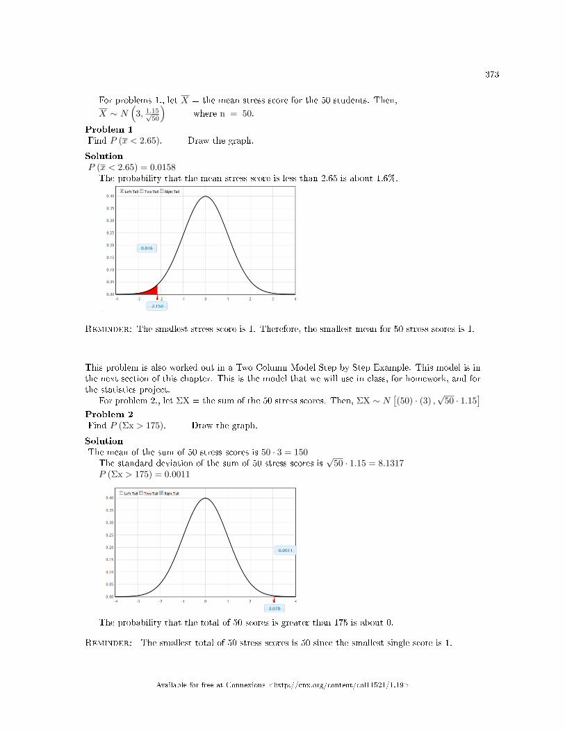
373
For problems 1., let X = the mean stress score for the 50 students. Then,
X ∼ N(
3, 1.15√50
)where n = 50.
Problem 1Find P (x < 2.65). Draw the graph.
SolutionP (x < 2.65) = 0.0158
The probability that the mean stress score is less than 2.65 is about 1.6%.
Reminder: The smallest stress score is 1. Therefore, the smallest mean for 50 stress scores is 1.
This problem is also worked out in a Two Column Model Step by Step Example. This model is inthe next section of this chapter. This is the model that we will use in class, for homework, and forthe statistics project.
For problem 2., let ΣX = the sum of the 50 stress scores. Then, ΣX ∼ N[(50) · (3) ,
√50 · 1.15
]Problem 2Find P (Σx > 175). Draw the graph.
SolutionThe mean of the sum of 50 stress scores is 50 · 3 = 150
The standard deviation of the sum of 50 stress scores is√
50 · 1.15 = 8.1317P (Σx > 175) = 0.0011
The probability that the total of 50 scores is greater than 175 is about 0.
Reminder: The smallest total of 50 stress scores is 50 since the smallest single score is 1.
Available for free at Connexions <http://cnx.org/content/col11521/1.19>
374 CHAPTER 7. THE CENTRAL LIMIT THEOREM
note: (HISTORICAL): Normal Approximation to the Binomial
Historically, being able to compute binomial probabilities was one of the most important applications of theCentral Limit Theorem. Binomial probabilities were displayed in a table in a book with a small value for n(say, 20). To calculate the probabilities with large values of n, you had to use the binomial formula whichcould be very complicated. Using the Normal Approximation to the Binomial simpli�ed the process.To compute the Normal Approximation to the Binomial, take a simple random sample from a population.You must meet the conditions for a binomial distribution:
�. there are a certain number n of independent trials�. the outcomes of any trial are success or failure�. each trial has the same probability of a success p
Recall that if X is the binomial random variable, then X∼B (n, p). The shape of the binomial distributionneeds to be similar to the shape of the normal distribution. To ensure this, the quantities np and nq mustboth be greater than 10 (np > 10 and nq > 10 ). Then the binomial can be approximated by the normaldistribution with mean µ = np and standard deviation σ =
√npq. Remember that q = 1 − p. In order to
get the best approximation, add 0.5 to x or subtract 0.5 from x (use x+ 0.5 or x− 0.5. The number 0.5 iscalled the continuity correction factor.
Example 7.5Suppose in a local Kindergarten through 12th grade (K - 12) school district, 53 percent of thepopulation favor a charter school for grades K - 5. A simple random sample of 300 is surveyed.
1. Find the probability that at least 150 favor a charter school.2. Find the probability that at most 160 favor a charter school.3. Find the probability that more than 155 favor a charter school.4. Find the probability that less than 147 favor a charter school.
Let X = the number that favor a charter school for grades K - 5. X∼B (n, p) where n = 300 andp = 0.53. Since np > 10 and nq > 10, use the normal approximation to the binomial. The formulasfor the mean and standard deviation are µ = np and σ =
√npq. The mean is 159 and the standard
deviation is 8.6447. The random variable for the normal distribution is Y . Y ∼ N (159, 8.6447).For Problem 1., you include 150 so P (x ≥ 150) has normal approximation P (Y ≥ 149.5) =
0.8641.For Problem 2., you include 160 so P (x ≤ 160) has normal approximation P (Y ≤ 160.5) =
0.5689.For Problem 3., you exclude 155 so P (x > 155) has normal approximation P (y > 155.5) =
0.6572.For Problem 4., you exclude 147 so P (x < 147) has normal approximation P (Y < 146.5) =
0.0741.Because of calculators and computer software that easily let you calculate binomial
probabilities for large values of n, it is not necessary to use the the Normal Approximation tothe Binomial provided you have access to these technology tools. Most school labs have MicrosoftExcel, an example of computer software that calculates binomial probabilities. Many students haveaccess to the TI-83 or 84 series calculators and they easily calculate probabilities for the binomial.In an Internet browser, if you type in "binomial probability distribution calculation," you can �ndat least one online calculator for the binomial.
Available for free at Connexions <http://cnx.org/content/col11521/1.19>
375
For Example 3, the probabilities are calculated using the binomial (n = 300 and p = 0.53)below. Compare the binomial and normal distribution answers. SeeDiscrete Random Variablesfor help with calculator instructions for the binomial.
P (x ≥ 150): 1 - binomialcdf (300, 0.53, 149) = 0.8641P (x ≤ 160): binomialcdf (300, 0.53, 160) = 0.5684P (x > 155): 1 - binomialcdf (300, 0.53, 155) = 0.6576P (x < 147): binomialcdf (300, 0.53, 146) = 0.0742P (x = 175): (You use the binomial pdf.) binomialpdf (175, 0.53, 146) = 0.0083
**Contributions made to Example 2 by Roberta Bloom
7.7 Central Limit Theorem: Two Column Model Step by Step Ex-ample of a Sampling Distribution for a Mean7
Two Column Step by Step Example of a Sampling Distribution for a MeanA study involving stress is done on a college campus among the students. The stress scores follow a
uniform distribution with the lowest stress score equal to 1 and the highest equal to 5.Using a random sample of 50 students, �nd the probability that the mean stress score for the 50 students
is less than 2.65.
Guidelines Example
Plan: State what we need to know. We are asked the probability that the mean stressscore of the sample of 50 students is less than 2.65.
Model: Think about the assumptions and checkthe conditions.
Randomization Condition: The problemstates that the sample was random.Independence Assumption: It is reasonable tothink that the stress scores of 50 randomly selectedstudents will be independent of each other. (Butthere could be exceptions, such as , if they were allfrom the same class that was having a major examthe next day.)10% Condition: I assume the student body is over500 students, so 50 students is less than 10% of thepopulation.Sample Size Condition: Since the distributionof the stress levels is uniform, a larger sample sizeis needed. I believe that my sample of 50 studentsseems large enough.
continued on next page
7This content is available online at <http://cnx.org/content/m46242/1.4/>.
Available for free at Connexions <http://cnx.org/content/col11521/1.19>
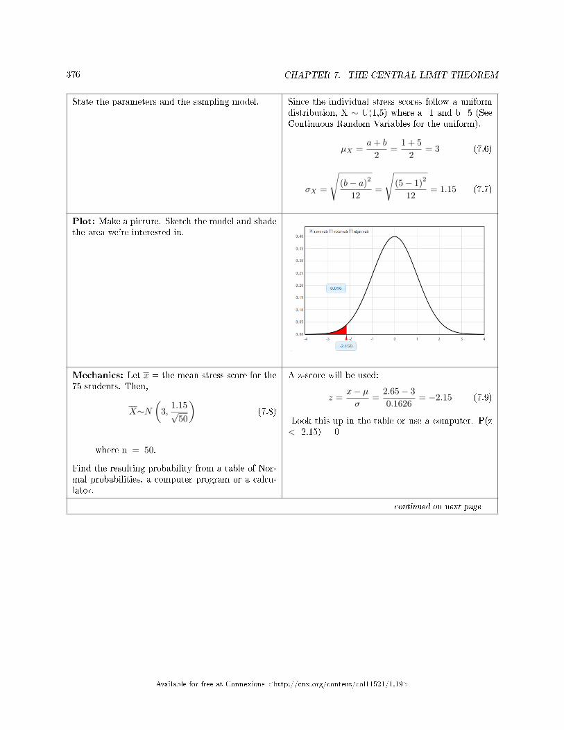
376 CHAPTER 7. THE CENTRAL LIMIT THEOREM
State the parameters and the sampling model. Since the individual stress scores follow a uniformdistribution, X ∼ U(1,5) where a=1 and b=5 (SeeContinuous Random Variables for the uniform).
µX =a+ b
2=
1 + 52
= 3 (7.6)
σX =
√(b− a)2
12=
√(5− 1)2
12= 1.15 (7.7)
Plot: Make a picture. Sketch the model and shadethe area we're interested in.
Mechanics: Let x = the mean stress score for the75 students. Then,
X∼N(
3,1.15√
50
)(7.8)
where n = 50.
Find the resulting probability from a table of Nor-mal probabilities, a computer program or a calcu-lator.
A z-score will be used:
z =x− µσ
=2.65− 30.1626
= −2.15 (7.9)
Look this up in the table or use a computer. P(z< -2.15) = 0
continued on next page
Available for free at Connexions <http://cnx.org/content/col11521/1.19>
377
Conclusion: Interpret your result in the propercontext, and relate it to the original question.
The probability that the mean stress score for the50 college students is less than 2.65 is about 0.
Table 7.2
7.8 Central Limit Theorem: Two Column Model Step by Step Ex-ample of a Sampling Distribution for a Binomial8
Two Column Model Step by Step Example of a Sampling Distribution for a BinomialSuppose in a local Kindergarten through 12th grade (K-12) school district, 53 percent of the population
favor a charter school for grades K-5. A simple random sample of 300 is surveyed.Find the probability that at least 150 favor a charter school.
Guidelines Example from book
Plan: State what we need to know. We are asked the probability that number of peoplewho favor a charter school is at least 150.
Model: Think about the assumptions and checkthe conditions. Check to see that these areBernoulli trials.
Randomization Condition: The sample wasstated to be random.Independence Assumption: It is reasonableto think that the opinions of 300 randomly selectedpeople are independent.10% Condition: I assume the population of theschool district is over 3000 people, so 300 people isless than 10% of the population.Success/Failure Condition success = favor
charter school, failure = do not favor p = 0.53, (1� p) = 0.47 np= 300(0.53) = 159 > 10, n(1-p)=300(0.47) =141 > 10
continued on next page
8This content is available online at <http://cnx.org/content/m46245/1.4/>.
Available for free at Connexions <http://cnx.org/content/col11521/1.19>
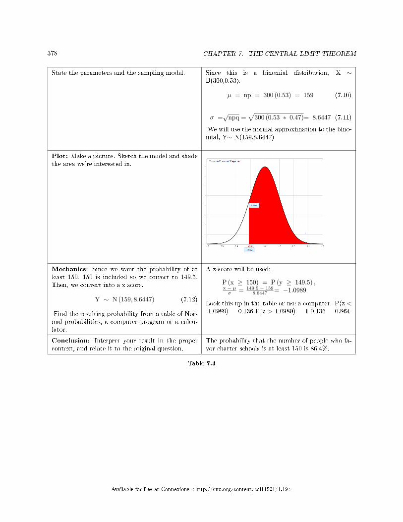
378 CHAPTER 7. THE CENTRAL LIMIT THEOREM
State the parameters and the sampling model. Since this is a binomial distribution, X ∼B(300,0.53).
µ = np = 300 (0.53) = 159 (7.10)
σ =√
npq =√
300 (0.53 ∗ 0.47)= 8.6447 (7.11)
We will use the normal approximation to the bino-mial, Y∼ N(159,8.6447)
Plot: Make a picture. Sketch the model and shadethe area we're interested in.
Mechanics: Since we want the probability of atleast 150, 150 is included so we correct to 149.5.Then, we convert into a z score.
Y ∼ N (159, 8.6447) (7.12)
Find the resulting probability from a table of Nor-mal probabilities, a computer program or a calcu-lator.
A z-score will be used:
P (x ≥ 150) = P (y ≥ 149.5) ,x − µσ = 149.5 − 159
8.6447 = −1.0989
Look this up in the table or use a computer. P(z <-1.0989) = 0.136 P(z >-1.0989) = 1-0.136 = 0.864
Conclusion: Interpret your result in the propercontext, and relate it to the original question.
The probability that the number of people who fa-vor charter schools is at least 150 is 86.4%.
Table 7.3
Available for free at Connexions <http://cnx.org/content/col11521/1.19>
379
7.9 Central Limit Theorem: Summary of Formulas9
Formula 7.1: Central Limit Theorem for Sample Means
X ∼ N(µX ,
σX√n
)The Mean
(X): µX
Formula 7.2: Central Limit Theorem for Sample Means Z-Score and Standard Error of the Meanz = x−µX“
σX√n
” Standard Error of the Mean (Standard Deviation(X)): σX√
n
Formula 7.3: Central Limit Theorem for SumsΣX ∼ N [(n) · µX ,
√n · σX ] Mean for Sums (ΣX): n · µX
Formula 7.4: Central Limit Theorem for Sums Z-Score and Standard Deviation for Sumsz = Σx−n·µX√
n·σXStandard Deviation for Sums (ΣX):
√n · σX
7.9.1 De�nitions
Average
• A number that describes the central tendency of the data. There are a number of specialized averages,including the arithmetic mean, weighted mean, median, mode, and geometric mean.
Central Limit Theorem
• Given a random variable (RV) with known mean µ and known standard deviation σ. We are samplingwith size n and we are interested in two new RVs - the sample mean,x, and the sample sum, ΣX. If thesize n of the sample is su�ciently large, then X ∼ N
(µX ,
σX√n
)and ΣX ∼ N (n · µX ,
√n · σX). If the
size n of the sample is su�ciently large, then the distribution of the sample means and the distributionof the sample sums will approximate a normal distribution regardless of the shape of the population.The mean of the sample means will equal the population mean and the mean of the sample sums willequal n times the population mean. The standard deviation of the distribution of the sample means, ,is called the standard error of the mean
Mean
• A number that measures the central tendency. A common name for mean is 'average.' The term'mean' is a shortened form of 'arithmetic mean.' By de�nition, the mean for a sample (denoted byx ) is x(the sum of all values in the sample divided by the number of values in the sample), and themean for a population (denoted by µ) is µ (the sum of all the values in the population divided by thenumber of values in the population) .
Standard Error of the Mean
• The standard deviation of the distribution of the sample means, σ√n
9This content is available online at <http://cnx.org/content/m48359/1.1/>.
Available for free at Connexions <http://cnx.org/content/col11521/1.19>
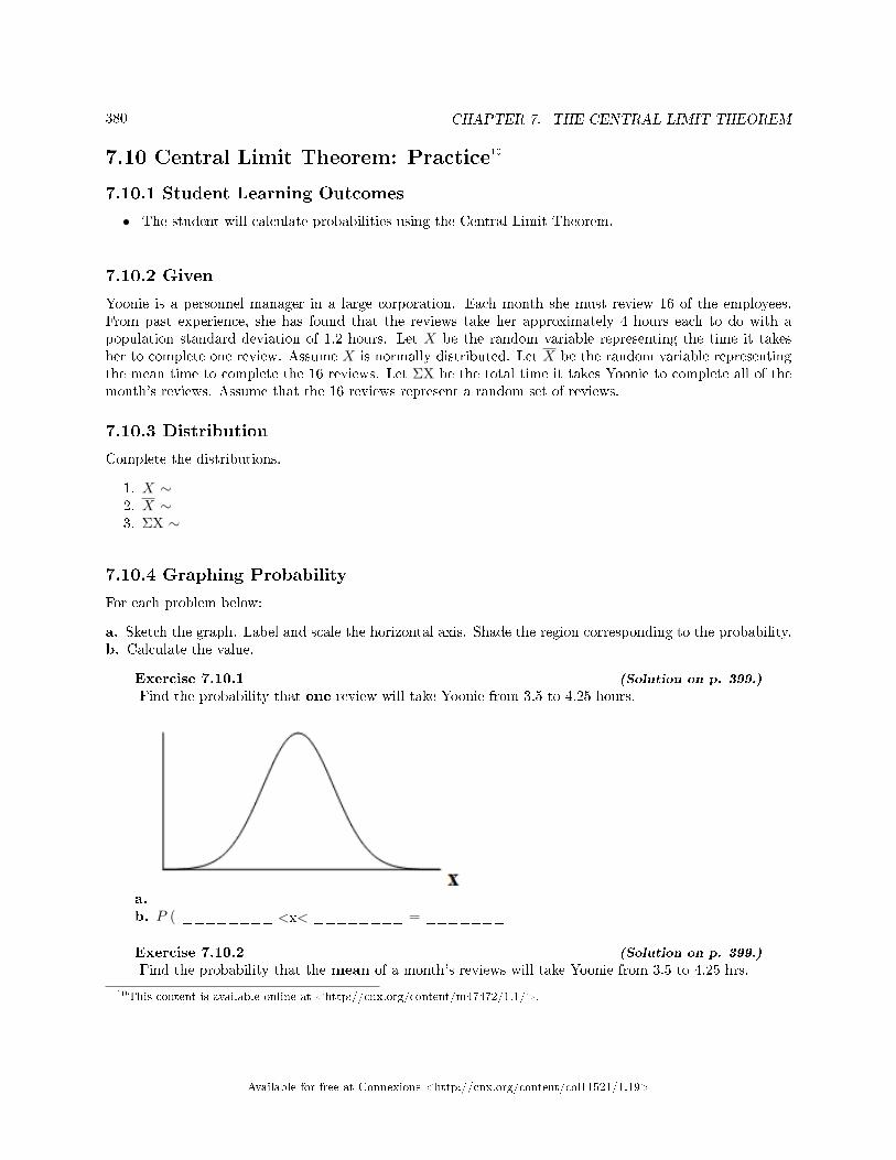
380 CHAPTER 7. THE CENTRAL LIMIT THEOREM
7.10 Central Limit Theorem: Practice10
7.10.1 Student Learning Outcomes
• The student will calculate probabilities using the Central Limit Theorem.
7.10.2 Given
Yoonie is a personnel manager in a large corporation. Each month she must review 16 of the employees.From past experience, she has found that the reviews take her approximately 4 hours each to do with apopulation standard deviation of 1.2 hours. Let X be the random variable representing the time it takesher to complete one review. Assume X is normally distributed. Let X be the random variable representingthe mean time to complete the 16 reviews. Let ΣX be the total time it takes Yoonie to complete all of themonth's reviews. Assume that the 16 reviews represent a random set of reviews.
7.10.3 Distribution
Complete the distributions.
1. X ∼2. X ∼3. ΣX ∼
7.10.4 Graphing Probability
For each problem below:
a. Sketch the graph. Label and scale the horizontal axis. Shade the region corresponding to the probability.b. Calculate the value.
Exercise 7.10.1 (Solution on p. 399.)
Find the probability that one review will take Yoonie from 3.5 to 4.25 hours.
a.b. P ( ________ <x< ________ = _______
Exercise 7.10.2 (Solution on p. 399.)
Find the probability that the mean of a month's reviews will take Yoonie from 3.5 to 4.25 hrs.
10This content is available online at <http://cnx.org/content/m47472/1.1/>.
Available for free at Connexions <http://cnx.org/content/col11521/1.19>
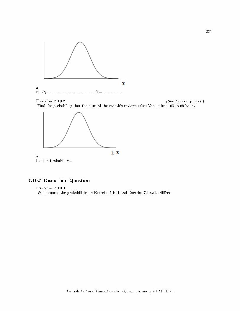
381
a.b. P (________________ ) =_______
Exercise 7.10.3 (Solution on p. 399.)
Find the probability that the sum of the month's reviews takes Yoonie from 60 to 65 hours.
a.b. The Probability=
7.10.5 Discussion Question
Exercise 7.10.4What causes the probabilities in Exercise 7.10.1 and Exercise 7.10.2 to di�er?
Available for free at Connexions <http://cnx.org/content/col11521/1.19>
382 CHAPTER 7. THE CENTRAL LIMIT THEOREM
7.11 Central Limit Theorem: Homework11
Exercise 7.11.1 (Solution on p. 399.)
X ∼ N (60, 9). Suppose that you form random samples of 25 from this distribution. Let X be therandom variable of averages. Let ΣX be the random variable of sums. For c - f, sketch the graph,shade the region, label and scale the horizontal axis for X, and �nd the probability.
a. Sketch the distributions of X and X on the same graph.b. X ∼c. P (x < 60) =e. P (56 < x < 62) =f. P (18 < x < 58) =g. Σx ∼h. Find the minimum value for the upper quartile for the sum.i. P (1400 < Σx < 1550) =
Exercise 7.11.2Determine which of the following are true and which are false. Then, in complete sentences, justifyyour answers.
a. When the sample size is large, the mean of X is approximately equal to the mean of X.b. When the sample size is large, X is approximately normally distributed.c. When the sample size is large, the standard deviation of X is approximately the same as the
standard deviation of X.
Exercise 7.11.3 (Solution on p. 399.)
The percent of fat calories that a person in America consumes each day is normally distributedwith a mean of about 36 and a standard deviation of about 10. Suppose that 16 individuals arerandomly chosen.
Let X =average percent of fat calories.
a. X~______ ( ______ , ______ )b. For the group of 16, �nd the probability that the average percent of fat calories consumed is
more than 5. Graph the situation and shade in the area to be determined.c. Find the �rst quartile for the average percent of fat calories.
Exercise 7.11.4 (Solution on p. 399.)
Suppose that the distance of �y balls hit to the out�eld (in baseball) is normally distributed witha mean of 250 feet and a standard deviation of 50 feet. We randomly sample 49 �y balls.
a. If X = average distance in feet for 49 �y balls, then X~______ ( ______ , ______ )b. What is the probability that the 49 balls traveled an average of less than 240 feet? Sketch the
graph. Scale the horizontal axis for X. Shade the region corresponding to the probability.Find the probability.
c. Find the 80th percentile of the distribution of the average of 49 �y balls.
Exercise 7.11.5Suppose that the weight of open boxes of cereal in a home with children is uniformly distributedfrom 2 to 6 pounds. We randomly survey 64 homes with children.
a. In words, X =11This content is available online at <http://cnx.org/content/m46218/1.4/>.
Available for free at Connexions <http://cnx.org/content/col11521/1.19>
383
b. X~c. µX =d. σX =e. In words, ΣX =f. ΣX~g. Find the probability that the total weight of open boxes is less than 250 pounds.h. Find the 35th percentile for the total weight of open boxes of cereal.
Exercise 7.11.6 (Solution on p. 399.)
Suppose that the duration of a particular type of criminal trial is known to have a mean of 21 daysand a standard deviation of 7 days. We randomly sample 9 trials.
a. In words, ΣX =b. ΣX~c. Find the probability that the total length of the 9 trials is at least 225 days.d. 90 percent of the total of 9 of these types of trials will last at least how long?
Exercise 7.11.7According to the Internal Revenue Service, the average length of time for an individual to complete(record keep, learn, prepare, copy, assemble and send) IRS Form 1040 is 10.53 hours (without anyattached schedules). The distribution is unknown. Let us assume that the standard deviation is 2hours. Suppose we randomly sample 36 taxpayers.
a. In words, X =b. In words, X =c. X~d. Would you be surprised if the 36 taxpayers �nished their Form 1040s in an average of more than
12 hours? Explain why or why not in complete sentences.e. Would you be surprised if one taxpayer �nished his Form 1040 in more than 12 hours? In a
complete sentence, explain why.
Exercise 7.11.8 (Solution on p. 399.)
Suppose that a category of world class runners are known to run a marathon (26 miles) in anaverage of 145 minutes with a standard deviation of 14 minutes. Consider 49 of the races.
Let X = the average of the 49 races.
a. X~b. Find the probability that the runner will average between 142 and 146 minutes in these 49
marathons.c. Find the 80th percentile for the average of these 49 marathons.d. Find the median of the average running times.
Exercise 7.11.9 (Solution on p. 399.)
Suppose that the length of research papers is uniformly distributed from 10 to 25 pages. Wesurvey a class in which 55 research papers were turned in to a professor. The 55 research papersare considered a random collection of all papers. We are interested in the average length of theresearch papers.
a. In words, X =b. X~c. µX =d. σX =
Available for free at Connexions <http://cnx.org/content/col11521/1.19>
384 CHAPTER 7. THE CENTRAL LIMIT THEOREM
e. In words, X =f. X~g. In words, ΣX =h. ΣX~i. Without doing any calculations, do you think that it's likely that the professor will need to read
a total of more than 1050 pages? Why?j. Calculate the probability that the professor will need to read a total of more than 1050 pages.k. Why is it so unlikely that the average length of the papers will be less than 12 pages?
Exercise 7.11.10The length of songs in a collector's CD collection is uniformly distributed from 2 to 3.5 minutes.Suppose we randomly pick 5 CDs from the collection. There is a total of 43 songs on the 5 CDs.
a. In words, X =b. X~c. In words, X=d. X~e. Find the �rst quartile for the average song length.f. The IQR (interquartile range) for the average song length is from _______ to _______.
Exercise 7.11.11 (Solution on p. 400.)
Salaries for teachers in a particular elementary school district are normally distributed with a meanof $44,000 and a standard deviation of $6500. We randomly survey 10 teachers from that district.
a. In words, X =b. In words, X =c. X~d. In words, ΣX =e. ΣX~f. Find the probability that the teachers earn a total of over $400,000.g. Find the 90th percentile for an individual teacher's salary.h. Find the 90th percentile for the average teachers' salary.i. If we surveyed 70 teachers instead of 10, graphically, how would that change the distribution for
X?j. If each of the 70 teachers received a $3000 raise, graphically, how would that change the distri-
bution for X?
Exercise 7.11.12The distribution of income in some Third World countries is not considered normal (many verypoor people, very few middle income people, and few to many wealthy people). We pick a countryconsistent with this non-normal distribution. We �nd the average salary be $2000 per year with astandard deviation of $8000. We randomly surveyed 1000 residents of that country.
a. In words, X =b. In words, X =c. X~d. How is it possible for the standard deviation to be greater than the average?e. Why is it more likely that the average of the 1000 residents will be from $2000 to $2100 than
from $2100 to $2200?
Exercise 7.11.13 (Solution on p. 400.)
The average length of a maternity stay in a U.S. hospital is said to be 2.4 days with a standarddeviation of 0.9 days. We randomly survey 80 women who recently bore children in a U.S. hospital.
Available for free at Connexions <http://cnx.org/content/col11521/1.19>
385
a. In words, X =b. In words, X =c. X~d. In words, ΣX =e. ΣX~f. Is it likely that an individual stayed more than 5 days in the hospital? Why or why not?g. Is it likely that the average stay for the 80 women was more than 5 days? Why or why not?h. Which is more likely:
i. an individual stayed more than 5 days; orii. the average stay of 80 women was more than 5 days?
i. If we were to sum up the women's stays, is it likely that, collectively they spent more than ayear in the hospital? Why or why not?
Exercise 7.11.14In 1940 the average size of a U.S. farm was 174 acres. Let's say that the standard deviation was55 acres. Suppose we randomly survey 38 farmers from 1940. (Source: U.S. Dept. of Agriculture)
a. In words, X =b. In words, X =c. X~d. The IQR for X is from _______ acres to _______ acres.
Exercise 7.11.15Use the Initial Public O�ering data12 (see �Table of Contents) to do this problem.
a. In words, X =b. i. µX =
ii. σX =iii. n =
c. Construct a histogram of the distribution. Start at x = −0.50. Make bar widths of $5.d. In words, describe the distribution of stock prices.e. Randomly average 5 stock prices together. (Use a random number generator.) Continue aver-
aging 5 pieces together until you have 15 averages. List those 15 averages.f. Use the 15 averages from (e) to calculate the following:
i. x =ii. sx =
g. Construct a histogram of the distribution of the averages. Start at x = −0.50. Make bar widthsof $5.
h. Does this histogram look like the graph in (c)? Explain any di�erences.i. In 1 - 2 complete sentences, explain why the graphs either look the same or look di�erent?j. Based upon the theory of the Central Limit Theorem, X~
7.11.1 Try these multiple choice questions (Exercises19 - 23).
The next two questions refer to the following information: The time to wait for a particular ruralbus is distributed uniformly from 0 to 75 minutes. 100 riders are randomly sampled to learn how long theywaited.
Exercise 7.11.16 (Solution on p. 400.)
The 90th percentile sample average wait time (in minutes) for a sample of 100 riders is:
12"Collaborative Statistics: Data Sets": Section Stock Prices <http://cnx.org/content/m17132/latest/#element-949>
Available for free at Connexions <http://cnx.org/content/col11521/1.19>
386 CHAPTER 7. THE CENTRAL LIMIT THEOREM
A. 315.0B. 40.3C. 38.5D. 65.2
Exercise 7.11.17 (Solution on p. 400.)
Would you be surprised, based upon numerical calculations, if the sample average wait time (inminutes) for 100 riders was less than 30 minutes?
A. YesB. NoC. There is not enough information.
Exercise 7.11.18 (Solution on p. 400.)
Which of the following is NOT TRUE about the distribution for averages?
A. The mean, median and mode are equalB. The area under the curve is oneC. The curve never touches the x-axisD. The curve is skewed to the right
The next three questions refer to the following information: The cost of unleaded gasoline in theBay Area once followed an unknown distribution with a mean of $4.59 and a standard deviation of $0.10.Sixteen gas stations from the Bay Area are randomly chosen. We are interested in the average cost of gasolinefor the 16 gas stations.
Exercise 7.11.19 (Solution on p. 400.)
The distribution to use for the average cost of gasoline for the 16 gas stations is
A. X ∼ N (4.59, 0.10)B. X ∼ N
(4.59, 0.10√
16
)C. X ∼ N
(4.59, 0.10
16
)D. X ∼ N
(4.59, 16
0.10
)Exercise 7.11.20 (Solution on p. 400.)
What is the probability that the average price for 16 gas stations is over $4.69?
A. Almost zeroB. 0.1587C. 0.0943D. Unknown
Exercise 7.11.21 (Solution on p. 400.)
Find the probability that the average price for 30 gas stations is less than $4.55.
A. 0.6554B. 0.3446C. 0.0142D. 0.9858E. 0
Exercise 7.11.22: (Example 7.5) (Solution on p. 400.)
For the Charter School Problem (Example 6) in Central Limit Theorem: Using the CentralLimit Theorem, calculate the following using the normal approximation to the binomial.
Available for free at Connexions <http://cnx.org/content/col11521/1.19>
387
A. Find the probability that less than 100 favor a charter school for grades K - 5.B. Find the probability that 170 or more favor a charter school for grades K - 5.C. Find the probability that no more than 140 favor a charter school for grades K - 5.D. Find the probability that there are fewer than 130 that favor a charter school for grades K - 5.E. Find the probability that exactly 150 favor a charter school for grades K - 5.
If you either have access to an appropriate calculator or computer software, try calculating theseprobabilities using the technology. Try also using the suggestion that is at the bottom of CentralLimit Theorem: Using the Central Limit Theorem for �nding a website that calculatesbinomial probabilities.
Exercise 7.11.23 (Solution on p. 400.)
Four friends, Janice, Barbara, Kathy and Roberta, decided to carpool together to get to school.Each day the driver would be chosen by randomly selecting one of the four names. They carpoolto school for 96 days. Use the normal approximation to the binomial to calculate the followingprobabilities. Round the standard deviation to 4 decimal places.
A. Find the probability that Janice is the driver at most 20 days.B. Find the probability that Roberta is the driver more than 16 days.C. Find the probability that Barbara drives exactly 24 of those 96 days.
If you either have access to an appropriate calculator or computer software, try calculating theseprobabilities using the technology. Try also using the suggestion that is at the bottom of CentralLimit Theorem: Using the Central Limit Theorem for �nding a website that calculatesbinomial probabilities.
**Exercise 24 contributed by Roberta Bloom
Available for free at Connexions <http://cnx.org/content/col11521/1.19>
388 CHAPTER 7. THE CENTRAL LIMIT THEOREM
7.12 Central Limit Theorem: Review13
The next three questions refer to the following information: Richard's Furniture Company deliversfurniture from 10 A.M. to 2 P.M. continuously and uniformly. We are interested in how long (in hours) pastthe 10 A.M. start time that individuals wait for their delivery.
Exercise 7.12.1 (Solution on p. 400.)
X ∼
A. U (0, 4)B. U (10, 2)D. N (2, 1)
Exercise 7.12.2 (Solution on p. 400.)
The average wait time is:
A. 1 hourB. 2 hourC. 2.5 hourD. 4 hour
Exercise 7.12.3 (Solution on p. 400.)
Suppose that it is now past noon on a delivery day. The probability that a person must wait atleast 1 1
2 more hours is:
A. 14
B. 12
C. 34
D. 38
Exercise 7.12.4 (Solution on p. 400.)
• 40% of full-time students took 4 years to graduate• 30% of full-time students took 5 years to graduate• 20% of full-time students took 6 years to graduate• 10% of full-time students took 7 years to graduate
The expected time for full-time students to graduate is:
A. 4 yearsB. 4.5 yearsC. 5 yearsD. 5.5 years
Exercise 7.12.5 (Solution on p. 400.)
Which distribution accurately describes the following situation?The chance that a teenage boy regularly gives his mother a kiss goodnight (and he should!!) is
about 20%. Fourteen teenage boys are randomly surveyed.X =the number of teenage boys that regularly give their mother a kiss goodnight
A. B (14, 0.20)B. P (2.8)C. N (2.8, 2.24)
13This content is available online at <http://cnx.org/content/m46220/1.2/>.
Available for free at Connexions <http://cnx.org/content/col11521/1.19>
389
Exercise 7.12.6 (Solution on p. 401.)
Which distribution accurately describes the following situation?A 2008 report on technology use states that approximately 20 percent of U.S. households have
never sent an e-mail. (source: http://www.webguild.org/2008/05/20-percent-of-americans-have-never-used-email.php) Suppose that we select a random sample of fourteen U.S. households .
X =the number of households in a 2008 sample of 14 households that have never sent an email
A. B (14, 0.20)B. P (2.8)C. N (2.8, 2.24)
**Exercise 9 contributed by Roberta Bloom
Available for free at Connexions <http://cnx.org/content/col11521/1.19>
390 CHAPTER 7. THE CENTRAL LIMIT THEOREM
7.13 Central Limit Theorem: Central Limit Theorem Lab I14
Class Time:Names:
7.13.1 Student Learning Outcomes:
• The student will demonstrate and compare properties of the Central Limit Theorem.
note: This lab works best when sampling from several classes and combining data.
7.13.2 Collect the Data
1. Count the change in your pocket. (Do not include bills.)2. Randomly survey 30 classmates. Record the values of the change.
__________ __________ __________ __________ __________
__________ __________ __________ __________ __________
__________ __________ __________ __________ __________
__________ __________ __________ __________ __________
__________ __________ __________ __________ __________
__________ __________ __________ __________ __________
Table 7.4
3. Construct a histogram. Make 5 - 6 intervals. Sketch the graph using a ruler and pencil. Scale theaxes.
14This content is available online at <http://cnx.org/content/m16950/1.10/>.
Available for free at Connexions <http://cnx.org/content/col11521/1.19>
391
Figure 7.1
4. Calculate the following (n = 1; surveying one person at a time):
a. x =b. s =
5. Draw a smooth curve through the tops of the bars of the histogram. Use 1 � 2 complete sentences todescribe the general shape of the curve.
7.13.3 Collecting Averages of Pairs
Repeat steps 1 - 5 (of the section above titled "Collect the Data") with one exception. Instead of recordingthe change of 30 classmates, record the average change of 30 pairs.
1. Randomly survey 30 pairs of classmates. Record the values of the average of theirchange.
__________ __________ __________ __________ __________
__________ __________ __________ __________ __________
__________ __________ __________ __________ __________
__________ __________ __________ __________ __________
__________ __________ __________ __________ __________
__________ __________ __________ __________ __________
Table 7.5
Available for free at Connexions <http://cnx.org/content/col11521/1.19>
392 CHAPTER 7. THE CENTRAL LIMIT THEOREM
2. Construct a histogram. Scale the axes using the same scaling you did for the section titled "Collectingthe Data". Sketch the graph using a ruler and a pencil.
Figure 7.2
3. Calculate the following (n = 2; surveying two people at a time):
a. x =b. s =
4. Draw a smooth curve through tops of the bars of the histogram. Use 1 � 2 complete sentences todescribe the general shape of the curve.
7.13.4 Collecting Averages of Groups of Five
Repeat steps 1 � 5 (of the section titled "Collect the Data") with one exception. Instead of recording thechange of 30 classmates, record the average change of 30 groups of 5.
1. Randomly survey 30 groups of 5 classmates. Record the values of the average of theirchange.
__________ __________ __________ __________ __________
__________ __________ __________ __________ __________
__________ __________ __________ __________ __________
__________ __________ __________ __________ __________
__________ __________ __________ __________ __________
__________ __________ __________ __________ __________
Available for free at Connexions <http://cnx.org/content/col11521/1.19>
393
Table 7.6
2. Construct a histogram. Scale the axes using the same scaling you did for the section titled "Collectthe Data". Sketch the graph using a ruler and a pencil.
Figure 7.3
3. Calculate the following (n = 5; surveying �ve people at a time):
a. x =b. s =
4. Draw a smooth curve through tops of the bars of the histogram. Use 1 � 2 complete sentences todescribe the general shape of the curve.
7.13.5 Discussion Questions
1. As n changed, why did the shape of the distribution of the data change? Use 1 � 2 complete sentencesto explain what happened.
2. In the section titled "Collect the Data", what was the approximate distribution of the data? X ∼3. In the section titled "Collecting Averages of Groups of Five", what was the approximate distribution
of the averages? X ∼4. In 1 � 2 complete sentences, explain any di�erences in your answers to the previous two questions.
Available for free at Connexions <http://cnx.org/content/col11521/1.19>
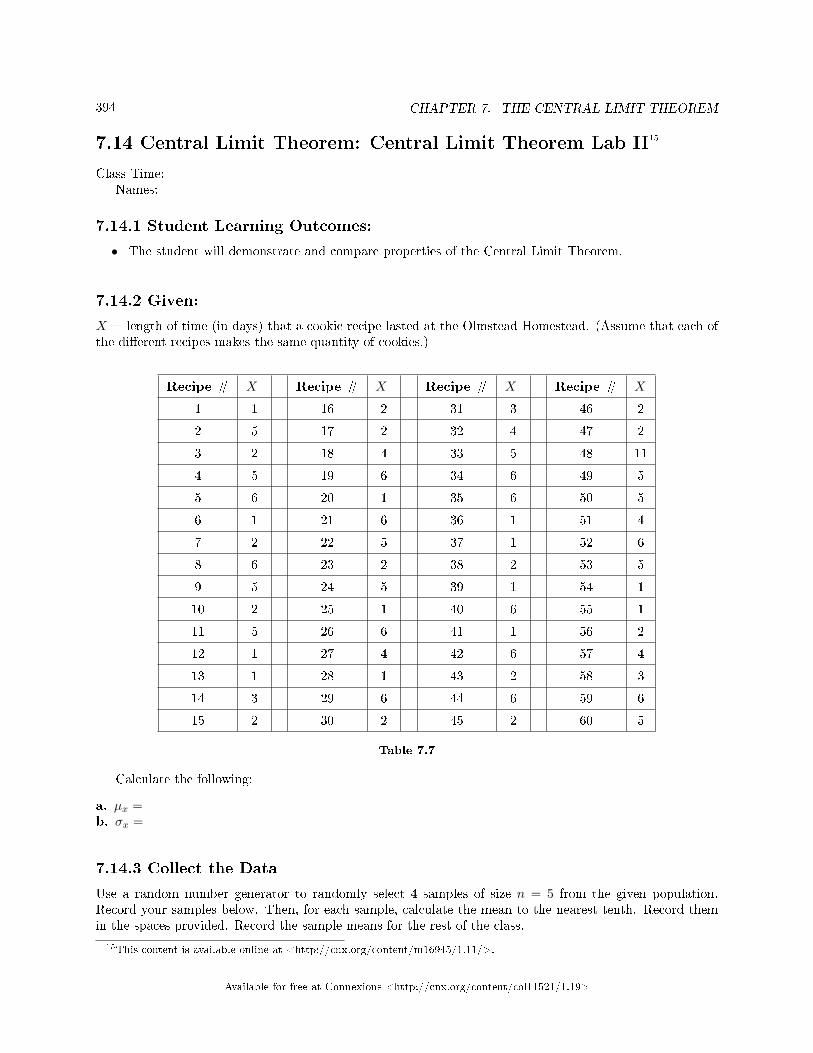
394 CHAPTER 7. THE CENTRAL LIMIT THEOREM
7.14 Central Limit Theorem: Central Limit Theorem Lab II15
Class Time:Names:
7.14.1 Student Learning Outcomes:
• The student will demonstrate and compare properties of the Central Limit Theorem.
7.14.2 Given:
X = length of time (in days) that a cookie recipe lasted at the Olmstead Homestead. (Assume that each ofthe di�erent recipes makes the same quantity of cookies.)
Recipe # X Recipe # X Recipe # X Recipe # X
1 1 16 2 31 3 46 2
2 5 17 2 32 4 47 2
3 2 18 4 33 5 48 11
4 5 19 6 34 6 49 5
5 6 20 1 35 6 50 5
6 1 21 6 36 1 51 4
7 2 22 5 37 1 52 6
8 6 23 2 38 2 53 5
9 5 24 5 39 1 54 1
10 2 25 1 40 6 55 1
11 5 26 6 41 1 56 2
12 1 27 4 42 6 57 4
13 1 28 1 43 2 58 3
14 3 29 6 44 6 59 6
15 2 30 2 45 2 60 5
Table 7.7
Calculate the following:
a. µx =b. σx =
7.14.3 Collect the Data
Use a random number generator to randomly select 4 samples of size n = 5 from the given population.Record your samples below. Then, for each sample, calculate the mean to the nearest tenth. Record themin the spaces provided. Record the sample means for the rest of the class.
15This content is available online at <http://cnx.org/content/m16945/1.11/>.
Available for free at Connexions <http://cnx.org/content/col11521/1.19>
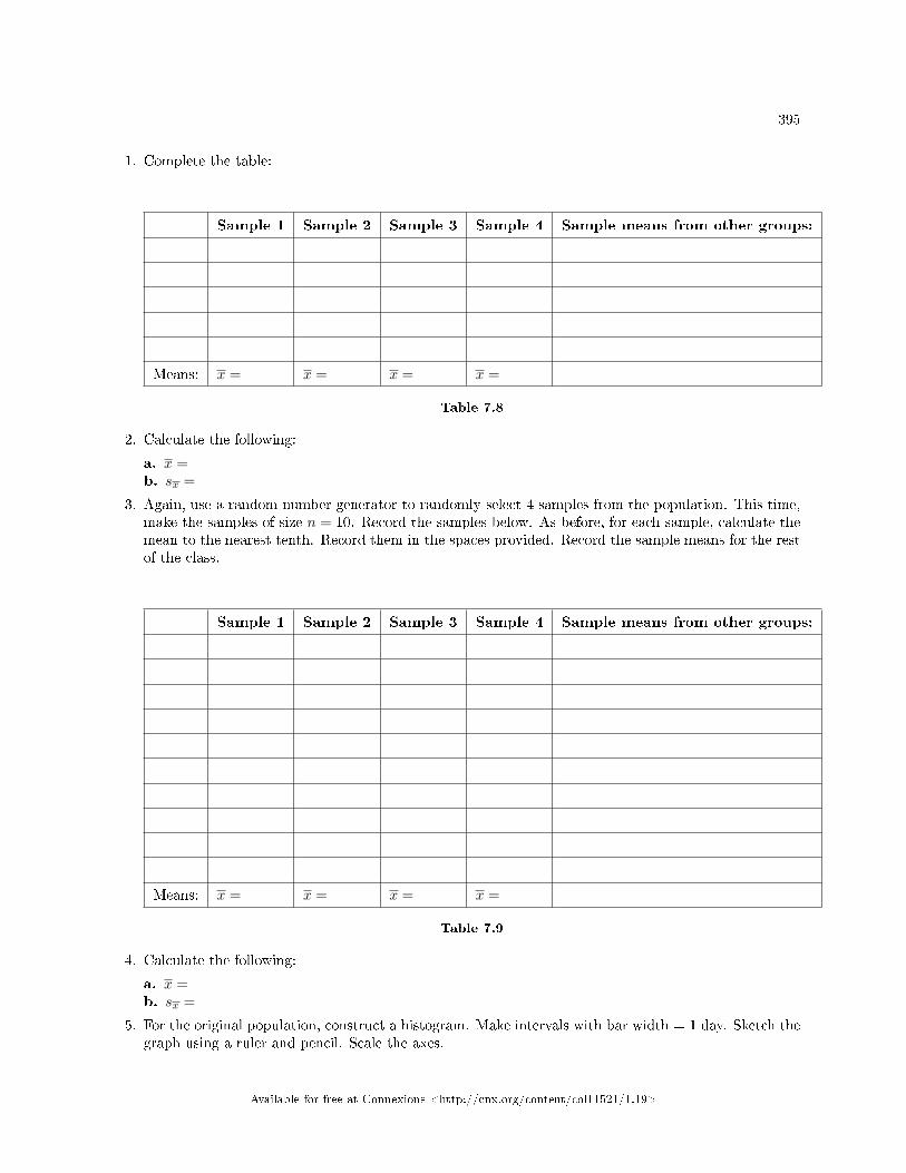
395
1. Complete the table:
Sample 1 Sample 2 Sample 3 Sample 4 Sample means from other groups:
Means: x = x = x = x =
Table 7.8
2. Calculate the following:
a. x =b. sx =
3. Again, use a random number generator to randomly select 4 samples from the population. This time,make the samples of size n = 10. Record the samples below. As before, for each sample, calculate themean to the nearest tenth. Record them in the spaces provided. Record the sample means for the restof the class.
Sample 1 Sample 2 Sample 3 Sample 4 Sample means from other groups:
Means: x = x = x = x =
Table 7.9
4. Calculate the following:
a. x =b. sx =
5. For the original population, construct a histogram. Make intervals with bar width = 1 day. Sketch thegraph using a ruler and pencil. Scale the axes.
Available for free at Connexions <http://cnx.org/content/col11521/1.19>
396 CHAPTER 7. THE CENTRAL LIMIT THEOREM
Figure 7.4
6. Draw a smooth curve through the tops of the bars of the histogram. Use 1 � 2 complete sentences todescribe the general shape of the curve.
7.14.4 Repeat the Procedure for n=5
1. For the sample of n = 5 days averaged together, construct a histogram of the averages (your meanstogether with the means of the other groups). Make intervals with bar widths = 1
2day. Sketch thegraph using a ruler and pencil. Scale the axes.
Available for free at Connexions <http://cnx.org/content/col11521/1.19>
397
Figure 7.5
2. Draw a smooth curve through the tops of the bars of the histogram. Use 1 � 2 complete sentences todescribe the general shape of the curve.
7.14.5 Repeat the Procedure for n=10
1. For the sample of n = 10 days averaged together, construct a histogram of the averages (your meanstogether with the means of the other groups). Make intervals with bar widths = 1
2day. Sketch thegraph using a ruler and pencil. Scale the axes.
Available for free at Connexions <http://cnx.org/content/col11521/1.19>
398 CHAPTER 7. THE CENTRAL LIMIT THEOREM
Figure 7.6
2. Draw a smooth curve through the tops of the bars of the histogram. Use 1 � 2 complete sentences todescribe the general shape of the curve.
7.14.6 Discussion Questions
1. Compare the three histograms you have made, the one for the population and the two for the samplemeans. In three to �ve sentences, describe the similarities and di�erences.
2. State the theoretical (according to the CLT) distributions for the sample means.
a. n = 5: X ∼b. n = 10: X ∼
3. Are the sample means for n = 5 and n = 10 �close� to the theoretical mean, µx? Explain why or whynot.
4. Which of the two distributions of sample means has the smaller standard deviation? Why?5. As n changed, why did the shape of the distribution of the data change? Use 1 � 2 complete sentences
to explain what happened.
note: This lab was designed and contributed by Carol Olmstead.
Available for free at Connexions <http://cnx.org/content/col11521/1.19>
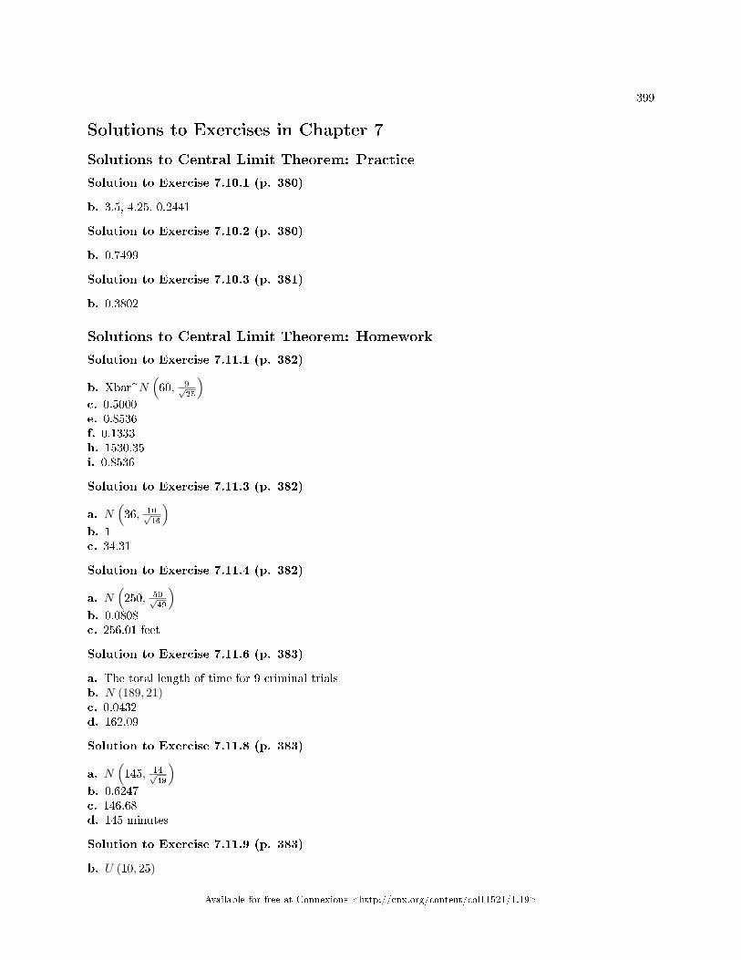
399
Solutions to Exercises in Chapter 7
Solutions to Central Limit Theorem: Practice
Solution to Exercise 7.10.1 (p. 380)
b. 3.5, 4.25, 0.2441
Solution to Exercise 7.10.2 (p. 380)
b. 0.7499
Solution to Exercise 7.10.3 (p. 381)
b. 0.3802
Solutions to Central Limit Theorem: Homework
Solution to Exercise 7.11.1 (p. 382)
b. Xbar~N(60, 9√
25
)c. 0.5000e. 0.8536f. 0.1333h. 1530.35i. 0.8536
Solution to Exercise 7.11.3 (p. 382)
a. N(36, 10√
16
)b. 1c. 34.31
Solution to Exercise 7.11.4 (p. 382)
a. N(250, 50√
49
)b. 0.0808c. 256.01 feet
Solution to Exercise 7.11.6 (p. 383)
a. The total length of time for 9 criminal trialsb. N (189, 21)c. 0.0432d. 162.09
Solution to Exercise 7.11.8 (p. 383)
a. N(145, 14√
49
)b. 0.6247c. 146.68d. 145 minutes
Solution to Exercise 7.11.9 (p. 383)
b. U (10, 25)
Available for free at Connexions <http://cnx.org/content/col11521/1.19>
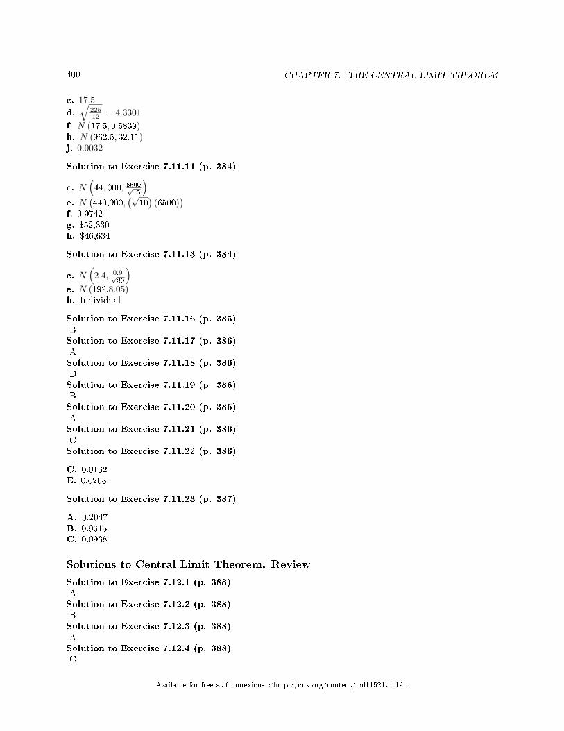
400 CHAPTER 7. THE CENTRAL LIMIT THEOREM
c. 17.5d.√
22512 = 4.3301
f. N (17.5, 0.5839)h. N (962.5, 32.11)j. 0.0032
Solution to Exercise 7.11.11 (p. 384)
c. N(44, 000, 6500√
10
)e. N
(440,000,
(√10)
(6500))
f. 0.9742g. $52,330h. $46,634
Solution to Exercise 7.11.13 (p. 384)
c. N(
2.4, 0.9√80
)e. N (192,8.05)h. Individual
Solution to Exercise 7.11.16 (p. 385)BSolution to Exercise 7.11.17 (p. 386)ASolution to Exercise 7.11.18 (p. 386)DSolution to Exercise 7.11.19 (p. 386)BSolution to Exercise 7.11.20 (p. 386)ASolution to Exercise 7.11.21 (p. 386)CSolution to Exercise 7.11.22 (p. 386)
C. 0.0162E. 0.0268
Solution to Exercise 7.11.23 (p. 387)
A. 0.2047B. 0.9615C. 0.0938
Solutions to Central Limit Theorem: Review
Solution to Exercise 7.12.1 (p. 388)ASolution to Exercise 7.12.2 (p. 388)BSolution to Exercise 7.12.3 (p. 388)ASolution to Exercise 7.12.4 (p. 388)C
Available for free at Connexions <http://cnx.org/content/col11521/1.19>

401
Solution to Exercise 7.12.5 (p. 388)ASolution to Exercise 7.12.6 (p. 389)A
Available for free at Connexions <http://cnx.org/content/col11521/1.19>

402 CHAPTER 7. THE CENTRAL LIMIT THEOREM
Available for free at Connexions <http://cnx.org/content/col11521/1.19>
Chapter 8
Con�dence Intervals
8.1 Con�dence Intervals: Introduction1
8.1.1 Student Learning Outcomes
By the end of this chapter, the student should be able to:
• Calculate and interpret con�dence intervals for one population mean and one population proportion.• Interpret the student-t probability distribution as the sample size changes.• Discriminate between problems applying the normal and the student-t distributions.
8.1.2 Introduction
Suppose you are trying to determine the mean rent of a two-bedroom apartment in your town. You mightlook in the classi�ed section of the newspaper, write down several rents listed, and average them together.You would have obtained a point estimate of the true mean. If you are trying to determine the percent oftimes you make a basket when shooting a basketball, you might count the number of shots you make anddivide that by the number of shots you attempted. In this case, you would have obtained a point estimatefor the true proportion.
We use sample data to make generalizations about an unknown population. This part of statistics is calledinferential statistics. The sample data help us to make an estimate of a population parameter.We realize that the point estimate is most likely not the exact value of the population parameter, but closeto it. After calculating point estimates, we construct con�dence intervals in which we believe the parameterlies.
In this chapter, you will learn to construct and interpret con�dence intervals. You will also learn a newdistribution, the Student's-t, and how it is used with these intervals. Throughout the chapter, it is importantto keep in mind that the con�dence interval is a random variable. It is the parameter that is �xed.
If you worked in the marketing department of an entertainment company, you might be interested inthe mean number of compact discs (CD's) a consumer buys per month. If so, you could conduct a surveyand calculate the sample mean, x, and the sample standard deviation, s. You would use x to estimate thepopulation mean and s to estimate the population standard deviation. The sample mean, x, is the pointestimate for the population mean, µ. The sample standard deviation, s, is the point estimate for thepopulation standard deviation, σ.
Each of x and s is also called a statistic.
1This content is available online at <http://cnx.org/content/m16967/1.16/>.
Available for free at Connexions <http://cnx.org/content/col11521/1.19>
403
404 CHAPTER 8. CONFIDENCE INTERVALS
A con�dence interval is another type of estimate but, instead of being just one number, it is an intervalof numbers. The interval of numbers is a range of values calculated from a given set of sample data. Thecon�dence interval is likely to include an unknown population parameter.
Suppose for the CD example we do not know the population mean µ but we do know that the populationstandard deviation is σ = 1 and our sample size is 100. Then by the Central Limit Theorem, the standarddeviation for the sample mean is
σ√n
= 1√100
= 0.1.The Empirical Rule, which applies to bell-shaped distributions, says that in approximately 95% of the
samples, the sample mean, x, will be within two standard deviations of the population mean µ. For our CDexample, two standard deviations is (2) (0.1) = 0.2. The sample mean x is likely to be within 0.2 units ofµ.
Because x is within 0.2 units of µ, which is unknown, then µ is likely to be within 0.2 units of x in 95% ofthe samples. The population mean µ is contained in an interval whose lower number is calculated by takingthe sample mean and subtracting two standard deviations ((2) (0.1)) and whose upper number is calculatedby taking the sample mean and adding two standard deviations. In other words, µ is between x − 0.2 andx+ 0.2 in 95% of all the samples.
For the CD example, suppose that a sample produced a sample mean x = 2. Then the unknownpopulation mean µ is between
x− 0.2 = 2− 0.2 = 1.8 and x+ 0.2 = 2 + 0.2 = 2.2We say that we are 95% con�dent that the unknown population mean number of CDs is between 1.8
and 2.2. The 95% con�dence interval is (1.8, 2.2).The 95% con�dence interval implies two possibilities. Either the interval (1.8, 2.2) contains the true
mean µ or our sample produced an x that is not within 0.2 units of the true mean µ. The second possibilityhappens for only 5% of all the samples (100% - 95%).
Remember that a con�dence interval is created for an unknown population parameter like the populationmean, µ. Con�dence intervals for some parameters have the form
(point estimate - margin of error, point estimate + margin of error)The margin of error depends on the con�dence level or percentage of con�dence.When you read newspapers and journals, some reports will use the phrase "margin of error." Other
reports will not use that phrase, but include a con�dence interval as the point estimate + or - the margin oferror. These are two ways of expressing the same concept.
note: Although the text only covers symmetric con�dence intervals, there are non-symmetriccon�dence intervals (for example, a con�dence interval for the standard deviation).
8.1.3 Optional Collaborative Classroom Activity
Have your instructor record the number of meals each student in your class eats out in a week. Assume thatthe standard deviation is known to be 3 meals. Construct an approximate 95% con�dence interval for thetrue mean number of meals students eat out each week.
1. Calculate the sample mean.2. σ = 3 and n = the number of students surveyed.
3. Construct the interval(x− 2 · σ√
n, x+ 2 · σ√
n
)We say we are approximately 95% con�dent that the true average number of meals that students eat out ina week is between __________ and ___________.
Available for free at Connexions <http://cnx.org/content/col11521/1.19>
405
8.2 Con�dence Interval: Assumptions and Conditions2
8.2.1 Assumptions and Conditions
When constructing con�dence intervals the assumptions and conditions of the central limit theorem mustbe met in order to use the normal model.
Randomization Condition: The data must be sampled randomly. Is one of the good sampling method-ologies discussed in the Sampling and Data chapter being used?
Independence Assumption: The sample values must be independent of each other. This means thatthe occurrence of one event has no in�uence on the next event. Usually, if we know that people or itemswere selected randomly we can assume that the independence assumption is met.
10% Condition: When the sample is drawn without replacement (usually the case), the sample size,n, should be no more than 10% of the population.
Sample Size Condition: The sample size must be su�ciently large. Although the Central LimitTheorem tells us that we can use a Normal model to think about the behavior of sample means when thesample size is large enough, it does not tell us how large that should be. If the population is very skewed, youwill need a pretty large sample size to use the CLT, however if the population is unimodal and symmetric,even small samples are ok. So think about your sample size in terms of what you know about the populationand decide whether the sample is large enough. In general a sample size of 30 is considered su�cient.
When working with numerical data and σ is unknown the assumptions of randomization, indepen-dence and the 10% condition must be met. In addition, with small sample sizes we cannot assume thatthat data follows a normal distribution so we need to check the nearly normal condition. To check thenearly normal condition start by making a histogram or stemplot of the data, it is a good idea to make anoutlier boxplot, too. If the sample is small, less than 15 then the data must be normally distributed. If thesample size is moderate, between 15 and 40, then a little skewing in the data will can be tolerated. Withlarge sample sizes, more than 40, we are concerned about multiple peaks (modes) in the data and outliers.The data might not be approximately normal with either of these conditions and you may want to run thetest both with and without the outliers to determine the extent of their e�ect. If there are multiple modesin the data if could be that there are two groups in the data that need to be separated.
When working with binomial or categorical data the assumptions of randomization, independenceand the 10% condition must be met. In addition, a new assumption, the success/ failure condition, mustbe checked. When working with proportions we need to be especially concerned about sample size whenthe proportion is close to zero or one. To check that the sample size is large enough calculate the successby multiplying the sample percentage by the sample size and calculate failure by multiplying one minus thesample percentage by the sample size. If both of these products are larger than ten then the condition ismet.
8.3 Con�dence Intervals: Con�dence Interval, Single PopulationMean, Population Standard Deviation Known, Normal3
8.3.1 Calculating the Con�dence Interval
To construct a con�dence interval for a single unknown population mean µ , where the populationstandard deviation is known, we need x as an estimate for µ and we need the margin of error. Themargin of error for a population mean (ME) is called sometimes called the error bound for a populationmean (abbreviated EBM). The sample mean x is the point estimate of the unknown population mean µ
The con�dence interval estimate will have the form:
(point estimate - margin of error, point estimate + margin of error) or, in symbols,(x−ME, x+ ME)
2This content is available online at <http://cnx.org/content/m46273/1.2/>.3This content is available online at <http://cnx.org/content/m46258/1.2/>.
Available for free at Connexions <http://cnx.org/content/col11521/1.19>
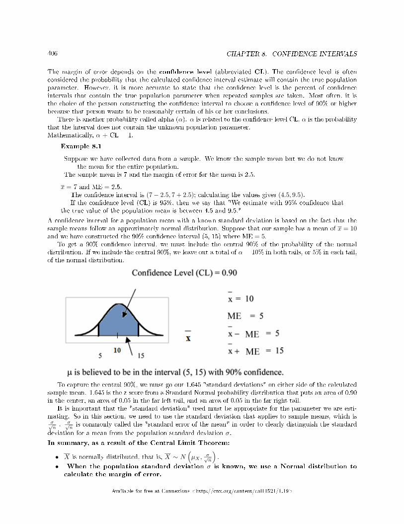
406 CHAPTER 8. CONFIDENCE INTERVALS
The margin of error depends on the con�dence level (abbreviated CL). The con�dence level is oftenconsidered the probability that the calculated con�dence interval estimate will contain the true populationparameter. However, it is more accurate to state that the con�dence level is the percent of con�denceintervals that contain the true population parameter when repeated samples are taken. Most often, it isthe choice of the person constructing the con�dence interval to choose a con�dence level of 90% or higherbecause that person wants to be reasonably certain of his or her conclusions.
There is another probability called alpha (α). α is related to the con�dence level CL. α is the probabilitythat the interval does not contain the unknown population parameter.Mathematically, α + CL = 1.
Example 8.1
Suppose we have collected data from a sample. We know the sample mean but we do not knowthe mean for the entire population.
The sample mean is 7 and the margin of error for the mean is 2.5.
x = 7 and ME = 2.5.The con�dence interval is (7− 2.5, 7 + 2.5); calculating the values gives (4.5, 9.5).If the con�dence level (CL) is 95%, then we say that "We estimate with 95% con�dence that
the true value of the population mean is between 4.5 and 9.5."
A con�dence interval for a population mean with a known standard deviation is based on the fact that thesample means follow an approximately normal distribution. Suppose that our sample has a mean of x = 10and we have constructed the 90% con�dence interval (5, 15) where ME = 5.
To get a 90% con�dence interval, we must include the central 90% of the probability of the normaldistribution. If we include the central 90%, we leave out a total of α = 10% in both tails, or 5% in each tail,of the normal distribution.
To capture the central 90%, we must go out 1.645 "standard deviations" on either side of the calculatedsample mean. 1.645 is the z-score from a Standard Normal probability distribution that puts an area of 0.90in the center, an area of 0.05 in the far left tail, and an area of 0.05 in the far right tail.
It is important that the "standard deviation" used must be appropriate for the parameter we are esti-mating. So in this section, we need to use the standard deviation that applies to sample means, which isσ√n. σ√
nis commonly called the "standard error of the mean" in order to clearly distinguish the standard
deviation for a mean from the population standard deviation σ.
In summary, as a result of the Central Limit Theorem:
• X is normally distributed, that is, X ∼ N(µX ,
σ√n
).
• When the population standard deviation σ is known, we use a Normal distribution tocalculate the margin of error.
Available for free at Connexions <http://cnx.org/content/col11521/1.19>
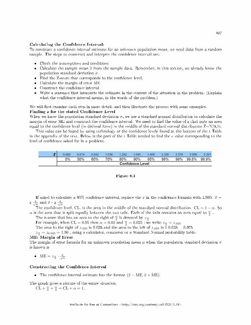
407
Calculating the Con�dence Interval:To construct a con�dence interval estimate for an unknown population mean, we need data from a randomsample. The steps to construct and interpret the con�dence interval are:
• Check the assumptions and conditions• Calculate the sample mean x from the sample data. Remember, in this section, we already know the
population standard deviation σ.• Find the Z-score that corresponds to the con�dence level.• Calculate the margin of error ME• Construct the con�dence interval• Write a sentence that interprets the estimate in the context of the situation in the problem. (Explain
what the con�dence interval means, in the words of the problem.)
We will �rst examine each step in more detail, and then illustrate the process with some examples.Finding z for the stated Con�dence LevelWhen we know the population standard deviation σ, we use a standard normal distribution to calculate themargin of error ME and construct the con�dence interval. We need to �nd the value of z that puts an areaequal to the con�dence level (in decimal form) in the middle of the standard normal distribution Z∼N(0,1).
This value can be found by using technology or the con�dence levels found at the bottom of the t Tablein the appendix of the text. Below is the part of the t Table needed to �nd the z value corresponding to thelevel of con�dence asked for in a problem.
Figure 8.1
If asked to calculate a 95% con�dence interval, replace the z in the con�dence formula with 1.960. x +z σ√
nand x - z σ√
n
The con�dence level, CL, is the area in the middle of the standard normal distribution. CL = 1− α. Soα is the area that is split equally between the two tails. Each of the tails contains an area equal to α
2 .The z-score that has an area to the right of α2 is denoted by zα
2
For example, when CL = 0.95 then α = 0.05 and α2 = 0.025 ; we write zα
2= z.025
The area to the right of z.025 is 0.025 and the area to the left of z.025 is 1-0.025 = 0.975zα
2= z0.025 = 1.96 , using a calculator, computer or a Standard Normal probability table.
ME: Margin of ErrorThe margin of error formula for an unknown population mean µ when the population standard deviation σis known is
• ME = zα2· σ√
n
Constructing the Con�dence Interval
• The con�dence interval estimate has the format (x−ME, x+ ME).
The graph gives a picture of the entire situation.CL + α
2 + α2 = CL + α = 1.
Available for free at Connexions <http://cnx.org/content/col11521/1.19>
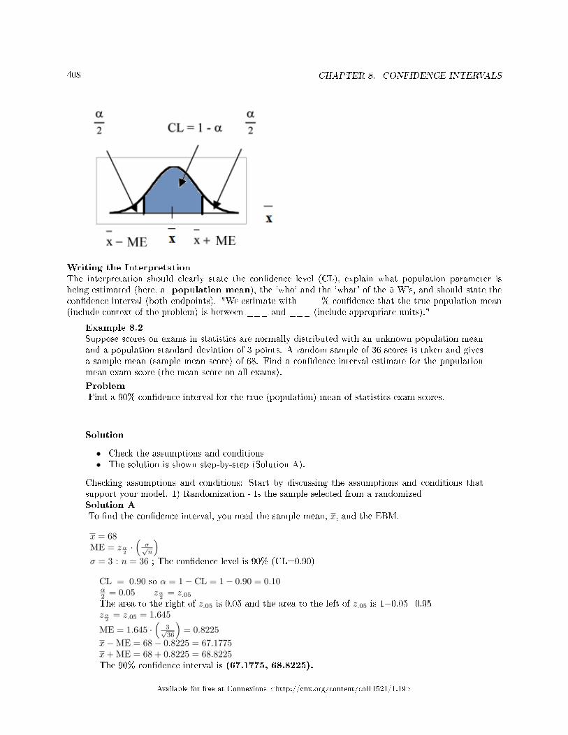
408 CHAPTER 8. CONFIDENCE INTERVALS
Writing the InterpretationThe interpretation should clearly state the con�dence level (CL), explain what population parameter isbeing estimated (here, a population mean), the 'who' and the 'what' of the 5 W's, and should state thecon�dence interval (both endpoints). "We estimate with ___% con�dence that the true population mean(include context of the problem) is between ___ and ___ (include appropriate units)."
Example 8.2Suppose scores on exams in statistics are normally distributed with an unknown population meanand a population standard deviation of 3 points. A random sample of 36 scores is taken and givesa sample mean (sample mean score) of 68. Find a con�dence interval estimate for the populationmean exam score (the mean score on all exams).
ProblemFind a 90% con�dence interval for the true (population) mean of statistics exam scores.
Solution
• Check the assumptions and conditions• The solution is shown step-by-step (Solution A).
Checking assumptions and conditions: Start by discussing the assumptions and conditions thatsupport your model. 1) Randomization - Is the sample selected from a randomizedSolution ATo �nd the con�dence interval, you need the sample mean, x, and the EBM.
x = 68ME = zα
2·(σ√n
)σ = 3 ; n = 36 ; The con�dence level is 90% (CL=0.90)
CL = 0.90 so α = 1− CL = 1− 0.90 = 0.10α2 = 0.05 zα
2= z.05
The area to the right of z.05 is 0.05 and the area to the left of z.05 is 1−0.05=0.95zα
2= z.05 = 1.645
ME = 1.645 ·(
3√36
)= 0.8225
x−ME = 68− 0.8225 = 67.1775x+ ME = 68 + 0.8225 = 68.8225The 90% con�dence interval is (67.1775, 68.8225).
Available for free at Connexions <http://cnx.org/content/col11521/1.19>
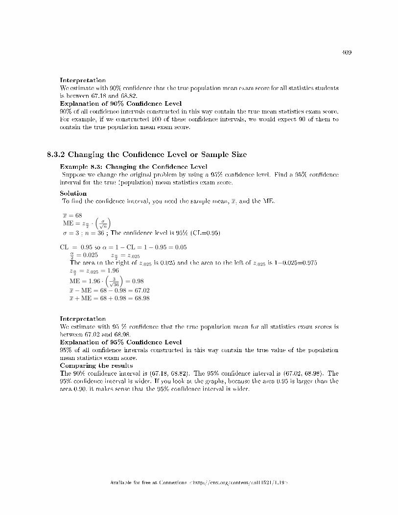
409
InterpretationWe estimate with 90% con�dence that the true population mean exam score for all statistics studentsis between 67.18 and 68.82.Explanation of 90% Con�dence Level90% of all con�dence intervals constructed in this way contain the true mean statistics exam score.For example, if we constructed 100 of these con�dence intervals, we would expect 90 of them tocontain the true population mean exam score.
8.3.2 Changing the Con�dence Level or Sample Size
Example 8.3: Changing the Con�dence LevelSuppose we change the original problem by using a 95% con�dence level. Find a 95% con�denceinterval for the true (population) mean statistics exam score.
SolutionTo �nd the con�dence interval, you need the sample mean, x, and the ME.
x = 68ME = zα
2·(σ√n
)σ = 3 ; n = 36 ; The con�dence level is 95% (CL=0.95)
CL = 0.95 so α = 1− CL = 1− 0.95 = 0.05α2 = 0.025 zα
2= z.025
The area to the right of z.025 is 0.025 and the area to the left of z.025 is 1−0.025=0.975zα
2= z.025 = 1.96
ME = 1.96 ·(
3√36
)= 0.98
x−ME = 68− 0.98 = 67.02x+ ME = 68 + 0.98 = 68.98
InterpretationWe estimate with 95 % con�dence that the true population mean for all statistics exam scores isbetween 67.02 and 68.98.Explanation of 95% Con�dence Level95% of all con�dence intervals constructed in this way contain the true value of the populationmean statistics exam score.Comparing the resultsThe 90% con�dence interval is (67.18, 68.82). The 95% con�dence interval is (67.02, 68.98). The95% con�dence interval is wider. If you look at the graphs, because the area 0.95 is larger than thearea 0.90, it makes sense that the 95% con�dence interval is wider.
Available for free at Connexions <http://cnx.org/content/col11521/1.19>
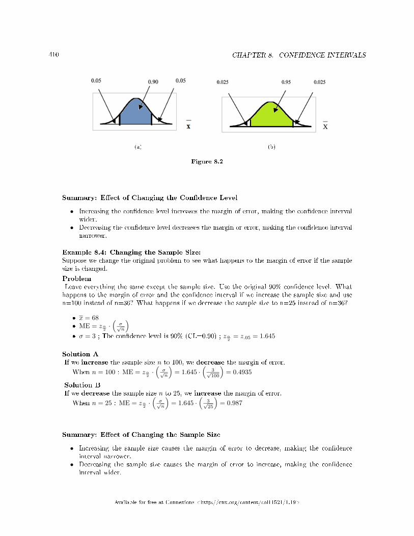
410 CHAPTER 8. CONFIDENCE INTERVALS
(a) (b)
Figure 8.2
Summary: E�ect of Changing the Con�dence Level
• Increasing the con�dence level increases the margin of error, making the con�dence intervalwider.
• Decreasing the con�dence level decreases the margin or error, making the con�dence intervalnarrower.
Example 8.4: Changing the Sample Size:Suppose we change the original problem to see what happens to the margin of error if the samplesize is changed.
ProblemLeave everything the same except the sample size. Use the original 90% con�dence level. Whathappens to the margin of error and the con�dence interval if we increase the sample size and usen=100 instead of n=36? What happens if we decrease the sample size to n=25 instead of n=36?
� x = 68� ME = zα
2·(σ√n
)� σ = 3 ; The con�dence level is 90% (CL=0.90) ; zα
2= z.05 = 1.645
Solution AIf we increase the sample size n to 100, we decrease the margin of error.
When n = 100 : ME = zα2·(σ√n
)= 1.645 ·
(3√100
)= 0.4935
Solution BIf we decrease the sample size n to 25, we increase the margin of error.
When n = 25 : ME = zα2·(σ√n
)= 1.645 ·
(3√25
)= 0.987
Summary: E�ect of Changing the Sample Size
• Increasing the sample size causes the margin of error to decrease, making the con�denceinterval narrower.
• Decreasing the sample size causes the margin of error to increase, making the con�denceinterval wider.
Available for free at Connexions <http://cnx.org/content/col11521/1.19>
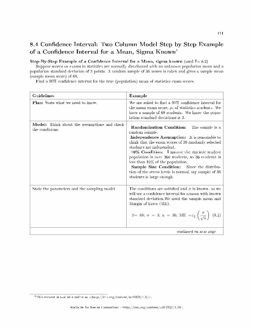
411
8.4 Con�dence Interval: Two Column Model Step by Step Exampleof a Con�dence Interval for a Mean, Sigma Known4
Step-By-Step Example of a Con�dence Interval for a Mean, sigma known (used Ex 8.2)Suppose scores on exams in statistics are normally distributed with an unknown population mean and a
population standard deviation of 3 points. A random sample of 36 scores is taken and gives a sample mean(sample mean score) of 68.
Find a 90% con�dence interval for the true (population) mean of statistics exam scores.
Guidelines Example
Plan: State what we need to know. We are asked to �nd a 90% con�dence interval forthe mean exam score, µ, of statistics students. Wehave a sample of 68 students. We know the popu-lation standard deviations is 3.
Model: Think about the assumptions and checkthe conditions.
Randomization Condition: The sample is arandom sample.Independence Assumption: It is reasonable tothink that the exam scores of 36 randomly selectedstudents are independent.10% Condition: I assume the statistic studentpopulation is over 360 students, so 36 students isless than 10% of the population.Sample Size Condition: Since the distribu-tion of the stress levels is normal, my sample of 36students is large enough.
State the parameters and the sampling model The conditions are satis�ed and σ is known, so wewill use a con�dence interval for a mean with knownstandard deviation.We need the sample mean andMargin of Error (ME).
x= 68; σ = 3; n = 36; ME =z a2
(σ√n
)(8.1)
continued on next page
4This content is available online at <http://cnx.org/content/m46276/1.3/>.
Available for free at Connexions <http://cnx.org/content/col11521/1.19>
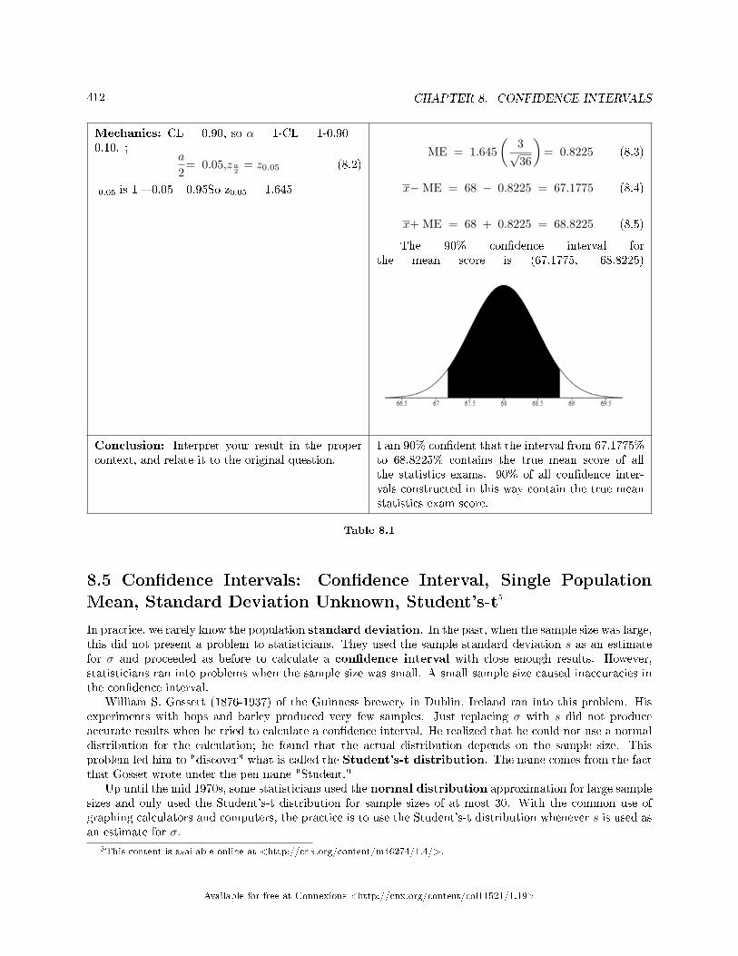
412 CHAPTER 8. CONFIDENCE INTERVALS
Mechanics: CL = 0.90, so α = 1-CL = 1-0.90 =0.10. ;
a
2= 0.05,z a
2= z0.05 (8.2)
0.05 is 1 � 0.05= 0.95So z0.05 = 1.645
ME = 1.645(
3√36
)= 0.8225 (8.3)
x− ME = 68 − 0.8225 = 67.1775 (8.4)
x+ ME = 68 + 0.8225 = 68.8225 (8.5)
The 90% con�dence interval forthe mean score is (67.1775, 68.8225)
Conclusion: Interpret your result in the propercontext, and relate it to the original question.
I am 90% con�dent that the interval from 67.1775%to 68.8225% contains the true mean score of allthe statistics exams. 90% of all con�dence inter-vals constructed in this way contain the true meanstatistics exam score.
Table 8.1
8.5 Con�dence Intervals: Con�dence Interval, Single PopulationMean, Standard Deviation Unknown, Student's-t5
In practice, we rarely know the population standard deviation. In the past, when the sample size was large,this did not present a problem to statisticians. They used the sample standard deviation s as an estimatefor σ and proceeded as before to calculate a con�dence interval with close enough results. However,statisticians ran into problems when the sample size was small. A small sample size caused inaccuracies inthe con�dence interval.
William S. Gossett (1876-1937) of the Guinness brewery in Dublin, Ireland ran into this problem. Hisexperiments with hops and barley produced very few samples. Just replacing σ with s did not produceaccurate results when he tried to calculate a con�dence interval. He realized that he could not use a normaldistribution for the calculation; he found that the actual distribution depends on the sample size. Thisproblem led him to "discover" what is called the Student's-t distribution. The name comes from the factthat Gosset wrote under the pen name "Student."
Up until the mid 1970s, some statisticians used the normal distribution approximation for large samplesizes and only used the Student's-t distribution for sample sizes of at most 30. With the common use ofgraphing calculators and computers, the practice is to use the Student's-t distribution whenever s is used asan estimate for σ.
5This content is available online at <http://cnx.org/content/m46274/1.4/>.
Available for free at Connexions <http://cnx.org/content/col11521/1.19>
413
If you draw a simple random sample of size n from a population that has approximately a normaldistribution with mean µ and unknown population standard deviation σ and calculate the t-score
t = x−µ“s√n
” ,
then the t-scores follow a Student's-t distribution with n− 1 degrees of freedom. The t-score hasthe same interpretation as the z-score. It measures how far x is from its mean µ. For each sample size n,there is a di�erent Student's-t distribution.
The degrees of freedom, n − 1, come from the calculation of the sample standard deviation s. InChapter 2, we used n deviations (x− x values) to calculate s. Because the sum of the deviations is 0, wecan �nd the last deviation once we know the other n− 1 deviations. The other n− 1 deviations can changeor vary freely. We call the number n− 1 the degrees of freedom (df).
Properties of the Student's-t Distribution
• The graph for the Student's-t distribution is similar to the Standard Normal curve.• The mean for the Student's-t distribution is 0 and the distribution is symmetric about 0.• The Student's-t distribution has more probability in its tails than the Standard Normal distribution
because the spread of the t distribution is greater than the spread of the Standard Normal. So thegraph of the Student's-t distribution will be thicker in the tails and shorter in the center than thegraph of the Standard Normal distribution.
• The exact shape of the Student's-t distribution depends on the "degrees of freedom". As the degreesof freedom increases, the graph Student's-t distribution becomes more like the graph of the StandardNormal distribution.
• The underlying population of individual observations is assumed to be normally distributed with un-known population mean µ and unknown population standard deviation σ. The size of the underlyingpopulation is generally not relevant unless it is very small. If it is bell shaped (normal) then theassumption is met and doesn't need discussion. Random sampling is assumed but it is a completelyseparate assumption from normality.
Calculators and computers can easily calculate any Student's-t probabilities. The TI-83,83+,84+ have a tcdffunction to �nd the probability for given values of t. The grammar for the tcdf command is tcdf(lower bound,upper bound, degrees of freedom). However for con�dence intervals, we need to use inverse probability to�nd the value of t when we know the probability.
A probability table for the Student's-t distribution can also be used. The table gives t-scores thatcorrespond to the con�dence level (column) and degrees of freedom (row). (The TI-86 does not have aninvT program or command, so if you are using that calculator, you need to use a probability table for theStudent's-t distribution.) When using t-table, note that some tables are formatted to show the con�dencelevel in the column headings, while the column headings in some tables may show only corresponding areain one or both tails.
Available for free at Connexions <http://cnx.org/content/col11521/1.19>
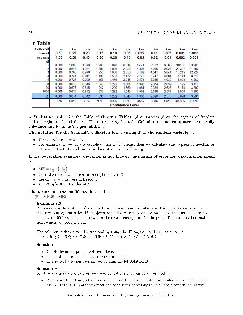
414 CHAPTER 8. CONFIDENCE INTERVALS
A Student's-t table (See the Table of Contents Tables) gives t-scores given the degrees of freedomand the right-tailed probability. The table is very limited. Calculators and computers can easilycalculate any Student's-t probabilities.
The notation for the Student's-t distribution is (using T as the random variable) is
• T ∼ tdf where df = n− 1.• For example, if we have a sample of size n=20 items, then we calculate the degrees of freedom as
df=n−1=20−1=19 and we write the distribution as T ∼ t19
If the population standard deviation is not known, the margin of error for a population meanis:
• ME = tα2·(
s√n
)• tα
2is the t-score with area to the right equal toα2
• use df = n− 1 degrees of freedom• s = sample standard deviation
The format for the con�dence interval is:(x−ME, x+ ME).
Example 8.5Suppose you do a study of acupuncture to determine how e�ective it is in relieving pain. Youmeasure sensory rates for 15 subjects with the results given below. Use the sample data toconstruct a 95% con�dence interval for the mean sensory rate for the population (assumed normal)from which you took the data.
The solution is shown step-by-step and by using the TI-83, 83+ and 84+ calculators.8.6; 9.4; 7.9; 6.8; 8.3; 7.3; 9.2; 9.6; 8.7; 11.4; 10.3; 5.4; 8.1; 5.5; 6.9
Solution
• Check the assumptions and conditions.• The �rst solution is step-by-step (Solution A).• The second solution uses an two column model(Solution B).
Solution AStart by discussing the assumptions and conditions that support you model.
• Randomization-The problem does not state that the sample was randomly selected. I willassume that it is in order to meet the conditions necessary to calculate a con�dence interval.
Available for free at Connexions <http://cnx.org/content/col11521/1.19>
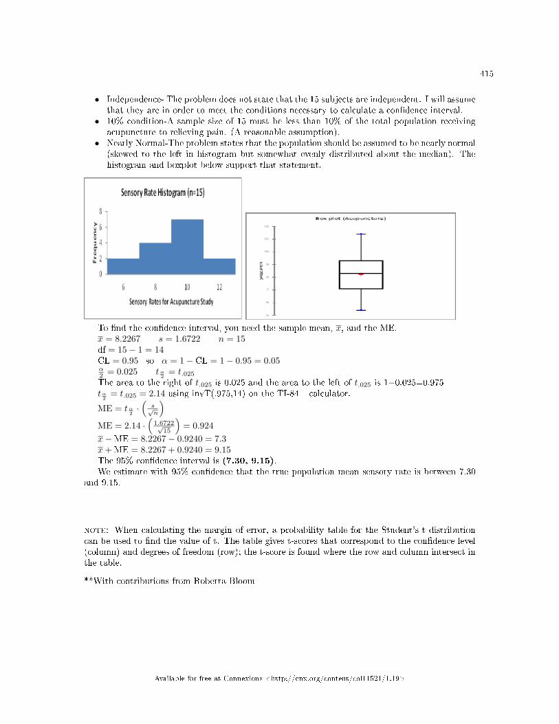
415
• Independence- The problem does not state that the 15 subjects are independent. I will assumethat they are in order to meet the conditions necessary to calculate a con�dence interval.
• 10% condition-A sample size of 15 must be less than 10% of the total population receivingacupuncture to relieving pain. (A reasonable assumption).
• Nearly Normal-The problem states that the population should be assumed to be nearly normal(skewed to the left in histogram but somewhat evenly distributed about the median). Thehistogram and boxplot below support that statement.
To �nd the con�dence interval, you need the sample mean, x, and the ME.x = 8.2267 s = 1.6722 n = 15df = 15− 1 = 14CL = 0.95 so α = 1− CL = 1− 0.95 = 0.05α2 = 0.025 tα
2= t.025
The area to the right of t.025 is 0.025 and the area to the left of t.025 is 1−0.025=0.975tα
2= t.025 = 2.14 using invT(.975,14) on the TI-84+ calculator.
ME = tα2·(
s√n
)ME = 2.14 ·
(1.6722√
15
)= 0.924
x−ME = 8.2267− 0.9240 = 7.3x+ ME = 8.2267 + 0.9240 = 9.15The 95% con�dence interval is (7.30, 9.15).We estimate with 95% con�dence that the true population mean sensory rate is between 7.30
and 9.15.
note: When calculating the margin of error, a probability table for the Student's-t distributioncan be used to �nd the value of t. The table gives t-scores that correspond to the con�dence level(column) and degrees of freedom (row); the t-score is found where the row and column intersect inthe table.
**With contributions from Roberta Bloom
Available for free at Connexions <http://cnx.org/content/col11521/1.19>
416 CHAPTER 8. CONFIDENCE INTERVALS
8.6 Con�dence Interval: Two Column Model Step by Step Exampleof a Con�dence Interval for a Mean, Sigma Unknown6
Step-By-Step Example of a Con�dence Interval for a Mean, sigma unknown (used Ex 8.7)Suppose you do a study of acupuncture to determine how e�ective it is in relieving pain. You measure
sensory rates for 15 random subjects with the results given below.8.6, 9.4, 7.9, 6.8, 8.3, 7.3, 9.2, 9.6, 8.7, 11.4, 10.3, 5.4, 8.1, 5.5, 6.9Use the sample data to construct a 95% con�dence interval for the mean sensory rate for the populations
(assumed normal) from which you took this data.
6This content is available online at <http://cnx.org/content/m46277/1.3/>.
Available for free at Connexions <http://cnx.org/content/col11521/1.19>
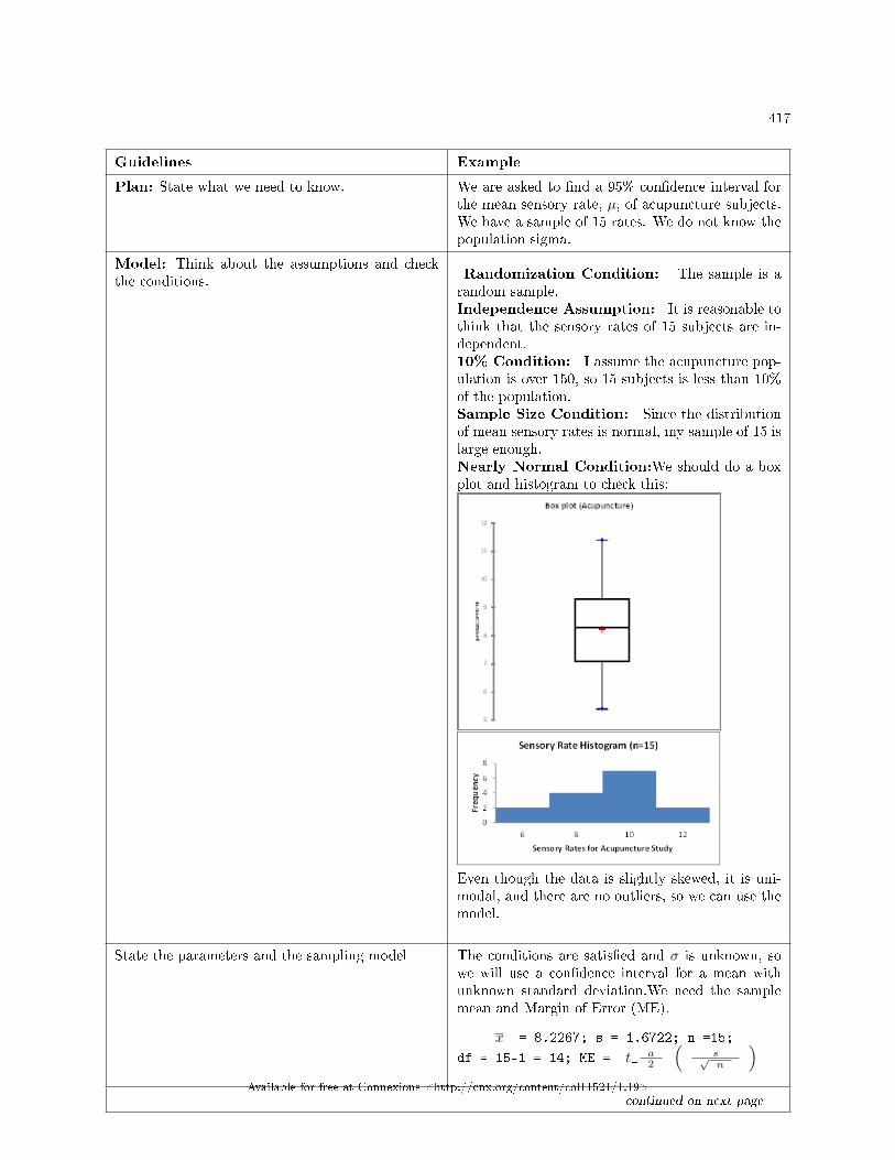
417
Guidelines Example
Plan: State what we need to know. We are asked to �nd a 95% con�dence interval forthe mean sensory rate, µ, of acupuncture subjects.We have a sample of 15 rates. We do not know thepopulation sigma.
Model: Think about the assumptions and checkthe conditions.
Randomization Condition: The sample is arandom sample.Independence Assumption: It is reasonable tothink that the sensory rates of 15 subjects are in-dependent.10% Condition: I assume the acupuncture pop-ulation is over 150, so 15 subjects is less than 10%of the population.Sample Size Condition: Since the distributionof mean sensory rates is normal, my sample of 15 islarge enough.Nearly Normal Condition:We should do a boxplot and histogram to check this:
Even though the data is slightly skewed, it is uni-modal, and there are no outliers, so we can use themodel.
State the parameters and the sampling model The conditions are satis�ed and σ is unknown, sowe will use a con�dence interval for a mean withunknown standard deviation.We need the samplemean and Margin of Error (ME).
x = 8.2267; s = 1.6722; n =15;
df = 15-1 = 14; ME = t_ a2
(s√n
)continued on next page
Available for free at Connexions <http://cnx.org/content/col11521/1.19>
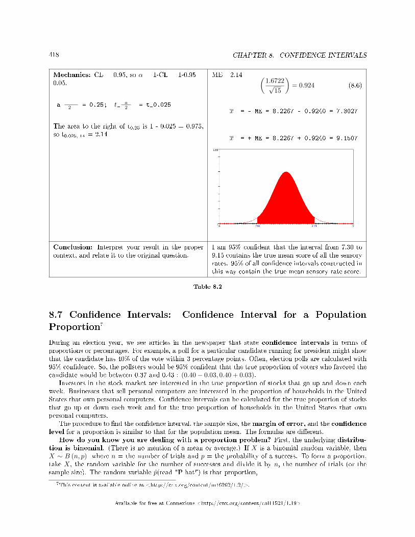
418 CHAPTER 8. CONFIDENCE INTERVALS
Mechanics: CL = 0.95, so α = 1-CL = 1-0.95 =0.05.
a 2 = 0.25; t_ a2 = t_0.025
The area to the right of t0.25 is 1 - 0.025 = 0.975,so t0.025, 14 = 2.14
ME =2.14 (1.6722√
15
)= 0.924 (8.6)
x = - ME = 8.2267 - 0.9240 = 7.3027
x = + ME = 8.2267 + 0.9240 = 9.1507
Conclusion: Interpret your result in the propercontext, and relate it to the original question.
I am 95% con�dent that the interval from 7.30 to9.15 contains the true mean score of all the sensoryrates. 95% of all con�dence intervals constructed inthis way contain the true mean sensory rate score.
Table 8.2
8.7 Con�dence Intervals: Con�dence Interval for a PopulationProportion7
During an election year, we see articles in the newspaper that state con�dence intervals in terms ofproportions or percentages. For example, a poll for a particular candidate running for president might showthat the candidate has 40% of the vote within 3 percentage points. Often, election polls are calculated with95% con�dence. So, the pollsters would be 95% con�dent that the true proportion of voters who favored thecandidate would be between 0.37 and 0.43 : (0.40− 0.03, 0.40 + 0.03).
Investors in the stock market are interested in the true proportion of stocks that go up and down eachweek. Businesses that sell personal computers are interested in the proportion of households in the UnitedStates that own personal computers. Con�dence intervals can be calculated for the true proportion of stocksthat go up or down each week and for the true proportion of households in the United States that ownpersonal computers.
The procedure to �nd the con�dence interval, the sample size, themargin of error, and the con�dencelevel for a proportion is similar to that for the population mean. The formulas are di�erent.
How do you know you are dealing with a proportion problem? First, the underlying distribu-tion is binomial. (There is no mention of a mean or average.) If X is a binomial random variable, thenX ∼ B (n, p) where n = the number of trials and p = the probability of a success. To form a proportion,take X, the random variable for the number of successes and divide it by n, the number of trials (or thesample size). The random variable p̂(read "P hat") is that proportion,
7This content is available online at <http://cnx.org/content/m46262/1.2/>.
Available for free at Connexions <http://cnx.org/content/col11521/1.19>
419
p̂ = Xn
(Sometimes the random variable is denoted as p', read "P prime".)When n is large and p is not close to 0 or 1, we can use the normal distribution to approximate the
binomial.X ∼ N
(n · p,√n · p · q
)If we divide the random variable by n, the mean by n, and the standard deviation by n, we get a normal
distribution of proportions with P̂ , called the estimated proportion, as the random variable. (Recall that aproportion = the number of successes divided by n.)
Xn = p̂ ∼ N
(n·pn ,√n·p·qn
)Using algebra to simplify :
√n·p·qn =
√p·qn
p̂ follows a normal distribution for proportions: p̂ ∼ N(p,√
p·qn
)The con�dence interval has the form (p̂−ME, p̂+ME).p̂ = x
np̂ = the estimated proportion of successes (p̂ is a point estimate for p, the true proportion)x = the number of successes.n = the size of the sampleThe margin of error for a proportion is
ME = zα2·√
p̂·q̂n whereq̂ = 1− p̂
This formula is similar to the margin of error formula for a mean, except that the "appropriate standarddeviation" is di�erent. For a mean, when the population standard deviation is known, the appropriate
standard deviation that we use is σ√n. For a proportion, the appropriate standard deviation is
√p·qn .
However, in the error bound formula, we use√
p̂·q̂n as the standard deviation, instead of
√p·qn
However, in the margin of error formula, the standard deviation is√
p̂·q̂n .
In the margin of error formula, the sample proportions p̂ and q̂ are estimates of the unknownpopulation proportions p and q. The estimated proportions p̂ and q̂ are used because p and q are notknown. p̂ and q̂ are calculated from the data. p̂ is the estimated proportion of successes. q̂ is the estimatedproportion of failures.
The con�dence interval can only be used if the number of successes np̂ and the number of failures nq̂ areboth larger than 10.
note: For the normal distribution of proportions, the z-score formula is as follows.
If p̂ ∼ N
(p̂√
p̂·q̂n
)then the z-score formula is z = p̂−p√
p̂·q̂n
Example 8.6Suppose that a market research �rm is hired to estimate the percent of adults living in a largecity who have cell phones. 500 randomly selected adult residents in this city are surveyed todetermine whether they have cell phones. Of the 500 people surveyed, 421 responded yes - theyown cell phones. Using a 95% con�dence level, compute a con�dence interval estimate for the trueproportion of adults residents of this city who have cell phones.
Solution
• Start by discussing the assumptions and conditions that support your model.• The solution is step-by-step.
SolutionAssumptions and Conditions:
Available for free at Connexions <http://cnx.org/content/col11521/1.19>
420 CHAPTER 8. CONFIDENCE INTERVALS
• Randomization � It is stated in the problem that the respondents were selected randomly.• independence � when a random sample is taken from the population independence is plausable.• 10% condition � the sample size of 500 is less than 10% all adult residents in the large city.• Success/ Failure � p̂n > 10(1− p̂) n > 10 0.842(500) = 241>10 and 1-0.842)(500)=79>10
where p̂ is the sample percentage and n is the sample size. Both products are larger than 10,so the success/ failure condition is met.
X = the number of people in the sample who have cell phones. X is binomial. X ∼ B(500, 421
500
).
To calculate the con�dence interval, you must �nd p̂, q̂, and ME.n = 500 x = the number of successes = 421p̂ = x
n = 421500 = 0.842
p̂ = 0.842 is the sample proportion; this is the point estimate of the population proportion.q̂ = 1− p̂ = 1− 0.842 = 0.158Since CL = 0.95, then α = 1− CL = 1− 0.95 = 0.05 α
2 = 0.025.Then zα
2= z.025 = 1.96
ME = zα2·√
p̂·q̂n = 1.96 ·
√(0.842)·(0.158)
500 = 0.032p̂−ME = 0.842− 0.032 = 0.81p̂+ ME = 0.842 + 0.032 = 0.874The con�dence interval for the true binomial population proportion is
(p̂−ME, p̂+ ME) =(0.810, 0.874).InterpretationWe estimate with 95% con�dence that between 81% and 87.4% of all adult residents of this cityhave cell phones.Explanation of 95% Con�dence Level95% of the con�dence intervals constructed in this way would contain the true value for thepopulation proportion of all adult residents of this city who have cell phones.
Example 8.7For a class project, a political science student at a large university wants to estimate the percentof students that are registered voters. He surveys 500 students and �nds that 300 are registeredvoters. Compute a 90% con�dence interval for the true percent of students that are registeredvoters and interpret the con�dence interval.
Solution
• Start by discussing the assumptions and conditions that support your model.• The solution is step-by-step.
Solution AAssumptions and Conditions:
• Randomization � no information is given in the problem about the sampling methodology.• independence � wsince we do not know how were respondents were chosen we do not know if
responses are independent.• 10% condition � the sample size of 500 is less than 10% all adult residents in the large city.
Available for free at Connexions <http://cnx.org/content/col11521/1.19>
421
• Success/ Failure � p̂n > 10(1− p̂) n > 10 0.60(500) = 300>10 and 1-0.60)(500)=200>10 wherep̂ is the sample percentage and n is the sample size. Both products are larger than 10, so thesuccess/ failure condition is met.(When assumptions and conditions are not met we note thatin our work, but continue on with the problem.)
Let X = the number of people in the sample who have cell phones. X is binomial. X ∼B(500, 421
500
).x = 300 and n = 500.
p̂ = xn = 300
500 = 0.600q̂ = 1− p̂ = 1− 0.600 = 0.400Since CL = 0.90, then α = 1− CL = 1− 0.90 = 0.10 α
2 = 0.05.zα
2= z.05 = 1.645
Use the the standard normal probability table to �nd z.05. Remember that the area to the rightof z.05 is 0.05 and the area to the left of z.05 is 0.95.
ME = zα2·√
p̂·q̂n = 1.645 ·
√(0.60)·(0.40)
500 = 0.036p̂−ME = 0.60− 0.036 = 0.564
p̂+ ME = 0.60 + 0.036 = 0.636The con�dence interval for the true binomial population proportion is
(p̂−ME, p̂+ ME) =(0.564, 0.636).Interpretation:
• We estimate with 90% con�dence that the true percent of all students that are registeredvoters is between 56.4% and 63.6%.
• Alternate Wording: We estimate with 90% con�dence that between 56.4% and 63.6% of ALLstudents are registered voters.
Explanation of 90% Con�dence Level90% of all con�dence intervals constructed in this way contain the true value for the populationpercent of students that are registered voters.
8.7.1 Calculating the Sample Size n
If researchers desire a speci�c margin of error, then they can use the error bound formula to calculate therequired sample size.
The error bound formula for a population proportion is
• ME = zα2·√
p̂q̂n
• Solving for n gives you an equation for the sample size.
• n =zα
22·p̂q̂
ME2
Example 8.8Suppose a mobile phone company wants to determine the current percentage of customers aged50+ that use text messaging on their cell phone. How many customers aged 50+ should thecompany survey in order to be 90% con�dent that the estimated (sample) proportion is within 3percentage points of the true population proportion of customers aged 50+ that use text messagingon their cell phone.
Available for free at Connexions <http://cnx.org/content/col11521/1.19>
422 CHAPTER 8. CONFIDENCE INTERVALS
SolutionFrom the problem, we know that ME=0.03 (3%=0.03) and
zα2
= z.05 = 1.645 because the con�dence level is 90%However, in order to �nd n , we need to know the estimated (sample) proportion p'. Remember
that q'=1-p'. But, we do not know p' yet. Since we multiply p' and q' together, we make themboth equal to 0.5 because p'q'= (.5)(.5)=.25 results in the largest possible product. (Try otherproducts: (.6)(.4)=.24; (.3)(.7)=.21; (.2)(.8)=.16 and so on). The largest possible product gives usthe largest n. This gives us a large enough sample so that we can be 90% con�dent that we arewithin 3 percentage points of the true population proportion. To calculate the sample size n, usethe formula and make the substitutions.
n = z2p̂q̂ME2 gives n = 1.6452(.5)(.5)
.032 =751.7Round the answer to the next higher value. The sample size should be 752 cell phone customers
aged 50+ in order to be 90% con�dent that the estimated (sample) proportion is within 3 percentagepoints of the true population proportion of all customers aged 50+ that use text messaging on theircell phone.
**With contributions from Roberta Bloom.
8.8 Con�dence Interval: Two Column Model Step by Step Exampleof a Con�dence Intervals for a Proportion8
Step-By-Step Example of a Con�dence Interval for a Proportion (used Ex 8.8)Suppose that a market research �rm is hired to estimate the percent of adults living in a large city who
have cell phones. 500 randomly selected adult residents in this city are surveyed to determine whether theyhave cell phones. Of the 500 people surveyed, 421 responded yes- they own cell phones.
Using a 95% con�dence level, compute a con�dence interval estimate for the true proportion of adultresidents of this city who have cell phones.
Guidelines Example
Plan: State what we need to know. We are asked to �nd a 95% con�dence interval forthe true proportion of city residents who have cellphones. We have a sample of 500 residents.
Model: Think about the assumptions and checkthe conditions.
Randomization Condition: The sample is arandom sample.Independence Assumption: It is reasonable tothink that the cell phone ownership of 500 residentsare independent.10% Condition: Since this is a large city thenumber of adult residents must be over 5000, so 500subjects is less than 10% of the population.Success/Failure Condition: np̂ = 500(0.842) =421 > 10; n(1 - p̂)= 500(0.158) = 79 > 10
continued on next page
8This content is available online at <http://cnx.org/content/m46278/1.2/>.
Available for free at Connexions <http://cnx.org/content/col11521/1.19>
423
State the parameters and the sampling model The conditions are satis�ed so I can use a Normalmodel to �nd a con�dence interval for a proportion.
n = 500; p̂ =421500
= 0.842 (8.7)
1 − p̂ = 1 − 0.842 = 0.158 (8.8)
Mechanics: CL = 0.95, so α = 1-CL = 1-0.95 =0.05.
a
2= 0.25;z a
2= z0.025 (8.9)
The area to the right of z0.25 is 1 � 0.025= 0.975Soz0.025, = 1.96
ME =z a2·√
p̂q̂n = 1.96 ·
√(0.842)·(0.158)
500 = 0.032
p̂− ME = 0.842 − 0.032 = 0.81 (8.10)
p̂+ ME = 0.842 + 0.032 = 0.874 (8.11)
The 95% con�dence interval for the binomial pop-ulation proportion is (0.810,0.874)
continued on next page
Available for free at Connexions <http://cnx.org/content/col11521/1.19>
424 CHAPTER 8. CONFIDENCE INTERVALS
Conclusion: Interpret your result in the propercontext, and relate it to the original question.
I am 95% con�dent that between 81% and 87.4% ofall adult residents of this city have cell phones.95%of all con�dence intervals constructed in this waycontain the true proportion of adults in this citywho have cell phones.
Table 8.3
8.9 Con�dence Intervals: Using Spreadsheets to Explore and DisplayCon�dence Intervals9
8.9.1 Con�dence Intervals using Spreadsheets
In this section we will discuss techniques using spreadsheet for creating con�dence intervals for a one popu-lation mean, population standard deviation known; a one population mean, population standard deviationunknown: and for a population proportion,
8.9.1.1 Con�dence Intervals Formulas
You can set up a worksheet in Excel to compute the con�dence interval be using one of the following formulasin Excel or Google Spreadsheet
Function Excel Formula Google Spreadsheet formula
Con�dence interval for one popu-lation mean, population standarddeviation known.
=con�dence.norm(alpha, stan-dard deviation, number insample)
=con�dence(alpha, standard de-viation, number in sample)
Con�dence interval for one popu-lation mean, population standarddeviation unknown.
=con�dence.t(alpha, standarddeviation, number in sample)
No built in formula
Con�dence interval for one popu-lation proportion.
There is no built in formula. .. we will calculate using modelbelow = p-hat±(critical value z-score*sqrt((p-hat*(1-p-hat)/n)
There is no built in formula. .. we will calculate using modelbelow = p-hat±(critical value z-score*sqrt((p-hat*(1-p-hat)/n)
Table 8.4
8.9.1.2 Displaying Con�dence Intervals:
To graph con�dence intervals the �Statistics Online Computational Resources (SOCR)� (just as in the pre-vious chapter) at http://socr.ucla.edu/htmls/SOCR_Distributions.html10 has in the dropdown menu forSOCR distribution the normal distribution and for a Student's t-distribution. For a normal distribution,you will need to have your mean and standard deviation and again your right and left cut o� values (whichin this case will be your critical values). For a Student's t-distribution, you will need to have degrees offreedom and again your right and left cut o� values (which in this case will be your critical values). Belowis a graph of the Student's t-distribution. We have used the example from 8.6 Two column Model step bystep example for this demonstration. The degrees of freedom were 14 and a 95% con�dence interval. We
9This content is available online at <http://cnx.org/content/m47496/1.1/>.10http://socr.ucla.edu/htmls/SOCR_Distributions.html
Available for free at Connexions <http://cnx.org/content/col11521/1.19>
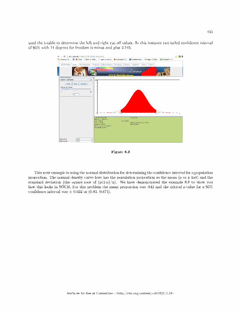
425
used the t-table to determine the left and right cut o� values. In this instance two tailed con�dence intervalof 95% with 14 degrees for freedom is minus and plus 2.145.
Figure 8.3
This next example is using the normal distribution for determining the con�dence interval for a populationproportion. The normal density curve here has the population proportion as the mean (p or p-hat) and thestandard deviation (the square root of (p(1-p)/n). We have demonstrated the example 8.8 to show youhow this looks in SOCR. For this problem the mean proportion was .842 and the critical z-value for a 95%con�dence interval was ± 0.032 or (0.81, 0.874).
Available for free at Connexions <http://cnx.org/content/col11521/1.19>
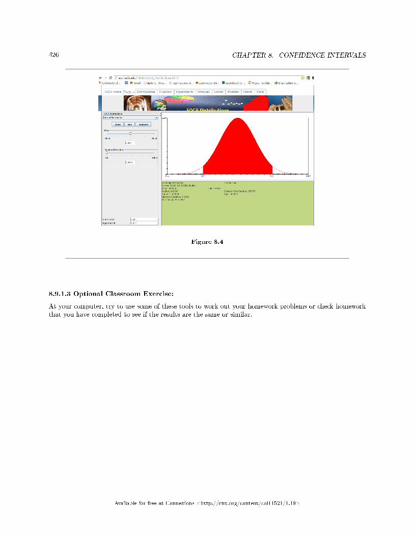
426 CHAPTER 8. CONFIDENCE INTERVALS
Figure 8.4
8.9.1.3 Optional Classroom Exercise:
At your computer, try to use some of these tools to work out your homework problems or check homeworkthat you have completed to see if the results are the same or similar.
Available for free at Connexions <http://cnx.org/content/col11521/1.19>
427
8.10 Con�dence Intervals: Summary of Formulas11
Formula 8.1: General form of a con�dence interval(lower value, upper value) = (point estimate−margin of error , point estimate + margin of error )Formula 8.2: To �nd the error bound when you know the con�dence intervalmargin of error = upper value − point estimate OR margin of error =
upper value−lower value2
Formula 8.3: Single Population Mean, Known Standard Deviation, Normal DistributionUse the Normal Distribution for Means (Section 7.3) ME = zα
2· σ√
n
The con�dence interval has the format (x−ME, x+ ME).Formula 8.4: Single Population Mean, Unknown Standard Deviation, Student's-t DistributionUse the Student's-t Distribution with degrees of freedom df = n− 1. ME = tα
2· s√
n
Formula 8.5: Single Population Proportion, Normal DistributionUse the Normal Distribution for a single population proportion p̂ = x
n
ME = zα2·√
p̂·q̂n p̂+ q̂ = 1
The con�dence interval has the format (p̂−ME, p̂+ ME).Formula 8.6: Point Estimatesx is a point estimate for µp̂ is a point estimate for ρs is a point estimate for σ
Formula 8.1: Critical Valuesz∗ is a critical value, based on the Normal Curve for an exact con�dence interval such as for a 95%con�dence interval. z∗ = 1.96
t∗ is a critical value, based on the Student's-t for an exact con�dence interval.
8.10.1 Glossary
Binomial DistributionA discrete random variable (RV) which arises from Bernoulli trials. There are a �xed number, n, of indepen-dent trials. �Independent� means that the result of any trial (for example, trial 1) does not a�ect the resultsof the following trials, and all trials are conducted under the same conditions. Under these circumstancesthe binomial RV X is de�ned as the number of successes in n trials. The notation is: X∼B (n, p). Themean is µ = np and the standard deviation is σ =
√npq. The probability of exactly x successes in n trials
is P (X = x) =(nx
)pxqn−x.
Con�dence Interval (CI)An interval estimate for an unknown population parameter. This depends on:(1). The desired con�dence level.(2). Information that is known about the distribution (for example, known standard deviation).(3). The sample and its size.Con�dence LevelThe percent expression for the probability that the con�dence interval contains the true population param-eter. For example, if the CL=90%, then in 90 out of 100 samples the interval estimate will enclose the truepopulation parameter.Degrees of Freedom (df)The number of objects in a sample that are free to vary.Margin of Error for a Population Mean (EBM)The margin of error. Depends on the con�dence level, sample size, and known or estimated populationstandard deviation.
11This content is available online at <http://cnx.org/content/m46275/1.4/>.
Available for free at Connexions <http://cnx.org/content/col11521/1.19>
428 CHAPTER 8. CONFIDENCE INTERVALS
Margin of Error for a Population Proportion (EBP)The margin of error. Depends on the con�dence level, sample size, and the estimated (from the sample)proportion of successes.Inferential StatisticsAlso called statistical inference or inductive statistics. This facet of statistics deals with estimating a pop-ulation parameter based on a sample statistic. For example, if 4 out of the 100 calculators sampled aredefective we might infer that 4 percent of the production is defectiveNormal DistributionA continuous random variable (RV) with pdf f(x) = 1
σ√
2πe−(x−µ)2/2σ2, where µ is the mean of the distri-
bution and σ is the standard deviation. Notation: X ∼ N (µ, σ). If µ = 0 and σ = 1, the RV is called thestandard normal distribution.ParameterA numerical characteristic of the population.Point EstimateA single number computed from a sample and used to estimate a population parameter.Student-t DistributionInvestigated and reported by William S. Gossett in 1908 and published under the pseudonym Student. Themajor characteristics of the random variable (RV) are:(1). It is continuous and assumes any real values.(2). The pdf is symmetrical about its mean of zero. However, it is more spread out and �atter at the apexthan the normal distribution.(3). It approaches the standard normal distribution as n gets larger.(4). There is a "family" of t distributions: every representative of the family is completely de�ned by thenumber of degrees of freedom which is one less than the number of dataStandard DeviationA number that is equal to the square root of the variance and measures how far data values are from theirmean. Notation: s for sample standard deviation and σ for population standard deviation.
Available for free at Connexions <http://cnx.org/content/col11521/1.19>
429
8.11 Con�dence Intervals: Practice 112
8.11.1 Student Learning Outcomes
• The student will calculate con�dence intervals for means when the population standard deviation isknown.
8.11.2 Given
The mean age for all Foothill College students for a recent Fall term was 33.2. The population standarddeviation has been pretty consistent at 15. Suppose that twenty-�ve Winter students were randomly selected.The mean age for the sample was 30.4. We are interested in the true mean age for Winter Foothill Collegestudents. (http://research.fhda.edu/factbook/FH_Demo_Trends/FoothillDemographicTrends.htm13
Let X = the age of a Winter Foothill College student
8.11.3 Calculating the Con�dence Interval
Exercise 8.11.1 (Solution on p. 454.)
x =Exercise 8.11.2 (Solution on p. 454.)
n=
Exercise 8.11.3 (Solution on p. 454.)
15=(insert symbol here)
Exercise 8.11.4 (Solution on p. 454.)
De�ne the Random Variable, X, in words.X =
Exercise 8.11.5 (Solution on p. 454.)
What is x estimating?
Exercise 8.11.6 (Solution on p. 454.)
Is σx known?
Exercise 8.11.7 (Solution on p. 454.)
As a result of your answer to (4), state the exact distribution to use when calculating the Con�denceInterval.
8.11.4 Explaining the Con�dence Interval
Construct a 95% Con�dence Interval for the true mean age of Winter Foothill College students.
Exercise 8.11.8 (Solution on p. 454.)
How much area is in both tails (combined)? α = ________
Exercise 8.11.9 (Solution on p. 454.)
How much area is in each tail? α2 = ________
Exercise 8.11.10 (Solution on p. 454.)
Identify the following speci�cations:
a. lower limit =b. upper limit =
12This content is available online at <http://cnx.org/content/m16970/1.13/>.13http://research.fhda.edu/factbook/FH_Demo_Trends/FoothillDemographicTrends.htm
Available for free at Connexions <http://cnx.org/content/col11521/1.19>
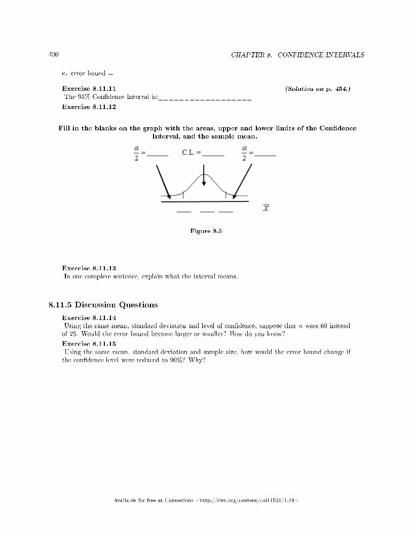
430 CHAPTER 8. CONFIDENCE INTERVALS
c. error bound =
Exercise 8.11.11 (Solution on p. 454.)
The 95% Con�dence Interval is:__________________
Exercise 8.11.12
Fill in the blanks on the graph with the areas, upper and lower limits of the Con�denceInterval, and the sample mean.
Figure 8.5
Exercise 8.11.13In one complete sentence, explain what the interval means.
8.11.5 Discussion Questions
Exercise 8.11.14Using the same mean, standard deviation and level of con�dence, suppose that n were 69 insteadof 25. Would the error bound become larger or smaller? How do you know?
Exercise 8.11.15Using the same mean, standard deviation and sample size, how would the error bound change ifthe con�dence level were reduced to 90%? Why?
Available for free at Connexions <http://cnx.org/content/col11521/1.19>
431
8.12 Con�dence Intervals: Practice 214
8.12.1 Student Learning Outcomes
• The student will calculate con�dence intervals for means when the population standard deviation isunknown.
8.12.2 Given
The following real data are the result of a random survey of 39 national �ags (with replacement betweenpicks) from various countries. We are interested in �nding a con�dence interval for the true mean numberof colors on a national �ag. Let X = the number of colors on a national �ag.
X Freq.
1 1
2 7
3 18
4 7
5 6
Table 8.5
8.12.3 Calculating the Con�dence Interval
Exercise 8.12.1 (Solution on p. 454.)
Calculate the following:
a. x =b. sx =c. n =
Exercise 8.12.2 (Solution on p. 454.)
De�ne the Random Variable, X, in words. X = __________________________
Exercise 8.12.3 (Solution on p. 454.)
What is x estimating?
Exercise 8.12.4 (Solution on p. 454.)
Is σx known?
Exercise 8.12.5 (Solution on p. 454.)
As a result of your answer to (4), state the exact distribution to use when calculating the Con�denceInterval.
14This content is available online at <http://cnx.org/content/m16971/1.14/>.
Available for free at Connexions <http://cnx.org/content/col11521/1.19>
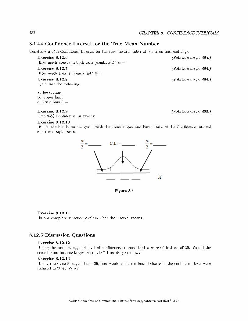
432 CHAPTER 8. CONFIDENCE INTERVALS
8.12.4 Con�dence Interval for the True Mean Number
Construct a 95% Con�dence Interval for the true mean number of colors on national �ags.
Exercise 8.12.6 (Solution on p. 454.)
How much area is in both tails (combined)? α =Exercise 8.12.7 (Solution on p. 454.)
How much area is in each tail? α2 =
Exercise 8.12.8 (Solution on p. 454.)
Calculate the following:
a. lower limit =b. upper limit =c. error bound =
Exercise 8.12.9 (Solution on p. 455.)
The 95% Con�dence Interval is:
Exercise 8.12.10Fill in the blanks on the graph with the areas, upper and lower limits of the Con�dence Intervaland the sample mean.
Figure 8.6
Exercise 8.12.11In one complete sentence, explain what the interval means.
8.12.5 Discussion Questions
Exercise 8.12.12Using the same x, sx, and level of con�dence, suppose that n were 69 instead of 39. Would theerror bound become larger or smaller? How do you know?
Exercise 8.12.13Using the same x, sx, and n = 39, how would the error bound change if the con�dence level werereduced to 90%? Why?
Available for free at Connexions <http://cnx.org/content/col11521/1.19>
433
8.13 Con�dence Intervals: Practice 315
8.13.1 Student Learning Outcomes
• The student will calculate con�dence intervals for proportions.
8.13.2 Given
The Ice Chalet o�ers dozens of di�erent beginning ice-skating classes. All of the class names are put into abucket. The 5 P.M., Monday night, ages 8 - 12, beginning ice-skating class was picked. In that class were 64girls and 16 boys. Suppose that we are interested in the true proportion of girls, ages 8 - 12, in all beginningice-skating classes at the Ice Chalet. Assume that the children in the selected class is a random sample ofthe population.
8.13.3 Estimated Distribution
Exercise 8.13.1What is being counted?
Exercise 8.13.2 (Solution on p. 455.)
In words, de�ne the Random Variable X. X =Exercise 8.13.3 (Solution on p. 455.)
Calculate the following:
a. x =b. n =
c.^p=
Exercise 8.13.4 (Solution on p. 455.)
State the estimated distribution of X. X ∼Exercise 8.13.5 (Solution on p. 455.)
De�ne a new Random Variable^p. What is
^p estimating?
Exercise 8.13.6 (Solution on p. 455.)
In words, de�ne the Random Variable p̂.
Exercise 8.13.7State the estimated distribution of p̂.
8.13.4 Explaining the Con�dence Interval
Construct a 92% Con�dence Interval for the true proportion of girls in the age 8 - 12 beginning ice-skatingclasses at the Ice Chalet.
Exercise 8.13.8 (Solution on p. 455.)
How much area is in both tails (combined)? α =Exercise 8.13.9 (Solution on p. 455.)
How much area is in each tail? α2 =
Exercise 8.13.10 (Solution on p. 455.)
Calculate the following:
15This content is available online at <http://cnx.org/content/m46732/1.2/>.
Available for free at Connexions <http://cnx.org/content/col11521/1.19>
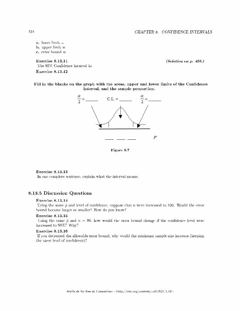
434 CHAPTER 8. CONFIDENCE INTERVALS
a. lower limit =b. upper limit =c. error bound =
Exercise 8.13.11 (Solution on p. 455.)
The 92% Con�dence Interval is:
Exercise 8.13.12
Fill in the blanks on the graph with the areas, upper and lower limits of the Con�denceInterval, and the sample proportion.
Figure 8.7
Exercise 8.13.13In one complete sentence, explain what the interval means.
8.13.5 Discussion Questions
Exercise 8.13.14Using the same p̂ and level of con�dence, suppose that n were increased to 100. Would the errorbound become larger or smaller? How do you know?
Exercise 8.13.15Using the same p̂ and n = 80, how would the error bound change if the con�dence level wereincreased to 98%? Why?
Exercise 8.13.16If you decreased the allowable error bound, why would the minimum sample size increase (keepingthe same level of con�dence)?
Available for free at Connexions <http://cnx.org/content/col11521/1.19>
435
8.14 Con�dence Intervals: Homework16
note: If you are using a student's-t distribution for a homework problem below, you may assumethat the underlying population is normally distributed. (In general, you must �rst prove thatassumption, though.)
Exercise 8.14.1 (Solution on p. 455.)
Among various ethnic groups, the standard deviation of heights is known to be approximately 3inches. We wish to construct a 95% con�dence interval for the mean height of male Swedes. 48male Swedes are surveyed. The sample mean is 71 inches. The sample standard deviation is 2.8inches.
a. i. x =________ii. σ = ________iii. sx =________iv. n =________v. n− 1 =________
b. De�ne the Random Variables X and X, in words.c. Which distribution should you use for this problem? Explain your choice.d. Construct a 95% con�dence interval for the population mean height of male Swedes.
i. State the con�dence interval.ii. Sketch the graph.iii. Calculate the margin of error.
e. What will happen to the level of con�dence obtained if 1000 male Swedes are surveyed insteadof 48? Why?
Exercise 8.14.2In six packages of �The Flintstones® Real Fruit Snacks� there were 5 Bam-Bam snack pieces. Thetotal number of snack pieces in the six bags was 68. We wish to calculate a 96% con�dence intervalfor the population proportion of Bam-Bam snack pieces.
a. De�ne the Random Variables X and p̂, in words.b. Which distribution should you use for this problem? Explain your choicec. Calculate p̂.d. Construct a 96% con�dence interval for the population proportion of Bam-Bam snack pieces
per bag.
i. State the con�dence interval.ii. Sketch the graph.iii. Calculate the margin of error.
e. Do you think that six packages of fruit snacks yield enough data to give accurate results? Whyor why not?
Exercise 8.14.3 (Solution on p. 455.)
A random survey of enrollment at 35 community colleges across the United States yielded thefollowing �gures (source: Microsoft Bookshelf ): 6414; 1550; 2109; 9350; 21828; 4300; 5944; 5722;2825; 2044; 5481; 5200; 5853; 2750; 10012; 6357; 27000; 9414; 7681; 3200; 17500; 9200; 7380; 18314;6557; 13713; 17768; 7493; 2771; 2861; 1263; 7285; 28165; 5080; 11622. Assume the underlyingpopulation is normal.
a. i. x =16This content is available online at <http://cnx.org/content/m46724/1.5/>.
Available for free at Connexions <http://cnx.org/content/col11521/1.19>
436 CHAPTER 8. CONFIDENCE INTERVALS
ii. sx = ________iii. n = ________iv. n− 1 =________
b. De�ne the Random Variables X and X, in words.c. Which distribution should you use for this problem? Explain your choice.d. Construct a 95% con�dence interval for the population mean enrollment at community colleges
in the United States.
i. State the con�dence interval.ii. Sketch the graph.iii. Calculate the margin of error.
e. What will happen to the margin of error and con�dence interval if 500 community colleges weresurveyed? Why?
Exercise 8.14.4From a stack of IEEE Spectrummagazines, announcements for 84 upcoming engineering conferenceswere randomly picked. The mean length of the conferences was 3.94 days, with a standard deviationof 1.28 days. Assume the underlying population is normal.
a. De�ne the Random Variables X and X, in words.b. Which distribution should you use for this problem? Explain your choice.c. Construct a 95% con�dence interval for the population mean length of engineering conferences.
i. State the con�dence interval.ii. Sketch the graph.iii. Calculate the m46730.
Exercise 8.14.5 (Solution on p. 456.)
Suppose that a committee is studying whether or not there is waste of time in our judicial system.It is interested in the mean amount of time individuals waste at the courthouse waiting to be calledfor service. The committee randomly surveyed 81 people. The sample mean was 8 hours with asample standard deviation of 4 hours.
a. i. x =________ii. sx = ________iii. n =________iv. n− 1 =________
b. De�ne the Random Variables X and X, in words.c. Which distribution should you use for this problem? Explain your choice.d. Construct a 95% con�dence interval for the population mean time wasted.
a. State the con�dence interval.b. Sketch the graph.c. Calculate the margin of error.
e. Explain in a complete sentence what the con�dence interval means.
Exercise 8.14.6Suppose that an accounting �rm does a study to determine the time needed to complete one person'stax forms. It randomly surveys 100 people. The sample mean is 23.6 hours. There is a knownstandard deviation of 7.0 hours. The population distribution is assumed to be normal.
a. i. x = ________ii. σ =________iii. sx =________
Available for free at Connexions <http://cnx.org/content/col11521/1.19>
437
iv. n = ________v. n− 1 =________
b. De�ne the Random Variables X and X, in words.c. Which distribution should you use for this problem? Explain your choice.d. Construct a 90% con�dence interval for the population mean time to complete the tax forms.
i. State the con�dence interval.ii. Sketch the graph.iii. Calculate the margin of error.
e. If the �rm wished to increase its level of con�dence and keep the margin of error the same bytaking another survey, what changes should it make?
f. If the �rm did another survey, kept the margin of error the same, and only surveyed 49 people,what would happen to the level of con�dence? Why?
g. Suppose that the �rm decided that it needed to be at least 96% con�dent of the populationmean length of time to within 1 hour. How would the number of people the �rm surveyschange? Why?
Exercise 8.14.7 (Solution on p. 456.)
A sample of 16 small bags of the same brand of candies was selected. Assume that the populationdistribution of bag weights is normal. The weight of each bag was then recorded. The mean weightwas 2 ounces with a standard deviation of 0.12 ounces. The population standard deviation is knownto be 0.1 ounce.
a. i. x = ________ii. σ = ________iii. sx =________iv. n = ________v. n− 1 = ________
b. De�ne the Random Variable X, in words.c. De�ne the Random Variable X, in words.d. Which distribution should you use for this problem? Explain your choice.e. Construct a 90% con�dence interval for the population mean weight of the candies.
i. State the con�dence interval.ii. Sketch the graph.iii. Calculate the margin of error.
f. Construct a 98% con�dence interval for the population mean weight of the candies.
i. State the con�dence interval.ii. Sketch the graph.iii. Calculate the margin of error.
g. In complete sentences, explain why the con�dence interval in (f) is larger than the con�denceinterval in (e).
h. In complete sentences, give an interpretation of what the interval in (f) means.
Exercise 8.14.8A pharmaceutical company makes tranquilizers. It is assumed that the distribution for the lengthof time they last is approximately normal. Researchers in a hospital used the drug on a randomsample of 9 patients. The e�ective period of the tranquilizer for each patient (in hours) was asfollows: 2.7; 2.8; 3.0; 2.3; 2.3; 2.2; 2.8; 2.1; and 2.4 .
a. i. x = ________ii. sx = ________
Available for free at Connexions <http://cnx.org/content/col11521/1.19>
438 CHAPTER 8. CONFIDENCE INTERVALS
iii. n = ________iv. n− 1 = ________
b. De�ne the Random Variable X, in words.c. De�ne the Random Variable X, in words.d. Which distribution should you use for this problem? Explain your choice.e. Construct a 95% con�dence interval for the population mean length of time.
i. State the con�dence interval.ii. Sketch the graph.iii. Calculate the margin of error.
f. What does it mean to be �95% con�dent� in this problem?
Exercise 8.14.9 (Solution on p. 456.)
Suppose that 14 children were surveyed to determine how long they had to use training wheels. Itwas revealed that they used them an average of 6 months with a sample standard deviation of 3months. Assume that the underlying population distribution is normal.
a. i. x = ________ii. sx = ________iii. n = ________iv. n− 1 = ________
b. De�ne the Random Variable X, in words.c. De�ne the Random Variable X, in words.d. Which distribution should you use for this problem? Explain your choice.e. Construct a 99% con�dence interval for the population mean length of time using training wheels.
i. State the con�dence interval.ii. Sketch the graph.iii. Calculate the margin of error.
f. Why would the margin of error change if the con�dence level was lowered to 90%?
Exercise 8.14.10 (Solution on p. 456.)
Suppose that the insurance companies did do a survey. They randomly surveyed 400 drivers andfound that 320 claimed to always buckle up. We are interested in the population proportion ofdrivers who claim to always buckle up.
a. i. x = ________ii. n = ________iii. p̂ = ________
b. De�ne the Random Variables X and p̂, in words.c. Which distribution should you use for this problem? Explain your choice.d. Construct a 95% con�dence interval for the population proportion that claim to always buckle
up.
i. State the con�dence interval.ii. Sketch the graph.iii. Calculate the margin of error.
e. If this survey were done by telephone, list 3 di�culties the companies might have in obtainingrandom results.
Exercise 8.14.11Unoccupied seats on �ights cause airlines to lose revenue. Suppose a large airline wants to estimateits mean number of unoccupied seats per �ight over the past year. To accomplish this, the recordsof 225 �ights are randomly selected and the number of unoccupied seats is noted for each of thesampled �ights. The sample mean is 11.6 seats and the sample standard deviation is 4.1 seats.
a. i. Available for free at Connexions <http://cnx.org/content/col11521/1.19>
439
x = ________ii. sx = ________iii. n = ________iv. n− 1 = ________
b. De�ne the Random Variables X and X, in words.c. Which distribution should you use for this problem? Explain your choice.d. Construct a 92% con�dence interval for the population mean number of unoccupied seats per
�ight.
i. State the con�dence interval.ii. Sketch the graph.iii. Calculate the margin of error.
Exercise 8.14.12 (Solution on p. 456.)
According to a recent survey of 1200 people, 61% feel that the president is doing an acceptablejob. We are interested in the population proportion of people who feel the president is doing anacceptable job.
a. De�ne the Random Variables X and p̂, in words.b. Which distribution should you use for this problem? Explain your choice.c. Construct a 90% con�dence interval for the population proportion of people who feel the presi-
dent is doing an acceptable job.
i. State the con�dence interval.ii. Sketch the graph.iii. Calculate the margin of error.
Exercise 8.14.13A survey of the mean amount of cents o� that coupons give was done by randomly surveying onecoupon per page from the coupon sections of a recent San Jose Mercury News. The following datawere collected: 20¢; 75¢; 50¢; 65¢; 30¢; 55¢; 40¢; 40¢; 30¢; 55¢; $1.50; 40¢; 65¢; 40¢. Assume theunderlying distribution is approximately normal.
a. i. x = ________ii. sx = ________iii. n = ________iv. n− 1 = ________
b. De�ne the Random Variables X and X, in words.c. Which distribution should you use for this problem? Explain your choice.d. Construct a 95% con�dence interval for the population mean worth of coupons.
i. State the con�dence interval.ii. Sketch the graph.iii. Calculate the margin of error.
e. If many random samples were taken of size 14, what percent of the con�dent intervals constructedshould contain the population mean worth of coupons? Explain why.
Exercise 8.14.14 (Solution on p. 457.)
An article regarding interracial dating and marriage recently appeared in the Washington Post. Ofthe 1709 randomly selected adults, 315 identi�ed themselves as Latinos, 323 identi�ed themselves asblacks, 254 identi�ed themselves as Asians, and 779 identi�ed themselves as whites. In this survey,86% of blacks said that their families would welcome a white person into their families. AmongAsians, 77% would welcome a white person into their families, 71% would welcome a Latino, and66% would welcome a black person.
Available for free at Connexions <http://cnx.org/content/col11521/1.19>
440 CHAPTER 8. CONFIDENCE INTERVALS
a. We are interested in �nding the 95% con�dence interval for the percent of all black families thatwould welcome a white person into their families. De�ne the Random Variables X and p̂, inwords.
b. Which distribution should you use for this problem? Explain your choice.c. Construct a 95% con�dence interval
i. State the con�dence interval.ii. Sketch the graph.iii. Calculate the margin of error.
Exercise 8.14.15Refer to the problem above.
a. Construct three 95% con�dence intervals.
i: Percent of all Asians that would welcome a white person into their families.ii: Percent of all Asians that would welcome a Latino into their families.iii: Percent of all Asians that would welcome a black person into their families.
b. Even though the three point estimates are di�erent, do any of the con�dence intervals overlap?Which?
c. For any intervals that do overlap, in words, what does this imply about the signi�cance of thedi�erences in the true proportions?
d. For any intervals that do not overlap, in words, what does this imply about the signi�cance ofthe di�erences in the true proportions?
Exercise 8.14.16 (Solution on p. 457.)
A camp director is interested in the mean number of letters each child sends during his/her campsession. The population standard deviation is known to be 2.5. A survey of 20 campers is taken.The mean from the sample is 7.9 with a sample standard deviation of 2.8.
a. i. x = ________ii. σ = ________iii. sx = ________iv. n = ________v. n− 1 = ________
b. De�ne the Random Variables X and X, in words.c. Which distribution should you use for this problem? Explain your choice.d. Construct a 90% con�dence interval for the population mean number of letters campers send
home.
i. State the con�dence interval.ii. Sketch the graph.iii. Calculate the margin of error.
e. What will happen to the margin of error and con�dence interval if 500 campers are surveyed?Why?
Exercise 8.14.17Stanford University conducted a study of whether running is healthy for men and women overage 50. During the �rst eight years of the study, 1.5% of the 451 members of the 50-Plus FitnessAssociation died. We are interested in the proportion of people over 50 who ran and died in thesame eight�year period.
a. De�ne the Random Variables X and p̂, in words.
Available for free at Connexions <http://cnx.org/content/col11521/1.19>
441
b. Which distribution should you use for this problem? Explain your choice.c. Construct a 97% con�dence interval for the population proportion of people over 50 who ran
and died in the same eight�year period.
i. State the con�dence interval.ii. Sketch the graph.iii. Calculate the margin of error.
d. Explain what a �97% con�dence interval� means for this study.
Exercise 8.14.18 (Solution on p. 457.)
In a recent sample of 84 used cars sales costs, the sample mean was $6425 with a standard deviationof $3156. Assume the underlying distribution is approximately normal.
a. Which distribution should you use for this problem? Explain your choice.b. De�ne the Random Variable X, in words.c. Construct a 95% con�dence interval for the population mean cost of a used car.
i. State the con�dence interval.ii. Sketch the graph.iii. Calculate the margin of error.
d. Explain what a �95% con�dence interval� means for this study.
Exercise 8.14.19A telephone poll of 1000 adult Americans was reported in an issue of Time Magazine. One of thequestions asked was �What is the main problem facing the country?� 20% answered �crime�. Weare interested in the population proportion of adult Americans who feel that crime is the mainproblem.
a. De�ne the Random Variables X and p̂, in words.b. Which distribution should you use for this problem? Explain your choice.c. Construct a 95% con�dence interval for the population proportion of adult Americans who feel
that crime is the main problem.
i. State the con�dence interval.ii. Sketch the graph.iii. Calculate the margin of error.
d. Suppose we want to lower the sampling error. What is one way to accomplish that?e. The sampling error given by Yankelovich Partners, Inc. (which conducted the poll) is ± 3%. In
1-3 complete sentences, explain what the ± 3% represents.
Exercise 8.14.20 (Solution on p. 457.)
Refer to the above problem. Another question in the poll was �[How much are] you worried aboutthe quality of education in our schools?� 63% responded �a lot�. We are interested in the populationproportion of adult Americans who are worried a lot about the quality of education in our schools.
1. De�ne the Random Variables X and p̂, in words.2. Which distribution should you use for this problem? Explain your choice.3. Construct a 95% con�dence interval for the population proportion of adult Americans worried
a lot about the quality of education in our schools.
i. State the con�dence interval.ii. Sketch the graph.iii. Calculate the margin of error.
Available for free at Connexions <http://cnx.org/content/col11521/1.19>
442 CHAPTER 8. CONFIDENCE INTERVALS
4. The sampling error given by Yankelovich Partners, Inc. (which conducted the poll) is ± 3%.In 1-3 complete sentences, explain what the ± 3% represents.
Exercise 8.14.21Six di�erent national brands of chocolate chip cookies were randomly selected at the supermarket.The grams of fat per serving are as follows: 8; 8; 10; 7; 9; 9. Assume the underlying distribution isapproximately normal.
a. Calculate a 90% con�dence interval for the population mean grams of fat per serving of chocolatechip cookies sold in supermarkets.
i. State the con�dence interval.ii. Sketch the graph.iii. Calculate the margin of error.
b. If you wanted a smaller margin of error while keeping the same level of con�dence, what shouldhave been changed in the study before it was done?
c. Go to the store and record the grams of fat per serving of six brands of chocolate chip cookies.d. Calculate the mean.e. Is the mean within the interval you calculated in part (a)? Did you expect it to be? Why or
why not?
Exercise 8.14.22A con�dence interval for a proportion is given to be (� 0.22, 0.34). Why doesn't the lower limit ofthe con�dence interval make practical sense? How should it be changed? Why?
8.14.1 Try these multiple choice questions.
The next three problems refer to the following: According to a Field Poll, 79% of California adults(actual results are 400 out of 506 surveyed) feel that �education and our schools� is one of the top is-sues facing California. We wish to construct a 90% con�dence interval for the true proportion of Cali-fornia adults who feel that education and the schools is one of the top issues facing California. (Source:http://�eld.com/�eldpollonline/subscribers/)
Exercise 8.14.23 (Solution on p. 457.)
A point estimate for the true population proportion is:
A. 0.90B. 1.27C. 0.79D. 400
Exercise 8.14.24 (Solution on p. 457.)
A 90% con�dence interval for the population proportion is:
A. (0.761, 0.820)B. (0.125, 0.188)C. (0.755, 0.826)D. (0.130, 0.183)
Exercise 8.14.25 (Solution on p. 457.)
The margin of error is approximately
A. 1.581
Available for free at Connexions <http://cnx.org/content/col11521/1.19>
443
B. 0.791C. 0.059D. 0.030
The next two problems refer to the following:A quality control specialist for a restaurant chain takes a random sample of size 12 to check the amount
of soda served in the 16 oz. serving size. The sample mean is 13.30 with a sample standard deviation of1.55. Assume the underlying population is normally distributed.
Exercise 8.14.26 (Solution on p. 457.)
Find the 95% Con�dence Interval for the true population mean for the amount of soda served.
A. (12.42, 14.18)B. (12.32, 14.29)C. (12.50, 14.10)D. Impossible to determine
Exercise 8.14.27 (Solution on p. 457.)
What is the margin of error?
A. 0.87B. 1.98C. 0.99D. 1.74
Exercise 8.14.28 (Solution on p. 457.)
What is meant by the term �90% con�dent� when constructing a con�dence interval for a mean?
A. If we took repeated samples, approximately 90% of the samples would produce the same con�-dence interval.
B. If we took repeated samples, approximately 90% of the con�dence intervals calculated fromthose samples would contain the sample mean.
C. If we took repeated samples, approximately 90% of the con�dence intervals calculated fromthose samples would contain the true value of the population mean.
D. If we took repeated samples, the sample mean would equal the population mean in approxi-mately 90% of the samples.
The next two problems refer to the following:Five hundred and eleven (511) homes in a certain southern California community are randomly surveyed
to determine if they meet minimal earthquake preparedness recommendations. One hundred seventy-three(173) of the homes surveyed met the minimum recommendations for earthquake preparedness and 338 didnot.
Exercise 8.14.29 (Solution on p. 457.)
Find the Con�dence Interval at the 90% Con�dence Level for the true population proportion ofsouthern California community homes meeting at least the minimum recommendations for earth-quake preparedness.
A. (0.2975, 0.3796)B. (0.6270, 6959)C. (0.3041, 0.3730)D. (0.6204, 0.7025)
Available for free at Connexions <http://cnx.org/content/col11521/1.19>

444 CHAPTER 8. CONFIDENCE INTERVALS
Exercise 8.14.30 (Solution on p. 457.)
The point estimate for the population proportion of homes that do not meet the minimum recom-mendations for earthquake preparedness is:
A. 0.6614B. 0.3386C. 173D. 338
Available for free at Connexions <http://cnx.org/content/col11521/1.19>
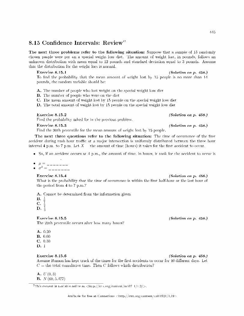
445
8.15 Con�dence Intervals: Review17
The next three problems refer to the following situation: Suppose that a sample of 15 randomlychosen people were put on a special weight loss diet. The amount of weight lost, in pounds, follows anunknown distribution with mean equal to 12 pounds and standard deviation equal to 3 pounds. Assumethat the distribution for the weight loss is normal.
Exercise 8.15.1 (Solution on p. 458.)
To �nd the probability that the mean amount of weight lost by 15 people is no more than 14pounds, the random variable should be:
A. The number of people who lost weight on the special weight loss dietB. The number of people who were on the dietC. The mean amount of weight lost by 15 people on the special weight loss dietD. The total amount of weight lost by 15 people on the special weight loss diet
Exercise 8.15.2 (Solution on p. 458.)
Find the probability asked for in the previous problem.
Exercise 8.15.3 (Solution on p. 458.)
Find the 90th percentile for the mean amount of weight lost by 15 people.
The next three questions refer to the following situation: The time of occurrence of the �rstaccident during rush-hour tra�c at a major intersection is uniformly distributed between the three hourinterval 4 p.m. to 7 p.m. Let X = the amount of time (hours) it takes for the �rst accident to occur.
• So, if an accident occurs at 4 p.m., the amount of time, in hours, it took for the accident to occur is_______.
• µ = _______• σ2 = _______
Exercise 8.15.4 (Solution on p. 458.)
What is the probability that the time of occurrence is within the �rst half-hour or the last hour ofthe period from 4 to 7 p.m.?
A. Cannot be determined from the information givenB. 1
6C. 1
2D. 1
3
Exercise 8.15.5 (Solution on p. 458.)
The 20th percentile occurs after how many hours?
A. 0.20B. 0.60C. 0.50D. 1
Exercise 8.15.6 (Solution on p. 458.)
Assume Ramon has kept track of the times for the �rst accidents to occur for 40 di�erent days. LetC = the total cumulative time. Then C follows which distribution?
A. U (0, 3)B. N (60, 5.477)
17This content is available online at <http://cnx.org/content/m46711/1.2/>.
Available for free at Connexions <http://cnx.org/content/col11521/1.19>
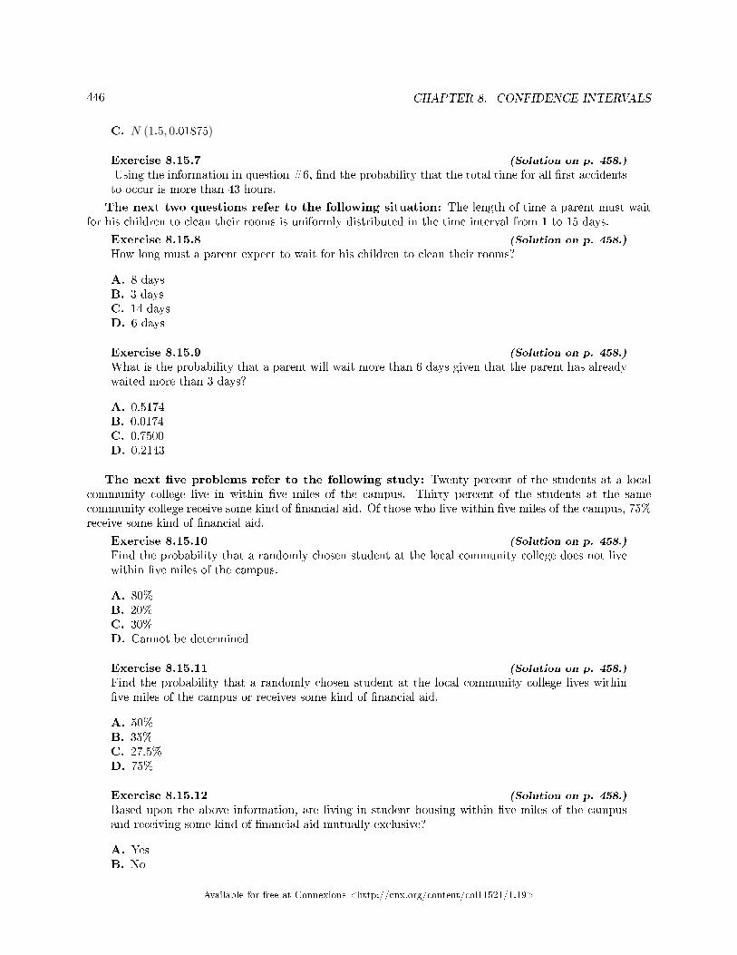
446 CHAPTER 8. CONFIDENCE INTERVALS
C. N (1.5, 0.01875)
Exercise 8.15.7 (Solution on p. 458.)
Using the information in question #6, �nd the probability that the total time for all �rst accidentsto occur is more than 43 hours.
The next two questions refer to the following situation: The length of time a parent must waitfor his children to clean their rooms is uniformly distributed in the time interval from 1 to 15 days.
Exercise 8.15.8 (Solution on p. 458.)
How long must a parent expect to wait for his children to clean their rooms?
A. 8 daysB. 3 daysC. 14 daysD. 6 days
Exercise 8.15.9 (Solution on p. 458.)
What is the probability that a parent will wait more than 6 days given that the parent has alreadywaited more than 3 days?
A. 0.5174B. 0.0174C. 0.7500D. 0.2143
The next �ve problems refer to the following study: Twenty percent of the students at a localcommunity college live in within �ve miles of the campus. Thirty percent of the students at the samecommunity college receive some kind of �nancial aid. Of those who live within �ve miles of the campus, 75%receive some kind of �nancial aid.
Exercise 8.15.10 (Solution on p. 458.)
Find the probability that a randomly chosen student at the local community college does not livewithin �ve miles of the campus.
A. 80%B. 20%C. 30%D. Cannot be determined
Exercise 8.15.11 (Solution on p. 458.)
Find the probability that a randomly chosen student at the local community college lives within�ve miles of the campus or receives some kind of �nancial aid.
A. 50%B. 35%C. 27.5%D. 75%
Exercise 8.15.12 (Solution on p. 458.)
Based upon the above information, are living in student housing within �ve miles of the campusand receiving some kind of �nancial aid mutually exclusive?
A. YesB. No
Available for free at Connexions <http://cnx.org/content/col11521/1.19>
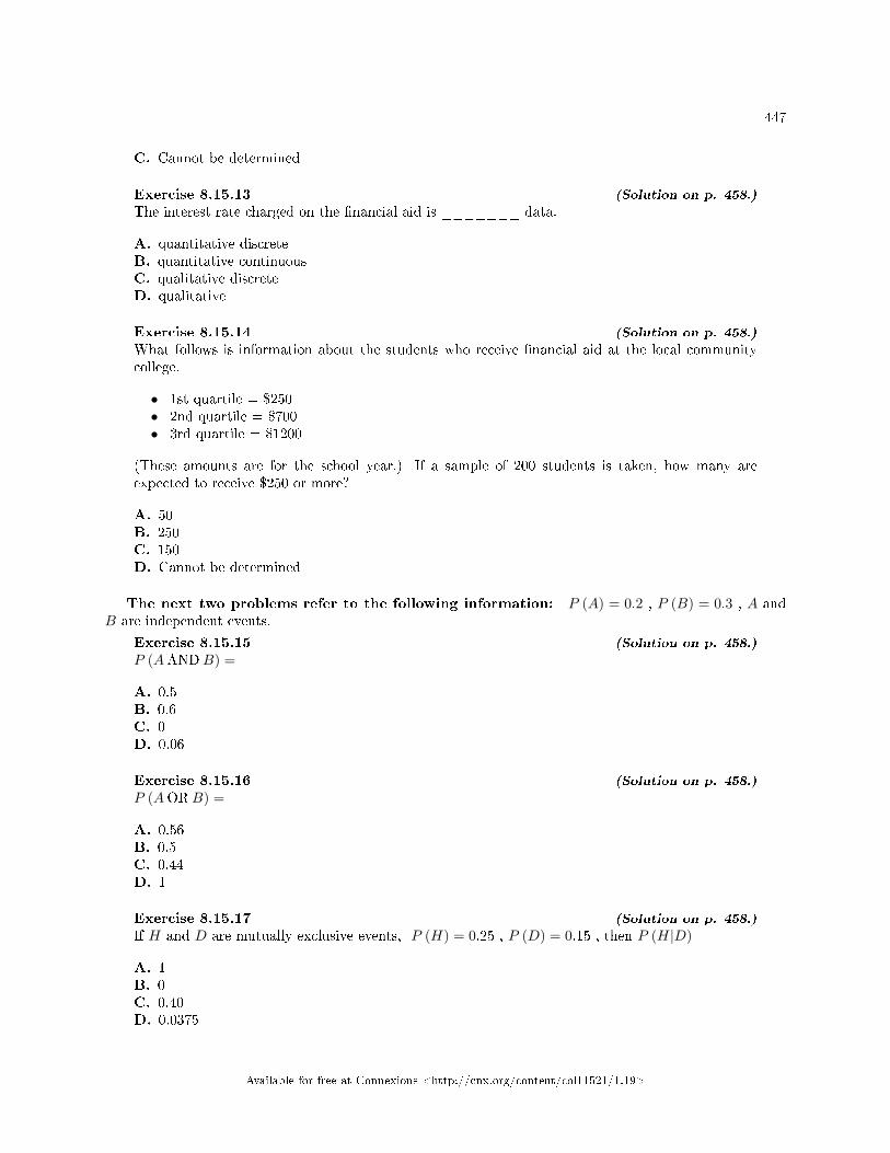
447
C. Cannot be determined
Exercise 8.15.13 (Solution on p. 458.)
The interest rate charged on the �nancial aid is _______ data.
A. quantitative discreteB. quantitative continuousC. qualitative discreteD. qualitative
Exercise 8.15.14 (Solution on p. 458.)
What follows is information about the students who receive �nancial aid at the local communitycollege.
• 1st quartile = $250• 2nd quartile = $700• 3rd quartile = $1200
(These amounts are for the school year.) If a sample of 200 students is taken, how many areexpected to receive $250 or more?
A. 50B. 250C. 150D. Cannot be determined
The next two problems refer to the following information: P (A) = 0.2 , P (B) = 0.3 , A andB are independent events.
Exercise 8.15.15 (Solution on p. 458.)
P (AANDB) =
A. 0.5B. 0.6C. 0D. 0.06
Exercise 8.15.16 (Solution on p. 458.)
P (AORB) =
A. 0.56B. 0.5C. 0.44D. 1
Exercise 8.15.17 (Solution on p. 458.)
If H and D are mutually exclusive events, P (H) = 0.25 , P (D) = 0.15 , then P (H|D)
A. 1B. 0C. 0.40D. 0.0375
Available for free at Connexions <http://cnx.org/content/col11521/1.19>
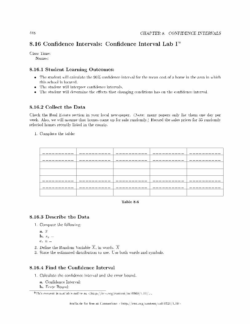
448 CHAPTER 8. CONFIDENCE INTERVALS
8.16 Con�dence Intervals: Con�dence Interval Lab I18
Class Time:Names:
8.16.1 Student Learning Outcomes:
• The student will calculate the 90% con�dence interval for the mean cost of a home in the area in whichthis school is located.
• The student will interpret con�dence intervals.• The student will determine the e�ects that changing conditions has on the con�dence interval.
8.16.2 Collect the Data
Check the Real Estate section in your local newspaper. (Note: many papers only list them one day perweek. Also, we will assume that homes come up for sale randomly.) Record the sales prices for 35 randomlyselected homes recently listed in the county.
1. Complete the table:
__________ __________ __________ __________ __________
__________ __________ __________ __________ __________
__________ __________ __________ __________ __________
__________ __________ __________ __________ __________
__________ __________ __________ __________ __________
__________ __________ __________ __________ __________
__________ __________ __________ __________ __________
Table 8.6
8.16.3 Describe the Data
1. Compute the following:
a. x =b. sx =c. n =
2. De�ne the Random Variable X, in words. X =3. State the estimated distribution to use. Use both words and symbols.
8.16.4 Find the Con�dence Interval
1. Calculate the con�dence interval and the error bound.
a. Con�dence Interval:b. Error Bound:
18This content is available online at <http://cnx.org/content/m16960/1.11/>.
Available for free at Connexions <http://cnx.org/content/col11521/1.19>
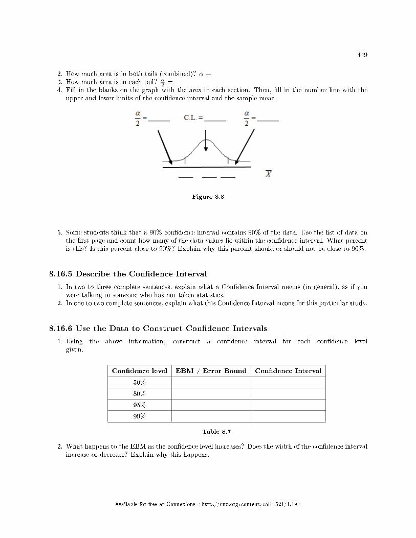
449
2. How much area is in both tails (combined)? α =3. How much area is in each tail? α
2 =4. Fill in the blanks on the graph with the area in each section. Then, �ll in the number line with the
upper and lower limits of the con�dence interval and the sample mean.
Figure 8.8
5. Some students think that a 90% con�dence interval contains 90% of the data. Use the list of data onthe �rst page and count how many of the data values lie within the con�dence interval. What percentis this? Is this percent close to 90%? Explain why this percent should or should not be close to 90%.
8.16.5 Describe the Con�dence Interval
1. In two to three complete sentences, explain what a Con�dence Interval means (in general), as if youwere talking to someone who has not taken statistics.
2. In one to two complete sentences, explain what this Con�dence Interval means for this particular study.
8.16.6 Use the Data to Construct Con�dence Intervals
1. Using the above information, construct a con�dence interval for each con�dence levelgiven.
Con�dence level EBM / Error Bound Con�dence Interval
50%
80%
95%
99%
Table 8.7
2. What happens to the EBM as the con�dence level increases? Does the width of the con�dence intervalincrease or decrease? Explain why this happens.
Available for free at Connexions <http://cnx.org/content/col11521/1.19>
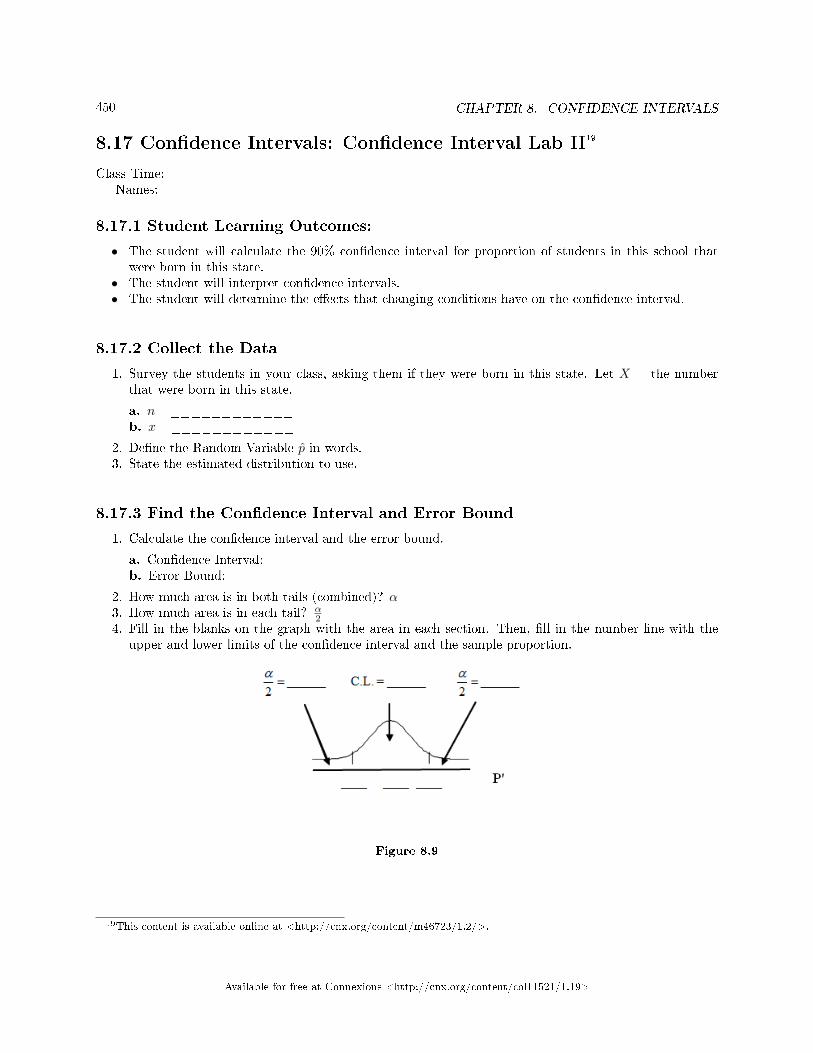
450 CHAPTER 8. CONFIDENCE INTERVALS
8.17 Con�dence Intervals: Con�dence Interval Lab II19
Class Time:Names:
8.17.1 Student Learning Outcomes:
• The student will calculate the 90% con�dence interval for proportion of students in this school thatwere born in this state.
• The student will interpret con�dence intervals.• The student will determine the e�ects that changing conditions have on the con�dence interval.
8.17.2 Collect the Data
1. Survey the students in your class, asking them if they were born in this state. Let X = the numberthat were born in this state.
a. n =____________b. x =____________
2. De�ne the Random Variable p̂ in words.3. State the estimated distribution to use.
8.17.3 Find the Con�dence Interval and Error Bound
1. Calculate the con�dence interval and the error bound.
a. Con�dence Interval:b. Error Bound:
2. How much area is in both tails (combined)? α=3. How much area is in each tail? α
2 =4. Fill in the blanks on the graph with the area in each section. Then, �ll in the number line with the
upper and lower limits of the con�dence interval and the sample proportion.
Figure 8.9
19This content is available online at <http://cnx.org/content/m46723/1.2/>.
Available for free at Connexions <http://cnx.org/content/col11521/1.19>
451
8.17.4 Describe the Con�dence Interval
1. In two to three complete sentences, explain what a Con�dence Interval means (in general), as if youwere talking to someone who has not taken statistics.
2. In one to two complete sentences, explain what this Con�dence Interval means for this particular study.3. Using the above information, construct a con�dence interval for each given con�dence level
given.
Con�dence level ME / Error Bound Con�dence Interval
50%
80%
95%
99%
Table 8.8
4. What happens to the ME as the con�dence level increases? Does the width of the con�dence intervalincrease or decrease? Explain why this happens.
Available for free at Connexions <http://cnx.org/content/col11521/1.19>
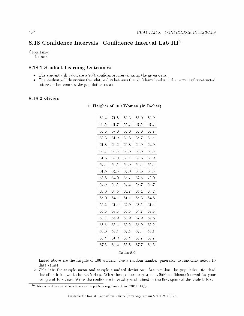
452 CHAPTER 8. CONFIDENCE INTERVALS
8.18 Con�dence Intervals: Con�dence Interval Lab III20
Class Time:Names:
8.18.1 Student Learning Outcomes:
• The student will calculate a 90% con�dence interval using the given data.• The student will determine the relationship between the con�dence level and the percent of constructed
intervals that contain the population mean.
8.18.2 Given:
1. Heights of 100 Women (in Inches)
59.4 71.6 69.3 65.0 62.9
66.5 61.7 55.2 67.5 67.2
63.8 62.9 63.0 63.9 68.7
65.5 61.9 69.6 58.7 63.4
61.8 60.6 69.8 60.0 64.9
66.1 66.8 60.6 65.6 63.8
61.3 59.2 64.1 59.3 64.9
62.4 63.5 60.9 63.3 66.3
61.5 64.3 62.9 60.6 63.8
58.8 64.9 65.7 62.5 70.9
62.9 63.1 62.2 58.7 64.7
66.0 60.5 64.7 65.4 60.2
65.0 64.1 61.1 65.3 64.6
59.2 61.4 62.0 63.5 61.4
65.5 62.3 65.5 64.7 58.8
66.1 64.9 66.9 57.9 69.8
58.5 63.4 69.2 65.9 62.2
60.0 58.1 62.5 62.4 59.1
66.4 61.2 60.4 58.7 66.7
67.5 63.2 56.6 67.7 62.5
Table 8.9
Listed above are the heights of 100 women. Use a random number generator to randomly select 10data values.
2. Calculate the sample mean and sample standard deviation. Assume that the population standarddeviation is known to be 3.3 inches. With these values, construct a 90% con�dence interval for yoursample of 10 values. Write the con�dence interval you obtained in the �rst space of the table below.
20This content is available online at <http://cnx.org/content/m16964/1.12/>.
Available for free at Connexions <http://cnx.org/content/col11521/1.19>
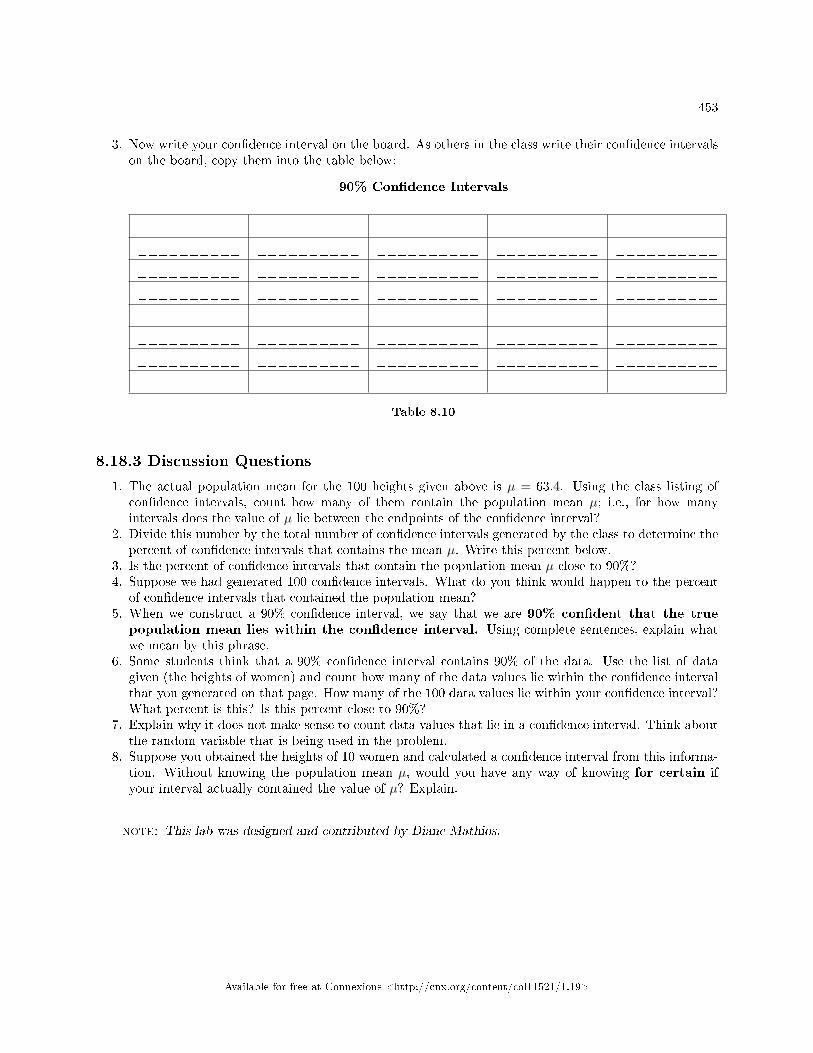
453
3. Now write your con�dence interval on the board. As others in the class write their con�dence intervalson the board, copy them into the table below:
90% Con�dence Intervals
__________ __________ __________ __________ __________
__________ __________ __________ __________ __________
__________ __________ __________ __________ __________
__________ __________ __________ __________ __________
__________ __________ __________ __________ __________
__________ __________ __________ __________ __________
__________ __________ __________ __________ __________
__________ __________ __________ __________ __________
Table 8.10
8.18.3 Discussion Questions
1. The actual population mean for the 100 heights given above is µ = 63.4. Using the class listing ofcon�dence intervals, count how many of them contain the population mean µ; i.e., for how manyintervals does the value of µ lie between the endpoints of the con�dence interval?
2. Divide this number by the total number of con�dence intervals generated by the class to determine thepercent of con�dence intervals that contains the mean µ. Write this percent below.
3. Is the percent of con�dence intervals that contain the population mean µ close to 90%?4. Suppose we had generated 100 con�dence intervals. What do you think would happen to the percent
of con�dence intervals that contained the population mean?5. When we construct a 90% con�dence interval, we say that we are 90% con�dent that the truepopulation mean lies within the con�dence interval. Using complete sentences, explain whatwe mean by this phrase.
6. Some students think that a 90% con�dence interval contains 90% of the data. Use the list of datagiven (the heights of women) and count how many of the data values lie within the con�dence intervalthat you generated on that page. How many of the 100 data values lie within your con�dence interval?What percent is this? Is this percent close to 90%?
7. Explain why it does not make sense to count data values that lie in a con�dence interval. Think aboutthe random variable that is being used in the problem.
8. Suppose you obtained the heights of 10 women and calculated a con�dence interval from this informa-tion. Without knowing the population mean µ, would you have any way of knowing for certain ifyour interval actually contained the value of µ? Explain.
note: This lab was designed and contributed by Diane Mathios.
Available for free at Connexions <http://cnx.org/content/col11521/1.19>
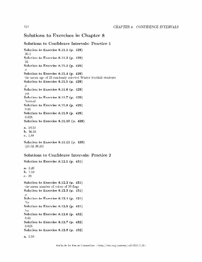
454 CHAPTER 8. CONFIDENCE INTERVALS
Solutions to Exercises in Chapter 8
Solutions to Con�dence Intervals: Practice 1
Solution to Exercise 8.11.1 (p. 429)30.4Solution to Exercise 8.11.2 (p. 429)25Solution to Exercise 8.11.3 (p. 429)σSolution to Exercise 8.11.4 (p. 429)the mean age of 25 randomly selected Winter Foothill studentsSolution to Exercise 8.11.5 (p. 429)µSolution to Exercise 8.11.6 (p. 429)yesSolution to Exercise 8.11.7 (p. 429)NormalSolution to Exercise 8.11.8 (p. 429)0.05Solution to Exercise 8.11.9 (p. 429)0.025Solution to Exercise 8.11.10 (p. 429)
a. 24.52b. 36.28c. 5.88
Solution to Exercise 8.11.11 (p. 430)(24.52, 36.28)
Solutions to Con�dence Intervals: Practice 2
Solution to Exercise 8.12.1 (p. 431)
a. 3.26b. 1.02c. 39
Solution to Exercise 8.12.2 (p. 431)the mean number of colors of 39 �agsSolution to Exercise 8.12.3 (p. 431)µSolution to Exercise 8.12.4 (p. 431)NoSolution to Exercise 8.12.5 (p. 431)t38Solution to Exercise 8.12.6 (p. 432)0.05Solution to Exercise 8.12.7 (p. 432)0.025Solution to Exercise 8.12.8 (p. 432)
a. 2.93
Available for free at Connexions <http://cnx.org/content/col11521/1.19>
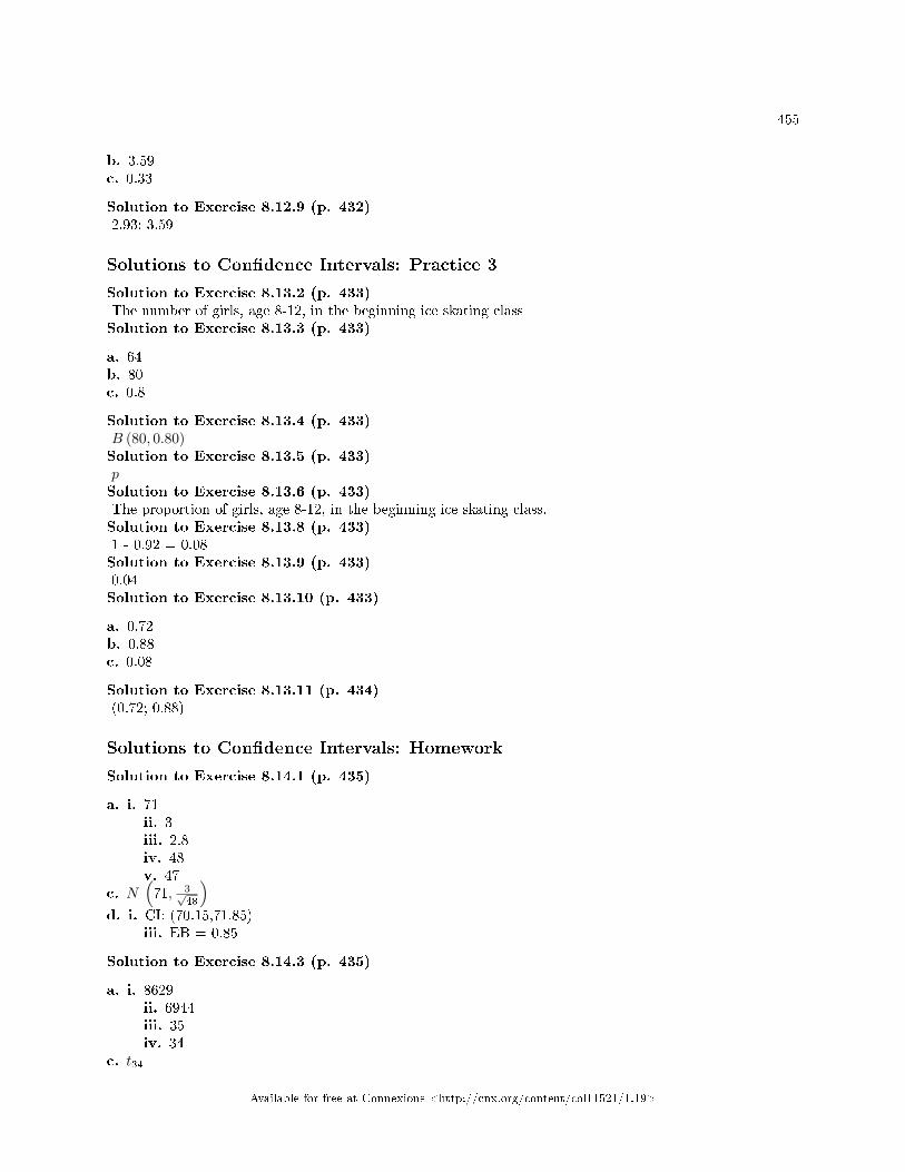
455
b. 3.59c. 0.33
Solution to Exercise 8.12.9 (p. 432)2.93; 3.59
Solutions to Con�dence Intervals: Practice 3
Solution to Exercise 8.13.2 (p. 433)The number of girls, age 8-12, in the beginning ice skating classSolution to Exercise 8.13.3 (p. 433)
a. 64b. 80c. 0.8
Solution to Exercise 8.13.4 (p. 433)B (80, 0.80)Solution to Exercise 8.13.5 (p. 433)pSolution to Exercise 8.13.6 (p. 433)The proportion of girls, age 8-12, in the beginning ice skating class.Solution to Exercise 8.13.8 (p. 433)1 - 0.92 = 0.08Solution to Exercise 8.13.9 (p. 433)0.04Solution to Exercise 8.13.10 (p. 433)
a. 0.72b. 0.88c. 0.08
Solution to Exercise 8.13.11 (p. 434)(0.72; 0.88)
Solutions to Con�dence Intervals: Homework
Solution to Exercise 8.14.1 (p. 435)
a. i. 71ii. 3iii. 2.8iv. 48v. 47
c. N(71, 3√
48
)d. i. CI: (70.15,71.85)
iii. EB = 0.85
Solution to Exercise 8.14.3 (p. 435)
a. i. 8629ii. 6944iii. 35iv. 34
c. t34
Available for free at Connexions <http://cnx.org/content/col11521/1.19>
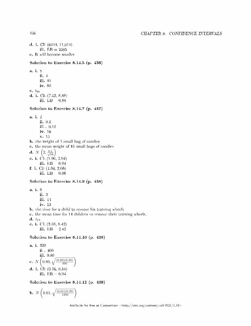
456 CHAPTER 8. CONFIDENCE INTERVALS
d. i. CI: (6244, 11,014)iii. EB = 2385
e. It will become smaller
Solution to Exercise 8.14.5 (p. 436)
a. i. 8ii. 4iii. 81iv. 80
c. t80d. i. CI: (7.12, 8.88)
iii. EB = 0.88
Solution to Exercise 8.14.7 (p. 437)
a. i. 2ii. 0.1iii . 0.12iv. 16v. 15
b. the weight of 1 small bag of candiesc. the mean weight of 16 small bags of candies
d. N(
2, 0.1√16
)e. i. CI: (1.96, 2.04)
iii. EB = 0.04f. i. CI: (1.94, 2.06)
iii. EB = 0.06
Solution to Exercise 8.14.9 (p. 438)
a. i. 6ii. 3iii. 14iv. 13
b. the time for a child to remove his training wheelsc. the mean time for 14 children to remove their training wheels.d. t13e. i. CI: (3.58, 8.42)
iii. EB = 2.42
Solution to Exercise 8.14.10 (p. 438)
a. i. 320ii . 400iii. 0.80
c. N
(0.80,
√(0.80)(0.20)
400
)d. i. CI: (0.76, 0.84)
iii. EB = 0.04
Solution to Exercise 8.14.12 (p. 439)
b. N
(0.61,
√(0.61)(0.39)
1200
)Available for free at Connexions <http://cnx.org/content/col11521/1.19>
457
c. i. CI: (0.59, 0.63)iii. EB = 0.02
Solution to Exercise 8.14.14 (p. 439)
b. N
(0.86,
√(0.86)(0.14)
323
)c. i. CI: (0.823, 0.898)
iii. EB = 0.038
Solution to Exercise 8.14.16 (p. 440)
a. i. 7.9ii. 2.5iii. 2.8iv. 20v. 19
c. N(
7.9, 2.5√20
)d. i. CI: (6.98, 8.82)
iii. EB: 0.92
Solution to Exercise 8.14.18 (p. 441)
a. t83b. mean cost of 84 used carsc. i. CI: (5740.10, 7109.90)
iii. EB = 684.90
Solution to Exercise 8.14.20 (p. 441)
b. N
(0.63,
√(0.63)(0.37)
1000
)c. i. CI: (0.60, 0.66)
iii. EB = 0.03
Solution to Exercise 8.14.23 (p. 442)CSolution to Exercise 8.14.24 (p. 442)ASolution to Exercise 8.14.25 (p. 442)DSolution to Exercise 8.14.26 (p. 443)BSolution to Exercise 8.14.27 (p. 443)CSolution to Exercise 8.14.28 (p. 443)CSolution to Exercise 8.14.29 (p. 443)CSolution to Exercise 8.14.30 (p. 444)A
Available for free at Connexions <http://cnx.org/content/col11521/1.19>
458 CHAPTER 8. CONFIDENCE INTERVALS
Solutions to Con�dence Intervals: Review
Solution to Exercise 8.15.1 (p. 445)CSolution to Exercise 8.15.2 (p. 445)0.9951Solution to Exercise 8.15.3 (p. 445)12.99Solution to Exercise 8.15.4 (p. 445)CSolution to Exercise 8.15.5 (p. 445)BSolution to Exercise 8.15.6 (p. 445)CSolution to Exercise 8.15.7 (p. 446)0.9990Solution to Exercise 8.15.8 (p. 446)ASolution to Exercise 8.15.9 (p. 446)CSolution to Exercise 8.15.10 (p. 446)ASolution to Exercise 8.15.11 (p. 446)BSolution to Exercise 8.15.12 (p. 446)BSolution to Exercise 8.15.13 (p. 447)BSolution to Exercise 8.15.14 (p. 447)
C. 150
Solution to Exercise 8.15.15 (p. 447)DSolution to Exercise 8.15.16 (p. 447)CSolution to Exercise 8.15.17 (p. 447)B
Available for free at Connexions <http://cnx.org/content/col11521/1.19>
Chapter 9
Hypothesis Testing: Single Mean, Single
Proportion
9.1 Hypothesis Testing of Single Mean and Single Proportion:Introduction1
9.1.1 Student Learning Outcomes
By the end of this chapter, the student should be able to:
• Di�erentiate between Type I and Type II Errors• Describe hypothesis testing in general and in practice• Conduct and interpret hypothesis tests for a single population mean, population standard deviation
known.• Conduct and interpret hypothesis tests for a single population mean, population standard deviation
unknown.• Conduct and interpret hypothesis tests for a single population proportion.
9.1.2 Introduction
One job of a statistician is to make statistical inferences about populations based on samples taken from thepopulation. Con�dence intervals are one way to estimate a population parameter. Another way to makea statistical inference is to make a decision about a parameter. For instance, a car dealer advertises thatits new small truck gets 35 miles per gallon, on the average. A tutoring service claims that its method oftutoring helps 90% of its students get an A or a B. A company says that women managers in their companyearn an average of $60,000 per year.
A statistician will make a decision about these claims. This process is called "hypothesis testing." Ahypothesis test involves collecting data from a sample and evaluating the data. Then, the statistician makesa decision as to whether or not there is su�cient evidence based upon analyses of the data, to reject the nullhypothesis.
In this chapter, you will conduct hypothesis tests on single means and single proportions. You will alsolearn about the errors associated with these tests.
Hypothesis testing consists of two contradictory hypotheses or statements, a decision based on the data,and a conclusion. To perform a hypothesis test, a statistician will:
1This content is available online at <http://cnx.org/content/m16997/1.11/>.
Available for free at Connexions <http://cnx.org/content/col11521/1.19>
459
460CHAPTER 9. HYPOTHESIS TESTING: SINGLE MEAN, SINGLE
PROPORTION
1. Set up two contradictory hypotheses.2. Collect sample data (in homework problems, the data or summary statistics will be given to you).3. Determine the correct distribution to perform the hypothesis test.4. Analyze sample data by performing the calculations that ultimately will allow you to reject or fail to
reject the null hypothesis.5. Make a decision and write a meaningful conclusion.
note: To do the hypothesis test homework problems for this chapter and later chapters, makecopies of the appropriate special solution sheets. See the Table of Contents topic "Solution Sheets".
9.2 Hypothesis Testing of Single Mean and Single Proportion: Nulland Alternate Hypotheses2
The actual test begins by considering two hypotheses. They are called the null hypothesis and thealternate hypothesis. These hypotheses contain opposing viewpoints.
Ho: The null hypothesis: It is a statement about the population that will be assumed to be trueunless it can be shown to be incorrect beyond a reasonable doubt.
Ha: The alternate hypothesis: It is a claim about the population that is contradictory to Ho andwhat we conclude when we reject Ho.
Example 9.1Ho: No more than 30% of the registered voters in Santa Clara County voted in the primary election.
Ha: More than 30% of the registered voters in Santa Clara County voted in the primary election.This null and alternative written in notation would look like, Ho:p = 30% and Ha:p > 30%
The 30% in this hypothesis is the called the hypothesized value and its symbol is po , pronounced p-naught. If the data is categorical like it is in this example the general notation of the null hypothesiswill be, Ha:p = po. There are three possibilities for the alternative hypothesis, Ha:p 6= po, or Ha:p> poor Ha:p < po You will need to read the problem carefully looking for key language to decidewhich alternative is appropriate for the problem. Hint: To determine the alternative hypothesislook for what the researcher wants to prove true. This is usually found in a question within thestory. Also, look for key language. The use of di�ers, change, or not the same would indicate thatthe alternative hypothesis is not equal to the hypothesized value. Language such as more than,bigger than, and increasing would tell us that a greater than symbol will be used in the alternative.Likewise, the use of less than, smaller, or decreasing would indicate using a less than symbol in thealternative hypothesis. When working with numerical data the hypothesize value is µo , pronouncedmu-naught. The general from of the null hypothesis will be, Ho: µ = µo with the three possiblealternatives Ha: µ 6= µo or Ha: µ > µo or Ha: µ < µo .
Example 9.2We want to test whether the mean grade point average in American colleges is di�erent from 2.0(out of 4.0).
Ho: µ = 2.0 Ha: µ 6= 2.0
Example 9.3We want to test if college students take less than �ve years to graduate from college, on the average.
Ho: µ = 5 Ha: µ < 5
Example 9.4Walking to class Sam notices many students listening to music with headphones or ear buds. Shewonders if more than half the students on campus listen to music while walking on campus.
2This content is available online at <http://cnx.org/content/m46712/1.3/>.
Available for free at Connexions <http://cnx.org/content/col11521/1.19>
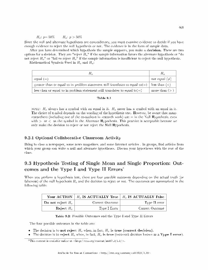
461
Ho: p= 50% Ha: p > 50%Since the null and alternate hypotheses are contradictory, you must examine evidence to decide if you haveenough evidence to reject the null hypothesis or not. The evidence is in the form of sample data.
After you have determined which hypothesis the sample supports, you make a decision. There are twooptions for a decision. They are "reject Ho" if the sample information favors the alternate hypothesis or "donot reject Ho" or "fail to reject Ho" if the sample information is insu�cient to reject the null hypothesis.
Mathematical Symbols Used in Ho and Ha:
Ho Ha
equal (=) not equal ( 6=)
greater than or equal to in problem statement still translates to equal to(=) less than (<)
less than or equal to in problem statement still translates to equal to(=) more than (> )
Table 9.1
note: Ho always has a symbol with an equal in it. Ha never has a symbol with an equal in it.The choice of symbol depends on the wording of the hypothesis test. However, be aware that manyresearchers (including one of the co-authors in research work) use = in the Null Hypothesis, evenwith > or < as the symbol in the Alternate Hypothesis. This practice is acceptable because weonly make the decision to reject or not reject the Null Hypothesis.
9.2.1 Optional Collaborative Classroom Activity
Bring to class a newspaper, some news magazines, and some Internet articles . In groups, �nd articles fromwhich your group can write a null and alternate hypotheses. Discuss your hypotheses with the rest of theclass.
9.3 Hypothesis Testing of Single Mean and Single Proportion: Out-comes and the Type I and Type II Errors3
When you perform a hypothesis test, there are four possible outcomes depending on the actual truth (orfalseness) of the null hypothesis Ho and the decision to reject or not. The outcomes are summarized in thefollowing table:
Your ACTION Ho IS ACTUALLY True Ho IS ACTUALLY False
Do not reject Ho Correct Outcome Type II error
Reject Ho Type I Error Correct Outcome
Table 9.2: Possible Outcomes and the Type I and Type II Errors
The four possible outcomes in the table are:
• The decision is to not reject Ho when, in fact, Ho is true (correct decision).• The decision is to reject Ho when, in fact, Ho is true (incorrect decision known as a Type I error).
3This content is available online at <http://cnx.org/content/m46713/1.1/>.
Available for free at Connexions <http://cnx.org/content/col11521/1.19>
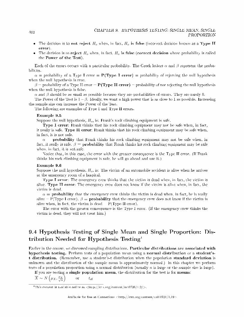
462CHAPTER 9. HYPOTHESIS TESTING: SINGLE MEAN, SINGLE
PROPORTION
• The decision is to not reject Ho when, in fact, Ho is false (incorrect decision known as a Type IIerror).
• The decision is to reject Ho when, in fact, Ho is false (correct decision whose probability is calledthe Power of the Test).
Each of the errors occurs with a particular probability. The Greek letters α and β represent the proba-bilities.
α = probability of a Type I error = P(Type I error) = probability of rejecting the null hypothesiswhen the null hypothesis is true.
β = probability of a Type II error = P(Type II error) = probability of not rejecting the null hypothesiswhen the null hypothesis is false.
α and β should be as small as possible because they are probabilities of errors. They are rarely 0.The Power of the Test is 1−β. Ideally, we want a high power that is as close to 1 as possible. Increasing
the sample size can increase the Power of the Test.The following are examples of Type I and Type II errors.
Example 9.5Suppose the null hypothesis, Ho, is: Frank's rock climbing equipment is safe.
Type I error: Frank thinks that his rock climbing equipment may not be safe when, in fact,it really is safe. Type II error: Frank thinks that his rock climbing equipment may be safe when,in fact, it is not safe.
α = probability that Frank thinks his rock climbing equipment may not be safe when, infact, it really is safe. β = probability that Frank thinks his rock climbing equipment may be safewhen, in fact, it is not safe.
Notice that, in this case, the error with the greater consequence is the Type II error. (If Frankthinks his rock climbing equipment is safe, he will go ahead and use it.)
Example 9.6Suppose the null hypothesis, Ho, is: The victim of an automobile accident is alive when he arrivesat the emergency room of a hospital.
Type I error: The emergency crew thinks that the victim is dead when, in fact, the victim isalive. Type II error: The emergency crew does not know if the victim is alive when, in fact, thevictim is dead.
α = probability that the emergency crew thinks the victim is dead when, in fact, he is reallyalive = P(Type I error). β = probability that the emergency crew does not know if the victim isalive when, in fact, the victim is dead = P(Type II error).
The error with the greater consequence is the Type I error. (If the emergency crew thinks thevictim is dead, they will not treat him.)
9.4 Hypothesis Testing of Single Mean and Single Proportion: Dis-tribution Needed for Hypothesis Testing4
Earlier in the course, we discussed sampling distributions. Particular distributions are associated withhypothesis testing. Perform tests of a population mean using a normal distribution or a student's-t distribution. (Remember, use a student's-t distribution when the population standard deviation isunknown and the distribution of the sample mean is approximately normal.) In this chapter we performtests of a population proportion using a normal distribution (usually n is large or the sample size is large).
If you are testing a single population mean, the distribution for the test is for means:
X ∼ N(µX ,
σX√n
)or tdf
4This content is available online at <http://cnx.org/content/m46726/1.2/>.
Available for free at Connexions <http://cnx.org/content/col11521/1.19>
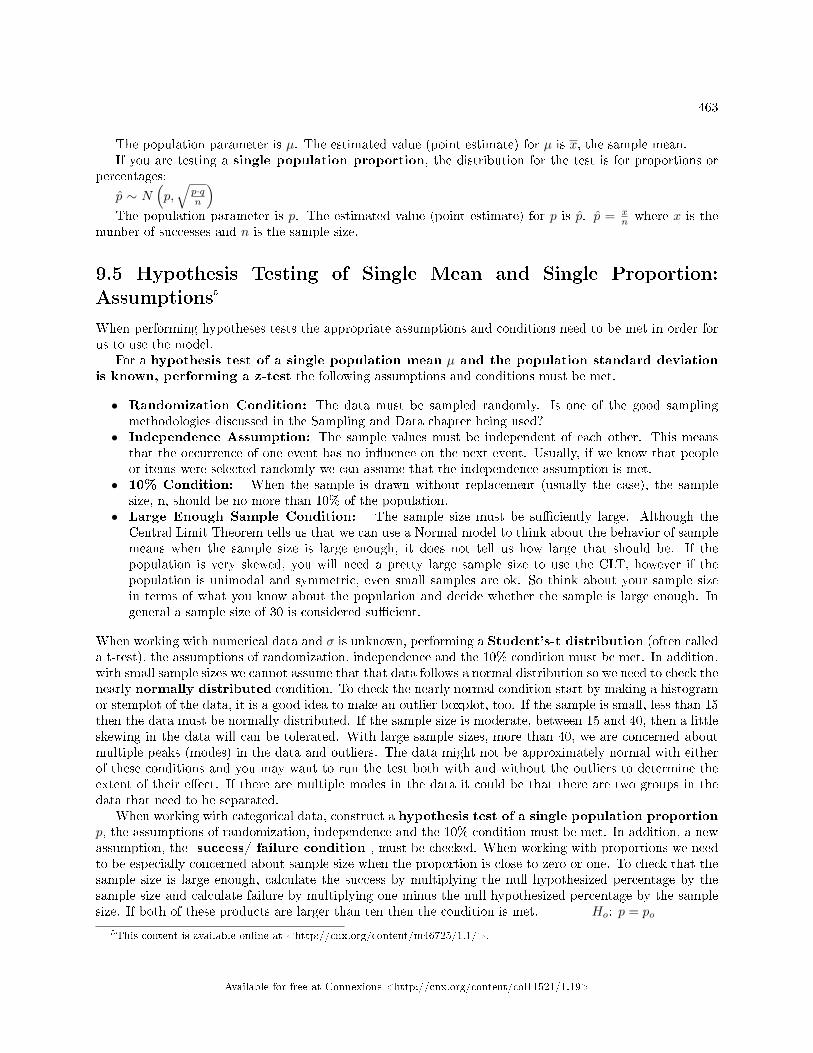
463
The population parameter is µ. The estimated value (point estimate) for µ is x, the sample mean.If you are testing a single population proportion, the distribution for the test is for proportions or
percentages:
p̂ ∼ N(p,√
p·qn
)The population parameter is p. The estimated value (point estimate) for p is p̂. p̂ = x
n where x is thenumber of successes and n is the sample size.
9.5 Hypothesis Testing of Single Mean and Single Proportion:Assumptions5
When performing hypotheses tests the appropriate assumptions and conditions need to be met in order forus to use the model.
For a hypothesis test of a single population mean µ and the population standard deviationis known, performing a z-test the following assumptions and conditions must be met.
• Randomization Condition: The data must be sampled randomly. Is one of the good samplingmethodologies discussed in the Sampling and Data chapter being used?
• Independence Assumption: The sample values must be independent of each other. This meansthat the occurrence of one event has no in�uence on the next event. Usually, if we know that peopleor items were selected randomly we can assume that the independence assumption is met.
• 10% Condition: When the sample is drawn without replacement (usually the case), the samplesize, n, should be no more than 10% of the population.
• Large Enough Sample Condition: The sample size must be su�ciently large. Although theCentral Limit Theorem tells us that we can use a Normal model to think about the behavior of samplemeans when the sample size is large enough, it does not tell us how large that should be. If thepopulation is very skewed, you will need a pretty large sample size to use the CLT, however if thepopulation is unimodal and symmetric, even small samples are ok. So think about your sample sizein terms of what you know about the population and decide whether the sample is large enough. Ingeneral a sample size of 30 is considered su�cient.
When working with numerical data and σ is unknown, performing a Student's-t distribution (often calleda t-test), the assumptions of randomization, independence and the 10% condition must be met. In addition,with small sample sizes we cannot assume that that data follows a normal distribution so we need to check thenearly normally distributed condition. To check the nearly normal condition start by making a histogramor stemplot of the data, it is a good idea to make an outlier boxplot, too. If the sample is small, less than 15then the data must be normally distributed. If the sample size is moderate, between 15 and 40, then a littleskewing in the data will can be tolerated. With large sample sizes, more than 40, we are concerned aboutmultiple peaks (modes) in the data and outliers. The data might not be approximately normal with eitherof these conditions and you may want to run the test both with and without the outliers to determine theextent of their e�ect. If there are multiple modes in the data it could be that there are two groups in thedata that need to be separated.
When working with categorical data, construct a hypothesis test of a single population proportionp, the assumptions of randomization, independence and the 10% condition must be met. In addition, a newassumption, the success/ failure condition , must be checked. When working with proportions we needto be especially concerned about sample size when the proportion is close to zero or one. To check that thesample size is large enough, calculate the success by multiplying the null hypothesized percentage by thesample size and calculate failure by multiplying one minus the null hypothesized percentage by the samplesize. If both of these products are larger than ten then the condition is met. Ho: p = po
5This content is available online at <http://cnx.org/content/m46725/1.1/>.
Available for free at Connexions <http://cnx.org/content/col11521/1.19>
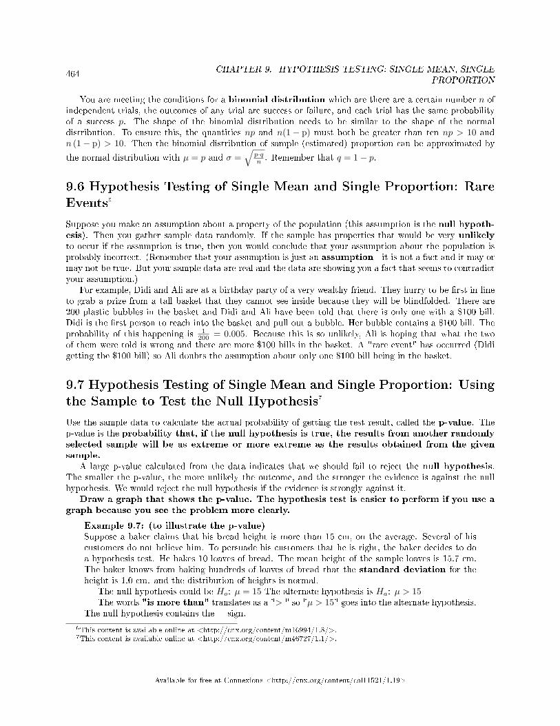
464CHAPTER 9. HYPOTHESIS TESTING: SINGLE MEAN, SINGLE
PROPORTION
You are meeting the conditions for a binomial distribution which are there are a certain number n ofindependent trials, the outcomes of any trial are success or failure, and each trial has the same probabilityof a success p. The shape of the binomial distribution needs to be similar to the shape of the normaldistribution. To ensure this, the quantities np and n(1− p) must both be greater than ten np > 10 andn (1− p) > 10. Then the binomial distribution of sample (estimated) proportion can be approximated by
the normal distribution with µ = p and σ =√
p·qn . Remember that q = 1− p.
9.6 Hypothesis Testing of Single Mean and Single Proportion: RareEvents6
Suppose you make an assumption about a property of the population (this assumption is the null hypoth-esis). Then you gather sample data randomly. If the sample has properties that would be very unlikelyto occur if the assumption is true, then you would conclude that your assumption about the population isprobably incorrect. (Remember that your assumption is just an assumption - it is not a fact and it may ormay not be true. But your sample data are real and the data are showing you a fact that seems to contradictyour assumption.)
For example, Didi and Ali are at a birthday party of a very wealthy friend. They hurry to be �rst in lineto grab a prize from a tall basket that they cannot see inside because they will be blindfolded. There are200 plastic bubbles in the basket and Didi and Ali have been told that there is only one with a $100 bill.Didi is the �rst person to reach into the basket and pull out a bubble. Her bubble contains a $100 bill. Theprobability of this happening is 1
200 = 0.005. Because this is so unlikely, Ali is hoping that what the twoof them were told is wrong and there are more $100 bills in the basket. A "rare event" has occurred (Didigetting the $100 bill) so Ali doubts the assumption about only one $100 bill being in the basket.
9.7 Hypothesis Testing of Single Mean and Single Proportion: Usingthe Sample to Test the Null Hypothesis7
Use the sample data to calculate the actual probability of getting the test result, called the p-value. Thep-value is the probability that, if the null hypothesis is true, the results from another randomlyselected sample will be as extreme or more extreme as the results obtained from the givensample.
A large p-value calculated from the data indicates that we should fail to reject the null hypothesis.The smaller the p-value, the more unlikely the outcome, and the stronger the evidence is against the nullhypothesis. We would reject the null hypothesis if the evidence is strongly against it.
Draw a graph that shows the p-value. The hypothesis test is easier to perform if you use agraph because you see the problem more clearly.
Example 9.7: (to illustrate the p-value)Suppose a baker claims that his bread height is more than 15 cm, on the average. Several of hiscustomers do not believe him. To persuade his customers that he is right, the baker decides to doa hypothesis test. He bakes 10 loaves of bread. The mean height of the sample loaves is 15.7 cm.The baker knows from baking hundreds of loaves of bread that the standard deviation for theheight is 1.0 cm. and the distribution of heights is normal.
The null hypothesis could be Ho: µ = 15 The alternate hypothesis is Ha: µ > 15The words "is more than" translates as a "> " so "µ > 15" goes into the alternate hypothesis.
The null hypothesis contains the = sign.
6This content is available online at <http://cnx.org/content/m16994/1.8/>.7This content is available online at <http://cnx.org/content/m46727/1.1/>.
Available for free at Connexions <http://cnx.org/content/col11521/1.19>
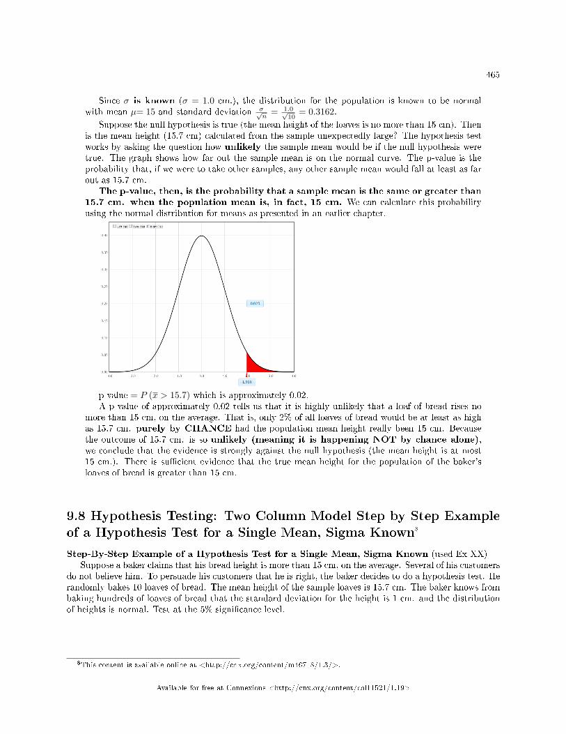
465
Since σ is known (σ = 1.0 cm.), the distribution for the population is known to be normalwith mean µ= 15 and standard deviation σ√
n= 1.0√
10= 0.3162.
Suppose the null hypothesis is true (the mean height of the loaves is no more than 15 cm). Thenis the mean height (15.7 cm) calculated from the sample unexpectedly large? The hypothesis testworks by asking the question how unlikely the sample mean would be if the null hypothesis weretrue. The graph shows how far out the sample mean is on the normal curve. The p-value is theprobability that, if we were to take other samples, any other sample mean would fall at least as farout as 15.7 cm.
The p-value, then, is the probability that a sample mean is the same or greater than15.7 cm. when the population mean is, in fact, 15 cm. We can calculate this probabilityusing the normal distribution for means as presented in an earlier chapter.
p-value = P (x > 15.7) which is approximately 0.02.A p-value of approximately 0.02 tells us that it is highly unlikely that a loaf of bread rises no
more than 15 cm, on the average. That is, only 2% of all loaves of bread would be at least as highas 15.7 cm. purely by CHANCE had the population mean height really been 15 cm. Becausethe outcome of 15.7 cm. is so unlikely (meaning it is happening NOT by chance alone),we conclude that the evidence is strongly against the null hypothesis (the mean height is at most15 cm.). There is su�cient evidence that the true mean height for the population of the baker'sloaves of bread is greater than 15 cm.
9.8 Hypothesis Testing: Two Column Model Step by Step Exampleof a Hypothesis Test for a Single Mean, Sigma Known8
Step-By-Step Example of a Hypothesis Test for a Single Mean, Sigma Known (used Ex XX)Suppose a baker claims that his bread height is more than 15 cm, on the average. Several of his customers
do not believe him. To persuade his customers that he is right, the baker decides to do a hypothesis test. Herandomly bakes 10 loaves of bread. The mean height of the sample loaves is 15.7 cm. The baker knows frombaking hundreds of loaves of bread that the standard deviation for the height is 1 cm. and the distributionof heights is normal. Test at the 5% signi�cance level.
8This content is available online at <http://cnx.org/content/m46718/1.3/>.
Available for free at Connexions <http://cnx.org/content/col11521/1.19>
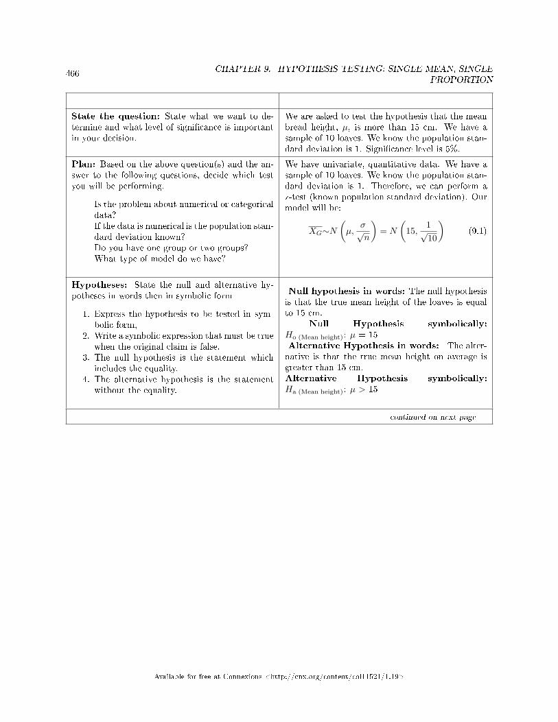
466CHAPTER 9. HYPOTHESIS TESTING: SINGLE MEAN, SINGLE
PROPORTION
State the question: State what we want to de-termine and what level of signi�cance is importantin your decision.
We are asked to test the hypothesis that the meanbread height, µ, is more than 15 cm. We have asample of 10 loaves. We know the population stan-dard deviation is 1. Signi�cance level is 5%.
Plan: Based on the above question(s) and the an-swer to the following questions, decide which testyou will be performing.
Is the problem about numerical or categoricaldata?If the data is numerical is the population stan-dard deviation known?Do you have one group or two groups?What type of model do we have?
We have univariate, quantitative data. We have asample of 10 loaves. We know the population stan-dard deviation is 1. Therefore, we can perform az-test (known population standard deviation). Ourmodel will be:
XG∼N(µ,
σ√n
)= N
(15,
1√10
)(9.1)
Hypotheses: State the null and alternative hy-potheses in words then in symbolic form
1. Express the hypothesis to be tested in sym-bolic form,
2. Write a symbolic expression that must be truewhen the original claim is false.
3. The null hypothesis is the statement whichincludes the equality.
4. The alternative hypothesis is the statementwithout the equality.
Null hypothesis in words: The null hypothesisis that the true mean height of the loaves is equalto 15 cm.
Null Hypothesis symbolically:Ho (Mean height): µ = 15Alternative Hypothesis in words: The alter-native is that the true mean height on average isgreater than 15 cm.Alternative Hypothesis symbolically:Ha (Mean height): µ > 15
continued on next page
Available for free at Connexions <http://cnx.org/content/col11521/1.19>
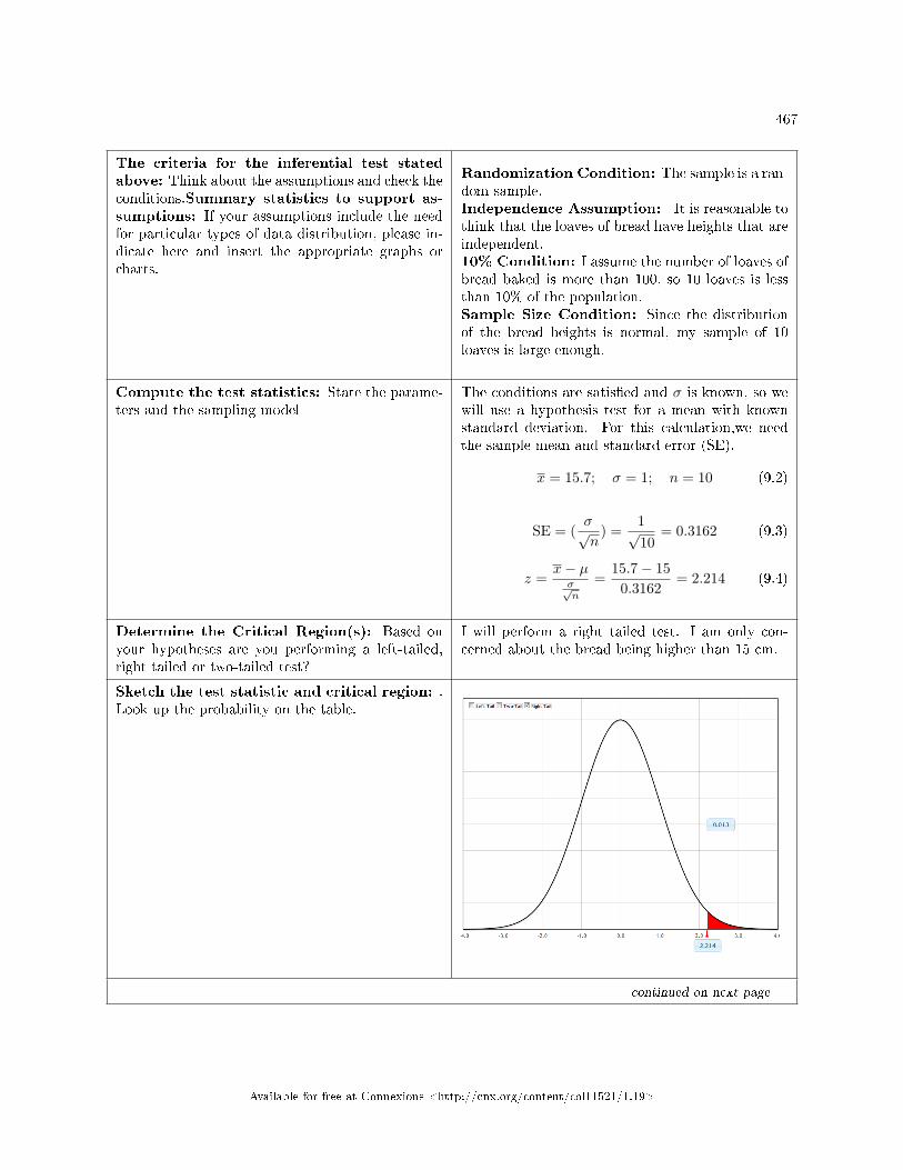
467
The criteria for the inferential test statedabove: Think about the assumptions and check theconditions.Summary statistics to support as-sumptions: If your assumptions include the needfor particular types of data distribution, please in-dicate here and insert the appropriate graphs orcharts.
Randomization Condition: The sample is a ran-dom sample.Independence Assumption: It is reasonable tothink that the loaves of bread have heights that areindependent.10% Condition: I assume the number of loaves ofbread baked is more than 100, so 10 loaves is lessthan 10% of the population.Sample Size Condition: Since the distributionof the bread heights is normal, my sample of 10loaves is large enough.
Compute the test statistics: State the parame-ters and the sampling model
The conditions are satis�ed and σ is known, so wewill use a hypothesis test for a mean with knownstandard deviation. For this calculation,we needthe sample mean and standard error (SE).
x = 15.7; σ = 1; n = 10 (9.2)
SE = (σ√n
) =1√10
= 0.3162 (9.3)
z =x− µσ√n
=15.7− 15
0.3162= 2.214 (9.4)
Determine the Critical Region(s): Based onyour hypotheses are you performing a left-tailed,right tailed or two-tailed test?
I will perform a right tailed test. I am only con-cerned about the bread being higher than 15 cm.
Sketch the test statistic and critical region: .Look up the probability on the table.
continued on next page
Available for free at Connexions <http://cnx.org/content/col11521/1.19>
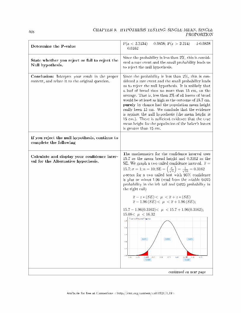
468CHAPTER 9. HYPOTHESIS TESTING: SINGLE MEAN, SINGLE
PROPORTION
Determine the P-valueP(z < 2.2134) = 0.9838; P(z > 2.214) = 1-0.9838= 0.0162
State whether you reject or fail to reject theNull hypothesis.
Since the probability is less than 2%, this is consid-ered a rare event and the small probability leads usto reject the null hypothesis.
Conclusion: Interpret your result in the propercontext, and relate it to the original question.
Since the probability is less than 2%, this is con-sidered a rare event and the small probability leadsus to reject the null hypothesis. It is unlikely thata loaf of bread rises no more than 15 cm, on theaverage. That is, less than 2% of all loaves of breadwould be at least as high as the outcome of 15.7 cm.purely by chance had the population mean heightreally been 15 cm. We conclude that the evidenceis against the null hypothesis (the mean height is15 cm.). There is su�cient evidence that the truemean height for the population of the baker's loavesis greater than 15 cm.
If you reject the null hypothesis, continue tocomplete the following
Calculate and display your con�dence inter-val for the Alternative hypothesis.
The mathematics for the con�dence interval uses15.7 as the mean bread height and 0.3162 as theSE. We graph a two tailed con�dence interval. x =15.7;σ = 1;n = 10; SE =
(σ√n
)= 1√
10= 0.3162
z-score for a two tailed test with 95% con�denceis plus or minus 1.96 (read from the z-table 0.025probability in the left tail and 0.025 probability inthe right tail)
x− z ∗ (SE)< µ < x+ z ∗ (SE)x− 1.96 (SE)< µ < x+ 1.96 (SE);
15.7− 1.96(0.3162)< µ < 15.7 + 1.96(0.3162);15.08< µ < 16.32
continued on next page
Available for free at Connexions <http://cnx.org/content/col11521/1.19>
469
Conclusion State your conclusion based onyour con�dence interval.
We are 95% con�dent that the true mean of thebakers bread height is greater than 15 cm. We are95% con�dent that the population mean height isbetween 15.08 cm. and 16.32 cm.
Table 9.3
9.9 Hypothesis Testing of Single Mean and Single Proportion: Deci-sion and Conclusion9
A systematic way to make a decision of whether to reject or not reject the null hypothesis is to comparethe p-value and a preset or preconceived α (also called a "signi�cance level"). A preset α is theprobability of a Type I error (rejecting the null hypothesis when the null hypothesis is true). It may ormay not be given to you at the beginning of the problem.
When you make a decision to reject or not reject Ho, do as follows:
• If α > p-value, reject Ho. The results of the sample data are signi�cant. There is su�cient evidenceto conclude that Ho is an incorrect belief and that the alternative hypothesis, Ha, may be correct.
• If α ≤ p-value, do not reject Ho. The results of the sample data are not signi�cant. There is notsu�cient evidence to conclude that the alternative hypothesis, Ha, may be correct.
• When you "do not reject Ho", it does not mean that you should believe that Ho is true. It simplymeans that the sample data have failed to provide su�cient evidence to cast serious doubt about thetruthfulness of Ho.
Conclusion: After you make your decision, write a thoughtful conclusion about the hypotheses interms of the given problem.
9.10 Hypothesis Testing of Single Mean and Single Proportion: Ad-ditional Information10
• In a hypothesis test problem, you may see words such as "the level of signi�cance is 1%." The "1%"is the preconceived or preset α.
• The statistician setting up the hypothesis test selects the value of α to use before collecting the sampledata.
• If no level of signi�cance is given, the accepted standard is to use α = 0.05.• When you calculate the p-value and draw the picture, the p-value is the area in the left tail, the right
tail, or split evenly between the two tails. For this reason, we call the hypothesis test left, right, or twotailed.
• The alternate hypothesis, Ha, tells you if the test is left, right, or two-tailed. It is the key toconducting the appropriate test.
• Ha never has a symbol that contains an equal sign.• Thinking about the meaning of the p-value: A data analyst (and anyone else) should have more
con�dence that he made the correct decision to reject the null hypothesis with a smaller p-value (forexample, 0.001 as opposed to 0.04) even if using the 0.05 level for alpha. Similarly, for a large p-valuelike 0.4, as opposed to a p-value of 0.056 (alpha = 0.05 is less than either number), a data analystshould have more con�dence that she made the correct decision in failing to reject the null hypothesis.This makes the data analyst use judgment rather than mindlessly applying rules.
9This content is available online at <http://cnx.org/content/m16992/1.11/>.10This content is available online at <http://cnx.org/content/m16999/1.13/>.
Available for free at Connexions <http://cnx.org/content/col11521/1.19>
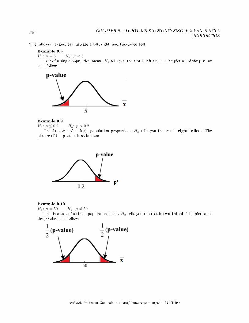
470CHAPTER 9. HYPOTHESIS TESTING: SINGLE MEAN, SINGLE
PROPORTION
The following examples illustrate a left, right, and two-tailed test.
Example 9.8Ho: µ = 5 Ha: µ < 5
Test of a single population mean. Ha tells you the test is left-tailed. The picture of the p-valueis as follows:
Example 9.9Ho: p ≤ 0.2 Ha: p > 0.2
This is a test of a single population proportion. Ha tells you the test is right-tailed. Thepicture of the p-value is as follows:
Example 9.10Ho: µ = 50 Ha: µ 6= 50
This is a test of a single population mean. Ha tells you the test is two-tailed. The picture ofthe p-value is as follows.
Available for free at Connexions <http://cnx.org/content/col11521/1.19>
471
9.11 Hypothesis Testing of Single Mean and Single Proportion: Sum-mary of the Hypothesis Test11
The hypothesis test itself has an established process. This can be summarized as follows:
1. Determine Ho and Ha. Remember, they are contradictory.2. Determine the random variable.3. Determine the distribution for the test.4. Draw a graph, calculate the test statistic, and use the test statistic to calculate the p-value. (A z-score
and a t-score are examples of test statistics.)5. Compare the preconceived α with the p-value, make a decision (reject or do not reject Ho), and write
a clear conclusion using English sentences.
Notice that in performing the hypothesis test, you use α and not β. β is needed to help determine thesample size of the data that is used in calculating the p-value. Remember that the quantity 1− β is calledthe Power of the Test. A high power is desirable. If the power is too low, statisticians typically increasethe sample size while keeping α the same. If the power is low, the null hypothesis might not be rejectedwhen it should be.
9.12 Hypothesis Testing of Single Mean and Single Proportion: Ex-amples Alternate Title12
Example 9.11A college football coach thought that his players could bench press amean weight of 275 pounds.The standard deviation of all college football players is unknown. Three of his playersthought that the mean weight wasmore than that amount. They asked 30 of their teammates fortheir estimated maximum lift on the bench press exercise. The data ranged from 205 pounds to 385pounds. The actual di�erent weights were (frequencies are in parentheses) 205(3); 215(3); 225(1);241(2); 252(2); 265(2); 275(2); 313(2); 316(5); 338(2); 341(1); 345(2); 368(2); 385(1). (Source:data from Reuben Davis, Kraig Evans, and Scott Gunderson. Adapted by Duranczyk, Loch, andStotttlemyer)
Conduct a hypothesis test using a 2.5% level of signi�cance to determine if the bench pressmean is more than 275 pounds.
SolutionSet up the Hypothesis Test:
Since the problem is about a mean weight, this is a test of a single population mean.Ho: µ = 275 Ha: µ > 275 This is a right-tailed test.Calculating the distribution needed:Random variable: X = the mean weight, in pounds, lifted by the football players.Distribution for the test: It is student t-test because σ is unknown, so we will need to check
normal distribution assumptions by looking at a histogram and box plot of the data as well as thedescriptive statistics. The data is slightly skewed to the right with no outliers, so we will proceedwith some reservation since the data is varies from a normal distribution. The median is 8 pointshigher than the mean. The sample standard deviation is 55.9. We will round the standard deviationto 56 for calculating the p-value.
X ∼ N(
275, 56√30
)x = 286.2 pounds (from the data).s = 56 pounds We assume µ = 275 pounds unless our data shows us otherwise.
11This content is available online at <http://cnx.org/content/m16993/1.6/>.12This content is available online at <http://cnx.org/content/m46721/1.1/>.
Available for free at Connexions <http://cnx.org/content/col11521/1.19>
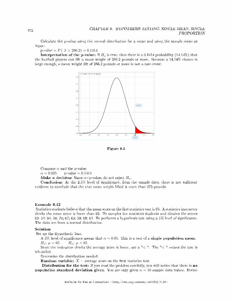
472CHAPTER 9. HYPOTHESIS TESTING: SINGLE MEAN, SINGLE
PROPORTION
Calculate the p-value using the normal distribution for a mean and using the sample mean asinput:
p-value = P ( x > 286.2) = 0.1414.Interpretation of the p-value: If Ho is true, then there is a 0.1414 probability (14.14%) that
the football players can lift a mean weight of 286.2 pounds or more. Because a 14.14% chance islarge enough, a mean weight lift of 286.2 pounds or more is not a rare event.
Figure 9.1
Compare α and the p-value:α = 0.025 p-value = 0.1414Make a decision: Since α<p-value, do not reject Ho.Conclusion: At the 2.5% level of signi�cance, from the sample data, there is not su�cient
evidence to conclude that the true mean weight lifted is more than 275 pounds.
Example 9.12Statistics students believe that the mean score on the �rst statistics test is 65. A statistics instructorthinks the mean score is lower than 65. He samples ten statistics students and obtains the scores62; 54; 64; 58; 70; 67; 63; 59; 69; 64. He performs a hypothesis test using a 5% level of signi�cance.The data are from a normal distribution.
SolutionSet up the Hypothesis Test:
A 5% level of signi�cance means that α = 0.05. This is a test of a single population mean.Ho: µ = 65 Ha: µ < 65Since the instructor thinks the average score is lower, use a "< ". The "< " means the test is
left-tailed.Determine the distribution needed:Random variable: X = average score on the �rst statistics test.Distribution for the test: If you read the problem carefully, you will notice that there is no
population standard deviation given. You are only given n = 10 sample data values. Notice
Available for free at Connexions <http://cnx.org/content/col11521/1.19>
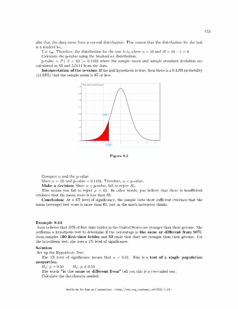
473
also that the data come from a normal distribution. This means that the distribution for the testis a student's-t.
Use tdf. Therefore, the distribution for the test is t9 where n = 10 and df = 10− 1 = 9.Calculate the p-value using the Student's-t distribution:p-value = P ( x < 63 )= 0.1193 where the sample mean and sample standard deviation are
calculated as 63 and 5.0111 from the data.Interpretation of the p-value: If the null hypothesis is true, then there is a 0.1193 probability
(11.93%) that the sample mean is 67 or less.
Figure 9.2
Compare α and the p-value:Since α = .05 and p-value = 0.1193. Therefore, α < p-value.Make a decision: Since α < p-value, fail to reject Ho.This means you fail to reject µ = 65. In other words, you believe that there is insu�cient
evidence that the mean score is less than 65.Conclusion: At a 5% level of signi�cance, the sample data show su�cient evidence that the
mean (average) test score is more than 65, just as the math instructor thinks.
Example 9.13Joon believes that 50% of �rst-time brides in the United States are younger than their grooms. Sheperforms a hypothesis test to determine if the percentage is the same or di�erent from 50%.Joon samples 100 �rst-time brides and 53 reply that they are younger than their grooms. Forthe hypothesis test, she uses a 1% level of signi�cance.
SolutionSet up the Hypothesis Test:
The 1% level of signi�cance means that α = 0.01. This is a test of a single populationproportion.
Ho: p = 0.50 Ha: p 6= 0.50The words "is the same or di�erent from" tell you this is a two-tailed test.Calculate the distribution needed:
Available for free at Connexions <http://cnx.org/content/col11521/1.19>
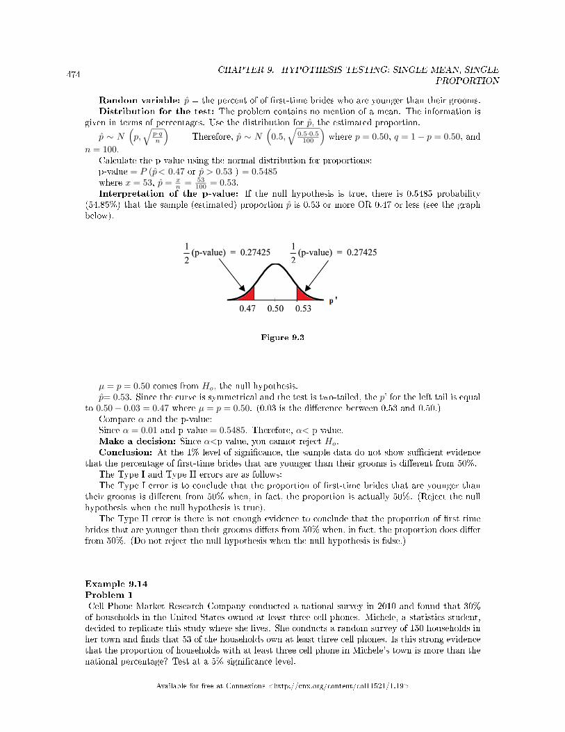
474CHAPTER 9. HYPOTHESIS TESTING: SINGLE MEAN, SINGLE
PROPORTION
Random variable: p̂ = the percent of of �rst-time brides who are younger than their grooms.Distribution for the test: The problem contains no mention of a mean. The information is
given in terms of percentages. Use the distribution for p̂, the estimated proportion.
p̂ ∼ N(p,√
p·qn
)Therefore, p̂ ∼ N
(0.5,
√0.5·0.5
100
)where p = 0.50, q = 1− p = 0.50, and
n = 100.Calculate the p-value using the normal distribution for proportions:p-value = P (p̂< 0.47 or p̂ > 0.53 ) = 0.5485where x = 53, p̂ = x
n = 53100 = 0.53.
Interpretation of the p-value: If the null hypothesis is true, there is 0.5485 probability(54.85%) that the sample (estimated) proportion p̂ is 0.53 or more OR 0.47 or less (see the graphbelow).
Figure 9.3
µ = p = 0.50 comes from Ho, the null hypothesis.p̂= 0.53. Since the curve is symmetrical and the test is two-tailed, the p' for the left tail is equal
to 0.50− 0.03 = 0.47 where µ = p = 0.50. (0.03 is the di�erence between 0.53 and 0.50.)Compare α and the p-value:Since α = 0.01 and p-value = 0.5485. Therefore, α< p-value.Make a decision: Since α<p-value, you cannot reject Ho.Conclusion: At the 1% level of signi�cance, the sample data do not show su�cient evidence
that the percentage of �rst-time brides that are younger than their grooms is di�erent from 50%.The Type I and Type II errors are as follows:The Type I error is to conclude that the proportion of �rst-time brides that are younger than
their grooms is di�erent from 50% when, in fact, the proportion is actually 50%. (Reject the nullhypothesis when the null hypothesis is true).
The Type II error is there is not enough evidence to conclude that the proportion of �rst timebrides that are younger than their grooms di�ers from 50% when, in fact, the proportion does di�erfrom 50%. (Do not reject the null hypothesis when the null hypothesis is false.)
Example 9.14Problem 1Cell Phone Market Research Company conducted a national survey in 2010 and found that 30%of households in the United States owned at least three cell phones. Michele, a statistics student,decided to replicate this study where she lives. She conducts a random survey of 150 households inher town and �nds that 53 of the households own at least three cell phones. Is this strong evidencethat the proportion of households with at least three cell phone in Michele's town is more than thenational percentage? Test at a 5% signi�cance level.
Available for free at Connexions <http://cnx.org/content/col11521/1.19>
475
SolutionSet up the Hypothesis Test:Ho: p = 0.30 Ha: p> 0.30Determine the distribution needed:The random variable is p̂ = proportion of households that have at least three cell phones.
The distribution for the hypothesis test is p̂ ∼ N
(0.30,
√(0.30)·(0.70)
150
)Problem 2The value that helps determine the p-value is p̂. Calculate p̂.
Problem 3What is a success for this problem?
Problem 4What is the level of signi�cance?
Draw the graph for this problem. Draw the horizontal axis. Label and shade appropriately.
Problem 5Calculate the p-value.
Problem 6Make a decision. _____________(Reject/Do not reject) H0 because____________.
The next example is a poem written by a statistics student named Nicole Hart. The solution to the problemfollows the poem. Notice that the hypothesis test is for a single population proportion. This means that thenull and alternate hypotheses use the parameter p. The distribution for the test is normal. The estimatedproportion p̂ is the proportion of �eas killed to the total �eas found on Fido. This is sample information.The problem gives a preconceived α = 0.01, for comparison, and a 95% con�dence interval computation.The poem is clever and humorous, so please enjoy it!
note: Hypothesis testing problems consist of multiple steps. To help you do the problems, solutionsheets are provided for your use. Look in the Table of Contents Appendix for the topic "SolutionSheets." If you like, use copies of the appropriate solution sheet for homework problems.
Example 9.15
My dog has so many fleas,
They do not come off with ease.
As for shampoo, I have tried many types
Even one called Bubble Hype,
Which only killed 25% of the fleas,
Unfortunately I was not pleased.
I've used all kinds of soap,
Until I had give up hope
Until one day I saw
An ad that put me in awe.
A shampoo used for dogs
Called GOOD ENOUGH to Clean a Hog
Available for free at Connexions <http://cnx.org/content/col11521/1.19>
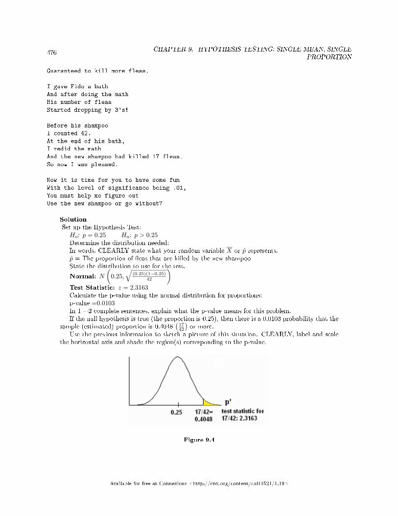
476CHAPTER 9. HYPOTHESIS TESTING: SINGLE MEAN, SINGLE
PROPORTION
Guaranteed to kill more fleas.
I gave Fido a bath
And after doing the math
His number of fleas
Started dropping by 3's!
Before his shampoo
I counted 42.
At the end of his bath,
I redid the math
And the new shampoo had killed 17 fleas.
So now I was pleased.
Now it is time for you to have some fun
With the level of significance being .01,
You must help me figure out
Use the new shampoo or go without?
SolutionSet up the Hypothesis Test:Ho: p = 0.25 Ha: p > 0.25Determine the distribution needed:In words, CLEARLY state what your random variable X or p̂ represents.p̂ = The proportion of �eas that are killed by the new shampooState the distribution to use for the test.
Normal: N
(0.25,
√(0.25)(1−0.25)
42
)Test Statistic: z = 2.3163Calculate the p-value using the normal distribution for proportions:p-value =0.0103In 1 � 2 complete sentences, explain what the p-value means for this problem.If the null hypothesis is true (the proportion is 0.25), then there is a 0.0103 probability that the
sample (estimated) proportion is 0.4048(
1742
)or more.
Use the previous information to sketch a picture of this situation. CLEARLY, label and scalethe horizontal axis and shade the region(s) corresponding to the p-value.
Figure 9.4
Available for free at Connexions <http://cnx.org/content/col11521/1.19>
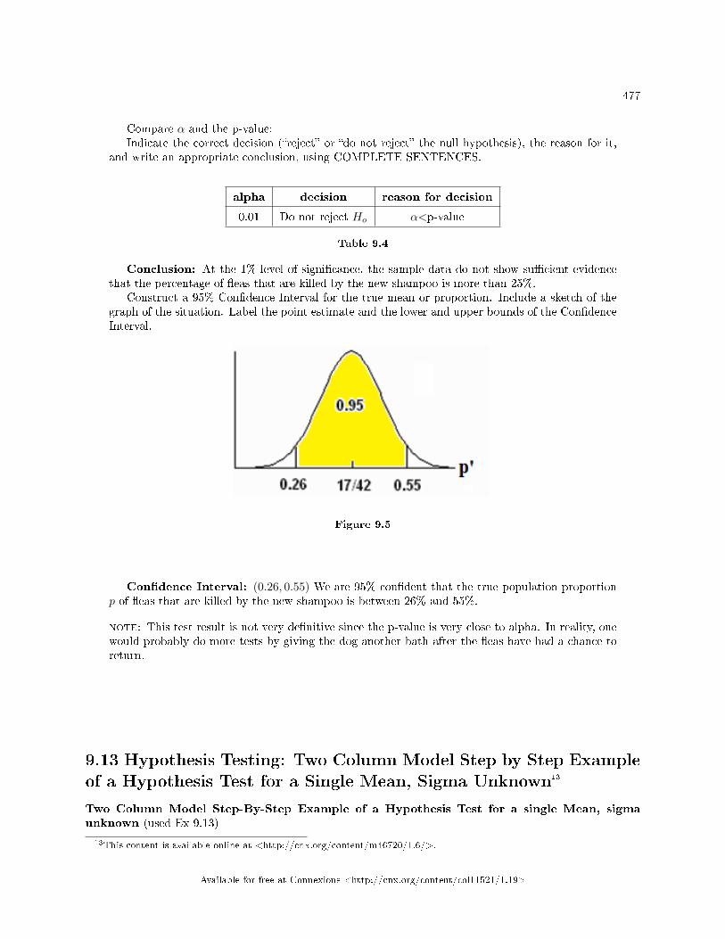
477
Compare α and the p-value:Indicate the correct decision (�reject� or �do not reject� the null hypothesis), the reason for it,
and write an appropriate conclusion, using COMPLETE SENTENCES.
alpha decision reason for decision
0.01 Do not reject Ho α<p-value
Table 9.4
Conclusion: At the 1% level of signi�cance, the sample data do not show su�cient evidencethat the percentage of �eas that are killed by the new shampoo is more than 25%.
Construct a 95% Con�dence Interval for the true mean or proportion. Include a sketch of thegraph of the situation. Label the point estimate and the lower and upper bounds of the Con�denceInterval.
Figure 9.5
Con�dence Interval: (0.26, 0.55) We are 95% con�dent that the true population proportionp of �eas that are killed by the new shampoo is between 26% and 55%.
note: This test result is not very de�nitive since the p-value is very close to alpha. In reality, onewould probably do more tests by giving the dog another bath after the �eas have had a chance toreturn.
9.13 Hypothesis Testing: Two Column Model Step by Step Exampleof a Hypothesis Test for a Single Mean, Sigma Unknown13
Two Column Model Step-By-Step Example of a Hypothesis Test for a single Mean, sigmaunknown (used Ex 9.13)
13This content is available online at <http://cnx.org/content/m46720/1.6/>.
Available for free at Connexions <http://cnx.org/content/col11521/1.19>

478CHAPTER 9. HYPOTHESIS TESTING: SINGLE MEAN, SINGLE
PROPORTION
Statistics students believe that the mean score on the �rst statistics test is 65. A statistics instructorthinks the mean score is lower than 65. He randomly samples ten statistics student scores and obtains thescores 62,54,64,58,70,67,63,59,69,64. He performs a hypothesis test using a 5% level of signi�cance.
Available for free at Connexions <http://cnx.org/content/col11521/1.19>
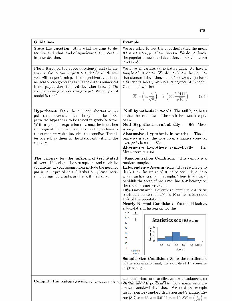
479
Guidelines Example
State the question: State what we want to de-termine and what level of signi�cance is importantin your decision.
We are asked to test the hypothesis that the meanstatistics score, µ, is less than 65. We do not knowthe population standard deviation. The signi�cancelevel is 5%.
Plan: Based on the above question(s) and the an-swer to the following questions, decide which testyou will be performing. Is the problem about nu-merical or categorical data? If the data is numericalis the population standard deviation known? Doyou have one group or two groups? What type ofmodel is this?
We have univariate, quantitative data. We have asample of 10 scores. We do not know the popula-tion standard deviation. Therefore, we can performa Student's t-test, with n-1, 9 degrees of freedom.Our model will be:
X ∼(µ,
s√n
)= T
(65,
5.0111√10
)(9.5)
Hypotheses: State the null and alternative hy-potheses in words and then in symbolic form Ex-press the hypothesis to be tested in symbolic form.Write a symbolic expression that must be true whenthe original claim is false. The null hypothesis isthe statement which included the equality. The al-ternative hypothesis is the statement without theequality.
Null hypothesis in words: The null hypothesisis that the true mean of the statistics exam is equalto 65.Null Hypothesis symbolically: H0: Meanscore µ = 65Alternative Hypothesis in words: The al-ternative is that the true mean statistics score onaverage is less than 65.Alternative Hypothesis symbolically: Ha:Mean score µ < 65
The criteria for the inferential test statedabove: Think about the assumptions and check theconditions. If your assumptions include the need forparticular types of data distribution, please insertthe appropriate graphs or charts if necessary.
Randomization Condition: The sample is arandom sample.Independence Assumption: It is reasonable tothink that the scores of students are independentwhen you have a random sample. There is no reasonto think the score of one exam has any bearing onthe score of another exam.10% Condition: I assume the number of statisticstudents is more than 100, so 10 scores is less than10% of the population.Nearly Normal Condition: We should look ata boxplot and histogram for this:
Sample Size Condition: Since the distributionof the scores is normal, my sample of 10 scores islarge enough.
Compute the test statistic:The conditions are satis�ed and σ is unknown, sowe will use a hypothesis test for a mean with un-known standard deviation. We need the samplemean, sample standard deviation and Standard Er-
ror (SE).x = 63; s = 5.0111;n = 10;SE =(
s√n
)=
5.0111√10
= 1.585;x = 63; df = 10− 1 = 9; t = x− µs√n
=63−651.585 = −1.2618
continued on next page
Available for free at Connexions <http://cnx.org/content/col11521/1.19>
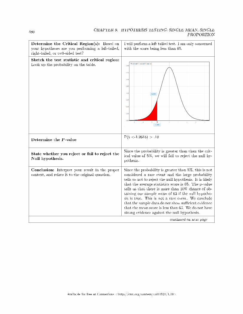
480CHAPTER 9. HYPOTHESIS TESTING: SINGLE MEAN, SINGLE
PROPORTION
Determine the Critical Region(s): Based onyour hypotheses are you performing a left-tailed,right-tailed, or tw0-sided test?
I will perform a left tailed test. I am only concernedwith the score being less than 65.
Sketch the test statistic and critical region:Look up the probability on the table.
Determine the P-valueP(t <-1.2618) > .10
State whether you reject or fail to reject theNull hypothesis.
Since the probability is greater than than the crit-ical value of 5%, we will fail to reject the null hy-pothesis.
Conclusion: Interpret your result in the propercontext, and relate it to the original question.
Since the probability is greater than 5%, this is notconsidered a rare event and the large probabilitytells us not to reject the null hypothesis. It is likelythat the average statistics score is 65. The p-valuetells us that there is more than 10% chance of ob-taining our sample mean of 63 if the null hypothe-sis is true. This is not a rare event. We concludethat the sample data do not show su�cient evidencethat the mean score is less than 65. We do not havestrong evidence against the null hypothesis.
continued on next page
Available for free at Connexions <http://cnx.org/content/col11521/1.19>
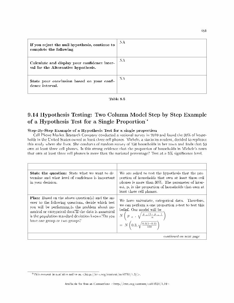
481
If you reject the null hypothesis, continue tocomplete the following
NA
Calculate and display your con�dence inter-val for the Alternative hypothesis.
NA
State your conclusion based on your con�-dence interval.
NA
Table 9.5
9.14 Hypothesis Testing: Two Column Model Step by Step Exampleof a Hypothesis Test for a Single Proportion14
Step-By-Step Example of a Hypothesis Test for a single proportionCell Phone Market Research Company conducted a national survey in 2010 and found the 30% of house-
holds in the United States owned at least three cell phones. Michele, a statistics student, decided to replicatethis study where she lives. She conducts of random survey of 150 households in her town and �nds that 53own at least three cell phones. Is this strong evidence that the proportion of households in Michele's townthat own at least three cell phones is more than the national percentage? Test at a 5% signi�cance level.
State the question: State what we want to de-termine and what level of con�dence is importantin your decision.
We are asked to test the hypothesis that the pro-portion of households that own at least three cellphones is more than 30%. The parameter of inter-est, p, is the proportion of households that own atleast three cell phones.
Plan: Based on the above question(s) and the an-swer to the following questions, decide which testyou will be performing.Is the problem about nu-merical or categorical data?If the data is numericalis the population standard deviation known?Do youhave one group or two groups?
We have univariate, categorical data. Therefore,we can perform a one proportion z-test to test thisbelief. Our model will be
N
(p o ,
√p o (1− p o )
n
)= N
(0.3,
√0.3(1−0.3)
150
)continued on next page
14This content is available online at <http://cnx.org/content/m46731/1.3/>.
Available for free at Connexions <http://cnx.org/content/col11521/1.19>
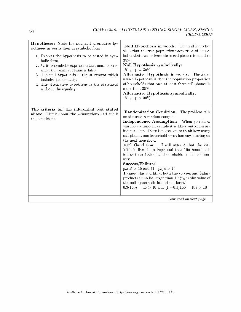
482CHAPTER 9. HYPOTHESIS TESTING: SINGLE MEAN, SINGLE
PROPORTION
Hypotheses: State the null and alternative hy-potheses in words then in symbolic form
1. Express the hypothesis to be tested in sym-bolic form,
2. Write a symbolic expression that must be truewhen the original claims is false.
3. The null hypothesis is the statement whichincludes the equality.
4. The alternative hypothesis is the statementwithout the equality.
Null Hypothesis in words: The null hypothe-sis is that the true population proportion of house-holds that own at least three cell phones is equal to30%.Null Hypothesis symbolically:H o : p = 30%Alternative Hypothesis in words: The alter-native hypothesis is that the population proportionof households that own at least three cell phones ismore than 30%.Alternative Hypothesis symbolically:H o : p > 30%
The criteria for the inferential test statedabove: Think about the assumptions and checkthe conditions.
Randomization Condition: The problem tellsus she used a random sample.Independence Assumption: When you knowyou have a random sample it is likely outcomes areindependent. There is no reason to think how manycell phones one household owns has any bearing onthe next household.10% Condition: I will assume that the cityMichele lives in is large and that 150 householdsis less than 10% of all households in her commu-nity.Success/Failure:p0(n) > 10 and (1 - p0)n > 10To meet this condition both the success and failureproducts must be larger than 10 (p0 is the value ofthe null hypothesis in decimal form.)0.3(150) = 45 > 10 and (1 � 0.3)150 = 105 > 10
continued on next page
Available for free at Connexions <http://cnx.org/content/col11521/1.19>
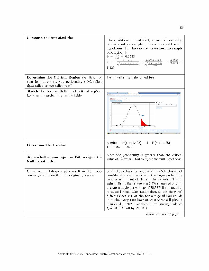
483
Compute the test statistic:The conditions are satis�ed, so we will use a hy-pothesis test for a single proportion to test the nullhypothesis. For this calculation we need the sampleproportion, p̂p̂ = 53
150 = 0.3533z = p̂ − p oq
p o ( 1 − p o )n
= 0.3533 − 0.3q0.3 (1 − 0.3)
150
= 0.05330.0374 =
1.425
Determine the Critical Region(s): Based onyour hypotheses are you performing a left-tailed,right tailed or two-tailed test?
I will perform a right tailed test.
Sketch the test statistic and critical region:Look up the probability on the table.
Determine the P-valuep-value = P(z > 1.425) = 1 � P(z <1.425) =1 - 0.923 = 0.077
State whether you reject or fail to reject theNull hypothesis.
Since the probability is greater than the criticalvalue of 5% we will fail to reject the null hypothesis.
Conclusion: Interpret your result in the propercontext, and relate it to the original question.
Since the probability is greater than 5%, this is notconsidered a rare event and the large probabilitytells us not to reject the null hypothesis. The p-value tells us that there is a 7.7% chance of obtain-ing our sample percentage of 35.33% if the null hy-pothesis is true. The sample data do not show suf-�cient evidence that the percentage of householdsin Michele city that have at least three cell phonesis more than 30%. We do not have strong evidenceagainst the null hypothesis.
continued on next page
Available for free at Connexions <http://cnx.org/content/col11521/1.19>
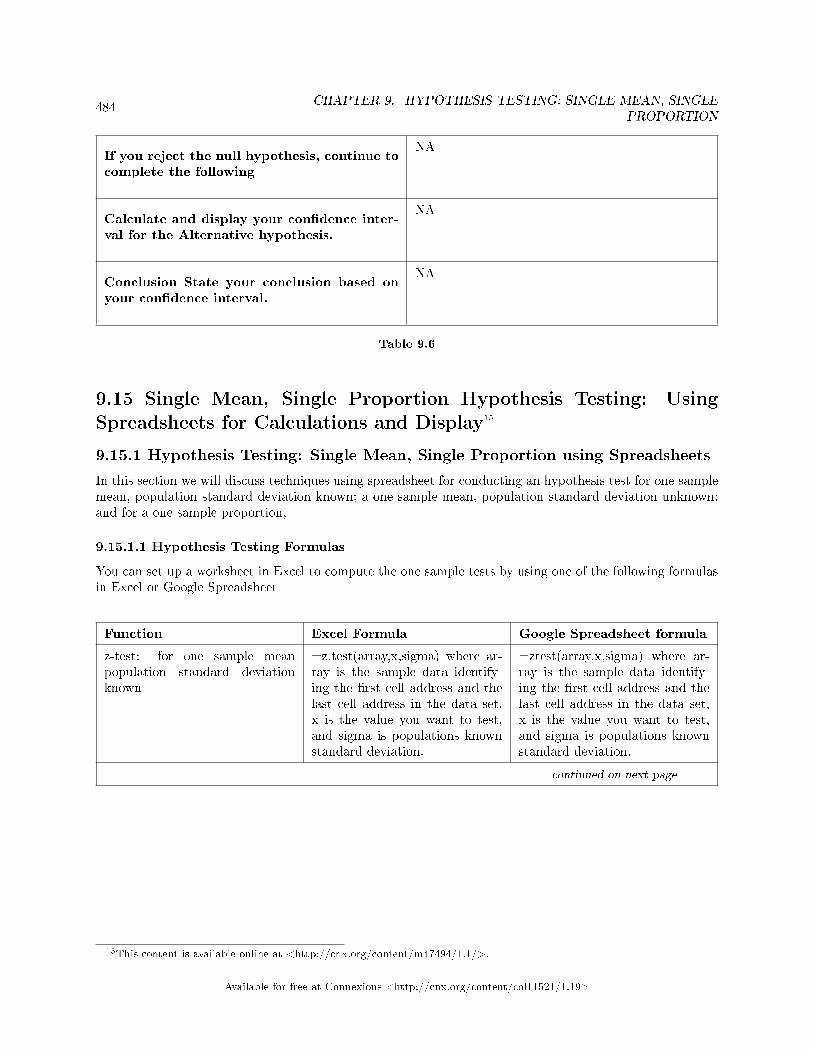
484CHAPTER 9. HYPOTHESIS TESTING: SINGLE MEAN, SINGLE
PROPORTION
If you reject the null hypothesis, continue tocomplete the following
NA
Calculate and display your con�dence inter-val for the Alternative hypothesis.
NA
Conclusion State your conclusion based onyour con�dence interval.
NA
Table 9.6
9.15 Single Mean, Single Proportion Hypothesis Testing: UsingSpreadsheets for Calculations and Display15
9.15.1 Hypothesis Testing: Single Mean, Single Proportion using Spreadsheets
In this section we will discuss techniques using spreadsheet for conducting an hypothesis test for one samplemean, population standard deviation known; a one sample mean, population standard deviation unknown:and for a one sample proportion,
9.15.1.1 Hypothesis Testing Formulas
You can set up a worksheet in Excel to compute the one sample tests by using one of the following formulasin Excel or Google Spreadsheet
Function Excel Formula Google Spreadsheet formula
z-test: for one sample meanpopulation standard deviationknown
=z.test(array,x,sigma) where ar-ray is the sample data identify-ing the �rst cell address and thelast cell address in the data set,x is the value you want to test,and sigma is populations knownstandard deviation.
=ztest(array,x,sigma) where ar-ray is the sample data identify-ing the �rst cell address and thelast cell address in the data set,x is the value you want to test,and sigma is populations knownstandard deviation.
continued on next page
15This content is available online at <http://cnx.org/content/m47494/1.1/>.
Available for free at Connexions <http://cnx.org/content/col11521/1.19>
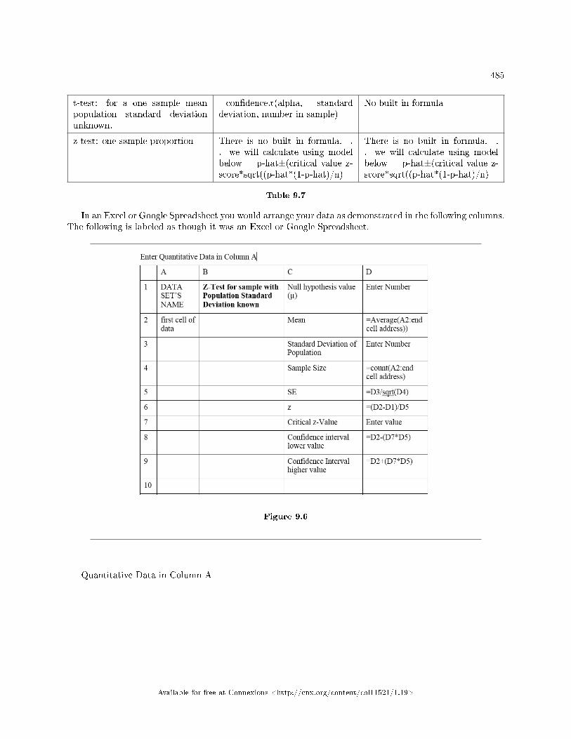
485
t-test: for a one sample meanpopulation standard deviationunknown.
=con�dence.t(alpha, standarddeviation, number in sample)
No built in formula
z-test: one sample proportion There is no built in formula. .. we will calculate using modelbelow = p-hat±(critical value z-score*sqrt((p-hat*(1-p-hat)/n)
There is no built in formula. .. we will calculate using modelbelow = p-hat±(critical value z-score*sqrt((p-hat*(1-p-hat)/n)
Table 9.7
In an Excel or Google Spreadsheet you would arrange your data as demonstrated in the following columns.The following is labeled as though it was an Excel or Google Spreadsheet.
Figure 9.6
Quantitative Data in Column A
Available for free at Connexions <http://cnx.org/content/col11521/1.19>
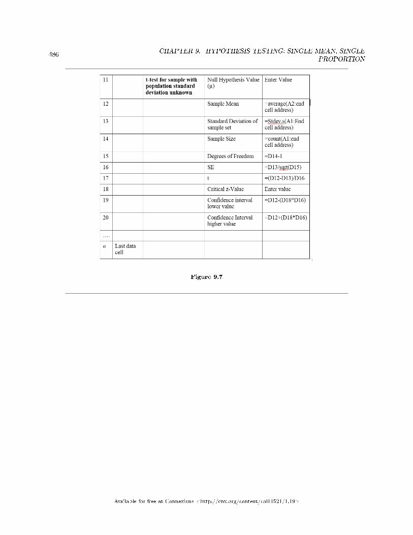
486CHAPTER 9. HYPOTHESIS TESTING: SINGLE MEAN, SINGLE
PROPORTION
Figure 9.7
Available for free at Connexions <http://cnx.org/content/col11521/1.19>
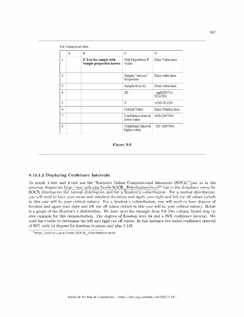
487
Figure 9.8
9.15.1.2 Displaying Con�dence Intervals:
To graph T-test and Z-test use the �Statistics Online Computational Resources (SOCR)�(just as in theprevious chapter)at http://socr.ucla.edu/htmls/SOCR_Distributions.html16 has in the dropdown menu forSOCR distribution the normal distribution and for a Student's t-distribution. For a normal distribution,you will need to have your mean and standard deviation and again your right and left cut o� values (whichin this case will be your critical values). For a Student's t-distribution, you will need to have degrees offreedom and again your right and left cut o� values (which in this case will be your critical values). Belowis a graph of the Student's t-distribution. We have used the example from 8.6 Two column Model step bystep example for this demonstration. The degrees of freedom were 14 and a 95% con�dence interval. Weused the t-table to determine the left and right cut o� values. In this instance two tailed con�dence intervalof 95% with 14 degrees for freedom is minus and plus 2.145.
16http://socr.ucla.edu/htmls/SOCR_Distributions.html
Available for free at Connexions <http://cnx.org/content/col11521/1.19>
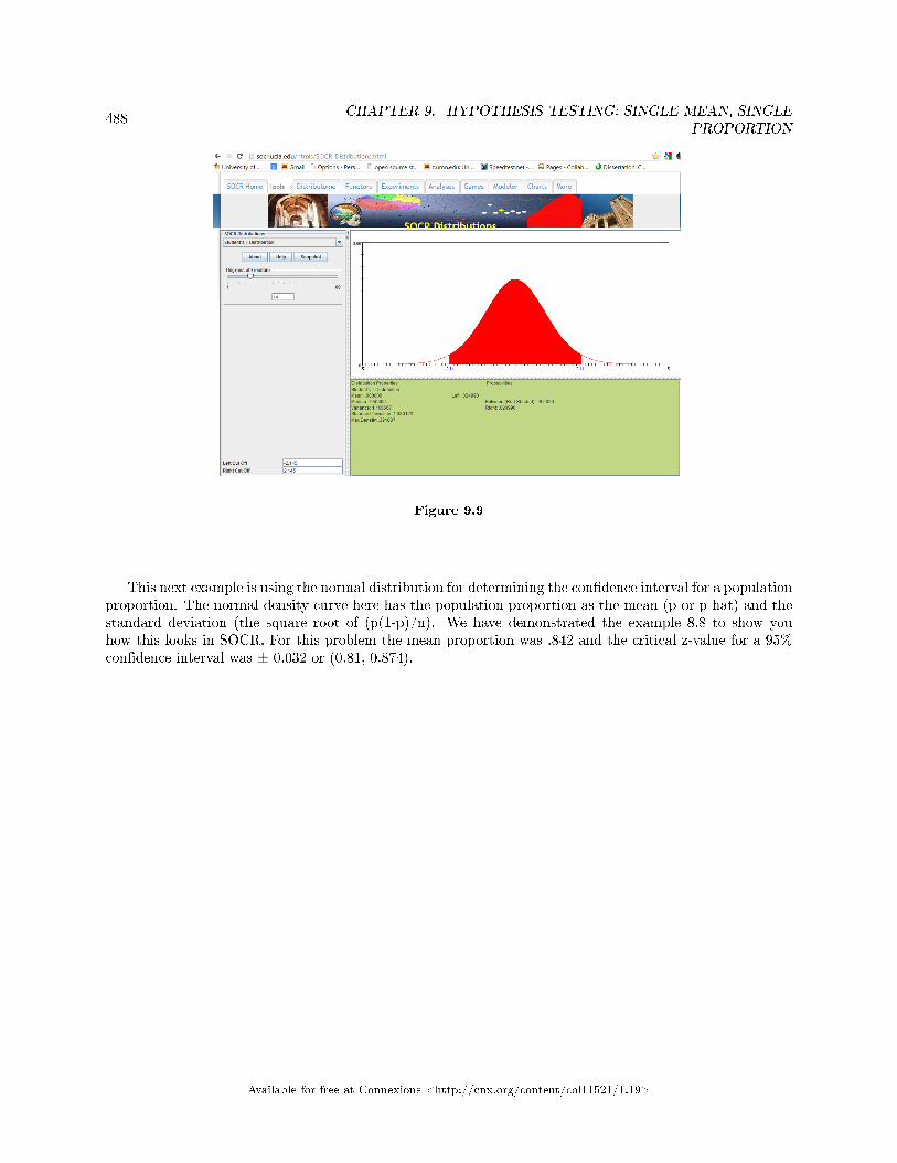
488CHAPTER 9. HYPOTHESIS TESTING: SINGLE MEAN, SINGLE
PROPORTION
Figure 9.9
This next example is using the normal distribution for determining the con�dence interval for a populationproportion. The normal density curve here has the population proportion as the mean (p or p-hat) and thestandard deviation (the square root of (p(1-p)/n). We have demonstrated the example 8.8 to show youhow this looks in SOCR. For this problem the mean proportion was .842 and the critical z-value for a 95%con�dence interval was ± 0.032 or (0.81, 0.874).
Available for free at Connexions <http://cnx.org/content/col11521/1.19>

489
Figure 9.10
9.15.1.3 Optional Classroom Exercise:
At your computer, try to use some of these tools to work out your homework problems or check homeworkthat you have completed to see if the results are the same or similar.
Available for free at Connexions <http://cnx.org/content/col11521/1.19>
490CHAPTER 9. HYPOTHESIS TESTING: SINGLE MEAN, SINGLE
PROPORTION
9.16 Hypothesis Testing of Single Mean and Single Proportion: Sum-mary of Formulas17
Ho and Ha are contradictory.
If Ho has: equal (=) greater than or equalto in problem statementstill translates to equalto (=)
less than or equal to inproblem statement stilltranslates to equal to(=)
then Ha has: not equal ( 6=) or greaterthan (> ) or less than(< )
less than (< ) greater than (> )
Table 9.8
If α ≤ p-value, then do not reject Ho.If α > p-value, then reject Ho .α is preconceived. Its value is set before the hypothesis test starts. The p-value is calculated from the
data.α = probability of a Type I error = P(Type I error) = probability of rejecting the null hypothesis when
the null hypothesis is true.β = probability of a Type II error = P(Type II error) = probability of not rejecting the null hypothesis
when the null hypothesis is false.If there is no given preconceived α, then use α = 0.05.
Types of Hypothesis Tests
• Single population mean, known population variance (or standard deviation): Normal test.• Single population mean, unknown population variance (or standard deviation): Student's-t test.• Single population proportion: Normal test.
9.16.1 Glossary
Binomial DistributionA discrete random variable (RV) which arises from Bernoulli trials. There are a �xed number, n, of indepen-dent trials. �Independent� means that the result of any trial (for example, trial 1) does not a�ect the resultsof the following trials, and all trials are conducted under the same conditions. Under these circumstancesthe binomial RV X is de�ned as the number of successes in n trials. The notation is: X∼B (n, p). Themean is µ = np and the standard deviation is σ =
√npq. The probability of exactly x successes in n trials
is P (X = x) =(nx
)pxqn−x.
Central Limit TheoremGiven a random variable (RV) with known mean µ and known standard deviation σ. We are sampling withsize n and we are interested in two new RVs - the sample mean, x, and the sample sum, ΣX. If the size n of
the sample is su�ciently large, then X ∼ N(µX ,
σX√n
)and ΣX ∼ N(nµ,
√nσ). If the size n of the sample
is su�ciently large, then the distribution of the sample means and the distribution of the sample sums willapproximate a normal distribution regardless of the shape of the population. The mean of the sample meanswill equal the population mean and the mean of the sample sums will equal n times the population mean.The standard deviation of the distribution of the sample means, σ√
nis called the standard error of the mean.
17This content is available online at <http://cnx.org/content/m46722/1.3/>.
Available for free at Connexions <http://cnx.org/content/col11521/1.19>
491
Con�dence Interval (CI)An interval estimate for an unknown population parameter. This depends on:(1). The desired con�dence level.(2). Information that is known about the distribution (for example, known standard deviation).(3). The sample and its size.HypothesisA statement about the value of a population parameter. In case of two hypotheses, the statement assumedto be true is called the null hypothesis (notation Ho ) and the contradictory statement is called the alternatehypothesis (notation Ha).Hypothesis TestingBased on sample evidence, a procedure to determine whether the hypothesis stated is a reasonable statementand cannot be rejected, or is unreasonable and should be rejected.Level of Signi�cance TestProbability of a Type I error (reject the null hypothesis when it is true). Notation: α. In hypothesis testing,the Level of Signi�cance is called the preconceived α or the preset α.Normal DistributionA continuous random variable (RV) with pdf f(x) = 1
σ√
2πe−(x−µ)2/2σ2, where µ is the mean of the distri-
bution and σ is the standard deviation. Notation: X ∼ N (µ, σ). If µ = 0 and σ = 1, the RV is called thestandard normal distribution.P-ValueThe probability that an event will happen purely by chance assuming the null hypothesis is true. The smallerthe p-value, the stronger the evidence is against the null hypothesis.Standard DeviationA number that is equal to the square root of the variance and measures how far data values are from theirmean. Notation: s for sample standard deviation and σ for population standard deviation.Student's-t DistributionInvestigated and reported by William S. Gossett in 1908 and published under the pseudonym Student. Themajor characteristics of the random variable (RV) are:(1). It is continuous and assumes any real values.(2). The pdf is symmetrical about its mean of zero. However, it is more spread out and �atter at the apexthan the normal distribution.(3). It approaches the standard normal distribution as n gets larger.(4). There is a "family" of t distributions: every representative of the family is completely de�ned by thenumber of degrees of freedom which is one less than the number of data.Type 1 ErrorThe decision is to reject the Null hypothesis when, in fact, the Null hypothesis is true.Type 2 ErrorThe decision is to not reject the Null hypothesis when, in fact, the Null hypothesis is false.
Available for free at Connexions <http://cnx.org/content/col11521/1.19>
492CHAPTER 9. HYPOTHESIS TESTING: SINGLE MEAN, SINGLE
PROPORTION
9.17 Hypothesis Testing of Single Mean and Single Proportion: Prac-tice 218
9.17.1 Student Learning Outcomes
• The student will conduct a hypothesis test of a single mean with unknown population standard devi-ation.
• The student will demonstrate their usage of the "Two Column Model" to conduct a hypothesis test ofa single mean with unknown population standard deviation.
9.17.2 Given
A random survey of 75 death row inmates revealed that the mean length of time on death row is 17.4 yearswith a standard deviation of 6.3 years. Could the population mean time on death row be di�erent than 15years. Test at a 5% signi�cance level.
Use the 'Two Column Model" to perform a step by step hypothesis test for the above problem. Examplesare included in the book and a form is also available in your course management system.
9.17.3 Hypothesis Testing: Single Mean
Exercise 9.17.1 (Solution on p. 511.)
Is this a test of means or proportions?
Exercise 9.17.2 (Solution on p. 511.)
State the null and alternative hypotheses.
a. Ho :b. Ha :
Exercise 9.17.3 (Solution on p. 511.)
Is this a right-tailed, left-tailed, or two-tailed test? How do you know?
Exercise 9.17.4 (Solution on p. 511.)
What symbol represents the Random Variable for this test?
Exercise 9.17.5 (Solution on p. 511.)
In words, de�ne the Random Variable for this test.
Exercise 9.17.6 (Solution on p. 511.)
Is the population standard deviation known and, if so, what is it?
Exercise 9.17.7 (Solution on p. 511.)
Calculate the following:
a. x =b. 6.3 =c. n =
Exercise 9.17.8 (Solution on p. 511.)
Which test should be used? In 1 -2 complete sentences, explain why.
Exercise 9.17.9 (Solution on p. 511.)
State the distribution to use for the hypothesis test.
18This content is available online at <http://cnx.org/content/m46728/1.2/>.
Available for free at Connexions <http://cnx.org/content/col11521/1.19>
493
Exercise 9.17.10Sketch a graph of the situation. Label the horizontal axis. Mark the hypothesized mean and thesample mean, x. Shade the area corresponding to the p-value.
Figure 9.11
Exercise 9.17.11 (Solution on p. 511.)
Find the p-value.
Exercise 9.17.12 (Solution on p. 511.)
At a pre-conceived α = 0.05, what is your:
a. Decision:b. Reason for the decision:c. Conclusion (write out in a complete sentence):
9.17.4 Discussion Question
Does it appear that the mean time on death row could be 15 years? Why or why not?
Available for free at Connexions <http://cnx.org/content/col11521/1.19>
494CHAPTER 9. HYPOTHESIS TESTING: SINGLE MEAN, SINGLE
PROPORTION
9.18 Hypothesis Testing of Single Mean and Single Proportion: Prac-tice 319
9.18.1 Student Learning Outcomes
• The student will conduct a hypothesis test of a single population proportion.• The student will used the 'Two Column Model" to conduct a hypothesis test of a single population
proportion.
9.18.2 Given
The National Institute of Mental Health published an article stating that in any one-year pe-riod, approximately 9.5 percent of American adults su�er from depression or a depressive illness.(http://www.nimh.nih.gov/publicat/depression.cfm) Suppose that in a survey of 100 people in a certaintown, seven of them su�ered from depression or a depressive illness. Determine if the true proportion ofpeople in that town su�ering from depression or a depressive illness is lower than the percent in the generaladult American population. Conduct the hypothesis test using a 5% con�dence level.
Use the 'Two Column Model' as presented in this chapter to conduct this hypothesis test. A blank formis available in your course management system.
9.18.3 Hypothesis Testing: Single Proportion
Exercise 9.18.1 (Solution on p. 511.)
Is this a test of means or proportions?
Exercise 9.18.2 (Solution on p. 511.)
State the null and alternative hypotheses.
a. Ho :b. Ha :
Exercise 9.18.3 (Solution on p. 511.)
Is this a right-tailed, left-tailed, or two-tailed test? How do you know?
Exercise 9.18.4 (Solution on p. 511.)
What symbol represents the Random Variable for this test?
Exercise 9.18.5 (Solution on p. 511.)
In words, de�ne the Random Variable for this test.
Exercise 9.18.6 (Solution on p. 511.)
Calculate the following:
a: x =b: n =c: p̂ =
Exercise 9.18.7 (Solution on p. 512.)
Calculate σp̂. Make sure to show how you set up the formula.
Exercise 9.18.8 (Solution on p. 512.)
State the distribution to use for the hypothesis test.
19This content is available online at <http://cnx.org/content/m46729/1.2/>.
Available for free at Connexions <http://cnx.org/content/col11521/1.19>
495
Exercise 9.18.9Sketch a graph of the situation. Label the horizontal axis. Mark the hypothesized mean and thesample proportion, p-hat. Shade the area corresponding to the p-value.
Exercise 9.18.10 (Solution on p. 512.)
Find the p-value
Exercise 9.18.11 (Solution on p. 512.)
At a pre-conceived α = 0.05, what is your:
a. Decision:b. Reason for the decision:c. Conclusion (write out in a complete sentence):
9.18.4 Discusion Question
Exercise 9.18.12Does it appear that the proportion of people in that town with depression or a depressive illnessis lower than general adult American population? Why or why not?
Available for free at Connexions <http://cnx.org/content/col11521/1.19>
496CHAPTER 9. HYPOTHESIS TESTING: SINGLE MEAN, SINGLE
PROPORTION
9.19 Hypothesis Testing: Hypothesis Testing of Single Mean andSingle Proportion: Homework20
Exercise 9.19.1 (Solution on p. 512.)
Some of the statements below refer to the null hypothesis, some to the alternate hypothesis.State the null hypothesis, Ho, and the alternative hypothesis, Ha, in terms of the appropriate
parameter (µ or p).
a. The mean number of years Americans work before retiring is 34.b. At most 60% of Americans vote in presidential elections.c. The mean starting salary for San Jose State University graduates is at least $100,000 per year.d. 29% of high school seniors get drunk each month.e. Fewer than 5% of adults ride the bus to work in Los Angeles.f. The mean number of cars a person owns in her lifetime is not more than 10.g. About half of Americans prefer to live away from cities, given the choice.h. Europeans have a mean paid vacation each year of six weeks.i. The chance of developing breast cancer is under 11% for women.j. Private universities mean tuition cost is more than $20,000 per year.
Exercise 9.19.2 (Solution on p. 512.)
For (a) - (j) above, state the Type I and Type II errors in complete sentences.
Exercise 9.19.3For (a) - (j) above, in complete sentences:
a. State a consequence of committing a Type I error.b. State a consequence of committing a Type II error.
Directions: For each of the word problems, use a 'Two Column Model' solution sheet to dothe hypothesis test. The model is used within this chapter and extra forms are in your coursemanagement system. Alternatively, Your instructor may assign the solution sheet. The solutionsheet is found in 14. Appendix (online book version: the link is "Solution Sheets"; PDF bookversion: look under 14.5 Solution Sheets). Please feel free to make copies of the solution sheets.For the online version of the book, it is suggested that you copy the .doc or the .pdf �les.
note: If you are using a student's-t distribution for a homework problem below, you may assumethat the underlying population is normally distributed. (In general, you must �rst prove thatassumption, though.)
Exercise 9.19.4A particular brand of tires claims that its deluxe tire averages at least 50,000 miles before it needsto be replaced. From past studies of this tire, the standard deviation is unknown. A survey ofowners of that tire design is conducted. From the 28 tires surveyed, the mean lifespan was 46,500miles with a standard deviation of 9800 miles. Do the data support the claim at the 5% level?
Exercise 9.19.5The cost of a daily newspaper varies from city to city. The standard deviation is unknown. Astudy was done to test the claim that the mean cost of a daily newspaper is $1.00. Twelve costsyield a mean cost of 95¢ with a standard deviation of 18¢. Do the data support the claim at the1% level?
20This content is available online at <http://cnx.org/content/m46730/1.3/>.
Available for free at Connexions <http://cnx.org/content/col11521/1.19>
497
Exercise 9.19.6 (Solution on p. 512.)
An article in the San Jose Mercury News stated that students in the California state universitysystem take 4.5 years, on average, to �nish their undergraduate degrees. Suppose you believe thatthe mean time is longer. You conduct a survey of 49 students and obtain a sample mean of 5.1with a sample standard deviation of 1.2. Do the data support your claim at the 1% level?
Exercise 9.19.7The mean number of sick days an employee takes per year is believed to be about 10. Members ofa personnel department do not believe this �gure. They randomly survey 8 employees. The numberof sick days they took for the past year are as follows: 12; 4; 15; 3; 11; 8; 6; 8. Let x = the numberof sick days they took for the past year. Should the personnel team believe that the mean numberis about 10?
Exercise 9.19.8 (Solution on p. 512.)
In 1955, Life Magazine reported that the 25 year-old mother of three worked, on average, an 80hour week. Recently, many groups have been studying whether or not the women's movement has,in fact, resulted in an increase in the average work week for women (combining employment andat-home work). Suppose a study was done to determine if the mean work week has increased. 81women were surveyed with the following results. The sample mean was 83; the sample standarddeviation was 10. Does it appear that the mean work week has increased for women at the 5%level?
Exercise 9.19.9Your statistics instructor claims that 60 percent of the students who take her Elementary Statisticsclass go through life feeling more enriched. For some reason that she can't quite �gure out, mostpeople don't believe her. You decide to check this out on your own. You randomly survey 64 ofher past Elementary Statistics students and �nd that 34 feel more enriched as a result of her class.Now, what do you think?
Exercise 9.19.10 (Solution on p. 512.)
A Nissan Motor Corporation advertisement read, �The average man's I.Q. is 107. The averagebrown trout's I.Q. is 4. So why can't man catch brown trout?� Suppose you believe that the browntrout's mean I.Q. is greater than 4. You catch 12 brown trout. A �sh psychologist determines theI.Q.s as follows: 5; 4; 7; 3; 6; 4; 5; 3; 6; 3; 8; 5. Conduct a hypothesis test of your belief.
Exercise 9.19.11Refer to the previous problem. Conduct a hypothesis test to see if your decision and conclusionwould change if your belief were that the brown trout's mean I.Q. is not 4.
Exercise 9.19.12 (Solution on p. 513.)
According to an article in Newsweek, the natural ratio of girls to boys is 100:105. In China, thebirth ratio is 100: 114 (46.7% girls). Suppose you don't believe the reported �gures of the percentof girls born in China. You conduct a study. In this study, you count the number of girls and boysborn in 150 randomly chosen recent births. There are 60 girls and 90 boys born of the 150. Basedon your study, do you believe that the percent of girls born in China is 46.7?
Exercise 9.19.13A poll done for Newsweek found that 13% of Americans have seen or sensed the presence of anangel. A contingent doubts that the percent is really that high. It conducts its own survey. Outof 76 Americans surveyed, only 2 had seen or sensed the presence of an angel. As a result of thecontingent's survey, would you agree with the Newsweek poll? In complete sentences, also givethree reasons why the two polls might give di�erent results.
Exercise 9.19.14 (Solution on p. 513.)
The mean work week for engineers in a start-up company is believed to be about 60 hours. Anewly hired engineer hopes that it's shorter. She asks 10 engineering friends in start-ups for the
Available for free at Connexions <http://cnx.org/content/col11521/1.19>
498CHAPTER 9. HYPOTHESIS TESTING: SINGLE MEAN, SINGLE
PROPORTION
lengths of their mean work weeks. Based on the results that follow, should she count on the meanwork week to be shorter than 60 hours?
Data (length of mean work week): 70; 45; 55; 60; 65; 55; 55; 60; 50; 55.
Exercise 9.19.15Use the �Lap time� data for Lap 4 (see Table of Contents) to test the claim that Terri �nishes Lap4, on average, in less than 129 seconds. Use all twenty races given.
Exercise 9.19.16Use the �Initial Public O�ering� data (see Table of Contents) to test the claim that the mean o�erprice was $18 per share. Do not use all the data. Use your random number generator to randomlysurvey 15 prices.
note: The following questions were written by past students. They are excellent problems!
Exercise 9.19.1718. "Asian Family Reunion" by Chau Nguyen
Every two years it comes around
We all get together from different towns.
In my honest opinion
It's not a typical family reunion
Not forty, or fifty, or sixty,
But how about seventy companions!
The kids would play, scream, and shout
One minute they're happy, another they'll pout.
The teenagers would look, stare, and compare
From how they look to what they wear.
The men would chat about their business
That they make more, but never less.
Money is always their subject
And there's always talk of more new projects.
The women get tired from all of the chats
They head to the kitchen to set out the mats.
Some would sit and some would stand
Eating and talking with plates in their hands.
Then come the games and the songs
And suddenly, everyone gets along!
With all that laughter, it's sad to say
That it always ends in the same old way.
They hug and kiss and say "good-bye"
And then they all begin to cry!
I say that 60 percent shed their tears
But my mom counted 35 people this year.
She said that boys and men will always have their pride,
So we won't ever see them cry.
I myself don't think she's correct,
So could you please try this problem to see if you object?
Exercise 9.19.18 (Solution on p. 513.)
"The Problem with Angels" by Cyndy Dowling
Available for free at Connexions <http://cnx.org/content/col11521/1.19>
499
Although this problem is wholly mine,
The catalyst came from the magazine, Time.
On the magazine cover I did find
The realm of angels tickling my mind.
Inside, 69% I found to be
In angels, Americans do believe.
Then, it was time to rise to the task,
Ninety-five high school and college students I did ask.
Viewing all as one group,
Random sampling to get the scoop.
So, I asked each to be true,
"Do you believe in angels?" Tell me, do!
Hypothesizing at the start,
Totally believing in my heart
That the proportion who said yes
Would be equal on this test.
Lo and behold, seventy-three did arrive,
Out of the sample of ninety-five.
Now your job has just begun,
Solve this problem and have some fun.
Exercise 9.19.19"Blowing Bubbles" by Sondra Prull
Studying stats just made me tense,
I had to find some sane defense.
Some light and lifting simple play
To float my math anxiety away.
Blowing bubbles lifts me high
Takes my troubles to the sky.
POIK! They're gone, with all my stress
Bubble therapy is the best.
The label said each time I blew
The average number of bubbles would be at least 22.
I blew and blew and this I found
From 64 blows, they all are round!
But the number of bubbles in 64 blows
Varied widely, this I know.
20 per blow became the mean
They deviated by 6, and not 16.
Available for free at Connexions <http://cnx.org/content/col11521/1.19>
500CHAPTER 9. HYPOTHESIS TESTING: SINGLE MEAN, SINGLE
PROPORTION
From counting bubbles, I sure did relax
But now I give to you your task.
Was 22 a reasonable guess?
Find the answer and pass this test!
Exercise 9.19.20 (Solution on p. 513.)
21. "Dalmatian Darnation" by Kathy Sparling
A greedy dog breeder named Spreckles
Bred puppies with numerous freckles
The Dalmatians he sought
Possessed spot upon spot
The more spots, he thought, the more shekels.
His competitors did not agree
That freckles would increase the fee.
They said, ``Spots are quite nice
But they don't affect price;
One should breed for improved pedigree.''
The breeders decided to prove
This strategy was a wrong move.
Breeding only for spots
Would wreak havoc, they thought.
His theory they want to disprove.
They proposed a contest to Spreckles
Comparing dog prices to freckles.
In records they looked up
One hundred one pups:
Dalmatians that fetched the most shekels.
They asked Mr. Spreckles to name
An average spot count he'd claim
To bring in big bucks.
Said Spreckles, ``Well, shucks,
It's for one hundred one that I aim.''
Said an amateur statistician
Who wanted to help with this mission.
``Twenty-one for the sample
Standard deviation's ample:
They examined one hundred and one
Dalmatians that fetched a good sum.
They counted each spot,
Mark, freckle and dot
And tallied up every one.
Available for free at Connexions <http://cnx.org/content/col11521/1.19>
501
Instead of one hundred one spots
They averaged ninety six dots
Can they muzzle Spreckles'
Obsession with freckles
Based on all the dog data they've got?
Exercise 9.19.21"Macaroni and Cheese, please!!" by Nedda Misherghi and Rachelle Hall
As a poor starving student I don't have much money to spend for even the bare necessities. Somy favorite and main staple food is macaroni and cheese. It's high in taste and low in cost andnutritional value.
One day, as I sat down to determine the meaning of life, I got a serious craving for this, oh, soimportant, food of my life. So I went down the street to Greatway to get a box of macaroni andcheese, but it was SO expensive! $2.02 !!! Can you believe it? It made me stop and think. Theworld is changing fast. I had thought that the mean cost of a box (the normal size, not some super-gigantic-family-value-pack) was at most $1, but now I wasn't so sure. However, I was determinedto �nd out. I went to 53 of the closest grocery stores and surveyed the prices of macaroni andcheese. Here are the data I wrote in my notebook:
Price per box of Mac and Cheese:
• 5 stores @ $2.02• 15 stores @ $0.25• 3 stores @ $1.29• 6 stores @ $0.35• 4 stores @ $2.27• 7 stores @ $1.50• 5 stores @ $1.89• 8 stores @ 0.75.
I could see that the costs varied but I had to sit down to �gure out whether or not I was right. Ifit does turn out that this mouth-watering dish is at most $1, then I'll throw a big cheesy party inour next statistics lab, with enough macaroni and cheese for just me. (After all, as a poor starvingstudent I can't be expected to feed our class of animals!)
Exercise 9.19.22 (Solution on p. 513.)
"William Shakespeare: The Tragedy of Hamlet, Prince of Denmark" by Jacqueline Ghodsi
THE CHARACTERS (in order of appearance):
• HAMLET, Prince of Denmark and student of Statistics• POLONIUS, Hamlet's tutor• HOROTIO, friend to Hamlet and fellow student
Scene: The great library of the castle, in which Hamlet does his lessonsAct I(The day is fair, but the face of Hamlet is clouded. He paces the large room. His tutor, Polonius,
is reprimanding Hamlet regarding the latter's recent experience. Horatio is seated at the large tableat right stage.)
POLONIUS: My Lord, how cans't thou admit that thou hast seen a ghost! It is but a �gmentof your imagination!
HAMLET: I beg to di�er; I know of a certainty that �ve-and-seventy in one hundred of us,condemned to the whips and scorns of time as we are, have gazed upon a spirit of health, or goblindamn'd, be their intents wicked or charitable.
POLONIUS If thou doest insist upon thy wretched vision then let me invest your time; be trueto thy work and speak to me through the reason of the null and alternate hypotheses. (He turns to
Available for free at Connexions <http://cnx.org/content/col11521/1.19>
502CHAPTER 9. HYPOTHESIS TESTING: SINGLE MEAN, SINGLE
PROPORTION
Horatio.) Did not Hamlet himself say, �What piece of work is man, how noble in reason, how in�nitein faculties? Then let not this foolishness persist. Go, Horatio, make a survey of three-and-sixtyand discover what the true proportion be. For my part, I will never succumb to this fantasy, butdeem man to be devoid of all reason should thy proposal of at least �ve-and-seventy in one hundredhold true.
HORATIO (to Hamlet): What should we do, my Lord?HAMLET: Go to thy purpose, Horatio.HORATIO: To what end, my Lord?HAMLET: That you must teach me. But let me conjure you by the rights of our fellowship, by
the consonance of our youth, but the obligation of our ever-preserved love, be even and direct withme, whether I am right or no.
(Horatio exits, followed by Polonius, leaving Hamlet to ponder alone.)Act II(The next day, Hamlet awaits anxiously the presence of his friend, Horatio. Polonius enters and
places some books upon the table just a moment before Horatio enters.)POLONIUS: So, Horatio, what is it thou didst reveal through thy deliberations?HORATIO: In a random survey, for which purpose thou thyself sent me forth, I did discover
that one-and-forty believe fervently that the spirits of the dead walk with us. Before my God, Imight not this believe, without the sensible and true avouch of mine own eyes.
POLONIUS: Give thine own thoughts no tongue, Horatio. (Polonius turns to Hamlet.) Butlook to't I charge you, my Lord. Come Horatio, let us go together, for this is not our test. (Horatioand Polonius leave together.)
HAMLET: To reject, or not reject, that is the question: whether `tis nobler in the mind tosu�er the slings and arrows of outrageous statistics, or to take arms against a sea of data, and, byopposing, end them. (Hamlet resignedly attends to his task.)
(Curtain falls)
Exercise 9.19.23"Untitled" by Stephen Chen
I've often wondered how software is released and sold to the public. Ironically, I work fora company that sells products with known problems. Unfortunately, most of the problems aredi�cult to create, which makes them di�cult to �x. I usually use the test program X, which teststhe product, to try to create a speci�c problem. When the test program is run to make an erroroccur, the likelihood of generating an error is 1%.
So, armed with this knowledge, I wrote a new test program Y that will generate the same errorthat test program X creates, but more often. To �nd out if my test program is better than theoriginal, so that I can convince the management that I'm right, I ran my test program to �nd outhow often I can generate the same error. When I ran my test program 50 times, I generated theerror twice. While this may not seem much better, I think that I can convince the management touse my test program instead of the original test program. Am I right?
Exercise 9.19.24 (Solution on p. 513.)
Japanese Girls' Namesby Kumi FuruichiIt used to be very typical for Japanese girls' names to end with �ko.� (The trend might have
started around my grandmothers' generation and its peak might have been around my mother'sgeneration.) �Ko� means �child� in Chinese character. Parents would name their daughters with�ko� attaching to other Chinese characters which have meanings that they want their daughters tobecome, such as Sachiko � a happy child, Yoshiko � a good child, Yasuko � a healthy child, and soon.
However, I noticed recently that only two out of nine of my Japanese girlfriends at this schoolhave names which end with �ko.� More and more, parents seem to have become creative, modern-ized, and, sometimes, westernized in naming their children.
Available for free at Connexions <http://cnx.org/content/col11521/1.19>
503
I have a feeling that, while 70 percent or more of my mother's generation would have nameswith �ko� at the end, the proportion has dropped among my peers. I wrote down all my Japanesefriends', ex-classmates', co-workers, and acquaintances' names that I could remember. Below arethe names. (Some are repeats.) Test to see if the proportion has dropped for this generation.
Ai, Akemi, Akiko, Ayumi, Chiaki, Chie, Eiko, Eri, Eriko, Fumiko, Harumi, Hitomi, Hiroko, Hi-roko, Hidemi, Hisako, Hinako, Izumi, Izumi, Junko, Junko, Kana, Kanako, Kanayo, Kayo, Kayoko,Kazumi, Keiko, Keiko, Kei, Kumi, Kumiko, Kyoko, Kyoko, Madoka, Maho, Mai, Maiko, Maki,Miki, Miki, Mikiko, Mina, Minako, Miyako, Momoko, Nana, Naoko, Naoko, Naoko, Noriko, Rieko,Rika, Rika, Rumiko, Rei, Reiko, Reiko, Sachiko, Sachiko, Sachiyo, Saki, Sayaka, Sayoko, Sayuri,Seiko, Shiho, Shizuka, Sumiko, Takako, Takako, Tomoe, Tomoe, Tomoko, Touko, Yasuko, Yasuko,Yasuyo, Yoko, Yoko, Yoko, Yoshiko, Yoshiko, Yoshiko, Yuka, Yuki, Yuki, Yukiko, Yuko, Yuko.
Exercise 9.19.25Phillip's Wish by Suzanne Osorio
My nephew likes to play
Chasing the girls makes his day.
He asked his mother
If it is okay
To get his ear pierced.
She said, ``No way!''
To poke a hole through your ear,
Is not what I want for you, dear.
He argued his point quite well,
Says even my macho pal, Mel,
Has gotten this done.
It's all just for fun.
C'mon please, mom, please, what the hell.
Again Phillip complained to his mother,
Saying half his friends (including their brothers)
Are piercing their ears
And they have no fears
He wants to be like the others.
She said, ``I think it's much less.
We must do a hypothesis test.
And if you are right,
I won't put up a fight.
But, if not, then my case will rest.''
We proceeded to call fifty guys
To see whose prediction would fly.
Nineteen of the fifty
Said piercing was nifty
And earrings they'd occasionally buy.
Then there's the other thirty-one,
Who said they'd never have this done.
So now this poem's finished.
Will his hopes be diminished,
Or will my nephew have his fun?
Exercise 9.19.26 (Solution on p. 513.)
The Craven by Mark Salangsang
Once upon a morning dreary
Available for free at Connexions <http://cnx.org/content/col11521/1.19>
504CHAPTER 9. HYPOTHESIS TESTING: SINGLE MEAN, SINGLE
PROPORTION
In stats class I was weak and weary.
Pondering over last night's homework
Whose answers were now on the board
This I did and nothing more.
While I nodded nearly napping
Suddenly, there came a tapping.
As someone gently rapping,
Rapping my head as I snore.
Quoth the teacher, ``Sleep no more.''
``In every class you fall asleep,''
The teacher said, his voice was deep.
``So a tally I've begun to keep
Of every class you nap and snore.
The percentage being forty-four.''
``My dear teacher I must confess,
While sleeping is what I do best.
The percentage, I think, must be less,
A percentage less than forty-four.''
This I said and nothing more.
``We'll see,'' he said and walked away,
And fifty classes from that day
He counted till the month of May
The classes in which I napped and snored.
The number he found was twenty-four.
At a significance level of 0.05,
Please tell me am I still alive?
Or did my grade just take a dive
Plunging down beneath the floor?
Upon thee I hereby implore.
Exercise 9.19.27Toastmasters International cites a report by Gallop Poll that 40% of Americans fear publicspeaking. A student believes that less than 40% of students at her school fear public speaking.She randomly surveys 361 schoolmates and �nds that 135 report they fear public speaking.Conduct a hypothesis test to determine if the percent at her school is less than 40%. (Source:http://toastmasters.org/artisan/detail.asp?CategoryID=1&SubCategoryID=10&ArticleID=429&Page=121
)
Exercise 9.19.28 (Solution on p. 513.)
68% of online courses taught at community colleges nationwide were taught by full-time faculty.To test if 68% also represents California's percent for full-time faculty teaching the online classes,Long Beach City College (LBCC), CA, was randomly selected for comparison. In the same year, 34of the 44 online courses LBCC o�ered were taught by full-time faculty. Conduct a hypothesis testto determine if 68% represents CA. NOTE: For more accurate results, use more CA community
21http://toastmasters.org/artisan/detail.asp?CategoryID=1&SubCategoryID=10&ArticleID=429&Page=1
Available for free at Connexions <http://cnx.org/content/col11521/1.19>
505
colleges and this past year's data. (Sources: Growing by Degrees by Allen and Seaman; AmitSchitai, Director of Instructional Technology and Distance Learning, LBCC).
Exercise 9.19.29According to an article inBloomberg Businessweek, New York City's most recent adult smokingrate is 14%. Suppose that a survey is conducted to determine this year's rate. Nine out of 70randomly chosen N.Y. City residents reply that they smoke. Conduct a hypothesis test to determineif the rate is still 14% or if it has decreased. (Source: http://www.businessweek.com/news/2011-09-15/nyc-smoking-rate-falls-to-record-low-of-14-bloomberg-says.html22 )
Exercise 9.19.30 (Solution on p. 514.)
The mean age of De Anza College students in a previous term was 26.6 years old. An instructorthinks the mean age for online students is older than 26.6. She randomly surveys 56 online studentsand �nds that the sample mean is 29.4 with a standard deviation of 2.1. Conduct a hypothesistest. (Source: http://research.fhda.edu/factbook/DAdemofs/Fact_sheet_da_2006w.pdf 23 )
Exercise 9.19.31Registered nurses earned an average annual salary of $69,110. For that same year, a survey wasconducted of 41 California registered nurses to determine if the annual salary is higher than $69,110for California nurses. The sample average was $71,121 with a sample standard deviation of $7,489.Conduct a hypothesis test. (Source: http://www.bls.gov/oes/current/oes291111.htm24 )
Exercise 9.19.32 (Solution on p. 514.)
La Leche League International reports that the mean age of weaning a child from breastfeedingis age 4 to 5 worldwide. In America, most nursing mothers wean their children much earlier.Suppose a random survey is conducted of 21 U.S. mothers who recently weaned their children. Themean weaning age was 9 months (3/4 year) with a standard deviation of 4 months. Conduct ahypothesis test to determine if the mean weaning age in the U.S. is less than 4 years old. (Source:http://www.lalecheleague.org/Law/BAFeb01.html25 )
9.19.1 Try these multiple choice questions.
Exercise 9.19.33 (Solution on p. 514.)
When a new drug is created, the pharmaceutical company must subject it to testing before receivingthe necessary permission from the Food and Drug Administration (FDA) to market the drug.Suppose the null hypothesis is �the drug is unsafe.� What is the Type II Error?
A. To conclude the drug is safe when in, fact, it is unsafeB. To not conclude the drug is safe when, in fact, it is safe.C. To conclude the drug is safe when, in fact, it is safe.D. To not conclude the drug is unsafe when, in fact, it is unsafe
The next two questions refer to the following information: Over the past few decades, public healtho�cials have examined the link between weight concerns and teen girls smoking. Researchers surveyed agroup of 273 randomly selected teen girls living in Massachusetts (between 12 and 15 years old). After fouryears the girls were surveyed again. Sixty-three (63) said they smoked to stay thin. Is there good evidencethat more than thirty percent of the teen girls smoke to stay thin?
Exercise 9.19.34 (Solution on p. 514.)
The alternate hypothesis is
22http://www.businessweek.com/news/2011-09-15/nyc-smoking-rate-falls-to-record-low-of-14-bloomberg-says.html23http://research.fhda.edu/factbook/DAdemofs/Fact_sheet_da_2006w.pdf24http://www.bls.gov/oes/current/oes291111.htm25http://www.lalecheleague.org/Law/BAFeb01.html
Available for free at Connexions <http://cnx.org/content/col11521/1.19>
506CHAPTER 9. HYPOTHESIS TESTING: SINGLE MEAN, SINGLE
PROPORTION
A. p < 0.30B. p ≤ 0.30C. p ≥ 0.30D. p > 0.30
Exercise 9.19.35 (Solution on p. 514.)
After conducting the test, your decision and conclusion are
A. Reject Ho: There is su�cient evidence to conclude that more than 30% of teen girls smoke tostay thin.
B. Do not reject Ho: There is not su�cient evidence to conclude that less than 30% of teen girlssmoke to stay thin.
C. Do not reject Ho: There is not su�cient evidence to conclude that more than 30% of teen girlssmoke to stay thin.
D. Reject Ho: There is su�cient evidence to conclude that less than 30% of teen girls smoke tostay thin.
The next three questions refer to the following information: A statistics instructor believes thatfewer than 20% of Evergreen Valley College (EVC) students attended the opening night midnight showingof the latest Harry Potter movie. She surveys 84 of her students and �nds that 11 of attended the midnightshowing.
Exercise 9.19.36 (Solution on p. 514.)
An appropriate alternative hypothesis is
A. p = 0.20B. p > 0.20C. p < 0.20D. p ≤ 0.20
Exercise 9.19.37 (Solution on p. 514.)
At a 1% level of signi�cance, an appropriate conclusion is:
A. There is insu�cient evidence to conclude that the percent of EVC students that attended themidnight showing of Harry Potter is less than 20%.
B. There is su�cient evidence to conclude that the percent of EVC students that attended themidnight showing of Harry Potter is more than 20%.
C. There is su�cient evidence to conclude that the percent of EVC students that attended themidnight showing of Harry Potter is less than 20%.
D. There is insu�cient evidence to conclude that the percent of EVC students that attended themidnight showing of Harry Potter is at least 20%.
Exercise 9.19.38 (Solution on p. 514.)
The Type I error is to conclude that the percent of EVC students who attended is
A. at least 20%, when in fact, it is less than 20%.B. 20%, when in fact, it is 20%.C. less than 20%, when in fact, it is at least 20%.D. less than 20%, when in fact, it is less than 20%.
The next two questions refer to the following information:It is believed that Lake Tahoe Community College (LTCC) Intermediate Algebra students get less than 7
hours of sleep per night, on average. A survey of 22 LTCC Intermediate Algebra students generated a mean
Available for free at Connexions <http://cnx.org/content/col11521/1.19>
507
of 7.24 hours with a standard deviation of 1.93 hours. At a level of signi�cance of 5%, do LTCC IntermediateAlgebra students get less than 7 hours of sleep per night, on average?
Exercise 9.19.39 (Solution on p. 514.)
The distribution to be used for this test is X ∼
A. N(
7.24, 1.93√22
)B. N (7.24, 1.93)C. t22D. t21
Exercise 9.19.40 (Solution on p. 514.)
The Type II error is to not reject that the mean number of hours of sleep LTCC students get pernight is at least 7 when, in fact, the mean number of hours
A. is more than 7 hours.B. is at most 7 hours.C. is at least 7 hours.D. is less than 7 hours.
The next three questions refer to the following information: Previously, an organization reportedthat teenagers spent 4.5 hours per week, on average, on the phone. The organization thinks that, currently,the mean is higher. Fifteen (15) randomly chosen teenagers were asked how many hours per week theyspend on the phone. The sample mean was 4.75 hours with a sample standard deviation of 2.0. Conduct ahypothesis test.
Exercise 9.19.41 (Solution on p. 514.)
The null and alternate hypotheses are:
A. Ho : x = 4.5, Ha : x > 4.5B. Ho : µ ≥ 4.5 Ha : µ < 4.5C. Ho : µ = 4.75 Ha:µ > 4.75D. Ho : µ = 4.5 Ha : µ > 4.5
Exercise 9.19.42 (Solution on p. 514.)
At a signi�cance level of a = 0.05, what is the correct conclusion?
A. There is enough evidence to conclude that the mean number of hours is more than 4.75B. There is enough evidence to conclude that the mean number of hours is more than 4.5C. There is not enough evidence to conclude that the mean number of hours is more than 4.5D. There is not enough evidence to conclude that the mean number of hours is more than 4.75
Exercise 9.19.43 (Solution on p. 514.)
The Type I error is:
A. To conclude that the current mean hours per week is higher than 4.5, when in fact, it is higher.B. To conclude that the current mean hours per week is higher than 4.5, when in fact, it is the
same.C. To conclude that the mean hours per week currently is 4.5, when in fact, it is higher.D. To conclude that the mean hours per week currently is no higher than 4.5, when in fact, it is
not higher.
Available for free at Connexions <http://cnx.org/content/col11521/1.19>
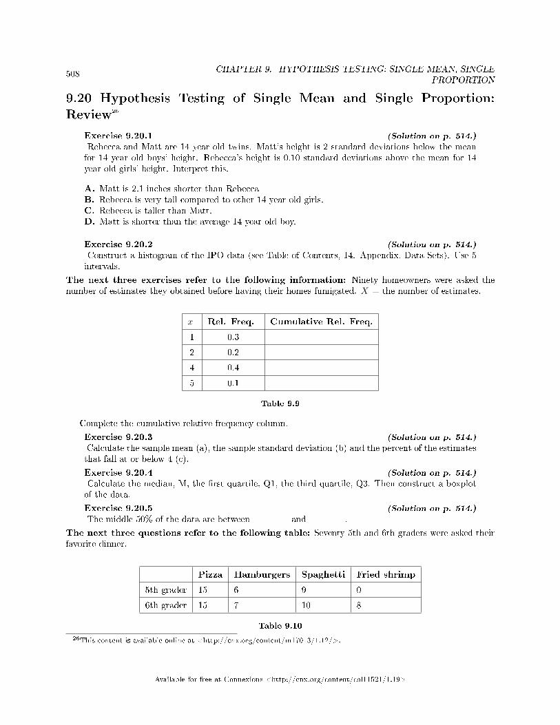
508CHAPTER 9. HYPOTHESIS TESTING: SINGLE MEAN, SINGLE
PROPORTION
9.20 Hypothesis Testing of Single Mean and Single Proportion:Review26
Exercise 9.20.1 (Solution on p. 514.)
Rebecca and Matt are 14 year old twins. Matt's height is 2 standard deviations below the meanfor 14 year old boys' height. Rebecca's height is 0.10 standard deviations above the mean for 14year old girls' height. Interpret this.
A. Matt is 2.1 inches shorter than RebeccaB. Rebecca is very tall compared to other 14 year old girls.C. Rebecca is taller than Matt.D. Matt is shorter than the average 14 year old boy.
Exercise 9.20.2 (Solution on p. 514.)
Construct a histogram of the IPO data (see Table of Contents, 14. Appendix, Data Sets). Use 5intervals.
The next three exercises refer to the following information: Ninety homeowners were asked thenumber of estimates they obtained before having their homes fumigated. X = the number of estimates.
x Rel. Freq. Cumulative Rel. Freq.
1 0.3
2 0.2
4 0.4
5 0.1
Table 9.9
Complete the cumulative relative frequency column.
Exercise 9.20.3 (Solution on p. 514.)
Calculate the sample mean (a), the sample standard deviation (b) and the percent of the estimatesthat fall at or below 4 (c).
Exercise 9.20.4 (Solution on p. 514.)
Calculate the median, M, the �rst quartile, Q1, the third quartile, Q3. Then construct a boxplotof the data.
Exercise 9.20.5 (Solution on p. 514.)
The middle 50% of the data are between _____ and _____.
The next three questions refer to the following table: Seventy 5th and 6th graders were asked theirfavorite dinner.
Pizza Hamburgers Spaghetti Fried shrimp
5th grader 15 6 9 0
6th grader 15 7 10 8
Table 9.10
26This content is available online at <http://cnx.org/content/m17013/1.12/>.
Available for free at Connexions <http://cnx.org/content/col11521/1.19>
509
Exercise 9.20.6 (Solution on p. 514.)
Find the probability that one randomly chosen child is in the 6th grade and prefers fried shrimp.
A. 3270
B. 832
C. 88
D. 870
Exercise 9.20.7 (Solution on p. 515.)
Find the probability that a child does not prefer pizza.
A. 3070
B. 3040
C. 4070
D. 1
Exercise 9.20.8 (Solution on p. 515.)
Find the probability a child is in the 5th grade given that the child prefers spaghetti.
A. 919
B. 970
C. 930
D. 1970
Exercise 9.20.9 (Solution on p. 515.)
A sample of convenience is a random sample.
A. trueB. false
Exercise 9.20.10 (Solution on p. 515.)
A statistic is a number that is a property of the population.
A. trueB. false
Exercise 9.20.11 (Solution on p. 515.)
You should always throw out any data that are outliers.
A. trueB. false
Exercise 9.20.12 (Solution on p. 515.)
Lee bakes pies for a small restaurant in Felton, CA. She generally bakes 20 pies in a day, on theaverage. Of interest is the num.ber of pies she bakes each day
a. De�ne the Random Variable X.b. State the distribution for X.c. Find the probability that Lee bakes more than 25 pies in any given day.
Available for free at Connexions <http://cnx.org/content/col11521/1.19>
510CHAPTER 9. HYPOTHESIS TESTING: SINGLE MEAN, SINGLE
PROPORTION
Exercise 9.20.13 (Solution on p. 515.)
Six di�erent brands of Italian salad dressing were randomly selected at a supermarket. The gramsof fat per serving are 7, 7, 9, 6, 8, 5. Assume that the underlying distribution is normal. Calculatea 95% con�dence interval for the population mean grams of fat per serving of Italian salad dressingsold in supermarkets.
Exercise 9.20.14 (Solution on p. 515.)
Given: uniform, exponential, normal distributions. Match each to a statement below.
a. mean = median 6= modeb. mean > median > modec. mean = median = mode
Available for free at Connexions <http://cnx.org/content/col11521/1.19>
511
Solutions to Exercises in Chapter 9
Solutions to Hypothesis Testing of Single Mean and Single Proportion: Practice2
Solution to Exercise 9.17.1 (p. 492)averagesSolution to Exercise 9.17.2 (p. 492)
a. Ho : µ = 15b. Ha : µ 6= 15
Solution to Exercise 9.17.3 (p. 492)two-tailedSolution to Exercise 9.17.4 (p. 492)XSolution to Exercise 9.17.5 (p. 492)the mean time spent on death row for the 75 inmatesSolution to Exercise 9.17.6 (p. 492)NoSolution to Exercise 9.17.7 (p. 492)
a. 17.4b. sc. 75
Solution to Exercise 9.17.8 (p. 492)t−testSolution to Exercise 9.17.9 (p. 492)t74Solution to Exercise 9.17.11 (p. 493)0.0015Solution to Exercise 9.17.12 (p. 493)
a. Reject the null hypothesis
Solutions to Hypothesis Testing of Single Mean and Single Proportion: Practice3
Solution to Exercise 9.18.1 (p. 494)ProportionsSolution to Exercise 9.18.2 (p. 494)
a. Ho : p = 0.095b. Ha : p < 0.095
Solution to Exercise 9.18.3 (p. 494)left-tailedSolution to Exercise 9.18.4 (p. 494)p̂Solution to Exercise 9.18.5 (p. 494)the proportion of people in that town surveyed su�ering from depression or a depressive illnessSolution to Exercise 9.18.6 (p. 494)
a. 7
Available for free at Connexions <http://cnx.org/content/col11521/1.19>
512CHAPTER 9. HYPOTHESIS TESTING: SINGLE MEAN, SINGLE
PROPORTION
b. 100c. 0.07
Solution to Exercise 9.18.7 (p. 494)0.0293Solution to Exercise 9.18.8 (p. 494)NormalSolution to Exercise 9.18.10 (p. 495)0.1969Solution to Exercise 9.18.11 (p. 495)
a. Do not reject the null hypothesis
Solutions to Hypothesis Testing: Hypothesis Testing of Single Mean and SingleProportion: Homework
Solution to Exercise 9.19.1 (p. 496)
a. Ho : µ = 34 ; Ha : µ 6= 34c. Ho : µ = 100, 000 ; Ha : µ < 100, 000d. Ho : p = 0.29 ; Ha : p 6= 0.29g. Ho : p = 0.50 ; Ha : p 6= 0.50i. Ho : p = 0.11 ; Ha : p < 0.11
Solution to Exercise 9.19.2 (p. 496)
a. Type I error: We conclude that the mean is not 34 years, when it really is 34 years. Type II error: Wedo not conclude that the mean is not 34 years, when it is not really 34 years.
c. Type I error: We conclude that the mean is less than $100,000, when it really is at least $100,000. TypeII error: We do not conclude that the mean is less than $100,000, when it is really less than $100,000.
d. Type I error: We conclude that the proportion of h.s. seniors who get drunk each month is not 29%,when it really is 29%. Type II error: We do not conclude that the proportion of h.s. seniors that getdrunk each month is not 29%, when it is really not 29%.
i. Type I error: We conclude that the proportion is less than 11%, when it is really at least 11%. Type IIerror: We do not conclude that the proportion is less than 11%, when it really is less than 11%.
Solution to Exercise 9.19.6 (p. 497)
e. 3.5f. 0.0005h. Decision: Reject null; Conclusion: µ > 4.5i. (4.7553, 5.4447)
Solution to Exercise 9.19.8 (p. 497)
e. 2.7f. 0.0042h. Decision: Reject Nulli. (80.789, 85.211)
Solution to Exercise 9.19.10 (p. 497)
d. t11e. 1.96f. 0.0380h. Decision: Reject null when a = 0.05 ; do not reject null when a = 0.01
Available for free at Connexions <http://cnx.org/content/col11521/1.19>
513
i. (3.8865, 5.9468)
Solution to Exercise 9.19.12 (p. 497)
e. -1.64f. 0.1000h. Decision: Do not reject nulli. (0.3216, 0.4784)
Solution to Exercise 9.19.14 (p. 497)
d. t9e. -1.33f. 0.1086h. Decision: Do not reject nulli. (51.886, 62.114)
Solution to Exercise 9.19.18 (p. 498)
e. 1.65f. 0.0984h. Decision: Do not reject nulli. (0.6836, 0.8533)
Solution to Exercise 9.19.20 (p. 500)
e. -2.39f. 0.0093h. Decision: Reject nulli. (91.854, 100.15)
Solution to Exercise 9.19.22 (p. 501)
e. -1.82f. 0.0345h. Decision: Do not reject nulli. (0.5331, 0.7685)
Solution to Exercise 9.19.24 (p. 502)
e. z = −2.99f. 0.0014h. Decision: Reject null; Conclusion: p < .70i. (0.4529, 0.6582)
Solution to Exercise 9.19.26 (p. 503)
e. 0.57f. 0.7156h. Decision: Do not reject nulli. (0.3415, 0.6185)
Solution to Exercise 9.19.28 (p. 504)
e. 1.32f. 0.1873h. Decision: Do not reject nulli. (0.65, 0.90)
Available for free at Connexions <http://cnx.org/content/col11521/1.19>
514CHAPTER 9. HYPOTHESIS TESTING: SINGLE MEAN, SINGLE
PROPORTION
Solution to Exercise 9.19.30 (p. 505)
e. 9.98f. 0.0000h. Decision: Reject nulli. (28.8, 30.0)
Solution to Exercise 9.19.32 (p. 505)
e. -44.7f. 0.0000h. Decision: Reject nulli. (0.60, 0.90) - in years
Solution to Exercise 9.19.33 (p. 505)BSolution to Exercise 9.19.34 (p. 505)DSolution to Exercise 9.19.35 (p. 506)CSolution to Exercise 9.19.36 (p. 506)CSolution to Exercise 9.19.37 (p. 506)ASolution to Exercise 9.19.38 (p. 506)CSolution to Exercise 9.19.39 (p. 507)DSolution to Exercise 9.19.40 (p. 507)DSolution to Exercise 9.19.41 (p. 507)DSolution to Exercise 9.19.42 (p. 507)CSolution to Exercise 9.19.43 (p. 507)B
Solutions to Hypothesis Testing of Single Mean and Single Proportion: Review
Solution to Exercise 9.20.1 (p. 508)DSolution to Exercise 9.20.2 (p. 508)No solution provided. There are several ways in which the histogram could be constructed.Solution to Exercise 9.20.3 (p. 508)
a. 2.8b. 1.48c. 90%
Solution to Exercise 9.20.4 (p. 508)M = 3 ; Q1 = 1 ; Q3 = 4Solution to Exercise 9.20.5 (p. 508)1 and 4
Available for free at Connexions <http://cnx.org/content/col11521/1.19>
515
Solution to Exercise 9.20.6 (p. 509)DSolution to Exercise 9.20.7 (p. 509)CSolution to Exercise 9.20.8 (p. 509)ASolution to Exercise 9.20.9 (p. 509)BSolution to Exercise 9.20.10 (p. 509)BSolution to Exercise 9.20.11 (p. 509)BSolution to Exercise 9.20.12 (p. 509)
b. P (20)c. 0.1122
Solution to Exercise 9.20.13 (p. 510)CI: (5.52, 8.48)Solution to Exercise 9.20.14 (p. 510)
a. uniformb. exponentialc. normal
Available for free at Connexions <http://cnx.org/content/col11521/1.19>

516CHAPTER 9. HYPOTHESIS TESTING: SINGLE MEAN, SINGLE
PROPORTION
Available for free at Connexions <http://cnx.org/content/col11521/1.19>
Chapter 10
Hypothesis Testing: Two Means, Two
Proportions
10.1 Hypothesis Testing: Two Population Means and Two PopulationProportions: Introduction1
10.1.1 Student Learning Outcomes
By the end of this chapter, the student should be able to:
• Classify hypothesis tests by type.• Conduct and interpret hypothesis tests for two population means, population standard deviations
unknown.• Conduct and interpret hypothesis tests for two population proportions.
10.1.2 Introduction
Studies often compare two groups. For example, researchers are interested in the e�ect aspirin has inpreventing heart attacks. Over the last few years, newspapers and magazines have reported about variousaspirin studies involving two groups. Typically, one group is given aspirin and the other group is given aplacebo. Then, the heart attack rate is studied over several years.
There are other situations that deal with the comparison of two groups. For example, studies comparevarious diet and exercise programs. Politicians compare the proportion of individuals from di�erent incomebrackets who might vote for them. Students are interested in whether SAT or GRE preparatory coursesreally help raise their scores.
In the previous chapter, you learned to conduct hypothesis tests on single means and single proportions.You will expand upon that in this chapter. You will compare two means or two proportions to each other.The general procedure is still the same, just expanded.
To compare two means or two proportions, you work with two groups. The groups are classi�ed either asindependent ormatched pairs. Independent groupsmean that the two samples taken are independent,that is, sample values selected from one population are not related in any way to sample values selected fromthe other population. Matched pairs consist of two samples that are dependent. The parameter testedusing matched pairs is the population mean. The parameters tested using independent groups are eitherpopulation means or population proportions.
This chapter deals with the following hypothesis tests:
1This content is available online at <http://cnx.org/content/m46781/1.1/>.
Available for free at Connexions <http://cnx.org/content/col11521/1.19>
517
518CHAPTER 10. HYPOTHESIS TESTING: TWO MEANS, TWO
PROPORTIONS
Independent groups (samples are independent)
� Test of two population means.� Test of two population proportions.
10.2 Hypothesis Testing: Two Population Means and Two PopulationProportions: Comparing Two Independent Population Means withUnknown Population Standard Deviations2
10.2.1 Assumptions and Conditions: Two Sample Means Test
When constructing a two sample mean hypothesis test the assumptions and conditions must be met in orderto use the t-distribution model.
Randomization Condition: The data must be sampled randomly. Is one of the good samplingmethodologies discussed in the Sampling and Data chapter being used?Independence Assumption: The sample values must be independent of each other. This meansthat the occurrence of one event has no in�uence on the next event. Usually, if we know that peopleor items were selected randomly we can assume that the independence assumption is met.10% Condition: When the sample is drawn without replacement (usually the case), the samplesize, n, should be no more than 10% of the population. This must be true for both groups.Nearly Normal Condition: This must be met for both groups. To check the nearly normal conditionstart by making a histogram or stemplot of the data for both groups, it is a good idea to make outlierboxplots, too. If the samples are small, less than 15 then the data must be normally distributed. Ifthe sample size is moderate, between 15 and 40, then a little skewing in the data will can be tolerated.With large sample sizes, more than 40, we are concerned about multiple peaks (modes) in the dataand outliers. When discussing nearly normal you should report the sample size, shape and outlier foreach group.Independent Groups: The two groups you are working with must be independent of one another. Isthere reason to believe that one group would have in�uence on the other group? A hypothesis test thatis comparing a group of respondent's pre-test and post-test scores would not be independent. Likewise,groups made by splitting married couples into husband and wife groups would not be independent.
note: The test comparing two independent population means with unknown and possibly unequalpopulation standard deviations is called the Aspin-Welch t-test. The degrees of freedom formulawas developed by Aspin-Welch.
The comparison of two population means is very common. A di�erence between the two samples dependson both the means and the standard deviations. Very di�erent means can occur by chance if there is greatvariation among the individual samples. In order to account for the variation, we take the di�erence ofthe sample means, X1 - X2 , and divide by the standard error (shown below) in order to standardize thedi�erence. The result is a t-score test statistic (shown below).
Because we do not know the population standard deviations, we estimate them using the two samplestandard deviations from our independent samples. For the hypothesis test, we calculate the estimatedstandard deviation, or standard error, of the di�erence in sample means, X1 - X2.
The standard error is: √(S1)2
n1+
(S2)2
n2(10.1)
2This content is available online at <http://cnx.org/content/m46780/1.1/>.
Available for free at Connexions <http://cnx.org/content/col11521/1.19>
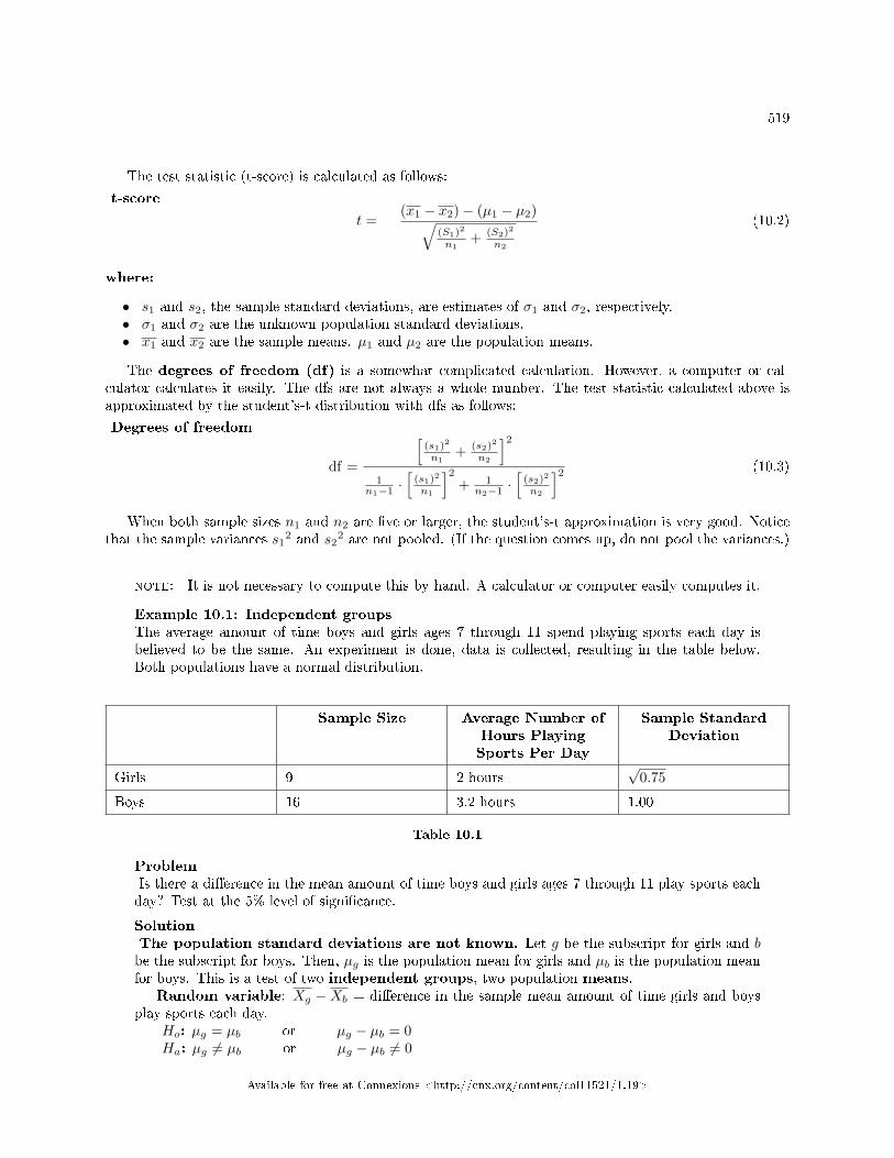
519
The test statistic (t-score) is calculated as follows:
t-score
t =(x1 − x2)− (µ1 − µ2)√
(S1)2
n1+ (S2)2
n2
(10.2)
where:
• s1 and s2, the sample standard deviations, are estimates of σ1 and σ2, respectively.• σ1 and σ2 are the unknown population standard deviations.• x1 and x2 are the sample means. µ1 and µ2 are the population means.
The degrees of freedom (df) is a somewhat complicated calculation. However, a computer or cal-culator calculates it easily. The dfs are not always a whole number. The test statistic calculated above isapproximated by the student's-t distribution with dfs as follows:
Degrees of freedom
df =
[(s1)2
n1+ (s2)2
n2
]21
n1−1 ·[
(s1)2
n1
]2+ 1
n2−1 ·[
(s2)2
n2
]2 (10.3)
When both sample sizes n1 and n2 are �ve or larger, the student's-t approximation is very good. Noticethat the sample variances s1
2 and s22 are not pooled. (If the question comes up, do not pool the variances.)
note: It is not necessary to compute this by hand. A calculator or computer easily computes it.
Example 10.1: Independent groupsThe average amount of time boys and girls ages 7 through 11 spend playing sports each day isbelieved to be the same. An experiment is done, data is collected, resulting in the table below.Both populations have a normal distribution.
Sample Size Average Number ofHours PlayingSports Per Day
Sample StandardDeviation
Girls 9 2 hours√
0.75
Boys 16 3.2 hours 1.00
Table 10.1
ProblemIs there a di�erence in the mean amount of time boys and girls ages 7 through 11 play sports eachday? Test at the 5% level of signi�cance.
SolutionThe population standard deviations are not known. Let g be the subscript for girls and bbe the subscript for boys. Then, µg is the population mean for girls and µb is the population meanfor boys. This is a test of two independent groups, two population means.
Random variable: Xg −Xb = di�erence in the sample mean amount of time girls and boysplay sports each day.
Ho: µg = µb or µg − µb = 0Ha: µg 6= µb or µg − µb 6= 0
Available for free at Connexions <http://cnx.org/content/col11521/1.19>
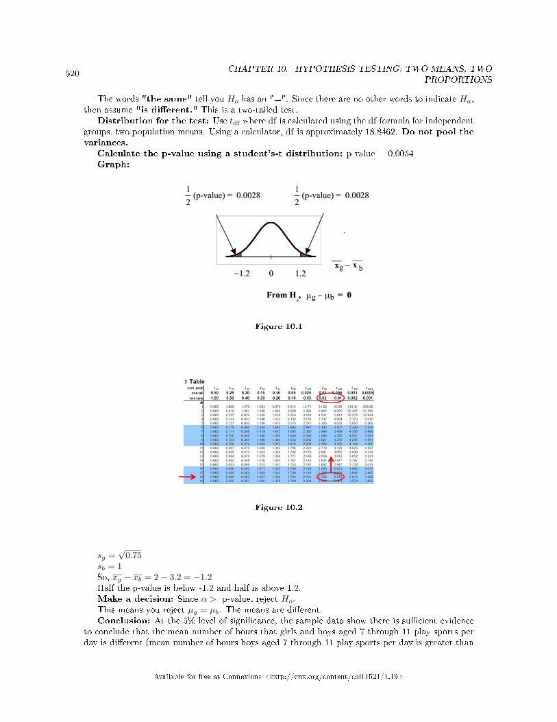
520CHAPTER 10. HYPOTHESIS TESTING: TWO MEANS, TWO
PROPORTIONS
The words "the same" tell you Ho has an "=". Since there are no other words to indicate Ha,then assume "is di�erent." This is a two-tailed test.
Distribution for the test: Use tdf where df is calculated using the df formula for independentgroups, two population means. Using a calculator, df is approximately 18.8462. Do not pool thevariances.
Calculate the p-value using a student's-t distribution: p-value = 0.0054Graph:
Figure 10.1
Figure 10.2
sg =√
0.75sb = 1So, xg − xb = 2− 3.2 = −1.2Half the p-value is below -1.2 and half is above 1.2.Make a decision: Since α > p-value, reject Ho.This means you reject µg = µb. The means are di�erent.Conclusion: At the 5% level of signi�cance, the sample data show there is su�cient evidence
to conclude that the mean number of hours that girls and boys aged 7 through 11 play sports perday is di�erent (mean number of hours boys aged 7 through 11 play sports per day is greater than
Available for free at Connexions <http://cnx.org/content/col11521/1.19>
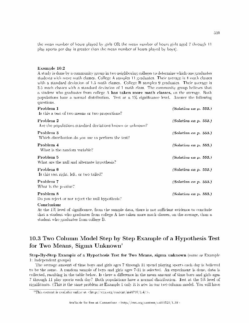
521
the mean number of hours played by girls OR the mean number of hours girls aged 7 through 11play sports per day is greater than the mean number of hours played by boys).
Example 10.2A study is done by a community group in two neighboring colleges to determine which one graduatesstudents with more math classes. College A samples 11 graduates. Their average is 4 math classeswith a standard deviation of 1.5 math classes. College B samples 9 graduates. Their average is3.5 math classes with a standard deviation of 1 math class. The community group believes thata student who graduates from college A has taken more math classes, on the average. Bothpopulations have a normal distribution. Test at a 1% signi�cance level. Answer the followingquestions.
Problem 1 (Solution on p. 553.)
Is this a test of two means or two proportions?
Problem 2 (Solution on p. 553.)
Are the populations standard deviations known or unknown?
Problem 3 (Solution on p. 553.)
Which distribution do you use to perform the test?
Problem 4 (Solution on p. 553.)
What is the random variable?
Problem 5 (Solution on p. 553.)
What are the null and alternate hypothesis?
Problem 6 (Solution on p. 553.)
Is this test right, left, or two tailed?
Problem 7 (Solution on p. 553.)
What is the p-value?
Problem 8 (Solution on p. 553.)
Do you reject or not reject the null hypothesis?
Conclusion:At the 1% level of signi�cance, from the sample data, there is not su�cient evidence to concludethat a student who graduates from college A has taken more math classes, on the average, than astudent who graduates from college B.
10.3 Two Column Model Step by Step Example of a Hypothesis Testfor Two Means, Sigma Unknown3
Step-By-Step Example of a Hypothesis Test for Two Means, sigma unknown (same as Example1: Independent groups)
The average amount of time boys and girls ages 7 through 11 spend playing sports each day is believedto be the same. A random sample of boys and girls ages 7-11 is selected. An experiment is done, data iscollected, resulting in the table below. Is there a di�erence in the mean amount of time boys and girls ages7 through 11 play sports each day? Both populations have a normal distribution. Test at the 5% level ofsigni�cance. (This is the same problem as Example 1 only it is now in our two column model. You will have
3This content is available online at <http://cnx.org/content/m46737/1.4/>.
Available for free at Connexions <http://cnx.org/content/col11521/1.19>
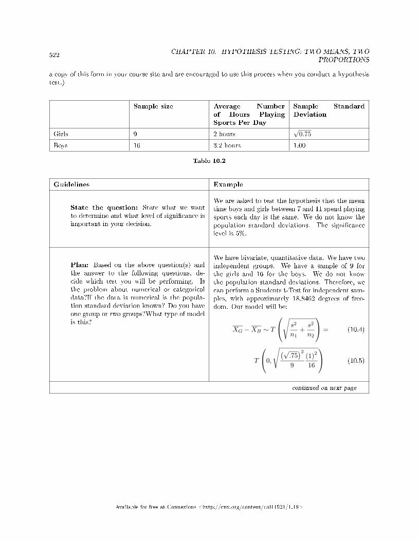
522CHAPTER 10. HYPOTHESIS TESTING: TWO MEANS, TWO
PROPORTIONS
a copy of this form in your course site and are encouraged to use this process when you conduct a hypothesistest.)
Sample size Average Numberof Hours PlayingSports Per Day
Sample StandardDeviation
Girls 9 2 hours√
0.75
Boys 16 3.2 hours 1.00
Table 10.2
Guidelines Example
State the question: State what we wantto determine and what level of signi�cance isimportant in your decision.
We are asked to test the hypothesis that the meantime boys and girls between 7 and 11 spend playingsports each day is the same. We do not know thepopulation standard deviations. The signi�cancelevel is 5%.
Plan: Based on the above question(s) andthe answer to the following questions, de-cide which test you will be performing. Isthe problem about numerical or categoricaldata?If the data is numerical is the popula-tion standard deviation known? Do you haveone group or two groups?What type of modelis this?
We have bivariate, quantitative data. We have twoindependent groups. We have a sample of 9 forthe girls and 16 for the boys. We do not knowthe population standard deviations. Therefore, wecan perform a Students t-Test for independent sam-ples, with approximately 18.8462 degrees of free-dom. Our model will be:
XG −XB ∼ T
√ s2
n1+s2
n2
= (10.4)
T
0,
√(√.75)2
9(1)2
16
(10.5)
continued on next page
Available for free at Connexions <http://cnx.org/content/col11521/1.19>
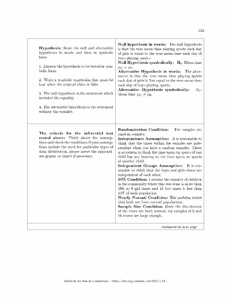
523
Hypothesis: State the null and alternativehypotheses in words and then in symbolicform
1. Express the hypothesis to be tested in sym-bolic form.
2. Write a symbolic expression that must betrue when the original claim is false.
3. The null hypothesis is the statement whichincluded the equality.
4. The alternative hypothesis is the statementwithout the equality.
Null hypothesis in words: The null hypothesisis that the true mean time playing sports each dayof girls is equal to the true mean time each day ofboys playing sports.Null Hypothesis symbolically: H0: Mean timeµG = µBAlternative Hypothesis in words: The alter-native is that the true mean time playing sportseach day of girls is Not equal to the true mean timeeach day of boys playing sports.Alternative Hypothesis symbolically: Ha:Mean time µG 6= µB
The criteria for the inferential teststated above: Think about the assump-tions and check the conditions.If your assump-tions include the need for particular types ofdata distribution, please insert the appropri-ate graphs or charts if necessary.
Randomization Condition: The samples arerandom samples.Independence Assumption: It is reasonable tothink that the times within the samples are inde-pendent when you have a random samples. Thereis no reason to think the time spent on sports of onechild has any bearing on the time spent on sportsof another child.Independent Groups Assumption: It is rea-sonable to think that the boys and girls times areindependent of each other.10% Condition: I assume the number of childrenin the community where this was done is more than250, so 9 girl times and 16 boy times is less than10% of each population.Nearly Normal Condition: The problem statesthat both are from normal populations.Sample Size Condition: Since the distributionof the times are both normal, my samples of 9 and16 scores are large enough.
continued on next page
Available for free at Connexions <http://cnx.org/content/col11521/1.19>
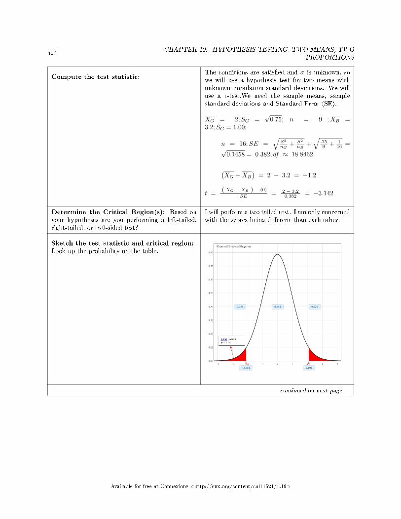
524CHAPTER 10. HYPOTHESIS TESTING: TWO MEANS, TWO
PROPORTIONS
Compute the test statistic:The conditions are satis�ed and σ is unknown, sowe will use a hypothesis test for two means withunknown population standard deviations. We willuse a t-test.We need the sample means, samplestandard deviations and Standard Error (SE).
XG = 2;SG =√
0.75; n = 9 ;XB =3.2;SG = 1.00;
n = 16;SE =√
S2
nG+ S2
nB+√
.759 + 1
16 =√
0.1458 = 0.382; df ≈ 18.8462
(XG −XB
)= 2 − 3.2 = −1.2
t = ( XG − XB ) − (0)
SE = 2 − 3.20.382 = −3.142
Determine the Critical Region(s): Based onyour hypotheses are you performing a left-tailed,right-tailed, or tw0-sided test?
I will perform a two tailed test. I am only concernedwith the scores being di�erent than each other.
Sketch the test statistic and critical region:Look up the probability on the table.
continued on next page
Available for free at Connexions <http://cnx.org/content/col11521/1.19>
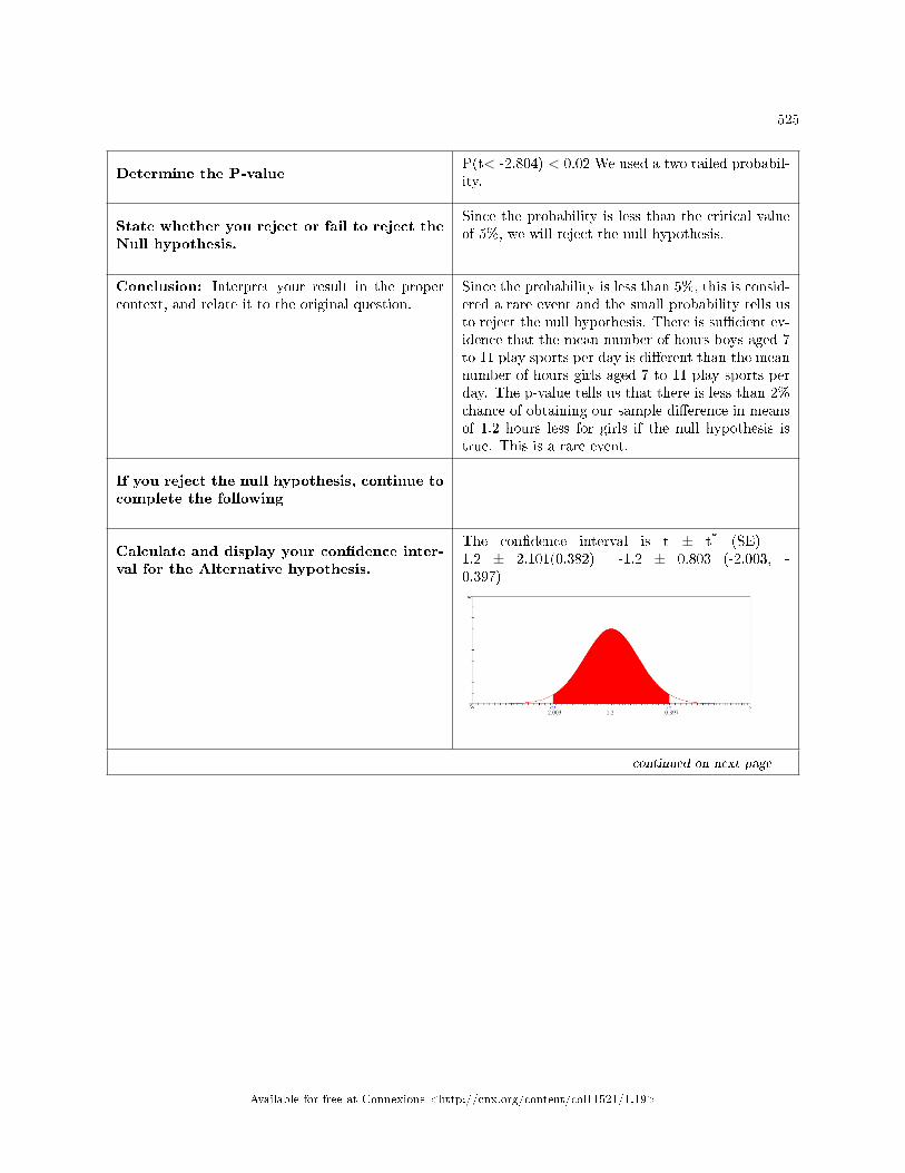
525
Determine the P-valueP(t< -2.804) < 0.02 We used a two tailed probabil-ity.
State whether you reject or fail to reject theNull hypothesis.
Since the probability is less than the critical valueof 5%, we will reject the null hypothesis.
Conclusion: Interpret your result in the propercontext, and relate it to the original question.
Since the probability is less than 5%, this is consid-ered a rare event and the small probability tells usto reject the null hypothesis. There is su�cient ev-idence that the mean number of hours boys aged 7to 11 play sports per day is di�erent than the meannumber of hours girls aged 7 to 11 play sports perday. The p-value tells us that there is less than 2%chance of obtaining our sample di�erence in meansof 1.2 hours less for girls if the null hypothesis istrue. This is a rare event.
If you reject the null hypothesis, continue tocomplete the following
Calculate and display your con�dence inter-val for the Alternative hypothesis.
The con�dence interval is t ± t* (SE) =-1.2 ± 2.101(0.382) =-1.2 ± 0.803 (-2.003, -0.397)
continued on next page
Available for free at Connexions <http://cnx.org/content/col11521/1.19>
526CHAPTER 10. HYPOTHESIS TESTING: TWO MEANS, TWO
PROPORTIONS
State your conclusion based on your con�-dence interval.
I am 95% con�dent that the true mean di�erence inthe number of hours girls 7 to 11 play sports eachday is between 0.301 and 2.099 hours less than thenumber of hour boys 7 to 11 play sports each day.
Table 10.3
10.4 Hypothesis Testing: Two Population Means and Two PopulationProportions: Comparing Two Independent Population Proportions4
10.4.1 Assumptions and Conditions: Two Sample Proportions Test
When constructing a two sample proportions hypothesis test the assumptions and conditions must be metin order to use the normal model.
Randomization Condition: The data must be sampled randomly. Is one of the good samplingmethodologies discussed in the Sampling and Data chapter being used?Independence Assumption: The sample values must be independent of each other. This meansthat the occurrence of one event has no in�uence on the next event. Usually, if we know that peopleor items were selected randomly we can assume that the independence assumption is met.10% Condition: When the sample is drawn without replacement (usually the case), the samplesize, n, should be no more than 10% of the population. This must be true for both groups.Success/ failure Condition: must be met for both groups. When working with proportions we needto be especially concerned about sample size when the proportion is close to zero or one. To checkthat the sample size is large enough calculate the successes by multiplying the sample percentages bythe sample sizes and calculate failure by multiplying one minus the sample percentages by the samplesizes. If all of these products are larger than ten then the condition is met.p̂1(n1) >10 and (1− p̂1) (n1)>10 andp̂2(n2) >10 and (1− p̂2) (n2) >10Independent Groups: The two groups you are working with must be independent of one another. Isthere reason to believe that one group would have in�uence on the other group? A hypothesis test thatis comparing a group of respondent's pre-test and post-test scores would not be independent. Likewise,groups made by splitting married couples into husband and wife groups would not be independent.
Comparing two proportions, like comparing two means, is common. If two estimated proportions are dif-ferent, it may be due to a di�erence in the populations or it may be due to chance. A hypothesis test canhelp determine if a di�erence in the estimated proportions (p̂A − p̂B) re�ects a di�erence in the populationproportions.
The di�erence of two proportions follows an approximate normal distribution. Generally, the null hy-pothesis states that the two proportions are the same. That is, Ho : pA = pB . To conduct the test, we usea pooled proportion, p̂pooled.
The pooled proportion is calculated as follows:
p̂pooled =xA + xBnA + nB
(10.6)
The distribution for the di�erences is:
p̂A − p̂B ∼ N
[0,
√p̂pooled · (1− p̂pooled) ·
(1nA
+1nB
)](10.7)
4This content is available online at <http://cnx.org/content/m46739/1.1/>.
Available for free at Connexions <http://cnx.org/content/col11521/1.19>
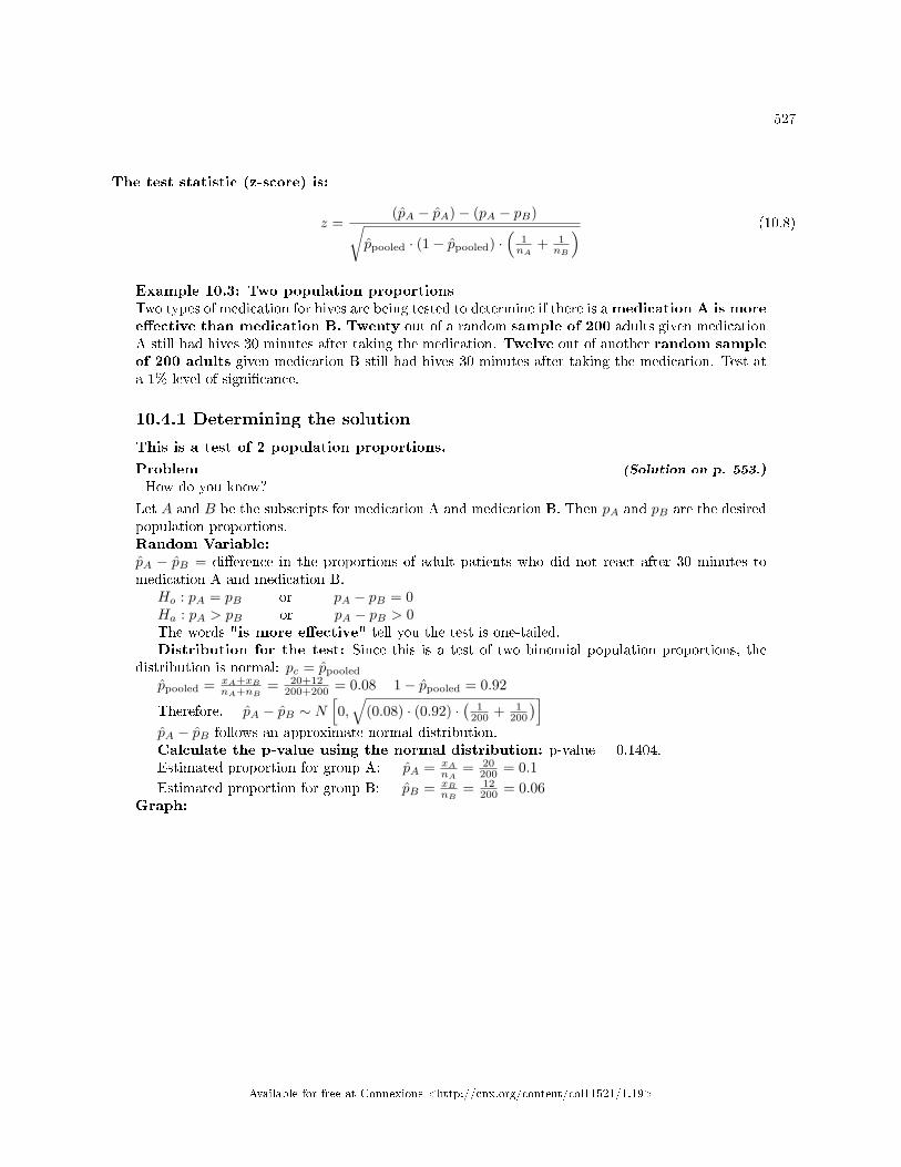
527
The test statistic (z-score) is:
z =(p̂A − p̂A)− (pA − pB)√
p̂pooled · (1− p̂pooled) ·(
1nA
+ 1nB
) (10.8)
Example 10.3: Two population proportionsTwo types of medication for hives are being tested to determine if there is amedication A is moree�ective than medication B. Twenty out of a random sample of 200 adults given medicationA still had hives 30 minutes after taking the medication. Twelve out of another random sampleof 200 adults given medication B still had hives 30 minutes after taking the medication. Test ata 1% level of signi�cance.
10.4.1 Determining the solution
This is a test of 2 population proportions.
Problem (Solution on p. 553.)
How do you know?
Let A and B be the subscripts for medication A and medication B. Then pA and pB are the desiredpopulation proportions.Random Variable:p̂A − p̂B = di�erence in the proportions of adult patients who did not react after 30 minutes tomedication A and medication B.
Ho : pA = pB or pA − pB = 0Ha : pA > pB or pA − pB > 0The words "is more e�ective" tell you the test is one-tailed.Distribution for the test: Since this is a test of two binomial population proportions, the
distribution is normal: pc = p̂pooled
p̂pooled = xA+xBnA+nB
= 20+12200+200 = 0.08 1− p̂pooled = 0.92
Therefore, p̂A − p̂B ∼ N[0,√
(0.08) · (0.92) ·(
1200 + 1
200
)]p̂A − p̂B follows an approximate normal distribution.Calculate the p-value using the normal distribution: p-value = 0.1404.Estimated proportion for group A: p̂A = xA
nA= 20
200 = 0.1Estimated proportion for group B: p̂B = xB
nB= 12
200 = 0.06Graph:
Available for free at Connexions <http://cnx.org/content/col11521/1.19>
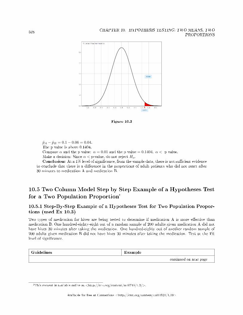
528CHAPTER 10. HYPOTHESIS TESTING: TWO MEANS, TWO
PROPORTIONS
Figure 10.3
p̂A − p̂B = 0.1− 0.06 = 0.04.The p-value is above 0.1404.Compare α and the p-value: α = 0.01 and the p-value = 0.1404. α < p-value.Make a decision: Since α < p-value, do not reject Ho.Conclusion: At a 1% level of signi�cance, from the sample data, there is not su�cient evidence
to conclude that there is a di�erence in the proportions of adult patients who did not react after30 minutes to medication A and medication B.
10.5 Two Column Model Step by Step Example of a Hypotheses Testfor a Two Population Proportion5
10.5.1 Step-By-Step Example of a Hypotheses Test for Two Population Propor-tions (used Ex 10.3)
Two types of medication for hives are being tested to determine if medication A is more e�ective thanmedication B. One hundred-eighty-eight out of a random sample of 200 adults given medication A did nothave hives 30 minutes after taking the medication. One hundred-eighty out of another random sample of200 adults given medication B did not have hives 30 minutes after taking the medication. Test at the 1%level of signi�cance.
Guidelines Example
continued on next page
5This content is available online at <http://cnx.org/content/m46748/1.3/>.
Available for free at Connexions <http://cnx.org/content/col11521/1.19>
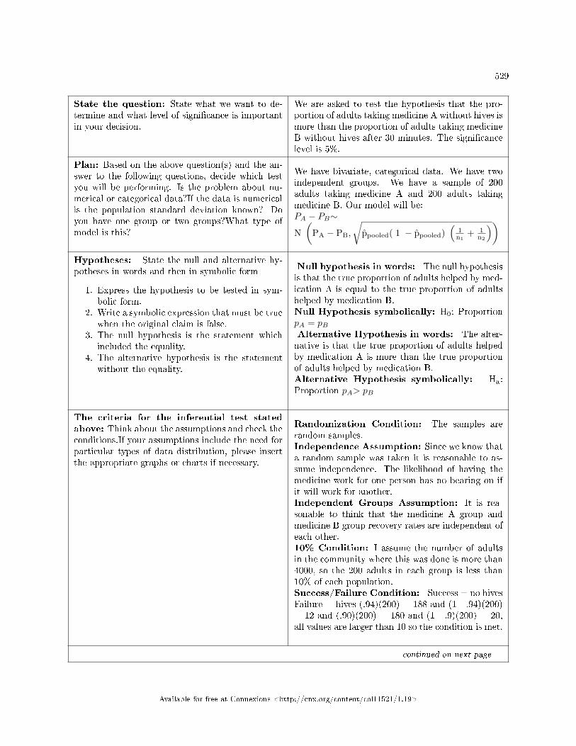
529
State the question: State what we want to de-termine and what level of signi�cance is importantin your decision.
We are asked to test the hypothesis that the pro-portion of adults taking medicine A without hives ismore than the proportion of adults taking medicineB without hives after 30 minutes. The signi�cancelevel is 5%.
Plan: Based on the above question(s) and the an-swer to the following questions, decide which testyou will be performing. Is the problem about nu-merical or categorical data?If the data is numericalis the population standard deviation known? Doyou have one group or two groups?What type ofmodel is this?
We have bivariate, categorical data. We have twoindependent groups. We have a sample of 200adults taking medicine A and 200 adults takingmedicine B. Our model will be:PA − PB∼
N(
PA − PB,
√p̂pooled( 1 − p̂pooled)
(1n1
+ 1n2
))Hypotheses: State the null and alternative hy-potheses in words and then in symbolic form
1. Express the hypothesis to be tested in sym-bolic form.
2. Write a symbolic expression that must be truewhen the original claim is false.
3. The null hypothesis is the statement whichincluded the equality.
4. The alternative hypothesis is the statementwithout the equality.
Null hypothesis in words: The null hypothesisis that the true proportion of adults helped by med-ication A is equal to the true proportion of adultshelped by medication B.Null Hypothesis symbolically: H0: ProportionpA = pBAlternative Hypothesis in words: The alter-native is that the true proportion of adults helpedby medication A is more than the true proportionof adults helped by medication B.Alternative Hypothesis symbolically: Ha:Proportion pA> pB
The criteria for the inferential test statedabove: Think about the assumptions and check theconditions.If your assumptions include the need forparticular types of data distribution, please insertthe appropriate graphs or charts if necessary.
Randomization Condition: The samples arerandom samples.Independence Assumption: Since we know thata random sample was taken it is reasonable to as-sume independence. The likelihood of having themedicine work for one person has no bearing on ifit will work for another.Independent Groups Assumption: It is rea-sonable to think that the medicine A group andmedicine B group recovery rates are independent ofeach other.10% Condition: I assume the number of adultsin the community where this was done is more than4000, so the 200 adults in each group is less than10% of each population.Success/Failure Condition: Success = no hivesFailure = hives (.94)(200) = 188 and (1 - .94)(200)= 12 and (.90)(200) = 180 and (1 - .9)(200) = 20,all values are larger than 10 so the condition is met.
continued on next page
Available for free at Connexions <http://cnx.org/content/col11521/1.19>
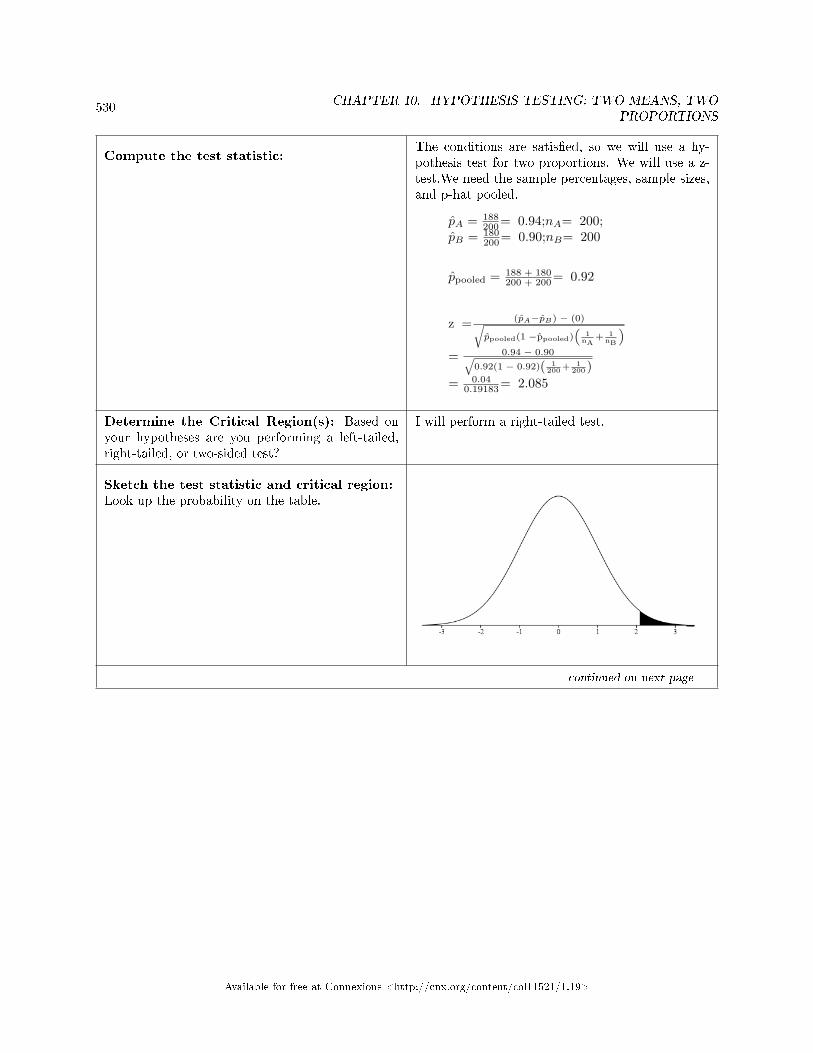
530CHAPTER 10. HYPOTHESIS TESTING: TWO MEANS, TWO
PROPORTIONS
Compute the test statistic:The conditions are satis�ed, so we will use a hy-pothesis test for two proportions. We will use a z-test.We need the sample percentages, sample sizes,and p-hat pooled.
p̂A = 188200= 0.94;nA= 200;
p̂B = 180200= 0.90;nB= 200
p̂pooled = 188 + 180200 + 200= 0.92
z = (p̂A−p̂B) − (0)rp̂pooled(1 −p̂pooled)
“1
nA+ 1
nB
”= 0.94 − 0.90q
0.92(1 − 0.92)( 1200 + 1
200 )= 0.04
0.19183= 2.085
Determine the Critical Region(s): Based onyour hypotheses are you performing a left-tailed,right-tailed, or two-sided test?
I will perform a right-tailed test.
Sketch the test statistic and critical region:Look up the probability on the table.
continued on next page
Available for free at Connexions <http://cnx.org/content/col11521/1.19>
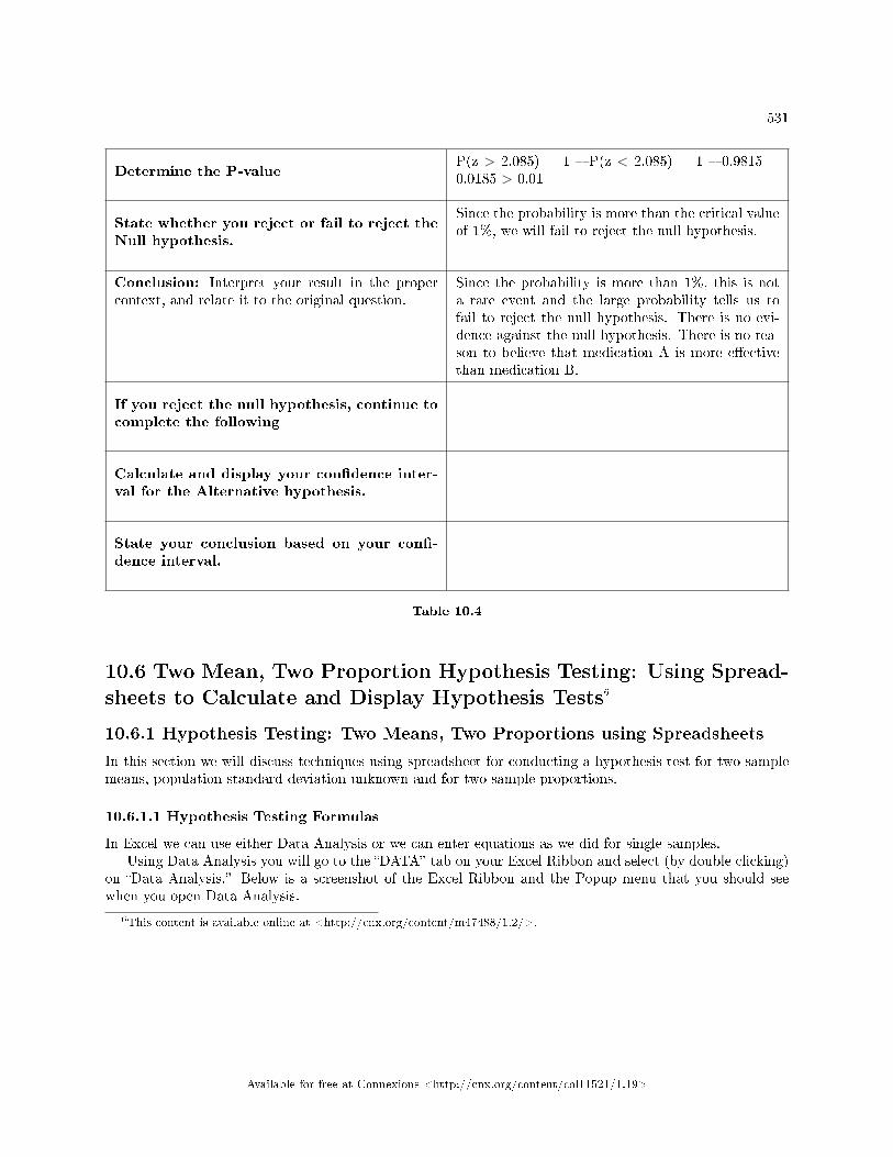
531
Determine the P-valueP(z > 2.085) = 1 � P(z < 2.085) = 1 � 0.9815 =0.0185 > 0.01
State whether you reject or fail to reject theNull hypothesis.
Since the probability is more than the critical valueof 1%, we will fail to reject the null hypothesis.
Conclusion: Interpret your result in the propercontext, and relate it to the original question.
Since the probability is more than 1%, this is nota rare event and the large probability tells us tofail to reject the null hypothesis. There is no evi-dence against the null hypothesis. There is no rea-son to believe that medication A is more e�ectivethan medication B.
If you reject the null hypothesis, continue tocomplete the following
Calculate and display your con�dence inter-val for the Alternative hypothesis.
State your conclusion based on your con�-dence interval.
Table 10.4
10.6 Two Mean, Two Proportion Hypothesis Testing: Using Spread-sheets to Calculate and Display Hypothesis Tests6
10.6.1 Hypothesis Testing: Two Means, Two Proportions using Spreadsheets
In this section we will discuss techniques using spreadsheet for conducting a hypothesis test for two samplemeans, population standard deviation unknown and for two sample proportions.
10.6.1.1 Hypothesis Testing Formulas
In Excel we can use either Data Analysis or we can enter equations as we did for single samples.Using Data Analysis you will go to the �DATA� tab on your Excel Ribbon and select (by double clicking)
on �Data Analysis.� Below is a screenshot of the Excel Ribbon and the Popup menu that you should seewhen you open Data Analysis.
6This content is available online at <http://cnx.org/content/m47488/1.2/>.
Available for free at Connexions <http://cnx.org/content/col11521/1.19>
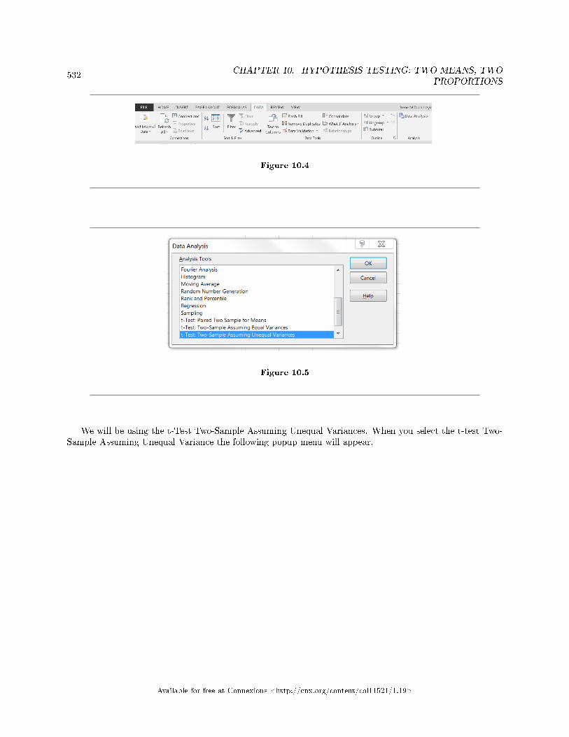
532CHAPTER 10. HYPOTHESIS TESTING: TWO MEANS, TWO
PROPORTIONS
Figure 10.4
Figure 10.5
We will be using the t-Test Two-Sample Assuming Unequal Variances. When you select the t-test Two-Sample Assuming Unequal Variance the following popup menu will appear.
Available for free at Connexions <http://cnx.org/content/col11521/1.19>
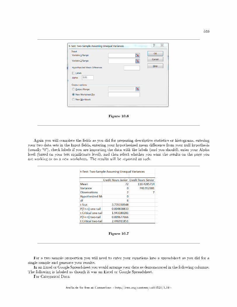
533
Figure 10.6
Again you will complete the �elds as you did for preparing descriptive statistics or histograms, enteringyour two data sets in the Input �elds, entering your hypothesized mean di�erence from your null hypothesis(usually �0�), check labels if you are importing the data with the labels (and you should), enter your Alphalevel (based on your test signi�cance level), and then select whether you want the results on the page youare working or on a new worksheet. The results will be reported as such.
Figure 10.7
For a two sample proportion you will need to enter your equations into a spreadsheet as you did for asingle sample and generate your results.
In an Excel or Google Spreadsheet you would arrange your data as demonstrated in the following columns.The following is labeled as though it was an Excel or Google Spreadsheet.
For Categorical Data:
Available for free at Connexions <http://cnx.org/content/col11521/1.19>
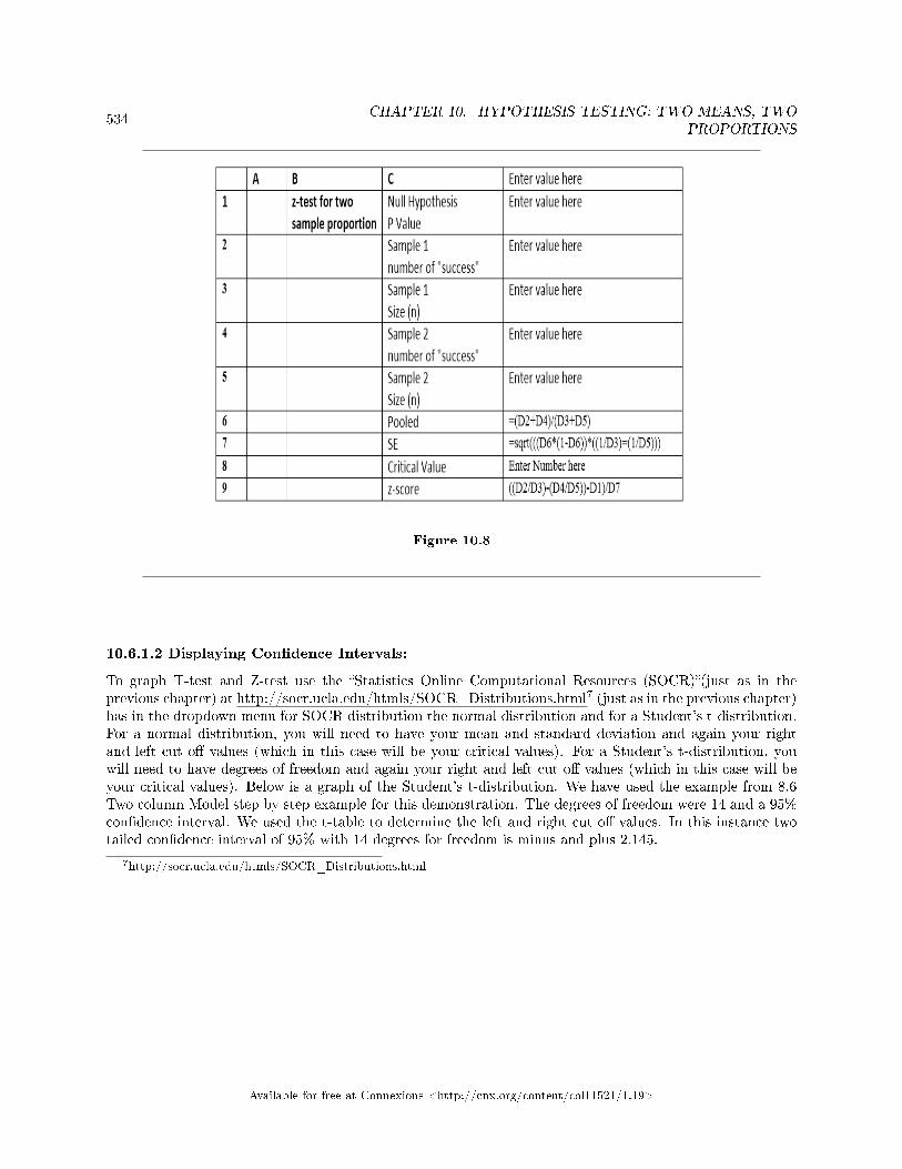
534CHAPTER 10. HYPOTHESIS TESTING: TWO MEANS, TWO
PROPORTIONS
Figure 10.8
10.6.1.2 Displaying Con�dence Intervals:
To graph T-test and Z-test use the �Statistics Online Computational Resources (SOCR)�(just as in theprevious chapter) at http://socr.ucla.edu/htmls/SOCR_Distributions.html7 (just as in the previous chapter)has in the dropdown menu for SOCR distribution the normal distribution and for a Student's t-distribution.For a normal distribution, you will need to have your mean and standard deviation and again your rightand left cut o� values (which in this case will be your critical values). For a Student's t-distribution, youwill need to have degrees of freedom and again your right and left cut o� values (which in this case will beyour critical values). Below is a graph of the Student's t-distribution. We have used the example from 8.6Two column Model step by step example for this demonstration. The degrees of freedom were 14 and a 95%con�dence interval. We used the t-table to determine the left and right cut o� values. In this instance twotailed con�dence interval of 95% with 14 degrees for freedom is minus and plus 2.145.
7http://socr.ucla.edu/htmls/SOCR_Distributions.html
Available for free at Connexions <http://cnx.org/content/col11521/1.19>
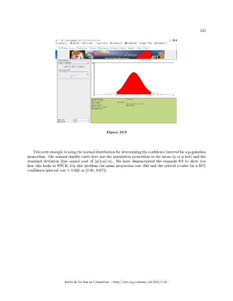
535
Figure 10.9
This next example is using the normal distribution for determining the con�dence interval for a populationproportion. The normal density curve here has the population proportion as the mean (p or p-hat) and thestandard deviation (the square root of (p(1-p)/n). We have demonstrated the example 8.8 to show youhow this looks in SOCR. For this problem the mean proportion was .842 and the critical z-value for a 95%con�dence interval was ± 0.032 or (0.81, 0.874).
Available for free at Connexions <http://cnx.org/content/col11521/1.19>
536CHAPTER 10. HYPOTHESIS TESTING: TWO MEANS, TWO
PROPORTIONS
Figure 10.10
10.6.1.3 Optional Classroom Exercise:
At your computer, try to use some of these tools to work out your homework problems or check homeworkthat you have completed to see if the results are the same or similar.
Available for free at Connexions <http://cnx.org/content/col11521/1.19>
537
10.7 Hypothesis Testing: Two Population Means and Two PopulationProportions: Summary of Types of Hypothesis Tests8
Two Population Means
• Populations are independent and population standard deviations are unknown.
Two Population Proportions
• Populations are independent.
10.7.1 Glossary
Degrees of FreedomThe number of objects in a sample that are free to vary.Standard DeviationA number that is equal to the square root of the variance and measures how far data values are from theirmean. Notation: s for sample standard deviation and σ for population standard deviation.Variance (Random Variable)A characteristic of interest in a population being studied. Common notation for variables are upper caseLatin letters X, Y, Z,...; common notation for a speci�c value from the domain (set of all possible values ofa variable) are lower case Latin letters x, y, z,.... For example, if X is the number of children in a family,then x represents a speci�c integer 0, 1, 2, 3, .... Variables in statistics di�er from variables in intermediatealgebra in two following ways.(1). The domain of the random variable (RV) is not necessarily a numerical set; the domain may be expressedin words; for example, if X = hair color then the domain is {black, blond, gray, green, orange}.(2). We can tell what speci�c value x of the Random Variable X takes only after performing the experiment.
8This content is available online at <http://cnx.org/content/m46779/1.2/>.
Available for free at Connexions <http://cnx.org/content/col11521/1.19>
538CHAPTER 10. HYPOTHESIS TESTING: TWO MEANS, TWO
PROPORTIONS
10.8 Hypothesis Testing of Two Means and Two Proportions:Homework9
For questions - Exercise 10.8.7, indicate which of the following choices best identi�es the hypothesis test.
A. Independent group means, population standard deviations and/or variances unknownB. Single meanC. 2 proportionsD. Single proportion
Exercise 10.8.1A new chocolate bar is taste-tested on consumers. Of interest is whether the proportion of childrenthat like the new chocolate bar is greater than the proportion of adults that like it.
Exercise 10.8.2 (Solution on p. 553.)
The mean number of English courses taken in a two�year time period by male and female collegestudents is believed to be about the same. An experiment is conducted and data are collected from9 males and 16 females.
Exercise 10.8.3A football league reported that the mean number of touchdowns per game was 5. A study is doneto determine if the mean number of touchdowns has decreased.
Exercise 10.8.4According to a YWCA Rape Crisis Center newsletter, 75% of rape victims know their attackers. Astudy is done to verify this.
Exercise 10.8.5 (Solution on p. 553.)
According to a recent study, U.S. companies have an mean maternity-leave of six weeks.
Exercise 10.8.6A recent drug survey showed an increase in use of drugs and alcohol among local high schoolstudents as compared to the national percent. Suppose that a survey of 100 local youths and 100national youths is conducted to see if the proportion of drug and alcohol use is higher locally thannationally.
Exercise 10.8.7University of Michigan researchers reported in the Journal of the National Cancer Institute thatquitting smoking is especially bene�cial for those under age 49. In this American Cancer Societystudy, the risk (probability) of dying of lung cancer was about the same as for those who had neversmoked.
10.8.1
Directions: For each of the word problems, use a solution sheet to do the hypothesis test. Usethe two column step by step model, as is used in the text. A blank form can be found in yourcourse management system. Please feel free to make copies of the step by step model forms.
note: If you are using a student's-t distribution for a homework problem below, including forpaired data, you may assume that the underlying population is normally distributed. (In general,you must �rst prove that assumption, though.)
9This content is available online at <http://cnx.org/content/m46777/1.4/>.
Available for free at Connexions <http://cnx.org/content/col11521/1.19>
539
Exercise 10.8.8 (Solution on p. 553.)
A powder diet is tested on 49 people and a liquid diet is tested on 36 di�erent people. Of interestis whether the liquid diet yields a higher mean weight loss than the powder diet. The powder dietgroup had an mean weight loss of 42 pounds with a standard deviation of 12 pounds. The liquiddiet group had an mean weight loss of 45 pounds with a standard deviation of 14 pounds.
Exercise 10.8.9The mean number of English courses taken in a two�year time period by male and female collegestudents is believed to be about the same. An experiment is conducted and data are collected from29 males and 16 females. The males took an average of 3 English courses with a standard deviationof 0.8. The females took an average of 4 English courses with a standard deviation of 1.0. Are themeans statistically the same?
Exercise 10.8.10 (Solution on p. 553.)
A recent drug survey showed an increase in use of drugs and alcohol among local high school seniorsas compared to the national percent. Suppose that a survey of 100 local seniors and 100 nationalseniors is conducted to see if the proportion of drug and alcohol use is higher locally than nationally.Locally, 65 seniors reported using drugs or alcohol within the past month, while 60 national seniorsreported using them.
Exercise 10.8.11A student at a four-year college claims that mean enrollment at four�year colleges is higher thanat two�year colleges in the United States. Two surveys are conducted. Of the 35 two�year collegessurveyed, the mean enrollment was 5068 with a standard deviation of 4777. Of the 35 four-yearcolleges surveyed, the mean enrollment was 5466 with a standard deviation of 8191. (Source:Microsoft Bookshelf )
Exercise 10.8.12 (Solution on p. 553.)
A study was conducted by the U.S. Army to see if applying antiperspirant to soldiers' feet for a fewdays before a major hike would help cut down on the number of blisters soldiers had on their feet.In the experiment, for three nights before they went on a 13-mile hike, a group of 328 West Pointcadets put an alcohol-based antiperspirant on their feet. A �control group� of 339 soldiers put ona similar, but inactive, preparation on their feet. On the day of the hike, the temperature reached83 ◦ F. At the end of the hike, 21% of the soldiers who had used the antiperspirant and 48% ofthe control group had developed foot blisters. Conduct a hypothesis test to see if the proportionof soldiers using the antiperspirant was signi�cantly lower than the control group. (Source: U.S.Army study reported in Journal of the American Academy of Dermatologists)
Exercise 10.8.13We are interested in whether the proportions of female suicide victims for ages 15 to 24 are thesame for the white and the black races in the United States. We randomly pick one year, 1992,to compare the races. The number of suicides estimated in the United States in 1992 for whitefemales is 4930. 580 were aged 15 to 24. The estimate for black females is 330. 40 were aged 15 to24. We will let female suicide victims be our population. (Source: the National Center for HealthStatistics, U.S. Dept. of Health and Human Services)
Exercise 10.8.14Elizabeth Mjelde, an art history professor, was interested in whether the value from the Golden
Ratio formula,(larger+smaller dimension
larger dimension
)was the same in the Whitney Exhibit for works from 1900
� 1919 as for works from 1920 � 1942. 37 early works were sampled. They averaged 1.74 witha standard deviation of 0.11. 65 of the later works were sampled. They averaged 1.746 with astandard deviation of 0.1064. Do you think that there is a signi�cant di�erence in the Golden Ratiocalculation? (Source: data from Whitney Exhibit on loan to San Jose Museum of Art)
Available for free at Connexions <http://cnx.org/content/col11521/1.19>
540CHAPTER 10. HYPOTHESIS TESTING: TWO MEANS, TWO
PROPORTIONS
Exercise 10.8.15 (Solution on p. 553.)
Mean entry level salaries for college graduates with mechanical engineering degrees and elec-trical engineering degrees are believed to be approximately the same. (Source: http://www.graduatingengineer.com10 ). A recruiting o�ce thinks that the mean mechanical engineeringsalary is actually lower than the mean electrical engineering salary. The recruiting o�ce randomlysurveys 50 entry level mechanical engineers and 60 entry level electrical engineers. Their meansalaries were $46,100 and $46,700, respectively. Their standard deviations were $3450 and $4210,respectively. Conduct a hypothesis test to determine if you agree that the mean entry level me-chanical engineering salary is lower than the mean entry level electrical engineering salary.
Exercise 10.8.16A recent year was randomly picked from 1985 to the present. In that year, there were 2051 Hispanicstudents at Cabrillo College out of a total of 12,328 students. At Lake Tahoe College, there were321 Hispanic students out of a total of 2441 students. In general, do you think that the percentof Hispanic students at the two colleges is basically the same or di�erent? (Source: Chancellor'sO�ce, California Community Colleges, November 1994)
Exercise 10.8.17Marketing companies have collected data implying that teenage girls use more ring tones on theircellular phones than teenage boys do. In one particular study of 40 randomly chosen teenage girlsand boys (20 of each) with cellular phones, the mean number of ring tones for the girls was 3.2with a standard deviation of 1.5. The mean for the boys was 1.7 with a standard deviation of 0.8.Conduct a hypothesis test to determine if the means are approximately the same or if the girls'mean is higher than the boys' mean.
Exercise 10.8.18 (Solution on p. 554.)
While her husband spent 2½ hours picking out new speakers, a statistician decided to determinewhether the percent of men who enjoy shopping for electronic equipment is higher than the percentof women who enjoy shopping for electronic equipment. The population was Saturday afternoonshoppers. Out of 67 men, 24 said they enjoyed the activity. 8 of the 24 women surveyed claimedto enjoy the activity. Interpret the results of the survey.
Exercise 10.8.19We are interested in whether children's educational computer software costs less, on average, thanchildren's entertainment software. 36 educational software titles were randomly picked from acatalog. The mean cost was $31.14 with a standard deviation of $4.69. 35 entertainment softwaretitles were randomly picked from the same catalog. The mean cost was $33.86 with a standarddeviation of $10.87. Decide whether children's educational software costs less, on average, thanchildren's entertainment software. (Source: Educational Resources, December catalog)
Exercise 10.8.20 (Solution on p. 554.)
Joan Nguyen recently claimed that the proportion of college�age males with at least one piercedear is as high as the proportion of college�age females. She conducted a survey in her classes. Outof 107 males, 20 had at least one pierced ear. Out of 92 females, 47 had at least one pierced ear.Do you believe that the proportion of males has reached the proportion of females?
Exercise 10.8.21Some manufacturers claim that non-hybrid sedan cars have a lower mean miles per gallon (mpg)than hybrid ones. Suppose that consumers test 21 hybrid sedans and get a mean of 31 mpg with astandard deviation of 7 mpg. Thirty-one non-hybrid sedans get a mean of 22 mpg with a standarddeviation of 4 mpg. Conduct a hypothesis test to the manufacturers claim.
10http://www.graduatingengineer.com/
Available for free at Connexions <http://cnx.org/content/col11521/1.19>
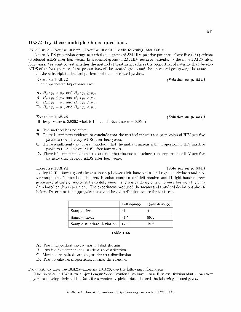
541
10.8.2 Try these multiple choice questions.
For questions Exercise 10.8.22 � Exercise 10.8.23, use the following information.A new AIDS prevention drugs was tried on a group of 224 HIV positive patients. Forty-�ve (45) patients
developed AIDS after four years. In a control group of 224 HIV positive patients, 68 developed AIDS afterfour years. We want to test whether the method of treatment reduces the proportion of patients that developAIDS after four years or if the proportions of the treated group and the untreated group stay the same.
Let the subscript t= treated patient and ut= untreated patient.
Exercise 10.8.22 (Solution on p. 554.)
The appropriate hypotheses are:
A. Ho : pt < put and Ha : pt ≥ putB. Ho : pt ≤ put and Ha : pt > putC. Ho : pt = put and Ha : pt 6= putD. Ho : pt = put and Ha : pt < put
Exercise 10.8.23 (Solution on p. 554.)
If the p -value is 0.0062 what is the conclusion (use α = 0.05 )?
A. The method has no e�ect.B. There is su�cient evidence to conclude that the method reduces the proportion of HIV positive
patients that develop AIDS after four years.C. There is su�cient evidence to conclude that the method increases the proportion of HIV positive
patients that develop AIDS after four years.D. There is insu�cient evidence to conclude that the method reduces the proportion of HIV positive
patients that develop AIDS after four years.
Exercise 10.8.24 (Solution on p. 554.)
Lesley E. Tan investigated the relationship between left-handedness and right-handedness and mo-tor competence in preschool children. Random samples of 41 left-handers and 41 right-handers weregiven several tests of motor skills to determine if there is evidence of a di�erence between the chil-dren based on this experiment. The experiment produced the means and standard deviations shownbelow. Determine the appropriate test and best distribution to use for that test.
Left-handed Right-handed
Sample size 41 41
Sample mean 97.5 98.1
Sample standard deviation 17.5 19.2
Table 10.5
A. Two independent means, normal distributionB. Two independent means, student's-t distributionC. Matched or paired samples, student's-t distributionD. Two population proportions, normal distribution
For questions Exercise 10.8.25� Exercise 10.8.26, use the following information.The Eastern and Western Major League Soccer conferences have a new Reserve Division that allows new
players to develop their skills. Data for a randomly picked date showed the following annual goals.
Available for free at Connexions <http://cnx.org/content/col11521/1.19>
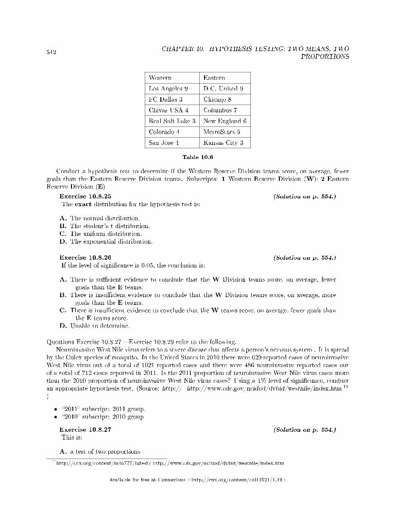
542CHAPTER 10. HYPOTHESIS TESTING: TWO MEANS, TWO
PROPORTIONS
Western Eastern
Los Angeles 9 D.C. United 9
FC Dallas 3 Chicago 8
Chivas USA 4 Columbus 7
Real Salt Lake 3 New England 6
Colorado 4 MetroStars 5
San Jose 4 Kansas City 3
Table 10.6
Conduct a hypothesis test to determine if the Western Reserve Division teams score, on average, fewergoals than the Eastern Reserve Division teams. Subscripts: 1 Western Reserve Division (W); 2 EasternReserve Division (E)
Exercise 10.8.25 (Solution on p. 554.)
The exact distribution for the hypothesis test is:
A. The normal distribution.B. The student's-t distribution.C. The uniform distribution.D. The exponential distribution.
Exercise 10.8.26 (Solution on p. 554.)
If the level of signi�cance is 0.05, the conclusion is:
A. There is su�cient evidence to conclude that the W Division teams score, on average, fewergoals than the E teams.
B. There is insu�cient evidence to conclude that the W Division teams score, on average, moregoals than the E teams.
C. There is insu�cient evidence to conclude that the W teams score, on average, fewer goals thanthe E teams score.
D. Unable to determine.
Questions Exercise 10.8.27 � Exercise 10.8.29 refer to the following.Neuroinvasive West Nile virus refers to a severe disease that a�ects a person's nervous system . It is spread
by the Culex species of mosquito. In the United States in 2010 there were 629 reported cases of neuroinvasiveWest Nile virus out of a total of 1021 reported cases and there were 486 neuroinvasive reported cases outof a total of 712 cases reported in 2011. Is the 2011 proportion of neuroinvasive West Nile virus cases morethan the 2010 proportion of neuroinvasive West Nile virus cases? Using a 1% level of signi�cance, conductan appropriate hypothesis test. (Source: http:// http://www.cdc.gov/ncidod/dvbid/westnile/index.htm 11
)
• �2011� subscript: 2011 group.• �2010� subscript: 2010 group
Exercise 10.8.27 (Solution on p. 554.)
This is:
A. a test of two proportions
11http://cnx.org/content/m46777/latest/ http://www.cdc.gov/ncidod/dvbid/westnile/index.htm
Available for free at Connexions <http://cnx.org/content/col11521/1.19>
543
B. a test of two independent meansC. a test of a single meanD. a test of matched pairs.
Exercise 10.8.28 (Solution on p. 554.)
An appropriate null hypothesis is:
A. p2011 = p2010B. p2011 ≥ p2010C. µ2011 ≤ µ2010D. p2011 > p2010
Exercise 10.8.29 (Solution on p. 554.)
The p-value is 0.0022. At a 1% level of signi�cance, the appropriate conclusion is
A. There is su�cient evidence to conclude that the proportion of people in the United States in2011 that got neuroinvasive West Nile disease is less than the proportion of people in theUnited States in 2010 that got neuroinvasive West Nile disease.
B. There is insu�cient evidence to conclude that the proportion of people in the United States in2011 that got neuroinvasive West Nile disease is more than the proportion of people in theUnited States in 2010 that got neuroinvasive West Nile disease.
C. There is insu�cient evidence to conclude that the proportion of people in the United Statesin 2011 that got neuroinvasive West Nile disease is less than the proportion of people in theUnited States in 2010 that got neuroinvasive West Nile disease.
D. There is su�cient evidence to conclude that the proportion of people in the United States in2011 that got neuroinvasive West Nile disease is more than the proportion of people in theUnited States in 2010 that got neuroinvasive West Nile disease.
Suppose a statistics instructor believes that there is no signi�cant di�erence between the mean class scoresof statistics day students on Exam 2 and statistics night students on Exam 2. She takes random samplesfrom each of the populations. The mean and standard deviation for 35 statistics day students were 75.86 and16.91. The mean and standard deviation for 37 statistics night students were 75.41 and 19.73. The �day�subscript refers to the statistics day students. The �night� subscript refers to the statistics night students.
Exercise 10.8.30 (Solution on p. 554.)
An appropriate alternate hypothesis for the hypothesis test is:
A. µday > µnightB. µday < µnightC. µday = µnightD. µday 6= µnight
Exercise 10.8.31 (Solution on p. 554.)
A concluding statement is:
A. There is su�cient evidence to conclude that statistics night students mean on Exam 2 is betterthan the statistics day students mean on Exam 2.
B. There is insu�cient evidence to conclude that the statistics day students mean on Exam 2 isbetter than the statistics night students mean on Exam 2.
C. There is insu�cient evidence to conclude that there is a signi�cant di�erence between the meansof the statistics day students and night students on Exam 2.
D. There is su�cient evidence to conclude that there is a signi�cant di�erence between the meansof the statistics day students and night students on Exam 2.
Available for free at Connexions <http://cnx.org/content/col11521/1.19>
544CHAPTER 10. HYPOTHESIS TESTING: TWO MEANS, TWO
PROPORTIONS
10.9 Hypothesis Testing: Two Population Means and Two PopulationProportions: Practice 112
10.9.1 Student Learning Outcomes
• The student will conduct a hypothesis test of two proportions.
10.9.2 Given
In the recent Census, 3 percent of the U.S. population reported being two or more races. However, the percentvaries tremendously from state to state. (Source: http://www.census.gov/prod/cen2010/briefs/c2010br-02.pdf ) Suppose that two random surveys are conducted. In the �rst random survey, out of 1000 NorthDakotans, only 9 people reported being of two or more races. In the second random survey, out of 500Nevadans, 17 people reported being of two or more races. Conduct a hypothesis test to determine if thepopulation percents are the same for the two states or if the percent for Nevada is statistically higher thanfor North Dakota.
10.9.3 Hypothesis Testing: Two Proportions
Exercise 10.9.1 (Solution on p. 554.)
Is this a test of means or proportions?
Exercise 10.9.2 (Solution on p. 554.)
State the null and alternative hypotheses.
a. H0 :b. Ha :
Exercise 10.9.3 (Solution on p. 554.)
Is this a right-tailed, left-tailed, or two-tailed test? How do you know?
Exercise 10.9.4What is the Random Variable of interest for this test?
Exercise 10.9.5In words, de�ne the Random Variable for this test.
Exercise 10.9.6 (Solution on p. 554.)
Which distribution (Normal or student's-t) would you use for this hypothesis test?
Exercise 10.9.7Explain why you chose the distribution you did for the above question.
Exercise 10.9.8 (Solution on p. 554.)
Calculate the test statistic.
Exercise 10.9.9Sketch a graph of the situation. Mark the hypothesized di�erence and the sample di�erence. Shadethe area corresponding to the p−value.
12This content is available online at <http://cnx.org/content/m17027/1.13/>.
Available for free at Connexions <http://cnx.org/content/col11521/1.19>
545
Figure 10.11
Exercise 10.9.10 (Solution on p. 554.)
Find the p−value:Exercise 10.9.11 (Solution on p. 554.)
At a pre-conceived α = 0.05, what is your:
a. Decision:b. Reason for the decision:c. Conclusion (write out in a complete sentence):
10.9.4 Discussion Question
Exercise 10.9.12Does it appear that the proportion of Nevadans who are two or more races is higher than the
proportion of North Dakotans? Why or why not?
Available for free at Connexions <http://cnx.org/content/col11521/1.19>
546CHAPTER 10. HYPOTHESIS TESTING: TWO MEANS, TWO
PROPORTIONS
10.10 Hypothesis Testing: Two Population Means and Two Popula-tion Proportions: Practice 213
10.10.1 Student Learning Outcome
• The student will conduct a hypothesis test of two means.
10.10.2 Given
The U.S. Center for Disease Control reports that the mean life expectancy for whites born in 1900 was 47.6years and for nonwhites it was 33.0 years. (http://www.cdc.gov/nchs/data/dvs/nvsr53_06t12.pdf ) Supposethat you randomly survey death records for people born in 1900 in a certain county. Of the 124 whites, themean life span was 45.3 years with a standard deviation of 12.7 years. Of the 82 nonwhites, the mean lifespan was 34.1 years with a standard deviation of 15.6 years. Conduct a hypothesis test to see if the meanlife spans in the county were the same for whites and nonwhites.
10.10.3 Hypothesis Testing: Two Means
Exercise 10.10.1 (Solution on p. 555.)
Is this a test of means or proportions?
Exercise 10.10.2 (Solution on p. 555.)
State the null and alternative hypotheses.
a. H0 :b. Ha :
Exercise 10.10.3 (Solution on p. 555.)
Is this a right-tailed, left-tailed, or two-tailed test? How do you know?
Exercise 10.10.4 (Solution on p. 555.)
What is the Random Variable of interest for this test?
Exercise 10.10.5 (Solution on p. 555.)
In words, de�ne the Random Variable of interest for this test.
Exercise 10.10.6Which distribution (Normal or student's-t) would you use for this hypothesis test?
Exercise 10.10.7Explain why you chose the distribution you did for the above question.
Exercise 10.10.8 (Solution on p. 555.)
Calculate the test statistic.
Exercise 10.10.9Sketch a graph of the situation. Label the horizontal axis. Mark the hypothesized di�erence andthe sample di�erence. Shade the area corresponding to the p−value.
13This content is available online at <http://cnx.org/content/m17039/1.12/>.
Available for free at Connexions <http://cnx.org/content/col11521/1.19>

547
Figure 10.12
Exercise 10.10.10 (Solution on p. 555.)
Find the p−value:Exercise 10.10.11 (Solution on p. 555.)
At a pre-conceived α = 0.05, what is your:
a. Decision:b. Reason for the decision:c. Conclusion (write out in a complete sentence):
10.10.4 Discussion Question
Exercise 10.10.12Does it appear that the means are the same? Why or why not?
Available for free at Connexions <http://cnx.org/content/col11521/1.19>
548CHAPTER 10. HYPOTHESIS TESTING: TWO MEANS, TWO
PROPORTIONS
10.11 Hypothesis Testing of Two Means and Two Proportions: LabI14
Class Time:Names:
10.11.1 Student Learning Outcomes:
• The student will select the appropriate distributions to use in each case.• The student will conduct hypothesis tests and interpret the results.
10.11.2 Supplies:
• The business section from two consecutive days' newspapers• 3 small packages of M&Ms®• 5 small packages of Reese's Pieces®
10.11.3 Increasing Stocks Survey
Look at yesterday's newspaper business section. Conduct a hypothesis test to determine if the proportion ofNew York Stock Exchange (NYSE) stocks that increased is greater than the proportion of NASDAQ stocksthat increased. As randomly as possible, choose 40 NYSE stocks and 32 NASDAQ stocks and complete thefollowing statements.
1. Ho
2. Ha
3. In words, de�ne the Random Variable. ____________=4. The distribution to use for the test is:5. Calculate the test statistic using your data.6. Draw a graph and label it appropriately. Shade the actual level of signi�cance.
a. Graph:
14This content is available online at <http://cnx.org/content/m17022/1.13/>.
Available for free at Connexions <http://cnx.org/content/col11521/1.19>
549
Figure 10.13
b. Calculate the p-value:
7. Do you reject or not reject the null hypothesis? Why?8. Write a clear conclusion using a complete sentence.
10.11.4 Decreasing Stocks Survey
Randomly pick 8 stocks from the newspaper. Using two consecutive days' business sections, test whetherthe stocks went down, on average, for the second day.
1. Ho
2. Ha
3. In words, de�ne the Random Variable. ____________=4. The distribution to use for the test is:5. Calculate the test statistic using your data.6. Draw a graph and label it appropriately. Shade the actual level of signi�cance.
a. Graph:
Available for free at Connexions <http://cnx.org/content/col11521/1.19>
550CHAPTER 10. HYPOTHESIS TESTING: TWO MEANS, TWO
PROPORTIONS
Figure 10.14
b. Calculate the p-value:
7. Do you reject or not reject the null hypothesis? Why?8. Write a clear conclusion using a complete sentence.
10.11.5 Candy Survey
Buy three small packages of M&Ms and 5 small packages of Reese's Pieces (same net weight as the M&Ms).Test whether or not the mean number of candy pieces per package is the same for the two brands.
1. Ho:2. Ha:3. In words, de�ne the random variable. __________=4. What distribution should be used for this test?5. Calculate the test statistic using your data.6. Draw a graph and label it appropriately. Shade the actual level of signi�cance.
a. Graph:
Available for free at Connexions <http://cnx.org/content/col11521/1.19>
551
Figure 10.15
b. Calculate the p-value:
7. Do you reject or not reject the null hypothesis? Why?8. Write a clear conclusion using a complete sentence.
10.11.6 Shoe Survey
Test whether women have, on average, more pairs of shoes than men. Include all forms of sneakers, shoes,sandals, and boots. Use your class as the sample.
1. Ho
2. Ha
3. In words, de�ne the Random Variable. ____________=4. The distribution to use for the test is:5. Calculate the test statistic using your data.6. Draw a graph and label it appropriately. Shade the actual level of signi�cance.
a. Graph:
Available for free at Connexions <http://cnx.org/content/col11521/1.19>
552CHAPTER 10. HYPOTHESIS TESTING: TWO MEANS, TWO
PROPORTIONS
Figure 10.16
b. Calculate the p-value:
7. Do you reject or not reject the null hypothesis? Why?8. Write a clear conclusion using a complete sentence.
Available for free at Connexions <http://cnx.org/content/col11521/1.19>
553
Solutions to Exercises in Chapter 10
Solution to Example 10.2, Problem 1 (p. 521)two meansSolution to Example 10.2, Problem 2 (p. 521)unknownSolution to Example 10.2, Problem 3 (p. 521)student's-tSolution to Example 10.2, Problem 4 (p. 521)XA −XB
Solution to Example 10.2, Problem 5 (p. 521)
• Ho : µA ≤ µB• Ha : µA > µB
Solution to Example 10.2, Problem 6 (p. 521)rightSolution to Example 10.2, Problem 7 (p. 521)0.1928Solution to Example 10.2, Problem 8 (p. 521)Do not reject.Solution to Example 10.3, Problem (p. 527)The problem asks for a di�erence in proportions.
Solutions to Hypothesis Testing of Two Means and Two Proportions: Homework
Solution to Exercise 10.8.2 (p. 538)ASolution to Exercise 10.8.5 (p. 538)BSolution to Exercise 10.8.8 (p. 539)
d. t68.44e. -1.04f. 0.1519h. Decision: Do not reject null
Solution to Exercise 10.8.10 (p. 539)
e. 0.73f. 0.2326h. Decision: Do not reject null
Solution to Exercise 10.8.12 (p. 539)
e. -7.33f. 0h. Decision: Reject null
Solution to Exercise 10.8.15 (p. 540)
d. t108e. t = −0.82f. 0.2066h. Decision: Do not reject null
Available for free at Connexions <http://cnx.org/content/col11521/1.19>
554CHAPTER 10. HYPOTHESIS TESTING: TWO MEANS, TWO
PROPORTIONS
Solution to Exercise 10.8.18 (p. 540)
e. 0.22f. 0.4133h. Decision: Do not reject null
Solution to Exercise 10.8.20 (p. 540)
e. -4.82f. 0h. Decision: Reject null
Solution to Exercise 10.8.22 (p. 541)DSolution to Exercise 10.8.23 (p. 541)BSolution to Exercise 10.8.24 (p. 541)BSolution to Exercise 10.8.25 (p. 542)BSolution to Exercise 10.8.26 (p. 542)CSolution to Exercise 10.8.27 (p. 542)ASolution to Exercise 10.8.28 (p. 543)ASolution to Exercise 10.8.29 (p. 543)DSolution to Exercise 10.8.30 (p. 543)DSolution to Exercise 10.8.31 (p. 543)C
Solutions to Hypothesis Testing: Two Population Means and Two PopulationProportions: Practice 1
Solution to Exercise 10.9.1 (p. 544)ProportionsSolution to Exercise 10.9.2 (p. 544)
a. H0:PN=PND
a. Ha:PN> PND
Solution to Exercise 10.9.3 (p. 544)right-tailedSolution to Exercise 10.9.6 (p. 544)NormalSolution to Exercise 10.9.8 (p. 544)3.50Solution to Exercise 10.9.10 (p. 545)0.0002Solution to Exercise 10.9.11 (p. 545)
a. Reject the null hypothesis
Available for free at Connexions <http://cnx.org/content/col11521/1.19>
555
Solutions to Hypothesis Testing: Two Population Means and Two PopulationProportions: Practice 2
Solution to Exercise 10.10.1 (p. 546)MeansSolution to Exercise 10.10.2 (p. 546)
a. H0 : µW = µNWb. Ha : µW 6= µNW
Solution to Exercise 10.10.3 (p. 546)two-tailedSolution to Exercise 10.10.4 (p. 546)XW −XNW
Solution to Exercise 10.10.5 (p. 546)The di�erence between the mean life spans of whites and nonwhites.Solution to Exercise 10.10.8 (p. 546)5.42Solution to Exercise 10.10.10 (p. 547)0.0000Solution to Exercise 10.10.11 (p. 547)
a. Reject the null hypothesis
Available for free at Connexions <http://cnx.org/content/col11521/1.19>

556CHAPTER 10. HYPOTHESIS TESTING: TWO MEANS, TWO
PROPORTIONS
Available for free at Connexions <http://cnx.org/content/col11521/1.19>
Chapter 11
The Chi-Square Distribution
11.1 The Chi-Square Distribution: Introduction1
11.1.1 Student Learning Outcomes
By the end of this chapter, the student should be able to:
• Interpret the chi-square probability distribution as the sample size changes.• Conduct and interpret chi-square test of independence hypothesis tests.
11.1.2 Introduction
Have you ever wondered if the number of sessions students spent in one-on-one tutoring in a year varied bythe students' grade level in school? How about if the types of movies people preferred were di�erent acrossdi�erent age groups? What about if there were di�erences in the major reasons various age groups usedpark trails? You could answer these questions by conducting a hypothesis test.
You will now study a new distribution, one that is used to determine the answers to the above examples.This distribution is called the Chi-square distribution.
In this chapter, you will learn one of the three major applications of the Chi-square distribution:
• The test of independence, which determines if events are independent, such as the examples above.
11.1.3 Optional Collaborative Classroom Activity
Look in the sports section of a newspaper or on the Internet for some sports data (baseball averages,basketball scores, golf tournament scores, football odds, swimming times, etc.). Plot a histogram and aboxplot using your data. See if you can determine a probability distribution that your data �ts. Have adiscussion with the class about your choice.
11.2 The Chi-Square Distribution: Facts About The Chi-SquareDistribution2
1. The curve is nonsymmetrical and skewed to the right.
1This content is available online at <http://cnx.org/content/m46789/1.1/>.2This content is available online at <http://cnx.org/content/m46797/1.2/>.
Available for free at Connexions <http://cnx.org/content/col11521/1.19>
557
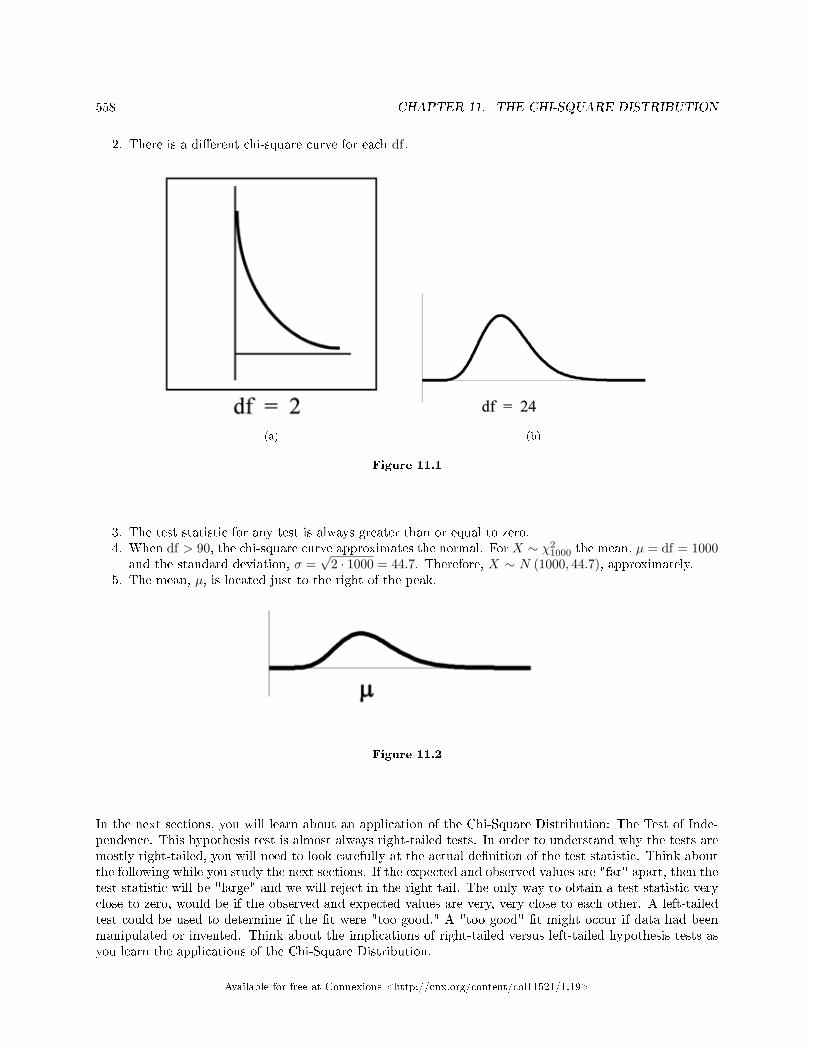
558 CHAPTER 11. THE CHI-SQUARE DISTRIBUTION
2. There is a di�erent chi-square curve for each df.
(a) (b)
Figure 11.1
3. The test statistic for any test is always greater than or equal to zero.4. When df > 90, the chi-square curve approximates the normal. For X ∼ χ2
1000 the mean, µ = df = 1000and the standard deviation, σ =
√2 · 1000 = 44.7. Therefore, X ∼ N (1000, 44.7), approximately.
5. The mean, µ, is located just to the right of the peak.
Figure 11.2
In the next sections, you will learn about an application of the Chi-Square Distribution: The Test of Inde-pendence. This hypothesis test is almost always right-tailed tests. In order to understand why the tests aremostly right-tailed, you will need to look carefully at the actual de�nition of the test statistic. Think aboutthe following while you study the next sections. If the expected and observed values are "far" apart, then thetest statistic will be "large" and we will reject in the right tail. The only way to obtain a test statistic veryclose to zero, would be if the observed and expected values are very, very close to each other. A left-tailedtest could be used to determine if the �t were "too good." A "too good" �t might occur if data had beenmanipulated or invented. Think about the implications of right-tailed versus left-tailed hypothesis tests asyou learn the applications of the Chi-Square Distribution.
Available for free at Connexions <http://cnx.org/content/col11521/1.19>
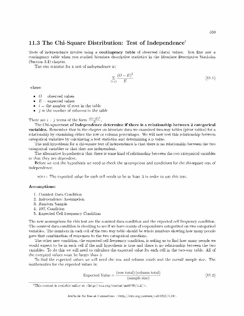
559
11.3 The Chi-Square Distribution: Test of Independence3
Tests of independence involve using a contingency table of observed (data) values. You �rst saw acontingency table when you studied bivariate descriptive statistics in the Bivariate Descriptive Statistics(Section 3.1) chapter.
The test statistic for a test of independence is:
Σ(i·j)
(O − E)2
E(11.1)
where:
• O = observed values• E = expected values• i = the number of rows in the table• j = the number of columns in the table
There are i · j terms of the form (O−E)2
E .The Chi-squaretest of independence determine if there is a relationship between 2 categorical
variables. Remember that in the chapter on bivariate data we examined two-way tables (pivot tables) for arelationship by examining either the row or column percentages. We will now test this relationship betweencategorical variables by calculating a test statistics and determining a p-value.
The null hypothesis for a chi-square test of independence is that there is no relationship between the twocategorical variables or that they are independent.
The alternative hypothesis is that there is some kind of relationship between the two categorical variablesor that they are dependent.
Before we test the hypothesis we need to check the assumptions and conditions for the chi-square test ofindependence.
note: The expected value for each cell needs to be at least 5 in order to use this test.
Assumptions:
1. Counted Data Condition2. Independence Assumption3. Random Sample4. 10% Condition5. Expected Cell Frequency Condition
The new assumptions for this test are the counted data condition and the expected cell frequency condition.The counted data condition is checking to see if we have counts of respondents categorized on two categoricalvariables. The numbers in each cell of the two-way table should be whole numbers showing how many peoplegave that combination of responses to the two categorical questions.
The other new condition, the expected cell frequency condition, is asking us to �nd how many people wewould expect to be in each cell if the null hypothesis is true and there is no relationship between the twovariables. To do this we will need to calculate the expected value for each cell in the two-way table. All ofthe excepted values must be larger than 5.
To �nd the expected values we will need the row and column totals and the overall sample size. Themathematics for the expected values is;
Expected Value =(row total) (column total)
(sample size)(11.2)
3This content is available online at <http://cnx.org/content/m46785/1.2/>.
Available for free at Connexions <http://cnx.org/content/col11521/1.19>
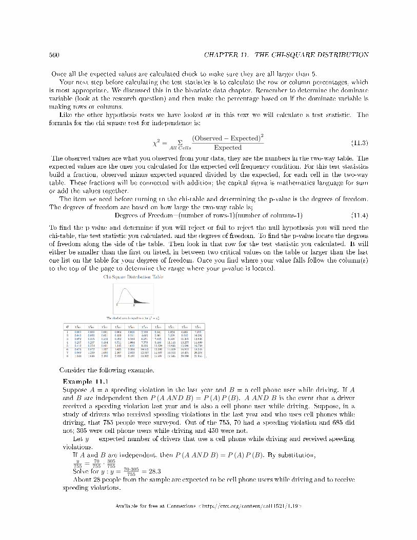
560 CHAPTER 11. THE CHI-SQUARE DISTRIBUTION
Once all the expected values are calculated check to make sure they are all larger than 5.Your next step before calculating the test statistics is to calculate the row or column percentages, which
is most appropriate. We discussed this in the bivariate data chapter. Remember to determine the dominatevariable (look at the research question) and then make the percentage based on if the dominate variable ismaking rows or columns.
Like the other hypothesis tests we have looked at in this text we will calculate a test statistic. Theformula for the chi-square test for independence is:
χ2 = ΣAll Cells
(Observed− Expected)2
Expected(11.3)
The observed values are what you observed from your data, they are the numbers in the two-way table. Theexpected values are the ones you calculated for the expected cell frequency condition. For this test statisticsbuild a fraction, observed minus expected squared divided by the expected, for each cell in the two-waytable. These fractions will be connected with addition; the capital sigma is mathematics language for sumor add the values together.
The item we need before turning to the chi-table and determining the p-value is the degrees of freedom.The degrees of freedom are based on how large the two-way table is;
Degrees of Freedom=(number of rows-1)(number of columns-1) (11.4)
To �nd the p-value and determine if you will reject or fail to reject the null hypothesis you will need thechi-table, the test statistic you calculated, and the degrees of freedom. To �nd the p-value locate the degreesof freedom along the side of the table. Then look in that row for the test statistic you calculated. It willeither be smaller than the �rst on listed, in between two critical values on the table or larger than the lastone list on the table for your degrees of freedom. Once you �nd where your value falls follow the column(s)to the top of the page to determine the range where your p-value is located.
Consider the following example.
Example 11.1Suppose A = a speeding violation in the last year and B = a cell phone user while driving. If Aand B are independent then P (A AND B) = P (A)P (B). A AND B is the event that a driverreceived a speeding violation last year and is also a cell phone user while driving. Suppose, in astudy of drivers who received speeding violations in the last year and who uses cell phones whiledriving, that 755 people were surveyed. Out of the 755, 70 had a speeding violation and 685 didnot; 305 were cell phone users while driving and 450 were not.
Let y = expected number of drivers that use a cell phone while driving and received speedingviolations.
If A and B are independent, then P (A AND B) = P (A)P (B). By substitution,y
755 = 70755 ·
305755
Solve for y : y = 70·305755 = 28.3
About 28 people from the sample are expected to be cell phone users while driving and to receivespeeding violations.
Available for free at Connexions <http://cnx.org/content/col11521/1.19>
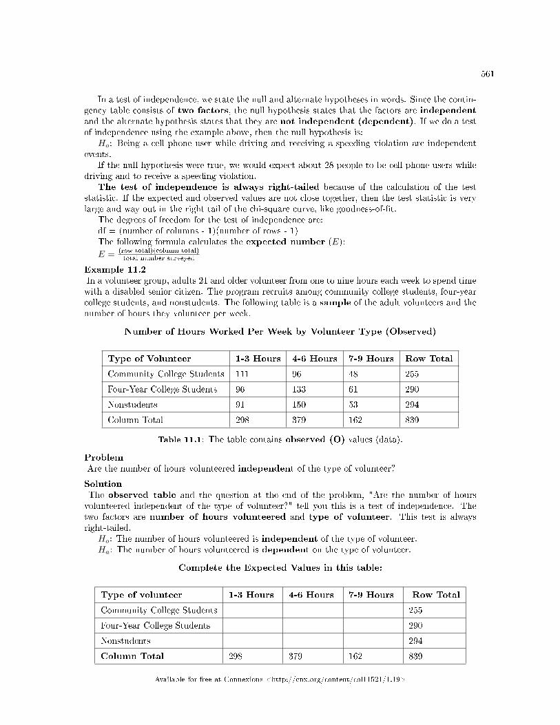
561
In a test of independence, we state the null and alternate hypotheses in words. Since the contin-gency table consists of two factors, the null hypothesis states that the factors are independentand the alternate hypothesis states that they are not independent (dependent). If we do a testof independence using the example above, then the null hypothesis is:
Ho: Being a cell phone user while driving and receiving a speeding violation are independentevents.
If the null hypothesis were true, we would expect about 28 people to be cell phone users whiledriving and to receive a speeding violation.
The test of independence is always right-tailed because of the calculation of the teststatistic. If the expected and observed values are not close together, then the test statistic is verylarge and way out in the right tail of the chi-square curve, like goodness-of-�t.
The degrees of freedom for the test of independence are:df = (number of columns - 1)(number of rows - 1)The following formula calculates the expected number (E):
E = (row total)(column total)total number surveyed
Example 11.2In a volunteer group, adults 21 and older volunteer from one to nine hours each week to spend timewith a disabled senior citizen. The program recruits among community college students, four-yearcollege students, and nonstudents. The following table is a sample of the adult volunteers and thenumber of hours they volunteer per week.
Number of Hours Worked Per Week by Volunteer Type (Observed)
Type of Volunteer 1-3 Hours 4-6 Hours 7-9 Hours Row Total
Community College Students 111 96 48 255
Four-Year College Students 96 133 61 290
Nonstudents 91 150 53 294
Column Total 298 379 162 839
Table 11.1: The table contains observed (O) values (data).
ProblemAre the number of hours volunteered independent of the type of volunteer?
SolutionThe observed table and the question at the end of the problem, "Are the number of hoursvolunteered independent of the type of volunteer?" tell you this is a test of independence. Thetwo factors are number of hours volunteered and type of volunteer. This test is alwaysright-tailed.
Ho: The number of hours volunteered is independent of the type of volunteer.Ha: The number of hours volunteered is dependent on the type of volunteer.
Complete the Expected Values in this table:
Type of volunteer 1-3 Hours 4-6 Hours 7-9 Hours Row Total
Community College Students 255
Four-Year College Students 290
Nonstudents 294
Column Total 298 379 162 839
Available for free at Connexions <http://cnx.org/content/col11521/1.19>
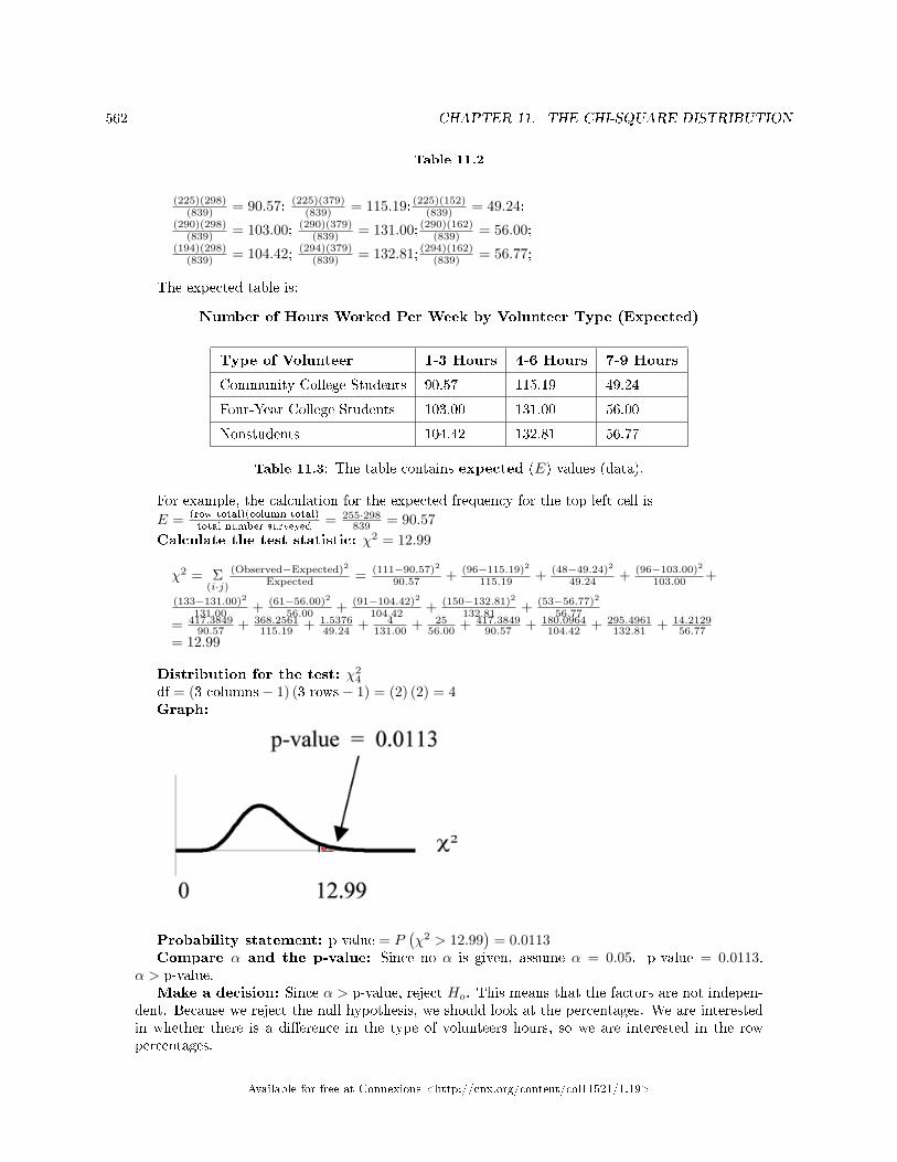
562 CHAPTER 11. THE CHI-SQUARE DISTRIBUTION
Table 11.2
(225)(298)(839) = 90.57; (225)(379)
(839) = 115.19; (225)(152)(839) = 49.24;
(290)(298)(839) = 103.00; (290)(379)
(839) = 131.00; (290)(162)(839) = 56.00;
(194)(298)(839) = 104.42; (294)(379)
(839) = 132.81; (294)(162)(839) = 56.77;
The expected table is:
Number of Hours Worked Per Week by Volunteer Type (Expected)
Type of Volunteer 1-3 Hours 4-6 Hours 7-9 Hours
Community College Students 90.57 115.19 49.24
Four-Year College Students 103.00 131.00 56.00
Nonstudents 104.42 132.81 56.77
Table 11.3: The table contains expected (E) values (data).
For example, the calculation for the expected frequency for the top left cell is
E = (row total)(column total)total number surveyed = 255·298
839 = 90.57Calculate the test statistic: χ2 = 12.99
χ2 = Σ(i·j)
(Observed−Expected)2
Expected = (111−90.57)2
90.57 + (96−115.19)2
115.19 + (48−49.24)2
49.24 + (96−103.00)2
103.00 +
(133−131.00)2
131.00 + (61−56.00)2
56.00 + (91−104.42)2
104.42 + (150−132.81)2
132.81 + (53−56.77)2
56.77= 417.3849
90.57 + 368.2561115.19 + 1.5376
49.24 + 4131.00 + 25
56.00 + 417.384990.57 + 180.0964
104.42 + 295.4961132.81 + 14.2129
56.77= 12.99
Distribution for the test: χ24
df = (3 columns− 1) (3 rows− 1) = (2) (2) = 4Graph:
Probability statement: p-value = P(χ2 > 12.99
)= 0.0113
Compare α and the p-value: Since no α is given, assume α = 0.05. p-value = 0.0113.α > p-value.
Make a decision: Since α > p-value, reject Ho. This means that the factors are not indepen-dent. Because we reject the null hypothesis, we should look at the percentages. We are interestedin whether there is a di�erence in the type of volunteers hours, so we are interested in the rowpercentages.
Available for free at Connexions <http://cnx.org/content/col11521/1.19>
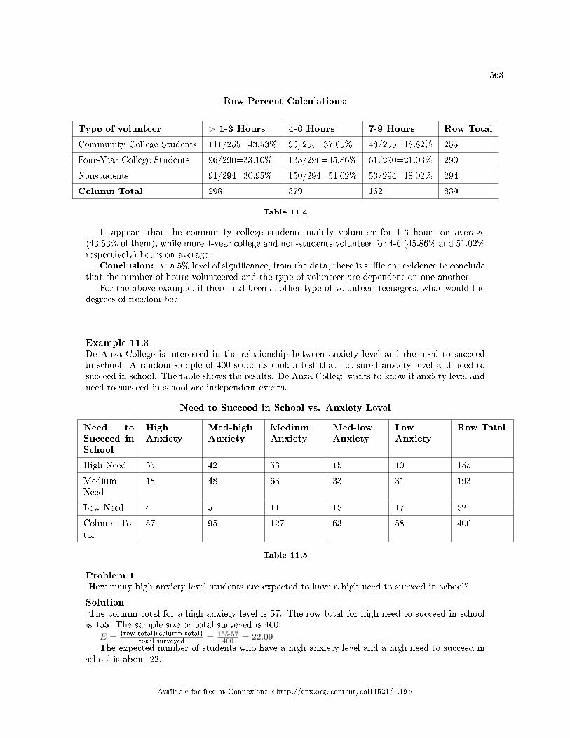
563
Row Percent Calculations:
Type of volunteer > 1-3 Hours 4-6 Hours 7-9 Hours Row Total
Community College Students 111/255=43.53% 96/255=37.65% 48/255=18.82% 255
Four-Year College Students 96/290=33.10% 133/290=45.86% 61/290=21.03% 290
Nonstudents 91/294=30.95% 150/294=51.02% 53/294=18.02% 294
Column Total 298 379 162 839
Table 11.4
It appears that the community college students mainly volunteer for 1-3 hours on average(43.53% of them), while more 4-year college and non-students volunteer for 4-6 (45.86% and 51.02%respectively) hours on average.
Conclusion: At a 5% level of signi�cance, from the data, there is su�cient evidence to concludethat the number of hours volunteered and the type of volunteer are dependent on one another.
For the above example, if there had been another type of volunteer, teenagers, what would thedegrees of freedom be?
Example 11.3De Anza College is interested in the relationship between anxiety level and the need to succeedin school. A random sample of 400 students took a test that measured anxiety level and need tosucceed in school. The table shows the results. De Anza College wants to know if anxiety level andneed to succeed in school are independent events.
Need to Succeed in School vs. Anxiety Level
Need toSucceed inSchool
HighAnxiety
Med-highAnxiety
MediumAnxiety
Med-lowAnxiety
LowAnxiety
Row Total
High Need 35 42 53 15 10 155
MediumNeed
18 48 63 33 31 193
Low Need 4 5 11 15 17 52
Column To-tal
57 95 127 63 58 400
Table 11.5
Problem 1How many high anxiety level students are expected to have a high need to succeed in school?
SolutionThe column total for a high anxiety level is 57. The row total for high need to succeed in schoolis 155. The sample size or total surveyed is 400.
E = (row total)(column total)total surveyed = 155·57
400 = 22.09The expected number of students who have a high anxiety level and a high need to succeed in
school is about 22.
Available for free at Connexions <http://cnx.org/content/col11521/1.19>
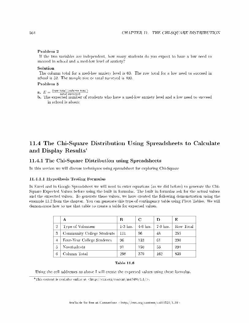
564 CHAPTER 11. THE CHI-SQUARE DISTRIBUTION
Problem 2If the two variables are independent, how many students do you expect to have a low need tosucceed in school and a med-low level of anxiety?
SolutionThe column total for a med-low anxiety level is 63. The row total for a low need to succeed inschool is 52. The sample size or total surveyed is 400.
Problem 3
a. E = (row total)(column total)total surveyed =
b. The expected number of students who have a med-low anxiety level and a low need to succeedin school is about:
11.4 The Chi-Square Distribution Using Spreadsheets to Calculateand Display Results4
11.4.1 The Chi-Square Distribution using Spreadsheets
In this section we will discuss techniques using spreadsheet for exploring Chi-Square
11.4.1.1 Hypothesis Testing Formulas
In Excel and in Google Spreadsheet we will need to enter equations (as we did before) to generate the Chi-Square Expected Values before using the built in formulas. The built in formulas ask for the actual valuesand the expected values. To generate these values, we have created the following demonstration using theexample 11.2 from the chapter. You can generate this type of contingency table using Pivot Tables. We willdemonstrate how to use that table to create a table for expected values.
A B C D E
2 Type of Volunteer 1-3 hrs. 4-6 hrs. 7-9 hrs. Row Total
3 Community College Students 111 96 48 255
4 Four-Year College Students 96 133 61 290
5 Nonstudents 91 150 53 294
6 Column Total 298 379 162 839
Table 11.6
Using the cell addresses as above I will create the expected values using these formulas.
4This content is available online at <http://cnx.org/content/m47486/1.1/>.
Available for free at Connexions <http://cnx.org/content/col11521/1.19>
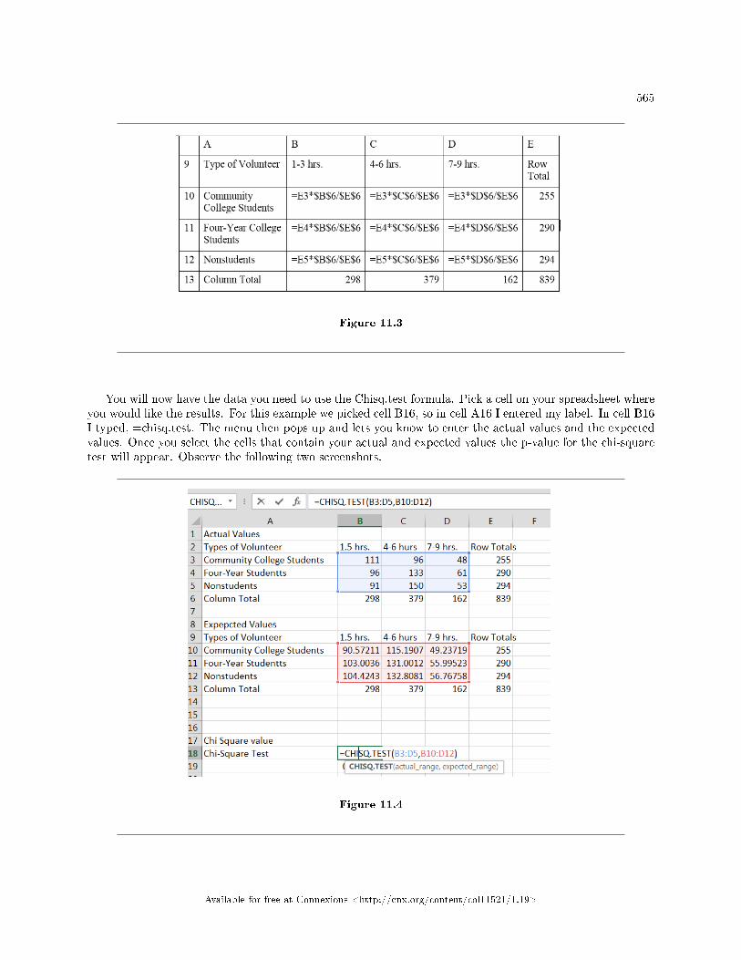
565
Figure 11.3
You will now have the data you need to use the Chisq.test formula. Pick a cell on your spreadsheet whereyou would like the results. For this example we picked cell B16, so in cell A16 I entered my label. In cell B16I typed, =chisq.test. The menu then pops up and lets you know to enter the actual values and the expectedvalues. Once you select the cells that contain your actual and expected values the p-value for the chi-squaretest will appear. Observe the following two screenshots.
Figure 11.4
Available for free at Connexions <http://cnx.org/content/col11521/1.19>
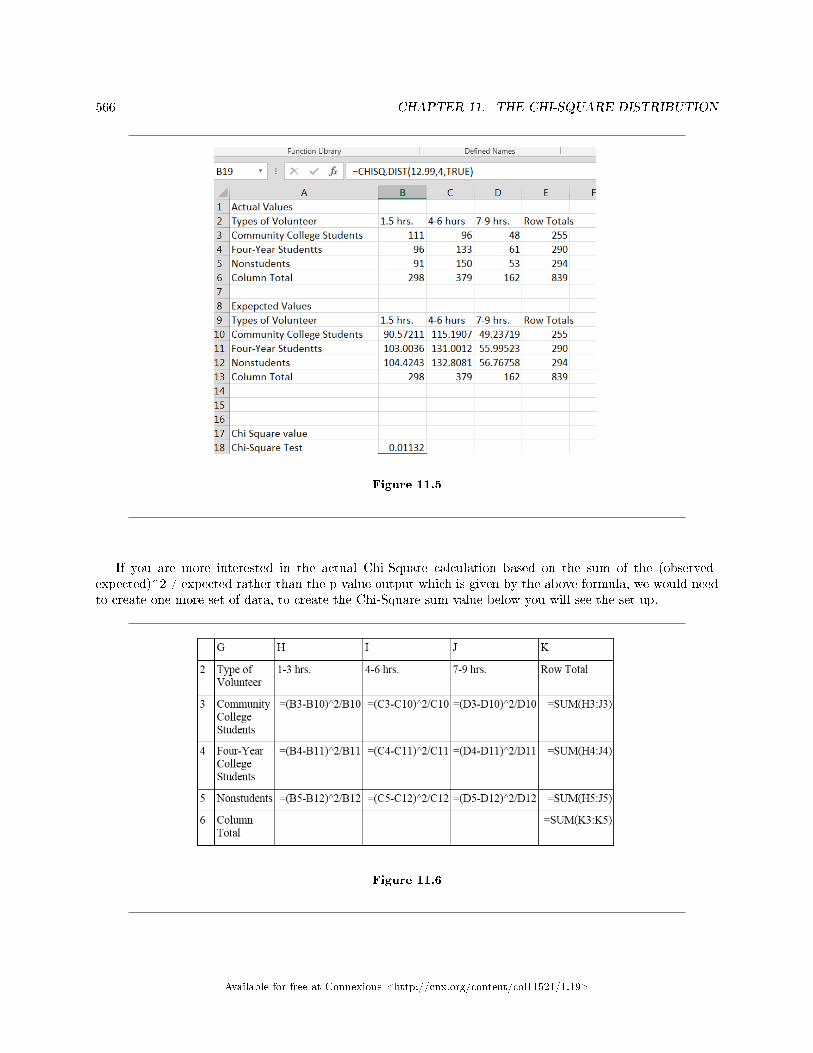
566 CHAPTER 11. THE CHI-SQUARE DISTRIBUTION
Figure 11.5
If you are more interested in the actual Chi-Square calculation based on the sum of the (observed-expected)^2 / expected rather than the p-value output which is given by the above formula, we would needto create one more set of data, to create the Chi-Square sum value below you will see the set up.
Figure 11.6
Available for free at Connexions <http://cnx.org/content/col11521/1.19>
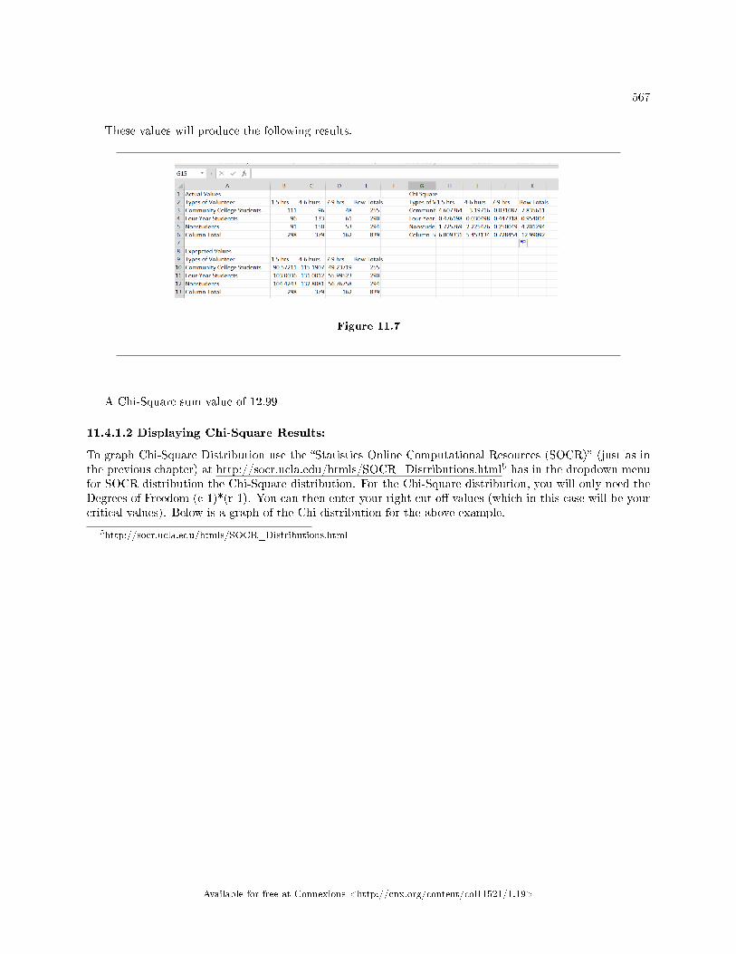
567
These values will produce the following results.
Figure 11.7
A Chi-Square sum value of 12.99
11.4.1.2 Displaying Chi-Square Results:
To graph Chi-Square Distribution use the �Statistics Online Computational Resources (SOCR)� (just as inthe previous chapter) at http://socr.ucla.edu/htmls/SOCR_Distributions.html5 has in the dropdown menufor SOCR distribution the Chi-Square distribution. For the Chi-Square distribution, you will only need theDegrees of Freedom (c-1)*(r-1). You can then enter your right cut o� values (which in this case will be yourcritical values). Below is a graph of the Chi distribution for the above example.
5http://socr.ucla.edu/htmls/SOCR_Distributions.html
Available for free at Connexions <http://cnx.org/content/col11521/1.19>
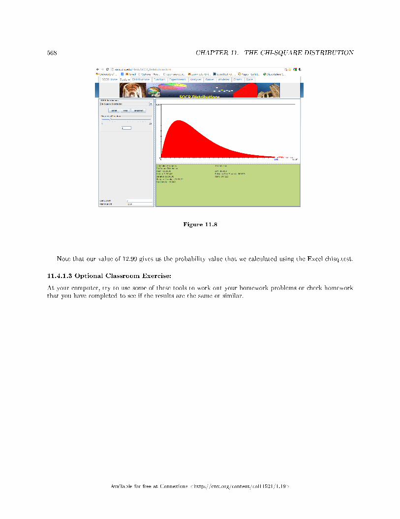
568 CHAPTER 11. THE CHI-SQUARE DISTRIBUTION
Figure 11.8
Note that our value of 12.99 gives us the probability value that we calculated using the Excel chisq.test.
11.4.1.3 Optional Classroom Exercise:
At your computer, try to use some of these tools to work out your homework problems or check homeworkthat you have completed to see if the results are the same or similar.
Available for free at Connexions <http://cnx.org/content/col11521/1.19>
569
11.5 The Chi-Square Distribution: Summary of Formulas6
Test of Independence
• Use the test of independence to test whether two factors are independent or not.• The degrees of freedom are equal to (number of columns - 1)(number of rows - 1).
• The test statistic is Σ(i·j)
(O−E)2
E where O = observed values, E = expected values, i = the number of
rows in the table, and j = the number of columns in the table.• The test is right-tailed.
• If the null hypothesis is true, the expected number E = (row total)(column total)total surveyed .
note: The expected value for each cell needs to be at least 5 in order to use the Independence test.
11.5.1 Glossary
Contingency TableThe method of displaying a frequency distribution as a table with rows and columns to show how twovariables may be dependent (contingent) upon each other. The table provides an easy way to calculateconditional probabilities
6This content is available online at <http://cnx.org/content/m46788/1.2/>.
Available for free at Connexions <http://cnx.org/content/col11521/1.19>
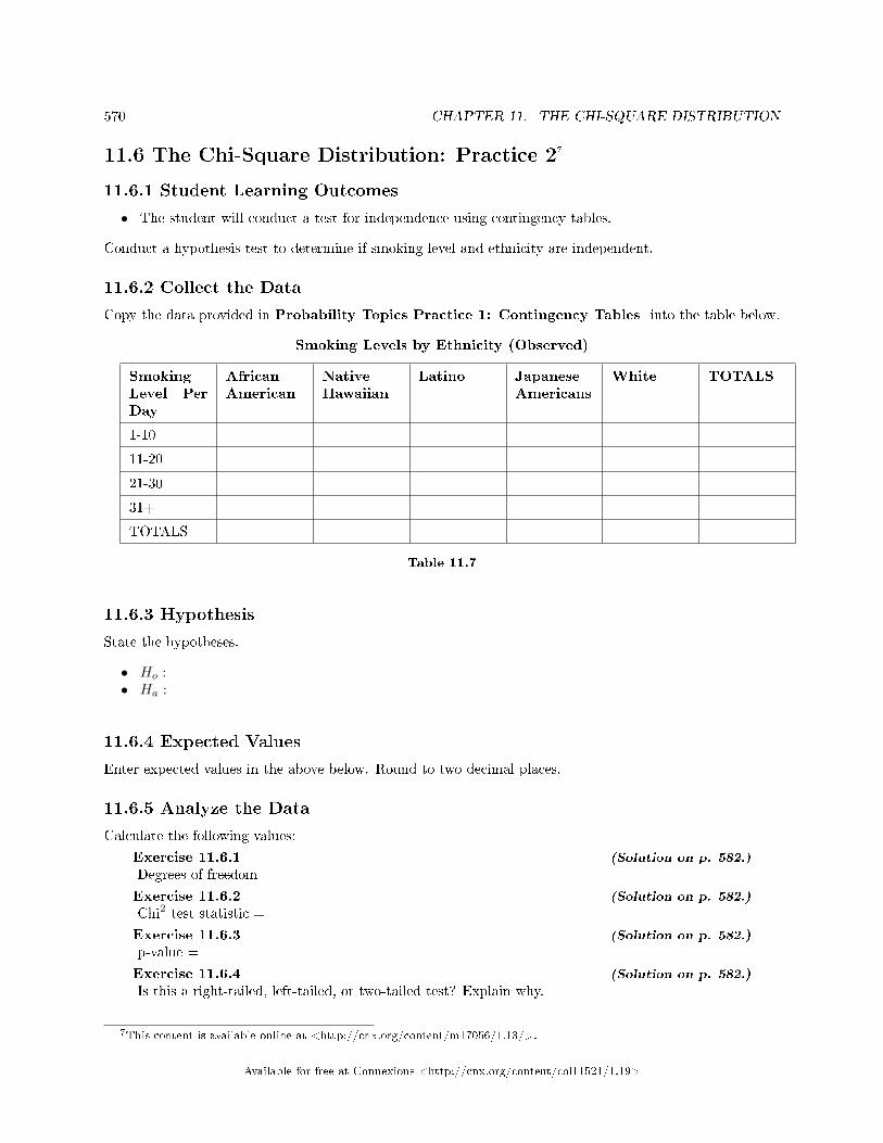
570 CHAPTER 11. THE CHI-SQUARE DISTRIBUTION
11.6 The Chi-Square Distribution: Practice 27
11.6.1 Student Learning Outcomes
• The student will conduct a test for independence using contingency tables.
Conduct a hypothesis test to determine if smoking level and ethnicity are independent.
11.6.2 Collect the Data
Copy the data provided in Probability Topics Practice 1: Contingency Tables into the table below.
Smoking Levels by Ethnicity (Observed)
SmokingLevel PerDay
AfricanAmerican
NativeHawaiian
Latino JapaneseAmericans
White TOTALS
1-10
11-20
21-30
31+
TOTALS
Table 11.7
11.6.3 Hypothesis
State the hypotheses.
• Ho :• Ha :
11.6.4 Expected Values
Enter expected values in the above below. Round to two decimal places.
11.6.5 Analyze the Data
Calculate the following values:
Exercise 11.6.1 (Solution on p. 582.)
Degrees of freedom =
Exercise 11.6.2 (Solution on p. 582.)
Chi2 test statistic =
Exercise 11.6.3 (Solution on p. 582.)
p-value =
Exercise 11.6.4 (Solution on p. 582.)
Is this a right-tailed, left-tailed, or two-tailed test? Explain why.
7This content is available online at <http://cnx.org/content/m17056/1.13/>.
Available for free at Connexions <http://cnx.org/content/col11521/1.19>
571
11.6.6 Graph the Data
Exercise 11.6.5Graph the situation. Label and scale the horizontal axis. Mark the mean and test statistic. Shadein the region corresponding to the p-value.
11.6.7 Conclusions
State the decision and conclusion (in a complete sentence) for the following preconceived levels of α .
Exercise 11.6.6 (Solution on p. 582.)
α = 0.05
a. Decision:b. Reason for the decision:c. Conclusion (write out in a complete sentence):
Exercise 11.6.7α = 0.01
a. Decision:b. Reason for the decision:c. Conclusion (write out in a complete sentence):
Available for free at Connexions <http://cnx.org/content/col11521/1.19>
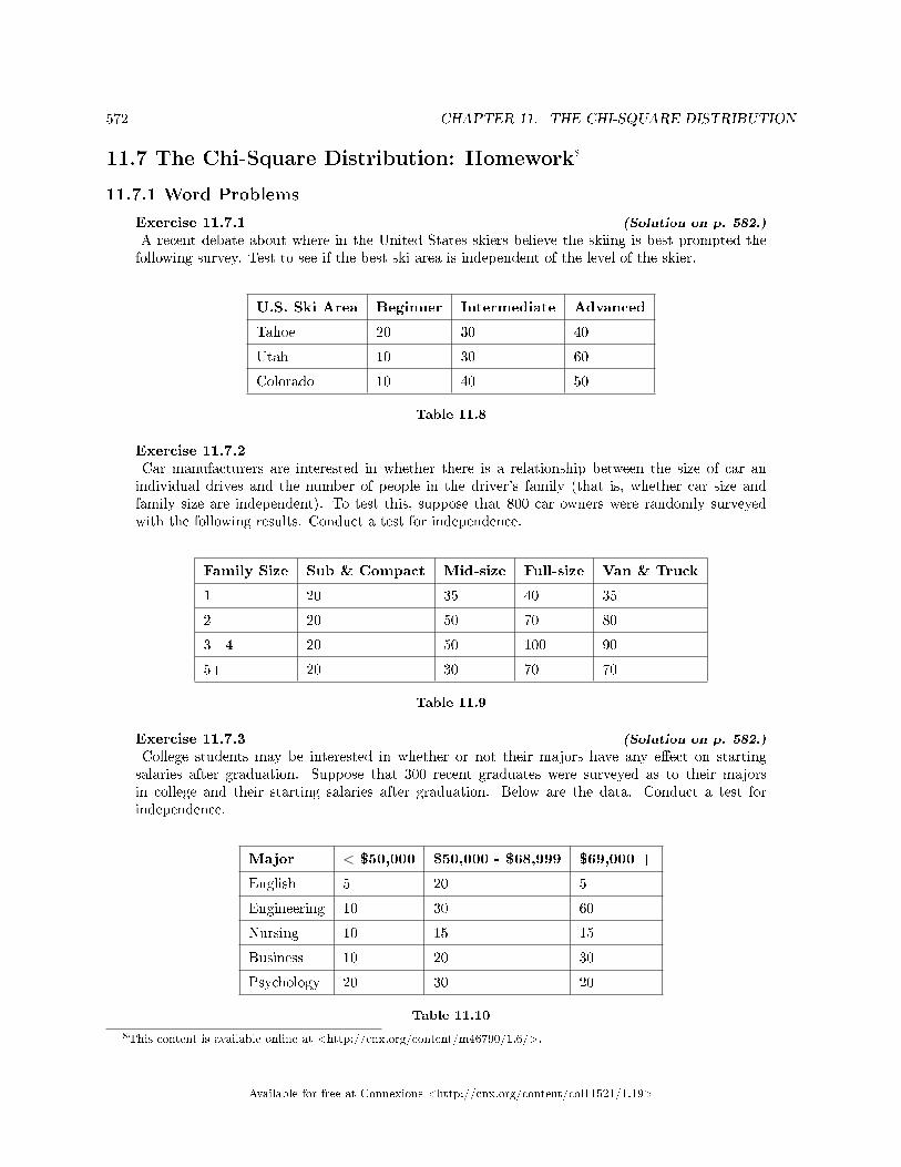
572 CHAPTER 11. THE CHI-SQUARE DISTRIBUTION
11.7 The Chi-Square Distribution: Homework8
11.7.1 Word Problems
Exercise 11.7.1 (Solution on p. 582.)
A recent debate about where in the United States skiers believe the skiing is best prompted thefollowing survey. Test to see if the best ski area is independent of the level of the skier.
U.S. Ski Area Beginner Intermediate Advanced
Tahoe 20 30 40
Utah 10 30 60
Colorado 10 40 50
Table 11.8
Exercise 11.7.2Car manufacturers are interested in whether there is a relationship between the size of car anindividual drives and the number of people in the driver's family (that is, whether car size andfamily size are independent). To test this, suppose that 800 car owners were randomly surveyedwith the following results. Conduct a test for independence.
Family Size Sub & Compact Mid-size Full-size Van & Truck
1 20 35 40 35
2 20 50 70 80
3 - 4 20 50 100 90
5+ 20 30 70 70
Table 11.9
Exercise 11.7.3 (Solution on p. 582.)
College students may be interested in whether or not their majors have any e�ect on startingsalaries after graduation. Suppose that 300 recent graduates were surveyed as to their majorsin college and their starting salaries after graduation. Below are the data. Conduct a test forindependence.
Major < $50,000 $50,000 - $68,999 $69,000 +
English 5 20 5
Engineering 10 30 60
Nursing 10 15 15
Business 10 20 30
Psychology 20 30 20
Table 11.10
8This content is available online at <http://cnx.org/content/m46790/1.6/>.
Available for free at Connexions <http://cnx.org/content/col11521/1.19>
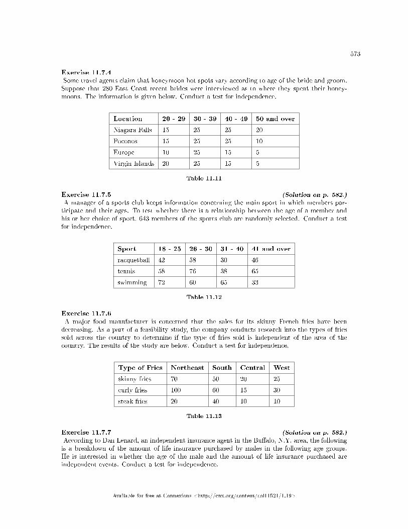
573
Exercise 11.7.4Some travel agents claim that honeymoon hot spots vary according to age of the bride and groom.Suppose that 280 East Coast recent brides were interviewed as to where they spent their honey-moons. The information is given below. Conduct a test for independence.
Location 20 - 29 30 - 39 40 - 49 50 and over
Niagara Falls 15 25 25 20
Poconos 15 25 25 10
Europe 10 25 15 5
Virgin Islands 20 25 15 5
Table 11.11
Exercise 11.7.5 (Solution on p. 582.)
A manager of a sports club keeps information concerning the main sport in which members par-ticipate and their ages. To test whether there is a relationship between the age of a member andhis or her choice of sport, 643 members of the sports club are randomly selected. Conduct a testfor independence.
Sport 18 - 25 26 - 30 31 - 40 41 and over
racquetball 42 58 30 46
tennis 58 76 38 65
swimming 72 60 65 33
Table 11.12
Exercise 11.7.6A major food manufacturer is concerned that the sales for its skinny French fries have beendecreasing. As a part of a feasibility study, the company conducts research into the types of friessold across the country to determine if the type of fries sold is independent of the area of thecountry. The results of the study are below. Conduct a test for independence.
Type of Fries Northeast South Central West
skinny fries 70 50 20 25
curly fries 100 60 15 30
steak fries 20 40 10 10
Table 11.13
Exercise 11.7.7 (Solution on p. 582.)
According to Dan Lenard, an independent insurance agent in the Bu�alo, N.Y. area, the followingis a breakdown of the amount of life insurance purchased by males in the following age groups.He is interested in whether the age of the male and the amount of life insurance purchased areindependent events. Conduct a test for independence.
Available for free at Connexions <http://cnx.org/content/col11521/1.19>
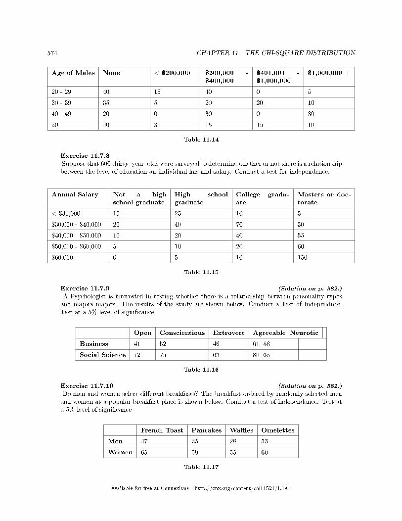
574 CHAPTER 11. THE CHI-SQUARE DISTRIBUTION
Age of Males None < $200,000 $200,000 -$400,000
$401,001 -$1,000,000
$1,000,000 +
20 - 29 40 15 40 0 5
30 - 39 35 5 20 20 10
40 - 49 20 0 30 0 30
50 + 40 30 15 15 10
Table 11.14
Exercise 11.7.8Suppose that 600 thirty�year�olds were surveyed to determine whether or not there is a relationshipbetween the level of education an individual has and salary. Conduct a test for independence.
Annual Salary Not a highschool graduate
High schoolgraduate
College gradu-ate
Masters or doc-torate
< $30,000 15 25 10 5
$30,000 - $40,000 20 40 70 30
$40,000 - $50,000 10 20 40 55
$50,000 - $60,000 5 10 20 60
$60,000 + 0 5 10 150
Table 11.15
Exercise 11.7.9 (Solution on p. 582.)
A Psychologist is interested in testing whether there is a relationship between personality typesand majors majors. The results of the study are shown below. Conduct a Test of Independnce.Test at a 5% level of signi�cance.
Open Conscientious Extrovert Agreeable Neurotic
Business 41 52 46 61 58
Social Science 72 75 63 80 65
Table 11.16
Exercise 11.7.10 (Solution on p. 582.)
Do men and women select di�erent breakfasts? The breakfast ordered by randomly selected menand women at a popular breakfast place is shown below. Conduct a test of independance. Test ata 5% level of signi�cance
French Toast Pancakes Wa�es Omelettes
Men 47 35 28 53
Women 65 59 55 60
Table 11.17
Available for free at Connexions <http://cnx.org/content/col11521/1.19>
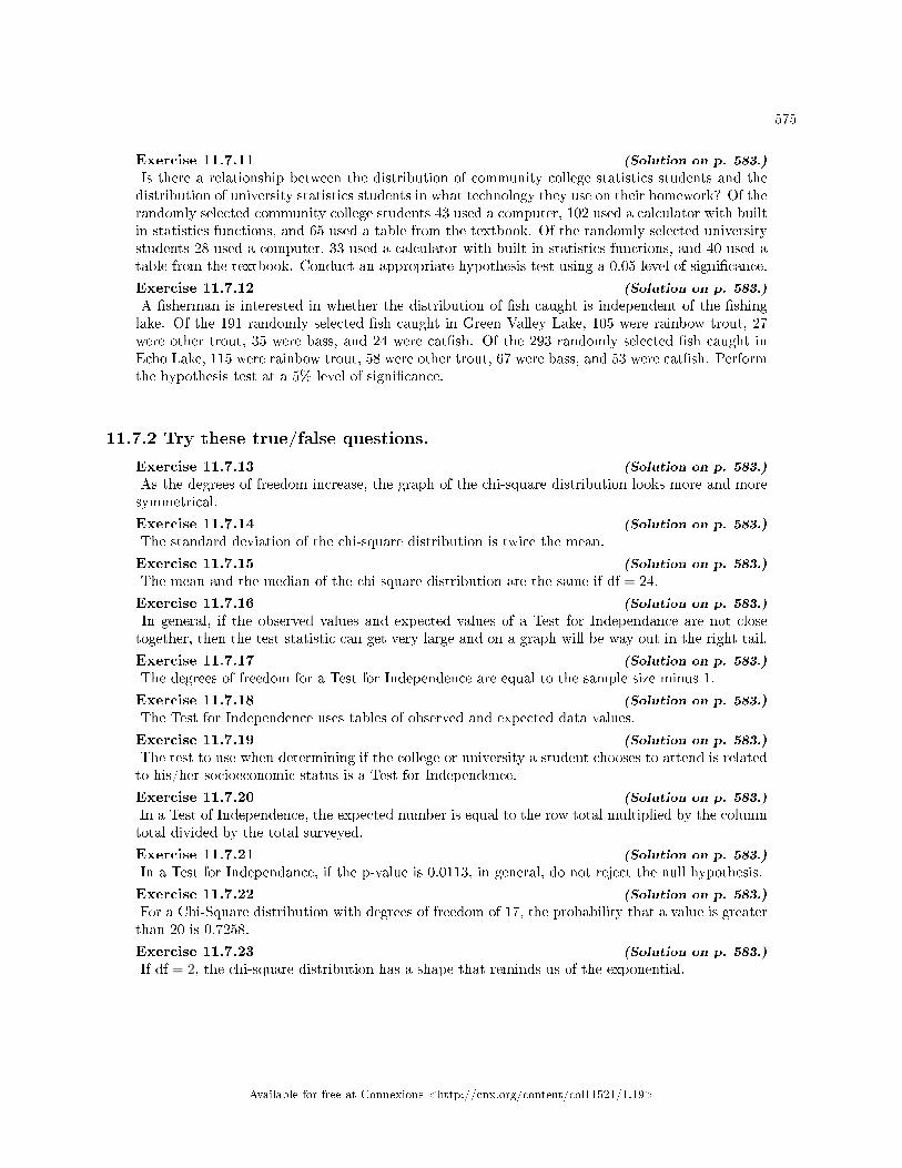
575
Exercise 11.7.11 (Solution on p. 583.)
Is there a relationship between the distribution of community college statistics students and thedistribution of university statistics students in what technology they use on their homework? Of therandomly selected community college students 43 used a computer, 102 used a calculator with builtin statistics functions, and 65 used a table from the textbook. Of the randomly selected universitystudents 28 used a computer, 33 used a calculator with built in statistics functions, and 40 used atable from the textbook. Conduct an appropriate hypothesis test using a 0.05 level of signi�cance.
Exercise 11.7.12 (Solution on p. 583.)
A �sherman is interested in whether the distribution of �sh caught is independent of the �shinglake. Of the 191 randomly selected �sh caught in Green Valley Lake, 105 were rainbow trout, 27were other trout, 35 were bass, and 24 were cat�sh. Of the 293 randomly selected �sh caught inEcho Lake, 115 were rainbow trout, 58 were other trout, 67 were bass, and 53 were cat�sh. Performthe hypothesis test at a 5% level of signi�cance.
11.7.2 Try these true/false questions.
Exercise 11.7.13 (Solution on p. 583.)
As the degrees of freedom increase, the graph of the chi-square distribution looks more and moresymmetrical.
Exercise 11.7.14 (Solution on p. 583.)
The standard deviation of the chi-square distribution is twice the mean.
Exercise 11.7.15 (Solution on p. 583.)
The mean and the median of the chi-square distribution are the same if df = 24.
Exercise 11.7.16 (Solution on p. 583.)
In general, if the observed values and expected values of a Test for Independance are not closetogether, then the test statistic can get very large and on a graph will be way out in the right tail.
Exercise 11.7.17 (Solution on p. 583.)
The degrees of freedom for a Test for Independence are equal to the sample size minus 1.
Exercise 11.7.18 (Solution on p. 583.)
The Test for Independence uses tables of observed and expected data values.
Exercise 11.7.19 (Solution on p. 583.)
The test to use when determining if the college or university a student chooses to attend is relatedto his/her socioeconomic status is a Test for Independence.
Exercise 11.7.20 (Solution on p. 583.)
In a Test of Independence, the expected number is equal to the row total multiplied by the columntotal divided by the total surveyed.
Exercise 11.7.21 (Solution on p. 583.)
In a Test for Independance, if the p-value is 0.0113, in general, do not reject the null hypothesis.
Exercise 11.7.22 (Solution on p. 583.)
For a Chi-Square distribution with degrees of freedom of 17, the probability that a value is greaterthan 20 is 0.7258.
Exercise 11.7.23 (Solution on p. 583.)
If df = 2, the chi-square distribution has a shape that reminds us of the exponential.
Available for free at Connexions <http://cnx.org/content/col11521/1.19>
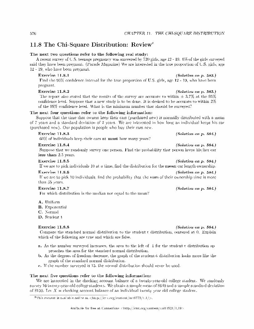
576 CHAPTER 11. THE CHI-SQUARE DISTRIBUTION
11.8 The Chi-Square Distribution: Review9
The next two questions refer to the following real study:A recent survey of U.S. teenage pregnancy was answered by 720 girls, age 12 - 19. 6% of the girls surveyed
said they have been pregnant. (Parade Magazine) We are interested in the true proportion of U.S. girls, age12 - 19, who have been pregnant.
Exercise 11.8.1 (Solution on p. 583.)
Find the 95% con�dence interval for the true proportion of U.S. girls, age 12 - 19, who have beenpregnant.
Exercise 11.8.2 (Solution on p. 583.)
The report also stated that the results of the survey are accurate to within ± 3.7% at the 95%con�dence level. Suppose that a new study is to be done. It is desired to be accurate to within 2%of the 95% con�dence level. What is the minimum number that should be surveyed?
The next four questions refer to the following information:Suppose that the time that owners keep their cars (purchased new) is normally distributed with a mean
of 7 years and a standard deviation of 2 years. We are interested in how long an individual keeps his car(purchased new). Our population is people who buy their cars new.
Exercise 11.8.3 (Solution on p. 584.)
60% of individuals keep their cars at most how many years?
Exercise 11.8.4 (Solution on p. 584.)
Suppose that we randomly survey one person. Find the probability that person keeps his/her carless than 2.5 years.
Exercise 11.8.5 (Solution on p. 584.)
If we are to pick individuals 10 at a time, �nd the distribution for the mean car length ownership.
Exercise 11.8.6 (Solution on p. 584.)
If we are to pick 10 individuals, �nd the probability that the sum of their ownership time is morethan 55 years.
Exercise 11.8.7 (Solution on p. 584.)
For which distribution is the median not equal to the mean?
A. UniformB. ExponentialC. NormalD. Student-t
Exercise 11.8.8 (Solution on p. 584.)
Compare the standard normal distribution to the student-t distribution, centered at 0. Explainwhich of the following are true and which are false.
a. As the number surveyed increases, the area to the left of -1 for the student-t distribution ap-proaches the area for the standard normal distribution.
b. As the degrees of freedom decrease, the graph of the student-t distribution looks more like thegraph of the standard normal distribution.
c. If the number surveyed is 15, the normal distribution should never be used.
The next �ve questions refer to the following information:We are interested in the checking account balance of a twenty-year-old college student. We randomly
survey 16 twenty-year-old college students. We obtain a sample mean of $640 and a sample standard deviationof $150. Let X = checking account balance of an individual twenty year old college student.
9This content is available online at <http://cnx.org/content/m46773/1.1/>.
Available for free at Connexions <http://cnx.org/content/col11521/1.19>
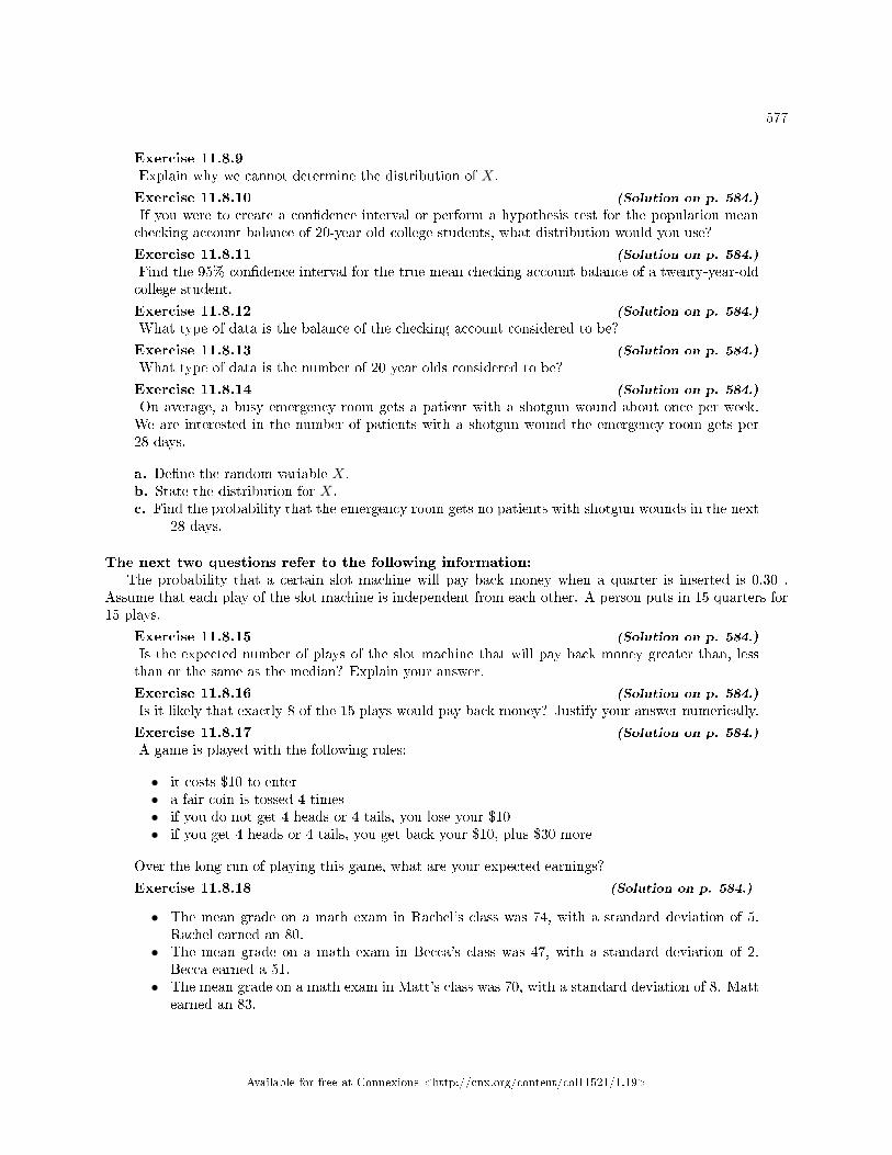
577
Exercise 11.8.9Explain why we cannot determine the distribution of X.
Exercise 11.8.10 (Solution on p. 584.)
If you were to create a con�dence interval or perform a hypothesis test for the population meanchecking account balance of 20-year old college students, what distribution would you use?
Exercise 11.8.11 (Solution on p. 584.)
Find the 95% con�dence interval for the true mean checking account balance of a twenty-year-oldcollege student.
Exercise 11.8.12 (Solution on p. 584.)
What type of data is the balance of the checking account considered to be?
Exercise 11.8.13 (Solution on p. 584.)
What type of data is the number of 20 year olds considered to be?
Exercise 11.8.14 (Solution on p. 584.)
On average, a busy emergency room gets a patient with a shotgun wound about once per week.We are interested in the number of patients with a shotgun wound the emergency room gets per28 days.
a. De�ne the random variable X.b. State the distribution for X.c. Find the probability that the emergency room gets no patients with shotgun wounds in the next
28 days.
The next two questions refer to the following information:The probability that a certain slot machine will pay back money when a quarter is inserted is 0.30 .
Assume that each play of the slot machine is independent from each other. A person puts in 15 quarters for15 plays.
Exercise 11.8.15 (Solution on p. 584.)
Is the expected number of plays of the slot machine that will pay back money greater than, lessthan or the same as the median? Explain your answer.
Exercise 11.8.16 (Solution on p. 584.)
Is it likely that exactly 8 of the 15 plays would pay back money? Justify your answer numerically.
Exercise 11.8.17 (Solution on p. 584.)
A game is played with the following rules:
• it costs $10 to enter• a fair coin is tossed 4 times• if you do not get 4 heads or 4 tails, you lose your $10• if you get 4 heads or 4 tails, you get back your $10, plus $30 more
Over the long run of playing this game, what are your expected earnings?
Exercise 11.8.18 (Solution on p. 584.)
• The mean grade on a math exam in Rachel's class was 74, with a standard deviation of 5.Rachel earned an 80.
• The mean grade on a math exam in Becca's class was 47, with a standard deviation of 2.Becca earned a 51.
• The mean grade on a math exam in Matt's class was 70, with a standard deviation of 8. Mattearned an 83.
Available for free at Connexions <http://cnx.org/content/col11521/1.19>
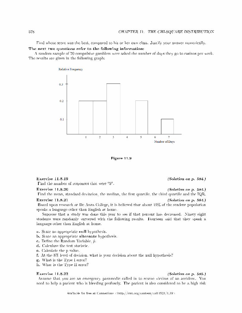
578 CHAPTER 11. THE CHI-SQUARE DISTRIBUTION
Find whose score was the best, compared to his or her own class. Justify your answer numerically.
The next two questions refer to the following information:A random sample of 70 compulsive gamblers were asked the number of days they go to casinos per week.
The results are given in the following graph:
Figure 11.9
Exercise 11.8.19 (Solution on p. 584.)
Find the number of responses that were �5".
Exercise 11.8.20 (Solution on p. 584.)
Find the mean, standard deviation, the median, the �rst quartile, the third quartile and the IQR.
Exercise 11.8.21 (Solution on p. 584.)
Based upon research at De Anza College, it is believed that about 19% of the student populationspeaks a language other than English at home.
Suppose that a study was done this year to see if that percent has decreased. Ninety-eightstudents were randomly surveyed with the following results. Fourteen said that they speak alanguage other than English at home.
a. State an appropriate null hypothesis.b. State an appropriate alternate hypothesis.c. De�ne the Random Variable, p̂.d. Calculate the test statistic.e. Calculate the p-value.f. At the 5% level of decision, what is your decision about the null hypothesis?g. What is the Type I error?h. What is the Type II error?
Exercise 11.8.22 (Solution on p. 585.)
Assume that you are an emergency paramedic called in to rescue victims of an accident. Youneed to help a patient who is bleeding profusely. The patient is also considered to be a high risk
Available for free at Connexions <http://cnx.org/content/col11521/1.19>
579
for contracting AIDS. Assume that the null hypothesis is that the patient does not have the HIVvirus. What is a Type I error?
Exercise 11.8.23 (Solution on p. 585.)
It is often said that Californians are more casual than the rest of Americans. Suppose that a surveywas done to see if the proportion of Californian professionals that wear jeans to work is greaterthan the proportion of non-Californian professionals. Fifty of each was surveyed with the followingresults. 15 Californians wear jeans to work and 6 non-Californians wear jeans to work.
• C = Californian professional• NC = non-Californian professional
a. State appropriate null and alternate hypotheses.b. De�ne the Random Variable.c. Calculate the test statistic and p-value.d. At the 5% signi�cance level, what is your decision?e. What is the Type I error?f. What is the Type II error?
Available for free at Connexions <http://cnx.org/content/col11521/1.19>
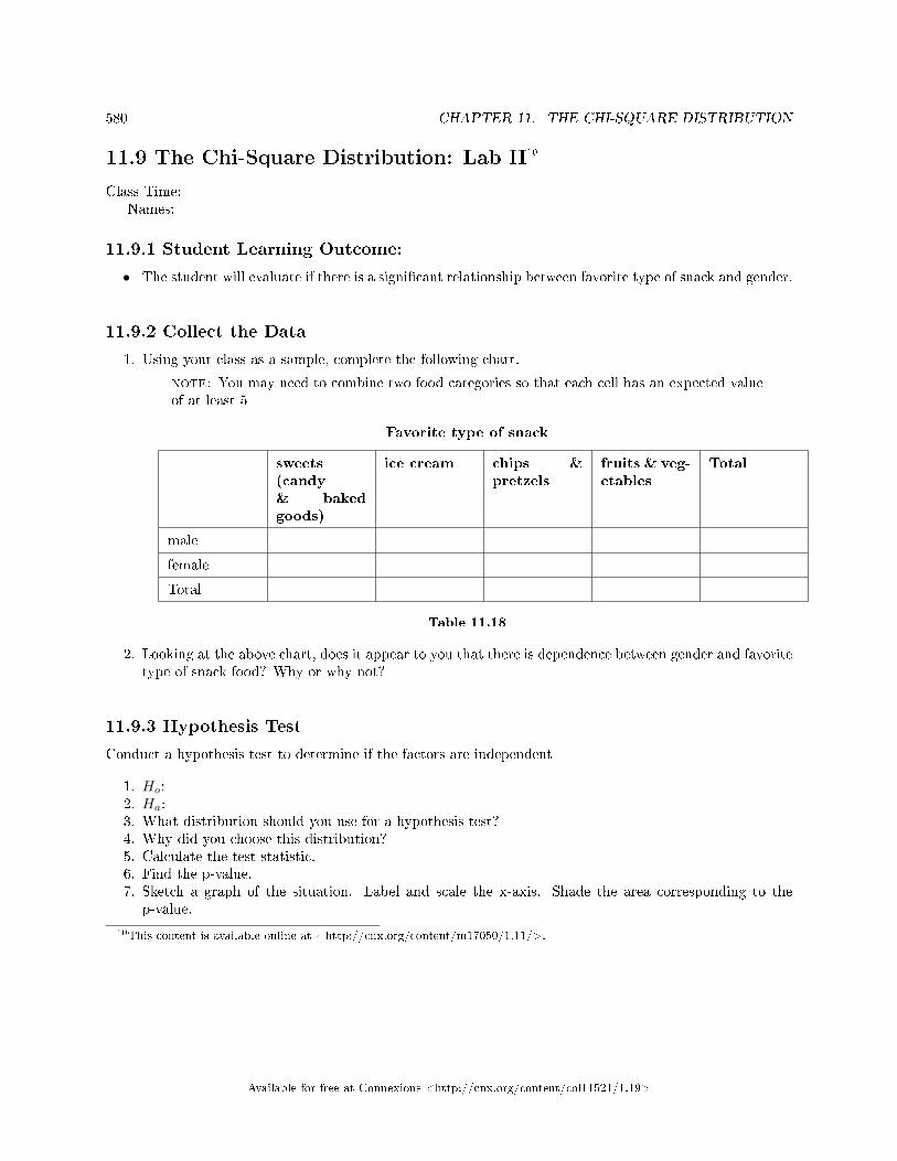
580 CHAPTER 11. THE CHI-SQUARE DISTRIBUTION
11.9 The Chi-Square Distribution: Lab II10
Class Time:Names:
11.9.1 Student Learning Outcome:
• The student will evaluate if there is a signi�cant relationship between favorite type of snack and gender.
11.9.2 Collect the Data
1. Using your class as a sample, complete the following chart.
note: You may need to combine two food categories so that each cell has an expected valueof at least 5
Favorite type of snack
sweets(candy& bakedgoods)
ice cream chips &pretzels
fruits & veg-etables
Total
male
female
Total
Table 11.18
2. Looking at the above chart, does it appear to you that there is dependence between gender and favoritetype of snack food? Why or why not?
11.9.3 Hypothesis Test
Conduct a hypothesis test to determine if the factors are independent
1. Ho:2. Ha:3. What distribution should you use for a hypothesis test?4. Why did you choose this distribution?5. Calculate the test statistic.6. Find the p-value.7. Sketch a graph of the situation. Label and scale the x-axis. Shade the area corresponding to the
p-value.
10This content is available online at <http://cnx.org/content/m17050/1.11/>.
Available for free at Connexions <http://cnx.org/content/col11521/1.19>
581
Figure 11.10
8. State your decision.9. State your conclusion in a complete sentence.
11.9.4 Discussion Questions
1. Is the conclusion of your study the same as or di�erent from your answer to (I2) above?2. Why do you think that occurred?
Available for free at Connexions <http://cnx.org/content/col11521/1.19>
582 CHAPTER 11. THE CHI-SQUARE DISTRIBUTION
Solutions to Exercises in Chapter 11
Solutions to The Chi-Square Distribution: Practice 2
Solution to Exercise 11.6.1 (p. 570)12Solution to Exercise 11.6.2 (p. 570)10301.8Solution to Exercise 11.6.3 (p. 570)0Solution to Exercise 11.6.4 (p. 570)rightSolution to Exercise 11.6.6 (p. 571)
a. Reject the null hypothesis
Solutions to The Chi-Square Distribution: Homework
Solution to Exercise 11.7.1 (p. 572)
c. 4e. 10.53f. 0.0324h. Decision: Reject null; Conclusion: Best ski area and level of skier are not independent.
Solution to Exercise 11.7.3 (p. 572)
c. 8e. 33.55f. 0h. Decision: Reject null; Conclusion: Major and starting salary are not independent events.
Solution to Exercise 11.7.5 (p. 573)
c. 6e. 25.21f. 0.0003h. Decision: Reject null
Solution to Exercise 11.7.7 (p. 573)
c. 12e. 125.74f. 0h. Decision: Reject null
Solution to Exercise 11.7.9 (p. 574)
c: 4d: Chi-Square with df = 4e: 3.01f: p-value = 0.5568h: ii. Do not reject the null hypothesis.
iv. There is insu�cient evidence to conclude that the personality types are dependent majors.
Solution to Exercise 11.7.10 (p. 574)
Available for free at Connexions <http://cnx.org/content/col11521/1.19>
583
c: 3e: 4.01f: p-value = 0.2601h: ii. Do not reject the null hypothesis.
iv. There is insu�cient evidence to conclude that the distribution of breakfast ordered is dependenton gender.
Solution to Exercise 11.7.11 (p. 575)
c: 2e: 7.05f: p-value = 0.0294h: ii. Reject the null hypothesis.
iv. There is su�cient evidence to conclude that the distribution of technology use for statistics home-work is not independent for statistics students at community colleges and at universities.
Solution to Exercise 11.7.12 (p. 575)
c: 3d: Chi-Square with df = 3e: 11.75f: p-value = 0.0083h: ii. Reject the null hypothesis.
iv. There is su�cient evidence to conclude that the distribution of �sh is dependent on the �shinglake. Green Valley Lake does not have the same distribution of �sh as Echo Lake.
Solution to Exercise 11.7.13 (p. 575)TrueSolution to Exercise 11.7.14 (p. 575)FalseSolution to Exercise 11.7.15 (p. 575)FalseSolution to Exercise 11.7.16 (p. 575)TrueSolution to Exercise 11.7.17 (p. 575)FalseSolution to Exercise 11.7.18 (p. 575)TrueSolution to Exercise 11.7.19 (p. 575)TrueSolution to Exercise 11.7.20 (p. 575)TrueSolution to Exercise 11.7.21 (p. 575)FalseSolution to Exercise 11.7.22 (p. 575)FalseSolution to Exercise 11.7.23 (p. 575)True
Solutions to The Chi-Square Distribution: Review
Solution to Exercise 11.8.1 (p. 576)(0.0424, 0.0770)
Available for free at Connexions <http://cnx.org/content/col11521/1.19>
584 CHAPTER 11. THE CHI-SQUARE DISTRIBUTION
Solution to Exercise 11.8.2 (p. 576)2401Solution to Exercise 11.8.3 (p. 576)7.5Solution to Exercise 11.8.4 (p. 576)0.0122Solution to Exercise 11.8.5 (p. 576)N (7, 0.63)Solution to Exercise 11.8.6 (p. 576)0.9911Solution to Exercise 11.8.7 (p. 576)BSolution to Exercise 11.8.8 (p. 576)
a. Trueb. Falsec. False
Solution to Exercise 11.8.10 (p. 577)student-t with df = 15Solution to Exercise 11.8.11 (p. 577)(560.07, 719.93)Solution to Exercise 11.8.12 (p. 577)quantitative - continuousSolution to Exercise 11.8.13 (p. 577)quantitative - discreteSolution to Exercise 11.8.14 (p. 577)
b. P (4)c. 0.0183
Solution to Exercise 11.8.15 (p. 577)greater thanSolution to Exercise 11.8.16 (p. 577)No; P (x = 8) = 0.0348Solution to Exercise 11.8.17 (p. 577)You will lose $5Solution to Exercise 11.8.18 (p. 577)BeccaSolution to Exercise 11.8.19 (p. 578)14Solution to Exercise 11.8.20 (p. 578)
�. Sample mean = 3.2�. Sample standard deviation = 1.85�. Median = 3�. Quartile 1 = 2�. Quartile 3 = 5�. IQR = 3
Solution to Exercise 11.8.21 (p. 578)
d. z = −1.19e. 0.1171
Available for free at Connexions <http://cnx.org/content/col11521/1.19>
585
f. Do not reject the null
Solution to Exercise 11.8.22 (p. 578)We conclude that the patient does have the HIV virus when, in fact, the patient does not.Solution to Exercise 11.8.23 (p. 579)
c. z = 2.21 ; p = 0.0136d. Reject the nulle. We conclude that the proportion of Californian professionals that wear jeans to work is greater than the
proportion of non-Californian professionals when, in fact, it is not greater.f. We cannot conclude that the proportion of Californian professionals that wear jeans to work is greater
than the proportion of non-Californian professionals when, in fact, it is greater.
Available for free at Connexions <http://cnx.org/content/col11521/1.19>

586 CHAPTER 11. THE CHI-SQUARE DISTRIBUTION
Available for free at Connexions <http://cnx.org/content/col11521/1.19>
Chapter 12
Testing the Signi�cance of the
Correlation Coe�cient
12.1 Inferencial Statistics: Testing the Signi�cance of the CorrelationCoe�cient1
12.1.1 Testing the Signi�cance of the Correlation Coe�cient
The correlation coe�cient, r, tells us about the strength of the linear relationship between x and y. However,the reliability of the linear model also depends on how many observed data points are in the sample. Weneed to look at both the value of the correlation coe�cient r and the sample size n, together.
We perform a hypothesis test of the "signi�cance of the correlation coe�cient" to decide whetherthe linear relationship in the sample data is strong enough to use to model the relationship in the population.
The sample data is used to compute r, the correlation coe�cient for the sample. If we had data for theentire population, we could �nd the population correlation coe�cient. But because we only have sampledata, we can not calculate the population correlation coe�cient. The sample correlation coe�cient, r, is ourestimate of the unknown population correlation coe�cient.
The symbol for the population correlation coe�cient is ρ, the Greek letter "rho".ρ = population correlation coe�cient (unknown)r = sample correlation coe�cient (known; calculated from sample data)
The hypothesis test lets us decide whether the value of the population correlation coe�cient ρ is "close to0" or "signi�cantly di�erent from 0". We decide this based on the sample correlation coe�cient r and thesample size n.
If the test concludes that the correlation coe�cient is signi�cantly di�erent from 0, we saythat the correlation coe�cient is "signi�cant".
• Conclusion: "There is su�cient evidence to conclude that there is a signi�cant linear relationshipbetween x and y because the correlation coe�cient is signi�cantly di�erent from 0."
• What the conclusion means: There is a signi�cant linear relationship between x and y. We can usethe regression line to model the linear relationship between x and y in the population.
If the test concludes that the correlation coe�cient is not signi�cantly di�erent from 0 (it isclose to 0), we say that correlation coe�cient is "not signi�cant".
1This content is available online at <http://cnx.org/content/m47477/1.1/>.
Available for free at Connexions <http://cnx.org/content/col11521/1.19>
587
588CHAPTER 12. TESTING THE SIGNIFICANCE OF THE CORRELATION
COEFFICIENT
• Conclusion: "There is insu�cient evidence to conclude that there is a signi�cant linear relationshipbetween x and y because the correlation coe�cient is not signi�cantly di�erent from 0."
• What the conclusion means: There is not a signi�cant linear relationship between x and y. Thereforewe can NOT use the regression line to model a linear relationship between x and y in the population.
note:
• If r is signi�cant and the scatter plot shows a linear trend, the line can be used to predict thevalue of y for values of x that are within the domain of observed x values.• If r is not signi�cant OR if the scatter plot does not show a linear trend, the line should notbe used for prediction.• If r is signi�cant and if the scatter plot shows a linear trend, the line may NOT be appropriateor reliable for prediction OUTSIDE the domain of observed x values in the data.
PERFORMING THE HYPOTHESIS TEST
SETTING UP THE HYPOTHESES:
• Null Hypothesis: Ho: ρ = 0• Alternate Hypothesis: Ha: ρ 6= 0
What the hypotheses mean in words:
• Null Hypothesis Ho: The population correlation coe�cient IS NOT signi�cantly di�erent from 0.There IS NOT a signi�cant linear relationship(correlation) between x and y in the population.
• Alternate Hypothesis Ha: The population correlation coe�cient IS signi�cantly DIFFERENTFROM 0. There IS A SIGNIFICANT LINEAR RELATIONSHIP (correlation) between x and y in thepopulation.
DRAWING A CONCLUSION:
There are various methods used to make the decision. The methods are equivalent and give the sameresult.We present the critical value method.
Using a table of critical valuesIn this chapter of this textbook, we will always use a signi�cance level of 5%, α = 0.05Note: The table of critical values provided in this textbook assumes that we are using a signi�cance level
of 5%, α = 0.05. (If we wanted to use a di�erent signi�cance level than 5% with the critical valuemethod, we would need di�erent tables of critical values that are not provided in this textbook.)
Using a table of Critical Values to make a decisionThe 95% Critical Values of the Sample Correlation Coe�cient Table (Section 12.2) at the endof this chapter (before the Summary2) may be used to give you a good idea of whether the computedvalue of r is signi�cant or not. Compare r to the appropriate critical value in the table. If r is outsidethe positive and negative critical values, then the correlation coe�cient is signi�cant. If r is signi�cant, thenyou may want to use the line for prediction.
Example 12.1Suppose you computed r = 0.801 using n = 10 data points. df = n − 2 = 10 − 2 = 8. Thecritical values associated with df = 8 are -0.632 and + 0.632. If r< negative critical value orr > positive critical value, then r is signi�cant. Since r = 0.801 and 0.801 > 0.632, r is signi�cantand the line may be used for prediction. If you view this example on a number line, it will helpyou.
2"Linear Regression and Correlation: Summary" <http://cnx.org/content/m17081/latest/>
Available for free at Connexions <http://cnx.org/content/col11521/1.19>
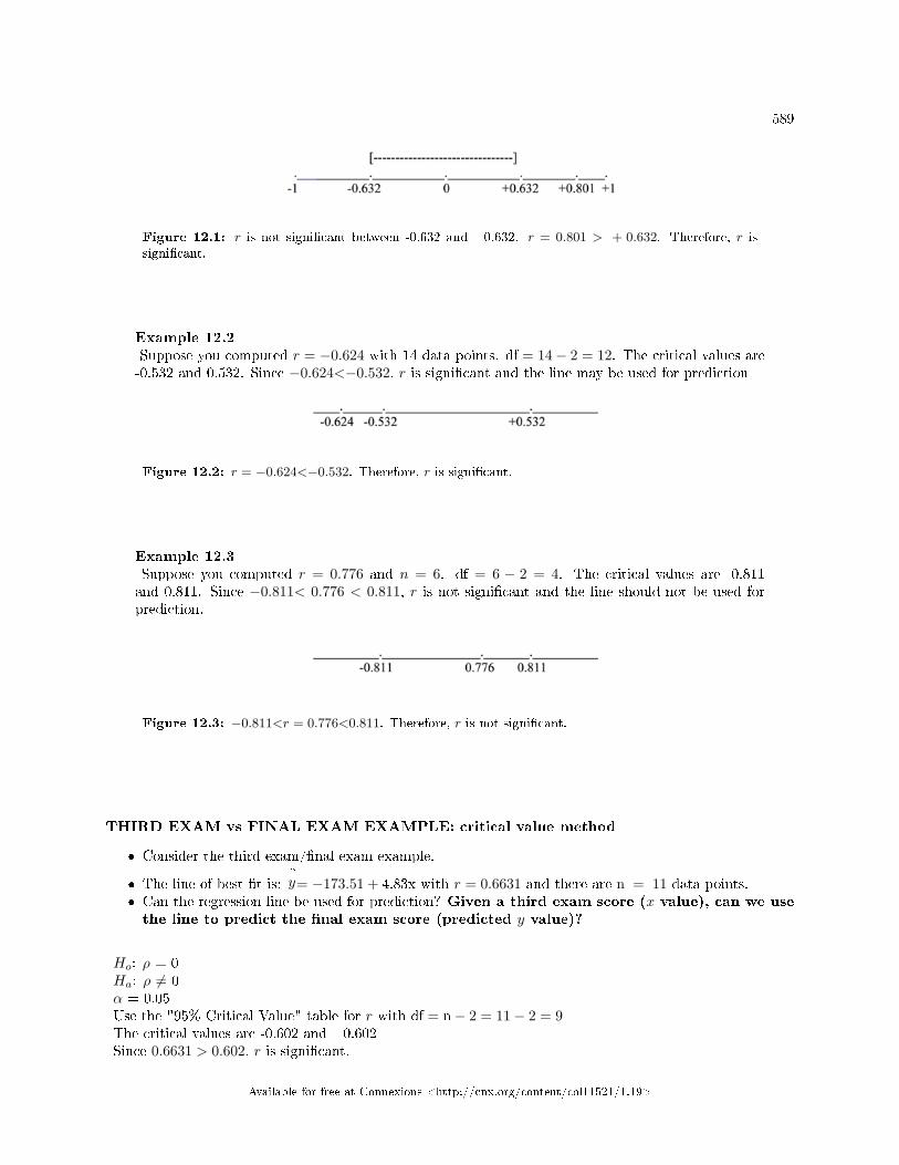
589
Figure 12.1: r is not signi�cant between -0.632 and +0.632. r = 0.801 > + 0.632. Therefore, r issigni�cant.
Example 12.2Suppose you computed r = −0.624 with 14 data points. df = 14− 2 = 12. The critical values are-0.532 and 0.532. Since −0.624<−0.532, r is signi�cant and the line may be used for prediction
Figure 12.2: r = −0.624<−0.532. Therefore, r is signi�cant.
Example 12.3Suppose you computed r = 0.776 and n = 6. df = 6 − 2 = 4. The critical values are -0.811and 0.811. Since −0.811< 0.776 < 0.811, r is not signi�cant and the line should not be used forprediction.
Figure 12.3: −0.811<r = 0.776<0.811. Therefore, r is not signi�cant.
THIRD EXAM vs FINAL EXAM EXAMPLE: critical value method
� Consider the third exam/�nal exam example.
� The line of best �t is:^y= −173.51 + 4.83x with r = 0.6631 and there are n = 11 data points.
� Can the regression line be used for prediction? Given a third exam score (x value), can we usethe line to predict the �nal exam score (predicted y value)?
Ho: ρ = 0Ha: ρ 6= 0α = 0.05Use the "95% Critical Value" table for r with df = n− 2 = 11− 2 = 9The critical values are -0.602 and +0.602Since 0.6631 > 0.602, r is signi�cant.
Available for free at Connexions <http://cnx.org/content/col11521/1.19>
590CHAPTER 12. TESTING THE SIGNIFICANCE OF THE CORRELATION
COEFFICIENT
Decision: Reject Ho:Conclusion:There is su�cient evidence to conclude that there is a signi�cant linear relationship between x
and y because the correlation coe�cient is signi�cantly di�erent from 0.Because r is signi�cant and the scatter plot shows a linear trend, the regression line can be
used to predict �nal exam scores.
Example 12.4: Additional Practice Examples using Critical ValuesSuppose you computed the following correlation coe�cients. Using the table at the end of thechapter, determine if r is signi�cant and the line of best �t associated with each r can be used topredict a y value. If it helps, draw a number line.
1. r = −0.567 and the sample size, n, is 19. The df = n − 2 = 17. The critical value is -0.456.−0.567<−0.456 so r is signi�cant.
2. r = 0.708 and the sample size, n, is 9. The df = n − 2 = 7. The critical value is 0.666.0.708 > 0.666 so r is signi�cant.
3. r = 0.134 and the sample size, n, is 14. The df = 14 − 2 = 12. The critical value is 0.532.0.134 is between -0.532 and 0.532 so r is not signi�cant.
4. r = 0 and the sample size, n, is 5. No matter what the dfs are, r = 0 is between the twocritical values so r is not signi�cant.
12.1.2 Assumptions in Testing the Signi�cance of the Correlation Coe�cient
Testing the signi�cance of the correlation coe�cient requires that certain assumptions about the data aresatis�ed. The premise of this test is that the data are a sample of observed points taken from a largerpopulation. We have not examined the entire population because it is not possible or feasible to do so. Weare examining the sample to draw a conclusion about whether the linear relationship that we see betweenx and y in the sample data provides strong enough evidence so that we can conclude that there is a linearrelationship between x and y in the population.
The regression line equation that we calculate from the sample data gives the best �t line for our particularsample. We want to use this best �t line for the sample as an estimate of the best �t line for the population.Examining the scatterplot and testing the signi�cance of the correlation coe�cient helps us determine if itis appropriate to do this.
The assumptions underlying the test of signi�cance are:
• There is a linear relationship in the population that models the average value of y for varying valuesof x. In other words, the expected value of y for each particular value lies on a straight line in thepopulation. (We do not know the equation for the line for the population. Our regression line fromthe sample is our best estimate of this line in the population.)
• The y values for any particular x value are normally distributed about the line. This implies thatthere are more y values scattered closer to the line than are scattered farther away. Assumption (1)above implies that these normal distributions are centered on the line: the means of these normaldistributions of y values lie on the line.
• The standard deviations of the population y values about the line are equal for each value of x. Inother words, each of these normal distributions of y values has the same shape and spread about theline.
• The residual errors are mutually independent (no pattern).
Available for free at Connexions <http://cnx.org/content/col11521/1.19>
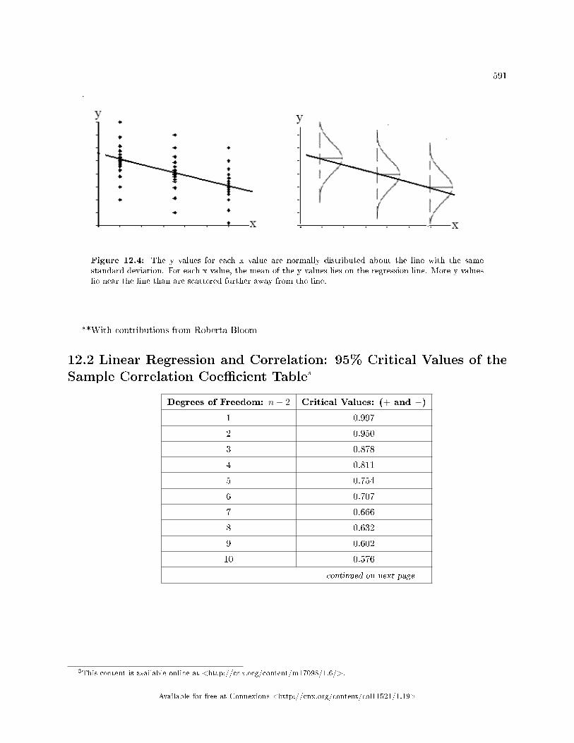
591
Figure 12.4: The y values for each x value are normally distributed about the line with the samestandard deviation. For each x value, the mean of the y values lies on the regression line. More y valueslie near the line than are scattered further away from the line.
**With contributions from Roberta Bloom
12.2 Linear Regression and Correlation: 95% Critical Values of theSample Correlation Coe�cient Table3
Degrees of Freedom: n− 2 Critical Values: (+ and −)1 0.997
2 0.950
3 0.878
4 0.811
5 0.754
6 0.707
7 0.666
8 0.632
9 0.602
10 0.576
continued on next page
3This content is available online at <http://cnx.org/content/m17098/1.6/>.
Available for free at Connexions <http://cnx.org/content/col11521/1.19>
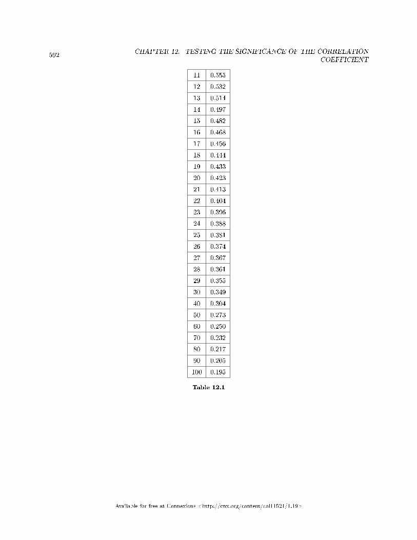
592CHAPTER 12. TESTING THE SIGNIFICANCE OF THE CORRELATION
COEFFICIENT
11 0.555
12 0.532
13 0.514
14 0.497
15 0.482
16 0.468
17 0.456
18 0.444
19 0.433
20 0.423
21 0.413
22 0.404
23 0.396
24 0.388
25 0.381
26 0.374
27 0.367
28 0.361
29 0.355
30 0.349
40 0.304
50 0.273
60 0.250
70 0.232
80 0.217
90 0.205
100 0.195
Table 12.1
Available for free at Connexions <http://cnx.org/content/col11521/1.19>
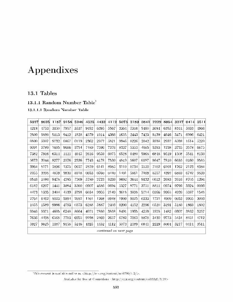
Appendixes
13.1 Tables
13.1.1 Random Number Table1
13.1.1.1 Random Number Table
5927 9625 1187 9158 5246 4325 4432 4112 5073 2189 0841 2229 8064 3217 0414 3511
4218 4753 3150 7957 3537 9452 6395 5567 3364 7316 5460 3684 6355 8344 5033 4966
2509 9880 5113 9412 1828 4579 1014 4366 1655 2443 7423 5139 4646 3471 6996 6421
0800 5007 9732 0867 0119 2362 2977 5821 9946 0226 2042 3938 2937 8598 1614 5220
9091 2789 1695 9666 5754 7489 7596 7276 8237 5353 4005 5393 1228 3725 3578 6675
7382 7916 6314 1121 4045 2616 9559 6075 6528 0480 5968 6848 9519 1508 5541 8130
5673 3044 8277 2576 2336 7743 4178 7530 4819 5607 0587 5647 7810 6635 0160 9585
3964 8171 2896 1375 0627 2870 6141 8985 3110 0734 2550 7102 6101 1762 2123 8384
2255 3298 4859 2830 8918 0653 0760 0440 1401 5861 7169 8557 4392 6889 6742 9839
0546 1080 9478 4285 7209 5780 2723 9239 9692 3644 9132 0012 2683 2016 8705 1294
6182 6207 1441 3084 5500 0907 4686 0694 5327 8771 3751 8811 0974 9799 3324 0093
4473 1335 3404 4539 3791 6034 9305 2149 3618 3898 5714 0266 9265 4926 5287 1548
2764 6462 8023 5994 2082 1161 1268 0948 1909 9025 0333 1721 4900 0053 9905 3003
1055 1589 9986 4793 0373 6288 5887 2403 0200 4152 2296 0520 3191 5180 1869 1802
9346 9371 4605 6248 8664 4071 7850 3858 8491 1935 4259 1975 1482 0307 3832 3257
7636 4498 6568 7703 6955 9198 2469 2657 6782 7062 8878 3430 9773 5434 8451 4712
5927 9625 1187 9158 5246 4325 4432 4112 5073 2189 0841 2229 8064 3217 0414 3511
continued on next page
1This content is available online at <http://cnx.org/content/m46799/1.2/>.
Available for free at Connexions <http://cnx.org/content/col11521/1.19>
593
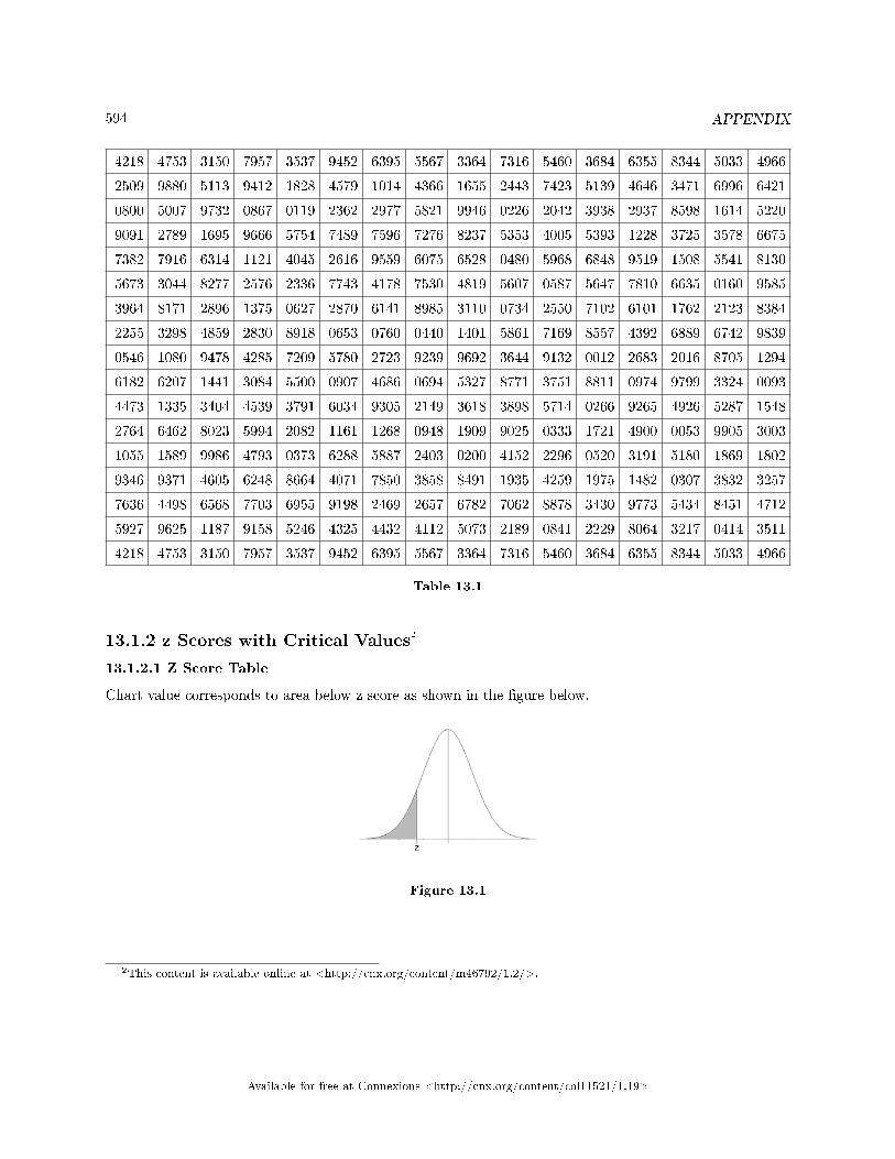
594 APPENDIX
4218 4753 3150 7957 3537 9452 6395 5567 3364 7316 5460 3684 6355 8344 5033 4966
2509 9880 5113 9412 1828 4579 1014 4366 1655 2443 7423 5139 4646 3471 6996 6421
0800 5007 9732 0867 0119 2362 2977 5821 9946 0226 2042 3938 2937 8598 1614 5220
9091 2789 1695 9666 5754 7489 7596 7276 8237 5353 4005 5393 1228 3725 3578 6675
7382 7916 6314 1121 4045 2616 9559 6075 6528 0480 5968 6848 9519 1508 5541 8130
5673 3044 8277 2576 2336 7743 4178 7530 4819 5607 0587 5647 7810 6635 0160 9585
3964 8171 2896 1375 0627 2870 6141 8985 3110 0734 2550 7102 6101 1762 2123 8384
2255 3298 4859 2830 8918 0653 0760 0440 1401 5861 7169 8557 4392 6889 6742 9839
0546 1080 9478 4285 7209 5780 2723 9239 9692 3644 9132 0012 2683 2016 8705 1294
6182 6207 1441 3084 5500 0907 4686 0694 5327 8771 3751 8811 0974 9799 3324 0093
4473 1335 3404 4539 3791 6034 9305 2149 3618 3898 5714 0266 9265 4926 5287 1548
2764 6462 8023 5994 2082 1161 1268 0948 1909 9025 0333 1721 4900 0053 9905 3003
1055 1589 9986 4793 0373 6288 5887 2403 0200 4152 2296 0520 3191 5180 1869 1802
9346 9371 4605 6248 8664 4071 7850 3858 8491 1935 4259 1975 1482 0307 3832 3257
7636 4498 6568 7703 6955 9198 2469 2657 6782 7062 8878 3430 9773 5434 8451 4712
5927 9625 1187 9158 5246 4325 4432 4112 5073 2189 0841 2229 8064 3217 0414 3511
4218 4753 3150 7957 3537 9452 6395 5567 3364 7316 5460 3684 6355 8344 5033 4966
Table 13.1
13.1.2 z Scores with Critical Values2
13.1.2.1 Z Score Table
Chart value corresponds to area below z score as shown in the �gure below.
Figure 13.1
2This content is available online at <http://cnx.org/content/m46792/1.2/>.
Available for free at Connexions <http://cnx.org/content/col11521/1.19>
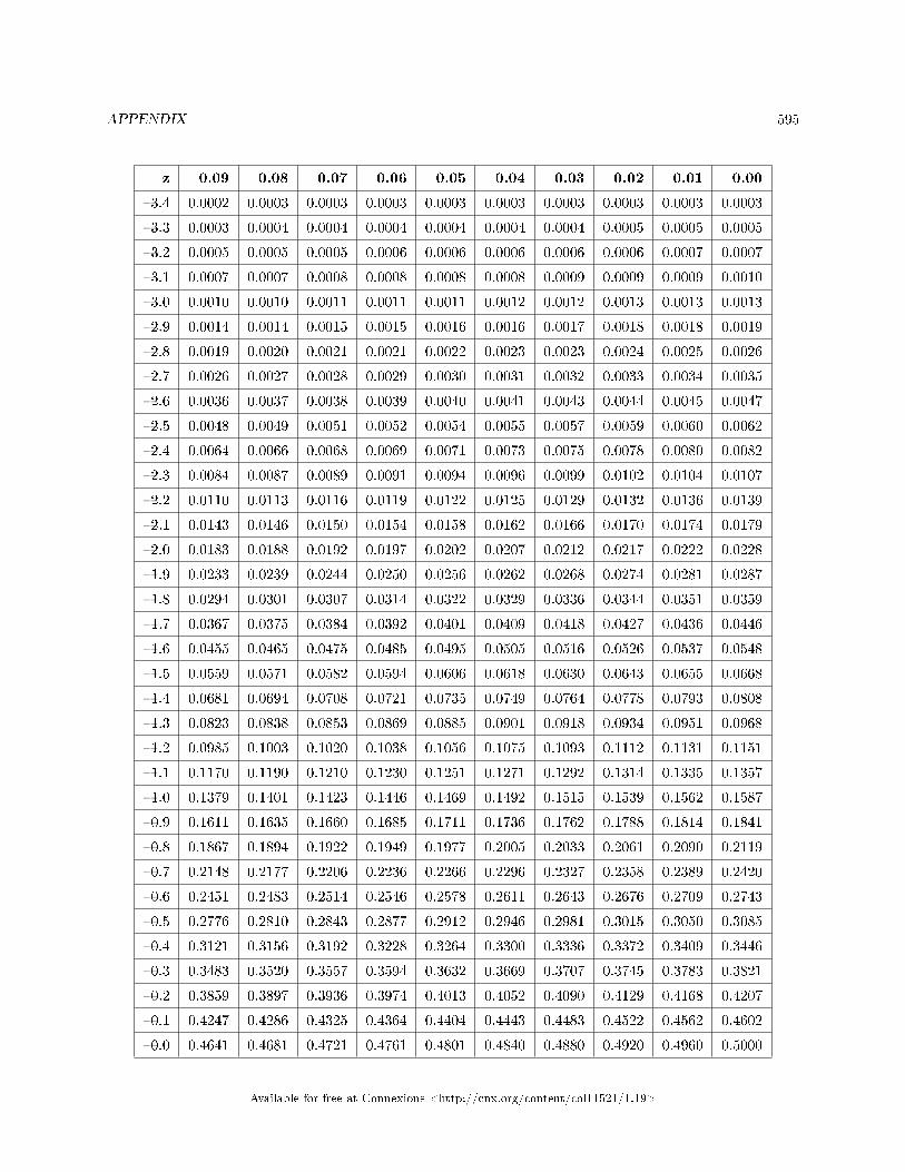
APPENDIX 595
z 0.09 0.08 0.07 0.06 0.05 0.04 0.03 0.02 0.01 0.00
�3.4 0.0002 0.0003 0.0003 0.0003 0.0003 0.0003 0.0003 0.0003 0.0003 0.0003
�3.3 0.0003 0.0004 0.0004 0.0004 0.0004 0.0004 0.0004 0.0005 0.0005 0.0005
�3.2 0.0005 0.0005 0.0005 0.0006 0.0006 0.0006 0.0006 0.0006 0.0007 0.0007
�3.1 0.0007 0.0007 0.0008 0.0008 0.0008 0.0008 0.0009 0.0009 0.0009 0.0010
�3.0 0.0010 0.0010 0.0011 0.0011 0.0011 0.0012 0.0012 0.0013 0.0013 0.0013
�2.9 0.0014 0.0014 0.0015 0.0015 0.0016 0.0016 0.0017 0.0018 0.0018 0.0019
�2.8 0.0019 0.0020 0.0021 0.0021 0.0022 0.0023 0.0023 0.0024 0.0025 0.0026
�2.7 0.0026 0.0027 0.0028 0.0029 0.0030 0.0031 0.0032 0.0033 0.0034 0.0035
�2.6 0.0036 0.0037 0.0038 0.0039 0.0040 0.0041 0.0043 0.0044 0.0045 0.0047
�2.5 0.0048 0.0049 0.0051 0.0052 0.0054 0.0055 0.0057 0.0059 0.0060 0.0062
�2.4 0.0064 0.0066 0.0068 0.0069 0.0071 0.0073 0.0075 0.0078 0.0080 0.0082
�2.3 0.0084 0.0087 0.0089 0.0091 0.0094 0.0096 0.0099 0.0102 0.0104 0.0107
�2.2 0.0110 0.0113 0.0116 0.0119 0.0122 0.0125 0.0129 0.0132 0.0136 0.0139
�2.1 0.0143 0.0146 0.0150 0.0154 0.0158 0.0162 0.0166 0.0170 0.0174 0.0179
�2.0 0.0183 0.0188 0.0192 0.0197 0.0202 0.0207 0.0212 0.0217 0.0222 0.0228
�1.9 0.0233 0.0239 0.0244 0.0250 0.0256 0.0262 0.0268 0.0274 0.0281 0.0287
�1.8 0.0294 0.0301 0.0307 0.0314 0.0322 0.0329 0.0336 0.0344 0.0351 0.0359
�1.7 0.0367 0.0375 0.0384 0.0392 0.0401 0.0409 0.0418 0.0427 0.0436 0.0446
�1.6 0.0455 0.0465 0.0475 0.0485 0.0495 0.0505 0.0516 0.0526 0.0537 0.0548
�1.5 0.0559 0.0571 0.0582 0.0594 0.0606 0.0618 0.0630 0.0643 0.0655 0.0668
�1.4 0.0681 0.0694 0.0708 0.0721 0.0735 0.0749 0.0764 0.0778 0.0793 0.0808
�1.3 0.0823 0.0838 0.0853 0.0869 0.0885 0.0901 0.0918 0.0934 0.0951 0.0968
�1.2 0.0985 0.1003 0.1020 0.1038 0.1056 0.1075 0.1093 0.1112 0.1131 0.1151
�1.1 0.1170 0.1190 0.1210 0.1230 0.1251 0.1271 0.1292 0.1314 0.1335 0.1357
�1.0 0.1379 0.1401 0.1423 0.1446 0.1469 0.1492 0.1515 0.1539 0.1562 0.1587
�0.9 0.1611 0.1635 0.1660 0.1685 0.1711 0.1736 0.1762 0.1788 0.1814 0.1841
�0.8 0.1867 0.1894 0.1922 0.1949 0.1977 0.2005 0.2033 0.2061 0.2090 0.2119
�0.7 0.2148 0.2177 0.2206 0.2236 0.2266 0.2296 0.2327 0.2358 0.2389 0.2420
�0.6 0.2451 0.2483 0.2514 0.2546 0.2578 0.2611 0.2643 0.2676 0.2709 0.2743
�0.5 0.2776 0.2810 0.2843 0.2877 0.2912 0.2946 0.2981 0.3015 0.3050 0.3085
�0.4 0.3121 0.3156 0.3192 0.3228 0.3264 0.3300 0.3336 0.3372 0.3409 0.3446
�0.3 0.3483 0.3520 0.3557 0.3594 0.3632 0.3669 0.3707 0.3745 0.3783 0.3821
�0.2 0.3859 0.3897 0.3936 0.3974 0.4013 0.4052 0.4090 0.4129 0.4168 0.4207
�0.1 0.4247 0.4286 0.4325 0.4364 0.4404 0.4443 0.4483 0.4522 0.4562 0.4602
�0.0 0.4641 0.4681 0.4721 0.4761 0.4801 0.4840 0.4880 0.4920 0.4960 0.5000
Available for free at Connexions <http://cnx.org/content/col11521/1.19>
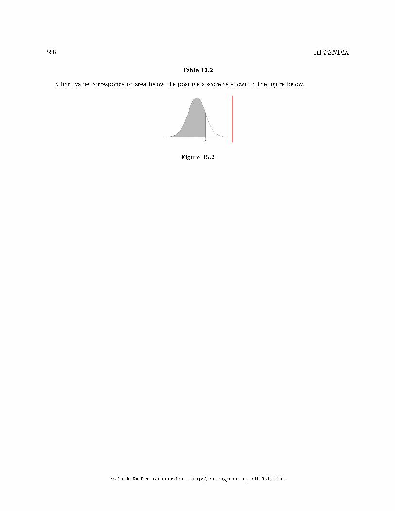
596 APPENDIX
Table 13.2
Chart value corresponds to area below the positive z score as shown in the �gure below.
Figure 13.2
Available for free at Connexions <http://cnx.org/content/col11521/1.19>
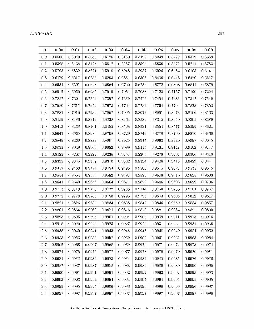
APPENDIX 597
z 0.00 0.01 0.02 0.03 0.04 0.05 0.06 0.07 0.08 0.09
0.0 0.5000 0.5040 0.5080 0.5120 0.5160 0.5199 0.5239 0.5279 0.5319 0.5359
0.1 0.5398 0.5438 0.5478 0.5517 0.5557 0.5596 0.5636 0.5675 0.5714 0.5753
0.2 0.5793 0.5832 0.5871 0.5910 0.5948 0.5987 0.6026 0.6064 0.6103 0.6141
0.3 0.6179 0.6217 0.6255 0.6293 0.6331 0.6368 0.6406 0.6443 0.6480 0.6517
0.4 0.6554 0.6591 0.6628 0.6664 0.6700 0.6736 0.6772 0.6808 0.6844 0.6879
0.5 0.6915 0.6950 0.6985 0.7019 0.7054 0.7088 0.7123 0.7157 0.7190 0.7224
0.6 0.7257 0.7291 0.7324 0.7357 0.7389 0.7422 0.7454 0.7486 0.7517 0.7549
0.7 0.7580 0.7611 0.7642 0.7673 0.7704 0.7734 0.7764 0.7794 0.7823 0.7852
0.8 0.7881 0.7910 0.7939 0.7967 0.7995 0.8023 0.8051 0.8078 0.8106 0.8133
0.9 0.8159 0.8186 0.8212 0.8238 0.8264 0.8289 0.8315 0.8340 0.8365 0.8389
1.0 0.8413 0.8438 0.8461 0.8485 0.8508 0.8531 0.8554 0.8577 0.8599 0.8621
1.1 0.8643 0.8665 0.8686 0.8708 0.8729 0.8749 0.8770 0.8790 0.8810 0.8830
1.2 0.8849 0.8869 0.8888 0.8907 0.8925 0.8944 0.8962 0.8980 0.8997 0.9015
1.3 0.9032 0.9049 0.9066 0.9082 0.9099 0.9115 0.9131 0.9147 0.9162 0.9177
1.4 0.9192 0.9207 0.9222 0.9236 0.9251 0.9265 0.9279 0.9292 0.9306 0.9319
1.5 0.9332 0.9345 0.9357 0.9370 0.9382 0.9394 0.9406 0.9418 0.9429 0.9441
1.6 0.9452 0.9463 0.9474 0.9484 0.9495 0.9505 0.9515 0.9525 0.9535 0.9545
1.7 0.9554 0.9564 0.9573 0.9582 0.9591 0.9599 0.9608 0.9616 0.9625 0.9633
1.8 0.9641 0.9649 0.9656 0.9664 0.9671 0.9678 0.9686 0.9693 0.9699 0.9706
1.9 0.9713 0.9719 0.9726 0.9732 0.9738 0.9744 0.9750 0.9756 0.9761 0.9767
2.0 0.9772 0.9778 0.9783 0.9788 0.9793 0.9798 0.9803 0.9808 0.9812 0.9817
2.1 0.9821 0.9826 0.9830 0.9834 0.9838 0.9842 0.9846 0.9850 0.9854 0.9857
2.2 0.9861 0.9864 0.9868 0.9871 0.9875 0.9878 0.9881 0.9884 0.9887 0.9890
2.3 0.9893 0.9896 0.9898 0.9901 0.9904 0.9906 0.9909 0.9911 0.9913 0.9916
2.4 0.9918 0.9920 0.9922 0.9925 0.9927 0.9929 0.9931 0.9932 0.9934 0.9936
2.5 0.9938 0.9940 0.9941 0.9943 0.9945 0.9946 0.9948 0.9949 0.9951 0.9952
2.6 0.9953 0.9955 0.9956 0.9957 0.9959 0.9960 0.9961 0.9962 0.9963 0.9964
2.7 0.9965 0.9966 0.9967 0.9968 0.9969 0.9970 0.9971 0.9972 0.9973 0.9974
2.8 0.9974 0.9975 0.9976 0.9977 0.9977 0.9978 0.9979 0.9979 0.9980 0.9981
2.9 0.9981 0.9982 0.9982 0.9983 0.9984 0.9984 0.9985 0.9985 0.9986 0.9986
3.0 0.9987 0.9987 0.9987 0.9988 0.9988 0.9989 0.9989 0.9989 0.9990 0.9990
3.1 0.9990 0.9991 0.9991 0.9991 0.9992 0.9992 0.9992 0.9992 0.9993 0.9993
3.2 0.9993 0.9993 0.9994 0.9994 0.9994 0.9994 0.9994 0.9995 0.9995 0.9995
3.3 0.9995 0.9995 0.9995 0.9996 0.9996 0.9996 0.9996 0.9996 0.9996 0.9997
3.4 0.9997 0.9997 0.9997 0.9997 0.9997 0.9997 0.9997 0.9997 0.9997 0.9998
Available for free at Connexions <http://cnx.org/content/col11521/1.19>
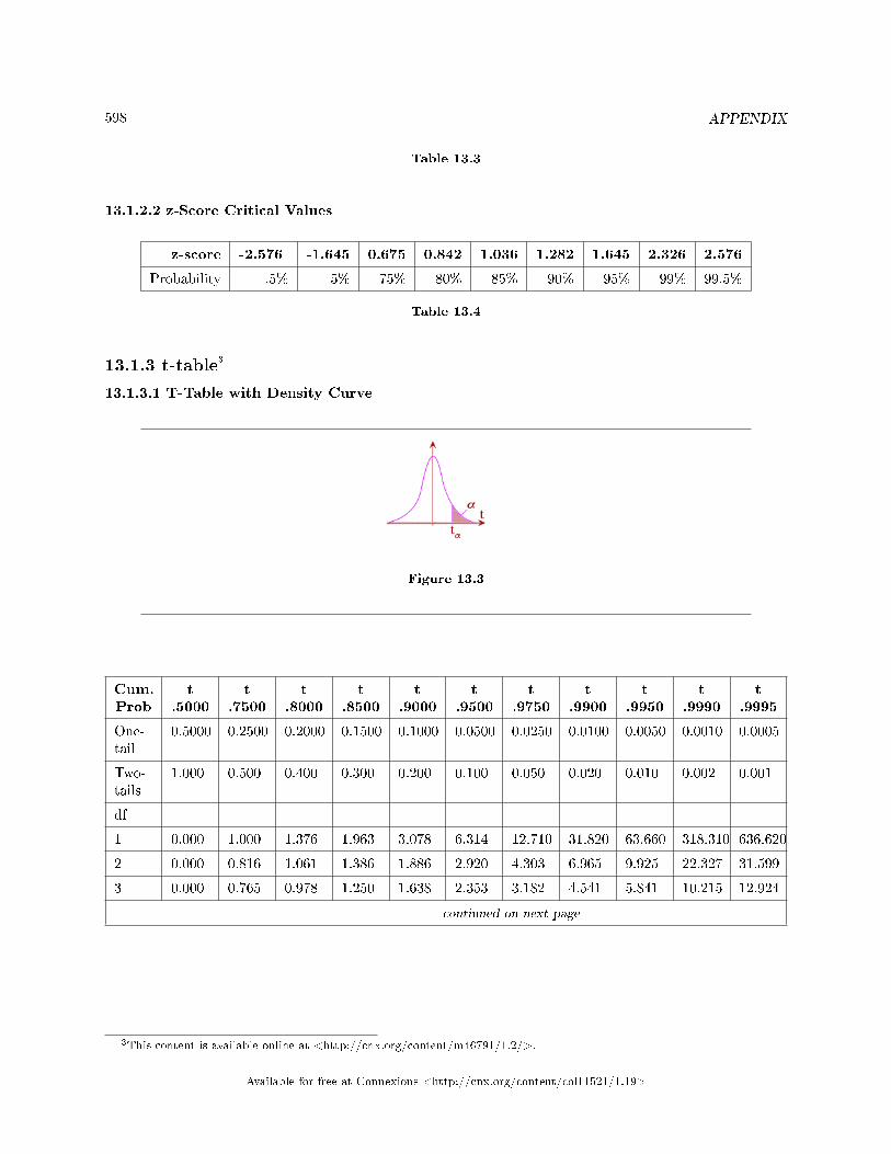
598 APPENDIX
Table 13.3
13.1.2.2 z-Score Critical Values
z-score -2.576 -1.645 0.675 0.842 1.036 1.282 1.645 2.326 2.576
Probability .5% 5% 75% 80% 85% 90% 95% 99% 99.5%
Table 13.4
13.1.3 t-table3
13.1.3.1 T-Table with Density Curve
Figure 13.3
Cum.Prob
t.5000
t.7500
t.8000
t.8500
t.9000
t.9500
t.9750
t.9900
t.9950
t.9990
t.9995
One-tail
0.5000 0.2500 0.2000 0.1500 0.1000 0.0500 0.0250 0.0100 0.0050 0.0010 0.0005
Two-tails
1.000 0.500 0.400 0.300 0.200 0.100 0.050 0.020 0.010 0.002 0.001
df
1 0.000 1.000 1.376 1.963 3.078 6.314 12.710 31.820 63.660 318.310 636.620
2 0.000 0.816 1.061 1.386 1.886 2.920 4.303 6.965 9.925 22.327 31.599
3 0.000 0.765 0.978 1.250 1.638 2.353 3.182 4.541 5.841 10.215 12.924
continued on next page
3This content is available online at <http://cnx.org/content/m46791/1.2/>.
Available for free at Connexions <http://cnx.org/content/col11521/1.19>
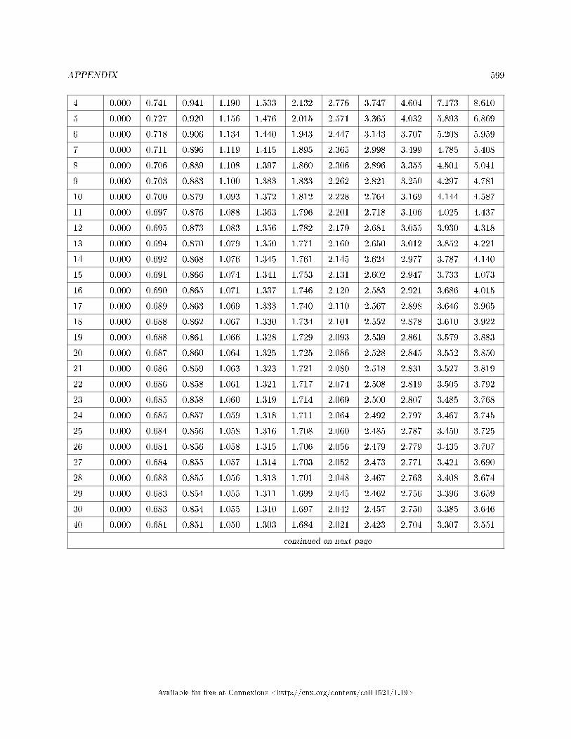
APPENDIX 599
4 0.000 0.741 0.941 1.190 1.533 2.132 2.776 3.747 4.604 7.173 8.610
5 0.000 0.727 0.920 1.156 1.476 2.015 2.571 3.365 4.032 5.893 6.869
6 0.000 0.718 0.906 1.134 1.440 1.943 2.447 3.143 3.707 5.208 5.959
7 0.000 0.711 0.896 1.119 1.415 1.895 2.365 2.998 3.499 4.785 5.408
8 0.000 0.706 0.889 1.108 1.397 1.860 2.306 2.896 3.355 4.501 5.041
9 0.000 0.703 0.883 1.100 1.383 1.833 2.262 2.821 3.250 4.297 4.781
10 0.000 0.700 0.879 1.093 1.372 1.812 2.228 2.764 3.169 4.144 4.587
11 0.000 0.697 0.876 1.088 1.363 1.796 2.201 2.718 3.106 4.025 4.437
12 0.000 0.695 0.873 1.083 1.356 1.782 2.179 2.681 3.055 3.930 4.318
13 0.000 0.694 0.870 1.079 1.350 1.771 2.160 2.650 3.012 3.852 4.221
14 0.000 0.692 0.868 1.076 1.345 1.761 2.145 2.624 2.977 3.787 4.140
15 0.000 0.691 0.866 1.074 1.341 1.753 2.131 2.602 2.947 3.733 4.073
16 0.000 0.690 0.865 1.071 1.337 1.746 2.120 2.583 2.921 3.686 4.015
17 0.000 0.689 0.863 1.069 1.333 1.740 2.110 2.567 2.898 3.646 3.965
18 0.000 0.688 0.862 1.067 1.330 1.734 2.101 2.552 2.878 3.610 3.922
19 0.000 0.688 0.861 1.066 1.328 1.729 2.093 2.539 2.861 3.579 3.883
20 0.000 0.687 0.860 1.064 1.325 1.725 2.086 2.528 2.845 3.552 3.850
21 0.000 0.686 0.859 1.063 1.323 1.721 2.080 2.518 2.831 3.527 3.819
22 0.000 0.686 0.858 1.061 1.321 1.717 2.074 2.508 2.819 3.505 3.792
23 0.000 0.685 0.858 1.060 1.319 1.714 2.069 2.500 2.807 3.485 3.768
24 0.000 0.685 0.857 1.059 1.318 1.711 2.064 2.492 2.797 3.467 3.745
25 0.000 0.684 0.856 1.058 1.316 1.708 2.060 2.485 2.787 3.450 3.725
26 0.000 0.684 0.856 1.058 1.315 1.706 2.056 2.479 2.779 3.435 3.707
27 0.000 0.684 0.855 1.057 1.314 1.703 2.052 2.473 2.771 3.421 3.690
28 0.000 0.683 0.855 1.056 1.313 1.701 2.048 2.467 2.763 3.408 3.674
29 0.000 0.683 0.854 1.055 1.311 1.699 2.045 2.462 2.756 3.396 3.659
30 0.000 0.683 0.854 1.055 1.310 1.697 2.042 2.457 2.750 3.385 3.646
40 0.000 0.681 0.851 1.050 1.303 1.684 2.021 2.423 2.704 3.307 3.551
continued on next page
Available for free at Connexions <http://cnx.org/content/col11521/1.19>
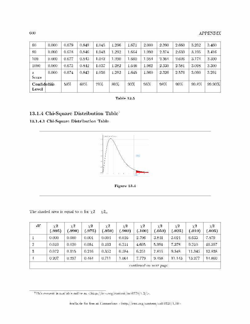
600 APPENDIX
60 0.000 0.679 0.848 1.045 1.296 1.671 2.000 2.390 2.660 3.232 3.460
80 0.000 0.678 0.846 1.043 1.292 1.664 1.990 2.374 2.639 3.195 3.416
100 0.000 0.677 0.845 1.042 1.290 1.660 1.984 2.364 2.626 3.174 3.390
1000 0.000 0.675 0.842 1.037 1.282 1.646 1.962 2.330 2.581 3.098 3.300
z-Score
0.000 0.674 0.842 1.036 1.282 1.645 1.960 2.326 2.576 3.090 3.291
Con�denceLevel
0% 50% 60% 70% 80% 90% 95% 98% 99% 99.8% 99.90%
Table 13.5
13.1.4 Chi-Square Distribution Table4
13.1.4.1 Chi-Square Distribution Table
Figure 13.4
The shaded area is equal to α for χ2 = χ2α
df χ2(.995)
χ2(.990)
χ2(.975)
χ2(.950)
χ2(.900)
χ2(.100)
χ2(.050)
χ2(.025)
χ2(.010)
χ2(.005)
1 0.000 0.000 0.001 0.004 0.016 2.706 3.841 5.024 6.635 7.879
2 0.010 0.020 0.051 0.103 0.211 4.605 5.991 7.378 9.210 10.597
3 0.072 0.115 0.216 0.352 0.584 6.251 7.815 9.348 11.345 12.838
4 0.207 0.297 0.484 0.711 1.064 7.779 9.488 11.143 13.277 14.860
continued on next page
4This content is available online at <http://cnx.org/content/m46778/1.2/>.
Available for free at Connexions <http://cnx.org/content/col11521/1.19>
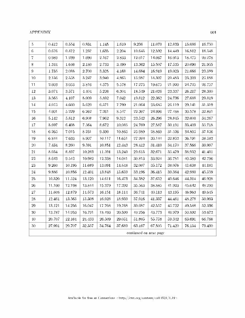
APPENDIX 601
5 0.412 0.554 0.831 1.145 1.610 9.236 11.070 12.833 15.086 16.750
6 0.676 0.872 1.237 1.635 2.204 10.645 12.592 14.449 16.812 18.548
7 0.989 1.239 1.690 2.167 2.833 12.017 14.067 16.013 18.475 20.278
8 1.344 1.646 2.180 2.733 3.490 13.362 15.507 17.535 20.090 21.955
9 1.735 2.088 2.700 3.325 4.168 14.684 16.919 19.023 21.666 23.589
10 2.156 2.558 3.247 3.940 4.865 15.987 18.307 20.483 23.209 25.188
11 2.603 3.053 3.816 4.575 5.578 17.275 19.675 21.920 24.725 26.757
12 3.074 3.571 4.404 5.226 6.304 18.549 21.026 23.337 26.217 28.300
13 3.565 4.107 5.009 5.892 7.042 19.812 22.362 24.736 27.688 29.819
14 4.075 4.660 5.629 6.571 7.790 21.064 23.685 26.119 29.141 31.319
15 4.601 5.229 6.262 7.261 8.547 22.307 24.996 27.488 30.578 32.801
16 5.142 5.812 6.908 7.962 9.312 23.542 26.296 28.845 32.000 34.267
17 5.697 6.408 7.564 8.672 10.085 24.769 27.587 30.191 33.409 35.718
18 6.265 7.015 8.231 9.390 10.865 25.989 28.869 31.526 34.805 37.156
19 6.844 7.633 8.907 10.117 11.651 27.204 30.144 32.852 36.191 38.582
20 7.434 8.260 9.591 10.851 12.443 28.412 31.410 34.170 37.566 39.997
21 8.034 8.897 10.283 11.591 13.240 29.615 32.671 35.479 38.932 41.401
22 8.643 9.542 10.982 12.338 14.041 30.813 33.924 36.781 40.289 42.796
23 9.260 10.196 11.689 13.091 14.848 32.007 35.172 38.076 41.638 44.181
24 9.886 10.856 12.401 13.848 15.659 33.196 36.415 39.364 42.980 45.559
25 10.520 11.524 13.120 14.611 16.473 34.382 37.652 40.646 44.314 46.928
26 11.160 12.198 13.844 15.379 17.292 35.563 38.885 41.923 45.642 48.290
27 11.808 12.879 14.573 16.151 18.114 36.741 40.113 43.195 46.963 49.645
28 12.461 13.565 15.308 16.928 18.939 37.916 41.337 44.461 48.278 50.993
29 13.121 14.256 16.047 17.708 19.768 39.087 42.557 45.722 49.588 52.336
30 13.787 14.953 16.791 18.493 20.599 40.256 43.773 46.979 50.892 53.672
40 20.707 22.164 24.433 26.509 29.051 51.805 55.758 59.342 63.691 66.766
50 27.991 29.707 32.357 34.764 37.689 63.167 67.505 71.420 76.154 79.490
continued on next page
Available for free at Connexions <http://cnx.org/content/col11521/1.19>
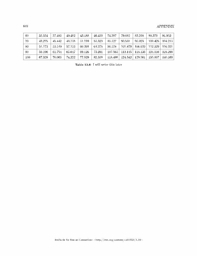
602 APPENDIX
60 35.534 37.485 40.482 43.188 46.459 74.397 79.082 83.298 88.379 91.952
70 43.275 45.442 48.758 51.739 55.329 85.527 90.531 95.023 100.425 104.215
80 51.172 53.540 57.153 60.391 64.278 96.578 101.879 106.629 112.329 116.321
90 59.196 61.754 65.647 69.126 73.291 107.565 113.145 118.136 124.116 128.299
100 67.328 70.065 74.222 77.929 82.358 118.498 124.342 129.561 135.807 140.169
Table 13.6: I will write this later
Available for free at Connexions <http://cnx.org/content/col11521/1.19>
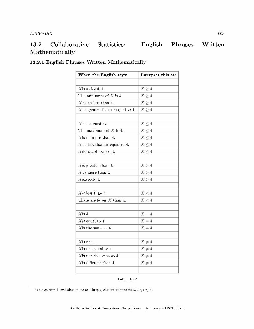
APPENDIX 603
13.2 Collaborative Statistics: English Phrases WrittenMathematically5
13.2.1 English Phrases Written Mathematically
When the English says: Interpret this as:
Xis at least 4. X ≥ 4
The minimum of X is 4. X ≥ 4
X is no less than 4. X ≥ 4
X is greater than or equal to 4. X ≥ 4
X is at most 4. X ≤ 4
The maximum of X is 4. X ≤ 4
Xis no more than 4. X ≤ 4
X is less than or equal to 4. X ≤ 4
Xdoes not exceed 4. X ≤ 4
Xis greater than 4. X > 4
X is more than 4. X > 4
Xexceeds 4. X > 4
Xis less than 4. X < 4
There are fewer X than 4. X < 4
Xis 4. X = 4
Xis equal to 4. X = 4
Xis the same as 4. X = 4
Xis not 4. X 6= 4
Xis not equal to 4. X 6= 4
Xis not the same as 4. X 6= 4
Xis di�erent than 4. X 6= 4
Table 13.7
5This content is available online at <http://cnx.org/content/m16307/1.6/>.
Available for free at Connexions <http://cnx.org/content/col11521/1.19>
604 APPENDIX
13.3 Collaborative Statistics: Symbols and their Meanings6
Symbols and their Meanings
6This content is available online at <http://cnx.org/content/m47518/1.1/>.
Available for free at Connexions <http://cnx.org/content/col11521/1.19>
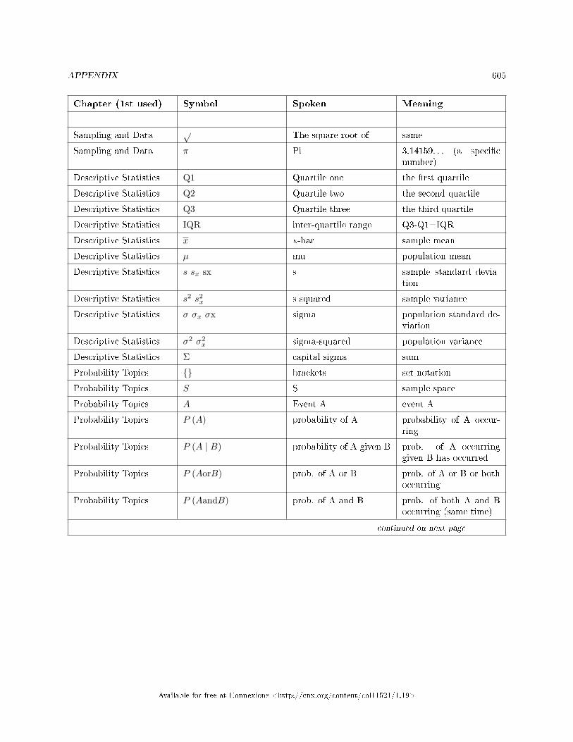
APPENDIX 605
Chapter (1st used) Symbol Spoken Meaning
Sampling and Data√
The square root of same
Sampling and Data π Pi 3.14159. . . (a speci�cnumber)
Descriptive Statistics Q1 Quartile one the �rst quartile
Descriptive Statistics Q2 Quartile two the second quartile
Descriptive Statistics Q3 Quartile three the third quartile
Descriptive Statistics IQR inter-quartile range Q3-Q1=IQR
Descriptive Statistics x x-bar sample mean
Descriptive Statistics µ mu population mean
Descriptive Statistics s sx sx s sample standard devia-tion
Descriptive Statistics s2 s2x s-squared sample variance
Descriptive Statistics σ σx σx sigma population standard de-viation
Descriptive Statistics σ2 σ2x sigma-squared population variance
Descriptive Statistics Σ capital sigma sum
Probability Topics {} brackets set notation
Probability Topics S S sample space
Probability Topics A Event A event A
Probability Topics P (A) probability of A probability of A occur-ring
Probability Topics P (A | B) probability of A given B prob. of A occurringgiven B has occurred
Probability Topics P (AorB) prob. of A or B prob. of A or B or bothoccurring
Probability Topics P (AandB) prob. of A and B prob. of both A and Boccurring (same time)
continued on next page
Available for free at Connexions <http://cnx.org/content/col11521/1.19>
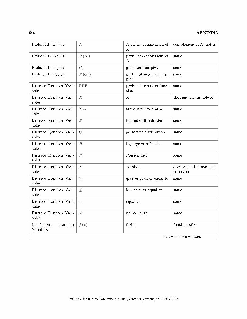
606 APPENDIX
Probability Topics A' A-prime, complement ofA
complement of A, not A
Probability Topics P (A') prob. of complement ofA
same
Probability Topics G1 green on �rst pick same
Probability Topics P (G1) prob. of green on �rstpick
same
Discrete Random Vari-ables
PDF prob. distribution func-tion
same
Discrete Random Vari-ables
X X the random variable X
Discrete Random Vari-ables
X ∼ the distribution of X same
Discrete Random Vari-ables
B binomial distribution same
Discrete Random Vari-ables
G geometric distribution same
Discrete Random Vari-ables
H hypergeometric dist. same
Discrete Random Vari-ables
P Poisson dist. same
Discrete Random Vari-ables
λ Lambda average of Poisson dis-tribution
Discrete Random Vari-ables
≥ greater than or equal to same
Discrete Random Vari-ables
≤ less than or equal to same
Discrete Random Vari-ables
= equal to same
Discrete Random Vari-ables
6= not equal to same
Continuous RandomVariables
f (x) f of x function of x
continued on next page
Available for free at Connexions <http://cnx.org/content/col11521/1.19>
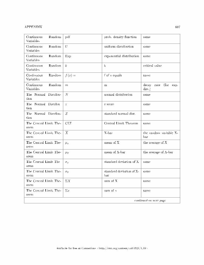
APPENDIX 607
Continuous RandomVariables
pdf prob. density function same
Continuous RandomVariables
U uniform distribution same
Continuous RandomVariables
Exp exponential distribution same
Continuous RandomVariables
k k critical value
Continuous RandomVariables
f (x) = f of x equals same
Continuous RandomVariables
m m decay rate (for exp.dist.)
The Normal Distribu-tion
N normal distribution same
The Normal Distribu-tion
z z-score same
The Normal Distribu-tion
Z standard normal dist. same
The Central Limit The-orem
CLT Central Limit Theorem same
The Central Limit The-orem
X X-bar the random variable X-bar
The Central Limit The-orem
µx mean of X the average of X
The Central Limit The-orem
µx mean of X-bar the average of X-bar
The Central Limit The-orem
σx standard deviation of X same
The Central Limit The-orem
σx standard deviation of X-bar
same
The Central Limit The-orem
ΣX sum of X same
The Central Limit The-orem
Σx sum of x same
continued on next page
Available for free at Connexions <http://cnx.org/content/col11521/1.19>
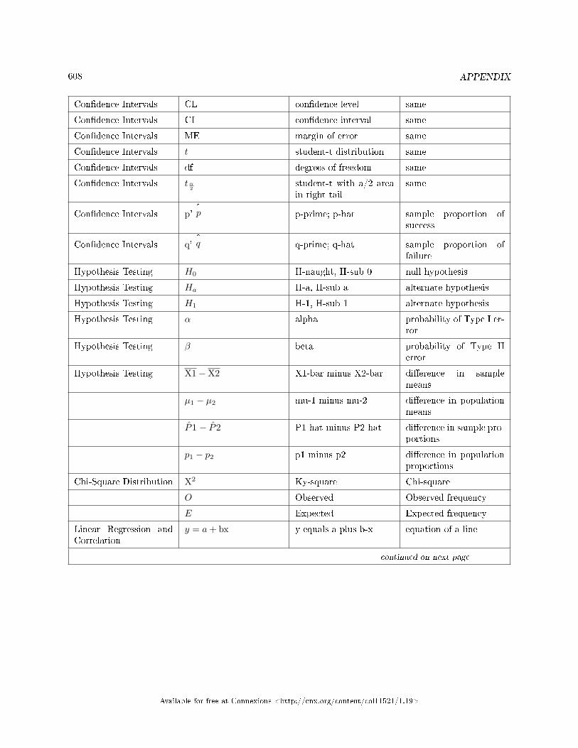
608 APPENDIX
Con�dence Intervals CL con�dence level same
Con�dence Intervals CI con�dence interval same
Con�dence Intervals ME margin of error same
Con�dence Intervals t student-t distribution same
Con�dence Intervals df degrees of freedom same
Con�dence Intervals tα2
student-t with a/2 areain right tail
same
Con�dence Intervals p'^p p-prime; p-hat sample proportion of
success
Con�dence Intervals q'^q q-prime; q-hat sample proportion of
failure
Hypothesis Testing H0 H-naught, H-sub 0 null hypothesis
Hypothesis Testing Ha H-a, H-sub a alternate hypothesis
Hypothesis Testing H1 H-1, H-sub 1 alternate hypothesis
Hypothesis Testing α alpha probability of Type I er-ror
Hypothesis Testing β beta probability of Type IIerror
Hypothesis Testing X1−X2 X1-bar minus X2-bar di�erence in samplemeans
µ1 − µ2 mu-1 minus mu-2 di�erence in populationmeans
P̂1 − P̂2 P1-hat minus P2-hat di�erence in sample pro-portions
p1 − p2 p1 minus p2 di�erence in populationproportions
Chi-Square Distribution X2 Ky-square Chi-square
O Observed Observed frequency
E Expected Expected frequency
Linear Regression andCorrelation
y = a+ bx y equals a plus b-x equation of a line
continued on next page
Available for free at Connexions <http://cnx.org/content/col11521/1.19>
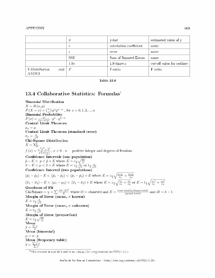
APPENDIX 609
^y y-hat estimated value of y
r correlation coe�cient same
ε error same
SSE Sum of Squared Errors same
1.9s 1.9 times s cut-o� value for outliers
F-Distribution andANOVA
F F-ratio F ratio
Table 13.8
13.4 Collaborative Statistics: Formulas7
Binomial DistributionX ∼ B (n, p)P (X = x) =
(nx
)pxqn−x , for x = 0, 1, 2, ..., n
Binomial ProbabilityP (x) = n!
(n−x)!x! · px · qn−x
Central Limit Theoremµx = µCentral Limit Theorem (standard error)σx = σ√
n
Chi-Square DistributionX ∼ X2
df
f (x) = xn−2
2 e−x2
2n2 Γ(n2 )
, x > 0 , n = positive integer and degrees of freedom
Con�dence Intervals (one population)p̂− E < p < p̂+ E where E = z a
2
√pqn
x− E < µ < x+ E where E = z a2
σ√nor t a
2
s√n
Con�dence Interval (two populations)
(p̂1 − p̂2)− E < (p̂1 − p̂2) < (p̂1 − p̂2) + E where E = z a2
√p̂1q̂1n1
+ p̂2q̂2n2
(x1 − x2)− E < (µ1 − µ2) < (x1 − x2) + E where E = z a2
√σ1n1
+ σ2n2
or E = t a2
√s12
n1+ s22
n2
Goodness of FitChi-Square = χ =
∑ (O−E)2
E where O = observed and E = (row total)(column total)(grand total) and df = k − 1
Margin of Error (mean, σ known)E = z a
2
σ√n
Margin of Error (mean, σ unknown)E = t a
2
s√n
Margin of Error (proportion)E = z a
2
√pqn
Meanx =
Pxn
Mean (binomial)µ = n · pMean (frequency table)
x =Pf ·xPf
7This content is available online at <http://cnx.org/content/m47474/1.1/>.
Available for free at Connexions <http://cnx.org/content/col11521/1.19>
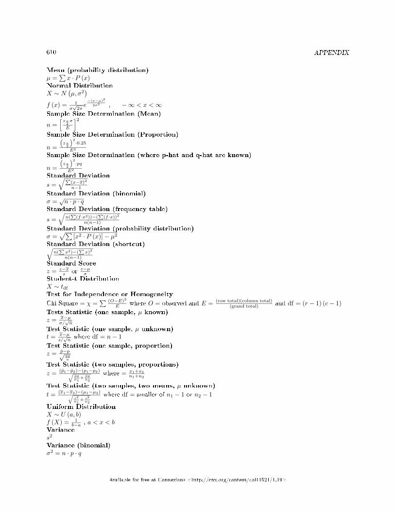
610 APPENDIX
Mean (probability distribution)µ =
∑x · P (x)
Normal DistributionX ∼ N
(µ, σ2
)f (x) = 1
σ√
2πe−(x−µ)2
2σ2 , −∞ < x <∞Sample Size Determination (Mean)
n =[z a
2σ
E
]2Sample Size Determination (Proportion)
n =
“z a
2
”2·0.25
E2
Sample Size Determination (where p-hat and q-hat are known)
n =
“z a
2
”2·pq
E2
Standard Deviation
s =√P
(x−x)2
n−1
Standard Deviation (binomial)σ =√n · p · q
Standard Deviation (frequency table)
s =√
n(P
(f ·x2))−(P
(f ·x))2
n(n−1)
Standard Deviation (probability distribution)σ =
√∑[x2 · P (x)]− µ2
Standard Deviation (shortcut)√n(Px2)−(
Px)2
n(n−1)
Standard Scorez = z−x
s or z−µσ
Student-t DistributionX ∼ tdf
Test for Independence or Homogeneity
Chi-Square = χ =∑ (O−E)2
E where O = observed and E = (row total)(column total)(grand total) and df = (r − 1) (c− 1)
Tests Statistic (one sample, µ known)z = x−µ
σ/√n
Test Statistic (one sample, µ unknown)t = x−µ
s/√nwhere df = n− 1
Test Statistic (one sample, proportion)z = p̂−p√
pqn
Test Statistic (two samples, proportions)
z = (p̂1−p̂2)−(p1−p2)qpqn1
+ pqn2
where = x1+x2n1+n2
Test Statistic (two samples, two means, µ unknown)
t = (x1−x2)−(µ1−µ2)qs2n1
+ s2n2
where df = smaller of n1 − 1 or n2 − 1
Uniform DistributionX ∼ U (a, b)f (X) = 1
b−a , a < x < bVariances2
Variance (binomial)σ2 = n · p · q
Available for free at Connexions <http://cnx.org/content/col11521/1.19>
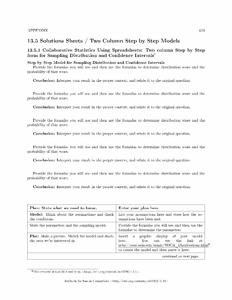
APPENDIX 611
13.5 Solutions Sheets / Two Column Step by Step Models
13.5.1 Collaborative Statistics Using Spreadsheets: Two column Step by Stepform for Sampling Distribution and Con�dence Intervals8
Step by Step Model for Sampling Distribution and Con�dence IntervalsProvide the formulas you will use and then use the formulas to determine distribution score and the
probability of that score.
Conclusion: Interpret your result in the proper context, and relate it to the original question.
Provide the formulas you will use and then use the formulas to determine distribution score and theprobability of that score.
Conclusion: Interpret your result in the proper context, and relate it to the original question.
Provide the formulas you will use and then use the formulas to determine distribution score and theprobability of that score.
Conclusion: Interpret your result in the proper context, and relate it to the original question.
Provide the formulas you will use and then use the formulas to determine distribution score and theprobability of that score.
Conclusion: Interpret your result in the proper context, and relate it to the original question.
Provide the formulas you will use and then use the formulas to determine distribution score and theprobability of that score.
Conclusion: Interpret your result in the proper context, and relate it to the original question.
Plan: State what we need to know. Enter your plan here
Model: Think about the assumptions and checkthe conditions.
List your assumptions here and state how the as-sumptions have been met
State the parameters and the sampling model. Provide the formulas you will use and then use theformulas to determine the parameters
Plot: Make a picture. Sketch the model and shadethe area we're interested in.
Insert a graphic display of your modelhere. You can use the link athttp://socr.ucla.edu/htmls/SOCR_Distributions.html6
to create the model and then paste it here.
continued on next page
8This content is available online at <http://cnx.org/content/m48796/1.1/>.
Available for free at Connexions <http://cnx.org/content/col11521/1.19>
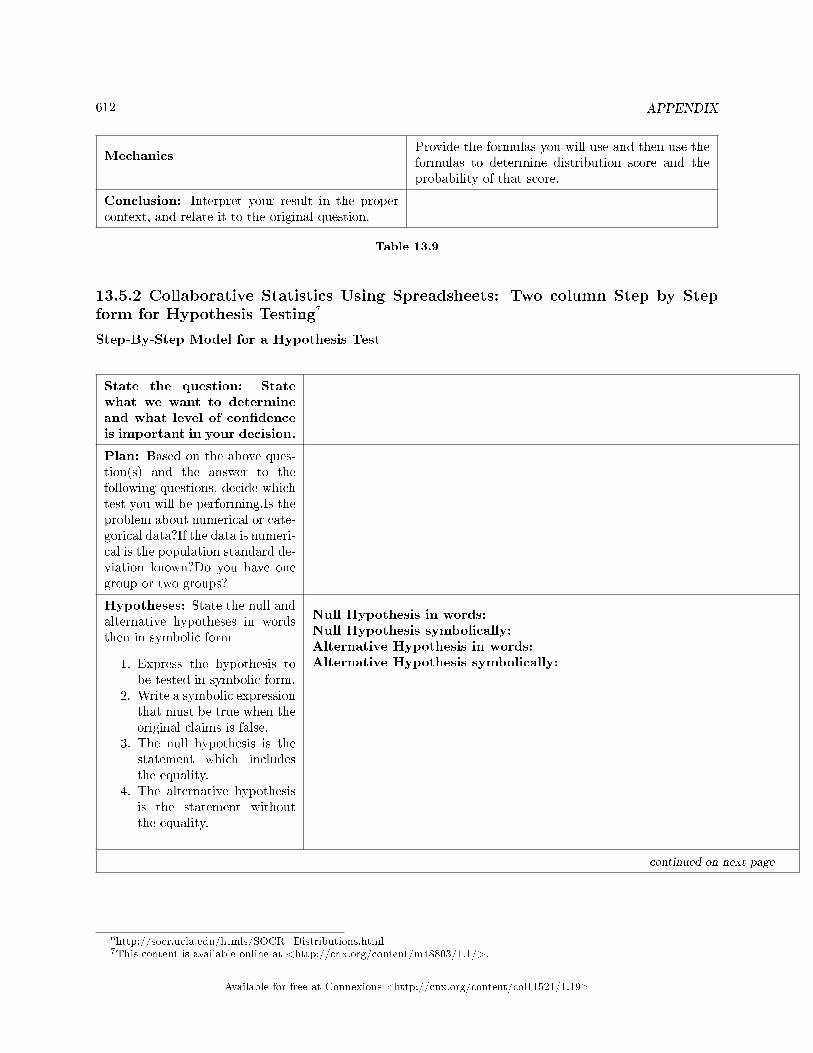
612 APPENDIX
MechanicsProvide the formulas you will use and then use theformulas to determine distribution score and theprobability of that score.
Conclusion: Interpret your result in the propercontext, and relate it to the original question.
Table 13.9
13.5.2 Collaborative Statistics Using Spreadsheets: Two column Step by Stepform for Hypothesis Testing7
Step-By-Step Model for a Hypothesis Test
State the question: Statewhat we want to determineand what level of con�denceis important in your decision.
Plan: Based on the above ques-tion(s) and the answer to thefollowing questions, decide whichtest you will be performing.Is theproblem about numerical or cate-gorical data?If the data is numeri-cal is the population standard de-viation known?Do you have onegroup or two groups?
Hypotheses: State the null andalternative hypotheses in wordsthen in symbolic form
1. Express the hypothesis tobe tested in symbolic form,
2. Write a symbolic expressionthat must be true when theoriginal claims is false.
3. The null hypothesis is thestatement which includesthe equality.
4. The alternative hypothesisis the statement withoutthe equality.
Null Hypothesis in words:Null Hypothesis symbolically:Alternative Hypothesis in words:Alternative Hypothesis symbolically:
continued on next page
6http://socr.ucla.edu/htmls/SOCR_Distributions.html7This content is available online at <http://cnx.org/content/m48803/1.1/>.
Available for free at Connexions <http://cnx.org/content/col11521/1.19>
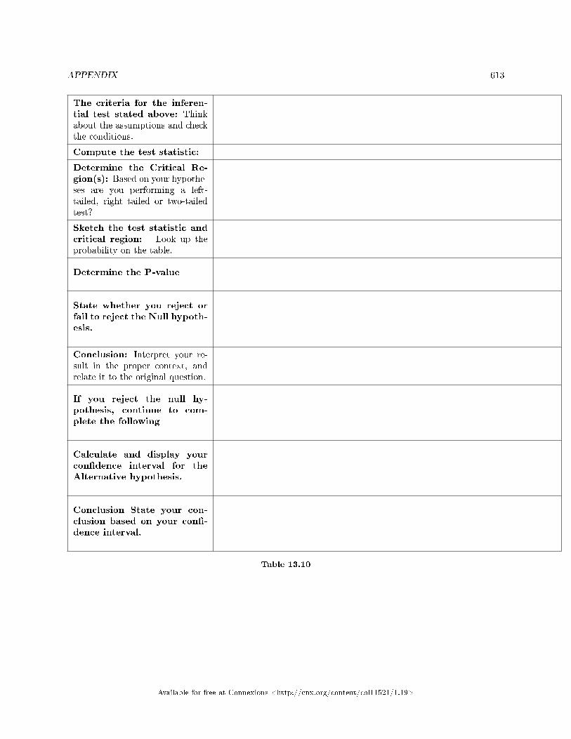
APPENDIX 613
The criteria for the inferen-tial test stated above: Thinkabout the assumptions and checkthe conditions.
Compute the test statistic:
Determine the Critical Re-gion(s): Based on your hypothe-ses are you performing a left-tailed, right tailed or two-tailedtest?
Sketch the test statistic andcritical region: Look up theprobability on the table.
Determine the P-value
State whether you reject orfail to reject the Null hypoth-esis.
Conclusion: Interpret your re-sult in the proper context, andrelate it to the original question.
If you reject the null hy-pothesis, continue to com-plete the following
Calculate and display yourcon�dence interval for theAlternative hypothesis.
Conclusion State your con-clusion based on your con�-dence interval.
Table 13.10
Available for free at Connexions <http://cnx.org/content/col11521/1.19>
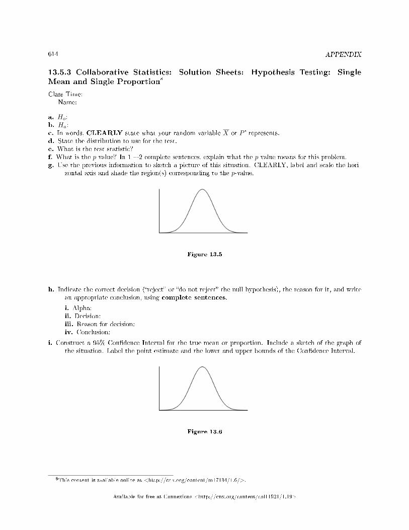
614 APPENDIX
13.5.3 Collaborative Statistics: Solution Sheets: Hypothesis Testing: SingleMean and Single Proportion8
Class Time:Name:
a. Ho:b. Ha:c. In words, CLEARLY state what your random variable X or P ' represents.d. State the distribution to use for the test.e. What is the test statistic?f. What is the p-value? In 1 � 2 complete sentences, explain what the p-value means for this problem.g. Use the previous information to sketch a picture of this situation. CLEARLY, label and scale the hori-
zontal axis and shade the region(s) corresponding to the p-value.
Figure 13.5
h. Indicate the correct decision (�reject� or �do not reject� the null hypothesis), the reason for it, and writean appropriate conclusion, using complete sentences.
i. Alpha:ii. Decision:iii. Reason for decision:iv. Conclusion:
i. Construct a 95% Con�dence Interval for the true mean or proportion. Include a sketch of the graph ofthe situation. Label the point estimate and the lower and upper bounds of the Con�dence Interval.
Figure 13.6
8This content is available online at <http://cnx.org/content/m17134/1.6/>.
Available for free at Connexions <http://cnx.org/content/col11521/1.19>
APPENDIX 615
13.5.4 Collaborative Statistics: Solution Sheets: Hypothesis Testing: TwoMeans, Paired Data, Two Proportions9
Class Time:Name:
a. Ho: _______b. Ha: _______c. In words, clearly state what your random variable X1 −X2, P1'− P2'- or Xd represents.d. State the distribution to use for the test.e. What is the test statistic?f. What is the p-value? In 1 � 2 complete sentences, explain what the p-value means for this problem.g. Use the previous information to sketch a picture of this situation. CLEARLY label and scale the
horizontal axis and shade the region(s) corresponding to the p-value.
Figure 13.7
h. Indicate the correct decision (�reject� or �do not reject� the null hypothesis), the reason for it, and writean appropriate conclusion, using complete sentences.
i. Alpha:ii. Decision:iii. Reason for decision:iv. Conclusion:
i. In complete sentences, explain how you determined which distribution to use.
9This content is available online at <http://cnx.org/content/m17133/1.6/>.
Available for free at Connexions <http://cnx.org/content/col11521/1.19>
616 APPENDIX
13.5.5 Collaborative Statistics: Solution Sheets: The Chi-Square Distribution10
Class Time:Name:
a. Ho: _______b. Ha: _______c. What are the degrees of freedom?d. State the distribution to use for the test.e. What is the test statistic?f. What is the p-value? In 1 � 2 complete sentences, explain what the p-value means for this problem.g. Use the previous information to sketch a picture of this situation. Clearly label and scale the horizontal
axis and shade the region(s) corresponding to the p-value.
Figure 13.8
h. Indicate the correct decision (�reject� or �do not reject� the null hypothesis) and write appropriate con-clusions, using complete sentences.
i. Alpha:ii. Decision:iii. Reason for decision:iv. Conclusion:
13.6 Data Analysis Flowcharts
13.6.1 What Inference Test Should I perform with my survey data?11
What Inference Test should I perform with my survey data?The following two charts visually represent the decision making process for how to move from your collecteddata to making a decision on what inference test to perform. The �rst chart covers steps 1 - 3 and the secondchart repeats step 3 and then adds steps 4-5. I hope you �nd this �ow chart helpful when looking at yourdata and trying to decide what is the best test to perform.
10This content is available online at <http://cnx.org/content/m17136/1.6/>.11This content is available online at <http://cnx.org/content/m48783/1.1/>.
Available for free at Connexions <http://cnx.org/content/col11521/1.19>
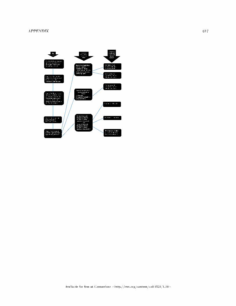
APPENDIX 617
Available for free at Connexions <http://cnx.org/content/col11521/1.19>
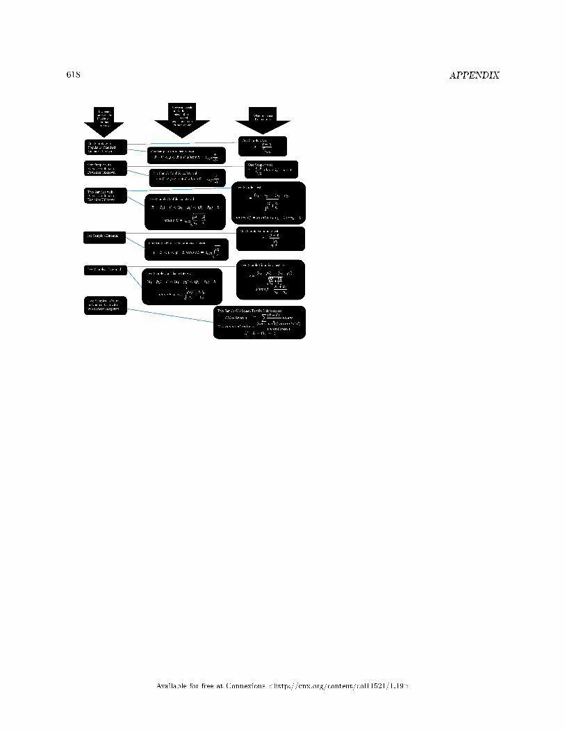
618 APPENDIX
Available for free at Connexions <http://cnx.org/content/col11521/1.19>
GLOSSARY 619
Glossary
A Average
A number that describes the central tendency of the data. There are a number of specializedaverages, including the arithmetic mean, weighted mean, median, mode, and geometric mean.
B Bernoulli Trials
An experiment with the following characteristics:
• There are only 2 possible outcomes called �success� and �failure� for each trial.• The probability p of a success is the same for any trial (so the probability q = 1− p of afailure is the same for any trial).
Binomial Distribution
A discrete random variable (RV) which arises from Bernoulli trials. There are a �xed number, n,of independent trials. �Independent� means that the result of any trial (for example, trial 1)does not a�ect the results of the following trials, and all trials are conducted under the sameconditions. Under these circumstances the binomial RV X is de�ned as the number of successesin n trials. The notation is: X∼B (n, p). The mean is µ = np and the standard deviation isσ =√
npq. The probability of exactly x successes in n trials is P (X = x) =(nx
)pxqn−x.
C Central Limit Theorem
Given a random variable (RV) with known mean µ and known standard deviation σ. We aresampling with size n and we are interested in two new RVs - the sample mean, X, and the sample
sum, ΣX. If the size n of the sample is su�ciently large, then X∼ N(µ, σ√
n
)and ΣX ∼
N (nµ,√nσ). If the size n of the sample is su�ciently large, then the distribution of the sample
means and the distribution of the sample sums will approximate a normal distribution regardlessof the shape of the population. The mean of the sample means will equal the population meanand the mean of the sample sums will equal n times the population mean. The standarddeviation of the distribution of the sample means, σ√
n, is called the standard error of the mean.
Coe�cient of Correlation
A measure developed by Karl Pearson (early 1900s) that gives the strength of associationbetween the independent variable and the dependent variable. The formula is:
r =Σ(xy)n − (x) (y)
sxsy
(n
n− 1
)(3.5)
where n is the number of data points. The coe�cient cannot be more then 1 and less then -1.The closer the coe�cient is to ±1, the stronger the evidence of a signi�cant linear relationshipbetween x and y.
Conditional Probability
The likelihood that an event will occur given that another event has already occurred.
Con�dence Interval (CI)
Available for free at Connexions <http://cnx.org/content/col11521/1.19>
620 GLOSSARY
An interval estimate for an unknown population parameter. This depends on:
• The desired con�dence level.• Information that is known about the distribution (for example, known standard deviation).• The sample and its size.
Con�dence Level (CL)
The percent expression for the probability that the con�dence interval contains the truepopulation parameter. For example, if the CL = 90%, then in 90 out of 100 samples the intervalestimate will enclose the true population parameter.
Contingency Table
The method of displaying a frequency distribution as a table with rows and columns to showhow two variables may be dependent (contingent) upon each other. The table provides an easyway to calculate conditional probabilities.
Continuous Random Variable
A random variable (RV) whose outcomes are measured.
Example: The height of trees in the forest is a continuous RV.
Cumulative Relative Frequency
The term applies to an ordered set of observations from smallest to largest. The CumulativeRelative Frequency is the sum of the relative frequencies for all values that are less than or equalto the given value.
D Data
A set of observations (a set of possible outcomes). Most data can be put into two groups:qualitative (hair color, ethnic groups and other attributes of the population) andquantitative (distance traveled to college, number of children in a family, etc.). Quantitativedata can be separated into two subgroups: discrete and continuous. Data is discrete if it isthe result of counting (the number of students of a given ethnic group in a class, the number ofbooks on a shelf, etc.). Data is continuous if it is the result of measuring (distance traveled,weight of luggage, etc.)
Degrees of Freedom (df)
The number of objects in a sample that are free to vary.
Discrete Random Variable
A random variable (RV) whose outcomes are counted.
E Equally Likely
Each outcome of an experiment has the same probability.
Event
A subset in the set of all outcomes of an experiment. The set of all outcomes of an experiment iscalled a sample space and denoted usually by S. An event is any arbitrary subset in S. It cancontain one outcome, two outcomes, no outcomes (empty subset), the entire sample space, etc.Standard notations for events are capital letters such as A, B, C, etc.
Expected Value
Expected arithmetic average when an experiment is repeated many times. (Also called themean). Notations: E (x) , µ. For a discrete random variable (RV) with probability distributionfunction P (x) ,the de�nition can also be written in the form E (x) = µ =
∑xP (x) .
Available for free at Connexions <http://cnx.org/content/col11521/1.19>
GLOSSARY 621
Experiment
A planned activity carried out under controlled conditions.
Exponential Distribution
A continuous random variable (RV) that appears when we are interested in the intervals of timebetween some random events, for example, the length of time between emergency arrivals at ahospital. Notation: X~Exp (m). The mean is µ = 1
m and the standard deviation is σ = 1m . The
probability density function is f (x) = me−mx, x ≥ 0 and the cumulative distribution function isP (X ≤ x) = 1− e−mx.
F Frequency
The number of times a value of the data occurs.
H Hypothesis
A statement about the value of a population parameter. In case of two hypotheses, thestatement assumed to be true is called the null hypothesis (notation H0) and the contradictorystatement is called the alternate hypothesis (notation Ha).
Hypothesis Testing
Based on sample evidence, a procedure to determine whether the hypothesis stated is areasonable statement and cannot be rejected, or is unreasonable and should be rejected.
I Independent Events
The occurrence of one event has no e�ect on the probability of the occurrence of any other event.Events A and B are independent if one of the following is true: (1). P (A|B) = P (A) ; (2)P (B|A) = P (B) ; (3) P (AandB) = P (A)P (B).
Inferential Statistics
Also called statistical inference or inductive statistics. This facet of statistics deals withestimating a population parameter based on a sample statistic. For example, if 4 out of the 100calculators sampled are defective we might infer that 4 percent of the production is defective.
Interquartile Range (IRQ)
The distance between the third quartile (Q3) and the �rst quartile (Q1). IQR = Q3 - Q1.
L Level of Signi�cance of the Test
Probability of a Type I error (reject the null hypothesis when it is true). Notation: α. Inhypothesis testing, the Level of Signi�cance is called the preconceived α or the preset α.
M Margin of Error for a Population Mean (ME)
The margin of error. Depends on the con�dence level, sample size, and known or estimatedpopulation standard deviation.
Margin of Error for a Population Proportion(ME)
The margin of error. Depends on the con�dence level, sample size, and the estimated (from thesample) proportion of successes.
Mean
Available for free at Connexions <http://cnx.org/content/col11521/1.19>
622 GLOSSARY
A number that measures the central tendency. A common name for mean is 'average.' The term'mean' is a shortened form of 'arithmetic mean.' By de�nition, the mean for a sample (denotedby x) is x = Sum of all values in the sample
Number of values in the sample , and the mean for a population (denoted by µ) is
µ = Sum of all values in the populationNumber of values in the population .
Median
A number that separates ordered data into halves. Half the values are the same number orsmaller than the median and half the values are the same number or larger than the median.The median may or may not be part of the data.
Mode
The value that appears most frequently in a set of data.
Mutually Exclusive
An observation cannot fall into more than one class (category). Being in more than one categoryprevents being in a mutually exclusive category.
N Normal Distribution
A continuous random variable (RV) with pdf f(x) = 1σ√
2πe−(x−µ)2/2σ2, where µ is the mean of
the distribution and σ is the standard deviation. Notation: X ∼ N (µ, σ). If µ = 0 and σ = 1,the RV is called the standard normal distribution.
O Outcome (observation)
A particular result of an experiment.
Outlier
An observation that does not �t the rest of the data.
P p-value
The probability that an event will happen purely by chance assuming the null hypothesis is true.The smaller the p-value, the stronger the evidence is against the null hypothesis.
Parameter
A numerical characteristic of the population.
Percentile
A number that divides ordered data into hundredths.
Example: Let a data set contain 200 ordered observations starting with
{2.3, 2.7, 2.8, 2.9, 2.9, 3.0...}. Then the �rst percentile is (2.7+2.8)2 = 2.75, because 1% of the data
is to the left of this point on the number line and 99% of the data is on its right. The second
percentile is (2.9+2.9)2 = 2.9. Percentiles may or may not be part of the data. In this example,
the �rst percentile is not in the data, but the second percentile is. The median of the data is thesecond quartile and the 50th percentile. The �rst and third quartiles are the 25th and the 75thpercentiles, respectively.
Point Estimate
A single number computed from a sample and used to estimate a population parameter.
Population
The collection, or set, of all individuals, objects, or measurements whose properties are beingstudied.
Available for free at Connexions <http://cnx.org/content/col11521/1.19>
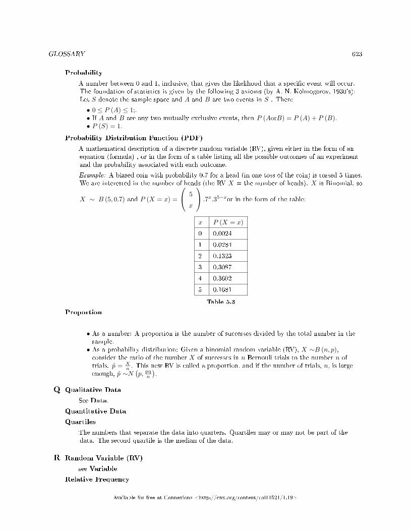
GLOSSARY 623
Probability
A number between 0 and 1, inclusive, that gives the likelihood that a speci�c event will occur.The foundation of statistics is given by the following 3 axioms (by A. N. Kolmogorov, 1930's):Let S denote the sample space and A and B are two events in S . Then:
• 0 ≤ P (A) ≤ 1;.• If A and B are any two mutually exclusive events, then P (AorB) = P (A) + P (B).• P (S) = 1.
Probability Distribution Function (PDF)
A mathematical description of a discrete random variable (RV), given either in the form of anequation (formula) , or in the form of a table listing all the possible outcomes of an experimentand the probability associated with each outcome.
Example: A biased coin with probability 0.7 for a head (in one toss of the coin) is tossed 5 times.We are interested in the number of heads (the RV X = the number of heads). X is Binomial, so
X ∼ B (5, 0.7) and P (X = x) =
5
x
.7x.35−xor in the form of the table:
x P (X = x)
0 0.0024
1 0.0284
2 0.1323
3 0.3087
4 0.3602
5 0.1681
Table 5.3
Proportion
• As a number: A proportion is the number of successes divided by the total number in thesample.• As a probability distribution: Given a binomial random variable (RV), X ∼B (n, p),consider the ratio of the number X of successes in n Bernouli trials to the number n oftrials. p̂ = X
n . This new RV is called a proportion, and if the number of trials, n, is largeenough, p̂ ∼N
(p, pq
n
).
Q Qualitative Data
See Data.
Quantitative Data
Quartiles
The numbers that separate the data into quarters. Quartiles may or may not be part of thedata. The second quartile is the median of the data.
R Random Variable (RV)
see Variable
Relative Frequency
Available for free at Connexions <http://cnx.org/content/col11521/1.19>
624 GLOSSARY
The ratio of the number of times a value of the data occurs in the set of all outcomes to thenumber of all outcomes.
S Sample
A portion of the population understudy. A sample is representative if it characterizes thepopulation being studied.
Sample Space
The set of all possible outcomes of an experiment.
Standard Deviation
A number that is equal to the square root of the variance and measures how far data values arefrom their mean. Notation: s for sample standard deviation and σ for population standarddeviation.
Standard Error of the Mean
The standard deviation of the distribution of the sample means, σ√n.
Standard Normal Distribution
A continuous random variable (RV) X~N (0, 1) .. When X follows the standard normaldistribution, it is often noted as Z~N (0, 1).
Statistic
A numerical characteristic of the sample. A statistic estimates the corresponding populationparameter. For example, the average number of full-time students in a 7:30 a.m. class for thisterm (statistic) is an estimate for the average number of full-time students in any class this term(parameter).
Student's-t Distribution
Investigated and reported by William S. Gossett in 1908 and published under the pseudonymStudent. The major characteristics of the random variable (RV) are:
• It is continuous and assumes any real values.• The pdf is symmetrical about its mean of zero. However, it is more spread out and �atter atthe apex than the normal distribution.• It approaches the standard normal distribution as n gets larger.• There is a "family" of t distributions: every representative of the family is completelyde�ned by the number of degrees of freedom which is one less than the number of data.
Student-t Distribution
T Tree Diagram
The useful visual representation of a sample space and events in the form of a �tree� withbranches marked by possible outcomes simultaneously with associated probabilities (frequencies,relative frequencies).
Type 1 Error
The decision is to reject the Null hypothesis when, in fact, the Null hypothesis is true.
Type 2 Error
The decision is to not reject the Null hypothesis when, in fact, the Null hypothesis is false.
U Uniform Distribution
Available for free at Connexions <http://cnx.org/content/col11521/1.19>
GLOSSARY 625
A continuous random variable (RV) that has equally likely outcomes over the domain, a < x < b.Often referred as the Rectangular distribution because the graph of the pdf has the form ofa rectangle. Notation: X~U (a, b). The mean is µ = a+b
2 and the standard deviation is
σ =√
(b−a)2
12 The probability density function is f (X) = 1b−a for a < x < b or a ≤ x ≤ b. The
cumulative distribution is P (X ≤ x) = x−ab−a .
V Variable (Random Variable)
A characteristic of interest in a population being studied. Common notation for variables areupper case Latin letters X, Y , Z,...; common notation for a speci�c value from the domain (setof all possible values of a variable) are lower case Latin letters x, y, z,.... For example, if X isthe number of children in a family, then x represents a speci�c integer 0, 1, 2, 3, .... Variables instatistics di�er from variables in intermediate algebra in two following ways.
• The domain of the random variable (RV) is not necessarily a numerical set; the domain maybe expressed in words; for example, if X = hair color then the domain is {black, blond,gray, green, orange}.• We can tell what speci�c value x of the Random Variable X takes only after performing theexperiment.
Variance
Mean of the squared deviations from the mean. Square of the standard deviation. For a set ofdata, a deviation can be represented as x− x where x is a value of the data and x is the samplemean. The sample variance is equal to the sum of the squares of the deviations divided by thedi�erence of the sample size and 1.
Venn Diagram
The visual representation of a sample space and events in the form of circles or ovals showingtheir intersections.
Z z-score
The linear transformation of the form z = x−µσ . If this transformation is applied to any normal
distribution X~N (µ, σ) , the result is the standard normal distribution Z~N (0, 1). If thistransformation is applied to any speci�c value x of the RV with mean µ and standard deviationσ , the result is called the z-score of x. Z-scores allow us to compare data that are normallydistributed but scaled di�erently.
Available for free at Connexions <http://cnx.org/content/col11521/1.19>
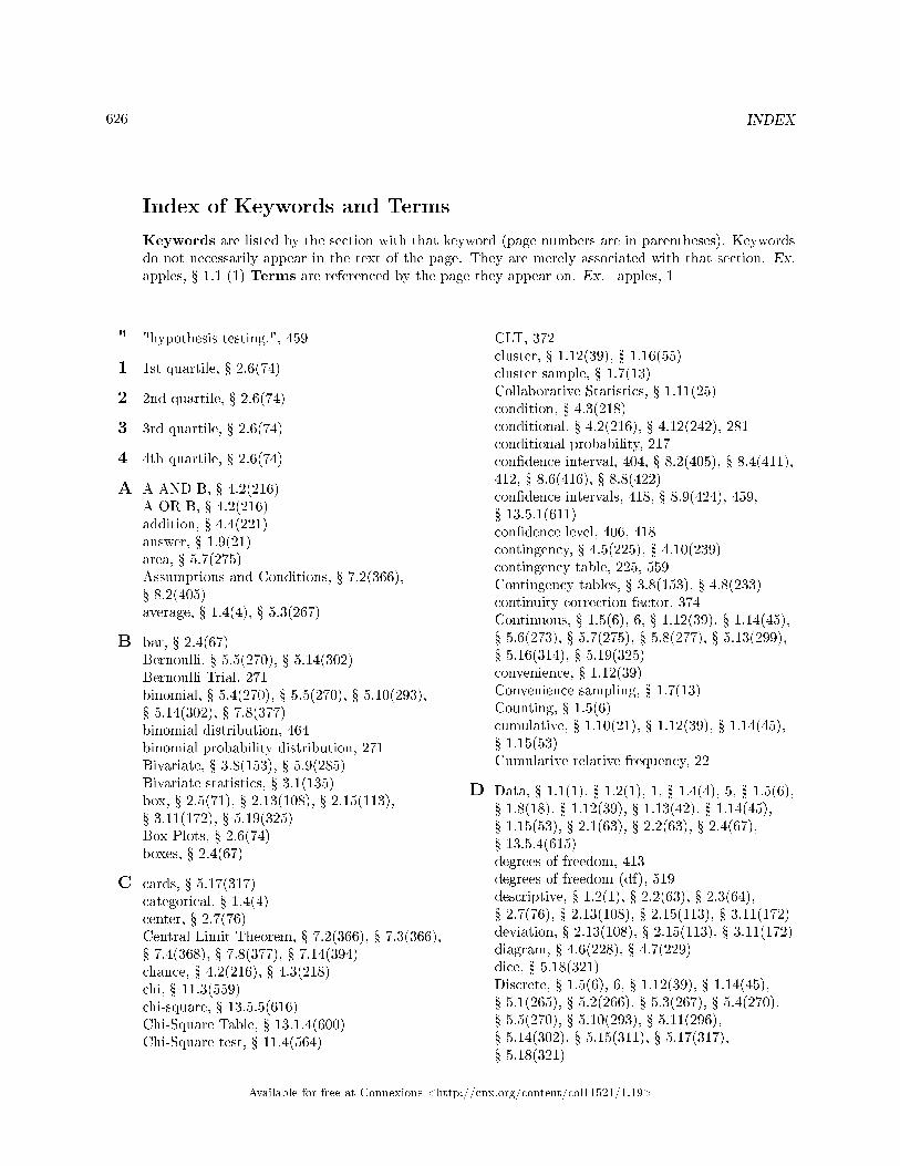
626 INDEX
Index of Keywords and Terms
Keywords are listed by the section with that keyword (page numbers are in parentheses). Keywordsdo not necessarily appear in the text of the page. They are merely associated with that section. Ex.apples, � 1.1 (1) Terms are referenced by the page they appear on. Ex. apples, 1
" "hypothesis testing.", 459
1 1st quartile, � 2.6(74)
2 2nd quartile, � 2.6(74)
3 3rd quartile, � 2.6(74)
4 4th quartile, � 2.6(74)
A A AND B, � 4.2(216)A OR B, � 4.2(216)addition, � 4.4(221)answer, � 1.9(21)area, � 5.7(275)Assumptions and Conditions, � 7.2(366),� 8.2(405)average, � 1.4(4), � 5.3(267)
B bar, � 2.4(67)Bernoulli, � 5.5(270), � 5.14(302)Bernoulli Trial, 271binomial, � 5.4(270), � 5.5(270), � 5.10(293),� 5.14(302), � 7.8(377)binomial distribution, 464binomial probability distribution, 271Bivariate, � 3.8(153), � 5.9(285)Bivariate statistics, � 3.1(135)box, � 2.5(71), � 2.13(108), � 2.15(113),� 3.11(172), � 5.19(325)Box Plots, � 2.6(74)boxes, � 2.4(67)
C cards, � 5.17(317)categorical, � 1.4(4)center, � 2.7(76)Central Limit Theorem, � 7.2(366), � 7.3(366),� 7.4(368), � 7.8(377), � 7.14(394)chance, � 4.2(216), � 4.3(218)chi, � 11.3(559)chi-square, � 13.5.5(616)Chi-Square Table, � 13.1.4(600)Chi-Square test, � 11.4(564)
CLT, 372cluster, � 1.12(39), � 1.16(55)cluster sample, � 1.7(13)Collaborative Statistics, � 1.11(25)condition, � 4.3(218)conditional, � 4.2(216), � 4.12(242), 281conditional probability, 217con�dence interval, 404, � 8.2(405), � 8.4(411),412, � 8.6(416), � 8.8(422)con�dence intervals, 418, � 8.9(424), 459,� 13.5.1(611)con�dence level, 406, 418contingency, � 4.5(225), � 4.10(239)contingency table, 225, 559Contingency tables, � 3.8(153), � 4.8(233)continuity correction factor, 374Continuous, � 1.5(6), 6, � 1.12(39), � 1.14(45),� 5.6(273), � 5.7(275), � 5.8(277), � 5.13(299),� 5.16(314), � 5.19(325)convenience, � 1.12(39)Convenience sampling, � 1.7(13)Counting, � 1.5(6)cumulative, � 1.10(21), � 1.12(39), � 1.14(45),� 1.15(53)Cumulative relative frequency, 22
D Data, � 1.1(1), � 1.2(1), 1, � 1.4(4), 5, � 1.5(6),� 1.8(18), � 1.12(39), � 1.13(42), � 1.14(45),� 1.15(53), � 2.1(63), � 2.2(63), � 2.4(67),� 13.5.4(615)degrees of freedom, 413degrees of freedom (df), 519descriptive, � 1.2(1), � 2.2(63), � 2.3(64),� 2.7(76), � 2.13(108), � 2.15(113), � 3.11(172)deviation, � 2.13(108), � 2.15(113), � 3.11(172)diagram, � 4.6(228), � 4.7(229)dice, � 5.18(321)Discrete, � 1.5(6), 6, � 1.12(39), � 1.14(45),� 5.1(265), � 5.2(266), � 5.3(267), � 5.4(270),� 5.5(270), � 5.10(293), � 5.11(296),� 5.14(302), � 5.15(311), � 5.17(317),� 5.18(321)
Available for free at Connexions <http://cnx.org/content/col11521/1.19>
INDEX 627
display, � 2.2(63)distribution, � 5.1(265), � 5.2(266), � 5.5(270),� 5.6(273), � 5.7(275), � 5.8(277), � 5.11(296),� 5.13(299), � 5.15(311), � 5.16(314),� 5.17(317), � 5.18(321), � 5.19(325),� 11.3(559), � 13.5.5(616)distribution is binomial, 418Distributions, � 5.9(285)dot plot, � 1.2(1)
E elementary, � 2.1(63), � 2.2(63), � 2.3(64),� 2.7(76), � 2.8(80), � 2.9(83), � 2.10(84),� 2.12(106), � 2.13(108), � 2.14(111),� 2.16(124), � 3.2(141), � 3.3(142), � 3.4(143),� 3.5(146), � 3.6(148), � 3.7(152), � 3.9(168),� 3.10(169), � 3.12(200), � 3.13(203),� 3.14(205), � 4.4(221), � 4.5(225), � 4.6(228),� 4.7(229), � 4.9(237), � 4.10(239), � 4.11(241),� 4.12(242), � 4.13(253), � 4.14(255),� 5.1(265), � 5.2(266), � 5.3(267), � 5.4(270),� 5.5(270), � 5.6(273), � 5.7(275), � 5.8(277),� 5.10(293), � 5.11(296), � 5.13(299),� 5.14(302), � 5.15(311), � 5.16(314),� 5.17(317), � 5.18(321), � 5.19(325),� 6.1(335), � 6.2(337), � 6.3(337), � 6.4(339),� 6.6(347), � 6.7(348), � 6.8(350), � 6.9(355),� 6.10(357), � 6.11(360), � 7.1(365), � 7.6(372),� 7.9(379), � 7.10(380), � 7.11(382),� 7.12(388), � 7.13(390), � 8.1(403), � 8.3(405),� 8.5(412), � 8.7(418), � 8.10(427), � 8.11(429),� 8.12(431), � 8.13(433), � 8.14(435),� 8.15(445), � 8.16(448), � 8.17(450),� 8.18(452), � 9.1(459), � 9.2(460), � 9.3(461),� 9.4(462), � 9.5(463), � 9.6(464), � 9.7(464),� 9.9(469), � 9.10(469), � 9.11(471),� 9.12(471), � 9.16(490), � 9.17(492),� 9.18(494), � 9.19(496), � 9.20(508),� 10.1(517), � 10.2(518), � 10.4(526),� 10.7(537), � 10.8(538), � 10.9(544),� 10.10(546), � 10.11(548), � 11.1(557),� 11.2(557), � 11.3(559), � 11.5(569),� 11.6(570), � 11.7(572), � 11.8(576),� 11.9(580), � 12.1(587), � 12.2(591),� 13.2(603), � 13.3(604), � 13.4(609),� 13.5.3(614), � 13.5.4(615), � 13.5.5(616)elementary statistics, � 2.15(113), � 3.11(172)empirical, � 5.19(325)equally likely, � 4.2(216), 216event, � 4.2(216), 216, � 4.12(242)example, � 7.8(377)Excel spreadsheets, � 8.9(424)exclusive, � 4.3(218), � 4.11(241), � 4.12(242)
exercise, � 1.16(55), � 2.15(113), � 3.11(172),� 4.10(239), � 4.14(255), � 5.13(299),� 5.14(302), � 5.15(311), � 5.16(314),� 5.17(317), � 5.18(321), � 5.19(325)exercises, � 4.13(253)expected, � 5.3(267)expected value, 267experiment, � 4.2(216), 216, � 5.1(265),� 5.5(270), � 5.17(317), � 5.18(321)exponential, � 5.6(273)
F formula, � 4.9(237), � 5.10(293)frequency, � 1.10(21), 21, � 1.12(39),� 1.13(42), � 1.14(45), � 1.15(53), � 1.16(55),67, � 2.13(108), � 2.15(113), � 3.11(172),� 4.2(216)function, � 5.2(266), � 5.4(270), � 5.5(270),� 5.6(273), � 5.8(277), � 5.10(293), � 5.13(299),� 5.15(311), � 5.16(314)functions, � 5.7(275)
G geometric, � 5.4(270)Google Spreadsheets, � 8.9(424)graph, � 2.2(63), � 2.3(64), � 5.6(273),� 5.13(299)Graphs, � 3.8(153)
H histogram, � 2.4(67), � 2.13(108), � 2.15(113),� 3.11(172), � 5.19(325)Homework, � 1.14(45), � 2.13(108),� 2.15(113), � 3.11(172), � 4.10(239),� 4.13(253), � 4.14(255), � 5.13(299),� 5.14(302), � 5.15(311), � 5.16(314),� 5.17(317), � 5.18(321), � 5.19(325)hypergeometric, � 5.4(270)hypotheses, 460, � 9.14(481)hypotheses test, � 10.3(521), � 10.5(528)hypotheses test - mean, � 9.8(465)hypothesis, � 13.5.3(614), � 13.5.4(615)hypothesis test, 463, 469, 471, � 13.5.2(612)Hypothesis test (mean), � 9.13(477)
I independence, � 11.3(559)independence assumption, � 7.2(366)independent, � 4.3(218), 218, 221, � 4.11(241),� 4.12(242)inferential, � 1.2(1)inferential statistics, 403Interquartile Range, � 2.6(74), 76Intro Statistics, � 13.5.1(611), � 13.5.2(612)Introduction, � 1.1(1), � 4.1(215), � 5.1(265)Introductory Statistics, � 13.6.1(616)IQR, � 2.6(74), � 2.7(76)
Available for free at Connexions <http://cnx.org/content/col11521/1.19>
628 INDEX
K key terms, � 4.2(216)
L lab, � 1.16(55), � 4.14(255), � 5.17(317),� 5.18(321), � 5.19(325), � 7.14(394)large, � 5.3(267)large enough sample condition, � 7.2(366)law, � 5.3(267)Law of Large Numbers, 372leaf, � 2.3(64)likelihood, � 1.3(4)location, � 2.7(76)long term, � 4.2(216)long-term, � 4.14(255), � 5.3(267)Lower Fence, � 2.6(74)
M margin of error for a population mean, 405,414margin of error� 418mean, 5, � 2.7(76), 80, � 2.13(108), � 2.15(113),� 3.11(172), � 5.3(267), 267, 365, 368, 372,� 7.7(375), � 8.4(411), � 8.6(416), � 13.5.3(614)means, � 13.5.4(615)measurement, � 1.8(18)Measuring, � 1.5(6)median, � 2.1(63), � 2.5(71), 71, � 2.7(76), 80,� 2.13(108), � 2.15(113), � 3.11(172)mode, � 2.7(76), 82, � 2.13(108), � 2.15(113),� 3.11(172)multiplication, � 4.4(221)mutually, � 4.3(218), � 4.11(241), � 4.12(242)mutually exclusive, 219, 221
N nonsampling errors, � 1.7(13)Normal, � 5.9(285)Normal Approximation to the Binomial, 374Normal Distribution, � 6.5(344), 412, 419, 462normally distributed, 367, 369, 463null hypothesis, 464, 464, 469numbers, � 5.3(267)numerical, � 1.4(4)
O One sample, � 9.14(481)outcome, � 4.2(216), 216, � 4.3(218)outlier, 64, 76Outliers, � 2.6(74), 76
P p-value, 464, 469, 469, 469, 471pair, � 13.5.4(615)parameter, � 1.4(4), 5, � 1.12(39), 403PDF, � 5.2(266)percentile, � 2.7(76), � 2.13(108), � 2.15(113),� 3.11(172)percentiles, 76
plot, � 2.13(108), � 2.15(113), � 3.11(172),� 5.19(325)point estimate, 403Poisson, � 5.4(270)population, � 1.4(4), 4, 19, � 1.12(39),� 2.15(113), � 3.11(172), � 5.16(314)practice, � 1.13(42), � 2.13(108), � 4.10(239),� 4.11(241), � 4.13(253), � 5.13(299),� 5.15(311), � 5.16(314)probability, � 1.3(4), 4, � 1.12(39), � 4.1(215),� 4.2(216), 216, � 4.3(218), � 4.4(221),� 4.5(225), � 4.6(228), � 4.7(229), � 4.8(233),� 4.9(237), � 4.10(239), � 4.11(241),� 4.12(242), � 4.13(253), � 4.14(255),� 5.2(266), � 5.3(267), � 5.4(270), � 5.5(270),� 5.6(273), � 5.7(275), � 5.8(277), � 5.10(293),� 5.11(296), � 5.13(299), � 5.15(311),� 5.16(314), � 5.17(317), � 5.18(321), � 6.5(344)probability distribution function, 266problem, � 2.15(113), � 3.11(172), � 5.14(302)proportion, � 1.4(4), 5, � 7.5(370), � 8.8(422),� 9.14(481), � 13.5.3(614), � 13.5.4(615)Proportions, � 10.5(528), � 11.4(564)
Q Qualitative, � 1.5(6), � 1.12(39), � 1.14(45)Qualitative data, 6Quantitative, � 1.5(6), � 1.12(39), � 1.14(45)Quantitative data, 6quartile, � 2.7(76), � 2.13(108), � 2.15(113),� 3.11(172)quartiles, � 2.5(71), 71, 76
R random, � 1.3(4), � 1.12(39), � 1.14(45),� 1.16(55), � 5.1(265), � 5.2(266), � 5.3(267),� 5.4(270), � 5.5(270), � 5.6(273), � 5.7(275),� 5.8(277), � 5.10(293), � 5.11(296),� 5.13(299), � 5.14(302), � 5.15(311),� 5.16(314), � 5.17(317), � 5.18(321)random number table, � 13.1.1(593)Random Numbers, � 4.8(233)random sampling, � 1.7(13)random variable, 265, 519Randomization condition, � 7.2(366)randomness, � 1.3(4)relative, � 1.10(21), � 1.12(39), � 1.14(45),� 1.15(53), � 2.15(113), � 3.11(172), � 4.2(216)relative frequency, 21, 67replacement, � 1.12(39), � 4.14(255)representative, � 1.4(4)review, � 4.13(253), � 5.15(311), � 5.16(314)round, � 1.9(21)rounding, � 1.9(21)
Available for free at Connexions <http://cnx.org/content/col11521/1.19>
INDEX 629
rule, � 4.4(221)
S sample, � 1.4(4), 4, � 1.7(13), � 1.8(18),� 1.12(39), � 1.14(45), � 1.16(55), � 2.15(113),� 3.11(172)Sample Means, � 7.3(366)sample size, � 7.2(366)sample space, � 4.2(216), 216, 221, 230samples, 19Sampling, � 1.1(1), � 1.4(4), 4, � 1.7(13),� 1.8(18), � 1.12(39), � 1.13(42), � 1.14(45),� 1.15(53), � 1.16(55)Sampling and Data, � 1.11(25)sampling distribution, 82, � 7.5(370),� 7.7(375), � 13.5.1(611)sampling errors, � 1.7(13)sampling variability of a statistic, 86sheet, � 13.5.3(614), � 13.5.4(615),� 13.5.5(616)Sigma known, � 8.4(411), � 9.8(465)Sigma unknown, � 8.6(416), � 9.13(477),� 10.3(521)simple, � 1.12(39)simple random sampling, � 1.7(13)single, � 13.5.3(614)single mean t-test, � 9.15(484)single mean z-test, � 9.15(484)Single Proportion z-test, � 9.15(484)size, � 1.8(18)skew, � 2.7(76)solution, � 13.5.3(614), � 13.5.4(615),� 13.5.5(616)Speadsheet techniques, � 1.11(25)spread, � 2.7(76)Spreadsheets, � 2.11(93)square, � 11.3(559)standard, � 2.13(108), � 2.15(113), � 3.11(172)standard deviation, 84, 412, 462, 463, 464standard error, 518standard error of the mean., 367standard normal distribution, 337statistic, � 1.4(4), 5, � 1.12(39), 83Statistics, � 1.1(1), � 1.2(1), 1, � 1.3(4),� 1.5(6), � 1.7(13), � 1.8(18), � 1.9(21),� 1.10(21), � 1.12(39), � 1.13(42), � 1.14(45),� 1.15(53), � 1.16(55), � 2.1(63), � 2.2(63),� 2.3(64), � 2.7(76), � 2.8(80), � 2.9(83),� 2.10(84), � 2.11(93), � 2.12(106), � 2.13(108),� 2.14(111), � 2.15(113), � 2.16(124),� 3.2(141), � 3.3(142), � 3.4(143), � 3.5(146),� 3.6(148), � 3.7(152), � 3.8(153), � 3.9(168),� 3.10(169), � 3.11(172), � 3.12(200),
� 3.13(203), � 3.14(205), � 4.1(215), � 4.2(216),� 4.3(218), � 4.4(221), � 4.5(225), � 4.6(228),� 4.7(229), � 4.9(237), � 4.10(239), � 4.11(241),� 4.12(242), � 4.13(253), � 4.14(255),� 5.1(265), � 5.2(266), � 5.3(267), � 5.4(270),� 5.5(270), � 5.6(273), � 5.7(275), � 5.8(277),� 5.10(293), � 5.11(296), � 5.13(299),� 5.14(302), � 5.15(311), � 5.16(314),� 5.17(317), � 5.18(321), � 5.19(325),� 6.1(335), � 6.2(337), � 6.3(337), � 6.4(339),� 6.6(347), � 6.7(348), � 6.8(350), � 6.9(355),� 6.10(357), � 6.11(360), � 7.1(365), � 7.3(366),� 7.4(368), � 7.6(372), � 7.9(379), � 7.10(380),� 7.11(382), � 7.12(388), � 7.13(390),� 7.14(394), � 8.1(403), � 8.3(405), � 8.5(412),� 8.7(418), � 8.10(427), � 8.11(429),� 8.12(431), � 8.13(433), � 8.14(435),� 8.15(445), � 8.16(448), � 8.17(450),� 8.18(452), � 9.1(459), � 9.2(460), � 9.3(461),� 9.4(462), � 9.5(463), � 9.6(464), � 9.7(464),� 9.9(469), � 9.10(469), � 9.11(471),� 9.12(471), � 9.16(490), � 9.17(492),� 9.18(494), � 9.19(496), � 9.20(508),� 10.1(517), � 10.2(518), � 10.4(526),� 10.7(537), � 10.8(538), � 10.9(544),� 10.10(546), � 10.11(548), � 11.1(557),� 11.2(557), � 11.3(559), � 11.5(569),� 11.6(570), � 11.7(572), � 11.8(576),� 11.9(580), � 12.1(587), � 12.2(591),� 13.2(603), � 13.3(604), � 13.4(609),� 13.5.3(614), � 13.5.4(615), � 13.5.5(616)stem, � 2.3(64)stemplot, � 2.3(64)strati�ed, � 1.12(39), � 1.16(55)strati�ed sample, � 1.7(13)Student's-t distribution, 412, 463student's-t distribution., 462Sums, � 7.4(368), � 7.5(370)survey, � 1.14(45)systematic, � 1.12(39), � 1.15(53), � 1.16(55)systematic sample, � 1.7(13)
T t-table, � 13.1.3(598)table, � 4.5(225), � 4.10(239)Terminology, � 4.2(216)test, � 10.6(531), � 11.3(559), � 13.5.3(614),� 13.5.4(615)The Central Limit Theorem, 365, 367tree, � 4.7(229)tree diagram, 229trial, � 5.5(270)two, � 13.5.4(615)
Available for free at Connexions <http://cnx.org/content/col11521/1.19>
630 INDEX
Two means, � 10.3(521)Two sample mean t-test, � 10.6(531)Two sample proportion z-, � 10.6(531)Type I error, 461, 469Type II error, 462
U uniform, � 5.6(273), � 5.8(277), � 5.9(285),� 5.13(299), � 5.19(325)uniform distribution, 277Univariate, � 2.11(93)Upper Fence, � 2.6(74)
V variability, � 1.8(18)variable, � 1.4(4), 5, � 1.12(39), � 5.1(265),� 5.2(266), � 5.3(267), � 5.4(270), � 5.5(270),� 5.6(273), � 5.8(277), � 5.10(293), � 5.11(296),
� 5.13(299), � 5.14(302), � 5.15(311),� 5.16(314), � 5.17(317), � 5.18(321)variance, 86variation, � 1.8(18)Venn, � 4.6(228)Venn diagram, 228
W with replacement, � 1.7(13)without replacement, � 1.7(13)
Z Z- table, � 13.1.2(594)z-score, 413z-scores, 337z-socres, � 6.5(344)
α α, 469
Available for free at Connexions <http://cnx.org/content/col11521/1.19>
ATTRIBUTIONS 631
Attributions
Collection: Collaborative Statistics Using SpreadsheetsEdited by: Irene Mary Duranczyk, Suzanne Loch, Janet StottlemyerURL: http://cnx.org/content/col11521/1.19/License: http://creativecommons.org/licenses/by/3.0/
Module: "Sampling and Data: Introduction"By: Irene Mary Duranczyk, Suzanne Loch, Janet StottlemyerURL: http://cnx.org/content/m46121/1.1/Page: 1Copyright: Irene Mary Duranczyk, Suzanne Loch, Janet StottlemyerLicense: http://creativecommons.org/licenses/by/3.0/Based on: Sampling and Data: IntroductionBy: Susan Dean, Barbara Illowsky, Ph.D.URL: http://cnx.org/content/m16008/1.9/
Module: "Sampling and Data: Statistics"By: Susan Dean, Barbara Illowsky, Ph.D.URL: http://cnx.org/content/m16020/1.16/Pages: 1-4Copyright: Max�eld FoundationLicense: http://creativecommons.org/licenses/by/3.0/
Module: "Sampling and Data: Probability"By: Susan Dean, Barbara Illowsky, Ph.D.URL: http://cnx.org/content/m16015/1.11/Page: 4Copyright: Max�eld FoundationLicense: http://creativecommons.org/licenses/by/3.0/
Module: "Sampling and Data: Key Terms"By: Irene Mary DuranczykURL: http://cnx.org/content/m46249/1.3/Pages: 4-6Copyright: Irene Mary DuranczykLicense: http://creativecommons.org/licenses/by/3.0/Based on: Sampling and Data: Key TermsBy: Susan Dean, Barbara Illowsky, Ph.D.URL: http://cnx.org/content/m16007/1.17/
Module: "Sampling and Data: Data"By: Susan Dean, Barbara Illowsky, Ph.D.URL: http://cnx.org/content/m16005/1.18/Pages: 6-12Copyright: Max�eld FoundationLicense: http://creativecommons.org/licenses/by/3.0/
Module: "The 5W's"By: Irene Mary Duranczyk, Suzanne Loch, Janet StottlemyerURL: http://cnx.org/content/m46118/1.2/Pages: 12-13Copyright: Irene Mary Duranczyk, Suzanne Loch, Janet StottlemyerLicense: http://creativecommons.org/licenses/by/3.0/
Available for free at Connexions <http://cnx.org/content/col11521/1.19>
632 ATTRIBUTIONS
Module: "Sampling and Data: Sampling"By: Irene Mary DuranczykURL: http://cnx.org/content/m46800/1.1/Pages: 13-18Copyright: Irene Mary DuranczykLicense: http://creativecommons.org/licenses/by/3.0/Based on: Sampling and Data: SamplingBy: Susan Dean, Barbara Illowsky, Ph.D.URL: http://cnx.org/content/m16014/1.17/
Module: "Sampling and Data: Variation and Critical Evaluation"By: Susan Dean, Barbara Illowsky, Ph.D.URL: http://cnx.org/content/m16021/1.15/Pages: 18-20Copyright: Max�eld FoundationLicense: http://creativecommons.org/licenses/by/3.0/
Module: "Sampling and Data: Answers and Rounding O�"By: Susan Dean, Barbara Illowsky, Ph.D.URL: http://cnx.org/content/m16006/1.8/Page: 21Copyright: Max�eld FoundationLicense: http://creativecommons.org/licenses/by/3.0/
Module: "Sampling and Data: Frequency, Relative Frequency, and Cumulative Frequency"By: Susan Dean, Barbara Illowsky, Ph.D.URL: http://cnx.org/content/m16012/1.20/Pages: 21-25Copyright: Max�eld FoundationLicense: http://creativecommons.org/licenses/by/3.0/
Module: "Sampling and Data: Using Spreadsheets to View and Summarize Data"By: Irene Mary Duranczyk, Suzanne Loch, Janet StottlemyerURL: http://cnx.org/content/m47493/1.2/Pages: 25-38Copyright: Irene Mary Duranczyk, Suzanne Loch, Janet StottlemyerLicense: http://creativecommons.org/licenses/by/3.0/
Module: "Sampling and Data: Summary"By: Irene Mary Duranczyk, Suzanne Loch, Janet StottlemyerURL: http://cnx.org/content/m46128/1.2/Pages: 39-41Copyright: Irene Mary Duranczyk, Suzanne Loch, Janet StottlemyerLicense: http://creativecommons.org/licenses/by/3.0/Based on: Sampling and Data: SummaryBy: Susan Dean, Barbara Illowsky, Ph.D.URL: http://cnx.org/content/m16023/1.10/
Module: "Sampling and Data: Practice 1"By: Susan Dean, Barbara Illowsky, Ph.D.URL: http://cnx.org/content/m16016/1.16/Pages: 42-44Copyright: Max�eld FoundationLicense: http://creativecommons.org/licenses/by/3.0/
Available for free at Connexions <http://cnx.org/content/col11521/1.19>
ATTRIBUTIONS 633
Module: "Sampling and Data: Homework"By: Irene Mary Duranczyk, Suzanne Loch, Janet StottlemyerURL: http://cnx.org/content/m46125/1.5/Pages: 45-52Copyright: Irene Mary Duranczyk, Suzanne Loch, Janet StottlemyerLicense: http://creativecommons.org/licenses/by/3.0/Based on: Sampling and Data: HomeworkBy: Susan Dean, Barbara Illowsky, Ph.D.URL: http://cnx.org/content/m16010/1.19/
Module: "Sampling and Data: Data Collection Lab I"By: Susan Dean, Barbara Illowsky, Ph.D.URL: http://cnx.org/content/m16004/1.11/Pages: 53-54Copyright: Max�eld FoundationLicense: http://creativecommons.org/licenses/by/2.0/
Module: "Sampling and Data: Sampling Experiment Lab II"By: Susan Dean, Barbara Illowsky, Ph.D.URL: http://cnx.org/content/m16013/1.15/Pages: 55-58Copyright: Max�eld FoundationLicense: http://creativecommons.org/licenses/by/3.0/
Module: "Descriptive Statistics: Introduction"By: Susan Dean, Barbara Illowsky, Ph.D.URL: http://cnx.org/content/m16300/1.9/Page: 63Copyright: Max�eld FoundationLicense: http://creativecommons.org/licenses/by/3.0/
Module: "Descriptive Statistics: Displaying Data"By: Susan Dean, Barbara Illowsky, Ph.D.URL: http://cnx.org/content/m16297/1.9/Pages: 63-64Copyright: Max�eld FoundationLicense: http://creativecommons.org/licenses/by/3.0/
Module: "Descriptive Statistics: Stem and Leaf Graphs (Stemplots), Line Graphs and Bar Graphs"By: Susan Dean, Barbara Illowsky, Ph.D.URL: http://cnx.org/content/m16849/1.17/Pages: 64-67Copyright: Max�eld FoundationLicense: http://creativecommons.org/licenses/by/3.0/
Module: "Descriptive Statistics: Histogram"By: Susan Dean, Barbara Illowsky, Ph.D.URL: http://cnx.org/content/m16298/1.14/Pages: 67-71Copyright: Max�eld FoundationLicense: http://creativecommons.org/licenses/by/3.0/
Available for free at Connexions <http://cnx.org/content/col11521/1.19>
634 ATTRIBUTIONS
Module: "Descriptive Statistics: Box Plot"By: Susan Dean, Barbara Illowsky, Ph.D.URL: http://cnx.org/content/m16296/1.13/Pages: 71-74Copyright: Max�eld FoundationLicense: http://creativecommons.org/licenses/by/3.0/
Module: "Box Plots with Outliers"By: Irene Mary Duranczyk, Suzanne Loch, Janet StottlemyerURL: http://cnx.org/content/m46129/1.1/Pages: 74-75Copyright: Irene Mary Duranczyk, Suzanne Loch, Janet StottlemyerLicense: http://creativecommons.org/licenses/by/3.0/
Module: "Descriptive Statistics: Measuring the Location of the Data"By: Irene Mary DuranczykURL: http://cnx.org/content/m47514/1.1/Pages: 76-80Copyright: Irene Mary DuranczykLicense: http://creativecommons.org/licenses/by/3.0/Based on: Descriptive Statistics: Measuring the Location of the DataBy: Susan Dean, Barbara Illowsky, Ph.D.URL: http://cnx.org/content/m16314/1.18/
Module: "Descriptive Statistics: Measuring the Center of the Data"By: Susan Dean, Barbara Illowsky, Ph.D.URL: http://cnx.org/content/m17102/1.13/Pages: 80-83Copyright: Max�eld FoundationLicense: http://creativecommons.org/licenses/by/3.0/
Module: "Descriptive Statistics: Skewness and the Mean, Median, and Mode"By: Susan Dean, Barbara Illowsky, Ph.D.URL: http://cnx.org/content/m17104/1.9/Pages: 83-84Copyright: Max�eld FoundationLicense: http://creativecommons.org/licenses/by/3.0/
Module: "Derived copy of Descriptive Statistics: Measuring the Spread of the Data"Used here as: "Descriptive Statistics: Measuring the Spread of the Data"By: Irene Mary DuranczykURL: http://cnx.org/content/m47515/1.1/Pages: 84-93Copyright: Irene Mary DuranczykLicense: http://creativecommons.org/licenses/by/3.0/Based on: Descriptive Statistics: Measuring the Spread of the DataBy: Susan Dean, Barbara Illowsky, Ph.D.URL: http://cnx.org/content/m17103/1.15/
Available for free at Connexions <http://cnx.org/content/col11521/1.19>
ATTRIBUTIONS 635
Module: "Univariate Descriptive Statistics Using Spreadsheet to View and Summarize Data"Used here as: "Univariate Descriptive Statistics Using Spreadsheets to View and Summarize Data"By: Irene Mary Duranczyk, Janet Stottlemyer, Suzanne LochURL: http://cnx.org/content/m47492/1.2/Pages: 93-105Copyright: Irene Mary Duranczyk, Janet Stottlemyer, Suzanne LochLicense: http://creativecommons.org/licenses/by/3.0/
Module: "Univariate Descriptive Statistics: Summary of Formulas"By: Irene Mary Duranczyk, Suzanne Loch, Janet StottlemyerURL: http://cnx.org/content/m46126/1.3/Pages: 106-107Copyright: Irene Mary Duranczyk, Suzanne Loch, Janet StottlemyerLicense: http://creativecommons.org/licenses/by/3.0/Based on: Descriptive Statistics: Summary of FormulasBy: Susan Dean, Barbara Illowsky, Ph.D.URL: http://cnx.org/content/m16310/1.9/
Module: "Derived copy of Descriptive Statistics: Practice 1"Used here as: "Univariate Descriptive Statistics: Practice 1"By: Irene Mary DuranczykURL: http://cnx.org/content/m47525/1.1/Pages: 108-110Copyright: Irene Mary DuranczykLicense: http://creativecommons.org/licenses/by/3.0/Based on: Descriptive Statistics: Practice 1By: Susan Dean, Barbara Illowsky, Ph.D.URL: http://cnx.org/content/m16312/1.12/
Module: "Descriptive Statistics: Practice 2"By: Susan Dean, Barbara Illowsky, Ph.D.URL: http://cnx.org/content/m17105/1.12/Pages: 111-112Copyright: Max�eld FoundationLicense: http://creativecommons.org/licenses/by/3.0/
Module: "Univariate Descriptive Statistics: Homework"By: Irene Mary Duranczyk, Suzanne Loch, Janet StottlemyerURL: http://cnx.org/content/m46199/1.6/Pages: 113-123Copyright: Irene Mary Duranczyk, Suzanne Loch, Janet StottlemyerLicense: http://creativecommons.org/licenses/by/3.0/Based on: Descriptive Statistics: HomeworkBy: Susan Dean, Barbara Illowsky, Ph.D.URL: http://cnx.org/content/m16801/1.25/
Module: "Descriptive Statistics: Descriptive Statistics Lab"By: Susan Dean, Barbara Illowsky, Ph.D.URL: http://cnx.org/content/m16299/1.13/Pages: 124-125Copyright: Max�eld FoundationLicense: http://creativecommons.org/licenses/by/3.0/
Available for free at Connexions <http://cnx.org/content/col11521/1.19>
636 ATTRIBUTIONS
Module: "Bivariate Descriptive Statistics: Introduction"By: Irene Mary Duranczyk, Suzanne Loch, Janet StottlemyerURL: http://cnx.org/content/m46177/1.2/Pages: 135-141Copyright: Irene Mary Duranczyk, Suzanne Loch, Janet StottlemyerLicense: http://creativecommons.org/licenses/by/3.0/
Module: "Linear Regression and Correlation: Linear Equations"By: Susan Dean, Barbara Illowsky, Ph.D.URL: http://cnx.org/content/m17086/1.4/Pages: 141-142Copyright: Max�eld FoundationLicense: http://creativecommons.org/licenses/by/2.0/
Module: "Linear Regression and Correlation: Slope and Y-Intercept of a Linear Equation"By: Susan Dean, Barbara Illowsky, Ph.D.URL: http://cnx.org/content/m17083/1.5/Pages: 142-143Copyright: Max�eld FoundationLicense: http://creativecommons.org/licenses/by/2.0/
Module: "Bivariate Descriptive Statistics: Linear Regression and Correlation: Scatter Plots"By: Irene Mary Duranczyk, Suzanne Loch, Janet StottlemyerURL: http://cnx.org/content/m46171/1.2/Pages: 143-145Copyright: Irene Mary Duranczyk, Suzanne Loch, Janet StottlemyerLicense: http://creativecommons.org/licenses/by/3.0/Based on: Linear Regression and Correlation: Scatter PlotsBy: Susan Dean, Barbara Illowsky, Ph.D.URL: http://cnx.org/content/m17082/1.8/
Module: "Bivariate Descriptive Statistics: Correlation Coe�cient and Coe�cient of Determination"By: Irene Mary Duranczyk, Suzanne Loch, Janet StottlemyerURL: http://cnx.org/content/m46185/1.3/Pages: 146-148Copyright: Irene Mary Duranczyk, Suzanne Loch, Janet StottlemyerLicense: http://creativecommons.org/licenses/by/3.0/Based on: Linear Regression and Correlation: Correlation Coe�cient and Coe�cient of DeterminationBy: Susan Dean, Barbara Illowsky, Ph.D.URL: http://cnx.org/content/m17092/1.12/
Module: "Bivariate Descriptive Statistics: The Regression Equation"By: Irene Mary Duranczyk, Suzanne Loch, Janet StottlemyerURL: http://cnx.org/content/m46176/1.3/Pages: 148-152Copyright: Irene Mary Duranczyk, Suzanne Loch, Janet StottlemyerLicense: http://creativecommons.org/licenses/by/3.0/Based on: Linear Regression and Correlation: The Regression EquationBy: Susan Dean, Barbara Illowsky, Ph.D.URL: http://cnx.org/content/m17090/1.15/
Available for free at Connexions <http://cnx.org/content/col11521/1.19>
ATTRIBUTIONS 637
Module: "Linear Regression and Correlation: Prediction"By: Susan Dean, Barbara Illowsky, Ph.D.URL: http://cnx.org/content/m17095/1.8/Page: 152Copyright: Max�eld FoundationLicense: http://creativecommons.org/licenses/by/3.0/
Module: "Bivariate Descriptive Statistics: Unsing Spreadsheets to View and Summarize Data"Used here as: "Bivariate Descriptive Statistics: Using Spreadsheets to View and Summarize Data"By: Irene Mary Duranczyk, Suzanne Loch, Janet StottlemyerURL: http://cnx.org/content/m47471/1.1/Pages: 153-167Copyright: Irene Mary Duranczyk, Suzanne Loch, Janet StottlemyerLicense: http://creativecommons.org/licenses/by/3.0/
Module: "Bivariate Descriptive Statistics: Summary"By: Irene Mary Duranczyk, Suzanne LochURL: http://cnx.org/content/m46200/1.2/Page: 168Copyright: Irene Mary Duranczyk, Suzanne LochLicense: http://creativecommons.org/licenses/by/3.0/Based on: Linear Regression and Correlation: SummaryBy: Susan Dean, Barbara Illowsky, Ph.D.URL: http://cnx.org/content/m17081/1.4/
Module: "Linear Regression and Correlation: Practice"By: Susan Dean, Barbara Illowsky, Ph.D.URL: http://cnx.org/content/m17088/1.12/Pages: 169-171Copyright: Max�eld FoundationLicense: http://creativecommons.org/licenses/by/3.0/
Module: "Bivariate Descriptive Statistics: Homework"By: Irene Mary Duranczyk, Suzanne Loch, Janet StottlemyerURL: http://cnx.org/content/m46174/1.7/Pages: 172-199Copyright: Irene Mary Duranczyk, Suzanne Loch, Janet StottlemyerLicense: http://creativecommons.org/licenses/by/3.0/Based on: Descriptive Statistics: HomeworkBy: Susan Dean, Barbara Illowsky, Ph.D.URL: http://cnx.org/content/m16801/1.25/
Module: "Bivariate Descriptive Statistics: Regression Lab I"By: Irene Mary Duranczyk, Suzanne Loch, Janet StottlemyerURL: http://cnx.org/content/m46172/1.1/Pages: 200-202Copyright: Irene Mary Duranczyk, Suzanne Loch, Janet StottlemyerLicense: http://creativecommons.org/licenses/by/3.0/Based on: Linear Regression and Correlation: Regression Lab IBy: Susan Dean, Barbara Illowsky, Ph.D.URL: http://cnx.org/content/m17080/1.11/
Available for free at Connexions <http://cnx.org/content/col11521/1.19>
638 ATTRIBUTIONS
Module: "Bivariate Descriptive Statistics: Linear Regression and Correlation: Regression Lab II"By: Irene Mary Duranczyk, Suzanne Loch, Janet StottlemyerURL: http://cnx.org/content/m46201/1.1/Pages: 203-204Copyright: Irene Mary Duranczyk, Suzanne Loch, Janet StottlemyerLicense: http://creativecommons.org/licenses/by/3.0/Based on: Linear Regression and Correlation: Regression Lab IIBy: Susan Dean, Barbara Illowsky, Ph.D.URL: http://cnx.org/content/m17087/1.9/
Module: "Bivariate Descriptive Statistics: Linear Regression and Correlation: Regression Lab III"By: Irene Mary Duranczyk, Suzanne Loch, Janet StottlemyerURL: http://cnx.org/content/m46202/1.1/Pages: 205-208Copyright: Irene Mary Duranczyk, Suzanne Loch, Janet StottlemyerLicense: http://creativecommons.org/licenses/by/3.0/Based on: Linear Regression and Correlation: Regression Lab IIIBy: Susan Dean, Barbara Illowsky, Ph.D.URL: http://cnx.org/content/m17079/1.8/
Module: "Probability Topics: Introduction"By: Susan Dean, Barbara Illowsky, Ph.D.URL: http://cnx.org/content/m16838/1.11/Pages: 215-216Copyright: Max�eld FoundationLicense: http://creativecommons.org/licenses/by/3.0/
Module: "Derived copy of Probability Topics: Terminology"Used here as: "Probability Topics: Terminology"By: Irene Mary DuranczykURL: http://cnx.org/content/m47517/1.1/Pages: 216-218Copyright: Irene Mary DuranczykLicense: http://creativecommons.org/licenses/by/3.0/Based on: Probability Topics: TerminologyBy: Susan Dean, Barbara Illowsky, Ph.D.URL: http://cnx.org/content/m16845/1.13/
Module: "Probability Topics: Independent & Mutually Exclusive Events"By: Susan Dean, Barbara Illowsky, Ph.D.URL: http://cnx.org/content/m16837/1.14/Pages: 218-221Copyright: Max�eld FoundationLicense: http://creativecommons.org/licenses/by/3.0/
Module: "Probability Topics: Two Basic Rules of Probability"By: Susan Dean, Barbara Illowsky, Ph.D.URL: http://cnx.org/content/m16847/1.11/Pages: 221-224Copyright: Max�eld FoundationLicense: http://creativecommons.org/licenses/by/3.0/
Available for free at Connexions <http://cnx.org/content/col11521/1.19>
ATTRIBUTIONS 639
Module: "Probability Topics: Contingency Tables"By: Susan Dean, Barbara Illowsky, Ph.D.URL: http://cnx.org/content/m16835/1.12/Pages: 225-227Copyright: Max�eld FoundationLicense: http://creativecommons.org/licenses/by/3.0/
Module: "Probability Topics: Venn Diagrams (optional)"By: Susan Dean, Barbara Illowsky, Ph.D.URL: http://cnx.org/content/m16848/1.12/Pages: 228-229Copyright: Max�eld FoundationLicense: http://creativecommons.org/licenses/by/3.0/
Module: "Probability Topics: Tree Diagrams (optional)"By: Susan Dean, Barbara Illowsky, Ph.D.URL: http://cnx.org/content/m16846/1.10/Pages: 229-232Copyright: Max�eld FoundationLicense: http://creativecommons.org/licenses/by/2.0/
Module: "Probability Topics: Using Spreadsheets to Explore Probability Topics"By: Irene Mary Duranczyk, Suzanne Loch, Janet StottlemyerURL: http://cnx.org/content/m47513/1.1/Pages: 233-236Copyright: Irene Mary Duranczyk, Suzanne Loch, Janet StottlemyerLicense: http://creativecommons.org/licenses/by/3.0/
Module: "Probability Topics: Summary of Formulas"By: Irene Mary DuranczykURL: http://cnx.org/content/m48323/1.3/Pages: 237-238Copyright: Irene Mary DuranczykLicense: http://creativecommons.org/licenses/by/3.0/Based on: Probability Topics: Summary of FormulasBy: Susan Dean, Barbara Illowsky, Ph.D.URL: http://cnx.org/content/m16843/1.5/
Module: "Probability Topics: Practice"By: Susan Dean, Barbara Illowsky, Ph.D.URL: http://cnx.org/content/m16839/1.11/Pages: 239-240Copyright: Max�eld FoundationLicense: http://creativecommons.org/licenses/by/3.0/
Module: "Probability Topics: Practice II"By: Susan Dean, Barbara Illowsky, Ph.D.URL: http://cnx.org/content/m16840/1.12/Page: 241Copyright: Max�eld FoundationLicense: http://creativecommons.org/licenses/by/3.0/
Available for free at Connexions <http://cnx.org/content/col11521/1.19>
640 ATTRIBUTIONS
Module: "Probability Topics: Homework"By: Susan Dean, Barbara Illowsky, Ph.D.URL: http://cnx.org/content/m16836/1.21/Pages: 242-252Copyright: Max�eld FoundationLicense: http://creativecommons.org/licenses/by/3.0/
Module: "Probability Topics: Review"By: Susan Dean, Barbara Illowsky, Ph.D.URL: http://cnx.org/content/m16842/1.9/Pages: 253-254Copyright: Max�eld FoundationLicense: http://creativecommons.org/licenses/by/2.0/
Module: "Probability Topics: Probability Lab"By: Susan Dean, Barbara Illowsky, Ph.D.URL: http://cnx.org/content/m16841/1.15/Pages: 255-257Copyright: Max�eld FoundationLicense: http://creativecommons.org/licenses/by/2.0/
Module: "Discrete and Continuous Random Variables: Introduction to Discrete Random Variables"By: Irene Mary Duranczyk, Suzanne Loch, Janet StottlemyerURL: http://cnx.org/content/m46207/1.1/Pages: 265-266Copyright: Irene Mary Duranczyk, Suzanne Loch, Janet StottlemyerLicense: http://creativecommons.org/licenses/by/3.0/Based on: Discrete Random Variables: IntroductionBy: Susan Dean, Barbara Illowsky, Ph.D.URL: http://cnx.org/content/m16825/1.14/
Module: "Discrete Random Variables: Probability Distribution Function (PDF) for a Discrete RandomVariable"By: Susan Dean, Barbara Illowsky, Ph.D.URL: http://cnx.org/content/m16831/1.14/Pages: 266-267Copyright: Max�eld FoundationLicense: http://creativecommons.org/licenses/by/3.0/
Module: "Discrete Random Variables: Mean or Expected Value and Standard Deviation"By: Susan Dean, Barbara Illowsky, Ph.D.URL: http://cnx.org/content/m16828/1.16/Pages: 267-270Copyright: Max�eld FoundationLicense: http://creativecommons.org/licenses/by/3.0/
Module: "Discrete Random Variables: Common Discrete Probability Distribution Functions"By: Susan Dean, Barbara Illowsky, Ph.D.URL: http://cnx.org/content/m16821/1.6/Page: 270Copyright: Max�eld FoundationLicense: http://creativecommons.org/licenses/by/3.0/
Available for free at Connexions <http://cnx.org/content/col11521/1.19>
ATTRIBUTIONS 641
Module: "Discrete Random Variables: Binomial"By: Susan Dean, Barbara Illowsky, Ph.D.URL: http://cnx.org/content/m16820/1.17/Pages: 270-273Copyright: Max�eld FoundationLicense: http://creativecommons.org/licenses/by/3.0/
Module: "Continuous Random Variables: Introduction"By: Susan Dean, Barbara Illowsky, Ph.D.URL: http://cnx.org/content/m16808/1.12/Pages: 273-275Copyright: Max�eld FoundationLicense: http://creativecommons.org/licenses/by/3.0/
Module: "Continuous Random Variables: Continuous Probability Functions"By: Susan Dean, Barbara Illowsky, Ph.D.URL: http://cnx.org/content/m16805/1.9/Pages: 275-277Copyright: Max�eld FoundationLicense: http://creativecommons.org/licenses/by/3.0/
Module: "Continuous Random Variables: The Uniform Distribution"By: Susan Dean, Barbara Illowsky, Ph.D.URL: http://cnx.org/content/m16819/1.17/Pages: 277-284Copyright: Max�eld FoundationLicense: http://creativecommons.org/licenses/by/3.0/
Module: "Discrete and Continuous Random Variables: Using Spreadsheets to Explore Distributions"By: Irene Mary Duranczyk, Suzanne Loch, Janet StottlemyerURL: http://cnx.org/content/m47485/1.1/Pages: 285-292Copyright: Irene Mary Duranczyk, Suzanne Loch, Janet StottlemyerLicense: http://creativecommons.org/licenses/by/3.0/
Module: "Discrete and Continuous Random Variables: Summary of the Discrete and Continuous ProbabilityFunctions"By: Irene Mary Duranczyk, Suzanne Loch, Janet StottlemyerURL: http://cnx.org/content/m46205/1.2/Pages: 293-295Copyright: Irene Mary Duranczyk, Suzanne Loch, Janet StottlemyerLicense: http://creativecommons.org/licenses/by/3.0/Based on: Discrete Random Variables: Summary of the Discrete Probability FunctionsBy: Susan Dean, Barbara Illowsky, Ph.D.URL: http://cnx.org/content/m16833/1.10/
Module: "Discrete Random Variables: Practice 1: Discrete Distributions"By: Susan Dean, Barbara Illowsky, Ph.D.URL: http://cnx.org/content/m16830/1.14/Page: 296Copyright: Max�eld FoundationLicense: http://creativecommons.org/licenses/by/3.0/
Available for free at Connexions <http://cnx.org/content/col11521/1.19>
642 ATTRIBUTIONS
Module: "Discrete Random Variables: Practice 2: Binomial Distribution"By: Susan Dean, Barbara Illowsky, Ph.D.URL: http://cnx.org/content/m17107/1.18/Pages: 297-298Copyright: Max�eld FoundationLicense: http://creativecommons.org/licenses/by/3.0/
Module: "Continuous Random Variables: Practice 1"By: Susan Dean, Barbara Illowsky, Ph.D.URL: http://cnx.org/content/m16812/1.14/Pages: 299-301Copyright: Max�eld FoundationLicense: http://creativecommons.org/licenses/by/3.0/
Module: "Discrete and Continuous Random Variables: Homework"By: Irene Mary Duranczyk, Suzanne Loch, Janet StottlemyerURL: http://cnx.org/content/m46206/1.2/Pages: 302-310Copyright: Irene Mary Duranczyk, Suzanne Loch, Janet StottlemyerLicense: http://creativecommons.org/licenses/by/3.0/Based on: Discrete Random Variables: HomeworkBy: Susan Dean, Barbara Illowsky, Ph.D.URL: http://cnx.org/content/m16823/1.20/
Module: "Discrete Random Variables: Review"By: Susan Dean, Barbara Illowsky, Ph.D.URL: http://cnx.org/content/m16832/1.11/Pages: 311-313Copyright: Max�eld FoundationLicense: http://creativecommons.org/licenses/by/3.0/
Module: "Continuous Random Variables: Review"By: Susan Dean, Barbara Illowsky, Ph.D.URL: http://cnx.org/content/m16810/1.11/Pages: 314-316Copyright: Max�eld FoundationLicense: http://creativecommons.org/licenses/by/3.0/
Module: "Discrete Random Variables: Lab I"By: Susan Dean, Barbara Illowsky, Ph.D.URL: http://cnx.org/content/m16827/1.12/Pages: 317-320Copyright: Max�eld FoundationLicense: http://creativecommons.org/licenses/by/3.0/
Module: "Discrete Random Variables: Lab II"By: Susan Dean, Barbara Illowsky, Ph.D.URL: http://cnx.org/content/m16826/1.12/Pages: 321-324Copyright: Max�eld FoundationLicense: http://creativecommons.org/licenses/by/3.0/
Available for free at Connexions <http://cnx.org/content/col11521/1.19>
ATTRIBUTIONS 643
Module: "Continuous Random Variables: Lab I"By: Susan Dean, Barbara Illowsky, Ph.D.URL: http://cnx.org/content/m16803/1.13/Pages: 325-327Copyright: Max�eld FoundationLicense: http://creativecommons.org/licenses/by/2.0/
Module: "Normal Distribution: Introduction"By: Irene Mary Duranczyk, Suzanne Loch, Janet StottlemyerURL: http://cnx.org/content/m46211/1.2/Pages: 335-336Copyright: Irene Mary Duranczyk, Suzanne Loch, Janet StottlemyerLicense: http://creativecommons.org/licenses/by/3.0/Based on: Normal Distribution: IntroductionBy: Susan Dean, Barbara Illowsky, Ph.D.URL: http://cnx.org/content/m16979/1.12/
Module: "Normal Distribution: Standard Normal Distribution"By: Susan Dean, Barbara Illowsky, Ph.D.URL: http://cnx.org/content/m16986/1.7/Page: 337Copyright: Max�eld FoundationLicense: http://creativecommons.org/licenses/by/2.0/
Module: "Normal Distribution: Z-scores"By: Susan Dean, Barbara Illowsky, Ph.D.URL: http://cnx.org/content/m16991/1.10/Pages: 337-339Copyright: Max�eld FoundationLicense: http://creativecommons.org/licenses/by/3.0/
Module: "Normal Distribution: Calculations of Probabilities"By: Irene Mary Duranczyk, Suzanne Loch, Janet StottlemyerURL: http://cnx.org/content/m46212/1.2/Pages: 339-344Copyright: Irene Mary Duranczyk, Suzanne Loch, Janet StottlemyerLicense: http://creativecommons.org/licenses/by/3.0/Based on: Normal Distribution: Calculations of ProbabilitiesBy: Susan Dean, Barbara Illowsky, Ph.D.URL: http://cnx.org/content/m16977/1.12/
Module: "The Normal Distribution: Using Spreadsheets to Explore the Normal Distribution"By: Irene Mary Duranczyk, Suzanne Loch, Janet StottlemyerURL: http://cnx.org/content/m47480/1.1/Pages: 344-346Copyright: Irene Mary Duranczyk, Suzanne Loch, Janet StottlemyerLicense: http://creativecommons.org/licenses/by/3.0/
Available for free at Connexions <http://cnx.org/content/col11521/1.19>
644 ATTRIBUTIONS
Module: "Normal Distribution: Summary of Formulas"By: Irene Mary DuranczykURL: http://cnx.org/content/m48355/1.2/Page: 347Copyright: Irene Mary DuranczykLicense: http://creativecommons.org/licenses/by/3.0/Based on: Normal Distribution: Summary of FormulasBy: Susan Dean, Barbara Illowsky, Ph.D.URL: http://cnx.org/content/m16987/1.5/
Module: "Normal Distribution: Practice"By: Susan Dean, Barbara Illowsky, Ph.D.URL: http://cnx.org/content/m16983/1.10/Pages: 348-349Copyright: Max�eld FoundationLicense: http://creativecommons.org/licenses/by/3.0/
Module: "Normal Distribution: Homework"By: Irene Mary Duranczyk, Suzanne Loch, Janet StottlemyerURL: http://cnx.org/content/m46210/1.2/Pages: 350-354Copyright: Irene Mary Duranczyk, Suzanne Loch, Janet StottlemyerLicense: http://creativecommons.org/licenses/by/3.0/Based on: Normal Distribution: HomeworkBy: Susan Dean, Barbara Illowsky, Ph.D.URL: http://cnx.org/content/m16978/1.20/
Module: "Normal Distribution: Review"By: Susan Dean, Barbara Illowsky, Ph.D.URL: http://cnx.org/content/m16985/1.10/Pages: 355-356Copyright: Max�eld FoundationLicense: http://creativecommons.org/licenses/by/3.0/
Module: "Normal Distribution: Normal Distribution Lab I"By: Susan Dean, Barbara Illowsky, Ph.D.URL: http://cnx.org/content/m16981/1.18/Pages: 357-359Copyright: Max�eld FoundationLicense: http://creativecommons.org/licenses/by/2.0/
Module: "Normal Distribution: Normal Distribution Lab II"By: Susan Dean, Barbara Illowsky, Ph.D.URL: http://cnx.org/content/m16980/1.16/Pages: 360-361Copyright: Max�eld FoundationLicense: http://creativecommons.org/licenses/by/3.0/
Module: "Central Limit Theorem: Introduction"By: Susan Dean, Barbara Illowsky, Ph.D.URL: http://cnx.org/content/m16953/1.17/Pages: 365-366Copyright: Max�eld FoundationLicense: http://creativecommons.org/licenses/by/3.0/
Available for free at Connexions <http://cnx.org/content/col11521/1.19>
ATTRIBUTIONS 645
Module: "Central Limit Theorem: Assumptions and Conditions"By: Irene Mary Duranczyk, Suzanne Loch, Janet StottlemyerURL: http://cnx.org/content/m46217/1.1/Page: 366Copyright: Irene Mary Duranczyk, Suzanne Loch, Janet StottlemyerLicense: http://creativecommons.org/licenses/by/3.0/
Module: "Central Limit Theorem: Central Limit Theorem for Sample Means"By: Susan Dean, Barbara Illowsky, Ph.D.URL: http://cnx.org/content/m16947/1.23/Pages: 366-368Copyright: Max�eld FoundationLicense: http://creativecommons.org/licenses/by/3.0/
Module: "Central Limit Theorem: Central Limit Theorem for Sums"By: Susan Dean, Barbara Illowsky, Ph.D.URL: http://cnx.org/content/m16948/1.16/Pages: 368-370Copyright: Max�eld FoundationLicense: http://creativecommons.org/licenses/by/3.0/
Module: "Two Column Model Step by Step Example of a Sampling Distribution for Sums"By: Irene Mary Duranczyk, Suzanne Loch, Janet StottlemyerURL: http://cnx.org/content/m46257/1.4/Pages: 370-372Copyright: Irene Mary Duranczyk, Suzanne Loch, Janet StottlemyerLicense: http://creativecommons.org/licenses/by/3.0/
Module: "Central Limit Theorem: Using the Central Limit Theorem"By: Irene Mary Duranczyk, Suzanne Loch, Janet StottlemyerURL: http://cnx.org/content/m46247/1.2/Pages: 372-375Copyright: Irene Mary Duranczyk, Suzanne Loch, Janet StottlemyerLicense: http://creativecommons.org/licenses/by/3.0/Based on: Central Limit Theorem: Using the Central Limit TheoremBy: Susan Dean, Barbara Illowsky, Ph.D.URL: http://cnx.org/content/m16958/1.21/
Module: "Central Limit Theorem: Two Column Model Step by Step Example of a Sampling Distributionfor a Mean"By: Irene Mary Duranczyk, Suzanne Loch, Janet StottlemyerURL: http://cnx.org/content/m46242/1.4/Pages: 375-377Copyright: Irene Mary Duranczyk, Suzanne Loch, Janet StottlemyerLicense: http://creativecommons.org/licenses/by/3.0/
Module: "Central Limit Theorem: Two Column Model Step by Step Example of a Sampling Distributionfor a Binomial"By: Irene Mary Duranczyk, Suzanne Loch, Janet StottlemyerURL: http://cnx.org/content/m46245/1.4/Pages: 377-378Copyright: Irene Mary Duranczyk, Suzanne Loch, Janet StottlemyerLicense: http://creativecommons.org/licenses/by/3.0/
Available for free at Connexions <http://cnx.org/content/col11521/1.19>
646 ATTRIBUTIONS
Module: "Central Limit Theorem: Summary of Formulas"By: Irene Mary DuranczykURL: http://cnx.org/content/m48359/1.1/Page: 379Copyright: Irene Mary DuranczykLicense: http://creativecommons.org/licenses/by/3.0/Based on: Central Limit Theorem: Summary of FormulasBy: Susan Dean, Barbara Illowsky, Ph.D.URL: http://cnx.org/content/m16956/1.8/
Module: "Central Limit Theorem: Practice"By: Irene Mary Duranczyk, Suzanne Loch, Janet StottlemyerURL: http://cnx.org/content/m47472/1.1/Pages: 380-381Copyright: Irene Mary Duranczyk, Suzanne Loch, Janet StottlemyerLicense: http://creativecommons.org/licenses/by/3.0/Based on: Central Limit Theorem: PracticeBy: Susan Dean, Barbara Illowsky, Ph.D.URL: http://cnx.org/content/m16954/1.12/
Module: "Central Limit Theorem: Homework"By: Irene Mary Duranczyk, Suzanne Loch, Janet StottlemyerURL: http://cnx.org/content/m46218/1.4/Pages: 382-387Copyright: Irene Mary Duranczyk, Suzanne Loch, Janet StottlemyerLicense: http://creativecommons.org/licenses/by/3.0/Based on: Central Limit Theorem: HomeworkBy: Susan Dean, Barbara Illowsky, Ph.D.URL: http://cnx.org/content/m16952/1.24/
Module: "Central Limit Theorem: Review"By: Irene Mary Duranczyk, Suzanne Loch, Janet StottlemyerURL: http://cnx.org/content/m46220/1.2/Pages: 388-389Copyright: Irene Mary Duranczyk, Suzanne Loch, Janet StottlemyerLicense: http://creativecommons.org/licenses/by/3.0/Based on: Central Limit Theorem: ReviewBy: Susan Dean, Barbara Illowsky, Ph.D.URL: http://cnx.org/content/m16955/1.12/
Module: "Central Limit Theorem: Central Limit Theorem Lab I"By: Susan Dean, Barbara Illowsky, Ph.D.URL: http://cnx.org/content/m16950/1.10/Pages: 390-393Copyright: Max�eld FoundationLicense: http://creativecommons.org/licenses/by/3.0/
Module: "Central Limit Theorem: Central Limit Theorem Lab II"By: Susan Dean, Barbara Illowsky, Ph.D.URL: http://cnx.org/content/m16945/1.11/Pages: 394-398Copyright: Max�eld FoundationLicense: http://creativecommons.org/licenses/by/3.0/
Available for free at Connexions <http://cnx.org/content/col11521/1.19>
ATTRIBUTIONS 647
Module: "Con�dence Intervals: Introduction"By: Susan Dean, Barbara Illowsky, Ph.D.URL: http://cnx.org/content/m16967/1.16/Pages: 403-404Copyright: Max�eld FoundationLicense: http://creativecommons.org/licenses/by/3.0/
Module: "Con�dence Interval: Assumptions and Conditions"By: Irene Mary Duranczyk, Janet Stottlemyer, Suzanne LochURL: http://cnx.org/content/m46273/1.2/Page: 405Copyright: Irene Mary Duranczyk, Janet Stottlemyer, Suzanne LochLicense: http://creativecommons.org/licenses/by/3.0/
Module: "Con�dence Intervals: Con�dence Interval, Single Population Mean, Population Standard DeviationKnown, Normal"By: Irene Mary Duranczyk, Suzanne Loch, Janet StottlemyerURL: http://cnx.org/content/m46258/1.2/Pages: 405-410Copyright: Irene Mary Duranczyk, Suzanne Loch, Janet StottlemyerLicense: http://creativecommons.org/licenses/by/3.0/Based on: Con�dence Intervals: Con�dence Interval, Single Population Mean, Population Standard Devia-tion Known, NormalBy: Susan Dean, Barbara Illowsky, Ph.D.URL: http://cnx.org/content/m16962/1.23/
Module: "Con�dence Interval: Two Column Model Step by Step Example of a Con�dence Interval for aMean, Sigma Known"By: Irene Mary Duranczyk, Suzanne Loch, Janet StottlemyerURL: http://cnx.org/content/m46276/1.3/Pages: 411-412Copyright: Irene Mary Duranczyk, Suzanne Loch, Janet StottlemyerLicense: http://creativecommons.org/licenses/by/3.0/
Module: "Con�dence Intervals: Con�dence Interval, Single Population Mean, Standard Deviation Unknown,Student's-t"By: Irene Mary Duranczyk, Suzanne Loch, Janet StottlemyerURL: http://cnx.org/content/m46274/1.4/Pages: 412-415Copyright: Irene Mary Duranczyk, Suzanne Loch, Janet StottlemyerLicense: http://creativecommons.org/licenses/by/3.0/Based on: Con�dence Intervals: Con�dence Interval, Single Population Mean, Standard Deviation Unknown,Student's-tBy: Susan Dean, Barbara Illowsky, Ph.D.URL: http://cnx.org/content/m16959/1.24/
Module: "Con�dence Interval: Two Column Model Step by Step Example of a Con�dence Interval for aMean, Sigma Unknown"By: Irene Mary Duranczyk, Suzanne Loch, Janet StottlemyerURL: http://cnx.org/content/m46277/1.3/Pages: 416-418Copyright: Irene Mary Duranczyk, Suzanne Loch, Janet StottlemyerLicense: http://creativecommons.org/licenses/by/3.0/
Available for free at Connexions <http://cnx.org/content/col11521/1.19>
648 ATTRIBUTIONS
Module: "Con�dence Intervals: Con�dence Interval for a Population Proportion"By: Irene Mary Duranczyk, Suzanne Loch, Janet StottlemyerURL: http://cnx.org/content/m46262/1.2/Pages: 418-422Copyright: Irene Mary Duranczyk, Suzanne Loch, Janet StottlemyerLicense: http://creativecommons.org/licenses/by/3.0/Based on: Con�dence Intervals: Con�dence Interval for a Population ProportionBy: Susan Dean, Barbara Illowsky, Ph.D.URL: http://cnx.org/content/m16963/1.20/
Module: "Con�dence Interval: Two Column Model Step by Step Example of a Con�dence Interval for aProportion"Used here as: "Con�dence Interval: Two Column Model Step by Step Example of a Con�dence Intervals fora Proportion"By: Irene Mary Duranczyk, Suzanne Loch, Janet StottlemyerURL: http://cnx.org/content/m46278/1.2/Pages: 422-424Copyright: Irene Mary Duranczyk, Suzanne Loch, Janet StottlemyerLicense: http://creativecommons.org/licenses/by/3.0/
Module: "Con�dence Intervals: Using Spreadsheets to Explore and Display Con�dence Intervals"By: Irene Mary DuranczykURL: http://cnx.org/content/m47496/1.1/Pages: 424-426Copyright: Irene Mary DuranczykLicense: http://creativecommons.org/licenses/by/3.0/
Module: "Con�dence Intervals: Summary of Formulas"By: Irene Mary Duranczyk, Suzanne Loch, Janet StottlemyerURL: http://cnx.org/content/m46275/1.4/Pages: 427-428Copyright: Irene Mary Duranczyk, Suzanne Loch, Janet StottlemyerLicense: http://creativecommons.org/licenses/by/3.0/Based on: Con�dence Intervals: Summary of FormulasBy: Susan Dean, Barbara Illowsky, Ph.D.URL: http://cnx.org/content/m16973/1.8/
Module: "Con�dence Intervals: Practice 1"By: Susan Dean, Barbara Illowsky, Ph.D.URL: http://cnx.org/content/m16970/1.13/Pages: 429-430Copyright: Max�eld FoundationLicense: http://creativecommons.org/licenses/by/3.0/
Module: "Con�dence Intervals: Practice 2"By: Susan Dean, Barbara Illowsky, Ph.D.URL: http://cnx.org/content/m16971/1.14/Pages: 431-432Copyright: Max�eld FoundationLicense: http://creativecommons.org/licenses/by/3.0/
Available for free at Connexions <http://cnx.org/content/col11521/1.19>
ATTRIBUTIONS 649
Module: "Con�dence Intervals: Practice 3"By: Irene Mary Duranczyk, Suzanne Loch, Janet StottlemyerURL: http://cnx.org/content/m46732/1.2/Pages: 433-434Copyright: Irene Mary Duranczyk, Suzanne Loch, Janet StottlemyerLicense: http://creativecommons.org/licenses/by/3.0/Based on: Con�dence Intervals: Practice 3By: Susan Dean, Barbara Illowsky, Ph.D.URL: http://cnx.org/content/m16968/1.13/
Module: "Con�dence Intervals: Homework"By: Irene Mary Duranczyk, Suzanne Loch, Janet StottlemyerURL: http://cnx.org/content/m46724/1.5/Pages: 435-444Copyright: Irene Mary Duranczyk, Suzanne Loch, Janet StottlemyerLicense: http://creativecommons.org/licenses/by/3.0/Based on: Con�dence Intervals: HomeworkBy: Susan Dean, Barbara Illowsky, Ph.D.URL: http://cnx.org/content/m16966/1.16/
Module: "Con�dence Intervals: Review"By: Irene Mary Duranczyk, Suzanne Loch, Janet StottlemyerURL: http://cnx.org/content/m46711/1.2/Pages: 445-447Copyright: Irene Mary Duranczyk, Suzanne Loch, Janet StottlemyerLicense: http://creativecommons.org/licenses/by/3.0/Based on: Con�dence Intervals: ReviewBy: Susan Dean, Barbara Illowsky, Ph.D.URL: http://cnx.org/content/m16972/1.10/
Module: "Con�dence Intervals: Con�dence Interval Lab I"By: Susan Dean, Barbara Illowsky, Ph.D.URL: http://cnx.org/content/m16960/1.11/Pages: 448-449Copyright: Max�eld FoundationLicense: http://creativecommons.org/licenses/by/3.0/
Module: "Con�dence Intervals: Con�dence Interval Lab II"By: Irene Mary Duranczyk, Suzanne Loch, Janet StottlemyerURL: http://cnx.org/content/m46723/1.2/Pages: 450-451Copyright: Irene Mary Duranczyk, Suzanne Loch, Janet StottlemyerLicense: http://creativecommons.org/licenses/by/3.0/Based on: Con�dence Intervals: Con�dence Interval Lab IIBy: Susan Dean, Barbara Illowsky, Ph.D.URL: http://cnx.org/content/m16961/1.11/
Module: "Con�dence Intervals: Con�dence Interval Lab III"By: Susan Dean, Barbara Illowsky, Ph.D.URL: http://cnx.org/content/m16964/1.12/Pages: 452-453Copyright: Max�eld FoundationLicense: http://creativecommons.org/licenses/by/3.0/
Available for free at Connexions <http://cnx.org/content/col11521/1.19>
650 ATTRIBUTIONS
Module: "Hypothesis Testing of Single Mean and Single Proportion: Introduction"By: Susan Dean, Barbara Illowsky, Ph.D.URL: http://cnx.org/content/m16997/1.11/Pages: 459-460Copyright: Max�eld FoundationLicense: http://creativecommons.org/licenses/by/3.0/
Module: "Hypothesis Testing of Single Mean and Single Proportion: Null and Alternate Hypotheses"By: Irene Mary Duranczyk, Suzanne Loch, Janet StottlemyerURL: http://cnx.org/content/m46712/1.3/Pages: 460-461Copyright: Irene Mary Duranczyk, Suzanne Loch, Janet StottlemyerLicense: http://creativecommons.org/licenses/by/3.0/Based on: Hypothesis Testing of Single Mean and Single Proportion: Null and Alternate HypothesesBy: Susan Dean, Barbara Illowsky, Ph.D.URL: http://cnx.org/content/m16998/1.14/
Module: "Hypothesis Testing of Single Mean and Single Proportion: Outcomes and the Type I and Type IIErrors"By: Irene Mary Duranczyk, Suzanne Loch, Janet StottlemyerURL: http://cnx.org/content/m46713/1.1/Pages: 461-462Copyright: Irene Mary Duranczyk, Suzanne Loch, Janet StottlemyerLicense: http://creativecommons.org/licenses/by/3.0/Based on: Hypothesis Testing of Single Mean and Single Proportion: Outcomes and the Type I and TypeII ErrorsBy: Susan Dean, Barbara Illowsky, Ph.D.URL: http://cnx.org/content/m17006/1.8/
Module: "Hypothesis Testing of Single Mean and Single Proportion: Distribution Needed for HypothesisTesting"By: Irene Mary Duranczyk, Suzanne Loch, Janet StottlemyerURL: http://cnx.org/content/m46726/1.2/Pages: 462-463Copyright: Irene Mary Duranczyk, Suzanne Loch, Janet StottlemyerLicense: http://creativecommons.org/licenses/by/3.0/Based on: Hypothesis Testing of Single Mean and Single Proportion: Distribution Needed for HypothesisTestingBy: Susan Dean, Barbara Illowsky, Ph.D.URL: http://cnx.org/content/m17017/1.13/
Module: "Hypotheses Testing: Hypothesis Testing of Single Mean and Single Proportion: Assumptions"Used here as: "Hypothesis Testing of Single Mean and Single Proportion: Assumptions"By: Irene Mary Duranczyk, Suzanne Loch, Janet StottlemyerURL: http://cnx.org/content/m46725/1.1/Pages: 463-464Copyright: Irene Mary Duranczyk, Suzanne Loch, Janet StottlemyerLicense: http://creativecommons.org/licenses/by/3.0/Based on: Hypothesis Testing of Single Mean and Single Proportion: AssumptionsBy: Susan Dean, Barbara Illowsky, Ph.D.URL: http://cnx.org/content/m17002/1.16/
Available for free at Connexions <http://cnx.org/content/col11521/1.19>
ATTRIBUTIONS 651
Module: "Hypothesis Testing of Single Mean and Single Proportion: Rare Events"By: Susan Dean, Barbara Illowsky, Ph.D.URL: http://cnx.org/content/m16994/1.8/Page: 464Copyright: Max�eld FoundationLicense: http://creativecommons.org/licenses/by/3.0/
Module: "Hypothesis Testing of Single Mean and Single Proportion: Using the Sample to Test the NullHypothesis"By: Irene Mary Duranczyk, Suzanne Loch, Janet StottlemyerURL: http://cnx.org/content/m46727/1.1/Pages: 464-465Copyright: Irene Mary Duranczyk, Suzanne Loch, Janet StottlemyerLicense: http://creativecommons.org/licenses/by/3.0/Based on: Hypothesis Testing of Single Mean and Single Proportion: Using the Sample to Test the NullHypothesisBy: Susan Dean, Barbara Illowsky, Ph.D.URL: http://cnx.org/content/m16995/1.17/
Module: "Hypotheses Testing: Two Column Model Step by Step Example of a Hypothesis Test for a SingleMean, Sigma Known"Used here as: "Hypothesis Testing: Two Column Model Step by Step Example of a Hypothesis Test for aSingle Mean, Sigma Known"By: Irene Mary Duranczyk, Suzanne Loch, Janet StottlemyerURL: http://cnx.org/content/m46718/1.3/Pages: 465-469Copyright: Irene Mary Duranczyk, Suzanne Loch, Janet StottlemyerLicense: http://creativecommons.org/licenses/by/3.0/
Module: "Hypothesis Testing of Single Mean and Single Proportion: Decision and Conclusion"By: Susan Dean, Barbara Illowsky, Ph.D.URL: http://cnx.org/content/m16992/1.11/Page: 469Copyright: Max�eld FoundationLicense: http://creativecommons.org/licenses/by/3.0/
Module: "Hypothesis Testing of Single Mean and Single Proportion: Additional Information"By: Susan Dean, Barbara Illowsky, Ph.D.URL: http://cnx.org/content/m16999/1.13/Pages: 469-470Copyright: Max�eld FoundationLicense: http://creativecommons.org/licenses/by/3.0/
Module: "Hypothesis Testing of Single Mean and Single Proportion: Summary of the Hypothesis Test"By: Susan Dean, Barbara Illowsky, Ph.D.URL: http://cnx.org/content/m16993/1.6/Page: 471Copyright: Max�eld FoundationLicense: http://creativecommons.org/licenses/by/3.0/
Available for free at Connexions <http://cnx.org/content/col11521/1.19>
652 ATTRIBUTIONS
Module: "Hypotheses Testing: Hypothesis Testing of Single Mean and Single Proportion: Examples"Used here as: "Hypothesis Testing of Single Mean and Single Proportion: Examples Alternate Title"By: Irene Mary Duranczyk, Suzanne Loch, Janet StottlemyerURL: http://cnx.org/content/m46721/1.1/Pages: 471-477Copyright: Irene Mary Duranczyk, Suzanne Loch, Janet StottlemyerLicense: http://creativecommons.org/licenses/by/3.0/Based on: Hypothesis Testing of Single Mean and Single Proportion: ExamplesBy: Susan Dean, Barbara Illowsky, Ph.D.URL: http://cnx.org/content/m17005/1.25/
Module: "Hypotheses Testing: Two Column Model Step by Step Example of a Hypothesis Test for a SingleMean, Sigma Unknown"Used here as: "Hypothesis Testing: Two Column Model Step by Step Example of a Hypothesis Test for aSingle Mean, Sigma Unknown"By: Irene Mary Duranczyk, Suzanne Loch, Janet StottlemyerURL: http://cnx.org/content/m46720/1.6/Pages: 477-481Copyright: Irene Mary Duranczyk, Suzanne Loch, Janet StottlemyerLicense: http://creativecommons.org/licenses/by/3.0/
Module: "Hypotheses Testing: Two Column Model Step by Step Example of a Hypothesis Test for a SingleProportion"Used here as: "Hypothesis Testing: Two Column Model Step by Step Example of a Hypothesis Test for aSingle Proportion"By: Irene Mary Duranczyk, Suzanne Loch, Janet StottlemyerURL: http://cnx.org/content/m46731/1.3/Pages: 481-484Copyright: Irene Mary Duranczyk, Suzanne Loch, Janet StottlemyerLicense: http://creativecommons.org/licenses/by/3.0/
Module: "Single Mean, Single Proportion Hypothesis Testing: Using Spreadsheets for Calculations andDisplay"By: Irene Mary Duranczyk, Suzanne Loch, Janet StottlemyerURL: http://cnx.org/content/m47494/1.1/Pages: 484-489Copyright: Irene Mary Duranczyk, Suzanne Loch, Janet StottlemyerLicense: http://creativecommons.org/licenses/by/3.0/
Module: "Hypothesis Testing of Single Mean and Single Proportion: Summary of Formulas"By: Irene Mary Duranczyk, Suzanne Loch, Janet StottlemyerURL: http://cnx.org/content/m46722/1.3/Pages: 490-491Copyright: Irene Mary Duranczyk, Suzanne Loch, Janet StottlemyerLicense: http://creativecommons.org/licenses/by/3.0/Based on: Hypothesis Testing of Single Mean and Single Proportion: Summary of FormulasBy: Susan Dean, Barbara Illowsky, Ph.D.URL: http://cnx.org/content/m16996/1.9/
Available for free at Connexions <http://cnx.org/content/col11521/1.19>
ATTRIBUTIONS 653
Module: "Hypothesis Testing of Single Mean and Single Proportion: Practice 2"By: Irene Mary Duranczyk, Suzanne Loch, Janet StottlemyerURL: http://cnx.org/content/m46728/1.2/Pages: 492-493Copyright: Irene Mary Duranczyk, Suzanne Loch, Janet StottlemyerLicense: http://creativecommons.org/licenses/by/3.0/Based on: Hypothesis Testing of Single Mean and Single Proportion: Practice 2By: Susan Dean, Barbara Illowsky, Ph.D.URL: http://cnx.org/content/m17016/1.13/
Module: "Hypothesis Testing of Single Mean and Single Proportion: Practice 3"By: Irene Mary DuranczykURL: http://cnx.org/content/m46729/1.2/Pages: 494-495Copyright: Irene Mary DuranczykLicense: http://creativecommons.org/licenses/by/3.0/Based on: Hypothesis Testing of Single Mean and Single Proportion: Practice 3By: Susan Dean, Barbara Illowsky, Ph.D.URL: http://cnx.org/content/m17003/1.15/
Module: "Hypotheses Testing: Hypothesis Testing of Single Mean and Single Proportion: Homework"Used here as: "Hypothesis Testing: Hypothesis Testing of Single Mean and Single Proportion: Homework"By: Irene Mary Duranczyk, Suzanne Loch, Janet StottlemyerURL: http://cnx.org/content/m46730/1.3/Pages: 496-507Copyright: Irene Mary Duranczyk, Suzanne Loch, Janet StottlemyerLicense: http://creativecommons.org/licenses/by/3.0/Based on: Hypothesis Testing of Single Mean and Single Proportion: HomeworkBy: Susan Dean, Barbara Illowsky, Ph.D.URL: http://cnx.org/content/m17001/1.14/
Module: "Hypothesis Testing of Single Mean and Single Proportion: Review"By: Susan Dean, Barbara Illowsky, Ph.D.URL: http://cnx.org/content/m17013/1.12/Pages: 508-510Copyright: Max�eld FoundationLicense: http://creativecommons.org/licenses/by/3.0/
Module: "Hypothesis Testing: Two Population Means and Two Population Proportions: Introduction"By: Irene Mary Duranczyk, Suzanne LochURL: http://cnx.org/content/m46781/1.1/Pages: 517-518Copyright: Irene Mary Duranczyk, Suzanne LochLicense: http://creativecommons.org/licenses/by/3.0/Based on: Hypothesis Testing: Two Population Means and Two Population Proportions: IntroductionBy: Susan Dean, Barbara Illowsky, Ph.D.URL: http://cnx.org/content/m17029/1.9/
Available for free at Connexions <http://cnx.org/content/col11521/1.19>
654 ATTRIBUTIONS
Module: "Hypothesis Testing: Two Population Means and Two Population Proportions: Comparing TwoIndependent Population Means with Unknown Population Standard Deviations"By: Irene Mary Duranczyk, Suzanne LochURL: http://cnx.org/content/m46780/1.1/Pages: 518-521Copyright: Irene Mary Duranczyk, Suzanne LochLicense: http://creativecommons.org/licenses/by/3.0/Based on: Hypothesis Testing: Two Population Means and Two Population Proportions: Comparing TwoIndependent Population Means with Unknown Population Standard DeviationsBy: Susan Dean, Barbara Illowsky, Ph.D.URL: http://cnx.org/content/m17025/1.18/
Module: "Two Column Model Step by Step Example of a Hypothesis Test for Two Means, Sigma Unknown"By: Irene Mary Duranczyk, Suzanne Loch, Janet StottlemyerURL: http://cnx.org/content/m46737/1.4/Pages: 521-526Copyright: Irene Mary Duranczyk, Suzanne Loch, Janet StottlemyerLicense: http://creativecommons.org/licenses/by/3.0/
Module: "Hypothesis Testing: Two Population Means and Two Population Proportions: Comparing TwoIndependent Population Proportions"By: Irene Mary Duranczyk, Suzanne Loch, Janet StottlemyerURL: http://cnx.org/content/m46739/1.1/Pages: 526-528Copyright: Irene Mary Duranczyk, Suzanne Loch, Janet StottlemyerLicense: http://creativecommons.org/licenses/by/3.0/Based on: Hypothesis Testing: Two Population Means and Two Population Proportions: Comparing TwoIndependent Population ProportionsBy: Susan Dean, Barbara Illowsky, Ph.D.URL: http://cnx.org/content/m17043/1.12/
Module: "Two Column Model Step by Step Example of a Hypotheses Test for a Two Population Proportion"By: Irene Mary Duranczyk, Suzanne Loch, Janet StottlemyerURL: http://cnx.org/content/m46748/1.3/Pages: 528-531Copyright: Irene Mary Duranczyk, Suzanne Loch, Janet StottlemyerLicense: http://creativecommons.org/licenses/by/3.0/
Module: "Two Mean, Two Proportion Hypothesis Testing: Using Spreadsheets to Calculate and DisplayHypothesis Tests"By: Irene Mary Duranczyk, Suzanne Loch, Janet StottlemyerURL: http://cnx.org/content/m47488/1.2/Pages: 531-536Copyright: Irene Mary Duranczyk, Suzanne Loch, Janet StottlemyerLicense: http://creativecommons.org/licenses/by/3.0/
Available for free at Connexions <http://cnx.org/content/col11521/1.19>
ATTRIBUTIONS 655
Module: "Hypothesis Testing: Two Population Means and Two Population Proportions: Summary of Typesof Hypothesis Tests"By: Irene Mary Duranczyk, Suzanne LochURL: http://cnx.org/content/m46779/1.2/Page: 537Copyright: Irene Mary Duranczyk, Suzanne LochLicense: http://creativecommons.org/licenses/by/3.0/Based on: Hypothesis Testing: Two Population Means and Two Population Proportions: Summary of Typesof Hypothesis TestsBy: Susan Dean, Barbara Illowsky, Ph.D.URL: http://cnx.org/content/m17044/1.5/
Module: "Hypothesis Testing of Two Means and Two Proportions: Homework"By: Irene Mary Duranczyk, Suzanne Loch, Janet StottlemyerURL: http://cnx.org/content/m46777/1.4/Pages: 538-543Copyright: Irene Mary Duranczyk, Suzanne Loch, Janet StottlemyerLicense: http://creativecommons.org/licenses/by/3.0/Based on: Hypothesis Testing of Two Means and Two Proportions: HomeworkBy: Susan Dean, Barbara Illowsky, Ph.D.URL: http://cnx.org/content/m17023/1.21/
Module: "Hypothesis Testing: Two Population Means and Two Population Proportions: Practice 1"By: Susan Dean, Barbara Illowsky, Ph.D.URL: http://cnx.org/content/m17027/1.13/Pages: 544-545Copyright: Max�eld FoundationLicense: http://creativecommons.org/licenses/by/3.0/
Module: "Hypothesis Testing: Two Population Means and Two Population Proportions: Practice 2"By: Susan Dean, Barbara Illowsky, Ph.D.URL: http://cnx.org/content/m17039/1.12/Pages: 546-547Copyright: Max�eld FoundationLicense: http://creativecommons.org/licenses/by/3.0/
Module: "Hypothesis Testing of Two Means and Two Proportions: Lab I"By: Susan Dean, Barbara Illowsky, Ph.D.URL: http://cnx.org/content/m17022/1.13/Pages: 548-552Copyright: Max�eld FoundationLicense: http://creativecommons.org/licenses/by/3.0/
Module: "The Chi-Square Distribution: Introduction"By: Irene Mary Duranczyk, Suzanne LochURL: http://cnx.org/content/m46789/1.1/Page: 557Copyright: Irene Mary Duranczyk, Suzanne LochLicense: http://creativecommons.org/licenses/by/3.0/Based on: The Chi-Square Distribution: IntroductionBy: Susan Dean, Barbara Illowsky, Ph.D.URL: http://cnx.org/content/m17048/1.9/
Available for free at Connexions <http://cnx.org/content/col11521/1.19>
656 ATTRIBUTIONS
Module: "Derived copy of The Chi-Square Distribution: Facts About The Chi-Square Distribution"Used here as: "The Chi-Square Distribution: Facts About The Chi-Square Distribution"By: Irene Mary DuranczykURL: http://cnx.org/content/m46797/1.2/Pages: 557-558Copyright: Irene Mary DuranczykLicense: http://creativecommons.org/licenses/by/3.0/Based on: The Chi-Square Distribution: Facts About The Chi-Square DistributionBy: Susan Dean, Barbara Illowsky, Ph.D.URL: http://cnx.org/content/m17045/1.6/
Module: "The Chi-Square Distribution: Test of Independence"By: Irene Mary Duranczyk, Suzanne LochURL: http://cnx.org/content/m46785/1.2/Pages: 559-564Copyright: Irene Mary Duranczyk, Suzanne LochLicense: http://creativecommons.org/licenses/by/3.0/Based on: The Chi-Square Distribution: Test of IndependenceBy: Susan Dean, Barbara Illowsky, Ph.D.URL: http://cnx.org/content/m17191/1.12/
Module: "The Chi-Square Distribution Using Spreadsheets to Calculate and Display Results"By: Irene Mary Duranczyk, Suzanne Loch, Janet StottlemyerURL: http://cnx.org/content/m47486/1.1/Pages: 564-568Copyright: Irene Mary Duranczyk, Suzanne Loch, Janet StottlemyerLicense: http://creativecommons.org/licenses/by/3.0/
Module: "The Chi-Square Distribution: Summary of Formulas"By: Irene Mary Duranczyk, Suzanne LochURL: http://cnx.org/content/m46788/1.2/Page: 569Copyright: Irene Mary Duranczyk, Suzanne LochLicense: http://creativecommons.org/licenses/by/3.0/Based on: The Chi-Square Distribution: Summary of FormulasBy: Susan Dean, Barbara Illowsky, Ph.D.URL: http://cnx.org/content/m17058/1.8/
Module: "The Chi-Square Distribution: Practice 2"By: Susan Dean, Barbara Illowsky, Ph.D.URL: http://cnx.org/content/m17056/1.13/Pages: 570-571Copyright: Max�eld FoundationLicense: http://creativecommons.org/licenses/by/3.0/
Module: "The Chi-Square Distribution: Homework"By: Irene Mary Duranczyk, Suzanne LochURL: http://cnx.org/content/m46790/1.6/Pages: 572-575Copyright: Irene Mary Duranczyk, Suzanne LochLicense: http://creativecommons.org/licenses/by/3.0/Based on: The Chi-Square Distribution: HomeworkBy: Susan Dean, Barbara Illowsky, Ph.D.URL: http://cnx.org/content/m17028/1.20/
Available for free at Connexions <http://cnx.org/content/col11521/1.19>
ATTRIBUTIONS 657
Module: "The Chi-Square Distribution: Review"By: Irene Mary Duranczyk, Suzanne Loch, Janet StottlemyerURL: http://cnx.org/content/m46773/1.1/Pages: 576-579Copyright: Irene Mary Duranczyk, Suzanne Loch, Janet StottlemyerLicense: http://creativecommons.org/licenses/by/3.0/Based on: The Chi-Square Distribution: ReviewBy: Susan Dean, Barbara Illowsky, Ph.D.URL: http://cnx.org/content/m17057/1.11/
Module: "The Chi-Square Distribution: Lab II"By: Susan Dean, Barbara Illowsky, Ph.D.URL: http://cnx.org/content/m17050/1.11/Pages: 580-581Copyright: Max�eld FoundationLicense: http://creativecommons.org/licenses/by/3.0/
Module: "Inferencial Statistics: Testing the Signi�cance of the Correlation Coe�cient"By: Irene Mary Duranczyk, Suzanne Loch, Janet StottlemyerURL: http://cnx.org/content/m47477/1.1/Pages: 587-591Copyright: Irene Mary Duranczyk, Suzanne Loch, Janet StottlemyerLicense: http://creativecommons.org/licenses/by/3.0/Based on: Linear Regression and Correlation: Testing the Signi�cance of the Correlation Coe�cientBy: Susan Dean, Barbara Illowsky, Ph.D.URL: http://cnx.org/content/m17077/1.15/
Module: "Linear Regression and Correlation: 95% Critical Values of the Sample Correlation Coe�cientTable"By: Susan Dean, Barbara Illowsky, Ph.D.URL: http://cnx.org/content/m17098/1.6/Pages: 591-592Copyright: Max�eld FoundationLicense: http://creativecommons.org/licenses/by/3.0/
Module: "Random Number Table"By: Irene Mary Duranczyk, Suzanne Loch, Janet StottlemyerURL: http://cnx.org/content/m46799/1.2/Pages: 593-594Copyright: Irene Mary Duranczyk, Suzanne Loch, Janet StottlemyerLicense: http://creativecommons.org/licenses/by/3.0/
Module: "z Scores with Critical Values"By: Irene Mary Duranczyk, Suzanne Loch, Janet StottlemyerURL: http://cnx.org/content/m46792/1.2/Pages: 594-598Copyright: Irene Mary Duranczyk, Suzanne Loch, Janet StottlemyerLicense: http://creativecommons.org/licenses/by/3.0/
Available for free at Connexions <http://cnx.org/content/col11521/1.19>
658 ATTRIBUTIONS
Module: "t-table"By: Irene Mary Duranczyk, Suzanne Loch, Janet StottlemyerURL: http://cnx.org/content/m46791/1.2/Pages: 598-600Copyright: Irene Mary Duranczyk, Suzanne Loch, Janet StottlemyerLicense: http://creativecommons.org/licenses/by/3.0/
Module: "Chi-Square Distribution Table"By: Irene Mary Duranczyk, Suzanne Loch, Janet StottlemyerURL: http://cnx.org/content/m46778/1.2/Pages: 600-602Copyright: Irene Mary Duranczyk, Suzanne Loch, Janet StottlemyerLicense: http://creativecommons.org/licenses/by/3.0/
Module: "Collaborative Statistics: English Phrases Written Mathematically"By: Susan Dean, Barbara Illowsky, Ph.D.URL: http://cnx.org/content/m16307/1.6/Page: 603Copyright: Max�eld FoundationLicense: http://creativecommons.org/licenses/by/3.0/
Module: "Collaborative Statistics: Symbols and their Meanings"By: Irene Mary Duranczyk, Suzanne Loch, Janet StottlemyerURL: http://cnx.org/content/m47518/1.1/Pages: 604-609Copyright: Irene Mary Duranczyk, Suzanne Loch, Janet StottlemyerLicense: http://creativecommons.org/licenses/by/3.0/Based on: Collaborative Statistics: Symbols and their MeaningsBy: Susan Dean, Barbara Illowsky, Ph.D.URL: http://cnx.org/content/m16302/1.9/
Module: "Collaborative Statistics: Formulas"By: Irene Mary Duranczyk, Janet Stottlemyer, Suzanne LochURL: http://cnx.org/content/m47474/1.1/Pages: 609-610Copyright: Irene Mary Duranczyk, Janet Stottlemyer, Suzanne LochLicense: http://creativecommons.org/licenses/by/3.0/Based on: Collaborative Statistics: FormulasBy: Susan Dean, Barbara Illowsky, Ph.D.URL: http://cnx.org/content/m16301/1.7/
Module: "Collaborative Statistics Using Spreadsheets: Two column Step by Step form for Sampling Distri-bution and Con�dence Intervals"By: Irene Mary DuranczykURL: http://cnx.org/content/m48796/1.1/Pages: 611-612Copyright: Irene Mary DuranczykLicense: http://creativecommons.org/licenses/by/3.0/
Available for free at Connexions <http://cnx.org/content/col11521/1.19>
ATTRIBUTIONS 659
Module: "Collaborative Statistics Using Spreadsheets: Two column Step by Step form for Hypothesis Test-ing"By: Irene Mary DuranczykURL: http://cnx.org/content/m48803/1.1/Pages: 612-613Copyright: Irene Mary DuranczykLicense: http://creativecommons.org/licenses/by/3.0/
Module: "Collaborative Statistics: Solution Sheets: Hypothesis Testing: Single Mean and Single Proportion"By: Susan Dean, Barbara Illowsky, Ph.D.URL: http://cnx.org/content/m17134/1.6/Page: 614Copyright: Max�eld FoundationLicense: http://creativecommons.org/licenses/by/2.0/
Module: "Collaborative Statistics: Solution Sheets: Hypothesis Testing: Two Means, Paired Data, TwoProportions"By: Susan Dean, Barbara Illowsky, Ph.D.URL: http://cnx.org/content/m17133/1.6/Page: 615Copyright: Max�eld FoundationLicense: http://creativecommons.org/licenses/by/2.0/
Module: "Collaborative Statistics: Solution Sheets: The Chi-Square Distribution"By: Susan Dean, Barbara Illowsky, Ph.D.URL: http://cnx.org/content/m17136/1.6/Page: 616Copyright: Max�eld FoundationLicense: http://creativecommons.org/licenses/by/3.0/
Module: "What Inference Test Should I perform with my survey data?"By: Irene Mary DuranczykURL: http://cnx.org/content/m48783/1.1/Pages: 616-618Copyright: Irene Mary DuranczykLicense: http://creativecommons.org/licenses/by/3.0/
Available for free at Connexions <http://cnx.org/content/col11521/1.19>
Collaborative Statistics Using SpreadsheetsThis is a modi�cation of the Illowsky and Dean Collaborative Statistics with modi�cation for use withspreadsheets for data collection and analysis.
About ConnexionsSince 1999, Connexions has been pioneering a global system where anyone can create course materials andmake them fully accessible and easily reusable free of charge. We are a Web-based authoring, teaching andlearning environment open to anyone interested in education, including students, teachers, professors andlifelong learners. We connect ideas and facilitate educational communities.
Connexions's modular, interactive courses are in use worldwide by universities, community colleges, K-12schools, distance learners, and lifelong learners. Connexions materials are in many languages, includingEnglish, Spanish, Chinese, Japanese, Italian, Vietnamese, French, Portuguese, and Thai. Connexions is partof an exciting new information distribution system that allows for Print on Demand Books. Connexionshas partnered with innovative on-demand publisher QOOP to accelerate the delivery of printed coursematerials and textbooks into classrooms worldwide at lower prices than traditional academic publishers.


