Embed Size (px)
Citation preview

Coarse-Grained Modelling of DNAand DNA self-assembly
Thomas Ouldridge
Keble College
University of Oxford
A thesis submitted in partial fulfillment of the requirements for the degreeof
Doctor of Philosophy
Trinity 2011
Acknowledgements
Many people have contributed to the successful completion of this thesis, both
deliberately and unconsciously; it is my pleasure to thank them here. Firstly, my
supervisors Ard Louis and Jon Doye, for showing me a fascinating problem and
giving me the support and resources needed to tackle it. My fellow students also
deserve a great deal of credit, for their thought-provoking discussions and much-
needed programming expertise: Iain Johnston, Alex Wilber, Peter Conlon, Aleks
Reinhardt, Adam Willans, Irwin Zaıd, Petr Sulc, Flavio Romano and Christian
Matek, your efforts were appreciated. Similarly, Jonathan Patterson and Andy
Eyre were very effective in limiting the damage of my computer use.
A number of others have also taken the time to listen to my questions and
share their ideas with me. In particular, working on DNA nanotechnology would
have been impossible without Andrew Turberfield, Jonathan Bath and Jonathan
Malo. I also thank Stephen Whitelam for discussing his excellent algorithm with
me, and Michael Zuker for his comments on nearest-neighbour modelling.
For indulging my love of rugby, board games and pretentious conversations for
the last four years, I must thank Bob Pittam, Ross McAdam, Maryann Noonan,
Edward Reeves, Rich Hopkins, Tom Dunton, Ricklef Wohlers, John Menzies,
Hannah Kirby, Tom Dunton, John Lyle, Richard Walters, Sameer Sengupta and
Daniel James. As always, my family have shown impressive belief in my abilities
throughout my time at Oxford, and your support has been ever-reliable.
Finally, it goes without saying that Christina Traher’s stirling efforts to keep
me cheerful in the tough times (and bearable in the good times) were greatly
appreciated, as was her work editing this thesis.

Abstract
In this thesis I present a novel coarse-grained model of deoxyribonucleic acid
(DNA). The model represents single-stranded DNA as a chain of rigid nu-
cleotides, and includes potentials to represent chain connectivity, excluded vol-
ume, hydrogen-bonding and base stacking interactions. The parameterization of
these interactions is justified by comparing the model’s representation of a range
of physical phenomena to experimental data. In particular, the geometrical
structure and elastic moduli of duplex DNA, and the flexibility of single-stranded
DNA, are shown to be physically reasonable. Additionally, the thermodynamics
of single-stranded stacking, duplex hybridization, hairpin formation and more
complex motifs are shown to agree well with experimental data.
The model is optimized for capturing the thermodynamic and mechanical changes
associated with duplex formation from single strands. Considerable attention
is therefore given to ensuring that single-stranded DNA behaves physically, an
approach which differs from previous attempts to model DNA. As a result, the
model is the first in which an explicit stacking transition is present in single
strands, and also the only coarse-grained model to date to capture both hairpin
formation within a single strand and duplex formation between strands.
The scope of the model is demonstrated by simulating DNA tweezers, an iconic
nanodevice – the first time that coarse-grained modelling has been applied to
dynamic DNA nanotechnology. The simulations suggest that branch migra-
tion during toehold-mediated strand displacement – a central feature of many
nanomachines – does not have a flat free-energy profile, as is generally assumed.

This finding may help to explain the observed dependence of displacement rate
on toehold length.
Finally, the operation of a two-footed DNA walker on a single-stranded DNA
track is considered. The model suggests that several aspects of the walker will
reduce its efficiency, including a tendency to bind to an undesired site on the
track. Several design modifications are suggested to improve the operation of
the walker.
iii

Contents
1 Introduction 1
1.1 DNA chemistry and structure . . . . . . . . . . . . . . . . . . . . . . . . . . 1
1.2 The role of DNA in biology . . . . . . . . . . . . . . . . . . . . . . . . . . . 4
1.3 DNA nanotechnology . . . . . . . . . . . . . . . . . . . . . . . . . . . . . . . 4
1.3.1 DNA nanostructures . . . . . . . . . . . . . . . . . . . . . . . . . . . 4
1.3.2 DNA nanodevices - switches . . . . . . . . . . . . . . . . . . . . . . . 7
1.3.3 DNA nanodevices - walkers . . . . . . . . . . . . . . . . . . . . . . . 9
1.3.4 DNA computation . . . . . . . . . . . . . . . . . . . . . . . . . . . . 10
1.4 Modelling DNA self-assembly . . . . . . . . . . . . . . . . . . . . . . . . . . 11
1.4.1 Why model DNA self-assembly? . . . . . . . . . . . . . . . . . . . . . 11
1.4.2 Atomistic and continuum models of DNA . . . . . . . . . . . . . . . . 12
1.4.3 Coarse-grained models of DNA . . . . . . . . . . . . . . . . . . . . . 13
2 A Novel DNA Model 20
2.1 A feasibility study . . . . . . . . . . . . . . . . . . . . . . . . . . . . . . . . 20
2.2 The philosophy of the model . . . . . . . . . . . . . . . . . . . . . . . . . . . 21
2.3 Degrees of freedom in the model . . . . . . . . . . . . . . . . . . . . . . . . . 23
2.4 The potential . . . . . . . . . . . . . . . . . . . . . . . . . . . . . . . . . . . 24
2.4.1 Functional forms . . . . . . . . . . . . . . . . . . . . . . . . . . . . . 24
2.4.2 Interactions . . . . . . . . . . . . . . . . . . . . . . . . . . . . . . . . 25
2.4.3 Parameterization . . . . . . . . . . . . . . . . . . . . . . . . . . . . . 31
2.4.4 Neglected features of DNA . . . . . . . . . . . . . . . . . . . . . . . . 35
2.4.5 Additional parameters required for dynamical simulations . . . . . . . 36
iv

3 Methods 37
3.1 Monte Carlo simulation . . . . . . . . . . . . . . . . . . . . . . . . . . . . . . 38
3.1.1 Metropolis Monte Carlo . . . . . . . . . . . . . . . . . . . . . . . . . 39
3.1.2 Cluster moves and Virtual Move Monte Carlo . . . . . . . . . . . . . 40
3.2 Langevin dynamics . . . . . . . . . . . . . . . . . . . . . . . . . . . . . . . . 43
3.3 Advanced sampling techniques . . . . . . . . . . . . . . . . . . . . . . . . . . 47
3.3.1 Umbrella sampling . . . . . . . . . . . . . . . . . . . . . . . . . . . . 47
3.3.2 Forward flux sampling . . . . . . . . . . . . . . . . . . . . . . . . . . 48
4 Finite Size Effects 49
4.1 Dimer formation in the canonical ensemble . . . . . . . . . . . . . . . . . . . 50
4.1.1 Heterodimer formation . . . . . . . . . . . . . . . . . . . . . . . . . . 50
4.1.2 Heterodimer convergence . . . . . . . . . . . . . . . . . . . . . . . . . 53
4.1.3 Homodimer formation . . . . . . . . . . . . . . . . . . . . . . . . . . 55
4.2 Summary . . . . . . . . . . . . . . . . . . . . . . . . . . . . . . . . . . . . . 56
5 Stuctural and mechanical properties of model DNA 57
5.1 Basic structure . . . . . . . . . . . . . . . . . . . . . . . . . . . . . . . . . . 57
5.2 Mechanical properties . . . . . . . . . . . . . . . . . . . . . . . . . . . . . . . 58
5.2.1 Double-stranded DNA . . . . . . . . . . . . . . . . . . . . . . . . . . 59
5.2.2 Single-stranded DNA . . . . . . . . . . . . . . . . . . . . . . . . . . . 62
5.3 Summary . . . . . . . . . . . . . . . . . . . . . . . . . . . . . . . . . . . . . 68
6 Thermodynamic properties of model DNA 69
6.1 Single-stranded stacking transition . . . . . . . . . . . . . . . . . . . . . . . 69
6.1.1 A statistical model of stacking . . . . . . . . . . . . . . . . . . . . . . 70
6.2 Duplex formation . . . . . . . . . . . . . . . . . . . . . . . . . . . . . . . . . 74
6.2.1 Free energy profile of duplex formation and fraying . . . . . . . . . . 76
6.2.2 A statistical model of duplex formation . . . . . . . . . . . . . . . . . 78
6.2.3 Structural motifs . . . . . . . . . . . . . . . . . . . . . . . . . . . . . 83
v

6.2.4 Coaxial stacking . . . . . . . . . . . . . . . . . . . . . . . . . . . . . 90
6.3 Summary . . . . . . . . . . . . . . . . . . . . . . . . . . . . . . . . . . . . . 93
7 Modelling DNA Tweezers 94
7.1 Tweezer simulation methods . . . . . . . . . . . . . . . . . . . . . . . . . . . 94
7.1.1 The model system . . . . . . . . . . . . . . . . . . . . . . . . . . . . 94
7.1.2 Sampling the transitions . . . . . . . . . . . . . . . . . . . . . . . . . 95
7.2 Results . . . . . . . . . . . . . . . . . . . . . . . . . . . . . . . . . . . . . . . 98
7.3 Discussion . . . . . . . . . . . . . . . . . . . . . . . . . . . . . . . . . . . . . 101
8 Modelling a DNA walker 104
8.1 Walker simulations . . . . . . . . . . . . . . . . . . . . . . . . . . . . . . . . 105
8.1.1 Binding of a foot to the track . . . . . . . . . . . . . . . . . . . . . . 105
8.1.2 Competition between feet . . . . . . . . . . . . . . . . . . . . . . . . 113
8.1.3 Fuel binding and displacement . . . . . . . . . . . . . . . . . . . . . . 114
8.1.4 Lifting of the wrong foot . . . . . . . . . . . . . . . . . . . . . . . . . 115
8.1.5 Fuel dissociation . . . . . . . . . . . . . . . . . . . . . . . . . . . . . 118
8.2 Discussion . . . . . . . . . . . . . . . . . . . . . . . . . . . . . . . . . . . . . 121
8.2.1 Considerations for design modifications . . . . . . . . . . . . . . . . . 123
9 Conclusions 125
9.1 Utility of the model . . . . . . . . . . . . . . . . . . . . . . . . . . . . . . . . 125
9.2 Limitations of the model . . . . . . . . . . . . . . . . . . . . . . . . . . . . . 127
9.3 Future work . . . . . . . . . . . . . . . . . . . . . . . . . . . . . . . . . . . . 128
Bibliography 130
A Representing forces and torques using quaternions 151
A.1 Nucleotide Description . . . . . . . . . . . . . . . . . . . . . . . . . . . . . . 151
A.2 Derivatives . . . . . . . . . . . . . . . . . . . . . . . . . . . . . . . . . . . . . 152
A.2.1 Derivatives of functional forms . . . . . . . . . . . . . . . . . . . . . . 153
vi

A.2.2 Derivatives with respect to the coordinates . . . . . . . . . . . . . . . 154
B Quaternion dynamics 159
B.1 Angular velocities represented in quaternions . . . . . . . . . . . . . . . . . . 159
B.2 Motion without noise or damping . . . . . . . . . . . . . . . . . . . . . . . . 159
B.3 Incorporating noise and damping . . . . . . . . . . . . . . . . . . . . . . . . 164
B.3.1 Subtleties related to the use of quaternions . . . . . . . . . . . . . . . 166
C Validation of simulation techniques 167
C.1 Comparison of Langevin and VMMC energies . . . . . . . . . . . . . . . . . 167
C.2 Comparison of hairpin folding speed as a function of step size in Langevin
Dynamics . . . . . . . . . . . . . . . . . . . . . . . . . . . . . . . . . . . . . 168
C.3 Comparison of unbiased and biased VMMC simulations . . . . . . . . . . . . 169
D Finite size effects for more complex systems 171
D.1 Monodisperse large homoclusters . . . . . . . . . . . . . . . . . . . . . . . . 171
D.2 Homocluster convergence . . . . . . . . . . . . . . . . . . . . . . . . . . . . . 174
D.2.1 Convergence at low yield . . . . . . . . . . . . . . . . . . . . . . . . . 175
D.2.2 Convergence at high yield . . . . . . . . . . . . . . . . . . . . . . . . 176
D.2.3 Intermediate cluster sizes . . . . . . . . . . . . . . . . . . . . . . . . . 178
D.3 Simulations in the grand canonical ensemble . . . . . . . . . . . . . . . . . . 181
D.4 Monodisperse large heteroclusters . . . . . . . . . . . . . . . . . . . . . . . . 183
D.5 Heterocluster convergence . . . . . . . . . . . . . . . . . . . . . . . . . . . . 187
D.6 Immobilized species . . . . . . . . . . . . . . . . . . . . . . . . . . . . . . . . 187
E Details of sampling methods for DNA tweezers 190
E.1 Sequences . . . . . . . . . . . . . . . . . . . . . . . . . . . . . . . . . . . . . 190
E.2 Definition of Q5 . . . . . . . . . . . . . . . . . . . . . . . . . . . . . . . . . . 190
E.3 Restrictions to the ensemble . . . . . . . . . . . . . . . . . . . . . . . . . . . 192
E.4 Comparing 〈E(Q)〉 from different windows . . . . . . . . . . . . . . . . . . . 194
vii
F Details of sampling methods for the DNA walker 195
F.1 Order parameters used in thermodynamic simulations . . . . . . . . . . . . . 195
F.2 Forward flux sampling of lifting the front foot . . . . . . . . . . . . . . . . . 198
F.2.1 Measuring the melting flux . . . . . . . . . . . . . . . . . . . . . . . . 199
F.2.2 Measuring the flux to a partially displaced state . . . . . . . . . . . . 200
viii

Chapter 1
Introduction
In this thesis I introduce a coarse-grained model of deoxyribonuceleic acid (DNA) which is
optimized for reproducing the thermodynamic and mechanical changes accompanying the
formation of B-DNA duplexes from single strands. This process, known as hybridization, is
a vital component of the fast-growing field of DNA nanotechnology, as well as being relevant
to a wide range of biological systems.
The layout of this thesis is as follows: in Chapter 1 I will first introduce the DNA
molecule, and discuss its relevance in biology and nanotechnology. Then I will consider
modelling of DNA, and highlight the need for a new coarse-grained approach. My novel
model is presented in Chapter 2, and the techniques used to simulate it are outlined in
Chapter 3 (a technical issue with simulation is discussed in Chapter 4). In Chapters 5
and 6, the model is fitted and validated by comparison to extensive experimental data on
thermodynamic and mechanical properties of DNA. Finally, to demonstrate the utility of
the model, it is applied to two nanodevices (DNA tweezers in Chapter 7 and a two-footed
DNA walker in Chapter 8) – in both cases, non-trivial results are observed.
1.1 DNA chemistry and structure
The discovery of the structure of (DNA) and its role in biology was one of the triumphs
of 20th century science, revealing the molecular basis of genetics. The existence of DNA
was first revealed in 1868/9 by Meischer [1], who discovered a novel substance common
to all nuclei that contained large amounts of phosphorus and no sulphur. Levene later
1

proposed that DNA consisted of nucleotides (base, sugar and phosphate moieties – see
Figure 1.1 (a)) linked by covalent bonds between the sugar and phosphate groups [4, 5], but
dismissed its potential as an information carrier due to a belief that the bases formed small
or repetitive chains. The hereditary significance of DNA was revealed in 1944 when Avery
et al., expanding on earlier work by Griffith [6], showed that DNA was responsible for the
transfer of traits observed when dead bacteria are mixed with a live population [7].
To understand the mechanism of inheritance, however, it was necessary to find the
structure of DNA. Although X-ray diffraction patterns of DNA existed prior to 1950, the
elucidation of DNA structure was initially hindered by the existence of two allomorphs of
DNA [8], the ‘A’ and ‘B’ forms. This dichotomy was realized by Rosalind Franklin [9], and
X-ray data from both forms were combined with chemical knowledge1 by Watson and Crick,
who concluded that DNA was a right handed double helix of nucleotides (Figure 1.1) (b).
The two strands are held together by specific hydrogen bonds between adenine (A) and
thymine (T), and guanine (G) and cytosine (C) bases, and these base pairs (bp) are stacked
on their neighbours. Thus, DNA forms a double helix stabilized by bases in the centre,
and with sugar and phosphate groups connecting the bases along the outer edge. It is this
complementary pairing of bases (AT and CG) that allows DNA to act as the mechanism of
inheritance, as will be discussed in Section 1.2.
Since the work of Watson and Crick, our understanding of DNA structure has grown
significantly, but the essential principle of DNA as a double helix of complementary base
pairs remains valid. The most common A and B forms are now well characterized and
example structures are shown in Figure 1.1 (b). Both are right-handed double helices, but
whereas in B-DNA the base pairs lie astride and almost perpendicular to the helix axis, A-
DNA base pairs are offset and significantly tilted with respect to the helix axis [8]. Specific
repetitive sequences can also form alternative structures, such as the left-handed Z-DNA
(Figure 1.1 (b)). B-DNA is the most common in physiological conditions, but A-DNA can
1Chargaff et al. had shown that of the four base types in DNA, the pair adenine and thymine alwaysoccur in equal amounts, as do guanine and cytosine [10]. Gulland and coworkers had also suggested thatbases were linked by hydrogen-bonding [11].
2

A−DNA B−DNA Z−DNA
Base Pairs Sugar−Phosphate Backbone
b)
a)
Figure 1.1: DNA chemistry and structure. (a) The chemical composition of DNA: twostrands of two nucleotides each are shown in a schematic view (taken from Reference [2]),with covalent bonds shown as solid lines and hydrogen bonds as dashed lines. (b) Helicalstructures of duplex DNA: the A, B and Z conformers (taken from Reference [3]).
3

be favoured by the lower humidity in X-ray scattering experiments, and RNA-DNA hybrids
also form A-type helices (as do RNA duplexes themselves) [12].
More exotic structures can also be formed through alternative binding mechanisms for
certain DNA sequences. Hydrogen bonding with a different side of the base (Hoogsteen
hydrogen bonding) allows the formation of ‘G-quadruplex’ structures [8], which occur in
nature as the telomeres at the end of a chromosome.
1.2 The role of DNA in biology
Complementary base-pairing is the key property that allows DNA to function as the mech-
anism of information storage and inheritance. Firstly, the sequence of bases in DNA stores
the information required to self-assemble and maintain an organism – the most obvious
example is the use of sequence to specify the proteins to be constructed in a cell [13]. The
specificity of DNA binding (A-T and G-C base pairs are the most favourable) means that
each strand in a double helix carries a negative image of the information on the other strand.
As a consequence, it is possible to copy DNA by separating the two strands and using the
information on both to construct copies of the original, as is done by DNA polymerase [13].
In order for the information stored in DNA sequences to be useful, the bases must be
accessible to enzymes such as RNA polymerase. These enzymes need to interpret the base
sequence in order to function – in the case of RNA polymerase, sequences are used to
generate messenger RNA molecules, which can trigger the assembly of specific proteins. It
is therefore necessary that base-pairing is only marginally stable, so that the helix can be
opened and the sequence read.
1.3 DNA nanotechnology
1.3.1 DNA nanostructures
With the advent of the ability to make short DNA sequences to order has come the realiza-
tion that DNA has ideal properties for use in nanotechnology. A set of single strands can
be designed with a pattern of complementarity that specifies a certain 2- or 3-dimensional
4

structure (usually formed from branched double-helices) as the global free energy minimum
of the system. Strands can then be mixed and self-assemble, provided the sequences are well
designed. The structural properties of DNA make it ideal for this purpose – double-stranded
DNA (dsDNA) is stiff on the nanoscale, with helices having a persistence length of around
50 nm or 150 bp [14]. By contrast, single-stranded DNA (ssDNA) has the flexibility to act
as hinges between duplex sections.
The idea of using DNA crystals to facilitate protein crystallography was the original
spark that led Nadrian Seeman to found the field of DNA nanotechnology. The self-assembly
of short strands (oligonucleotides) was first demonstrated by the Seeman lab, who created
a four-armed junction [15]. Junctions of this type, and more complex motifs [16, 17],
have been used to create lattices [18, 19, 20] and ribbons [17]. Recently, proteins have been
attached to a two-dimensional DNA crystal to facilitate electron cryomicroscopy studies [21].
3-dimensional structures have also been realized: initially, the Seeman group constructed
a cube [22] and a truncated octahedron [23] in several discrete stages. Polyhedral cages
that rapidly form as solutions of oligonucleotides are cooled have recently been developed
[24, 25, 26, 27, 28]. Self-interactions within a single strand have also been used to create a
tetrahedron [29].
An alternative approach to self-assembly, DNA origami, was recently developed by
Rothemund [30]. In this case, a long single strand is folded into a desired structure by
short “staple” strands, allowing the assembly of an enormous range of 2-dimensional struc-
tures. This approach has recently been extended to three dimensions, either by linking
together 2-dimensional sheets [31, 32], or by using the twist of DNA to form inherently
3-dimensional folded strands [33]. By designing the staples to form links between helices
that are not commensurate with DNA periodicity, strain can be incorporated into origami
structures, allowing curved and twisted structures to be created [34]. Recently, complex
3-dimensional curved structures such as spheres and bottles have also been realized [35]
Origami has already been shown to have useful applications. It has become a biophysical
breadboard, allowing nanoscale placement of the components of interest, such as the binding
sites of a DNA walker [37]. The Dietz lab have also developed origami tools for specific
5

b)
c)a)
Figure 1.2: Examples of DNA nanostructures. a) Illustrations and a reconstruction fromtunneling electron microscopy data of polyhedra constructed by the Turberfield group [24,25, 36]. b) Atomic-force microscope (AFM) images from Rothemund’s original DNA origamiwork [30]. c) Illustrations and AFM images of icosahedra constructed from origami subunitsby the Shih group, taken from Reference [33].3
uses in the laboratory, sub as DNA ‘calipers’ for measuring biomolecular dimensions and
fluctuations [38]. Liquid crystals of stiff origami rods have also been used to partially align
membrane proteins to allow NMR structure determination [39].
The use of origami within more sophisticated structures has also recently been pioneered.
Origami tiles have been connected by ‘sticky ends’ (extra bases which can bind to bases on
other tiles) to form tubes, 1-dimensional arrays and cages [33, 40, 41]. Some of the edges of
an origami consist of blunt-ended helices, which can undergo coaxial stacking interactions
with other origami edges to form extended structures, as is evident from the images in
Rothemund’s original paper [30]. Recent work has explored the possibility of making such
3Some of the images in this figure were reproduced with permission from the following sources. CryoEMimage in a): T. Kato et al.. High-resolution structural analysis of a DNA nanostructure by cryoEM. NanoLetters, 9(7):2747-2750, 2009. Copyright 2009 American Chemical Society. Bipyramid image in a): C. M.Erben et al.. A self-assembled DNA bipyramid. J. Am. Chem. Soc., 129(22):6992-6993, 2007. Copyright2007 American Chemical Society. c): S. M. Douglas et al.. Nature, 459:414-418, 2009. Copyright 2009Macmillan Publishers Ltd:Nature.
6

interactions selective by introducing patterning to the origami edges [42]. Liedl et al. [43]
have linked origami (in the form of bundles of DNA double helices) with ssDNA to engineer
‘tensegrity’ structures. In these systems, the three-dimensional conformation of the system
is maintained by a balance of tension within the ssDNA sections and compression of the
origami bundles.
DNA has also been combined with other materials to create pre-assembled components
for self-assembly. Small organic molecules have been used as vertices in structures held
together by DNA [44, 45], and colloidal crystallization has been achieved by functionaliz-
ing nanoparticles with DNA [46]. Another possibility is to use DNA in combination with
ribonucleic acid (RNA) [47], itself a promising material for use in nanotechnology [48].
1.3.2 DNA nanodevices - switches
Marginal stability is thought to be useful for a wide class of assembly processes, as it
allows malformed structures to rearrange themselves into the desired configuration [49, 50,
51]. Thermal fluctuations in DNA binding, however, have been explicitly put to use in
designing dynamic nanodevices [52]. Two principles are central to much of the work on
DNA nanodevices:
• DNA binding can introduce mechanical change to a system, as binding causes strands
to be held (reasonably rigidly) in close proximity, and unbinding causes this restriction
to be released.
• A strand in a partially-formed duplex with a substrate can be replaced by a strand
with a greater degree of complementarity with the substrate [53]. This process is
known as toehold-mediated strand displacement – see Figure 1.3. Displacement relies
on the fluctuational opening of base pairs, so that strands can compete for binding.
The potential for creating nanodevices using these principles was demonstrated by Yurke,
Turberfield and coworkers, who constructed the iconic ‘DNA tweezers’ [54], a nanodevice
which is the topic of Chapter 7. The tweezers, shown in Figure 1.3, consist of three strands
that form two rigid arms with a flexible ssDNA joint. The arms possess overhanging ssDNA
7

Figure 1.3: DNA tweezers, an example of a DNA nanodevice which relies upon stranddisplacement. The tweezer unit is initially open. When the fuel (F ) is added, it bindsto the tweezer arms, bringing them together and closing the tweezers. The antifuel (F )is then added and binds to the fuel toehold. The antifuel competes with the tweezers forbonding to the fuel. Finally, the tweezers are displaced by the antifuel, allowing them toopen again. Reproduced by permission from Macmillan Publishers Ltd:Nature. B. Yurke etal.. A DNA-fueled molecular machine made of DNA. Nature, 406:605-608, 2000. Copyright2000.
sections, and a strand of the correct sequence (known as the fuel) can bind to the two
arms and pull the tweezers shut. The fuel, however, also possesses an overhanging toehold.
Introducing a further strand (the antifuel) which is complementary to the entirety of the
fuel leads to the eventual displacement of the tweezers, returning them to their original
open state and producing a waste duplex. The tweezers can be thought of as a switch that
changes state in response to changes in the environment.
The tweezers themselves do not have an obvious purpose, except perhaps as a method
to sense the presence of the fuel strand, but the basic mechanism is at the heart of work to
develop potentially useful devices. DNA hybridization and strand displacement have been
8
used to create boxes [31] and cages [55] that can be opened or closed in response to the
presence of certain species of ssDNA in solution (these containers have a size comparable
to a small virus). Strand-displacement triggered release of gold nanoparticles from within
wires constructed from DNA and small organic molecules has also been demonstrated [56].
Displacement on a much grander scale has also been used to reconfigure a Mobius strip
constructed from DNA origami [57], offering a new assembly technique which may assist
the construction of topologically complex structures.
DNA strands are not the only signal to which switches can be designed to respond.
Douglas et al. [58] have designed a DNA origami cage that is locked by two duplexes. One
of the strands in these duplexes, however, is an aptamer for a cancer marker, which can
displace the other locking strand and lead to the opening of the cage only when bound to
a cancerous cell. The system shows promise as a mechanism for the targeted drug delivery.
1.3.3 DNA nanodevices - walkers
An attractive idea is to couple the mechanical changes to directional motion, creating ‘walk-
ers’ inspired by the molecular motors of biology. Typically, walkers have one or two feet
which attach to binding sites on a track. The earliest designs used sequential addition of
strands to generate coordinated, unidirectional motion (via displacement) [59, 60].
Autonomous, unidirectional motion, which does not rely on external control of the envi-
ronment (in this case through manipulating the concentrations of fuel strands as a function
of time), must catalyze the release of free energy from a fuel source [52]. The free energy
release upon the hydrolysis of the phosphodiester backbone of nucleic acids can be used for
this purpose [37, 61, 62]. In these systems, the presence of a walker catalyzes the hydrolysis
of the single-stranded binding site to which it is attached, thereby encouraging the walker
to step to the next site. Unidirectional motion arises as the track behind the walker is
modified, making it unfavourable to step backwards.
An alternative source of free energy is in catalyzing DNA hybridization itself [63]. If the
fuel strands are designed to form self-complementary hairpins, whose opening is catalyzed
by the walker operation, the need for sequential addition of strands can be overcome. This
9

idea has been used to create a two-footed walker that catalyzes the association of fuel with
its track [64].
By coordinating the interaction of the feet of a two-footed walker with its track, the
Turberfield group have also demonstrated the possibility of autonomous motion on a track
that can be reused. Motors have been designed that catalyze both the hydrolysis and
hybridization of fuel strands [65, 66] – the former of which is the subject of Chapter 8.
As an alternative to conventional strand-displacement, the migration of the branch point
of a four-armed (Holliday) junction has also been used in the design of walkers [67, 68]. The
principle here is very similar to displacement, except that instead of one strand taking base
pairs from another, base pairs are transferred between the helices at the branch point. By
including an additional toehold, the reaction can be biased in the desired direction.
Walking devices have a clear potential to act as active agents in a molecular assembly line.
Initial studies have demonstrated the possibility of using DNA hybridization to accelerate
chemical processes through bringing reagents into close proximity [69], and the possibility
of using a walker to selectively pick up gold nanoparticle cargo [70].
1.3.4 DNA computation
The ability of DNA to carry information and undergo reactions based on that information
has lead to the suggestion that it can be used for computation. In 1994, Adleman demon-
strated that a Hamiltonian path problem could be encoded into DNA strands, which could
then solve the problem upon being mixed [71]. The novel aspect of DNA computation is the
high parallelization – the presence of a thermodynamically large number of strands means
that the system can attempt many solutions to a combinatorial problem simultaneously.
This potential for high parallelization has lead to a great deal of work aimed at creating
architectures for DNA computation that have the potential to solve useful problems [72].
Considerable effort has also been devoted to developing logic gates based on DNA displace-
ment [73].
Although DNA possesses the advantages of parallelism and miniaturization over conven-
tional computing technology, it also possesses several obvious disadvantages. Firstly, the
10

creation of the strands and analysis of the results are complicated and time-consuming. This
problem is made worse by the fact that DNA computers are currently ‘one-shot’ devices:
you have to recreate your system every time you want to run a new calculation, and they
cannot be programmed easily [72].
Perhaps the best hope for applications of DNA-based decision-making is to use it in vivo,
where its ability to interface directly with biological matter becomes an advantage, and the
difficulty in extracting human-readable output may not be relevant. For example, one might
consider a system that could perform a logical calculation based on the environment in a
cell, and respond in a potentially therapeutic manner (such as by releasing drugs from
containers like those discussed in Section 1.3.2). In this case the massively parallel nature
of DNA computation would be used to treat many cells at once, and there would be no
need to convert the results into readable output. Indeed, RNA computation has recently
been used to trigger selective cell death in response to the presence of a cancer marker [74].
1.4 Modelling DNA self-assembly
1.4.1 Why model DNA self-assembly?
As discussed in Section 1.3, DNA nanotechnology is a rapidly growing field of great potential.
Much of DNA nanotechnology relies either largely or entirely upon the formation of B-
DNA duplexes from single strands (although other transitions can be exploited, such as the
formation of ‘i-motif’ structures [75]).
Currently there is only a limited theoretical understanding of the processes involved
in DNA self-assembly, which hampers efforts to design ever more sophisticated systems.
In particular, information about the intermediate states in assembly processes, which are
often difficult to resolve in experiment yet crucial to the processes as a whole, would aid
the design of nanotechnology. Computer modelling, provided it can capture the transition
between single- and double-stranded DNA, has the potential to offer significant insight into
these systems. For example, a simulation might be able to explain why some systems are
more successful than others, or provide an efficient way to test novel ideas.
11

A model of DNA that captures the transition from ssDNA to dsDNA would therefore
be of great use to the DNA nanotechnology community. Furthermore, many systems of
biological relevance (such as the opening of transient ‘bubbles’ (stretches of broken bps)
within helices and the extrusion of cruciform structures in negatively supercoiled DNA [76])
are governed by the properties of single and double strands, and the competition between
the two. A reliable model would also deepen our understanding of such systems.
1.4.2 Atomistic and continuum models of DNA
At the most detailed level, atomistic simulations using force fields such as AMBER or
CHARM offer an intimate representation of DNA [77]. A large-scale systematic study of
the structural properties of short sequences as represented by AMBER has been carried out
by the Ascona B-DNA Consortium [78]. Unfortunately, the number of degrees of freedom
(including those of the solvating H2O molecules) prohibits the simulation of large molecules
for long periods of time. For example, simulations of double helices (on the scale of 10–20
base pairs) have only recently been extended to time scales of ∼ 1µs [79, 80]. The use of
enhanced sampling techniques has given atomistic simulations some access to hybridization
transitions in the smallest duplexes [81] and hairpins [82, 83], although larger systems remain
prohibitively expensive to model.
At the other end of the spectrum, continuum models of DNA [84] treat the double helix
as a uniform medium. Whilst these approaches can provide important insight into DNA
behaviour on long length-scales, they are by definition unable to deal directly with processes
involving duplex hybridization or melting.
It is also worth noting models that have been introduced for the explicit purpose of
modelling DNA origami. Sherman and Seeman have presented a geometrical scheme for
minimizing strain in origami structures [85], and a finite element method (which treats
dsDNA as an elastic rod) has been developed by Castro et al. [86] to predict the structure
of stressed origami. Although these tools are useful in the nanotechnology design process,
they are also inherently inapplicable to the assembly process itself.
12

1.4.3 Coarse-grained models of DNA
To gain further insight into hybridization, coarse-grained models, which represent DNA
through a reduced set of degrees of freedom with effective interactions, are required. Models
of DNA with approximately 10 coarse-grained units per nucleotide have been successfully
used to study the interaction of DNA with lipids [87, 88], but in order to explore assembly
transitions simpler models are required. In particular, models whose coarse-grained scale is
approximately that of the nucleotide may provide the ideal compromise between resolution
and computational speed for assembly transitions.
Statistical models of DNA
The simplest available coarse-grained models are statistical, neglecting structural and dy-
namical detail. These models use sequence-dependent parameters that describe the free-
energy gain per base pair relative to the denatured state, with extra parameters used for ini-
tialization of duplex regions and to describe unpaired sections within the structure. Among
the most popular are the Poland-Scheraga [89] and nearest-neighbour models [90, 91], gen-
erally used in the context of polynucleotide and oligonucletide melting, respectively. A
particularly important version of the nearest-neighbour model, which has been shown to
reproduce experimental melting temperatures of duplexes ranging from 4–16 bp in length
with a standard deviation of 2.3 K, was introduced by SantaLucia and Hicks [90, 91]. In
this model, the concentrations of oligonucletides A and B, and their duplex AB, are given
by:
[AB]
[A][B]= exp
(− β
(∆HAB − T∆SAB
)), (1.1)
where the constants ∆HAB and ∆SAB are computed by summing contributions from each
nearest-neighbour set of two base pairs, together with terms for helix initiation and various
structural features, all of which are assumed to be temperature independent. Such a de-
scription, in which ∆HAB and ∆SAB are temperature independent, constitutes a ‘two-state’
model. A two-state model essentially neglects the variation in energy within the bound and
unbound ensembles, and is equivalent to approximating each as a single state.
13

Statistical models, although extremely useful, are unable to describe dynamics of systems
or the effects that arise from the geometry and topology of DNA, and hence are not complex
enough to study many of the processes involved in DNA nanotechnology.
Models of DNA with reduced dimensionality
Alternatives to these purely statistical models have also been proposed. Everaers et al. [92]
have suggested a lattice model of DNA explicitly designed to unify nearest-neighbour and
Poland-Scheraga models, with the added advantage that some structural information is also
preserved. Peyrard-Bishop-Dauxois (PBD) models [93] represent base pairs through a con-
tinuous 1-dimensional coordinate, allowing dynamical simulations of denaturation bubbles
in polynucleotide DNA. An extension of the PBD model to include twist has also made the
investigation of torque induced denaturation possible [94, 95]. None of the models discussed,
however, provide a sufficiently sophisticated representation of the 3-dimensional structure
of DNA to allow the detailed study of the transitions involved in nanotechnology.
Rigid base-pair models
Rigid base-pair models, in which undeformable base pairs are the fundamental unit, have
been used to study perturbations to DNA such as those induced by enzymes [96]. By def-
inition, such models cannot represent the transition from single strands to duplexes, and
hence are inappropriate for the study of assembly processes. Lankas et al. [97] directly
compared rigid base-pair and rigid base models that were parameterized to reproduce posi-
tional time-series that were generated from atomistic simulations of B-DNA. Interestingly,
the authors found that the rigid base models, in which the base pairs are deformable and
nucleotides are the essential unit of simulation, generated a more local representation of
the interactions than rigid base-pair models did, suggesting that the individual bases are a
more appropriate level of description for structural and mechanical properties of B-DNA.
Rigid and stiff base models
To study the processes involved in nucleic acid structure formation, a fully 3-dimensional
coarse-grained model, in which individual bases are able to move separately, is required.
14

Several models in which the base is either represented as a rigid unit, or with stiff internal
degrees of freedom, have been proposed in the last decade. These models represent nu-
cleotides by one or more interaction sites, and can be divided into two kinds. Firstly, some
modellers parameterize their effective force fields by direct comparison with either atom-
istic simulations or data from crystal structures. An alternative is to take a more heuristic
approach, designing force fields to provide a reasonable description of a range of large-scale
properties (such as melting temperatures of helices) when compared to experiment: these
two approaches could be described as ‘bottom-up’ and ‘top-down’, respectively.
Bottom-up approaches have been used to study RNA nanostructures [98], the response
of DNA minicircles to supercoiling [99, 100, 101], the behaviour of B-DNA over a range of
conditions [102], and the properties of the resultant DNA model as a function of parame-
terization [103]. These models have one [99, 100, 101], three [98, 103] or six [102] sites per
nucleotide.
Typically, adjacent sites within a strand are connected by ‘bonded interactions’, which
involve bond stretching, angular and dihedral potentials and provide much of the structure
of the model. Additional, ‘non-bonded’ interactions represent base-pairing, stacking, ex-
cluded volume and in some cases electrostatic interactions (either treated with explicit ions
[101] or implicit linearized Poisson-Boltzmann methods [102, 103]). Additional structural
information, enabling the specificity of double helix structures, is encoded in potentials
which represent hydrogen-bonding. This is done either through terms which depend on the
orientation of individual bases [103], by having bases with internal structure [102] or by
having hydrogen-bonding interactions depend on the location of several sites neighbouring
the bases in queston [98, 99, 100, 101]. In some cases, the interactions are specified by the
‘native state’ of a certain system, so that in a given simulation bases can only bind in one
way [98, 99, 100, 101].
Many of these models are parameterized using all-atom simulations of DNA by extracting
the distribution functions of various degrees of freedom from small simulations, and then
fitting CG potentials to reproduce these distributions. Often this is done using ‘Boltzmann
inversion’ (whereby potentials of a variable q are taken as V (q) = −1/β lnW (q), with W (q)
15

being the distribution function of q in the original simulation) as an initial approximation
[98, 100, 103]. This procedure has also been performed using X-ray crystal structures of
DNA as the source of W (q) [99]. Alternatively, Savalyev and Papoian have pioneered the
‘molecular renormalization group’ technique, which is a systematic method for reproducing
correlations in the CG model [101].
It is also worth mentioning the application of a similar methodology to the study of DNA
binding to the nucleosome [104]. This model involves one interaction site for each amino
acid Cα atom and one for each phosphate of DNA, and interactions are parameterized by
Boltzmann inversion of atomistic simulations to reproduce fluctuations around the native
state.
Although systematically coarse-graining removes some of the arbitrary choices in design-
ing a minimal model, there are drawbacks. Firstly, the resultant force-field will be biased
towards the structures with which it was parameterized: in particular, equilibrium duplex
structures are often the primary source of information, and hence single-stranded behaviour
is not necessarily well reproduced. In some cases, the potential is actually designed only to
reproduce fluctuations about a certain structure of interest [98, 104], and in many cases the
bonding pattern of the ‘native state’ is required as an input [98, 99, 100, 101, 104], reducing
the general applicability of such models. It is worth noting that there has been little use of
these models to date to rigorously study systems and effects other than those with which
they were parameterized.
Secondly, the transition between ssDNA and dsDNA may be poorly represented: indeed,
none of the bottom-up approaches described above have been used to investigate melting
transitions in a rigorous way, with the focus being largely on structural properties. Thirdly,
‘representability problems’ [105] mean that careful fitting to distribution functions will not
necessarily reproduce thermodynamic properties in a reliable fashion [106]. Finally, it is not
yet known how accurate atomistic simulations are in reproducing the duplex hybridization
transition – indeed, some authors have commented that their CG potentials give incor-
rect structural properties due to issues with the atomistic potentials from which they were
parameterized [101].
16
All coarse-grained models represent a compromise, and an appropriate model must be
chosen for the investigation at hand. Current examples of bottom-up approaches seem well-
suited to studying fluctuations in the vicinity of the equilibrium structure in question. By
contrast, top-down approaches appear to lend themselves to the study of larger changes,
particularly assembly transitions.
Top down approaches have been used to study RNA folding and unfolding [107, 108, 109,
110, 111]. These methods have variable levels of detail – several have multiple interaction
sites per nucleotide, with complex interactions designed to mimic specific effects like stacking
and hydrogen-bonding [108, 109, 110]. The model of Ding et al. [109] appears to be
particularly promising. It has been used to predict with some success a number of structures
formed from a single folded RNA with no input except sequence, including systems as
large as tRNA (almost 80 nucleotides in length). It should be noted, however, that this
description includes an additional (arbitrary) multi-body loop formation term, with the
need to parameterize this term effectively reducing the predictive power of the model. A
more simple, one site-per-nucleotide approach has also been used to study the folding and
unfolding of large RNA motifs [108]. In this case, attractive interactions are introduced
between neighbouring nucleotides specifically to reproduce a certain native state, reducing
the general applicability of the approach.
Top-down models of DNA have also been suggested, all with multiple interaction sites
per nucleotide, and physically motivated potentials such as stacking and hydrogen-bonding
[112, 113, 114, 115, 116, 117, 118, 119, 120, 121, 122, 123, 124, 125, 126, 127]. Drukker et al.
[112] suggested the first fully 3-dimensional, helical, dynamical4 model of DNA, and used
it to observe denaturation. Several simpler models of DNA in which helicity is neglected
were then used to study the thermodynamics of duplex hybridiztion [125], duplex mediatied
gelation of colloids [114] and self-complementary hairpin formation [113, 115, 116]. Using an
alternative helical model, Niewieczerza l and Cieplak studied the affects of applying tension
to a duplex [117].
4In this context a dynamical model is one that makes predictions for the kinetics of processes, as opposedto a statistical model which does not directly give kinetic information.
17

A large body of work has also been based around a model initially proposed by Knotts
et al. [118]. Similarly to many of the bottom-up approaches, this model involves three
sites-per-nucleotide, one each for base, sugar and phosphate groups. The potential in-
cludes extensional, angular and dihedral terms associated with the covalent links within
each strand, and hydrogen-bondng, intrastrand stacking, excluded volume and a Debye-
Huckel electrostatic term between phosphates. In the original work, very little rigorous
analysis of the model was performed, but it was used to study the conformations of a ring
nanostructure [119]. Later work has studied the melting transition in some detail [120, 121]
and hybridization when one of the strands is tethered [126, 127]. It should be noted that
the methodology neglects significant issues with inferring bulk properties from small simu-
lations, as discussed in Chapter 4. In this updated work, the model was re-parameterized
and a medium-range attractive potential, the origin of which is unclear, was introduced
to facilitate duplex formation. A variant of the model with sequence-dependent structural
properties has been applied to nucleosome binding [124]. Other authors have attempted
to augment the potential with explicit electrostatics [122] and even an explicit representa-
tion of the solvent [123]. It is clear from these approaches that replacing a given implicit,
effective interaction with a more explicit form is not a trivial process.
For the purposes of this work, the study of complexes involving B-DNA and their for-
mation, a good representation of the structural, mechanical and thermodynamic properties
of single strands and B-DNA is required. Previous models have not been optimized for this
purpose. In many cases, models can only represent the duplex state [101], or are strongly
biased towards a representation of a single native confirmation [98, 99, 100, 102, 104]. Of the
models which are designed to capture duplex formation, the majority represent the helicity
of DNA in a somewhat unphysical fashion. Physically, the helicity of DNA derives from the
tendency of consecutive bases to form coplanar stacks, with an average separation of around
3.4 A [128], shorter than the equilibrium separation of phosphates of approximately 6.5 A
[129]. As a result, single strands undergo a transition from a largely ordered, helical struc-
ture at low temperature to a disordered one at high temperature [12]. This transition has
been largely neglected in the past (helicity is usually either absent [113, 114, 115, 116, 125] or
18
enforced largely through dihedral and angular potentials imposed on the backbone of a sin-
gle strand [112, 120, 121, 117, 122, 123, 124, 126, 127]), but it has important consequences.
In particular, unstacked strands are extremely flexible relative to duplexes, permitting the
formation of DNA structures which involve sharply bent single-stranded regions, such as
hairpins. It is worth noting that none of the models of duplex formation have been used to
study even simple hairpin-forming systems. Furthermore, it has significant consequences for
the thermodynamics and kinetics of assembly (the role of stacking in the thermodynamics
of duplex formation is discussed in Chapter 6).
The work of Morriss-Andrews et al. [103] and Ding et al. [109] are exceptions to
the previous comments, in that they capture helicity of duplexes whilst permitting single
strands to be unstacked and flexible. The key aspect of these models is that stacking and
hydrogen-bonding interactions have orientational dependence, meaning that the potentials
which maintain the backbone structure need to be less specific for right-handed double
helices to form. The model presented in this work will pursue a similar approach.
As well as the structure and flexibility of duplexes and single strands, the thermodynam-
ics of hybridization is an important aspect to capture. Rigorous thermodynamic simulations,
in which melting temperatures are compared to experiment, have not been performed on
the majority of models. Of those models for which such comparisons have been made, it
has either been exclusively for duplexes [120] or hairpins [113, 115]. An additional concern
is the temperature ranges over which transitions occur. For complex assembly processes
involving several interactions, it is important that the widths of transitions (and not just
the melting temperatures) are similar to experiment, so that certain features such as hierar-
chical assembly are preserved. More generally, transition widths determine the response of
melting temperatures to concentration changes and the addition of stabilizing/destabilizing
motifs. Where it was considered, the melting transition in previous models was generally
significantly wider than experimentally reported [113, 115, 120].
19

Chapter 2
A Novel DNA Model
2.1 A feasibility study
When this project was started in 2007, very few models were available in the literature.
In particular, no thermodynamic simulations of systems involving branched duplexes had
been performed. It was therefore necessary to establish whether the aim of simulating
nanotechnology with a coarse-grained model was a feasible one.
At the time, the model which had been studied most rigorously and used to simulate the
largest systems (involving many particles undergoing DNA-mediated aggregation) was that
of Starr and Sciortino [114]. This model represents DNA as an essentially linear molecule
which has the potential to form ladder-like duplexes with its complementary strand. I
adapted this model and used it to investigate the formation of ‘Holliday Junctions’, branched
four-armed junctions involving four strands of DNA [51].
The junctions considered were based on those used by Malo et al. [19] to construct a
two-dimensional DNA crystal. These junctions, as shown in Figure 2.1, had two 13-bp long
arms and two 7-bp long arms. Due to the extra bonding in the longer arms, these were
predicted to be stable at higher temperature, and indeed UV absorbance did suggest that
the junction forming process proceeded in two stages as the system was cooled.
Rigorous model thermodynamics were obtained for the entire assembly process, demon-
strating the possibility of using coarse-grained models to simulate DNA nanotechnology.
The model reproduced the greater stability of 13-bp duplexes, and also suggested the pos-
sibility of hierarchical assembly at constant temperature (having formed the longer arms,
20

CGC ATG AGC AGG A
CTA ACT C // AA TGC CTT CTG GA
// GAGTTAG
TGT TCC G // TC CTG CTC ATC GC
TCC AGA AGG CAT T // CG GAA CA
a) b)
Figure 2.1: a) Strand sequences and schematic Holliday Junction structure from the system simulated inReference [51]. b) Five identical Holliday junctions as represented by the model of Reference [51].
the two shorter arms of the junction could form cooperatively at temperatures above their
individual melting points). Another pleasing result was that displacement of strands from
partially bound duplexes was observed, an important process in DNA nanotechnology. As
is evident from Figure 2.1 (b), however, there were significant issues with this model. Due
to the ladder-like nature of the model and absence of an explicit stacking interaction, the
geometrical and mechanical properties of duplex DNA were far from realistic. For example,
the duplex arms in Figure 2.1 (b) are unrealistically flexible perpendicular to the plane of
bonding.
2.2 The philosophy of the model
Having established that modelling DNA nanotechnology was feasible, it was important to
decide which aspects of DNA to emphasize in the new model. For the purposes of simulating
much of DNA nanotechnology, I have aimed to embed the thermodynamics of transitions
involving ssDNA and dsDNA (in the most common B-form) into a 3-dimensional, dynamical,
coarse-grained representation that provides a reasonable description of the structural and
mechanical features of the molecule. This ambition naturally coincides with a top-down
approach. I have not been primarily concerned with the chemical details of interactions,
but rather their net effect with regard to the properties of DNA.
21

Thermodynamically, the most important transitions to represent are the stacking of sin-
gle strands, the formation of single-stranded hairpins and the hybridization of two separate
strands to form duplexes. In terms of structure, it is vital that a model captures the ability
of single strands to be both helically ordered and disordered. The helicity of dsDNA is also
crucial, as it has a potentially large role in the kinetics of assembly, in particular leading
to frustration of bonding when strands are topologically constrained [130]. A reasonable
representation of the mechanical properties of DNA is also necessary. Single strands should
be flexible, and duplexes comparatively stiff to represent their roles in nanotechnology. Fur-
ther, quantities like the torsional and extensional moduli of dsDNA are important if the
model is to be used to study systems involving DNA under stress, such as minicircles [131].
I have attempted to capture these properties by using only physically motivated interac-
tions. Pairwise potentials representing excluded volume, backbone connectivity, hydrogen-
bonding, stacking, coaxial stacking and cross-stacking have been included (with no terms
that possess explicitly length or loop size dependence [109, 120]). Analogously to the work
of Morriss-Andrews et al. [103] and Ding et al. [109], the structure of dsDNA in the model
is largely enforced by orientational dependencies of the hydrogen-bonding and stacking po-
tentials.
An additional consideration in model design is the need for computational efficiency (if
assembly transitions of complex structures are to be simulated). In the model, all inter-
actions are pairwise (i.e., only involve two nucleotides, which are taken as rigid bodies).
This pairwise character allows me to make efficient use of cluster-move Monte Carlo (MC)
algorithms [132], which facilitate relaxation on all length-scales in a bound structure, and
allow a much larger typical step size than possible in explicitly dynamical simulations (for
more information, refer to Chapter 3). Designing the interactions to be truncated at short
distances also improves simulation efficiency.
22
Base repulsion site
Backbone repulsion site
Hydrogen−bonding site
Stacking site(a)
(b)
(c)
Figure 2.2: (a) Model interaction sites. For clarity, the stacking/hydrogen-bonding sites are shownon one nucleotide and the base excluded volume on the other. The sizes of the spheres correspond tointeraction ranges: two repulsive sites interact with a Lennard-Jones σ (see main text) equal to the sum ofthe radii shown (note that the truncation and smoothing procedure extends the repulsion slightly beyondthis distance). The distance at which hydrogen-bonding and stacking interactions are at their most negativeis given by the diameter of the spheres. Visualization was found to be clearer with nucleotides depicted asin (b), with the subfigures (a) and (b) representing identical nucleotides on the same scale. The ellipsoidalbases allow a representation of the planarity inherent in the model, with the shortest axis corresponding tothe base normal. (c) A 12 bp duplex as represented by the model.
2.3 Degrees of freedom in the model
The model consists of rigid nucleotides with three interaction sites, illustrated in Figure 2.2.
The three interaction sites lie in a line, with the base stacking and hydrogen-bonding/base
excluded volume sites separated from the backbone excluded volume site by 6.3 A and 6.8 A
respectively. The orientation of bases is specified by a normal vector, which gives the
notional plane of the base: the relative angle of base planes is used to modulate interactions
(rather than through the use of off-axis sites).
It must be emphasized that the (often fairly complex) details of the interactions should
not be over-interpreted – they are a means to an end. They are an attempt to mathemat-
ically quantify the tendency of nucleotides to interact favourably when in the geometry of
duplex DNA, through the positions and orientations of the rigid model nucleotides. The
widths and well depths of these potentials have been optimized to fit the properties of DNA,
under the condition that the formation of unphysical structures was limited.
For the rest of this work, the model will be described in terms of reduced units, where
one unit of length corresponds to l = 8.518 A (this value was chosen to give a rise per bp of
23
approximately 3.4 A) and one unit of energy is equal to E = 4.142×10⁻²⁰ J (or equivalently,
kT at T = 300 K corresponds to 0.1E).
2.4 The potential
2.4.1 Functional forms
The potential used to model DNA consists of a sum of terms designed to represent physical
interactions, such as excluded volume, base-stacking and hydrogen bonding. These terms
are constructed from the functions given below:
• FENE spring (used to connect backbones):
VFENE(r, ε, r0,∆) = − ε2
ln
(1− (r − r0)2
∆2
). (2.1)
• Morse potential (used for stacking and H-bonding):
VMorse(r, ε, r0, a) = ε
(1− exp (−(r − r0)a)
)2. (2.2)
• Harmonic potential (used for cross-stacking and coaxial stacking):
Vharm(r, k, r0) =k
2
(r − r0
)2. (2.3)
• Lennard - Jones potential (used for soft repulsion):
VLJ(r, ε, σ) = 4ε
((σr
)12
−(σr
)6). (2.4)
• Quadratic terms (used for modulation):
Vmod(θ, a, θ0) = 1− a(θ − θ0)2. (2.5)
• Quadratic smoothing terms for truncation:
Vsmooth(x, b, xc) = b(xc − x)2. (2.6)
These functional forms are combined to give the following truncated, smooth and differ-
entiable functions:
24

• The radial part of the stacking and hydrogen-bonding potentials:
f1(r) =
VMorse(r, ε, r
0, a)− VMorse(rc, ε, r0, a)) if rlow < r < rhigh,
εVsmooth(r, blow, rc,low) if rc,low < r < rlow,
εVsmooth(r, bhigh, rc,high) if rhigh < r < rc,high,
0 otherwise.
(2.7)
• The radial part of the cross-stacking and coaxial stacking potentials:
f2(r) =
Vharm(r, k, r0)− Vharm(rc, k, r0) if rlow < r < rhigh,
kVsmooth(r, blow, rc,low) if rc,low < r < rlow,
kVsmooth(r, bhigh, rc,high) if rhigh < r < rc,high,
0 otherwise.
(2.8)
• The radial part of the excluded volume potential:
f3(r) =
VLJ(r, ε, σ) if r < r?,
εVsmooth(r, b, rc) if r? < r < rc,
0 otherwise.
(2.9)
• The angular modulation factor used in stacking, hydrogen-bonding, cross-stacking and
coaxial stacking:
f4(θ) =
Vmod(θ, a, θ0) if θ0 −∆θ? < θ < θ0 + ∆θ?,
Vsmooth(θ, b, θ0 −∆θc) if θ0 −∆θc < θ < θ0 −∆θ?,
Vsmooth(θ, b, θ0 + ∆θc) if θ0 + ∆θ? < θ < θ0 + ∆θc,
0 otherwise.
(2.10)
• Another modulating term which is used to impose right-handedness (effectively a one-
sided modulation):
f5(φ) =
1 if x > 0,
Vmod(x, a, 0) if x? < x < 0,
Vsmooth(x, b, xc) if xc < x < x?,
0 otherwise.
(2.11)
2.4.2 Interactions
The functional forms of Section 2.4.1 are combined to produce a potential for model DNA:
V =∑nn
(Vbackbone + Vstack + V ′exc
)+
∑other pairs
(VHB + Vcross stack + Vcoaxial stack + Vexc
).
(2.12)
Here the sum over nn runs over consecutive bases within strands. For illustrations of the
degrees of freedom to which the potential is applied, refer to Figure 2.3.
25

δ
rstack
rHB
rback−base
rbase
rbackbone
θ1
θ2
θ3
θ4
θ5
θ6
θ7
θ8
rbase−back
Backbone−base vectorBase normal
0.80 units
0.74 units
δ
δ
δ
δ
δ
Figure 2.3: Illustration of the variables used to parameterize the potential. Not shown in this diagram arethe chirality inducing terms cos(φ1), cos(φ2), cos(φ3) and cos(φ4), which are discussed in detail in Sections2.4.2 and 2.4.2. It is convenient to define each pairwise interaction as if one nucleotide (coloured red in thispicture) is being influenced by the other (coloured black): this allows each angle to be well-defined whencalculating forces and torques. When calculating the energy, of course, the final result does not depend onthe labelling of nucleotides. I define θ2, θ5 and θ7 as being measured with respect to the orientation of thered nucleotide, and θ3, θ6 and θ8 with respect to the orientation of the other nucleotide.
26

Backbone springs
Consecutive backbone sites on the same strand are connected by finitely-extensible nonlinear
elastic (FENE) springs, which maintain backbone connectivity and specify the equilibrium
separation of bases along the backbone (δr0backbone). As bases are linked by several covalent
bonds in physical DNA, the extensibility of the backbone represents the possibility of rotat-
ing these covalent bonds with respect to each other, as well as the extension of the bonds
themselves. Here, δrX is the separation of interaction sites X on two nucleotides.
Vbackbone = VFENE(δrbackbone, εbackbone, δr0backbone,∆backbone). (2.13)
Excluded volume
In order to prevent the collapse of model DNA into a dense, strongy-interacting cluster
it is necessary to include excluded volume terms (which also prevent the backbones of
two strands crossing during dynamical simulations). Excluded volume interactions occur
between all combinations of backbone and base excluded volume sites on any two nucleotides
(see Figure 2.2). The only exception is for nearest neighbours, for which the backbone
excluded volume sites do not interact (as their separation is controlled by the backbone
FENE spring).
Vexc = f3(δrbackbone, εexc, σbackbone, δr?backbone) + f3(δrbase, εexc, σbase, δr
?base))
+f3(δrback−base, εexc, σback−base, δr?back−base)
+f3(δrbase−back, εexc, σback−base, δr?back−base).
(2.14)
V ′exc = f3(δrbase, εexc, σbase, δr?base)
+f3(δrback−base, εexc, σback−base, δr?back−base)
+f3(δrbase−back, εexc, σback−base, δr?back−base).
(2.15)
Stacking
Bases have a tendency to form coplanar stacks, which drives the formation of helices in
single- and double-stranded DNA due to the difference in length between the separation of
bases along the backbone, and the optimal distance of stacking. The model reproduces this
tendency with a stacking interaction between nearest neighbours on the same strand. The
potential contains a radial term on the distance between stacking sites (rstack), modulated
27

by angular terms that favour the alignment of base normals with each other (θ4) and with
the separation between stacking sites (θ5′ , θ6′). Right-handed helices are imposed through
additional modulating factors which reduce the interaction to zero for increasing amounts
of left-handed twist (measured by the quantities cos(φ1) and cos(φ2)).
Vstack = f1(δrstack, εstack, astack, δr0stack, δr
c,lowstack , δr
c,highstack , δr
lowstack, δr
highstack)
× f4(θ4, astack,4, θ0stack,4,∆θ
?stack,4)
× f4(θ5′ , astack,5, θ0stack,5,∆θ
?stack,5) f4(θ6′ , astack,6, θ
0stack,6,∆θ
?stack,6)
× f5(cos(φ1), astack,1, cos(φ1)?stack) f5(cos(φ2), astack,2, cos(φ2)?stack).
(2.16)
When calculating an interaction, it is convenient to arbitrarily label one of the nucleotides
as being influenced by the other, as the angles can then all be defined with respect to one
or other of the nucleotides (see Figure 2.3). This is helpful when calculating the torques
on a nucleotide, as in this situation one must consider the forces and torques on one of the
nucleotides due to the other (and vice versa). If the labelling is swapped, there is of course
no difference in the overall energy, and in most cases the interaction is symmetric under
exchange of nucleotides so the calculation is also unaffected.
The stacking term is unusual, in that it is not symmetric under the exchange of the two
nucleotides in question. θ5′ and θ6′ are calculated differently depending on which nucleotide
is chosen to be influenced by the other, allowing the interaction to distinguish between the
3′ and 5′ directions.
• If the labelled nucleotide is in the 5′ direction, θ5′ = π − θ5 and θ6′ = θ6.
• If the labelled nucleotide is in the 3′ direction, θ5′ = θ5 and θ6′ = π − θ6.
By defining θ5′ and θ6′ in this way, it is possible to require that stacking can only occur
when both normals point in the 5′ direction. The base normals then define an axis about
which the handedness of twist can be measured, and allow anti-parallel base-pairing to be
enforced.
The chirality of DNA is introduced into the model via the terms cos(φ1) and cos(φ2) in
the stacking interaction, which also distinguish between the 3′ and 5′ directions. Assume
one of the nucleotides has been chosen to be labelled – the vector δrbackbone is then the
normalized vector to this nucleotide from the other one. Let y and y by the unit vectors
28
See errata at end of document.

defined by the cross product of the normal and backbone-base vectors of the labelled and
unlabelled nucleotides respectively.
• Labelled nucleotide in the 5′ direction: cos(φ1) = y.δrbackbone, cos(φ2) = y.δrbackbone.
• Labelled nucleotide in the 3′ direction, cos(φ1) = −y.δrbackbone, cos(φ2) = −y.δrbackbone.
When the stack forms in a right-handed fashion, cos(φ1) and cos(φ2) will be negative (this
result relies on the fact that stacking normals must point in the 3′ to 5′ direction).
Hydrogen bonding
DNA bases can undergo hydrogen bonding with each other, most commonly along the
‘Watson-Crick’ faces (the edge of the base furthest from the sugar group), with the planes
of the bases approximately antiparallel. When taken in conjunction with stacking, the result
is the famous B-DNA double helix. The model reproduces base-pairing through the VHB
term, which incorporates a radial term dependent on the separation of hydrogen-bonding
sites, δrHB. This interaction is modulated by terms that encourage the co-linear alignment
of all four backbone and hydrogen-bonding sites (quantified by the angles θ1, θ2, and θ3).
A further factor is included to encourage the planes of bases to be antiparallel (measured
by θ4). Finally, terms are included that penalize pairs in which the separation of bonding
sites is far from orthogonal with the base normals (these angles are θ7 and θ8). This final
term tends to have only a small role for correctly formed base pairs, but is important in
minimizing hydrogen bonding between bases that are not opposite each other in the helix.
VHB = f1(δrHB, εNB, aHB, δr0HB, δr
c,lowHB , δrc,highHB , δrlowHB , δr
highHB )
× f4(θ1, aHB,1, θ0HB,1,∆θ
?HB,1) f4(θ2, aHB,2, θ
0HB,2,∆θ
?HB,2)
× f4(θ3, aHB,3, θ0HB,3,∆θ
?HB,3) f4(θ4, aHB,4, θ
0HB,4,∆θ
?HB,4)
× f4(θ7, aHB,7, θ0HB,7,∆θ
?HB,7) f4(θ8, aHB,8, θ
0HB,8,∆θ
?HB,8).
(2.17)
Cross-stacking
Vcross stack represents cross-stacking interactions between a base in a base pair and nearest-
neighbour bases on the opposite strand, providing additional stabilization of the duplex [133,
134]. Here it is incorporated through a potential which is a function of the distance between
29

hydrogen-bonding sites rHB, modulated by the alignment of base normals and backbone-
base vectors with the separation vector (the same angles that appear in the definition of the
hydrogen bonding potential) in such a way that its minimum is approximately consistent
with the structure of model duplexes.
Vcross stack = f2(δrHB, kcross, δr0cross, δr
c,lowcross , δr
c,highcross , δr
lowcross, δr
highcross)f4(θ1, across,1, θ
0cross,1,∆θ
?cross,1)
× f4(θ2, across,2, θ0cross,2,∆θ
?cross,2) f4(θ3, across,3, θ
0cross,3,∆θ
?cross,3)
×(f4(θ4, across,4, θ
0cross,4,∆θ
?cross,4) + f4(π − θ4, across,4, θ
0cross,4,∆θ
?cross,4)
)×
(f4(θ7, across,7, θ
0cross,7,∆θ
?cross,7) + f4(π − θ7, across,7, θ
0cross,7,∆θ
?cross,7)
)×
(f4(θ8, across,8, θ
0cross,8,∆θ
?cross,8) + f4(π − θ8, across,8, θ
0cross,8,∆θ
?cross,8)
).
(2.18)
Coaxial stacking
The final term, Vcoax stack, is introduced to capture the tendency of stacking across nicked
backbones to stabilize the binding of oligomers to duplexes with overhanging single-stranded
tails [91, 135, 136, 137, 138, 139] (coaxial stacking between blunt helix ends is also known to
cause origami structures to associate [42]). The interaction is designed to be very similar in
form to conventional stacking, with minor differences. Firstly, the radial component of the
potential is taken to be of a more truncated, quadratic form – this was to prevent interactions
between two bases which were stacked above and below their mutual neighbour. Secondly, it
is impossible to define a 3′ – 5′ axis with two non-neighbouring helices: hence it was necessary
to make the potential symmetric with respect to the alignment of base normals with their
separation (θ5 and θ6). Similarly, without a 3′ to 5′ axis, the modulating terms which impose
right-handedness also have to be designed differently – the new quantities cos(φ3) and
cos(φ4) are defined below. Finally, in the case of nearest-neighbour stacking, the restriction
of the backbone link between nucleotides means that the modulations described in Section
2.4.2 are enough to describe the geometry of stacking. For non-neighbour nucleotides,
however, it was found that configurations in which the nucleotides were poorly stacked
also gave significant interactions. To overcome this, an additional modulation in the angle
30
between the two nucleotides’ backbone–base vectors (θ1) was also included.
Vcoax stack = f2(δrstack, k, δr0coax, δr
c,lowcoax , δr
c,highcoax , δrlowcoax, δr
highcoax) f4(θ4, acoax,4, θ
0coax,4,∆θ
?coax,4)
×(f4(θ1, acoax,1, θ
0coax,1,∆θ
?coax,1) + f4(2π − θ1, acoax,1, θ
0coax,1,∆θ
?coax,1)
)×
(f4(θ5, acoax,5, θ
0coax,5,∆θ
?coax,5) + f4(π − θ5, acoax,5, θ
0coax,5,∆θ
?coax,5)
)×
(f4(θ6, acoax,6, θ
0coax,6,∆θ
?coax,6) + f4(π − θ6, acoax,6, θ
0coax,6,∆θ
?coax,6)
)× f5(cos(φ3), acoax,3′ , cos(φ3)?coax) f5(cos(φ4), acoax,4′ , cos(φ4)?coax).
(2.19)
Chirality is also imposed for the coaxial stacking term. Here there is no natural 3′ to 5′
direction, and so the vector between stacking sites rather than base normals must be used.
I define the vector δrstack to be the normalized vector to the labelled nucleotide’s stacking
site from the other nucleotide, with a similar definition for δrbackbone. Taking b and b to
be the backbone-base vectors for the labelled and unlabelled nucleotides respectively:
• cos(φ3) = δrstack.(δrbackbone × b).
• cos(φ4) = δrstack.(δrbackbone × b).
In this case, cos(φ3) and cos(φ4) are both positive for a right-handed stack.1
2.4.3 Parameterization
The previous section is summarized in Tables 2.1 and 2.2, where the values of parameters
of the model are also given. Note that the hydrogen bonding interaction is taken as non-
zero only for complementary base pairs A–T and G–C, but beyond this there is no sequence
dependence in the model. Also note that the factors b and xc used in the quadratic smoothing
parts of each interaction are not explicitly given. For each funtion, these quantities are
specified by domanding differentiability and continuity at the point where the form of the
potential changes. For example, consider an angular modulation f4(θ). To be continuous
at θ0 ±∆θ∗, we require:
1− a(∆θ∗)2 = b(θc − (θ0 ±∆θ∗))2, (2.20)
and
2a(∆θ∗) = 2b(θc − (θ0 ±∆θ∗)). (2.21)
1In fact, after the model was implemented it was found that cos(φ3) = cos(φ4), and so the modulationcould be simply calculated as cos2(φ3).
31

Interaction Parameters
Vbackbone VFENE(δrbackbone) εbackbone = 2 ∆backbone = 0.25 δr0backbone = 0.7525
VHB f1(δrHB) εHB = 1.077 aHB = 8 δr0HB = 0.4
δrcHB = 0.75 δrlowHB = 0.34 δrhighHB = 0.70f4(θ1) aHB,1 = 1.50 θ0
HB,1 = 0 ∆θ?HB,1 = 0.70f4(θ2) aHB,2 = 1.50 θ0
HB,2 = 0 ∆θ?HB,2 = 0.70f4(θ3) aHB,3 = 1.50 θ0
HB,3 = 0 ∆θ?HB,3 = 0.70f4(θ4) aHB,4 = 0.46 θ0
HB,4 = π ∆θ?HB,4 = 0.70f4(θ7) aHB,7 = 4.00 θ0
HB,7 = π/2 ∆θ?HB,7 = 0.45f4(θ8) aHB,8 = 4.00 θ0
HB,8 = π/2 ∆θ?HB,8 = 0.45
Vstack f1(δrstack) εstack = 1.3448 astack = 6 δr0stack = 0.4
+2.6568 kT
δrcstack = 0.9 δrlowstack = 0.32 δrhighstack = 0.75f4(θ4) astack,4 = 1.30 θ0
stack,4 = 0 ∆θ?stack,4 = 0.8f4(θ5′) astack,5 = 0.90 θ0
stack,5 = 0 ∆θ?stack,5 = 0.95f4(θ6′) astack,6 = 0.90 θ0
stack,6 = 0 ∆θ?stack,6 = 0.95f5(cos(φ1)) astack,1 = 2.00 cos(φ1)?stack = 0.65f5(cos(φ2)) astack,2 = 2.00 cos(φ2)?stack = 0.65
Vexc f3(δrbackbone) εexc = 2.00 σbackbone = 0.70 δr?backbone = 0.675+f3(δrbase) εexc = 2.00 σbase = 0.33 δr?base = 0.32
+f3(δrback−base) εexc = 2.00 σback−base = 0.515 δr?back−base = 0.50+f3(δrbase−back) εexc = 2.00 σback−base = 0.515 δr?back−base = 0.50
Table 2.1: Parameter values in the model. In this table, all energies and lengths are in termsof the simulation units E and l. When more than one function is listed for an interaction, thetotal interaction is a product of all the terms. Given the parameters of the main part of theinteraction (for example, ε, r0, a and rc for the VMorse part of f1(r)), the parameters of thesmoothed cutoff regions are uniquely determined by ensuring continuity and differentiabilityat the boundaries (rlow and rhigh for f1(r)).
Given a, θ0 and ∆θ∗, b and θc can be extracted by solving Equations 2.20 and 2.21 simulta-
neously. An equivalent procedure can be performed for any of the product functions which
constitute a given interaction.
There are many free parameters in this model. This is, however, somewhat deceptive.
The parameters relating to smoothing the truncation of potentials are generally of minor
importance (at least for the thermodynamics of the system), as the effect of a potential well
32
See errata at end of document.

Interaction Parameters
Vcross stack f2(δrHB) k = 47.5 r0cross = 0.575 δrccross = 0.675
δrlowcross = 0.495 δrhighcross = 0.655f4(θ1) across,1 = 2.25 θ0
cross,1 = π − 2.35 ∆θ?cross,1 = 0.58f4(θ2) across,2 = 1.70 θ0
cross,2 = 1.00 ∆θ?cross,2 = 0.68f4(θ3) across,3 = 1.70 θ0
cross,3 = 1.00 ∆θ?cross,3 = 0.68f4(θ4) + f4(π − θ4) across,4 = 1.50 θ0
cross,4 = 0 ∆θ?cross,4 = 0.65f4(θ7) + f4(π − θ7) across,7 = 1.70 θ0
cross,7 = 0.875 ∆θ?cross,7 = 0.68f4(θ8) + f4(π − θ8) across,8 = 1.70 θ0
cross,8 = 0.875 ∆θ?cross,8 = 0.68
Vcoax stack f2(δrcoax) kcoax = 46 δr0coax = 0.4 δrccoax = 0.6
δrlowcoax = 0.22 δrhighcoax = 0.58f4(θ1) + f4(2π − θ1) acoax,1 = 2.00 θ0
coax,1 = π − 0.60 ∆θ?coax,1 = 0.65f4(θ4) acoax,4 = 1.30 θ0
coax,4 = 0 ∆θ?coax,4 = 0.8f4(θ5) + f4(π − θ5) acoax,5 = 0.90 θ0
coax,5 = 0 ∆θ?coax,5 = 0.95f4(θ6) + f4(π − θ6) acoax,6 = 0.90 θ0
coax,6 = 0 ∆θ?coax,6 = 0.95f5(cos(φ3)) acoax,3′ = 2.00 cos(φ3)?coax = −0.65f5(cos(φ4)) acoax,4′ = 2.00 cos(φ4)?coax = −0.65
Table 2.2: Further model parameters.
is largely determined by its width and depth rather than the details of its edge. Furthermore,
a number of parameters are essentially dictated by DNA geometry, and of those that are
unconstrained, many are necessarily equal to others by symmetry. The parameters are
also constrained by the requirement that the model behaves ‘like DNA’. In other words, if
stacking and pairwise bonding are to drive the formation of double helices, rather than just
cause collapse, the potentials need to have fairly narrow widths. Despite these caveats, there
are still a large number of parameters to fit, especially via a top-down approach. This fitting
is made more complex as it involves a compromise between the representation of various
aspects of DNA. In particular, a given parameter may influence a wide range of properties
and it is difficult to design a simple metric to compare the reproduction of thermodynamic
and mechanical DNA behavior. In this case, lengths and potential minima were initially
chosen to give model duplexes approximate B-DNA geometry. The stacking interaction
strength and stiffness were then altered by hand to be consistent with the experimental
thermodynamics reported for 14-base oligomers by Holbrook et al. [140]. Hydrogen-bonding
33

and cross-stacking potentials were then added, and adjusted to give duplex and hairpin
formation thermodynamics consistent with the SantaLucia parameterization of the nearest-
neighbour model [91], which can be viewed as an accurate empirical fit to experimental
data. For comparison with Reference [91], I considered an ‘average base pair step’ – details
are provided in Chapter 6 – as the model contains limited sequence dependence. Mechanical
properties, such as persistence lengths, were then compared to experiment and interaction
stiffnesses adjusted by hand to provide improved agreement. This process was then iterated
until the current set of parameters was found.2
In general, the interaction energy in a coarse-grained model should be interpreted as a
free energy, as it incorporates a number of implicit degrees of freedom [92], and thus it is
plausible that interaction strengths could be temperature dependent. To reduce free pa-
rameters, I have avoided this temperature dependence except with regard to the stacking
interaction. It was found that it was difficult to generate a stacking transition with an
entropy as small as required (for details, refer to Chapter 6) whilst maintaining an appro-
priate stiffness for dsDNA. I therefore took the stacking strength parameter to be linearly
dependent on temperature: over the range 270-370 K, the stacking strength increases by ∼
6%, in effect reducing the entropy cost of the transition.
There are several possible causes of this underestimation of the transition width. A con-
tribution may be that in order to replicate the flexibility of single strands, the conformation
of bases is unrestricted except by excluded volume, certainly a significant simplification.
For physical DNA, a range of different conformations are accessible (allowing the large
flexibility of unstacked single strands), but the available fraction of configuration space is
restricted by specific steric clashes, which would be exceedingly difficult to reproduce in a
bead-spring model such as mine. This overestimate of available configurations is the com-
promise necessary to allow hairpins and nanostructures to form. An alternative cause may
be the lack of stacking heterogeniety. In reality, each pair of bases will stack with a different
strength, resulting in a different stacking probability from other neighbouring bases. When
2as the coaxial stacking term has an almost negligible effect on the properties discussed above, it wasseparately fitted to thermodynamic data on coaxial stacking [91, 141, 137, 138, 139, 136, 142, 143].
34

looking at the average properties of a mixed sequence, however, an observer would see a
combination of a number of transitions which would appear broader than the individual
transitions themselves. This broadening effect is absent in my average base model. Finally,
the stacking interaction itself is thought to rely partially on hydrophobic effects [12, 144],
and hence would be temperature dependent in any model without explicit water.
2.4.4 Neglected features of DNA
The model currently neglects some features of DNA. Although it incorporates sequence
specificity (only A–T and G–C hydrogen bonds are possible), there is no other sequence
dependence of interactions. I have made the simplifying assumption that noncomplementary
base pairs have zero attraction, and also neglected the possibility of alternative base-pair
geometries (such as Hoogsteen [12]). Due to this simplification, this version of the model
cannot probe many sequence-dependent effects, such as the preferred sites of of bubble
formation (internal melting of base pairs) in DNA.
There are no explicit electrostatic interactions in the model, which may be expected to
be important as bare ssDNA has a charge of −e per base associated with the phosphate
groups. For this reason, I fit to experimental data (where possible) at [Na+] = 500 mM,
where electrostatic properties are strongly screened. Indeed, at these ionic concentrations,
the Debye screening length is approximately 4.3 A, smaller than the excluded volume di-
ameter for backbone-backbone interactions in our model (∼ 6 A). At the shortest distances
allowed by the steric interactions, charges would have an energy of ∼ 2kT in a Debye-
Huckel approximation. Other authors have attempted to explicitly include a Debye-Huckel
term [120], but also included a salt-dependent, medium-range attraction between strands
in monovalent salt to facilitate hybridization, the physical origin of which is unclear. Due
to this simplification, the model is unable to probe low salt regimes, and any result which
relies upon DNA backbones coming into close proximity should be treated with caution.
The model also simplifies the geometry of DNA. Although the pitch, rise and diameter
of helices are approximately consistent with experimental data, the grooves in between the
backbones are of equal size. For physical DNA, by contrast, the major groove is significantly
35

larger than the minor groove [12]. This is important for protein binding, and is also likely
to have consequences for the strain inherent in certain origami designs [59].
Finally, it should be noted again that the description of the behaviour of the backbone of
single-strands is very simplistic. In particular, bases are fully able to rotate and bend about
the backbone bond with no restriction except for steric clashes. Whilst this seems to give a
reasonable description of large-scale single-stranded mechanical properties (as discussed in
Chapter 5), one should be wary of any predictions that rely heavily on one or two nucleotides
adopting a particular configuration.
The simplifications in the model were made partly to reduce the number of possible pa-
rameters. For example, sequence dependence would give 16 combinations of stacking pairs,
each pair requiring several parameters to describe their interaction. It was also felt that, as
an initial step in modelling, it was important to obtain a good physical representation of
the underlying properties of DNA assembly (such as the generic dependence of melting tem-
perature on length), before incorporating sequence specific or low salt effects. Furthermore,
some generic effects may be obscured by sequence-specific terms (for instance, free-energy
profiles such as those in Chapter 6 would have sequence-dependent fluctuations overlying
the general trend).
2.4.5 Additional parameters required for dynamical simulations
The parameters presented so far specify the thermodynamic properties of the model. To use
explicitly dynamical algorithms, one must introduce masses, moments of inertia and drag
coefficients. For simplicity, I assume that each nucleotide is a uniform density sphere centred
on the backbone-base axis, 0.24l from the backbone site (this assumption is discussed in
Section 3.2). Taking the unit of mass in simulations to be M = 100 AMU, an average
mass of a nucleotide is around 3.1575M , and the moment of inertia is 0.43512 in simulation
units. Using Langevin dynamics to simulate the model is discussed further in Chapter 3
and Appendix B, where the damping coefficients are defined and given values. Note that
this definition of M , when combined with the reduced length and energy scales L and E,
defines the reduced unit of time in simulations T = (E/M/L2)−0.5 = 1.706 ps.
36

Chapter 3
Methods
Due to the number of nucleotides in a typical system of interest, and the complexity of
the interactions between them, it is impossible to find exact analytical expressions for the
behaviour of a general coarse-grained model of DNA. Computer simulations can provide
numerical information in the absence of any exact solutions, and guide the application of
simpler, analytic descriptions.
For an atomistic (classical) model of DNA with explicit solvent, the obvious way to
extract information from the model would be to integrate Newton’s equations of motion
from a variety of initial states. The trajectories generated could then be used to extract
statistical and kinetic properties of the system.
For efficiency of simulation, solvent effects are usually treated implicitly in coarse-grained
models. Thus solvent-mediated interactions must be directly included as interactions be-
tween solute particles. Even if, however, the statistical consequences of these interactions
are perfectly captured by the implicit solvent model, the question of how to generate dynam-
ical trajectories remains. Simply integrating Newton’s equations would generate unphysical
ballistic motion of solute particles between collisions, and would also result in simulations
at constant total energy (whereas in reality the solvent acts as a thermal reservoir for the
solute).
In this chapter, the two basic algorithms used in this work (Langevin dynamics and
cluster-move Monte Carlo) are discussed. Techniques for enhancing sampling of thermody-
namics (umbrella sampling) and kinetics (forward flux sampling) are also introduced.
37

3.1 Monte Carlo simulation
Technically, Monte Carlo (MC) simulation evades the question of dynamics altogether, and
simply randomly generates microstates1 with a probability distribution appropriate to a
given ensemble. For example, consider a system in the canonical ensemble (i.e., a system
at constant volume but in contact with a thermal reservoir at temperature T ). Elementary
classical statistical mechanics dictates that the microstates of a system of N bodies should
be occupied with a density:
ρ(rN ,pN ,ΩN ,LN) ∝ exp(−βH(rN ,pN ,ΩN ,LN)), (3.1)
where rN , pN , ΩN and LN are the centre of mass position, centre of mass momentum, angu-
lar orientation and angular momentum of N bodies, β = 1/kBT and H is the Hamiltonian
of the system [145].
Generally, pN and LN enter the Hamiltonian in the form:
H =N∑n
((pn)T (pn)
2mn
+1
2(Ln)T I−1
n Ln
)+ V (rN ,ΩN), (3.2)
where I−1n is the inverse of the 3 x 3 moment of inertia tensor. The quadratic terms in the
generalized momenta are trivially integrated over, giving a constant independent of rN and
ΩN . As a consequence, the occupation of microstates with a given configuration (rN ,ΩN)
is simply given by:
ρ(rN ,ΩN) α exp(−βV (rN ,ΩN)). (3.3)
Monte Carlo simulation (in the canonical ensemble) generates configurations sampled from
this distribution. The role of the solvent as a thermal bath is therefore directly incorporated
– generalizations to alternative ensembles can also be considered.
1To avoid confusion, I shall take the term microstate to be a given set of positions, orientations, veloc-ities and angular velocities for the system in question. The configuration is defined by the positions andorientation of entities in the sysem. Finally, I shall use the term state more broadly, to apply to a set ofmicrostates or configurations which are in some way similar (for instance, the ‘duplex state’ consists of allmicrostates in which the two strands are bound to each other.
38

3.1.1 Metropolis Monte Carlo
An enduringly simple and elegant Monte Carlo method was developed by Metropolis et al.
in 1953 [146]. In this algorithm, one devises an arbitrary (ergodic) set of trial moves with
which to generate new configurations from existing ones. Typically, these moves involve
translations (and rotations) of single particles. The simulation then steps stochastically
through the states of the system. At each step, a single move is chosen randomly which
converts an initial configuration µ into a new configuration ν, and the move is accepted
with the probability:
Pacc(µ→ ν) = min1, exp (−β(Eν − Eµ)), (3.4)
where Eµ and Eν are the configurational energies in the old and new configurations. Pro-
vided the probability of generating a trial move from state µ, Pgen(µ → ν), is equal to the
probability of generating the reverse move when in state ν, Pgen(ν → µ), one can easily
show that:
Pmove(µ→ ν)
Pmove(ν → µ)=Pgen(µ→ ν)Pacc(µ→ ν)
Pgen(ν → µ)Pacc(ν → µ)= exp (−β(Eν − Eµ)). (3.5)
This condition is known as detailed balance. If it holds for all pairs of states of the system,
then the stationary distribution of the Monte Carlo process (the distribution that it samples
from in the limit of infinite steps) is such that:
ρ(µ)
ρ(ν)=Pmove(µ→ ν)
Pmove(ν → µ)= exp (−β(Eν − Eµ)). (3.6)
Such a stationary distribution is exactly the one required by Equation 3.3.
Metropolis MC has been extremely widely used since its invention, and has been em-
ployed to study self-assembly processes [50, 147, 148] and even DNA [113]. One of its major
advantages is that it does not involve integration of equations of motion, and hence there
is no issue with convergence or stability if the typical moves are fairly large (one can even
choose unphysical moves). Such large moves mean that systems simulated using Metropolis
MC can be made to equilibrate extremely quickly (in terms of computer time).
39

It does, however, have its drawbacks. Firstly, as there are no equations of motion, one
cannot rigorously study the dynamics of processes using Monte Carlo. It has been argued
that Metropolis MC can give a qualitative picture of the ease with which a system explores
its state-space [50, 147, 148], but it is difficult to make concrete statements beyond the fact
that isolated particles will undergo diffusive dynamics [149].
One of the particular issues with interpreting a Metropolis MC dynamically is the ten-
dency to suppress the diffusion of clusters of particles [149], as there is no opportunity for
particles to move cooperatively. For an aggregate to move, each individual element must
separately move in the desired direction. Furthermore, the vast majority of large moves of
monomers will cause a significant increase in energy. Consequentially, these moves will tend
to be rejected by the criterion of Equation 3.4. The result is that strongly bound clusters,
which in reality move in coordination due to the forces between their constituents, diffuse
unreasonably slowly compared to monomers.
The problem of suppressed cluster motion can become so severe that it hinders not
only dynamical interpretation of Metropolis MC trajectories, but also the ability of these
trajectories to reach states representative of equilibrium [51, 132, 149].
3.1.2 Cluster moves and Virtual Move Monte Carlo
In order to overcome the issue of the suppressed motion of aggregates in Monte Carlo
simulations, a variety of ‘cluster algorithms’ have recently been introduced [132, 149, 150,
151]. In general, these algorithms aim to reproduce cooperative motion by proposing changes
of state that involve several particles moving in unison, in a way that reflects the interactions
within the system.
In particular, the Virtual Move Monte Carlo (VMMC) algorithm of Whitelam and
Geissler [132, 149], illustrated in Figure 3.1, has been extensively used in this work.2 The
algorithm requires the random choice of a seed particle and a move (typically translation or
rotation). Links are then attempted with all particles with which the seed interacts in the
2The algorithm used is actually the variant detailed in the appendix of Reference [132].
40
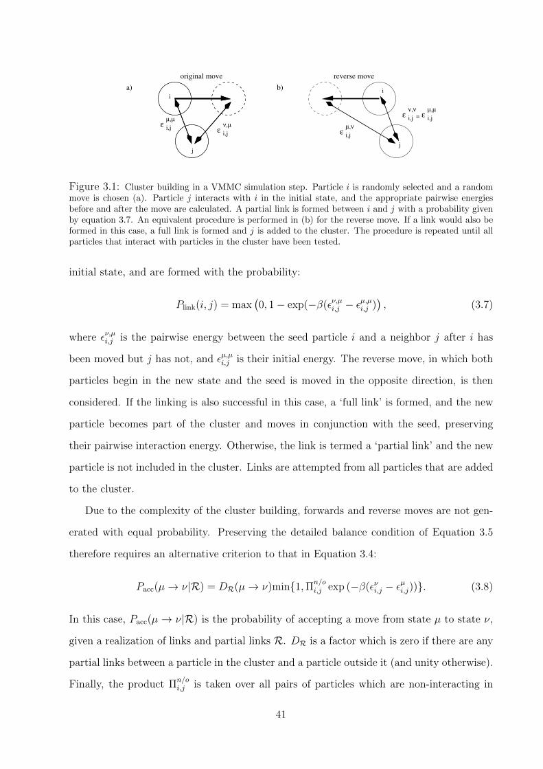
j
i,jεµ,µ
i,jεν,µ
i,jεµ,µ
b)
i,jεν,ν
i,jεµ,ν
a)
original move reverse move
=
i
j
i
Figure 3.1: Cluster building in a VMMC simulation step. Particle i is randomly selected and a randommove is chosen (a). Particle j interacts with i in the initial state, and the appropriate pairwise energiesbefore and after the move are calculated. A partial link is formed between i and j with a probability givenby equation 3.7. An equivalent procedure is performed in (b) for the reverse move. If a link would also beformed in this case, a full link is formed and j is added to the cluster. The procedure is repeated until allparticles that interact with particles in the cluster have been tested.
initial state, and are formed with the probability:
Plink(i, j) = max(0, 1− exp(−β(εν,µi,j − ε
µ,µi,j )), (3.7)
where εν,µi,j is the pairwise energy between the seed particle i and a neighbor j after i has
been moved but j has not, and εµ,µi,j is their initial energy. The reverse move, in which both
particles begin in the new state and the seed is moved in the opposite direction, is then
considered. If the linking is also successful in this case, a ‘full link’ is formed, and the new
particle becomes part of the cluster and moves in conjunction with the seed, preserving
their pairwise interaction energy. Otherwise, the link is termed a ‘partial link’ and the new
particle is not included in the cluster. Links are attempted from all particles that are added
to the cluster.
Due to the complexity of the cluster building, forwards and reverse moves are not gen-
erated with equal probability. Preserving the detailed balance condition of Equation 3.5
therefore requires an alternative criterion to that in Equation 3.4:
Pacc(µ→ ν|R) = DR(µ→ ν)min1,Πn/oi,j exp (−β(ενi,j − ε
µi,j)). (3.8)
In this case, Pacc(µ → ν|R) is the probability of accepting a move from state µ to state ν,
given a realization of links and partial links R. DR is a factor which is zero if there are any
partial links between a particle in the cluster and a particle outside it (and unity otherwise).
Finally, the product Πn/oi,j is taken over all pairs of particles which are non-interacting in
41

state µ and have positive energy in state ν, and vice versa. ενi,j and εµi,j are simply pairwise
energies in the trial configuration and before the move respectively.
The algorithm and acceptance probability are more opaque than for Metropolis MC.
The net result, however, is that collective moves are possible for aggregates (or subsections
of aggregates) that at least partially reflect the gradients in potential energy of the system.
The outcome, at least for the DNA model introduced in Chapter 2, is vastly improved
sampling when compared to basic Metropolis MC, which more than compensates for the
extra complexity of the algorithm.
The primary distinction between this algorithm, and others such as that suggested by
Troisi and coworkers [151], is that this version considers the energy change due to the move
when building a cluster, rather than simply the strength of interaction in the initial state.
As a consequence, proposed moves are more sensitive to potential energy gradients than
in other algorithms. A drawback is that the cluster-building process is more complex, and
hence each step requires greater computational power. The relative advantages of these
factors remains unclear at the time of writing.
By their very nature, cluster algorithms are most effective when the majority of the inter-
actions in the system are pairwise, as clusters are built up by considering pairwise energies.
Multi-body potentials can be included, but not within the cluster building framework, and
they simply modify the final acceptance criterion:
Pacc(µ→ ν|R) = DR(µ→ ν)min
1,(
Πn/oi,j e(−β(ενi,j−ε
µi,j)))
e−β(Eνm−Eµm), (3.9)
where here Eµm and Eν
m are the multi-body contributions to the total energy of the initial
and trial-move states. The utility of pairwise interactions in this regard was a consideration
in designing the model, and led to the use of rigid-body nucleotides.
As with Metropolis MC, cluster move algorithms do not technically provide a dynamical
representation of the time evolution of the model system. If the moves used are ‘local’,
involving small displacements and rotations of clusters of particles, one can interpret the
sequence of states visited as a pseudo-dynamical description of the model. The rates of
processes then give some idea of the ease with which the free-energy landscape of the system
42
is navigated. However, although cluster moves overcome the Metropolis issue of extremely
slowly diffusing clusters, it is not easy to ensure that clusters of different sizes move at the
appropriate relative rates. In addition, it is an even more challenging task to ensure that
internal relaxation and diffusion of clusters happen at appropriate rates. Furthermore, due
to the subtleties of the move generation and acceptance criteria, it is difficult to compare
the rates of processes in simulations of slightly different systems.
3.2 Langevin dynamics
The Langevin formalism is a self-consistent way of incorporating an implicit source of noise
and dissipative forces into deterministic equations of motion [152], such that the simulation
will sample microstates with a weight given by Equation 3.1. For example, the model pre-
sented here can be described in terms of a Hamiltonian
H(rN ,pN ,qN ,ΠN), which is a function of the positions, momenta, orientations (here rep-
resented through quaternions – refer to Appendices A and B for details) and generalized
angular momenta of all objects in the system. Such a Hamiltonian would generate deter-
ministic motion via the equations:
ri =∂
∂piH, pi = − ∂
∂riH, qi =
∂
∂Πi
H, Πi = − ∂
∂qiH. (3.10)
Following the Langevin formalism, as detailed by Davidchack et al. [153], one augments
these equations with damping and noise terms so that:3
pi = − ∂
∂riH− γpi + bwi(t), Πi = − ∂
∂qiH− ΓG(qi,Πi) +BWi(t). (3.11)
Here γ and Γ give the strength of linear and rotational damping, and G(qi,Πi) is a four-
dimensional vector that couples the rotational momenta. wi(t) and Wi(t) are 3- and 4-
vectors, each component being a gaussian distributed random force with zero mean and
lag-covariance δ(t, 0). b and B are constants which give the magnitude of the random
forces. In principle, γ, Γ, b and B are matrices, coupling the noise and friction applied to
3Here I consider only additive noise, and can therefore neglect the subtleties of the distinction betweenIto and Stratonovich calculus [152].
43

different degrees of freedom. For simplicity, I have chosen to assume that all translational
modes (and separately all rotational modes) experience the same strength of noise and
damping.
By requiring that the stationary distribution of the Fokker-Planck process that corre-
sponds to this Langevin equation is given by the Boltzmann distribution, one can relate the
damping and noise terms by fluctuation-dissipation relations, as discussed in Appendix B:
γ =βb2
2m, Γ =
βB2
2M, and M =
4
Tr(I−1). (3.12)
Here, I is taken as the moment of inertia tensor in the principal axis frame, and the form
of Here γ and Γ give the strength of linear and rotational damping, and G(qi,Πi) is given
in Appendix B. These equations can be integrated numerically, using the methods outlined
by Davidchack et al. [153] – in this work, I use the ‘Langevin A’ algorithm.
Unlike Monte Carlo, Langevin algorithms are explicitly dynamical, but issues remain
with inferring kinetics from the simulations. Firstly, it is well known that coarse-graining
has the effect of speeding up dynamics by smoothing free-energy landscapes [154]. Although
this may seem undesirable, it is, in a sense, one of the advantages of coarse graining that al-
lows long time scale processes to be accessed. Secondly, rare event kinetics are exponentially
sensitive to the heights of free-energy barriers, which are difficult to fit in a coarse-grained
model. Perhaps the most important problem, however, is the lack of hydrodynamic inter-
actions in coarse-grained Langevin methods.
Hydrodynamic effects arise because the solvent flow induced by the motion of one solute
particle affects the motion of nearby solute particles [155]. The affect can be approximately
treated within an implicit solvent model, for example by use of Oseen tensor formalism
[155], but such methods are extremely computationally expensive.
A typical consequence of neglecting hydrodynamics is that collective motion is sup-
pressed. For example, the Rouse model of polymer diffusion (which neglects hydrodynamic
interactions) predicts that the diffusion coefficient scales as 1/N , where N is the molecular
weight of the polymer [155]. By contrast, the Zimm model (which incorporates an approxi-
44

mate treatment of hydrodynamics) predicts a diffusion coefficient which scales as the inverse
of the radius of gyration [155].
When implementing Langevin dynamics, one has a degree of choice of the form of the fric-
tion and damping terms, although they must always be related by a fluctuation-dissipation
theorem if the equilibrium distribution is to be the correct one. Given the degree of simpli-
fication inherent in the simulation, it seems unlikely that being precise about the damping
terms will prove significantly beneficial. This reasoning justified the simplifying assump-
tions about the form of the noise and damping terms, effectively treating each nucleotide
as a sphere for dynamical purposes
If each nucleotide is taken as a sphere of radius r0 = 5 A, mass m = 315.75 AMU and
uniform density, continuum hydrodynamics for an isolated nucleotide would then give
γ =6πηr0
mand Γ = 8πηr3
0 Tr(I−1) = 10γ (3.13)
In principle, one could take 1/γ = 0.03 in reduced time units (giving γ ≈ 20 ps−1), which
would correspond to a nominal value of η = 1.1× 10⁻³ kg m−1 s−1, similar to experimental
values for water at around 300 K.
Due to hydrodynamic interactions, however, such a drag coefficient would seriously un-
derestimate the diffusion of large aggregates, which are necessary for the majority of pro-
cesses of interest in this work (for example, the association of two single strands to form a
duplex). In particular, it was found that such large drag coefficients led to prohibitively slow
dynamics for large systems, such as the walker discussed in Chapter 8. Given the number
of simplifications already present in the Langevin model of dynamics, it was decided that
there was little justification in maintaining high drag coefficients at the expense of efficient
sampling. It was therefore decided to set γ = 1 and Γ = 3 in reduced units, values which
maintain the diffusive behaviour of the system but accelerate the dynamics.4
4Despite this reduction in noise, dynamics are still highly damped. For example, a simulation of a 10- bpduplex at 300 K initiated with all 10 base pairs formed but far from an optimal configuration (with around70% of the typical binding energy and no kinetic energy) will reach states typical of equilibrium in around10 units of reduced time. For comparison, diffusion over its own length is around 10− 100 times slower fora 10- bp duplex.
45

Despite the difficulty of directly inferring time scales from Langevin simulations, there
are clear advantages over Monte Carlo for analyzing kinetics. Firstly, there are qualitatively
different methods to generate trial MC moves (for example, the algorithms discussed in
Section 3.1.2), with potentially large (and poorly understood) consequences for the kinetics
of simulated processes. Secondly, for a given implementation of a cluster MC algorithm, it
is extremely difficult to compare rates of processes for similar but distinct simulations. This
difficulty arises because the probabilities with which moves are generated and accepted vary
in a non-trivial manner with factors such as system size, temperature and external forces.
For example, the comparison of the rate of binding of a DNA walker’s foot to a track with
and without tension, as presented in Chapter 8, would have been much more problematic
with MC simulations.
By contrast, applying Langevin dynamics to a given model involves significantly less
arbitrary choice (and the choices are of a more quantitative, rather than a qualitative na-
ture). Further, the kinetics of different systems can be directly compared, as the algorithm
changes in a more intuitive and well-understood fashion as the parameters are changed.
Nonetheless, all results should be interpreted with caution. In particular, due to the ab-
sence of hydrodynamic interactions between solute particles, small scale fluctuations will be
excessively fast compared to large scale diffusion.
Given the caveats associated with Langevin dynamics, it is only sensible to compare
relative rates for similar processes. Further, any relative difference that is observed should
only be believed if a physical cause (which is not a peculiar result of the dynamics) can
be identified. One possible consistency check is to compare the Langevin results with the
pseudo-dynamics of VMMC – if the results are similar, despite the vast differences in algo-
rithms, one can be confident that the result is a generic one.
In this work I use a time step of h = 0.003 units of simulation time (∼ 5 ps). The
accuracy of this time step, and of my implementation of both Langevin Dynamics and
VMMC algorithms in general, is checked in Appendix C.
46
3.3 Advanced sampling techniques
Much of this thesis involves stuying processes that require duplex hybridization and dis-
placement. Such processes are rare-event dominated, in that they typically involve tran-
sitions between (meta)stable states such as duplexes and dissociated single strands, via
unfavourable intermediate states.
Such processes can require long simulations, and it is particularly difficult to obtain
enough statistics for reliable thermodynamic or kinetic data. As a consequence, a variety of
techniques have been developed to improve the sampling of rare events – this work utilizes
umbrella sampling and forward flux sampling.
3.3.1 Umbrella sampling
Umbrella sampling, introduced by Torrie and Valleau [156], uses unphysical biasing of con-
figurations to encourage transitions between (meta)stable states. Firstly, an order parameter
Q(rN ,ΩN), which identifies the extent of reaction, is defined. If the order parameter Q is
well chosen, the free energy F (Q) (defined in terms of the probability P (Q) that the system
is in state Q by F (Q) = −kBT lnP (Q)) will have minima at the metastable states and high
values at the unfavourable states that cause the reaction bottleneck.
Umbrella sampling involves introducing an additional bias w(Q) to the sampling distri-
bution, so that configurations are sampled according to w(Q)e−βV (rNΩN ). w(Q) is generally
chosen to increase the probability of occupying transition states, thereby increasing the flux
between minima.
The thermodynamic average of any function A(rN ,ΩN) is given by:
〈A〉 =
∫drNdΩNA(rN ,ΩN) e−βV (rNΩN )∫
drNdΩN e−βV (rNΩN )=
∫drNdΩN A(rN ,ΩN )
w(Q)w(Q)e−βV (rNΩN )∫
drNdΩN 1w(Q)
w(Q) e−βV (rNΩN ). (3.14)
In order to unbias the results, therefore, one records A/w(Q) and normalizes with respect
to 1/w(Q).
In this work, umbrella sampling is used in conjunction with VMMC. w(Q) is in effect an
additional multi-body interaction which must be considered separately from the cluster gen-
47

eration, such that the final term in the braces of Equation 3.9 is modified by w(Qν)/w(Qµ),
with Qµ and Qν representing the initial and final values of the order parameter respectively.
For particularly difficult systems, it can be advantageous to split the simulation into
several ‘windows’, each of which is strongly biased to remain within a certain range of
Q. Equilibration within each window is easier than for the transition as a whole, and the
separate windows can be combined using the WHAM algorithm of Kumar et al. [157].
3.3.2 Forward flux sampling
Although umbrella sampling is an extremely powerful technique for extracting thermody-
namic averages, it technically provides no direct information on the pathways and kinetics
of assembly processes. Forward flux sampling is an alternative which allows one to calcu-
late the flux of systems between two local minima of free energy, and also sample from the
trajectories that link the two minima [158, 159].
Once again, one considers an order parameter Q which measures the extent of the
reaction, such that non-interacting interfaces, λnn−1 can be drawn between consecutive values
of Q. Initially, simulations are performed that begin in the lowest value of Q (which I shall
define as Q = −2), and the flux of trajectories crossing the surface λ0−1 (for the first time
since leaving Q = −2) is measured.
The total flux of trajectories from Q = −2 to the alternative minima (Q = N) is then
calculated as the flux across λ0−1 from Q = −2, multiplied by the conditional probability
that these trajectories reach Q = N before returning to to Q = −2. This probability can
be factorized into the product of the probabilities of trajectories starting from the interface
λnn−1 reaching the interface λn+1n before returning to Q = −2.
P (λNN−1|λ0−1) = ΠN
n P (λnn−1|λn−1n−2). (3.15)
The simulation then proceeds by randomly loading microstates which correspond to the
crossing of λ0−1, and using these as initial points from which to estimate P (λ1
0|λ0−1). The
process is then iterated for successive interfaces, allowing the estimation of flux and the
construction of trajectories sampled from the distribution of transition pathways.
48

Chapter 4
Finite Size Effects
If the self-assembly of model DNA systems was easy to simulate, the best way to study such
processes would be to model a large system where a number of the assembled structures
can simultaneously form. This direct approach is not generally feasible, however, as the
presence of significant free energy barriers to assembly makes equilibrium hard to achieve.
Equilibration can be driven by rare-event techniques such as umbrella sampling (see Chapter
3), but these techniques are best suited to simulating a single target structure (I am unaware
of any studies where biased sampling is used to simulate the formation of multiple targets).
So if the assembly of a single structure is simulated, what issues arise with inferring the
properties of a bulk system of the same strands?
Firstly, interactions between assembled structures are neglected. This is often a good
approximation, because the interactions between them are likely to be mainly associated
with excluded volume – any attractions are likely to be weak compared to the forces associ-
ated with the assembly itself – and assembly often occurs at relatively low concentrations.
In addition to neglecting the interactions of assembled structures, such simulations will not
capture states in which aggregates larger than the target structure have formed. Depending
on the details of the system, these aggregates may constitute metastable states that can be
significant in the dynamics.
The second potential source of error is due to neglected fluctuations of the local con-
centration of reactants, and this is the topic of this chapter. In particular, I will show that
these finite-size errors in canonical ensemble simulations of dimerization can be significant,
49

but also how they can be corrected under the assumption that species behave ideally. I will
also examine how the assembly yields converge towards the bulk values as the system size
is increased, enabling the assumptions of the corrections to be checked. In Appendix D I
discuss larger clusters and simulations in the grand canonical ensemble.
Although the extrapolation is not a complex procedure, it has been neglected in the past.
In particular, simulations have been performed on DNA duplex formation [120, 121, 126, 127]
without applying corrections. An attempt to correct for finite size effects during duplex
formation was made by Prytkova et al. [122], but the method (which is not justified in the
paper) involves an unclear renormalizaton of temperature and doesn’t appear to correct for
concentration fluctuations.
One should note that specific methods have been developed to calculate the equilibrium
thermodynamics of heterodimer formation in the protein-ligand binding literature [160].
Such techniques aim to estimate the partition function of bound and separated molecules
directly, and typical methods include calculating a potential of mean force for a certain
pathway between bound and unbound structures, incorporating the effects of overall trans-
lational degrees of freedom separately. These techniques are optimized for problems of great
computational difficulty and do not generalize well to multicomponent assembly. Further-
more, they lack the flexibility and simplicity of the approach analysed here in which nothing
need be approximated or assumed about the nature of bonding, and no pathway need be
imposed a priori.
4.1 Dimer formation in the canonical ensemble
4.1.1 Heterodimer formation
The physical cause of finite size statistical corrections can be seen by considering heterodimer
formation – such a system may correspond to protein binding or DNA hybridization. Con-
sider a simulation in a periodic cell of volume v, containing one monomer of type ‘A’ and
one of type ‘B’. Assuming a criterion exists for defining a subset of states as ‘bound’,1 a
1The details of this criterion are not important, except for the fact that bound particles must be separatedby a small distance compared to the simulation volume, and that the correlation of particles in the unbound
50
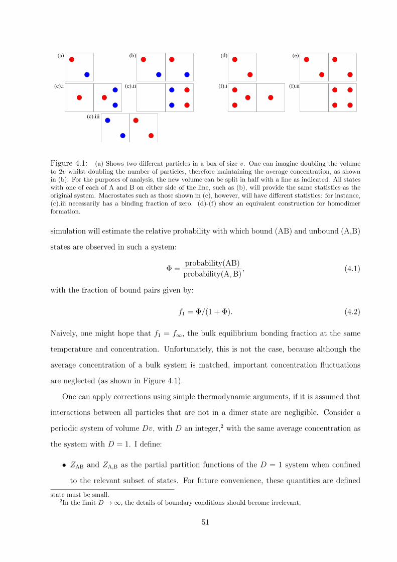
(c).i
(d)
(f).ii
(e)
(f).i
(c).iii
(c).ii
(b)(a)
Figure 4.1: (a) Shows two different particles in a box of size v. One can imagine doubling the volumeto 2v whilst doubling the number of particles, therefore maintaining the average concentration, as shownin (b). For the purposes of analysis, the new volume can be split in half with a line as indicated. All stateswith one of each of A and B on either side of the line, such as (b), will provide the same statistics as theoriginal system. Macrostates such as those shown in (c), however, will have different statistics: for instance,(c).iii necessarily has a binding fraction of zero. (d)-(f) show an equivalent construction for homodimerformation.
simulation will estimate the relative probability with which bound (AB) and unbound (A,B)
states are observed in such a system:
Φ =probability(AB)
probability(A,B), (4.1)
with the fraction of bound pairs given by:
f1 = Φ/(1 + Φ). (4.2)
Naively, one might hope that f1 = f∞, the bulk equilibrium bonding fraction at the same
temperature and concentration. Unfortunately, this is not the case, because although the
average concentration of a bulk system is matched, important concentration fluctuations
are neglected (as shown in Figure 4.1).
One can apply corrections using simple thermodynamic arguments, if it is assumed that
interactions between all particles that are not in a dimer state are negligible. Consider a
periodic system of volume Dv, with D an integer,2 with the same average concentration as
the system with D = 1. I define:
• ZAB and ZA,B as the partial partition functions of the D = 1 system when confined
to the relevant subset of states. For future convenience, these quantities are defined
state must be small.2In the limit D →∞, the details of boundary conditions should become irrelevant.
51
using distinguishable statistics, although it does not matter at this stage. Note that
Φ = ZAB/ZA,B.
• N as the total number of particles of type A or B (here N = D).
• Ni as the number of molecules of species i (in this case i is A, B or AB).
• qi as the single particle partition function for species i, in the volume Dv, with the
internal degrees of freedom treated using indistinguishable statistics.
• µi as the chemical potential of species i.
The µi are given by a standard result of statistical mechanics:
µi = −kBT∂
∂Ni
ln
(qNi
i
Ni!
)≈ −kBT ln
(qi
Ni
), (4.3)
where the approximation becomes an equality in the thermodynamic limit. In this limit,
equilibrium thermodynamics gives∑
i νiµi = 0, where νi are the stoichiometric coefficients
of the species in the reaction, resulting in:
NAB
NANB
=qAB
qAqB
. (4.4)
As each qi scales with the volume of the system:
qAB = DZAB, (4.5)
qAqB = D2ZA,B, (4.6)
which gives (using D = N):
[AB]
[A][B]=vZAB
ZA,B
= vΦ = KeqA,B. (4.7)
Note that the quantity ZAB/ZA,B is that which is generally directly estimated in pro-
tein/ligand binding studies [160]; this is then multiplied by a reference concentration to
give the equilibrium constant.
Substituting (4.1), (4.5) and (4.6) into (4.4) yields:
f∞(1− f∞)2
= Φ (4.8)
52

Figure 4.2: (a) Dimer yield for a system described by a two-state model Z2/Z1,1 = exp(−∆E/T + ∆S),with ∆E = 2 and ∆S = 15 in reduced units, with the values chosen for illustrative convenience. Plotted arethe yield for a two-particle system and the bulk values at the same average concentration for homodimersand heterodimers. (b) Heterodimer yield as a function of system size D, with average concentration fixed.The ‘x’ symbols indicate results from simulations of my DNA model that were capable of forming D DNAduplexes of 5 bp, and the ‘+’ are the predictions of Equation (4.11), with Φ chosen to reproduce the D = 1result. The solid line indicates f∞. Simulations were performed in a periodic cell of length l = 10×2(log2D)L,where L is the reduced length scale of the model defined in Chapter 2, at a temperature of 303.03 K. At eachD, a minimum of 1.5 × 10¹¹ VMMC steps per strand were performed in total. No statistically significantdeviations from the theory presented here were found.
=⇒ f∞ =
(1 +
1
2Φ
)−
√(1 +
1
2Φ
)2
− 1. (4.9)
In this case, f∞ < f1 for all values of Φ, as is illustrated for a model dimer-forming system
in Figure 4.2. It is also noticeable that the transition is wider for the bulk system. The
physical causes of these two effects will be discussed at the end of Section 4.1.3.
4.1.2 Heterodimer convergence
It is useful to consider how the bonding fraction converges to the bulk result as the system
size is increased from one cluster to the thermodynamic limit. Consider a system of volume
Dv, and calculate the fraction of dimers (fD) as a function of Φ, again neglecting interactions
except dimer formation. Consider the macrostate with b dimers formed (out of a possible D).
The partition functions of individual monomers and dimers scale with the size of the system
(Dv), and the partition function of the system is the product of the individual partition
functions together with combinatorial factors. Using ZAB and ZA,B as defined before, the
partition function of a macrostate with b dimers (using distinguishable statistics) is given
53

by:
Zb(D) =(DZAB)b(D2ZA,B)D−b
b!
(D!
(D − b)!
)2
, (4.10)
in which the combinatorial factor is obtained from the total number of permutations of A
and B (D!2) divided by the permutations which exchange monomers for monomers ((D −
b!)2)) or dimers for dimers (b!). The expression is divided by D!2 to make the statistics
indistinguishable. fD is found in the usual way, using equation (4.1) to simplify:
fD =
∑Db=1 b
(ΦD
)b ( 1(D−b)!
)21b!∑D
b=0D(
ΦD
)b ( 1(D−b)!
)21b!
=
∑Db=0 bZ
′b∑D
b=0DZ′b
. (4.11)
Plotting fD against D for Φ = 1.54 (Figure 4.2(b)) shows that the bonding fraction falls
from 0.606 to a large D limit of 0.482. It is possible to formally find this limit by noting that
for any value of Φ, Z ′b is sharply peaked about its maximum bmode for large D. This allows
the use of the saddle point approximation, whereby Z ′b is taken as Gaussian and therefore
f∞ = bmode/D by symmetry. Maximizing lnZ ′b with Stirling’s approximation yields:
d lnZ ′bdb
≈ ln
(Φ
D
)+ 2 ln(D − b)− ln(b), (4.12)
=⇒ Φ(D − bmode)2
Dbmode
= 1. (4.13)
Using bmode/D = f∞, Equations (4.13) and (4.8) are identical, as they should be.
The microscopic approach provides a simple mechanism for evaluating the accuracy of
the correction scheme in certain cases. If it is possible to simulate the simultaneous formation
of two or more targets, one can compare the change in dimer yield to the predictions of the
microscopic approach, and then extend to the thermodynamic limit if the agreement is good.
This is particularly useful if it is possible to consider an example with the relevant model
where the self-assembly process is relatively simple. For example, for my DNA model,
all interactions are truncated within distances much shorter than the typical separation
of unbound strands, making the assumptions of ideality reasonable. Simulating duplex
formation for short strands of about five bases in length is simple, and simulations forming
several targets can be performed. The results are plotted in Figure 4.2 (b), showing perfect
54

agreement with Equation (4.11). Longer duplexes and complicated branched structures
are much more challenging to simulate, meaning that only single target simulations are
feasible. From the fact that the correction is successful for shorter duplexes, however, one
can be confident that it will apply to longer strands when the concentration of DNA bases
is similar.3 Throughout the rest of this work, I will use finite size corrections as detailed in
this chapter to infer bulk binding properties of DNA systems.
4.1.3 Homodimer formation
It is instructive to consider the differences between homodimer and heterodimer corrections.
For homodimers formed from two particles of type A, the partition functions of each particle
species are given by:
q2A =DZ2A
2. (4.14)
qAqA = D2ZA,A, (4.15)
where the factor of two compensates for the overcounting of indistinguishable states in Z2A.
Proceeding as in Section 4.1.1:
[2A]
[A]2=
vZ2A
2ZA,A
=vΦ
2= Keq
2A. (4.16)
The bound fraction in the thermodynamic limit follows as:
f∞ =
(1 +
1
4Φ
)−
√(1 +
1
4Φ
)2
− 1. (4.17)
The behaviour of the correction is significantly different from that of heterodimers, as shown
in Figure 4.2. In this case, the midpoint of the transition is unchanged, but the width is
noticeably larger in bulk than for the two-particle system, i.e. f∞ > f1 for f1 <12, and
f∞ < f1 for f1 >12.
3Due to the lack of non-specific attractions in my DNA model, it is unlikely that it will form largeclusters unless the sequences are specifically designed for this purpose. This study shows that, neglectingthe possibility of aggregation through base-pairing, the model’s bulk behaviour is well described by thestatistical extrapolation from a small system presented here. Bulk aggregation of DNA is possible, asdiscussed in Chapter 1, but in these examples the strands were specifically designed to form extendedbase-paired structures, and in other cases it can be neglected.
55

The physical mechanism for the broadening of the transition can be understood in terms
of concentration fluctuations. Figure 4.1 (f) shows the states of a four-particle homodimer-
forming system which cannot be sampled in a two-particle simulation. Of these, (f).i shows
the smallest fluctuation in concentration, with three of the particles occupying half the
volume and the remainder containing only one. In this case, it is impossible to have a
binding fraction of unity. A binding fraction of zero is also less likely than in the two-
particle case as the three monomers occupying the ‘right’ half of the system have a higher
probability of forming one dimer than the two particles did in the original system. As
a consequence, the fraction of dimers is pushed towards 12
as the system grows in size,
because larger concentration fluctuations are allowed which in turn favour the less probable
configuration (whether dimer or monomer), leading to a broader transition in bulk.
The same argument can be applied to heterodimers, but with an important distinction.
In this case, concentrations of individual species A and B can separately fluctuate. Unlike
total concentration fluctuations, fluctuations in the relative concentrations of A and B will
always reduce the probability of forming dimers, because of configurations like that in Figure
4.1 (c).iv where no dimers can be formed. Consequently the heterodimer yield is lower in
bulk than for a two particle system, as well as having a broader transition.
4.2 Summary
In this chapter I have highlighted a necessity to correct equilibrium yields when extrapo-
lating from small, canonical ensemble simulations of dimerization to bulk systems. I have
provided a methodology to perform this correction and established a framework to explore
it’s accuracy. I have tested the accuracy of the extrapolation for my model: agreement is
essentially perfect, suggesting that, unless sequences are specifically designed to aggregate,
small simulations are sufficient to extract the bulk thermodynamic properties of my model.
Dimerization in the canonical ensemble is of particular relevance to this thesis, especially
in Chapter 6. In Appendix D, the discussion is extended to larger clusters, systems in the
grand canonical ensemble and systems in which some of the reactants are localized.
56

Chapter 5
Stuctural and mechanical propertiesof model DNA
5.1 Basic structure
The model is specifically designed to allow an approximate representation of B-DNA in its
double-stranded state. The relative sizes of the equilibrium backbone separation and ideal
stacking distance lead to a pitch of 10.34 bp per turn at 296.15 K (23oC, approximately
room temperature) similar to experimental estimates of 10–10.5 [12, 76]. The model length
scale is chosen so that the average rise per bp at room temperature is 3.4 A [128], which
results in a helix with a radius (taken as the furthest extent of the excluded volume) of
11.5 A, comparable to the experimental value of 11.5–12 A [128, 161].
If strands are to form a double helix, it is not possible to optimize the stacking interaction,
as consecutive stacking sites cannot sit directly above one another. Single strands, however,
are not constrained in this way and hence form tighter helices, with a radius approximately
80% that of a duplex, similar to the 70-80% observed for a number of polynucleotide single
helices [161]. A pleasing result is that, in order to alleviate the reduction in stacking,
hydrogen-bonded bases in the model undergo ‘propellor twisting’ whereby bases in a pair
twist in opposite directions in order to better align their stacking centres with adjacent
bases in the same strand. Experimentally, propellor twist is seen to vary from around 5
to 15 in GC rich regions and from 15 to 25 in sections with large AT content [162]: my
model has a slightly larger average propellor twist of 21.7 at 296.15 K.
57

(a) (b)
(c)
Figure 5.1: Typical configurations indicating relative flexibility of double-stranded, stacked single-strandedand unstacked single-stranded DNA. (a) 202 bp double helix at 296.15 K. (b) Stacked single strand of 202bases at 277.15 K. (c) Unstacked single strand of 160 bases at 296.15 K.
5.2 Mechanical properties
It is important that the model captures the tendency of duplex DNA to be very stiff on
the nanoscale, and the fact that ssDNA is comparatively flexible, if the model is to be
used to study nanotechnology. As shown in Figure 5.1, this qualitative tendency is indeed
reasonably well captured.
To make more quantitative statements, it is necessary to define metrics of rigidity. A
commonly used measure of the large-scale properties of a polymer is its persistence length.
A general definition is given, for example, in the textbook by Cantor and Schimmel [163]:
Lps =〈L.l0〉〈l0〉
, (5.1)
with L being the end to end vector of the polymer and l0 representing the vector between
the first two monomers. For the case of an infinitely long, semi-flexible polymer in which the
correlations in alignment decay exponentially with separation, Equation 5.1 is equivalent to
the commonly used form:
〈ln.l0〉 = exp(−n〈l0〉/Lps). (5.2)
An alternative measure of polymer properties, the Kuhn length, is defined by [164]:
bK = 〈L2〉/(Lmax), (5.3)
58

and gives the length of monomers for a freely-jointed chain (FJC) [164] with the same
maximum end-to-end length Lmax and 〈L2〉 as the polymer in question. For long semi-
flexible chains bK = 2Lps but for other models this equivalence may not hold.
5.2.1 Double-stranded DNA
Persistence-length
The persistence length of dsDNA is generally accepted to be approximately 450-500 nm at
moderate to high [Na+], corresponding to around 130–150 base pairs [14, 165]. I performed
four simulations of a duplex of length 202 bp at 296.15 K for 2 × 10⁹ MC steps to extract
the persistence length. It was found that base pairs at either end of single- or double-
stranded DNA possess an increased relative flexibility. In order to obtain persistence length
values that are valid for long strands where end effects are negligible, the behaviour of
bases near the end of strands was ignored. The correlation of the helix axis (defined as
the distance between consecutive base-pair midpoints) at two points was observed to decay
exponentially with distance, allowing an estimate of Lduplexps through Equation 5.2. Figure
5.2 (a) indicates a model persistence length of around 123 base pairs, in reasonable agreement
with experiment.
Torsional and extensional moduli
The stiffness of DNA duplexes is also manifested in a resistance to twisting. Torsional
rigidity (in the linear regime) is quantified by an elastic modulus C, which relates applied
torque G to resultant twist ∆θ of a duplex of length l: C = Gl/∆θ. Estimates for C
have been made using cyclization kinetics and topiosomer distributions for minicircles [14,
166, 167], luminescence depolarization [168] and from twisting of DNA under tension [169],
giving values in the range 170–440 fJ fm, with the effect of salt on C currently unclear from
the literature [168].
Calculating the response to torsion is non-trivial, as the curvature of the DNA axis
makes the twist between two ends hard to define. An approximate estimate of the torsional
modulus can be obtained by considering the twisting of the central 10 base pairs of a 20 bp
59

Figure 5.2: (a) Decay of the correlation of helix axis plotted against base pair separation for duplex at296.15 K. The solid line is a fit of exponential behaviour. (b) Tension applied against extension for thecentral 100 bp of a 110-bp duplex at 296.15 K. The squares are simulation results, the solid line is a fit ofEquation 5.4.
duplex, and the central 20 base pairs of a 30 bp duplex at 296.15 K. Such short sections are
extremely stiff, minimizing the natural bending fluctuations. To provide an unambiguous
definition of torsion and twist, Monte Carlo moves were chosen so that the base pairs at the
end of the central section remained perpendicular to the vector between their midpoints,
allowing the vector between the midpoints to define an axis about which torsion could be
applied and twist measured.
Simulations were performed in which the torque applied to the end bases was varied
between ±8 pN nm, and the resultant twist used to infer C. A separate estimate was also
obtained using the equipartition result for the variance in twist at zero torque: 〈∆θ2twist〉 =
kT l/C. Further simulations used the equipartition result to estimate C under a tension of
9 pN, to ensure that stretching the duplexes had no effect. All estimates (for both 10- and
20-bp regions of interest) gave C ∼ 450 − 475 fJ fm, suggesting that this is a reasonably
robust estimate of the torsional stiffness of DNA duplexes in the model.
A long molecule of dsDNA under low tension responds as an extensible wormlike chain,
with the behaviour initially dominated by the straightening of the chain, before stretching
the base-pair rise itself becomes relevant as the chain extension approaches the contour
length [170, 171]. At higher forces, the duplex undergoes an overstretching transition and
the B-DNA structure breaks down [172]. Early experimental estimates for the extensional
60
modulus K, obtained from fitting force-extension curves to extensible wormlike chain mod-
els, give K in the region of 1050–1250 pN at high salt [170, 171], with smaller values at lower
salt. A more recent study, at a monovalent salt concentration of 50 mM, claims K ∼ 1500 pN
[173].
The extensional modulus K was estimated by applying tension to a 100-bp region within
a 110-bp double helix, and fitting the resultant force-extension curve to the result of Odijk
for extensible wormlike chains [174]:
x = L0
(1 +
F
K− kT
2F[1 + y coth y]
), (5.4)
where:
y =
(FL2
0
LpskT
)1/2
, (5.5)
in which x is the extension resulting from a force F applied to a duplex of contour length
L0 and persistence length Lps. Performing an unconstrained three-parameter fit with the
values of L0, Lps and K gave an excellent agreement with the data, as shown in Figure
5.2 (b), with K = 2166 pN, L0 = 339.6 A and Lps = 431.0 A (126 bp). The value of L0 is
similar to that expected from the rise of a short duplex (exactly 3.4 A per base pair would
give L0 = 336.6 A), and Lps is only slightly larger than the estimate from the decay of the
correlation of the helix axis (123 bp). This agreement suggests that the extensible wormlike
chain model provides a good description of the model’s properties in this regime, and that
the value of K = 2165 pN is a reasonably robust one for my model.
The model gives C ≈ 450 − 475 fJ fm (slightly larger than the top of the experimental
range of 170–440 fJ fm) and K ≈ 2165 pN, (around ∼ 1.5 to 2 times as large as typical
experimental estimates). Although large, these values are not sufficiently different from
measured values as to invalidate the majority of conclusions drawn from the model (although
certain quantities, such as the critical twist density at which plectonemes are extruded, will
be affected). It was found to be difficult to reparameterize the model to reduce these moduli
without decreasing the persistence length, which is already slightly below experimental
estimates. I feel that the current compromise, in which the persistence length is most
61
faithfully reproduced, is a reasonable one as it is easier to imagine that nanostructures and
nanodevices would be more sensitive to bending than torsional or extensional stiffness.
It is worth noting that recent investigations have suggested that DNA initially overwinds
when stretched [175]. The model does not reproduce this anti-intuitive behaviour, instead
slightly untwisting as the stacking distance is extended. It is possible, therefore, that the
model fails to capture the softness of a mode of deformation that leads to this behaviour
– perhaps the sloping of base pairs with respect to the axis [176]. If this is the case, it is
perhaps unsurprising that the estimated moduli are larger than experimental observations.
5.2.2 Single-stranded DNA
The mechanical properties of ssDNA are less well established than those of dsDNA. Further-
more, long single strands of DNA will generally be partially stacked, resulting in sections
of substantially different flexibility [177, 178]. First, I shall explore persistence length of
ssDNA when stacked.
Persistence length of stacked single strands
Mills et al. [177] have investigated the flexibility of gapped duplexes connected by poly(dA)
(long single stands of DNA in which all the bases are adenine) at 4C, when the bases are
largely stacked into single helices. Although the interpretation depends on the probability
of stacking, the intrinsic persistence length of the stacked regions was estimated to be
around 100 A, corresponding to approximately 30 bases. This value is noticeably larger
than expected for unstacked strands (see Section 5.2.2), but smaller than for duplexes. For
comparison, I performed four simulations of single strands of 202 identical bases at 4C
for 2 × 10⁹ MC steps each (ignoring the data from the five bases at either end), requiring
that all bases maintained a stacking interaction of ≥ −0.60 kcal mol−1 with their neighbours
(doubling this value had no discernible effect).
Taking the vectors between adjacent stacking sites as the axis of the polymer, Figure 5.3
shows that the correlation of these vectors decays exponentially with separation and hence
that Equation 5.2 can be used to extract the persistence length of stacked ssDNA. Such a
62

Figure 5.3: (a) Decay of the correlation of helix axis plotted against base separation for stacked singlestrands at 277.15 K (crosses), plotted logarithmically. The line is a fit of an exponential decay. Also shown(solid line, no symbols) is the decay of the correlation of backbone vectors for an unstacked single strandat 296.15 K. (b) Kuhn and persistence length inferred from simulations of unstacked single strands, as afunction of the length of ssDNA over which they are measured.
fit gives Lstackps /〈l0〉 = 41.6 bases, somewhat larger than the value reported by Mills et al.
[177], but not unreasonable.
Persistence length of unstacked single strands
Poly(dT) is generally assumed to be entirely unstacked at room temperature, and has little
tendency to form secondary structure [12, 177]. As a consequence, it can be used to test the
inherent flexibility of unstacked single strands. Gapped helices have been used by Mills et
al. [177], who inferred a high salt persistence length of 20–30 A from rotational decay rates,
and Rivetti et al. [179], who studied length distributions with atomic force microscopy,
finding ∼ 16 A for short sections (< 5 bases), growing to around 28 A for longer regions.
Fluorescence resonance energy transfer between donors and acceptors attached to either
end of poly(dT) has also been used to fit polymer models to chain end-to-end distributions,
with Murphy et al. finding a persistence length of around 19.4 A at 500 mM [Na+] [129].
All of these results suggest persistence lengths on the scale of 2-5 bases.
In general, these results are obtained by first assuming a model of ssDNA (often a
wormlike chain), and measuring a quantity which depends upon the conformational or
dynamical properties of such a chain. The parameters of the model are then fitted to a
63

theory of the measured quantity which incorporates a polymer model. As such, the results
are likely to be dependent on the choice of model for the polymer, and the accuracy of the
theory used to interpret the data. As a consequence, one should treat these results with
caution, but they do clearly indicate that unstacked ssDNA is very flexible.
When stacking and hydrogen-bonding interactions are removed from the model presented
in this work, the conformation of ssDNA is exclusively determined by excluded volume inter-
actions. Steric clashes limit backbone orientation, and this restriction on nearby nucleotides
results in an effective stiffness of single strands. This description of ssDNA is undoubtedly
a simplification, but it has the advantage of not biasing a particular structure and keeps all
interactions as pairwise, which is ideal for the VMMC algorithm used in simulation.
To compare the model to experiment, I simulated single strands of one base type with
stacking interactions set to zero to mimic poly(dT) (four simulations each for a range of
strand lengths were performed at 296.15 K for 4×10¹⁰ VMMC steps. A typical configuration
is shown in Figure 5.1 (c)). As the stiffness of ssDNA in my model results from excluded
volume interactions, meaning that interactions between non-neighbouring nucleotides play
a role, it should not be a surprise that the correlation of backbone vectors does not decay
exponentially with separation along the chain, as shown in Figure 5.3 (a). It is therefore
impossible to use Equation 5.2 to evaluate Lps. If Equation 5.1 is used instead in order to
compare to experimental results, the persistence length is observed to rise with the contour
length considered (measured regions were embedded within strands with 30 extra bases at
each end to avoid end effects), as shown in Figure 5.3 (b). Similar behaviour is observed for
the Kuhn length bK , also shown in Figure 5.3 (b). For strands of ∼ 100 bases, the persistence
length obtained using Equation 5.1 is similar to experimentally inferred values (19–30 A),
suggesting that the simplified description used in the model is not unreasonable.
Given that the experimentally inferred persistence lengths are so short, it seems plau-
sible that non-neighbour interactions (which in physical DNA would include explicit elec-
trostatic repulsion) may contribute towards single-stranded stiffness in physical DNA. Such
interactions have been observed to dominate at lower salt concentrations in force-extension
64

experiments (see Section 5.2.2), when electrostatic interactions have a longer range, but
they may also have a role at higher salt concentrations.
Force-extension properties
A number of groups have considered the stretching of ssDNA. In the work that first revealed
the overstretching of dsDNA, Smith et al. [172] extended λ-phage ssDNA with optical
tweezers. At moderately high salt (150 mM [Na+]), the force-extension curve was well fitted
by an extensible FJC model, with a Kuhn length of 15 A and a stretch modulus of each
Kuhn segment of 800 pN. At very low salt concentrations (and with formaldehyde present),
the force-extension properties of the molecule were very similar to the higher salt results
above 15 pN, but the DNA was much easier to extend at lower forces.
Even ignoring the failure of the FJC model to account for the behaviour in the second
case, the use of the FJC in the first case is non-self-consistent. An assumption of the
FJC model is that interactions between different segments can be neglected, but here the
segment length (15 A) is comparable both to the Debye screening length and the width of
the polymer. In other words, if DNA really did want to behave like an FJC with segment
length 15 A, then at low forces it would find that it repeatedly bumped into itself and
actually failed to behave like an FJC at all!
If the FJC model is not valid, one must explain why DNA in moderately high salt
appears so hard to extend at low tension. Several authors have claimed that hairpins in the
single strand, which must be unzipped if the molecule is to be extended, explain the original
result of Smith et al. [172]. In the second case, formaldehyde and long-range electrostatic
repulsion prevent the formation of hairpins, making ssDNA easier to extend. The long
range repulsion, a result of low salt concentration, also favours extended conformations of
a hairpin-free strand, making extension even easier.
To test the intrinsic force-extension behaviour of ssDNA, it is therefore necessary to
prevent the formation of hairpins. Dessinges et al. considered stretching DNA in the
presence of denaturants [180], and other authors have used homopolymers which are unlikely
to form secondary structure [178, 181, 182, 183]. Both approaches, however, have their
65

Figure 5.4: (a) Force - extension curves for model ssDNA compared to experiments. Solid curves representsimulations of model DNA: green for the normal parameterization, and blue without stacking. Dashed curvesare inferred from the fits of Seol et al. [178]: magenta for poly(C) and cyan for poly(A). Black “+” are pointsfrom the force-extension curve of single-stranded λ-DNA in 150 mM [Na+], from Smith et al. [172]. Red“x” are points from the force-extension curve of charmoid DNA in low salt conditions and in the presenceof denaturatants, as measured by Dessinges et al. [180]. (b) Derivative of force-extension curve for modelDNA when stacking is possible, calculated by differentiating a cubic spline fitted to the force-extensiondata. Note the plateau around at an extension of ∼ 0.35 nm per base.
drawbacks: denaturants may have additional consequences beyond destabilizing the duplex,
and homopolymers may behave in a manner which is not typical of a less ordered sequence.
Homopolymer stretching has revealed some non-trivial behaviour. When stretching ss-
RNA (poly(A) and poly(C)), Seol et al. observed plateaus in the force-extension curve that
were not seen for poly(U) [178, 181]. The authors were able to fit the curves using a statis-
tical model in which the RNA was treated as a string of rigid, helically stacked sections and
flexible, unstacked bases. Mishra et al. stretched homopolymeric ssDNA with an atomic
force microscope, and found evidence of another plateau at higher forces (∼ 110 pN) for
poly(dA) that was absent for poly(dT) [182]. The existence of this plateau was confirmed
by Chen et al., who showed that it was associated with considerable hysteresis [183].
Testing the force-extension properties of model ssDNA is not difficult with the model
– I simulated strands of 400 identical bases under constant tension, and extracted the
average extension of the central 360 bases. Simulations were performed for 1010 VMMC
steps and systems both with and without stacking interactions were considered. The results
are plotted in Figure 5.4 (a), along with a number of experimental curves.
From Figure 5.4 (a) it is clear that the behaviour of model DNA is qualitatively rea-
66

sonable. It is difficult, however, to draw too many quantitative conclusions, as direct com-
parison to all curves is problematic. In particular, the curves of Seol et al. were obtained
at the salt concentration appropriate to my model, but homopolymeric RNA may not give
a good representation of generic DNA. Furthermore, the strand lengths in the experiment
were unknown and only derived from fitting models to the data. The curve of Dessinges et
al. was obtained in the presence of denaturants and at low salt, and hence the fact that
ssDNA is far more extensible (particularly at low tension) is not surprising. The result of
Smith et al., as discussed above, shows the effect of hairpin formation (hence the resistance
to extension at low force – the force at 0.1 nm/base is well above other curves ). Above
∼ 10 pN, however, hairpins should be of limited relevance and hence comparison may be
worthwhile (although the salt concentration of 150 mM sodium is lower than that used to
fit the model).
The effect of stacking
Seol et al. attributed plateaus in the force-extension curves of RNA to stacking in single
strands [178]. They modelled ssRNA as a non-self-avoiding chain consisting of bases that
could be stacked or random coil-like. Stacked regions had a shorter monomer length than
unstacked sections, but a significantly larger persistence length. The assumptions of the
statistical model used to fit the curves, at first sight, seems to apply fairly well to my
system, and so it is worth considering my model in this light.
The first thing to note is that model strands are significantly easier to extend (above
10 pN) if stacking interactions are removed (Figure 5.4 (a)). This is indeed a result of the
need to break stacking interactions in order to align more backbone vectors with the force.
Furthermore, although it is not easy to see in Figure 5.4 (a), there is a plateau-like feature
in the force-extension curve which is evident if the gradient is plotted (Figure 5.4 (b)). This
feature becomes more obvious if the stacking strength is increased.
An obvious question is why my model shows a weaker plateau-like feature than the curves
of Seol et al., given that if anything the stacking interaction in my model is stronger than
that used to fit the curves. The answer is that, in the model of Seol et al., the separation
67

of stacked bases is assumed to lie along the helix axis, which tends to align with the force.
This is a reasonable assumption for long helices, but for shorter sections with only a few
bases, stacked regions will tend to rotate to align the longer vector between exterior sugars
with the force. In my model, at high tension, single strands typically break up into a series
of stacked pairs, which are capable of aligning their backbones with the applied force. By
contrast, in the model of Seol et al., the number of stacked bases tends to zero at high
tension and this is why a relatively weak stacking interaction is able to provide such a
strong signal.
Although my model’s description of the backbone is simplistic, it is hard to see why
the general principle that stacked bases can align their backbone separation, rather than
their helix axis, with the applied force should be invalid. My model therefore suggests that
the stacking parameters obtained from fitting the statistical model of Seol et al. to their
data should be treated with some caution, although it supports the general principle that
plateaus in force-extension curves can arise from the unstacking of helices.
5.3 Summary
Overall, the model gives a reasonably physical representation of the mechanical properties
of DNA. Care must be used in systems when the specific values of moduli (rather than their
order of magnitude) are of importance – for instance, the critical value of torque at which
plectoneme extrusion occurs will be sensitive to the exact value of the torsional modulus.
The model does, however, capture the tendency of dsDNA to be essentially rigid on the
nanoscale, whilst single strands are extremely flexible – properties essential for much of
DNA nanotechnology.
68

Chapter 6
Thermodynamic properties of modelDNA
6.1 Single-stranded stacking transition
The attractive stacking interaction between adjacent bases causes single strands to form he-
lical stacks at low temperature, with this order being disrupted as the temperature increases
[12]. The literature is divided on both the nature of the attraction and the thermodynamics
of the transition. The relative contributions of van der Waals, induced dipole, hydrophobic
and permanent polar/electrostatic interactions remain unclear [144]. There has also been
much debate on the cooperativity with which bases stack. Vesnaver and Bresslauer claim
that a 13-base strand undergoes a completely cooperative transition between helical and
random coil [184], whereas other authors have inferred essentially uncooperative transitions
for the individual stacks in poly(C) and poly(A) [185, 186, 187, 188, 189]. Other groups
claim weak to moderate cooperativity, with stacking probability affected by nearby base
stacking [190, 191, 192]. It is clear, however, that stacking has a large influence on the
thermodynamics of double helix formation, as the magnitude of the enthalpy and entropy
changes of hybridization increase as the single-stranded state becomes more disordered
[140, 184, 191, 193]. A limited number of short atomistic simulations of ssDNA have been
performed [194, 195, 196, 197, 198]: all observe that the strands tend to adopt partially-
stacked configurations, but there is insufficient data to draw firm conclusions about the
thermodynamics of the process.
Given the uncertain nature of stacking behaviour it is difficult to constrain the model
69

in this regard. To introduce a large degree of cooperativity would, however, require adding
internal degrees of freedom to the nucleotide or including next-nearest-neighbour interac-
tions. For simplicity, therefore, I compare the model to reported uncooperative stacking.
The study of Holbrook et al. [140] is most appropriate, as it deals with heterogeneous
strands rather than homopolymers, and hence might be expected to provide a reasonable
estimate of the average stacking strength.
To characterize the stacking properties of my model, I simulated oligonucleotides consist-
ing of identical nucleotides (preventing the possibility of hydrogen bonding), and recorded
the distribution of the number of neighbours with a stacking interaction stronger than a cut-
off value1 as a function of temperature and oligonucleotide length. For each strand length
(5–9 and 14 bases), four simulations were performed at T = 333 K for 4 × 10⁹ VMMC
simulation steps each, and I extrapolated the results to other temperatures using single
histogram reweighting. For a 14-base nucleotide, around 50% of neighbours were found to
be stacked at 338 K, with the transition being so broad that around 30% of neighbours
remained stacked at 373 K, and 70% were stacked at around 306 K. Typical stacked and
unstacked configurations are shown in Figure 6.1.
6.1.1 A statistical model of stacking
It is instructive to characterize the thermodynamics of stacking using a simpler, statistical
model, as it highlights the causes of certain behaviour. I model the stacking transition using
a statistical description based on that of Poland and Scheraga [199]. In this model, a given
pair of neighbours can be either stacked or unstacked, and the list of stacked pairs specifies
the system configuration.
If each stacking pair were independent and identical, the contribution to the partition
function from a configuration (its relative probability of occurring) would be given by:
Zconfig = z0uNivNj (6.1)
1Bases were counted as stacked if their stacking interaction was less than -0.1 reduced units, or approx-imately −0.60 kcal mol−1 (relative to a typical stacked interaction of −6 kcal mol−1). Adjusting the cutoffto −1.2 kcal mol−1 had a negligible effect.
70
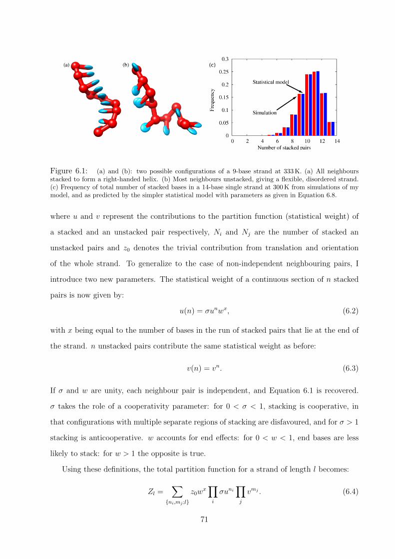
Figure 6.1: (a) and (b): two possible configurations of a 9-base strand at 333 K. (a) All neighboursstacked to form a right-handed helix. (b) Most neighbours unstacked, giving a flexible, disordered strand.(c) Frequency of total number of stacked bases in a 14-base single strand at 300 K from simulations of mymodel, and as predicted by the simpler statistical model with parameters as given in Equation 6.8.
where u and v represent the contributions to the partition function (statistical weight) of
a stacked and an unstacked pair respectively, Ni and Nj are the number of stacked an
unstacked pairs and z0 denotes the trivial contribution from translation and orientation
of the whole strand. To generalize to the case of non-independent neighbouring pairs, I
introduce two new parameters. The statistical weight of a continuous section of n stacked
pairs is now given by:
u(n) = σunwx, (6.2)
with x being equal to the number of bases in the run of stacked pairs that lie at the end of
the strand. n unstacked pairs contribute the same statistical weight as before:
v(n) = vn. (6.3)
If σ and w are unity, each neighbour pair is independent, and Equation 6.1 is recovered.
σ takes the role of a cooperativity parameter: for 0 < σ < 1, stacking is cooperative, in
that configurations with multiple separate regions of stacking are disfavoured, and for σ > 1
stacking is anticooperative. w accounts for end effects: for 0 < w < 1, end bases are less
likely to stack: for w > 1 the opposite is true.
Using these definitions, the total partition function for a strand of length l becomes:
Zl =∑
ni,mj ;l
z0wx∏i
σuni∏j
vmj . (6.4)
71

Here, ni, rj; l specifies a configuration, ni being the number of stacked pairs in the ith
contiguous sequence of stacked neighbours, mj being the number of unstacked pairs in the
mth sequence of unstacked bases and x =∑
i xi is the total number of bases at the end of
the strand involved in stacking.
Defining t = u/v, n =∑
i ni and letting p be the total number of stacked regions:
Zl = Zul
∑ni,mj ;l
wxσptn. (6.5)
with Zul = z0v
l−1 being the partition function of a completely unstacked strand. To compare
directly with simulations, the ratio of the probability of observing r stacked pairs to the
probability of observing a completely unstacked strand is required:
Zl(r)
Zul
=∑n=r;l
wxσptn = tr2∑
x=0
wx∑p
σpΩx,r,p;l, (6.6)
with Ωx,r,p;l defined as the number of distinct configurations of length l with r stacked
pairs, of which x are at the end of the strand, divided between p contiguous regions of
stacking. The advantage of this representation is that finding Ωx,r,p;l is simply a matter of
combinatorics.
Ωx,r,p;l is given by the number of ways to split r stacked pairs into p sections, multiplied
by the number of ways to split l − r − 1 unstacked pairs into p + x − 1 sections, with an
additional factor of two for x = 1 as the order of stacked and unstacked regions can be
swapped. This is equivalent to the number of ways of selecting p− 1 objects from a set of
r − 1 objects (without replacement), multiplied by the number of ways to select p + x− 2
objects from a set of size l − r − 2. This is because there are r − 1 possible ways to divide
the stacked pairs into non-empty sets, and we must do this division p− 1 times. Thus:
Ωx,r,p;l =(1 + δx,1)(r − 1)!(l − r − 2)!
(r − p)!(p− 1)!(l − r − 2− p+ x)!(p− x)!, (6.7)
for all possible values of x, r and p for a strand of length l, with the exception that Ω0,0,0;l =
Ω2,l−1,1;l = 1.
I assume that the temperature dependence of stacking is manifested in the parameter
t, which is defined as t = exp(−∆hst/RT + ∆sst/R), with ∆hst and ∆sst representing the
72
(assumed constant) enthalpy and entropy changes associated with stack formation.2 I take
w and σ to be entropic (this will be justified later) and hence temperature independent.
The four parameter model detailed above can be fitted to simulation data, yielding:
∆hst = −5.47 kcal mol−1,∆sst = −15.77 cal mol−1 K−1,
σ = 0.755,w = 0.789.
(6.8)
As σ and w are close to unity, the model shows only weak cooperative and end effects.
The entropy and enthalpy parameters are similar to those found by Holbrook et al. [140],
to which the model’s stacking behaviour was compared during fitting. The authors esti-
mated ∆hst = −5.7 and −5.3 kcal mol−1 and ∆sst = −16.0 and −15.0 cal mol−1 K−1 for two
different strands at [Na+] = 120 mM. Similar results at [Na+] = 50mM suggest weak salt
dependence in this regime [140].
Simulations performed in which the repulsive steric interactions were set to zero gave
a slightly higher ∆sst and values of σ and w consistent with unity. Thus I conclude that
the small cooperative effects in the model result from excluded volume. To understand
the cause of the cooperativity, consider a chain of bases A, B, and C, and without loss of
generality, consider B fixed whilst A and C move relative to it. Due to the requirement that
base normals must point in the 3′ to 5′ direction to stack, the regions of space in which A
and C stack with B do not overlap. Therefore, if A and B are stacked, the excluded volume
that A represents to C only prevents C adopting conformations in which it is unstacked. By
contrast, if A and B are unstacked, the excluded volume of A can prevent C adopting both
stacked and unstacked configurations. As a consequence, C has a slightly higher tendency
to stack if A and B are stacked, resulting in positive cooperativity. Similarly, end bases
experience more freedom due to the reduction in excluded volume, and are therefore less
likely to stack.
2Simulations are performed in the canonical ensemble, and hence should be described in terms of energyand entropy changes. I assume that, as dilute DNA strands contribute a very small partial pressure,discrepancies between constant volume and constant pressure results are small: we therefore use the term‘enthalpy’ to describe what are in fact energies in the model, for consistency with experimental literature.
73
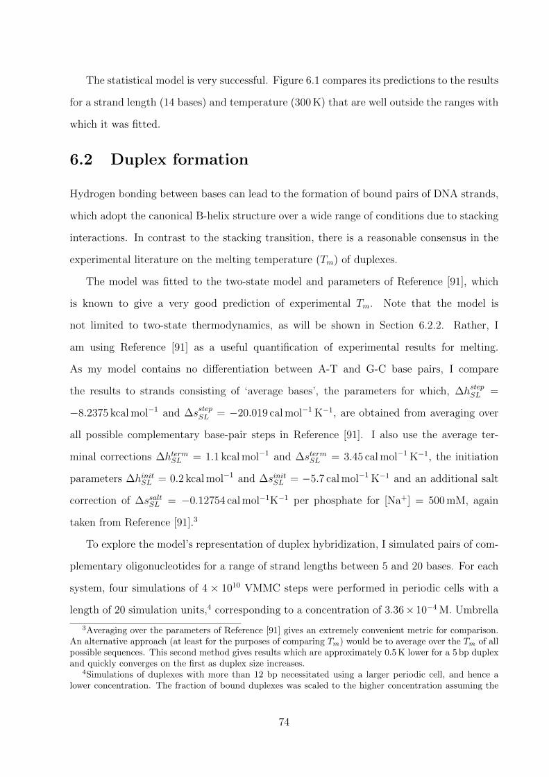
The statistical model is very successful. Figure 6.1 compares its predictions to the results
for a strand length (14 bases) and temperature (300 K) that are well outside the ranges with
which it was fitted.
6.2 Duplex formation
Hydrogen bonding between bases can lead to the formation of bound pairs of DNA strands,
which adopt the canonical B-helix structure over a wide range of conditions due to stacking
interactions. In contrast to the stacking transition, there is a reasonable consensus in the
experimental literature on the melting temperature (Tm) of duplexes.
The model was fitted to the two-state model and parameters of Reference [91], which
is known to give a very good prediction of experimental Tm. Note that the model is
not limited to two-state thermodynamics, as will be shown in Section 6.2.2. Rather, I
am using Reference [91] as a useful quantification of experimental results for melting.
As my model contains no differentiation between A-T and G-C base pairs, I compare
the results to strands consisting of ‘average bases’, the parameters for which, ∆hstepSL =
−8.2375 kcal mol−1 and ∆sstepSL = −20.019 cal mol−1 K−1, are obtained from averaging over
all possible complementary base-pair steps in Reference [91]. I also use the average ter-
minal corrections ∆htermSL = 1.1 kcal mol−1 and ∆stermSL = 3.45 cal mol−1 K−1, the initiation
parameters ∆hinitSL = 0.2 kcal mol−1 and ∆sinitSL = −5.7 cal mol−1 K−1 and an additional salt
correction of ∆ssaltSL = −0.12754 cal mol−1K−1 per phosphate for [Na+] = 500 mM, again
taken from Reference [91].3
To explore the model’s representation of duplex hybridization, I simulated pairs of com-
plementary oligonucleotides for a range of strand lengths between 5 and 20 bases. For each
system, four simulations of 4 × 10¹⁰ VMMC steps were performed in periodic cells with a
length of 20 simulation units,4 corresponding to a concentration of 3.36× 10⁻⁴ M. Umbrella
3Averaging over the parameters of Reference [91] gives an extremely convenient metric for comparison.An alternative approach (at least for the purposes of comparing Tm) would be to average over the Tm of allpossible sequences. This second method gives results which are approximately 0.5 K lower for a 5 bp duplexand quickly converges on the first as duplex size increases.
4Simulations of duplexes with more than 12 bp necessitated using a larger periodic cell, and hence alower concentration. The fraction of bound duplexes was scaled to the higher concentration assuming the
74
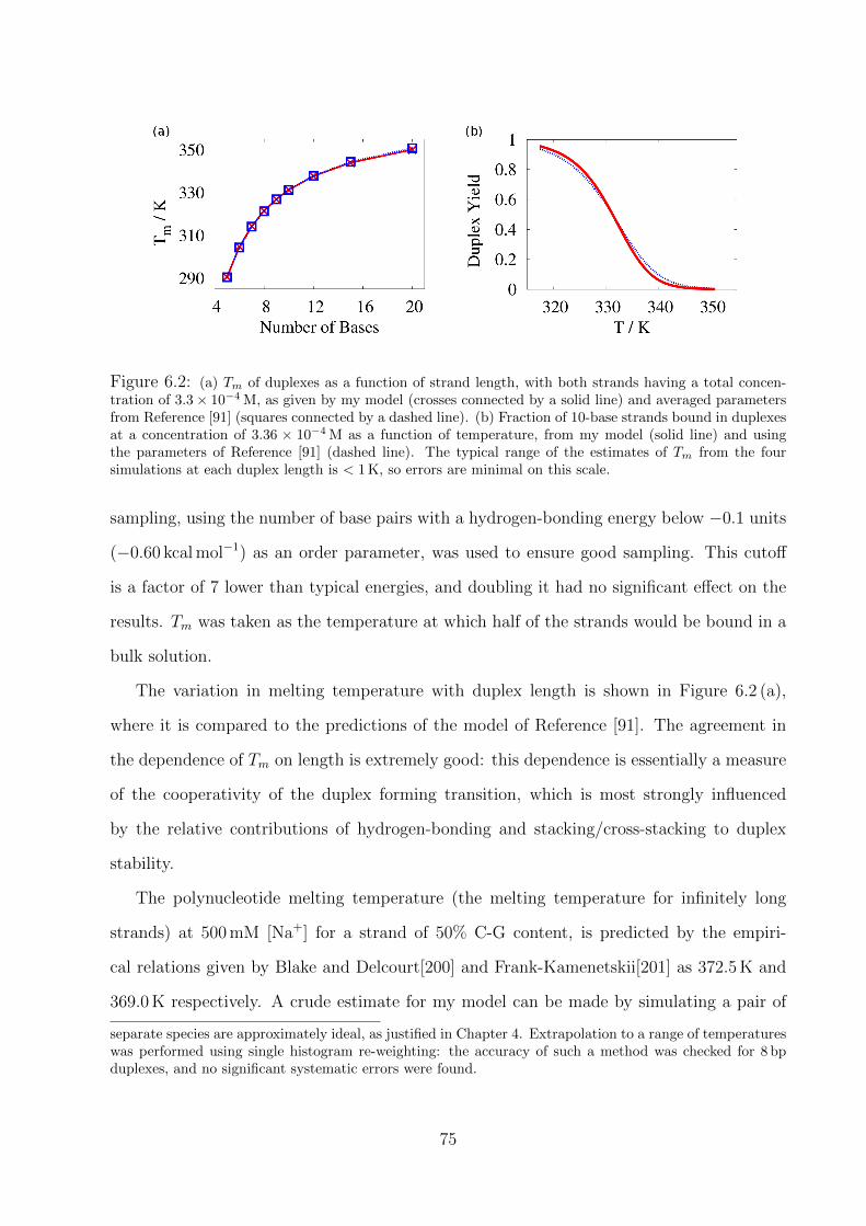
Figure 6.2: (a) Tm of duplexes as a function of strand length, with both strands having a total concen-tration of 3.3× 10⁻⁴ M, as given by my model (crosses connected by a solid line) and averaged parametersfrom Reference [91] (squares connected by a dashed line). (b) Fraction of 10-base strands bound in duplexesat a concentration of 3.36 × 10⁻⁴ M as a function of temperature, from my model (solid line) and usingthe parameters of Reference [91] (dashed line). The typical range of the estimates of Tm from the foursimulations at each duplex length is < 1 K, so errors are minimal on this scale.
sampling, using the number of base pairs with a hydrogen-bonding energy below −0.1 units
(−0.60 kcal mol−1) as an order parameter, was used to ensure good sampling. This cutoff
is a factor of 7 lower than typical energies, and doubling it had no significant effect on the
results. Tm was taken as the temperature at which half of the strands would be bound in a
bulk solution.
The variation in melting temperature with duplex length is shown in Figure 6.2 (a),
where it is compared to the predictions of the model of Reference [91]. The agreement in
the dependence of Tm on length is extremely good: this dependence is essentially a measure
of the cooperativity of the duplex forming transition, which is most strongly influenced
by the relative contributions of hydrogen-bonding and stacking/cross-stacking to duplex
stability.
The polynucleotide melting temperature (the melting temperature for infinitely long
strands) at 500 mM [Na+] for a strand of 50% C-G content, is predicted by the empiri-
cal relations given by Blake and Delcourt[200] and Frank-Kamenetskii[201] as 372.5 K and
369.0 K respectively. A crude estimate for my model can be made by simulating a pair of
separate species are approximately ideal, as justified in Chapter 4. Extrapolation to a range of temperatureswas performed using single histogram re-weighting: the accuracy of such a method was checked for 8 bpduplexes, and no significant systematic errors were found.
75
long, complementary strands in a partially bound state, and finding the temperature at
which the free-energy change of adding an additional base pair to a partially formed duplex
is zero. Simulations of partially formed 100 bp strands (with the duplex/single-stranded
DNA interface at a variety of points) gave values of T in the range 363.7 to 366.8 K, around
6 K below the empirical relations. The model’s estimate, however, is very rough (as it
neglects the stabilizing effect of bubbles and the destabilizing effect of intrastrand hairpins).
Figure 6.2 (b) compares the 10-bp duplex yield as a function of temperature for our
model with the predictions of Reference [91]. The widths of the transitions are consistent
to within a few degrees Kelvin, with my model consistently producing a marginally sharper
transition for all duplex lengths. The width of the transition determines the response of
the system to changes in concentration. Consider, for example, a simple two-state model of
DNA hybridization, as used in Reference [91] and expressed in Equation 1.1. Assuming equal
total concentrations of each strand ([A0]), the width of the transition scales approximately
as:
∆T ∼ kBT2m
∆H, (6.9)
and the change in Tm with concentration is given by:
dTmd[A0]
= − kBT2m
[A0]∆H∼ ∆T
[A0], (6.10)
and hence agreement in both Tm and the transition width at a given concentration imply
agreement in Tm over a range of concentrations.
6.2.1 Free energy profile of duplex formation and fraying
The free energy of duplex formation of a 15-bp duplex is plotted in Figure 7.3 as a function of
the number of base pairs (the order parameter of umbrella sampling). To avoid complicating
features in the free-energy profile due to hairpins and misbonds, which can conceal the
underlying trends at low numbers of bonds, only base pairs that are present in the desired
duplex were given a non-zero strength of hydrogen bonding in this simulation. The general
form of the free-energy profile is qualitatively similar to that found for another coarse-
grained model of DNA [121], with an initial entropy penalty for the formation of the first
76

0
2
4
6
8
10
12
0 2 4 6 8 10 12 14 16
Fre
e E
ner
gy
/ k
Tâ
Number of base pairs
Figure 6.3: Free-energy profile of formation for a single 15-bp duplex from two strands in a cell of sidelength 30 simulation units, as a function of the number of base pairs, at 343 K.
base pair, followed by a downhill slope as the duplex ‘zips up’ in a cooperative fashion. As
can be seen, the formation of the final base pair is actually free-energetically unfavourable,
and the typical state consists of a duplex with ‘frayed’ ends. This fraying arises because
bases at the end of the duplex lack the stabilizing influence of neighbouring base pairs on
either side and entropy favours the open state.
Although fraying is a widely accepted phenomenon [202], experimental data is rather
sparse, though it is established that weaker AT ends fray more easily than CG capped
helices [203]. Nonin et al. inferred fraying probabilities of terminal AT bps of around
0.375 and 0.7 at 273 K and 298 K respectively, and found 0.015 and 0.12 for GC pairs at
the same temperatures (at moderate salt concentrations) [203]. Patel et al. found much
higher melting temperatures for terminal base AT pairs, concluding that they were around
50% frayed at 313 K at high salt concentration [204]. My model shows approximately 10%
fraying at 273 K, increasing to around 20% at 300 K and reaching 50% at approximately
337 K, reasonable values for ‘average’ base pairs. It is worth noting that fraying probability
for actual DNA will not only depend on the identity of the final base pair, but also its
neighbour due to the sequence dependence of stacking interactions, an additional sequence-
dependent effect that will not be reproduced by my model. Note that in many cases,
particularly at low temperature, end bps in our model break but remain stacked, adopting
conformations to maximize stacking at the expense of hydrogen bonding.
77

6.2.2 A statistical model of duplex formation
I attempted to fit the duplex yield as a function of temperature, for each strand length l,
using a two-state model of the form in Equation 1.1.
[AlBl]
[Al][Bl]= v
ZllZ2l
= exp(− β
(∆Hl − T∆Sl
)), (6.11)
where [Al] is the concentration of strand A of length l and [Bl] and [AlBl] are the concen-
trations of its complementary strand and the bound pair. v is the volume simulated, Zll
and Zl are the statistical weights (contributions to the partition function) of the duplexes
and single-stranded states to a simulation and ∆Hl and ∆Sl the (assumed T -independent)
enthalpy and entropy of the transition. It was found, however, to be an unsatisfying fit
to the melting curves, and further attempts to fit ∆Hl and ∆Sl as a linear function in l
(by analogy with the nearest-neighbour model), were unsuccessful. The failure of a simple
two-state model should not come as a surprise, however, as several authors have indicated
that the entropy and enthalpy of duplex formation show temperature dependence due to
the single-stranded stacking transition [140, 184, 191, 193].
Two-state descriptions typically fail when the macrostates that constitute the reactants
and products show significant temperature dependence. In the rest of this section, I attempt
to factor out the temperature dependence of reactant and product macrostates, thereby pro-
ducing a multi-state statistical model that highlights the cause of the full model’s description
of duplex thermodynamics.
It is possible to devise a statistical model of duplex formation that takes the stacking
transition into account. In particular, one can use the results of Section 6.1.1 to factor out
the temperature dependence of the unbound state.
[AlBl]
[Al][Bl]= v
ZllZ2l
= vexp
(− β
(∆H ′l − T∆S ′l
))(Zu
l )2
Z2l
, (6.12)
where in this case ∆H ′l and ∆S ′l are the enthalpy and entropy difference between the duplex
and unstacked single-stranded macrostates. It might be expected that, having factored out
the temperature dependence of the single-stranded state, ∆H ′l and ∆S ′l should be tempera-
ture independent. Unfortunately, although fitting to Equation 6.12 with constant ∆H ′l and
78

∆S ′l was more successful than assuming constant ∆Hl and ∆Sl, it overcorrected for the
variations in ∆Sl and ∆Hl with temperature. This failure arises primarily from neglecting
the dependence of the bound state on temperature, which has two main contributions:
• As temperature increases, increased fraying leads to smaller entropy and enthalpy
differences between typical bound states and completely unstacked single strands, as
bound states become more disordered.
• Frayed ends themselves undergo a stacking transition, once more resulting in the
entropy and enthalpy of bound states relative to unstacked strands becoming less
negative with temperature.
To incorporate these effects within a statistical model, I split the duplex macrostate into
states with y out of l possible base pairs formed. Stacking of the frayed ends is treated by
viewing the 2(l − y) unpaired bases as undergoing stacking with the same ∆hst and ∆sst
given in Section 6.1.1. Cooperativity and end effects are ignored for these bases as it would
be difficult to include them consistently when stacking is initiated adjacent to a duplex
region.
Therefore, defining Zll(y) as the statistical weight of a duplex state with y out of l base
pairs:
Zll =∑y
Zll(y) =∑y
Zull(y)
(1 + exp
(− β(∆hst − T∆sst)
))2(l−y)
. (6.13)
Here Zull(y) is the statistical weight of a duplex state with y out of l base pairs formed, and
the other bases unstacked.
The hypothesis of the multi-state model is that the temperature dependence of the
macrostates measured by Zull(y) and Zu
l should be minimal, and hence that:
vZull(y)
(Zul )2
= exp(− β
(∆H0
l (y)− T∆S0l (y)
)), (6.14)
with constant ∆H0l (y) and ∆S0
l (y), which represent the enthalpy and entropy differences
between unstacked single strands and the states contributing to Zull(y).
79

Figure 6.4: (a) ∆H0l (y) against duplex length l. Points are styled according to the total number of bonds
formed, b = l−y. The solid lines are linear fits for the dependence of ∆H0l (y) on l for fixed y. (b) Variation
with T of enthalpies associated with the formation of a 15-bp duplex. Solid lines represent simulation results,dashed lines the predictions of the statistical model outlined in the text. The lines labeled ∆Htransition givethe enthalpy change upon duplex formation for the simulations and the statistical model. The lines labeledHss and Hds are the enthalpies of the duplex and single strands relative to a completely unstacked state.The transition enthalpy in the statistical model is the difference between the latter two curves.
It is possible to extract the probability of forming l base pairs in a simulation of duplex
formation, and the stacking parameters can be taken from Section 6.1.1. Hence ∆H0l (y)
and ∆S0l (y) can be fitted via:(
∆H0l (y)− T∆S0
l (y))/kBT = − ln
(vZull(y)
(Zul )2
)= − ln
(vΦl(y)(Zl/Z
ul )2
(1+exp(−β(∆hst−T∆sst)))2(l−y)
),
(6.15)
where Φl(y) is the relative probability (extracted from simulation) of being in a state with
y base pairs compared to the probability of having zero base pairs. Temperature indepen-
dent ∆H0l (y) and ∆S0
l (y) fit the data extremely well, indicating that the statistical model
successfully captures the temperature dependence of the bound and unbound states.
Furthermore, as shown in Figure 6.4, ∆H0l (y) (and ∆S0
l (y), which is not shown) are
linear in l for fixed y to an excellent approximation. Thus, having factored out sources
of variation with temperature in the initial and final states, I obtain a result similar to
the initial hypothesis of the nearest-neighbour model: adding an extra bp to a helix (i.e.,
increasing the length of the strands by one base, and forming one extra base pair, so that the
number of unpaired bases is constant) contributes a constant enthalpy and entropy change
relative to unstructured single strands.
80
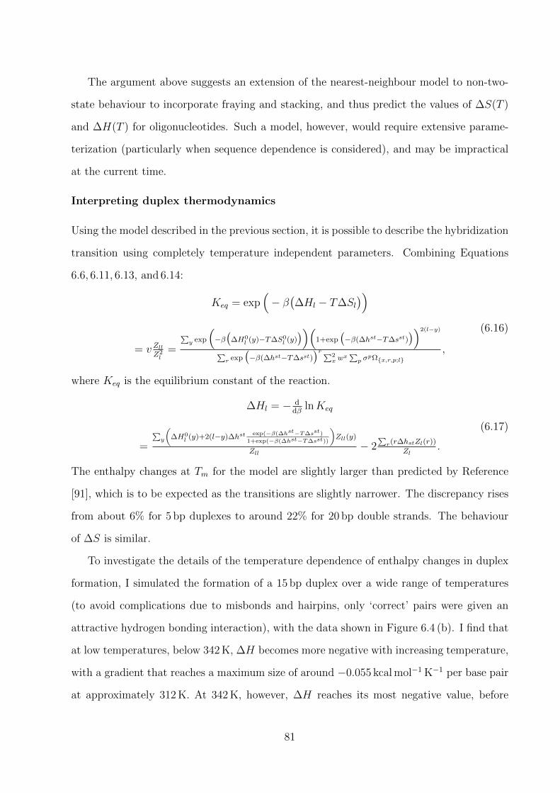
The argument above suggests an extension of the nearest-neighbour model to non-two-
state behaviour to incorporate fraying and stacking, and thus predict the values of ∆S(T )
and ∆H(T ) for oligonucleotides. Such a model, however, would require extensive parame-
terization (particularly when sequence dependence is considered), and may be impractical
at the current time.
Interpreting duplex thermodynamics
Using the model described in the previous section, it is possible to describe the hybridization
transition using completely temperature independent parameters. Combining Equations
6.6, 6.11, 6.13, and 6.14:
Keq = exp(− β
(∆Hl − T∆Sl
))
= vZllZ2l
=
∑y exp
(−β(
∆H0l (y)−T∆S0
l (y)))(
1+exp(−β(∆hst−T∆sst)
))2(l−y)
∑r exp
(−β(∆hst−T∆sst)
)r∑2x w
x∑p σ
pΩx,r,p;l,
(6.16)
where Keq is the equilibrium constant of the reaction.
∆Hl = − ddβ
lnKeq
=
∑y
(∆H0
l (y)+2(l−y)∆hstexp(−β(∆hst−T∆sst)
1+exp(−β(∆hst−T∆sst))
)Zll(y)
Zll− 2
∑r(r∆hstZl(r))
Zl.
(6.17)
The enthalpy changes at Tm for the model are slightly larger than predicted by Reference
[91], which is to be expected as the transitions are slightly narrower. The discrepancy rises
from about 6% for 5 bp duplexes to around 22% for 20 bp double strands. The behaviour
of ∆S is similar.
To investigate the details of the temperature dependence of enthalpy changes in duplex
formation, I simulated the formation of a 15 bp duplex over a wide range of temperatures
(to avoid complications due to misbonds and hairpins, only ‘correct’ pairs were given an
attractive hydrogen bonding interaction), with the data shown in Figure 6.4 (b). I find that
at low temperatures, below 342 K, ∆H becomes more negative with increasing temperature,
with a gradient that reaches a maximum size of around −0.055 kcal mol−1 K−1 per base pair
at approximately 312 K. At 342 K, however, ∆H reaches its most negative value, before
81

heading rapidly towards zero. The statistical model highlights the cause of this behaviour,
as illustrated in Figure 6.4 (b).
Well below 340 K, the enthalpy of the bound state is seen to be approximately constant
whereas the enthalpy of the single strands becomes less negative with increased temperature
as they unstack, causing the observed tendency for ∆H of the transition to become more
negative. At higher temperatures, however, the enthalpy of the bound state becomes less
negative due to fraying, as the typical bound state changes from being a fully formed duplex
at low temperatures to a higher enthalpy partially-melted state at higher temperatures. As
the polynucleotide melting temperature is approached, fraying becomes more significant,
resulting in the observed decrease in the magnitude of ∆H for the transition.
A change in enthalpy due to the stacking transition has been observed experimentally by
several groups [140, 184, 191, 193, 205], who deduced values for the typical enthalpy gradient
of −0.050, −0.095, −0.05 to −0.1, −0.068 to −0.87 and −0.062 kcal mol−1 K−1 per base pair,
respectively, in reasonable agreement with the model. These investigations were generally
performed with either oligonucleotides with several CG pairs at the end [140, 184, 191, 193]
or polynucleotides [205], both of which would massively reduce the impact of fraying: if I
set the fraying contribution to zero in the statistical fit, I obtain a typical value of −0.06 to
−0.07 kcal mol−1 K−1, in even better agreement with experiment.
In addition, Jelesarov et. al. [193] considered another duplex with AT bps at the end of
the helix, which showed ∆H becoming more negative with increasing T at low temperature,
before flattening-off by around 320 K, in agreement with the predictions of the model for
the consequences of fraying. Measurements were not performed at high enough T to check
for an eventual decrease in the magnitude of ∆H, but my model predicts the effect should
be observable. In particular, duplexes with large AT end regions and a stabilizing GC cores
should demonstrate such an effect.
82

Figure 6.5: A hairpin with a 12 bp stem and an 18-base loop at 343 K.
6.2.3 Structural motifs
Hairpins
DNA hairpins, which occur when a self-complementary strand binds to itself, forming a
duplex stem and an unhybridized loop (Figure 6.5), are a common structural motif. They
have biological importance as a mechanism for release of superhelicity through cruciform
formation [76], and relevance to nanotechnology as metastable states (either occurring by
accident [206] or through design [66, 130]). In addition, they are an extremely common motif
in biological RNA structures [207]. To date, there have been no coarse-grained models which
have been applied to both hairpins and bimolecular duplexes. An approach in which the
single strands have the potential to be extremely flexible allows for hairpins and duplexes
to have appropriate relative stabilities.
To demonstrate the ability of the model to represent hairpins, I simulated them with
stem sizes ranging from 5–12 bps, and loops of 5–18 bases. Four simulations for each hairpin
were performed in the vicinity of Tm for 4× 10¹⁰ VMMC steps, with umbrella sampling as
a function of hydrogen-bonded base pairs used to ensure good statistics. In this case, I
considered only states with at least one of the ‘native’ bps in the stem present as being a
hairpin, as long loops had the potential to form transient base pairs with little relevance to
the stability of the target structure. SantaLucia has presented parameters for estimating the
83
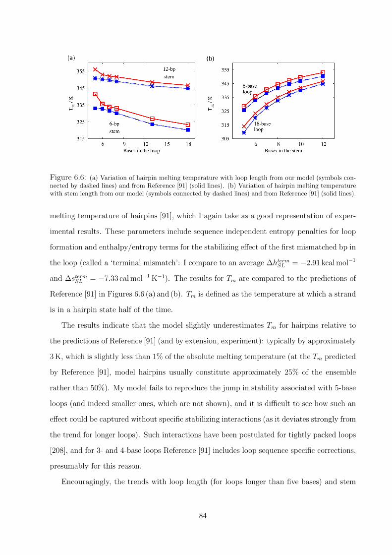
Figure 6.6: (a) Variation of hairpin melting temperature with loop length from our model (symbols con-nected by dashed lines) and from Reference [91] (solid lines). (b) Variation of hairpin melting temperaturewith stem length from our model (symbols connected by dashed lines) and from Reference [91] (solid lines).
melting temperature of hairpins [91], which I again take as a good representation of exper-
imental results. These parameters include sequence independent entropy penalties for loop
formation and enthalpy/entropy terms for the stabilizing effect of the first mismatched bp in
the loop (called a ‘terminal mismatch’: I compare to an average ∆htermSL = −2.91 kcal mol−1
and ∆stermSL = −7.33 cal mol−1 K−1). The results for Tm are compared to the predictions of
Reference [91] in Figures 6.6 (a) and (b). Tm is defined as the temperature at which a strand
is in a hairpin state half of the time.
The results indicate that the model slightly underestimates Tm for hairpins relative to
the predictions of Reference [91] (and by extension, experiment): typically by approximately
3 K, which is slightly less than 1% of the absolute melting temperature (at the Tm predicted
by Reference [91], model hairpins usually constitute approximately 25% of the ensemble
rather than 50%). My model fails to reproduce the jump in stability associated with 5-base
loops (and indeed smaller ones, which are not shown), and it is difficult to see how such an
effect could be captured without specific stabilizing interactions (as it deviates strongly from
the trend for longer loops). Such interactions have been postulated for tightly packed loops
[208], and for 3- and 4-base loops Reference [91] includes loop sequence specific corrections,
presumably for this reason.
Encouragingly, the trends with loop length (for loops longer than five bases) and stem
84

size are well reflected by the model (this is particularly pleasing, as the dependence on loop
length was not used in parameterization), an indication that the majority of the physics of
hairpin formation is well represented by the model. As found with duplex formation, model
transition widths are slightly smaller than predicted by Reference [91] (the discrepancy is
very similar to that indicated in Figure 6.2 (b)). Note that, if the duplex transitions were
as broad as predicted by the SantaLucia model, hairpin stem formation would be somewhat
more favourable at these temperatures well above the duplex Tm. The slightly narrower
transitions of my model might therefore contribute to the lowering of hairpin Tm relative to
Reference [91], as well as the representation of the loop itself.5
Mismatches, bulges and internal bubbles
A variety of other DNA motifs exist, such as duplexes involving mismatches between non-
complementary base pairs or with one strand carrying extra, unpaired bases. SantaLucia
[91] has provided parameters for the influence of these motifs on Tm. In many cases, they
are highly sequence dependent and it is less clear than in the simple double-helix case
(where the variations in parameters are relatively smaller) that averaging over ∆S and ∆H
contributions for all sequences is a reasonable approach to find an average effect. It should,
however, give a rough estimate of the typical change in melting temperature due to a motif.
I compared the effect of several motifs on model duplex Tm to the predictions of Reference
[91], again averaged over all possible sequences (Table 6.1). The simplest possible case is
that of a single unpaired base at the end of a strand, generally referred to as a ‘dangling
end’. Typically, dangling ends are observed to provide a stabilizing influence, assumed to
result from cross-stacking with the final base pair of the duplex, although the degree of
stabilization is highly sequence dependent [91, 144]. The cross-stacking interaction included
in the model provides such a stabilizing effect, and the degree of stabilization is in good
agreement with the predictions of Reference [91]. In contrast to dangling ends, extra,
5For example, if the melting transition of an 8-bp duplex was as wide as predicted by Reference [91],one would expect the statistical weight of an 8-bp duplex in my model to be increased by around a factorof two at 341 K. This is the approximate melting temperature of a hairpin with an 8-bp stem and a 6-baseloop: increasing the statistical weight of the hairpin by a factor of two would translate into an increase inTm of around 2 K.
85

Motif Complementary Motif size ∆Tm / Kbp My Model Ref. [91]
Dangling end 5 1 base +3.42 +4.248 1 base +1.33 +1.4415 1 base +0.66 +0.70
Bulge 8 1 base −17.98 −23.192 bases −23.92 −26.73
15 1 base −8.18 −12.362 bases −11.03 −11.585 bases −15.97 −13.11
Terminal mismatch 5 1 base / strand +6.71 +8.608 1 base / strand +3.02 +2.7115 1 base / strand +0.94 +0.31
Internal mismatch 8 1 base / strand −8.81 −13.99/ bubble 2 bases / strand −15.77 −21.86
5 bases / strand −25.70 −28.8115 1 base / strand −4.92 −4.88
2 bases / strand −9.18 −11.515 bases / strand −15.37 −15.65
Table 6.1: Effect on the melting temperature of a complementary duplex due to the addition of a motif.In this table, ∆Tm is the difference between the Tm of a structure with the motif and a fully complementaryduplex consisting of the same number of complementary bps as the motif structure. For internal mismatches,bulges and bubbles, the motif was placed at the centre of the duplex.
unpaired bases on one strand within the helix are highly destabilizing, as they disrupt the
helix structure. In the terminology of SantaLucia, these are known as bulges. In general,
our model slightly underestimates the destabilization of helices due to bulges compared to
the predictions of Reference [91], although the melting observed temperatures remain within
2% of the predictions.
If a non-complementary pair of bases is added to an otherwise complementary duplex
to form a mismatch, the effect is generally stabilizing at the end of a duplex (this is a
‘terminal mismatch’) and destabilizing in the interior. The model reproduces this tendency
as shown in Table 6.1, and also captures the increase in destabilization if the mismatch region
is extended (to form an internal ‘bubble’). Once again, the destabilizing effect of motifs
86

internal to the duplex tend to be slightly underestimated relative to the predictions of
Reference [91], but the observed melting temperatures remain within 2% of the predictions.
Such motifs provide a good test of the model, as many were not considered in parame-
terization (although the dangling ends and terminal mismatches were used to constrain the
strength of cross-stacking). In addition, misbonded structures involving these motifs may
have a role in the kinetics of nanostructure assembly, and hence it is important that the
model provides a reasonable representation of them. Although in some cases the quanti-
tative agreement with Reference [91] is not perfect, the model represents these motifs in a
physically sensible way and the trends in stability at least qualitatively reflect the average
properties of DNA. Furthermore, the typical magnitudes of ∆Tm are reasonable, with the
Tm remaining within 2% of the average predictions of Reference [91]. It is possible that an
underestimate of the disruptive effect of extra bases on the helical structure [76], perhaps
because the excluded volume of bases is smaller than in reality, causes the underestimate of
∆Tm due to internal motifs. Another consideration may be that as the model hybridization
transition is slightly narrower than predicted by Reference [91], a given destabilizing ∆G
will have a smaller effect on model Tm than for the statistical description of SantaLucia.
Given the good agreement between the model and Reference [91] for a single mismatch
added to a 15-bp duplex, I investigated how the position of the mismatch affected stability.
Tm is plotted against the position of the mismatch in Figure 6.7 (a). As can be seen, there
are two distinct regimes, with the melting temperature initially decreasing as the mismatch
is moved from the end of the strand (where it is stabilizing) towards the centre. Eventually,
however, it reaches a plateau at around five bases from the end of the strand.
The cause of this plateau can be identified from examining the free energy profiles for
duplexes with mismatches located one and six bp from the end (Figure 6.7 (b)). The first
point to note is that the stability of duplexes with the maximum number of base pairs (15)
is nearly identical, despite the difference in mismatch position. This suggests that provided
a mismatch is surrounded by base pairs on either side, changing its location has little effect
on the total free energy. The difference in Tm arises instead from a difference in the nature
of the lowest free-energy state.
87

Figure 6.7: (a) Melting temperature of 15-bp complementary helix with an additional mismatch addedagainst the distance of that mismatch from the end of the strand. The melting temperature in the absenceof a mismatch is indicated via the horizontal line. (b) Free energy profile at 339 K for a 15-base-pair duplexwith one additional mismatch placed 1 base from the end (squares) and 6 bases from the end (crosses)
When the mismatch is near to the strand end (in the regime where Tm depends on
mismatch position), the most stable state consists of the larger section of duplex formed
with the bases beyond the mismatch unpaired. In this regime, the total free energy gain
from pairing the bases beyond the mismatch does not compensate for the cost of enclosing
a mismatch in a helix. As the mismatch is moved towards the centre, the larger section
loses bases and so becomes less stable, with the consequence that Tm drops. At some
point, however, the possible number of base pairs in the region beyond the mismatch makes
it favourable for the base pairs in this region to form. From this point onwards, the most
stable state consists of the two duplex regions surrounding the mismatch. When this occurs,
the net effect of moving the mismatch towards the centre can be viewed (in the average base-
pair case) as the transfer of a base pair from the centre of the larger duplex to the centre
of the smaller duplex, where the contribution to stability will be unchanged. As a result a
plateau in Tm is observed.
As the temperature is lowered, the free-energy gain from base pair formation increases.
As a consequence, the number of bases required before the region beyond the mismatch is
stable as a duplex decreases. For example, I find that for a mismatch two bases from the
end of a duplex, the enclosed mismatch state becomes the most stable just below 320 K.
It is claimed in Reference [91] that the stability of a mismatch is independent of its
88

(a) (b)
mismatch
Figure 6.8: Typical configurations of a duplex with 15 complementary bp and 1 internal mismatch at335 K. a) Mismatch two bp from the end of the strands, with unpaired bases after the mismatch. b)Mismatch six bp from the end of the strand, enclosed by two intact helices.
position, except for terminal mismatches and mismatches occurring one base from the end,
which may cause the final base pair to be unstable. My simulations suggest, however, that
the distance of the mismatch from the duplex end at which Tm plateaus should increase with
strand length (as longer strands melt at higher temperature). Further, a similar temperature
dependent influence of motif location should hold for all destabilizing internal bubbles and
bulges, as the plateau simply indicates the point at which it is free-energetically favourable
to form the second helix beyond the disruption.
A dependence of Tm on mismatch location has been reported in the DNA microarray
literature [209, 210]. In particular, You et al. [209] observed that 21 bp duplexes had their
melting temperatures reduced by 1.8-2.2 K due to a mismatch 3 bp from the end, and by
3.5 K due to a central mismatch, values comparable to those found here (although slightly
smaller, as would be expected from a longer duplex with a narrower transition). Naiser
et al. [210] have even attempted to explain the effect of mismatch location by using the
model of Reference [91] to predict the relative population of partially bound states, in
an approach similar to that of the Zuker group [211, 212]. This methodology, however,
is somewhat suspect – the SantaLucia parameters are fitted to reproduce the free-energy
difference between the bound and unbound ensembles, and hence partially-formed states
are already included implicitly in the fitting. Using the parameters to separately evaluate
89

the free energy of partially bound states therefore represents a form of double-counting.
My model therefore reproduces the observed tendency of mismatch location to influence
melting temperature, and even supports a hypothesis for the cause of this non-trivial effect.
This is particularly pleasing, as the model was in no way parameterized for this purpose.
6.2.4 Coaxial stacking
Coaxial stacking occurs when non-neighbouring bases (often from different strands) stack
with each other. Such an interaction has been used to explain the stabilization of duplexes
by adjacent hairpin stems [91, 135, 136, 137, 138, 139] and the association of DNA origami
tiles [42].
The strength of the coaxial stacking interaction has been measured experimentally in
two ways. The Frank-Kamenetskii group have attempted to infer the probability that a
nicked duplex is in a state with stacking across the nick from gel mobility studies [142,
143]. Other authors have considered the thermodynamic stabilization of duplexes due to
the presence of an adjacent double-stranded region, with which coaxial stacking can occur
[91, 135, 136, 137, 138, 139].
The direct measurements of the coaxial stacking/unstacking equilibrium from the Frank-
Kamenetskii lab were performed by measuring the mobility of duplexes undergoing gel elec-
trophoresis. The mobilities of duplexes with a nick in one of the backbones were compared
to the same duplexes without a nick and gapped duplexes containing two single G bases.
Assuming the coaxially stacked state of nicked duplexes had the same mobility as the un-
nicked duplexes, and that the unstacked state had the same mobility as the gapped duplexes,
the authors were able to infer a probability of DNA being in each configuration.6
Initial experiments [142] were performed at 37oC and low monovalent salt concentra-
tions (around 15 Mm Na+). These results give ∆Gcoax ≈ −0.3 to − 3.5 kT for a range of
sequences, where e−∆Gcoax/kT is the ratio of occupancy of stacked and unstacked configura-
tions. A noticeable trend is that stacks of CG base pairs seem to be much stronger. Later
6Note that the experiments were performed in a range of concentrations of denaturing urea, then ex-trapolated to zero urea concentration.
90
work explored higher salt concentrations, with ∆Gcoax typically becoming more negative by
around 0.65 kT between 15 mM and 100 mM [Na+], giving an average of around −2.62 kT
at 100 mM [Na+] [143].
A number of other groups have tried to estimate the stabilizing contribution to the free
energy of hybridization, which I shall call ∆∆Ghybr., from the presence of an adjacent duplex.
The Santalucia lab has inferred ∆∆Ghybr. from analyzing the formation hybridization of six-
base strands to the dangling ends of hairpins at high salt, finding an average stabilization
of around −2.74 kT at 37oC (although there is strong sequence dependence). Pyshnyi and
Ivanova considered 7 bp duplexes stabilized by hairpins at high salt, and inferred an average
∆∆Ghybr. of around −2.62 kT at approximately 37oC, noting not only dependence on the
bases at the coaxial stack site, but also on the next-nearest neighbours [136, 137]. Lane et al.
measured the hybridization of a 13-base strand to the dangling end of a hairpin at 115 mM
monovalent salt, comparing cases in which the duplex was adjacent to the hairpin stem and
in which there was a two nucleotide gap. The first duplex was found to be more stable by
about −1.87 kT at around 325 K – as the authors point out, however, the gapped system is
stabilized by dangling ends and hence this value is expected to be somewhat smaller than
the true ∆∆Ghybr.. Finally, Vasiliskov et al. considered the hybridization of a 5-base strand
to the overhanging end of a duplex that was tethered to surface in a microarray [139]. The
results are difficult to draw direct comparisons with, as the system may be quite distinct
from solution-based assays, but the authors report that stabilization is much stronger if
adenine is involved in the coaxial stacking.
It is tempting to draw direct comparisons between ∆∆Ghybr. and ∆Gcoax, but they would
be fallacious, as the quantities represent free energy differences between different pairs of
macrostates. For my model, they are quite different, and ∆Gcoax is significantly larger than
∆∆Ghybr.. The main reason for the difference is that single-stranded dangling ends can be
stacked onto the end of a duplex, and indeed one would expect them typically to be stacked
as dangling ends tend to stabilize duplexes. This stacking of dangling ends tends to reduce
the value of ∆∆Ghybr., as it makes the unbound state more favourable.
91

Modelling coaxial stacking
The coaxial stacking interaction in my model, described in Chapter 2, is based on the
nearest-neighbour stacking interaction, with several differences. In particular, I have allowed
the strength of the interaction to be different form the nearest-neighbour term – given
that the stacking interaction implicitly incorporates a host of backbone effects, it is not
surprising that this is necessary. As the interaction is only important in certain situations,
the model was initially parameterized without it [213], and it has since been included with
the interaction strength as a fitting parameter.
To compare the resulting interaction to experiment, I have simulated a system analogous
to that studied by the Frank-Kamenetskii group. Specifically, I have measured the proba-
bility that a 20 base duplex with a nick in the centre unstacks about the nick site, at 37oC,
finding ∆Gcoax = −4.3 kT . This is somewhat more negative than the Frank-Kamenetskii
group’s average value, even if the salt dependence is extrapolated to [Na+] = 500 Mm.
I have also attempted to compare directly to the thermodynamic measurements of
∆∆Ghybr.. In particular, I simulated 6-, 7- and 8-bp duplex formation adjacent to a hairpin
stem7. The duplex melting tempertures were raised by 9.88 K, 7.66 K and 6.25 K respectively
by the presence of the hairpin stem. By comparison, the averaged Santalucia parameters for
coaxial stacking predict slightly larger stabilizations of 11.7 K, 8.5 K and 6.4 K. The results
of Pyshnyi and Ivanova for ∆∆Ghybr. are similar on average to those of the SantaLucia
lab, and hence give similar stabilizations if they are used in conjunction with the remaining
Santalucia nearest-neighbour parameters. The actual value of ∆∆Ghybr. at 37oC is given by
my model as −2.43 kT , slightly less negative than the estimates of References [136], [137]
and [141]. Note also the difference between ∆∆Ghybr. and ∆Gcoax in my model, as discussed
above.
There are issues with all of these comparisons. The thermodynamic results are limited,
as References [136], [137] and [141] considered systems with fairly low Tm, and the predictive
power of their parameterizations have not been tested (particularly for systems with a higher
7Hairpin stems contained 12 bp and loops consisted of six bases. For each system, four VMMC simulationswere performed for 4× 10¹⁰ steps, using umbrella sampling to improve equilibration.
92

intrinsic Tm). The measurements of the Frank-Kamenetskii group also require some care:
in particular, they rely on the assumption that the unstacked state of the nicked duplex
has the same flexibility as a duplex containing two G nucleotides [142]. This will only be a
reasonable assumption if the stacking along the single-stranded gap is always broken. This
seems to be a very strong assumption, and if it is violated the effect would be to overestimate
the probability of the nicked duplex being in the unstacked state.
The chosen parameterization gives a stabilization of duplexes by coaxial stacking which
is similar to (if slightly smaller than) the average predicted by the Santalucia lab [141] and
Pyshnyi and Ivanova [136, 137]. For the stacked/unstacked equilibrium of a nicked duplex,
this parameterization gives ∆Gcoax as ∼ 1 to 1.5 kT more negative than that found by the
Frank-Kamenetskii group [142, 143]. Neither discrepancy is overly large, and if stacking can
occur across the two G nucleotides in a gapped duplex, this might make the agreement even
better.
6.3 Summary
Overall, the model gives a good description of the average properties of the thermodynamics
associated with the ssDNA to B-duplex transition. It is the only model to date to consis-
tently describe stacking, duplex hybridization and hairpin formation, and it also provides
a reasonable representation of various DNA motifs. Sequence-dependent effects are cur-
rently absent, but in some cases this can be an advantage. For example, the temperature
dependence of mismatch location (see Section 6.2.3) may have been somewhat obscured by
sequence-dependent variation. Further discussion of model properties and its accuracy is
given in Chapter 9.
93

Chapter 7
Modelling DNA Tweezers
As mentioned in Chapter 1, DNA tweezers were initially introduced by Yurke et al. in 2000
as a prototypical DNA nanodevice [54]. The tweezers, consisting of strands which form the
arms α and β, and the hinge (h), can be switched between open and closed states by the
addition of fuel (f) and antifuel (f) strands, as shown in Figure 7.1. The tweezers demonstrate
the possibility of using DNA hybridization and toehold-mediated strand displacement to
perform mechanical operations. As such, they have inspired the growing field of DNA
nanodevices, as outlined in Chapter 1.
I have studied DNA tweezers to prove the versatility and efficiency of my model. When
the simulations were originally performed [206] (with an older version of the model), no
DNA nanodevice had ever been simulated with a coarse-grained approach. This is partly
because of the complexity of such systems and partly due to the need to simultaneously rep-
resent rigid duplexes, flexible single strands and the hybridization transition. To date, I am
unaware of any other simulations of nanodevices, excepting subsequent studies performed
with my model (such as the two-footed walker simulation presented in Chapter 8).
7.1 Tweezer simulation methods
7.1.1 The model system
For computational simplicity, I chose to model a system approximately half the size of that
used by Yurke et al.: the sequences are given in Appendix E. The duplex regions which
form the body of the tweezers are 10 bp in length, and the overhanging sections for fuel
94

(a) (b) (c)
(d)(e)(f)(g)
hinge
α
β
f
_f
Figure 7.1: Simulation snapshots showing stages of operation of DNA tweezers. a) Tweezers initiallyopen. b) Fuel (f) is added and binds to one arm (β). c) Fuel binds to the second arm (α) and closes thetweezers. d) Antifuel (f) is added and binds to the toehold of the fuel. e) Antifuel begins to displace firstarm of the tweezers. f) Tweezers open as first arm is displaced, and antifuel displaces the second arm. g)Antifuel fully hybridizes to fuel and the waste duplex is formed.
binding are 8 bases long. The toehold which facilitates the displacement of the tweezers is
also taken to be 8 bases in length. I have sampled the free energy landscape of the system
consisting of one set of tweezers and a single f and f at 300 K, in a periodic cell of length 40
reduced units (3.96× 10⁻²⁰ litres).
7.1.2 Sampling the transitions
The sampling of the free energy landscape was performed using the VMMC algorithm, as
introduced in Chapter 3. Every stage of the cycle is observable using unbiased simulations
at 300 K. To obtain the free energy landscape, however, umbrella sampling was used to bias
the ensemble and favour multiple transitions between (meta)stable states, as discussed in
Chapter 3. As in the simulations of duplex formation performed in Chapter 6, the number
of hydrogen-bonded base pairs (with energy below −0.1 simulation units) is a convenient
order parameter to divide configuration space into regions which can then be biased. Due
to the complexity of the tweezer system I found it necessary to introduce a four-dimensional
order parameter Q = (Q1, Q2, Q3, Q4), with:
• Q1 as the number of correct base pairs between α and f.
95

• Q2 as the number of correct base pairs between β and f.
• Q3 as the number of correct base pairs between f and f, restricted to the bases of f
which bind to α or are in the toehold.
• Q4 as the number of correct base pairs between f and f, restricted to the bases of f
which bind to β.
In this context, correct base pairs are those which are intended to form during tweezer
operation. Note that other base pairs are not forbidden, they are simply not included in the
order parameter. Even an order parameter as complex as this was not sufficient to sample
the tweezer cycle, particularly the transitions accompanying the displacement of the final
bp of α and β from f. To estimate the free energy change associated with these processes, it
is necessary to encourage the displaced strand to reattach. This requires that the displaced
strand comes into close proximity with the duplex from which it was displaced, and that
the duplex undergoes some fraying to allow it to reattach – a process not particularly well
quantified by Q as it stands.
Q was therefore augmented with a fifth dimension, Q5, which depends on the actual
separation of strands in addition to hydrogen-bonding matrices. Any configuration of the
system is within one of 15 discrete values of Q5 – the definitions are given in Appendix E.
Even with this complex order parameter, capturing the entire tweezer cycle in one sim-
ulation would be impractical. Instead, individual simulations were restricted to sampling
small, overlapping ranges of Q (for instance, the binding of the fuel to the first arm of the
tweezers), and the results combined to give the free energy of the entire cycle. Ten simula-
tions were performed in each sampling window for 4×10¹⁰ VMMC steps each. The windows
used are detailed in Appendix E. The possibility of such an approach was suggested in the
original work of Torrie and Valleau on umbrella sampling [156]. Kumar et al. [157] have
proposed the weighted-histogram analysis method (WHAM) for systematically combining
the results from overlapping simulation windows. This is particularly important for my
system, as it has 185895 possible values of Q, and 11 separate simulation windows which
must be patched together.
96

In order to facilitate the windowed umbrella sampling scheme, several restrictions were
imposed on the system during the simulations. These restrictions are outlined in Appendix
E.
Simulation validity
When performing windowed sampling, the system has restricted movement through state
space, which can lead to sampling errors. For example, it is conceivable that the state space
corresponding to a certain order parameter range could be split into two non-connected
regions. If this were the case, only one of these regions would be sampled in any simulation
restricted to this range of the order parameter (ergodicity would be broken).
For the windowing scheme outlined in Appendix E, it seems unlikely that such a problem
would arise. To be sure, however, I calculated the average energy as a function of the order
parameter, 〈E(Q)〉, in each simulation. For each pair of overlapping windows, the value of
〈E(Q)〉 was compared for two frequently sampled values of Q. In all cases, 〈E(Q)〉 was
found to be consistent between windows to within the error of the simulations (details are
given in Appendix E). As a result, I am confident that simulations of each overlapping pair
of windows had access to the same microstates, and therefore that the state space for each
window was ergodically sampled.
The accuracy of the simulations can also be checked by considering that in going from
the initial to the final state of the cycle, f and f form a duplex, and the tweezers are
in the open state in both cases. Thus the free energy change between the states with
Q1 = Q2 = Q3 = Q4 = 0 and those with Q1 = Q2 = 0, Q3 > 0, Q4 > 0 should be the same
as that for the formation of an isolated duplex of f and f (assuming interactions between
unbound molecules are minimal, as justified in Chapter 4). For the windowed tweezer
simulations, ∆G was found to be 48.88 kT , and from the isolated duplex simulations I
obtained ∆G = 48.83 kT . These values appear to agree well – in order to perform a
statistical test of the agreement, 10 separate estimates of ∆G for the tweezer pathway were
obtained by patching individual simulation results together. I compared this set to the
six individual estimates of ∆G obtained for the simulation of duplexes in isolation using
97

Figure 7.2: (a) Free energy F as a function of the number of f/α and f/β base pairs during initial bindingof the fuel. The arrows indicate the cooperative lowest free-energy pathways. (b) Free energy F plottedas a function the number of f/f and f/tweezer base pairs for DNA tweezers at 300 K. White areas indicateregions of high free-energy relative to their environment that were unsampled.
Welch’s unpaired t-test [214]. The result was a test statistic of 0.9413, suggesting that any
systematic errors are smaller than the random error of the simulations.
7.2 Results
The free-energy landscape of the tweezer cycle is shown in Figure 7.2. To study the cycle
in detail, it is convenient to consider a one-dimensional pathway through the landscape; I
use that shown by the arrows in Figure 7.2 (b).
The gross features of the free energy landscape are as expected. Duplex formation is
highly cooperative; the pairing of two strands involves a high entropic cost for forming the
first base pair, then a downhill slope in free energy as additional bonds are formed. This is
reflected in Figure 7.3 (a) by stages ‘b’, ‘c’ and ‘d’ which essentially involve duplex formation.
The large cooperativity suggests that f will fully bind to one arm of the tweezers before
binding to the second. The displacement processes (indicated by ‘e’ and ‘f’ in Figure 7.3)
are comparatively flat as the total number of interstrand base pairs is constant. Returning
the tweezers to the open state (between ‘e’ and ‘f’) and the decoupling of the ff duplex from
the tweezers (‘g’) release the free energy stored in bringing strands together, resulting in
large decreases in free energy.
Simulations allow for a detailed inspection of processes like displacement. Thus, Figure
98
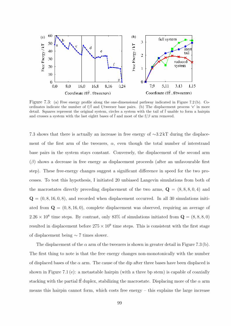
Figure 7.3: (a) Free energy profile along the one-dimensional pathway indicated in Figure 7.2 (b). Co-ordinates indicate the number of f/f and f/tweezer base pairs. (b) The displacement process ‘e’ in moredetail. Squares represent the original system, circles a system with the tail of f unable to form a hairpinand crosses a system with the last eightt bases of f and most of the f/β arm removed.
7.3 shows that there is actually an increase in free energy of ∼3.2 kT during the displace-
ment of the first arm of the tweezers, α, even though the total number of interstrand
base pairs in the system stays constant. Conversely, the displacement of the second arm
(β) shows a decrease in free energy as displacement proceeds (after an unfavourable first
step). These free-energy changes suggest a significant difference in speed for the two pro-
cesses. To test this hypothesis, I initiated 20 unbiased Langevin simulations from both of
the macrostates directly preceding displacement of the two arms, Q = (8, 8, 8, 0, 4) and
Q = (0, 8, 16, 0, 8), and recorded when displacement occurred. In all 30 simulations initi-
ated from Q = (0, 8, 16, 0), complete displacement was observed, requiring an average of
2.26 × 10⁸ time steps. By contrast, only 83% of simulations initiated from Q = (8, 8, 8, 0)
resulted in displacement before 275× 109 time steps. This is consistent with the first stage
of displacement being ∼ 7 times slower.
The displacement of the α arm of the tweezers is shown in greater detail in Figure 7.3 (b).
The first thing to note is that the free energy changes non-monotonically with the number
of displaced bases of the α arm. The cause of the dip after three bases have been displaced is
shown in Figure 7.1 (e): a metastable hairpin (with a three bp stem) is capable of coaxially
stacking with the partial ff duplex, stabilizing the macrostate. Displacing more of the α arm
means this hairpin cannot form, which costs free energy – this explains the large increase
99
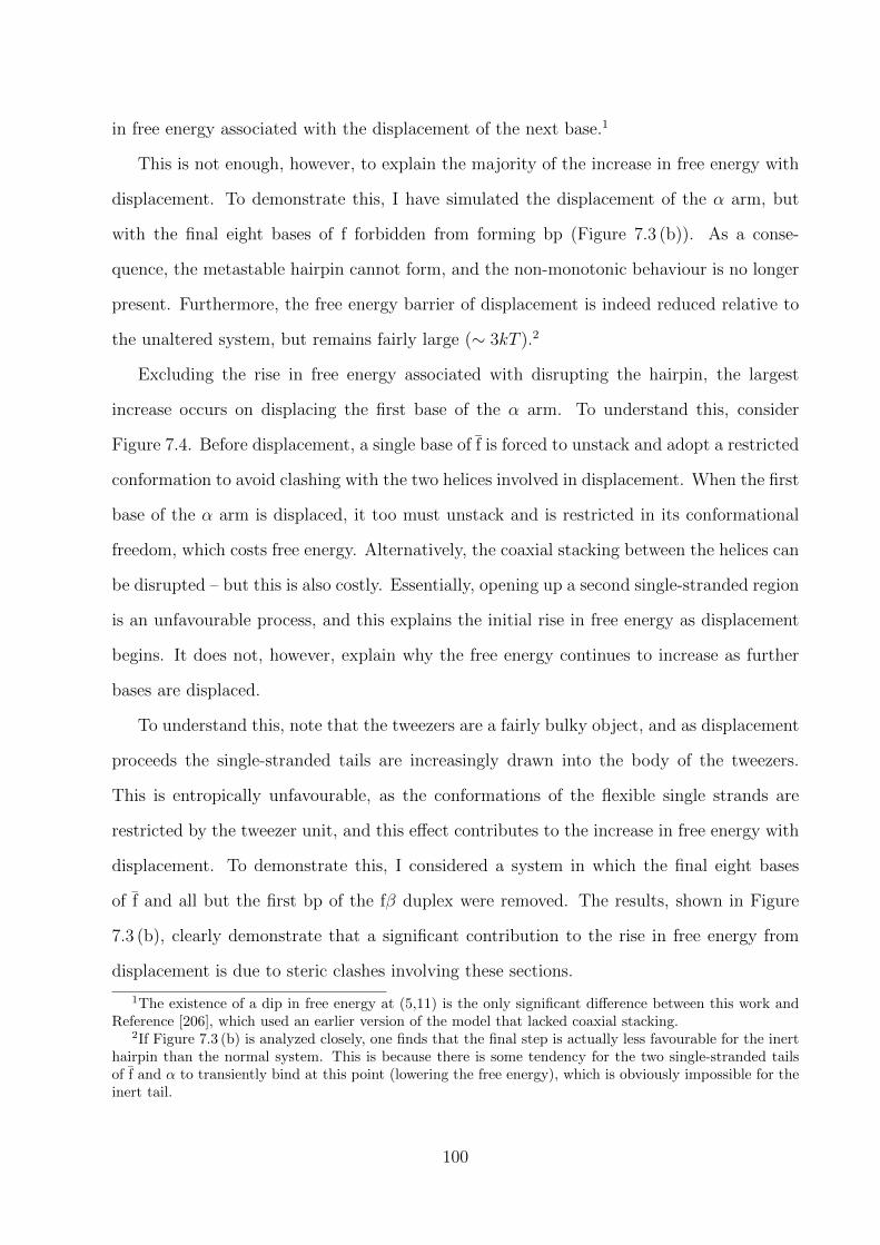
in free energy associated with the displacement of the next base.1
This is not enough, however, to explain the majority of the increase in free energy with
displacement. To demonstrate this, I have simulated the displacement of the α arm, but
with the final eight bases of f forbidden from forming bp (Figure 7.3 (b)). As a conse-
quence, the metastable hairpin cannot form, and the non-monotonic behaviour is no longer
present. Furthermore, the free energy barrier of displacement is indeed reduced relative to
the unaltered system, but remains fairly large (∼ 3kT ).2
Excluding the rise in free energy associated with disrupting the hairpin, the largest
increase occurs on displacing the first base of the α arm. To understand this, consider
Figure 7.4. Before displacement, a single base of f is forced to unstack and adopt a restricted
conformation to avoid clashing with the two helices involved in displacement. When the first
base of the α arm is displaced, it too must unstack and is restricted in its conformational
freedom, which costs free energy. Alternatively, the coaxial stacking between the helices can
be disrupted – but this is also costly. Essentially, opening up a second single-stranded region
is an unfavourable process, and this explains the initial rise in free energy as displacement
begins. It does not, however, explain why the free energy continues to increase as further
bases are displaced.
To understand this, note that the tweezers are a fairly bulky object, and as displacement
proceeds the single-stranded tails are increasingly drawn into the body of the tweezers.
This is entropically unfavourable, as the conformations of the flexible single strands are
restricted by the tweezer unit, and this effect contributes to the increase in free energy with
displacement. To demonstrate this, I considered a system in which the final eight bases
of f and all but the first bp of the fβ duplex were removed. The results, shown in Figure
7.3 (b), clearly demonstrate that a significant contribution to the rise in free energy from
displacement is due to steric clashes involving these sections.
1The existence of a dip in free energy at (5,11) is the only significant difference between this work andReference [206], which used an earlier version of the model that lacked coaxial stacking.
2If Figure 7.3 (b) is analyzed closely, one finds that the final step is actually less favourable for the inerthairpin than the normal system. This is because there is some tendency for the two single-stranded tailsof f and α to transiently bind at this point (lowering the free energy), which is obviously impossible for theinert tail.
100
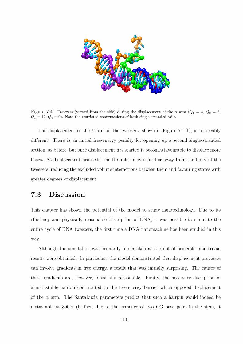
Figure 7.4: Tweezers (viewed from the side) during the displacement of the α arm (Q1 = 4, Q2 = 8,Q3 = 12, Q4 = 0). Note the restricted confirmations of both single-stranded tails.
The displacement of the β arm of the tweezers, shown in Figure 7.1 (f), is noticeably
different. There is an initial free-energy penalty for opening up a second single-stranded
section, as before, but once displacement has started it becomes favourable to displace more
bases. As displacement proceeds, the ff duplex moves further away from the body of the
tweezers, reducing the excluded volume interactions between them and favouring states with
greater degrees of displacement.
7.3 Discussion
This chapter has shown the potential of the model to study nanotechnology. Due to its
efficiency and physically reasonable description of DNA, it was possible to simulate the
entire cycle of DNA tweezers, the first time a DNA nanomachine has been studied in this
way.
Although the simulation was primarily undertaken as a proof of principle, non-trivial
results were obtained. In particular, the model demonstrated that displacement processes
can involve gradients in free energy, a result that was initially surprising. The causes of
these gradients are, however, physically reasonable. Firstly, the necessary disruption of
a metastable hairpin contributed to the free-energy barrier which opposed displacement
of the α arm. The SantaLucia parameters predict that such a hairpin would indeed be
metastable at 300 K (in fact, due to the presence of two CG base pairs in the stem, it
101

would be significantly more stable than average, with a melting temperature predicted as
313.7 K). Furthermore, although this small system could be designed so as to eliminate such
a hairpin, careful design would be needed to prevent similar structures forming when longer
scale displacements are required. As hairpins will tend to form either at the start or end
of displacement, when long single-stranded regions are available, they will constitute a free
energy barrier in the middle stages of displacement, thereby slowing down the process.
The second contribution to the free energy rise during displacement is the initial cost
of creating two single-stranded sections, which necessitates disrupting stacking interactions.
Although there is little experimental data with which to compare this prediction, its moti-
vation is physically reasonable. Furthermore, it is possible that in reality the sharp bending
of single strands to avoid the branch point of displacement may incur some energy penalty
that is not captured by the model, which would exaggerate the effect.
Finally, there is a significant entropy cost associated with bringing the single-stranded
displacement tails into a region of high DNA density (the centre of the tweezers). Again, the
physical basis of this effect is applicable to real DNA. Indeed, it is possible that electrostatic
effects would exaggerate it further, particularly at moderate or low salt concentrations. In
addition, as the tweezers of Yurke et al. are larger than those simulated here and thus have
longer single-stranded tails, the consequences of steric interactions may be more significant
for their system.
For the tweezers, in which the displacement process is fast compared to the initial as-
sociation of duplexes [54], the consequences of any free-energy barrier to displacement are
probably fairly minimal. The observation of a barrier to displacement, however, may help
to explain an initially puzzling result. Yurke and Mills have shown that the rate of toehold-
mediated strand displacement depends exponentially on the toehold length (or equivalently
the free energy of toehold binding), up to a length of at least six bases when displacing
26 bp [53]. Zhang and Winfree have reported similar results, and have also demonstrated
that the rate plateaus for longer toeholds [215]. Such a result could only be fitted with
kinetics that assumed displacement was essentially a two-state process with a single rate
102

constant, rather than a random walk in which each intermediate state was equally proba-
ble. My simulations suggest that metastable hairpins and the consequences of having two
single-stranded regions rather than one make the intermediate states less favourable. Such
arguments make displacement look more like a process in which the system must hop from
one low free-energy basin to another than an unbiased random walk, and hence may go
someway to explaining the results of References [53] and [215].
As ever, all results should be viewed with the approximations of the model in mind. In
this case, the tweezer arms are brought into close proximity when they are closed by the fuel
– electrostatic repulsion will probably be relevant here, even at high salt. In addition, the
lack of restriction on the conformation of ssDNA in the model may mean that the stability
of the fα – fβ junction is overestimated.3 Either of these considerations may mean that the
stability of the closed state of the tweezers is exaggerated by the model, but they should not
affect the primary conclusions related to the displacement process drawn from the study.
3It is plausible that the destabilizing effect of electrostatics could account for the population of partiallyopen tweezers inferred from the single-molecule FRET analysis of tweezers performed by the Simmel group[216].
103

Chapter 8
Modelling a DNA walker
In this chapter I study the operation of a two-footed DNA walker proposed by Bath et al.
[65]. The walker consists of two single-stranded ‘foot’ domains which are linked together by
a duplex (Figure 8.1). The feet are intended to bind to adjacent sites on a single-stranded
track. The binding sites overlap, meaning that the feet compete for binding to the track.
As a consequence, a single-stranded region of one foot or the other is always exposed. A
fuel strand that is also present in solution can bind to either exposed toehold. If the fuel
has bound to the back foot,1 then it is able to compete with the track for binding to the
rest of the foot. The fuel can thus displace the track and cause the foot to be raised.
If, alternatively, the fuel has bound to an exposed toehold of the front foot, conventional
toehold-mediated strand displacement is impossible and the fuel should eventually detach.
The fuel contains a recognition site for the nicking enzyme N.BbvC IB, which can cleave
the fuel when it is in a duplex state (the duplex partner is not cleaved). With the fuel in
two separate pieces, the fuel/foot duplex is unstable and the fuel will eventually detach,
allowing the foot to rebind to the track. If it binds in front of the other foot, a forwards
step is taken – if it binds behind the other foot, the system has returned to its original state
and an idle step has occurred.
Due to the intended asymmetry of foot-lifting, the walker is expected to undergo unidi-
rectional, autonomous motion. For the walker to function in this way (with the potential
to perform work), it must catalyze the equilibriation of a non-equilibrium system – in this
1Throughout this chapter, the terms back or backwards are defined by the 5′ direction of the track, andfront or forwards by the 3′ direction.
104

case, it facilitates the enzymatic cleavage of ssDNA fuel strands.
To date, the principle of operation of the walker has been demonstrated on a short track
of two sites [65]. Preferential lifting of the front foot by a fuel strand has been achieved (as
has lifting of the back foot by a ‘reverse fuel’). The release of the fuel has also been shown,
and walkers have been found to successfully catalyze the hydrolysis of ≥ 64 fuel strands.
8.1 Walker simulations
I have simulated every stage of walker operation, with the exception of the hydrolysis of
the fuel strand (for obvious reasons). As the sizes of individual components are potentially
pivotal to walker operation, I considered the system exactly as introduced by Reference [65],
at a temperature of 310 K (the sequences are given in Figure 8.1).
8.1.1 Binding of a foot to the track
Consider the stage in the walker’s cycle corresponding to moving from state (v) to (vi) or (i)
in Figure 8.1 (a).2 To study this process, I performed 50 Langevin simulations of a system
consisting of a track of three binding sites, with one foot attached to the middle site of the
track, and the other initially in a raised position (Figure 8.2 (b)). Figure 8.3 shows the state
of these simulations after 5× 10⁹ steps, at the end of the simulations.
Typically, two types of initial binding were observed:
• binding to the front or back site in the intended (correct) manner (Figures 8.2 (a) and
(c)).
• binding to the front or back site in an unintended manner (forming misbonds - Figures
8.2 (d), (e), (f), (g) and (h)).
Misbonds occurred for one of two reasons – either, as in Figure 8.2 (d) and (g), because
the foot possesses two competition domains and these can attach to the track in the wrong
place, or as in Figure 8.2 (e), (f) and (h), because the sequence of the toehold domain is
2In fact, it is not clear that the fuel must completely detach before the foot rebinds to the track – thepossible consequences of this will be discussed in Section 8.1.5.
105

GTATTATCGTTAGTCTtttt
AGACTAACGATAATACtttt
Track
Site (c)Site (a)
Motor 1
Motor 2
CCTCAGCC^TCAGCATC
Fuel
Site (b)
GATGCT GATGCT
GATGCT GATGCT
AGCATC
GAGGCTGAGG
CTTCAGCTTCAGCATC
GAGGCTGAGG
CTTCAGCTTC CTTCAGCTTCAGCATC AGCATC
(b)
(iii)(ii)(i)
(viii)(vii)
(iv)(v)
(a)
(vi)
Figure 8.1: (a) Schematic diagram of walker operation, adapted from Reference [65]. Reactions whichare expected to show a large decrease in free energy are shown as irreversible. (i) and (vii) Walker boundto track, with competition between the two feet for binding. (ii) Fuel binds to raised toehold of the backfoot. (iii) Fuel competes with the track for binding to the back foot. (iv) Back foot detaches from track andnicking enzyme binds to the recognition site. (v) Fuel is nicked by the enzyme and detaches. The raisedfoot can then rebind either in front (vi) or behind (vii) the attached foot, corresponding to taking an activestep or idling respectively. As an alternative to (ii), the fuel can bind to the raised toehold of the front foot:due to the geometry of the strands, however, conventional displacement cannot proceed from this point.(b) Sequences used in the tweezers (written in 5′ to 3′ notation). Green highlighting indicates competition(or toehold) domains, and yellow the non-competition (non-toehold) domains associated with binding tothe track. Three adjacent binding sites of the track are shown here. The lower case ‘t’s represent the baseswhich link the walker body duplex to the feet. To prevent cleavage of the track by the nicking enzyme,mismatches are included between foot and track: these mismatches are indicated by bars. The nicking siteof the enzyme within the fuel is indicated by the ˆ symbol.
106
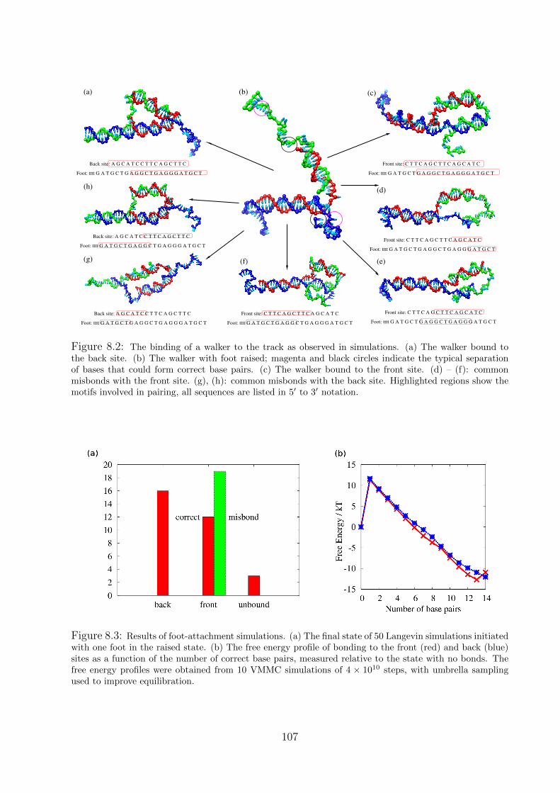
Foot: tttt G A T G C T G A G G C T G A G G G A T G C T
Front site: C T T C A G C T T C A G C A T C
Foot: tttt G A T G C T G A G G C T G A G G G A T G C T
Front site: C T T C A G C T T C A G C A T C
Foot: tttt G A T G C T G A G G C T G A G G G A T G C T
Front site: C T T C A G C T T C A G C A T C
Foot: tttt G A T G C T G A G G C T G A G G G A T G C T
Front site: C T T C A G C T T C A G C A T C
(b) (c)
(d)
(e)
(a)
(f)
(h)
(g)
Back site: A G C A T C C T T C A G C T T C
Foot: tttt G A T G C T G A G G C T G A G G G A T G C T
Back site: A G C A T C C T T C A G C T T C
Foot: tttt G A T G C T G A G G C T G A G G G A T G C T
Back site: A G C A T C C T T C A G C T T C
Foot: tttt G A T G C T G A G G C T G A G G G A T G C T
Figure 8.2: The binding of a walker to the track as observed in simulations. (a) The walker bound tothe back site. (b) The walker with foot raised; magenta and black circles indicate the typical separationof bases that could form correct base pairs. (c) The walker bound to the front site. (d) – (f): commonmisbonds with the front site. (g), (h): common misbonds with the back site. Highlighted regions show themotifs involved in pairing, all sequences are listed in 5′ to 3′ notation.
Figure 8.3: Results of foot-attachment simulations. (a) The final state of 50 Langevin simulations initiatedwith one foot in the raised state. (b) The free energy profile of bonding to the front (red) and back (blue)sites as a function of the number of correct base pairs, measured relative to the state with no bonds. Thefree energy profiles were obtained from 10 VMMC simulations of 4 × 10¹⁰ steps, with umbrella samplingused to improve equilibration.
107

very similar to the non-toehold domain (which itself contains a repeated motif). The most
common (and most stable) misbonds were those shown in Figure 8.2 (d) and (e).
In some simulations, misbonds were displaced by correct bonding to the track. The most
obvious way that this can occur is in an ‘inchworm’ fashion, wherein some correct base pairs
are formed, creating a bulge that is eventually pushed through the misbond, leaving the
correct bonding in place. An intermediate stage of displacing a misbond such as that in
Figure 8.2 (h) is shown in Figure 8.4 (a). For this particular misbond, the displacement
process is facile as correct base pairs can form without disrupting the misbond, acting as a
toehold for displacement. Other misbonds do not provide obvious toeholds, and hence the
rate of displacement is suppressed.
An alternative mechanism exhibited by my model is far less obvious. In this case,
one strand reaches back to form a ‘double-X’ structure, shown in Figure 8.4 (b). There is
no obvious route to fully displace the misbonding from this position, but the misbond is
somewhat destabilized (partially due to the loss of dangling end stabilization) and hence
has a greater tendency to melt than in a normal configuration. If the misbonding melts
before the other half of the structure, displacement has, in effect, taken place. This process
has been observed for the misbonds of type (d) and (g), for which the inchworm form of
displacement is particularly slow. Misbonds of type (f) are reasonably rare, and the only
example of displacement involving this structure caused it to be converted into a type (d)
misbond by a double-X mediated process.
I have also observed displacement wherein the back site displaces a misbond with the
front. This process is similar to normal strand displacement, except it is generally slowed
by pauses at the mismatch locations.
In some other cases, misbonds were observed to detach from the track, allowing the foot
to rebind. Whether through displacement or melting, all misbonded feet would be expected
to find the lower free-energy states of correct bonding eventually.3
3Unbiased VMMC simulations performed at the same temperature demonstrate similar behaviour, sug-gesting that these results are not overly dependent on the details of the simulation technique. Althoughstatistics are fairly poor, the VMMC simulations appear to give a somewhat higher probability of anymisbonds melting before they are displaced – nevertheless, binding through displacement is still observed.
108
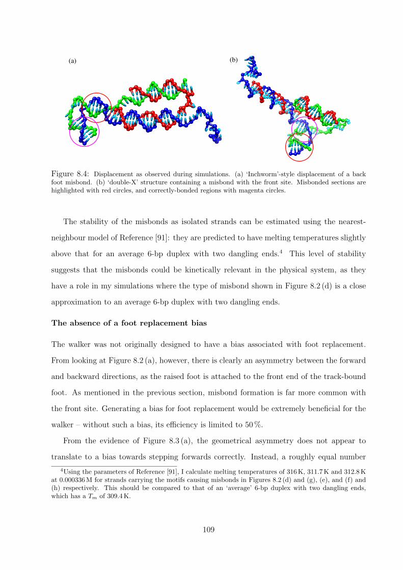
(b)(a)
Figure 8.4: Displacement as observed during simulations. (a) ‘Inchworm’-style displacement of a backfoot misbond. (b) ‘double-X’ structure containing a misbond with the front site. Misbonded sections arehighlighted with red circles, and correctly-bonded regions with magenta circles.
The stability of the misbonds as isolated strands can be estimated using the nearest-
neighbour model of Reference [91]: they are predicted to have melting temperatures slightly
above that for an average 6-bp duplex with two dangling ends.4 This level of stability
suggests that the misbonds could be kinetically relevant in the physical system, as they
have a role in my simulations where the type of misbond shown in Figure 8.2 (d) is a close
approximation to an average 6-bp duplex with two dangling ends.
The absence of a foot replacement bias
The walker was not originally designed to have a bias associated with foot replacement.
From looking at Figure 8.2 (a), however, there is clearly an asymmetry between the forward
and backward directions, as the raised foot is attached to the front end of the track-bound
foot. As mentioned in the previous section, misbond formation is far more common with
the front site. Generating a bias for foot replacement would be extremely beneficial for the
walker – without such a bias, its efficiency is limited to 50 %.
From the evidence of Figure 8.3 (a), the geometrical asymmetry does not appear to
translate to a bias towards stepping forwards correctly. Instead, a roughly equal number
4Using the parameters of Reference [91], I calculate melting temperatures of 316 K, 311.7 K and 312.8 Kat 0.000336 M for strands carrying the motifs causing misbonds in Figures 8.2 (d) and (g), (e), and (f) and(h) respectively. This should be compared to that of an ‘average’ 6-bp duplex with two dangling ends,which has a Tm of 309.4 K.
109

of simulations were observed to be bound correctly in front of or behind the attached foot
at the end of the simulations. Even if all of the simulations that were ended while in a
misbonded state were destined to eventually attach correctly to the front site, the ratio of
forwards to backwards steps would still only be ∼ 2 : 1. It is clear that my model predicts
that any bias associated with foot replacement is minimal.
The lack of an obvious bias was initially surprising, as Figure 8.2 (b) suggests that the
raised foot is inherently closer to the front site. Part of the reason may be the greater
ease with which back misbonds can be converted into correct binding to the back site,
as discussed in the previous section. Many simulations, however, directly formed correct
bonding, and simulations in which misbonding was forbidden provided little evidence of a
substantial bias for stepping forwards.
The flexibility of single strands ensures that this difference in proximity of the front and
back sites is somewhat illusory. In order to form a correct base pair between the front site of
the track and the raised foot, it is necessary for a single-stranded region to stretch across the
length of the 16-bp duplex which links the two feet together – this is decidedly unfavourable
(see Figure 8.2 (b)). By contrast, forming a correct base pair with the back site does not
require such stretching (only the approximate anti-alignment of the walker body and the
track/foot duplex). This visual argument is borne out by the free energy of bonding for the
front and back sites, which indicate only a marginally lower free energy cost for forming the
first few (correct) base pairs with the front site than with the back (Figure 8.3 (b)).
Binding of the feet to a track under tension
In the previous section, it was argued that the asymmetry of the walker did not result in a
large bias for binding correctly to the front site over the back site due to the contractility
of ssDNA. A possible method of overcoming this difficulty, and thereby generating biased
foot replacement, would be to apply a tension to the track. The question of how the walker
behaves on a stretched track is also an interesting problem in its own right, as tracks will
have to be stretched to generate motion in a chosen direction.
110

Figure 8.5: Results of foot-attachment simulations with a tension of 14.6 pN applied to the track. (a)The final state of 50 Langevin simulations initiated with one foot in the raised state. (b) The free energyprofile of bonding to the front (red) and back (blue) sites as a function of the number of correct base pairs,measured relative to the state with no bonds. The free energy profiles were obtained from 10 VMMCsimulations of 4× 10¹⁰ steps, with umbrella sampling used to improve equilibriation.
I performed 50 Langevin simulations of 5 × 10⁹ steps in which the track was subjected
to a constant tension of 14.6 pN, a physically reasonable force to apply to a DNA (enough
to cause significant extension of single strands, as shown in Chapter 5, but not sufficient to
cause overstretching of long duplexes). The results, shown in Figure 8.5 (a), now indicate
a significant (although not overwhelming) preference for stepping forwards (similar results
were obtained using unbiased VMMC and with tracks under half the tension). The majority
of this bias is a result of the increased rate of directly binding to the front site in the correct
manner, as the bases at the end of the track are now automatically stretched into a more
convenient location for binding. Such an explanation is supported by the free energy profiles
of binding under tension shown in Figure 8.5 (b), which show that the result of the force is
to make the formation of the first few correct base pairs with the front site far easier. The
mechanism is further highlighted by considering the probability of having a single correct
base pair with different bases along the track as measured in VMMC umbrella sampling
simulations. The application of tension dramatically increases the weight of being paired to
bases at the far end of the front site (by approximately a factor of 7), whilst barely affecting
the probability of pairing with bases closer to the attached foot, and slightly suppressing
pairing with bases at the far end of the back site.
111

Figure 8.6: Results of foot-attachment simulations with a tension of 14.6 pN applied to a track with sixavailable binding sites. (a) The final state of 50 Langevin simulations initiated with one foot in the raisedstate. (b) A double over-stepped configuration, exhibiting considerable fraying.
Binding to an extended track
If the walker is to be useful, it will have to take many consecutive steps along an extended
track. To test the feasibility of such a process, simulations were performed for 3.5 × 10⁹
steps on a track with seven binding sites (hereafter labelled t–z from back to front), with
one foot initially bound to site w and the other raised. The track was subjected to a
tension of 14.6 pN. The results, shown in Figure 8.6 (a), indicate that the most common
result is binding to site y; a single overstep. This would be a disaster for the walker – when
overstepped, there is no competition between the two feet and hence the lifting of either
foot is strongly suppressed. In this configuration, the walker is essentially stuck.
It is even possible to double overstep, by binding to site z. Such binding, however,
requires considerable stretching and hence walkers bound in this configuration have a ten-
dency for the front foot to fray away from the track (Figure 8.6 (b)). Consequently, the fuel
112

binding site can be revealed and the foot lifted.
Misbonds are also relatively common – generally they are based on the motifs of Figure
8.2 (e) and (f). The extra length of track in these simulations allows the formation of a few
extra base pairs. To form these extra pairs, the duplex must enclose several mismatches or
internal loops. In my model, these structures are stable at 310 K – as discussed in Chapter
6, however, my model generally overestimates the stability of structures involving internal
loops and mismatches relative to Reference [91]. It is therefore probable that these kinetic
traps would be less of an impediment for the actual walker than in my system, although they
may still be kinetically relevant. In particular, the most common misbond in simulations
involves binding to site y in the manner of Figure 8.2 (f), with some additional pairing with
site x. It its likely that the additional pairing would likely be less stable in reality than
in my model – this would open up a toehold for an inchworm-type displacement of the
misbond by correct binding to the y site. No backwards steps were observed in this set of
simulations. However, this is likely to be due to the low statistics, given that backwards
steps were observed for a short track under tension.
Note that the mismatches such as those shown in Figures 8.2 (d) and (g) do not have an
analogue in this larger system – with an extended track, these misbonds constitute partial
correct binding an the adjacent site.
Simulations performed with a tension of 7.3 pN gave similar results. Differences are as
would be expected – binding to site z is more frequent and stable at lower tension, for
example.
8.1.2 Competition between feet
Figure 8.7 (a) shows the free-energy landscape associated with the competition between the
two feet of the walker (attached to the front two sites of a short track). The maximum
number of base pairs for each foot is 20 (that foot has then ‘won’ the competition, and
the toehold on the other foot is raised), and the maximum number of base pairs with the
non-toehold domain is 14. There appears to be only a small free energy difference between
having the front and back foot toeholds raised. Note that when the front foot has lost the
113

Figure 8.7: Free-energy landscapes associated with the competition between toehold domains, obtainedfrom 10 VMMC simulations of 4× 10¹⁰ steps each. (a) With no applied tension. (b) With the track undera tension of 14.6 pN.
competition, it tends to fray as it is not favourable to enclose a mismatch only one base
pair from the end of the duplex.
The important point to note is that there is remarkably little difference between Figure
8.7 (a) and Figure 8.7 (b) (which shows the free-energy landscape for displacement under a
tension of 14.6 pN). The similarity suggests that such a tension should have a limited effect
on the bias of foot-lifting, as the relative exposure of toeholds is virtually unchanged. The
effect of the tension appears to be to differentially influence the transition states of foot-
binding, and hence the probability of binding to the front and back sites, but not the final
states of foot-binding. This is perhaps not surprising, as the bases in the track are essentially
transferred from one duplex to another by competition, and so the track’s extensibility is
similar in both cases.
8.1.3 Fuel binding and displacement
Figure 8.8 (a) shows the free-energy landscape of fuel binding to the feet of a walker (attached
to the front two sites of a short track) without tension. The probability of binding to each
foot is roughly equal, with a slight bias towards the front foot toehold (possibly because when
the front toehold is exposed, it is not constrained by being part of a loop). When bound
to the back foot, displacement can proceed: the free-energy profile for the displacement of
the fuel and release of the foot is shown in Figure 8.8 (b). The steps at 7 and 12 bp between
the track and the foot indicate points at which mismatches are repaired. These mismatches
114

Figure 8.8: Free-energy profiles associated with (a) the binding of fuel to the raised toeholds and (b)the displacement of the track from the back foot by the fuel. Each profile was obtained from 10 VMMCsimulations of steps, performed in a periodic cell of side length 80 reduced units.
give a strong bias favouring displacement, which in this case is likely to be beneficial as the
fuel is unable to displace all the bp between track and foot, and must wait for the final 6 bp
to detach spontaneously.
8.1.4 Lifting of the wrong foot
Bath et al. [65] performed an experiment in which one of the feet had its non-competition
domain mutated so as to be non-complementary with the fuel. The rate of fuel binding was
estimated by addition of a fluorescently-labeled fuel molecule whose signal would increase
upon binding. The signal was observed to increase around 30 times faster when the mutant
foot was the front foot, suggesting that the bias for lifting the back foot was approximately
30:1. For back-foot lifting, the signal was well modeled by a second-order process; the lifting
of the front foot appeared to be more complex.
Two possible mechanisms which could lead to this leak current are:
• The front foot is able to fray from its far end, partially revealing the binding site for
the fuel and allowing displacement.
• The fuel can bind to the toehold of the front foot, and then somehow displace the
front foot from the track using this as a toehold.
115
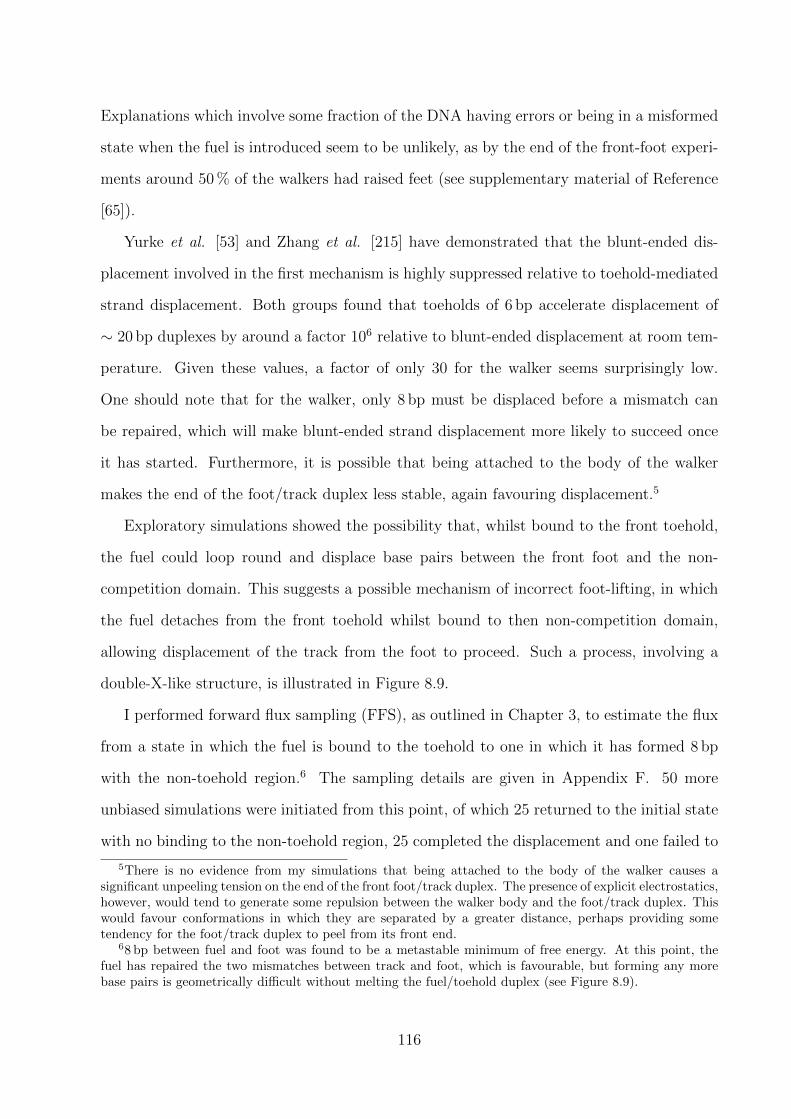
Explanations which involve some fraction of the DNA having errors or being in a misformed
state when the fuel is introduced seem to be unlikely, as by the end of the front-foot experi-
ments around 50 % of the walkers had raised feet (see supplementary material of Reference
[65]).
Yurke et al. [53] and Zhang et al. [215] have demonstrated that the blunt-ended dis-
placement involved in the first mechanism is highly suppressed relative to toehold-mediated
strand displacement. Both groups found that toeholds of 6 bp accelerate displacement of
∼ 20 bp duplexes by around a factor 106 relative to blunt-ended displacement at room tem-
perature. Given these values, a factor of only 30 for the walker seems surprisingly low.
One should note that for the walker, only 8 bp must be displaced before a mismatch can
be repaired, which will make blunt-ended strand displacement more likely to succeed once
it has started. Furthermore, it is possible that being attached to the body of the walker
makes the end of the foot/track duplex less stable, again favouring displacement.5
Exploratory simulations showed the possibility that, whilst bound to the front toehold,
the fuel could loop round and displace base pairs between the front foot and the non-
competition domain. This suggests a possible mechanism of incorrect foot-lifting, in which
the fuel detaches from the front toehold whilst bound to then non-competition domain,
allowing displacement of the track from the foot to proceed. Such a process, involving a
double-X-like structure, is illustrated in Figure 8.9.
I performed forward flux sampling (FFS), as outlined in Chapter 3, to estimate the flux
from a state in which the fuel is bound to the toehold to one in which it has formed 8 bp
with the non-toehold region.6 The sampling details are given in Appendix F. 50 more
unbiased simulations were initiated from this point, of which 25 returned to the initial state
with no binding to the non-toehold region, 25 completed the displacement and one failed to
5There is no evidence from my simulations that being attached to the body of the walker causes asignificant unpeeling tension on the end of the front foot/track duplex. The presence of explicit electrostatics,however, would tend to generate some repulsion between the walker body and the foot/track duplex. Thiswould favour conformations in which they are separated by a greater distance, perhaps providing sometendency for the foot/track duplex to peel from its front end.
68 bp between fuel and foot was found to be a metastable minimum of free energy. At this point, thefuel has repaired the two mismatches between track and foot, which is favourable, but forming any morebase pairs is geometrically difficult without melting the fuel/toehold duplex (see Figure 8.9).
116

(b)
(c)(d)
(a)
Figure 8.9: Postulated mechanism for raising the front foot via displacement. (a) Fuel is bound to raisedfront toehold. (b) Fuel is bound to first three bases of the non-competition domain, having displaced thetrack. Fuel displaces more bases, forming a double-X-like structure. Fuel detaches from toehold, allowingdisplacement to proceed.
do either within the simulation time. I compared the overall flux for displacement to that
for simple dissociation of the fuel from the walker.
The two estimates give a relative flux of 286:1 (error∼ 17.2 %) in favour of simply melting
the fuel/toehold duplex, rather than melting the toehold whilst displacing the track. Thus
∼ 0.35 % of systems with toehold binding to the front foot should displace the track from
the foot rather than simply dettaching.
Thus the model suggests that this mechanism should have a rate of order 300 times
slower than the lifting of the back foot by the fuel. This number should be treated with
great caution – a number of limitations in the model may cause it to be significantly different
for real DNA (for instance, electrostatic effects may suppress the configurations required,
or the extra destabilization of the foot/track duplex due to mismatches may favour the
mechanism). Nonetheless, the model suggests that this mechanism for a leak current is not
completely implausible.
It should be relatively simple to distinguish between the two displacement mechanisms
in experiment. By mutating one or other of the two toehold domains of the front foot, either
process can be effectively prevented from happening. If the leak current is unaffected by
117

the change, the mechanism in question can be eliminated as a cause.
Establishing the dominant cause of lifting the wrong foot is important for optimizing
the walker. In particular, the mechanism analyzed here is strongly favoured by the location
of a mismatch near to the end of the non-toehold domain, which leads to increased fraying
and favours displacement. If this mechanism is discovered to dominate the leak current,
the sequence design could be reconsidered. Furthermore, the pathway explored above is
unlikely to be particularly sensitive to whether the walker is attempting to do work against
a force. Such a force would favour peeling of the front end of the foot/track duplex, and
hence exacerbate the alternative blunt-ended displacement.
8.1.5 Fuel dissociation
In Section 8.1.1, it was assumed that reattachment of the foot occurs after the severed fuel
and nicking enzyme have completely dissociated from the foot. This may not, however, be
the case. One plausible scenario is that one or other of the halves of the fuel, along with
the enzyme, will dissociate first, leaving the other half still attached. What consequences
could the presence of half of the fuel have for reattachment (here, the terms proximal and
distal refer to the proximity of the fuel to the body of the walker – see Figure 8.10 (a)):
• Proximal half of the fuel still attached. In this case, the section of the foot which
would bind to the back site is mostly exposed, whereas the front binding site is largely
inhibited.
• Distal half of the fuel still attached. In this case both binding sites are partially
inhibited by the presence of the fuel.
I have performed exploratory simulations for each of systems with both long and short
tracks under tension in which the walker is initiated with either half of the fuel still attached
to the raised foot. Currently data is limited, but the preliminary findings are given below.
• Proximal half of fuel remaining: misbonds of type (d) and (e) are very common, but
displacement by the correct site is prevented by the presence of the fuel remnant. The
118

fuel segment
(a)
(b)
Figure 8.10: Raised foot with (a) proximal and (b) distal half of fuel attached.
12 available bp with sites v and y mean that the foot often binds in these configurations
(overwhelmingly with y for an extended track). Displacement of the remainder of the
fuel is reasonably facile for site y, but not for v as the other foot blocks displacement
of more than 2 bp. Presumably, however, detachment of the fuel will eventually
occur. Successful binding to site x (involving fuel displacement) has been observed,
but appears to be rare.
• Distal half of fuel remaining: binding to the 8 available bases at the front of the x site
is most probable. Binding to site v appears to be suppressed, although it has been
observed, and binding to site y can also occur. Although no full displacement of the
fuel by site x has been observed in this system to date (a mismatch hampers progress),
the eventual outcome is likely to be that the fuel is displaced by the track, as this will
have a lower free-energy barrier than simply melting the track/foot duplex.
Fully binding to any site on the track requires that the fuel fragment dissociate. This
could occur whilst the foot is raised, which would leave the system in a state identical to
119

that considered in Section 8.1.1. As the fuel remnant/foot duplex should be more stable
than any misbond, it seems likely that misbonded feet will detach from the track before
fuel dissociation, and so misbonds are likely to constitute only a kinetic trap rather than a
pathway to binding.
Partially binding in the correct fashion, however, may lead directly to full binding. In
particular, the track has been seen to displace the fuel from the foot, although such a process
is suppressed by the existence of mismatched bp between the track and foot that are absent
in the fuel/foot duplex. To date, I have only observed displacement of the proximal half
of the fuel by correct binding to site y, but it should be possible in other cases. The only
exception would be when the foot binds to site v with the proximal half of the fuel still
attached. In this case, 12 bp form with the track without displacing the fuel and so full
displacement of more than two base pairs of the fuel is impossible. Nonetheless, one would
expect the partial binding to the track to be more stable than the foot/fuel duplex. It
therefore seems likely that once in this state, the fuel fragment would eventually detach,
allowing complete binding.
Overall, the preliminary simulations seem to suggest that a foot with the proximal
half of the fuel still attached will be more likely to overstep or step backwards than in a
system with no fuel remnant. By contrast, a foot with the distal half of the fuel present
seems to be likely to bind correctly to the site immediately in front of the attached foot,
although overstepping is still possible. It would be beneficial to have greater experimental
characterization of the behaviour of the nicking enzyme, but it seems likely that to preserve
any forward-stepping bias it would be useful to ensure that the proximal half of the fuel
detaches first. This might be achieved by using more AT base pairs in this half of the fuel
strand, or alternatively moving the nicking site so that it is closer to the proximal end of
the fuel.
120

8.2 Discussion
In this chapter I have presented the results of simulations into the operation of a two-footed
DNA walker, the first time a simulation of a system such as this has been attempted. The
model and simulation techniques were able to successfully describe a system this complex,
and several novel predictions were made.
The model suggests that:
• In the original system introduced by Bath et al., if the walker is released from a state
with one foot raised, it can either bind directly to the front or back site, or initially
misbond with the track. Misbonds will eventually melt or be displaced.
• The foot/track duplex can displace incorrect bonding via an ‘inchworm’ mechanism,
or via a novel ‘double-X’ state.
• There is little or no bias for a raised foot to step forwards correctly.
• Applying a tension of around 15 pN to the track favours directly binding with the front
site over the back site, and will tend to bias the walker towards stepping forwards.
• Applying tension has a very small effect on the competition between feet once both
are bound.
• If the track is extended to include multiple binding sites, the most probable result is
a single overstep (even under tension). The singly-overstepped state does not appear
to be particularly susceptible to fraying from the front end (which would encourage
fuel binding), meaning that it would be difficult for the walker to recover from such a
configuration.
• A possible method by which the fuel could lift the front foot has been suggested,
involving initial binding to the raised toehold before reaching back to displace the
track from the foot.
121

• It is plausible that the one or other of the halves of the fuel will remain attached to the
track after the other has detached. Early results suggest that if the half that is closest
to the body of the walker remains, it will strongly inhibit binding to the desired site
(whilst permitting backwards stepping and overstepping). By contrast, if the half of
fuel that is furthest from walker’s body is still present, the bias for stepping forward
seems to be preserved, and overstepping is not strongly favoured compared to the case
with no fuel present.
The majority of these predictions rely primarily on the basic geometrical, thermody-
namic and mechanical properties of DNA, which the model reproduces reasonably well.
In particular, it is difficult to see how the conclusion that overstepping is probable could
be avoided, and similarly the consequences of having half of the fuel still attached seem
physically robust.
The relative probability of reaching correct binding directly or through a displacement-
based pathway is quite sensitive to the rates of different types of binding. The model does,
however, highlight the possibility of previously unexpected binding pathways from a system
with one raised foot (and no fuel attached). Although misbonding is still possible with fuel
fragments present, the pathway to full binding is strongly suppressed.
My model predicts that tension will favour stepping forward primarily by increasing the
rate at which correct pairing will occur with the front site relative to the back site. Note,
however, that tension will also prevent the back site from displacing misbonds that occur
with the front site. As a consequence, tension could increase any bias for stepping forwards
regardless of which pathway (direct binding or via displacement) is more common in reality.
The model’s representation of a mechanism for lifting the front foot indicates that it is
plausible, but the number of factors which contribute to the process mean that it should be
treated with caution.
The ‘double-X’ configuration does not appear to put the DNA under unusual strain, but,
due to the simplicity of the description of the backbone in the model, this predicted dis-
placement mechanism can only be described as plausible. The inchworm method, however,
122

only requires the formation of bulged duplexes, which are known to exist.
The main caveat is that the walker, like the tweezers, often brings duplexes into reason-
ably close proximity. As a consequence, it is possible that electrostatic repulsion may have
a significant role. Duplexes tend to be closest when in the fully bound state. In this case,
electrostatic repulsion may tend to push the body of the walker away from the track, which
would encourage more fraying than is observed in my simulations. Some misbonds also tend
to involve looser, more open structures, and this means that they too might be penalized
less by explicit electrostatics than correct bonding. If this is the case, the displacement route
to correct bonding may be more common than observed in my simulations. Displacement
itself, however, usually involves a higher density of strands (particularly when the double-X
mechanism is involved), and so the effect on the kinetics is not obvious.
It is not easy to see whether electrostatics would penalize the initial states of binding to
either the front or back site more than the other. If so, however, this effect would influence
the bias for binding correctly to the front foot under tension. If electrostatic interactions
jeopardize the performance of the walker, higher salt concentrations could be considered.
8.2.1 Considerations for design modifications
Having studied the walker using my model, several modifications to the design appear to
be sensible. Most importantly, the tendency to overstep must be reduced. One approach
would be to have two distinct toehold domains, two distinct non-toehold domains, and two
fuel strands (see Figure 8.11). This would prevent overstepping by a single site, and would
also have the benefit of suppressing the possible leak current suggested in this work.
The most stable misbonds (ignoring those which correspond to overstepping) arise be-
cause the toehold domain and non-toehold domain have regions of very similar sequence,
and due to a repeated motif in the non-toehold domain. The behaviour of the system could
be simplified by removing this similarity, as direct binding to the correct sites would domi-
nate. It is not clear, however, that such a system would be any more efficient. Furthermore,
if the fuel typically detaches in stages, the role of misbonds as intermediates to correct
binding appears to be reduced. In the original work, the sequence was somewhat limited
123
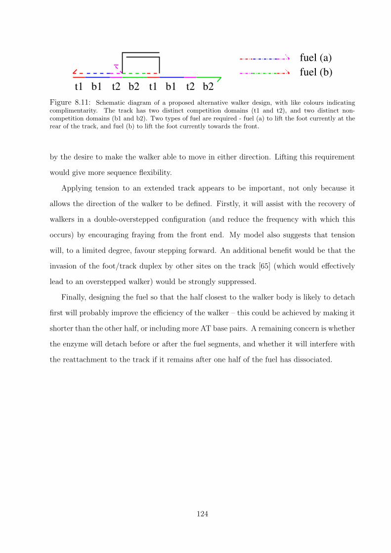
fuel (b)
t1 t2b1 b2 t1 t2b1 b2
fuel (a)
Figure 8.11: Schematic diagram of a proposed alternative walker design, with like colours indicatingcomplimentarity. The track has two distinct competition domains (t1 and t2), and two distinct non-competition domains (b1 and b2). Two types of fuel are required - fuel (a) to lift the foot currently at therear of the track, and fuel (b) to lift the foot currently towards the front.
by the desire to make the walker able to move in either direction. Lifting this requirement
would give more sequence flexibility.
Applying tension to an extended track appears to be important, not only because it
allows the direction of the walker to be defined. Firstly, it will assist with the recovery of
walkers in a double-overstepped configuration (and reduce the frequency with which this
occurs) by encouraging fraying from the front end. My model also suggests that tension
will, to a limited degree, favour stepping forward. An additional benefit would be that the
invasion of the foot/track duplex by other sites on the track [65] (which would effectively
lead to an overstepped walker) would be strongly suppressed.
Finally, designing the fuel so that the half closest to the walker body is likely to detach
first will probably improve the efficiency of the walker – this could be achieved by making it
shorter than the other half, or including more AT base pairs. A remaining concern is whether
the enzyme will detach before or after the fuel segments, and whether it will interfere with
the reattachment to the track if it remains after one half of the fuel has dissociated.
124
Chapter 9
Conclusions
This thesis introduces a novel coarse-grained model of DNA which is specifically designed
to capture the structural, mechanical and thermodynamic properties associated with single-
stranded and duplex DNA, and the transition between the two. The model has been shown
to give a physically reasonable description of a range of DNA properties, and has been
applied to two nanotechnological systems (DNA tweezers and a two-footed DNA walker).
These studies represent the first investigations into dynamic DNA devices using a coarse-
grained model.
Unlike many alternatives in the literature, my model aims to reproduce DNA behaviour
in a manner which is as physically motivated as possible. In particular, the structure of du-
plexes is enforced through the directionality of stacking and hydrogen-bonding interactions,
rather than through backbone constraints. This approach allows for a stacking transition
for single strands (which is absent in the majority of alternative models). Such a transition
allows single strands to be extremely flexible when unstacked, and makes the simulation of
hairpins and more complex motifs possible. To implement directional interactions, it was
found to be important to represent the planarity of bases in the model, another feature that
was novel when the model was introduced.
9.1 Utility of the model
In Chapters 5 and 6, the model’s properties were discussed in great detail. I have shown
that a model which is fairly simple in principle can give a good description of a wide range of
125
DNA properties (a far wider range than has been considered by other authors). Specifically,
my model has been shown to:
• Give an approximate representation of the structure of B-DNA.
• Have a broad, almost uncooperative stacking transition.
• Reproduce the average melting temperatures and transition widths of short duplexes
extremely well (when compared to the SantaLucia parameterization of the two-state
model [91]).
• Give a reasonable representation of the stability of structures involving hairpins,
bulges, mismatches and dangling ends. In particular, the dependence of hairpin sta-
bility on loop and stem size agrees well with Reference [91].
• Quantitatively reproduce the tendency of stacked single strands to be stiffer than
unstacked ssDNA, with duplex DNA seen to be even less flexible.
• Give a good description of the repsonse of duplexes and single strands to tension, and
the response of dsDNA to applied torsion.
Many of the properties mentioned above were used to parameterize the model. Although
it is noteworthy that such a range of features can be described by a model of this kind, to
be really useful, it is important that the model makes predictions that extend beyond its
parameterization (a feature somewhat lacking in the field of coarse-grained DNA modelling
to date). The model reproduces some well-established physical properties of DNA that were
in no way considered in parameterization. For example, the propellor twist of base pairs
arises naturally in the model for the same reason as in real DNA. Similarly, the dependence
of Tm on motif location for duplexes with mismatches was initially surprising, but actually
reflects experimentally reported behaviour.
In addition, the model also makes non-trivial predictions, which are based on sufficiently
generic properties that they should prove robust to the approximations present in my de-
scription of DNA. Below I highlight some of these predictions that may be amenable to
experimental investigation:
126
• The model suggests that at low temperatures, the magnitude of the enthalpy associ-
ated with duplex formation should increase with temperature, as has been observed
experimentally. At high enough temperatures, however, the model predicts that du-
plex fraying will cause this gradient to change sign. Such a feature should be particu-
larly easy to detect for a duplex with a CG-rich core and AT bases towards the ends,
as fraying will be significant close to the melting temperature of the duplex.
• It was found that the strand displacement process during the operation of DNA tweez-
ers was far from flat in free energy, as is generally assumed. In part this was due to
specific features of the system, but a component was due to the unfavourability of
opening up a second single-stranded region when displacement begins, a feature which
should apply to all displacement processes. An initial increase in free energy during
displacement may help to explain the observed dependence of displacement rate on
toehold length, the strength of which is currently difficult to justify [215].
• Simulation of a two-footed walker on a track demonstrated a range of non-trivial be-
haviour. Most significantly, it was found that the current design would typically lead
to overstepping, an extremely undesirable event. The possibility that rebinding may
occur before both halves of the hydrolyzed fuel have detached may also tend to favour
overstepping and stepping backwards. Finally, applying a tension to the track was
shown to improve the probability of stepping forwards, assuming the difficulties men-
tioned above can be overcome. Potential design changes to eliminate these problems
are discussed in Chapter 8.
9.2 Limitations of the model
Any coarse-grained model is a compromise, and my description of DNA certainly neglects or
heavily simplifies many features of potential importance. In particular, the simplistic rep-
resentation of electrostatic interactions is probably the major factor limiting the predictive
power of the model at this stage. This is particularly true for much of nanotechnology, which
127

often involves duplexes being brought into close proximity (DNA origami, for instance, is a
dense array of double helices).
The next most obvious simplification is the limited sequence dependence of model. Fea-
tures such as the tendency of bubbles to form in regions of weaker base-pairing cannot.
therefore, be captured – an average base description has the advantage, however, of not
disguising general trends through sequence-specific effect.
The model’s structural and mechanical description of DNA on the level of one base is
unlikely to be very accurate, as the representation of a nucleotide is necessarily simplistic
and the model is fitted to long length scale properties. In particular, the simplicity of the
backbone interaction between nucleotides may allow structures that in reality are penalized.
Note also that minor and major grooving are absent in the model, asymmetrical groove sizes
being important in determining the stresses involved in DNA origami [59].
9.3 Future work
The most obvious avenues for further work involve improving the current limitations of the
model, by introducing a more physical representation of electrostatics, increased sequence
dependence and exploring the description of DNA mechanics on the level of one base. None
of these goals will be simple to achieve. The electrostatic behavior of DNA is potentially very
complex, particularly for systems which involve divalent cations. In fact, an understanding
of the consequences of electrostatics for the stability of systems like DNA origami would
be interesting in its own right. For instance, it is a puzzle as to why ‘CANDO’ (a package
with no explicit electrostatics) is able to reproduce the structures of complex 3-dimensional
DNA origami [38]. Introducing sequence dependence of all interactions to the model would
result in an enormous number of parameters, which would be difficult to constrain given
the experimental data available (this is particularly true of stacking). The description of
DNA on the level of a single base could potentially be compared to atomistic simulations,
such as those of the Maddocks group [97], which would show which modes of deformation
are too easy or too stiff in my model. It will not necessarily be trivial, however, to deduce
128

which interactions are responsible for the differences between force fields.
Despite the caveats mentioned in the previous section, I believe the model is capable
of providing insight into a range of phenomena as it stands. For example, I am beginning
to investigate the fundamental principles of strand displacement (in a range of scenarios)
and duplex formation under tension, topics which were inspired by the simulations of nan-
otechnology presented in this thesis. Other authors have published work on the pathways
involved in duplex formation [120, 121]: it would be instructive to see if I find similar results,
or whether the results are strongly model-dependent.
Further development of the model, as outlined above, will enable more systems to be
considered, such as DNA origami. From a broader perspective, it would be interesting to
investigate more biological behaviour. In particular, the model could be used to explore how
the forces and torques due to protein binding might induce biologically useful behaviour,
such as gene regulation and the origin of replication in bacteria. Such work would require
collaboration with researchers who study the detailed mechanics of DNA/protein binding
[96]. Another possible extension would be to consider modelling RNA with an approach
similar to that presented in this thesis. Such a model may be of use in predicting the
secondary structure of biologically relevant RNAs, and could also provide information on
the pathways by which these molecules fold to their native state.
129

Bibliography
[1] R. Dahm. Discovering DNA: Friedrich Miescher and the early years of nucleic acid
research. Hum. Genet., 122(6):565–581, 2008.
[2] M. P. Ball. http://en.wikipedia.org/wiki/File:DNA chemical structure.svg
[3] R. Wheeler. http://en.wikipedia.org/wiki/File:A-DNA, B-DNA and Z-DNA.png
[4] G. K. Hunter. Phoebus Levene and the tetranucleotide structure of nucleic acids.
Ambix, 46(2):73–103, 1999.
[5] P. A. Levene. The structure of yeast nucleic acid: IV. ammonia hydrolysis. J. Biol.
Chem., 40(2):415–424, 1919.
[6] F. Griffith. The significance of pneumococcal types. J. Hyg., 27(2):113–159, 1928.
[7] O. T. Avery, C. M. MacCleod, and M. McCarty. Studies on the chemical nature of the
substance inducing transformation of pneumococcal types. J. Exp. Med., 79(2):137–
158, 1944.
[8] S. Neidle. Oxford handbook of nucleic acid structure. Oxford University Press, Oxford,
1999.
[9] R. Franklin and R. G. Gosling. Molecular configuration in sodium thymonucleate.
Nature, 171:738–740, 1953.
[10] E. Chargaff et al.. The composition of the desoxyribonucleic acid of salmon sperm.
J. Biol. Chem., 192(1):223–230, 1951.
130

[11] J. M. Creeth, J. M. Gulland, and D. O. Jordan. Deoxypentose nucleic acids; viscosity
and streaming birefringence of solutions of the sodium salt of the deoxypentose nucleic
acid of calf thymus. J. Chem. Soc., 25:1141–1145, 1947.
[12] W. Saenger. Principles of Nucleic Acid Structure. Springer-Verlag, New York, 1984.
[13] B. Alberts, et al.. Molecular Biology of the Cell, 4th ed. Garland Science, New York,
2002.
[14] P. J. Hagerman. Flexibility of DNA. Annu. Rev. Biophys. Biophys. Chem., 17:265–
286, 1988.
[15] N. R. Kallenbach, R-I. Ma, and N. C. Seeman. An immobile nucleic acid junction
constructed from oligonucleotides. Nature, 305(5937):829–831, 1983.
[16] T. J. Fu and N. C. Seeman. DNA double-crossover molecules. Biochemistry,
32(13):3211, 1993.
[17] H. Yan, et al.. DNA-Templated Self-Assembly of Protein Arrays and Highly Conduc-
tive Nanowires. Science, 301(5641):1882–1884, 2003.
[18] E. Winfree et al.. Design and self-assembly of two-dimensional dna crystals. Nature,
394:539, 1998.
[19] J. Malo, et al.. Engineering a 2D protein-DNA crystal. Angew. Chem. Int. Ed.,
44:3057–3061, 2005.
[20] J. Zheng, et al.. From molecular to macroscopic via the rational design of a self-
assembled 3D DNA crystal. Nature, 461:74, 77 2009.
[21] D. N. Selmi et al.. DNA-templated protein arrays for single-molecule imaging. Nano
Lett., 11(2):657–660, 2011.
[22] J. Chen and N. C. Seeman. Synthesis from DNA of a molecule with the connectivity
of a cube. Nature, 350(6319):631–633, 1991.
131
[23] Y. Zhang and N. C. Seeman. Construction of a DNA-truncated octahedron. J. Am.
Chem. Soc., 116(5):1661, 1994.
[24] R. P. Goodman, et al.. Rapid chiral assembly of rigid DNA building blocks for molec-
ular nanofabrication. Science, 310:1661–1665, December 2005.
[25] C. M. Erben, R. P. Goodman, and A. J. Turberfield. A self-assembled DNA bipyramid.
J. Am. Chem. Soc., 129(22):6992–6993, 2007.
[26] W. M. Shih, J. D. Quispe, and G. F. Joyce. A 1.7-kilobase single-stranded dna that
folds into a nanoscale octahedron. Nature, 427(6975):618–621, 2004.
[27] F. F. Andersen et al.. Assembly and structural analysis of a covalently closed nano-
scale DNA cage. Nucl. Acids Res., 36(4):1113–1119, 2008.
[28] Y. He et al.. Hierarchical self-assembly of DNA into symmetric supramolecular poly-
hedra. Nature, 452:198–201, 2008.
[29] Z. Li et al.. A replicable tetrahedral nanostructure self-assembled from a single DNA
strand. J. Am. Chem. Soc., 131(36):13093–13098, 2009.
[30] P. W. K. Rothemund. Folding DNA to create nanoscale shapes and patterns. Nature,
440(7082):297–302, 2006.
[31] E. S. Andersen et al.. Self-assembly of a nanoscale DNA box with a controllable lid.
Nature, 459:73–76, 2009.
[32] Y. Ke et al.. Scaffolded DNA origami of a DNA tetrahedron molecular container.
Nano Lett., 9(6):2445–2447, 2009.
[33] S. M. Douglas et al.. Self-assembly of DNA into nanoscale three-dimensional shapes.
Nature, 459:414–418, 2009.
[34] H. Dietz, S. M. Douglas, and W. M. Shih. Folding DNA into twisted and curved
nanoscale shapes. Science, 325(5941):725–730, 2009.
132
[35] D. Han et al.. DNA origami with complex curvatures in three-dimensional space.
Science, 332(6027):342–346, 2011.
[36] T. Kato et al. High-resolution structural analysis of a DNA nanostructure by cryoEM
Nano Letters, 7(9):2747-2750, 2009.
[37] S. F. J. Wickham et al.. Direct observation of stepwise movement of a synthetic
molecular transporter. Nat. Nanotechnol., 6:166–169, 2011.
[38] C. Castro and H. Dietz. A DNA origami caliper device for the study of single molecule
conformaronal dynamics. unpublished.
[39] M. J. Berardi et al.. Mitochondrial uncoupling protein 2 structure determined by nmr
molecular fragment searching. Nature, Published online, 2011.
[40] M. Endo et al.. DNA prism structures constructed by folding of multiple rectangular
arms. J. Am. Chem. Soc., 131(43):15570–15571, 2009.
[41] Z. Li et al.. Molecular behavior of DNA origami in higher-order self-assembly. J. Am.
Chem. Soc., 132(38):13545–13552, 2010.
[42] S. Woo and P. W. K. Rothemund. Programmable molecular recognition based on the
geometry of DNA nanostructures. Nature Chem., 3:620–627, 2011.
[43] T. Liedl et al.. Self-assembly of three-dimensional prestressed tensegrity structures
from DNA. Nat. Nanotechnol., 5(7):520–524, 2010.
[44] F. A. Aldaye and H. F. Sleiman. Modular acces to structurally switchable 3D discrete
DNA assemblies. J. Am. Chem. Soc., 129:13376–13377, 2007.
[45] J. Zimmermann et al.. Self-assembly of a DNA dodecahedron from 20 trisoligonu-
cleotides with C(3h) linkers. Angew. Chem. Int. Ed., 47(19):3626–30, 2008.
[46] A. J. Kim, P. L. Biancaniello, and J. C. Crocker. Engineering DNA-mediated colloidal
crystallization. Langmuir, 22(5):1991–2001, 2006.
133

[47] S. H. Ko et al.. Synergistic self-assembly of RNA and DNA molecules. Nature Chem.,
2:1050–1055, 2010.
[48] P. Guo. The emerging field of RNA nanotechnology. Nat. Nanotechnol., 5:833–842,
2010.
[49] M. F. Hagan and D. Chandler. Dynamic pathways for viral capsid assembly. Biophys.
J., 91:42–54, 2006.
[50] A. W. Wilber et al.. Reversible self-assembly of patchy particles into monodisperse
icosahedral clusters. J. Chem. Phys., 127(8):085106, 2007.
[51] T. E. Ouldridge et al.. The self-assembly of DNA Holliday junctions studied with a
minimal model. J. Chem. Phys., 130:065101, 2009.
[52] J. Bath and A. J. Turberfield. DNA nanomachines. Nat. Nanotechnol., 2:275–284,
2007.
[53] B. Yurke and A. Mills. Using DNA to power nanostructures. Genetic Programming
and Evolvable Machines, 4:111–122, 2003.
[54] B. Yurke et al.. A DNA-fueled molecular machine made of DNA. Nature, 406:605–608,
2000.
[55] R. P. Goodman et al.. Reconfigurable, braced, three-dimensional DNA nanostructures.
Nat. Nanotechnol., 3:93–96, 2008.
[56] P. K. Lo et al.. Loading and selective release of cargo in DNA nanotubes with longi-
tudinal variation. Nature Chem., 2:319–328, 2010.
[57] D. Han et al.. Folding and cutting DNA into reconfigurable topological nanostructures.
Nat. Nanotechnol., 5:712–717, 2010.
[58] S. M. Douglas. unpublished.
134

[59] W. B. Sherman and N. C. Seeman. A precisely controlled DNA biped walking device.
Nano Lett., 4(7):1203–1207, 2004.
[60] J-S. Shin and N. A. Pierce. A synthetic DNA walker for molecular transport. J. Am.
Chem. Soc., 126(35):10834–10835, 2004.
[61] J. Bath, S. J. Green, and A. J. Turberfield. A free-running DNA motor powered by a
nicking enzyme. Angew. Chem. Int. Ed., 117(28):4432–4435, 2005.
[62] Y. Tian et al.. A DNAzyme that walks processively and autonomously along a one-
dimensional track. Angew. Chem. Int. Ed., 44(28):4355–4358, 2005.
[63] A. J. Turberfield et al.. DNA fuel for free-running nanomachines. Phys. Rev. Lett.,
90(11):118102–118105, 2003.
[64] T. Omabegho, R. Sha, and N. C. Seeman. A bipedal DNA brownian motor with
coordinated legs. Science, 324:67–71, 2009.
[65] J. Bath et al.. Mechanism for a directional, processive and reversible DNA motor.
Small, 5:1513–1516, 2009.
[66] S. J. Green, J. Bath, and A. J. Turberfield. Coordinated chemoechanical cycles: a
mechanism for autonomous molecular motion. Phys. Rev. Lett., 101(23):238101, 2008.
[67] S. Venkataraman et al.. An autonomous polymerization motor powered by DNA
hybridization. Nat. Nanotechnol., 2:490–494, 2007.
[68] R. A. Muscat, J. Bath, and A. J. Turberfield. A programmable molecular robot. Nano
Lett., 11(3):982–987, 2011.
[69] M. L. McKee et al.. Multistep DNA-templated reactions for the synthesis of functional
sequence controlled oligomers. Angew. Chem. Int. Ed., 49(43):7948–7951, 2010.
[70] H. Gu, J. Chao, S.-J. Xiao, and N. C. Seeman. A proximity-based programmable
DNA nanoscale assembly line. Nature, 465:202–205, 2010.
135
[71] L. M. Adleman. Molecular computation of solutions to combinatorial problems. Sci-
ence, 266(5187):1021–1024, 1994.
[72] S. Tagore et al.. DNA computation: application and perspectives. J. Proteomics
Bioinform., 3:234–343, 2010.
[73] G. Seelig et al.. Enzyme-free nucleic acid logic circuits. Science, 314(5805):1585–1588,
2006.
[74] S. Venkataraman et al.. Selective cell death mediated by small conditional RNAs.
Proc. Natl. Acad. Sci. U.S.A, 107(39):16777–16782, 2010.
[75] T. Liedl and F. C. Simmel. Switching the conformation of a DNA molecule with a
chemical oscillator. Nano Lett., 5(10):1894–1898, 2005.
[76] R. R. Sinden. DNA structure and function. Academic Press Inc., London, 1994.
[77] M. Orozco et al.. Theoretical methods for the simulation of nucleic acids. Chem. Soc.
Rev., 32:350–364, 2003.
[78] R. Lavery et al.. A systematic molecular dynamics study of nearest-neighbor effects
on base pair and base pair step conformations and fluctuations in B-DNA. Nucl. Acids
Res., 38:299–313, 20010.
[79] A. Perez, F. J. Luque, and M. Orozco. Dynamics of B-DNA on the microsecond time
scale. J. Am. Chem. Soc., 129(47):14739–45, 2007.
[80] C. Mura and A. J. McCammon. Molecular dynamics of a κ B DNA element: base
flipping via cross-strand intercalative stacking in a microsecond-scale simulation. Nucl.
Acids Res., 36(15):4941–4955, 2008.
[81] S. Kannan and M. Zacharias. Simulation of DNA double-strand dissociation and for-
mation during replica-exchange molecular dynamics simulations. Phys. Chem. Chem.
Phys., 11:10589–10595, 2009.
136

[82] E. J. Sorin et al.. Insights into nucleic acid conformational dynamics from massively
parallel stochastic simulations. Biophys. J., 85:790–803, 2003.
[83] S. Kannan and M. Zacharias. folding a DNA hairpin loop structurre in explicit solvent
using replica-exchange molecular dynaics simulations. Biophys. J., 93(9):3218–3228,
2007.
[84] D. Swigon. Mathematics of DNA structure, function and interactions, volume 150 of
The IMA volumes on mathematics and its applications, chapter 13, pages 293–320.
Springer, New York, 2009.
[85] W. B. Sherman and N. C. Seeman. Design of minimally strained nucleic acid nan-
otubes. Biophys. J., 90(12):4546 – 4557, 2006.
[86] C. E. Castro et al.. M. Bathe, and H. Dietz. A primer to scaffolded DNA origami.
Nat. Meth., 8:221–229, 2011.
[87] S. Khalid et al.. DNA and lipid bilayers: self-assembly and insertion. Journal of The
Royal Society Interface, 5:241–250, 2008.
[88] J. Corsi et al.. DNA lipoplexes: Formation of the inverse hexagonal phase observed by
coarse-grained molecular dynamics simulation. Langmuir, 26(14):12119–12125, 2010.
[89] D. Poland and H. A. Scheraga. Occurrence of a phase transition in nucleic acid models.
J. Chem. Phys., 45:1464, 1966.
[90] J. SantaLucia, Jr. A unified view of polymer, dumbbell, and oligonucleotide DNA
nearest-neighbor thermodynamics. Proc. Natl. Acad. Sci. U.S.A, 17(95(4)):1460–5,
1998.
[91] J. SantaLucia, Jr. and D. Hicks. The thermodynamics of DNA structural motifs.
Annu. Rev. Biophys. Biomol. Struct., 33:415–40, 2004.
137

[92] R. Everaers, S. Kumar, and C. Simm. Unified description of poly- and oligonucleotide
DNA melting: Nearest-neighbor, poland-sheraga, and lattice models. Phys. Rev. E,
75:041918, 2007.
[93] T. Dauxois, M. Peyrard, and A. R. Bishop. Dynamics and thermodynamics of a
nonlinear model for dna denaturation. Phys. Rev. E, 47(1):684–695, Jan 1993.
[94] M. Barbi et al.. A twist opening model for DNA. J. Biol. Phys., 24:97–114, 1999.
[95] C. Nisoli and A. R. Bishop. Thermomechanics of DNA. arXiv:1101.5182v2, 2011.
[96] N. B. Becker and R. Everaers. DNA nanomechanics: how proteins deform the double
helix. J. Chem. Phys., 130:135102, 2009.
[97] F. Lankas et al.. On the parameterization of rigid basepair models of DNA from
molecular dynamics simulations. Phys. Chem. Chem. Phys., 11:10565–10588, 2009.
[98] M. Paliy, R. Melnik, and B. A. Shapiro. Coarse graining RNA nanostructures for
molecular dynamics simulations. arxiv:1004.2035, 2010.
[99] F. Trovato and V. Tozzini. Supercoiling and local denaturation of plasmids with a
minimalist DNA model. J. Phys. Chem. B, 112(42):13197–13200, 2008.
[100] M. Sayar, B. Avsaroglu, and A. Kabakcıoglu. Twist-writhe partitioning in a coarse-
grained DNA minicircle model. Phys. Rev. E, 81:041916, 2010.
[101] A. Savelyev and G. A. Papoian. Chemically accurate coarse graining of double-
stranded DNA. Proc. Natl. Acad. Sci. U.S.A, 107(47):20340–20345, 2010.
[102] P. D. Dans et al.. A coarse grained model for atomic-detailed DNA simulations with
explicit electrostatics. J. Chem. Theory Comput., 6(5):1711–1725, 2010.
[103] A. Morriss-Andrews, J. Rottler, and S. S. Plotkin. A systematically coarse-grained
model for DNA and its predictions for persistence length, stacking, twist and chirality.
J. Chem. Phys., 132:035105, 2010.
138

[104] K. Voltz et al.. Coarse-grained force field for the nucleosome from self-consistent
multiscaling. J. Comput. Chem., 29(9):1429–1439, 2008.
[105] A. A. Louis. Beware of density dependent pair potentials. J. Phys.: Condens. Matter,
14:9187, 2002.
[106] M. E. Johnson, T. Head-Gordon, and A. A. Louis. Representability problems for
coarse-grained water potentials. J. Chem. Phys., 126:144509, 2007.
[107] C. Hyeon and D. Thirumalai. Mechanical unfolding of RNA hairpins. Proc. Natl.
Acad. Sci. U.S.A., 102(19):6789–6794, 2005.
[108] C. Hyeon and D. Thirumulai. Mechanical unfolding of RNA: from hairpins to struc-
tures with internal multiloops. Biophys. J., 92(3):731–743, 2007.
[109] F. Ding et al.. Ab initio RNA folding by discrete molecular dynamics: From structure
prediction to folding mechanisms. RNA, 14:1164–1173, 2008.
[110] S. Pasquali and P. Derreumaux. HiRE-RNA: A high resolution coarse-grained energy
model for RNA. The Journal of Physical Chemistry B, 114(37):11957–11966, 2010.
[111] A. Dickson et al.. Flow-dependent unfolding and refolding of an RNA by nonequilib-
rium umbrella sampling. arXiv:1104.5180v1, 2011.
[112] K. Drukker, G. Wu, and G. C. Schatz. Model simulations of DNA denaturation
dynamics. J. Chem. Phys., 114(1):579–590, 2001.
[113] M. Sales-Pardo et al.. Mesoscopic modelling fo nucleic acid chain dynamics. Phys.
Rev. E, 71:051902, 2005.
[114] F. W. Starr and F. Sciortino. Model for assembly and gelation of four-armed DNA
dendrimers. J.Phys.: Condens. Matter, 18:L347–L353, 2006.
[115] M. Kenward and K. D. Dorfman. Brownian dynamics simulations of single-stranded
DNA hairpins. J. Chem. Phys., 130:095101, 2009.
139
[116] M. C. Linak and K. Dorfman. Analysis of a DNA simulation model through hairpin
melting experiments. J. Chem. Phys., 133(12):125101–125112, 2010.
[117] S. Niewieczerza l and M. Cieplak. Stretching and twisting of the DNA duplexes in
coarse-grained dynamical models. J. Phys.: Condens. Matter, 21(47):474221, 2009.
[118] T. A. Knotts et al.. A coarse grain model for DNA. J. Chem. Phys., 126(084901),
2007.
[119] F. B. Bombelli et al.. DNA closed nanostructures: A structural and Monte Carlo
simulation study. J. Phys. Chem. B, 112(48):15283, 15294 2008.
[120] E. J. Sambriski, V. Ortiz, and J. J. de Pablo. Sequence effects in the melting and
renaturation of short DNA oligonucleotides: structure and mechanistic pathways.
J.Phys.: Condens. Matter, 21(034105), 2009.
[121] E. J. Sambriski, D. C. Schwartz, and J. J. de Pablo. A mesoscal model of DNA and
its renaturation. Biophys. J., 96:1675–1690, 2009.
[122] T. R. Prytkova et al.. DNA melting in small-molecule-DNA-hybrid dimer structures:
Experimental characterization and coarse-grained molecular dynamics simulations.
The Journal of Physical Chemistry B, 114(8):2627–2634, 2010.
[123] R. C. DeMille, T. E. Cheatham III, and V. Molinero. A coarse-grained model of DNA
with explicit solvation by water and ions. J. Phys. Chem. B, 115(1):132–142, 2011.
[124] V. Ortiz and J. J. de Pablo. Molecular origins of DNA flexibility: Sequence effects on
conformational and mechanical properties. Phys. Rev. Lett., 106(23):238107–238110,
2011.
[125] J. C. Araque, A. Z. Panagiotopoulos, and M. A. Robert. Lattice model of oligonu-
cleotide hybridization in solution. i. Model and thermodynamics. J. Chem. Phys.,
134(16):165103–165116, 2011.
140

[126] T. J. Schmitt and T. A. Knotts IV. Thermodynamics of DNA hybridization on
surfaces. J. Chem. Phys., 134(205105-113), 2011.
[127] M. J. Hoefert, E. J. Sambriski, and J. J. de Pablo. Molecular pathways in DNA-DNA
hybridization of surface-bound oligonucleotides. Soft Matter, 7:560–566, 2011.
[128] S. Pitchiaya and Y. Krishnan. First blueprint, now bricks: DNA as construction
material on the nanoscale. Chem. Soc. Rev., 35:1111–1121, 2006.
[129] M. C. Murphy et al.. Probing single-stranded DNA conformational flexibility using
flourescence spectroscopy. Biophys. J., 86:2530–2537, 2004.
[130] J. Bois et al.. Topological constraints in nucleic acid hybridization kinetics. Nucl.
Acids Res., 33(13):4090–4095, 2005.
[131] S. A. Harris, C. A. Laughton, and T. B. Liverpool. Mapping the phase diagram of
the writhe of DNA nanocircles using atomistic molecular dynamics simulations. Nucl.
Acids Res., 36(1):21–29, 2008.
[132] S. Whitelam et al.. The role of collective motion in examples of coarsening and self-
assembly. Soft Matter, 5(6):1521–1262, 2009.
[133] M. Swart et al.. π–π stacking tackled with density functional theory. J. Mol. Model.,
13(12):1245–1257, 2007.
[134] J. Sponer et al.. Nature of base stacking: Reference quantum-chemical stacking ener-
gies in ten unique B-DNA base-pair steps. Chem. Eur. J., 12(10):2854–2865, 2006.
[135] N. Peyret. Prediction of nucleic acid hybridization: parameters and algorithms. PhD
thesis, Wayne State University, 2000.
[136] D. V. Pyshnyi and E. M. Ivanova. Thermodynamic parameters of coaxial stacking on
stacking hybridization of oligodeoxyribonucleotides. Russ. Chem. B+, 51:1145–1155,
2002.
141

[137] D. V. Pyshnyi and E. M. Ivanova. The influence of nearest neighbors on the efficiency
of coaxial stacking at contiguous stacking hybridization of oligodeoxyribonucleotides.
Nucleos. Nucleot. Nucl., 23(6-7):1057–1064, 2004.
[138] M. J. Lane et al.. The thermodynamic advantage of DNA oligonucleotide ‘stacking hy-
bridization’ reactions: Energetics of a DNA nick. Nucl. Acids Res., 25(3):611–616, 1997.
[139] V. A. Vasiliskov, D. V. Prokopenko, and A. D. Mirzabekov. Parallel multiplex ther-
modynamic analysis of coaxial base stacking in DNA duplexes by oligodeoxyribonu-
cleotide microchips. Nucl. Acids Res., 29(11):2303–2313, 2001.
[140] J. A. Holbrook et al.. Enthalpy and heat capacity changes for formation of an
oligomeric DNA duplex: Interpretation in terms of coupled processes of formation
and association of single-stranded helices. Biochemistry, 38(26):8409–8422, 1999.
[141] N. Peyret et al.. Nearest-neighbour thermodynamics and NMR of DNA sequences
with internal AA, CC, GG and TT mismatches. Biochemistry, 38:3468–3477, 1999.
[142] E. Protozanova, P. Yakovchuk, and M. D. Frank-Kamenetskii. Stacked-unstacked
equilibrium at the nick site of DNA. J. Mol. Biol., 342(3):775 – 785, 2004.
[143] P. Yakovchuk, E. Protozanova, and M. D. Frank-Kamenetskii. Base-stacking and
base-pairing contributions into thermal stability of the dna double helix. Nucl. Acids
Res., 34(2):564–574, 2006.
[144] K. M. Guckan et al.. Factors contributing to aromatic stacking in water: evaluation
in the context of DNA. J. Am. Chem. Soc., 122(10):2213–2222, 2000.
[145] K. Huang. Statistical Mechanics, Second Edition. John Wiley & Sons, Inc., New York,
1987.
[146] N. Metropolis et al.. Equation of state calculation by fast computing machines. J.
Chem. Phys., 21(6):1087–1092, 1953.
142
[147] A. W. Wilber, J. P. K. Doye, and A. A. Louis. Self-assembly of monodisperse clusters:
dependence on target geometry. J. Chem. Phys., 131:175101, 2009.
[148] I. G. Johnston, A. A. Louis, and J. P. K. Doye. Modelling the self-assembly of virus
capsids. J. Phys.: Condens. Matter, 22(10):104101, 2010.
[149] S. Whitelam and P. L. Geissler. Avoiding unphysical kinetic traps in Monte Carlo
simulations of strongly attractive particles. J. Chem. Phys., 127:154101, 2007.
[150] E. Luijten. Fluid simulation with the geometric cluster monte carlo algorithm. Com-
puting in Science & Engineering, 8(2):20–29, 2006.
[151] A. Bhattacharyay and A. Troisi. Self-assembly of sparsely distributed molecules: An
efficient cluster algorithm. Chem. Phys. Lett., 458(1-3):210 – 213, 2008.
[152] N. G. Van Kampen. Stochastic processes in physics and chemistry. Elsevier, Amster-
dam, 2007.
[153] R. L. Davidchack, R. Handel, and M. V. Tretyakov. Langevin thermostat for rigid
body dynamics. J. Chem. Phys., 130(23):234101, 2009.
[154] P. Depa, C. Chen, and J. K. Maranas. Why are coarse-grained force fields too fast?
a look at dynamics of four coarse-grained polymers. J. Chem. Phys., 134(1):014903,
2011.
[155] M. Doi and S. F. Edwards. The theory of polymer dynamics. Oxford University Press,
Oxford, 1986.
[156] G. M Torrie and J. P. Valleau. Nonphysical sampling distributions in monte carlo
free-energy estimation: Umbrella sampling. J. Comp. Phys., 23:187–199, 1977.
[157] S. Kumar et al.. The weighted histogram analysis method for free-energy calculations
on biomolecules. i. the method. J. Comput. Chem., 13(8):1011–1021, 1992.
143
[158] R. J. Allen, P. B. Warren, and P. R. ten Wolde. Sampling rare switching events in
biochemical networks. Phys. Rev. Lett., 94(1):018104, 2005.
[159] R. J. Allen, C. Valeriani, and P. R. ten Wolde. Forward flux sampling for rare event
simulations. J. Phys.: Condens. Matter, 21(46):463102, 2009.
[160] M. K. Gilson and H. Zhou. Calculation of protein-ligand binding affinities. Annu.
Rev. Biophys. Biomol. Struct., 36:21–42, 2007.
[161] P. Chen and C. M. Li. Nanopore unstacking of single-stranded DNA helices. Small,
3(7):1204–1208, 2007.
[162] C. R. Calladine et al.. Understanding DNA. Elsevier Academic Press, London, 2004.
[163] C. R. Cantor and P. R. Schimmel. Biophysical Chemistry part III: The behaviour of
biological macromolecules. Freeman, San Francisco, 1980.
[164] M. Rubinstein and R. H. Colby. Polymer physics. Oxford University Press, New York,
2003.
[165] C. G. Baumann et al.. Ionic effects on the elasticity of single DNA molecules. Proc.
Natl. Acad. Sci. USA, 94:6185–6190, 1997.
[166] D. M. Crothers et al.. DNA bending, flexibility and helical repeat by cyclization
kinetics. Methods Enzymol., 212:3–29, 1992.
[167] M. Vologodskaia and A. Vologodskii. Contribution of the intrinsic curvature to mea-
sured DNA persistence length. J. Mol. Biol., 317(2):205 – 213, 2002.
[168] B. S. Fujimoto, G. P. Brewood, and J. M. Schurr. Torsional rididity of wakly strainded
DNAs. Biophys. J., 91(11):4166–4179, 2006.
[169] Z. Bryant et al.. Structural transitions and elasticity from torque measurements on
DNA. Nature, 424(6946):338–341, 2003.
144

[170] M. D. Wang et al.. Stretching dna with optical tweezers. Biophys. J., 72(3):1335 –
1346, 1997.
[171] J. R. Wenner et al.. Salt dependence of the elasticity and overstretching transition of
single DNA molecules. Biophys. J., 82(6):3160 – 3169, 2002.
[172] S. B. Smith, Y. Cui, and C. Bustamante. Overstretching B-DNA: the elastic re-
sponse of individual double-stranded and single-stranded DNA molecules. Science,
271(5250):795–799, 1996.
[173] P. Gross, N. Laurens, and L. B. Oddershede. Quantifying how DNA stretches, melts
and changes twist under tension. Nat. Phys., published online, 2011.
[174] T. Odijk. Stiff chains and filaments under tension. Macromolecules,28(20):7016-7018,
1995.
[175] J. Gore et al.. DNA overwinds when stretched. Nature, 442:836–839, 2006.
[176] T. Lionnet et al.. Wringing out DNA. Phys. Rev. Lett., 96(17):178102, 2006.
[177] J. B. Mills, E. Vacano, and P. J. Hagerman. Flexibility of single-stranded DNA: use of
gapped duplex helices to determine the persistence lengths of Poly(dT) and Poly(dA).
J. Mol. Biol., 285(1):245–257, 1999.
[178] Y. Seol et al.. Stretching of homopolymeric RNA reveals single-stranded helices and
base-stacking. Phys. Rev. Lett., 98(15):158103, 2007.
[179] C. Rivetti, C. Walker, and C. Bustamante. Polymer chain statistics and conforma-
tional analysis of DNA molecules with bends or sections of different flexibility. J. Mol.
Biol., 280:41–59, 1998.
[180] M.-N. Dessinges et al.. Stretching single stranded DNA, a model polyelectrolyte. Phys.
Rev. Lett., 89(24):248102, 2002.
145

[181] Y. Seol, G. M. Skinner, and K. Visscher. Elastic properties of a single-stranded charged
homopolymeric ribonucleotide. Phys. Rev. Lett., 93(11):118102, 2004.
[182] G. Mishra, D. Giri, and S. Kumar. Stretching of a single-stranded DNA: Evidence for
structural transition. Phys. Rev. E, 79(3):031930, 2009.
[183] W.-S. Chen et al.. Direct observation of multiple pathways of single-stranded DNA
stretching. Phys. Rev. Lett., 105(21):218104, 2010.
[184] G. Vesnaver and K. J. Breslauer. The contribution of DNA single-stranded order to
the thermodynamics of duplex formation. Proc. Natl. Acad. Sci. U.S.A, 88:3569–3573,
1991.
[185] M. Leng and G. Felsenfeld. A study of polyadenylic acid at neutral ph. J. Mol. Biol.,
15(2):455 – 466, 1966.
[186] R. M. Epand and H. A. Scheraga. Enthalpy of stacking in single-stranded polyriboad-
enylic acid. J. Am. Chem. Soc., 89(15):3888–3892, 1967.
[187] D. Porschke. The nature of stacking interactions in polynucleotides. molecular states
in oligo- and polyribocytidylic acids by relaxation analysis. Biochemistry, 15(7):1495–
1499, 1976.
[188] S. M. Freier et al.. Solvent effects on the kinetics and thermodynamics of stacking in
poly(cyticylic acid). Biochemistry, 20:1419–1426, 1981.
[189] C. S. M. Olsthoorn et al.. Circular dichroism study of stacking properties of
oligodeoxyadenylates and polydeoxyadenylate. Eur. J. Biochem., 115(2):309–321,
1981.
[190] J. Zhou et al.. Conformational changes in single-strand DNA as a function of tem-
perature by SANS. Biophys. J., 90(2):544 – 551, 2006.
[191] P. J. Mikulecky and A. L. Feig. Heat capacity changes associated with nucleic acid
folding. Biopolymers, 82(1):38–58, 2006.
146

[192] J. Applequist and V. Damle. Thermodynamics of the one-stranded helix-coil equilib-
rium in polyadenylic acid. J. Am. Chem. Soc., 88(17):3895–3900, 1966.
[193] I. Jelesarov et al.. The energetics of HMG box interactions with DNA: thermodynamic
description of the target dna duplexes. J. Mol. Biol., 294(4):981 – 995, 1999.
[194] J. Norberg and L. Nilsson. Potential of mean force calculations of the stacking-
unstacking process in single-stranded deoxyribodinucleoside monophosphates. Bio-
phys. J., 69(6):2277 – 2285, 1995.
[195] S. Sen and L. Nilsson. MD simulations of homomorphous PNA, DNA, and RNA
single strands: characterization and comparison of conformations and dynamics. J.
Am. Chem. Soc., 123(30):7414–7422, 2001.
[196] J. M. Martınez, S. K. C. Elmroth, and L. Kloo. Influence of sodium ions on the
dynamics and structure of single-stranded DNA oligomers: A molecular dynamics
study. J. Am. Chem. Soc., 123(49):12279–12289, 2001.
[197] S. Tonzani and G. C. Schatz. Electronic excitations and spectra in single-stranded
DNA. Journal of the American Chemical Society, 130(24):7607–7612, 2008.
[198] O.-S. Lee and G. C. Schatz. Interaction between DNAs on a gold surface. The Journal
of Physical Chemistry C, 113(36):15941–15947, 2009.
[199] D. Poland and H. A. Scheraga. Theory of Helix-Coil Transitions in Biopolymers: Sta-
tistical Mechanical Theory of Order-disorder Transitions in Biological Macromolecules.
Academic Press, New York, 1970.
[200] R. D. Blake and S. G. Delcourt. Thermal stability of DNA. Nucl. Acids Res.,
26(14):3323–3332, 1998.
[201] M. D. Frank-Kamenetskii. Simplification of the empirical relationship between melting
temperature of DNA, its GC content and concentration of sodium ions in solution.
Biopolymers, 10:2623–2624, 1971.
147

[202] D. Andreatta et al.. Ultrafast dynamics in DNA: Fraying at the end of the helix. J.
Am. Chem. Soc., 128(21):6885–6892, 2006.
[203] S. Nonin, J.-L. Leroy, and M. Gueron. Terminal base pairs of oligodeoxynucleotides:
Imino proton exchange and fraying. Biochemistry, 34(33):10652–10659, 1995.
[204] D. J. Patel and C. W. Hilbers. Proton nuclear magnetic resonance investigations
of fraying in double-stranded d-ApTpGpCpApT in aqueous solution. Biochemistry,
14(12):2651–2656, 1975.
[205] A. Tikhomirova, N. Taulier, and T. V. Chalikian. Energetics of nucleic acid stability:
The effect of ∆CP . J. Am. Chem. Soc., 126(50):16387–16394, 2004.
[206] T. E. Ouldridge, A. A. Louis, and J. P. K. Doye. DNA nanotweezers studied with a
coarse-grained model of DNA. Phys. Rev. Lett., 104:178101, 2010.
[207] D. K. Hendrix, S. E. Brenner, and S. R. Holbrook. RNA structural motifs: building
blocks of a modular biomolecule. Q. Rev. Biophys., 38(03):221–243, 2005.
[208] S. Kuznetsov et al.. A semiflexible polymer model applied to loop formation in DNA
hairpins. Biophys. J., 81:2864–2875, 2001.
[209] Y. You et al.. Design of LNA probes that improve mismatch discrimination. Nucl.
Acids Res., 34(8):e60, 2006.
[210] T. Naiser et al.. Position dependent mismatch discrimination on DNA microarrays -
experiments and model. BMC Bioinformatics, 9(1):509, 2008.
[211] R. A. Dimitrov and M. Zuker. Predictio of hybridization and melting for double-
stranded nucleic acids. Biophys. J., 87:215–226, 2004.
[212] N. R. Markham and M. Zuker. DINAMelt web server for nucleic acid meting predic-
tion. Nucl. Acids Res., 33:W577–W581, 2005.
148

[213] T. E. Ouldridge, A. A. Louis, and J. P. K. Doye. Structural, mechanical and thermody-
namic properties of a coarse-grained model of DNA. J. Chem. Phys., 134:085101, 2011.
[214] B. L. Welch. The generalization of ‘student’s’ problem when several different popula-
tion variances are involved. Biometrika, 34(1-2):28–35, 1947.
[215] D.Y. Zhang and E. Winfree. Control of DNA strand displacement kinetics using
toehold exchange. J. Am. Chem. Soc., 131(47):17303–17314, 2009.
[216] B. K. Muller et al.. Single-pair fret characterization of DNA tweezers. Nano Letters,
6(12):2814–2820, 2006.
[217] D.C Rapaport. Molecular dynamics simulation using quaternions. J. Comp. Phys.,
60(2):306 – 314, 1985.
[218] T. F. Miller III et al.. Symplectic quaternion scheme for biophysical molecular dy-
namics. J. Chem. Phys., 116(20):8649–8659, 2002.
[219] D. C. Rapaport. Role of reversibility in viral capsid growth: A paradigm for self-
assembly. Phys. Rev. Lett., 101(186101), 2008.
[220] H. D. Nguyen, V. S. Reddy, and C. L. Brooks. Deciphering the kinetic mechanism of
spontaneous self-assembly of icosahedral capsids. Nano Lett., 7(2):338–344, 2007.
[221] A. W. Wilber et al.. Monodisperse self-assembly in a model with protein-like interac-
tions. J. Chem. Phys., 131(175102), 2009.
[222] G. Villar et al.. The self-assembly and evolution of homomeric protein complexes.
Phys. Rev. Lett., 102:118106, 2009.
[223] R. Schwartz et al.. Local rules simulation of the kinetics of virus capsid self-assembly.
Biophys. J., 75(6):2626–2636, 1998.
[224] T. E. Ouldridge, A. A. Louis, and J. P. K. Doye. Extracting bulk properties of
self-assembling systems from small simulations. J. Phys.:Condens. Matter,22:104102,
2010.
149

[225] D. Frenkel and B. Smit. Understanding Molecular Simulation. Academic Press Inc.
London, 2001.
[226] I. Kusaka, Z.-G. Wang, and J. H. Seinfeld. Direct evaluation of the equilibrium
distribution of physical clusters by a grand canonical Monte Carlo simulation. J.
Chem. Phys., 108(9):3416–3423, 1998.
[227] P. G. Bolhuis and D. Frenkel. Microscopic and mesoscopic simulation of entropic
micelles. Physica A, 244(1-4):45 – 58, 1997.
[228] I. Kusaka and D. W. Oxtoby. A Monte Carlo simulation of nucleation in am-
phiphilic solution simulation of nucleation in amphiphilic solution. J. Chem. Phys.,
115(10):4883–4889, 2001.
[229] R. Pool and P. G. Bolhuis. Accurate free energies of micelle formation. J. Phys. Chem.
B, 109(12):6650–6657, 2005.
[230] S. H. Kim and W. H. Jo. A Monte Carlo simulation for the micellization of ABA- and
BAB-type triblock copolymers in a selective solvent. Macromolecules, 34(20):7210–
7218, 2001.
[231] M. A. Floriano, E. Caponetti, and A. Z. Panagiotopoulos. Micellization in model
surfactant systems. Langmuir, 15:3143–3151, 1999.
[232] A. Z. Panagiotopoulos, M. A. Floriano, and S. K. Kumar. Micellization and phase
separation of diblock and triblock model surfactants. Langmuir, 18:2940–2948, 2002.
[233] I. Kusaka and D. W. Oxtoby. Identifying physical clusters in vapor phase nucleation.
J. Chem. Phys., 110(11):5249–5261, 1999.
[234] H. Reiss, Y. Djikaev, and R. K. Bowles. On a debate over the simulation and mapping
of physical clusters in small cells. J. Chem. Phys., 117(2):557–566, 2002.
[235] A. J. Williamson et al.. Templated self-assembly of patchy particles. Soft Matter,
7:3423–3431, 2011.
150

Appendix A
Representing forces and torques usingquaternions
Langevin simulations in this work were performed using an algorithm which requires a
quaternion representation of rigid body orientation [153]. The details of quaternion dy-
namics are discussed in Appendix B – here I present the forms of the derivatives which are
required by the algorithm.
A.1 Nucleotide Description
Any set of coordinates that are used to construct the potential must specify the position
and orientation of each nucleotide. Firstly, position can be specified by a vector r which
gives the location of the centre of mass of a nucleotide. Associated with each nucleotide
there is also a unit vector which indicates the direction of the base sites from the backbone
site (b) and a unit vector giving the normal to the plane of the base (n). When represented
in the space-fixed frame, call them bs and ns, and in a body-fixed frame bb and nb. Define
the body-fixed frame such that bbi = δi,1 and nbi = δi,3. The vectors can be mapped between
frames using the rotation matrix:
xs(t) = AT (t)xb. (A.1)
The rotation matrix A gives the orientation of the rigid body in the space-fixed frame. A
possesses only three independent degrees of freedom, and so can be uniquely specified by a
four-dimensional unit vector. Defining a quaternion q = (q0, q1, q2, q3), any rotation matrix
151

can be constructed via:
A =
q20 + q2
1 − q22 − q2
3 2(q1q2 + q0q3) 2(q1q3 − q0q2)2(q1q2 − q0q3) q2
0 − q21 + q2
2 − q23 2(q2q3 + q0q1)
2(q1q3 + q0q2) 2(q2q3 − q0q1) q20 − q2
1 − q22 + q2
3
, (A.2)
with∑
i q2i = 1. An explicit discussion of the relationship between q and the Euler angles of
a rotation is given in Reference [217]. The quaternion q is then a convenient representation
of the orientation of the nucleotide. Using the quaternion representation of orientation:
• Backbone-base orientation:
bs = AT (t)bb =
q20 + q2
1 − q22 − q2
3
2(q1q2 + q0q3)2(q1q3 − q0q2)
. (A.3)
• Normal orientation:
ns = AT (t)nb =
2(q1q3 + q0q2)2(q2q3 − q0q1)
(q20 − q2
1 − q22 + q2
3)
. (A.4)
• Third axis (defined by n× b, useful for the chiral term of stacking):
ys = AT (t)yb =
2(q1q2 − q0q3)q2
0 − q21 + q2
2 − q23
2(q2q3 + q0q1)
. (A.5)
• Interaction site position:
rX = r + dXAT (t)bb = r + dX
q20 + q2
1 − q22 − q2
3
2(q1q2 + q0q3)2(q1q3 − q0q2)
, (A.6)
where dx is the distance of the interaction site x from the centre of mass along the b
direction.
A.2 Derivatives
The potential of the model is described in Chapter 2. As outlined in Appendix B, derivatives
with respect to the centre of mass position and quaternion of each nucleotide are required
to perform Langevin simulations. The potential is a sum over pairwise interactions, and for
each interaction one must differentiate the potential with respect to the position vector and
orientation quaternion for both nucleotides involved.
152

For a nearest-neighbour interaction:
∇q,rVneighbour =
dVFENE(δrbackbone)dδrbackbone
∇q,r(δrbackbone) +∑
x,y?df3(δrxy)
dδrxy∇q,r(δrxy)
+ Vstack
f1(δrstack)df1(δrstack)dδrstack
∇q,r(δrstack) +∑
i=4,5′,6′Vstack
f4(θi)df4(θi)dθi∇q,r(θi)
+ Vstack
f5(cos(φ1))df5(cos(φ1))d cos(φ1)
∇q,r(cos(φ1))
+ Vstack
f5(cos(φ2))df5(cos(φ2))d cos(φ2)
∇q,r(cos(φ2)),
(A.7)
where the sum over x, y? means all combinations of repulsion centres except for the two
backbone sites. For non-neighbouring nucleotides,
∇q,rVnon−neighbour =
∑x,y
df3(δrxy)
dδrx,y∇q,r(δrxy) + VHB
f1(δrHB)df1(δrHB)dδrHB
∇q,r(δrHB)
+∑
i=1−4,7,8VHB
f4(θi)df4(θi)dθi∇q,r(θi)
+Vcross stack
f2(δrHB)df2(δrHB)dδrHB
∇q,r(δrHB) +∑3
i=1Vcross stack
f4(θi)df4(θi)dθi∇q,r(θi)
+∑
i=1,7,8Vcross stack
f4(θi)+f4(π−θi)d(f4(θi)+f4(π−θi)
dθi∇q,r(θi)
+ Vcoax stack
f2(δrstack)df2(δrstack)dδrstack
∇q,r(δrstack) + Vcoax stack
f4(θ4)df4(θ4)dθ4∇q,r(θ4)
+ Vcoax stack
f4(θ1)+f4(2π−θ1)d(f4(θ1)+f4(2π−θ1)
dθ1∇q,r(θ1)
+∑6
i=5Vcoax stack
f4(θi)+f4(π−θi)d(f4(θi)+f4(π−θi)
dθi∇q,r(θi)
+∑4
i=3Vcoax stack
f4(cos(φi))df4(cos(φi))d cos(φi)
∇q,r cos(φi),
(A.8)
where in this case the sum over x, y means all combinations of repulsion centres of the two
nucleotides. For each instance of an interaction, the parameters such as strength and cutoffs
are constant and so they have been suppressed in the equations above.
A.2.1 Derivatives of functional forms
Equations A.7 and A.8 contain derivatives of the functional forms VFENE and fi with respect
to their arguments, which are generally angles or distances. These are given by:
dVFENE(r)
dr=
ε(r − r0)
∆2 − (r − r0)2. (A.9)
153
See errata at end of document.

df1(r)
dr=
2εa exp(−(r − r0)a)(1− exp(−(r − r0)a) if rlow < r < rhigh,
2εblow(r − rc,low), if rc,low < r < rlow,
2εbhigh(r − rc,high) if rhigh < r < rc,high,
0 otherwise.
(A.10)
df2(r)
dr=
k(r − r0) if rlow < r < rhigh,
2kblow(r − rc,low), if rc,low < r < rlow,
2kbhigh(r − rc,high) if rhigh < r < rc,high,
0 otherwise.
(A.11)
df3(r)
dr=
4εσ
(6(σr
)7 − 12(σr
)13)
if r < r?,
2εb(r − rc) if r? < r < rc,
0 otherwise.
(A.12)
df4(θ)
dθ=
−2a(θ − θ0) if θ0 −∆θ? < θ < θ0 + ∆θ?,
2b(θ − (θ0 −∆θc)) if θ0 −∆θc < θ < θ0 −∆θ?,
2b(θ − (θ0 + ∆θc)) if θ0 + ∆θ? < θ < θ0 + ∆θc,
0 otherwise.
(A.13)
df5(cos(φ))
d cos(φ)=
−2a cos(φ) if cos(φ)? < cos(φ) < 0,
2b(cos(φ)− cos(φ)c) if cos(φ)c < cos(φ) < cos(φ)?,
0 otherwise.
(A.14)
A.2.2 Derivatives with respect to the coordinates
The somewhat clumsy definitions of angles in Chapter 2 are now extremely useful, as it
is natural to consider one nucleotide as being influenced by another when calculating the
force or torque. Label the nucleotide for which the force or torque is being calculated as α,
and its partner as β. Define δrxy to be the vector to the interaction site x on α from site
y on β. Let δr be a normalized vector, and let b, n and y represent the orientation of β.
θ2, θ5, θ7, φ1 and φ3 involve angles with respect to the orientation of α, and θ3, θ6, θ8, φ2
and φ4 to involve angles with the orientation of β. The stacking interaction is intentionally
asymmetric with respect to the 3′ to 5′ direction for neighbouring nucleotides. The result
is that ∇r,q(θ5′), ∇r,q(θ6′), ∇r,q(cos(φ1)) and ∇r,q(cos(φ2)) all have a sign that depends on
whether α is in the 5′ direction of β: if it is, then the first option is taken, if not, then the
alternative.
154
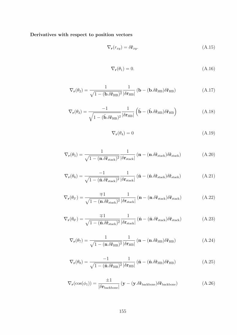
Derivatives with respect to position vectors
∇r(rxy) = δrxy. (A.15)
∇r(θ1) = 0. (A.16)
∇r(θ2) =1√
1− (b.δrHB)2
1
|δrHB|(b− (b.δrHB)δrHB) (A.17)
∇r(θ3) =−1√
1− (b.δrHB)2
1
|δrHB|
(b− (b.δrHB)δrHB
)(A.18)
∇r(θ4) = 0 (A.19)
∇r(θ5) =1√
1− (n.δrstack)2
1
|δrstack|(n− (n.δrstack)δrstack) (A.20)
∇r(θ6) =−1√
1− (n.δrstack)2
1
|δrstack|(n− (n.δrstack)δrstack) (A.21)
∇r(θ5′) =∓1√
1− (n.δrstack)2
1
|δrstack|(n− (n.δrstack)δrstack) (A.22)
∇r(θ6′) =∓1√
1− (n.δrstack)2
1
|δrstack|(n− (n.δrstack)δrstack) (A.23)
∇r(θ7) =1√
1− (n.δrHB)2
1
|δrHB|(n− (n.δrHB)δrHB) (A.24)
∇r(θ8) =−1√
1− (n.δrHB)2
1
|δrHB|(n− (n.δrHB)δrHB) (A.25)
∇r(cos(φ1)) =±1
|δrbackbone|(y − (y.δrbackbone)δrbackbone) (A.26)
155

∇r(cos(φ2)) =±1
|δrbackbone|(y − (y.δrbackbone)δrbackbone) (A.27)
∇r(cos(φ3)) = −(
δrstack
|δrstack|2+ δrbackbone
|δrbackbone|2
)((δrstack × δrbackbone).b)
+b×(δrstack−δrbackbone)|δrstack||δrbackbone|
(A.28)
∇r(cos(φ4)) = −(
δrstack
|δrstack|2+ δrbackbone
|δrbackbone|2
)((δrstack × δrbackbone).b
)+ b×(δrstack−δrbackbone)
|δrstack||δrbackbone|
(A.29)
Derivatives with respect to orientation quaternions
∇q(δrxy) = δrxy.∂δrxy∂q
(A.30)
∇q(θ1) =−1√
1− (bs.bs)2
b.∂b
∂q(A.31)
∇q(θ2) =1√
1− (b.δrHB)2
(∂b
∂q.δrHB +
1
|δrHB|b.∂δrHB
∂q− 1
|δrHB|3b.δrHB
(δrHB.
∂δrHB
∂q
))(A.32)
∇q(θ3) =−1√
1− (b.δrHB)2
(1
|δrHB|b.∂δrHB
∂q− 1
|δrHB|3b.δrHB
(δrHB.
∂δrHB
∂q
))(A.33)
∇q(θ4) =−1√
1− (n.n)2n.∂n
∂q(A.34)
∇q(θ5) =1√
1− (n.δrstack)2
∂n∂q.δrstack + 1
|δrstack|n.∂δrstack
∂q
− 1|δrstack|3
n.δrstack
(δrstack.
∂δrstack
∂q
) (A.35)
∇q(θ6) =−1√
1− (n.δrstack)2
(1
|δrstack|n.∂δrstack
∂q− 1
|δrstack|3n.δrstack
(δrstack.
∂δrstack
∂q
))(A.36)
156

∇q(θ5′) =∓√
1− (n.δrstack)2
∂n∂q.δrstack + 1
|δrstack|n.∂δrstack
∂q
− 1|δrstack|3
n.δrstack
(δrstack.
∂δrstack
∂q
) (A.37)
∇q(θ6′) =∓√
1− (n.δrstack)2
(1
|δrstack|n.∂δrstack
∂q− 1
|δrstack|3n.δrstack
(δrstack.
∂δrstack
∂q
))(A.38)
∇q(θ7) =1√
1− (n.δrHB)2
(∂n
∂q.δrHB +
1
|δrHB|n.∂δrHB
∂q− 1
|δrHB|3n.δrHB
(δrHB.
∂δrHB
∂q
))(A.39)
∇q(θ8) =−1√
1− (n.δrHB)2
(1
|δrHB|n.∂δrHB
∂q− 1
|δrHB|3n.δrHB
(δrHB.
∂δrHB
∂q
))(A.40)
∇q(cos(φ1)) = ±(∂y∂q.δrbackbone + 1
|δrbackbone|y.∂δrbackbone
∂q
)∓ 1
|δrbackbone|3y.δrbackbone
(δrbackbone.
∂δrbackbone
∂q
) (A.41)
∇q(cos(φ2)) = ± 1|δrbackbone|
y.∂δrbackbone
∂q
∓ 1|δrbackbone|3
y.δrbackbone
(δrbackbone.
∂δrbackbone
∂q
) (A.42)
∇q(cos(φ3)) = − ((δrstack × δrbackbone).b)(δrstack.∂δrstack/∂q
|δrstack|2+ δrbackbone.∂δrbackbone/∂q
|δrbackbone|2
)+ 1
|δrstack|1
|δrbackbone|
((∂δrstack
∂q× δrbackbone − ∂δrbackbone
∂q× δrstack
).b)
+ 1|δrstack|
1|δrbackbone|
(∂b∂q.(δrstack × δrbackbone)
)(A.43)
∇q(cos(φ4)) = −((δrstack × δrbackbone).b
) (δrstack.∂δrstack/∂q
|δrstack|2+ δrbackbone.∂δrbackbone/∂q
|δrbackbone|2
)+ 1
|δrstack|1
|δrbackbone|
((∂δrstack
∂q× δrbackbone − ∂δrbackbone
∂q× δrstack
).b)(A.44)
157
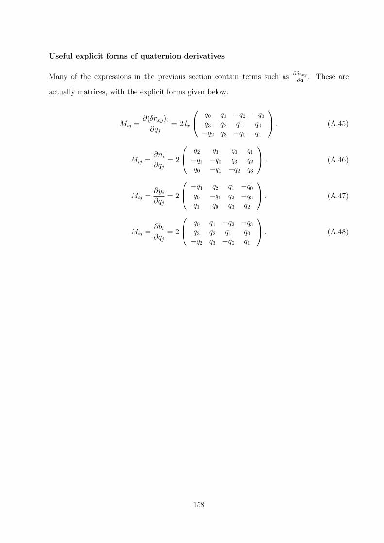
Useful explicit forms of quaternion derivatives
Many of the expressions in the previous section contain terms such as ∂δrxy∂q
. These are
actually matrices, with the explicit forms given below.
Mij =∂(δrxy)i∂qj
= 2dx
q0 q1 −q2 −q3
q3 q2 q1 q0
−q2 q3 −q0 q1
. (A.45)
Mij =∂ni∂qj
= 2
q2 q3 q0 q1
−q1 −q0 q3 q2
q0 −q1 −q2 q3
. (A.46)
Mij =∂yi∂qj
= 2
−q3 q2 q1 −q0
q0 −q1 q2 −q3
q1 q0 q3 q2
. (A.47)
Mij =∂bi∂qj
= 2
q0 q1 −q2 −q3
q3 q2 q1 q0
−q2 q3 −q0 q1
. (A.48)
158

Appendix B
Quaternion dynamics
The algorithm of Davidchack et al. [153] was used for the Langevin simulations in this thesis.
This algorithm extends the method of Miller et al. [218], which generates Newtonian motion
of rigid bodies described by quaternions. As neither paper fully explains the origin of the
equations of motion, I derive them here from first principles.
B.1 Angular velocities represented in quaternions
In Appendix A, quaternions were defined in terms of a rotation matrix relating the orien-
tation of a vector in the body-fixed frame xb to one in the space-fixed frame xs. Rapaport
[217] has shown that the angular velocity of an object in the body-fixed frame is given by:0wb1wb2wb3
= 2
q0 q1 q2 q3
−q1 q0 q3 −q2
−q2 −q3 q0 q1
−q3 q2 −q1 q0
q0
q1
q2
q3
. (B.1)
I label the matrix in (B.1) as STq .
B.2 Motion without noise or damping
The full Lagrangian for my model, in the absence of any noise or damping, is given by:
L =∑
i
((12mi(ri)
T (ri) + 2|qi|4
(STqiqi
)TIi(STqiqi
))+ λi
(∑j(qi)j(qi)j − 1
))−U(q, r).
(B.2)
The second term in Equation B.2 is simply the kinetic energy of rotation. At this stage,
I have not fixed the normalization for each quaternion to unity, but instead imposed a
159
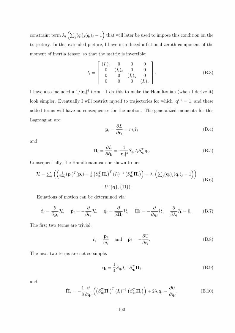
constraint term λi
(∑j(qi)j(qi)j − 1
)that will later be used to impose this condition on the
trajectory. In this extended picture, I have introduced a fictional zeroth component of the
moment of inertia tensor, so that the matrix is invertible:
Ii =
(Ii)0 0 0 0
0 (Ii)x 0 00 0 (Ii)y 00 0 0 (Ii)z
. (B.3)
I have also included a 1/|qi|4 term – I do this to make the Hamiltonian (when I derive it)
look simpler. Eventually I will restrict myself to trajectories for which |qi|2 = 1, and these
added terms will have no consequences for the motion. The generalized momenta for this
Lagrangian are:
pi =∂L
∂ri= miri (B.4)
and
Πi =∂L
∂qi=
4
|qi|4SqiIiS
Tqi
qi. (B.5)
Consequentially, the Hamiltonain can be shown to be:
H =∑
i
((1
2mi(pi)
T (pi) + 18
(STqiΠi
)T(Ii)
−1(STqiΠi
))− λi
(∑j(qi)j(qi)j − 1
))+U(q, Π).
(B.6)
Equations of motion can be determined via:
ri =∂
∂piH, pi = − ∂
∂riH, qi =
∂
∂Πi
H, Πi = − ∂
∂qiH, ∂
∂λiH = 0. (B.7)
The first two terms are trivial:
ri =pimi
and pi = −∂U
∂ri. (B.8)
The next two terms are not so simple:
qi =1
4SqiI
−1i STqiΠi (B.9)
and
Πi = −1
8
∂
∂qi
((STqiΠi
)T(Ii)
−1(STqiΠi
))+ 2λiqi −
∂U
∂qi. (B.10)
160

Hence forth the sunscript i indicating the identity of the particle will be assumed, to
avoid complication with index notation. I will also drop the q label on Sq. I can now use
the ∂∂λH term to impose |q|2 = 1, which means that SqS
Tq = 1. The easiest way to eliminate
λ is by evaluating the angular velocity ω. ω is given by:
ω = 2ST q =1
2(I)−1STΠ, (B.11)
in which I have used Equation B.9, and the fact that S is orthorgonal once |q|2 = 1 is
imposed. Therefore
ω =1
2(I)−1 d
dt
(STΠ
). (B.12)
Using Π = − ∂∂qiH,
d
dt
(STΠ
)= STΠ + ST
(−1
8
∂
∂q
((STΠ
)T(I)−1
(STΠ
))+ 2λq− ∂U
∂q
). (B.13)
The best way to treat these equations is to use tensor notation. Defining the third rank
tensor Dσνρ by:
Dσνρqσ = (ST )νρ, (B.14)
and Fργβ by:
Fργβ =∂Sγβ∂qρ
, (B.15)
I can express Equations B.12 and B.13 as:
ωµ = 12(I−1)µν [DσνρqσΠρ]
+12(I−1)µν
[(ST )νρ
(−18
Πα
(Fραβ(I−1)βγ(S
T )γσ + Sαβ(I−1)βγFρσγ)
Πσ + 2λqρ − ∂U∂qρ
)].
(B.16)
Using the fact that (I−1)βγ is symmetric, it can be shown that the second and third terms
are equal. Hence,
ωµ =1
2(I−1)µν
[DσνρqσΠρ −
1
4(ST )νρΠα
(Fραβ(I−1)βγ(S
T )γσ)
Πσ + 2λ(ST )νρqρ − (ST )νρ∂U
∂qρ
].
(B.17)
Consider the first term in the bracket. Inverting the definitions in Equation B.11:
DσνρqσΠρ = Dσνρ1
2Sσαωα.2SρδIδβωβ = DσνρSσαSρδIδβωαωβ (B.18)
161

Similarly the second term in the bracket becomes:
14(ST )νρΠαFραβ(I−1)βγ(S
T )γσΠσ = 14(ST )νρ(2SαφIφθωθ)Fραβ(I−1)βγ(S
T )γσ(2SσχIχψωψ)
= (ST )νρSαφIφθFραβ(I−1)βγδγχIχψωθωψ
= (ST )νρSαφIφθFραβ(I−1)βγIγψωθωψ
= (ST )νρSαφIφθFραβδβψωθωψ
= (ST )νρSαφIφθFραβωθωβ
= (ST )νρSγσIσαFργβωαωβ(B.19)
So,
ωµ =1
2(I−1)µν
([DσνρSσαSρδIδβ − SρνSγσIσαFργβ]ωαωβ + 2λ(ST )νρqρ − (ST )νρ
∂U
∂qρ
).
(B.20)
With
D0νρ =
1 0 0 00 1 0 00 0 1 00 0 0 1
, D1νρ =
0 1 0 0−1 0 0 00 0 0 10 0 −1 0
, (B.21)
D2νρ =
0 0 1 00 0 0 −1−1 0 0 00 1 0 0
, D3νρ =
0 0 0 10 0 1 00 −1 0 0−1 0 0 0
,
and
F0νρ =
1 0 0 00 1 0 00 0 1 00 0 0 1
F1νρ =
0 −1 0 01 0 0 00 0 0 −10 0 1 0
(B.22)
F2νρ =
0 0 −1 00 0 0 11 0 0 00 −1 0 0
, F3νρ =
0 0 0 −10 0 −1 00 1 0 01 0 0 0
.
The summations can be done explicitly, giving:
ω0 = λ/I0 + τ0/I0,
ω1 = Iy−IzIx
ω2ω3 + τ1/Ix,
ω2 = Iz−IxIy
ω3ω1 + τ2/Iy,
ω3 = Ix−IyIz
ω1ω2 + τ3/Iy,
(B.23)
162

with the torque τ given by τµ = −12(ST )µρ
∂U∂qρ
. Imposing qµqµ = 1 implies that ω0 =
2qµqµ = 0 and hence that ω0 = 0. The Lagrange multiplier can therefore be identified as
λ = −τ0. When this is substituted back into the expression for Π, it cancels the effect
of any component of ∂U∂q
along q, which is exactly what is needed to retain qµqµ = 1. So,
returning to the explicit use of particle labels and STqi , the expression for Πi becomes:
Πi = −1
8
∂
∂qi
((STqiΠi
)T(Ii)
−1(STqiΠi
))−(∂U
∂qi−(
qTi∂U
∂qi
)qi
). (B.24)
Note that once the condition |q|2 = 1 has been applied, (Ii)0 cancels out from Equations
B.9 and B.24. In fact, in the work of Miller et al. and Davidchack et al., the kinetic term
is written (equivalently) as:
1
8
(STqiΠi
)T(Ii)
−1(STqiΠi
)=
3∑k=1
hk(qi,Πi), (B.25)
with
hk(qi) =1
8Iik[ΠT
i Pk(qi)]2, (B.26)
in which
P1(qi) = (−(qi)1, (qi)0, (qi)3,−(qi)2)T , P2(qi) = (−(qi)2,−(qi)3, (qi)0, (qi)1)T (B.27)
and P3(qi) = (−(qi)3, (qi)2,−(qi)1, (qi)0)T
Quaternions and generalized quaternion momenta then evolve as:
qi =3∑
k=1
∂
∂Πi
hk(qi,Πi) and Πi = −3∑
k=1
∂
∂qihk(qi,Πi)−
(∂U
∂qi−(
qTi∂U
∂qi
)qi
).
(B.28)
Interestingly, if the−(qTi
∂U∂qi
)qi term is left out of this expression, there are no consequences
for the dynamics of physical observables. By dropping this term, the component of Π
parallel to q is not fixed at zero, as it technically should be. ∂∂Π,qi
hk(qi,Πi) is easily shown
to be independent of any term of Π parallel to q, however – therefore such a term has no
effect on the motion or energy of the system. qi also remains orthogonal to qi, as it must.
163

B.3 Incorporating noise and damping
Equations B.8 and B.28 can be integrated to give Newtonian dynamics of rigid bodies,
as outlined in Reference [218]. In this work, I am interested in motion driven by noise
and damping, implicitly representing the presence of a solvent. Davidchack et al. [153]
have developed an algorithm for this purpose [153] – here I discuss some aspects in more
detail. For convenience, the −(qTi
∂U∂qi
)qi term is not included in the equation of motion
by the authors of Reference. From now on, the moment of inertia tensor I is taken to be
three-dimensional again.
One can attempt to add noise and damping in the following simple fashion:
ri = pimi,
pi = − ∂U∂ri− γpi + bwi(t),
(B.29)
qi =∑3
k=1∂∂Πi
hk(qi,Πi) and
Πi = −∑3
k=1∂∂qihk(qi,Πi)− ∂U
∂qi− ΓG(qi,Πi) +BWi(t),
(B.30)
where wi(t) and Wi(t) are 3- and 4-dimensional Wiener processes with unit variance and
independent dimensions.1
To specify the damping and noise terms that will result in sampling of the canonical
ensemble, it is helpful to find the Fokker-Planck description equivalent to Equations B.29
and B.30. For a Langevin process with additive and independent noise, v = A(v) +
CW(t) (where C is a constant diagonal matrix), the equivalent Fokker-Planck equation for
a probability density ρ(v, t) is given by [152]:
∂ρ(v, t)
∂t= − ∂
∂v.(A(v)ρ(v, t)) +
1
2
∑i
C2ii
∂2ρ(v, t)
∂vi2. (B.31)
For sampling of the canonical ensemble it is necessary that ∂ρ0/∂t = 0, where
ρ0 ∝ exp
(−β
(∑i
(3∑
k=1
hk(qi,Πi) + p2i /2m
))+ U(r, q)
)(B.32)
is the Boltzmann distribution. Substituting Equation B.32 into Equation B.31, it is imme-
diately obvious that cancellation of terms will occur separately for each particle, and also
1Having different strengths of noise and damping for each particle would be a simple addition.
164

separately for linear and angular components. For the linear terms,
− pimi
.∂ρ0
∂ri+ (
∂U
∂ri+ γpi).
∂ρ0
∂pi+ 3γρ0 +
b2
2
∂2ρ0
∂p2i
= 0, (B.33)
=⇒ βpimi
.∂U
∂riρ0 − (
∂U
∂ri+ γpi).
βpimi
ρ0 + 3γρ0 +b2
2
(−3β
m+β2p2
i
m2
)ρ0 = 0. (B.34)
It is fairly trivial to infer that the appropriate relationship between b and γ is:
γ = b2 β
2m. (B.35)
For the angular terms,
−(∑3
k=1∂∂qi. ∂∂Πi
hk(qi,Πi))ρ0 −
(∑3k=1
∂∂Πi
hk(qi,Πi)).∂ρ0
∂qi
+(∑3
k=1∂∂Πi
. ∂∂qihk(qi,Πi)
)ρ0 + Γ
(∂∂Πi
.G(qi,Πi))ρ0
+(∑3
k=1∂∂qihk(qi,Πi) + ∂U
∂qi+ ΓG(qi,Πi)
). ∂ρ0
∂Πi+ B2
2∂2ρ0
∂Π2i
= 0.
(B.36)
It is fairly simple to show that:
∂ρ0
∂qi=
(−β
3∑k=1
∂
∂qihk(qi,Πi)− β
∂U
∂qi
)ρ0, (B.37)
∂ρ0
∂Πi
= −β
(3∑
k=1
∂
∂Πi
hk(qi,Πi)
)ρ0 (B.38)
and
∂2ρ0
∂Π2i
=
β2
(3∑
k=1
∂
∂Πi
hk(qi,Πi)
)2
− β3∑
k=1
∂2
∂Π2i
hk(qi,Πi)
ρ0 (B.39)
Thus,
Γ(
∂∂Πi
.G(qi,Πi)− βG(qi,Πi).∑3
k=1∂∂Πi
hk(qi,Πi))
= B2
2
(β2(∑3
k=1∂∂Πi
hk(qi,Πi))2
− β∑3
k=1∂2
∂Π2ihk(qi,Πi)
)ρ0.
(B.40)
Equation B.40 is evidently satisfied by:
ΓG(qi,Πi) =B2
2β
3∑k=1
∂
∂Πi
hk(qi,Πi) (B.41)
One way to express this result is:
Γ =βB2
2M, M =
4
Tr((Ii)−1)and G(qi,Πi) = J(qi)Πi, (B.42)
165
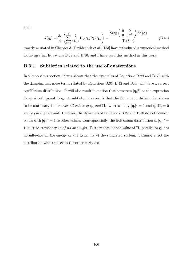
and:
J(qi) =M
4
(3∑
k=1
1
(Ii)kPk(qi)P
Tk (qi)
)=
S(q)
(0 00 I−1
)ST (q)
Tr(I−1), (B.43)
exactly as stated in Chapter 3. Davidchack et al. [153] have introduced a numerical method
for integrating Equations B.29 and B.30, and I have used this method in this work.
B.3.1 Subtleties related to the use of quaternions
In the previous section, it was shown that the dynamics of Equations B.29 and B.30, with
the damping and noise terms related by Equations B.35, B.42 and B.43, will have a correct
equilibrium distribution. It will also result in motion that conserves |qi|2, as the expression
for qi is orthogonal to qi. A subtlety, however, is that the Boltzmann distribution shown
to be stationary is one over all values of qi and Πi, whereas only |qi|2 = 1 and qi.Πi = 0
are physically relevant. However, the dynamics of Equations B.29 and B.30 do not connect
states with |qi|2 = 1 to other values. Consequentially, the Boltzmann distribution at |qi|2 =
1 must be stationary in of its own right. Furthermore, as the value of Πi parallel to qi has
no influence on the energy or the dynamics of the simulated system, it cannot affect the
distribution with respect to the other variables.
166

Appendix C
Validation of simulation techniques
It is important to ensure that the algorithms have been implemented correctly, and in the
case of Langevin dynamics, that the time step of simulations is small enough to give accurate
results.
C.1 Comparison of Langevin and VMMC energies
Langevin and VMMC methods can both be used to estimate the average energy of a system.
As the methods are independent, a consensus is a good indicator that both algorithms are
correctly sampling the system.
Simulations were performed on a system in which all the interactions present in the model
occur frequently – a 30-base strand bound to two 10-base strands. The shorter strands bind
to adjacent regions of the longer strand, and hence can undergo coaxial stacking across the
joint.
Four VMMC simulations (of 5×10⁹ steps per simulation), and four Langevin simulations
each at a range of time steps h (for 5× 10⁸ steps per simulation) were performed at 300 K.
The average potential energies measured in each simulation are show in Table C.1. As
can be seen, the values agree well, with the average at each step size within 0.04% of the
average obtained from VMMC simulations. No noticeable dependence of the maximum
possible time step on the values of friction coefficients in the vicinity of γ = 1 and Γ = 3
was observed.
167

Simulation Method VMMC LangevinTimestep h N/A h = 0.005 h = 0.003 h = 0.001 h = 0.0005
-59.0067 -59.0360 -58.9919 -58.9409 -58.9648〈U〉 in -59.0118 -59.0146 -59.0042 -58.9646 -59.0070
each simulation -59.0253 -59.0165 -59.0202 -59.1566 -59.0763-59.0290 -58.9882 -59.0313 -58.9267 -59.0295
Overall 〈U〉 -59.0182 -59.0138 -59.0119 -58.9972 -59.0194Test statistic N/A 0.7152 0.5681 0.7232 0.9630
Table C.1: Comparison of average potential energies obtained from VMMC and Langevin simulations.Timesteps and energies are quoted in the reduced units of the model. The test statistic is the result ofapplying Welch’s unpaired t-test [214] to the distributions of 〈U〉 in the VMMC and Langevin code. Forh = 0.003 (5.12 ps), the difference between VMMC and Langevin estimates of 〈U〉 is around 0.01% of thetotal, and is not statistically significant.
C.2 Comparison of hairpin folding speed as a function
of step size in Langevin Dynamics
As discussed in Section C.1, Langevin dynamics with a step size of h = 0.003 in reduced
units appears to provide thermodynamic averages consistent with the results of VMMC.
Such a result, however, does not necessarily imply that the kinetics of simulations at these
time steps are reliable.
As Langevin dynamics is used in this thesis to explore the kinetics of processes, it is
important that the time step is small enough to reproduce them reliably. To test this,
simulations were performed to measure the rate of spontaneous folding of a small hairpin
as a function of step size. I considered a hairpin consisting of a stem of six base pairs and a
loop of five bases, measuring the average time (from 100 simulations) required for a strand
(initialized in the open state) to fold into a fully-formed hairpin at 300 K. The results are
shown in Figure C.1.
As is evident from Figure C.1, there is no systematic dependence on hairpin folding
rate on the step size h up to h = 0.005 simulation units. Therefore I use h = 0.003 with
confidence throughout this work.
168

0e+00
2e+04
4e+04
6e+04
8e+04
1e+05
0 0.001 0.002 0.003 0.004 0.005
Av
erag
e fo
ldin
g t
imeâ
Step size
Figure C.1: Average simulation time for hairpin folding as a function of step size (in reduced units T ,T = 1 corresponding to 1.706 ps). Error bars are calculated assuming that hairpin folding is a Poissonprocess.
C.3 Comparison of unbiased and biased VMMC sim-
ulations
Umbrella sampling is central to much of the work presented here. Due to its (often heavy)
biasing of some configurations, it can be very sensitive to errors in algorithm implemen-
tation and typically responds differently from unbiased simulations. As a test of both the
algorithm in general and the umbrella sampling code itself, therefore, simulations of the
melting transition of a five-base pair duplex were performed both with and without biasing.
I performed four unbiased simulations at 297.03 K for 2 × 10¹¹ VMMC steps each, and
four biased simulations at 294.11 K for 4 × 10¹⁰ VMMC steps. The results (extrapolated
to nearby temperatures using single-histogram re-weighting) are given in Table C.2. The
results are clearly consistent, supporting the accuracy of my implementation of the VMMC
algorithm and umbrella sampling.
169

Temperature Unbiased BiasedAverage yield σ Average Yield σ
309.28 5.31E-02 4.33E-04 5.27E-02 7.46E-04306.12 8.87E-02 6.89E-04 8.81E-02 1.16E-03303.03 1.41E-01 1.01E-03 1.40E-01 1.66E-03300.00 2.11E-01 1.33E-03 2.10E-01 2.16E-03297.03 2.96E-01 1.58E-03 2.95E-01 2.53E-03294.12 3.89E-01 1.71E-03 3.87E-01 2.70E-03291.26 4.82E-01 1.70E-03 4.81E-01 2.67E-03288.46 5.70E-01 1.60E-03 5.69E-01 2.48E-03285.71 6.48E-01 1.43E-03 6.47E-01 2.21E-03
Table C.2: Comparison of the bulk duplex yield inferred from four biased and four unbiased simulationsof the formation of a five bp duplex (extrapolation to the bulk limit performed as outlined in Chapter 4).The average and standard deviation (σ) over the four simulations are shown.
170
Appendix D
Finite size effects for more complexsystems
In Chapter 4, finite size effects relating to dimerization processes simulated in the canonical
ensemble were discussed. In this appendix, the formalism is extended to multi-component
assembly (of relevance to systems such as virus capsids and micelles, as well as more complex
assemblies of DNA). Simulations using the grand canonical ensemble, and systems with one
species immobilized, are also considered.
D.1 Monodisperse large homoclusters
Consider the formation of larger clusters of a specific size from identical monomers, a case
relevant to the assembly of virus capsid-like objects [49, 50, 147, 219, 220, 221], and ho-
momeric protein complexes [222]. If the formation of a single cluster is simulated in the
canonical ensemble, once again, the statistics of the various cluster sizes do not directly
correspond to bulk properties, but under the assumption that interactions which do not
constitute bonding are negligible it is possible to extrapolate to large system sizes. Firstly,
some definitions:
• n is the number of monomers needed to form the target, equal to the number of
monomers simulated.
• zi is the partition function for species i (a cluster of i identical monomers), in the
simulation volume v, with the internal degrees of freedom treated distinguishably.
171

• Zi,j,k... is the partition function of a system of volume v when in a state which contains
one cluster of species i, one of species j etc. This partition function is calculated
using distinguishable statistics. i, j, k... can therefore be taken to specify a macrostate
corresponding to the set of clusters i, j, k....
• ηm the number of clusters of size m in the macrostate – consequentially, an alternative
way to specify the macrostate is via the set ηm (Zi,j,k... = Zηm).
• Z(n) is the total partition function of the n-particle system in a volume v, calculated
using distinguishable statistics.
• as all monomers are identical, the A index will be omitted for clarity.
The thermodynamically relevant quantities are the qi/(q1)i, because given these it is a
simple task to calculate the bulk concentrations of each species using:
Ni
(N1)i=
qi(q1)i
(D.1)
and ∑i
iNi = nD = N. (D.2)
The quantities that are directly accessible from simulation are Zi,j,k.../Z. Exactly how
these can be accessed depends on how the system is sampled. A sensible choice, however,
is to sample states by the largest cluster size – this neatly divides the partition function Z
into n parts, and I label these subdivisions Ωi. There are now n equations, one for each Ωi:
Ωi
Z=∑j,k...
Zi,j,k...Z
, (D.3)
where the summation over j, k... is the sum over all sets of indices such that j, k... ≤ i and
the indices sum to n. Zi,j,k... are given by:
Zi,j,k... = n!i∏m
(zm/m!)ηm
ηm!, (D.4)
I now have n simultaneous equations for zi/Zi/n in terms of the measured quantities
Ωi/Z. In addition, these simultaneous equations have already been decoupled as each Ωi/Z
172

expression contains only zm with m ≤ i, and thus finding zi/Zi/n amounts to solving a
polynomial of order i. All that remains is to find qi in terms of zi. This is reasonably
simple:
qi = Dzii!, (D.5)
where in dividing by i! I account for the reduction in states imposed by indistinguishability.
I can then obtain the right hand side of (D.1) by:
qi(q1)i
=Dzi
i!(Dz1)i=
Dzi/Zi/n
i!(Dz1/Z1/n)i, (D.6)
in which the right hand side is expressed in terms of the known quantities zi/Zi/n. I can
now eliminate the arbitrary large factor D by converting to concentrations (which equates
to multiplying both sides by (Dv)(i−1)), giving:
[Ni]
[N1]i= vi−1 zi/Z
i/n
i!(z1/Z1/n)i. (D.7)
Once again, the system of equations can be closed by conserving the total monomer number:∑i
i[Ni] = n/v. (D.8)
To illustrate the form of finite size corrections, consider the artificial example of com-
pletely cooperative hexamer formation (in which we approximate clusters of intermediate
size as having zero probability). The complicating effects of additional states will be dis-
cussed in Section D.2. For comparison with Section 4.1.3, I will assume that the small
system can be described by an equivalent two-state model, so that the yields of hexamers
and homodimers are identical in the small simulation volume:
Z6/Z1,1,1,1,1,1 = exp(−∆E/T + ∆S), (D.9)
with ∆E = 2 and ∆S = 15 in reduced units. The result, plotted in Figure D.1 (c), indicates
once again a much broader transition in the bulk case, this time with a slightly adjusted mid-
point. Furthermore, this broadening is much more pronounced for hexamers than dimers.
This trend is a general one, with larger clusters experiencing greater broadening due to
finite-size corrections. This is because smaller relative concentration fluctuations are re-
quired to push the system towards a yield of approximately 50% for a clustering transition
involving many monomers as opposed to dimers, as illustrated in Figure D.1 (b).
173

Figure D.1: (a) The top image shows six identical particles in a volume v. Doubling the volume meansthat only a relatively minor concentration fluctuation is required to make the formation of two hexamersimpossible (and the formation of one hexamer more likely), compared to the equivalent situation for dimers.As a consequence, the broadening effect of bulk corrections increases with the size of the target structure.(b) Fractional yield of hexamers in the statistical model of equation (D.9). Plotted are the yields for a singlecluster system (red), for hexamers in bulk (blue) and for an equivalent extrapolation to bulk for homodimerformation (green).
D.2 Homocluster convergence
Many canonical simulations of self-assembly are performed using systems large enough to
form several or many clusters [49, 50, 219, 220, 223]. I apply the formalism of the previous
sections to explore the convergence of cluster statistics on bulk values as system size is
increased. As in the previous section, I consider a reference system of n particles in a volume
v, where n is the size of the largest cluster, and proceed using the partition functions zi
defined in this volume.
The statistical weight of the macrostate i, j, k.., containing a total of Dn monomers in
a volume D, with all degrees of freedom treated indistinguishably, is given by:
Qηm(D) =n∏l
(Dzl)ηl
ηl!(l!)ηl, (D.10)
Defining ψl(D) = zl/(zl1D
l−1), I obtain an expression for the fractional yield of a cluster of
size c in a system of size D:
fc(D) =c∑ηm ηc
∏nl
1(ηl)!
(ψll!
)ηlDn
∑ηm
∏nl
1(ηl)!
(ψll!
)ηl . (D.11)
174

Figure D.2: (a) Relative fractional error on the yield of various cluster sizes as a function of 1/D in asystem with a maximum cluster size of six. All clusters show convergence with 1/D scaling in the large Dregime (as highlighted in (b)).
This expression for fc(D) can be used to check that the extrapolation scheme is valid for
the system in question, by simulating a system with D = 2 and comparing to the results
expected from a D = 1 simulation. Such a simulation would also allow the examination of
clusters larger than the target structure, and their incorporation into the statistics if their
presence is significant.
In all cases that I have been able to study to high D (the meaning of ‘high’ will be
clarified later), fc(D) − fc(∞) is observed to scale as 1/D in the large D limit (see Figure
D.2). The question of convergence speed then reduces to how large D must be for this
scaling to hold, and the the value of fc(D) − fc(∞) at this point. In general there are
two distinct regimes of convergence, determined by the yield of target structures. I shall
illustrate these regimes by considering completely cooperative transitions (in which only the
target cluster and monomer concentrations are non-negligible), before commenting on the
effects of other cluster sizes.
D.2.1 Convergence at low yield
Section D.1 indicates that simulations of a single cluster underestimate the transition width
and hence underestimate the number of clusters at low yield. In effect, in order to have
a high isolated monomer fraction in bulk despite the effects of volume fluctuations, the
fraction of monomers in a single target simulation must be even higher. As the system size
175

Figure D.3: Fractional yield of hexamers in a perfectly cooperative model as a function of system size Dfor (a) low yield (5% hexamers) and (b) high yield (95% hexamers). The ‘+’ symbols are the calculatedpoints and the flat line the bulk value. The curve in (a) is a fit to a 1/D convergence.
is increased, concentration fluctuations tend to transfer statistical weight from the extreme
state favoured at D = 1 towards a more balanced cluster size distribution.
At low yield this effect produces a steady increase in the proportion of clusters with D,
with the deviation from the bulk fraction scaling as approximately 1/D from low D (see
Figure D.3(a)). At very low yield, initial convergence becomes noticeably slower than 1/D—
this effect increases with target size. As a consequence, relative errors remain significant at
increasingly large values of D as the yield is decreased or the target size increased.
D.2.2 Convergence at high yield
At high yield, single target simulations overestimate the monomer fraction, for reasons
similar to the underestimate at low yield. Convergence, however, does not initially show
a 1/D behaviour, as illustrated in Figure D.3(b). Instead, a period of slow convergence is
followed by a rapid drop to a target yield just below the bulk value, leading eventually to
an oscillation in the vicinity of the bulk yield. These oscillations persist for approximately
n− 1 half-cycles, before settling in to a 1/D convergence (n being the target cluster size).
These oscillations result from certain configurations disproportionately biasing the en-
semble, due to the inherently discrete nature of a small system. At D = 1, the system is
restricted to two states: one cluster or n monomers. At high cluster yield, n monomers
are extremely unfavourable and hence the single cluster state is overwhelmingly observed,
176

causing fn(1) to exceed fn(∞). As the system size is increased, the zero monomer state
continues to exert a disproportionate influence on the ensemble, keeping fn(D) well above
fn(∞). Eventually, however, the system becomes sufficiently large that the state with
D− 1 clusters is most favourable. Due to the discreteness of the system, this occurs before
(D − 1)/D = fn(∞). As a consequence, fn(D) is then underestimated (or equivalently
the number of monomers is overestimated), resulting in the observed drop of fn(D). At
still larger values of D, the state with D − 1 clusters remains most favourable but now
constitutes an overestimate of fn(D), resulting in the observed rise in fn(D). This process
is repeated for increasing number of monomers, leading to oscillations which are eventually
overwhelmed by the 1/D convergence at large system size.
The question is then why oscillations are observed at high but not low yield, where the
discreteness of the system is still present. To answer this, it is illuminating to allow D to
take non-integer values so that the system size n′ = Dn can take any integer value. At high
yield, as shown in Figure D.4(b), one sees that the system is extremely sensitive to the exact
number of particles, because if D is not an integer there are necessarily excess monomers.
This results in the rapid oscillation of fn(n′) with a period of approximately n. Closer
inspection, however, reveals that the period is longer than n, due to the fact that states
with no monomers present become increasingly unfavourable as D gets larger. The region
in which the fn(n′) peaks transfer from n′ mod n = 0 to n′ mod n = 1 corresponds to the
region in which fn(D) drops off rapidly. By contrast, fn(n′) increases monotonically with n′
at low yield (Figure D.4(a)). In this regime, the fraction of clusters is not high enough for
the value of n′ mod n to be significant, and so the general tendency to transfer statistical
weight to states with a greater mix of cluster sizes is dominant, and smooth convergence is
observed.
As a consequence of this behaviour, convergence at high cluster yield is extremely poor
until D is sufficiently large that the state with D − 1 clusters has approximately the same
weight as the state with D clusters:
(ψn)D−1ψ1
(D − 1)!(n!)D−1n!≈ (ψn)D
(D)!(n!)D. (D.12)
177

Figure D.4: Fractional yield of hexamers in a perfectly cooperative model as a function of n′ for (a) lowyield (5% hexamers) and (b) high yield (95% hexamers). The ‘+’ symbols are the calculated points andthe flat line the bulk value. ‘x’ symbols indicate system sizes for which D = n/n′ is integral. The dashedline in (b) is added as a guide to the eye.
Substituting using the definition of ψi(D) gives:
Dcrosssover ≈(znzn1
)1/n
. (D.13)
The quantity zn/zn1 corresponds to the ratio of cluster to monomers at D = 1, and conse-
quentially increases with n at fixed bulk yield. This increase is offset by the 1/n exponent,
meaning that the value of Dcrosssover is relatively independent of target size, but increases
with the target yield. It should also be noted that the oscillations persist until a system size
of approximately nDcrossover, although they are generally reasonably small. It is this value,
D ≈ nDcrossover, that defines the large D limit.
In the intermediate yield regime near to the midpoint of the transition, the initial error
is small and zn/zn1 is not large, hence convergence is fast (whether it proceeds by the first or
second method). Away from the midpoint, however, significant relative discrepancies can
persist up to surprisingly large system sizes.
D.2.3 Intermediate cluster sizes
An additional complication for n > 2 is the fact that intermediate cluster sizes may be
relevant to the system, which can affect convergence. I shall analyze the effects of the
presence of intermediate cluster sizes under the assumption that the majority of particles
are found either as isolated monomers or in the target cluster size: for the purposes of
178
this section, the term ‘majority species’ applies to the most prevalent of either the target
cluster or monomers, and ‘minority species’ to the less common of these two. Note that our
discussions will compare the effects of intermediate cluster sizes in systems with a certain
yield of the majority species, as it is the tendency of one species to dominate in bulk despite
concentration fluctuations that causes the large discrepancies at D = 1. Firstly, I consider
the low yield case. Here, the presence of clusters of intermediate sizes with bulk yields
comparable to the target cluster has little effect on the relative error of the target yield
at D = 1, which is largely determined by the bulk fraction of monomers. By contrast, if
the relevant intermediate cluster size is small (for instance a dimer in a system forming a
dodecahedron), the relative error between dimer and isolated monomers is comparatively
small, meaning that f2(1) ≈ f2(∞), because from the perspective of the monomer/dimer
equilibrium the system has an effective size of Deff = n/2. As a consequence, states including
dimers are common and so the entropic penalty associated with having no target clusters is
reduced, meaning that statistical weight is transferred to larger clusters more slowly as the
system size is increased. The effect manifests itself as a poor convergence in the first few
steps, as shown in Figure D.5 (a). Also shown is the effect of having a significant presence
of large intermediate clusters, which is smaller as they do not relieve the entropic penalty of
having many monomers as swiftly as dimers do (the relative error is seen to behave similarly
to a completely cooperative system with the same monomer yield).
I now consider the effect of a significant presence of intermediate clusters on the conver-
gence of the yield of isolated monomers at high cluster fraction. If the relevant intermediate
clusters are large, the initial error is significantly reduced as the relative error between two
large clusters of similar size is much smaller than for a large cluster and a monomer, and
in forming intermediate clusters some monomers are ‘spare’. Convergence, however, is not
improved as instead of the state with D − 1 target clusters and D monomers coming to
dominate the ensemble, as in the completely cooperative case, states containing interme-
diate clusters become most prevalent (in effect, they reduce the ‘entropy cost’ associated
with having few monomers in the system). If the intermediate clusters are large, there will
be few monomers in these states and as a consequence, statistical weight is transferred to
179

Figure D.5: (a) Fractional yield of dodecamers in a dodecamer forming system at low yield (90% isolatedmonomers, 5% dodecamers in bulk). (b) Fractional yield of isolated monomers in a dodecamer formingsystem at high yield (90% dodecamers, 5% monomers in bulk). Plotted are points for systems in whichthe other 5% is assumed to consist entirely of either 2-mers or 11-mers. Also shown (dashed curves) arethe results for completely cooperative systems with the same 90% majority species yield. These have beenscaled by a factor of 0.5 so that the relative errors can be directly compared.
isolated monomers more slowly. This effect is illustrated in Figure D.5 (b): also plotted is
a case with a significant presence of small intermediate clusters. In this case convergence is
not dramatically slowed (relative to a completely cooperative system with the same target
cluster yield), as the states which become prevalent contain D− 1 target clusters and a mix
of smaller species, including several monomers.
In summary, for monodisperse clusters, the significant presence of intermediate cluster
sizes tends to reduce the rate of convergence of the fractional yield of the minority species
relative to a completely cooperative system (at a fixed yield of the majority species), par-
ticularly if the relevant intermediate clusters are closer in size to the majority species, by
reducing the entropic penalty associated with having few of the minority species in the
system. In several cases, authors have studied systems capable of forming approximately
10 to 20 clusters [49, 220, 223]. It is probable that the finite-size effects illustrated here are
relevant to these systems in the regimes dominated by one cluster size.
Small-system simulations on the formation of micelles have also been performed in the
canonical ensemble (examples are given in Reference [224]). Micelles are not monodisperse,
but show some variation about a typical finite size. The techniques shown in this section can
be equally well applied to such a process, with qualitatively similar results – in particular,
180

convergence to bulk yields appears to be extremely slow when the micellar concentration is
low. The details are discussed in Reference [224].
D.3 Simulations in the grand canonical ensemble
As an alternative to NV T simulations, it is possible to use the grand canonical ensemble.
Here, instead of fixing the number of particles absolutely, one simulates a system in a volume
v such that configurations containing n particles are sampled with the relative probability
[225]:
P (n) ∝ eβµnZ(n)
n!, (D.14)
where Z(n)/n! is the partition function of an n-particle system, calculated using distinguish-
able statistics. Configurations of the same n have the same relative Boltzmann weighting as
in the canonical ensemble. Thus a configuration containing nj clusters of size j is observed
in a simulation with probability:
P (nj) =∏j>0
znjj
nj! jnjeβµjnj (D.15)
To date, grand canonical techniques (and related semi-grand canonical approaches) have
primarily been used to study the formation of micellar structures [226, 227, 228, 229, 230,
231, 232], as opposed to mondisperse target structures. In many of these cases, monomer
concentrations are taken to be so low that the probability of finding more than one cluster in
a simulation volume is neglected, and the number of monomers in the simulation is taken as a
proxy for cluster size [226, 227, 228, 229]. There has been considerable debate on the details
of inferring cluster probabilities from simulations in which one monomer is fixed at the centre
of the simulation volume, under this extremely dilute assumption [226, 233, 234]. Other
workers have explicitly simulated the formation of multiple micellar clusters [230, 231, 232].
The advantage of the grand canonical formalism for large micelles is obvious, as it allows
a small simulation volume to contain a large number of particles without requiring a high
average concentration. There is no reason, however, why the technique could not also be
applied to smaller, monodisperse self-assembling systems.
181

In principle, grand-canonical simulations are capable of capturing the concentration
fluctuations which must be considered to extract the bulk thermodynamics from a small
simulation. This is only true, however, if the simulation samples the formation of multiple
clusters. Under the assumptions of ideal behaviour of separate species, the errors are simple
to quantify. In bulk equilibrium:
[N1] =z1eβµ
v, (D.16)
where concentrations are measured relative to the simulation volume v, and:
[Nj] = [N1]j(Dv)j−1 qj
qj1=
zjvj!
eβµj. (D.17)
I assume that a simulation samples states which contain at most a single cluster of more
than one particle. In this case, the probability of observing a cluster of size j > 1 is given
by:
p(j) =
zjj!
eβµj∑
n≥0zn1 eβµn
n!(1 +
∑k>1
zkk!
eβµk)∑
n≥0zn1 eβµn
n!
, (D.18)
Thus the simulation concentration (measured relative to the simulation volume) is:
[Nj]sim =
zjvj!
eβµj(1 +
∑∞k=2
zkk!
eβµk) =
[Nj]
1 +∑
k>1[Nk]v(D.19)
Note that all [Nj] are inversely proportional to the simulation volume v – hence rela-
tive errors initially grow with the simulation volume, before plateauing in the limit of∑k>1[Nk] >> 1 (when the relative error is approximately unity).
[Nj]− [Nj]sim
[Nj]=
∑k>1[Nk]v
1 +∑
k>1[Nk]v. (D.20)
Extracting [Nj] from the measured [Nj]sim is simple. It can be shown that, under our
assumptions of ideality, [N1] = [Nj]sim for such a simulation.
Equation D.19 can be rearranged to give jmax−1 linear simultaneous equations for [Nj],
where jmax is the largest cluster considered ([N1] is trivially given by [N1] = [N1]sim). The
validity of the extrapolation can be simply checked by simulating the system in a different
volume and observing whether the [Nj]sim are predicted by the [Nj] inferred from the original
simulation.
182

In reality, it is unlikely that simulations are explicitly forbidden from sampling states
with multiple large clusters. If, however, cluster formation involves a significant free energy
barrier, and only the formation of a single cluster is actively biased by the simulation,
multiple large clusters will not be observed. In these cases, Equation D.19 can be used, but
any rare instances where multiple clusters do occur (for example, two dimers) must not be
included in evaluating [Nj]sim. In the extremely dilute limit, the results obtained from this
method will coincide with the assumption that at most one cluster exists in a simulation
volume. Given the simplicity of the extrapolation scheme presented here, however, this
assumption seems unnecessary.
D.4 Monodisperse large heteroclusters
Interesting structures are not only formed from identical subunits. DNA nanostructures,
such as the Turberfireld group’s tetrahedra [24], often involve one each of several different
single strands. Virus capsids can require more than one type of coat protein, and some
work has been undertaken to simulate models of such structures [148]. Simulators have also
considered templated assembly, in which distinct shells of particles form cooperatively [235].
To discuss finite size effects present in large heterocluster formation, it is necessary to
extend the definitions of Section D.1.
• y is the number of distinct monomer species present.
• nx is the number of monomers of species x required to form one target structure.
n =∑
x nx
• z(i1,i2...iy) is the partition function for species (i1, i2...iy) (a cluster of i1 monomers of
type 1, i2 monomers of type 2 etc.), in the simulation volume v, with the internal
degrees of freedom treated distinguishably.
• let i denote (i1, i2, i3) to conserve space.
183

• Z(i1,i2...iy),(j1,j2...jy)... = Zi,j... is the partition function of a system of volume v when
in a state which contains one molecule of species (i1, i2...iy), one of species (j1, j2...jy)
etc.. This partition function is calculated using distinguishable statistics.
• Z(n) is the total partition function of the n-particle system in a volume v, calculated
using distinguishable statistics.
• q(i1,i2...iy) = qi is the partition function for species (i1, i2...iy) in a volume Dv, with
the internal degrees of freedom treated indistinguishably.
• ηm is the number of times that the cluster (m1,m2, ...my) appears in a macrostate.
The macrostate is therefore completely specified by the set ηm, or alternatively
the list of clusters i, j, k... – both alternatives will prove useful.
As in Section D.1, the important quantities to estimate are:
(Dv)i0−1 q(i1,i2...iy)
qi1(1,0,...0)qi2(0,1,...0) ... q
iy(0,0,...1)
, (D.21)
where i0 =∑
x ix. Given these ratios, the bulk concentrations are found by solving:
∑i1,i2...iy
ix[N(i1,i2...iy)] =nxv
(D.22)
for every x, using:
[N(i1,i2...iy)]
[N(1,0,...0)]i1 [N(0,1,...0)]i2 ...[N(0,0,...1)]iy= (Dv)i0−1 q(i1,i2...iy)
qi1(1,0,...0)qi2(0,1,...0) ... q
iy(0,0,...1)
. (D.23)
One can relate the q(i1,i2...iy) to z(i1,i2...iy), which are closer to the quantities directly measur-
able in simulation, via:
q(i1,i2...iy) = Dz(i1,i2...iy)∏y
x ix!. (D.24)
Clearly, this is a more involved problem than the homocluster case. Having obtained
z(i1,i2...iy), one must then solve y nonlinear simultaneous equations, rather than just a single
polynomial equation. A more subtle problem, however, is how to extract the relative values
of z(i1,i2...iy) from the simulation data. For the homocluster case, the method presented in
Section D.1 is a natural one. The size of the largest cluster is a good order parameter, and
184
it is likely that any sampling scheme that forces the system between monomers and the
target will sample all of the intervening states accurately.
By contrast, the order parameters for heterocluster formation are naturally multi-dimensional
(simply sampling according to the largest cluster size is insufficient to isolate zi). The ques-
tion of how to best disentangle the information is then somewhat system dependent. One
simple approach would be to obtain an estimate for each individual Zi,j,k.../Z(n) from
simulation, and then fit zi/Z(n)i0/n to reproduce these estimates, using:
Zηm/Z(n) =
y∏x
nx!∏l
(1
ηl!
)(zl/Z(n)l0/n
Πyxlx!
)ηl, (D.25)
where i0 =∑
x ix, and the product over l runs over all possible clusters. Note that
the presence of Z(n), which arises because only relative measurements are possible, is not
important as it will always cancel when values are substituted into quotients such as on the
RHS of Equation D.23.
Alternatively, one could construct a set of simultaneous equations to obtain a subset of
zi)/Z(n)i0/n, and then use this subset to obtain all zi/Z(n)i0/n. This approach is similar
to the one used in Section D.1, but is complicated by the fact that there is no obvious order
parameter which immediately decouples all zi/Z(n)i0/n. This approach is best illustrated
with a basic example – consider the assembly of two species A and B into a structure which
contains two of each type of particle.
With a system this simple, it is trivial to enumerate all possible macrostates of a small
simulation and quantify their probabillity of occuring.
1. No clusters of more than one particle:
Z(1,0),(1,0),(0,1),(0,1)/Z(4) = (2!)2(z(1,0)/Z(4)1/4
1!
)2 (z(0,1)/Z(4)1/4
1!
)2 (12!
)2.
2. One cluster of two A particles:
Z(2,0),(0,1),(0,1)/Z(4) = (2!)2(z(2,0)/Z(4)1/2
2!
)(z(0,1)/Z(4)1/4
1!
)2 (12!
).
3. One cluster of two A particles, one cluster of two B particles:
Z(2,0),(0,2)/Z(4) = (2!)2(z(2,0)/Z(4)1/2
2!
)(z(0,2)/Z(4)1/2
2!
).
185
4. One cluster of two B particles:
Z(1,0),(1,0),(0,2)/Z(4) = (2!)2(z(1,0)/Z(4)1/4
1!
)2 (z(0,2)/Z(4)1/2
2!
) (12!
).
5. One cluster of one A and one B particle:
Z(1,1),(1,0),(0,1)/Z(4) = (2!)2(z(1,1)/Z(4)2/4
1!1!
)(z(1,0)/Z(4)1/4
1!
)(z(0,1)/Z(4)1/4
1!
).
6. Two cluster of one A and one B particle:
Z(1,1),(1,1)/Z(4) = (2!)2(z(1,1)/Z(4)2/4
1!1!
)2 (12!
).
7. One cluster of three particles (two A and one B):
Z(2,1),(0,1)/Z(4) = (2!)2(z(2,1)/Z(4)3/4
2!1!
)(z(0,1)/Z(4)1/4
1!
)2
.
8. One cluster of three particles (two B and one A):
Z(1,2),(1,0)/Z(4) = (2!)2(z(1,2)/Z(4)3/4
2!1!
)(z(0,1)/Z(4)1/4
1!
)2
.
9. One cluster of four particles (two B and two A):
Z(2,2)/Z(4) = (2!)2(z(2,2)/Z(4)
2!2!
).
It is possible to take the simulation results for macrostates 1, 5 and 6 above and use them to
solve for z(0,1)/Z(4)1/4, z(1,0)/Z(4)1/4 and z(1,1)/Z(4)1/2. Given these values, one can simply
find the remaining z(i,j) by substituting them into expressions for macrostates 2, 4, 7 and 8
and 9.
Although the method is fairly simple in this case, it is not obvious that a systematic
process (that will work well for all situations) exists. For example, in this case macrostate
3 (which consists of two homoclusters) is neglected in the calculation. This is wasteful of
information, particularly if macrostate 3 is frequently sampled in simulations. It is possible
to combine macrostates 3 and 4, and use the aggregated data to find z(i,j), but there is no
reason why this particular aggregation should be made rather than, for instance, 2 and 4.
As systems get larger and more complex, further arbitrary decisions will have to be made.
186

D.5 Heterocluster convergence
If a simulation of the formation of a single heterocluster has been performed, and the quan-
tities z(i1,i2...iy) extracted, one can use the formalism of the previous section to extrapolate
to bulk, under the assumption that distinct species behave ideally. As with homoclusters
and dimers, it is useful to be able to predict not only the bulk yield, but how fractional
yields will change as the system is increased in size, so that the assumption of ideality can
be checked.
Proceeding by analogy with Section D.2, consider a system of size D containing Dn
particles. Defining the fraction of particles of type a in cluster (c1, c2, ...cy) as fa(c1,c2,...cy)(D):
fa(c1,c2,...cy)(D) =
∑ηm
caη(c1,c2,...cy)
∏l
(ψl/ (Πy
xlx!))ηl(
ηl)!
Dna∑ηm
∏l
(ψl/ (Πy
xlx!))ηl(
ηl)!
, (D.26)
where:
ψl(D) =z(l1,l2,...ly)
Dl0−1zl1(1,0,...0)zl2(0,1,...0) ... z
ly(0,0,...1)
. (D.27)
To illustrate this convergence, the behaviour of a tetramer formed from two particles each
of two different types is shown in Figure D.6.
D.6 Immobilized species
In some experimental systems, the particles which associate are not all free to diffuse. For
example, DNA microarray assays consist of DNA ‘probes’ which are tethered to a surface
and ‘target’ molecules which diffuse through solution [139, 210]. Another possibility would
be DNA walkers, which are generally stuck to a track and may in some applications be
effectively localized.
It is not a priori obvious whether tethering one reactant will change the result of the
previous sections, in which local concentration fluctuations were invoked to explain the
difference between bulk and small-system statistics. Note that here I am not concerned
with whether the mechanism of tethering interacts with the particles, either destabilizing
187

0
0.2
0.4
0.6
0.8
1
0 5 10 15 20 25 30
Concentr
ati
on
D
tetramers
monomers
Figure D.6: Convergence of the concentration (measured in clusters per unit simulation volume) in atetramer forming system, as the system size D is increased. Yields are calculated for a system with bulkconcentrations of [N10] = [N01] = 0.4, [N20] = [N02] = 0.005, N11 = 0.04, [N21] = [N12] = 0.05 and[N22] = 0.7.
or stabilizing the bound state, but rather whether extrapolation to bulk for a given set of
zi differs from Section D.4.
To analyze this problem, it is instructive to consider how the standard result of Equation
4.3 arises directly from the partition function. Consider the contribution to the partition
function of a large system of a state which has Ni clusters of type i:
QNi(D) =∏i
qNii
Ni!=∏i
(Dzi/∏y
x ix!)Ni
Ni!. (D.28)
In this expression, the Ni! term arises to avoid double counting of states, and must be
included because each qi includes a separate integral for each cluster over the whole of the
system volume. Maximizing QNi with respect to Ni yields Equation 4.3.
I now consider a system in which one of the reactants is immobilized (let this be particle
type 1).1 The first consequence is that there is no need to divide by Ni! when the cluster i
includes the immobilized species, as there is no tendency to double count when the clusters
cannot move over all space. One must, however, still deal with combinatorial effects. In
particular, I now have to calculate the combinatorial factor associated with the number
of different choices of immobilized particles that are involved in cluster formation. This
1I will also assume that all particles of type 1 are localized.
188
introduces a factor:
N total1 !∏
i,i1 6=0 Ni!(D.29)
The second effect is that qi does not scale with system volume for i1 6= 0, so that:
qi =zi∏yx ix!
for i1 6= 0. (D.30)
Combining these two differences, I obtain:
Qimmob.Ni (D) =
∏i,i1=0
qNii
Ni!
∏i,i1 6=0
qNii
( Ntotal1 !∏
i,i1 6=0 Ni!
).
=
∏i,i1=0
(Dzi/∏y
x ix!)Ni
Ni!
∏i,i1 6=0
(zi/∏y
x ix!)Ni
Ni!
N total1 !
(D.31)
It is trivial to check that for two sets of clusters Ni and N ′i, Qimmob.Ni /Q
immob.N ′i
has
exactly the same functional dependence on zi, Ni and N ′i as QNi/QN ′i. Therefore
there are no statistical consequences of tethering one of the reactants – a given set of zi
will produce identical bulk yields to the case when all species are free to diffuse.
Physically, this is because in this idealized limit the only important coordinates are
the relative separation of cluster-forming particles. Consequentially, it is irrelevant that
particles of type 1 are tethered, as the concentration fluctuations of the other particles in
the vicinity of type 1 provide the same statistical correction as the untethered case.
Such an argument does not hold if two particles involved in an assembly are localized.
For a trivial counter-example, one could take heterodimer formation. Localizing both species
will give thermodynamics identical to the small system limit.
When performing simulations of this kind, it is possible that non-tethered particles will
interact with the tethering mechanism in the unbound state. If this has a significant effect
on the unbound partition function, it will lead to errors in the extrapolation. Such effects
can be checked by changing the simulation volume and observing whether the statistics of
bound states change in the expected way.
189

Appendix E
Details of sampling methods for DNAtweezers
E.1 Sequences
The strand sequences used in simulations are given below in the 5′–3′ convention.
Hinge (h): AGCT TCGA CCTT TTAG GGCC TTAT.
Tweezer arm 1 (α): GTCA GCCA ATAA GGCC CT.
Tweezer arm 2 (β): GGTC GAAG CTT C GAAG CT.
Fuel (f): AGCT TCGA TGGC TGAC CTTA TTCA.
Antifuel (f): TGAA TAAG GTCA GCCA TCGA AGCT.
E.2 Definition of Q5
As discussed in Chapter 7, a reaction coordinate Q was used to bias the ensemble of the
tweezers to facilitate sampling. The first four dimensions of Q were simply given by:
• Q1: the number of correct base pairs between α and f.
• Q2: the number of correct base pairs between β and f.
• Q3: the number of correct base pairs between f and f, restricted to the bases of f that
bind to α or are in the toehold.
190

Q5 value bp Separation
0 Q1 = Q2 = Q3 = Q4 = 0 f.α> 4 AND f.β > 41 (Q1 = 0 OR Q2 = 0) AND Q3 = Q4 = 0 f.α> 4 XOR f.β > 42 (Q1 = 0 OR Q2 = 0) AND Q3 = Q4 = 0 f.α< 4 AND f.β < 43 Q1 > 0 AND Q2 > 0 AND Q3 = Q4 = 0 f.ftoehold> 44 Q1 > 0 AND Q2 > 0 AND Q4 = 0 f.ftoehold< 45 Q2 > 0 AND Q3 > 0 AND Q1 = Q4 = 0 f8.α7< 3
AND No bp between f8 and f15
6 Q2 > 0 AND Q3 > 0 AND Q1 = Q4 = 0 AND((No bp between f8 and f15 AND 3< f8.α7< 5)
OR (bp between f8 and f15 AND f8.α7< 3))7 Q2 > 0 AND Q3 > 0 AND Q1 = Q4 = 0 AND
(bp between f8 and f15 AND 3< f8.α7< 5))8 Q2 > 0 AND Q3 > 0 AND Q1 = Q4 = 0 f8.α7> 59 Q2 > 0 AND Q3 > 0 AND Q1 = 0 AND Q4 > 0 none10 Q3 > 0 AND Q4 > 0 AND Q1 = Q2 = 0 f0.β17< 3
AND No bp between f0 and f23
11 Q3 > 0 AND Q4 > 0 AND Q1 = Q2 = 0 AND((No bp between f0 and f23 AND 3< f0.β17< 5)
OR (bp between f0 and f23 AND f0.β17< 3))12 Q3 > 0 AND Q4 > 0 AND Q1 = Q2 = 0 AND
(bp between f0 and f23 AND 3< f0.β17< 5))13 Q3 > 0 AND Q4 > 0 AND Q1 = Q2 = 0 f0.β17> 514 Any forbidden state (see Section E.3) none
Table E.1: Table showing the definiton of Q5. In this table, the “.” symbol indicates the minimumdistance, measured in simulation units, between any two bases which can form a correct base pair for thestrands indicated. For example, f.β < 4 means that at least two of the fuel and β-arm bases that can bepaired in the closed tweezer state are within 4 simulation units. Subscript indicates that a specific base orbases (counting from the 5′ end, starting from 0), rather than the entire strand, should be considered.
• Q4: the number of correct base pairs between f and f, restricted to the bases of f that
bind to β.
Here, a base pair was considered to be formed if the H-bond energy between nucleotides
was below −0.1 in reduced units. A fifth coordinate, which explicitly depended on the
separation of strands as well as the number of base pairs, was also defined. Its definition is
given in Table E.1. The definition is fairly complex, but the general idea is to favourably
bias states in which strands are close but not yet paired. The most difficult transitions to
sample involve the completion of displacement of either arm, as it is necessary to sample
191
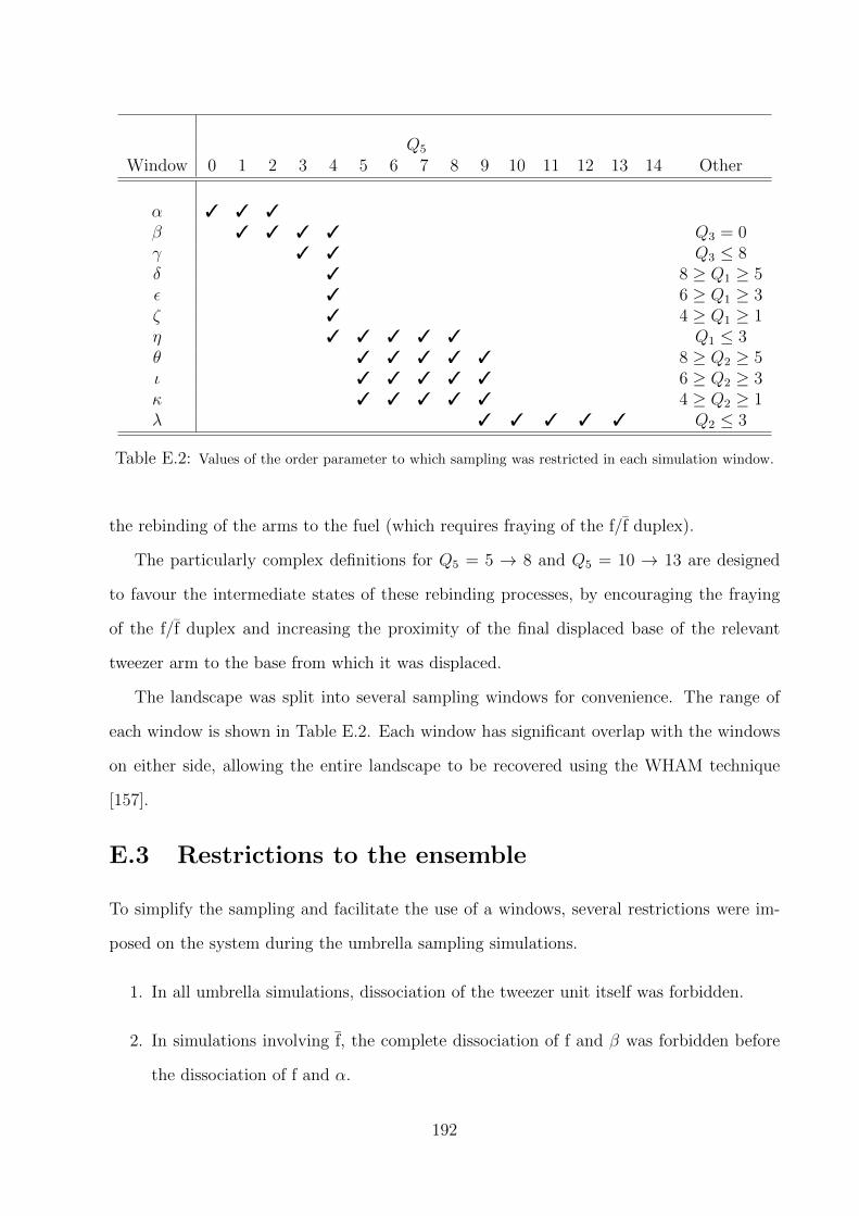
Q5
Window 0 1 2 3 4 5 6 7 8 9 10 11 12 13 14 Other
α 3 3 3
β 3 3 3 3 Q3 = 0γ 3 3 Q3 ≤ 8δ 3 8 ≥ Q1 ≥ 5ε 3 6 ≥ Q1 ≥ 3ζ 3 4 ≥ Q1 ≥ 1η 3 3 3 3 3 Q1 ≤ 3θ 3 3 3 3 3 8 ≥ Q2 ≥ 5ι 3 3 3 3 3 6 ≥ Q2 ≥ 3κ 3 3 3 3 3 4 ≥ Q2 ≥ 1λ 3 3 3 3 3 Q2 ≤ 3
Table E.2: Values of the order parameter to which sampling was restricted in each simulation window.
the rebinding of the arms to the fuel (which requires fraying of the f/f duplex).
The particularly complex definitions for Q5 = 5 → 8 and Q5 = 10 → 13 are designed
to favour the intermediate states of these rebinding processes, by encouraging the fraying
of the f/f duplex and increasing the proximity of the final displaced base of the relevant
tweezer arm to the base from which it was displaced.
The landscape was split into several sampling windows for convenience. The range of
each window is shown in Table E.2. Each window has significant overlap with the windows
on either side, allowing the entire landscape to be recovered using the WHAM technique
[157].
E.3 Restrictions to the ensemble
To simplify the sampling and facilitate the use of a windows, several restrictions were im-
posed on the system during the umbrella sampling simulations.
1. In all umbrella simulations, dissociation of the tweezer unit itself was forbidden.
2. In simulations involving f, the complete dissociation of f and β was forbidden before
the dissociation of f and α.
192

i) ii) iii)
hinge
α
βf
f
Figure E.1: Illustration of the formation of a pathological state in windowed sampling.
3. Letting X denote the base furthest from the toehold along f to which f is bound, states
with tweezer strands bound to f at bases between X and the toehold were explicitly
forbidden.
To sample states violated by restrictions 1 and 2, it would have been necessary to
drive the relevant dissociation/hybridization reactions, thereby complicating the sampling.
I decided that the most honest approach was to explicitly forbid these possibilities, rather
than simply fail to sample them.
Restriction 3 was based on the need to split the umbrella sampling into windows. I used
umbrella windows designed specifically to sample the progression of the displacement of the
α arm (windows γ to ζ), in which complete detachment from the fuel was forbidden, and
a window designed to sample the release and reattachment equilibrium for the final few
base-pairs of the α/f duplex (window η).
In an early simulation of a window in which the dissociation of α and f was forbidden,
the situation illustrated in Figure E.1 occurred. (i) The α/f duplex was reduced to one
base pair. (ii) A weak bond then formed further up the α arm to a base of f already bound
to f (a bound base can form transient, weak bonds to other bases in our model). (iii) In
this instance, the original α/f base pair broke first, leaving α and f weakly attached. This
state actually has a low free energy compared to others in the simulation window, as it
maximizes the number of strong base pairs, but the bond would have quickly broken and
allowed the tweezers to open in a simulation in which dissociation was possible. In this case,
this easy escape was prohibited, and so the simulation was essentially stuck (although low
in free energy, the state was hard to access, requiring a peculiar sequence of events - it was
193

Windows Q test statistic Windows Q test statistic
α/β (8,0,0,0,1) 0.0413 ζ/η (2,8,14,0,4) 0.8182α/β (0,8,0,0,1) 0.6610 ζ/η (1,8,15,0,4) 0.3882β/γ (8,8,0,0,3) 0.8951 η/θ (0,8,16,0,6) 0.5098β/γ (7,7,0,0,3) 0.9349 η/θ (0,8,16,0,8) 0.6719γ/δ (8,8,8,0,4) 0.9435 θ/ι (0,6,16,2,9) 0.8249γ/δ (7,7,7,0,4) 0.9316 θ/ι (0,5,16,3,9) 0.3024δ/ε (6,8,10,0,4) 0.7710 ι/κ (0,4,16,4,9) 0.2573δ/ε (5,8,11,0,4) 0.7278 ι/κ (0,3,16,5,9) 0.9430ε/ζ (4,8,12,0,4) 0.6722 κ/λ (0,2,16,6,9) 0.6473ε/ζ (3,8,13,0,4) 0.7310 κ/λ (0,1,16,7,9) 0.9651
Table E.3: Test statistics obtained from comparing the distribution of E(Q) in overlapping windows.
consequentially also difficult to escape from). Rather than attempting to force the sampling
of these states, it was decided to impose restriction 3 to prevent them forming.
To ensure that the neglected states were not significant in the operational cycle of the
tweezers, simulations were also performed in which no artificial weighting or bias was im-
posed. Many complete (irreversible) cycles were recorded: no violations of restrictions 1
and 2 were observed. Rare, transient violations of the restriction 3 were observed, but they
had no noticeable affect on the displacement processes.
E.4 Comparing 〈E(Q)〉 from different windows
To be certain that windowing of simulations did not affect sampling accuracy by limiting
ergodicity, as outlined in Chapter 7, values of 〈E(Q)〉 were compared for two commonly
sampled values of Q for each overlap region between adjacent windows. The distributions of
E(Q) measured in the simulation were tested for significance using Welch’s unpaired t-test
[214]. The results, shown in Table E.3, are as would be expected for consistent sampling
(only one order parameter appears to show significant difference at the 95% level, as would
be expected from 20 tests).
194

Appendix F
Details of sampling methods for theDNA walker
Three types of simulation were performed on the DNA walker system presented in Chapter
8. Firstly, simple unbiased Langevin and VMMC simulations were performed to study the
kinetics of foot-binding, and also to explore the possibility of lifting of the wrong foot.
To obtain thermodynamic data, VMMC simulations were performed with biases that are
discussed in the following section. Finally, Langevin simulations using forward flux sampling
were used to study the possible mechanism of lifting the wrong foot from the track.
F.1 Order parameters used in thermodynamic simu-
lations
Generally, order parameters were primarily constructed using the number of hydrogen-
bonding interactions with energies below −0.1 (in reduced units). An additional dimension,
analogous to the Q5 introduced for the tweezers (see Appendix E), was sometimes used to
favour bringing duplexes into close proximity. For all simulations considered in this section,
base pairs were deemed to be formed if hydrogen-bonding energy was < −0.1 simulation
units.
• Front site binding: 3-dimensional order parameter.
– Q1: the number of correct bp between foot 21 and the front site.
1the initially raised foot
195

– Q2: the number of misbonded bp between foot 2 and the front site.
– Q3: based on the separation of foot 2 from the front site when in the unbound
state.
In these simulations, binding to the back site was forbidden, as was the dissociation
of the initially attached foot from the track. Correct bonds and misbonds with the
front site were limited to 14 and 2 bp respectively.
• Back site binding simulations were performed exactly analogously to the front site
calculations.
• Competion between toehold domains: 3-dimensional order parameter.
– Q1: the number of correct bp between foot 1 and the middle site.
– Q2: the number of correct bp between foot 2 and the front site.
– Q3: if either of the bp at the ends of the duplexes away from the competition
region had frayed, Q3 = 1, otherwise Q3 = 0 .
To encourage migration of the displacement junction, states with one fewer than the
maximum number of bonds were favourably biased. The unintended result of this
bias (when first applied) was that additional fraying was observed at the far ends
of the walker/track duplexes, rather than fraying near the junction point. Q3 was
therefore included to distinguish between states with and without frayed ends, allowing
fraying at the displacement junction to be selectively favoured. In these simulations,
detachment of either foot was prohibited, as was any binding to the back site.
• Fuel binding: 6-dimensonal order parameter.
– Q1: the number of correct bp between foot 1 and the middle site.
– Q2: the number of correct bp between foot 2 and the front site.
– Q3: if either of the bp at the ends of the duplexes away from the competition
region had frayed, Q3 = 1, otherwise Q3 = 0 .
196
– Q4: the number of correct bp with the competing toehold domain and the non-
toehold domain of the back foot.
– Q5: the number of correct bp with the competing toehold domain of the front
foot.
– Q6: based on the separation of the fuel from the toehold domain of the feet.
Both fuel-binding dimensions were limited to a maximum of 6 bp, and detachment
from the track of either foot was prohibited. An additional dimension was included to
bias the fuel towards approaching the toehold domains. In these simulations, binding
to the back site was prohibited and incorrect pairing involving the fuel or foot 2 was
limited to 2 bp.
• Displacement: 3-dimensional order parameter.
– Q1: the number of correct bp between foot 1 and the middle site.
– Q2: the number of correct bp between foot 1 and the fuel.
– Q3: if either of the bp at the ends of the foot 1/fuel or foot 1/track duplexes
away from the competition region had frayed, Q3 = 1, otherwise Q3 = 0 .
Migration of the branch point was accelerated in a manner analogous to the simulation
of the competition domain. Once again, binding to the back site and total detachment
of either foot from the track was prohibited, as was the detachment of fuel from the
back foot. Incorrect pairing involving the fuel or the front foot was limited to 2 bp.
In order to sample the two mismatch repairing steps, it was found to be advantageous
to split the displacement into two windows that were combined using the WHAM
algorithm [157].
• Foot lifting: 3-dimensional order parameter.
– Q1: the number of correct bp between foot 1 and the middle site.
– Q2: the number of correct bp between foot 1 and the fuel.
197

– Q3: based on the separation of foot 1 and the back site when in the unbound
state.
In these simulations, detachment of foot 2 from the track, detachment of the fuel from
foot 1 and any binding to the back site were forbidden. Bonds between foot 1 and the
middle site were limited to 7 or fewer, and incorrect pairing involving the fuel or the
front foot was limited to 2 bp. As the dimensions used for foot lifting were not identical
with the displacement simulations, WHAM cannot be used to combine the two sets
of data. Instead, the data was condensed onto a 1-dimensional axis (the number of
bp between back foot and the middle site of the track) for both windows, and a near-
perfect agreement in the overlap region used to combine the data to produce Figure
8.8 (b).
As with the tweezers, the restrictions to the system were imposed to ensure that accurate
and well-defined sampling could be performed. In this case, unbiased simulations have
revealed a number of effects not visible in the restricted thermodynamics simulations – such
as the possibility of binding proceeding via misbonds. Nonetheless, the thermodynamic
simulations provide a good starting point in understanding the kinetic results, such as the
bias for binding correctly to the front site under tension.
F.2 Forward flux sampling of lifting the front foot
In Chapter 8, a possible mechanism for lifting the front foot after binding to its raised toehold
is suggested. Once bound to the raised toehold, the fuel can either detach or reach round
and begin to displace the track from the front foot. I estimated the relative probability of
these two events occurring using forward flux sampling. Forward flux sampling is discussed
in detail in Chapter 3.
Unlike umbrella sampling, forward flux sampling does not easily generalize to a transition
which can only be well described by a two-dimensional order parameter. In this case, I am
essentially interested in finding the relative probability of fuel dissociating normally from
the front toehold compared to fuel unbinding from the toehold whilst bound to another
198

part of the foot, leading to displacement of the track. A natural order parameter, therefore,
would have one dimension related to the binding of the fuel to the toehold and another
describing the binding of the fuel to the rest of the foot.
To simplify the requirements of the algorithm, I used forward flux sampling to mea-
sure the flux from a state in which the fuel is bound to the toehold to one in which it
has dissociated, and separately to one in which it has formed 8 bp with the non-toehold
region (but still attached to the toehold). Such a partially-displaced state was observed
to be a metastable minimum of free energy, corresponding to a ‘double-X’ configuration.
Individually, both processes are relatively simple to describe using a one-dimensional or-
der parameter. I then assumed that trajectories that reached the metastable minimum of
partial displacement tend to equilibriate within the local minimum before either the fuel
detaches from the toehold or the non-toehold region. Using this assumption, I ran separate
simulations initiated from states with 8 bp between the non-toehold region and the fuel to
calculate the probability of successful foot-raising after such a state has been reached.2
F.2.1 Measuring the melting flux
I measured the flux from a state in which the fuel is bound to the raised toehold of the front
foot to a state in which the hydrogen-bonding sites of the fuel are separated by at least
3 simulation units from the hydrogen-bonding sites of the toehold. The order parameter
definitions and simulation results are given in Table F.1.
Multiplying the initial flux by the probabilities gives a melting flux of Φmelt = 1.24×10⁻⁷
per unit simulation time.3 An error on this quantity can be estimated in the following
manner. 10 simulations were performed to estimate the initial flux, with a standard error
on the mean of 1.43× 10⁻⁴ per unit time (compared to an average of 7.33× 10⁻³ per unit
time). The later stages can be modelled as Bernoulli trials – the probability of success
2It should be noted that the estimate of displacement only includes trajectories that reach 8 bp betweenthe non-toehold region and the fuel prior to dissociation of the fuel from the toehold. It is possible thatdisplacement may occur without such a state being reached, and also that there are completely differentpathways to displacement that are not sampled due to the chosen order parameter.
3Due to the caveats with comparing simulation time to absolute time, I will report all fluxes in terms ofthe simulation time, and only compare relative values.
199
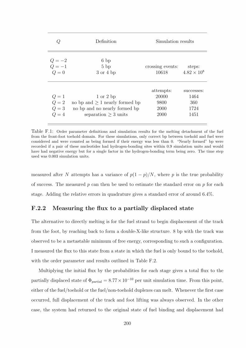
Q Definition Simulation results
Q = −2 6 bpQ = −1 5 bp crossing events: steps:Q = 0 3 or 4 bp 10618 4.82× 10⁸
attempts: successes:Q = 1 1 or 2 bp 20000 1464Q = 2 no bp and ≥ 1 nearly formed bp 9800 360Q = 3 no bp and no nearly formed bp 2000 1724Q = 4 separation ≥ 3 units 2000 1451
Table F.1: Order parameter definitions and simulation results for the melting detachment of the fuelfrom the front-foot toehold domain. For these simulations, only correct bp between toehold and fuel wereconsidered and were counted as being formed if their energy was less than 0. “Nearly formed” bp wererecorded if a pair of these nucleotides had hydrogen-bonding sites within 0.9 simulation units and wouldhave had negative energy but for a single factor in the hydrogen-bonding term being zero. The time stepused was 0.003 simulation units.
measured after N attempts has a variance of p(1 − p)/N , where p is the true probability
of success. The measured p can then be used to estimate the standard error on p for each
stage. Adding the relative errors in quadrature gives a standard error of around 6.4%.
F.2.2 Measuring the flux to a partially displaced state
The alternative to directly melting is for the fuel strand to begin displacement of the track
from the foot, by reaching back to form a double-X-like structure. 8 bp with the track was
observed to be a metastable minimum of free energy, corresponding to such a configuration.
I measured the flux to this state from a state in which the fuel is only bound to the toehold,
with the order parameter and results outlined in Table F.2.
Multiplying the initial flux by the probabilities for each stage gives a total flux to the
partially displaced state of Φpartial = 8.77×10⁻¹⁰ per unit simulation time. From this point,
either of the fuel/toehold or the fuel/non-toehold duplexes can melt. Whenever the first case
occurred, full displacement of the track and foot lifting was always observed. In the other
case, the system had returned to the original state of fuel binding and displacement had
200

Q Definition Simulation results
Q = −2 separation between correct bp of fueland non-competion domain > 4 units
Q = −1 4 ≥ separation > 2 units crossing events: steps:Q = 0 2 ≥ separation > 1 unit 3850 3.84× 10⁹
attempts: successes:Q = 1 separation ≤ 1 and no bp 20000 1798
or nearly-formed bpQ = 2 no bp and ≥ 1 nearly formed bp 4500 1343Q = 3 1 or 2 bp 20000 824Q = 4 3 or 4 bp 20000 956Q = 5 5,6 or 7 bp 3573 462Q = 6 ≥ 8 bp 5000 2020
Table F.2: Order parameter definitions and simulation results for the initiation of wrong-foot displacementafter the fuel has bound to the front-foot toehold domain. For these simulations, only correct bp wereconsidered and were counted as being formed if their energy was less than −0.5 in simulation units. ‘Nearlyformed’ bp were recorded if a pair of these nucleotides had a hydrogen-bonding energy of 0 > E ≥ −0.5,or had hydrogen-bonding sites within 0.9 simulation units and would have had negative energy but for asingle factor in the hydrogen-bonding term being zero. The time step used was 0.003 simulation units.
failed. Both processes are reasonably fast (being in the double-X configuration destabilizes
the fuel/toehold duplex), so the relative rates could be estimated simply by running unbiased
simulations starting from the intermediate displacement state. Of 50 simulations initiated
from the partially displaced state, 25 completed the displacement and 25 returned to the
original state of having the fuel bound to the track only (one failed to do either in the
simulation time). Combining this estimate with the flux to the partially displaced state, I
obtain a flux to successful displacement from a state with fuel bound to the walker toehold
of Φdisplacement = 4.39×10⁻¹⁰ per unit simulation time, with an error of around 16.2%. Thus,
Φdisplacement
Φmelt
= 0.0035, (F.1)
with an error of around 17.2%.
201

Thesis errata
Thomas Ouldridge
27/4/2012
For anyone intending to use the description of the model in this text to simulate said model, thefollowing corrections are important.
1. The final line of Equation 2.16 should have additional minus signs, giving:
Vstack = f1(δrstack, εstack, astack, δr0stack, δr
c,lowstack , δr
c,highstack , δr
lowstack, δr
highstack)
× f4(θ4, astack,4, θ0stack,4,∆θ
?stack,4)
× f4(θ5′ , astack,5, θ0stack,5,∆θ
?stack,5) f4(θ6′ , astack,6, θ
0stack,6,∆θ
?stack,6)
× f5(− cos(φ1), astack,1,− cos(φ1)?stack) f5(− cos(φ2), astack,2,− cos(φ2)
?stack).
2. The Vstack entry into Table 2.1 should have additional minus signs, giving:
Interaction Parameters
Vstack f1(δrstack) εstack = 1.3448 astack = 6 δr0stack = 0.4+2.6568 kT
δrcstack = 0.9 δrlowstack = 0.32 δrhighstack = 0.75f4(θ4) astack,4 = 1.30 θ0stack,4 = 0 ∆θ?stack,4 = 0.8f4(θ5′) astack,5 = 0.90 θ0stack,5 = 0 ∆θ?stack,5 = 0.95f4(θ6′) astack,6 = 0.90 θ0stack,6 = 0 ∆θ?stack,6 = 0.95
f5(− cos(φ1)) astack,1 = 2.00 − cos(φ1)?stack = −0.65
f5(− cos(φ2)) astack,2 = 2.00 − cos(φ2)?stack = −0.65
3. Equation (A.7) should contain additional minus signs, giving:
∇q,rVneighbour =
dVFENE(δrbackbone)dδrbackbone
∇q,r(δrbackbone) +∑
x,y?df3(δrxy)
dδrxy∇q,r(δrxy)
+ Vstackf1(δrstack)
df1(δrstack)dδrstack
∇q,r(δrstack) +∑
i=4,5′,6′Vstackf4(θi)
df4(θi)dθi∇q,r(θi)
+ Vstackf5(− cos(φ1))
df5(− cos(φ1))d cos(φ1)
∇q,r(cos(φ1))
+ Vstackf5(− cos(φ2))
df5(− cos(φ2))d cos(φ2)
∇q,r(cos(φ2)),
1

4. Equation (A.8) contains a mistake: some f4 functions should be replaced by f5, giving:
∇q,rVnon−neighbour =
∑x,y
df3(δrxy)
dδrx,y∇q,r(δrxy) + VHB
f1(δrHB)df1(δrHB)dδrHB
∇q,r(δrHB)
+∑
i=1−4,7,8VHB
f4(θi)df4(θi)dθi∇q,r(θi)
+Vcross stack
f2(δrHB)df2(δrHB)dδrHB
∇q,r(δrHB) +∑3
i=1Vcross stack
f4(θi)df4(θi)dθi∇q,r(θi)
+∑
i=1,7,8Vcross stack
f4(θi)+f4(π−θi)d(f4(θi)+f4(π−θi)
dθi∇q,r(θi)
+ Vcoax stack
f2(δrstack)df2(δrstack)dδrstack
∇q,r(δrstack) + Vcoax stack
f4(θ4)df4(θ4)dθ4∇q,r(θ4)
+ Vcoax stack
f4(θ1)+f4(2π−θ1)d(f4(θ1)+f4(2π−θ1)
dθ1∇q,r(θ1)
+∑6
i=5Vcoax stack
f4(θi)+f4(π−θi)d(f4(θi)+f4(π−θi)
dθi∇q,r(θi)
+∑4
i=3Vcoax stack
f5(cos(φi))df5(cos(φi))d cos(φi)
∇q,r cos(φi),
2


