Embed Size (px)
Citation preview

Classification of Constraints by Set Covering
by
Ashok Krishnamurthy
A Major PaperSubmitted to the Faculty of Graduate Studies and Researchthrough the Department of Mathematics and Statistics
in partial fulfillment of the Requirements forthe Degree of Master of Science at the
University of Windsor
Windsor, Ontario, Canada
c© 2001 Ashok Krishnamurthy
Abstract
In this major paper, we explore Boneh’s Set-Covering (SC) equivalence
technique for the classification of constraints in mathematical programmes as
either redundant or necessary. At the core of Boneh’s technique is a method
for sampling in n-space and for each such point generating a binary row of a
SC matrix, Ep0 , whose jth component is one if and only if the jth constraint
is violated at that point. We describe a simple implementation of Boneh’s
technique that we refer to as the base method. The base method produces a
redundancy free constraint matrix for a SC problem. Boneh has shown that
any solution to the SC problem yields a constraint classification, which, in
turn, yields a reduction of the constraint set.
Our contribution is an improvement over the base method that reduces
the time required to find the redundancy free SC matrix. We call this the
filter method as it utilizes a technique to filter out sample points in n-space for
which it can be determined a priori that the corresponding binary row will be
redundant in the SC constraint matrix.
In addition to the filter method, we also provide new theorems about the
SC equivalence and limited numerical results and we give a description of our
computer implementation.
iii

Acknowledgements
The research that has gone into this major paper has been thoroughly
enjoyable. That enjoyment is largely a result of the interaction that I have had
with my supervisors and the people who have tested and used the resulting
software. I feel very privileged to have worked with my co-supervisors, Dr.
Richard J. Caron and Dr. Tim Traynor. To each of them I owe a great debt
of gratitude for their patience, inspiration and friendship. Dr. Richard J.
Caron and Dr. Tim Traynor have taught me a great deal about the field of
Operational Research by sharing with me the joy of discovery and investigation
that is the heart of research.
The Department of Mathematics and Statistics and The Operational
Research Laboratory have provided an excellent environment for my research.
Finally, thanks also to my family who have been extremely understanding
and supportive of my studies. I feel very lucky to have a family that shares
my enthusiasm for academic pursuits.
iv

Contents
Abstract iii
Acknowledgments iv
1 Introduction 11.1 Introduction . . . . . . . . . . . . . . . . . . . . . . . . . . . . . 11.2 Notation and Definitions . . . . . . . . . . . . . . . . . . . . . . 21.3 Historical Perspective . . . . . . . . . . . . . . . . . . . . . . . . 51.4 Contributions and Outline . . . . . . . . . . . . . . . . . . . . . 71.5 Conclusion . . . . . . . . . . . . . . . . . . . . . . . . . . . . . . 7
2 The Base Method 82.1 Introduction . . . . . . . . . . . . . . . . . . . . . . . . . . . . . 82.2 Boneh’s SC equivalence . . . . . . . . . . . . . . . . . . . . . . . 82.3 The Base method . . . . . . . . . . . . . . . . . . . . . . . . . . 142.4 Examples . . . . . . . . . . . . . . . . . . . . . . . . . . . . . . 162.5 Conclusion . . . . . . . . . . . . . . . . . . . . . . . . . . . . . . 19
3 A Filter Method 213.1 Introduction . . . . . . . . . . . . . . . . . . . . . . . . . . . . . 213.2 A Filter Method . . . . . . . . . . . . . . . . . . . . . . . . . . . 213.3 Examples . . . . . . . . . . . . . . . . . . . . . . . . . . . . . . 253.4 Conclusion . . . . . . . . . . . . . . . . . . . . . . . . . . . . . . 27
4 File Format and Visual Basic 6.0 Implementation 284.1 Introduction . . . . . . . . . . . . . . . . . . . . . . . . . . . . . 284.2 The Input File and Format . . . . . . . . . . . . . . . . . . . . . 284.3 Implementation in Visual Basic 6.0 . . . . . . . . . . . . . . . . 304.4 Conclusion . . . . . . . . . . . . . . . . . . . . . . . . . . . . . . 42
5 Conclusion 435.1 Contributions . . . . . . . . . . . . . . . . . . . . . . . . . . . . 435.2 Future work . . . . . . . . . . . . . . . . . . . . . . . . . . . . . 435.3 Conclusion . . . . . . . . . . . . . . . . . . . . . . . . . . . . . . 43
Appendix A 44
Bibliography 46
v

1 Introduction
1.1 Introduction
In this major paper, we are concerned with pre-processing sets of con-
straints that arise in mathematical programming problems. A mathematical
programming problem is a problem of determining the value of variables that
will satisfy a set of constraints and that will also optimize an objective which
depends on those variables.
Some of the objectives of a pre-processing step are the detection of un-
boundedness or infeasibility, and the reduction of the size of the constraint set.
Such an reduction can be achieved by detecting and removing the so called
redundant constraints.
A redundant constraint is one that can be removed without causing a
change in the feasible region. Removal of redundancy not only produces a
cleaner, more useful constraint set, but it can also have an enormous impact
on the solution time.
The problem of identifying redundant constraints can be solved by ei-
ther probabilistic methods or the deterministic methods. We will consider a
particular probabilistic technique introduced by Boneh that can be used to
identify redundancy for very general constraints. At the core of Boneh’s tech-
nique is a method for sampling in n-space and for each such point generating
a binary row of a Set-Covering (SC) matrix, Ep0 , whose jth component is one
if and only if the jth constraint is violated at that point. We describe a simple
implementation of Boneh’s technique that we refer to as the base method. The
1

base method produces a redundancy free constraint matrix for a SC problem.
Boneh has shown that any solution to the SC problem yields a reduction of
the constraint set.
Our contribution is an improvement over the base method that reduces
the time required to find the redundancy free SC matrix. We call this the
filter method as it utilizes a technique to filter out sample points in n-space for
which it can be determined a priori that the corresponding binary row will be
redundant in the SC constraint matrix.
In addition to the filter method, we also provide new theorems about the
SC equivalence and provide limited numerical results and give a description of
our computer implementation.
1.2 Notation and Definitions
In this paper we adopt the notation and definitions given in [5].
We begin with the set J having cardinality |J | which indexes the con-
straint set
C(J) = {gj(x) ≤ 0, j ∈ J}.
We refer to “gj(x) ≤ 0” as the jth constraint. The set of constraints is
given in a general form that allows traditional linear, quadratic and continuous
nonlinear constraints.
The feasible region for the constraint set is
R(J) = {x ∈ Rn | gj(x) ≤ 0, j ∈ J}.
If R(J) = ∅, we say that R(J) is empty and that C(J) is infeasible. If
2
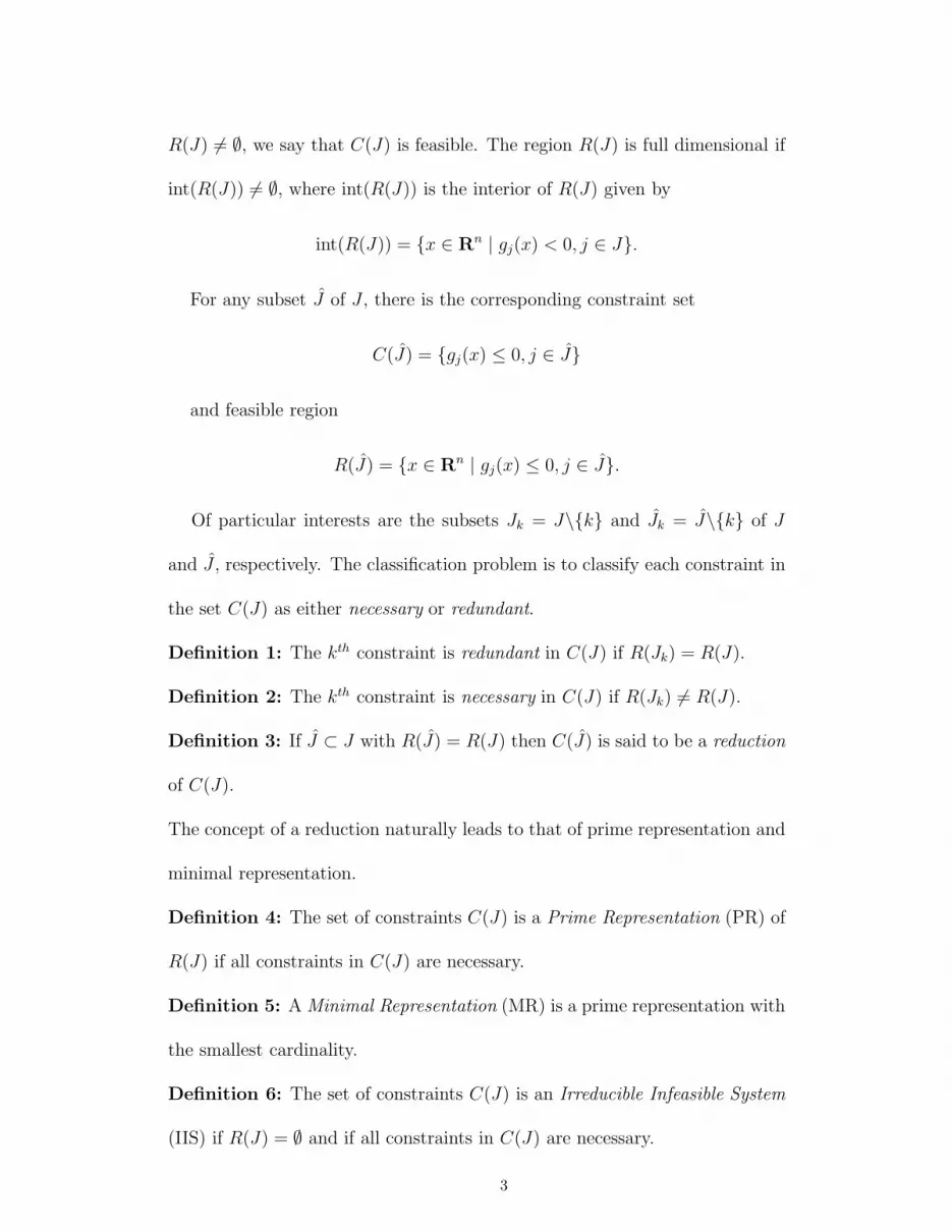
R(J) �= ∅, we say that C(J) is feasible. The region R(J) is full dimensional if
int(R(J)) �= ∅, where int(R(J)) is the interior of R(J) given by
int(R(J)) = {x ∈ Rn | gj(x) < 0, j ∈ J}.
For any subset J of J , there is the corresponding constraint set
C(J) = {gj(x) ≤ 0, j ∈ J}
and feasible region
R(J) = {x ∈ Rn | gj(x) ≤ 0, j ∈ J}.
Of particular interests are the subsets Jk = J\{k} and Jk = J\{k} of J
and J , respectively. The classification problem is to classify each constraint in
the set C(J) as either necessary or redundant.
Definition 1: The kth constraint is redundant in C(J) if R(Jk) = R(J).
Definition 2: The kth constraint is necessary in C(J) if R(Jk) �= R(J).
Definition 3: If J ⊂ J with R(J) = R(J) then C(J) is said to be a reduction
of C(J).
The concept of a reduction naturally leads to that of prime representation and
minimal representation.
Definition 4: The set of constraints C(J) is a Prime Representation (PR) of
R(J) if all constraints in C(J) are necessary.
Definition 5: AMinimal Representation (MR) is a prime representation with
the smallest cardinality.
Definition 6: The set of constraints C(J) is an Irreducible Infeasible System
(IIS) if R(J) = ∅ and if all constraints in C(J) are necessary.
3

Definition 7: Let C(J) be an infeasible constraint set and let J ⊂ J . Then
C(J) is an infeasibility set of C(J) if C(J\J) is feasible.
Definition 8: A minimal infeasibility set (MIS) is a minimum cardinality
infeasibilty set.
In the next chapter we will show how Boneh’s SC equivalence technique can
be used to find a PR, MR, IIS, and MIS.
4

1.3 Historical Perspective
An algorithm used to detect redundant constraints can usually be classified
as either a probabilistic hit-and-run method or a deterministic mathematical
programming based method. In addition to these two approaches, Boneh [1]
proposed a probabilistic method based on an equivalence between the problem
of finding a reduction to a set of constraints and the problem of finding a
feasible solution to a set-covering problem.
The deterministic methods are based on the connection between the
classification of a constraint and the solution of a particular mathematical
program. The first paper devoted entirely to redundancy was given by Boot [4]
in 1962. Boot suggested checking the redundancy of a constraint by replacing
the inequality of a constraint by a strict inequality in the reverse direction.
The constraint is redundant if the resulting system is infeasible. Specifically,
the kth constraint is redundant if {x ∈ Rn | gk(x) > 0, gj(x) ≤ 0, j �= k, j ∈ J}
is empty. Instead of the feasibility problem we could solve the mathematical
program max { gk(x) | x ∈ R(Jk) }. If the problem has an optimal solution x∗
with gk(x∗) ≤ 0 then the kth constraint is redundant.
Let’s suppose that C(J) is a set of linear constraints. If R(J) �= ∅,
then the deterministic method produces a prime representation C(J) of R(J).
Indeed, if there are no implicit equalities, then C(J) is a minimal representation
of R(J). For a feasible system, the deterministic algorithm is, in fact, the
foundation for all the simplex based methods in Karwan et al. [10] and the
method in Caron et al. [6].
5

While the deterministic algorithm provides a useful way to approach the
constraint classification problem, its usefulness is really restricted to systems
linear constraints. Even then, the time taken to classify constraints is rarely
compensated by the resulting savings in the time to solve the reduced prob-
lem. Because of the shortcomings, researchers were drawn to the probabilistic
methods.
The first probabilistic method, which came to be known as the hyper-
sphere direction hit-and-run method was introduced in [3]. Without the loss of
generality we assume that there are no duplicate constraints. The hit-and-run
methods depend upon the provision of a point x0 ∈ int(R(J)). The next step
is to choose a point uniformly in the unit hypersphere to serve as a direction
vector. The point x0 together with the direction vector define a random line
which passes through the feasible region. It can be shown that, under appro-
priate assumptions on the constraint functions, the end points of the feasible
segment of the random line detect one or two necessary constraints. Finally, a
randomly chosen point on the feasible line segment provides the next interior
point. Shortcomings of the hit-and-run method are that they can only be used
if the feasible region is non-empty and that there is a need for an initial interior
feasible point.
For general nonlinear problems it may well be that neither the determin-
istic nor the hit and run methods are suitable. This major paper is concerned
with a particular probabilistic method introduced by Boneh [1], which can be
used for the classification problem.
6

1.4 Contributions and Outline
In chapter 2, we present Boneh’s [1] set-covering (SC) equivalence technique
for the classification of constraints as either necessary or redundant. We give an
implementation of the SC approach which we call our base method and supply
examples. We also present two new theorems about the SC equivalence.
In chapter 3, we present an improvement over the base method, which
we call the filter method. Our contribution is an improvement over the base
method that reduces the time required to find the redundancy free SC matrix.
We call this the filter method as it utilizes a technique to filter out sample points
in n-space for which it can be determined a priori that the corresponding binary
row will be redundant in the SC constraint matrix. We present examples and
compare the results with the base method.
Finally, in chapter 4, we present a brief description of the Visual Basic
6.0 software developed for the implementation of the methods discussed in
chapters 2 and 3.
1.5 Conclusion
In this chapter we gave the necessary notation and definitions. We briefly
reviewed deterministic and probabilistic redundancy algorithms for mathemat-
ical programs.
7

2 The Base Method
2.1 Introduction
In this chapter, we present the method of detecting redundancy by a set-
covering (SC) equivalence that was introduced by Boneh [1] in 1984. We give a
simple implementation of Boneh’s method which we call our base method. We
also present two examples to demonstrate the method. This chapter provides
a foundation for our new method presented in chapter 3.
2.2 Boneh’s SC equivalence
Boneh’s equivalence is based upon the following theorem, a reformulation
of the fact that at least one of the constraints violated by an infeasible point
x ∈ Rn must be necessary.
Theorem 1: [8] Let J ⊂ J . Then C(J) is a reduction of C(J) if and
only if whenever x is an infeasible point, there exists j ∈ J with gj(x) > 0.
Proof: Since we always have R(J) ⊇ R(J), C(J) is a reduction of C(J)
if and only if R(J) ⊆ R(J). Considering complements, this holds if and only
if each x which does not belong to R(J), does not belong to R(J). But this
means whenever x is an infeasible point, there exists j ∈ J with gj(x) > 0, as
required.
Now, let’s refer to x ∈ Rn as an observation. Corresponding to this obser-
vation is a binary row of length m given by
e(x) = (e1(x), e2(x), . . . , em(x)),
8

where
ej(x) =
{1 if gj(x) > 00 if gj(x) ≤ 0
for j = 1, 2, . . . , m.
Suppose that C(J) is a reduction of C(J) and let y ∈ {0, 1}m be such that
yj = 0 if j ∈ J\J and yj = 1 if j ∈ J . Theorem 1 implies that
e(x)y ≥ 1.
This inequality reminds us of the constraints of a set-covering (SC) prob-
lem min {1T · y|Ey ≥ 1, y ∈ {0, 1}m}, where, 1 is a vector of “ones”. For each
x ∈ Rn, we have the binary row e(x). Let E0 have rows e(x), ∀x ∈ Rn, with
the condition that all duplicate rows are removed.
Since 0 · y ≥ 1 is impossible, we define E to be the matrix E0 with
the zero row removed, if it exists, to get a suitable matrix for a set-covering
problem. Note that e(x) = 0 if and only if x ∈ R(J).
First, we note that in general the number of rows in E is bounded by
2m−1, the number of different, nonzero binary rows of lengthm. The following
theorem gives a better upper bound on the number of rows, provided the
constraints are linear. In the linear case there is a one-to-one correspondence
between the number of rows in E and the number of full dimensional regions
created by the constraint hyperplanes.
Theorem 2: The number of full dimensional regions in Rn determined
by m hyperplanes is at most 1 + m +
(m2
)+
(m3
)+ · · · +
(mn
).
Proof: See [11, page 1].
9

The following example shows how large this can be, and it compares the
two bounds on the number of rows.
For n = 4 and m = 20 we have the first bound 220 = 1, 048, 576 and the
new, tight bound, 1 + 20 +
(202
)+
(203
)+
(204
)= 6196.
Unfortunately, theorem 2 shows, the number of rows in E grows expo-
nentially with problem size but polynomially for a fixed number of variables.
It is very unlikely that we will be able to create the matrix E for practical
problems.
Implementing Boneh’s set covering technique requires a method of sam-
pling points in Rn to generate rows of E0. The result is a matrix Ep0 which is a
submatrix of E0. We remove the row e(x) = 0 from Ep0 , if it exists, to get the
matrix Ep. In the next section we present an implementation which we call
the base method. The next theorem provides a characterization of redundancy
for constraints in a SC problem.
Theorem 3: Let ei = (ei1, ......, eim) and ek = (ek1, ......, ekm) be two
rows of E. Then eij ≥ ekj , j = 1, 2, ..., m if and only if the constraint eiy ≥ 1
is redundant with respect to the constraint eky ≥ 1.
Proof: Suppose that eky ≥ 1. Since eij ≥ ekj, j = 1, 2, ..., m we have
that eiy =∑
j eijyj ≥ ∑j ekjyj = eky. Since y ∈ {0, 1}m and eky ≥ 1, eiy ≥ 1.
Now suppose that eky ≥ 1 implies that eiy ≥ 1. Suppose that ekj = 1. Then
ekyj = 1, where yj = (0, ...., 0, 1, 0, ..., 0) with a “1” in position j. This implies
that eiyj ≥ ekyj = 1 so that eij = 1. Thus, eij ≥ ekj , j = 1, ...., m.
10

Definition 9: Let Ep be a submatrix of Ep such that (i) Ep and Ep both
have m columns and (ii) Ep has no redundant rows. We say that Ep is a
redundancy free reduction of Ep.
The next theorem provides a situation for which we can give a lower
bound on the number of necessary constraints. The theorem was suggested by
Boneh [2], but the proof is original.
Theorem 4: Let E be a binary matrix with m columns. If all
(mi
)
binary rows of length m and sum i are rows of E and Ey ≥ 1, then∑
j yj ≥
m+ 1− i.
Proof: Suppose∑
j yj ≤ m − i. Let z be any binary word such that
z ≤ 1−y and∑
z = i. Then z is a row of E since all rows with sum i are rows
of E. Also z · y = 0. This contradicts Ey ≥ 1. Therefore,∑
j yj ≥ m+ 1− i.
Theorem 3 tells us that, if there are
(mi
)rows with row sum i, then at
least m+ 1− i constraints are necessary.
The next theorem provides a situation where information related to un-
boundedness or infeasibilty of the region can be obtained.
Theorem 5: Suppose the constraints in C(J) are linear. If there exists
a point where all the constraints are violated, then the region defined by the
constraint set is either empty or unbounded.
Proof: If there is a point where all the constraints are violated and
no point where all the constraints are satisfied then the region defined by the
constraint set is empty, which proves the first part of the theorem.
Let y be the point where all the constraints are violated and x be the point
11

where all the constraints are satisfied. Let us represent the linear constraints
by Ax ≤ b. Since Ay > b we have, −Ay < −b. Also, Ax ≤ b, therefore,
A(x − y) < b − b = 0. Thus, (x − y) is the direction of unboundedness.
We now give the connection between the constraint classification problem
and the SC feasibility problem Ey ≥ 1. Let y ∈ {0, 1}m satisfy Ey ≥ 1
and define J = {j|yj = 1}. Then C(J) is a reduction of C(J). If y solves
min {1T · y|Ey ≥ 1}, then C(J) is a minimal representation of R(J). We will
further explore the SC matrix E and reveal its connection to the problem of
finding a PR, as well as the problem of finding an IIS and an MIS.
The matrix E0 can be used to determine much about the constraint set
in addition to the results of theorems 4 and 5. Consider the following:
1. R(J) is non-empty if and only E0 has the zero row.
2. If R(J) �= ∅ then a solution to min {1T · y|Ey ≥ 1}, gives a MR.
3. If R(J) = ∅ then min {1T · y|Ey ≥ 1} gives an IIS.
4. If R(J) = ∅ we can get an MIS in the following way. Let e be a row of
E with minimum row sum. The constraints corresponding to ‘ones’ in e
gives an MIS.
Consider the following example, we can find IIS and MIS as follows.
Example 1: Consider Figure 1. We have four linear constraints that divide
the plane into nine full dimensional regions. The regions are labeled with their
12

corresponding binary rows. The arrows indicate the feasible half-spaces for
each constraint. The system is infeasible.
We have
E =
0 1 1 01 0 1 00 1 0 11 0 0 11 1 1 01 0 1 10 1 1 11 1 0 11 1 1 1
We obtain an IIS by solving min {1T · y|Ey ≥ 1}which has a solution y =
(1 1 0 0
). Thus {1,2} give an IIS. To get an MIS we note that the min-
imal row sum is 2 obtained from any of rows 1, 2, 3 and 4. Consider the first
row where the ones appear in columns 2 and 3. Thus {2,3} is an MIS. We
see from the diagram that removing constraints 2 and 3 results in a feasible
region.
13

2.3 The Base method
For clarity in the presentation of our comparison of algorithms, we present a
pseudo code for a base method.
Inputs:
n = number of variables,
m = number of constraints and
N = number of iterations.
Initialization:
Initialize Ep0 , E
p and Ep to be matrices with no rows andm columns.
Set:
i = 1
Repeat:
Choose a point xi ∈ Rn
Set e(xi) = (e1(xi), e2(xi), . . . , em(xi)) where
ej(xi) =
{0 if gj(xi) ≤ 01 otherwise.
If e(xi) /∈ Ep0
Add e(xi) to Ep0 .
End If
i = i+1
Until:
Stopping Rule.
Calculation:
Remove the zero row, if it exists, from Ep0 to get Ep .
Remove redundant rows from Ep to get Ep.
Output:
Ep.
There are many ways in which the points x ∈ Rn can be chosen. We
suggest uniform sampling in a hypercube. Our implementation is based on
14

the assumption that under the uniform distribution on L ≤ x ≤ U , there is
positive probability that there is an x with e(x) = e for each row e of E. We
use an iteration limit as the stopping rule.
15

2.4 Examples
Example 2: Consider the following set of six linear constraints
g1(x) = −x1
g2(x) = −x2
g3(x) = 3x1 + 4x2 − 12g4(x) = x1 − 3g5(x) = x2 − 3g6(x) = 4x1 + 3x2 − 16,
with L1 = −15, U1 = 25, L2 = −15, and U2 = 25.
From Figure 2 we see that constraints 5 and 6 are redundant. The arrows
point to the feasible half space for each constraint. The feasible region is
shaded.
Figure 2: Diagram for Example 2.
16

The matrices Ep0 and Ep obtained from our implementation of the base
method (see chapter 4) are
Ep0 =
0 0 0 0 0 00 0 0 1 0 00 0 1 0 0 00 1 0 0 0 01 0 0 0 0 00 0 1 0 0 10 0 1 0 1 00 0 1 1 0 00 1 0 1 0 01 0 0 0 1 01 1 0 0 0 00 0 1 0 1 10 0 1 1 0 10 1 0 1 0 11 0 1 0 1 00 0 1 1 1 10 1 1 1 0 11 0 1 0 1 1
and
Ep =
0 0 0 1 0 00 0 1 0 0 00 1 0 0 0 01 0 0 0 0 0
.
It is easy to see that a solution to min {1T · y|Epy ≥ 1}
is y =(1 1 1 1 0 0
)which says that constraints 5 and 6 are redun-
dant. Since the redundancy free SC matrix Ep contains only rows with a
single “1”, we have an easily solved SC problem.
17

Example 3: Consider the following set of four quadratic constraints and five
linear constraintsg1(x) = −x1 − x2 + 1g2(x) = −x2
1 − x22 + 1
g3(x) = −9x21 − x2
2 + 9g4(x) = −x2
1 + x2
g5(x) = −x22 + x1
g6(x) = −x1 − 50g7(x) = x1 − 50g8(x) = −x2 − 50g9(x) = x2 − 50,
with L1 = −75, U1 = 75, L2 = −75, and U2 = 75.
From Figure 3 we see that constraints 2, 3, 8 and 9 are redundant. The
arrows point to the feasible half space for each constraint. The feasible region
is shaded.
Figure 3: Diagram for Example 3.
18

The matrices Ep0 and Ep obtained from our implementation of the base
method (see chapter 4) are
Ep0 =
0 0 0 0 0 0 0 0 00 0 0 1 0 0 0 0 01 0 0 0 0 0 0 0 00 0 0 0 0 0 1 0 00 0 0 0 1 0 0 0 00 0 0 0 0 1 0 0 01 0 0 0 0 0 0 0 10 0 1 1 0 0 0 0 00 0 0 0 0 1 0 0 10 0 0 0 0 1 1 0 00 0 0 1 0 0 1 0 00 0 0 0 0 0 1 1 00 0 0 0 1 1 0 0 01 0 0 0 0 0 0 1 01 0 1 0 0 0 0 0 01 0 0 0 0 1 0 0 11 0 0 0 0 0 1 1 01 0 0 0 0 0 1 0 11 1 1 1 0 0 0 0 0
and
Ep =
0 0 0 1 0 0 0 0 01 0 0 0 0 0 0 0 00 0 0 0 0 0 1 0 00 0 0 0 1 0 0 0 00 0 0 0 0 1 0 0 0
.
It is easy to see that a solution to min {1T · y|Epy ≥ 1}
is y =(1 0 0 1 1 1 1 0 0
)which says that constraints 2, 3, 8 and 9
are redundant.
2.5 Conclusion
In this chapter, we briefly described the deterministic and probabilistic
algorithms and we have seen that both these methods have limitations in the
types of problem that can be handled. We discussed Boneh’s SC equivalence
19

technique. The main advantage of Boneh’s SC approach is that it can be used
for very general constraint sets. A further advantage of the SC approach is
that we can solve the PR, IIS and MIS problems provided we have the full
matrix E. We proved three theorems that are related to the SC equivalence.
We presented a pseudo code of the base method. We also presented examples
to demonstrate an implementation of the base method. In the next chapter
we present an improvement of the base method which we call a filter method.
20

3 A Filter Method
3.1 Introduction
In this chapter we present a filter method for the collection of rows for
the matrix Ep0 . The key idea behind the filter method is that we filter out
observations that we know will give redundant information when creating the
SC matrix. We also present numerical results to show the effectiveness of the
filter method over the base method. In the last section of this chapter we will
see that the filtering decreases the time required to find Ep.
3.2 A Filter Method
We begin with an example.
Example 4: Suppose that e(x) =(0 0 0 0 0 1 0 0 0 0 0 0
)for
some x ∈ Rn and for some constraint set C(J), |J | = 12. From theorem 1 we
see that constraint 6 must be necessary. Let x ∈ Rn be such that e6(x) = 1,
that is, g6(x) > 0. From theorem 3, we see that e(x) is a redundant row. Note
that the conclusion did not depend upon the entries ej(x), j �= 6.
From example 4, we can imagine a modification of the base method
where, for an observation x ∈ Rn, the constraints that have been classified as
necessary are evaluated first. As soon as one of them is found to be violated,
we stop further calculations at x since e(x) is redundant in the SC matrix.
On the other hand, if all the constraints that have been classified as necessary
are satisfied at x, we proceed with the full calculation of e(x). This idea is
the basis for our filter method, for which a pseudo code is given in the next
section. We call it filter method as it filters out observations x that provide
21

redundant information prior to the complete evaluation of e(x).
Inputs:
n = number of variables,
m = number of constraints and
N = number of iterations.
Initialization:
Initialize Ep0 , E
p and Ep to be matrices with no rows andm columns.
Initialize J, index for the set of constraints.
Initialize P , the set of necessary constraints.
Initialize SKIP, FLAG as False.
Set:
i = 1.
P = ∅.Repeat:
Choose a point xi ∈ Rn
If FLAG = True
SKIP = False
For j ∈ P
If gj(xi) ≤ 0
Set ej(xi) = 0
Else
Set SKIP = True
Exit For
End If
Next j
If SKIP = False
For j /∈ P
If gj(xi) ≤ 0
Set ej(xi) = 0
Else
Set ej(xi) = 1
End If
Next j
22

Set e(xi) = (e1(xi), e2(xi), . . . , em(xi)) where
ej(xi) =
{0 if gj(xi) ≤ 01 otherwise.
If e(xi) /∈ Ep0
If∑
i e(xi) = 1
P = P ∪ {k}, where ek(xi) = 1
End If
Add e(xi) to Ep0 .
End If
Else
i = i + 1
End If
Else (Flag = False)
Set e(xi) = (e1(xi), e2(xi), . . . , em(xi)) where
ej(xi) =
{0 if gj(xi) ≤ 01 otherwise.
If e(xi) /∈ Ep0
If∑
i e(xi) = 1
Set FLAG = True
P = P ∪ {k}, where ek(xi) = 1
End If
Add e(xi) to Ep0 .
Else
i = i + 1
End If
Until:
Stopping Rule.
Calculation:
Remove the zero row, if it exists, from Ep0 to get Ep .
Remove redundant rows from Ep to get Ep.
Output:
Ep.
23

Note that for both methods the output matrix Ep is the same, provided
the same sequence of random points is used.
24

3.3 Examples
In this section we once again consider example 2 and example 3 and discuss
our implementation of the filter method (see chapter 4) on these examples.
Matrices Ep0 and Ep for example 2 are given by
Ep0 =
0 0 0 0 0 00 0 0 1 0 00 0 1 0 0 00 1 0 0 0 01 0 0 0 0 00 0 1 0 0 10 0 1 0 1 01 0 0 0 1 00 0 1 0 1 10 0 1 1 0 10 0 1 1 1 11 0 1 0 1 1
and
Ep =
0 0 0 1 0 00 0 1 0 0 00 1 0 0 0 01 0 0 0 0 0
.
For example 3 the implementation of the filter method gives
Ep0 =
0 0 0 0 0 0 0 0 00 0 0 1 0 0 0 0 01 0 0 0 0 0 0 0 00 0 0 0 0 0 1 0 00 0 0 0 1 0 0 0 00 0 0 0 0 1 0 0 01 0 0 0 0 0 0 0 1
and
Ep =
0 0 0 1 0 0 0 0 01 0 0 0 0 0 0 0 00 0 0 0 0 0 1 0 00 0 0 0 1 0 0 0 00 0 0 0 0 1 0 0 0
.
25

Note that, in both examples, the Ep0 from the filter method has fewer rows
than that of the Ep0 from the base method.
We give the test results in Table 1. The table compares the computational
effort required to create matrix Ep by the base method and by the filter method
on the same processing unit. The first column is the problem number. The
second and third columns give n, the number of variables and m, the number
of constraints, respectively. The fourth column is the number of redundancies
in the constraint set and the fifth column gives the source of the problem. The
sixth and seventh columns gives the total time to the nearest second taken for
the formation of the matrix Ep, by the base method and the filter method,
respectively.
Problems 1-20 are linear problems and problems 21-24 are two-variable
quadratic problems. Notice that the time taken for the filter method is always
less than the base method. For example, consider problem 18, the time taken
by base method is 43 seconds whereas by filter method the time taken is just
8 seconds.
26

Table 1: Numerical Results
# n m R Source Base Method Filter Method1 2 4 0 [7] 00 002 2 4 2 [7] 07 033 2 5 1 [10] 10 004 2 5 2 [10] 09 045 2 6 2 [10] 11 046 2 7 2 [10] 12 047 2 7 4 [7] 10 048 2 8 2 [7] 15 049 2 10 6 [6] 16 0510 2 11 8 [7] 22 0511 2 23 18 [7] 30 2012 3 8 0 * 02 0013 3 8 2 * 19 0514 3 9 2 * 22 0615 3 10 4 [9] 24 0416 4 10 2 [9] 51 0617 4 20 11 [9] 87 0918 5 24 18 [7] 43 0819 23 36 6 [7] 223 18320 26 65 39 [7] 759 48321 2 4 2 [1] 06 0422 2 5 1 [9] 08 0223 2 6 2 * 09 0624 2 9 4 [9] 13 05
* These problems are supplied by the author and are given in Appendix A.
3.4 Conclusion
In this chapter we presented a filter method to create the matrix Ep0 by
filtering observations that give redundant information. We presented pseudo
code for the filter method. We presented the time comparisons for the methods
discussed in chapter 2 and chapter 3 in table 1. The test results reflect the
efficiency of the filter method over the base method.
27

4 File Format and Visual Basic 6.0 Implementation
4.1 Introduction
All the linear and two-variable quadratic programs are stored as MS Excel
files. MS Excel is a user-friendly application that can be easily accessed from
the front end Visual Basic Interface. The Microsoft Visual Basic development
system version 6.0 was chosen because it is a very productive tool for creating
high-performance components and applications and is a Rapid Application
Development tool for creating user friendly packages.
4.2 The Input File and Format
An example spreadsheet showing the data for example 2 is given in Figure
4. The number of variables is stored in cell A1, the number of constraints in
cell B1 and the iteration limit in cell C1. The lower and upper bounds for
variable x1 are stored in cells A2 and B2, respectively. The lower and upper
bounds for the variable x2 are stored in cells A3 and B3, respectively. The
constraint co-efficients are stored in cells A4 to B4 through A9 to B9 and the
right hand side values are stored in cells D4 to D9. That is, rows 4 to 9 give
the data for constraints, 1 to 6, respectively.
28

Figure 4: Input data for example 2
29

4.3 Implementation in Visual Basic 6.0
In this section, we present brief description of our Visual Basic 6.0 appli-
cation. This application is titled CAUS: Constraint Analysis Using Sampling.
We will present details and screen shots of the process that will help the reader
gain a better understanding of the problem. The software is stored on a CD
which is enclosed with this major paper.
Figure 5 shows the first screen that appears when executing the software.
This screen is called the “Splash Screen”.
Figure 5: The Splash Screen
30

In figure 6, we give a picture of the second screen. It describes the various
types of problems (linear and two-variable quadratic constraints) from which
the user can select. In addition to this, constraints can be added one by one
by selecting the option “New” from the main menu, or constraint data files
can be directly loaded from a MS Excel file by selecting the option “Open”
from the main menu.
Figure 6: Problem Type Window
31

In figure 7, we give the picture of the constraint data in a Visual Basic
window read from the MS Excel file for example 2. The respective variable
bounds and the iteration limit are also printed in the window. There are
two options, namely, the base method and the filter method. The constraint
classification process begins when the button “Redundancy Analysis” on the
right corner is clicked.
Figure 7: Constraint Set Window
32

In figure 8, we give the picture of the matrix Ep0 which is the output using
our implementation of the base method for example 2. In the main window
of the screen shot, the row sums are given in the two left most columns and
the rows of Ep0 are given in the right-hand-side. The small box at the bottom
gives the index of the constraints classified as necessary by rows with unit row
sum. This window also gives us details about the constraint set, which includes
the number of variables, number of constraints and the iteration limit. The
execution time is also printed on the window. The redundant rows from Ep0
are removed when the button “Remove Redundant Rows” is clicked. The next
screen is in figure 9. The feasibility of the problem is determined by whether
there is a zero row or not. In addition to this, we also implement the results
of theorem 3, i.e., if there is a zero row and there is a row with row sum m,
then the region defined by the constraint set, if it is linear, is unbounded.
33

Figure 8: Output Window for example 2
34
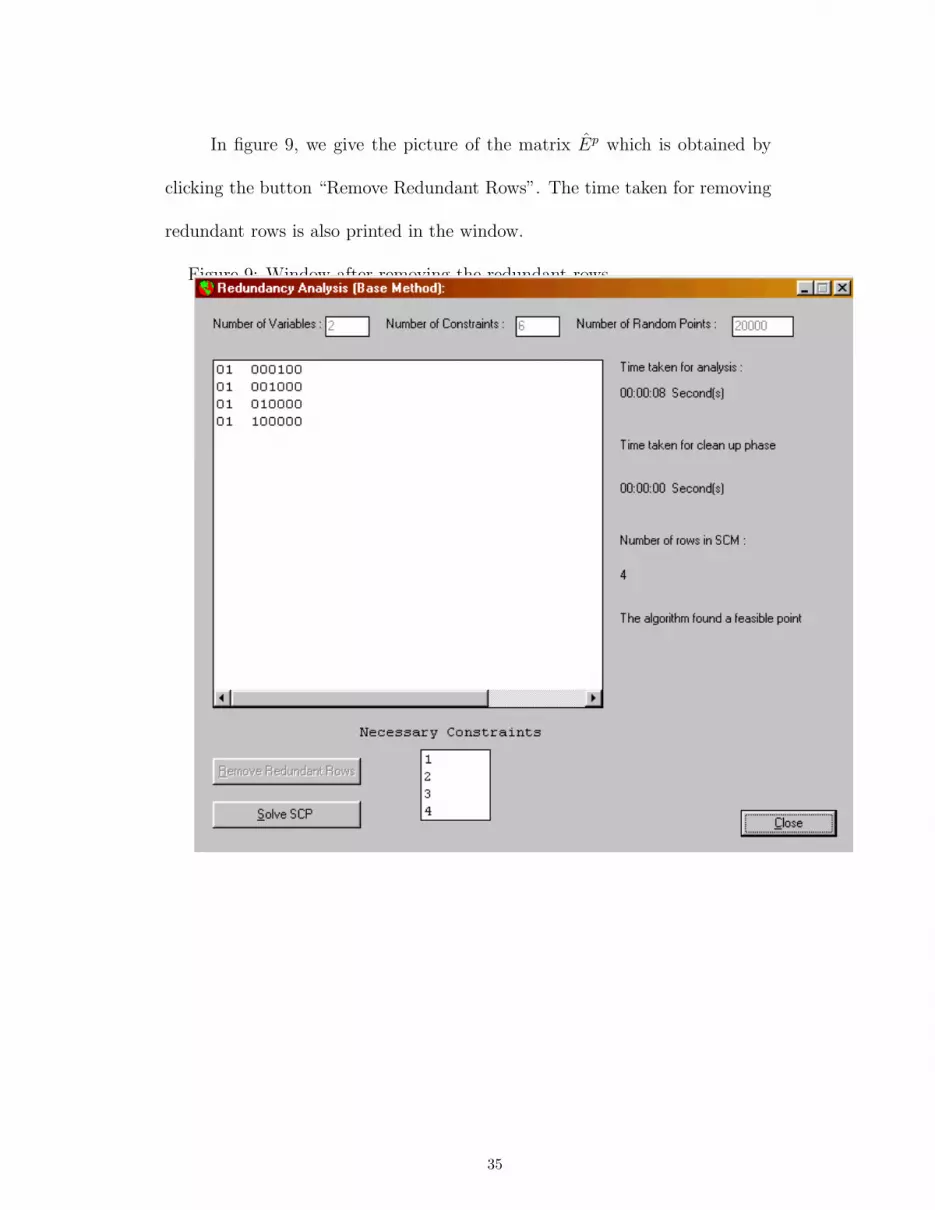
In figure 9, we give the picture of the matrix Ep which is obtained by
clicking the button “Remove Redundant Rows”. The time taken for removing
redundant rows is also printed in the window.
Figure 9: Window after removing the redundant rows
35
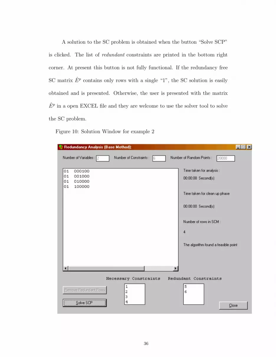
A solution to the SC problem is obtained when the button “Solve SCP”
is clicked. The list of redundant constraints are printed in the bottom right
corner. At present this button is not fully functional. If the redundancy free
SC matrix Ep contains only rows with a single “1”, the SC solution is easily
obtained and is presented. Otherwise, the user is presented with the matrix
Ep in a open EXCEL file and they are welcome to use the solver tool to solve
the SC problem.
Figure 10: Solution Window for example 2
36
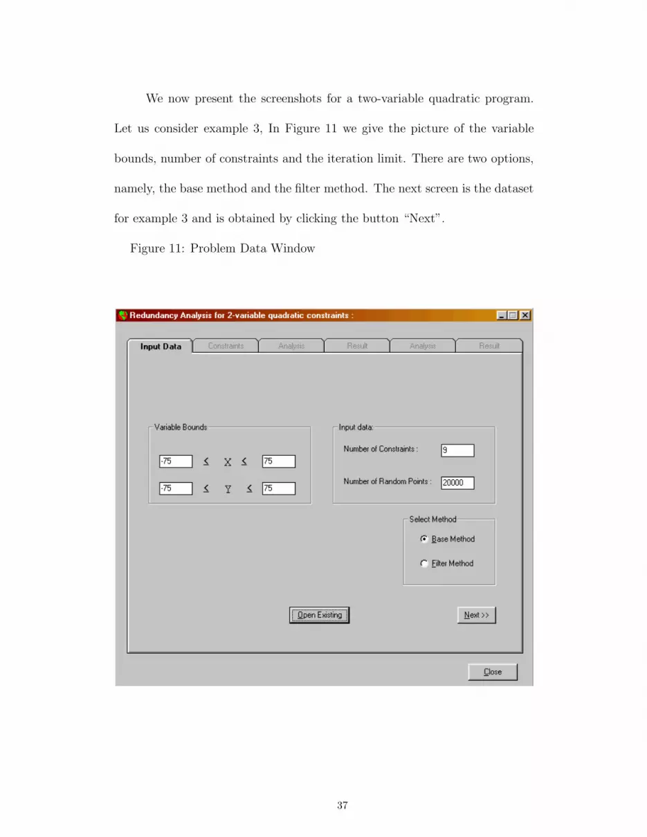
We now present the screenshots for a two-variable quadratic program.
Let us consider example 3, In Figure 11 we give the picture of the variable
bounds, number of constraints and the iteration limit. There are two options,
namely, the base method and the filter method. The next screen is the dataset
for example 3 and is obtained by clicking the button “Next”.
Figure 11: Problem Data Window
37

In figure 12, we give the picture of the constraint data in a Visual Basic
window read from MS Excel file for example 3. The constraint classification
process begins when the button “Redundancy Analysis” on the right corner is
clicked.
Figure 12: Constraint Set Window
38

In figure 13, we give the picture of the matrixEp0 which is the output using
our implementation of the base method for example 3. In the main window of
the screen shot, the row sums are given in the two left most columns and the
rows of the Ep0 are given in the right-hand-side. The redundant rows from Ep
0
are removed when the button “Remove Redundant Rows” is clicked.
Figure 13: Output Window for example 3
39

In figure 14, we give the picture of the matrix Ep which is obtained by
clicking the button “Remove Redundant Rows”.
Figure 14: Window after removing the redundant rows
40

In figure 15, the time taken for creating matrix Ep0 and Ep are printed.
This window also gives us details about the constraint set, which includes the
number of variables, number of constraints and the iteration limit. A solution
to the SC problem is obtained when the button “Solve SCP” is clicked. The
list of redundant constraints are printed in the bottom right corner. If the
redundancy free SC matrix Ep contains only rows with a single “1”, the SC
solution is easily obtained and is presented. Otherwise, the user is presented
with the matrix Ep in a open EXCEL file and they are welcome to use the
solver tool to solve the SC problem.
Figure 15: Solution Window for example 3
41

4.4 Conclusion
In this chapter we discussed the input file and file format and we also gave a
brief description of the Visual Basic package developed for the implementation
of the two methods. We presented screenshots and described briefly what they
meant for linear and two-variable quadratic programs.
42

5 Conclusion
5.1 Contributions
The first contribution of this major paper is a filter method that filters
observations x that provide redundant information prior to the complete eval-
uation of e(x). Filtering such observations not only produces a cleaner matrix
Ep0 , i.e., one with fewer redundant rows, but it can have an enormous impact
on the execution time.
The next contribution of this major paper is that we presented two new
theorems, namely theorem 4 and 5 about the SC equivalence.
Finally, this major paper has provided a user friendly computer aided-
tool developed in Visual Basic 6.0 for the constraint classification for small
sized linear and two-variable quadratic programs.
5.2 Future work
The algorithm was tested on small sized linear and two-variable quadratic
problems. The maximum number of constraints the software can handle is 99.
Future work includes implementation of filter method for larger problems and
general non-linear problems. The future work also includes an implementation
of the probabilistic Hit-and-Run algorithm once a feasible point is found.
5.3 Conclusion
This chapter highlighted the contributions of this major paper and indicated
very interesting projects for future work.
43

Appendix A
Problem # 12 from Table 1.
g1(x) = x1 − 50,g2(x) = x2 − 50,g3(x) = x3 − 50,g4(x) = −x1 − 15,g5(x) = −x2 − 15,g6(x) = −x3 − 15,g7(x) = x1 + x2 + x3 − 120,g8(x) = −x1 − x2 − x3 − 30,
with L1 = −75, U1 = 75, L2 = −75, U2 = 75 L3 = −75, and U3 = 75.
************************************
Problem # 13 from Table 1.
g1(x) = x1 + x2 − 450,g2(x) = x1 − 250,g3(x) = 2x1 + 2x2 + x3 − 800,g4(x) = x1 + x2 − 450,g5(x) = 2x1 + x2 + x3 − 600,g6(x) = −x1 − 0,g7(x) = −x2 − 0,g8(x) = −x3 − 0,
with L1 = −50, U1 = 500, L2 = −50, U2 = 500 L3 = −50, and U3 = 500.
************************************
Problem # 14 from Table 1.
g1(x) = x1 − 6,g2(x) = x2 − 4,g3(x) = x3 − 5,g4(x) = −x1 − 0,g5(x) = −x2 − 0,g6(x) = −x3 − 0,g7(x) = 0.3x1 + 0.2x2 + 0.4x3 − 10,g8(x) = 0.6x1 + 0.8x2 + 0.8x3 − 6,g9(x) = 0.5x1 + 0.7x2 + 0.4x3 − 12,
with L1 = −5, U1 = 15, L2 = −5, U2 = 15 L3 = −5, and U3 = 15.
************************************
44

Problem # 23 from Table 1.
g1(x) = −x1x2 − 25g2(x) = −x1 − x2 − 25g3(x) = x1 − 50g4(x) = −x1 − 2g5(x) = x2 − 50g6(x) = −x2 − 0,
with L1 = −10, U1 = 60, L2 = −10, and U2 = 60.
************************************
45

References
[1] A. Boneh, “Identification of redundancy by a set covering equivalence,” in:J.P.Brans, ed., Operational Research ’84, Proceedings of the tenth Interna-tional Conference on Operational Research (North Holland, Amsterdam,1984) pp.407-422.
[2] A. Boneh, Private communication with R. Caron (2001).
[3] A. Boneh and A. Golan, “Constraints redundancy and feasible regionboundedness by a random feasible point generator (RFPG),” contributedpaper, Third European congress on operations research, EURO III (Am-sterdam, The Netherlands, April 1979).
[4] J.C.G. Boot, “On trivial and binding constraints in programming prob-lems,” Management Science 8 (1962) 419-441.
[5] R.J. Caron, A. Boneh, and S. Boneh, Redundancy. In H.J. Greenberg andJ. Gal, editors. Recent Advances in Sensitivity Analysis and ParametricProgramming. (Kluwer Academic Publishers Holland, Amsterdam, 1997)pages 13.1-13.43.
[6] R.J. Caron, J.F. McDonald and C.M. Ponic, “A degenerate extreme pointstrategy for the classification of linear constraints as redundant or neces-sary,” Journal of Optimization Theory and Applications 62 (1989) 225-237.
[7] R.J. Caron, J.F. McDonald and R. Pidgeon, “A catalogue of LP testproblems and Linear Constraints,” Windsor Mathematics Report, WMR88-16, Department of Mathematics and Statistics, University of Windsor(Windsor, Ontario, 1988).
[8] J. Feng, “Redundancy in Nonlinear systems : A set covering approach,”Master Thesis, University of Windsor (Windsor,ON, 1999).
[9] W. Hock , K. Schittkowski, editors. Test Examples for Nonlinear Pro-gramming Codes Springer-Verlag Berlin Heidelberg, Berlin, 1981.
[10] M.H. Karwan, V. Lotfi, J. Telgen and S. Zionts, Redundancy in Mathe-matical Programming (Springer-Verlag, Berlin, 1983).
[11] Peter Orlik and Hiroaki Terao, editors. Arrangements of HyperplanesSpringer-Verlag Berlin Heidelberg, Berlin, 1992.
46


