AN EVALUATION OF THE USE OF

COILS OF DIFFERENT ORIENTATIONS FOR THE

EDDY CURRENT INSPECTION OF

AUSTENITIC STAINLESS STEEL VESSELS.

by

ROBIN PAUL CLARK B.Sc. (Eng)

A thesis submitted for the degree of Doctor of Philosophy

Department of Mechanical Engineering University College London University of London

October 1989

'People think they see a mountain but its just a little hill

And the problems that surround them are just the mood they feel'

From the Musical 'Smike'By Roger Holman and Simon May

ABSTRACT

With the advent of the next generation of nuclear reactors, the liquid metal cooled fast breeder reactors (LMFBR), new problems are being considered in many fields including that of non-destructive testing (NDT). Within NDT the more extensive use of eddy current techniques as an alternative to ultrasonics is one such area of investigation, particularly with regard to the inspection of the austenitic stainless steel primary vessel of the fast reactor.

The inspection of the outer surface of the pressure vessel for surface breaking defects has been considered. The feasibility ofdefect detection in stainless steel welds using eddy currents has been demonstrated using standard eddy current equipment.

An evaluation of the use of coils in a horizontal orientation hasbeen undertaken, both from theoretical and experimental viewpoints. The comparison of these results with those obtained for a more conventional vertical axis coil has indicated that the horizontal axis coil has potential advantages for this particular inspection case. A coil optimisation study has demonstrated that the potential advantages of horizontal axis coils can be more fully realised through a careful choice of probe coil.

The investigation has highlighted the increased understanding that can be obtained about eddy current testing by way of complimentaryexperimental and theoretical studies which consider an engineeringproblem of current interest.

CONTENTSLIST OF TABLES ivLIST OF FIGURES V

LIST OF PLATES xiiLIST OF SYMBOLS xiiiPUBLICATIONS AND PRESENTATIONS xv1. INTRODUCTION 1

1.1 Objectives of the work 11.2 Method of Investigation 51.3 Achievements 7

2. BACKGROUND 92.1 NDE in the Nuclear Industry 92.2 The Eddy Current Technique 13

2.2.1 History 132.2.2 Principles 142.2.3 Impedance Plane Analysis 192.2.4 Instrumentation and Probes 20

2.3 Practical Developments 232.4 Modelling 31

2.4.1 Analytical Techniques 332.4.2 Numerical Techniques 36

3. THEORETICAL WORK 423.1 Eddy Current Equations 423.2 Approximate Model 46

3.2.1 Basic Formulation 463.2.2 Ordinary Differential Equation Solution 483.2.3 Final Solution 523.2.4 Theory for AL Determination 563.2.5 Model Extension 62

ii4. THEORIES OF BURKE 66

4.1 Perturbation Expansion Expression 674.2 Exact Theory 684.3 Method of Programming 704.4 Extension to Layers 774.5 Magnetic Field Determination 87

5. ADDITIONAL THEORIES 925.1 Theory of Dodd and Deeds 92

5.1.1 Formulation Used 925.1.2 Method of Programming 955.1.3 Magnetic Field Determination 96

5.2 Uniform Field Theory 975.2.1 Theories of Auld 975.2.2 Work of Moulder 995.2.3 Application to Horizontal Axis Coils 102

6. EXPERIMENTAL WORK 1076.1 Conventional Equipment Familiarisation 1076.2 Horizontal Axis Coil Evaluation 111

6.2.1 Performance Evaluation 1116.2.2 Comparison with Vertical Axis Coils 127

6.3 Stainless Steel Weld Inspection 1326.3.1 Vertical Coils 1336.3.2 Horizontal Coils 136

7. TECHNIQUE CAPABILITY/COIL OPTIMISATION 1427.1 Technique Capability Considerations 1427.2 Preliminary Coil Optimisation Study 150

8. DISCUSSION 1618.1 Half Space Case 1618.2 Layered Half Space Case 1648.3 Edge Case 169

iii8.4 Magnetic Field Determination 1718.5 Uniform Field Theory 1798.6 Horizontal Coils Against Vertical Coils 1828.7 Additional Points 185

9. CONCLUSIONS 1899.1 Concluding Remarks 1899.2 Suggestions for Further Work 190

ACKNOWLEDGEMENTS 192REFERENCES 193TABLES 214FIGURES 229PLATES 332APPENDICES

A Approximate Theory Coefficients I-VIIIB Burke Exact Theory Extension I-IXC Temperature Considerations I-IV

iv

Table 2.:

Table 2.:

Table 2. Table 2.

Table 2.

Table 4.

Table 5.

Table 5.

Table 5.

Table 6. Table 6.

Table 8. Table 8.

Table 8.

Table 8. Table 8.

LIST OF TABLESFast Experimental and Test Reactors (from Waltar and Reynolds (1981))Prototype and Demonstration Fast Breeder Reactors (from Waltar and Reynolds (1981))Skin Depth Variation with FrequencyNumerical Treatment of Eddy Current Test Problems; Plates (from Becker et al (1986))■Numerical Treatment of- Three^-dimensional• Eddy Current Problems (from Becker et al (1986))

Burke Exact Theory - Computer Programs

Shape Parameters for a Rectangular Flaw (from Auld et al (1986))Shape Parameters for a Semi-elliptical Flaw (from Auld et al (1986) and Moulder et al (1987))Calibration Shape Factors

Electromagnetic Parameters of Materials Considered Horizontal v Vertical - Results for Comparison

1.62 mm of Copper on Stainless Steel (140 Turn Coil)6.35 mm of Stainless Steel on Aluminium Alloy (140 Turn Coil)6.35 mm of Stainless Steel on Aluminium Alloy (182 Turn Coil)Two-dimensional Uniform Field Theory Results Three-dimensional Uniform Field Theory Results

215

215

216 217

217

218

219

220

221

222

223

224225

226

227228

V

LIST OF FIGURESFigure 1.1 Basic Flow Diagram for a Periodic Inspection (from 230

Saglio and Prot (1976))Figure 1.2 Liquid Metal Cooled Fast Breeder Reactor (LMFBR) 231

(from Waltar and Reynolds (1981))a) Pool-typeb) Loop-typec) Pool-type reactor heat transport system

Figure 1.3 Eddy Current Coil Orientations 233

Figure 2.1 The Eddy Current Principle 234Figure 2.2 Skin Depth Effects 235Figure 2.3 Typical Impedance Plane Diagram 236Figure 2.4 Eddy Current System 237Figure 2.5 Surface and Circumferential Coils 238Figure 2.6 AC Bridge Circuit 239Figure 2.7 Uniform Field Eddy Current Probe (from Smith 240

(1985))Figure 2.8 Basic Capacitive Probe (from Gimple and Auld 241

(1987))

Figure 3.1 Approximate Model Geometry 242Figure 3.2 Surface H Field Determination 243Figure 3.3 Region of AR and AL evaluation 244Figure 3.4 Flowchart for Approximate Model Program 245Figure 3.5 Primary and Secondary Fields 246Figure 3.6 Crossover Frequency Characteristic 247Figure 3.7 Horizontal Coil at an Edge 248Figure 3.8 Eddy Current Deflection at an Edge 249Figure 3.9 Edge Extension to Approximate Model 249Figure 3.10 Horizontal Coil Above a Two Conductor Region 250

Figure 4.1 Burke Exact Theory Test Case 251Figure 4.2 Layered System 252

viFigure 4.3

Figure 5.1 Figure 5.2

Figure 6.1

Figure 6.2 Figure 6.3 Figure 6.4 Figure 6.5

Figure 6.6 Figure 6.7 Figure 6.8

Figure 6.9

Figure 6.10

Figure 6.11

Figure 6.12

Two Layer and a Half Space System

Vertical Axis Coil GeometryAuld Theory - Two-Dimensional Crack in a Uniform Field (Large a/6) (from Auld et al (1982))

a) Scan Over a Mild Steel Blockb) Mild Steel Block Containing Six SlotsLift-off LociPredicted Austenitic Weld TraceMild Steel Weld Specimen - Lift-off LociSlots in Aluminiuma) 50 kHzb) 10 kHzSlots in Stainless SteelImpedance Analyser Experimental Set-up140 Turn Coil Above 316 Stainless Steela) AR v Frequencyb) AL v Frequencyc) AR v Lift-off (100 kHz)d) AL v Lift-off (100 kHz)140 Turn Coil Above 6.35 mm of 316 Stainless Steel on Aluminium Alloya) AR v Frequencyb) AL v Frequency140 Turn Coil Above 316 Stainless Steel Edge - (a)and (b) Coil Length Parallel to Edge (c) and (d)Coil Length Perpendicular to Edgea) R v Coil Positionb) L v Coil Positionc) R v Coil Positiond) L v Coil PositionHorizontal Axis Coil used for Slot Detection (100 kHz)a) mild steelb) aluminiumc) stainless steelEddy Currents Induced by a Horizontal Axis Coil in a Conducting Material (From Bowler (1988))

253

254255

256

257257258259

260 261 262

264

265

267

268

Figure 6.

Figure 6.

Figure 6.

Figure 6.

Figure 6.

Figure 6.

Figure 6.

Figure 6.

Figure 6.

Figure 6.

Figure 6.

VI1

L3 Coil Orientation Relative to a Slot in Mild Steel 269(100 kHz)

L4 R and L v Position (250 Turn Horizontal Axis Coil) 270a) Mild Steel Specimen containing Six Slots

(20 kHz)b) Aluminium Specimen containing Six Slots

(20 kHz)c) Stainless Steel Specimen containing Six Slots

(20 kHz)d) Stainless Steel Specimen containing Six Slots

(5 kHz)L5 Ferromagnetic and Non-ferromagnetic Materials 274

illustrated on the impedance planeL6 Horizontal Coil Above 10 mm deep slot in Mild Steel 275

- variation of angular position, a) and b) - 140 Turn Air-cored Coil, c) and d) - 72 Turn Ferrite-cored coila) R v Angular Positionb) L v Angular Positionc) R v Angular Positiond) L v Angular Position

L7 Horizontal Coil v Vertical Coil 277a) AR v Lift-off (100 kHz)b) AL v Lift-off (100 kHz)

L8 Comparison of Horizontal and Vertical Coil 278Orientationsa) 10 mm Deep Slot in Mild Steelb) Six Slots in a Mild Steel Block

L9 Horizontal and Vertical Orientations - 3 mm Deep 279Slot in Stainless Steel

20 a) Stainless Steel Weld Specimen 1 280b) Stainless Steel Weld Specimen 2

21 Absolute Pencil Probe Traces for 5 mm and 10 mm 282Deep Slots in Stainless Steel Weld Specimen 1

22 Shielded Probe Trace for 5.5 mm Long Slit in 282Stainless Steel Weld Specimen 2

23 5.5 mm Long Calibration Slit in Stainless Steel 283a) Shielded Probeb) Absolute Probe

viiiFigure 6.

Figure 6.

Figure 6.

Figure 6.

Figure 6.

Figure 6.

Figure 6.

Figure 6.

Figure 6.

Figure 6.

Figure 6.

24 Weld Impurity Defect 1a) Shielded Probeb) Absolute Probe

25 Weld Impurity Defect 2a) Shielded Probeb) Absolute Probe

26 175 Turn Air-cored Horizontal Coil used to Inspect Stainless Steel Weld Specimen 1

27 Horizontal Coil Orientation Relative to a 10 mm Deep Slot in a Stainless Steel Welda) Coil Axis Perpendicular to Slot Lengthb) Coil Axis at Various Orientations to Slot

Length28 Ferrite-cored Horizontal Coil - Scan Over 5 mm Deep

Slot in Stainless Steel Weld Specimen 129 Ferrite-cored Horizontal Coil - Scans Over Weld

Inpurity Defects in Stainless Steel Weld Specimen 230 Ferrite-cored Horizontal Coil - Scans Over Slits in

Weld of Stainless Steel Weld Specimen 231 Stainless Steel Weld Specimen 2 - Weld Scan using

Ferrite-cored Horizontal Coil (300 kHz)a) R v Probe Positionb) L v Probe PositionStainless Steel Weld Specimen 2 - Weld Impurity Defect 1 (300 kHz)

a) R v Probe Positionb) L v Probe PositionStainless Steel Weld Specimen 2 - Weld Impurity Defect 2 (300 kHz)

a) R v Probe Positionb) L v Probe PositionStainless Steel Weld Specimen 2a) 5.5 mm Long Slit (300 kHz) - R v Probe Positionb) 5.5 mm Long Slit (300 kHz) - L v Probe Positionc) 3.5 mm Long Slit (300 kHz) - R v Probe Positiond) 3.5 mm Long Slit (300 kHz) - L v Probe Position

284

285

286

287

288

288

289

290

291

292

293

ixFigure 6.35 Ferrite-cored Horizontal Coil - Scan Over Fusion 295

Line Slits in Stainless Steel Weld Specimen 1a) Base Slitb) Slits on the Fusion Linec) Slits near the Fusion Line

Figure 7.1 Geometry for Measurement Window AnalysisFigure 7.2 Measurement Window Plot - AR' v t/5

(Approximate Model, 10 kHz, 140 Turn Coil)Figure 7.3 * Measurement Window Plot - AR' v t/6

(Burke Model, 10 kHz, 140 Turn Coil)Figure 7.4 Measurement Window Plot (Burke Model, 100 kHz,

140 Turn Coil)a) AR' v t/6b) AL' v t/6

Figure 7.5 AR v Coil Lengtha) 1 kHzb) 10 kHzc) 100 kHz

296297

298

299

301

Figure 7.6 Figure 7.7

Figure 7.8

Figure 7.9

Figure 7.10

AL v Coil Length (10 kHz) 303Burke Theory/Experiment Comparison for Different 304 Coil Diameters (100 kHz)a) AR v Coil Lengthb) AL v Coil Lengtha) AR v Coil Diameter - 140 Turn Coil, 10 kHz 306b) AR v Coil Diameter - 200 Turn Coil, 10 kHzc) AL v Coil Diameter - 140 Turn Coil, 10 kHzApproximate Model - Coil Diameter Effect on H Field 308 DeterminationScan Over a 10 mm Deep Slot in Mild Steel for Different Coil Diameters (100 kHz)

309

a) AR v Coil Lengthb) AL v Coil Length

Figure 8.1 140 Turn Coil above 316 Stainless Steela) AR v Frequencyb) AL v Frequency

Figure 8.2 200 Turn Coil above 316 Stainless Steela) AR v Frequencyb) AL v Frequency

311

312

Figure 8.3 140 Turn Coil above Copper

Figure 8.4

Figure 8.5

Figure 8.6

Figure 8.7

Figure 8.8

Figure 8.9

Figure 8.10

Figure 8.11

a) AR v Frequencyb) AL v FrequencyImpedance Plane Diagram to Illustrate Lift-off Variation (140 Turn Coil above 316 Stainless Steel)140 Turn Coil above Copper on 316 Stainless Steela) AR v Frequencyb) AL v Frequency140 Turn Coil above 316 Stainless Steel on Aluminium Alloya) AR v Frequencyb) AL v FrequencyStainless Steel on Aluminium Alloy System (140 Turn Coil)a) AR v Thickness of Stainless Steelb) AL v Thickness of Stainless SteelAR v Thickness of Stainless Steel - Stainless Steel on Liquid Sodium (LMFBR) System at 200°C140 Turn Coil above 316 Stainless Steel Edge (100 kHz)a) AR v Coil Positionb) AL v Coil PositionTangential Magnetic Field for Vertical and Horizontal Dipoles (Lift-off = 0.508 cm,6 = 0.0508 cm) (from Riaziat and Auld (1984))a) Tangential Magnetic Field at Material Surface

Under a Very Small Horizontal Axis Coilb) Tangential Magnetic Field at Material Surface

Under a Very Small Vertical Axis CoilFigure 8.12 a] Tangential Magnetic Field at Material Surface

Under 103 Turn Air-cored Horizontal Axis Coilb) Tangential Magnetic Field at Material Surface

Under 103 Turn Air-cored Vertical Axis CoilFigure 8.13 Tangential Magnetic Field at Material Surface Under

a 103 Turn Air-cored Horizontal CoilFigure 8.14 Eddy current (dotted lines) and Magnetic Field

(solid lines) Distributions for Simple Probe Geometries (from Auld et al (1982))

313

314

315

316

317

319

320

322

323

325

327

328

Figure 8.15

Figure 8.16

Figure 8.17

xi120 Turn Air-cored Coil above a 316 Stainless Steel 329 Block (75 kHz) - Lift-off Variation for Both Coil Orientationsa) AR v Lift-offb) AL v Lift-off182 Turn Vertical Axis Coil above 6.35 mm of 316 330Stainless Steel on Aluminium Alloya) AR v Frequencyb) AL v FrequencyPreliminary Probe Design for Austenitic Vessel 331Inspection

xiiLIST OF PLATES

Plate 5.1 HP4194A Impedance/Gain-Phase Analyser 333

Plate 6.1 Hocking AV100L and an Absolute Pencil Probe 334Plate 6.2 Wayne Kerr 6425 Impedance Analyser 335

xiiiLIST OF SYMBOLS

8 skin depthjj

jjr

absolute magnetic permeability (= jjc jjo'-7permeability of free space (= 4n x 10 H/m)

relative magnetic permeability a electrical conductivityf frequencyt time0 phase lagp volume charge densitye electrical permittivityD electric flux densityB magnetic flux densityE electric field intensityH magnetic field intensityJ current densityw angular frequency (= 2 n f)A magnetic vector potential<f> electric scalar potentialT electric vector potentialS2 magnetic scalar potentialx,y,z co-ordinate system for approximate model (x is depth into

material)

o' l'^2 va ues x R resistanceL inductanceZ impedanceAR change in resistanceAL change in inductanceAZ impedance change

xiv

j J -1V voltageI current

*L inductive reactance (= wL)N number of turns in coil

XV

PUBLICATIONS AND PRESENTATIONS

1. Clark R, Dover W D and Bond L J, (1987), 'The effect of crack closure on the reliability of NDT predictions of crack size', NDT International, 20, 269-275.

2. Clark R and Bond L J, (1988), 'Horizontal axis eddy current coils for austenitic pressure vessel inspection', presented at British Institute of Non-Destructive Testing Symposium 'Eddy Currents - On the Fringe', October.

3. Clark R, Bond L J and French P, (1989), 'The use of horizontalaxis coils for the eddy current inspection of fast breederreactor primary vessels', Review of Progress in Quantitative Non-Destructive Evaluation, 8A, 283-290, Editors D 0 Thompson and D E Chimenti, Plenum.

4. Clark R and Bond L J, (1989), 'The response of horizontal axis eddy current coils to layered media - a theoretical and experimental study', submitted to IEE Proceedings Part A in May.

5. Clark R and Bond L J, (1989), 'An investigation of horizontalaxis coils for eddy current inspection', submitted to NDTInternational in June.

6. Clark R and Bond L J, (1989), 'An investigation of the use ofcoils of different orientations for austenitic vessel inspection using eddy currents', to be presented at the 28th Annual British Conference on Non-Destructive Testing (NDT 89) in September

Clark R, (1989), 'The application of uniform field theory to horizontal axis eddy current coils', submitted to NDT International in August.

1. INTRODUCTION1

1.1 Objectives of the Work

The role of non-destructive evaluation (NDE) in industry is becoming increasingly important. Greater awareness of the benefits of employing non-destructive testing (NDT) in many industrial situations has led to the increased application of the various inspection techniques. With this wider usage, the need for further development and greater understanding of the various techniques and phenomena involved has become apparent (Nicholson (1982)). The part played by NDT in the construction and maintenance of a nuclear plant for instance, is apparent from Figure 1.1. A combination of the various techniques available are used both for the inspection of the materials and joints of the structure during the construction of the plant and for the in-service inspection (ISI) of the plant. The combination of information from the NDT, the material properties and the loading on the structure enables, through the use of fracture mechanics, a decision to be made as to whether any flaws detected in the structure will have a detrimental effect on the continued operation of the plant (Saglio and Prot (1976)).

Of the five major inspection techniques employed, these being dye penetrant testing, magnetic particle inspection (MPI), radiography, ultrasonic inspection and eddy current testing, it is the latter technique which currently offers the most scope for further development (McGonnagle (1982)). A review of the research into and usage of the various NDT techniques in the UK detailed by Sharpe (1982) indicated that of all the NDT performed in industry, 80% of the firms used radiography, 71% used penetrant inspection and 49%

used ultrasonic techniques and MPI, eddy current testing was not even mentioned. In contrast to this, at a British Institute of NDT symposium in October 1988, one of the speakers indicated that 54% of the NDT performed by the Royal Air Force employed the eddy current technique. This increased consideration and use of eddy current NDT has been partly responsible for this research study. Although eddy current testing is one of the oldest NDT methods, the first experiments being performed in 1879 (American Society of Metals (1976)), it is generally regarded as one of the least understood and least developed methods (McMaster (1985)).

The wide range of NDT applications and the diversity of requirements mean that much of the research into NDT development and understanding is performed with a specific application in mind. NDE is primarily concerned with quality assurance and ensuring structural integrity. Quality assurance involves the inspection of materials or goods after they have been through some form of production process. The more commonly encountered area of NDT application is the assurance of structural integrity. This area of interest ranges from theinspection of North Sea oil platforms with the inherent problem of testing underwater, to the inspection of power generation plant (especially nuclear plant, frequently with the undesirable feature of a radioactive environment) and the severe set of testing requirements imposed by the aerospace industry (Bond (1988)).

3This study brings together the eddy current testing technique and an application involving the inspection of a nuclear power plant. The aim of the work is to carry out a feasibility study on the use of the eddy current technique for inspecting the outer surface of the primary vessel of a liquid metal cooled fast breeder reactor (LMFBR) (Figure 1.2).

The following inspection procedure is planned for use in practice. Initially a television camera would be used to carry out a preliminary remote inspection of the vessel. On observing any indications of a possible flaw in the material surface, the eddy current technique would be introduced to inspect the area more thoroughly and determine whether any flaws were actually present and if so to size the flaws identified.

The austenitic stainless steel (316 stainless steel) which forms the vessel wall of the LMFBR, has an essentially constant magnetic permeability and a favourable large electromagnetic skin depth. At a given frequency, the depth of eddy current penetration is greater in 316 stainless steel than in most other commonly encountered materials such as copper, aluminium alloy or mild steel. Both of these characteristics make the material conducive to eddy current inspection.

For the application under consideration, two important questions need to be considered.

41) The ferromagnetic nature of the welds on the vessel (regions of

variable permeability and conductivity) will make the evaluation of any indications very difficult using the eddy current technique. Since the welds and the associated heat affected zones are the most likely regions on the structure to possess flaws, it needs to be determined if flaws can be detected in the weld metal and the neighbouring heat affected zones. If so, what indications will the flaws produce on inspection with eddy currents and how can these indications be interpreted to characterise the flaw?

2) The liquid sodium in contact with the vessel wall will be at about 200°C during the inspection. How will the increased temperature of the vessel wall affect the indications produced by the eddy current inspection? Again the question of interpretation of data will need to be considered.

In conjunction with answering these questions, the aim has been to try and understand the important factors that determine the success or failure of the implementation of the eddy current technique, especially when considering the fast reactor inspection application. Much of the work has focussed on the orientation of the eddy current coil used to perform the inspection. The flaws of interest in the outer wall surface were considered to be surface breaking flaws (most likely fatigue cracks or deep scratches) with a depth of greater than 2 mm.

1.2 Method of Investigation

An approach has been adopted whereby both theoretical modelling and experimental work have been performed to investigate the system of interest. The data obtained from both of these areas of study have been considered in order to ascertain the applicability of the eddy current technique to the required inspection.

The initial modelling work concentrated on the development of an approximate model for the eddy currents in a stratified half space, which was based on the assumption that a uniform field was induced in the material. This model represents the basic system under consideration, although in practice the situation reduces to that for the eddy currents in a homogeneous half space, since the vessel wall is too thick (30 - 50 mm) to allow complete eddy current penetration. To achieve complete penetration (ie the wall thickness = the electromagnetic skin depth) a coil excitation frequency of around 100 Hz would be needed.

A considerable amount of experimental work has been performed to aid the verification of the approximate model. A horizontal coil orientation was considered since it was the most suitable experimental configuration for representing the approximate model. The work has basically consisted of investigating the impedance change of several coils when they are placed, one at a time, above homogeneous and stratified metallic half spaces. An exact analytical theory for the case of a horizontal axis coil above a homogeneous conducting half space (Burke (1986)) was used to provide another set of results with which the approximate theory could be compared. This

exact theory was then extended to consider half space stratification. The aim of this was to understand the response from the fast reactor system, without weld material and defects present, when an eddy current coil was brought close to the vessel wall.

The coil orientation used (Figure 1.3), with the coil axis parallel to the surface of the material, is not the conventionally used coil orientation. Hence the work moved on to evaluate the merits of the horizontal axis coil as compared to the more conventional vertical axis coil. This study made use of both theoretical and experimental data. Part of the reason for this comparison was a proposal by Riaziat and Auld (1984), that horizontal axis coils may be less sensitive to lift-off and more sensitive to defects than vertical axis coils.

An experimental investigation of the feasibility of defect detection in 316 stainless steel weld material was conducted using coils of both orientations. This enabled the basic question of feasibility to be answered. The remainder of the work concentrated on a more complete evaluation of the horizontal axis coils based on the favourable characteristics they had demonstrated in the initial phases of the work.

The approximate model was based on the assumption that a uniform field was induced in the material. Using a calibration theory proposed by Auld (Moulder et al (1987)) for uniform field cases and the formulae of Auld et al (1984) for the coil impedance change due to a flaw when the incident electromagnetic field is uniform, the validity of the uniform field idea as applied to the horizontal axis coil was investigated.

7An extension to the approximate model was introduced, which was designed to indicate that by making simple but realistic assumptions about the fields in the material, useful first order approximations for the impedance change of an inspection coil can be obtained. The model proved to be of great use when the idea of coil optimisation was investigated, since it negated the need for vast numbers of experiments to be performed using different coils.

1.3 Achievements

The work presented in this thesis has investigated the feasibility of using the eddy current technique for non-destructively inspecting austenitic stainless steel vessels. The achievements of this work are considered to be as follows:

(1) It has been demonstrated experimentally that the eddy current inspection of austenitic material (316 stainless steel), both the base material and the weld regions, is possible using both vertical axis and horizontal axis coils. In addition, it is predicted that the inspection should be possible at a temperature of 200°C (the typical liquid sodium temperature at fast reactor shutdown) without any adverse effects on the test performance.

(2) A thorough experimental and theoretical analysis of the use of horizontal axis eddy current coils has been performed. This has entailed the development of a novel approximate model to describe the eddy currents in a stratified conducting media and the extension of an existing exact theory to be able to consider

8stratified as well as homogeneous conducting materials. The differences between vertical axis and horizontal axis coils have been addressed, resulting in the demonstration that horizontal axis coils may be advantageous when considering the inspection of large austenitic vessels for a number of reasons, all of which are detailed in Chapter 9.

(3) Having demonstrated the detection capabilities of simple horizontal axis coils, an attempt has been made at detailing the necessary considerations for probe optimisation and a more quantitative approach to the determination of technique capability. An investigation of the possible application of uniform field theory ideas to horizontal axis coils has proved encouraging and demonstrated the possibility of using the theory for ascertaining estimates of crack size using horizontal axis coil impedance change data.

2. BACKGROUND9

2.1 NDE in the Nuclear Industry

The development of nuclear power production throughout the world has necessitated the corresponding development of NDT technology to help ensure that the nuclear power plant is capable of safe power production (Oates (1988)). At present the construction and maintenance of safe plant is under particular scrutiny following the Three Mile Island [1979] and Chernobyl [1986] nuclear accidents. Although neither accident was due to the presence of a crack or other such defect in the plant, both accidents have highlighted the potential dangers of a nuclear power plant failure and thus the question of safety has become particularly important. This was very apparent at the Sizewell B public inquiry from 1983 to 1985 (Layfield(1987)).

Much NDE expertise is already employed in the nuclear industry, both for the inspection of materials and joints during construction of the plant and for the in-service inspection of the plant (Figure 1.1). In the USA much of the nuclear plant orientated NDT research is performed for and by the Electric Power Research Institute (EPRI). Most of the European countries which have nuclear plants perform NDT research, the most prominent research programmes being performed in France (Commissariat a l'Energie Atomique), Belgium (Association Vin^otte), West Germany (BAM, IZFP) and the UK (UKAEA, CEGB). Notable research programmes are also being conducted in Canada (Atomic Energy of Canada Ltd) and India (Reactor Research Centre, India).

10All of the major NDE conferences are useful sources of information on current work involving nuclear plant applications. One particularly valuable source of information is the 'International Conference on NDE in the Nuclear Industry' which is held every two years.

Since most of the nuclear plants in the world are pressurised water reactors (FWR's), much of the research to date has been concerned with FWR inspection (Caussin and Dombret (1985), Nichols (1982)). The most prominent techniques have been radiographic and ultrasonic techniques, although eddy current testing has been used in certain areas, especially for the inspection of tubes (Poikonen and Lahdenpera (1986)). Fagenbaum (1984), has outlined several possible radiographic techniques other than the most conventional, x-radiography. A series of trials, the PISC (Programme of Inspection of Steel Components) trials, have been used to assess the current capability of ultrasonic NDT when considering nuclear plant inspection (Hemsworth (1985)). One major problem with ultrasonic inspection is the difficulty in inspecting the weldments between austenitic stainless steel plates, a commonly encountered joint in a nuclear plant since the nuclear pressure vessels are generally fabricated or clad using austenitic stainless steel. The problems that arise are due to the large grain size in the austenitic weld material. This leads to scattering of the ultrasound, high ultrasound attenuation and beam skewing. These effects can result in false indications. Many authors have considered this problem and suggested possible solutions (Hudgell and Gray (1985), Farley and Thomson (1983), Herberg et al (1976)). The most recent developments in the UKAEA programme of development work investigating the ultrasonic inspection of austenitic components have been discussed by Atkinson et al (1989). The improvement of the automated ultrasonic

11inspection of austenitic castings and welds has considered the colour graphical display of multi-probe inspection data, the use of the time-of-flight diffraction (TOFD) technique for sizing surface breaking cracks in austenitic castings and the use of signal processing and averaging techniques in order to enhance the defect signal-to-noise ratios obtained. Gray (1987) and Chirou et al (1987) have reviewed the use of eddy current testing for steam generator inspection in nuclear plant. A more general paper on electromagnetic inspection as used by the CEGB on all power plants has been detailed by Warnes (1988). In his paper, Warnes has indicated that eddy current techniques are at present essentially only considered as a tool for defect detection, not sizing.

The proposed next generation of nuclear reactor is going to be the liquid metal cooled fast breeder reactor, the major reason being its desirable fuel cycle (Patterson (1986)). The next European fast reactor is planned for the 1990's and where possible previous NDT research experience will be utilised when addressing the inspection problem, although at the same time new considerations will also need to be introduced. The overall consideration of LMFBR inspection has been addressed by Spanner (1977) and McClung et al (1977). Work has already been carried out in the UK to develop an under sodium ultrasonic viewing system (McKnight and Barrett (1985)). Prototype fast reactors have been built and used for small scale power generation and/or research purposes in several countries, eg, Dounreay in the UK (Tables 2.1 and 2.2).

The worlds first major power producing fast reactor, Superphenix at Creys-Malville near Lyon in France, started to deliver electricity to the European grid in early 1986 (Energie Nucleaire Magazine (1983)).

12In-service inspection of Superphenix has been researched and a variety of techniques are employed (d'Argentre et al (1986)). The inspection of the primary vessel of the Superphenix fast reactor in France with the aid of the MIR (Module d' Inspection pour reacteurs Rapides) inspection vehicle has been detailed by Asty et al (1985). The method of inspection is predominantly ultrasonics although an eddy current technique is used to help guide the inspection vehicle over the vessel surface (David and Pigeon (1985)). Special ultrasonic transducers are needed for the inspection of the primary vessel due to the high temperatures present. At high temperatures the major problem is with the materials from which the transducers are fabricated (British Institute of NDT (1987)).

As part of the European collaboration on the development of the LMFBR, workers at the West German research establishment IZFP (Fraunhofer-Institut fur zerstorungsfreie Priifverfahren) in Saarbrucken, West Germany are also investigating the use of electromagnetic techniques for inspecting the fast reactor primary vessel. To date, much of the work has concentrated on a technique for the electromagnetic generation of ultrasound (Hiibschen and Salzburger(1988)). The ultrasonic waves produced are horizontally polarised shear waves, which are less influenced by the coarse anisotropic grain structure present in austenitic weld material than other types of ultrasonic wave. EMAT's (Electromagnetic Acoustic Transducers) also have the desirable feature that they do not require the use of a couplant between the transducer and the material being inspected. Using this technique, defect detection has proved to be possible in austenitic weld material. A probe has also been fabricated and used

successfully at the expected inspection temperature of around 250°C. Other work at IZFP has considered the use of a multi-frequency eddy current technique, using four frequencies, for a related inspection problem (Gray (1989)).

NDT, primarily radiography, has been used for the inspection of the JET (Joint European Torus) fusion reactor at Abingdon in Oxfordshire, UK, whilst the reactor was being constructed (Walravens (1985)). Thus it is clear that NDE makes a valuable contribution to ensuring the structural integrity of all nuclear plant, both fission and fusion, both in construction and in-service.

2.2 The Eddy Current Technique

2.2.1 History

Eddy current testing is based on the principles of electromagnetic induction which were originally discovered by Faraday in 1831. Maxwell's dynamic theory of the electromagnetic field is generally regarded as the basis of electromagnetic theory. His equations developed in 1864 describe all of the electromagnetic phenomena encountered in eddy current NDT (Thomas and Meadows (1985)).

In 1879, Hughes performed some of the first eddy current testing experiments (American Society of Metals (1976)). He used the eddy current method to detect differences in electrical conductivity, magnetic permeability and temperature in a metal. It was not until the 1920's though, that the first instruments for eddy current testing were developed. In Germany during World War II a considerable amount of work was performed by Forster in advancing the

14eddy current technique. Fdrster's work was primarily concerned with explaining qualitatively the theory behind eddy current NDT and developing the instruments capable of performing the eddy current tests. Much of the work, which included the introduction of impedance plane analysis for eddy current testing, was not published until 1952 (McGonnagle (1982). Since then, with Maxwell's equations providing a firm theoretical base and Forster's work a solid practical base, further research has been concerned with both theoretical development and understanding and the development of inproved instrumentation and better techniques.

2.2.2 Principles

Eddy currents are induced in a metal whenever the metal is brought into an alternating magnetic field. The eddy currents create a secondary magnetic field which opposes the inducing magnetic field. This decreases the magnetic flux through the exciting coil. By monitoring this effect, information can be determined about the metal being studied (Figure 2.1).

The secondary electromagnetic field is investigated by observing the effect it has on the electrical characteristics of the exciting coil, ie, on the coil impedance, or by the presence of an induced voltage if a separate detector coil is used. The coil impedance or the induced voltage will change with variations in the eddy current flow, which are, in turn, brought about by variations in the condition of the metal being studied. The following material conditions will affect the secondary electromagnetic field and can thus be investigated using the eddy current technique;

15electrical conductivity

- magnetic permeability grain sizeheat treatment condition hardnessmaterial thickness cracksflaws (voids, inclusions, etc) case depth composition cold workphase transformationstrengthtemperature

In each case the change in a material condition can essentially be considered to be a change in the material electrical conductivity and/or magnetic permeability.

The eddy currents induced in the material obey a skin effect phenomenon. This results in an exponential decay in eddy current density with increasing depth into the metal. At a certain distance below the surface of a thick specimen there are effectively no eddy currents flowing. The standard depth of penetration or skin depth (6) is defined to be the depth at which the eddy current density has been reduced to 1/e (36.8%) of the surface density. The skin depth is given by

S - (n y (J f ) 1/2 2.1

*These c h a r a c te r is t ic s a re o n ly s t r i c t l y a p p lic a b le when the e le c tro m a g n e tic

f i e l d can be cons idered to be a p lane wave in c id e n t on th e m a te r ia l

s u rfa c e . For a r e a l eddy c u rre n t c o i l the in c id e n t e le c tro m a g n e tic f i e l d is

n o t a s im ple p lan e wave, i e , th e c o i l has a f i n i t e le n g th , hence the

r e la t io n s h ip s a re o n ly ap p ro x im a tio n s . For most p r a c t ic a l eddy c u rre n t

purposes th e approx im ations a re s a t is fa c to r y , a lth o u g h a more d e ta i le d

a n a ly s is o f the e le c tro m a g n e tic f i e l d in the m a te r ia l would re v e a l the

a c tu a l s k in depth and phase la g c h a r a c te r is t ic s .

16where f = frequency of exciting alternating current (ac)

The reduced current flow found at greater depth is due to the reduced magnetic flux caused by the interaction of the primary and secondary magnetic fields and the inevitable decrease in magnetic field strength with increased distance from the inducing coil. A depth of 36 is considered to be the practical limit of defect detection (eddy current density is 5% of the surface eddy current density). Hagemaier(1985) has indicated that the eddy current density falls to zero at a depth of 4.68. A compromise is needed when performing eddy current tests, since although employing a lower frequency ac will increase the depth of penetration, it also reduces the sensitivity of flawdetection. The frequencies usually used are of the order of kHz, butany frequency in the range 1 Hz to 6 MHz can generally be used. Table2.3 shows the variation in skin depth with changing frequency for stainless steel, aluminium and copper. For inspection purposes, the frequency should be chosen such that the skin depth is equal to the maximum depth of penetration required.

Subsurface eddy currents are out of phase with those at the surface.The phase lag (3) increases linearly with depth and is given by

3 = x/S rad 2.2

where x = depth below surface

The skin depth and phase lag phenomena are illustrated in Figure 2.2.

*

17When inspecting a non-ferromagnetic material, the secondary magnetic field is due to the eddy currents alone. With a ferromagnetic material, additional magnetic effects occur due to the high and variable magnetic permeability of the material. These effects tend to cover up those due to the eddy currents. In order to overcome this problem, such that ferromagnetic materials can be inspected, the ferromagnetic material needs to be magnetised to saturation prior to testing (Mayo and Carter (1985)). This is achieved by applying astatic (dc, direct current) magnetic field using an electromagnet or a large permanent magnet. When the ferromagnetic material issaturated, its relative permeability becomes 1 and it can then be treated as though it were a non-ferromagnetic material. Despite the ferromagnetic nature of certain materials, in practice it is often possible to detect defects in ferromagnetic materials without the need for saturation. When inspecting mild steel for instance, all that is required for a successful inspection is a careful choice of frequency (a high frequency is generally considered to be best).

An important factor which needs to be considered when performing an eddy current test is that of lift-off. Lift-off is used to describe the spacing between the inspection coil and the conductor being inspected. The phenomenon is often responsible for maskingindications from defects present in the material, since a change inlift-off results in a change in coil impedance. The electromagnetic field is strongest close to the coil, thus the lift-off will determine the density of the eddy currents induced in the material and hence the strengths of all of the fields that result.

18To characterise defects completely a calibration needs to be performed prior to the inspection. For the calibration, it is important that the test materials are duplicated both in geometry and in electrical and magnetic properties. Calibration defects are generally simple machined defects, ie, slots or flat bottomed holes. The eddy current test is thus an indirect test, since it does not measure any specific characteristic directly.

The technique has several advantages over other NDT methods. It does not require contact between the probe and the specimen. The idea of a non-contact technique is highly desirable for situations where it is important that the surface being inspected is not harmed or polluted in any way, ie, in the nuclear industry, or where the inspection must be performed through some type of non-conducting surface coating, ie, paint. The instruments are generally portable and the technique can be adapted for high speed inspection and automation. The main disadvantage of the method is the need for a complete understanding of how eddy current testing works, as signal interpretation can be complicated, requiring experience of implementing the technique for a correct answer to be reached. It is generally accepted that at present the eddy current technique is a defect detection tool not a defect sizing tool.

A detailed explanation of all of the principles associated with eddy current testing is given by the American Society of Metals (1976) and by Halmshaw (1987) amongst others.

192.2.3 Impedance Plane Analysis

When dc flows in a coil, the magnetic field reaches a constant level and the only limitation to the flow of current is the electrical resistance of the wire. For ac, two limitations are imposed, namely the ac resistance of the wire and the inductive reactance. Together these form the coil impedance. The inductive reactance is thecombined effect of inductance and frequency.

For a loaded coil (ie, the flux links the coil and the material), the resistance has two components, the ac resistance of the coil wire and the apparent resistance due to the specimen. The ac resistance of the wire does not vary by a large amount, hence any change in the resistance is predominantly due to the metal specimen. A change in the electromagnetic field will result in a change in the coilimpedance. The coil impedance thus reflects the condition of the metal specimen. This is the basis of impedance plane analysis. George (1987) has described the basic principles of impedance plane analysis in great detail. Impedance plane diagrams can be prepared to illustrate the change in a particular condition of the metal (Figure 2.3).

When performing a test, the effect of the secondary electromagnetic field is that it changes the magnitude and angular component of the coil impedance. The presence of defects in a metal specimen andvariations in the specimen condition result in a change inconductivity and/or permeability of regions within the metal. Hence the secondary electromagnetic field will be changed and thus so will the coil impedance. In order to completely characterise defects, both the amplitude and phase of the impedance plane signal must be

20analysed. Large subsurface defects may yield signal amplitudes similar to those for small surface defects, but the phase lag for the surface defect will be less than that for the subsurface defect. Hence the phase lag can help to determine the differences between detected defects (Van Drunen and Cecco (1984)).

It should always be remembered that the impedance plane signal is an integrated response. This form of analysis is the basis for almost all of the eddy current instruments used today. Now that eddy current testing is becoming a more quantitative technique, some researchers are no longer using just the impedance plane diagram for representing results. In some cases, the diagrams are being replaced and complimented by plots of coil resistance or coil inductance against a parameter of interest, ie, frequency or case thickness.

2.2.4 Instrumentation and Probes

Modern eddy current instruments have a variable frequency excitation current source, with the eddy current probe forming part of a bridge network which is used to measure the small impedance changes due to defects. Figure 2.4 illustrates the form of a basic eddy current system. In order to understand how the system operates, each of the various probe configurations needs to be considered.

There are two different types of coil, surface or probe coils and circumferential or solenoid coils (Figure 2.5). The coils can be arranged to form a probe in one of two ways, either by an absolute arrangement or by a differential arrangement, which leads to three

21possible probe configurations. These are explained in turn by considering the ac bridge circuit outlined in Figure 2.6. In each case the coils can act as both exciter and pick-up or a separateexciter coil can be employed.

1) ABSOLUTE MODE - SINGLE COIL PROBE: The coil impedance changesdue to the presence of a defect, this results in an unbalancedbridge and an output voltage proportional to the coil impedance.

2) ABSOLUTE MODE - IWO COIL PROBE: One coil is the test coil andthe other is a reference coil. The coils compare an unknown (the specimen) with a standard. The two coils are connected such that when their impedances are the same, there is no output voltage(series-opposing connection).

3) DIFFERENTIAL MODE - TWO COIL PROBE: Both coils sense the material being inspected thus comparing one region of the object with an adjacent region. If the two regions being sensed are the same, there is no output voltage.

In the context of the whole eddy current system, the method ofoperation should now be apparent. The exciting signal sets up eddy currents in the material, changes in which are detected by the detector coil. The signal from the detector coil, having been amplified, is analysed by comparing it with the signal from the exciting coil. This leads to some form of output from the system, (eg, an analogue or digital meter reading, an impedance plane diagram, an audible alarm, etc).

22Surface probes generally have an absolute arrangement. They have a low sensitivity parallel to the windings, a maximum sensitivity across the windings and zero sensitivity at the centre of the coil. Circumferential probes can have either coil arrangement, both resulting in a circumferential eddy current flow. They have no sensitivity to circumferential cracks and maximum sensitivity to defects parallel to the coil axis. The absolute arrangement is sensitive to dimensional variations as well as defects, which can lead to defect indications being masked. Gradual dimensional variations are not indicated if a differential arrangement is employed, although abrupt discontinuities, ie, defects are very apparent. If the coils making up the probe are both a source and a detector, the probe is known as an active probe. Alternatively, when a coil is only a detector and a separate driving coil is also required, the detection probe is known as a passive probe.

When considering the response from flaws, two important factors need to be considered. For maximum response the flow of eddy currents must be perpendicular to the flaw and for maximum resolution the ratio of the defect volume to the inspection volume must be as near 1:1 as possible.

For the inspection of materials with different electromagnetic properties, different probes are used. At any frequency the skin depth value will vary depending on the material being inspected. This means that different fields are present in different materials and thus different probe constructions (core and windings) need to be used to ensure the maximum sensitivity possible when performing the eddy current test. Although most eddy current probes have a ferrite

23core, some probes especially those used by certain research groups, have an air core. Probes with an air core are easier to describe theoretically. The ferrite core helps with defect detection as it strengthens and concentrates the fields in the material under inspection.

When considering surface probes, the coil axis is usually perpendicular to the material surface (vertical axis coils) but in this study, most of the coils used have their axis parallel to the material surface (horizontal axis coils). Alternative names used for horizontal axis coils are 'parallel' or 'tangential' coils.

The whole area of eddy current instrumentation and eddy current probes is vast since many research groups develop their own equipment rather than use standard apparatus. The details outlined in this section indicate the basic principles behind all eddy current apparatus (American Society of Metals (1976)), although it should be realised that this is by no means an exhaustive study. It is advised that all references to eddy current NDT encountered should be studied with care in order to identify any unusual or unique equipment features present. A review of eddy current system technology has been given by McNab (1988). The paper considers many of the instrumentation and signal processing aspects of eddy current testing.

2.3 Practical Developments

McMaster (1985) has provided a general review of the eddy current testing technique, considering both the principles involved and the possible areas of application. The paper goes on to outline the way

24forward for eddy current testing in the future, eg, the introduction of coil arrays, probe development for deeper penetration and more flexibility, and microprocessor control of eddy current tests. McMaster makes the point that the scope for further development is considerable. The points made by McMaster are a modern extension to the work of Libby (1971). Libby's book, 'An Introduction to Electromagnetic NDT Methods', is generally regarded as one of the standard works on eddy current NDT. It explains most of the basic principles of electromagnetic NDT, both experimental and theoretical, although nowadays it does start to appear limited and dated given the recent developments in all areas of electromagnetic NDT. Many of the important developments in electromagnetic NDT research since Libby's book are considered in an American Society for Testing and Materials Special Technical Publication edited by Birnbaum and Free (1981). Although the collection of papers presented in the volume are taken from a symposium in 1979 most of the contributors are still recognised today as the major researchers in the field of eddy current NDE.

Much of the practical eddy current literature is concerned with the inspection of thin-walled stainless steel tubes, particularly those used for nuclear fuel element cladding (Barat et al (1982), Beck (1971), Ryden (1968)). This is not surprising since eddy current testing lends itself very well to the inspection of non-ferromagnetic cylindrical components using a circumferential coil set up. The geometry allows for an easy understanding of the physics of the inspection, as well as encouraging the implementation of an automated system (Forster (1968)). Dufayet (1969) has specifically considered the eddy current inspection of fast reactor fuel subassembly clads. The in-service inspection of 316 stainless steel tubes less than

252.5 mm thick using an eddy current technique has been described by Hudgell (1976). The tubes are in the secondary heat exchangers of the Prototype Fast Reactor (PFR) at Dounreay in Scotland. The use of eddy currents for tube inspection is not confined to the nuclear industry. The inspection of non-magnetic cast material tubes in the chemical industry has been described by Wehrmeister (1973). The inspection objective is to detect metallurgical changes in the tube material in areas of the tube that have been exposed to high temperatures.

The majority of the work involving eddy current inspection considers specific applications of the technique. Mayo and Carter (1985), Owston (1985) and Cecco (1973) have addressed the problem of inspecting ferromagnetic materials. All of the authors have highlighted the need for local magnetisation of the material to saturation or close to saturation prior to inspection. Brewer and Moment (1976) and Dodd and Simpson (1971) have considered the detection of areas of ferrite in austenitic stainless steel welds and the measurement of small permeability changes respectively. Holler et al (1984) and Meier (1978) have investigated the inspection of austenitic welds, tackling the problem of the effect of ferromagnetism due to the presence of residual ferrite in the weld material. Holler et al suggest the use of a multi-frequency instrument to enable signal discrimination in these cases. The multi-frequency approach has been used by Scott and Dodd (1981) for the inspection of austenitic stainless steel base material up to 13 mm thick.

26Burkhardt et al (1987) have considered the variability in probe response to flaws for several different probes* A wide variation in probe response was found for the probes studied, even when considering the same flaw. Blitz has considered many aspects of the physics of eddy current testing, examples being instrumentation and impedance plane analysis (Blitz (1983)), the effect of high lift-off (Blitz et al (1987)) and the effect of temperature variations on the eddy current coils (Blitz and Razzak (1981)). Other general discussions of the advantages and disadvantages of eddy current testing have been offered by Julier (1985) and Van Drunen and Cecco(1984). Impedance plane analysis is often used but not clearly explained. An easily understandable outline of the basic principles of the analysis has been presented by George (1987), along with a discussion of the use of the eddy current technique for inspecting aircraft structures.

Multi-frequency and pulsed eddy current testing are being considered increasingly, since they enable more information to be obtained about the material being inspected due to the increased number of frequencies being used. Different information can be obtained from each frequency component. The multi-frequency work (Scott and Dodd (1981), Davis (1980)) considers the use of three or more different discrete frequencies for simultaneous eddy current inspection, whereas the pulsed technique (Sather (1981), Wittig and Thomas (1981)) uses the range of frequencies present in an eddy current pulse. Crostack and Nehring (1983) have considered the use of the pulsed eddy current technique. They have investigated the use of controlled signals for better signal separation. When considering the

27use of more than one inspection frequency, the aim is to determine information about different parts of the material with each frequency, ie, a high frequency is used for near-surface inspection whereas a low frequency is used for subsurface inspection. The two techniques have been compared by Deeds (1982).

An eddy current technique for inspecting tubes has recently been undergoing development. The remote-field eddy current technique considers the detection of the electromagnetic field outside a tube by a coil inside the tube which is a finite axial distance away from the transmission coil (Atherton et al (1988)). The technique is sensitive to defects in the external surface of the tube wall, as well as to those in the internal surface.

The use of horizontal axis coils for eddy current testing is not very common, although it has been suggested that they do offer advantages over the more conventional vertical coils (Riaziat and Auld (1984)). From a dipole analysis, it has been found that horizontal dipoles are less sensitive to lift-off and more sensitive to defects than vertical dipoles. Uniform field eddy current (UFEC) probes, also called tape head probes, make use of these characteristics (Smith(1986), Moulder et al (1987) and Shull et al (1987)). The probe consists of a horizontal coil wound on a toroidal ferrite core (Figure 2.7). The field produced between the poles of the ferrite core is essentially uniform and thus more easily described theoretically. UFEC probes have been successfully used to detect and size both slots and fatigue cracks in a Ti/Al/V alloy (Moulder et al(1987)).

28Eddy currents can be generated at microwave frequencies (low GHz) to provide a testing technique which is very sensitive to small surface cracks. The eddy currents are generated using a ferromagnetic resonance probe (FMR probe) which, because it is so small, enables the inspection of many virtually inaccessible areas (Auld et al (1978)).

There are several other techniques closely related to the eddy current technique that have been developed and used successfully for inspecting components. The electric current perturbation method (ECP) involves setting up a current flow in the material to be inspected, and any current perturbations caused by the presence of a defect result in a change in the flux density above the material surface. This change in flux density is detected using a non-contacting differential magnetometer probe (Teller and Burkhardt (1981)). The electric current in the material can be injected or induced. Computer modelling can enable the optimisation of electric current perturbation probe design (Beissner and Burkhardt (1985)).

AC field measurement (ACFM) is an electromagnetic technique closely related to eddy current testing. It makes considerable use of the skin effect phenomenon to provide a technique which is capable of fairly rapid quantitative crack measurements (Collins et al (1985) and Dover et al (1981)). The technique is a potential drop technique. This involves the measurement of electric potential differences at various positions on the material surface using a surface contacting probe. If the two contacts of the probe straddle a surface breaking defect, the potential difference is greater than if the defect were not present. The technique was originally developed to enable the

29monitoring of fatigue crack growth in tubular joints. These structures are found extensively in the offshore industry, ie, in oil rig fabrication (Collins and Dover (1984)). A recent development in the ACFM technique has been the consideration of a non-contacting ACFM technique which is similar to the ECP method. The technique described by Lugg et al (1988) considers the measurement of the magnetic field perturbation produced by a crack at a point above the crack. The other electromagnetic techniques related to eddy current testing, dc potential drop and flux leakage techniques, are only rarely considered (Lord (1980)).

All of the eddy current probes in use today are inductive probes. Gimple and Auld (1987) have started to consider the use of capacitive probes. The basic probe is a parallel plate capacitor that has been opened up (Figure 2.8). A voltage is applied to the source, and the current to ground from the receiver is measured. The amount of capacitive coupling is thus the property of interest. This coupling will depend on the component being scanned by the probe. Another novel experimental approach is the use of flexible substrate eddy current coil arrays which have been described by Krampfner and Johnson (1988).

When considering the inspection of nuclear plant it is important to be aware of the problems that can arise with the use of eddy current inspection at high temperatures. Edenborough (1968) has considered the use of the eddy current technique to inspect parts of nuclear rocket engines under high thermal gradients. A tungsten-rhenium wire coil was used for the inspection up to temperatures of 1760°C. The probe on which the coil was positioned was water-cooled. Shaternikov

30and Denisov (1968) have considered the use of eddy current sensors made of glass insulated wire in a ceramic housing for use at temperatures up to 500°C. A water-cooled sensor has been used for on-line crack detection in hot slabs (Holmstrom (1987)).

The need for eddy current coil optimisation to help improve defect detection has been considered by Dodd and Deeds (1971) for the case of encircling coils. Beissner and Sablik (1984a) have considered ECP probe optimisation using a mathematical model for the probe response. The ECP analysis has been taken one step further by Burkhardt and Beissner (1985) to consider the probability of detection for flaws in a disc from a gas turbine engine.

The integration of computers into eddy current test lines has been described by Stumm (1984). Computers introduce an element of reliability and repeatability to the inspection process through computer controlled operation and analysis. The major functions of the microcomputer are to control the inspection system, ie, the set up and operation of the test line, to record and display the eddy current test data and to aid with the signal evaluation once the test has been performed.

This section has outlined many of the important areas of practical eddy current NDT research. The references given are to the work of the most encountered researchers in the literature. The review is as complete as is possible at the time of writing. It provides a fairly comprehensive guide to what has been studied to date and what is currently being investigated in the field.

2.4 Modelling31

The development of mathematical models for the various electromagnetic NDE techniques is beneficial since it enables the techniques to be quantified. The models describe the interaction between the fields induced by a probe and both flawed and unflawed conducting structures. Models can aid probe design and the optimisation of test parameters, without the need for the fabrication of several different probes and the performance of a large number of experiments. This can lead to improved techniques for inspection. By quantifying the eddy current technique, the models are able to help with flaw sizing. This requires the development of inversion schemes which are able to determine the flaw size from the measured or calculated impedance change of a probe coil. These general points have been discussed by Burke (1988a).

Apart from the above uses of mathematical models in electromagnetic NDE, they can also be used to help in the statistical description of the various techniques, ie, the consideration of probability of detection (POD) characteristics and the reliability of the techniques in different inspection situations (Beissner (1986)).

Electromagnetic NDE modelling is currently an area of much research. To date most of the models developed have concentrated on the forward problem, ie, to predict the probe response to a known defect, although inversion has been considered by many researchers. The models will be discussed in two sections, analytical models and then numerical models. The former are models that require the rigorous derivation of mathematical expressions for the probe response, ie, the probe impedance change, AZ. Numerical models make use of

32numerical techniques such as finite element modelling which involve the discretisation of the problem prior to solution. Once the individual parts of the problem have been solved, the overall solution is then pieced together using these solution elements (Stephenson (1985)). In each type of model the requirement is to find the solution to a partial differential equation describing the system of interest.

A review paper of interest which considers the mathematical modelling of most of the major NDT techniques has been produced by Georgiou and Blakemore (1987). More specifically, for electromagnetic NDT, Becker et al (1986) have reviewed the application of mathematical modelling to all of the major techniques. The summary tables presented by Becker et al are very informative, outlining the work performed for one-dimensional, two-dimensional, two-dimensional axisymmetric and three-dimensional problems (Tables 2.4 and 2.5). A general introduction to the use of theoretical models, both numerical and analytical, for electromagnetic NDT has been given by Boness (1987). An overview of partial differential equations and their part in NDE has been given by Lord (1988). All of the authors indicate the benefits of mathematical models with the note that models are only ever as good as the input data used.

332.4.1 Analytical Techniques

The modelling of electromagnetic fields is a complex process. For very simple geometries analytical solutions can be obtained to the eddy current problem, often with the aid of simplifying assumptions about the fields. These analytical solutions are invariably limited, but they do help to demonstrate a mathematical understanding of the eddy current problem.

The analytical work of Dodd and Deeds (1968) is recognised as one of the most important investigations of eddy current problems. Theapproach used is the derivation of a partial differential equationdescribing a vertical axis delta function coil (ie, a coil which has an infinitesimal thickness) above a conducting material, in terms of the magnetic vector potential (A). This is then solved using the separation of variables method to produce a Bessel equation. Onsolving the Bessel equation (and introducing Bessel functions), an expression for the magnetic vector potential of a delta function coil is obtained. In order to determine A for a finite cross-section coil, the superposition of several co-axial delta function coils is performed. Once this expression has been obtained, all of the other relevant electromagnetic phenomena can be calculated using theexpression for A. Much of the work has been incorporated into BASIC computer programs (Luquire et al (1969)). The expressions can be applied to both circumferential coils and surface coils near homogeneous and stratified conducting materials. Dodd and Deeds have taken some account of defects in their theory by considering flaws in the material to be of an ellipsoidal shape.

34When considering analytical modelling, the work of Burrows (1964) is still regarded as one of the most useful pieces of work. Burrows developed a small flaw theory based on the Lorentz reciprocity theorem. This analytical theory of Burrows which considers the representation of a flaw as a dipole source, has been extended by Kincaid (1981) to provide a more complete theory of eddy current NDE. The theory can consider both surface and subsurface defects in non-magnetic materials.

One of the major pieces of analytical work which has considered the eddy current distribution at real cracks has been presented by Kahn et al (1977). By separating the problem into two parts, ie, the eddy currents near a semi-infinite crack with a sharp tip and the eddy currents near a square corner, the magnetic field around a longsurface crack in a conductor has been determined. The solutions havethen been combined to determine the eddy current power loss at a crack. This is done by evaluating the integral of the Poynting vector (Poynting vector, S » 0.5[E x H*]) over a closed surface containing the crack. The analysis considers the incident ac magnetic field to be uniform and parallel to the length of the crack, and the solutions produced are valid for a crack greater than or equal to 4S deep.

Auld et al (1984) considered many aspects of the analytical approach to eddy current modelling. The basic theory is built around the Lorentz reciprocity relation which is used to obtain an expression relating the change in impedance of a coil due to a flaw in amaterial, to the electric and magnetic fields in both the flawed andthe unflawed materials. The work has considered both uniform and non-uniform electromagnetic fields incident on the flaw. The uniform

I

I 35field approach has been considered extensively by Collins et al (1985) when modelling the ac field measurement (ACFM) or ac potential drop (ACPD) technique. The ACFM work uses a stream function approach to the problem, a concept used extensively in fluid mechanics.

The use of a perturbation expansion expression for the impedance change of a vertical axis coil when it is brought close to a conducting material has been outlined by Burke (1985). The results produced using this expression are only applicable in the limit of small skin depth. The problem is initially formulated in terms of the magnetic vector potential. Burke has developed his work further to consider a perturbation expansion expression and an exact expression for the case of a horizontal axis coil above a homogeneous conducting half space (Burke (1986)). The derivation of the exact expression essentially follows the same approach as Dodd and Deeds (1968), except the resultant expression for AZ, coil impedance change, is that for a horizontal axis coil. Bowler (1987) has used a Greens function approach to solving the partial differential equation for the horizontal axis coil case. This approach, using Greens functions, has also been used by Bowler to consider the eddy current detection of subsurface defects, the defects being modelled as electric dipole distributions (Bowler (1986)).

Kincaid and McCary (1983) have considered eddy current probe design, and their study resulted in a recommended ranking for the probes considered when concerned with detecting small surface cracks. The first choice probe was a recording head probe (essentially a uniform field eddy current probe), ahead of a coil with a core and shield and a simple coil. An analysis of the eddy currents induced in a conducting half space by a non-symmetric coil element has been

36performed by Beissner and Sablik (1984b). The conclusions of particular interest relate to the relative performances of a vertical and a horizontal dipole. The horizontal dipole produces slightly larger eddy current densities in the material than an identical vertical dipole. In addition, the horizontal dipole is less

isensitive to lift-off variations. Both of these observations indicate that the horizontal coil may have advantages over the vertical coil when considering flaw detection. This confirms the ideas of Riaziat and Auld (1984).

Bowler et al (1987) have highlighted the way in which computer modelling can be used to help optimise eddy current probe characteristics. The work has considered the use of ferrite cores and shields in the probes.

2.4.2 Numerical Techniques

As stated in Section 2.4.1, the analytical solutions to electromagnetic NDE problems are invariably limited. For more realistic geometries and fields, the need for numerical models is apparent. This becomes obvious when it is realised that the equations describing the fields in the vicinity of a defect are generally non-linear three-dimensional partial differential equations with awkward boundary conditions. This has led to the development of both two-dimensional and three-dimensional numerical models. Most of the models are based on the finite element technique, although some models consider the finite difference method.

37Numerical models are made up of both a mathematical solution of the governing physical equations (the diffusion equation for eddy current problems) and a complete set of physical data representing the test object. The object is considered to be made up of several elements, thus forming a mesh. The corners of the elements are called nodes. The main difference between the two major numerical modelling techniques (finite difference and finite element) is as follows. The finite difference method considers the relationship and its continuity at the nodes, whereas the finite element method considers an approximate relationship across each element which is matched along the element boundaries rather than at discrete points (Stephenson (1985)). The differential equation is solved directly using the finite difference method, unlike the finite element method which solves the differential equation describing the electromagnetic field by first expressing the relation as an integral equation.

Although for simple problems both techniques are generally considered equally applicable, when considering two-dimensional axisymmetric and three-dimensional problems, the advantages of the finite element method really become apparent. The finite element method is easier to solve, more flexible, faster, it requires less computer storage and is more accurate. Overall the finite element method produces a better model of the electromagnetic field (French (1987)).

A paper by Lari and Turner (1983) illustrates quite convincingly the vast amount of numerical modelling work currently being performed all over the world. Much of the numerical modelling of electromagnetic fields makes use of the finite element method. The NAG-SERC (Numerical Algorithms Group - Science and Engineering Research Council) finite element library is a flexible group of computer

38routines which are suitable for use in finite element work (Greenough and Emson (1985)). The routines can be used to form the basis of finite element programs for several applications, eg, structural analysis, fluid flow problems and electromagnetic field problems (both two-dimensional and three-dimensional).

There are many specially written finite element programs that are used for specific applications. PE2D is a finite element program that has been developed by the Rutherford Appleton Laboratory (RAL). It is suitable for electromagnetic and electrostatic problems in two-dimensions as described by Laplace, Poisson, Helmholtz or diffusion equations (Armstrong and Biddlecombe (1982)). The package uses a magnetic vector potential formulation of the partial differential equation describing the problem. TOSCA is a package, also developed at RAL, which uses magnetic scalar potentials to solve three-dimensional non-linear static electromagnetic field problems (Simkin and Trowbridge (1980)). Peat and Penman (1985) have developed a finite element program specifically for modelling eddy current NDT. The program is suitable for two-dimensional axisymmetric geometries, eg, tubes, and it was specifically developed for helping with LMFBR heat exchanger tube eddy current inspection.

Rodger and King (1986) have produced a three-dimensional finite element program for modelling eddy current NDT. The program is concerned with predicting the electromagnetic fields around a surface flaw. The fields are modelled in terms of the magnetic vector potential (conducting regions) and the magnetic scalar potential (non-conducting regions).

39All of these specially written finite element programs use a Galerkin weighted residual technique for solving the problem. The partial differential equation describing the problem is known, as are the boundary conditions. Trial functions (approximations) are considered to describe the behaviour of the electromagnetic fields in each ofthe elements making up the finite element mesh. The aim of theprocedure is to use the known information to modify the trial functions such that the 'residual' between the known values and the values from the trial functions becomes zero. Hence trial functions are obtained that model the electromagnetic field behaviour.

In order to reduce the 'residual' over the whole domain it isrequired that an appropriate number of integrals of error over theregion, weighted in different ways, are zero. For the Galerkin method, the trial functions are taken as the weighting functions (Zienkiewicz (1983)).

CARMEN is another three-dimensional eddy current package (Emson et al(1985)). It has been developed at RAL and is designed to be suitable for a wide range of three-dimensional electromagnetic field problems. A modified magnetic vector potential (incorporating an electric scalar potential) is the variable used for the conducting regions and a magnetic scalar potential is used for the non-conducting regions. Although it is in use, this package is still in the process of being developed. CARMEN has been used extensively by Holt and Davies(1988) to investigate the deflected eddy currents at a slot that flow along the length of the slot near the material surface. It is suggested that the technique is less sensitive to material property changes than conventional eddy current techniques.

40Other major work on the finite element modelling of electromagnetic fields has been performed by Lord (now at Iowa State University) and his associates at Colorado State University in the United States. The work performed uses the magnetic vector potential approach and it has produced some convincing results (Lord (1985), Palanisamy and Lord (1980)), particularly for two-dimensional and two-dimensional axisymmetric problems. Three-dimensional problems are currently being investigated. At UCL, French has considered the development of a three-dimensional finite element program formulated in terms of H for modelling the eddy currents in a non-ferromagnetic material (French and Bond (1989)).

An example of the finite difference work performed is given by Muller and Knoblauch (1985). The analysis has been used to consider both two-dimensional and three-dimensional electromagnetic field problems. A scalar magnetic potential is used in non-conducting regions and a modified electric field vector is used within conducting regions. The resulting system of linear complex equations is solved using a finite difference technique. Since a large number of unknowns requires a large amount of computing time and a large amount of computer storage capacity, the problem is broken down into subregions prior to solution. An iterative technique is used to solve the difference equations set up in each subregion. The final results are obtained for the electromagnetic fields when sufficient convergence has been achieved. The need for a large amount of computer storage capacity is a problem with the finite difference technique. It arises from the need of the finite difference technique for more grid points than the finite element method (Knoblauch and Muller (1983)).

41An outline of several of the possible formulations of the electromagnetic field equations has been given by Trowbridge (1985). The equations are detailed for low frequency electromagnetic field computation in three-dimensions, the case of eddy current NDT being one area of application.

Although much of the numerical work uses a finite element or a finite difference approach, other numerical methods are also used. One approach of interest is the use of the boundary element method, or boundary integral equation method (Kahn (1984)). A magnetic vector potential formulation of the governing equations is used. The equations describing the system are solved along a boundary, eg, the surface of a conductor in which there may be a surface breaking flaw. As with the other approaches, the equations are solved and the results used to obtain the impedance change of the eddy current test coil. This is done by using the electromagnetic field values evaluated with the numerical technique in an expression which relates the coil impedance to the electromagnetic field.

3. THEORETICAL WORK42

3.1 The Eddy Current Equations

In determining expressions for the eddy current equations, Maxwell's electromagnetic field equations are used as the building blocks. The derivation of Maxwell's equations can be found in any electrpmagnetic theory text (Hayt Jr (1981), Lorrain and Corson (1970)).

Maxwell's equations in differential form are as follows.

7 . D = p V . B = 0

3B7 x E ----

at

ap7 x H = J + — 3.4

at

The equations are expressed in standard vector notation. For the definition of the various symbols, see the nomenclature.

The various constitutive relations and the continuity of charge equation are given as follows

Ohm's Law J = <x E 3.5B = P H 3.6D = e E 3.7

3pContinuity of charge 7 . J = ---- 3.8

at

3.13.2

3.3

43Since D, E, B, H and J are all 3 by 1 vectors, we have 16 unknowns and 18 relations. Hence two of the relations are redundant.

It is assumed that a, y , and e are all constant, ie, they do not depend on the values of the field variables and they are time independent. This assumption is only valid for a non-magnetic material. It is the changes in a, y, and e that determine the contrast between a defect and the specimen material.

The aim is to produce a linear partial differential equation by coupling the differential equations and the constitutive relations.

Initially determine the two redundant relations. Apply the div operator to (3.4)

3Dy . ( v x h ) = o = v . j + y . — 3.9

at

-a (y . d ) -a Py . j = = — 3.10

at at

This is the charge continuity relation, hence (3.8) can be considered to be redundant. Apply the div operator to (3.3)

-3By . (y x e ) = y . — = o 3.11

at

-a(y . b )--------- = o

at

y . B = 0 3.12

44This expression follows from the fact that magnetic monopoles do not exist. Hence (3.2) can be considered redundant, thus leaving 16 equations with 16 unknowns. For typical eddy current testfrequencies (a few hundred Hz to MHz), 3D/3t can be ignored. If we consider a single frequency (harmonic excitation), we can write 3/3tas jco. In order to derive the eddy current equations in terms of Eand H, we start by usfn9 (3.3) and (3.4).

V x E = -jco B 3.13V x H = cj E 3.14

The curl curl equations now need to be considered. Taking the curl of (3.13)

curl curl E = - curl ( yjofl) 3.15= - ([V y] x jail + y [ V x jail])= — (V y ) jail - y a jcoE 3.16

Taking the curl of (3.16)

curl curl H = curl a E 3.17= 7<r x E + a (7 x E)=* 7<r x E - y <t jail 3.18

Since y and a are constant within a specified range, 7 y = 0 andV a = 0 .

curl curl E = - y a jcoE 3.19curl curl H = - y a jcoH 3.20

45Using the standard vector calculus relation

curl curl E = 7 (V . E) - V2 E 3.21

and assuming

V . E = 0 3.22

we can obtain

72 E = y a jcoE 3.23

Similarly for H

V2 H - y a jccH 3.24

Equations (3.23) and (3.24) are the eddy current equations. They are written as complex Helmholtz equations, although if jco were written as 3/3t, they would be diffusion equations, the more general form. 7 . E = 0 follows from the assumptions that a is independent of position and p = 0. V . H = 0 follows from the assumption that y is independent of position.

The eddy current equations apply to infinite, homogeneous and isotropic media. They do not apply in this form to a magnetic material. For the inclusion of flaws, regions of different conductivity and/or permeability need to be considered. Hence the conditions at the boundaries of the various regions need careful consideration for the eddy current equations to still hold.

46The methods of solution of the eddy current equations are numerous. Most of the numerical models introduce potentials to help solve the problem rather than use fields. One of the most commonly used sets of potentials are A, the magnetic vector potential, and <f>, the electric scalar potential. The eddy current equation can be formulated in terms of A and <j> using

B = 7 x A .................................................3.25

3AE V <f> 3.26

3t

Assuming 7 . A = 0, a curl curl equation of the following form can be obtained.

curl curl A = - jj af 9A— + 2 K at

3.27

Another set of potentials that have been used are T, the electric vector potential, and S2, the magnetic scalar potential (Trowbridge (1985)).

3.2 Approximate Model

3.2.1 Basic Formulation

Using Maxwell's electromagnetic field equations as the building blocks, equations can be obtained in terms of E, the electric field intensity, and H, the magnetic field intensity, which describe the

47electromagnetic field in an infinite, homogeneous and isotropic media (Libby (1971)). The equation in terms of H has been used as the basis of a new model which considers the eddy currents induced in a stratified conducting half space

? 9HV H = y a — 3.28

at

The corresponding equation for the E field is

V2 E - p a — 3.299 t

These are the diffusion equation forms of the eddy current partial differential equations.

In order to keep the model simple the form of the H field was chosen to be

H =r 0

I H(x)3.30

given the co-ordinate system in Figure 3.1. This essentially reduced the problem to one dimension. This was best represented practically by considering a horizontal axis test coil.

The H field is assumed to have only a z-component and its magnitude only varies with x, the depth into the material. The associated electric field can also be determined.

481 1

E - - J = - (V x H)a a

3.31

E = -dH(x) ^dx

E -' 1 'l < <T

dH(x)dx

3.32

Hence the eddy current flow is in the y-direction, perpendicular to the direction of the H field.

3.2.2 Ordinary Differential Equation Solution

Since the field is assumed to vary sinusoidally with time, the partial differential equation for H can be written as an ordinary differential equation in the following form

d2H ~= k H 3.33

dx

2 where k = j co a y since > j wat

The corresponding equation for E is given by

d2E -■ I T E 3 .3 4

dx

The general solutions for these equations are

493.35

and

3.36

where i denotes the layer that is being considered in a stratified half space and A and B are coefficients that need to be evaluated.

In order to determine the H and E fields in a stratified half space, the first step is to evaluate the coefficients A and B by applying the boundary conditions to the problem. There are three sets of boundary conditions,

1) at x = 0 H * H and E = 3.37o o

(H and E^ are the surface field values) o o

2) at t = tn Hfc _ =Hfc + and Efc _ = Efc + 3.38n n n n

(the tangential components of the H and E fields are continuous at the layer interfaces)

3) as x ■> «, H and E -» 0 3.39

(otherwise the field has infinite energy)

When evaluating the coefficients, the algebra involved is complex. In order to help with the accurate determination of the expressions for the coefficients, a computer package called REDUCE was used (Rand Corporation (1984)). The package, based on standard LISP, can be used to perform algebraic operations accurately. It deals with

50variables and constants in the same way as other computer languages, except when REDUCE evaluates a variable, the variable can stand foritself. The solutions were produced in a FORTRAN compatible form,ready for use in the model program. In Appendix A, the coefficients are determined by hand for the cases of a half space, one layer and a half space and two layers and a half space. The first two of these three cases were checked against the computer generated coefficients in order to ensure that the coefficients were correct and that confidence could be put in the REDUCE package when considering more complicated cases. It should be stated that the package required a large amount of computer memory to run.

The value of H on the central axis of a solenoid is given by

NIH = — sin 9 3.40c 21

where 21 = length of coil

f coil half length "0 = tan ---------------

, coil radius

For the case of an infinitely long solenoid, since there is no return path for the flux, the field outside the solenoid is zero. When considering a finite length solenoid, the field outside the solenoid is no longer zero.

The field outside a finite length solenoid decreases with increasing distance from the coil. Although this is an obvious physical phenomenon, the mathematical description of the field outside a finite length solenoid is complex and it is most often evaluated numerically.

51In this model a new approach has been put forward based on the theory of Brick and Snyder (1965). This analytical approach again makes simplifying assumptions about the electromagnetic field generated by the coil. Assuming magnetostatic conditions, the expression for H in the z-direction outside the coil and at large radial distances from the coil is

■3/2..................................r ‘ 'H -

, 212 . 1 + "7lV. J- /3.41

where n = number of turns/metre a = coil radiusr - radial distance from z-axis to external point

A point was considered at a large radial distance from the coil. At this point it was assumed that the field (H) value had decreased to0.1% of the value of H on the central axis of the solenoid

' 0.1 ' f NI ]ie, H = --- — sin 91 100 J I 21 J 3.42

Using (3.41) the value of r at this point was determined. This value of r was then referred to as r m , the point at which the field could be considered to have decreased to zero.

For simplicity it was assumed that the field decayed from the coil axis to ra. Based on a knowledge of electromagnetic theory the decay mode was taken to be of the form 1/r, as indicated by the Biot Savart law (Hayt Jr (1981)).

1dH

52

3.43

1/. H a - 3.44

r

This decay was verified to some extent by the work of Simkin and Trowbridge (1980) who have used a similar approach in the electromagnetic software package, TOSCA. The expression used to determine the external field at a point is

The reason for this formulation was the need to determine the value of H at the surface of the conducting half space beneath the coil (Hq) such that the first boundary condition could be imposed (Figure 3.2). This enabled the complete determination of the coefficients A and B and thus the H and E fields in the material.

3.2.3 Final Solution

Having determined H, it needed to be related to the changes in resistance and inductance of the measuring coil due to the presence of the conducting half space. The eddy currents in the material set up ohmic losses. In order to maintain the field in the material, more power needed to be drawn from the supply. Hence there was an apparent increase in the supply resistance (ie, coil resistance).

eddy currents power = IV = J . E dv 3.46vol

532supply power = IV = I R 3.47

i2 r = J . E dv 3.48vol

This leads to an equation relating the effective resistance contributed to the coil by the eddy currents (Re( ) to H in the material.

Reddy " « " J ?dH dH

. dv 3.49vol dx dx

*where H = complex conjugate of H (this is required since H is complex but AR is real)

It also needs to be stated that

R ., = R + AR 3.50coil o

where = coil resistance in the presence of the half space

R = coil resistance in air o

A similar argument follows for the inductance change. The fluxcarrying capacity of the material was reduced due to the eddy currents. This resulted in a reduction in the coil inductance.

reduced magnetic flux

energy associated with magnetic field =0.5 B . H dv 3.51vol

reduced coil inductance54

power associated with reduced coil inductance = VIdl

= LI — 3.52dt

2energy = 0.5 LI 3.53

0.5 LI2 = 0.5 B . H dv 3.54vol

The resulting equation relating the inductance due to the eddy currents (Lg^y) to H *n the material is

at yeddy = AL = 71 H . H* dv 3.55vol

As before, it also needs to be stated that

Lcoil - Le " “ ■ 3-56

where Lcoii = inductance of the coil in the presence of the material being investigated

= inductance of the coil in airo

The final step required for determining AR and AL involved the evaluation of the integrals. For the model to be valid, field uniformity was necessary. This was considered to be the case directly underneath the test coil (Figure 3.3) where the majority of the energy associated with the eddy currents was concentrated. Hence the volume over which the integrations were performed was taken to be

dv = 21 . 2a . dx 3.57

55ie, volume = coil length x coil diameter x depth into the material

Thus Equations (3.49) and (3.55) become

AR = ---*• . 21 . 2aa I

r dH dHdx dx

dx 3.58

00......................AL = — . 21 . 2a

IzH . H dx

n3.59

Furthermore, if the half space is stratified

1AR = j . 21 . 2a

- i 1

^1 dH1 dH1*dx +

dx dx

°2 1‘. 21 . 2a

nt2 dH2 dH2* dx dx

dx +

. 21 . 2ar dH3 dH3

dx .dx dx

3.60

A similar expression was obtained for AL.

This theory constitutes the approximate model for the eddy currents in a stratified half space. The effect of the assumptions made will be discussed when analysing the results. The theory was coded using FORTRAN 77 and the basic flow diagram for the program produced is shown in Figure 3.4.

56The approximate model can be used to consider layer problems, ie, thickness variations or the presence of a corrosion layer. The model assumes constant conductivity and permeability, thus it is not suitable for considering regions where these properties vary, ie, any weld regions. These regions can only be considered if it is assumed that the relevant electromagnetic parameters remain constant throughout the regions.

3.2.4 Theory for AL Determination

The results obtained using the theory in Section 3.2.3 were in good agreement with the experimental results for the AR values, as will be explained in Chapter 8. The values obtained for AL though, did not agree with the experimental values. In this section an explanation of and solution to the problem will be presented.

When an alternating current (ac) flows through the horizontal coil a primary flux field is set up. This primary field interacts with the material present to induce eddy currents in the metal. These eddy currents lead to the induction of a secondary flux field, which according to Lenz's law will oppose the primary field. This results in a reduced flux linking the coil and thus a reduction in the coil inductance. In a non-magnetic test piece, the secondary field is dependant on the eddy currents produced, which are in turn determined by the material conductivity, the size of the object being inspected, the operating frequency used and the presence of any defects. Changes in the eddy current distribution, eg, due to a defect, will result in a change in the secondary flux.

57Consider the case of an infinite homogeneous half space. The solution to the one-dimensional diffusion equation in terms of H for this case is an expression for the primary magnetic field strength.

H = H e kx 3.61P PO

where = primary magnetic field strength= primary magnetic field strength at the surface of the metal (ie, H at x = 0)r

This solution has been confirmed by the work of Libby (1971). This primary field induces the eddy currents in the material. Hence

1 -kxE « — H k e 3.62P a P°

where E - primary electric field strengthr

andJ = H k e kx 3.63P P°

where = induced eddy current density

The eddy currents induced are only dependent on the primary flux field. It is as though the secondary flux has not yet been induced. When considering the ohmic losses and thus the AR value, it would appear to be correct to assume that it is the primary flux field that determines the values of these quantities. As well as making

58physical and mathematical sense, this was confirmed by the good agreement between theory and experiment for the AR results. It was thus clear that the Hq value obtained from the Brick and Snyder theory was that for HpQ.

As the eddy currents flow through the material, ohmic losses occur. The eddy currents also induce a secondary flux field which, as explained earlier, is dependent on several factors. The presence of a secondary flux field results in a change in the coil inductance. It thus starts to become obvious that the AL value is dependent onthe secondary rather than the primary field. The theory in Section3.2.3 did not consider this fundamental point.

For the tests considered, the only variation in each case was the ac frequency. The same specimen was used throughout and it contained no defects. Hence for this particular model, the secondary flux would be expected to be dependent on frequency only.

H = f(ac frequency) 3.64s

—kxwhere Hg = secondary magnetic field strength - Hgo eH = surface value of Hso s

The idea of two parts to the problem linked by the eddy current distribution is clearly correct. It also indicates why the inductive component of the coil AZ is so important, since it is obvious that the resistive component will only represent half of the information about the material condition.

59If we consider the primary and secondary flux fields to be as represented in Figure 3.5, the expression for AL becomes

y r *AL = — *r H . H dv 3.65_Z s sJvol

The problem arises when trying to determine the value of Hgo. The literature on electromagnetic theory has been studied to help overcome this problem, but no solution has been found. In general, eddy current tests and solutions do not consider each of the physical interactions that take place individually, the system as a whole is modelled mathematically negating the need for a determination of the secondary flux field.

In considering the AL problem it has become clear that the problem is basically due to a boundary condition. A simple expression for Hgo based on

i) the experimental and computing work performed, andii) an understanding of what is happening in the material

has been put forward to help overcome this problem. This may appear to be quite simply a case of fitting the model to obtain the correct results, but it is considered to be the only option open, and one that has been justified by the foregoing discussion.

Propose an expression of the form

H = H f(frequency)SO pO u 3.66

I t is im p o rta n t to be aware th a t th is c o n s id e ra t io n o f th e secondary f i e l d

is n o n -p h y s ic a l s in c e i t suggests th a t th e secondary f i e l d is g r e a te r than

th e p rim a ry f i e l d f o r h ig h fre q u e n c ie s . T h is p a ra m e tr ic approach w ould n o t

be necessary i f a more thorough a n a ly s is had been used to d e te rm in e th e

m agnetic f i e l d a t th e m a te r ia l s u rfa c e eg , s p a t ia l freq u en cy a n a ly s is .

60At low frequency (no variation in the limit), no eddy currents will be produced. Hence there will be no secondary field and thus AL = 0. At high frequency, a lot of eddy currents will be produced, thus inducing a large secondary field. This will result in a large negative AL value.

From the incorrect AL results an interesting point was noted. In Figure 3.6 it can be seen that at one point the approximate model and experimental results can be considered to agree, at f (the crossover frequency). The following behaviour can be considered by bearing this point in mind.

Frequency0

fcohigh

PrimaryHpoH ->poH -»po

constant

Secondary <- 0

Hpo^ n H po n >1

increase withfrequency

Due to the fact that there will be a phase difference between theprimary and secondary fields, it does not mean that at f there isno overall field in the material (H = H ). The phase differenceso podoes not figure in the analysis since it is the magnitude of the surface fields that are of interest, but it is important to be aware of the phase difference.

Now that two points are in effect known (f = 0 and f = fCQ)/ a simple expression relating Hsq and f can be proposed.

*

A lthough i n i t i a l l y based on sound e le c tro m a g n e tic p r in c ip le s , the

approxim ate model as i t is p resen ted here is n o t p h y s ic a lly c o r r e c t . The

assum ptions made to enable th e f i n a l n u m erica l e v a lu a tio n o f th e express ions

d e riv e d fo r A R and A L in tro d u c e d the u n d e rs ira b le n o n -p h y s ic a l

c h a r a c te r is t ic s . S t r i c t l y the model should no t r e a l ly be v a l id under any

c ircu m stan ce s , a lth o u g h fo r the range o f a ir -c o r e d h o r iz o n ta l c o i ls

considered in th e i n i t i a l phase o f the work the model r e s u lts agreed q u ite

w e ll w ith those o b ta in ed e x p e r im e n ta lly . Th is was the ju s t i f i c a t i o n fo r

u s ing the model f u r t h e r , bu t w ith c a re .

The volume o f in te g r a t io n chosen d id not re p re s e n t the e n t ir e volume o f

m a te r ia l in w h ich eddy c u rre n ts were induced. The eddy c u rre n ts induced

away from th e ends o f the c o i l a ls o c o n tr ib u te d to AR and A L , hence by

d is c o u n tin g th e e f f e c t o f these eddy c u rre n ts in the approxim ate model

in a c c u ra c ie s w ere being in tro d u c e d . A m ajor assum ption was made about th e

decay o f th e m agnetic f i e l d from the c o i l to th e m a te r ia l su rfa c e when

t r y in g to e v a lu a te H a t the m a te r ia l s u rfa c e . A more exac t approach would

have been th e use o f s p a t ia l frequency a n a ly s is fo r the d e te rm in a tio n o f the

s u rface H.

The approach whereby the p rim ary f i e l d is used to determ ine AR and the

secondary f i e l d is used to determ ine A L is n o t c o r re c t s ince both f i e ld s

c o n tr ib u te to b o th AR and A L . The secondary f i e l d is in e f f e c t the means

by w hich th e in fo rm a tio n about eddy c u rre n t d is t o r t io n is passed to th e c o i l

and hence i t must c o n tr ib u te to both AR and A L . I f tim e had a llo w e d th e

more dubious p a r ts o f the approxim ate model would have been in v e s t ig a te d and

changed in o rd e r to make th e approxim ate model more s c i e n t i f i c a l l y c o r r e c t .

Propose61

Hso - HpoCO 3.67

H = H SO po 3.68CO

since u and <j are the same at f and fco

The experimental AL results exhibited a characteristic, whereby at high frequency they tended towards a limiting value. This was much the same as the skin effect behaviour seen in wire (Terman (1951)). In wire as the frequency increases, AR increases indefinitely but AL reaches a limiting value. In order to consider the limiting values as exhibited by the experimental results, the experimental plots were studied and what were considered sensible limiting values chosen. For high conductivity materials the value of AL at 10fCQ was taken as a limit. For low conductivity materials the limiting value was taken at 5fCQ. An expression could be made to fit the experimental results better than Equation (3.68), but it could not be justified based on current knowledge. It is important to remember that the model is only approximate and as such simplifying approximations and assumptions need to be made. Reasonably good results were obtained using Equation(3.68) over the frequency range considered, although it must be remembered that it did require a set of experimental data for it to be of use. The results are presented in Chapter 8.

*

3.2.5 Model Extension62

If the case of a horizontal axis coil moving over the edge of a blockof metal is considered, the two limiting cases are clearly known, ie,the coil in air and the coil above the conductor. By making some simple assumptions about the behaviour of the eddy currents at anedge, an extension can be made to the approximate model which can beused to predict the impedance change of a horizontal axis coil as it crosses the edge.

The approximate model is based on an assumption that it is only the field directly underneath the coil that contributes to the coil impedance change. This leads to the case whereby the coil impedance change is constant as the coil is moved over the surface of the material towards the edge. This will hold until the coil reaches the position whereby the coil axis is parallel to the edge and where oneedge of the coil is at the edge of the material (Figure 3.7). Anyfurther movement of the coil over the edge of the material willresult in a change in the calculated impedance change of the coil.When no part of the coil is above the material (Figure 3.7), the coil impedance will be calculated to be that of the coil in air. In reality, the coil impedance will still have an effect due to the eddy currents induced in the material when the coil is in this final position. For the purpose of this approximate theoretical analysis, this contribution to the coil impedance will be considered to be negligible.

The impedance of the coil as it crosses the edge is essentially modified by changing the effective surface area of the material in which the eddy currents can be considered to be induced. The approach

63to the consideration of the coil impedance as the coil crosses the material edge was based on some observations made from a paper by Holt and Boness (1988) which studied the modelling of eddy current deflections at cracks.

The eddy currents induced in the material surface underneath the coil are deflected at the material edge and flow down the side of the edge(Figure 3.8). These eddy currents down the side of the material willalso contribute to the coil impedance. In the paper by Holt and Boness the distance down the side of the material to which the eddycurrents flow always seems to be less than or equal to the horizontalsurface length in which the eddy currents are present. These are observations based on the finite element modelling work of Holt and Boness. Using these ideas obtained from the physical representation of the system of interest, the two following approaches to the edge problem have been considered.

The expressions for the coil AR and AL were given earlier in Section3.2.3 (Equations (3.58) and (3.59)). The expression for AR will be used to help explain this extension to the approximate model.

1AR = — it . 21 . 2a

a l

00 *dH dH— . dx 3.69dx dx

The area of the surface in which the eddy currents are induced is given by 2a x 21, where 2a is the coil diameter and 21 is the coil length.

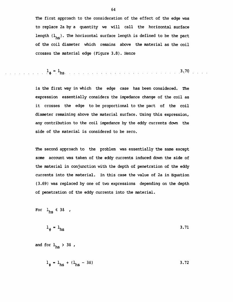
64The first approach to the consideration of the effect of the edge was to replace 2a by a quantity we will call the horizontal surface length The horizontal surface length is defined to be the partof the coil diameter which remains above the material as the coil crosses the material edge (Figure 3.8). Hence

is the first way in which the edge case has been considered. The expression essentially considers the impedance change of the coil as it crosses the edge to be proportional to the part of the coil diameter remaining above the material surface. Using this expression, any contribution to the coil impedance by the eddy currents down the side of the material is considered to be zero.

The second approach to the problem was essentially the same except some account was taken of the eddy currents induced down the side of the material in conjunction with the depth of penetration of the eddy currents into the material. In this case the value of 2a in Equation(3.69) was replaced by one of two expressions depending on the depth of penetration of the eddy currents into the material.

For lhs < 36 ,

V 1*

and for 1^ > 35 ,

3.71

■ h * + (1hs - 35> 3.72

*

The c o n s id e ra t io n o f a c o i l a t an edge was e s s e n t ia l ly based on a p o s it io n -

w eig h ted l in e a r com bination o f the two l im i t in g cases i e , the c o i l above the

m a te r ia l and th e c o i l in a i r . Th is was n o t p h y s ic a lly a c c u ra te , b u t g iven

the o v e r a l l n a tu re o f the approxim ate m odel, i t was considered a s e n s ib le

f i r s t s tep to take in the tim e a v a i la b le .

65These two cases are illustrated in Figure 3.9.

The relative merits of these two approaches to the edge case will be discussed in Chapter 8. Only the case of the coil length parallel to the material edge was considered since similar simplifying assumptions based on the physical case for the eddy currents induced parallel to the edge could not be justified. This was proved when some experiments were performed with the coil length perpendicular to the edge. The trends exhibited were not clear from the physical understanding of the system. These experiments will be discussed in Chapter 6. For completeness, the case of a vertical axis coiltraversing an edge has been considered by Burke (1987).

The work performed considering a coil crossing an edge could potentially be adapted slightly to consider a coil above a two conductor region (Figure 3.10). The eddy currents induced in the material would be considered to flow in a direction perpendicular to the interface between the two regions. Since the two materials would have different skin depth values, the basis of the extension of the model would be to consider the contribution made to the coilimpedance by the eddy currents in each material. This contribution would be assumed to be proportional to the part of the coil diameter above each of the individual materials (Figure 3.10).

These ideas for extending the approximate model, like the modelitself, are in the main based on a physical picture of the systembeing investigated. The theoretical expressions proposed are not exact, they are only intended to produce a first approximation to the value of the coil impedance change expected when a coil is placed above the material considered.

*■

4. THEORIES OF BURKE66

Burke (1986) has put forward two analytical expressions which can be used to calculate the impedance change of a horizontal axis coil as it is brought close to a homogeneous conducting half space. One expression is a perturbation expansion expression which is only valid for small skin depth, 8, values and the other is an exact expression which is valid for all values of 8.

The derivations of both expressions are given in Burke's 1986 paper. Both derivations consider a similar approach whereby the electromagnetic fields for a delta-function coil (or current loop)are considered initially. The delta-function coil is considered to bein air. Several delta-function coils are then superposed and the presence of a homogeneous conducting half space is considered. This enables the determination of the electromagnetic fields for a horizontal coil of finite dimensions above a conducting half space. The final stage of the analysis relates the electromagnetic fields produced by the coil to the impedance change of the coil. Theimpedance change (AZ) is that which occurs when the coil is movedfrom a position in air to a position close to the material half space. This final step in the analysis is performed using the reciprocity relation for the exact theory case.

4.1

67where S = surface of integration

E = source electric field intensity Hs = source magnetic field intensity E = electric field intensity in the conductor H = magnetic field intensity in the conductor

The separate impedances for the coil in air and for the coil close .to. the material are determined directly in the perturbation expansion theory case.

AZ = Z , - Z .cond air 4.2

where zconcj = impedance of coil close to the materialZ.„ = impedance of coil in airal l

4.1 Perturbation Expansion Expression

The perturbation expansion expression has the form

AZ = -2joo u.N

s,t ( a ^ ) ,

2 2 —g sin (st) M (sa^,sa2 ) R(sd)s

4.3where t = coil half length

a^ = coil inner radius a2 = coil outer radiusd = distance from coil axis to material surface s = variable of integration

M(sa^ , sa2) =jsa.

sa.d(sa) sa 1^ (sa) 4.4

681^ = modified Bessel function of the first kind of order one.

R(sd) = Kq(2 sd) + (j - 1) s 6 Ki (2sd) + 4.5

K = modified Bessel function of the second kind of order zero o= modified Bessel function of the second kind of order one

The principle variable used in the derivation of the AZ relation is the magnetic vector potential, A. A is related to the magnetic induction, B, by the following relation

B = curl A 4.6

4.2 Exact Theory

The exact theory expression has the form

2 r>°°AZ = 2jw y

N 2 2 -g- M (sa^ , sa2 ) sin (st) xs

( y a - a. )d p ------------ exp (-2 ad)

a( y r a + )

where a = (p^ + s ^ ) ^ ^

, 2 ^ . ,1/2 a^ = (a + jwa y)p = variable of integration

4.7

and the other terms are as defined for the perturbation expansion expression (Section 4.1).

69The analysis is performed using the magnetic Hertz potential (D as the parameter from which the electromagnetic fields are obtained. The relations between the magnetic Hertz potential and the electromagnetic fields are as follows.

B = grad' ar '

, 3y ,- jto y a T y 4.8

where y positive is the co-ordinate axis perpendicular to thematerial surface going away from the surface into the air (thesurface is at y = 0).

A

Ej| = - jw curl (Ty) 4.9

Ey = 0 4.10

where E|| is the electric field intensity vector for the electricfield parallel to the material surface (ie, in the xz plane).

Magnetic Hertz potentials were initially used by Weaver (1970) for considering problems concerned with half space induction. Although Weaver's approach is general, it was developed with applications to geophysical problems in mind. The central result of Weaver's work, which is the basis of Burke's exact formulation, is that 'the magnetic Hertz potential (T) can be expressed as a closed form integral involving the Fourier Transform (Gs) of the source Hertz potential (Ts)' and once the magnetic Hertz potential has been determined 'the electric and magnetic fields can be calculated anywhere in the system'.

In o rd e r to ensure th a t the NAG ro u tin e s would be s u ita b le , the NAG manual

was co n su lted and th e form o f the express ion th a t was to be in te g ra te d

considered to t r y and h ig h l ig h t any p o te n t ia l problems th a t could occur i e ,

a non -convergen t in te g r a t io n .

704.3 Method of Programming

When the Burke expressions for coil AZ were coded up using FORTRAN 77, such that they could be evaluated using a computer, several observations were made, all of which need to be noted. The overall conclusion that can be drawn from this part of the study is that great, care . must .be. taken, when trying, to evaluate . complex integral, expressions directly using a computer, since it has proved to be very easy to obtain results that appear correct but are in fact not correct.

The exact theory expression for AZ will be considered since the evaluation of this expression has been studied extensively. The AZ expression can essentially be considered as a double integration from 0 to 00.

AZ = 2jco uN

{ t(a2 - a1) ) v2 2 —g M (sa^,sa2) sin (st)

s

( y a - cl.)

d p ------------ exp (-2 ad)a( Ur a + a^)

4.11

Since the double integration was not trivial, the use of library integration routines was considered the best approach to the problem. The initial routine considered was a numerical integration routine from the NAG library. The routine, D01AMF, calculates an approximation to the integral of a function over an infinite or semi-infinite interval. Since the AZ expression integration was a double integration, the same routine, D01AMF, could not be used for

71both of the integrations because it would have meant the routine being called from inside itself, something that cannot be done. This was overcome by obtaining a copy of the routine D01AMF and renaming it DD1AMF. This enabled the same routine to be used for both of the integrations.

The two parts to the integration needed, some, close consideration2prior to the coding. In the outer integral, the M expression needed

to be expanded in order to enable the evaluation of the overall expression. M(sa^ , sa2 ) is given by

rSa-M(sa^ , sa2) =

sa,d(sa) sa 1^ (sal 4.12

M(sa^ , sa2 ) -jsa. jsa .

sa 1^ (sa) d(sa) - sa 1^ (sa) d(sa)

= M^(sa2) - M^(sa^) 4.13

The expression was expanded by considering a power series expansion for 1^ (sa)

sa (sa)3 (sa)^I. (sa) = — + —«----+ —s----- --- + ..... 4.141 2 2 . 4 2 . 4 .6

The integration was then performed to produce an expression for M(sa^ , sa2)

M(sa^ , sa2) =

72e3, 3 _ 3v 5, 5 a 5. 1. 1 7.

2 1 2 26 80 2688

165888

3 5 7 9= ^ . SJ + c2 . S3 + c3 . s' + c4 . S + 4.15

The’ numberof terns used in the M expression was determined by the computer, since if too many terms were used the computer program crashed. The reason for this was that numbers outside the range of

integral was finally evaluated numerically. It should be noted that at this point the result of the AZ calculation appeared to have converged sufficiently, ie, successive results agreed to within the specified numerical accuracy, thus indicating that sufficient terms were being used in the M expression.

The inner integrand resulted in a complex expression. This caused problems when considering the computation because of the following reasons. The use of the NAG routines required the variables to be double precision. The computer used did not have the facility to consider double precision complex variables, hence the separation of the inner integrand into real and imaginary parts was considered to be a necessary first step. The complex nature of the inner integrand resulted from the fact that ot was a complex number,

—78 76the computer (0.53 x 10” to 0.72 x 10 ) were occurring when the

4.16

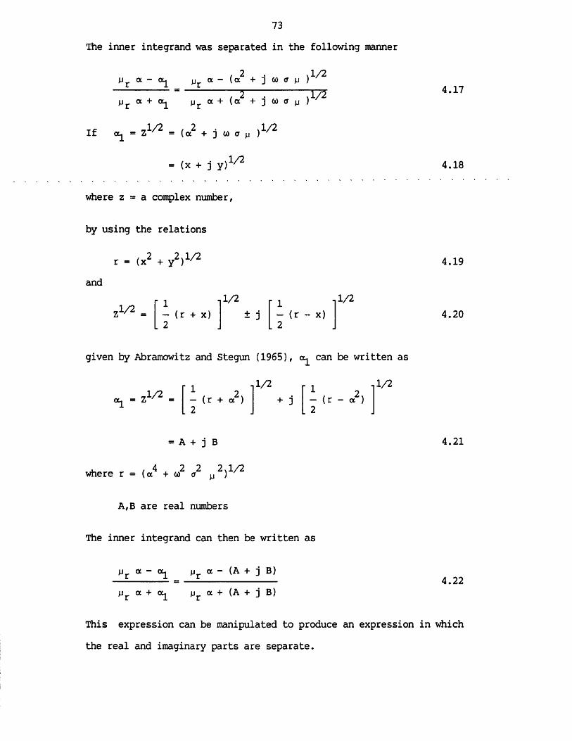
73The inner integrand was separated in the following manner

, 2 . ,1/2 JJr a - o ^ jjr <x-(a + ] w it |j ). , 2 . J 7 2

^ r a + <>i j jr a + ( a + ] w a y ) 7

T* rjl/2 . 2 . ,I f = Z = ( a + j w <7 )

= (x + j y ) 1 /2

1/2

4.17

4.18

where z = a complex number,

by using the relations

, 2 ^ 2,1/2 r = (x + y )and

,1/2 __ - (r + x) 2

1/2± j - (r - x)

2

1/2

4.19

4.20

given by Abramowitz and Stegun (1965), can be written as

= Z1 /2 = - (r + a ) 2

1/2+ D r 1 , 2, - ( r - a )

2

-.1/2

4.21

. , 4 2 2 2,1/2where r = (a + go a jj }

A,B are real numbers

The inner integrand can then be written as

jJr a - a - (A + j B)

p r a + “ l jJr a + (A + j B)4.22

This expression can be manipulated to produce an expression in which the real and imaginary parts are separate.

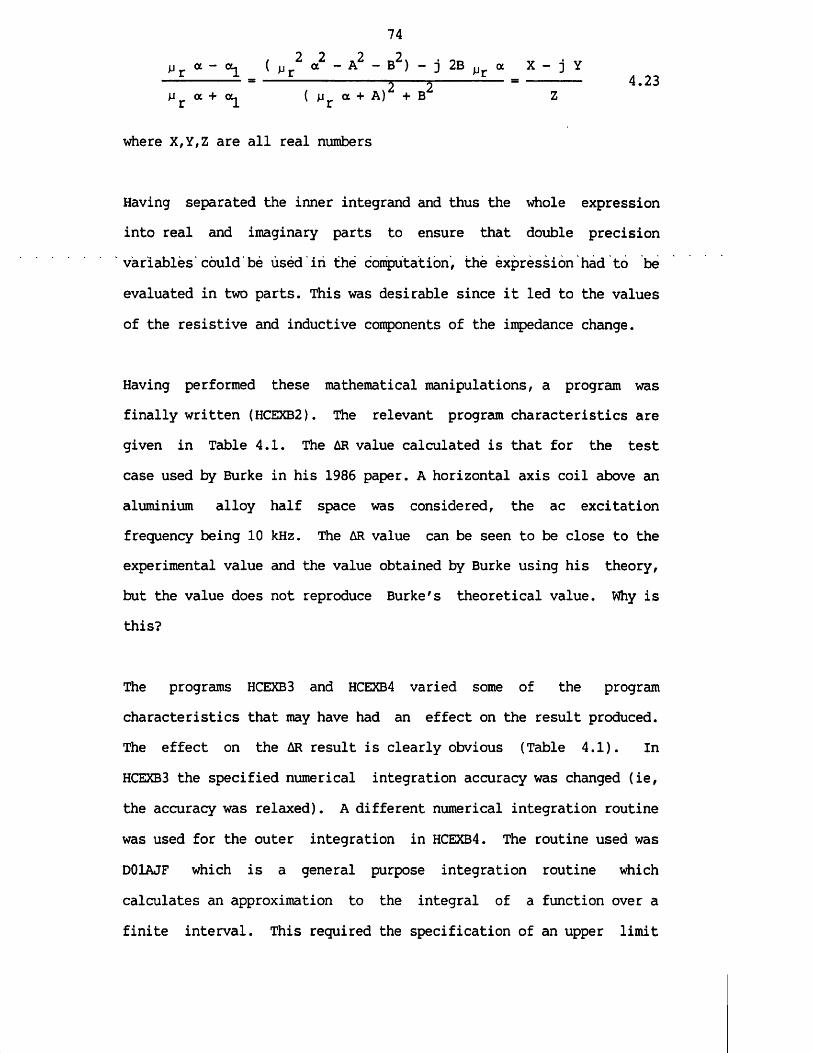
74/Jr a - ( j j r 2 a2 - A2 - B2) - j 2B JJr a = , *--------

JJ a + ( jjj, a + A) + B

where X,Y,Z are all real numbers

Having separated the inner integrand and thus the whole expression into real and imaginary parts to ensure that double precision variables’could be used in the computation, the expression had to be evaluated in two parts. This was desirable since it led to the values of the resistive and inductive components of the impedance change.

Having performed these mathematical manipulations, a program was finally written (HCEXB2). The relevant program characteristics are given in Table 4.1. The AR value calculated is that for the test case used by Burke in his 1986 paper. A horizontal axis coil above an aluminium alloy half space was considered, the ac excitation frequency being 10 kHz. The AR value can be seen to be close to theexperimental value and the value obtained by Burke using his theory,but the value does not reproduce Burke's theoretical value. Why is this?

The programs HCEXB3 and HCEXB4 varied some of the program characteristics that may have had an effect on the result produced. The effect on the AR result is clearly obvious (Table 4.1). In HCEXB3 the specified numerical integration accuracy was changed (ie, the accuracy was relaxed). A different numerical integration routine was used for the outer integration in HCEXB4. The routine used was D01AJF which is a general purpose integration routine which calculates an approximation to the integral of a function over afinite interval. This required the specification of an upper limit

X - j Y4.23

75for the integration. The value chosen was one at which the results produced were considered to have converged. By using D01AJF as the outer integration routine it was possible to add more terms to the M expression without causing the computer program to crash.

2Attention was then turned to the expression for M followingconsultation with Dr Burke in Australia. The Equation (4.15)previously presented was not strictly a correct representation of thequantity M. The power series expansion for I^(sa) is only valid for arange of values of sa, for -3.75 < sa < 3.75. For values of sa > 8,by integrating the expression for M^(sa) by parts a more exactexpression can be obtained, which involves the use of a polynomialapproximation and the direct evaluation of a modified Bessel functionof order zero (IQ) using the NAG library function S18AEF (Burke(1988b)). For the intermediate sa values, Burke derived a hybridexpression which again required a direct evaluation of IQ, but thistime a different polynominal representation was used for theremaining part of the expression resulting from the integration byparts. All of these contributions to the calculation of M wereincluded in a subroutine written by Dr Burke called SERIES. This

2subroutine was used to determine M in all of the subsequent programs written.

In HCEXB5, the inner (p) integration was performed using DD1AMF whereas the outer (s) integration was carried out using D01AJF. The integration from zero to infinity (routine D01AMF) was applied twice in HCEXB6. These two new programs both led to two more different values for the AR value in the chosen test case (Table 4.1).

In order to try and understand what was happening, two further attempts at the integration were made. Firstly Burke's own programming technique was considered. The approach considered the use of complex numbers rather than the evaluation of separate real part and imaginary part expressions. This could only be achieved by the use of real complex numbers and then the change from type real to type double precision when using the NAG routines. The results obtained from this program agreed well with the experimental results and were identical to the tabulated results of Burke (as would be expected).

The final computer program considered the evaluation of M using standard NAG routines, the inner integration evaluation by means of D01AJF and the outer integration being performed using Simpsons Rule. A result identical to that obtained from HCEXB5 was produced.

None of the programs written seemed to indicate the reason for the differing results, other than to show that the numerical evaluation of complicated integral expressions can produce results close to the value expected, but by using different integration strategies different numerical results can be obtained. Another point of interest is that the integration strategies and accuracies need to be considered in conjunction with the units system used. The use of a different units system other than that for which the program was written proved to be a source of erroneous results. The integration accuracies were chosen for two reasons, firstly to provide results that could be considered sufficiently accurate and secondly to produce computer programs that could be run for several different test cases without crashing.

77In order to indicate the closeness of two of the sets of theoretical results, Figure 4.1 is presented. The results were produced for the test case given in Burke's 1986 paper. The results compare Burke's theoretical results, experimental results and the values obtained from HCEXB2. The perturbation expansion results are those of Burke.

The use of a perturbation expansion resulted in the limitation that the expression for AZ was only valid in the limit of small skin depth. As for the previous analytical work of Burke, a NAG numerical integration routine (DOlAMF) was used to help solve the expression. NAG routines were also used to obtain expressions for Kq and (function routines S18ACF and S18ADF) and as before the expression was separated into real and imaginary parts before the integration was performed, the results finally produced being values of AR and AL.

4.4 Extension to Layers

The exact theory of Burke, although thorough, has the limitation that it is only able to predict the impedance change of a horizontal axis coil when the coil is brought close to a homogeneous conducting half space. If a layered half space needs to be considered, as in the case of the fast reactor system (ie, stainless steel on liquid sodium), the theory of Burke needs to be extended. The extension has been considered and the details are presented below.

Initially the system under consideration needs to be understood (Figure 4.2). The figure clearly shows the individual components of the incident electromagnetic wave that need to be considered once the

78incident wave has interacted with the layered material half space (Wait (1962)). The reflected waves are of great importance since they are essentially the means by which the presence of a layered rather than a homogeneous half space is indicated.

The extension to the exact theory makes use of the magnetic Hertz potential (T) as detailed in Burke's paper. Weaver (1970) stated that the magnetic Hertz potential within and on a conductor is related to the two-dimensional Fourier Transform of the source magnetic Hertz potential (Gs) by the following integral expression.

r =n J

dsa G“

dp ,-7 (0^ ) e-jsz e-jpx 4>24a + “1

where x,y,z = co-ordinate system used (material surface is in the xz plane at y = 0, and y negative is in the direction of increasing depth into the material). The co-ordinate system is illustrated in Figure 4.2.

This expression is only valid for the case of a homogeneous conducting half space. The exciting field is produced by a 6-function current loop with its central axis parallel to the material surface.

If the case of a layer on a half space is considered, based on the expression for r used in Equation (4.24), the following equations can be proposed for the electromagnetic field in the layer and in the half space.

79Layer (1)

ri =

00 00

dsa Gfc

d p ---------»r a + «i

-ya [ A j e V t B]_ e-°iy 1

x e^ sz e-3Px 4.25

where A^ = a coefficient that needs to be determined which indicates the proportion of’ the incident electromagnetic wave that is transmitted into the layer

= a coefficient that needs to be determined which indicates the proportion of the electromagnetic wave incident on the layer/half space interface that is reflected from theinterface., 2 . .1/2 o^ = (a + j w a 1 JJ )

Half space (2)

rhs = ds<x> g

dp 1 L _ e-Y“ A, e ¥ e-isz e^Px"r “ + “2 4.26

where A~ = a coefficient that needs to be determined which indicates*2the proportion of the electromagnetic wave incident on the layer/half space interface that is transmitted into thehalf space., 2 . ,1/2 <X2=(a + ■ } Oi a 2 ^ 2 '

The incident electromagnetic wave magnetic Hertz potential for the homogeneous half space case is given by Burke as

- I aj.s _ on

ds I^(sa) sin(sz dp C0S(PX) -a(d-y)a 4.27

80where a = the loop radius

d = the distance from the loop axis to the material surface

This expression is valid for y < d - a.

Since the expression in Equation (4.27) has only an e0 term, it isclear that it only represents the electromagnetic wave transmitted by the source, ie, the electromagnetic wave incident on the material surface. This is sufficient for the homogeneous half space case since the reflected component of the incident wave from the material surface does not require consideration in the analysis. In order to fully determine the field in the air above the material (but below the current loop), some account must be taken of the electromagnetic wave reflected from the material surface. This leads to the following expression for the magnetic Hertz potential in the air.

where = a coefficient that needs to be determined which indicatesathe proportion of the electromagnetic wave incident on the material surface that is reflected from the surface and in the case of a layered half space, includes any parts of the electromagnetic wave that are transmitted back into the air across the material surface following reflection within the material.

00 cos(px)ds I^(sa) sin(sz) dp

^oX

n ao

e-a d 4.28

81By substituting for Gs in Equations (4.25) and (4.26), and considering the superposition of several 6-function coils in order to form a finite length horizontal coil, the magnetic Hertz potential in the air, the layer and the half space can be determined.

Using

GS = — dx s <jsz e:px - i u i a /j \i — Ii(sa) e y2a

4.29

the following expressions can be determined.

Layer

- 2 jj I Nri = n t(a2 - ax)

r ds—r M(sa- , sa~) sin(st)

dpcos(px) sin(sz) e-ad

a( ----— ----- r JL e V + B, e"8!* 1u a + al) L 1 1 J

= Ccos(px) sin(sz) ( JJr a + a^)

where- 2 u I N

C =n t(a2 - a1) .

' ds— M(sa. , sa9) sin(st)

o s

4.30

® -ad edp

Half space

rhs = C

Air

cos(px) sin(szi ( a + o^) *2 .°2* 4.31

r . = — cos(px) sin(sz) I" e0 + B e 1air 2a L a J

4.32

82The magnetic Hertz potential in each region can be used to determine the electromagnetic field in each region using the following relations

E = - j co curl (r y) 4.33

' 3r 'B = grad — - j to jj a T y 4.341 3y J

In order to determine the unknown coefficients A^, B^, ^ and Bq/ the correct electromagnetic boundary conditions need to be applied to the problem. These are that the tangential components of both the E and H fields are continuous at any interfaces, ie, at the material surface, y = 0, and at the layer/half space interface, y = -t,

E. = E 4.35n n

andHt = Ht _ 4.36n n

Hence by considering the x and z components of both the E and H fields at each interface, four equations can be written down containing four unknown coefficients. By solving the equations, the four coefficients can be determined. The x and z components of the fields are given in Appendix Bl.

The four equations produced are

at y = 0

(A^ - B^) .2( ) j r a + ) (1 - Ba )

- 1 = 0 4.37

83(A1 + B.) , 2 a— ---- 1 = 0 4.38

( jj r a + a^) (1 + Bq )

at y = -t

<x (A^ e alt - B1 eCXlt)( j j r a + )

( jj r a + A 2 e a2t

(A^ e + B^ e06! ^ a + o !

- 1 = 0 4.39

-out(fjr <x+oc1) A 2 e a2- 1 = 0 4.40

These equations can be solved to determine the four coefficients A^,

Bl' ^2 anc* Ba* T^e a -9e^raic manipulation required is detailed in Appendix B2.

The coefficients produced are

2a. t( a + 0^) e “l ( < * 2 + 0^)e2olt (ctj + oc )(a + a) + (al - a2)(a “■ al)

( ur a + ° ^ ) - a2)<«2 + oc )(a + a) + (al - 0 2 Hex -■ al)

< »«,f a + . 2 a^ (2alt2a, t /e “1 ( 0 2 + a^)(a^ + a) + (al - 0^) (a -■ al)

2a f e2alt ( € * 2 + 0^) + (a - a2) ]

4.41

B, = -*— r ------ 4.42

4.43

B = -5— r----------------------------------------1 4.44e “l (0C2 + o£ )(a + a) + (oc - o^Ma - 0^)

As a check to ensure that the coefficients derived are correct, can be made equal to 0^. This makes the material a homogeneous half space. In this case the following relations are obtained.

84A 1 = 1.0 4.45

Bx = 0.0 4.46

A2 = 1.0 4.47

a " “1Ba 4.48

These coefficients are as expected. B^ = 0.0 indicates that there is no reflection from the layer/half space interface. This is correct since the layer and the half space are the same material (ie, there is no mismatch between the electromagnetic parameters of the two materials). * 1.0 and - 1.0 indicates that all of theelectromagnetic waves entering the material are transmitted through the material, none are reflected. The form of the coefficient for B

cl

resembles that of a reflection coefficient at the material surface.

Having determined the coefficients and hence the electromagnetic fields associated with the layered system, the final step in the analysis is to relate the fields to the coil impedance change due to the presence of the layered system. This is performed using the AZ reciprocity relation.

1 r°° 00* f \A A

AZ = —*■ dx dz n x E . H - n x E . Hi2 . — OO — CO

where ES,HS = 'source' fields

E,H = fields in the material

The algebraic manipulation required uses the fact that

The complete manipulation is detailed in Appendix B3. The surface of integration used is the surface of the material, ie, the xz plane at y 0; The 'source' fields in the reciprocity relation do not include the term associated with the reflection from the material surface and any internal reflections that result in part of the electromagnetic wave being transmitted back into the air. The only part of the 'source' field that is required in the reciprocity relation is the electromagnetic wave incident on the material surface as produced by the source coil (ie, it is as though the layered half space were not present).

The exp ress ion fo r AZ fo r th e one la y e r on a h a l f space case is g iv e n

as

/ N 2 P®

= - 2 j « jjoU(a2 a1)J JQ

00 —2(xdex dp ^o

4.51

where th e c o e f f ic ie n ts A^ and a re as d e fin e d in Equations (4.41) and (4.42) re s p e c t iv e ly .

86The coefficients A^ and have been confirmed using the algebraic manipulation package, REDUCE. The same package has been used to consider the two layers and a half space case. The coefficients produced were lengthy algebraic expressions. The basic equations that were solved are given below. There are 6 equations and 6 unknowns.

..............................................

( ^ - B1 ) (1 - Ba )

Mr a + «i 2

(A1 + Bx) (1 + Ba) jj a + a^ 2a

y ■ - t

0^ (A1 e-0!.1 - B^ e®^) ct, e~a£' - B2 ea2t)

jjra+0£i r a + “2

(A1 e”alt + B1 ealt) (Aj e_a2t + B2 ea2t)

,Jr a + a l iJr a + a 2

Y = -fci

“2 (Aj e “2*1 - B2 e ^ l ) a3 A3 e “3*1

,Jr a + a 2 ,Jr a + a 3

(A2 e~cl2tl + B2 e ^ l ) A3 e ' ^ l jjr a + 02 jJr a +

The system considered is illustrated in Figure 4.3

4.52

4.53

4.54

4.55

4.56

4.57

87The extension to Burke's exact theory was added to the Burke theory computer program already in use. The results obtained will be discussed in Chapter 8.

4.5 Magnetic Field Determination

Using the exact theory derived by Burke (1986), expressions for the three components of the magnetic field intensity at the conducting material surface can be found. The starting point for the derivations of the H field components is the magnetic Hertz potential expression

-2 jjI Nr =

t(a2 - ax) ,ds

M sin(st) xs

-ood

dp cos(px) sin(sz) e*Vo a( j j r a + a^)

> C cos(px) sin(sz) e0 4.58

where M = M(sa^ , sa2 )

-2 jj!

and the o p e ra to r C is g iven by

NC =

7i t ( a 2 - a 1 ) ,

ds—j M sin(st)

o s

-addp

a( m r a + o^)

This describes the magnetic Hertz potential on and within a homogeneous conducting half space.

The magnetic Hertz potential is related to the magnetic field on and within the material by the following expression

This leads to the following expressions for the three components of the magnetic flux density

Bx = jj Hx = C sin(sz) e0 . - p sin(px) 4.60

By = u Hy = C cos(px) sin(sz) e*]? - j w jj a C cos(px)sin(sz) e0 4.61

B = p H = C cos(px) ou e ' V . s cos(sz) 4.62Z Z X

Since it is the magnetic field at the material surface that isrequired, the Equations (4.60) to (4.62) can be simplified by putting y = 0 (the y axis is the axis perpendicular to the metal surface).

89Bx = C sin(sz) . - p sin(px) 4.63

By * C cos(px) sin(sz) - j go u a C cos(px) sin(sz)

= C cos(px) sin(sz) a 4.64

Bz = C cos(px) . s cos(sz) 4.65

If the expressions for magnetic field intensity (H) rather than magnetic flux density (B) are considered, the components become

21 NH = — x n t(a2 - a1) ,

'°° ds—r M sin(st) sin(sz) x s

-ocd

dpa( a + )

p sin(px) 4.66

-21 NH =y n t(a2 - a^ .

ds—j M sin(st) sin(sz) x s

co -ceded p ---------

0 ^r a + “1COS(px) . a 4.67

-21 NH = z n t(a2 - a^ „

ds—j M sin(st) cos(sz) x

-a d

dpq a( j j r a + )

cos(px) 4.68

When these three components are evaluated, the results are three complex numbers. Hence the magnitude of each component needs to be evaluated,

90

ie, if Hx = A + i B

|HX | = -I A2 + B2 4.69

Similarly, in order to obtain the magnitude of the magnetic field intensity at the material surface, the three components need to be considered,

More importantly, the magnitude of the tangential magnetic field (Hfc) at the material surface can be calculated.

It is this value that can help to determine the sensitivity of the eddy current test.

The method of programming used for the magnetic field intensity expression was based on the approach used by Burke for the AZ calculation. Each of the components of the magnetic field were calculated in turn and then the tangential magnetic field at the material surface and the total magnetic field at the material surface were calculated from the individual field components as detailed in Equations (4.70) and (4.71).

In order to provide a comparison, a program was also written based on HCEXB6 to produce H field results using a different integration strategy. As would be expected from the previous work (Section 4.3), different results were obtained from the two computer programs. The results obtained using the Burke integration strategy were considered

ie, |H| = J H 2 + H 2 + H 2 ' 11 x y z 4.70

4.71

91to be correct, although the range of values of x and z over which data could be obtained was restricted by the integration. At relatively large distances from the coil being considered, the results of the integration become unstable and the data produced could not be considered correct. The co-ordinates (x,z) at which this occurred varied for different coils.

5. ADDITIONAL THEORIES92

5.1 Theory of Dodd and Deeds

5.1.1 Formulation Used.

A thorough analysis of the vertical axis coil above a homogeneous or stratified conducting half space was presented by Dodd and Deeds in 1968. The method used for deriving the impedance change expressions for the coil was described earlier in Section 2.4.1. In this section the expressions obtained are presented.

For the case of the coil in air, ie, away from the conducting half space, the impedance of the coil is generally considered to be given by the coil inductance (Lq) . The expression derived by Dodd and Deeds is as follows,

L_ = j 2n u w J oN

I 2t(a2 - a^ J ,ds7

I (sa^ , sa2) x

[exp (-2st) - 1 + 2st] 5.1where

Kqx - q2> =P2

<*1dq q J^a)

= Bessel function of the first kind of order one

t, s, a^ and a2 are all as defined in Chapter 4,

In air, the resistance of the coil (RQ) is purely due to theresistance of the coil wire, ie,

93

1 PRo = 5.2

where 1 = length of wirep = wire material resistivity A = wire cross-sectional area

Both of these expressions quite' obviously hold for the horizontal axis coil as well.

Bahr and Cooley (1983) presented the Dodd and Deeds expression for the impedance of a vertical axis coil at a normalised height, h, above a homogeneous conducting half space in the following form

n r N2Z = j m ■ A v2 * *2 EXP(t . Ar) a &

(h) 5.3

whereGO 2" I (a . ar)

lEXB (h) " a1

2t + - a

2 (e_at - 1) + e~2ah

e-at _ i)2 a -da

I(a . Ar) =ra( l+Ar/2)

a( l-Ar/2)u (u) du

a + j 2

Ar = r2 rl

The coil geometry for this case is shown in Figure 5.1,

94Dodd and Deeds extended the theory to consider the case of a two conductor half space. The above expression (5.3) holds but with the following substitution.

Thea - “i term is replaced by

a +

( a + a - )((V v al “ “2) + (a - ) e2 a -2 a- C

( a - a ^ ) (a ^ - ol ) + ( a + a^M o^ + e °^

where

a + j 2/ r n2

a + j 2' r '2

C = the thickness of the layer of material 1 on a half space of material 2

The expression ( a - a ^ ) / ( a + a^) is, in effect, a reflectioncoefficient term. The substitution thus modifies the reflectioncoefficient such that account is taken of the electromagnetic wavereflection from the boundary between materials 1 and 2 and thetransmission of the electromagnetic waves into material 2.

95In order to determine the individual components of the impedance (Z) the real and imaginary parts need to be taken since z will be a complex number. Hence the following relations can be used to determine the coil resistance and inductance changes due to the presence of the material half space.

AR = real (Z) - Rq 5.4

and

imaginary (Z)AL -------------- Lq 5.5

co

5.1.2 Method of Programming

In order to evaluate the expression for Lq (Equation (5.1)), NAG routines were used. was determined using the NAG function routine S17AFF, the inner integration to determine I(sa^ , sa2 > was performed using the numerical integration routine D01BDF and the outer integration required the use of D01AMF.

The method used to program the expression for coil impedance, Z, as given in Equation (5.3) was to use a NAG routine for the integration to determine I(a . Ar) and then to use a Simpson's rule approach to the outer integration. This was based on the program written by Bahr and Cooley to accompany their 1983 paper. The program was obtained from a source in the USA during the course of the work. The NAG function routine S17AFF was used to determine J^. The Simpson's rule integration required the specification of an upper limit to the integration. This upper limit needed to be considered in conjunction with the units system used when the expression was programmed with

96the length variables not normalised. With the lengths normalised by r the results were consistent whatever the units system used.

5.1.3 Magnetic Field Determination

When considering eddy current inspection of materials, the radial magnetic field at the surface of the material can be used as an ■indicator of the’test sensitivity. The greater the surface field, the greater the eddy current density within the material, hence the greater the test sensitivity.

An expression for the radial magnetic field at the material surface, Hq, normalised by the coil driving current, I, has been presented by Bahr and Cooley (1983) based on the analytical expressions derived by Dodd and Deeds in 1968.

H -NoI r(t . Ar) IEXPP

where

■expp <h>r I(a • flr) -«h - »t^ Jx (a) e ^ (1 - e at)

a “1

5.6

da

and h, t and Ar are all normalised by r. The coil geometry is illustrated in Figure 5.1.

When programming the calculation of the magnetic field the same approach was used as for the coil impedance calculation. The values of magnetic field at the material surface were calculated for several points on a radial line from the central axis of the coil. Close to

97and underneath the coil the step sizes were smaller than those atlarge distances from the coil. Due to the large number of points atwhich the H field value was calculated, the program generally had tobe run as a batch job.

5.2 Uniform Field Theory

5.2.1 Theory of Auld

Auld et al (1984) have considered the modelling of eddy current NDT extensively. Expressions have been derived to describe the coil impedance change when the induced electromagnetic field is either uniform or non-uniform and for defects that can be considered either two-dimensional or three-dimensional. Different skin depth regimes have also been considered.

The expression used in this study concerned a two-dimensional crack in a uniform field in the small skin depth regime, ie, large a/S (a is the crack depth). This expression was given by Auld et al in 1982. Figure 5.2 illustrates the system considered.

2 (1 + j) - - 1.56 + - 6

a Au- (1 + j) —

65.7

t1

t2

t3

t4

where AZ = probe impedance change per unit length h1 = incident magnetic field intensity Au = crack opening Ap = crack opening area

For an EDM (electro-discharge machined) slot

Ap = a Au 5.8

and for a fatigue crack

a Au 5.92.........................................

These were given by Auld et al (1984).

The various parts of the expression (5.7) can be describedphysically,

1. represents the wall effect (surface impedance).

2. results from the Kahn effect. This describes the 'bunching' of eddy current lines at the crack edge and at the crack tip. The dimension of the region in which this effect occurs is of the order 5. The Kahn effect is illustrated in Figure 5.2 and it is a resistive loss term.

3. represents the Faraday effect, ie, an inductance due to the finite crack opening which is encircled by the currents in the material.

4. is the unperturbed surface impedance of the system.

All of these points have been described by Auld et al (1982).

5.2.2 Work of Moulder99

Moulder (originally at the National Bureau of Standards, Boulder, Colorado, USA and now at Iowa State University, Ames, Iowa, USA) and his colleagues have worked extensively on uniform field eddy current (UFEC) probes (Moulder et al (1987)). The probes were described earlier in Section 2.3.

The theoretical analysis of the UFEC probes makes use of a general theory developed by Auld et al (1984) for the impedance change of a coil which induces a spatially uniform magnetic field incident on a two-dimensional or three-dimensional flaw. The expression is only valid in the limit of small skin depth.

c HAZ ---7

a Ic - c Au 1

E + (1 + j) — E + j — y- E16 r

5.10

where H = uniform interrogating field (= h1 in Equation (5.7))c * crack half lengthE°,E^ = shape parameters that depend only on a/c, the aspect

ratio. The numerically calculated shape parameters aregiven in Tables 5.1 and 5.2 for the cases of a rectangular flaw and a semi-elliptical flaw respectively.

For the case of the semi-elliptical flaw, the numerically calculated values of the shape parameters have been fit to polynominals using a least squares procedure. The polynominals obtained are as follows (Moulder et al (1987)),

100' a ' f a )= - 3.0 - 1.35 — + 0.66 — C 4 , c ,

5.11

I1 = - 0.02 + 2.56' a ' f a ' f a 1

— + 1.11 — - 1.70 —

, c , < c > , c ,5.12

All of the formulae in Sections 5.2.1 and 5.2.2 have been coded up using FORTRAN 77 to produce a program which uses accepted theory to describe the coil impedance change due to a two-dimensional or three- dimensional defect in a uniform interrogating field.

In the Auld expressions for AZ, one particular relation is of considerable importance and needs to be determined before the AZ values can be evaluated. This relation is H/I, the magnetic field strength at the material surface per unit current. Using the theory of Dodd and Deeds (1968) for vertical axis air cored coils or thetheory of Burke (1986) for horizontal axis air cored coils, H/I canbe determined for these simple coil cases ready for use in the AZexpressions. For more complicated probes like the UFEG probe or even ferrite cored coils, the H/I values need to be determined using acalibration.

The calibration is performed by considering the coil impedance change due to a cylindrical or part spherical recess in the surface of the material being inspected. Auld has adapted a formula from a microwave perturbation theory solution for a smooth dimple in the surface of a perfect conductor, which can be used in the case of a cylindrical recess of depth greater than the skin depth to determine H/I (Moulder et al (1987)). A general equation based on this formulation has been proposed by Moulder et al (1987).

101/ H 2 C V

AZ = j 2 5.13I J <x 6

where V = volume of recess (cylindrical or part spherical)C - empirical shape factor, the value of which depends on the

shape and depth of the recess relative to S. Some of the values of C determined by Moulder and his co-workers are

Of the two possible calibration defects that can be used, the part spherical recess is the best since it most closely resembles a dimple. Hence the theory used for the calibration is more correct with a part spherical recess. Since the H value is the value of magnetic field intensity at the material surface, it would follow that the ideal calibration procedure would consider a very shallow and wide cylindrical calibration defect (Moulder et al (1988)). The surface electromagnetic fields in this case would be essentially unperturbed by the flaw present.

There are two conditions required when considering a calibration defect,

given in Table 5.3.

a- > > 1 5

5.14

anda- < < 1 d

5.15

where d = the radius of the defect (usually a cylindrical defect)

102The first of these conditions has been determined by the performance of several tests by Moulder and his co-workers. The calibration relation was found to hold best at reasonably high frequencies. In order to use Auld's relations, it is important that this condition is satisfied. The second relation follows from the need for a wide, shallow defect. One final point that also needs to be considered is that the probe must be operating well below its self resonant frequency when performing the calibration, otherwise the calibration will not be successful and not provide a useful H/I value.

An alternative calibration method mentioned by Moulder et al (1987) is to measure AZ for an EDM notch of known dimensions, and then, using one of Auld's AZ relations, determine H/I by forcing the calculated flaw signal to equal the experimental one. The value of H/I thus calculated can then be used in subsequent evaluations of AZ or defect size parameters, depending on whether the AZ expressions are being used to consider the forward problem or the inverse problem.

Much of this work using Auld's uniform field AZ expressions has been performed by Moulder and his co-workers to provide a complete analysis of the UFEC probe.

5.2.3 Application to Horizontal Axis Coils

Since part of the electromagnetic field produced by a horizontal axis coil can be considered essentially uniform, it was decided to investigate whether or not the uniform field theory detailed in the

103previous two sections (5.2.1 and 5.2.2) could be applied to the case of horizontal axis coils. This would give some idea as to how 'uniform' the horizontal axis coil field could be considered to be.

The work was performed in two distinct parts, the first of which considered the case of a 2D flaw in a metal block. The coil considered was an air-cored, 103 turn horizontal axis coil. It was25.5 mm long and had a core diameter of 12.5 mm. All of the specimens considered were aluminium blocks. Three slots were investigated, the dimensions of which are given below.

i) 2 mm wide and 3 mm deepii) 2 mm wide and 4.5 mm deepiii) 0.25 mm wide and 3 mm deep

The experimental test procedure involved measuring the two components of the coil impedance when the coil was placed above the base material (lift-off = 0.143 mm) and then above the slot being investigated. In order to determine these values the coil was connected, via a test fixture, to a Hewlett Packard HP4194A impedance/gain-phase analyser (Plate 5.1). The instrument measured the impedance of the coil over a specified frequency range within the limits of 100 Hz to 40 MHz. It was possible to vary the time taken to determine each impedance value and also to vary the display format for the trace data (ie, the data recorded over the specified frequency range). The tests could generally be performed quickly and the current through the coil could be monitored whilst performing the sweep. Using an increased integration time (ie, the time to determine a result) it was possible to reduce the noise, but it did increase the sweep time.

104The frequency values at which the impedance results were considered were determined such that the small skin depth requirement of the uniform field theory was satisfied and such that the coil was operating well below resonance. The coil resonant frequency was around 3 MHz, and in order to ensure that a/5 > 3.0, a frequency greater than 7 kHz was required. This led to the choice of four test frequencies between these limits, 150 kHz, 300 kHz, 450 kHz and 1 MHZ.

In order to apply the uniform field theory it was necessary to determine H/I for the coil at the material surface directly underneath the coil. This value was calculated using the computer program written, which was based on the theory detailed in Section 4.5. The theory used was based on the exact horizontal axis coil theory of Burke. The experimental values determined were compared with the theoretical predictions in order to ascertain the correctness of applying the two-dimensional uniform field theory to horizontal axis coils. These results will be discussed in Chapter 8.

The second part of the work considered a three-dimensional flaw. The flaw, a semi-elliptical spark eroded slot, was fabricated in a 316 stainless steel block. The flaw dimensions were as follows.

2c = surface length = 6.5 mm a = depth at centre = 0.6 mm aspect ratio = a/c = 0.185

105In order to consider a more realistic inspection case, a small ferrite-cored probe was used. The probe was 2 mm long with a 1 mmdiameter ferrite core, and three layers of 20 turns of 0.1 mmdiameter coated copper wire. The same experimental procedure was adopted as for the two-dimensional case.

The choice of frequency of operation for this case required another consideration apart from those of satisfying the small skin depthcondition and the need to operate below probe resonance. This condition was that of the need for a calibration defect. Since theprobe had a ferrite-core the theoretical determination of H/I was no longer possible, hence the calibration defect approach of Moulder (as detailed in Section 5.2.2) was employed. The frequency of operation chosen was 4 MHz. A spherical cap calibration defect of depth at the centre approximately equal to 5 at 4 MHz was considered suitable for determining H/I.

Two calibration defects both of depth approximately equal to 0.2 mm (5 at 4 MHz) were fabricated. One was made using a hardness testing machine. A 1 mm diameter hardened steel ball was 'dropped' under a known load onto the surface of the stainless steel block. This made an indentation in the material surface, the dimensions of which could be measured using a microscope device attached to the hardness testing machine. The second calibration defect was fabricated by actually removing a small quantity of material using a 1.5 mm diameter ball cutter. In both cases the value of the empirical shape factor, C, was taken to be 4.0.

106Both defects were considered when performing the calibration, the aim being to see whether one method of fabrication was preferred over the other (ie, metal deformation or metal removal). The probe AZ determined using the impedance analyser for when the calibration defect was traversed by the probe was used to determine a value for H/I. The value of H/I was used in the three-dimensional uniform field theory, and the theoretical AZ predictipns .were compared with the experimental AZ results for the case of the semi-elliptical defect. As for the two-dimensional results, the applicability of the three-dimensional uniform field theory to horizontal axis coils will be discussed in Chapter 8.

1076 EXPERIMENTAL WORK

6.1 Conventional Equipment Familiarisation

In order to obtain an understanding of how a conventional piece of eddy current equipment operates and the range of materials it can be used to inspect, some simple experiments were performed using a Hocking AV100L. The equipment was set up as detailed in the manual (Hocking NDT Ltd) and an absolute pencil probe and a balancing load were connected.

The equipment (Plate 6.1) is a relatively easy to operate impedance plane display instrument. It is a single frequency, keypad operated instrument which uses microprocessor control. The unit is portable and it can be battery operated or mains driven. The frequency range of the instrument is from 80 Hz to 6 MHz. A printer can be connected to the instrument which allows a screen dump to be produced. The instrument settings can, if required, be continuously displayed on the screen and thus transferred to paper when a screen dump is performed. High and low pass filters allow a certain amount of signal processing using the basic instrument. Other features of the instrument are detailed in the manual.

The aim of the experiments performed was to investigate the capability of the instrument and to illustrate some of the most common effects associated with eddy current testing. The balance load of 5.6 H was chosen in order to match the inductance of the ferrite cored absolute coil used as the probe. The frequency range specified for the probe was 0.5 to 4 MHz.

108Each of the results obtained will be discussed in turn. Figure 6.1a illustrates the trace obtained when the probe was brought close to a mild steel block, moved over a 2 mm deep slot in the centre of the block and then passed over the edge of the block such that the probe was once again in air. Each of the traces (lift-off, slot and edge) can be easily distinguished and, apart from the early part of the edge trace which is similar to the slot locus, all of the traces can be easily separated. A similar experiment was performed using another mild steel sample. In this case the specimen contained six slots of varying depths from 0.5 mm to 3.0 mm. Each of the slots can be clearly distinguished on the impedance plane (Figure 6.1b), thus indicating that slots can quite easily be detected in mild steel. This was considered surprising since it was expected that the magnetic permeability noise would cover most of the signals from the slots. This is encouraging when considering the detection of defects in a stainless steel weld (a ferromagnetic material). In both cases the frequency used was 1 MHz. This was a high frequency to use when performing eddy current testing and it was the most probable reason for the lack of permeability noise affecting the signals obtained. At lower frequencies, the effect of magnetic permeability variations would have been more significant and may well have masked the signals obtained from the slots (Hull and John (1988)).

The lift-off loci for several different materials are indicated in Figure 6.2. It can be seen that the ferromagnetic materials are quite clearly separated from the non-ferromagnetic ones. By combining Figures 6.1 and 6.2 it is possible to start to predict the form of the impedance plane trace for a probe traversing an austenitic weld with a slot machined at the weld centre line (Figure 6.3). If the austenitic weld material lift-off trace is assumed to be similar to

109that for mild steel (both materials are ferromagnetic), the predicted composite signal for the complete scan can be produced. This trace will be considered further in Section 6.3, but it does indicate that stainless steel weld inspection is, in principle, possible.

Figure 6.4 illustrates the variation in lift-off loci for the various parts of a simple mild steel specimen which has a single V butt weld in it. The three regions are indicated on the figure and they are the base material, the heat affected zone (HAZ) and the weld material. The figure indicates that when considering a weld region, the electromagnetic parameters of both the weld itself and the HAZ are modified sufficiently during welding to cause obvious changes in the lift-off loci for both regions when they are compared to the locusfor the base material.

The consideration of a non-ferromagnetic material is illustrated in Figures 6.5a and 6.5b, the material being aluminium. Initially afrequency of 50 kHz and a 14 dB amplification were used. It can clearly be seen (Figure 6.5a) that although the defects could be detected, the indications from the slots of different depths couldnot be clearly distinguished. By reducing the frequency (10 kHz) and increasing the amplification (40 dB) it can be seen that better separation of the traces could be obtained (Figure 6.5b). The slots varied in depth from 0.5 mm to 3 mm and there were six present in the sample.

Stainless steel results are illustrated in Figure 6.6. All of the defects can be clearly distinguished (6 mm deep down to 3.5 mm deep). As with the aluminium tests, a lower frequency (10 kHz) was usedcompared to the mild steel tests. The stainless steel sample with the

110slots in it was not known to be 316 stainless steel specifically, hence the lift-off trace for a block of 316 stainless steel was also added to the figure. The closeness of the two lift-off plots suggests that even if the sample with the slots in it was not 316 stainless steel it was very similar.

The results obtained for the non-ferromagnetic materials indicated that, in general, to achieve clear, reasonably well separated signals from the slots present in the material, lower frequencies than those used to inspect mild steel are required. Frequencies of the order kHz rather than MHz are more often used when inspecting non-ferromagnetic materials. It should also be noted that although some results were obtained from the non-ferromagnetic samples using the absolute probe available, the probe was not best suited to operating at the test frequencies used.

Several general points can be made about eddy current inspection based on this simple experimental study. Firstly it must be noted that for each test we were restricted to the equipment available and no form of technique optimisation was possible, apart from adjusting the test frequency and display amplification which did help to make the results clearer in certain cases. The points that need to be noted are

defect detection is possible in ferromagnetic materials using eddy currents provided the test frequency is high enough (of the order MHz).

the distinct skin depth difference in mild steel base material, HAZ and weld material can be clearly seen.

Illslots can be easily detected in both aluminium and stainless steel (non-ferromagnetic materials) using a frequency of the order kHz.

for non-ferromagnetic materials the slot and lift-off loci are not separated by as large an angle as for ferromagnetic materials.

Overall the results have indicated that it would be useful to perform some simple experiments on a stainless steel weld specimen to try and ascertain the feasibility of defect detection. The composite signal illustrated in Figure 6.3 indicates that defect detection in stainless steel weld regions should be feasible and predicts the form of a trace obtained from a scan across an austenitic weld containing a slot. Stainless steel weld inspection is considered further in Section 6.3

6.2 Horizontal Axis Coil Evaluation

6.2.1 Performance Evaluation

Much of the experimental work performed was designed to provide data with which both the Burke theory and the results from the approximate model could be compared. This required the measurement of coil impedance change values. A simple set up was used (Figure 6.7 and Plate 6.2).

112Initially two single layer coils were wound on separate perspex rod formers using coated copper wire. A coil winding machine available at UKAEA Risley was used for the coil fabrication. The details of the two coils are as follows:-

Coil 1: 140 turnsRod Diameter = 10 mm Coil Length = 39 mm Wire Diameter = 0.234 mm

(0.25 mm diameter coated copper wire) Lift-off = 0.143 mm

Coil 2: 200 turnsRod Diameter = 10 mm Coil Length = 29 mm Wire Diameter = 0.122 mm Lift-off = 0.143 mm

The coils would be described as single layer air-cored coils. Plastic tape was needed to hold the coils together once they had been wound. The wire at the ends of the coil was cleaned of the coating and tinned with solder in order to ensure a good connection to the instrument.

The coils were connected to a Wayne Kerr 6425 precision component analyser (Wayne Kerr Instruments Ltd) using Kelvin clips attached to the instrument leads. The Kelvin clips automatically made the correct connections to a lead eliminator circuit within the instrument which, as far as possible, eliminated the effect of the extra capacitance due to long connecting leads. Using the Kelvin clips also helped to

113ensure a very low contact resistance when making the connections to the coil. The instrument was microprocessor based and it provided a direct read out of the impedance of a component which was connected between the two output terminals of the instrument. Apart from the need to balance the instrument prior to the start of testing, no other special procedures were necessary for the accurate use of the instrument. Testing could be performed at several . discrete frequencies in the range from 20 Hz to 300 kHz. An X-Y chart recorder was linked to the impedance analyser through the instrument analogue output sockets, such that a hard copy of the results could be obtained. The plots obtained were of series coil resistance v series coil inductance.

The metal specimens used were blocks of 316 stainless steel and aluminium (99.5% purity), and a sheet of copper (half hard condition). Two layered specimens were also considered, one consisted of 1.62 mm of copper on a stainless steel block and the other was 6.35 mm of 316 stainless steel on an aluminium alloy block. The sizes of the blocks were chosen such that economic use was made of the material and the edge effects were minimised (ideally 150 mm x 150 mm for the top face). It was also important that each sample could be considered to represent a half space over as large a frequency range as possible. The electromagnetic parameters of the materials considered are presented in Table 6.1.

The test procedure involved bringing each coil close to each specimen at several frequencies in the range 100 Hz to 100 kHz. Given the ultimate inspection requirements, a frequency range of 100 Hz - 100 kHz was considered to be the most useful for initial investigation. The reason for this was that in this frequency range

114the electromagnetic skin depth is quite large (42.0 mm to 1.33 mm in stainless steel), thus allowing good eddy current penetration. In each test a lift-off of 0.143 mm was maintained due to the thickness of the plastic tape used to hold the coil together, unless stated otherwise. The values for the change in resistance and the change in inductance of the coil were recorded. For the frequencies up to and including 20 kHz a constant current drive was in operation(100mA rms) and for 50 kHz and 100 kHz a constant voltage drive wasin operation (IV rms). With the constant current drive, the voltage across the component was accurately measured, thus enabling the impedance of the component to be determined. When the constantvoltage drive was in operation, the current through the component wasaccurately measured.

For many of the coils used, but most especially the early ones, the choice of coil parameters was arbitrary. This meant that the coils used would not have exhibited the best signal-to-noise ratio possible. This indicated the need for coil optimisation (Chapter 7).

a) Horizontal coil above a homogeneous conducting half space

For this series of experiments two separate readings were taken for each test. The resistance and inductance of the coil were measured in air and close to the specimen being considered. The values of AR and AL due to the presence of the material were then calculated.

Figures 6.8a and 6.8b indicate the trends in AR and AL with changing frequency for the case of the 140 turn coil above a 316 stainless steel specimen. With different coils and different materials the trends were identical, it was just the absolute values of AR and AL

115that changed. With increasing frequency the value of AR increased, becoming more positive, and the value of AL increased, becoming more negative. These characteristics are typical when considering eddy current induction.

A detailed study of the effect of coil lift-off has been conducted using the 140 turn coil above the 316 stainless steel block. Figures 6.8c and 6.8d indicate the trends observed. It is clear from thefigures that both components of AZ change quicker when the coil is closest to the material and being moved away from the material. This is due to the density of the eddy currents in the material changing as the coil moves away from the material. As the coil resistance and inductance start to reach the coil in air values, the changes become less apparent since by this point only a very small amount of eddycurrents are being induced in the material and their contribution to the coil impedance is almost negligible. The results were obtained at a frequency of 100 kHz.

b) Horizontal coil above a stratified conducting half space.

The same method was employed for the study of a layered system as wasused for the homogeneous material case. The trends exhibited by AR and AL are also identical to those for the single material case.

The example presented is that of the 140 turn coil being used to consider the stainless steel on aluminium alloy specimen (Figures 6.9a and 6.9b). In both of these figures the results obtained for the stainless steel half space are also included. At low frequencies, as expected, the two plots diverge. This indicates that in the layered specimen the skin depth was sufficiently large to cause the

116induction of eddy currents in the aluminium alloy. Hence the values of AR and AL were modified by the eddy currents induced in the aluminium alloy. At the high frequency end, the layered half space and homogeneous half space plots are essentially identical. The reason for this was that eddy currents were only being induced in the stainless steel. In effect the eddy current coil was not 'seeing' the aluminium alloy due to the small electromagnetic skin depth at the frequencies considered.

In order to ensure that the experimental characteristics were repeatable for different coils, a second experiment was performed using a 182 turn air-cored coil above the stainless steel on aluminium alloy specimen. The coil details are given below.

Coil 3: 182 turnsRod Diameter = 10 mm Coil Length = 45.5 mm Wire Diameter = 0.234 mm

(0.25 mm diameter coated copper wire) Lift-off ~ 0.0 mm

The trends exhibited agreed with those illustrated in Figures 6.9a and 6.9b (see Table 8.3).

The stainless steel on aluminium alloy system is essentially like the LMFBR inspection case of stainless steel on liquid sodium, ie, a low conductivity material on a high conductivity material. These experiments indicate that in the LMFBR system the liquid sodium will contribute to the measured AR and AL values if the electromagnetic skin depth is large enough.

117The 182 turn coil has also been used in a vertical orientation with a lift-off of 2 mm to investigate the stainless steel on aluminium alloy specimen. This produced a set of experimental results with which data from the extended theory of Dodd and Deeds (which is capable of considering stratified media) could be compared. This comparison is made in Chapter 8.

c) Horizontal coil close to an edge

Edge effect is often considered to be a major problem with eddy current testing. It refers to the spurious signals superimposed on the signal of interest (ie, the signal due to the presence of the material or a defect) because of the inspection coil position close to an edge or step in the material surface. The coil impedance change as an air-cored horizontal axis coil transverses an edge has been considered. As with the previous cases, the example considered is that of the 140 turn coil above a 316 stainless steel block. A frequency of 100 kHz was used.

Figures 6.10a and 6.10b indicate the coil R and L characteristics respectively as the coil crosses the edge with the coil length parallel to the edge. The plots indicate a steady reduction in the eddy currents induced in the material as the coil crosses the edge. When the coil is close to the edge but no longer above any material, eddy currents are still induced in part of the material since the coil impedance is not that for the coil in air. As the coil crosses

118the edge, eddy currents are induced in the side of the edge as well as in the upper surface of the edge. This point is illustrated more clearly for the case when the coil crosses the edge with its length perpendicular to the edge.

The coil R and L characteristics for this case are illustrated in Figures 6.10c and 6.10d. As the coil starts to cross the edge, the coil resistance and inductance start to change. Once about a quarter of the coil length has crossed the edge, the change in R and L becomes less rapid. This is especially true for the coil resistance which becomes essentially constant as more of the coil crosses the edge. The reason for this can be considered to be that as the coilcrosses the edge the magnetic field distribution is such that asfewer eddy currents are induced in the upper surface of the edge, more eddy currents are induced in the side of the edge. This effect causes the coil R and L values to become almost constant for a range of coil positions. Once about three quarters of the coil length has crossed the edge, the coil R and L start changing more rapidly again, thus indicating the reduced eddy current density in the material.All of the characteristics described can generally be repeated fordifferent coils and materials at different frequencies to those considered here.

d) Horizontal coil traversing a defect

The final experiments performed as part of the horizontal axis coil evaluation considered the coil impedance change as the coil was moved across defects, ie, slots in various materials. The initial experiments considered an air-cored horizontal axis coil connected to

119the Hocking AV100L impedance plane eddy current instrument. From the results of the experiments performed the aim was to get an indication of the form of signal produced by a simple horizontal coil as it traversed a slot.

The details about the coil used are given below.

Coil 4: 175 turnsRod Diameter = 5 mm Coil Length = 41 mm Wire Diameter = 0.193 mm Lift-off = 0.143 mm

Two identical coils were wound on separate perspex rod formers. Both of the coils were connected to separate BNC plugs using a short length of shielded cable. This enabled the coils to be connected to the Hocking eddy current instrument. One of the coils was acting as a balance load whilst the other coil was the probe used for the inspection experiment. In each case described, the coils were made to traverse the slot with the coil axis parallel to the slot length. This resulted in the eddy currents impinging on the slot perpendicular to the slot length, ie, the eddy current distribution was such as to be the most favourable for detecting the slots.

The first three traces indicate the capability of the simple horizontal axis coil quite convincingly. In each case the frequency used was 100 kHz. Figure 6.11a illustrates the defect detection capability when the coil was moved across a mild steel block containing six slots with depths varying from 3 mm down to 0.5 mm. All of the slots can be clearly distinguished since the coil is able

120to give some indication as to the size of each defect relative to the neighbouring defects. A less clear trace was obtained for the case of a similar specimen in aluminium containing identical defects to those in the mild steel block but in aluminium (Figure 6.11b). Aluminium, being a higher conductivity material, had a smaller skin depth than mild steel at the frequency used. This was considered to be the reason for the less clear discrimination between the signals from the various slots in the specimen. In addition the fact that the phase of the defect signals from the aluminium was very close to the phase of the lift-off signal, ie, in the trace all of the signals are essentially horizontal, did not help separate the signals for clear identification. A stainless steel specimen was then considered. It contained six slots of depths ranging from 6 mm down to 3.5 mm. The trace produced indicates all six defects clearly (Figure 6.11c), and as with the mild steel specimen some indication of relative slot size is produced.

Having demonstrated the basic slot detection capability of a simple horizontal axis coil, two additional experiments were performed to illustrate the effect of traversing the slot with the coil axis parallel to the slot length and then perpendicular to the slot length. Bowler (1988) has illustrated clearly the actual eddy current distribution associated with a horizontal axis coil (Figure 6.12). This illustration will be considered when describing the next two traces. Figure 6.13 illustrates the trace obtained when the coil traverses a 10 mm deep slot in a mild steel block with the coil axis parallel to the slot length. The slot trace, as expected, is very clear. A large trace would be expected since the defect is deep and wide and the eddy currents are incident perpendicular on the slot length. This leads to the maximum eddy current distortion. For the

121case of the coil length perpendicular to the slot length, the eddy currents will essentially be parallel to the slot and thus experience a minimum amount of distortion. This would suggest no signal beingrecorded as the coil traverses the slot. In practice this does notprove to be the case (Figure 6.13). Two signals smaller in magnitude than that for the coil parallel case are seen on the instrument display. One signal occurs as one end of the coil traverses the slot. The instrument then registers no signal as the central part of the coil crosses the slot, but then as the other end of the coil traverses the slot, a second signal identical to the first signal is recorded. At first this would appear incorrect, but with reference to Figure 6.12 the reason for the two signals becomes clear. The eddy current distribution at the ends of the coil clearly indicates that as the ends of the coil cross the slot some eddy currents will beincident perpendicularly on the slot and thus distorted by the slot.This leads to the two signals as indicated in Figure 6.13.

In order to try and increase the amount of eddy currents in the material and to obtain some quantitative results a ferrite-cored coil with two layers of turns was used, connected to the Wayne Kerr 6425. The coil details are given below.

Coil 5: 2 layers of 125 turns = 250 turns totalWire Diameter 0.193 mmCoil Length 29 mmCore Diameter 5 mmLift-off 0.143 mm

122Each of the three specimens investigated contained six slots of varying depths. All of the tests were performed at a frequency of 20 kHz.

Figures 6.14a, 6.14b and 6.14c illustrate plots of AR and AL against coil position for the specimens in mild steel, aluminium and stainless steel respectively. The consideration in each case was Uiat of defect detection not sizing. Figure 6.14a which illustrates the AR and AL variation as the coil is scanned over the mild steel block, indicates the importance of both the resistive and inductive components of the coil impedance change. By considering the AL characteristics, all of the slots down to 0.5 mm deep can be clearlyseen. The AR results are only capable of indicating down to the1.5 mm deep defect. Both plots indicate the feasibility of slot detection in mild steel using a horizontal axis coil.

Apart from a slight anomaly with the AR value for the 1.5 mm deep defect, all of the defects down to 0.5 mm deep could be quite clearly seen when considering the aluminium specimen (Figure 6.14b). The AL changes were particularly clear, indicating the variations in depth of the slots.

The characteristics for the stainless steel specimen were not as clear as for the previous two specimens, although it was felt that all of the slots down to 3.5 mm deep could be detected (Figure 6.14c). The AR results were all positive values, although the sign of the change in AR as a slot was crossed was different for thedeeper slots as compared to the shallower slots. The reason for thiswas not clear. The only explanation that could be offered was that for a deep slot at the skin depth value used with the coil used, the

i

*

I t is im p o rta n t to n o te th a t th e specimens used when g e n e ra tin g th e da ta

p resen ted in F ig u re 6 .1 4 were n o t s u f f ic ie n t ly la rg e to e l im in a te a l l o f the

l i k e l y e f f e c ts on th e eddy c u rre n t f i e l d o th e r than those o f in t e r e s t i e ,

those due to th e s lo t being in v e s t ig a te d . The m ajor problems were those due

to edge e f f e c t , i e , th e specimen was n o t w ide enough, and the spacing o f the

s lo ts in th e specimen i e , th e s lo ts were too c lo se to g e th e r . In o rd e r to

avo id t h is th e specimen should have been la r g e r and th e s lo ts more w id e ly

spaced. T h is was n o t p o s s ib le to o b ta in due to the f in a n c ia l c o n s tra in ts o f

the p r o je c t .

123amount of material contributing to the resistive losses was reduced compared to that present in the unflawed case, ie, the coil 'saw' a lot of air. Hence this resulted in a reduced AR as the flaw was crossed. This reasoning is similar to that used in the development of the approximate model extension. The AL results indicated the presence of each of the slots, but no feeling for the depth variation was present.

For each specimen, the defects could, in general, be detected quite easily by considering one or both of the components of the impedance change. It should be remembered that neither the coil nor the test frequency were optimised, something that would have improved the detection capability of the set-up. This is demonstrated in Figure 6.14d where the frequency used was 5 kHz, a value that was considered to be better than 20 kHz for inspecting the stainless steel specimen based on the previous experimental work. The slots can be seen more clearly at 5 kHz with both impedance change components. The aim of the work was to demonstrate that horizontal axis coils can be quite easily employed for defect detection in several different materials. The fact that the defects could be detected in the mild steel specimen was a promising sign for the detection of surface defects in a stainless steel weld specimen.

*One point that needs to be clarified is that although the AR values were positive and the AL values negative for the non-ferromagnetic materials, for the ferromagnetic material the AR values were positive but the AL values were also positive. Also the trends in the AR values as a slot was crossed were the exact opposite for each type of material. Based on the results obtained, the trends exhibited on an impedance plane are illustrated in Figure 6.15.

124The forms of the plots for each type of material appear similar, the only difference is the angle 0 between the two plots. This angular difference between the lift-off plots was illustrated experimentally when performing the tests using the AV100L and is due to the fact that one set of materials are ferromagnetic whereas the others are non-ferromagnetic.

The final experiments performed to evaluate the use of a horizontal axis coil considered an investigation of the orientation of the horizontal axis coil relative to the defect being studied. Horizontal axis coils produce what can be considered as directional eddy current fields. This quite obviously leads to preferred coil orientations when investigating each type of defect.

Two horizontal axis coils were used, one was the air-cored 140 turn coil detailed earlier and the other was a ferrite-cored coil, the details of which are given below.

Coil 6: Number of turns ~ 72Wire Diameter ~ 0.27 mmLift-off ~ 0.0 mm

19.5 mm 15 mm<----------------->i<---------->i

10 mm% 8 8 A 8 8 8 A A A A 8 8 Si

coii. core

At the small angular values the eddy currents are experiencing very little distortion by the slot ie, the eddy currents are essentially parallel to the slot length. This results in very little change in the A R and AL values. As the angular value increases a greater proportion of the eddy currents are distorted, hence the A R and A L values increase in magnitude. The peak values occur when the eddy currents are perpendicular

to the slot length (90°). These characteristics are very clear from thei

graphs in Figure 6.16. The differences between the base material lines and

the R and L values at angular positions close to 0° indicated the possible

differences in measured base material R and L values. These differences did

not in any way affect the angular variation characteristics.

125In each case the procedure used to produce the results was identical. Starting with the coil central axis perpendicular to a slot 10 mm deep in a mild steel plate, values of coil R and L were recorded using the Wayne Kerr 6425. The coil was then turned through an angle of 10°, still keeping the coil above the slot, and further readings were taken. This was repeated for every 10° until the coil axis was along the length of the slot, ie, the coil had been turned through an angle of 90°. The frequency used was 10 kHz.

Plots of R and L v coil position are presented in Figures 6.16a and6.16b for the 140 turn coil and Figures 6.16c and 6.16d for the 72turn coil. In each case the trends demonstrated are essentially identical. The values of AR and AL for changes in angular position are greater for the ferrite-cored coil due to the increasedconcentration of eddy currents in the material. The majority of thevariation in R and L occurred in the angular range from 40° - 50° to 90°. The first 40° of rotation resulted in very little change in the R and L values. This would indicate that for a complete inspection to be performed for defects of all orientations, two horizontal axis coils at right angles to one another would be the most sensible probe configuration. The results also indicate the potential use of single horizontal axis coils for determining defect orientation.

*

e) Additional Points

In all of the experiments detailed in this chapter it was ensured that the frequencies at which the coils were operating were well below the resonant frequency of each coil. A sample calculation is included here to illustrate the procedure used to determine the coil resonant frequency.

At resonance126

fr CCB— = fr Lco 4 „2 6.1

where = coil resonant frequency = lead capacitance = coil inductance

The case of the 140 turn coil (coil 1) will be considered with an0.5 m lead connecting the coil to the impedance analyser. Hence

s 0.5 x lOOpF = 50pF

based on the assumption that the lead capacitance of a 1 m length of lead is about lOOpF. LCQ is taken to be 46 jj H (determined by experiment).

C CCB LCO 4 "2

fr = 3.32 MHz.

All of the experiments performed using the 140 turn coil were thus performed at frequencies well below 3.32 MHz. This ensured that the signals produced when the coil was used to inspect specimens were as clear as possible and free of any noise/signals due to coil resonance.

127When using the AVlOOL equipment, a simple calculation could be performed each time in order to ascertain the correct frequency range in which any non-standard eddy current coils could be used to best effect. The impedance bridge in the instrument had arm values of 50 Q, hence in order to match the coil to the bridge and determine the best operating frequency for the coil, the coil inductive reactance was matched to the value 50 S2.

ie, 2 n f LCQ = 5 0 6.2

Once Li£Q is known, the value of f can be easily determined. The inductive reactance is matched to 50 S2 since the coil resistance can be considered to have a negligible value in comparison.

These last two points indicate that by carefully choosing the frequency at which the coil is to operate, it is possible to help maximise the coil signal-to-noise ratio. This is important if good, reliable experimental results are to be obtained.

6.2.2 Comparison with Vertical Axis Coils

The comparison between vertical axis coils and horizontal axis coils has considered the two parameters of most interest when considering eddy current coils, the effect of lift-off and the effect of a defect.

Initially some simple experiments were performed to directly compare the performance of a coil when it was used in a horizontal and a vertical orientation. Coil 6, the 72 turn ferrite-cored coil, was

I[! 128i

used for this investigation. Two specimens were considered, a mild steel block with a 10 mm deep rectangular slot in it (10 kHz) and a stainless steel block with six slots of different depths in it (10 kHz and 100 kHz). A slot of depth 6 mm was considered when performing the experiments using the stainless steel block.

The general observations made were that the horizontal coil was less sensitive to lift-off and either more sensitive to defects or of comparable sensitivity to defects when compared to the vertical coil. These results are illustrated in Table 6.2. The characteristics agree with the ideas of Riaziat and Auld (1984) which were based on the consideration of the coil as a magnetic dipole.

The results obtained using the stainless steel specimen were subject to extraneous signals from edges, since the specimen used was relatively small compared to the coil dimensions. This would have been especially true for the horizontal coil, which has a more spread out field. The effect of the extra length of ferrite was to increase further the field concentration in the material and thus increase the signal-to-noise ratio of the coil response. The trends exhibited by the two different coil orientations were not affected by the extra length of ferrite.

The sensitivity of the two different coil orientations to lift-off has been investigated extensively. The experimental results obtained have been compared with those results obtained from the available theoretical models. The results comparing theory with experiment are considered in Chapter 8. They consider the use of the following coil above a 316 stainless steel block.

129Coil 7: 144 turns

Coil Length = 36 mm Core Diameter = 10 mm Wire Diameter = 0.25 mm Lift-off = variable

Figures 6.17a and 6.17b illustrate Idie variation in AR and AL with lift-off. The plots quite clearly show the increased sensitivity of the vertical coil to lift-off as compared to the horizontal coil. The coil used for these results was the 140 turn air-cored coil detailed earlier and the frequency used was 100 kHz. A block of 316 stainless steel was the material used for the investigation. The trends exhibited by both coil orientations are essentially identical apart from the increased vertical coil AR and AL values at low lift-off values.

Using the Hocking AV100L some additional experiments were performed in order to compare the horizontal and vertical coil orientations. Two sets of experiments were performed using two different coils. The first results were obtained using coil 4, the 175 turn air-cored coil. The coil was used in both orientations, the lift-off in each case being approximately zero.

Figure 6.18a illustrates the traces produced when the coil was brought close to a mild steel plate then moved across a 10 mm deep slot in the centre of the plate. A frequency of 100 kHz was used. From the traces produced the following results can be extracted.

Vertical Coil130

|lift-off| =2.55 units |defect| =1.25 units

Horizontal Coil

|lift-off| =2.40 units |defect| =1.40 units

These results confirmed all of the observations previously made about the relative merits of the two orientations, ie, vertical coils are more sensitive to lift-off but less sensitive to defects. It must be remembered that these statements can only be made when the same coil is being considered in both orientations.

Using the same coil a series of slots in a narrow mild steel plate were scanned using both coil orientations at 100 kHz (Figure 6.18b). In this case the vertical coil signals due to the defects were greater than those for the horizontal coil. This was explained by the fact that since the plate was narrow and the coil of almost comparable length to the plate width, a significant amount of the field associated with the horizontal coil was in effect lost and did not contribute to the defect signal. This was essentially the edge effect. This effect started to indicate an important point that was emphasised by the results obtained using the second coil connected to the AV100L.

131The second coil used for the final set of experiments comparing the two different coil orientations directly was made by Mr C Batten at Rolls Royce PLC in Bristol, UK. The probe was much smaller than any of those previously described. It was ferrite cored and fixed to a plastic rod which enabled the probe to be used in a pencil probe manner.

Coil 8: 3 layers of 20 turns = 60 turns totalFerrite Core Diameter = 1 mm Coil Length = 2 mmWire Diameter = 0.1 mmLift-off ~ 0.0 mm

Figure 6.19 is the trace obtained when the pencil probe was brought close to a stainless steel block and then moved across a 3 mm deep slot. Both orientations are compared in the same figure as before. The vertical orientation traces are greater both for the lift-off signal and the defect signal. Why is this?

The explanation of these observed characteristics is essentially that there are additional effects coming into consideration. In all of the comparison experiments performed so far, apart from the one currently being considered, the coils used have been large compared to any defect widths and small compared to any defect lengths or the size of the material blocks/plates used. In effect this meant that, until now, both coil orientations 'saw' the same situation (ie, the same material/defect combination). In Figure 6.18b it was apparent that the horizontal coil was large compared to the material width. This resulted in an edge effect being included in the results (ie, the defect signals were reduced). In Figure 6.19 it is the defect width

132that becomes important. The total coil diameter is 1.6 mm and the slot width is 1 mm. Since the vertical coil field will in general be less spread out, when the vertical coil is directly above the slot, there is less interaction between the eddy currents and the material due to the wide slot. This produces a trace which indicates that the vertical coil appears to 'see' a greater change in the material underneath it than the horizontal coil as the slot is traversed.

The main point is that if secondary effects come into consideration, the vertical axis coil may well prove to be more sensitive to defects than the horizontal axis coil. This contradicts the earlier observations but is a point that must be remembered when conqparing two coil orientations experimentally.

6.3 Stainless Steel Weld Inspection

Two stainless steel weld specimens were used in this experimental investigation. Specimen 1, illustrated in Figure 6.20a, was a single V preparation butt weld. At the weld centre-line two rectangular slots had been cut, one 5 mm deep and one 10 mm deep. The base material was known to be 316 stainless steel. Specimen 2, illustrated in Figure 6.20b, was a more complicated weld specimen. The weld was between two stainless steel plates of different thicknesses. The defects present in this specimen were smaller and thus more realistic. Four slits had been cut in the central region of the weld, two along the weld and two across the weld. In addition two defects had been produced at the fusion line by adding inconel impurities to the weld when the weld was laid down. All of the defects were surface breaking. Two calibration slits were cut in the base material of the second weld specimen.

6.3.1 Vertical Coils133

The vertical coils used were both standard pencil probes supplied by Hocking NDT Ltd. The first was a ferrite-cored absolute pencil probe for use in the frequency range 0 . 5 - 5 MHz. The second probe was a smaller 6 MHz shielded, ferrite-cored pencil probe. By using a shield of ferrite in the probe construction, the eddy current field produced by the coil is concentrated quite considerably in the region underneath the coil when the probe is brought close to a material. The shield emphasises the effect of the ferrite core.

Initially the two probes were passed over the two slots in specimen1. Figure 6.21 illustrate the traces produced using the ferrite-cored absolute pencil probe at a frequency of 600 kHz. The lift-off, weld and defect signals are all clearly visible. The traces show that the slots were machined essentially at the weld centre-line. It is apparent which of the two slots is deeper, but the difference between the defect signals is small enough to indicate that the probe is at the limits of relative depth determination. The only difference between the traces in Figure 6.21 and those obtained using the shielded probe are that the shielded probe defect signals are generally of a larger magnitude. This would be expected given that the field associated with the shielded probe should be more concentrated in the material. Using the shielded probe the difference between the traces from the 5 mm and 10 mm deep slots was minimal. Since the frequency used was 6 MHz for the shielded probe and the probe was of a small diameter, this very small difference between the two defect traces was understandable.

134When the second specimen was considered the differences between the traces obtained using the two probes were more marked. The first defect investigated was the 5.5 mm long slit cut in the weld material. Figure 6.22 shows the trace obtained as the shielded probe was moved over the slit at 6 MHz. The defect signal is very clear and is positioned at the end of the weld trace (ie, the defect is approximately positioned on the weld centre-line). The signal from the 3.5 mm long slit was identical to that for the 5.5 mm long slit. This indicated that the field induced in the material was very concentrated, since neither the different length or depth of the 3.5 mm long slit registered on the defect signal. The trace in Figure 6.22 also indicates the different lift-off loci obtained for the base material on either side of the weld run. This was due to the fact that although the base material on either side of the weld was stainless steel, the two pieces of stainless steel had slightly different electromagnetic properties.

When the absolute pencil probe was used to investigate the two slits, no defect signals were produced. The field produced by the coil in this case was not sufficiently concentrated for the eddy currents distorted by the slit to register a signal on the impedance plane.

Both probes were capable of detecting the 5.5 mm long calibration slit in the stainless steel base material. Again the signal produced by the shielded probe at 6 MHz (Figure 6.23a) was of a greater magnitude than that due to the absolute pencil probe at 3 MHz (Figure 6.23b). The fact that the absolute pencil probe was capable of

135detecting the slit in the base material but not the slit in the weld metal indicated the masking effect of the electromagnetic properties of the weld, ie, the ferromagnetic nature of the weld and the varying electromagnetic properties across the weld.

The weld impurity defects were detected using both probes. Figure 6.24 illustrates the impedance plane diagrams produced when each probe traversed weld impurity defect number 1 (Figure 6.20b). The signal from the shielded probe was again greater (Figure 6.24a). A major point was demonstrated by both traces that could lead to problems with defect detection in this inspection situation. Although the defect was of a sufficient size to produce a significant defect signal on the impedance plane, the position of the defect on the fusion line was such as to make the defect signal almost overlay the material lift-off signal. This is shown quite clearly in Figure 6.24. The angular position of the defect signal on the impedance plane is essentially identical to that for the lift-off signal. This indicated that there could be potential problems when trying to detect small defects at the fusion line of austenitic welds using vertical axis coils.

Weld impurity defect number 2 was also traversed by both vertical axis coils, the results produced being as shown in Figure 6.25. In this case, since the defect was on the weld, a small distance (approximately 1-2 mm) away from the fusion line, the large defect signals produced using both coils did not become mixed up with the material lift-off signals.

136In all of the traces included in this section of results, the frequencies and instrument settings used were chosen such as to produce clear, understandable diagrams. In some cases different frequencies and settings may have enhanced the signals produced and thus made the diagrams a little clearer. This indicates that although the diagrams produced illustrated the necessary points that needed to be made, in no case were the probes or instrument settings intentionally optimised, only careful scientific choices were made.

6.3.2 Horizontal Coils

Both qualitative and quantitative results were obtained when considering the use of horizontal axis coils. The first set of results concern the use of a 175 turn air-cored coil (coil 4) to investigate the two slots in weld specimen 1.

The traces in Figure 6.26 compare the signal from the weld and the signals from the two slots. Both slots are easily detected and the fact that the two slots are of different depths is also clear. A frequency of 100 kHz was used (hence a large skin depth) which, in addition to the fact that the horizontal coil has a fairly spread out field, made the difference between the 5 mm deep slot trace and the 10 mm deep slot trace understandable. As far as the defects in the second weld specimen were concerned, none of them could be detected using this air-cored probe.

An additional experiment was performed using the first weld specimen in order to investigate the effect of coil orientation. The coil was moved across the 10 mm deep slot at 100 kHz ac excitation such that the coil axis was perpendicular to the slot length. The trace

137obtained is illustrated in Figure 6.27a. Initially it was expectedthat no signal due to the defect would be produced since the coil orientation was such as to induce most of the eddy currents parallel to the coil length, thus minimising any eddy current distortion. Having performed the experiment it was found that clear signals due to the defect were produced. The reason for these became clear when Figure 6.12 was considered. As explained in Section 6.2.1, as the end of the coil approaches the defect some of the eddy currents are perpendicular to the defect length. These lead to eddy currentdistortion sufficient to produce a signal on the impedance plane. The same situation occurs once the coil has crossed the slot and is moved away the other side of the slot, hence the second signal. Since the electromagnetic properties vary across the weld, it was encouraging to see that the same characteristic signals were being produced as on the base material when the horizontal coil was being moved acrossslots in the weld material. Figure 6.27b indicates the relative defect signal magnitudes as the coil is rotated from a position where the eddy currents are perpendicular to the slot to a position where the eddy currents are essentially parallel to the slot. A frequency of 50 kz was used. It can be seen from the trace that the maximumamount of signal change occurs in the first 30° to 40° of rotation.This confirms the numerical results presented in Section 6.2.1.

The first set of experiments performed using a horizontal axis coil to scan a stainless steel weld specimen demonstrated the feasibility of the technique for detecting defects in austenitic welds. The conclusion drawn from the work was that if the defects in the second

138weld specimen were to be detected, a smaller probe coil producing a much more concentrated field would be needed. This led to the design and use of coil 8, a small ferrite-cored coil with three layers rather than one layer of turns.

As before, the qualitative results were obtained using the Hocking AV100L eddy current instrument. A scan over the 5 mm deep slot in thefirst weld specimen using a frequency of 500 kHz is illustrated inFigure 6.28. The slot in the weld material is clearly visible. By comparing the trace in Figure 6.28 with the corresponding trace in Figure 6.26 which was obtained using the simple air-cored coil, the increased sensitivity to a defect of the three layered ferrite-cored coil is very apparent. Using Coil 8, the traces from both slots in the first weld specimen were identical.

When the second weld specimen was considered, all of the defects were easily detectable. The traces obtained from the two weld impurity defects are shown in Figure 6.29. A frequency of 500 kHz was used. The small 'hook' at the end of the trace for one of the weld defects was due to the fact that the small probe got caught on the edge ofthe defect as the probe was scanned over the material surface. Itwas felt that the traces obtained from the weld impurity defects at or near the weld fusion line using the horizontal coil demonstrated a slightly better phase separation from the lift-off trace than the traces obtained using the shielded vertical axis coil. This indicated that perhaps fusion line defect detection would not be such a problem.

139Figure 6.30 illustrates the traces due to the two slits machined in the stainless steel weld material along the line of the weld. The traces indicate some difference in size between the two defects. Since the probe was of a comparable size to the two defect lengths, the difference in the magnitudes of the two traces may well have been due to differences in slit length as well as slit depth. As before a frequency of 500 kHz was used.

Quantitative results were obtained for the inspection of weld specimen 2 by connecting coil 8 to the Wayne Kerr 6425 impedance analyser. A frequency of 300 kHz was used when performing the experiments. All of the results are presented as plots of R and L against coil position. In each case the lift-off was taken to be zero. The weld scan with no defects present is illustrated in Figure 6.31. The peaks in both R and L as the probe scans the weld indicate the variation in the weld material electromagnetic properties across the weld. Figures 6.32, 6.33 and 6.34 illustrate the resistance and inductance characteristics as the probe scans the two weld impurity defects (Figures 6.32 and 6.33) and the two slits (Figure 6.34). All of the characteristics are essentially identical. As the defects are crossed, the R value decreases and the L value increases. By referring to Figure 6.15 presented earlier, it is clear that these characteristics are typical for the presence of a defect in a ferromagnetic material.

One question raised by the results of the stainless steel weld inspection work was whether defects at the weld fusion line could be easily detected using the eddy current technique. In order to investigate this important question, four new slits were spark eroded in the first stainless steel weld specimen. All of the slits made

i

140were identical, ie, surface length = 6 mm, width = 0.5 mm and depth at the centre = 0.6 mm. The slits were essentially a semi-elliptical shape (ie, as for a fatigue crack). One slit was positioned in the base material (316 stainless steel) away from the weld material, one was positioned as near as could be determined on the fusion line and the other two slits were made 2 mm either side of the fusion line, ie, one in the weld material and one in the base material.

All of the slits were traversed by probe 8 which was connected to the Hocking AV100L eddy current instrument. Despite the encouraging results produced when traversing the weld impurity defects near the fusion line in the second weld specimen, all of the results from both vertical and horizontal probes indicated that the detection of defects, especially small slits, at the weld fusion line could be difficult due to the phase of the defect signals. Figure 6.35a indicates the signal obtained from the slit in the base material. By increasing the x - axis (horizontal) amplification, better separation of the defect and lift-off signals could be obtained. The trace shows that the slit is clearly detectable.

In Figure 6.35b the left hand trace represents that produced as the probe traverses the fusion line and the right hand trace represents the signal produced as the probe traverses the fusion line where there is a slit on the fusion line. The distortion of the right hand trace due to the presence of the slit is very clear, thus indicating that potentially there should be no problem with detecting defects at the fusion line. The traces obtained from the two slits near the fusion line also indicate that the detection of defects on or near an austenitic weld fusion line is possible (Figure 6.35c). Both defects produced a distortion of the generally straight line weld trace.

141The results presented in this section have demonstrated using both qualitative and quantitative techniques the feasibility of defect detection in austenitic weld material using horizontal axis coils. The results have also demonstrated that by a simple piece of probe development, enhanced defect signals can be obtained which compare well with signals obtained from a commercial shielded, vertical axis coil probe.

1427. TECHNIQUE CAPABILITY/COIL OPTIMISATION

7.1 Technique Capability Considerations

To completely answer the question of the feasibility of the eddy current technique for inspecting LMFBR primary vessels, some consideration must be made about the capability of the technique. This would involve a study of the sensitivity and the reliability of the inspection method.

NDT capability is currently an area of great interest (Bond (1988)). One important point to note though is that the technique capability is dependent on the inspection situation being considered, ie, the equipment used, the part geometry, the defect population, the inspection conditions, etc. Hence any analysis, however simple, will be unique to the particular inspection problem being considered.

The sensitivity of the technique can be considered using twocomplementary approaches. Firstly the idea of a system detectionlimit can be used, ie, the smallest size of defect that the systemcan detect. This is very much an experimentally determined parameter, although with the aid of a suitable mathematical model and sufficient information about the system noise level, a prediction could be made for the detection limit.

The second approach considers an idea put forward by Thompson from the Ames Laboratory at Iowa State University, USA (Bond and Saffari (1984), Thompson (1981)). In order to quantify a system'sperformance, the concept of a measurement window has been considered. The measurement window is determined from a plot of system

143sensitivity to change, or signal to noise ratio, against a controlled test parameter. Consider the example of the sensitivity to change in thickness of 316 stainless steel when it is above liquid sodium at 200°C. A sensible controlled parameter would be t/S, where t is the thickness of stainless steel. The use of a horizontal axis eddy current coil was considered.

Referring to Figure 7.1, for a fixed t/8 consider a At of +0.25 mm. If we have AR^ at t and AR2 at (t + At), the AR' (A signal) value can be given by

AR' = AR2 - AR1 7.1

ARf = sensitivity to change in thickness (resistive component)

By plotting AR' v t/6 and assuming some realistic noise level, the measurement window can be determined (Figure 7.2).

The data presented in Figure 7.2 was generated using the approximatemodel. The frequency was 10 kHz and the coil was the 140 turnair-cored coil. The noise levels were chosen after considering theexperimental data obtained for the case of the 140 turn coil at10 kHz above 316 stainless steel at room temperature. Theexperimental AR results were ±10%. Hence it was assumed that themaximum noise level would be given by 20% of ARr . This results3 maxfrom the assumption that

overall noise level = variation in AR^ + variation in AR2

= (±10%) + (±10%)= ±20% 7.2

2020% of AR' x 1.3 mS2 = 0.26 mS2max 10Q

The minimum noise level would be that due to the thermal (Johnson)

Vthe resistance noise = R = — =2.3 jjS2

I

Both of these noise levels are drawn on the plot (Figure 7.2). Hence the maximum and minimum measurement windows for this test case can be determined. These are indicated in Figure 7.2.

noise

7.3

E = rms voltage noiserms 3-23k = Boltzmann constant = 1.38 x 10 J/K

T = temperature in K = 473KR = component (coil) resistance = 2GAf = bandwidth = 1 MHz maximum

/. Erms - 2.3 x 10 7 V

I t h r o u g h the coil = 100 mA. Thus by Ohms law

V = IR 7.4

145The AR' characteristic for this inspection case has also been considered using data generated by the extended Burke exact theory, ie, the Burke theory which has been extended to consider layered media (Section 4.4). Figure 7.3 illustrates the AR' v t/8characteristic. The measurement windows predicted using the Burketheory agree with those from the approximate theory with a few exceptions. The AR v t characteristic determined using the Burketheory has a slightly different shape to that plotted using theapproximate theory data. At low t/S, the Burke theory plot indicates a negative AR' value, becoming more positive with increasing t/S. This follows from the decrease in AR with increasing t for small t values. This characteristic of the system, which is dependent on the electromagnetic properties of the materials making up the system, only become apparent when considering the exact analytical analysis of the electromagnetic fields. The effect of this system behaviour is to create gaps in the range of t/S, effectively centred on the t/S value where AR' becomes zero. This is clearly illustrated in Figure 7.3. The effect is quite understandably, more significant for the case of the minimum measurement window. Also due to the shape of the AR v t characteristic determined by the Burke model, the predicted measurement windows in Figure 7.3 extend to t/S = 0. Apart from the shape of the AR v t characteristic, the magnitude of the AR values predicted by the Burke theory were smaller than those predicted by the approximate model. This led to reduced AR' values. Despite this fact, the Burke theory predicted measurement windows still compared well with those from the approximate model.

146The same system was considered at a higher inspection frequency, 100 kHz, using the Burke model. For this case both the AR and AL components were considered. As for AR', AL' is defined as

AL' = AL2 - AL1 7.5

AL' * sensitivity to change in thickness (inductive component)

At 100 kHz the experimental AR and AL values were ±0%, ie,experimental noise level = 0 mS2. For the thermal noise, theresistance noise was as calculated before (ie, 2.3 jj S2) and the

-12inductance noise was calculated to be of the order 10 H. Both of these thermal noise values became negligible when considering the values of AR' and AL' predicted for this higher frequency. The plots of AR' v t/6 and AL' v t/S are given in Figures 7.4a and 7.4b respectively.

The AR' plot at 100 kHz is essentially the same shape as that at 10 kHz, thus indicating a similarly shaped AR v t characteristic. At 100 kHz though, two very important observations can be made. Firstly the AR' values at 100 kHz are of a greater magnitude (ie, the peak value at 10 kHz = 0.6 mS2, whereas at 100 kHz the peak value = 13.5 mS2). This factor leads logically to the second observation, which is that the measurement window at 100 kHz is greater than that at 10 kHz. Since the AR' values are greater in magnitude and the noise levels are almost negligible, the increased measurement window would be expected. The AL' characteristic (Figure 7.4b) also indicates a measurement window similar in size to that predicted by the AR' plot. These characteristics, when compared, illustrate the need for a consideration of both of the components of the coil

147impedance change. Since there would in reality be some thermal noise present, when the AR' plot crosses the AR' = 0 line there will be a small gap in the measurement window as predicted by the AR' data. If at this point the AL' plot is inspected, it can be seen that when AR' is close to zero, the AL' value is changing most rapidly. Hence the overall measurement window (considering both AR' and AL') will have no gaps in it. The same is true in reverse when AL' is close to zero.

Overall, by considering this simple but relevant test case, the benefits of the measurement window analysis have been clearly demonstrated. The approach has indicated the range of t/8 at which the coil is most sensitive to changes in t. This highlights the potential for a suitable inspection procedure to be chosen for a particular inspection problem by performing a comprehensive measurement window analysis. Although the noise levels were only approximated in these test cases, the concept of minimum and maximum measurement windows is clear (ie, worst and best cases). If the experimental noise can be reduced, the size of the measurement window may well be increased. The complimentary nature of the AR and AL results has also become clear. This is another factor which can help ensure a larger measurement window. In the test cases the factor being investigated was the sensitivity to At. Could this give a first idea as to the sensitivity of the system to a defect? This, quite obviously, would be the next stage in the analysis, ie, the consideration of defects.

The results presented in this section have indicated some first approximations to the consideration of the technique capability. All of the results presented are unique to the cases considered. If a different coil, frequency or temperature were needed, the simple

148analysis would have to be repeated. The measurement window approach is one method of gaining information about the capability of a particular NDT technique when applied to a certain inspection situation. Ultimately the consideration of system capability points to the need for a thorough coil optimisation procedure to be performed before any final inspection system is decided upon. The use of computer models can be of great value in this process, negating the need for expensive and time-consuming experimental work. The approximate model and the Burke theory programs, having been verified by experiment, have been used for some preliminary horizontal axis coil optimisation studies. These studies are considered in Section 7.2.

The work outlined in this chapter is not sufficient to draw any major general conclusions but the capability of the eddy current technique using horizontal axis coils for inspecting LMFBR pressure vessels at 200°C. The forms of analysis introduced, along with the examples given, are intended to provide some first ideas about the capability of the eddy current technique when considering horizontal axis coils near a stainless steel/liquid sodium system at 200°C. Apart from some of the coil optimisation work, defects were not considered at any point in the analysis. This was essentially due to the fact that the presence of defects could not be studied using either of the computer models available. If defects could be considered in the system, the next step after the measurement window analysis would be to start to consider some form of POD (probability of detection) analysis for the technique and the system of interest.

149In the past, the majority of probability of detection (POD) analyses for determining NDT technique reliability have been based on experimental data (Clark, Dover and Bond (1987)). Although this is an effective way of performing these analyses, it can be both expensive and time-consuming, and restrict the amount of data that can be obtained and used in the statistical analysis. With the increasing use of mathematical models for obtaining results from proposed inspections, the possibility of using these models to generate data for a POD analysis is available (Burkhardt and Beissner (1985)). Obviously the model to be used must be verified experimentally before it can be used with any confidence, but once this has been done, the model can help to build up a large data base of flaw, At or lift-off response data. This data can then be used as required to determine single POD values, as when given a detection threshold which the signals must exceed, or to obtain complete POD curves for a range of defect sizes, At values, lift-off values etc. Parameters can then be changed in order to achieve acceptable POD values for given inspection problems. The quantifying of the system noise can be a problem with these analyses, since it is difficult to determine. It should also be emphasised that the system mathematical models required to generate the data to be used in the statistical analysis are far from trivial and are a major focus for some of the current NDT research and development work (Beissner (1986)).

1507.2 Preliminary Coil Optimisation Study

In order to ensure that an inspection is going to detect any defects of interest in a material, the technique used must be carefully chosen. When considering eddy current inspection, one particular factor that needs investigation is the optimisation of the eddy current coil used.

Firstly it is important that the various parameters of interest are identified. For coil optimisation the following parameters are important

surface Hthe extent of the field

- wire diameter coil diametercoil length/number of turnsfrequency/Scurrent through coilnumber of layers of turnsthe defect it is required to detect

By considering a variation in each of the parameters above, it would be possible to build up a picture of how the coil response varies fordifferent coils. The approximate model and the theory of Burke havebeen used to generate coil response data for various horizontal coilswhen they are brought close to a conducting half space. All of theresults consider a 316 stainless steel half space.

151The response to variations in frequency, coil length and coil diameter were the first cases considered. Much of the work performed using the approximate model and the theory of Burke has investigated the changes in AR and AL, for a particular coil when it is brought close to a material half space, with changes in frequency. The general trends are an increase in AR and a more negative AL with increased frequency. These results will be discussed further in Chapter 8.

Once aware of the effect of changes in frequency, the next variation considered was that of changes in the coil length. This work was performed in two parts. Initially results were generated using the Burke exact theory model and the approximate theory model for coils of the same diameter, but with various different lengths. For each coil the same diameter wire was used (0.193 mm diameter), the coil lift-off was the same (0.143 mm), an identical current passed through the coil wire (0.1414 A) and the same instrument was considered to be used (ie, if the results had been generated experimentally). The data was obtained at three different frequencies, 1 kHz, 10 kHz and 100 kHz. All of the coils considered the wire turns to form a single layer on a non-conducting coil former. Data was generated using the approximate model in order to establish some bounds on the model and to determine where it could be used with a reasonable amount of confidence. This was achieved by comparing the approximate model data with that obtained from the exact Burke theory.

A comparison between the results obtained using the approximate model and the Burke theory model for AR is presented in Figure 7.5. A separate plot is given for each of the three frequencies used. Each

Having made this suggestion it is clear from the Burke data that for long coils the trend is not physically correct. After the problems experienced with the programming of the Burke theory, the reasons for the discrepancy in the Burke results may well be due to problems occurring with the numerical integration or they may be an inherent feature of the Burke formulation.Both of these suggestions would need further investigation for a more positive explanation to be offered.

152of the plots clearly shows that for 'long' coils the approximate model greatly overestimates the value of AR, although it must be stated that the 'long' coils considered are really unrealistic for use in practice, ie 200 mm - 300 mm long coils. The data also illustrates that there appears to be better agreement between the Burke model and the approximate model, for realistic coils, at the highest frequency considered. The results generated by the Burke model show a more erratic characteristic when varying coil length. At small coil lengths, both models predict a steady increase in AR with increasing coil length. For coil lengths greater than 80 mm or so, the Burke model results no longer increase steadily with coil length but start to increase and decrease slightly in what appears to be a random manner. The precise reason for this is not clear, although it is suggested that for 'long' coils some combinations of coil length, coil diameter and frequency of ac excitation produce eddy current distributions which, in stainless steel, lead to greater AR values than for other combinations.*

By considering the results for coils of practical lengths (ie, <100 mm), it should be possible to put some realistic bounds on the range of coil length values for which the approximate model can be considered to hold. From an inspection of the results produced it is suggested that, except for the lowest frequency case considered, the approximate model can be considered to be valid for a range of coil lengths from 0 mm to 80 mm. This range includes all coils which can be considered of real practical use. Over this range the general trend is for an increase in AR with increasing length. This would be expected, since a longer coil with more turns, and thus producing more eddy currents, will produce a more widespread eddy current distribution and more of the material will be 'seen' by the eddy

153c u r re n t c o i l . T h is w i l l in c re a s e th e l i f t - o f f s ig n a l b u t n o t th e

s e n s i t i v i t y to a d e fe c t o f comparable o r s m a lle r le n g th th an t h a t o f

th e c o i l . The reason fo r t h is is th a t w ith in c re a s e d c o i l le n g th ,

th e in c re a s e d eddy c u rre n ts in th e m a te r ia l w i l l be no more

c o n c e n tra te d th an fo r a s h o rte r c o i l , even though th e re a re more o f

them . I t i s c le a r th a t more tu rn s w i l l le a d to a g re a te r AR fo r

l i f t - o f f , b u t a s im ila r e f f e c t cou ld be ach ieved by h av in g s e v e ra l

la y e r s o f tu rn s and keeping th e c o i l le n g th r e l a t i v e l y s m a ll. T h is

w ould le a d to an in c rease d s e n s i t i v i t y to sm all d e fe c ts as w e l l ,

s in c e th e in c re a s e d eddy c u rre n ts would be le s s w idespread and more

c o n c e n tra te d in th e m a te r ia l under th e c o i l and c lo s e to th e c o i l ,

( i e , more c o n cen tra ted near th e d e f e c t ) . Hence t h is h ig h l ig h ts th e

f a c t th a t bo th th e eddy c u rre n t d is t r ib u t io n in th e m a te r ia l and th e

m agnitude o f th e eddy c u rre n t d e n s ity in th e m a te r ia l a re im p o rta n t

when c o n s id e rin g th e perform ance o f an eddy c u rre n t c o i l .

The AL characteristic for 10 kHz (Figure 7.6) illustrates a more negative AL with increased coil length. As for AR, the AL values from the Burke theory are more erratic for 'long' coils than those predicted using the approximate model. The data confirms the range of coil length values for which the approximate model can be considered to provide a reasonable first approximation to the coil AR and AL values when considering a coil near a conducting half space.

When c o n s id e rin g th e l im i t s th a t need to be p la c e d on th e approxim ate

model fo r when i t can be used w ith c o n fid e n c e , n o t o n ly i s th e

com parison between th e Burke and approxim ate th e o r ie s im p o rta n t, b u t

154also the region over which the Brick and Snyder expression is valid needs consideration (Section 3.2) The Brick and Snyder expression used to aid the determination of the surface H value was only valid for

r > > a 1 > > a

r » distance from coil axis to point of interest (r^). The Brick and Snyder expression was used to determine r , the extent of the field,

a = radius of coil 1 = coil length

Based on these c o n d it io n s , more p re c is e l im i t s on th e approxim ate

model were co n s id ered . These new l im i t s were chosen i n t u i t i v e l y and

th e y a re

coil length > 2ar > 4a 00

Figures 7.7a and 7.7b illustrate the AR v coil length and AL v coil length characteristics respectively for coils over a much smaller range of coil lengths (0 to 0.05 mm long). This was the second approach to the consideration of signal variation with increasing coil length. In both plots results generated using the Burke exact theory are compared with experimental results at a frequency of 100 kHz. The experiments were performed using the same Wayne Kerr 6425 precision component analyser described in Chapter 6. The agreement between theory and experiment is excellent. The

155c h a r a c te r is t ic s dem onstrated co n firm those p re v io u s ly p re d ic te d u s in g

o n ly d a ta o b ta in e d from m athem atica l m odels. The c o i ls co n s id e red

were r e a l i s t i c c o i ls , th e dim ensions o f w hich were such t h a t th e

approxim ate model cou ld a ls o have been used to d e s c rib e them.

Having considered the effect of variations in coil length, the next parameter investigated was coil diameter. The same two part approach to the problem was considered as for the coil length. Two different coil lengths were considered, a 140 turn coil of length 39 mm and a 200 turn coil of length 55.7 mm. The AR v coil diameter characteristics are illustrated in Figures 7.8a and 7.8b for the 140 turn coil and 200 turn coil respectively. The general trend is an increase in AR with increasing coil diameter. The AL v coil diameter characteristic is given in Figure 7.8c for the 140 turn coil only. As for AR, the signal magnitude increases with increasing coil diameter. All of the results were generated at 10 kHz.

When th e c o i l d ia m e te r v a r ia t io n was c o n s id ered , th e i n i t i a l r e s u lts

from th e approxim ate model in d ic a te d a re d u c tio n in AR w ith in c re a s e d

d ia m e te r . T h is was cons idered to be in c o r r e c t , a c o n c lu s io n t h a t was

confirm ed by th e v a lu e s o b ta in e d u s in g th e th e o ry o f B urke. The

approxim ate model assumes th a t th e H f i e l d decay occurs from th e c o i l

c e n t r a l a x is . G iven th e good agreem ent between th e model and

e x p e rim e n ta l v a lu e s fo r th e 10 mm d iam ete r c o i l case , t h is assum ption

was co n s id ered to be re a s o n a b le . For c o i ls w ith a d ia m e te r s m a lle r

th an 10 mm i t was f e l t th a t t h is c o n d it io n cou ld s t i l l be co n s id ered

to h o ld , b u t poor r e s u lts were a n t ic ip a te d s in ce th e approx im ate

m odel, w hich is based on th e id e a o f a u n ifo rm f i e l d under th e c o i l ,

would n o t be v a l id . The u n ifo rm f i e l d id e a does n o t h o ld fo r s m a ll

d ia m e te r c o i ls , re g a rd le s s o f th e c o i l le n g th .

156In reality the H field decay occurs from the coil edge, not the coil axis. Bearing this fact in mind, it would seem clear that for coils with a diameter greater than 10 mm, the axis from which decay occurs could not be considered to coincide with the central axis of the coil. Using the 10 mm diameter coil as a verified case, it was assumed that for coils with a diameter greater than 10 mm, the H field decay started from a point 5 mm inside the coil from the coil edge. This idea is illustrated in Figure 7.9. Although 5 mm from the edge was basically an intuitive choice, it would seen to make physical sense and it has been used as a first approximation. This imposed the limit on the approximate model that only coils with diameters greater than or equal to 10 mm could be considered.

Having considered this correction when generating the approximate theoretical results, the comparison between the Burke model results and the approximate model results is only reasonable for a small range of coil diameter values (Figure 7.8). For the 140 turn coil the values only show reasonable agreement for 10 mm < coil diameter < 15 mm. A similar, although perhaps slightly larger range would be envisaged for the 200 turn coil. Hence, from these results, the approximate model can be considered to be valid for the following ranges of coil dimensions,

coil length from 0 mm to 80 mm andcoil diameter from 10 mm to 15 mm

These l im i t s a re based on th e r e s u l t p resen ted in t h is s e c tio n o n ly

and th e y were chosen i n t u i t i v e l y .

157Results considering variations in coil diameter were also presented in Figures 7.7a and 7.7b. Again good agreement was demonstrated between theory and experiment and the trends previously described from the theoretical work were confirmed. These results lead to the conclusions that when considering a practical air-cored horizontal axis eddy current coil close to a stainless steel half space, the coil signals (AR and AL) will increase with

increasing coil length/turns (using a fixed coil diameter and coil wire diameter)increasing coil diameter (using a fixed coil length and coil wire diameter).increasing excitation frequency (reduced 6).

All of the coils used for the experimental work were would using wire of diameter 0.193 mm. In order to investigate the effect of different coil wire diameter, two additional coils were wound using wire of diameter 0.122 mm. The coils were 10 mm in diameter and comprised of 100 turns and 200 turns respectively. The AR and AL values for these two coils at 10 kHz are plotted in Figures 7.7a and 7.7b. It can be clearly seen that if the number of coil turns and the coil diameter are fixed, by reducing the coil wire diameter the AR and AL signals increase.

These results have illustrated some of the ways in which air-cored horizontal axis eddy current coils can be optimised in order to try and maximise the coil signals produced when considering a particular inspection situation. The data presented only considers the simple case of a coil near a conducting half space, but it is suggested that

158many of the points raised will hold for situations where real defects are present. The final results to be presented consider real defects. All of the data was obtained experimentally using air-cored horizontal axis eddy current coils. The coils were the same ones as considered in Figure 7.7. The defect was a 10 mm deep slot in a mild steel plate and the frequency used was 100 kHz. Coil impedancereadings were taken in air, above the base material and above the slot. The AR and AL results are presented in Figures 7.10a and 7.10b respectively for the case of the coil moving from a position above the base material to a position above the slot.

Both components of AZ show that increasing the coil length generally has very little effect on the signal due to the slot. There are some small variations in the AR and AL values with increasing coil length, but none are sufficient to really indicate a strong trend. The only possible characteristic that can be seen is that the values do seem to peak for the 144 turn coil (36 mm long), although it must be stated that the peak value is not much different to the values for the other coils considered. The effect of variations in coil diameter is much more significant. The signals are greatly increased for larger coil diameters. This leads to the suggestion that by using a large coil diameter, the coil sensitivity to the essentially 2D slot is increased. To increase the sensitivity further the coil diameter could be made large by considering several layers of turns on a relatively small diameter perspex (non-conducting) core. The increased turns in layers would increase the eddy current density in the material without increasing the coil length. Reducing the coil wire diameter also has the effect of increasing the signal due to the slot. This is illustrated in Figure 7.10.

159From these results it can be suggested that a coil of diameter 20 mm made up of several layers of turns, and of length approximately 35 mm with a wire diameter of 0.122 mm would be a sensible air-cored horizontal axis coil to use in order to 'maximise' the signalobtained from a 10 mm deep slot in a mild steel plate. A testfrequency of 100 kHz would be suitable. These predictions, although only approximate, are based on the information obtained from the experimental work performed and they will go some way to increasing the signal from the slot.

The results for the 182 turn coil (45.5 mm long) may well have been affected by the fact that the specimen was only 76 mm wide, ie, edge effect. This may account for the small peak with the 144 turn coilresults. This would need to be investigated further to provide aconclusive answer. All of the signals could have been increased further by considering a ferrite core rather than an air core. In addition, increasing the current through the coil would increase the magnetic field associated with the coil and thus the eddy current density in the material.

In t h is s e c tio n th e q u e s tio n o f c o i l o p t im is a t io n has been

in v e s t ig a te d and through a s e r ie s o f e x p e rim e n ta l and t h e o r e t ic a l

r e s u lts , suggestions as to how eddy c u rre n t c o i l s ig n a ls can be

im proved have been in tro d u c e d . Some o f th e suggestions a re o b v io u s ,

b u t o th e rs a re le s s so. The conc lus ions a re n o t supposed to be th e

d e f in i t i v e ru le s fo r c o i l o p t im is a t io n b u t ju s t a s e r ie s o f id e a s fo r

im proving c o i l s ig n a ls when g iv e n a p a r t ic u la r in s p e c tio n s i t u a t io n

th a t needs to be s tu d ie d . A l l o f th e comments made a p p ly to

h o r iz o n ta l a x is eddy c u r re n t c o i ls . D i f f e r e n t d e fe c ts w i l l re q u ire

160different combinations of coil parameters for a 'maximum' signal to be produced, thus coil optimisation considering one particular defect may well prove to be of little use when considering a differentdefect. The process of coil optimisation is often based purely onintuition, in this section though, the aim has been to try andprovide some numerical background to the procedure for simpleair-cored horizontal axis coils. Cecco and Sharpe (1987) have considered the essentially intuitive approach to probe optimisation for more complicated ferrite-cored coils.

The n e x t s tep would be to d es ign and te s t an o p tim ised c o i l . Th is was n o t

c a r r ie d out due to th e la c k o f tim e a v a i la b le .

8 . DISCUSSION

161

Each o f th e m ajor s e c tio n s o f work n o t p re v io u s ly d iscussed w i l l be

co n s id e red in tu r n . Much o f th e work d e t a i le d in t h is c h a p te r

compares th e o r e t ic a l and e x p e rim e n ta l d a ta o b ta in e d fo r v a r io u s eddy

c u r re n t in s p e c tio n s itu a t io n s . In a l l cases , u n less o th e rw is e s ta te d ,

th e c o i ls considered a re h o r iz o n ta l a x is a ir -c o r e d c o i ls . The

m ath em atica l models used in th is work have o n ly been used to c o n s id e r

n o n -fe rro m a g n e tic m a te r ia ls due to th e u n c e r ta in ty in v o lv e d in

d e te rm in in g fo r fe rro m a g n e tic m a te r ia ls .

8.1 Half Space Case

A l l o f th e re s u lts d iscussed in th is s e c tio n c o n s id er h o r iz o n ta l a x is

c o i ls n ear homogeneous conducting h a l f spaces. S e v e ra l t e s t cases

have been co n s id ered u s in g bo th computer models (ap p ro x im ate and

e x a c t) and by p erfo rm in g some s im ple exp e rim e n ts . The r e s u lts

p resen ted have been chosen to dem onstrate th e use o f two d i f f e r e n t

c o i ls , th e s tu d y o f two d i f f e r e n t m a te r ia ls and th e e f f e c t o f

v a r ia t io n s in l i f t - o f f . Most o f th e re s u lts a re p re s e n te d as p lo ts o f

AR v freq u en cy and AL v freq u en cy ra th e r than as impedance p la n e

diagram s. T h is was done in o rd e r to make th e r e s u lts fo r th e two

components o f th e impedance change c le a r e r and e a s ie r to u n d e rs ta n d .

The com plete s p e c if ic a t io n o f each o f th e c o i ls co n s id ered i s g iv e n

in C hap ter 6 .

162Figures 8.1a and 8.1b illustrate the resistance and inductance characteristics when the 140 turn coil (coil 1) is brought close to a 316 stainless steel block over a range of frequencies. The trends demonstrated are as expected, AR becomes more positive with increased frequency and AL becomes more negative with increased frequency.

The approximate model and experiment agree quite well over the range of frequency used when considering AR, although the two plots do start to diverge at high frequency (100kHz). At high frequencies the skin effect phenomenon in the coil wire becomes significant (Terman (1S51)). This results in an increase in the coil resistance and a decrease in the coil inductance, both of which are independent of the eddy currents induced in the metal block. This was not considered in the approximate model and would thus account for some of the model underestimation of the AR value. The results obtained from the Burke exact solution (program HCEXB2) were an over estimation of the experimental AR values at high frequencies. The trend exhibited though was similar to that of the experimental data. The reason for the difference was considered to be due to errors with the exact solution computation and errors introduced when performing the experiments. It should be noted that the experimental results obtained for frequencies below 1.5kHz were subject to large possible errors (AR ± 105%, AL ± 41%).

The AL results (Figure 8.1b) show good agreement across the entire frequency range considered. The results produced by the approximate model theory compare well, thus indicating the usefulness of the simple expression developed.

*

The n u m e ric a l in te g r a t io n

e x p re s s io n o ver th e whole

scheme used was no t c o r re c t f o r the fo rm o f the

range o f frequency c o n s id ered .

163Figures 8.2a and 8.2b illustrate the results for the 200 turn coil (coil 2) when it is brought close to a 316 stainless steel block. The results show reasonable agreement over most of the frequency range although at high frequency the agreement is less definite. This was especially true when considering the Burke exact data. The differences were attributed to computational errors and experimental errors as discussed earlier. The results presented in Figures ,8.3a and 8.3b are for a copper half space, ie, a material with a higher conductivity. As with the previous results the trends exhibited by both of the models compare well with the experimental data.

The d is c o n t in u ity in th e Burke e x a c t th e o ry AL c h a r a c te r is t ic (F ig u re*

8.3b) was due to the method of computation used. As stated earlier in Section 4.3, the results obtained using the computer program HCEXB2 were close to those obtained using program BURKE (a more rigorous and exact method of computation), but differences in the numerical values obtained from each program were present, although the overall trends and order of the results were generally the same regardless of which computer program was used. Using the BURKE computer program, the discontinuity in the AL results did not occur (the results started to level out at around - 1.3 for highfrequencies). It should be stated that using BURKE, the Burke exact theory results in all cases were generally found to be closer to the experimental results (ie, at 100kHz for the 140 turn coil, above acopper half space, AR = 0.024 S2 and AL = -1.28 jjH). This, althoughnot illustrated, would be expected given the more rigorous method of computation used in the program BURKE. Apart form the results discussed in Section 8.1, all of the other Burke exact theory resultsdiscussed in this thesis were obtained using the computer programBURKE.

164Using the 140 turn coil above the 316 stainless steel block, an investigation of the effect of lift-off variation was performed (Figure 8.4). These results indicate that although the horizontal coil is sensitive to lift-off, the impedance changes associated with varying degrees of lift-off using these simple air-cored horizontal coils are small compared to those obtained with a conventional ferrite-cored vertical axis coil in the same situation. It must be stated that the signals (AR and AL) obtained from these horizontal axis coils are, in general, smaller (m2 and jj H) than those obtained from conventional vertical axis coils (2 and mH). The addition of a ferrite core would considerably increase the horizontal coil signals. Despite the small signals, Figure 8.4 indicates that small impedance changes can be measured using a simple experimental configuration, and that the values obtained compare favourably with those obtained from theoretical work based on an approximate model of the system and theoretical work based on a detailed analytical description of the system.

8.2 Layered Half Space Case

In order to demonstrate the use of the approximate model for the consideration of a stratified half space, two layered specimens have been investigated. A 1.62 mm thick layer of copper on a 316 stainless steel block was the first specimen studied. As with the previous results (AR and AL v frequency), the approximate model does not reproduce the experimental values exactly, but the trendsexhibited provide a useful first approximation to the experimentalvalues of AR and AL (Figures 8.5a and 8.5b). Given that thehorizontal coils produce small signals anyway, the differencesbetween the model and experimental values are, in many cases, very

165small. Similar comments can be made about the second layered specimen which consisted of a 6.35 mm thick layer of 316 stainless steel on an aluminium alloy block. Figures 8.6a and 8.6b illustrate the good agreement between the model and experimental results. In both cases the 140 turn coil was used.

The same two la y e re d specimens were in v e s t ig a te d u s in g th e extended

Burke e x a c t th e o ry (program BURKE e x te n d e d ). E xp erim en ta l and

t h e o r e t ic a l v a lu e s o f AR and AL a re p resen ted in T ab les 8.1 to 8.3. The v a lu e s a re g iv e n fo r a range o f fre q u e n c ie s .

T a b le 8.1 i l l u s t r a t e s th e good agreem ent between th e th e o ry and

exp erim en t fo r th e case o f th e copper la y e r on th e s ta in le s s s te e l

b lo c k . The r e s u lts fo r th e s ta in le s s s te e l on a lum inium a l lo y case

a re g iv e n in T ab le 8.2. Both s e ts o f r e s u lts co n s id ered th e use o f

th e 140 tu rn c o i l .

A s e t o f r e s u lts fo r th e s ta in le s s s te e l on a lum inium a l lo y case have

a ls o been o b ta in e d u s in g th e 182 tu rn c o i l ( c o i l 3). T h is d a ta is

p re s e n te d in T ab le 8.3. In each case good agreem ent is dem onstrated

between th e th e o r e t ic a l and e x p e rim e n ta l v a lu e s . A t low freq u en cy

v a lu e s th e good agreem ent d im in is h e s . T h is was due to th e decreased

s ig n a l to n o ise r a t io ach ieved when p e rfo rm in g th e exp erim en ts .

A pproxim ate e r ro rs in b o th th e th e o r e t ic a l and e x p e rim e n ta l v a lu e s

g iv e n in T ab les 8.1 to 8.3 have been d e te rm in ed . For th e th e o r e t ic a l

r e s u l ts , th e m ajor source o f e r r o r was th a t in tro d u c e d by th e v a lu e s

o f th e m a te r ia l e le c tro m a g n e tic p r o p e r t ie s , e s p e c ia l ly th e e le c t r i c a l

166conductivity (cr). This follows because the electromagnetic properties are obtained from a data book which has only approximate values of the quantities tabulated. The material electromagnetic property values used in this study are tabulated in Table 6.1.

In order to estimate the accuracy of the theoretical results the case of a change in c was considered a realistic approach. At a frequency of 10 kHz a change of ± 0.01 x 10^ S/m was considered. This resulted in accuracy values of ± 0.00001 2 for the AR results and ± 0.001 jj H for the AL results. These values were approximate since they were only based on a change in one of the pieces of data required to evaluate the theoretical expression for coil impedance change (A Z ).

The experimental errors were estimated based on a multiple of the basic instrument errors. The maximum multiple of instrument error used was 100. Since the experimental data available was limited, the error estimates stated were considered to be worst case errors.

The variation in thickness of a layer on a half space was considered theoretically. A frequency of 10 kHz was considered. The 140 turn coil was used in this example and it was taken to be above the stainless steel layer on an aluminium alloy half space system. Figures 8.7a and 8.7b illustrate the changes in AR and AL

respectively as the thickness of stainless steel is varied. When the layer is thin, the values are essentially those for an aluminium alloy half space, ie, the stainless steel in effect is so thin that it becomes invisible. It would follow therefore, that when the layer

167is thick, all of the eddy currents will be induced in the stainless steel and the aluminium alloy will not be 'seen'. This will lead to AR and AL values which are those for a homogeneous stainless steel half space. Figures 8.7a and 8.7b illustrate these points.

These l a t t e r r e s u lts h ig h l ig h t th e p o s s ib i l i t y o f u s in g th e

t h e o r e t ic a l model o f th e la y e r system to co n s id er th e measurement o f

c o n d u c tive c o a tin g s or cases on conducting base m a te r ia ls . One

exam ple which is re la te d to th e n u c le a r in d u s try i s th a t o f s ta in le s s

s t e e l c la d z i r c a l lo y tubes used to form th e f u e l e lem ent cas ings in

some typ es o f n u c le a r re a c to r . I f a q u a n t i t a t iv e eddy c u r re n t

measurement has been o b ta in e d e x p e r im e n ta lly , th e model cou ld be used

to a s c e r ta in th e th ic k n e s s o f c o a tin g m a te r ia l on th e base m e ta l. The

re v e rs e procedure cou ld a ls o be p erfo rm ed . O b v io u s ly a c a l ib r a t io n

w ould be d e s ira b le to ensure th e v a l i d i t y o f th e model as a p p lie d to

th e p a r t ic u la r system o f in t e r e s t a t th e o u ts e t , b u t once t h is f a c t

had been a s c e rta in e d th e model cou ld then be used w ith o u t th e need

fo r fu r th e r experim ents to be perfo rm ed .

The re s u lts d iscussed in S ec tio n s 8.1 and 8.2 have dem onstrated th e

r e l a t i v e l y good agreem ent between th e e x p e rim e n ta l d a ta and th e d a ta

p re d ic te d u s in g th e e x a c t th e o ry o f Burke and th e new ly developed

approxim ate m odel. The assum ptions in c lu d e d in th e approxim ate model

o b v io u s ly had an e f f e c t on th e accuracy o f th e re s u lts produced, b u t

th e work has dem onstrated th a t g iv e n th e ease o f programming and th e

speed o f c a lc u la t io n r e la t iv e to th e Burke e x a c t th e o ry , th e

approxim ate model o f f e r s a u s e fu l f i r s t ap p ro x im atio n fo r th e v a lu e s

o f AR and AL. In say ing t h is , i t is in d ic a t in g th a t th e assum ptions

made when d e v e lo p in g th e approxim ate th e o ry h o ld up q u ite w e l l when

u s in g th e model fo r th e s itu a t io n s c o n s id ered .

168The e x te n s io n to th e Burke e x a c t th e o ry has en ab led a c o r re c t

m ath em atica l model fo r th e eddy c u rre n ts in a la y e re d media to be

used and v e r i f i e d by com parison w ith e x p e rim e n ta l d a ta . The

t h e o r e t ic a l approach used when d eve lo p in g th e e x a c t th e o ry e x te n s io n

i s capab le o f b e in g extended to co n s id er m u lt i - la y e r e d systems th a t

may be o f e n g in e e rin g in t e r e s t .

The u n d e r ly in g problem o f in t e r e s t in t h is p r o je c t was th e in s p e c tio n

o f th e proposed f a s t re a c to r a u s te n it ic p rim a ry v e s s e l. T h is problem

was co n s id ered s im p ly u s in g bo th th e e x a c t and approxim ate m odels.

F ig u re 8 .8 shows th e p re d ic te d v a r ia t io n in AR w ith in c re a s in g 316 s ta in le s s s te e l th ic k n e s s a t 200°C in a 316 s ta in le s s s t e e l / l i q u i d

sodium system as would be p re s e n t in an LMFBR. The r e s u lts were

o b ta in e d from bo th models by c o n s id e rin g th e use o f th e 140 tu rn c o i l

a t a freq u en cy o f 10kHz. The approxim ate model p re d ic ts g re a te r AR

v a lu e s th an th e e x a c t m odel, b u t th e b a s ic shapes o f th e two model

p re d ic t io n s a re th e same. The e x a c t model r e s u lts can be co n s id ered

more r e a l i s t i c , b u t bo th p lo ts in d ic a te th a t th e c o n tra s t between

s ta in le s s s te e l and l iq u id sodium w i l l be s u f f i c ie n t to produce an

e a s i ly m easurable AR v a lu e when th e th ic k n e s s o f th e s ta in le s s s te e l

is such th a t a t le a s t some o f th e eddy c u rre n ts a re induced in th e

l iq u id sodium. T h is can be co n s id ered to be th e f i r s t s te p tow ards

in d ic a t in g th e f e a s i b i l i t y o f t h is eddy c u rre n t te ch n iq u e fo r

in s p e c tin g th e LMFBR p rim a ry v e s s e l.

8.3 Edge Case169

The purpose o f t h is p ie c e o f work was to s tudy th e ap p ro x im ate model

id e a s more c lo s e ly to see i f , by making a fu r th e r assum ption about

th e eddy c u rre n t f i e l d in th e m a te r ia l , th e model co u ld be extended

to c o n s id e r th e case o f a h o r iz o n ta l a x is c o i l n ear an edge. T h is

s i t u a t io n was in v e s t ig a te d e x p e r im e n ta lly , th e r e s u lts produced b e in g

d iscu ssed in C hapter 6 .

When fo rm u la t in g th e e x te n s io n to th e approxim ate model (S e c tio n

3.2.5), a param eter was in tro d u c e d w hich was c a l le d th e e f f e c t iv e

s u rfa c e le n g th . The v a lu e o f t h is param eter was d e te rm in e d by

c o n s id e rin g th e p a r t o f th e c o i l above th e m a te r ia l as th e c o i l

crossed th e edge, and th e depth o f th e eddy c u rre n t p e n e tra t io n in to

th e m a te r ia l . The te s t case p resen ted h ere is th a t o f th e 140 tu rn

c o i l above a 316 s ta in le s s s te e l b lo c k a t a freq u en cy o f 100 kH z.

The results in Figures 8.9a and 8.9b are for the variation in AR and AL with coil position respectively, as the coil crosses the edge. For AR, the agreement between the model results and experiment are good as the coil crosses the edge, but the model predicts a peak in the AR

value as the coil starts to cross the edge, a characteristic that is not demonstrated by the experimental data. The agreement between model and experiment is not as good for the AL results, and as for the AR values, a peak AL result is predicted by the model at the point where the coil starts to cross the edge. The peaks can be explained by the fact that as the coil starts to cross the edge, since it has been attempted in the model to consider the effect of

170eddy c u r re n t p e n e tra t io n in some way, th e e f f e c t iv e s u rfa c e le n g th

c a lc u la te d by th e model is too la r g e . T h is w ould in d ic a te th a t a t

t h is p o in t v e ry few eddy c u rre n ts a re induced in th e s id e o f th e edge

(most a re induced on th e to p o f th e edge, d i r e c t l y underneath th e

c o i l ) .

These r e s u lts le d to a m o d if ic a t io n o f th e edge case fo rm u la t io n . In

th e amended e f f e c t iv e s u rfa c e le n g th e x p re s s io n , no account was ta k e n

o f th e e f f e c t o f eddy c u rre n t p e n e tra t io n . T h is le d to th e fo l lo w in g

e x p re s s io n .

effective surface length = p for all 6 8.1

where p = th e s iz e o f th e c o i l d ia m e te r rem ain ing above th e

cond u ctin g m a te r ia l .

Results obtained using this modified formulation are also plotted in Figure 8.9. The data shows good agreement with the experimental values for both components of AZ. Of the two approaches used to develop the model edge extension, this latter one was considered the most promising.

The trends shown in Figure 8.9 were repeated considering the same situation at 10 kHz and considering an aluminium block using the 140 turn coil at 100 kHz. Due to the increased skin depth at 10 kHz, the results obtained at this frequency were identical for both formulations of the approximate model extension.

171The results produced have indicated that the approximate model extension can be used to provide a first approximation to the coil AR and AL values as a horizontal axis coil crosses a 90° material edge. Better results were obtained when no consideration was made of the eddy currents induced in the side of the edge. Since the formulation essentially just considers a proportionality approach, the more complex characteristics demonstrated experimentally for the case of the coil axis perpendicular to the edge could not be included in this model extension. The possibility of extending the approximate model further to consider a coil above two different materials side by side or a coil above a two-dimensional slot can be considered real, although it must be remembered that any results produced will only be approximate, and the approach used may prove not to be correct in these different cases.

8.4 Magnetic Field Determination

U sing th e e x a c t th e o ry o f B urke, exp ress ion s were d e r iv e d to d e s c rib e

th e m agnetic f i e l d produced by th e h o r iz o n ta l a x is c o i l a t th e

m a te r ia l s u rfa c e underneath th e c o i l (S e c tio n 4.5). An e x p re s s io n fo r

th e t a n g e n t ia l m agnetic f i e l d a t th e m a te r ia l s u rfa c e as produced by

a v e r t i c a l a x is c o i l was p resen ted in S e c tio n 5.1.3 based on th e

th e o ry o f Dodd and Deeds. U sing these m agnetic f i e l d e x p re s s io n s , th e

ta n g e n t ia l m agnetic f ie ld s o f v e r t i c a l and h o r iz o n ta l m agnetic

d ip o le s above a m a te r ia l were co n s id e red . The aim was to v e r i f y th e

work o f R ia z ia t and A u ld (1984) and to e s ta b l is h th a t th e h o r iz o n ta l

c o i l m agnetic f i e l d fo rm u la tio n was c o r r e c t .

172Riaziat and Auld (1984) stated that 'the sensitivity of a probe to a

2flaw is proportional to (Ht/I) ' where is the tangential magnetic field at the material surface produced by the probe and I is the current through the coil making up the probe. When consideringdipoles rather than finite eddy current coils, Riaziat and Auld determined the following relation.

'Ht l 2m a x V = 0-74 I H t l 2* * H

" '“t'max V - °-86 '“t'max H 8-2

where V = vertical dipoleH = horizontal dipole

This relation between the peak tangential fields clearly indicates that the horizontal dipole should be more sensitive to a flaw than the vertical dipole. The peak tangential field for the horizontal dipole occurs directly underneath the dipole, whereas for the vertical dipole the peak tangential field occurs at a distance Zq/2 away from the central dipole axis (ZQ = the distance the dipole is above the material surface). This point was illustrated by Riaziat and Auld in a figure, given here as Figure 8.10. The relation in Equation (8.2) was derived for the case of a perfectly conducting material, although Riaziat and Auld found that the ratio also held when imperfectly conducting materials were considered. Riaziat and Auld did add a qualification to their work, stating that their analysis only applied to dipoles and should not be extended to real coils which have different fields to those produced by dipoles.

173Despite this fact, Riaziat and Auld concluded that the field shape of a tapehead probe (very much like a UFEC probe) is more suitable for flaw detection than that of a cup-core probe (a vertical axis ferrite-cored and ferrite-shielded probe).

Using the magnetic field expressions for both coil orientations, a very small air-cored coil was considered and values were calculated. The small coil of finite size was taken to represent a dipole. By considering a very small coil the aim was to reduce the effect of coil size on the H. values produced and thus model a dipole as closely as possible.

The details of the coil considered are given below:

0.2 mmi<— >i

The lift-off was taken to be 2 mm.

Even with such a small coil, the effect of the finite coil size was still obvious in the results obtained. For the case of the horizontal dipole two sets of results were produced. One set considered the finite coil size, ie, the distance from the coil axis to the material surface =2.2 mm, and the other set did not consider the finite coil size, ie, the distance from the coil axis to the material surface = 2 mm. For the vertical axis coil, the only parameter required in

J 0.1 mm"T 0.1 mm v

174the analysis was the lift-off, thus only one set of results was produced. The results were generated considering the coil to be above a 316 stainless steel half space with an ac excitation frequency of 10 kHz.

The values calculated by the computer programs, which had been written using the magnetic field formulations, were for H^/I. The following peak value results were obtained,

H 1Vertical, — = 0.01094 —

I cm

H 1Horizontal (2.2 mm case), — = 0.01106 —

I cm

H 1Horizontal (2 mm case), — = 0.01459 —

I cm

This led to the following relations between the horizontal dipole and vertical dipole Hfc values,

2 mm case |Hfc|v = 0.75 I I H

2.2 mm case |HfcIv = 0.99 IHt [H

Riaziat and Auld prediction |HfcIv = 0.86 I I H

The prediction of Riaziat and Auld lies almost midway between the two limits predicted using the tangential magnetic field formulations for a small finite-sized air-cored coil. This was taken to be sufficient verification of the prediction of Riaziat and Auld and a successful

175validation of the horizontal coil magnetic field formulation. If the effect of finite coil size could be eliminated completely from the analysis, it is suggested that the Riaziat and Auld prediction could be reproduced exactly.

The tangential magnetic field as calculated around both orientations of the small coil is illustrated in Figure 8.11. The characteristics shown confirm those predicted by Riaziat and Auld (Figure 8.10).

Having established the correctness of the horizontal coil magnetic field formulation, the next stage of the work was to consider a real air-cored coil as used for performing experiments. The details of the coil are given below:

103 turnsRod diameter = 12.5 mm Coil length = 25.5 mmWire diameter = 0.234 mm (0.25 mm coated wire)Lift-off = 0.143 mm

The aim of the work was to establish

i) the characteristic shape of the field underneath and around a real horizontal coil,

ii) the extent to which the field underneath a horizontal coil can be considered uniform, and

176iii) whether or not the formulation could be used to determine values

of H^/I for use in the uniform field theory of Auld, when the theory was applied to horizontal axis coils.

The characteristic tangential magnetic field plots for the 103 turn coil above a 316 stainless steel half space at 100 kHz are illustrated in Figure 8.12. Both horizontal and vertical coil orientations are considered in the figure. Both plots are of a similar shape to the dipole plots. The differences in the characteristics are clearly due to the finite size of the coil. One point that needs stating is the fact that the peak tangential field for the vertical coil orientation is greater than that for the horizontal coil orientation. This is the opposite situation to that for the dipole and it is a point that will be discussed in more detail later in this section.

Figure 8.13 illustrates the tangential magnetic field underneath and around the 103 turn horizontal axis coil. The position of the coil is indicated on the figure. Even though the figure only considers a quarter of the actual coil, it can be seen that over the central portion of the coil, the tangential magnetic field at the material surface can be considered fairly uniform. Towards the ends of the coil the magnitude of the magnetic field increases, before decaying away from the coil. From this it is suggested that the uniform field ideas could be applied to the case of a horizontal axis coil with a reasonable degree of confidence. It should be remembered that even for the UFEC probe, part of the magnetic field produced by the probe is really non-uniform. For the purpose of the uniform field theory, an average value of H^/I for the region directly underneath

177the coil could be used in the analysis. This average value would provide a satisfactory estimate of the uniform tangential magnetic field intensity per unit current and it could be determined using the magnetic field formulation based on the exact theory of Burke.

When experiments were performed comparing the vertical and horizontal orientations of the same coil, it was generally found that the horizontal orientation was less sensitive to lift-off but more sensitive to defects. Following the work considered in this section some ideas about the reasons for these observations will now be discussed.

The results have generally demonstrated that the magnetic field associated with the horizontal coil is more spread-out and thus less concentrated than the vertical coil field. This fact explains the horizontal axis coil's reduced sensitivity to lift-off. The more spread-out magnetic field of the horizontal orientation is less clear to see when considering dipoles rather than real coils. This is not surprising since the increased field area is in some respects due to the greater size of the horizontal coil projection on the material surface as compared to that for the vertical coil.

When considering the sensitivity to defects the explanation is less clear. The tangential magnetic field intensity at the material surface most definitely influences the sensitivity of a particular coil to defects, but for real coils it is suggested that it is not the only factor of influence. For dipoles, the increased value of for the horizontal orientation leads to an increased sensitivity to flaws. As indicated earlier, when considering dipoles, the magnetic field area is reasonably similar for both orientations.

178For real coils, the horizontal coil peak value is less than that for the vertical coil. This has been demonstrated for the 103 turn coil. If this is the case, why are horizontal coils found to be more sensitive to two-dimensional defects than vertical coils? It appears that the shape and extent of the magnetic field at the material surface are the factors that cause the increased horizontal coil sensitivity. The respective electromagnetic field shapes for the two coils are illustrated in Figure 8.14. It would appear reasonable to suggest that it is the combination of field strength, field shape and field extent that determine a coils sensitivity to defects. Based on these ideas, if a two-dimensional flaw is considered, the results indicate that the horizontal axis coil produces eddy currents of a reasonable intensity at a favourable orientation for defect detection, but over a greater portion of the flaw length than the vertical coil. The vertical coil produces eddy currents of the same orientation at a higher intensity, but over a smaller part of the flaw length. These ideas would also explain why, when considering three-dimensional defects of length smaller or comparable to the coil size, the vertical coil tends to be more sensitive to the defects than the horizontal coil. In this case the increased eddy current intensity of the vertical coil becomes more important than the increased length of eddy current interaction with the flaw of the horizontal coil.

By considering the tangential magnetic field intensity at the material surface and the resulting eddy currents induced, it has been possible to explain some of the experimental observations detailed in

179Chapter 6 when comparing horizontal and vertical coils. The work has also helped extend the physical insight into the horizontal axis coil, and thus the determination of the suitability of horizontal coils for the fast reactor inspection situation.

8.5 Uniform Field Theory

The aim of the work performed for discussion here was to ascertain whether or not the uniform field theory ideas detailed in Section 5.2 could be applied to the study of horizontal axis coils. Following the results discussed in the previous section, this prospect would appear to be promising.

Initially the application of the two-dimensional theory, as applied to the consideration of a 103 turn air-cored horizontal coil above three different slots in separate aluminium blocks, will be discussed. The details of the study are given in Section 5.2.3. Using the Burke theory magnetic field formulation, the average value of H/I under the 103 turn coil at each of the frequencies considered was calculated. This was used in the two-dimensional uniform field theory to determine values of coil AR and AL due to the presence of the slots for each frequency. When the experiments were performed a long integration time (100 msec) was used to try and eliminate as much of the noise as possible.

In Tables 8.4(a), (b) and (c) the theoretical and experimental AR and AL values are presented for each specimen considered. For each specimen the results are included for each of the four frequencies considered. In general the results show reasonable agreement between the experimental and theoretical values. This is encouraging

180considering a large proportion of the horizontal axis coil field is non-uniform. The AL results show better agreement than the AR values, an observation that was not surprising since at shorter integration times it was very clear that the AR results were affected most by noise.

When evaluating the theoretical values, the extent of the uniform field was considered to be equal to the coil length. This may well have led to the theoretical underestimation of the AR value when it was compared to the experimental value. As a first approximation, this assumption for the extent of the field was quite successful. Overall, the work demonstrated that the application of the two-dimensional uniform field theory to the study of horizontal axis coils was possible. The values obtained for the components of AZ were of the same order as the experimental values, although the resistive component indicated that the presence of the non-uniform part of the horizontal coil field required some consideration in the analysis. This will need to be investigated further in the future.

If the experimental AR and AL results were used in the theory to determine values of slot depth, the tendency would be for the depth of the slot to be overestimated based on the results produced so far. This effect would be reduced if the contribution of the non-uniform part of the field was considered when applying the uniform field theory.

The application of the three-dimensional uniform field theory went some way to confirming the conclusions of the two-dimensional work. The results for the test case considered are presented in Table 8.5. The first conclusion that can be drawn from the results is that the

cut calibration defect is best for the calibration. The defect made using the hardness testing machine resulted in AR and AL values due to the defect that were much greater than the experimental values. It was suspected that in deforming the material, when the resulting defect was interrogated using the eddy current coil, the eddy currents in the material underwent more distortion due to the presence of the deformed material as well as the defect. This resulted in a greater value of H/I being obtained from the calibration than should have been.

When using a cut calibration defect, the results produced using the theory compared well with the experimental values. As for the two- dimensional case, it was suspected that much of the discrepancy between the values was due to the non-uniform part of the horizontal coil field. In this case almost the reverse situation was occurring. The coil was 2 mm long and the semi-elliptical slot investigated was6.5 mm long. In the three-dimensional theory the entire length of the slot is considered to be interrogated by a uniform field (ie, an eddy current field in the best orientation for defect detection). In practice this was not the case, part of the slot was interrogated by a non-uniform field (ie, some eddy currents were not incident perpendicular to the slot length). The effect of this would be to reduce the experimentally measured AR and AL values, as was found. In order to overcome this it is suggested that a coil of comparable size to the three-dimensional flaw length should be used. This would be expected to produce experimental results more comparable to the theoretical values. This would need to be investigated further in the future.

182In general the application of both the two-dimensional and three- dimensional uniform field theories to the case of horizontal axis coils looks promising based on the results presented and discussed in this section. In order to obtain a complete picture of the applicability of the theory, more work will need to be performed in the future.

8.6 Horizontal Coils Against Vertical Coils

The relative performance of the horizontal axis coils and the vertical axis coils has already been discussed quite thoroughly when considering the experimental work in Chapter 6 and the surface magnetic field determination work in Section 8.4. In this section, the remaining work comparing horizontal and vertical axis coils will be discussed and all of the observations and ideas presented in this thesis will be considered in the context of the fast reactor primary vessel inspection problem.

The lift-off case has been considered both experimentally and theoretically for both orientations of a particular coil. Plots of AR and AL against lift-off are presented in Figure 8.15 comparing theory and experiment for each coil orientation. The details of the air-cored coil considered are given below:

120 turns 30 mm longCore diameter = 10 mm0.25 mm diameter coated copper wire

183A frequency of 75 kHz was used and the coil was brought close to a block of 316 stainless steel. The horizontal coil theoretical results were generated using the exact theory of Burke (program BURKE was used) and the vertical coil theoretical results were generated using the theory of Dodd and Deeds.

The results show good agreement between theory and experiment for each coil orientation. It is also clear from the plots that the vertical coil orientation is more sensitive to lift-off, an observation made earlier in the work.

The extended Dodd and Deeds theory, which is capable of considering a vertical coil above a stratified media, has been used to consider the case of a 182 turn air-cored coil (Coil 3 from Chapter 6) above the layered specimen detailed earlier, comprising a 6.35 mm plate of 316 stainless steel on an aluminium alloy block. The lift-off was 2 mm. Figure 8.16 compares the theoretical and experimental data for AR and AL over a range of frequency values for when the coil is brought close to the layered specimen. As before good agreement is demonstrated between theory and experiment.

This final piece of work comparing the coil orientations has demonstrated that for the simple case of coil lift-off, exact analytical models capable of considering both homogeneous and layered media are available for both horizontal and vertical air-cored coil orientations. Both models have been shown to produce results in good agreement with measured experimental data.

184When considering the inspection of the fast reactor primary austenitic vessel, it is suggested that the horizontal coil orientation has certain advantages over the vertical coil orientation. These conditions will be discussed in turn. Initially it is clear that the horizontal coil lift-off signal is smaller than that for the vertical coil. This will reduce any signals due to small variations in the distance between the coil and the surface being inspected, signals which may mask defect signals or perhaps be misinterpreted as defect signals. Provided the choice of coil is sensible (something that can be helped by the application of a coil optimisation procedure as outlined in Chapter 7), the horizontal coil can be made more sensitive to defects than the same coil in a vertical orientation. This results from the more desirable electromagnetic field shape produced by the horizontal coil. Two additional benefits follow from the desirable field shape of the horizontal coil. Firstly the coil can be used to investigate defect orientation if it is of interest and secondly, the application of uniform field theory ideas to horizontal axis coils appears a possibility. This latter point could lead to the opportunity for approximations to defect sizes being obtained.

The use of both coil orientations for inspecting austenitic weld regions has been demonstrated. When considering surface-breaking defects on or near the weld fusion line, the horizontal coil used (ferrite-cored) demonstrated better discrimination between the lift-off signal and the defect signal than was possible using the vertical axis coil (ferrite-cored and ferrite-shielded) developed by

185the eddy current instrument manufacturers for stainless steel weld inspection. This was very desirable since the weld fusion line was considered to be one of the prime locations for any surface-breaking defects that may occur in the real vessel.

The final advantage of the horizontal coil is the fact that the electromagnetic field produced by the coil is more spread-out than that of the vertical coil. This has the potential for reducing the time needed to scan the large surface area of the primary vessel, a benefit that could lead to a reduced reactor down-time.

Having discussed the advantages of the horizontal coil over the vertical coil orientation it must be stated that these advantages are only considered in terms of the fast reactor primary vessel inspection. Some of the advantages will hold for other inspection situations, but for the detection of small defects (ie depth < 2 mm) and the detection of defects in parts with a complex geometrical shape, it is considered that vertical axis coils are most applicable. In these cases, the smaller electromagnetic field produced by the vertical coil and the potential for concentrating the field even more by shielding the probe, are benefits that the horizontal coil cannot realistically match. The nearest probe to a horizontal axis coil that could compete with the vertical axis coil in these situations is the UFEC probe.

8.7 Additional Points

The work discussed so far has indicated that it is possible to use the eddy current technique to inspect austenitic material. When considering the inspection of the proposed fast reactor primary

186vessel, the benefits of horizontal axis over vertical axis coils have been outlined. Coil optimisation has been highlighted as a possible means of improving further the performance of the eddy current technique when considering a particular inspection situation.

When considering the proposed fast reactor primary vessel inspection, one point has not really been discussed in great detail, that point concerns the effect of the high temperature at which the inspection will need to be performed. By making some assumptions about the primary vessel contents at reactor shutdown, and performing a simple heat transfer analysis of the system, it has been predicted that the temperature difference across the stainless steel vessel wall will be small enough to mean that the effect of temperature on the eddy current test performance will be negligible (Appendix C). The temperature difference across the vessel wall will lead to a small material electrical conductivity variation across the vessel wall. In the study performed, a temperature difference of approximately 2.5°C across a material skin depth of 8 mm was predicted. This was considered to be a worst case situation. At the temperatures likely to be present during reactor shutdown, this would lead to an electrical conductivity difference of approximately 0.27 x 10^ S/m across the electromagnetic skin depth. This is based on an approximate electrical conductivity - temperature dependence of 0.017 x 10^ S/m per °C (Colombier and Hochmann (1967)). From this it is predicted that the conductivity difference will not be sufficient to adversely affect the results produced during an eddy current inspection.

187In order to ensure that this is the case, it is suggested that a differential probe arrangement be used when considering the actual vessel inspection at high temperature. As well as helping to eliminate some of the electromagnetic noise present and reducing any effect of changes in lift-off, the differential arrangement will reduce any noise due to temperature induced effects, the most significant one of which would be the presence of a conductivity gradient across the vessel wall. David and Pigeon (1985) have used eddy current coils at around 200°C to guide the French fast reactor inspection vehicle, hence the development of eddy current coils for use at elevated temperatures is possible. The surface finish of the proposed pressure vessel will be sufficiently smooth such that it is expected there will be no problems with signals due to surface roughness (ie, small lift-off variations). The surface profile target is for 0.5 mm variation in 50 mm with a surface finish of 6.3 jj m Ra (Gray (1989)). The surface finish is like that achieved by a milling or planing operation.

In addition to considering a differential probe arrangement, in order to achieve a complete inspection of the material surface, each probe will need to consist of two coils at 90° to one another (Figure 8.17). This results in a basic probe design comprising of four ferrite-cored horizontal axis coils. In order to ensure that one coil field does not affect the other, it is suggested that the two different coil orientations are excited separately, one after the other.

The work presented in this thesis has resulted in a basic horizontal axis coil probe design for the inspection of the proposed fast reactor primary vessel. The desired eddy current inspection is deemed to be feasible based on the work performed in this study.

9. CONCLUSIONS189

9.1 Concluding Remarks

This work has demonstrated that it is possible to use the eddy current non-destructive testing technique to inspect austenitic material for surface breaking defects. The feasibility has been shown experimentally using both vertical axis and horizontal axis coils. From this demonstration it can be concluded that an inspection of the proposed fast reactor primary vessel using the eddy current technique will be possible.

A theoretical and experimental study of the benefits of horizontal axis coils over vertical axis coils has suggested that when considering the fast reactor inspection situation, the use of horizontal axis coils will be roost desirable. The advantages of the horizontal coils are their reduced sensitivity to lift-off, an increased sensitivity to certain defects, the possibility of obtaining information about defect orientation and an increased inspection area which can lead to a reduced inspection time. In addition, the experimental work has shown that using a horizontal axis coil better separation between the lift-off signal and the defect signal can be obtained when considering weld fusion line defects in austenitic material. The application of the uniform field theory to the study of horizontal axis coils has produced some encouraging results and indicated the potential for defect sizing.

The effect of the high temperature during inspection on the performance of the eddy current test has been considered and found to be very small based on the simple analysis performed. In order to

190ensure this last point and to take advantage of the favourable horizontal axis coil features, a preliminary probe design has been suggested. The design recommended the use of a differential coil arrangement consisting of two sets of two ferrite-cored horizontal axis coils at 90° to one another.

The mathematical models used in the work have helped strengthen the physical understanding of the eddy current technique. An exact theory for the consideration of horizontal axis coils above stratified conducting media (ie, as found in the fast reactor system) has been developed based on the exact theory of Burke. This horizontal axis coil model parallels that for vertical axis coils developed by Dodd and Deeds.

9.2 Suggestions for Further Work

Based on the probe design outlined in Chapter 8, the next step would be to fabricate the probe and test its performance and itssuitability for inspecting austenitic material. This will require some consideration of the instrumentation used to determine andpresent the probe response. Having performed this evaluation satisfactorily at room temperature, the high temperature performance of the system would then need to be investigated, bearing in mind the actual inspection temperature for the fast reactor primary vessel inspection. The logical development of these ideas would then be to consider the possibility of using coil arrays, thus increasing the inspection area further, and the use of multi-frequency techniques soas to enable inspection for defects at different depths within thematerial. The inspection for defects, other than those that are surface-breaking on the inspection side, would need to be

191investigated experimentally. These defects would comprise of weld defects ie, lack of weld fusion, slag inclusions and porosity, and defects initiated from the remote side of the primary vessel wall. These latter defects would inevitably be sodium-filled.

In parallel with the experimental development work aimed at producing an inspection system for use in practice, it is envisaged that a programme of mathematical modelling work would also be undertaken in order to help strengthen the theoretical understanding of the use of horizontal axis coils for the eddy current inspection of austenitic material. The two major considerations to start with would be the inclusion of a simple defect and the consideration of austenitic weld material. It is suggested that this could initially be investigated using a finite element model of the system and then the extension of the exact Burke theory to include these two points of interest could be considered. When studying the austenitic weld material, the magnetic permeability relation would need to be thoroughly investigated.

Further work would be necessary to establish the minimum detectable size for different flaw types in different positions in the vessel wall. This study could be carried out in conjunction with the eddy current probe and system development.

The final suggestions for further work are the continued investigation of the application of the uniform field theory to the study of horizontal axis coils and a more thorough investigation of coil optimisation. By pursuing the coil optimisation ideas, it is hoped that the coils used in the suggested probe design would be essentially the best possible.

192ACKNOWLEDGEMENTS

I would like to thank my supervisor at UCL, Dr L J Bond, and my supervisors at UKAEA Risley, Mr B S Gray and Mr R J Hudgell, for their guidance during the course of this project.

Thanks are also due to the following people for some helpful discussions and advice; Dr S Burke (Aeronautical Research Laboratories, Melbourne, Australia), Mr J Moulder (Iowa State University, USA), Mr R Dacey (UKAEA, Risley) and Mr P French, Prof D H Michael, Mr P Albach (UCL).

In addition I would like to thank Mr W Foot (AEA Winfrith) for the loan of the Wayne Kerr 6425 impedance analyser, Mr A Lewis (UCL) for allowing me to use the Hewlett Packard impedance analyser, Mr C Batten (Rolls Royce PLC, Bristol) for the fabrication of some eddy current probes, M Muhammad Ashraf for his help with some of the vertical axis coil work and the SERC and UKAEA Risley for their financial support for the project.

Finally, I would like to thank my parents for their encouragement and support throughout the course of the work and my wife Vanessa for her constant support and her help with the typing and preparation of this thesis.

REFERENCES193

A bram ow itz M and Stegun I A, [E d i t o r s ] , (1965), 'Handbook o f

m ath e m a tic a l fu n c t io n s ', Dover P u b lic a t io n s In c .

American Society for Metals, (1976), 'N D I and quality control' Metals Handbook, 11, 8th edition.

Armstrong A G and Biddlecombe C S, (1982), 'The PE2D package for transient eddy current analysis', IEEE Transactions on Magnetics, Mag-18, 411-415.

Asty M, Viard J, Lerat B and Saglio R, (1985), 'In-service inspection of Superphenix 1 vessels : MIR', Proceedings of the 7th International Conference on Non-Destructive Evaluation in the Nuclear Industry, Grenoble, France, 137-140.

Atherton D L, Sullivan S and Daly M, (1988), 'A remote field eddy current tool for inspecting nuclear reactor pressure tubes', British Journal of Non-Destructive Testing, 30, 22-27.

Atkinson I , Charlesworth J P, Hawker B M and Rogerson A , (1989), 'Automated ultrasonic inspection of austenitic castings and welds', Non-Destructive Testing (Proceedings of the 12th World Conference), 2, 1019-1024, Editors J Boogaard and G M van Dijk, Elsevier Science Publishers.

194Auld B A, Jefferies S, Moulder J C and Gerlitz J C, (1986), 'Semi-elliptical surface flaw eddy current interaction and inversion: theory', Review of Progress in Quantitative Non-DestructiveEvaluation, 5A, 383-393, Editors D 0 Thompson and D E Chimenti,Plenum.

Auld B A, Muennemann F G and Riaziat M, (1984), 'Quantitative modelling of flaw responses in eddy current testing', ResearchTechniques in Non-Destructive Testing, 7, 37-76, Editor R S Sharpe, Academic Press.

Auld B A, Muennemann F G, Riaziat M and Winslow D K, (1982), 'Analytical methods in eddy current non-destructive evaluation', Review of Progress in Quantitative Non-Destructive Evaluation, 1, 363-367, Editors D 0 Thompson and D E Chimenti, Plenum.

Auld B A, Elston G and Winslow D K, (1978), 'A novel microwave ferromagnetic resonance probe for eddy current detection of surface flaws in metals', Proceedings of the 8th European MicrowaveConference, Paris, France, 603-607.

Bahr A J and Cooley D W, (1983), 'Analysis and design of eddy current measurement systems', Review of Progress in Quantatitve Non-Destructive Evaluation, 2A, 225-244, Editors D 0 Thompson and D E Chimenti, Plenum.

Barat P, Raj B and Bhattacharya D K, (1982), 'A standardised procedure for eddy current testing of stainless steel, thin walled nuclear fuel element cladding tubes', NDT International, 15, 251-255.

195Beck W N, (1971), 'Eddy current inspection technique for detection of cracks in irradiated fuel element cladding', Materials Evaluation, 29, No 7, 25A-26A.

Becker R, Betzold K, Boness K D, Collins R, Holt C C and Simkin J, (1986), 'The modelling of electrical current non-destructive testing methods and its application to weld testing' British Journal of Non-Destructive Testing, 28, Part 1 - 286-294, Part 2 - 361-370.

Beissner R E, (1986), 'Predictive models and reliability improvement in electromagnetic non-destructive evaluation', Review of Progress in Quantitative Non-Destructive Evaluation, 5A, 919-927, Editors D 0 Thompson and D E Chimenti, Plenum.

Beissner R E and Burkhardt G L, (1985), 'Application of a computer model to electric current perturbation probe design', Review of Progress in Quantitative Non-Destructive Evaluation, 4A, 371-378, Editors D 0 Thompson and D E Chimenti, Plenum.

Beissner R E and Sablik M J, (1984a), 'Theory of electric current perturbation probe optimisation', Review of Progress in Quantitative Non-Destructive Evaluation, 3A, 633-641, Editors D 0 Thompson and D E Chimenti, Plenum.

Beissner R E and Sablik M J, (1984b), 'Theory of eddy currents induced by a non-symmetric coil above a conducting half space', Journal of Applied Physics, 56, 448-454.

Birnbaum G and Free G, [Editors], (1981), 'Eddy current characterisation of materials and structures', ASTM STP 722.

196Blitz J, (1983), 'Non-destructive testing using electromagnetic instrumentation', Journal of Physics E: Sci Instrum, 16, 1135-1141.

Blitz J and Razzak A G, (1981), 'Temperature control of eddy current testing coils', NDT International, 14, 185-188.

B l i t z J , W i l l s t a t t e r V J , Oaten S R and H a jia n N T , (1987), 'Eddy

c u rre n t s u rfa c e crack s iz in g in s t e e l w ith h ig h l i f t - o f f ' , NDT

In t e r n a t io n a l , 20, 105-109.

Bond L J, (1988), 'Review of existing non-destructive testing technologies and their capabilities', presented at AGARD/NATO Structures and Materials Panel Spring Meeting, AGARD SMP TX103 Workshop on Non-Destructive Evaluation.

Bond L J and Saffari N, (1984), 'Mode conversion ultrasonic testing', Research Techniques in Non-Destructive Testing, 7, 145-189, Editor R S Sharpe, Academic Press.

Boness K D, (1987), 'Review of theoretical models of electromagnetic non-destructive testing and their applications', NDT 86, Proceedings of the 21st Annual British Conference on Non-Destructive Testing, 541-548, EMAS.

Bowler J R, (1988), 'Electromagnetic fields in advanced composites', Proceedings of the 4th European Conference on Non-Destructive Testing, 1, 736-741, Pergamon Press.

Bow ler J R, (1987), 'Eddy c u rre n t c a lc u la t io n s u s in g h a lf -s p a c e

G re e n 's F u n c tio n s ', Jo u rn a l o f A p p lie d P h y s ic s , 61, 833-839.

197Bowler J R, (1986), 'Eddy current field theory for a flawed conducting half space', Review of Progress in Quantitative Non-Destructive Evaluation, 5A, 149-155, Editors D 0 Thompson and D E Chimenti, Plenum.

Bowler J R, Smith K J and Batten C, (1987), 'Eddy current modelling of crack detection', NDT 86, Proceedings of the 21st Annual British Conference on Non-Destructive Testing, 515-522, EMAS.

Brew er A W and Moment R L , (1976), 'Techn iques and s tandards fo r

m easuring f e r r i t e in a u s te n i t ic s ta in le s s s t e e l w e ld s ', W eld ing

R esearch , 55, 159s-164s.

Brick D B and Snyder AW, (1965), 'External dc field of a long solenoid', American Journal of Physics, 33, 905-909.

British Institute of Non-Destructive Testing, (1988), 'Eddy current testing - On the fringe', Symposium, October.

British Institute of Non-Destructive Testing, (1987), 'Ultrasonic non-destructive testing at elevated temperatures', Symposium, June.

Burke S K, (1988a), 'Field-flaw modelling in electromagnetic NDE', Summary report on 1987 Workshop at Dayton, Ohio, USA. TTCP, Subgroup P (Materials Technology), Technical Panel 5 (NDE).

Burke S K, (1988b), P r iv a te Communication.

198Burke S K, (1987), 'Eddy current induction by a coil near a conducting edge in 2D', Review of Progress in Quantitative Non-Destructive Evaluation, 6A, 169-175, Editors D 0 Thompson and D E Chimenti, Plenum.

Burke S K, (1986), 'Impedance of a horizontal coil above a conducting half space', Journal of Physics D: Appl Phys, 19, 1159-1173.

Burke S K, (1985), 'A perturbation method for calculating coil impedance in eddy current testing', Journal of Physics D: Appl Phys, 18, 1745-1760.

Burkhardt G L and Beissner R E, (1985), 'Probability of Detection of flaws in a gas turbine engine component using electric current perturbation', Review of Progress in Quantitative Non-Destructive Evaluation, 4A, 333-341, Editors D O Thompson and D E Chimenti,Plenum.

Burkhardt G L, Beissner R E and Fisher J L, (1987), 'Eddy current probe performance variability', Review of Progress in Quantitative Non-Destructive Evaluation, 6A, 727-735, Editors D 0 Thompson and D E Chimenti, Plenum.

Burrows M L, (1964), 'A theory of eddy current flaw detection' PhD thesis, University of Michigan, Ann Arbor, Michigan, USA.

Caussin P and Dombret Ph, (1985), 'Nuclear non-destructive testing in Belgium', NDT 85, Proceedings of the 20th Annual British Conference on Non-Destructive Testing, 25-32, EMAS.

199Cecco V S, (1973), 'Eddy c u rre n t in s p e c tio n o f fe rro m a g n e tic M onel

tu b e s ', A tom ic Energy o f Canada L td R e p o rt, 'AECL R esearch and

Developm ent in E n g in e e rin g - W in te r 1973', AECL 4606, 5-9.

Cecco V S and Sharp F L , (1987), 'Probes to overcome eddy current limitations' presented at 5th Pan Pacific Conference on Non-Destructive Testing, Vancouver, British Columbia, Canada, Paper B-10-1030.

Chirou D, Bodson F and Launay J P, (1987), 'European developments in eddy current methods' International Journal of Pressure Vessels and Piping, 28, 163-170.

C la rk R, Dover W D and Bond L J, (1987), 'The e f f e c t o f c rack c lo s u re

on th e r e l i a b i l i t y o f n o n -d e s tru c t iv e te s t in g p re d ic t io n s o f c ra c k

s i z e ' , NDT In t e r n a t io n a l , 20, 269-275.

Collins R and Dover W D, (1984), 'Cracks in offshore oil platforms', American Scientist, November/December, 553-557.

Collins R, Dover W D and Michael D H, (1985), 'The use of ACFM for non-destructive testing', Research Techniques in Non-Destructive Testing, 8, 211-267, Editor R S Sharpe, Academic Press.

C olom bier L and Hochmann J, (1967), 'S ta in le s s and h e a t - r e s is t in g

s t e e l s ' , Edward A rn o ld .

200C ro s ta c k H A and N ehring J B, (1983), ' In v e s t ig a t io n on th e

a p p l ic a t io n o f th e p u lsed eddy c u r re n t method o f n o n -d e s tru c t iv e

t e s t in g u s in g c o n tr o lle d s ig n a ls ( C S -te c h n iq u e ) ' , M a te r ia lp r t ifu n g ,

25, 306-310, BISI t r a n s la t io n 22249.

d'Argentre E, Barrau F and Asty M, (1986), 'In-service inspection at the Creys-Malville plant', Nuclear Europe, 6, No 6, 12-13.

David B and Pigeon M, (1985), 'Eddy current guidance of the automatic inspection machine for the main vessel of the Superphenix reactor', Proceedings of the 7th International Conference on Non-Destructive Evaluation in the Nuclear Industry, Grenoble, France, 141-144.

Davis T J, (1980), 'Multi frequency eddy current inspection with continuous wave methods', Materials Evaluation, 38, 62-68.

Deeds W E, (1982), 'A comparison of multiple frequency and pulsed eddy current techniques', Review of Progress in Quantitative Non-Destructive Evaluation, 1, 117-118, Editors D O Thompson and D E Chimenti, Plenum.

Dodd C V and Deeds W E, (1968), 'Analytical solutions to eddy current probe coil problems', Journal of Applied Physics, 39, 2829-2838.

Dodd C V, Deeds W E and Spoeri W G, (1971), 'Optimising defect detection in eddy current testing', Materials Evaluation, 29, 59-63.

Dodd C V and Simpson w A , (1971), 'Measurem ent o f s m a ll m agnetic

p e r m e a b il i ty changes by eddy c u rre n t te c h n iq u e s ', M a te r ia ls

E v a lu a t io n , 29, 217-221.

201Dover W D, C h arlesw o rth F D W , T a y lo r K A , C o l l in s R and M ic h a e l D H,

(1981), 'The use o f ACFM to d e te rm in e th e shape and s iz e o f a c ra c k

in a m e t a l ' , ASTM STP 722, 401-427, E d ito rs G Birnbaum and G F re e .

Dufayet J, (1969), 'Eddy current testing of fast reactor fuel subassembly dads', Materials Evaluation, 27, 129-134.

Edenborough N B, (1968), 'High temperature eddy current crack detection', Materials Evaluation, 26, 251-253.

Emson C R I, Simkin J and Trowbridge C W, (1985), 'Further developments in three dimensional eddy current analysis', IEEE Transactions on Magnetics, Mag-21, 2231-2234.

E n e rg ie N u c le a ire M agazine, (1983), 'F a s t b re e d e r te c h n o lo g y : a

trum p c a r d ' , 41-42, 'S u p erp h en ix : in a y e a r from n o w ', 43-44,'C r e y s -M a lv i l le : a 1200 MW f a s t b re e d e r on th e banks o f th e R hone;,

45, 'S u p erp h en ix : a p ro to ty p e w hich is a lre a d y in d u s t r ia l in s iz e '

46-51, June.

Fagenbaum J , (1984), 'N o n -d e s tru c tiv e e v a lu a t io n : i t s r o le in n u c le a r

p o w e r ', M echan ica l E n g in e e rin g , F e b ru a ry , 34-37.

Farley J M and Thomson J L, (1983), 'Procedures for the ultrasonic examination of austenitic and austenitic/ferritic transition welds', presented at Conference, 'Non-destructive evaluation in relation to structural integrity'.

202Forster F, (1968), 'Electromagnetic methods with extreme defect resolution for non-destructive testing of reactor tubes', Proceedings of the 12th Conference on Metallurgy, Saclay, France, 141-153.

French P C, (1987), Private Communication.

French P C and Bond L J, (1988), 'Finite element modelling of eddy current non-destructive evaluation', Journal of NDE, 7, 55-69.

George D L, (1987), 'An introduction to impedance plane phaseanalysis eddy current equipment and its use on aircraft structures',British Journal of Non-Destructive Testing, 29, 88-93.

Georgiou G A and Blakemore M, (1987), 'Mathematical modelling and non-destructive testing: A state of the art', Proceedings of the 6th International Symposium in Offshore Mechanics and Arctic Engineering, Houston, Texas, USA, 531-545.

Gimple M and Auld B A, (1987), 'Capacitive arrays for roboticsensing', Review of Progress in Quantitative Non-DestructiveEvaluation, 6A, 737-743, Editors D O Thompson and D E Chimenti,Plenum.

Gray B S, (1989), Private Communication.

Gray B S, (1987), 'European developments in non-destructiveevaluation for steam generators', International Journal of PressureVessels and Piping, 28, 209-217.

203Greenough C and Emson C R I, (1985), 'A flexible finite element system suitable for electromagnetic research', presented atCompumag-85, Fort Collins, Colorado, USA.

Hagem aier D J , (1985), 'Eddy c u rre n t s tan d ard dep th o f p e n e t r a t io n ' ,

M a te r ia ls E v a lu a t io n , 43, 1438-1442 and 1454.

Halmshaw R, (1987), 'N o n -d e s tru c t iv e t e s t in g ' , Edward A rn o ld .

Hayt Jr W H, (1981), 'Engineering Electromagnetics', 4th edition, McGraw Hill.

Hemsworth B, (1985), 'Inspection proposals - a regulatory view', presented at 11th World Conference on Non-Destructive Testing, Las Vegas, Nevada, USA.

H erb erg G, M u lle r W and G anglbauer 0, (1976), 'P r e l im in a r y r e s u lts

fo r p r a c t ic a l u l t r a s o n ic t e s t in g o f a u s te n it ic s t e e l w e ld s ' NDT

In t e r n a t io n a l , 9, 239-241.

Hocking NDT Ltd, 'AV100L - Operating instructions and generalinformation'.

Holler P, Becker R and Sharpe R S, (1984), 'The application of eddy currents in weld testing', Welding in the World, 22, 164-177.

Holm strom J -A , (1987), 'O n - l in e c rack d e te c t io n fo r h o t s la b s ' , ASEA

J o u rn a l, 60, No 2, 12-15.

204Holt C C and Boness K D, (1988), 'Current deflection at cracks - some insights for modelling', Proceedings of the 4th European Conference on Non-Destructive Testing, 1, 641-648, Pergamon Press.

Holt C C and Davies C C, (1988), 'Defect detection using deflected eddy currents', Proceedings of the IOP short meeting 'Electromagnetic Inspection', 1-8.

Hubschen G and Salzburger H J, (1988), 'Inspection of dissimilar metal welds using horizontally polarised shear waves and electromagnetic ultrasonic (EMUS) probes', Proceedings of the IAEA Specialists Meeting on Inspection of Austenitic Dissimilar Materials and Welds, Espoo, Finland, 189-205, Technical Research Centre of Finland.

Hudgell R J, (1976), 'In-service inspection of PFR secondary heat exchangers', presented at Ultrasonic Inspection of Reactor Components Specialists meeting, Risley, UK.Committee on the Safety of Nuclear Installations, OECD Nuclear Energy Agency, Paris.

Hudgell R J and Gray B S, (1985), 'The ultrasonic inspection of austenitic materials - State of the Art report', UKAEA Northern Division Report, ND-R-1201(R), CSNI Report No 94.

Hull B and John V, (1988), 'Non-Destructive Testing', Macmillan Education.

205Julier A G, (1985), 'Reducing unwanted effects - recent developments in eddy current equipment features', Proceedings of the 5th Canadian Conference on Non-Destructive Testing, 16-26.

Kahn A H, (1984), 'Impedance of a coil in the vicinity of a crack', Review of Progress in Quantitative Non-Destructive Evaluation, 3A, 579-587, Editors D 0 Thompson and D E Chimenti, Plenum.

Kahn A H, Spal R and Feldman A, (1977), 'Eddy current losses due to a surface crack in conducting material', Journal of Applied Physics, 48, 4454-4459.

Kincaid T G, (1981), 'A theory of eddy current non-destructive evaluation for cracks in non-magnetic materials', Review of Progress in Quantitative Non-Destructive Evaluation, 1, 355-356, Editors D 0 Thompson and D E Chimenti, Plenum.

Kincaid T G and McCary R 0, (1983), 'Eddy current probe design', Review of Progress in Quantitative Non-Destructive Evaluation, 2A, 171-188, Editors D 0 Thompson and D E Chimenti, Plenum.

Knoblauch A and Muller W, (1983), 'Finite difference solution of three-dimensional eddy current distributions', IEEE Transactions on Magnetics, Mag-19, 2393-2396.

Krampfner Y D and Johnson D D, (1988), 'Flexible substrate eddy current coil arrays', Review of Progress in Quantitative Non-Destructive Evaluation, 7A, 471-478, Editors D 0 Thompson and D E Chimenti, Plenum.

206Lari R J and Turner L R, (1983), 'Survey of eddy current programs', IEEE Transactions on Magnetics, Mag 19, 2474-2477.

Layfield F, (1987), 'Sizewell B public inquiry - Summary of conclusions and recommendations', Her Majesty's Stationary Office, London.

L ib b y H L , (1971), ' In t r o d u c t io n to e le c tro m a g n e tic n o n -d e s tru c t iv e

t e s t in g m eth o d s ', W ile y - In te r s c ie n c e .

Lord W, (1988), 'Partial differential equations and the non-destructive evaluation inverse problem', Review of Progress in Quantitative Non-Destructive Evaluation, 7A, 425-430, Editors D 0Thompson and D E Chimenti, Plenum.

L o rd W, (1985), 'A p p lic a t io n s o f n u m e ric a l f i e l d m o d e llin g to

e le c tro m a g n e tic methods o f n o n -d e s tru c tiv e t e s t i n g ' , E le c tro m a g n e tic

methods o f N o n -D e s tru c tiv e T e s tin g , 1-19, E d ito r W L o rd ,

N o n -D e s tru c tiv e T e s tin g Monographs and T ra c ts , 3, E d ito r in C h ie f W J

McGonnagle, Gordon and Breach Science P u b lis h e rs .

Lord W, (1980), 'A survey o f e le c tro m a g n e tic methods o f

n o n -d e s tru c t iv e t e s t i n g ' , Mechanics o f N o n -D e s tru c tiv e T e s t in g ,

77-100, E d ito r W W Stinchcom b, Plenum.

Lorrain P and Corson D, (1970), 'Electromagnetic fields and waves', 2nd edition, Freeman.

207Lugg M C, Lewis A M, Michael D H and Collins R, (1988), 'The non-contacting ACFM technique' Proceedings of the IOP short meeting 'Electromagnetic Inspection', 41-48.

Luquire J W, Dodd C V, Deeds W E and Spoeri W G, (1969), 'Computer programs for some eddy current problems', Oak Ridge National Lab Report, ORNL-TM-2501.

Mayo W R and Carter J R, (1985), 'Eddy current inspection of mildly ferromagnetic tubing' Proceedings of the 5th Canadian Conference on Non-Destructive Testing, 235-249.

McClung R W, Spanner J C and Hagen E W, (1977), 'In-service inspection techniques for liquid metal cooled fast breeder reactors', Nuclear Safety, 18, 469-480.

McGonnagle W J, (1982), 'Non-destructive testing', 2nd edition, Gordon and Breach Science Publishers.

McKnight J A and Barrett L M, (1985), 'The development of ultrasonics for the under-sodium inspection of LMFBR', NDT 85, Proceedings of the 20th Annual British Conference on Non-Destructive Testing, 71-84, EMAS.

McMaster R C, (1985), 'The p re s e n t and fu tu r e o f eddy c u r re n t

t e s t i n g ' , M a te r ia ls E v a lu a t io n , 43, 1512-1521.

McNab A, (1988), 'A review of eddy current system technology', British Journal of Non-Destructive Testing, _30r 249-256.

208Meier W, (1978), 'Eddy current testing of austenitic welds, claddings and cast materials', Materialpriifung, 20, 57-62, BISI translation17439.

Moulder J C, Nakagawa N and Shull P J, (1988), 'Progress in uniform field eddy current methods', Review of Progress in Quantitative Non-Destructive Evaluation, 7A, 147-155, Editors D 0 Thompson and D E Chimenti, Plenum.

Moulder J C, Shull P J and Capobianco T E, (1987), Uniform field eddy current probe: Experiments and inversion for realistic flaws', Review of Progress in Quantitative Non-Destructive Evaluation, 6A, 601-610, Editors D 0 Thompson and D E Chimenti, Plenum.

Muller W and Knoblauch A, (1985), 'A method for numerical calculation of three-dimensional eddy currents', IEEE Transactions on Magnetics, Mag-21, 2217-2222.

Nichols R W, (1982), 'The role of non-destructive testing in assuring the integrity of FWR pressure vessels', British Journal of Non-Destructive Testing, 24, 215-217.

N ic h o ls o n S, (1982), 'The r o le o f n o n -d e s tru c t iv e te s t in g w i t h in QA programmes a p p lie d to p re s s u re v e s s e ls and o th e r process p l a n t ' ,

B r i t i s h J o u rn a l o f N o n -D e s tru c tiv e T e s t in g , 24, 121-127.

Oates G, (1988), 'The need for nuclear energy and the associated role of non-destructive testing', Proceedings of the 4th European Conference on Non-Destructive Testing, 1, 3-23, Pergamon Press.

Owston C N, (1985), 'On-site examination of ferritic steel tubes in heat exchangers using an internal probe and an electromagnetic technique', British Journal of Non-Destructive Testing, 27, 227-231.

Palanisamy R and Lord W, (1980), 'Finite element analysis of eddy current phenomena', Materials Evaluation, 38, 39-43.

Patterson W C, (1986), 'Nuclear Power', 2nd edition, Penguin books.

Peat T and Penman J, (1985) UKAEA Dounreay Internal Document.

Poikonen L and Lahdepera K, (1986), 'In-service inspection of steam generators at Loviisa', Nuclear Europe, 6, No 6, 17-18.

Rand C o rp o ra tio n , (1984), 'REDUCE u s e r 's m a n u a l', V e rs io n 3.1, E d ito r

A C H earn , The Rand C o rp o ra tio n , Santa M onica, C a l i f o r n ia , USA.

Riaziat M and Auld B A, (1984), 'Angular spectrum analysis applied to undercladding flaws and dipole probes', Review of Progress in Quantitative Non-Destructive Evaluation, 3A, 511-521, Editors D 0 Thompson and D E Chimenti, Plenum.

Riaziat M and Auld B A, (1983), 'Eddy current probe design and matched filtering for optimum flaw detection', Review of Progress in Quantitative Non-Destructive Evaluation, 2A, 189-204, Editors D 0 Thompson and D E Chimenti, Plenum.

210Rodger D and King A F, (1986), '3D finite element modelling in eddy current non-destructive testing', IEE Proceedings Part A, 134, 301-306.

Ryden J, (1968), 'Non-destructive testing of small diameter stainless steel fuel clad tubing', USAEC report BNWL-SA-2275.

Saglio R and Prot A C, (1976), 'Effective ultrasonic beam characteristics as the basis for objective non-destructive testing specifications', presented at Ultrasonic Inspection of Reactor Components Specialists meeting, Risley, UK. Committee on the Safety of Nuclear Installations, OECD Nuclear Energy Agency, Paris.

S a th e r A , (1981), 'In v e s t ig a t io n in to th e d ep th o f p u lsed eddy

c u r re n t p e n e t r a t io n ' ASTM STP 722, 374-386, E d ito rs G Bim baum and G F re e .

Scott G W and Dodd C V, (1981), 'Volumetric inspection of moderately thick austenitic stainless steels by multi-frequency eddy currents', Journal of NDE, 2, 23-33.

Sharpe R S, (1982), 'Organisation and range of non-destructive testing research in the UK', British Journal of Non-Destructive Testing, 24, 303-310.

S h a te rn ik o v V E and D enisov V A, (1968), 'H ig h tem p era tu re eddy

c u r re n t s e n s o rs ', S o v ie t J o u rn a l o f N o n -D e s tru c tiv e T e s t in g , 4, 189-191, (D e fe k to s k o p iy a , No 3, 31-34).

211Shull P J , Capobianco T E and Moulder J C, (1987), 'Design and characterisation of uniform field eddy current probes', Review of Progress in Quantitative Non-Destructive Evaluation, 6A, 695-703, Editors D 0 Thompson and D E Chimenti, Plenum.

Simkin J and Trowbridge C W, (1980), 'Three dimensional non-linear electromagnetic field computations using scalar potentials', IEE Proceedings Part B, 127, 368-374.

Sm ith E , (1986), 'U n ifo rm in te r r o g a t in g f i e l d eddy c u r r e n t te c h n iq u e

and i t s a p p l i c a t io n ' , Review o f P rogress in Q u a n t i ta t iv e

N o n -D e s tru c tiv e E v a lu a t io n , 5A, 165-176, E d ito rs D O Thompson and D E

C h im e n ti, Plenum.

Spanner J C, (1977), 'P r e l im in a r y developm ent o f in -s e r v ic e

in s p e c t io n methods fo r LMFBRs', NDT In t e r n a t io n a l , 10, 73-79.

Stephenson G, (1985), 'Partial differential equations for scientists and engineers', 3rd edition, Longman.

Stumm W, (1984), 'A review of the integration of microcomputers into eddy current test lines', British Journal of Non-Destructive Testing, 26, 154-158.

T e l le r C M and B u rkh ard t G L , (1981), 'D e te c t io n and c h a r a c te r is a t io n

o f d e fe c ts by th e e l e c t r i c c u r re n t p e r tu rb a t io n m e th o d ', P roceed ings

o f th e DARPA/AFWAL Review o f P rogress in Q u a n t ita t iv e N o n -D e s tru c tiv e

E v a lu a t io n , 477-483.

212Terman F E, (1951), 'Radio Engineering', 3rd edition, McGraw Hill.

Thomas E G and Meadows A J, (1985), 'Maxwell's equations and their applications', Student Monographs in Physics series, Adam Hilger.

Thompson R B, (1981), 'Evaluation of inversion algorithms', Project 1, Unit 1, Task 4e, Ames Laboratory Report on Quantitative Non-Destructive Evaluation, 1/10/80 - 31/3/81, DARPA Order No 4106.

Trowbridge C W, (1985), 'Low frequency electromagnetic field computation in 3D', RAL Report, RAL-85-006.

Van Drunen G and Cecco V S, (1984), 'Recognising limitations in eddy current testing', NDT International, 17, 9-17.

Wait J R, (1962), 'Electromagnetic waves in stratified media', International Series of Monographs on electromagnetic waves, 3, Pergamon Press.

Walravens M, (1985), 'Welding and brazing of the JET machine components', JET report, JET-R(85)04.

Waltar A E and Reynolds A B, (1981), 'Fast breeder reactors', Pergamon Press.

Warnes M C, (1988), 'Electromagnetic inspection in the CEGB - present and future', Proceedings of the IOP short meeting 'Electromagnetic Inspection', 57-69.

213Wayne Kerr Instruments Ltd, 'Wayne Kerr Precision Component Analyser 6425 - Operating Instructions', Reference number TP212.

Weaver J T, (1970), 'The general theory of electromagnetic induction in a conducting half space', Geophysical Journal of the Royal Astronomical Society, 22, 83-100.

W eh rm eis ter A E, (1973), 'Eddy c u r re n t system fo r m aintenance

in s p e c t io n o f chem ical r e fo rm e rs ', M a te r ia ls E v a lu a t io n , 31' 21-24.

Wittig G and Thomas H M, (1981), 'Design of a pulsed eddy current test equipment with digital signal analysis', ASTM STP 722, 387-397, Editors G Birnbaum and G Free.

Zienkiewicz 0 C, (1983), 'The finite element method', 3rd edition, McGraw Hill.

214

TABLES

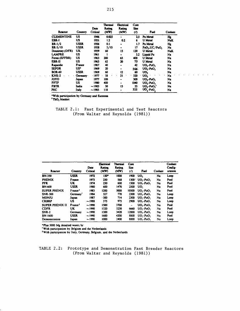
215

Reactor CountryDate

Critical

ThermalRating(MW)

ElectricalRating(MW)

CoreSize(/) Fuel Coolant

CLEMENTINE US 1946 0.025 - L5 Pu Metal HgEBR-I US 1951 11 0.2 6 U Metal NaKBR-l/2 USSR 1956 0.1 - 1.7 Pu Metal HgBR-5/10 USSR 1958 5/10 - 17 PuOj.UC/PuOi NaDounreay (DFR) UK 1959 60 15 120 U Metal NaKLAMPRE US 1961 1 - 31 Liquid Pu NaFermi (EFFBR) US 1963 200 65 400 U Metal NaEBR-II US 1963 62 20 73 U Metal NaRapsodie France 1967 40 - 42 UOj-PuOj NaSEFOR US‘ 1969 20 - 566 UOj-PuO, NaBOR-60 USSR 1969 60 12 60 uo, NaKNK-2 Germany 1977 58 21 320 uo, • Na ‘JOYO Japan 1977 100 - 300 UOj-PuOj NaFFTF US 1980 400 - 1040 UOj-PuOj NaFBTR India -1983 50 15 55 UOj-PuO/ NaPEC Italy -1985 118 - 325 UOj-PuO Na

‘ With participation by Germany and Euratom tThOJ blanket

TABLE 2.1: Fast Experimental and Test Reactors(From Waltar and Reynolds (1981))

Electrical Thermal Core CoolantDate Rating Rating Size Config­

Reactor Country Critical (MW) (MW) (/> Fuel Coolant urationBN-350 USSR 1972 150* 1000 1900 UO, Na LoopPHENDt France 1973 250 568 1300' UO,-PuO Na PoolPFR UK 1974 250 600 1500 u o L puo Na PoolBN-600 USSR 1980 600 1470 2500 uoj Na PoolSUPER PHENIX France1 1983 1200 3000 10500 UO.-PuO Na PoolSNR-300 Germany1 1984 327 770 2300 UO.-PuO Na LoopMONJU Japan 1987 300 714 2300 UO -PuO Na LoopCRBRP US -1988 375 975 2900 UO;-PuO Na LoopSUPER PHENIX II France* -1990 1500 3700 - UO.-PuO Na PoolCDFR UK -1990 1320 3230 6660 UO.-PuO Na PoolSNR-2 Germany -1990 1300 3420 12000 UO.-PuO Na LoopBN-1600 USSR -1990 1600 4200 8800 UO.-PuO Na PoolDemonstration Japan -1990 1000 2400 8000 UO.-PuO Na Loop

‘ Plus 5000 Mg desalted w ater/hrf With participation by Belgium and the Netherlands‘ With participation by Italy. Germany. Belgium, and the Netherlands

TABLE 2.2: Prototype and Demonstration Fast Breeder Reactors(From Waltar and Reynolds (1981))

216

Frequency(Hz)

Stainless Steel 6 (mm)

A l

S (mm)cu • • 6 (mm)

10 133.00 25.900 20.800100 42.00 8.200 6.560

1000 13.30 2.590 2.08010000 4.20 0.820 0.656

100000 1.33 0.259 0.2081000000 0.42 0.082 0.066

S k in d e p th , 6 1A 71 jj

TABLE 2.3: Skin depth variation with frequency

217FIELDS H. E EDDY CURRENTS

E - E,(Y)

J - J,fY)

H - H , (Y)

E “ E# (r, z)

J - l 9 (r.z)

H - (H „ O, HJ

H - H, (*, y)

E • (E „ E* O)

PROCEDURE FOR SOLUTION

ANALYTICAL SOLUTION (LECTURES ON ELECTRO­MAGNETICS)

ANALYTICAL SOLUTION: COMPUTER EVALUATION OF INTEGRAL EXPRESSIONS

(DODD. DEEDS I96S)

ANALYTICAL SOLUTION: (SPECIAL FUNCTIONS)

EDDY CURRENT DISTRIBUTION. PENETRATION DEPTH

EC- AND FIELD DISTRIBUTION

IMPEDANCE OF TEST COILS

EDDY CURRENT AND FIELD DISTRIBUTION

APPLICATIONS FOR ENGINEERING AND EVALUATION

OPTIMIZATION OF COILS AND FREQUENCIES:NO DEFECTS

"SMALL” SPHEROIDAL FLAW: EQUIVALENT DIPOLE REPRESENTATION

ANALYTICAL SOLUTION: (COMPATIBLE WITH DODD'S INTEGRAL SOLUTION)

(BURROWS 1964)

IMPEDANCE OF TEST COILS IN THE PRESENCE OF "SM ALL” DEFECTS

OPTIMIZATION OF TEST COILS AND FREQUENCIES INCLUDING SPECIAL DEFECTS

E - (E „ E „ E j

H • (H „ H „ HJ

J - (J» J^JJ

3-DIM, FE-SOLUTION (IDA 1962DEMERDASH. NEHL 1912)

EDDY CURRENT AND FIELD DISTRIBUTION:IMPEDANCE OF TEST COILS FOR ANY KIND OF DEFECTS

OPTIMIZATION OF TEST COILS AND FREQUENCIES INCLUDING ANY KIND OF DEFECTS

TABLE 2.4: Numerical Treatment of Eddy Current Test Problems; Plates(From Becker et al (1986))

FIELDS H . E EDDY CURRENTS J

PROCEDURE FOR SOLUTION

APPLICATIONS FOR TEST-SYSTEM DESIGN

MATERIAL PROPERTIES

SIMKINBIDDLECOMBE

WOLFFMULLER

DEMERDASHNEHL

PRESTONREECE

vErttE

E - (E „ E „ EJ

H - (H „ H „ HJ

I - (J „ J „ JJ

EDDY CURRENT AND FIELD DISTRIBUTION: IMPEDANCE OF TEST COILS FOR ANY KIND OF DEFECTS WHERE THE PERMEABILITY. RESISTIVITY AND SHAPE ARE KNOWN

3-DIM FEM RESTRICTED TO BRICK ELEMENTS

3-DIM FEM T-O-METHOD

OPTIMIZATION OF TEST COILS AND FREQUENCIES

LINEARISOTROPICNONHOMOGENEOUS

NONLINEARISOTROPICNONHOMOGENEOUS

NONLINEARISOTROPICNONHOMOGENEOUS

NONLINEARNONISOTROPICNONHOMOGENEOUS

LINEARISOTROPICNONHOMOGENEOUS

NONLINEARISOTROPICNONHOMOGENEOUS

LINEARNONISTROPICNONHOMOGENEOUS

UNEAR (NONLINEAR)ISOTROPICNONHOMOGENEOUS

NONUNEARISOTROPICNONHOMOGENEOUS

TABLE 2.5: Numerical Treatment of Three-dimensionalEddy Current Problems

(From Becker et al (1986))

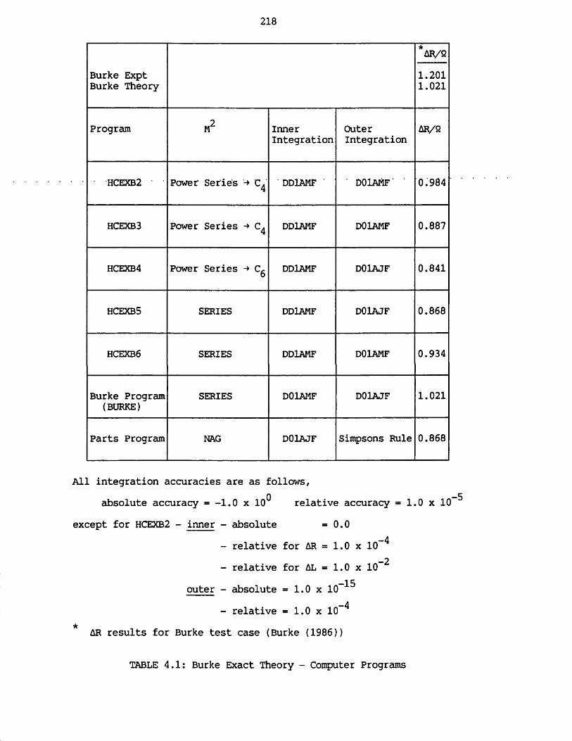
218

Burke Expt Burke Theory

*AR/S21.2011.021

Program M2 InnerIntegration

OuterIntegration

AR/S2

HCEXB2 Power Series ’ DDLAMF ‘ ‘ D01AMF‘ 0.984

HCEXB3 Power Series -> DDlAMF D01AMF 0.887

HCEXB4 Power Series -» Cg DDlAMF D01AJF 0.841

HCEXB5 SERIES DDlAMF D01AJF 0.868

HCEXB6 SERIES DDlAMF D01AMF 0.934

Burke Program (BURKE)

SERIES D01AMF D01AJF 1.021

Parts Program NAG D01AJF Simpsons Rule 0.868

All integration accuracies are as follows,0 -5absolute accuracy = -1.0 x 10 relative accuracy = 1.0 x 10

except for HCEXB2 - inner - absolute =0.0- relative for AR = 1.0 x 10~^- relative for AL = 1.0 x 10

-15outer - absolute = 1.0 x 10-4- relative = 1.0 x 10

AR results for Burke test case (Burke (1986))

TABLE 4.1: Burke Exact Theory - Computer Programs

219

a/c E° Z1

0.100 -3.1533 0.37690.200 -3.2309 0.71150.3375 -3.3402 1.10090.4750 -3.4336 1.40940.5000 -3.4473 1.45710.6125 -3.4949 1.64251.0 -3.5132 1.9978

TABLE 5.1: Shape Parameters for a Rectangular Flaw(From Auld et al (1986))

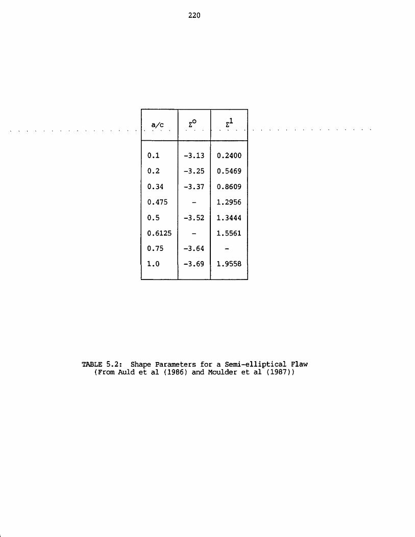
220

a/c Z° E1

0.1 -3.13 0.24000.2 -3.25 0.54690.34 -3.37 0.86090.475 - 1.29560.5 -3.52 1.34440.6125 - 1.55610.75 -3.64 -1.0 -3.69 1.9558

TABLE 5.2: Shape Parameters for a Semi-elliptical Flaw(From Auld et al (1986) and Moulder et al (1987))

221

RECESS+a

sc

Cylindrical > 2 1

Cylindrical « 1 1.2

Spherical Cap > 1 2

Spherical Cap = 1 4

+ a = depth of recess

TABLE 5.3: Calibration Shape Factors

222

MATERIAL a (S /m ) ^r

A i r .......................................

316 S ta in le s s S te e l 1.43 x 106 1.0

316 S ta in le s s S te e l 1.13 x 106 1.0

A lum inium 4" 3.77 x 107 1.0

Copper 5.88 x 107 1.0

M ild S te e l 6.67 x 106 -225

kL iq u id Sodium 7.4 x 106 1.0

+ A lum in ium a l lo y assumed to have th e same e le c tro m a g n e tic p r o p e r t ie s as a lum in ium

k Values at a temperature of 200°C (ie, fast reactor inspection temperature).

TABLE 6.1: Electromagnetic Parameters of Materials Considered

223

AR and AL

10 kHz Mild Steel 10 kHz Stainless Steel

100 kHz Stainless Steel

H V H V H V

LIFT-O FF

+31.6

+2.76 2

+49.3 jj H

+3.25 2

-18.5 jjH

+747.2 m2

-24.5 jjH

+913.5 m2

-31.75 jjH

+3.36 2

-40.6 jjH

+4.34 2

SLOT

+26.18 jj H

+0.30 2

+22.45 p H

+0.26 2

+2.98 p H

-76.6 m2

+2.38 jjH

-135.4 m2

+2.65 jjH

+0 • 48 2

+2.3 jjH

+0.46 2

H = H o r iz o n ta l

V = V e r t ic a l

TABLE 6.2: Horizontal v Vertical - Results for Comparison

224

Frequency/Hz

AR/S2 AL/ jj H

Theory Expt Theory Expt

100 0.00023 0.0 -0.2238 -0.2000

1000 0.00195 0.00240 -0.9800 -0.9500

5000 0.00424 0.00430 -1.1490 -1.1910

10000 0.00665 0.00625 -1.1930 -1.2060

50000 0.01663 0.01600 -1.2630 -1.2700

ErrorEstimates ±0.00001 ±0.0005* ±0.001 ±0.05+

* 10 x instrument error

+ 100 x instrument error

TABLE 8.1: 1.62 mm of Copper on Stainless Steel140 Turn Coil

225

Frequency/Hz

AR/S2 AL/ » H

Theory Expt Theory E xp t

100 0.00007 -0.00190 -0.182 -0.050

1000 0.00085 0.00025 -0.333 -0.250

5000 0.00829 0.01090 -0.514 -0.470

10000 0.01893 0.02150 -0.673 -0.675

50000 0.06977 0.07200 -0.985 -1.000

100000 0.11360 0.11600 -1.073 -1.100

E r ro rE s tim a te s ±0.00001 ±0.005* ±0.001 ±0.1+

* 100 x instrument error

+ 20 x instrument error

TABLE 8.2: 6.35 mm of Stainless Steel on Aluminium Alloy140 Turn Coil

226

Frequency/Hz

AR/S2 AL/ ,j H

Theory E xp t Theory Expt

1000 0.00114 -0.0014 -0.4763 -0.355

5000 0.01100 0.0108 -0.7176 -0.652

10000 0.02510 0.0250 -0.9274 -0.892

25000 0.05590 0.0590 -1.1953 -1.180

50000 0.09380 0.0980 -1.3452 -1.340

75000 0.1250 0.1300 -1.4185 -1.420

100000 0.1520 0.1480 -1.4645 -1.460

E rro rE s tim a tes ±0.00001 ±0.005* ±0.001 ±0.05+

★ 25 x instrument error

+ 50 x instrument error

TABLE 8.3: 6.35 mm of Stainless Steel on Aluminium Alloy182 Turn Coil

a ) Specimen 1227

Frequency Experiment Theory150 kHz 0.04538

0.18220.009500.1669

AR/S2 AL/ j j H

300 kHz 0.077010.1853

0.013180.1563

ARAL

450 kHz 0.086380.1966

0.016470.1563

ARAL

1 MHz 0.193360.2915

0.025300.1564

ARAL

b) Specimen 2

Frequency Experiment Theory150 kHz 0.03152

0.23060.017280.25304

AR/S2AL/*jH

300 kHz 0.068090.2223

0.023680.23633

ARAL

450 kHz 0.069930.2130

0.029440.23598

ARAL

1 MHz 0.099900.1819

0.044900.23563

ARAL

c) Specimen 3

Frequency Experiment Theory150 kHz 0.01755

0.07110.014040.03529

AR/S2 AL/ jj H

300 kHz 0.028610.0591

0.019310.02929

ARAL

450 kHz 0.038880.0532

0.024040.02757

ARAL

1 MHz 0.068270.0414

0.036730.02501

ARAL

TABLE 8.4: Two-dimensional Uniform Field Theory Results

228

E xperim ent Cut M a te r ia l C a l ib r a t io n D e fe c t

Deform ed M a te r ia l C a l ib r a t io n D e fe c t

AR/S2 8.106 12.283 26.401

AL/p H 0.9408 1.5661 2.5610

TABLE 8.5: Three-dimensional Uniform Field Theory Results

229

FIGURES

230

NON DESTRUCTIVE TESTINGULTRA SONIC WAVES

RADIOGRAPHY - GAMMAGRAPHYVISUAL EXAMINATION

DYE PENETRANT - MAGNETOSCOPYEDDY CURRENTSOTHER TESTS

DISCONTINUITIESLOCATIONSHAPESSIZE

ORIENTATIONDISTRIBUTION

NATURE

METALLURGY MECHANICSMETALLURGICAL STATE FRACTURE MECHANICSFATIGUE STRESS

TEMPERATURESIMILAR THEORYRADIATION FIELD

DURATION

DETRIMENTAL EFFECTS

SHUT-DOWN YES

REPAIRS ^ OPERATION

FIGURE 1.1: Basic Flow Diagram for a Periodic Inspection(From Saglio and Prot (1976))

231

IHX = intermediate heat exchanger

KEY:

~ — PRIMARY SYSTEM

W lll/IM SECONDARY SYSTEM

. °.C i- PUMP ~

OPo a&>XO<h

.': op-1'

(a) Pool-type

•<a0 %T OV,

- / * -

TyO liiiin il/vO a*s?

(b) Loop-type

FIGURE 1.2: Liquid Metal Cooled Fast Breeder Reactor (LMFBR)(From Waltar and Reynolds (1981))

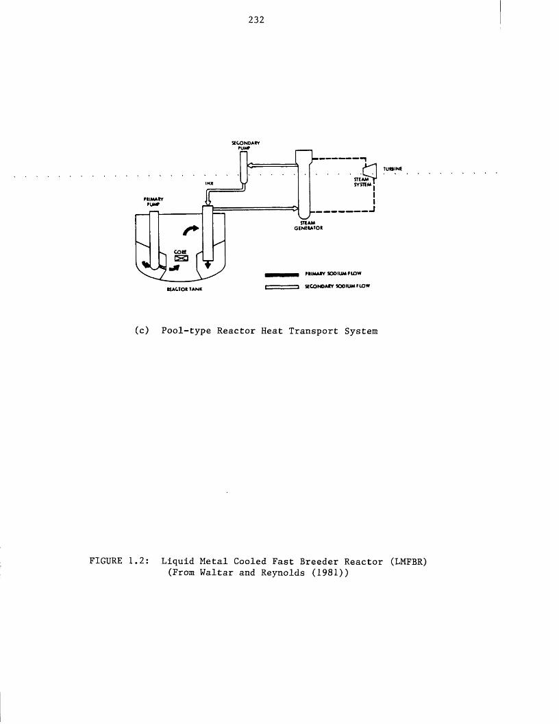
232

SECONDARY

“ISTEAMSYSTEM

STEAMGENEtATOK

COtESIPRIMARY SODIUM FLOW

SECONDAtY SOOIUM FLOWREACTOR t a n k

(c) Pool-type Reactor Heat Transport System

FIGURE 1.2: Liquid Metal Cooled Fast Breeder Reactor (LMFBR)(From Waltar and Reynolds (1981))

Horizontal Axis

Coil

Vertical Axis

Coil

2334-1Gcu63

a) S-i J2 4-1 4-» COGO *H

<4-1

•H

4-1

CO

M

cd (U •H CJ *4 Cd (U M-l 4-1 Mcd G

234rH•HoO cO /—\

M0 0 CO O£ cO 4-)

•H a4-1 X J cu•H CU 4-1a CO CUX) £ X

w s- ^

a•H4->(U£00cOSf*.u'CO '

X I£ x)O rHu <u0 ) *H

CO Fn

00£CO£ x l M rHa; cu4J -H th fh<a aF*. -H M 4-1 CO CU 6 £

■H 0 0 V-i cO PH S

i-H i-H•H COO 4-1

C J CO •H<

CUSoo co

fl CO CU•H u4-1 x J M•H CU £a co OX £ CO

w

X4-1COa,

X )cuCOo

>■» i-H X J O ■"O v—W

COX J 4-1CU £a <u£ P4

X ) £ £ £ M U FIGURE

2.1:

The

Eddy

Current

Prin

cipl

e

Surface

of Metal

Edly

Current

Density

Phase

Lag

235

cu Xacd X4 -i 4-»U CX3 (UCO Td

4J +Jcd cd

—

a 4-1<U *H M CO•X3 U C-d 3 0)

W CJ Q

FIGURE

2.2:

Skin

Depth

Effe

cts

236

InductiveReactance,

variation in a metal condition

Resistance

FIGURE 2.3: Typical Impedance Plane Diagram

237

4-1

4 J

4-1

+JOJ /—N

a.

FIGURE

2.4: Edd

y Current

Syst

em

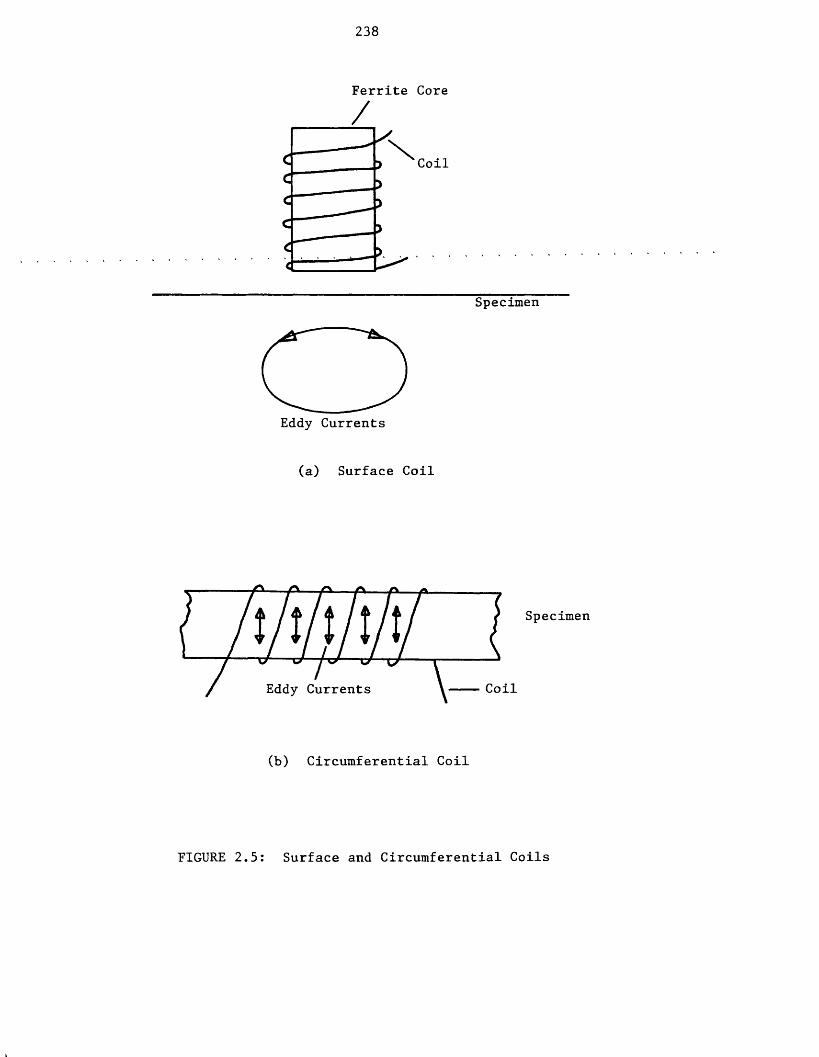
Ferrite Core/Coil

Specimen

Eddy Currents

(a) Surface Coil

CoilEddy Currents

(b) Circumferential Coil

FIGURE 2.5: Surface and Circumferential Coils

• "J

•

239

<uae03

<u<uos

<Dos

l-l

CJ

u

u

o

CM

M

240

To Impedance Analyser

HorizontalCoil

Toroidal Ferrite Co.re. .

MaterialMagnetic Field Lines

SIDE VIEW

Foot of the Core

Eddy Current Flow Lines

\Magnetic Field Lines

PLAN VIEW

FIGURE 2.7: Uniform Field Eddy Current Probe(From Smith (1985))

241

Source Receiver

Electric Field Lines

FIGURE 2.8: Basic Capacitive Probe(From Gimple and Auld (1987))

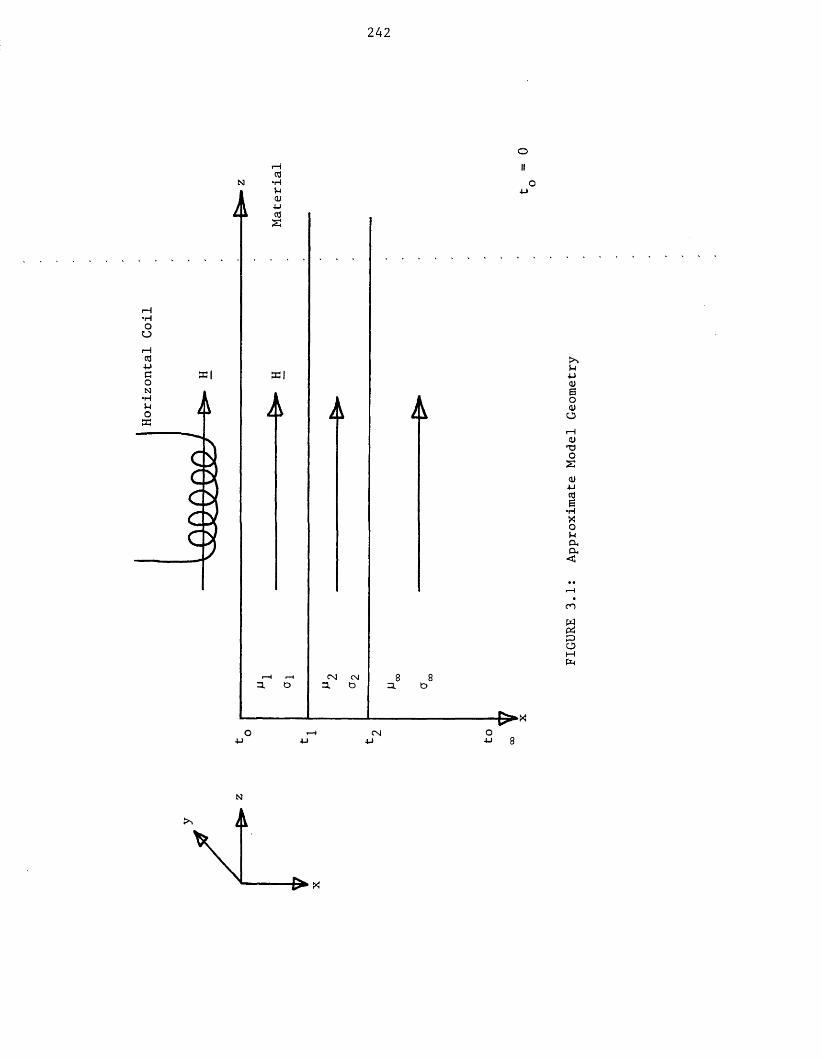
Horizontal

Coil

242

4-1

o4J

O CM84-1 4J

N

243

CA•H

3•HOU

4-1

4->

o

o

o

FIGURE

3.2:

Surface

H Field

Dete

rmin

atio

n

244

SIDE END

U 21 r j 2a^ ------ &

Coil

MagneticFieldMaterial

Approximately Uniform Field Region(for AR and AL evaluation)

FIGURE 3.3: Region of AR and AL Evaluation

245

Start

End

Determine Surface H

Determine Coefficients .‘.H Field

OutputResults

InputData

Calculate AR and AL

Calculate Skin Depth For System

FIGURE 3.4: Flowchart for Approximate Model Program

246

aju

i-H cdcd 14-1•M n0) P

s CO X Ii—l

X a)X •HI Pm

P*.o JmCO cd

S3 X Ie

II oo

CO 0)S3 CO

X Xi—1

1 <Da)

o

•Hpin

cxS3

cdII e

■HCL,

S3 Pm

FIGURE

3.5:

Primary

and

Secondary

Fiel

ds

247

aeajQJos4-1

cr

o

<4-1

O•H4->CD•H0)4-1OcducdJSC_J>>aca)3cra)Mp£4u0)>oCOCOouvO

wpcitooMU-i

248

4-1

4-44->

4-1

<4-4

4-1OON

•H

OSS

Awpen&Ol-lpt4

249

hs

Coil

1hs or 36(whichever is greater)

EddyCurrents

FIGURE 3.8: Eddy Current Deflection at an Edge

H 1hs 1$ " ihs + (1hs _ 36)

FIGURE 3.9: Edge Extension to Approximate Model

250

i-Coil

MaterialV

Eddy Currents

ActiveRegion

6 1 6 2

AZ^ AZ2

Propose AZ = AZ- + AZ2

FIGURE 3.10: Horizontal Coil Above a Two Conductor Region

X 251

1.00

\ Exact0.99

100 Hz

0.98

. / \ .* PerturbationExpansion

0.97

//

Burke500 kHz/ - -/0.96

Clark

0.950.005 0.010 0.015 AR

X„

FIGURE 4.1: Burke Exact Theory Test Case

Horizontal Ax

is

Eddv

Current

Co

252

<uucd

<+-iS-iDCOcd•HU■ucda

a)ocda,C/D

i+ -irH <u cd cj Cd cd■—. l+Hn na), cu. >> u cd Ci-J i—i

4-4 pq

4-1

o

w

o

m cq

•HBcoCcd

H

•Hscotd CMcd <3 s-i H

B<U4-1CO

COrrda)Mcucd

1-3

CM

WcdCuoM

253

incidentB.

y = 0 material surface

1 LayerT B,

y - -t

2 Layert B,

y = -ti

3 Half space

FIGURE 4.3: Two layer and a half space system

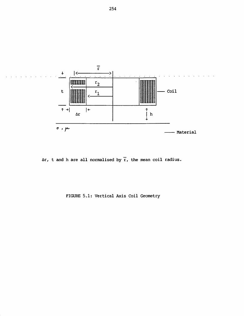
254

r

Coil

<y , Material

Ar, t and h are all normalised by r, the mean coil radius.

FIGURE 5.1: Vertical Axis Coil Geometry

255

Au

T 2 f(h1) a Ap AuA Z " = T P - 2 ( l t i,7 - ' ! 6 + i- p - - ( , + j ) — '© © (k> ®

(7) WALL EFFECT - SURFACE IMPEDANCE(2a), (2b) KANN EFFECT - R A NGE « 8

(?) FARADAY EFFECT - CRACK OPENING INDUCTANCE- A f s OPENING AREA

(4) UNPERTURBED SURFACE IMPEDANCEJ = eddy current density

FIGURE 5.2: Auld Theory - Two-dimensional Crack in aUniform Field (large a/6)(From Auld et al (1982))

256

Lift-off

AirMetal

EdgeSlot

FIGURE 6.1(a): Scan Over a Mild Steel Block(1 MHz, 20 dB)

0.5 mm

3 mm

FIGURE 6.1(b): Mild Steel Block containing Six Slots(1 MHz, 22.5 dB)

257

Brass316 \Stainless Steel

A1

Mild Steel (two base metal traces, one weld)

Weld.

FIGURE 6.2: Lift-off Loci (1 MHz, 22.5 dB)

Weld

Lift-offSlot

Air

FIGURE 6.3: Predicted Austenitic Weld Trace

258

Weld HAZ BaseHAZBase

Air — HAZ— Base Metal

Weld

FIGURE 6.4: Mild Steel Weld Specimen - Lift-off Loci(1 MHz)

259

Defects

AirLift-off

FIGURE 6.5(a): Slots in Aluminium - 50 kHz(14 dB)

3 mm

0.5 mmLift-offAir

FIGURE 6.5(b): Slots in Aluminium - 10 kHz(40 dB)

260

6 mmLift-off II----- 3.5 mm

Air -j----------- ---/

/316 Stainless Steel__ Lift-off

FIGURE 6.6: Slots in Stainless Steel(10 kHz, 40 dB)

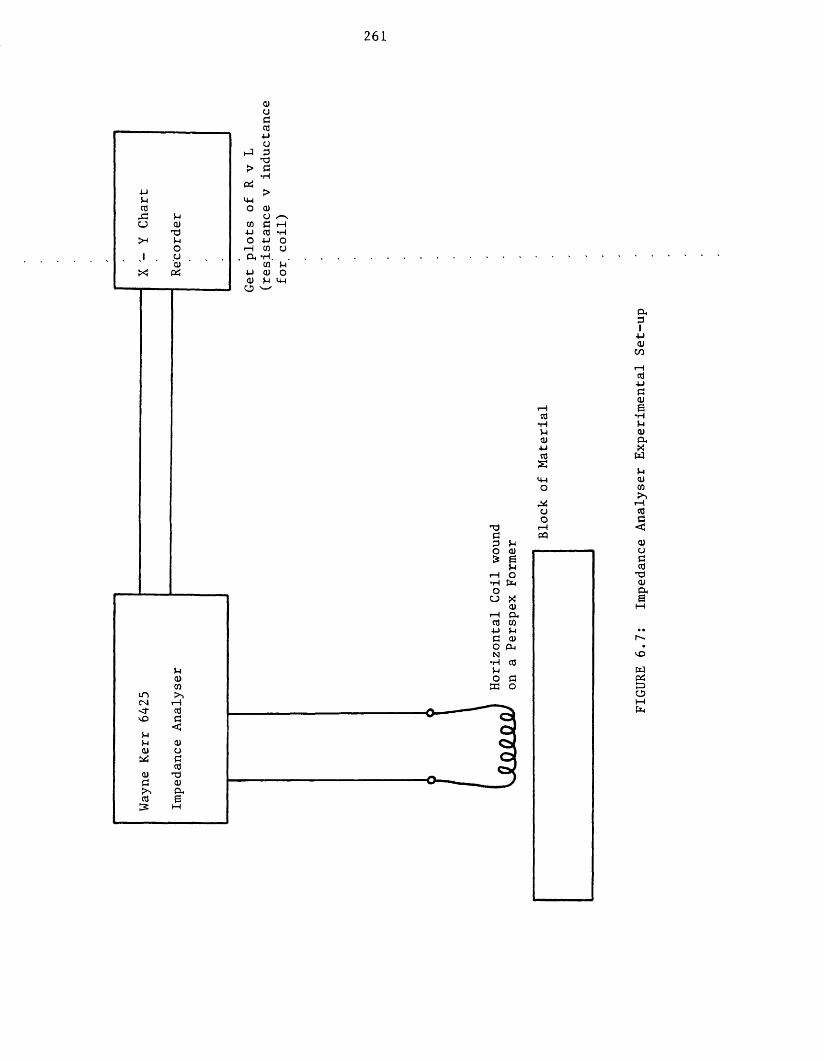
261

o

■■d4-1

o

■M4-1

LP|CNl

M

FIGURE

6.7:

Impedance

Analyser

Experimental

Set-

up

-0.05 ____________ __________________________* 1 0 0 * 1 0 0 0 l o o o o l o o o o oFrequency/Hz (log scale)

(a) AR v Frequency

AL/jjH

-0.4

- 0.8

-l.CL

- 1.2-

-1.4 l o o oFrequency/Hz (log scale)

l o o o o 10000000

(b) AL v Frequency

FIGURE 6.8: 140 Turn Coil above 316 Stainless Steel

263AR/ft

0.06 —

0.04__

0.02__

20Lift-off/mm

(c) AR v Lift-off (100 kHz)

AL x (—1) /iJH

0.4--

0.2__

20Lift-off/mm

(d) AL v Lift-off (100 kHz)FIGURE 6.8: 140 Turn Coil above 316 Stainless Steel

AR / Q

0.15

0.10

264(a) AR v Frequency

X Stainless Steel

O Stainless Steel on Aluminium Alloy

//A'

0.05 ✓

1 0 0 1000 10000

Frequency/Hz (log scale)

100000

-0.4

- 0.8

- 1.2

100

Frequency/Hz (log scale),1000 ,10000

AL/jjH

"Ho\

\

100000

(b) AL v Frequency

FIGURE 6.9: 140 Turn Coil above 6.35 mm of 316 Stainless Steelon Aluminium Alloy

i

265R/fi

2.13 MaterialN

2.10--

2.05 —

Air

2.0- 1

Position (in coil diameters from the position at 0) (a) R v Coil Position

L/jjH (b) L v Coil PositionAir

46.5

46.0__

Material

45.5- 1

Position (in coil diameters from the position at 0)FIGURE 6.10: 140 Turn Coil above 316 Stainless Steel Edge (100 kHz)

- Coil Length Parallel to Edge

266R/ft

2.13- Material

2.05___

Air

Position (in coil diameters from the position at 0)(c) R v Coil Position

L/jjH

46.5-

46.0-

45.5-

(d) L v Coil Position

i X -

Air

Material

-1 '0 »1 «2 '3Position (in coil diameters from the position at 0)

FIGURE 6.10: 140 Turn Coil above 316 Stainless Steel Edge (100 kHz)- Coil Length Perpendicular to Edge

Iii

(a) Mild Steel

Signals from Slots'

STOREERASEALARMjl LEVELSTD I1 , LR STO !

ii PROS--1-J !p call m 1 IJ SAVE Ii CLEAR I

(b) Aluminium

3.5 mm deep

6 mm deep

id* / I 1!xX\\(\\i J

i

STOREERASE FULLALARMLEVEL

-PROGCALL mCLEAR

(c) Stainless Steel

FIGURE 6.11: Horizontal Axis Coil used for Slot Detection

268

H

Coil

EddyCurrents

FIGURE 6.12: Eddy Currents Induced by a Horizontal AxisCoil in a Conducting Material

(From Bowler (1988))

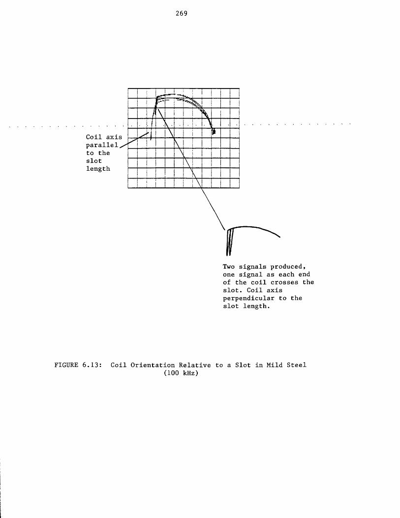
269

FIGURE

I

Coil axis parallel^ to the slot length

Two signals produced, one signal as each end of the coil crosses the slot. Coil axis perpendicular to the slot length.

6.13: Coil Orientation Relative to a Slot in Mild Steel(100 kHz)

270

a r/n

0.5mm*ep

.5

0.45

x\A

0 . 4 __

X / \

/ \I '

AL/jjH

.5 1

AI \I \

/

A0 . 4 __

I \

\ I

0.35__

\ I x1 I\ I\ / X

I f1 /X

0.3

/X

1 A

1 1) I X

0.5A

19 mm

\ /\ / X

Slots

Position

Position

FIGURE 6.14(a): R and L v Position (250 Turn Horizontal Axis Coil)- Mild Steel Specimen containing Six Slots (20 kHz)

271AR/ft

mm*ep

2.5 L.5 1

0.018

/»

0-.016:

0.014 L9 mm >

0.90»c/»

XM

x / I

X/ V / \

0.85.

0.80-

\!

0,5

/ \

Slots

Position

Position

FIGURE 6.14(b): R and L v Position (250 Turn Horizontal Axis Coil)- Aluminium Specimen containing Six Slots (20 kHz)

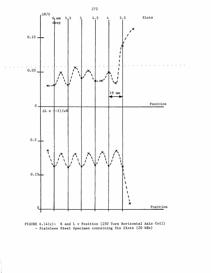
272AR/n

6 mm deep

0.10

0.05

x-

A / \ / V

AL x - D / p H

0.5

A

0.2'

A / \

4.5 3.5 Slots

A / \

A A

vx/

19 mm ►

A\

Position

\X

Position

FIGURE 6.14(c): R and L v Position (250 Turn Horizontal Axis Coil)- Stainless Steel Specimen containing Six Slots (20 kHz)

273

,AR x (-1)/^6dt

mmeP

0.005

/X

\ / \ /

19 mm

Slots

0.0025-

AL x

0.2 —

0.15__

V /V'

Position- D / jjH

x/\/ \

X / \/ \/ \I \

A / \ A

/ \

VV/

0.1 Position

FIGURE 6.14(d): R and L v Position (250 Turn Horizontal Axis Coil)- Stainless Steel Specimen containing Six Slots (5 kHz)

274

•— defect

lift-off

defect

lift-off

ferromagnetic

non­ferromagnetic

FIGURE 6.15: Ferromagnetic and Non-ferromagnetic Materialsillustrated on the impedance plane

1.999--

1.998—

Material1.997- —

1.996__

1.995--

1.994—

1.993.!0 30 40Angular Position/degrees

60 70 80 9050

(a) R v Angular Position (140 Turn Air-cored Coil)

L/jjH

47.2--

47.1__

Material

47.020 30 40Angular Position/degrees

50 80 90

(b) L v Angular Position (140 Turn Air-cored Coil)

FIGURE 6.16: Horizontal Coil above a 10 mm Deep Slot in Mild Steel- Variation of Angular Position

276

R/fi

3.2— Material

3.1 —

3.0—

8020 30 40 50Angular Position/degrees

60

(c) R v Angular Position (72 Turn Ferrite-cored Coil)L/pH

195

190

185

180

Material170

165 10 20 ' 30 40 '50 'Angular Position/degrees

(d) L v Angular Position (72 Turn Ferrite-cored Coil)

FIGURE 6.16: Horizontal Coil above a 10mm Deep Slot in Mild Steel- Variation of Angular Position

277AR/fi

O0 . 0 6 + I

I

0.04*

O

\x . \'>A\l

0.02--

\ VI---------- - a ------------*10 *20 *30

Lift-off/mm

-=SL

(a) AR v Lift-off (100 kHz)

X — — x Horizontal AL x (-1) /jjH O ---- O Vertical

0.6 - -

0.4---

0.2 - —

20Lift-off/mm

(b) AL v Lift-off (100 kHz)

FIGURE 6.17: Horizontal Coil v Vertical Coil

278

Slot

KHZ

* STORE STO pERASE FULL iALARM OFF | LEVEL .61 Y ■ X 1 ' 1 f HP STD LP STDVertical

AirCALLSAYECLEARHorizontal

Lift-off

(a) 10 mm Deep Slot in Mild Steel

Vertical

Horizontal

\ H -l—V

?

. <:v.L

i— - F D 0 jflF—— iIKHZ 1 0 0 II

OB 4 0 . 0 I S 1 3 3 . 0 I

STORE STD E R A S E FULL! ALARM OFF LEVEL 61 Y'X 1'1 HP STO LP STO STO PROG 1ICALL ISAVE ICLEAR I

(b) Six Slots in a Mild Steel Block

FIGURE 6.18: Comparison of Horizontal and Vertical Coil Orientations

i

279

i-- F DB S-- 1

1I “ ( U B 13-0 1 k £ 131.311 i— -— A U X — — --ip 11 “ I STORE STO 1 p ERASE FULL 1 Jl Al APR OFF 1\ 1 1 LEVEL 50 1 | Y ' H _ P I I

LP STO 1jl I/P^d LOU 1jp- - - PROG-- -i

/ /-- 1 1CALL 1 S SAVE 1LLkrtK 1

Vertical Horizontal

FIGURE 6.19: Horizontal and Vertical Orientations- 3 mm Deep Slit in Stainless Steel

316

Stainless

Stee

l

280

om o.m

o

o

o

1 +JO 4-1Pi i— 1 o•H CO 1—1CO p. CO

PI <U a,O 0) CU*H T3 CUCO ndPI<U

uim ee &•H oi-H mi— 1 ii ll>—1

3 _mT

sT" Vm

<eu

wo

FIGURE

6.20(a):

Stainless

Steel

Weld

Spec

imen

281

Ic•HCOeo•HCOc(U&•HXt

1oCMT

omCM

1

4->

4-150 C

r—I4-1 50 rH

•HC cu m CU si CU 4-1 CO

LO4-1 tJ m tj mCM

CM

I—I

CM

UOCM

oCM

FIGURE

6.20(b):

Stainless

Steel

Weld

Specimen

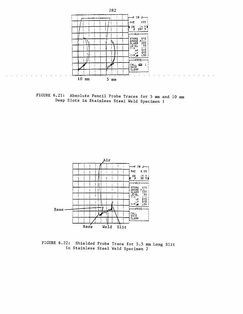
282

FIGURE

, F 09 §-- 1

-*n-hwj I— i—t-4

500 !14.51 357.5 I

jl KHZ |lfc OB*h AUK -!l i-9 STORE STO I'j ERASE FULL !J ALARJ1 OFF Ip LEVEL 50 !I Y • X 1 ' 1 i4 HP STD I!l l F STO iI-'PJl LOU I

-PROGCALLSAVECLEAR

10 mm 5 mm

6.21: Absolute Pencil Probe Traces for 5 mm and 10 mm Deep Slots in Stainless Steel Weld Specimen 1

Air

Base

H STORE STD j! ERASE FULu j ALARM OFF jl LEVEL 50 J Y ■ K I : 1 f HP STO jl L ? STO J 1'?^ LOU

|l CALL j| SAVE 1 CLEAR

Base Weld Slit

FIGURE 6.22: Shielded Probe Trace for 5.5 mm Long Slit in Stainless Steel Weld Specimen 2

283

jr— “-flU 1*1 ™ — “i| i1 STORE STD I;! ERASE FUL. ;j SLftRH OFF ii! LEVEL 00 !

Slit Signal

(a) Shielded Probe

a F 08 SF—■jlU PIHZ 3.00 It OB IE .0

1 STORE STi il ERASE FULi $ ALARM OF jl LEVELSlit ^

Signal HPLP

j! CLEAR

(b) Absolute Probe

FIGURE 6.23: 5.5 mm Long Calibration Slit in Stainless Steel

284

ji huxil ERASE FULL ! 4 ii L P R F '|i LEVEL jl V 1 X 1 HP STD LP STD

Defect '—rSignal \

(a) Shielded Probe

! i

I MHZI"if OB

[I g ;JT-3.0011.51 31 .5 I

! ■: i 1 _S._ i-- ! - - - !l--- -- - _iJ , —r** i-— ! !

_ - — T -3 1 U P. i 3 IU 1i II ERfiSE FULL 1 ! !| A! mPW ncf 1

! ! I ! ! 11 LEVEL 50 1 1 V 'X I'll

f | [ M i l ! 1 L? STD i I / P J LOU 1- - - FROO- - - *i ji CALL B 1 ! SftVE 1 ^j-LERR !

i | i j

i ;* ii ! I ! !i ! ! 1 j i ! !i ! { j

_ J J i 1 ■ I l l

(b) Absolute Probe

FIGURE 6.24: Weld Impurity Defect 1

285

ii— f o g

1 MHS

It STORE STDp ERftSE FULL i41 ftLfiRR OFF I|l LEVEL 50 |

Ii FROG!l CftLL I! SAVE l! OLEfiR

DefectSignal

(a) Shielded Probe

tl PIHZ 3.00 itIt OB ii.;

DefectSignal

VEL

(b) Absolute Probe

FIGURE 6.25: Weld Impurity Defect 2

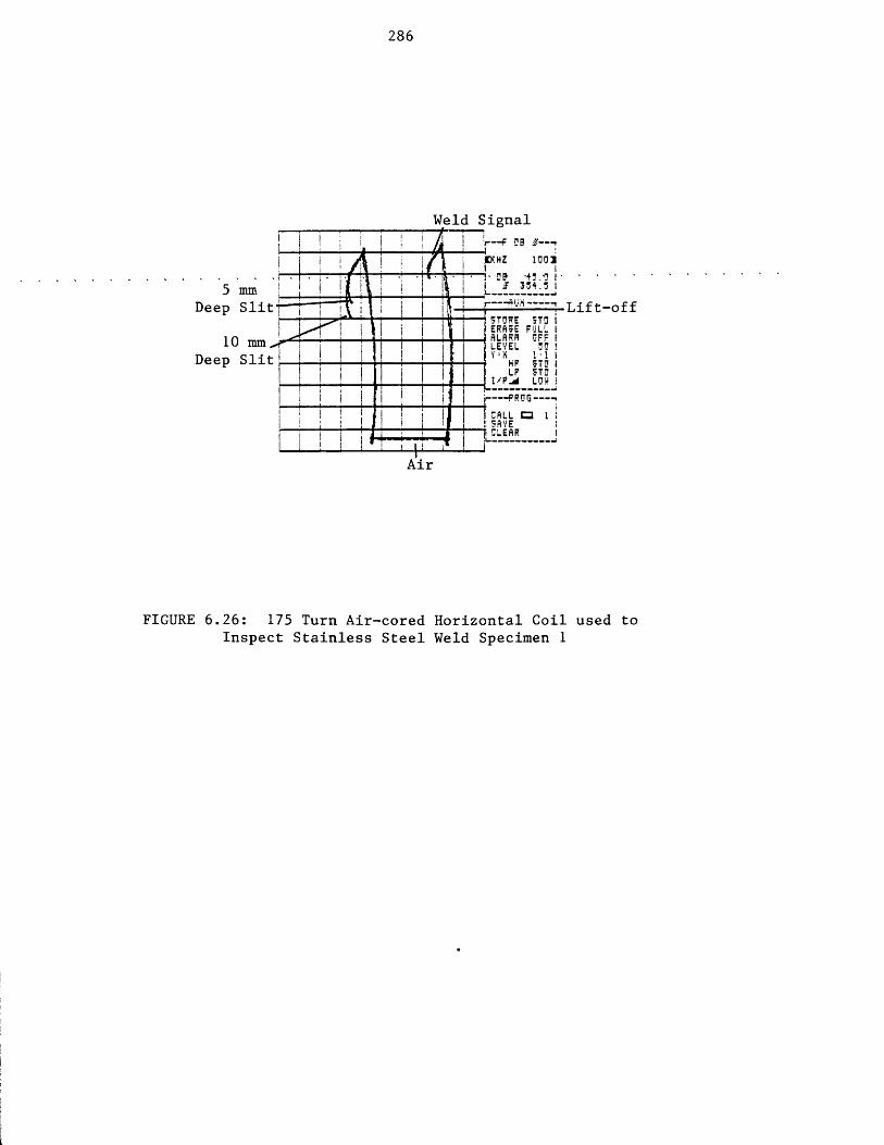
286

Weld Signalk , r " 58 *f \ I I X H Z

5 mm Deep Slit Lift-off

I 5T0RE 5T0 Iil ERASE FULL Iil ALARA OFF Iii LEVEL 00 !10 mm „ Deep Slit HF STO LP STO

SAVECLEAR

Air

FIGURE 6.26: 175 Turn Air-cored Horizontal Coil used toInspect Stainless Steel Weld Specimen 1

287Two Signals

i! KHZWeld [Signal ;

1 STORE STOil ERRSE F'JLl1 hLhRU OFFii LEVEL 00' X 1: 1 ■H HP STO

il SftVE Il OLEnR

(a) Coil Axis Perpendicular to Slot Length

H KHZ 30.0

0° Axis f Parallel* LEVEL

30° 90° AxisPerpendicular

(b) Coil Axis at Various Orientations to Slot Length

FIGURE 6.27: Horizontal Coil Orientation Relative to a 10 mmDeep Slot in a Stainless Steel Weld

288

— FKHZ

t D8

STORE STO ERASE FULL ALARM OFF LEVEL 30Slot _ Signal

LP STDLOW PROS--CALLSAVECLEAR

FIGURE 6.28: Ferrite-cored Horizontal Coil - Scan over 5 mm DeepSlot in Stainless Steel Weld Specimen 1

KXHZ

3 138.0 AUK- - -STORE STD ERASE FULL ALARM OFF LEVEL 30

HP STD

PROGCALLSAVECLEAR

Defect 1 Defect 2

FIGURE 6.29: Ferrite-cored Horizontal Coil - Scan Over WeldImpurity Defects in Stainless Steel Weld Specimen 2

289

Ii F DB S 1KHZ 500-OB 17.0 I ■S 138.0 I

ftUH .STORE STO ERASE FULL ftLARH OFF LEVEL

I'P.

S' 11 HP STO I LP STD I LOU I PROG 1

5.5 mm Long

3.5 mm Long

FIGURE 6.30: Ferrite-cored Horizontal Coil - Scan OverSlits in Weld of Stainless Steel Weld Specimen 2

290

ThickSection

Thin Section

WELD

Position/mm

(a) R v Probe Position

(b) L v Probe Position

L/jjH

13.4---

13.2

13.0

12.8

20Position/mm

FIGURE 6.31: Stainless Steel Weld Specimen 2 - Weld Scan usingFerrite-cored Horizontal Coil (300 kHz)

291

DefectThickSection

Thin Section ^

WELD

15Position/mm

(a) R v Probe Position

(b) L v Probe PositionL / jjH Defect

13.4

13.2

13.0

12.8

Position/mm

FIGURE 6.32: Stainless Steel Weld Specimen 2 - WeldImpurity Defect 1 (300 kHz)

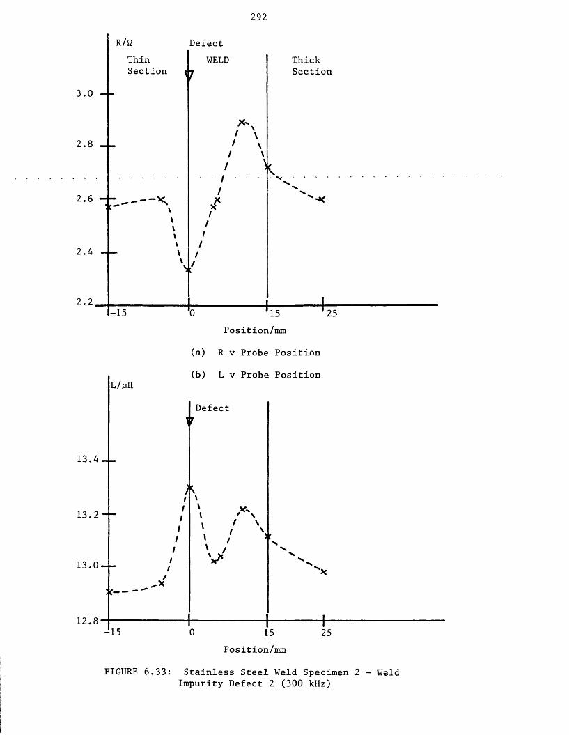
292

ThickSection

Thin Section

WELD

-15 15Position/mm

(a) R v Probe Position

(b) L v Probe PositionL / jjH

Defect

13.4

13.2

x.13.0

12.8-15

Position/mm

FIGURE 6.33: Stainless Steel Weld Specimen 2 - WeldImpurity Defect 2 (300 kHz)

293WELD

ThickSection

Thin Section

O Value on Weld Material (no Slit)

13.6

13.4

13.2

13.0

12.8

L / jjH

15Position/mm

(a) R v Probe Position

(b) L v Probe Position

Imt

' --

O Value on Weld Material (no slit)

-15 15Position/mm

25

FIGURE 6.34: Stainless Steel Weld Specimen 2 - 5 . 5 mm Long Slit(300 kHz)

R/nThinSection

3.0

2.8

2.6,-------

I

294 WELD

Slit

o AA / \\ / >V

ThickSection

Value on .Weld Material (no slit)

2.4

2.2-15

L / jjH

13.6 - L

13.4

(c)(d)

15 25Position/mm

R v Probe Position L v Probe Position

SlitJ\f O I

13.2

Sc13.0

3C-~

12. 8.-15

O Value onWeld Material (no slit)

15Position/nun

25

FIGURE 6.34: Stainless Steel Weld Specimen 2 - 3 . 5 mm Long Slit(300 kHz)

2951 ,Ii-- F 00 £— -t•41 16 KHZ 300 i

1Ik. u b s u .u s» 3 M S . 3 1 '- - - - - - - - - j\

I

Jr— AUK n"n STORE STD 1 1 ERASE FULL 1 i fli flnn npp i

\Il LEVEL 30 1 JY'K 1 'S 11 LP STO 1jl M P ^ LOW 1P -- PROG- - - .fCALL 1 ( SAVE 1-- S CLEHH 1

(a) Base Slit

i F D0 3-- ,I II KHZ 300 I I IX 00 so.OS

I -ft UK--I STORE STOI ERASE FULLIALARH OFF I LEVEL 30i y k i'sI HP STOI LP STO

PROOI CALL I SAVE I CLEAR

Weld Trace Scan OverSlit

(b) Slit on the Fusion Line

i F 00 3-1|KHZ 300 I K 00 SO.OS

i AUK ,I STORE STO IERASE FULL IIALARR OFF ILEVEL 30 I

LP STO

PROGI CALL I SAVE I CLEAR

On WeldOn Base

(c) Slits near the Fusion Line

FIGURE 6.35: Ferrite-cored Horizontal Coil - Scan Overi Fusion Line Slits in Stainless Steel Weld Specimen 1|

296

297

Pi ,C< 1 O

< 1

cd<U

P h

<4-1O

oCN|

a)co•HOC030

•He

•H0 *o<uco

•HOJScd0(UrCEH

oXC•HIS0o0

•HXcdS

CSeo

s

's

CSJ

■M O i—I

Ph

SoT3C

•H5

csj

WPionPm

•HO

O

Cup

Eh

OO-

-U> OC -H 0)E ?Q) r—iU 3COcd <u

a;XIoS

a14-'cd0*H!*CUP .P ,< 1

m

o

298

4-1

u

<<

4-1

>

FIGURE

7.3:

Measurement

Window

Plot

- AR

(Burke Model, 10

kHz, 140

Turn

Coil)

299

<u00

<

■u

M-lM-l ■MO

CJ■M4-*

o4-1

4-1e m 0)6 o a> oV4 —I

4-1

o

e -h■H 0 0 W

I—I

mo

o 00 o CN

(-

i)A

jH

300

4-1

4-t4-1

OICN

4-1

<4-4<4-1

4-1

CM

O

'— I /

CO

un co o

<o4-1

>

<

oiHeuSoT3S4->a<u0a)u3COcfl(US

rO_✓Mfr--WpH£3oMP=4

oo

oo

oo

oo

oo

oo

oo oI

(Burke Model,

100

kHz,

140

Turn

Coil)

AR/mfi301

100

Approximate Model50 -

Burke Model<ftfe-0-0— o-o---<j *t-Q --------- O___I________0 O.'l 0*. 2 0/3

Coil Length/m

(a) 1 kHz

AR/mQ

200

/100

Approximate Model

Burke Model

O.'l O'. 2Coil Length/m(b) 10 kHz

0.3

FIGURE 7.5: AR v Coil Length

302

400

300 - “

AR/mfi

600

500- f ✓x///////

s

200 "f

xApproximate Model

✓'ft

o O ' O100-fo K'o 0✓® ° Burke Model^ — I----------- 4______________I________Oil 0 7 2 0 1 3

Coil Length/m

(c) 100 kHz

FIGURE 7.5: AR v Coil Length

303

AL x

5 --

2 —

<o

Q_______0

Approximate / Model

sX/////

✓X/

x ' ' .✓x o

fc' ° ° ° Burke Modelot r 0.2 0.3

Coil Length/m

FIGURE 7.6: AL v Coil Length (10 kHz)

304

4-154a)4-1a)gcd

•HQ

4-1

OCM O O

0 +

5-4a)4-1QJgcd•HQ

5-ia)4-1a)§

•HQ

r-KMCM

>-i014J0)Scd

•HQ

X4-160Cai

•HOO

LOo

OX OX * >

CM00NEC

OO

< *

10

xo ox

o JO o^ CM

o( ox oCM

O

coO

6 0C01

.-4

•HOCJ

PCh<

» ox 0(

COd

O 5-i _ . ° dOt r—H £—4

coo

CMO

cd '— r^ .

r »

WOeJC3o

c?Pd< 3

54014-1aiScd

•HQ

Ncoadd

H

00O

vjoo

vj-o

CM

o

Burke

Theory

/Exp

erim

ent

Comparison

for Different

Coil

Diam

eter

s

Burk

eTh

eory

305

•H

Omo o

X a 0 +

o

ox

oo

ox

COos oyo

CNOO

OO

Oo

o

o

oo COi—H

ON C J 33M 4Jco ai0 M1 4 QJW M_l

4-1 X *H +-> Q00c ^ cu o

4-1

cocn•HM10a.SooGx <u^ sr~- *rH • V-i r— <u CX W X pci W t=>O So Uo <u xH aju 3 PQ

Pn

80

60

40

20

0

80

60

40

20

0

AR/mft

AR/mft

306(a) 140 Turn Coil 10 kHz

/ypBurke Model

//

/ ^/

* Approximate Model

/s

01.005 0.01 0‘. 015 0:02Coil Diameter/m

(b) 200 Turn Coil 10 kHz

///^ Approximate Model

- 7s ' '

s ^ Burke Model

« * ' /'/

//

//Oyy

J! 005 olol ob015 0102Coil Diameter/m

FIGURE 7.8: AR v Coil Diameter

307

AL x

6 --

2 --

0

(c) 140 Turn Coil 10 kHz

O///s'S

s' ^

//

//

//

//

/ Burke Model

83'““” Approximate Model 1—

0.005 O.'Ol 01.015Coil Diameter/m

/O

-x —

0.02

FIGURE 7.8: AL v Coil Diameter

308

10 mm diameter diameter > 10 mm

5 mm

FIGURE 7.9: Approximate Model- Coil diameter effect on H field determination

309

u<u4Ja)6cd

•HQ

CO Epi g M0 o

Eh cm

Icsj00

~3-

oCsj

ono

a,p2"<

o o

4-1

4J o o O -H

P ia>4-Ja)

§•H01m

SXI4-100a<u

6 <u cd g•HQ

i—io lCSI o

+ xX

oO S

no

sto

cno

COCPiS '

H

O.O

P i<U4-1<Ugcd

•HQ

00O

vOO

sfO

csjO

CSIO

O

O

< S

P i<D>o

PIcdaco

I

AL/jj

H

310

a)4-1<u6cd•HQ

OCM

CM c oCMi-H i-H

• •o o

ii II

M(U CU4-1 4JCU CU6 6cd cd

•H •HQ .Q .

(U CUM

•H *Hr s &

0 X

S-ia)4-1a)6cd•HQ

Ucu4-1tuecd•HQ

r-iCSjCM

uCU4-1CU6cd•HQ

J34->t>0ScuhJ•rlOU

mo

* ™A 0 0

o

o O ooCM

COO

CO> 9

COausH

CMO

Oo2MCU4-1cu0cd

•HX)

Oo

COC»-iH

CO

oiT)o o

CMo

FIGURE

7.10(b):

AL v

Coil

Length

(100

kHz)

Scan

over

a 10

mm Dee

p Slo

t in

Mild

Steel

for Different

Coil

Diam

eter

s

AR/fl

0.25

0.20-

0.15-

0.10-

0.05-

— -#■

-0.05.1000100 10000 100000

0 Burke Exact□ Experiment

— X— Approximate Model

Frequency/Hz (log scale)

(a) AR v Frequency

AL/uH o

-0.2

-0. A

-0.6

-0.8

-1.0

-1.2

-1.4100 1000 10000 100000

Frequency/Hz (log scale)

(b) AL v Frequency

Burke ExactExperiment Approximate Model

FIGURE 8.1: 140 Turn Coil above 316 Stainless Steel

312AR/A

AL/uR

100 1000 10000 100000Frequency/Hz (log scale)

(a) AR v Frequency

0 Burke Exact-0— Experiment-#— Approximate Model

-1-

-2-

-J

100000100001000100Frequency/Hz (log scale)

(b) AL v Frequency

"0 Burke Exact "6— Experiment

Approximate Model

FIGURE 8.2: 200 Turn Coil above 316 Stainless Steel

313AR/JL

AL/pH

0.04 -

0.03 -

0 .02

0.01 •

100 1000 10000 100000

Frequency/Hz (log scale)

(a) AR v Frequency

-0.2

-0.4

-0.6 .

-0.8 -

-1.61000001000 10000100

Frequency/Hz (log scale)

(b) AL v Frequency

Burke Exact Experiment

-X— Approximate Model

0 " Burke Exact — B- Experiment — X— Approximate Model

FIGURE 8.3: 140 Turn Coil above Copper

314

1.000

0 .9 95 -

0 .9 5 0 r

0 .9 8 5 -

0 .9 8 0 -

0 .9 750 .0 0 8 0.0100 .0 0 60 .0 0 40.0020

ARXo

AR = change in resistance= inductive reactance of coil near material

XQ = inductive reactance of coil in air

0 Burke Exact — 0— Experiment — X— Approximate Model

FIGURE 8.4: Impedance Plane Diagram to Illustrate Lift-offVariation

(140 Turn Coil above 316 Stainless Steel)

315AR/Jl

0.020

0.015-

0.010-

0.005-

100 1000 10000 100000Frequency/Hz (log scale)

(a) AR v Frequency

0 ’ Experiment'** Approximate Model

AL/yH-0.2

-0.4 -

-0.6 -

-0.8 -

-1.4100 1000 10000 100000

Frequency/Hz (log scale)

(b) AL v Frequency

-0— Experiment X Approximate Model

FIGURE 8.5: 140 Turn Coil above Copper on 316 Stainless Steel

316o.

AR/a

o.

0.1

0.1

0.1

0.1

-0.(

AL/pH

1 -0.;

-o.

-o.

-o.

-l.

-l.

FIGURE I

o

100 1000 10000 100000

2 -

Q - Experiment• X Approximate Model

Frequency/Hz (log scale)

(a) AR v Frequency

■*---2

10000 1000001000100

0 Experiment* Approximate Model

Frequency/Hz (log scale)

(b) AL v Frequency

.6: 140 Turn Coil above Stainless Steel on Aluminium Alloy

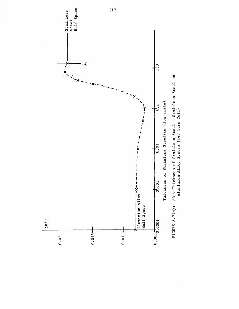
AR/ft

CUCO oCO 3CU o .

iH CO3 r-H

•H CU 14-1cd CU r-H4-> u CdCO CO PC

317

/IX

<oco

Y “ cfX/

IIXIto0

1 rHiH<

<U0 O3 3

•H a,3 CO

•H0 <4-13 1—11—1 cd

, <3 PC

CMoini“ Hoo

oo

ss Steel

on

/—\ (U(U r—l

1—I 3cd •H0 3 1—1CO 4-1 *H

CO O0 0 U0 11— 1 3^—* r—l

CU 30 CU Ha 4-4

CO Or—1 O f<U CO 1—HCU CO W4-4 CUCO r - l 0

3 3CO •H 4-tCO 3 CO(U 4-1 to

i - 13

CO CO

•H <4-1 tocd O 04J I—1CO CO i-H

CO <3<4-1 3O 3 0

3CO u •HCO •H 3CU ,3 •H3 H 0

3a > i - l

•H < 3,3 PCH <

ounoo

3 ' —' n-00WPCt=>OM

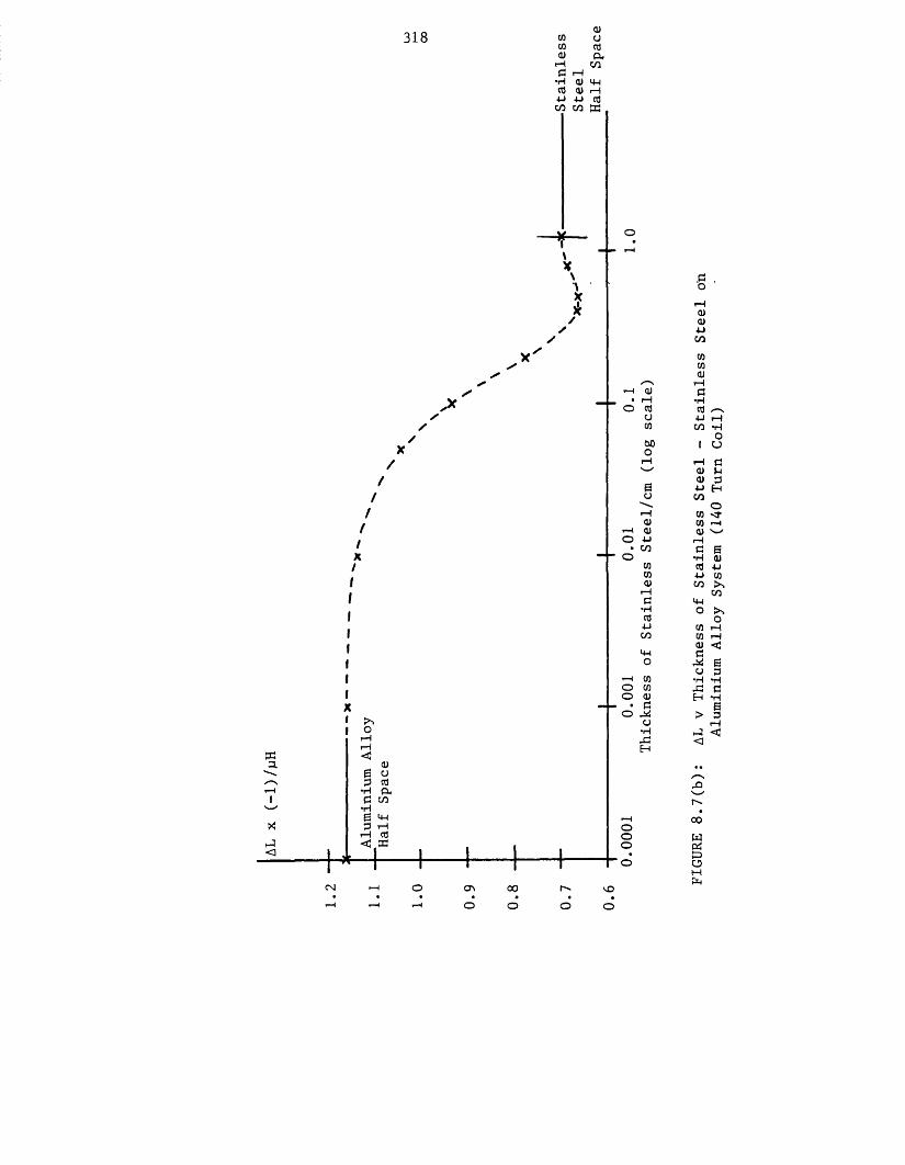
318 0)oCtJex.coi—iCU 4-1

<U i- l

CO CO ffl

o

o

4-JCOO

4-1CO4-1

OOO

C CO •H0 4-t 3 i—l r— I CCj<J. ffi

oooo

C\| o 00 FIGURE

8.7(b):

AL v

Thickness

of Stainless

Steel

- Stainless

Steel

on

Aluminium

Alloy

System

(140

Turn

Coil)

^App

roxi

mate

Mo

del

319

oa)rGHOn)Xw<u5-13PQ

o o o dp") Cs! * FIGURE 8.8:

AR v

Thickness

of Stainless

Steel

- Stainless

Steel

on Li

quid

Sodium

(LMFBR)

System

at 20

0°C

320

c COo i—i 4J•H (U cCO T3 (Uc O MCU a4-> Pg X (U O

w 4->o 03 CU1 1 i—l B T3 T3(U •H T3 •HII TU X CU CO

O O5-1 a 5-1 O P<u a a •rl4J CU aa) 4-1 4J < T3e C cU P CUCU S T3 o >-i•H 6 •H CU •H CUQ ■H X •H CO T3

. H . Q . M-l P •Hr-i a) U •H CU CO•H a Cu T3 4-> PO X a O X OU w < a w O

+ X O

i r

w w

FIGURE

8.9(a):

140

Turn

Coil

above

a 316

Stainless

Steel

Edge

(100

kHz)

- AR

v Coi

l Po

siti

on

321 tj a)Cd T 3US w

a CO p eo r—1p 4-1 O•H (U C CU PCO T3 cu s ppfi O p(U £ p <P rHP d O *H§ X CU a ow P <u oo cd >> cu oT—1 rp e T3 'd C cpCU •HTU -H cd oII T3O XO CU CO pCO TUP £ P o c H Ca) a C *H 3 Wp <U a'—✓<U P p <3 TJ6 c cd £ CUco cu 6 ■d O P•H e •H cu•H CUQ •H X •H CO T3.P . .O . y-i.C ;H . CN •i— 1 <u P •H CU CO o•H a a. T3 P C "SO X a O X O iU w <1 £ W O

FIGURE

8.9(b):

140

Turn

Coil

above

a 316

Stainless

Steel

Edge

(100

kHz)

- AL

v Coi

l Po

siti

on

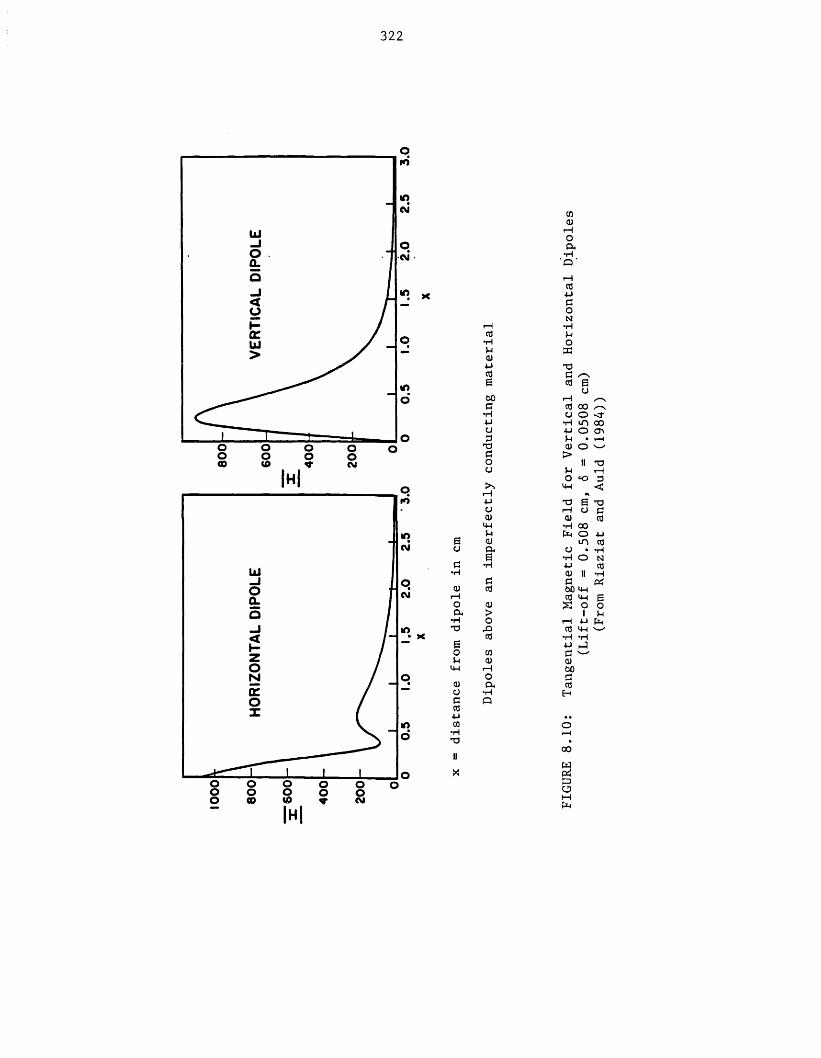
322

io

CM •

m

CM

x

oex

•HTJeou

4-10)ocCO4-1CO

• r lTO

Dip

ole

s

r-1

i—icO4-1fioN•H

CO Xi•H O>4 33<U4-> TOCO C ~se cO s00 r-H

o/—\

c CO 00 r-s•H O o <r4-> *H LO 00a ■u O CT>3 • i—H

TO a) OC >O II TOO u i—l

o <o $>i 4-1 <T—1 •t,4-1 X) 6 noa i—1 o a<U 0) cO4-4 •H 00M P<4 O 4-1a) in coex O • *HS •H O N•H 4-1 COQJ II -He a Oi!cO 00 4-1

CO 4-1 ga) s O O> 1 Uo 1—1 4-1

-O CO 4-1 wcO •H •H

4JCO e3 '—-<u aj

T—1 00o C3ex cO•H H

Q

8.1

0:

oo oo OO oo ooo CD <0|H|

«■ CM

WpcS&o

323

cm

loO □distance/cm (along coil axis)

distance/cm (perpendicular to coil axis)

0.0Position ofCoil

FIGURE 8.11(a): Tangential Magnetic Field at Material Surfaceunder a Very Small Horizontal Axis Coil

324

CMIO

4-J I EC M

<u6 •

vO

IICO

•H ° lX N | CMcO

Ui—1 cO•H <UO 13O /—\ g ■—^

\u g 4-16 '_' cOo CMV-i CO T3

4-1 0 II 0)•H 4->

<1) /■“N . Oo cO ‘O (UC5 U g N acO g V—/ X4J i—1 <uCO •H m 4-1

•H O i—H 4-1 4-J 113 O • O

IH

o 14->II II 4-1 cO•H <UPi In t-3 pL|

X/

'x/

/)<

/X/X/I"X—\

\

V^x

Pi

CM

M<uT 3cpa)cjcomM3COco•Ha)■ucoa■MCO'OrH<U•HPmO•H•MCUC6 0COa

COCO

cO -U <U C P-i 0)— — 60 co ecOH

00WPi£3O

00O

vOO

<0-o

CMO

Very

Small

Vertical Axis

Coil

distance

along

coil

axis

325

tti |h

Air-cored

Horizontal

Coil

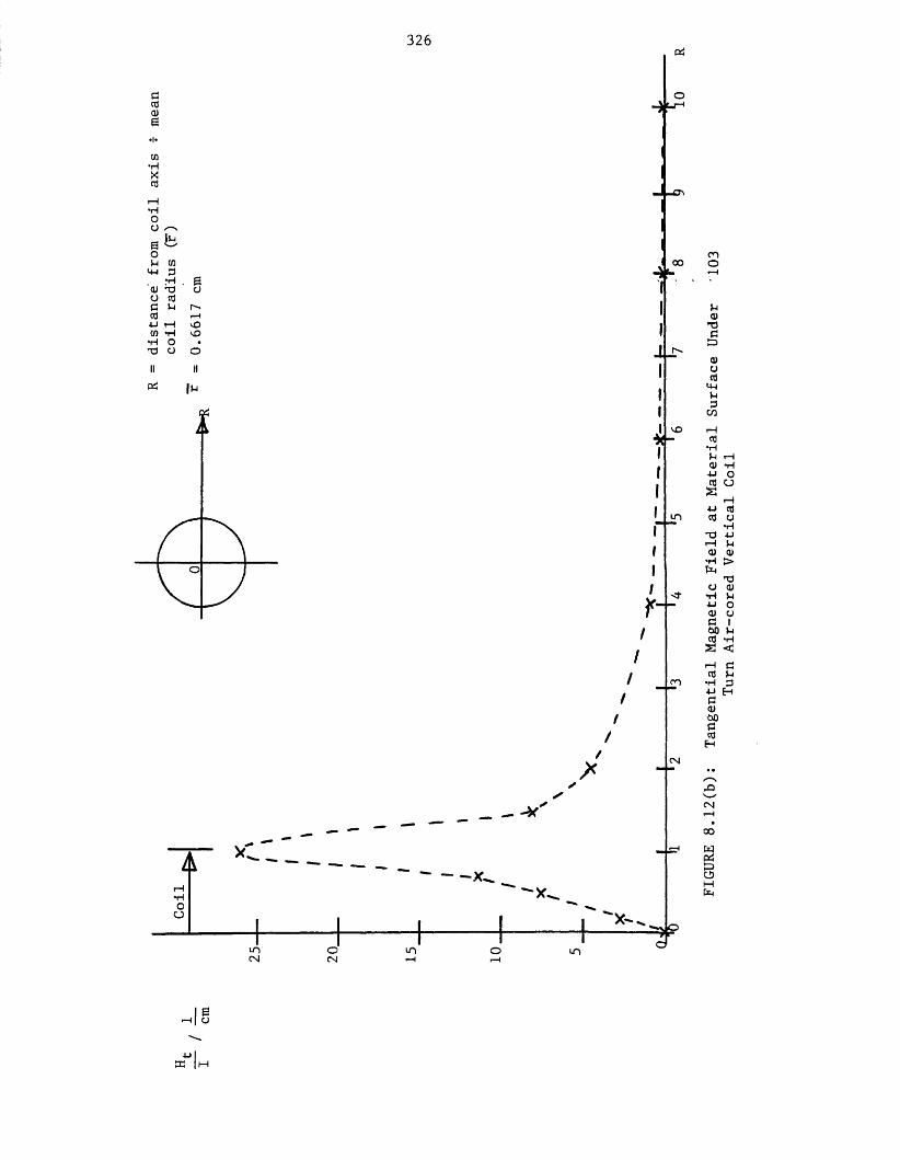
distance'

from

coil

axis

t me

an

326

FIGURE

8.12(b):

Tangential Magnetic

Field

at Material

Surface

Under

103

Turn

Air-cored

Vertical

Coil

327

cm

2 o 00

00distance/cm 50 distance/cm

00

Position of 7 Coil

FIGURE 8.13: Tangential Magnetic Field at Material Surfaceunder a 103 Turn Air-cored Horizontal Coil

328

(a ) NORMAL PROBE

V J & L ) J z o(vertical probe) ? / / ' / / / 77V t y / / s s s s / / / /tz

SURFACE EDDY CURRENT STREAM LINES

(b) PARALLEL PROBE

STRUCTURE

(horizontal probe) t T t 7 7 ; , 7> w / a / s '/ / / / / / A

IISURFACE

EDDY CURRENT STREAM LINES

*Y

FIGURE 8.14: Eddy Current (dotted line) and Magnetic Field(solid line) Distributions for Simple Probe Geometries

(From Auld et al (1982))

329

AR/ft

0.14

0.12

0.10

0.08

0.06

0.04

0.02

0.0.

Horizontal Coil X Theory O Experiment Vertical Coil + Theory • Experiment

t s\ ° \ sv

I in I i s '?n I10Lift-off/mm

(a) AR v Lift-off

25

Lift-off/mm20

- 0.2

-0.4

-0.6- 0.8

-1.0

-1.2 -<►*-1.4

AL/pH

(b) AL v Lift-off

FIGURE 8.15: 120 Turn Air-cored Coil above a 316 Stainless SteelBlock (75 kHz) - Lift-off Variation for both Coil Orientations

330

0.3

0.2

0.1

AR/fl

O Theory X Experiment

4 > = - = - *1000

- 0.1

10000 1100000 Frequency/Hz (log scale)

(a) AR v Frequency

101

0-

-0.2

-0.4

-0.6

-0.8

- 1.0

- 1.2

-1.4

1000

Frequency/Hz (log scale)10000 |100000 101

O Theory X Experiment

AL/jjH (b) AL v Frequency

FIGURE 8.16: 182 Turn Vertical Axis Coil above 6.35 mm of 316Stainless Steel on Aluminium Alloy

0000

'0000

Excited

Toge

ther

331

p-i

332

PLATES

333

9*i saw *iff — * *• if ^aa«3D 5iPP •

PLATE 5.1: HP4194A Impedance/Gain-Phase Analyser

(a horizontal axis air-cored coil is shown connected to the instrument using a test fixture)

334

PLATE 6.1: Hocking AV100L and an Absolute Pencil Probe

335

PLATE 6.2: Wayne Kerr 6425 Impedance Analyser

IAPPENDIX A

Approximate Theory Coefficients

This appendix contains the initial mathematical work performed on the approximate analytical model for the eddy currents in a stratified half space.

Al Solution for the problem of a uniform half space (formulated in terms of H).

A2 Solution for the problem of one layer and a half space(formulated in terms of H).

A3 Solution for the problem of two layers and a half space(formulated in terms of H).

In each case the equations are solved to obtained the unknowncoefficients.

Al Consider a uniform half space

A H00

> 00

x = 0 H = H X -» 00 H = 0o0 = ACO

Hence H = H e k®x on.

IIA2 Consider one layer and a half space

A H

-> 00

x = 0 H - H H - 0

a_ = 0

Consider interface at x = t

Ht+ - vA. eklt + B. e~klt - A ek“t + B e~k“t

X X oo 00

Et+ ■ vA2.1

k t —kA e ® - e ® 00 00 f]A2.2

Require all coefficients.

B1 = H - A 1 1 o 1

In (A2.1)

A 1 eklfc + (Hq - A ^ e klfc = Bro e k®fc A2.3

In (A2.2)

~ — [ *1 ek]t ■ (Ho - V e kl fc ] ■ — B. e k- fc

Using

sinh x =x -x e - e

2

Equate (A2.3) and (A2.4)

and

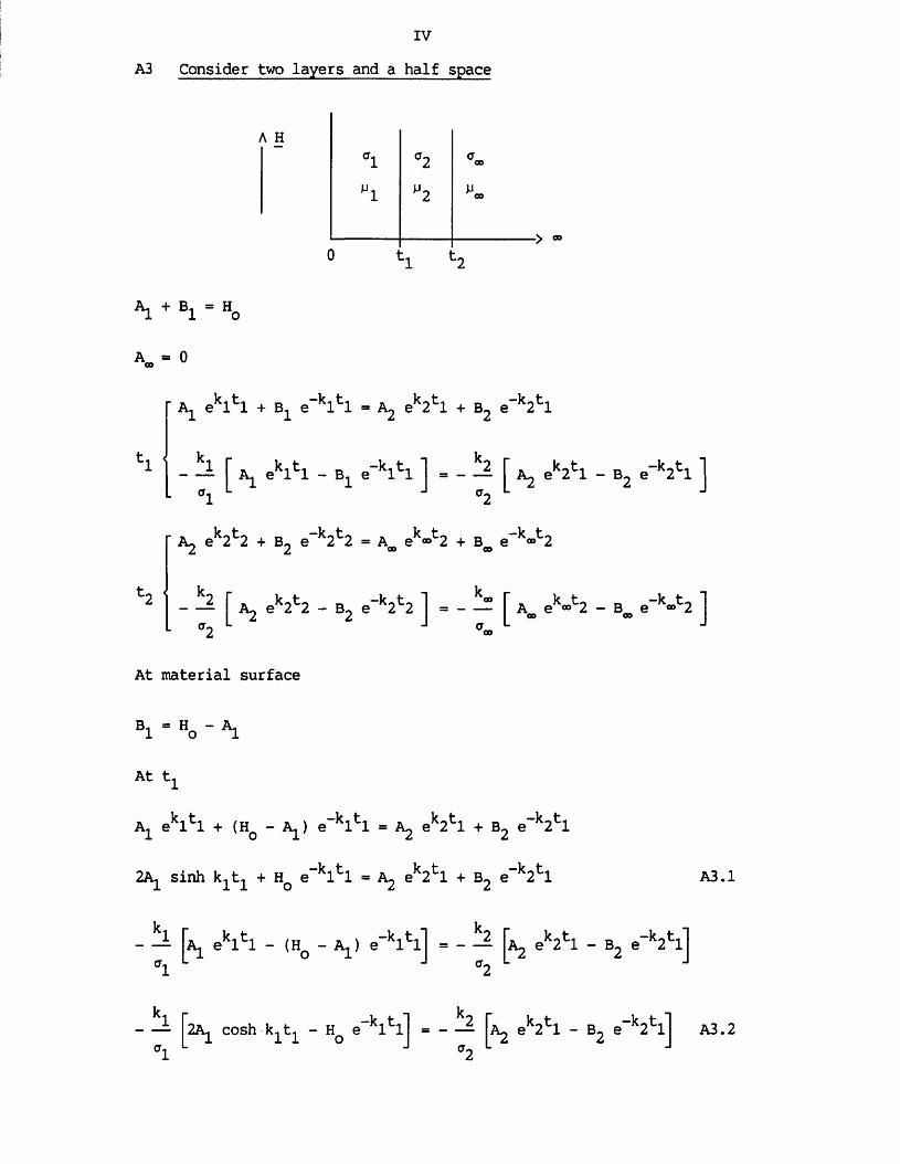
IVA3 Consider two layers and a half space

A H* 1 a2 ^ 0 0

"l " 2 »<o

() 1- 1 t

-> 00

*1 + B 1 = Ho

A_ = 0

A 1 eklfcl + B1 e~klfcl = A 2 ek2 fcl + B2 e”k2 tl

- ~ £ A 1 ekltl - B1 e klfcl J = - ek2 tl - B2 e k2 fcl J

'2 '

. k~t~ , „ -k0t0 . k t« , -kt,A 2 e 2 2 + B2 e 2 2 = Am e 0 0 2 + B^ e 0 0 2

- [ Aj ek2 f c 2 - B2 e k2fc2 j - - - - [ A. ek » f c 2 - B„ e" k » t 2 JAt material surface

B 1 = Ho - *1

At t.

A, e

1k, t« -ki t. k~t« -k-t,1 6 1 1 + (Hq - Aj ) e 1 1 = A 2 e 2 1 + B2 e 2 1

2Aj sinh k1 t1 + Hq e^lH = A 2 ek2fcl + B2 e"k2tl A3.1

ekltl - (Hq - A1) e klfclj = --- jkj ek2tl - B2 e k2fclJ

- — ^ cosh k1 t1 - Hq e klfclj = - — ek2fcl - B2 e k2fclj A3.2

Equate

n -k t-, . „ -k~t-oo 2 = A 2 e 2 2 + B2 e 2 2 = —

From (A3.1)

^ ek2fcl + B2 e“k2fcl - HQ e“kltl 2 sinh

= A,

Substitute in (A3.2)

2 cosh k^t^' ek2 fcl + B2 e"

2 sinh k^t

“ ~ [ *2 ek2tl " B2 e k2tl ]

Hence

Get I$2 in tenns of

cothffi

ai

kltl * 2 ek2tl --- coth k1 t 1 B 2 e k2tl°1

—k t —k tcoth k1 t* H e 1 1 + — H e 1Z1 1 1 0 o"1

- Aj ek2tl + — B2 e_k2t:l '2 °2

Hence

Hence

VIII

kl k 2 g°» CT1 a2 k«

Hq y 1 + coth k^t^ 1ek2 (tl t2 ) klfcl

k 2 kl— + — coth k^t^ ° 2 al

x both sides byf k2 k- — + — coth k^t^a2 °1

*2f k k >

2 1 — + — coth k^t^ ek2 f c 2 +

f k k > 2 1

-------------------------coth k-t. ek2 (2tl t2 ). , <J7 o. X X

< CT9 <T. y

k2 g- a 2 k»

k 2 p. ff2 k»

= e 2 L 1

( k k 'i 2 1 — + — coth k^t^ ek2 f c 2

" a2 al

( k k > 2 1 — - — coth k1 t1 ek2 (2 tr t2 )

" a2 CT1 ■

-t2) kxtx I i + coth k1 t1 1 — Hq f ko °a> 1

2 * 1 iJ ffl °2 <° '

*2 ek 2 < fci t2 ) kltl £ 1 + coth j — H ' k 2 q-

' a2 k»- 1

ek2 t 2

( k k > 2 1 — + — coth k^t^

( k- a 1 + 2 ”

■ ' c2 a 2 k® '

+ ek2 (2tl Vf k k >

2 1 ------- coth k^t^ f ko am ] i 2 "< a2 °1 ; a 2 k«° ' -

Hence A^, B^ and can be found using the expression detailedearlier in this analysis.

I

APPENDIX B

This appendix contains much of the algebraic manipulation employed in the extension to the theory of Burke (1986)

Bl

The components of the electric field intensity in the plane of the material (the xz plane) are obtained from

A

E = -j to curl (T y) Bl .1

In air

2aB1.2

dx

C-j co sin (sz) (-p) sin (px) Bl .3

2a

-2 M I N -adewhere C =

* ^ * * 2 " al> Jo—j M(sa^ , sa2) sin (st) dp

a

In the layer

EX1 - -i “ c ------- s cos (sz) A 1 e“l^ + B1 e Bl.4( a + a1 ) L J

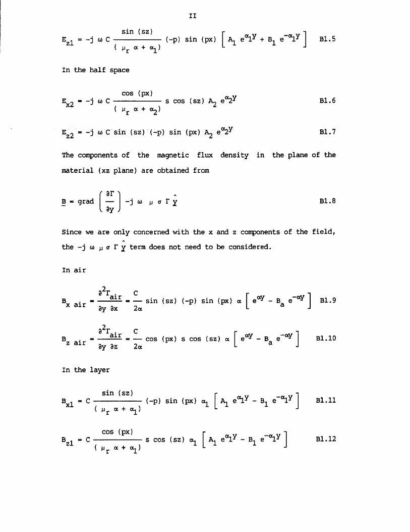
II

Ezl = -3 w Csin (sz)

( JJr « + <*i(-p) sin (px) £ A^ e ' V + e”®!^ j Bl.5

In the half space

cos <Px) ~ vEx 2 = -j w C ----------- s cos (sz) A 2 e( ur a + oe )

Ez 2 = -j co C sin (sz) (-p) sin (px) A 2 e0

B l.6

Bl .7

The components of the magnetic flux density in the plane of the material (xz plane) are obtained from

B = grad' ar 'i

, 3y-j w jj a T y B l.8

Since we are only concerned with the x and z components of the field,A

the -j co jj a T y term does not need to be considered.

In air

B 9 r a i r cx air 9y 3x 2 a

= — sin (sz) (-p) sin (px) a I"L - b e-°y3 J B l.!

B 9 Fair Cz air 3y 3z 2 a

= — cos (px) s cos (sz) a e0 - B^ e j Bl.10

In the layer

Bx l “ C

sin (sz)( ur a + a1)

(-p) sin (px) a^ A^ e0!^ - B^ e”®!^ j

cos ( Px ) T ~ v v “IBz = C ------------ s cos (sz) a^ A^ e^.y - B^ e

Bl .11

Bl.12( a + 0^)

In the half space

sin (sz)= C ------------ (-p) sin (px) ( * 2 A 2 e0 Bl.13

( a + <*2 )

cos (px)Bz 2 = C ------------ s cos (sz) « 2 A 2 e“2^ Bl.14

( jjr a + 0 2 )

B2IV

Having applied the boundary conditions at the material surface and at the layer/half space interface, the following four equationscontaining four unknowns are obtained.

“i (*x - Bi> 1 - B<( jJr a + a ) ■ 2 ' '

A^ + Bi 1 + Ba( U r « + ot) 2a

“i (Ai e-0^ - B1 e0 ) “2 *2 ertf< Pr a +■ V ( Pr “ + o )

A^ e"’“lt + B1 e*1* *2 e "•a2t

( Pr a 4• “I* ( nr a + Oj)

From (B2.1)

“i (Ai - Bi> X - Ba( « + o )

(1 - B ,) ( a + a^)A - B = 3 rA1 B1

.-.A1 =

ZO^

1 - Ba ) ( a + a^)

B2.1

B2.2

B 2.3

B2.4

+ B. B2.1a

From (B2.2)

2a (A. + B. )B = ----- 1 B2.2a

a ( j j r a + o^)

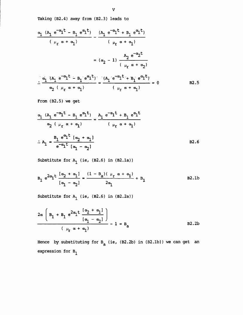
VTaking (B2.4) away from (B2.3) leads to

“1 (A1 e alt - B1 ealt) e”alt + B1 ealt)( jjr a + a )

= («2 - 1) h e'“2tHr “ + °2)

e-®!* - e“lt) (Aj e"®!* + Bj e®!*)'<*2 ( jjf a + o^)

From (B2.5) we get

( jjr a + o^)

(Ax e"0 - Bx ealt) A1 e “l*1 + Bx e0£lt <*2 ( jJr a + o^) ( jjr a + o )

B^ e01!^ [ 0 2 + 0 1 2 ]-O L , t*1 [0^ - O^I

Substitute for A^ (ie, (B2.6) in (B2.1a))

B^ e2ajt [°2 + “l1 _ (1 ~ Ba)( ^ ® + ®1> +[<*1 - <*2 ] 2ol

B,

Substitute for A^ (ie, (B2.6) in (B2.2a))

+ [ou + 0 ] ' 2a B- + B- e — -----—

i®i - ®2]( fjr a + 0 )

- 1 = B_

B2.5

B2.6

B2.1b

B2.2b

Hence by substituting for Ba (ie, (B2.2b) in (B2.1b)) we can get anclexpression for B2

e2o1t [a2 + “l1 t“l - “2)

VI

( JJ r a + ®l)

1 -

2aB- + 2aB1 e2alt ^ + ^t«l - °2l - 1

JJr a + «i+ B.

B,( jjr a + o^) [a^ - 0 2 ]‘

^a2 + al [ 0 2 + a] + [0 2 - 0 2 ] [0 - 0 2 ]B2.7

By substituting for B2 (ie, (B2.7) in (B2.6)) we get

( jjr a + a^) e2alt [ © 2 + 0&2 ]^a2 + al [ 0 2 + a] + [0 2 - 0 2 ] [ a - 0 2 ]

B2.8

Bfl can be determined by substituting for A 2 and B2 in (B2.2a)

2a £ e2oclt [02 + 02] + [02 - otj] J

“l [©2 + 02] [02 + 0] + [ 0 2 - 0 2 ] [ a - 0 2 ]- 1 B2.9

Finally, using (B2.4) and substituting for A 2 and B2 we can get A 2

*2 -( jJr 01 + “2 )( jjr a + 0 2 ) e

:,A2 ~jj r a + 0 2 ) e“2^ 2 a2 e01!^

alt [ 0 2 + 0 2 ] [ 0 2 + a] + [c* 2 — 0 2 ] [a - 0 2 ]B2.10

A 2 , B2 , A 2 and Ba are the coefficients for the one layer on a half space case.

VIIB3

The AZ reciprocity relation used to determine AZ is given as

QO 00

AZ = dx dz (n x Es . H - n x E . Hs) B3.1

In order to evaluate the expression we use

(n x Es . H - n x E . Hs)

(EzS Hx + ExS Hz) - (Ez HxS + Ex HzS) B3.2

since n =

By substituting for the components of the electromagnetic fields we get

( E S H + E S H ) - ( E H S + E H S) v z x x z ' z x x z

(-j) w sin (sz) (-p) sin (px) (e0 + B_e °^) . 2a a

C sin (sz) jj ( jjr a + o^)

(—p) sin (px) a^ (A2 e®!^ - B2 e “l^)

+ (-j) w — cos (px) s cos (sz) (e0 + B e °^) . 2a a

C cos (px)jj ( jjr a + 0 2 !

s cos (sz) 0 2 (A2 e°l - e “l^)

VIIIsin (sz)

(-j) co C (-p) sin (px) (A- e0!* + B1 e”01!/)( ur a + ol )

C 1 _ sin (sz) (-p) sin (px) a (e0 - B e ° )2 a u 3

C 0 S (P X ) a - V - O . V+ (-j) co C ----------- s cos (sz) (A^ e r + B e T.y ) .( jjr a + °^)

C 1 cos (px) s cos (sz) a (e0 - B e °^)2a jj

B3.3

By recognising that

00 CO

dx dz (p2 sin2 (sz) sin2 (px) + s2 cos2 (px) cos2 (sz)) * n2 a2

B3.4when inverse Fourier Transforms are taken, we get

CO 00dx

— 00

dz (n X Es . H - n X E . Hs)

J2 2 2C n a-] co

2a jj ( jj a + a^)

c: n a- 3 co

2a jj ( jj r a + o^)

'e0 + Ba e °^) a^ (A^ e01!^ - B^ e *1 ^)

(A^ e01!^ + B^ e acl^) a (e0 - Ba e °^)

4 u I2 ~ 2 N 2

~2 .2, 772n t (a2 - a ^ vr ds 2 2 -g- M (sa^ , sa2) sin (st)o s

n°° -2 od , .. 2 2e (-3 ) co n adp — 2---------------------

a 2a j j ( a + 0^)

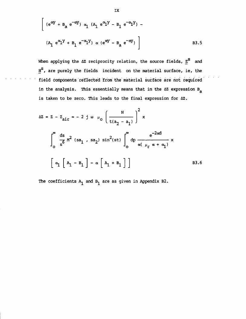
IX

(e 0 + ea e“ < *) «2 (Aj_ e V - Bx e“V ) -

{P e®!7 + Bx e ®ly ) a (e0 - Bfl e ay) B3.5

When applying the AZ reciprocity relation, the source fields, E andeH , are purely the fields incident on the material surface, ie, the field components reflected from the material surface are not required in the analysis. This essentially means that in the AZ expression BQ is taken to be zero. This leads to the final expression for AZ.

N

» , a> —2 ad2 2 f e-g- M (sa^ / sa2) sin (st) d p -------------

s JG a( a + o^)

[ “i [ *i - Bi ] - “ [ *i + Bi ] ] B3.6

The coefficients A^ and B^ are as given in Appendix B2.

IAPPENDIX C

Temperature Considerations

The aim o f t h is a n a ly s is is to in v e s t ig a te , in a sim ple manner th e

tem p eratu re g ra d ie n t th a t could be p re s e n t across th e p rim a ry v e s s e l

w a ll when th e LMFBR is on shutdown and th e p rim ary v e s s e l is b e in g

in s p e c te d . C onvection w i l l be n e g le c te d .

Consider Superphenix (Energie Nucleaire Magazine (1983)).Primary vessel height, h = 19.5 m Primary vessel diameter, 2r = 21.0 m

Assuming th e p rim a ry v e s s e l to be a c y lin d e r ,

2 3the vessel volume = n r h = 6754 m C.l

The core is inside the primary vessel. 33.8% of the core is liquid sodium.

Core volume = 10.766 m3

Volume o f l i q u id sodium in th e p rim ary v e s s e l,

V = 6754 - (66.2% o f 10.766)= 6747 m3

A t in s p e c tio n th e ves s e l co n ta in s 6747 m3 o f l iq u id sodium a t

200°C.

This is just a first approximation. The fast reactor is essentially being modelled as a stainless steel cylinder containing liquid sodium.

IIThe surface area of the vessel over which energy can be transferred,

A = 2 7i rh + 2 n r C.22= 1979 m of stainless steel

To determine the temperature difference across the primary vessel wall use the conduction equation (Waltar and Reynolds (1981)).

q = k At/b C.3

q = heat flux = Q/A Q = heat transferred across the wall A - area over which the transfer takes place k = thermal conductivity of the wall material At = temperature difference across the wall b = wall thickness

To determine At, an assumption needs to be made about Q. Assume that Q is equivalent to a 5°C change in the liquid sodium temperature over the course of an hour. This was considered a realistic assumption.

Q = m c A0 C.4

m = mass of materialc = specific heat capacity (SHC) of material A0 = rate of change of temperature of material

Q = V p c A0 C.5

3p = density of liquid sodium =815 kg/m c = 1.3 kJAg K

Na Inert gas200°C

Stainless steel vessel wall

< ■>50 mm

At = qb/k = (Q/A)(b/k) C.6

k varies with temperature. This is taken account of in the following expression (Waltar and Reynolds (1981)),

k = 16.68 W/m K .*. At = 15.04°C

If we assume a linear temperature distribution across the vessel wall and an electromagnetic skin depth of 8 mm in the stainless steel, the temperature at a distance 6 from the inert gas side = 187.37°C

k - 9.248 + 0.01571(273 + T) W/m K C.7

Take T * 200°C

IVHence across the skin depth we have a temperature change of 2.41°C. This is a small change in temperature but it does signify a small conductivity change across the skin depth. The effect of this conductivity gradient needs to be investigated further, but based on a knowledge of the eddy current technique, it would be expected that this temperature difference across the vessel wall could be considered negligible and thus have no effect on the successful performance of the eddy current test.