Embed Size (px)
Citation preview
Thesis presented for the Ph.D degree (Doctor of Philosophy) in Physics
Charged particle multiplicity distributionsinto forward pseudorapidities in pp andPbPb collisions at the LHC
Casper NygaardNiels Bohr InstituteUniversity of Copenhagen
Academic Advisor:Jens Jørgen GaardhøjeNiels Bohr InstituteUniversity of Copenhagen
October, 2011


Contents
Preface 1
1 The Standard Model of Particle Physics 51.1 Quantum Chromo Dynamics . . . . . . . . . . . . . . . . . . . . . . . . . . 71.2 Quark Gluon Plasma . . . . . . . . . . . . . . . . . . . . . . . . . . . . . . 81.3 Kinematic Variables . . . . . . . . . . . . . . . . . . . . . . . . . . . . . . 101.4 Relativistic Collisions . . . . . . . . . . . . . . . . . . . . . . . . . . . . . . 12
1.4.1 Relativistic Heavy Ion Collisions . . . . . . . . . . . . . . . . . . . . 121.4.2 Proton-Proton Collisions . . . . . . . . . . . . . . . . . . . . . . . . 16
1.5 Previous Heavy Ion Results . . . . . . . . . . . . . . . . . . . . . . . . . . 19
2 Charged Particle Multiplicity 272.1 Negative Binomial Distributions . . . . . . . . . . . . . . . . . . . . . . . . 272.2 Koba–Nielsen–Olesen Scaling . . . . . . . . . . . . . . . . . . . . . . . . . 302.3 Previous Multiplicity Measurements . . . . . . . . . . . . . . . . . . . . . . 33
2.3.1 Multiplicity Distributions . . . . . . . . . . . . . . . . . . . . . . . 332.3.2 dN/dη measurements . . . . . . . . . . . . . . . . . . . . . . . . . . 382.3.3 Mean Multiplicity Energy Dependence . . . . . . . . . . . . . . . . 40
3 Experimental Setup 433.1 The Large Hadron Collider . . . . . . . . . . . . . . . . . . . . . . . . . . . 43
3.1.1 Colliding Protons . . . . . . . . . . . . . . . . . . . . . . . . . . . . 433.1.2 Colliding Lead Ions . . . . . . . . . . . . . . . . . . . . . . . . . . . 44
3.2 The ALICE Experiment . . . . . . . . . . . . . . . . . . . . . . . . . . . . 453.3 Central Barrel Detectors . . . . . . . . . . . . . . . . . . . . . . . . . . . . 45
3.3.1 Inner Tracking System . . . . . . . . . . . . . . . . . . . . . . . . . 463.3.2 Time Projection Chamber . . . . . . . . . . . . . . . . . . . . . . . 473.3.3 Transition Radiation Detector . . . . . . . . . . . . . . . . . . . . . 483.3.4 Time Of Flight . . . . . . . . . . . . . . . . . . . . . . . . . . . . . 483.3.5 Photon Spectrometer . . . . . . . . . . . . . . . . . . . . . . . . . . 483.3.6 Electro Magnetic Calorimeter . . . . . . . . . . . . . . . . . . . . . 493.3.7 High Momentum Particle Identification Detector . . . . . . . . . . . 49
3.4 Muon Spectrometer . . . . . . . . . . . . . . . . . . . . . . . . . . . . . . . 493.5 Forward detectors . . . . . . . . . . . . . . . . . . . . . . . . . . . . . . . . 49
3.5.1 Photon Multiplicity Detector . . . . . . . . . . . . . . . . . . . . . 503.5.2 T0 . . . . . . . . . . . . . . . . . . . . . . . . . . . . . . . . . . . . 503.5.3 V0 . . . . . . . . . . . . . . . . . . . . . . . . . . . . . . . . . . . . 513.5.4 Zero Degree Calorimeter . . . . . . . . . . . . . . . . . . . . . . . . 51
3.6 Data Acquisition System . . . . . . . . . . . . . . . . . . . . . . . . . . . . 52
I

II
4 The FMD and SPD 53
4.1 Semi-conductor properties . . . . . . . . . . . . . . . . . . . . . . . . . . . 53
4.1.1 Doped Crystals . . . . . . . . . . . . . . . . . . . . . . . . . . . . . 54
4.2 Semi-conductor detectors . . . . . . . . . . . . . . . . . . . . . . . . . . . . 55
4.2.1 n-p junctions . . . . . . . . . . . . . . . . . . . . . . . . . . . . . . 55
4.3 Energy loss in Silicon . . . . . . . . . . . . . . . . . . . . . . . . . . . . . . 56
4.4 Forward Multiplicity Detector . . . . . . . . . . . . . . . . . . . . . . . . . 60
4.4.1 Design and Motivation . . . . . . . . . . . . . . . . . . . . . . . . . 60
4.4.2 FMD Sensors and Electronics . . . . . . . . . . . . . . . . . . . . . 61
4.4.3 Pedestals and Gain . . . . . . . . . . . . . . . . . . . . . . . . . . . 65
4.5 Silicon Pixel Detector . . . . . . . . . . . . . . . . . . . . . . . . . . . . . . 66
5 Off-line Data Processing 69
5.1 ROOT and AliROOT . . . . . . . . . . . . . . . . . . . . . . . . . . . . . . 69
5.2 Simulations . . . . . . . . . . . . . . . . . . . . . . . . . . . . . . . . . . . 69
5.2.1 Digitisation . . . . . . . . . . . . . . . . . . . . . . . . . . . . . . . 70
5.3 Reconstruction . . . . . . . . . . . . . . . . . . . . . . . . . . . . . . . . . 71
5.4 Analysis Structure . . . . . . . . . . . . . . . . . . . . . . . . . . . . . . . 72
5.5 GRID and AliEn . . . . . . . . . . . . . . . . . . . . . . . . . . . . . . . . 74
5.6 Data sets for analysis . . . . . . . . . . . . . . . . . . . . . . . . . . . . . . 76
6 Analysis 79
6.1 Event Selection . . . . . . . . . . . . . . . . . . . . . . . . . . . . . . . . . 79
6.1.1 Trigger Selection . . . . . . . . . . . . . . . . . . . . . . . . . . . . 79
6.1.2 Vertex Selection . . . . . . . . . . . . . . . . . . . . . . . . . . . . . 81
6.1.3 Centrality Selection . . . . . . . . . . . . . . . . . . . . . . . . . . . 83
6.2 FMD Particle Counting . . . . . . . . . . . . . . . . . . . . . . . . . . . . 84
6.2.1 Energy distributions . . . . . . . . . . . . . . . . . . . . . . . . . . 84
6.2.2 Hit Sharing . . . . . . . . . . . . . . . . . . . . . . . . . . . . . . . 87
6.2.3 Counting Methods . . . . . . . . . . . . . . . . . . . . . . . . . . . 94
6.2.4 FMD Acceptance . . . . . . . . . . . . . . . . . . . . . . . . . . . . 97
6.3 SPD Particle Counting . . . . . . . . . . . . . . . . . . . . . . . . . . . . . 99
6.3.1 SPD Acceptance . . . . . . . . . . . . . . . . . . . . . . . . . . . . 100
6.4 Secondary particles . . . . . . . . . . . . . . . . . . . . . . . . . . . . . . . 101
6.5 Strangeness Correction . . . . . . . . . . . . . . . . . . . . . . . . . . . . . 108
6.6 Unfolding . . . . . . . . . . . . . . . . . . . . . . . . . . . . . . . . . . . . 109
6.6.1 Bayesian Iterative Unfolding . . . . . . . . . . . . . . . . . . . . . . 110
6.6.2 Single Value Decomposition Unfolding . . . . . . . . . . . . . . . . 112
6.6.3 Unfolding Quality Measure . . . . . . . . . . . . . . . . . . . . . . . 114
6.7 Trigger-Vertex Bias Correction . . . . . . . . . . . . . . . . . . . . . . . . . 118
6.8 Defining Analysis Parameters . . . . . . . . . . . . . . . . . . . . . . . . . 119
7 Systematic Errors 125
7.1 Uncertainty on event multiplicity . . . . . . . . . . . . . . . . . . . . . . . 125
7.2 Uncertainty on trigger–vertex bias correction and unfolding method . . . . 129
7.3 Total systematic error . . . . . . . . . . . . . . . . . . . . . . . . . . . . . 131

III
8 Results 1338.1 Multiplicity Distributions . . . . . . . . . . . . . . . . . . . . . . . . . . . 134
8.1.1 pp collisions . . . . . . . . . . . . . . . . . . . . . . . . . . . . . . . 1348.1.2 PbPb collisions . . . . . . . . . . . . . . . . . . . . . . . . . . . . . 137
8.2 KNO . . . . . . . . . . . . . . . . . . . . . . . . . . . . . . . . . . . . . . . 1398.2.1 pp collisions . . . . . . . . . . . . . . . . . . . . . . . . . . . . . . . 1398.2.2 PbPb collisions . . . . . . . . . . . . . . . . . . . . . . . . . . . . . 143
8.3 dNch
dη. . . . . . . . . . . . . . . . . . . . . . . . . . . . . . . . . . . . . . . 145
8.3.1 pp collisions . . . . . . . . . . . . . . . . . . . . . . . . . . . . . . . 1458.3.2 PbPb collisions . . . . . . . . . . . . . . . . . . . . . . . . . . . . . 146
8.4 Mean Multiplicity Energy dependence . . . . . . . . . . . . . . . . . . . . . 1478.5 Outlook . . . . . . . . . . . . . . . . . . . . . . . . . . . . . . . . . . . . . 148
9 Conclusion 151
A Lorentz Invariance of dy 153
B The Glauber Model 155
C Sharing algoritm 157
D Comparison between Poisson and Energy Fits counting 159
E Q1 in central η-interval 163
F Detailed comparisons of multiplicity distributions 165

IV
List of Figures
1.1 Quark Quark potential . . . . . . . . . . . . . . . . . . . . . . . . . . . . . 81.2 The formation of QGP through compression of matter. . . . . . . . . . . . 81.3 QCD phase diagram. . . . . . . . . . . . . . . . . . . . . . . . . . . . . . . 91.4 ALICE coordinate system . . . . . . . . . . . . . . . . . . . . . . . . . . . 111.5 Schematic illustration of a relativistic heavy ion collision. . . . . . . . . . . 121.6 Proposed space-time evolution of a heavy ion collision. . . . . . . . . . . . 141.7 Simplistic view of a collision in the transparent picture. . . . . . . . . . . . 141.8 Simplistic view of a collision in the stopping picture. . . . . . . . . . . . . 151.9 Schematic of a pp collision. . . . . . . . . . . . . . . . . . . . . . . . . . . . 161.10 Chew-Frautschi plot . . . . . . . . . . . . . . . . . . . . . . . . . . . . . . 171.11 Diffractive event class differences . . . . . . . . . . . . . . . . . . . . . . . 181.12 Nuclear modification factors from BRAHMS and ALICE. . . . . . . . . . . 191.13 Nuclear modification factors from CMS and PHENIX. . . . . . . . . . . . . 201.14 Jet Quenching . . . . . . . . . . . . . . . . . . . . . . . . . . . . . . . . . . 211.15 Dijet imbalance . . . . . . . . . . . . . . . . . . . . . . . . . . . . . . . . . 221.16 The missing energy as a function of the dijet asymmetry from CMS . . . . 221.17 Flow measurements from ALICE. . . . . . . . . . . . . . . . . . . . . . . . 231.18 Reaction plane and nuclei overlap. . . . . . . . . . . . . . . . . . . . . . . . 241.19 Long range azimuthal correlation from ALICE . . . . . . . . . . . . . . . . 25
2.1 Various Negative Binomial Distributions . . . . . . . . . . . . . . . . . . . 282.2 Split Field Magnet detector multiplicity measurements . . . . . . . . . . . 332.3 UA5 multiplicity measurements . . . . . . . . . . . . . . . . . . . . . . . . 342.4 UA1 multiplicity measurements . . . . . . . . . . . . . . . . . . . . . . . . 342.5 CDF multiplicity measurements. . . . . . . . . . . . . . . . . . . . . . . . . 352.6 ALICE and CMS multiplicity measurements at
√s = 900 GeV, 2360 GeV,
and 7000 GeV . . . . . . . . . . . . . . . . . . . . . . . . . . . . . . . . . . 362.7 Multi-component NBD fits to UA5 data. . . . . . . . . . . . . . . . . . . . 372.8 dNch
dηmeasurements from pre-LHC experiments. . . . . . . . . . . . . . . . 38
2.9 dNch
dηmeasurements from ALICE and CMS. . . . . . . . . . . . . . . . . . . 39
2.10 Preliminary dNch
dηmeasurements from ATLAS. . . . . . . . . . . . . . . . . 39
2.11 Unpublished PbPb dNch
dηmeasurements from ALICE. . . . . . . . . . . . . . 40
2.12 Mean multiplicity collision energy scaling. . . . . . . . . . . . . . . . . . . 412.13 dNch
dηpredictions at mid-rapidity in PbPb collisions at
√sNN
= 2760 GeV . . 41
3.1 Schematic view of the CERN accelerator complex. . . . . . . . . . . . . . . 443.2 Overview of the ALICE detector . . . . . . . . . . . . . . . . . . . . . . . . 453.3 Pseudorapidity coverage of ALICE . . . . . . . . . . . . . . . . . . . . . . 463.4 ALICE central barrel detectors . . . . . . . . . . . . . . . . . . . . . . . . 473.5 Muon Spectrometer . . . . . . . . . . . . . . . . . . . . . . . . . . . . . . . 50
V

VI
3.6 Forward Detectors . . . . . . . . . . . . . . . . . . . . . . . . . . . . . . . 51
4.1 Band-gaps in insulators, semi-conductors and metals. . . . . . . . . . . . . 534.2 Semi-conductor bindings . . . . . . . . . . . . . . . . . . . . . . . . . . . . 544.3 The stopper power for µ in Copper. . . . . . . . . . . . . . . . . . . . . . . 574.4 Landau distribution. . . . . . . . . . . . . . . . . . . . . . . . . . . . . . . 594.5 Overview of the FMD detector system . . . . . . . . . . . . . . . . . . . . 604.6 Overview of FMD rings . . . . . . . . . . . . . . . . . . . . . . . . . . . . . 624.7 Schematic of the FMD electronics. . . . . . . . . . . . . . . . . . . . . . . . 634.8 Capacitance and leakage current. . . . . . . . . . . . . . . . . . . . . . . . 644.9 Depletion depth and leakage current stability. . . . . . . . . . . . . . . . . 644.10 Pedestal distribution and gain calibration. . . . . . . . . . . . . . . . . . . 654.11 Pedestal means. . . . . . . . . . . . . . . . . . . . . . . . . . . . . . . . . . 664.12 Overview of the ITS detector system. . . . . . . . . . . . . . . . . . . . . . 674.13 Close up view of the SPD. . . . . . . . . . . . . . . . . . . . . . . . . . . . 67
5.1 Tracklet construction and vertex finding. . . . . . . . . . . . . . . . . . . . 725.2 Schematic of analysis train structure. . . . . . . . . . . . . . . . . . . . . . 735.3 Schematic of the analysis chain in ALICE. . . . . . . . . . . . . . . . . . . 745.4 Overview of the GRID computing centres in Europe and Egypt. . . . . . . 75
6.1 vz versus η acceptance. . . . . . . . . . . . . . . . . . . . . . . . . . . . . . 816.2 The measured z-vertex distribution. . . . . . . . . . . . . . . . . . . . . . . 826.3 The measured xy-vertex distribution . . . . . . . . . . . . . . . . . . . . . 836.4 An example of measured centrality classes by the V 0 detector. . . . . . . . 846.5 The measured energy distributions in FMD2I. . . . . . . . . . . . . . . . . 856.6 Energy distributions in the simulations. . . . . . . . . . . . . . . . . . . . . 866.7 Illustration of the concept of hit sharing. . . . . . . . . . . . . . . . . . . 876.8 Relation between the energy deposit in neighbouring strips. . . . . . . . . . 886.9 Single, double and triple merged signals. . . . . . . . . . . . . . . . . . . . 896.10 Simulated single, double and triple merged signals. . . . . . . . . . . . . . 906.11 Sharing hit cut. . . . . . . . . . . . . . . . . . . . . . . . . . . . . . . . . . 926.12 Example of the effect of merging shared signals on the energy distributions. 936.13 Example of a multiple (Gaussian convoluted) Landau fit. . . . . . . . . . . 946.14 The correction for high occupancy in the Poisson counting method. . . . . 956.15 Mean Occupancy . . . . . . . . . . . . . . . . . . . . . . . . . . . . . . . . 976.16 Counting methods comparison in pp collisions at
√s = 900GeV . . . . . . 98
6.17 Inner ring φ-acceptance. . . . . . . . . . . . . . . . . . . . . . . . . . . . . 996.18 The frequency of various cluster patterns in the SPD. . . . . . . . . . . . . 1006.19 The actual φ-acceptance of the SPD as a function of η. . . . . . . . . . . . 1016.20 The origin of secondary particles within the central region of ALICE. . . . 1026.21 The origin of the secondary particles, which eventually hit the FMD system. 1026.22 The origin of secondary particles hitting each individual FMD ring. . . . . 1046.23 Origin of secondary particles hitting either the FMD or SPD inner layer. . 1056.24 Origin of secondary particles hitting the FMD rings and the SPD inner layer.1066.25 FMD3I secondary correction map. . . . . . . . . . . . . . . . . . . . . . . . 1076.26 SPD secondary correction map. . . . . . . . . . . . . . . . . . . . . . . . . 1076.27 Strangeness correction factor . . . . . . . . . . . . . . . . . . . . . . . . . . 1086.28 Response matrix. . . . . . . . . . . . . . . . . . . . . . . . . . . . . . . . . 1106.29 Number of iterations in Bayesian unfolding. . . . . . . . . . . . . . . . . . 111

VII
6.30 Over and under-regularisation . . . . . . . . . . . . . . . . . . . . . . . . . 1136.31 Characteristic regions of multiplicity distributions. . . . . . . . . . . . . . . 1146.32 Q1 unfolding quality. . . . . . . . . . . . . . . . . . . . . . . . . . . . . . . 1166.33 The best unfolding solutions for |η| < 2.4. . . . . . . . . . . . . . . . . . . 1176.34 Trigger–Vertex bias correction factor. . . . . . . . . . . . . . . . . . . . . . 1186.35 Secondary correction test. . . . . . . . . . . . . . . . . . . . . . . . . . . . 1196.36 Acceptance gaps test. . . . . . . . . . . . . . . . . . . . . . . . . . . . . . . 1206.37 Event generator test. . . . . . . . . . . . . . . . . . . . . . . . . . . . . . . 1226.38 Vertex range test. . . . . . . . . . . . . . . . . . . . . . . . . . . . . . . . . 123
7.1 Material density uncertainty. . . . . . . . . . . . . . . . . . . . . . . . . . . 1257.2 Event generator uncertainty in the FMD. . . . . . . . . . . . . . . . . . . . 1267.3 Event generator uncertainty in the SPD. . . . . . . . . . . . . . . . . . . . 1277.4 Example of systematic errors on event multiplicity . . . . . . . . . . . . . . 1297.5 Example of total systematic error. . . . . . . . . . . . . . . . . . . . . . . . 130
8.1 Multiplicity distributions for NSD pp collisions at√s = 900 GeV. . . . . . 133
8.2 Multiplicity distributions for NSD pp collisions at√s = 2760 GeV. . . . . . 134
8.3 Multiplicity distributions for NSD pp collisions at√s = 7000 GeV. . . . . . 135
8.4 pp multiplicity distributions in |η| < 0.5 at√s = 900 GeV. . . . . . . . . . 136
8.5 pp multiplicity distributions in |η| < 1.0 at√s = 7000 GeV. . . . . . . . . 136
8.6 Multiplicity distribution for 0-5% PbPb collisions . . . . . . . . . . . . . . 1378.7 Multiplicity distribution in −3.4 < η < 5.1 for PbPb collisions . . . . . . . 1388.8 pp NSD collisions in KNO variables . . . . . . . . . . . . . . . . . . . . . . 1398.9 Detailed KNO scaling comparison . . . . . . . . . . . . . . . . . . . . . . . 1408.10 Moments for |η| < 0.5 multiplicity distributions . . . . . . . . . . . . . . . 1418.11 Moments for |η| < 2.4 multiplicity distributions . . . . . . . . . . . . . . . 1428.12 KNO scaling in PbPb collisions in various centrality classes. . . . . . . . . 1438.13 KNO scaling in central PbPb collisions in various η-intervals . . . . . . . . 1448.14 dNch
dηin pp NSD collisions . . . . . . . . . . . . . . . . . . . . . . . . . . . . 145
8.15 dNch
dηin PbPb collisions . . . . . . . . . . . . . . . . . . . . . . . . . . . . . 146
8.16 Mean multiplicity per participant pair scaling with collision energy. . . . . 1478.17 Preliminary tuning of the simulated energy distributions. . . . . . . . . . . 149
B.1 Npart versus impact parameter using the Glauber model. . . . . . . . . . . 155
C.1 Illustration of the concept of hit sharing. . . . . . . . . . . . . . . . . . . . 157C.2 Flow chart of the sharing algoritm. . . . . . . . . . . . . . . . . . . . . . . 158
D.1 Counting methods comparison in pp collisions at√s = 2760GeV . . . . . . 159
D.2 Counting methods comparison in pp collisions at√s = 7000GeV . . . . . . 160
D.3 Counting methods comparison in PbPb collisions at√sNN
= 2760 GeV. . . 161
E.1 Q1 parameter for the peak region in |η| < 1.0. . . . . . . . . . . . . . . . . 163E.2 Q1 parameter for the peak region in |η| < 1.0. . . . . . . . . . . . . . . . . 164
F.1 pp multiplicity distributions in |η| < 0.5 at√s = 900 GeV. . . . . . . . . . 165
F.2 pp multiplicity distributions in |η| < 1.0 at√s = 900 GeV. . . . . . . . . . 166
F.3 pp multiplicity distributions in |η| < 1.5 at√s = 900 GeV. . . . . . . . . . 166
F.4 pp multiplicity distributions in |η| < 2.0 at√s = 900 GeV. . . . . . . . . . 167
F.5 pp multiplicity distributions in |η| < 2.4 at√s = 900 GeV. . . . . . . . . . 167

VIII
F.6 pp multiplicity distributions in |η| < 3.0 at√s = 900 GeV. . . . . . . . . . 168
F.7 pp multiplicity distributions in |η| < 0.5 at√s = 7000 GeV. . . . . . . . . 168
F.8 pp multiplicity distributions in |η| < 1.0 at√s = 7000 GeV. . . . . . . . . 169
F.9 pp multiplicity distributions in |η| < 1.5 at√s = 7000 GeV. . . . . . . . . 169
F.10 pp multiplicity distributions in |η| < 2.0 at√s = 7000 GeV. . . . . . . . . 170
F.11 pp multiplicity distributions in |η| < 2.4 at√s = 7000 GeV. . . . . . . . . 170

List of Tables
1.1 Overview of the fermions in the Standard Model . . . . . . . . . . . . . . . 51.2 Overview of the bosons in the Standard Model. . . . . . . . . . . . . . . . 6
4.1 Overview of the segmentation and placement of the individual FMD rings. 61
5.1 Reconstruction in the FMD and SPD. The signal column show the variousstored signals from the two detectors. The tracking column denotes thestored tracks, based on the measured signals. . . . . . . . . . . . . . . . . . 72
5.2 Data samples used. . . . . . . . . . . . . . . . . . . . . . . . . . . . . . . . 765.3 Flat multiplicity productions used. . . . . . . . . . . . . . . . . . . . . . . 775.4 Normal simulation productions used. . . . . . . . . . . . . . . . . . . . . . 77
6.1 Overview of the trigger conditions used in this work. . . . . . . . . . . . . 806.2 Strangeness correction parametrisation. . . . . . . . . . . . . . . . . . . . . 108
7.1 Systematic uncertainty of the FMD and SPD measurements. . . . . . . . . 1277.2 Event multiplicity systematic uncertainty. . . . . . . . . . . . . . . . . . . 128
C.1 Overview over the amount of single, double and triple signals. . . . . . . . 158
IX

X
Preface
More than 10 years ago I was lured into the field of heavy ion physics as a young firstyear Astronomy student. This first endeavour resulted in a project for the High EnergyHeavy Ion (HEHI) group, measuring the lifetime of the K-meson using the BRAHMSexperiment at the Relativistic Heavy Ion Collider (RHIC). I continued in both the groupand the BRAHMS collaboration, doing my bachelor’s thesis on high pT suppression at√sNN
= 200 GeV, together with fellow students Signe Riemer Sørensen and Hans HjersingDalsgaard. After this, Hans and I measured the nuclear stopping in Au-Au collisions at√sNN
= 62.4 GeV, a measurement which ultimately was accepted for publication in PhysicsLetters B [1].
In 2007 I turned in my Master’s thesis, which revolved around the rapidity dependenceof deuteron coalescence at
√sNN
= 200 GeV. This work was accepted for publicationby Physical Review C [2]. My master’s thesis marked the end of my involvement in theBRAHMS experiment.
When I started as a Ph.D. student I also started working on the ALICE experiment,located at the, at the time not operational, Large Hadron Collider (LHC). With the firstcollisions of the LHC on 23rd of November 2009, the entire field of high energy physicsentered a new regime with collision energies potentially more than 20 times that of RHIC.
This thesis is the culmination of helping prepare the, locally built, Forward Multiplic-ity Detector (FMD) for first collisions, as well as studying the topic of charged particlemultiplicities into forward pseudorapidities.
The thesis will start off with an introduction to the world of relativistic collisions,introducing both useful concepts as well as presenting some of the cutting edge results,that define the frontier of the field today. Following this is a chapter focusing on thetheory behind the main topic of this work, the charged particle multiplicity distributions.This chapter also includes a review of previous multiplicity measurements, performed overthe last decades. Chapter 3 focuses on introducing the LHC accelerator facility as well asthe ALICE experiment. This leads directly to the next chapter, which zooms in on thespecific ALICE detectors used for the measurements of this work; the Silicon Pixel Detector(SPD) and the FMD. Included in this chapter is also a review of relevant semi-conductordetector physics.
The next chapter functions as a transition towards the actual analysis done. It isdevoted to discussing the analysis tools used, the initial reconstruction of data as well asthe simulations, that are a crucial part of high energy physics. The analysis, the veryheart of this work, follows in chapter 6. It presents all the analysis steps going from theinitial energy depositions in the active detector elements to the fully corrected measurementresults.
After presenting the analysis, the systematic uncertainties on the measurements aretreated, before finally arriving at the presentation of the final measurement results. Theresults are split into four groups, namely measurements of charged particle multiplicitydistributions, KNO scaling violation, pseudorapidity densities and finally the energy de-
1

2
pendence of the mean multiplicity.Many people have helped in the process of creating this work. I would like to first
thank my supervisor Professor Jens Jørgen Gaardhøje, for the opportunity to experienceand participate at the frontier of scientific research, as well as guiding me in the rightdirection when needed. A special thanks goes to Post.Docs Christian Holm Christensenand Kristjan Guldbrandsen as well as fellow Ph.D. students Hans Hjersing Dalsgaard andCarsten Søgaard. Also a big thank to former Master student (and now Ph.D. student)Alexander Hansen. They have all been a joy to be around, and have contributed withinvaluable inputs during countless fruitful discussions. I also wish to thank the rest of theHEHI group, Associate Professors Ian Bearden, Hans Bøggild and Børge Svane Nielsen forbeing ready with advice and letting me lean on their experiences when needed. Anotherone who deserves a thanks is Professor Jamie Nagle, who spend 6 months as a guest in thegroup. With his insights and energy, he managed to make a big impact in a short time.
Finally, I want to thank my family and friends for their love and support. In particularI want to thank my wife Yvonne for her love and patience with me. Without her supportI would not be able to do the things I do.
When I entered the field of heavy ion physics as a new student 10 years ago, RHIChad recently started operations. Back then no-one could predict how the field wouldevolve. Quantities, which were deemed very important for understanding the dynamics ofrelativistic collisions, were suddenly seen as redundant, and new quantities took their placeat the front row. Today, once more we find ourselves at the start of a new era and onceagain I am excited to see how deep the rabbit hole goes. Happy reading.
Casper NygaardCopenhagen, October 2011

3
Contact information:
Address Tøjmestervej 12, st.2400 Copenhagen NW, Denmark
E–mail [email protected]
Supervisor Professor Dr. Jens Jørgen Gaardhøje, Niels Bohr InstituteE–mail [email protected]
Chair of Opponents Associate Professor Stefania Xella, Niels Bohr Institute.Opponent Professor Torbjorn Sjostrand, Lund UniversityOpponent Professor Birger Bo Back, Argonne National Laboratory

4
“...Thus the yeoman work1in any science, and especially in physics, is done bythe experimentalist, who must keep the theoreticians honest.”
Michio Kaku, co-founder of string field theory [3]
1Old English expression for regular hard, loyal and often great work.

Chapter 1
The Standard Model of Particle Physics
With the advent of the Large Hadron Collider, a new era of particle and nuclear physicsis signalled. Never before have physcisists had so much energy available to investigatethe fundamental forces of nature, not least the elusive strong force. The Standard Modelof particle physics is a quantum field gauge theory describing three of the four knownfundamental interactions between the elementary particles that constitute all matter. Itrepresents the current best knowledge we have obtained through decades of experiments.
The LHC also marks the beginning of investigations into physics that is beyond theStandard Model.
Fermions
The building blocks of matter in the Standard Model are labelled fermions and comes intwo subgroups; the quarks and leptons. There are six different quark flavours, namelythe up (u), down (d), charm (c), strange (s), bottom (b) and top (t) quark respectively.Similarly six flavours of leptons exist, the electron (e), electron neutrino (νe), muon (µ),muon neutrino (νµ), tau (τ) and the tau neutrino (ντ ). Each quark and lepton has acounterpart with identical mass but opposite charges. These are labelled anti-particles.The fermionic particles all have half-odd integer (e.g. 1
2, 32, . . .) intrinsic spin and follow
the Pauli exclusion principle. The fermionic matter is grouped in three generations; I, IIand III. All observed matter in nature consists solely of the light generation I fermions,since the higher (and heavier) generations are unstable and decay into lighter fermions.The Large Electron Positron (LEP) collider has shown that precisely three generations ofmatter exist [4]. For an overview of the available fermions in the Standard Model see table1. For more details consult [5].
FermionsGeneration I II IIIQuarks u c t
d s bLeptons e µ τ
νe νµ ντ
Table 1.1: Overview of the fermions in the Standard Model. Each particle has ananti-particle associated with it.
5

6 Chapter 1. The Standard Model of Particle Physics
BosonsForce Electromagnetic Weak nuclear Strong NuclearMediating boson γ W+, W−, Z0 g
Table 1.2: Overview of the bosons in the Standard Model.
Bosons
Besides the fermions the Standard Model includes bosons, which mediate the fundamentalforces. All bosons have integer intrinsic spin, and thus do not follow the Pauli exclusionprinciple. Currently only three of the known four fundamental forces are described bythe Standard Model2. These three are the weak nuclear interaction, the strong nuclearinteraction and the electromagnetic interaction. The main purpose of particle physics isto study the fundamental interactions. The force mediating bosons are :
W+,W−,Z0 : These three bosons mediate the weak nuclear interaction betweenparticles of different flavours. It has (as the only force) the ability to change a parti-cle’s flavour as seen in the β-decay, where a down quark in a neutron is transmutedto an up quark by emitting a W-boson.
Photon (γ) : Photons mediate the electromagnetic force between electrically chargedparticles; i.e quarks, electrons, muons, tau, W+ and W−. They are mass-less andare described by Quantum Electro-Dynamics (QED) [7]. In addition the photon andthe three bosons of the weak interaction have been theoretically connected and canbe treated as a single electroweak interaction.
Gluon (g) : Gluons mediate the strong nuclear force between quarks of differentcolour charge, the interaction charge specific to the strong interaction. Gluons aremass-less and, contrary to the other force mediators, carry the interaction charge andcan therefore interact with themselves. The strong interaction is described by thetheory of Quantum Chromo Dynamics (QCD) [6].
In addition to the mentioned bosons, the inclusion of the so-called Higgs boson into theStandard Model, is needed. Without the Higgs boson the electroweak gauge bosons mustbe mass-less, which is inconsistent with experimental measurements (in the case of W±
and Z0).This problem of apparent masses of the electroweak gauge bosons, is solved in the
Standard Model, by introducing a Higgs mechanism, where the masses of the other gaugebosons are given by their ability to interact with a field of Higgs bosons. The higherinteraction rate with this field, the higher mass. The Higgs mechanism thus can explainthe current measured gauge boson masses. However it should be stressed that currently theHiggs boson has not been discovered. The potential discovery of it is one of the scientificcornerstones in the entire LHC physics program.
Composite Particles
Composite particles made up from quarks and/or anti-quarks are designated as hadrons.The hadrons are composed of two subgroups, the baryons and the mesons:
2The fourth force, gravity, has not yet been incorporated successfully into the Standard Model, but aforce carrier boson, the graviton, has been proposed [6], but has so far not been detected.
1.1. Quantum Chromo Dynamics 7
Baryons: Baryons are made up of three quarks (or three anti-quarks). Since eachquark has half-integer spin, the baryons are fermions themselves. The most wellknown baryons are the proton (uud) and the neutron (udd).
Mesons: Mesons consists of a quark and an anti-quark, and are therefore bosons.
1.1 Quantum Chromo Dynamics
QCD is the theory describing the strong nuclear interaction. As briefly introduced pre-viously, all strongly interacting particles carry colour charge. Colour charge is the stronginteraction equivalent to electric charge in QED. There are three different colour charges forquarks, typically labelled red, green and blue. The colour charge have no real resemblanceto macroscopic colours. The chosen labels merely utilise the analogy of three primarycolours, adding up to be colour neutral3. Anti-quarks carry anti-colour charge, sometimeslabelled anti-red, anti-green and anti-blue4. The gluons mediating the strong force carryboth colour, and anti-colour. In total eight independent types of gluons exist [8].
Mathematically several approaches exist for working with QCD. One of these is per-turbative QCD (pQCD), where the small coupling constant, αs, can be approximated asan expansion, and perturbation theory can be applied. pQCD is only applicable at veryshort distance scales or large momentum transfers.
Of the non-pertubative approaches the lattice QCD (lQCD) is the most established.lQCD describes space with a set of discrete points (the lattice), thus making it possible doQCD calculations on supercomputers.
Confinement
The potential between two quarks have the following form [9]:
V (r) = −4αs(r)~c3r
+ k · r (1.1)
Here k is the colour string tension and αs(r) is the strong interaction coupling constant.Unlike in QED the coupling constant is however not really a constant in QCD. For smallvalues of r it diminishes; a phenomenon known as asymptotic freedom. The quark-quarkpotential can be seen in figure 1.1.
The first part of (1.1) is reminiscent to the 1r-dependence of the electromagnetic poten-
tial in QED. However, in QCD the second linear term becomes dominant at large r. Thisterm is a consequence of the gluon self-interaction [8]. Thus the gluons act like a rubberband, storing more and more energy when stretched further apart. This continues untilsufficient energy is available to create new quark/anti-quark pairs.
Therefore it is always favourable entropy-wise to create a quark/anti-quark pair, insteadof having the two individual quarks roam freely. This effectively confines all quarks insidecolour neutral objects.
Scattering experiments, where one basically tries to separate the quarks by pulling themapart, confirms this, since only colour neutral objects has ever been measured [11].
3Analogous to white ‘neutral’ light being composed of the primary colours red, green and blue.4and sometimes as complementary colours, cyan, magenta and yellow respectively.
8 Chapter 1. The Standard Model of Particle Physics
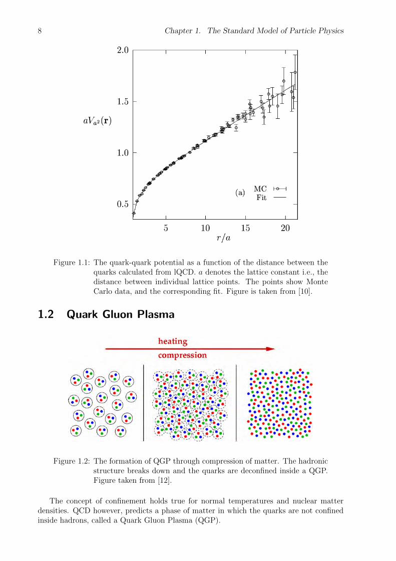
Figure 1.1: The quark-quark potential as a function of the distance between thequarks calculated from lQCD. a denotes the lattice constant i.e., thedistance between individual lattice points. The points show MonteCarlo data, and the corresponding fit. Figure is taken from [10].
1.2 Quark Gluon Plasma
Figure 1.2: The formation of QGP through compression of matter. The hadronicstructure breaks down and the quarks are deconfined inside a QGP.Figure taken from [12].
The concept of confinement holds true for normal temperatures and nuclear matterdensities. QCD however, predicts a phase of matter in which the quarks are not confinedinside hadrons, called a Quark Gluon Plasma (QGP).

1.2. Quark Gluon Plasma 9
Figure 1.3: QCD Phase Diagram. The paths of several large experiments areshown. Furthermore the conditions in the early Universe, nuclearmatter and neutron stars are indicated. It is worth mentioning thatplotting the phase space as a function of baryon density or baryon-chemical potential (as used in the text) makes no conceptual differ-ence, since the two are thermodynamically conjugate variables. Figuretaken from [12].
The main idea of a heavy ion physics QGP, sketched in figure 1.2, is as follows. Con-sider a fixed volume, in which hadrons are filled. Since hadrons have a non-zero spatialvolume [9], there exists a critical point where the hadrons completely fill out the vol-ume. Adding even more hadrons (or decreasing the size of the volume) will thus causethe hadronic structure to break down, creating a plasma of ‘free’ quarks and gluons. Itis worth mentioning that the quarks/gluons are still confined inside the plasma, but notinside hadrons.
The term plasma suggests a gas-like behaviour with few interactions. However thestate of matter created at the Relativistic Heavy Ion Collider (RHIC) at centre-of-massenergy
√sNN
= 200 GeV and at the LHC at√sNN
= 2760 GeV indicates a more stronglyinteracting QGP, with more interactions, thus behaving more like a perfect fluid [13].
The phase transition to QGP is predicted to happen at a critical temperature of TC =173 ± 3 MeV [14] for a chemical potential of µB = 0. An illustration of the QCD phasediagram can be seen in figure 1.3.
It is obvious from figure 1.3 that there are essentially two ways of gauging the QGPphase; by raising either the temperature or by raising the chemical potential. At the LargeHadron Collider5 the former approach is used.
5And the same is the case in previous experiments. The upcoming FAIR collider will follow the otherapproach.

10 Chapter 1. The Standard Model of Particle Physics
Cosmological Quark Gluon Plasma
Observational evidence in the field of cosmology coherently suggests that our Universestarted as a mathematical singularity exploding spectacularly in the Big Bang. All thematter/energy of the Universe thus was concentrated in a volume of high density, temper-ature and pressure; the necessary conditions for a QGP to have formed. As a consequenceof the rapid expansion, the Universe cooled down quickly. At approximately 1µs afterthe Big Bang the very hot Universe is believed to have been in a QGP phase, beforehadronising.
The cosmological QGP and the QGP probably created in heavy ion collisions are notbelieved to be identical. Firstly the cosmological QGP is believed to have existed for a timescale of 10−6 s whereas the observed heavy ion QGP has a lifetime of the order of 10−23 s∼ 1 fm/c [15]. Secondly, the baryon number densities of the early Universe is thought tobe of the order Nb/N ∼ 10−10 compared to the Nb/N ∼ 10−1 in heavy ion collisions [15].Here N refers to all particle types, i.e. hadrons, leptons, photons etc.
In the heavy ion collision QGP the baryonic density is sufficiently large, that stronginteractions between quarks and gluons will happen regularly, and thus the medium canbe said to be strongly interacting. This is believed to be in contrast to the situation inthe early Universe where the scarcity of baryons makes strong interactions improbable.Furthermore the lifetime of the cosmological QGP certainly allows it to reach thermalequilibrium. For the heavy ion collision QGP this is still a topic of dispute. Howeverrecent theoretical calculations indicate that thermalisation might be possible as early as0.35 fm/c after the collision [16].
1.3 Kinematic Variables
This section introduces kinematic variables and concepts which are fundamental to highenergy/heavy ion physics in general.
The four-momentum of a particle of rest mass m0, momentum ~p, and energy E is givenas:
P = (E, ~p) = (E, px, py, pz) (1.2)
The traditional convention of setting ~ = c = 1 is utilised here. For 2→ 2 particle reactionswith four-momenta P1 and P2 before the reaction and four-momenta P ′1 and P ′2 after thereaction, the so-called Mandelstam variables are useful:
s = (P1 + P2) = (P ′1 + P ′2)
t = (P1 − P ′1) = (P2 − P ′2)u = (P1 − P ′2) = (P2 − P ′1) (1.3)
Thus√s is the collision energy in the centre-of-mass frame, and similarly
√t is the momen-
tum transfer. For heavy ion collisions, the collision energy is typically given per nucleonpair in the notation
√sNN .
Kinematic variables are expressed in terms of the ALICE global coordinate system,which is illustrated in figure 1.4.
The momenta of the created particles, are split into a longitudinal component, pz, alongthe beam-line and a transverse momentum component, pT , orthogonal to the beam. The
1.3. Kinematic Variables 11
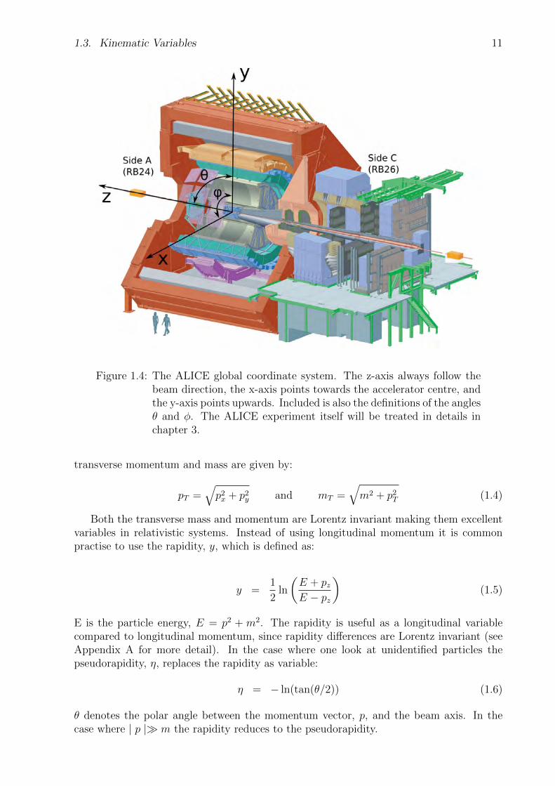
Figure 1.4: The ALICE global coordinate system. The z-axis always follow thebeam direction, the x-axis points towards the accelerator centre, andthe y-axis points upwards. Included is also the definitions of the anglesθ and φ. The ALICE experiment itself will be treated in details inchapter 3.
transverse momentum and mass are given by:
pT =√p2x + p2y and mT =
√m2 + p2T (1.4)
Both the transverse mass and momentum are Lorentz invariant making them excellentvariables in relativistic systems. Instead of using longitudinal momentum it is commonpractise to use the rapidity, y, which is defined as:
y =1
2ln
(E + pzE − pz
)(1.5)
E is the particle energy, E = p2 + m2. The rapidity is useful as a longitudinal variablecompared to longitudinal momentum, since rapidity differences are Lorentz invariant (seeAppendix A for more detail). In the case where one look at unidentified particles thepseudorapidity, η, replaces the rapidity as variable:
η = − ln(tan(θ/2)) (1.6)
θ denotes the polar angle between the momentum vector, p, and the beam axis. In thecase where | p | m the rapidity reduces to the pseudorapidity.

12 Chapter 1. The Standard Model of Particle Physics
Figure 1.5: Schematic illustration of a relativistic heavy ion collision. The partic-ipant nucleons of the overlap region between the colliding nuclei formthe high density fireball, whereas the rest of the nucleons continuesunaffected as spectators. Picture taken from [17].
1.4 Relativistic Collisions
Relativistic collisions can be divided into three categories:
AA Collisions between heavy ions. Heavy nuclei are collided, creating thousands of finalstate particles in each collision. At the ALICE experiment, which is the foundationfor this work, the main focus is on heavy ion PbPb collisions. Heavy ion collisionsare expected to create a QGP, before cooling down.
pp Collisions between protons. The main focus on the LHC pp program (that take up thevast majority of beam time) is to discover the Higgs boson and possibly verifying theexistence of SUper SYmmetric (SUSY) particles. However since ALICE is a heavyion detector, it does not have the trigger rate to gather enough statistics to be viablein those searches. Instead pp collisions at ALICE play another, but also importantrole in both looking for new physics, as well as a baseline measurement for PbPbcollisions.
pA Collisions between protons and heavy ions. The LHC has not provided collisionsbetween protons and lead-ions yet. For the heavy ion community this is a highpriority, since these asymmetrical collisions, does not have a dense hot medium, andthus can yield important insights into the initial state of collisions. The LHC willattempt to deliver the first pA collisions at the end of 2011. The run plans for thefollowing years will be heavily influenced depending on their success.
In the following an introduction to both proton-proton collisions and heavy ion collisionsis given.
1.4.1 Relativistic Heavy Ion Collisions
While the majority of the results in this thesis are from pp collisions, one should keep inmind that due to the ALICE experiment being a heavy ion detector, the long range mainfocus is still on heavy ion physics. Furthermore the concepts from heavy ion physics might

1.4. Relativistic Collisions 13
prove more and more useful, since pp collisions at very high energies start to resembleheavy ion collisions more and more, with for instance collective effects appearing [18].
In Figure 1.5 an illustration of a relativistic collision is shown as seen from the laboratoryframe of the nuclei. Each nucleus is highly Lorentz contracted along its direction of motion.
Participants and Spectators
The nucleons directly involved in the collision, called participants, interact strongly givingrise to a high density volume, known as the fireball. Nucleons outside the overlappingregion of the two nuclei are called spectators. They are unaffected by the collision exceptfor Coulomb-interactions and they retain their initial momentum, flying away from thefireball.
Figure 1.5 also introduces the impact parameter, b, which is the transverse distancebetween the centres of the two nuclei. Hence a large impact parameter corresponds to aperipheral collision, where a small region of the nuclei overlap, whereas a small impactparameter gives a central collision with a large overlapping region. As it is practicallyimpossible to measure the impact parameter directly, an experimental technique is used toconnect impact parameter with centrality. The centrality can be measured using the totalcharged particle multiplicity of the events. This is discussed in section 6.1.3.
The impact parameter is through models connected to the centrality of the collision inthe following way:
c =
∫ bc0
dσin(b′)
db′db′
σin(1.7)
Here σin,dσin(b′)
db′and bc are the total inelastic nuclear reaction cross section, the differential
cross section and a cut-off in the impact parameter respectively. Thus the centrality, c,denotes the probability that a collision occurs with a impact parameter of b ≤ bc. For asolid sphere dσin(b)
db= 2πbdb and thereby under the assumption that nuclei are identical and
spherical the centrality becomes:
c =
∫ bc0
2πbdb∫ 2R
02πbdb
=b 2c
4R2(1.8)
Here R denotes the radius of the nuclei. The impact parameter and the number of partic-ipants in the collision are statistically related. Their relation can be estimated using theGlauber model [19]. A short introduction to it can be found in Appendix B.
The Bjorken Picture
A very important contribution to heavy ion physics is a paper from 1983 by Bjorken[21], which uses a hydrodynamical description of the central rapidity region in heavy ioncollisions. The description relies on four important assumptions on collisions between nucleiwith nucleon number A:
Boost invariance : The rapidity densities dNdy
are independent of rapidity for at leasta few units of rapidity around mid-rapidity in pp and pA collisions. From this it isassumed that the same is true for AA collisions.

14 Chapter 1. The Standard Model of Particle Physics
Figure 1.6: Proposed space-time evolution of a heavy ion collision. Quarks andgluon are at first deconfined in a QGP which thermalises; eventuallythe hadrons freeze out and streams away freely. Picture taken from[20].
Transparency : The nuclei interpenetrates in the AA collision and the central plateauis formed through particle production from the breaking of colour strings. The frag-ments of the original nuclei end up some units of rapidity away from mid-rapidity.In Lorentz frames with velocities close to the mid-rapidity frame, the nuclei look likeflat pancakes.
Transverse expansion : The transverse expansion of the source can be ignoredfor most of the collisions because of the large initial transverse scale of the sourcecompared to its longitudinal scale. This is only true for central collisions and reducesthe problem to a 2-dimensional problem in the coordinates z and t.
Thermalisation : At some early time, assumed to be of the order of the characteristichadronic time scale t ∼ 1 fm/c, the system thermalises and hydrodynamics governsthe evolution and expansion of the source.
Figure 1.7: Simplistic view of a collision in the transparent Bjorken picture. Pic-ture taken from [12].

1.4. Relativistic Collisions 15
If it is assumed that at t ∼ 0 the longitudinal extension, z, is negligible, and the propertime, τ , is given by:
τ ≡ t
γ=
√t2(1− z2
t2)
=√t2 − z2 (1.9)
In a space-time diagram this yields hyperbolas of constant energy densities, which can beused to distinguish different evolutionary phases in heavy ion collisions. In figure 1.6 asketch of the space-time evolution of a central collision is shown.
In the Bjorken picture the incoming nuclei are transparent to each other as mentioned,allowing them to interpenetrate without loosing much of their initial kinetic energy. How-ever, upon doing so they leave a highly excited colour field between them, in which particleproduction take place due to the breaking of colour strings. The concept of transparencyis illustrated in figure 1.7.
The Landau Picture
Figure 1.8: Simplistic view of a collision in the stopping picture. Picture takenfrom [12].
The opposite of the transparent Bjorken picture is a picture where full nuclear stoppingis assumed. This picture was proposed by Landau in [22]. Landau argued that:
Full stopping : The incoming nuclei are fully stopped when hitting each other. Alltheir initial kinetic energy is deposited in the fireball.
Hydrodynamics : Particles in the fireball have small mean free paths, so the fireballcan be treated as an ideal fluid in the sense that it is non-viscous and non-heatconducting.
Adiabatic expansion : The fluid expands adiabatically, i.e. the entropy is constant.
A collision in accordance with the Landau picture is illustrated in figure 1.8. These twoextreme pictures corresponds to very different macroscopic physical phenomena. The trans-parent Bjorken picture is reminiscent of the early Universe, with very high temperature andlow baryo-chemical potential, µB. In the other end of the scale, Landau’s stopping pictureis reminiscent of the conditions inside stellar objects like neutron stars, with large µB andrelatively low temperature. At RHIC it was found by nuclear stopping measurements, thatthe higher the collision energy is, the more transparent the collision is [1, 23].

16 Chapter 1. The Standard Model of Particle Physics
Figure 1.9: Schematic of a pp collision. Figure is from [24]. An incoming partonmight branch (q → qg) before the collision in an initial-state shower.Similarly a parton branching after the collision is referred to as afinal-state shower. After the collision colour string span between theoutgoing quarks and gluons. These fragments into colourless hadrons,as described previously. The fragmented hadrons can be unstable, andfurther decay.
1.4.2 Proton-Proton Collisions
Initially, collisions between two protons might seem much simpler than collisions of ions,with hundreds of participants, but it is a truth with heavy modifications.
pp collisions serve as a great reference measurement for heavy ion measurements dueto a number of reasons. One of the main reasons is that pp collisions have not previouslybeen believed to create a QGP. Thus deviations in measured quantities in pp and heavy ioncollisions can serve as a probe of the differences between the two systems. And therefore,if no QGP is created in pp collisions, then differences between the two systems is usefulfor directly probing the characteristics of the QGP formed in PbPb collisions. However,it should be noted that it has been proposed that collective effects, and possibly even theformation of a QGP, could occur in very high energy pp collisions [18].
Regardless of whether or not such a QGP is formed in pp collisions, pp measurementsdoes have a full physics motivation in its own right, with an important contribution beingmultiplicity results as presented in this work.
A schematic of a pp collisions is shown in figure 1.9.
Diffraction
When dealing with inelastic pp collisions it is customary to distinguish between non-diffractive, single-diffractive and double diffractive events (ND, SD, and DD respectively).
The concept of diffraction in particle physics is analogous to diffraction in optics, wherelight beams scatter on obstacles.
A diffractive event is characterised by the colliding particle(s) being excited. Thisexcitation creates a diffractive system, that carries the quantum number of the originalparticle, and subsequently fragments/decays into final state particles. For SD events only

1.4. Relativistic Collisions 17
Figure 1.10: Left panel: Feynman diagram of a Regge Pole. The two gluonsexchange a particle of spin J = α(t). Right panel: An example of aChew-Frautschi plot, with the Regge trajectories for the ρ, ω and fmesons indicated.
one of the colliding particles becomes a diffractive system, whereas both of the particlesbecome diffractive systems in the case of DD events. As the name implies no diffractivesystems are created for ND events. The excitation of one or both of the incoming nucleonsare thought to stem from gluons exchanging a so-called Pomeron. In this context thePomeron is a strongly interacting colour singlet, which carry the quantum numbers ofthe vacuum [25]. However the exact nature and role of the pomeron in QCD is still notcompletely clear. [26]. In the following the theoretical motivation for the notion of pomeronexchange is briefly presented.
The introduction of the Pomeron stem from Regge Field Theory [26]. It describes theso-called Regge Pole, which corresponds to exchanging an object of spin J (which couldbe complex). A schematic Feynman diagram of the Regge Pole exchange is seen in theleft panel of figure 1.10. A way to organise particles is to map them by plotting J as afunction of mass squared, mJ . This plot is called a Chew-Frautschi plot, and is shown inthe right panel of figure 1.10. Hadrons of the same type (in this context meaning sameisospin, same parity etc.) can all be described by so-called Regge trajectories adhering tothe linear form:
J = α(t) = α0 + α′(t)m2J (1.10)
For all hadrons the intersection value of J at m2J = 0, ao, is below unity. The first equality
of (1.10) is due to the spin being dependent on the transferred momentum, t.
The contribution to the scattering amplitude in a Regge pole exchange at large energiess is given by [26]:
A(s, t) ∝ sα(t) (1.11)
Additionally the optical theorem for large s, can be rewritten, and yields the following

18 Chapter 1. The Standard Model of Particle Physics
Figure 1.11: The difference in rapidity density shape for ND, SD, and DD events.Note that the scale is different.
contribution to the total cross section from the Regge Pole [25]:
σtot =1
s=(A(s, 0)) ∝ sα(0) (1.12)
Since all hadrons follow Regge trajectories with a0 < 1 this can not explain the experimen-tal evidence that the total cross-section rises slightly with collision energy. For that a objectwith a0 > 1 is needed. This object is named the Pomeron, responsible for creating diffrac-tive systems. Having a single Regge Pole Pomeron exchange would make the cross-sectionrise as a power law of s. This is in contradiction to the Froissart-Martin bound [27], whichstates that the cross-section can not increase faster than ln2 s for s→∞. The contradictionis resolved by including multiple Pomeron exchanges (referred to as eikonalisation), whichin the end ensures that the cross-section increase is within the Froissart-Martin limit6.
Now turning back to the different types of diffractive events. The Pomeron exchangeand excitation of the incoming nuclei heavily affect the distribution of final state particlesobserved. Figure 1.11 shows the pseudorapidity density of ND, SD, and DD events. ForND events the distribution is maximum around mid-rapidity and falls of steeply. For SDevents one of the nuclei continues unaffected ending up at beam rapidity, whereas the otherfragments (mostly) into forward rapidities. In DD events both nuclei fragment giving twopeaks at forward rapidities and a minor dip in the central region.
Since the physics processes of collisions with diffraction and without can be significantlydifferent one would ideally measure only ND events. However this is seldom possible. His-torically, experiments have measured Non Single Diffractive events (i.e excluding the SDevents). This is experimentally possible by discriminating the SD events due to their rapid-ity asymmetry. The DD events however are difficult to separate from the ND events, whythe NSD event class is often used. Furthermore the cross-section of DD events comparedto ND events are not too significant (σDD/σINEL ∼ 0.1 [28]), and thus the NSD event classis not too different from a pure inelastic event class.
In this work NSD events have been analysed for pp collisions, and Minimum Bias eventshave been analysed for PbPb-collisions.
6A closing historical remark on this is that the Regge trajectories can be explained by either the hadronsbeing composite objects, or if they are describable by elastic strings. This observation is among theinfluences that lead to the realisation by Gell-Mann that hadrons are indeed composite objects, composedof quarks. The other possibility of having elastic strings heavily influenced the eventual creation of thefirst string theories.

1.5. Previous Heavy Ion Results 19
Figure 1.12: Left Panel: Nuclear modification factors measured by BRAHMS [29]in central AuAu and dAu collisions at
√sNN
= 200 GeV. Rightpanel: Nuclear modification factors measured in three centrality binsfor PbPb collisions at
√sNN
= 2760 GeV by ALICE [30]. The sup-pression seen at RHIC is confirmed by ALICE. The nuclear modifi-cation factor rises slowly with pT at very high pT .
1.5 Previous Heavy Ion Results
This section is devoted to giving a brief overview of some of the experimental highlights ofthe recent years. It is an intriguing period with two strong experimental programs settingthe stage; LHC gauging the highest energy possible, hoping to discover new physics andRHIC focused on scanning lower energies, in order to pin-point a possible QCD criticalpoint7
Interesting results have already been published, and will continue to be so in the comingtime. This chapter will only focus on briefly presenting three of the topics that have beeninstrumental in shaping the understanding of the medium created in heavy ion collisionsover the past years. The next chapter is dedicated solely to multiplicity theory and previousmultiplicity results.
High pT Suppression
One of the first indications of a QGP at RHIC was the discovery that high pT particlesin central AuAu collisions at
√sNN
= 200 GeV were suppressed compared to pp collisions.Experimentally this is measured by the nuclear modification factor:
RAA ≡d2N/dpTdηAA
Nbind2N/dpTdηpp(1.13)
where RAA is the transverse particle production of A+A collisions relative to a referenceof pp collisions scaled by the number of binary collisions, Nbin.
The results from RHIC [31, 32] prompted the measurement of RAA to be one of thetop priorities at the LHC. The first LHC results confirms the suppression of high pT par-
7QCD predicts a first order phase transition from hadronic matter to a QGP to have a minimum baryo-chemical potential. The onset of this 1st order transition is called the critical point. At lower potentialsthe phase transition is thought to be a smooth crossover.

20 Chapter 1. The Standard Model of Particle Physics
Figure 1.13: Nuclear modification factors for various particle species measuredby PHENIX and CMS. Left panel shows PHENIX data [31, 32, 35]from RHIC for π0, η and direct photons at
√sNN
= 200 GeV. Rightpanel shows preliminary CMS data [33] for charged particles, isolatedphotons and Z0. In both cases it is seen that the photons (and Z0),which do not interact strongly, are not suppressed.
ticles at LHC energies [30, 33]. Figure 1.12 shows the RAA results for three centralityclasses measured by ALICE in PbPb collisions at
√sNN
= 2760 GeV as well as RAA re-sults from BRAHMS at
√sNN
= 200 GeV. It is seen that there is heavy suppression overa very large pT -range, especially for the most central collisions. The suppression is at-tributed to coloured objects interacting strongly with the medium, by emitting gluons asbremsstrahlung [13]. This is in contrast to dAu collisions, as measured by BRAHMS, whereno suppression is seen, in accordance with expectations of no formed hot medium [29].
At very high pT the nuclear modification factor starts rising gently, thus there is lesssuppression. The cause of this rise is not fully understood, but various models includingGyulassy-Levai-Vitev energy loss models predicts this behaviour [33,34].
Direct photons, stemming from the initial interaction point/time, were however foundnot to be suppressed at RHIC [35]. Since they only couple to the electromagnetic force it isindicative that the medium suppressing high pT particles is in fact strongly interacting, butnot electromagnetically interacting. The nuclear modification factor of various particlesincluding direct and isolated photons8 from PHENIX and CMS respectively is shown infigure 1.13.
High pT suppression is a clear indication of the formation of a strongly interacting QGP.
Jet Quenching
Another of the early indications of the presence of a QGP at RHIC was the measurementof dihadron azimuthal correlations. The STAR experiment presented this in [36,37], whichis shown in the left panel of figure 1.14. Dihadron azimuthal correlation revolves aroundobserving jets of high momentum particles near the fireball edge. One of the jets (the
8Direct and isolated photons are both probes of the very early phase, but the terms are not necessarilyinterchangeable. Direct photon analyses have decay photons statistically removed; isolated photon analysestry to eliminate these by requiring that the selected photon is spatially isolated. Thus there can be subtledifferences between them. However, in the high pT suppression physics perspective they are comparable.

1.5. Previous Heavy Ion Results 21
Figure 1.14: Left panel: Jet Quenching measured by STAR at√sNN
= 200 GeV[36, 37]. The jet travelling the shortest path through the medium(∆φ ∼ 0) is enhanced compared to the jet travelling through thelongest path in the medium (∆φ ∼ π). This in not seen in dAuand pp collisions, and is interpreted as the existence of a stronglyinteracting QGP at RHIC. Right panel: A concrete example of a jetreconstruction from CMS at
√sNN
= 2760 GeV [38]. The leading jetappears to be much more energetic than the away-side jet.
leading jet) is emitted away from the fireball, while the other is emitted in the oppositedirection through the hot medium. In pp and dAu collisions the jets are measured at∆φ ∼ 0 and ∆φ ∼ π. However in AuAu collisions only the first jet is observed. Thejet traversing the longest distance through the medium is not detected. This is due to itinteracted strongly with the medium; it has been completely quenched by loosing most ofits energy to the medium.
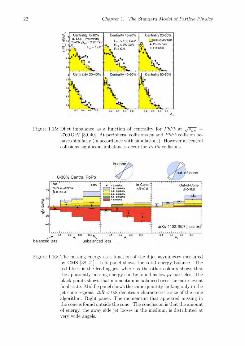
Moving to LHC energies, significant jet quenching is also seen. However at the LHCthe (weakened) away side jet escapes through the medium. This is shown by CMS [38]in the right panel of figure 1.14. However a lot of energy is missing. This dijet energyimbalance can be quantified by:
Aj =pT,1 − pT,2pT,1 + pT,2
(1.14)
Here pT,i is the transverse momentum of the ith jet. Figure 1.15 shows the number ofevents as a function of Aj for various centralities at
√sNN
= 2760 GeV, measured byATLAS [39, 40]. It is seen that for central collisions the jet events become increasinglyimbalanced, a feature not seen in neither pp collisions or HIJING/PYTHIA simulations.
The energy and momentum balance can be recovered by considering the entire final stateevent. For central heavy ion collisions the jet energy lost in the medium is re-distributedover the full φ-range. This is shown in figure 1.16. It shows (as a function of Aj) the
missing momentum by the quantity p‖T , which is the projection of pT on the leading jet
axis. Negative values show an excess towards the leading jet, and positive values show anexcess away from the leading jet. Thus it is seen that the leading jet consists mainly ofhigh pT particles in the cone region. On the opposite side, the entire momentum of theaway side jet is not found in the cone. Looking in the region outside the cone, it is seenthat the remaining momentum of the away side jet has been redistributed to this region.Overall the momentum balance of the entire final state is conserved.
22 Chapter 1. The Standard Model of Particle Physics
Figure 1.15: Dijet imbalance as a function of centrality for PbPb at√sNN
=2760 GeV [39,40]. At peripheral collisions pp and PbPb collision be-haves similarly (in accordance with simulations). However at centralcollisions significant imbalances occur for PbPb collisions.
Figure 1.16: The missing energy as a function of the dijet asymmetry measuredby CMS [38, 41]. Left panel shows the total energy balance. Thered block is the leading jet, where as the other colours shows thatthe apparently missing energy can be found as low pT particles. Theblack points shows that momentum is balanced over the entire eventfinal state. Middle panel shows the same quantity looking only in thejet cone regions. ∆R < 0.8 denotes a characteristic size of the conealgorithm. Right panel: The momentum that appeared missing inthe cone is found outside the cone. The conclusion is that the amountof energy, the away side jet looses in the medium, is distributed atvery wide angels.

1.5. Previous Heavy Ion Results 23
Figure 1.17: Measurements of flow from ALICE [42–44]. Left panel: The ellip-tic flow at various centralities, compared to the measurements fromSTAR at RHIC energies. It is seen that the elliptic flow is simi-lar at both energies. Right panel: The flow components, v2 − v5.Comparisons with hydrodynamical calculations show agreement (tosome extent). It indicates that the medium created flows perfectly(or close to).
Flow
One of the collective dynamics of particles, which has garnered significant interest in recentyears, is the concept of anisotropic transverse flow. Anisotropic transverse flow is caused byinitial spatial asymmetries in the overlap region between the colliding nuclei. This spatialasymmetry give rise to pressure gradients, which causes a momentum asymmetry and thusasymmetry in the azimuthal distribution of particles. The distribution can be describedby a Fourier expansion [45]:
r(φ) =a02π
+1
π
∞∑n=1
(xn cos(nφ) + yn sin(nφ)) (1.15)
Here a0 is a constant. xn and yn are the components of the expansion along the respectiveaxis’. The Fourier transformation of (1.15) is used to quantise the flow [46]:
Ed3N
d3p=
1
2π
d2N
pTdpTdy(1 +
∞∑n=1
2vn cos(n(φ−Ψr))) (1.16)
Here Ψr is the azimuthal angle of the reaction plane to the xz-plane. The reaction planeis by definition spanned by the impact parameter vector and the z-axis. The harmonicscoefficients vn describes the various types of flow. v1 is called direct flow and v2 is calledelliptic flow. Up until recently, especially the elliptic flow was deemed important in thedescription of heavy ion collisions. Now the consensus is that the higher harmonics play alarge role as well.
In the left panel of figure 1.17 the newest measurement by ALICE [42,44] of the ellipticflow at different centralities can be seen. Comparisons to STAR measurements at RHICenergies show that the elliptic flow is comparable over the large range of energy.
Traditionally the overlap region between the colliding nuclei have been perceived as analmond shape. However recent calculations show that the fluctuations in the position ofindividual partons for each event causes the overlap to deviate significantly from almondshape. This can be seen in figure 1.18.

24 Chapter 1. The Standard Model of Particle Physics
Figure 1.18: Left panel: An illustration of the concept of reaction plane. Figureis from [47]. Right panel: Detailed calculations of the overlap regionbetween the nuclei, show that the shape can deviate significantlyfrom almond shaped. This is due to fluctuations in the positions ofthe individual partons at the time of collisions. Figure is from [48].
In the right panel of figure 1.17 measurements from ALICE [43, 44] show the higherharmonics (v2 − v5) for semi-peripheral collisions (30-40%). Also shown is the theoreticalpredictions from hydrodynamical calculations with the shear viscosity per entropy, η/s,being either 0 or 0.08 (∼ 1/(4π)).
Anti de Sitter/Conformal Field Theory (AdS/CFT), a proposed duality between stringtheory and quantum field theory, predicts that the universally lowest possible value of η/sis 1/(4π) [16]. This value corresponds to a perfect fluid. As can be seen there is reasonableagreement between the AdS/CFT calculations and the data, which is the main reason theQGP of heavy ion collisions is often termed a perfect fluid.
Another thing to note about the right panel of figure 1.17 is that it appears that v2 isclearly dominant over the higher order harmonics. However the strength of v2 is caused bythe main pressure gradients of the almond shape, which is very prevalent in semi-peripheralcollisons. Going to more and more central collisions will make the overlap region less andless almond shaped (for a full head on collision it is the shape of the nuclei). Howeverfluctuations will create variances in each event. Thus for central collisions, v2 becomesless and less dominant compared to the higher order harmonics. At very central collisionsv2 ∼ v3 ∼ v4.
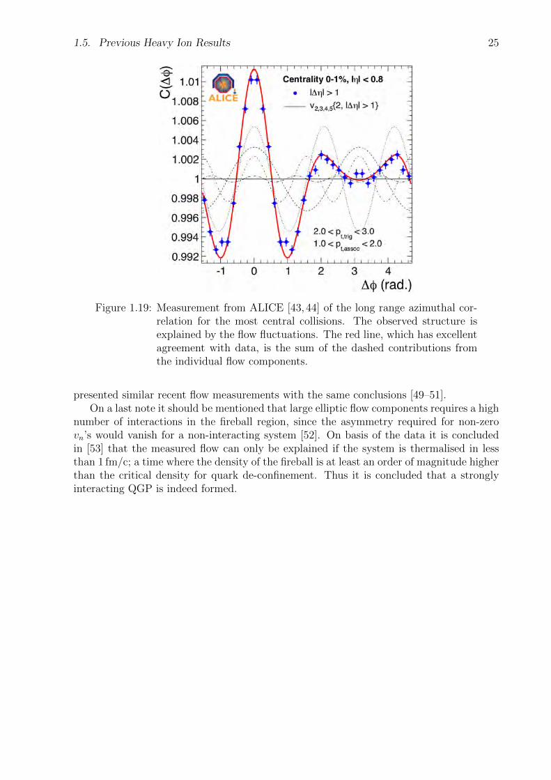
A clear example of the importance of higher harmonics comes from the measurementsof azimuthal long range correlations i.e., taking one jet particle in a given pT region andthen comparing it to all particles some minimum ∆η away at another pT range. Themeasurement by ALICE [43, 44] of this correlation can be seen in figure 1.19. Included asthe dashed lines are the contributions of the different flow types. The red line is the sum ofthe dashed lines i.e., it is not a fit to the data. The agreement is excellent. Thus fluctuations(and hence significant higher order flow) can completely account for the observed doublehump structure of long range azimuthal correlations. Until quite recently this structurewas attributed to a so-called Mach cone shock wave explanation. With the data presentedhere it is clear that the Mach cone idea is not needed for explaining the phenomenon.The other LHC experiments besides ALICE, as well as the PHENIX experiment, have also
1.5. Previous Heavy Ion Results 25
Figure 1.19: Measurement from ALICE [43, 44] of the long range azimuthal cor-relation for the most central collisions. The observed structure isexplained by the flow fluctuations. The red line, which has excellentagreement with data, is the sum of the dashed contributions fromthe individual flow components.
presented similar recent flow measurements with the same conclusions [49–51].On a last note it should be mentioned that large elliptic flow components requires a high
number of interactions in the fireball region, since the asymmetry required for non-zerovn’s would vanish for a non-interacting system [52]. On basis of the data it is concludedin [53] that the measured flow can only be explained if the system is thermalised in lessthan 1 fm/c; a time where the density of the fireball is at least an order of magnitude higherthan the critical density for quark de-confinement. Thus it is concluded that a stronglyinteracting QGP is indeed formed.

26 Chapter 1. The Standard Model of Particle Physics
Chapter 2
Charged Particle Multiplicity
Measuring the charged particle multiplicity of relativistic collisions, is one of the very fun-damental measurements. For the same reason the first publications from a new experimentwill often revolve around charged particle multiplicities. These topics will then usually berevisited later on with improved statistics and better detector understanding.
From this point on, the shorter term ’multiplicity’ will denote ‘charged particle multi-plicity’, where nothing else is specifically stated.
Multiplicity measurements typically fall into the following sub-groups:
Pseudorapidity density dNch
dη: Measurement of the average multiplicity as a functions of
η.
Multiplicity distributions P(Nch): Measurement of the distribution of integrated multi-plicities i.e., the total multiplicities of events in a given η-interval.
KNO scaling 〈Nch〉P(z): Derives from the multiplicity distribution, by plotting it inKNO-variables, P (Nch) 〈Nch〉 as a function of z ≡ Nch/ 〈Nch〉. This probes the energyscaling behaviour of multiplicity distributions.
Energy scaling: Derives from either dNch
dηor the multiplicity distributions by surveying the
multiplicity at a given pseudorapidity as a function of energy.
Measurements of multiplicities yield some insight into the collisions themselves, but arealso crucial as input parameters for a multitude of models, explaining various phenomenonsat later stages in the collisions.
The main goal of this work is to present multiplicity distributions and look for KNOscaling, but throughout this work, results will be presented on all four sub-groups. Theremainder of this section is devoted to presenting some of the theoretical framework behindunderstanding charged particle multiplicity, followed by an overview of the measurementspreviously conducted on multiplicities.
2.1 Negative Binomial Distributions
It is found that a Negative Binomial Distribution (NBD) describe the observed multiplicitydistributions at lower energies very well [24]. In general it is given by:
P (n; p; k) =
(n+ k − 1
n
)(1− p)npk (2.1)
27

28 Chapter 2. Charged Particle Multiplicity
Figure 2.1: Examples of negative binomial distributions, with different parametervalues. For NBDs with the same 〈n〉, the k-parameter determinesthe shape of the distribution. Lower k-values correspond to a flatterdistribution.
To describe NBDs, consider a series of Bernoulli trials, each with two potential outcomes— ‘success’ or ‘failure’ — with the probabilities p and (1− p) respectively. The NBD thendescribes the distribution of number of successes, n, observed before having the kth failure.For k →∞ the NBD reduces to the Poisson distribution, and for k = 1 it is the geometricdistribution.
Multiplicity distributions are described well using NBDs with p−1 = 1 + 〈n〉 /k, where〈n〉 is the average multiplicity, thus yielding the following form [54]:
P (n; 〈n〉 ; k) =
(n+ k − 1
n
)(〈n〉 /k
1 + 〈n〉 /k
)n1
(1 + 〈n〉 /k)k(2.2)
Fig. 2.1 illustrates several NBDs, with different parameters.
Why multiplicity distributions are well described by NBDs are still not fully under-stood. Various attempts to theoretically generate negative binomially shaped multiplicitydistributions from general particle production principles have been undertaken over theyears [55]. The one most frequently used is referred to as the clan model [56, 57], and willbe introduced in the following.
Multiplicity distributions can be characterized by a recurrence relation between collisionwith n+1 particles and n particles. While the individual particles can be of the same type,they are always distinguishable by their momenta. In general, a given collision of n + 1particles can be related to n + 1 collisions each having n particles. These n + 1 collisions(of n particles) are the ones left if any single one of the particles from the initial n + 1multiplicity collision were removed. Thus the simplest recurrence relation, g(n), is given

2.1. Negative Binomial Distributions 29
by:
g(n) =(n+ 1)P (n+ 1)
P (n)(2.3)
Inserting (2.2) into (2.3), and using(ij
)= i!/j!(i− j)! yields:
g(n) = (n+ k)〈n〉 /k
(〈n〉 /k) + 1
=〈n〉 k〈n〉+ k
+ n〈n〉〈n〉+ k
= a+ bn where a =〈n〉 k〈n〉+ k
and b =〈n〉〈n〉+ k
(2.4)
Thus for a negative binomial distribution the recurrence relation gives that g(n) is linearin n.
The clan model describes particle multiplicity in terms of clusters (or clans). In thissense a cluster consists of all particles originating (directly or indirectly) from the originallyproduced particle, which is denoted the ancestor of the cluster. The additional clusterparticles can come from various cascading processes such as decays and fragmentation. If anancestor does not produce any other particle, it is considered a one-particle cluster, and isits own ancestor. In the clan model it is assumed that ancestors are created independently,i.e. with no regard to whether other ancestors exist.
Thus, the production of the (N + 1)th ancestor is independent of the existance of theother N ancestors. The production follows a Poisson distribution, P (n) = γne−γ/n! [58].It is characterized by having g(n) = γ = constant, and thus the production of ancestorsis represented by the constant term of (2.4). The linear term, bn, then represents theeffect of the particles created within clusters. It is a reasonable assumption that this effectis proportional to the number of already present particles in the cluster, and thus then-dependence.
As discussed the probability, P ′(N), to produce N clans is given by a Poisson distri-bution. The probability, Pc(nc), to produce nc particles in the cth clan is given by therequirement that a clan cannot be empty
Pc(0) = 0 , (2.5)
and the assumption that producing nc + 1 is proportional to nc with the probability p
(nc + 1)Pc(nc + 1)
Pc(nc)= pnc . (2.6)
By induction, it can be shown that
Pc(nc) = Pc(1)pnc−1
nc. (2.7)
The probability to produce a total of n particles is given by
P (n) =n∑N
[P ′(N)
(n1+...+nN=n∑ N∏
c
Pc(nc)
)], (2.8)
where nci ∈ [1, n] is the number particles produced by the cth clan. Using the definition ofthe Poisson distribution and inserting (2.7) into (2.8) yields:
P (n) ∝ pnn∑N
[1
N !
(〈N〉Pc(1)
p
)N (n1+...+nN=n∑(n1...nN)−1
)]. (2.9)
30 Chapter 2. Charged Particle Multiplicity
The expression in (2.9) can be identified as a NBD by Taylor expanding the relation(1− z)−L = exp(−L ln(1− z)), and equating its coefficients [56]. This yield an identity ofthe form:
n∑N
kN
N !
n1+...+nN=n∑(n1...nN)−1 = k(k + 1)...(k + n− 1)/n! (2.10)
where
k =〈N〉Pc(1)
p(2.11)
Thus we end up with the expression:
P (n) ∝ pnk(k + 1)...(k + (n− 1)
n!=
(n+ k − 1
n
)pn (2.12)
which is recognized as the negative binomial form from (2.1) (without a factor of pk).We end this section by summarising, that if the collision dynamics follows the clan
model, the resulting multiplicity distributions will be well described by negative binomialdistributions.
2.2 Koba–Nielsen–Olesen Scaling
In his 1969 paper [59], Feynman concludes that the mean total number of particles riseslogarithmically with
√s. He argues that the probability of finding a particle of type i,
mass m, transverse momentum pT , and longitudinal momentum pz is of the form:
Pi(pT , pz,m) = fi(pT , pz/W )dpzd
2pTE
(2.13)
where the energy of the particle E, and the parameter W is given by:
E =√m2 + p2T + p2z =
√m2T + p2z and W =
√s
2(2.14)
The function fi(pT , pz/W ) is a structure function and is known as the Feynman function.Feynman’s assumption is that fi is independent of W, which is called Feynman scaling.Furthermore the fractional longitudinal momentum in fi, xF ≡ pz/W , is often referred toas the Feynman-x.
One can rewrite (2.13) using the invariant cross section, σ:
1
σE
d3σ
dpzd2pT= fi(pT , xF ) (2.15)
Integrating (2.15) and using that fi factorizes such that∫fi(pT , xF )d2pT = fi(xF ) [24]
gives the following expression for the mean multiplicity:
〈N〉 ≡∫ ∞−∞
1
σE
d3σ
dpzd2pT
d3p
E=
∫ ∞−∞
fi(pT , xF )d3p
E=
∫ ∞−∞
fi(xF )dpz√
W 2x2F +m2T
(2.16)
which by changing integration variable through dpz = WdxF becomes:
〈N〉 =
∫ 1
−1fi(xF )
dxF√x2F +
m2T
W 2
(2.17)

2.2. Koba–Nielsen–Olesen Scaling 31
For collisions of identical particles fi(xF ) is symmetrical, and thus the integral is alsosymmetrical9. Integration by parts of (2.17) yields:
〈N〉 =
[2fi(xF ) ln
(xF +
√x2F +
m2T
W 2
)]10
− 2
∫ 1
0
∂fi(xF )
∂xFln
(xF +
√x2F +
m2T
W 2
)dxF
(2.18)The second term can be shown to converge to a constant for all W [24]. Thus, (2.18) thenbecomes:
〈N〉 = 2fi(1) ln
(1 +
√1 +
m2T
W 2
)− 2fi(0) ln
(mT
W
)+ constant (2.19)
In the limit of W →∞, (2.19) becomes:
limW→∞
〈N〉 = limW→∞
2fi(1) ln
(1 +
√1 +
m2T
W 2
)− lim
W→∞2fi(0) ln(mT ) +
limW→∞
2fi(0) ln(W ) + limW→∞
constant
= 2fi(0) ln(W ) + constants (2.20)
The limit of the first, second and fourth term in (2.20) are all constants, and thus underthe assumption Feynman made, that fi(0) > 0 it is clear that for large W:
〈N〉 ∝ ln(W ) ∝ ln(√s) (2.21)
The concept of Feynman scaling was the main assumption when Koba, Nielsen, and Olesensuggested a similar scaling in 1972 [60]. This scaling is now called KNO scaling. It is derivedfrom generalising (2.17) to a q-dimensional Feynman scaling function, f (q) i.e., q particleswith energy Eq, momenta pz,q and pT,q and Feynman-x xF,q. Thus we have:
〈n(n− 1)...(n− q − 1)〉 =
∫f (q)((xF,1, pT,1); ...; (xF,q, pT,q))
dpz,1E1
dp2T,1...dpz,qEq
dp2T,q (2.22)
As in the Feynman scaling case integration by parts is used for all xF,q in (2.22) whichultimately (after a significant amount of calculations [60]) leads to:
〈n(n− 1)...(n− q − 1)〉 =
∫ [f q((0, pT,1); ...; (0, pT,q)) +O
(1
ln(s)
)]×∏q
ln
(s
p2T,q +m2
)d2pT,1...d
2pT,q
= f (q)(0, ..., 0)(ln(s))q +O((ln(s))q−1) (2.23)
O((ln(s))q−1) refers to all terms which go at most like ln(s)q−1 and f (q)(xF,1, ..., xF,q) =∫d2pT,1...d
2pT,qf(q)((xF,1, pT,1); ...; (xF,q, pT,q)). It can be shown [60] that (2.23) can be
rewritten in the form
〈nq〉 ≡∑n
Pn(s)nq ∼∫ ∞0
Pn(s)nqdn = f (q)(0, ..., 0)(ln(s))q +O((ln(s))q−1)(2.24)
9For collision systems where the participants are not identical, the integral can be done separately fornegative and positive xF , yielding the same result as in the symmetric case [24].
32 Chapter 2. Charged Particle Multiplicity
By dividing both sides of (2.24)by (ln(s))q(f (1)(0))q it takes the form:∫ ∞0
Pn(s)zq ln(s)f (1)(0)dz = cq +O(
1
ln(s)
)(2.25)
where
z =n
ln(s)f (1)(0)and cq =
f (q)(0, ..., 0)
(f (1)(0))q(2.26)
The moments cq, which are independent of W , thus uniquely determines the multiplicitydistribution:
Pn(s) =1
ln(s)f (1)(0)Φ
(n
ln(s)f (1)(0)
)+O
(1
ln(s)2
)(2.27)
It can be shown that 〈n〉 ∼ ln(s)f (1)(0) [60], and thus z = n/ 〈n〉, which yields theKNO scaling law in the following form:
Pn(s) =1
〈n〉Ψ(z) +O
(1
〈n〉2
)(2.28)
The functional form of Ψ(z) is not known a priori, and in principle could be different fordifferent collision systems, and dependent on which type of particle being measured.
Substituting z = n/ 〈n〉 into (2.25) yields the moments in the following form:
cq =〈nq〉〈n〉q
(2.29)

2.3. Previous Multiplicity Measurements 33
2.3 Previous Multiplicity Measurements
This section is devoted to presenting previous multiplicity measurements. Since multiplicityis one of the fundamental quantities it has been measured at various accelerator facilitiesaround the world over many decades.
This section will first present measurements on multiplicity distributions (including inKNO variables), followed by measurements on dNch
dηand energy scaling.
2.3.1 Multiplicity Distributions
The very first hadron collider was the ISR (Intersecting Storage Ring). It was located atCERN, and was operated from 1971 to 1984. The ISR has collided pp, pp, and pα at a topcenter of mass energy 63 GeV. At the ISR the Split Field Magnet detector [61] measuredmultiplicities at four energies;
√s = 30.4, 44.5, 52.6 and 62.2 GeV [62]. These can be seen
in figure 2.2.
Figure 2.2: Charged particle multiplicity distributions from the Split Field Mag-net detector at the ISR at four energies [62]. Left panel shows thenormalised distributions and the right panel show them in KNO vari-ables. It is clear that KNO scaling is valid at ISR energies.
In 1976 CERN started operating the SPS (Super Proton Synchroton). Over the yearsthe SPS has accelerated e−, e+, p, p and ions in various combinations. Later on, aftermodifications, the SPS collided pp at the top energy
√s = 900 GeV10.
At the SPS two different experiments have published a variety of multiplicity measure-ments; UA1 [69] and UA5 [70] (Underground Area 1 & 5 respectively). Both publishedresults at
√s = 200, 540 and 900 GeV [63–68]. Besides these common energies, UA1 also
published multiplicities at√s = 500 GeV [67].
Measurements from UA5 of multiplicity distributions with |η| < 1.5 at their threeenergies can be seen in figure 2.3. Furthermore the UA1 results (|η| < 2.5) can be seenin figure 2.4. Even though UA5 and UA5 published for different η-ranges it is interestingto compare the two. UA1 finds that KNO scaling holds up to and including 900 GeV,
10In this period it is sometimes referred to as SppS. However throughout in this work it will still bereferred to as SPS.
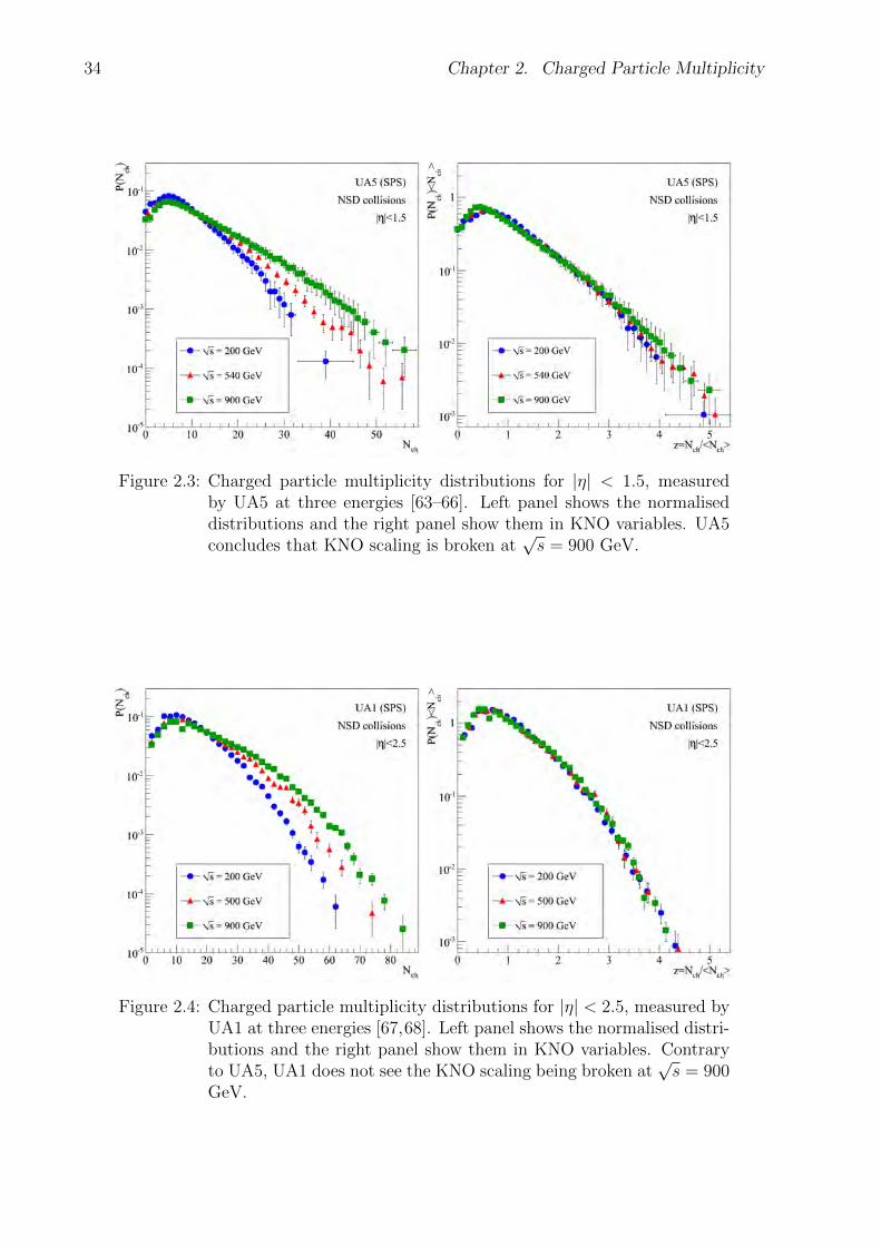
34 Chapter 2. Charged Particle Multiplicity
Figure 2.3: Charged particle multiplicity distributions for |η| < 1.5, measuredby UA5 at three energies [63–66]. Left panel shows the normaliseddistributions and the right panel show them in KNO variables. UA5concludes that KNO scaling is broken at
√s = 900 GeV.
Figure 2.4: Charged particle multiplicity distributions for |η| < 2.5, measured byUA1 at three energies [67,68]. Left panel shows the normalised distri-butions and the right panel show them in KNO variables. Contraryto UA5, UA1 does not see the KNO scaling being broken at
√s = 900
GeV.
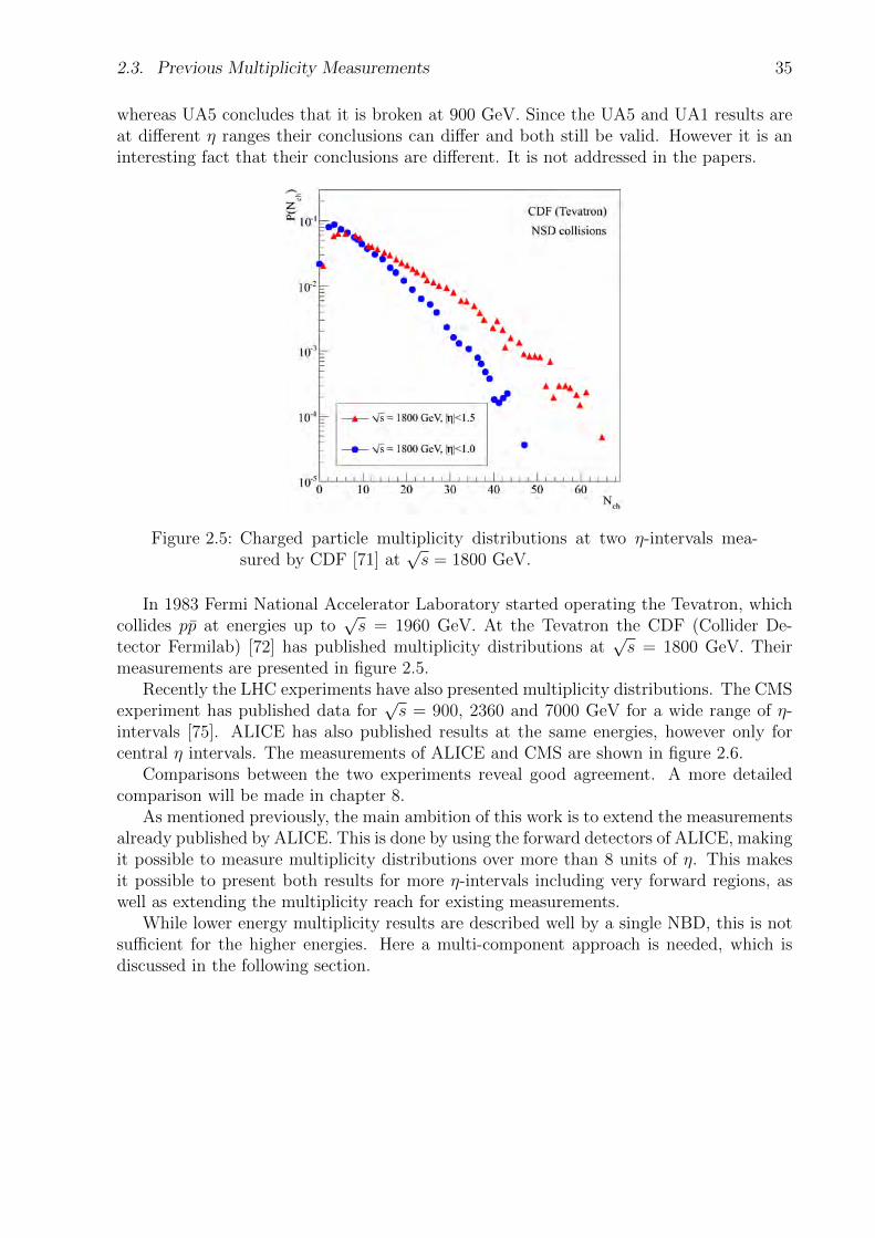
2.3. Previous Multiplicity Measurements 35
whereas UA5 concludes that it is broken at 900 GeV. Since the UA5 and UA1 results areat different η ranges their conclusions can differ and both still be valid. However it is aninteresting fact that their conclusions are different. It is not addressed in the papers.
Figure 2.5: Charged particle multiplicity distributions at two η-intervals mea-sured by CDF [71] at
√s = 1800 GeV.
In 1983 Fermi National Accelerator Laboratory started operating the Tevatron, whichcollides pp at energies up to
√s = 1960 GeV. At the Tevatron the CDF (Collider De-
tector Fermilab) [72] has published multiplicity distributions at√s = 1800 GeV. Their
measurements are presented in figure 2.5.Recently the LHC experiments have also presented multiplicity distributions. The CMS
experiment has published data for√s = 900, 2360 and 7000 GeV for a wide range of η-
intervals [75]. ALICE has also published results at the same energies, however only forcentral η intervals. The measurements of ALICE and CMS are shown in figure 2.6.
Comparisons between the two experiments reveal good agreement. A more detailedcomparison will be made in chapter 8.
As mentioned previously, the main ambition of this work is to extend the measurementsalready published by ALICE. This is done by using the forward detectors of ALICE, makingit possible to measure multiplicity distributions over more than 8 units of η. This makesit possible to present both results for more η-intervals including very forward regions, aswell as extending the multiplicity reach for existing measurements.
While lower energy multiplicity results are described well by a single NBD, this is notsufficient for the higher energies. Here a multi-component approach is needed, which isdiscussed in the following section.

36 Chapter 2. Charged Particle Multiplicity
Figure 2.6: Charged particle multiplicity distributions at various η-intervals mea-sured by ALICE [73,74] and CMS [75] at
√s = 900 GeV, 2360 GeV,
and 7000 GeV.
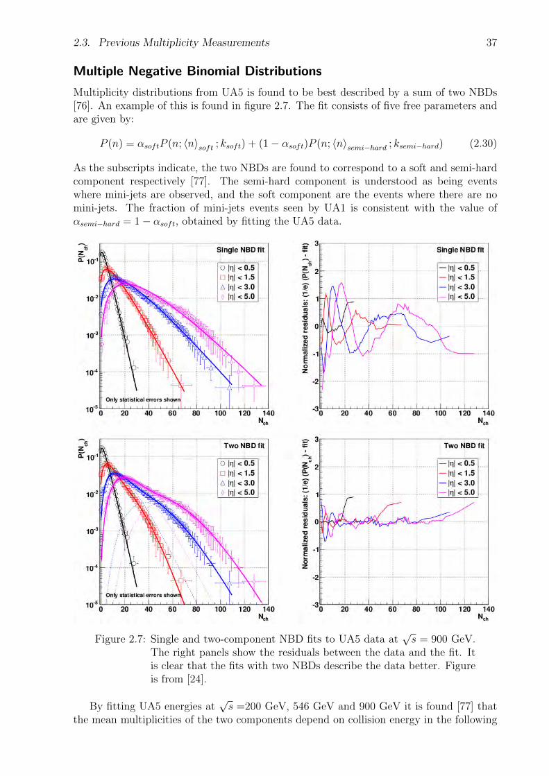
2.3. Previous Multiplicity Measurements 37
Multiple Negative Binomial Distributions
Multiplicity distributions from UA5 is found to be best described by a sum of two NBDs[76]. An example of this is found in figure 2.7. The fit consists of five free parameters andare given by:
P (n) = αsoftP (n; 〈n〉soft ; ksoft) + (1− αsoft)P (n; 〈n〉semi−hard ; ksemi−hard) (2.30)
As the subscripts indicate, the two NBDs are found to correspond to a soft and semi-hardcomponent respectively [77]. The semi-hard component is understood as being eventswhere mini-jets are observed, and the soft component are the events where there are nomini-jets. The fraction of mini-jets events seen by UA1 is consistent with the value ofαsemi−hard = 1− αsoft, obtained by fitting the UA5 data.
Figure 2.7: Single and two-component NBD fits to UA5 data at√s = 900 GeV.
The right panels show the residuals between the data and the fit. Itis clear that the fits with two NBDs describe the data better. Figureis from [24].
By fitting UA5 energies at√s =200 GeV, 546 GeV and 900 GeV it is found [77] that
the mean multiplicities of the two components depend on collision energy in the following

38 Chapter 2. Charged Particle Multiplicity
way:
〈n〉soft = −5.54 + 4.72 ln(√s) (2.31)
〈n〉semi−hard ∼ 2 〈n〉soft (2.32)
In [77] a correction of the order 〈n〉 ln2(√s) to (2.32) is also proposed. However, due
to the quality of the fits to the data in [77], it is still debated if the correction is actuallythere, or (2.32) is valid.
On a similar note it should be mentioned that the fits to the UA5 data finds thatthe shape parameter of the soft component is energy independent (ksoft ∼ 7), which isequivalent to KNO scaling being valid. For the semi-hard component this is not true. Athigher collision energies a third component has been proposed [78].
The authors of [79] and [80] conclude that the second and possibly third components arethe results of multi-parton interactions. Multi-parton interactions denote having multipleindependent parton-parton interactions within a single collision. In the context of thisdiscussion the semi-hard and the third component are identified as double-parton andtriple-parton interactions. Thus, said in a different way, the cause of mini-jet events mightbe double-parton interactions.
2.3.2 dN/dη measurements
Figure 2.8: dNch
dηmeasurements from pre-LHC experiments [62, 63, 65, 68, 81–83].
Going up in collision energy increases and widens the distribution. Alldistributions are from NSD collisions except the lowest energy resultfrom SFM, which are INEL.
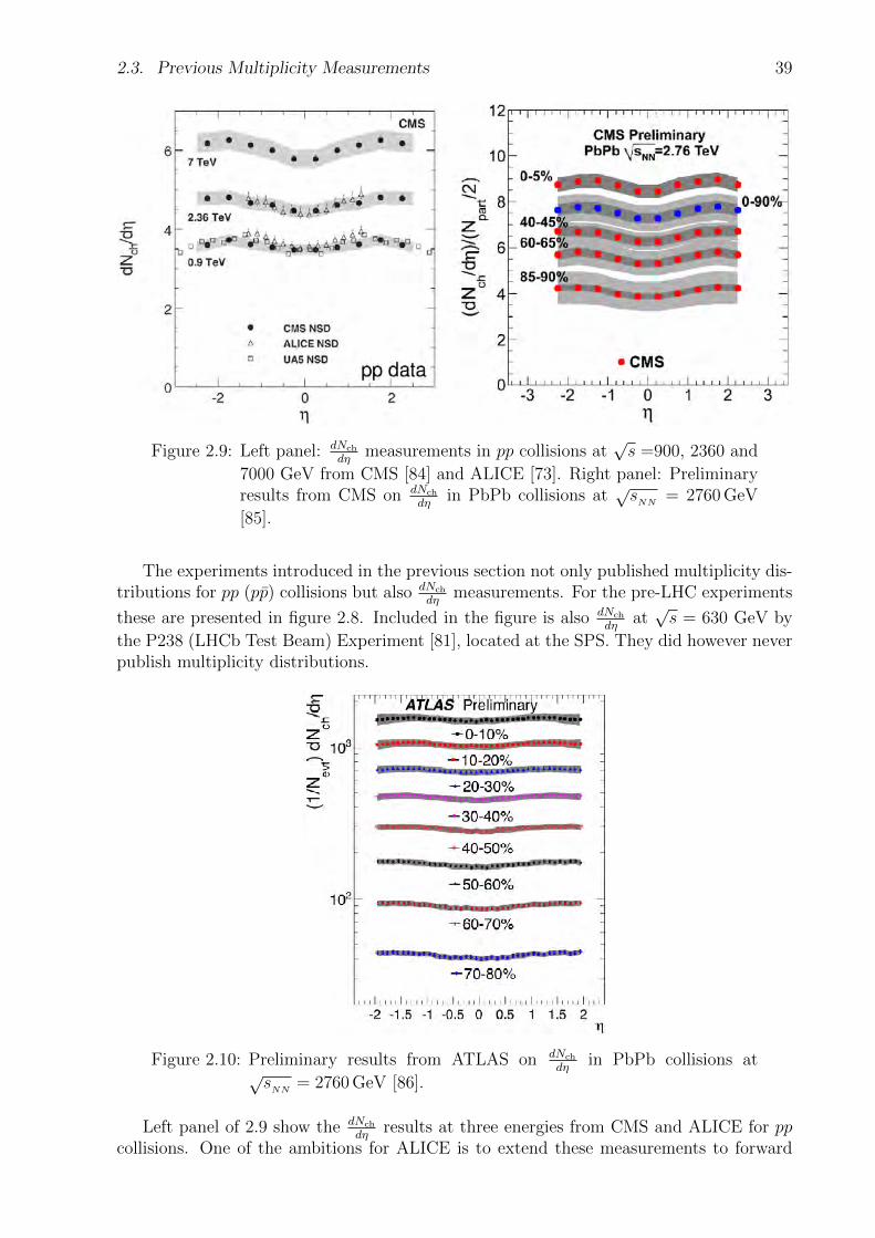
2.3. Previous Multiplicity Measurements 39
Figure 2.9: Left panel: dNch
dηmeasurements in pp collisions at
√s =900, 2360 and
7000 GeV from CMS [84] and ALICE [73]. Right panel: Preliminaryresults from CMS on dNch
dηin PbPb collisions at
√sNN
= 2760 GeV
[85].
The experiments introduced in the previous section not only published multiplicity dis-tributions for pp (pp) collisions but also dNch
dηmeasurements. For the pre-LHC experiments
these are presented in figure 2.8. Included in the figure is also dNch
dηat√s = 630 GeV by
the P238 (LHCb Test Beam) Experiment [81], located at the SPS. They did however neverpublish multiplicity distributions.
Figure 2.10: Preliminary results from ATLAS on dNch
dηin PbPb collisions at
√sNN
= 2760 GeV [86].
Left panel of 2.9 show the dNch
dηresults at three energies from CMS and ALICE for pp
collisions. One of the ambitions for ALICE is to extend these measurements to forward

40 Chapter 2. Charged Particle Multiplicity
η-3 -2 -1 0 1 2 3 4 5
ηdch
dN ev
N1
200
400
600
800
1000
1200
1400
1600
1800
20000 - 5 %5 - 10 %10 - 20 %20 - 30 %30 - 40 %40 - 50 %50 - 60 %60 - 70 %70 - 80 %
Figure 2.11: Still unpublished dNch
dηmeasurements over the entire η-range of AL-
ICE for PbPb collisions at√sNN
= 2760 GeV [87].
regions using the FMD system.Right panel of figure 2.9 show the preliminary dNch
dηmeasurements in PbPb collisions
at√sNN
= 2760 GeV from CMS. Similarly figures 2.10 and 2.11 show preliminary PbPbresults from ATLAS and ALICE respectively.
In general, it is found that the plateau in mid-rapidity increases and widens as a functionof collision energy.
2.3.3 Mean Multiplicity Energy Dependence
In this last section results on the energy scaling of the mean multiplicity is presented. Figure2.12 show dNch
dηat mid-rapidity published by many experiments over a wide interval of
collision systems and energies. The mean multiplicity is scaled by the number of participantpairs of the collisions, to correct for different collision systems and centrality selections.It is seen that AA and pp collisions have slightly different behaviours. Both, however areproportional to sANN .
Figure 2.13 show the theoretical predictions for the dNch
dηat mid-rapidity in PbPb colli-
sions at√sNN
= 2760 GeV, compared to the measurement from ALICE. It is obvious that

2.3. Previous Multiplicity Measurements 41
predicting this is far from trivial, as seen by the large variance in predicted values11. Thereference numbers for the individual models in figure 2.13 corresponds to the referencesin [88], where the figure is from.
Figure 2.12: Mean multiplicity at mid-rapidity scaled with number of participantpairs, over a wide range of collision systems and energies. For bothpp and PbPb collisions the mean multiplicity increases as sANN , butwith different values of A. Figure is from [88].
Figure 2.13: Theoretical predictions of the dNch
dηat mid-rapidity in PbPb collisions
at√sNN
= 2760 GeV. In the top the measured value from ALICEis indicated. The reference numbers for the individual models in thefigure corresponds to the references in [88], where the figure is from.
11though these predictions at LHC energies are more in agreement with each other, than the predictionsmade about RHIC energies, when it started operations.

42 Chapter 2. Charged Particle Multiplicity

Chapter 3
Experimental Setup
3.1 The Large Hadron Collider
The Large Hadron Collider (LHC) [90] is located under the Swiss-French border nearGeneva. It is CERNs latest collider, reusing the existing tunnel from the Large ElectronPositron (LEP) collider. The LHC tunnel has a circumference of approximately 27km, andhouses more than 1200 super-conducting dipole magnets. The LHC is designed to collideprotons with up to
√s = 14000 GeV, and lead ions up to
√sNN
= 5500 GeV. A schematicof the CERN accelerator complex can be seen in figure 3.1.
During the very last preparations (only hours/days from the first ever collisions) in theplanned September 2008 start up, the LHC encountered a serious problem. A faulty elec-trical connection between two super-conducting magnets sparked an electrical arc, whichpunctured the Helium enclosure, leading to a massive leak of liquid Helium. Once investi-gated it was obvious that the same construction defect existed numerous places around thering. A conclusion of the investigation was that further safety mechanisms had to be imple-mented before the LHC could safely collide particles at the top design energy. Meanwhile,the LHC repaired the parts of the ring, which were deemed to have the worst electricalconnections. A full year later LHC operations started again, culminating in the first colli-sions of protons at
√s = 900 GeV on 23rd of November 2009. The current top energy is√
s = 7000 GeV for protons and√sNN
= 2760 GeV for lead ions. The schedule currentlyis to have a full year of shut down in 2013, where the remaining safety mechanisms areimplemented, allowing the LHC to run at top design energies in 2014 and onwards.
3.1.1 Colliding Protons
The protons used for p+p collisions stems from Hydrogen, being stripped of the electronsin the linear accelerator LINAC 2. They are injected from LINAC 2 into the BOOSTERat an energy of 50 MeV. The BOOSTER accelerates them to 1.4 GeV before they are sentto the Proton Synchroton (PS), which further accelerates the protons to 25 GeV. Fromthe PS they are sent to the Super Proton Synchroton (SPS), where they yet again areaccelerated, this time to 450 GeV. And finally they are transferred to the LHC ring. Theyare split into 2808 bunches travelling the ring either clockwise or counter-clockwise. Thebunches of protons are then accelerated to their final energy, and made to collide at thelocation of the four experiments ALICE, ATLAS, CMS and LHCb.
43
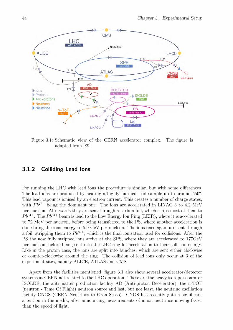
44 Chapter 3. Experimental Setup
Figure 3.1: Schematic view of the CERN accelerator complex. The figure isadapted from [89].
3.1.2 Colliding Lead Ions
For running the LHC with lead ions the procedure is similar, but with some differences.The lead ions are produced by heating a highly purified lead sample up to around 550°.This lead vapour is ionised by an electron current. This creates a number of charge states,with Pb27+ being the dominant one. The ions are accelerated in LINAC 3 to 4.2 MeVper nucleon. Afterwards they are sent through a carbon foil, which strips most of them toPb54+. The Pb54+ beam is lead to the Low Energy Ion Ring (LEIR), where it is acceleratedto 72 MeV per nucleon, before being transferred to the PS, where another acceleration isdone bring the ions energy to 5.9 GeV per nucleon. The ions once again are sent througha foil, stripping them to Pb82+, which is the final ionisation used for collisions. After thePS the now fully stripped ions arrive at the SPS, where they are accelerated to 177GeVper nucleon, before being sent into the LHC ring for acceleration to their collision energy.Like in the proton case, the ions are split into bunches, which are sent either clockwiseor counter-clockwise around the ring. The collision of lead ions only occur at 3 of theexperiment sites, namely ALICE, ATLAS and CMS.
Apart from the facilities mentioned, figure 3.1 also show several accelerator/detectorsystems at CERN not related to the LHC operation. These are the heavy isotope separatorISOLDE, the anti-matter production facility AD (Anti-proton Decelerator), the n-TOF(neutron - Time Of Flight) neutron source and last, but not least, the neutrino oscillationfacility CNGS (CERN Neutrinos to Gran Sasso). CNGS has recently gotten significantattention in the media, after announcing measurements of muon neutrinos moving fasterthan the speed of light.
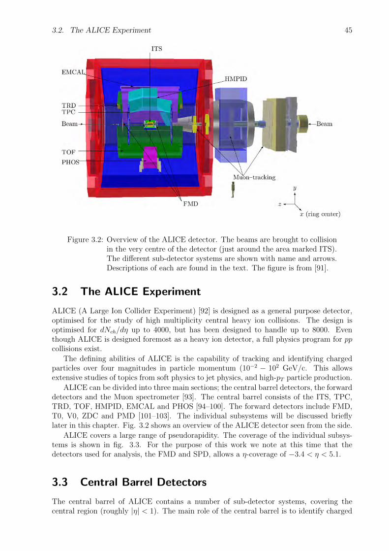
3.2. The ALICE Experiment 45
Figure 3.2: Overview of the ALICE detector. The beams are brought to collisionin the very centre of the detector (just around the area marked ITS).The different sub-detector systems are shown with name and arrows.Descriptions of each are found in the text. The figure is from [91].
3.2 The ALICE Experiment
ALICE (A Large Ion Collider Experiment) [92] is designed as a general purpose detector,optimised for the study of high multiplicity central heavy ion collisions. The design isoptimised for dNch/dη up to 4000, but has been designed to handle up to 8000. Eventhough ALICE is designed foremost as a heavy ion detector, a full physics program for ppcollisions exist.
The defining abilities of ALICE is the capability of tracking and identifying chargedparticles over four magnitudes in particle momentum (10−2 − 102 GeV/c. This allowsextensive studies of topics from soft physics to jet physics, and high-pT particle production.
ALICE can be divided into three main sections; the central barrel detectors, the forwarddetectors and the Muon spectrometer [93]. The central barrel consists of the ITS, TPC,TRD, TOF, HMPID, EMCAL and PHOS [94–100]. The forward detectors include FMD,T0, V0, ZDC and PMD [101–103]. The individual subsystems will be discussed brieflylater in this chapter. Fig. 3.2 shows an overview of the ALICE detector seen from the side.
ALICE covers a large range of pseudorapidity. The coverage of the individual subsys-tems is shown in fig. 3.3. For the purpose of this work we note at this time that thedetectors used for analysis, the FMD and SPD, allows a η-coverage of −3.4 < η < 5.1.
3.3 Central Barrel Detectors
The central barrel of ALICE contains a number of sub-detector systems, covering thecentral region (roughly |η| < 1). The main role of the central barrel is to identify charged

46 Chapter 3. Experimental Setup
Figure 3.3: The pseudorapidity coverage of ALICE. Subsystems not having fullazimuthal coverage is marked with an asterisk. The figure is from [24].
particles and their pT , using a variety of different methods and technology. Fig. 3.4 showsthe central barrel detectors.
3.3.1 Inner Tracking System
The Inner Tracking System (ITS) [92,94] consist of 6 layers of Silicon. They are located atradii between 3.9 cm to 43 cm from the interaction point. This makes the innermost layerthe detector closest to the interaction point.
The ITS is divided into 3 subsystems; the two innermost layers constitute the SiliconPixel Detector (SPD), the middle two layers are named the Silicon Drift Detector (SDD)and finally the two outermost layers are the Silicon Strip Detector (SSD).
The SPD layers are based on hybrid silicon pixels consisting of silicon detector diodeswith a thickness of 200 µm. When a charged particle traverse a pixel a digital signal is readout from that pixel. The SPD does not retain any information on the energy deposition.Thus, SPD signal is binary; either there is a hit or there is not. The signals in the two SPDlayers are sufficient to form so-called tracklets, which can be used to measure the chargedmultiplicity in |η| < 2.1. Due to extreme fine segmentation of the SPD, only an occupancyof around 1% is expected, making it extremely capable of multiplicity measurements. TheSPD is used for analysis in this work, and will be revisited in more detail in section 4.
The SDD works as a drift chamber, where the charged particles ionise the gas whentraversing the SDD volume. The created electrons drifts towards the readout, due to anelectric field over the SDD. The coordinates of the particle are then directly correlated tothe drift time.
The SSD utilises the energy loss from charged particles traversing strips of silicon. TheSSD in this manner is quite similar to the FMD, which will be described in more detaillater.
The main purposes for the ITS as a whole is:
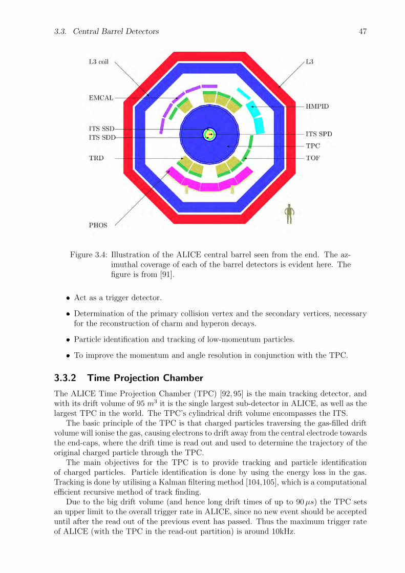
3.3. Central Barrel Detectors 47
Figure 3.4: Illustration of the ALICE central barrel seen from the end. The az-imuthal coverage of each of the barrel detectors is evident here. Thefigure is from [91].
Act as a trigger detector.
Determination of the primary collision vertex and the secondary vertices, necessaryfor the reconstruction of charm and hyperon decays.
Particle identification and tracking of low-momentum particles.
To improve the momentum and angle resolution in conjunction with the TPC.
3.3.2 Time Projection Chamber
The ALICE Time Projection Chamber (TPC) [92, 95] is the main tracking detector, andwith its drift volume of 95 m3 it is the single largest sub-detector in ALICE, as well as thelargest TPC in the world. The TPC’s cylindrical drift volume encompasses the ITS.
The basic principle of the TPC is that charged particles traversing the gas-filled driftvolume will ionise the gas, causing electrons to drift away from the central electrode towardsthe end-caps, where the drift time is read out and used to determine the trajectory of theoriginal charged particle through the TPC.
The main objectives for the TPC is to provide tracking and particle identificationof charged particles. Particle identification is done by using the energy loss in the gas.Tracking is done by utilising a Kalman filtering method [104,105], which is a computationalefficient recursive method of track finding.
Due to the big drift volume (and hence long drift times of up to 90µs) the TPC setsan upper limit to the overall trigger rate in ALICE, since no new event should be accepteduntil after the read out of the previous event has passed. Thus the maximum trigger rateof ALICE (with the TPC in the read-out partition) is around 10kHz.

48 Chapter 3. Experimental Setup
3.3.3 Transition Radiation Detector
The Transition Radiation Detector (TRD) [92,96], located radially right outside the TPC,relies on the phenomenon of transition radiation for particle identification. Transitionradiation occurs when a particle crosses the boundary between two materials with differ-ent dielectric constants. The emitted radiation is linearly dependent on the γ factor ofthe particle, thereby making it very useful at distinguishing pions and electrons at highmomenta.
The TRD is built up from six layers each containing a radiator, drift chamber and readout electronics. The radiator material is responsible for creating the transition radiationphotons, which are then converted in the drift chamber to electrons, being detected in theread out electronics. The information of the six layers are then combined into tracklets,which are used to identify high momentum electrons. This is used as a trigger to enhancethe recorded yield of Υ’s and high pT J/Ψ.
The TRD does not have full azimuthal coverage. This is a design decision in order forthe HMPID and PHOS detectors to also have areas without too much material in front ofthem. This is seen in figure 3.4.
3.3.4 Time Of Flight
The Time Of Flight (TOF) [92,97] detector is placed just outside the TRD, and measuresthe flight time of particles going from the interaction point through the TOF. The mo-mentum information, p, and the length of the trajectory, l, of the particle is known fromthe tracking in the ITS, TPC, and TRD. This is used together with the flight time, t, todetermine the particle mass, m :
m = p
√t2
l2− 1 (3.1)
The TOF consists of Multigap Resistive Plate Chambers, which are stacks of very thinstructures, featuring a gas volume with a uniform high electric field over. When a particletraverse the gas it immediately looses energy triggering an avalanche, which is detected atthe anode of the detector.
As with the TRD, the TOF does not have full azimuthal coverage, due to a desire tominimise the material in front of HMPID and PHOS.
3.3.5 Photon Spectrometer
The PHOton Spectrometer (PHOS) [92, 100] is an electromagnetic calorimeter, composedof lead-tungsten crystals. It is located in the bottom part of ALICE outside the TOF.Charged particles are rejected by multi-wire proportional chambers in front of the PHOS.
The PHOS detects photons, π0, and η mesons. The measurements are used for analysingthe initial temperature through direct single photons and/or di-photons, as well as probingdeconfinement through jet quenching of high pT π
0’s and investigating signals of restorationof chiral symmetry12.
12Chiral symmetry restoration, which is the restoration of invariance under parity, is one of the trulysmoking guns of a QGP.

3.4. Muon Spectrometer 49
3.3.6 Electro Magnetic Calorimeter
The Electro Magnetic CALorimeter (EMCAL) [92,99] was never meant to be a part of thefirst run period of the LHC. However due to the initial breakdown and subsequent repairs,the EMCAL was partially installed for the first runs. It is located outside the TOF.
The focus of the EMCAL is jet quenching in heavy ion collisions. Together with thetracks from the TPC and ITS, the EMCAL allows complete reconstruction of jets.
Furthermore the EMCAL functions as a trigger for hard jets, photons and electrons.
3.3.7 High Momentum Particle Identification Detector
The High Momentum Particle Identification Detector (HMPID) [92,98] is a Ring ImagingCherenkov detector (RICH), which is used to identify high momentum particles. It consistsof a layer of radiator material, and a Multi-Wire Proportionality Chamber behind to detectCherenkov radiation. Any particle traversing a medium with a speed higher than the speedof light in that medium, will emit Cherenkov radiation. The radiation is emitted as ashock wave at an angle with respect to the track of the particle, defined by the speed ofthe particle. This Cherenkov angle, θC , is given by:
cos θC =1
nβ(3.2)
Here β=v/c is the particle velocity relative to the speed of light and n is the refractive indexof the medium. The emitted Cherenkov radiation is read out as a ring on the read-outplane. The ring radius is used to determine the velocity of the particle. This information isthen used together with momentum information from for instance the TPC, to determinethe mass of the particle.
3.4 Muon Spectrometer
The Muon spectrometer [92, 93] is sitting in the very forward region of ALICE, with acoverage of −4 < η < −2.5. The purpose of the Muon spectrometer is to measure thecomplete spectrum of heavy quark vector-meson resonances (i.e. J/Ψ, Ψ′, Υ, Υ′, and Υ′′)and the φ meson. All of these measurements are done in the µ+µ− decay channel. TheMuon spectrometer can be seen in figure 3.5. Closest to the interaction point is the frontabsorber. The absorber consists of mainly carbon, concrete, and steel in order to preventanything else but muons from passing through.
After the front absorber, tracking stations 1 and 2 are located. Tracking station 2 islocated such that it determines precisely where the muons exit the solenoidal field of L3,encompassing most of ALICE. Then follows a dipole magnet, yielding the momentum ofthe muon by deflection. Inside the dipole magnet, tracking station 3 is placed to enhancethe determination of the deflection. After the dipole magnet two more tracking stationssits, with an iron absorber in between them. In the end there are resistive plate chambersto determine the time of flight, and thus the particle mass (as in the TOF).
3.5 Forward detectors
The forward detectors of ALICE is comprised of the PMD, T0, V0 and the FMD. Thefirst three will be briefly discussed in the following. A more complete description of the
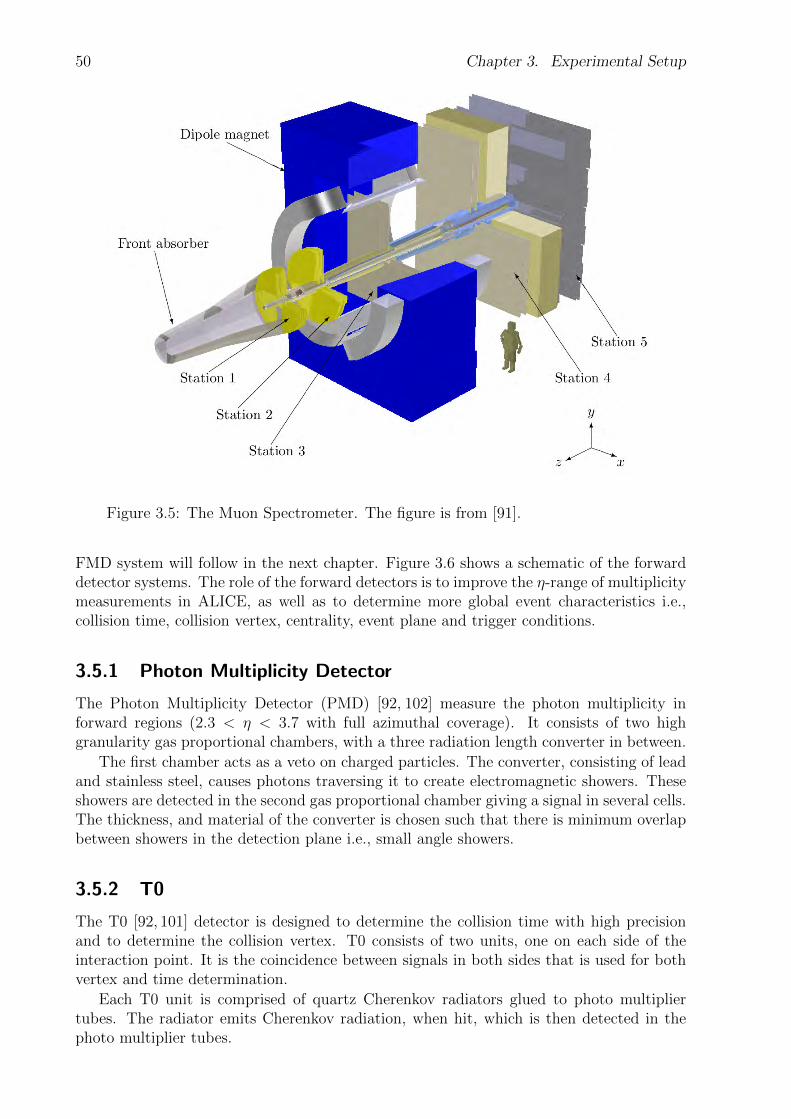
50 Chapter 3. Experimental Setup
Figure 3.5: The Muon Spectrometer. The figure is from [91].
FMD system will follow in the next chapter. Figure 3.6 shows a schematic of the forwarddetector systems. The role of the forward detectors is to improve the η-range of multiplicitymeasurements in ALICE, as well as to determine more global event characteristics i.e.,collision time, collision vertex, centrality, event plane and trigger conditions.
3.5.1 Photon Multiplicity Detector
The Photon Multiplicity Detector (PMD) [92, 102] measure the photon multiplicity inforward regions (2.3 < η < 3.7 with full azimuthal coverage). It consists of two highgranularity gas proportional chambers, with a three radiation length converter in between.
The first chamber acts as a veto on charged particles. The converter, consisting of leadand stainless steel, causes photons traversing it to create electromagnetic showers. Theseshowers are detected in the second gas proportional chamber giving a signal in several cells.The thickness, and material of the converter is chosen such that there is minimum overlapbetween showers in the detection plane i.e., small angle showers.
3.5.2 T0
The T0 [92, 101] detector is designed to determine the collision time with high precisionand to determine the collision vertex. T0 consists of two units, one on each side of theinteraction point. It is the coincidence between signals in both sides that is used for bothvertex and time determination.
Each T0 unit is comprised of quartz Cherenkov radiators glued to photo multipliertubes. The radiator emits Cherenkov radiation, when hit, which is then detected in thephoto multiplier tubes.

3.5. Forward detectors 51
Figure 3.6: The forward detectors of ALICE. The figure is from [91].
T0 furthermore acts as a early wake-up signal to other detectors. Due to the lowacceptance of T0 it is only reliable for AA collisions where the particle multiplicity is muchhigher than in pp collisions.
3.5.3 V0
Since the T0 has a low trigger efficiency in pp collisions, the V0 [92, 101] detector wasdesigned with a much larger acceptance, in order for it to perform as a minimum bias triggerin both pp and AA collisions. Furthermore it is used to determine the event centrality andthe event plane. It can also be used at studies of multiplicities at very forward angles,however with less precision than the FMD and PMD.
V0 consists of two units of scintillator counters located on each side of the interactionpoint.
3.5.4 Zero Degree Calorimeter
The Zero Degree Calorimeters (ZDC) [92,103] are positioned at very forward angles. Theirrole is to measure the spectator nucleons from heavy ion collisions, in order to estimatethe number of participants, and hence the centrality.
The two ZDC themselves are positioned on each side of the interaction point, 116 metersaway from it. Counted as part of the ZDC system are also two electromagnetic calorimeters(ZEM). These are placed on either side of the beam pipe, but only 7 meters away fromthe interaction point on the opposite side of the muon absorber. The ZEM measuresthe photons from particles emitted at forward rapidities, which is used for determining thecentrality of very central collisions where few spectators escape to the ZDCs. Similarly theyare also used for very peripheral collisions. For very peripheral collisions, the spectatorsresemble the incoming nuclei (both in amount and direction), and thus might continueinside the beam pipe, avoiding detection in the ZDCs.

52 Chapter 3. Experimental Setup
3.6 Data Acquisition System
This chapter ends with a brief overview of the Data AcQuisition (DAQ) [92,106] in ALICE.The DAQ is responsible for collecting the signals from the various sub-detectors, andbuilding the event. Furthermore the DAQ exports the collected events for storage.
Event building is a two step procedure. The data from the sub-detectors are transferredvia Detector Data Link (DDL) optical fibers to Local Data Concentrators (LDCs). On theLDCs, the received data is gathered into sub-events, which are then shipped to GlobalData Concentrators (GDCs). The GDCs collect the sub-events from all the LDCs, andassemble the final event from this.
The event is sent for immediate storage in a disc system called Transient Data Storage(TDS), before being transferred to permanent storage at magnetic tapes.
The full DAQ system of ALICE consists of 200 LDCs and 60 GDCs. [24].When running, the DAQ can manage data taking in several partitions at the same time.
A partition includes a subset of sub-detectors, that run under the same conditions. As anexample of partitions, one could have separate partitions with fast or slow trigger ratesrespectively. Detectors that for some reason are restricted by long read-out times, like theTPC, can then run in the slow partition at one interaction rate, while the other detectorsrun at a higher interaction rate in the fast partition.

Chapter 4
The FMD and SPD
This work relies on the measurements of charged particles from the FMD, as well as fromthe first layer of Silicon in the SPD. Both are Silicon semi-conductor devices. The FMD isa strip detectors, where as the SPD is a pixel detector.
This chapter will start by detailing basic concepts regarding Silicon detectors in general,before moving on to presenting the two detectors.
4.1 Semi-conductor properties
Semi-conductors is a term denoting materials, characterised by the band-gap between thevalence and conduction bands being quite small. This means that it takes little energyto excite an electron into the conduction band, leaving a hole in the valence band. Semi-conductors fall in between insulators, characterised by a large band-gap, and metals, thathave no band-gap, allowing electrons to roam freely. A schematic of all three materialtypes can be be seen in figure 4.1
Semi-conductors, such as Silicon and Germanium, are popular mediums for physicsdetectors. The basic principle of semi-conductor detectors is analogous to gas ionisationdetectors such as drift chambers etc.. The main advantage of semi-conductors is that theenergy required to create electron-hole pairs are ten times smaller than for gas ionisation[107]. Thus the amount of ionisation at a given energy will be much higher, leading to abetter energy loss resolution.
Figure 4.1: Illustration of the band-gap between the valence and conductionbands in insulators, semi-conductors and metals.
53

54 Chapter 4. The FMD and SPD
Figure 4.2: (a) At low temperatures the tetravalent Silicon crystal form four co-valent bindings with neighbouring Silicon atoms. (b) At non-zerotemperatures valence electrons can be thermally excited into the con-duction band, leaving holes in the valence band. (c) A Silicon crystalhave been doped with a pentavalent donor impurity. The excess elec-tron create allowed energy states between the conduction and valencebands. The figure is from [91].
4.1.1 Doped Crystals
In pure Silicon crystals the electrons are bound covalently. The small band-gap allows evenminor thermal excitation to bring the valence electrons into the conduction band, leavingan extra electron in the conduction band, as well as a hole in the valence band, both ofwhich function as charge carriers. To increase the numbers of charge carriers the Siliconcrystals are doped.
The basic idea is to introduce material with either one extra or one less valence electronthan the material to be doped. Silicon is tetravalent13. Doping Silicon with pentavalentatoms thus gives one extra electron. This creates another allowed energy state in the band-gap just below the conduction band. The electron is easily exited into this state, increasingthe conductivity. In figure 4.2 the covalent binding of Silicon, thermal excitation of valenceelectrons and a doped Silicon crystal is illustrated.
Doping with trivalent atoms on the other hand ensures that there are not enoughelectrons to fill the valence band. Furthermore it introduces another allowed energy statein the band gap, this time close to the valence band. Thus electrons in the valence bandcan easily be excited into this state, leaving even more holes in the valence band.
Semiconductors with an excess of electrons are called n-type semi-conductors, and ifthere is an excess of holes they are called p-type semi-conductors. Normally the concen-tration of the dopant impurities is very small, around 10−9 [107].
However, heavily doped semi-conductors (usually labelled n+ and p+ respectively) arealso used extensively in for instance electrical contacts. In heavily doped semi-conductorsdopant concentrations can be as high as 10−3, leaving them highly conductive [107].
13Tetravalent atoms have four valence electrons. Similarly petravalent and trivalent atoms have five andthree valence electrons respectively.

4.2. Semi-conductor detectors 55
4.2 Semi-conductor detectors
The basic idea behind Silicon detectors uses the fact that if a particle traverse the Silicon itexcite electrons into the conduction band, leaving electron-hole pairs behind. If one appliesan external electrical field over the crystal, the electrons drift to the anode, and the holestoward the cathode, thereby inducing a current over the crystal. This current can be readout.
However, just using n or p type crystals as described in the last section is not viable.Since the band-gap is sufficiently small, thermal excitations would also create a currentand thus the detector would be very noisy. In the following will be described what is doneto avoid this.
4.2.1 n-p junctions
The practical implementation in detectors is to make a junction between a n-type anda p-type semi-conductor. Due to the difference in concentration of electrons and holesbetween the two sides there will be an initial diffusion of electrons towards the p-side andof holes towards the n-side. Since each side was initially neutral it follows that the p-sidewill become negatively charged, due to the added electrons, and the n-side will becomepositive, due to the added holes. This creates an electrical field gradient over the junction,which eventually stops the diffusion, since the electrons and holes need to perform work toovercome the created contact potential over the junction. This leaves a region of immobilecharge carriers near the junction. Any electron or hole created in this region, which iscalled the depletion zone, will immediately be swept away by the electric field. Thus anyexternal particles traversing the depletion zone, will create new electron-hole pairs, thatare swept away, and can be read out.
The depletion zone depth, d, in a regular n-p junction is quite small and is givenby [107]:
d ∼ αc ·√ρc · V0 (4.1)
where αc is a constant of the order of unity, slightly different depending on whetherit is the n or p-side, ρc is the crystal resistivity, and V0 is the contact potential. Takingtypical values for the n-side for instance (αn=0.53, ρn ∼ 5000 Ωcm and V0 ∼ 1 V) yieldsa depletion depth of roughly 35µm. This depth is very small compared to the radiationlength in Silicon, making it less likely that any radiation traversing the sensor wouldcreate a significant amount of electron-hole pairs. Furthermore the noise from the sensoris proportional to the capacitance, C, of the crystal, which is connected to the depletiondepth through [107]:
C = ε · Ad
(4.2)
Here ε is the dielectric constant of Silicon, A is the crystal area and d is the depletionzone depth. Thus in order to decrease the noise, and increase the chance that a traversingparticle will be detected, it is necessary to increase the depletion depth.
This is done by applying a so-called reverse bias voltage, Vb. It is a negative voltageapplied to the p-side of the junction. It causes the excess holes and electrons to be drawnfurther away from the junction, thereby increasing the depletion depth. The depletiondepth is still given by (4.1), with the substitution of V0 with Vb. There exist a maximumvoltage, determined by the resistivity of the crystal, which limits the depletion depth. Ifthe reverse bias voltage is above this maximum the n-p junction breaks down.

56 Chapter 4. The FMD and SPD
Ideally, the n-p junction is not conducting, even when applying a reverse bias voltage.However for various reasons this is not completely true. When the reverse bias voltage isapplied a small current may flow over the sensor. This current is called the leakage current,and it contributes to the read-out noise of the sensors.
4.3 Energy loss in Silicon
Silicon detectors generally works through the detection of the energy lost when particlestraverse the Silicon sensor. The average energy loss per unit length is called the stoppingpower, and is well described by the Bethe-Bloch equation [5]:
−dEdx
= 4πNAr2emec
2z2Z
A
1
β2
[1
2ln
(2mec
2γ2β2TmaxI2
)− β2 −
δ(βγ)
2+C
Z
]) , (4.3)
whereNA Avogadro’s number 6.0221415(10)× 1023 mol-1
re Classic electron radius 2.817940325(28) fmme Electron mass 0.510998918(44) MeVc Speed of lightz Charge of incident particle eZ Atomic number of material Si: 14A Atomic mass of material Si: 28.0855β = p/m of incident particle
γ = 1/√
1− β2 of incident particleTmax Maximum energy transfer in a single collision MeVI Mean excitation energy eV
δ(βγ) Density effect correction to ionisation energy lossC Shell correction
Tmax is a measure of the maximum energy transferred in a single interaction between theincident particle and the electrons in the material. It is given by:
Tmax =2mec
2β2γ2
1 + 2γme/m+ (m2/m)2(4.4)
with m being the mass of the incident particle. The mean excitation energy, I, is ex-perimentally found to vary quite a bit with atomic number [5]. Its main features areparametrised by:
I
Z=
12 + 7
ZZ < 13
9.76 + 58.8Z−1.19 Z ≥ 13, (4.5)
Bethe and Bloch derived the main portion of (4.3) (the exception is the terms incurly brackets) from a quantum mechanical description of particles scattering softly on theelectrons in dense matter.
The terms in the curly brackets were added later on as corrections for density effects(δ(βγ)/2) and shell effects (C/Z). They are important at high and low energies respectively.
The density correction takes into account the fact that the electrical field of the incidentparticle will polarise the atoms it passes. This polarisation makes electrons contribute lessto the total energy loss. The polarisation becomes bigger at higher particle velocities, aswell as in denser media.

4.3. Energy loss in Silicon 57
Figure 4.3: The stopper power for µ in Copper [5]. The low and high energy lossregimes can not be described adequately by the Bethe-Bloch equation.However for medium energy losses around the minimum ionisation theBethe-Bloch equation is a good description.
The need for the shell correction stems from the assumption by Bethe and Bloch thatthe electrons are at rest compared to the incident particle. However when the orbitalelectron velocity becomes comparable to the incident particle velocity this assumptionbreaks down, and the correction comes into play.
Shown in figure 4.3 is the stopping power of muons, µ, in Copper. It is given as afunction of both momentum and βγ = β√
1−β . In the very low regime (βγ < 0.1) the
description by (4.3) is not valid. Other models are indicated in the figure for the low end.Similarly at very high energies the Bethe-Bloch equation again becomes insufficient. Inthis regime radiative effects like brehmsstrahlung and Cherenkov radiation occur, requiringthe description by other models.
The minimum of the Bethe-Bloch curve (around βγ ∼ 3.5 in figure 4.3) denote theminimum ionisation energy. A traversing particle depositing this energy is said to be aMinimum Ionising Particle (MIP).
Equation (4.3) and the full curve shown in figure 4.3 requires the thickness of the struckmaterials to be comparable to the mean interaction length of particles in that material.However for thin absorbers, such as the FMD and SPD this is not true.
For thin absorbers the following apply [108]:
The incident particle will not suffer enough collisions for the central limit theoremto hold. Thus the energy loss probability distribution, dN/d∆, is not Gaussian (asis the case for thick absorbers).
The incident particle does not encounter enough material for the radiative effects tobuild up.
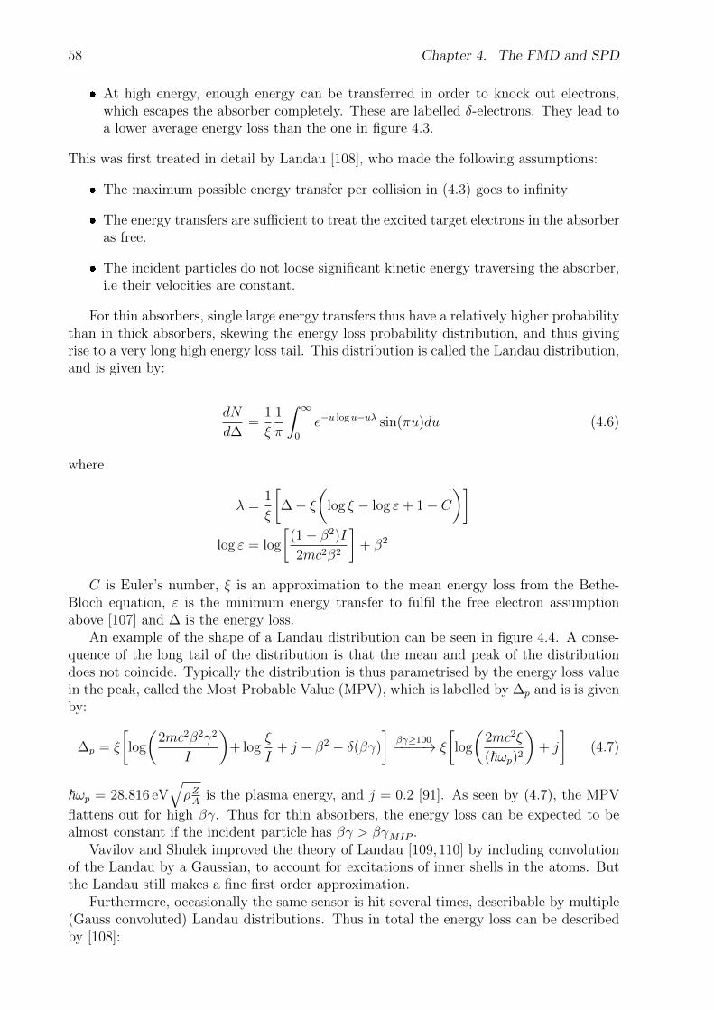
58 Chapter 4. The FMD and SPD
At high energy, enough energy can be transferred in order to knock out electrons,which escapes the absorber completely. These are labelled δ-electrons. They lead toa lower average energy loss than the one in figure 4.3.
This was first treated in detail by Landau [108], who made the following assumptions:
The maximum possible energy transfer per collision in (4.3) goes to infinity
The energy transfers are sufficient to treat the excited target electrons in the absorberas free.
The incident particles do not loose significant kinetic energy traversing the absorber,i.e their velocities are constant.
For thin absorbers, single large energy transfers thus have a relatively higher probabilitythan in thick absorbers, skewing the energy loss probability distribution, and thus givingrise to a very long high energy loss tail. This distribution is called the Landau distribution,and is given by:
dN
d∆=
1
ξ
1
π
∫ ∞0
e−u log u−uλ sin(πu)du (4.6)
where
λ =1
ξ
[∆− ξ
(log ξ − log ε+ 1− C
)]log ε = log
[(1− β2)I
2mc2β2
]+ β2
C is Euler’s number, ξ is an approximation to the mean energy loss from the Bethe-Bloch equation, ε is the minimum energy transfer to fulfil the free electron assumptionabove [107] and ∆ is the energy loss.
An example of the shape of a Landau distribution can be seen in figure 4.4. A conse-quence of the long tail of the distribution is that the mean and peak of the distributiondoes not coincide. Typically the distribution is thus parametrised by the energy loss valuein the peak, called the Most Probable Value (MPV), which is labelled by ∆p and is is givenby:
∆p = ξ
[log
(2mc2β2γ2
I
)+ log
ξ
I+ j − β2 − δ(βγ)
]βγ≥100−−−−→ ξ
[log
(2mc2ξ
(~ωp)2
)+ j
](4.7)
~ωp = 28.816 eV√ρZA
is the plasma energy, and j = 0.2 [91]. As seen by (4.7), the MPV
flattens out for high βγ. Thus for thin absorbers, the energy loss can be expected to bealmost constant if the incident particle has βγ > βγMIP .
Vavilov and Shulek improved the theory of Landau [109,110] by including convolutionof the Landau by a Gaussian, to account for excitations of inner shells in the atoms. Butthe Landau still makes a fine first order approximation.
Furthermore, occasionally the same sensor is hit several times, describable by multiple(Gauss convoluted) Landau distributions. Thus in total the energy loss can be describedby [108]:

4.3. Energy loss in Silicon 59
Figure 4.4: Left panel: Example of the form of a landau distribution. The mostprobable value and the mean differs, in contrast to a Gaussian wherethey are identical. Right panel: Example of the differences betweenthe original Landau distribution, and further developments in describ-ing the energy loss in thin absorbers. While the Landau is not themost correct of them, it remains a very good first approximation.Figure is from [91].
F (∆) =n∑i=1
aiFn(∆)
=n∑i=1
ai(Li(∆)⊗Gi(∆))
=n∑i=1
ai
∫ ∞−∞
d∆′ L(∆; ∆′, ξi) exp−(∆p,i −∆′)2
2σ2(4.8)
with Li and Gi denoting Landau with most probable value ∆p,i and width ξi and Gaussiandistributions for i particles depositing energy respectively. The ai’s are the weights of eachof the convoluted distributions.
It can be shown that (4.8) has n + 2 free parameters [108]. Three of those stem fromthe Landau and Gaussian, and are the σ of the Gaussian component and the single particleLandau parameters ∆p and ξ. The remaining parameters are the ai’s of the n individualLandau distributions. a1 is defined to be unity, which leaves n− 1 ai’s as parameters.
The Landau parameters for the ith distribution are connected to the single particledistribution by [111]:
ξi = iξ (4.9)
∆p,i = i∆p + ξi ln i (4.10)
To sum up, the energy deposits in thin absorbers, like the FMD, can be described bymultiple landau distributions, convoluted by Gaussians. From the amplitudes of the indi-

60 Chapter 4. The FMD and SPD
Figure 4.5: Overview of the FMD system. FMD2 and FMD 3 are placed nearlysymmetrically around the interaction point, and FMD1 is locatedsome distance away from the interaction. Ideally, one could havehoped for another FMD at around z = -320 cm (mirroring FMD1), butdue to the massive Muon absorber sitting there, this is not possible.
vidual Landau distributions it can thus be inferred for a given energy deposit whether itwas caused by a single or more incident particles.
4.4 Forward Multiplicity Detector
The Forward Multiplicity Detector (FMD) is one of the main contributions to ALICE fromthe Niels Bohr Institute at the University of Copenhagen. It is designed, built and testedlocally before being installed in ALICE. The FMD is a Silicon strip detector, with fineη-segmentation, and adequate φ-segmentation.
The FMD system consists in total of 5 Silicon rings, grouped into 3 sub-detectors namedFMD1, FMD2 and FMD3. The latter two consist of 2 rings each, an inner ring and anouter ring. FMD1 only consists of an inner ring. Thus when referring to individual rings,the name will consist of the sub-detector name, with an addition of either I or O (Inner orOuter) i.e., FMD1I, FMD2I, FMD2O, FMD3I, FMD3O.
Figure 3.6 in the previous chapter showed the location of the different FMD sub-detectors with respect to the beam pipe, ITS and interaction point.
4.4.1 Design and Motivation
The main physics purpose of the FMD detector is to extend the charged particle coverageof ALICE into very forward rapidity regions, as seen in figure 3.3. This is essential forgetting a more complete picture of particle production, as well as generally understandingthe most forward regions.
Another of the main motivations for the FMD is its capability to provide independentmeasurements of the collision reaction plane and furthermore measurements of the variousflow harmonics, vn, in the forward region. The independence from the mid-rapidity barreldetectors in determining the reaction plane, will allow those detectors to use that measure-

4.4. Forward Multiplicity Detector 61
ment in their determination of vn in the mid-rapidity region (and vice versa the FMD willutilise their reaction plane measurements).
The mentioned physics goals for the FMD lead to the following design requirements:
Broad η coverage.
Fine η segmentation. This is important in order to have a low average detectoroccupancy, and thus a high measurement resolution for multiplicities. There are 512and 256 η-segments in inner and outer rings respectively.
Full φ coverage. The segmentation in φ however is limited, with 20 and 40 segmentsin inner and outer rings respectively.
Ideally, tracking capabilities would be available to a detector like the FMD. Howeverdue to the very forward η coverage this is not possible. Particles emitted in forwardregions have extremely high momentum, and thus are deflected very little in the magneticfield. Hence, in order to have a tracking detector with good momentum resolution at thesepseudorapidities, the detector would need to be located very far from the interaction point.
Sub– Ring # ϕ # r z rin routdetector segments segments [cm] [cm] [cm]FMD1 I 20 512 320.0 4.2 17.2FMD2 I 20 512 83.4 4.2 17.2
O 40 256 75.2 15.4 28.4FMD3 I 20 512 -62.8 4.2 17.2
O 40 256 -75.2 15.4 28.4
Table 4.1: Overview of the segmentation and placement of the individual FMDrings.
The design requirements lead to a detector design, with rings (positioned around thebeam pipe) of Silicon semi-conductor sensors. In Table 4.1 and Figure 4.5 the placementof the rings, and several characteristics are shown.
4.4.2 FMD Sensors and Electronics
Each of the FMD rings consist of a number of identical base units, referred to as FMDsensors. The top part of figure 4.6 shows both an inner and outer ring, consisting of 10and 20 sensors respectively. Each FMD sensor has two sectors on it, meaning that innerrings consist of 20 sectors and outer rings consist of 40 sectors. Each inner ring sector isradially divided into 512 Silicon detection strips, whereas the outer rings are only dividedinto 256 strips per sector.
In total this means that each FMD ring has 10240 channels, totalling up to 51200individual detection channels for the entire FMD system. The bottom part of figure 4.6shows the layout of both an outer and inner FMD sensor.
Each FMD sensor has an electronics card glued to it, which handles the pre-amplificationof the incoming analog signal for the two sectors of the sensor. The amplification is takencare of by so-called V A13 chips each responsible for 128 strips. Thus each hybrid cards haseither 4 or 2 V A13 chips depending on if it is an inner or outer sensor. The electronics cardsof each half-ring send the analog signal to a digitiser board, where the signal is convertedto a digital signal by an Analog-to-Digital Converter (ADC). Converting from analog to
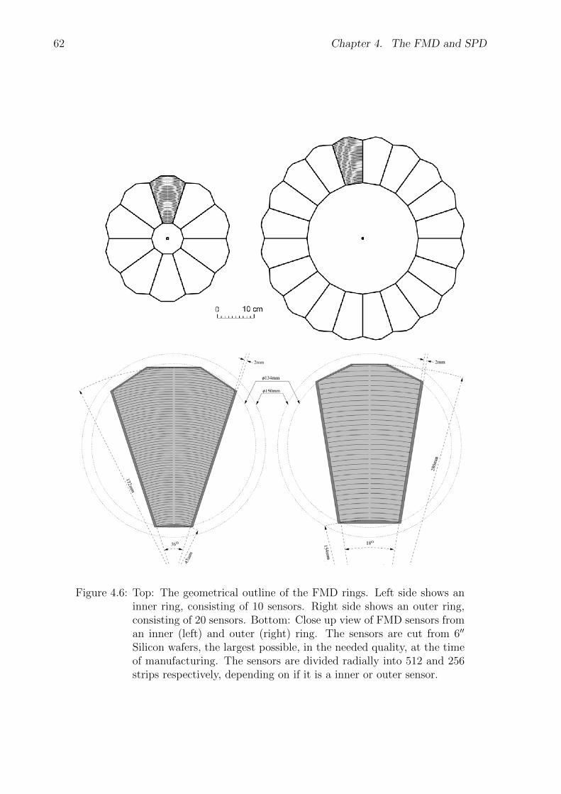
62 Chapter 4. The FMD and SPD
Figure 4.6: Top: The geometrical outline of the FMD rings. Left side shows aninner ring, consisting of 10 sensors. Right side shows an outer ring,consisting of 20 sensors. Bottom: Close up view of FMD sensors froman inner (left) and outer (right) ring. The sensors are cut from 6′′
Silicon wafers, the largest possible, in the needed quality, at the timeof manufacturing. The sensors are divided radially into 512 and 256strips respectively, depending on if it is a inner or outer sensor.

4.4. Forward Multiplicity Detector 63
digital is done by the ALTRO chip, which is an ADC developed for the ALICE TPC14.Besides the TPC and FMD, it is also utilised by the EMCAL and PHOS.
The output of the ALTRO chip is the signal strength given in ADC counts, rangingfrom 0 to 1023. The digital signal is sent for the Read-out Controller Unit (RCU), whichmanages the readout of the ALTRO chips, as well as handling triggers, monitoring andcontrolling the states of the digitiser cards. Individual RCUs exist for each of the threeFMDs. The RCUs used in the FMD are also originally developed for the ALICE TPC15.
From the RCU the digital signals are sent to the DAQ for read-out and storage. Aschematic presentation of the front end electronics of the FMD is shown in figure 4.7.
Figure 4.7: Schematic of the FMD electronics. Analog signals in the sensors aresent via the V A13 chips to the digitiser cards, where the ALTROsconvert the analog signals into digital signals. These are sent for theRCUs, which handles read-out and sending it onwards for the DAQ,where it might be stored.
The individual sensors have been extensively tested by the manufacturer, Hamamatsu.Figure 4.9 shows the capacitance, and thus noise, and leakage current of an arbitrarilychosen inner and outer sector as a function of the reverse bias voltage.
Once full depletion is reached the capacitance becomes flat. The leakage current con-tinuously increase as a function of the bias voltage. Therefore the optimal bias voltage isset just above the point where full depletion is reached. For inner sectors this is around 70V and for outer sectors it is around 120 V.
Next, figure 4.8 shows the test measurements of the leakage current stability over timein the same two sectors. It is found that there is little variation over time.
Additionally in figure 4.8 the depletion depth of all FMD sectors is shown. For allsectors it is 325± 3µm.

64 Chapter 4. The FMD and SPD
Figure 4.8: The capacitance and leakage current as a function of the reverse biasvoltage for an inner and outer sector. For the outer sector a biasvoltage of 120 V is chosen, whereas it is 70 V for the inner sectors.The figure is taken from [91].
Figure 4.9: Top panel: The depletion depth of the individual sectors of the FMD.Bottom panel: The stability of the leakage current under optimaloperating conditions for an arbitrarily chosen inner and outer sector.The figure is from [91].

4.4. Forward Multiplicity Detector 65
ADC value0 50 100 150 200 250 300 350 400
Eve
nts
0
50
100
150
200
250
DAC input0 50 100 150 200
AD
C r
espo
nse
0
100
200
300
400
500
600
700
800
p0 71.84p1 2.858
Figure 4.10: Left panel: Example of the pedestal distribution of a strip. The meanof the distribution is considered the pedestal value for that strip,whereas the standard deviation is the noise of the strip. Right Panel:Example of the concept of gain calibration of a strip. Each pointcorresponds to the read-out signals from a known input pulse, whichis converted to a analog signal by a Digital-to-Analog Converter(DAC). The slope of the fit to the 8 points are the gain of thatparticular strip.
4.4.3 Pedestals and Gain
Due to the constant large external voltage kept over the FMD and noise from the electronicsitself, there will always be signals in each strip, that are read out, regardless of whetherthere was a collision or not.
These signals are labelled pedestals, and must be subtracted from the data, whenreconstructing the events. The pedestal calibrations are recorded in special calibration runswith no beams in the LHC. Roughly 1000 events are recorded, and all channels are readout. This yields pedestal distributions for each strip. The mean of the pedestal distributionis the pedestal value used for subtraction. The width of the pedestal distribution is labelledthe noise of the strip. The left panel of figure 4.10 show a typical example of a pedestal ina pedestal calibration run.
In the top of figure 4.11 the means of the pedestals for all strips are shown. Similarlythe noise of all strips can be seen in the middle of that figure. It is seen that the pedestalmeans are ∼ 100 ADC counts, and the noise of the strips are ∼ 2 and ∼ 2.5 ADC countsfor inner and outer rings respectively.
The pre-amplification of each strip can vary slightly. Thus each strip need to be cali-brated to the same gain. This is again done in a special gain calibration run, which usesa pulser with a known output voltage. The 128 strips of a V A13 chip are calibrated se-quentially, which means, that for each event the same strip on each V A13 chip is beingcalibrated. For each of 8 different pulser inputs, 100 events are collected to estimate theresponse of the strip. Thus in total at least 102400 events are needed for the calibration.The response of each of the inputs are fitted to a straight line. The slope of this is what islabelled the gain of that strip. The right panel of figure 4.10 show an example of the gaincalibration procedure. Figure 4.11 show the gains for all strips.
The noise and pedestal are used for subtracting the pedestals online. This dramatically
14ALTRO is an acronym for ALice Tpc ReadOut15The choice of using the ALTRO chips dictates also using the TPC RCU

66 Chapter 4. The FMD and SPD
Figure 4.11: From top to bottom: Pedestal, noise, and gain values for all the51200 channels of the FMD. In the pedestal and noise panels, onenotices that an area in FMD1I (∼ channel 3500) is malfunctioning.It is an entire V A13 chip being dead. These channels are removedduring analysis.
decrease the read-out volume of the FMD, since only events with signals above the pedestalsignal are read out.
4.5 Silicon Pixel Detector
The SPD is the innermost part of the ITS. It is the detector closest to the interactionpoint. As described in section 3.3.1 it consists of two concentric cylindrical layers of Silicon,enveloping the beam pipe. Figure 4.12 shows a schematic of the ITS.
The innermost layer of the SPD is located at only r = 3.9 cm, just roughly 7 mmoutside the beam pipe, whereas the outer layer is located at r = 7.6 cm.
The SPD is grouped into base modules, labelled half-staves, each consisting of twosensor ladders and the corresponding readout electronics. Each ladder contain 40960(=160× 256) Silicon pixels. In total the SPD consists of 60 such half-staves. Thus the SPDhas extremely fine segmentation with more than 2 million channels. In figure 4.13 a zoomedview of the SPD seen from the end is shown.
The individual SPD pixels do not retain the energy deposition information when aparticle traverse it. Instead it solely registers if a pixel was hit with signal above a certainthreshold. Due to the extremely fine segmentation of the SPD, particles traversing thedetector can easily fire multiple pixels. Such a group of hits in adjacent pixels are referredto as a cluster. Using the clusters of both layers and the primary vertex information, it ispossible to form so-called tracklets, pointing back to the interaction point. Since trackletsby definition points back to the interaction points, they are particles stemming directlyfrom the collision and thus tracklets has very low contamination from particles created

4.5. Silicon Pixel Detector 67
Figure 4.12: Overview of the ITS detector system. As seen the SPD is the twoinnermost concentric layers of the ITS.
Figure 4.13: Close up view of the SPD, as seen from the end. Indicated in thebottom is the location of the beam pipe, only 7 mm from the innerlayer of the SPD. The placement of the detector staves is shown.
later on in decays, material interactions etc..Ideally, the information from the tracklets could just be used in the central region to
count charged particles for this work. However since the aim is to provide multiplicitydistributions for wide pseudorapidity intervals this is not possible. The tracklet coverageis limited by the coverage of the second SPD layer, which is around |η| < 1.5 (for verticesaround vz ∼ 0). Thus, creating a continous wide η-interval multiplicity distribution is notpossible, but would have large gaps in it. These gaps would be different depending onthe vertex position. However, the innermost layer of the SPD has a coverage of roughly|η| < 2 for collisions around the nominal interaction point. This means that by selectingonly events in a limited z vertex region there is full overlap between the inner layer of theSPD and FMD in every event. Thus in this work the inner layer of the SPD is used foranalysis16.
16One might state that the inner layer of the SPD is treated as ’yet another’ FMD ring, in the sense thatit is treated similarly. The drawbacks of this obviously is that one can not utilise the powerful trackingcapabilities of the SPD to eliminate contamination from particles away from the interaction point. But asdescribed it allows for the analysis of a very broad continuous η interval.

68 Chapter 4. The FMD and SPD

Chapter 5
Off-line Data Processing
In this chapter the tools used for analysis is presented. These tools include the basic analysisprograms over the specific analysis framework structure of ALICE to the simulations used.
Presented in this chapter is also information on the selected data sets being analysedin this work. The analysis itself is presented in the next chapter.
5.1 ROOT and AliROOT
The base tool for analysis is called ROOT17 [112]. ROOT was mainly developed at CERNas a platform on which to build systems for entire experiments. ROOT contain functionsfor handling most analysis tasks; data storage, data management, data visualisation aswell as a wealth of mathematical and statistical tools.
AliROOT (Alice ROOT) [113] is an extension to ROOT, developed specifically by theALICE collaboration. AliROOT has implemented the detector geometry of ALICE aswell as a full simulation environment. In addition to this AliROOT also contains thereconstruction code for all sub-detectors, and the analysis code.
5.2 Simulations
In this section an overview of the simulations used in this work is given. In general,simulated data play a crucial role in heavy ion physics. The ability to describe the physicsand detector setup in high detail in simulations yield great possibilities for comparisonswith theoretical predictions as well as using the simulation results for corrections on thephysics data.
Simulations consist of two separate components: An event generator and a transportcode. The event generator is responsible for creating simulated particles according to thetheoretical understanding of collision dynamics. Event generators are typically tuned tobest match physics results from earlier experiments. Quite a number of different eventgenerators exist. They include various physics processes and theories.
In this work three different event generators are used:
PYTHIA This is the most widely used general-purpose generator for pp and pp collisions.PYTHIA has a wide variety of physics implemented, including hard/soft QCD pro-cesses, Heavy-flavour production, Prompt photon production, photon-induced pro-cesses, deep inelastic scattering, W/Z production etc. Furthermore there are imple-mentations for non-Standard Model theories such as Technicolour, SUperSYmmetry
17recursively short for ROOT’s Object Oriented Tools.
69

70 Chapter 5. Off-line Data Processing
(SUSY) and non-Standard Higgs doublet production [114]. ALICE uses PYTHIAversion 6.4.
PHOJET This pp event generator is a implementation of the Dual Parton Model, whichfocuses on the description of diffractive physics by Pomeron exchanges as describedin section 1.4.2 [115].
HIJING (Heavy Ion Jet INteraction Generator) This event generator has implementationsfor both pp and heavy ion collisions. However the main usage of HIJING [116] is forheavy ion collisions. HIJING uses a pQCD approach. For the description of multipleinteractions in heavy ions it uses a Glauber model.
The event generator output is a stack of particles, used as input for the transportmodel. In this work the transport model used is GEANT 3.21 (GEometry ANd Tracking)[117]. GEANT has implementations of most interactions, such as hadronic interactions,bremsstrahlung, decays, Compton/multiple scatterings and many more.
Each particle is propagated through a virtual model of the experiment in small steps. Ateach step, possible interactions or decays are calculated. If new particles are created fromsuch a process, it is placed on the stack and are subsequently propagated independently.Each time a particle enters or exits an active sub-detector volume, routines specific to thatsub-detector determines which information to store as a hit. As an example, consider aparticle hitting the FMD. Here the procedure is that this hit is stored with both space-timeand detector coordinates (x, y, z, t, detector, ring, sector, strip), as well as the total energyloss by the particle and the length of the trajectory through that strip. The informationsabout the hits are the output of the GEANT transport.
The simulated data is often referred to as Monte Carlo (MC) simulations, even thoughthe transport models does not exclusively use Monte Carlo techniques. However, thenomenclature is heavily ingrained in the community. In this work the term MC will stillbe used occasionally for some concepts.
5.2.1 Digitisation
Creating hits in GEANT is not the end of the road for a simulation. To make the simulateddata look more like physics data, it undergoes another step, known as digitisation.
In the case of the FMD the digitisation takes the integrated energy loss, ∆i, from allparticles hitting strip i in an event, and converts this into a ADC count. This value is alsoreferred to as a digit. The conversion from hit to digit for a given strip i is given by:
ci = pi + x+ gi∆iΩ (5.1)
where pi and gi are the pedestal mean and gain of the strip respectively. x is a randomvalue from a Gaussian with a standard deviation of the noise of the strip, ni. Ω is aconstant factor describing the relation between gain calibrated signals and ADC counts. Ωis dependent on the FMD electronics, and has the value Ω = 29.67 MeV/DAC [91].
Finally, the digits18 are processed into the event format defined by the ALTRO’s, en-suring that the simulation data are in the exact same raw format as the physics data. Thishas the advantage that both can be reconstructed from digits.
18The hits are also stored as summable digits (s-digits). The only difference between digits and s-digitsin the FMD is the inclusion of the random noise component, x, in the digits. The s-digits are usefulif looking for rare signals, where the s-digits of background events and signal events are added, beforeapplying noise to the combined signal instead of the individual signals.

5.3. Reconstruction 71
5.3 Reconstruction
As described, both physics data and simulated data end up in the same raw data format.This raw data is then reconstructed using the same algorithms. The extent of operations
performed during reconstruction vary a lot from sub-detector to sub-detector.For the FMD the procedure is as follows. For each digit the reconstruction calculates
the pedestal subtracted ADC counts. However this contains the noise of the pedestaldistribution. Thus a noise cut is applied in the following way:
c′i =
ci − pi for ci > pi + fni
0 otherwise(5.2)
where c′i denotes the ADC value after the cut. f is how many standard deviations of thenoise distribution that will be suppressed. For this work f = 3 is chosen, which should cutaway 99.7% of the pedestal tail, since the noise is approximately Gaussian distributed.
The pedestal subtracted ADC values are then converting into energy depositions (inunits of MIP energy):
E ′dep,iEMIP
= c′i1
giΩ(5.3)
Most particles hitting the FMD do not traverse the strips perpendicularly. Thus the pathlength is different depending on the incident angle. The energy signal is corrected for thedifferent path length by:
Edep,iEMIP
= cos(θ)E ′dep,iEMIP
(5.4)
where
θ = tan−1(ri
zi − vz) ,where ri =
√x2i + y2i (5.5)
Thus θ is the angle between the beam axis (at interaction z-vertex vz) and the strip beinghit.
The output of the FMD reconstruction isEdep,i
EMIPas well as the η of strip i and the strip
coordinates.Reconstruction in the SPD (and ITS) is done in more steps, and has more output. The
process will be outlined in the following.
The digits are first run through a clusteriser, which identifies pixels that have a hitabove a certain threshold. A cluster can consist of a single hit or hits in severaladjacent pixels. The vast majority (around 97%) of the clusters consist of only asingle pixel, or two adjacent pixels. This will be discussed further in section 6.3.
Next, the clusters of the two layers are matched up to form so-called tracklets, whilstdetermining the collision vertex. It is done by matching a cluster in the inner layerwith all possible clusters in the outer layer within a small azimuthal window. Inthis way a number of tracklets are found, and extrapolated back to the z-axis, wherethey are checked for distance to other tracklets. The vertex is then determined asthe minimisation of distances between tracklets. The entire procedure is then runagain, this time with more narrow cuts. Clusters that cannot be matched up to formtracklets are still kept, being stored as what is labelled unused clusters.
Now the tracklets from the SPD are matched with tracklets from the SSD and SDD,forming what is labelled ITS tracks.

72 Chapter 5. Off-line Data Processing
Figure 5.1: Left side shows tracklets construction. Clusters from the first layerlooks for another cluster in the second layer in a narrow ∆φ window,in order to define a tracklet. Right hand side shows a number oftracklets all pointing back towards the interaction vertex.
Detector Signal Tracking Vertex Finder
FMD Edep/EMIP None None
SPD Unused clusters Clusters matched into tracklets YesTracklets Tracklets matched into ITS
tracksITS tracks ITS tracks matched into global tracksGlobal tracks
Table 5.1: Reconstruction in the FMD and SPD. The signal column show thevarious stored signals from the two detectors. The tracking columndenotes the stored tracks, based on the measured signals.
The last step is that the ITS tracks are matched to tracks in the TPC and TRD,forming global tracks.
Therefore, the output from the ITS reconstruction is the collision vertex (x, y, z) loca-tion, unused clusters, tracklets, ITS tracks and in combination with the TPC and TRD,global tracks.
The reconstruction process of the FMD and SPD is summarised in table 5.1.
5.4 Analysis Structure
The reconstructed data are stored in so-called Event Summary Data (ESD) files. The ESDfiles contain all relevant information for all sub-detectors for all analyses. This is typicallytrigger information, collision vertex measurements from several sub-detectors, individualparticle tracks from several sub-detectors, particle identification measurements etc.
The ESD files are often stored online, and are not practical for local analysis, due totheir shear size. They are however the natural starting point for any analysis.
Instead of storing the ESDs locally Analysis Object Data (AOD) files are created. Theidea behind AODs is to make a first pass over the ESDs, storing only information relevantfor a more specific analysis. This makes AOD files useful for local analysis.

5.4. Analysis Structure 73
Figure 5.2: Schematic of analysis train structure. The analysis managers loopsover the ESD/AOD data. The various analysis tasks can get inputsfrom simulated truth and/or separate acceptance and efficiency ob-jects. Each analysis task is run on the data, storing its output in theAOD file(s).
The actual specific analysis can run with the AOD files as input. This in principle alsoenables one to create another AOD, with for instance stricter cuts, from an existing AOD,and use the new AOD as input.
The transition from ESDs to AODs is done by using the ALICE analysis framework.This is done by running so-called ’analysis trains’ [118] over the physics or simulation data.In principle the input data can be in the form of either ESDs or AODs.
The analysis trains consist of an ’engine’ called the analysis manager, which handlesall input/output, and are responsible for the actual loop over the data. The engine canhave any number of ’cars’, called analysis tasks, attached to it. The analysis tasks areperforming the main analyses. Each analysis task do one analysis, and stores the outputin the AOD file(s).
The analysis presented in this work uses this framework to create AODs with mainlythe relevant information from the SPD inner layer, the FMD, as well as other relevantinformation regarding vertices, centrality and trigger conditions.
Figure 5.2 illustrates the analysis framework.
Figure 5.3 summarises the flow of the simulation/physics data analysis. The figureshows the process of going from simulated particles in the top left corner to raw data inthe bottom and then back up to reconstructed particles in the top right corner. Includedis also the path for physics data, where the output from the DAQ leads to the raw dataformat, and from there on out through the same reconstruction as for simulations.
As a final remark on simulated data, it is useful to distinguish between two simulationconcepts:
MC Truth This refers to the actual output information from the event generators them-selves. Thus it is in no way modified by the analysis. In figure 5.3 it corresponds tothe top left corner.
MC Analysed This refers to the result of reconstructing the digitised simulated events,and performing the same analysis as on physics data. In figure 5.3 it corresponds tothe top right corner.

74 Chapter 5. Off-line Data Processing
Figure 5.3: Schematic of the software chain in ALICE, going from either simula-tions or physics data recorded in the DAQ, through the reconstructionto ESD data.
5.5 GRID and AliEn
Analysing high energy physics data on local computers or computer farms is becomingincreasingly difficult, due to the data volume as well as the processing power requirementsincreasing dramatically.
At the LHC it is estimated that roughly 15 million Gigabytes of data are stored annually[119]. Besides that data volume, significant extra space is needed for backup of the data,space for users etc. This is a task which can not be handled by a single computer facility.
This challenge is solved by parallel computing, where computer centres around the worldshare resources. This system is named the LHC Computing Grid (LCG), or typically TheGrid for short. The name is an analogy to the electricity in our everyday lives. Whenturning on the TV at home, we do not care where exactly the electricity comes from, orhow it was produced. And we do not need to care since we are connected to the electricalgrid.
Similarly with The Grid, the main motivation is that the end user should not careexactly where their data is stored, or where it is analysed. The only thing the end usershould care about is that their request of computing resources and storage is met.
The Grid currently consists of more than 150 computer centres around the world,working together as a huge virtual file system. These centres are tiered, with the biggestcentre being the CERN tier 0 centre. The tier 0 stores the first copy of the raw data,as well as being responsible for the first reconstruction of data. The tier 0 furthermoredistributes raw data and reconstruction output to 11 tier 1 centres. These 11 centresare major national computer centres, and are responsible for also storing raw data and

5.5. GRID and AliEn 75
Figure 5.4: Overview of the GRID computing centres in Europe and Egypt. Thecoloured circles denote the live status of the centres, where read meansno jobs are currently running (or possible) and green/yellow showsjobs running.
reconstruction output. They are also responsible for the distribution to a large number oftier 2 centres. A tier 2 centre could typically be the computer farm of a single university.Similarly tier 3 denote the individual user’s computer.
Doing analysis on The Grid is done using a middleware software. The ALICE middle-ware is called AliEn (ALICE Environment), and is responsible for all the details of gettingthe data and assigning computing resources.
When submitting an analysis job on The Grid, AliEn splits the job into subsets of datato be analysed at the individual computer centres. The sub-jobs are run in parallel eachresulting in output files, that must be merged afterwards.
The concept of The Grid means that a user could submit a job from Copenhagen, thatrequires data stored in Japan, to be analysed on a centre in USA, with the output beingstored in Italy. This obviously put high requirements on the network capabilities of thecentres. In general AliEn tries to optimise this process by allocating processing units thatare close to the storage units.
Each computer centre is supposed to have identical versions of the analysis softwareinstalled. This is ensured by taking weekly tags of AliROOT and propagating them toall centres. Similarly synchronised upgrades to other softwares are performed. If a userrequires newer revisions for an analysis, it is possible to send the updated code along withthe job to the individual machines, recompiling the software.
Due to both network issues, individual machines crashing etc. one can never be certainthat two identical jobs will end up analysing exactly the same fraction of the data. Failedsub-jobs can be re-submitted, and thus a sub-job completion rate of 95% is obtainable,without too many iterations of re-submitting.

76 Chapter 5. Off-line Data Processing
Run Period Collision system Energy Run numbers ∼ no.events[GeV] [×106]
LHC10c pp 900118506, 118507, 118512, 118556,
10.6118558, 118560, 118561, 121039,121040
LHC11a pp 2760
146686, 146688, 146689, 146746,
66.9146747, 146748, 146801, 146802,146803, 146804, 146805, 146806,
146807, 146817, 146824
LHC10d pp 7000
125085, 125097, 125101, 125847,
67.3125848, 125849, 125850, 125851,125855, 126097, 126351, 126352,126359, 126404, 126406, 126407,126408, 126409, 126422, 126424
LHC10h PbPb 2760138190, 138364, 138396, 138442,
7.7138534, 138653
Table 5.2: Data samples used.
It is possible to monitor the services from AliEn through MonALISA (Monitoring ALarge InfraStructure Architecture) [120]. Figure 5.4 illustrates this, showing the activityin AliEn of the computer centres in Europe and Egypt.
5.6 Data sets for analysis
In this section, the data sets used for analysis in the next chapter are presented. For ppcollisions three separate energies,
√s = 900 GeV, 2760 GeV and 7000 GeV, are analysed,
whereas for the PbPb collisions a single energy is available√sNN
= 2760 GeV. For allenergies the following types of data are used at some point in the analysis:
Physics data Not surprisingly, the main ingredients of the physics analysis is the actualphysics data.
Flat MC This is a special simulation specifically for this type of analysis. The flat MCdoes not have a physical multiplicity distribution, but instead is tuned such thatthe probability of having N particles (inside |η| < 1) is the same, up until aroundN = 100. This is needed for creating detector response matrices (which are detailedin section 6.6), where significant statistics are needed for high multiplicities as well.
Normal MC The normal simulation productions are needed for various checks, includingthe correction dependence on choice of event generator as well as quality measures.In principle the normal MC could be used for the creation of response matrices, butthe amount of statistics needed to populated the higher multiplicities makes thisunpractical.
Table 5.2 shows the physics data runs chosen for analysis. Similarly table 5.3 and table5.4 shows the data sets used for flat multiplicity distributions as well as normal simulationruns.

5.6. Data sets for analysis 77
Production Description Runs no.events[×106]
LHC10f1 pp, 900 GeV, PYTHIA ,Flat 118506- 7.1LHC10c anchor runs 121040
LHC11b10c pp, 2760 GeV, PYTHIA, Flat 146686- 1.4LHC11a anchor runs 146860
LHC10h16 pp, 7000 GeV, PYTHIA, Flat 125186- 4.2LHC10d anchor runs 126437
Table 5.3: Flat multiplicity productions used to create response matrices. Theconcept of anchor run denotes that the simulation is run with theexact settings of the corresponding physics run period.
Production Description Runs no.events[×106]
LHC11b1a pp, 900, PYTHIA 118506 2.1LHC10c anchor runs
LHC11c1 pp, 900 GeV, PHOJET 118506 2.1LHC10c anchor runs
Table 5.4: Normal simulation productions used.

78 Chapter 5. Off-line Data Processing

Chapter 6
Analysis
This chapter is devoted to going through the details of the analysis procedure done in thiswork. The main headlines of the analysis are summarised here:
Event Selection This denotes all of the analysis pertaining the global event selections,specifically trigger, vertex, and centrality selection.
FMD Particle Counting The main ingredients of this section is the measurement in theFMD of energy deposition distributions, as well as presenting two methods for count-ing hits. Furthermore the concept of hit merging i.e., correcting for particles hittingseveral strips, is also covered in this part.
SPD Particle Counting The method of counting particles in the SPD is presented in thissection.
Secondary particles Particles, not stemming from the initial collision, constitute a signif-icant part of the signals, especially in the FMD. This section discuss the secondaryparticle contamination in ALICE, and how to correct for it.
Strangeness Correction In the simulations, too few secondary particles containing strangequarks are created. This must be corrected for.
Unfolding The measured distributions need to be corrected for detector response. This isdone by unfolding the measurements with the simulated response of the detector.
Trigger-Vertex Bias Correction At low multiplicities, the efficiency of reconstructing avertex and triggers drops. This is corrected for through simulations.
6.1 Event Selection
Event selection covers global cuts applied to the data. In the following, three selectionsare presented: Trigger, vertex, and centrality selection.
6.1.1 Trigger Selection
Selecting only the relevantly triggered events is the very first selection criteria of the anal-ysis. A special analysis task ensures the selection of the proper trigger words for a givenconfiguration of the Central Trigger Processor (CTP).
79

80 Chapter 6. Analysis
System Energy [GeV] Name Trigger conditionpp 900 INEL V0A or V0C or SPD pixel fired
NSD (V0A and V0C) or SPD pixels fired ≥ 5pp 2760 INEL V0A or V0C or SPD pixel fired
NSD (V0A and V0C) or SPD pixels fired ≥ 5pp 7000 INEL V0A or V0C or SPD pixed fired
NSD (V0A and V0C) or SPD pixels fired ≥ 5PbPb 2760 MB Min. fulfil 2 of:
a) Pixels fired in SPD outer layer > 2b) V0Ac) V0C
Table 6.1: Overview of the trigger conditions used in this work. V 0A and V 0Crefers to having a single signal in the V 0 on the A- and C-side respec-tively. The SPD pixels fired requirement refers to having a signal inthat number of pixels in the SPD.
In general one can distinguish between online and offline triggers. Online triggersdesignate trigger signals obtained while running. Combinations of trigger detector signalsconstitute different so-called trigger words. When the condition of a trigger word is fulfilled,that trigger word is sent along with the data of the event. Many trigger words can befulfilled for a single event. After reconstruction the trigger conditions are recreated fromthe reconstructed trigger detector signals. Only events fulfilling both the online triggerwords as well as the reconstructed trigger words are kept for analysis.
Offline triggers under one heading, are selection conditions put on the reconstructeddata. The replayed online triggers are technically an offline trigger, but there are alsooffline triggers that have no online counterpart. These are what is typically labelled offlinetriggers.
For this work a few trigger words, summarised in table 6.1, are of particular interest:
INEL The physical motivation of the INEL trigger mask is to select actual inelastic colli-sions. It is an online trigger, that uses the V0 and SPD detectors. It requires thatthere is a signal in either the SPD or at least one of the sides of the V0 (labelled V0Aand V0C), in conjunction with a beam bunch crossing signalled from the LHC itself.
NSD The purpose of the NSD trigger is to select the subset of the INEL events that areNSD events. It is an offline trigger that requires coincidence between both sides ofthe V0, or more than 5 pixels fired in the SPD, in conjunction with a bunch crossing.The NSD trigger class is the main trigger class for pp collisions analysed in this work.
MB The Minimum Bias trigger is only used for the PbPb collisions, and as the name im-plies it aims at providing a sample with minimum or virtually no bias. The conditionfor the MB trigger is that at least two out of three requirements are fulfilled. Theserequirements are a) 2 hits in the outer SPD layer, b) signal in V0A and c) signal inV0C.
INEL>0 ALICE occasionally use this trigger condition as an alternative to the NSD trig-ger. As indicated by the name it selects inelastic collisions with at least one pixelfired in the SPD. If the trigger efficiency for NSD collisions is unknown INEL>0 canbe used.

6.1. Event Selection 81
η-4 -3 -2 -1 0 1 2 3 4 5 6
z-ve
rtex
[cm
]
-10
-5
0
5
10
FMD1IFMD2IFMD2OFMD3I &FMD3O
SPD
Figure 6.1: η-acceptance for the combination of the FMD and the SPD innerlayer as a function of z-vertex. Red denotes there is acceptance,and blue denotes no acceptance. The black lines are there to guidethe eye to better illustrate the extent of the SPD (dashed lines) andFMD2O/FMD3O (solid lines). There is full overlap between FMD3Iand FMD3O. To minimise the acceptance gaps, only events with−4 < vz < 4 is selected. The selection is indicated by the lightblue dashed lines.
Pile Up Occasionally, several collisions occur near the interaction point in the time windowof a single event. This is referred to as a pile up event. These are flagged by theoffline pile up trigger, which uses the SPD tracklets to identify the additional vertexof the second collision. The requirement for an event to be flagged as pile up is thatat least three tracklets contribute to determining the second vertex, and that thetwo vertices are at least 0.8 cm apart. Events that are triggered as pile up events arediscarded. The pile up removal is however not very efficient. It is estimated that onlyaround half the actual pile up events are removed in this manner [121]. This is dueto the requirement of the vertices being minimum 0.8 cm apart. There is currently aworking group in ALICE, determining how to best correct for this. This correctionis not done in this work.
6.1.2 Vertex Selection
The determination of the vertex position of an event is done by the SPD, as described insection 5.3. There are a few considerations regarding selecting vertex range.
The vertex z-distribution, vz, is maximum around the nominal interaction point (z ∼ 0),falling off on either side. Assuming that the probability of having beam-gas interactions isroughly independent of z, there will from some high |z| be a point, where the amount ofbeam-gas events is comparable to the amount of physics events.
Thus one restricts analysis to within a certain vz-range to avoid this. To avoid problems

82 Chapter 6. Analysis
[cm]zv-20 -15 -10 -5 0 5 10 15 20
Eve
nts
310
410
510
610=900 GeVspp @
[cm]zv-20 -15 -10 -5 0 5 10 15 20
Eve
nts
310
410
510
610=2760 GeVspp @
[cm]zv-20 -15 -10 -5 0 5 10 15 20
Eve
nts
310
410
510
610=7000 GeVspp @
[cm]zv-20 -15 -10 -5 0 5 10 15 20
Eve
nts
310
410
510
610=2760 GeVNNsPbPb @
Figure 6.2: The measured z-vertex distribution for pp collisions at√s =900 GeV,
2760 GeV, and 7 GeV, as well as PbPb collisions at√sNN
= 2760 GeV.The selected vertex interval for this analysis is indicated.
with beam-gas interaction pollution even a wide vz-range of −10 < vz < 10 would suffice.
However for this particular analysis an extra requirement further limits the vertexselection. We require that for each event, maximum η-coverage must exist between theSPD inner layer and the FMD. This is illustrated in figure 6.1, where the red area denotesthe acceptance of the combined SPD and FMD system. The blue area denotes areaswithout acceptance. On the basis of this, the selected z-vertex range used in this work is−4 < vz < 4.
The areas without acceptance between the FMD rings is corrected for later on by un-folding (see section 6.6). In principle it is possible to also do this for the gaps between theSPD and FMD for |vz| > 4. However it is decided best to use the biggest possible accep-tance, keeping the correction to be made as small as possible. In section 6.8 comparisonswith different vertex selections will be presented.
In figure 6.2 the z-vertex distribution, including the selection of this work, is shown.Figure 6.3 shows the vertex distribution in the xy-plane. It is seen that a minor offset ofa few millimeters from (0,0) is found. This offset has no effect on the analysis, since itonly affect the η of the particles minamally. When using simulations, the same off-sets are

6.1. Event Selection 83
[cm]xv-0.4 -0.2 0 0.2 0.4
[cm
] yv
-0.4
-0.2
0
0.2
0.4
1
10
210
310
410
=900 GeVspp @
[cm]xv-0.4 -0.2 0 0.2 0.4
[cm
] yv
-0.4
-0.2
0
0.2
0.4
1
10
210
310
410
=2760 GeVspp @
[cm]xv-0.4 -0.2 0 0.2 0.4
[cm
] yv
-0.4
-0.2
0
0.2
0.4
1
10
210
310
410
510
=7000 GeVspp @
[cm]xv-0.4 -0.2 0 0.2 0.4
[cm
] yv
-0.4
-0.2
0
0.2
0.4
1
10
210
310
410
=2760 GeVNNsPbPb @
Figure 6.3: The measured xy-vertex distribution for pp collisions at√s =900
GeV, 2760 GeV, and 7 GeV, as well as PbPb collisions at√sNN
=2760 GeV.
however included, due to the concept of anchoring the simulations to the particular physicsruns. There is no cut imposed on the xy-vertex range.
6.1.3 Centrality Selection
When analysing PbPb collisions an additional selection criteria is imposed on the data toonly select the desired centrality classes.
The centrality selection in ALICE is done by using the V 0 detector. The centralityclasses are determined by counting fractions of the total multiplicity from the top multi-plicity. It is done by integrating the multiplicity distribution from the high end, until forinstance the integral is 5% of the total number of events. This selection, the 5% eventswith highest multiplicities, is thus the centrality class, 0-5%. One should note that themultiplicity distributions used for centrality selection are just raw measurements with anarbitrary scale. For centrality, the absolute multiplicity value does not matter, only thefraction of the multiplicity.
Figure 6.4 show an example of the centrality determination from the V 0.
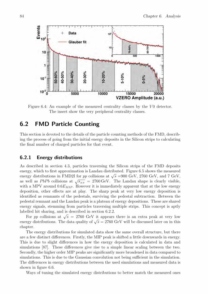
84 Chapter 6. Analysis
Figure 6.4: An example of the measured centrality classes by the V 0 detector.The insert show the very peripheral centrality classes.
6.2 FMD Particle Counting
This section is devoted to the details of the particle counting methods of the FMD, describ-ing the process of going from the initial energy deposits in the Silicon strips to calculatingthe final number of charged particles for that event.
6.2.1 Energy distributions
As described in section 4.3, particles traversing the Silicon strips of the FMD depositsenergy, which to first approximation is Landau distributed. Figure 6.5 shows the measuredenergy distributions in FMD2I for pp collisions at
√s =900 GeV, 2760 GeV, and 7 GeV,
as well as PbPb collisions at√sNN
= 2760 GeV. The Landau shape is clearly visible,with a MPV around 0.6EMIP . However it is immediately apparent that at the low energydeposition, other effects are at play. The sharp peak at very low energy deposition isidentified as remnants of the pedestals, surviving the pedestal subtraction. Between thepedestal remnant and the Landau peak is a plateau of energy depositions. These are sharedenergy signals, stemming from particles traversing multiple strips. This concept is aptlylabelled hit sharing, and is described in section 6.2.2.
For pp collisions at√s = 2760 GeV it appears there is an extra peak at very low
energy distributions. The data quality of√s = 2760 GeV will be discussed later on in this
chapter.
The energy distributions for simulated data show the same overall structure, but thereare a few distinct differences. Firstly, the MIP peak is shifted a little downwards in energy.This is due to slight differences in how the energy deposition is calculated in data andsimulations [87]. These differences give rise to a simple linear scaling between the two.Secondly, the higher order MIP peaks are significantly more broadened in data compared tosimulations. This is due to the Gaussian convolution not being sufficient in the simulation.The differences in energy distributions between the used simulations and measured data isshown in figure 6.6.
Ways of tuning the simulated energy distributions to better match the measured ones

6.2. FMD Particle Counting 85
MIP/Edepx = E0 0.5 1 1.5 2 2.5 3
)M
IP N
(x)
/ N(E
-310
-210
-110
1
10 =900 GeVsFMD2I in pp @
MIP/Edepx = E0 0.5 1 1.5 2 2.5 3
)M
IP N
(x)
/ N(E
-310
-210
-110
1
10 =2760 GeVsFMD2I in pp @
MIP/Edepx = E0 0.5 1 1.5 2 2.5 3
)M
IP N
(x)
/ N(E
-310
-210
-110
1
10 =7000 GeVsFMD2I in pp @
MIP/Edepx = E0 0.5 1 1.5 2 2.5 3
)M
IP N
(x)
/ N(E
-310
-210
-110
1
10 =2760 GeVNNsFMD2I in PbPb @
Figure 6.5: The measured energy distributions in FMD2I for pp collisions at√s =900 GeV, 2760 GeV, and 7 GeV, as well as PbPb collisions
at√sNN
= 2760 GeV. At very low energy deposits remnants ofthe pedestals are seen, following by a region of shared signals. AtEdep/EMIP ∼ 0.5 the Landau distribution begins.

86 Chapter 6. Analysis
MIP/Edepx = E0 0.5 1 1.5 2 2.5 3
N(x
) [s
cale
d to
1st
Lan
dau
peak
]
-310
-210
-110
1
10 =900 GeVsFMD2I in pp @
MIP/Edepx = E0 0.5 1 1.5 2 2.5 3
N(x
) [s
cale
d to
1st
Lan
dau
peak
]
-310
-210
-110
1
10 =2760 GeVsFMD2I in pp @
MIP/Edepx = E0 0.5 1 1.5 2 2.5 3
N(x
) [s
cale
d to
1st
Lan
dau
peak
]
-310
-210
-110
1
10 =7000 GeVsFMD2I in pp @
Data
MC
MIP/Edepx = E0 0.5 1 1.5 2 2.5 3
N(x
) [s
cale
d to
1st
Lan
dau
peak
]
-310
-210
-110
1
10 =2760 GeVNNsFMD2I in PbPb @
Figure 6.6: Energy distributions in the simulations compared to the measuredenergy distributions from figure 6.5. It is found that the peaks areshifted slightly and are smeared more in the physics data comparedto the simulations.
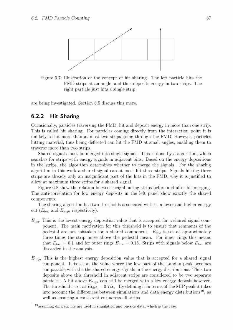
6.2. FMD Particle Counting 87
Figure 6.7: Illustration of the concept of hit sharing. The left particle hits theFMD strips at an angle, and thus deposits energy in two strips. Theright particle just hits a single strip.
are being investigated. Section 8.5 discuss this more.
6.2.2 Hit Sharing
Occasionally, particles traversing the FMD, hit and deposit energy in more than one strip.This is called hit sharing. For particles coming directly from the interaction point it isunlikely to hit more than at most two strips going through the FMD. However, particleshitting material, thus being deflected can hit the FMD at small angles, enabling them totraverse more than two strips.
Shared signals must be merged into single signals. This is done by a algorithm, whichsearches for strips with energy signals in adjacent bins. Based on the energy depositionsin the strips, the algorithm determines whether to merge the signals. For the sharingalgorithm in this work a shared signal can at most hit three strips. Signals hitting threestrips are already only an insignificant part of the hits in the FMD, why it is justified toallow at maximum three strips for a shared signal.
Figure 6.8 show the relation between neighbouring strips before and after hit merging.The anti-correlation for low energy deposits in the left panel show exactly the sharedcomponents.
The sharing algorithm has two thresholds associated with it, a lower and higher energycut (Elow and Ehigh respectively).
Elow This is the lowest energy deposition value that is accepted for a shared signal com-ponent. The main motivation for this threshold is to ensure that remnants of thepedestal are not mistaken for a shared component. Elow is set at approximatelythree times the strip noise above the pedestal mean. For inner rings this meansthat Elow = 0.1 and for outer rings Elow = 0.15. Strips with signals below Elow arediscarded in the analysis.
Ehigh This is the highest energy deposition value that is accepted for a shared signalcomponent. It is set at the value where the low part of the Landau peak becomescomparable with the the shared energy signals in the energy distributions. Thus twodeposits above this threshold in adjacent strips are considered to be two separateparticles. A hit above Ehigh can still be merged with a low energy deposit however.The threshold is set at Ehigh = 0.7∆p. By defining it in terms of the MIP peak it takesinto account the differences between simulations and data energy distributions19, aswell as ensuring a consistent cut across all strips.
19assuming different fits are used in simulation and physics data, which is the case.
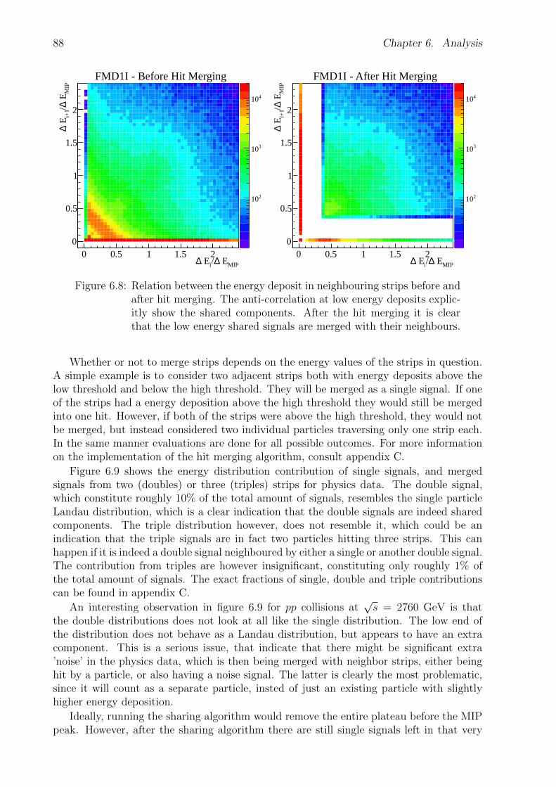
88 Chapter 6. Analysis
MIP E∆/i E∆0 0.5 1 1.5 2
MIP
E∆/i+
1 E∆
0
0.5
1
1.5
2
210
310
410
FMD1I - Before Hit Merging
MIP E∆/i E∆0 0.5 1 1.5 2
MIP
E∆/i+
1 E∆
0
0.5
1
1.5
2
210
310
410
FMD1I - After Hit Merging
Figure 6.8: Relation between the energy deposit in neighbouring strips before andafter hit merging. The anti-correlation at low energy deposits explic-itly show the shared components. After the hit merging it is clearthat the low energy shared signals are merged with their neighbours.
Whether or not to merge strips depends on the energy values of the strips in question.A simple example is to consider two adjacent strips both with energy deposits above thelow threshold and below the high threshold. They will be merged as a single signal. If oneof the strips had a energy deposition above the high threshold they would still be mergedinto one hit. However, if both of the strips were above the high threshold, they would notbe merged, but instead considered two individual particles traversing only one strip each.In the same manner evaluations are done for all possible outcomes. For more informationon the implementation of the hit merging algorithm, consult appendix C.
Figure 6.9 shows the energy distribution contribution of single signals, and mergedsignals from two (doubles) or three (triples) strips for physics data. The double signal,which constitute roughly 10% of the total amount of signals, resembles the single particleLandau distribution, which is a clear indication that the double signals are indeed sharedcomponents. The triple distribution however, does not resemble it, which could be anindication that the triple signals are in fact two particles hitting three strips. This canhappen if it is indeed a double signal neighboured by either a single or another double signal.The contribution from triples are however insignificant, constituting only roughly 1% ofthe total amount of signals. The exact fractions of single, double and triple contributionscan be found in appendix C.
An interesting observation in figure 6.9 for pp collisions at√s = 2760 GeV is that
the double distributions does not look at all like the single distribution. The low end ofthe distribution does not behave as a Landau distribution, but appears to have an extracomponent. This is a serious issue, that indicate that there might be significant extra’noise’ in the physics data, which is then being merged with neighbor strips, either beinghit by a particle, or also having a noise signal. The latter is clearly the most problematic,since it will count as a separate particle, insted of just an existing particle with slightlyhigher energy deposition.
Ideally, running the sharing algorithm would remove the entire plateau before the MIPpeak. However, after the sharing algorithm there are still single signals left in that very

6.2. FMD Particle Counting 89
MIP/EdepE0 0.2 0.4 0.6 0.8 1 1.2 1.4 1.6 1.8 2 2.2
Eve
nts
1
10
210
310
410
510
610SinglesDoublesTriples
=900 GeVspp @
MIP/EdepE0 0.2 0.4 0.6 0.8 1 1.2 1.4 1.6 1.8 2 2.2
Eve
nts
1
10
210
310
410
510
610SinglesDoublesTriples
=2760 GeVspp @
MIP/EdepE0 0.2 0.4 0.6 0.8 1 1.2 1.4 1.6 1.8 2 2.2
Eve
nts
1
10
210
310
410
510
610SinglesDoublesTriples
=7000 GeVspp @
MIP/EdepE0 0.2 0.4 0.6 0.8 1 1.2 1.4 1.6 1.8 2 2.2
Eve
nts
1
10
210
310
410
510
610
710
810 SinglesDoublesTriples
=2760 GeVNNsPbPb @
Figure 6.9: Energy distributions after hit merging for single, double and triplesignals in physics data.

90 Chapter 6. Analysis
MIP/EdepE0 0.2 0.4 0.6 0.8 1 1.2 1.4 1.6 1.8 2 2.2
Eve
nts
1
10
210
310
410
510
610SinglesDoublesTriples
=900 GeVsMC pp @
MIP/EdepE0 0.2 0.4 0.6 0.8 1 1.2 1.4 1.6 1.8 2 2.2
Eve
nts
1
10
210
310
410
510
610SinglesDoublesTriples
=2760 GeVsMC pp @
MIP/EdepE0 0.2 0.4 0.6 0.8 1 1.2 1.4 1.6 1.8 2 2.2
Eve
nts
1
10
210
310
410
510
610SinglesDoublesTriples
=7000 GeVsMC pp @
MIP/EdepE0 0.2 0.4 0.6 0.8 1 1.2 1.4 1.6 1.8 2 2.2
Eve
nts
1
10
210
310
410
510
610SinglesDoublesTriples
=2760 GeVNNsMC PbPb @
Figure 6.10: Energy distributions after hit merging for single, double and triplesignals in simulated data. The low energy deposit plateau after hitmerging is about an order of magnitude lower than in physics data.
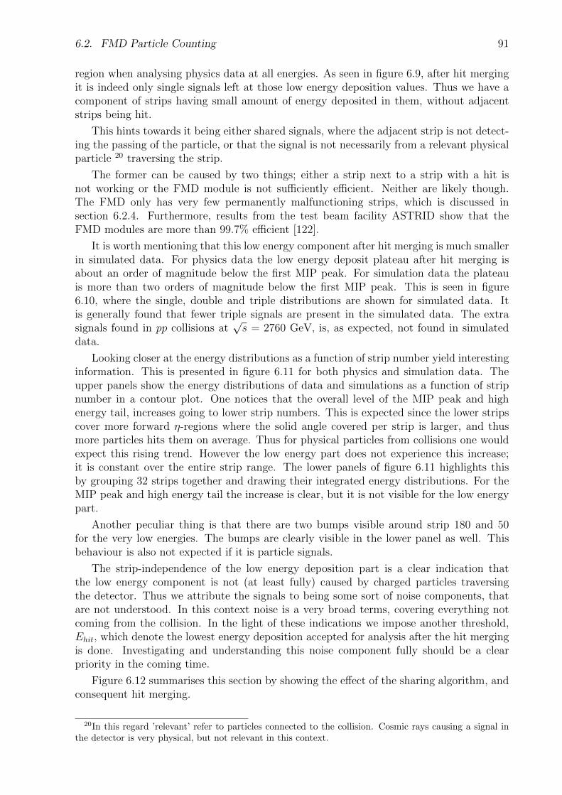
6.2. FMD Particle Counting 91
region when analysing physics data at all energies. As seen in figure 6.9, after hit mergingit is indeed only single signals left at those low energy deposition values. Thus we have acomponent of strips having small amount of energy deposited in them, without adjacentstrips being hit.
This hints towards it being either shared signals, where the adjacent strip is not detect-ing the passing of the particle, or that the signal is not necessarily from a relevant physicalparticle 20 traversing the strip.
The former can be caused by two things; either a strip next to a strip with a hit isnot working or the FMD module is not sufficiently efficient. Neither are likely though.The FMD only has very few permanently malfunctioning strips, which is discussed insection 6.2.4. Furthermore, results from the test beam facility ASTRID show that theFMD modules are more than 99.7% efficient [122].
It is worth mentioning that this low energy component after hit merging is much smallerin simulated data. For physics data the low energy deposit plateau after hit merging isabout an order of magnitude below the first MIP peak. For simulation data the plateauis more than two orders of magnitude below the first MIP peak. This is seen in figure6.10, where the single, double and triple distributions are shown for simulated data. Itis generally found that fewer triple signals are present in the simulated data. The extrasignals found in pp collisions at
√s = 2760 GeV, is, as expected, not found in simulated
data.
Looking closer at the energy distributions as a function of strip number yield interestinginformation. This is presented in figure 6.11 for both physics and simulation data. Theupper panels show the energy distributions of data and simulations as a function of stripnumber in a contour plot. One notices that the overall level of the MIP peak and highenergy tail, increases going to lower strip numbers. This is expected since the lower stripscover more forward η-regions where the solid angle covered per strip is larger, and thusmore particles hits them on average. Thus for physical particles from collisions one wouldexpect this rising trend. However the low energy part does not experience this increase;it is constant over the entire strip range. The lower panels of figure 6.11 highlights thisby grouping 32 strips together and drawing their integrated energy distributions. For theMIP peak and high energy tail the increase is clear, but it is not visible for the low energypart.
Another peculiar thing is that there are two bumps visible around strip 180 and 50for the very low energies. The bumps are clearly visible in the lower panel as well. Thisbehaviour is also not expected if it is particle signals.
The strip-independence of the low energy deposition part is a clear indication thatthe low energy component is not (at least fully) caused by charged particles traversingthe detector. Thus we attribute the signals to being some sort of noise components, thatare not understood. In this context noise is a very broad terms, covering everything notcoming from the collision. In the light of these indications we impose another threshold,Ehit, which denote the lowest energy deposition accepted for analysis after the hit mergingis done. Investigating and understanding this noise component fully should be a clearpriority in the coming time.
Figure 6.12 summarises this section by showing the effect of the sharing algorithm, andconsequent hit merging.
20In this regard ’relevant’ refer to particles connected to the collision. Cosmic rays causing a signal inthe detector is very physical, but not relevant in this context.

92 Chapter 6. Analysis
Figure 6.11: Top Panels: The single energy distributions for each strip of FMD2Ofor PbPb collisions at
√sNN
= 2760 GeV. Both physics data (left)and simulated data (right) is shown. Lower panels: The energydistributions of groups of 32 strips. It is found that there is a distinctdifference at the low energy deposits, where there is many moresignals in data compared to simulations. The reason for this extracomponent is not understood. Since it is not in the simulations a cut,Ehit ∼ 0.7δp, is imposed to cut away single strips with low energydeposits.

6.2. FMD Particle Counting 93
Figure 6.12: Example of the effect of merging shared signals on the energy dis-tributions. Shown is each individual FMD ring in pp collisions at√s = 900 GeV.

94 Chapter 6. Analysis
MIP / EdepE0 0.5 1 1.5 2 2.5 3
Cou
nts
[sca
led
to p
eak]
-210
-110
1
pp @ 900 GeV 1 particle fit
2 particle fit
3 particle fit
MIP / EdepE0 0.5 1 1.5 2 2.5 3
Cou
nts
[sca
led
to p
eak]
-210
-110
1
PbPb @ 2760 GeV 1 particle fit
2 particle fit
3 particle fit
Figure 6.13: Example of a multiple (Gaussian convoluted) Landau fit to the en-ergy distributions for pp collisions at
√s = 900 GeV and PbPb colli-
sions at√sNN
= 2760 GeV. Fits including 1-3 Landau distributionsare shown.
6.2.3 Counting Methods
Next step in the analysis is to take into account the high occupancy i.e., cases whereseveral particles hit the same strip21. This is what gives rise to the higher order MIPpeaks, discussed previously. However, a single slow-moving particle depositing a lot ofenergy, and several particles depositing lower energies are indistinguishable in the FMD.Thus when counting the actual number of charged particles hitting the FMD, this mustbe taken into account. It has been tested using two distinct methods, which are describedin this section.
Energy Fit Method
Multiple Landau distributions, each convoluted with a Gaussian, as described in section 4.3,are fitted to the energy distributions. Each of the fitted Landau distributions correspondsto 1, 2 or 3 MIPs depositing energy in the detection element. Figure 6.13 show the resultsof fitting the data with 1-3 Landau distributions respectively. The fits are shown for ppcollisions at
√s = 900 GeV and PbPb collisions at
√sNN
= 2760 GeV. Even using onlya few Landau distributions yield excellent agreement with the data. For the analysis 3Landau distribution fits are sufficient.
The energy fit method takes high occupancy into account by directly using the fits tothe energy distributions. It is done by calculating the weighted mean of the entire energydistribution, by using the weights, ai, for the individual MIP peaks.
Nch =
∑3i=1 iaiFi∑3i=1 aiFi
(6.1)
where the fit (and thus the sum) is restricted to include the first 3 Landau distributions.Fi = Li(∆)⊗Gi(∆) denotes the ith Gaussian convoluted Landau distribution as describedin section 1.4.1.
21Not to be confused with hit sharing as discussed in the previous section, where a single particle hitseveral strips.

6.2. FMD Particle Counting 95
Fraction of Channels Hit0 0.2 0.4 0.6 0.8 1C
orre
ctio
n =
Tot
al H
its
/ Cha
nnel
s H
it (
i.e. >
=1
hit)
1
1.5
2
2.5
3
3.5
4
4.5
5Channel Group = 8Channel Group = 16Channel Group = 32Channel Group = 64Channel Group = 128Channel Group = 256Channel Group = 512
Fraction of Channels Hit0 0.1 0.2 0.3 0.4 0.5 0.6 0.7 0.8 0.9 1
Rat
io o
f C
orre
ctio
n Fa
ctor
s
0.96
0.98
1
1.02
1.04
1.06
1.08
1.1
1.12
Figure 6.14: The correction for high occupancy in the Poisson counting method.Left panel shows the correction factor for different region sizes asa function of the occupancy. The analytical expression is shown asthe solid black line. Right panel: The ratio between the correctionfactors of the different region sizes and the analytical solution. Itis seen that the agreement becomes better and better for increasingregion sizes.
Poisson Method
The second method used for counting particles in the FMD takes high occupancy intoaccount by using Poisson statistics.
To illustrate this, let us start out by defining the true occupancy for a region of theFMD as the mean number of particles per strip traversing this region.
µ = Nch/Nchannels (6.2)
Similarly the measured occupancy of a single event is given by:
µmeas = Nhits/Nchannels (6.3)
where Nhits is the number of strips with a hit above Ehit. If the assumption is made thatthe distribution of particles hitting a region of the FMD is uniform, then the number ofparticles hitting that region is described by Poisson statistics i.e., the probability of findingNch = n particles in the region is:
P (n) =µne−µ
n!(6.4)
The measured occupancy, which is the probability of having any number of hits in theregion, can then be related to the true occupancy:
µmeas = P (n > 0) = 1− P (0) = 1− e−µ (6.5)

96 Chapter 6. Analysis
Now, for a strip being hit the average number of particles hitting it will be:
C =
∑n>0 nP (n)∑n>0 P (n)
=e−µ
1− e−µ∑n>0
nµn
n!
=e−µ
1− e−µµ∑n>0
µn−1
(n− 1)!
=e−µ
1− e−µµ∑k=n−1
µk
k!=
e−µ
1− e−µµeµ
=µ
1− e−µ(6.6)
µ can in principle be calculated analytically, but can also be found by inverting (6.5),yielding
µ =1
ln(1− µmeas)(6.7)
This is done in regions of the FMD each containing 256 strips. Thus each strip being hitin this region takes high occupancy into account by scaling with C for that region.
Figure 6.14 shows the motivation for using at least 256 strips as a region. The leftpanel shows the correction factor as a function of the occupancy for several choices ofregion size. Also included is the analytical calculation plotted on top as a solid black line.The right panel shows the ratio of the correction of the various region sizes compared tothe analytical curve. It is clear that for our selection of 256 strips there is great agreementwith the analytical curve to very high occupancies. The regions used, consists of 64 stripsin 4 adjacent sectors.
Even better agreement could be reached by using 512 strips, but it comes at a cost inthe sense that it would mean larger regions in either η or φ. Having too large regions cancause problems due to the number of particles varying over the region. Thus, we aim athaving regions with sufficient strips to ensure agreement with the analytical calculationwithout washing out changes in number of particles over a region. The difference between256 and 512 strips in figure 6.14 is around 0.1%.
As seen regions of 256 strips has good agreement until the highest occupancies. Figure6.15 show the distribution of region occupancies for one of the FMD rings for pp collisionsat√s =900 GeV and PbPb collisions at
√sNN
= 2760 GeV. As is evident, even in PbPbcollisions the mean region occupancy of the FMD system is low enough to ensure that thechosen regions of 256 strips are in accordance with the analytical curve.
Comparison between Poisson and Energy Fit counting
Both methods of counting are viable. Figure 6.16 show the comparison between the twomethods for each FMD ring in pp collisions at
√s = 900GeV. The comparison for pp
collisions at√s = 2760 GeV and 7000 GeV and PbPb collisions at
√sNN
= 2760 GeV canbe found in appendix D.
In both cases good agreement is found between the two methods, with the regressionslope close to unity. The agreement is better for the inner rings, compared to outer rings.The reason for this is not understood and must be studied more. For the results presentedin chapter 8 the Poisson method is used, since it is the simpler of the two methods. Theminor disagreements between the two methods are included as a systematic uncertainty.

6.2. FMD Particle Counting 97
Occupancy0 10 20 30 40 50 60 70 80 90
#FM
D R
egio
ns w
ith 2
56 s
trip
s
1
10
210
310
410
510
610
710
810 =900 GeVspp @
Mean Occupancy = 0.08 %
Occupancy0 10 20 30 40 50 60 70 80 90
#FM
D R
egio
ns w
ith 2
56 s
trip
s
1
10
210
310
410
510
610
710
810 =2760 GeVspp @
Mean Occupancy = 0.09 %
Occupancy0 10 20 30 40 50 60 70 80 90
#FM
D R
egio
ns w
ith 2
56 s
trip
s
1
10
210
310
410
510
610
710
810 =7000 GeVspp @
Mean Occupancy = 0.15 %
Occupancy0 10 20 30 40 50 60 70 80 90
#FM
D R
egio
ns w
ith 2
56 s
trip
s
1
10
210
310
410
510
610
710
810 =2760 GeVNNsPbPb @
Mean Occupancy = 7.36 %
Figure 6.15: Occupancy distribtion in regions of 256 strips in FMD2I for pp colli-sions at
√s = 900 GeV, 2760 GeV, and 7000 GeV, as well as PbPb
collisions at√sNN
= 2760 GeV.
6.2.4 FMD Acceptance
As any other detector, the FMD does not have perfect acceptance. The issues with accep-tance can be grouped into three types of acceptances, that will be corrected for separately:
η acceptance The edge of the outermost η bins in each ring might not coincide with theactual η value of the outermost strip. This means that the outermost bin mightbe only partially full, and thus consist of fewer strips. This can cause corrections inthose bins to blow up, as well as general edge effects from rapidly changing acceptancecompared to limited resolution. Thus a cut is imposed to cut away the outer partialbin. In section 6.8 comparisons between the analysis with 0,1 or 2 bins cut away willbe discussed.
φ acceptance The FMD is in principle built as a detector with full φ-coverage. However,atthe time of construction, it was not possible to manufacture silicon wafers at thequality required for the FMD, in sizes bigger than 6”. To maximise the η coverageit was decided to cut away the corners of the individual sensors (as seen in figure4.6). Thus the outermost strips span a shorter arc length than the rest, and thereforedoes not have full φ acceptance. This is solved by geometrically calculating the ratiobetween the length of the actual strip and the length of the strip if the corners hadbeen there, and correcting the signal by this ratio. An example of this correction isshown in figure 6.17.
Dead Channels Over time individual strips will permanently malfunction. Typically,what will happen, is that individual strips become completely unresponsive. But
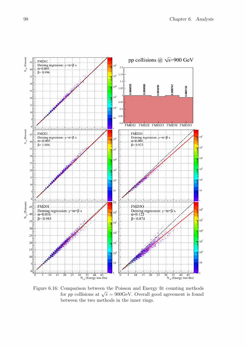
98 Chapter 6. Analysis
Figure 6.16: Comparison between the Poisson and Energy fit counting methodsfor pp collisions at
√s = 900GeV. Overall good agreement is found
between the two methods in the inner rings.

6.3. SPD Particle Counting 99
Figure 6.17: Example of the φ-acceptance of an inner ring. There is full azimuthalcoverage until the outermost strips, where the acceptance drops dueto the corners being cut off on the FMD silicon wafers.
in principle one could also have strips malfunction such that they are giving a highsignal every event, regardless of whether or not there is a hit. This latter effect hasnot been observed yet however.
The dead strips must be taken out of the analysis, and a correction for the missingstrips must be made. A channel in the FMD is considering active and well if it fulfils
0.5 < gi < 5
0 < ni < 10 (6.8)
where gi and ni corresponds to the gain and noise of strip i respectively.
For the initial run period at√s = 900 GeV the fraction of dead channels amount to
0.93%. Due to a better implementation of the software on the front-end electronics,the amount of dead channels decreased to 0.25% after the initial run period.
It is found that the 0.25% stems almost solely of a single V A13 chip in FMD1I beingentirely faulty. This particular dead region was also pointed out in in the figures4.11, 4.11 and 4.11.
The correction factor for a given (η, φ)-bin is given by calculating the ratio of workingstrips to the total number of strips in that bin.
6.3 SPD Particle Counting
Counting particles in the SPD inner layer is simpler than in the FMD case.The analysis procedure does not make use of the tracklets, but instead only uses the
clusters from the inner layer. In some sense the analysis procedure is very similar to theone used for the FMD rings i.e., the inner layer is seen as a silicon layer with no trackinginformation.
In the reconstruction of the SPD data, both the tracklets and unused clusters weresaved as described in section 5.3. Thus the number of particles in the SPD in a given ηrange is simply given by:
Nch =∑t
1 +∑c
1 (6.9)

100 Chapter 6. Analysis
Figure 6.18: The frequency of various cluster patterns in the SPD [123]. Theyellow bars are for physics data and the black points are for simula-tions. It is seen that 68% of hits in the SPD are single pixels beinghit. Less than 3% of hits consist of more than two adjacent pixelsfiring.
Here the sum is over c and t, which are the unused clusters and the tracklets in thefirst layer respectively.
The big challenges in the FMD with hit sharing and high occupancy are not present inthe SPD. Due to the very fine segmentation in η it is very unlikely to have multiple signalsin the same pixel, which removes the need for taking high occupancy into account.
The individual clusters can consist of signals in several adjacent pixels. But again, dueto the fine resolution, it is unlikely that two particles would hit adjacent pixels.
Therefore even multi-pixel signals are very likely to be just a single particle. Further-more, since the SPD is a pixel threshold detector, the deposited amount of energy is notavailable, and thus no hit merging could be done if needed.
Figure 6.18 show the frequency of the various cluster signatures in the SPD, both forphysics data and from simulated data [123]. 97% of all cluster are either single pixel clustersor clusters made up of two adjacent pixels.
6.3.1 SPD Acceptance
As in the case of the FMD there are similar acceptance issues regarding the SPD innerlayer.
η acceptance In the same manner as in the FMD, the first η bin is cut away, since itmight be partly filled with pixels only.
φ acceptance The SPD is designed with full 2π φ-coverage.

6.4. Secondary particles 101
η-2 -1.5 -1 -0.5 0 0.5 1 1.5 2
acce
ptan
ce c
orre
ctio
n
0.3
0.4
0.5
0.6
0.7
0.8
0.9 -4 < z < -2 cm
-2 < z < 0 cm
0 < z < 2 cm
2 < z < 4 cm
Figure 6.19: The actual φ-acceptance of the SPD as a function of η. As discussedin the text, cooling issues has meant that parts of the SPD is turnedoff. This leaves large holes in the acceptance.
Dead channels The SPD have two contributions to dead channels. The first is malfunc-tioning pixels, connectors, etc., analogous to the malfunctioning strips in the FMD.This type of dead channels only amount to less than 1 % of the number of pixels [123].
The second contribution is much bigger. The cooling requirements for the SPD arevery large. And so far the cooling capabilities of the SPD has not been sufficient.The unfortunate consequence is that parts of the SPD has been turned off for datataking to avoid overheating. Thus while the SPD is designed with full φ-coverage,it does not have it, due to turned off channels. Figure 6.19 shows the acceptancecorrection as a function of η for the running conditions, and later on, figure 6.26shows the large holes in the (η,φ) acceptance of the SPD.
6.4 Secondary particles
Particles can be grouped as either primary particles or secondary particles. For this workall particles stemming directly from the initial collision are considered primary particles.On the other hand, particles created by decays, interaction with materials on the way tothe SPD or FMD is labelled secondary particles.
This section will discuss the secondary contamination in both detectors, as well asdescribe how to correct for secondary particles.
We start out by looking at the amount of secondary particles hitting each detector, aswell as where they were created. This is done using simulated data. If the implementedvirtual model of the experiment, as well as the physics processes in the transport model,is accurate, then the simulation describes the actual physics collisions well. Figure 6.20show an example of the origin of all secondary particles in the central (z, r) region. It isimmediately possible to identify sub-detectors, support structures etc., by the secondaryparticles created in their material. Figure 6.21 shows a similar example, but this time onlythe the origin of the secondary particles eventually hitting one of the FMD rings.
What is apparent is that there is a vast difference in the amount of material in frontof the SPD and FMD respectively. The SPD, sitting just outside the beam-pipe, has verylittle material in front of it, and thus a low secondary particle contamination. The FMD
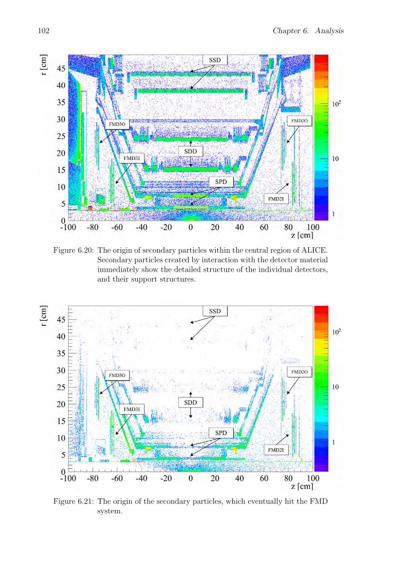
102 Chapter 6. Analysis
Figure 6.20: The origin of secondary particles within the central region of ALICE.Secondary particles created by interaction with the detector materialimmediately show the detailed structure of the individual detectors,and their support structures.
Figure 6.21: The origin of the secondary particles, which eventually hit the FMDsystem.

6.4. Secondary particles 103
on the other hand has a considerable amount of material in front of it.Another point worth bringing up is that secondary particles hitting a detector element
in a certain region in η is quite likely to originate from that same η region. Thus, mostsecondary particles created continues in a similar direction as their primary ancestor. Thisis illustrated in figure 6.22, which show the origin of secondary particles hitting each of theindividual FMD rings.
Using figure 6.20 as a reference it is possible to define geometrical shapes in (z, r),that correspond to certain detectors. Summing up everything inside these shapes will thusyield the secondary particles contribution from that selection. For this study, five differentselections are sufficient to get a clear picture of the origin of the secondary particles hittingthe SPD or FMD. These are:
Early Decay This is used as a common name for all secondary particles created inside thebeam pipe.
Beam Pipe These are the secondary particles created in the beam pipe material, as theprimary (or early decay secondary) particles traverse it.
ITS These secondaries are created inside the ITS volume.
FMD These secondaries are created inside the FMD volume.
OTHER All the rest of the secondary particles are grouped together. This is viable, sincethe vast majority of secondary particles hitting either the FMD or SPD falls into oneof the four other categories.
In figure 6.23 the total contamination of secondary particles for both the FMD andSPD region is shown. In the region of η-overlap between FMD3I and FMD3O i.e., aroundη ∼ −2, contributions from each sub-detector is added together, giving a peak structure. Infigure 6.24 the same information is shown per sub-detector. It is seen that the secondaryparticles hitting the FMD stems mainly from itself and the ITS. Going more and moreforward in η yields a bigger and bigger contribution from the beam pipe, since the effectivepath length through the beam pipe becomes longer and longer22. The amount of secondaryparticles hitting the FMD is in some areas almost twice as big as the amount of primarieshitting it. In the SPD the amount of secondaries is in the order of 10% of the amount ofprimaries.
It is necessary to correct for the secondary particles, in order to retrieve the primarydistribution. This can either be done in a separate step, which we label the secondarycorrection, or be done later on during the unfolding process, described in section 6.6.
The secondary correction is done by using simulations, to determine the amount ofsecondary particles compared to the total number of particles in each (η, φ) bin. Thus, thecorrection factor for a given (η, φ) bin is:
Csec(η, ϕ) =
∑iN
ich, prim(η, ϕ)∑
iNich, sec + prim(η, ϕ)
(6.10)
The sums run over the simulated data sample, having a valid vertex and trigger. The totalnumber of charged particles hitting the chosen FMD bin in event i is denoted N i
ch, sec + prim.Similarly N i
ch, prim is the number of primary charged particles as given immediately after
22This is not the only reason though. At z ∼ −35 cm, the Beryllium beam pipe stops, replaced by steel,which create many more beam pipe secondary particles in FMD3I, compared to the other rings.
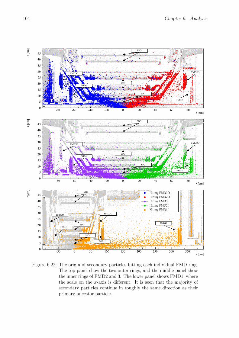
104 Chapter 6. Analysis
Figure 6.22: The origin of secondary particles hitting each individual FMD ring.The top panel show the two outer rings, and the middle panel showthe inner rings of FMD2 and 3. The lower panel shows FMD1, wherethe scale on the x-axis is different. It is seen that the majority ofsecondary particles continue in roughly the same direction as theirprimary ancestor particle.
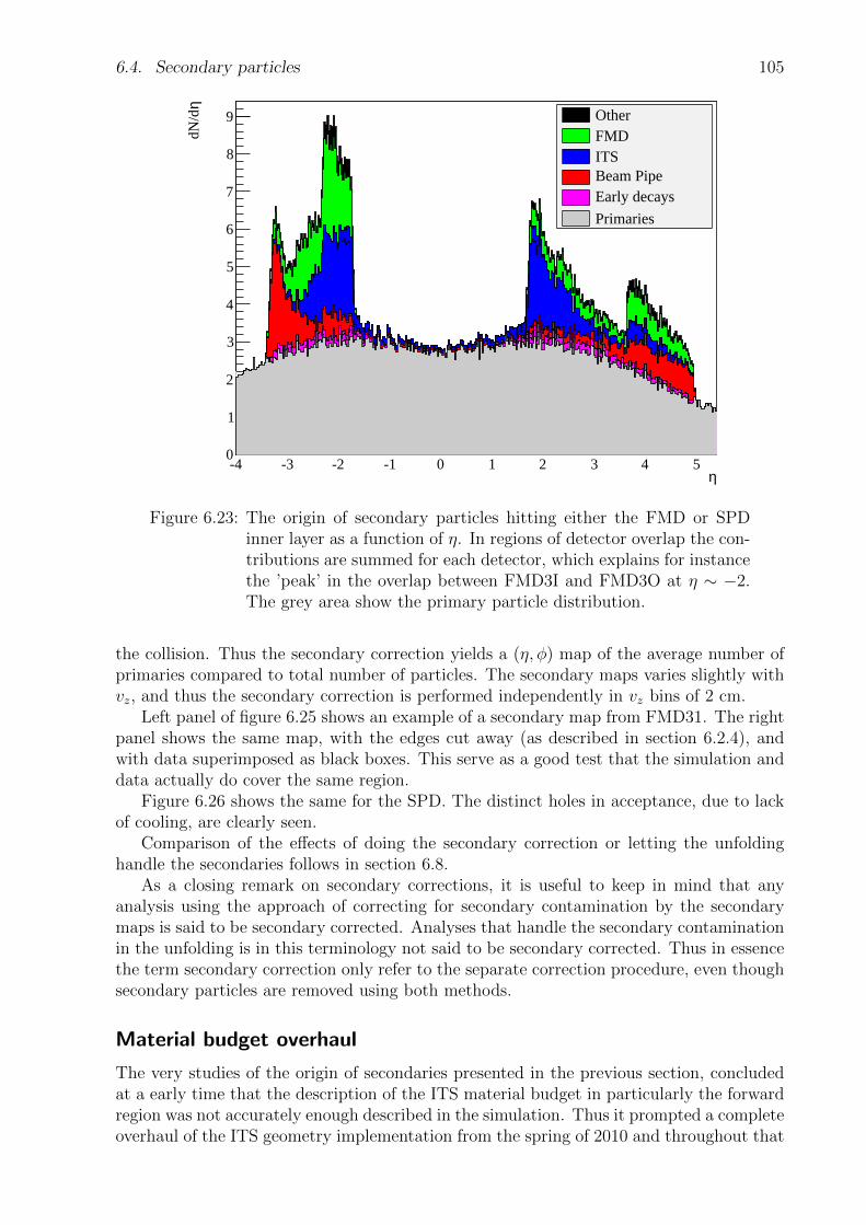
6.4. Secondary particles 105
η-4 -3 -2 -1 0 1 2 3 4 5
ηdN
/d
0
1
2
3
4
5
6
7
8
9 OtherFMDITSBeam PipeEarly decays
Primaries
Figure 6.23: The origin of secondary particles hitting either the FMD or SPDinner layer as a function of η. In regions of detector overlap the con-tributions are summed for each detector, which explains for instancethe ’peak’ in the overlap between FMD3I and FMD3O at η ∼ −2.The grey area show the primary particle distribution.
the collision. Thus the secondary correction yields a (η, φ) map of the average number ofprimaries compared to total number of particles. The secondary maps varies slightly withvz, and thus the secondary correction is performed independently in vz bins of 2 cm.
Left panel of figure 6.25 shows an example of a secondary map from FMD31. The rightpanel shows the same map, with the edges cut away (as described in section 6.2.4), andwith data superimposed as black boxes. This serve as a good test that the simulation anddata actually do cover the same region.
Figure 6.26 shows the same for the SPD. The distinct holes in acceptance, due to lackof cooling, are clearly seen.
Comparison of the effects of doing the secondary correction or letting the unfoldinghandle the secondaries follows in section 6.8.
As a closing remark on secondary corrections, it is useful to keep in mind that anyanalysis using the approach of correcting for secondary contamination by the secondarymaps is said to be secondary corrected. Analyses that handle the secondary contaminationin the unfolding is in this terminology not said to be secondary corrected. Thus in essencethe term secondary correction only refer to the separate correction procedure, even thoughsecondary particles are removed using both methods.
Material budget overhaul
The very studies of the origin of secondaries presented in the previous section, concludedat a early time that the description of the ITS material budget in particularly the forwardregion was not accurately enough described in the simulation. Thus it prompted a completeoverhaul of the ITS geometry implementation from the spring of 2010 and throughout that
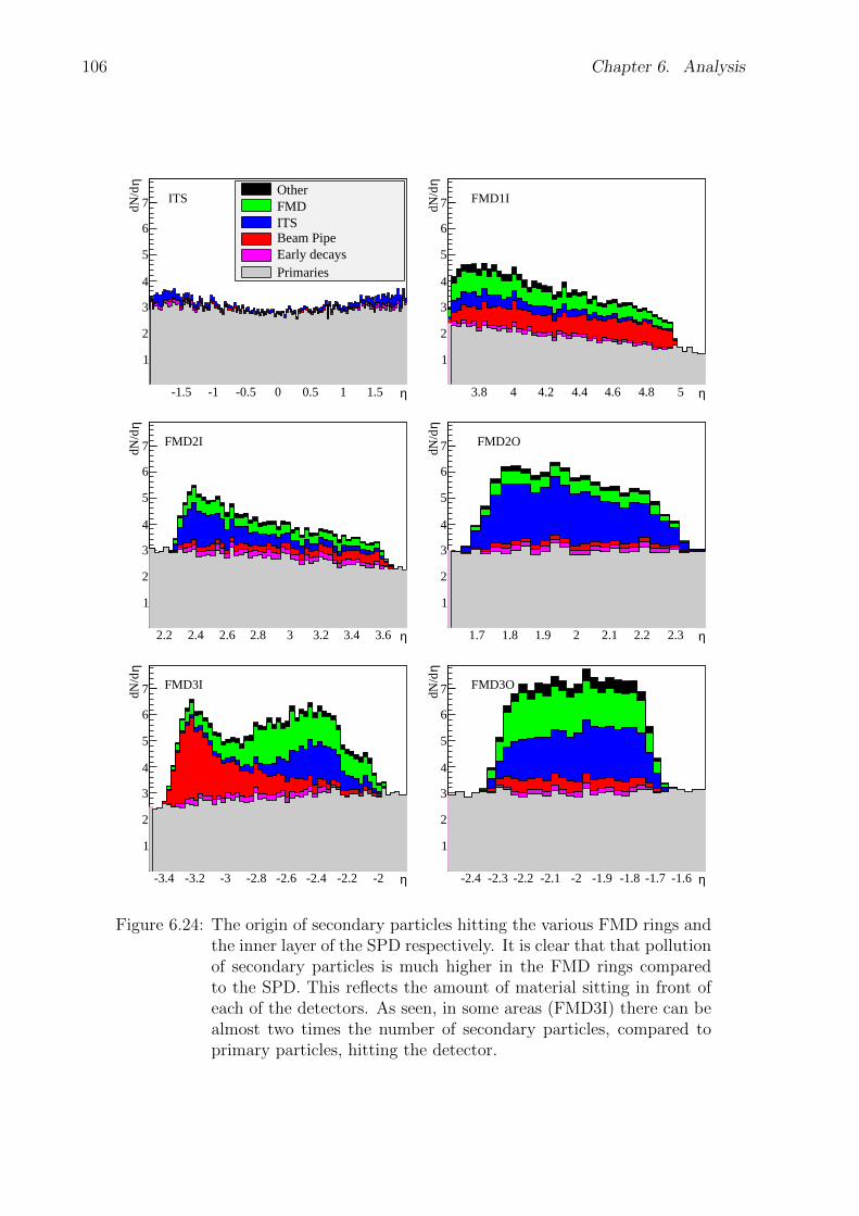
106 Chapter 6. Analysis
η-1.5 -1 -0.5 0 0.5 1 1.5
ηdN
/d
1
2
3
4
5
6
7 ITSOtherFMDITSBeam PipeEarly decaysPrimaries
η3.8 4 4.2 4.4 4.6 4.8 5
ηdN
/d
1
2
3
4
5
6
7 FMD1I
η2.2 2.4 2.6 2.8 3 3.2 3.4 3.6
ηdN
/d
1
2
3
4
5
6
7 FMD2I
η1.7 1.8 1.9 2 2.1 2.2 2.3
ηdN
/d
1
2
3
4
5
6
7 FMD2O
η-3.4 -3.2 -3 -2.8 -2.6 -2.4 -2.2 -2
ηdN
/d
1
2
3
4
5
6
7 FMD3I
η-2.4 -2.3 -2.2 -2.1 -2 -1.9 -1.8 -1.7 -1.6
ηdN
/d
1
2
3
4
5
6
7 FMD3O
Figure 6.24: The origin of secondary particles hitting the various FMD rings andthe inner layer of the SPD respectively. It is clear that that pollutionof secondary particles is much higher in the FMD rings comparedto the SPD. This reflects the amount of material sitting in front ofeach of the detectors. As seen, in some areas (FMD3I) there can bealmost two times the number of secondary particles, compared toprimary particles, hitting the detector.

6.4. Secondary particles 107
η-3.4 -3.2 -3 -2.8 -2.6 -2.4 -2.2 -2
[rad
ians
]φ
0
1
2
3
4
5
6
0
0.5
1
1.5
2
2.5
3
η-3.4 -3.2 -3 -2.8 -2.6 -2.4 -2.2 -2
[ra
dian
s]φ
0
1
2
3
4
5
6
0
0.5
1
1.5
2
2.5
3
Figure 6.25: Left panel: An example from FMD3I of a secondary correction map.The dashed line shows the bins that are cut away at the edges. Rightpanel: Data superimposed on top of the secondary map as boxes.
η-2 -1.5 -1 -0.5 0 0.5 1 1.5 2
[rad
ians
]φ
0
1
2
3
4
5
6
0
0.2
0.4
0.6
0.8
1
1.2
1.4
η-2 -1.5 -1 -0.5 0 0.5 1 1.5 2
[ra
dian
s]ϕ
0
1
2
3
4
5
6
0
0.2
0.4
0.6
0.8
1
1.2
1.4
Figure 6.26: Left panel: Example of a SPD secondary correction map. The shutoff parts of the SPD are clearly visible. Right panel: Data superim-posed on top of the secondary map as boxes.

108 Chapter 6. Analysis
Range Correction factor0.00 < pT < 0.17 1.000.17 < pT < 0.40 1.00 + 0.3(pT − 0.17)0.40 < pT < 0.60 1.07 + 0.9(pT − 0.4)0.60 < pT < 1.20 1.25 + 0.42(pT − 0.6)1.20 < pT 1.50
Table 6.2: Strangeness correction parametrisation.
year. This was crucial to particularly the FMD analysis effort, due to the large secondaryparticle contamination, as well as the lack of any tracking capabilities (since trackingdetectors can immediately cut away secondary particles, not pointing back to the nominalinteraction point.)
The changes made was a great leap forward for the analysis efforts of the forwarddetectors. The case of the material budget is still not closed however. There are stillsuspicions that there might still be minor inaccuracies in the material description in theforward regions. There are plans in place to hopefully once and for determine this. Thesewill be discussed in section 8.5
6.5 Strangeness Correction
In the central (|η| < 0.5) region, there is found a discrepancy between simulations anddata in the amount of secondary particles, containing strange quarks [124]. Thus too fewstrange secondary particles are included in the simulations, and this must be corrected for.
The excess of strange secondary particles in data is found to be dependent on pT . Thecorrection factor parametrisation as a function of pT is found in table 6.2.
This parametrisation is applied to each secondary particle in a special simulation run,and then compared to a reference simulation. The strangeness correction factor is thus
Figure 6.27: The strangeness correction factor as a function of η, given as theratio between a special simulation, where each secondary particle isweighted in accordance to data, and a reference simulation.

6.6. Unfolding 109
given as the ratio between the two. The correction factor as a function of η is seen in figure6.27. It is found to be roughly a 2% correction over all η.
However it must be stressed that this is a quite ill-determined correction. It assumesthat all conditions in the midrapidity region holds for the forward region as well. Howeverstrangeness production could in principle easily depend on η, 〈pT 〉 or other quantitieschanging when moving to forward regions. To illustrate this we assign a relative error of100% to the correction such that the correction becomes 2± 2%.
6.6 Unfolding
If one had ideal detectors, the measured distribution of a quantity would by definition alsobe the ‘true’ distribution of that quantity. However detectors are not ideal systems. Thusin real detectors the actual ‘true’ measurement of a quantity can be complicated by thefollowing effects [125]:
Limited acceptance The detector acceptance is generally less than unity, as described insections 6.2.4 and 6.3.1.
Transformation Often, the desired quantity is not measured directly. Instead anotherrelated quantity is measured. The transformation from one to the other can havenon-linear terms in some detector components. An example on such a transformationis the measurement in the FMD system, where the energy deposited in the Siliconstrips are measured, and then transformed into a number of particles.
Finite resolution Measurements conducted will be smeared, due to finite resolution of thedetector.
All these effects can be corrected by unfolding the measured distribution. Unfolding isa term mostly used in heavy ion physics. The concept of unfolding however is also knownin mathematics in general as inverse problems, and in other areas of application it is knownas deconvolution or unsmearing.
The basic idea behind all unfolding techniques is to construct the detector responsein the form of a response matrix. The response matrix connects the true signal to themeasured signal in the detector. The correlation given by the response matrix is then usedrecover the true signal.
The relation between the measured distribution m, and the truth distribution t is thusgiven by:
m = Rt (6.11)
where R is the response matrix.Unfolding aims to find the truth distribution by matrix inversion, either directly or by
some approximation i.e.,:
t = R−1m (6.12)
There exists several methods of unfolding. This work concentrates on two methods, namelythe so-called Bayesian iterative unfolding and Single Value Decomposition (SVD) unfolding.
As discussed in section 5.6 the response matrices used in this work are constructedusing special flat multiplicity simulations. This is necessary, since it is imperative that thevery high multiplicity part of the response matrix is well populated. Figure 6.28 shows anexample of a response matrix.

110 Chapter 6. Analysis
(MC truth)chN0 20 40 60 80 100 120 140 160 180
(M
C a
naly
sed)
chN
0
50
100
150
200
250
1
10
210
310
Response matrixpp NSD collisions
=900 GeVs|<2.4η|
Figure 6.28: Example of a response matrix for |η| < 2.4 in√s =900 GeV pp
collisions. Each generated true multiplicity is propagated throughthe detector simulation and analysis code, resulting in a distributionof measured multiplicities.
6.6.1 Bayesian Iterative Unfolding
One way of doing the unfolding is using a technique known as Bayesian iterative unfolding.The starting point is Bayes’ Theorem
P (A|B) =P (B|A)P (A)
P (B)(6.13)
where P (A) and P (B) are probabilities of two outcomes A and B, and P (A|B) is theconditional probability of having A under the condition of B being true (and vice versafor P (B|A)).
Let A denote a collision with a given true multiplicity, and B is collision with a givenmeasured multiplicity in the detector. P (B) is then the measured multiplicity distribution,and P (A) is the true distribution, we aim to determine through unfolding. SimilarlyP (B|A) is identified as the response matrix.
The two unknown quantities of (6.13) is the true distribution, P (A) and P (A|B), whichis sometimes referred to as the smearing matrix. Determining these is the main ingredientof the Bayesian iterative unfolding method.
It can be done by following a iterative procedure by D’Agostini [126, 127]. Equation(6.13) is rewritten as:
Stm =RmtPt∑t′ Rmt′Pt′
(6.14)
Stm denotes the smearing matrix entry (t,m) and Rmt is the response matrix. Pt is an apriori guess of the true distribution. The denominator in (6.14) comes from the concept ofthe detector response i.e., that the true distribution folded with the response matrix willyield the measured distribution.

6.6. Unfolding 111
chN0 20 40 60 80
)ch
P(N
-410
-310
-210
-110=900 GeVspp NSD collisions @
Bayesian unfolding|<2.4η|
1 iteration
2 iterations
5 iterations
10 iterations
20 iterations
30 iterations
chN0 20 40 60 80
Rat
io to
30
itera
tions
0.80.850.9
0.951
1.051.1
1.151.2
1.25
Figure 6.29: The unfolded solution from Bayesian unfolding, stopping the unfold-ing after different numbers of iterations. It is seen that few itera-tions are needed. For this work 20 iterations is used for the Bayesianmethod. The lower panel shows the ratio of the different solutionsto the solution involving 30 iterations. It is found that going from 20to 30 iterations changes to solution with at maximum 1-2% locally.
The choice of prior distribution Pt is somewhat arbitrary. One can choose for instancethe measured distribution as prior, or even a flat distribution if no previous knowledge ofthe distribution is available. The choice of prior has very little effect on the solution, butmainly on the number of iterations needed for the unfolding [128].
Having found the smearing matrix, Stm from (6.14) one can determine the unfoldedsolution:
P †t =∑m
StmMm (6.15)
Here Mm is the mth value of the measured distribution. If P †t = Pt, then Pt is the exacttrue unfolded distribution. If not P †t will be between Pt and the true distribution [126].The iterative part of the method is that P †t is used as the next prior for the next iteration.In general the number of iterations can be decided on beforehand, or one can set up aconvergence criteria for when the difference between P †t and Pt is within a predefinedtolerance.
For this work the Bayesian unfolding is stopped after a predetermined number of itera-
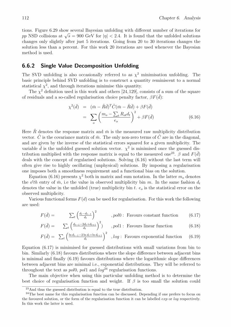
112 Chapter 6. Analysis
tions. Figure 6.29 show several Bayesian unfolding with different number of iterations forpp NSD collisions at
√s = 900 GeV for |η| < 2.4. It is found that the unfolded solutions
changes only slightly after just 5 iterations. Going from 20 to 30 iterations changes thesolution less than a percent. For this work 20 iterations are used whenever the Bayesianmethod is used.
6.6.2 Single Value Decomposition Unfolding
The SVD unfolding is also occasionally referred to as χ2 minimisation unfolding. Thebasic principle behind SVD unfolding is to construct a quantity reminiscent to a normalstatistical χ2, and through iterations minimise this quantity.
The χ2 definition used is this work and others [24,129], consists of a sum of the squareof residuals and a so-called regularisation choice penalty factor, βF (d):
χ2(d) = (m− Rd)T C(m− Rd) + βF (d)
=∑o
(mo −
∑tRotdt
eo
)2
+ βF (d) (6.16)
Here R denotes the response matrix and m is the measured raw multiplicity distributionvector. C is the covariance matrix of m. The only non-zero terms of C are in the diagonal,and are given by the inverse of the statistical errors squared for a given multiplicity. Thevariable d is the unfolded guessed solution vector. χ2 is minimised once the guessed dis-tribution multiplied with the response matrix is equal to the measured one23. β and F (d)deals with the concept of regularised solutions. Solving (6.16) without the last term willoften give rise to highly oscillating (unphysical) solutions. By imposing a regularisationone imposes both a smoothness requirement and a functional bias on the solution.
Equation (6.16) presents χ2 both in matrix and sum notation. In the latter mo denotesthe o′th entry of m, i.e the value in observed multiplicity bin m. In the same fashion dtdenotes the value in the unfolded (true) multiplicity bin t. eo is the statistical error on theobserved multiplicity.
Various functional forms F (d) can be used for regularisation. For this work the followingare used:
F (d) =∑
t
(dt−dt−1
dt
)2, pol0 : Favours constant function (6.17)
F (d) =∑
t
(dt−1−2dt+dt+1
dt
)2) , pol1 : Favours linear function (6.18)
F (d) =∑
t
(ln dt−1−2 ln dt+ln dt+1
dt
)2, log : Favours exponential function (6.19)
Equation (6.17) is minimised for guessed distributions with small variations from bin tobin. Similarly (6.18) favours distributions where the slope difference between adjacent binsis minimal and finally (6.19) favours distributions where the logarithmic slope differencesbetween adjacent bins are minimal i.e., exponential distributions. They will be referred tothroughout the text as pol0, pol1 and log24 regularisation functions.
The main objective when using this particular unfolding method is to determine thebest choice of regularisation function and weight. If β is too small the solution could
23And thus the guessed distribution is equal to the true distribution.24The best name for this regularisation function can be discussed. Depending if one prefers to focus on
the favoured solution, or the form of the regularisation function it can be labelled exp or log respectively.In this work the latter is used.
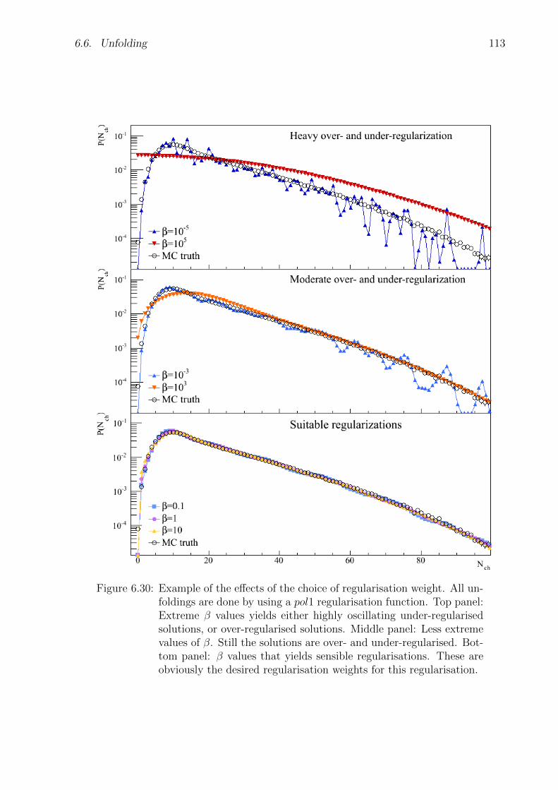
6.6. Unfolding 113
Figure 6.30: Example of the effects of the choice of regularisation weight. All un-foldings are done by using a pol1 regularisation function. Top panel:Extreme β values yields either highly oscillating under-regularisedsolutions, or over-regularised solutions. Middle panel: Less extremevalues of β. Still the solutions are over- and under-regularised. Bot-tom panel: β values that yields sensible regularisations. These areobviously the desired regularisation weights for this regularisation.
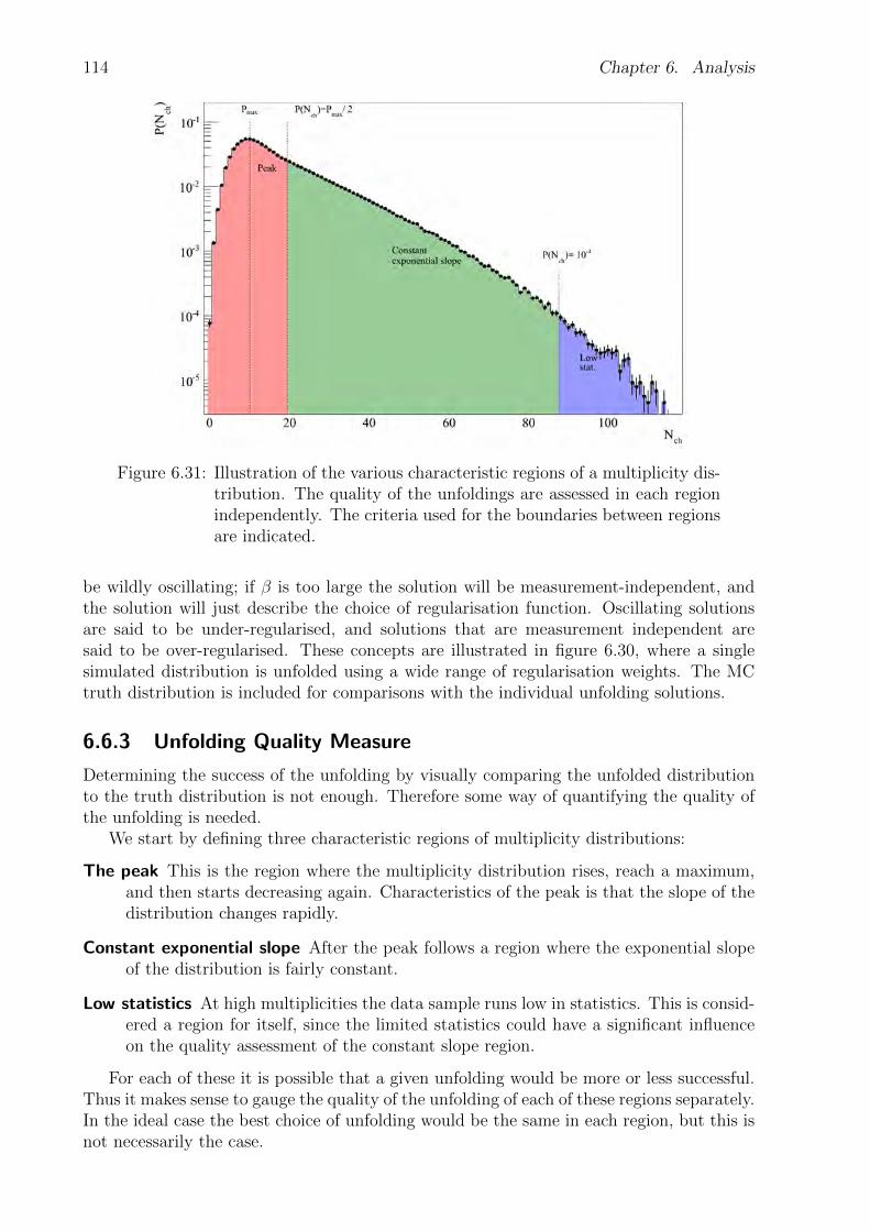
114 Chapter 6. Analysis
Figure 6.31: Illustration of the various characteristic regions of a multiplicity dis-tribution. The quality of the unfoldings are assessed in each regionindependently. The criteria used for the boundaries between regionsare indicated.
be wildly oscillating; if β is too large the solution will be measurement-independent, andthe solution will just describe the choice of regularisation function. Oscillating solutionsare said to be under-regularised, and solutions that are measurement independent aresaid to be over-regularised. These concepts are illustrated in figure 6.30, where a singlesimulated distribution is unfolded using a wide range of regularisation weights. The MCtruth distribution is included for comparisons with the individual unfolding solutions.
6.6.3 Unfolding Quality Measure
Determining the success of the unfolding by visually comparing the unfolded distributionto the truth distribution is not enough. Therefore some way of quantifying the quality ofthe unfolding is needed.
We start by defining three characteristic regions of multiplicity distributions:
The peak This is the region where the multiplicity distribution rises, reach a maximum,and then starts decreasing again. Characteristics of the peak is that the slope of thedistribution changes rapidly.
Constant exponential slope After the peak follows a region where the exponential slopeof the distribution is fairly constant.
Low statistics At high multiplicities the data sample runs low in statistics. This is consid-ered a region for itself, since the limited statistics could have a significant influenceon the quality assessment of the constant slope region.
For each of these it is possible that a given unfolding would be more or less successful.Thus it makes sense to gauge the quality of the unfolding of each of these regions separately.In the ideal case the best choice of unfolding would be the same in each region, but this isnot necessarily the case.
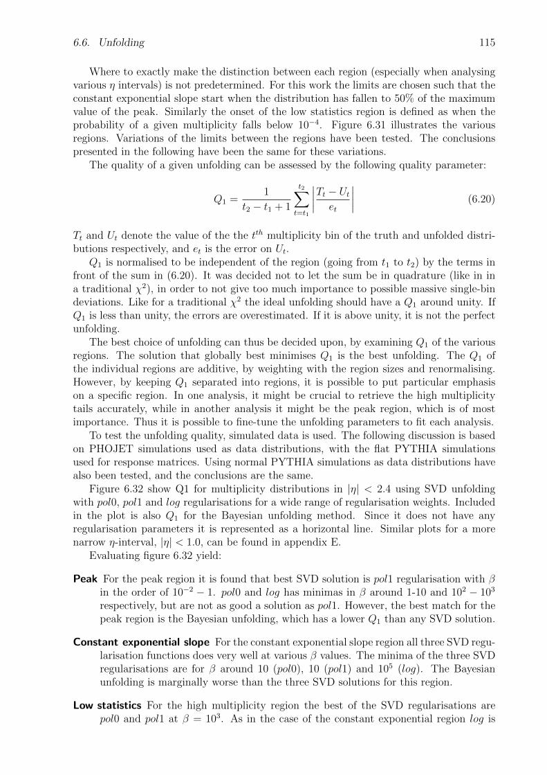
6.6. Unfolding 115
Where to exactly make the distinction between each region (especially when analysingvarious η intervals) is not predetermined. For this work the limits are chosen such that theconstant exponential slope start when the distribution has fallen to 50% of the maximumvalue of the peak. Similarly the onset of the low statistics region is defined as when theprobability of a given multiplicity falls below 10−4. Figure 6.31 illustrates the variousregions. Variations of the limits between the regions have been tested. The conclusionspresented in the following have been the same for these variations.
The quality of a given unfolding can be assessed by the following quality parameter:
Q1 =1
t2 − t1 + 1
t2∑t=t1
∣∣∣∣Tt − Utet
∣∣∣∣ (6.20)
Tt and Ut denote the value of the the tth multiplicity bin of the truth and unfolded distri-butions respectively, and et is the error on Ut.
Q1 is normalised to be independent of the region (going from t1 to t2) by the terms infront of the sum in (6.20). It was decided not to let the sum be in quadrature (like in ina traditional χ2), in order to not give too much importance to possible massive single-bindeviations. Like for a traditional χ2 the ideal unfolding should have a Q1 around unity. IfQ1 is less than unity, the errors are overestimated. If it is above unity, it is not the perfectunfolding.
The best choice of unfolding can thus be decided upon, by examining Q1 of the variousregions. The solution that globally best minimises Q1 is the best unfolding. The Q1 ofthe individual regions are additive, by weighting with the region sizes and renormalising.However, by keeping Q1 separated into regions, it is possible to put particular emphasison a specific region. In one analysis, it might be crucial to retrieve the high multiplicitytails accurately, while in another analysis it might be the peak region, which is of mostimportance. Thus it is possible to fine-tune the unfolding parameters to fit each analysis.
To test the unfolding quality, simulated data is used. The following discussion is basedon PHOJET simulations used as data distributions, with the flat PYTHIA simulationsused for response matrices. Using normal PYTHIA simulations as data distributions havealso been tested, and the conclusions are the same.
Figure 6.32 show Q1 for multiplicity distributions in |η| < 2.4 using SVD unfoldingwith pol0, pol1 and log regularisations for a wide range of regularisation weights. Includedin the plot is also Q1 for the Bayesian unfolding method. Since it does not have anyregularisation parameters it is represented as a horizontal line. Similar plots for a morenarrow η-interval, |η| < 1.0, can be found in appendix E.
Evaluating figure 6.32 yield:
Peak For the peak region it is found that best SVD solution is pol1 regularisation with βin the order of 10−2 − 1. pol0 and log has minimas in β around 1-10 and 102 − 103
respectively, but are not as good a solution as pol1. However, the best match for thepeak region is the Bayesian unfolding, which has a lower Q1 than any SVD solution.
Constant exponential slope For the constant exponential slope region all three SVD regu-larisation functions does very well at various β values. The minima of the three SVDregularisations are for β around 10 (pol0), 10 (pol1) and 105 (log). The Bayesianunfolding is marginally worse than the three SVD solutions for this region.
Low statistics For the high multiplicity region the best of the SVD regularisations arepol0 and pol1 at β = 103. As in the case of the constant exponential region log is

116 Chapter 6. Analysis
continuously falling having its minimum at the high limit of the survey. Bayesianunfolding does equally well as pol0 and pol1 for this region.
β-510 -410 -310 -210 -110 1 10 210 310 410 510
1Q
1
10
210
Peak region
|<2.4η|
β-510 -410 -310 -210 -110 1 10 210 310 410 510
1Q
1
10
210
pol0
pol1
log
bayesian
Constant exponential slope region
β-510 -410 -310 -210 -110 1 10 210 310 410 510
1Q
1
10
210
Low statistics region
Figure 6.32: The unfolding quality parameter, Q1, for the three distinct multi-plicity distribution regions for |η| < 2.4 . SVD unfolding with threeregularisation functions are checked over a large range of β weightparameters. Included is also the Bayesian unfolding as the horison-tal dashed red line. The Bayesian unfolding is found to be the bestsolution.
As discussed, the log regularisation is falling continuously in both the constant expo-nential and low statistics regions. However for the Peak, log regularisation rapidly becomesworse for very high β. Thus, even though the minima is perhaps not reached for the regionsbesides the peak, there is found no reason to expand the β range surveyed. This is due to

6.6. Unfolding 117
the peak region becoming worse and worse at higher regularisation weights, and thus theoverall solution will never become the best.
Figure 6.33 shows a comparison of the best SVD and Bayesian unfolding for |η| < 2.4.Overall it is found that the Bayesian unfolding is the best solution for unfolding. Of theSVD regularisations it is found that pol1 is the best choice with a β around 1. The nextbest choices for pol1 are also included in figure 6.33. These illustrate an issue with the SVDmethod at broader η-intervals. Lowering the β value increases the accuracy of the very firstbins. But doing so, causes oscillations in the higher multiplicities. This is not seen for thenarrow η-intervals, the oscillations set in at lower β-values. Thus for the narrow η-intervalsthe SVD unfolding is a reasonable option, and has been used by ALICE previously [73,74].
Figure 6.33: The best unfolding solutions for |η| < 2.4. It is found that Bayesianunfolding overall show best agreement with MC truth. SVD unfold-ing with pol1 and β = 1 is the best SVD solution. The insert showthe very first multiplicity bins. It is found that β = 10−1 gives betteragreement in the very low bins, but the oscillations start appearingat higher multiplicities. The lower panel show the ratio to MC truthfor the various solutions. The oscillations of the under-regularisedsolutions are seen.

118 Chapter 6. Analysis
6.7 Trigger-Vertex Bias Correction
After unfolding the measured distributions, they need to be corrected for trigger and vertexinefficiency. This is referred to as the trigger–vertex bias correction.
At very low multiplicities, few particles hit the detectors, which makes reconstructionof a vertex increasingly difficult, and thus the vertex efficiency decreases. Similarly fewparticles makes it difficult for the trigger algorithms to recognise a given collision trigger.
The trigger–vertex bias correction is done by simulations, and is given by:
C =P (Nch,MCNSD)
P (Nch,ESDNSD)(6.21)
The subscript MCNSD denote events that have a vertex between −4 < vz < 4, and areNSD events according to the simulation truth. Similarly the subscript ESDNSD denoteevents, where a vertex is reconstructed within −4 < vz < 4, and that are triggered as aNSD event in the analysis.
The correction for pp collisions at√s = 900 GeV is shown in 6.34. As seen the main
part of the correction is in the very low multiplicity region. A thing worth mentioningis that the correction becomes slightly less than unity in some range before ending atunity for higher multiplicities. This drop below unity is caused by the triggering algorithmmisidentifying SD events as NSD events. This is not clearly visible in figure 6.34.
For the very broad η-intervals the limited statistics becomes an issue. This is due tothe extremely low probability of having a triggered NSD event with a vertex but with noparticles over 8 units of η. As an example, the first point (Nch = 0) of the −3.4 < η < 5.1curve in figure 6.34, stems from only 3 ESDNSD events, and 5400 MCNSD events out ofthe roughly 3 millions events of the simulation. This obviously means that there will be ahuge error assigned to the correction (which is already very large) in this point. This errorcan in theory be reduced drastically by running over many times more simulated data. Forthis work, this has not been possible.
chN0 2 4 6 8 10 12
Tri
gger
Ver
tex
Bia
s C
orre
ctio
n
1
10
210
310=900GeVspp NSD collisions @
< 5.1η-3.4 < | < 3.4η|| < 3.0η|| < 2.4η|| < 2.0η|| < 1.5η|| < 1.0η|| < 0.5η|
Figure 6.34: Trigger–Vertex bias correction factor for various η-intervals for ppNSD collisions at
√s = 900 GeV. It is seen that it only affects the
very low multiplicity bins. For the broader η-intervals, the uncer-tainty on the correction becomes quite large for the first few multi-plicity bins, due to lack of statistics.
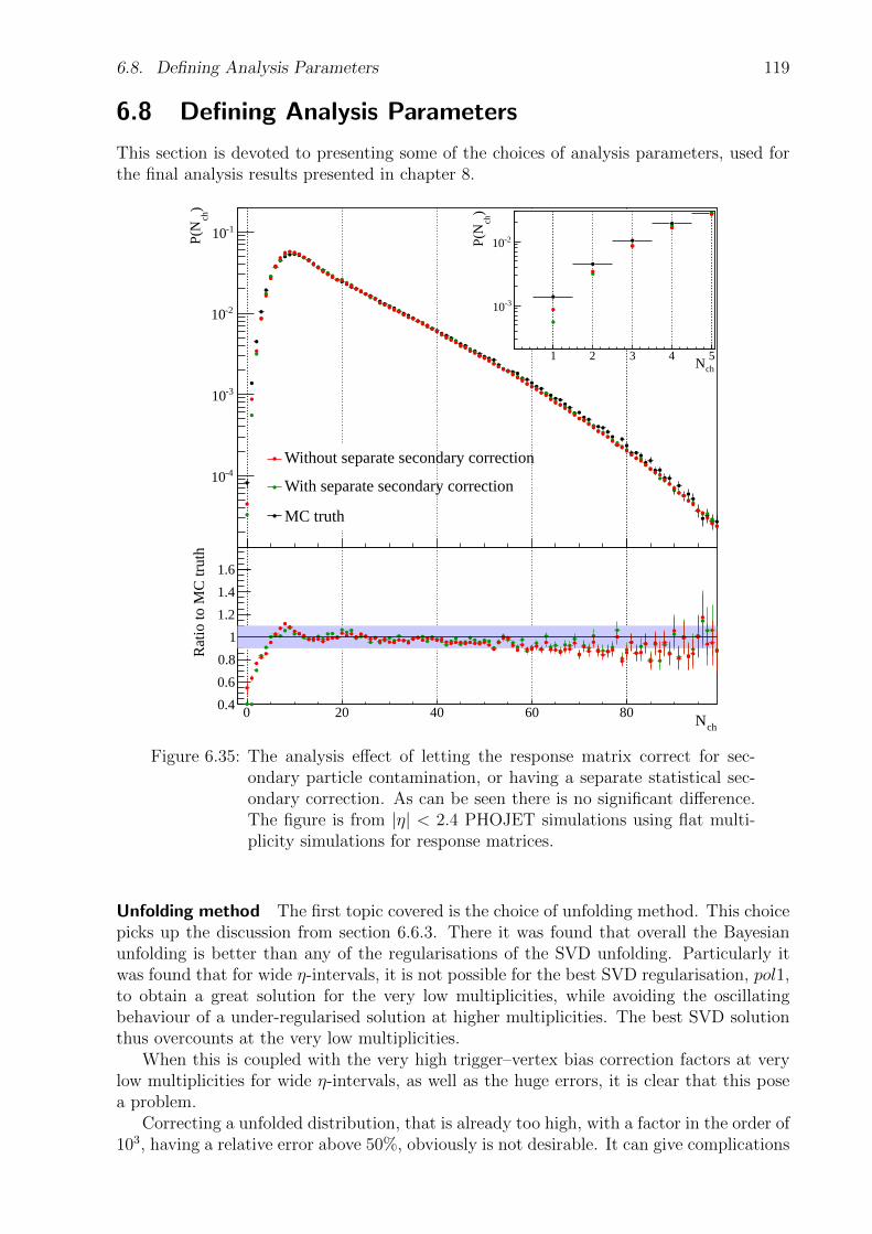
6.8. Defining Analysis Parameters 119
6.8 Defining Analysis Parameters
This section is devoted to presenting some of the choices of analysis parameters, used forthe final analysis results presented in chapter 8.
chN0 20 40 60 80
)ch
P(N
-410
-310
-210
-110
Without separate secondary correction
With separate secondary correction
MC truth
chN0 20 40 60 80
Rat
io to
MC
trut
h
0.4
0.6
0.8
1
1.2
1.4
1.6
chN1 2 3 4 5
)ch
P(N
-310
-210
Figure 6.35: The analysis effect of letting the response matrix correct for sec-ondary particle contamination, or having a separate statistical sec-ondary correction. As can be seen there is no significant difference.The figure is from |η| < 2.4 PHOJET simulations using flat multi-plicity simulations for response matrices.
Unfolding method The first topic covered is the choice of unfolding method. This choicepicks up the discussion from section 6.6.3. There it was found that overall the Bayesianunfolding is better than any of the regularisations of the SVD unfolding. Particularly itwas found that for wide η-intervals, it is not possible for the best SVD regularisation, pol1,to obtain a great solution for the very low multiplicities, while avoiding the oscillatingbehaviour of a under-regularised solution at higher multiplicities. The best SVD solutionthus overcounts at the very low multiplicities.
When this is coupled with the very high trigger–vertex bias correction factors at verylow multiplicities for wide η-intervals, as well as the huge errors, it is clear that this posea problem.
Correcting a unfolded distribution, that is already too high, with a factor in the order of103, having a relative error above 50%, obviously is not desirable. It can give complications

120 Chapter 6. Analysis
with the zero bin being much too high, when renormalising the multiplicity distribution,and thus pushing the overall distribution significantly downwards.
The Bayesian unfolding does a better job at the zero bin, and thus is not as affectedby this. However also in this case, one should keep the massive uncertainty of the first binin mind.
Thus the choice is made to use the Bayesian unfolding method. The performance of theSVD unfolding will be used to estimate the uncertainty on the results due to the unfolding.This is discussed in the next chapter.
Figure 6.36: Comparisons of the analysis effect of changing the amount of accep-tance gaps allowed. It is decided to use the setting, where a singleedge bin in each FMD ring and the SPD is but away.
Secondary particle contamination The next test presented revolves around using thecorrection maps for secondary particle correction as described in section 6.4, or letting theunfolding handle it. The result is shown in 6.35.
It is found that it makes very little difference which approach is used. At the very lowmultiplicities, letting the unfolding handle the secondary contamination is closer to thesimulation truth, whereas the multiplicity tail show very slightly better agreement for theseparate secondary correction approach.
For the analysis, it is decided to use the method of removing the secondaries as part ofthe unfolding in pp collisions.
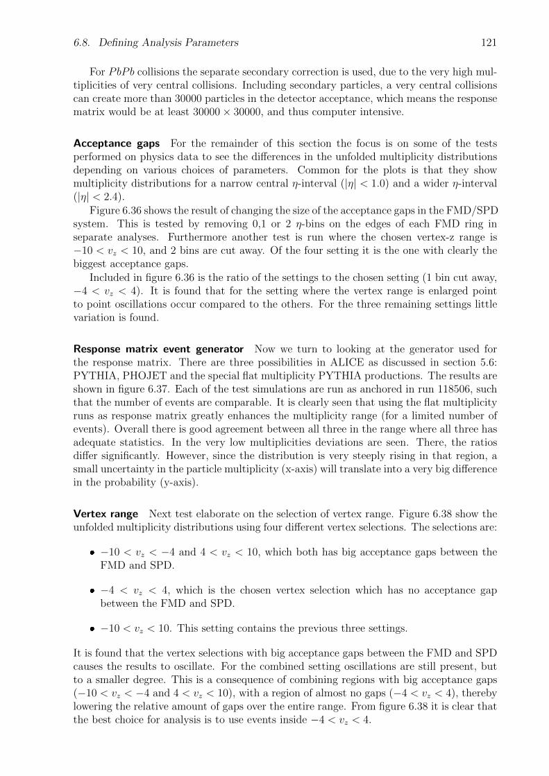
6.8. Defining Analysis Parameters 121
For PbPb collisions the separate secondary correction is used, due to the very high mul-tiplicities of very central collisions. Including secondary particles, a very central collisionscan create more than 30000 particles in the detector acceptance, which means the responsematrix would be at least 30000× 30000, and thus computer intensive.
Acceptance gaps For the remainder of this section the focus is on some of the testsperformed on physics data to see the differences in the unfolded multiplicity distributionsdepending on various choices of parameters. Common for the plots is that they showmultiplicity distributions for a narrow central η-interval (|η| < 1.0) and a wider η-interval(|η| < 2.4).
Figure 6.36 shows the result of changing the size of the acceptance gaps in the FMD/SPDsystem. This is tested by removing 0,1 or 2 η-bins on the edges of each FMD ring inseparate analyses. Furthermore another test is run where the chosen vertex-z range is−10 < vz < 10, and 2 bins are cut away. Of the four setting it is the one with clearly thebiggest acceptance gaps.
Included in figure 6.36 is the ratio of the settings to the chosen setting (1 bin cut away,−4 < vz < 4). It is found that for the setting where the vertex range is enlarged pointto point oscillations occur compared to the others. For the three remaining settings littlevariation is found.
Response matrix event generator Now we turn to looking at the generator used forthe response matrix. There are three possibilities in ALICE as discussed in section 5.6:PYTHIA, PHOJET and the special flat multiplicity PYTHIA productions. The results areshown in figure 6.37. Each of the test simulations are run as anchored in run 118506, suchthat the number of events are comparable. It is clearly seen that using the flat multiplicityruns as response matrix greatly enhances the multiplicity range (for a limited number ofevents). Overall there is good agreement between all three in the range where all three hasadequate statistics. In the very low multiplicities deviations are seen. There, the ratiosdiffer significantly. However, since the distribution is very steeply rising in that region, asmall uncertainty in the particle multiplicity (x-axis) will translate into a very big differencein the probability (y-axis).
Vertex range Next test elaborate on the selection of vertex range. Figure 6.38 show theunfolded multiplicity distributions using four different vertex selections. The selections are:
−10 < vz < −4 and 4 < vz < 10, which both has big acceptance gaps between theFMD and SPD.
−4 < vz < 4, which is the chosen vertex selection which has no acceptance gapbetween the FMD and SPD.
−10 < vz < 10. This setting contains the previous three settings.
It is found that the vertex selections with big acceptance gaps between the FMD and SPDcauses the results to oscillate. For the combined setting oscillations are still present, butto a smaller degree. This is a consequence of combining regions with big acceptance gaps(−10 < vz < −4 and 4 < vz < 10), with a region of almost no gaps (−4 < vz < 4), therebylowering the relative amount of gaps over the entire range. From figure 6.38 it is clear thatthe best choice for analysis is to use events inside −4 < vz < 4.
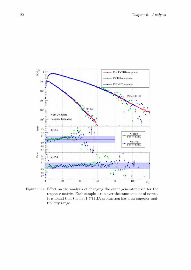
122 Chapter 6. Analysis
Figure 6.37: Effect on the analysis of changing the event generator used for theresponse matrix. Each sample is run over the same amount of events.It is found that the flat PYTHIA production has a far superior mul-tiplicity range.
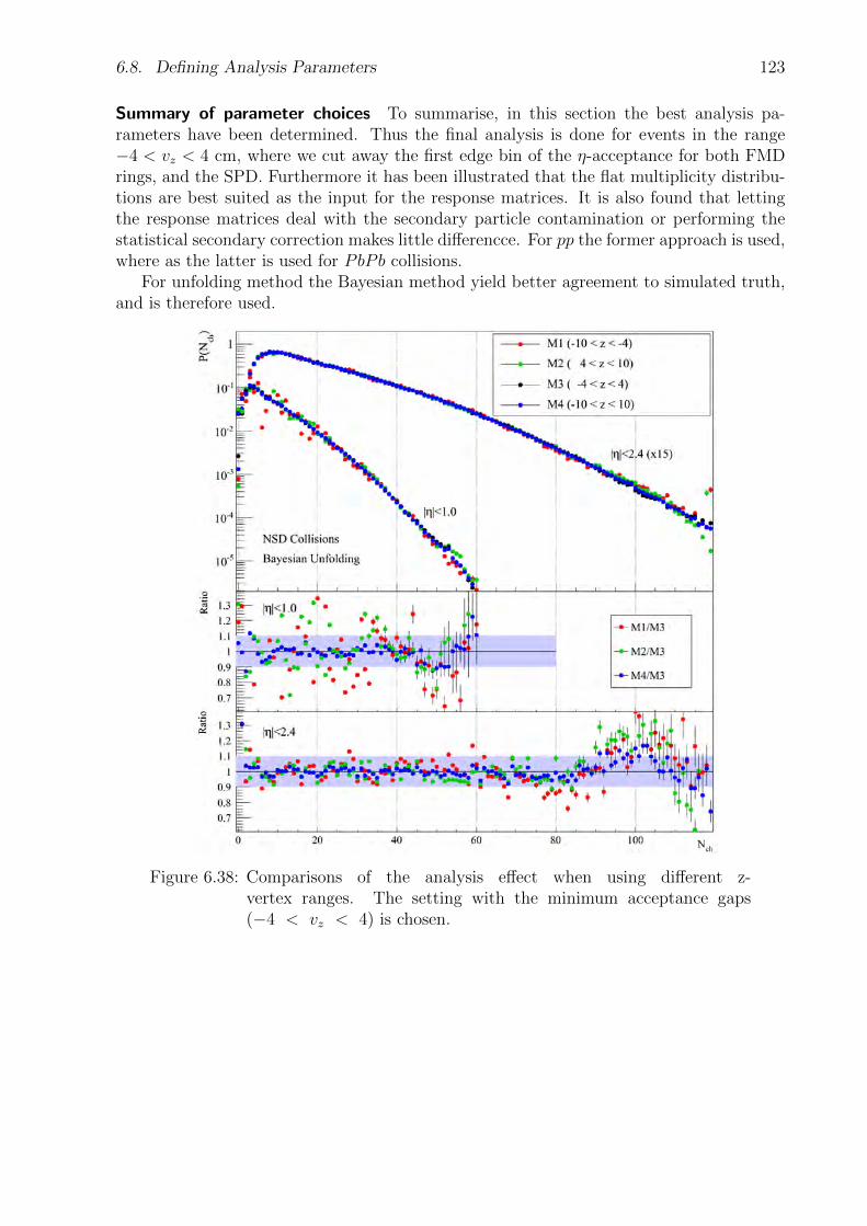
6.8. Defining Analysis Parameters 123
Summary of parameter choices To summarise, in this section the best analysis pa-rameters have been determined. Thus the final analysis is done for events in the range−4 < vz < 4 cm, where we cut away the first edge bin of the η-acceptance for both FMDrings, and the SPD. Furthermore it has been illustrated that the flat multiplicity distribu-tions are best suited as the input for the response matrices. It is also found that lettingthe response matrices deal with the secondary particle contamination or performing thestatistical secondary correction makes little differencce. For pp the former approach is used,where as the latter is used for PbPb collisions.
For unfolding method the Bayesian method yield better agreement to simulated truth,and is therefore used.
Figure 6.38: Comparisons of the analysis effect when using different z-vertex ranges. The setting with the minimum acceptance gaps(−4 < vz < 4) is chosen.

124 Chapter 6. Analysis

Chapter 7
Systematic Errors
This chapter is devoted to the treatment of systematic errors for multiplicity distributions.The systematic errors are composed of three parts; the systematic error on the number ofmeasured particles in a given event, a contribution from the trigger–vertex bias correction,as well as a contribution from the choice of unfolding method.
7.1 Uncertainty on event multiplicity
η-4 -3 -2 -1 0 1 2 3 4 5 6
Rat
io
0.85
0.9
0.95
1
1.05
1.1
1.15
FMD: 7%
η-2 -1.5 -1 -0.5 0 0.5 1 1.5 2
Rat
io
0.85
0.9
0.95
1
1.05
1.1
1.15
SPD: 1%
+10% material
-10% material
Figure 7.1: Effect of scaling the material density of all of ALICE up and downby 10%. The left panel shows the ratio of the changed material sim-ulations to the reference simulations. The change in material yieldsa 7% difference. The right panel shows the same for the SPD. Theeffect of adding and removing material is only around 1%.
The following effects are considered for determining the systematic error on the eventmultiplicity.
Material budget The accuracy of the description of the material budget is by far thebiggest contribution to the systematic error in the FMD, and also constitute a significantpart for the SPD. The accuracy of the material description directly effect the responsematrix, and thus the unfolded solution.
The systematic error from the material budget is estimated by using special simulations,where the material density of every single component in ALICE is scaled up and down by10%. These special runs are then compared to a reference simulation.
125

126 Chapter 7. Systematic Errors
For the FMD this yields an estimate of the systematic error of ∼ 7% on the measuredmultiplicity. Since the amount of material in front of the SPD is much less, the effect issmaller there. The estimate of the systematic error in the SPD is ∼ 2%. For both detectorsthe estimate can be seen in figure 7.1.
While it is quite unlikely that there are global inaccuracies in the material descriptionof this magnitude, it could however occur locally. This might especially be true in for-ward regions, which do not only house the forward detectors. The service structures ofthe central barrel detectors are also located in this region. These include large amountsof bundled cables, which can not be modelled individually, but instead are modelled aseffective volumes.
Section 8.5 will discuss how to determine how accurate the current description is.
Event generator The implemented physics of different input generators leads to differ-ences in the production of secondary particles, and thus yields a systematic uncertainty.This contribution is estimated by testing PHOJET and PYTHIA, and using the ratio ofsecondary particles produced as the uncertainty estimate. The effect amounts to ∼ 2% inboth the FMD and SPD. Illustrations of this are shown in figures 7.2 and 7.3 for the FMDand SPD respectively.
η-3.5 -3 -2.5 -2 -1.5
φ
0
1
2
3
4
5
6
0
0.2
0.4
0.6
0.8
1
η-3.5 -3 -2.5 -2 -1.5
PYT
HIA
/PH
OJE
T
0.9
0.92
0.94
0.96
0.98
1
1.02
1.04
1.06
1.08
1.1
Figure 7.2: Effect of the choice of event generator in FMD3I. The left panel showsPYTHIA/PHOJET ratio as a function of (η, φ). The right panelshows the projection onto the η-axis. The choice of event generatoryields a 2% difference.
Strangeness Correction The strangeness correction is not well determined as describedin section 6.5. Thus it was decided to impose a large systematic uncertainty of 2% (= 100%relative error) to it for both the SPD and FMD.
Sharing cuts Variation of Ehit and Ehigh, discussed in section 6.2.2, yields a ∼ 2% un-certainty in PbPb collisions, and ∼ 3% in pp collisions. Concretely, this estimate is gottenby changing Ehigh and Ehit up and down with 0.1EMPV , and comparing the results to thereference analysis. This systematic effect only applies to the FMD analysis.
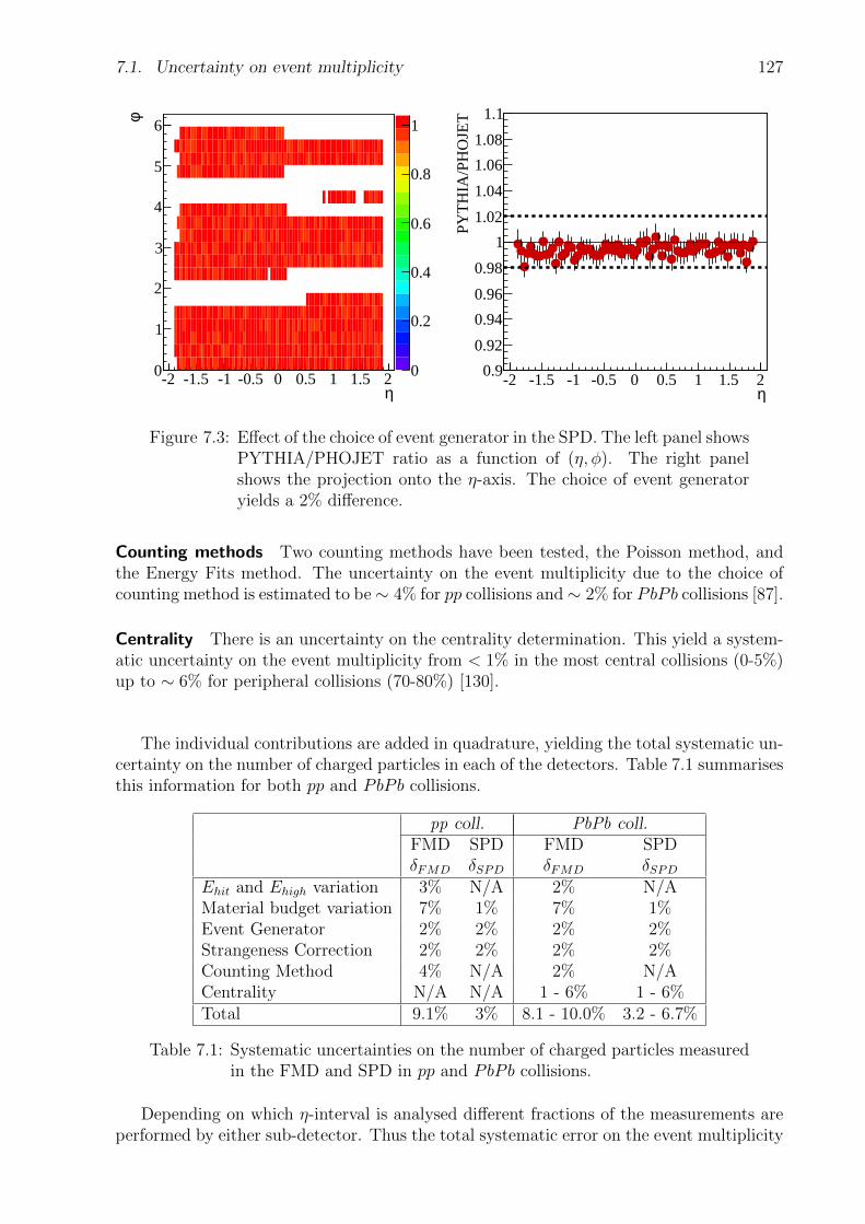
7.1. Uncertainty on event multiplicity 127
η-2 -1.5 -1 -0.5 0 0.5 1 1.5 2
φ
0
1
2
3
4
5
6
0
0.2
0.4
0.6
0.8
1
η-2 -1.5 -1 -0.5 0 0.5 1 1.5 2
PYT
HIA
/PH
OJE
T
0.9
0.92
0.94
0.96
0.98
1
1.02
1.04
1.06
1.08
1.1
Figure 7.3: Effect of the choice of event generator in the SPD. The left panel showsPYTHIA/PHOJET ratio as a function of (η, φ). The right panelshows the projection onto the η-axis. The choice of event generatoryields a 2% difference.
Counting methods Two counting methods have been tested, the Poisson method, andthe Energy Fits method. The uncertainty on the event multiplicity due to the choice ofcounting method is estimated to be∼ 4% for pp collisions and∼ 2% for PbPb collisions [87].
Centrality There is an uncertainty on the centrality determination. This yield a system-atic uncertainty on the event multiplicity from < 1% in the most central collisions (0-5%)up to ∼ 6% for peripheral collisions (70-80%) [130].
The individual contributions are added in quadrature, yielding the total systematic un-certainty on the number of charged particles in each of the detectors. Table 7.1 summarisesthis information for both pp and PbPb collisions.
pp coll. PbPb coll.FMD SPD FMD SPDδFMD δSPD δFMD δSPD
Ehit and Ehigh variation 3% N/A 2% N/AMaterial budget variation 7% 1% 7% 1%Event Generator 2% 2% 2% 2%Strangeness Correction 2% 2% 2% 2%Counting Method 4% N/A 2% N/ACentrality N/A N/A 1 - 6% 1 - 6%Total 9.1% 3% 8.1 - 10.0% 3.2 - 6.7%
Table 7.1: Systematic uncertainties on the number of charged particles measuredin the FMD and SPD in pp and PbPb collisions.
Depending on which η-interval is analysed different fractions of the measurements areperformed by either sub-detector. Thus the total systematic error on the event multiplicity
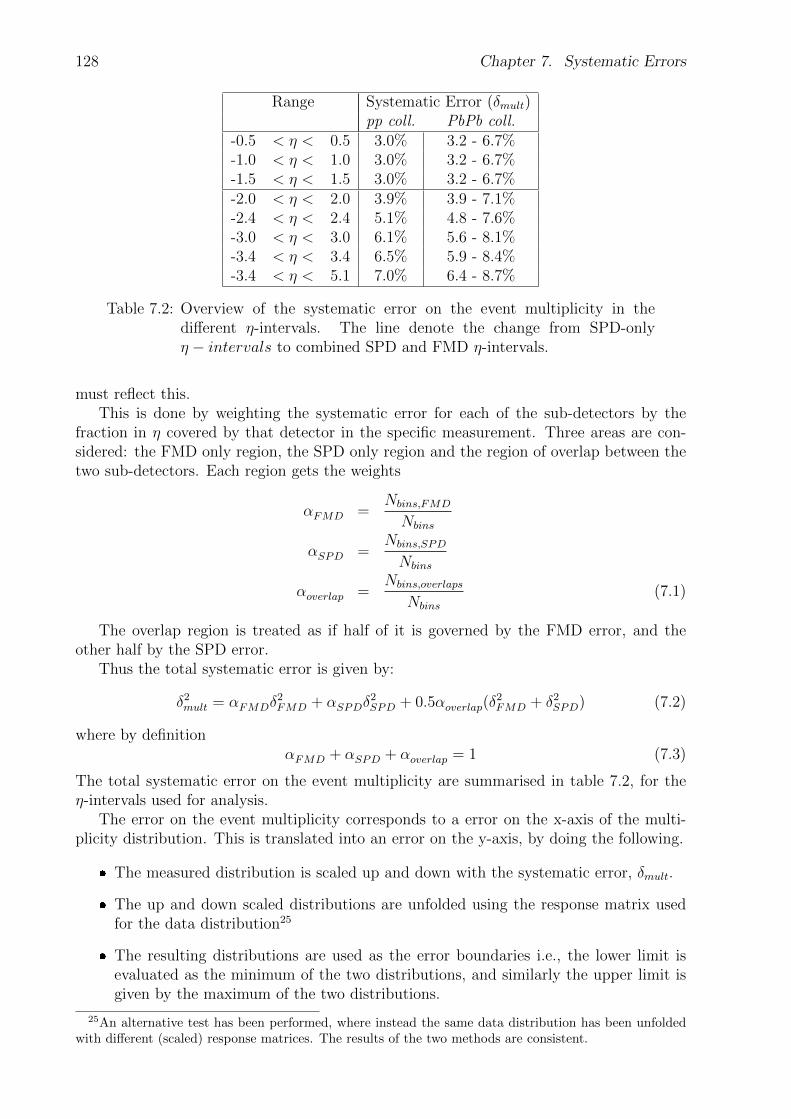
128 Chapter 7. Systematic Errors
Range Systematic Error (δmult)pp coll. PbPb coll.
-0.5 < η < 0.5 3.0% 3.2 - 6.7%-1.0 < η < 1.0 3.0% 3.2 - 6.7%-1.5 < η < 1.5 3.0% 3.2 - 6.7%-2.0 < η < 2.0 3.9% 3.9 - 7.1%-2.4 < η < 2.4 5.1% 4.8 - 7.6%-3.0 < η < 3.0 6.1% 5.6 - 8.1%-3.4 < η < 3.4 6.5% 5.9 - 8.4%-3.4 < η < 5.1 7.0% 6.4 - 8.7%
Table 7.2: Overview of the systematic error on the event multiplicity in thedifferent η-intervals. The line denote the change from SPD-onlyη − intervals to combined SPD and FMD η-intervals.
must reflect this.This is done by weighting the systematic error for each of the sub-detectors by the
fraction in η covered by that detector in the specific measurement. Three areas are con-sidered: the FMD only region, the SPD only region and the region of overlap between thetwo sub-detectors. Each region gets the weights
αFMD =Nbins,FMD
Nbins
αSPD =Nbins,SPD
Nbins
αoverlap =Nbins,overlaps
Nbins
(7.1)
The overlap region is treated as if half of it is governed by the FMD error, and theother half by the SPD error.
Thus the total systematic error is given by:
δ2mult = αFMDδ2FMD + αSPDδ
2SPD + 0.5αoverlap(δ
2FMD + δ2SPD) (7.2)
where by definitionαFMD + αSPD + αoverlap = 1 (7.3)
The total systematic error on the event multiplicity are summarised in table 7.2, for theη-intervals used for analysis.
The error on the event multiplicity corresponds to a error on the x-axis of the multi-plicity distribution. This is translated into an error on the y-axis, by doing the following.
The measured distribution is scaled up and down with the systematic error, δmult.
The up and down scaled distributions are unfolded using the response matrix usedfor the data distribution25
The resulting distributions are used as the error boundaries i.e., the lower limit isevaluated as the minimum of the two distributions, and similarly the upper limit isgiven by the maximum of the two distributions.
25An alternative test has been performed, where instead the same data distribution has been unfoldedwith different (scaled) response matrices. The results of the two methods are consistent.

7.2. Uncertainty on trigger–vertex bias correction and unfolding method 129
Figure 7.4: Example of the systematic uncertainty on the event multiplicity for|η| < 2.4 in
√s = 900 GeV collisions. The raw multiplicity distri-
bution is unfolded by the detector response, yielding the unfoldeddistribution. The systematic error bands are estimated by scalingthe raw distribution upwards and downwards with the uncertainty oncounting particles, and then unfolding these distributions with thesame response matrix.
The errors are now translated to the y-axis, yielding a band around the unfoldeddistribution.
7.2 Uncertainty on trigger–vertex bias correction and un-folding method
Besides the uncertainty on event multiplicity, error contributions from both the trigger biasvertex correction and unfolding method has to be taken into account. Both are treated inthis section.
We start by considering the trigger–vertex bias correction. As discussed in section 6.7,the trigger–vertex bias correction require a large amount of statistics, especially for thebroadest η-intervals. Thus any error assigned to it, can be decreased by having a largersimulated sample.
The systematic uncertainty on the correction is given by:
δ2bias = ε2MCNSD + ε2ESDNSD (7.4)
εMCNSD is the error on the number of events labelled NSD by the simulation, and εESDNSDis similarly the number of events found by the analysis as NSD events. These errors aregiven as εx = 1/
√Nx, where x is either MCNSD or ESDNSD.
Thus (7.4) reduces to:
δbias =
√1
NMCNSD
+1
NESDNSD
(7.5)

130 Chapter 7. Systematic Errors
chN0 10 20 30 40 50
)ch
P(N
0
0.01
0.02
0.03
0.04
0.05 unfold
2δ+mult2δ + bias
2δ = totδ
mult2δ + bias
2δ
biasδ
unfolded distribution
Figure 7.5: Example of the various contributions to the systematic uncertaintyfor |η| < 2.4 in
√s = 900 GeV collisions. δbias includes the statistical
error added in quadrature with trigger–vertex bias uncertainty. Forclarity the distribution is shown on a linear scale, and the tail is notshown. In the tail region the total uncertainty is fully dominated byδmult.
The error contribution from the trigger–vertex bias correction is only significant in the verylowest multiplicity bins.
The last contribution is from the unfolding method itself. Figure 6.33 presented thebest unfolding solutions for both the Bayesian method and the SVD method. In thatfigure it was found that there was generally good agreement between the unfoldings andthe simulated truth. Over the entire multiplicity range it is estimated that the deviationsfrom simulated truth are of the order of 10 %. This will be used as a systematic uncertaintyof the unfolding method, δunfold.
The systematic uncertainty of the hit merging i.e., the variation of Ehigh and Ehit couldbe a component in both δmult as well as δunfold. How much it factors into δunfold is notknown.
However in comparison to some of the other errors its contribution is not dominant,and thus it has little effect on the final errror. Therefore it is assumed that it does notfactor into δunfold.

7.3. Total systematic error 131
7.3 Total systematic error
The total systematic uncertainty is thus constructed by adding the three contributions inquadrature bin-by-bin:
δ2tot = δ2unfold + δ2bias + δ2mult (7.6)
In figure 7.5 an example of the total systematic uncertainty is shown.For PbPb collisions the uncertainties become much simpler, since trigger and vertex
efficiency is unity [87]. Furthermore, as discussed in the previous chapter, PbPb collisionsare not unfolded. Thus the only systematic uncertainty is given by the event multiplicityuncertainty, δtot = δmult.

132 Chapter 7. Systematic Errors

Chapter 8
Results
In this chapter the results of this thesis are presented. The chapter is divided into foursections: Multiplicity distribution results, KNO scaling results, dNch
dηresults, and mean
multiplicity energy dependence results. The first three have separate subsections for ppand PbPb collisions, whereas the fourth section treats them simultaneously.
chN0 20 40 60 80 100 120 140 160 180
)ch
P(N
-610
-510
-410
-310
-210
-110
1
10
210
310
410
510
610
710
This workCMS (publ.)UA5 (publ.)ALICE (publ.)
|<0.5η||<1.0 (x10)η|
)2|<1.5 (x10η|)3|<2.0 (x10η|)4|<2.4 (x10η|)5|<3.0 (x10η|)6|<3.4 (x10η|
)7 <5.1 (x10η-3.4 <
I
II
III
IV
V
VI
VII
VIII
III
III
IV
V
VI
VII
VIII
NSD CollisionsBayesian Unfolding
=900 GeVs
Figure 8.1: Charged particle multiplicity distributions for NSD pp collisions at√s = 900 GeV. Included in the plot are previously published results
from CMS, UA5 and ALICE.
133

134 Chapter 8. Results
chN0 50 100 150 200
)ch
P(N
-610
-510
-410
-310
-210
-110
1
10
210
310
410
510
610
710
810
This work
CMS (publ.)
ALICE (publ.)
|<0.5η||<1.0 (x10)η|
)2|<1.5 (x10η|)3|<2.0 (x10η|)4|<2.4 (x10η|)5|<3.0 (x10η|)6|<3.4 (x10η|
)7 <5.1 (x10η-3.4 <
I
II
III
IV
V
VI
VII
VIII
I
II
III
IV
V VI VII
VIII
NSD CollisionsBayesian Unfolding
=2760 GeVs=2360 GeV)s(CMS & ALICE (publ.) at
Figure 8.2: Charged particle multiplicity distributions for NSD pp collisions at√s = 2760 GeV. As discussed in the text there are clear indications
that the data quality of this run period is bad.
8.1 Multiplicity Distributions
8.1.1 pp collisions
The first results presented in this section are considered the main measurement of thiswork, namely the multiplicity distributions for pp NSD collisions at the available energies.Figures 8.1, 8.2 and 8.3 show these at the three energies
√s = 900 GeV, 2760 GeV and
7000 GeV respectively.For both
√s = 900 GeV and 7000 GeV it is found that there are good agreement
between the results in this analysis, and the published results from other experiments.This is particularly true for the more narrow η-intervals. For the very broad intervalsthe tails are systematically higher in this analysis, compared to CMS and UA5. Howeverthey are still consistent within the uncertainties. The cause of this systematic deviation iscurrently unknown, but a likely explanation is that the implementation of the geometry inthe forward region is not accurate enough, as described in section 6.4.
The published ALICE results are made using SPD tracklets, which restricts that anal-ysis to the very central region. One of the ambitions of this work is to expand the alreadyexisting ALICE measurements.
It is found that the collisions at√s = 2760 GeV has serious problems. The bump at
very high multiplicities is clearly unphysical. It is present already in the raw multiplicitydistributions. It is not present in simulations, and thus the unfolding can not handle it.
It is the culmination of the trend seen from various of the plots in the analysis chapter,where the
√s = 2760 GeV behaves abnormally. All seems to indicate that these data are
heavily polluted, compared to the other energies, with some form of background signals.

8.1. Multiplicity Distributions 135
chN0 50 100 150 200 250
)ch
P(N
-610
-510
-410
-310
-210
-110
1
10
210
310
410
510
610
710
810
This work
CMS (publ.)
ALICE (publ.)
|<0.5η||<1.0 (x10)η|
)2|<1.5 (x10η|)3|<2.0 (x10η|)4|<2.4 (x10η|)5|<3.0 (x10η|)6|<3.4 (x10η|
)7 <5.1 (x10η-3.4 <
I
II
III
IV
V
VI
VII
VIII
III
III
IV
V
VI
VII
VIII
NSD CollisionsBayesian Unfolding
=7000 GeVs
Figure 8.3: Charged particle multiplicity distributions for NSD pp collisions at√s = 7000 GeV. Included in the plot are previously published results
from CMS and ALICE.
The data at√s = 2760 GeV is recorded in 2011, compared to the other energies, which
were recorded in 2010. There are other indications that both the FMD in particular andALICE in general might have problems with the data quality in the latter run periods26.
While the results for√s = 2760 GeV are presented here alongside the results for the
other two energies, they will not be used further in derived results. Understanding andhopefully improving the data quality for
√s = 2760 GeV is a high priority issue in the
coming time.
While figures like 8.1, 8.2 and 8.3 are good for an overview, they are not very usefulfor detailed comparison. Figures 8.4 and 8.5 show two examples of detailed comparisonsbetween the individual measurements for |η| < 0.5 at
√s = 900 GeV and for |η| < 1.0 at√
s = 7000 GeV. In appendix F the comparisons for the remaining multiplicity distributionscan be found.
In both figures good agreement between measurements of this work and the previouslypublished values is found. For the
√s = 7000 GeV comparison it is found that there is
better agreement with the CMS measurement than with the ALICE measurement. This isattributed to the fact that the CMS measurements also use the Bayesian unfolding method,whereas the published ALICE measurements use the SVD method.
26This seem to be a problem which has gotten progressively worse over time. On a ALICE level it hasgotten so bad, that ALICE currently does not start taking data immediately when the LHC declare stablebeams. Instead they wait until the background levels are tolerable. This is a new practise, and was notimplemented during the
√s = 2760 GeV runs. The cause and precise extent of the background is not fully
understood.
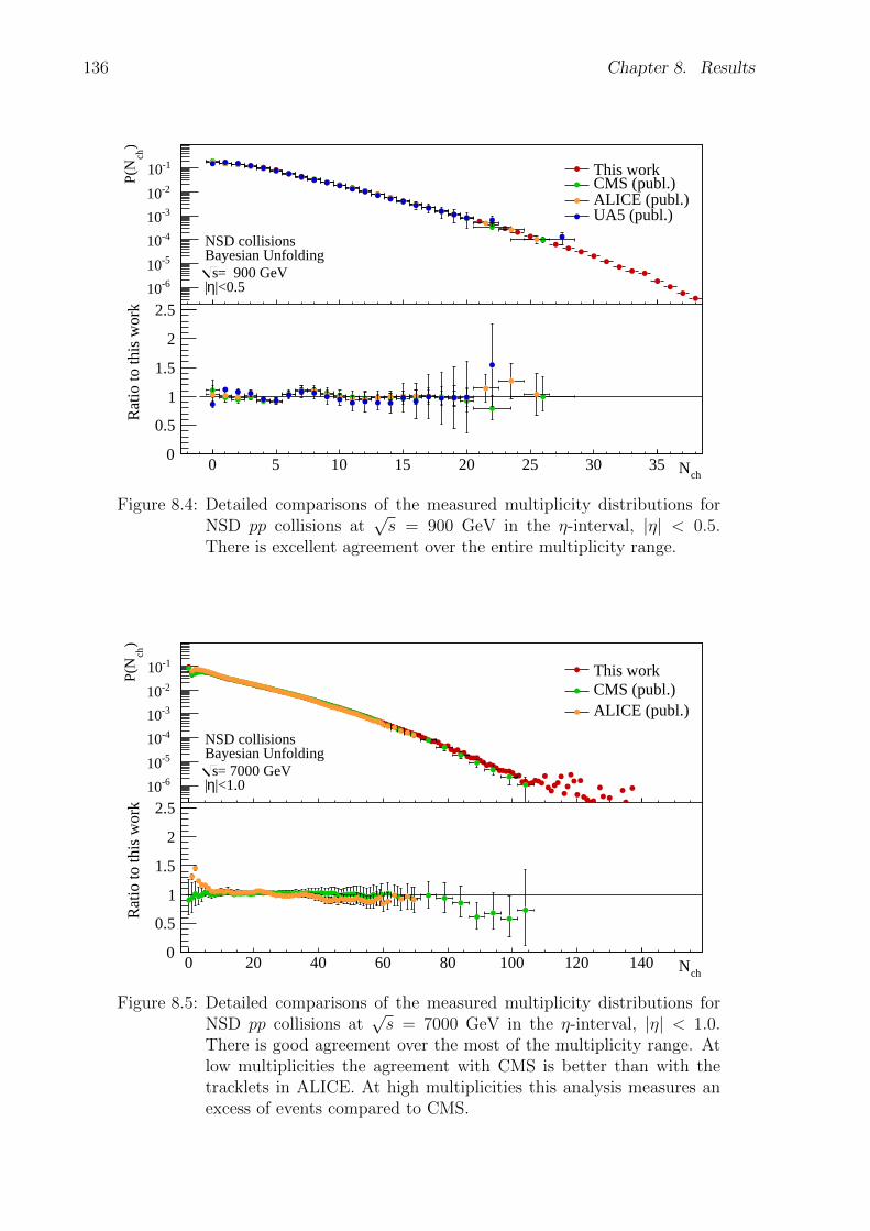
136 Chapter 8. Results
chN
0 5 10 15 20 25 30 35
)ch
P(N
-610
-510
-410
-310
-210
-110
NSD collisionsBayesian Unfolding
= 900 GeVs|<0.5η|
This workCMS (publ.)ALICE (publ.) UA5 (publ.)
chN0 5 10 15 20 25 30 35
Rat
io to
this
wor
k
0
0.5
1
1.5
2
2.5
Figure 8.4: Detailed comparisons of the measured multiplicity distributions forNSD pp collisions at
√s = 900 GeV in the η-interval, |η| < 0.5.
There is excellent agreement over the entire multiplicity range.
chN
0 20 40 60 80 100 120 140
)ch
P(N
-610
-510
-410
-310
-210
-110
NSD collisionsBayesian Unfolding
= 7000 GeVs|<1.0η|
This workCMS (publ.)ALICE (publ.)
chN0 20 40 60 80 100 120 140
Rat
io to
this
wor
k
0
0.5
1
1.5
2
2.5
Figure 8.5: Detailed comparisons of the measured multiplicity distributions forNSD pp collisions at
√s = 7000 GeV in the η-interval, |η| < 1.0.
There is good agreement over the most of the multiplicity range. Atlow multiplicities the agreement with CMS is better than with thetracklets in ALICE. At high multiplicities this analysis measures anexcess of events compared to CMS.
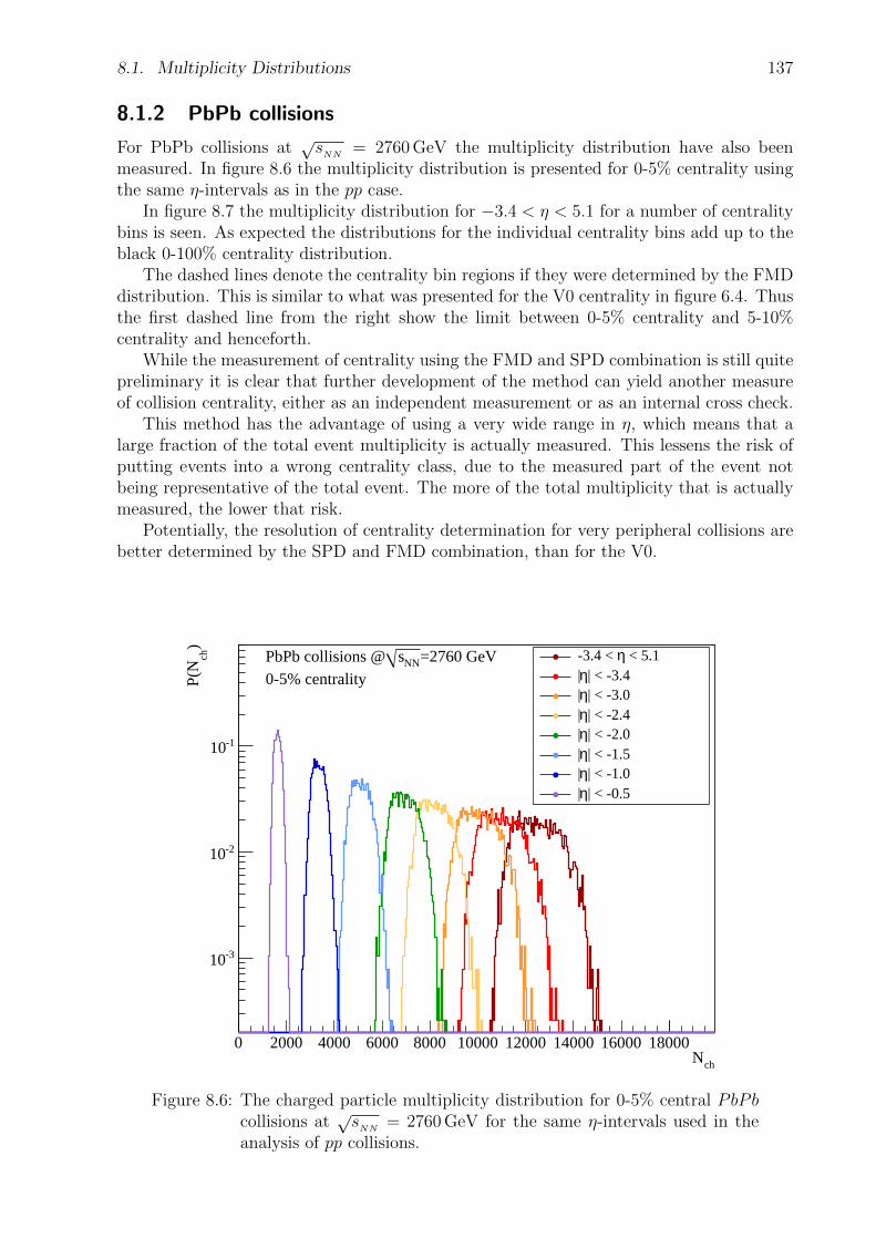
8.1. Multiplicity Distributions 137
8.1.2 PbPb collisions
For PbPb collisions at√sNN
= 2760 GeV the multiplicity distribution have also beenmeasured. In figure 8.6 the multiplicity distribution is presented for 0-5% centrality usingthe same η-intervals as in the pp case.
In figure 8.7 the multiplicity distribution for −3.4 < η < 5.1 for a number of centralitybins is seen. As expected the distributions for the individual centrality bins add up to theblack 0-100% centrality distribution.
The dashed lines denote the centrality bin regions if they were determined by the FMDdistribution. This is similar to what was presented for the V0 centrality in figure 6.4. Thusthe first dashed line from the right show the limit between 0-5% centrality and 5-10%centrality and henceforth.
While the measurement of centrality using the FMD and SPD combination is still quitepreliminary it is clear that further development of the method can yield another measureof collision centrality, either as an independent measurement or as an internal cross check.
This method has the advantage of using a very wide range in η, which means that alarge fraction of the total event multiplicity is actually measured. This lessens the risk ofputting events into a wrong centrality class, due to the measured part of the event notbeing representative of the total event. The more of the total multiplicity that is actuallymeasured, the lower that risk.
Potentially, the resolution of centrality determination for very peripheral collisions arebetter determined by the SPD and FMD combination, than for the V0.
chN0 2000 4000 6000 8000 10000 12000 14000 16000 18000
)ch
P(N
-310
-210
-110
=2760 GeVNNsPbPb collisions @ 0-5% centrality
< 5.1η-3.4 < | < -3.4η|| < -3.0η|| < -2.4η|| < -2.0η|| < -1.5η|| < -1.0η|| < -0.5η|
Figure 8.6: The charged particle multiplicity distribution for 0-5% central PbPbcollisions at
√sNN
= 2760 GeV for the same η-intervals used in theanalysis of pp collisions.
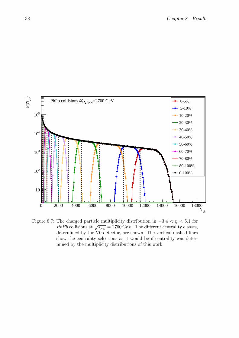
138 Chapter 8. Results
chN0 2000 4000 6000 8000 10000 12000 14000 16000 18000
)ch
P(N
10
210
310
410
510
=2760 GeVNNsPbPb collisions @ 0-5%
5-10%
10-20%
20-30%
30-40%
40-50%
50-60%
60-70%
70-80%
80-100%
0-100%
Figure 8.7: The charged particle multiplicity distribution in −3.4 < η < 5.1 forPbPb collisions at
√sNN
= 2760 GeV. The different centrality classes,determined by the V0 detector, are shown. The vertical dashed linesshow the centrality selections as it would be if centrality was deter-mined by the multiplicity distributions of this work.

8.2. KNO 139
⟩ch
N⟨/chz = N0 2 4 6 8 10 12
)ch
P(N
⟩ch
N⟨
-610
-410
-210
1
210
410
610
810
1010
1210
1410
=900 GeVs
=7000 GeVs
|<0.5η|)2|<1.0 (x10η|)4|<1.5 (x10η|)6|<2.0 (x10η|)8|<2.4 (x10η|)10|<3.0 (x10η|)12|<3.4 (x10η|
)14 <5.1 (x10η-3.4 <
I
II
III
IV
V
VI
VII
VIII
I
II
III
IV
V
VI
VII
VIII NSD CollisionsBayesian Unfolding
Figure 8.8: pp NSD collisions in KNO variables at√s = 900 GeV and 7000 GeV.
It is found that KNO scaling is violated in all η-intervals, exceptperhaps the most central η-region.
8.2 KNO
The next group of results revolves around KNO scaling. The first results presented will befor pp collisions, and in the next subsection the results from PbPb collisions are shown.
8.2.1 pp collisions
Figure 8.8 show pp NSD collisions at√s = 900 GeV and 7000 GeV in KNO variables. It
is found that the broader the observed η-interval, the more KNO scaling is violated whenmoving from
√s = 900 GeV to
√s = 7000 GeV. For the most narrow η-interval, |η| < 0.5,
it is difficult to conclude whether KNO scaling is also violated, but any violation is at bestvery small. CMS concludes that KNO scaling holds for |η| < 0.5 [75].
Figure 8.9 show comparisons between this work and CMS for |η| < 0.5 and |η| < 2.4.It is seen that there is good agreement in both intervals. The ratio between
√s = 900 GeV
and 7000 GeV for both set of measurements is included in figure 8.9.
It is interesting to notice that the shape of the ratio-distribution is the same for both|η| < 0.5 and |η| < 2.4. For the latter this is a clear sign that the KNO multiplicitydistributions are distinctly different, and thus KNO scaling is violated. For |η| < 0.5 theshape is similar, but the magnitude of the effect is clearly smaller. However it appears asif the overall picture is the same, namely that KNO scaling is possibly violated also forthe |η| < 0.5 interval. In order to reach a firm conclusion on this, better control of the

140 Chapter 8. Results
⟩ch
N⟨/chz = N0 2 4 6 8 10
)ch
P(N
⟩ch
N⟨
-510
-410
-310
-210
-110
1
10=900 GeV - This works
=7000 GeV - This works
=900 GeV - CMSs
=7000 GeV - CMSs
|<0.5η|
⟩ch
N⟨/chz = N0 2 4 6 8 10
900G
eV/7
000G
eV
00.20.40.60.8
11.21.4
This work
CMS
⟩ch
N⟨/chz = N0 1 2 3 4 5 6
)ch
P(N
⟩ch
N⟨
-310
-210
-110
1
10 =900 GeV - This works
=7000 GeV - This works
=900 GeV - CMSs
=7000 GeV - CMSs
|<2.4η|
⟩ch
N⟨/chz = N0 1 2 3 4 5 6
900G
eV/7
000G
eV
00.20.40.60.8
11.21.4
This work
CMS
Figure 8.9: Detailed comparison of KNO scaling in |η| < 0.5 and |η| < 2.4 be-tween CMS and this work. Good agreement is found between theexperiments for the multiplicity distributions in KNO variables. Theshape of the ratio between
√s = 900 GeV and 7000 GeV is similar
for both η intervals, however the scale of the deviations from unity isless in the |η| < 0.5 case. This might indicate that KNO scaling isalso violated for |η| < 0.5, however very slightly.
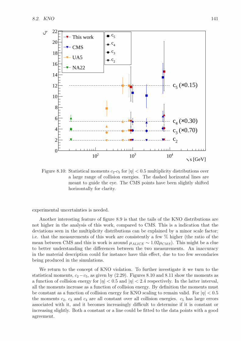
8.2. KNO 141
[GeV]s210 310 410
qc
0
2
4
6
8
10
12
14
16
18
20
22
2c0.70)× (3c
0.30)× (4c
0.15)× (5c
This work
CMS
UA5
NA22
5c
4c
3c
2c
Figure 8.10: Statistical moments c2-c5 for |η| < 0.5 multiplicity distributions overa large range of collision energies. The dashed horizontal lines aremeant to guide the eye. The CMS points have been slightly shiftedhorizontally for clarity.
experimental uncertainties is needed.
Another interesting feature of figure 8.9 is that the tails of the KNO distributions arenot higher in the analysis of this work, compared to CMS. This is a indication that thedeviations seen in the multiplicity distributions can be explained by a minor scale factor;i.e. that the measurements of this work are consistently a few % higher (the ratio of themean between CMS and this is work is around µALICE ∼ 1.02µCMS). This might be a clueto better understanding the differences between the two measurements. An inaccuracyin the material description could for instance have this effect, due to too few secondariesbeing produced in the simulations.
We return to the concept of KNO violation. To further investigate it we turn to thestatistical moments, c2−c5, as given by (2.29). Figures 8.10 and 8.11 show the moments asa function of collision energy for |η| < 0.5 and |η| < 2.4 respectively. In the latter interval,all the moments increase as a function of collision energy. By definition the moments mustbe constant as a function of collision energy for KNO scaling to remain valid. For |η| < 0.5the moments c2, c3 and c4 are all constant over all collision energies. c5 has large errorsassociated with it, and it becomes increasingly difficult to determine if it is constant orincreasing slightly. Both a constant or a line could be fitted to the data points with a goodagreement.
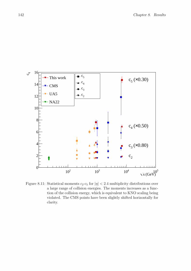
142 Chapter 8. Results
(GeV)s210 310 410 510
qc
0
2
4
6
8
10
12
14
16
2c
0.80)× (3c
0.50)× (4c
0.30)× (5cThis work
CMS
UA5
NA22
5c
4c
3c
2c
Figure 8.11: Statistical moments c2-c5 for |η| < 2.4 multiplicity distributions overa large range of collision energies. The moments increases as a func-tion of the collision energy, which is equivalent to KNO scaling beingviolated. The CMS points have been slightly shifted horizontally forclarity.

8.2. KNO 143
⟩ch
N⟨/chz = N0 0.5 1 1.5 2 2.5 3
⟩ch
N⟨)ch
P(N
-110
1
10
210
=2760 GeVNNsPbPb collisions @ 0-5%
5-10%
10-20%
20-30%
30-40%
40-50%
50-60%
60-70%
70-80%
80-100%
Figure 8.12: Multiplicity distributions of various centrality classes in PbPb colli-sions in KNO variables. No scaling with respect to the mean multi-plicity is apparent.
8.2.2 PbPb collisions
For PbPb collisions the multiplicity distributions have also been studied in KNO variables.In figure 8.12 they are shown for a number of centrality classes. It is seen that thereis no apparent scaling with respect to the mean multiplicity. It does however look as ifnormalising to the mean multiplicity is not the best choice. Looking at the two most centraldistribution, which only span 5% centrality each, it is found that they are significantlydifferent than the rest, which span 10% centrality each.
Thus the distributions are not independent of the choice of centrality bins, which ob-viously makes it a sub-optimal choice. For further studies it could be interesting to see ifit is possible to find another way to scale the distributions. Letting the scaling involve themean number of participants springs to mind as a place to start. This avenue has not beenpursued further in this work.
However, another study has been performed. Figure 8.13 shows the multiplicity dis-tributions in KNO variables for various η-intervals. The top panel includes the sameη-intervals as for pp collisions. It is seen that there is a clear scaling with respect to themean multiplicity that persists over even the broadest η-interval. The origin of this scalingis currently not understood. Going forward in η, each interval includes the previous one.If there is any changes going to forward regions, this could be washed out by the inclusionof the more central region. To rule this out, the KNO multiplicity distributions are alsomeasured for narrow η-intervals of ∆η = 0.5. These are presented in the lower panel offigure 8.13. There is clear scaling with respect to the mean multiplicity visible for all theη-intervals. Quite surprisingly there are two intervals which deviate slightly from the rest,namely 2.0 < η < 2.5 and 3.5 < η < 4.0. The reason for this is not understood.
The scaling itself is also not understood at this time. It is entirely possible that it is amundane effect, or could perhaps hint at interesting physics.

144 Chapter 8. Results
⟩ch
N⟨/ch
z=N0.7 0.8 0.9 1 1.1 1.2 1.3 1.4 1.5
⟩ch
N⟨)ch
P(N
1
10
210
310 =2760 GeVNNsPbPb collisions @ 0-5% centrality
< 5.1η-3.4 < | < 3.4η|| < 3.0η|| < 2.4η|| < 2.0η|| < 1.5η|| < 1.0η|| < 0.5η|
⟩ch
N⟨/chz=N0.6 0.8 1.0 1.2 1.4 1.6
⟩ch
N⟨)ch
P(N
1
10
210
=2760 GeVNNsPbPb collisions @
0-5% centrality < -2.5η-3.0 <
< -2.0η-2.5 < < -1.5η-2.0 <
< -1.0η-1.5 <
< -0.5η-1.0 < < 0.0η-0.5 <
< 0.5η 0.0 < < 1.0η 0.5 <
< 1.5η 1.0 < < 2.0η 1.5 <
< 2.5η 2.0 < < 3.0η 2.5 <
< 3.5η 3.0 < < 4.0η 3.5 <
< 4.5η 4.0 <
< 5.0η 4.5 <
Figure 8.13: An attempt at looking at KNO scaling in PbPb collisions for thecentrality class 0-5%. The upper panel shows the the multiplicitydistributions for the same η-intervals used for analysis of pp colli-sions. The lower panel show small ∆η = 0.5 intervals. For bothrepresentations, a clear scaling with respect to the mean multiplicityis seen.

8.3. dNch
dη145
8.3 dNchdη
Next up are the derived measurements of dNch
dη. These are created by running the analysis
for very narrow pseudorapidity intervals, ∆η = 0.5, as described in the previous section.The mean value of these distributions each give a point in the dNch
dηdistributions.
8.3.1 pp collisions
Figure 8.14 show dNch
dηfor pp NSD collisions at
√s = 900 GeV and 7000 GeV. It is found
that for the mid-rapidity region, there is good agreement between this method and thepublished data from other experiments. For the forward region in
√s = 900 GeV the
agreement is not very good. For√s = 7000 GeV there is no published data at forward
angles, and the ALICE comparison is done to the trigger class INEL>0.The cause of the disagreement at forward angles is not fully understood, but it is
likely that it is due to problems unfolding the very narrow η-intervals. At especially√s = 900 GeV the raw multiplicity distribution for a narrow η-interval does not extend to
very high multiplicities. In the forward region the secondary contamination is very large,and thus the unfolding changes the shape of the multiplicity distribution dramatically.
When the multiplicity distribution only spans few multiplicity values, this can causeproblems with the unfolding precision. This can give unfolded distributions, which are
η-4 -3 -2 -1 0 1 2 3 4 5
η/d
chdN
0
1
2
3
4
5
6
7
This work
UA5 (publ.)
CMS (publ.)
ALICE (publ.)
ALICE INEL>0 (publ.)
NSD collisions
=7000 GeVs
=900 GeVs
Figure 8.14: dNch
dηin pp NSD collisions measured as the mean of narrow unfolded
multiplicity distributions. Included are measurements from CMS,UA5 and ALICE for reference. In the mid-rapidity region goodagreement is seen. For forward regions there are significant devi-ations.

146 Chapter 8. Results
η-4 -2 0 2 4
η/d
chdN
210
310
=2760 GeVNNsPbPb collisions @
0-5%5-10%
10-20%
20-30%
30-40%
40-50%
50-60%
60-70%
70-80%
Figure 8.15: dNch
dηin PbPb collisions at
√sNN
= 2760 GeV, measured as the meanof narrow unfolded multiplicity distributions. Included is a referencemeasurement from another preliminary ALICE analysis [87]. Overallreasonable agreement is found between the two methods.
not reminiscent to the true distribution, and thus the mean value determination will beinaccurate 27.
However, for the mid-rapidity region, the contamination of secondaries are very low,and thus the response matrix is almost diagonal. Thus the unfolding does not dramaticallychange the shape.
This can explain why good agreement is seen for the SPD range, where there are fewsecondaries, compared to the poor agreement in the secondary rich forward regions.
8.3.2 PbPb collisions
Figure 8.15 shows the dNch
dηfor PbPb collisions at
√sNN
= 2760 GeV. Included as grey
points are also the preliminary measurements of another current analysis by ALICE [87].It is found that there overall seem to be reasonable agreement between the two methods.
Making dNch
dηmeasurements in this way, was never a main ambition of this work. Instead
it is meant as a simple, and fun exercise. Given more time it is possible to further enhancethe method, thereby providing a real alternative for dNch
dηmeasurements.
27for η-bins of size ∆η = 0.2 the unfolding has been tested, and regularly breaks down completely,yielding very unphysical solutions.

8.4. Mean Multiplicity Energy dependence 147
(GeV)NNs210 310
)⟩pa
rt N⟨
)/(0
.5η
/dch
(dN
0
2
4
6
8
10
pp NSD ALICEpp NSD CMS
NSD CDFpp NSD UA5pp NSD UA1pp
pp NSD STARpp NSD - This work
AA(0-5 %) ALICEAA(0-5 %) NA50AA(0-5 %) BRAHMSAA(0-5 %) PHENIXAA(0-5 %) STARAA(0-6 %) PHOBOSAA(0-5 %) - This work
0.11NN s∝
0.15NN s∝
NN ln s∝AA
)ppp(p
Figure 8.16: Mean multiplicity per participant pair scaling with collision energy.Good agreement is found with previous measurements. The mea-surements of this work is shifted upwards in energy for clarity. Figureis adapted from [88].
8.4 Mean Multiplicity Energy dependence
The last result presented is the collision energy scaling of the mean multiplicity in mid-rapidity per participant pair. In this context mid-rapidity is the η-interval |η| < 0.5. Theresults for pp NSD collisions at
√s = 900 GeV and 7000 GeV, as well as PbPb collisions
at√sNN
= 2760 GeV are shown in figure 8.16.The measurements are consistent with the published values from ALICE, as well as for
the CMS measurement for pp NSD collisions at√s = 7000 GeV.
Thus, the conclusions from those experiments, that the mean multiplicity in mid-rapidity scales in both pp and PbPb collisions as a function of sa [88] is supported bythese measurements. The scaling is different for the two collision systems. It is found that:
1
0.5 〈Npart〉dNch
dη∝ s0.11 , for pp collisions
1
0.5 〈Npart〉dNch
dη∝ s0.15NN , for PbPb collisions (8.1)
(8.2)

148 Chapter 8. Results
8.5 Outlook
While the FMD is fairly well understood, as demonstrated throughout this thesis, thereare still numerous issues where a better understanding is needed. Improving upon theseareas is paramount to increasing the accuracy of measurements of the FMD.
Material budget of ALICE
The largest uncertainty in the FMD measurements is the accuracy of the virtual modelof the experiment. While the major geometry revision in 2010 definitely was a great leapforward, there could be inaccuracies still in the geometry description.
There are immediately plans for starting a study, that can once and for all put this issueto rest. This study is similar to how the TPC has mapped their geometry very preciselyin the mid-rapidity region.
Their method revolves around photons interacting with material, thus creating electron-positron pairs, that are eventually tracked in the TPC. By extrapolating the tracks backit is possible to determine exactly where the photon conversions happened. By doing soit is possible to get very detailed information of the material distribution in ALICE. Insome sense it is reminiscent to the secondary particles origin plots presented in section 6.4.However the main advantage of the TPC method is that the actual physics data are used,and can be directly compared to the simulations. By using this method the TPC groupwas able to discover, amongst other things, a thin layer of glue missing in the materialdescription.
The TPC only covers the mid-rapidity region, for collisions around the nominal inter-action point. However if collisions with vertices at high |vz|, are used, particles stemmingfrom conversions in the forward regions are possible to be measured by the TPC.
Getting this study underway in collaboration with the TPC group has highest priority.
FMD energy distributions
Another issue which was touched upon in section 6.2.1 is the differences between the energydistributions in physics data and simulated data. The energy distributions of simulationshave much less smeared Landau peaks than in physics data.
A way to tune the simulations to better match the physics data is outlined in thefollowing. First, it is assumed that the underlying energy loss signal is described by aLandau distribution, given by the variable (∆−∆p)/ξ where ∆p is the MPV energy loss,∆ is the energy loss and ξ denotes the spread of the landau distribution. The energydistribution we are looking for after tuning is similarly given by (∆′ − ∆′p)/ξ
′. For now,focus is only on changing the width of the distributions, not the peak location, and thereforewe set ∆′p = ∆p. Thus the relation between the two distributions are given by:
∆−∆p
ξ=
∆′ −∆′pξ′
, and thus ∆′ =ξ′
ξ∆ +
(1− ξ′
ξ
)∆p (8.3)
Retrieving ξ/ξ′ from fits of the physics data and simulations respectively, it is possible torecalculate the tuned energy distribution from the original one.
Two examples of this are shown in figure 8.17. As seen the simulated energy distri-butions changes to better resemble the physics data energy distributions after tuning. Inthe same manner it is possible to also shift the Landau peaks of the simulated energydistributions.

8.5. Outlook 149
MIP/EdepE0 0.5 1 1.5 2 2.5 3 3.5 4
Cou
nts
210
310
410
= 1.6ξ'/ ξTuned with
= 1.9ξ'/ ξTuned with
Present Simulation
Figure 8.17: Preliminary tests of tuning the simulated energy distributions. Fur-ther tests will help ensuring that the energy distributions in sim-ulations matches energy simulations in physics data as closely aspossible
It is worth mentioning that the fraction of singles, doubles and triples in simulationscompared to physics data is seemingly unaffected by the tuning of the energy distributions.Similarly the tuning will not have any effect on the appearance of very low energy depositionsignals in physics data. These are issues which has to be dealt with separately.
Once the energy distributions for simulations matches the physics data, it needs to beincluded in new official ALICE simulation productions.
pPb collisions
The LHC has so-far successfully provided both pp and PbPb collisions. At the end of 2011they will attempt to setup and make the first pPb collisions.
As briefly discussed in section 1.4 this asymmetric collision systems is very interesting,since it is hoped that it will yield major insights into the initial conditions of the collisions.
In particular it will be exciting to study whether the gluon density is saturated, whichwould be clearly indicative of a Colour Glass Condensate state of matter. Colour GlassCondensate is theorised to be the state of matter of the nuclei just before they collide.
The existence of a Colour Glass Condensate can explain some of the unsolved problemsof how exactly particles are produced in relativistic collisions as well as the distribution ofmatter inside particles themselves [131].
The FMD is perfect to look for signs of gluon saturation by examining how the multi-plicity scales in pPb collisions as opposed to either pp or PbPb collisions.

150 Chapter 8. Results

Chapter 9
Conclusion
When the LHC succeeded providing pp collisions at√s =900 GeV on 23rd of Novem-
ber 2009, it was the culmination of 25 years of planning and extraordinary experimentalingenuity. Since then the LHC has provided pp collisions at higher energies, as well asPbPb collisions at
√sNN
= 2760 GeV. This work has presented analysis of these initial runperiods.
The analysis framework and capabilities of the FMD has been discussed in detail. Amethod of using the FMD together with the inner layer of the SPD has been presented.This method have enabled ALICE to perform multiplicity analysis over a very large rangein pseudorapidity.
With this method the charged particle multiplicities for pp NSD collisions at three col-lision energies have been measured for many η-intervals, the largest covering more than 8units of η. It has been found that the measurements in this work are consistent with pre-vious measurements from CMS and UA5. Even though they fall within the uncertainties,the multiplicity tails are systematically, if only slightly, higher in this analysis.
For√s = 2760 GeV collisions the conclusion is that the data quality is too poor,
that reliable analysis is not a possibility at this time. The exact extent of this is beinginvestigated extensively in ALICE. Hopefully a focused effort can help improve the dataquality.
Going from√s = 900 GeV to 7000 GeV it is concluded that KNO scaling is strongly
violated for at least all η-intervals except perhaps |η| < 0.5, where no clear conclusion canbe drawn from the available data. This was further investigated in the presentation ofthe statistical moments for |η| < 0.5 and |η| < 2.4. Smaller systematic uncertainties areneeded to conclude definitively whether KNO scaling is violated at |η| < 0.5.
For PbPb collisions scaling in KNO variables has also been investigated; both as afunction of centrality and η-interval. In the former case, no scaling is seen. For the latterthere is clear scaling over all η-ranges. The multiplicity distributions are very similar inKNO variables from mid-rapidity to the most forward regions. The origin of this scalingis not understood, and must be investigated further.
It has furthermore been demonstrated that it is possible to make dNch
dηdistributions by
taking the mean value of multiplicity distributions from very narrow η-intervals. Partic-ularly in pp collisions there are however unsolved issues in the forward regions, but goodagreement with previous experiments in the mid-rapidity region.
The last result presented was the mean multiplicity per participant paris in |η| < 0.5for both pp and PbPb collisions. It is found that there is good agreement with previousmeasurements from CMS and ALICE.
Summing up, a variety of the first LHC results of analysis using the FMD has been
151

152 Chapter 9. Conclusion
presented in this work. There are however still much room for improvement in the de-tailed understanding of the FMD system. This continued effort of reducing the systematicuncertainties is very important for both the analyses presented in this work, but also forsubsequent analysis, that might be even more susceptible to the remaining issues.
Gaining a better understanding of the FMD, and solving the remaining issues, willleave the FMD in great shape when the LHC finally starts colliding particles at the designtop energy in 2014.
Casper Nygaard, October 2011

Appendix A
Lorentz Invariance of dy
The Lorentz transformation is given by:
E∗ = γE − γβpzpz∗ = −γβE + γpz (A.1)
Here β velocity of the frame from which we view the collision and γ is defined asγ = 1√
1−β2)
The transformation is done by inserting the transformations of E and pz into the defi-nition of the rapidity:
y∗ =1
2lnE ∗+pz∗E ∗ −pz∗
=1
2lnγE − γβpz − γβE + γpzγE − γβpz + γβE − γpz
=1
2lnE + pzE ∗ −pz
+1
2lnγ − γβγ + γβ
= y +1
2lnγ − γβγ + γβ
(A.2)
(A.3)
This means that:
dy∗ = y ∗2 −y∗1 = y2 − y1 = dy (A.4)
Thus rapidity differences are Lorentz invariant.
153

154 Appendix A. Lorentz Invariance of dy
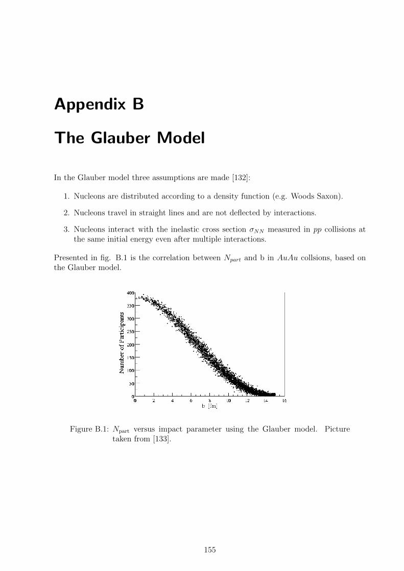
Appendix B
The Glauber Model
In the Glauber model three assumptions are made [132]:
1. Nucleons are distributed according to a density function (e.g. Woods Saxon).
2. Nucleons travel in straight lines and are not deflected by interactions.
3. Nucleons interact with the inelastic cross section σNN measured in pp collisions atthe same initial energy even after multiple interactions.
Presented in fig. B.1 is the correlation between Npart and b in AuAu collsions, based onthe Glauber model.
Figure B.1: Npart versus impact parameter using the Glauber model. Picturetaken from [133].
155

156 Appendix B. The Glauber Model

Appendix C
Sharing algoritm
Stripn-1 n n+1
E [
arbi
trar
y un
its]
∆
Cut
Stripn-1 n n+1
E [
arbi
trar
y un
its]
∆
Cut
Stripn-1 n n+1
E [
arbi
trar
y un
its]
∆
Cut
Stripn-1 n n+1
E [
arbi
trar
y un
its]
∆
Cut
Stripn-1 n n+1
E [
arbi
trar
y un
its]
∆
Cut
Stripn-1 n n+1
E [
arbi
trar
y un
its]
∆
Cut
Before Hit Merging After Hit Merging
Figure C.1: Illustration of the concept of hit sharing. Incoming particles cantraverse multiple strips, deposting energy in all of them. A hit sharingalgoritm searches for neighboring strips with energy signals above thelow threshold. The shared energy signals are merged into one signal.
In figure C.1 a few examples of hit merging with 3 strips hit are illustrated. In figureC.2 the flow chart of the sharing algorithm is shown.
In the case of merging two strips, the merged signal is always placed in the strip withthe highest energy deposition. For three strips being merged, the signal is placed in themiddle strip. There are arguments for/against placing it in the middle strip compared toplacing it in the highest deposit strip like for the two-strip case. The difference however is
157

158 Appendix C. Sharing algoritm
Start in strip n
no
?low > EnEyes
no
No Signal = 0m
nEGo to strip n+1
high < EnE
or ?high < En+1 < ElowE
no Single Signal
n = EmnE
Go to strip n+1
yes
?high < En+2 < ElowEyes
Triple Signal = 0m
nE
n+2+En+1+En = Emn+1E
= 0mn+2E
Go to strip n+3no
n+2 < EhighE
and ?high < E
n+1 and Ehigh < EnE
yes
no
?n+1 < EnE yes
no
Double Signal = 0m
nE
n+1+En = Emn+1E
Go to strip n+2
Double Signal
n+1+En = EmnE
= 0mn+1E
Go to strip n+2
Figure C.2: Flow chart of the sharing algoritm. Up to three adjacent strip aresearched through and their deposited energy merged depending onthe energy deposits in each of the strips.
completely negligible due to the tiny η difference between two adjacent strips, as well asthe fact that having merged signals from three strips are quite rare.
pp @√s = 900GeV
Signal FMD1I FMD2I FMD2O FMD3I FMD3OSingle 86.99 % 87.07 % 92.26 % 85.65 % 91.96 %Double 12.71 % 12.67 % 7.64 % 13.99 % 7.86 %Triple 0.30 % 0.26 % 0.10 % 0.36 % 0.18 %
PbPb @√s = 2760GeV
Signal FMD1I FMD2I FMD2O FMD3I FMD3OSingle 88.95% 88.48% 91.22 % 88.24 % 91.79 %Double 9.67 % 9.95% 7.91 % 10.17 % 7.37 %Triple 1.38 % 1.58 % 0.87 % 1.59 % 0.84 %
Table C.1: Overview over the amount of single, double and triple signals in eachof the FMD rings.

Appendix D
Comparison between Poisson andEnergy Fits counting
Figure D.1: Comparison between the Poisson and Energy fit counting methodsfor pp collisions at
√s = 2760GeV.
159

160 Appendix D. Comparison between Poisson and Energy Fits counting
Figure D.2: Comparison between the Poisson and Energy fit counting methodsfor pp collisions at
√s = 7000GeV.

161
(Energy loss fits)chN0 10 20 30 40 50 60 70
(Po
isso
n)ch
N
0
10
20
30
40
50
60
70
1
10
210
310
410
510
610
710FMD1I xβ+αDeming regression: y=
=-0.085α= 1.013β
(Energy loss fits)chN0 10 20 30 40 50 60 70
(Po
isso
n)ch
N
0
10
20
30
40
50
60
70
1
10
210
310
410
510
610
710FMD2I xβ+αDeming regression: y=
=-0.104α= 1.031β
(Energy loss fits)chN0 10 20 30 40 50 60 70
(Po
isso
n)ch
N
0
10
20
30
40
50
60
70
1
10
210
310
410
510
610
710FMD3I xβ+αDeming regression: y=
=-0.180α= 1.039β
0.98
4807
0.98
6354
0.98
8992
0.98
2577
0.99
071
FMD1I FMD2I FMD2O FMD3I FMD3Or
0.8
0.85
0.9
0.95
1
1.05
1.1
1.15
1.2
=2760 GeVNNsPbPb collisions @
(Energy loss fits)chN0 10 20 30 40 50 60 70
(Po
isso
n)ch
N
0
10
20
30
40
50
60
70
1
10
210
310
410
510
610
710FMD2O xβ+αDeming regression: y=
=-0.036α= 0.984β
(Energy loss fits)chN0 10 20 30 40 50 60 70
(Po
isso
n)ch
N
0
10
20
30
40
50
60
70
1
10
210
310
410
510
610
710FMD3O xβ+αDeming regression: y=
=-0.044α= 0.981β
Figure D.3: Comparison between the Poisson and Energy fit counting methodsfor PbPb collisions at
√sNN
= 2760 GeV.

162 Appendix D. Comparison between Poisson and Energy Fits counting
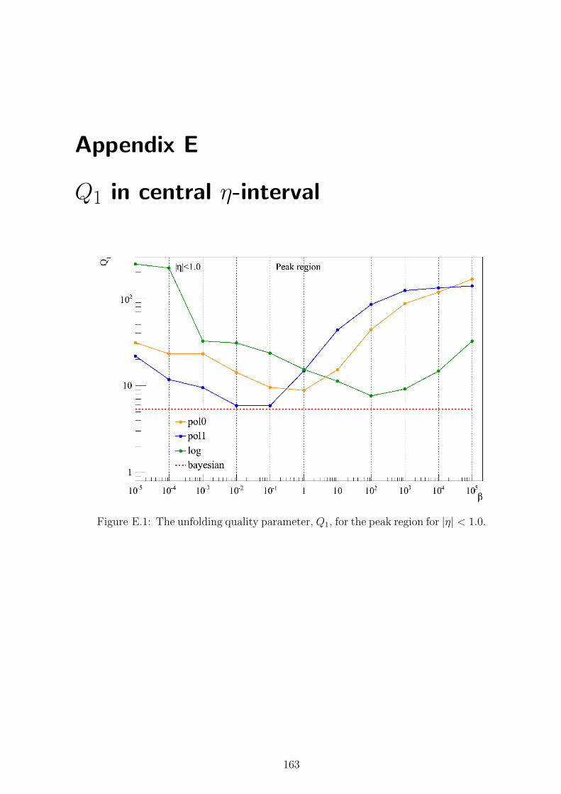
Appendix E
Q1 in central η-interval
Figure E.1: The unfolding quality parameter, Q1, for the peak region for |η| < 1.0.
163

164 Appendix E. Q1 in central η-interval
Figure E.2: Q1 for the constant exponential slope region and the low statisticsregion for |η| < 1.0.
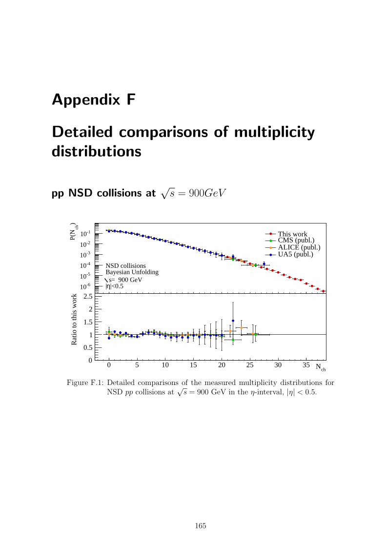
Appendix F
Detailed comparisons of multiplicitydistributions
pp NSD collisions at√s = 900GeV
chN
0 5 10 15 20 25 30 35
)ch
P(N
-610
-510
-410
-310
-210
-110
NSD collisionsBayesian Unfolding
= 900 GeVs|<0.5η|
This workCMS (publ.)ALICE (publ.) UA5 (publ.)
chN0 5 10 15 20 25 30 35
Rat
io to
this
wor
k
0
0.5
1
1.5
2
2.5
Figure F.1: Detailed comparisons of the measured multiplicity distributions forNSD pp collisions at
√s = 900 GeV in the η-interval, |η| < 0.5.
165

166 Appendix F. Detailed comparisons of multiplicity distributions
chN
0 10 20 30 40 50 60 70
)ch
P(N
-610
-510
-410
-310
-210
-110
NSD collisionsBayesian Unfolding
= 900 GeVs|<1.0η|
This workCMS (publ.)ALICE (publ.)
chN0 10 20 30 40 50 60 70
Rat
io to
this
wor
k
0
0.5
1
1.5
2
2.5
Figure F.2: Detailed comparisons of the measured multiplicity distributions forNSD pp collisions at
√s = 900 GeV in the η-interval, |η| < 1.0.
chN
0 10 20 30 40 50 60 70 80 90
)ch
P(N
-610
-510
-410
-310
-210
-110
NSD collisionsBayesian Unfolding
= 900 GeVs|<1.5η|
This workCMS (publ.)UA5 (publ.)
chN0 10 20 30 40 50 60 70 80 90
Rat
io to
this
wor
k
0
0.5
1
1.5
2
2.5
Figure F.3: Detailed comparisons of the measured multiplicity distributions forNSD pp collisions at
√s = 900 GeV in the η-interval, |η| < 1.5.
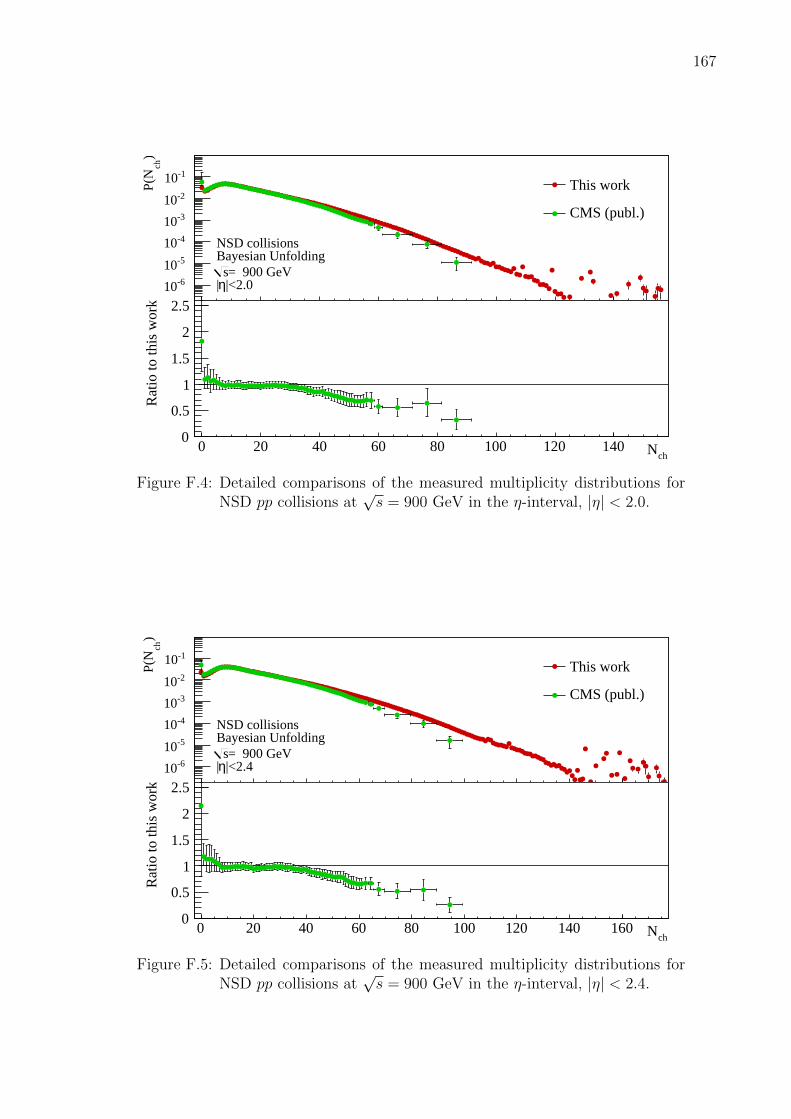
167
chN
0 20 40 60 80 100 120 140
)ch
P(N
-610
-510
-410
-310
-210
-110
NSD collisionsBayesian Unfolding
= 900 GeVs|<2.0η|
This work
CMS (publ.)
chN0 20 40 60 80 100 120 140
Rat
io to
this
wor
k
0
0.5
1
1.5
2
2.5
Figure F.4: Detailed comparisons of the measured multiplicity distributions forNSD pp collisions at
√s = 900 GeV in the η-interval, |η| < 2.0.
chN
0 20 40 60 80 100 120 140 160
)ch
P(N
-610
-510
-410
-310
-210
-110
NSD collisionsBayesian Unfolding
= 900 GeVs|<2.4η|
This work
CMS (publ.)
chN0 20 40 60 80 100 120 140 160
Rat
io to
this
wor
k
0
0.5
1
1.5
2
2.5
Figure F.5: Detailed comparisons of the measured multiplicity distributions forNSD pp collisions at
√s = 900 GeV in the η-interval, |η| < 2.4.

168 Appendix F. Detailed comparisons of multiplicity distributions
chN
0 20 40 60 80 100 120 140 160
)ch
P(N
-610
-510
-410
-310
-210
-110
NSD collisionsBayesian Unfolding
= 900 GeVs|<3.0η|
This work
UA5 (publ.)
chN0 20 40 60 80 100 120 140 160
Rat
io to
this
wor
k
0
0.5
1
1.5
2
2.5
Figure F.6: Detailed comparisons of the measured multiplicity distributions forNSD pp collisions at
√s = 900 GeV in the η-interval, |η| < 3.0.
pp NSD collisions at√s = 7000GeV
chN
0 10 20 30 40 50 60 70
)ch
P(N
-610
-510
-410
-310
-210
-110
NSD collisionsBayesian Unfolding
= 7000 GeVs|<0.5η|
This work
CMS (publ.)
chN0 10 20 30 40 50 60 70
Rat
io to
this
wor
k
0
0.5
1
1.5
2
2.5
Figure F.7: Detailed comparisons of the measured multiplicity distributions forNSD pp collisions at
√s = 7000 GeV in the η-interval, |η| < 0.5.

169
chN
0 20 40 60 80 100 120 140
)ch
P(N
-610
-510
-410
-310
-210
-110
NSD collisionsBayesian Unfolding
= 7000 GeVs|<1.0η|
This workCMS (publ.)ALICE (publ.)
chN0 20 40 60 80 100 120 140
Rat
io to
this
wor
k
0
0.5
1
1.5
2
2.5
Figure F.8: Detailed comparisons of the measured multiplicity distributions forNSD pp collisions at
√s = 7000 GeV in the η-interval, |η| < 1.0.
chN
0 20 40 60 80 100 120 140 160
)ch
P(N
-610
-510
-410
-310
-210
-110
NSD collisionsBayesian Unfolding
= 7000 GeVs|<1.5η|
This work
CMS (publ.)
chN0 20 40 60 80 100 120 140 160
Rat
io to
this
wor
k
0
0.5
1
1.5
2
2.5
Figure F.9: Detailed comparisons of the measured multiplicity distributions forNSD pp collisions at
√s = 7000 GeV in the η-interval, |η| < 1.5.

170 Appendix F. Detailed comparisons of multiplicity distributions
chN
0 50 100 150 200
)ch
P(N
-610
-510
-410
-310
-210
-110
NSD collisionsBayesian Unfolding
= 7000 GeVs|<2.0η|
This work
CMS (publ.)
chN0 50 100 150 200
Rat
io to
this
wor
k
0
0.5
1
1.5
2
2.5
Figure F.10: Detailed comparisons of the measured multiplicity distributions forNSD pp collisions at
√s = 7000 GeV in the η-interval, |η| < 2.0.
chN
0 50 100 150 200 250
)ch
P(N
-610
-510
-410
-310
-210
-110
NSD collisionsBayesian Unfolding
= 7000 GeVs|<2.4η|
This work
CMS (publ.)
chN0 50 100 150 200 250
Rat
io to
this
wor
k
0
0.5
1
1.5
2
2.5
Figure F.11: Detailed comparisons of the measured multiplicity distributions forNSD pp collisions at
√s = 7000 GeV in the η-interval, |η| < 2.4.

Bibliography
[1] BRAHMS Collaboration, I. Arsene et al., ‘Nuclear stopping and rapidity loss inAu+Au collisions at s(NN)**(1/2) = 62.4-GeV,’ Phys.Lett., B677 (2009) 267–271.
[2] BRAHMS Collaboration, I. Arsene et al., ‘Rapidity dependence of deuteronproduction in Au+Au collisions at
√sNN = 200 GeV,’ Phys.Rev., C83 (2011)
044906.
[3] M. Kaku, Hyperspace. Oxford University Press, 1995.
[4] ALEPH Collaboration, D. Decamp et al., ‘A Precise Determination of the Numberof Families with Light Neutrinos and of the Z Boson Partial Widths,’ Phys. Lett.B235, (1990) 399–411.
[5] Particle Data Group Collaboration, K. Nakamura et al., ‘The Review of ParticlePhysics,’ J. Phys., G37 (2010).
[6] F. Halzen and A. D. Martin, Quarks and Leptons: An Introductory Course inModern Particle Physics. John Wiley & Sons, Inc., 1984.
[7] J. Schwinger, ed., Selected Papers on Quantum Electrodynamics. DoverPublications, 1958.
[8] M. E. Peskin and D. V. Scroeder, An Introduction to Quantum Field Theory.Westview Press, 1995.
[9] C. S. B. Povh, K. Rith and F. Zetsche, Particles and Nuclei. Springer-Verlag, 4thedition ed., 2003.
[10] T. R. Klassen, ‘QCD (lattice) potential and coupling: How to accurately interpolatebetween multiloop QCD and the string picture,’ Phys. Rev., D51 (1995) 5130.
[11] M. L. Perl, E. R. Lee, and D. Loomba, ‘A Brief Review of the Search for IsolatableFractional Charge Elementary Particles,’ Mod. Phys. Lett., A19 (2004) 2595–2610.
[12] C. O. E. Jørgensen, ‘Charged Particle Production in Au+Au Collisions at,’Master’s thesis, University of Copenhagen, 2001.
[13] BRAHMS Collaboration, I. Arsene et al., ‘Quark Gluon Plasma and Color GlassCondensate at RHIC? The perspective from the BRAHMS experiment,’Nucl.Phys., A757 (2005).
[14] Z.Fodor and S. Katz, ‘Lattice determination of the critical point of QCD at finite Tand µ,’ JHEP 0203, 014 (2002).
171

172 Bibliography
[15] J. Letessier and J. Rafelski, Hadrons and Quark–Gluon Plasma, vol. 18 ofCambridge Monographs on Particle Physics, Nuclear Physics and Cosmology.Cambridge University Press, 2005.
[16] P. Kovtun, D. Son, and A. Starinets, ‘Viscosity in strongly interacting quantumfield theories from black hole physics,’ Phys.Rev.Lett., 94 (2005) 111601. An Essaysubmitted to 2004 Gravity Research Foundation competition.
[17] R. Karabowicz, ‘Study of Nuclear Modification Factors in Au+Au collisions at√sNN
= 200 GeV,’. PhD thesis, Jagellonian University, 2006.
[18] F.-M. Liu and K. Werner, ‘Direct photons at low transverse momentum – a QGPsignal in pp collisions at LHC,’.
[19] M. L. Miller, K. Reygers, S. J. Sanders, and P. Steinberg, ‘Glauber modeling inhigh energy nuclear collisions,’ Ann. Rev. Nucl. Part. Sci., 57 (2007) 205–243.
[20] J. Jia, ‘High-pT Charged Hadron Suppression in Au− Au Collisions at√sNN
= 200 GeV,’. PhD thesis, State University of New York at Stony Brook, 2003.
[21] J. Bjorken, ‘Highly Relativistic Nucleus-Nucleus Collisions: The Central RapidityRegion,’ Phys. Rev., D27 (1983) 140.
[22] L. D. Landau, ‘On the multiparticle production in high-energy collisions (InRussian),’ Izv. Akad. Nauk. SSSR Ser. Fiz., 17 (1953) 51–54. [English translationin: Collected Papers of L. D. Landau, D. Ter Haar (ed.), Intl Pub Distributor Inc,1965].
[23] BRAHMS Collaboration, I. G. Bearden et al., ‘Nuclear stopping in Au + Aucollisions at s(NN)**(1/2) = 200-GeV,’ Phys.Rev.Lett., 93 (2004) 102301.
[24] J. F. Große-Oetringhaus, ‘Measurement of the Charged-Particle Multiplicity inProton–Proton Collisions with the ALICE Detector,’. PhD thesis, University ofMunster, 2009.
[25] A. Kaidalov, ‘Regge poles in QCD,’ (2001).
[26] P. D. B. Collins, An Introduction to Regge Theory and High Energy Physics.Cambridge University Press, 1977.
[27] E. Predazzi, ‘Diffraction: Past, present and future,’ (1998).
[28] M. Poghosyan, Diffraction dissociation of protons in proton-proton collisions at√s =0.9 TeV, 2.76 TeV and 7 TeV with ALICE at the LHC Quark Matter 2011
parallel talk.
[29] BRAHMS Collaboration, I. Arsene et al., ‘Phys. Rev. Lett.,’ Transverse momentumspectra in Au+Au and d+Au collisions at
√sNN
= 200 GeV and the pseudorapiditydependence of high pT suppression., 91 (2003), no. 072305,.
[30] H. Appelhaeuser, Particle Production at Large Transverse Momentum with ALICEQuark Matter 2011 plenary talk.

Bibliography 173
[31] PHENIX Collaboration, A. Adare et al., ‘Suppression Pattern of Neutral Pions atHigh Transverse Momentum in Au+ Au Collisions at sNN = 200GeV andConstraints on Medium Transport Coefficients,’ Phys. Rev. Lett., 101 (Dec, 2008)232301.
[32] PHENIX Collaboration, A. Adare et al., ‘Transverse momentum dependence ofmeson suppression η suppression in Au+Au collisions at
√sNN = 200 GeV,’
Phys.Rev., C82 (2010) 011902.
[33] Y. J. Lee, Nuclear Modification Factors From the CMS Experiment Quark Matter2011 plenary talk.
[34] M. Gyulassy, P. Levai, and I. Vitev, ‘Reaction operator approach to nonAbelianenergy loss,’ Nucl.Phys., B594 (2001) 371–419. nucl-th/0006010.
[35] M. L. Purschke, RAA Measurements in PHENIX Quark Matter 2011 plenary talk.
[36] STAR Collaboration, C. Adler et al., ‘Disappearance of back-to-back high pThadron correlations in central Au+Au collisions at
√sNN = 200-GeV,’
Phys.Rev.Lett., 90 (2003) 082302.
[37] STAR Collaboration, J. Adams et al., ‘Evidence from d + Au measurements forfinal state suppression of high p(T) hadrons in Au+Au collisions at RHIC,’Phys.Rev.Lett., 91 (2003) 072304.
[38] C. Roland, Jet Meaurements by the CMS experiment in pp and PbPb collisionsQuark Matter 2011 plenary talk.
[39] ATLAS Collaboration, G. Aad et al., ‘Observation of a Centrality-Dependent DijetAsymmetry in Lead-Lead Collisions at sqrt(S(NN))= 2.76 TeV with the ATLASDetector at the LHC,’ Phys.Rev.Lett., 105 (2010) 252303.
[40] B. A. Cole, Jet Probes of√sNN
= 27600 GeV Pb+Pb Collisions with the ATLASdetector Quark Matter 2011 plenary talk.
[41] CMS Collaboration, S. Chatrchyan et al., ‘Observation and studies of jet quenchingin PbPb collisions at nucleon-nucleon center-of-mass energy = 2.76 TeV,’.
[42] ALICE Collaboration, K. Aamodt et al., ‘Elliptic flow of charged particles in Pb-Pbcollisions at 2.76 TeV,’ Phys.Rev.Lett., 105 (2010).
[43] ALICE Collaboration, K. Aamodt et al., ‘Higher harmonic anisotropic flowmeasurements of charged particles in Pb-Pb collisions at 2.76 TeV,’ Phys.Rev.Lett.,107 (2011) 032301.
[44] R. Snellings, Anisotropic flow measurements from ALICE Quark Matter 2011plenary talk.
[45] S. A. Voloshin and Z. Y., ‘Flow study in relativistic nuclear collisions by Fourierexpansion of azimuthal particle distributions,’ Z. Phys., C70 (1996) 665–672.
[46] A. M. Poskanzer and S. A. Voloshin, ‘Methods for analyzing anisotropic flow inrelativistic nuclear collisions,’ Phys. Rev., C58 (1998) 1671–1678.
[47] R. Snellings, ‘Elliptic Flow: A Brief Review,’ New J.Phys., 13 (2011) 055008.
174 Bibliography
[48] G.-Y. Qin, H. Petersen, S. A. Bass, and B. Muller, ‘Translation of collisiongeometry fluctuations into momentum anisotropies in relativistic heavy-ioncollisions,’ Phys.Rev., C82 (2010) 064903.
[49] J. Velkovska, Flow Measurements from CMS Quark Matter 2011 plenary talk.
[50] J. Jia, ATLAS vn results Quark Matter 2011 plenary talk.
[51] S. Esumi, Collective Flow Measurements from the PHENIX Experiment QuarkMatter 2011 plenary talk.
[52] PHOBOS Collaboration, B. B. Back et al., ‘The PHOBOS Perspective onDiscoveries at RHIC,’ Nucl. Phys., A757 (2005) 28–101.
[53] P. F. Kolb and U. W. Heinz, ‘Hydrodynamic description of ultrarelativisticheavy-ion collisions,’ Quark-Gluon Plasma, (2003) 634.
[54] UA5 Collaboration, G. J. Alner et al., ‘An Investigation of MultiplicityDistributions in Different Pseudorapidity Intervals in p+p Reactions at a CMSEnergy of 540 GeV,’ Phys. Lett. B, 160 (1985) 193.
[55] D. Ghosh, A. Deb, and S. Dutta, ‘Nonmonotonic target excitation dependence ofpion clans in relativistic nucleus-nucleus collisions,’ Int. J. Mod. Phys., A25 (2010)1507–1518.
[56] A. Giovannini and L. Van Hove, ‘Negative binomial multiplicity distributions inhigh energy hadron collisions,’ Z. Phys., C30 (1986) 391.
[57] A. Giovannini and L. Van Hove, ‘Negative binomial properties and clan structure inmultiplicity distributions,’ Acta Phys. Polon., B19 (1988) 495.
[58] J. Benecke and J. Kuhn, ‘How to See Independent Emission in HadronicProduction,’ Nucl. Phys., B140 (1978) 179–188.
[59] R. P. Feynman, ‘Very high-energy collisions of hadrons,’ Phys. Rev. Lett., 23 (1969)1415–1417.
[60] Z. Koba, H. B. Nielsen, and P. Olesen, ‘Scaling of multiplicity distributions inhigh-energy hadron collisions,’ Nucl. Phys., B40 (1972) 317–334.
[61] CERN-College de France-Heidelberg-Karlsruhe Collaboration, M. Della Negra et al.,‘Observation of Jet Structure in High pT Events at the ISR and the Importance ofParton Transverse Momentum,’ Nucl.Phys., B127 (1977) 1.
[62] Ames-Bologna-CERN-Dortmund-Heidelberg-Warsaw Collaboration, A. Breakstone etal., ‘Charged Multiplicity Distribution in p p Interactions at ISR Energies,’Phys.Rev., D30 (1984) 528.
[63] UA5 Collaboration, G. Alner et al., ‘An Investigation of Multiplicity Distributionsin Different Pseudorapidity Intervals in anti-p p Reactions at a CMS Energy of540-GeV,’ Phys.Lett., B160 (1985) 193.
[64] UA5 Collaboration, G. Alner et al., ‘Scaling Violations in Multiplicity Distributionsat 200-GeV and 900-GeV,’ Phys.Lett., B167 (1986) 476–480.

Bibliography 175
[65] UA5 Collaboration, R. Ansorge et al., ‘Charged Particle Multiplicity Distributionsat 200-GeV and 900-GeV Center-Of-Mass Energy,’ Z.Phys., C43 (1989) 357.
[66] UA5 Collaboration, G. Alner et al., ‘Scaling Violation Favoring High MultiplicityEvents at 540-GeV CMS Energy,’ Phys.Lett., B138 (1984) 304.
[67] UA1 Collaboration, C. Albajar et al., ‘A Study of the General Characteristics of ppCollisions at
√s = 0.2-TeV to 0.9-TeV,’ Nucl.Phys., B335 (1990) 261.
[68] UA1 Collaboration, G. Arnison et al., ‘Charged Particle Multiplicity Distributionsin Proton Anti-Proton Collisions at 540-GeV Center-of-Mass Energy,’ Phys.Lett.,B123 (1983) 108. Revised version.
[69] UA1 Collaboration, A. Astbury et al., A 4π solid angle detector for the SPS used asa proton-antiproton collider at a centre of mass energy of 540 GeV Tech. Rep.CERN-SPSC-78-6. CERN-SPSC-78-06, CERN, Geneva, Jan, 1978.
[70] Bonn-Brussels-Cambridge-CERN-Stockholm Collaboration, J. G. Rushbrooke et al.,‘The UA5 Streamer Chamber Experiment at the SPS p anti-p Collider,’Phys.Scripta, 23 (1981) 642–648.
[71] CDF Collaboration, F. Rimondi, ‘Multiplicity distributions in pp interactions at√s
= 1800-GeV,’ Aspen Multipart. Dyn., (1993).
[72] CDF Collaboration, F. Abe et al., ‘The CDF Detector: An Overview,’Nucl.Instrum.Meth., A271 (1988) 387–403.
[73] ALICE Collaboration, K. Aamodt et al., ‘Charged-particle multiplicitymeasurement in proton-proton collisions at sqrt(s) = 0.9 and 2.36 TeV with ALICEat LHC,’ Eur.Phys.J., C68 (2010) 89–108.
[74] ALICE Collaboration, K. Aamodt et al., ‘Charged-particle multiplicitymeasurement in proton-proton collisions at sqrt(s) = 7 TeV with ALICE at LHC,’Eur.Phys.J., C68 (2010) 345–354.
[75] CMS Collaboration, V. Khachatryan et al., ‘Charged particle multiplicities in ppinteractions at sqrt(s) = 0.9, 2.36, and 7 TeV,’ JHEP, 1101 (2011) 079.
[76] C. Fuglesang, ‘UA5 Multiplicity Distributions and Fits of Various Functions,’.Presented at Festschrift Leon Van Hove.
[77] A. Giovannini and R. Ugoccioni, ‘Possible scenarios for soft and semihardcomponents structure in central hadron hadron collisions in the TeV region:Pseudorapidity intervals,’ Phys.Rev., D60 (1999) 074027.
[78] A. Giovannini and R. Ugoccioni, ‘On signals of new physics in global eventproperties in pp collisions in the TeV energy domain,’ Phys.Rev., D68 (2003)034009.
[79] T. Alexopoulos, E. Anderson, N. Biswas, A. Bujak, D. Carmony, et al., ‘The role ofdouble parton collisions in soft hadron interactions,’ Phys.Lett., B435 (1998)453–457.
[80] W. D. Walker, ‘Multiparton interactions and hadron structure,’ Phys.Rev., D69(2004) 034007.

176 Bibliography
[81] R. Harr, C. Liapis, P. Karchin, C. Biino, S. Erhan, et al., ‘Pseudorapiditydistribution of charged particles in pp collisions at
√s = 630-GeV,’ Phys.Lett.,
B401 (1997) 176–180.
[82] CDF Collaboration, F. Abe et al., ‘Pseudorapidity distributions of charged particlesproduced in pp interactions at
√s = 630 GeV and 1800 GeV,’ Phys.Rev., D41
(1990) 2330.
[83] Aachen-CERN-Heidelberg-Munich Collaboration, W. Thome et al., ‘Charged ParticleMultiplicity Distributions in p p Collisions at ISR Energies,’ Nucl.Phys., B129(1977) 365.
[84] CMS Collaboration, V. Khachatryan et al., ‘Transverse-momentum andpseudorapidity distributions of charged hadrons in pp collisions at sqrt(s) = 7 TeV,’Phys.Rev.Lett., 105 (2010) 022002.
[85] K. Krajczar, Charged hadron multiplicity and transverse energy densities in PbPbcollisions from CMS Quark Matter 2011 parallel talk.
[86] Y. Chen, Measurement of charged particle pseudorapidity density in Pb+Pbcollisions at
√sNN = 2.76TeV with the ATLAS detector Quark Matter 2011
parallel talk.
[87] H. H. Dalsgaard, ‘Pseudorapidity densities in p+p and Pb+Pb collisions at theLHC measured with the ALICE experiment,’. PhD thesis, University ofCopenhagen, 2011.
[88] The ALICE Collaboration, K. Aamodt et al., ‘Charged-particle multiplicity densityat mid-rapidity in central Pb-Pb collisions at sqrt(sNN) = 2.76 TeV,’Phys.Rev.Lett., 105 (2010) 252301.
[89] C. Vanoli, ‘CERN accelerator complex,’ 2006. http://documents.cern.ch/cgi-bin/setlink?base=PHO&categ=photo-di&id=0606052.
[90] O. S. Bruning, P. Collier, P. Lebrun, S. Myers, R. Ostojic, J. Poole, andP. Proudlock, ‘Lhc design report vol. i-iii.’ CERN-2004-003-V-1.
[91] C. H. Christensen, ‘ALICE Forward Multiplicity Detector - From Design toInstallation,’. PhD thesis, University of Copenhagen, 2007.
[92] ALICE Collaboration, K. Aamodt et al., ‘The ALICE experiment at the CERNLHC,’ JINST, 3 (2008) S08002.
[93] ALICE Collaboration, ‘Technical design report of the muon spectrometer.’ALICE-DOC-2004-004 v.1.
[94] ALICE Collaboration, ‘Technical design report of the inner tracking system.’ALICE-DOC-2005-002 v.1.
[95] ALICE Collaboration, ‘Technical design report of the time projection chamber.’ALICE-DOC-2004-006 v.1.
[96] ALICE Collaboration, ‘Technical design report of the transition radiation detector.’ALICE-DOC-2004-009 v.1.

Bibliography 177
[97] ALICE Collaboration, ‘Technical design report of the time of flight system.’ALICE-DOC-2004-002.
[98] ALICE Collaboration, ‘Technical design report of the high momentum particleidentification detector.’ ALICE-DOC-1998-01 v.1.
[99] ALICE Collaboration, ‘Technical design report of the electromagnetic calorimeter.’ALICE-TDR-014.
[100] ALICE Collaboration, ‘Technical design report of the photon spectrometer.’ALICE-DOC-2004-008 v.1.
[101] ALICE Collaboration, ‘Technical design report on forward detectors: Fmd, t0, v0.’ALICE-DOC-2004-010 v.1.
[102] ALICE Collaboration, ‘Technical design report of the photon multiplicity detector.’ALICE-DOC-2004-007 v.1.
[103] ALICE Collaboration, ‘Technical design report of the zero degree calorimeter.’ALICE-DOC-2004-003 v.1.
[104] P. Billoir and S. Qian, ‘Simultaneous pattern recognition and track fitting by theKalman filtering method,’ Nucl.Instrum.Meth., A294 (1990) 219–228.
[105] R. Fruhwirth, ‘Application of Kalman filtering to track and vertex fitting,’Nucl.Instrum.Meth., A262 (1987) 444–450.
[106] ALICE Collaboration, ‘Technical design report of the trigger, data acquisition,high-level trigger, and control system.’ ALICE-DOC-2004-001 v.2.
[107] W. R. Leo, Techniques for Nuclear and Particle Physics Experiments: A How–toApproach. Springer-Verlag, Berlin, Germany, 1987.
[108] L. Landau, ‘On the energy loss of fast particles by ionization,’ J.Phys.(USSR), 8(1944) 201–205.
[109] S. Hancock, F. James, J. Movchet, P. Rancoita, and L. Van Rossum, ‘Energy LossDistributions for Single Particles and Several Particles in a Thin Silicon Absorber,’Nucl.Instrum.Meth., B1 (1984) 16.
[110] S. Hancock, F. James, J. Movchet, P. Rancoita, and L. Van Rossum, ‘Energy Lossand Energy Straggling of Protons and Pions in the Momentum Range 0.7-GeV/c to115-GeV/c,’ Phys.Rev., A28 (1983) 615.
[111] P. Sarin, ‘Measurement of Charged Particle Multiplicity Distributions in Au+AuCollisions up 200 GeV,’. PhD thesis, Massachusetts Institute of Technology, 2003.
[112] http://root.cern.ch - ROOT webpage.
[113] http://aliceinfo.cern.ch/Offline/ - ALICE offline webpage.
[114] T. Sjostrand, S. Mrenna, and P. Z. Skands, ‘PYTHIA 6.4 Physics and Manual,’JHEP, 0605 (2006) 026.

178 Bibliography
[115] F. W. Bopp, R. Engel, and J. Ranft, ‘Rapidity gaps and the PHOJET MonteCarlo,’ in LAFEX International School On High-Energy Physics (LISHEP 98)Session A: Particle Physics For High School Teachers - Session B: Advanced SchoolIn HEP - Session C: Workshop On Diffractive Physics, pp. 729–741. 1998.
[116] http://www-nsdth.lbl.gov/ xnwang/hijing/doc.html - HIJING webpage.
[117] http://wwwasd.web.cern.ch/wwwasd/geant/ - GEANT webpage.
[118] http://aliceinfo.cern.ch/Offline/Activities/Analysis/AnalysisFramework/index.html- ALICE analysis framework webpage.
[119] http://public.web.cern.ch/public/en/lhc/Computing-en.html - CERN LHCcomputing webpage.
[120] http://alimonitor.cern.ch/map.jsp - MonALISA webpage.
[121] L. Barnby, ‘Private communication.’
[122] C. Søgaard, ‘ALICE Forward Multiplicity Detector - Test Beam,’ Master’s thesis,University of Copenhagen, 2007.
[123] ALICE Collaboration, R. Santoro, ‘Status of the ALICE silicon pixel detector,’Nucl.Instrum.Meth., A581 (2007) 330–334.
[124] A. Dainese, ITS Tracking: Rejection of secondaries for pT paper ALICE InternalPresentation.
[125] V. Blobel, An Unfolding method for high-energy physics experimentshep-ex/0208022, 2002.
[126] G. D’Agostini, ‘A Multidimensional unfolding method based on Bayes’ theorem,’Nucl. Instrum. Meth., A362 (1995) 487.
[127] G. D’Agostini, ‘Bayesian reasoning in high-energy physics: Principles andapplications,’ CERN Yellow Report, (1999). CERN-YELLOW-99-03.
[128] G. D’Agostini, Improved iterative Bayesian unfolding Alliance Workshop onUnfolding and Data Correction, 2010.
[129] A. Hocker and V. Kartvelishvili, ‘SVD Approach to Data Unfolding,’ Nucl.Instrum. Meth., A372 (1996) 469–481.
[130] ALICE collaboration, ”Analysis note for Pb+Pb multiplicity papers”, Internalnote, 2011.
[131] E. Iancu and R. Venugopalan, ‘The Color glass condensate and high-energyscattering in QCD,’ (2003).
[132] P. H. L. Christiansen, ‘Stopping in central√sNN
= 200 GeV Au+Au Collisions atRHIC,’. PhD thesis, University of Copenhagen, 2003.
[133] D. Ouerdane, ‘Charged Pion and Kaon Production in Central Au+Au Collisions at√sNN
= 200 GeV,’. PhD thesis, University of Copenhagen, 2003.


![Charged-Particle Multiplicity Density at Midrapidity in Central Pb-Pb Collisions at sqrt[s_{NN}]=2.76 TeV](https://img.dokumen.tips/doc/110x75/6348730f09e11fdd740ac579/charged-particle-multiplicity-density-at-midrapidity-in-central-pb-pb-collisions-1699693062.jpg)