C

Fa

b

c

cd

a

ARR2AA

KMNSC

C

I

((

1d

Renewable and Sustainable Energy Reviews 16 (2012) 1709– 1720

Contents lists available at SciVerse ScienceDirect

Renewable and Sustainable Energy Reviews

j ourna l h o mepage: www.elsev ier .com/ locate / rser

haracterization of solar flat plate collectors

. Cruz-Peragona, J.M. Palomara, P.J. Casanovab, M.P. Doradoc, F. Manzano-Agugliarod,∗

Dept. of Mechanics and Mining Engineering, EPS de Jaen, Universidad de Jaen, Campus Las Lagunillas s/n, 23071 Jaen, SpainDept. of Electronics Engineering and Automation, ESP de Jaen, Universidad de Jaen, Campus Las Lagunillas s/n, 23071 Jaen, SpainDept. of Physical Chemistry and Applied Thermodynamics, EPS, Campus de Rabanales, Universidad de Cordoba, Campus de Excelencia Internacional Agroalimentario,eiA3, 14071 Cordoba, SpainDept. Rural Engineering, University of Almería, 04120 Almería, Spain

r t i c l e i n f o

rticle history:eceived 8 March 2011eceived in revised form1 November 2011ccepted 25 November 2011vailable online 18 January 2012

eywords:odel optimizationumerical approach

a b s t r a c t

Characterization of solar collectors is based on experimental techniques next to validation of associ-ated models. Both techniques may be adopted assuming different complexities. In this work, a generalmethodology to validate a collector model, with undetermined associated complexity, is presented. Itserves to characterize the device by means of critical coefficients, such as the film (convection) transfercoefficient, plate absortance or emmitance. The first step consists of identifying those significant param-eters that match the selected model with the experimental data, via nonlinear optimization techniques,applied to steady state conditions. Second, new correlations must be adopted, in those terms where it isnecessary (i.e. film coefficient equations). Finally, the overall model must be checked in transient regime.To illustrate the technique, a tailor-made prototype flat plate solar collector has been analyzed. An inter-

olar collectororrelation functions

mediate complex collector model has been proposed (2D finite-difference method). Both steady andtransient states were analyzed under different operating conditions. Parameter identification is based onNewton’s method optimization. For parameter approximation, exponential regression functions throughmultivariate analysis of variance is proposed among many other alternatives. Results depicted a robust-ness of the overall proposed method as starting point to optimize models applied to solar collectors.

© 2011 Elsevier Ltd. All rights reserved.

ontents

1. Introduction and previous work . . . . . . . . . . . . . . . . . . . . . . . . . . . . . . . . . . . . . . . . . . . . . . . . . . . . . . . . . . . . . . . . . . . . . . . . . . . . . . . . . . . . . . . . . . . . . . . . . . . . . . . . . . . . . . . . . . . . . 17092. Materials and methods. . . . . . . . . . . . . . . . . . . . . . . . . . . . . . . . . . . . . . . . . . . . . . . . . . . . . . . . . . . . . . . . . . . . . . . . . . . . . . . . . . . . . . . . . . . . . . . . . . . . . . . . . . . . . . . . . . . . . . . . . . . . . . . 1711

2.1. Equipment . . . . . . . . . . . . . . . . . . . . . . . . . . . . . . . . . . . . . . . . . . . . . . . . . . . . . . . . . . . . . . . . . . . . . . . . . . . . . . . . . . . . . . . . . . . . . . . . . . . . . . . . . . . . . . . . . . . . . . . . . . . . . . . . . . . . 17112.2. Collector model . . . . . . . . . . . . . . . . . . . . . . . . . . . . . . . . . . . . . . . . . . . . . . . . . . . . . . . . . . . . . . . . . . . . . . . . . . . . . . . . . . . . . . . . . . . . . . . . . . . . . . . . . . . . . . . . . . . . . . . . . . . . . . . 1711

2.2.1. Steady state equations . . . . . . . . . . . . . . . . . . . . . . . . . . . . . . . . . . . . . . . . . . . . . . . . . . . . . . . . . . . . . . . . . . . . . . . . . . . . . . . . . . . . . . . . . . . . . . . . . . . . . . . . . . . . . . 17142.2.2. Transient state equations . . . . . . . . . . . . . . . . . . . . . . . . . . . . . . . . . . . . . . . . . . . . . . . . . . . . . . . . . . . . . . . . . . . . . . . . . . . . . . . . . . . . . . . . . . . . . . . . . . . . . . . . . . . 1714

2.3. Solution to model optimization procedure . . . . . . . . . . . . . . . . . . . . . . . . . . . . . . . . . . . . . . . . . . . . . . . . . . . . . . . . . . . . . . . . . . . . . . . . . . . . . . . . . . . . . . . . . . . . . . . . . . 17153. Results . . . . . . . . . . . . . . . . . . . . . . . . . . . . . . . . . . . . . . . . . . . . . . . . . . . . . . . . . . . . . . . . . . . . . . . . . . . . . . . . . . . . . . . . . . . . . . . . . . . . . . . . . . . . . . . . . . . . . . . . . . . . . . . . . . . . . . . . . . . . . . . . 1717

3.1. Steady state parameter identification . . . . . . . . . . . . . . . . . . . . . . . . . . . . . . . . . . . . . . . . . . . . . . . . . . . . . . . . . . . . . . . . . . . . . . . . . . . . . . . . . . . . . . . . . . . . . . . . . . . . . . . . 17173.2. New functions and model review . . . . . . . . . . . . . . . . . . . . . . . . . . . . . . . . . . . . . . . . . . . . . . . . . . . . . . . . . . . . . . . . . . . . . . . . . . . . . . . . . . . . . . . . . . . . . . . . . . . . . . . . . . . . 17183.3. Transient state analyses further to model review. Final validations . . . . . . . . . . . . . . . . . . . . . . . . . . . . . . . . . . . . . . . . . . . . . . . . . . . . . . . . . . . . . . . . . . . . . . . . 1719

4. Conclusions . . . . . . . . . . . . . . . . . . . . . . . . . . . . . . . . . . . . . . . . . . . . . . . . . . . . . . . . . . . . . . . . . . . . . . . . . . . . . . . . . . . . . . . . . . . . . . . . . . . . . . . . . . . . . . . . . . . . . . . . . . . . . . . . . . . . . . . . . . 1719References . . . . . . . . . . . . . . . . . . . . . . . . . . . . . . . . . . . . . . . . . . . . . . . . . . . . . . . . . . . . . . . . . .

Abbreviations: CFD, computational fluid dynamics; FEM, finite element method;HTP, inverse heat transfer problem; RMSE, root mean square error.∗ Corresponding author. Tel.: +34 950015396; fax: +34 950015491.

E-mail addresses: fcruz@ujaen.es (F. Cruz-Peragon), jpalomar@ujaen.esJ.M. Palomar), casanova@ujaen.es (P.J. Casanova), pilar.dorado@uco.esM.P. Dorado), fmanzano@ual.es (F. Manzano-Agugliaro).

364-0321/$ – see front matter © 2011 Elsevier Ltd. All rights reserved.oi:10.1016/j.rser.2011.11.025

. . . . . . . . . . . . . . . . . . . . . . . . . . . . . . . . . . . . . . . . . . . . . . . . . . . . . . . . . . . . . . . . . . . . . . . . . 1719

1. Introduction and previous work

Processes of industrialization and economic development

require important energy inputs [1]. Fuels are the world’s mainenergy resource and are considered the center of energy demands.However, reserves of fossil fuels are limited and their large-scaleuse is associated with environmental deterioration [2]. These facts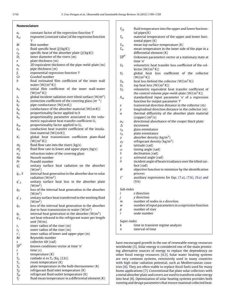

1710 F. Cruz-Peragon et al. / Renewable and Sustainable Energy Reviews 16 (2012) 1709– 1720

Nomenclature

al constant factor of the regression function ‘l’bul exponent (constant value) of the regression function

‘l’Bi Biot numbercf fluid specific heat (J/(kg K))cp specific heat of the absorber plate (J/(kg K))Di inner diameter of the risers (m)e plate thickness (m)eq 2D equivalent thickness of the pipe-weld-plate (m)er pipe thickness (m)fl exponential regression function ‘l’Gr Grashof numberh final estimated film coefficient of the inner wall

water (W/(m2 K))ho initial film coefficient of the inner wall-water

(W/(m2 K))IT global incident radiation over tilted surface (W/m2)ke extinction coefficient of the covering glass (m−1)kf pipe conductance (W/(m K))kp conductance of the absorber material (W/(m K))kh proportionality factor applied to hkq proportionality parameter associated to the volu-

metric equivalent heat transfer coefficient Uc

kuc proportionality factor applied to Uc

kiT conduction heat transfer coefficient of the insula-tion material (W/(m K))

Kc global heat transmission coefficient plate-fluid(W/(m2 K))

mf fluid flow rate into the risers (kg/s)m′

ffluid flow rate in lower and upper pipes (kg/s)

n2 refraction index of the covering glassNu Nusselt numberPr Prandtl numberq′′

1 unitary surface heat radiation on the absorber(W/m2)

q1, S internal heat generation in the absorber due to solarradiation (W/m3)

q′′

2 unitary surface heat loss in the absorber plate(W/m2)

q2 loss of the internal heat generation in the absorber(W/m3)

q′′

3 unitary surface heat transferred to the working fluid(W/m2)

q3 loss of the internal heat generation in the absorberdue to heat transmission to water (W/m3)

qv internal heat generation in the absorber (W/m3)q′

u net heat released in the refrigerant water per lengthunit (W/m)

ri inner radius of the riser (m)re outer radius of the riser (m)r′

i inner radius of lower and upper pipe (m)Re Reynolds numbers collector tilt (rad)SP

nknown conditions vector at time ‘n’

t time (s)T temperature (K)Ta cuidado si es To (Eq. (2.b))To room temperature (K)Tb plate temperature in the bulb thermometer (K)Tfi refrigerant fluid inlet temperature (K)Tfo refrigerant fluid outlet temperature (K)Tf fluid mean temperature in a differential element (K)

Tf,p fluid temperature into the upper and lower horizon-tal pipes(K)

Tp material temperature of the upper and lower hori-zontal pipes (K)

Tm mean top surface temperature (K)Tw mean temperature in the inner side of the pipe in a

differential element (K)UP

nUnknown parameters vector at a stationary state attime ‘n’

UL volumetric heat transfer loss coefficient of the col-lector (W/(m3 K))

Ul global heat loss coefficient of the collector(W/(m2 K))

Ub heat loss behind the collector (W/(m2 K))Ut top heat loss (W/(m2 K))UC volumetric equivalent heat transfer coefficient of

the control volume pipe-weld-plate (W/(m3 K))Xul standardized input parameter ‘u’ of a regression

function for output parameter ‘l’x transversal direction distance in the collector (m)y longitudinal direction distance in the collector (m)

thermal diffusivity of the absorber plate material(copper) (m2/s)

˛� directional absorbance of the cooper black plate� incrementεg glass emmitanceεp plate emmitance� absorber density (kg/m3)�f refrigerant density (kg/m3)ϕ latitude (rad)ω timing angle (rad)ı declination (rad)� azimutal angle (rad)� incident angle of beam irradiance over the tilted sur-

face (rad) objective function to minimize by the identification

process auxiliary expressions for Eqs. (7.a), (7.b), (9.a) and

(9.b)

Sub-indexi x directionj y directionm number of nodes in x directionw number of input parameters in a regression functionp number of riserr node number

Super-indexk time in transient regime analysis

n interval of time

have encouraged growth in the use of renewable energy resourcesworldwide [3]. Solar energy is considered one of the main promis-ing alternative sources of energy to replace the dependency onother fossil energy resources [4,5]. Solar water heating systemsare very common systems, extensively used in many countrieswith high solar radiation potential, such as Mediterranean coun-tries [6]. They are often viable to replace fossil fuels used for many

home applications [7]. Conventional flat plate solar collectors witha metal absorber plate and covers are used to transform solar energyinto heat [8]. Optimization of solar heating systems provides bothrunning and design parameters that ensure maximal collected heat.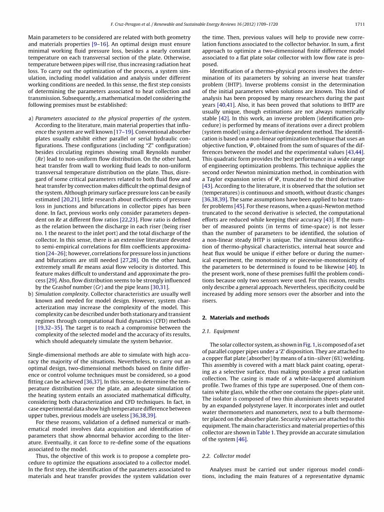

ainab

Mamttluwotf

b

Sroefiptccu

epaa

cIm

F. Cruz-Peragon et al. / Renewable and Sust

ain parameters to be considered are related with both geometrynd materials properties [9–16]. An optimal design must ensureinimal working fluid pressure loss, besides a nearly constant

emperature on each transversal section of the plate. Otherwise,emperature between pipes will rise, thus increasing radiation heatoss. To carry out the optimization of the process, a system sim-lation, including model validation and analysis under differentorking conditions are needed. In this sense, the first step consists

f determining the parameters associated to heat collection andransmission. Subsequently, a mathematical model considering theollowing premises must be established:

a) Parameters associated to the physical properties of the system.According to the literature, main material properties that influ-ence the system are well known [17–19]. Conventional absorberplates usually exhibit either parallel or serial hydraulic con-figurations. These configurations (including “Z” configuration)besides circulating regimes showing small Reynolds number(Re) lead to non-uniform flow distribution. On the other hand,heat transfer from wall to working fluid leads to non-uniformtransversal temperature distribution on the plate. Thus, disre-gard of some critical parameters related to both fluid flow andheat transfer by convection makes difficult the optimal design ofthe system. Although primary surface pressure loss can be easilyestimated [20,21], little research about coefficients of pressureloss in junctions and bifurcations in collector pipes has beendone. In fact, previous works only consider parameters depen-dent on Re at different flow ratios [22,23]. Flow ratio is definedas the relation between the discharge in each riser (being riserno. 1 the nearest to the inlet port) and the total discharge of thecollector. In this sense, there is an extensive literature devotedto semi-empirical correlations for film coefficients approxima-tion [24–26]; however, correlations for pressure loss in junctionsand bifurcations are still needed [27,28]. On the other hand,extremely small Re means axial flow velocity is distorted. Thisfeature makes difficult to understand and approximate the pro-cess [29]. Also, flow distribution seems to be strongly influencedby the Grashof number (Gr) and the pipe leans [30,31].

) Simulation complexity. Collector characteristics are usually wellknown and needed for model design. However, system char-acterization may increase the complexity of the model. Thiscomplexity can be described under both stationary and transientregimes through computational fluid dynamics (CFD) methods[19,32–35]. The target is to reach a compromise between thecomplexity of the selected model and the accuracy of its results,which should adequately simulate the system behavior.

ingle-dimensional methods are able to simulate with high accu-acy the majority of the situations. Nevertheless, to carry out anptimal design, two-dimensional methods based on finite differ-nce or control volume techniques must be considered, so a goodtting can be achieved [36,37]. In this sense, to determine the tem-erature distribution over the plate, an adequate simulation ofhe heating system entails an associated mathematical difficulty,onsidering both characterization and CFD techniques. In fact, inase experimental data show high temperature difference betweenpper tubes, previous models are useless [36,38,39].

For these reasons, validation of a defined numerical or math-matical model involves data acquisition and identification ofarameters that show abnormal behavior according to the liter-ture. Eventually, it can force to re-define some of the equationsssociated to the model.

Thus, the objective of this work is to propose a complete pro-edure to optimize the equations associated to a collector model.n the first step, the identification of the parameters associated to

aterials and heat transfer provides the system validation over

le Energy Reviews 16 (2012) 1709– 1720 1711

the time. Then, previous values will help to provide new corre-lation functions associated to the collector behavior. In sum, a firstapproach to optimize a two-dimensional finite difference modelassociated to a flat plate solar collector with low flow rate is pro-posed.

Identification of a thermo-physical process involves the deter-mination of its parameters by solving an inverse heat transferproblem (IHTP). Inverse problems consist in the determinationof the initial parameters when solutions are known. This kind ofanalysis has been proposed by many researchers during the pastyears [40,41]. Also, it has been proved that solutions to IHTP areusually unique, though estimations are not always numericallystable [42]. In this work, an inverse problem (identification pro-cedure) is performed by means of iterations over a direct problem(system model) using a derivative dependent method. The identifi-cation is based on a non-linear optimization technique that uses anobjective function, , obtained from the sum of squares of the dif-ferences between the model and the experimental values [43,44].This quadratic form provides the best performance in a wide rangeof engineering optimization problems. This technique applies thesecond order Newton minimization method, in combination witha Taylor expansion series of , truncated to the third derivative[43]. According to the literature, it is observed that the solution set(temperatures) is continuous and smooth, without drastic changes[36,38,39]. The same assumptions have been applied to heat trans-fer problems [45]. For these reasons, when a quasi-Newton methodtruncated to the second derivative is selected, the computationalefforts are reduced while keeping their accuracy [43]. If the num-ber of measured points (in terms of time-space) is not lesserthan the number of parameters to be identified, the solution ofa non-linear steady IHTP is unique. The simultaneous identifica-tion of thermo-physical characteristics, internal heat source andheat flux would be unique if either before or during the numer-ical experiment, the monotonicity or piecewise-monotonicity ofthe parameters to be determined is found to be likewise [40]. Inthe present work, none of these premises fulfil the problem condi-tions because only two sensors were used. For this reason, resultsonly describe a general approach. Nevertheless, specificity could beincreased by adding more sensors over the absorber and into therisers.

2. Materials and methods

2.1. Equipment

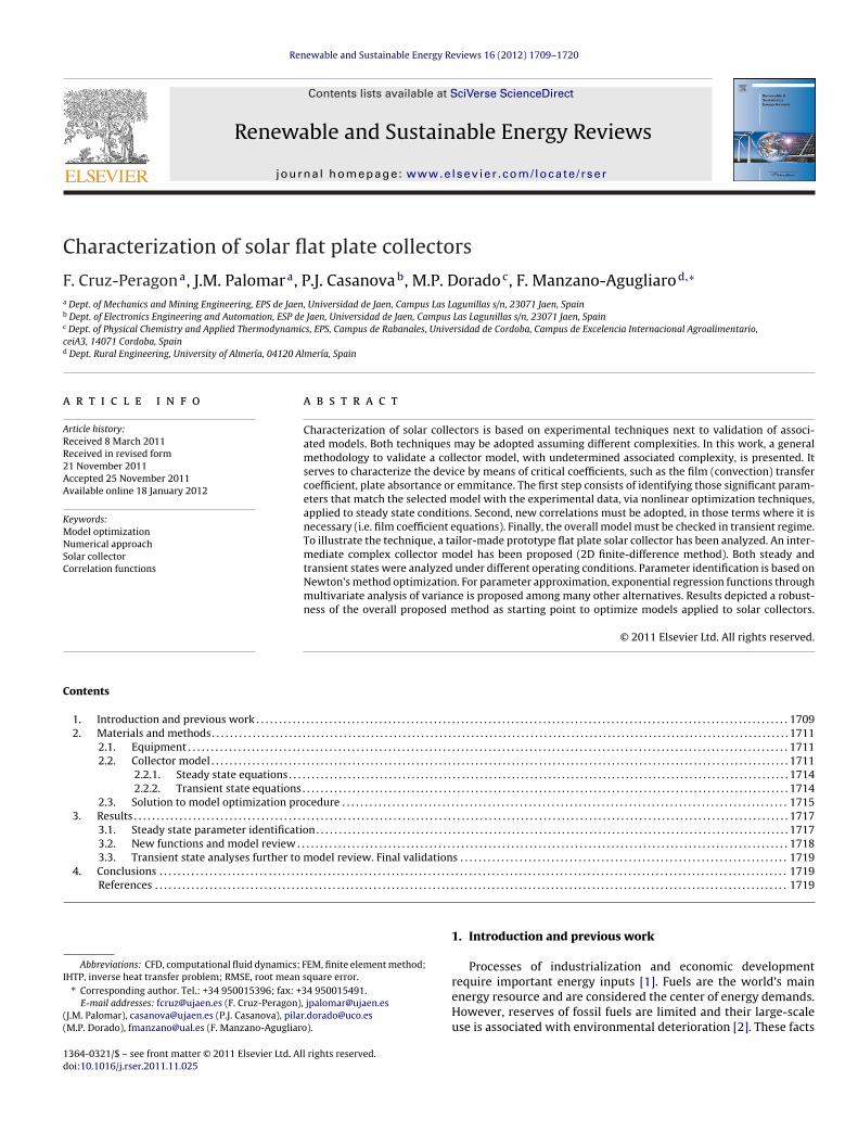
The solar collector system, as shown in Fig. 1, is composed of a setof parallel copper pipes under a ‘Z’ disposition. They are attached toa copper flat plate (absorber) by means of a tin–silver (6%) welding.This assembly is covered with a matt black paint coating, operat-ing as a selective surface, thus making possible a great radiationcollection. The casing is made of a white-lacquered aluminiumprofile. Two frames of this type are superposed. One of them con-tains white glass, while the other one contains the pipes-plate unit.The isolator is composed of two thin aluminium sheets separatedby an expanded polystyrene layer. It incorporates inlet and outletwater thermometers and manometers, next to a bulb thermome-ter placed on the absorber plate. Security valves are attached to thisequipment. The main characteristics and material properties of thiscollector are shown in Table 1. They provide an accurate simulationof the system [46].

2.2. Collector model

Analyses must be carried out under rigorous model condi-tions, including the main features of a representative dynamic

1712 F. Cruz-Peragon et al. / Renewable and Sustainable Energy Reviews 16 (2012) 1709– 1720

Fig. 1. Collector under study.

Table 1Collector properties.

Property Value

Absorber material CopperAbsorber thickness (mm) 2Absorber useful surface (m2) 0.21Inner diameter of the horizontal tubes, R′

T(mm) 20

Inner diameter of the riser, Ri (mm) 10Number of risers 15Riser length (mm) 450Distance between risers (mm) 30Glazing thickness (mm) 4Complete useful surface (m2) 0.37Posterior insulation (mm) 10 (aluminium

sandwich) + 7(polyurethane)

st

(

cally distributed regarding the y-axis, thus dividing the plate in 30

Collector plate efficiency factor, FR 0.7

imulation model and applied only to the plate-risers unit [47]. Inhis particular case, the following conditions were adopted:

(i) A heat transfer analysis by finite difference approach of theabsorber plate and the fluid that flows through the pipes mustbe carried out. Some simplifications consider the plate as a two-dimension system and each pipe as a one-dimension system.The model consists of a set of non linear equations for bothsteady and transient states, which must be solved by iterations[48].

(ii) Conduction coefficients and diffusivities of the plate, pipesand cover, as well as insulating materials must be taken into

consideration. On the other hand, densities, specific heat, vis-cosity, conductivity and Prandtl number of the circulating fluid(water) are approximated by 4th-order polynomial functions,

Fig. 2. Sample network.

depending on the fluid temperature [49]. The necessary dataare collected from the literature [50].

iii) Heat loss coefficients of the plate are considered to be depen-dent on both average and room temperatures, at each intervalof time.

(iv) Temporary variations of irradiation, room and water inlet tem-peratures are considered model inputs. In this sense, both theunitary heat release of the tilted surface (adjusted with thehelp of an isotropic model, with reflectance equal to 0.2) andthe absorptance–transmittance product depend on time [17].Additionally, time variations of water outlet temperature andbulb temperature (over the flat plate) are known but only usedduring the identification process.

(v) According to Streeter et al., flow distribution into each pipemay be calculated by means of the friction loss and conven-tional techniques [20]. However, secondary loss coefficientsapplied to collector junctions and bifurcations are both Re (ofthe main pipe flow) and flow rate dependent [22]. Accordingto Wietbrecht et al., they may be approximated by exponentialfunctions [22].

(vi) Film heat transfer coefficients are initially approached bymeans of semi-empirical equations [24,25,28,50,51]. Althoughthere are many particular correlations, those listed in Incroperaet al. have been selected [50]. Once the optimization process isfinished, the coefficients are empirically evaluated to validatethe model.

To carry out the analysis, the absorber surface was divided intomultiple similar units, using a mesh, so it could be considered a dis-crete problem. A grid sample is shown in Fig. 2. According to this,the complete study could be approximated by means of finite differ-ence technique [52]. Because pipes distribution along the absorberplate is considered to be constant, only a portion of the plate wasexamined. The plate is attached to 15 identical tubes, symmetri-

similar zones. However, only half of the area between tubes is con-sidered, provided the symmetry in the geometric design. For thisreason, only 14 similar zones were considered, as shown in Fig. 2, in

F. Cruz-Peragon et al. / Renewable and Sustainab

1 2 3 4 5 6 7 8 9 10 11 12 13 14 15150.04

0.06

0.08

0.1

0.12

0.14

0.16

0.18F

low

dis

trib

utio

n ra

tio

aipr

urtmhPthttsdt[

g

˛

wktha

oflcsbtgwb

ii

q (t)

Number of riser

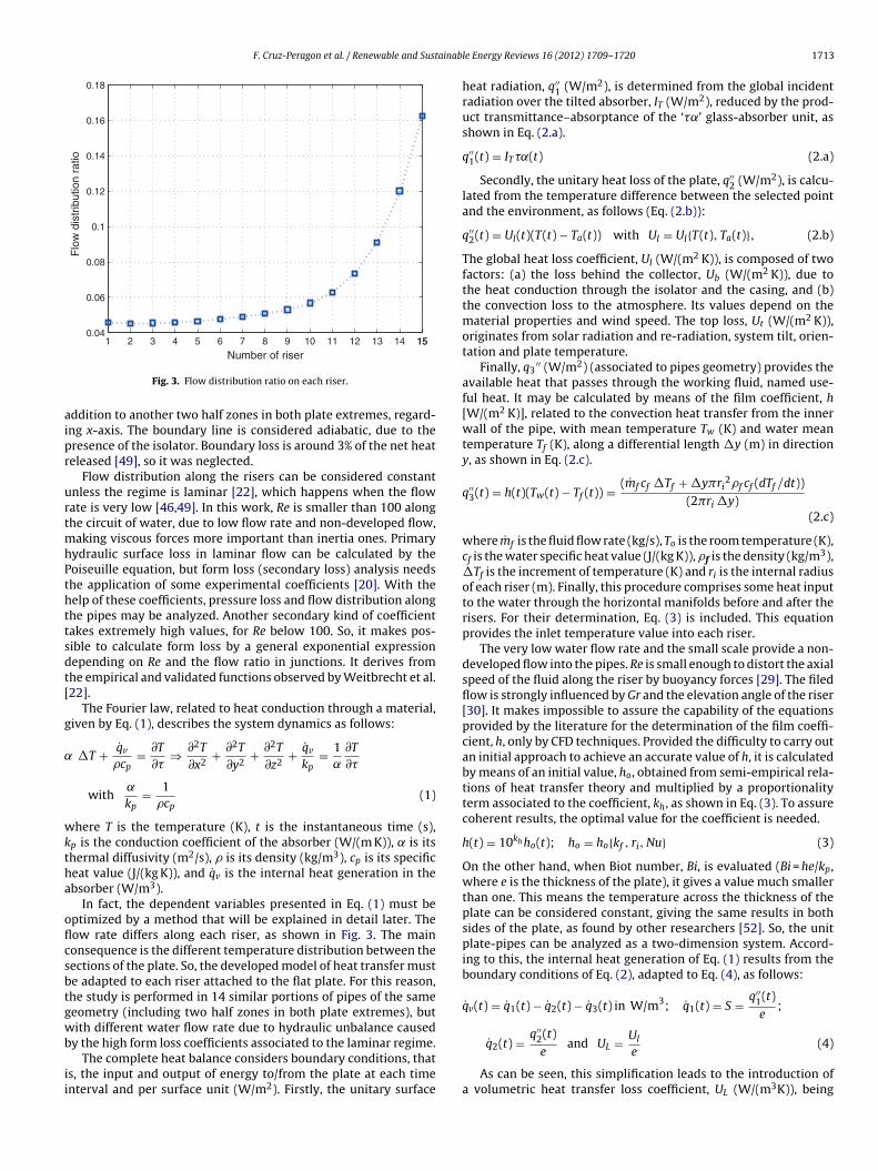
Fig. 3. Flow distribution ratio on each riser.

ddition to another two half zones in both plate extremes, regard-ng x-axis. The boundary line is considered adiabatic, due to theresence of the isolator. Boundary loss is around 3% of the net heateleased [49], so it was neglected.

Flow distribution along the risers can be considered constantnless the regime is laminar [22], which happens when the flowate is very low [46,49]. In this work, Re is smaller than 100 alonghe circuit of water, due to low flow rate and non-developed flow,

aking viscous forces more important than inertia ones. Primaryydraulic surface loss in laminar flow can be calculated by theoiseuille equation, but form loss (secondary loss) analysis needshe application of some experimental coefficients [20]. With theelp of these coefficients, pressure loss and flow distribution alonghe pipes may be analyzed. Another secondary kind of coefficientakes extremely high values, for Re below 100. So, it makes pos-ible to calculate form loss by a general exponential expressionepending on Re and the flow ratio in junctions. It derives fromhe empirical and validated functions observed by Weitbrecht et al.22].

The Fourier law, related to heat conduction through a material,iven by Eq. (1), describes the system dynamics as follows:

�T + qv

�cp= ∂T

∂�⇒ ∂2T

∂x2+ ∂2T

∂y2+ ∂2T

∂z2+ qv

kp= 1

˛

∂T

∂�

with˛

kp= 1

�cp(1)

here T is the temperature (K), t is the instantaneous time (s),p is the conduction coefficient of the absorber (W/(m K)), is itshermal diffusivity (m2/s), � is its density (kg/m3), cp is its specificeat value (J/(kg K)), and qv is the internal heat generation in thebsorber (W/m3).

In fact, the dependent variables presented in Eq. (1) must beptimized by a method that will be explained in detail later. Theow rate differs along each riser, as shown in Fig. 3. The mainonsequence is the different temperature distribution between theections of the plate. So, the developed model of heat transfer muste adapted to each riser attached to the flat plate. For this reason,he study is performed in 14 similar portions of pipes of the sameeometry (including two half zones in both plate extremes), butith different water flow rate due to hydraulic unbalance caused

y the high form loss coefficients associated to the laminar regime.The complete heat balance considers boundary conditions, that

s, the input and output of energy to/from the plate at each timenterval and per surface unit (W/m2). Firstly, the unitary surface

le Energy Reviews 16 (2012) 1709– 1720 1713

heat radiation, q′′1 (W/m2), is determined from the global incident

radiation over the tilted absorber, IT (W/m2), reduced by the prod-uct transmittance–absorptance of the ‘�˛’ glass-absorber unit, asshown in Eq. (2.a).

q′′1(t) = IT �˛(t) (2.a)

Secondly, the unitary heat loss of the plate, q′′2 (W/m2), is calcu-

lated from the temperature difference between the selected pointand the environment, as follows (Eq. (2.b)):

q′′2(t) = Ul(t)(T(t) − Ta(t)) with Ul = Ul{T(t), Ta(t)}, (2.b)

The global heat loss coefficient, Ul (W/(m2 K)), is composed of twofactors: (a) the loss behind the collector, Ub (W/(m2 K)), due tothe heat conduction through the isolator and the casing, and (b)the convection loss to the atmosphere. Its values depend on thematerial properties and wind speed. The top loss, Ut (W/(m2 K)),originates from solar radiation and re-radiation, system tilt, orien-tation and plate temperature.

Finally, q3′′ (W/m2) (associated to pipes geometry) provides the

available heat that passes through the working fluid, named use-ful heat. It may be calculated by means of the film coefficient, h[W/(m2 K)], related to the convection heat transfer from the innerwall of the pipe, with mean temperature Tw (K) and water meantemperature Tf (K), along a differential length �y (m) in directiony, as shown in Eq. (2.c).

q′′3(t) = h(t)(Tw(t) − Tf (t)) = (mf cf �Tf + �y ri

2�f cf (dTf /dt))(2 ri �y)

(2.c)

where mf is the fluid flow rate (kg/s), To is the room temperature (K),cf is the water specific heat value (J/(kg K)), �f is the density (kg/m3),�Tf is the increment of temperature (K) and ri is the internal radiusof each riser (m). Finally, this procedure comprises some heat inputto the water through the horizontal manifolds before and after therisers. For their determination, Eq. (3) is included. This equationprovides the inlet temperature value into each riser.

The very low water flow rate and the small scale provide a non-developed flow into the pipes. Re is small enough to distort the axialspeed of the fluid along the riser by buoyancy forces [29]. The filedflow is strongly influenced by Gr and the elevation angle of the riser[30]. It makes impossible to assure the capability of the equationsprovided by the literature for the determination of the film coeffi-cient, h, only by CFD techniques. Provided the difficulty to carry outan initial approach to achieve an accurate value of h, it is calculatedby means of an initial value, ho, obtained from semi-empirical rela-tions of heat transfer theory and multiplied by a proportionalityterm associated to the coefficient, kh, as shown in Eq. (3). To assurecoherent results, the optimal value for the coefficient is needed.

h(t) = 10kh ho(t); ho = ho{kf , ri, Nu} (3)

On the other hand, when Biot number, Bi, is evaluated (Bi = he/kp,where e is the thickness of the plate), it gives a value much smallerthan one. This means the temperature across the thickness of theplate can be considered constant, giving the same results in bothsides of the plate, as found by other researchers [52]. So, the unitplate-pipes can be analyzed as a two-dimension system. Accord-ing to this, the internal heat generation of Eq. (1) results from theboundary conditions of Eq. (2), adapted to Eq. (4), as follows:

qv(t) = q1(t) − q2(t) − q3(t) in W/m3; q1(t) = S = q′′1(t)e

;

′′

q2(t) = 2

eand UL = Ul

e(4)

As can be seen, this simplification leads to the introduction ofa volumetric heat transfer loss coefficient, UL (W/(m3K)), being

1 ainab

nppitdstadtlflttTttom

q

Ept�

2

�o

= −�

L + U

kp

x �

FnitaE

714 F. Cruz-Peragon et al. / Renewable and Sust

ecessary to analyze in detail the useful heat. As a result of theroposed two-dimension problem, the temperature of the unitlate-pipes across its section is assumed to be constant. Concern-

ng the risers, this assumption is not accurate because an inner wallemperature for each riser, Tw, is established. This temperature isifferent from the mean top surface temperature, Tm; temperatureet varies from the top to the inner wall. The weld that connectshe pipes to the plate is also included in the study. These consider-tions, besides the geometry and materials of each control volume,ifficult the calculation of the global heat transfer coefficient ofhe plate-fluid, KC [W/(m2 K)]. So, the equation of useful heat col-ected by the working fluid must be recalculated. The simplificationrom three to two dimensions obliges to accommodate the prob-em. For this purpose, an equivalent thickness, eq (m), in additiono a volumetric equivalent heat transfer coefficient, Uc [W/(m3K)],hat considers the heat from the top to the inner wall, are evaluated.hese terms must include a proportional coefficient depending onhe pipe geometry, plate weld and position, called kuc. As happenedo kh term, the optimal value that provides an adequate behaviorf the collector depends on time. So the heat released to the fluidatches Eq. (5):

˙ ′3(t) = Kc(t)(Tm(t) − Tf (t)) → q3(t) = q′3(t)eq

;

eq = (e �x + (r2e − r2

i))

�x; e = re − ri; Kc(t) = 10kuc

·(

re

ri· 1

h(t)+ re

kpln

(re

ri

))−1

; q3(t) = Uc(t)(Tm(t) − Tf (t));

UC = Kc(t)eq

= 10kuc�x

(e �x + (r2e − r2

i))

·(

re

ri· 1

h(t)+ re

kpln

(re

ri

))−1

(5)

qs. (4) and (5) help to determine the temperature in particularoints of the plate. The one dimensional useful heat that passeso the water, qu′ (t) (W/m), considering steady state conditions and

y, may be calculated according to Eq. (6) as follows:

q′u(t)

∣∣�y

= mf cf �Tf

�y= 2 rih(t)(Tw − Tf ) (6)

.2.1. Steady state equationsFor each (i,j) point of the mesh, and depending on the increments

x and �y on the absorber fin, the numeric adaptation of the setf Eqs. (1)–(6) for steady state analysis follows the expressions:

general form : Ti−1,j + Ti+1,j + Ti,j−1 + Ti,j+1 − Ti,j

[4 + UL

kp�x �y

]

adiabatic riser boundary form : 2Ti−1,j + Ti,j−1 + Ti,j+1 − Ti,j

[4 + U

adiabatic fin boundary form : 2Ti+1,j + Ti,j−1 + Ti,j+1 − Ti,j

[4 + UL

kp�

or a finite different approach, m corresponds to the number ofodes in ‘x’ direction (i varies from 1 to m). Moreover, the work-

ng fluid receives a certain quantity of heat when passing from y = jo j + 1. It flows into the riser placed at each extreme of the mesh,s shown in Fig. 2. Thus, an additional equation for each one, i.e.q. (6), is needed. A numerical approach is presented in Eq. (7.b),

le Energy Reviews 16 (2012) 1709– 1720

x �y

kp(S + ULTo)

c �x �y

]+ Ti+1,j

Uc

kp�x �y = −�x �y

kp(S + ULTo)

y

]= −�x �y

kp(S + ULTo)

(7.a)

considering both limits (T0,j and Tm+1 correspond to fluid tempera-tures associated to nodes r = 1 and r = m, respectively).

T1,j + T0,j−1 − T0,j(1 + ) = 0; Tm,j + Tm+1,j−1

− Tm−1,j(1 + ′) = 0; = 2 ri �yh

2mf,rcf; (7.b)

The set of (m + 2)n Eqs. (7.a) and (7.b) is used to establish the basicmodel in the plate-pipes unit, considering the unknown tempera-tures on the plate (two-dimension) and the working fluid passingthrough the tube (one-dimension). This is referred to the systemportion described above (Fig. 2).

A non-linear set of equations that must be solved by iterationis presented. For this purpose, plate temperature is considered tobe room temperature. Then, the rest of the parameters such as UL,Uc, h and S will be calculated. A matrix calculus is built-up, result-ing in a new set of plate temperatures. This process continues untiltemperatures converge to constant values. It is very important toadvise that this iterative process belongs to the optimization pro-cess explained below, considering known all the parameters thatdefine UP

n.

To evaluate the set of Eq. (7) for each riser, the inlet water tem-perature must be estimated. For this purpose, a light modificationis adopted and applied to the input horizontal manifold. In thispipe, the temperature is evaluated for only one dimension (x-axis),between the junctions that connect two consecutive risers. Pro-vided that the global input flow temperature and flow distributionthroughout the unit are known, the equations set can be success-fully solved. It gives information about the heat delivered to thewater in the lower pipe (with inner radius r′

i), from the riser p tothe riser p + 1, separated �l. It results in the following expression:

Tp−1 + Tp+1 − Tp

[2 + UL + Uc

kp�x′ �y′

]+ Tf,p

Uc

kp�x′ �y′

= −�x′ �y′

kp(S + ULTo) (8.a)

Tf,p ′ + Tf,p−1 − Tf,p+1(1 + ′) = 0; ′ = 2 r′i�lh

2m′fcf

; (8.b)

where �x′ = �l, �y′ = 2r′i. The fluid that flows through the lower

pipe is non-uniform and continuously reduced, as shown in Fig.3. Once the evaluation of Eq. (7) is finished, the upper pipe isanalyzed. This will provide the outlet global temperature of thefluid.

The proposed numerical analysis has been compared to otheranalytical methods from the literature, providing similar results forthe film coefficient h and same qualitative tendencies for pressureloss [53].

2.2.2. Transient state equationsWhen Eqs. (7.a), (7.b), (8.a) and (8.b) are used under transient

state condition, the inclusion of settings that consider the deriva-tive of temperature vs. time is required. To evaluate it, an implicit

ainab

mnltaaa(

T

T

2

a

b

- IT: global irradiance over the tilted collector (W/m ).- Ta: room temperature (K)- Tfi: fluid inlet temperature (K)

F. Cruz-Peragon et al. / Renewable and Sust

ethod has been proposed. The method is very stable and doesot require extremely narrow intervals of time. In this case, a simi-

ar equations set depending on known values of characteristics andemperatures of a previous state, k, is introduced [52]. Once temper-tures are known for t = k, they will be calculated for t = k + 1 usingn additional coefficient. The general coefficients from Eqs. (7.a)nd (7.b) are changed according to Eqs. (9.a) and (9.b), respectivelyother terms and equations are adapted accordingly).

k+1i−1,j

+ Tk+1i+1,j

+ Tk+1i,j−1 + Tk+1

i,j+1 − Tk+1i,j

A = −�x �y

kp(S + ULTo) − rTk

i,j;

A =[

4 + UL

kp�x �y + r

]; r = �x �y

�t(9.a)

k+1i,j

+ Tk+1i±1,j−1 − Tk+1

i±1,j(1 + + p)

= −pTki±1,j p = ri

2 �y �f

4mf �t; for i = 1 and i = m (9.b)

.3. Solution to model optimization procedure

The proposed procedure consists in the following steps:

) The system and its model are defined analytically and numer-ically for one and two dimensions [46,54]. Initially, the valuesof certain physical properties of the collector materials (inputparameters of the model) are provided according to the lit-erature. These parameters are integrated into the vector ofcharacteristics UP that may vary for each instant of time n(named UP

n). Initially, the parameters included in this vector

are the following:- ke: extinction coefficient of the covering glass (m−1)- n2: refraction index of the glass

- ˛�: directional absorbance of the copper black plate, consid-

ering an incident angle of irradiation over the tilted surface, �,depending on tilt, latitude, declination, solar time, etc.

- εp: plate emissivity

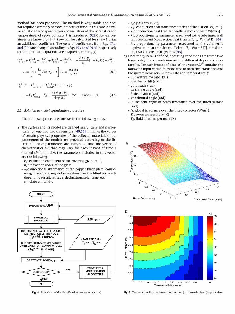
Fig. 4. Flow chart of the identification process (steps a–c).

le Energy Reviews 16 (2012) 1709– 1720 1715

- εg: glass emissivity- kiT: conduction heat transfer coefficient of insulation [W/(mK)]- kp: conduction heat transfer coefficient of copper [W/(mK)]- kh: proportionality parameter associated to the tube inner wall

film coefficient (convection heat transfer), ho [W/(m2 K)] [46].- kq: proportionality parameter associated to the volumetric

equivalent heat transfer coefficient, UC [W/(m3 K)], consider-ing two-dimensional systems [46].

) Once the system is defined, operating conditions are tested twohours a day. These conditions include different days and collec-tor tilts. For each instant of time ‘n’, the vector SP

ncontains the

following input variables associated to both the irradiation andthe system behavior (i.e. flow rate and temperatures):- mf : water flow rate (kg/s)- s: collector tilt (rad)- ϕ: latitude (rad)- ω: timing angle (rad)- ı: declination (rad)- �: azimutal angle (rad)- �: incident angle of beam irradiance over the tilted surface

(rad)2

Fig. 5. Temperature distribution on the absorber: (a) isometric view; (b) plant view.

1716 F. Cruz-Peragon et al. / Renewable and Sustainable Energy Reviews 16 (2012) 1709– 1720

Table 2Characteristic angles of the collector for some random measures.

Stationary test no. Collector tilt s (◦) Latitude ϕ (◦) Solar hour angle ω (◦) Declination ı (◦) Azimutal angle � (◦) Incident angle of directirradiation � (◦)

1 38 38 15 20.73 0 25.562 28 38 22.5 21.27 0 24.473 48 38 15 21.43 0 34.9

Table 3Input–output data values of random measures from Table 2.

Stationary testno.

Solar incidentradiation IT (W/m2)

Room temperatureTo (◦C)

Inlet watertemperature Ti (◦C)

Outlet watertemperature To (◦C)

Bulb platetemperature Tp (◦C)

Fluid flow ratemf (kg/h)

1 936.8 23.2 31 50.5 57 6.422 900.8 19.4 26 39 49.5 7.353 862.1 25.3 33 46 50.5 7.35

Table 4Optimized values for unknown parameters after the identification process shown in Tables 2 and 3.

Test no. ke (mm−1) n2 ˛� εp εg kIt (W/(m K)) kp (W/(m K)) Uc (W/(m3 K)) h (W/(m2 K))

Initial 0.4 1.526 0.801 0.039 0.88 0.029 402.4 11.8 × 103 11Initial value fortest No. 1

Initial value fortest No. 1

0 4

00

Fs

1 0.4022 1.5649 0.7543 0.0391 0.8804

2 0.4016 1.5667 0.7405 0.0391 0.8802

3 0.4019 1.5569 0.7668 0.0391 0.8803

c) To undertake the simulation, the variation of the input data ofthe vector SP

nvs. time is required. On the other hand, vector

UPn, built-up with the previously mentioned unknown terms

(provided by the literature), could lead to a weak approxima-tion to reality. Thus, the target of the application at this step isto identify the real values of those unknown terms, simulatingthe real behavior of the collector over the time. This methodis used for steady state analysis. The objective function iscalculated from the sum of squares of differences between themodel response and the empirical system response values, asso-ciated to both the outlet temperature of the working fluid from

the collector Tfo (K) and the plate temperature of a represen-tative point of the plate, Tb (K), placed near to the top of theabsorber (the real value is measured by a bulb thermometer), as

0 0.05 0.1 0.15 0.2 0.25 0.3 0.35 0.4 0.4542

44

46

48

50

y =

0 m

0 0.05 0.1 0.15 0.2 0.25 0.3 0.35 0.4 0.4545

50

55

60

y =

0,2

2 m

0 0.05 0.1 0.15 0.2 0.25 0.3 0.35 0.4 0.4545

50

55

60

65

y =

0,4

35 m

Transversal length (m)

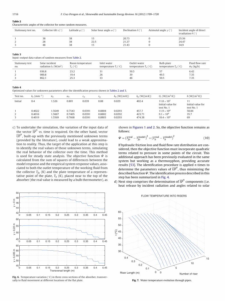
ig. 6. Temperature variation (◦C) in three cross sections of the absorber, transver-ally to fluid movement at different locations of the flat plate.

d

.0293 457.7 11.9 × 10 58.84

.0292 423.71 9.1 × 104 35.7

.0293 474.38 18.4 × 104 69

shown in Figures 1 and 2. So, the objective function remains asfollows:

= (T realfo − Tmodel

fo )2 + (T real

b − Tmodelb )

2(10)

If hydraulic friction loss and fluid flow rate distribution are con-sidered, then the objective function must incorporate quadraticterms related to pressure in some points of the circuit. Thisadditional approach has been previously evaluated in the samesystem but working as a thermosyphon, providing accurateresults [53]. The identification procedure is applied n times todetermine the parameters values of UP

n, thus minimizing the

described function . The identification process described in thisstep has been summarized in Fig. 4.

) Next step comprises the determination of SPn

components (i.e.heat release by incident radiation and angles related to solar

0

5

10

15

00.1

0.20.3

0.4

30

35

40

45

50

55

60

Number of riser

FLOW TEMPERATURE INTO RISERS

Riser Length (m)

t (ºC

)

Fig. 7. Water temperature evolution through pipes.

F. Cruz-Peragon et al. / Renewable and Sustainable Energy Reviews 16 (2012) 1709– 1720 1717

3 4 5 6 7 8 9 10 11 12 132

4

6

8

10

12

14

True Skew

a

b

Pre

dict

ed S

kew

RealPredicted

0.4 0.6 0.8 1 1.2 1.4 1.6 1.8 2 2.20.4

0.6

0.8

1

1.2

1.4

1.6

1.8

2

2.2

2.4

True Skew

Pre

dict

ed S

kew

RealPredicted

F(

e

3

eScm2

29

31

33

35

37

39

41

43

45

47

11,51110,5109,5

Solar time (hour)

a

b

Tem

pera

ture

(ºC

)

RealModel

35

40

45

50

55

9,5 10 10,5 11 11,5

Solar time (hour)

Tem

pera

ture

(ºC

)

Rea lModel

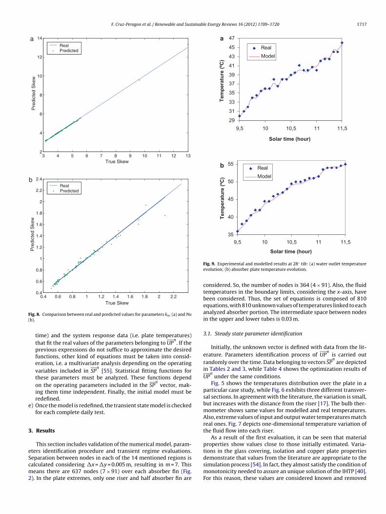
ig. 8. Comparison between real and predicted values for parameters kuc (a) and Nub).

time) and the system response data (i.e. plate temperatures)that fit the real values of the parameters belonging to UP

n. If the

previous expressions do not suffice to approximate the desiredfunctions, other kind of equations must be taken into consid-eration, i.e. a multivariate analysis depending on the operatingvariables included in SP

n[55]. Statistical fitting functions for

these parameters must be analyzed. These functions dependon the operating parameters included in the SP

nvector, mak-

ing them time independent. Finally, the initial model must beredefined.

) Once the model is redefined, the transient state model is checkedfor each complete daily test.

. Results

This section includes validation of the numerical model, param-ters identification procedure and transient regime evaluations.

eparation between nodes in each of the 14 mentioned regions isalculated considering �x = �y = 0.005 m, resulting in m = 7. Thiseans there are 637 nodes (7 × 91) over each absorber fin (Fig.

). In the plate extremes, only one riser and half absorber fin are

Fig. 9. Experimental and modelled results at 28◦ tilt: (a) water outlet temperatureevolution; (b) absorber plate temperature evolution.

considered. So, the number of nodes is 364 (4 × 91). Also, the fluidtemperatures in the boundary limits, considering the x-axis, havebeen considered. Thus, the set of equations is composed of 810equations, with 810 unknown values of temperatures linked to eachanalyzed absorber portion. The intermediate space between nodesin the upper and lower tubes is 0.03 m.

3.1. Steady state parameter identification

Initially, the unknown vector is defined with data from the lit-erature. Parameters identification process of UP

nis carried out

randomly over the time. Data belonging to vectors SPn

are depictedin Tables 2 and 3, while Table 4 shows the optimization results ofUP

nunder the same conditions.

Fig. 5 shows the temperatures distribution over the plate in aparticular case study, while Fig. 6 exhibits three different transver-sal sections. In agreement with the literature, the variation is small,but increases with the distance from the riser [17]. The bulb ther-mometer shows same values for modelled and real temperatures.Also, extreme values of input and output water temperatures matchreal ones. Fig. 7 depicts one-dimensional temperature variation ofthe fluid flow into each riser.

As a result of the first evaluation, it can be seen that materialproperties show values close to those initially estimated. Varia-tions in the glass covering, isolation and copper plate properties

demonstrate that values from the literature are appropriate to thesimulation process [54]. In fact, they almost satisfy the condition ofmonotonicity needed to assure an unique solution of the IHTP [40].For this reason, these values are considered known and removed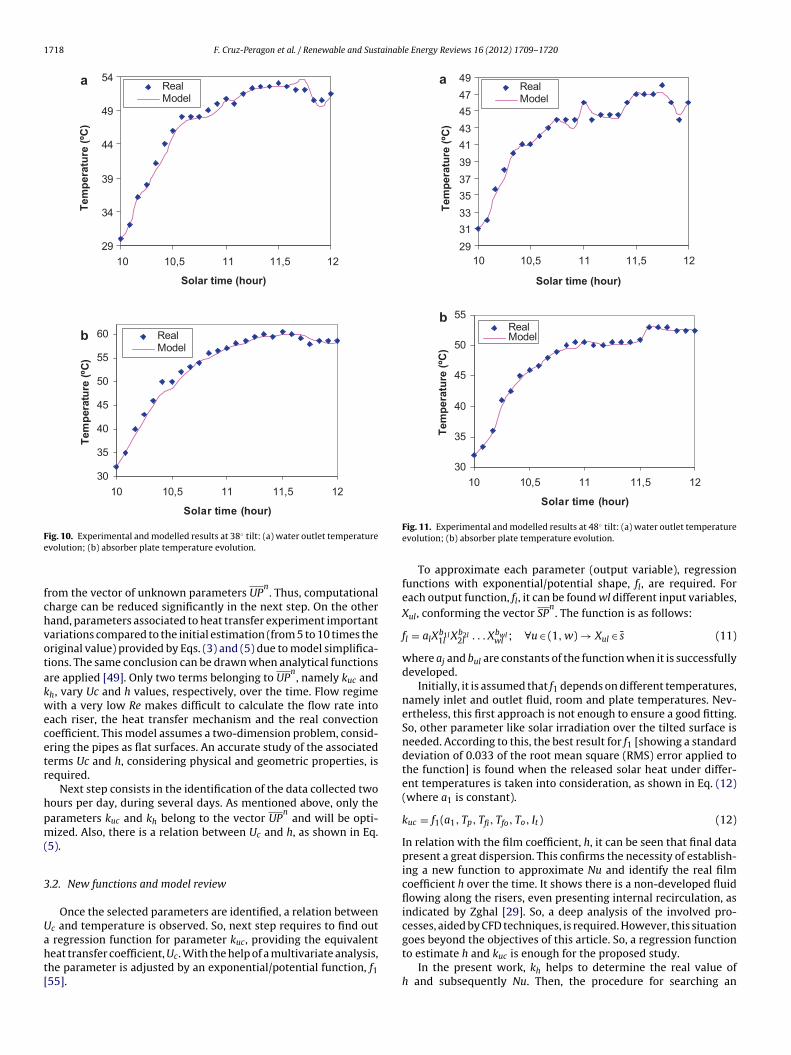

1718 F. Cruz-Peragon et al. / Renewable and Sustainable Energy Reviews 16 (2012) 1709– 1720

29

34

39

44

49

54

1211,51110,510

Solar time (hour)

a

b

Tem

pera

ture

(ºC

)RealMod el

30

35

40

45

50

55

60

10 10,5 11 11,5 12

Solar time (hou r)

Tem

pera

ture

(ºC

)

Rea lModel

Fe

fchvotakwecetr

hpm(

3

Uaht[

2931333537394143454749

1211,51110,510

Solar time (hour)

a

b

Tem

pera

ture

(ºC

)

RealMod el

30

35

40

45

50

55

10 10,5 11 11,5 12

Solar time (hou r)

Tem

pera

ture

(ºC

)

Rea lModel

goes beyond the objectives of this article. So, a regression function

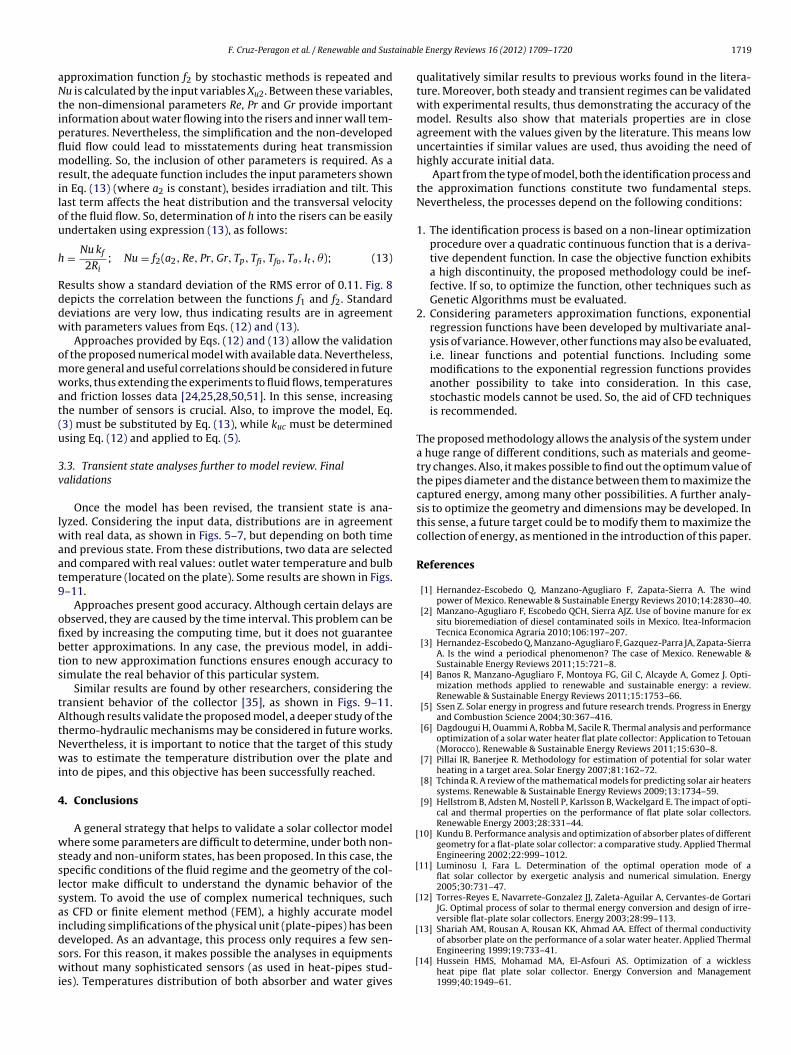
ig. 10. Experimental and modelled results at 38◦ tilt: (a) water outlet temperaturevolution; (b) absorber plate temperature evolution.

rom the vector of unknown parameters UPn. Thus, computational

harge can be reduced significantly in the next step. On the otherand, parameters associated to heat transfer experiment importantariations compared to the initial estimation (from 5 to 10 times theriginal value) provided by Eqs. (3) and (5) due to model simplifica-ions. The same conclusion can be drawn when analytical functionsre applied [49]. Only two terms belonging to UP

n, namely kuc and

h, vary Uc and h values, respectively, over the time. Flow regimeith a very low Re makes difficult to calculate the flow rate into

ach riser, the heat transfer mechanism and the real convectionoefficient. This model assumes a two-dimension problem, consid-ring the pipes as flat surfaces. An accurate study of the associatederms Uc and h, considering physical and geometric properties, isequired.

Next step consists in the identification of the data collected twoours per day, during several days. As mentioned above, only thearameters kuc and kh belong to the vector UP

nand will be opti-

ized. Also, there is a relation between Uc and h, as shown in Eq.5).

.2. New functions and model review

Once the selected parameters are identified, a relation betweenc and temperature is observed. So, next step requires to find out

regression function for parameter kuc, providing the equivalent

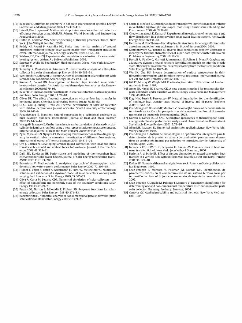
eat transfer coefficient, Uc. With the help of a multivariate analysis,he parameter is adjusted by an exponential/potential function, f155].

Fig. 11. Experimental and modelled results at 48◦ tilt: (a) water outlet temperatureevolution; (b) absorber plate temperature evolution.

To approximate each parameter (output variable), regressionfunctions with exponential/potential shape, fl, are required. Foreach output function, fl, it can be found wl different input variables,Xul, conforming the vector SP

n. The function is as follows:

fl = alXb1l1l Xb2l

2l . . . Xbwlwl ; ∀u ∈ (1, w) → Xul ∈ s (11)

where aj and bul are constants of the function when it is successfullydeveloped.

Initially, it is assumed that f1 depends on different temperatures,namely inlet and outlet fluid, room and plate temperatures. Nev-ertheless, this first approach is not enough to ensure a good fitting.So, other parameter like solar irradiation over the tilted surface isneeded. According to this, the best result for f1 [showing a standarddeviation of 0.033 of the root mean square (RMS) error applied tothe function] is found when the released solar heat under differ-ent temperatures is taken into consideration, as shown in Eq. (12)(where a1 is constant).

kuc = f1(a1, Tp, Tfi, Tfo, To, It) (12)

In relation with the film coefficient, h, it can be seen that final datapresent a great dispersion. This confirms the necessity of establish-ing a new function to approximate Nu and identify the real filmcoefficient h over the time. It shows there is a non-developed fluidflowing along the risers, even presenting internal recirculation, asindicated by Zghal [29]. So, a deep analysis of the involved pro-cesses, aided by CFD techniques, is required. However, this situation

to estimate h and kuc is enough for the proposed study.In the present work, kh helps to determine the real value of

h and subsequently Nu. Then, the procedure for searching an

ainab

aNtipflmrilou

h

Rddw

omwat(u

3v

lwaat9

ofibts

tAtNwi

4

wsslsaidswi

[

[

[

[

F. Cruz-Peragon et al. / Renewable and Sust

pproximation function f2 by stochastic methods is repeated andu is calculated by the input variables Xu2. Between these variables,

he non-dimensional parameters Re, Pr and Gr provide importantnformation about water flowing into the risers and inner wall tem-eratures. Nevertheless, the simplification and the non-developeduid flow could lead to misstatements during heat transmissionodelling. So, the inclusion of other parameters is required. As a

esult, the adequate function includes the input parameters shownn Eq. (13) (where a2 is constant), besides irradiation and tilt. Thisast term affects the heat distribution and the transversal velocityf the fluid flow. So, determination of h into the risers can be easilyndertaken using expression (13), as follows:

= Nu kf

2Ri; Nu = f2(a2, Re, Pr, Gr, Tp, Tfi, Tfo, To, It, �); (13)

esults show a standard deviation of the RMS error of 0.11. Fig. 8epicts the correlation between the functions f1 and f2. Standardeviations are very low, thus indicating results are in agreementith parameters values from Eqs. (12) and (13).

Approaches provided by Eqs. (12) and (13) allow the validationf the proposed numerical model with available data. Nevertheless,ore general and useful correlations should be considered in futureorks, thus extending the experiments to fluid flows, temperatures

nd friction losses data [24,25,28,50,51]. In this sense, increasinghe number of sensors is crucial. Also, to improve the model, Eq.3) must be substituted by Eq. (13), while kuc must be determinedsing Eq. (12) and applied to Eq. (5).

.3. Transient state analyses further to model review. Finalalidations

Once the model has been revised, the transient state is ana-yzed. Considering the input data, distributions are in agreement

ith real data, as shown in Figs. 5–7, but depending on both timend previous state. From these distributions, two data are selectednd compared with real values: outlet water temperature and bulbemperature (located on the plate). Some results are shown in Figs.–11.

Approaches present good accuracy. Although certain delays arebserved, they are caused by the time interval. This problem can bexed by increasing the computing time, but it does not guaranteeetter approximations. In any case, the previous model, in addi-ion to new approximation functions ensures enough accuracy toimulate the real behavior of this particular system.

Similar results are found by other researchers, considering theransient behavior of the collector [35], as shown in Figs. 9–11.lthough results validate the proposed model, a deeper study of the

hermo-hydraulic mechanisms may be considered in future works.evertheless, it is important to notice that the target of this studyas to estimate the temperature distribution over the plate and

nto de pipes, and this objective has been successfully reached.

. Conclusions

A general strategy that helps to validate a solar collector modelhere some parameters are difficult to determine, under both non-

teady and non-uniform states, has been proposed. In this case, thepecific conditions of the fluid regime and the geometry of the col-ector make difficult to understand the dynamic behavior of theystem. To avoid the use of complex numerical techniques, suchs CFD or finite element method (FEM), a highly accurate modelncluding simplifications of the physical unit (plate-pipes) has been

eveloped. As an advantage, this process only requires a few sen-ors. For this reason, it makes possible the analyses in equipmentsithout many sophisticated sensors (as used in heat-pipes stud-

es). Temperatures distribution of both absorber and water gives

[

le Energy Reviews 16 (2012) 1709– 1720 1719

qualitatively similar results to previous works found in the litera-ture. Moreover, both steady and transient regimes can be validatedwith experimental results, thus demonstrating the accuracy of themodel. Results also show that materials properties are in closeagreement with the values given by the literature. This means lowuncertainties if similar values are used, thus avoiding the need ofhighly accurate initial data.

Apart from the type of model, both the identification process andthe approximation functions constitute two fundamental steps.Nevertheless, the processes depend on the following conditions:

1. The identification process is based on a non-linear optimizationprocedure over a quadratic continuous function that is a deriva-tive dependent function. In case the objective function exhibitsa high discontinuity, the proposed methodology could be inef-fective. If so, to optimize the function, other techniques such asGenetic Algorithms must be evaluated.

2. Considering parameters approximation functions, exponentialregression functions have been developed by multivariate anal-ysis of variance. However, other functions may also be evaluated,i.e. linear functions and potential functions. Including somemodifications to the exponential regression functions providesanother possibility to take into consideration. In this case,stochastic models cannot be used. So, the aid of CFD techniquesis recommended.

The proposed methodology allows the analysis of the system undera huge range of different conditions, such as materials and geome-try changes. Also, it makes possible to find out the optimum value ofthe pipes diameter and the distance between them to maximize thecaptured energy, among many other possibilities. A further analy-sis to optimize the geometry and dimensions may be developed. Inthis sense, a future target could be to modify them to maximize thecollection of energy, as mentioned in the introduction of this paper.

References

[1] Hernandez-Escobedo Q, Manzano-Agugliaro F, Zapata-Sierra A. The windpower of Mexico. Renewable & Sustainable Energy Reviews 2010;14:2830–40.

[2] Manzano-Agugliaro F, Escobedo QCH, Sierra AJZ. Use of bovine manure for exsitu bioremediation of diesel contaminated soils in Mexico. Itea-InformacionTecnica Economica Agraria 2010;106:197–207.

[3] Hernandez-Escobedo Q, Manzano-Agugliaro F, Gazquez-Parra JA, Zapata-SierraA. Is the wind a periodical phenomenon? The case of Mexico. Renewable &Sustainable Energy Reviews 2011;15:721–8.

[4] Banos R, Manzano-Agugliaro F, Montoya FG, Gil C, Alcayde A, Gomez J. Opti-mization methods applied to renewable and sustainable energy: a review.Renewable & Sustainable Energy Reviews 2011;15:1753–66.

[5] Ssen Z. Solar energy in progress and future research trends. Progress in Energyand Combustion Science 2004;30:367–416.

[6] Dagdougui H, Ouammi A, Robba M, Sacile R. Thermal analysis and performanceoptimization of a solar water heater flat plate collector: Application to Tetouan(Morocco). Renewable & Sustainable Energy Reviews 2011;15:630–8.

[7] Pillai IR, Banerjee R. Methodology for estimation of potential for solar waterheating in a target area. Solar Energy 2007;81:162–72.

[8] Tchinda R. A review of the mathematical models for predicting solar air heaterssystems. Renewable & Sustainable Energy Reviews 2009;13:1734–59.

[9] Hellstrom B, Adsten M, Nostell P, Karlsson B, Wackelgard E. The impact of opti-cal and thermal properties on the performance of flat plate solar collectors.Renewable Energy 2003;28:331–44.

10] Kundu B. Performance analysis and optimization of absorber plates of differentgeometry for a flat-plate solar collector: a comparative study. Applied ThermalEngineering 2002;22:999–1012.

11] Luminosu I, Fara L. Determination of the optimal operation mode of aflat solar collector by exergetic analysis and numerical simulation. Energy2005;30:731–47.

12] Torres-Reyes E, Navarrete-Gonzalez JJ, Zaleta-Aguilar A, Cervantes-de GortariJG. Optimal process of solar to thermal energy conversion and design of irre-versible flat-plate solar collectors. Energy 2003;28:99–113.

13] Shariah AM, Rousan A, Rousan KK, Ahmad AA. Effect of thermal conductivity

of absorber plate on the performance of a solar water heater. Applied ThermalEngineering 1999;19:733–41.

14] Hussein HMS, Mohamad MA, El-Asfouri AS. Optimization of a wicklessheat pipe flat plate solar collector. Energy Conversion and Management1999;40:1949–61.

1 ainab

[

[

[

[

[

[

[

[

[

[

[

[

[

[

[

[

[

[

[

[

[

[

[

[

[

[

[

[

[

[

[

[

[

[

[

[

[

[

[

[54] Cruz-Peragón F, Dorado M, Palomar J, Montoro V. Parameter identification for

720 F. Cruz-Peragon et al. / Renewable and Sust

15] Badescu V. Optimum fin geometry in flat plate solar collector systems. EnergyConversion and Management 2006;47:2397–413.

16] Lates R, Visa I, Lapusan C. Mathematical optimization of solar thermal collectorsefficiency function using MATLAB. Athens: World Scientific and EngineeringAcad and Soc; 2008.

17] Duffie JA, Beckman WA. Solar engineering of thermal processes. 3rd ed. NewYork: John Wiley & Sons Inc.; 2006.

18] Reddy KS, Avanti P, Kaushika ND. Finite time thermal analysis of groundintegrated-collector-storage solar water heater with transparent insulationcover. International Journal of Energy Research 1999;23:925–40.

19] Saldana JGB, Diez PQ. Experimental–computational evaluation of a solar waterheating system. Leiden: A a Balkema Publishers; 2004.

20] Streeter V, Wylie BE, Bedford KW. Fluid mechanics. 9th ed. New York: McGraw-Hill; 1998.

21] Sumathy K, Venkatesh A, Sriramulu V. Heat-transfer analysis of a flat-platecollector in a solar thermal pump. Energy 1994;19:983–91.

22] Weitbrecht V, Lehmann D, Richter A. Flow distribution in solar collectors withlaminar flow conditions. Solar Energy 2002;73:433–41.

23] Kumar A, Prasad BN. Investigation of twisted tape inserted solar waterheaters—heat transfer, friction factor and thermal performance results. Renew-able Energy 2000;19:379–98.

24] Baker LH. Film heat-transfer coefficients in solar collector tubes at low Reynoldsnumbers. Solar Energy 1967;11:78–84.

25] Oliver DR. The effect of natural convection on viscous-flow heat transfer inhorizontal tubes. Chemical Engineering Science 1962;17:335–50.

26] Li XL, You SJ, Zhang H, You ZP. Thermal performance of solar air collectorwith slit-like perforations. Journal of Central South University of Technology2009;16:145–9.

27] Papanicolaou E. Transient natural convection in a cylindrical enclosure athigh Rayleigh numbers. International Journal of Heat and Mass Transfer2002;45:1425–44.

28] Wang AB, Travncek Z. On the linear heat transfer correlation of a heated circularcylinder in laminar crossflow using a new representative temperature concept.International Journal of Heat and Mass Transfer 2001;44:4635–47.

29] Zghal M, Galanis N, Nguyen CT. Developing mixed convection with aiding buoy-ancy in vertical tubes: a numerical investigation of different flow regimes.International Journal of Thermal Sciences 2001;40:816–24.

30] Orfi J, Galanis N. Developing laminar mixed convection with heat and masstransfer in horizontal and vertical tubes. International Journal of Thermal Sci-ences 2002;41:319–31.

31] Dahl SD, Davidson JH. Performance and modeling of thermosyphon heatexchangers for solar water heaters. Journal of Solar Energy Engineering Trans-ASME 1997;119:193–200.

32] Belessiotis V, Mathioulakis E. Analytical approach of thermosyphon solardomestic hot water system performance. Solar Energy 2002;72:307–15.

33] Hilmer F, Vajen K, Ratka A, Ackermann H, Fuhs W, Melsheimer O. Numericalsolution and validation of a dynamic model of solar collectors working withvarying fluid flow rate. Solar Energy 1999;65:305–21.

34] Oliva A, Costa M, Segarra CDP. Numerical simulation of solar collectors—theeffect of nonuniform and nonsteady state of the boundary-conditions. Solar

Energy 1991;47:359–73.

35] Prapas DE, Norton B, Milonidis E, Probert SD. Response functions for solar-energy collectors. Solar Energy 1988;40:371–83.

36] Kazeminejad H. Numerical analysis of two dimensional parallel flow flat-platesolar collector. Renewable Energy 2002;26:309–23.

[

le Energy Reviews 16 (2012) 1709– 1720

37] Cerne B, Medved S. Determination of transient two-dimensional heat transferin ventilated lightweight low sloped roof using Fourier series. Building andEnvironment 2007;42:2279–88.

38] Chuawittayawuth K, Kumar S. Experimental investigation of temperature andflow distribution in a thermosyphon solar water heating system. RenewableEnergy 2002;26:431–48.

39] Hermann M. FracTherm—fractal hydraulic structures for energy efficient solarabsorbers and other heat exchangers. In: Proc of Eurosun 2004. 2004.

40] Moultanovsky AV, Rekada M. Inverse heat conduction problem approach toidentify the thermal characteristics of super-hard synthetic materials. InverseProblems in Engineering 2002;10:19–39.

41] Baccoli R, Ubaldo C, Mariotti S, Innamorati R, Solinas E, Mura P. Graybox andadaptative dynamic neural network identification models to infer the steadystate efficiency of solar thermal collectors starting from the transient condition.Solar Energy 2010;84:1027–46.

42] Wu SK, Chu HS. Inverse determination of surface temperature in thin-film/substrate systems with interface thermal resistance. International Journalof Heat and Mass Transfer 2004;47:3507–15.

43] Gill PE, Murray W, Wright MH. Practical optimization. 11th edition ed. London:Academic Press; 1997.

44] Amer EH, Nayak JK, Sharma GK. A new dynamic method for testing solar flat-plate collectors under variable weather. Energy Conversion and Management1999;40:803–23.

45] Engl HW, Fusek P, Pereverzev SV. Natural linearization for the identificationof nonlinear heat transfer laws. Journal of Inverse and III-posed Problems2005;13:567–82.

46] Cruz-Peragon F, Dorado MP, Montoro V, Palomar JM, Garcia AI. Pequeno sistematérmico de captación solar para prácticas de laboratorio. In: Proc of III Jornadasnacionales de Ingeniería Termodinámica. 2003.

47] Norton B, Eames PC, Lo SNG. Alternative approaches to thermosyphon solar-energy water heater performance analysis and characterisation. Renewable &Sustainable Energy Reviews 2001;5:79–96.

48] Allen MB, Isaacson EL. Numerical analysis for applied science. New York: JohnWiley and Sons; 1998.

49] Cruz-Peragon F. Análisis de metodologías de optimización inteligentes para ladeterminación de la presión en cámara de combustión para motores alterna-tivos de combustión interna por métodos no intrusivos. Seville: University ofSeville, Spain; 2005.

50] Incropera FP, DeWitt DP, Bergman TL, Lavine AS. Fundamentals of heat andmass transfer. 6th ed. New York: John Wiley & Sons Inc.; 2006.

51] Barletta A, di Schio ER. Effect of viscous dissipation on mixed convection heattransfer in a vertical tube with uniform wall heat flux. Heat and Mass Transfer2001;38:129–40.

52] Ketkar SP. Numerical thermal analysis. New York: American Society of Mechan-ical Engineers; 1999.

53] Cruz-Peragón F, Montoro V, Palomar JM, Dorado MP. Identificación deparámetros críticos en el comportamiento de un sistema térmico solar portermosifón. In: Proc of IV Jornadas nacionales de ingeniería termodinámica.2005.

determining one and two-dimensional temperature distribution in a flat platesolar collector. Germany, Freiburg: Eurosun; 2004.

55] Canavos GC. Applied probability and statistical methods. New York: McGraw-Hill; 1984.