Characterization and Understanding of Bare Soil Respiration Spatial Variability at Plot Scale

www.vadosezonejournal.org · Vol. 8, No. 3, August 2009 762

A the Intergovernmental Panel on Climate

Change (2007), 60% of the greenhouse eff ect is attributed

to CO2. Between 1400 and 1500 Pg of C are stored in the soil

(Schimel, 1995). Since this is about twice the amount of C in the

atmosphere, a small change in soil C storage can cause a signifi -

cant increase in atmospheric CO2 levels (Ryan and Law, 2005).

In terrestrial systems, the key pathway for the transfer of C to the

atmosphere is soil respiration (Trumbore, 2006). Soil respiration

is divided into a heterotrophic contribution originating from the

microbial decomposition of soil C, and an autotrophic contri-

bution generated by the metabolism of plant roots (Tang and

Baldocchi, 2005). Averaged across various ecosystems, 54% of soil

respiration is of heterotrophic nature (Hanson et al., 2000).

Soil respiration measurements with open- or closed-chamber

systems are commonly used to quantify the important contribu-

tions of respiration to C balance at the local scale (Akinremi et

al., 1999; Rayment and Jarvis, 2000; Reth et al., 2005; Tang and

Baldocchi, 2005; Moyano et al., 2007). In addition, chamber-

based CO2 fl ux measurements are frequently used to support

eddy-covariance methods (Drewitt et al., 2002; Reth et al., 2005),

in which the chamber measurements are used to separate het-

erotrophic and autotrophic root respiration and to fi ll in possible

gaps in the eddy-covariance measurements, which occur when all of the

requirements for the eddy-covariance method are not met, for example

during the night (Lavigne et al., 1997; Ohkubo et al., 2007).

Soil respiration is known to be highly variable with time

(Akinremi et al., 1999; Nakadai et al., 2002; Vincent et al., 2006,

Yuste et al., 2007). Th e temporal variability is, in most cases, quite

easy to capture by simply using an appropriate frequency of auto-

mated measurements (Parkin and Kaspar, 2004). Quantifying

the spatial variability is more diffi cult. Little is known about the

autocorrelation length of heterotrophic soil respiration and about

variations within a given fi eld or test plot. Rochette et al. (1991)

measured bare soil respiration along transects with variable spac-

ing and found a signifi cant autocorrelation across 20 m on one

measurement date using a spacing of 1 m. Th erefore, they con-

cluded that a signifi cant part of the variability in heterotrophic

respiration occurs at a scale smaller than 0.15 m, which was the

smallest spacing they used. Aiken et al. (1991) measured soil

respiration in an 18- by 18-m plot, cropped with wheat (Triticum aestivum L.), using a regular 3-m grid; they found no spatial

autocorrelation. For a boreal forest, a high degree of spatial

autocorrelation was detected for locations separated by <1 m

(Rayment and Jarvis, 2000). Pringle and Lark (2006) detected a

range of 174 m using 156 sampling points on a 1024-m transect,

for which incubated bare soil samples were used to measure soil

Characteriza on and Understanding of Bare Soil Respira on Spa al Variability at Plot ScaleM. Herbst,* N. Prolingheuer, A. Graf, J. A. Huisman, L. Weihermüller, and J. Vanderborght

Agrosphere Ins tute, ICG-4, Forschungszentrum Jülich GmbH, D-52425 Jülich, Germany. Received 14 Mar. 2008. *Corresponding author ([email protected]).

Vadose Zone J. 8:762–771doi:10.2136/vzj2008.0068

© Soil Science Society of America677 S. Segoe Rd. Madison, WI 53711 USA.All rights reserved. No part of this periodical may be reproduced or transmi ed in any form or by any means, electronic or mechanical, including photocopying, recording, or any informa on storage and retrieval system, without permission in wri ng from the publisher.

A : MRD, mean relative diff erence.

S S

: A I

Soil respira on is known to be highly variable with me. Less is known, however, about the spa al variability of heterotrophic soil respira on at the plot scale. We simultaneously measured soil heterotrophic respira on, soil tem-perature, and soil water content at 48 loca ons with a nested sampling design and at 76 loca ons with a regular grid plus refi nement within a 13- by 14-m bare soil plot for 15 measurement dates. Soil respira on was measured with a closed chamber covering a surface area of 0.032 m2. A geosta s cal data analyses indicated a mean range of 2.7 m for heterotrophic soil respira on. We detected rather high coeffi cients of varia on of CO2 respira on between 0.13 and 0.80, with an average of 0.33. The number of observa ons required to es mate average respira on fl uxes at a 5% error level ranged between 5 and 123. The analysis of the temporal persistence revealed that a subset of 17 sampling loca ons is suffi cient to es mate average respira on fl uxes at a tolerable root mean square error of 0.15 g C m−2 d−1. Sta s cal analysis revealed that the spa otemporal variability of heterotrophic soil respira on could be explained by the state variables soil temperature and water content. The spa al variability of respira on was mainly driven by vari-ability in soil water content; the variability in the soil water content was almost an order of magnitude higher than the variability in soil temperature.


respiration. For a tropical rainforest, Kosugi et al. (2007) deter-

mined ranges between 4.4 and 24.7 m on a 50- by 50-m plot. In

general, studies show that the spatial correlation of soil respiration

depends on the scale of investigation, similar to what has been

observed for other spatially variable parameters such as soil water

content (e.g., Western and Blöschl, 1999). It is also evident that

a considerable part of the spatial variability of soil respiration

occurs at a small scale, which aggravates the estimation of the

spatial autocorrelation for certain land uses.

In the presence of vegetation, the spatial pattern of soil res-

piration obviously is a mixture of the patterns of heterotrophic

and autotrophic respiration. Autotrophic respiration can increase

the spatial variability of soil respiration if the presence of a root

system adds heterogeneity. For example, agricultural fi elds have

higher soil respiration rates close to the rows of the crops due

to increased root respiration (Rochette et al., 1991). Similarly,

soil respiration in forests is higher close to the stems due to

increasing root density (Tang and Baldocchi, 2005). Variability

in heterotrophic respiration can also be infl uenced by vegetation,

however. Th is may be caused by, for example, higher amounts

of litter input (Fang et al., 1998) or the eff ects of vegetation on

abiotic state variables infl uencing heterotrophic soil respiration.

Both soil water content and temperature are known to depend on

the distance to the crop row (Hupet and Vanclooster, 2005) and

hence are important drivers for heterotrophic soil respiration.

Th e pattern of soil respiration is determined by biotic and

abiotic factors. Biotic factors that have been identifi ed are the

soil C content (Fang et al., 1998; Trumbore, 2006), pH, and

C/N ratio (Reth et al., 2005; Vincent et al., 2006; Kosugi et al.,

2007). Biotic factors are relatively stable with time compared

with the abiotic factors of soil temperature and soil water content.

Soil temperature is known to have a signifi cant infl uence on the

microbial decomposition of soil C (Davidson and Janssens, 2006;

Nakadai et al., 2002; Vincent et al., 2006; Yuste et al., 2007). Soil

water content is often considered to be an important additional

driving factor (Davidson et al., 1998; Zak et al., 1999; Rayment

and Jarvis, 2000; Vincent et al., 2006; Yuste et al., 2007; Kosugi

et al., 2007; Weihermüller et al., 2009). Th e eff ect of soil water

content on soil respiration is twofold. In the lower soil water

content range, soil respiration is reduced because of the low avail-

ability of water and associated nutrients for soil microorganisms.

In the upper soil water content range, CO2 transport may be

limited due to a decrease in the eff ective diff usion coeffi cient with

increasing water content (Millington and Quirk, 1961; Moldrup

et al., 2000). In addition, wet soils are usually prone to O2 defi -

cits, which limit CO2 production (Smith et al., 2003).

A question linked to spatial autocorrelation is the variability

within a certain area. Since the coeffi cient of variation of soil

respiration in space is rather high (Rochette et al., 1991; Dugas,

1993; Kosugi et al., 2007), it is important to know how many

observations are required to obtain an accurate estimate of the

mean respiration fl ux. Because of high coeffi cients of variation,

Dugas (1993, p. 124) stated: “… that a large number of soil

chamber CO2 measurements are required to obtain a representa-

tive measurement of soil CO2 fl ux.” He did not give a distinct

number, however. Rochette et al. (1991) determined that between

25 and 190 samples were required to estimate the average CO2

fl ux in a 1-ha wheat plot within a 10% tolerance level, depend-

ing on atmospheric and soil conditions. Th ese studies assumed

a random selection of sampling sites. It has been shown that

representative mean values for large areas can be estimated more

effi ciently when spatial patterns are persistent in time. Th is

approach was successfully used for soil water content (Vachaud

et al., 1985; Pachepsky et al., 2005; Schneider et al., 2008) and

might also be useful for estimating mean areal soil respiration

fl uxes with a reasonable number of measurements.

Th e aims of this study were twofold. We fi rst aimed to char-

acterize the spatial variability of respiration measurements, its

change with time, the persistence of spatial patterns in respiration,

and the correlation between respiration and other abiotic factors

such as soil moisture and soil temperature. In a second step, we

used this information to determine a measurement scheme that would

estimate the mean areal respiration fl ux with a predefi ned accuracy.

Materials and Methods

Test Plot and SamplingTh e bare soil test plot (50°52'9'' N, 6°27'0'' E) was located in

the middle of a gently sloping agricultural fi eld (FLOWatch test

site) located 6 km southeast of the Research Centre Jülich, close

to Selhausen, Germany. Th e soil type is a Haplic Luvisol devel-

oped in silt loam according to the USDA textural classifi cation

(Weihermüller et al., 2007). A 33-cm plow horizon containing

17.8% clay, 67.1% silt, and 15.1% sand in the fi ne-textured soil

and with an organic C content of 0.0113 g g−1 and a stone frac-

tion of about 12% was found above a 15-cm-thick horizon with

slightly higher clay contents (22.0%), lower organic C contents

(0.0043 g g−1), and almost the same coarse fraction. Below this

horizon, we found stone-free, loamy-textured material containing

very little organic C to a depth of 130 cm. Th e test plot covered

an area of 182 m2 and was power harrowed 2 d before the start

of the sampling campaign.

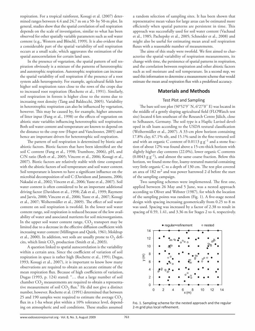
Two sampling schemes were implemented. Th e fi rst one,

applied between 26 May and 5 June, was a nested approach

according to Oliver and Webster (1987), for which the location

of the sampling points was random (Fig. 1). A fi ve-stage nested

design with spacing increasing geometrically from 0.25 to 8 m

was used. Spacing was increased by a factor of 2.38 to result in

spacing of 0.59, 1.41, and 3.36 m for Stages 2 to 4, respectively.

F . 1. Sampling scheme for the nested approach and the regular 2-m grid plus local refi nement.


Four starting points with a separation of 8 m were symmetrically

located in the test plot. Starting at each of these four points, 11

more sampling points were randomly located according to the

fi ve-stage scheme, which resulted in a total of 48 sampling points.

Th is approach has the advantage that good coverage of sample dis-

tances can be obtained with a relatively small number of sampling

points. Th is is advantageous when the range is not known a priori.

Th e second sampling scheme, which was applied starting on 18

June, was a locally refi ned 2-m grid (Fig. 1). In every second grid

box, an additional sampling point was randomly located. Th is

was done to ensure the availability of sampling distances <2 m in

the data set. Th e total number of sampling points for this second

approach was 76, which was signifi cantly higher than for the

nested approach.

Experimental MethodsAn automated non-steady-state closed chamber designed for

survey measurements (LICOR 8100-103, Lincoln, NE) was used

in combination with an infrared gas analyzer (LI8100) to measure

soil respiration, Rs. Polyvinyl chloride collars with a diameter of

20 cm and a height of 7 cm were inserted in such a way that 2 cm

of the collar remained above the soil surface. Th e chamber was

closed for 120 s and the linear increase of CO2 concentration in

the chamber was used to estimate soil respiration.

Soil temperature was measured with a thermocouple (Type T,

TC Direkt, Mönchengladbach, Germany) at a depth of 3 cm. Soil

water content of the upper 5 cm was measured with an ECH2O

probe (Decagon Devices, Pullman, WA) with an input voltage

of 5 V. To estimate the dielectric permittivity ε (dimensionless)

from the output voltage v (V), we used an equation proposed by

Bogena et al. (2007):

( )1

2

0.170460.23554 0.06336v

v

−⎡ ⎤⎛ ⎞⎟⎜⎢ ⎥ε =− + − + ⎟⎜ ⎟⎜⎢ ⎥⎝ ⎠⎣ ⎦ [1]

Th e soil water content θ (cm3 cm−3) was calculated from the

dielectric permittivity according to the empirical equation of

Topp et al. (1980).

Since it took about 2 to 3 h to perform all measurements, we

removed the temporal trends in the soil temperature and soil res-

piration data, which are known to have a strong diurnal variation.

Th is was done by fi tting a linear trend to the data. To prevent

the elimination of spatial trends, the sampling locations were

measured in a random order. Th is detrending removed between

1 and 10% of the original variation in the data.

Soil water contents and soil temperatures were measured

continuously at the 15-cm depth approximately 1 m east from

the middle of the eastern side of the test plot. Time domain

refl ectometry was used to measure soil water contents, while a

PT100 sensor was used to measure soil temperatures.

Geosta s csTh e spatial autocorrelation of each measured variable Z was

quantifi ed using the semivariance γ:

( )( )

( ) ( )( ) 2

1

1

2

n h

i ji

h Z x Z xn h =

⎡ ⎤γ = −⎢ ⎥⎣ ⎦∑ [2]

where the distance between two sampling points xi and xj occurs

within the class of lag distances around h, and n(h) is the number

of observation pairs in that class. A theoretical variogram was

fi tted to the experimental semivariances, since for geostatisti-

cal methods the semivariance for any given distance is required

(Herbst et al., 2006). Several variogram models are available for this

purpose. In this study, we used the spherical variogram model:

( )

3

0 1 1s 1 1

0 1 1

1.5 0.5 for

for

h hc c h a

h a a

c c h a

⎧ ⎡ ⎤⎪ ⎛ ⎞⎪ ⎢ ⎥⎟⎜⎪ ⎟+ − ≤⎜⎪ ⎢ ⎥⎟⎪ ⎜ ⎟⎜γ = ⎝ ⎠⎨ ⎢ ⎥⎪ ⎣ ⎦⎪⎪ + >⎪⎪⎩

[3]

where c0 is the nugget, c1 is the sill, and a1 is the range. For variogram

calculation and fi tting, the VESPER software was used (Minasny

et al., 2005). Following Cambardella et al. (1994), we defi ned the

nugget eff ect Ne as the ratio between the nugget and the total sill:

0e

0 1

cN

c c=+

[4]

Before the geostatistical analysis, the soil respiration values were

logarithmically transformed because the distribution of our respi-

ration data revealed signifi cant skewness. Others also found that

soil respiration is lognormally distributed (Rochette et al., 1991;

Pringle and Lark, 2006; Kosugi et al., 2007).

Required Number of Observa onsTo determine the number of observations required to esti-

mate the mean within a given error tolerance, a generalized

statistical approach based mainly on the standard deviation of the

data set was used. Th is approach was applied to log-transformed

data since a nonskewed distribution of data is required. First the

mean x and the standard deviation sx of the log-transformed

data were calculated. Th e upper confi dence limit, UCL, at the

(1 − α)100% level is given by (Singh et al., 1997)

, 1UCL n xt sx

n

α −= + [5]

where tα,n−1 is the upper αth quantile of Student’s t distribution

with n − 1 degrees of freedom. Replacing the upper confi dence

interval by the criterion x + 0.125 and n by the number of

observations required, mCL, yields

2, 1

CL0.125

n xt sm α −⎛ ⎞⎟⎜= ⎟⎜ ⎟⎟⎜⎝ ⎠

[6]

where tα,n−1 was set to 1.96 for a 95% confi dence limit of infi -

nitely large n. We emphasize that this approach is based on the

assumption of having uncorrelated data. Th is could cause an

underestimation of the confi dence intervals because the variance

of the spatially correlated data tends to underestimate the true

variance (Legendre, 1993; Ferguson and Bester, 2002).

Temporal PersistenceTwo statistical methods were used to infer the temporal per-

sistence in the variables. Th e methods were originally suggested

by Vachaud et al. (1985) for soil water content measurements.

Th e fi rst one uses the two-dimensional, linear, product-moment

coeffi cient of correlation r, computed according to

1

2 2

1 1

ni ii

n ni ii i

a br

a b

=

= =

′ ′=

′ ′

∑∑ ∑

[7]


where ai'= ai − a is the covariance of the measurement date, and

bi'= bi − b is the covariance of the consecutive measurement

dates. Index i loops across all sampling points. In our study, we

used the Pearson correlation coeffi cient between two consecutive

measurement dates to quantify temporal stability.

Th e second measure of temporal stability is the ranked mean

relative diff erence. First, the relative diff erence for each measure-

ment date is calculated according to

,,

i j ji j

j

a a

a

−ξ = [8]

where ξi,j is the relative diff erence from the mean value at sam-

pling point i and time j, ai,j is the variable value at sampling point

i and time j, and ja is the average across the sampling point

values at the same time. Next, the mean relative diff erence, MRD,

for each sampling point i is calculated according to

,1

1MRD

m

i i jjm =

= ξ∑ [9]

where m is the number of measurement dates. Th e standard devi-

ation of the relative diff erences was computed analogous to the

mean. Th e MRD was only applied to data of the nested sampling

approach (m = 10).

Results and DiscussionSpa al Variability

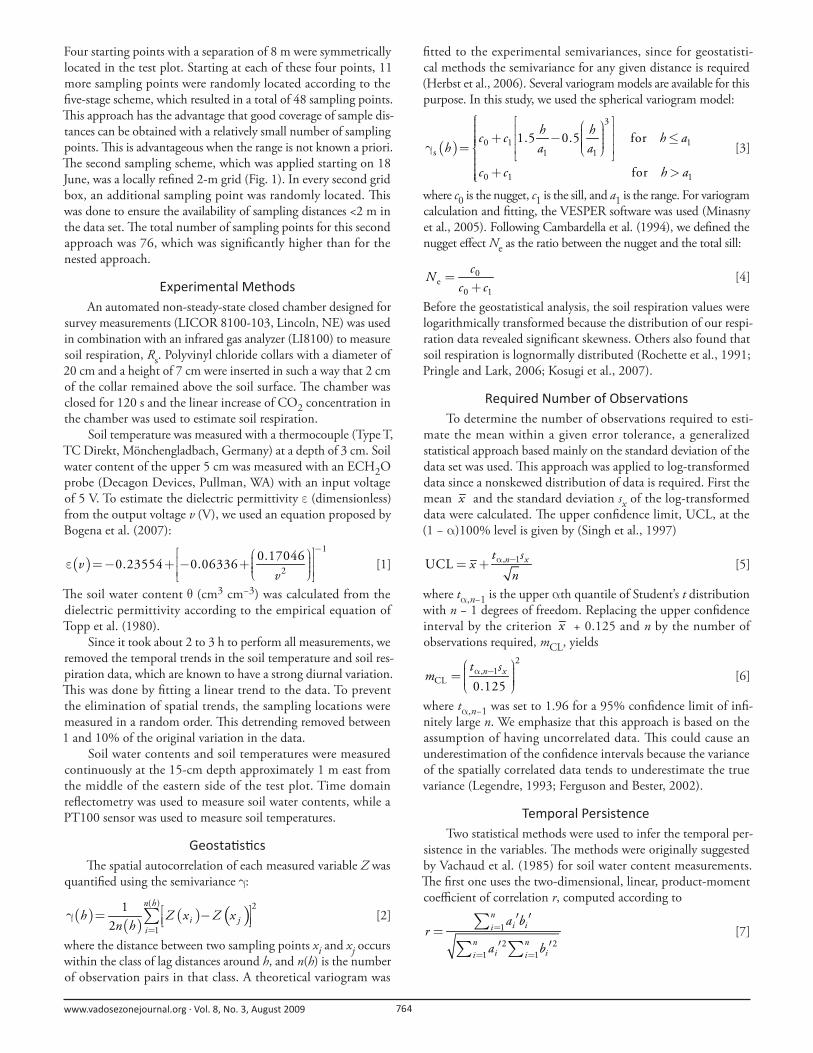
Th e fi rst measurement date was 26 Apr. 2007, after the

test plot was power harrowed. Due to the harrowing and the

warm weather, the measured water contents were low for the

fi rst two measurement dates. Th is changed after the fi rst pre-

cipitation on 9 May, which wetted the soil to the 15-cm depth

(Fig. 2). After this precipitation event (between the second and

third measurement dates), the average soil respiration increased

from 2.3 to 3.1 g C m−2 d−1, the average soil water content in

the top 5 cm increased from 0.05 to 0.14 cm3 cm−3, and the

average soil temperature measured at the 3-cm depth decreased

from 30.1 to 16.7°C. Th ereafter, a broad range of atmospheric

and soil conditions occurred until the last measurements on 25

July. Dry soil conditions were accompanied by relatively high

temperatures (e.g., 3 May) and vice versa (e.g., 28 June). Th e

average soil water content of the upper 5 cm ranged between

0.05 and 0.24 cm3 cm−3 (Table 1). Th e average soil water con-

tent for the entire measurement period was 0.17 cm3 cm−3. Th e

average soil temperature at the 3-cm depth varied between 16.7

and 35.6°C, while the average soil temperature for the entire

period was 24.0°C. Th e average soil respiration varied between

1.33 and 4.17 g C m−2 d−1, which is within a typical range for

bare soil respiration (Dugas, 1993; Nakadai et al., 2002; Reth et

al., 2005). Th e average soil respiration for the entire period was

2.49 g C m−2 d−1, which is also within a typical range for spring

to early summer (Nakadai et al., 2002; Herbst et al., 2008). Th e

spatial variation within the 13- by 14-m plot was high. Th e CV

of the soil respiration ranged from 0.13 to 0.80, with a mean of

0.33. Th e high spatial variation within the plot is in line with the

results of Dugas (1993) and many other researchers.

Figure 3 shows normalized variograms of soil respiration,

soil temperature, and soil water content for the nested sampling

approach (left column) and the regular 2-m grid plus refi nement

(right column). Th e nugget eff ect for soil respiration diff ered

much between sampling dates and was relatively high, ranging

between 0.19 and 0.90 with an average of 0.71. Th e range also

varied among the measurement dates, ranging between 0.44 and

3.6 m. To calculate a mean range for soil respiration, we selected

only measurement dates where the following two criteria applied.

First, the coeffi cient of determination (R2) between

the experimental and fi tted variograms should be

higher than 0.5, which reduces the impact of errone-

ous variogram fi ttings on the mean range estimate.

Second, the nugget eff ect should be lower than 0.75

to ensure a minimum structural component of the

variogram. An average range of 2.7 m was calculated

for data from the three measurement dates that met

both criteria (3, 24, and 30 May, see Fig. 3a). Kosugi

et al. (2007) detected higher ranges, between 4.4

and 24.7 m, for a tropical rain forest. Th is was prob-

ably a result of the slightly larger spatial domain (50

by 50 m) and the additional root respiration, which

might have been more homogeneous in space. Our

range of 2.7 m is in agreement with the fi ndings of

Aiken et al. (1991), who stated that the range for

respiration must be somewhat below 3 m for their

F . 2. Temporal evolu on of point-measured soil water contents (θ15) and soil tem-peratures (T15) as well as spa ally averaged soil water content (θ5), soil temperature (T3), and soil respira on (Rs); bars indicate standard devia ons.

T 1. Number of sampling points n, mean values μ , and CVs for soil respira on Rs, soil water content θ5, and soil temperature T3.

Date in2007

n μRs CVRs μθ5 CVθ5 μT3 CVT3

gC m−2 d−1 cm3 cm−3 °C26 Apr. 48 2.63 0.18 0.06 0.15 23.9 0.063 May 48 2.28 0.24 0.05 0.18 30.1 0.0510 May 48 3.13 0.30 0.14 0.23 16.7 0.0214 May 48 2.54 0.21 0.07 0.42 18.3 0.0115 May 48 2.43 0.23 0.15 0.25 19.2 0.0322 May 48 2.68 0.13 0.11 0.18 27.0 0.0424 May 48 4.17 0.21 0.24 0.17 28.0 0.0325 May 48 2.97 0.22 0.23 0.16 24.3 0.0230 May 48 1.66 0.42 0.23 0.14 22.4 0.025 June 48 2.67 0.32 0.24 0.12 27.2 0.0218 June 77 1.56 0.66 0.22 0.16 22.0 0.0119 June 76 2.61 0.53 0.23 0.17 25.2 0.0228 June 74 1.33 0.80 0.24 0.15 18.4 0.0316 June 76 2.81 0.19 0.12 0.23 35.6 0.0425 June 76 1.92 0.33 0.19 0.20 22.2 0.03


18- by 18-m plot on a silt loam soil that is similar to the soil in

this study.

Th e nugget eff ect values of soil respiration determined from

the regular grid plus refi nement (Fig. 3b) were higher than the

ones determined from the nested approach (Fig. 3a). Th e lowest

nugget eff ect for the regular grid plus refi nement was 0.69 (Table

2), which might be attributed to a lack of measurements with a

short separation despite the local refi nements. Th is lack of short

separation distances made it diffi cult to accurately estimate the

nugget. Th e sill and range could be determined more precisely. For

the nested approach, 61 sampling pairs were available to calculate

the semivariance for the smallest distance class, which had an

average separation of 0.54 m. For the regular grid plus refi nement,

only 47 sampling pairs were available for the smallest separation

class, which had an average separation of 0.92 m. It should be

noted that this lack of short distances for the regular grid occurred

despite a considerably larger number of samples (Table 1). Th is

again confi rms that the nested sampling approach is better suited

for estimating variogram models (Oliver and Webster, 1987). It

should be noted, however, that the nested sampling scheme pro-

vides poor spatial coverage, which is problematic when spatial

predictions using an interpolation method are required. Finally,

it should be mentioned that the diff erent nugget eff ect values of

the two sampling approaches could be a result of the sampling

dates not overlapping for the two sampling designs, with the

resulting potential for changes in the underlying variables for the

two diff erent time periods.

Th e nugget eff ect values for soil temperature and soil water

content were, on average, lower than for soil respiration (Table

2). Th e range of soil temperature was, on average, slightly higher

than for soil respiration (Fig. 3c and 3d). Applying the same two

criteria defi ned above led to an average range of 3.3 m calculated

from nine measurement dates. For these nine measurement dates,

the shortest range was 1.6 m (14 May) and the largest range was

5.4 m (28 June). Th e largest ranges were detected for the soil

water content (Fig. 3e and 3f ). Again applying the two criteria,

we found an average range of 5.8 m calculated from 11 measure-

ment dates. For these measurement dates, the range varied from

4.1 m (22 May) to 9.3 m (15 May). Schume et al. (2003) deter-

mined an average range of 4.8 m for soil water content, which is

quite close to the value determined in this study. With an average

CV of 0.11, Schume et al. (2003) found slightly lower variability

than the average CV of 0.19 we detected,

which can probably be attributed simply

to their diff erent land use (mixed spruce

[Picea abies (L.) Karst]–beech [Fagus syl-vatica L.]) and soil. Guo et al. (2002)

determined ranges between 0.8 and 17.5

m for the soil water content, which also

agrees quite well with the data plotted in

Fig. 3c and 3d.

Required Number of Observa onsAssuming a lognormal distribution

(Eq. [6]), between fi ve and 123 sampling

points are required to estimate the geo-

metric mean with an accuracy of 12.5%

in log-space (Table 3). On average, 31

samples were required. Th e related stan-

dard deviation was 34, indicating that

a conservative estimate for the number

of samples required to cover the whole

measurement period would be at least

65. For an accuracy of 10%, Rochette

et al. (1991) found that between 25 and

190 samples were required for a 100- by

100-m wheat plot. Th e average number

of samples required was 83, which is

higher than the mean value we deter-

mined; however, the number is close to

our conservative estimate. Th e diff erence

may be attributed to diff erent measure-

ment methods and a larger spatial extent,

which probably leads to higher variability

and thus more samples to accurately esti-

mate the mean. It is important to note

that these estimates are only valid for

uncorrelated measurements, thus imply-

ing that the minimum separation should

be at least 2.7 m in this study. Given the

F . 3. Selected normalized semivariograms for (a) nested and (b) regular grid plus refi nement soil respira on (Rs), (c) nested and (d) regular grid plus refi nement soil temperature (T3), and (e) nested and (f) regular grid plus refi nement soil water content (θ5). Results are for three dates in 2007 as indicated. Figure 3a shows the three semivariograms used to calculate the mean range of Rs.


conservative estimate of 65 samples and a fi eld size of 13 by 14

m, it is unlikely that all the measurements are uncorrelated. Th is

indicates the limitations of the classical statistical approach and

suggests that the required number of observations might even be

higher than the conservative estimate.

Temporal PersistenceWe described above how the number of samples required

to estimate average soil respiration can be determined using a

classical statistical approach based on standard deviation. Th is

approach assumes that sampling locations are chosen randomly.

If repeated measurements of a measurement confi guration are

available, it could be possible to further reduce the number of

sampling locations using those locations that show temporal per-

sistence. Temporal persistence was analyzed in two steps. First, the

overall temporal stability of the variables was determined using

correlation coeffi cients. In a second step, the temporal stability of

every single point was investigated using the MRD.

High correlation coeffi cients between consecutive measure-

ment dates indicate temporal stability of spatial patterns (Table

4). On average, the highest temporal stability was detected for

the soil water content, although the correlation coeffi cients are

mostly relatively low compared with other studies (Vachaud et

al., 1985; Schneider et al., 2008). Th ere is a weak tendency for

correlation to be higher for short intervals between consecutive

measurement dates. For example, for 1-d intervals, the correlation

coeffi cients were 0.68, 0.49, and 0.23. Th e latter indicates that

even for short periods, the correlation can be rather low. Th e next

highest temporal stability was shown by soil respiration, although

the correlation coeffi cients were even lower. In contrast to the soil

water content, correlation coeffi cients do not noticeably depend

on the measurement interval for soil respiration. Th e three mea-

surement dates with only 1 d between have weak correlations

between 0.32 and 0.40. Th e highest correlation coeffi cient of 0.81

occurred for a 7-d interval. Th e lowest correlation coeffi cients

were found for soil temperatures. Th e highest correlation coef-

fi cient was 0.35, while even slightly negative correlations were

detected for three measurements. Th is is probably related to the

low variability (Table 1) in relation to the accuracy of the soil

temperature measurements.

A single sampling point can be used to estimate the areal

average when (i) the MRD is close to zero and (ii) the standard

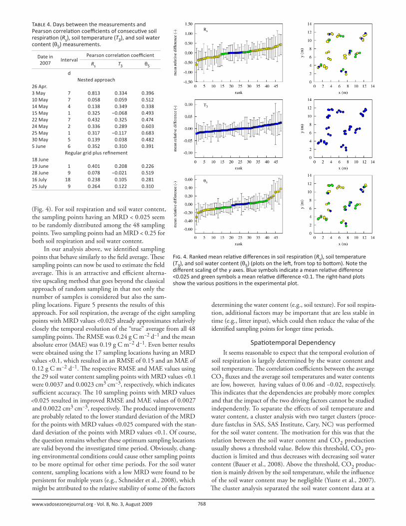
deviation of the relative diff erence is small. Figure 4 shows the

ranked MRD of the 48 sampling points of the nested approach

for soil respiration, soil temperature, and soil water content. For

soil respiration, 17 sampling points had an MRD lower than

0.1, while eight out of those 17 points had an MRD lower than

0.025. Th e high variability of soil respiration compared with the

other two variables is refl ected in the large range of MRD values

and the large standard deviations of the MRD values. For soil

temperature, variability was much lower, with all sampling points

having an MRD < 0.025 (i.e., all sampling points deviated <2.5%

from the average). Soil water content variability was intermediate,

with 29 sampling points having an MRD < 0.1. For 10 sampling

points, the MRD was even lower than 0.025. It is interesting to

analyze the location of those sampling points with a low MRD

T 2. Variogram parameters (Eq. [3]) and coeffi cients of determina on (R2) between the experimental variograms and the fi ed spheri-cal func ons for soil respira on, soil temperature, and soil water content. Values for the range (a1) are given in metres.

Date in 2007Soil respira on Soil temperature Soil water content

c0 c1 a1 R2 c0 c1 a1 R2 c0 c1 a1 R2

–– log10(g C m2 d−1)2 –– m —––— °C —––— m –––– % (v/v) –––– mNested approach

26 Apr. 0.0056 0.0006 1.4 0.05 1.88 0.49 4.2 0.25 0.21 0.78 7.1 0.533 May 0.0074 0.0032 3.1 0.79 2.18 0.83 1.8 0.34 0.72 0.15 9.4 0.0110 May 0.0120 0.0064 0.4 0.04 0.00 0.14 2.3 0.85 4.12 8.75 9.3 0.6114 May 0.0065 0.0007 0.0 0.01 0.02 0.04 1.6 0.76 9.40 0.01 0.0 –15 May 0.0074 0.0033 1.4 0.27 0.17 0.19 1.9 0.18 6.66 10.5 9.3 0.5522 May 0.0032 0.0003 3.1 0.06 0.56 0.54 4.5 0.57 0.71 3.85 4.1 0.8224 May 0.0020 0.0085 2.4 0.97 0.29 0.48 10.9 0.42 4.08 13.3 3.6 0.7425 May 0.0078 0.0011 3.6 0.14 0.08 0.18 5.2 0.62 10.6 1.95 2.7 0.2830 May 0.0220 0.0139 2.6 0.51 0.07 0.08 2.4 0.69 1.70 11.6 4.1 0.67

Regular grid plus refi nement5 June 0.0085 0.0127 2.4 0.71 0.11 0.24 2.1 0.67 6.14 2.38 7.0 0.1518 June 0.0554 0.0 0.0 – 0.09 0.00 – 0.42 0.0 11.2 2.5 0.6619 June 0.0352 0.0059 3.5 0.01 0.06 0.18 3.2 0.64 8.66 6.92 3.2 0.7828 June 0.0653 0.0291 2.8 0.40 0.25 0.16 5.4 0.76 8.17 5.68 4.1 0.6316 July 0.0044 0.0017 3.4 0.33 0.00 1.65 1.6 0.67 3.22 4.67 9.3 0.8525 July 0.0169 0.0041 2.4 0.38 0.10 0.29 3.9 0.87 9.32 7.12 6.9 0.92

T 3. Required number of observa ons (mCL) according to a 95% confi dence limit with the upper αth quan le of Student’s t distribu on with n − 1 degrees of freedom (tα,n−1) = 1.96 for an absolute error tolerance of 0.125 (log space).

Date in 2007 mCL

26 Apr. 93 May 1410 May 2214 May 1115 May 1422 May 524 May 1125 May 1230 May 405 June 2518 June 9019 June 6128 June 12316 July 925 July 26


(Fig. 4). For soil respiration and soil water content,

the sampling points having an MRD < 0.025 seem

to be randomly distributed among the 48 sampling

points. Two sampling points had an MRD < 0.25 for

both soil respiration and soil water content.

In our analysis above, we identifi ed sampling

points that behave similarly to the fi eld average. Th ese

sampling points can now be used to estimate the fi eld

average. Th is is an attractive and effi cient alterna-

tive upscaling method that goes beyond the classical

approach of random sampling in that not only the

number of samples is considered but also the sam-

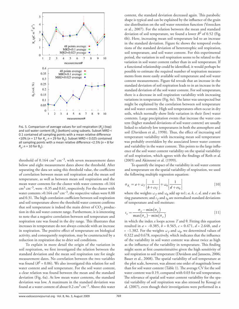
pling locations. Figure 5 presents the results of this

approach. For soil respiration, the average of the eight sampling

points with MRD values <0.025 already approximates relatively

closely the temporal evolution of the “true” average from all 48

sampling points. Th e RMSE was 0.24 g C m−2 d−1 and the mean

absolute error (MAE) was 0.19 g C m−2 d−1. Even better results

were obtained using the 17 sampling locations having an MRD

values <0.1, which resulted in an RMSE of 0.15 and an MAE of

0.12 g C m−2 d−1. Th e respective RMSE and MAE values using

the 29 soil water content sampling points with MRD values <0.1

were 0.0037 and 0.0023 cm3 cm−3, respectively, which indicates

suffi cient accuracy. Th e 10 sampling points with MRD values

<0.025 resulted in improved RMSE and MAE values of 0.0027

and 0.0022 cm3 cm−3, respectively. Th e produced improvements

are probably related to the lower standard deviation of the MRD

for the points with MRD values <0.025 compared with the stan-

dard deviation of the points with MRD values <0.1. Of course,

the question remains whether these optimum sampling locations

are valid beyond the investigated time period. Obviously, chang-

ing environmental conditions could cause other sampling points

to be more optimal for other time periods. For the soil water

content, sampling locations with a low MRD were found to be

persistent for multiple years (e.g., Schneider et al., 2008), which

might be attributed to the relative stability of some of the factors

determining the water content (e.g., soil texture). For soil respira-

tion, additional factors may be important that are less stable in

time (e.g., litter input), which could then reduce the value of the

identifi ed sampling points for longer time periods.

Spa otemporal DependencyIt seems reasonable to expect that the temporal evolution of

soil respiration is largely determined by the water content and

soil temperature. Th e correlation coeffi cients between the average

CO2 fl uxes and the average soil temperatures and water contents

are low, however, having values of 0.06 and −0.02, respectively.

Th is indicates that the dependencies are probably more complex

and that the impact of the two driving factors cannot be studied

independently. To separate the eff ects of soil temperature and

water content, a cluster analysis with two target clusters (proce-

dure fastclus in SAS, SAS Institute, Cary, NC) was performed

for the soil water content. Th e motivation for this was that the

relation between the soil water content and CO2 production

usually shows a threshold value. Below this threshold, CO2 pro-

duction is limited and thus decreases with decreasing soil water

content (Bauer et al., 2008). Above the threshold, CO2 produc-

tion is mainly driven by the soil temperature, while the infl uence

of the soil water content may be negligible (Yuste et al., 2007).

Th e cluster analysis separated the soil water content data at a

T 4. Days between the measurements and Pearson correla on coeffi cients of consecu ve soil respira on (Rs), soil temperature (T3), and soil water content (θ5) measurements.

Date in 2007

IntervalPearson correla on coeffi cient

Rs T3 θ5

dNested approach

26 Apr.3 May 7 0.813 0.334 0.39610 May 7 0.058 0.059 0.51214 May 4 0.138 0.349 0.33815 May 1 0.325 −0.068 0.49322 May 7 0.432 0.325 0.47424 May 2 0.336 0.289 0.60325 May 1 0.317 −0.117 0.68330 May 5 0.139 0.038 0.4825 June 6 0.352 0.310 0.391

Regular grid plus refi nement18 June19 June 1 0.401 0.208 0.22628 June 9 0.078 −0.021 0.51916 July 18 0.238 0.105 0.28125 July 9 0.264 0.122 0.310

F . 4. Ranked mean rela ve diff erences in soil respira on (Rs), soil temperature (T3), and soil water content (θ5) (plots on the le , from top to bo om). Note the diff erent scaling of the y axes. Blue symbols indicate a mean rela ve diff erence <0.025 and green symbols a mean rela ve diff erence <0.1. The right-hand plots show the various posi ons in the experimental plot.


threshold of 0.164 cm3 cm−3, with seven measurement dates

below and eight measurement dates above the threshold. After

separating the data set using this threshold value, the coeffi cient

of correlation between mean soil respiration and the mean soil

temperature, as well as between mean soil respiration and the

mean water contents for the cluster with water contents <0.164

cm3 cm−3, were −0.35 and 0.61, respectively. For the cluster with

water contents >0.164 cm3 cm−3, the respective values were 0.88

and 0.31. Th e high correlation coeffi cient between soil respiration

and soil temperature above the threshold water content confi rms

that soil temperature is indeed the main driver of CO2 produc-

tion in this soil water content range. Furthermore, it is interesting

to note that a negative correlation between soil temperature and

respiration rate was found in the dry range. Th is illustrates that

increases in temperature do not always coincide with an increase

in respiration. Th e positive eff ect of temperature on biological

activity, and consequently respiration, may be counteracted by a

reduction in respiration due to drier soil conditions.

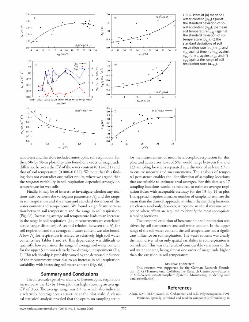
To explain in more detail the origin of the variation in

soil respiration, we fi rst investigated the relation between the

standard deviation and the mean soil respiration rate for single

measurement dates. No correlation between the two variables

was found (R2 = 0.06). We also investigated this relation for soil

water content and soil temperature. For the soil water content,

a clear relation was found between the mean and the standard

deviation (Fig. 6a). At low mean water contents, the standard

deviation was low. A maximum in the standard deviation was

found at a water content of about 0.2 cm3 cm−3. Above this water

content, the standard deviation decreased again. Th is parabolic

shape is typical and can be explained by the infl uence of the grain

size distribution on the soil water retention function (Vereecken

et al., 2007). For the relation between the mean and standard

deviation of soil temperature, we found a lower R2 of 0.52 (Fig.

6b). Here, increasing mean soil temperature led to an increase

in the standard deviation. Figure 6c shows the temporal evolu-

tions of the standard deviation of heterotrophic soil respiration,

soil temperature, and soil water content. For this experimental

period, the variation in soil respiration seems to be related to the

variation in soil water content rather than in soil temperature. If

a functional relationship could be identifi ed, it would perhaps be

possible to estimate the required number of respiration measure-

ments from more easily available soil temperature and soil water

content measurements. Figure 6d reveals that an increase in the

standard deviation of soil respiration leads to in an increase in the

standard deviation of the soil water content. For soil temperature,

there is a decrease in soil respiration variability with increasing

variations in temperature (Fig. 6e). Th e latter was unexpected but

might be explained by the correlation between soil temperature

and soil water content. High soil temperatures often occur in dry

soils, which normally show little variation in their (low) water

contents. Large precipitation events that increase the water con-

tent (higher standard deviations of soil water content) are usually

linked to relatively low temperatures in both the atmosphere and

soil (Davidson et al., 1998). Th us, the eff ect of increasing soil

temperature variability with increasing mean soil temperature

was probably overridden by the associated lower water content

and variability in the water content. Th is points to the large infl u-

ence of the soil water content variability on the spatial variability

of soil respiration, which agrees with the fi ndings of Reth et al.

(2005) and Akinremi et al. (1999).

To quantify the impact of the variability in soil water content

and temperature on the spatial variability of respiration, we used

the following multiple regression equation:

s

1 1R T

T

ab cs d es

θθ

⎡ ⎤ ⎡ ⎤⎢ ⎥ ⎢ ⎥σ = +ω +ω⎢ ⎥ ⎢ ⎥+ +⎣ ⎦ ⎣ ⎦

[10]

where the weights ωT and ωθ add up to1; a, b, c, d, and e are fi t-

ting parameters; and sT and sθ are normalized standard deviations

of temperature and soil moisture:

( )( ) ( )

min

max min

x xx

x x

sσ − σ

=σ − σ

[11]

in which the index x loops across T and θ. Fitting this equation

resulted in a = −0.385, b = 0.565, c = 0.471, d = 2.648, and e = −1.382. For the weights ωT and ωθ, we determined values of

0.322 and 0.678, respectively, which indicates that the infl uence

of the variability in soil water content was about twice as high

as the infl uence of the variability in temperature. Th is fi nding

might seem at fi rst counterintuitive given the high sensitivity of

soil respiration to soil temperature (Davidson and Janssens, 2006;

Bauer et al., 2008). Th e spatial variability of soil temperature at

the plot scale, however, was almost one order of magnitude lower

than for soil water content (Table 1). Th e average CV for the soil

water content was 0.19, compared with 0.03 for soil temperature.

Th e relevance of spatial soil water content variability for the spa-

tial variability of soil respiration was also stressed by Kosugi et

al. (2007), even though their investigations were performed in a

F . 5. Comparison of average values for soil respira on (Rs) (top) and soil water content (θ5) (bo om) using subsets. Subset MRD < 0.1 contained all sampling points with a mean rela ve diff erence <10% (n = 17 for Rs; n = 29 for θ5). Subset MRD < 0.025 contained all sampling points with a mean rela ve diff erence <2.5% (n = 8 for Rs; n = 10 for θ5).


rain forest and therefore included autotrophic soil respiration. For

their 50- by 50-m plot, they also found one order of magnitude

diff erence between the CV of the water content (0.12–0.31) and

that of soil temperature (0.008–0.027). We note that this fi nd-

ing does not contradict our earlier results, where we argued that

the temporal variability in soil respiration depended strongly on

temperature for wet soils.

Finally, it may be of interest to investigate whether any rela-

tions exist between the variogram parameters Ne and the range

in soil respiration and the mean and standard deviation of the

water content and temperature. We found a signifi cant correla-

tion between soil temperature and the range in soil respiration

(Fig. 6f ). Increasing average soil temperature leads to an increase

in the range in soil respiration (i.e., measurements are correlated

across larger distances). A second relation between the Ne for

soil respiration and the average soil water content was also found.

A low Ne for respiration is related to relatively high soil water

contents (see Tables 1 and 2). Th is dependency was diffi cult to

quantify, however, since the range of average soil water content

for the upper 5 cm was relatively low during our experiment (Fig.

2). Th is relationship is probably caused by the decreased infl uence

of the measurement error due to an increase in soil respiration

variability with increasing soil water content (Fig. 6d).

Summary and ConclusionsTh e microscale spatial variability of heterotrophic respiration

measured at the 13- by 14-m plot was high, showing an average

CV of 0.33. Th e average range was 2.7 m, which also indicates

a relatively heterogeneous structure at the plot scale. A classi-

cal statistical analysis revealed that the optimum sampling setup

for the measurement of mean heterotrophic respiration for this

plot, and at an error level of 5%, would range between fi ve and

123 sampling locations separated at a distance of at least 2.7 m

to ensure uncorrelated measurements. Th e analysis of tempo-

ral persistence enables the identifi cation of sampling locations

that are suitable to estimate areal averages. For this data set, 17

sampling locations would be required to estimate average respi-

ration fl uxes with acceptable accuracy for the 13- by 14-m plot.

Th is approach requires a smaller number of samples to estimate the

mean than the classical approach, in which the sampling locations

are chosen randomly; however, it requires an initial measurement

period where eff orts are required to identify the most appropriate

sampling locations.

Th e temporal evolution of heterotrophic soil respiration was

driven by soil temperature and soil water content. In the upper

range of the soil water content, the soil temperature had a signifi -

cant infl uence on soil respiration. Th e water content was clearly

the main driver when only spatial variability in soil respiration is

considered. Th is was the result of considerable variations in the

soil water content, being almost one order of magnitude higher

than the variation in soil temperature.

ATh is research was supported by the German Research Founda-

tion DFG (Transregional Collaborative Research Centre 32—Patterns in Soil–Vegetation–Atmosphere Systems: Monitoring, modelling and data assimilation).

ReferencesAiken, R.M., M.D. Jawson, K. Grahammer, and A.D. Polymenopoulos. 1991.

Positional, spatially correlated and random components of variability in

F . 6. Plots of (a) mean soil water content (μθ5) against the standard devia on of soil water content (σθ5), (b) mean soil temperature (μT3) against the standard devia on of soil temperature (σT3), (c) the standard devia ons of soil respira on rate (σRs), σT3, and σθ5 against me, (d) σθ5 against σRs, (e) σT3 against σRs, and (f) μT3 against the range of soil respira on rates (a1Rs).


carbon dioxide effl ux. J. Environ. Qual. 20:301–308.

Akinremi, O.O., S.M. McGinn, and H.D. McLean. 1999. Eff ects of soil tem-

perature and moisture on soil respiration in barley and fallow plots. Can.

J. Soil Sci. 79:5–13.

Bauer, J., M. Herbst, J.A. Huisman, L. Weihermüller, and H. Vereecken. 2008.

Sensitivity of simulated soil heterotrophic respiration to temperature and

moisture reduction functions. Geoderma 145:17–27.

Bogena, H.R., J.A. Huisman, C. Oberdörster, and H. Vereecken. 2007. Evalu-

ation of a low-cost soil water content sensor for wireless network applica-

tions. J. Hydrol. 344:32–42.

Cambardella, C.A., T.B. Moormann, J.M. Novak, T.B. Parkin, D.L. Karlen, R.F.

Turco, and A.E. Konopka. 1994. Field-scale variability of soil properties in

central Iowa soils. Soil Sci. Soc. Am. J. 58:1501–1511.

Davidson, E.A., E. Belk, and R.D. Boone. 1998. Soil water content and tem-

perature as independent or confounded factors controlling soil respiration

in a temperate mixed hardwood forest. Global Change Biol. 4:217–227.

Davidson, E.A., and I.A. Janssens. 2006. Temperature sensitivity of soil carbon

decomposition and feedbacks to climate change. Nature 440:165–173.

Drewitt, G.B., T.A. Black, Z. Nesic, B.R. Humphreys, E.M. Jork, R. Swanson,

G.J. Ethier, T. Griffi s, and K. Morgenstern. 2002. Measuring forest fl oor

CO2 fl uxes in a Douglas-fi r forest. Agric. For. Meteorol. 110:299–317.

Dugas, W.A. 1993. Micrometeorological and chamber measurements of CO2

fl ux from bare soil. Agric. For. Meteorol. 67:115–128.

Fang, C., J.B. Moncrieff , H.L. Gholz, and L. Clark. 1998. Soil CO2 effl ux and its

spatial variation in a Florida slash pine plantation. Plant Soil 205:135–146.

Ferguson, J.W.H., and M.N. Bester. 2002. Th e treatment of spatial autocorrelation in

biological surveys: Th e case of line transect surveys. Antarct. Sci. 14:115–122.

Guo, D., P. Mou, R.H. Jones, and R.J. Mitchell. 2002. Temporal changes in

spatial patterns of soil moisture following disturbance: An experimental

approach. J. Ecol. 90:338–347.

Hanson, P.J., N.T. Edwards, C.T. Garten, and J.A. Andrews. 2000. Separating

root and soil microbial contributions to soil respiration: A review of meth-

ods and observations. Biogeochemistry 48:115–146.

Herbst, M., B. Diekkrüger, and H. Vereecken. 2006. Geostatistical co-regional-

ization of soil hydraulic properties in a micro-scale catchment using terrain

attributes. Geoderma 132:206–221.

Herbst, M., H.J. Hellebrand, J. Bauer, J.A. Huisman, J. Šimůnek, L. Weiher-

müller, A. Graf, J. Vanderborght, and H. Vereecken. 2008. Multiyear het-

erotrophic soil respiration: Evaluation of a coupled CO2 transport and

carbon turnover model. Ecol. Modell. 214:271–283.

Hupet, F., and M. Vanclooster. 2005. Micro-variability of hydrological processes

at the maize row scale: Implications for soil water content measurements

and evapotranspiration estimates. J. Hydrol. 303:247–270.

Intergovernmental Panel on Climate Change. 2007. Climate change 2007: Th e physi-

cal science basis. Summary for policymakers. IPCC, Geneva, Switzerland.

Kosugi, Y., T. Mitani, M. Itoh, S. Noguchi, M. Tani, N. Matsuo, S. Takanashi, S.

Ohkubo, and A.R. Nik. 2007. Spatial and temporal variation in soil respira-

tion in a Southeast Asian tropical rainforest. Agric. For. Meteorol. 147:35–47.

Lavigne, M.B., M.G. Ryan, D.E. Anderson, D.D. Baldocchi, P.M. Crill, D.R.

Fitzjarrald, M.L. Goulden, S.T. Gower, J.M. Massheder, J.H. McCaughy,

M. Rayment, and R.G. Striegel. 1997. Comparing nocturnal eddy covari-

ance measurements to estimates of ecosystem respiration made by scal-

ing chamber measurements at six coniferous boreal sites. J. Geophys. Res.

102:28977–28985.

Legendre, P. 1993. Spatial autocorrelation: Trouble or new paradigm? Ecology

74:1659–1673.

Millington, R.J., and J.M. Quirk. 1961. Permeability of porous solids. Trans.

Faraday Soc. 57:1200–1207.

Minasny, B., A.B. McBratney, and B.M. Whelan. 2005. VESPER version 1.62.

Available at www.usyd.edu.au/agric/acpa/pag.htm (verifi ed 13 May 2009).

Aust. Ctr. for Precision Agric., Univ.of Sydney, NSW.

Moldrup, P., T. Olesen, P. Schjønning, T. Yamaguchi, and D.E. Rolston. 2000.

Predicting the gas diff usion coeffi cient in undisturbed soil from soil water

characteristics. Soil Sci. Soc. Am. J. 64:94–100.

Moyano, F.E., W.L. Kutsch, and E.-D. Schulze. 2007. Response of mycorrhizal,

rhizosphere and soil basal respiration to temperature and photosysnthesis

in a barley fi eld. Soil Biol. Biochem. 39:843–853.

Nakadai, T., M. Yokozawa, H. Ikeda, and H. Koizumi. 2002. Diurnal changes

of carbon dioxide fl ux from bare soil in agricultural fi eld in Japan. Appl.

Soil Ecol. 19:161–171.

Ohkubo, S., Y. Kosugi, S. Takanashi, T. Mitani, and M. Tani. 2007. Compari-

son of the eddy covariance and automated closed chamber methods for

evaluating nocturnal CO2 exchange in a Japanese cypress forest. Agric. For.

Meteorol. 142:50–65.

Oliver, M.A., and R. Webster. 1987. Th e elucidation of soil pattern in the Wyre

Forest of the West Midlands, England: II. Spatial distribution. J. Soil Sci.

38:293–307.

Pachepsky, Ya.A., K. Guber, and D. Jacques. 2005. Temporal persistence in verti-

cal distributions of soil moisture contents. Soil Sci. Soc. Am. J. 69:347–352.

Parkin, T.B., and T.C. Kaspar. 2004. Temporal variability of soil carbon dioxide

fl ux: Eff ect of sampling frequency on cumulative carbon loss estimation.

Soil Sci. Soc. Am. J. 68:1234–1241.

Pringle, M.J., and R.M. Lark. 2006. Spatial analysis of model error, illustrated by

soil carbon dioxide emissions. Vadose Zone J. 5:168–183.

Rayment, M.B., and P.G. Jarvis. 2000. Temporal and spatial variation of soil

CO2 effl ux in a Canadian boreal forest. Soil Biol. Biochem. 32:35–45.

Reth, S., M. Göckede, and E. Falge. 2005. CO2 fl ux from agricultural soils in

eastern Germany: Comparison of a closed chamber system with eddy co-

variance measurements. Th eor. Appl. Climatol. 80:105–120.

Rochette, P., R.L. Desjardins, and E. Pattey. 1991. Spatial and temporal variabil-

ity of soil respiration in agricultural fi elds. Can. J. Soil Sci. 71:189–196.

Ryan, M.G., and B.E. Law. 2005. Interpreting, measuring, and modelling soil

respiration. Biogeochemistry 73:3–27.

Schimel, D.S. 1995. Terrestrial ecosystems and the carbon cycle. Global Change

Biol. 1:77–91.

Schneider, K., J.A. Huisman, L. Breuer, Y. Zhao, and H.-G. Frede. 2008. Tem-

poral stability of soil moisture in various semi-arid steppe ecosystems and

its application in remote sensing. J. Hydrol. 359:16–29.

Schume, H., G. Jost, and K. Katzensteiner. 2003. Spatio-temporal analysis of

the soil water content in a mixed Norway spruce (Picea abies (L.) Karst.)–

European beech (Fagus sylvatica L.) stand. Geoderma 112:273–287.

Singh, A.K., A. Singh, and M. Engelhardt. 1997. Th e lognormal distributions in en-

vironmental applications. EPA/600/S-97/006. Tech. Support Ctr. for Moni-

toring and Site Characterization, Natl. Exposure Res. Lab., Las Vegas, NV.

Smith, K.A., T. Ball, F. Conen, K.E. Dobbie, J. Massheder, and A. Rey. 2003.

Exchange of greenhouse gases between soil and atmosphere: Interactions of

soil physical factors and biological processes. Eur. J. Soil Sci. 54:779–791.

Tang, J., and D.B. Baldocchi. 2005. Spatial-temporal variation in soil respiration

in an oak–grass savanna ecosystem in California and its partitioning into

autotrophic and heterotrophic components. Biogeochemistry 73:183–207.

Topp, G.C., J.L. Davies, and A.P. Annan. 1980. Electromagnetic determination

of soil water content: Measurements in coaxial transmission lines. Water

Resour. Res. 16:574–582.

Trumbore, S. 2006. Carbon respired by terrestrial ecosystems: Recent progress

and challenges. Global Change Biol. 12:141–153.

Vachaud, G., A. Passerat De Silans, P. Balabanis, and M. Vauclin. 1985. Tem-

poral stability of spatially measured soil water probability density function.

Soil Sci. Soc. Am. J. 49:822–828.

Vereecken, H., T. Kamai, T. Harter, R. Kasteel, J. Hopmans, and J. Vander-

borght. 2007. Explaining soil moisture variability as a function of mean

soil moisture: A stochastic unsaturated fl ow perspective. Geophys. Res.

Lett. 34:L22402, doi:10.1029/2007GL031813.

Vincent, G., A.R. Shahriari, E. Lucot, P.-M. Badot, and D. Epron. 2006. Spatial

and seasonal variations in soil respiration in a temperate deciduous forest

with fl uctuating water table. Soil Biol. Biochem. 38:2527–2535.

Weihermüller, L., J.A. Huisman, A. Graf, M. Herbst, and J.-M. Sequaris. 2009.

Multistep outfl ow experiments to determine soil physical and carbon diox-

ide production parameters. Vadose Zone J. 8:772–782 (this issue).

Weihermüller, L., J.A. Huisman, S. Lambot, M. Herbst, and H. Vereecken. 2007.

Mapping the spatial variation of soil water content at the fi eld scale with

diff erent ground penetrating radar techniques. J. Hydrol. 340:205–216.

Western, A., and G. Blöschl. 1999. On the spatial scaling of soil moisture. J.

Hydrol. 217:203–224.

Yuste, J.C., D.D. Baldocchi, A. Gershenson, A. Goldstein, L. Mission, and S.

Wong. 2007. Microbial soil respiration and its dependency on carbon in-

puts, soil temperature and moisture. Global Change Biol. 13:2018–2035.

Zak, D.R., W.E. Holmes, N.W. MacDonald, and K.S. Pregitzer. 1999. Soil tem-

perature, matric potential, and the kinetics of microbial respiration and

nitrogen mineralization. Soil Sci. Soc. Am. J. 63:575–584.

Documents

Characterization and Understanding of Bare Soil Respiration Spatial Variability at Plot Scale