Embed Size (px)
Citation preview
Modified from:
Database System Concepts, 6th Ed.
©Silberschatz, Korth and Sudarshan
See www.db-book.com for conditions on re-use
Chapter 11: Indexing and Storage
©Silberschatz, Korth and Sudarshan11.2CS425 – Fall 2013 – Boris Glavic
Chapter 11: Indexing and Storage
n DBMS Storage
l Memory hierarchy
l File Organization
l Buffering
n Indexing
l Basic Concepts
l B+-Trees
l Static Hashing
l Index Definition in SQL
l Multiple-Key Access

Modified from:
Database System Concepts, 6th Ed.
©Silberschatz, Korth and Sudarshan
See www.db-book.com for conditions on re-use
Memory Hierarchy
©Silberschatz, Korth and Sudarshan11.4CS425 – Fall 2013 – Boris Glavic
DBMS Storage
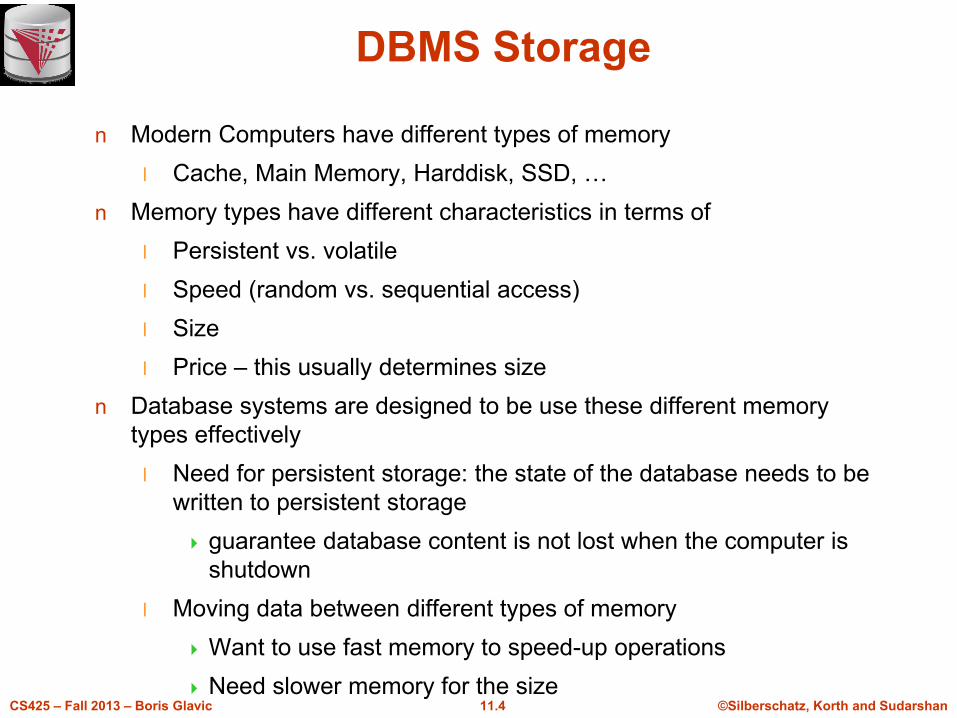
n Modern Computers have different types of memory
l Cache, Main Memory, Harddisk, SSD, …
n Memory types have different characteristics in terms of
l Persistent vs. volatile
l Speed (random vs. sequential access)
l Size
l Price – this usually determines size
n Database systems are designed to be use these different memory
types effectively
l Need for persistent storage: the state of the database needs to be
written to persistent storage
guarantee database content is not lost when the computer is
shutdown
l Moving data between different types of memory
Want to use fast memory to speed-up operations
Need slower memory for the size
©Silberschatz, Korth and Sudarshan11.5CS425 – Fall 2013 – Boris Glavic
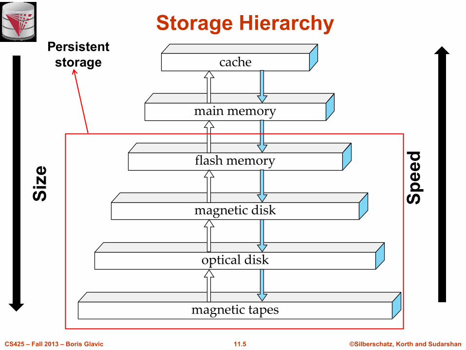
Storage Hierarchy
cache
main memory
flash memory
magnetic disk
optical disk
magnetic tapes
Siz
e
Sp
ee
d
Persistent
storage
©Silberschatz, Korth and Sudarshan11.6CS425 – Fall 2013 – Boris Glavic
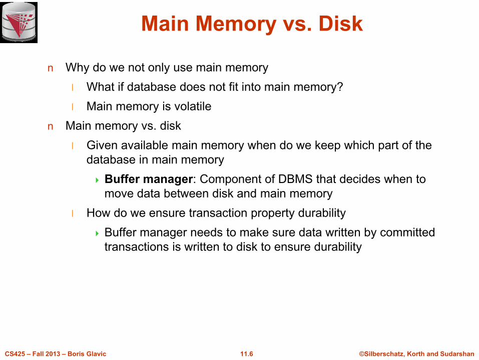
Main Memory vs. Disk
n Why do we not only use main memory
l What if database does not fit into main memory?
l Main memory is volatile
n Main memory vs. disk
l Given available main memory when do we keep which part of the
database in main memory
Buffer manager: Component of DBMS that decides when to
move data between disk and main memory
l How do we ensure transaction property durability
Buffer manager needs to make sure data written by committed
transactions is written to disk to ensure durability

©Silberschatz, Korth and Sudarshan11.7CS425 – Fall 2013 – Boris Glavic
Random vs. Sequential Access
n Transfer of data from disk has a minimal size = 1 block
l Reading 1 byte is as fast as reading one block (e.g., 4KB)
n Random Access
l Read data from anywhere on the disk
l Need to get to the right track (seek time)
l Need to wait until the right sector is under the arm (on avg ½ time
for one rotation) (rotational delay)
l Then can transfer data at ~ transfer rate
n Sequential Access
l Read data that is on the current track + sector
l can transfer data at ~ transfer rate
n Reading large number of small pieces of data randomly is very slow
compared to sequential access
l Thus, try layout data on disk in a way that enables sequential
access
Modified from:
Database System Concepts, 6th Ed.
©Silberschatz, Korth and Sudarshan
See www.db-book.com for conditions on re-use
File Organization
©Silberschatz, Korth and Sudarshan11.9CS425 – Fall 2013 – Boris Glavic
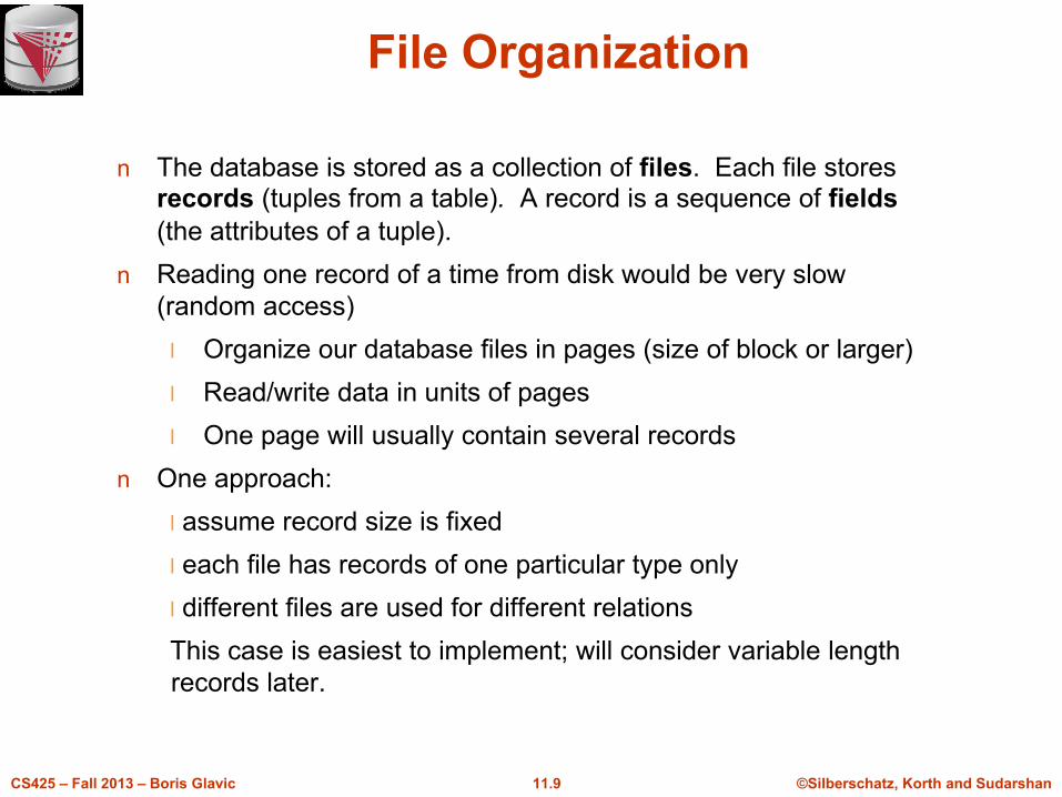
File Organization
n The database is stored as a collection of files. Each file stores records (tuples from a table). A record is a sequence of fields
(the attributes of a tuple).
n Reading one record of a time from disk would be very slow
(random access)
l Organize our database files in pages (size of block or larger)
l Read/write data in units of pages
l One page will usually contain several records
n One approach:
l assume record size is fixed
l each file has records of one particular type only
l different files are used for different relations
This case is easiest to implement; will consider variable length
records later.
©Silberschatz, Korth and Sudarshan11.10CS425 – Fall 2013 – Boris Glavic
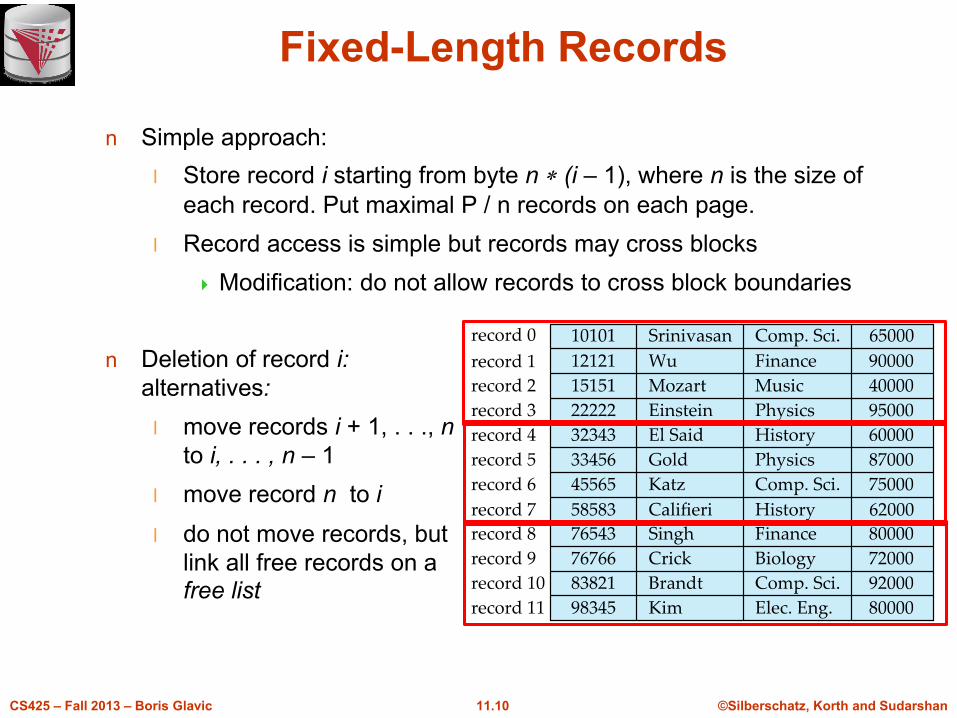
Fixed-Length Records
n Simple approach:
l Store record i starting from byte n (i – 1), where n is the size of
each record. Put maximal P / n records on each page.
l Record access is simple but records may cross blocks
Modification: do not allow records to cross block boundaries
n Deletion of record i:
alternatives:
l move records i + 1, . . ., n
to i, . . . , n – 1
l move record n to i
l do not move records, but
link all free records on afree list
©Silberschatz, Korth and Sudarshan11.11CS425 – Fall 2013 – Boris Glavic
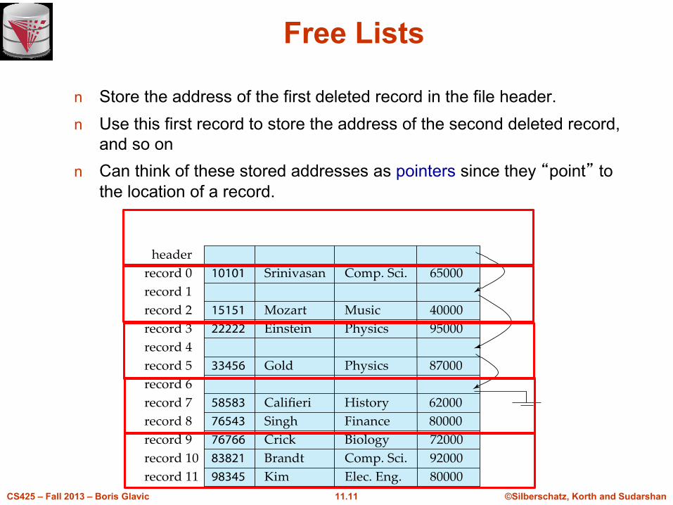
Free Lists
n Store the address of the first deleted record in the file header.
n Use this first record to store the address of the second deleted record,
and so on
n Can think of these stored addresses as pointers since they “point” to
the location of a record.
©Silberschatz, Korth and Sudarshan11.12CS425 – Fall 2013 – Boris Glavic
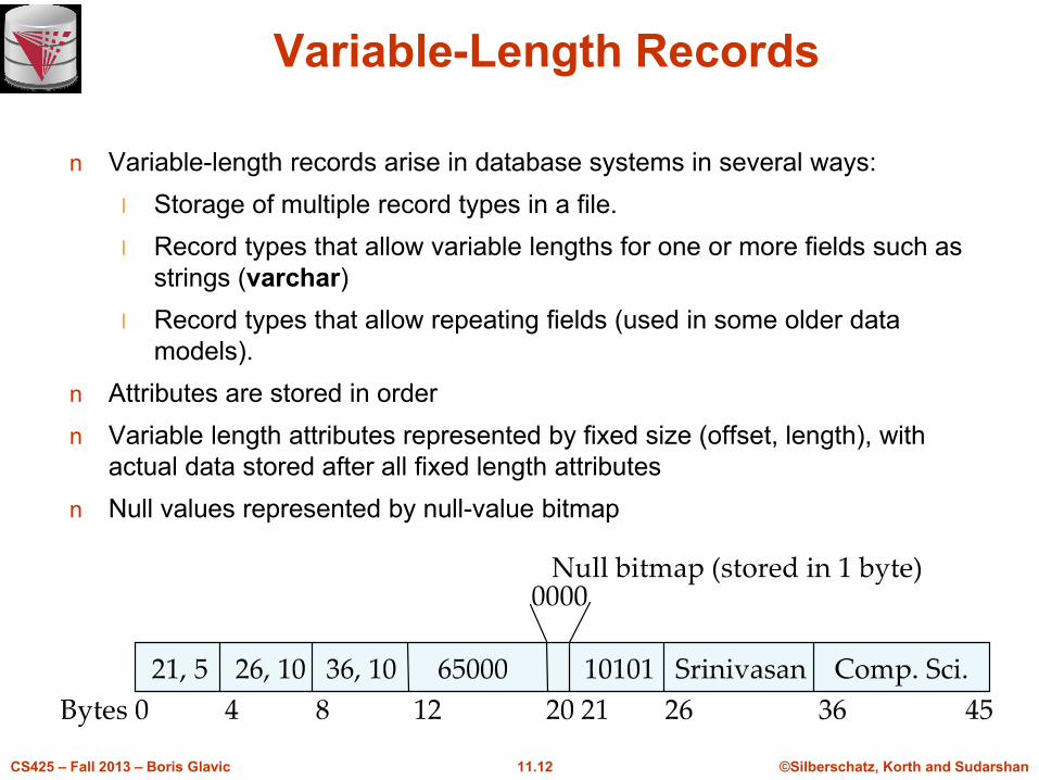
Variable-Length Records
n Variable-length records arise in database systems in several ways:
l Storage of multiple record types in a file.
l Record types that allow variable lengths for one or more fields such as
strings (varchar)
l Record types that allow repeating fields (used in some older data
models).
n Attributes are stored in order
n Variable length attributes represented by fixed size (offset, length), with
actual data stored after all fixed length attributes
n Null values represented by null-value bitmap
©Silberschatz, Korth and Sudarshan11.13CS425 – Fall 2013 – Boris Glavic
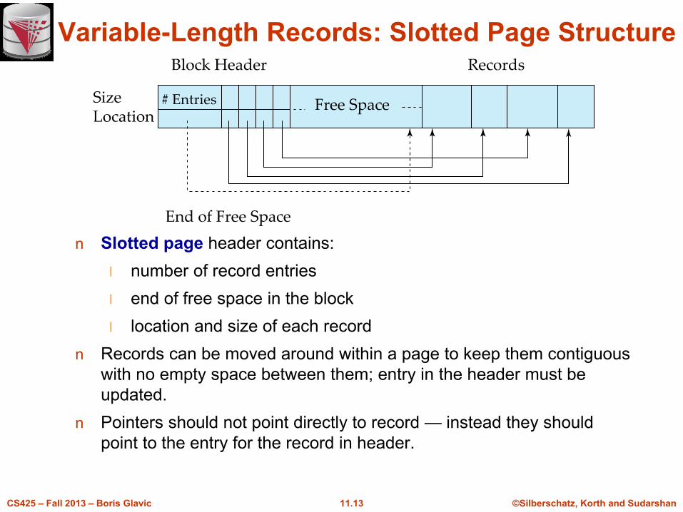
Variable-Length Records: Slotted Page Structure
n Slotted page header contains:
l number of record entries
l end of free space in the block
l location and size of each record
n Records can be moved around within a page to keep them contiguous
with no empty space between them; entry in the header must be
updated.
n Pointers should not point directly to record — instead they should
point to the entry for the record in header.
©Silberschatz, Korth and Sudarshan11.14CS425 – Fall 2013 – Boris Glavic
Organization of Records in Files
n Heap – a record can be placed anywhere in the file where there
is space
l Deletion efficient
l Insertion efficient
l Search is expensive
Example: Get instructor with name Glavic
– Have to search through all instructors
n Sequential – store records in sequential order, based on the
value of some search key of each record
l Deletion expensive and/or waste of space
l Insertion expensive and/or waste of space
l Search is efficient (e.g., binary search)
As long as the search is on the search key we are
ordering on
Modified from:
Database System Concepts, 6th Ed.
©Silberschatz, Korth and Sudarshan
See www.db-book.com for conditions on re-use
Buffering
©Silberschatz, Korth and Sudarshan11.16CS425 – Fall 2013 – Boris Glavic
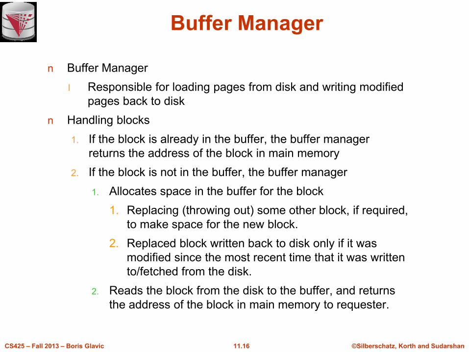
Buffer Manager
n Buffer Manager
l Responsible for loading pages from disk and writing modified
pages back to disk
n Handling blocks
1. If the block is already in the buffer, the buffer manager
returns the address of the block in main memory
2. If the block is not in the buffer, the buffer manager
1. Allocates space in the buffer for the block
1. Replacing (throwing out) some other block, if required,
to make space for the new block.
2. Replaced block written back to disk only if it was
modified since the most recent time that it was written
to/fetched from the disk.
2. Reads the block from the disk to the buffer, and returns
the address of the block in main memory to requester.
©Silberschatz, Korth and Sudarshan11.17CS425 – Fall 2013 – Boris Glavic
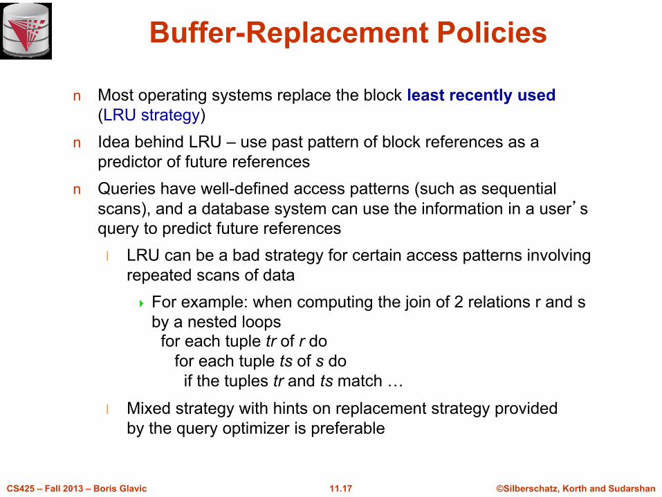
Buffer-Replacement Policies
n Most operating systems replace the block least recently used
(LRU strategy)
n Idea behind LRU – use past pattern of block references as a
predictor of future references
n Queries have well-defined access patterns (such as sequential
scans), and a database system can use the information in a user’s
query to predict future references
l LRU can be a bad strategy for certain access patterns involving
repeated scans of data
For example: when computing the join of 2 relations r and s
by a nested loops for each tuple tr of r do
for each tuple ts of s do
if the tuples tr and ts match …
l Mixed strategy with hints on replacement strategy provided
by the query optimizer is preferable
©Silberschatz, Korth and Sudarshan11.18CS425 – Fall 2013 – Boris Glavic
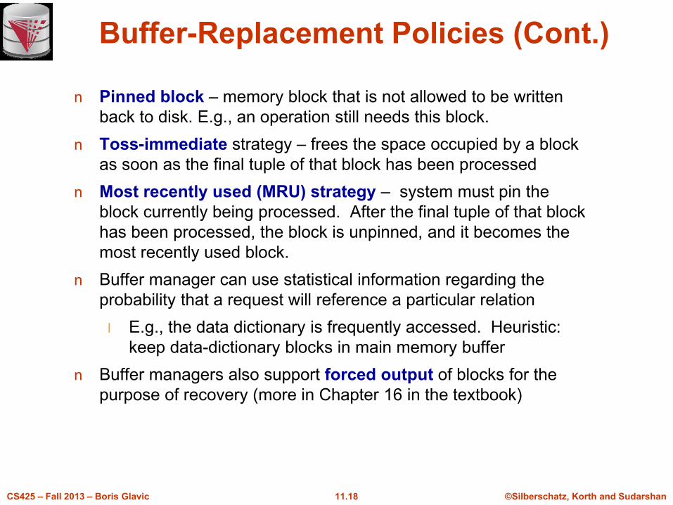
Buffer-Replacement Policies (Cont.)
n Pinned block – memory block that is not allowed to be written
back to disk. E.g., an operation still needs this block.
n Toss-immediate strategy – frees the space occupied by a block
as soon as the final tuple of that block has been processed
n Most recently used (MRU) strategy – system must pin the
block currently being processed. After the final tuple of that block
has been processed, the block is unpinned, and it becomes the
most recently used block.
n Buffer manager can use statistical information regarding the
probability that a request will reference a particular relation
l E.g., the data dictionary is frequently accessed. Heuristic:
keep data-dictionary blocks in main memory buffer
n Buffer managers also support forced output of blocks for the
purpose of recovery (more in Chapter 16 in the textbook)
Modified from:
Database System Concepts, 6th Ed.
©Silberschatz, Korth and Sudarshan
See www.db-book.com for conditions on re-use
Indexing and Hashing
©Silberschatz, Korth and Sudarshan11.20CS425 – Fall 2013 – Boris Glavic
Basic Concepts
n Indexing mechanisms used to speed up access to desired data.
l E.g., author catalog in library
n Search Key - attribute or set of attributes used to look up records in a
file.
n An index file consists of records (called index entries) of the form
n Index files are typically much smaller than the original file
n Two basic kinds of indices:
l Ordered indices: search keys are stored in some sorted order
l Hash indices: search keys are distributed uniformly across
“buckets” using a “hash function”.
search-key pointer
©Silberschatz, Korth and Sudarshan11.21CS425 – Fall 2013 – Boris Glavic
Index Evaluation Metrics
n Access types supported efficiently. E.g.,
l records with a specified value in the attribute
l or records with an attribute value falling in a specified range of
values.
n Access time
n Insertion time
n Deletion time
n Space overhead
©Silberschatz, Korth and Sudarshan11.22CS425 – Fall 2013 – Boris Glavic
Ordered Indices
n In an ordered index, index entries are stored sorted on the search key
value. E.g., author catalog in library.
n Primary index: in a sequentially ordered file, the index whose search
key specifies the sequential order of the file.
l Also called clustering index
l The search key of a primary index is usually but not necessarily the
primary key.
n Secondary index: an index whose search key specifies an order
different from the sequential order of the file. Also called
non-clustering index.
n Index-sequential file: ordered sequential file with a primary index.
©Silberschatz, Korth and Sudarshan11.23CS425 – Fall 2013 – Boris Glavic
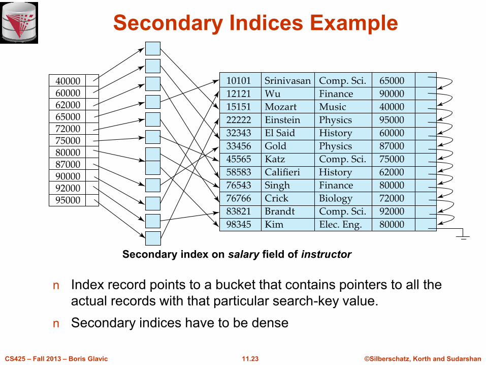
Secondary Indices Example
n Index record points to a bucket that contains pointers to all the
actual records with that particular search-key value.
n Secondary indices have to be dense
Secondary index on salary field of instructor
©Silberschatz, Korth and Sudarshan11.24CS425 – Fall 2013 – Boris Glavic
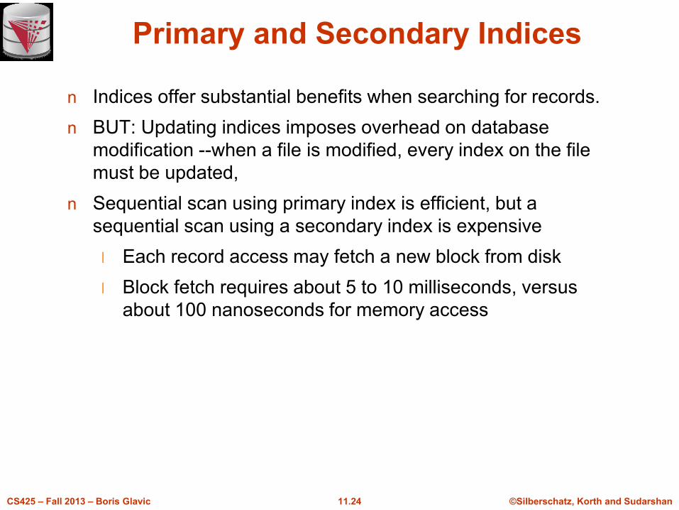
Primary and Secondary Indices
n Indices offer substantial benefits when searching for records.
n BUT: Updating indices imposes overhead on database
modification --when a file is modified, every index on the file
must be updated,
n Sequential scan using primary index is efficient, but a
sequential scan using a secondary index is expensive
l Each record access may fetch a new block from disk
l Block fetch requires about 5 to 10 milliseconds, versus
about 100 nanoseconds for memory access
©Silberschatz, Korth and Sudarshan11.25CS425 – Fall 2013 – Boris Glavic
Secondary Indices
n Frequently, one wants to find all the records whose values in
a certain field (which is not the search-key of the primary
index) satisfy some condition.
l Example 1: In the instructor relation stored sequentially by
ID, we may want to find all instructors in a particular
department
l Example 2: as above, but where we want to find all
instructors with a specified salary or with salary in a
specified range of values
n We can have a secondary index with an index record for
each search-key value
©Silberschatz, Korth and Sudarshan11.26CS425 – Fall 2013 – Boris Glavic
B+-Tree Index
n Disadvantage of indexed-sequential files
l performance degrades as file grows, since many overflow blocks get created.
l Periodic reorganization of entire file is required.
n Advantage of B+-tree index files:
l automatically reorganizes itself with small, local, changes, in the face of insertions and deletions.
l Reorganization of entire file is not required to maintain performance.
n (Minor) disadvantage of B+-trees:
l extra insertion and deletion overhead, space overhead.
n Advantages of B+-trees outweigh disadvantages
l B+-trees are used extensively
B+-tree indices are an alternative to indexed-sequential files.
©Silberschatz, Korth and Sudarshan11.27CS425 – Fall 2013 – Boris Glavic
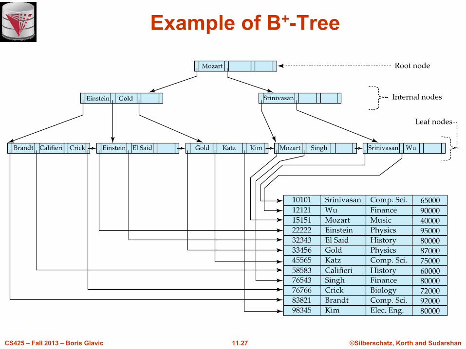
Example of B+-Tree
©Silberschatz, Korth and Sudarshan11.28CS425 – Fall 2013 – Boris Glavic
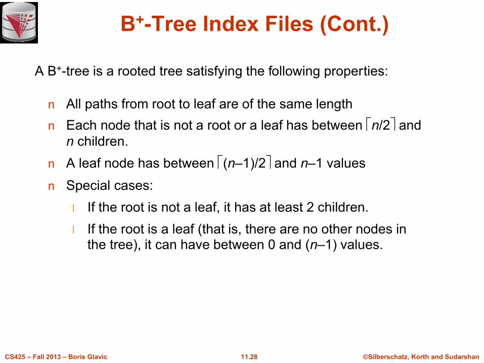
B+-Tree Index Files (Cont.)
n All paths from root to leaf are of the same length
n Each node that is not a root or a leaf has between n/2 and
n children.
n A leaf node has between (n–1)/2 and n–1 values
n Special cases:
l If the root is not a leaf, it has at least 2 children.
l If the root is a leaf (that is, there are no other nodes in the tree), it can have between 0 and (n–1) values.
A B+-tree is a rooted tree satisfying the following properties:
©Silberschatz, Korth and Sudarshan11.29CS425 – Fall 2013 – Boris Glavic
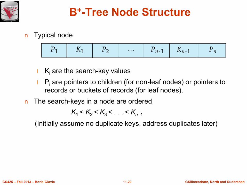
B+-Tree Node Structure
n Typical node
l Ki are the search-key values
l Pi are pointers to children (for non-leaf nodes) or pointers to
records or buckets of records (for leaf nodes).
n The search-keys in a node are ordered
K1 < K2 < K3 < . . . < Kn–1
(Initially assume no duplicate keys, address duplicates later)
©Silberschatz, Korth and Sudarshan11.30CS425 – Fall 2013 – Boris Glavic
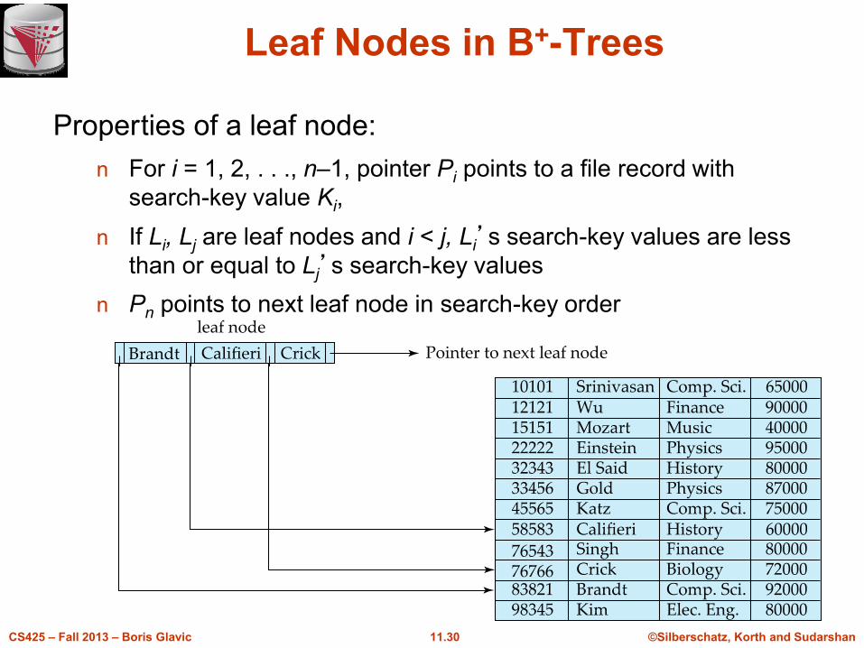
Leaf Nodes in B+-Trees
n For i = 1, 2, . . ., n–1, pointer Pi points to a file record with
search-key value Ki,
n If Li, Lj are leaf nodes and i < j, Li’s search-key values are less
than or equal to Lj’s search-key values
n Pn points to next leaf node in search-key order
Properties of a leaf node:
©Silberschatz, Korth and Sudarshan11.31CS425 – Fall 2013 – Boris Glavic
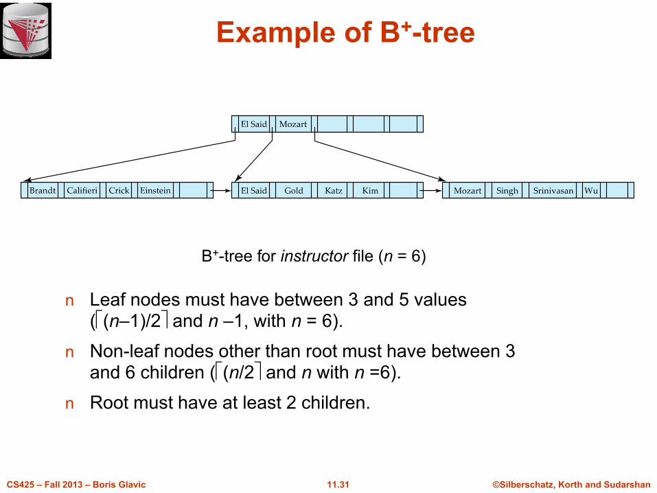
Example of B+-tree
n Leaf nodes must have between 3 and 5 values ((n–1)/2 and n –1, with n = 6).
n Non-leaf nodes other than root must have between 3 and 6 children ((n/2 and n with n =6).
n Root must have at least 2 children.
B+-tree for instructor file (n = 6)
©Silberschatz, Korth and Sudarshan11.32CS425 – Fall 2013 – Boris Glavic
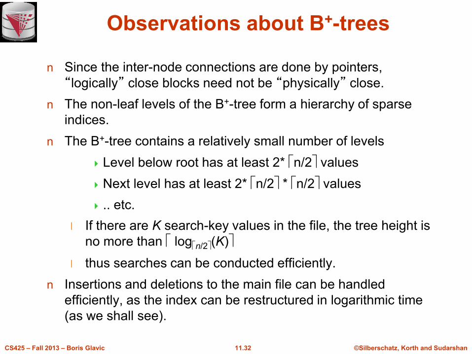
Observations about B+-trees
n Since the inter-node connections are done by pointers,
“logically” close blocks need not be “physically” close.
n The non-leaf levels of the B+-tree form a hierarchy of sparse
indices.
n The B+-tree contains a relatively small number of levels
Level below root has at least 2* n/2 values
Next level has at least 2* n/2 * n/2 values
.. etc.
l If there are K search-key values in the file, the tree height is
no more than logn/2(K)
l thus searches can be conducted efficiently.
n Insertions and deletions to the main file can be handled
efficiently, as the index can be restructured in logarithmic time
(as we shall see).
©Silberschatz, Korth and Sudarshan11.33CS425 – Fall 2013 – Boris Glavic
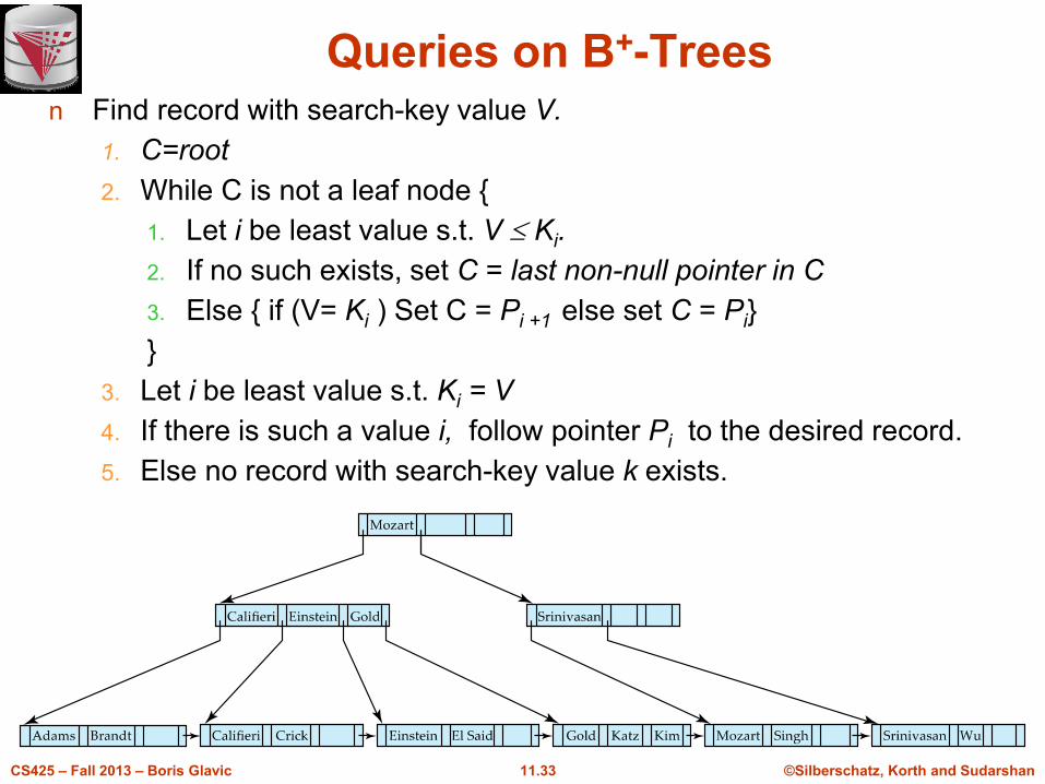
Queries on B+-Treesn Find record with search-key value V.
1. C=root
2. While C is not a leaf node {
1. Let i be least value s.t. V Ki.
2. If no such exists, set C = last non-null pointer in C
3. Else { if (V= Ki ) Set C = Pi +1 else set C = Pi}
}
3. Let i be least value s.t. Ki = V
4. If there is such a value i, follow pointer Pi to the desired record.
5. Else no record with search-key value k exists.
©Silberschatz, Korth and Sudarshan11.34CS425 – Fall 2013 – Boris Glavic
Handling Duplicates
n With duplicate search keys
l In both leaf and internal nodes,
we cannot guarantee that K1 < K2 < K3 < . . . < Kn–1
but can guarantee K1 K2 K3 . . . Kn–1
l Search-keys in the subtree to which Pi points
are Ki,, but not necessarily < Ki,
To see why, suppose same search key value V is present in two leaf node Li and Li+1. Then in parent node Ki must be equal to V
©Silberschatz, Korth and Sudarshan11.35CS425 – Fall 2013 – Boris Glavic
Queries on B+-Trees (Cont.)
n If there are K search-key values in the file, the height of the tree is no
more than logn/2(K).
n A node is generally the same size as a disk block, typically 4
kilobytes
l and n is typically around 100 (40 bytes per index entry).
n With 1 million search key values and n = 100
l at most log50(1,000,000) = 4 nodes are accessed in a lookup.
n Contrast this with a balanced binary tree with 1 million search key
values — around 20 nodes are accessed in a lookup
l above difference is significant since every node access may need
a disk I/O, costing around 20 milliseconds
©Silberschatz, Korth and Sudarshan11.36CS425 – Fall 2013 – Boris Glavic
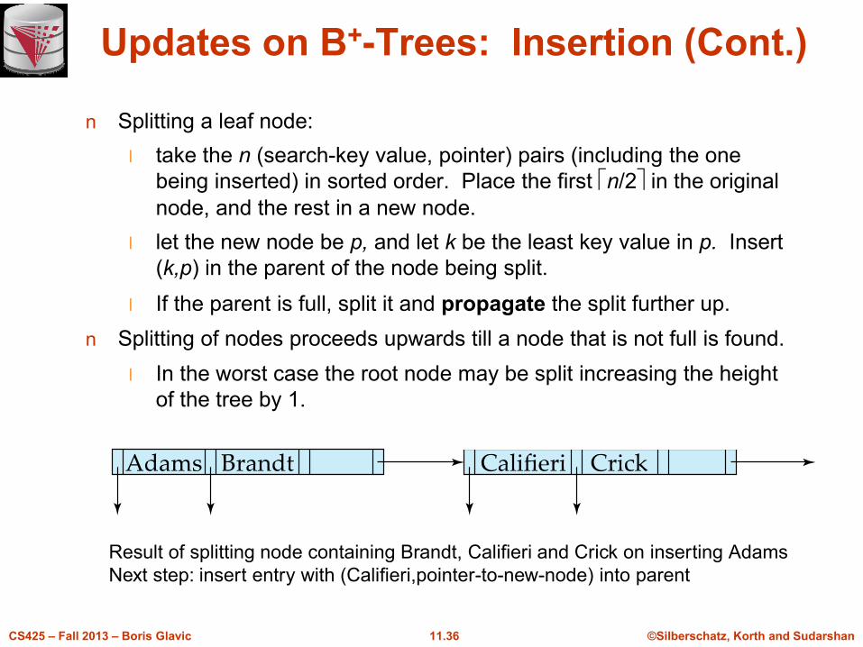
Updates on B+-Trees: Insertion (Cont.)
n Splitting a leaf node:
l take the n (search-key value, pointer) pairs (including the one
being inserted) in sorted order. Place the first n/2 in the original
node, and the rest in a new node.
l let the new node be p, and let k be the least key value in p. Insert
(k,p) in the parent of the node being split.
l If the parent is full, split it and propagate the split further up.
n Splitting of nodes proceeds upwards till a node that is not full is found.
l In the worst case the root node may be split increasing the height
of the tree by 1.
Result of splitting node containing Brandt, Califieri and Crick on inserting Adams
Next step: insert entry with (Califieri,pointer-to-new-node) into parent
©Silberschatz, Korth and Sudarshan11.37CS425 – Fall 2013 – Boris Glavic
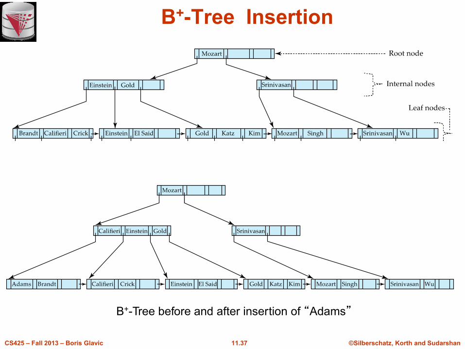
B+-Tree Insertion
B+-Tree before and after insertion of “Adams”
©Silberschatz, Korth and Sudarshan11.38CS425 – Fall 2013 – Boris Glavic
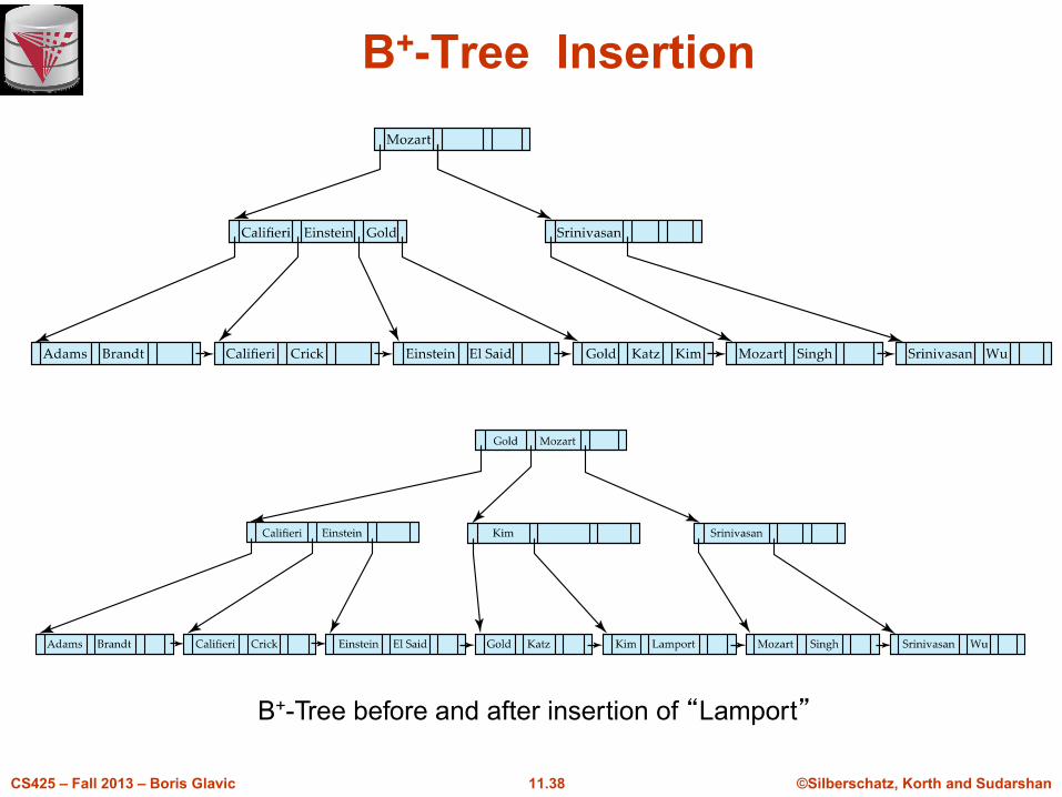
B+-Tree Insertion
B+-Tree before and after insertion of “Lamport”
©Silberschatz, Korth and Sudarshan11.39CS425 – Fall 2013 – Boris Glavic
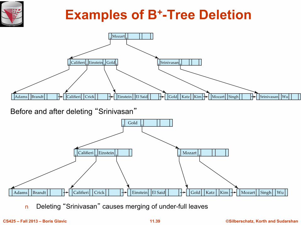
Examples of B+-Tree Deletion
n Deleting “Srinivasan” causes merging of under-full leaves
Before and after deleting “Srinivasan”
©Silberschatz, Korth and Sudarshan11.40CS425 – Fall 2013 – Boris Glavic
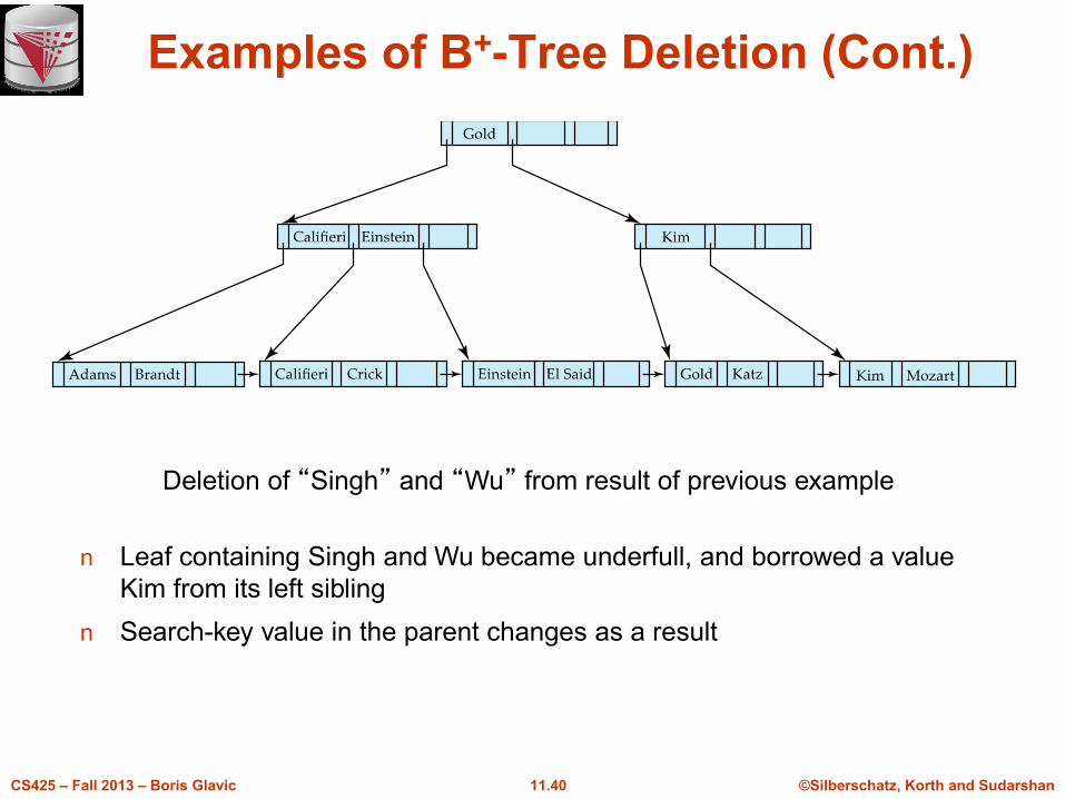
Examples of B+-Tree Deletion (Cont.)
Deletion of “Singh” and “Wu” from result of previous example
n Leaf containing Singh and Wu became underfull, and borrowed a value
Kim from its left sibling
n Search-key value in the parent changes as a result
©Silberschatz, Korth and Sudarshan11.41CS425 – Fall 2013 – Boris Glavic
Non-Unique Search Keys
n Alternatives to scheme described earlier
l Buckets on separate block (bad idea)
l List of tuple pointers with each key
Extra code to handle long lists
Deletion of a tuple can be expensive if there are many
duplicates on search key (why?)
Low space overhead, no extra cost for queries
l Make search key unique by adding a record-identifier
Extra storage overhead for keys
Simpler code for insertion/deletion
Widely used
Modified from:
Database System Concepts, 6th Ed.
©Silberschatz, Korth and Sudarshan
See www.db-book.com for conditions on re-use
Hashing
©Silberschatz, Korth and Sudarshan11.43CS425 – Fall 2013 – Boris Glavic
Static Hashing
n A bucket is a unit of storage containing one or more records (a
bucket is typically a disk block).
n In a hash file organization we obtain the bucket of a record directly
from its search-key value using a hash function.
n Hash function h is a function from the set of all search-key values K
to the set of all bucket addresses B.
n Hash function is used to locate records for access, insertion as well
as deletion.
n Records with different search-key values may be mapped to the
same bucket; thus entire bucket has to be searched sequentially to
locate a record.
©Silberschatz, Korth and Sudarshan11.44CS425 – Fall 2013 – Boris Glavic
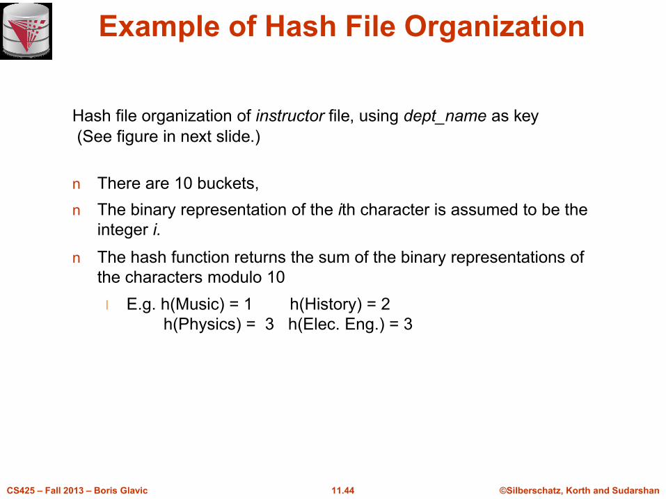
Example of Hash File Organization
n There are 10 buckets,
n The binary representation of the ith character is assumed to be the
integer i.
n The hash function returns the sum of the binary representations of
the characters modulo 10
l E.g. h(Music) = 1 h(History) = 2
h(Physics) = 3 h(Elec. Eng.) = 3
Hash file organization of instructor file, using dept_name as key
(See figure in next slide.)
©Silberschatz, Korth and Sudarshan11.45CS425 – Fall 2013 – Boris Glavic
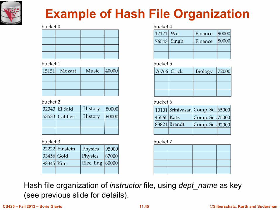
Example of Hash File Organization
Hash file organization of instructor file, using dept_name as key
(see previous slide for details).
©Silberschatz, Korth and Sudarshan11.46CS425 – Fall 2013 – Boris Glavic
Hash Functions
n Worst hash function maps all search-key values to the same bucket;
this makes access time proportional to the number of search-key
values in the file.
n An ideal hash function is uniform, i.e., each bucket is assigned the
same number of search-key values from the set of all possible values.
n Ideal hash function is random, so each bucket will have the same number of records assigned to it irrespective of the actual distribution of
search-key values in the file.
n Typical hash functions perform computation on the internal binary
representation of the search-key.
l For example, for a string search-key, the binary representations of
all the characters in the string could be added and the sum modulo
the number of buckets could be returned. .
©Silberschatz, Korth and Sudarshan11.47CS425 – Fall 2013 – Boris Glavic
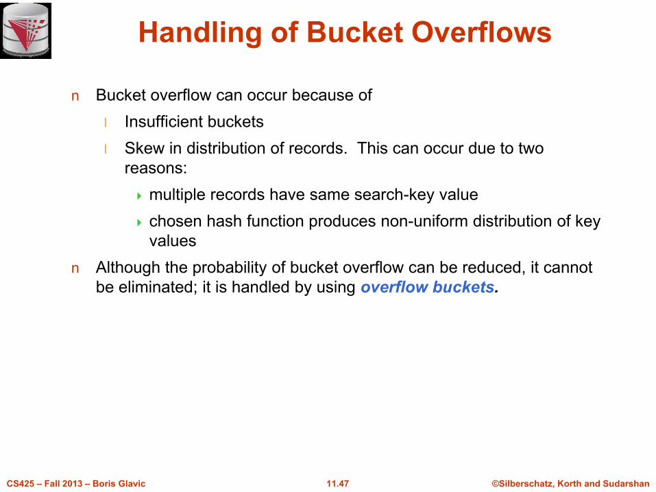
Handling of Bucket Overflows
n Bucket overflow can occur because of
l Insufficient buckets
l Skew in distribution of records. This can occur due to two
reasons:
multiple records have same search-key value
chosen hash function produces non-uniform distribution of key
values
n Although the probability of bucket overflow can be reduced, it cannot
be eliminated; it is handled by using overflow buckets.
©Silberschatz, Korth and Sudarshan11.48CS425 – Fall 2013 – Boris Glavic
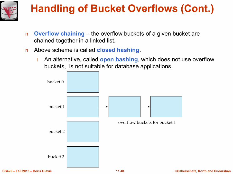
Handling of Bucket Overflows (Cont.)
n Overflow chaining – the overflow buckets of a given bucket are
chained together in a linked list.
n Above scheme is called closed hashing.
l An alternative, called open hashing, which does not use overflow
buckets, is not suitable for database applications.
©Silberschatz, Korth and Sudarshan11.49CS425 – Fall 2013 – Boris Glavic
Hash Indices
n Hashing can be used not only for file organization, but also for index-
structure creation.
n A hash index organizes the search keys, with their associated record
pointers, into a hash file structure.
n Strictly speaking, hash indices are always secondary indices
l if the file itself is organized using hashing, a separate primary
hash index on it using the same search-key is unnecessary.
l However, we use the term hash index to refer to both secondary
index structures and hash organized files.
©Silberschatz, Korth and Sudarshan11.50CS425 – Fall 2013 – Boris Glavic
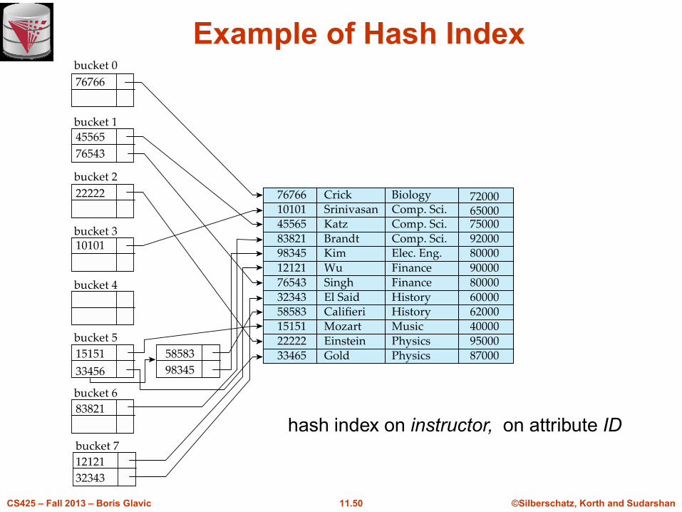
Example of Hash Index
hash index on instructor, on attribute ID
©Silberschatz, Korth and Sudarshan11.51CS425 – Fall 2013 – Boris Glavic
Deficiencies of Static Hashing
n In static hashing, function h maps search-key values to a fixed set of B
of bucket addresses. Databases grow or shrink with time.
l If initial number of buckets is too small, and file grows, performance
will degrade due to too much overflows.
l If space is allocated for anticipated growth, a significant amount of
space will be wasted initially (and buckets will be underfull).
l If database shrinks, again space will be wasted.
n One solution: periodic re-organization of the file with a new hash
function
l Expensive, disrupts normal operations
n Better solution: allow the number of buckets to be modified dynamically.
©Silberschatz, Korth and Sudarshan11.52CS425 – Fall 2013 – Boris Glavic
Index Definition in SQL
n Create an index
create index <index-name> on <relation-name>
(<attribute-list>)
E.g.: create index b-index on branch(branch_name)
n Use create unique index to indirectly specify and enforce the
condition that the search key is a candidate key is a candidate key.
n To drop an index
drop index <index-name>
n Most database systems allow specification of type of index, and
clustering.
Modified from:
Database System Concepts, 6th Ed.
©Silberschatz, Korth and Sudarshan
See www.db-book.com for conditions on re-use
End of Chapter


