Chapter 1Introduction to Operations Research

2nd Edition

Operations Research: A Practical IntroductionBy

Michael Carter

Camille C. Price

Ghaith Rabadi

Learning Objectives

■ Learn about the origins and applications of operations research

■ Understand system modeling principles

■ Understand algorithm efficiency and problem complexity

■ Contrast between the optimality and practicality

■ Learn about software for operations research

1.1 The origins and applications of operations research■ Operations Research can be defined as the use of quantitative methods to assist analysts and

decision-makers in designing, analyzing, and improving the performance or operation of systems. A system can be:

– A manufacturing system– Engineering System– Financial– Service– Many others

■ The field of Operations Research incorporates analytical tools from many different disciplines, so that they can be applied in a rational way to help decision-makers solve problems and control the operations of systems and organizations in the most practical or advantageous way.

■ The ideas and methodologies of Operations Research have been taking shape throughout the history of science and mathematics, but most notably since the industrial revolution.

■ Operations Research (also called Management Science) became an identifiable discipline during the days leading up to World War II. In the 1930s, the British military buildup centered around the development of weapons, devices, and other support equipment.

1.2 System Modeling Principles

■ A model is a simplified, idealized representation of a real object, a real process, or a real system.

■ The models used are called mathematical models because the building blocks of the models are mathematical structures (equations, inequalities, matrices, functions, and operators).

■ Step in building a model:1. Discover an area that is in need of study or improvement. 2. Determine which aspects of the system are controllable and which are not 3. Identify the goals or purpose of the system, 4. Identify the constraints or limitations that govern the operation of the system 5. Create a model that implicitly or explicitly embodies alternative courses of action6. Collect data that characterize the system being modeled.7. Solve the model and conduct your analysis

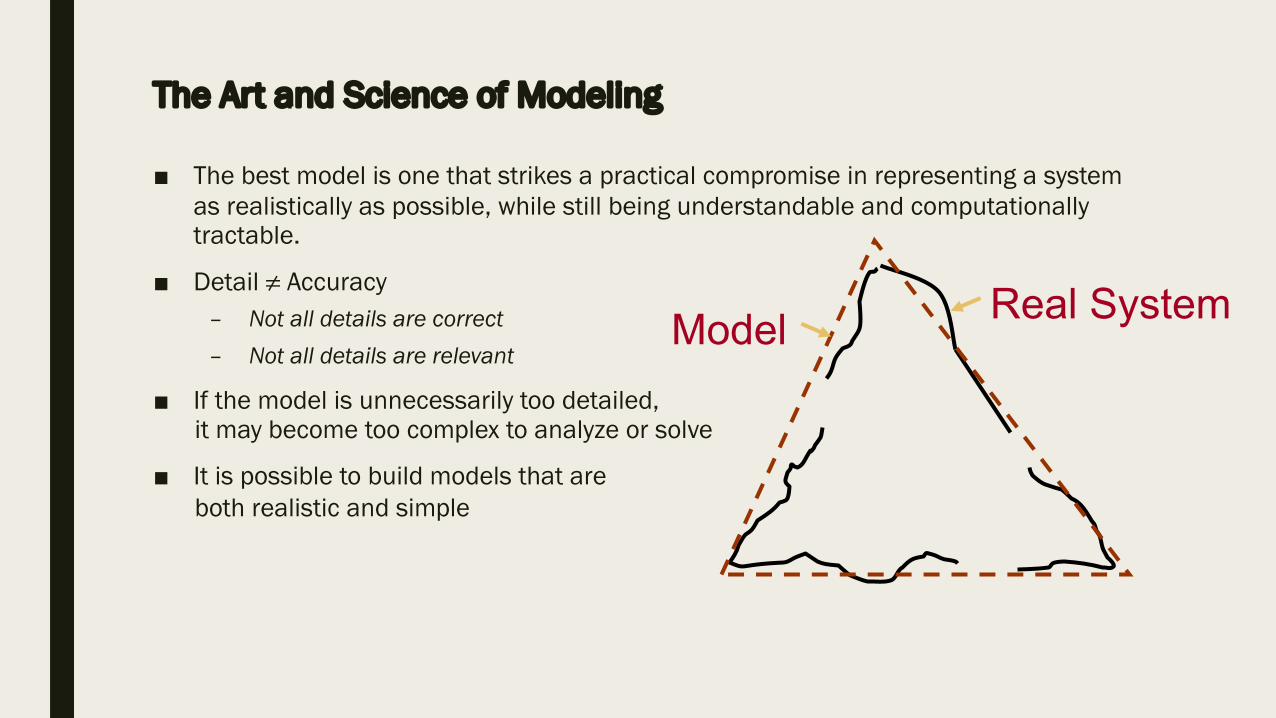
The Art and Science of Modeling

■ The best model is one that strikes a practical compromise in representing a system as realistically as possible, while still being understandable and computationally tractable.

■ Detail ≠ Accuracy – Not all details are correct – Not all details are relevant

■ If the model is unnecessarily too detailed, it may become too complex to analyze or solve

■ It is possible to build models that are both realistic and simple

Real SystemModel

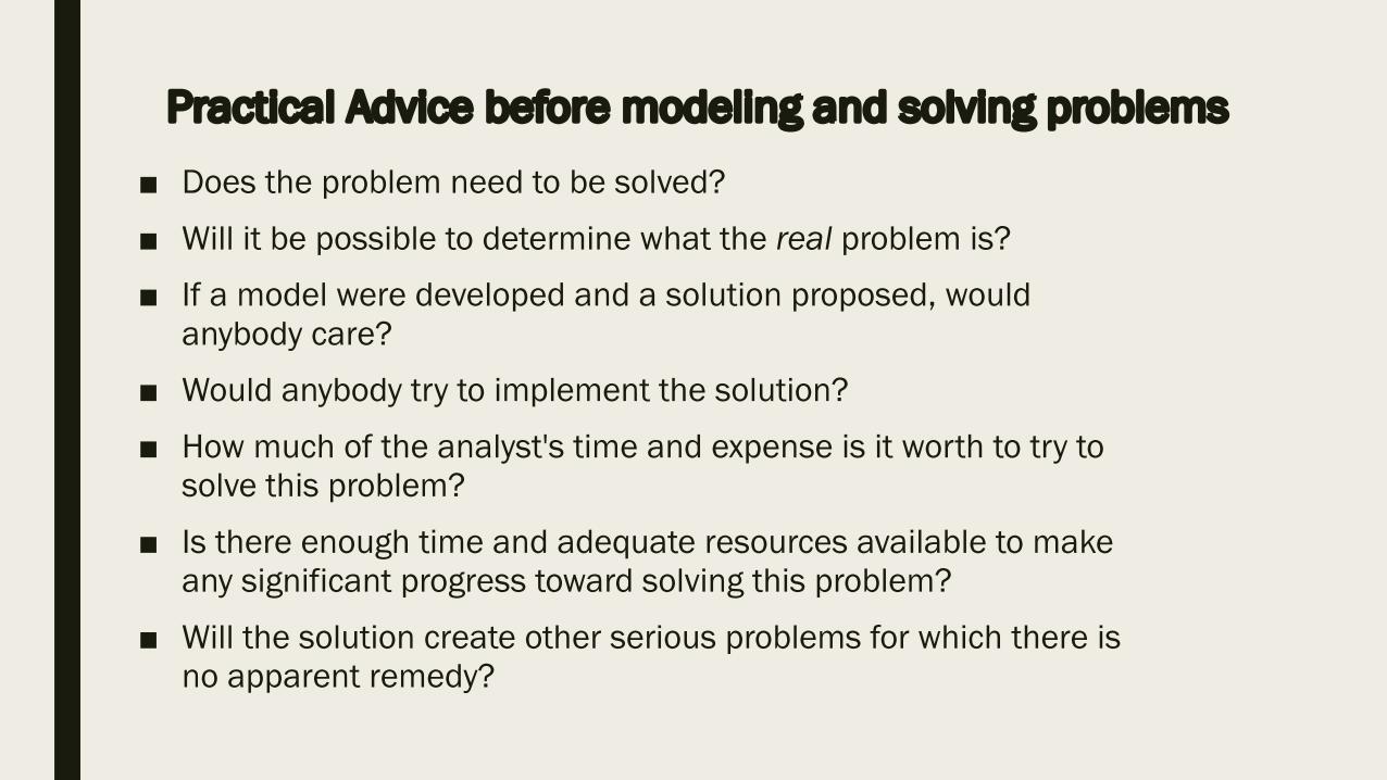
Practical Advice before modeling and solving problems■ Does the problem need to be solved?

■ Will it be possible to determine what the real problem is?

■ If a model were developed and a solution proposed, would anybody care?

■ Would anybody try to implement the solution?

■ How much of the analyst's time and expense is it worth to try to solve this problem?

■ Is there enough time and adequate resources available to make any significant progress toward solving this problem?

■ Will the solution create other serious problems for which there is no apparent remedy?

1.3 Algorithm Efficiency and Problem Complexity

■ An algorithm is a sequence of operations that can be carried out in a finite amount of time.

■ An algorithm may be called repeatedly or recursively but it will eventually terminate.

■ Several factors influence the amount of time it takes for a computer program to execute to solve a problem:

– the programming language used, – the programmer's skill, – the hardware used in executing the program, – and the task load on the computer system during execution.

■ None of these factors is a direct consequence of the underlying algorithm that has been implemented

■ The performance of an algorithm is often described as a function of problem size, which denotes the size of the data set that is input to the algorithm.

– Example: Sorting algorithm takes longer to sort a list of 10,000 names than to sort a list of 100 names.

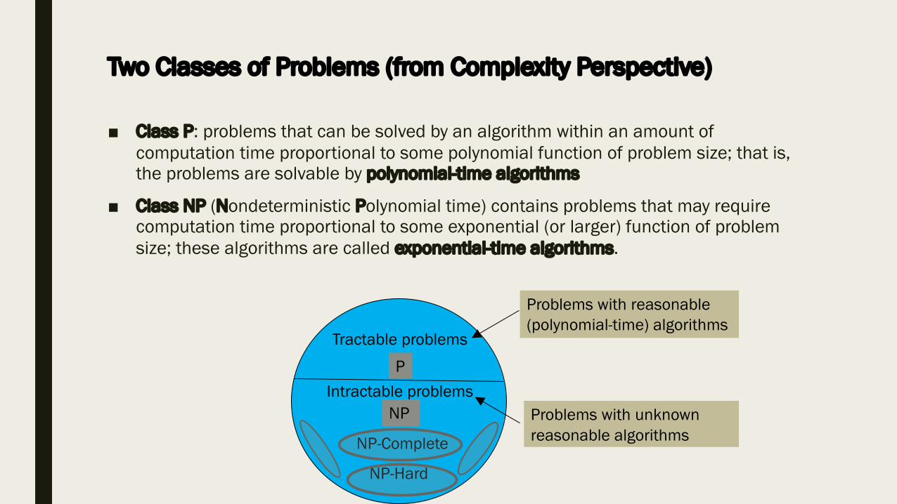
■ Class P: problems that can be solved by an algorithm within an amount of computation time proportional to some polynomial function of problem size; that is, the problems are solvable by polynomial-time algorithms

■ Class NP (Nondeterministic Polynomial time) contains problems that may require computation time proportional to some exponential (or larger) function of problem size; these algorithms are called exponential-time algorithms.

Two Classes of Problems (from Complexity Perspective)

Tractable problems

Intractable problemsProblems with unknown reasonable algorithms

Problems with reasonable (polynomial-time) algorithms

P

NP

NP-Complete

NP-Hard

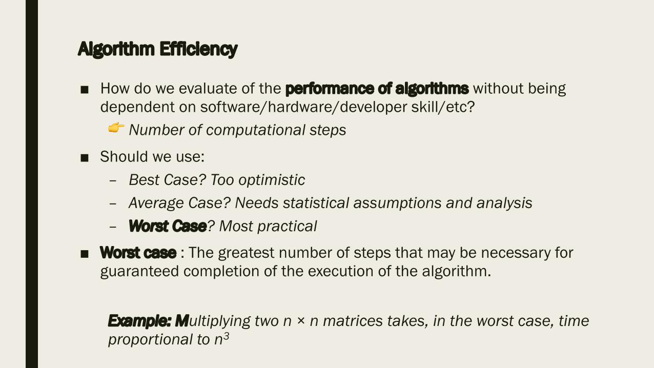
■ How do we evaluate of the performance of algorithms without being dependent on software/hardware/developer skill/etc?👉 Number of computational steps

■ Should we use:– Best Case? Too optimistic– Average Case? Needs statistical assumptions and analysis– Worst Case? Most practical

■ Worst case : The greatest number of steps that may be necessary for guaranteed completion of the execution of the algorithm.

Example: Multiplying two n × n matrices takes, in the worst case, time proportional to n3

Algorithm Efficiency

Big-Oh notation (Order-of)

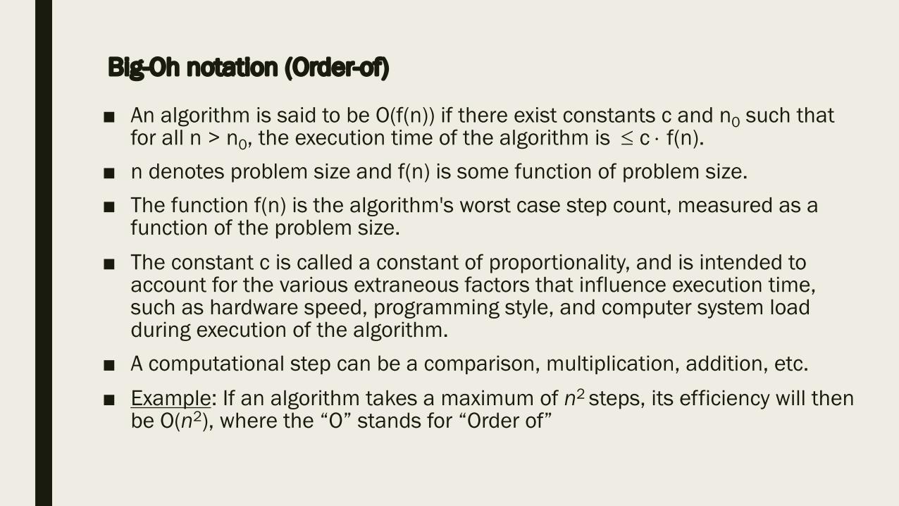
■ An algorithm is said to be O(f(n)) if there exist constants c and n0 such that for all n > n0, the execution time of the algorithm is £ c × f(n).

■ n denotes problem size and f(n) is some function of problem size. ■ The function f(n) is the algorithm's worst case step count, measured as a

function of the problem size. ■ The constant c is called a constant of proportionality, and is intended to

account for the various extraneous factors that influence execution time, such as hardware speed, programming style, and computer system load during execution of the algorithm.

■ A computational step can be a comparison, multiplication, addition, etc.■ Example: If an algorithm takes a maximum of n2 steps, its efficiency will then

be O(n2), where the “O” stands for “Order of”

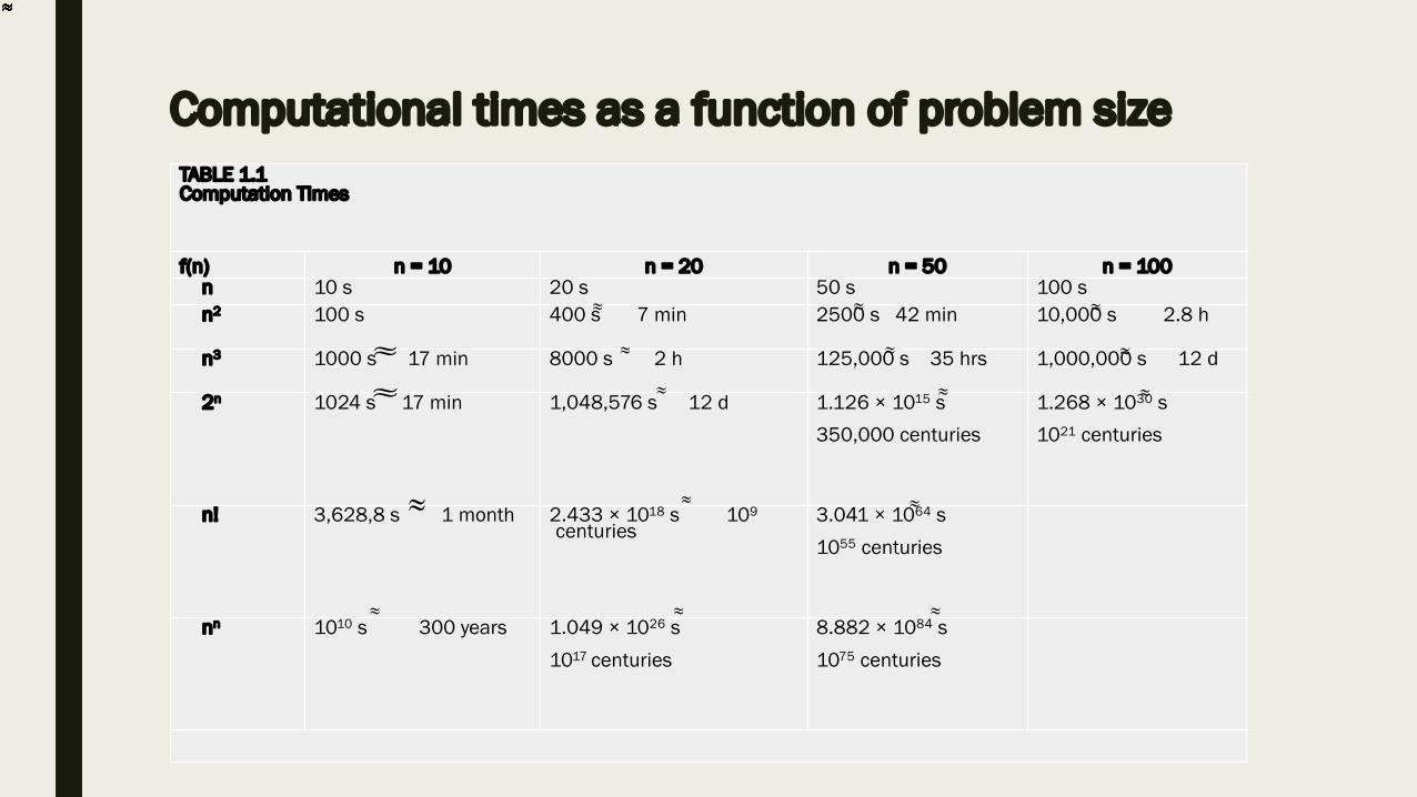
Computational times as a function of problem sizeTABLE 1.1Computation Times

f(n) n = 10 n = 20 n = 50 n = 100n 10 s 20 s 50 s 100 sn2 100 s 400 s 7 min 2500 s 42 min 10,000 s 2.8 h

n3 1000 s 17 min 8000 s 2 h 125,000 s 35 hrs 1,000,000 s 12 d

2n 1024 s 17 min 1,048,576 s 12 d 1.126 × 1015 s 350,000 centuries

1.268 × 1030 s 1021 centuries

n! 3,628,8 s 1 month 2.433 × 1018 s 109

centuries3.041 × 1064 s 1055 centuries

nn 1010 s 300 years 1.049 × 1026 s 1017 centuries

8.882 × 1084 s 1075 centuries

»

»

»»

»

»

»

»»

»

»

»

»

»

»

»

»»»»»»»»»»»»»»»»»

»

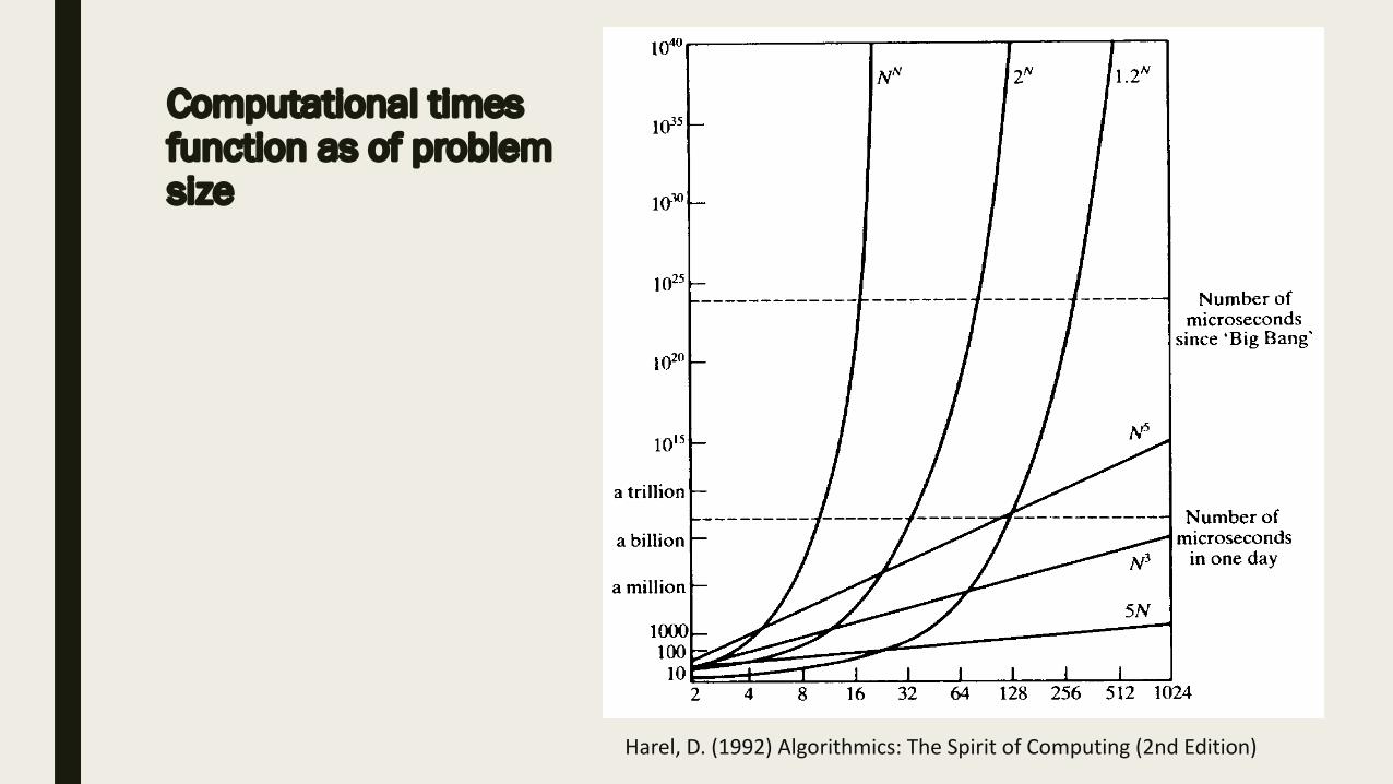
Computational times function as of problemsize

Harel, D. (1992) Algorithmics: The Spirit of Computing (2nd Edition)

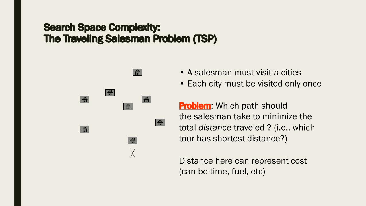
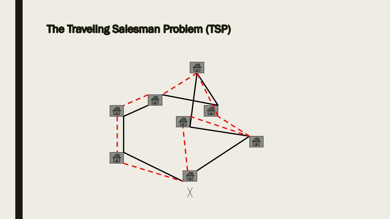
Search Space Complexity:The Traveling Salesman Problem (TSP)

• A salesman must visit n cities• Each city must be visited only once

Problem: Which path should the salesman take to minimize thetotal distance traveled ? (i.e., whichtour has shortest distance?)

Distance here can represent cost (can be time, fuel, etc)

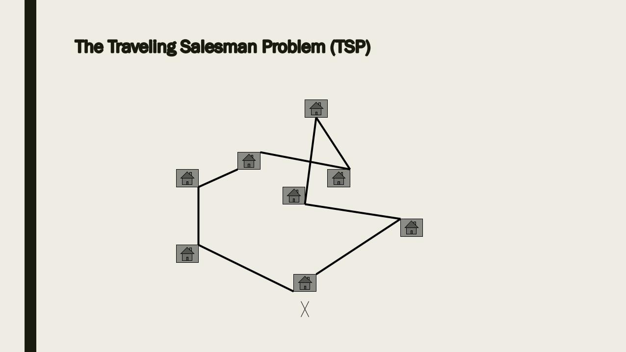
The Traveling Salesman Problem (TSP)

The Traveling Salesman Problem (TSP)

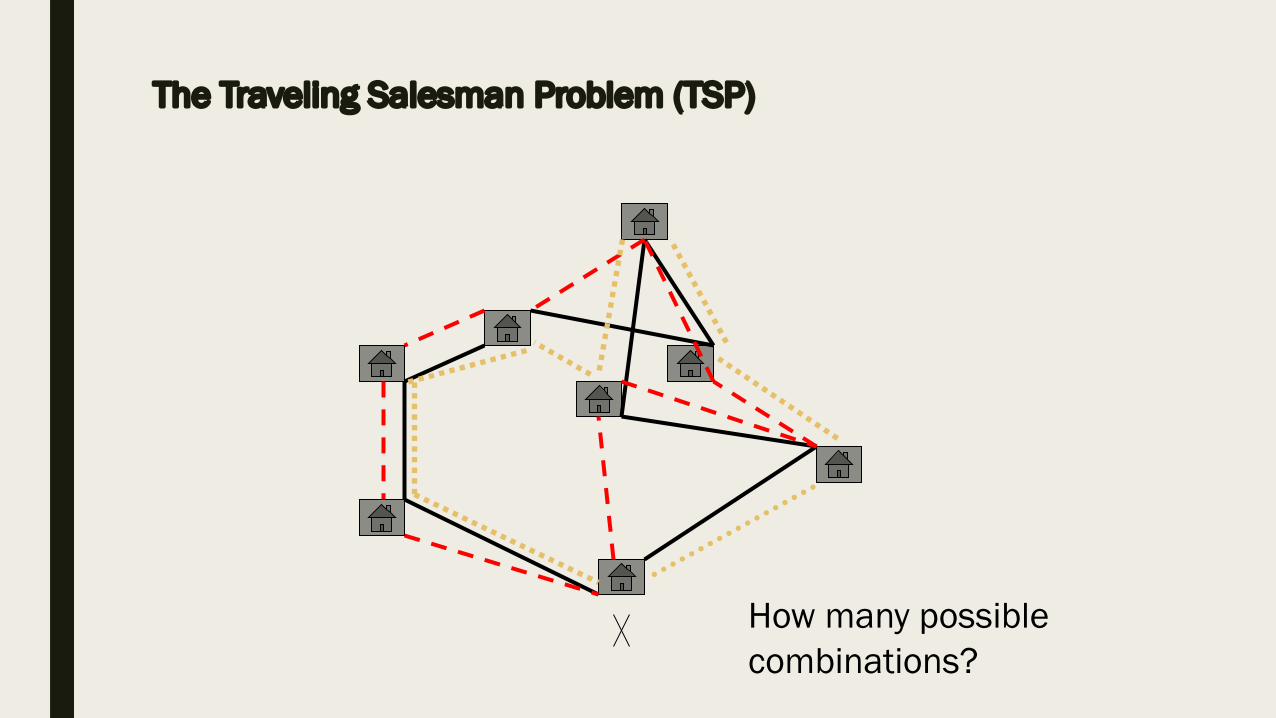
The Traveling Salesman Problem (TSP)

How many possiblecombinations?

The TSP

■ Try a small example by handA TSP instance of n = 4

1 2 3 4

1 10 20 5

2 15 35 10

3 15 10 40

4 5 20 20

dij

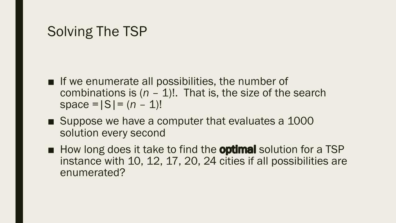
Solving The TSP

■ If we enumerate all possibilities, the number of combinations is (n – 1)!. That is, the size of the search space =|S|= (n – 1)!

■ Suppose we have a computer that evaluates a 1000 solution every second

■ How long does it take to find the optimal solution for a TSP instance with 10, 12, 17, 20, 24 cities if all possibilities are enumerated?

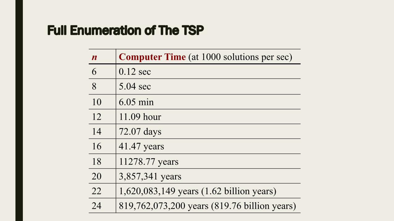
Full Enumeration of The TSP

n Computer Time (at 1000 solutions per sec)6 0.12 sec8 5.04 sec10 6.05 min12 11.09 hour14 72.07 days16 41.47 years18 11278.77 years20 3,857,341 years22 1,620,083,149 years (1.62 billion years)24 819,762,073,200 years (819.76 billion years)

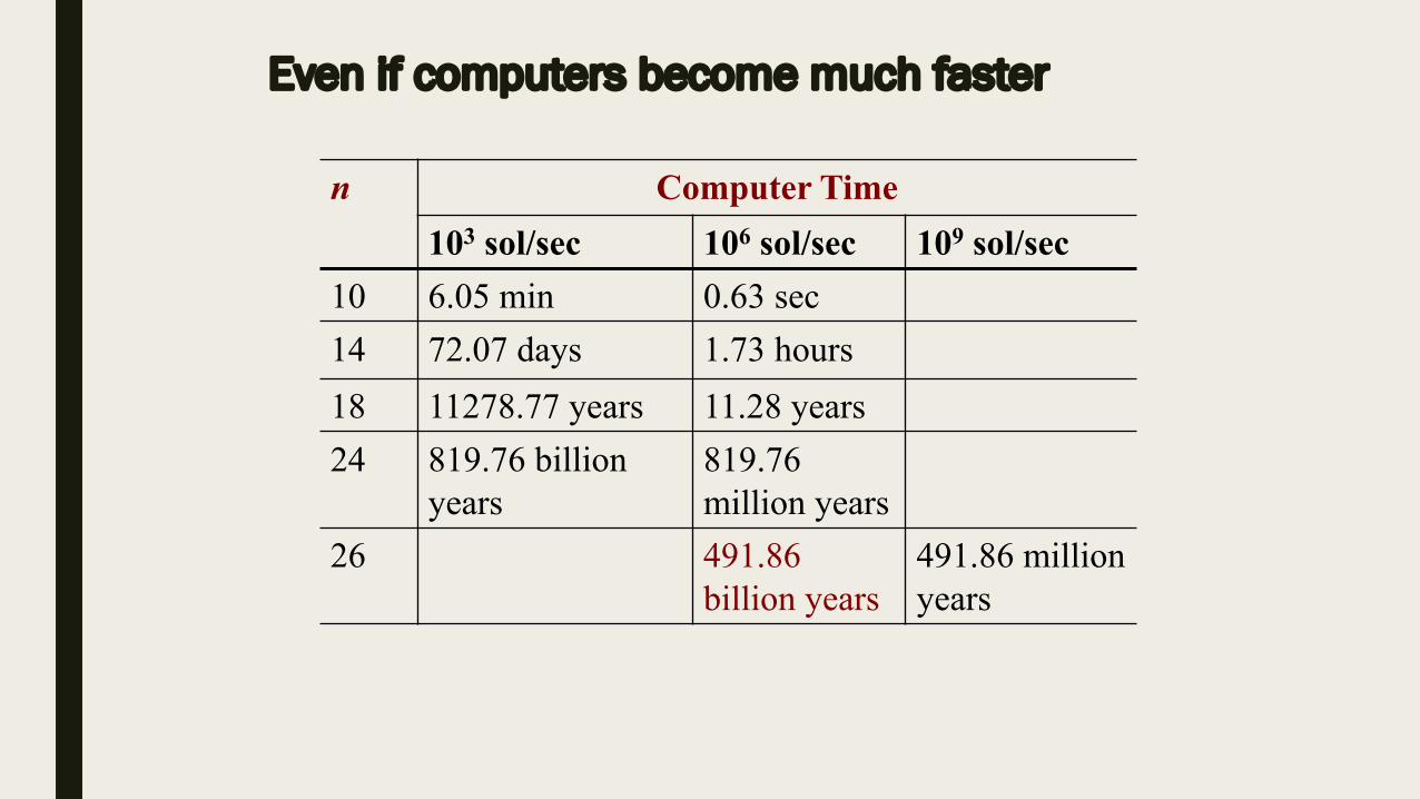
Even if computers become much faster

n Computer Time103 sol/sec 106 sol/sec 109 sol/sec

10 6.05 min 0.63 sec14 72.07 days 1.73 hours18 11278.77 years 11.28 years24 819.76 billion

years819.76 million years

26 491.86 billion years

491.86 million years

1.4 Optimality and Practicality

■ We have been trained to search for exact (perfect) solutions to problems using mathematics, but this is not always possible for various reasons:

👉 Models are approximate representations of the real system. So, even if we obtain exact solutions to the model, such solutions would not necessarily constitute exact solutions to real system.

👉 Automatic computing devices cannot store exact representation of real numbers, so numbers are often rounded off. Accumulated round-off error can distort the final results.

👉 In many cases, input data are approximated values, which means exact solutions are not perfect for the exact problem

👉 Finally, the inherent difficulty of some problems might suggest that accepting suboptimal solutions is the only practical approach especially for algorithms that take an exponential amount of computation time to guarantee optimal solutions.

■ Settling for solutions of merely “good enough” is not always settling for lower standards especially in a complex and subjective world.

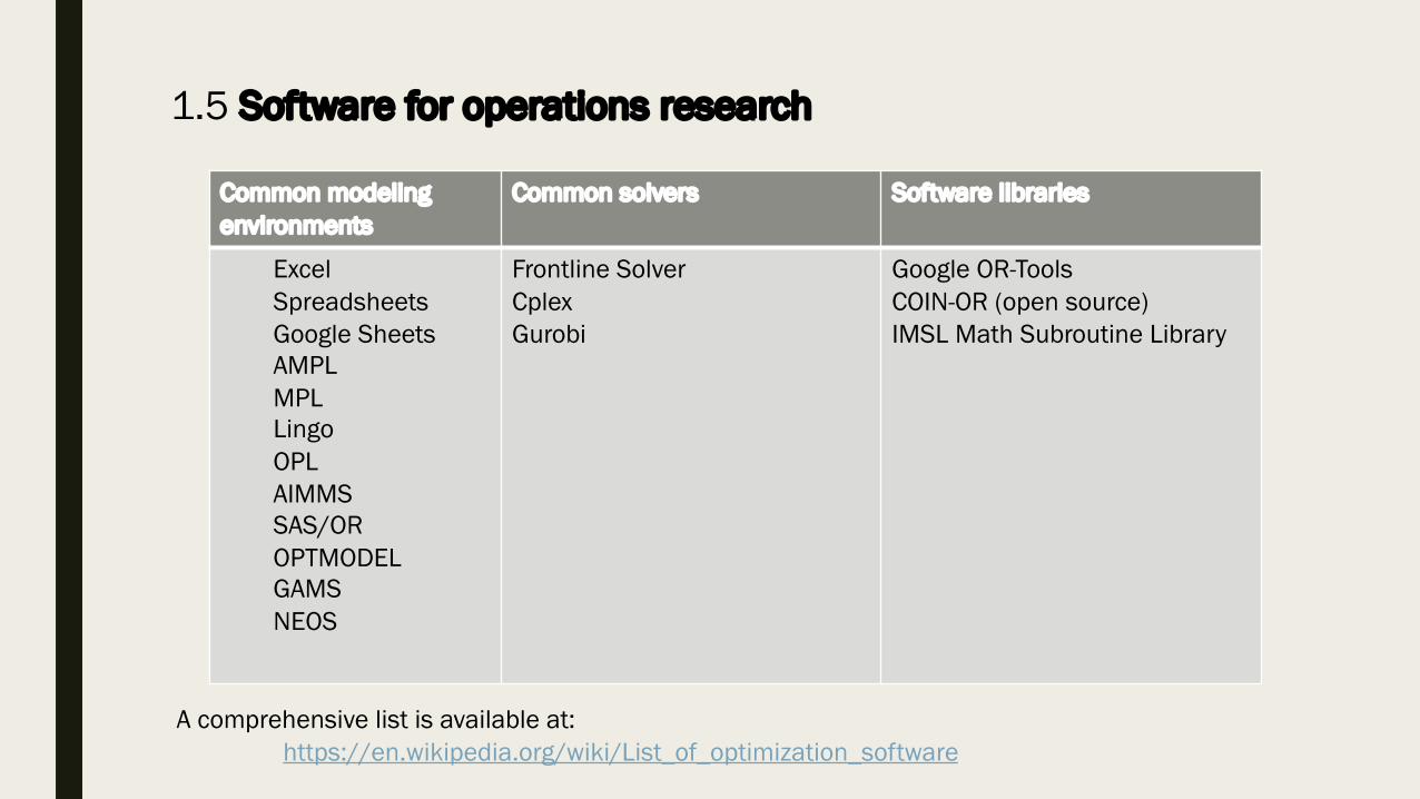
1.5 Software for operations research

Common modeling environments

Common solvers Software libraries

Excel SpreadsheetsGoogle SheetsAMPLMPLLingoOPLAIMMSSAS/OR OPTMODEL GAMS NEOS

Frontline SolverCplexGurobi

Google OR-ToolsCOIN-OR (open source)IMSL Math Subroutine Library

A comprehensive list is available at: https://en.wikipedia.org/wiki/List_of_optimization_software