CfA Plasma Talks

Antoine Bret

Notes from a series of 13 one hour (or more) lectures on Plasma Physics given to RameshNarayan’ research group at the Harvard-Smithsonian Center for Astrophysics, between Jan-uary and July 2012.

Lectures 1 to 5 cover various key Plasma Physics themes. Lectures 6 to 12 mainly go overthe Review Paper on “Multidimensional electron beam-plasma instabilities in the relativis-tic regime” [Physics of Plasmas 17, 120501 (2010)]. Lectures 13 talks about the so-calledBiermann battery and its ability to generate magnetic fields from scratch.

Contents

1 Introduction 2

2 Kinetic theory 4

3 From Kinetic to Fluid to MHD Equations 6

4 Linear Landau damping - The Maths 8

5 Landau damping - The Physics, Plasma Echo, and a (little) word about thenon-linear problem 18

6 Beam Plasma Instabilities - Introduction 23

7 Two-stream Instability 24

8 Filamentation Instability - Part 1 28

9 Filamentation Instability - Part 2 32

10 Oblique Modes 38

11 Temperature Effects 45

12 Non-Linear Regime 49

13 Ohm’s law and the Biermann battery 55

1

arX

iv:1

205.

6259

v3 [

astr

o-ph

.HE

] 1

1 Ju

l 201

2

1 Introduction

When is a gas ionized?

• Ionization can come from the plasma itself, if hot enough. With X = Ne/Nneutral,Saha equation gives,

X2

1−X=

1

nh2(2πmekBT )3/2e−I/kBT , (1)

where I is the Ionization energy. Comes from statistical physics inside atom + Maxwelldistribution outside. X → 0 for kBT < I, and X → 1 for kBT I.

Figure 1: Degree for Ionization for Hydrogen, with, I = 13.6 eV.

• Ionization can come from external medium (Ionosphere ? T = say 1000 K).

• Ionization can come from the proximity of atoms ? Share electrons : metal.

Classification

Say temperature T , density N .Typical distance between two electrons: N−1/3.Typical Coulomb energy: e2/N−1/3.Typical kinetic energy in classical regime: kBT .More kinetic energy than Coulomb: kBT > e2/N−1/3. Big frontier.Classical relativistic: kBT > mc2.Then come quantum effects. When T > Fermi temperature TF , with kBTF = ~2(3π2N)2/3/2me.Thus, for T < TF , energy increases with density, not temperature.kBTF < mc2, kB scales like N2/3.kBTF > mc2, kB scales like N1/3 (White Dwarfs to Neutron Stars?).

2

Important quantities

Time it takes to neutralize charge in-balance: Plasma frequency

ω2p =

4πNe2

me

= 9000√N [cm−3]. (2)

That’s why some waves bounce against the ionosphere.Distance over which charge in-balance can exist: Debye length

λD =Vthωp

=

√kBT

4πNe= 7.43 102

√T [K]/N [cm−3] [cm]. (3)

Figure 2: Classification of plasmas.

3

2 Kinetic theory

Vlasov and Boltzmann equations

Say only electrons + fixed positive background. Most basic description level. G(r,p, t)d3rd3p= number of particles in d3rd3p around (r,p) at time t. How does it evolve?

Say a particle has momentum p at position r, at time t. Say a force F acts on it. At timet+ dt, it will have momentum p + Fdt, and position r + p/γm dt (non-quantum treatment).Therefore, ALL particles in d3rd3p around (r,p) at time t MUST be in d3rd3p around (r +p/γm dt,p + Fdt) at time t+ dt. That means,

G

(r +

p

γmdt,p + Fdt, t+ dt

)= G(r,p, t) (1)

The “hyper” volume element d3rd3p does not change (Jacobian = 1 here). Just Taylor expandthe left-hand-side to get the Vlasov Equation,

G(r,p, t) +∂G

∂r· p

γmdt+

∂G

∂p· Fdt+

∂G

∂tdt = G(r,p, t),

⇒ ∂G

∂r· p

γm+∂G

∂p· F +

∂G

∂t= 0. (2)

Now, this result is NOT always right. Why?We have assumed the force F does not change over dt. But F is an averaged force, in thesame way the function G is averaged (IGM = 10−6 part/cm−3. If not averaged, d3r must begigantic, not infinitesimal). What if something “un-smooth” happened during dt ?

Close collisions are local, quasi-instantaneous processes, sending some particles OUT ofd3p around p, and some other particles INSIDE d3p around p, during dt. (Think aboutbilliard ball collisions: local and instantaneous). We’ll then have,

G(r,p, t) +∂G

∂r· p

γmdt+

∂G

∂p· Fdt+

∂G

∂tdt

= G(r,p, t) + [Collisions(r, t), q→ p,∀q]− [Collisions(r, t), p→ q,∀q], (3)

giving the Boltzmann Equation,

∂G

∂r· p

γm+∂G

∂p· F +

∂G

∂t=

∫q

[Collisions(r, t), q→ p]− [Collisions(r, t), p→ q]. (4)

The right-hand-side, referred to as the “collision term”, is analitically untractable. Yet,that’s the one driving the relaxation to a Maxwellian distribution GM ∝ e−v

2. For practical

purposes, alternative forms have been worked-out (Fokker-Planck/Landau, Balescu, Krookν(GM −G). . . ).

4

Vlasov or Boltzmann ?

In a plasma, particles are influenced by,

• Close collisions, changing p rapidly and appreciably (say θ > π/2). Accounted for bythe collision term in the kinetic equation.

• “Distant” collisions, which amount to the influence of the overall plasma (ρ,J→ E,B).Accounted for by the Force term in the kinetic equation.

Define a “close” collision by closest approach1 < RL, such as e2/RL = EK where EK is thetypical Kinetic energy (kBT or kBTF ). Frequency for such collisions is roughly ν ∼ nR2

LvK ,with mv2

K = EK . Time scale for “distant” collisions if ∼ ω−1p . Vlasov’s equation, with collision

term = 0, is valid for ν ωp, i.e.,

n

(e2

EK

)2√EKm√

4πne2

m⇔ e2n1/3 EK , (5)

which just defines weakly coupled plasmas, where there is more kinetic energy than Coulombpotential energy, whether degenerate or not.

The Vlasov-Maxwell system

For weakly coupled plasmas, the first equation needed is therefore Vlasov’s with F = Lorentz,

∂G

∂t+

p

γm· ∂G∂r

+ q[E(r, t) +

v

c×B(r, t)

]· ∂G∂p

= 0. (6)

System is closed with Maxwell’s equations, where charge and current densities are given by,

ρ(r, t) =

∫G(r,p, t)d3p,

J(r, t) =

∫qG(r,p, t)vd3p. (7)

Eqs. (6,7), together with Maxwell’s, form the Vlasov-Maxwell closed system of equations. In1D along axis x, we just have for G(x, p, t) and E(x, t),

∂G

∂t+

p

γm

∂G

∂x+ qE

∂G

∂p= 0,

∂E

∂x= 4πq

∫G(x, p, t)dp, (8)

with q = −e for electrons. Landau damping comes from these 2, originally with γ = 1.

1Subscript L stands (again) for Landau.

5

3 From Kinetic to Fluid to MHD Equations

From Kinetic to Fluid

Fluid equations can be deduced from the moments of the kinetic equation1. The fluid macro-scopic density n, velocity v and pressure tensor P are defined through,

n(r, t) =

∫F (r,u, t)d3u, P(r, t) =

∫m(u− v)⊗ (u− v)F (r,u, t)d3u,

n(r, t)v(r, t) =

∫uF (r,u, t)d3u, (1)

where ⊗ is “dyadic” product u ⊗ v = (uivj). If our plasma is cold, which kinetically meansF (r,u, t) = δ[u − v(r, t)]G(r, t), the density n(r, t) and the velocity v(r, t) are what wewould expect. Interestingly enough, the pressure tensor vanishes. Microsopic velocity spreadtranslates to macroscopic pressure. Consider now the non-relativistic Vlasov kinetic equation,

∂F

∂t+ v · ∂F

∂r+

E + v ×B/c

m· ∂F∂v

= 0. (2)

The moments of the equation give,2∫[Vlasov] d3p ⇒ ∂n

∂t+

∂

∂r· (nv) = 0,∫

mu [Vlasov] d3p ⇒ mn

(∂v

∂t+ v · ∂v

∂r

)= qn

(E +

v

c×B

)− ∂

∂r·P. (3)

For isotropic pressure3 with P = pI, the last term is just the usual gradient ∂p/∂r = ∇p.The “convective derivative” term (∂t + v · ∇) simply follows a fluid element.

At this stage, you can close the system introducing a relation between n(r, t) and p(r, t),that is, an equation of state. Like for the first moment and the pressure, the Vlasov moment∫un( )d3u always yields a macroscopic quantity ∝

∫un+1( )d3u from the v · ∂F/∂r term.

Still regarding the micro/macro duality: a non-zero collision term in the Vlasov equation isneeded to recover viscosity or friction on the macro level.

From Fluid to MHD

We have initially one distribution function Fi(r,u, t) per species. The procedure above showswe eventually have one set of fluid equations per species. Assume we just have protons and

1See the Appendix of Spitzer’s Physics of Fully Ionized Gases for details. Also, Chapter I of William L.Kruer, The Physics of Laser Plasma Interactions (Previewed on Google Books).

2Not straightforward. See Kruer for details. Note that ∂/∂r is an alternative notation for ∇.3If the pressure tensor is anisotropic, with P = (pi,j),

∂

∂r·P =

(∂pxx∂x

+∂pyx∂y

+∂pzx∂z

,∂pxy∂x

+∂pyy∂y

+∂pzy∂z

,∂pxz∂x

+∂pyz∂y

+∂pzz∂z

).

6

electrons of densities np(r, t) and ne(r, t). If we want to describe fast phenomenon whereelectrons could be decoupled from protons (faster than ω−1

p , or smaller than λD), we need tokeep two sets of equations. The so-called Braginskii Equations might be the most elaborateversion of this option.

What if we’re interested in slow τ ω−1p , and large scale λD, effects? Electrons are

expected to closely follow protons. The plasma is a electron/proton “soup”. Electroneutralityon these scales gives np(r, t) ∼ ne(r, t). In the same way we defined the fluid quantities (1)and found they obey Eqs. (3), we define the MHD variables,

ρ(r, t) = mpnp(r, t) +mene(r, t), V(r, t) =meve +mpvp

me +mp

J(r, t) = qnp(r, t)vp(r, t)− qne(r, t)ve(r, t). (4)

Combining the fluid equations for electrons and protons yields4,

∂ρ

∂t+∂(ρV)

∂r= 0, (5)

ρ

(∂V

∂t+ V · ∂V

∂r

)=

J

c×B−∇(

P︷ ︸︸ ︷pi + pe) + ρg, (6)

where ρE is neglected with respect to the Lorentz force, as ne ∼ np ⇒ E ∼ 0. Also, a gravityterm ρg is added here. Its fluid counterpart in Eq. (3) would obviously be nmg. The systemis closed through,

∂B

∂t= −c∇× E, ∇×B =

4π

cJ +

1

c

∂E

∂t. (7)

Inserting J = c∇×B/4π into Eq. (6) gives the usual magnetic pressure and tension terms.The last equation used to close the system is Ohm’s law, which simplest version reads

J = σ

(E +

V

c×B

), (8)

where σ is the medium conductivity. This equation is just J = σE in the fluid-frame atvelocity V, transformed in the Lab. frame5. Ideal MHD sets σ =∞, so that E = −V×B/c.Two concluding remarks:

• Yes, we sometime consider E = 0, like in Eqs. (6) and (7-right), and sometime E 6= 0like in Ohm’s law or (7-left). Kulsrud6 explains well how this proves reasonable.

• We’ve cheated a little bit. We use the collisionless Vlasov’s equation, and then talkabout EOS or Ohm’s law, which imply collisions. It’s just far simpler to forget aboutcollisions at the kinetic/micro level, derive the fluid equations, and then get collisionsback into the game, kind of empirically, at the fluid/macro level.

4Eqs. (3) formally give a non-linear term npmp(vp · ∇)vp + neme(ve · ∇)ve 6= ρ(V · ∇)V. An “=” isobtained neglecting the electron momentum, and considering V ∼ vp.

5J.D. Jackson, Classical Electrodynamics, p. 472.6R.M. Kulsrud, Plasma Physics for Astrophysics, p. 44.

7

4 Linear Landau damping - The Maths

Just a piece of a vast problem: Energy exchange between waves and particles in a plasma.Simply put, in terms of the energy transfer direction:• Waves → Particles: Particle acceleration, wave damping.

• Particles → Waves: Wave instability.

The original paper is Ref. [1]. Landau damping is one of the most studied/debated problemin plasma physics. Nice Maths and Physical derivation1.

Calculation overview

Since the calculation is quite subtle and long, it may be useful to get a general overview fromthe very beginning. Here are the steps we will follow:

1. Derivation of the dispersion equation ε(k, ω) = 0 from the 1D Vlasov-Poisson system.

2. Landau contour, the continuity requirement and the Laplace transform.

3. Resolution for small damping and any distribution function.

4. Maxwellian distribution.

Dispersion Equation

Start from 1D non-relativistic equations2 for F (x, v = p/m, t) and field E(x, t),

0 =∂F

∂t+ v

∂F

∂x− eE

m

∂F

∂v, (1)

∂E

∂x= 4πe

[n0 −

∫F (x, v, t)dv

], (2)

where n0 =∫F0dv is the equilibrium density. Assume F = F0 + F1, with | F1 || F0 |, F0

being an equilibrium solution. Same for E. The equilibrium electric field E0 = 0. LinearizingEqs. (1,2), assuming F1, E1 ∝ exp(ikx− iωt), gives

0 = −iωF1 + ikvF1 − eE1

m

∂F0

∂v, (3)

ikE1 = −4πe

∫F1(x, v, t)dv. (4)

1See Kip Thorne’s Caltech course “Applications of Classical Physics”, Chapter 21 mostly for the Mathspart at http://www.pma.caltech.edu/Courses/ph136/yr2004/.

2Easily generalized to 3D.

8

Figure 3: Imaginary part of G =∫e−u

2du/u− x, for x ∈ C. The real axis is a discontinuity.

Extract F1 from the first equation, and plug it into the second,

ε(k, ω) = 0, with,

ε(k, ω) = 1−ω2p

k2

∫f ′0

v − ω/kdv, (5)

where ω2p = 4πn0e

2/m, f0 = F0/n0 and f ′0 = ∂f0/∂v. This dispersion relation was firstobtained by Vlasov in 1925 [2]. It shows ω should be imaginary. Otherwise, we have aproblem, unless f ′0(ω/k) = 0. The dielectric function ε(k, ω) has therefore a real and animaginary part, which for all kind of systems, is related to dissipation.

We could just consider ω imaginary and take this quadrature as it is, integrating alongthe real axis. But there’s a problem. The resulting function of ω is discontinuous, preciselywhen crossing the real axis. As an illustration, Fig. 3 displays the imaginary part of G =∫e−u

2du/u − x, for x ∈ C. The discontinuity is obvious around Im(x) = 0. One part of

the plan has to be physically meaningful, and the other not. But which one? We couldtry both options, and check that damping comes only when choosing the upper one. Butwhat if we didn’t know in the first place that a Maxwellian is stable? We shall see that aLaplace analysis of the problem can fully answer the question, and will indeed tell us that the“physical” half-plane is the upper one.

Admitting for now the upper-plane is the physical one, what do we do with the lowerone? The answer is that we have to “analytically continuate” the function we have on theupper-plane, to the lower one. This means finding a function on the lower plane which makesa continuous, “analytical” junction, with what we have on the upper one. In this respect,a uniqueness theorem from complex analysis helps: if somehow we find an expression in thelower plane matching what we have in the upper one, then this is the only one. The Landaucontour is going to do all of that for us: providing a contour of integration equivalent to anintegration over the real axis for Im(ω) > 0, and an analytical continuation of the later in thelower plane Im(ω) < 0.

9

ω / kω / k

v

ω / k

Figure 4: The Landau integration contour. It is not closed. It lies always on the same side ofthe pole. It lies below the pole.

Landau contour, the continuity requirement and the Laplace trans-form

Let’s first give the solution found by Landau, namely the famous “Landau contour”. Figure4 shows this integration contour has 3 very distinctive features:

1. The Landau contour is not closed by the “usual” semi-circle in the lower or upperhalf-plane.

2. The pole ω/k = (ωr + iδ)/k must always lie on the same side of the Landau contour.

3. So, which side? The Landau contour goes below the pole.

These contour prescriptions are called the “Landau prescriptions”, and the correspondingcontour, the “Landau contour”. We thus rewrite from now on Eq. (5) as

ε(k, ω) = 1−ω2p

k2

∫L

f ′0v − ω/k

dv, (6)

where∫L

means integration along the Landau contour. Let’s now find out about these 3features.

The contour is not closed

The contour just goes from v = −∞ to +∞, and is not closed in the upper or lower half-plane, as “usual”, because we have no guarantee f ′0(v) behaves correctly there, so as to cancelthe integration on the semi-circle at infinite radius. Indeed, considering a Maxwellian withf ′0 ∝ e−v

2and setting v = Rve

iθv to parameterize the integration on a circle of radius Rv, wefind f ′0 ∝ e−R

2v cos 2θv which can hardly be considered a vanishing quantity at Rv →∞ for any

θv ∈ [0, π] (or [0,−π], if you close in the lower half-plane).

Always on the same side

Assume ω = ωr + iδ, with δ > 0. As long as δ remains positive in Eq. (5), the calculationdoes not pose any conceptual problem as the pole is not on the real axis, and continuity isguaranteed.

10

Now, what if δ approaches 0, and the pole ω/k even gets to cross the real axis? We wouldlike ε(k, ω) to be a continuous function of ω. Assume first we leave the integration contourunchanged (the real axis for v), and compare the quadrature for ω = ωr + iδ and ω = ωr− iδ.The influence of the pole is mostly felt where the denominator is minimum at v ∼ ωr/k, solet’s locally get f ′0 out of the integral and compare,

I1 =

∫dv

v − (ωr + iδ)/kand I2 =

∫dv

v − (ωr − iδ)/k. (7)

The difference I1 − I2 is,

I1 − I2 = 2i

∫δ/k

(v − ωr/k)2 + (δ/k)2dv. (8)

The continuity of ε(k, ω) demands the expression above vanishes when δ → 0+. The problemis that it does not. Instead, the quadrature tends to π (see function G2 in Appendix A), sothat we indeed have a jump of amplitude 2iπ when crossing the real axis3.

The only way to avoid this is to deform the integration contour in such a way that italways lies on the same side of the pole ω/k.

The contour goes below the pole

To understand why the contour goes below the pole and not above like in Fig. 6, we needto follow Landau in rethinking the problem in terms of the time evolution of a perturbationapplied at t = 0. The Fourier technique is not well suited for that because it entails anintegration from t = −∞ to +∞. By design, it does not single out any special momentin between. By contrast, the Laplace transform involves times only from zero to +∞. Asshall be checked, the Laplace transform technique gives an unambiguous response about thelocation of the pole with respect to the integration contour.

Considering a function h(t), its Laplace transform h(ω) and the inversion formula4, read

h(ω) =

∫ ∞0

eiωth(t)dt, (10)

h(t) =

∫CL

e−iωth(ω)dω, (11)

where the contour CL pictured on Fig. 5, passes above all the poles of h(ω) at height σ > 0,and can be closed in the lower half-plane where e−iωt behaves conveniently as to cancel the

3It can also be said that for I1, the integration path makes a counter -clockwise half-turn around the pole,so that I1 = iπ. But for I2, the half-turn around the pole is clockwise, so that I2 = −iπ and I1 − I2 = 2iπ.

4I here follow Landau’s book, [3], p. 139, in defining the Laplace transform this way. That’s just the usualone,

g(p) =

∫ ∞0

g(t)e−ptdt, (9)

for p = −iω. It avoids having to rotate everything in the complex plane to relate the calculation to Eq. (5).

11

Re(ω)

Im(ω)

σ > 0ω1

ω2ω3

ω5

ω6

ω4

ωn

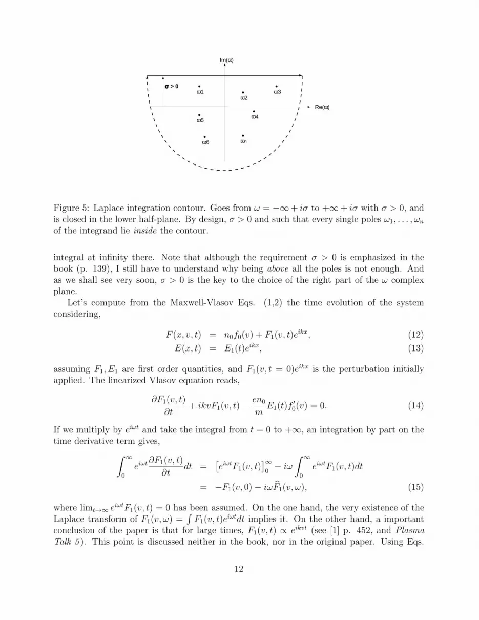
Figure 5: Laplace integration contour. Goes from ω = −∞+ iσ to +∞+ iσ with σ > 0, andis closed in the lower half-plane. By design, σ > 0 and such that every single poles ω1, . . . , ωnof the integrand lie inside the contour.

integral at infinity there. Note that although the requirement σ > 0 is emphasized in thebook (p. 139), I still have to understand why being above all the poles is not enough. Andas we shall see very soon, σ > 0 is the key to the choice of the right part of the ω complexplane.

Let’s compute from the Maxwell-Vlasov Eqs. (1,2) the time evolution of the systemconsidering,

F (x, v, t) = n0f0(v) + F1(v, t)eikx, (12)

E(x, t) = E1(t)eikx, (13)

assuming F1, E1 are first order quantities, and F1(v, t = 0)eikx is the perturbation initiallyapplied. The linearized Vlasov equation reads,

∂F1(v, t)

∂t+ ikvF1(v, t)− en0

mE1(t)f ′0(v) = 0. (14)

If we multiply by eiωt and take the integral from t = 0 to +∞, an integration by part on thetime derivative term gives,∫ ∞

0

eiωt∂F1(v, t)

∂tdt =

[eiωtF1(v, t)

]∞0− iω

∫ ∞0

eiωtF1(v, t)dt

= −F1(v, 0)− iωF1(v, ω), (15)

where limt→∞ eiωtF1(v, t) = 0 has been assumed. On the one hand, the very existence of the

Laplace transform of F1(v, ω) =∫F1(v, t)eiωtdt implies it. On the other hand, a important

conclusion of the paper is that for large times, F1(v, t) ∝ eikvt (see [1] p. 452, and PlasmaTalk 5 ). This point is discussed neither in the book, nor in the original paper. Using Eqs.

12

ω / k ω / k

v

ω / k

Figure 6: Forbidden option for the contour. Continuity is preserved, but the contour liesabove the pole, in contradiction with the Laplace prescription.

(15,14) then gives,

(ikv − iω)F1(v, ω)− en0

mE1(ω)f ′0(v) = F1(v, 0), (16)

where F1(v, 0) now acts like a “source term” at the right-hand-side. A few more manipulationsexploiting Poisson’s equation (2) give,

E1(ω) =1

ε(k, ω)

4πe

k2

∫ ∞−∞

F1(v, 0)dv

v − ω/k, (17)

where ε(k, ω) is identical to Eq. (5). The time dependant electric field given by the inversionformula (11) is,

E1(t) =

∫CL

e−iωtE1(ω)dω =

∫CL

e−iωt

ε(k, ω)

[4πe

k2

∫ ∞−∞

F1(v, 0)dv

v − ω/k

]dω. (18)

In contradistinction with Eq. (5) where the contour issue is puzzling, the Laplace tech-nique used here is clear: The v-integration in ε(k, ω) does go along the real axis, and theω-integration is performed at fixed Im(ω) = σ > 0. It means that in Eq. (18), which com-putes a physical quantity, the dielectric function ε(k, ω) is calculated with ω above the realv-axis.

That answers the question we had: the physically meaningful half-plane we were wonderingabout after Eq. (5) is the upper one. The kind of contour pictured on Fig. 6 is thus“forbidden”.

Incidentally, what are the poles of the integrand in Eq. (18)? For “normal”, smooth initialexcitations F1(v, 0), the term between brackets won’t have poles, so that our poles ω1, . . . , ωnare eventually the zeros of ε(k, ω). The ω-integration of Eq. (18) on the closed contour CLwill thus give, with ωj = ωr,j + iδi,

E1(t) = 2iπn∑j=1

Res(j) ≡n∑j=1

Aj exp(−iωjt) =n∑j=1

Aj exp(−iωr,jt)eδjt, (19)

which for large times will be governed by the largest δj. Therefore, the Laplace transformapproach cannot spare us the resolution of ε(k, ω) = 0, as these zeros are the building blocksof the temporal response of the system.

13

Resolution for small damping

We suppose small damping, that is |δ| |ωr|, and Taylor expand Eq. (6),

ε(k, ωr + iδ) = εr(k, ωr) + iδ∂εr∂ωr

∣∣∣∣δ=0

+ i

[εi(k, ωr) + iδ

∂εi∂ωr

∣∣∣∣δ=0

]= εr(k, ωr) + iεi(k, ωr) + δ

[i∂εr∂ωr− ∂εi∂ωr

]δ=0

= ε(k, ωr) + iδ∂εr∂ωr

∣∣∣∣δ=0

+ o(δ), (20)

where the o(δ) (negligible with respect to δ), comes from the fact that εi(δ = 0) = 0 (nodamping, no dissipation, no imaginary dielectric function).

The first term ε(k, ωr) is given by Eq. (6) setting ω = ωr, or taking the limit of ε(k, ωr+iδ)for δ → 0+. The part of the integration along the real axis for v ∈ [−∞, ωr/k − ε] ∪ [ωr/k +ε,+∞] gives the so-called “Cauchy Principal Part”, denoted P here. The part correspondingto the semi-circle (see Fig. 4 middle) gives the semi-residue for v = ωr/k. An alternative wayof deriving this result, considering the limit δ → 0+, is reported in Appendix A. We thus get,

ε(k, ωr) = 1−ω2p

k2

[P

∫f ′0

v − ωr/kdv + iπf ′0(ωr/k)

]. (21)

This result allows to compute ∂εr/∂ωr in Eq. (20), which eventually gives,

ε(k, ω) = 1−ω2p

k2P

∫f ′0

v − ωr/kdv − i

ω2p

k2

[πf ′0(ωr/k) + δ

∂

∂ωrP

∫f ′0

v − ωr/kdv

]. (22)

Equating the real part to zero yields,

ω2p

k2P

∫f ′0

v − ωr/kdv = 1, (23)

which was the result obtained by Vlasov in the first place. Canceling the imaginary part givesdirectly the damping rate,

δ = −π f ′0(ωr/k)∂∂ωr

P∫ f ′0

v−ωr/kdv. (24)

Eqs. (23, 24) formally solve the problem in terms of the distribution function. A first orderevaluation of P∼ k2/ω2

r (see Eq. (27) below), gives

ωr = ωp, and then (25)

δ

ωp=

π

2

ω2p

k2f ′0(ωp/k).

The rate δ has the sign of f ′0(ωp/k). That means that if f0 decreases for v = ωp/k, thewaves is damped because δ < 0. But if f0 increases for v = ωp/k, we have δ > 0 and the wavecan actually grow.

14

One could argue we started initially assuming δ positive, and find it can be negative here.It is not a problem for the following reason: Eq. (22) we found assuming δ > 0 is continuousat δ = 0. It must therefore be identical to the integration on the Landau contour on bothsides of the real axis. We can therefore confidently solve it regardless of the sign of δ. Inother words, thanks to the Landau contour, we can compute the result as if δ was positive,and then don’t care about the sign.

Historically, Vlasov first ran into Eq. (5). He escaped the problem posed by the pole onthe real axis by considering only the P of the quadrature. He did so apparently without muchfoundation, which Landau denounced without mercy in [1]. We understand from the analysisabove that doing so, he missed the imaginary part which would have led to the “Vlasovdamping”.

Maxwellian distribution

Let’s finally consider a 1D Maxwellian distribution,

f0(v) =1√

2πkBT/me−mv

2/2kBT . (26)

For phase velocities ωr/k much larger than the thermal velocity Vth =√kBT/m, we can

expand the denominator in powers of kv/ωr, since that quantity is small where the numeratoris relevant. We thus have,

P

∫f ′0

v − ωr/kdv = − k

ωr

∫f ′0

(1 +

kv

ωr+k2v2

ω2r

+k3v3

ω3r

+ · · ·)dv

=k2

ω2r

+ 3kBT

m

k4

ω4r

+ · · · (27)

For small k, namely kVth/ωr ∼ kVth/ωp 1, Eq. (23) now gives,

ω2r = ω2

p(1 + 3k2λ2D), with λD =

√kBT/m

ωp. (28)

We finally (phew!) use Eq. (24) to extract the damping rate. On the one hand, we computethe derivative of the P with respect to ωr using Eq. (27), and then simply set ωr = ωp in theresult. On the other hand, we set ωr = ωp in f ′0 to find5

δ = −ωp√π/8

k3λ3D

exp

(− 1

2k2λ2D

). (29)

Fluid theory just gives the real part of the frequency, namely Eq. (28), so that Landaudamping is a purely kinetic effect.

5Some authors insert the full expression of ωr from Eq. (28), yielding −1/2k2λ2D − 3/2 in the argument ofthe exponential.

15

-4 -2 2 4 6 8 10v

0.2

0.4

0.6

0.8

1.0

G1

-4 -2 2 4 6 8 10v

1

2

3

4

5

G2

Figure 7: Functions G1 and G1 involved in Eq. (32). For small δ/k, G1 is almost 1 everywhere,except for v = ωr/k, where it is 0. G2 peaks at v = ωr/k and tends to 0 elsewhere, while itsintegral is always π, like a Dirac δ function. Parameters are ωr/k = 4, δ/k = 0.2 for G1, andδ/k = 0.2, 0.5, 1 for G2.

Appendix A

Let’s derive, ∫L

f ′0v − ωr/k

dv = P

∫f ′0

v − ωr/kdv + iπf ′0(ωr/k), (30)

used for Eq. (21), without using the residue theorem. For ω = ωr + iδ with δ > 0, integrationalong the Landau contour is equivalent to an integration along the real axis. Let’s thus assumeδ > 0 and compute,

I = limδ→0+

∫ ∞−∞

f ′0v − (ωr + iδ)/k

dv. (31)

We multiply the numerator and the denominator of the integrand by (v − ωr/k) + iδ/k,which is the complex conjugate of the denominator. We get an expression with a purely real,non singular denominator, and clearly separated real and imaginary parts,

I = limδ→0+

∫ ∞−∞

(v − ωr/k)2

(v − ωr/k)2 + (δ/k)2︸ ︷︷ ︸G1

f ′0(v − ωr/k)

dv + i

∫ ∞−∞

δ/k

(v − ωr/k)2 + (δ/k)2︸ ︷︷ ︸G2

f ′0dv. (32)

Regarding the real part, the factor G1 of the integrand is 0 for v = ωr/k, and ∼ 1 forδ/k |v− ωr/k|. It tends to the P

∫f ′0/(v− ωr/k) for small δ/k (see Fig. 7). The factor G2

of the integrand of the imaginary part departs from 0 only for v ∼ ωr/k. But its integral isalways π. For small δ/k, the quadrature thus tends to πf ′0(ωr/k), and we are back to (30)6.

6 The limit of iδ with δ → 0+ is sometimes written “i0”. The identity

limδ→0+

∫ ∞−∞

h(x)

x− a− iδdx ≡

∫ ∞−∞

h(x)

x− a− i0dx = P

∫ ∞−∞

h(x)

x− adx+ iπh(a),

16

This calculation is consistent with the Landau contour integration only for δ → 0+. Thisis because in such case, the real axis along which we perform the integration (32) coincidewith the Laundau contour. If we were to compute Eq. (32) for δ → 0−, we would find theopposite imaginary part, just because in this case, the real axis no longer fits the Landaucontour. The latter, instead, is deformed and keeps passing below the pole, precisely to avoidthe discontinuity.

References

[1] L.D. Landau, J. Phys. (U.S.S.R.) 10, 25 (1946).

[2] A. Vlasov, J. Phys. 9, 25 (1945).

[3] L.D. Landau and E.M. Lifshitz, Course of Theoretical Physics, Physical Kinetic.

can be referred to as the “Plemelj Formula” in the literature. For δ → 0−, the imaginary part above is−iπh(a).

17

5 Landau damping - The Physics, Plasma Echo, and a

(little) word about the non-linear problem

While the original paper [1] is purely mathematical, a clearer physical picture is providedin Landau’s book ([2], §30 p. 126). Suppose we switch on at t = 0 a 1D electrostatic waveE = E0 sin(kx − ωt)x, traveling at vφ = ω/k along with a particle with velocity v0 at t = 0.For v0 slightly larger than vφ, the particle is trapped in the wave potential, where it is goingto oscillate. Doing so, it ends up with an average velocity close to the wave velocity vφ. Itshould thus loose energy, and the energy goes to the wave. Situation is reversed for particlesinitially slightly slower than the wave. They end up gaining energy from the wave.

If slower particles are more numerous than the faster ones, the wave looses more thanit gains, which means it is damped. Let’s now “Fermi-calculate” this, not following Fermibut Jackson [3] and Spitzer [4] (who follows Jackson). Landau uses a slightly different ap-proach, still implying a calculation with some small parameter eventually tending to zero.I chose Jackson1 precisely because there’s no such trick in his strategy. The reasoning isnon-relativistic.

To start with, which particles can enter the game? If their velocity is too high relativelyto the wave, they will flow from one potential crest to another, without much net energyexchange. The ones for which energy exchange is possible, are the ones which will be trappedby the potential. The wave potential height is,

∆ϕ =qE0

k. (1)

The maximum particle velocity ∆v in the wave-frame at vφ must then satisfy,

1

2m(∆v)2 = ∆ϕ ⇒ (∆v)2 =

2qE0

mk. (2)

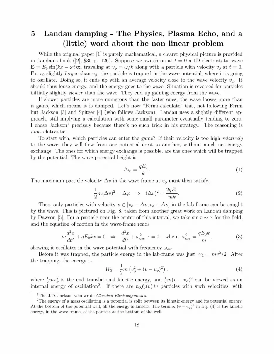
Thus, only particles with velocity v ∈ [vφ −∆v, vφ + ∆v] in the lab-frame can be caughtby the wave. This is pictured on Fig. 8, taken from another great work on Landau dampingby Dawson [5]. For a particle near the center of this interval, we take sinx ∼ x for the field,and the equation of motion in the wave-frame reads

md2x

dt2+ qE0kx = 0 ⇒ d2x

dt2+ ω2

osc x = 0, where ω2osc =

qE0k

m, (3)

showing it oscillates in the wave potential with frequency ωosc.Before it was trapped, the particle energy in the lab-frame was just W1 = mv2/2. After

the trapping, the energy is

W2 =1

2m(v2φ + (v − vφ)2

), (4)

where 12mv2

φ is the end translational kinetic energy, and 12m(v − vφ)2 can be viewed as an

internal energy of oscillation2. If there are n0f0(v)dv particles with such velocities, with

1The J.D. Jackson who wrote Classical Electrodynamics.2The energy of a mass oscillating is a potential is split between its kinetic energy and its potential energy.

At the bottom of the potential well, all the energy is kinetic. The term ∝ (v − vφ)2 in Eq. (4) is the kineticenergy, in the wave frame, of the particle at the bottom of the well.

18

v

φv

φ+∆vv

φ−∆v

resonantnon-resonant

Figure 8: Division of the plasma between non-resonant and resonant (trapped) particles. Onlyresonant particles contribute to the calculation. After [5].

∫f0 = 1, the energy shift is

dW = n0f0(v)dv(W2 −W1), (5)

which we integrate over all particles capable of such exchange,

∆W =

∫ vφ+∆v

vφ−∆v

n0f0(v)dv1

2m(v2φ + (v − vφ)2 − v2

). (6)

Expanding f0(v) = f0(vφ) + (v− vφ)f ′0(vφ) + · · · , the term corresponding to f0(vφ) in Eq. (6)vanishes3, and we find

∆W = −2

3mn0vφ∆v3f ′0(vφ). (7)

If, like on Fig. 8, particles slower than vφ are more numerous than faster ones, f ′0(vφ) < 0and ∆W > 0, which means particles gain energy at the expense of the wave. The wave isdamped. We now just have to write that this energy leaves the field E over a time scale ω−1

osc,

d(E20/8π)

dt= −ωosc∆W = ωosc

2

3mn0vφ∆v3f ′0(vφ). (8)

Plugging here the expressions for ∆v and ωosc from Eqs. (2,3) we find,

d(E20/8π)

dt=

8√

2

3ωω2p

k2f ′0(vφ)

(E2

0

8π

),

≡ 2δ

(E2

0

8π

). (9)

3It does not vanish if you omit the “internal energy” term in Eq. (4).

19

As the field energy ∝ E20 is damped at 2δ, the field itself is damped at δ. Setting finally

ω = ωp, we have

δ

ωp=

4√

2

3

ω2p

k2f ′0(ωp/k), (10)

identical to Eq. (25) of Plasma Talk 4, up to a numerical pre-factor close to 1 (π/2 = 1.57and 4

√2/3 = 1.88). A discussion of the non-Galilean invariance of Eq. (10) is available in

[3] (p. 180).

A word on Landau damping and gravitation

According to Ref. [6], Landau Damping of Gravitational Waves would not be possible. Muchhas been done with respect of Landau Damping of more mundane “gravity waves”. Thestability and vibrations of a gas of stars, by Lynden-Bell, seems to be a quite influential paper[7]. The abstract concludes stating “Landau Damping occurs for wave-length smaller thanthe critical one [Jean’s]”.

Plasma Echo

Fascinating consequence of the fact that the density relaxes whereas the distribution functiondoes not (many functions have the same integral). Original idea by Gould et al. [16].

Suppose we produce an initial electric field perturbation ∝ e−ik1x in the plasma. TheLaplace analysis [1] of the distribution function temporal evolution (not the field, nor thedensity) shows it indefinitely oscillates with F = f0 +f1(v) exp(ik1vt− ik1x). For large times,any velocity integral “phase”-vanishes,

limt→∞

∫f1(v)eik1vt−ik1xdv = 0, (11)

which is how we recover zero field and density perturbations. The density perturbation andthe field associated with f1 die out, but f1 doesn’t. This is how you reconcile the necessaryreversibility of the Vlasov-Maxwell system, with the apparent irreversibility of Landau Damp-ing. There only seems to be a macroscopic irreversibility, but the evolution in microscopicallyreversible.

Is it possible to detect this ever oscillating f1(v) at later times ? Yes. Assume we wait fora time τ , and send another perturbation in the plasma ∝ eik2x. The second perturbation isgoing to modulate both f0 and f1 according to eik2v(t−τ)−ik2x. Regarding f1, we will recoversomething varying like

eik1vt−ik1xeik2x−ik2v(t−τ) = ei(k2−k1)x+ik2vτ−i(k2−k1)vt. (12)

The key-point here is that contrary to Eq. (11), where k1t 6= 0 implies the velocity integralvanishes at large times, together with the first order density and field, the coefficient of v inthe exponential above is exactly canceled at time,

t =k2

k2 − k1

τ. (13)

20

At this time, the velocity integral will not vanish, and an electric field should reappear in theplasma. So you perturb a plasma. You wait until everything apparently calmed down. Thenyou send another perturbation, and at the time prescribed by Eq. (13), an electric field willsuddenly pop-up “out of nowhere”, related to the perturbation you first sent. That is the“plasma echo”.

The idea was experimentally tested soon after the theory came, and the echo was found[17]. Mouhot & Villani put it this ways: “A plasma which is apparently back to equilibriumafter an initial disturbance, will react to a second disturbance in a way that shows that it hasnot forgotten the first one” ([14], p. 40).

Regarding gravitational systems, Lynden-Bell wrote “A system whose density has achieveda steady state will have information about its birth still stored in the peculiar velocities of itsstars” ([7], p. 295).

Nonlinear Landau damping

We found linear waves are damped. Landau Damping has been experimentally confirmed [8].Here are a few landmarks for large amplitude waves (1D, non-relativistic)4:

• Isichenko 1997 [9]: Landau damping valid ∀ amplitude (Theory).

• Manfredi 1997 [10]: Some large amplitude waves do not decay until t =∞ (Numerical).

• Lancellotti & Dorning 1998 [11]: Existence of “critical initial states” for which limt→∞E 6=0 (Theory).

• Caglioti & Maffei 1998 [12]: Mathematical proof of the existence of some dampedsolutions (Theory).

• Medvedev et al. 1998 [13]: Damping of waves of finite amplitude and arbitrary shapeaccording to eδt, with limt→∞ δ = 0 (Theory).

Mouhot & Villani 2010 [14, 15]: End of the controversy. Nonlinear Landau damping forgeneral interactions, including Coulomb and Newton (therefore also including the case ofgalactic dynamics).

For any potential V (r) such that |V (k)| = O (|k|−2−ε), with ε > 0, and any linearlystable distribution function f0(x, v), large amplitude perturbations relax in such a way thatall observables (density, field. . . ),

Ψ(t) =

∫f(t, x, v)ψ(x, v)dxdv, (14)

relax exponentially with time. The distribution function itself does not relax to its value att = 0. For small perturbations, f(t, x, v) converges to something that is close to f0(x, v). Forlarger perturbations, the distribution function converges to something that is far from f0, or

4Thanks to Giovanni Manfredi for the summary!

21

it does not converge at all. The large time behavior of a strongly disturbed solution is stillan open mystery.

See [14] for the full report, and a great history of the problem, or [15] for a shorter version.Villani was awarded the 2010 Fields Medal for this.

References

[1] L.D. Landau, J. Phys. (U.S.S.R.) 10, 25 (1946).

[2] L.D. Landau and E.M. Lifshitz, Course of Theoretical Physics, Physical Kinetic.

[3] J.D. Jackson, J. Nucl. Energy, Part C Plasma Phys. 1, 171 (1960).

[4] L. Spitzer, Physics of Fully Ionized Gases.

[5] J. Dawson, Phys. Fluids 4, 869 (1961).

[6] S. Gayer and C.F. Kennel, Phys. Rev. D 19, 1070 (1979)

[7] D. Lynden-Bell, MNRAS 124, 279 (1962)

[8] J.H. Malmberg and C.B. Wharton, Phys. Rev. Lett. 19, 775 (1967).

[9] M.B. Isichenko, Phys. Rev. Lett. 78, 2369 (1997).

[10] G. Manfredi, Phys. Rev. Lett. 79, 2815 (1997).

[11] C. Lancellotti and J.J. Dorning, Phys. Rev. Lett. 81, 5137 (1998).

[12] E. Caglioti and C. Maffei, J. Stat. Phys. 92, 301 (1998).

[13] M.V. Medvedev, P.H. Diamond, M.N. Rosenbluth and V.I. Shevchenko, Phys. Rev. Lett.81, 5824 (1998).

[14] C. Mouhot and C. Villani, Acta Mathematica 207, 29 (2011) - arXiv:0904.2760.

[15] C. Mouhot and C. Villani, J. Math. Phys. 51, 015204 (2010) - arXiv:0905.2167.

[16] R.W. Gould, T.M. O’Neil and J.H. Malmberg, Phys. Rev. Lett. 19, 219 (1967).

[17] J.H. Malmberg, C. Wharton, R.W. Gould, and T.M. O’Neil, Phys. Rev. Lett. 20, 95(1968).

22

6 Beam Plasma Instabilities - Introduction

Miscellaneous

From now on, and for a number of Lectures, I’ll just go through the Review Paper, “Multidi-mensional electron beam-plasma instabilities in the relativistic regime”, Physics of Plasmas,17, 120501 (2010).

Counter-streaming flows, possibly relativistic. Lots of them. Basic system: counter-streaming electron beams with nb0, np0,vb0,vp0 over a background of fixed protons ni. Mainhypothesis:

• Collisionless, Vlasov-Maxwell plasmas (i.e. weakly coupled, see Plasma Talk 2 ),

• Homogenous, no boundaries (system size c/ωp),

• Initially current and charge neutral, nb0vb0 = np0vp0 and nb0 + np0 = ni,

• No B0, to start with. . .

Motivations : simplest system + Fast Ignition Scenario for Inertial Fusion + Shock Accel-eration physics (SNR’s, GRB’s). See Fig. 2 of Review Paper.

Particle-In-Cell Simulations: great tool for testing/guiding - See Fig. 3 of Review Paper.

A multidimensional unstable spectrum

• 1948: some perturbations with k ‖ to the flow are unstable - Two-stream modes.

• 1959: some perturbations with k ⊥ to the flow are unstable - Filamentation modes.Still 1959: collisionless plasma with Tx > Ty, unstable for k ‖ y. Weibel.Difference between them discussed in Sec. III. F of Review.

• 1960: some perturbations with k arbitrarily oriented are unstable - Oblique modes.

Bottom line here: Which one will Nature choose? The fastest. Need to tackle the problemglobally.

First: look at flow aligned, then flow-perp and the oblique modes. Second: which onegrows faster?

23

7 Two-stream Instability

Two-stream (flow-aligned) modes

Interesting starting with a cold fluid 1D model. Equivalent to Vlasov with f0(v) ∝ δ(v− v0).Non-relativistic. General case shows it’s still relevant for the 3D case.Linearize conservation and Euler equations. One set for each electron species, and I omitsubscripts for clarity. Consider first orders quantities n1p, n1b, E1 ∝ eikx−iωt. Conservationand Euler equations read,

∂n

∂t+∂(nv)

∂x= 0, (1)

m∂v

∂t+mv

∂v

∂x= qE. (2)

Once linearized, they respectively give

n1 = n0kv1

ω − kv0

, (3)

v1 = iqE1/m

ω − kv0

, (4)

so that,

n1 =qn0

m

ikE1

(ω − kv0)2. (5)

Then, from Poisson’s equation1

ikE1 = 4πq(n1b + n1p), (6)

we get,

1 =ω2pb

(ω − kv0b)2+

ω2pp

(ω − kv0p)2, with ω2

p,bp =4πq2n0,bp

m. (7)

The frequency ω − kv is the Doppler shifted frequency. Can’t help but thinking it lookslike an energy conservation equation. Without drifts, v0,bp = 0 and we just have

(~ω)2 = (~ωpb)2 + (~ωpp)2. (8)

Any ideas?Until Eq. (5), species are disconnected from each other in the calculation. It is Poisson’s

equation which puts them together, summing the contribution of each species. Assume aninfinite amount of these, each beamlet going at velocity v, with density n0f0(v)dv,

∫f0 = 1.

The extension of Eq. (7) reads,

1 =

∫4πq2n0f0(v)dv

m(ω − kv)2=ω2p0

k2

∫f0(v)dv

(v − ω/k)2, ω2

p0 =4πq2n0

m. (9)

1Poisson’s equation brings a vectorial equation down to a scalar one. We thus loose information, unlessk ·E = kE. The full 3D analysis shows modes with k⊥ = 0 are precisely like this.

24

identical with the one encountered in Plasma Talk 4, up to an integration by part.So if we “Fermi understand” Eq. (7), we have everything.Introducing the dimensionless variables,

x =ω

ωpp, Z =

kv0b

ωpp, α =

n0b

n0p

, (10)

Eq. (7) reads,

1 =α

(x− Z)2+

1

(x+ αZ)2. (11)

Diluted beam, α 1

There are techniques2 to solve Eq. (11) in this regime, always approximately, for all Z. I justshow here how to find the mode growing the most.

The beam is just a perturbation to the plasma. The modes of the system should be closeto the modes of the plasma alone. We thus look for solutions at ω ∼ ωpp, i.e. x = 1 + ε. Wealso know that the fastest growing mode should efficiently exchange energy with the beam.It should thus have have ω/k ∼ v0b. With ω ∼ ωp, that means Z ∼ 1. Eq (11) now reads,

1 =α

(1 + ε− Z)2+

1

(1 + ε+ αZ)2. (12)

As we’ll checked, | 1− Z | ε and αZ ∼ α ε, which gives

1 =α

ε2+

1

(1 + ε)2⇒ 1 =

α

ε2+ 1− 2ε ⇒ ε3 =

α

2. (13)

By setting ε = ρeiθ, we find

ρ =(α

2

)1/3

, θ = −2π

3, 0,

2π

3. (14)

With e±i2π/3 = −1/2± i√

3/2, we obtain 3 modes

x =ω

ωpp= 1− α1/3

24/3− i√

3

24/3α1/3, (15)

= 1− α1/3

24/3, (16)

= 1− α1/3

24/3+ i

√3

24/3α1/3, Unstable. (17)

As evidenced on Fig. 9, the most unstable mode has Z ∼ 1, that is k/ωpp ∼ v0b. An electronfrom the beam always sees the same electric field.

How to compute these results in a Fermi-like way?

2See S. A. Bludman, K. M. Watson, and M. N. Rosenbluth, Phys. Fluids 3, 747 (1960).

25

0.5 1.0 1.5 2.0Z

0.1

0.2

0.3

0.4

0.5

Im Hx L

0.5 1.0 1.5 2.0Z

-0.2

0.2

0.4

0.6

0.8

x2

Figure 9: Left: Plot of Im(x) in terms of Z for α = 10−3, 10−2, 10−1 and 1. Right: Plot ofEq. (19), x2 = 1 + Z2 −

√1 + 4Z2. The system is unstable, x2 < 0, for Z <

√2.

Symmetric beams, α = 1

Eq. (11) now reads,

1 =1

(x− Z)2+

1

(x+ Z)2, (18)

which can be solved exactly for all Z, giving

x2 = 1 + Z2 ±√

1 + 4Z2. (19)

For Z <√

2, the solution with a minus sign is unstable (see Fig. 9), with a most unstablewave-vector Zm and its frequency xm given by

Zm =

√3

2, xm = 0 + i

1

2. (20)

For the diluted beam regime, unstable modes are plasma Langmuir waves at ω ∼ ωp,traveling with the beam. Things are not so clear here. The beam is no longer a perturba-tion. The waves have Re(ω) = 0, and are the modes of the full counter-streaming system“beam+plasma”, each of equal density.

To wrap-up the most unstable mode characteristics in terms of α ∈ [0, 1]:

• Growth-rate: Im(ω/ωpp) =√

324/3

α1/3 −→ 12

(Note that√

324/3∼ 0.68 > 1

2).

• Frequency: Re(ω/ωpp) = 1−√

324/3

α1/3 −→ 0.

• Most unstable wave-vector: Z = 1 −→√

32

.

Relativistic effects

Maxwell’s and conservation equations are the same. Euler is now (subscripts omitted),

m∂(γv)

∂t+mv

∂(γv)

∂x= qE. (21)

26

It turns out that when linearizing “γv” instead of “v”, one finds,

γv = γ0v0 + v1γ30 + · · · (22)

As a result, Eq. (11) is replaced by,

1 =α

(x− Z)2γ3b

+1

(x+ αZ)2γ3p

. (23)

Intuitively, where does these 1/γ3 come from ? If a particle oscillates along its maindirection of motion, its mass gets a γ3 relativistic boost. Changing m to mγ3 is Eq. (7) givesthe result above.

Diluted beam, α 1

Here, γp ∼ 1, so that we can recycle the non-relativistic results for diluted beam, formallyreplacing α→ α/γ3

b , i.e. nb → nb/γ3b . The unstable modes given by Eq. (17) now reads,

x =ω

ωpp= 1− 1

24/3

α1/3

γb+ i

√3

24/3

α1/3

γb. (24)

Symmetric beams, α = 1

With two symmetric beams, the Lorentz factors are the same γp = γb ≡ γ. Equation (23)now reads,

1 =1

(x− Z)2γ3+

1

(x+ Z)2γ3. (25)

Here again, we just replace x → xγ3/2 and Z → Zγ3/2, and we’re formally back to thenon-relativistic case. Equation (20) then gives

Zm =

√3

2γ3/2, xm = 0 + i

1

2γ3/2. (26)

27

8 Filamentation Instability - Part 1

We still consider the same counter-streaming system, but look now at perturbations withk ⊥ to the flow. With respect to the Two-stream instability (k ‖ to the flow), the situation isreversed: The physics is simple, but the full maths are involved. Let’s start with the physics.

Physical picture

Suppose two particle currents of same radius a and density n but opposite velocities u, per-fectly overlap (Fig. 10, left). The system is charge and current neutral, in equilibrium. Wenow set them apart by a distance R (Fig. 10, right). The first current generates a B field atthe level on the second one. The field is such that the Lorentz force F produced repels theother current even more. Unstable system. We can write,

F = dMd2R

dt2, (1)

where dM is the mass of the volume element. The force reads,

F = dqu

cB, (2)

where dq is the charge of the volume element. With a density n, and particles of charge qand rest mass m, the charge dq and the mass dM of the volume dV read respectively,

dq = qndV, and dM = γmndV, (3)

where γm is the relativistic mass boost for transverse motion. Equation (1) now reads,

qndVu

cB = γmndV

d2R

dt2, i.e, q

u

cB = γm

d2R

dt2. (4)

B is the field created by the current, so that

B =2I

cR, where I = nquπa2. (5)

Replacing the current I by its expression, we find

d2ξ

dt2=δ2

ξ, with δ = ωp

β√2γ, and ξ =

R

a, β =

u

c, (6)

with ω2p = 4πnq2/m. Although this equation won’t give ξ ∝ eδt, it does tell the system

does not relax to its initial state, on a time scale ∝ δ−1, which fits exactly the result of thelinear theory1. Maybe an exponential grow would be obtained starting from opposite currentpartially overlapping.

1Up to a factor of order unity, as usual.

28

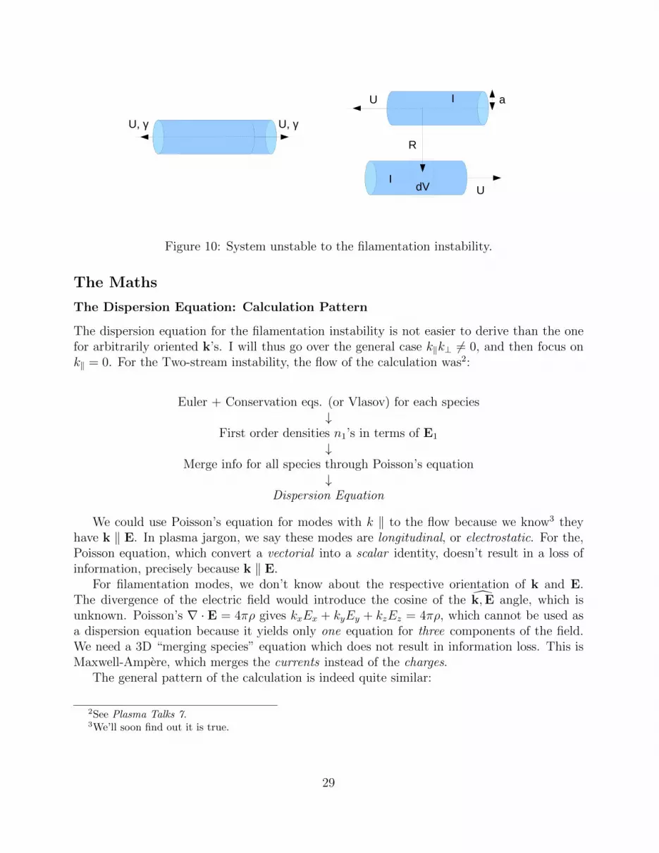
U

U a

R

U, γ

I

I

dV

U, γ

Figure 10: System unstable to the filamentation instability.

The Maths

The Dispersion Equation: Calculation Pattern

The dispersion equation for the filamentation instability is not easier to derive than the onefor arbitrarily oriented k’s. I will thus go over the general case k‖k⊥ 6= 0, and then focus onk‖ = 0. For the Two-stream instability, the flow of the calculation was2:

Euler + Conservation eqs. (or Vlasov) for each species↓

First order densities n1’s in terms of E1

↓Merge info for all species through Poisson’s equation

↓Dispersion Equation

We could use Poisson’s equation for modes with k ‖ to the flow because we know3 theyhave k ‖ E. In plasma jargon, we say these modes are longitudinal, or electrostatic. For the,Poisson equation, which convert a vectorial into a scalar identity, doesn’t result in a loss ofinformation, precisely because k ‖ E.

For filamentation modes, we don’t know about the respective orientation of k and E.The divergence of the electric field would introduce the cosine of the k,E angle, which isunknown. Poisson’s ∇ · E = 4πρ gives kxEx + kyEy + kzEz = 4πρ, which cannot be used asa dispersion equation because it yields only one equation for three components of the field.We need a 3D “merging species” equation which does not result in information loss. This isMaxwell-Ampere, which merges the currents instead of the charges.

The general pattern of the calculation is indeed quite similar:

2See Plasma Talks 7.3We’ll soon find out it is true.

29

Euler + Conservation eqs. (or Vlasov) for each species↓

First order currents J1’s in terms of E1

↓Merge info for all species through Maxwell-Ampere equations

↓Dispersion Equation

Let’s see this more in details, reasoning again from the fluid equations. Every equilib-rium quantities are now slightly perturbed with terms ∝ exp(ik · r − iωt). The linearizedconservation equations give for each species:

n1 = n0k · v1

ω − k · v0

. (7)

The linearized non-relativistic (so far) Euler equation give, still for each species:

v1 =−iq/mω − k · v0

(E1 +

v0 ×B1

c

). (8)

It is easy to eliminate B1 through Maxwell-Faraday equation,

B1 =c

ωk× E1, (9)

so that we see how Eqs. (7,8) eventually give n1 and v1 in terms of E1 alone, for each species,

v1 =−iq/mω − k · v0

(E1 +

v0 × (k× E1)

ω

),

n1 =−iqn0

m

k

(ω − k · v0)2·(

E1 +v0 × (k× E1)

ω

). (10)

We may now write Maxwell-Ampere equation, to merge the information from all thespecies into one single equation depending of E1 only,

ik×B1 =−iωc

E1 +4π

cJ1, (11)

and eliminate B1 from Maxwell-Faraday Eq. (9) to obtain,

c2

ω2k× (k× E1) + E1 +

4iπ

ωJ1 = 0. (12)

The first order current is finally expressed through,

J1 = n0,bv1,b + n1,bv0,b︸ ︷︷ ︸Beam part

+n0,pv1,p + n1,pv0,p︸ ︷︷ ︸Plasma part

. (13)

30

Although the end result is not really “user friendly”, we can see how Eqs. (10,12,13) eventuallyyield a tensorial equation of the form

T · E1 = 0. (14)

When starting from the Vlasov equation, linearization gives the first order distributionfunction for each species,

f1(k,v, ω) =iq/m

ω − k · v

(E1 +

v ×B1

c

)· ∂f0

∂v. (15)

Here again, Maxwell-Faraday Eq. (9) together with n1 =∫f1dv and v1 =

∫f1vdv, allow to

reach the dispersion equation.

31

9 Filamentation Instability - Part 2

Dispersion Equation Analysis

The tensorial equation T · E1 at the end of Plasma Talk 8 has the obvious solution E1 = 0.Now, the proper modes of our system are precisely the non-trivial solutions T ·E1 = 0, withE1 6= 01.

That tells us two things:

• If (∃ E1 6= 0 / T · E1 = 0) ⇒ det T = 0. That’s the dispersion equation, yielding ω interms of k.Assume we pick up one wave vector k. The dispersion equation

det T(k, ω) = 0, (1)

gives one or more ω’s, (ω1,k, . . . , ωN,k) ∈ CN . Each couple (k, ωj,k) defines a propermode of the system. Unstable modes have Im(ω) < 0.The fluid model usually gives a polynomial dispersion equation. Each new ingredientto the model (mobile ions, magnetic field,. . . ), adds waves. Polynomial of degree largerthan 10 are common.

• The proper modes of the system E1(k, ω) are in the Kernel of T, which is precisely theset of non-zero E1’s fulfilling T · E1 = 0.Assume again we picked up one wave vector k. The dispersion equation gives a seriesof frequencies (ω1,k, . . . , ωN,k). We thus have N tensors with vanishing determinants.Each of these N tensors has a Kernel of dimension 1 or 2 (a Kernel of dimension 3 wouldimply T=0).

T(k, ω1,k) ⇒ E1,i (k, ω1,k)i=1 or 2 ,

...

T(k, ωN,k) ⇒ E1,i(k, ωN,k)i=1 or 2 ,

So, for one couple (k, ωk), the formalism tells how is the E1 field. It lies either along a

given direction, or in a plane. In particular, the formalism tells us about the k,E angle.We don’t have to assume waves are longitudinal2 (k ‖ E), or transverse (k ⊥ E). Theformalism decides for us.

For a flow ‖ z, and k = (kx, 0, kz) as pictured on Fig. 11, the final form of the tensor T isgiven by,

T =

∣∣∣∣∣∣η2εxx − k2

z 0 η2εxz + kzkx0 η2εyy − k2 0

η2εxz + kxkz 0 η2εzz − k2x

∣∣∣∣∣∣ , (2)

where η = ω/c and εαβ is given by Eq. (8) of the Review Paper.

1We could also say we look for the eigen-vectors associated with the eigen-value λ = 0.2Also referred to as “electrostatic”.

32

z

x

y

kkx

kz

Flow

Figure 11: Axis conventions.

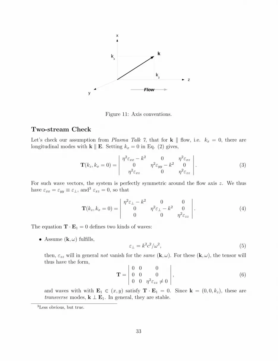
Two-stream Check

Let’s check our assumption from Plasma Talk 7, that for k ‖ flow, i.e. kx = 0, there arelongitudinal modes with k ‖ E. Setting kx = 0 in Eq. (2) gives,

T(kz, kx = 0) =

∣∣∣∣∣∣η2εxx − k2 0 η2εxz

0 η2εyy − k2 0η2εxz 0 η2εzz

∣∣∣∣∣∣ . (3)

For such wave vectors, the system is perfectly symmetric around the flow axis z. We thushave εxx = εyy ≡ ε⊥, and3 εxz = 0, so that

T(kz, kx = 0) =

∣∣∣∣∣∣η2ε⊥ − k2 0 0

0 η2ε⊥ − k2 00 0 η2εzz

∣∣∣∣∣∣ . (4)

The equation T · E1 = 0 defines two kinds of waves:

• Assume (k, ω) fulfills,ε⊥ = k2c2/ω2, (5)

then, εzz will in general not vanish for the same (k, ω). For these (k, ω), the tensor willthus have the form,

T =

∣∣∣∣∣∣0 0 00 0 00 0 η2εzz 6= 0

∣∣∣∣∣∣ , (6)

and waves with with E1 ∈ (x, y) satisfy T · E1 = 0. Since k = (0, 0, kz), these aretransverse modes, k ⊥ E1. In general, they are stable.

3Less obvious, but true.

33

• If we consider now (k, ω) fulfillingεzz = 0, (7)

we find non-zero solutions of T · E1 = 0 are waves with E1 ∈ (z), as the tensor nowtakes the form,

T =

∣∣∣∣∣∣η2ε⊥ − k2 6= 0 0 0

0 η2ε⊥ − k2 6= 0 00 0 0

∣∣∣∣∣∣ . (8)

Since k = (0, 0, kz), these are longitudinal modes, k ‖ E1, with dispersion equation,

which indeed are our two-stream modes. It is thus checked that the modes we investi-gated in Plasma Talk 7 do exist.

The Filamentation Instability

About the Dispersion Equation

Let’s now consider kz = 0 in Eq. (2). We find,

T =

∣∣∣∣∣∣η2εxx 0 η2εxz

0 η2εyy − k2 0η2εxz 0 η2εzz − k2

∣∣∣∣∣∣ , (9)

where T · E1 = 0 again defines two kinds of modes:

• Modes with E1 ∈ (y), therefore transverse since k ‖ x, with dispersion equation,

εyy = k2c2/ω2. (10)

• The Filamentation modes (at last), with E1 ∈ (x, z) and dispersion equation,

εxx(εzz − k2c2/ω2) = εxz. (11)

Of course, we would like to have εxz = 0, which would ease our life and give a simpler, twobranches dispersion equation,

εxx = 0,

εzz = k2c2/ω2. (12)

Eq. (12) has been frequently used in the literature to study the Filamentation instability4.It defines purely transverse waves with E1 ∈ (z), that is, ‖ to the flow. The problem is thatthese papers never say they assume εxz = 0. In general, they are wrong.

I wrote “in general”, because on rare occasions, they study settings for which truly, εxz = 0.Which are they? Remember that even if we now focus on k = (kx, 0, 0), this tensor element

4See Bret et al., Phys. Plasmas, 14, 032103 (2007).

34

still depends on the beam and plasma distribution functions. A detailed study5 shows εxzstrictly vanishes only if our counter streaming species are perfectly symmetric.

So, unless our density ratio is 1, and we have the same temperatures on the beam and theplasma, the same Lorentz factors, the same. . . everything, the correct dispersion equation isEq. (11), not (12).

Cold Analysis - Relativistic effects

What we’ve said is so far non-relativistic. Still in the fluid model, the main relativistic effectis displayed when linearizing the Euler equation. The relativistic Euler equation reads,

∂p

∂t+ (v · ∇)p = q

(E +

v ×B

c

), p = γmv. (13)

Its two linearized versions are,

im(k · v0 − ω)v1 = q

(E1 +

v0 ×B1

c

), non− relativistic,

im(k · v0 − ω)(γ0v1 + γ3

0

v1 · v0

c2v0

)= q

(E1 +

v0 ×B1

c

), relativistic. (14)

Everything is in the anisotropic linearization of γ0v around v0. We see above that for a smallmotion along the flow, the relativistic mass increase goes like γ3

0 . But for small motion normalto the flow, v1 · v0 = 0 and the mass increase only goes with γ. This of course, adds a levelof complexity to the general calculation, as Eq. (10) from Plasma Talk 8 for v1 is even moreinvolved.

For the filamentation instability, we have v1 · v0 = 0, and we find we can just formallyreplace m→ γm. Assuming a cold beam with density nb, Lorentz factor γb, and cold plasmaelectrons with density np and Lorentz factor γp, the tensor elements are6,

εxx = 1− α

x2γb− 1

x2γp,

εyy = 1− α

x2γb− 1

x2γp,

εzz = 1− α

x2γb− αZ2

x4γb− 1

x2γp− α2Z2

x4γp,

εxz =αZ

x3γp

(1

γp− 1

γb

), (15)

with again,

x =ω

ωpp, Z =

kvbωpp

, α =nbnp. (16)

5Ibid.6Ibid.

35

1 2 3 4Z

0.1

0.2

0.3

0.4

∆Ωp

Figure 12: Filamentation instability growth-rate for density ratios α = 1, 0.5 and 0.1, fromhigher to lower curves respectively. The beam Lorentz factor is γb = 10.

The numerical resolution of Eq. (11), when plugging the tensor elements above, yieldsthe growth-rate curves pictured on Fig. 12. As evidenced, the growth-rate just saturates forlarge Z. A trick to recover the large Z growth-rate, consists in extracting the coefficient anof Zn in the polynomial dispersion equation, as an = 0 is the asymptotic dispersion equationfor Z →∞. Doing so, one finds a zero real frequency and

limZ→∞

δ

ωpp=

vbc

√α

γb, α 1, (17)

=vbc

√2

γb, α = 1, (18)

where the agreement with Eq. (6) of Plasma Talk 8 can be checked. Note that for α = 1,the tensor elements (15) simplify substantially. Equation (12) for unstable modes is valid andreads,

x2 − 2

γ3b

− 2Z2x

x2γb=Z2x

β2, (19)

which can be solved exactly.We can follow the same line of reasoning for the “wrong” transverse dispersion equation

(12), in order to check its inaccuracy. The exact result is for any α,

limZ→∞

δTωpp

= β

√α(αγb + γp)

γbγp= β

√α(αγb + 1)

γb, α 1, (20)

= β

√2

γb, α = 1. (21)

36

As expected, the result for the symmetric case α = 1 is the same. But for the diluted beamregime α 1, the “transverse” growth-rate δT differs from the exact one by,

δT = δ√

1 + αγb, (22)

so that the transverse calculation overestimates the growth-rate by a factor which can bearbitrarily large.

37

10 Oblique Modes

z

x

y

kkx

kz

Flow

Figure 13: Axis conventions and setup.

The electrostatic approximation

We now come to these fast growing “oblique” modes in the relativistic regime. They arefound for both k‖ 6= 0 and k⊥ 6= 0, thus their name.

Let’s remind the general dispersion equation for a set-up like to one pictured on Fig. 13.From Eqs. (1,2) of Plasma Talk 9, we have the dispersion equation1

det T(k, ω) = 0, (1)

with,

T =

∣∣∣∣∣∣η2εxx − k2

z 0 η2εxz + kzkx0 η2εyy − k2 0

η2εxz + kxkz 0 η2εzz − k2x

∣∣∣∣∣∣ , (2)

where η = ω/c and εαβ is given by Eq. (8) of the Review Paper. We could just go on withthis expression, plug some distribution functions for the beam and the plasma, and solve thedispersion equation. Doing so, we would realize something important for these oblique modes:unless we’re really close the k‖ = 0, these modes have k × E ∼ 0. That had already beennoticed long ago in the first papers on the topic2, for the cold case. That’s been confirmedrecently for the hot case with various distribution functions3, but to my knowledge, it hasn’tbeen proved from the formalism.

It is then fruitful to assume k× E = 0. Although this approximation breaks down for knear the normal direction, it has so far been found valid for the fastest growing oblique mode.The approximation is called the “electrostatic” or “longitudinal” approximation.

1There are some general symmetry requirements on the distribution function. See Review Paper.2 Bludman et al., Phys. Fluids 3, 741 & 747 (1960). Fainberg et al., Sov. Phys. JETP 30, 528 (1970).3Bret et al., Phys. Rev. E 70, 046401 (2004) & Phys. Rev. E 81, 036402 (2010).

38

Poisson’s equation can still deliver a dispersion equation, but in a slighter intricate waybecause of relativistic effects (a derivation from Ampere’s equation, similar to the filamenta-tion one, is exposed in the Appendix). We simply go through the calculations of Plasma Talk8 & 9, assuming at each steps k× E1 = 0, implying B1 = 0 as well.

The relativistic linearized conservation and Euler equations give for each species,

n1 = n0k · v1

ω − k · v0

m(γ0v1 + γ3

0

v1 · v0

c2v0

)= q

(E1 +

v0 ×B1

c

). (3)

Solving these two equations gives for the perturbed density,

n1 = ikzE1z + γ2kxE1x

(ω − k · v0)2. (4)

Inputs from each species are then merged through Poisson’s equation,

k · E1 = ω2pb

kzE1z + γ2bkxE1x

(ω − k · v0b)2+ ω2

pp

kzE1z + γ2pkxE1x

(ω − k · v0p)2, (5)

which may be put under the form W · E1 = 0, where the vector W reads,

W =

kx0kz

− ω2pb

(ω − k · v0b)2

γ2bkx0kz

− ω2pp

(ω − k · v0p)2

γ2pkx0kz

. (6)

Now, k ‖ E1 and W · E1 = 0, implies W · k = 0, which gives,

1− k2z + k2

xγ2b

k2z + k2

x

ω2pb/γ

3b

(ω − kzvb)2−k2z + k2

xγ2p

k2z + k2

x

ω2pp/γ

3p

(ω − kzvp)2= 0. (7)

Note that in this longitudinal approximation, there are no oblique effects for γb = γp = 1.A generalization of the result to the kinetic level is not as obvious as in the 1D theory for thetwo-stream instability, precisely because we are not 1D. The kinetic equation reads4,

0 = 1 +4πq2

k2

∫k · ∂f0(p)/∂p

ω − k · vd3p, p

mv√1− v2/c2

. (8)

It should not be very difficult to derive intuitively Eq. (8) from Eq. (7) summing the beamletscontributions, as we did for the 1D case. In terms of the usual dimensionless variables,

x =ω

ωpp, Z =

kvbωpp

, α =nbnp, (9)

and using vp = −αvb, Eq. (7) reads,

0 = 1− Z2z + γ2

bZ2x

Z2z + Z2

x

α/γ3b

(x− Zz)2︸ ︷︷ ︸beam

−Z2z + γ2

pZ2x

Z2z + Z2

x

1/γ3p

(x+ Zzα)2︸ ︷︷ ︸plasma

. (10)

4The quantity equal to 0 here is called the dispersion “function”. See S. Ichimaru, Basic Principles ofPlasma Physics: A Statistical Approach, Chapter 3.

39

Figure 14: LEFT: Exact growth rate from dispersion equation (18) (transparent) vs. longi-tudinal for α = 10−2 and γb = 3. RIGHT: Same for α = 1 and γb = 1.1.

Diluted beam

For α 1, γp ∼ 1 and Eq. (10) reads,

0 = 1− Z2z + γ2

bZ2x

Z2z + Z2

x

α/γ3b

(x− Zz)2− 1

(x+ Zzα)2. (11)

This equation is very similar to the one we found for the diluted two-stream case (non-relativistic). We formally deal with a diluted beam of equivalent density ratio,

α′ =α

γ3b

Z2z + γ2

bZ2x

Z2z + Z2

x

. (12)

The maximum growth rate will be found for Zz ∼ 1, and the frequency of the unstable modereads,

=(x) =

√3

24/3

α1/3

γb

(1 + γ2

bZ2x

1 + Z2x

)1/3

, (13)

<(x) = 1− 1

24/3

α1/3

γb

(1 + γ2

bZ2x

1 + Z2x

)1/3

.

The growth rate (13) displays THE oblique effect: For perp components of the wave vector

such that γ2bZ

2x 1, we switch from a γ−1

b to a γ−1/3b scaling.

The validity of the longitudinal approximation is tested on Fig. 14 where it is comparedto the exact solution. As expected, it breaks down for small Zz while the exact calculationrenders the filamentation growth rate as well.

Fixing Zz = 1, we can compare the exact solution, the longitudinal result and Eq. (13)along the perp Zx direction. The result is displayed on Fig. 15.

40

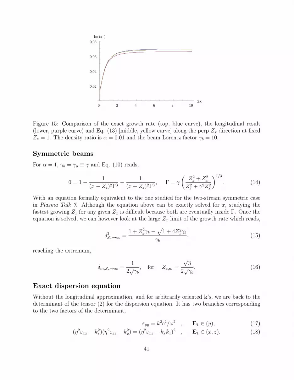
0 2 4 6 8 10Zx

0.02

0.04

0.06

0.08

Im Hx L

Figure 15: Comparison of the exact growth rate (top, blue curve), the longitudinal result(lower, purple curve) and Eq. (13) [middle, yellow curve] along the perp Zx direction at fixedZz = 1. The density ratio is α = 0.01 and the beam Lorentz factor γb = 10.

Symmetric beams

For α = 1, γb = γp ≡ γ and Eq. (10) reads,

0 = 1− 1

(x− Zz)2Γ3− 1

(x+ Zz)2Γ3, Γ = γ

(Z2z + Z2

x

Z2z + γ2Z2

x

)1/3

. (14)

With an equation formally equivalent to the one studied for the two-stream symmetric casein Plasma Talk 7. Although the equation above can be exactly solved for x, studying thefastest growing Zz for any given Zx is difficult because both are eventually inside Γ. Once theequation is solved, we can however look at the large Zx limit of the growth rate which reads,

δ2Zx→∞ =

1 + Z2zγb −

√1 + 4Z2

zγbγb

, (15)

reaching the extremum,

δm,Zx→∞ =1

2√γb, for Zz,m =

√3

2√γb. (16)

Exact dispersion equation

Without the longitudinal approximation, and for arbitrarily oriented k’s, we are back to thedeterminant of the tensor (2) for the dispersion equation. It has two branches correspondingto the two factors of the determinant,

εyy = k2c2/ω2 , E1 ∈ (y), (17)

(η2εxx − k2z)(η

2εzz − k2x) = (η2εxz − kxkz)2 , E1 ∈ (x, z). (18)

41

The second branch therefore holds the two-stream, the oblique and the filamentation insta-bilities. As evidenced by the exact plot on Figs. 14, there is a continuous transition fromtwo-stream to filamentation modes, probably linked to a common underlying physics. Anyideas ?

Cold hierarchy

We may finally establish the hierarchy of modes for the cold regime in the (α, γb) phase space.The competing modes, with their variation from α 1 to 1, are

Two− stream, =(x) =

√3

24/3

α1/3

γb→ 1

2γ3/2b

,

Oblique, =(x) =

√3

24/3

(α

γb

)1/3

→√

3

2γ1/2b

,

Filamentation, =(x) =vbc

√α

γb→ vb

c

√2

γb. (19)

The Two-stream case is quickly settled: it is always slower than the oblique unless γb = 1. Inthe cold regime, the two-stream instability never governs the unstable spectrum5.

We are thus left comparing oblique and filamentation modes. For the diluted regime,the γb scaling clearly favors the oblique. Situation is more involved near the symmetricregime. As evidenced on Fig. 14 RIGHT, the longitudinal approximation gives the goodorder of magnitude for the growth rate, but is not enough to render the “fine structure” ofthe problem.

What is this “fine structure”? In the diluted beam regime, we clearly have a local ex-tremum for oblique vectors corresponding to oblique modes. When approaching the symmetricregime, this may no longer be the case. To evidence this, we’ve plotted on Fig. 16 LEFTthe growth rate at Zx →∞ for different parameters. For α = 0.3, we clearly find an obliqueextremum, which turns to be the dominant mode. But in the symmetric case α = 1, thelocal extremum disappears, giving rise to a monotonous behavior and a system governed byfilamentation.

As a consequence, the oblique/filamentation frontier has to be determined numericallyfor large density ratios. The resulting hierarchy plot can be found on Fig. 16, RIGHT.The frontier position for α = 1 can be determined exactly from the dispersion equation atZx → ∞. At α = 1, the equation can be solved, and the local oblique extremum vanisheswhen the second derivative of the growth rate at Zz = 0 vanishes. For α 6= 1, this secondderivative vanishes on the blue line. Note the frontier gets closer to α = 1 for large γb’s, witha convergence numerically found like γ−0.395

b .More detailed in the Review Paper, Section IV-A.

5We’ll see later that temperature effects change this. This is why the two-stream instability can be observedin some real systems.

42

0.2 0.4 0.6 0.8 1.0 1.2 1.4Zz

0.1

0.2

0.3

0.4

0.5

0.6

Im Hx L

Figure 16: LEFT: Growth rate Zx → ∞ in terms of the parallel wave vector Zz, for γb = 5,and α = 0.3 and 1 (lower and upper curves respectively). The local oblique extremum vanisheswhen approaching the symmetric case. RIGHT: Dominant mode in terms of (γb, α).

Appendix

We here derive the dispersion equation (7) from Maxwell-Ampere equation. The equation weused to merge information from each species, namely Eq. (12) from Plasma Talk 8 simplifiesin the longitudinal approximation,

c2

ω2k× (k× E1) + E1 +

4iπ

ωJ1 = 0. (20)

From Eqs. (3,4), the first order current is expressed in terms of E1, leading again to a tensorialequation of the form,

T · E1 = 0. (21)

If we have but two counter-streaming species (beam + plasma), the tensor reads6,

T =

ω +ω2pb

γb(kzvb−ω)+

ω2pp

γp(kzvp−ω)0 0

0 0 0

−kx(

vbω2pb

γb(kzvb−ω)2+

vpω2pp

γp(kzvp−ω)2

)0 ω

(1− ω2

pb

γ3b (kzvb−ω)2− ω2

pp

γ3p(kzvp−ω)2

) . (22)

The summing of elements from each species is here obvious again. Note that when k is alignedwith the main axis, that is k⊥ = 0 or k‖ = 0, the respective orientation of k and E1 is easilydetermined, because E1 is also found along the very same main axis. Things are here differentbecause the orientation of k is arbitrary while the “easy” axis of our tensor are still the mainones.

6Interestingly, it is not symmetric. I don’t understand why. I did check you don’t find the correct result ifyou artificially add the missing element [1,3] to make it symmetric.

43

Assume we have E1 fulfilling Eq. (21) and E1 ‖ k. Because T is a linear operator, thatimplies T · k is also the null vector:

T · k = 0. (23)

The scalar product k · (T · k) must therefore also vanish,

k · (T · k) = 0. (24)

The advantage is that the left-hand-side of Eq. (24) is now a scalar, giving us the dispersionequation for longitudinal waves with arbitrarily oriented k’s. That quantity can be calculatedfrom (22), and gives the dispersion equation (7).

44

11 Temperature Effects

I will quickly go through the main temperature, i.e. energy spread effects, on our insta-bilities. Let’s first start finding out about the limits of the cold regime.

When are we no longer “cold”?

The instability process is a matter of wave-particle interaction1. Assume a mode k is ex-changing energy with a group of particles. If during one growth period, all particles remainin phase with the wave, the interaction is virtually cold. The wave grows as if there wasno thermal spread at all. Writing that after one growth period, the velocity spread along kproduces a spatial spread smaller than the wavelength, we find the condition for the validityof the cold model2,

∆vk δ−1 k−1, (1)

where δ is the growth rate. Note worthily, the condition is not homogenous throughout thek space. The spread ∆vk and the growth rate both depend on k. A given system may bevirtually cold for the two-stream instability, and hot for the filamentation.

The same physical picture allows to understand the main effect of temperature. Thermalspread reduces the growth rates, precisely because if condition (1) is not fulfilled, the wavecan exchange energy only with a fraction of the particles involved in the cold regime.

See Section III.C of the Review.

Two-stream modes

Assume a 1D beam/plasma system with a velocity distribution such as the one pictured onFig. 17 LEFT, and define the temperature parameter,

ρ =VtV. (2)

For ρ = 0, we have two counter-streaming symmetric beams. But it is obvious that if ρ = 1,the two distributions make contact, and we end up with a total distribution equivalent to anhomogenous stable plasma at rest, with velocity spread equal to ±2V .

Indeed, the dispersion equation is easily computed, and reads in terms of the usual di-mensionless parameters,

1− 1

(x+ Z)2 − (ρZ)2− 1

(x− Z)2 − (ρZ)2= 0. (3)

A plot of the growth rate is pictured on Fig. 17 RIGHT, evidencing the progressive stabiliza-tion of the system for ρ approaching unity.

The same pattern holds for more realistic distribution functions. The so-called “PenroseCriterion”3 states that distribution functions are unstable if they have more than one local

1Though there could be some issues here. See the end of the two-stream section.2 Fainberg et al., Sov. Phys. JETP 30, 528 (1970).3Oliver Penrose, brother of Roger Penrose, Phys. Fluids 3, 258 (1960).

45

-V V

2 Vt 2 Vt

1 2 3 4 5Z

0.1

0.2

0.3

0.4

0.5

Im Hx L

Figure 17: LEFT: Simple toy model for the stabilization of the 1D two-stream instability.RIGHT: Growth rate in terms of Z = kV/ωp for ρ = 0, 0.9 and 0.999 from higher to lowercurves respectively. The system is stable for ρ > 1.

extremum. Bottom line: for hot enough beam and/or plasma, two-stream can be stabilized,relativistic or not4.

Something interesting: It is tempting to relate the former criterion to the formula forLandau Damping giving a growth rate ∝ f ′0(ω/k). Nevertheless, we find here unstable waveswith a distribution function which derivative is almost always zero5! In addition, when thesystem is unstable for ρ < 1, the real part of the unstable modes is found at ω = 0, so thatf ′0(ω/k) = 0 in our case, while there are no particles at v = 0. This is not an artifact of ourdistribution functions, because ω = 0 also with two counter-streaming symmetric Maxwellianspecies.

I have never seen this kind of issues discussed, except in one single paper6. There arethings left to understand. . .

Filamentation modes

Let’s extend our toy model consisting in distributions flat up to a certain velocity (“wa-terbag”). Consider the 3 distribution functions pictured on Fig. 18. The shaded areas areuniformly filled with particles in velocity space.

• A is a counter-streaming system. Unstable to both two-stream and filamentation insta-bilities.

• In B, we just extend the parallel spread until the distributions come in contact. Ac-cording to the previous paragraph, the result is two-stream stable. But the result isalso anisotropic. Weibel found7 it is unstable to perturbations with k normal to the

4Buschauer, MNRAS, 137 99 (1977).5To be more accurate, the derivative of the distribution function pictured in Fig. 17 LEFT, goes like a

Dirac’ δ for v = ±V ± Vt.6Phys. Rev. B 43, 14009 (1991), where the problem is pointed out, but not solved.7Weibel, Phys. Rev. Lett., 2, 83 (1959).

46

FLOW

Vz

VxC

FLOW

Vz

VxB

FLOW

Vz

VxA

Figure 18: Distribution functions with different stability properties.

highest thermal spread: that’s filamentation here. B is therefore two-stream stable andfilamentation unstable.

• C is built from B, equating the spread in every directions. The result is stable.

We thus find we can “play” with temperature parameters in order to stabilize some parts ofthe spectrum, or all of it. The bottom line here is that filamentation can be stabilized.

Note that in Fig. 18, we carefully tailor the spreads of every species to cancel the instability.What if we just play with the beam, that is, the component around vz > 0 on Fig. 18-A?The end result depends on the distribution:

• For waterbag distributions, filamentation is stabilized beyond a certain amount of beamtransverse spread. That can be understood as follows8: Assume a current filament ofradius 1/k and density nb. The current is I ∼ qnbk

−2vb. It creates at the surface ofthe filament a field B = 2I/ck−1. A charge at the surface is therefore pulled in by theLorentz force

FB = qvbB

c=(vbc

)2

q2nbk−1. (4)

If there is no temperature, nothing prevents the filament from further pinching, whichis why the instability extends up to k =∞ in the cold regime. But if we’re hot, kineticpressure opposes the pinching: A little piece of filament near the surface, with volumedV and surface dS, is pulled in by FBnbdV , and pushed out by nbkBTdS. Pinching isprevented if,

nbkBTdS > FBnbdV ⇒ k > qvbc

√nbkBT

≡ km⊥ ∝√nbvtb

, (5)

which is the scaling found from the theory with waterbag distributions9 (we have useddV ∼ k−1dS, and vtb is the thermal beam spread.).

8Silva et al., Physics of Plasmas, 9, 2458 (2002).9Bret at al., Physical Review E, 72, 016403 (2005).

47

• For relativistic Maxwellians, it has been proved that filamentation never vanishes com-pletely10. If Tb is the beam temperature, the maximum filamentation growth-rate scaleslike T

−3/2b . In addition, this result still holds for any plasma temperature.

Oblique modes - general thermal “rules”

Two-stream modes are unstable up to a finite km‖, and filamentation up to yet anotherfinite km⊥. How do we close the unstable domain? Two different answers according to thedistribution. With waterbag, we close from, and to infinity. See Fig. 10a of the Review.With a Maxwellian, these large k oblique modes are stabilized, and we close “normally”, aspictured for example on Fig. 14 of the Review.

Oblique modes’ temperature sensitivity is intermediate between two-stream and filamen-tation. As evidenced in Plasma Talk 10, they tend to be interesting only in the relativisticregime, due to the γb scaling which favors them. Two thermal “rules” are useful to grasp theinfluence of the beam spread over the full spectrum:

• Parallel spread hardly matters. Why? Because in the relativistic regime, it takes a hugeparallel energy spread to get a reasonable parallel velocity spread. All velocities aresqueezed against c. See Fig. 13 of the Review.

• Two-stream does not care about the transverse spread, because particles differing onlyby their transverse velocity will equally stay tuned with a plane wave at k ‖ flow. Forthe same reason, filamentation do care.As a result, modes are all the more affected by beam temperature than they are oblique.

We could rank, from best to worst, the 3 kinds of modes in terms of the way they “resist”the various effects:

Relativistic: Oblique → Filamentation → two-stream.

Density ratio: Filamentation → Oblique/two-stream.

Beam temperature: Two-stream → Oblique → Filamentation.

All this ends up with the mode hierarchy pictured on Fig. 20 of the Review Paper.

The phase velocity diagram - Fig. 17 of the Review

A great tool to understand the physics. Plot, on the very same graph, the distributionfunctions and the phase velocities of the unstable modes. On can straightforwardly checkwhich species are in resonance with which kind of modes.

10Gremillet, Unpublished, Bret et al., Physical Review E, 81, 036402 (2010),

48

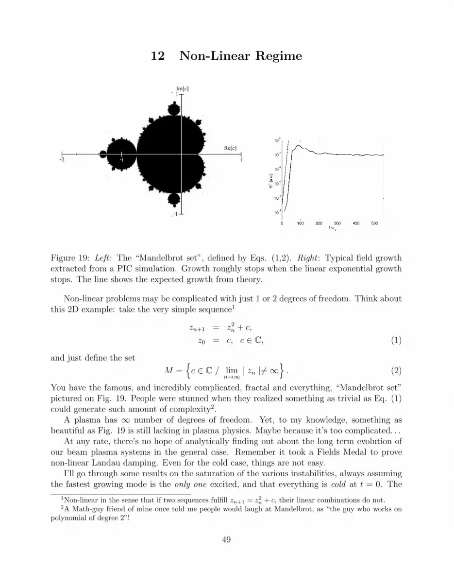
12 Non-Linear Regime

Figure 19: Left : The “Mandelbrot set”, defined by Eqs. (1,2). Right : Typical field growthextracted from a PIC simulation. Growth roughly stops when the linear exponential growthstops. The line shows the expected growth from theory.

Non-linear problems may be complicated with just 1 or 2 degrees of freedom. Think aboutthis 2D example: take the very simple sequence1

zn+1 = z2n + c,

z0 = c, c ∈ C, (1)

and just define the set

M =c ∈ C / lim

n→∞| zn |6=∞

. (2)

You have the famous, and incredibly complicated, fractal and everything, “Mandelbrot set”pictured on Fig. 19. People were stunned when they realized something as trivial as Eq. (1)could generate such amount of complexity2.

A plasma has ∞ number of degrees of freedom. Yet, to my knowledge, something asbeautiful as Fig. 19 is still lacking in plasma physics. Maybe because it’s too complicated. . .

At any rate, there’s no hope of analytically finding out about the long term evolution ofour beam plasma systems in the general case. Remember it took a Fields Medal to provenon-linear Landau damping. Even for the cold case, things are not easy.

I’ll go through some results on the saturation of the various instabilities, always assumingthe fastest growing mode is the only one excited, and that everything is cold at t = 0. The

1Non-linear in the sense that if two sequences fulfill zn+1 = z2n + c, their linear combinations do not.2A Math-guy friend of mine once told me people would laugh at Mandelbrot, as “the guy who works on

polynomial of degree 2”!

49

former is quite reasonable, as the most unstable mode grows exponentially faster than therest. Relativistic effects help as they drive a sharper unstable spectrum, where growth ratesvary rapidly from one mode to another. The later is a limitation.

The idea is to find out when the linear theory should break down, and to claim thatgrowth stops at that point. Granted, exponential growth should stop there. But other kindof growth could keep on. Yet the observed field growth in PIC simulations is always like toone pictured on Fig. 19. Why?

See Section V of the Review Paper, and references therein.

Two-stream and oblique instabilities

Two-stream, non-relativistic

We assume a diluted beam. There, two-stream is resonant with the beam. Say the waveEeikx−iωt is growing, traveling along with the beam electrons. Electrons will start oscillatingin the field at the “bouncing” frequency3,

ω2b =

qEk

m. (3)

The linear assumption that all electrons have v = vb during one growth period δ−1 breaksdown when,

ωb = δ ⇒ Es =δ2

ωp

mvbq, (4)

giving the value of the field at saturation (I’ve set here k ∼ ωp/vb). A great by-product of Esis the beam energy loss ∆Wb. Since the field energy can only come from the beam energy, wecan write,

∆Wb

12nbmv2

b

=E2s/8π

12nbmv2

b

(5)

=npnb

(δ

ωp

)4

∼(nbnp

)1/3

,

where I just replaced the growth-rate by its cold value√

324/3

(nb/np)1/3ωp. We could even write

the energy lost is shared between the plasma and the field4. In such case, ∆Wb/Wb is halfthe result (5).

As the field grows and traps the beam electrons, they start oscillating in the wave potential.PIC people love to plot density graphs in the (x, vx) phase-space (say x is our dimension)such as the one pictured on Fig. 20. At t = 0, the beam and the plasma are just two lines. Inthe instability phase, the plasma does not move a lot, but the beam particles start oscillatingin the wave, creating “holes” in the phase-space.

3See Plasma Talk 5 on Landau damping.4Lorenzo Sironi told me you see this in the PICs. But why?

50

Phase-spacehole

x

px

Beam

Plasma

px

Potential well

Plasma

t=0

Figure 20: Phase-space hole.

Two-stream, Relativistic

A naive reasoning gives the right answer. As the oscillatory trapping motion is along the flow,we replace m→ γ3

bm in the bouncing frequency (3). This gives the field at saturation5,

Es =δ2

ωp

γ3bmvbq

. (6)

The relative energy loss is then computed as in Eq. (5), replacing the growth-rate by itsrelativistic value. It reads,

∆Wb

nbγbmc2∼ γbβ

2

(nb2np

)1/3

. (7)

Of course, this quantity has to remain small since linear regime means unperturbed trajecto-ries, that is, ∆Wb Wb. The energy loss eventually relies on the parameter S with6

S = γbβ2

(nb2np

)1/3

. (8)

If you do the “clean” calculation going to the wave frame, like in the footnote, you need thebeam dynamic in that frame to be non-relativistic in order to compute easily a bouncing

5Let’s denote quantities in the wave frame with a prime. If the beam dynamic in the wave frame isnon-relativistic, we have

ω′2b =qEk′

m,

where the field E does not need prime as it is parallel to the motion. The bouncing frequency in the lab frameis simply ωb = ω′b/γb. In addition, k = γbk

′ since in the wave frame, ω′ = 0. We thus find

ω2b =

qEk

γ3bm,

retrieving the m→ γ3bm “rule”.6See Review Paper.

51

frequency. Doing so requires S 1, as explained in the Review. For arbitrary S’s, one has

∆Wb

Wb

∼ S

(S + 1)5/2, (9)

yielding a maximum energy loss in the linear phase

∆Wb

Wb max

=6

25

√3

5∼ 0.18 for S =

2

3. (10)

Oblique instability

Poorly known. What is known is that Eq. (9) roughly works until S ∼ 0.45. For larger S’s,∆Wb/Wb seems quite insensitive to S, and remains around 0.18 given by Eq. (10).

Filamentation instability

There are 3 different ways to evaluate the field at saturation!

1. Cyclotron frequency = growth rate. Filamentation instability grows magneticfield. Such field B affects particles on a time scale given by the cyclotron frequency,

ωc =qB1

γbmc. (11)

Writing again that the linear regime keeps on until ωc = δ, we get,

Bs1 =γbmc

qδ. (12)

If one tries to compute the relative energy lossB2s1

8π/nbγbmc

2, the cold result gives afactor of order β2, without any more scaling in γb, and almost none in α = nb/np (seeTable 1). The conclusion is that estimating the energy loss requires a finer calculationthan this one, and that the result is quite stable in terms of these variables.

2. Bouncing frequency = growth rate. Historically, the field at saturation has ratherbeen evaluated this way. With v0b = (0, 0, vb) and k = (kx, 0, 0), the growing magneticfield reads B1 = (0, B1 sin kxx, 0). At first order, Newton’s law projected on the x axisgives,

γbmd2x

dt2= qB1

vbc

sin kxx. (13)

Particles at x ∼ 0 oscillate at,

ω2b =

qB1vbkxγbmc

. (14)

Note that we assumed there’s only a B field here. We know that unless the system isstrictly symmetric, it’s wrong. Here again, we can claim exponential growth keeps onwhile the motion is almost unperturbed, that is until

qB1vbkxγbmc

= δ2 ⇒ Bs2 =γbmc

q

δ2

vbkx. (15)

52

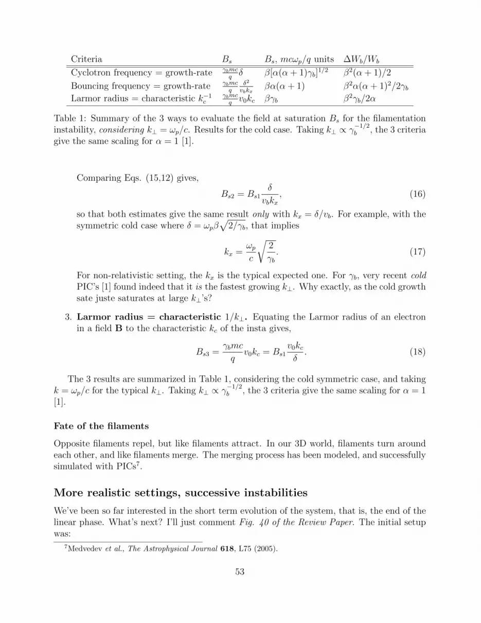
Criteria Bs Bs, mcωp/q units ∆Wb/Wb

Cyclotron frequency = growth-rate γbmcqδ β[α(α + 1)γb]

1/2 β2(α + 1)/2

Bouncing frequency = growth-rate γbmcq

δ2

vbkxβα(α + 1) β2α(α + 1)2/2γb

Larmor radius = characteristic k−1c

γbmcqv0kc βγb β2γb/2α

Table 1: Summary of the 3 ways to evaluate the field at saturation Bs for the filamentationinstability, considering k⊥ = ωp/c. Results for the cold case. Taking k⊥ ∝ γ

−1/2b , the 3 criteria

give the same scaling for α = 1 [1].

Comparing Eqs. (15,12) gives,

Bs2 = Bs1δ

vbkx, (16)

so that both estimates give the same result only with kx = δ/vb. For example, with thesymmetric cold case where δ = ωpβ

√2/γb, that implies

kx =ωpc

√2

γb. (17)

For non-relativistic setting, the kx is the typical expected one. For γb, very recent coldPIC’s [1] found indeed that it is the fastest growing k⊥. Why exactly, as the cold growthsate juste saturates at large k⊥’s?

3. Larmor radius = characteristic 1/k⊥. Equating the Larmor radius of an electronin a field B to the characteristic kc of the insta gives,

Bs3 =γbmc

qv0kc = Bs1

v0kcδ. (18)

The 3 results are summarized in Table 1, considering the cold symmetric case, and takingk = ωp/c for the typical k⊥. Taking k⊥ ∝ γ

−1/2b , the 3 criteria give the same scaling for α = 1

[1].

Fate of the filaments

Opposite filaments repel, but like filaments attract. In our 3D world, filaments turn aroundeach other, and like filaments merge. The merging process has been modeled, and successfullysimulated with PICs7.

More realistic settings, successive instabilities

We’ve been so far interested in the short term evolution of the system, that is, the end of thelinear phase. What’s next? I’ll just comment Fig. 40 of the Review Paper. The initial setupwas:

7Medvedev et al., The Astrophysical Journal 618, L75 (2005).

53

Beam: Maxwellian, nb = np/10, γb = 3, Tb = 50 keV.Plasma: Maxwellian, Tp = 5 keV.

• 0 < ωpt < 80: System initially governed by oblique modes. E field grows at 0.07ωp.Heating “kills” de oblique.

• 80 < ωpt < 160: System switches to a two-stream regime. E field grows at 0.016ωp.Heating “kills” two-stream.

• 200 < ωpt < 600: Remaining drift feeds filamentation. B field grows at 0.005ωp.

By the end of the simulation ωpt ∼ 600, the beam had lost about 30% of its energy,entirely transferred to plasma electrons. Open questions:

• Is filamentation the necessary end state of every initial setup?

• Does the drift eventually ends (in the frame of the fixed ion background)? That is, isthe drift energy eventually converted at 100% into heat? Sounds reasonable. Is thatsure?

Indeed, the interesting question might be how long does it take?

References

[1] A. Bret et al., Submitted to Physics of Plasmas, (2012).

54

13 Ohm’s law and the Biermann battery

The original 1950 paper is Ref. [1], “Uber den Ursprung der Magnetfelder auf Sternen undim interstellaren Raum”, published in Zeitschrift Naturforschung Teil A. Cited more than 200times, and probably read by no one but the happy few who 1) read German and 2) couldaccess it.

The MHD equations are formed from the fluid equations for electrons and ions (droppingsubindices),

∂n

∂t+

∂

∂r· (nv) = 0,

mn

(∂v

∂t+ v · ∂v

∂r

)= qn

(E +

v

c×B

)−∇p+ nmg. (1)

The MHD variables are defined from ne,i(r, t),ve,i(r, t) as1,

ρ(r, t) = mini +mene,

J(r, t) = qnivi − qneve,

V(r, t) =1

ρ(r, t)(nemeve +minivi).

Merging the fluid Euler equations for both species gives,

ρ

(∂V

∂t+ V · ∂V

∂r

)=

J

c×B−∇(

P︷ ︸︸ ︷pi + pe) + ρg. (2)

Ohm’s law is the equation giving the current J. Where does it come from? What we didin Plasma Talk 3 was to follow the basic, “business as usual” procedure: sit in the frame ofthe fluid locally at V. There, the electric field is E′. Ohm’s law gives the current in the labframe from E′, as J′ = σE′. Because E′ = E + V×B/c, we get the famous (non-relativistic)

J = σ

(E +

V

c×B

). (3)

What about J′ = σE′? It arises from the microscopic picture that under the action ofan electric field, particles, mostly electrons, are accelerated in the direction of the field, whilecollisions with the ions act like a friction force2. Writing something like m∂tv = qE′ − νvwhere ν is some collision frequency, and setting ∂t = 0, indeed yields v = q

νE′ and then

J′ = qn qνE′. Ideal MHD assumes ν = 0, giving

E′ = E +V

c×B = 0. (4)

1In Plasma Talk 3, the MHD velocity V was defined through (me + mi)V = meve + mivi. Most books[2, 3] present definition (2) above. It is more rigorous, as it gives a ρV MHD term exactly equal to the totalmomentum. At any rate, the difference between the two quantities is ∝ (ne − ni)(ve − vi). This is a secondorder quantity in the MHD regime, where electrons are expected to closely follow the ions, so that ne ∼ niand ve ∼ vi.

2Solid state physics call this the “Drude model”, from Paul Drude, who came up with this idea in 1900.

55

Shock

Cold

Diluted

Cold

Diluted

Cold

Diluted

Hot

Dense

Cold

Diluted

Warm

Diluted

T

n

Figure 21: How a finite size shock can generate non-parallel density and temperature (hencepressure) gradients. From [4], p. 406.

But we inadvertently assumed many things. For example, ∂t = 0 assumes E′ variesslowly enough with time. If variations are too fast, the stationary regime does not haveenough time to set in, and some ω dependency appears. Also, we assumed particles areaccelerated only by E′ between two collisions. What if B is strong enough to curve thetrajectories in between? In this case, the resistivity in the direction normal to the field ishigher (×1.9) than along the field ([2] p. 28, or [4] p. 43).

Since conductivity comes from the electrons3, let’s write their full Euler equation,

mene

(∂ve∂t

+ ve ·∂ve∂r

)= qene

(E +

vec×B

)−∇pe − ν(ve − vi). (5)

Neglecting the left-hand-side for the small electrons inertia, and setting ν = 0 for ideal MHDyields,

E +vec×B =

∇peqene

. (6)

According to Kulsrud [4] p. 405, the pressure term above is negligible when there is a B field.WHY? But for small B’s, or even B = 0, you need to keep it. Inserting the electric fieldabove in ∂tB = −c∇× E and setting ve ∼ V gives4,

∂B

∂t= ∇× (V ×B) + c

∇ne ×∇peqn2

e

. (7)

The second term is our Biermann Battery. There’s no B in there, so that it can make it fromnothing. Still, the microscopic derivation shows we need ionization, just to be able to createelectronic currents moved by the electronic pressure.

But, an equation of state usually gives pe(ne). The gradients for pe and ne are thus

3The σ of J′ = σE′ has the mass on the denominator.4We need a little drag between ions and electrons to write ve ∼ V.

56

likely to be parallel, so that the cross product vanishes. How do we break this? Severalpossibilities,

1. Try a system in rotation around z, with Ω(z). The pressure gradient reads ∇P ∝Ω2(z)ρ(r, θ). It has a z component, while ∇ρ(r, θ) has not. Those who’ve read thepaper say Biermann considered this option.

2. Try the scheme of Figure 21. Suppose a finite size shock travels through a cold, dilutedupstream. The downstream just behind the shock is dense and hot. Far downstreamthough, the plasma expands but remains warm, so that it is now warm and diluted.The figure shows well how this can generate non-parallel density and temperature (hencepressure) gradients. A non-spherical shock also does the job for similar reasons.

Everything is easily adapted to a system partially ionized. If nn is the density of theneutral, define χ = ne/(ni + nn). Eq. (7) can be adapted dividing the Battery term by 1 + χ([4], p. 406). See [7].

Kulsrud proposed this mechanism to produce Cosmic Fields from scratch in 1997 [5]. Yet,he co-authored in 1992 another paper [6] advocating spontaneous plasmas fluctuations.

Also Khanna [8], showed that a rotating BH in a plasma will always generate toroidal andpoloidal magnetic fields.

Ref. [9] studied the Biermann Battery effects in Cosmological MHD Simulations of Pop-ulation III Star Formation. In its own terms, “We find that the Population III stellar coresformed including this effect are both qualitatively and quantitatively similar to those fromhydrodynamics-only (non-MHD) cosmological simulations”. No dynamical effects.

The Biermann battery mechanism was successfully tested in the lab in 2012 [10].

References

[1] L. Biermann, Uber den Ursprung der Magnetfelder auf Sternen und im interstellarenRaum, Zeitschrift Naturforschung Teil A, 5, 65 (1950).

[2] L. Spitzer, Physics of Fully Ionized Gases.

[3] J.P. Goedbloed and S. Poedts, Principles of Magnetohydrodynamics: With Applicationsto Laboratory and Astrophysical Plasmas.

[4] R.M. Kulsrud, Plasma Physics for Astrophysics.

[5] R.M. Kulsrud et al., Protogalactic Origin for Cosmic Magnetic Fields, ApJ, 480, 481(1997).

[6] T. Tajima et al., On the origin of cosmological magnetic fields, ApJ, 390, 309 (1992).

[7] L. Mestel and D.L. Moss, On the Biermann ’battery’ process in uniformly rotating,chemically inhomogeneous stars, MNRAS, 204, 557 (1983).

57

[8] R. Khanna, Generation of magnetic fields by a gravitomagnetic plasma battery, MNRAS,295, L6 (1983).

[9] H. Xu et al., The Biermann Battery in Cosmological MHD Simulations of Population IIIStar Formation, ApJ, 688, L57 (2008).

[10] G. Gregori et al., Generation of scaled protogalactic seed magnetic fields in laser-producedshock waves, Nature, 481, 480 (2012).

58