case study of an inland salt marsh in northern Thuringia

Geophysical analysis of an area affected by subsurface dissolution –case study of an inland salt marsh in northern Thuringia, GermanySonja H. Wadas1, Hermann Buness1, Raphael Rochlitz1, Peter Skiba2,3, Thomas Günther1,Michael Grinat1, David C. Tanner1, Ulrich Polom1, Gerald Gabriel1,4, and Charlotte M. Krawczyk5,6

1Leibniz Institute for Applied Geophysics, Stilleweg 2, 30655 Hannover, Germany2formerly Leibniz Institute for Applied Geophysics, Stilleweg 2, 30655 Hannover, Germany3Federal Institute for Geosciences and Natural Resources, Stilleweg 2, 30655 Hannover, Germany4Leibniz University Hannover – Institute of Geology, Callinstraße 30, 30167 Hannover, Germany5GFZ – German Research Centre for Geosciences, Telegrafenberg, 14473 Potsdam, Germany6Technical University Berlin – Institute for Applied Geosciences, Ernst-Reuter-Platz 1, 10587 Berlin, Germany

Correspondence: Sonja H. Wadas ([email protected])

Abstract. The subsurface dissolution of soluble rocks, also called subrosion, can affect areas over a long period of time and

pose a severe hazard. We show the benefits of a combined approach using P-wave- and SH -wave reflection seismics, electrical

resistivity tomography, transient electromagnetics, and gravimetry for a better understanding of the subrosion process. The

study area, ’Esperstedter Ried’ in northern Thuringia, Germany, located south of the Kyffhäuser hills, is a large inland salt

marsh that developed due to dissolution of soluble rocks at approximately 300 m depth. We were able to locate buried subrosion5

structures, subrosion zones, faults and fractures, and potential fluid pathways, aquifers and aquitards based on seismic and

electromagnetic surveys. Further improvement of the subrosion model was accomplished by analyzing gravimetry data that

indicates subrosion-induced mass movement as shown by local minima of the Bouguer anomaly for the Esperstedter Ried.

Forward modelling of the gravimetry data, in combination with the seismic results, delivered a cross section through the inland

salt marsh from north to south. We conclude that the tectonic movements during the Tertiary, which led to the uplift of the10

Kyffhäuser hills and the formation of faults parallel and perpendicular to the low mountain range, were the initial trigger for

subrosion. The faults and the fractured Triassic and Lower Tertiary deposits serve as fluid pathways for groundwater to leach

the deep Permian Zechstein deposits, since subrosion is more intense near faults. The artesian-confined salt water ascends

towards the surface along the faults and fracture networks, and formed the inland salt marsh over time. In the past, subrosion

of the Zechstein formations formed several, now buried, sagging and collapse structures, and, since the entire region is affected15

by recent sinkhole development, subrosion is still ongoing. From the results of this study, we suggest that the combined

geophysical investigation of subrosion areas can improve the knowledge of control factors, risk areas, and thus local subrosion

processes.

1 Introduction

Subrosion, the subsurface dissolution/leaching of soluble rocks, poses a major geohazard, especially if it occurs in urbanized20

areas (Gutiérrez et al., 2014; Parise, 2015). In particular the sudden formation of sinkholes, also called dolines, can cause

1

https://doi.org/10.5194/egusphere-2022-164Preprint. Discussion started: 2 May 2022c© Author(s) 2022. CC BY 4.0 License.

building and infrastructure damage and life-threatening situations (Beck, 1988; Waltham et al., 2005). Therefore, to gain a

better understanding of the subrosion process, its controlling factors and the resulting structures is of high importance.

The subrosion process requires the presence of soluble rocks (e.g. evaporites), unsaturated groundwater or meteoric water,

and fractures, joints or faults which may serve as fluid pathways (Waltham et al., 2005). The process leads to mass movement25

and forms cavities that may migrate upward over time (Davies, 1951; White & White, 1969). It results in a continuous sagging

of the surface that generates a depression, or a sudden collapse, which generates a sinkhole (Waltham et al., 2005; Gutiérrez

et al., 2008).

Several studies have dealt with the understanding of the processes and the imaging of subrosion structures, such as cavi-

ties, sinkholes, and depressions, using different types of methods. The most suitable methods for the monitoring of sinkhole30

development are aerial photos, differential GPS, and radar interferometry (Yechieli et al., 2002; Abelson et al., 2003; Vey

et al., 2021). For the detection of cavities and mass movement, gravimetric methods have shown to be useful (Neumann, 1977;

Butler, 1984), but they also deliver information about possible cavity fills, as do electrical resistivity tomography (ERT), and

various electromagnetic methods (Militzer et al., 1979; Bosch & Müller, 2001; Miensopust et al., 2015). To get an image of

the subsurface the most common techniques are ground-penetrating radar (Kaspar & Pecen, 1975; Batayneh et al., 2002) and35

reflection seismics (Steeples et al., 1986; Miller & Steeples, 2008; Krawczyk et al., 2012; Wadas et al., 2016). Several studies

in karst regions using P-wave reflection seismics have been carried out (Evans et al., 1994; Keydar et al., 2012), but inves-

tigations using SH -wave reflection seismics that enable high-resolution imaging of the near-surface (Krawczyk et al., 2012;

Wadas et al., 2016, 2017; Polom et al., 2018), or even in combination with P-waves, are sparse or missing. Since subrosion and

the development of its corresponding structures are a complex phenomenon, a combination of various methods (e.g. Malehmir40

et al. (2016); Al-Halbouni et al. (2021); Ezersky et al. (2021)) is needed to better understand the components and controlling

factors associated with it. The more boundary conditions that influence the processes and the structures that can be determined,

the better, e.g., dynamic models (Augarde et al., 2003; Shalev et al., 2006; Al-Halbouni et al., 2019) can be adapted in order

to make better predictions of risk areas.

In this study, we show the benefits of a combined approach using P- and SH -wave reflection seismics including ERT (Doetsch45

et al., 2012; Wiederhold et al., 2013; Ronczka et al., 2017; Nickschick et al., 2019; Tanner et al., 2020), transient electromagnet-

ics (TEM; Rochlitz et al. (2018); Steuer et al. (2011)) and gravimetry (Eppelbaum et al., 2008; Ezersky et al., 2013b; Flechsig

et al., 2015) to better understand the local subrosion of an inland salt marsh in Thuringia, Germany. We analyze depressions and

collapse structures and determine the vertical and lateral fluid pathways and areas of subsurface mass movement. Furthermore,

we recommend a workflow for geophysical investigations of subrosion areas to determine control factors and risk areas.50

2 Geology

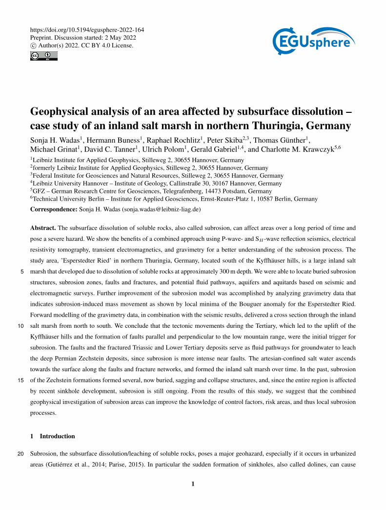
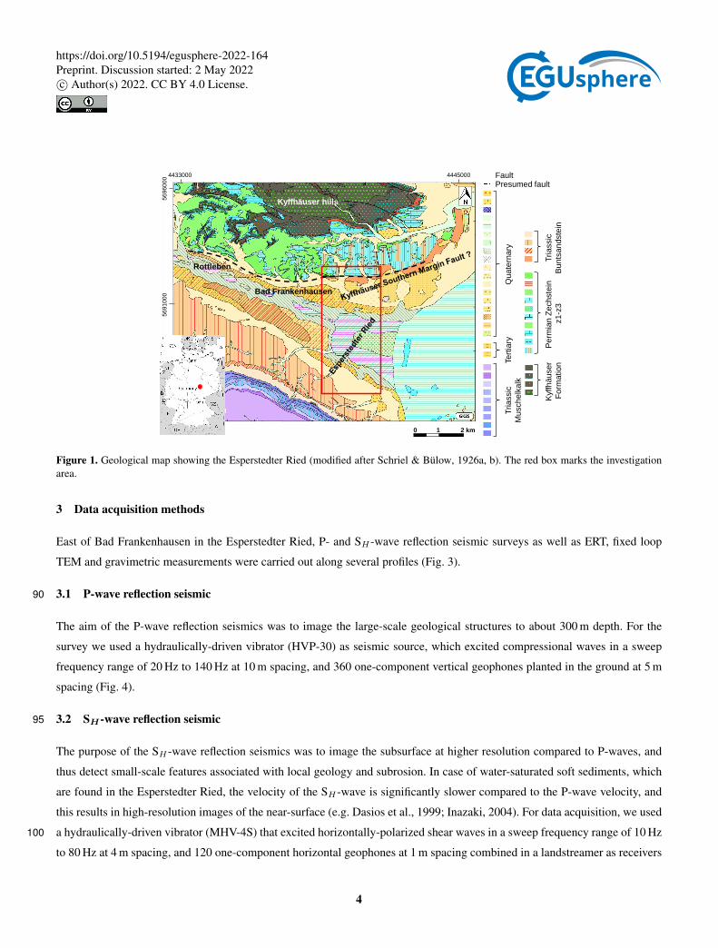
Germany suffers from a widespread sinkhole problem, because soluble deposits are close to the surface in many areas. One

of the main subrosion areas is located along the Kyffhäuser-Southern-Margin-Fault (KSMF) in Thuringia. The Esperstedter

Ried to the south of the Kyffhäuser hills is part of this subrosion area. It is a 5 km2 wide sink and it is the largest inland salt

2


marsh of Thuringia (Fig. 1). It developed due to leaching of salt-bearing rocks at approximately 300 m depth (Schriel & Bülow,55

1926a, b).

2.1 Geological evolution

The Kyffhäuser hills have a N–S extension of 6 km, a W–E extension of 13 km, and they are one of the smallest low mountain

ranges in Germany. To the south, the hills are bounded by the northward-dipping, W–E striking KSMF, a major thrust fault

(Schriel & Bülow, 1926a, b).60

An epicontinental ocean, the Zechstein Sea, covered the area during the Permian, and due to sealevel changes, conglomerates,

carbonates, sulfates, and salt were cyclically deposited (Richter-Bernburg, 1953). As a result, the central part of the Kyffhäuser

hills consists of sandstones and conglomerates, and the southern part consists of gypsum and anhydrite. The main Zechstein

Formations south of the hills are the Werra-, Staßfurt- and Leine Formations (z1–z3). Anhydrite and gypsum of z1 to z2

formations represent the main subrosion horizon in the research area (Schriel & Bülow, 1926a, b). The erosion of the Variscan65

Orogen at the Permian-Carboniferous transition led to deposition of eroded material in the Molasse Basin, and today these

clastic sediments form the central part of the Kyffhäuser hills (Schriel, 1922; Knoth & Schwab, 1972). Triassic deposits are

only found at isolated locations, and Cretaceous and Jurassic rocks have been completely eroded (Schriel & Bülow, 1926a, b;

Reuter, 1962). During the Upper Cretaceous and the Tertiary, the low mountain range was uplifted and tilted, which resulted

in the formation of a fault scarp to the north and a southward-dipping terrain (Freyberg, 1923). Tertiary deposits are found near70

Bad Frankenhausen and Esperstedt, and Quaternary sediments, such as silt and loess, cover a large area (Schriel & Bülow,

1926a, b).

The presence of salt springs and the occurrence of sinkholes and depressions in the near-surface indicate soluble rocks in the

underground such as the Zechstein formations, and they show that Bad Frankenhausen and Esperstedt are affected by subrosion

(Reuter, 1962).75

2.2 Stratigraphy

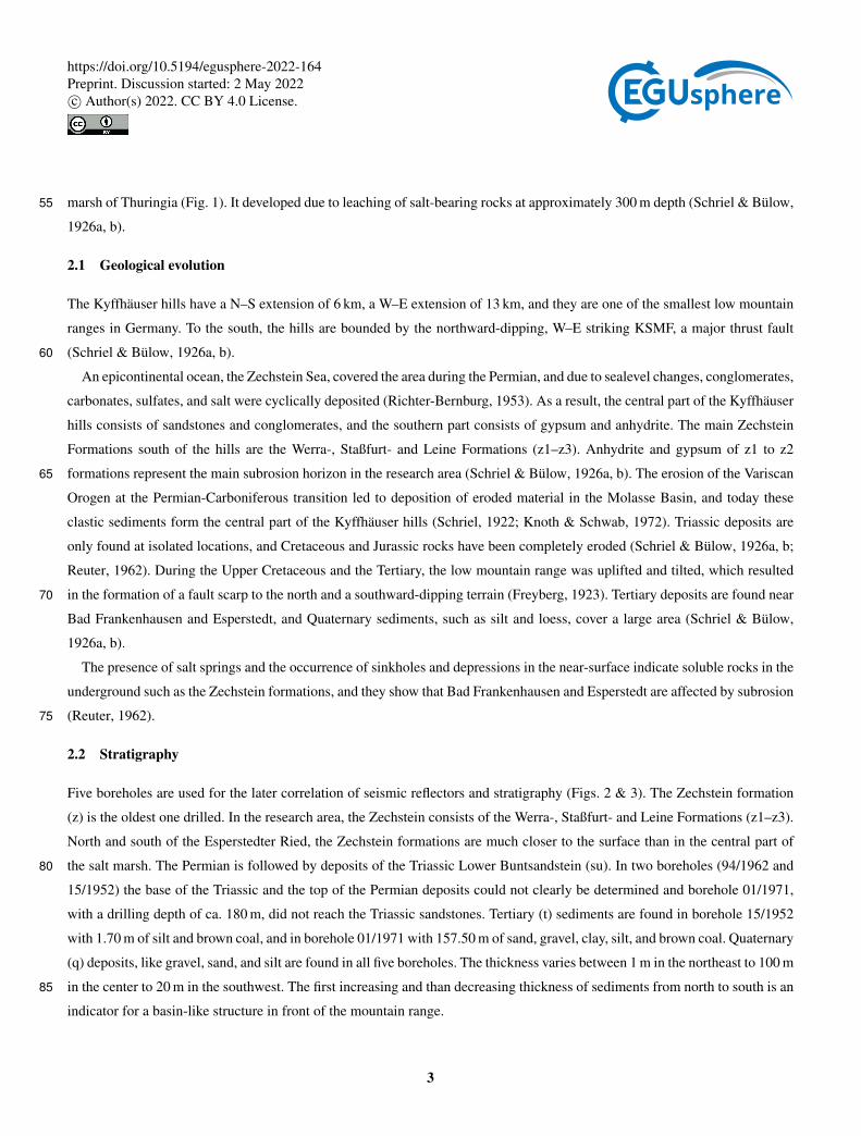
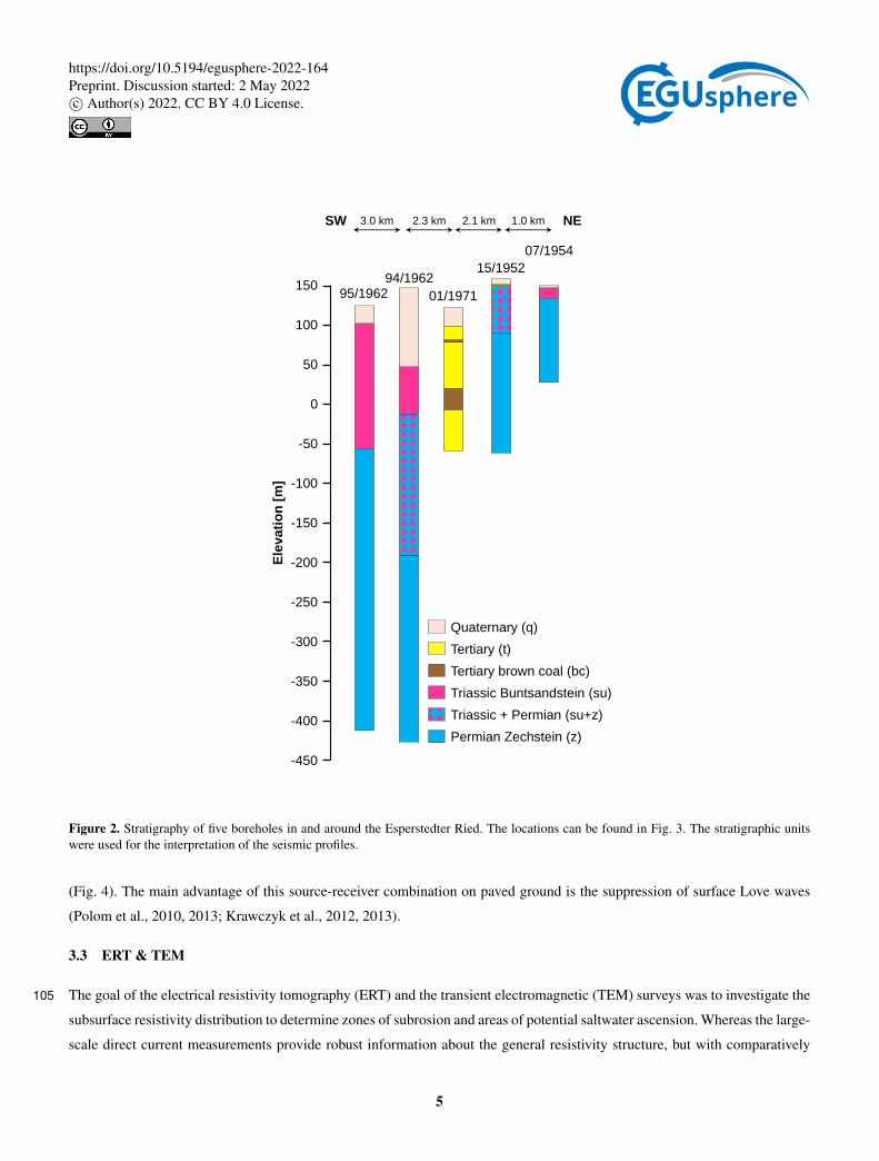
Five boreholes are used for the later correlation of seismic reflectors and stratigraphy (Figs. 2 & 3). The Zechstein formation

(z) is the oldest one drilled. In the research area, the Zechstein consists of the Werra-, Staßfurt- and Leine Formations (z1–z3).

North and south of the Esperstedter Ried, the Zechstein formations are much closer to the surface than in the central part of

the salt marsh. The Permian is followed by deposits of the Triassic Lower Buntsandstein (su). In two boreholes (94/1962 and80

15/1952) the base of the Triassic and the top of the Permian deposits could not clearly be determined and borehole 01/1971,

with a drilling depth of ca. 180 m, did not reach the Triassic sandstones. Tertiary (t) sediments are found in borehole 15/1952

with 1.70 m of silt and brown coal, and in borehole 01/1971 with 157.50 m of sand, gravel, clay, silt, and brown coal. Quaternary

(q) deposits, like gravel, sand, and silt are found in all five boreholes. The thickness varies between 1 m in the northeast to 100 m

in the center to 20 m in the southwest. The first increasing and than decreasing thickness of sediments from north to south is an85

indicator for a basin-like structure in front of the mountain range.

3


Kyffhäuser hills

Rottleben

Bad Frankenhausen

0 1 2 km

56960

00

56910

00

4433000 4445000

Kyffh

äu

se

r

Fo

rma

tio

n

Pe

rmia

nZ

ech

ste

in

z1-z

3

Tria

ssic

Mu

sch

elk

alk

Tria

ssic

Bu

nts

an

dste

in

Te

rtia

ryQ

ua

tern

ary

FaultPresumed fault

Figure 1. Geological map showing the Esperstedter Ried (modified after Schriel & Bülow, 1926a, b). The red box marks the investigationarea.

3 Data acquisition methods

East of Bad Frankenhausen in the Esperstedter Ried, P- and SH -wave reflection seismic surveys as well as ERT, fixed loop

TEM and gravimetric measurements were carried out along several profiles (Fig. 3).

3.1 P-wave reflection seismic90

The aim of the P-wave reflection seismics was to image the large-scale geological structures to about 300 m depth. For the

survey we used a hydraulically-driven vibrator (HVP-30) as seismic source, which excited compressional waves in a sweep

frequency range of 20 Hz to 140 Hz at 10 m spacing, and 360 one-component vertical geophones planted in the ground at 5 m

spacing (Fig. 4).

3.2 SH -wave reflection seismic95

The purpose of the SH -wave reflection seismics was to image the subsurface at higher resolution compared to P-waves, and

thus detect small-scale features associated with local geology and subrosion. In case of water-saturated soft sediments, which

are found in the Esperstedter Ried, the velocity of the SH -wave is significantly slower compared to the P-wave velocity, and

this results in high-resolution images of the near-surface (e.g. Dasios et al., 1999; Inazaki, 2004). For data acquisition, we used

a hydraulically-driven vibrator (MHV-4S) that excited horizontally-polarized shear waves in a sweep frequency range of 10 Hz100

to 80 Hz at 4 m spacing, and 120 one-component horizontal geophones at 1 m spacing combined in a landstreamer as receivers

4


01/1971

94/196215/1952

07/1954

Ele

va

tio

n [

m]

150

50

-50

-150

-450

-250

-350

SW NE1.0 km2.3 km 2.1 km

Quaternary (q)

Tertiary (t)

Triassic Buntsandstein (su)

Permian Zechstein (z)

Triassic + Permian (su+z)

Tertiary brown coal (bc)

100

0

-100

-200

-300

-400

95/1962

3.0 km

Figure 2. Stratigraphy of five boreholes in and around the Esperstedter Ried. The locations can be found in Fig. 3. The stratigraphic unitswere used for the interpretation of the seismic profiles.

(Fig. 4). The main advantage of this source-receiver combination on paved ground is the suppression of surface Love waves

(Polom et al., 2010, 2013; Krawczyk et al., 2012, 2013).

3.3 ERT & TEM

The goal of the electrical resistivity tomography (ERT) and the transient electromagnetic (TEM) surveys was to investigate the105

subsurface resistivity distribution to determine zones of subrosion and areas of potential saltwater ascension. Whereas the large-

scale direct current measurements provide robust information about the general resistivity structure, but with comparatively

5


07/1954

15/1952

01/1971

94/1962

Bad Frankenhausen

Esperstedter Ried

Esperstedt

P1

P2

S1

GR

Kyffhäuser hills

S2

ERT

km0 1 2 30.5

TEM1

TEM2

TEM3

95/1962

Figure 3. Esri ArcGIS map showing the locations of the P-wave (light blue lines) and the SH -wave (red lines) reflection seismic profiles, thegravimetric profile (dark blue line), the ERT profile (pink line), the TEM profiles (yellow lines) and the boreholes (orange dots). The thrustfault (KSMF) is marked by a dashed black line with triangles on the hanging wall.

poor resolution, TEM is especially suited to resolve good conductors down to a few hundred metres depth (Milsom & Eriksen,

2011). The ERT survey was conducted with a dipole-dipole configuration using 26 pairs of electrodes with approximately

200 m spacing along the 4.5 km N–S profile. The transmitter provided up to 30 A of source current, voltages were recorded110

with nine remotely-controlled data loggers (Fig. 4) developed at LIAG (Oppermann & Günther, 2018).

The ERT was restricted by power lines, roads and a gas pipe. By choosing a fixed-loop setup for the TEM survey, it was

possible to cover parts of the profile that are nearly unaffected by strong artificial electromagnetic noise. Receiver positions had

50 m spacing in N–S direction and are placed across four large transmitter loops with 250 m × 250 m dimensions. For more

information about the survey and specific details of sensors and data analysis we refer to Rochlitz et al. (2018).115

6


horizontal geophonevertical geophone

hydraulic vibrator

voltage supply

data logger

GPS/GSM

antenna

GSM modem

PC with

software

current injection

Geode recording system

a

b

d

f

cg

power source

with generator

e

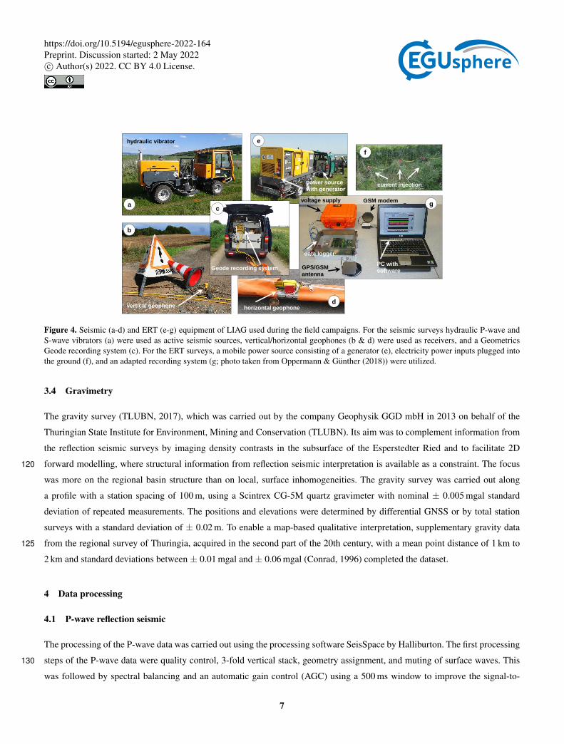
Figure 4. Seismic (a-d) and ERT (e-g) equipment of LIAG used during the field campaigns. For the seismic surveys hydraulic P-wave andS-wave vibrators (a) were used as active seismic sources, vertical/horizontal geophones (b & d) were used as receivers, and a GeometricsGeode recording system (c). For the ERT surveys, a mobile power source consisting of a generator (e), electricity power inputs plugged intothe ground (f), and an adapted recording system (g; photo taken from Oppermann & Günther (2018)) were utilized.

3.4 Gravimetry

The gravity survey (TLUBN, 2017), which was carried out by the company Geophysik GGD mbH in 2013 on behalf of the

Thuringian State Institute for Environment, Mining and Conservation (TLUBN). Its aim was to complement information from

the reflection seismic surveys by imaging density contrasts in the subsurface of the Esperstedter Ried and to facilitate 2D

forward modelling, where structural information from reflection seismic interpretation is available as a constraint. The focus120

was more on the regional basin structure than on local, surface inhomogeneities. The gravity survey was carried out along

a profile with a station spacing of 100 m, using a Scintrex CG-5M quartz gravimeter with nominal ± 0.005 mgal standard

deviation of repeated measurements. The positions and elevations were determined by differential GNSS or by total station

surveys with a standard deviation of ± 0.02 m. To enable a map-based qualitative interpretation, supplementary gravity data

from the regional survey of Thuringia, acquired in the second part of the 20th century, with a mean point distance of 1 km to125

2 km and standard deviations between ± 0.01 mgal and ± 0.06 mgal (Conrad, 1996) completed the dataset.

4 Data processing

4.1 P-wave reflection seismic

The processing of the P-wave data was carried out using the processing software SeisSpace by Halliburton. The first processing

steps of the P-wave data were quality control, 3-fold vertical stack, geometry assignment, and muting of surface waves. This130

was followed by spectral balancing and an automatic gain control (AGC) using a 500 ms window to improve the signal-to-

7


noise ratio (S/N ratio). Short wavelength refraction statics and residual statics were applied and after velocity analysis an initial

velocity model was calculated. A Kirchhoff pre-stack depth migration was carried out, and the velocity model was iteratively

improved by residual moveout (RMO) analysis. Finally, additional spectral balancing, trace mute, and a frequency-wavenumber

filter (F-K filter) were used to further improve S/N ratio and resolution. For detailed explanations of the processing algorithms,135

see Hatton et al. (1986); Lavergne (1989); Yilmaz (2001).

4.2 SH -wave reflection seismic

The processing of the S-wave data was carried out using the processing software VISTA Version 10.028 by Gedco (now

Schlumberger). The first processing steps of the SH -wave data were vibroseis correlation, geometry assignment, amplitude

balancing, frequency filtering, and 2-fold vertical stack to improve the S/N ratio. This was followed by a top mute and a F-K140

filter to eliminate noise and harmonic distortions. The datasets were sorted by Common Mid Point (CMP) following interactive

velocity analysis, normal-moveout (NMO) correction, and residual statics correction. A stacked seismic section in time domain

was created, bandpass- and F-K filters removed remaining noise, and spectral balancing was applied. A finite-difference (FD)

migration moved the dipping reflectors to their true position and finally, the sections in time domain were converted to depth.

For detailed descriptions of the processing algorithms, see Hatton et al. (1986); Lavergne (1989); Yilmaz (2001).145

4.3 ERT & TEM

The ERT surveys yielded time series of 27 current injections and for each of them 26 potential difference measurements with

GPS base. The resistances were determined using a lock-in algorithm, where the potential difference is extracted from the noisy

time series by using the known time-dependence of the injected current signal (Oppermann & Günther, 2018). The apparent

resistivities were calculated by multiplication of the resistance with a geometric factor, which depends on the distances between150

the potential and current electrodes. From these apparent resistivities a pseudosection was created. The true resistivities were

then reconstructed using the BERT inversion algorithm (Günther et al., 2006) based on a triangular model discretization that

is able to take topography into account. For regularization, we used a geostatistical operator (Hermans et al., 2012; Jordi et al.,

2018) with a correlation length of 800 m for the horizontal direction and 70 m for the vertical direction, in order to account for

the predominant layering of the geological strata.155

Processing of TEM data mainly includes noise removal by selective stacking and logarithmic gating. 1D inversion of the

processed data was challenging due to affection by strong atmospheric and anthropogenic noise. The two obtained resistivity

distributions based on the coil and SQUID receivers are overall similar, but the inversion results based on the SQUID receiver

exhibited a higher consistency between neighboring stations, greater penetration depths and less artifacts caused by anthro-

pogenic noise (Rochlitz et al., 2018). Nevertheless, using resistivity constraints from ERT and structural information from160

seismics, the reliability of inversion results could be evaluated.

8


4.4 Gravimetry

The processing of the gravity data (densely sampled stations along a profile in the Esperstedter Ried and sparse stations from

regional surveys nearby) consisted of a uniform conversion of gravity observations to Bouguer anomalies. The calculation

refers to common geodetic and geophysical reference systems (ETRS89, DHHN92, and IGSN71), a standard Bouguer density165

of 2670 kg m−3, and a maximum radial distance of 166.70 km for the calculation of a spherical Bouguer cap and terrain effects.

The formulas used comply with international standards (for details, see e.g. Hinze et al. (2005)): normal gravity by closed form

formula of Somigliana (Somigliana, 1929); atmospheric correction to normal gravity; free air correction by a series expansion

to the 2nd order; Bouguer correction by closed formula for the gravity effect of a spherical cap of 166.70 km radius. Spherical

terrain corrections were calculated in two steps: step 1 considered the near field terrain between 0 km and 25 km distance from170

a station using a DEM with 1 arcsec (ca. 25 m) cell size; step 2 considered the far field terrain between 25 km to 166.70 km

distance using a DEM with 10 arcsec (ca. 250 m) cell size. The resulting complete Bouguer anomaly is the difference between

the observed gravity and the sum of all correction terms. The regional data surrounding the Esperstedter Ried (12 km x 12 km

area) has been gridded using kriging. This grid of Bouguer anomalies was subject to spectral filtering, to enhance the visibility

of regional density contrasts and potential faults. The anomalies along the local profile in the Esperstedter Ried served as input175

for iterative forward modelling. This quantitative interpretation step was realized using IGMAS+ (Interactive Geophysical

Modelling Application System; Schmidt et al. (2011)). This software, originally designed for 3D gravity data, gravity gradient

and magnetic modelling, enables the definition of bodies with constant or varying densities on polygonal cross sections (2D

vertical planes) with finite strike length, thus enabling 2.5D forward modelling. A 2.5D model allows the rapid verification of

hypotheses about the mass distribution in the subsurface, in cases where structural information is available only along profiles.180

As structural constraints, the interpreted sections of the seismic profiles P2 and S2 and a cross section through the geological

map (Schriel & Bülow, 1926a, b) were used.

5 Results

5.1 Interpretation of seismic profiles P1 & S1 (W–E)

The reflection seismic profiles P1 and S1 were carried out across the Esperstedter Ried from west to east. P-wave profile P1 is185

of 2.98 km length and SH -wave profile S1 is of 1.04 km length. Profile S1 was surveyed after P1 and covers a selected area of

P1.

In P1 and S1 (Fig. 5a, d) from the surface down to ca. 100 m depth and between ca. 1.20 km and 1.50 km profile length, mostly

horizontal and continuous reflectors with partly high amplitudes are imaged, which represent Quaternary and Tertiary deposits

(Fig. 5). These impedance contrasts represent layer boundaries. The high-amplitude reflector at ca. 10 m to 25 m depth, which190

is visible in both sections and traceable throughout the entire profile of S1, represents the boundary between the Quaternary

gravel and silt, and the Tertiary clay. In section P1 (Fig. 5a), in about 100 m depth, within the Tertiary deposits, another high-

amplitude reflector is imaged. It is mostly continuous and traceable throughout the entire profile, which we interpret as Tertiary

9


brown coal and use as a marker horizon (Fig. 5b). In S1 (Fig. 5d), the brown coal shows no distinct reflector, but instead the

internal structures of the Quaternary and Tertiary deposits can be observed in more detail compared to the P-wave section (for195

details see section 5.3 and Fig. 7). Below the top Triassic, at ca. 250 m depth in P1, a horizontal reflector showing a partly strong

impedance contrast is imaged in the east of both sections between 1 km and 2.40 km profile length, especially in P1 (Fig. 5a, b).

This is interpreted as the boundary between the Lower Triassic sandstones, and the Permian evaporites. The sandstones of the

Lower Triassic show almost no internal structures and the area below the top of the Permian contains only poor reflections,

probably due to limited penetration depth of the seismic waves and the resolution limits.200

To the west of P1 and S1, between 0 km and ca. 0.75 km profile length, shallowly-dipping reflectors form a bowl-shaped

structure ca. 0.70 km in length at 100 m to 300 m depth within the Tertiary, Triassic and Permian deposits (Fig. 5a, c, d). The

brown coal marker horizon was used to support the interpretation, since no boreholes are available in this area. Profile S1

shows only the eastern margin of this structure, but it gives more detailed information on the internal features of the formations

with respect to the P-wave profile (Fig. 5d, e). Onlapping silt and clay layers of the Tertiary are observed above the coal, and205

further above are horizontal Tertiary and Quaternary deposits. Between ca. 0.80 km and 0.90 km profile length at ca. 100 m to

280 m depth V-shaped reflectors are observed in P1 (Fig. 5c). The same zone is characterized by synclinal reflectors and low

reflectivity in S1 (Fig. 5d).

The Triassic sediments show local thinning and a general decrease in thickness from east to west. Numerous faults and

fractures in the Tertiary, Triassic and Permian formations are imaged (Fig. 5f). In P1 steeply-dipping normal and reverse faults,210

which transverse the seismic profile, are identified, and in S1 not only the faults of P1 are imaged, but also other steep faults

and many nearly vertical fractures within the bowl-shaped structures, which are not all drawn in the interpretation (Fig. 5).

These are not be observed in P1 since their scale is below the resolution limit of the P-wave profiles (Fig. 5e).

We interpret the large bowl-shaped structure (Fig. 5b, e, f) to be a former sinkhole that opened during the Tertiary due to

subrosion. The nearly vertical fractures within and below the depression that crosscut the Triassic and the Permian indicate215

collapse of an underground cavity. Since the brown coal layer dips and is crosscut by some of the fractures, the sinkhole must

have occurred after the deposition of the organic material. This is supported by the onlapping Tertiary and the horizontally-

layered Quaternary sand and gravel above. The small structure more to the east seems to be a second collapse with steep

margins (Fig. 5e, f).

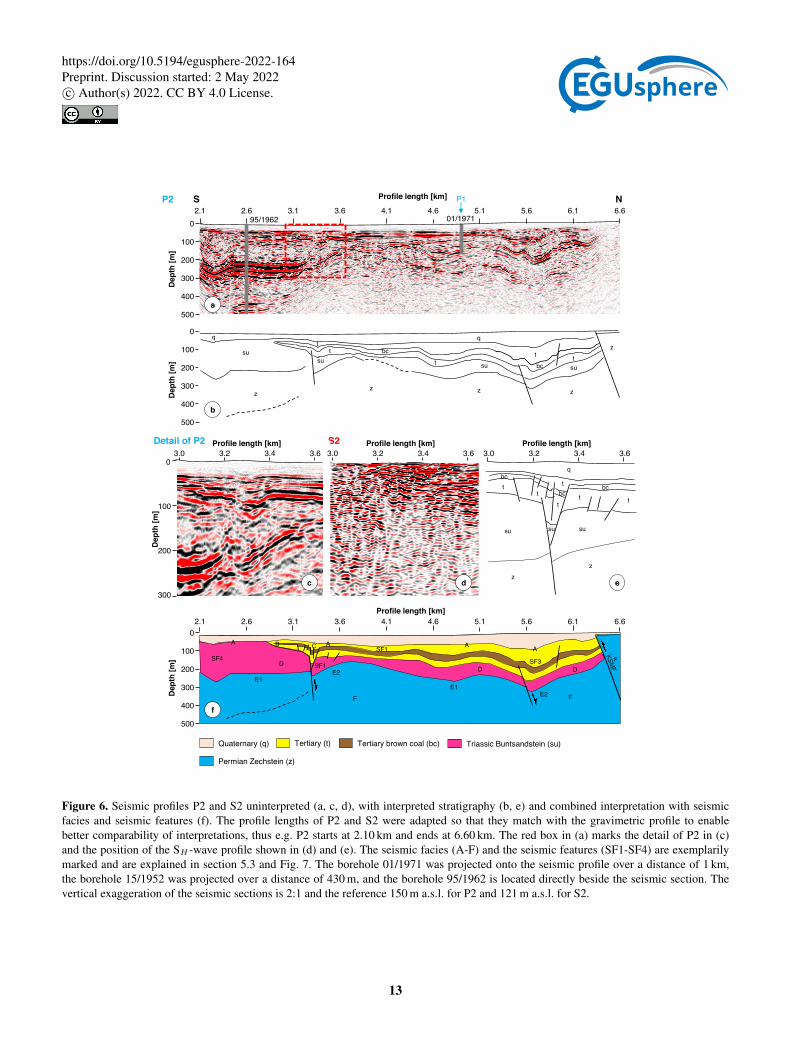
5.2 Interpretation of seismic profiles P2 & S2 (S–N)220

Reflection seismic profiles P2 and S2 were carried out from south to north. P-wave profile P2 is of 5.10 km length, but only

the first 4.50 km are analyzed, because of poor reflectivity in the most northern part. The SH -wave profile S1 is of 0.67 km

length. Profile S2 was surveyed after P2 and covers a selected area of P2. The profile lengths of P2 and S2 were adapted so

that they match the gravimetric profile to enable better comparability of interpretations, thus e.g. P2 starts at 2.10 km and ends

at 6.60 km.225

10


Profile length [km]WD

epth

[m]

P1 E0 0.5 2 2.51 1.5

01/1971

Dep

th[m

]D

epth

[m]

Profile length [km]

z

qt

bc

su

t bct t

susu

zz

z zz

bc ttt sususu

S1

htpeD

[m]

Profile length [km] Profile length [km]

a

b

f

susu

z

t

z

q

t

suz

zz

susu

susu

bct

bct

bc

t

tt

0

300

200

100

P2

Quaternary (q)


Tertiary (t)

Tertiary brown coal (bc)

Triassic Buntsandstein (su)

0

500

100

200

300

400

0

500

100

200

300

400

0

500

100

200

300

400

ABC

D

E1

F

A

D

E2

F

A

D

E2F

SF1SF2

SF2

SF1

ed

Detail of P1

c

0.5 1.0 1.25 1.50.75Profile length [km]

0 0.5 2 2.51 1.5

0.5 1.0 1.25 1.50.75 0.5 1.0 1.25 1.50.75

Figure 5. Seismic profiles P1 and S1 uninterpreted (a, c, d), with interpreted stratigraphy (b, e) and combined interpretation with seismicfacies and seismic features (f). The red box in (a) marks the detail of P1 in (c) and the position of the SH -wave profile shown in (d) and(e). The seismic facies (A–F) and the seismic features (SF1–SF2) are exemplarily marked and are explained in section 5.3 and Fig. 7. Thevertical exaggeration is 2:1 and the reference datum is 126 m a.s.l. for P1 and 124 m a.s.l. for S1.

The most northern part of P2 between ca. 6.35 km and 6.60 km profile length from the surface down to about 400 m depth

(Fig. 6a, b) shows irregular and discontinuous reflectors of low amplitudes. They represent the Permian Zechstein formations

of the Kyffhäuser hills. This area is separated from the south by a steep, northward-dipping thrust fault, the KSMF.

South of the KSMF, at 50 m to 100 m depth (Fig. 6a, b), a continuous, high-amplitude reflector is imaged, which is traceable

throughout almost the entire profile. Just as in P1 and S1, this impedance contrast is interpreted as the boundary between230

the Quaternary and Tertiary deposits. A second, mostly continuous reflector with high impedance contrast is visible between

ca. 2.90 km and 6.35 km profile length at 100 m to 200 m depth, which is interpreted as the top of the brown coal (Fig. 6a, b, d, e),

11


and is further used as a marker horizon. The thickness of the Tertiary formation decreases from north to south. The Triassic

sandstones below show no internal structures, but at ca. 250 m depth, a discontinuous, high-amplitude reflector is imaged. This

is interpreted as the top of the Permian Zechstein, which is traceable throughout the entire profile P2 (Fig. 6a, b). Repeatedly,235

between 3.20 km and 6.35 km profile length the reflector shows low reflectivity, but between ca. 2.40 km and 3.20 km profile

length it is continuous and has even higher amplitudes. These two areas are separated by a steep northward-dipping normal

fault (Fig. 6b, e, f).

Directly south of the KSMF, between 5.10 km and 6.35 km profile length, dipping reflectors that form a bowl-shaped struc-

ture within the Quaternary to Permian deposits are imaged (Fig. 6a, b, f). In contrast to the two structures observed in P1240

and S1, the Quaternary is affected too. The deepest point of the bowl-shaped structure is at ca. 400 m depth and coincides

with a low reflectivity zone in the Permian Zechstein. Another 0.30 km wide depression was identified to the south between

2.10 km and 2.40 km profile length at 200 m to 350 m depth within the Quaternary to Permian sediments (Fig. 6a, b). A third

bowl-shaped structure was imaged at shallow depth, in the near-surface between 3.30 km and 3.45 km profile length at ca. 40 m

to 100 m depth. This was pointed out as the area of interest for the SH -wave reflection seismic survey S2 (Fig. 6c, d, e). The245

high-amplitude reflectors of the top of the Tertiary are also observed in S2, but the impedance contrast is weaker than in P2. In

S2 details of the internal structure of the different formations can be recognized (for details, see section 5.3 and Fig. 7).

Besides the KSMF, other steep faults are identified below the northern depression and below the near-surface depression to

the south (Fig. 6f). The profiles P2 and S2 reveal that the fault below the near-surface depression, between 3.30 km and 3.45 km

profile length at ca. 40 m to 100 m depth, is not a single fault, but instead is a fault zone and nearly vertical fractures within the250

Lower Tertiary sediments are also imaged in S2.

The low reflectivity areas of the top Permian are assumed to be the result of leaching processes, similar to the bowl-shaped

structures, which are interpreted as a near-surface sinkhole due to cavity collapse and syn-sedimentary sagging of the surface

due to slow mass movement of material induced by subrosion. In contrast to the leached Permian to the north, it is less

affected by subrosion to the south, as indicated by strong impedance contrasts, which are probably the result of unimpaired255

evaporite sequences. The steep fault, at ca. 3.20 km profile length, may serve as a barrier for groundwater flow coming from

the Kyffhäuser hills.

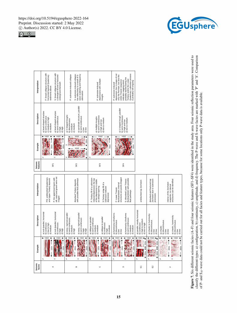
5.3 Seismic facies analysis

The procedure of the seismic facies analysis is based on Roksandic (1978). A total of six seismic facies types (A–F) and four

seismic features (SF1–SF4) can be identified in the P- and the SH -wave seismic data on the basis of configuration, continuity,260

amplitude, and frequency content (Fig. 7). A comparison of P-wave and S-wave was not possible for all facies and feature

types, because for some locations only P-wave data was available.

The three facies A–C are characterized by continuous to semi-continuous reflectors and represent more or less undisturbed

layers. Facies A consists of Quaternary and Upper Tertiary with continuous, horizontal, and parallel reflectors. Compared to

the S-wave sections, the P-wave sections show low amplitudes in the uppermost part due to resolution limits. As a result,265

the silt, sand and gravel layers of the Quaternary are not imaged, and the deeper parts are of high amplitudes. The S-wave

12


Profile length [km]SP22.1 2.6 4.1 4.6 5.65.13.1 3.6 6.66.1

N

01/1971

Profile length [km]

S2

htpeD

[m]

htpeD

[m]

htp eD

[m]

a

f

P1

Quaternary (q) Tertiary (t) Tertiary brown coal (bc) Triassic Buntsandstein (su)


A

D

E2

SF4 SF3

A

DE2

F

A

D

E1

F

AB C

E1

F

0

500

100

200

300

400

0

500

100

200

300

400

0

500

100

200

300

400

SF1

SF1

h tp eD

]m[

0

100

300

200

t

z

t

su

t

bcbc

bcttt

su su

z

q

Profile length [km] Profile length [km]

c d

3.2 3.4 3.63.0

e

Detail of P2 Profile length [km]

2.1 2.6 4.1 4.6 5.65.13.1 3.6 6.66.1

3.2 3.4 3.63.0 3.2 3.4 3.63.0

95/1962

q

tbc su

zz

z

z

su

su

t

z

q

ttsu

tbc

b

Figure 6. Seismic profiles P2 and S2 uninterpreted (a, c, d), with interpreted stratigraphy (b, e) and combined interpretation with seismicfacies and seismic features (f). The profile lengths of P2 and S2 were adapted so that they match with the gravimetric profile to enablebetter comparability of interpretations, thus e.g. P2 starts at 2.10 km and ends at 6.60 km. The red box in (a) marks the detail of P2 in (c)and the position of the SH -wave profile shown in (d) and (e). The seismic facies (A-F) and the seismic features (SF1-SF4) are exemplarilymarked and are explained in section 5.3 and Fig. 7. The borehole 01/1971 was projected onto the seismic profile over a distance of 1 km,the borehole 15/1952 was projected over a distance of 430 m, and the borehole 95/1962 is located directly beside the seismic section. Thevertical exaggeration of the seismic sections is 2:1 and the reference 150 m a.s.l. for P2 and 121 m a.s.l. for S2.

13


data, however, shows generally high amplitudes with a high frequency content and the differentiation of individual reflectors

within the two formations is more detailed, because of the improved resolution. Facies A might be a good water conduit for

horizontal water flow, due to the permeable gravel and sand layers, but noticeable vertical fluid pathways, which are important

for subrosion, were not found. Facies B shows the internal structures of the lower Tertiary silt, gravel, sand, and clay, and it270

has semi-continuous, wavy to sigmoid-parallel reflector patterns. Both P- and S-wave data show a high frequency content, but

the amplitudes in the S-wave are higher for this facies and the reflectors are thinner and more detailed compared to the P-wave

data. Facies B, with its semi-continuous reflector patterns, could favour vertical water flow. Facies C shows the Tertiary fill of

a subrosion-induced depression with oblique to parallel reflectors. P-wave and S-wave data show slightly different images. In

the P-wave data the Tertiary fill is visible as semi-continuous reflectors of medium amplitudes and medium frequency content,275

and in the S-wave data an onlap fill is observed with continuous reflectors, high amplitudes, and medium frequency content. In

contrast to the Tertiary deposits of Facies B, the depression fill does not seem to be strongly fractured.

The three facies D-F are characterized by mostly discontinuous reflectors and represent disturbed layers. Facies D consists of

Lower Triassic sandstones of the Buntsandstein, and the pattern configuration can be described as hummocky-clinoforms. In the

P-wave data this facies is discontinuous, of low amplitudes and low frequency content, and in the S-wave data semi-continuous280

reflectors of medium amplitudes and medium frequencies are observed. The sandstones are disturbed and no internal structures

are identified for both wave types, as a result it is most likely that the fractured, permeable sandstones serve as fluid pathways

for vertical and lateral groundwater flow. Facies E shows the different types of the top Permian horizon, which are identified in

the seismic sections. Facies E1 shows the undisturbed case with continuous, mostly horizontal and parallel reflector patterns.

Two differentiations for the undisturbed evaporite can be made. High amplitudes might indicate thicker salt layers that generate285

a stronger impedance contrast against the Triassic sandstones above, compared to medium amplitudes of possibly evaporite

(anhydrite, gypsum) that would generate a weaker impedance contrast. Facies E2 shows the disturbed case with discontinuous,

hummocky to chaotic reflection patterns, low amplitudes, and low frequency content. Both P-and S-wave data show the same

characteristics and this facies is interpreted as fractured and leached Zechstein formations, and are used for the determination

of subrosion zones. Facies F images the interior of the Permian Zechstein formations. Just like for Facies E2, P- and S-wave290

data are very similar showing discontinuous and chaotic reflectors with no internal structures.

The seismic feature SF1 consists of semi-continuous reflector patterns that form a bowl-shaped structure in both P- and

SH -wave data, although the amplitudes in the SH -wave data are generally higher, as is the frequency content. It is interpreted

as a broad sinkhole with more or less horizontal layers above. In the S-wave data a divergent fill and a fractured underground

beneath the sinkhole are identified. Seismic feature SF2 shows different characteristics in P-wave and S-wave. In the P-wave295

data, discontinuous reflectors form V-shaped troughs of medium amplitudes and medium frequency content, whereas in the SH -

wave data semi-continuous reflectors form parallel, synclinal structures of low amplitudes and low frequency. It is interpreted as

another subrosion-induced, steeper sinkhole. Seismic feature SF3 consists of multiple troughs of continuous to semi-continuous

reflectors of high and low amplitudes and medium to low frequency content. It is interpreted as a subrosion-induced depression

and the sagging is either still ongoing or was active until recent times, which is supported by the fact that all formations from300

the Permian to the Quaternary are affected. Seismic feature SF4 is similar to SF3, but in contrast only a U-shaped trough

14


Se

ism

ic

fac

ies

Ex

am

ple

De

sc

rip

tio

nIn

terp

reta

tio

n

A

a)

su

b-/

pa

ralle

l, h

ori

zo

nta

l

b)

co

ntin

uo

us

c)

low

to h

igh

d)

me

diu

m

a)

su

b-/

pa

ralle

l, h

ori

zo

nta

l

b)

co

ntin

uo

us

c)

hig

h

d)

hig

h

P/S

: u

nd

istu

rbe

dQ

ua

tern

ary

an

d U

pp

er

Te

rtia

ry d

ep

osits

P:

the

up

pe

rmo

st la

ye

rs w

ith

silt

, sa

nd

an

d g

rave

l w

ere

no

t

ima

ge

d

B

a)

wa

vy,

sig

mo

id p

ara

llel

b)

se

mi-

co

ntin

uo

us

c)

me

diu

m

d)

hig

h

a)

wa

vy,

sig

mo

id-p

ara

llel

b)

se

mi-

co

ntin

uo

us

c)

hig

h

d)

hig

h

dis

turb

ed

Te

rtia

ry d

ep

osits

with

po

ssib

le flu

id p

ath

wa

ys

C

a)

ob

liqu

e to

pa

ralle

l

b)

se

mi-

co

ntin

uo

us

c)

me

diu

m

d)

med

ium

a)

ob

liqu

e to

pa

ralle

l

b)

co

ntin

uo

us

c)

hig

h

d)

me

diu

m

P:

Te

rtia

ry f

illo

f a

su

bro

sio

n-

ind

uce

d d

ep

ressio

n; th

e to

p

of th

e d

epre

ssio

n is

vis

ible

as o

bliq

ue

laye

rin

g

S:T

ert

iary

on

lap

fill

of a

su

bro

sio

n-i

nd

uce

d

de

pre

ssio

n

D

a)

hu

mm

ocky-c

lino

form

s

b)

dis

co

ntin

uo

us

c)

low

d)

low

a)

hu

mm

ocky c

lino

form

s

b)

sem

i-con

tinuou

s

c)

me

diu

m

d)

me

diu

m

P:

Lo

we

r T

ria

ssic

Bu

nts

an

dste

in; in

tern

al

str

uctu

res a

re p

oo

rly im

ag

ed

S:

dis

turb

ed

Lo

we

r T

ria

ssic

Bunts

an

dste

inw

ith

possib

le

flu

id p

ath

wa

ys

E1

a)

pa

ralle

l, m

ostly h

ori

zo

nta

l

b)

co

ntin

uo

us

c)

hig

h to

me

diu

m

d)

low

to

hig

h

un

dis

turb

ed

to

p Z

ech

ste

in

E2

a)

ch

ao

tic to

hu

mm

ocky

b)

dis

co

ntin

uo

us

c)

low

d)

low

dis

turb

ed

an

d fra

ctu

red

to

p

Ze

ch

ste

ind

ue

to

su

bro

sio

n

pro

ce

sse

s

F

a)

ch

ao

tic

b)

dis

con

tinu

ous

c)

low

d)

low

a)

ch

ao

tic, h

um

mo

cky

b)

dis

co

ntin

uo

us

c)

low

d)

low

inte

rio

r o

f th

e Z

ech

ste

in

eva

po

rite

; n

o in

tern

al

str

uctu

res c

an

be

id

en

tifie

d

150m

100m

150m

100m

P S

200m

100m200m

100m

P S

100m

100m

100m

100m

P S

150m

100m

150m

100m

P S

100m

P

200m

200m

100m

P

300m

300m

S

300m

100m

300m

100m

P S

P

Se

ism

ic

fea

ture

sE

xa

mp

leD

es

cri

pti

on

Inte

rpre

tati

on

SF

1

a)

bo

wl-

sh

ap

ed

str

uctu

re

b)

se

mi-

co

ntin

uo

us

c)

me

diu

m to

hig

h

d)

me

diu

m

a)

bo

wl-

sh

ap

ed

str

uctu

re

b)

se

mi-

co

ntin

uo

us

c)

hig

h

d)

hig

h

P:

bro

ad

co

llap

se

str

uctu

re w

ith

ho

rizo

nta

l la

ye

red

Qu

ate

rna

ry

se

dim

en

tsa

bo

ve

S:

bro

ad

co

llap

se

str

uctu

re w

ith

a d

ive

rge

nt fill

an

d a

fra

ctu

red

un

de

rgro

un

d b

en

ea

th

SF

2

a)

V-s

ha

pe

d tro

ug

hs

b)

dis

co

ntin

uo

us

c)

me

diu

m

d)

me

diu

m

a)

syn

clin

ale

str

uctu

re, p

ara

llel

b)

se

mi-

co

ntin

uo

us

c)

low

d)

low

P:

su

bro

sio

n-in

duced

co

llap

se

S:

su

bro

sio

n-in

duced

co

llap

se

;

low

refle

ctivitiy

isa

re

su

lto

f S

-

wa

ve

sca

tte

rin

ga

nd

fre

qu

en

cy

att

en

ua

tio

n

SF

3

a)

mu

ltip

le tro

ug

hs

b)

se

mi-

/co

ntin

uo

us

c)

hig

h a

nd

low

d)

low

to

me

diu

m

P:

sub

rosio

n-ind

uced

de

pre

ssio

ns

with

mu

ltip

le

tro

ug

hs

SF

4

a)

U-s

ha

pe

d tro

ug

h, p

ara

llel

b)

se

mi-

/co

ntin

uo

us

c)

hig

h a

nd

lo

w

d)

low

to

me

diu

m

P:

su

bro

sio

n-in

duced

de

pre

ssio

n;th

e U

-sh

ap

eo

f n

ot

on

lyth

e P

erm

ian

, b

ut a

lso

th

e

en

tire

Tri

assic

se

qu

en

ce

ind

ica

tes

sa

gg

ing

wh

ich

pro

ba

bly

sta

rte

dd

uri

ng

the

Te

rtia

rya

nd

/or

the

Lo

we

r

Qua

tern

ary

; sub

rosio

n p

rocess

isp

rob

ab

lystill

on

go

ing

300m

100m

S

300m

100m

P

200m

200m

PS

200m

200m

700m

P

200m

350m

P

250m

Figu

re7.

Six

diff

eren

tsei

smic

faci

es(A

–F)a

ndfo

urse

ism

icfe

atur

es(S

F1–S

F4)w

ere

iden

tified

inth

est

udy

area

.Fou

rsei

smic

refle

ctio

npa

ram

eter

sw

ere

used

tocl

assi

fyth

edi

ffer

entt

ypes

:a)c

onfig

urat

ion,

b)co

ntin

uity

,c)a

mpl

itude

,and

d)fr

eque

ncy.

The

P-w

ave

and

S-w

ave

faci

esar

em

arke

dw

ith’P

’and

’S’.

Com

pari

son

ofP-

and

S H-w

ave

data

coul

dno

tbe

carr

ied

outf

oral

lfac

ies

and

feat

ure

type

s,be

caus

efo

rsom

elo

catio

nson

lyP-

wav

eda

tais

avai

labl

e.

15


0

200

100

300

400

500

Dep

th [m

]

600

a) Survey length [m]2.1 2.6 3.1 3.6 4.1 4.6 5.1 5.6 6.1 6.6TEM FL1 TEM FL3TEM FL2

Res

istiv

ity [Ω

m]

100

102

101

b) Survey length [m]2.1 2.6 3.1 3.6 4.1 4.6 5.1 5.6 6.1 6.6

0

200

100

300

400

500

Dep

th [m

]

600

susu

zz

zt

bc tqq

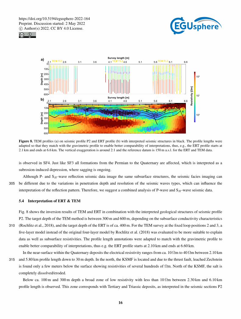
Figure 8. TEM profiles (a) on seismic profile P2 and ERT profile (b) with interpreted seismic structures in black. The profile lengths wereadapted so that they match with the gravimetric profile to enable better comparability of interpretations, thus, e.g., the ERT profile starts at2.1 km and ends at 6.6 km. The vertical exaggeration is around 2:1 and the reference datum is 150 m a.s.l. for the ERT and TEM data.

is observed in SF4. Just like SF3 all formations from the Permian to the Quaternary are affected, which is interpreted as a

subrosion-induced depression, where sagging is ongoing.

Although P- and SH -wave reflection seismic data image the same subsurface structures, the seismic facies imaging can

be different due to the variations in penetration depth and resolution of the seismic waves types, which can influence the305

interpretation of the reflection pattern. Therefore, we suggest a combined analysis of P-wave and SH -wave seismic data.

5.4 Interpretation of ERT & TEM

Fig. 8 shows the inversion results of TEM and ERT in combination with the interpreted geological structures of seismic profile

P2. The target depth of the TEM method is between 300 m and 600 m, depending on the subsurface conductivity characteristics

(Rochlitz et al., 2018), and the target depth of the ERT is of ca. 400 m. For the TEM survey at the fixed loop positions 2 and 3, a310

five-layer model instead of the original four-layer model by Rochlitz et al. (2018) was evaluated to be more suitable to explain

data as well as subsurface resistivities. The profile length annotations were adapted to match with the gravimetric profile to

enable better comparability of interpretations, thus e.g. the ERT profile starts at 2.10 km and ends at 6.60 km.

In the near-surface within the Quaternary deposits the electrical resistivity ranges from ca. 10 Ωm to 40 Ωm between 2.10 km

and 5.80 km profile length down to 30 m depth. In the north, the KSMF is located and due to the thrust fault, leached Zechstein315

is found only a few meters below the surface showing resistivities of several hundreds of Ωm. North of the KSMF, the salt is

completely dissolved/eroded.

Below ca. 100 m and 300 m depth a broad zone of low resistivity with less than 10 Ωm between 2.30 km and 6.10 km

profile length is observed. This zone corresponds with Tertiary and Triassic deposits, as interpreted in the seismic sections P2

16


and S2. Within this zone is an extremely conductive thin layer of approximately 1 Ωm, which is in particular resolved by the320

TEM data. The boundaries of this layer coincide well with main seismic reflectors. It is interpreted to match with saline aquifers

between the lignite and Triassic Buntsandstein. Unfortunately, there are no continuous TEM-soundings across the entire profile

available. In contrast, the ERT inversion data smears this layer over greater thickness due to limitations of resolution, but proves

its continuity.

From 3.10 km to 2.10 km profile length the extremely conductive layer vanishes and resistivities between 100 m and 300 m325

depth increase slightly, as shown by the ERT and TEM FL 1, which is probably related to the fault zone at 3.20 km. The fault

might hamper the lateral groundwater flow, and therefore, the lateral distribution of the salt water coming from the leached

Permian deposits, which migrated upward along the faults and fractures to the north due to artesian-confined groundwater

conditions.

The top Permian at 250 m to 300 m depth, as indicated by seismic interpretation, correlates with the top of the TEM basement330

layer with high resistivities of more than 100 Ωm. This is also visible in the ERT result, but the contrast is smoother and does

not reveal a unique basement depth. At 5.50 km profile length, the ERT shows lower electrical resistivities reaching depths of

500 m. This coincides well with the interpreted fault. This area correlates also with the position of subrosion-induced structures,

like the sinkholes above. Therefore, it is an indicator for salt-water ascension, due to dissolution of Zechstein evaporites and

artesian-confined groundwater conditions. The ascending salt water is the reason for the development of the inland salt marsh.335

A similar low-resistivity area at such great depths is located at 2.10 km to 2.50 km on the profile. However, since the profile

ends there, detailed interpretation is speculative.

Overall, the ERT and TEM results are in very good agreement with the seismic interpretation, although no joint inversion

was carried out, which would improve the quality of the datasets and their interpretation.

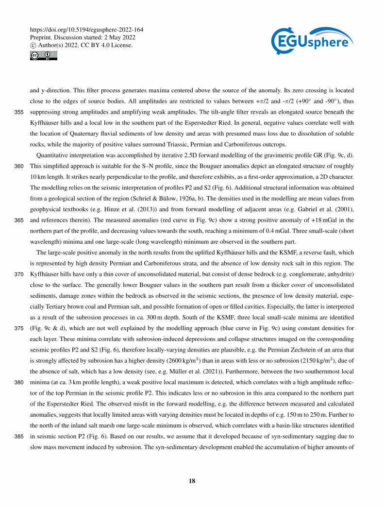
5.5 Interpretation of gravimetry340

The prominent features on the Bouguer map (Fig. 9a) are in remarkably good agreement with the near-surface strata on the

geological map (Fig. 1). The contours of the central positive Bouguer anomaly of +18 mGal (1 Gal = 0.01 m/s2) clearly follow

the outline of the Carboniferous (Kyffhäuser Formation) and Permian (Zechstein) rocks. The roundish negative anomaly of

-8 mGal to the SW correlates with outcropping Triassic (Muschelkalk) formations, whereas the WNW–ESE strike direction of

an elongated, central gradient zone matches the geometry of Tertiary and Quaternary sediments in the Esperstedter Ried.345

Several spectral domain filters were applied in order to locate possible sources of gravity anomalies and to highlight fine

changes in the gravity field. As an example, Fig. 9b shows the result of the so called ’tilt derivative’ or ’tilt angle’ filter (Miller

& Singh, 1994), which is defined as

Θ = tan−1 VDRTHDR

,350

where VDR is the first vertical derivative of the gravitational potential, which describes the vertical gravity component, and

THDR is the total horizontal derivative, which describes the combined horizontal gravity components of the field vector in x-

17


and y-direction. This filter process generates maxima centered above the source of the anomaly. Its zero crossing is located

close to the edges of source bodies. All amplitudes are restricted to values between +π/2 and -π/2 (+90 and -90), thus

suppressing strong amplitudes and amplifying weak amplitudes. The tilt-angle filter reveals an elongated source beneath the355

Kyffhäuser hills and a local low in the southern part of the Esperstedter Ried. In general, negative values correlate well with

the location of Quaternary fluvial sediments of low density and areas with presumed mass loss due to dissolution of soluble

rocks, while the majority of positive values surround Triassic, Permian and Carboniferous outcrops.

Quantitative interpretation was accomplished by iterative 2.5D forward modelling of the gravimetric profile GR (Fig. 9c, d).

This simplified approach is suitable for the S–N profile, since the Bouguer anomalies depict an elongated structure of roughly360

10 km length. It strikes nearly perpendicular to the profile, and therefore exhibits, as a first-order approximation, a 2D character.

The modelling relies on the seismic interpretation of profiles P2 and S2 (Fig. 6). Additional structural information was obtained

from a geological section of the region (Schriel & Bülow, 1926a, b). The densities used in the modelling are mean values from

geophysical textbooks (e.g. Hinze et al. (2013)) and from forward modelling of adjacent areas (e.g. Gabriel et al. (2001),

and references therein). The measured anomalies (red curve in Fig. 9c) show a strong positive anomaly of +18 mGal in the365

northern part of the profile, and decreasing values towards the south, reaching a minimum of 0.4 mGal. Three small-scale (short

wavelength) minima and one large-scale (long wavelength) minimum are observed in the southern part.

The large-scale positive anomaly in the north results from the uplifted Kyffhäuser hills and the KSMF, a reverse fault, which

is represented by high density Permian and Carboniferous strata, and the absence of low density rock salt in this region. The

Kyffhäuser hills have only a thin cover of unconsolidated material, but consist of dense bedrock (e.g. conglomerate, anhydrite)370

close to the surface. The generally lower Bouguer values in the southern part result from a thicker cover of unconsolidated

sediments, damage zones within the bedrock as observed in the seismic sections, the presence of low density material, espe-

cially Tertiary brown coal and Permian salt, and possible formation of open or filled cavities. Especially, the latter is interpreted

as a result of the subrosion processes in ca. 300 m depth. South of the KSMF, three local small-scale minima are identified

(Fig. 9c & d), which are not well explained by the modelling approach (blue curve in Fig. 9c) using constant densities for375

each layer. These minima correlate with subrosion-induced depressions and collapse structures imaged on the corresponding

seismic profiles P2 and S2 (Fig. 6), therefore locally-varying densities are plausible, e.g. the Permian Zechstein of an area that

is strongly affected by subrosion has a higher density (2600 kg/m3) than in areas with less or no subrosion (2150 kg/m3), due of

the absence of salt, which has a low density (see, e.g. Müller et al. (2021)). Furthermore, between the two southernmost local

minima (at ca. 3 km profile length), a weak positive local maximum is detected, which correlates with a high amplitude reflec-380

tor of the top Permian in the seismic profile P2. This indicates less or no subrosion in this area compared to the northern part

of the Esperstedter Ried. The observed misfit in the forward modelling, e.g. the difference between measured and calculated

anomalies, suggests that locally limited areas with varying densities must be located in depths of e.g. 150 m to 250 m. Further to

the north of the inland salt marsh one large-scale minimum is observed, which correlates with a basin-like structures identified

in seismic section P2 (Fig. 6). Based on our results, we assume that it developed because of syn-sedimentary sagging due to385

slow mass movement induced by subrosion. The syn-sedimentary development enabled the accumulation of higher amounts of

18


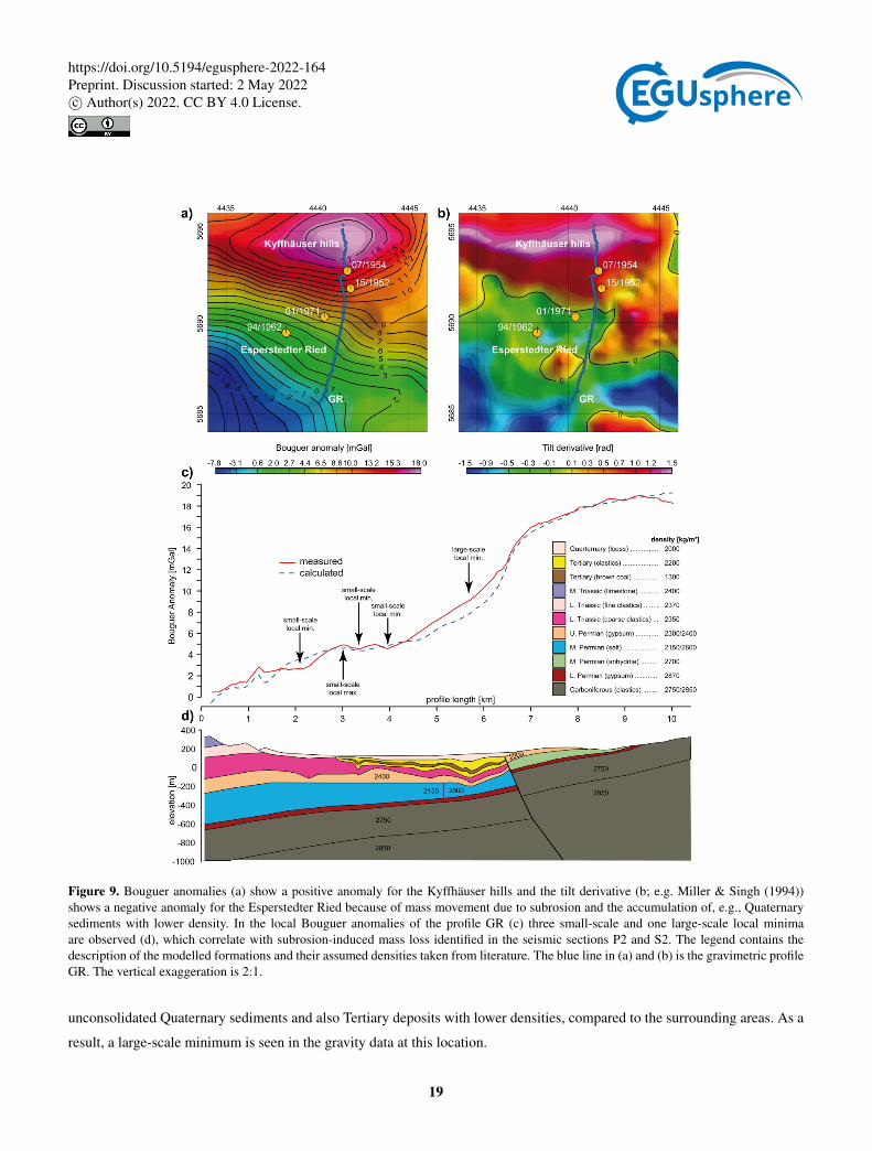
Figure 9. Bouguer anomalies (a) show a positive anomaly for the Kyffhäuser hills and the tilt derivative (b; e.g. Miller & Singh (1994))shows a negative anomaly for the Esperstedter Ried because of mass movement due to subrosion and the accumulation of, e.g., Quaternarysediments with lower density. In the local Bouguer anomalies of the profile GR (c) three small-scale and one large-scale local minimaare observed (d), which correlate with subrosion-induced mass loss identified in the seismic sections P2 and S2. The legend contains thedescription of the modelled formations and their assumed densities taken from literature. The blue line in (a) and (b) is the gravimetric profileGR. The vertical exaggeration is 2:1.

unconsolidated Quaternary sediments and also Tertiary deposits with lower densities, compared to the surrounding areas. As a

result, a large-scale minimum is seen in the gravity data at this location.

19


The results show that even large-scale gravimetry can help to identify possible areas affected by subrosion-induced mass

movement.390

6 Discussion

6.1 Conceptual subrosion model of the Esperstedter Ried

To better understand the local subrosion processes of the Esperstedter Ried the geological evolution of the region has to be

first reconstructed. This includes the sedimentary depositional history and the development of large-scale geological structures,

like faults or basins (McCann & Saintot, 2003), which can be identified directly using seismic and indirectly using gravimetric395

methods (Conrad, 1996; Hinze et al., 2013). These structures can have an influence on past and recent subrosion processes,

e.g., enhanced subrosion at faults (Closson & Abou Karaki, 2009; Del Prete et al., 2010; Ezersky & Frumkin, 2013a; Wadas

et al., 2017). After reconstructing the general geological evolution of the Esperstedter Ried, the factors controlling the local

subrosion will be outlined and a conceptual model will be presented.

In the Esperstedter Ried the P- and SH -wave reflection seismics and the gravimetric investigation revealed large- and small-400

scale structures, like faults, fractures and thickness variations, delivering a structural model of the area. With regard to the fault

development, it is known that from the Upper Cretaceous to the Lower Tertiary, the Kyffhäuser hills were upthrusted and the

KSMF developed (Freyberg, 1923; Seidel, 2003). This fault has a Hercynian strike, which can be observed in the geological

map of Bad Frankenhausen (Schriel & Bülow, 1926a, b) and in the gravimetry data (Fig. 9). This preferred Hercynian strike

direction of northern Germany can also be observed in the formations shown in the reflection seismic profiles P2 and S2405

(Fig. 6), in which other faults were identified that transverse the profiles, cut the Lower Tertiary, and show approximately a

NW–SE strike. It has to be noted that the Bouguer anomaly maps shown in this study have a resolution limit of 1 km and

therefore cannot image this scale of faulting.

Furthermore, we assume that the uplift of the Kyffhäuser hills led to flexural isostasy (Watts, 2001) in the southern foreland

and therefore regional, large-scale subsidence, which has to be distinguished from the local subrosion-induced subsidence.410

After Weber (1930), subrosion-induced sagging/subsidence can be subdivided into three phases: (1) dissolution of salt, (2)

hydration of anhydrite and transformation into gypsum, and (3) leaching of gypsum. During the first phase, planar cavities

are formed along the salt layer resulting in local sagging and during the third phase funnel-shaped cavities are formed and

after collapse they form a sinkhole. These three phases can be identified in the Esperstedter Ried, utilizing the seismic sections

(Figs. 5 & 6) and the gravimetric modelling results. They enabled the identification of large sagging structures, e.g. visible415

by thickness variations (explained in more detail below) and salt water ascension that represent the first phase, and mass

movement and collapse structures that represent the third phase. These structures can be correlated with local minima of the

Bouguer anomaly (Fig. 9), which is evidence of mass movement and mass removal. Altogether this proves the assumption of

subrosion-induced subsidence at the Esperstedter Ried.

Overall, the Permian, Triassic and Tertiary formations show thickness variations across the study area. Except for local420

variations, a general decrease in thickness from south to north, towards the KSMF, is observed for the Permian and Triassic

20


deposits. The thickness variation of the Triassic is probably a result of erosion after deposition and a varying accommodation

space during deposition, but the thickness variations of the Zechstein are mostly the result of subrosion. Since faults are able to

enhance subrosion (Closson & Abou Karaki, 2009; Del Prete et al., 2010; Ezersky & Frumkin, 2013a; Wadas et al., 2017), the

leaching process is more intense close to the KSMF and more salt and gypsum are dissolved leading to mass movement and a425

decrease in thickness of the Zechstein formation. Other reasons, such as active diapirs and salt movement, as reasons for the

Zechstein thickness variations can be excluded. According to the geological map, the top Carboniferous is found in ca. 550 m

depth and the thickness of the Permian is expected to be between ca. 350 m to 400 m. The salt in the Permian deposits needs to

be much thinner, so even if the top Carboniferous varies in depth it is highly unlikely that the salt layer would be thick enough

to form active diapirs (Schultz-Ela et al., 1993; Jackson et al., 1994). Salt movement due to increased differentiated load is also430

unlikely, because areas with a thicker Triassic Buntsandstein do not correlate with areas of thinner Permian deposits (Schultz-

Ela et al., 1993), instead the opposite is observed. However, the thickness of the Triassic sandstones does have an influence

on the formation of subrosion-induced structures. Great thicknesses of a compact rock are relatively stable against subrosion-

induced subsidence and collapse, because even when cavities are formed in the Zechstein formations beneath, the sediments

above the cavity would form a structural arch (Waltham et al., 2005), which prevents collapse and subsidence. Whereas low435

thicknesses of the Triassic sandstones increase the possibility of cavity collapse and local subsidence, which is the case in

the Esperstedter Ried. Further evidence for the long lasting subsidence is given by the Tertiary brown coal that was deposited

during the Oligocene, and which shows a varying thickness and a dip variation of 10° to 60° (Frank, 1845). It is unlikely

that the brown coal was deposited with such a high dip, so we assume that the brown coal thickness variations are a result of

continued subrosion-induced sagging during deposition, with thinner brown coal at the basin margins and thicker brown coal440

at the basin centre.

A better understanding of especially the recent local subrosion processes, however, also requires detailed knowledge about

the fluid pathways and the localization of subrosion zones. This was accomplished using ERT/TEM, and seismic facies analysis

of P- and SH -waves. The top of the soluble Permian rocks was detected at 250 m to 300 m depth, so near-surface subrosion, as

it is the case for the town of Bad Frankenhausen, north of the KSMF (Wadas et al., 2016; Kobe et al., 2019), is not possible. The445

unsaturated groundwater needs to reach greater depths in order to leach the evaporites such as salt and anhydrite. One of this

groundwater levels is detected in 150 m to 200 m depth according to the TEM data, which shows a low resistivity zone in this

depth. Regarding this, downward water flow through a fracture network is required for subrosion (Billi et al., 2007). Although

this process takes place mostly at shallower depths, a correlation between fractures and subrosion features is observed for the

Esperstedter Ried from the seismic facies analysis. The low resistivity zone of the TEM data is connected with the soluble450

rocks through a fractured seismic facies of the Triassic and Lower Tertiary, as shown in the S-wave data (Fig. 7). Faults are

also very important for vertical water flow, and this is shown by the ERT data. At faults the water can migrate downwards

and dissolve the deeper soluble rocks, as observed in seismic profile P2 and the ERT (Figs. 6 & 8), where below the sagging

structures steep faults crosscut the Tertiary, Triassic and probably Permian deposits, and serve as large fluid pathways. The

water can also migrate upward along the fault planes (Legrand & Stringfield, 1973) and fractures (Pusch et al., 1997; Westhus455

et al., 1997), mostly due to artesian-confined groundwater flow towards the surface, as is the case for the Esperstedter Ried.

21


The ERT identified an area of low resistivity at the surface between 3.9 km and 4.7 km profile length, which is the centre of

the inland salt marsh (Fig. 8). Besides the fluid pathways, possible subrosion zones have also been identified by the P-wave

reflection seismic profiles and the ERT. Areas affected by subrosion show a less pronounced top Zechstein reflector, and a

lower resistivity. The leaching and the mass movement destroy the layer boundary and the layering of the Zechstein, therefore460

no continuous reflector can be observed (e.g. below the large sagging structure to the north of P2). The opposite is visible in

the south of P2, where a strong impedance contrast without a low resistivity zone is imaged for the top Zechstein, indicating

less subrosion.

Altogether, the tectonic and depositional history indicate that subrosion was probably triggered by tectonic movements and

fault development and therefore, was probably most active during and after the tectonic phases of the Tertiary, but it is still465

ongoing, as it is evidenced by continuous salt water ascension at the Esperstedter Ried (TMLNU, 2008) and recent subsidence

and sinkhole development (Jankowski, 1964; Wadas et al., 2016; Kobe et al., 2019).

6.2 Workflow for geophyiscal investigations of subrosion areas

Based on the results of this study, we propose that our combined geophysical approach is suitable to generally investigate sub-

rosion areas and to create conceptual models that describe the factors controlling subrosion-induced subsidence and sinkhole470

formation, which also help to identify risk areas. Our recommended workflow (Fig. 10) will be explained in the following,

including conditions and limitations of the proposed methods that have to be kept in mind.

Reflection seismics is the preferred method to identify sagging- and collapse structures, and also faults and fractures, even in

urbanized regions, as other studies have shown for P-waves (e.g. Steeples et al. (1986); Evans et al. (1994); Miller & Steeples

(2008); Keydar et al. (2012)) and for S-waves (e.g. Miller et al. (2009); Pugin et al. (2013); Polom et al. (2016); Wadas475

et al. (2016); Polom et al. (2018)). Especially the combined approach of using P- and SH -waves in this study improves the

understanding of local subrosion structures. With the P-wave reflection seismics large-scale and with the SH -wave reflection

seismics small-scale structures can be identified. But since subrosion results in strong vertical and lateral variations of the

underground a densely-spaced seismic survey has to be acquired in order to image these variations. Furthermore, the penetration

depth of the seismic waves has to be considered. Shear-waves can image the underground at higher resolution than P-waves in480

the case of water-saturated and unconsolidated sediments, but the penetration depth is lower. As a result, with the equipment

used in this study, shear-wave reflection seismics is able to image the underground down to ca. 300 m depth and the P-wave

reflection seismics delivers images from ca. 30 m below surface to ca. 400 m to 500 m depth. Another seismic source with a

higher energy transmission might solve this problem, and to detect smaller subrosion features at the near-surface higher sweep

frequencies, and at least a smaller source and receiver spacing should be used. The seismic facies analysis has shown that485

one and the same facies unit can have different characteristics, depending on the wave-type applied, but both, P- and SH -

wave reflection seismic methods combined, can give valuable information about subrosion- and fracture zones, and therefore

potential fluid pathways. With a combined approach the advantages of both methods can be used to create a structural model

covering a wide range of scales from deep and large-scale structures to near-surface and small-scale features. Based on such a

sophisticated structural model, the sedimentary depositional history can be reconstructed.490

22


Another type of geophysical methods are geoelectric (e.g. ERT) and electromagnetic (e.g. TEM) techniques. ERT has shown

to be useful in identifying aquifers and fluid pathways in karst regions (e.g. Militzer et al. (1979); Bosch & Müller (2001);

Miensopust et al. (2015)), especially in combination with seismic methods that deliver structural constraints (e.g. Sandersen &

Jørgensen (2003); Bosch & Müller (2005); Tanner et al. (2020)). The advantage of TEM over ERT is the improved resolution

in the near-surface down to ca. 300 m depth, but without ERT the information about the electrical resistivity in greater depths495

e.g. 400 m to 500 m would be missing, where subrosion at faults may occur at greater depths. In general, ERT is better suited to

detect lateral resistivity variations, whereas TEM is highly sensitive to conductive structures. Similar to seismic methods, the

source and receiver spacing is the determining factor for the possibility to detect aquifers, fluid pathways, or subrosion zones.

In this study, the spacing of 200 m for the ERT and of 50 m for the TEM survey was sufficient to recover larger subrosion

features (e.g., the low resistivity zone at the fault in profile P2 at 5.60 km profile length), but targeting near-surface, small-500

scale subrosion zones would require survey layouts with denser source and receiver spacings. It is also necessary to note, that

ERT has a restricted applicability in urban areas due to disturbances by electromagnetic noise. In contrast Rochlitz et al. (2018)

demonstrated that the inversion results of a SQUID-based TEM exhibits a higher consistency between neighboring stations and

less artifacts caused by anthropogenic noise compared to classical coil-based TEM. The identified aquifers and salt-water bear-

ing areas combined with the structural model can than be used to derive a hydrological model. From this hydrological model,505

together with the reconstructed sedimentary facies and depositional history of the region, the fluid pathways and subrosion

zones can be derived.

Both reflection seismic- and electromagnetic methods do not deliver information about local mass movements or cavities

induced by subrosion. For this gravimetry is the preferred method for near-surface investigations in order to depict density

contrasts and local gravity anomalies (e.g. Butler (1984); Kersten et al. (2017); Kobe et al. (2019)). In our study, we show that510

structures and zones affected by subrosion as identified by the reflection seismic- and electromagnetic methods correlate with

local minima of the Bouguer anomaly due to reduced densities. Therefore, the gravity data together with the structural model

can be utilized to get a density-distribution model of the subsurface from which the local mass movement can be deduced. The

station spacing for the gravimetry profile in this study was 100 m, which was appropriate to detect mass movement on a larger

scale (e.g. the near-surface collapse structures producing local minima had a lateral extent of at least ca. 100 m), but in case of515

the detection of small-scale subrosion, as it is necessary for urban environments, we suggest to use a smaller station spacing

(e.g. < 50 m).

By combining all the models/results the local control factors of subrosion-induced subsidence and sinkhole formation can

be determined and risk areas can be identified (Fig. 10).

7 Conclusions520

The initial trigger of subrosion at the inland salt marsh of the Esperstedter Ried were the tectonic movements during the Tertiary,

which led to the uplift of the Kyffhäuser hills and the formation of faults parallel and perpendicular to the low mountain range.

The faults and the fractured Triassic and Lower Tertiary deposits serve as fluid pathways for groundwater to leach the deep

23


Density-distribution

model

Control factors of subrosion-induced subsidence / sinkhole formation & identification of risk areas

Site inspection

(e.g. satellite data, historical information,

geological maps, boreholes)

Structural model

P-wave reflection seismic

Depth: 30 – 500 m

Property: impedance contrast

Identification of deep & large-

scale geological structures

SH-wave reflection seismic

Depth: 0 – 300 m

Property: impedance contrast

Identification of near-surface

small-scale structures

ERT/TEM

Depth: 0 – 400 m

Property: resistivity

Identification of fluids &

saltwater

Gravimetry

Depth: 0 – 1000 m

Property: Bouguer anomaly

Identification of density

contrasts & local minima

Mass movementFluid pathways & subrosion zones Sediment facies & history

Hydrological model

Figure 10. Recommended workflow for geophysical investigations of subrosion areas to determine controlling factors and risk areas.

Zechstein deposits, since subrosion is more intense near faults. The artesian-confined salt water ascends towards the surface

along the faults and fracture networks, which formed the inland salt marsh over time. In the past, subrosion of the Zechstein525

formations formed, now buried, sagging and collapse structures, but subrosion features are also found near the surface and,

since the entire region is affected by recent sinkhole development, subrosion must be still ongoing.

We show that the combined analysis of P-wave and SH -wave reflection seismics is well suited to develop a structural model

and locate buried subrosion structures, subrosion zones, faults and fractures, and potential aquifers and aquitards, on the basis of

seismic facies analysis. To get a better insight into the hydrological conditions of an investigation area, ERT/TEM are effective530

in identifying and characterizing aquifers, aquitards, fluid pathways an subrosion zones. Further improvement is accomplished

by including gravimetry to identify density contrasts and to detect subrosion-induced mass movement. Based on our results,

we suggest a combined geophysical investigation of subrosion areas to identify controlling factors and risk areas to better

understand the subrosion processes.

In a next step, the structural and physical and geological constraints derived from our proposed geophysical investigation535

workflow described above, could be used as input parameters for numerical modelling. Numerical modelling is widely used

to better understand, e.g., physio-chemical or mechanical processes. In the context of subrosion, numerical modelling is ap-

plied to, e.g., simulate the time-dependent dissolution processes and the collapse mechanisms of sinkholes (Parise & Lollino,

2011; Salmiet al., 2017; Al-Halbouni et al., 2018; Shiau & Hassan, 2021). Important structural input parameters from our

recommended workflow are layer boundaries, facies types, faults, fractures, and sinkhole geometries. In addition, density and540

electrical resistivity values, and elastic parameters can be used as physical constraints, in order to depict, e.g., the mechanical

24


strength of the modelled layers/formations. The derived geophysical and structural constraints could also be extended by adding

a time component in the form of repeated surveys that enable the detection of time-varying parameters (e.g. mass loss rates

and fracture propagation; e.g. Herwanger et al. (2013); Kobe et al. (2019)), which would enhance risk scenario simulations.

Furthermore, the presented workflow could also be applied to investigate other geohazards with similar controlling factors,545

such as landslides (Malehmir et al., 2016), which are affected by subsurface structures and facies distribution, ground stability

of the layers/formations, hydrological conditions, e.g., fluid pathways, and mass redistribution.

Data availability. The seismic, ERT and TEM data are the property of LIAG. The data are available from the first author upon request.

Please contact Sonja H. Wadas for details. The gravimetry data is the property of the Thuringian State Institute for Environment, Mining and

Conservation.550

Author contributions. The seismic data was conducted by SW, HB and UP, and LIAG’s seismic field crew. Data processing of the SH -wave

seismic data was carried out by SW and data processing of the P-wave seismic data was carried out by HB. The seismic facies was analyzed

by SW. The ERT and TEM data was surveyed by RR, TG and MG, and inversion of the ERT data was carried out by TG and processing of the

TEM data was performed by RR. The modelling of the gravimetry data was carried out by PS. All authors contributed to the interpretations.

SW created all figures except for figure 8 which were created by RR and TG. SW prepared and discussed the results with all co-authors. SW555

wrote the manuscript and all co-authors inspired and improved the manuscript.

Competing interests. The authors declare that they have no conflict of interest.

Acknowledgements. We thank our colleagues Jan Bayerle, Dieter Epping, Eckhardt Großmann, Siegfried Grüneberg, Robert Meyer, Frank

Oppermann, Wolfgang Südekum and Sven Wedig for their excellent work during the field surveys. Furthermore we thank Lutz Katzschmann,

Sven Schmidt and Ina Pustal from the Thuringian State Institute for Environment, Mining and Conservation for supporting this work and560

providing the gravity data. Further thanks go to Ronny Stolz and Andreas Chwala from IPHT Jena and Supracon AG Jena for conducting

the TEM survey, which was funded by the Federal Ministry of Education and Research (BMBF), as part of INFLUINS under BMBF

grant 031S2091A. We thank Matthias Queitsch and Nina Kukowski from University of Jena for their advice on TEM data processing and

interpretation as well as Pritam Yogeshwar and Sascha Janser from University of Cologne for providing the inversion code EMUPLUS.

25


References565

Abelson, M., Baer, G., Shtivelman, V., Wachs, D., Raz, E., Crouvi, O., Kurzon, I. & Yechieli, Y.: Collapse-sinkholes and radar interferometry

reveal neotectonics concealed within the Dead Sea basin, Geophys. Res. Lett., 30, 10, 52.1–52.3, doi = 10.1029/2003GL017103, 2003.

Al-Halbouni, D., Holohan, E.P., Taheri, A., Schöpfer, M.P.J., Emam, S. & Dahm, T.: Geomechanical modelling of sinkhole development

using distinct elements: model verification for a single void space and application to the Dead Sea area, Solid Earth, 9, 1341–1373, doi =

10.5194/se-9-1341-2018, 2018.570

Al-Halbouni, D., Holohan, E.P., Abbas, T., Watson, R.A., Polom, U., Schöpfer, M.P.J., Emam, S. & Dahm, T.: Distinct element geomechan-

ical modelling of the formation of sinkhole clusters within large-scale karstic depressions, Solid Earth, 10, 1219–1241, doi = 10.5194/se-

10-1219-2019, 2019.

Al-Halbouni, D., Watson, R.A., Holohan, E.P., Meyer, R., Polom, U., Dos Santos, F.M., Comas, X., Alrshdan, H., Krawczyk, C.M. & Dahm,

T.: Dynamics of hydrological and geomorphological processes in evaporite karst at the eastern Dead Sea - a multidisciplinary study,575

Hydrol. Earth Syst. Sci., 25, 3351–3395, doi = 10.5194/hess-25-3351-2021, 2021.

Augarde, C.E., Lyamin, A.V. & Sloan, S.W.: Prediction of Undrained Sinkhole Collapse, J. Geotech. Geoenviron., 129, 3, 197–205, doi =

10.1061/(ASCE)1090-0241(2003)129:3(197), 2003.

Batayneh, A.T., Abueladas, A.A. & Moumani, K.A.: Use of ground-penetrating radar for assessment of potential sinkhole conditions: an

example from Ghor al Haditha area, Jordan, Environ. Geol., 41, 8, 977–983, doi = 10.1007/s00254-001-0477-8, 2002.580

Beck, B.F.: Environmental and engineering effects of sinkholes – the process behind the problems, Environ. Geol., 12, 2, 71–78, doi =

10.1007/BF02574791, 1988.

Billi, A., Valle, A., Brilli, M., Faccenna, C. & Funiciello, R.: Fracture-controlled fluid circulation and dissolutional weathering in sinkhole-

prone carbonate rocks from central Italy, Journal of Structural Geology, 29, 385–395, doi = 10.1016/j.jsg.2006.09.008, 2007.

Bosch, F.P. & Müller, I.: Continuous gradient VLF measurements: a new possibility for high resolution mapping of karst structures, First585

Break, 19, 6, 343–350, doi = 10.1046/j.1365-2397.2001.00173.x, 2001.

Bosch, F.P. & Müller, I.: Improved karst exploration by VLF-EM-gradient survey: comparison with other geophysical methods, Near Surface

Geophysics, 3, 299–310, doi = 10.3997/1873-0604.2005025, 2005.

Butler, K.: Microgravimetric and gravity gradient techniques for detection of subsurface cavities, Geophysics, 49, 7, 1084–1096, doi =

10.1190/1.1441723, 1984.590

Closson, D. & Abou Karaki, N.: Salt karst and tectonics: sinkholes development along tension cracks between parallel strike-slip faults, Dead

Sea, Jordan, Earth Surf. Process. Landforms, 34, 1408-–1421, doi = 10.1002/esp.1829, 2009.

Conrad, W.: Die Schwerekarte der Länder Brandenburg, Mecklenburg-Vorpommern, Sachsen, Sachsen-Anhalt und Thüringen 1:500 000,

Landesvermessung Sachsen, Freiberg, Germany, 1996.

Dasios, A., McClann, C., Astin, T.R., McCann, D.M., & Fenning, P.: Seismic imaging of the shallow subsurface: shear-wave case histories,595

Geophys. Prospect., 47, 565–591, doi = 10.1046/j.1365-2478.1999.00138.x, 1999.

Davies, W.E.: Mechanics of Cavern Breakdown, Nat. Speleo. Soc., 13, 36–43, 1951.

Del Prete, S., Iovine, G., Parise, M. & Santo, A.: Origin and distribution of different types of sinkholes in the plain areas of Southern Italy,

Geodinamica Acta, 23, 1–3, 113–127, doi = 10.3166/ga.23.113-127, 2010.

Doetsch, J., Linde, N., Pessognelli, M., Green, A.G. & Günther, T.: Constraining 3-D electrical resistance tomography with GPR reflection600

data for improved aquifer characterization, J. Appl. Geophys., 78, 68–76, doi = 10.1016/j.jappgeo.2011.04.008, 2012.

26


Eppelbaum, L.V., Ezersky, M., Al-Zoubi, A., Goldshmidt, V., & Legchenko, A.: Study of the factors affecting the karst volume assessment

in the Dead Sea sinkhole problem using microgravity field analysis and 3-D modeling, Advances in Geosciences, 19, 97–115, doi =

10.5194/adgeo-19-97-2008, 2008.

Evans, M.W., Snyder, S.W. & Hine, A.C.: High-resolution seismic expression of karst evolution within the Upper Floridian aquifer system;605

Crooked Lake, Polk County, Florida, J. Sediment. Res., 64, 2b, 232–244, doi = 10.1306/D4267F9B-2B26-11D7-8648000102C1865D,

1994.

Ezersky, M.G. & Frumkin, A.: Fault — Dissolution front relations and the Dead Sea sinkhole problem, Geomorphology, 201, 35–44, doi =

10.1016/j.geomorph.2013.06.002, 2013a.

Ezersky, M.G., Eppelbaum, L.V., Al-Zoubi, A., Keydar, S., Abueladas, A., Akkawi, E. & Medvedev, B.: Geophysical prediction and following610

development sinkholes in two Dead Sea areas, Israel and Jordan, Environmental Earth Sciences, 70, 1463–1478, doi = 10.1007/s12665-

013-2233-2, 2013b.

Ezersky, M.G., Eppelbaum, L.V., Legchenko, A., Al-Zoubi, A. & Aboueladas, A.: Salt layer characteristics in the Ghor Al-Haditha area,

Jordan: comprehensive combined reprocessing of geophysical data, Environmental Earth Sciences, 80, 1–20, doi = 10.1007/s12665-021-

09373-4, 2021.615

Flechsig, C., Heinicke, J., Mrlina, J., Kämpf, H., Nickschick, T., Schmidt, A., Bayer, T., Günther, T., Rücker, C., Seidel, E. & Seidl, M.:

Integrated geophysical and geological methods to investigate the inner and outer structures of the Quaternary Mytina maar (W-Bohemia,

Czech Republic), Int. J. Earth Sci., 104, 8, 2087–2105, doi = 10.1007/s00531-014-1136-0, 2015.

Frank, C.: Beitrag zur geognostischen Kenntnis des Kyffhäusergebirges, Berg- und Hüttenmännische Zeitung, 4, 10–12, 201–257, Freiberg,

Germany, 1845.620

Freyberg, B.V.: Die tertiären Landoberflächen in Thüringen. Fortschritte der Geologie und Paläontologie Vol. 6, Gebrüder Bornträger Verlag,

Berlin, Germany, 1923.

Gabriel, G., Jahr, T. & Weber, U.: The gravity field south of the Harz Mountains: Predominated by granitic material?, Z. geol. Wiss., 29, 3,

249–266, http://www.zgw-online.de/en/media/249-013.pdf, 2001.

Günther, T., Rücker, C. & Spitzer, K.: 3-D modeling and inversion of DC resistivity data incorporating topography - Part II: Inversion,625

Geophys. J. Int., 166, 506–517, doi = 10.1111/j.1365-246X.2006.03011.x, 2006.

Gutiérrez, F., Guerrero, J. & Lucha, P.: A genetic classification of sinkholes illustrated from evaporite paleokarst exposures in Spain, Environ.

Geol., 53, 5, 993–1006, doi = 10.1007/s00254-007-0727-5, 2008.

Gutiérrez, F., Parise, M., De Waele, J. & Jourde, H.: A review on natural and human-induced geohazards and impacts in karst, Earth-Science

Reviews, 138, 61–88, doi = 10.1016/j.earscirev.2014.08.002, 2014.630

Hatton, L., Worthington, M.H. & Malin, J.: Seismic Data Processing–Theory and Practice, Blackwell Scientific Publications, Oxford, UK,

1986.

Hermans, T., Vandenbohede, A., Lebbe, L., Martin, R., Kemna, A., Beaujean, J. & Nguyen, F.: Imaging artificial salt water infil-

tration using electrical resistivity tomography constrained by geostatistical data, Journal of Hydrology, 438–439, 168–180, doi =

10.1016/j.jhydrol.2012.03.021, 2012.635

Herwanger, J.V., Mohamed, F.R., Newman, R. & Vejbæk, O.: Time-lapse seismic data-calibrated geomechanical model reveals hydraulic

fracture re-orientation, SEG Technical Program Expanded Abstracts 2013, 4949–4953, doi = 10.1190/segam2013-0947.1, 2013.

Hinze, W.J., Aiken, C., Brozena, J., Coakley, B., Dater, D., Flanagan, G., Forsberg, R., Hildenbrand, T., Keller, G.R. & Kellogg, J.: New

standards for reducing gravity data: The North American gravity database, Geophysics, 70, J25–J32, doi = 10.1190/1.1988183, 2005.

27


Hinze, W.J., Von Frese, R. & Saad, A.: Gravity and Magnetic Exploration: Principles, Practices, and Applications, Cambridge University640

Press, Cambridge, UK, 2013.

Inazaki, T.: High resolution reflection surveying at paved areas using S-wave type land streamer, Explor. Geophys., 35, 1–6, 2004.

Jackson, M.P.A., Vendeville, B.C. & Schultz-Ela, D.D.: Structural dynamics of salt systems, Anu. Rev. Earth Planet Sci., 22, 93–117, doi =

10.1146/annurev.ea.22.050194.000521, 1994.

Jankowski, G.: Die Tertiärbecken des südöstlichen Harzvorlandes und ihre Beziehungen zur Subrosion, Geologie-Beiheft, 43, 1–60, 1964.645

Jordi, C., Doetsch, J., Günther, T., Schmelzbach, C. & Robertsson, J.O.A.: Geostatistical regularization operators for geophysical inverse

problems on irregular meshes , Geophysical Journal International, 213, 1374–1386, doi = 10.1093/gji/ggy055, 2018.

Kaspar, M. & Pecen J.: Detection of caves in a karst formation by means of electromagnetic waves, Geophys. Prospect., 23, 4, 611–621, doi

= 10.1111/j.1365-2478.1975.tb01548.x, 1975.

Kersten, T., Kobe, M., Gabriel, G., Timmen, L., Schön, S. & Vogel, D.: Geodetic monitoring of subrosion-induced subsidence processes in650

urban areas, J. Appl. Geodesy, 11, 1, 21–29, doi = 10.1515/jag-2016-0029, 2017.

Keydar, S., Medvedev, B., Ezersky, M. & Sobolevsky, L.: Imaging Shallow Subsurface of Dead Sea Area by Common Shot Point Stacking

and Diffraction Method Using Weighted Multipath Summation (Case Study), J. Civil Eng. Sci., 1, 2, 75–79, 2012.

Knoth, W. & Schwab, M.: Abgrenzung und geologischer Bau der Halle-Wittenberg-Scholle, Geologie, 12, 10, 1153–1172, 1972.

Kobe, M., Gabriel, G., Weise, A. & Vogel, D.: Time-lapse gravity and levelling surveys reveal mass loss and ongoing subsidence in the urban655

subrosion-prone area of Bad Frankenhausen, Germany, Solid Earth, 10, 599–619, doi = 10.5194/se-10-599-2019, 2019.

Krawczyk, C.M., Polom, U., Trabs, S. & Dahm, T.: Sinkholes in the city of Hamburg–New urban shear-wave reflection seismic system

enables high-resolution imaging of subrosion structures, J. Appl. Geophys., 78, 133–143, doi = 10.1016/j.jappgeo.2011.02.003, 2012.

Krawczyk, C.M., Polom, U. & Beilecke, T.: Shear-wave reflection seismics as a valuable tool for near-surface urban applications, The

Leading Edge, 32, 3, 256–263, doi = 10.1190/tle32030256.1, 2013.660

Lavergne, M.: Seismic methods, Éditions Technip, Paris, 1989.

Legrand, H.E. & Stringfield, V.T.: Karst Hydrology – A Review, Journal of Hydrology, 20, 97–120, 1973.

Malehmir, A., Socco, L.V., Bastani, M., Krawczyk, C.M., Pfaffhuber, A.A., Miller, R.D., Maurer, H., Frauenfelder, R., Suto, K., Bazin,

S., Merz, K. & Dahm, T.: Near-Surface Geophysical Characterization of Areas Prone to Natural Hazards: A Review of the Current and

Perspective on the Future, In: Nielsen, L. (ed.), Advances in Geophysics Vol. 57, Elsevier Publishing, doi = 10.1016/bs.agph.2016.08.001,665

2016.

McCann, T. & Saintot, A.: Tracing Tectonic Deformation Using the Sedimentary Record, Geological Society of London Special

Publications, 208, http://www.doganaydal.com/nesneler/kutuphanekitaplar/TRACING_TECTONIC_DEFORMATION_USING_THE_

SEDIMENTARY_RECORD.PDF, 2003.

Miensopust, M.P., Igel, J., Günther, T., Dlugosch, R. & Hupfer, S.: Electric and Electromagnetic Investigation of a Karst System, Near Surface670

Geoscience 2015–21st European Meeting of Environmental and Engineering Geophysics, Turin, 06 Septembre 2015, doi = 10.3997/2214-

4609.201413704, 2015.

Militzer, H., Rösler, R. & Lösch, W.: Theoretical and experimental investigations for cavity research with geoelectrical resistivity methods,

Geophys. Prospect., 27, 3, 640–652, doi = 10.1111/j.1365-2478.1979.tb00991.x, 1979.

Miller, H.G. & Singh, V.: Potential field tilt – a new concept for location of potential field sources, J. Appl. Geophys., 32, 213–217, doi =675

10.1016/0926-9851(94)90022-1, 1994.

28


Miller, R.D. & Steeples, D.W.: High-resolution Seismic-reflection Imaging of I-70 Sinkholes, Russell County, Kansas, Kans. Geol. Surv.,

USA, 2008.

Miller, R.D., Ivanov, J., Sloan, S.D., Walters, S.L., Leitner, B., Rech, A., Wedel, B.A., Wedel, A.R., Anderson, J.A., Metheny, O.M. &

Schwarzer, J.C.: Shear-wave Seismic Study above Vigindustries, Inc. Legacy Salt Jugs in Hutchinson, Kansas, Kans. Geol. Surv., USA,680

2009.

Milsom, J. & Eriksen, A.: Field Geophysics – Fourth Edition, John Wiley & Sons, Oxford, UK, 2011.

Müller, C.O., Wächter, J., Jahnke, C., Pueyo Morer, E.L., Riefstahl, F. & Malz, A.: Integrated geological and gravity modelling to im-

prove 3-D model harmonization-methods and benefits for the Saxony-Anhalt/Brandenburg cross-border region (North German Basin),

Geophysical Journal International, 227, 2, 1295–1321, doi = 10.1093/gji/ggab256, 2021.685

Neumann, R.: Microgravity method applied to the detection of cavities, Symposium on Detection of Subsurface Cavities at Vicksburg,

Mississippi, USA, 1977.

Nickschick, T., Flechsig, C., Mrlina, J., Oppermann, F., Löbig, F. & Günther, T.: Large-scale electrical resistivity tomography in the Cheb

Basin (Eger Rift) at an ICDP monitoring drill site to image fluid-related structures, Solid Earth, 10, 1951–1969, doi = 10.5194/se-10-

1951-2019, 2019.690

Oppermann, F. & Günther, T.: A remote-control datalogger for large-scale resistivity surveys and robust processing of its signals using a

software lock-in approach, Geosci. Instrum. Method. Data Syst. Discuss., 7, 55–66, doi = 10.5194/gi-2017-37, 2018.

Parise, M. & Lollino P.: A preliminary analysis of failure mechanisms in karst and man-made underground caves in Southern Italy, Geomor-

phology, 134, 132–143, doi = 10.1016/j.geomorph.2011.06.008, 2011.

Parise, M.: A procedure for evaluating the susceptibility to natural and anthropogenic sinkholes, Georisk, 8, 4, 272–285, doi:695

10.1080/17499518.2015.1045002, 2015.

Polom, U., Hansen, L., Sauvin, G., L´Heureux, J.-S., Lecomte, I., Krawczyk, C.M., Vanneste, M. & Longva, O.: High-resolution SH-wave

Seismic Reflection for Characterization of Onshore Ground Conditions in the Trondheim Harbor, Central Norway, Advances in Near-

surface Seismology and Ground-penetrating Radar, 297–312, doi = 10.1190/1.9781560802259.ch18, 2010.

Polom, U., Bagge, M., Wadas, S., Winsemann, J., Brandes, C., Binot, F. & Krawczyk, C.M.: Surveying near-surface depocentres by means700

of shear wave seismics, First Break, 31, 8, 67–79, 2013.

Polom, U., Mueller, C., Nicol, A., Villamor, P., Langridge, R.M. & Begg, J.G.: Finding the concealed section of the Whakatane Fault

in the Whakatane Township with a shear wave land streamer system: A seismic surveying report, GNS Science Report, 41, URL =

http://www.eqc.govt.nz/sites/public_files/3798-Finding-concealed-section-Whakatane-fault-shear-wave-land-streamer.pdf, 1–41, 2016.

Polom, U., Alrshdan, H., Al-Halbouni, D., Holohan, E.P., Dahm, T., Sawarieh, A., Atallah, M.Y. & Krawczyk, C.M.: Shear wave reflection705

seismic yields subsurface dissolution and subrosion patterns: application to the Ghor Al-Haditha sinkhole site, Dead Sea, Jordan, Solid

Earth,9, 1079–1098, doi = 10.5194/se-9-1079-2018, 2018.

Pugin, A.J.-M., Brewer, K., Cartwrigth, T., Pullan, S.E., Didier, P., Crow, H. & Hunter, J.A.: Near surface S-wave seismic reflection profiling–

new approaches and insights, First Break, 31, 49–60, 2013.

Pusch, J., Barthel, K.-J. & Westhus, W.: Naturnahe Binnensalzstellen in Thüringen, In: Binnensalzstellen in Thüringen – Situation,710

Gefährdung und Schutz – Naturschutzreport 12, Thüringer Ministerium für Landwirtschaft, Naturschutz und Umwelt (TMLNU), Erfurt,

Germany, https://www.thueringen.de/imperia/md/content/tmlnu/themen/naturschutz/binnensalzstellen_mitteleuropas.pdf, 1997.

Reuter, F.: Gebäudeschäden durch Untergrundsenkungen in Bad Frankenhausen (Kyffhäuser), internal report, 1962.

Richter-Bernburg, G.: Stratigraphische Gliederung des deutschen Zechsteins, Zeitschr. Deutsch. Geol. Gesell., 105, 843–854, 1953.

29


Rochlitz, R., Queitsch, M., Yogeshwar, P., Günther, T., Chwala, A., Janser, S., Kukowski, N. & Stolz, R.: Capability of low temperature715

SQUID for transient electromagnetics under anthropogenic noise conditions, Geophysics, 83, 6, E371–E383, doi = 10.1190/geo2017-

0582.1, 2018.

Roksandic, M.M.: Seismic Facies Analysis Concepts, Geophysical Prospecting, 26, 2, 383–398, doi = 10.1111/j.1365-2478.1978.tb01600.x,

1978.

Ronczka, M., Hellma„ K., Günther, T., Wisen, R. & Dahlin, T.: Electric resistivity and seismic refraction tomography, a challenging joint720

underwater survey at Aspö hard rock laboratory, Solid Earth, 8, 671–682, doi = 10.5194/se-8-671-2017, 2017.

Salmi, E.F., Nazem, M. & Giacomini, A.: A Numerical Investigation of Sinkhole Subsidence Development over Shallow Excavations in

Tectonised Weak Rocks: The Dolaei Tunnel’s Excavation Case, Geotechnical and Geological Engineering, 35, 4, 1685–1716, doi =

10.1007/s10706-017-0202-3, 2017.

Sandersen, P.B.E. & Jørgensen, F.: Buried Quaternary valleys in western Denmark – occurrence and inferred implications for groundwater725

resources and vulnerability, J. Appl. Geophys., 53, 229–248, doi = 10.1016/j.jappgeo.2003.08.006, 2003.

Schmidt, S., Plonka, C., Götze, H.-J. & Lahmeyer, B.: Hybrid modelling of gravity, gravity gradients and magnetic fields, Geophysical

Prospecting, 58, 1046–1051, doi = 10.1111/j.1365-2478.2011.00999.x, 2011.

Schriel, W. : Alte und junge Tektonik am Kyffhäuser und Südharz, Abhandlung der preußischen geologischen Landesanstalt, Neue Folge,

93, 1–65, Berlin, Germany, 1922.730

Schriel, W. & Bülow, K.v.: Geologische Karte von Preußen und benachbarten deutschen Ländern. Map Frankenhausen 4632, Lieferung 9, 2.

Auflage, Preußische Geologische Landesanstalt, Berlin, Germany, 1926a.

Schriel, W. & Bülow, K.v.: Geologische Karte von Preußen und benachbarten deutschen Ländern. Map Kelbra 4532, Lieferung 9, 2. Auflage,

Preußische Geologische Landesanstalt, Berlin, Germany, 1926b.

Schultz-Ela, D.D., Jackson, M.P.A. & Vendeville, B.C.: Mechanics of active salt diapirism, Tectonophysics, 228, 275–312, doi =735

10.1016/0040-1951(93)90345-K, 1993.

Seidel, G.: Geologie von Thüringen, Schweizerbart’sche Verlagsbuchhandlung, Stuttgart, Germany, 2003.

Shalev, E., Lyakhovsky, V. & Yechieli, Y.: Salt dissolution and sinkhole formation along the Dead Sea shore, JGR – Solid Earth, 111, B03102,

1–12, doi = 10.1029/2005JB004038, 2006.

Shiau, J. & Hassan M.M.: Numerical modelling of three-dimensional sinkhole stability using finite different method, Innovative Infrastructure740

Solutions, 6, 1–9, doi = 0.1007/s41062-021-00559-0, 2021.

Smyth, C.H.Jr.: The Relative Solubilities of the Chemical Constituents of Rocks, J. Geol., 21, 2, 105–120, doi = 10.1086/622044, 1913.

Somigliana, C.: Teoria generale del campo gravitazionale dell’ellissoide di rotazione , Memorie della Società Astronomia Italiana, 4, 1929.

Steeples, D., Knapp, R. & McElwee, C.: Seismic reflection investigations of sinkholes beneath Interstate Highway 70 in Kansas, Geophysics,

51, 295–301, 1986.745

Steuer, S., Smirnova, M., Becken, M., Schiffler, M., Günther, T., Rochlitz, R., Yogeshwar, P., Mörbe, W., Siemon, B., Costabel, S., Preugschat,

B., Ibs-von Seht, M., Zampa, L.S. & Müller, F.: Comparison of novel semi-airborne electromagnetic data with multi-scale geophysical,

petrophysical and geological data from Schleiz, Germany, J. Appl. Geophys., 182, 1–20, doi = 10.1016/j.jappgeo.2020.104172, 2020.

Tanner, D.C., Buness, H., Igel, J., Günther, T., Gabriel, G., Skiba, P., Plenefisch, T., Gestermann, N. & Walter, T.: Fault Detection, In: Tanner,

D.C. & Brandes, C. (eds.), Understanding Faults, Elsevier Publishing, 380 p., doi = 10.1016/B978-0-12-815985-9.00003-5, 2020.750

30


TMLNU – Thuringian Ministry for Agriculture, Nature Conservation, and Environment: Inland salt locations around the Kyffhäuser Moun-

tains, Thuringian Ministry for Agriculture, Nature Conservation, and Environment, Erfurt, Germany, https://www.thueringen.de/imperia/

md/content/tmlnu/themen/naturschutz/2008_laienbericht_englisch_binnensalzstellen.pdf, 2008.

TLUBN – Thuringian State Institute for Environment, Mining and Conservation: Gravimetry data, personal communication, 2017.

Vey, S., Al-Halbouni, D., Haghshenas Haghighi, M., Alshawaf, F., Vüllers, J., Güntner, A., Dick, G., Ramatschi, M., Teatini, P., Wickert, J.755

& Weber, M.: Delayed subsidence of the Dead Sea shore due to hydro-meteorological changes, Nature – Scientific Reports, 11, 1–10, doi

= 10.1038/s41598-021-91949-y, 2021.

Wadas, S.H., Polom, U. & Krawczyk, C.M.: High-resolution shear-wave seismic reflection as a tool to image near-surface subrosion struc-

tures – a case study in Bad Frankenhausen, Germany, Solid Earth, 7, 1491–1508, doi = 10.5194/se-7-1491-2016, 2016.

Wadas, S.H., Tanner, D.C., Polom, U. & Krawczyk, C.M.: Structural analysis of S-wave seismics around an urban sinkhole; evidence of760

enhanced subrosion in a strike-slip fault zone, Nat. Hazards Earth Syst. Sci., 1, 2335–2350, doi = 10.5194/nhess-17-2335-2017, 2017.

Wadas, S.H., Tschache, S., Polom, U. & Krawczyk, C.M.: Ground instability of sinkhole areas indicated by elastic moduli and seismic

attributes, Geophysical Journal International, 222, 289–304, doi = 10.1093/gji/ggaa167, 2020.

Waltham, T., Bell, F.G. & Culshaw, M.: Sinkholes and Subsidence – Karst and Cavernous Rocks in Engineering and Construction, Springer-

Verlag, Berlin, Germany, 2005.765

Watts, A.B.: Isostasy and Flexure of the Lithosphere, Cambridge University Press, Cambridge, UK, 2001.

Weber, H.: Zur Systematik der Auslaugung, Zeitschrift d. deutschen geologischen Gesellschaft, 82, 179–186, 1930.

Westhus, W., Fritzlar, F., Pusch, J. & van Elsen, T.: Binnensalzstellen in Thüringen – Situation, Gefährdung und Schutz – Naturschutzreport

12, Thüringer Ministerium für Landwirtschaft, Naturschutz und Umwelt (TMLNU), Erfurt, Germany, https://www.thueringen.de/imperia/

md/content/tmlnu/themen/naturschutz/binnensalzstellen_mitteleuropas.pdf, 1997.770

White, E.L. & White, W.B.: Processes of Cavern Breakdown, Nat. Speleo. Soc., 31, 4, 83–96, 1969.

Wiederhold, H., Sulzbacher, H., Grinat, M., Günther, T., Igel, J., Burschil, T. & Siemon, B.: Hydrogeophysical characterization of freshwa-

ter/saltwater systems – case study: Borkum Island, Germany, First Break, 31, 8, 109–117, 2013.

Yechieli, Y., Wachs, D., Shtivelman, V., Abelson, M., Onn, C., Raz, E. & Baer, G.: Formation of sinkholes along the shore of the Dead Sea

– -Ssummary of the first stage of investigation, GSI Curr. Res., 13, 1–6, 2002.775

Yilmaz, Ö.: Seismic Data Analysis: Processing, Inversion, and Interpretation of Seismic Data Vol. 1, Soc. Explor. Geophys., Tulsa, USA,

2001.

31


Documents

case study of an inland salt marsh in northern Thuringia