CANADA-MANITOBA LAKE WINNIPEG,

CHURCHILL and NELSON RIVERS STUDY

The Fisheries of Southern Indian Lake:

Present Conditions,

and

Implications of Hydroelectric Development

by

Helen A. Ayles and Gordon D. Koshinsky

Environment Canada

Fisheries Service

501 University Crescent

Winnipeg, Manitoba

February, 1974

TABLE OF CONTENTS

Table of· contents ..................................... .

List of tables .......... .

List of figures

Acknowledgments

6. Summary ............................................... .

6 .1 Introduction ....•......................................

6.2 Methods .................. ............................ . 6.2.1. 6.2.2. 6.2.3 6.2.4. 6.2.5. 6.2.6. 6.2.7. 6.2.8.

Fish sampling .............................. . Stomach samples ............................ . Age determination .......................... . Back-calculation ...................... .... . Length-frequency ........................... . Growth rate ................................ . Condition .................................. . Catch per unit effort ...................... .

6. 3 Species composition ................................... .

6. 4 Fish production ....................................... .

6. 5 .. Whi tefi.sh .................................•............ 6.5.1. Back calculation ........................... . 6. 5. 2. Age, length frequency ...................... . 6.5.3. Growth rate, age and lengths ............... . 6.5.4. Condition ........... ...................... . 6 . 5 . 5 . Food ......••............................. 6. 5. 6. Catch per unit effort ............... ...... . 6. 5. 7. Implications of flooding and diversion

on whitefish . , ... , ....................... .

6.6. Yellow walleye ........................................ .

6.7

6. 6 .1. Back calculation ........................... . 6.6.2. Length-frequency ........................... . 6.6.3. Growth rate ................................ . 6.6.4. Condition and mean length .................. . 6.6.5. Food ....................................... . 6.6.6. Catch per unit effort ...................... . 6.6.7. Implications of flooding and diversion

Northern 6. 7 .1. 6.7.2. 6.7.3. 6.7.4.

on walleye ............................... ,

pike •

Length-frequency ........................... . Growth rate and age ........................ . Condi ti on .................................. . Food . ........ ' Q ... ... ..

i

Page

i

iiivi

vii

1

4

5 5 6 9

10 11 11 12 12

13

16

21 21 22 27 33 35 39

42

43 43 43 48 53 53 55

55

58 58 58 59 63

6.8

6.7.5. 6,7.6.

Lake cisco 6.8 .1. 6.8.2. 6.8.3. 6.8.4. 6.8.5.

Catch per unit effort ............•.......... Implications of flooding and diversion

on northern pike ..................•.......

Length-frequency and catch per unit effort .. Age determination and growth rate .......... Condition ........ ........................ Food . Implications of flooding and diversion'

on lake cisco ............................ .

6 . 9 Sauger .... ' '

6.9.1. Implications of flooding and diversion on sauger ................................ .

6.10 White sucker .......................................... . 6.10.1. Implications of flooding and diversion

on white suckers ......................... .

6.11 Longnose sucker ....................................... . 6.11.1. Implications of flooding and diversion

on longnose suckers ...................... .

6.12 Yellow perch ..................................... 6.12.1. Implications of flooding and diversion

on yellow perch .......................... .

6 .13 Trout-perch .................... ............. ........ . 6.13.1. Implications of flooding and diversion

on trout-perch ........................... .

6.14 Burbot . Q. \

6.14.1. Implications of flooding and diversion on burbot \

6.15 Goldeye ... ....

6. 16 Recommendations .......................... ............ .

6 .17 Personal communications cited ......................... .

6.18 Literature cited ............................•..........

6 .19 Appendix .............................................. .

ii

Page

64

65

68 69 72 74 74

76 77

82

84

85

88

88

89

90

93

93

94

95

96

97

99

100

104

Table 1.

Table 2.

Table 3.

Table 4.

Table 5.

Table 6.

Table 7.

Table 8.

Table 9.

Table 10.

Table 11.

LIST OF TABLES

Occurrences of fish species in six lakes in the Churchill drainage basin ....................... .

Mean catch per unit effort in pounds of fish from a single gang of nets from seven regions of Southern Indian Lake, 1972.

Anticipated impacts of flooding and diversion on productivity of particular fish species in Southern Indian Lake, prior to shoreline stabilization .................... , ............. .

Back-calculated fork lengths at the time of annulus formation for each age group of whitefish from 6 different stations on Southern Indian Lake ....

Mean lengths at age of whitefish from 7 stations during trip II on Southern Indian Lake, 1972

Mean weights and mean lengths of whitefish from Southern Indian Lake taken from 2 sizes of gillnets in 1952 and 1972 ...................... .

Mean lengths of whitefish from 6 stations at two different times of the summer .................. .

Growth rates (regression coefficients) and Y­intercepts of whitefish from northern Canadian

iii

15

19

20

23

26

28

32

lakes ......................•.......... . . . . . . . . . 34

Food of whitefish as percent weight by items from 7 major stations on Southern Indian Lake, 1972

Catch per unit effort of whitefish from 7 lakes in northern Saskatchewan and Manitoba .......... .

Back-calculated fork lengths at the time of annulus formation for each age group of walleye from 6 different stations on Southern Indian Lake .......... . . . . . ...... ..... ...... .

38

41

44

Table 12.

Table 13.

Table 14.

Table 15.

Table 16.

Table 17.

Table 18.

Table 19.

Table 20.

Table 21.

Table 22.

Table 23.

A comparison of mean lengths and weights of walleye in 1952 and 1972 from Southern Indian Lake ..... .

Summary of statistical comparisons of growth rate and elevations of growth curves for walleye from nine locations in Southern Indian Lake .......... .

Summary of statistical comparisons of slopes of condition regressions for walleye from nine locations in Southern Indian Lake .............. .

Food of walleye as percent weight by items from 7 regions on Southern Indian Lake, 1972 ........ .

Total catch of walleye, in numbers, from two gangs of nets set at different stations during three trips from Southern Indian Lake, 1972

Mean weight and mean length of northern pike taken in a 2 3/4" mesh gillnet from Southern Indian Lake .................................... .

Food of northern pike as percent weight by items from 7 regions on Southern Indian Lake, 1972

Number and mean lengths of northern pike caught in a gang of gillnets in shallow and deep sets during three trips from Southern Indian Lake, 1972 ..................................... .

Catch per unit effort of ciscoes from 9 stations during three trips on Southern Indian Lake, 1972.

Statistical comparisons of two parameters between the larger and older cisco in stations in region 7 and those in the main lake ......... .

Food of ciscoes as percent weight by item from 6 regions in Southern Indian Lake, 1972 ........ .

Mean ages, lengths and weights of sauger from three stations on Southern Indian Lake, 1972

iv

49

51

52

54

56

61

63

66

71

73

75

79

Table 24.

Table 25.

Table 26.

Table 27.

Table 28.

Table 29.

Catch per unit effort of sauger from 4 stations on Southern Indian Lake, 1972 ....... .......... .

Food of sauger as percent weight by items from two regions on Southern Indian Lake, 1972

Rates of growth and positions of Y-intercepts for sauger from three lakes in Canada .......... .

Percent stomach contents by weight for yellow perch from Southern Indian Lake, 1972 .......... .

Catch per unit effort of yellow perch from 21 stations on Southern Indian Lake taken during the summer of 1972 .........................

Catch per unit effort of burbot from 13 stations on Southern Indian Lake during trip II, 1972 .....

v

81

81

82

89

90

94

Fig. 1.

Fig. 2.

Fig. 3.

Fig. 4.

Fig. 5.

Fig. 6.

Fig. 6a.

Fig. 7.

Fig. 8.

Fig. 9.

Fig. 10.

Fig. 11.

Fig. 12.

Fig. 13.

Fig. 14.

Fig. 15.

LIST OF FIGURES

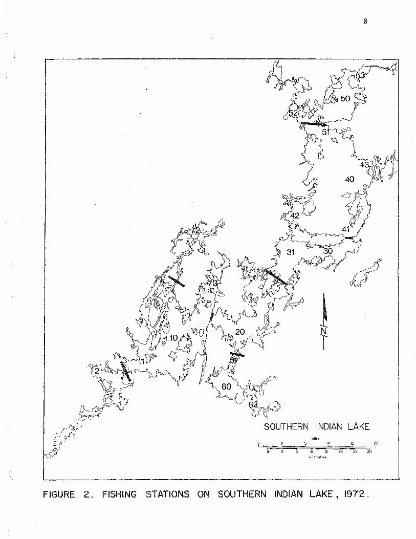
Geographic regions of Southern Indian Lake assigned by fisheries-limnology study component ......... .

Fishing stations on Southern Indian Lake, 1972 .....

Catch per unit effort of 8 species of fish from 8 regions in Southern Indian Lake, 1972 ........ .

Length-frequency composition of whitefish in Southern Indian Lake, during 1952 and during 3 trips in 1972 .................................. .

Comparative growth curves of whitefish during 2 trips on Southern Indian Lake, 1972 ............ .

Comparative condition regressions of whitefish during 2 trips on Southern Indian Lake, 1972

Comparative condition regression of whitefish on Southern Indian Lake, 1952 and 1972 ......... .

Total number of whitefish caught in two gangs of gillnets at the major stations during 3 fishing trips on Southern Indian Lake, 1972 ............ .

Length-frequency composit:ion of walleye in Southern Indian Lake, 1972 and 1952 ..................... .

Length-frequency composition of northern pike in Southern Indian Lake, 1972 and 1952 ............ .

Length-frequency composition of cisco during 3 trips on Southern Indian Lake, 1972 ........... .

Comparative growth curves of sauger during 2 trips on Southern Indian Lake, 1972 ............ .

Length-frequency composition of sauger in Southern Indian Lake, 1972 .............................. .

Catch of white sucker from two gangs of nets during 3 trips on Southern Indian Lake, 1972

Length-frequency composition of white sucker in Southern Indian Lake, 1972 ..................... .

Length-frequency composition of yellow perch in Southern Indian Lake, 1972 ..................... .

vi

7

8

18

24

30

35

36

40

45

60

70

78

80

86

87

91

vii

ACKNOWLEDGEMENTS

The success of a program is dependent upon the field and laboratory

programs. I should like to thank Mrs. D. Barnes, and Messrs. J. Sigurdson,

G. Shead, and L. Siemieniuk for the laboratory analyses and preliminary

data evaluation. Messrs. J. Sigurdson, G. Shead, W. Baxter, L. Siemieniuk,

A. Cumberland, L. Sherwood, M. Kreger, G. Cumberland, and R. Winkworth

were actively involved in the field program. I am particularly indebted

to Mr. T. Cleugh for his participation in these two phases of the program.

Finally I would like to thank Drs. A. Hamilton, R. Hecky and

K. Patalas and Messrs. T. Cleugh, L. Sunde, and K. Weagle who gave their

time and assistance in the compilation of this report.

1

6.0. SUMMARY

a) The existing data on the fisheries of Southern Indian Lake

are presented and discussed, and recommendations with respect to these

data are put forward.

b) At least 19 fish species are present in Southern Indian Lake

including lake whitefish, northern pike, yellow walleye, sauger, perch,

cisco, goldeye and suckers.

c) Whitefish are present in greatest abundance in regions 2, 4

and 5 of Southern Indian Lake. Mean lengths and mean weights of white­

fish from region 5 are greater than from elsewhere in the lake. Mean

lengths, weights and ages of whitefish are high in region 2 during mid­

summer, but decrease coincidentally with an increase in these parameters

in whitefish in region 4 during late summer. Food of whitefish is

predominantly amphipods, sphaeriids and gastropods. There is no evidence

of an over-exploitation of the whitefish population by the commercial

fishery. Impoundment will increase the size of the whitefish population

initially, but the final result will be a population size somewhat less

than exists today.

d) Walleye are present in all parts of Southern Indian Lake, but

are present in different densities at different times of the summer.

Data suggest the walleye are using the Barrington, Muskwesi and Waddi

Rivers as well as streams in region 6 for spawning purposes. By late

summer the concentrations of spawning walleye have disbursed and growth

rate and condition of walleye is similar in all parts of the lake. Food

of walleye is predominatly cisco and/or whitefish. Impoundment should

not have an adverse effect on stream-spawning walleye providing new

spawning sites are available above the high-water level (see Weagle and

Baxter, 1973). Change in the flow of the Churchill River could disorient

migration patterns.

e) Marked differences in catch per unit effort of northern pike

are noted at different stations during different times of the summer.

During mid-summer pike from different stations are similar in length and

weight but by late summer significant differences in mean lengths and

weights suggest segregation into discrete populations. Oisco, whitefish,

white sucker and burbot are the main dietary items of pike. Impoundment

will have a positive effect on northern pike, with initial increases

anticipated in size, condition and number.

f) Cisco in region 7 are significantly largerand older than cisco

from elsewhere in Southern Indian Lake. Cisco from the rest of the lake

appear to be similar throughout. Mysids are taken most often for food

though mayfly nymphs and zooplankton are important. Impoundment could

enhance the cisco popuation initially, but final results should be similar

to whitefish.

2

g) Sauger appear to be close to their northern limits in Southern

Indian Lake and are reasonably abundant only in regions 1 and 6. Food of

sauger is primarily cisco or whitefish, with some trout-perch. Impoundment

will likely create new habitat idea:! for sauger although until shoreline

clearing either by artifical or natural methods is accomplished availability

of spawning sites is questionable.

3

h) White sucker are present in most areas of Southern Indian Lake

at depths down to 70 feet. Longnose sucker are more prevalent in the main

lake regions. Probably neither of these species will be adversely affected

by the flooding and diversion. New lake conditions should be an improve­

ment for yellow perch and areas that are now devoid of this species (areas

of strong river flow) should contain perch. Neither trout-perch nor burbot

occur in large quantities in Southern Indian Lake and there will likely be

little change in their numbers following impoundment.

i) Recommendations include

1) Future water level fluctuations to follow historical

pattern of fluctuation in Southern Indian Lake.

2) Sites for future spawning beds for specific fish species

be prepared prior to flooding.

3) Continued study of Southern Indian Lake to monitor changes

in fish dynamics.

4

6.1. INTRODUCTION

This portion of the fisheries program of the Lake Winnipeg, Churchill

and Nelson Rivers Study was originally charged with the task of studying

the dynamics of the fish population of Southern Indian Lake, including

the collection of data pertinent to species composition, distribution,

growth, food, and condition. This report attempts to summarize the data

gathered, to highlight particular information which exemplifies aspects of

the existing population as it was found and to put forward recommendations

for the fishery that arise from the existing data.

This report is restricted to the fisheries of Southern Indian Lake

and Opachaunau Lake. It does not deal with the commercial or sports

fishing complex of Southern Indian Lake. Data for this report is exclusively

from the results of the 1972 summer field program with comparisons made

where appropriate to the work done in 1952 on Southern Indian Lake by

W. McTavish.

The report is broken down into components consisting of the

individual fish species. Discussion of each species is limited by the

amount of information available; and, indirectly, by the economic

importance of the species to the area. Where the amount of data and

general biological information on the species is great enough the impli­

cations of the hydro proposal on a fish species has been discussed.

Finally, conclusions and recommendations to minimize fishery disbenefits

based on the above are put forward.

5

6. 2. METHODS

6.2.1. Fish sampling:

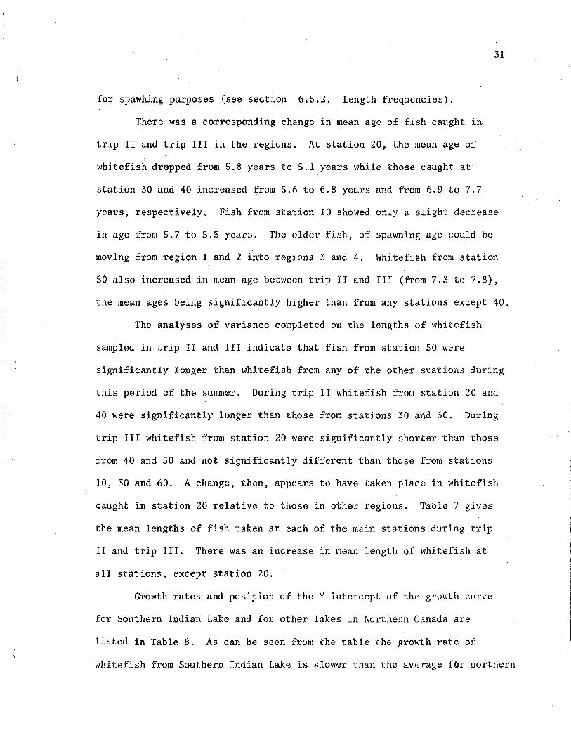
Fishing was carried out in the 7 major regions of the lake

throughout the summer of 1972 at individual stations within each region

(Figures 1 and 2). Three "trips" through the seven regions were completed

during the summer with stations 10, 20, 30, 40, 50 and 60 being visited at

each trip. All other stations were fished at least once, some twice. The

dates for the three trips were; trip I July 1-17; trip II August 9-26;

and trip III August 30 to September 9.

Two types of nets were used for most sets. The standard gang, used

consistently throughout the study consisted of 6 multi-filament nylon nets,

each 50 yards long of the following size and order (stretch mesh): 5 1/ 4",

1 1/2", 4 1/4", 2", 3 1/2", 2 3/4". Usually, two gangs were set at a

station, one in shallow water (3-7 meters) and one in deep (greater than 8

meters). The second type of net, a "Swedish" net, is a specially designed

single test monofilament net consisting of 12 combined mesh sizes from 3/4"

to 6" (stretch mesh) each 10 feet long. This net was set with each gang

of regular nets where possible. It proved to be considerably more fragile

than the regular nets and could not be set in rough weather conditions.

All sets were bottom sets left in overnight and the depths at both ends

of each mesh were recorded. At the time of set the temperature profile

(surface to bottom) was recoTded.

Species, fork lengths, weights, and sex were taken and recorded for

all fish captured. Scale samples and stomach samples were taken from the

first ten fish of each species in each mesh. The stomach samples were

preserved in 10% formalin.

For greater detail of field methods see Appendix.

6.2.2. Stomach samples:

6

In the field, stomachs were removed from the first ten fish of each

species in each mesh. Stomachs from northern pike, yellow walleye, burbot,

and sauger were opened and if empty were noted as such on the scale

envelope and discarded. Preliminary analysis was carried out in the field

providing it was possible to positively identify the specimens as well as

record the weight.

The bulk of the sampled stomachs were preserved in formalin and

returned to the lab for detailed analysis. The samples were soaked in

water for several hours prior to examination then all liquid drained off.

For each species at each station the wet weights of each type of food

organism were pooled and the percent of the total represented by each

type, was calculated. Stomachs of whitefish, cisco, pike, walleye, sauger,

perch and burbot were examined. Because of the degree of difficulty in

identifying stomach contents of suckers, they were not examined at this

time.

Unless unrecognizable because of the degree of digestion (unidentified

fish or unidentified invertebrate), all organisms were identified and wet

weights taken (2/3 of the weight of molluscs was removed to allow for

shell weight). Fish, mysids, and amphipods were identified to species;

sphaeriids to genus; gastropods and copepods to family; and chironomid

larvae, mayfly nymphs, caddis larvae and cladocera to order. Items included

7

SOUTHERN INDIAN LAKE miles

5

5 15 20 kilometres

GEOGRAPHIC REGIONS SET UP BY THE FISHERIES .. LIMNOLOGY COMPONENT

(note: arrows indicate direction of flow of major streams)

8

SOUTHERN INDIAN LAKE miles

kilometres

FIGURE 2. FISHING STATIONS ON SOUTHERN INDIAN LAKE , 1972 .

9

originally under the title miscellaneous were bottom detritus, iron nodules,

sand, gravel, phytoplankton, and unidentified terrestrial insects.

6.2.3. Age determination:

For the purpose of determining growth curves in this study ages of

fish were considered to be the same as the number of true annuli or rings

appearing on the fish scale. Carlander (1956) states that this is a valid

assumption provided that the possible presence of false annuli is recognized.

While the scales removed from the fish were not key scales, they

were removed from the same area on each species. Scales were aged by two

people although each completed an entire trip for any one species, and

usually completed the aging for an entire species. It is felt that between

the two people, the ages assigned to be five years or under were the same

better than 95% of the time. The similarity of those assigned older years

could drop to 50% although the discrepancy was rarely greater than + 1

year. Measurements of scale radius and distance between annuli were recorded

on paper tape for later measurement.

Mean lengths and standard error at each age were calculated for each

major species of fish at each station.

6.2.4. Back calculation:

The validity of body length-scale size relationships is usually

dependent upon the assumption that the scale radius increases in size in

direct proportion to the body length of the fish. Scale samples removed

must be key scales i.e. the same scales from each fish, or at least, as

supported by Dryer (1963) from the same area on the fish.

Body-scale relationships in this study, for the two commercial

10

species of fish (whitefish and walleye) have been considered to be linear

as is the case in all literature cited here. Carlander (1956) states

that in actual fact the relationship in every population is probably

curvilinear but that there is a greater opportunity to introduce error in

attempting to describe the curvilinear relationship than there would be in

making the assumption that the relationship is linear.

The formula used for calculation was:

ln-c = (1-c) s (Tesch 1971)

where: In = fork length of fish at given annulus

I = fork length of fish at time of sampling

sn = radius of given annulus

s = total scale radius

c = correction

The correction factor is required where the relationship between fork length:

scale radius is linear, but not directly proportional. This 'C' value,

defined as the intercept on the length axis from a least-squares fit of

the length:radius data is considered by most to be the length of the fish

at scale formation. Hile (1970) cautions that this is not a correct assumption

although the 'C' value often is near to the length of the fish when scales

are formed.

With the Southern Indian Lake data, 'C' values were calculated from

whitefish data at the major stations. In one case where the number of

samples was too small to be fitted to a regression line an intercept value

11

was assigned based on an average of the other calculated 'C' values.

The data from walleye could not be shown to be linear, although

this problem does not seem to appear in the literature. The problem

probably lies in the fact that the positioning on the scale for measurement

was not as consistent as could have been. To alleviate this problem a 'C'

value derived from the literature (Glenn, 1969) was assigned to all

samples. Once the 'C' value had been assigned the position of measurement

of the scale becomes meaningless since the length calculations are based

on a ratio between annulus and radius measurements. However, by assigning

a 'C' value the opportunity to compare back calculated lengths from our

data with those from data taken elsewhere is precluded.

6.2.5. Length-frequency composition:

The number of each species that fell in one inch length intervals

was plotted for most stations on each trip. Although the number and length

of sets were about the same for each station and each trip, the actual

numbers of fish within each size range were not considered for comparisons.

Instead, the relative numbers and the position of the highest frequency in

the inch intervals were utilized as the basis for comparison.

6.2.6 Growth rate:

Growth rates were calculated for the major species by fitting a

linear regression to age and length of fish collected during the final two

trips. For each species an analysis of covariance was used to calculate

the significance of differences in elevations and slopes of regression

lines. Level of significance wasp 0.05. Differences in slope indicate '

differences in growth rate while differences in elevation of the regression

lines indicates differences in length at age.

6.2.7. Condition:

The relationship between length and weight of a fish is a measure

of the plumpness or condition of the fish. Within a species, differences

in the condition of fish of different areas is indicative of population

differences between those areas.

Length-weight relationships of the major species were determined

by fitting a log-log linear regression to the data. Slopes, elevations

12

and mean lengths were tested for significant differences in the same manner

as was outlined for growth rate data. Condition regressions are commonly

calculated in metric units (grams, millimeters) and Southern Indian Lake

data were converted to metric to facilitate comparisons. The condition factor

for the productivity ratings was calculated using the formula:

Weight (grams) x þÿ�1�0 u�

Length (millimeters)3 (Carlander 1969) Factor =

6.2.8. Catch per unit effort:

Although all gillnet sets were made for approximately equal lengths

of time, to give a more precise representation of fishing effort the

duration of all sets were adjusted mathematically to 16 hours. The basic

unit of catch per unit effort is thus the total number of fish caught in a

gang of nets in 16 hours. Catch per unit effort, for a particular mesh,

was determined for walleye and whitefish and was based on the fish caught

in a net of that mesh in the standard gang nets.

13

6.3. SPECIES COMPOSITION

Fish species found in Southern Indian Lake in 1972 are listed in

Table 1. Though, as the list indicates, the species diversification is

large, there were undoubtedly species missed, McTavish (1952) did not

find spoonhead sculpin, lake chub, longnose dace, bluntnose darter and

brook stickleback but he did take samples of two other species, johnny

darter (Boleosoma nigreen) 1 and lake or emerald shiner (Notropis atherinoides)

and noted the possible presence of lake sturgeon (Acipenser fulvescens)

and goldeye Hiodon alosoides. McTavish also records the presence of

two species of cisco (Leucichthys tullibee and Leucichthys zenithicus

(shortjaw cisco)). The first, L. tullibee,is usually considered to be a

synonym of Coregonus artedii (McPhail & Lindsey, 1970). The fishing crew

on Southern Indian Lake in 1972 recorded only C. artedii, however,

observations of two size groups of ciscoes at sexual maturity were made,

parti.cularly from region 7. McPhail and Lindsey (1970) note also the

presence of two size groups of cisco from various lakes in northern Canada

and suggest that one of them is C. artedii while the other is more likely

a member of the Coregonus sardinella complex (least cisco).

Fish species compositions of lakes elsewhere in the Churchill

drainage are presented in Table 1 . The predominance of the lake shiner

in other lakes in the Churchill drainage suggests the possibility that

1. American Fisheries Society lists the scientific name of johnny darter

as Etheostoma nigrum.

14

this species is present in Southern Indian Lake but was missed in the

investigation. The presence of longnose dace in Southern Indian should

perhaps be noted. Rawson (1960) found this species in Otter Lake as well

as other lakes in that immediate vicinity but he felt it was rare else­

where in the Churchill drainage.

{/)

hut

T bla

lo ::i

(/)

N ..

Lak

e w

hit

efis

h

(Cor

egon

us

clu

pea

form

is)

Rou

nd

wh

itef

ish

(P

roso

pium

cyl

indr

aceu

m)

Raw

xx

xx

xC

isco

(C

oreg

onus

art

ed

ii)

aws

p

xx

xx

xx

xL

ongn

ose

suck

er

(Cat

osto

mus

ca

tost

omus

)

xx

xx

xx

xW

hite

su

cker

(C

atos

tom

us

com

mer

soni

)

Atx

Red

hors

e su

cker

(M

oxos

tom

a au

reol

um)

i

tn

tY

ello

ww

alle

ye

(Sti

zost

edio

n v

itre

um

vit

re

xx

xx

in

xx

xx

Sau

ger

(Sti

zost

edio

n c

anad

ense

) a

9 5x

xx

xx

xx

Yel

low

per

ch

(Per

cafl

uv

iati

lis)

ake

sx

xx

xx

xx

Nor

ther

n p

ike

(Eso

x lu

ciu

s)

---

inx

xx

xx

x.

xB

ur b

ot

(Lot

a lo

ta)

Lo

ra lo

ta)

Gol

deye

(H

iodo

n al

oso

ides

) om

Lak

e tr

ou

t (S

alv

elin

us

nam

aycu

sh)

Chu

xx

xx

xx

xx

xx

' x

. S

po

t-ta

il s

hin

er

(Not

ropi

s hu

dson

ius)

xx

xx

xL

ake

shin

er

(No

tro

pis

at

her

ino

ides

)I-

'

Nin

espi

ne s

tick

leb

ack

(P

un

git

ius

pu

ng

itiu

s)

xx

. x

x.

xx

x

xx

xx

xx

. x

Sli

my

scu

lpin

(C

ott

us

cog

nat

us)

..

xx

xx

xIo

wa

dart

er

(Eth

eost

oma

ex

ile)

xx

xx

x'

xT

rou

t-p

erch

(P

erco

psi

s om

isco

may

cus)

b

fa

rs

Spo

onhe

ad

scu

lpin

(C

ottu

s ri

cei)

i

ox

xn

om.

><

xx

Bro

ok

stic

kle

bac

k

(Cul

aea

inco

nst

ans)

w

Lon

gnos

e da

ce

(Rh

inic

hth

ys

cata

ract

ae)

sx

xn

xx

xx

Lak

e ch

ub

(Cou

esiu

s pl

umbe

us)

1 9x

John

ny d

arte

r(E

theo

stom

anigrum)

-x

xx

Log

perc

h x

(Per

chin

acap

rod

es)

Fat

head

min

now

(P

imep

hale

spr

omel

as)

xx

x

Bla

ckno

se s

hin

er (

Not

ropi

sh

eter

ole

pis

) x

xD

eepw

ater

sc

ulp

in {

Myo

xoce

phal

us x

quad

ric

orni

s)x

. x

Gra

yli

ng

(T

hym

allu

s are

ticu

s)

st

6.4. FISH PRODUCTION

The catch per unit effort (C.U.E.) for fish species in different

regions of Southern Indian Lake varies according to the species and

habitat available in particular regions of the lake (Figure 3). Numbers

16

of whitefish and white sucker in the main lake stations (1, 2, 3 and 4)

suggest a positive response to the flow of the Churchill River through the

lake. Conversely a fish such as the yellow perch could be expected to be

more plentiful in areas of the lake where flow was not particularly evident.

The C.U.E. for walleye is likely more consistent throughout the lake than

is represented in Figure 3. High values in regions 0, 5, 6 and 7 have been

influenced by very high concentrations of walleye found in these regions

during the time of spawning.

Catch per unit effort alone cannot be assumed to represent production.

To assess the quality of fish, mean weights of each fish species were

applied to the mean number of fish caught in a net to give catch per unit

effort in pounds (Table 2) which represented production. Production of all

fish species was high in the main lake regions and region 5, and was lower

in two regions not directly receiving the Churchill flow.

6.4.1. Implication of flooding and diversion on fish production:

An attempt has been made to describe possible effects of both the

flooding and the diversion on some of the major fish species in Southern

Indian Lake (Table 3). The effects to the lake must necessarily be

de.scribed in general terms and hence predicted effects on a fish species

must be generalizations also. Negative impacts were not recorded for

17

regions where, prior to impoundment, a fish species was in low concentrations.

As suggested by Table 3 the anticipated effects prior to shoreline

stabilization for all but pike and possibly sauger will be an overall

decrease in fish production.

Based on changes to regions 3, 4 and 6 by the action of diversion

as predicted by Hecky et. al. (1974), Patalas (1974) and Hamilton (1974)

an attempt to predict the changes to the commerically important fish species

(whitefish and walleye) has been made. These predictions are related to

the diversion only, and have been made with the following assumptions in mind;

2) that the productivity of whitefish and walleye will decline

as the productivity of lower trophic levels declines, although not necessarily

in proportion to their decline, and

b) that although the diversion will increase the rate of turnover in

region 6 substantially, it will also increase the biological production of

the region to a level similar to region 2 on a unit area basis.

From the table it can be seen that, within approximately 20 years

production of walleye and whitefish will likely decline in regions 3 and 4,

although production of whitefish will increase in region 6, relative to

that in existence at present.

75

50

25

0

WHITEFISH

WALLEYE

NORTHERN PIKE

CISCO

WHITE SUCKER

LONGNOSE SUCKER

SAUGER

BURBOT

REGIONS

Figure 3. Catch per unit effort of 8 species of fish from 8 regions in Southern Indian Lake, 1972.

--- -

Table 2.

Region Arca (Acres)

1 117

2 55

3 49

4 155

5 52

6 29

7 12

\

\

Mean catch per unit effort in pounds of fish from a single gang of nets from seven regions of Southern Indian Lake, 1972. Estimate of catch per unit effort following diversion (Post) for whitefish and walleye appears in brackets.

Whitefish (pre) (post)

25 (25)

113 (113)

43 (34)

80 (64)

100 (100)

13 (70)

30 (30)

Walleye (pre) (post)

13 (13)

7 (7)

7 (6)

3 (2)

74 (74)

29 (32)

30 (30)

Pike

28

52

61

38

42

31

51

Cisco

8

18

7

6

11

17

52

White Sucker

148

135

34

27

42.

41

20

Longnose Sucker

22

42

117

70

42

1

2

Sauger Burbot

7 6

l 9

16

8

9

6

1 10

Total

257

377

285

232

320

138

196

Table 3. Anticipated impacts of flooding and diversion on productivity of particular fish species in Southern Indian Lake, prior to shoreline stabilization. The number of symbols is to denote relative differences and is not to suggest absolut.e numbers; the sign denotes expected direction of impact.

Region Development Anticipated Effect Anticipated Relative Effect

Whitefish Walleye Pike Cisco Sauger Other

l Flooding Altered near-shore habitat + Altered lake spawning habitat ++

2 Flooding Altered near-shore habitat + (east) Altered lake-spawning habitat ++

2 Flooding Altered near-shore habitat + (west) Altered lake-spawning habitat ++

'Diversion Decreased flushing time Disoriented migration

3 Flooding Altered near-shore habitat +

Altered lake-spawning habitat ++

Diversion Decreased primary production Increased lake habitat ++ + ++ ++ + +

4 Flooding Altered near-shore habitat + Altered lake-spawning habitat ++

Diversion Decreased primary production Disoriented migration

s Flooding Altered near-shore habitat +

Altered lake spawning habitat ++

6 Flooding Altered near-shore habitat +

Altered lake-spawning habitat ++

Diversion Increased primary productivity ++ + + ++ + ++

7 Flooding Altered near-shore habitat + Altered lake spawning habitat +

21

6.5. WHITEFISH

6.5.1. Back calculation:

Van Oosten (1923) and Dryer (1963) both found a linear body length-

scale radius relationship for whitefish with the intercept at 0 Edsall

(1960), Kennedy (1943), and Carlander (1969) found the relationship to be

linear with a positive intercept. Regression analyses of this study's data

indicate a linear fit with an intercept of between 32 to 40 mm depending

upon the area from which the fish were taken. At some stations where the

number of samples was very small, the average intercept from all other

stations was used for the back calculations.

In a lake such as Southern Indian where there is significant

commercial fishing the selective fishing mortality might be expected to

result in a situation in which "back calculations of length exhibit a

tendency for computed lengths at a given age to be smailer, the older the

fish from which they are computed" (,Lee's phenomenon, Tesch, 1971). However,

there is no evidence of "Lee's phenomenon" occurring in any of the areas

(Table 2) whether they have been fished, commercially, or not. Thus, this

calculation gives no evidence of selective fishing mortality i.e. no evidence

of over-exploitation by the commercial fishery.

As will be discussed in the section on growth rate (Section 6.5.3)

annual increments of length calculated from scalemeasurements at any one

age differ from station to station. Whitefish taken from stations 50 and

20 had greater average annual increments than did those from other stations

even though whitefish from station 20 were smaller than those from station

30 at the formation of the first annulus. Length at the time of first

annulus formation is significantly greater at station 50 than station 40

22

(t = 8.04, df 184), This suggests that whitefish in region 5 have an early

advantage in growth over those in region 4. This is supported by evidence

discussed in the section on growth rate where the same observation is made

from actual, not back calculated data. The same does not hold true for

comparisons between actual and back calculated data during the first years

at both stations 30 and 60. From back calculations, the size at age 1 of

whitefish sampled from stations 30 and 60 is greater relative to values

calculated at other stations and relative to values taken from fish aged

1 year. From age-length information, however, the annual increments decrease

at a greater rate at stations 30 and 60 than those at other stations. Thus

it appears that whitefish at these two locations could have an early

advantage for growth, but following this initial increase the subsequent

growth is too slow for the advantage to remain evident.

6.5.2. Age, length frequency:

Depending upon the time of the year and the area of the lake, there

were several dominant length classes occurring in Southern Indian Lake

(Figure 4). During trips I and II at stations 10, 20, 30, 40 and 60 the

dominant length classes were indicative of fish between 3 and 6 years, with

no particular age the strongest consistently throughout the lake. At

station 50, the dominant length probably consisted of fish about 8 years

at all three sampling times.

Data collected during trip III indicate that a shift in location of

23

Tub le 4. at t of f t

uf on fork lengths and annual increment for al l age

groups are i included.

NO. FORK LENGTHS( l INCHES) AT ANNULUS FORMATION

AGE AT OF

CAPTURE FISH 2 3 s 6 7 8 9 10 11 12

Stat ion JO

s 3 4. S.9 7.8 9.8 11.8 6 + 2 3.5 5.4 7.0 8.4 9.7 10.8 7 + 3 3.3 4.8 6.5 8.0 9.2 10.4 ll. 7 8 l 3.2 4.7 6.2 8.7 9.7 12. l 13.7 14.9

Ave. Fork Length 3.6 5.2 6.9 8.7 10.1 11. l 12.7 14.9 Annual Increments 3.6 1.6 l. 7 1.8 1.4 1.0 1.6 2.2

Station 20

1 • 3.5 : 2 + 6 3.3 5.4 3 • 8 3. 2 5.2 7.04 . 10 3.5 S.4 7.2 8.7 5 • s 3.2 5.2 6.8 8.3 9.8 6 • 12 3.3 5.3 6.8 8.7 10. 7 12.67 + 12 3.3 4.9 6,4 8.0 9.8 11.5 13.08 + 1 3.7 5.9 7.4 8.5 10.9 12.4 13.9 15.5 9 + 4 3.0 4.7 6.4 8.0 9.S 11.0 12.4 14.0 15.8

10 + l 3.1 4.3 6.4 7.6 9.1 11. l 13.3 15.0 16,4 18.0 Ave. Fork Length 3.3 5.1 6.8 8.3 9.9 11. 7 13.2 14 .8 ,16. l 18.0Annual Increments 3.3 1.8 1. 7 1.5 1.6 l.8 1.5 1.6 1.3 J.9

Station 30

2 + 4 3.9 5.7 3 + 2 4.2 5.8 7.0 4 + 10 3.7 5.3 6.7 7.9 s t 4 4.2 5.6 7.0 8.3 9.56 .. 4 3. 7 5.3 6.9 8.S 9.8 11. l 7 + 3 3.1 4.5 5.6 6.7 8.1 9.1 10.28 + 5 3.7 5.4 6.8 8.3 10.0 11.6 12.8 13.8

10 + 2 3.3 S.4 7.2 8.6 10.0 11.3 12.3 13.4 1-1.8 16.4 11 + 6 3.9 5.4 6.7 8.1 9.2 10.3 11. 7 10. 7 14.2 15.4 16.412 + 4 3.5 s.o 6.3 7.5 8.7 10.1 11.1 12.3 13.4 144 15.3 !6.3

Ave. Fork Length 3.7 5.3 6.7 s.o 9.3 10.6 ll.6 12.5 14. l 15.4 15.8 16.3Annual Increments 3.7 1.6 1.4 1.3 1.3 1.3 1.0 0.9 1.6 1.3 0.. 1 0.5

Station 40

2 + 6 3.7 5.23 + 7 3.1 14. 7 6.1 4 l 3.5 5.4 6.7 7.9 5 + 7 3.6 5.2 6.7 8.3 9.56 + 6 3.4 4.8 6.1 7.8 9. J 10.37 + 3 3.5 5.1 6.6 8.5 10.7 12.2 13.9 8 + 1.7 3.4 4 .9 6.4 7.8 9.3 10.6 12.0 13.9 9 + 20 3.3 4.8 6.3 7.8 9.3 10.6 11.6 13.3 14.5

10 + 17 3.2 4.7 6.1 7.6 9.2 10.5 ll. 7 13.0 14.2 16.4 11 + 10 3.6 5.2 6.5 7.9 9.1 10.4 11. 7 13.0 14.3 15.5 16.6 12 + 1 3.9 s.o 5.8 6.8 8.0 9.0 10.7 12.2 12.9 13.8 14.8

Ave. Fork Length 3.4 s.o 6.3 7,8 9.3 10.5 11.8 12.8 13.8 14 .9 15.2 14.8 Annual Increments 5.4 1.6 1.3 1.5 1.5 l.2 l.3 1.0 1.0 l. 1 0.3

Station so

3 + 3 3.9 5.5 6.9 4 + 5 4.2 5.9 7.6 8.4 s + 7 4.3 S.9 7.5 8.8 10.2 6 + 17 4.0 5.8 7 .6 9.2 10.8 12.l 7 . 15 3.9 5.4 7.1 8 .1 10.6 12.4 13.6 8 + 12 4.0 5.6 7 .1 8.7 10.4 12.l 13.9 15.4 9 + 19 4.0 5.6 7.0 8.6 10.2 11. l 13.4 14. 9 16.0

10 + 16 3.7 5.3 7 .0 8.7 10.6 12.2 13.8 15.3 16. 7 16.711 + 7 3.9 5.7 7.4 8.7 10.0 11.4 12.8 14. 0 15.2 16.6 17.812 + 1 3.4 4.9 6.4 8.5 10.0 11 5 12.6 13.9 16.7 18 .o 19.0

Ave. Fork Length 3.9 S.6 7.1 8.6 10.3 l 1.8 13.3 14. 7 16.1 17.l 18.4Annual increments 3.9 l. 7 1.5 1.s 1.77 1.5 l.5 1.4 1.4 l. 0 1.3

Station 60

l + l 3.92 + 2 3.9 5.63 + 3 3.6 4.9 6.14 . 2 3.9 5.7 7.8 9.2 5 . 2 4.5 6.0 7 .4 9.1 10.6 6 + 2 3 .9 5.2 6.8 8.2 9.5 10.87 4 4.3 5.7 7. 1 8.5 9.8 11. 13.08 + 3 4.2 5.4 6.9 6. l 9.8 11.. 12.8 14.09 + 1 3.8 5. 3 7 .o 9.0 10.4.41 12 .o 13.2 14.1 15.0

16 + 1 4.8 5.9 5.9 8.5 9.3 11.0 12..5 15.06 14.8ll 4 .0 5.0 5 9 6. !l 8.0 8.9 10 .. 11. 7 13 .6 l 4 .4

Ave FfORT h 3.9 5 ' 4 6.8 8 9. 5 10.6 12.1 13.l 1: .u 14 2 14.4Annual increme nt s 9 1.5 1 4 1 .. 4 1. 3 1.1 1.5 1 n 0.0 0.2 0.. 2

55

50

4 5 STATION 10

40

14

10

5

STATION 20 STATION 30 STATION 40

24

STATION 50 STATION GO

5 10 15 20 5 10 15 20 5 10 15 20 5 10 15 20 5 10 15 20 5 10 15 20LENGTH OF FISH IN INCHES

30

(\

30

15

10

5

20

10

5

10 15 20 5 10 15 20 5 10 15 20 5 10 15 20 5 10 15 20 5 10 15 20LENGTH OF FISH IN INCHES

5 10 . 15 20 5 10 15 20 5 10 15 20 5 10 15 20 5 15 20 5 10 15 20LENGTH OF FISH IN INCHES

5 10 15 20 5 10 15 20 5 10 15 20 5 10 15 20 5 10 15 20 5 10 15 20 LENGTH OF FISH IN INCHES

Figure 4. Length-frequency composition of whitefish in Southern Indian Lake, during 1952 and during 3 trips in 1972.

25

the predominant peak occurs at station 40 and to a lesser degree at station

30. Because of the difficulty in replicating exact fishing locations there

is a possibility that choice of location could affect results. However, it

is unlikely that relative numbers between older year classes could be

affected by fishing locations. Instead it is felt that this shift could be

a movement into these areas of fish about to spawn. Weagle and Baxter (1973) found

that spawning whitefish in Southern Indian Lake average 8.9 years and Qadri

(1968) states that spawning whitefish in Lac la Ronge are 8 years and over.

Qadri (1968) reports migration to spawning grounds in Lac la Range and

Kennedy (1954) found movement to be as far as 30 miles to spawning areas in

Lake Winnipeg. The shift in relative numbers at station 40 was to the

length of fish that could be expected to be 8 years from a length corres-

ponding to the 5 year olds. This was observed at a time of year (September

7) when some migration for spawning could be expected.

Data taken from McTavish (1952) in Figure 4 suggest that the year

class structure in 1952 differs from the present one. In general, the fish

caught by McTavish were longer than those caught in 1972. In a comparison

between fish caught in comparable mesh sizes in 1952 and 1972 (Table 6) there

were even greater differences in the smaller 2 3/4" mesh than in the 5 1/4"

mesh.

L. Sunde (pers comm) suggests that this discrepancy could be the

result of two influences:

1. Though the winter fishery had been in operation since 1941 the summer

fishery had just been initiated at the time of McTavish's investigation so

that the fish population at that time was less exploited relative to the

Table 5,

26

Mean lengths at age of whitefish from 7 stations during trip II on Southern Indian Lake, 1972.

Station Age(years) 3 4 5 6 7 8

10 7.8 9.2 11.8 12.1 13.3 15.7

20 8.8 10.2 12.6 14.0 14.7 16.0

30 8.3 9.1 11.0 11. 2 12.6 14.2

40 8.1 9.5 10.8 11.6 14.7 15.2

50 8.1 10.4 12.1 14.2 15.4 15.8

60 7.9 12.2

71 8.8 9.5 12.0 13.8 14.3 16.l

(

27

fish population of 1972. From his experience Mr. Sunde has found that an

unexploited fishery has a tendency to "stock pile" fish of many year

classes all at the same size and that these fish crowd the gillnet biasing

the results towards one length class. After regular commercial exploitation

of a fishery over a number of years this "stock pile" would be depleted and

gillnet meshes of different sizes would show a larger variation of length

frequencies.

2. Although McTavish used nylon gillnets, it had been about 1952 that

the switch from cotton to nylon twine had taken place and the nylon twine

was the same thickness as the older cotton twine and much thicker than

today's nylon twine. The 2 3/4" mesh particularly of thicker twine is

capable of gilling and holding much larger whitefish (of 5 to 6 pounds) at

the head, biasing the sample taken.

It appears then that commercial fishing could account for the apparent

decrease in mean lengths and weights of whitefish in Southern Indian Lake

but that these decreases are not the effect of over-exploitation by the

fishery. Although the commercial fishing has probably removed the larger

whitefish (jumbo's) that were once said to exist in this lake, from the

information on back calculation (Section 6. 5 .1) as well as in this section

there is no evidence to suggest that over-exploitation of the fish stocks

of Southern Indian Lake is occurring.

6.5.3. Growth rate, age and lengths:

The age-length data of whitefish from trips II and III were plotted

to compare rates of growth of these fish in different areas of the lake as

28

Table 6. Mean weights and mean lengths of whitefish from Southern Indian Lake taken from 2 sizes of gillnets in 1952 (McTavish) and 1972.

Stations

10 30 40 60

1952 1972 1952 1972 1952 1972 1952 1972

2 3/4" Mesh

Mean weight (pounds) 1.8 0.7 2.9 1. 2 3.4 0.7 2.2 1.4 Mean length (inches) 14.5 10.8 17.0 12.2 16.9 11. 0 14.8 13.4

5 1/4" Mesh

Mean weight (pounds) 3.6 3.0 3.0 2.7 3.2 2.0 Mean length (inches) 17.9 17.0 18.l 16.9 17.6 15.9

observed at different times of the growing season. The trip II data

include information from the major station plus station 71, trip III

data only from the major stations (Figure 5).

29

Growth curves from data taken during trip II show that there were

no significant differences between rates of growth of fish at the 7

stations. However, there were significant differences between the

elevations of the growth curves of particular stations. Growth curves

from both stations 50 and 20 were significantly higher in elevation than

the other major stations. Since the rate of growth of fish in this area

was not greater, an early advantage in growth could account for the

substantially higher elevations. Station 71 also had a significantly

higher elevation than did stations 30 and 60.

The results of the third trip show that the whitefish that were taken

from station 20 had a significantly faster growth rate than did whitefish

from other stations. As in trip II whitefish taken from station 50 were

larger at age and appear to have had an early advantage in growth. For this

trip whitefish taken from station 10 were also larger.

From these data it appears that while there was little difference

in the rate of growth between different regions some areas do appear to

have an advantage in the first years. This apparent early advantage of

whitefish from station 50 is discussed from a different aspect and in

more detail in section 6.5.l. (Back-Calculation).

The unique significantly different growth rate at station 20 as

observed during trip III could be the result of movement out of the

region, of the older, usually more slowly growing whitefish (Dryer 1963)

13

12

11

10w ..J

9

8 3 4 5

15

. 14

13

12w

w 10

9

8 3 4

30

TRIP II

MEAN AGE

MEAN LENGTH ADJUSTEDTO A COMMON- AGE

GROWTH CURVE REGRESSIONS

STATION 10 LENGTH 1.46 ( AGEl 3.76

STATION 20 LENGTH= 1.22 (AGE)

STATION 30 LENGTH= 1.15 (AGE) 4.72

STATION 40 LENGTH= 1.30 (AGe) 4.38

STATION 50 LENGTH (AGE) 6.49

STATION 60 LENGTH 1.21 (AGE) 4.70

STATION 71 LENGTH= 1.37 (AGE) = 4.73

6 7 8

AGE ( YEARS)

TRIP IlI

5

AGE

0 MEAN AGE

MEAN LENGTH ADJUSTED TO A COMMON AGE.

GROWTH CURVE REGRESSIONS STATION 10: LENGTH= 4.86 1.39 AGE)

STATION 20: LENGTH = 3.90 + 1.50 ( AGE)

STATION 30: LENGTH= 4.70 1.14 (AGE)

STATION 40: LENGTH = 4.44 + 1.20 (AGEi)

STATION 50 LENGTH = 5.45 + 1.27 (AGE)

STATION 60 LENGTH = 4.53 + 1.23 (AGE)

6 7

Figure 5. Comparative growth curves of whitefish during 2 trips on Southern Indian Lake, 1972.

9

8

31

for spawning purposes (see section 6.5.2. Length frequencies).

There was a corresponding change in mean age of fish caught in

trip II and trip III in the regions. At station 20, the mean age of

whitefish dropped from 5.8 years to 5.1 years while those caught at

station 30 and 40 increased from 5.6 to 6.8 years and from 6.9 to 7.7

years, respectively. Fish from station 10 showed only a slight decrease

in age from 5.7 to 5.5 years. The older fish, of spawning age could be

moving from region 1 and 2 into regions 3 and 4. Whitefish from station

50 also increased in mean age between trip II and III (from 7.3 to 7.8),

the mean ages being significantly higher than from any stations except 40.

The analyses of variance completed on the lengths of whitefish

sampled in trip II and III indicate that fish from station 50 were

significantly longer than whitefish from any of the other stations during

this period of the summer. During trip II whitefish from station 20 and

40 were significantly longer than those from stations 30 and 60. During

trip III whitefish from station 20 were significantly shorter than those

from 40 and 50 and not significantly different than those from stations

10, 30 and 60. A change, then, appears to have taken place in whitefish

caught in station 20 relative to those in other regions. Table 7 gives

the mean lengths of fish taken at each of the main stations during trip

II and trip I II. There was an increase in mean length of whitefish at

all stations, except station 20.

Growth rates and position of the Y-intercept of the growth curve

for Southern Indian Lake and for other lakes in Northern Canada are

listed in Table 8. As can be seen from the table the growth rate of

whitefish from Southern Indian Lake is slower than the average for northern

Table 7. Mean lengths of whitefish from 6 stations at two different times of the summer.

Trip II Trip III

(Aug. 9 - Aug. 26) (Aug. 30 - Sept.

Station Number Mean Length Mean Length

(inches) (inches)

10 11. 5 12.2 20 12.6 10.8 30 10.6 11.9 40 12.9 13.1 50 14.2 15 .1 60 9.7 10.8

32

9)

33

Canadian lakes (Carlander 1969) and in fact is slower than was found in

many other lakes on the Churchill River drainage system. The Y-intercept

values for Southern Indian Lake are, in most cases greater than the average

and close to those given for other lakes on the Churchill River system.

6.5.4. Condition:

The 'condition' of whitefish in Southern Indian Lake (Figure 6)

does not vary as greatly as does the growth rate.

Elevation of the curves from station 20 and 50 were significantly

higher than those from stations 30, 40 and 71 as observed for whitefish

taken during trip II, indicating that these fish (from station 20 and 50)

were heavier for their length than those from the other stations. There

were no significant differences in condition of whitefish collected during

trip III. The differences between trip II and trip III could be the result

of movement of the fish. While it is difficult to state what type of

change in the population of whitefish could have occurred to produce these

Tesults, if fish are moving from a particular region towards spawning beds,

it would be those fish in better 'condition' (i.e. heavier per unit length)

that would be moving. Alternately, if fish in a region are in better

condition in general, movement of any sized fish could create the same

leveling off effect of the elevations.

McTavish (1952) found whitefish sampled from Watty Bay (station 50),

to be "thin and in poor shape" "as compared with those gilled in the

southern waters". This was a subjective observation that does not hold up

when actual values of length and weight for these whitefish are plotted

Table 8, Growth rates (regression coefficients) and Y-intercepts of whitefish from northern Canadian lakes.

Churchill River

Southern Indian Otter a Wollastonb Lac la Ronged Mac Kaye Contacte Sulphidee Big Peter þÿ�P�o�n�d�œ� Ile a la þÿ�C�r�o�s�s�e�œ

Nelson River

Northern Lake þÿ�W�i�n�n�i�p�e�g� � þÿ�P�l�a�y�g�r�e�e�n� Kiskittogisu & Kiskittof

Northern Canadian þÿ�L�a�k�e�s�M�

a Rawson 1960 b Rawson 1959 c Rawson 1957 d Rawson & Atton 1953 e Koshinsky 1965 f Koshinsky 1973 g Carlander 1969

Growth Rate

(Reg. Coef)

inches/year

1.25 1.63 1. 29 1. 31 1.37 1. 28 1.05 1.38 1. 07

1.35 1.60 1.20

1. 51

Y-Intercept

inches

4.83 7.05 5.16 4.30 4.59 5.738.28 4.96 6.72

8.037.4

10.5

3.97

34

2.90

2.80

2.70

2.60

2.50

2.40

2.80

2.70

2.60

w

2.50

2.40

MEAN LENGTH MEAN WEIGHT ADJUSTED TO A COMMON LENG TH

2.40

STATION

STATION

2.40

35

TRIP II

CONDITION REGRESSIONS

7t

40

30

STATION 10: LOG WEIGHT:-5.17 + 3.14 ( LOG LENGTH) STATION 20: LOGWEIGHT = 4.29+2.79(LOG LENGTH)

STATION 30: LOG WEIGHT: =5.52+3.25 (LOG LENGTH)STATION 40: LOG WEIGHT+-5.29 +3.16 (LOG LENGTH)STATION 50: LOG wei GHT:-3.81 + 2.60 ( LOG LENGTH)STATION 60: LOG WEIGHT=-4.71 + 2.95 (LOG LENGTH) STATION 70: LOG WEIGHT+-5.46 + 3.23 (LOG LENGTH)

2.35 2.50 2.55 LOG LENGTH ( mm)

TRIP III

2.45

MEAN LENGTH

MEAN WEIGHT adjusted to a common leng th

CONDITION REGRESSIONS

STATION 10: LOG WEIGHT = -4.94 + 3.03 (LOG .. LENGTH)

STATION 20: LOG WEIGHT = -5.46 + 3.25 ( LOG LENGTH l

STATION 30: LOG WEIGHT = -5.49 + 3.25 (LOG LENGTH)STATION 40: LOG WEIGHT =-5.51 + 3.26 (LOG LENGTH)

STATION 50: LOG WEIGHT=-6.15 + 3.51 (LOG LENGTH) STATION 60: LOG WEIGHT= -6.01 + 3.16 ! LOG LENGTH)

2.50 2.55 LOG LENGTH ( mm.)

Figure 6. Comparative condition regressions of whitefish during 2 trips on Southern Indian Lake, 1972.

36

against the condition regression for 1952 whitefish caught in region 4 and

1972 whitefish caught in both region 4 and region 5 (Fig. 6a). Therefore,

it appears that whitefish in region 5 have been and are in at least as

good condition as whitefish in other regions of the lake even though this

region is not under the influence of the nutrient-rich Churchill River.

3.1

3.

. 2.9.

LENGTH-WEIGHT RELATIONSHIPS - WHITEFISH

1972 REGION 5

REGION 4

REGION 4

1952 Fish poor "

condition

2.55 LOG LENGTH

2.6 mm

2.65

Figure 6a. Comparative condition regression of whitefish on Southern Indian Lake, 1952 and 1972.

6.5.5. Food:

Principal food items of whitefish during the summer of 1972 were

amphipods ( 45.0% by weight) sphaeriids ( 21.6%), gastropods ( 12.8%),

chironomid larvae (. 8. 4% ) as well as small numbers of mayfly nymphs

/

(2. 4%), caddis fly nymphs (5. 3%), corixids (1. 3%) and conchostracans (3. 3%)

37

were also eaten.

An apparent preference for specific food becomes evident when the

diet of whitefish from each region is considered (Table 9). However,

preference must be tempered by availability of the food organisms.

According to Hamilton (1974) Pontoporeia (amphipods) were, quantitatively,

in largest supply in all regions except region 6 where the gastropods were

dominant. In regions 2, 4, and 5 amphipods were the main dietary organism

although only in 2 did whitefish appear to be selectively taking this item

(amphipods were 68% of the diet, but only 54% of the available benthic

population). In region 3 and 7 gastropods were the major organisms found

in the stomachs although they comprised less than 1% of the sampled benthic

population at both stations. In region 1, sphaeriids were about 5% of the

sampled benthic population, but were 39% of the diet of the whitefish,

although this may be indicative of a slower digestive rate for mollusca

rather than an apparent preference for these organisms. From two stations

chironomids were an important food item (region 1, 28% and region 4, 15%).

In region 4 it was likely the large chironomids, Chironomini (subfamily

Chironominae), which is present in region 4 in greater numbers than other

chironomids, that was taken. Chironomini were not predominant in region 1

although likely they comprised a large percentage of the total weight of

chironomids taken by whitefish at this station.

Koshinsky (1971) found amphipods to be the principal food item of

whitefish in Trout and Mcintosh Lake as did McPhail and Lindsey (1970) in

Great Slave Lake and Lake Athabaska, and Bajkov (1930) in Lake Winnipeg.

Table 9. Food of whitefish as percent weight by items from 7 regions on Southern Indian Lake, 1972.

Amphipods Sphaeriids Gastropods Chironomid. larvae Caddis larvae Corixidae Conchostraca Mayfly nymphs

Number examined % feeding

1

19.48 37.40 1.42

25.65 6.49 1.05 1.10 7.41

105 66

2

67.84 6.96 0.56

11. 700.44 0.60 4.00 7.90

197 44

3

10.47 9.67

31.38 3.92

17.68 10.92 8.74 7.22

107 52

Region

4

47.02 15.56 13.05 15.36 4.73 1. 08 2.82 0.38

383 65

5

53.88 28.76 4.67 3. 71 5.93 0.03 2.26 0.70

383 63

6

0.70 35.44 57. 77

0.02 2.48 0.76 0.70 2.13

79 77

7

10.8213.45 32.97

1. 60 0.33 6.73

19.75 14.35

74 47

6.5.6. Catch per unit effort:

Numbers of whitefish caught in the experimental nets during the

three trips on Southern Indian Lake have been compared between the major

stations .and between trips (Fig. 7). During trip I the greatest return for

effort was at station 20 with that from station 50 being the next.

39

During the next two trips the catch per unit effort at station 20 progressively

decreased while that at 50 remained approximately the same. Also, during

trip II, the catch per unit effort at station 40 showed a decrease, followed

by a marked increase (300%) during trip III. In general, it appears

that the population size as estimated from catch per unit effort at stations

10, 50 and 60 remained stable, while in area 20 it decreased and in area

40 increased.

Providing the experimental nets were set in a manner that would

replicate the results of the preceding trips, it appears that the population

of whitefish in region 4 during trip III had been augmented from another

source. From the appearance of the data it appears possible that the other

source could have been region 2.

The average catch per unit effort for whitefish from the major

stations on Southern Indian Lake in 1972 is much higher than the catch per

unit effort from other lakes in northern Manitoba and Saskatchewan (Table 8).

Although some of the lakes listed are on the Churchill River in Saskatchewan

the river at this location is considerably smaller than when it reaches

Southern Indian Lake (approximately 1/3 the size). Only Playgreen Lake,

receiving the full flow of another major river system (Nelson) displays

a similar C.U.E. suggesting that in Southern Indian Lake (Churchill River)

w

w

z

10 20

TRIP I

TRIP II

TRIP III

30

STATIONS

50

.. ..

60

Figure 7. Total number of whitefish caught in one gang of gillnets at the major stations during 3fishing trips on Southern Indian Lake, 1972.

41

Table 10. Catch per unit effort (C.U.E.) for whitefish from twelve lakes in Northern Saskatchewan and Manitoba. All data except from Southern Indian Lake have been changed to the standards set for the Southern Indian Lake data to allow for comparison.

Lake C.U.E. Lake

Southern Indian 45 þÿ�C�h�u�r�c�h�i�l�l�C� Southern Indian* 56 þÿ�C�r�e�e�œ

Mountainc Playgreenb 46 Nistowiakc Lac la Rongea 44 DrinkingC Big Peter þÿ�P�o�n�d�C 42 Ott ere Reindeera 25 Wollastond 20

* a b c d

C.U.E. for whitefish from the main lake regions; 1, 2, 3 and 4. from Koshinsky 1965. from Ayles 1973. from Rawson 1960. from Rawson 1959.

C.U.E.

20 20 13

9 9 2

42

and Playgreen Lake (Nelson River) a major river system is of importance to

the productivity of the lake.

6.5.7. Implications of flooding and diversion on whitefish:

There is insufficient evidence to state that whitefish migration

between region 2 and 4 is important to the whitefish population in Southern

Indian Lake. However movement connected with an economically important

population of whitefish (region 4) does appear to be present. Little is

known about the plasticity of homing in this species but the diversion of

the Churchill water away from region 4 could disrupt the migration pattern.

Flooding will submerge existing spawning beds to greater depths

possibly adversely affecting the spawning success of whitefish. Increased

sediment loads in the lake water resulting from the inundation of unstable

shorelines could result in the "smothering" of whitefish eggs. While

these effects will not immediately reduce the size of the whitefish

population alarmingly there is liable to be some reduction in whitefish

recruitment. at least initially, and thus lower populations in the future,

According to Hamilton (1974) the overall benthic production in

Southern Indian Lake following diversion will likely be reduced by 15-30%

with reductions as great as 50% occurring in regions 3 and 4. Even if

this reduction does not create a "starving'' effect on whitefish it could

reduce the usually very fast growth rate of the young enough to lengthen

the time this vulnerable stage is available to predators, and hence could

increase mortality at this stage (Lindstrom 1963).

If Southern Indian Lake follows the pattern of other northern

reservoirs (Crooks, 1972) it is to be expected that the whitefish population

will suffer an initial decrease in recruitment, This should be followed

by an increase as inundated areas release nutrients to the system, then a

final stabilization somewhat lower than the present population size.

6.6. YELLOW WALLEYE

6.6.1. Back calculation

Because relatively few older walleye were caught in mo.st regions of

Southern Indian Lake, information from the back calculations is not

extensive enough to suggest the presence or absence of Lee's phenomenon

(Table 11). From the back calculated data the mean length of the walleye

at the formation of the first annulus is approximately the same throughout

the lake, and average annual increments do not vary greatly. Weagle and

Baxter (1973) found that because of the warmth of the streams entering

Southern Indian Lake in May spawning took place.at approximately the same

time everywhere.

6.6.2. Length-frequency:

The length-frequency distribution for walleye at particular stations

in Southern Indian Lake (Figure 8) indicates some regional differences at

particular times of the year within the lake. While the gillnettings of

walleyes is dependent upon the activity of these fish, and hence dependent

to some extent onthe time of the year the netting is done, difference

within any one trip should be indicative of population size and structure.

During trip I few walleyes were caught in stations 10-50 relative to

those caught in the remaining stations, and in these stations, except

43

at station 50, the fish that were caught were almost all of a size too small

for spawning. From stations 2, 52, 53 and 60, however, the number of walleyes

caught was large, and the dominant length class was the size of spawning walleye.

(According to Weagle and Baxter (1973) average size of spawning

44

Table 11. Back calculated fork lengths at the time of each annulus formation for each age group of walleye from 6 different stations on Southern Indian Lake. Average fork lengths and annual increments for all age groups are included.

NO. FORK LENGTH (INCHES) AT ANNULUS FORMATIONAGE AT OFCAPTURE FISH 1 2 3 4 s 6 7

Station 10

4 + 6 5.2 7.4 9.9 11. 7 5 + 11 5.2 7.2 9.2 . 11 12.5 6 + 8 4.4 6.3 7.8 9.3 10.9 12.57 + 3 5.1 7.1 9.3 10.9 12.7 14.1 15.5

5.0 6.9 9.1 10.7 12.0 13.3 15.5s.o l.9 2.2 1.8 . 1.3 1.3 1.3

Station 20

3 + 2 5.6 8.2 10.54 + 7 4.5 6.9 8.8 10.9 s + 9 4.6 6.6 8.5 10. l 11.8

4.9 7.2 9.3 10.5 11.8 4.9 2.3 2.1 1.2 1.3

Station 30

2 + 4 6 .1 9.0 3 + 8 4.4 6.9 9.2 4 + 11 4.3 6.3 E.2 9.9 5.+ 7 5.1 6.8 8.2 9.7 11.1 6 + 3 4.8 6.5 8.3 10.0 11.5 12.8

6.9 7.l 8.5 9.9 11.3 12.8 4.9 2.2 1.4 1.4 1.4 1.5

Station 40

2 + 3 4.8 7.7 3 + 4 4.9 7.3 9.2 4 + 4 4.7 6.8 8,8 10.8 s + l 5.1 7.3 8.8 10.0 11.3

4.9 7.3 8.9 10.4 11.3 4.9 2.4 1.6 l.5 0

Station so

3 + 6 6.1 8.8 11.0 4 + 16 4.6 6.8 9.0 11.0 . s + 21 4.8 7.1 9.3 11.5 13.36 + 4 s.s 8.1 10.4 12.3 14.l 15.7 1 + 3 3.9 6.0 ., . 9 9.7 11. 7 13.5 15.5

5.0 1.4. 9.S 11.1 13.0 14.6 15.5 5.0 2.4 . 2 .1 1.6 1.9 1.6 0.9

Station 60

3 + 2 4.2 6.7 9.4 4 + 12 5.2 7.4 9.8 11.8 s + lS 4.9 7.2 9,2 11. l 12.8 6 .j. 7 4.4 6.1 7.9 9.6 11. l 12.57 + 4 4.8 7.S 9.6 10.7 13.7 15. l 16.4

4.7 7.0 9.2 10.8 12.5 185.8 16.4 4.7 2.3 2.2 1.6 1. 7 1.3 2.6

STATION STATION 2 STATION 10 STATION 20 STATION 30 STATION 40 STATION 50 STATION 52 STATION 3 STATION 60 STATION 61

30

25

15

10

5

0 20 10 15 20 10 15 20 10 15 20 10 15

20 20 10 15 20 10 15 20 10 15 20 10 15 20

15

0 10

5

10 15 20 10 15 20 10 15 20 10 15 20 10 15 20 15 20 10 15 20 10 15 20 10 15 20 10 15 20 10 15 20

20

15

o !O

5

0 10 15 20 10 15 20 10 15 20 10 15 20 10 15 20 10 15 20 10 15 20 10 15 20 10 15 20 10 15 20 10 15 20

20

15

10 ' -- - 5z

010 15 20 10 15 20 10 15 20 10 15 20 10 15 20 10 15 20 10 15 20 10 15 20 10 15 20 10 15 20 10 15 20

FORK LENGTH IN INCHES

Figure 8. Length-frequency composition of walleye in Southern Indian Lake, 1972 and 1952.

(

\

46

walleye is approximately 14.2 inches). There was also a relatively large

catch of walleye from station 61 al though the dominant length class, ll. 5

inches, is probably too small to consist of significant numbers of spawning

walleye.

The walleye caught in stations 2, 52, 53 and 60 were probably

remaining concentrations of the spawning populations that move to the

Barrington, Muskwesi, Waddi Rivers and streams in the South Bay, respectively.

While these were captured well after the time of spawning (July 1 - July 17),

there is evidence to suggest that after spawning in these streams walleye

move further upstream, not returning to the lake until early July (Weagle,

pers comm). Rawson's (1956) work supports this and suggests walleye may

remain upstream from 3 to 6 weeks after spawning. Figure 8a, showing the

walleye length-frequency curve for station 2 on July 7, 1972 and for the

Barrington River on May 27, 1973, shows the similarity in the shape of the

curve at these two times, The data from the Barrington consists of fish

selected specifically for spawning information which could explain the shift

to the right for these data.

The major peak at station 61 as well as the minor peaks at station

52 and 53, all approximately at the 10 inch size suggest the presence of a

second dominant size class in the lake which is present with the older walleye.

During trip II there was a more equal representation of walleye in

all stations, suggesting a movement back into all areas from spawning grounds.

Depending on the location of the station, the dominant length class in trip

II and trip III was either about 10 inches or about 15 inches (with the

exception of station 10 where the dominant length class was about 12.5 inches).

47

In most cases, it was those stations that had what appeared to be the

35 STATION 2 BARRINGTON RIVER

30

25

20 \

15 \

' 10 \

\ \

5 \ \

0 5 10 15 20 25

LENGTH {INCHES)

Figure 8a. For explanation, see text.

spawning sized walleye in trip I that maintained the dominant length class

at 15 inches, and those that did not that recorded the strength in the 10

inch length class. The major exceptionsto this appeared at station 50

and 52. During trip II the walleye population decreased in size at station

52 (see also Catch per unit effort Section 6.5.6.) and in trip III, no

walleye were caught there. There was an increase in relative number of

fish at station 50 during trip II with a very dominant length class at about

15 inches. In trip III the relative number of fish was maintained but the

dominant 15 inch class had disappeared. Since the number of fish caught that

were about 10 inches long did not change appreciably between trip II and

48

trip III, it is unlikely that the decrease in larger fish. was caused by a

change in catch per unit effort. Furthermore, the dominant age class was

5 years at trips II and III but the mean length for the five year olds

changed from 15.6 inches to 11.1 inches. There is no apparent explanation

for this marked reduction in number of only larger sized fish of an age

class.

The dominant length class of walleye from stations 10, 20, 40 and

60 (Figure 8) in 1952 (McTavish) was always greater than 15 inches, and

usually greater than 17 inches. In a comparison of mean lengths and weights

of walleye caught in the 2 3/4" mesh in 1952 and 1972 (Table 12), only at

station 10 were fish from the 1972 catch larger and at all other stations

the 1972 mean was much smaller. The apparent general decrease in the weights

and lengths of walleye since 1952 probably can be attributed to the effects

of the commercial fishery, as was the change in the meart weights and lengths

of whitefish (Section 6.5.2). No walleye were caught in the commercial

sized experimental gillnet (5 1/4") during trip II of the 1972 collection.

This is not unexpected, nor a reflection of over-exploitation by the

commercial fishery. Large walleye are difficult to catch, both experi-

mentally, and commercially during mid-summer.

6.6.3. Growth rate:

There were definite differences in the age-length regressions

calculated for those samples taken during trip II that were aged that were

not noticeable in those samples taken during trip III.

The rate of growth of walleye as observed during trip II was

l

Table 12. A comparison of mean lengths and weights of walleye caught in the 2 3/4 inch mesh in 1952 and 1972 from Southern Indian Lake.

Station 10 Station 20 Station 40 Station 60

49

Year 1952a 1972 1952a 1972 1952a 1972 1952a 1972 (Number of fish) (3) (3) (22) (3) (ll) (3) (22) (17)

Mean weight (pounds) 0.8 1.5 2.4 0.7 1.8 0.9 2.0 1.5

Mean length (inches) 12.3 15.1 18.0 11.9 15.9 12.8 17.5 14,8

a from McTavish (1952)

significantly greater at stations 5O, and 53 than at stations 60, 72 and

72A but not greater than growth of walleye taken elsewhere in the lake

(Table 13). The elevations of the regression curves of data from 50, 51,

53, 60, 72 and 72A are all greater, significantly, than those from the

50

main lake stations (10, 20, 30 and 40). It appears then that walleye

caught in the north end of the lake (50, 51 and 53) were from a distinct

population and were growing at a faster rate; a rate great enough to create

a significantly high elevation of the regression line as well. Fish from

stations 60, 72 and 72A did not appear to have the same high rate of growth,

but for their age, they were significantly longer (elevation) suggesting

an increased growth rate had occurred at some time, probably in early

years of growth.

Mean age of walleye sampled during trip II was greater at stations

53, 60, 72 and 72A than mean age of walleye from other stations.

In almost all cases, the regions discussed in this section as having

distinct populations of walleye are regions that were shown to have residual

populations of spawning walleye during trip I (see section 6.6.2. walleye

length-frequency). Although experimental netting did not take place in

region 7 during trip I, other investigations in region 7 in 1973 indicate

a large population of mature walleye at the time of spawning (Weagle and

Baxter, 1973). There is evidence that, following return from the spawning

area, walleye show an early summer concentration, particularly inshore,

followed by a wide dispersal in August and September (Rawson 1956; Crowe 1962).

These sub-populations of walleye, then, are significantly different from

walleye elsewhere in the lake because of the lingering effect of the concentration

Table 13.

72A

20 -/-

30 -/72A

40 -/-50 . 50/-

51 51/-

53 53/53

60 -/-

72 -/-

Summary of statistical comparisons of growth rate and elevations of growth curves for walleye from nine locations in Southern Indian Lake. Where differences between pairs were found to be significant, the number of the station with the higher value is given (growth rate, above oblique line; elevation, below oblique line). If no significant difference was found, a (-) is given.

72 60 53 51 50 40

-/- -/- -/53 -/- -/50 -/-

-/72 -/30 -/53 -/- -/50 -/-

-/72 -/60 -/53 -/- -/50

50/- 50/- -/- -/50

51/72 51/60 -/53

53/53 53/53

-/-

51

30

-/-

Table 14.

72A

20

30

40

so

Sl

53

60

72

Summary of statistical comparisons of slopes of condition regressions for walleye from nine locations in Southern Indian Lake. Where differences between pairs were found to be significant, the number of the station with the higher value is given. If no significant difference was found a (-) is given.

72 60 53 Sl 50 40

S3

40

50 so

53 53

S2

30

(

of the older fish in the area. By trip III (August 30 - September 9) the

growth rates of walleye were not significantly different at any of the

major stations, suggesting that the distinct sub-populations of walleye

present in trip II had dispersed.

6.6,4. Condition and mean length:

53

The regression lines of length against weight for walleye taken during

trip II and trip III show little differences between data from each of the

regions suggesting a uniformity of condition for walleye throughout the

lake (Table 14).

However, a significant difference did exist between the mean lengths

of walleye taken during trip II as calculated by an analyses of variance.

Walleye from stations 50, 51, 53, 60, 72 and 72A were all significantly

longer than walleye from the other major stations of the lake. This

corresponds to the difference found in the growth analyses (section 6.6.3)

and again, is probably indicative of concentrations of mature walleye

remaining in particular areas within the lake. By trip III there were no

significant differences between lengths of walleye taken at the sampled

stations which supports the suggestion that the mature stocks were more

uniformly dispersed.

6.6.5. Food:

Walleye fed almost exclusively on fish with cisco and/or whitefish

being predominant (Table 15). Trout-perch, usually considered to be

important forage fish for walleye (McPhail and Lindsey, 1970), were not

found in any of the stomachs sampled. Mayfly nymphs and caddis nymphs

54

were identifiable but only in very small quantities.

This predominance of fish on the diets of walleye in Southern Indian

Lake is much different from that found for walleye in other Churchill River

lakes (Trout Lake, Koshinsky 1971; Otter Lake, etc., Rawson, 1960) where

invertebrates were much more important. Koshinsky (1971) does say, however,

that a fish diet is probably more typical of walleye 'from large Shield lakes.

Table 15. Food of walleye as percent weight by items in seven regions of Southern Indian Lake, 1972.

Region

1 2-3 4 5 6 7

Cisco 35.2 59.1 36.6 57.9 41. 7

Cisco and/or 56.5 47.2 27.4 33.3 44.4 13.4 34.7whitefish

Perch 21.3

Nine spine 2.1 1.4 1. 3 stickleback

ScuI pin 2.3 11. 0 1. 2 1.4

Unidentified 22.2 17.6 9.1 41. 9 14.6 28.7 1:8. 2 fish remains 13.8 2.7

Gaddis larvae 13.8 2.7

Mayfly nymphs 1. 8

no fish sampled 23 42 61 33 179 126 75

% feeding 52 52 28 55 35 56 29

6.6.6. Catch per unit effort:

Catch per unit effort for walleye changed among trips and among

stations following the same pattern as was determined from the length

frequency and growth rate analyses. During trip I, at about the time the

walleye would be returning from the streams, the values for catch per unit

effort (C.U.E.) were high in those stations (Table 16: Stations 02, 52,

53, 60 and 61) that were at the mouths of spawning streams. During trip II

the C.U.E. decreased at these stations and increased at the other stations

in the lake until during trip III the C.U.E. was similar at all stations

sampled.

6.6.7. Implications of flooding and diversion on walleye:

Changes made to the particular spawning sites, usually streams, by

the raising of the water level, as well as changes in water movement within

the lake that could change the methods for homing could effectively reduce

the number of successful spawners enough to harm the size of the walleye

population in Southern Indian Lake. Changes in water flow in streams by

raising the water level would increase sedimentation rates on the existing

spawning grounds which would have an adverse affect on incubating eggs.

However, it is likely that adequate spawning grounds will be established

55

at higher positions on the streams that will not be directly affected by the

flooding. Incubating eggs of shore-spawning walleyes could also be

affected by increased sedimentation rates within the main lake. It is

evident from research completed on walleye elsewhere (Crowe 1962; Eschmeyer

and Crowe 1955; Rawson 1956) that walleye have a tendencr to "home" to

Table 16.

Trip I

Trip II

Trip III

Total catch of walleye, in numbers, from one gang of nets set at different stations during three trips from Southern Indian Lake, 1972.

Stations

01 02 10 20 30 40 50 51 52 53 60 61 62

13 86 2 6 2 0 4 1 103 157 . 40 58 19

11 52 12 10 23 6 37 16 18 87 40 15 8

NF NF 13 10 6 2 9 NF NF NF 12 NF 5

NF - not fished

.. 57

particular spawning sites. Migration for the purpose of spawning can

involve distances as great as 175 miles (Eschmeyer and Crowe, 1955) so

that walleye could be moving from any part of Southern Indian Lake to a

particular stream to spawn. Diversion of the Churchill River from a large

area of Southern Indian Lake could prevent mature walleye from returning

to their spawning grounds.

According to Patalas (197 4) and Hamilton (1914) th.ere could be a

significant decrease in the productivity of both plankton and benthic

organisms following diversion, particularly in regions 3 and 4. A decrease

in these food items will likely have a direct (adverse) affect on young

walleye, and an indirect (again adverse) affect on adult walleye.

58

6.7. NORTHERN PIKE

6.7.1. Length-frequency:

The length-frequency curves prepared for pike (Figure 9) show

essential similarity in numbers of pike at specific lengths among stations

and trips. The dominant length-class in almost all situations is

approximately 20 inches and according to the aging data this is representative

of pike aged 5 years.

During trip I there were concentrations of longer (hence older)

pike at such stations as 02, 30 and 50 which decreased by trip II. These

concentrations were likely post-spawning pike prior to their dispersion to

other parts of the lake.

Mean weight and mean length of pike have decreased since 1952

(McTavish 1952) (Table 17). As well, McTavish captured pike in the 5 1/4"

mesh, while there were no pike taken in the 5 1/4" mesh in 1972. Such a

decrease in mean sizes could normally be attributed to exploitation of a

species by a commercial fishery, however, northern pike on Southern Indian

has never been considered to be a commercially desirable fish. Incidental

catches of northern pike in the commercial and domestic gillnets could

account for some pressure on this species.

6.6.2. Growth rate and age:

There were no significant differences between major stations in

growth rates and elevations of growth curves (age-length) for pike taken

during trip II, with the exception of station 10. Pike taken from station

10 were unusually small; for example the mean at age 3 was 7.6 inches at

station 10 and 20 inches at station 20 ., yet these small fish did not

59

appear in the catches taken from station 10 in trip III. Either the pike

taken at station 10 during trip II were from an unusually stunted population,

or the sample taken, though supposedly random, was not truly representative

of the population at station 10. The mean ages of pike at all the

stations during this trip were the same also, with the exception of pike

taken from station 72A which were significantly older pike than taken any­

where else in the lake at this time.

Pike taken from station 30 during trip III had a faster growth rate

than pike from other stations though the intercept on the Y-axis is

uncharacteristically low.

Except for the pike from station 40, which were significantly longer,

the mean length of pike at a common age was not different between stations.

Pike from station 60 were significantly younger and shorter than

those from other regions of the lake during trip III, and from those taken

from station 60 in trip II. There does not appear to be an obvious

explanation for this shift in age-class in the South Bay.

6.7.3. Condition:

Northern pike from Southern Indian Lake are not as in good condition,

in general, with a length-weight relationship of

Log weight= 6.71 + 2.6 (log length)

as those from Lake of the Woods (Carlander 1969)

15

5

0

15

10

5

0

15

10

0

Figure 9.

STATION 2

10 20 30

10 20 30

STATION 10 STATION 20

10 20 30 10 30

10 20 30 20 30

10 20 30 10 20 30

10 20 30 10 20 30

STATION 30 STATION 40

10 20 30 10 20 30 FORK LENGTH OF FISH

10 20 30 10 20 30 FORK LENGTH OF FISH

. 20 30 10 20 30

FORK LENGTH OF FISH

10 20 30 FORK LENGTH OF FISH

STATION 50 STATION 60

10 20 30 10 20 30 ( INCHES )

10 20 30 10 20 30 . ( INCHES )

10 20 30 10 20 30 ( INCHES)

( INCHES )

i 10 20 30

STATION

10 20 30 ,

10 20 30

Length-frequency composition of northern pike in Southern Indian Lake, 1972 and 1952.

Table 17.

Year

Mean weight and mean length of northern pike taken in a 2 3/4" mesh gillnet from Southern Indian Lake. The numbers in brackets are the number of fish used to derive the means.

Station 10 Station 40 Station 60

1952* 1972 1952* 1972 1952* 1972 [Number of fish) (13) (3) (7) (6) (10) (17)

Mean weight (pounds) 6 2.2 4.8 2.9 3.1 2.1

Mean length (inches) 27.6 21.5 27.3 22.6 23.7 20.5

* from McTavish (1952}

61

Log weight = 6.2 + 3.1 (log length)

and from Lac la Ronge (Koshinsky 1972)

Log weight = -5.4 + 3.1 (log length)

Within the lake, differences between stations and between trips become

apparent. During trip II, the pike from different stations were similar

in length and weight. The sample taken during trip III indicates, however,

that although the weight per unit length of pike as observed from station

30 increases at a faster rate than does weight per unit length of pike

observed elsewhere, for a common length they are not as heavy as pike from

other parts of the lake. This could suggest that pike observed from this

station are not in as good condition, at this time of year, although it

seems unlikely that a significant change could occur between trips II and

III.

Pike observed from station 60 during trip III had a significantly

smaller mean length than pike observed from the same station during trip II

and from other stations also during trip II. A significant difference

suggests a population (or sub-population) of pike different from the main

lake population. Yet this difference did not appear during trip II. It is

possible that during the time that trip II was in progress post-spawning

dispersal was still taking place and it was not until the time of trip III

that the resident populations had reformed. This would explain the

variations between trip II and III in both growth rate and condition.

Extensive migration of pike has not been found in lake conditions,

however Hill suggests that in a river situation migration of pike may be

62

more prevalent (Koshinsky 1972). Though Southern Indian is considered to

be a lake, many riverine conditions are maintained by the strong flow of

the Churchill River through it and hence extensive migration of pike could

well exist.

6.7.4. Food:

Fish were found in all pike stomachs that contained food, with

cisco and/or whitefish usually predominating (Table 18). Pike also fed

extensively on white sucker in regions 1 and 5, and on burbot in regions

6 and 7. There is some evidence for selectivity since, with the exception

of white sucker in region 1, these food sources were scarce in the

experimental gillnets set in these regions.

Table 18. Food of northern pike as percent weight by items in 7 regions of Southern Indian Lake, 1972.

Regions

0 1 2-3 4 5 6 7

Cisco 22.0 26.6 22.4 42.4 25.3 24.6 Cisco and/or whitefish 8.7 26.6 2.8 3.4 7.6 35.8 Whitefish 32.8 32.8 15.8 25.4 White sucker 60.4 3.2 15.6 23.7 5.4 1.3 Bu bot 31.3 26.6 Walleye 6.4 Perch 10.9 1. 2 1.4 Trout-perch 3.4 7.5 10.6 1.4 Ninespine stickleback 1.2 Sculpin 2.5 1.4 Unidentified remains 5.5 13.6 13.2 5.5 2.6 5.3 Crayfish 86.4 5.0Mayfly nymphs 2.7

No fish examined 15 39 167 148 136 134 118 % feeding 33 38 43 41 36 39 35

63

'\

6.7.5. Catch per unit effort:

The catch_per unit effort (C.U.E.) of northern pike at each of the

main stations in the lake changed markedly throughout the summer except at

station 40 as can be seen in the following C.U.E. 's:

Station

Trip I

Trip II

Trip III

10

9

4

5

20

11

25

30

30

31

4

7

40

10

13

11

so

25

14

22

64

60

26

15

30

Although evidence from the literature (Koshinsky 1972) suggests that northern

pike movement in a lake situation is limited (typically less than 2 miles),

this may not apply to more riverine situations such as Southern Indian Lake.

From the data it appears that there is a decrease in the early concentration

of northern pike in region 3 and region 1 between trip I and II, and this

concentration remains low through trip III. Coincidentally, the catch per

unit effort in region 2 continued to increase between trips. Northern pike

have been observed to remain in spawning areas anywhere up to 90 days before

returning to the lake (Carbine 1942) and it may be that fish in region 1 and

3 during trip I may have subsequently dispersed, or possibly moved into

region 2.

Koshinsky (1972) suggested that young pike in Lac la Range showed a

greater preference for shallow water than did the larger fish and that there

65

was no evidence that the pike sought the cooler deep water during the summer

months. Data from Southern Indian Lake (Table 19) show that during trip II

a relatively greater number of pike could be found at deeper depths at

stations 10, 20 and 30 but in general the length of the pike at the deeper

depths was not greater. Probably, because the water at the greater depths

in Southern Indian is not appreciably cooler the observations at stations

10, 20 and 30 were simply indicative of a general dispersion of pike as

the summer progressed and not the seeking of any specific preferred condition.

6.7.6. Implications of flooding and diversion on northern pike:

Northern pike can be expected to respond positively, at least initially,

to the new impoundment. Crooks (1972) found that following inundation of

Lac Seul the commercial catch (in weight) of northern pike increased more

than 4 times in 18 years. Although increased turbidity could adversely

effect incubating northern pike eggs in the lake it is unlikely the effect

will be widespread. In general, the newly inundated land will provide

ideal pike habitat. New areas of submerged vegetation will increase

available spawning areas. Flooding of uncleared land will increase the

nutrient supply to parts of the lake with an end result of an increase

in supply of some sources of food such as white sucker, perch and zoo­

plankton (for fry). At the same time the new impoundment could adversely

affect the growth of other sources of food (see whitefish 6,5.7) thus

increasing the length of time they are available as prey to pike.

Increased growth, condition and availability of this species

Table 19.

Stations

10

20

30

40

50

60

Number and mean lengths (inches) of northern pike caught in a gang of gillnets in shallow and deep sets at three different times of the summer season from Southern Indian Lake, 1972.

Trip I Trip II Trip III

Shallow Deep Shallow Deep Shallow Deep.

No Mean No Mean No Mean No Mean No Mean No Mean Length Length Length Length Length Length

10 23.1 3 26.2 2 21.3 5 23.6 5 20.8 4 24.2

7 15.9 11 21. 2 2 24.9 40 19.2 31 21.5 18 22.2

46 21.4 8 25.2 2 22.8 4 19.3 3 17.1 8 17.4

39 22.5 0 17 21.1 5 23.4 15 24.3 2 23.1

23 21. 7 17 21.5 23 20.7 1 27.4 29 23.3 4 23.2

32 19.8 17 20.3 11 20.5 14 20.4 31 17.1 17 20.9

following impoundment should provi.de much more attractive northern pike,

both for sport and commercial fishing for a number of years. However,

if the pattern is the same as shown for Lac Seul (Crooks, 1972) the final

northern pike fishery will drop to less than the potential prior to

impoundment.

67

6. 8. LAKE CISCO

There is some confusion among fisheries investigators about the

species group with the common names "cisco" and "tullibee". Bajkov (1930)

discusses several (probably 3) species all of which were called "tullibee"

and were given a total of 6 different descriptive names by commercial

fishermen. He felt that as well as the obvious meristic differences (e.g.

gill raker counts) there were differences in feeding habits and growth

rates. Carlander (1969) differentiates between cisco and tullibee by

defining tullibee as "herring of smaller lakes usually deeper bodied". He

is able to show differences in condition and growth between the two types

though he never defines them specifically. McPhail and Lindsey (1970)

admit that there is a high degree of variability between ciscoes which may

or may not be strictly phenotypic. They discuss ciscoes under the specific

name of the "Coregonus artedii complex" though they do suggest the

possibility of the presence of a second species C. sardinella in some

locations.

With these. inconsistencies in mind, no attempt has been made to

differentiate species of Coregonus within the lake although the possibility

exists that there is more than one species (e.g. from region 7, three levels

of maturity were found in ciscoes of the same size (J. Sigurdson, pers.

comm.)). For this discussion it is assumed that, exclusively, Coregonus

artedii was taken from Southern Indian Lake, and that its common name is

lake cisco.

68

'69

6. 8 .1. Length-frequencyand catch per unit effort:

Movement of ciscoes during the summer months has been well

documented. Fry (1937) was able to show the presence of both ho:ri.zontal

and vertical movement of ciscoes in Lake Nipissing although horizontal

movement was related to vertical migrations which, in turn appeared to be

governed by the temperature of the surface waters. Temperatures of 20°C

were the upper limit for ciscoes. In Southern Indian Lake the surface

temperature of water never reached 20°C and there was no evidence from

catch per unit effort data to suggest that vertical migration during summer

months occurred in anything but a random or short-term fashion.

Length-frequency curves for ciscoes for the different stations and

trips (Figure 10) show very strong length class predominance existing at

several of the stations. Stations in region 7, particularly, had a

preponderance of S to 7 inch fish, probably 2 and 3 years old. At station

72.A a second peak of longer fish probably 7-9 years old, was present.

Observations made at stations in region 5 also showed the stronger, :younger

peak, both during trip II and trip I II. The other major stations had a

more even distribution of length classes though between trips there is some

evidence for movements between stations.

Ciscoes in Lake Nipissing spawned at age 3 (Fry 1937) and in Manitoba

lakes, according to Bajkov (1930) ciscoes were at least 4 years before

spawning and the sexes could be differentiated only with a microscope, at

age 3 years. Ciscoes from Southern Indian Lake appeared to be reaching

maturity by age 3 years and were probably spawning by 4 years. Increased

catch per unit effort (Table 20) and an increase in 4 year-old and older

60

50

STATION 2 STATION 10 STATION 20 STATION 30 STATION 40 STATION 50 STATION 51 TATION 52 STATION60 STATION 61 STATION 71B STATION72a

10

0 5 10 !5 5 10 15 5 10 15 5 10 15 5 10 15 5 10 15 5 10 5 10 15 5 10 15 5 10 15 5 10 15 5 10 15

FORK LENGTH IN INCHES

8070

60

50

40

30

20

10

0 5 10 15 5 10 15 5 10 15 5 10 15 5 10 10 10

FORK LENGTH IN INCHES

150

60

50

40

30

20

10

0 . 0 5 1 15 5 10 15 5 10 15 5 10 15 5 10 15 5 10 15 5 10 15 5 10 15 5 10 15 5 10 15 5 10 15 5 10 15

FORK LENGTH !N INCHES

Figure 10. . Length-frequency composition of cisco during 3 trips on Southern Indian Lake, 1972.

'.

Table 20. Catch per unit effort of ciscoes from 9 stations during three trips on Southern Indian Lake, 1972.

Stations

02 10 20 30 40 50 51 52

Trip I 18 39 35 9 23 16 55 46

Trip II 107 36 42 7 5 21 43 307

60

2

31

Trip III 22 58 29 2 114 26 112

- not sampled

71

72

ciscoes at stations 20 and 60 as the autumn time of spawning neared

suggests a movement of ciscoes into spawning areas.

6.8.2. Age determination and growth rate:

There is little difference in either tate of growth or elevation of

growth curves of cisco from different sampling stations. Ciscoes taken

from station 72A were significantly larger than ciscoes from several of

the other stations (Table 21), but the significant difference was not great.

There were, however, definite differences in mean age between these

stations. Ciscoes taken from region 7, including station 71, were

significantly older than ciscoes elsewhere in Southern Indian Lake.

During trip III, there appeared to be no significant differences

in growth rates, size, or mean ages of ciscoes but ciscoes from region 7

were not sampled. The suggestion, from the trip II results, that there is

a difference in size between region 7 and elsewhere in the lake suggests

the presence of either a different sub-poP.ulation of ciscoes, a different

species of cisco, or different conditions in region 7 that effect a specific

portion of the total lake's population of ciscoes. Either of the latter

two could be the correct assumption.

In comparing present growth curves with those prepared from data in

Carlander (1969) for Canadian ciscoes (as opposed to tullibee) it appears

that the Southern Indian Lake ciscoes are of a smaller size but have a

greater growth rate than "Canadian" ciscoes. This suggests that early

growth, not appearing on the growth curve, is typically much greater for

"Canadian" ciscoes than for those from Southern Indian Lake.

Table 21.

Region

72A

Region 7

71A 72 72A 72B

Statistical comparisons of length-at-age and mean age between the larger and older cisco at stations in region 7 and stations in the main lake. Numerical values given ate "t" values. A value greater than 1.96 is significant and the larger the value, the greater the significance. Values are reported in terms of region 7 versus the main lake stations.

10

3.5 3.5 5.3 3.1

10

2.1

20

3.9 4.1 5.8 3.6

Length at Age

Station

20

2.2

Mean Age

Station

30

NSD NSD 2.6 NSD

30

NSD

50

NSD NSD 2.8 NSD

40

2.4

60

3.6 3.7 5.5 3.5

NSD - no significant difference

73

6.8.3. Condition:

There was little difference in the condition of ciscoes among

stations and among trips in Southern Indian Lake. In general ciscoes

observed during trip III were heavier for their length than ciscoes

observed during earlier trips, but these differences were not great

enough to be statistically significant.

As was the case in growth rate of cisco (section 6.8.2) mean lengths

of cisco do differ between region 7 and the rest of the lake during trip

II.

The condition formula for ciscoes for Southern Indian Lake (log W =

-6.8 + 3.18 [log F.L.]) lies about mid-way in the list of formulae for

ciscoes from different lakes listed by Carlander (1969) and it does reach

the level that Carlander considers typical of "tullibee" (log W = -5.06 +

3.17 [log (S.L.]). It appears from this data that although Southern Indian

Lake cisco have a faster growth rate than do "Canadian cisco" (see growth

rate section 6.8.2) the condition of these fish, in general make them equal

to the standards as set by Carlander defining tullibee.

6.8 .4. Food:

The total diet of ciscoes was more varied than that of whitefish

74

and there were greater regional differences as well. Overall the crustacean

Mysis relicta was consumed in greatest quantities (26% by weight) though

mayfly nymphs were a close second at 24% and unidentified fish remains

accounted for about 18% of the total weight of the ingested food. The

fish consumed were likely spoonhead sculpins or ninespine sticklebacks.

There were ample supplies of the amphipod Pontoporeia (Hamilton

1973) but only in one area (region 7) were these found in cisco stomachs,

and then in very small quantities (Table 22). Small numbers of sphaeriids

were consumed in regions 1-3.

Zooplankton intake was high in one region (7) which might help to

explain the larger size of ciscoes from station 72A. Koshinsky (1971)

suggests that the large size of Trout Lake ciscoes, which are even larger

than ciscoes from station 72A, may be attributed to heavy use of existing

plankton.

Table 22. Food of ciscoes as percent weight from 6 regions in Southern Indian Lake, 1972.

Regions

l 2&3 4 5 6 7

Mys is 4.9 17.3 6.3 35.3 80.7 19.0 Zooplankton 2.3 4.1 2.8 6.9 4.0 81. 0 Mayfly nymphs 80.8 10.4 80.8 11.9 Caddi s mymphs 3.8 1.9 8.1 Immature

dipterans 5.3 1.5 5.5 3.4 Sphaeriids 2.9 1.6 Gastropods 13.0 Unidentified

fish remains 51. 7 52.3

No fish examined '88 111 42 100 69 207 % feeding 44 41 55 53 38 44

75

6. 8. s. Implications of flooding and diversion on lake cisco:

Although from the data lake cisco are not predominant in the same

areas of Southern Indian Lake as are whitefish, conditions required for

successful spawning are very similar to those of whitefish and the same

implications probably hold true. If, as postulated in section 6.7.1,

region 6 is a spawning area for ciscoes, the new flow of the Churchill

River through this region could disorient migrating ciscoes as well as

render old spawning areas unsuitable. As there appears to be little

difference between cisco populations within the main lake (.e.g. between

region 4 and 5) reduction of the flow of the Churchill to regions such as

3 and 4 should show little effect on the ciscoes. The one region where

ciscoes are in great numbers, and are larger and in better condition

(region 7) will receive the effects of the increased water levels, but

not the change in water regime, and it is expected that only minor changes

to the population will occur.

76

6.9. SAUGER

The distribution of sauger in northern Canada is very limited.

McPhail and Lindsey (1970) had no reports of sauger in the area of Canada

covered by their manuscript and though Rawson (1960) found them in all five

lakes on the Churchill that he discussed, he noted that they had not

previously been recorded north of the Saskatchewan River. On the other

hand, Bajkov (1930) describes sauger as "extremely abundant" in Lake

Winnipeg and Lake Winnipegosis. In Southern Indian Lake, sauger appeared

frequently at some stations and infrequently at others.

Although sauger is a commercially important species in Southern

Manitoba they have not been actively exploited at Southern Indian Lake.

Discussion of the sauger data has been limited to those areas of

the lake where the catch was large enough to give results that could be

meaningful.

Samples large enough to be analyzed for growth rate (and condition)

(i.e. n >20) were taken from stations 10 and 60 during trip II and stations

10, 60 and 62 during trip III.

During trip II and trip III the rates of growth of sauger were not

significantly different between stations 10 and 60 (and 62) (Figure 11).

Neither were there significant differences in mean ages, or mean lengths

in trip II. However, during trip III sauger caught at station 60 were

significantly longer at age, and had a mean length and mean age (Table 23)

significantly greater than sauger from stations 62 and 10. Obviously

during trip III, the sauger sampled at station 60 were of a different

77

Figure 11.

TRIP II

AGE

TRIP III

4

(YEARS)

4 5

AGE (YEARS)

MEAN AGE

MEAN LENGTH ADJUSTED TO A COMMON AGE.

GROWTH CURVE REGRESSIONS

STATION 10: LENGTH= 5.5 + 1.40 (AGE)

STATION 60: LENGTH= 6.8 + 0.94 ( AGE

5 6

MEAN AGE

0 MEAN LENGTH ADJUSTEDTO A COMMON AGE

GROWTH CURVE REGRESSIONS

STATION 10: LENGTH = 5.4 + 0.91 (AGE l

STATION 50: LENGTH = 9.4 þÿ�C0.49 (AGE )

STATION 62: LENGTH = 5.5 + 1.06 lAGEl

6 7

Comparative growth curves of sauger during 2 trips on Southern Indian Lake, 1972.

78

8

aggregation than those at either of the other two stations.

Table 23, Mean ages, lengths and weights of sauger from three stations on Southern Indian Lake, 1972.

TRIP II TRIP III

Station Mean Mean Mean Mean Mean Mean

8 79

age length weight age length weight (years) (inches) (pounds) (years) (inches) (pounds)

10 3.5 3.5 9.5 4.4 9.5 0.4 60 4.1 10.9 0 . s 5.4 11.6 0.6 62 ns 10.9 0.5 4.4 9.9 0.4

ns - no sample

At station 10 the frequency of smaller sized sauger increased during

the summer (Figure 12) with relatively few fish greater than 10 inches.

Another station in region 1 with good sauger catches, station 11, also had

a high frequency of smaller sized sauger during trip I and II. At station

60 the frequency of the larger sauger (greater than 10 inches) increased

steadily, and at 62, decreased.

Numbers of sauger at these stations changed also. Catch per unit

effort of sauger at station 10 increased slightly over the course of the

summer, and at station 11 decreased dramatically. At station 60 the

increase was 200% between trips I and II and another 100% between trips II

and I II (Table 24).

STATION 01 STATION 02 STATION 10 STATION 11 STATION 20 STATION 60 STATION 61 STATION 62

15·

10

5

05 10 15 5 10 15 5 10 15 5 10 15 5 10 15 .5 15 5 10 15 5 10 15

FORK LENGTH IN INCHES

153

10

5.

0 . 5 10 15 5 10 15 5 10 15 5 10 15 5 10 15 5 10 15 5 10 15 5 10 15

FORK LENGTH IN INCHES

15

10

5 -o:

z 5· 10 15 5 10 15 5 10 15 10 15 5 10 10 15FORK LENGTH IN INCHES

Figure 12. Length-freuqency compositions of sauger in Southern Indian Lake, 1972.

...

Table 24.

Station

10 11 60 62

Catch per unit effort for sauger at 4 stations on Southern Indian Lake, 1972.

Trip I Trip II Trip III

10 20 13 63 17

6 17 33 24 17 13

ns - no sample

The food of sauger taken from regions 1 and 6 (Table 25) was very

similar to that of walleyes taken from the same regions. The diet was

almost exclusively of fish although some mayfly nymphs were taken in

81

region 1. In region 6 trout-perch were found in sauger stomachs even though

they had been absent in the experimental gillnets.

Table 25. Food of sauger as percent weight by items from two regions in Southern Indian Lake, 1972.

Cisco and/or whitefish Ninespine stickleback Trout-perch Sculpin Perch Unidentified fish remains Mayfly nymphs

No. fish examined % feeding

l

73.2 1.0

9.3

15.4 1.1

60 42

Region

6

30.6

12.9

3.6 52.9

81 31

(

(-

Thus, of the areas in Southern Indian that were sampled four

stations in particular had sauger in plentiful numbers. From the analyses

it appears that immediately following the time of spawning (late May to

early June) the size of the sauger population, a population of larger,

older sauger, increases at station 60, and a smaller size population

characterized by smaller, younger sauger remains at station 10.

Comparable rates of growth for sauger from other lakes (Table 26)

show that sauger from Southern Indian Lake have, on the average, a slower

rate of growth than sauger from elsewhere, including two lakes on the

Churchill River system.

Table 26. Rates of growth and positions of Y-intercepts for sauger from three lakes in Canada. Length increments (Y axis) are in inches.

Lake

Southern Indian Lake Winnipega Lake Winnipegb Drinking & þÿ�O�t�t�e�r�œ

a Baj kov. 1930 b Kennedy, 1949 c from Rawson, 1960

Slope (growth rate)

0.82 1. 25 0.97 0.97

Y-intercept

6.8 4.6 7.4 5.0

6. 9 .1. Implications of flooding and diversion on sauger;

Although changes within the population 0£ sauger in Southern

Indian Lake will occur, except for a possible increase in number of sa.uger

82

83

in regions where they were previously scarce, these changes will likely

not be noticeable. The region of the lake which appears to be most

suitable for sauger (region 6) is to receive the full flow of the Churchill

after the diversion, however, new areas as suitable for this species of

fish will be created in the flooded regions of 3, 4 and 5.

Priegle (1969) states that sauger are known to spawn in either lakes

or streams depending upon local conditions but Pollard (pers. conun.) has

never recorded sauger spawning in streams in Manitoba. If sauger spawning

in Southern Indian Lake is restricted to sandy shorelines and gravel shoals

and reefs the flooding of up to 10 feet could put these sites in water too

deep for successful spawning and new shoreline and/or reefs will consist of

uncleared organic debris. Although little is known about the ability of

the sauger to adapt to new habitats it seems likely that clearing of specific

shoreline areas for future sauger spawning sites would increase the chance

for maintenance of this species.

.(

: 84

6.10. WHITE SUCKER

The white, or common sucker as it is known was present in most

areas of Southern Indian Lake that were sampled. It is typically found

in a wide variety of lak,e and stream conditions though in the more northern

limits of its range it is usually found in more shallow waters (McPhail

and Lindsey 1970). Koshinsky (1965) and Rawson (1959) found white suckers

predominantly in the shallow waters of the lake studied. In Southern

Indian this was not found to be true for the most part. Except for

particular areas near the time of spawning, white suckers were taken in

reasonable numbers from depths to 70 feet.

Mean length of white sucker was 13. 9 inches and mean weight 1. 73

pounds. These white suckers are probably not in quite as good condition

as those from other North American lakes (median weight value. for length

class 13.5-14.3 inches, 1.91 pounds, Carlander 1969).

Catch per unit effort (C.U.E.) was very high at stations 01 and 11

during trip I, then dropped to values similar to other stations during trip

II (Figure 13). White suckers spawn in late spring in inlet or outlet

streams and along lake margins on shallow gravel areas (McPhail and

Lindsey, 1970) and it is possible that the high C.U.E. at particular

stations in early July could be the result of a spawning aggregation of

white sucker still present. The very dominant length class of suckers at

these two stations during trip I (15 inches) which becomes greatly reduced

during trip II (Figure 14) is a size consistent with that of mature white

. (

suckers (Carlander 1969).

6.10.1. Implications of flooding and diversion on white suckers:

.The flooding of Southern Indian Lake could have a detrimental effect

on shore-spawning white suckers if areas of clear gravel are not available.

However, experience with white suckers in newly flooded reservoirs in the

past has been that they react positively to new impoundments, and that an

increase in number and size of white sucker, at least initially, can be

expected. Following shoreline stabilization, white sucker production will

decrease and because of the decrease in nutrients previously contributed by

the Churchill River, this decrease will likely be to a level that is less

than exists prior to impoundment and diversion.

85

(

(

04

(/)

oz

.............

2010

02001. .

J )

.

Fig

ure 1

3.

Catch

of w

hite

suck

er from

of n

ets du

ring

3 trips

on S

outhern In

dian

L

ake, 1972.

(/)

80

70 TRIP

60 TRIP II

!J... 50 STATION 01 STATION 02 STATION 10 STATION 11

30

20z \ \

\

5 10 15 5 10 15 5 10 15 5 10 15 5

FORK LENGTH INCHES

Figure 14. Length-frequency composition of white sucker in Southern Indian Lake, 1972.

6.11. LONGNOSE SUCKER

Longnose suckers were taken from all parts of Southern Indian Lake,

though they were very much more prevalent in particular regions. This

deep, cold-water species was taken in large numbers from the main lake

stations (10, 30, 40, 41, 43, 51) under the direct influence of the

Churchill River. It was found in depths from 10 to 100 feet, and appeared

more numerous in depths greater than 40 feet. Mean length for the entire

sample was 15.6 inches and mean weight 2.4 pounds. Carlander (1969) gives

longnose suckers at 15.8 inches a median weight of 2.44 pounds which is

slightly lighter than suckers of comparable length from Southern Indian

Lake.

6.11.1. Implications of flooding and diversion on longnose suckers:

Although there is a market for longnose suckers, transportation

costs from Southern Indian Lake precludes this lake as a source for these

fish. However, as the economic value of this species and of other coarse

fish species increases transportation costs will become less of a factor

and these fish will become more important commercially.

The change of the direction of the Churchill River flow from regions

3 and 4 with subsequent flooding and increasing turbidity could change

88

these regions enough to cause a decrease in number of longnose suckers where

they are now in the largest supply. However, regions 1 and 2 should not

change markedly, and likely region 6 will improve in terms of longnose

sucker habitat, with the result that probably the population of longnose

sucker in Southern Indian Lake will not change overall.

(

89

6.12. YELLOW PERCH

A very prominent length class of yellow perch of 5.5 to 7.0 inches

was present at all stations where these fish were caught (Figure 15)

This peak corresponds to an age of about 4 to 5 years and should consist

of mature fish (McPhail & Lindsey, 1970). A second peak, dominant at

station 53 and present at most other stations consisted of 2 to 3 year olds

many of which were immature.

There was no significant difference in growth rates between perch

taken at different locations in Southern Indian Lake, and rate of growth

in the lake in general appears to be fair. According to McPhail and Lindsey

(1970) 3 year old perch from the more southerly Lake Manitoba were 5 inches

long and weighed 1 ounce. Three year old perch on Southern Indian Lake

averaged 5.25 inches and 1.5 ounces.

MacKay (1963) states young perch are highly dependent on zooplankton

and the success or failure of a strong year class is dependent on the

availability of this food for the young. Older perch showed a strong

preference for mayfly nymphs (Table 27) with mysids and small fish such as

sculpins second.

Table 27. Percent stomach contents by weight for yellow perch from Southern Indian Lake, 1972.

Mayfly nymph Mys ids Unidentified fish Sculpins Amphipods Immature dipteran

33.1 17.4 22.5 17.4 5.1 0.3

(

\

(

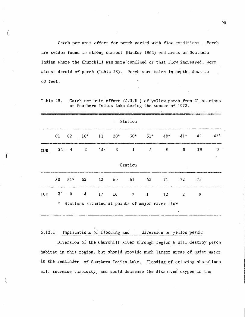
90

Catch per unit effort for perch varied with flow conditions. Perch

are seldom found in strong current (MacKay 1963) and areas of Southern

Indian where the Churchill was more confined or that flow increased, were

almost devoid of perch (Table 28). Perch were taken in depths down to

60 feet.

Table 28. Catch per unit effort (C. U. E.) of yellow perch from 21 stations on Southern Indian Lake during the summer of 1972.

Station

01 02 10* 11 20* 30* 31* 40* 41* 42 43*

cue 3 4 2 14 5 1 3 0 0 13 0

Station

50 51* 52 53 60 61 62 71 72 73

CUE 2 0 4 17 16 7 l 12 2 8

* Stations situated at points of major river flow

6 .12. 1. Implications of flooding and diversion on yellow perch:

Diversion of the Churchill River through region 6 will destroy perch

habitat in this region, but should provide much larger areas of quiet water

in the remainder of Southern Indian Lake. Flooding of existing shorelines

will increase turbidity, and could decrease the dissolved oxygen in the

35

30

2520

5

02 10

10 5 10 5 10

STATIONS

11 20 42

J \ 5 10 5 10 5 10

LENGTH OF FISH

52 53 60 61 71A

ii ' '

5 10 5 10 5 10 5 10 5 10

IN INCHES Figure 15. Length-frequency composition of yellow perch in Southern Indian Lake, 1972.

water, especially under the ice in shallow bays. Perch appear to be

tolerant of lower oxygen values, at least more so than walleye, but are

not found in large numbers in areas;of turbidity or siltation (MacKay

1963).

92

Probably the flooding will have little effect on the success of their

spawning. Perch spawning areas typically are shallow weedy bays with depths

of 5 to 10 feet. Unless siltation becomes a major problem throughout the

lake, there should be many areas of shallow weedy conditions ideal for

perch spawning.

6.13. TROUT-PERCH

Trout-perch are not economically important fish in themselves but

are important as forage fish for sauger and possibly walleye and pike.

They are common to slower water areas (McPhail and Lindsey, 1970) but were

taken from some of the faster flowing areas (station 30) and were absent

from obvious regions of quiet waters (e.g. region 6) in Southern Indian

Lake.

Large numbers were not taken from the experimental nets but of those

taken the mean length was 3. 77 inches and mean weight 0. 33 ounces. McPhail

and Lindsey (1970) stated that trout-perch in their area usually did not

exceed 4 inches which appears to be the size range of this species in

Southern Indian Lake.

6.13.1. Implications of flooding and diversion on trout-perch:

93

Little is known about many aspects of these fish but it seems

unlikely that there will be little adverse affect on this species. They can

be either lake or stream spawners and although changes will affect shore

spawning areas, at least temporarily, new spawning areas in the streams

will be available. Although the food of trout-perch (plankton) will likely

drop in number in regions 3 and 4 significant (Patalas 1974) food does

not appear to be the limiting factor under present conditions and it is

unlikely that the trout-perch population will decrease as a direct result

of this adverse effect on the plankton.

94

6 .14. BURBOT

Burbot are not plentiful in Southern Indian Lake, occurring in almost

equal numbers throughout the lake except in region 6 where none were

taken (Table 29). Region 6 is a relatively shallow bay, with warmer water

than elsewhere in the lake (Cleugh 1974), habitat which, according to

McPhail & Lindsey (1970) is not preferable for burbot. Elsewhere in the

lake burbot were taken at varying depths, usually greater than 20 feet and

most often about 60 feet.

With a mean length of 22.35 inches and mean weight of 2.64 pounds

the burbot from Southern Indian Lake appear to grow more slowly than is

typical of burbot from other North American lakes (mean weight of 3.5 pounds

at 22-23 inches, Car lander, 1969).

Of the bur bot examined the prime source of food was other fish with

percentages by weight being: cisco 41.8%, cisco and/or whitefish 24.4%,

trout-perch 7.3%, perch 6.8%, sculpin 4.6%, ninespine stickleback 4.2% and

95

unidentified fish remains 10.9%.

6.14.1. Implications of flooding and diversion on burbot:

Burbot are known to spawn in swift water of streams and on sand and

gravel shoals of lakes (MacKay 1963) in from l to 3 feet of water. While

diversion is unlikely to adversely change the habitat for burbot, flooding

of uncleared land will temporarily reduce the spawning sites to those in

streams entering Southern Indian Lake.

96

6 .15. GOLDEYE

Although McTavish in 1952 recorded no goldeye from Southern Indian

Lake he noted that they were reported to be in the lake, and that commercial

fishermen were takirig some from Opachuanau Lake. The research crew in 1972

were unsuccessful in their attempts to take goldeye in the experimental nets,

until directed by a native to try in the vicinity of station 62 where one

goldeye was taken. From this it is apparent that there are a few goldeye

in isolated areas of Southern Indian Lake. According to McPhail and

Lindsey (1970) they inhabit turbid shallows of lakes and ascend rivers or

tributary streams to spawn. At present turbid shallows are not plentiful

in Southern Indian Lake, however, following flooding and the diversion much

larger areas of the lake are liable tci become much more turbid as new shore-

lines are carved from existing clay banks. The new Southern Indian Lake

may provide greater areas for goldeye and this species could increase in

number.

6.16. Recommendations

1. Under the interim licence it will be possible for Manitoba Hydro

to decrease the flow through Missi Rapids to a yearly'minimum of 1000 cfs

(from 30,000 cfs). This will substantially decrease the inflow of

nutrients to region 4 contributed by the Churchill River, thereby

decreasing productivity in this region. To_maintain basic productivity of

this part of the lake at an acceptable level it has been reconunended

97

(Hecky et. al.1974), that a mean annual flow of 5000 cfs be guaranteed at

Missi Rapids. Considering the importance of region 4 to fish (both standing

crop and commerical yield) this reconunendation is strongly supported.

2. Sites for future spawning beds for whitefish, and possibly cisco

and shore-spawning sauger could be prepared prior .to the flooding of Southern

Indian Lake. Such sites for whitefish as formulated by Weagle and Baxter

(1973) and cisco would consist of large boulders, and bedrock areas

cleared and grubbed to the rock base. For sauger (and possibly sho.re­

spawning walleye) spawning beds would consist of cleared and grubbed areas

of shoreline that will be sandy, or gravel shores or ridges under the new

water regime. Although artifically prepared spawning sites may not attract

the mature fish, prior clearing will speed the natural forces of erosion

and will ensure that some type of spawning site is available for the

fish populations.

3. Monitoring of Southern Indian Lake and its fishery should be

maintained following impoundment to determine.

i) effect of the flow of the Churchill on fish in region 6.

ii) extent of fish movement from Southern Indian Lake to the former

Rat River System.

iii) the effect that the reduction of flow of the Churchill River

(

through regions 3 and 4 will have on such parameters as food

and habitat for fish.

iv) the effect of increased water levels in all regions on the

fish, but in particular those regions (0, 1, 2, S and 7) that

will remain unchanged relative to the Churchill River flow.

98

6.17. PERSONAL COMMUNICATIONS CITED

Pollard, W.R. Fisheries Biologist, Eastern Region, Manitoba Dept, Mines,

Resources, and Environmental Management. Winnipeg.

Sigurdson, J. Fisheries Technician, Dept. of the Environment, Fisheries

Service. Winnipeg.

99

Sunde, L. Fisheries Biologist, Dept. of the Environment, Fisheries Service.

Winnipeg.

Weagle, K.V. Fisheries Biologist, Dept. of the Environment, Fisheries

Service, Winnipeg.

6.18. LITERATURE CITED 100

Ayles, H.A. MS 1973. The limnology-fisheries of Playgreen and Kiskittogisu

Lakes, Manitoba. Part II. Morphometry, biology and fisheries.

Manitoba Hydro MS rep.

Bajkov, A. 1930a. Fishing industry and fisheries investigations in the

Prairie Provinces. Trans. Amer. Fish. Soc. 60:215-37.

1930b. A study of whitefish (Coregonus clupeaformis) in

Manitoban lakes. Contr. Can. Biol. Fish., N.S. V, 443-455.

Carbine, W.F. 1942. Observations on the life history of the northern

pike, Esox lucius L., in Houghton Lake, Michigan. Trans. Amer.

Fish. Soc. 71(1941):149-164.

Carlander, K.D. 1956. Appraisal of fish population study - Part I. Fish

growth rate studies: techniques and role in surveys and management.

Trans. twenty-first N. Amer. Wild. Conf. :262-274.

1969. Handbook of freshwater fishery biology. Vol. I.

Iowa State Univ. Press, Ames, Iowa. 752 p.

Cleugh, T. MS 1974. Hydrography of Southern Indian Lake: present conditions

and implications of hydroelectric development. MS prepared for

Canada-Manitoba Lake Winnipeg, Churchill and Nelson Rivers Study.

Environment Canada, Fisheries Service.

Crooks, S. 1972. Water.-level fluctuations and yellow pickeral, northern

pike and lake whitefish in Lac Seul. Ont. Min. Nat. Res. MS Rep.

Crowe, Walter R. 1962. Homing behaviour in walleye. Trans. Am. Fish. Soc.

91(4):350-354.

Dryer, W.R. 1963. Age and growth of the whitefish in Lake Superior, U.S.

Fish and Wildlife Service, Fishery Bulletin 1, Vol. 63:77-95.

101

Edsall, T.A. 1960. Age and growth of the whitefish Coregonus clupeaformis

of Munising Bay, Lake Superior. Trans. Am. Fish. Soc. 89(4):323-332.

Eschmeyer, P.H. and W.R. Crowe. 1955. The movements and recovery of tagged

walleyes in Michigan, 1929-1953. Mich. Dept. Cons., Inst. Fish. Res.

Bull. 8. 32 pp.

Franklin, D.R. and L. L. Smith. 1960. No'te on development of scale patterns

in the northern pike Esox lucius L. Trans. Am. Fish. Soc. 89(1) :83.

Fry, F.E.J. 1937. The summer migration of cisco (Leucichthys artedi) (Le

Sueur) in Lake Nipissing, Ont. Univ. of Tor. Stud. Biol. No. 44,

Pub. Ont. Fish. Res. Lab, No. 55.

Glenn, C.L. 1969. Seasonal rates of growth within a population of walleye,

Stizostedion vitreurn vitreum (Mitchell), in West Blue Lake, Manitoba,

during 1966-1967. MS, Univ. of Manitoba.

Hamilton, A.L. MS 1974. Zoobenthos survey of Southern Indian Lake, MS prepared

for Canada-Manitoba Lake Winnipeg, Churchill and Nelson Rivers Study.

Environment Canada, Fisheries Service.

Hecky, R.E., R. Harper, H. Kling. MS 1974. Phytoplankton and primary produc­

tion in Southern Indian Lake. MS prepared for Canada-Manitoba Lake

Winnipeg, Churchill and Nelson Rivers Study. Environment Canada, Fisheries

Service.

Hile, R. 1970. Body-scale relation and calculation of growth in fishes.

Trans. Amer. Fish. Soc. 99(3):468-474.

Kennedy, W.A. 1943. The whitefish, Coregonus clupeaformis (Mitchell), of

Lake Opeongo, Algonquin Park, Ontario. Publ. Ont. Fish. Res. Lab. No. 62

1954. Tagging returns, age studies, and fluctuations in

abundance of Lake Winnipeg whitefish, 1931-1951. J. Fish. Res. Board

Can. 11(3): 284-309.

Koshinsky, G.D. 1965. Limnology and fisheries of five Precambrian headwater

lakes near Lac la Ronge. Saskatchewan. Sask. Dept. Nat. Res. Fish.

MS 1971. Trout and McIntosh Lakes: The comparative

limnology and fisheries of a Churchill River lake and an adjacent

Shield lake in central Saskatchewan. Sask. Fish. Lab. Dept. Nat.

Res. MS Rep. 97 p.

102

MS 1972. The ecology, dynamics, and explotation-manage

ment of northern pike, Esox lucius L., at Lac la Ronge, Saskatchewan.

Sask. Fish. Lab. Dept. Nat. Res. MS Rep. 306 p.

MS 1973. Preliminary report on the limnology-fisheries of

the Lake Winnipeg outlet lakes area: present conditions and impli­

cations of hydroelectric development. Environment Canada Fisheries

Service MS Rep. 156 p.

Lindstrom, T. 1962. Life history of whitefish young (Coregonus) in two lake

reservoirs. Rep. Inst, Freshw. Res., Drottningham. 44:113-144.

MacKay, H.H. 1963. Fishes of Ontario. Ont. Dept. Lands and Forests. 292 p.

McPhail, J.D. and C.C. Lindsey. 1970. Freshwater fishes of northwestern

Canada and Alaska. Fish. Res. Bd. Can. Bull. 173. 381 p.

McTavish, W.B. 1952. A biological survey of Southern Indian Lake. Rep.

for the Man. Dept. of Mines and Nat. Res.

Patalas K. MS 1974. Preliminary report on zooplankton study in Southern

Indian Lake. MS prepared for Canada-Manitoba Lake Winnipeg, Churchill

and Nelson Rivers Study. Environment Canada, Fisheries Service.

Preiegel, G.R. 1969. The Lake Winnebago sauger. Age, growth, reproduction,

food habits and early life history. Tech. Bull. 43. Wisc. Dept. Nat. Res.

Qadri, S.U. 1968. Growth and reproduction of the lake whitefish, Coregonus

clupeaformia in Lac la Ronge, Saskatchewan. J. Fish. Res. Board Can.

25(10):2091-2100.

(

Rawson, D.S. 1956. The life history and ecology of the yellow walleye.

Stizostedion vitreum, in Lac la Ronge, Saskatchewan. Trans. Am.

Fish. Soc. 86:15-37.

1957. Limnology and fisheries of five lakes in the upper

Churchill drainage, Saskatchewan. Sask. Dept. Nat. Res. Fish. Rep.

3. 61 p.

1959. Limnology and fisheries of Cree and Wollaston Lakes

in northern Saskatchewan. Sask. Dept. Nat. Res. Fish. Rep. 4. 73 p.

1960. Five lakes on the Churchill River near Stanley,

Saskatchewan. Sask. Dept. Nat. Res. Fish. Rep. 5. 39 p.

Rawson, D.S. and F.M. Atton. 1953. Biological investigation and fisheries

management at Lac la Ronge, Saskatchewan. Sask. Dept. Nat. Res.

Fish. Rep. 39 p.

Ricker, W.E. 1971. Methods for assessment of fish production in fresh

waters. Publ. Intn. Biol. Prog., Blackwell Scientific Publications,

Oxford and Edinburgh. IBP Handbook No. 3.

Van Oosten, J. 1923. The whitefishes (Coregonus clupeaformis). A

study of the scales of whitefishes of known ages. Zoologica (N.Y.).

2:381-412.

Weagle, K.V. and W. Baxter, MS 1973. The fisheries of Southern Indian

103

Lake: exploitation and reproduction . MS prepared for Canada­

Manitoba Lake Winnipeg, Churchill and Nelson Rivers Study. Environment

Canada, Fisheries Service.

6 .19. APPENDIX

Report on the 1972 Fishing Survey

on Southern Indian Lake,

Manitoba

by

Johann Sigurdson

104

APPENDIX

List of tables .....•...............•......... 105

1. Introduction ............................................. .

2. Methods 2.1 2.2 2.3

of recording data o o

Scale envelopes ...........•..... The fish card supplement ......... .............. . The master sheet .................. ... ... ... .

3. Field methods . ....... o

Table A.

Table B.

Table C.

LIST OF TABLES

Total number and total weight of all fish species taken in the experimental gillnets at specific stations on Southern Indian Lake, 1972 ...................•............

Total number and total weight of individual species of fish taken from Southern Indian Lake, 1972 ... o. .........

Total number and total weight of 9 fish species caught at specific fishing stations in Southern Indian Lake, 1972 ................... .

106

108 108 109 110

112

116

117

118

105

1. INTRODUCTION

The summer of 1972 was the first summer of field work for the

fisheries section of the Churchill-Nelson River diversion project carried

out by the Department of the Environment, FRB of Canada, Freshwater

Institute. The summer's work for the fisheries crew was to concentrate

on systematically fishing Opachuanau and Southern Indian Lakes.

The lakes were divided into seven major areas but with only six

major stations. (Since this inception station 72 has almost attained

major station status in the fisheries data.) The seven areas were chosen

mainly because of geographical boundaries but also for convenience in

identification of areas in subsequent data. The major stations were in

a series of tens, e.g. 10, 20, 30, 40, SO, 60. The minor stations in

each area had the first digit of the major plus another from 1-9. In

special cases in the data some of these stations were identified with a

letter, e.g. 72A, 72B. These indicate the order of occurrence when

duplicated within the same trip. The six major stations plus fifteen more

which were chosen randomly to cover each area were used as the twenty-one

fishing stations.

The original plan was to fish each of the 21 stations three times

over the summer season. In actuality there were two trips completed and

the third trip consisted of the major stations and three others; 72, 62

and 52. The trips were divided as follows during 1972:

Trip I Day 179-199

Trip II Day 216-241

Trip III Day 242-253

106

To facilitate later data processing a number code was devised to

record fish species. These were as follows:

1 - whitefish

2 - pickerel

3 - pike

4 - white sucker

5 - longnose sucker

6 - burbot

7 - cisco

8 - sauger

9 - perch

The rarer fish caught or the smaller species were not coded in the

field but have since been coded by the Computer Centre and they are as

follows:

10 - trout-perch

11 - sculpin

12 - spot-tail shiner

13 unknown (unidentified in the field)

14 - goldeye

107

108

2. METHODS OF RECORDING DATA

2.1. Scale envelopes:

The scale envelope was used where a scale sample was taken and the

data for an individual fish were entered directly onto this card. Note

example 1 below.

Example 1.

.,

CHURCHILL - NELSON

C. Ser. Date

Sp. Lake

Ln.

Wt. G-M

s. M. ' N°. 5998

'.:.

An important feature was the Catch Serial Number in the upper left

corner. Each mesh size for each set had a different number. It was a

4-digit number beginning in O,e.g. 0001 was the first, 0002 the second,

etc. The numbers for Swedish nets all started with a 9 and were also 4

digits, e.g. 9001.

Also important was the scale envelope number which later allowed

109

the individual fish to be found after the aging work had been completed.

This feature was only available on the second and third trips as unnumbered

cards had been used previous to this.

2.2. The fish card supplement [example 2]

This card was used when an incomplete analysis was done. The catch

serial number was carried over to this card for each mesh of each gang set.

Basic data from fish which were completely analyzed were also entered here

from the scale envelopes to give complete basic data on one card for all

fish caught from one mesh. See example 2 below.

Example 2.

CHURCHILL- NELSON FISH CARD SUPPLEMENT

C . Ser. No. C. Ser.No. C. Ser. No. c. Ser. No.

Sp. Fork L. Rd. wt. Sp. Fork l. Rd. wt Sp. Fork L. Rd. wt. Sp. Fork L. Rd. wt. -

... 110

2.3. The master sheet [example 3]:

This sheet summarized all the data collected for the day. There are

7 columns for the major species and 4 columns for minor species. The

numbers along the left margin correspond to the mesh sizes set. The first

7 rows indicate the shallow set and the last 7 rows indicate the deep set.

The depths at the end of each mesh size appear in the second and third

columns.

Station number, lift day, and time set and lifted appear at the top

of the sheet. Catch serial number for each mesh size appears below and to

the right of this. In the lower left corner of the sheet the total number

of fish caught that day is shown over the total number of pounds caught.

These figures for individual species are along the bottom of the sheet.

A master sheet for Station 40 is attached as example 3. Along with the

master sheet a map of the area was prepared showing the relatiQnship of

the shoreline to the gang of nets and to the mesh sizes. There was also

a short note on procedures for the day and on general observations made.

Mesh ! Size

99

15

20

28

35

4252

151s 20

28

3 35

42

52

99325

589 .43

l

CATCH RECORD

Depth Whitefish wa.lleye

M M No. Lbs No. Lbs.

s.s 7 5. 08 1 0.44 s .. 6.0 6.0 9 6.03

. . 6.0 s.s 12 10.37 1 2.94

6.0 5.5 9 11.24 1 0.63

s.s 6.0 s 7 .31 ..

6.0 6.0 7 14.63

3. s 6.0 2 5.69

14.0 15.0 17 7.35

15.0 15.0 34 24.91

35 50.66

15.1 15.5 33 53.88

15.0 15.0 23 48.31

14.0 14.0 s 12.63

N Jt set

198

258.09 4 .01

Example 3 Master Sheet

Stj Lift Time

Day Set Lift u

1 2 l 40 251 1900 0800

Pike w. Sucker L Sucker Bur bot Cisco Catch Trout+perch Sculpin

No. tbs. No. Lbs, No. Lbs. No. lbs. No. Lbs. Ser. No. No. Lbs No. Lbs.

2 3.69 7 8.63 4 18.31 9074 1 0.01 1 -3 9.69 2 0.27 0542 . 1 2.69 0543

1 3.00 8 9.97 l 1.88 0544

4 . 12 .94 5 8.13 4 11.19 1 1.38 0545

3 16.19 4 8.06 4 32.13 0545

1 15.0 1 3.44 8 30.38 0547 .. 8,46 1 0.14 0548 l 0.01

5 7.61 l 0.22 0549 . 2 3.31 6 11.34 0550

10 22.19 0551

12 24,44 0552

14 52.63 0553

i

17 27 76 1 2 l

66.51 38.50 220.56 1. 74 0.02

3. FIELD METHODS

A fifty foot converted trapnet boat, the "M9", belonging to the

Manitoba Department of Mines, Resources and Environmental Management,

was used as a base and as such was utilized for sleeping and eating

accommodation for a fishing crew of 5 as well as for 2 crew members of

the morphometric team. It was also used to carry gasoline and supplies

for three other boats; 2 - 19 foot steel yawls and a 16 foot aluminum

runabout. This mobile base camp was moved almost daily.

A "standard gang" of nets consisted of 6 - 50 yard nylon nets

112

joined with bridles to make up one almost continuous net 300 yards in length.

The 6 mesh sizes were expressed in a number code as follows:

1 1/2" - 15

2 - 20

2 3/4" - 28

3 1/2" - 35

4 1/4" .. 42

5 1/4" - 52 (stretch size)

These mesh sizes were always kept in the same order as follows: 52-15-

42-20-35-28 or in other words largest-smallest-2nd largest-2nd smallest-

3rd largest-3rd smallest. At each station where possible one of these

gangs would be set in a shallow location, and one would be set in a deep

location. Originally it was planned to set three gangs but after two

days this proved to net too many fish to handle efficiently and so the

number was reduced to two gangs. The shallow set would be generally

between 3-7 meters and the deep set 8 or more meters. Also, where possible,

a "Swedish" net, a specially designed single test net consisting of 12 mesh

sizes from 3/4"-6" and 40 yards long, was set. This practice however was

precluded in many cases because of bad weather and high winds which broke

the delicate and fragile net. All sets were bottom sets.

Sets were usually located within a one-mile radius of the station

and were chosen for the following reasons:

a) High winds made setting in the lee of an island, point, or bay

almost mandatory. The sets were with the wind in these cases.

b) If the area was fairly shallow the deep set was made in the

first deep area located.

c) If the area was deep the shallow set was made in the first

shallow area located.

d) If bad weather was expected the next day the set was made where

it would be sheltered.

e) If an area was known to be exceptionally deep, the deep set was

made there. This happened at stations 50 and 30.

f) Areas were randomly chosen to sample weedy, rocky, and sandy

shorelines.

g) Where a tributary was located a net was usually set across the

current (but not in the stream) .

h) Areas were chosen after consulting topographic maps of the lake.

The gangs were usually set around 17:00-18:00 and lifted at

08:00-09:00. On a few rare occasions because of inclement weather they

remained set for two nights. Also on a few rare occasions because of high

winds only one gang was set, usually the shallow, in the lee of the shore.

With a full fishing crew, two crew members in a yawl would usually

be responsible for the setting and lifting of one gang. All the meshes

113

were kept separate by placing the fish in different tubs labeled by mesh

size. These fish were taken back to the "M9" to be recorded. The basic

data taken were as follows: fork length, weight, sex. These were recorded

on the supplement card except in a few rare cases where the fish were

counted and weighed 'en masse'. As well, on the first ten fish of each

species from each mesh size the following were taken: scale sample,

stomach sample, possibly fin clips from suckers and whitefish and otoliths

from burbot. Only the stomachs which were full were preserved when it was

possible to ascertain; such as in pike, pickerel, sauger and burbot. In

the whitefish, suckers and cisco all stomachs were preserved.

For specimens from which a scale sample was taken the data were

recorded directly onto a scale envelope. For all others it was recorded

onto the supplement card. The data on the scale envelopes were later

transferred to supplement cards also and then these data were summarized

onto the master sheet. With this master sheet was also placed a rough map

of the location of the sets, the relation of the mesh sizes, the location

of the Swedish nets, depth at the end of each mesh, duration of set, and

the temperature gradient and location taken. There was also a short note

on procedure during the day and some observations on the general conditions

of the day.

114

The fish taken by the Swedish nets were weighed and measured only.

Later in the field season when staff became short only a certain mesh

size per day from each gang were analyzed. These were chosen for the

following reasons:

a) If a mesh size contained many of a species which was fairly

115

rare such as sauger or perch it was done to record these fish.

b) If a mesh size contained many large individuals of a species it

was done (e.g. pike, burbot).

c) If a mesh size contained many small individuals it was done to

record these fish (e.g. pike).

d) If the gangs contained basically the same species composition

the large meshes were analyzed from one gang and the small meshes

from the other.

e) If the catch was small all the fish were completely analyzed.

In the cases of partial catch analysis fish from the rest of the

meshes were weighed and measured only.

Fish were disposed of by the following methods:

given to the local people for dog food;

- consumed by the fishing crew;

- fed to seagulls and predators;

- buried on shore;

- some specimens were preserved and brought back to the lab.

The gangs of nets were completely replaced for the second trip, and

the 52 mesh was again replaced for the third trip.

Table A. Total number and total weight of all fish species taken in the experimental gillnets at specific stations on Southern Indian Lake, 1972.

Station Total number Total weight in pounds

01 559 856

02 621 845

11 972 1372

10 889 1206

73 279 398

72 830 1065

71 516 707

61 566 599

60 896 899

62 406 252

20 1487 1746

31 490 878

30 821 1451

41 595. 1014

42 611 839

53 458 533

50 1030 1616

52 653 680

51 691 1102

40 974 1580

43 607 1316

Grand total 14,951 20,954

116

Table B.

Species

Whitefish

Walleye

Pike

White sucker

Total number and total weight of individual species of fish taken from Southern Indian Lake, 1972.

Total number . Total weight in pounds

3,500 4,613

1,556 1,951

1,309 3,374

2,618 4,684

Longnose sucker 1,457 3,702

Bur bot 203 952

Cisco 3,433 1,344

Perch 381 95

Sauger 494 239

Grand total 14,951 20,954

117

Stn Whitefish

No. lbs

Walleye

No lbs

Pike No. lbs ----

01

02

42 59 so 51 27 72

11

10

73

9

75

149

60

72 16

71 142

61 25

60 73

62 so 20 475

31 136

30 245

41 248

42 206

53 64

so 467

52 54

51 271

40 507

43 186

3,500

12 189 206 88

48

29

51

219

144

84

124

90 56 59

158 so 52

59 54 58

32

211

32

77

47

597

169

228

311

244

57

809

84

431

685

221

4,613

151

13

127

,157

30

43

23

50

8

10

208

86

180

28

14

29

1,536

397 63 198

16 74 206

130 38 81

186 122 263

29 35 70

39 109 260

29 99 269

34 71 178.

8 98 242

7 36 71

257 23 66

100 97 276

194 51 138

24 35 88

10 70 205

65 45 120

1,951 1,309 3,374

White sucker

No, lbs

309 537

184

533

299

66

31

58.

142

125

10

195

58

97

43

100

64

44

72

29

48

111

2,618

320

926

565

120

36

56

248

243

12

428

109

175

77

166.

135

112

123

53

49

189

4,684

Sturgeon sucker No. lbs,

45 97

16 106

s

1

7

1

l

81

84

278

117

60

1

60

23

142

214

215

1,457

25

228

13

6

18

3

1

232

243

793

292

158

2

167

58

369

sos 491

3,702

Burbot

No. lbs.

4 3

4

11

2

12

16

22

8

7

10

25

27

8

19

21

7

203

13

37

10

41

46

98

31

17

44

117

75

19 88

.87

226

952

Cisco No. lbs.

38 25

129

79

161

18

543

484

172

238

174

225

70

68

71

122

68

247

247

167

100

12

3,433

81

32

54

8

355

159

66

68

49

81

25

25

40

45

8

77

55

49

39

1,344

Perch No. lbs,

11 1

13

44

9

23

9

23

25

86 4

26

12

4

44

29

2

16

l

331

3

9

l

6

1

4

8

10

1

5

3

1

31

0.1

4

0.2

95

7

Sauger No. lbs.

33 11

9

117

75

s 5

30

94

102

11

l

9

1

2

1

494

4

74

27

5

3

16

49

43

6

.01

.01

2

0.1

0.3

239