Embed Size (px)
Citation preview
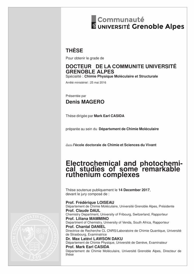
THÈSEPour obtenir le grade de
DOCTEUR DE UNIVERSITÉ
Spécialité : Chimie Physique Mol culaire et Structurale
Arrêté ministériel : 25 mai 2016
Présentée par
Denis MAGERO
Thèse dirigée par Mark Earl CASIDA
préparée au sein Départ ment de Chimie Moléculaire
Chimie et Sciences du Vivant
Electrochemical and hotochemi-cal tudies of ome emarkableuthenium omplexes
Thèse soutenue publiquement le 14 December 2017,devant le jury composé de :
Prof. Frédérique LOISEAUDépartement de Chimie Moléculaire, Université Grenoble Alpes, Présidente
Prof. Claude DAULChemistry Department, University of Fribourg, Switzerland, Rapporteur
Prof. Liliana MAMMINODepartment of Chemistry, University of Venda, South Africa, Rapporteur
Prof. Chantal DANIELDirectrice de Recherche CL CNRS/Laboratoire de Chimie Quantique, Universitéde Strasbourg, Examinatrice
Dr. Max Latévi LAWSON DAKUDépartement de Chimie Physique, Université de Genève, Examinateur
Prof. Mark Earl CASIDADépartement de Chimie Moléculaire, Université Grenoble Alpes, Directeur dethèse
Remerciements
I wish to sincerely thank Prof. Mark CASIDA for offering me an oppor-
tunity to work with him. Being a student from Africa, I understand how
difficult it is to get an opportunity to study abroad, and even if you do, the
chances of being accepted are very slim because you are not ‘known’. Mark
took the risk and decided to give me the golden opportunity and I sincerely
thank him. Thank you for inspiring the growth of Quantum Chemistry in
Africa. You have planted a seed, a seed that will grow and produce other
seeds, your legacy will for long be remembered in Africa.
This dream would not be a reality without the support of the French
Embassy in Kenya. Thank you for the doctoral scholarship. In particular
I would like to acknowledge all the people who were involved in planning
for my stay in France. Thank you Sarah Ayito NGUEMA, for your concern
and commitment towards ensuring that I had a comfortable stay in France
as well as striving hard to ensure that we establish a collaboration. My
gratitude also goes out to Matthew RENAUD, Pauline MOUTAUX and Ma-
rine GAZIKIAN for your support. To the staff and personnel at the École
Doctorale Chimie et Science du Vivant and in particular Pourtier MAG-
ALI, thank you for the assistance in all the administrative work. Thanks
to Campus France and CROUS for organizing the stays and for financial
administration. I wish to extend my gratitude to the people in France, for
your kindness and warm welcome whenever I visited you and for making me
confirm that ‘bureaucracy’ is truly a French word.
Thanks to the International Centre for Theoretical Physics (ICTP) for
sponsoring a number of schools that I have attended. This has indeed con-
i

tributed greatly to my personal profile and academic growth.
My directors in Kenya, Dr. Nicholas MAKAU, Prof. George AMOLO
and Prof. Lusweti KITUYI have been and continue to be a great inspiration.
From my masters to Ph.D, you are honestly a blessing. Your constant calls
of encouragements have been the much required fuel that has keep me going
in this long journey. I may not have enough words to describe what I feel,
but all I say is thank you very much.
Many thanks to my comité de suivie de thèse, Dr. Max Latévi LAWSON
DAKU and Prof. Chantal DANIEL for taking their time to review my work,
and for their support through exchange of ideas throughout my study. I
am sincerely very thankful of that gesture. Thanks to my jury, for having
accepted to read and examine this work.
To my lovely wife Rodah Cheruto SOY, thank you for being an inspira-
tion. Your encouragement and support has brought me this far. For the time
that I have been away studying, all the weekends that I have been spending
in the lab, sleeping late and waking up early, literally, being absent during
all this time, you have been patient with me and I thank you for that. To my
daughter, the little ‘Professor’, Judith Aloo MAGERO, thank you for being
a good time keeper, always waking me up at the right time of the night for
me to go for study. We appreciate your presence in our life.
I wish to extend my gratitude to my dear parents, for the sacrifices that
they made to bring me this far. It has been a journey that has not been
easy, with roadblocks placed at every point, and preformed minds that we
could not make it. Today, my heart is filled with a lot of gratitude because
my parents can also stand tall and be counted, because I have gone through
barriers that they never imagined. It has been a long journey, I remember
many years ago, mum would pack for me some bread in the lunch box then
dad would drop me to school with his ‘Zebra’ bicycle . My promise to you
has been fulfilled, and wherever you are, I am sure that you must be very
proud. To my brother Pius Gumo MAGERO, thank you for the efforts that
you have put in. Your encouragement and support have made me to come
this far.
I wish to thank the Chimie théorique group and especially my dear friend

Ala Aldin M. Hani M. DARGHOUTH for the support and encouragement
throughout my study, and for being a true brother and colleague. Thank
you Pierre GÉRARD for having solutions to my computing problems and
for being there always to support. Thanks to Nicolas ALTOUNIAN, Rolf
DAVID, Walid TOUWALI and Tarek MESTIRI. Thanks to Prof. Carlos
PEREZ, for the encouragement and exchange of ideas. I wish to thank Prof.
Anne MILET for the useful scientific discussions. I also acknowledge Prof.
Heléne JAMET and Dr. Myneni HEMANADHAN for your useful scientific
discussions and for the great brotherhood that you brought with the spicy
food.
I owe an appreciation to Dr. Joseph CHAVUTIA, the my head of depart-
ment at the Eldoret Polytechnic, for having a listening ear and being very
understanding. It is because of your support that I was able to teach and
study at the same time. I am truly very thankful for your gesture. I wish to
thank my Kenyan family in Grenoble for the great company and guidance
that you gave. Thanks to Carolyne MARTINS and Abdi FARAH and his
family.
Members of the Computational Material Science Group in Kenya have
been of invaluable help. Thanks to Victor MENGWA, Perpetual WANJIRU,
Tolbert NGEYWO, Valid MWALUKUKU and Geoffrey ARUSEI. I also wish
to give special thanks to Dr. Cleophas Muhavini WAWIRE for his great help
in starting off this work.
I may not have acknowledged everyone in this writing, but I want to
thank everybody that was involved in making this work a success.

To my grandmother Marita Dienya and my grandfather Bill Masengeli
Walubengo. You passed on before seeing this come true, this is for you.
Résumé
Cette thèse fait partie d’un projet franco-keyan dénommé ELEPHOX
(ELEctrochemical and PHOto Properties of Some Remarkable Ruthenium
and Iron CompleXes). En particulier, notre focus est la continuation du tra-
vail de C. Muhavini Wawire, Damien Jouvenot, Fréderique Loiseau, Pablo
Baudin, Sébastien Liatard, Lydia Njenga, Geoffrey Kamau, et Mark E.
Casida, “Density-Functional Study of Lumininescence in Polypyridine Ruthe-
nium Complexes,” J. Photochem. and Photobiol. A 276, 8 (2014). Cet article
a proposé une indice orbitalaire de temps de luminescence pour les complexes
de ruthénium. Cependant cet article n’était limité qu’à quelques molecules.
Afin d’avoir une théorie plus fiable et donc potentiellement plus utile, il fau-
dra tester l’indice de luminescence sur beaucoup plus de molécules. Ayant
établi le protocol, il était “évident” mais toujours un défi de le tester sur
encore une centaine de molécules pour démonter ou infirmer l’indice pro-
posée. Pour ce faire, j’ai examiné les 98 pages de la Table I de A. Juris, V.
Balzani, F. Bargelleti, S. Campagna, P. Belser, et A.V. Zelewsky, “Ru(II)
polypyridine complexes: Photophysics, photochemistry, electrochemistry, and
chemiluminescence,” Chem. Rev. 84, 85 (1988) et j’ai extrait un nombre im-
portant de données susceptibles à comparaison avec les résultats des calculs
de la théorie de la fonctionelle de la densité (DFT) et la DFT dépendante
du temps (TD-DFT). Comme les résultats étaient suffisament encourageant,
le modèle DFT était examiné de plus près avec la méthode d’une théorie de
champs de ligands (LFT) à la base de la densité des états partielle (PDOS).
Ainsi j’ai pu tester l’indice de luminescence proposée précédement par la
méthode PDOS-LFT et j’ai trouvé des difficultés avec l’indice initialement
v
proposée. Par contre, nous avons pu proposer une nouvelle indice de lumi-
nescence qui, à quelques exceptions près, a une corrélation linéaire avec une
barrière énergétique moyenne pour l’état triplet excité dérivée à partir des
données experimentales. À l’avenir nous pouvons proposer une investiga-
tion plus directe de la barrière sur la surface triplet excité pour remplacer
la valeur approximative déduite de l’expérience. Puis nous voulons voir si
notre indice de luminescence s’appliquent aux cas des complexes d’iridium.
Mots-Clé: Chimie Quantique, Photochimie, État Excités, Complexes polypyri-
dine ruthénium, Luminescence, Théorie de la Fonctionnelle de la Densité,
Théorie de la Fonctionnelle de la Densité Dépendente du Temps, Densité
d’état partielle, Surface d’énergie Potentielle pour un état Triplet, État de
Transition.
Abstract
This thesis is part of the Franco-Kenyan project ELEPHOX (ELEctrochemical
and PHOto Properties of Some Remarkable Ruthenium and Iron Com-
pleXes) project. In particular, it focused on the continuation of the work of
C. Muhavini Wawire, Damien Jouvenot, Fréd erique Loiseau, Pablo Baudin,
Sébastien Liatard, Lydia Njenga, Geoffrey Kamau, and Mark E. Casida,
“Density-Functional Study of Lumininescence in Polypyridine Ruthenium
Complexes,” J. Photochem. and Photobiol. A 276, 8 (2014). That paper
proposed a luminescence index for estimating whether a ruthenium com-
plex will luminesce or not. However that paper only tested the theory on
a few molecules. In order for the theory to have a significant impact, it
must be tested on many more molecules. Now that the protocol has been
worked out, it was a straightforward but still quite challenging matter to
do another 100 or so molecules to prove or disprove the theory. In order to
do so, I went through the 98 pages of Table I of A. Juris, V. Balzani, F.
Bargelleti, S. Campagna, P. Belser, and A.V. Zelewsky, “Ru(II) polypyridine
complexes: Photophysics, photochemistry, electrochemistry, and chemilumi-
nescence,” Chem. Rev. 84, 85 (1988) and extracted data suitable for compar-
ing against density-functional theory (DFT) and time-dependent (TD-)DFT.
Since the results were sufficiently encouraging, the DFT model was examined
in the light of partial density of states ligand field theory (PDOS-LFT) and
the previously proposed luminescence indices were tested. In fact, the origi-
nally proposed indices were not found to be very reliable but we were able to
propose a new luminescence index based upon much more data and in anal-
ogy with frontier-molecular orbital ideas. Except for a few compounds, this
vii

index provides a luminescence index with a good linear correlation with an
experimentally-derived average excited-state activation energy barrier. Fu-
ture work should be aimed at both explicit theoretical calculations of this
barrier for ruthenium complexes and extension of the luminescence index
idea to iridium complexes.
Keywords: Quantum Chemistry, Photochemistry, Excited States, Polypyri-
dine ruthenium complexes, Luminescence, Density-functional theory, Time-
dependent density-functional theory, Partial density of states, Triplet Sur-
face, Transition State.
Table of Contents
Remerciements i
Résumé v
Abstract vii
List of Tables xiv
List of Figures xvi
I Introduction 1
1 Introduction 2
1.1 Objectives . . . . . . . . . . . . . . . . . . . . . . . . . . . . . 4
1.2 Structure and Organization . . . . . . . . . . . . . . . . . . . 5
II Background Material 8
2 Transition Metal Complexes 9
2.1 Introduction . . . . . . . . . . . . . . . . . . . . . . . . . . . . 9
2.2 Definitions . . . . . . . . . . . . . . . . . . . . . . . . . . . . . 10
2.2.1 Coordination number . . . . . . . . . . . . . . . . . . . 10
2.2.2 Charge . . . . . . . . . . . . . . . . . . . . . . . . . . . 11
2.2.3 Nomenclature . . . . . . . . . . . . . . . . . . . . . . . 12
ix
2.3 Transition Metal Structure and Properties . . . . . . . . . . . 12
2.3.1 Geometries . . . . . . . . . . . . . . . . . . . . . . . . 12
2.3.2 Crystal Field Theory . . . . . . . . . . . . . . . . . . . 13
2.3.2.1 Octahedral complexes . . . . . . . . . . . . . 13
2.4 Ligand Field Theory . . . . . . . . . . . . . . . . . . . . . . . 15
2.4.1 Molecular Orbitals . . . . . . . . . . . . . . . . . . . . 15
2.4.2 Molecular Orbital Formation . . . . . . . . . . . . . . 17
2.5 Photophysical Processes for Transition Metal Complexes . . . 18
3 Schrödinger Equation 22
3.1 Ultraviolet Catastrophe . . . . . . . . . . . . . . . . . . . . . 23
3.2 Photoelectric Effect . . . . . . . . . . . . . . . . . . . . . . . . 23
3.3 Quantization of Electronic Angular Momentum . . . . . . . . 24
3.4 Wave-Particle Duality . . . . . . . . . . . . . . . . . . . . . . 25
3.5 Time-Independent Schrödinger Equation . . . . . . . . . . . . 26
3.6 Time-Dependent Schrödinger Equation . . . . . . . . . . . . . 29
3.7 Molecular Hamiltonian . . . . . . . . . . . . . . . . . . . . . . 30
3.8 Atomic Units . . . . . . . . . . . . . . . . . . . . . . . . . . . 32
3.9 Born-Oppenheimer Approximation . . . . . . . . . . . . . . . 34
4 Photophenomena and Luminescence 38
4.1 Introduction . . . . . . . . . . . . . . . . . . . . . . . . . . . . 38
4.2 Electronic Excitation . . . . . . . . . . . . . . . . . . . . . . . 39
4.2.1 How does Electronic Excitation Occur? . . . . . . . . 40
4.2.2 Types of Electronic Transitions . . . . . . . . . . . . . 40
4.3 State Energy Diagram . . . . . . . . . . . . . . . . . . . . . . 43
4.4 Excited State Deactivation . . . . . . . . . . . . . . . . . . . . 44
4.4.1 Introduction . . . . . . . . . . . . . . . . . . . . . . . . 44
4.4.2 Luminescence . . . . . . . . . . . . . . . . . . . . . . . 44
4.4.2.1 Jablonski Diagram . . . . . . . . . . . . . . . 45
4.4.3 Vibrational relaxation . . . . . . . . . . . . . . . . . . 46
4.4.4 Radiationless Deactivation . . . . . . . . . . . . . . . . 47
4.4.5 Radiative Deactivation . . . . . . . . . . . . . . . . . . 48
4.4.5.1 Fluorescence . . . . . . . . . . . . . . . . . . 48
4.4.5.2 Phosphorescence . . . . . . . . . . . . . . . . 49
4.5 Photochemical Processes on Potential Energy Surfaces . . . . 49
4.6 Excited State Lifetime . . . . . . . . . . . . . . . . . . . . . . 50
4.7 Quantum Yield . . . . . . . . . . . . . . . . . . . . . . . . . . 50
5 Hartree-Fock Approximation 53
5.1 The Hartree Product . . . . . . . . . . . . . . . . . . . . . . . 54
5.2 Slater Determinant . . . . . . . . . . . . . . . . . . . . . . . . 55
5.3 The Electronic Hamiltonian . . . . . . . . . . . . . . . . . . . 55
5.4 Coulomb and Exchange Integrals . . . . . . . . . . . . . . . . 56
5.5 Coulomb and Exchange Operators . . . . . . . . . . . . . . . 59
5.6 Hartree-Fock Orbitals and Orbital energies . . . . . . . . . . . 61
5.7 Koopmans’ Theorem . . . . . . . . . . . . . . . . . . . . . . . 63
5.8 Roothaan-Hall Equation . . . . . . . . . . . . . . . . . . . . . 64
6 Density-Functional Theory 69
6.1 Hohenberg-Kohn Theorems . . . . . . . . . . . . . . . . . . . 70
6.2 Thomas-Fermi Model . . . . . . . . . . . . . . . . . . . . . . . 74
6.3 Kohn-Sham Approach . . . . . . . . . . . . . . . . . . . . . . 75
6.4 Exchange-Correlation Approximations (Jacob’s Ladder) . . . 79
6.4.1 Local Density Approximation(LDA) . . . . . . . . . . 79
6.4.2 Generalized Gradient Approximation (GGA) . . . . . 80
6.4.3 Hybrid Functionals . . . . . . . . . . . . . . . . . . . . 81
6.4.4 Meta-Generalized Gradient Approximation (meta-GGA) 82
6.4.5 Double hybrid functionals . . . . . . . . . . . . . . . . 82
6.4.6 Jacob’s Ladder of Density Functional Approximations 82
7 Basis Sets and Effective Core Potentials 87
7.1 Definition of a Basis Set . . . . . . . . . . . . . . . . . . . . . 87
7.2 Types of Basis Functions (Atomic Orbitals) . . . . . . . . . . 88
7.2.1 Slater-Type Orbitals (STOs) . . . . . . . . . . . . . . 89
7.2.2 Gaussian-type orbitals (GTOs) . . . . . . . . . . . . . 90
7.3 Classification of Basis Sets . . . . . . . . . . . . . . . . . . . . 92
7.3.1 Minimal Basis Sets (Single Zeta) . . . . . . . . . . . . 92
7.3.2 Double, Triple and Multi Zeta (ζ) Basis Sets and Split
Valence Basis Sets . . . . . . . . . . . . . . . . . . . . 93
7.3.3 Polarization Function-Supplemented Basis Functions . 94
7.3.4 Diffuse-Function-Augmented Basis Functions . . . . . 95
7.3.5 Effective Core Potential (ECP) Basis Functions (Pseu-
dopotentials) . . . . . . . . . . . . . . . . . . . . . . . 96
7.4 6-31G and 6-31G(d) Basis Sets . . . . . . . . . . . . . . . . . 98
7.4.1 6-31G . . . . . . . . . . . . . . . . . . . . . . . . . . . 98
7.4.2 6-31G(d) . . . . . . . . . . . . . . . . . . . . . . . . . 98
7.5 Basis Set Superposition Error (BSSE) . . . . . . . . . . . . . 99
7.5.1 Counterpoise Method . . . . . . . . . . . . . . . . . . 100
7.5.2 Chemical Hamiltonian Approach . . . . . . . . . . . . 100
7.5.3 Other Methods . . . . . . . . . . . . . . . . . . . . . . 100
8 Partial Density of States (PDOS) 106
9 Time-Dependent Density Functional Theory 109
9.1 Time-Dependent Schrödinger Equation . . . . . . . . . . . . . 110
9.2 First Runge-Gross theorem . . . . . . . . . . . . . . . . . . . 112
9.3 Second Runge-Gross theorem . . . . . . . . . . . . . . . . . . 113
9.4 Time-Dependent Kohn-Sham Equation . . . . . . . . . . . . 115
9.5 Exchange-Correlation Potentials . . . . . . . . . . . . . . . . . 117
9.6 Linear Response Theory (LR) . . . . . . . . . . . . . . . . . . 118
9.7 Linear Response TD-DFT (LR TD-DFT) . . . . . . . . . . . 118
9.7.1 Time-dependent linear density response . . . . . . . . 119
9.7.2 Kohn-Sham Linear Density Response . . . . . . . . . . 122
9.8 Casida Equations . . . . . . . . . . . . . . . . . . . . . . . . . 124
9.9 ‘Deadly Sins’ of TD-DFT . . . . . . . . . . . . . . . . . . . . 127
III Original Research 131
10 DFT and TD-DFT for Ruthenium Complexes 132
10.1 Introduction . . . . . . . . . . . . . . . . . . . . . . . . . . . . 132
10.2 Computational Details . . . . . . . . . . . . . . . . . . . . . . 133
10.3 Results and Discussion . . . . . . . . . . . . . . . . . . . . . . 134
11 Partial Density of States Ligand Field Theory (PDOS-LFT):
Recovering a LFT-Like Picture and Application to Photo-
properties of Ruthenium(II) Polypyridine Complexes 140
11.1 Background Information on the Problem . . . . . . . . . . . . 141
12 Located a Transition State on the Excited-State Triplet Sur-
face 165
12.1 Introduction . . . . . . . . . . . . . . . . . . . . . . . . . . . . 165
12.1.1 Background Information on the Problem . . . . . . . . 165
12.2 Computational Details . . . . . . . . . . . . . . . . . . . . . . 172
12.3 Results and Discussion . . . . . . . . . . . . . . . . . . . . . . 173
12.4 Conclusion . . . . . . . . . . . . . . . . . . . . . . . . . . . . . 179
12.5 Acknowledgement . . . . . . . . . . . . . . . . . . . . . . . . . 180
IV Conclusion 185
13 Summary and Conclusion 186
A Supplementary Material: Partial Density of States Ligand
Field Theory (PDOS-LFT): Recovering a LFT-Like Picture
and Application to the Photoproperties of Ruthenium Polypyri-
dine Complexes 192
B Curriculum Vitae 296
Index 192
List of Tables
2.1 Table of the Werner complex colors. . . . . . . . . . . . . . . 14
3.1 Classical to quantum transformation of cartesian position and
momentum operators. . . . . . . . . . . . . . . . . . . . . . . 30
3.2 Symbols used to show the interaction between nuclei electrons. 31
3.3 Atomic Units . . . . . . . . . . . . . . . . . . . . . . . . . . . 33
4.1 Classification of different types of luminescence based upon
the source of excitation energy. . . . . . . . . . . . . . . . . . 45
7.1 Output of orbital functions for a 6-31G basis set from Gaus-
sian 09 for the carbon atom. . . . . . . . . . . . . . . . . . . 99
10.1 Comparison of parameters for geometries optimized at HF and
DFT. Bond lengths are in (Å) and bond angles are in degrees. 135
10.2 Comparison of the position of spectral peaks calculated at
different levels of theory; CIS, TD-HF and TD-DFT for 6-
31G and 6-31G(d) basis sets. Wavelength is given in nm and
the corresponding molar extinction coefficient is in parenthesis
with units of 103 M−1. cm−1. . . . . . . . . . . . . . . . . . . 137
12.1 Optimized structural bond lengths (Å) in acetonitrile for the
three states for [Ru(bpy)3]2+. . . . . . . . . . . . . . . . . . . 173
12.2 Optimized structural bond lengths (Å) in acetonitrile for the
three states for [Ru(mbpy)3]2+. . . . . . . . . . . . . . . . . . 174
xiv

12.3 Optimized structural bond lengths (Å) in acetonitrile for the
three states for [Ru(mphen)3]2+. . . . . . . . . . . . . . . . . 175
List of Figures
1.1 World energy consumption [1]. . . . . . . . . . . . . . . . . . 3
2.1 Coordination complex. . . . . . . . . . . . . . . . . . . . . . . 10
2.2 The 2,2’-bipyridine molecule (bpy) showing the two nitrogen
lone pairs which “bite” the central metal atom. . . . . . . . . 11
2.3 The hexacoordinate [Ru(bpy)3]2+ complex. Hydrogen atoms
have not been included for clarity purposses. . . . . . . . . . . 11
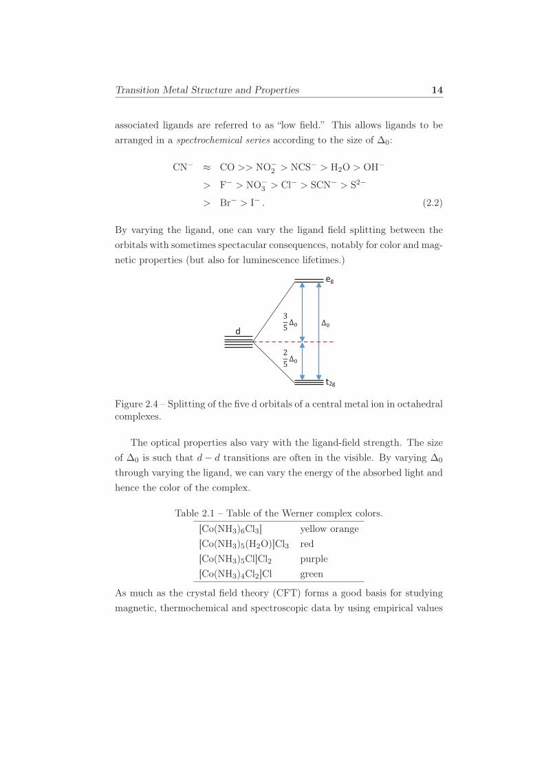
2.4 Splitting of the five d orbitals of a central metal ion in octa-
hedral complexes. . . . . . . . . . . . . . . . . . . . . . . . . . 14
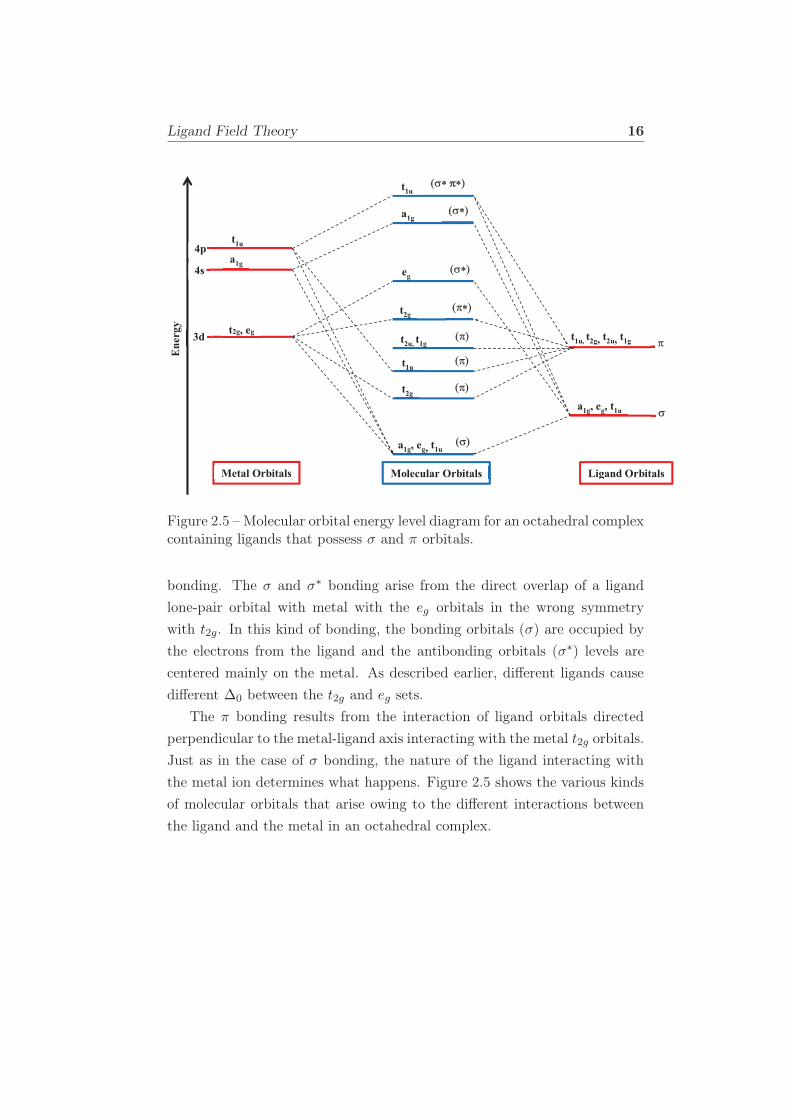
2.5 Molecular orbital energy level diagram for an octahedral com-
plex containing ligands that possess σ and π orbitals. . . . . . 16
2.6 Molecular orbital diagram representing various types of elec-
tronic transitions in octahedral complexes. . . . . . . . . . . . 18
3.1 xyz directions . . . . . . . . . . . . . . . . . . . . . . . . . . . 31
3.2 Molecular Hamiltonian. . . . . . . . . . . . . . . . . . . . . . 34
4.1 Potential energy diagrams with vertical transitions as in the
Franck-Condon principle. . . . . . . . . . . . . . . . . . . . . 41
4.2 Singlet ground state to excited allowed singlet state. . . . . . 41
4.3 Singlet ground state to excited forbidden triplet state. . . . . 42
4.4 Excited State Deactivation . . . . . . . . . . . . . . . . . . . . 44
4.5 Jablonski diagram. . . . . . . . . . . . . . . . . . . . . . . . . 46
4.6 Jablonski diagram showing the various processes. Original
source [14]. . . . . . . . . . . . . . . . . . . . . . . . . . . . . 47
xvi
5.1 SCF solution of the Hartree-Fock equation [14]. . . . . . . . . 61
6.1 Jacob’s ladder of Density Functional Approximations. Repro-
duced from (Ref. [25]) with permission of the PCCP Owner
Societies. . . . . . . . . . . . . . . . . . . . . . . . . . . . . . 83
7.1 Distortion of orbitals resulting from the inclusion of s and p
orbitals. . . . . . . . . . . . . . . . . . . . . . . . . . . . . . . 94
7.2 Distortion of orbitals resulting from the inclusion of p and d
orbitals. . . . . . . . . . . . . . . . . . . . . . . . . . . . . . . 94
9.1 Runge-Gross theorem: A pictorial illustration. . . . . . . . . . 113
9.2 An illustration of the LR theory . . . . . . . . . . . . . . . . . 118
10.1 ORTEP diagram showing the optimized structure of [Ru(trpy)2]2+
with different measured bond lengths and angles. The ellip-
soidal probability is at 70%. . . . . . . . . . . . . . . . . . . . 135
10.2 Comparison of experimental with calculated absorption spec-
tra at different levels of theory; CIS, TD-HF and TD-DFT
for [Ru(trpy)2]2+. Calculated spectra has been done with 100
singlet states and 6-31G basis set. Experimental spectra; mea-
sured at room temperature in acetonitrile [1]. . . . . . . . . . 136
10.3 Comparison of experimental with calculated absorption spec-
tra at different levels of theory; CIS, TD-HF and TD-DFT
for [Ru(trpy)2]2+. Calculated spectra has been done with 100
singlet states and 6-31G(d) basis set. Experimental spectra;
measured at room temperature in acetonitrile [1]. . . . . . . . 136
12.1 The diagram shows the principle potential energy curves in
our model. The abscissa corresponds to a reaction pathway
involving partial removal of a ligand while the ordinate rep-
resents the state energy. The dashed lines indicate diabatic
states whose avoided crossing leads to the energetic barrier on
the adiabatic surface between the 3MLCT and 3MC minima. 166
12.2 Pseudo-octahedral ligand field theory diagram for Ru com-
plexes. . . . . . . . . . . . . . . . . . . . . . . . . . . . . . . 169
12.3 Spin density distribution of 3MLCT state on [Ru(bpy)3]2+ in
acetonitrile. . . . . . . . . . . . . . . . . . . . . . . . . . . . 176
12.4 Spin density distribution of 3MLCT state on [Ru(mbpy)3]2+
in acetonitrile. . . . . . . . . . . . . . . . . . . . . . . . . . . 177
12.5 Spin density distribution of 3MLCT state on [Ru(mphen)3]2+
in acetonitrile. . . . . . . . . . . . . . . . . . . . . . . . . . . 177
12.6 Spin density distribution of 3MC state on [Ru(bpy)3]2+ in
acetonitrile. . . . . . . . . . . . . . . . . . . . . . . . . . . . 178
12.7 Spin density distribution of 3MC state on [Ru(mbpy)3]2+ in
acetonitrile. . . . . . . . . . . . . . . . . . . . . . . . . . . . 178
12.8 Spin density distribution of 3MC state on [Ru(mphen)3]2+ in
acetonitrile. . . . . . . . . . . . . . . . . . . . . . . . . . . . 179
12.9 3MLCT to 3MC state potential energy scan along the reac-
tion coordinate of the axial distortion of the 3MC state for
[Ru(bpy)3]2+. . . . . . . . . . . . . . . . . . . . . . . . . . . 179
List of Acronyms and
Abbreviations
H(t) TD Hamiltonian
ω Fourier-transformed frequency domain
Φ Quantum yield
AA Adiabatic Approximation
BSSE Basis Set Superposition Error
CFT Crystal Field Theory
DFT Density Functional Theory
DZ Double Zeta
Exc Exchange-Correlation Potentials
EA Electron Affinity
ECPs Effective Core Potentials
GGA Generalized Gradient Approximation
GTOs Gaussian-type Orbitals
HAOs Hydrogen-like Atomic Orbitals
HP Hartree Product
IC Internal Conversion
xix
IE Ionization Energy
IP Ionization Potential
ISC Intersystem Crossing
KS Kohn-Sham
LCAO Linear Combination of Atomic Orbitals
LDA Local Density Approximation
LFT Ligand Field Theory
LR Linear Response Theory
LR TD-DFT Linear Response TD-DFT
mGGA Meta-Generalized Gradient Approximation
MO Molecular Orbital
PES Potential Energy Surfaces
QZ Quadruple Zeta
RG Runge-Gross theorem
STOs Slater-type orbitals
SV Split Valence
TD-DFT Time-Dependent Schrödinger Equation
TD-KS Time-Dependent Kohn-Sham Equation
TZ Triple Zeta
vr Vibrational relaxation
χρρ Generalized Susceptibility

Part I
Introduction
1
Chapter 1
Introduction
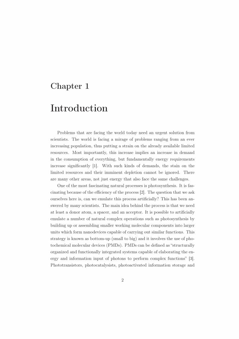
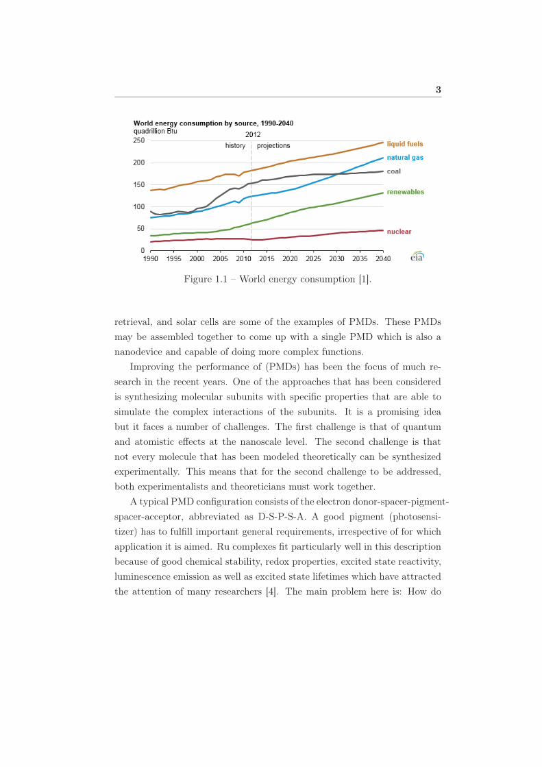
Problems that are facing the world today need an urgent solution from
scientists. The world is facing a mirage of problems ranging from an ever
increasing population, thus putting a strain on the already available limited
resources. Most importantly, this increase implies an increase in demand
in the consumption of everything, but fundamentally energy requirements
increase significantly [1]. With such kinds of demands, the stain on the
limited resources and their imminent depletion cannot be ignored. There
are many other areas, not just energy that also face the same challenges.
One of the most fascinating natural processes is photosynthesis. It is fas-
cinating because of the efficiency of the process [2]. The question that we ask
ourselves here is, can we emulate this process artificially? This has been an-
swered by many scientists. The main idea behind the process is that we need
at least a donor atom, a spacer, and an acceptor. It is possible to artificially
emulate a number of natural complex operations such as photosynthesis by
building up or assembling smaller working molecular components into larger
units which form nanodevices capable of carrying out similar functions. This
strategy is known as bottom-up (small to big) and it involves the use of pho-
tochemical molecular devices (PMDs). PMDs can be defined as “structurally
organized and functionally integrated systems capable of elaborating the en-
ergy and information input of photons to perform complex functions” [3].
Phototransistors, photocatalysists, photoactivated information storage and
2
3
Figure 1.1 – World energy consumption [1].
retrieval, and solar cells are some of the examples of PMDs. These PMDs
may be assembled together to come up with a single PMD which is also a
nanodevice and capable of doing more complex functions.
Improving the performance of (PMDs) has been the focus of much re-
search in the recent years. One of the approaches that has been considered
is synthesizing molecular subunits with specific properties that are able to
simulate the complex interactions of the subunits. It is a promising idea
but it faces a number of challenges. The first challenge is that of quantum
and atomistic effects at the nanoscale level. The second challenge is that
not every molecule that has been modeled theoretically can be synthesized
experimentally. This means that for the second challenge to be addressed,
both experimentalists and theoreticians must work together.
A typical PMD configuration consists of the electron donor-spacer-pigment-
spacer-acceptor, abbreviated as D-S-P-S-A. A good pigment (photosensi-
tizer) has to fulfill important general requirements, irrespective of for which
application it is aimed. Ru complexes fit particularly well in this description
because of good chemical stability, redox properties, excited state reactivity,
luminescence emission as well as excited state lifetimes which have attracted
the attention of many researchers [4]. The main problem here is: How do
Objectives 4
you tell which Ru complex will make a good pigment? Progress has been
made on the prediction of what would make a good pigment before the
lengthy project of working out its synthesis. To this end, [5] worked out
some promising simple molecular-orbital (MO) based luminescence indices
which may be helpful in estimating which compounds are likely to remain
excited long enough to luminescence or transfer an electron or which may
simply undergo unproductive radiationless deactivation back to the ground
state. The two molecular orbital-based luminescence indices, both of which
were based on the idea that luminescence quenching is the result of a low3MLCT → 3MC barrier. One luminescence index proposes the difference
between the e∗g and the lowest energy π∗ PDOS bands (∆E) as an indicator.
The second luminescence index is a product of the amount of π character
in the t2g band with the amount of ruthenium d character in the 1π∗ band
summarized as d× π. The indices are proposed as qualitative luminescence
predictors. Using the indices, which were tested on five compounds, they
found that low values of ∆E and high values of d×π correlated with lack of
luminescence while high values of ∆E and low values of d× π correlate well
with luminescence. We work further on this indices by looking at more Ru
complexes from [4].
The main objectives in this work are:
1.1 Objectives
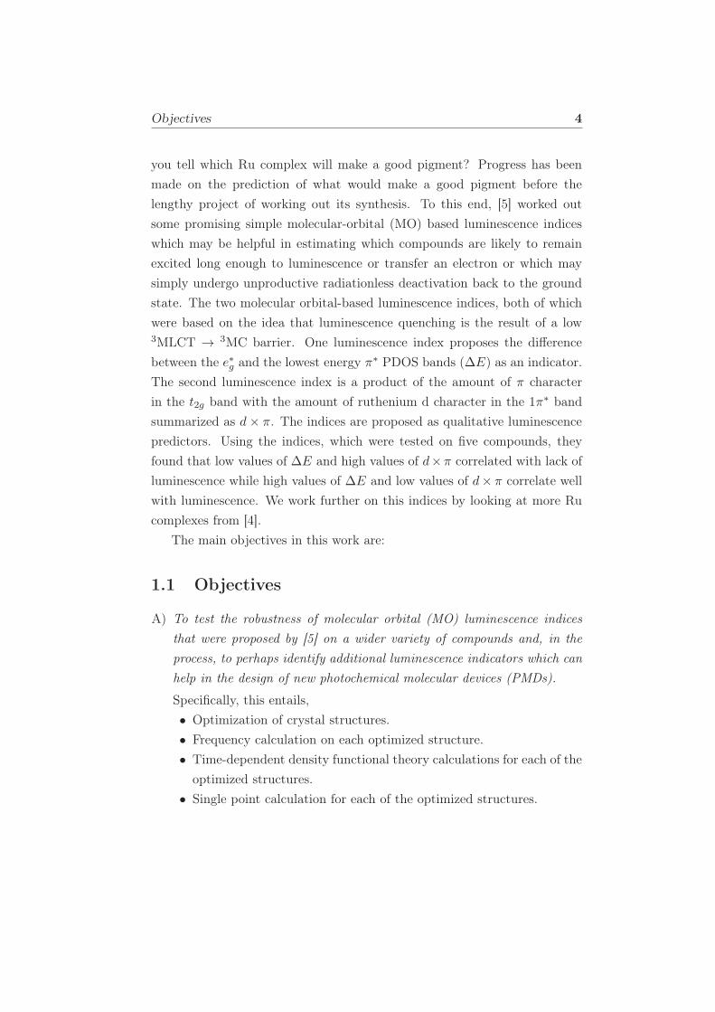
A) To test the robustness of molecular orbital (MO) luminescence indices
that were proposed by [5] on a wider variety of compounds and, in the
process, to perhaps identify additional luminescence indicators which can
help in the design of new photochemical molecular devices (PMDs).
Specifically, this entails,
• Optimization of crystal structures.
• Frequency calculation on each optimized structure.
• Time-dependent density functional theory calculations for each of the
optimized structures.
• Single point calculation for each of the optimized structures.
Structure and Organization 5
• Extraction of partial density of states information using various in-
house programs.
B) Study the Ru complex triplet excited transition state and find the size of
the energy barrier.
1.2 Structure and Organization
This thesis is divided into four major parts. The first part consists of
one chapter, the introduction, that outlines what kind of problem is being
tackled in the work as well as the objectives that are covered.
The second part is part two: background material consisting of eight
chapters. The number of chapters contained in this particular part outlines
the importance of understanding each and every process before the actual
work is done.
Chapter two looks at transition metal complexes. This is actually what
is being studied in this work. It outlines what they are and the various
processes that they undergo. It is critical since it is the bare minimum with
which one should familiarize oneself.
Chapter three introduces the Schrödinger equation. A good understand-
ing of this equation provides a solid base for understanding photophenomena
and luminescence.
Chapter four is the chapter on photophenomena and luminescence. The
idea behind this chapter is that it looks at what happens in the excited state.
This is important because we are dealing with excited state phenomena.
Chapters five to nine look at the wave function-based electronic structure
theory. This is the method that is actually used in the work. In the various
chapters, each of the methods, (all of which are important in this work) have
been discussed exhaustively.
The third part is the part on original work. It is chapter 10, 11 and 12.
This part is actually the core of this thesis. It is a detailed presentation of
results that were achieved and gives the publications that resulted out of the
work, both published and also work in progress.

Structure and Organization 6
The fourth part is a summary and conclusion. The chapter summarizes
what we have accomplished and what could possibly be done to further
improve the work. The other section consists of the appendices and gives
supplementary information for the published paper and my curriculum vitae.
BIBLIOGRAPHY 7
Bibliography
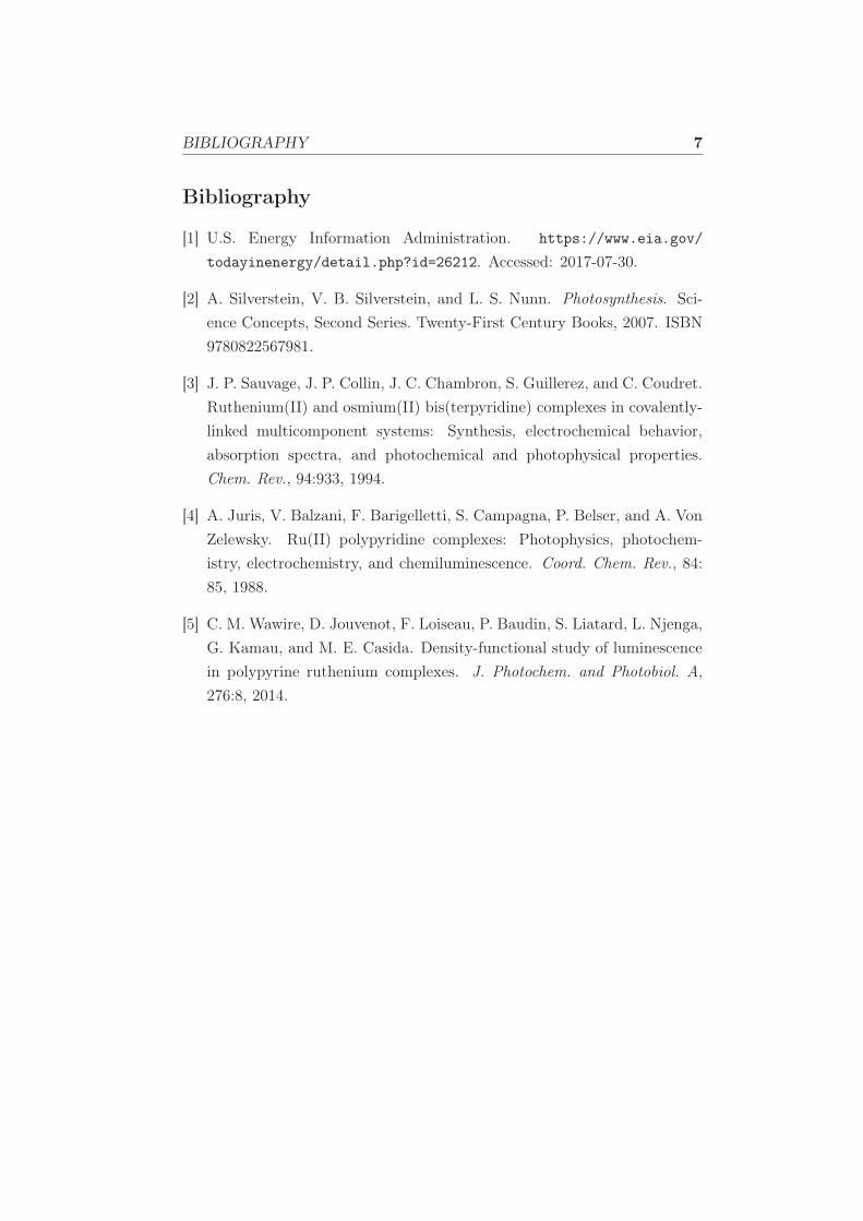
[1] U.S. Energy Information Administration. https://www.eia.gov/
todayinenergy/detail.php?id=26212. Accessed: 2017-07-30.
[2] A. Silverstein, V. B. Silverstein, and L. S. Nunn. Photosynthesis. Sci-
ence Concepts, Second Series. Twenty-First Century Books, 2007. ISBN
9780822567981.
[3] J. P. Sauvage, J. P. Collin, J. C. Chambron, S. Guillerez, and C. Coudret.
Ruthenium(II) and osmium(II) bis(terpyridine) complexes in covalently-
linked multicomponent systems: Synthesis, electrochemical behavior,
absorption spectra, and photochemical and photophysical properties.
Chem. Rev., 94:933, 1994.
[4] A. Juris, V. Balzani, F. Barigelletti, S. Campagna, P. Belser, and A. Von
Zelewsky. Ru(II) polypyridine complexes: Photophysics, photochem-
istry, electrochemistry, and chemiluminescence. Coord. Chem. Rev., 84:
85, 1988.
[5] C. M. Wawire, D. Jouvenot, F. Loiseau, P. Baudin, S. Liatard, L. Njenga,
G. Kamau, and M. E. Casida. Density-functional study of luminescence
in polypyrine ruthenium complexes. J. Photochem. and Photobiol. A,
276:8, 2014.

Part II
Background Material
8
Chapter 2
Transition Metal Complexes
‘The Nobel Prize in Chemistry 1913 was awarded to Alfred Werner “in
recognition of his work on the linkage of atoms in molecules by which he has
thrown new light on earlier investigations and opened up new fields of
research especially in inorganic chemistry”. ’
http: // www. nobelprize. org/ nobel_ prizes/ chemistry/ laureates/
1913/ 14thOct, 2017
2.1 Introduction
Transition metal compounds form the core of the research in this thesis.
They are also referred to as coordination compounds. In the field of pho-
tochemistry and photophysics, they form an important class of compounds
essentially because of their extensive photophysical and photochemical prop-
erties [1]. In a coordination complex MLn, there is typically a central atom
which is a d metal or the cation of a d metal, M. The central atom is sur-
rounded by anions (or cations in some cases such as nitroso (NO+), cationic
oniom ligands and hydrazinium (H2N-NH+3 ) and its derivatives [2–5]) or
molecules called ligands, L. A simple illustration of such a complex is shown
in Fig. 2.1.
A coordination compound may also be defined as any compound that
contains a coordination entity. A coordination entity is an ion or neutral
9
Definitions 10
Metal
L
L
L
L
L
L
Figure 2.1 – Coordination complex.
molecule that is composed of a central atom, usually that of a metal, to
which is attached a surrounding array of other atoms or groups of atoms,
each of which is called a ligand [6]. Transition metal complexes have high
symmetry, chemically significant oxidation states and often have an open-
shell d orbital configuration. Coordination of the metal ion or atom in a
non-spherically symmetric environment, that is, a ligand field, differentiates
the energies of the d-orbitals [7]. There are several common terms that will
be referred to in coordination chemistry, they have been reviewed in the next
section.
2.2 Definitions
2.2.1 Coordination number
The coordination number is the number of ligands (donor atoms) bonded
to the central atom [8]. Typical values of the coordination number are 2,
4 and 6. In the case of [Ru(bpy)3]2+, the coordination number is 6. In
this complex, each ligand “bites” the cation twice. This is why we speak of
monodentate complexes because there is a single pair of “fangs” (that is lone
pairs to form a coordinate bond). Certain have more than one lone pair that
Definitions 11
N N
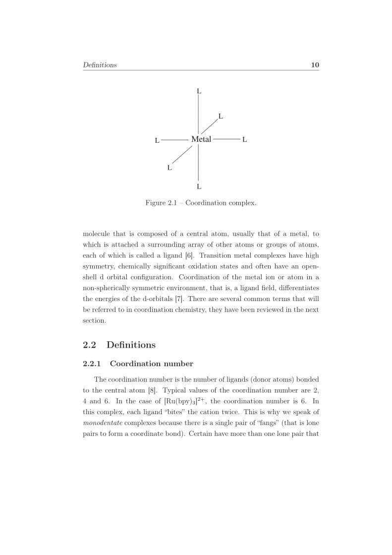
Figure 2.2 – The 2,2’-bipyridine molecule (bpy) showing the two nitrogenlone pairs which “bite” the central metal atom.
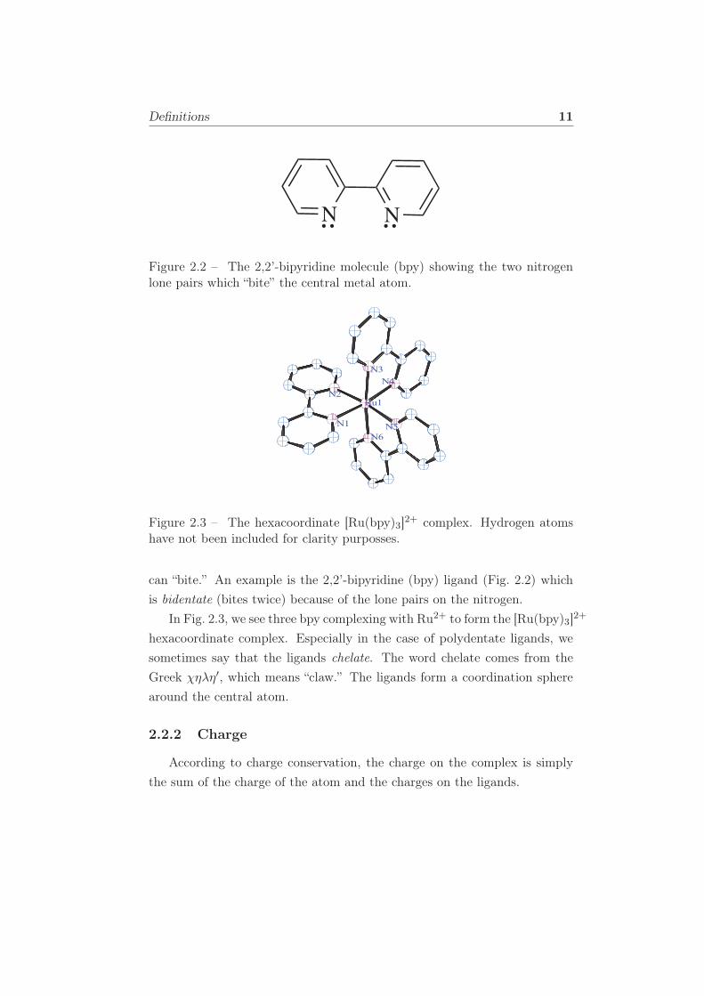
Figure 2.3 – The hexacoordinate [Ru(bpy)3]2+ complex. Hydrogen atomshave not been included for clarity purposses.
can “bite.” An example is the 2,2’-bipyridine (bpy) ligand (Fig. 2.2) which
is bidentate (bites twice) because of the lone pairs on the nitrogen.
In Fig. 2.3, we see three bpy complexing with Ru2+ to form the [Ru(bpy)3]2+
hexacoordinate complex. Especially in the case of polydentate ligands, we
sometimes say that the ligands chelate. The word chelate comes from the
Greek χηλη′, which means “claw.” The ligands form a coordination sphere
around the central atom.
2.2.2 Charge
According to charge conservation, the charge on the complex is simply
the sum of the charge of the atom and the charges on the ligands.
Transition Metal Structure and Properties 12
Example:
Ru2+ + 3 bpy → [Ru(bpy)3]2+ (2.1)
2.2.3 Nomenclature
How do we name complexes? The naming of complexes follows the rules
described in the IUPAC red book (https://www.iupac.org/cms/wp-content/
uploads/2016/07/Red\_Book\_2005.pdf) under chapter IR-9 Coordination
Compounds [6]. The reader is referred to this book if they wish to seek fur-
ther details regarding the naming of coordination complexes.
2.3 Transition Metal Structure and Properties
Alfred Werner won the Nobel prize in chemistry in 1913. He had studied
[Co(NH3)n(H2O)lClm]Cl3−m complexes with n + l +m = 6. Some of these
complexes have the same empirical formula but different colors! Werner
came up with the modern explanation of transition metal complexes while
trying to figure out why this was so [9].
2.3.1 Geometries
Geometries of transition metal complexes can generally be classified into:
(1) Octahedral (n = 6) where the central metal ion is surrounded by six lig-
ands. It contains equatorial and axial positions. The equatorial position
is the horizontal square planar arrangement in the xy-plane containing four
ligands and the axial positions are the vertical positions along the z-axis. (2)
Square planar (n = 4) where four ligands are attached to a central metal
ion. It is considered to be an extremely z-out distorted octahedral complex
because the ligands will be on the x- and y-axes. (3) Tetrahedral (n = 4)
where four ligands are attached to a central metal ion. Its difference with
the square planar geometry is that the four ligands approach the central
metal ion in between the axes [10]. The three dimensionality of these struc-
tures means that there can be confirmational (cis/trans) isomers and optical
Transition Metal Structure and Properties 13
isomers (enantiomers).
2.3.2 Crystal Field Theory
In this theory, the ligands are treated as negative point charges which set
up an electrostatic field that repels electrons in the d orbitals of the central
metal ion [11]. The interaction of the electrostatic field of the ligands with
the d electrons results in splitting of the d orbitals into groups with different
energies. In a gaseous transition-metal ion, the five d orbitals with different
values of the magnetic quantum number (m) are degenerate (have the same
energy). Symmetry plays a critical role in how the d orbitals split. In a
complex with spherically symmetric ligand field, the five d orbitals end up in
higher energy than the free ion because of the repulsion between the metal
ion electron density and the spherical field of negative charge. This is an ideal
case which never happens in reality. Practically, d orbitals are split according
to the particular symmetry of the complex. Of particular interest is the
octahedral symmetry where the central metal ion is surrounded by six ligands
since the transition metals that are studied in this work have this symmetry.
It should however be noted that, although most of the complexes studied
have only pseudo-octahedral symmetry, octahedral symmetry is assumed as
a first approximation in assigning orbitals.
2.3.2.1 Octahedral complexes
They are octahedral and highly symmetric. In the presence of an octahe-
dral crystal field, the five d-orbitals interact differently with the surrounding
ligands resulting in their splitting into a lower-energy triply degenerate set
(t2g composed of dxy, dxz and dyz) and a higher-energy doubly degenerate
set (eg composed of dz2 and dx2−y2) separated by an energy, ∆0, known as
ligand field splitting parameter [12]. The size of the ligand-field splitting ∆0
of the d orbitals which results in the eg and t2g orbitals depends upon how
strongly the ligands interact with the central atom. Those which interact
more strongly with the central atom will result in a larger ∆0 and are said
to be “high field,” while small ∆0 means only a small interaction and the
Transition Metal Structure and Properties 14
associated ligands are referred to as “low field.” This allows ligands to be
arranged in a spectrochemical series according to the size of ∆0:
CN− ≈ CO >> NO−2 > NCS− > H2O > OH−
> F− > NO−3 > Cl− > SCN− > S2−
> Br− > I− . (2.2)
By varying the ligand, one can vary the ligand field splitting between the
orbitals with sometimes spectacular consequences, notably for color and mag-
netic properties (but also for luminescence lifetimes.)
t2g
eg
3
5
2
5
d
Figure 2.4 – Splitting of the five d orbitals of a central metal ion in octahedralcomplexes.
The optical properties also vary with the ligand-field strength. The size
of ∆0 is such that d − d transitions are often in the visible. By varying ∆0
through varying the ligand, we can vary the energy of the absorbed light and
hence the color of the complex.
Table 2.1 – Table of the Werner complex colors.
[Co(NH3)6Cl3] yellow orange
[Co(NH3)5(H2O)]Cl3 red
[Co(NH3)5Cl]Cl2 purple
[Co(NH3)4Cl2]Cl green
As much as the crystal field theory (CFT) forms a good basis for studying
magnetic, thermochemical and spectroscopic data by using empirical values
Ligand Field Theory 15
of ∆0, it faces a number of limitations. It does not take into account the
overlap of ligand and metal atom orbitals because it treats ligands as point
charges. As a consequence of this, it cannot account for the ligand spectro-
chemical series. The ligand field theory takes a broader look and addresses
the weaknesses in the CFT. In the next section, we take a look at the ligand
field theory.
2.4 Ligand Field Theory
Data from several experiments has shown that the metal-ligand bond in
transition metal complexes is composed of some degree of covalency [12].
Ligand field theory (LFT)[13] is the theory that best accounts for the effects
of covalent bonding as well as considering all the conceptual aspects of the
simple crystal field theory (CFT). Ideally, LFT works in a similar manner as
does CFT for the calculation of the energy level diagrams but it also considers
spin-orbit coupling and inter-electronic repulsion when a free metal ion is
converted to a complexed one. LFT is an application of molecular orbital
theory that concentrates on the d orbitals of the central metal atom, thus
providing a more substantial framework for understanding the origins of ∆0.
Any chemist interested in the spectroscopy of metal complexes is obliged to
use LFT.
2.4.1 Molecular Orbitals
The bonding and antibonding molecular orbitals for metal complexes
are obtained by combining metal and ligand orbitals which have the same
symmetry properties. Generally speaking, the formulation of a MO is [12],
ψ = amϕm + alϕl, (2.3)
where ϕm and ϕl are metal and ligand orbital combinations and am and
al are coefficients whose values are restricted by conditions of normalization
and orthogonality.
Two types of bonding arise out of that combination, namely σ and π
Ligand Field Theory 16
t2g, eg
a1g
t1u
3d
4s
4p
t1u
a1g
eg
t2g
t2u,
t1g
t1u
t2g
a1g
, eg, t1u
t1u,
t2g, t2u, t1g
a1g
, eg, t
1u
s
p
(p)
(p)
(p)
(p*)
(s* p*)
(s*)
(s*)
(s)
Metal Orbitals Molecular Orbitals Ligand Orbitals
En
erg
y
Figure 2.5 – Molecular orbital energy level diagram for an octahedral complexcontaining ligands that possess σ and π orbitals.
bonding. The σ and σ∗ bonding arise from the direct overlap of a ligand
lone-pair orbital with metal with the eg orbitals in the wrong symmetry
with t2g. In this kind of bonding, the bonding orbitals (σ) are occupied by
the electrons from the ligand and the antibonding orbitals (σ∗) levels are
centered mainly on the metal. As described earlier, different ligands cause
different ∆0 between the t2g and eg sets.
The π bonding results from the interaction of ligand orbitals directed
perpendicular to the metal-ligand axis interacting with the metal t2g orbitals.
Just as in the case of σ bonding, the nature of the ligand interacting with
the metal ion determines what happens. Figure 2.5 shows the various kinds
of molecular orbitals that arise owing to the different interactions between
the ligand and the metal in an octahedral complex.
Ligand Field Theory 17
2.4.2 Molecular Orbital Formation
Several considerations must be made before the construction of the molec-
ular orbitals of a complex, these include: shape determination and their rel-
ative energies. Symmetry plays an essential role in the construction of the
MOs since it will give information of whether the overlap is non-zero or zero
and hence the ability to predict whether an interaction can occur or not. To
construct the molecular orbital, we consider orbitals from the metal ion as
well as orbitals from the ligand [8].
i. Metal Orbitals
In the metal ion, nine valence shell orbitals are considered. The nine
valence shell orbitals come from the 3d (5 atomic orbitals), 4s (1 atomic
orbital) and 4p (3 atomic orbitals) orbitals. Owing to the fact that
octahedral complexes are the most important to us, their symmetry in
the Oh point group they may be classified according to symmetry as:
3dz2, 3dx2 − y2; eg (2.4)
3dxy, 3dxz, 3dyz t2g (2.5)
4s a1g (2.6)
4px t1u . (2.7)
ii. Ligand Orbitals
Each of the ligand σ orbitals make up a total of six symmetry orbitals.
By choosing the linear combinations of ligand σ orbitals that have the
same symmetry properties as the various metal σ orbitals, MO construc-
tion is done in such a way that each of them overlaps with a particular
one of the six metal ion orbitals that are suitable for σ bonding.
Photophysical Processes for Transition Metal Complexes 18
2.5 Photophysical Processes for Transition Metal
Complexes
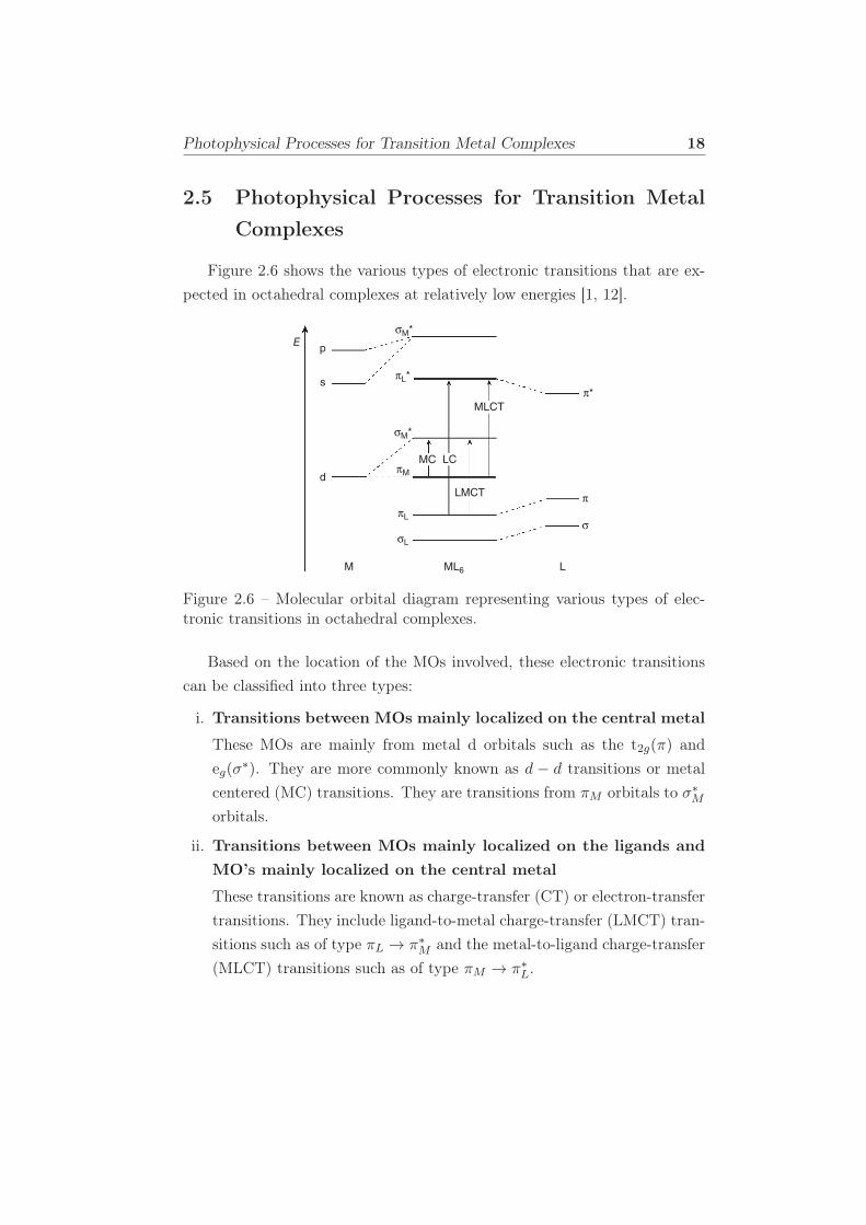
Figure 2.6 shows the various types of electronic transitions that are ex-
pected in octahedral complexes at relatively low energies [1, 12].
Ep
s
d
σM*
πL*
π*
σM*
πM
πL
σL
σ
π
MC LC
LMCT
MLCT
M ML6 L
Figure 2.6 – Molecular orbital diagram representing various types of elec-tronic transitions in octahedral complexes.
Based on the location of the MOs involved, these electronic transitions
can be classified into three types:
i. Transitions between MOs mainly localized on the central metal
These MOs are mainly from metal d orbitals such as the t2g(π) and
eg(σ∗). They are more commonly known as d − d transitions or metal
centered (MC) transitions. They are transitions from πM orbitals to σ∗Morbitals.
ii. Transitions between MOs mainly localized on the ligands and
MO’s mainly localized on the central metal
These transitions are known as charge-transfer (CT) or electron-transfer
transitions. They include ligand-to-metal charge-transfer (LMCT) tran-
sitions such as of type πL → π∗M and the metal-to-ligand charge-transfer
(MLCT) transitions such as of type πM → π∗L.

Photophysical Processes for Transition Metal Complexes 19
iii. Transitions between MOs mainly localized on the ligands
They only involve ligand orbitals which are almost unaffected by coor-
dination to the metal. These include ligand centered (LC) transitions of
type πL → π∗L.
BIBLIOGRAPHY 20
Bibliography
[1] P. S. Wagenknecht and P. C. Ford. Metal centered ligand field excited
states: their roles in the design and performance of transition metal
based photochemical molecular devices. Coord. Chem. Rev., 255(5):
591–616, 2011.
[2] V. L. Goedken, L. M. Vallarino, and J. V. Quagliano. Cationic ligands.
coordination of the 1, 1, 1-trimethylhydrazinium cation to nickel (II).
Inorg. Chem., 10(12):2682–2685, 1971.
[3] S. Govindarajan, K. C. Patil, H. Manohar, and P. Werner. Hydrazinium
as a ligand: structural, thermal, spectroscopic, and magnetic studies of
hydrazinium lanthanide di-sulphate monohydrates; crystal structure of
the neodymium compound. Dalton Trans., (1):119–123, 1986.
[4] O. S. Bushuyev, F. A. Arguelles, P. Brown, B. L. Weeks, and L. J.
Hope-Weeks. New energetic complexes of copper (II) and the acetone
carbohydrazide schiff base as potential flame colorants for pyrotechnic
mixtures. Eur. J. Inorg. Chem., 2011(29):4622–4625, 2011.
[5] A. D. McNaught and A. Wilkinson. IUPAC. Compendium of Chemical
Terminology, the “Gold Book”, volume II. Blackwell Scientific Publica-
tions, Oxford, 1997.
[6] N. G. Connelly, Royal Society of Chemistry (Great Britain), Interna-
tional Union of Pure, and Applied Chemistry. Nomenclature of In-
organic Chemistry: IUPAC recommendations 2005. Royal Society of
Chemistry Publishing/IUPAC, 2005. ISBN 9780854044382.
[7] P. C. Ford. The ligand field photosubstitution reactions of d6 hexaco-
ordinate metal complexes. Coord. Chem. Rev., 44(1):61–82, 1982.
[8] M. Gerloch and E. C. Constable. Transition Metal Chemistry: The
Valence Shell in d-Block Chemistry. Wiley, 1994. ISBN 9783527292189.
[9] F. A. Cotton and G. Wilkinson. Advanced inorganic chemistry: a com-
prehensive text. Interscience Publishers, 1972. ISBN 9780471175605.
BIBLIOGRAPHY 21
[10] K. Sridharan. Spectral Methods in Transition Metal Complexes. Elsevier
Science, 2016. ISBN 9780128096543.
[11] P. Atkins. Shriver and Atkins’ Inorganic Chemistry. Oxford University
Press, Oxford, United Kingdom, 2010. ISBN 9780199236176.
[12] M. Montalti, A. Credi, L. Prodi, and M. T. Gandolfi. Handbook of
Photochemistry. CRC Press, third edition, 2006. ISBN 9781420015195.
[13] Figgis B. N. and M. A. Hitchman. Ligand field theory and its applica-
tions. Special topics in inorganic chemistry. Wiley-VCH, 2000. ISBN
9780471317760.
Chapter 3
Schrödinger Equation
It is by logic that we prove, but by intuition that we discover.
J. H. Poincaré, ca. 1900.
Introduction
In this chapter, an introductory review of elementary quantum mechan-
ics is given. Advanced concepts of the density functional theory are built
starting from the fundamental aspects of electronic structure theory using
mathematical manipulation techniques to solve the fundamental equations.
All these concepts lead to the build up of the Schrödinger equation, which
is the ‘backbone’ of electronic structure and methods. Starting from the
ultraviolet calamity and the photoelectric effect (ideas that spurred the im-
provement of quantum mechanics) a step by step approach is shown of how
the Schrödinger equation builds up. Also discussed in this chapter is the
Born-Oppenheimer approximation, which separates the motion of an elec-
tron from that of the nucleus. They are reviewed herein. This chapter has
been written based on the following references [1–9]; among others cited in
text.
22
Ultraviolet Catastrophe 23
3.1 Ultraviolet Catastrophe
This is also referred to as black-body radiation. A black-body is an ideal-
ized object which absorbs and emits all incident radiation without favouring
particular frequencies [9]. The Rayleigh-Jeans law is an equation that de-
scribes the intensity of black-body radiation as a function of frequency for
a fixed temperature. The law works for low frequencies but fails for high
frequencies. This phenomenon is referred to as the ultraviolet catastrophe.
Max Planck explained the black-body radiation by introducing the concept
of quantization of energy using the Planck’s constant (h) in his equation:
E = nh, (3.1)
where h is the Planck’s constant (6.626 × 10⁻²⁷ J.s). Planck could not
give a justification for his assumption of energy quantization. The idea was
taken up further by Einstein who adopted Planck’s assumption to explain
the photoelectric effect.
3.2 Photoelectric Effect
Photoelectric effect is the ejection of electrons from a metal surface by
light. The classical wave theory of light suggested that the intensity of the
light determined the amplitude of the wave. Experiments however showed
that the kinetic energy of the ejected electrons depends on the colour (which
is a function of frequency) of the light. Einstein explained the observation
by assuming that the light consisted of packets of energy (photons), with
each photon having an energy [8, 10],
Ephoton = hν, (3.2)
where h is Plancks constant and ν is the frequency of the light.
Einstein went ahead to explain that for an electron to be ejected, the
forces holding the electron in the metal must first be overcome [what is com-
monly referred to as the work function (Φ)] and then the extra energy that
Quantization of Electronic Angular Momentum 24
remains is the one which removes the electron from the metal. Conservation
of energy results in the equation for the photoelectric effect written as,
hν = Ephoton = Φ+KEmax, (3.3)
where Φ is the minimum energy needed by an electron to escape the metal
(metal’s work function), and KEmax is the maximum kinetic energy of an
emitted electron. The equation in essence tells us two things; first, increasing
the light’s frequency will increase the photon energy and therefore the kinetic
energy of the emitted electron. Secondly, increasing light intensity at fixed
frequency will increase the rate of emission of electrons, but has no effect on
the kinetic energy of the emitted electron. Consequently, reaping from the
fruits of his hard work, Einstein was awarded the Nobel prize [11] in physics
in 1921 for his work. The photoelectric effect shows that light can exhibit
both particle-and wavelike behaviour from diffraction experiments.
3.3 Quantization of Electronic Angular Momentum
The discussion about quantization of electronic angular momentum takes
us back to the structure of matter. Various experiments in the 19th century
such as the electric discharge tube and radioactivity led to the discovery of
charged particles, electrons and protons. The important fact to any chemist
is that chemical properties of atoms and molecules are determined by their
electronic structure. This raises the question about the nature of the motions
and energies of the electrons. To this extent, several atomic models were
proposed to explain the above question. The specific models will not be
dealt with in detail but the problem that is at hand is that classical physics
could not explain what held the electron in position as it moved around the
nucleus since it was expected to lose energy by radiation and therefore would
spiral toward the nucleus.
Neil Bohr brought in the concept of quantization of energy for the hy-
drogen atom to solve the problem. According to Bohr, electrons orbit about
the nucleus of an atom in stable allowed electronic orbits with a quantized
Wave-Particle Duality 25
electronic angular momentum [12] of,
l = mvr = nh, with h =h
2π. (3.4)
A quantized angular momentum implies that the energy will in-turn be
quantized. Bohr used the principle of quantization to explain the line spec-
trum of the hydrogen atom. A photon of light of frequency ν is absorbed or
emitted with the transition of an electron from one allowed energy level to
another.
Eupper − Elower = hν. (3.5)
Bohr’s expression for the allowed energy levels worked perfectly for the
hydrogen atom spectrum but failed in atoms with more than one electron.
It did not account for chemical bonding in molecules also. This failure could
be attributed to the use of classical mechanics for the description of the elec-
tronic motions in atoms. The main difference is that, in quantum mechanics,
only certain energies of motion are allowed (i.e., energy is quantized) while in
classical mechanics, a continuous range of energies is allowed. This prompted
Louis de Broglie to introduce the wave aspect for electrons.
3.4 Wave-Particle Duality
The failure of Bohr to describe the electronic motion in atoms prompted
de Broglie to suggest that the motion of electrons has a wave aspect. The
wavelength (λ) of an electron of mass m and speed v is,
λ =h
mv=h
p, (3.6)
where ~p = m~v is the particle momentum (whose magnitude is p) and m
refers to the relativistic mass. The wave-particle duality of light was proven
by the fact that light behaves as a wave since it can be diffracted, and as a
particle because it contains packets of energy [8].
For an electron behaving as a wave, the wave completing the integral
Time-Independent Schrödinger Equation 26
number of wavelength for a stable electron orbit is,
2πr = nλ. (3.7)
This can be rewritten as below with the inclusion of the de Broglie relation,
mvr = nh. (3.8)
The wave-particle duality leads to the Heisenberg’s uncertainty principle.
The question is, how can an electron be both a particle (localized) and a
wave (non localized)? The Heisenberg’s uncertainty principle states that the
position and momentum of a particle cannot be known simultaneously at the
same time.
∆x∆p ≥ h
2. (3.9)
If the orbital radius of an electron in an atom is known exactly (position),
then the angular momentum must be completely unknown. This principle set
in a new quantum theory that was consistent with the uncertainity principle
since the Bohr model specifies the exact radius and that the orbital angular
momentum must be an integer hence a weakness. In general, the more
precisely the position is measured, the less accurate is the determination
of momentum because the act of measurement introduces an uncontrollable
disturbance in the system being measured. Schrödinger replaced this idea
with the probability of finding an electron in a particular position or volume
of space.
3.5 Time-Independent Schrödinger Equation
The Schrödinger equation is classified under what is called ‘modern quan-
tum mechanics’ [10] based on the Copenhagen interpretation. In his equa-
tion, Schrödinger replaced the wave in classical mechanics with a wave func-
tion ψ(r) = ψ(x, y, z). There exist two forms of the Schrödinger equation,
the time-dependent and the time-independent Schrödinger equation, distin-
Time-Independent Schrödinger Equation 27
guished by whether the wave is stationary or travelling. In the next section
of the discussion, a heuristic justification of the Schrödinger equation is given
starting from the basic idea of the wave equation.
The time-independent Schrödinger equation is mostly used because we
are interested in atoms and molecules without the time-dependent interac-
tions. Starting from the basic idea of the classical one-dimensional wave
equation,
∂2u
∂x2=
1
v2∂2u
∂t2. (3.10)
We can solve this wave equation by the separating the variables, by
writing u(x, t) as the product of a function of x and a harmonic function of
time:
u(x, t) = ψ(x) cos(ωt), (3.11)
where ψ(x) is the spatial amplitude of the wave. Replacing Eq.(3.11) in Eq.
(3.10) gives the equation for the spartial amplitude,
d2ψ
dx2+ω2
v2ψ(x) = 0, (3.12)
but ω = 2πv and νλ = v leading to,
d2ψ
dx2+
4π2
λ2ψ(x) = 0. (3.13)
This is an ordinary differential equation describing the spatial amplitude
of the matter wave as a function of position. From Eq. (3.13), the idea of
de Broglie matter waves can be introduced. The total energy of a particle is
the sum of its kinetic energy and its potential energy, given by the equation
below,
E =p2(x)
2m+ V (x). (3.14)
Solving for momentum, p, yields,
p(x) =√
2m[E − V (x)]. (3.15)
Time-Independent Schrödinger Equation 28
Using the de Broglie formula, an expression for the wavelength can be found
as,
λ =h
p=
h√
2m[E − V (x)]. (3.16)
Substituting λ into Eq.(3.13),
d2ψ
dx2+
2m
h2[E − V (x)]ψ(x) = 0, (3.17)
which can be rewritten as,
− h2
2m
d2ψ(x)
dx2+ V (x)ψ(x) = Eψ(x). (3.18)
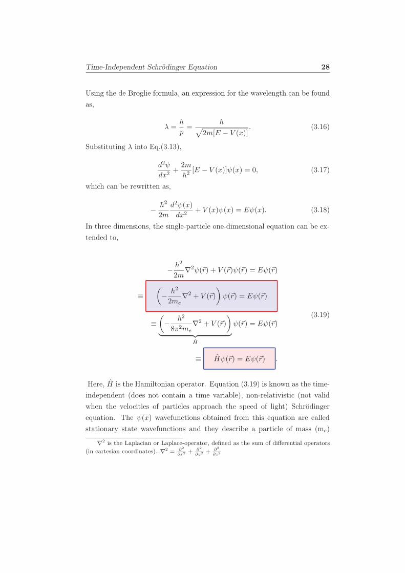
In three dimensions, the single-particle one-dimensional equation can be ex-
tended to,
− h2
2m∇2ψ(~r) + V (~r)ψ(~r) = Eψ(~r)
≡(
− h2
2me∇2 + V (~r)
)
ψ(~r) = Eψ(~r)
≡(
− h2
8π2me∇2 + V (~r)
)
︸ ︷︷ ︸
H
ψ(~r) = Eψ(~r)
≡ Hψ(~r) = Eψ(~r) .
(3.19)
Here, H is the Hamiltonian operator. Equation (3.19) is known as the time-
independent (does not contain a time variable), non-relativistic (not valid
when the velocities of particles approach the speed of light) Schrödinger
equation. The ψ(x) wavefunctions obtained from this equation are called
stationary state wavefunctions and they describe a particle of mass (me)
∇2 is the Laplacian or Laplace-operator, defined as the sum of differential operators
(in cartesian coordinates). ∇2=
∂2
∂x2 +∂2
∂y2 +∂2
∂z2
Time-Dependent Schrödinger Equation 29
moving in a potential field V (x). From this equation, the energy and any
other related properties of a molecule may be obtained by solving it. Solu-
tions to Eq. (3.19) correspond to different stationary states of a particle and
the one with the lowest energy is called the ground state.
3.6 Time-Dependent Schrödinger Equation
Although most of the problems of chemical interest can be described
by the time-independent non-relativistic Schrödinger equation, the time-
dependent Schrödinger equation is described herein for the purposes of dis-
tinction between the two of them. The time-dependent Schrödinger equa-
tion is given as a postulate of quantum mechanics, unlike the Schrödinger
equation that can be derived starting from the classical wave equation.
The “derivation” is only heuristic but not rigorous. The time-independent
Schrödinger equation can be rigorously derived from the time-independent
Schrödinger equation. From Eq. (3.13) the idea of de Broglie matter waves
with the space and time variable [φ(x, t)] is introduced. The only differ-
ence between this equation and the time-independent Schrödinger equation
is that the time variable has been introduced. The total energy of a particle
is the sum of its kinetic energy and its potential energy, given by,
E =p2(x)
2m+ V (x, t). (3.20)
The other steps have been omitted as they are similar to those for the time-
independent equation,
∂2ψ(x, t)
∂x2+
2m
h2[ih
∂
∂t− V (x, t)]ψ(x, t) = 0, (3.21)
Which can be rewritten as;
[−h22m
∂2
∂x2+ V (x, t)
]
Ψ(x, t) = ih∂
∂tΨ(x, t). (3.22)
This is the time-dependent Schrödinger equation.
Molecular Hamiltonian 30
3.7 Molecular Hamiltonian
Hψ(~r) = Eψ(~r) , (3.23)
H is the Hamiltonian operator. This operator is constructed from the energy
expression in classical mechanics. In classical mechanics, the classical energy
is calculated as:
E = kinetic energy + potential energy
=1
2mev
2 − Ze2
4πǫ0r
=p2
2me− Ze2
4πǫ0r
. (3.24)
Replacing each cartesian and momentum coordinate by the corresponding
operator in Table 3.1,
Table 3.1 – Classical to quantum transformation of cartesian position andmomentum operators.
Position Momentumx → x px → pxy → y py → pyz → z pz → pz
Results in:H =
1
2me
(p2x + p2y + p2z
)
= − h2
2me
(δ2
δx2+
δ2
δy2+
δ2
δz2
)
− Ze2
4πǫ0r
=h2
2me∇2 − Ze2
4πǫ0r
. (3.25)
In other words, H is composed of the kinetic and potential energy operator,
H = T + V . (3.26)
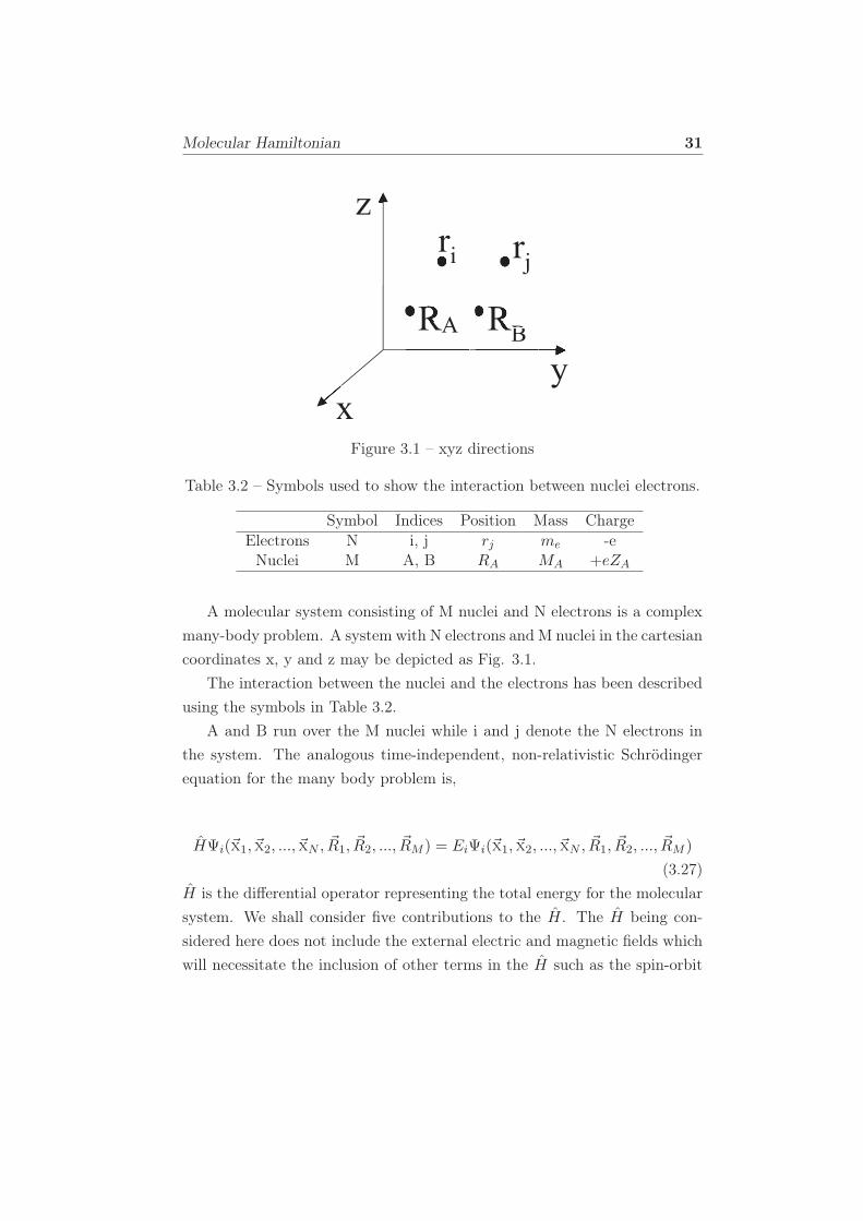
Molecular Hamiltonian 31
RA RBA
ri
B
rj
z
yx
Figure 3.1 – xyz directions
Table 3.2 – Symbols used to show the interaction between nuclei electrons.
Symbol Indices Position Mass ChargeElectrons N i, j rj me -eNuclei M A, B RA MA +eZA
A molecular system consisting of M nuclei and N electrons is a complex
many-body problem. A system with N electrons and M nuclei in the cartesian
coordinates x, y and z may be depicted as Fig. 3.1.
The interaction between the nuclei and the electrons has been described
using the symbols in Table 3.2.
A and B run over the M nuclei while i and j denote the N electrons in
the system. The analogous time-independent, non-relativistic Schrödinger
equation for the many body problem is,
HΨi(~x1, ~x2, ..., ~xN , ~R1, ~R2, ..., ~RM ) = EiΨi(~x1, ~x2, ..., ~xN , ~R1, ~R2, ..., ~RM )
(3.27)
H is the differential operator representing the total energy for the molecular
system. We shall consider five contributions to the H. The H being con-
sidered here does not include the external electric and magnetic fields which
will necessitate the inclusion of other terms in the H such as the spin-orbit
Atomic Units 32
coupling. The H is given as,
H = Te + TN + Vee + VNN + VeN , (3.28)
where,
Te = −N∑
i
h2
2me∇2i
TN = −M∑
A
h2
2MA∇2A
Vee =
N∑
i<j
e2
4πǫ0|ri − rj |
VNN =M∑
A<B
e2ZAZB4πǫ0|RA −RB|
VeN =N∑
i
M∑
A
e2ZA4πǫ0|ri −RA|
.
(3.29)
In SI units.
3.8 Atomic Units
The system of atomic units was developed to simplify mathematical equa-
tions by setting many fundamental constants equal to 1. Equations are ex-
pressed in a very compact form, without any fundamental physical constants.
Consequently, atomic units remove units from equations. Physical quantities
such as the mass of an electron, me, the modulus of its charge, |e|, Planck’s
constant h divided by 2π, the 2π times the permittivity of the vacuum, are
all set to unity. A new set of units called the atomic units is defined; the
atomic unit of energy is called a hartree and is denoted by Eh. The atomic
units that have been adopted are shown in Table 3.3.
With the expression of the physical constants as unity, H simplifies to,
Atomic Units 33
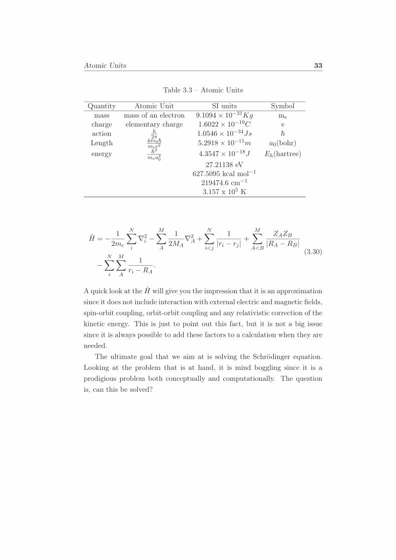
Table 3.3 – Atomic Units
Quantity Atomic Unit SI units Symbolmass mass of an electron 9.1094× 10⁻³¹Kg me
charge elementary charge 1.6022× 10⁻¹⁹C eaction h
2π 1.0546× 10⁻³⁴Js h
Length 4πǫ0hmee2
5.2918× 10⁻¹¹m a0(bohr)
energy h2
mea204.3547× 10−18J Eh(hartree)
27.21138 eV627.5095 kcal mol−1
219474.6 cm−1
3.157 x 10⁵ K
H = − 1
2me
N∑
i
∇2i −
M∑
A
1
2MA∇2A +
N∑
i<j
1
|ri − rj |+
M∑
A<B
ZAZB|RA −RB|
−N∑
i
M∑
A
1
ri −RA.
(3.30)
A quick look at the H will give you the impression that it is an approximation
since it does not include interaction with external electric and magnetic fields,
spin-orbit coupling, orbit-orbit coupling and any relativistic correction of the
kinetic energy. This is just to point out this fact, but it is not a big issue
since it is always possible to add these factors to a calculation when they are
needed.
The ultimate goal that we aim at is solving the Schrödinger equation.
Looking at the problem that is at hand, it is mind boggling since it is a
prodigious problem both conceptually and computationally. The question
is, can this be solved?
Born-Oppenheimer Approximation 34
Molecular Hamiltonian
Born Oppenheimer
Approximation
Electronic
Hamiltonian
Nuclear
Hamiltonian
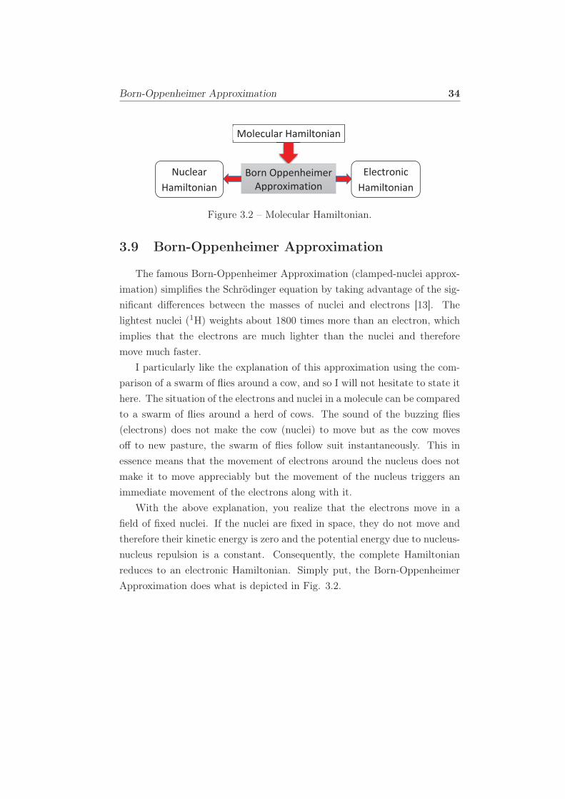
Figure 3.2 – Molecular Hamiltonian.
3.9 Born-Oppenheimer Approximation
The famous Born-Oppenheimer Approximation (clamped-nuclei approx-
imation) simplifies the Schrödinger equation by taking advantage of the sig-
nificant differences between the masses of nuclei and electrons [13]. The
lightest nuclei (1H) weights about 1800 times more than an electron, which
implies that the electrons are much lighter than the nuclei and therefore
move much faster.
I particularly like the explanation of this approximation using the com-
parison of a swarm of flies around a cow, and so I will not hesitate to state it
here. The situation of the electrons and nuclei in a molecule can be compared
to a swarm of flies around a herd of cows. The sound of the buzzing flies
(electrons) does not make the cow (nuclei) to move but as the cow moves
off to new pasture, the swarm of flies follow suit instantaneously. This in
essence means that the movement of electrons around the nucleus does not
make it to move appreciably but the movement of the nucleus triggers an
immediate movement of the electrons along with it.
With the above explanation, you realize that the electrons move in a
field of fixed nuclei. If the nuclei are fixed in space, they do not move and
therefore their kinetic energy is zero and the potential energy due to nucleus-
nucleus repulsion is a constant. Consequently, the complete Hamiltonian
reduces to an electronic Hamiltonian. Simply put, the Born-Oppenheimer
Approximation does what is depicted in Fig. 3.2.
Born-Oppenheimer Approximation 35
Helec(r;R) = −1
2
N∑
i=1
∇2i −
N∑
i=1
M∑
A=1
ZAriA
+
N∑
i=1
M∑
i<j
1
rij
= T (r) + VNe(r;R) + Vee(r).
(3.31)
R︸︷︷︸
Matrix
= (~R1, ~R2, ..., ~RM )︸ ︷︷ ︸
Vectors
is a parameter in the above equation. In this case,
the Schrödinger equation is solved for the electronic problem for a given set
of fixed nuclear positions. If a new set of nuclear coordinates is generated,
the electronic problem must be solved for this set also as it is an entirely new
problem. The Schrödinger equation involving the electronic Hamiltonian is,
He(r;R)ΨeI(x;R) = EeI (R)Ψe
I(x;R). (3.32)
Solutions of the electronic Schrödinger equation for a large number of nuclear
geometries and for electronic states are useful in constructing the molecular
potential energy surface (PES),
V (R) = Vnn(R) + EeI (R). (3.33)
BIBLIOGRAPHY 36
Bibliography
[1] W. Koch and M. C. Holthausen. A Chemist’s Guide to Density Func-
tional Theory. Wiley-VCH, Germany, 2015. ISBN 9783527802814.
[2] A. C. Phillips. Introduction to Quantum Mechanics. Manchester Physics
Series. Wiley, 2013. ISBN 9781118723258.
[3] K. I. Ramachandran, G. Deepa, and K. Namboori. Computa-
tional Chemistry and Molecular Modeling: Principles and Applications.
Springer Berlin Heidelberg, 2008. ISBN 9783540773023.
[4] D. B. Cook. Handbook of Computational Quantum Chemistry. Dover
Books on Chemistry. Dover Publications, 2005. ISBN 9780486443072.
[5] T. Tsuneda. Density Functional Theory in Quantum Chemistry.
SpringerLink : Bücher. Springer, Japan, 2014. ISBN 9784431548256.
[6] F. Jensen. Introduction to Computational Chemistry. Wiley, Great
Britain, 1999. ISBN 9780471980858,0471980854,0471984256.
[7] J. G. Lee. Computational Materials Science: An Introduction, Second
Edition. CRC Press, 2016. ISBN 9781498749763.
[8] I. N. Levine. Quantum Chemistry. Pearson Education, 2013. ISBN
9780321918185. pp. 3-6.
[9] P. W. Atkins and R. S. Friedman. Molecular Quantum Mechanics. Ox-
ford University Press, Oxford, 2011. ISBN 9780199541423.
[10] D. A. McQuarrie. Quantum Chemistry. University Science Books, 2008.
ISBN 9781891389504.
[11] The nobel prize in physics 1921. http://www.nobelprize.org/nobel_
prizes/physics/laureates/1921/einstein-facts.html, 2017. Ac-
cessed: 2017-02-14.

BIBLIOGRAPHY 37
[12] A. Szabo and N. S. Ostlund. Modern Quantum Chemistry: Introduc-
tion to Advanced Electronic Structure Theory. Macmillan Publishing
Company, New York, 1982.
[13] L. Piela. Ideas of Quantum Chemistry. Elsevier Science, 2006. ISBN
9780080466767.
Chapter 4
Photophenomena and
Luminescence
‘And God said, “Let there be light,” and there was light. God saw that the
light was good, and he separated the light from the darkness.’
Genesis 1:3-4
4.1 Introduction
Photochemistry can be viewed as the study of the interaction of light
with matter [1]. It has been argued by some scientists, including my own
Prof. Mark Casida that photochemistry came into action when God said: “
Let there be light.”
Photochemistry has a wide range of uses and applications that include:
photosynthetic processes in green plants, a type of photo-catalysis, accumu-
lation of fossil fuels, vision, cancer treatment, water treatment, charge sep-
aration and energy migration which are key in applications of solar energy
conversion and signal processing, luminescent sensors, optical brighteners,
atmospheric photochemistry, electrochemiluminescent materials (light emit-
ting diodes (LEDs), organic light emitting diodes (OLEDs), light-emitting
electrochemical cells (LECs)), photodegradation, photostabilization, pho-
tolithography, and stereolithography. It also has applications in the fields
38
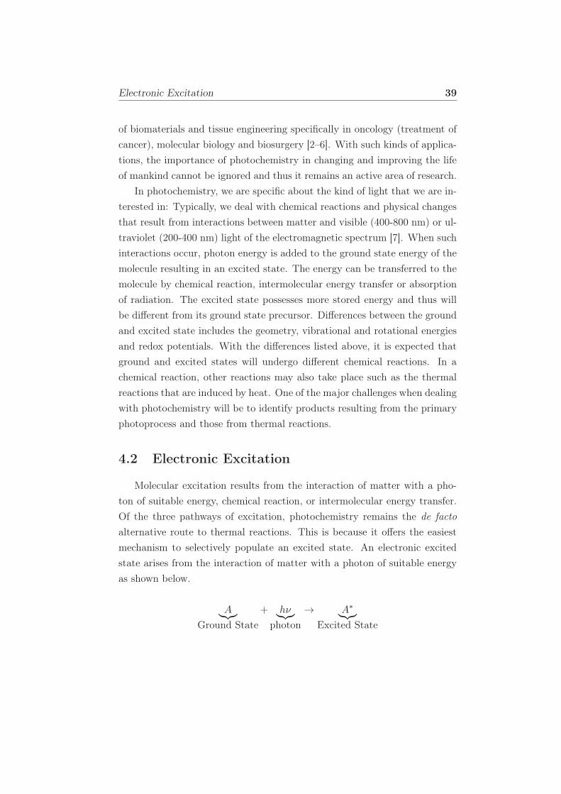
Electronic Excitation 39
of biomaterials and tissue engineering specifically in oncology (treatment of
cancer), molecular biology and biosurgery [2–6]. With such kinds of applica-
tions, the importance of photochemistry in changing and improving the life
of mankind cannot be ignored and thus it remains an active area of research.
In photochemistry, we are specific about the kind of light that we are in-
terested in: Typically, we deal with chemical reactions and physical changes
that result from interactions between matter and visible (400-800 nm) or ul-
traviolet (200-400 nm) light of the electromagnetic spectrum [7]. When such
interactions occur, photon energy is added to the ground state energy of the
molecule resulting in an excited state. The energy can be transferred to the
molecule by chemical reaction, intermolecular energy transfer or absorption
of radiation. The excited state possesses more stored energy and thus will
be different from its ground state precursor. Differences between the ground
and excited state includes the geometry, vibrational and rotational energies
and redox potentials. With the differences listed above, it is expected that
ground and excited states will undergo different chemical reactions. In a
chemical reaction, other reactions may also take place such as the thermal
reactions that are induced by heat. One of the major challenges when dealing
with photochemistry will be to identify products resulting from the primary
photoprocess and those from thermal reactions.
4.2 Electronic Excitation
Molecular excitation results from the interaction of matter with a pho-
ton of suitable energy, chemical reaction, or intermolecular energy transfer.
Of the three pathways of excitation, photochemistry remains the de facto
alternative route to thermal reactions. This is because it offers the easiest
mechanism to selectively populate an excited state. An electronic excited
state arises from the interaction of matter with a photon of suitable energy
as shown below.
A︸︷︷︸
Ground State
+ hν︸︷︷︸
photon
→ A∗︸︷︷︸
Excited State
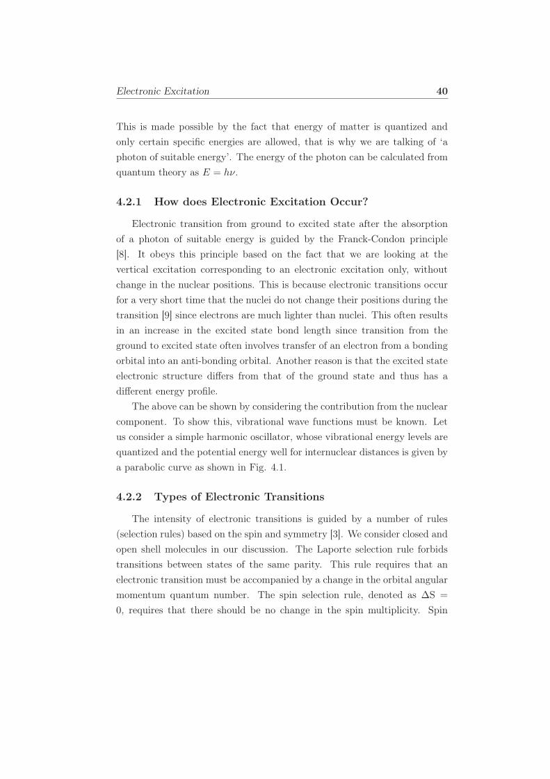
Electronic Excitation 40
This is made possible by the fact that energy of matter is quantized and
only certain specific energies are allowed, that is why we are talking of ‘a
photon of suitable energy’. The energy of the photon can be calculated from
quantum theory as E = hν.
4.2.1 How does Electronic Excitation Occur?
Electronic transition from ground to excited state after the absorption
of a photon of suitable energy is guided by the Franck-Condon principle
[8]. It obeys this principle based on the fact that we are looking at the
vertical excitation corresponding to an electronic excitation only, without
change in the nuclear positions. This is because electronic transitions occur
for a very short time that the nuclei do not change their positions during the
transition [9] since electrons are much lighter than nuclei. This often results
in an increase in the excited state bond length since transition from the
ground to excited state often involves transfer of an electron from a bonding
orbital into an anti-bonding orbital. Another reason is that the excited state
electronic structure differs from that of the ground state and thus has a
different energy profile.
The above can be shown by considering the contribution from the nuclear
component. To show this, vibrational wave functions must be known. Let
us consider a simple harmonic oscillator, whose vibrational energy levels are
quantized and the potential energy well for internuclear distances is given by
a parabolic curve as shown in Fig. 4.1.
4.2.2 Types of Electronic Transitions
The intensity of electronic transitions is guided by a number of rules
(selection rules) based on the spin and symmetry [3]. We consider closed and
open shell molecules in our discussion. The Laporte selection rule forbids
transitions between states of the same parity. This rule requires that an
electronic transition must be accompanied by a change in the orbital angular
momentum quantum number. The spin selection rule, denoted as ∆S =
0, requires that there should be no change in the spin multiplicity. Spin
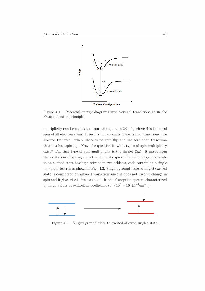
Electronic Excitation 41
Figure 4.1 – Potential energy diagrams with vertical transitions as in theFranck-Condon principle.
multiplicity can be calculated from the equation 2S+1, where S is the total
spin of all electron spins. It results in two kinds of electronic transitions; the
allowed transition where there is no spin flip and the forbidden transition
that involves spin flip. Now, the question is, what types of spin multiplicity
exist? The first type of spin multiplicity is the singlet (S0). It arises from
the excitation of a single electron from its spin-paired singlet ground state
to an excited state having electrons in two orbitals, each containing a single
unpaired electron as shown in Fig. 4.2. Singlet ground state to singlet excited
state is considered an allowed transition since it does not involve change in
spin and it gives rise to intense bands in the absorption spectra characterized
by large values of extinction coefficient (ǫ ≈ 102 − 104 M−1cm−1).
Figure 4.2 – Singlet ground state to excited allowed singlet state.
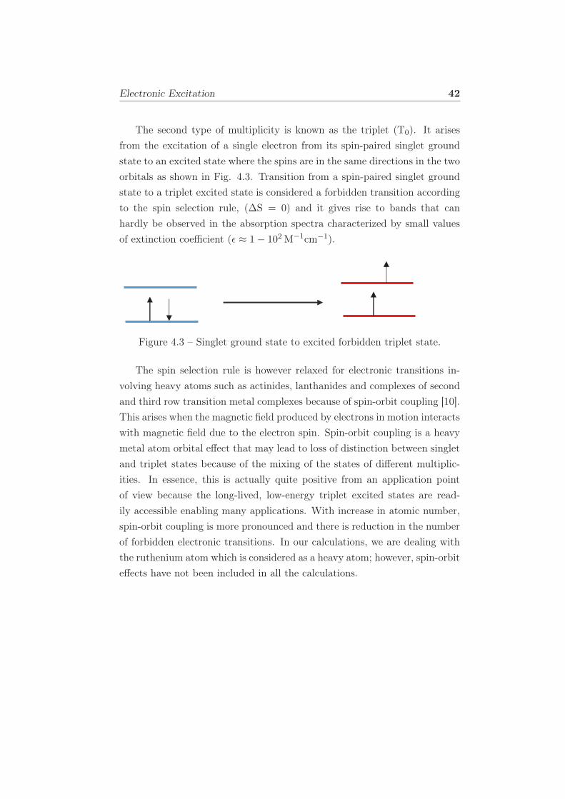
Electronic Excitation 42
The second type of multiplicity is known as the triplet (T0). It arises
from the excitation of a single electron from its spin-paired singlet ground
state to an excited state where the spins are in the same directions in the two
orbitals as shown in Fig. 4.3. Transition from a spin-paired singlet ground
state to a triplet excited state is considered a forbidden transition according
to the spin selection rule, (∆S = 0) and it gives rise to bands that can
hardly be observed in the absorption spectra characterized by small values
of extinction coefficient (ǫ ≈ 1− 102 M−1cm−1).
Figure 4.3 – Singlet ground state to excited forbidden triplet state.
The spin selection rule is however relaxed for electronic transitions in-
volving heavy atoms such as actinides, lanthanides and complexes of second
and third row transition metal complexes because of spin-orbit coupling [10].
This arises when the magnetic field produced by electrons in motion interacts
with magnetic field due to the electron spin. Spin-orbit coupling is a heavy
metal atom orbital effect that may lead to loss of distinction between singlet
and triplet states because of the mixing of the states of different multiplic-
ities. In essence, this is actually quite positive from an application point
of view because the long-lived, low-energy triplet excited states are read-
ily accessible enabling many applications. With increase in atomic number,
spin-orbit coupling is more pronounced and there is reduction in the number
of forbidden electronic transitions. In our calculations, we are dealing with
the ruthenium atom which is considered as a heavy atom; however, spin-orbit
effects have not been included in all the calculations.
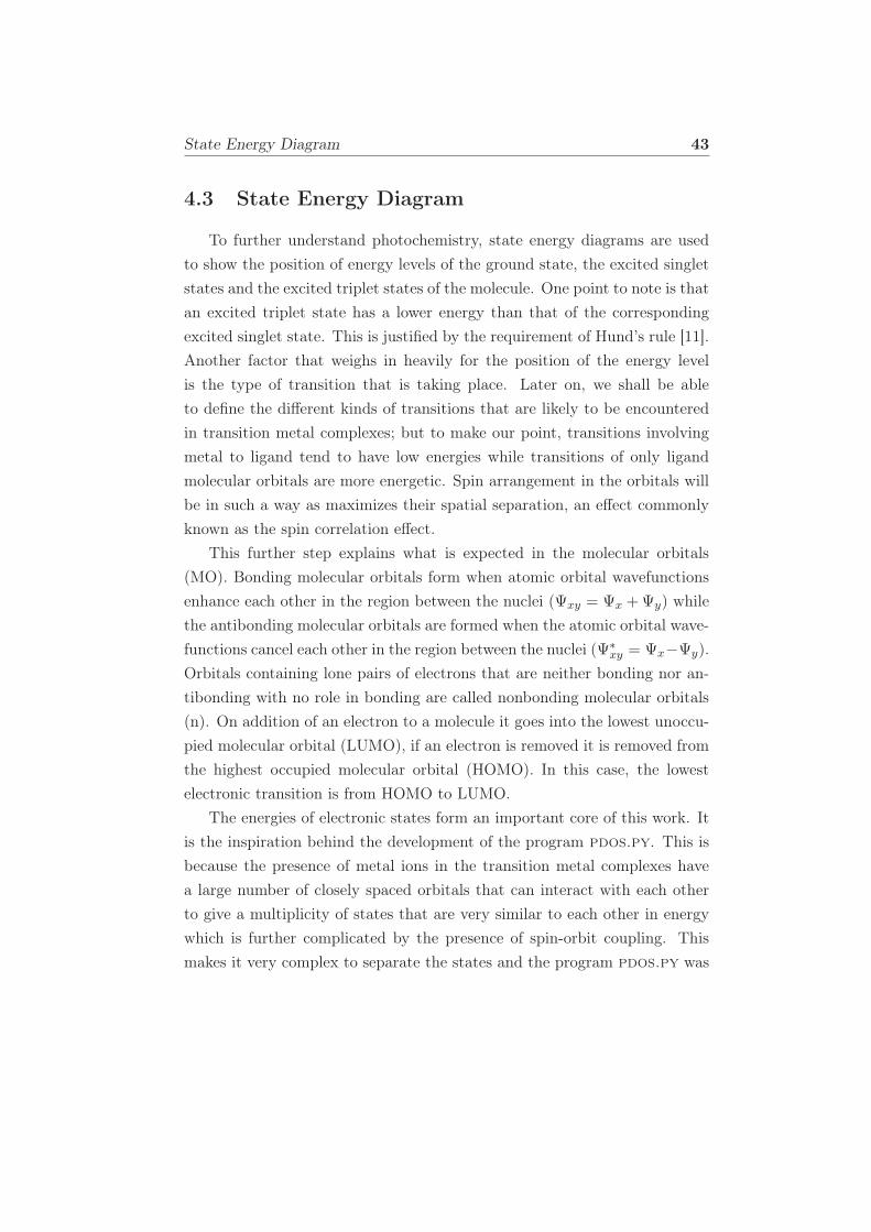
State Energy Diagram 43
4.3 State Energy Diagram
To further understand photochemistry, state energy diagrams are used
to show the position of energy levels of the ground state, the excited singlet
states and the excited triplet states of the molecule. One point to note is that
an excited triplet state has a lower energy than that of the corresponding
excited singlet state. This is justified by the requirement of Hund’s rule [11].
Another factor that weighs in heavily for the position of the energy level
is the type of transition that is taking place. Later on, we shall be able
to define the different kinds of transitions that are likely to be encountered
in transition metal complexes; but to make our point, transitions involving
metal to ligand tend to have low energies while transitions of only ligand
molecular orbitals are more energetic. Spin arrangement in the orbitals will
be in such a way as maximizes their spatial separation, an effect commonly
known as the spin correlation effect.
This further step explains what is expected in the molecular orbitals
(MO). Bonding molecular orbitals form when atomic orbital wavefunctions
enhance each other in the region between the nuclei (Ψxy = Ψx +Ψy) while
the antibonding molecular orbitals are formed when the atomic orbital wave-
functions cancel each other in the region between the nuclei (Ψ∗xy = Ψx−Ψy).
Orbitals containing lone pairs of electrons that are neither bonding nor an-
tibonding with no role in bonding are called nonbonding molecular orbitals
(n). On addition of an electron to a molecule it goes into the lowest unoccu-
pied molecular orbital (LUMO), if an electron is removed it is removed from
the highest occupied molecular orbital (HOMO). In this case, the lowest
electronic transition is from HOMO to LUMO.
The energies of electronic states form an important core of this work. It
is the inspiration behind the development of the program pdos.py. This is
because the presence of metal ions in the transition metal complexes have
a large number of closely spaced orbitals that can interact with each other
to give a multiplicity of states that are very similar to each other in energy
which is further complicated by the presence of spin-orbit coupling. This
makes it very complex to separate the states and the program pdos.py was
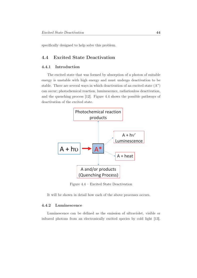
Excited State Deactivation 44
specifically designed to help solve this problem.
4.4 Excited State Deactivation
4.4.1 Introduction
The excited state that was formed by absorption of a photon of suitable
energy is unstable with high energy and must undergo deactivation to be
stable. There are several ways in which deactivation of an excited state (A∗)
can occur; photochemical reaction, luminescence, radiationless deactivation,
and the quenching process [12]. Figure 4.4 shows the possible pathways of
deactivation of the excited state.
A + hh A*
Photochemical reaction
products
A + h
Luminescence
A + heat
A and/or products
(Quenching Process)
Figure 4.4 – Excited State Deactivation
It will be shown in detail how each of the above processes occurs.
4.4.2 Luminescence
Luminescence can be defined as the emission of ultraviolet, visible or
infrared photons from an electronically excited species by cold light [13].
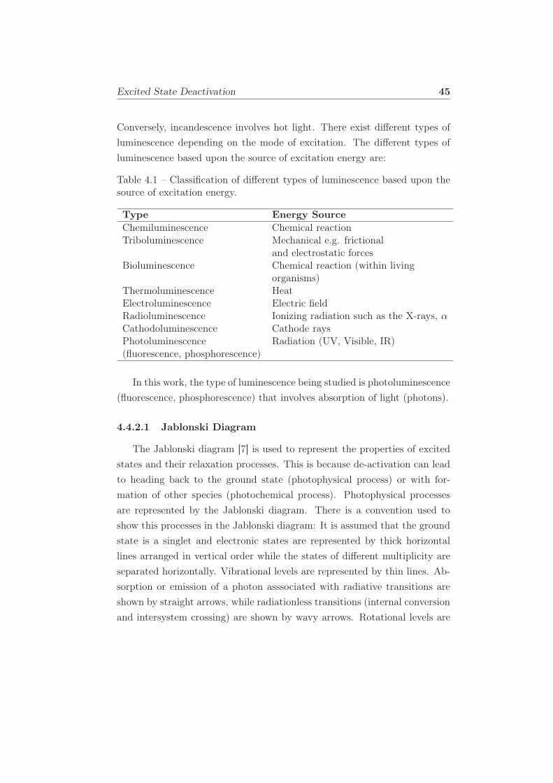
Excited State Deactivation 45
Conversely, incandescence involves hot light. There exist different types of
luminescence depending on the mode of excitation. The different types of
luminescence based upon the source of excitation energy are:
Table 4.1 – Classification of different types of luminescence based upon thesource of excitation energy.
Type Energy SourceChemiluminescence Chemical reactionTriboluminescence Mechanical e.g. frictional
and electrostatic forcesBioluminescence Chemical reaction (within living
organisms)Thermoluminescence HeatElectroluminescence Electric fieldRadioluminescence Ionizing radiation such as the X-rays, αCathodoluminescence Cathode raysPhotoluminescence Radiation (UV, Visible, IR)(fluorescence, phosphorescence)
In this work, the type of luminescence being studied is photoluminescence
(fluorescence, phosphorescence) that involves absorption of light (photons).
4.4.2.1 Jablonski Diagram
The Jablonski diagram [7] is used to represent the properties of excited
states and their relaxation processes. This is because de-activation can lead
to heading back to the ground state (photophysical process) or with for-
mation of other species (photochemical process). Photophysical processes
are represented by the Jablonski diagram. There is a convention used to
show this processes in the Jablonski diagram: It is assumed that the ground
state is a singlet and electronic states are represented by thick horizontal
lines arranged in vertical order while the states of different multiplicity are
separated horizontally. Vibrational levels are represented by thin lines. Ab-
sorption or emission of a photon asssociated with radiative transitions are
shown by straight arrows, while radiationless transitions (internal conversion
and intersystem crossing) are shown by wavy arrows. Rotational levels are
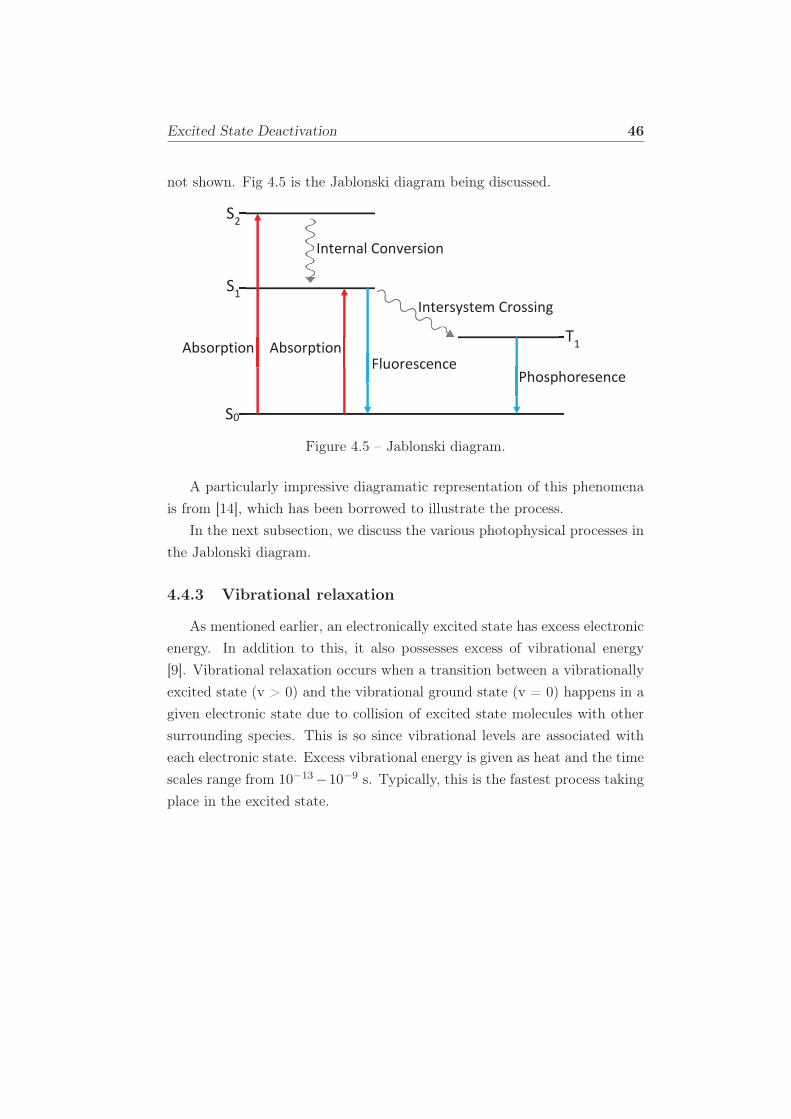
Excited State Deactivation 46
not shown. Fig 4.5 is the Jablonski diagram being discussed.
S0
S1
S2
Internal Conversion
Absorption Absorption
Intersystem Crossing
Fluorescence
Phosphoresence
T1
Figure 4.5 – Jablonski diagram.
A particularly impressive diagramatic representation of this phenomena
is from [14], which has been borrowed to illustrate the process.
In the next subsection, we discuss the various photophysical processes in
the Jablonski diagram.
4.4.3 Vibrational relaxation
As mentioned earlier, an electronically excited state has excess electronic
energy. In addition to this, it also possesses excess of vibrational energy
[9]. Vibrational relaxation occurs when a transition between a vibrationally
excited state (v > 0) and the vibrational ground state (v = 0) happens in a
given electronic state due to collision of excited state molecules with other
surrounding species. This is so since vibrational levels are associated with
each electronic state. Excess vibrational energy is given as heat and the time
scales range from 10−13−10−9 s. Typically, this is the fastest process taking
place in the excited state.
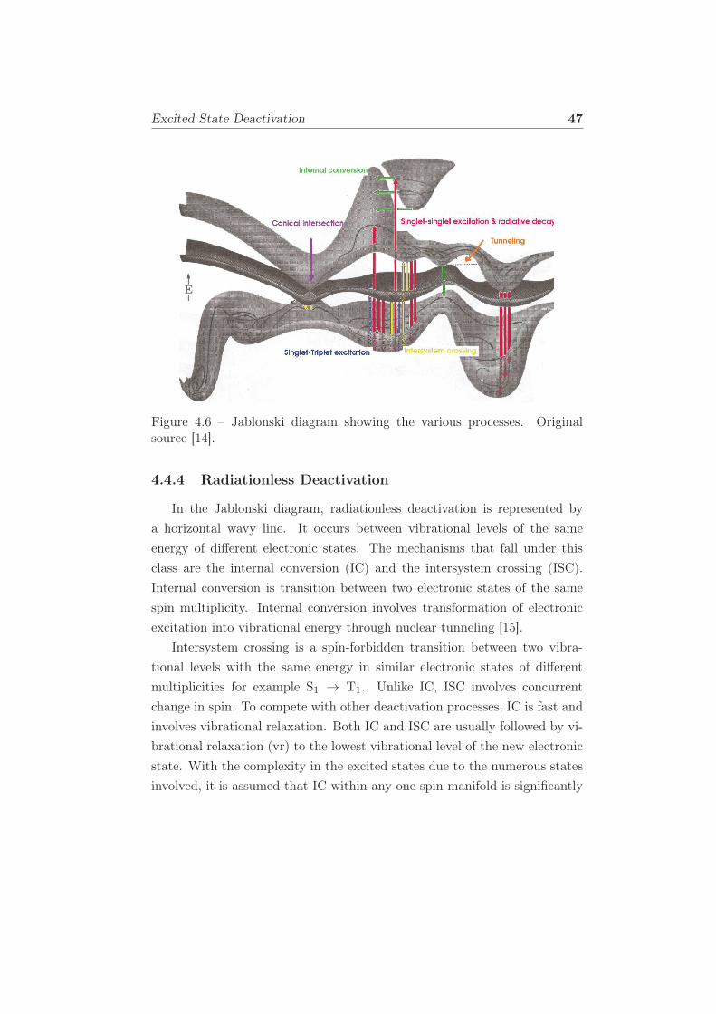
Excited State Deactivation 47
Figure 4.6 – Jablonski diagram showing the various processes. Originalsource [14].
4.4.4 Radiationless Deactivation
In the Jablonski diagram, radiationless deactivation is represented by
a horizontal wavy line. It occurs between vibrational levels of the same
energy of different electronic states. The mechanisms that fall under this
class are the internal conversion (IC) and the intersystem crossing (ISC).
Internal conversion is transition between two electronic states of the same
spin multiplicity. Internal conversion involves transformation of electronic
excitation into vibrational energy through nuclear tunneling [15].
Intersystem crossing is a spin-forbidden transition between two vibra-
tional levels with the same energy in similar electronic states of different
multiplicities for example S1 → T1. Unlike IC, ISC involves concurrent
change in spin. To compete with other deactivation processes, IC is fast and
involves vibrational relaxation. Both IC and ISC are usually followed by vi-
brational relaxation (vr) to the lowest vibrational level of the new electronic
state. With the complexity in the excited states due to the numerous states
involved, it is assumed that IC within any one spin manifold is significantly
Excited State Deactivation 48
faster than direct deactivation to the ground state or ISC [3]. According to
Kasha’s rule[16], IC between excited states is more rapid than IC to ground
state since emission occurs from the lowest excited-state of a given multi-
plicity.
4.4.5 Radiative Deactivation
These deactivation mechanisms obey the same selection rules as the
ones for light absorption. The mechanisms here are understood in terms
of the Pauli exclusion principle. Deactivation from S1 is allowed, leading
to a ground state with spin-paired electrons in one orbital hence a short-
lived excited state (fluorescence). Forbidden de-excitation, such as that of
a triplet excited state, violates the Pauli exclusion principle and has a long
lived excited state (phosphorescence).
4.4.5.1 Fluorescence
Fluorescence is a spin allowed photon emission between states of the same
multiplicity from the lowest vibrational level of the lowest excited singlet
state, S1(v = 0) [7]. It occurs in timescales of 10−12 − 10−6 s. It can be
expressed as,
S1 −→ S0 + hν. (4.1)
The characteristics of fluorescence emission are independent of the ex-
citation wavelength except for polarization and in cases where there is a
small energy gap between the initial and final electronic states. The Franck-
Condon principle plays an important role in determining the band shapes
for radiative deactivation. At the 0-0 transition, the excited state is undis-
torted and a sharp line shaped emission band is expected. On the contrary, a
distorted excited state (<0-0 energy) will result in a broad Gaussian-shaped
emission band. The 0-0 transition is usually the same for absorption and
fluorescence [13]. This is not however the case for energies higher than the
0-0 energy where the absorption and emission spectra for the same transition
is shifted. This shift is called the Stokes shift. It is simply the difference in
Photochemical Processes on Potential Energy Surfaces 49
wavelength between the maximum of the excitation spectrum (shorter wave-
length, higher energy), and the maximum of the emission spectrum (longer
wavelength, lower energy) [17]. It can be used to measure of the extent of dis-
tortion between the ground and the excited state. The larger the magnitude
of Strokes shift the greater the structural or solvation differences between
the two states.
4.4.5.2 Phosphorescence
Phosphorescence is defined as a spin forbidden transition between states
of different multiplicity, normally from the lowest vibrational level of the
lowest excited triplet state, T1(v = 0) [7]. It occurs in timescales of 10−3−102s. It can be expressed as,
T1(v = 0) −→ S0 + hν. (4.2)
There are two routes in which the triplet state may be populated; the
first one is by direct absorption from the ground state, which is not very
significant because it is a forbidden transition. The other alternative is by
first excitation by an allowed transition from S0 to S1 then followed by an
inter-system crossing from S1 to T1 . Phosphorescence can generally occur
because of any of the two methods described above. Excited state lifetimes
resulting from phosphorescence are long.
4.5 Photochemical Processes on Potential Energy
Surfaces
Potential energy surface (PES) can be defined as a mathematical function
that gives the energy of a molecule as a function of its geometry. Within the
limits of the Born-Oppenheimer approximation, we can be able to show what
happens on the PES when photochemical reactions occur. For more details
on the Born-Oppenheimer approximation and PES, the reader is referred to
section 3.9. Here, each electronic state of a molecule can be represented by a
PES that describes the change in energy of the system on changing nuclear
Excited State Lifetime 50
coordinates [18]. How do we represent this processes on the PES? We begin
the reaction coordinate once we have an excited state from photo-excitation
then terminate it at the ground state [19].
4.6 Excited State Lifetime
The excited-state lifetime (τ) is the time taken for a given excited state
to survive before decaying by radiative or nonradiative mechanisms to the
ground state [7]. It can also be defined from a kinetic point of view as the
rate of depopulation of the excited (singlet or triplet) states following an op-
tical excitation from the ground state. From excited state dynamics, several
intramolecular decay steps are involved and each one of them is character-
ized by its own rate constant and each excited state is characterized by its
lifetime, given by,
τ =1
∑
iki, (4.3)
where ki is the first order rate constant for unimolecular or pseudo-unimolecular
processes that causes the disappearance of the excited state [12].
Experimentally, it is possible to measure the excited state lifetime from
a time-resolved experiment in which a very short pulse excitation is made,
followed by measurement of the time-dependent intensity.
4.7 Quantum Yield
Quantum yield (Φ) can be defined as a measure of the efficiency of a
photoreaction, that is, how efficient the process of absorption of light leads
to the production of excited state molecules [7]. It is a measure of the
number of moles of a species produced upon absorption of a mole of photons.
Mathematically, it can be expressed as,
Φ =number of excited state molecules formed
number of photons absorbed. (4.4)
BIBLIOGRAPHY 51
Bibliography
[1] V. Balzani and S. Campagna. Photochemistry and Photophysics of Co-
ordination Compounds II. Topics in Current Chemistry. Springer Berlin
Heidelberg, 2007. ISBN 9783540733492.
[2] B. P. Chan. Biomedical applications of photochemistry. Tissue Eng.
Part B-Re., 16(5):509–522, 2010.
[3] P. S. Wagenknecht and P. C. Ford. Metal centered ligand field excited
states: their roles in the design and performance of transition metal
based photochemical molecular devices. Coord. Chem. Rev., 255(5):
591–616, 2011.
[4] V. Balzani, G. Bergamini, and P. Ceroni. Photochemistry and photo-
catalysis. Rend. Fis. Acc. Lincei, 28 (Suppl 1):S125–S142, 2017.
[5] Q. Sun, S. Mosquera-Vazquez, Y. Suffren, J. Hankache, N. Amstutz,
L. M. L. Daku, E. Vauthey, and A. Hauser. On the role of ligand-field
states for the photophysical properties of ruthenium (II) polypyridyl
complexes. Coord. Chem. Rev., 282:87–99, 2015.
[6] C. Daniel. Photochemistry and photophysics of transition metal com-
plexes: Quantum chemistry. Coord. Chem. Rev., 282-283:19, 2015.
[7] B. Wardle. Principles and Applications of Photochemistry. Wiley, 2009.
ISBN 9780470710135.
[8] M. Nic, J. Jirat, Division of Chemical Nomenclature, Structure Rep-
resentation International Union of Pure, Applied Chemistry, and
B. Kosata. IUPAC goldbook. IUPAC, 2006.
[9] D. M. Roundhill. Photochemistry and Photophysics of Metal Complexes.
Modern Inorganic Chemistry. Springer US, 2013. ISBN 9781489914958.
[10] K. K. Rohatgi-Mukherjee. Fundamentals of Photochemistry. A Halsted
Press book. Wiley, 1978. ISBN 9780852267844.
BIBLIOGRAPHY 52
[11] M. Sauer, J. Hofkens, and J. Enderlein. Handbook of Fluorescence Spec-
troscopy and Imaging: From Ensemble to Single Molecules. Wiley, 2010.
ISBN 9783527633524.
[12] A. Juris, V. Balzani, F. Barigelletti, S. Campagna, P. Belser, and A. Von
Zelewsky. Ru(II) polypyridine complexes: Photophysics, photochem-
istry, electrochemistry, and chemiluminescence. Coord. Chem. Rev., 84:
85, 1988.
[13] B. Valeur and M. N. Berberan-Santos. Molecular Fluorescence: Princi-
ples and Applications. Wiley, 2013. ISBN 9783527650026.
[14] J. Michl and V. V. Bonačić-Koutecky. Electronic aspects of organic
photochemistry. Wiley, 1990. ISBN 9780471896265.
[15] Wawire C. Theoretical Investigation of Ruthenium Photosensitizers.
PhD thesis, Université de Grenoble, 2012.
[16] M. Kasha. Characterization of electronic transitions in complex
molecules. Discussions of the Faraday society, 9:14–19, 1950.
[17] D. Ganten and K. Ruckpaul. Stokes Shift, pages 1807–1807. Springer
Berlin Heidelberg, 2006. ISBN 978-3-540-29623-2. doi: 10.1007/
3-540-29623-9_8808.
[18] V. Balzani, P. Ceroni, and A. Juris. Photochemistry and Photophysics:
Concepts, Research, Applications. Wiley, 2014. ISBN 9783527671052.
[19] M. A. Robb and M. Olivucci. Photochemical processes: potential en-
ergy surface topology and rationalization using VB arguments. J. Pho-
tochem. and Photobiol. A, 144(2):237–243, 2001.
Chapter 5
Hartree-Fock Approximation
“Let us, as nature directs, begin first with first principles.”
Aristotle, Poetics I.
Methods used for electronic structure calculations have a long history of
development dating back to 1926 after the discovery of the Schrödinger equa-
tion. Starting from the initial methods that were not quite as accurate (no
electron correlation) and could only allow for the calculation of compounds
with few atoms to the current methods that are more accurate (includes elec-
tron correlation) and offer the possibility of calculating a greater number of
atoms. This chapter looks back at the background and theory of electronic
structure methods, starting with the most basic approximate methods used
to solve the Schrödinger equation to advanced quantum chemical techniques
which will be reviewed in later chapters. In the core of the development of
these methods lies the Hartree-Fock approximation. This is quite an exten-
sive topic that has been discussed here in detail but here are other references,
in addition to what has been quoted in text; [1–8].
As the ultimate goal is to solve the many-electron Schrödinger equa-
tion, at the point that we are, it still poses an unsolved problem. Previous
steps taken aimed towards solving this problem direct us to this step. The
Hartree-Fock approximation comes in handy at this step. In a nut shell,
it gives the simplest lowest energy variational solution of the Schrödinger
equation. Using a single Slater determinant for the trial wave function, the
53
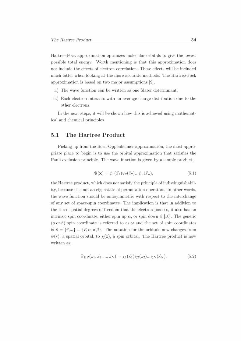
The Hartree Product 54
Hartree-Fock approximation optimizes molecular orbitals to give the lowest
possible total energy. Worth mentioning is that this approximation does
not include the effects of electron correlation. These effects will be included
much latter when looking at the more accurate methods. The Hartree-Fock
approximation is based on two major assumptions [9],
i.) The wave function can be written as one Slater determinant.
ii.) Each electron interacts with an average charge distribution due to the
other electrons.
In the next steps, it will be shown how this is achieved using mathemat-
ical and chemical principles.
5.1 The Hartree Product
Picking up from the Born-Oppenheimer approximation, the most appro-
priate place to begin is to use the orbital approximation that satisfies the
Pauli exclusion principle. The wave function is given by a simple product,
Ψ(x) = ψ1(~x1)ψ2(~x2)...ψn(~xn), (5.1)
the Hartree product, which does not satisfy the principle of indistinguishabil-
ity, because it is not an eigenstate of permutation operators. In other words,
the wave function should be antisymmetric with respect to the interchange
of any set of space-spin coordinates. The implication is that in addition to
the three spatial degrees of freedom that the electron possess, it also has an
intrinsic spin coordinate, either spin up α, or spin down β [10]. The generic
(α orβ) spin coordinate is referred to as ω and the set of spin coordinates
is ~x = ~r, ω ≡ ~r, α orβ. The notation for the orbitals now changes from
ψ(~r), a spatial orbital, to χ(~x), a spin orbital. The Hartree product is now
written as:
Ψhp(~x1,~x2, ...,~xN ) = χ1(~x1)χ2(~x2)...χN (~xN ). (5.2)
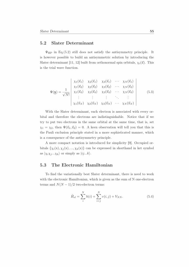
Slater Determinant 55
5.2 Slater Determinant
Ψhp in Eq.(5.2) still does not satisfy the antisymmetry principle. It
is however possible to build an antisymmetric solution by introducing the
Slater determinant [11, 12] built from orthonormal spin orbitals, χi(~x). This
is the trial wave function.
Ψ(x) =1√N !
∣∣∣∣∣∣∣∣∣∣∣∣∣
χ1(~x1) χ2(~x1) χ3(~x1) · · · χN (~x1)
χ1(~x2) χ2(~x2) χ3(~x2) · · · χN (~x2)
χ1(~x3) χ2(~x3) χ3(~x3) · · · χN (~x3)...
......
. . ....
χ1(~xN ) χ2(~xN ) χ3(~xN ) · · · χN (~xN )
∣∣∣∣∣∣∣∣∣∣∣∣∣
(5.3)
With the Slater determinant, each electron is associated with every or-
bital and therefore the electrons are indistinguishable. Notice that if we
try to put two electrons in the same orbital at the same time, that is, set
χ1 = χ2, then Ψ(~x1,~x2) = 0. A keen observation will tell you that this is
the Pauli exclusion principle stated in a more sophisticated manner, which
is a consequence of the antisymmetry principle.
A more compact notation is introduced for simplicity [9]. Occupied or-
bitals χi(x), χj(x), ..., χk(x) can be expressed in shorthand in ket symbol
as |χiχj ...χk〉 or simply as |ij...k〉.
5.3 The Electronic Hamiltonian
To find the variationally best Slater determinant, there is need to work
with the electronic Hamiltonian, which is given as the sum of N one-electron
terms and N(N − 1)/2 two-electron terms:
Hel =
N∑
i
h(i) +
N∑
i<j
υ(i, j) + VNN . (5.4)
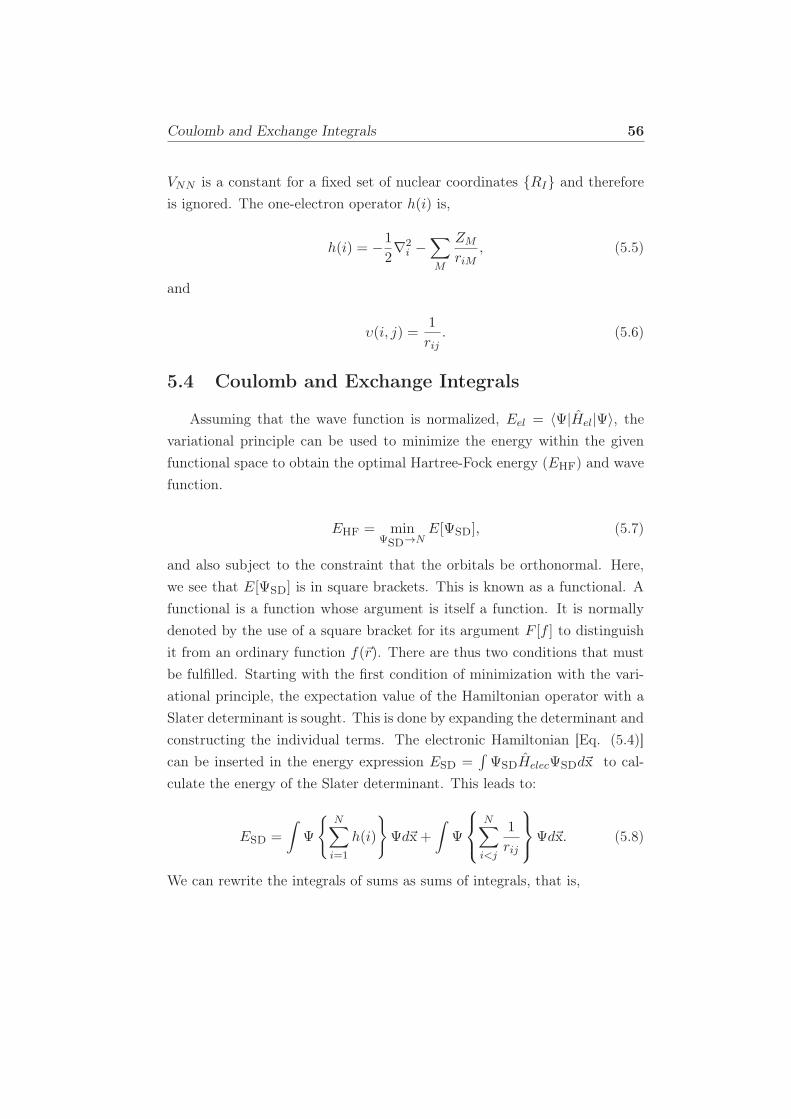
Coulomb and Exchange Integrals 56
VNN is a constant for a fixed set of nuclear coordinates RI and therefore
is ignored. The one-electron operator h(i) is,
h(i) = −1
2∇2i −
∑
M
ZMriM
, (5.5)
and
υ(i, j) =1
rij. (5.6)
5.4 Coulomb and Exchange Integrals
Assuming that the wave function is normalized, Eel = 〈Ψ|Hel|Ψ〉, the
variational principle can be used to minimize the energy within the given
functional space to obtain the optimal Hartree-Fock energy (Ehf) and wave
function.
Ehf = minΨsd→N
E[Ψsd], (5.7)
and also subject to the constraint that the orbitals be orthonormal. Here,
we see that E[Ψsd] is in square brackets. This is known as a functional. A
functional is a function whose argument is itself a function. It is normally
denoted by the use of a square bracket for its argument F [f ] to distinguish
it from an ordinary function f(~r). There are thus two conditions that must
be fulfilled. Starting with the first condition of minimization with the vari-
ational principle, the expectation value of the Hamiltonian operator with a
Slater determinant is sought. This is done by expanding the determinant and
constructing the individual terms. The electronic Hamiltonian [Eq. (5.4)]
can be inserted in the energy expression Esd =∫ΨsdHelecΨsdd~x to cal-
culate the energy of the Slater determinant. This leads to:
Esd =
∫
Ψ
N∑
i=1
h(i)
Ψd~x +
∫
Ψ
N∑
i<j
1
rij
Ψd~x. (5.8)
We can rewrite the integrals of sums as sums of integrals, that is,
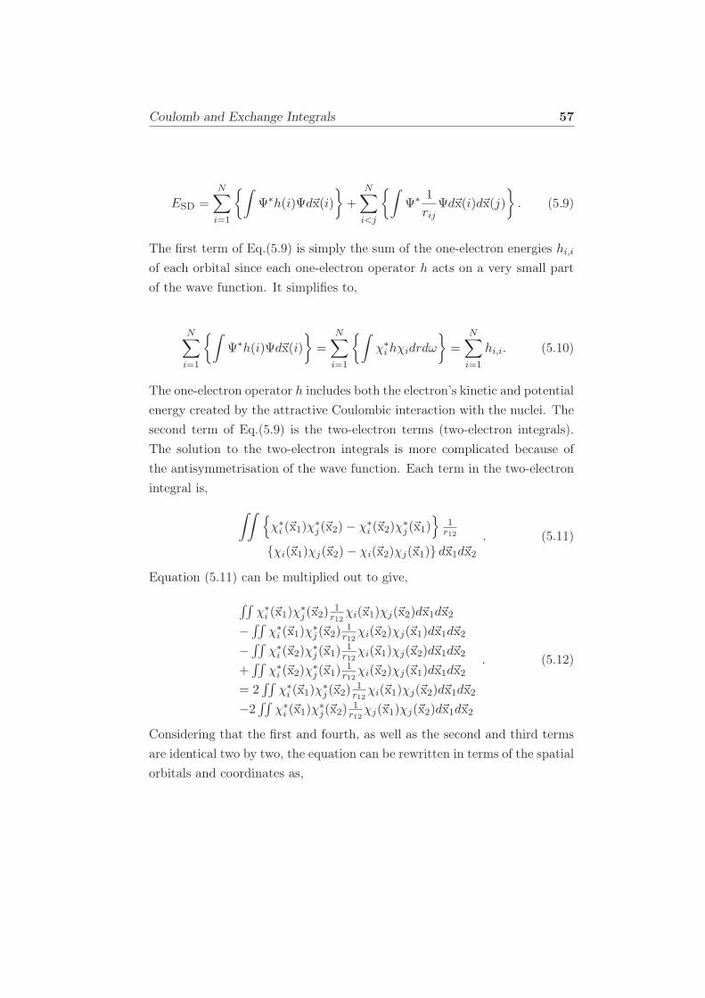
Coulomb and Exchange Integrals 57
Esd =N∑
i=1
∫
Ψ∗h(i)Ψd~x(i)
+N∑
i<j
∫
Ψ∗ 1
rijΨd~x(i)d~x(j)
. (5.9)
The first term of Eq.(5.9) is simply the sum of the one-electron energies hi,iof each orbital since each one-electron operator h acts on a very small part
of the wave function. It simplifies to,
N∑
i=1
∫
Ψ∗h(i)Ψd~x(i)
=
N∑
i=1
∫
χ∗ihχidrdω
=
N∑
i=1
hi,i. (5.10)
The one-electron operator h includes both the electron’s kinetic and potential
energy created by the attractive Coulombic interaction with the nuclei. The
second term of Eq.(5.9) is the two-electron terms (two-electron integrals).
The solution to the two-electron integrals is more complicated because of
the antisymmetrisation of the wave function. Each term in the two-electron
integral is,
∫∫
χ∗i (~x1)χ
∗j (~x2)− χ∗
i (~x2)χ∗j (~x1)
1r12
χi(~x1)χj(~x2)− χi(~x2)χj(~x1) d~x1d~x2. (5.11)
Equation (5.11) can be multiplied out to give,
∫∫χ∗i (~x1)χ
∗j (~x2)
1r12χi(~x1)χj(~x2)d~x1d~x2
−∫∫
χ∗i (~x1)χ
∗j (~x2)
1r12χi(~x2)χj(~x1)d~x1d~x2
−∫∫
χ∗i (~x2)χ
∗j (~x1)
1r12χi(~x1)χj(~x2)d~x1d~x2
+∫∫
χ∗i (~x2)χ
∗j (~x1)
1r12χi(~x2)χj(~x1)d~x1d~x2
= 2∫∫
χ∗i (~x1)χ
∗j (~x2)
1r12χi(~x1)χj(~x2)d~x1d~x2
−2∫∫
χ∗i (~x1)χ
∗j (~x2)
1r12χj(~x1)χj(~x2)d~x1d~x2
. (5.12)
Considering that the first and fourth, as well as the second and third terms
are identical two by two, the equation can be rewritten in terms of the spatial
orbitals and coordinates as,
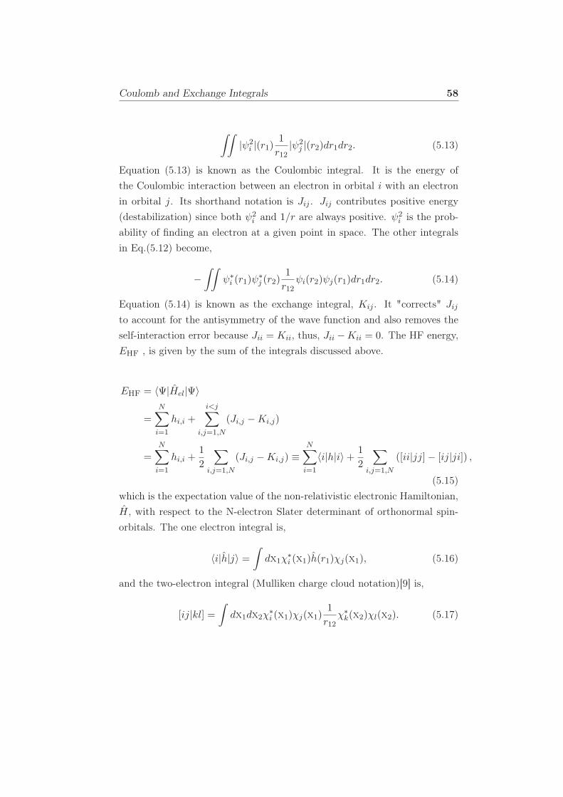
Coulomb and Exchange Integrals 58
∫∫
|ψ2i |(r1)
1
r12|ψ2j |(r2)dr1dr2. (5.13)
Equation (5.13) is known as the Coulombic integral. It is the energy of
the Coulombic interaction between an electron in orbital i with an electron
in orbital j. Its shorthand notation is Jij . Jij contributes positive energy
(destabilization) since both ψ2i and 1/r are always positive. ψ2
i is the prob-
ability of finding an electron at a given point in space. The other integrals
in Eq.(5.12) become,
−∫∫
ψ∗i (r1)ψ
∗j (r2)
1
r12ψi(r2)ψj(r1)dr1dr2. (5.14)
Equation (5.14) is known as the exchange integral, Kij . It "corrects" Jij
to account for the antisymmetry of the wave function and also removes the
self-interaction error because Jii = Kii, thus, Jii −Kii = 0. The HF energy,
Ehf , is given by the sum of the integrals discussed above.
Ehf = 〈Ψ|Hel|Ψ〉
=N∑
i=1
hi,i +
i<j∑
i,j=1,N
(Ji,j −Ki,j)
=N∑
i=1
hi,i +1
2
∑
i,j=1,N
(Ji,j −Ki,j) ≡N∑
i=1
〈i|h|i〉+ 1
2
∑
i,j=1,N
([ii|jj]− [ij|ji]) ,
(5.15)
which is the expectation value of the non-relativistic electronic Hamiltonian,
H, with respect to the N-electron Slater determinant of orthonormal spin-
orbitals. The one electron integral is,
〈i|h|j〉 =∫
dx1χ∗i (x1)h(r1)χj(x1), (5.16)
and the two-electron integral (Mulliken charge cloud notation)[9] is,
[ij|kl] =∫
dx1dx2χ∗i (x1)χj(x1)
1
r12χ∗k(x2)χl(x2). (5.17)
Coulomb and Exchange Operators 59
5.5 Coulomb and Exchange Operators
It can be seen that Ehf, [Eq.(5.15)], is a functional of the spin orbitals,
Ehf = E[χi]. The next step is to determine the set of spin orbitals which
give the best single determinant. This is done by minimizing Eq.(5.15), EHF ,
with respect to the constraint that the spin-orbitals are orthonormal, and
what better way to do it than to use the Lagrange method of undetermined
multipliers,
L [χi] = Ehf[χi]−∑
ij
ǫij(〈i|j〉 − δij). (5.18)
Here the ǫij are the Lagrange multipliers and 〈i|j〉 is the overlap between spin
orbitals i and j. δij is the constraint that the orbitals must be orthonormal,
that is, 〈χi|χj〉 = δij . And the solution, which is the equation for the best
Hartree-Fock spin orbitals is,
h(~x1)χi(~x1) +∑
j 6=i
[∫
dx2|χj(~x2)|2r−112
]
χi(~x1)−∑
j 6=i
[∫
dx2χ∗j (~x2)χi(~x2)r
−112
]
χj(~x1)
= ǫiχi(~x1),
(5.19)
where ǫi is the energy eigenvalue (orbital energy) associated with spin orbital
χi. The term,
∑
j 6=i
[∫
dx2|χj(~x2)|2r−112
]
χi(~x1), (5.20)
in Eq. (5.19) is known as the Coulomb term. It is the Coulomb interaction
of an electron in spin orbital χi with the average charge distribution of
the other electrons. It shows that the first electron χi experiences a one-
electron Coulomb potential. The Coulomb term contains a self-interaction
error which must be removed since an electron cannot interact with itself.
The corresponding Coulomb operator is,
Coulomb and Exchange Operators 60
Jj(~x1) =
∫
dx2|χj(~x2)|2r−112 , (5.21)
and
Kj(~x1)χi(~x1) =
[∫
dx2χ∗j (~x2)χi(~x2)r
−112
]
χj(~x1), (5.22)
is called the exchange term and it arises from the antisymmetric nature of the
wave function since it exchanges spin orbitals χi and χj . The Hartree-Fock
equations can be expressed in terms of the Coulomb and exchange operators
in a more compact form as,
h(~x1) +∑
j 6=i
Jj(~x1)−∑
j 6=i
Kj(~x1)
χi(~x1) = ǫiχi(~x1). (5.23)
A keen inspection of the above equation tells us that it is an eigenvalue
equation and the exchange operators serves to remove the self-interaction
error in the Coulomb energy since,
Ji(~x1)χi(~x1) = Ki(~x1)χi(~x1). (5.24)
This implies that the restriction i 6= j can be removed making fi orbital
independent. It also shows that obeying the Pauli exclusion principle keeps
the electrons apart in space and therefore reduces the total electron repulsion
energy. The new operator, known as the Fock operator is,
f(~x1) = h(~x1) +∑
j
(
Jj(~x1)− Kj(~x1))
. (5.25)
The canonical Hartree-Fock (molecular orbital) equation is:
f(~x1)χi(~x1) = ǫiχi(~x1), (5.26)
where ǫi is the orbital energy of χi. The next step involves finding spin
orbitals that are eigenfunctions of the Fock operator. In this regard, there
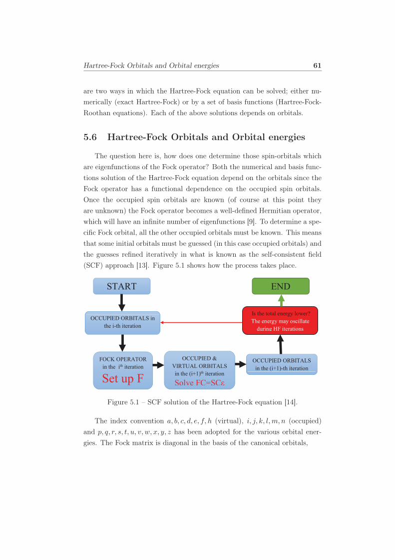
Hartree-Fock Orbitals and Orbital energies 61
are two ways in which the Hartree-Fock equation can be solved; either nu-
merically (exact Hartree-Fock) or by a set of basis functions (Hartree-Fock-
Roothan equations). Each of the above solutions depends on orbitals.
5.6 Hartree-Fock Orbitals and Orbital energies
The question here is, how does one determine those spin-orbitals which
are eigenfunctions of the Fock operator? Both the numerical and basis func-
tions solution of the Hartree-Fock equation depend on the orbitals since the
Fock operator has a functional dependence on the occupied spin orbitals.
Once the occupied spin orbitals are known (of course at this point they
are unknown) the Fock operator becomes a well-defined Hermitian operator,
which will have an infinite number of eigenfunctions [9]. To determine a spe-
cific Fock orbital, all the other occupied orbitals must be known. This means
that some initial orbitals must be guessed (in this case occupied orbitals) and
the guesses refined iteratively in what is known as the self-consistent field
(SCF) approach [13]. Figure 5.1 shows how the process takes place.
START
OCCUPIED ORBITALS in
the i-th iteration
FOCK OPERATOR
in the ith iteration
Set up F
OCCUPIED &
VIRTUAL ORBITALS
in the (i+1)th iteration
OCCUPIED ORBITALS
in the (i+1)-th iteration
Is the total energy lower?
The energy may oscillate
during HF iterations
END
Figure 5.1 – SCF solution of the Hartree-Fock equation [14].
The index convention a, b, c, d, e, f, h (virtual), i, j, k, l,m, n (occupied)
and p, q, r, s, t, u, v, w, x, y, z has been adopted for the various orbital ener-
gies. The Fock matrix is diagonal in the basis of the canonical orbitals,
Hartree-Fock Orbitals and Orbital energies 62
Fi,j = 〈χi|h|χj〉 = ǫi〈χi|χi〉 = ǫjδi,j . (5.27)
We can express the orbital energies as,
ǫi = Fi,i
= 〈χi|h|χi〉+∑
k
〈χi|(Jk −Kk|χi〉
= 〈χi|h|χi〉+∑
k
(
〈χi|Jk|χi〉 −∑
k
〈χi|Kk|χi〉)
= ǫ(0)i +
∑
k
((ii||kk)− (ik||ki)).
(5.28)
Considering the index convention that was adopted above, the occupied or-
bitals can be expressed as,
ǫi = ǫ(0)i +
∑
j
((ii||jj)− (ij||ji))
= ǫ(0)i +
j 6=i∑
j
((ii||jj)− (ij||ji)),(5.29)
and virtual orbitals,
ǫa = ǫ(0)a +∑
k
((aa||kk)− (ak||ka)). (5.30)
From Eq.(5.29), it can be seen that ǫi is the energy of occupied spin orbital
(χi). It includes ǫ(0)i which is the attraction to the nuclei and kinetic energy.
It also includes Coulomb and exchange interactions with each of the remain-
ing electrons (N−1). The unoccupied orbital energy ǫa, shown in Eq.(5.30),
includes the Coulomb and exchange interactions with N electrons of the
Hartree-Fock ground state. Adding up the orbital energies of the occupied
states results in,
∑
i=1,N
ǫi =∑
i=1,N
ǫ(0)i +
∑
j,k=1,N
([jj||kk]− [kj||jk]). (5.31)
Koopmans’ Theorem 63
A comparison of Eq.(5.31), the total energies of the occupied states and the
total Hartree-Fock energy Eq.(5.15) can be written as,
Ehf =
N∑
i=1
〈i|h|i〉+ 1
2
∑
i,j=1,N
([ii|jj]− [ij|ji]), (5.32)
which shows that,
Ehf 6=∑
i=1,N
ǫi. (5.33)
This can be justified by the fact that ǫi includes exchange and Coulomb
interactions between an electron in a spin orbital χi and electrons in all
other occupied spin orbitals χj . Similarly, ǫj includes exchange and Coulomb
interactions between an electron in χj and electrons in all other occupied spin
orbitals χi. The sum of orbital energies thus includes the electron-electron
interactions twice because addition of ǫi and ǫj includes electron-electron
interactions between an electron in χi and χj twice. To account for this
error, a factor of 12 is included in the energy expression for the total energy.
5.7 Koopmans’ Theorem
To attach physical meaning to the orbital energies ǫi and ǫa shown in
the previous section, we use the Koopmans’ theorem. It states that given an
N -electron Hartree-Fock single determinant ΨN with occupied and virtual χ
energies ǫi and ǫa, then the ionization potential to produce an (N − 1) elec-
tron single determinant ΨN−1 = aiΨ with identical spin orbitals, obtained
by removing an electron from spin orbital χa, and the electron affinity to
produce an (N + 1) electron single determinant Ψa = a†aΨ with identical
spin orbitals, obtained by adding an electron to spin orbital χr are just −ǫiand −ǫa respectively. Let us consider the energy of a system with one elec-
tron removed from orbital number k, and assume that the molecular orbitals
are identical for the two systems.
Roothaan-Hall Equation 64
EN =
N∑
i=1
hi,i +1
2
∑
i,j=1,N
(Ji,j −Ki,j) + Vnn
EkN−1 =N−1∑
i=1
hi,i +1
2
∑
i,j=1,N−1
(Ji,j −Ki,j) + Vnn.
(5.34)
Subtracting the two energies,
EN − EkN−1 = hk +∑
i,j=1,N
(Jk,i −Kk,i) = ǫk. (5.35)
The energy obtained in eq.(5.35), ǫk is seen to be exactly the same as the or-
bital energy obtained in eq.(5.28), ǫi. As a result of the Koopmans’ theorem,
the ionization energy (I.E) within the frozen molecular orbital approximation
is given simply as the orbital energy. Similarly, the electron affinity (EA) of
a neutral molecule is given as the orbital energy of the corresponding anion
or as the energy of the kth unoccupied orbital energy in the neutral species.
Mathematically,
EkN+1 − EN = ǫk. (5.36)
In a nutshell, the Koopmans’ theorem gives us a way of calculating approxi-
mate ionization potentials (IP) and electron affinities (EA). Koopmans’ IPs
are reasonable first approximations to experimental IPs. Electron affinities
from Koopmans’ theory are badly reproduced because correlation and relax-
ation effects do not cancel.
5.8 Roothaan-Hall Equation
The Hartree-Fock equation can be solved in two ways; either numerically
[15] (exact Hartree-Fock, that is, by mapping the orbitals on a set of grid
points) or by a set of basis functions (Hartree-Fock-Roothan equations).
Numerical methods are more applicable in small highly symmetric systems,
like atoms and diatomic molecules. Most if not all calculations use a basis set
expansion which expresses the unknown molecular orbitals in terms of a set
Roothaan-Hall Equation 65
of known functions. A basis function may be a Gaussian, exponential, plane
wave or polynomial. This study has adopted the finite basis set of Gaussian-
type orbitals (GTOs) which is preferred by most quantum chemists. All
our calculations include scalar relativistic effects of core electrons for the
ruthenium atom.
Introducing a basis set (linear combination of atomic orbitals (LCAO),
MO=LCAO) transforms the Hartree-Fock equations into the Roothaan equa-
tions [16]. Each MO is expanded as a linear combination of three dimen-
sional one electron functions, known as atomic orbitals 1. Typically, these
atomic orbitals are called Slater-type orbitals. Denoting the atomic orbital
basis functions as χµ,
χi(~x) =
K∑
µ=1
χµCµi(~x), (5.37)
for each spin orbital i. K is an integer relating to the size of the basis set
which is typically larger than the number of electrons in the system. A matrix
equation can be obtained for the set of molecular orbital expansion coeffi-
cients (Cµi) by substituting the linear expansion Eq.(7.1) into Eq.(5.26) 2
Using the index ν leads to,
f(~x1)∑
ν
Cνiχν(~x1) = ǫi∑
ν
Cνiχν(~x1). (5.38)
Multiplying from the left by a specific basis function χ∗µ(~x1) and integrating
gives a matrix equation,
∑
ν
Cνi
∫
dx1χ∗µ(~x1)f(~x1)χν(~x1) = ǫi
∑
ν
Cνi
∫
dx1χ∗µ(~x1)χν(~x1). (5.39)
Introducing the matrix element notation,
1. They are not solutions to the atomic HF problem.2. The idea behind this is that the problem of calculating the Hartree-Fock molec-
ular orbitals reduces to the problem of calculating the set of expansion coefficients Cµi
variationally.
Roothaan-Hall Equation 66
Sµν =
∫
dx1χ∗µ(~x1)χν(~x1) ≡ 〈χµ|χν〉, (5.40)
Fµν =
∫
dx1χ∗µ(~x1)f(~x1)χν(~x1) ≡ 〈χµ|F |χν〉. (5.41)
simplifies the Hartree-Fock-Roothaan equations [16] which can be written in
matrix form as,
∑
ν
FµνCνi = ǫi∑
ν
SµνCνi, (5.42)
or simply as matrices in the form,
FC = SCǫ, (5.43)
where ǫ is a diagonal matrix of the orbital energies ǫi. To determine the un-
known MO coefficients, Cµi, the Fock matrix must be diagonalized 3. Equa-
tion (5.43) is therefore solved self consistently [17].
3. The Fock matrix is only known if all the MO coefficients are known.
BIBLIOGRAPHY 67
Bibliography
[1] J. C. Slater. A simplification of the Hartree-Fock method. Phys. Rev.,
81(3):385, 1951.
[2] T. Tsuneda. Density Functional Theory in Quantum Chemistry.
SpringerLink : Bücher. Springer, Japan, 2014. ISBN 9784431548256.
[3] D. B. Cook. Handbook of Computational Quantum Chemistry. Dover
Books on Chemistry. Dover Publications, 2005. ISBN 9780486443072.
[4] K. I. Ramachandran, G. Deepa, and K. Namboori. Computa-
tional Chemistry and Molecular Modeling: Principles and Applications.
Springer Berlin Heidelberg, 2008. ISBN 9783540773023.
[5] T. Helgaker, P. Jorgensen, and J. Olsen. Molecular Electronic-Structure
Theory. Wiley, 2014. ISBN 9781119019558.
[6] R. F. Nalewajski. Perspectives in Electronic Structure Theory. Springer
Berlin Heidelberg, 2012. ISBN 9783642201806.
[7] G. Giuliani and G. Vignale. Quantum Theory of the Electron Liquid.
Masters Series in Physics and Astronomy. Cambridge University Press,
2005. ISBN 9780521821124.
[8] E. K. U. Gross, E. Runge, and O. Heinonen. Many-Particle Theory,.
Taylor & Francis, 1991. ISBN 9780750301558.
[9] A. Szabo and N. S. Ostlund. Modern Quantum Chemistry: Introduc-
tion to Advanced Electronic Structure Theory. Macmillan Publishing
Company, New York, 1982.
[10] W. Koch and M. C. Holthausen. A Chemist’s Guide to Density Func-
tional Theory. Wiley-VCH, Germany, 2015. ISBN 9783527802814.
[11] J. C. Slater. The theory of complex spectra. Phys. Rev., 34:1293–1322,
Nov 1929. doi: 10.1103/PhysRev.34.1293.
[12] J. C. Slater. Note on Hartree’s method. Phys. Rev., 35(2):210, 1930.
BIBLIOGRAPHY 68
[13] F. Jensen. Introduction to Computational Chemistry. Wiley, Great
Britain, 1999. ISBN 9780471980858,0471980854,0471984256.
[14] L. Piela. Ideas of Quantum Chemistry. Elsevier Science, Netherlands,
2013.
[15] J. Kobus. Diatomic molecules: Exact solutions of HF equations. Adv.
Quantum Chem., 28:1–14, 1997.
[16] C. C. J. Roothaan. New developments in molecular orbital theory. Rev.
Mod. Phys., 23(2):69, 1951.
[17] Cramer C. J. Essentials of Computational Chemistry Theories and Mod-
els. Wiley, Great Britain, 2nd edition, 2004.
Chapter 6
Density-Functional Theory
“At the moment I am struggling with a new atomic theory. I am very
optimistic about this thing and expect that if I can only solve it, it will be
very beautiful.”
Erwin Schrödinger.
In the study of electronic structure methods, the Hartree-Fock approx-
imation was introduced in the previous chapter. It was noted that the
Hartree-Fock approximation does not include electron correlation. In this
chapter, the density functional theory (DFT) method which includes the
electron correlation is discussed.
DFT [1, 2] is presently the most promising and successful approach to
computing the electronic structure of matter having a wide range of ap-
plications including, but not limited to atoms, molecules and solids, and
quantum fluids. DFT is based on the idea of replacing the wave function
Ψ(~x1, ~x2, ..., ~xN ), which is a complicated function of 3N spatial coordinates
and N spin coordinates, with the spin density ρ(~r), which is a simpler object
which depends only upon the three coordinates (x, y, z) and the spin σ. In
DFT, there is a shift from the use of wave functions (which are considered to
be complicated and computationally expensive in terms of solving the many-
electron problem) to a functional of the electronic density with an electron
density ρ(~r). (A functional is a function of a function. Square brackets [ ] are
used to distinguish a functional from a simple function). Ideally, DFT re-
69
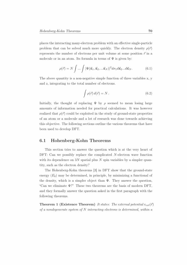
Hohenberg-Kohn Theorems 70
places the interacting many-electron problem with an effective single-particle
problem that can be solved much more quickly. The electron density ρ(~r)
represents the number of electrons per unit volume at some position ~r in a
molecule or in an atom. Its formula in terms of Ψ is given by:
ρ(~r) = N
∫
...
∫
|Ψ(~x1, ~x2, ...~xN )|2dσ1d~x2...d~xN . (6.1)
The above quantity is a non-negative simple function of three variables x, y
and z, integrating to the total number of electrons.
∫
ρ(~r) d(~r) = N . (6.2)
Initially, the thought of replacing Ψ by ρ seemed to mean losing large
amounts of information needed for practical calculations. It was however
realized that ρ(~r) could be exploited in the study of ground-state properties
of an atom or a molecule and a lot of research was done towards achieving
this objective. The following sections outline the various theorems that have
been used to develop DFT.
6.1 Hohenberg-Kohn Theorems
This section tries to answer the question which is at the very heart of
DFT: Can we possibly replace the complicated N -electron wave function
with its dependence on 3N spatial plus N spin variables by a simpler quan-
tity, such as the electron density?
The Hohenberg-Kohn theorems [3] in DFT show that the ground-state
energy (E0) may be determined, in principle, by minimizing a functional of
the density, which is a simpler object than Ψ. They answer the question,
“Can we eliminate Ψ?” These two theorems are the basis of modern DFT,
and they formally answer the question asked in the first paragraph with the
following theorems.
Theorem 1 (Existence Theorem) It states: The external potential vext(~r)
of a nondegenerate system of N interacting electrons is determined, within a
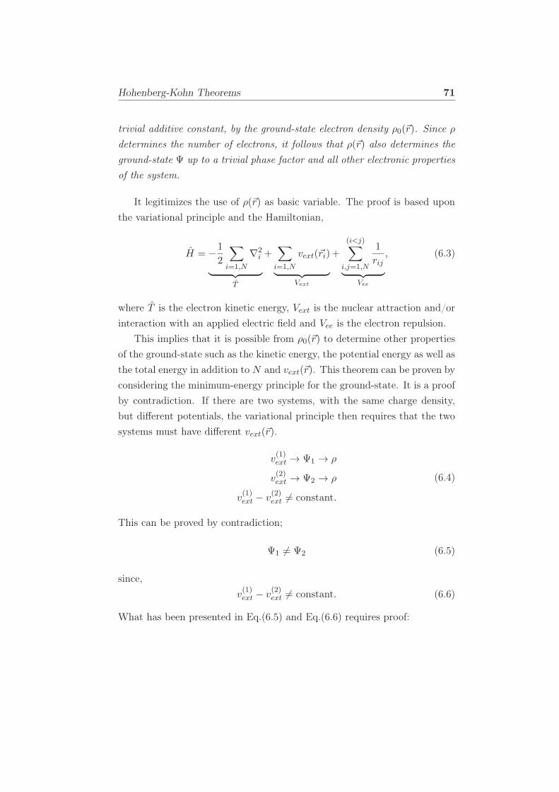
Hohenberg-Kohn Theorems 71
trivial additive constant, by the ground-state electron density ρ0(~r). Since ρ
determines the number of electrons, it follows that ρ(~r) also determines the
ground-state Ψ up to a trivial phase factor and all other electronic properties
of the system.
It legitimizes the use of ρ(~r) as basic variable. The proof is based upon
the variational principle and the Hamiltonian,
H = −1
2
∑
i=1,N
∇2i
︸ ︷︷ ︸
T
+∑
i=1,N
vext(~ri)
︸ ︷︷ ︸
Vext
+
(i<j)∑
i,j=1,N
1
rij︸ ︷︷ ︸
Vee
, (6.3)
where T is the electron kinetic energy, Vext is the nuclear attraction and/or
interaction with an applied electric field and Vee is the electron repulsion.
This implies that it is possible from ρ0(~r) to determine other properties
of the ground-state such as the kinetic energy, the potential energy as well as
the total energy in addition to N and vext(~r). This theorem can be proven by
considering the minimum-energy principle for the ground-state. It is a proof
by contradiction. If there are two systems, with the same charge density,
but different potentials, the variational principle then requires that the two
systems must have different vext(~r).
v(1)ext → Ψ1 → ρ
v(2)ext → Ψ2 → ρ
v(1)ext − v
(2)ext 6= constant.
(6.4)
This can be proved by contradiction;
Ψ1 6= Ψ2 (6.5)
since,
v(1)ext − v
(2)ext 6= constant. (6.6)
What has been presented in Eq.(6.5) and Eq.(6.6) requires proof:
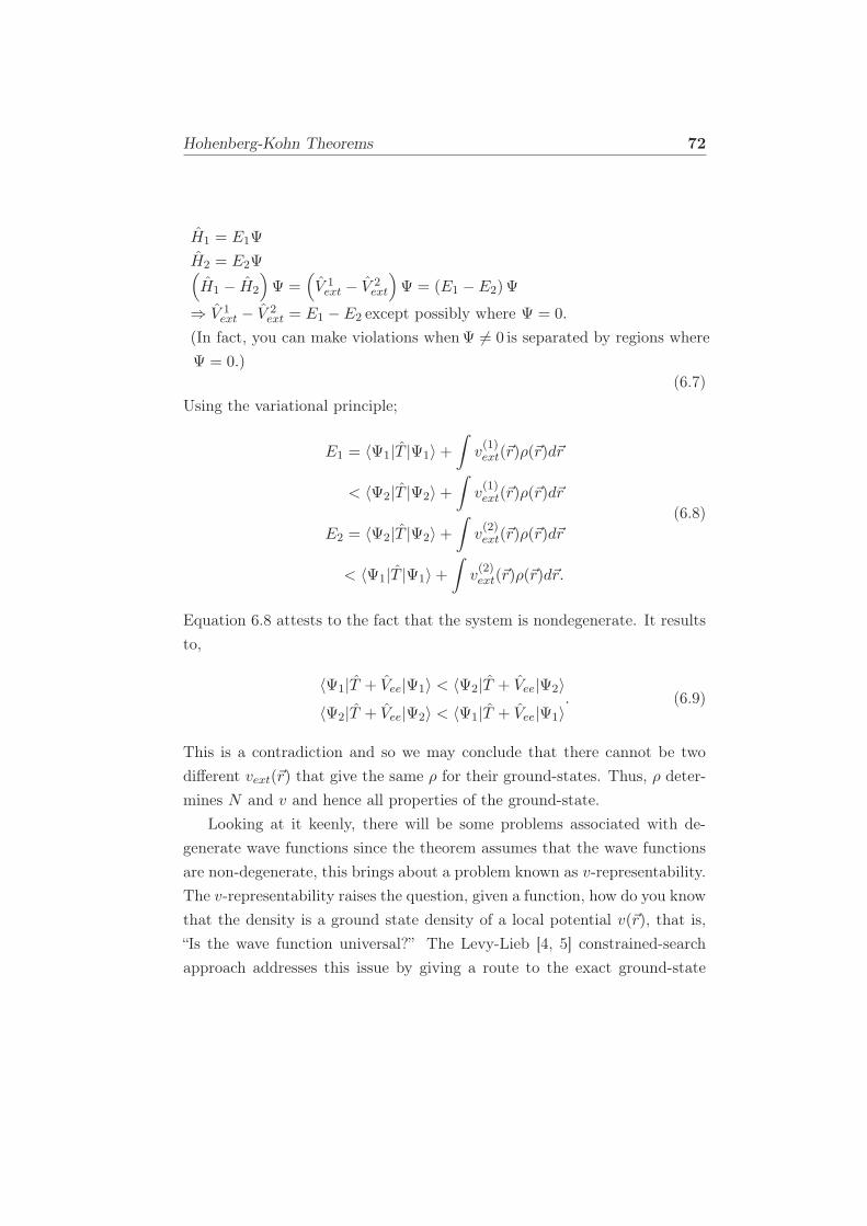
Hohenberg-Kohn Theorems 72
H1 = E1Ψ
H2 = E2Ψ(
H1 − H2
)
Ψ =(
V 1ext − V 2
ext
)
Ψ = (E1 − E2)Ψ
⇒ V 1ext − V 2
ext = E1 − E2 except possibly where Ψ = 0.
(In fact, you can make violations whenΨ 6= 0 is separated by regions where
Ψ = 0.)
(6.7)
Using the variational principle;
E1 = 〈Ψ1|T |Ψ1〉+∫
v(1)ext(~r)ρ(~r)d~r
< 〈Ψ2|T |Ψ2〉+∫
v(1)ext(~r)ρ(~r)d~r
E2 = 〈Ψ2|T |Ψ2〉+∫
v(2)ext(~r)ρ(~r)d~r
< 〈Ψ1|T |Ψ1〉+∫
v(2)ext(~r)ρ(~r)d~r.
(6.8)
Equation 6.8 attests to the fact that the system is nondegenerate. It results
to,
〈Ψ1|T + Vee|Ψ1〉 < 〈Ψ2|T + Vee|Ψ2〉〈Ψ2|T + Vee|Ψ2〉 < 〈Ψ1|T + Vee|Ψ1〉
. (6.9)
This is a contradiction and so we may conclude that there cannot be two
different vext(~r) that give the same ρ for their ground-states. Thus, ρ deter-
mines N and v and hence all properties of the ground-state.
Looking at it keenly, there will be some problems associated with de-
generate wave functions since the theorem assumes that the wave functions
are non-degenerate, this brings about a problem known as v-representability.
The v-representability raises the question, given a function, how do you know
that the density is a ground state density of a local potential v(~r), that is,
“Is the wave function universal?” The Levy-Lieb [4, 5] constrained-search
approach addresses this issue by giving a route to the exact ground-state
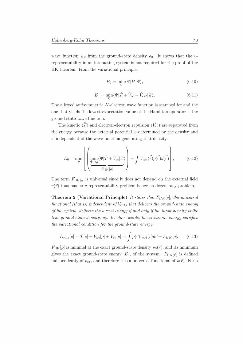
Hohenberg-Kohn Theorems 73
wave function Ψ0 from the ground-state density ρ0. It shows that the v-
representability in an interacting system is not required for the proof of the
HK theorem. From the variational principle,
E0 = minΨ〈Ψ|H|Ψ〉, (6.10)
E0 = minΨ〈Ψ|T + Vee + Vext|Ψ〉, (6.11)
The allowed antisymmetric N -electron wave function is searched for and the
one that yields the lowest expectation value of the Hamilton operator is the
ground-state wave function.
The kinetic ˆ(T ) and electron-electron repulsion ˆ(Vee) are separated from
the energy because the external potential is determined by the density and
is independent of the wave function generating that density.
E0 = minρ
minΨ→ρ
〈Ψ|T + Vee|Ψ︸ ︷︷ ︸
Fhk[ρ]
〉
+
∫
Vext ~(r)ρ ~(r)d ~(r)
, (6.12)
The term Fhk[ρ] is universal since it does not depend on the external field
v(~r) thus has no v-representability problem hence no degeneracy problem.
Theorem 2 (Variational Principle) It states that FHK [ρ], the universal
functional (that is; independent of Vext) that delivers the ground-state energy
of the system, delivers the lowest energy if and only if the input density is the
true ground-state density, ρ0. In other words, the electronic energy satisfies
the variational condition for the ground-state energy.
Evext [ρ] = T [ρ] + Vne[ρ] + Vee[ρ] =
∫
ρ(~r)vext(~r)d~r + FHK [ρ]. (6.13)
Fhk[ρ] is minimal at the exact ground-state density ρ0(~r), and its minimum
gives the exact ground-state energy, E0, of the system. Fhk[ρ] is defined
independently of vext and therefore it is a universal functional of ρ(~r). For a
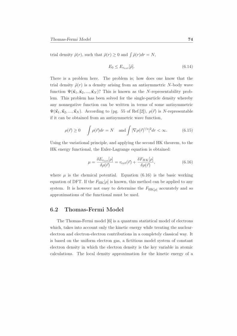
Thomas-Fermi Model 74
trial density ρ(r), such that ρ(r) ≥ 0 and∫ρ(r)dr = N ,
E0 ≤ Evext [ρ]. (6.14)
There is a problem here. The problem is; how does one know that the
trial density ρ(r) is a density arising from an antisymmetric N -body wave
function Ψ(~x1, ~x2, ..., ~xN )? This is known as the N -representability prob-
lem. This problem has been solved for the single-particle density whereby
any nonnegative function can be written in terms of some antisymmetric
Ψ(~x1, ~x2, ..., ~xN ). According to (pg. 55 of Ref.[2]), ρ(~r) is N -representable
if it can be obtained from an antisymmetric wave function,
ρ(~r) ≥ 0
∫
ρ(~r)dr = N and∫
|∇ρ(~r)1/2|2dr <∞. (6.15)
Using the variational principle, and applying the second HK theorem, to the
HK energy functional, the Euler-Lagrange equation is obtained:
µ =δEvext [ρ]
δρ(~r)= vext(~r) +
δFHK [ρ]
δρ(~r), (6.16)
where µ is the chemical potential. Equation (6.16) is the basic working
equation of DFT. If the Fhk[ρ] is known, this method can be applied to any
system. It is however not easy to determine the Fhk[ρ] accurately and so
approximations of the functional must be used.
6.2 Thomas-Fermi Model
The Thomas-Fermi model [6] is a quantum statistical model of electrons
which, takes into account only the kinetic energy while treating the nuclear-
electron and electron-electron contributions in a completely classical way. It
is based on the uniform electron gas, a fictitious model system of constant
electron density in which the electron density is the key variable in atomic
calculations. The local density approximation for the kinetic energy of a
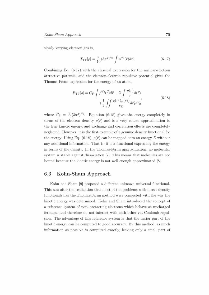
Kohn-Sham Approach 75
slowly varying electron gas is,
Ttf[ρ] =3
10(3π2)
2/3
∫
ρ5/3(~r)d~r. (6.17)
Combining Eq. (6.17) with the classical expression for the nuclear-electron
attractive potential and the electron-electron repulsive potential gives the
Thomas-Fermi expression for the energy of an atom,
Etf[ρ] = CF
∫
ρ5/3 ~(r)d~r − Z
∫ρ(~r)
rd(~r)
+1
2
∫∫ρ(~r1)ρ(~r2)
r12d~r1d~r2
, (6.18)
where Cf = 310(3π
2)2/3. Equation (6.18) gives the energy completely in
terms of the electron density ρ(~r) and is a very coarse approximation to
the true kinetic energy, and exchange and correlation effects are completely
neglected. However, it is the first example of a genuine density functional for
the energy. Using Eq. (6.18), ρ(~r) can be mapped onto an energy E without
any additional information. That is, it is a functional expressing the energy
in terms of the density. In the Thomas-Fermi approximation, no molecular
system is stable against dissociation [7]. This means that molecules are not
bound because the kinetic energy is not well-enough approximated [8].
6.3 Kohn-Sham Approach
Kohn and Sham [9] proposed a different unknown universal functional.
This was after the realization that most of the problems with direct density
functionals like the Thomas-Fermi method were connected with the way the
kinetic energy was determined. Kohn and Sham introduced the concept of
a reference system of non-interacting electrons which behave as uncharged
fermions and therefore do not interact with each other via Coulomb repul-
sion. The advantage of this reference system is that the major part of the
kinetic energy can be computed to good accuracy. By this method, as much
information as possible is computed exactly, leaving only a small part of
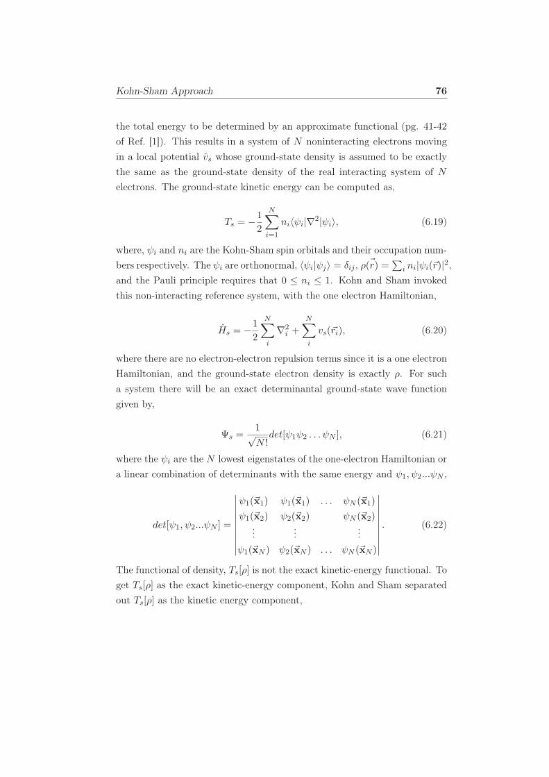
Kohn-Sham Approach 76
the total energy to be determined by an approximate functional (pg. 41-42
of Ref. [1]). This results in a system of N noninteracting electrons moving
in a local potential vs whose ground-state density is assumed to be exactly
the same as the ground-state density of the real interacting system of N
electrons. The ground-state kinetic energy can be computed as,
Ts = −1
2
N∑
i=1
ni〈ψi|∇2|ψi〉, (6.19)
where, ψi and ni are the Kohn-Sham spin orbitals and their occupation num-
bers respectively. The ψi are orthonormal, 〈ψi|ψj〉 = δij , ρ ~(r) =∑
i ni|ψi(~r)|2,and the Pauli principle requires that 0 ≤ ni ≤ 1. Kohn and Sham invoked
this non-interacting reference system, with the one electron Hamiltonian,
Hs = −1
2
N∑
i
∇2i +
N∑
i
vs(~ri), (6.20)
where there are no electron-electron repulsion terms since it is a one electron
Hamiltonian, and the ground-state electron density is exactly ρ. For such
a system there will be an exact determinantal ground-state wave function
given by,
Ψs =1√N !det[ψ1ψ2 . . . ψN ], (6.21)
where the ψi are the N lowest eigenstates of the one-electron Hamiltonian or
a linear combination of determinants with the same energy and ψ1, ψ2...ψN ,
det[ψ1, ψ2...ψN ] =
∣∣∣∣∣∣∣∣∣∣
ψ1(~x1) ψ1(~x1) . . . ψN (~x1)
ψ1(~x2) ψ2(~x2) ψN (~x2)...
......
ψ1(~xN ) ψ2(~xN ) . . . ψN (~xN )
∣∣∣∣∣∣∣∣∣∣
. (6.22)
The functional of density, Ts[ρ] is not the exact kinetic-energy functional. To
get Ts[ρ] as the exact kinetic-energy component, Kohn and Sham separated
out Ts[ρ] as the kinetic energy component,
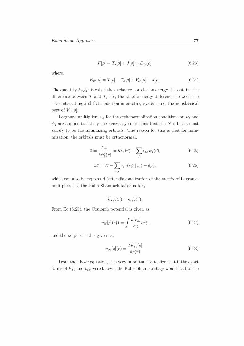
Kohn-Sham Approach 77
F [ρ] = Ts[ρ] + J [ρ] + Exc[ρ], (6.23)
where,
Exc[ρ] = T [ρ]− Ts[ρ] + Vee[ρ]− J [ρ]. (6.24)
The quantity Exc[ρ] is called the exchange-correlation energy. It contains the
difference between T and Ts i.e., the kinetic energy difference between the
true interacting and fictitious non-interacting system and the nonclassical
part of Vee[ρ].
Lagrange multipliers ǫij for the orthonormalization conditions on ψi and
ψj are applied to satisfy the necessary conditions that the N orbitals must
satisfy to be the minimizing orbitals. The reason for this is that for mini-
mization, the orbitals must be orthonormal.
0 =δL
δψ∗i~(r)
= hψi(~r)−∑
j
ǫi,jψj(~r), (6.25)
L = E −∑
i,j
ǫi,j(〈ψi|ψj〉 − δij), (6.26)
which can also be expressed (after diagonalization of the matrix of Lagrange
multipliers) as the Kohn-Sham orbital equation,
hsψi(~r) = ǫiψi(~r).
From Eq.(6.25), the Coulomb potential is given as,
vH [ρ](~r1) =
∫ρ(~r2)
r12d~r2, (6.27)
and the xc potential is given as,
vxc[ρ](~r) =δExc[ρ]
δρ(~r). (6.28)
From the above equation, it is very important to realize that if the exact
forms of Exc and vxc were known, the Kohn-Sham strategy would lead to the
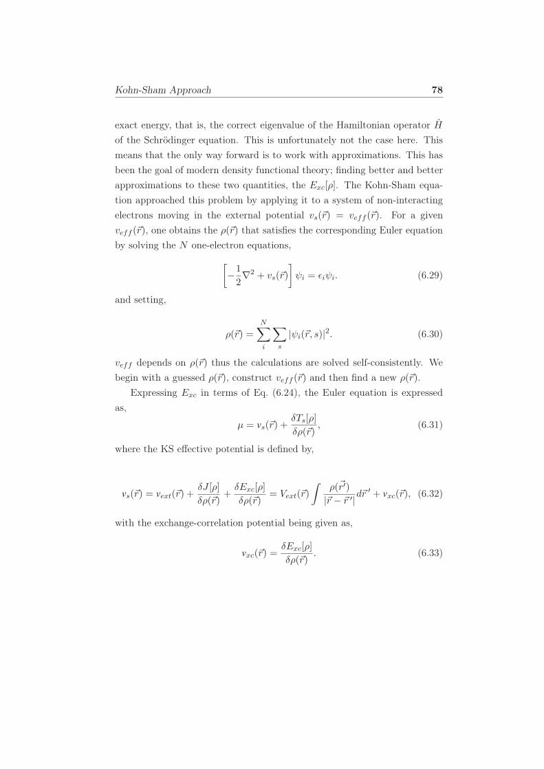
Kohn-Sham Approach 78
exact energy, that is, the correct eigenvalue of the Hamiltonian operator H
of the Schrödinger equation. This is unfortunately not the case here. This
means that the only way forward is to work with approximations. This has
been the goal of modern density functional theory; finding better and better
approximations to these two quantities, the Exc[ρ]. The Kohn-Sham equa-
tion approached this problem by applying it to a system of non-interacting
electrons moving in the external potential vs(~r) = veff (~r). For a given
veff (~r), one obtains the ρ(~r) that satisfies the corresponding Euler equation
by solving the N one-electron equations,
[
−1
2∇2 + vs(~r)
]
ψi = ǫiψi. (6.29)
and setting,
ρ(~r) =N∑
i
∑
s
|ψi(~r, s)|2. (6.30)
veff depends on ρ(~r) thus the calculations are solved self-consistently. We
begin with a guessed ρ(~r), construct veff (~r) and then find a new ρ(~r).
Expressing Exc in terms of Eq. (6.24), the Euler equation is expressed
as,
µ = vs(~r) +δTs[ρ]
δρ(~r), (6.31)
where the KS effective potential is defined by,
vs(~r) = vext(~r) +δJ [ρ]
δρ(~r)+δExc[ρ]
δρ(~r)= Vext(~r)
∫ρ(~r′)
|~r − ~r ′|d~r′ + vxc(~r), (6.32)
with the exchange-correlation potential being given as,
vxc(~r) =δExc[ρ]
δρ(~r). (6.33)
Exchange-Correlation Approximations (Jacob’s Ladder) 79
6.4 Exchange-Correlation Approximations (Jacob’s
Ladder)
In the previous section, it has been shown that the Kohn-Sham formalism
allows an exact treatment of most of the contributions to the electronic
energy of an atomic or molecular system, including the major fraction of
the kinetic energy. The remaining unknown parts are summed into the
exchange-correlation functional Exc[ρ]. The exact form of this functional
is not known and an approximate description is used instead. The quality
of the density functional approach depends solely on the accuracy of the
chosen approximation to Exc. The following sections outline some of the Excfunctionals that have been developed over time. Ideally, these functionals
can be classified into two major classes, those that are based on the electronic
wave function (generalized Kohn-Sham theory) and those that are based on
the electron density (pure density functionals).
6.4.1 Local Density Approximation(LDA)
In summary, the Exc employs only the local density at each point. The
exchange-correlation functionals are guided by studies of the hypothetical
uniform electron gas because it is the only system for which the form of
the exchange and correlation energy functionals is known exactly or at least
to very high accuracy. LDA assumes that the density ρ(~r) can be treated
locally as an uniform electron gas (UEG); the exchange-correlation density
at each point in the system is the same as that of an uniform electron gas of
the same density. Exc is given as,
ELDAxc =
∫
ǫUEGxc (ρ(~r))ρ(~r)d~r, (6.34)
where ǫUEGxc is the exchange-correlation energy per particle of a uniform
electron gas of density ρ(~r). The energy per particle is weighted with the
probability ρ(~r) that there is an electron at this position in space. ǫUEGxc (ρ(~r)
Exchange-Correlation Approximations (Jacob’s Ladder) 80
can be further divided into exchange and correlation contributions,
ǫxc(ρ(~r)) = ǫx(ρ(~r)) + ǫc(ρ(~r)). (6.35)
The ǫx(ρ(~r)) is known and it is given by the Hartree Fock exchange for the
homogeneous electron gas,
ǫx(ρ(~r)) = −3
4
(3
πρ (~r)
)1/3
. (6.36)
Replacing the above in Eq. (6.34) gives the ρ4/3(~r) of the exchange energy. For
the correlation part, ǫc(ρ(~r)) such an explicit expression is not known. For
the ǫx(ρ(~r)), accurate values can be obtained courtesy of quantum Monte-
Carlo calculations of the homogeneous electron gas by Ceperly and Alder
[10, 11]. Based on results from the explicit calculations, authors have come
up with an approximate analytic expression for ǫc. Some of the ǫc expressions
include that by Vosko, Wilk, and Nusair [12], Perdew and Wang [13] and
Perdew, Burke and Ernzerhof [14]. The LDA has an advantage of producing
many experimentally relevant physical properties to a good level of accu-
racy in strongly bound systems. It however tends to overestimate bonding
energies as well as underestimating bond lengths.
6.4.2 Generalized Gradient Approximation (GGA)
The accuracy that was achieved by using the LDA was not sufficient for
most applications in chemistry. This is because LDA used only the infor-
mation about the density ρ(~r) at a particular point ~r. What the GGA does
is to bring in information about the gradient of the charge density, ~∇ρ(~r)to account for the true in-homogeneous electron density. The local density
approximation is interpreted as the first term of a Taylor expansion of the
uniform density, resulting in,
EGEAxc [ρ] =
∫
ǫUEGxc (ρ)ρ(~r)d~r +
∫
Cxc(ρ(~r))x(~r)d~r, (6.37)
where the reduced gradient is given by,
Exchange-Correlation Approximations (Jacob’s Ladder) 81
x(~r) =|~∇ρ(~r)|ρ4/3(~r)
. (6.38)
Equation (6.37) is known as the gradient expansion approximation (GEA).
The GEA did not however perform to the required expectations in that there
was no improved accuracy and it often performed even worse than the simple
local density approximation. The generalized gradient approximation, GGA,
was the more successful approach,
EGGAxc =
∫
ǫxc(ρ(~r), x(~r))ρ(~r)d~r. (6.39)
Different versions of the GGA include the Perdew and Wang (PW91) [15],
Perdew, Burke, and Enzerhof (PBE) [14] and Beeke-Lee-Yang-Parr (BLYP)
[16, 17].
6.4.3 Hybrid Functionals
These functionals mix a fraction of exact exchange (Hartree-Fock ex-
change) with GGA exchange and correlation [18, 19]. The simplest hybrid
functional takes the form,
Ehybxc = aEexactxc + (1− a)EGGAx + EGGAc , (6.40)
where the constant a ≈ 1/4 for molecules from empirical or theoretical esti-
mations [20].
All the calculations in this work utilized the B3LYP (Becke, three-parameter,
Lee-Yang-Parr) hybrid functional [12, 17, 18, 21]. It takes the form,
EB3LY Pxc = (1−a)ELDAx +aELDAxc + bEB88
x + cELY Pc +(1− c)ELDAc . (6.41)
where a = 0.20, b = 0.72, and c = 0.81 from the B3P functional [18], LDA
is the local density approximation, B88 is Becke’s 1988 generalized gradient
approximation (GGA) for exchange, and LYP is the Lee, Yang, and Parr’s
1988 GGA for correlation. At this point in time, it is important to note that
with the improvements, these functionals are perhaps the most accurate
Exchange-Correlation Approximations (Jacob’s Ladder) 82
density functionals in use for quantum chemical calculations having been
used for many calculations in the recent years and currently.
6.4.4 Meta-Generalized Gradient Approximation (meta-GGA)
Meta-GGAs (mGGAs) [22], in addition to the local density and the first
gradient as input, also requires the orbital kinetic energy density. The corre-
lation energy in this functional is free of self-interaction error. Meta-GGAs
significantly improve the molecular atomization energies and metal surface
energies compared to GGA while the lattice constants are changed slightly.
The general form [23] of the mGGA is,
EXC [ρ] =
∫
exc(ρ(~r),∇ρ(~r), τ(~r))ρ(~r) d~r, (6.42)
where the kinetic-energy density is given by;
τ(~r) =1
2
∑
i
[
~∇ψi(~r)]
.[
~∇ψi(~r)]
︸ ︷︷ ︸
|~∇ψi(~r)|2
. (6.43)
6.4.5 Double hybrid functionals
Double hybrid functionals [24] include a certain amount of HF exchange
with semilocal exchange density functional and second-order Møller-Plesset
(MP2) correlation with a semilocal correlation density functional. This func-
tional includes unoccupied KS orbitals in the calculation.
6.4.6 Jacob’s Ladder of Density Functional Approximations
Jacob’s ladder of density functional approximations [26] gives the line
of development of density functionals for the exchange-correlation energy.
It suggests moving from the Hartree world up to the Heaven of chemical
accuracy. As shown in Fig. 6.1, the ladder has five rungs, each corresponding
to the increase in complexity of choices for the ingredients of the energy
density. At the lowest rung of the ladder, rung 1, the dependence is on
the local density only (LDA), followed by rung 2 where there is an explicit
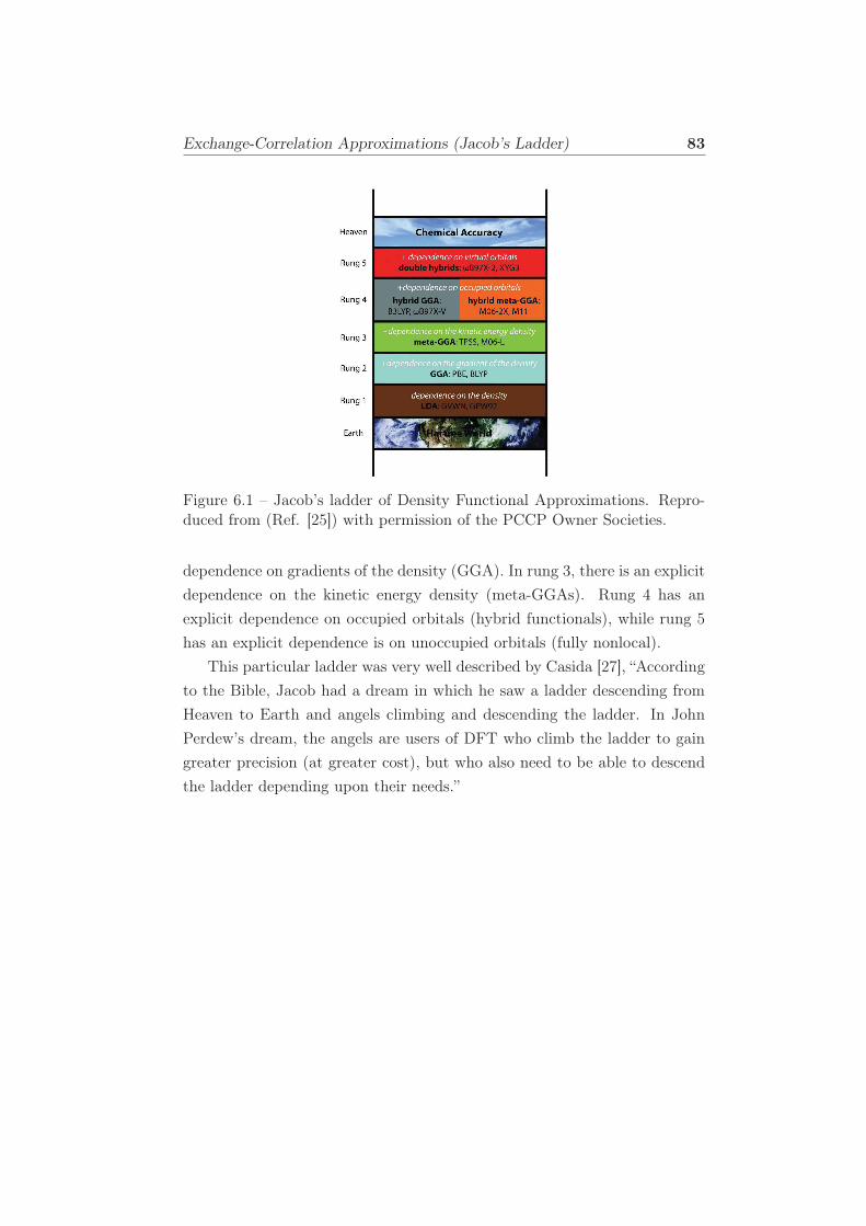
Exchange-Correlation Approximations (Jacob’s Ladder) 83
Figure 6.1 – Jacob’s ladder of Density Functional Approximations. Repro-duced from (Ref. [25]) with permission of the PCCP Owner Societies.
dependence on gradients of the density (GGA). In rung 3, there is an explicit
dependence on the kinetic energy density (meta-GGAs). Rung 4 has an
explicit dependence on occupied orbitals (hybrid functionals), while rung 5
has an explicit dependence is on unoccupied orbitals (fully nonlocal).
This particular ladder was very well described by Casida [27], “According
to the Bible, Jacob had a dream in which he saw a ladder descending from
Heaven to Earth and angels climbing and descending the ladder. In John
Perdew’s dream, the angels are users of DFT who climb the ladder to gain
greater precision (at greater cost), but who also need to be able to descend
the ladder depending upon their needs.”
BIBLIOGRAPHY 84
Bibliography
[1] W.Koch and M.C. Holthausen. A Chemist’s Guide to Density Func-
tional Theory. Wiley/VCH, Weinheim, 2001.
[2] R. G. Parr and W. Yang. Density Functional Theory of Atoms and
Molecules. Oxford University Press, New York, 1989.
[3] P. Hohenberg and W. Kohn. Inhomogeneous electron gas. Phys. Rev.,
136(3B):B864, 1964.
[4] Mel Levy. Universal variational functionals of electron densities, first-
order density matrices, and natural spin-orbitals and solution of the
v-representability problem. P. Nat. Acad. Sci., 76(12):6062–6065, 1979.
[5] Elliott H. Lieb, R. M. Dreizler, and J da Providencia. Density functional
methods in physics. Nato Asi Series B, 123, 1985.
[6] L. H. Thomas. The calculation of atomic fields. In Mathematical Pro-
ceedings of the Cambridge Philosophical Society, volume 23, pages 542–
548. Cambridge Univ Press, 1927.
[7] E. Teller. On the stability of molecules in the Thomas-Fermi theory.
Rev. Mod. Phys., 34:627–631, Oct 1962. doi: 10.1103/RevModPhys.34.
627. URL https://link.aps.org/doi/10.1103/RevModPhys.34.627.
[8] E. H. Lieb. Thomas-Fermi and related theories of atoms and molecules.
Rev. Mod. Phys., 53(4):603, 1981.
[9] W. Kohn and L. J. Sham. Self-consistent equations including exchange
and correlation effects. Phys. Rev., 140:A1133, 1965.
[10] D. M. Ceperley and B. J. Alder. Ground state of the electron gas by a
stochastic method. Phys. Rev. Lett., 45(7):566, 1980.
[11] G. Ortiz and P. Ballone. Correlation energy, structure factor, radial
distribution function, and momentum distribution of the spin-polarized
uniform electron gas. Phys. Rev. B, 50(3):1391, 1994.
BIBLIOGRAPHY 85
[12] S. H. Vosko, L. Wilk, and M. Nusair. Accurate spin-dependent electron
liquid correlation energies for local spin density calculations: A critical
analysis. Can. J. Phys., 58(8):1200–1211, 1980.
[13] J. Perdew and Y. Wang. Accurate and simple analytic representation of
the electron-gas correlation energy. Phys. Rev. B, 45(23):13244, 1992.
[14] J. P. Perdew, K. Burke, and M. Ernzerhof. Generalized gradient ap-
proximation made simple. Phys. Rev. Lett., 77(18):3865, 1996.
[15] J. P. Perdew, J. A. Chevary, S. H. Vosko, K. A. Jackson, M. R. Pederson,
D. J. Singh, and C. Fiolhais. Atoms, molecules, solids, and surfaces:
Applications of the generalized gradient approximation for exchange
and correlation. Phys. Rev., B 46:6671, 1993.
[16] A. D. Becke. Density-functional exchange-energy approximation with
correct asymptotic behavior. Phys. Rev. A, 38(6):3098, 1988.
[17] C. Lee, W. Yang, and R. G. Parr. Development of the Colle-Salvetti cor-
relation energy formula into a functional of the electron density. Phys.
Rev. B, 37:785, 1988.
[18] A. D. Becke. Density-functional thermochemistry. III. The role of exact
exchange. J. Chem. Phys., 98:5648, 1993.
[19] A. D. Becke. A new mixing of Hartree-Fock and local density-functional
theories. J. Chem. Phys., 98(2):1372–1377, 1993.
[20] J. P. Perdew, M. Ernzerhof, and K. Burke. Rationale for mixing exact
exchange with density functional approximations. J. Chem. Phys., 105
(22):9982–9985, 1996.
[21] P. J. Stephens, F. J. Devlin, C. F. Chabalowski, and M. J. Frisch.
Ab initio calculation of vibrational absorption and circular dichroism
spectra using density functional force fields. J. Phys. Chem., 98(45):
11623–11627, 1994.
BIBLIOGRAPHY 86
[22] J. P. Perdew, S. Kurth, A. Zupan, and P. Blaha. Accurate density
functional with correct formal properties: A step beyond the generalized
gradient approximation. Phys. Rev. Lett., 82(12):2544, 1999.
[23] F. Zahariev, S. S. Leang, and M. S. Gordon. Functional derivatives of
meta-generalized gradient approximation (meta-GGA) type exchange-
correlation density functional. J. Chem. Phys., 138(24):244108, 2013.
[24] Y. Zhao, B. J. Lynch, and D. G. Truhlar. Doubly hybrid meta DFT:
New multi-coefficient correlation and density functional methods for
thermochemistry and thermochemical kinetics. J. Phys. Chem. A, 108
(21):4786–4791, 2004.
[25] N. Mardirossian and M. Head-Gordon. ωB97X-V: A 10-parameter,
range-separated hybrid, generalized gradient approximation density
functional with nonlocal correlation, designed by a survival-of-the-fittest
strategy. Phys. Chem. Chem. Phys., 16(21):9904–9924, 2014.
[26] J. P. Perdew and K. Schmidt. Jacob’s ladder of density functional
approximations for the exchange-correlation energy. In AIP Conference
Proceedings, pages 1–20. IOP Institute of Physics Publishing Limited,
2001.
[27] M. E. Casida. John perdew’s Jacob’s ladder. https://sites.google.
com/site/markcasida/dft, 2015. online; accessed 27th August, 2015.
Chapter 7
Basis Sets and Effective Core
Potentials
Basis sets form the core of quantum mechanical calculations since they
are used to provide the best representation of the unknown molecular or-
bitals. To solve the Hartree-Fock equation, there is need to choose a nu-
merical method. A basis set comes in handy for this purpose, either the
Gaussian-type orbitals (GTOs) or Slater-type orbitals (STOs). In this chap-
ter, the description of what a basis set is, how it works, and different types
is given. In this work, ruthenium polypyridine complexes have been studied
extensively. Ruthenium is classified as a heavy atom and this explains why
there is also a review of the effective core potentials (ECPs) which are used
to include scalar relativistic effects of core electrons.
7.1 Definition of a Basis Set
A basis set is a mathematical description of orbitals of a system, which
is used for the purpose of approximate theoretical calculations [1]. As men-
tioned earlier on, introducing a basis set which ideally is a linear combination
of atomic orbitals (LCAO, MO=LCAO) transforms the Hartree-Fock equa-
tions into the Roothaan equations [2]. Each unknown MO is expanded as
a linear combination of three dimensional one electron functions, known as
87

Types of Basis Functions (Atomic Orbitals) 88
atomic orbitals. Denoting the atomic orbital basis functions as χµ, for each
spin orbital i,
ψi(~r) =
K∑
µ=1
χµ(~r)Cµi (7.1)
where K is an integer relating to the size of the basis set larger than the
number of electrons in the system.
Any wave function may be expanded as a linear combination of a com-
plete set of basis functions, hence not an approximation. This kind of a
basis set requires that an infinite number of functions must be used, which
is normally impossible in actual calculations. Use of a finite basis set usu-
ally implies that the MO is approximate [3]. Keeping the total number of
basis functions to a minimum is computationally attractive but it is more
useful to choose basis set functional forms that permit the various integrals
appearing in the HF equations to be evaluated in a computationally efficient
fashion. The basis functions must be chosen to have a form that is useful
in a chemical sense in that the functions should have large amplitude in re-
gions of space where the electron probability density is also large and small
amplitudes where the probability density is small.
7.2 Types of Basis Functions (Atomic Orbitals)
The types of basis sets used in atomistic modelling is extremely diverse.
Atomistic calculations often use spherical symmetry to reduce the Scrödinger
equation to a one-dimensional problem which may be solved by numerical
integration. A similar approach is possible for diatomics. Some polyatomic
quantum chemistry programs use tabulated numerical atomic orbitals as ba-
sis functions, however by far the most popular choice in molecular calcula-
tions has been the use of analytic basis functions. These may be divided into
two types according to whether their decay with the radial variable r is ex-
ponential [Slater-type orbitals (STOs)(e−ζr)] [4] or Gaussian [Gaussian-type
orbitals (GTOs)(e(−αr2))].
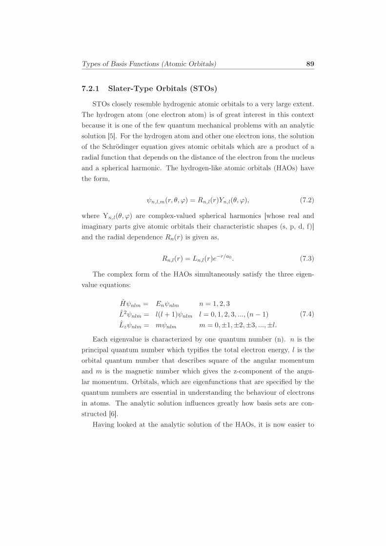
Types of Basis Functions (Atomic Orbitals) 89
7.2.1 Slater-Type Orbitals (STOs)
STOs closely resemble hydrogenic atomic orbitals to a very large extent.
The hydrogen atom (one electron atom) is of great interest in this context
because it is one of the few quantum mechanical problems with an analytic
solution [5]. For the hydrogen atom and other one electron ions, the solution
of the Schrödinger equation gives atomic orbitals which are a product of a
radial function that depends on the distance of the electron from the nucleus
and a spherical harmonic. The hydrogen-like atomic orbitals (HAOs) have
the form,
ψn,l ,m(r, θ, ϕ) = Rn,l (r)Yn,l (θ, ϕ), (7.2)
where Yn,l (θ, ϕ) are complex-valued spherical harmonics [whose real and
imaginary parts give atomic orbitals their characteristic shapes (s, p, d, f)]
and the radial dependence Rn(r) is given as,
Rn,l(r) = Ln,l(r)e−r/a0 . (7.3)
The complex form of the HAOs simultaneously satisfy the three eigen-
value equations:
Hψnlm = Enψnlm n = 1, 2, 3
L2ψnlm = l(l + 1)ψnlm l = 0, 1, 2, 3, ..., (n− 1)
Lzψnlm = mψnlm m = 0,±1,±2,±3, ...,±l.(7.4)
Each eigenvalue is characterized by one quantum number (n). n is the
principal quantum number which typifies the total electron energy, l is the
orbital quantum number that describes square of the angular momentum
and m is the magnetic number which gives the z-component of the angu-
lar momentum. Orbitals, which are eigenfunctions that are specified by the
quantum numbers are essential in understanding the behaviour of electrons
in atoms. The analytic solution influences greatly how basis sets are con-
structed [6].
Having looked at the analytic solution of the HAOs, it is now easier to
Types of Basis Functions (Atomic Orbitals) 90
link STOs to hydrogenic atomic orbitals. STOs have the form,
Yl,m(θ, ϕ)rn−1e−ζr or xnymzle−ζr
or[ζ3
π
]0.5e−ζr(Simplified equation for hydrogen-like systems).
(7.5)
The distance between the nucleus and electron has an exponential de-
pendence that mirrors the exact orbitals for the hydrogen atom. STOs differ
from HAOs in the radial part Rn(r), which is independent of l. One obvious
implication of this difference is that STOs do not possess radial nodes like
a real atomic orbital because of the wrong behaviour of the ns functions
when n > 1 resulting in some loss of orthogonality. By making LCAO of
STOs, the radial nodes can be introduced (Schmidt orthogonalization) [7].
Owing to the large number of the integrals needed for computation, STOs
face a problem in the analytical calculation of integrals centered on three or
four different atoms. This limits their utility in molecular systems of any
significant size because of the difficulty in calculation of integrals which is
computationally very expensive. It is still possible to use STOs for atomic
and diatomic calculations where such restrictions do not exist [3, 8, 9]. STOs
exhibit correct short and long range behaviour. One of the commercial codes
that use the STOs even for polyatomic molecules is the Amsterdam Den-
sity Functional code, (ADF)[10].
7.2.2 Gaussian-type orbitals (GTOs)
GTOs come in as a solution to the problem of STOs, which is, the diffi-
culty of calculating certain matrix elements in the Fock matrix. GTOs which
contain the exponential (e−αr2
), replace the STOs (e−ζr) with functions that
look like STOs but in which the matrix elements can be calculated in an eas-
ier way. The aspect of simplification arises from the fact that the product
of two GTOs at two different positions can be rewritten as a GTO centered
between these two positions. GTOs have the form,
Yl,m(θ, ϕ)rn−1e−αr
2
or xnymzle−αr2 (7.6)
Types of Basis Functions (Atomic Orbitals) 91
One major difference between STOs and GTOs is that the r-factor of the
exponential in GTO is squared. Although GTOs are convenient to use from a
computational point of view, the exponential difference leads to two obvious
problems arising from their use: first, faster decay at larger r , consequently
leading to poor approximation of the true radial function in the outer region
and secondly, lack of cusps (discontinous derivative) at r = 0 compared to
real HAOs that have a cusp hence improper representation of the behaviour
near the nucleus. Both the STOs (gives proper radial shape) and GTOs
(computational efficiency) have attractive features that any computational
chemist would love to combine for purposes of computational efficiency and
accuracy. The question is, how can we do this? It is possible by linearly
combining several GTOs (primitive Gaussians) with fixed coefficients to form
the contracted GTO. One would expect that with contracted GTOs there
will be lack of accuracy, but this is not the case because the core orbitals are
insensitive to the molecular environment hence making linear combination
possible. Primitive Gaussians are the original GTOs centered on the same
nucleus. They have a standardized form and some examples corresponding
to s, p, d, and f atomic orbitals are represented as:
s function : e−αr2
,
p function : (x, y, z)e−αr2
,
d function : (x2, y2, z2, xy, yz, zx)e−αr2
,
f function : (x3, y3, z3, x2y, x2z, xy2, y2z, yz2, xz2, xyz)e−αr2
,
(7.7)
Mathematically, a contracted GTO with three Gaussians (3G) can be defined
as,
e(−αr) ≈ c1e−α1r2 + c2e
−α2r2 + c3e−α3r2 (7.8)
There are 6 cartesian d functions. This is a consequence of the fact that the
x2 + y2 + z2 = r2 combination is really an s function. Similar remark for
the f functions times the appropriate angular part xn + ym + zl. There are
various types of functions for contracted GTOs; these will be discussed later
Classification of Basis Sets 92
on in this chapter. In quantum chemistry, GTOs dominate for molecular
computation owing to the large number of integrals that must be computed.
7.3 Classification of Basis Sets
7.3.1 Minimal Basis Sets (Single Zeta)
An AO is described by one STO (or STO-like) basis function. In this basis
set, a minimal number of functions are used to represent all the electrons
of the ground state atoms and any empty valence orbitals. To explain this
further, specific examples of H (1s1) and C (1s22s22p2) atoms are considered.
The minimal basis set for hydrogen is one “1s” orbital and “1s” orbital, “2s”
orbital and the full set of three “2p” orbitals for the carbon atom respectively.
For the methane molecule, the total number of basis sets can be calculated
as; 4×(1s)+1s+2s+2px, 2py, 2pz = 9 basis functions [11]. There are several
minimal basis sets that are used in computation. The STO-nG [12–15] basis
sets approximating STOs akin to AOs with n primitive functions is the most
common. It is a linear combination of n GTOs fitted to each STO. Some
examples include STO-3G, STO-4G, STO-6G. The STO-3G basis set implies
that each basis function is a contraction of three primitive Gaussians. Its
radial part can be written as;
STO-3G = c1e−α1r2 + c2e
−α2r2 + c3e−α3r2 . (7.9)
Another example of the minimal basis set is the MINI sets of Huzinaga
and co-workers [13] such as the MINI-1, MINI-2. The difference comes in
from the number of primitives used for different kinds of functions. Minimal
basis sets are unsuitable in calculations including electron correlation. They
provide poor results for molecules owing to their inadequacy at describing the
process of bond formation and deviation from the spherical symmetry [12].
Another weakness is that energies and wave functions from minimal basis
set are not very close to the HF limits. For more accurate calculations, more
extensive basis sets must be used. The next basis set involves improvement
of the minimal basis set.
Classification of Basis Sets 93
7.3.2 Double, Triple and Multi Zeta (ζ) Basis Sets and Split
Valence Basis Sets
Each AO is described by two basis functions for the double zeta (DZ),
three basis functions for the triple zeta (TZ) and four basis functions for the
quadruple zeta (QZ) basis sets. A DZ basis set uses two s-functions for 1s
(1s and 1s’), four s-functions for 1s and 2s (1s, 1s’, 2s and 2s’) and two sets
of p-functions (2p and 2p’) for first row elements. DZ basis sets make better
descriptions of bond formation because they describe bonding in different
directions uniquely [12]. Increasing the size of the basis functions has an
advantage of inching closer and closer to the HF limit. Chemical intuition
helps in deciding which AOs to add. The most significant observation is that
core orbitals hardly participate in chemical bonding while valence orbitals
mainly contribute to chemical bonding. This chemical consequence ideally
means that flexibility in the valence basis functions is more beneficial than in
the core; therefore, many basis functions should be used for valence orbitals
to calculate electronic states accurately. If, for instance, we look at atoms
bonded to more electropositive elements, they will take on partial negative
charge from loss of valence electrons, thus affecting the density distribution
of the remaining electrons [16]. This particular observation brought in the
development of the ‘split valence’ or ‘valence-multiple-ζ’ basis sets.
Split valence (SV) basis functions split each valence orbital into two parts,
an inner shell and an outer shell. One type of contracted Gaussian-type func-
tion is used for core orbitals and multiple contracted functions for valence
orbitals. Some examples of SV basis sets developed by Pople [17] are 3-
21G, 6-21G, 4-31G, 6-31G and 6-311G. It is easy to identify the contraction
method used in the SV basis set from its naming. The number of primitives
used in the contracted core functions is indicated by the first number. Pre-
ceding numbers after the hyphen show the numbers of primitives used in the
valence functions. Two such numbers indicate that it is a valence-double-ζ
basis and three numbers, valence-triple-ζ. To illustrate this, for the 6-31G
basis set, ‘6’ means 6 primitive functions for core orbitals and ‘31’ means the
use of doubly-split basis functions combining contracted basis functions of 3
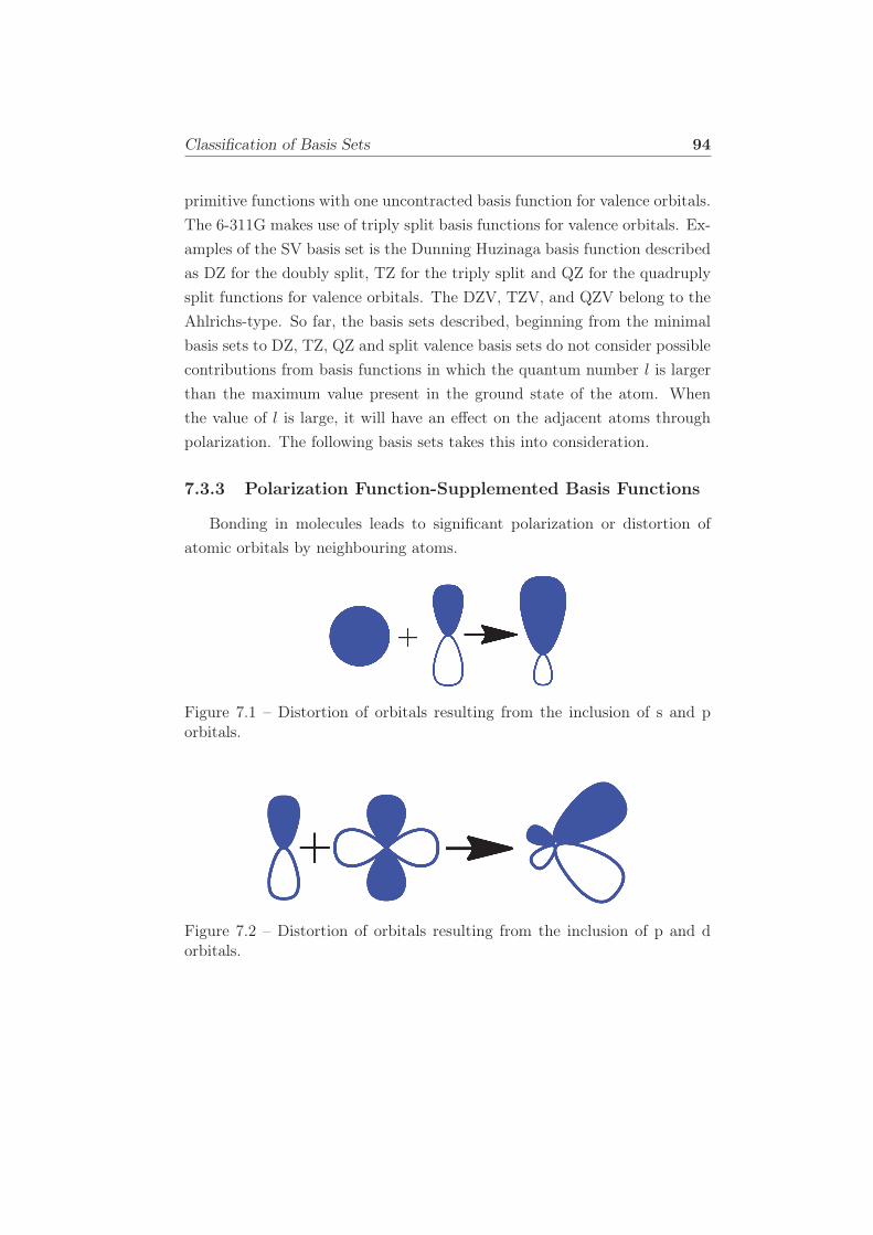
Classification of Basis Sets 94
primitive functions with one uncontracted basis function for valence orbitals.
The 6-311G makes use of triply split basis functions for valence orbitals. Ex-
amples of the SV basis set is the Dunning Huzinaga basis function described
as DZ for the doubly split, TZ for the triply split and QZ for the quadruply
split functions for valence orbitals. The DZV, TZV, and QZV belong to the
Ahlrichs-type. So far, the basis sets described, beginning from the minimal
basis sets to DZ, TZ, QZ and split valence basis sets do not consider possible
contributions from basis functions in which the quantum number l is larger
than the maximum value present in the ground state of the atom. When
the value of l is large, it will have an effect on the adjacent atoms through
polarization. The following basis sets takes this into consideration.
7.3.3 Polarization Function-Supplemented Basis Functions
Bonding in molecules leads to significant polarization or distortion of
atomic orbitals by neighbouring atoms.
Figure 7.1 – Distortion of orbitals resulting from the inclusion of s and porbitals.
Figure 7.2 – Distortion of orbitals resulting from the inclusion of p and dorbitals.
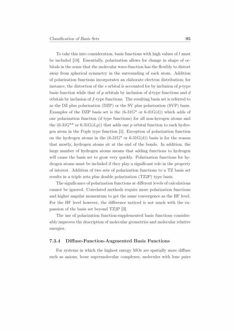
Classification of Basis Sets 95
To take this into consideration, basis functions with high values of l must
be included [18]. Essentially, polarization allows for change in shape of or-
bitals in the sense that the molecular wave-function has the flexibly to distort
away from spherical symmetry in the surrounding of each atom. Addition
of polarization functions incorporates an elaborate electron distribution; for
instance, the distortion of the s orbital is accounted for by inclusion of p-type
basis function while that of p orbitals by inclusion of d-type functions and d
orbitals by inclusion of f -type functions. The resulting basis set is referred to
as the DZ plus polarization (DZP) or the SV plus polarization (SVP) basis.
Examples of the DZP basis set is the (6-31G* or 6-31G(d)) which adds of
one polarization function (d type functions) for all non-hyrogen atoms and
the (6-31G** or 6-31G(d,p)) that adds one p orbital function to each hydro-
gen atom in the Pople type function [1]. Exception of polarization function
on the hydrogen atoms in the (6-31G* or 6-31G(d)) basis is for the reason
that mostly, hydrogen atoms sit at the end of the bonds. In addition, the
large number of hydrogen atoms means that adding functions to hydrogen
will cause the basis set to grow very quickly. Polarization functions for hy-
drogen atoms must be included if they play a significant role in the property
of interest. Addition of two sets of polarization functions to a TZ basis set
results in a triple zeta plus double polarization (TZ2P) type basis.
The significance of polarization functions at different levels of calculations
cannot be ignored. Correlated methods require more polarization functions
and higher angular momentum to get the same convergence as the HF level.
For the HF level however, the difference noticed is not much with the ex-
pansion of the basis set beyond TZ2P [3].
The use of polarization function-supplemented basis functions consider-
ably improves the description of molecular geometries and molecular relative
energies.
7.3.4 Diffuse-Function-Augmented Basis Functions
For systems in which the highest energy MOs are spatially more diffuse
such as anions, loose supermolecular complexes, molecules with lone pairs
Classification of Basis Sets 96
(notably hydrogen-bonding N, O and F atoms) and highly excited electronic
states than standard valence size functions, diffuse basis functions are used to
allow the weakly bound electrons to localize far from the remaining electron
density. This means that the orbitals are able to occupy a larger region of
space [16]. Addition of a diffuse function is shown by a plus (+) in Pople-type
basis functions. Examples include the 6-31+G(d) basis set in which one s and
one set of p functions have been added to the heavy atoms. 6-3l++G(d),
adds diffuse functions to the H atoms too. Addition of diffuse functions
on hydrogen atoms often makes a noticeable change in accuracy. Other
examples are in the MIDI! and MIDIY basis sets in which diffuse sp sets
have augmented leading to MIDIX+ and MIDIY+. The ‘aug’ prefix is used
to indicate the presence of diffuse fucnctions for the correlation consistent
basis sets cc-pVnZ. Examples under this family are aug-cc-pVTZ which has
diffuse f, d, p, and s functions on heavy atoms and diffuse d, p, and s functions
on H and He.
Diffuse-function-augmented basis functions produce better results for the
calculation of acidities and electron affinities.
7.3.5 Effective Core Potential (ECP) Basis Functions (Pseu-
dopotentials)
The previous types of basis sets discussed mainly deal with the first and
second row elements of the periodic table. As we move towards the third row
elements and beyond (heavy elements), there is an increase in the number
of electrons and this poses several challenges to a computational chemist.
The first challenge is that with the increase in the number of electrons and
orbitals, a large number of basis functions are required to describe them.
Since most of these electrons are core, there is a challenge to represent them
adequately. The second challenge is that the core electrons in heavy elements
reach velocities sufficiently close speed of light that they show relativistic
effects. Relativistic effects have an effect on geometries, energies and other
properties. It is impossible for a non-relativistic Hamiltonian operator to
account for such effects. The third challenge is reduction in the speed of ab-
Classification of Basis Sets 97
initio calculations due to the large number of two-electron repulsion integrals
involved. These problems can be circumvented by using an ECP [19].
An ECP or pseudo-potential adds to the Fock operator a one-electron
operator which treats core electrons as an imaginary sphere of dense charge
distribution providing a highly repulsive potential and preventing the va-
lence electrons from collapsing into the inner orbital [1]. In the N electron
HF Roothan-Hall equations, the core electrons are replaced by an effective
potential function instead of being counted explicitly. ECPs drastically re-
duce the number of basis functions, incorporate the relativistic effects of the
core electrons and speed up calculations by reducing the scope of the elec-
tronic structure problem for heavy elements. ECPs obey the Pauli exclusion
principle.
The construction of ECPs is dependent on the number of electrons to be
included in the core. Based on this, ECPs can largely be classified into two;
‘large-core’ ECPs which include everything except the outermost (valence)
shell and ‘small-core’ ECPs which scale back to the next lower shell. For
calculations involving heavier metals, the small-core ECPs that include the
sub valence shell are preferred because polarization of the sub shell has some
chemical consequences. Examples of ECP basis functions are LanL2DZ, of
Los Alamos National Laboratory (DZ means double-zeta) and the Stuttgart
relativistic small core (STRSC) and large core (STRLC) ECP basis functions
(Germany).
Calculations on transition metal molecules rely heavily on the use of
ECPs. Specifically, this work studies ruthenium (Ru) transition metal com-
plexes and an ECP is used for the Ru atom. Ru (Z=44) is a fifth row
atom with an atomic configuration of [Kr]4d75s1 which justifies the use of
an ECP since it is a heavy element. The double-ζ quality LanL2DZ basis
set for ruthenium along with the corresponding ECP was used. Since Ru is
a heavy element, the core electrons of are not chemically important because
they are not actively involved in chemical bonding. The ECP also serves to
account for the relativistic effects. Ru is a heavy metal and the small-core
ECP that includes the subvalence shell is used. The ECP is composed of
28 core electrons ([Ar]3d10) and the double-ζ basis set treats the remaining
6-31G and 6-31G(d) Basis Sets 98
(4s24p64d75s1, 16 electrons).
7.4 6-31G and 6-31G(d) Basis Sets
These two basis sets were used for all calculations with the atoms C, N,
O, and Cl. This explains the reason why they are reviewed here in more
detail.
7.4.1 6-31G
This is a Pople-type split valence basis set. For each atom (except H) in
the molecule, the 6-31G basis, consists of one contracted Gaussian composed
of six primitives for each core orbital and two functions for each valence-shell
orbital, a contracted Gaussian of three primitives and a single uncontracted
primitive. An example of the carbon atom using this basis set means that
the core orbital, (1s) is represented by six primitives and the four valence
orbitals (2s, 2px, 2py, 2pz) are represented by two contracted orbitals. Each
contracted orbital contains four primitives comprised of three contracted
and one uncontracted orbital. The total number of primitives required to
represent the C atom is 6 (inner) + 4 × 4 (valence electrons) = 22. Below
is an output of orbital functions for a 6-31G basis set from Gaussian 09 for
the carbon atom which relates to what had been discussed previously.
Similarly, N and O will have the same number of orbital functions as C
because they share the core and the valence electron orbitals.
7.4.2 6-31G(d)
This basis set was used in order to study the effect of adding the polar-
ization function on the results. It is exactly the same as the 6-31G with the
difference coming in due to the addition of six d-type polarization functions
for each non-hydrogen atom.

Basis Set Superposition Error (BSSE) 99
Table 7.1 – Output of orbital functions for a 6-31G basis set from Gaussian09 for the carbon atom.
2 0S 6 1.00 0.000000000000
0.4173511460D+04 0.1834772160D-020.6274579110D+03 0.1399462700D-010.1429020930D+03 0.6858655181D-010.4023432930D+02 0.2322408730D+000.1282021290D+02 0.4690699481D+000.4390437010D+01 0.3604551991D+00
SP 3 1.00 0.0000000000000.1162636186D+02 -0.1149611817D+00 0.6757974388D-010.2716279807D+01 -0.1691174786D+00 0.3239072959D+000.7722183966D+00 0.1145851947D+01 0.7408951398D+00
SP 1 1.00 0.0000000000000.2120314975D+00 0.1000000000D+01 0.1000000000D+01
7.5 Basis Set Superposition Error (BSSE)
Gaussian basis sets remain the choice of many in representing molecular
orbitals in electronic structure calculations [20–23]. The use of finite basis
sets (basis sets that are far from the basis set limit) often introduces system-
atic errors in the results. BSSE is an error that arises from the use of finite
basis sets. It results from calculations of the interaction energy of two weakly
bound systems leading to an overestimation of the attractive interaction [24].
To understand the BSSE, we look at two basis sets for different systems, one
combined and the other isolated. Pooled basis sets of two fragments in the
system is closer to the basis set limit i.e., (complete basis) than is the frag-
ment basis set in the isolated systems. The interaction energy between two
molecules or atoms (monomers) close enough to form a dimer is calculated
as the energy difference between the product complex AB (dimer) and its
components A and B (monomers),
Eint = E(AB, rc)− E(A, re)− E(B, re), (7.10)
Basis Set Superposition Error (BSSE) 100
where rc is the distance between A and B in the dimer AB and re is the
size of the separate reactants (monomers). Eint is often too large, thus
overestimating the stability of the complex. Several methods have been used
to minimize the BSSE; they are discussed below.
7.5.1 Counterpoise Method
The counterpoise method (CP)[25] is an approximate method for esti-
mating the size of the BSSE. In this method, the energies of the monomer
are calculated by using the same (combined) basis set as the dimer. The CP
corrected interaction energy is calculated as,
Eint(CP ) = E(AB, rc)AB − E(A, re)
AB − E(B, re)AB. (7.11)
Superscripts AB indicate that the complex and the separate components are
calculated in the same (combined) basis. This method tends to overestimate
the BSSE effect. The overestimation can be attributed to the fact that the
full basis set is used for the monomer calculations.
7.5.2 Chemical Hamiltonian Approach
The chemical Hamiltonian approach (CHA) [26] eliminates the BSSE
in the conventional Hamiltonian with a new one designed to prevent basis
set mixing. This is done by removing all the projector-containing terms
which would allow basis set extension removing the terms of the Hamiltonian
making BSSE.
7.5.3 Other Methods
Other methods [24] used to reduce the BSSE include; The same number
of optimized parameters (SNOOP) method. In this method, there is an
identical number of wave function parameters in the monomer and dimer
calculations at both the HF and correlated levels of theory. The LSDalton

Basis Set Superposition Error (BSSE) 101
2016 program [27] has been used to do these calculations. The restricted
localized orbital (RLO) has been used to estimate intramolecular BSSE.
BIBLIOGRAPHY 102
Bibliography
[1] K. I. Ramachandran, G. Deepa, and K. Namboori. Computa-
tional Chemistry and Molecular Modeling: Principles and Applications.
Springer Berlin Heidelberg, 2008. ISBN 9783540773023.
[2] C. C. J. Roothaan. New developments in molecular orbital theory. Rev.
Mod. Phys., 23(2):69, 1951.
[3] F. Jensen. Introduction to Computational Chemistry. Wiley, Great
Britain, 1999. ISBN 9780471980858,0471980854,0471984256.
[4] J. C. Slater. Atomic shielding constants. Phys. Rev., 36(1):57, 1930.
[5] X. L. Yang, S. H. Guo, F. T. Chan, K. W. Wong, and W. Y. Ching.
Analytic solution of a two-dimensional hydrogen atom. I. Nonrelativistic
theory. Phys. Rev. A, 43(3):1186, 1991.
[6] Valerio Magnasco. Methods of Molecular Quantum Mechanics : An
Introduction to Electronic Molecular Structure. John Wiley and Sons,
2009.
[7] G. B. Arfken and H. J. Weber. Mathematical Methods for Physicists.
Elsevier Science, Netherlands, 2013. ISBN 9781483288062.
[8] I. Ema, D. L. V. Garcia, G. Ramírez, R. López, R. J. Fernández,
H. Meissner, and J. Paldus. Polarized basis sets of Slater-type orbitals:
H to Ne atoms. J. Comp. Chem., 24(7):859–868, 2003.
[9] M. Springborg. Methods of Electronic-Structure Calculations - from
Molecules to Solids. Wiley-VCH, New York, 2000.
[10] Evert Jan Baerends, Tom Ziegler, A. J. Atkins, Jochen Autschbach,
Donald Bashford, O. Baseggio, A. Bérces, F. Matthias Bickelhaupt,
C. Bo, P. M. Boerritger, Luigi Cavallo, C. Daul, D. P. Chong, D. V.
Chulhai, L. Deng, R. M. Dickson, J. M. Dieterich, D. E. Ellis, M. van
Faassen, A. Ghysels, A. Giammona, Stan J. A. van Gisbergen, A. Goez,
BIBLIOGRAPHY 103
A. W. Götz, S. Gusarov, F. E. Harris, P. van den Hoek, Z. Hu,
Christoph R. Jacob, H. Jacobsen, L. Jensen, L. Joubert, J. W. Kamin-
ski, G. van Kessel, C. König, F. Kootstra, A. Kovalenko, Mykhaylo
Krykunov, Erik van Lenthe, D. A. McCormack, A. Michalak, M. Mi-
toraj, S. M. Morton, Johannes Neugebauer, V. P. Nicu, Louis Noodle-
man, V. P. Osinga, S. Patchkovskii, Michele Pavanello, C. A. Peeples,
Pierre Herman Theodoor Philipsen, D. Post, Cory C. Pye, H. Ramanan-
toanina, P. Ramos, W. Ravenek, J. I. Rodríguez, P. Ros, R. Rüger,
P. R. T. Schipper, D. Schlüns, H. van Schoot, G. Schreckenbach, J. S.
Seldenthuis, Mike Seth, Jaap G. Snijders, Miquel Solà, Stener M.,
M. Swart, D. Swerhone, G. te Velde, V. Tognetti, P. Vernooijs, L. Ver-
sluis, Lucas Visscher, O. Visser, Fan Wang, T. A. Wesolowski, E. M.
van Wezenbeek, G. Wiesenekker, S. K. Wolff, T. K. Woo, and A. L.
Yakovlev. ADF2017, SCM, Theoretical Chemistry, Vrije Universiteit,
Amsterdam, The Netherlands, https://www.scm.com.
[11] R. Poirier, R. Kari, and I. G. Csizmadia. Handbook of Gaussian ba-
sis sets: A compendium for ab-initio molecular orbital calculations, vol-
ume 24 of Physical Sciences Data. Elsevier, 1985. ISBN 9780444424938.
[12] F. Jensen. Atomic orbital basis sets. WIREs Comput. Mol. Sci., 3(3):
273–295, 2013.
[13] W. J. Pietro and W. J. Hehre. Molecular orbital theory of the properties
of inorganic and organometallic compounds. 3. STO-3G basis sets for
first-and second-row transition metals. J. Comp. Chem., 4(2):241–251,
1983.
[14] W. J. Hehre, R. F. Stewart, and J. A. Pople. Self-consistent molecular-
orbital methods. I. Use of gaussian expansions of Slater-type atomic
orbitals. J. Chem. Phys., 51(6):2657–2664, 1969.
[15] J. B. Collins, P. R. Schleyer, J. S. Binkley, and J. A. Pople. Self-
consistent molecular orbital methods. XVII. geometries and binding en-
ergies of second-row molecules. a comparison of three basis sets. J.
Chem. Phys., 64(12):5142–5151, 1976.
BIBLIOGRAPHY 104
[16] Cramer C. J. Essentials of Computational Chemistry Theories and Mod-
els. Wiley, Great Britain, 2nd edition, 2004.
[17] R. Krishnan, M. J. Frisch, and J. A. Pople. Contribution of triple sub-
stitutions to the electron correlation energy in fourth order perturbation
theory. J. Chem. Phys., 72(7):4244–4245, 1980.
[18] P. W. Atkins and R. S. Friedman. Molecular Quantum Mechanics. Ox-
ford University Press, Oxford, 2011. ISBN 9780199541423.
[19] T. R. Cundari, M. T. Benson, M. L. Lutz, and S. O. Sommerer. Effective
Core Potential Approaches to the Chemistry of the Heavier Elements,
pages 145–202. John Wiley and Sons, Inc., 2007. ISBN 9780470125854.
doi: 10.1002/9780470125854.ch3.
[20] C. M. Wawire, D. Jouvenot, F. Loiseau, P. Baudin, S. Liatard,
L. Njenga, G. Kamau, and M. E. Casida. Density-functional study
of luminescence in polypyrine ruthenium complexes. J. Photochem. and
Photobiol. A, 276:8, 2014.
[21] Q. Sun, B. Dereka, E. Vauthey, L. M. Lawson-Daku, and A. Hauser.
Ultrafast transient IR spectroscopy and DFT calculations of ruthenium
(II) polypyridyl complexes. Chem. Sci., 8(1):223–230, 2017.
[22] N. Yoshikawa, S. Yamabe, S. Sakaki, N. Kanehisa, T. Inoue, and
H. Takashima. Transition states of the 3MLCT to 3MC conversion
in [Ru(bpy)2- (phen derivative)]2+ complexes. J. Mol. Struct., 1094:
98–108, 2015.
[23] C. Daniel. Photochemistry and photophysics of transition metal com-
plexes: Quantum chemistry. Coord. Chem. Rev., 282-283:19, 2015.
[24] F. Jensen. Using valence bond methods to estimate intramolecular basis
set superposition errors. J. Chem. Phys., 146(18):184109, 2017.
[25] F. Jensen. An atomic counterpoise method for estimating inter and
intramolecular basis set superposition errors. J. Chem. Theory Comput.,
6(1):100–106, 2009.
BIBLIOGRAPHY 105
[26] B. I. Mayer. BSSE-free second-order intermolecular perturbation theory.
Mol. Phys., 92(3):503–510, 1997.
[27] Kęstutis Aidas, Celestino Angeli, Keld L. Bak, Vebjørn Bakken,
Radovan Bast, Linus Boman, Ove Christiansen, Renzo Cimiraglia,
Sonia Coriani, Pål Dahle, Erik K. Dalskov, Ulf Ekström, Thomas
Enevoldsen, Janus J. Eriksen, Patrick Ettenhuber, Berta Fernández,
Lara Ferrighi, Heike Fliegl, Luca Frediani, Kasper Hald, Asger Halkier,
Christof Hättig, Hanne Heiberg, Trygve Helgaker, Alf Christian Hen-
num, Hinne Hettema, Eirik Hjertenæs, Stinne Høst, Ida-Marie Høyvik,
Maria Francesca Iozzi, Branislav Jansík, Hans Jørgen Aa. Jensen, Dan
Jonsson, Poul Jørgensen, Joanna Kauczor, Sheela Kirpekar, Thomas
Kjærgaard, Wim Klopper, Stefan Knecht, Rika Kobayashi, Henrik
Koch, Jacob Kongsted, Andreas Krapp, Kasper Kristensen, Andrea
Ligabue, Ola B Lutnæs, Juan I. Melo, Kurt V. Mikkelsen, Rolf H.
Myhre, Christian Neiss, Christian B. Nielsen, Patrick Norman, Jeppe
Olsen, Jógvan Magnus H. Olsen, Anders Osted, Martin J. Packer, Filip
Pawlowski, Thomas B. Pedersen, Patricio F. Provasi, Simen Reine, Zilv-
inas Rinkevicius, Torgeir A. Ruden, Kenneth Ruud, Vladimir V. Ry-
bkin, Pawel Sałek, Claire C. M. Samson, Alfredo Sánchez de Merás,
Trond Saue, Stephan P. A. Sauer, Bernd Schimmelpfennig, Kristian
Sneskov, Arnfinn H. Steindal, Kristian O. Sylvester-Hvid, Peter R. Tay-
lor, Andrew M. Teale, Erik I. Tellgren, David P. Tew, Andreas J. Thor-
valdsen, Lea Thøgersen, Olav Vahtras, Mark A. Watson, David J. D.
Wilson, Marcin Ziolkowski, and Hans Ågren. The Dalton quantum
chemistry program system. WIREs Comput. Mol. Sci., 4(3):269–284,
2014. doi: 10.1002/wcms.1172.
Chapter 8
Partial Density of States
(PDOS)
Partial density of states (PDOS) analysis is a well-established procedure
in condensed matter theory, though there are several variants of the PDOS
procedure to be found in the literature. The variant we use is essentially the
same as the one proposed by Roald Hoffmann and sketched on pp. 32-36
of Ref. [1]. For concreteness, we give here a brief description of our PDOS
analysis.
The density of states (DOS) function is given by,
DOS(ǫ) =∑
i
g(ǫ− ǫi) , (8.1)
where g is a normalized gaussian,
∫
g(ǫ) dǫ = 1 , (8.2)
with fixed full-width-at-half-maximum (FWHM, chosen to be 1 eV in the
present study) and ǫi is the energy of the ith molecular orbital (MO). The
formula for the PDOS for the µth atomic orbital (AO) is,
PDOSµ(ǫ) =∑
i
qµ,ig(ǫ− ǫi) , (8.3)
106
107
where qµ,i is the Mulliken charge of the µth AO in the ith MO. It is calculated
as,
qµ,i =∑
ν
Sµ,νPµ,ν , (8.4)
where,
Sµ,ν = 〈µ|ν〉 , (8.5)
is the AO overlap matrix and,
P (i)µ,ν = Cν,iCν,i , (8.6)
is the ith MO density matrix calculated from the MO coefficient matric, C.
Normally we are interested in the PDOS for a group of orbitals (such as all
the d orbitals on the ruthenium atom). In that case, thie appropriate PDOS
is obtained as a sum over the PDOS of all relevant orbitals,
PDOS(ǫ) =∑
µ
PDOSµ(ǫ) . (8.7)
These equations were implemented in our own in-house Python program
PDOS.py. PDOS.py has the same functionality as the Python program
GaussSum (http://gausssum.sourcegourge.net/) and against which it
has been checked.
An advantage of PDOS.py is that multiple PDOS as well as the total
DOS may be plotted on the same graph. We needed this for the present
work and it does not seem to be very easy to do with GaussSum. All of
the PDOS figures presented in the main article and in this supplementary
material were prepared using PDOS.py.
Users of GaussSum should note that GaussSum and PDOS.py differ
in their definitions of the gaussian convolution. In GaussSum, the gaussians
always have unit height. In PDOS.py, the gaussians always have unit area.
This latter choice seems more logical to us. This means that the ratio of
BIBLIOGRAPHY 108
peak heights calculated with GaussSum to that of PDOS.py is,
GaussSum
PDOS.py=
√π
log 2
FWHM2
. (8.8)
Bibliography
[1] R. Hoffmann. Solids and Surfaces: A Chemist’s View of Bonding in
Extended Structures. VCH Publishers, New York, 1988.
Chapter 9
Time-Dependent Density
Functional Theory
“DFT and TD-DFT are like identical twins who are born at the same time
but change with time and separation.”
MAGERO Denis.
Among the other references quoted in text, this chapter is also based on
references [1–15].
The Hohenberg-Kohn-Sham DFT makes exclusive use of the ground-state
electron density (ρ(~r)) to completely describe the N -electron system, thus,
it is limited to ground-state time-independent problems. As chemists, we
are also interested in phenomena occurring in electronic excited-states and
those may be derived from an aspect of time evolution. For instance in our
case, we need to look at the excited-state spectra which is just one among
the many excited-state phenomena of interest in chemistry. Time-dependent
density-functional theory (TD-DFT) has been specifically tailored to address
excited-state problems. It is not surprising at all if we compare DFT and
TD-DFT to identical twins who are born at the same time but changes come
in with time and separation. This is because both methods have a similar
idea of replacing the wave function Ψ with the spin density ρ, which is a
simpler object. In TD-DFT, the complicated many-body time-dependent
109
Time-Dependent Schrödinger Equation 110
Schrödinger equation is replaced by a set of time-dependent single-particle
equations whose orbitals result in the same time-dependent density ρ(~r, t).
The time-dependent density ρ(~r, t) is simply a function of how electrons are
distributed in the system at a given time.
The next sections describe the formalism of TD-DFT starting from the
Runge-Gross theorem [16], time-dependent generalization of the Hohenberg-
Kohn theorem [17], Kohn-Sham construction [18], exchange-correlation (xc)
functionals and ending with the Casida equation.
9.1 Time-Dependent Schrödinger Equation
We start by considering an N -electron system with coordinates r =
(~r1, ..., ~rN ) described by the non-relativistic time-dependent Schrödinger equa-
tion and moving in an explicitly time-dependent external scalar potential
υ(~r, t),
H(t)Ψ(t) = i∂
∂tΨ(t) = i
∂Ψ(t)
∂t. (9.1)
Using Eq. (9.1), we can calculate the Ψ at any other time t provided that
the state of the system at an initial time t0 is known. It describes what is
known as an initial value problem. This means that if you have Ψ0 = Ψ(t0),
you can obtain Ψ(t) by propagating the wave function forward in time:
Ψ(t0)
↓HΨ(t0)
↓ih
(δΨδt
)
t=t0
↓Ψ(t0 + dt) = Ψ(t0)− i
hHΨdt.
(9.2)
The implication is that Ψ at time t is a functional of the wave function at
time t0,Ψ[Ψ0](t). The Hamiltonian is given as,
Time-Dependent Schrödinger Equation 111
H(t) = T + W + Vext(t). (9.3)
The first term is the kinetic energy expressed as,
T = −1
2
N∑
i=1
∇2i , (9.4)
the second term is the electron-electron interaction,
W =1
2
N∑
i<j
1
|~ri − ~rj |, (9.5)
and the last term is the time-dependent potential operator,
Vext(t) =
N∑
i=1
υext(~ri, t). (9.6)
As one moves from time, t = t0 to t = tn, the system also evolves in time
from an initial state at t = t0 to some state at t = tn and changes in density
also come with the evolution. The electron density can be calculated as,
ρ(~r, t) = N
∫
d3~r2...
∫
d3~rN |Ψ(~r, ~r2, ..., ~rN , t)|2, (9.7)
where ρ(~r, t)d3~r is the probability of finding an electron in a region d3~r at
time t. The density is normalized to the number of electrons:
∫
d3~rρ(~r, t) = N. (9.8)
From Eq. (9.1), the associated value of a physical observable, O is obtained
from the expectation value,
〈O〉(t) = 〈Ψ(t)|O|Ψ(t)〉 (9.9)
From the above equation, the current density ~j can be expressed. Since the
formal TD-DFT is ultimately based upon ~j, it is only logical to show that O
are functionals of the time-dependent charge density. Ideally, the TD density
First Runge-Gross theorem 112
gives all the information that is needed about the electronic problem. The
Runge-Gross theorem shows this logic.
9.2 First Runge-Gross theorem
TD-DFT [19] has been improving over the years with new developments
being incorporated. The basic mathematical foundations of TD-DFT are
presented in the Runge-Gross theorem [20]. It formalizes the TD generaliza-
tion of the Hohenberg-Kohn theorem as well its construction.
The Runge-Gross theorem is thus a proof that two spatially-different
external potentials cannot induce the same time-dependent densities. It
deals with the quantum states arising from a fixed initial state. This is
because the TD Schrödinger equation is a first-order differential equation in
the time coordinate.
Theorem 3 (Existence Theorem) In other words, the densities ρ(~r, t)
and ρ′(~r, t) evolving from a common initial state Ψ0 under the influence
of two potentials v(~r, t) and v′(~r, t) both Taylor-expandable around t0 are
always different provided that the potentials differ by more than a purely
time-dependent function c(t). The external potential is assumed to be time-
independent for t < t0 and the time-dependent field comes on exactly at time
t0. That is,
v(~r, t) 6= v′(~r, t) + c(t)⇒ ρ(~r, t) 6= ρ′(~r, t). (9.10)
Figure 9.1 is an illustration of the Runge-Gross theorem.
This theorem is analogous to the first Hohenberg-Kohn theorem of DFT.
There is a one-to-one correspondence between the external potential and the
density and the TD potential is a functional of the TD density unique up to
a time-dependent phase α(t).
Ψ(t) = Ψ [ρ,Ψ0] (t)eiα(t), (9.11)
For a system is in its ground-state,
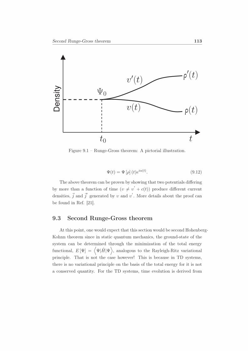
Second Runge-Gross theorem 113
Den
sity
t0 t
Ψ0
v(t)
v′(t)
(t)
′(t)
Figure 9.1 – Runge-Gross theorem: A pictorial illustration.
Ψ(t) = Ψ [ρ] (t)eiα(t). (9.12)
The above theorem can be proven by showing that two potentials differing
by more than a function of time (υ 6= υ′
+ c(t)) produce different current
densities, ~j and ~j′
generated by υ and υ′
. More details about the proof can
be found in Ref. [21].
9.3 Second Runge-Gross theorem
At this point, one would expect that this section would be second Hohenberg-
Kohnn theorem since in static quantum mechanics, the ground-state of the
system can be determined through the minimization of the total energy
functional, E [Ψ] =⟨
Ψ|H|Ψ⟩
, analogous to the Rayleigh-Ritz variational
principle. That is not the case however! This is because in TD systems,
there is no variational principle on the basis of the total energy for it is not
a conserved quantity. For the TD systems, time evolution is derived from
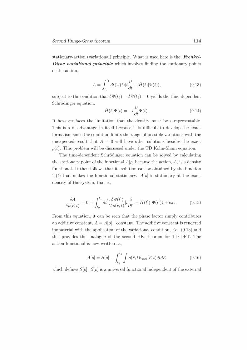
Second Runge-Gross theorem 114
stationary-action (variational) principle. What is used here is the; Frenkel-
Dirac variational principle which involves finding the stationary points
of the action,
A =
∫ t1
t0
dt〈Ψ(t)|i ∂∂t− H(t)|Ψ(t)〉, (9.13)
subject to the condition that δΨ(t0) = δΨ(t1) = 0 yields the time-dependent
Schrödinger equation.
H(t)Ψ(t) = −i ∂∂t
Ψ(t). (9.14)
It however faces the limitation that the density must be v-representable.
This is a disadvantage in itself because it is difficult to develop the exact
formalism since the condition limits the range of possible variations with the
unexpected result that A = 0 will have other solutions besides the exact
ρ(t). This problem will be discussed under the TD Kohn-Sham equation.
The time-dependent Schrödinger equation can be solved by calculating
the stationary point of the functional A[ρ] because the action, A, is a density
functional. It then follows that its solution can be obtained by the function
Ψ(t) that makes the functional stationary. A[ρ] is stationary at the exact
density of the system, that is,
δA
δρ(~r, t)= 0 =
∫ t1
t0
dt′〈 δΨ(t
′
)
δρ(~r, t)|i ∂∂t′
− H(t′
)|Ψ(t′
)〉+ c.c., (9.15)
From this equation, it can be seen that the phase factor simply contributes
an additive constant, A = A[ρ]+constant. The additive constant is rendered
immaterial with the application of the variational condition, Eq. (9.13) and
this provides the analogue of the second HK theorem for TD-DFT. The
action functional is now written as,
A[ρ] = S[ρ]−∫ t1
t0
∫
ρ(~r, t)vext(~r, t)dtd~r, (9.16)
which defines S[ρ]. S[ρ] is a universal functional independent of the external
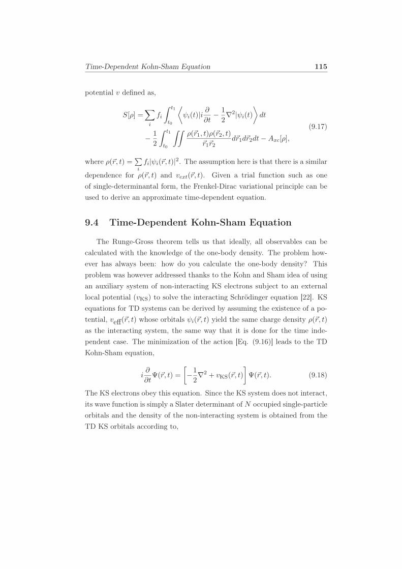
Time-Dependent Kohn-Sham Equation 115
potential v defined as,
S[ρ] =∑
i
fi
∫ t1
t0
⟨
ψi(t)|i∂
∂t− 1
2∇2|ψi(t)
⟩
dt
− 1
2
∫ t1
t0
∫∫ρ(~r1, t)ρ(~r2, t)
~r1~r2d~r1d~r2dt−Axc[ρ],
(9.17)
where ρ(~r, t) =∑
ifi|ψi(~r, t)|2. The assumption here is that there is a similar
dependence for ρ(~r, t) and vext(~r, t). Given a trial function such as one
of single-determinantal form, the Frenkel-Dirac variational principle can be
used to derive an approximate time-dependent equation.
9.4 Time-Dependent Kohn-Sham Equation
The Runge-Gross theorem tells us that ideally, all observables can be
calculated with the knowledge of the one-body density. The problem how-
ever has always been: how do you calculate the one-body density? This
problem was however addressed thanks to the Kohn and Sham idea of using
an auxiliary system of non-interacting KS electrons subject to an external
local potential (vks) to solve the interacting Schrödinger equation [22]. KS
equations for TD systems can be derived by assuming the existence of a po-
tential, veff(~r, t) whose orbitals ψi(~r, t) yield the same charge density ρ(~r, t)
as the interacting system, the same way that it is done for the time inde-
pendent case. The minimization of the action [Eq. (9.16)] leads to the TD
Kohn-Sham equation,
i∂
∂tΨ(~r, t) =
[
−1
2∇2 + vks(~r, t)
]
Ψ(~r, t). (9.18)
The KS electrons obey this equation. Since the KS system does not interact,
its wave function is simply a Slater determinant of N occupied single-particle
orbitals and the density of the non-interacting system is obtained from the
TD KS orbitals according to,
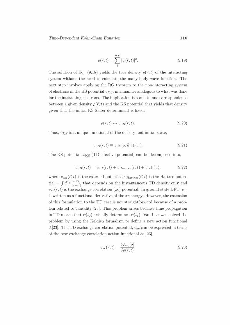
Time-Dependent Kohn-Sham Equation 116
ρ(~r, t) =
occ∑
i
|ψ(~r, t)|2. (9.19)
The solution of Eq. (9.18) yields the true density ρ(~r, t) of the interacting
system without the need to calculate the many-body wave function. The
next step involves applying the RG theorem to the non-interacting system
of electrons in the KS potential vKS , in a manner analogous to what was done
for the interacting electrons. The implication is a one-to-one correspondence
between a given density ρ(~r, t) and the KS potential that yields that density
given that the initial KS Slater determinant is fixed:
ρ(~r, t)↔ vks(~r, t). (9.20)
Thus, vKS is a unique functional of the density and initial state,
vks(~r, t) ≡ vks[ρ,Ψ0](~r, t). (9.21)
The KS potential, vks (TD effective potential) can be decomposed into,
vks(~r, t) = vext(~r, t) + vHartree(~r, t) + vxc(~r, t), (9.22)
where vext(~r, t) is the external potential, vHartree(~r, t) is the Hartree poten-
tial =∫d3r
′ ρ(~r,t)
|r−r′ |that depends on the instantaneous TD density only and
vxc(~r, t) is the exchange correlation (xc) potential. In ground-state DFT, vxcis written as a functional derivative of the xc energy. However, the extension
of this formulation to the TD case is not straightforward because of a prob-
lem related to causality [23]. This problem arises because time propagation
in TD means that ψ(t0) actually determines ψ(t1). Van Leeuwen solved the
problem by using the Keldish formalism to define a new action functional
A[23]. The TD exchange-correlation potential, vxc can be expressed in terms
of the new exchange correlation action functional as [23],
vxc(~r, t) =δAxc[ρ]
δρ(~r, t). (9.23)
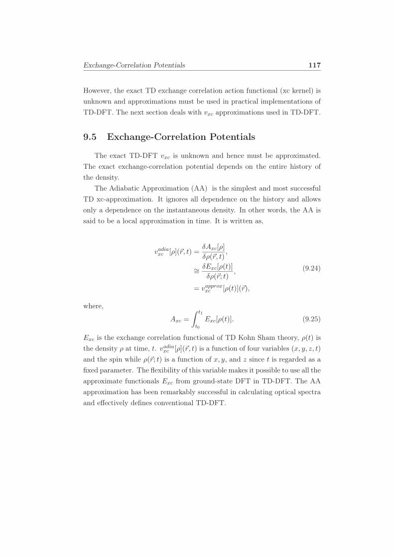
Exchange-Correlation Potentials 117
However, the exact TD exchange correlation action functional (xc kernel) is
unknown and approximations must be used in practical implementations of
TD-DFT. The next section deals with vxc approximations used in TD-DFT.
9.5 Exchange-Correlation Potentials
The exact TD-DFT vxc is unknown and hence must be approximated.
The exact exchange-correlation potential depends on the entire history of
the density.
The Adiabatic Approximation (AA) is the simplest and most successful
TD xc-approximation. It ignores all dependence on the history and allows
only a dependence on the instantaneous density. In other words, the AA is
said to be a local approximation in time. It is written as,
vadiaxc [ρ](~r, t) =δAxc[ρ]
δρ(~r, t),
∼= δExc[ρ(t)]
δρ(~r; t),
= vapproxxc [ρ(t)](~r),
(9.24)
where,
Axc =
∫ t1
t0
Exc[ρ(t)]. (9.25)
Exc is the exchange correlation functional of TD Kohn Sham theory, ρ(t) is
the density ρ at time, t. vadiaxc [ρ](~r, t) is a function of four variables (x, y, z, t)
and the spin while ρ(~r; t) is a function of x, y, and z since t is regarded as a
fixed parameter. The flexibility of this variable makes it possible to use all the
approximate functionals Exc from ground-state DFT in TD-DFT. The AA
approximation has been remarkably successful in calculating optical spectra
and effectively defines conventional TD-DFT.
Linear Response Theory (LR) 118
9.6 Linear Response Theory (LR)
The ultimate goal of many, if not all chemists is to study excited-state
properties. Time-dependent density functional theory forms the basis used
to calculate excitation energies and optical spectra because it captures the
essential dynamical nature of an excitation process. In particular, the linear
response theory (LR) [24] is used when considering response of a molecular
property (dynamic polarizability) to a weak time-dependent external per-
turbation of the unperturbed molecule. It is a way of describing how matter
interacts with the electromagnetic field. The weak perturbation may be
compared with a spectroscopy experiment. The LR of a system will contain
all the information about its excitation spectrum. It determines single exci-
tation energies of molecules from first principles. Simply put, the response
theory figures out how a system reacts to outside influences. Linear response
theory can be depicted schematically as in Fig. 9.2.
Perturbation Excitation Response
Figure 9.2 – An illustration of the LR theory.
9.7 Linear Response TD-DFT (LR TD-DFT)
In this section a discussion of the Fourier-transformed frequency domain
(ω) is done. Spectral information about the system can be obtained from the
KS orbitals since they reproduce the exact density in frequency-space, and
Linear Response TD-DFT (LR TD-DFT) 119
via a Fourier-transform of the KS orbitals in a similar manner as in Sec. 9.4.
In a consistent step by step manner, it will be shown how LR TD-DFT can
be used to extract linear absorption spectra by inducing small perturbations
to the KS orbitals [25].
9.7.1 Time-dependent linear density response
Three components will be key in describing the TD linear response den-
sity, the Hamiltonian, H(t), Eq. (9.3), TD external perturbation δvext(~r, t)
and the external potential vext(~r) at t < t0, the ground-state (Ψ0) and at
t > t0 where there is time evolution. For convenience, bra (〈|) ket ( |〉) [26]
notation has been used. Thus, the ground-state (Ψ0) at t < t0 can be ex-
pressed as |Ψ0〉. A small perturbation, δvext(~r, t), is slowly introduced in the
KS Hamiltonian at t = t0. Considering the two variables of time at t < t0
and t > t0, vext(~r, t) is given as,
t < t0, vext(~r, t) = vext(~r) and, (9.26)
t > t0, vext(~r, t) = vext(~r) + δvext(~r, t). (9.27)
This means that at t < t0, the density evolution is simply the ground-state
density ρ0(~r) and the density at t > t0 is time-dependent starting from the
ground-state density as shown below,
t < t0, ρ(~r, t) = ρ0(~r) and, (9.28)
t > t0, ρ(~r, t) = ρ0(~r) + δρ(~r, t). (9.29)
ρ(~r, t) can be expanded in powers of the potential as,
ρ(~r, t) = ρ0(~r) + δρ(~r, t) + ..., (9.30)
Since we are interested in the density evolution with time, we keep the first
order term, δρ(~r, t). It is possible to relate δρ(~r, t) and δvext(~r, t) mathemat-
ically as,
Linear Response TD-DFT (LR TD-DFT) 120
δρ(~r, t) =
∫
d3r′
∫
dt′
χρρ(~r, ~r′
; t− t′)δvext(~r′
, t′
). (9.31)
This is known as the linear density response, δρ(~r, t) to the perturbation
δvext(~r, t). The density-density response function or generalized susceptibil-
ity, χρρ(~r, ~r′
; t− t′) can be expressed in terms functionals as,
χρρ(~r, ~r′
; t− t′) = δρ[vext](~r, t)
δvext(~r′t′)
∣∣∣∣vext[ρ0]
,
or
χρρ(~r, ~r′
; t− t′) = −iΘ(t− t′)⟨
Ψ0|[ρ(~r, t− t′
), ρ(~r′
)]|Ψ0
⟩
,
where
ρ(~r) =∑
r
Ψr(~r)Ψ∗r(~r)a
+r ar (2
ndquantization),
(9.32)
where Θ(t − t′
) is known as the Heaviside step function that takes care of
causality. A Fourier transform of Eq. (9.32) gives spectral information about
the system, that is, χρρ(~r, ~r′
; t − t′
) becomes χρρ(~r, ~r′
;ω). The Lehmann
representation of the density density response function given as,
χρρ(~r, ~r′
, ω) =∑
n
〈Ψ0|ρ(~r)|Ψn〉
⟨
Ψn|ρ(~r′
)|Ψ0
⟩
ω − ωn0 + iη
−
⟨
Ψ0|ρ(~r′
)|Ψn
⟩
〈Ψn|ρ(~r)|Ψ0〉ω + ωn0 + iη
.
(9.33)
Equation (9.33) forms the core of LR theory since it shows explicitly how
a frequency-dependent perturbation couples to the excitation spectrum of a
system. Excitation energies lie at the poles of χρρ and oscillator strengths
are obtained from the residues. We can also get the absorption spectrum by
taking the imaginary part of Eq. (9.33). We wish to show how the spectral
Linear Response TD-DFT (LR TD-DFT) 121
function,
S(ω) =∑
I
fI [δ(ω − ωI) + δ(ω + ωI)] , (9.34)
may be calculated from the dynamic polarizability,
α(ω) =∑
I
fIω2I − ω2
, (9.35)
as
S(ω) =2ω
πlimη→0
α(ω + iη) . (9.36)
We do this by noticing that
α(ω) =∑
I
(fI2ω
)(1
ωI − ω− 1
ωI + ω
)
, (9.37)
so that,
2ω
πα(ω + iη) =
∑
I
fIπ
(1
ωI − ω − iη− 1
ωI + ω + iη
)
=∑
I
fIπ
[ωI − ω + iη
(ωI − ω − iη) (ωI − ω + iη)
]
(9.38)
−∑
I
fIπ
[ωI + ω − iη
(ωI + ω + iη) (ωI + ω − iη)
]
=∑
I
fIπ
[ωI − ω + iη
(ωI − ω) + η2− ωI + ω − iη
(ωI + ω)2 + η2
]
=∑
I
fIπ
[ωI − ω
(ωI − ω)2 + η2− ωI + ω
(ωI + ω)2 + η2
]
+ i∑
I
fIπ
[η
(ωI − ω)2 + η2+
η
(ωI + ω)2 + η2
]
.(9.39)
Linear Response TD-DFT (LR TD-DFT) 122
It is now easy to separate the real and imaginary parts:
2ω
πℜα(ω + iη) =
∑
I
fIπ
[ωI − ω
(ωI − ω)2 + η2− ωI + ω
(ωI + ω)2 + η2
]
2ω
πℑα(ω + iη) =
∑
I
fIπ
[η
(ωI − ω)2 + η2+
η
(ωI + ω)2 + η2
]
.(9.40)
Since the Lorentzian representation of the Dirac delta function is
δ(x) =1
πlimη→0
η
x2 + η2, (9.41)
it follows that so that,
2ω
πlimη→0
ℑα(ω + iη) =∑
I
fI [δ(ωI − ω) + δ(ωI + ω)] (9.42)
which is just the spectral function of Eq. (9.34) because the Dirac delta
function is an even function [δ(x) = −δ(x)]. Interestingly, if η is small but
finite, not taking the limit simply corresponds to Lorentzian broadening of
the spectral function.
9.7.2 Kohn-Sham Linear Density Response
In Sec. 9.7.1, a discussion has been made of how to extract the various
quantities from the density-density response. However, the practically of the
equations discussed in Sec. 9.7.1 remains limited because it is an interacting
system of electrons and thus requires an input of many-body eigenstates
and eigenenergies. To make the equations more practical, we consider a
fictitious system of non-interacting KS electrons that produces the same
density response as the interacting system. The only difference between this
section and the previous section is that here, we are considering a system
of non-interacting electrons and thus utilize the KS orbitals, φi. The initial
equations that share similarities have been skipped and we start from the
dressed KS potential which is given as,
Linear Response TD-DFT (LR TD-DFT) 123
δvks[ρ,Ψ0,Φ0](~r, t) = δvext[ρ](~r, t) +
∫
d3~r′δρ(~r′, t)
|~r − ~r′|+ δvxc[ρ,Ψ0,Φ0](~r, t).
(9.43)
(but both Ψ0[ρ],Φ0[ρ] are eliminated if you begin from the ground-state.)
The density response is related to the KS potential by,
δρ(~r, t) =
∫
d3~r′∫
dt′
χksρρ (~r, ~r′; t− t′)δvks(~r′, t
′
), (9.44)
and the Lehmann spectral representation for the KS system is,
χksρρ (~r, ~r′;ω) =
∑
n
〈Φ0|ρ(~r)|Φn〉
⟨
Φn|ρ(~r′)|Φ0
⟩
ω − ωksn0 + iη
−
⟨
Φ0|ρ(~r′)|Φn⟩
〈Φn|ρ(~r)|Φ0〉ω + ωks
n0 + iη
,
(9.45)
where Φn is the excited KS determinant of the ground-state KS potential
and ωksn0 is the corresponding KS excitation frequency. Equation (9.45) can
further simplify to the sum over KS single excitations to be,
χksρρ (~r, ~r′;ω) =
N∑
k=0
∞∑
j=N+1
[
φj(~r)φ∗k(~r)φ
∗j (~r′)φk(~r′)
ω − (ǫj − ǫk) + iη
−φk(~r)φ
∗j (~r)φ
∗k(~r′)φj(~r′)
ω + (ǫj − ǫk) + iη
]
.
(9.46)
As mentioned earlier, the χksρρ results from KS single excitations and thus
does not contain double and higher multiple KS excitations hence not a
true representation of excitations from the interacting system. To get a true
picture, there is need to relate the interacting, χρρ, and KS density-density
response functions χksρρ . The equation is,
Casida Equations 124
χρρ(~r, ~r′; t− t′
) =χksρρ (~r, ~r′; t− t′) +
∫
d3x
∫
dτ
∫
d3x′
∫
dτ′
χksρρ (~r,x, t− τ)
×
δ(τ − τ ′
)
|x′ − x| + fxc[ρ0](x,x′
, τ − τ ′
)
χρρ(x′
, r′
, τ′ − t′),
(9.47)
where fxc[ρ0](~r, ~r′, t− t′
) is the TD xc kernel defined as,
fxc[ρ0](~r, ~r′, t− t′
) =δvxc(~r, t)
δρ(~r′ , t′)
∣∣∣∣ρ(~r
′ ,t′ )=ρ0
. (9.48)
The role of fxc is to bring in the missing double and higher multiple exci-
tations that were missing in the χksρρ . To obtain accurate spectra in TD-
DFT, accurate approximations to fxc must be constructed. Doing a Fourier-
transform on Eq. (9.47) gives the frequency domain equation,
χρρ(~r, ~r′;ω) =χksρρ (~r, ~r′;ω) +
∫
d3~x
∫
d3x′χksρρ (~r, ~x, ω)
×
1
|x′ − x| + fxc[ρ0](~x, ~x′
, ω)
χρρ(~x′, ~r′, ω).
(9.49)
From the Eq. (9.49), we can see that two situations arise, one ideal and
the other of practical. Looking at the ideal situation: from the ground-
state DFT, the χKSρρ can be constructed and χρρ solved self-consistently.
Practically, as will be seen in the next section under the Casida equations, it
has to be rewritten as a non-linear eigenvalue problem in terms of matrices
represented in a basis set of molecular orbitals.
9.8 Casida Equations
As mentioned earlier, we are interested in the response of a system ini-
tially in a stationary state (ground-state), Ψ0, to a weak external perturba-
tion. Typically, we can obtain the dynamic response of the charge density
Casida Equations 125
from TD-DFT. There are several methods that can be used to extract exci-
tations from TD-DFT: A case in point is the absorption spectrum obtained
from the poles of the excitation energies, ωI and the oscillator strengths,
fI . The biggest challenge has been how to compute the said quantities ac-
curately. This challenge was overcome in 1995 by Casida, [27], by using
the Casida equations that efficiently convert the search for poles of response
functions into a large eigenvalue problem. He provided a procedure of how
to calculate the said quantities using knowledge from the linear density re-
sponse of the system by reformulating the linear response time-dependent
density functional response theory to resemble the standard implementation
of LR-TDHF. The dynamic polarizability, α(ω), that describes the response
of the dipole moment to a TD electric field can be calculated from the re-
sponse of the charge density obtained from TD-DFT. With such information,
the electronic excitation spectrum in the usual dipole approximation can be
determined.
We can derive the Casida equation by considering an N -electron system
initially in its ground stationary state, Ψ0, exposed to a TD perturbation
turned on adiabatically at time, t = −∞. The equation for the dynamic
response of the KS density matrix is,
ω
[
1 0
0 −1
]
−[
A B
B∗ A∗
](
δ ~P (ω)
δ ~P ∗(ω)
)
=
(
~vappl(ω)
~v∗appl(ω)
)
. (9.50)
Rearranging this expression to the form of dynamic polarizability according
to the sum-over-states (SOS) relation,
α(ω) =∑
I 6=0
fIω2I − ω2
(9.51)
we can extract the excitation energies and oscillator strengths. In Eq. (9.51),
fI is given as,
fI =2
3ωI(| 〈Ψ0|x|ΨI〉 |2 + | 〈Ψ0|y|ΨI〉 |2 + | 〈Ψ0|z|ΨI〉 |2), (9.52)
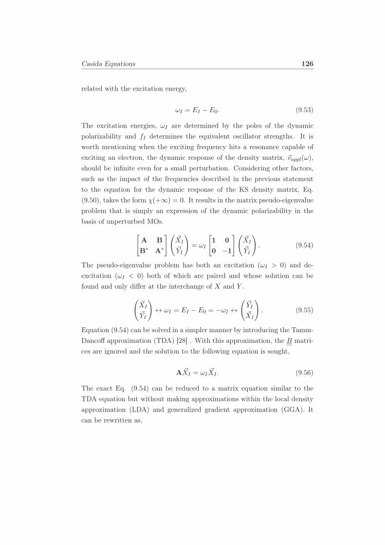
Casida Equations 126
related with the excitation energy,
ωI = EI − E0. (9.53)
The excitation energies, ωI are determined by the poles of the dynamic
polarizability and fI determines the equivalent oscillator strengths. It is
worth mentioning when the exciting frequency hits a resonance capable of
exciting an electron, the dynamic response of the density matrix, ~vappl(ω),
should be infinite even for a small perturbation. Considering other factors,
such as the impact of the frequencies described in the previous statement
to the equation for the dynamic response of the KS density matrix, Eq.
(9.50), takes the form χ(+∞) = 0. It results in the matrix pseudo-eigenvalue
problem that is simply an expression of the dynamic polarizability in the
basis of unperturbed MOs.
[
A B
B∗ A∗
](~XI
~YI
)
= ωI
[
1 0
0 −1
](~XI
~YI
)
. (9.54)
The pseudo-eigenvalue problem has both an excitation (ωI > 0) and de-
excitation (ωI < 0) both of which are paired and whose solution can be
found and only differ at the interchange of X and Y .
(~XI
~YI
)
↔ ωI = EI − E0 = −ωI ↔(~YI~XI
)
. (9.55)
Equation (9.54) can be solved in a simpler manner by introducing the Tamm-
Dancoff approximation (TDA) [28] . With this approximation, the B matri-
ces are ignored and the solution to the following equation is sought,
A ~XI = ωI ~XI . (9.56)
The exact Eq. (9.54) can be reduced to a matrix equation similar to the
TDA equation but without making approximations within the local density
approximation (LDA) and generalized gradient approximation (GGA). It
can be rewritten as,
‘Deadly Sins’ of TD-DFT 127
Ω~FI = ωI ~FI , (9.57)
where,
Ω = (A−B)+1/2(A + B)(A−B)+1/2
~FI = (A−B)−1/2( ~XI + ~YI).(9.58)
The excitation energies of the system can be obtained from the eigenvalues of
Eq. (9.57) while the eigenvectors ( ~XI , ~YI)† give the spectroscopic oscillator
strengths and to assign the symmetry of each transition, although in practice,
the symmetry of the excited-state is many times already reflected in ~FI . To
solve the Casida’s equations, one is needed to diagonalize the ground-state
Hamiltonian in order to get a number of the empty KS states.
9.9 ‘Deadly Sins’ of TD-DFT
‘Deadly Sins’ of TD-DFT are simply the possible sources of errors when
doing calculations with TD-DFT. If one commits any of this ‘sins’, then one
is likely not to go to Heaven (get accurate TD-DFT results) [29]. According
to [29], there are four of them:
• Errors can arise from ground-state DFT calculation. If one begins
with wrong KS orbital energies, TD-DFT calculations cannot produce
accurate results. This is known as The sin of the ground-state.
• Errors arising from local approximations to an adiabatic fxc(r, r′
),
that is properties that require nonlocality are known as The sin of
locality.
• The sin of forgetfulness arises from phenomena missing when the adi-
abatic approximation is made, that is, properties that require nonlo-
cality in time, and finally,
• The sin of the wave function arises from the difference between the
true wave function and the KS wave function.
BIBLIOGRAPHY 128
Bibliography
[1] D. G. Tempel. Time-Dependent Density Functional Theory for Open
Quantum Systems and Quantum Computation. PhD thesis, Harvard
University, 2012.
[2] D. Presti. Quantum computational methodologies for the study of molec-
ular crystals. PhD thesis, Université Pierre et Marie Curie - Paris VI,
2015.
[3] Fundamentals of time-dependent density functional theory. Lec-
ture Notes in Physics. Springer Berlin Heidelberg, 2012. ISBN
9783642235177.
[4] M. Marques. Time-dependent density functional theory. Lecture Notes
in Physics. Springer, 2006. ISBN 9783540354222.
[5] C. Fiolhais, F. Nogueira, and M. A. L. Marques. A Primer in Density
Functional Theory. Lecture Notes in Physics. Springer Berlin Heidel-
berg, 2008. ISBN 9783540370727.
[6] R. Van Leeuwen. Key concepts in time-dependent density-functional
theory. International Journal of Modern Physics B, 15(14):1969–2023,
2001.
[7] E. K. U. Gross, C. A. Ullrich, and U. J. Gossmann. Density functional
theory of time-dependent systems. In Density Functional Theory, pages
149–171. Springer, 1995.
[8] R. E. Stratmann, G. E. Scuseria, and M. J. Frisch. An efficient imple-
mentation of time-dependent density-functional theory for the calcula-
tion of excitation energies of large molecules. J. Chem. Phys., 109(19):
8218–8224, 1998.
[9] P. Elliott, F. Furche, and K. Burke. Excited states from time-dependent
density functional theory. Rev. Comp. Chem., 26:91, 2009.
BIBLIOGRAPHY 129
[10] M. E. Casida and M. Huix-Rotllant. Progress in time-dependent
density-functional theory. Ann. Rev. Phys. Chem., 63:287–323, 2012.
[11] M. A. L. Marques and E. K. Gross. Time-dependent density functional
theory. Annu. Rev. Phys. Chem., 55:427–455, 2004.
[12] M. E. Casida. Time-dependent density-functional theory for the calcu-
lation of molecular electronic excited states 2nd year masters, theoret-
ical chemistry. https://sites.google.com/site/markcasida/tddft,
January 2009. online; accessed 1st July, 2017.
[13] R. F. Nalewajski. Perspectives in Electronic Structure Theory. Springer
Berlin Heidelberg, 2012. ISBN 9783642201806.
[14] N. Ferré, M. Filatov, and M. Huix-Rotllant. Density-Functional Methods
for Excited States. Topics in Current Chemistry. Springer International
Publishing, 2015. ISBN 9783319220819.
[15] X. Gonze. Adiabatic density-functional perturbation theory. Phys. Rev.
A, 52(2):1096, 1995.
[16] E. Runge and E. K. U. Gross. Density-functional theory for time-
dependent systems. Phys. Rev. Lett., 52:997, 1984.
[17] P. Hohenberg and W. Kohn. Inhomogeneous electron gas. Phys. Rev.,
136(3B):B864, 1964.
[18] W. Kohn and L. J. Sham. Self-consistent equations including exchange
and correlation effects. Phys. Rev., 140:A1133, 1965.
[19] E. K. U. Gross and W. Kohn. Time-dependent density functional theory.
Adv. Quant. Chem, 21:255–291, 1990.
[20] E. K. U. Gross and W. Kohn. Local density-functional theory of
frequency-dependent linear response. Phys. Rev. Lett., 55(26):2850,
1985.
BIBLIOGRAPHY 130
[21] C. Ullrich. Time-Dependent Density-Functional Theory: Concepts and
Applications. Oxford Graduate Texts. Oxford University Press, Oxford,
2012. ISBN 9780199563029.
[22] E. K. U. Gross, J. F. Dobson, and M. Petersilka. Density functional
theory of time-dependent phenomena. In Density functional theory II,
pages 81–172. Springer, 1996.
[23] R. Van Leeuwen. Causality and symmetry in time-dependent density-
functional theory. Phys. Rev. Lett., 80(6):1280, 1998.
[24] M. E. Casida. Time-dependent density functional response theory of
molecular systems: Theory, computational methods, and functionals.
Theo. Comput. Chem., 4:391 – 439, 1996. ISSN 1380-7323. doi: http:
//dx.doi.org/10.1016/S1380-7323(96)80093-8.
[25] M. Petersilka, U. J. Gossmann, and E. K. U. Gross. Excitation energies
from time-dependent density-functional theory. Phys. Rev. Lett., 76:
1212, 1996.
[26] A. Szabo and N. S. Ostlund. Modern Quantum Chemistry: Introduc-
tion to Advanced Electronic Structure Theory. Macmillan Publishing
Company, New York, 1982.
[27] M. E. Casida. Time-dependent density-functional response theory for
molecules. In D. P. Chong, editor, Recent Advances in Density Func-
tional Methods, Part I, page 155. World Scientific, Singapore, 1995.
[28] S. Hirata and M. Head-Gordon. Time-dependent density functional
theory within the Tamm-Dancoff approximation. Chem. Phys. Lett.,
314:291, 1999.
[29] K. Burke, J. Werschnik, and E. K. U. Gross. Time-dependent density
functional theory: Past, present, and future. J. Chem. Phys., 123(6):
062206, 2005.
Part III
Original Research
131
Chapter 10
DFT and TD-DFT for
Ruthenium Complexes
This chapter is my contribution to a projected review article,
“Challenge of time-dependent density-functional theory for pho-
tochemistry”
by Mark E. Casida, Myneni Hemanadhan, Ala M. H. H. Aldin
Darghouth, and Denis Magero.
It gives a good basic introduction to how well (TD-)DFT works for ruthenium
complexes. The next chapter will then go into this subject in much more
detail.
10.1 Introduction
Ruthenium complexes have attracted intense research in the recent years
and also in the past. This is because ruthenium complexes have a wide range
of applications in every day life such as the organic solar cells, light emitting
diodes and photo-molecular chemical devices just to mention but a few[1]. To
make its application a reality, the excited state properties of the compound
must be studied. This have been done experimentally in various ways but
there is also need to develop theoretical methods that can accurately predict
the excited state properties so as to compliment experimental data and vice
132
Computational Details 133
versa. To this date, there are several methods that can be used to study
excited state properties theoretically. Some of the methods that can be
used include the time-dependent density-functional theory (TD-DFT), time-
dependent Hartree Fock (TD-HF), and the configuration interaction (CI)
among many others. This works compares the three methods to find out
which one is able to predict excited state properties accurately by comparing
with experimental spectra.
10.2 Computational Details
Ground state optimization was done with density functional theory (DFT)
and Hartree Fock. The DFT calculations were performed by using the
Gaussian09[2] (version D.01) program package. Calculated gas phase ab-
sorption spectra for the compound was done using different methods for ex-
cited state calculations including the time dependent (TD) density-functional
theory (TD-DFT)[3], time-dependent Hartree Fock (TD-HF) and configura-
tion interaction (CI) levels of theory. All the calculations were done with the
Becke three parameters hybrid exchange and the Lee-Yang-Parr correlation
functionals (B3LYP)[4, 5]. All-electron 6-31G and 6-31G(d)[6–12] basis set
was used for C, H and N atoms while a double-ζ quality basis set LANL2DZ
and the corresponding effective core potential (ECP) was used for Ru[13] .
X-ray crystallographic data for the compound was obtained from the
Cambridge crystallographic data centre (CCDC) with reference code BEN-
HUZ. Ground state optimization was done by starting with the crystallo-
graphic data. The minima was tested by calculating vibrational frequencies
and checking out for the presence or absence of imaginary frequencies. The
absence of imaginary frequencies gave an indication that the geometry was at
the minima. Excited state calculations used the optimized ground state ge-
ometries with the same basis sets and functionals. Calculations were done at
different levels of theory including the CI, TD-DFT and TD-HF. The number
of excited states for all the calculations was 100 singlet states. Results ob-
tained from theoretical calculations are obtained as spectral functions. The
oscillator strength can be obtained from the spectral function which is given
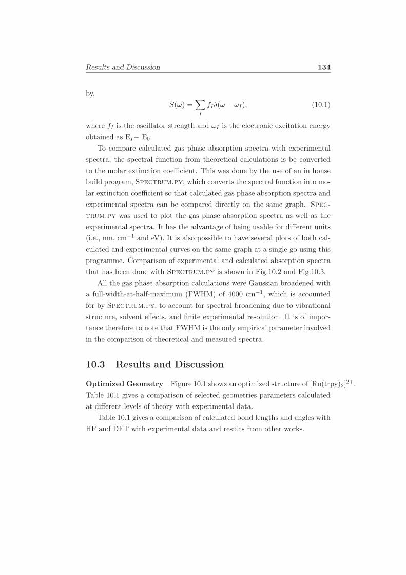
Results and Discussion 134
by,
S(ω) =∑
I
fIδ(ω − ωI), (10.1)
where fI is the oscillator strength and ωI is the electronic excitation energy
obtained as EI− E0.
To compare calculated gas phase absorption spectra with experimental
spectra, the spectral function from theoretical calculations is be converted
to the molar extinction coefficient. This was done by the use of an in house
build program, Spectrum.py, which converts the spectral function into mo-
lar extinction coefficient so that calculated gas phase absorption spectra and
experimental spectra can be compared directly on the same graph. Spec-
trum.py was used to plot the gas phase absorption spectra as well as the
experimental spectra. It has the advantage of being usable for different units
(i.e., nm, cm−1 and eV). It is also possible to have several plots of both cal-
culated and experimental curves on the same graph at a single go using this
programme. Comparison of experimental and calculated absorption spectra
that has been done with Spectrum.py is shown in Fig.10.2 and Fig.10.3.
All the gas phase absorption calculations were Gaussian broadened with
a full-width-at-half-maximum (FWHM) of 4000 cm−1, which is accounted
for by Spectrum.py, to account for spectral broadening due to vibrational
structure, solvent effects, and finite experimental resolution. It is of impor-
tance therefore to note that FWHM is the only empirical parameter involved
in the comparison of theoretical and measured spectra.
10.3 Results and Discussion
Optimized Geometry Figure 10.1 shows an optimized structure of [Ru(trpy)2]2+.
Table 10.1 gives a comparison of selected geometries parameters calculated
at different levels of theory with experimental data.
Table 10.1 gives a comparison of calculated bond lengths and angles with
HF and DFT with experimental data and results from other works.
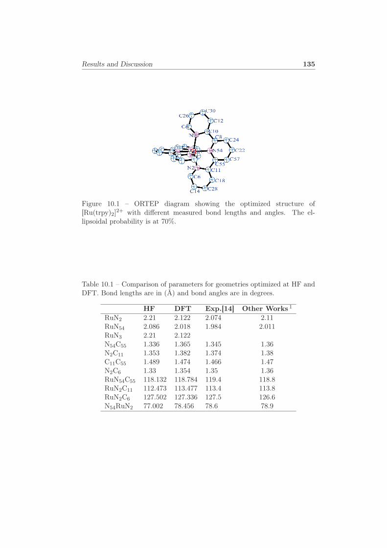
Results and Discussion 135
Figure 10.1 – ORTEP diagram showing the optimized structure of[Ru(trpy)2]2+ with different measured bond lengths and angles. The el-lipsoidal probability is at 70%.
Table 10.1 – Comparison of parameters for geometries optimized at HF andDFT. Bond lengths are in (Å) and bond angles are in degrees.
HF DFT Exp.[14] Other Works 1
RuN2 2.21 2.122 2.074 2.11RuN54 2.086 2.018 1.984 2.011RuN3 2.21 2.122N54C55 1.336 1.365 1.345 1.36N2C11 1.353 1.382 1.374 1.38C11C55 1.489 1.474 1.466 1.47N2C6 1.33 1.354 1.35 1.36RuN54C55 118.132 118.784 119.4 118.8RuN2C11 112.473 113.477 113.4 113.8RuN2C6 127.502 127.336 127.5 126.6N54RuN2 77.002 78.456 78.6 78.9
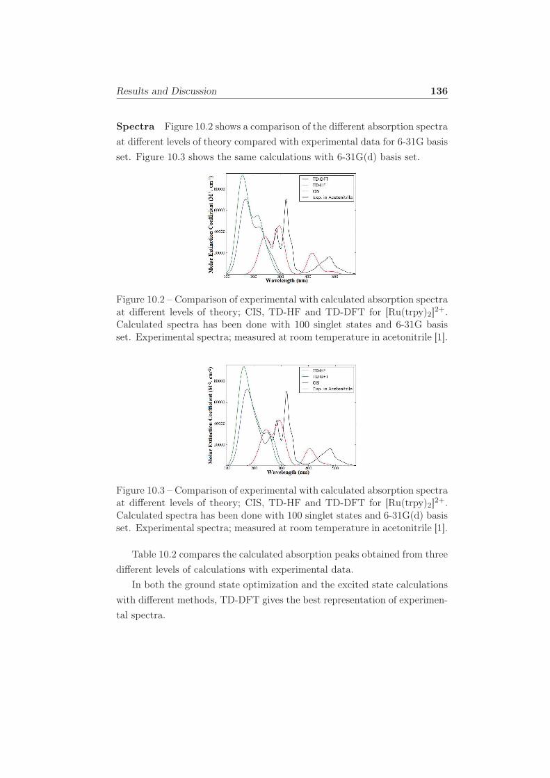
Results and Discussion 136
Spectra Figure 10.2 shows a comparison of the different absorption spectra
at different levels of theory compared with experimental data for 6-31G basis
set. Figure 10.3 shows the same calculations with 6-31G(d) basis set.
Figure 10.2 – Comparison of experimental with calculated absorption spectraat different levels of theory; CIS, TD-HF and TD-DFT for [Ru(trpy)2]2+.Calculated spectra has been done with 100 singlet states and 6-31G basisset. Experimental spectra; measured at room temperature in acetonitrile [1].
Figure 10.3 – Comparison of experimental with calculated absorption spectraat different levels of theory; CIS, TD-HF and TD-DFT for [Ru(trpy)2]2+.Calculated spectra has been done with 100 singlet states and 6-31G(d) basisset. Experimental spectra; measured at room temperature in acetonitrile [1].
Table 10.2 compares the calculated absorption peaks obtained from three
different levels of calculations with experimental data.
In both the ground state optimization and the excited state calculations
with different methods, TD-DFT gives the best representation of experimen-
tal spectra.
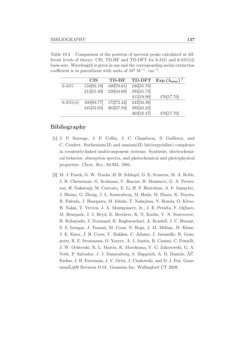
BIBLIOGRAPHY 137
Table 10.2 – Comparison of the position of spectral peaks calculated at dif-ferent levels of theory; CIS, TD-HF and TD-DFT for 6-31G and 6-31G(d)basis sets. Wavelength is given in nm and the corresponding molar extinctioncoefficient is in parenthesis with units of 103 M−1. cm−1.
CIS TD-HF TD-DFT Exp.(λmax) 2
6-31G 158[93.19] 169[70.61] 240[35.78]213[55.40] 220[44.68] 293[45.73]
415[19.90] 476[17.70]6-31G(d) 160[93.77] 172[72.42] 242[34.38]
245[32.03] 262[27.93] 292[43.22]403[16.47] 476[17.70]
Bibliography
[1] J. P. Sauvage, J. P. Collin, J. C. Chambron, S. Guillerez, and
C. Coudret. Ruthenium(II) and osmium(II) bis(terpyridine) complexes
in covalently-linked multicomponent systems: Synthesis, electrochemi-
cal behavior, absorption spectra, and photochemical and photophysical
properties. Chem. Rev., 94:933, 1994.
[2] M. J. Frisch, G. W. Trucks, H. B. Schlegel, G. E. Scuseria, M. A. Robb,
J. R. Cheeseman, G. Scalmani, V. Barone, B. Mennucci, G. A. Peters-
son, H. Nakatsuji, M. Caricato, X. Li, H. P. Hratchian, A. F. Izmaylov,
J. Bloino, G. Zheng, J. L. Sonnenberg, M. Hada, M. Ehara, K. Toyota,
R. Fukuda, J. Hasegawa, M. Ishida, T. Nakajima, Y. Honda, O. Kitao,
H. Nakai, T. Vreven, J. A. Montgomery, Jr., J. E. Peralta, F. Ogliaro,
M. Bearpark, J. J. Heyd, E. Brothers, K. N. Kudin, V. N. Staroverov,
R. Kobayashi, J. Normand, K. Raghavachari, A. Rendell, J. C. Burant,
S. S. Iyengar, J. Tomasi, M. Cossi, N. Rega, J. M. Millam, M. Klene,
J. E. Knox, J. B. Cross, V. Bakken, C. Adamo, J. Jaramillo, R. Gom-
perts, R. E. Stratmann, O. Yazyev, A. J. Austin, R. Cammi, C. Pomelli,
J. W. Ochterski, R. L. Martin, K. Morokuma, V. G. Zakrzewski, G. A.
Voth, P. Salvador, J. J. Dannenberg, S. Dapprich, A. D. Daniels, ÃŰ.
Farkas, J. B. Foresman, J. V. Ortiz, J. Cioslowski, and D. J. Fox. Gaus-
sianâĹij09 Revision D.01. Gaussian Inc. Wallingford CT 2009.
BIBLIOGRAPHY 138
[3] M. E. Casida. Time-dependent density-functional theory for molecules
and molecular solids. J. Molec. Struct.: THEOCHEM, 914(1):3, 2009.
[4] A. D. Becke. Density-functional thermochemistry. III. The role of exact
exchange. J. Chem. Phys., 98:5648, 1993.
[5] C. Lee, W. Yang, and R. G. Parr. Development of the Colle-Salvetti cor-
relation energy formula into a functional of the electron density. Phys.
Rev. B, 37:785, 1988.
[6] R. Ditchfield, W. J. Hehre, and J. A. Pople. Self-consistent molecular-
orbital methods. IX. An extended Gaussian-type basis for molecular-
orbital studies of organic molecules. J. Chem. Phys., 54(2):724–728,
1971.
[7] W. J. Hehre, R. Ditchfield, and J. A. Pople. Self-consistent molecular
orbital methods. XII. Further extensions of Gaussian-type basis sets for
use in molecular orbital studies of organic molecules. J. Chem. Phys.,
56(5):2257–2261, 1972.
[8] P. C. Hariharan and J. A. Pople. The influence of polarization functions
on molecular orbital hydrogenation energies. Theor. Chim. Acta, 28(3):
213–222, 1973.
[9] P. C. Hariharan and J. A. Pople. Accuracy of AHn equilibrium geome-
tries by single determinant molecular orbital theory. Mol. Phys., 27(1):
209–214, 1974.
[10] M. M. Francl, W. J. Pietro, W. J. Hehre, J. S. Binkley, M. S. Gordon,
D. J. DeFrees, and J. A. Pople. Self-consistent molecular orbital meth-
ods. XXIII. A polarization-type basis set for second-row elements. J.
Chem. Phys., 77(7):3654–3665, 1982.
[11] V. A. Rassolov, M. A. Ratner, J. A. Pople, P. C. Redfern, and L. A.
Curtiss. 6-31G* basis set for third-row atoms. J. Comp. Chem., 22(9):
976–984, 2001.
BIBLIOGRAPHY 139
[12] G. A. Petersson and M. A. Al-Laham. A complete basis set model
chemistry. II. Open-shell systems and the total energies of the first-row
atoms. J. Chem. Phys., 94(9):6081–6090, 1991.
[13] P. J. Hay and W. R. Wadt. Ab initio effective core potentials for molec-
ular calculations. potentials for K to Au including the outermost core
orbitals. J. Chem. Phys., 82:299, 1985.
[14] M. Kozlowska, P. Rodziewicz, D. M. Brus, J. Breczko, and K. Brzezin-
ski. Bis (2, 2’: 6’, 2”-terpyridine) ruthenium (II) bis (perchlorate) hemi-
hydrate. Acta. Crystallogr. E, 68(11):1414–1415, 2012.
[15] X. Zhou, A. Ren, and J. Feng. Theoretical studies on the ground states
in (M= Fe, Ru, Os) and excited states in using density functional theory.
J. Organomet. Chem., 690(2):338–347, 2005.
Chapter 11
Partial Density of States
Ligand Field Theory
(PDOS-LFT): Recovering a
LFT-Like Picture and
Application to Photoproperties
of Ruthenium(II) Polypyridine
Complexes
Introduction
This chapter forms the core part of my thesis. The work that was done
and the contribution towards scientific knowledge is divided into two sections.
In the first section, the MO indices that were proposed by [1] are validated
by applying them to a bigger number of compounds that were carefully se-
lected from [2] which contains data about hundreds of Ru complexes based
on the length of the excited state lifetime both at room temperature and
140
Background Information on the Problem 141
at liquid nitrogen temperature. In particular, the work involved modelling
using Gaussview or using the X-ray crystal structures of 112 Ru complexes.
Optimization of the ground state structures and frequency calculations were
also done. All the optimized complexes that did not have imaginary fre-
quencies were considered as the probable global minimum. Excited state
calculations and TD-DFT calculations were done also.
11.1 Background Information on the Problem
Ru complexes have a wide range of applications as light harvesting an-
tennas or photocatalytic centers in photochemical molecular devices (PMDs)
such as phosphorescent dyes for display applications (commonly referred to
as the organic light emitting diode OLED), photomolecular photoswitch,
sensitizers of solar energy conversion and photocatalysis.[3–13]. This has
attracted a lot of research in these complexes owing to their wide range of
applications. For these complexes to have meaningful applications that have
been listed above, they must have a long lived excited state lifetime (atleast
1 µs) that is able to facilitate electron transfer. It is therefore paramount
that the excited state lifetime must be well understood. This understand-
ing is in terms of the deactivation mechanisms and what leads to the long
or short excited state lifetime. This work looks at how to estimate the ex-
cited state lifetimes of Ru complexes using quantum chemical calculations.
Quantum chemical calculations have been used many times before to study
the structural and electronic properties of these complexes [14]. The article
resulting from this work is given below.
Partial density of states ligand field theory (PDOS-LFT): Recovering aLFT-like picture and application to photoproperties of ruthenium(II)polypyridine complexes
Denis Mageroa, Mark E. Casidaa,*, George Amolob, Nicholas Makauc, Lusweti Kituyid
aDépartement de Chimie Moléculaire (DCM, UMR CNRS/UGA 5250), Institut de Chimie Moléculaire de Grenoble (ICMG, FR2607), Université Grenoble-Alpes,
301 rue de la Chimie, BP 53, F-38041 Grenoble Cedex 9, FrancebDepartment of Physics and Space Science, The Technical University of Kenya, PO Box 52428-00200, Nairobi, KenyacComputational Materials Science Group, Department of Physics, University of Eldoret, PO Box 1125-30100, Eldoret, KenyadDepartment of Chemistry and Biochemistry, University of Eldoret, PO Box 1125-30100, Eldoret, Kenya
A R T I C L E I N F O
Article history:
Received 13 June 2017Received in revised form 27 July 2017Accepted 27 July 2017Available online 31 August 2017
Keywords:
Polypyridine ruthenium complexesLuminescenceDensity-functional theoryTime-dependent density-functional theoryPartial density of states
A B S T R A C T
Gas phase density-functional theory (DFT) and time-dependent DFT (TD-DFT) calculations are reportedfor a data base of 98 ruthenium(II) polypyridine complexes. Comparison with X-ray crystal geometriesand with experimental absorption spectra measured in solution show an excellent linear correlation withthe results of the gas phase calculations. Comparing this with the usual chemical understanding basedupon ligand field theory (LFT) is complicated by the large number of molecular orbitals present andespecially by the heavy mixing of the antibonding metal e!g orbitals with ligand orbitals. Nevertheless, we
show that a deeper understanding can be obtained by a partial density-of-states (PDOS) analysis whichallows us to extract approximate metal t2g and e!g and ligand p* orbital energies in a well-defined way,
thus providing a PDOS analogue of LFT (PDOS-LFT). Not only do PDOS-LFT energies generate aspectrochemical series for the ligands, but orbital energy differences provide good estimates of TD-DFTabsorption energies. Encouraged by this success, we use frontier-molecular-orbital-theory-like reasoningto construct a model which allows us in most, but not all, of the cases studied to use PDOS-LFT energies toprovide a semiquantitative relationship between luminescence lifetimes at room temperature and liquidnitrogen temperature.
© 2017 Elsevier B.V. All rights reserved.
1. Introduction
Karl Ernst Claus had the highly unhealthy habit of tasting hischemicals, but (though it made him seriously sick on more thanone occasion) it did help him to discover ruthenium in 1884, inpart, by following the taste from one solution to another as hesuccessively purified his samples [1]. At first this newcomer to thegroup of platinum metals seemed to have few applications. Thesituation soon changed, first with the discovery of importantapplications in catalysis, and now because of the rich photochem-istry of ruthenium compounds [2–13]. In particular, rutheniumcomplexes may be used as pigments to capture light for drugdelivery, photocatalysis, solar cells, or display applications [2,3].Many of these applications rely on optical excitation leading to an
excited state with a long enough lifetime (typically about 1 ms) tolead to charge transfer. This paper concerns a relatively simplemodel and its use to help us to understand and predict thephotophenomena of ruthenium complexes.
The ideal model would be both quantitative and simple. Inprevious work [3], it was shown for five complexes that gas-phasedensity-functional theory (DFT) and time-dependent DFT (TD-DFT) provide quantitative tools for predicting ruthenium complexcrystal geometries and solution absorption spectra. Equallyimportantly, the results were reduced to a ligand-field theory(LFT) [14] like framework that can be easily related back to theusual interpretive tool used by transition-metal-complex chem-ists. This was done via the use of the concepts of the density-of-states (DOS) and partial DOS (PDOS) of DFT molecular orbitals(MOs) to identify the energy range of the antibonding rutheniume!g orbitals whose mixing with ligand orbitals otherwise makes
them notoriously difficult to locate, unlike the much easier case ofthe nonbonding ruthenium t2g orbitals. Luminescence indices
* Corresponding author.E-mail addresses: [email protected] (D. Magero),
[email protected] (M.E. Casida), [email protected] (G. Amolo).
http://dx.doi.org/10.1016/j.jphotochem.2017.07.0371010-6030/© 2017 Elsevier B.V. All rights reserved.
Journal of Photochemistry and Photobiology A: Chemistry 348 (2017) 305–325
Contents lists available at ScienceDirect
Journal of Photochemistry and Photobiology A:Chemistry
journal homepa ge: www.elsev ier .com/ locate / jphotochem
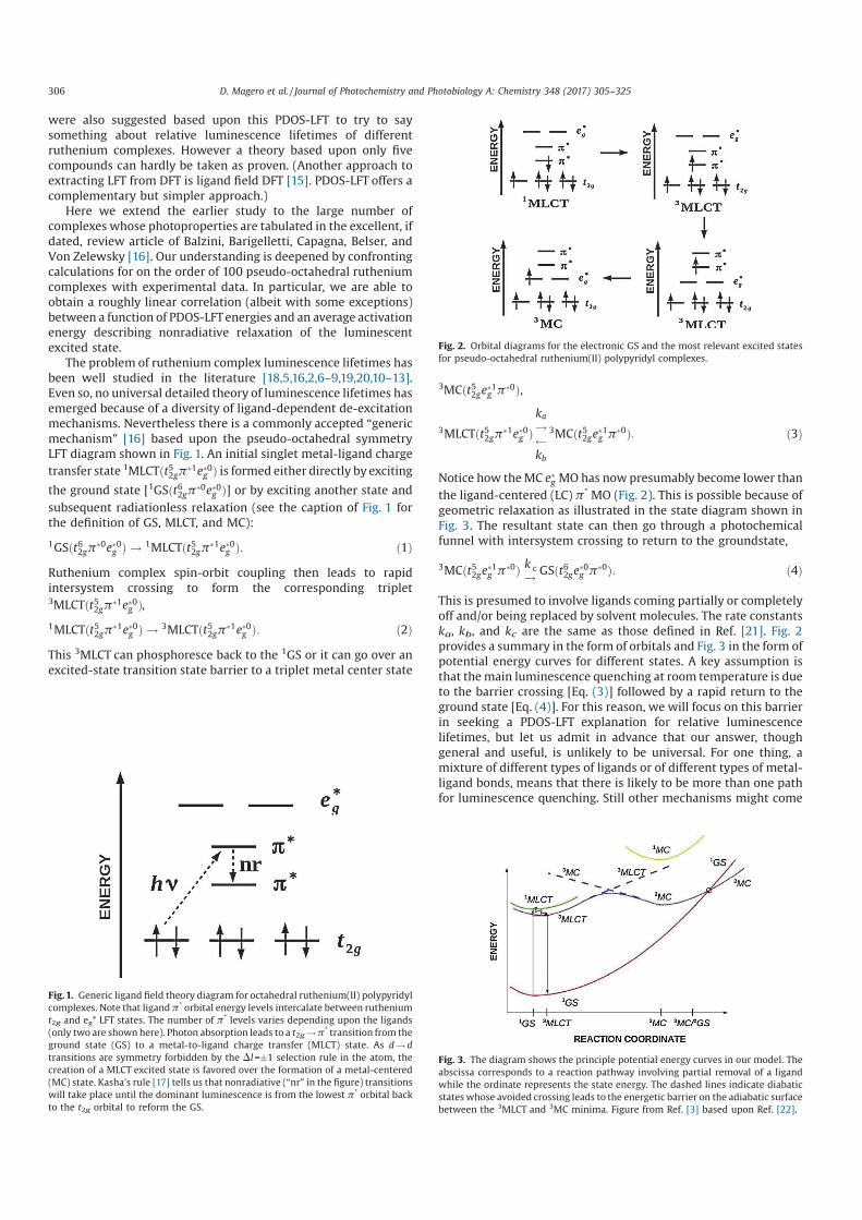
were also suggested based upon this PDOS-LFT to try to saysomething about relative luminescence lifetimes of differentruthenium complexes. However a theory based upon only fivecompounds can hardly be taken as proven. (Another approach toextracting LFT from DFT is ligand field DFT [15]. PDOS-LFT offers acomplementary but simpler approach.)
Here we extend the earlier study to the large number ofcomplexes whose photoproperties are tabulated in the excellent, ifdated, review article of Balzini, Barigelletti, Capagna, Belser, andVon Zelewsky [16]. Our understanding is deepened by confrontingcalculations for on the order of 100 pseudo-octahedral rutheniumcomplexes with experimental data. In particular, we are able toobtain a roughly linear correlation (albeit with some exceptions)between a function of PDOS-LFT energies and an average activationenergy describing nonradiative relaxation of the luminescentexcited state.
The problem of ruthenium complex luminescence lifetimes hasbeen well studied in the literature [18,5,16,2,6–9,19,20,10–13].Even so, no universal detailed theory of luminescence lifetimes hasemerged because of a diversity of ligand-dependent de-excitationmechanisms. Nevertheless there is a commonly accepted “genericmechanism” [16] based upon the pseudo-octahedral symmetryLFT diagram shown in Fig. 1. An initial singlet metal-ligand charge
transfer state 1MLCTðt52gp!1e!0g Þ is formed either directly by exciting
the ground state [1GSðt62gp!0e!0g Þ] or by exciting another state and
subsequent radiationless relaxation (see the caption of Fig. 1 forthe definition of GS, MLCT, and MC):
1GSðt62gp!0e!0g Þ ! 1MLCTðt52gp
!1e!0g Þ: ð1Þ
Ruthenium complex spin-orbit coupling then leads to rapidintersystem crossing to form the corresponding triplet3MLCTðt52gp
!1e!0g Þ,
1MLCTðt52gp!1e!0g Þ ! 3MLCTðt52gp
!1e!0g Þ: ð2Þ
This 3MLCT can phosphoresce back to the 1GS or it can go over anexcited-state transition state barrier to a triplet metal center state
3MCðt52ge!1g p
!0Þ,
3MLCTðt52gp!1e!0g Þ
ka! kb
3MCðt52ge!1g p
!0Þ: ð3Þ
Notice how the MC e!g MO has now presumably become lower than
the ligand-centered (LC) p* MO (Fig. 2). This is possible because ofgeometric relaxation as illustrated in the state diagram shown inFig. 3. The resultant state can then go through a photochemicalfunnel with intersystem crossing to return to the groundstate,
3MCðt52ge!1g p
!0Þk c!
GSðt62ge!0g p
!0Þ: ð4Þ
This is presumed to involve ligands coming partially or completelyoff and/or being replaced by solvent molecules. The rate constantska, kb, and kc are the same as those defined in Ref. [21]. Fig. 2provides a summary in the form of orbitals and Fig. 3 in the form ofpotential energy curves for different states. A key assumption isthat the main luminescence quenching at room temperature is dueto the barrier crossing [Eq. (3)] followed by a rapid return to theground state [Eq. (4)]. For this reason, we will focus on this barrierin seeking a PDOS-LFT explanation for relative luminescencelifetimes, but let us admit in advance that our answer, thoughgeneral and useful, is unlikely to be universal. For one thing, amixture of different types of ligands or of different types of metal-ligand bonds, means that there is likely to be more than one pathfor luminescence quenching. Still other mechanisms might come
Fig. 1. Generic ligand field theory diagram for octahedral ruthenium(II) polypyridylcomplexes. Note that ligand p* orbital energy levels intercalate between rutheniumt2g and eg* LFT states. The number of p* levels varies depending upon the ligands(only two are shown here). Photon absorption leads to a t2g! p* transition from theground state (GS) to a metal-to-ligand charge transfer (MLCT) state. As d ! d
transitions are symmetry forbidden by the Dl =&1 selection rule in the atom, thecreation of a MLCT excited state is favored over the formation of a metal-centered(MC) state. Kasha's rule [17] tells us that nonradiative (“nr” in the figure) transitionswill take place until the dominant luminescence is from the lowest p* orbital backto the t2g orbital to reform the GS.
Fig. 2. Orbital diagrams for the electronic GS and the most relevant excited statesfor pseudo-octahedral ruthenium(II) polypyridyl complexes.
Fig. 3. The diagram shows the principle potential energy curves in our model. Theabscissa corresponds to a reaction pathway involving partial removal of a ligandwhile the ordinate represents the state energy. The dashed lines indicate diabaticstates whose avoided crossing leads to the energetic barrier on the adiabatic surfacebetween the 3MLCT and 3MC minima. Figure from Ref. [3] based upon Ref. [22].
306 D. Magero et al. / Journal of Photochemistry and Photobiology A: Chemistry 348 (2017) 305–325
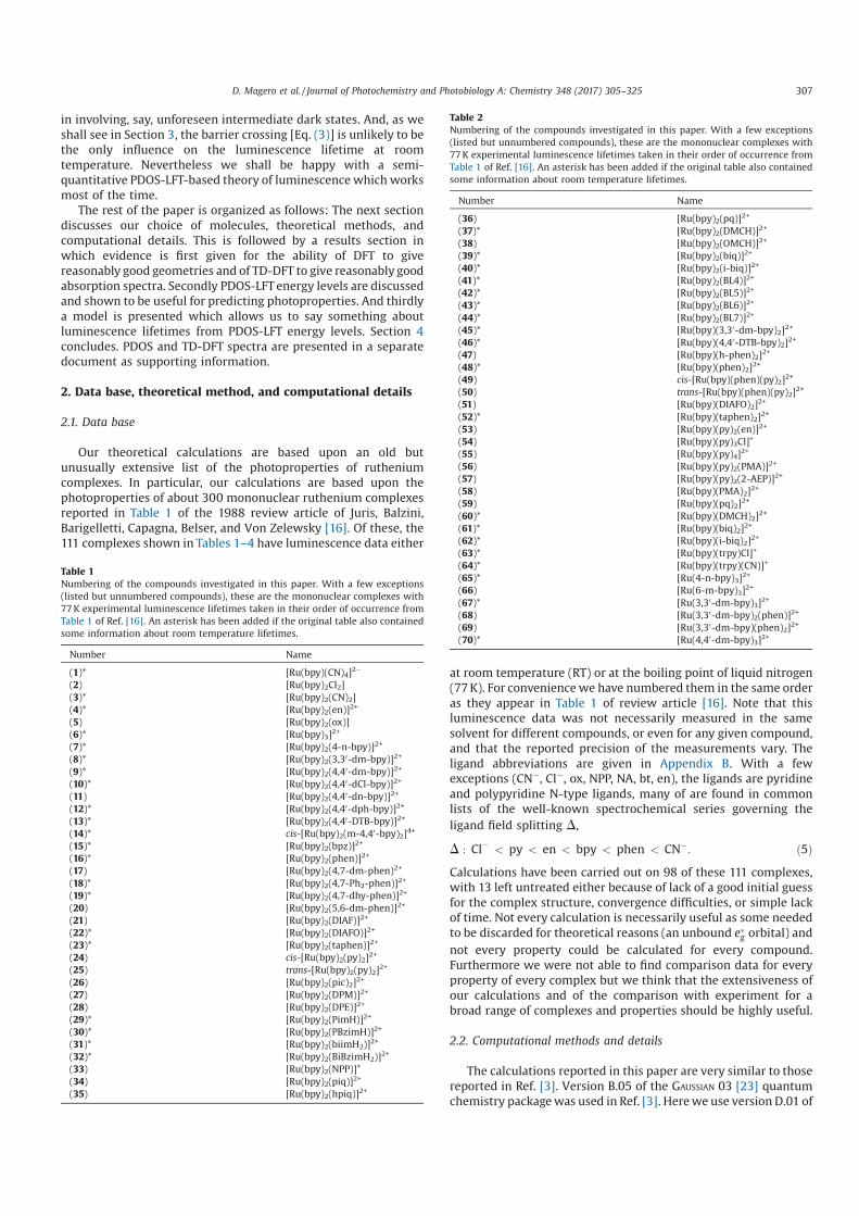
in involving, say, unforeseen intermediate dark states. And, as weshall see in Section 3, the barrier crossing [Eq. (3)] is unlikely to bethe only influence on the luminescence lifetime at roomtemperature. Nevertheless we shall be happy with a semi-quantitative PDOS-LFT-based theory of luminescence which worksmost of the time.
The rest of the paper is organized as follows: The next sectiondiscusses our choice of molecules, theoretical methods, andcomputational details. This is followed by a results section inwhich evidence is first given for the ability of DFT to givereasonably good geometries and of TD-DFT to give reasonably goodabsorption spectra. Secondly PDOS-LFT energy levels are discussedand shown to be useful for predicting photoproperties. And thirdlya model is presented which allows us to say something aboutluminescence lifetimes from PDOS-LFT energy levels. Section 4concludes. PDOS and TD-DFT spectra are presented in a separatedocument as supporting information.
2. Data base, theoretical method, and computational details
2.1. Data base
Our theoretical calculations are based upon an old butunusually extensive list of the photoproperties of rutheniumcomplexes. In particular, our calculations are based upon thephotoproperties of about 300 mononuclear ruthenium complexesreported in Table 1 of the 1988 review article of Juris, Balzini,Barigelletti, Capagna, Belser, and Von Zelewsky [16]. Of these, the111 complexes shown in Tables 1–4 have luminescence data either
at room temperature (RT) or at the boiling point of liquid nitrogen(77 K). For convenience we have numbered them in the same orderas they appear in Table 1 of review article [16]. Note that thisluminescence data was not necessarily measured in the samesolvent for different compounds, or even for any given compound,and that the reported precision of the measurements vary. Theligand abbreviations are given in Appendix B. With a fewexceptions (CN', Cl', ox, NPP, NA, bt, en), the ligands are pyridineand polypyridine N-type ligands, many of are found in commonlists of the well-known spectrochemical series governing theligand field splitting D,
D : Cl' < py < en < bpy < phen < CN': ð5Þ
Calculations have been carried out on 98 of these 111 complexes,with 13 left untreated either because of lack of a good initial guessfor the complex structure, convergence difficulties, or simple lackof time. Not every calculation is necessarily useful as some neededto be discarded for theoretical reasons (an unbound e!g orbital) and
not every property could be calculated for every compound.Furthermore we were not able to find comparison data for everyproperty of every complex but we think that the extensiveness ofour calculations and of the comparison with experiment for abroad range of complexes and properties should be highly useful.
2.2. Computational methods and details
The calculations reported in this paper are very similar to thosereported in Ref. [3]. Version B.05 of the GAUSSIAN 03 [23] quantumchemistry package was used in Ref. [3]. Here we use version D.01 of
Table 1Numbering of the compounds investigated in this paper. With a few exceptions(listed but unnumbered compounds), these are the mononuclear complexes with77 K experimental luminescence lifetimes taken in their order of occurrence fromTable 1 of Ref. [16]. An asterisk has been added if the original table also containedsome information about room temperature lifetimes.
Number Name
(1)* [Ru(bpy)(CN)4]2'
(2) [Ru(bpy)2Cl2](3)* [Ru(bpy)2(CN)2](4)* [Ru(bpy)2(en)]
2+
(5) [Ru(bpy)2(ox)](6)* [Ru(bpy)3]
2+
(7)* [Ru(bpy)2(4-n-bpy)]2+
(8)* [Ru(bpy)2(3,30-dm-bpy)]2+
(9)* [Ru(bpy)2(4,40-dm-bpy)]2+
(10)* [Ru(bpy)2(4,40-dCl-bpy)]2+
(11) [Ru(bpy)2(4,40-dn-bpy)]2+
(12)* [Ru(bpy)2(4,40-dph-bpy)]2+
(13)* [Ru(bpy)2(4,40-DTB-bpy)]2+
(14)* cis-[Ru(bpy)2(m-4,40-bpy)2]4+
(15)* [Ru(bpy)2(bpz)]2+
(16)* [Ru(bpy)2(phen)]2+
(17) [Ru(bpy)2(4,7-dm-phen)2+
(18)* [Ru(bpy)2(4,7-Ph2-phen)]2+
(19)* [Ru(bpy)2(4,7-dhy-phen)]2+
(20) [Ru(bpy)2(5,6-dm-phen)]2+
(21) [Ru(bpy)2(DIAF)]2+
(22)* [Ru(bpy)2(DIAFO)]2+
(23)* [Ru(bpy)2(taphen)]2+
(24) cis-[Ru(bpy)2(py)2]2+
(25) trans-[Ru(bpy)2(py)2]2+
(26) [Ru(bpy)2(pic)2]2+
(27) [Ru(bpy)2(DPM)]2+
(28) [Ru(bpy)2(DPE)]2+
(29)* [Ru(bpy)2(PimH)]2+
(30)* [Ru(bpy)2(PBzimH)]2+
(31)* [Ru(bpy)2(biimH2)]2+
(32)* [Ru(bpy)2(BiBzimH2)]2+
(33) [Ru(bpy)2(NPP)]+
(34) [Ru(bpy)2(piq)]2+
(35) [Ru(bpy)2(hpiq)]2+
Table 2Numbering of the compounds investigated in this paper. With a few exceptions(listed but unnumbered compounds), these are the mononuclear complexes with77 K experimental luminescence lifetimes taken in their order of occurrence fromTable 1 of Ref. [16]. An asterisk has been added if the original table also containedsome information about room temperature lifetimes.
Number Name
(36) [Ru(bpy)2(pq)]2+
(37)* [Ru(bpy)2(DMCH)]2+
(38) [Ru(bpy)2(OMCH)]2+
(39)* [Ru(bpy)2(biq)]2+
(40)* [Ru(bpy)2(i-biq)]2+
(41)* [Ru(bpy)2(BL4)]2+
(42)* [Ru(bpy)2(BL5)]2+
(43)* [Ru(bpy)2(BL6)]2+
(44)* [Ru(bpy)2(BL7)]2+
(45)* [Ru(bpy)(3,30-dm-bpy)2]2+
(46)* [Ru(bpy)(4,40-DTB-bpy)2]2+
(47) [Ru(bpy)(h-phen)2]2+
(48)* [Ru(bpy)(phen)2]2+
(49) cis-[Ru(bpy)(phen)(py)2]2+
(50) trans-[Ru(bpy)(phen)(py)2]2+
(51) [Ru(bpy)(DIAFO)2]2+
(52)* [Ru(bpy)(taphen)2]2+
(53) [Ru(bpy)(py)2(en)]2+
(54) [Ru(bpy)(py)3Cl]+
(55) [Ru(bpy)(py)4]2+
(56) [Ru(bpy)(py)2(PMA)]2+
(57) [Ru(bpy)(py)2(2-AEP)]2+
(58) [Ru(bpy)(PMA)2]2+
(59) [Ru(bpy)(pq)2]2+
(60)* [Ru(bpy)(DMCH)2]2+
(61)* [Ru(bpy)(biq)2]2+
(62)* [Ru(bpy)(i-biq)2]2+
(63)* [Ru(bpy)(trpy)Cl]+
(64)* [Ru(bpy)(trpy)(CN)]+
(65)* [Ru(4-n-bpy)3]2+
(66) [Ru(6-m-bpy)3]2+
(67)* [Ru(3,30-dm-bpy)3]2+
(68) [Ru(3,30-dm-bpy)2(phen)]2+
(69) [Ru(3,30-dm-bpy)(phen)2]2+
(70)* [Ru(4,40-dm-bpy)3]2+
D. Magero et al. / Journal of Photochemistry and Photobiology A: Chemistry 348 (2017) 305–325 307
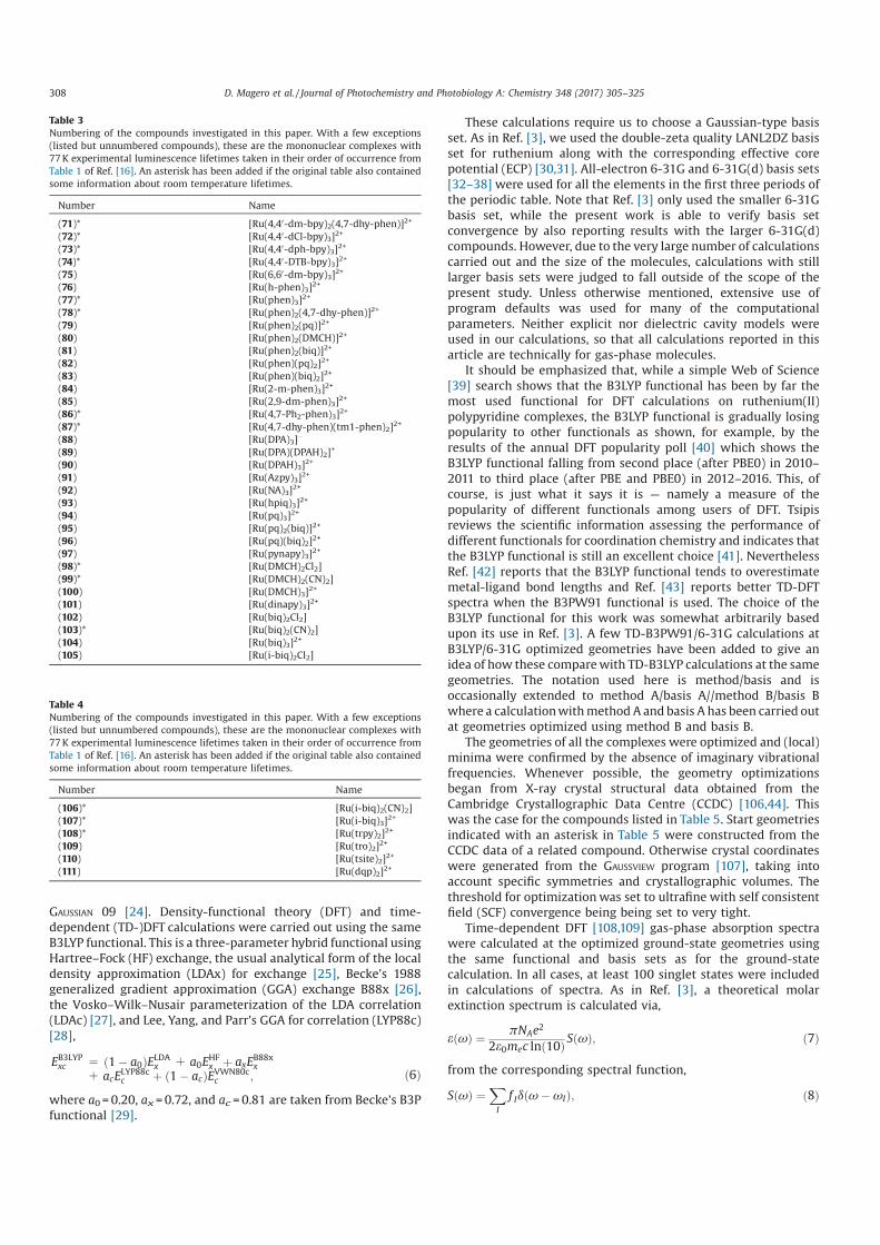
GAUSSIAN 09 [24]. Density-functional theory (DFT) and time-dependent (TD-)DFT calculations were carried out using the sameB3LYP functional. This is a three-parameter hybrid functional usingHartree–Fock (HF) exchange, the usual analytical form of the localdensity approximation (LDAx) for exchange [25], Becke's 1988generalized gradient approximation (GGA) exchange B88x [26],the Vosko–Wilk–Nusair parameterization of the LDA correlation(LDAc) [27], and Lee, Yang, and Parr's GGA for correlation (LYP88c)[28],
EB3LYPxc¼ ð1 ' a0ÞE
LDAxþ a0E
HFx þ axE
B88xx
þ acELYP88cc þ ð1 ' acÞE
VWN80cc ; ð6Þ
where a0= 0.20, ax = 0.72, and ac = 0.81 are taken from Becke's B3Pfunctional [29].
These calculations require us to choose a Gaussian-type basisset. As in Ref. [3], we used the double-zeta quality LANL2DZ basisset for ruthenium along with the corresponding effective corepotential (ECP) [30,31]. All-electron 6-31G and 6-31G(d) basis sets[32–38] were used for all the elements in the first three periods ofthe periodic table. Note that Ref. [3] only used the smaller 6-31Gbasis set, while the present work is able to verify basis setconvergence by also reporting results with the larger 6-31G(d)compounds. However, due to the very large number of calculationscarried out and the size of the molecules, calculations with stilllarger basis sets were judged to fall outside of the scope of thepresent study. Unless otherwise mentioned, extensive use ofprogram defaults was used for many of the computationalparameters. Neither explicit nor dielectric cavity models wereused in our calculations, so that all calculations reported in thisarticle are technically for gas-phase molecules.
It should be emphasized that, while a simple Web of Science[39] search shows that the B3LYP functional has been by far themost used functional for DFT calculations on ruthenium(II)polypyridine complexes, the B3LYP functional is gradually losingpopularity to other functionals as shown, for example, by theresults of the annual DFT popularity poll [40] which shows theB3LYP functional falling from second place (after PBE0) in 2010–2011 to third place (after PBE and PBE0) in 2012–2016. This, ofcourse, is just what it says it is — namely a measure of thepopularity of different functionals among users of DFT. Tsipisreviews the scientific information assessing the performance ofdifferent functionals for coordination chemistry and indicates thatthe B3LYP functional is still an excellent choice [41]. NeverthelessRef. [42] reports that the B3LYP functional tends to overestimatemetal-ligand bond lengths and Ref. [43] reports better TD-DFTspectra when the B3PW91 functional is used. The choice of theB3LYP functional for this work was somewhat arbitrarily basedupon its use in Ref. [3]. A few TD-B3PW91/6-31G calculations atB3LYP/6-31G optimized geometries have been added to give anidea of how these compare with TD-B3LYP calculations at the samegeometries. The notation used here is method/basis and isoccasionally extended to method A/basis A//method B/basis Bwhere a calculation with method A and basis A has been carried outat geometries optimized using method B and basis B.
The geometries of all the complexes were optimized and (local)minima were confirmed by the absence of imaginary vibrationalfrequencies. Whenever possible, the geometry optimizationsbegan from X-ray crystal structural data obtained from theCambridge Crystallographic Data Centre (CCDC) [106,44]. Thiswas the case for the compounds listed in Table 5. Start geometriesindicated with an asterisk in Table 5 were constructed from theCCDC data of a related compound. Otherwise crystal coordinateswere generated from the GAUSSVIEW program [107], taking intoaccount specific symmetries and crystallographic volumes. Thethreshold for optimization was set to ultrafine with self consistentfield (SCF) convergence being being set to very tight.
Time-dependent DFT [108,109] gas-phase absorption spectrawere calculated at the optimized ground-state geometries usingthe same functional and basis sets as for the ground-statecalculation. In all cases, at least 100 singlet states were includedin calculations of spectra. As in Ref. [3], a theoretical molarextinction spectrum is calculated via,
eðvÞ ¼pNAe
2
2e0mec lnð10ÞSðvÞ; ð7Þ
from the corresponding spectral function,
SðvÞ ¼X
I
f Idðv ' vIÞ; ð8Þ
Table 3Numbering of the compounds investigated in this paper. With a few exceptions(listed but unnumbered compounds), these are the mononuclear complexes with77 K experimental luminescence lifetimes taken in their order of occurrence fromTable 1 of Ref. [16]. An asterisk has been added if the original table also containedsome information about room temperature lifetimes.
Number Name
(71)* [Ru(4,40-dm-bpy)2(4,7-dhy-phen)]2+
(72)* [Ru(4,40-dCl-bpy)3]2+
(73)* [Ru(4,40-dph-bpy)3]2+
(74)* [Ru(4,40-DTB-bpy)3]2+
(75) [Ru(6,60-dm-bpy)3]2+
(76) [Ru(h-phen)3]2+
(77)* [Ru(phen)3]2+
(78)* [Ru(phen)2(4,7-dhy-phen)]2+
(79) [Ru(phen)2(pq)]2+
(80) [Ru(phen)2(DMCH)]2+
(81) [Ru(phen)2(biq)]2+
(82) [Ru(phen)(pq)2]2+
(83) [Ru(phen)(biq)2]2+
(84) [Ru(2-m-phen)3]2+
(85) [Ru(2,9-dm-phen)3]2+
(86)* [Ru(4,7-Ph2-phen)3]2+
(87)* [Ru(4,7-dhy-phen)(tm1-phen)2]2+
(88) [Ru(DPA)3]'
(89) [Ru(DPA)(DPAH)2]+
(90) [Ru(DPAH)3]2+
(91) [Ru(Azpy)3]2+
(92) [Ru(NA)3]2+
(93) [Ru(hpiq)3]2+
(94) [Ru(pq)3]2+
(95) [Ru(pq)2(biq)]2+
(96) [Ru(pq)(biq)2]2+
(97) [Ru(pynapy)3]2+
(98)* [Ru(DMCH)2Cl2](99)* [Ru(DMCH)2(CN)2](100) [Ru(DMCH)3]
2+
(101) [Ru(dinapy)3]2+
(102) [Ru(biq)2Cl2](103)* [Ru(biq)2(CN)2](104) [Ru(biq)3]
2+
(105) [Ru(i-biq)2Cl2]
Table 4Numbering of the compounds investigated in this paper. With a few exceptions(listed but unnumbered compounds), these are the mononuclear complexes with77 K experimental luminescence lifetimes taken in their order of occurrence fromTable 1 of Ref. [16]. An asterisk has been added if the original table also containedsome information about room temperature lifetimes.
Number Name
(106)* [Ru(i-biq)2(CN)2](107)* [Ru(i-biq)3]
2+
(108)* [Ru(trpy)2]2+
(109) [Ru(tro)2]2+
(110) [Ru(tsite)2]2+
(111) [Ru(dqp)2]2+
308 D. Magero et al. / Journal of Photochemistry and Photobiology A: Chemistry 348 (2017) 305–325
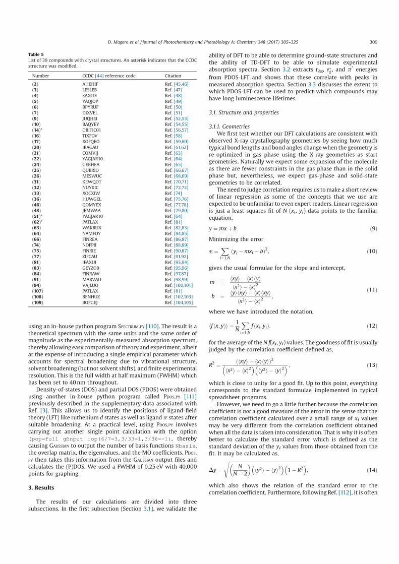
using an in-house python program SPECTRUM.PY [110]. The result is atheoretical spectrum with the same units and the same order ofmagnitude as the experimentally-measured absorption spectrum,thereby allowing easy comparison of theory and experiment, albeitat the expense of introducing a single empirical parameter whichaccounts for spectral broadening due to vibrational structure,solvent broadening (but not solvent shifts), and finite experimentalresolution. This is the full width at half maximum (FWHM) whichhas been set to 40 nm throughout.
Density-of-states (DOS) and partial DOS (PDOS) were obtainedusing another in-house python program called PDOS.PY [111]previously described in the supplementary data associated withRef. [3]. This allows us to identify the positions of ligand-fieldtheory (LFT) like ruthenium d states as well as ligand p states aftersuitable broadening. At a practical level, using PDOS.PY involvescarrying out another single point calculation with the option(pop=full gfinput iop(6/7=3,3/33=1,3/36=-1), therebycausing GAUSSIAN to output the number of basis functions Nbasis,the overlap matrix, the eigenvalues, and the MO coefficients. PDOS.PY then takes this information from the GAUSSIAN output files andcalculates the (P)DOS. We used a FWHM of 0.25 eV with 40,000points for graphing.
3. Results
The results of our calculations are divided into threesubsections. In the first subsection (Section 3.1), we validate the
ability of DFT to be able to determine ground-state structures andthe ability of TD-DFT to be able to simulate experimentalabsorption spectra. Section 3.2 extracts t2g, e!g , and p* energies
from PDOS-LFT and shows that these correlate with peaks inmeasured absorption spectra. Section 3.3 discusses the extent towhich PDOS-LFT can be used to predict which compounds mayhave long luminescence lifetimes.
3.1. Structure and properties
3.1.1. Geometries
We first test whether our DFT calculations are consistent withobserved X-ray crystallography geometries by seeing how muchtypical bond lengths and bond angles change when the geometry isre-optimized in gas phase using the X-ray geometries as startgeometries. Naturally we expect some expansion of the moleculeas there are fewer constraints in the gas phase than in the solidphase but, nevertheless, we expect gas-phase and solid-stategeometries to be correlated.
The need to judge correlation requires us to make a short reviewof linear regression as some of the concepts that we use areexpected to be unfamiliar to even expert readers. Linear regressionis just a least squares fit of N (xi, yi) data points to the familiarequation,
y ¼ mx þ b: ð9Þ
Minimizing the error
E ¼X
i¼1;N
yi ' mxi ' bð Þ2; ð10Þ
gives the usual formulae for the slope and intercept,
m ¼hxyi ' hxihyi
hx2i ' hxi2
b ¼hyihxyi ' hxihxyi
hx2i ' hxi2;
ð11Þ
where we have introduced the notation,
hf ðx; yÞi ¼1N
X
i¼1;N
f ðxi; yiÞ: ð12Þ
for the average of the N f(xi, yi) values. The goodness of fit is usuallyjudged by the correlation coefficient defined as,
R2 ¼hxyi ' hxihyið Þ2
hx2i ' hxi2" #
hy2i ' hyi2" # ; ð13Þ
which is close to unity for a good fit. Up to this point, everythingcorresponds to the standard formulae implemented in typicalspreadsheet programs.
However, we need to go a little further because the correlationcoefficient is not a good measure of the error in the sense that thecorrelation coefficient calculated over a small range of xi valuesmay be very different from the correlation coefficient obtainedwhen all the data is taken into consideration. That is why it is oftenbetter to calculate the standard error which is defined as thestandard deviation of the yi values from those obtained from thefit. It may be calculated as,
Dy ¼
ffiffiffiffiffiffiffiffiffiffiffiffiffiffiffiffiffiffiffiffiffiffiffiffiffiffiffiffiffiffiffiffiffiffiffiffiffiffiffiffiffiffiffiffiffiffiffiffiffiffiffiffiffiffiffiffiffiffiffiffiffiffiffiffiffiffiffi
N
N ' 2
% &
hy2i ' hyi2" #
1 ' R2" #
s
; ð14Þ
which also shows the relation of the standard error to thecorrelation coefficient. Furthermore, following Ref. [112], it is often
Table 5List of 39 compounds with crystal structures. An asterisk indicates that the CCDCstructure was modified.
Number CCDC [44] reference code Citation
(2) AHEHIF Ref. [45,46](3) LESLEB Ref. [47](4) SAXCIE Ref. [48](5) YAQJOP Ref. [49](6) BPYRUF Ref. [50](7) DIXVEL Ref. [51](9) JUQHEI Ref. [52,53](10) BAQYEY Ref. [54,55](14)* OBITIC01 Ref. [56,57](16) TIXFOV Ref. [58](17) XOFQEO Ref. [59,60](20) IBAGAU Ref. [61,62](21) COMVIJ Ref. [63](22) YAGJAR10 Ref. [64](24) GEBHEA Ref. [65](25) QUBRIO Ref. [66,67](26) MESWUC Ref. [68,69](31) KEWQOT Ref. [70,71](32) NUYKIC Ref. [72,73](33) XOCXIW Ref. [74](36) HUWGEL Ref. [75,76](46) QOMYEX Ref. [77,78](48) JEMWAA Ref. [79,80](51)* YAGJAR10 Ref. [64](62)* PATLAX Ref. [81](63) WAKRUX Ref. [82,83](64) NAMFOY Ref. [84,85](66) FINREA Ref. [86,87](74) NOFPII Ref. [88,89](75) FINRIE Ref. [90,87](77) ZIFCAU Ref. [91,92](81) IFAXUI Ref. [93,94](83) GEYZOB Ref. [95,96](84) FINRAW Ref. [97,87](91) MARVAD Ref. [98,99](94) VAJLUO Ref. [100,101](107) PATLAX Ref. [81](108) BENHUZ Ref. [102,103](109) BOFGEJ Ref. [104,105]
D. Magero et al. / Journal of Photochemistry and Photobiology A: Chemistry 348 (2017) 305–325 309
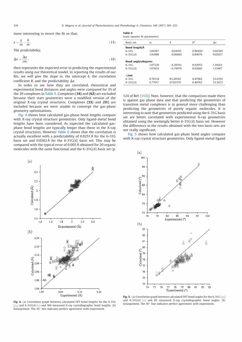
more interesting to invert the fit so that,
x ¼y
m'
b
m: ð15Þ
The predictability,
Dx ¼Dy
jmj; ð16Þ
then represents the expected error in predicting the experimentalresults using our theoretical model. In reporting the results of ourfits, we will give the slope m, the intercept b, the correlationcoefficient R, and the predictability Dx.
In order to see how they are correlated, theoretical andexperimental bond distances and angles were compared for 35 ofthe 39 complexes in Table 5. Complexes (14) and (62) are excludedbecause their start geometries were a modified version of theoriginal X-ray crystal structures. Complexes (33) and (51) areexcluded because we were unable to converge the gas-phasegeometry optimizations.
Fig. 4 shows how calculated gas-phase bond lengths comparewith X-ray crystal structure geometries. Only ligand-metal bondlengths have been considered. As expected the calculated gas-phase bond lengths are typically longer than those in the X-raycrystal structures. However Table 6 shows that the correlation isactually excellent with a predictability of 0.0251 Å for the 6-31Gbasis set and 0.0262 Å for the 6-31G(d) basis set. This may becompared with the typical error of 0.005 Å obtained for 20 organicmolecules with the same functional and the 6-31G(d) basis set (p.
124 of Ref. [113]). Note, however, that the comparison made thereis against gas phase data and that predicting the geometries oftransition metal complexes is in general more challenging thanpredicting the geometries of purely organic molecules. It isinteresting to note that geometries predicted using the 6-31G basisset are better correlated with experimental X-ray geometriesobtained using the seemingly better 6-31G(d) basis set. Howeverthe differences in the results obtained with the two basis sets arenot really significant.
Fig. 5 shows how calculated gas-phase bond angles comparewith X-ray crystal structure geometries. Only ligand-metal-ligand
Fig. 4. (a) Correlation graph between calculated DFT bond lengths for the 6-31G(~) and 6-31G(d) (.) and 184 measured X-ray crystallographic bond lengths. (b)Enlargement. The 45. line indicates perfect agreement with experiment.
Table 6Least squares fit parameters.
Basis set m b R2 Dx
Bond length/Å6-31G 1.04387 '0.04195 0.90450 0.025056-31G(d) 1.02988 '0.00602 0.89674 0.02617
Bond angles/degrees6-31G 1.07230 '6.39743 0.93055 1.102636-31G(d) 1.07424 '6.79970 0.92682 1.13407
l/nm6-31G 0.78134 81.20545 0.47982 33.63196-31G(d) 0.77617 67.65579 0.40762 53.5672
Fig. 5. (a) Correlation graph between calculated DFT bond angles for the 6-31G (~)and 6-31G(d) (.) and 85 measured X-ray crystallographic bond angles. (b)Enlargement. The 45. line indicates perfect agreement with experiment.
310 D. Magero et al. / Journal of Photochemistry and Photobiology A: Chemistry 348 (2017) 305–325
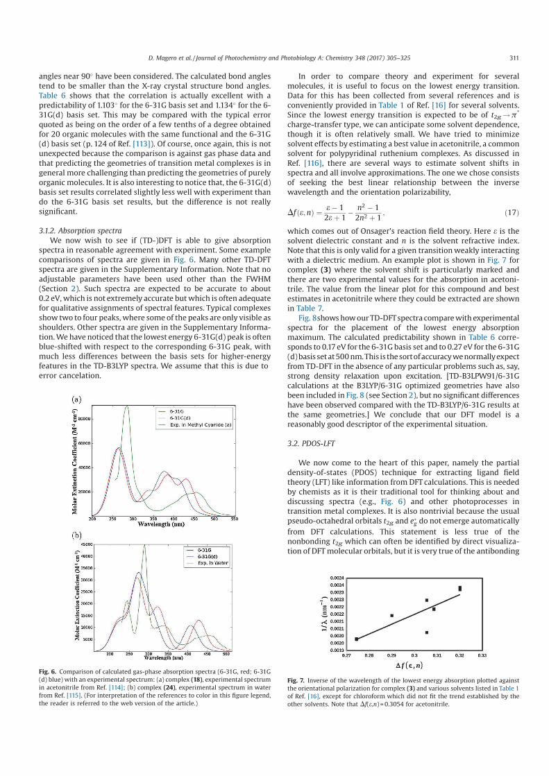
angles near 90. have been considered. The calculated bond anglestend to be smaller than the X-ray crystal structure bond angles.Table 6 shows that the correlation is actually excellent with apredictability of 1.103. for the 6-31G basis set and 1.134. for the 6-31G(d) basis set. This may be compared with the typical errorquoted as being on the order of a few tenths of a degree obtainedfor 20 organic molecules with the same functional and the 6-31G(d) basis set (p. 124 of Ref. [113]). Of course, once again, this is notunexpected because the comparison is against gas phase data andthat predicting the geometries of transition metal complexes is ingeneral more challenging than predicting the geometries of purelyorganic molecules. It is also interesting to notice that, the 6-31G(d)basis set results correlated slightly less well with experiment thando the 6-31G basis set results, but the difference is not reallysignificant.
3.1.2. Absorption spectra
We now wish to see if (TD-)DFT is able to give absorptionspectra in reasonable agreement with experiment. Some examplecomparisons of spectra are given in Fig. 6. Many other TD-DFTspectra are given in the Supplementary Information. Note that noadjustable parameters have been used other than the FWHM(Section 2). Such spectra are expected to be accurate to about0.2 eV, which is not extremely accurate but which is often adequatefor qualitative assignments of spectral features. Typical complexesshow two to four peaks, where some of the peaks are only visible asshoulders. Other spectra are given in the Supplementary Informa-tion. We have noticed that the lowest energy 6-31G(d) peak is oftenblue-shifted with respect to the corresponding 6-31G peak, withmuch less differences between the basis sets for higher-energyfeatures in the TD-B3LYP spectra. We assume that this is due toerror cancelation.
In order to compare theory and experiment for severalmolecules, it is useful to focus on the lowest energy transition.Data for this has been collected from several references and isconveniently provided in Table 1 of Ref. [16] for several solvents.Since the lowest energy transition is expected to be of t2g! p*
charge-transfer type, we can anticipate some solvent dependence,though it is often relatively small. We have tried to minimizesolvent effects by estimating a best value in acetonitrile, a commonsolvent for polypyridinal ruthenium complexes. As discussed inRef. [116], there are several ways to estimate solvent shifts inspectra and all involve approximations. The one we chose consistsof seeking the best linear relationship between the inversewavelength and the orientation polarizability,
Df ðe; nÞ ¼e ' 12e þ 1
'n2 ' 12n2 þ 1
; ð17Þ
which comes out of Onsager's reaction field theory. Here e is thesolvent dielectric constant and n is the solvent refractive index.Note that this is only valid for a given transition weakly interactingwith a dielectric medium. An example plot is shown in Fig. 7 forcomplex (3) where the solvent shift is particularly marked andthere are two experimental values for the absorption in acetoni-trile. The value from the linear plot for this compound and bestestimates in acetonitrile where they could be extracted are shownin Table 7.
Fig. 8shows how our TD-DFTspectra compare with experimentalspectra for the placement of the lowest energy absorptionmaximum. The calculated predictability shown in Table 6 corre-sponds to 0.17 eV for the 6-31G basis set and to 0.27 eV for the 6-31G(d)basis set at500 nm. This is thesortofaccuracy wenormallyexpectfrom TD-DFT in the absence of any particular problems such as, say,strong density relaxation upon excitation. [TD-B3LPW91/6-31Gcalculations at the B3LYP/6-31G optimized geometries have alsobeen included in Fig. 8 (see Section 2), but no significant differenceshave been observed compared with the TD-B3LYP/6-31G results atthe same geometries.] We conclude that our DFT model is areasonably good descriptor of the experimental situation.
3.2. PDOS-LFT
We now come to the heart of this paper, namely the partialdensity-of-states (PDOS) technique for extracting ligand fieldtheory (LFT) like information from DFT calculations. This is neededby chemists as it is their traditional tool for thinking about anddiscussing spectra (e.g., Fig. 6) and other photoprocesses intransition metal complexes. It is also nontrivial because the usualpseudo-octahedral orbitals t2g and e!g do not emerge automatically
from DFT calculations. This statement is less true of thenonbonding t2g which can often be identified by direct visualiza-tion of DFT molecular orbitals, but it is very true of the antibonding
Fig. 6. Comparison of calculated gas-phase absorption spectra (6-31G, red; 6-31G(d) blue) with an experimental spectrum: (a) complex (18), experimental spectrumin acetonitrile from Ref. [114]; (b) complex (24), experimental spectrum in waterfrom Ref. [115]. (For interpretation of the references to color in this figure legend,the reader is referred to the web version of the article.)
Fig. 7. Inverse of the wavelength of the lowest energy absorption plotted againstthe orientational polarization for complex (3) and various solvents listed in Table 1of Ref. [16], except for chloroform which did not fit the trend established by theother solvents. Note that Df(e,n) = 0.3054 for acetonitrile.
D. Magero et al. / Journal of Photochemistry and Photobiology A: Chemistry 348 (2017) 305–325 311
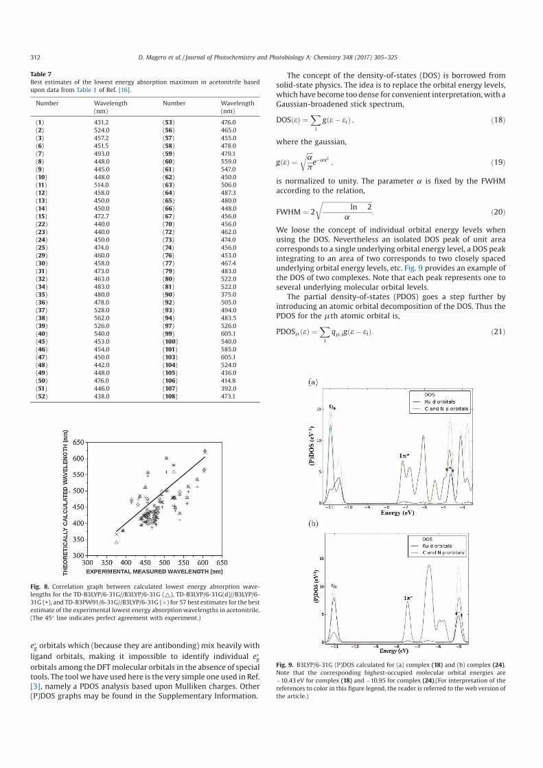
e!g orbitals which (because they are antibonding) mix heavily with
ligand orbitals, making it impossible to identify individual e!gorbitals among the DFT molecular orbitals in the absence of specialtools. The tool we have used here is the very simple one used in Ref.[3], namely a PDOS analysis based upon Mulliken charges. Other(P)DOS graphs may be found in the Supplementary Information.
The concept of the density-of-states (DOS) is borrowed fromsolid-state physics. The idea is to replace the orbital energy levels,which have become too dense for convenient interpretation, with aGaussian-broadened stick spectrum,
DOSðeÞ ¼X
i
gðe ' eiÞ ; ð18Þ
where the gaussian,
gðeÞ ¼
ffiffiffiffi
a
p
r
e'ax2; ð19Þ
is normalized to unity. The parameter a is fixed by the FWHMaccording to the relation,
FWHM ¼ 2
ffiffiffiffiffiffiffiffiffiffiffiffiffiffiffiffiffiffiffiffiffiffiffiffiffiffiffiffiffiffiffiffi
ln 2a
r
: ð20Þ
We loose the concept of individual orbital energy levels whenusing the DOS. Nevertheless an isolated DOS peak of unit areacorresponds to a single underlying orbital energy level, a DOS peakintegrating to an area of two corresponds to two closely spacedunderlying orbital energy levels, etc. Fig. 9 provides an example ofthe DOS of two complexes. Note that each peak represents one toseveral underlying molecular orbital levels.
The partial density-of-states (PDOS) goes a step further byintroducing an atomic orbital decomposition of the DOS. Thus thePDOS for the mth atomic orbital is,
PDOSmðeÞ ¼X
i
qm;igðe ' eiÞ: ð21Þ
Table 7Best estimates of the lowest energy absorption maximum in acetonitrile basedupon data from Table 1 of Ref. [16].
Number Wavelength Number Wavelength(nm) (nm)
(1) 431.2 (53) 476.0(2) 524.0 (56) 465.0(3) 457.2 (57) 455.0(6) 451.5 (58) 478.0(7) 493.0 (59) 479.1(8) 448.0 (60) 559.0(9) 445.0 (61) 547.0(10) 448.0 (62) 450.0(11) 514.0 (63) 506.0(12) 458.0 (64) 487.3(13) 450.0 (65) 480.0(14) 450.0 (66) 448.0(15) 472.7 (67) 456.0(22) 440.0 (70) 456.0(23) 440.0 (72) 462.0(24) 450.0 (73) 474.0(25) 474.0 (74) 456.0(29) 460.0 (76) 453.0(30) 458.0 (77) 467.4(31) 473.0 (79) 483.0(32) 463.0 (80) 522.0(34) 483.0 (81) 522.0(35) 480.0 (90) 375.0(36) 478.0 (92) 505.0(37) 528.0 (93) 494.0(38) 562.0 (94) 483.5(39) 526.0 (97) 526.0(40) 540.0 (99) 605.1(45) 453.0 (100) 540.0(46) 454.0 (101) 585.0(47) 450.0 (103) 605.1(48) 442.0 (104) 524.0(49) 448.0 (105) 436.0(50) 476.0 (106) 414.8(51) 446.0 (107) 392.0(52) 438.0 (108) 473.1
Fig. 8. Correlation graph between calculated lowest energy absorption wave-lengths for the TD-B3LYP/6-31G//B3LYP/6-31G (~), TD-B3LYP/6-31G(d)//B3LYP/6-31G (+), and TD-B3PW91/6-31G//B3LYP/6-31G (/) for 57 best estimates for the bestestimate of the experimental lowest energy absorption wavelengths in acetonitrile.(The 45. line indicates perfect agreement with experiment.)
Fig. 9. B3LYP/6-31G (P)DOS calculated for (a) complex (18) and (b) complex (24).Note that the corresponding highest-occupied molecular orbital energies are'10.43 eV for complex (18) and '10.95 for complex (24).(For interpretation of thereferences to color in this figure legend, the reader is referred to the web version ofthe article.)
312 D. Magero et al. / Journal of Photochemistry and Photobiology A: Chemistry 348 (2017) 305–325
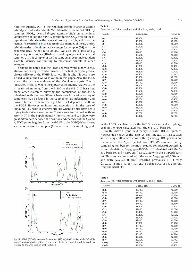
Here the quantity qm,i is the Mulliken atomic charge of atomicorbital m in molecular orbital i. We obtain the ruthenium d PDOS bysumming PDOSm over all d-type atomic orbitals on ruthenium.Similarly we obtain the p PDOS by summing PDOSm over all the p-type atomic orbitals on the heavy atoms (e.g., on C, N, and O) on theligands. As seen in Fig. 9, the approximate energies of the t2g and e!gorbitals on the ruthenium clearly emerge for complex (24) with theexpected peak height ratio of 3:2. We also see a loss of t2gdegeneracy for complex (18) due to breaking of perfect octahedralsymmetry in this complex as well as some small seemingly randomd-orbital density contributing to molecular orbitals at otherenergies.
It should be noted that the PDOS analysis, while highly useful,also contains a degree of arbitrariness. In the first place, the precisepicture will vary as the FWHM is varied. This is why it is best to usea fixed value of the FWHM as we do in this paper. Also, the PDOSshares the basis-dependence of the Mulliken analysis. This isillustrated in Fig. 10 where the e!g peak shifts slightly relative to the
p* peaks when going from the 6-31G to the 6-31G(d) basis set.Many other examples allowing the comparison of the PDOScalculated with the two different basis sets for a wide variety ofcomplexes may be found in the Supplementary Information andprovide further evidence for slight basis-set dependent shifts inthe PDOS. However an important exception is in the case ofunbound (i.e., positive energy) orbitals where a finite basis set istrying to describe a continuum. These cases are marked with anasterisk (*) in the Supplementary Information and can show verygreat differences between the position and character of the t2g ande!g PDOS peaks in going from the 6-31G to the 6-31G(d) basis sets,
such as is the case for complex (7)* where there is a simple t2g peakin the PDOS calculated with the 6-31G basis set and a triple t2gpeak in the PDOS calculated with the 6-31G(d) basis set.
We thus have a ligand-field theory (LFT) like PDOS-LFT picture.However it is not LFT as the PDOS-LFT splitting DPDOS'LFTcalculatedas the energy difference between the e!g and t2g PDOS peaks is not
the same as the DLFT expected from LFT. We can see this bycomparing numbers for the much studied complex (6). Accordingto our calculations, DPDOS'LFT =49,300 cm'1 calculated with the 6-31G basis set and 48,200 cm'1 calculated with the 6-31G(d) basisset. This can be compared with the value DPDOS'LFT =48,000 cm'1
and with DLFT =28,600 cm'1 reported previously [3]. ClearlyDPDOS'LFT is much larger than DLFT so that PDOS-LFT is differentfrom the usual LFT.
Fig. 10. B3LYP (P)DOS calculated for complex (18): (a) 6-31G basis and (b) 6-31G(d)basis.(For interpretation of the references to color in this figure legend, the reader isreferred to the web version of the article.)
Table 8DPDOS'LFT (cm'1) for complexes with simple t2g and e!g peaks.
Number 6-31G6-31G 6-31G(d)
(6) 49,300. 48,200.(8) 48,800. 48,100.(9) 48,900. 48,000.(11) 49,300. 47,800.(13) 49,100. 47,900.(14) 47,800. 46,900.(15) 49,500. 48,300.(16) 48,800. 47,800.(17) 48,300. 47,400.(19) 47,800. 46,500.(20) 48,800. 47,400.(23) 48,400. 47,400.(24) 48,400. 47,300.(25) 48,400. 47,100.(26) 48,300. 47,200.(27) 48,000. 46,800.(28) 47,700. 46,700.(29) 48,700. 47,500.(30) 48,500. 47,500.(31) 48,500. 47,000.(32) 48,000. 46,700.(34) 49,000. 47,900.(40) 48,700. 47,400.(41) 48,900. 47,700.(42) 48,800. 48,000.(46) 48,900. 47,700.(47) 48,800. 47,600.(48) 48,700. 47,200.(50) 48,300. 47,100.
Table 9DPDOS'LFT (cm'1) for complexes with simple t2g and e!g peaks.
Number 6-31G6-31G 6-31G(d)
(52) 48,100. 46,800.(53) 47,400. 46,700.(55) 47,100. 45,700.(56) 47,700. 46,600.(57) 47,300. 46,300.(58) 47,600. 46,400.(70) 48,300. 47,500.(71) 47,800. 46,600.(75) 45,400. 44,700.(76) 48,400. 47,600.(77) 48,300. 47,300.(78) 47,800. 46,600.(85) 43,800. 43,400.(87) 47,700. 46,300.(90) 47,400. 45,700.(93) 47,500. 46,600.(94) 46,100. 44,700.(96) 43,600. 42,500.(97) 48,500. 47,100.(104) 43,000. 42,200.(107) 48,000. 47,400.
D. Magero et al. / Journal of Photochemistry and Photobiology A: Chemistry 348 (2017) 305–325 313
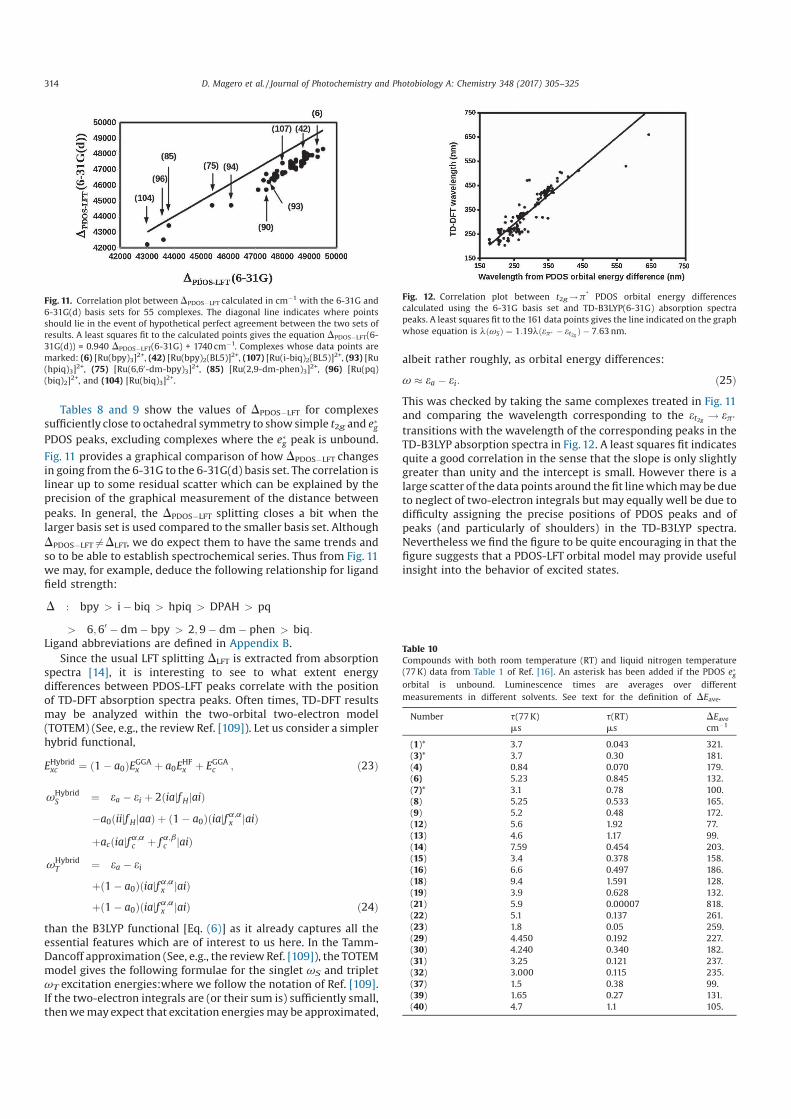
Tables 8 and 9 show the values of DPDOS'LFT for complexessufficiently close to octahedral symmetry to show simple t2g and e!gPDOS peaks, excluding complexes where the e!g peak is unbound.
Fig. 11 provides a graphical comparison of how DPDOS'LFT changesin going from the 6-31G to the 6-31G(d) basis set. The correlation islinear up to some residual scatter which can be explained by theprecision of the graphical measurement of the distance betweenpeaks. In general, the DPDOS'LFT splitting closes a bit when thelarger basis set is used compared to the smaller basis set. AlthoughDPDOS'LFT 6¼ DLFT, we do expect them to have the same trends andso to be able to establish spectrochemical series. Thus from Fig. 11we may, for example, deduce the following relationship for ligandfield strength:
D : bpy > i ' biq > hpiq > DPAH > pq
> 6; 60 ' dm ' bpy > 2; 9 ' dm ' phen > biq:Ligand abbreviations are defined in Appendix B.
Since the usual LFT splitting DLFT is extracted from absorptionspectra [14], it is interesting to see to what extent energydifferences between PDOS-LFT peaks correlate with the positionof TD-DFT absorption spectra peaks. Often times, TD-DFT resultsmay be analyzed within the two-orbital two-electron model(TOTEM) (See, e.g., the review Ref. [109]). Let us consider a simplerhybrid functional,
EHybridxc ¼ ð1 ' a0ÞEGGAx þ a0E
HFx þ EGGAc ; ð23Þ
vHybridS ¼ ea ' ei þ 2ðiajfHjaiÞ
'a0ðiijfHjaaÞ þ ð1 ' a0Þðiajfa;ax jaiÞ
þacðiajfa;ac þ f
a;bc jaiÞ
vHybridT ¼ ea ' ei
þð1 ' a0Þðiajfa;ax jaiÞ
þð1 ' a0Þðiajfa;ax jaiÞ ð24Þ
than the B3LYP functional [Eq. (6)] as it already captures all theessential features which are of interest to us here. In the Tamm-Dancoff approximation (See, e.g., the review Ref. [109]), the TOTEMmodel gives the following formulae for the singlet vS and tripletvT excitation energies:where we follow the notation of Ref. [109].If the two-electron integrals are (or their sum is) sufficiently small,then we may expect that excitation energies may be approximated,
albeit rather roughly, as orbital energy differences:
v 1 ea ' ei: ð25Þ
This was checked by taking the same complexes treated in Fig. 11and comparing the wavelength corresponding to the et2g ! ep!
transitions with the wavelength of the corresponding peaks in theTD-B3LYP absorption spectra in Fig. 12. A least squares fit indicatesquite a good correlation in the sense that the slope is only slightlygreater than unity and the intercept is small. However there is alarge scatter of the data points around the fit line which may be dueto neglect of two-electron integrals but may equally well be due todifficulty assigning the precise positions of PDOS peaks and ofpeaks (and particularly of shoulders) in the TD-B3LYP spectra.Nevertheless we find the figure to be quite encouraging in that thefigure suggests that a PDOS-LFT orbital model may provide usefulinsight into the behavior of excited states.
Fig. 11. Correlation plot between DPDOS'LFT calculated in cm'1 with the 6-31G and6-31G(d) basis sets for 55 complexes. The diagonal line indicates where pointsshould lie in the event of hypothetical perfect agreement between the two sets ofresults. A least squares fit to the calculated points gives the equation DPDOS'LFT(6-31G(d)) = 0.940 DPDOS'LFT(6-31G) + 1740 cm'1. Complexes whose data points aremarked: (6) [Ru(bpy)3]
2+, (42) [Ru(bpy)2(BL5)]2+, (107) [Ru(i-biq)2(BL5)]
2+, (93) [Ru(hpiq)3]
2+, (75) [Ru(6,60-dm-bpy)3]2+, (85) [Ru(2,9-dm-phen)3]
2+, (96) [Ru(pq)(biq)2]
2+, and (104) [Ru(biq)3]2+.
Fig. 12. Correlation plot between t2g! p* PDOS orbital energy differencescalculated using the 6-31G basis set and TD-B3LYP(6-31G) absorption spectrapeaks. A least squares fit to the 161 data points gives the line indicated on the graphwhose equation is lðvSÞ ¼ 1:19lðep! ' et2g Þ ' 7:63 nm.
Table 10Compounds with both room temperature (RT) and liquid nitrogen temperature(77 K) data from Table 1 of Ref. [16]. An asterisk has been added if the PDOS e!gorbital is unbound. Luminescence times are averages over different
measurements in different solvents. See text for the definition of DEave.
Number t(77 K) t(RT) DEavems ms cm'1
(1)* 3.7 0.043 321.(3)* 3.7 0.30 181.(4) 0.84 0.070 179.(6) 5.23 0.845 132.(7)* 3.1 0.78 100.(8) 5.25 0.533 165.(9) 5.2 0.48 172.(12) 5.6 1.92 77.(13) 4.6 1.17 99.(14) 7.59 0.454 203.(15) 3.4 0.378 158.(16) 6.6 0.497 186.(18) 9.4 1.591 128.(19) 3.9 0.628 132.(21) 5.9 0.00007 818.(22) 5.1 0.137 261.(23) 1.8 0.05 259.(29) 4.450 0.192 227.(30) 4.240 0.340 182.(31) 3.25 0.121 237.(32) 3.000 0.115 235.(37) 1.5 0.38 99.(39) 1.65 0.27 131.(40) 4.7 1.1 105.
314 D. Magero et al. / Journal of Photochemistry and Photobiology A: Chemistry 348 (2017) 305–325
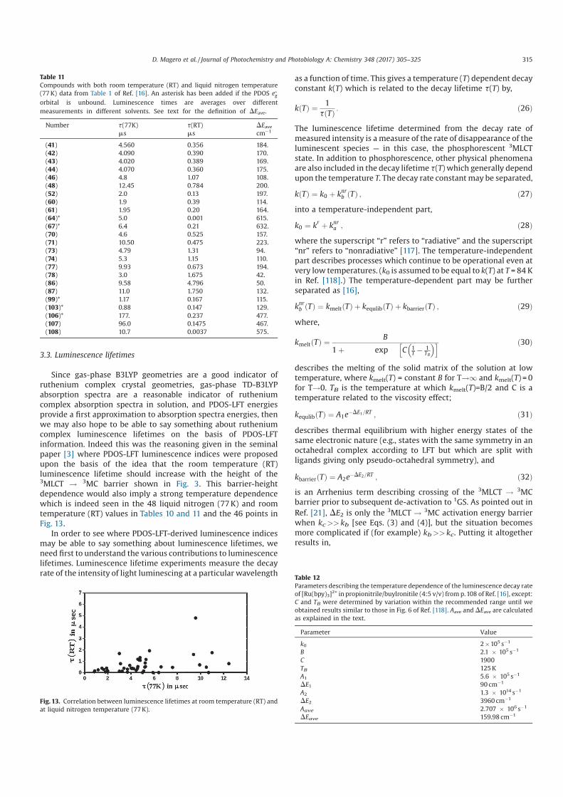
3.3. Luminescence lifetimes
Since gas-phase B3LYP geometries are a good indicator ofruthenium complex crystal geometries, gas-phase TD-B3LYPabsorption spectra are a reasonable indicator of rutheniumcomplex absorption spectra in solution, and PDOS-LFT energiesprovide a first approximation to absorption spectra energies, thenwe may also hope to be able to say something about rutheniumcomplex luminescence lifetimes on the basis of PDOS-LFTinformation. Indeed this was the reasoning given in the seminalpaper [3] where PDOS-LFT luminescence indices were proposedupon the basis of the idea that the room temperature (RT)luminescence lifetime should increase with the height of the3MLCT ! 3MC barrier shown in Fig. 3. This barrier-heightdependence would also imply a strong temperature dependencewhich is indeed seen in the 48 liquid nitrogen (77 K) and roomtemperature (RT) values in Tables 10 and 11 and the 46 points inFig. 13.
In order to see where PDOS-LFT-derived luminescence indicesmay be able to say something about luminescence lifetimes, weneed first to understand the various contributions to luminescencelifetimes. Luminescence lifetime experiments measure the decayrate of the intensity of light luminescing at a particular wavelength
as a function of time. This gives a temperature (T) dependent decayconstant k(T) which is related to the decay lifetime t(T) by,
kðTÞ ¼1
tðTÞ: ð26Þ
The luminescence lifetime determined from the decay rate ofmeasured intensity is a measure of the rate of disappearance of theluminescent species — in this case, the phosphorescent 3MLCTstate. In addition to phosphorescence, other physical phenomenaare also included in the decay lifetime t(T) which generally dependupon the temperature T. The decay rate constant may be separated,
kðTÞ ¼ k0 þ knrb ðTÞ ; ð27Þ
into a temperature-independent part,
k0 ¼ krþ k
nra ; ð28Þ
where the superscript “r” refers to “radiative” and the superscript“nr” refers to “nonradiative” [117]. The temperature-independentpart describes processes which continue to be operational even atvery low temperatures. (k0 is assumed to be equal to k(T) at T = 84 Kin Ref. [118].) The temperature-dependent part may be furtherseparated as [16],
knrb ðTÞ ¼ kmeltðTÞ þ kequlibðTÞ þ kbarrierðTÞ ; ð29Þ
where,
kmeltðTÞ ¼B
1 þ exp C 1T '
1TB
" #h i ð30Þ
describes the melting of the solid matrix of the solution at lowtemperature, where kmelt(T) = constant B for T!1 and kmelt(T) = 0for T!0. TB is the temperature at which kmelt(T)=B/2 and C is atemperature related to the viscosity effect;
kequlibðTÞ ¼ A1e'DE1=RT ; ð31Þ
describes thermal equilibrium with higher energy states of thesame electronic nature (e.g., states with the same symmetry in anoctahedral complex according to LFT but which are split withligands giving only pseudo-octahedral symmetry), and
kbarrierðTÞ ¼ A2e'DE2=RT ; ð32Þ
is an Arrhenius term describing crossing of the 3MLCT ! 3MCbarrier prior to subsequent de-activation to 1GS. As pointed out inRef. [21], DE2 is only the 3MLCT ! 3MC activation energy barrierwhen kc>> kb [see Eqs. (3) and (4)], but the situation becomesmore complicated if (for example) kb>> kc. Putting it altogetherresults in,
Table 11Compounds with both room temperature (RT) and liquid nitrogen temperature(77 K) data from Table 1 of Ref. [16]. An asterisk has been added if the PDOS e!gorbital is unbound. Luminescence times are averages over different
measurements in different solvents. See text for the definition of DEave.
Number t(77K) t(RT) DEavems ms cm'1
(41) 4.560 0.356 184.(42) 4.090 0.390 170.(43) 4.020 0.389 169.(44) 4.070 0.360 175.(46) 4.8 1.07 108.(48) 12.45 0.784 200.(52) 2.0 0.13 197.(60) 1.9 0.39 114.(61) 1.95 0.20 164.(64)* 5.0 0.001 615.(67)* 6.4 0.21 632.(70) 4.6 0.525 157.(71) 10.50 0.475 223.(73) 4.79 1.31 94.(74) 5.3 1.15 110.(77) 9.93 0.673 194.(78) 3.0 1.675 42.(86) 9.58 4.796 50.(87) 11.0 1.750 132.(99)* 1.17 0.167 115.(103)* 0.88 0.147 129.(106)* 177. 0.237 477.(107) 96.0 0.1475 467.(108) 10.7 0.0037 575.
Fig. 13. Correlation between luminescence lifetimes at room temperature (RT) andat liquid nitrogen temperature (77 K).
Table 12Parameters describing the temperature dependence of the luminescence decay rateof [Ru(bpy)3]
2+ in propionitrile/buylronitile (4:5 v/v) from p. 108 of Ref. [16], except:C and TB were determined by variation within the recommended range until weobtained results similar to those in Fig. 6 of Ref. [118]. Aave and DEave are calculatedas explained in the text.
Parameter Value
k0 2 / 105 s'1
B 2.1 / 105 s'1
C 1900TB 125 KA1 5.6 / 105 s'1
DE1 90 cm'1
A2 1.3 / 1014 s'1
DE2 3960 cm'1
Aave 2.707 / 106 s'1
DEave 159.98 cm'1
D. Magero et al. / Journal of Photochemistry and Photobiology A: Chemistry 348 (2017) 305–325 315
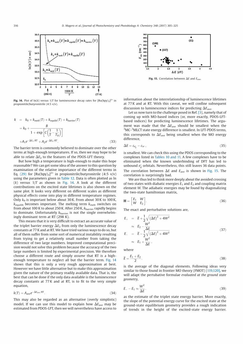
k ¼ k0 þ kmeltðTÞ þ kequlibðTÞ þ kbarrierðTÞ
¼ k0 þB
1 þ exp C1T'
1TB
% &+ ,
þA1e'DE1=RT þ A2e
'DE2=RT : ð33Þ
The barrier term is commonly believed to dominate over the otherterms at high-enough temperatures. If so, then we may hope to beable to relate DE2 to the features of the PDOS-LFT theory.
But how high a temperature is high-enough to make this hopereasonable? We can get some idea of the answer to this question byexamination of the relative importance of the different terms inEq. (29) for [Ru(bpy)3]
2+ in propionitrile/butyronitrile (4:5 v/v)using the parameters given in Table 12. Data is often plotted as ln(k) versus 1/T as shown in Fig. 14. A look at the differentcontributions on the excited state lifetimes is also shown on thesame plot. It looks very different on different scales as differentphysical effects come into play in different temperature regimes.Only k0 is important below about 30 K. From about 30 K to 100 K,kequilib becomes important. The melting term kmelt switches onfrom about 100 K to about 250 K. After 250 K, kbarrier rapidly beginsto dominate. Unfortunately kbarrier is not the single overwhelm-ingly dominant term at RT (298 K).
This means that it is very difficult to extract an accurate value ofthe triplet barrier energy DE2 from only the luminescence decayconstants at 77 K and at RT. We have tried various ways to do so, butall of them suffer from some sort of numerical instability resultingfrom trying to get a relatively small number from taking thedifference of two large numbers. Improved computational preci-sion would not solve this problem because the accuracy of the twolarge numbers is limited by experimental precision. We thereforechoose a different route and simply assume that RT is a high-enough temperature to neglect all but the barrier term. Fig. 14shows that this is only a very rough approximation at best.However we have little alternative but to make this approximationgiven the nature of the primary readily available data. That is, thebest that can be done if the only data available is the luminescencedecay constants at 77 K and at RT, is to fit to the very simpleequation,
kðTÞ ¼ Aavee'DEave=RT : ð34Þ
This may also be regarded as an alternative (overly simplistic)model. If we can use this model to explain how DEave may beestimated from PDOS-LFT, then we will nevertheless have access to
information about the interrelationship of luminescence lifetimesat 77 K and at RT. With this caveat, we will confine subsequentdiscussion to luminescence indices for predicting DEave.
Let us now turn to the challenge posed in Ref. [3], namely that ofcoming up with MO-based indices (or, more exactly, PDOS-LFT-based indices) for predicting luminescence lifetimes. The argu-ment was made that the DEave should be smallest when the3MC-3MLCT state energy difference is smallest. In LFT-PDOS terms,this corresponds to DEave being smallest when the MO energydifference,
DE ¼ ee!g ' ep! ; ð35Þ
is smallest. We can check this using the PDOS corresponding to thecomplexes listed in Tables 10 and 11. A few complexes have to beeliminated when the known underbinding of DFT has led tounbound e!g orbitals. Nevertheless, this still leaves 36 data points.
The correlation between DE and Eave is shown in Fig. 15. Thecorrelation is surprisingly bad.
We are thus led to think more deeply about the avoided crossingof two states with diabatic energies E1 and E2 and coupling matrixelement W. The adiabatic energies may be found by diagonalizingthe two-state hamiltonian matrix,
H ¼E1 WW E2
+ ,
: ð36Þ
The exact and perturbative solutions are,
Eþ ¼ E þ12
ffiffiffiffiffiffiffiffiffiffiffiffiffiffiffiffiffiffiffiffiffiffiffiffiffiffiffiffiffi
DE- .2
þ 4W2q
1 E2 'W2
DE
E' ¼ E '12
ffiffiffiffiffiffiffiffiffiffiffiffiffiffiffiffiffiffiffiffiffiffiffiffiffiffiffiffiffi
DE- .2
þ 4W2q
1 E1 þW2
DE;
ð37Þ
where
E ¼E1 þ E2
2: ð38Þ
is the average of the diagonal elements. Following ideas verysimilar to those found in frontier MO theory (FMOT) [119,120], wewill adapt the pertubative formulae evaluated at the ground state
geometry,
E' ' E1 1W2
DE: ð39Þ
as the estimate of the triplet state energy barrier. More exactly,the slope of the potential energy curve for the excited state at theground-state equilibrium geometry provides a rough indicationof trends in the height of the excited-state energy barrier.
Fig. 14. Plot of ln(k) versus 1/T for luminescence decay rates for [Ru(bpy)3]2+ in
propionitile/butyronitrile (4:5 v/v).
Fig. 15. Correlation between DE and Eave.
316 D. Magero et al. / Journal of Photochemistry and Photobiology A: Chemistry 348 (2017) 305–325
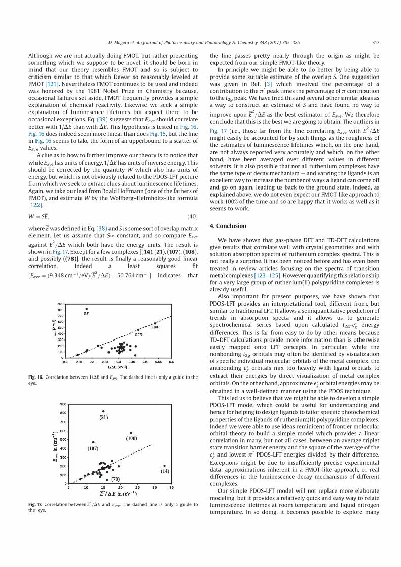
Although we are not actually doing FMOT, but rather presentingsomething which we suppose to be novel, it should be born inmind that our theory resembles FMOT and so is subject tocriticism similar to that which Dewar so reasonably leveled atFMOT [121]. Nevertheless FMOT continues to be used and indeedwas honored by the 1981 Nobel Prize in Chemistry because,occasional failures set aside, FMOT frequently provides a simpleexplanation of chemical reactivity. Likewise we seek a simpleexplanation of luminesence lifetimes but expect there to beoccasional exceptions. Eq. (39) suggests that Eave should correlatebetter with 1/DE than with DE. This hypothesis is tested in Fig. 16.Fig. 16 does indeed seem more linear than does Fig. 15, but the linein Fig. 16 seems to take the form of an upperbound to a scatter ofEave values.
A clue as to how to further improve our theory is to notice thatwhile Eave has units of energy,1/DE has units of inverse energy. Thisshould be corrected by the quantity W which also has units ofenergy, but which is not obviously related to the PDOS-LFT picturefrom which we seek to extract clues about luminescence lifetimes.Again, we take our lead from Roald Hoffmann (one of the fathers ofFMOT), and estimate W by the Wolfberg–Helmholtz-like formula[122],
W ¼ SE; ð40Þ
where E was defined in Eq. (38) and S is some sort of overlap matrixelement. Let us assume that S1 constant, and so compare Eave
against E2=DE which both have the energy units. The result is
shown in Fig.17. Except for a few complexes [(14), (21), (107), (108),and possibly ((78)], the result is finally a reasonably good linearcorrelation. Indeed a least squares fit
[Eave ¼ ð9:348 cm'1=eVÞðE2=DEÞ þ 50:764 cm'1] indicates that
the line passes pretty nearly through the origin as might beexpected from our simple FMOT-like theory.
In principle we might be able to do better by being able toprovide some suitable estimate of the overlap S. One suggestionwas given in Ref. [3] which involved the percentage of d
contribution to the p* peak times the percentage of p contributionto the t2g peak. We have tried this and several other similar ideas asa way to construct an estimate of S and have found no way to
improve upon E2=DE as the best estimator of Eave. We therefore
conclude that this is the best we are going to obtain. The outliers in
Fig. 17 (i.e., those far from the line correlating Eave with E2=DE
might easily be accounted for by such things as the roughness ofthe estimates of luminescence lifetimes which, on the one hand,are not always reported very accurately and which, on the otherhand, have been averaged over different values in differentsolvents. It is also possible that not all ruthenium complexes havethe same type of decay mechanism — and varying the ligands is anexcellent way to increase the number of ways a ligand can come offand go on again, leading us back to the ground state. Indeed, asexplained above, we do not even expect our FMOT-like approach towork 100% of the time and so are happy that it works as well as itseems to work.
4. Conclusion
We have shown that gas-phase DFT and TD-DFT calculationsgive results that correlate well with crystal geometries and withsolution absorption spectra of ruthenium complex spectra. This isnot really a surprise. It has been noticed before and has even beentreated in review articles focusing on the spectra of transitionmetal complexes [123–125]. However quantifying this relationshipfor a very large group of ruthenium(II) polypyridine complexes isalready useful.
Also important for present purposes, we have shown thatPDOS-LFT provides an interpretational tool, different from, butsimilar to traditional LFT. It allows a semiquantitative prediction oftrends in absorption specta and it allows us to generatespectrochemical series based upon calculated t2g-e!g energy
differences. This is far from easy to do by other means becauseTD-DFT calculations provide more information than is otherwiseeasily mapped onto LFT concepts. In particular, while thenonbonding t2g orbitals may often be identified by visualizationof specific individual molecular orbitals of the metal complex, theantibonding e!g orbitals mix too heavily with ligand orbitals to
extract their energies by direct visualization of metal complexorbitals. On the other hand, approximate e!g orbital energies may be
obtained in a well-defined manner using the PDOS technique.This led us to believe that we might be able to develop a simple
PDOS-LFT model which could be useful for understanding andhence for helping to design ligands to tailor specific photochemicalproperties of the ligands of ruthenium(II) polypyridine complexes.Indeed we were able to use ideas reminicent of frontier molecularorbital theory to build a simple model which provides a linearcorrelation in many, but not all cases, between an average tripletstate transition barrier energy and the square of the average of thee!g and lowest p* PDOS-LFT energies divided by their difference.
Exceptions might be due to insufficiently precise experimentaldata, approximations inherent in a FMOT-like approach, or realdifferences in the luminescence decay mechanisms of differentcomplexes.
Our simple PDOS-LFT model will not replace more elaboratemodeling, but it provides a relatively quick and easy way to relateluminescence lifetimes at room temperature and liquid nitrogentemperature. In so doing, it becomes possible to explore many
Fig. 16. Correlation between 1/DE and Eave. The dashed line is only a guide to theeye.
Fig. 17. Correlation between E2=DE and Eave. The dashed line is only a guide to
the eye.
D. Magero et al. / Journal of Photochemistry and Photobiology A: Chemistry 348 (2017) 305–325 317
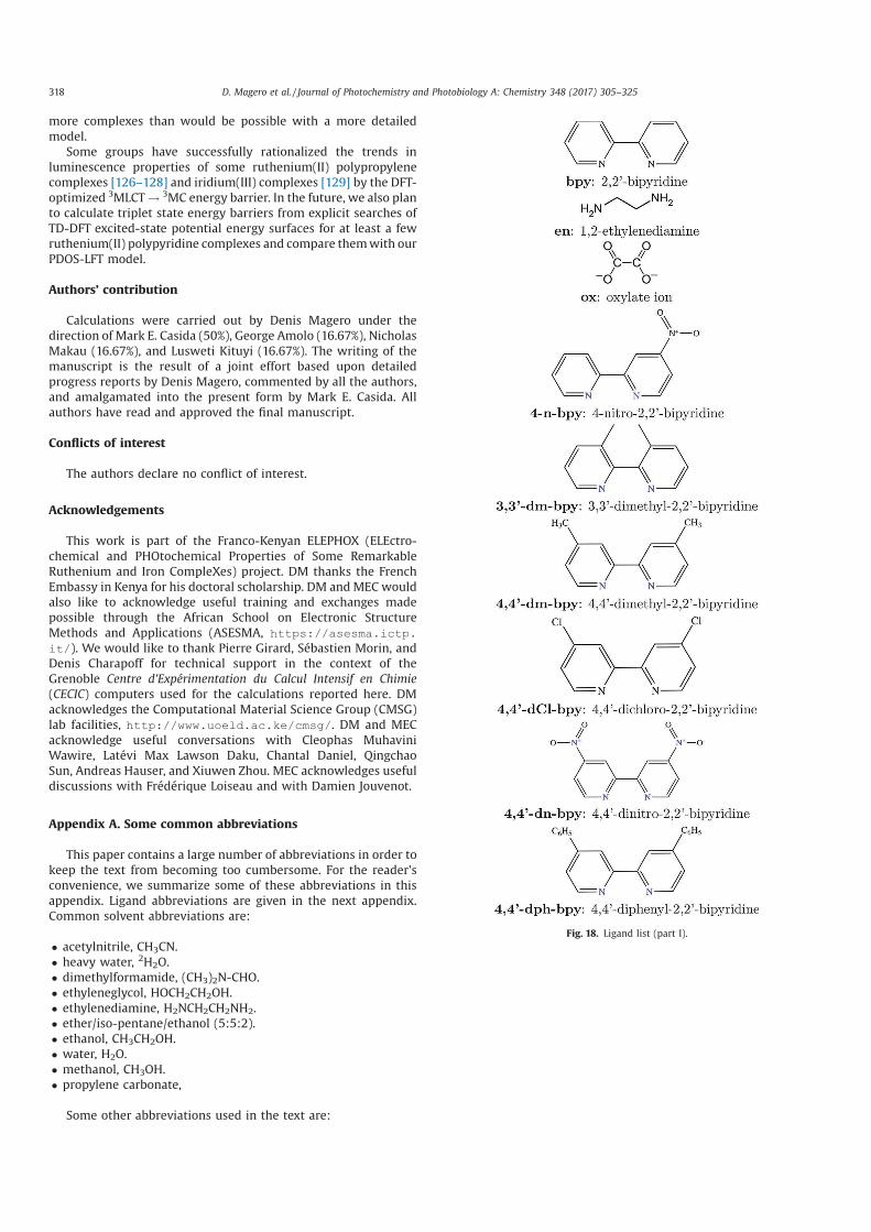
more complexes than would be possible with a more detailedmodel.
Some groups have successfully rationalized the trends inluminescence properties of some ruthenium(II) polypropylenecomplexes [126–128] and iridium(III) complexes [129] by the DFT-optimized 3MLCT ! 3MC energy barrier. In the future, we also planto calculate triplet state energy barriers from explicit searches ofTD-DFT excited-state potential energy surfaces for at least a fewruthenium(II) polypyridine complexes and compare them with ourPDOS-LFT model.
Authors’ contribution
Calculations were carried out by Denis Magero under thedirection of Mark E. Casida (50%), George Amolo (16.67%), NicholasMakau (16.67%), and Lusweti Kituyi (16.67%). The writing of themanuscript is the result of a joint effort based upon detailedprogress reports by Denis Magero, commented by all the authors,and amalgamated into the present form by Mark E. Casida. Allauthors have read and approved the final manuscript.
Conflicts of interest
The authors declare no conflict of interest.
Acknowledgements
This work is part of the Franco-Kenyan ELEPHOX (ELEctro-chemical and PHOtochemical Properties of Some RemarkableRuthenium and Iron CompleXes) project. DM thanks the FrenchEmbassy in Kenya for his doctoral scholarship. DM and MEC wouldalso like to acknowledge useful training and exchanges madepossible through the African School on Electronic StructureMethods and Applications (ASESMA, https://asesma.ictp.
it/). We would like to thank Pierre Girard, Sébastien Morin, andDenis Charapoff for technical support in the context of theGrenoble Centre d’Expérimentation du Calcul Intensif en Chimie
(CECIC) computers used for the calculations reported here. DMacknowledges the Computational Material Science Group (CMSG)lab facilities, http://www.uoeld.ac.ke/cmsg/. DM and MECacknowledge useful conversations with Cleophas MuhaviniWawire, Latévi Max Lawson Daku, Chantal Daniel, QingchaoSun, Andreas Hauser, and Xiuwen Zhou. MEC acknowledges usefuldiscussions with Frédérique Loiseau and with Damien Jouvenot.
Appendix A. Some common abbreviations
This paper contains a large number of abbreviations in order tokeep the text from becoming too cumbersome. For the reader'sconvenience, we summarize some of these abbreviations in thisappendix. Ligand abbreviations are given in the next appendix.Common solvent abbreviations are:
3 acetylnitrile, CH3CN.3 heavy water, 2H2O.3 dimethylformamide, (CH3)2N-CHO.3 ethyleneglycol, HOCH2CH2OH.3 ethylenediamine, H2NCH2CH2NH2.3 ether/iso-pentane/ethanol (5:5:2).3 ethanol, CH3CH2OH.3 water, H2O.3 methanol, CH3OH.3 propylene carbonate,
Some other abbreviations used in the text are:
Fig. 18. Ligand list (part I).
318 D. Magero et al. / Journal of Photochemistry and Photobiology A: Chemistry 348 (2017) 305–325
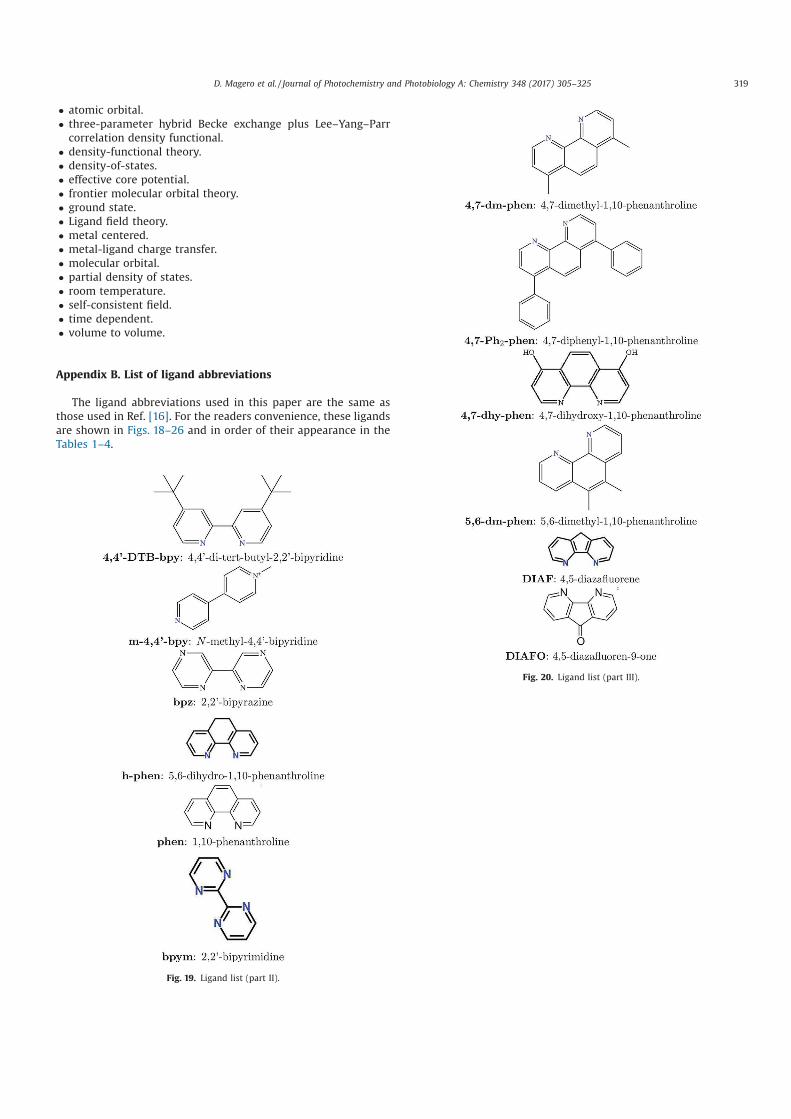
3 atomic orbital.3 three-parameter hybrid Becke exchange plus Lee–Yang–Parrcorrelation density functional.3 density-functional theory.3 density-of-states.3 effective core potential.3 frontier molecular orbital theory.3 ground state.3 Ligand field theory.3 metal centered.3 metal-ligand charge transfer.3 molecular orbital.3 partial density of states.3 room temperature.3 self-consistent field.3 time dependent.3 volume to volume.
Appendix B. List of ligand abbreviations
The ligand abbreviations used in this paper are the same asthose used in Ref. [16]. For the readers convenience, these ligandsare shown in Figs. 18–26 and in order of their appearance in theTables 1–4.
Fig. 19. Ligand list (part II).
Fig. 20. Ligand list (part III).
D. Magero et al. / Journal of Photochemistry and Photobiology A: Chemistry 348 (2017) 305–325 319
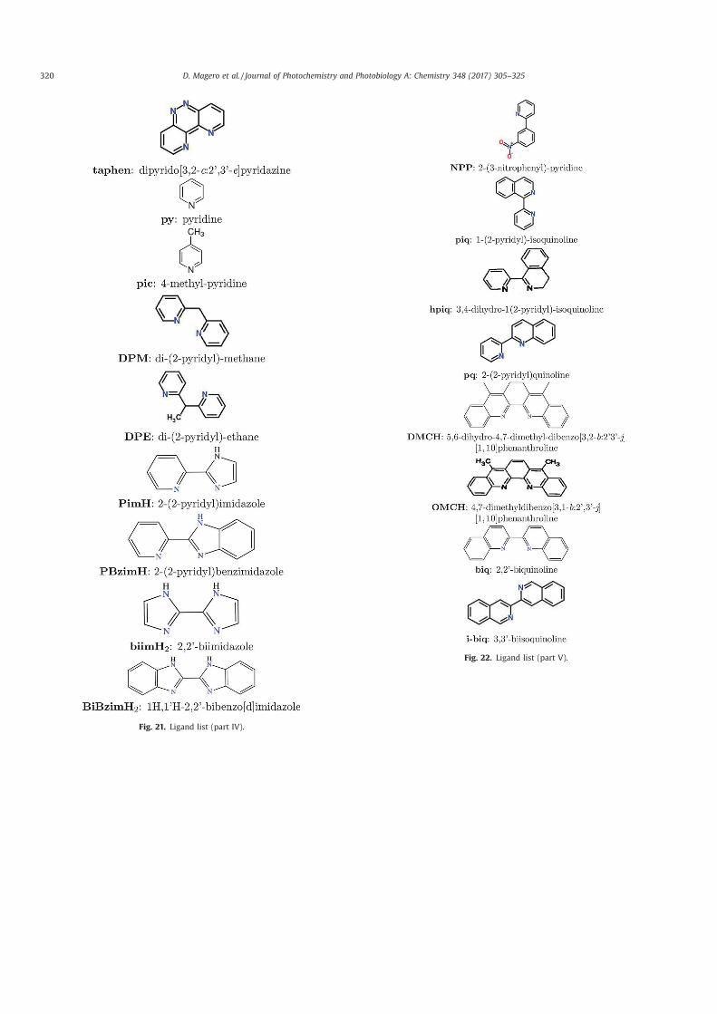
Fig. 21. Ligand list (part IV).
Fig. 22. Ligand list (part V).
320 D. Magero et al. / Journal of Photochemistry and Photobiology A: Chemistry 348 (2017) 305–325
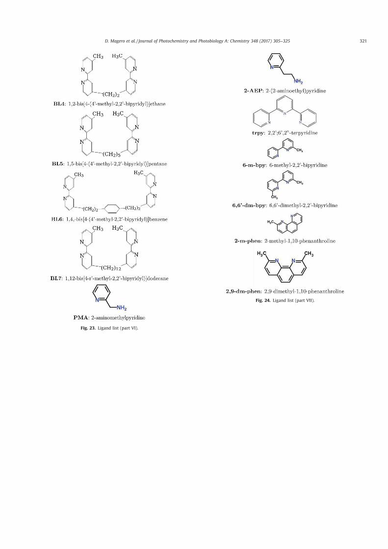
Fig. 23. Ligand list (part VI).
Fig. 24. Ligand list (part VII).
D. Magero et al. / Journal of Photochemistry and Photobiology A: Chemistry 348 (2017) 305–325 321
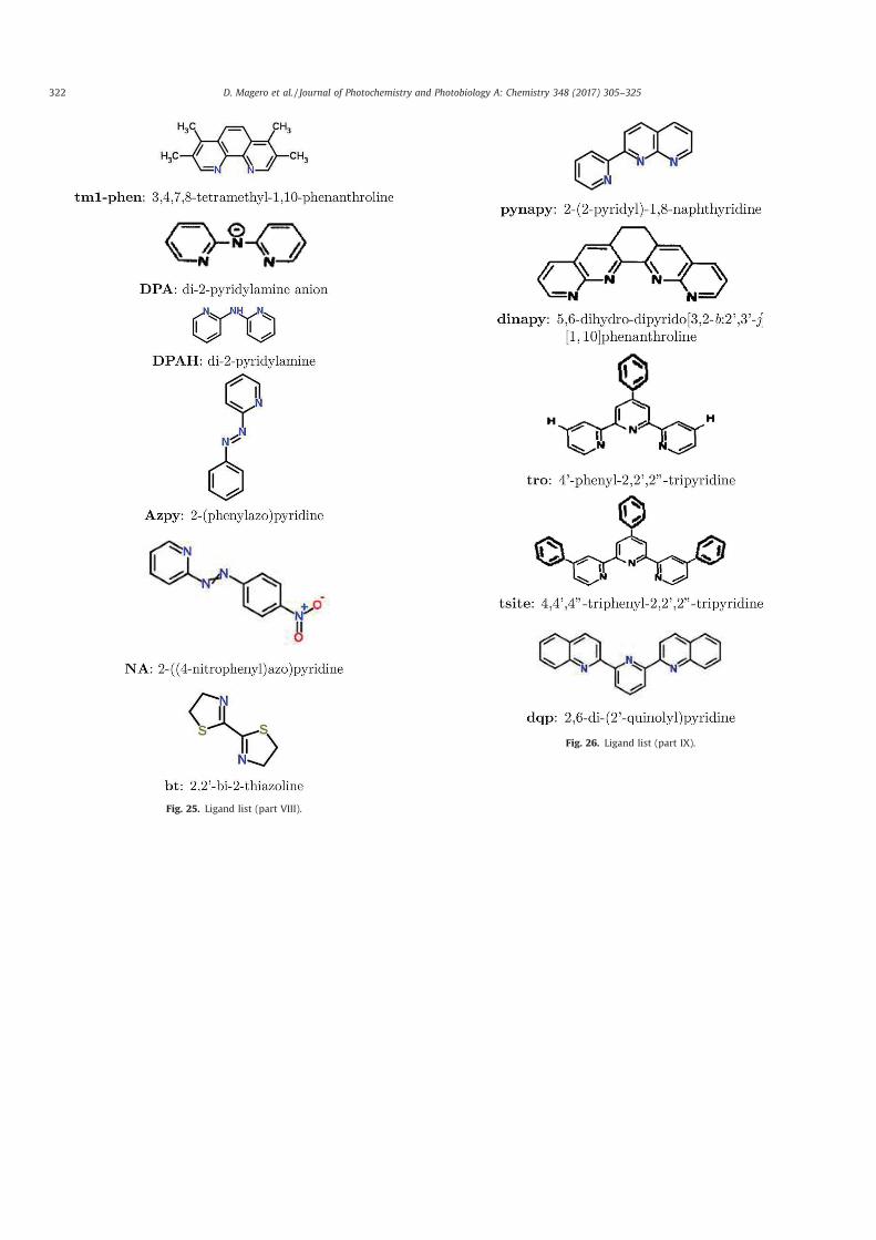
Fig. 26. Ligand list (part IX).
Fig. 25. Ligand list (part VIII).
322 D. Magero et al. / Journal of Photochemistry and Photobiology A: Chemistry 348 (2017) 305–325

Appendix C. Supplementary data
Supplementary data associated with this article can be found, inthe online version, at http://dx.doi.org/10.1016/j.jphotochem.2017.07.037.
References
[1] D.E. Lewis, Klaus at Kazon is a place name (https://en.wikipedia.org/wiki/Kazan) and so should be capitalized.kazon: the discovery of ruthenium (1),Bull. Hist. Chem. 41 (2016) 3.
[2] J. Sauvage, et al., Ruthenium(II) and Osmium(II) bis(terpyridine) complexesin covalently-linked multicomponent systems: synthesis, electrochemicalbehavior, absorption spectra, and photochemical and photophysicalproperties, Chem. Rev. 94 (1994) 993.
[3] C.M. Wawire, et al., Density-functional study of lumininescence inpolypyridine ruthenium complexes, J. Photochem. Photobiol. A 276 (2014) 8.
[4] V. Balzani, A. Juris, Photochemistry and photophysics of Ru (II) polypyridinecomplexes in the Bologna group. From early studies to recent developments,Coord. Chem. Rev. 211 (2001) 97.
[5] K. Nakamaru, Synthesis, luminescence quantum yields, and lifetimes oftrischelated ruthenium(II) mixed-ligand complexes including 3,3’-dimethyl-2,2’-bipyridyl, Bull. Chem. Soc. Jpn. 55 (1982) 2697.
[6] G. Liebsch, I. Klimant, O.S. Wolfbeis, Luminescence lifetime temperaturesensing based on sol-gels and poly(acrylonitrile)s dyed with rutheniummetal–ligand complexes, Adv. Mater. 11 (1999) 1296.
[7] A. Harriman, A. Khatyr, R. Ziessel, Extending the luminescence lifetime ofruthenium(II) poly(pyridine) complexes in solution at ambient temperature,Dalton Trans. 10 (2003) 2061.
[8] M. Duati, et al., Enhancement of luminescence lifetimes of mononuclearruthenium(II)–terpyridine complexes by manipulation of the s-donorstrength of ligands, J. Inorg. Chem. 42 (2003) 8377.
[9] E.A. Medlycott, G.S. Hanan, Designing tridentate ligands for ruthenium(II)complexes with prolonged room temperature luminescence lifetimes, Chem.Soc. Rev. 34 (2005) 133.
[10] K.J. Morris, M.S. Roach, W. Xu, J.N. Demas, B.A. DeGraff, Luminescencelifetime standards for the nanosecond to microsecond range and oxygenquenching of ruthenium(II) compounds, Anal. Chem. 79 (2007) 9310.
[11] L.J. Nurkkala, et al., The effects of pendant vs. fused thiophene attachmentupon the luminescence lifetimes and electrochemistry of tris(2,2’-bipyridine)ruthenium(II) complexes, Eur. J. Inorg. Chem. 26 (2008) 4101.
[12] R.O. Steen, et al., The role of isometric effects on the luminescence lifetimesand electrochemistry of oligothienyl-bridged dinuclear tris(2,2’-bipyridine)ruthenium(II) complexes, Eur. J. Inorg. Chem. 11 (2008) 1784.
[13] S. Ji, et al., Tuning the luminescence lifetimes of ruthenium(II) polypyridinecomplexes and its application in luminescent oxygen sensing, J. Mater. Chem.20 (2010) 1953.
[14] B.N. Figgis, M.A. Hitchman, Ligand Field Theory and Its Applications, Wiley-VCH, New York, 2000.
[15] H. Ramanantoanina, W. Urland, A. Garciá-Fuente, F. Cimpoesu, C. Daul, Ligandfield density functional theory for the prediction of future domestic lighting,Phys. Chem. Chem. Phys. 28 (2014) 14625.
[16] A. Juris, et al., Ru(II) polypyridine complexes: photophysics, photochemistry,electrochemistry, and chemiluminescence, Coord. Chem. Rev. 84 (1988) 85.
[17] M. Kasha, Characterization of electronic transitions in complex molecules,Discuss. Faraday Soc. 9 (1950) 14.
[18] G.A. Crosby, Spectroscopic investigations of excited states of transition-metalcomplexes, Acc. Chem. Res. 8 (1975) 231.
[19] V. Balazni, S. Campagna (Eds.), Photochemistry and Photophysics ofCoordination Compounds. I., Vol. 280 of Top. Curr. Chem., Springer,Heidelberg, 2007.
[20] V. Balazni, S. Campagna (Eds.), Photochemistry and Photophysics ofCoordination Compounds. II., Vol. 281 of Top. Curr. Chem., Springer,Heidelberg, 2007.
[21] F. Barigelletti, A. Juris, V. Balzani, P. Belser, A. von Zelewsky, Temperaturedependence of the Ru(bpy)2(CN)2 and Ru(bpy)2(i-biq)
2+ luminescence, J.Phys. Chem. 91 (1987) 1095.
[22] J. Heully, F. Alaray, M. Boggio-Pasqua, Spin-orbit effects on the photophysicalproperties of [Ru(bpy)3]
2+, J. Chem. Phys. 131 (2009) 184308.[23] M.J. Frisch, et al., Gaussian 03, Revision B. 05, Gaussian, Inc., Pittsburgh, PA,
2003.[24] M.J. Frisch, et al., Gaussian 09 Revision D.01, (2009) .[25] W. Kohn, L.J. Sham, Self-consistent equations including exchange and
correlation effects, Phys. Rev. 140 (1965) A1133.[26] A.D. Becke, Density-functional exchange-energy approximation with correct
asymptotic behavior, Phys. Rev. A 38 (1988) 3098.[27] S.H. Vosko, L. Wilk, M. Nusair, Accurate spin-dependent electron liquid
correlation energies for local spin density calculations: a critical analysis,Can. J. Phys. 58 (1980) 1200.
[28] C. Lee, W. Yang, R.G. Parr, Development of the Colle–Salvetti correlation-energy formula into a functional of the electron density, Phys. Rev. B 37(1988) 785.
[29] A.D. Becke, Density-functional thermochemistry. III. The role of exactexchange, J. Chem. Phys. 98 (1993) 5648.
[30] P.J. Hay, W.R. Wadt, Ab initio effective core potentials for molecularcalculations. potentials for K to Au including the outermost core orbitals,J. Chem. Phys. 82 (1985) 299.
[31] P.J. Hay, W.R. Wadt, Ab initio effective core potentials for molecularcalculations. Potentials for the transition metal atoms Sc to Hg, J. Chem.Phys. 82 (1985) 270.
[32] R. Ditchfield, W. Hehre, J.A. Pople, Self-consistent molecular-orbital methods.IX. An extended Gaussian-type basis for molecular-orbital studies of organicmolecules, J. Chem. Phys. 54 (1971) 724.
[33] W.J. Hehre, R. Ditchfield, J.A. Pople, Self-consistent molecular orbitalmethods. XII. Further extensions of Gaussian-type basis sets for use inmolecular orbital studies of organic molecules, J. Chem. Phys. 56 (1972) 2257.
[34] P. Hariharan, J.A. Pople, The influence of polarization functions on molecularorbital hydrogenation energies, Theor. Chim. Acta 28 (1973) 213.
[35] P.C. Hariharan, J.A. Pople, Accuracy of AHn equilibrium geometries by singledeterminant molecular orbital theory, Mol. Phys. 27 (1974) 209.
[36] M.M. Francl, et al., Self-consistent molecular orbital methods. XXIII. Apolarization-type basis set for second-row elements, J. Chem. Phys. 77 (1982)3654.
[37] V.A. Rassolov, M.A. Ratner, J.A. Pople, P.C. Redfern, L.A. Curtiss, 6-31G* basisset for third-row atoms, J. Comp. Chem. 22 (2001) 976.
[38] G.A. Petersson, M.A. Al-Laham, A complete basis set model chemistry. II.Open-shell systems and the total energies of the first-row atoms, J. Chem.Phys. 94 (1991) 6081.
[39] The Web of Science may be found at https://pcs.webofknowledge.com(accessed 16.07.17).
[40] The annual Density Functional Theory popularity poll is organized by MarcelSwart, Matthias Bickelhaupt, and Miquel Duran and its results may be foundat http://www.marcelswart.eu/dft-poll/ (accessed 16.07.17).
[41] A.C. Tsipis, DFT flavor of coordination chemistry, Coord. Chem. Rev. 272(2014) 1.
[42] R.K. Hocking, R.J. Deeth, T.W. Hambley, DFT study of the systematic variationsin metal-ligand bond lengths of coordination complexes: the crucial role ofthe condensed phase, Inorg. Chem. 46 (2007) 8238.
[43] C. Latouche, A. Balardi, V. Barone, Virtual eyes designed for quantitativespectroscopy of inorganic complexes: Vibronic signatures in thephosphorescence spectra of terpyridine derivatives, J. Phys. Chem. B 119(2015) 7253.
[44] The Cambridge Crystallographic Data Centre (CCDC), https://www.ccdc.cam.ac.uk/ (accessed 06.02.16).
[45] R. Prajapati, V.K. Yadav, S.K. Dubey, B. Durham, L. Mishra, CCDC 667743:Experimental Crystal Structure Determination, (2007), doi:http://dx.doi.org/10.5517/ccqdv31.
[46] R. Prajapati, V.K. Yadav, S.K. Dubey, B. Durham, L. Mishra, Reactivity of metal(ZnII, RuII)-2,2’-bipyridyl with some bifunctional ligands, Indian J. Chem.Sect. A 47 (2008) 1780.
[47] O.S. Odongo, J.F. Endicott, M.J. Heeg, CCDC 613874: Experimental CrystalStructure Determination, (2006), doi:http://dx.doi.org/10.5517/ccnlsdd.
[48] F.R. Fronczek, CCDC 287967: Experimental Crystal Structure Determination,(2005), doi:http://dx.doi.org/10.5517/cc9nn8v.
[49] H. Shen, et al., A new three-dimensional ruthenium(II) complex via hydrogenbonds: Ru(bpy)2(ox)44H2O (bpy = 2,2’-bipyridine, ox = oxalate ion), Inorg.Chem. Commun. 2 (1999) 615.
[50] D.P. Rillema, D.S. Jones, H.A. Levy, Structure of tris(2,2-bipyridyl)ruthenium(II) hexafluorophosphate, [Ru(bipy)3][PF6]2; X-ray crystallographicdetermination, J. Chem. Soc. Chem. Commun. 1979 (1979) 849.
[51] P. Reveco, R.H. Schmehl, W.R. Cherry, F.R. Froczek, J. Selbin, Cyclometalatedcomplexes of ruthenium. 2. Spectral and electrochemical properties and X-ray structure of bis(2,2’-bipyridine)(4-nitro-2-(2-pyridyl)phenyl)ruthenium(II), Inorg. Chem. 24 (1985) 4078.
[52] D. Hesek, et al., CCDC 116354: Experimental Crystal Structure Determination,(1999), doi:http://dx.doi.org/10.5517/cc3x2cf.
[53] D. Hesek, et al., Conversion of a new chiral reagent D-[Ru(bpy)2(dmso)Cl]PF6to (dmbpy = 4,4]’-dimethyl-2,2’-bipyridine), Chem. Commun. 5 (1999) 403.
[54] L.E. Hansen, et al., CCDC 212499: Experimental Crystal StructureDetermination, (2003), doi:http://dx.doi.org/10.5517/cc743t8.
[55] L.E. Hansen, et al., Syntheses and characterization of some chloro, methoxy,and mercapto derivatives of [Ru(h2-2,2’-bipyridine)3]
2+2PF 6': crystal andmolecular structures of [Ru(h2-2,2’-bipyridine)2(h
2-4,4’-(X)2-2,2’-bipyridine)]2+2PF6' (X=Cl, OCH3), Inorg. Chim. Acta 348 (2003) 91.
[56] M. Du, X. Ge, H. Liu, X. Bu, CCDC 169415: Experimental Crystal StructureDetermination, (2001), doi:http://dx.doi.org/10.5517/cc5p904.
[57] M. Du, X. Ge, H. Liu, X. Bu, Synthesis, spectra, and crystal structures of two RuII
complexes with polypyridyl ligands: cis-[Ru(pby)2(4,4’-bpy)Cl](PF6)4H2O andcis-[Ru(phen)2(CH3CN)2](PF6)2, J. Mol. Struct. 610 (2002) 207.
[58] B. Ye, X. Chen, T. Zeng, L. Ji, syntheses, spectra and crystal structures ofruthenium(II) complexes with polypyridyl:[Ru(bipy)2(phen)](ClO4)2.H2Oand [Ru(bipy)2 (Me-phen)] C l O4ð Þ2 , Inorg. Chim. Acta 240 (1995) 5.
[59] V.W. Yam, B. Li, N. Zhu, CCDC 182310: Experimental Crystal StructureDetermination, (2002), doi:http://dx.doi.org/10.5517/cc63pzy.
[60] V.W. Yam, B. Li, N. Zhu, Synthesis of mesoporous silicates with controllablepore size using surfactant ruthenium(II) complexes as templates, Adv. Mater.14 (2002) 719.
[61] C.M. Kepert, et al., CCDC 230551: Experimental Crystal StructureDetermination, (2004), doi:http://dx.doi.org/10.5517/cc7qx4z.
D. Magero et al. / Journal of Photochemistry and Photobiology A: Chemistry 348 (2017) 305–325 323
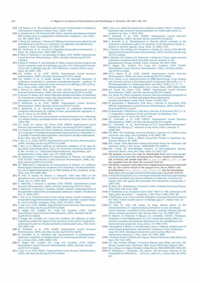
[62] C.M. Kepert, et al., The synthesis and structure of heteroleptic tris(diimine)ruthenium(II) complexes, Dalton Trans. (2004) 1766.
[63] L.J. Henderson Jr., F.R. Fronczek, W.R. Cherry, Selective perturbation of ligandfield excited states in polypyridine ruthenium(II) complexes, J. Am. Chem.Soc. 106 (1984) 5876.
[64] Y. Wang, D.C. Jackman, C. Woods, D.P. Rillema, Crystal structure, physical, andphotophysical properties of a ruthenium (II) bipyridine diazafluorenonecomplex, J. Chem. Crystallogr. 25 (1995) 549.
[65] P.B. Hitchcock, et al., Cis-bis(2,2’-bipyridine)bis(pyridine)ruthenium(II), J.Chem. Soc. Dalton Trans. 1988 (1988) 1837.
[66] B. Klop, H. Viebrock, A. von Zelewsky, D. Abeln, CCDC 162056: ExperimentalCrystal Structure Determination, (2001), doi:http://dx.doi.org/10.5517/cc5fmmt.
[67] B. Klop, H. Viebrock, A. von Zelewsky, D. Abeln, Crystal structure analysis andchiral recognition study of D-[Ru(bpy)2(py)2][(+)-O,O’-dibenzoyl-D-tatrate]412H2O and L-[Ru(bpy)2(py)2][(-)-O,O’-dibenzoyl-L-tatrate]412H2O, Inorg.Chem. 40 (2001) 1196.
[68] A.H. Velders, et al., CCDC 143552: Experimental Crystal StructureDetermination, (2000), doi:http://dx.doi.org/10.5517/cc4tcq0.
[69] A.H. Velders, et al., A simple example of the fluxional behaviour ofruthenium-coordinated C2-symmetric monodentate ligands – synthesis 1HNMR spectroscopic study and crystal structure of cis-[Ru(bpy)2(4Pic)2](PF6)2,Eur. J. Inorg. Chem. 2002 (2002) 193.
[70] S. Derossi, H. Adams, M.D. Ward, CCDC 622792: Experimental CrystalStructure Determination, (2006), doi:http://dx.doi.org/10.5517/ccnx22p.
[71] S. Derossi, H. Adams, M.D. Ward, Hydrogen-bonded assemblies of ruthenium(II)–biimidazole complex cations and cyanometallate anions: structures andphotophysics, Dalton Trans. 2007 (2007) 33.
[72] N. Rockstroh, et al., CCDC 760286: Experimental Crystal StructureDetermination, (2010), doi:http://dx.doi.org/10.5517/cctj4ct.
[73] N. Rockstroh, et al., Structural properties of ruthenium biimidazolecomplexes determining the stability of their supramolecular aggregates, Z.Nat. B: Chem. Sci. 65 (2010) 281.
[74] P. Wang, et al., Structure and properties of diastereoisomers of a ruthenium(II) complex having a pyridylpyrazoline derivative as a ligand, Chem. Lett. 30(2001) 940.
[75] A.A. Farah, D.V. Stynes, W.J. Pietro, CCDC 140838: Experimental CrystalStructure Determination, (2000), doi:http://dx.doi.org/10.5517/cc4qk5k.
[76] A.A. Farah, D.V. Stynes, W.J. Pietro, Syntheses, characterization and structuresof 2-(2-pyridyl)-4-methylcarboxyquinoline ligand and bis(2,2-bipyridine)-2-(2-pyridyl)-4-methylcarboxyquinoline ruthenium(II) hexafluorophosphate,Inorg. Chim. Acta 343 (2003) 295.
[77] S. Rau, et al., CCDC 236778: Experimental Crystal Structure Determination,(2004), doi:http://dx.doi.org/10.5517/cc7yd0k.
[78] S. Rau, et al., Efficient synthesis of ruthenium complexes of the type (R-bpy)2RuCl2 and [(R-bpy)2Ru(L-L)]Cl+2 by microwave-activated reactions (R:H, Me, tert-But) (L-L: substituted bibenzimidazoles, bipyrimidine, andphenanthroline), Inorg. Chim. Acta 357 (2004) 4496.
[79] P.U. Maheswari, V. Rajendiran, M. Palaniandavar, R. Thomas, G.U. Kulkarni,CCDC 623203: Experimental Crystal Structure Determination, (2006), doi:http://dx.doi.org/10.5517/ccnxhbc.
[80] P.U. Maheswari, V. Rajendiran, M. Palaniandavar, R. Thomas, G.U. Kulkarni,Mixed ligand ruthenium(II) complexes of 5,6-dimethyl-1,10-phenanthroline:the role of ligand hydrophobicity on DNA binding of the complexes, Inorg.Chim. Acta 359 (2006) 4601.
[81] M. Kato, K. Sasano, M. Kimura, S. Yamauchi, Solid state effect on thephosphorescence spectrum of a tris(3,3’-biisoquinoline)ruthenium(II) salt,Chem. Lett. 21 (1992) 1887.
[82] A. Taketoshi, T. Koizumi, T. Kanbara, CCDC 789502: Experimental CrystalStructure Determination, (2010), doi:http://dx.doi.org/10.5517/ccvhjtn.
[83] A. Taketoshi, T. Koizumi, T. Kanbara, Aerobic oxidative dehydrogenation ofbenzylamines catalyzed by cyclometalated ruthenium complex, TetrahedronLett. 51 (2010) 6457.
[84] C. Tsai, et al., Characterization of low energy charge transfer transitions in(terpyridine)(bipyridine)ruthenium(II) complexes and their cyanide-bridgebi- and tri-metallic analogues, Inorg. Chem. 50 (2011) 11965.
[85] C. Tsai, et al., CCDC: 868664: Experimental Crystal Structure Determination,(2012), doi:http://dx.doi.org/10.5517/ccy4xfd.
[86] D. Onggo, M.L. Scudder, D.C. Craig, H.A. Goodwin, CCDC: 222020Experimental Crystal Structure Determination, (2003), doi:http://dx.doi.org/10.5517/cc7g0ym.
[87] D. Onggo, M.L. Scudder, D.C. Craig, H.A. Goodwin, The influence of ortho-substitution within the ligand on the geometry of the tris(2,2’-bipyridine)ruthenium(II) and tris(1,10-phenanthroline)ruthenium(II) ions, J. Mol. Struct.738 (2005) 129.
[88] M. Schwalbe, et al., CCDC 614185: Experimental Crystal StructureDetermination, (2006), doi:http://dx.doi.org/10.5517/ccnm3fs.
[89] M. Schwalbe, et al., Synthesis and characterisation of poly(bipyridine)ruthenium complexes as building blocks for heterosupramolecular arrays,Eur. J. Inorg. Chem. 2008 (2008) 3310.
[90] D. Onggo, M.L. Scudder, D.C. Craig, H.A. Goodwin, CCDC 222021:Experimental Crystal Structure Determination, (2003), doi:http://dx.doi.org/10.5517/cc7g0zn.
[91] J. Gao, et al., CCDC 900121: Experimental Crystal Structure Determination,(2012), doi:http://dx.doi.org/10.5517/ccz6n5z.
[92] J. Gao, et al., Molecule-based water-oxidation catalysts (WOCs): cluster-size-dependent dye-sensitized polyoxometalates for visible-light-driven O2
evolution, Sci. Rep. 3 (2013) 1853.[93] E. Baranoff, et al., CCDC 182680: Experimental Crystal Structure
Determination, (2002), doi:http://dx.doi.org/10.5517/cc642x9.[94] E. Baranoff, et al., Photochemical or thermal chelate exchange in the
ruthenium coordination sphere of complexes of the Ru(phen)2L family (L =diimine or dinitrile ligands), Inorg. Chem. 41 (2002) 1215.
[95] E. Wachter, D.K. Heidary, B.S. Howerton, S. Parkin, E.C. Glazer, CCDC 881148:Experimental Crystal Structure Determination, (2012), doi:http://dx.doi.org/10.5517/ccykx4j.
[96] E. Wachter, D.K. Heidary, B.S. Howerton, S. Parkin, E.C. Glazer, Light-activatedruthenium complexes photo bind DNA and are cytotoxic in thephotodynamic therapy window, Chem. Commun. 48 (2012) 9649.
[97] D. Onggo, M.L. Scudder, D.C. Craig, H.A. Goodwin, CCDC 222019:Experimental Crystal Structure Determination, (2003), doi:http://dx.doi.org/10.5517/cc7g0xl.
[98] A.C.G. Hotze, et al., CCDC 251699: Experimental Crystal StructureDetermination, (2004), doi:http://dx.doi.org/10.5517/cc8fxbx.
[99] A.C.G. Hotze, et al., Characterization by NMR Spectroscopy, X-ray Analysisand Cytotoxic Activity of the Ruthenium(II) Compounds [RuL3](PF6)2 (L = 2-Phenylazopyridine or o-Tolylazopyridine) and [RuL’2L”](PF6)2 (L’, L” = 2-Phenylazopyridine, 2,2’-Bipyridine), Eur. J. Inorg. Chem. 2005 (2005) 2648.
[100] A.A. Farah, W.J. Pietro, CCDC 199681: Experimental Crystal StructureDetermination, (2002), doi:http://dx.doi.org/10.5517/cc6psbz.
[101] A.A. Farah, W.J. Pietro, Synthesis, structure and electrochemical properties oftris(2-(2-pyridyl)-4-methylcarbonylquinoline)ruthenium(II)hexafluorophosphate, Inorg. Chem. Comm. 6 (2003) 662.
[102] M. Kozlowska, P. Rodziewicz, D.M. Brus, J. Breczko, K. Brzezinski, CCDC909756: Experimental Crystal Structure Determination, (2012), doi:http://dx.doi.org/10.5517/cczjnz3.
[103] M. Kozlowska, P. Rodziewicz, D.M. Brus, J. Breczko, K. Brzezinski, Bis (2, 2’: 6’,2”-terpyridine) ruthenium (II) bis (perchlorate) hemihydrate, ActaCrystallogr. Sect. E: Struct. 68 (2012) 1414.
[104] E.C. Constable, et al., CCDC 676373: Experimental Crystal StructureDetermination, (2008), doi:http://dx.doi.org/10.5517/ccqpthp.
[105] E.C. Constable, et al., Bis(4’-phenyl-2,2’:6’,2”-terpyridine)ruthenium(II):Holding the [Ru(tpy)2]
2+ embraces at bay, Inorg. Chem. Commun. 11(2008) 805.
[106] F.H. Allen, The Cambridge structural database: a quarter of a million crystalstructures and rising, Acta Crystallogr. B 58 (2002) 380.
[107] R. Dennington, T. Keith, J. Millam, GaussView Version 5, Semichem Inc.,Shawnee Mission, KS, 2009.
[108] M.E. Casida, Time-dependent density-functional theory for molecules andmolecular solids, J. Mol. Struct.: THEOCHEM 914 (2009) 3.
[109] M.E. Casida, M. Huix-Rotllant, Progress in time-dependent density-functional theory, Annu. Rev. Phys. Chem. 63 (2012) 287.
[110] The program SPECTRUM_V3.PY may be downloaded from https://sites.google.com/site/markcasida/tddft. Documentation (Project_Analyse_Numerique.pdf, in French) and sample input files nm_exp.txt and nm_theo.txt arealso available from the same site (accessed 15.07.15).
[111] The PDOS.PY program is described in the supplementary data associated withRef. [3]. The current version of the program PABLO_BAUDIN_PDOS.PY anddocumentation Pablo_Baudin_User_Guide.txt may be downloadedfrom https://sites.google.com/site/markcasida/stages (accessed 15.07.15).
[112] A.A.M.H.M. Darghouth, et al., Assessment of density-functional tight-bindingionization potentials and electron affinities of molecules of interest fororganic solar cells against first-principles GW calculations, Computation 3(2015) 616.
[113] W. Koch, M.C. Holtzhausen, A Chemist's Guide to Density Functional Theory,Wiley-VCH, New York, 2000.
[114] N. Yoshikawa, et al., Transition states of the 3 MLCT to 3 MC conversion in Ru(bpy)2(phen derivative) 2+ complexes, J. Mol. Struct. 1094 (2015) 98.
[115] E. Borfecchia, et al., X-ray transient absorption structural characterization ofthe 3MLCT triplet excited state of cis-[Ru(bpy)2(py)2]
2+, Dalton Trans. 42(2013) 6564.
[116] J.Y. Choi, E.J. Park, S.H. Chang, T.J. Kang, Solvent effects on thesolvatochromism of 7-aminocoumarin derivatives in neat and binarysolvent mixtures: correlation of the electronic transition energies with thesolvent polarity parameters, Bull. Korean Chem. Soc. 30 (2009) 1452.
[117] M. Maestri, N. Armaroli, V. Blazani, E.C. Constable, A.M.W.C. Thompson,Complexes of the Ruthenium(II)-2,2’;6’,2”-terpyridine Family. Effect ofelectron-accepting and donating substituents on the photophysical andelectrochemical properties, Inorg. Chem. 34 (1995) 2759.
[118] F. Barigelletti, P. Belser, A. von Zelewsky, A. Juris, V. Balzani, Luminescence ofmixed-ligand polypyridine-ruthenium(II) complexes in the temperaturerange 84–250 K. Interligand interactions and viscosity effects onradiationless processes, J. Phys. Chem. 89 (1985) 3680.
[119] I. Fleming, Frontier Orbitals and Organic Chemical Reactions, John Wiley andSons, New York, 1976.
[120] N.T. Anh, Frontier Orbitals: A Practical Manual, John Wiley and Sons, TheAtrium, Soutern Gate, Chichester, West Sussex PO19 8SQ, England, 2007.
[121] M.J.S. Dewar, A critique of frontier orbital theory, THEOCHEM 200 (1989) 301.[122] M. Wolfsberg, L. Helmholtz, The spectra and electronic structure of the
tetrahedral ions MnO Mn O' '4 , CrO Cr O'4 , and Cr O'4 , J. Chem. Phys. 20 (1952)
837.
324 D. Magero et al. / Journal of Photochemistry and Photobiology A: Chemistry 348 (2017) 305–325

[123] C. Daniel, Electronic spectroscopy and photoreactivity in transition metalcomplexes, Coord. Chem. Rev. 238–239 (2003) 143.
[124] A. Rosa, G. Ricciardi, O. Gritsenko, E.J. Baerends, Excitation energies of metalcomplexes with time-dependent density functional theory, Stuct. Bond. 112(2004) 49.
[125] A.V.S. Záliš Jr., Modeling of charge-transfer transitions and excited states in d6
transition metal complexes by DFT techniques, Coord. Chem. Rev. 251 (2007)258.
[126] E. Lebon, et al., Can a functionalized phosphine ligand promote roomtemperature luminescence of the [Ru(bpy)(tpy)]2+ core? Chem. Commun. 48(2012) 741.
[127] E. Lebon, et al., Phosphoryl Group as a strong s-donor anionic phosphine-type ligand: a combined experimental and theoretical study on long-livedroom temperature luminescence of the [Ru(tpy)(bpy)(Ph2PO)]
+ Complex,Inorg. Chem. 53 (2014) 1946.
[128] Q. Sun, B. Dereka, E. Vauthey, L.M. Lawson Daku, A. Hauser, Ultrafast transientIR spectroscopy and DFT calculations of ruthenium(II) polypyridylcomplexes, Chem. Sci. 8 (2016) 223.
[129] X. Zhou, P.L. Burn, B.J. Powell, Bond fission and non-radiative decay in iridium(III) complexes, Inorg. Chem. 55 (2016) 5266.
D. Magero et al. / Journal of Photochemistry and Photobiology A: Chemistry 348 (2017) 305–325 325
BIBLIOGRAPHY 163
Bibliography
[1] C. M. Wawire, D. Jouvenot, F. Loiseau, P. Baudin, S. Liatard,
L. Njenga, G. Kamau, and M. E. Casida. Density-functional study
of luminescence in polypyrine ruthenium complexes. J. Photochem. and
Photobiol. A, 276:8, 2014.
[2] A. Juris, V. Balzani, F. Barigelletti, S. Campagna, P. Belser, and A. Von
Zelewsky. Ru(II) polypyridine complexes: Photophysics, photochem-
istry, electrochemistry, and chemiluminescence. Coord. Chem. Rev., 84:
85, 1988.
[3] J. P. Sauvage, J. P. Collin, J. C. Chambron, S. Guillerez, and
C. Coudret. Ruthenium(II) and osmium(II) bis(terpyridine) complexes
in covalently-linked multicomponent systems: Synthesis, electrochemi-
cal behavior, absorption spectra, and photochemical and photophysical
properties. Chem. Rev., 94:933, 1994.
[4] V. Balzani and A. Juris. Photochemistry and photophysics of Ru(II)
polypyridine complexes in the Bologna group. From early studies to
recent developments. Coordin. Chem. Rev., 211(1):97–115, 2001.
[5] K. Nakamaru. Synthesis, luminescence quantum yields, and lifetimes
of trischelated ruthenium (II) mixed-ligand complexes including 3, 3’-
dimethyl-2, 2’-bipyridyl. B. Chem. Soc. Jpn, 55(9):2697–2705, 1982.
[6] G. Liebsch, I. Klimant, and O. S. Wolfbeis. Luminescence lifetime tem-
perature sensing based on sol-gels and poly(acrylonitrile)s dyed with
ruthenium metal-ligand complexes. Adv. Mat., 11:1296, 1999.
[7] A. Harriman, A. Khatyr, and R. Ziessel. Extending the luminescence
lifetime of ruthenium(II) poly(pyridine) complexes in solution at ambi-
ent temperature. Dalton Trans., 10:2061, 2003.
[8] M. Duati, S. Tasca, F. C. Lynch, H. Bohlen, J. G. Vos, S. Stagni, and
M. D. Ward. Enhancement of luminescence lifetimes of mononuclear
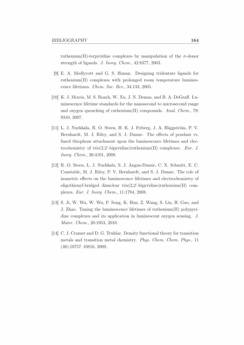
BIBLIOGRAPHY 164
ruthenium(II)-terpyridine complexes by manipulation of the σ-donor
strength of ligands. J. Inorg. Chem., 42:8377, 2003.
[9] E. A. Medlycott and G. S. Hanan. Designing tridentate ligands for
ruthenium(II) complexes with prolonged room temperature lumines-
cence lifetimes. Chem. Soc. Rev., 34:133, 2005.
[10] K. J. Morris, M. S. Roach, W. Xu, J. N. Demas, and B. A. DeGraff. Lu-
minescence lifetime standards for the nanosecond to microsecond range
and oxygen quenching of ruthenium(II) compounds. Anal. Chem., 79:
9310, 2007.
[11] L. J. Nurkkala, R. O. Steen, H. K. J. Friberg, J. A. Häggström, P. V.
Bernhardt, M. J. Riley, and S. J. Dunne. The effects of pendant vs.
fused thiophene attachment upon the luminescence lifetimes and elec-
trochemistry of tris(2,2’-bipyridine)ruthenium(II) complexes. Eur. J.
Inorg. Chem., 26:4101, 2008.
[12] R. O. Steen, L. J. Nurkkala, S. J. Angus-Dunne, C. X. Schmitt, E. C.
Constable, M. J. Riley, P. V. Bernhardt, and S. J. Dunne. The role of
isometric effects on the luminescence lifetimes and electrochemistry of
oligothienyl-bridged dinuclear tris(2,2’-bipyridine)ruthenium(II) com-
plexes. Eur. J. Inorg. Chem., 11:1784, 2008.
[13] S. Ji, W. Wu, W. Wu, P. Song, K. Han, Z. Wang, S. Liu, H. Guo, and
J. Zhao. Tuning the luminescence lifetimes of ruthenium(II) polypyri-
dine complexes and its application in luminescent oxygen sensing. J.
Mater. Chem., 20:1953, 2010.
[14] C. J. Cramer and D. G. Truhlar. Density functional theory for transition
metals and transition metal chemistry. Phys. Chem. Chem. Phys., 11
(46):10757–10816, 2009.
Chapter 12
Located a Transition State on
the Excited-State Triplet
Surface
This is preliminary work aimed at finding the nature and height of the
barrier on the lowest triplet excited-state surface.
12.1 Introduction
12.1.1 Background Information on the Problem
Ruthenium complexes continue to illicit immense interest owing to their
wide range of applications ranging from photochemical molecular devices
(PMDs), biological sensors, organic light emitting diodes (OLEDS) and
biomedical applications just to mention but a few; and which has been the
subject of many studies [1–11]. When talking about these complexes, the
idea that comes into mind is the excited state lifetime. Study of the excited
state lifetime demands that the working of the complexes must be under-
stood in terms of the deactivation mechanisms and what leads to the long or
short excited state lifetime. However, in this work we do not focus on how to
modify the complex to have a long or short excited state lifetime, our focus
165
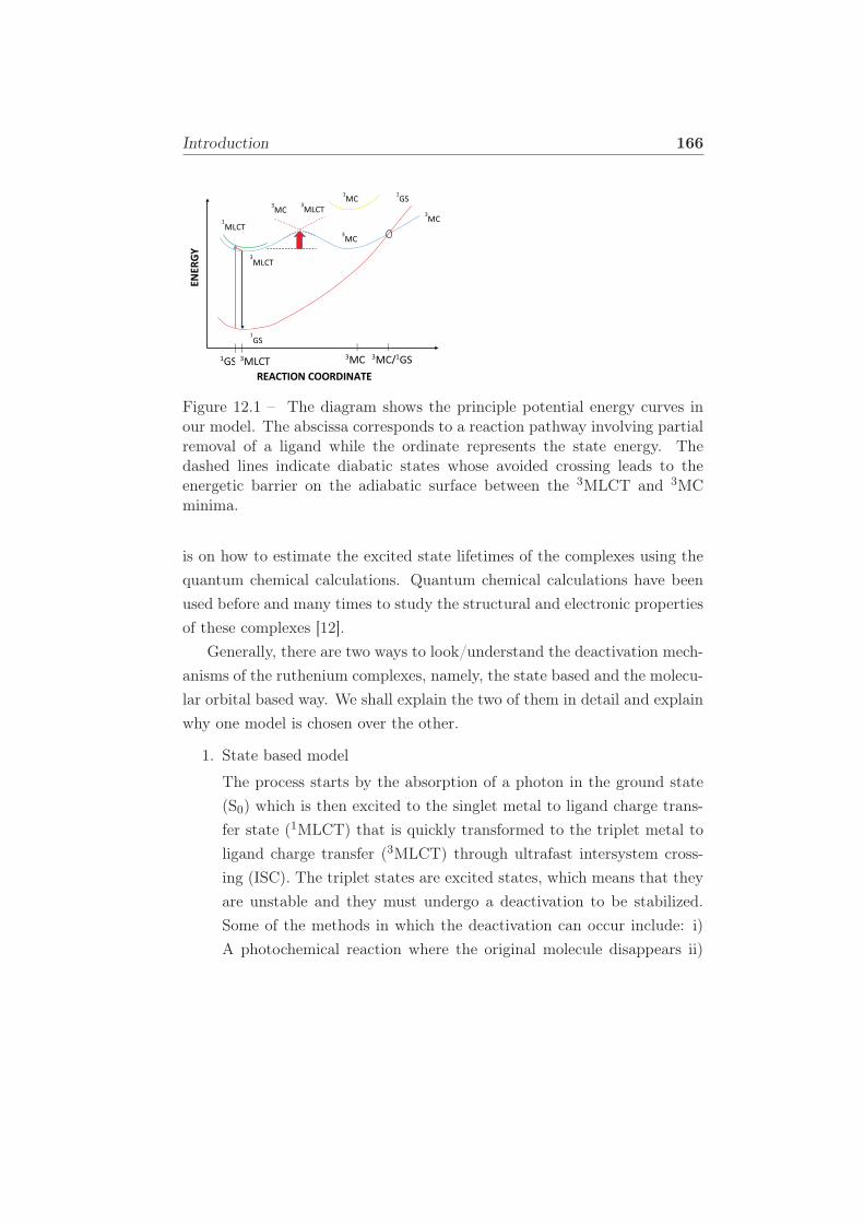
Introduction 166
EN
ER
GY
1GS S 3MLCT3MC 3MC/1GS
REACTION COORDINATE
1
GS
3
MLCT
1
MLCT
3MLCT
3MC
3MC
3MC
1GS
1MC
Figure 12.1 – The diagram shows the principle potential energy curves inour model. The abscissa corresponds to a reaction pathway involving partialremoval of a ligand while the ordinate represents the state energy. Thedashed lines indicate diabatic states whose avoided crossing leads to theenergetic barrier on the adiabatic surface between the 3MLCT and 3MCminima.
is on how to estimate the excited state lifetimes of the complexes using the
quantum chemical calculations. Quantum chemical calculations have been
used before and many times to study the structural and electronic properties
of these complexes [12].
Generally, there are two ways to look/understand the deactivation mech-
anisms of the ruthenium complexes, namely, the state based and the molecu-
lar orbital based way. We shall explain the two of them in detail and explain
why one model is chosen over the other.
1. State based model
The process starts by the absorption of a photon in the ground state
(S0) which is then excited to the singlet metal to ligand charge trans-
fer state (1MLCT) that is quickly transformed to the triplet metal to
ligand charge transfer (3MLCT) through ultrafast intersystem cross-
ing (ISC). The triplet states are excited states, which means that they
are unstable and they must undergo a deactivation to be stabilized.
Some of the methods in which the deactivation can occur include: i)
A photochemical reaction where the original molecule disappears ii)
Introduction 167
luminescence iii) radiationless deactivation and iv) quenching process
[13]. The luminescent 3MLCT can be depopulated in two ways, either
through a radiative (emission) or non-radiative pathway. The major
deactivation route at room temperature is believed to be to the 3MLCT
to the metal centered, 3MC state. It is possible to determine the emis-
sion quantum yields and the excited state lifetimes from the individual
rate constants. Experimentally, excited state lifetime is measured as a
decay rate of the intensity of light luminescing at a particular wave as
a function of time. Temperature, the decay constant k(T) and decay
lifetime τ(T ) are related by,
k(T ) =1
τ(T ). (12.1)
The decay lifetime τ(T ) is temperature dependent and the decay rate
constant can be separated into the temperature dependent and inde-
pendent parts. The temperature independent processes are those that
continue to occur even at very low temperatures.
k(T ) = k0 + knrb (T ) , (12.2)
where k0 is the temperature dependent part and knrb (T ) is the tempera-
ture independent part. The temperature dependent term is associated
with;
(a) Activated surface crossing to another excited state. For our case,
we shall assume that this is the 3MLCT to 3MC surface crossing.
This particular term will be studied more exhaustively later on.
(b) Onset of vibrational modes that do not occur at low temperatures
because of the frozen environment. Vibrational modes can favour
radiationless decay.
The temperature dependent term may further be further expressed as,
knrb (T ) = kmelt(T ) + kequlib(T ) + kbarrier(T ) , (12.3)
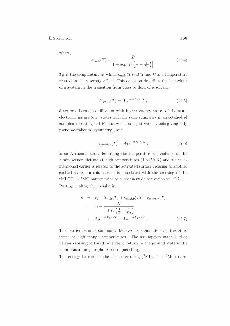
Introduction 168
where,
kmelt(T ) =B
1 + exp[
C(
1T − 1
TB
)] . (12.4)
TB is the temperature at which kmelt(T )=B/2 and C is a temperature
related to the viscosity effect. This equation describes the behaviour
of a system in the transition from glass to fluid of a solvent.
kequlib(T ) = A1e−∆E1/RT , (12.5)
describes thermal equilibrium with higher energy states of the same
electronic nature (e.g., states with the same symmetry in an octahedral
complex according to LFT but which are split with ligands giving only
pseudo-octahedral symmetry), and
kbarrier(T ) = A2e−∆E2/RT , (12.6)
is an Arrhenius term describing the temperature dependence of the
luminescence lifetime at high temperatures (T>250 K) and which as
mentioned earlier is related to the activated surface crossing to another
excited state. In this case, it is associated with the crossing of the3MLCT → 3MC barrier prior to subsequent de-activation to 1GS.
Putting it altogether results in,
k = k0 + kmelt(T ) + kequlib(T ) + kbarrier(T )
= k0 +B
1 + C(
1T − 1
TB
)
+ A1e−∆E1/RT +A2e
−∆E2/RT . (12.7)
The barrier term is commonly believed to dominate over the other
terms at high-enough temperatures. The assumption made is that
barrier crossing followed by a rapid return to the ground state is the
main reason for phosphorescence quenching.
The energy barrier for the surface crossing (3MLCT → 3MC) is re-
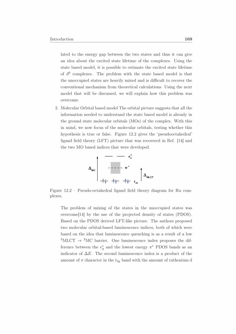
Introduction 169
lated to the energy gap between the two states and thus it can give
an idea about the excited state lifetime of the complexes. Using the
state based model, it is possible to estimate the excited state lifetime
of d6 complexes. The problem with the state based model is that
the unoccupied states are heavily mixed and is difficult to recover the
conventional mechanism from theoretical calculations. Using the next
model that will be discussed, we will explain how this problem was
overcome.
2. Molecular Orbital based model The orbital picture suggests that all the
information needed to understand the state based model is already in
the ground state molecular orbitals (MOs) of the complex. With this
in mind, we now focus of the molecular orbitals, testing whether this
hypothesis is true or false. Figure 12.2 gives the ‘pseudooctahedral’
ligand field theory (LFT) picture that was recovered in Ref. [14] and
the two MO based indices that were developed.
Figure 12.2 – Pseudo-octahedral ligand field theory diagram for Ru com-plexes.
The problem of mixing of the states in the unoccupied states was
overcome[14] by the use of the projected density of states (PDOS).
Based on the PDOS derived LFT-like picture. The authors proposed
two molecular orbital-based luminescence indices, both of which were
based on the idea that luminescence quenching is as a result of a low3MLCT → 3MC barrier. One luminescence index proposes the dif-
ference between the e∗g and the lowest energy π∗ PDOS bands as an
indicator of ∆E. The second luminescence index is a product of the
amount of π character in the t2g band with the amount of ruthenium d
Introduction 170
character in the 1π∗ band summarized as d×π. The frontier molecular
orbital theory that we recently looked at also looks at the activation
barriers to estimate the excited state lifetime but it is relies on the
experimental activation barrier.
Using the above information, work was done on more than 90 com-
plexes so as to validate the molecular orbital indices that were devel-
oped by [14]. In this work, a quantitative structure activity relationship
(QSPR) was developed by identifying the target molecules that had a
long excited state lifetime (those that are likely to remain excited long
enough to luminescence or transfer an electron), and comparing against
all the other complexes. The complexes studied were identified from
[13] based on the length of their excited state lifetime. If a complex
was within the parameter space, it was likely to have a long excited
state lifetime, but if it did not lie within the parameter space, then it
was not worth synthesising since it will not be very useful practically.
But there was a gap in terms of just how much information could be
extracted. In particular, the data about the lifetimes at room tem-
perature and the activation barrier was not easy to come by, and this
prompted the extension of this study to find how big or small the acti-
vation barrier is. This is because with this information, it is possible,
using the luminescence indices to get exactly which complexes are go-
ing to have a long excited state lifetime or not since the height of the
activation barrier is related to the length of the excited state lifetime.
In this work, we seek to get the activation barriers theoretically. In-
deed, we are not delving into a completely new world but each complex
comes with its own challenges especially in the excited state. Recent
work has shown that it possible to calculate the activation energy from3MLCT to 3MC [15]. The transition states of the 3(MLCT → MC)
conversion was determined as well as the energy barriers of the con-
version. Those in complexes containing bpy and terpyridine ligands
were reported to have small activation energies (less than 5 kcal/mol).
The study employed DFT method with the Lee-Yang-Parr correlation
functionals (B3YPP) [16, 17] and a double-zeta quality SDD basis set
Introduction 171
for the ruthenium atom and the other atoms were described by a split
valence Pople basis plus one polarization function (6-311G*). Calcula-
tions were done in acetronitrile solvent using the PCM method.
In Ref. [18], ultrafast transient infrared spectroscopy and DFT calcu-
lations of ruthenium(II) polypyridyl complexes has been used to char-
acterize the transition from 3(MLCT → MC). It has been shown from
the potential energy curves that for [Ru(bpy)3]2+, the triplet manifold
along the metal-ligand distance for the 3dd state is at a higher energy
than the 3MLCT state and that there is a substantial barrier between
the two minima. The study makes use of the Gaussian 09 program
package with the mPW1PW91 functional, D95V basis set for H, C and
N atoms and the LANL2DZ basis set for ruthenium. Calculations were
performed in the gas phase and with the PCM method in order to take
solvent effects into account.
In this work, the height of the activation barrier from 3MLCT to 3MC is
the main interest. For this to be done, the relevant excited states must
be identified so that a plot of the potential energy surface (PES) and
the energies obtained can be used to calculate the height of the barrier.
The 3MLCT and 3MC excited states must be correctly identified and
the energies calculated as the transition occurs from one excited state
to the other. The question is, how do we do this theoretically?
Mulliken spin density analysis has been used as an important tool to
identify the nature of the excited electronic state. This method has
been used previously [15, 18, 19, 19–21] for the same purpose. A unity
net spin on ruthenium was associated with the 3MLCT state while
a net spin of 2 on ruthenium was identified as the 3MC state. Jahn
Teller effect [22] is used as the key principle to help in differentiating
the different kinds of excited states. As the transition occurs from the3MLCT to 3MC, there is lowering of the symmetry and therefore the
axial bond lengths are distorted by the population of the eg orbital.
The two bond lengths are expected to be significantly longer compared
to the other bonds in the molecule. The location of the 3MC involves
Computational Details 172
the distortion of the structures to get a good starting guess for the
triplet optimization. The reasoning behind this distortion is as follows;
displacing ligands away from the ruthenium core will lower the energy
of the unoccupied d orbitals, to a point at which the (dz2 or dx2−y2)
become occupied. Therefore, by the elongation of the Ru-N bonds in
the xy plane, the energy of the unoccupied orbitals decreases, hence
populating the dx2−y2 orbital, leading to the 3MC state [23].
The Mulliken population analysis has been used in this work to char-
acterize the nature of the triplet states in this work, the ultimate goal
being the calculation of the size of the activation barrier.
12.2 Computational Details
All calculations have been done with the Gaussian09 [24] code (version
D.01). The first step involved the ground state optimization of all the three
complexes in gas phase. The 3MLCT and 3dd states were also optimized both
in gas phase and in acetonitrile using the PCM model to account for the sol-
vent effects. A double-ζ quality basis set LANL2DZ and the corresponding
effective core potential (ECP) [25] was used to characterize Ru. H, N and
C atoms were described by the D95V basis set [26]. Frequency calculations
were performed on the optimized geometries so as to check whether they
were the true minima (with no imaginary frequencies). The MPW1PW91
exchange-correlation hybrid functional [27] was used. For all the calcula-
tions, (pop=full) was set to full so as to extract all the information. A
density value of 0.004 was used in Gaussview to generate the spin density
diagrams from cube files. 3MLCT was obtained by optimizing the optimized
ground state with the triplet spin, first in gas phase and then in solvent. The3MC excited state was obtained by elongating the two axial bond lengths to
2.4000 Å and then optimizing first in gas phase and then in solvent. All the
optimized excited states converged to the true minima as an analysis of the
frequencies did not show any negative frequencies. The potential energy scan
was obtained by increasing the bond length of the two axial bonds in steps
of 0.002 Å and fixing those particular parameters during an optimization.
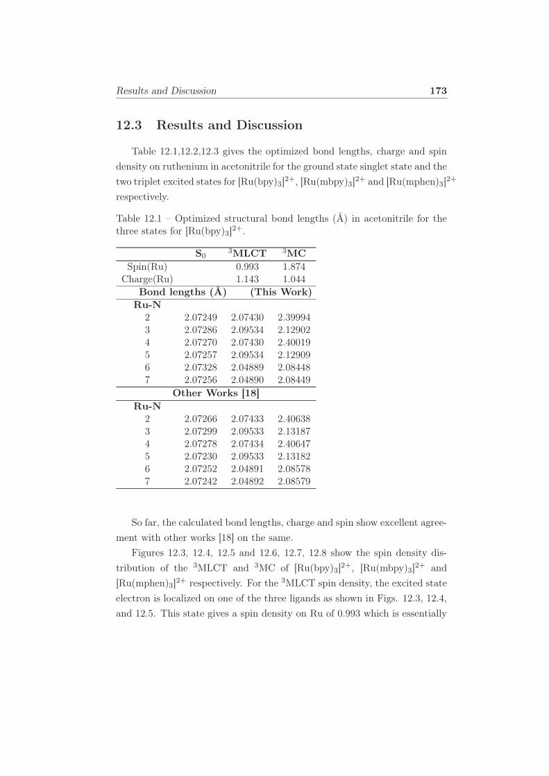
Results and Discussion 173
12.3 Results and Discussion
Table 12.1,12.2,12.3 gives the optimized bond lengths, charge and spin
density on ruthenium in acetonitrile for the ground state singlet state and the
two triplet excited states for [Ru(bpy)3]2+, [Ru(mbpy)3]2+ and [Ru(mphen)3]2+
respectively.
Table 12.1 – Optimized structural bond lengths (Å) in acetonitrile for thethree states for [Ru(bpy)3]2+.
S03MLCT 3MC
Spin(Ru) 0.993 1.874Charge(Ru) 1.143 1.044
Bond lengths (Å) (This Work)Ru-N
2 2.07249 2.07430 2.399943 2.07286 2.09534 2.129024 2.07270 2.07430 2.400195 2.07257 2.09534 2.129096 2.07328 2.04889 2.084487 2.07256 2.04890 2.08449
Other Works [18]Ru-N
2 2.07266 2.07433 2.406383 2.07299 2.09533 2.131874 2.07278 2.07434 2.406475 2.07230 2.09533 2.131826 2.07252 2.04891 2.085787 2.07242 2.04892 2.08579
So far, the calculated bond lengths, charge and spin show excellent agree-
ment with other works [18] on the same.
Figures 12.3, 12.4, 12.5 and 12.6, 12.7, 12.8 show the spin density dis-
tribution of the 3MLCT and 3MC of [Ru(bpy)3]2+, [Ru(mbpy)3]2+ and
[Ru(mphen)3]2+ respectively. For the 3MLCT spin density, the excited state
electron is localized on one of the three ligands as shown in Figs. 12.3, 12.4,
and 12.5. This state gives a spin density on Ru of 0.993 which is essentially
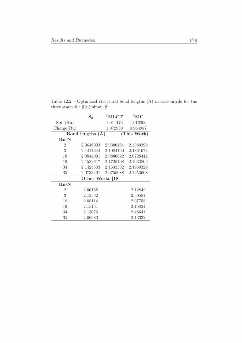
Results and Discussion 174
Table 12.2 – Optimized structural bond lengths (Å) in acetonitrile for thethree states for [Ru(mbpy)3]2+.
S03MLCT 3MC
Spin(Ru) 1.011473 1.916306Charge(Ru) 1.072959 0.964987
Bond lengths (Å) (This Work)Ru-N
2 2.0646903 2.0386164 2.13803993 2.1417344 2.1084160 2.486167418 2.0844091 2.0886892 2.072844219 2.1582617 2.1725408 2.163380634 2.1424503 2.1633302 2.495032935 2.0733401 2.0755988 2.1253608
Other Works [18]Ru-N
2 2.06168 2.128423 2.13532 2.5058118 2.08114 2.0775819 2.15151 2.1582134 2.13675 2.4864135 2.06983 2.13332
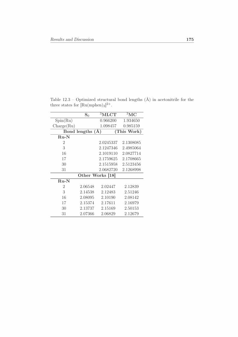
Results and Discussion 175
Table 12.3 – Optimized structural bond lengths (Å) in acetonitrile for thethree states for [Ru(mphen)3]2+.
S03MLCT 3MC
Spin(Ru) 0.966200 1.934650Charge(Ru) 1.098457 0.985159
Bond lengths (Å) (This Work)Ru-N
2 2.0245337 2.13080853 2.1247346 2.498506416 2.1019110 2.082771417 2.1759625 2.170866530 2.1515958 2.512345631 2.0682720 2.1268998
Other Works [18]Ru-N
2 2.06548 2.02447 2.128393 2.14538 2.12483 2.5124616 2.08095 2.10190 2.0814217 2.15374 2.17611 2.1697930 2.13737 2.15169 2.5015331 2.07366 2.06829 2.12679
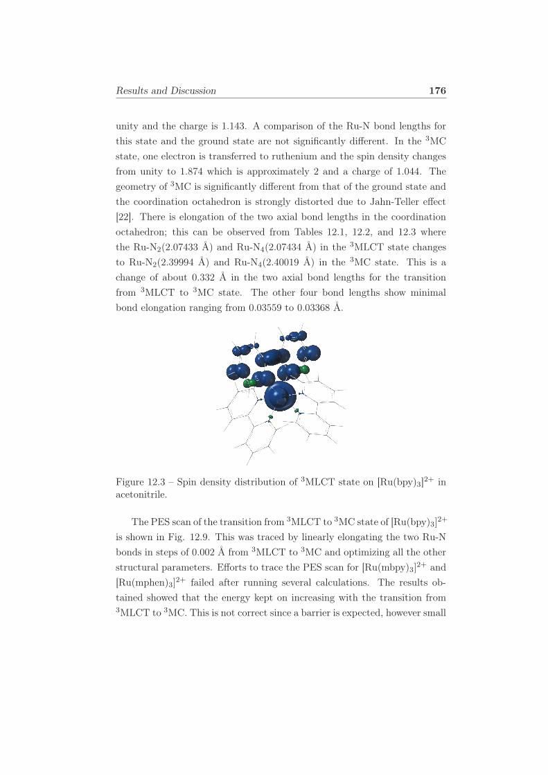
Results and Discussion 176
unity and the charge is 1.143. A comparison of the Ru-N bond lengths for
this state and the ground state are not significantly different. In the 3MC
state, one electron is transferred to ruthenium and the spin density changes
from unity to 1.874 which is approximately 2 and a charge of 1.044. The
geometry of 3MC is significantly different from that of the ground state and
the coordination octahedron is strongly distorted due to Jahn-Teller effect
[22]. There is elongation of the two axial bond lengths in the coordination
octahedron; this can be observed from Tables 12.1, 12.2, and 12.3 where
the Ru-N2(2.07433 Å) and Ru-N4(2.07434 Å) in the 3MLCT state changes
to Ru-N2(2.39994 Å) and Ru-N4(2.40019 Å) in the 3MC state. This is a
change of about 0.332 Å in the two axial bond lengths for the transition
from 3MLCT to 3MC state. The other four bond lengths show minimal
bond elongation ranging from 0.03559 to 0.03368 Å.
Figure 12.3 – Spin density distribution of 3MLCT state on [Ru(bpy)3]2+ inacetonitrile.
The PES scan of the transition from 3MLCT to 3MC state of [Ru(bpy)3]2+
is shown in Fig. 12.9. This was traced by linearly elongating the two Ru-N
bonds in steps of 0.002 Å from 3MLCT to 3MC and optimizing all the other
structural parameters. Efforts to trace the PES scan for [Ru(mbpy)3]2+ and
[Ru(mphen)3]2+ failed after running several calculations. The results ob-
tained showed that the energy kept on increasing with the transition from3MLCT to 3MC. This is not correct since a barrier is expected, however small
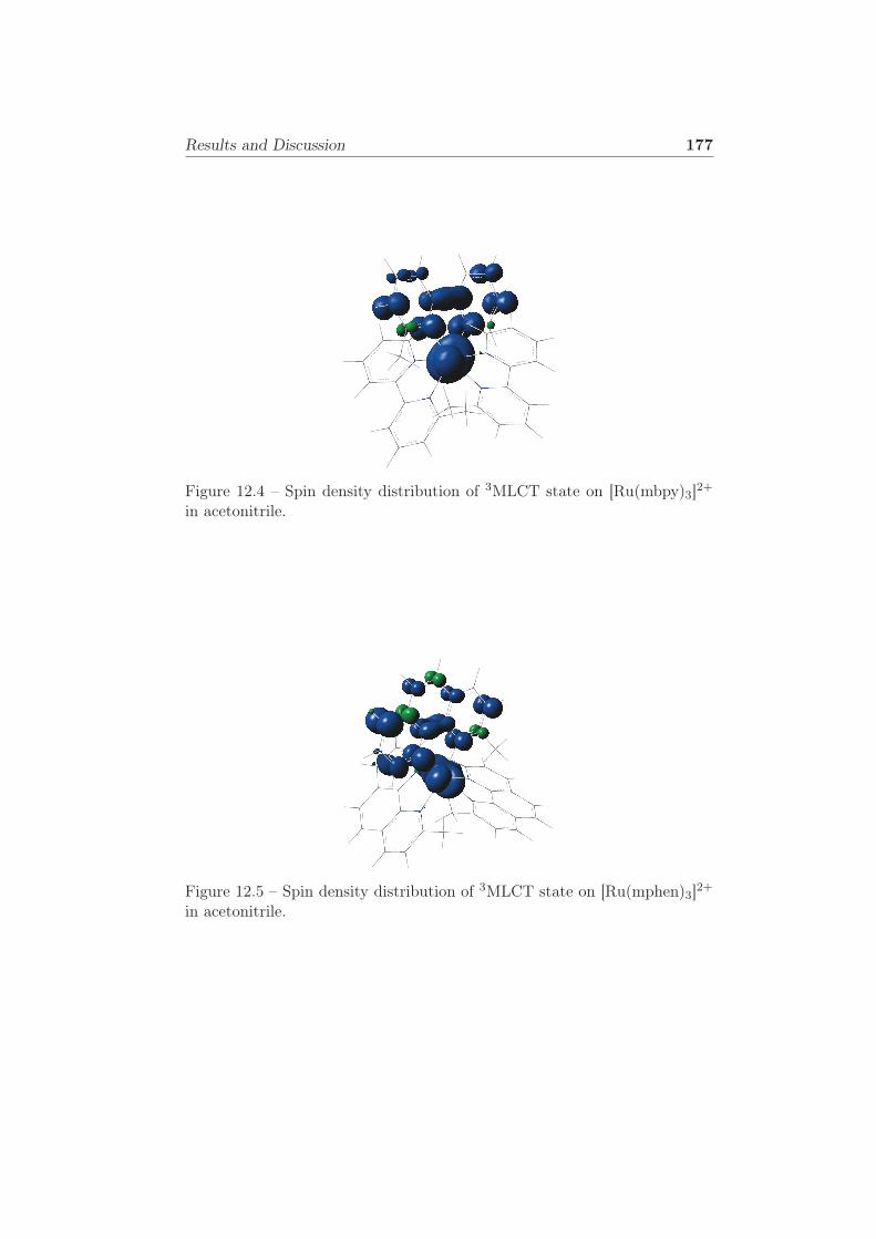
Results and Discussion 177
Figure 12.4 – Spin density distribution of 3MLCT state on [Ru(mbpy)3]2+
in acetonitrile.
Figure 12.5 – Spin density distribution of 3MLCT state on [Ru(mphen)3]2+
in acetonitrile.
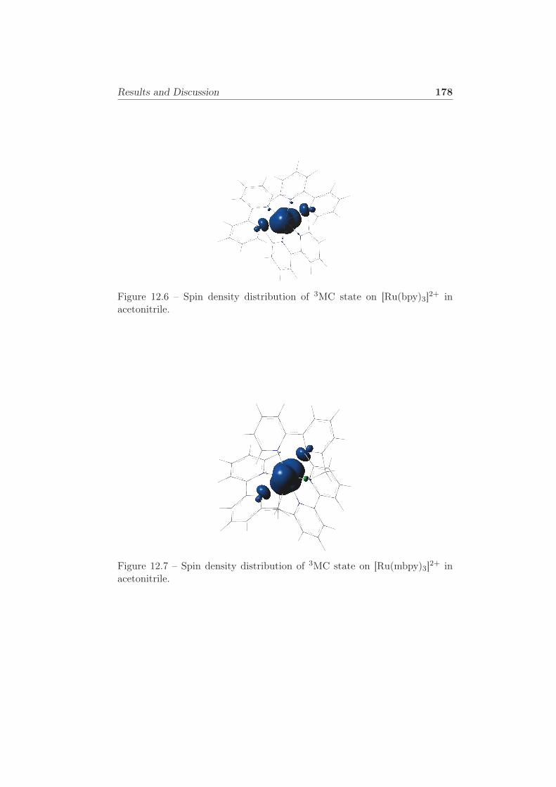
Results and Discussion 178
Figure 12.6 – Spin density distribution of 3MC state on [Ru(bpy)3]2+ inacetonitrile.
Figure 12.7 – Spin density distribution of 3MC state on [Ru(mbpy)3]2+ inacetonitrile.
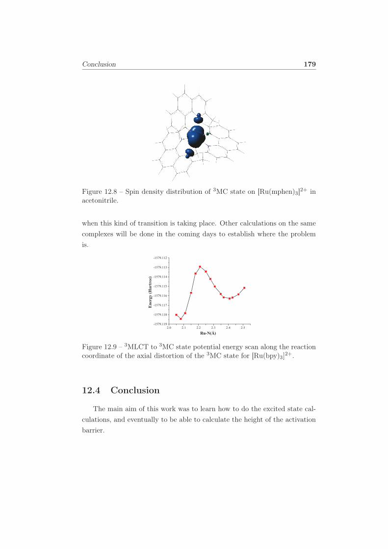
Conclusion 179
Figure 12.8 – Spin density distribution of 3MC state on [Ru(mphen)3]2+ inacetonitrile.
when this kind of transition is taking place. Other calculations on the same
complexes will be done in the coming days to establish where the problem
is.
!" !# ! !$ !% !&
'#&()!##)
'#&()!##*
'#&()!##(
'#&()!##+
'#&()!##&
'#&()!##%
'#&()!##$
'#&()!##
!"#$%&'()#*#""+
!"#$%&
Figure 12.9 – 3MLCT to 3MC state potential energy scan along the reactioncoordinate of the axial distortion of the 3MC state for [Ru(bpy)3]2+.
12.4 Conclusion
The main aim of this work was to learn how to do the excited state cal-
culations, and eventually to be able to calculate the height of the activation
barrier.
Acknowledgement 180
Information about the height of the activation barrier would be use-
ful in terms of predicting the excited state lifetimes more directly. So far,
this has been achieved to some extent as the excited state calculations
for [Ru(bpy)3]2+ have been done. Calculations for two other complexes,
[Ru(mbpy)3]2+ and [Ru(mphen)3]2+ were not successful for reasons that have
not yet been established since the 3MLCT and 3MC states were sucessfully
identified. It is worthy mentioning that excited state dynamics are not the
same for every ruthenium complex [18, 28, 29]. This is based on the fact that
each complex may have different ligands as well as other factors that have a
significant influence on the excited state dynamics that come into play such
as the solvent effects. Results obtained for [Ru(bpy)3]2+ are encouraging
since with this information the activation barrier can be calculated directly.
Most of the efforts will be directed towards the study of the activation barrier
of homoleptic transition metal complexes.
12.5 Acknowledgement
The author thanks Anne MILET and Xiuwen ZHOU for the useful dis-
cussions regarding ruthenium complexes and particularly in helping in the
calculations regarding the location of the triplet states.
BIBLIOGRAPHY 181
Bibliography
[1] J. P. Sauvage, J. P. Collin, J. C. Chambron, S. Guillerez, and
C. Coudret. Ruthenium(II) and osmium(II) bis(terpyridine) complexes
in covalently-linked multicomponent systems: Synthesis, electrochemi-
cal behavior, absorption spectra, and photochemical and photophysical
properties. Chem. Rev., 94:933, 1994.
[2] V. Balzani and A. Juris. Photochemistry and photophysics of Ru(II)
polypyridine complexes in the Bologna group. From early studies to
recent developments. Coordin. Chem. Rev., 211(1):97–115, 2001.
[3] K. Nakamaru. Synthesis, luminescence quantum yields, and lifetimes
of trischelated ruthenium (II) mixed-ligand complexes including 3, 3’-
dimethyl-2, 2’-bipyridyl. B. Chem. Soc. Jpn, 55(9):2697–2705, 1982.
[4] G. Liebsch, I. Klimant, and O. S. Wolfbeis. Luminescence lifetime tem-
perature sensing based on sol-gels and poly(acrylonitrile)s dyed with
ruthenium metal-ligand complexes. Adv. Mat., 11:1296, 1999.
[5] A. Harriman, A. Khatyr, and R. Ziessel. Extending the luminescence
lifetime of ruthenium(II) poly(pyridine) complexes in solution at ambi-
ent temperature. Dalton Trans., 10:2061, 2003.
[6] M. Duati, S. Tasca, F. C. Lynch, H. Bohlen, J. G. Vos, S. Stagni, and
M. D. Ward. Enhancement of luminescence lifetimes of mononuclear
ruthenium(II)-terpyridine complexes by manipulation of the σ-donor
strength of ligands. J. Inorg. Chem., 42:8377, 2003.
[7] E. A. Medlycott and G. S. Hanan. Designing tridentate ligands for
ruthenium(II) complexes with prolonged room temperature lumines-
cence lifetimes. Chem. Soc. Rev., 34:133, 2005.
[8] K. J. Morris, M. S. Roach, W. Xu, J. N. Demas, and B. A. DeGraff. Lu-
minescence lifetime standards for the nanosecond to microsecond range
and oxygen quenching of ruthenium(II) compounds. Anal. Chem., 79:
9310, 2007.
BIBLIOGRAPHY 182
[9] L. J. Nurkkala, R. O. Steen, H. K. J. Friberg, J. A. Häggström, P. V.
Bernhardt, M. J. Riley, and S. J. Dunne. The effects of pendant vs.
fused thiophene attachment upon the luminescence lifetimes and elec-
trochemistry of tris(2,2’-bipyridine)ruthenium(II) complexes. Eur. J.
Inorg. Chem., 26:4101, 2008.
[10] R. O. Steen, L. J. Nurkkala, S. J. Angus-Dunne, C. X. Schmitt, E. C.
Constable, M. J. Riley, P. V. Bernhardt, and S. J. Dunne. The role of
isometric effects on the luminescence lifetimes and electrochemistry of
oligothienyl-bridged dinuclear tris(2,2’-bipyridine)ruthenium(II) com-
plexes. Eur. J. Inorg. Chem., 11:1784, 2008.
[11] S. Ji, W. Wu, W. Wu, P. Song, K. Han, Z. Wang, S. Liu, H. Guo, and
J. Zhao. Tuning the luminescence lifetimes of ruthenium(II) polypyri-
dine complexes and its application in luminescent oxygen sensing. J.
Mater. Chem., 20:1953, 2010.
[12] C. J. Cramer and D. G. Truhlar. Density functional theory for transition
metals and transition metal chemistry. Phys. Chem. Chem. Phys., 11
(46):10757–10816, 2009.
[13] A. Juris, V. Balzani, F. Barigelletti, S. Campagna, P. Belser, and A. Von
Zelewsky. Ru(II) polypyridine complexes: Photophysics, photochem-
istry, electrochemistry, and chemiluminescence. Coord. Chem. Rev., 84:
85, 1988.
[14] C. M. Wawire, D. Jouvenot, F. Loiseau, P. Baudin, S. Liatard,
L. Njenga, G. Kamau, and M. E. Casida. Density-functional study
of luminescence in polypyrine ruthenium complexes. J. Photochem. and
Photobiol. A, 276:8, 2014.
[15] N. Yoshikawa, S. Yamabe, S. Sakaki, N. Kanehisa, T. Inoue, and
H. Takashima. Transition states of the 3MLCT to 3MC conversion
in [Ru(bpy)2- (phen derivative)]2+ complexes. J. Mol. Struct., 1094:
98–108, 2015.
BIBLIOGRAPHY 183
[16] A. D. Becke. Density-functional thermochemistry. III. The role of exact
exchange. J. Chem. Phys., 98:5648, 1993.
[17] C. Lee, W. Yang, and R. G. Parr. Development of the Colle-Salvetti cor-
relation energy formula into a functional of the electron density. Phys.
Rev. B, 37:785, 1988.
[18] Q. Sun, B. Dereka, E. Vauthey, L. M. Lawson-Daku, and A. Hauser.
Ultrafast transient IR spectroscopy and DFT calculations of ruthenium
(II) polypyridyl complexes. Chem. Sci., 8(1):223–230, 2017.
[19] O. A. Borg, S. S. Godinho, M. J. Lundqvist, S. Lunell, and P. Pers-
son. Computational study of the lowest triplet state of ruthenium
polypyridyl complexes used in artificial photosynthesis. J. Phys. Chem.
A, 112(19):4470–4476, 2008.
[20] E. Ruiz, J. Cirera, and S. Alvarez. Spin density distribution in transition
metal complexes. Coord. Chem. Rev., 249(23):2649–2660, 2005.
[21] Q. Sun, S. Mosquera-Vazquez, Y. Suffren, J. Hankache, N. Amstutz,
L. M. L. Daku, E. Vauthey, and A. Hauser. On the role of ligand-field
states for the photophysical properties of ruthenium (II) polypyridyl
complexes. Coord. Chem. Rev., 282:87–99, 2015.
[22] F. Alary, M. Boggio-Pasqua, J. Heully, C. J. Marsden, and P. Vicendo.
Theoretical characterization of the lowest triplet excited states of the
tris- (1, 4, 5, 8-tetraazaphenanthrene) ruthenium dication complex. In-
org. Chem., 47(12):5259–5266, 2008.
[23] A. Maria, M. J. Lundqvist, H. Wolpher, O. Johansson, L. Eriksson,
J. Bergquist, T. Rasmussen, H. Becker, L. Hammarström, and P. Nor-
rby. Steric influence on the excited-state lifetimes of ruthenium com-
plexes with bipyridyl-alkanylene-pyridyl ligands. Inorg. chem., 47(9):
3540–3548, 2008.
[24] M. J. Frisch, G. W. Trucks, H. B. Schlegel, G. E. Scuseria, M. A. Robb,
J. R. Cheeseman, G. Scalmani, V. Barone, B. Mennucci, G. A. Peters-
BIBLIOGRAPHY 184
son, H. Nakatsuji, M. Caricato, X. Li, H. P. Hratchian, A. F. Izmaylov,
J. Bloino, G. Zheng, J. L. Sonnenberg, M. Hada, M. Ehara, K. Toyota,
R. Fukuda, J. Hasegawa, M. Ishida, T. Nakajima, Y. Honda, O. Kitao,
H. Nakai, T. Vreven, J. A. Montgomery, Jr., J. E. Peralta, F. Ogliaro,
M. Bearpark, J. J. Heyd, E. Brothers, K. N. Kudin, V. N. Staroverov,
R. Kobayashi, J. Normand, K. Raghavachari, A. Rendell, J. C. Burant,
S. S. Iyengar, J. Tomasi, M. Cossi, N. Rega, J. M. Millam, M. Klene,
J. E. Knox, J. B. Cross, V. Bakken, C. Adamo, J. Jaramillo, R. Gom-
perts, R. E. Stratmann, O. Yazyev, A. J. Austin, R. Cammi, C. Pomelli,
J. W. Ochterski, R. L. Martin, K. Morokuma, V. G. Zakrzewski, G. A.
Voth, P. Salvador, J. J. Dannenberg, S. Dapprich, A. D. Daniels, ÃŰ.
Farkas, J. B. Foresman, J. V. Ortiz, J. Cioslowski, and D. J. Fox. Gaus-
sianâĹij09 Revision D.01. Gaussian Inc. Wallingford CT 2009.
[25] P. J. Hay and W. R. Wadt. Ab initio effective core potentials for molec-
ular calculations. potentials for K to Au including the outermost core
orbitals. J. Chem. Phys., 82:299, 1985.
[26] T. H. Dunning and P. J. Hay. Applications of Electronic Structure The-
ory, volume 3. Springer, New York, 1976. ISBN 9781468485417.
[27] C. Adamo and V. Barone. Exchange functionals with improved long-
range behavior and adiabatic connection methods without adjustable
parameters: The mPW and mPW1PW models. J. Chem. Phys., 108
(2):664–675, 1998.
[28] M. Schwalbe, B. Schäfer, H. Görls, S. Rau, S. Tschierlei, M. Schmitt,
J. Popp, G. Vaughan, W. Henry, and J. G. Vos. Synthesis and char-
acterisation of poly(bipyridine)ruthenium complexes as building blocks
for heterosupramolecular arrays. Eur. J. Inorg. Chem., 2008(21):3310–
3319, 2008. ISSN 1099-0682.
[29] F. Alary, J. L. Heully, L. Bijeire, and P. Vicendo. Is the 3MLCT the
only photoreactive state of polypyridyl complexes? Inorg. chem., 46(8):
3154–3165, 2007.

Part IV
Conclusion
185
Chapter 13
Summary and Conclusion
Transition metal complexes and ruthenium and iridium complexes in
particular have found an important role in electronic devices, including solar
cells and organic light emitting diodes. One reason for this is the presence of
a long-lived triplet excited state which is accessible via singlet excitation fol-
lowed by intersystem crossing due to strong spin-orbit coupling. Such devices
and the experiments needed to develop new materials for new devices can be
expected to benefit from improved understanding through better theoretical
modeling. However realistic modeling of these complexes, while increasingly
possible, is complicated and compute intensive, hence limiting the number
of complexes which can be treated. That is why a much simpler approach
has been taken in this thesis, namely to see how much information about
luminesence lifetimes may be obtained just by looking at gas-phase opti-
mized geometries of ruthenium complexes and their orbital energies. On the
order of 100 ruthenium complexes were studied and it was shown that the
gas-phase DFT geometries are reasonably close to experimentally-measured
crystal geometries. Furthermore TD-DFT spectra correlate reasonably well
with solution spectra corrected for solvent effects. This authorizes us to
use (TD-)DFT as a model for further investigation of the underlying phys-
ical chemical reasons why some complexes have longer lifetimes than other
lifetimes. We immediately faced two difficulties.
The first difficulty is that it is difficult to overcome is to find a way to
186
187
relate the calculated DFT orbital energies with LFT energies. This is impor-
tant because, not only do experimentalists rely highly upon LFT to explain
their results and to plan experiments, but LFT brings out common features
between related but different compounds. We were able to do this by taking
advantage of earlier results from the Franco-Kenyan collaboration, namely
the use of partial density of states (PDOS) analysis. In particular, while
the nonbonding ruthenium t2g orbitals are often identifiable by visualizing
DFT orbitals, this is no longer true of the antibonding e∗g orbitals which mix
with the ligand orbitals in such a way that their density is split over many
DFT energy levels. The PDOS approach takes this splitting specifically into
account and allows us to find approximate e∗g energy levels even when the e∗gdensity has been split over many DFT orbitals. This provides an LFT-like
picture which is not LFT but which resembles it enough to be able to use
similar reasoning.
Another difficulty that had to be overcome is that the most common the-
ory for ruthenium complex luminescence lifetimes is based upon estimations
of the height of the transition state barrier on the triplet excited state curve.
However this transition energy is rarely available experimentally. We were
able to overcome this in the first instance by looking at an average lumines-
cence lifetime calculated from experimentally available room temperature
and liquid nitrogen lifetimes.
We were then able to check the value of luminescence indices proposed
in earlier work from our Franco-Kenyan collaboration and found them to
be less than optimal. However frontier-molecular orbital ideas led us to a
new proposal for luminescence indices which, except for a few points, pro-
vides a reasonably linear correlation with the average luminescence lifetime.
The few exceptions observed may be due to qualitatively different relaxation
pathways, to the need for more or better experimental data in these cases,
or, perhaps, still other as yet unimaginable reasons.
One approach for improving this study would be to cut out the need for
experimentally-determined average barriers by direct calculation of theoret-
ical activation energies for de-excitation of the triple excited state. We have
included a chapter in this thesis where we have begun to explore this ap-

188
proach. It is indeed more difficult than the orbital-based approach but it is
worthwhile. Though time did not allow us to finish this part of the project,
it is envisaged that the work will continue after finishing the PhD.
Another avenue, and one suggested by a referee for our published paper,
is that the study be extended to iridium compounds. This is also on our list
of future “to-dos.”
Index
‘Deadly Sins’ of TD-DFT, 127
6-31G, 98
6-31G and 6-31G(d) basis sets, 98
6-31G(d), 98
Adiabatic approximation, 117
Atomic units, 32
Basis set, 87
Basis set superposition error
(BSSE), 99
Basis sets and effective core
potentials, 87
Born-Oppenheimer
approximation, 34
Casida equations, 124
Chemical hamiltonian approach
(CHA), 100
Coulomb and exchange integrals,
56
Coulomb and exchange operators,
59
Counterpoise method (CP), 100
Crystal field theory, 13
Diffuse-function-augmented basis
functions, 95
Double hybrid functionals, 82
Double, triple and multi zeta (ζ)
basis sets and split
valence basis sets, 93
Effective core potential (ECP)
basis functions
(pseudopotentials), 96
Effective core potentials, 87
Electronic excitation, 39
Electronic hamiltonian, 55
Electronic transition, 40
Exchange-correlation
approximations, 79
Exchange-correlation potentials,
117
Excited state deactivation, 44
Existence theorem, 70, 112
First Runge-Gross theorem, 112
Fluorescence, 48
Forbidden electronic transitions,
42
189
190
Franck-Condon principle, 40
Frenkel-Dirac variational
principle, 114
Gaussian-type orbitals, 87
Gaussian-type orbitals (GTOs),
90
Generalized gradient
approximation (GGA),
80
Generalized susceptibility, 120
Hartree product, 54
Hartree-Fock approximation, 53
Hartree-Fock orbitals and orbital
energies, 61
Highest occupied molecular
orbital (HOMO), 43
Hohenberg-Kohn theorems, 70
Hybrid functionals, 81
Incandescence, 45
Internal conversion, 47
Intersystem crossing, 47
Introduction, 2
Jablonski diagram, 45
Jacob’s ladder, 79, 82
Kohn-Sham approach, 75
Kohn-Sham linear density
response, 122
Koopmans’ theorem, 63
Laporte selection rule, 40
Ligand field theory, 15
Linear combination of atomic
orbitals, 87
Linear response TD-DFT, 118
Linear response theory, 118
Local density
approximation(LDA), 79
Lowest unoccupied molecular
orbital (LUMO), 43
Luminescence, 44
Meta-generalized gradient
approximation
(meta-GGA), 82
Minimal basis sets (single zeta),
92
Molecular hamiltonian, 30
Molecular orbitals, 43
Partial density of states (PDOS),
106
Phosphorescence, 49
Photochemical process, 45
Photoelectric effect, 23
Photophenomena and
luminescence, 38
Photophysical processes, 45
Polarization
function-supplemented
basis functions, 94
Potential energy surfaces, 49
Quantization of electronic angular
momentum, 24
191
Quantum yield, 50
Radiationless deactivation, 47
Radiative deactivation, 48
Restricted localized orbital
(RLO), 101
Second Runge-Gross theorem, 113
Singlet, 41
Slater determinant, 55
Slater-type Orbitals, 87
Slater-type orbitals, 89
SNOOP, 100
Spin selection rule, 40
Spin-orbit coupling, 42
State energy diagram, 43
STO-3G, 92
Tamm-Dancoff approximation
(TDA), 126
Thomas-Fermi model, 74
Time-dependent density
functional theory
(TD-DFT), 109
Time-dependent Kohn-Sham
equation, 115
Time-dependent linear density
response, 119
Time-dependent Schrödinger
equation, 110
Time-dependent Schrödinger
equation, 29
Time-independent Schrödinger
equation, 26
Triplet, 42
Types of basis functions (Atomic
orbitals), 88
Types of electronic transitions, 40
Ultraviolet catastrophe, 23
Variational principle, 73
Vibrational relaxation, 46, 47
Wave-particle duality, 25
Appendix A
Supplementary Material:
Partial Density of States
Ligand Field Theory
(PDOS-LFT): Recovering a
LFT-Like Picture and
Application to the
Photoproperties of Ruthenium
Polypyridine Complexes
192
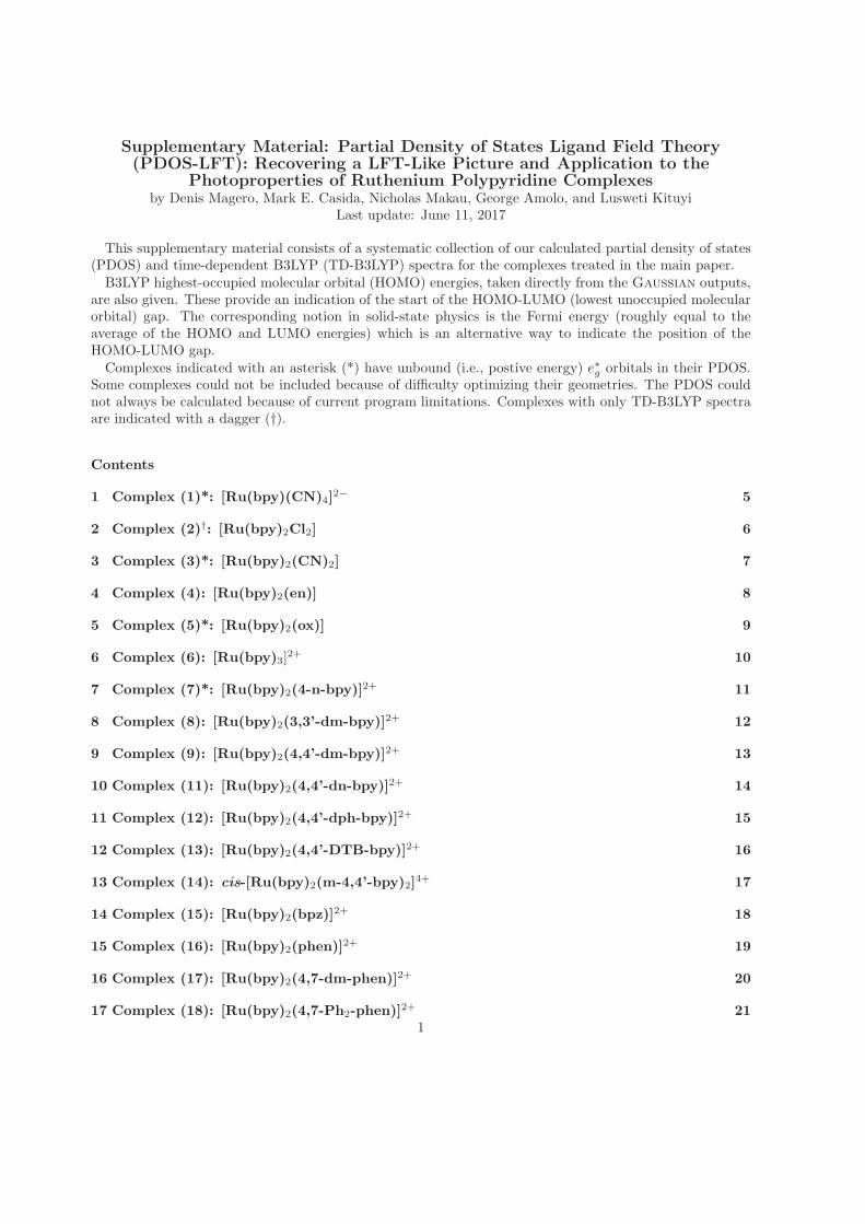
Supplementary Material: Partial Density of States Ligand Field Theory(PDOS-LFT): Recovering a LFT-Like Picture and Application to the
Photoproperties of Ruthenium Polypyridine Complexesby Denis Magero, Mark E. Casida, Nicholas Makau, George Amolo, and Lusweti Kituyi
Last update: June 11, 2017
This supplementary material consists of a systematic collection of our calculated partial density of states(PDOS) and time-dependent B3LYP (TD-B3LYP) spectra for the complexes treated in the main paper.B3LYP highest-occupied molecular orbital (HOMO) energies, taken directly from the Gaussian outputs,
are also given. These provide an indication of the start of the HOMO-LUMO (lowest unoccupied molecularorbital) gap. The corresponding notion in solid-state physics is the Fermi energy (roughly equal to theaverage of the HOMO and LUMO energies) which is an alternative way to indicate the position of theHOMO-LUMO gap.Complexes indicated with an asterisk (*) have unbound (i.e., postive energy) e∗
gorbitals in their PDOS.
Some complexes could not be included because of difficulty optimizing their geometries. The PDOS couldnot always be calculated because of current program limitations. Complexes with only TD-B3LYP spectraare indicated with a dagger (†).
Contents
1 Complex (1)*: [Ru(bpy)(CN)4]2− 5
2 Complex (2)†: [Ru(bpy)2Cl2] 6
3 Complex (3)*: [Ru(bpy)2(CN)2] 7
4 Complex (4): [Ru(bpy)2(en)] 8
5 Complex (5)*: [Ru(bpy)2(ox)] 9
6 Complex (6): [Ru(bpy)3]2+ 10
7 Complex (7)*: [Ru(bpy)2(4-n-bpy)]2+ 11
8 Complex (8): [Ru(bpy)2(3,3’-dm-bpy)]2+ 12
9 Complex (9): [Ru(bpy)2(4,4’-dm-bpy)]2+ 13
10 Complex (11): [Ru(bpy)2(4,4’-dn-bpy)]2+ 14
11 Complex (12): [Ru(bpy)2(4,4’-dph-bpy)]2+ 15
12 Complex (13): [Ru(bpy)2(4,4’-DTB-bpy)]2+ 16
13 Complex (14): cis-[Ru(bpy)2(m-4,4’-bpy)2]4+ 17
14 Complex (15): [Ru(bpy)2(bpz)]2+ 18
15 Complex (16): [Ru(bpy)2(phen)]2+ 19
16 Complex (17): [Ru(bpy)2(4,7-dm-phen)]2+ 20
17 Complex (18): [Ru(bpy)2(4,7-Ph2-phen)]2+ 21
1
18 Complex (19): [Ru(bpy)2(4,7-dhy-phen)]2+ 22
19 Complex (20): [Ru(bpy)2(5,6-dm-phen)]2+ 23
20 Complex (21): [Ru(bpy)2(DIAF)]2+ 24
21 Complex (22)†: [Ru(bpy)2(DIAFO)]2+ 25
22 Complex (23): [Ru(bpy)2(taphen)]2+ 26
23 Complex (24): cis-[Ru(bpy)2(py)2]2+ 27
24 Complex (25): trans-[Ru(bpy)2(py)2]2+ 28
25 Complex (26): [Ru(bpy)2(pic)2]2+ 29
26 Complex (27): [Ru(bpy)2(DPM)]2+ 30
27 Complex (28): [Ru(bpy)2(DPE)]2+ 31
28 Complex (29): [Ru(bpy)2(PimH)]2+ 32
29 Complex (30): [Ru(bpy)2(PBzimH)]2+ 33
30 Complex (31): [Ru(bpy)2(biimH2)]2+ 34
31 Complex (32): [Ru(bpy)2(BiBzimH2)]2+ 35
32 Complex (34): [Ru(bpy)2(piq)]2+ 36
33 Complex (35): [Ru(bpy)2(hpiq)]2+ 37
34 Complex (36): [Ru(bpy)2(pq)]2+ 38
35 Complex (37): [Ru(bpy)2(DMCH)]2+ 39
36 Complex (38)†: [Ru(bpy)2(OMCH)]2+ 40
37 Complex (39)†: [Ru(bpy)2(biq)]2+ 41
38 Complex (40): [Ru(bpy)2(i-biq)]2+ 42
39 Complex (41): [Ru(bpy)2(BL4)]2+ 43
40 Complex (42): [Ru(bpy)2(BL5)]2+ 44
41 Complex (46): [Ru(bpy)(4,4’-DTB-bpy)2]2+ 45
42 Complex (47): [Ru(bpy)(h-phen)]2+ 46
43 Complex (48): [Ru(bpy)(phen)2]2+ 47
44 Complex (50): trans-[Ru(bpy)(phen)(py)2]2+ 48
45 Complex (52): [Ru(bpy)(taphen)2]2+ 49
2
46 Complex (53): [Ru(bpy)(py)2(en)]2+ 50
47 Complex (55): [Ru(bpy)(py)4]2+ 51
48 Complex (56): [Ru(bpy)(py)2(PMA)]2+ 52
49 Complex (57): [Ru(bpy)(py)2(2-AEP)]2+ 53
50 Complex (58): [Ru(bpy)(PMA)2]2+ 54
51 Complex (60): [Ru(bpy)(DMCH)2]2+ 55
52 Complex (61): [Ru(bpy)(biq)2]2+ 56
53 Complex (63)†: [Ru(bpy)(trpy)Cl]+ 57
54 Complex (64)*: [Ru(bpy)(trpy)(CN)]+ 58
55 Complex (66)*: [Ru(6-m-bpy)3]2+ 59
56 Complex (67)*: [Ru(3,3’-dm-bpy)3]2+ 60
57 Complex (69): [Ru(3,3’-dm-bpy)(phen)2]2+ 61
58 Complex (70): [Ru(4,4’-dm-bpy)3]2+ 62
59 Complex (71): [Ru(4,4’-dm-bpy)2(4,7-dhy-phen)]2+ 63
60 Complex (73): [Ru(4,4’-dph-bpy)3]2+ 64
61 Complex (74): [Ru(4,4’-DTB-bpy)3]2+ 65
62 Complex (75): [Ru(6,6’-dm-bpy)3]2+ 66
63 Complex (76): [Ru(h-phen)3]2+ 67
64 Complex (77): [Ru(phen)3]2+ 68
65 Complex (78): [Ru(phen)2(4,7-dhy-phen)]2+ 69
66 Complex (79): [Ru(phen)2(pq)]2+ 70
67 Complex (80): [Ru(phen)2(DMCH)]2+ 71
68 Complex (81): [Ru(phen)2(biq)]2+ 72
69 Complex (82): [Ru(phen)(pq)2]2+ 73
70 Complex (83): [Ru(phen)(biq)2]2+ 74
71 Complex (84): [Ru(2-m-phen)3]2+ 75
72 Complex (85): [Ru(2,9-dm-phen)3]2+ 76
73 Complex (86): [Ru(4,7-Ph2-phen)3]2+ 77
3
74 Complex (87): [Ru(4,7-dhy-phen)(tm1-phen)2]2+ 78
75 Complex (88)*: [Ru(DPA)3]− 79
76 Complex (89): [Ru(DPA)(DPAH)2]+ 80
77 Complex (90): [Ru(DPAH)3]2+ 81
78 Complex (91): [Ru(Azpy)3]2+ 82
79 Complex (92): [Ru(NA)3]2+ 83
80 Complex (93): [Ru(hpiq)3]2+ 84
81 Complex (94): [Ru(pq)3]2+ 85
82 Complex (95): [Ru(pq)2(biq)]2+ 86
83 Complex (96): [Ru(pq)(biq)2]2+ 87
84 Complex (97): [Ru(pynapy)3]2+ 88
85 Complex (98)†: [Ru(DMCH)2Cl2] 89
86 Complex (99)*: [Ru(DMCH)2(CN)2] 90
87 Complex (100): [Ru(DMCH)3]2+ 91
88 Complex (101): [Ru(dinapy)3]2+ 92
89 Complex (102)†: [Ru(biq)2Cl2] 93
90 Complex (103)*: [Ru(biq)2(CN)2] 94
91 Complex (104): [Ru(biq)3]2+ 95
92 Complex (105)†: [Ru(i-biq)2Cl2] 96
93 Complex (106)*: [Ru(i-biq)2(CN)2] 97
94 Complex (107): [Ru(i-biq)3]2+ 98
95 Complex (108): [Ru(trpy)2]2+ 99
96 Complex (109): [Ru(tro)2]2+ 100
97 Complex (110): [Ru(tsite)2]2+ 101
98 Complex (111)*: [Ru(dqp)2]2+ 102
4
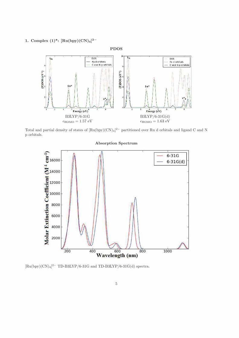
1. Complex (1)*: [Ru(bpy)(CN)4]2−
PDOS
B3LYP/6-31G B3LYP/6-31G(d)ǫHOMO = 1.57 eV ǫHOMO = 1.63 eV
Total and partial density of states of [Ru(bpy)(CN)4]2− partitioned over Ru d orbitals and ligand C and N
p orbitals.
Absorption Spectrum
[Ru(bpy)(CN)4]2− TD-B3LYP/6-31G and TD-B3LYP/6-31G(d) spectra.
5
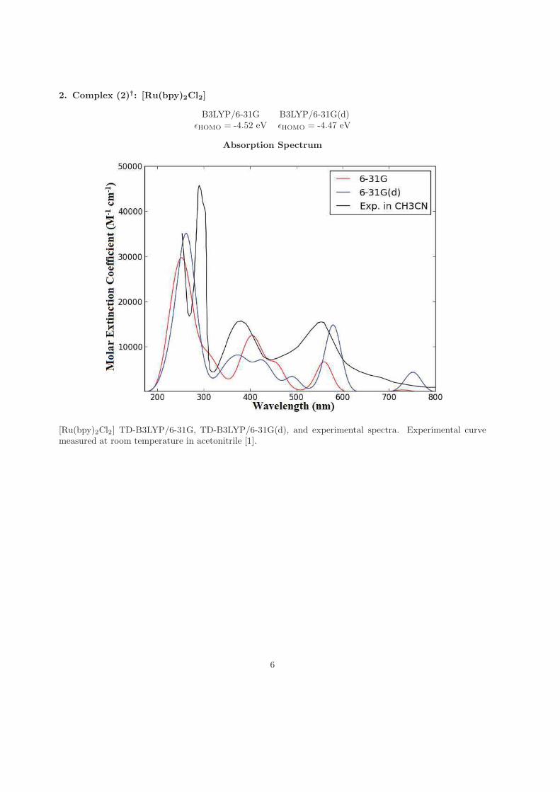
2. Complex (2)†: [Ru(bpy)2Cl2]
B3LYP/6-31G B3LYP/6-31G(d)ǫHOMO = -4.52 eV ǫHOMO = -4.47 eV
Absorption Spectrum
[Ru(bpy)2Cl2] TD-B3LYP/6-31G, TD-B3LYP/6-31G(d), and experimental spectra. Experimental curvemeasured at room temperature in acetonitrile [1].
6
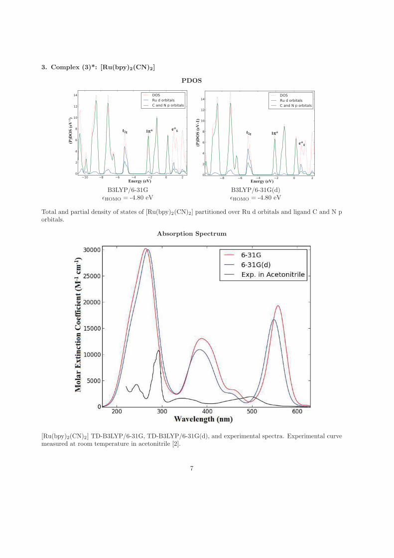
3. Complex (3)*: [Ru(bpy)2(CN)2]
PDOS
10 8 6 4 2 0 2
0
2
4
6
8
10
12
14
DOS
Ru d orbitals
C and N p orbitals
8 6 4 2 0 2
0
2
4
6
8
10
12
14
DOS
Ru d orbitals
C and N p orbitals
B3LYP/6-31G B3LYP/6-31G(d)ǫHOMO = -4.80 eV ǫHOMO = -4.80 eV
Total and partial density of states of [Ru(bpy)2(CN)2] partitioned over Ru d orbitals and ligand C and N porbitals.
Absorption Spectrum
[Ru(bpy)2(CN)2] TD-B3LYP/6-31G, TD-B3LYP/6-31G(d), and experimental spectra. Experimental curvemeasured at room temperature in acetonitrile [2].
7
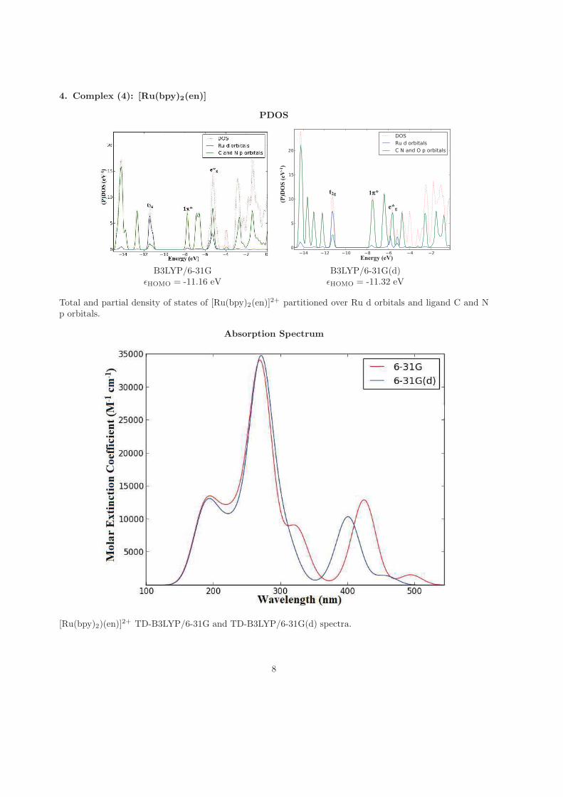
4. Complex (4): [Ru(bpy)2(en)]
PDOS
14 12 10 8 6 4 2
0
5
10
15
20
DOS
Ru d orbitals
C N and O p orbitals
B3LYP/6-31G B3LYP/6-31G(d)ǫHOMO = -11.16 eV ǫHOMO = -11.32 eV
Total and partial density of states of [Ru(bpy)2(en)]2+ partitioned over Ru d orbitals and ligand C and N
p orbitals.
Absorption Spectrum
[Ru(bpy)2)(en)]2+ TD-B3LYP/6-31G and TD-B3LYP/6-31G(d) spectra.
8
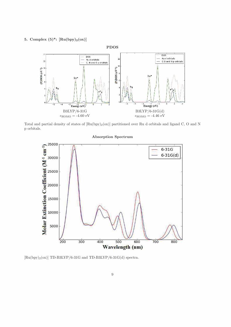
5. Complex (5)*: [Ru(bpy)2(ox)]
PDOS
B3LYP/6-31G B3LYP/6-31G(d)ǫHOMO = -4.60 eV ǫHOMO = -4.46 eV
Total and partial density of states of [Ru(bpy)2(ox)] partitioned over Ru d orbitals and ligand C, O and Np orbitals.
Absorption Spectrum
[Ru(bpy)2(ox)] TD-B3LYP/6-31G and TD-B3LYP/6-31G(d) spectra.
9
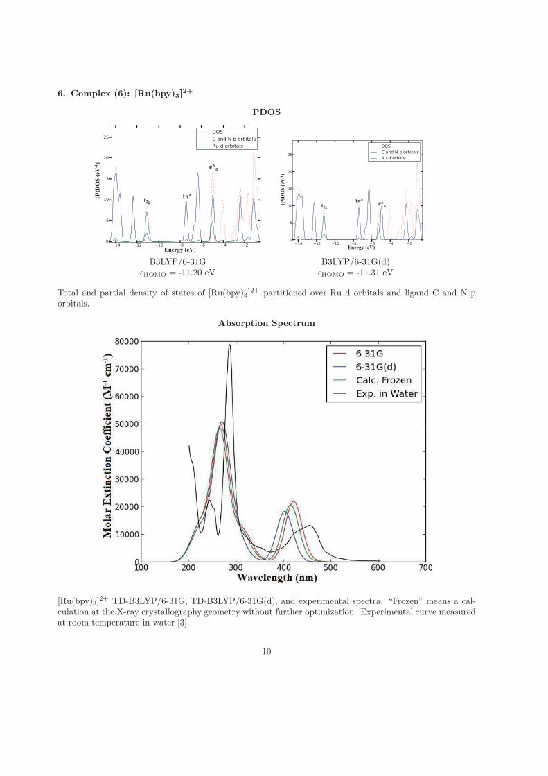
6. Complex (6): [Ru(bpy)3]2+
PDOS
14 12 10 8 6 4 2
0
5
10
15
20
25
DOS
C and N p orbitals
Ru d orbitals
14 12 10 8 6 4 2
0
5
10
15
20
25
DOS
C and N p orbitals
Ru d orbital
B3LYP/6-31G B3LYP/6-31G(d)ǫHOMO = -11.20 eV ǫHOMO = -11.31 eV
Total and partial density of states of [Ru(bpy)3]2+ partitioned over Ru d orbitals and ligand C and N p
orbitals.
Absorption Spectrum
[Ru(bpy)3]2+ TD-B3LYP/6-31G, TD-B3LYP/6-31G(d), and experimental spectra. “Frozen” means a cal-
culation at the X-ray crystallography geometry without further optimization. Experimental curve measuredat room temperature in water [3].
10
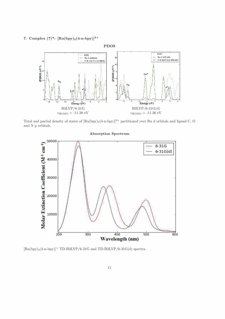
7. Complex (7)*: [Ru(bpy)2(4-n-bpy)]2+
PDOS
B3LYP/6-31G B3LYP/6-31G(d)ǫHOMO = -11.28 eV ǫHOMO = -11.36 eV
Total and partial density of states of [Ru(bpy)2(4-n-bpy)]2+ partitioned over Ru d orbitals and ligand C, O
and N p orbitals.
Absorption Spectrum
[Ru(bpy)2(4-n-bpy)]+ TD-B3LYP/6-31G and TD-B3LYP/6-31G(d) spectra.
11
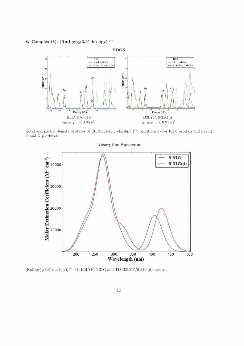
8. Complex (8): [Ru(bpy)2(3,3’-dm-bpy)]2+
PDOS
B3LYP/6-31G B3LYP/6-31G(d)ǫHOMO = -10.84 eV ǫHOMO = -10.97 eV
Total and partial density of states of [Ru(bpy)2(3,3’-dm-bpy)]2+ partitioned over Ru d orbitals and ligandC and N p orbitals.
Absorption Spectrum
[Ru(bpy)2(3,3’-dm-bpy)]2+ TD-B3LYP/6-31G and TD-B3LYP/6-31G(d) spectra.
12
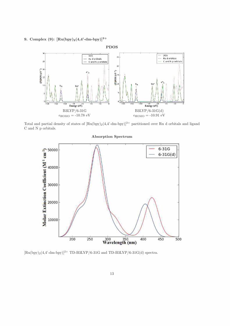
9. Complex (9): [Ru(bpy)2(4,4’-dm-bpy)]2+
PDOS
B3LYP/6-31G B3LYP/6-31G(d)ǫHOMO = -10.78 eV ǫHOMO = -10.91 eV
Total and partial density of states of [Ru(bpy)2(4,4’-dm-bpy)]2+ partitioned over Ru d orbitals and ligandC and N p orbitals.
Absorption Spectrum
[Ru(bpy)2(4,4’-dm-bpy)]2+ TD-B3LYP/6-31G and TD-B3LYP/6-31G(d) spectra.
13
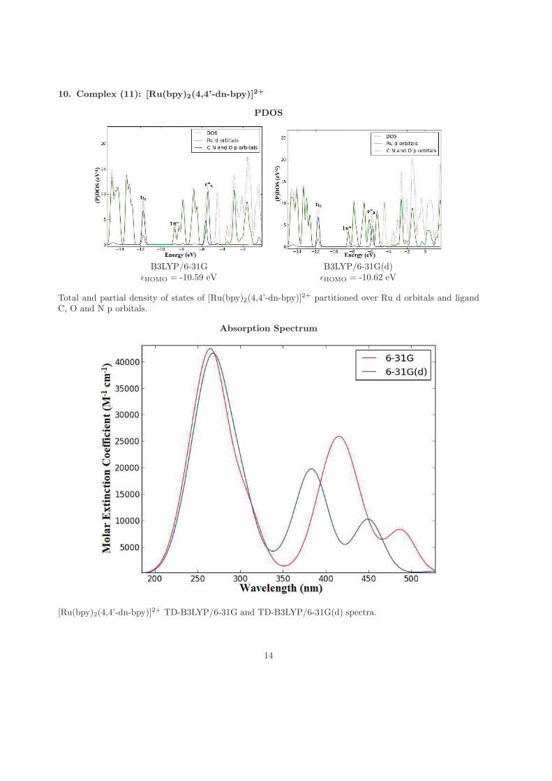
10. Complex (11): [Ru(bpy)2(4,4’-dn-bpy)]2+
PDOS
B3LYP/6-31G B3LYP/6-31G(d)ǫHOMO = -10.59 eV ǫHOMO = -10.62 eV
Total and partial density of states of [Ru(bpy)2(4,4’-dn-bpy)]2+ partitioned over Ru d orbitals and ligand
C, O and N p orbitals.
Absorption Spectrum
[Ru(bpy)2(4,4’-dn-bpy)]2+ TD-B3LYP/6-31G and TD-B3LYP/6-31G(d) spectra.
14
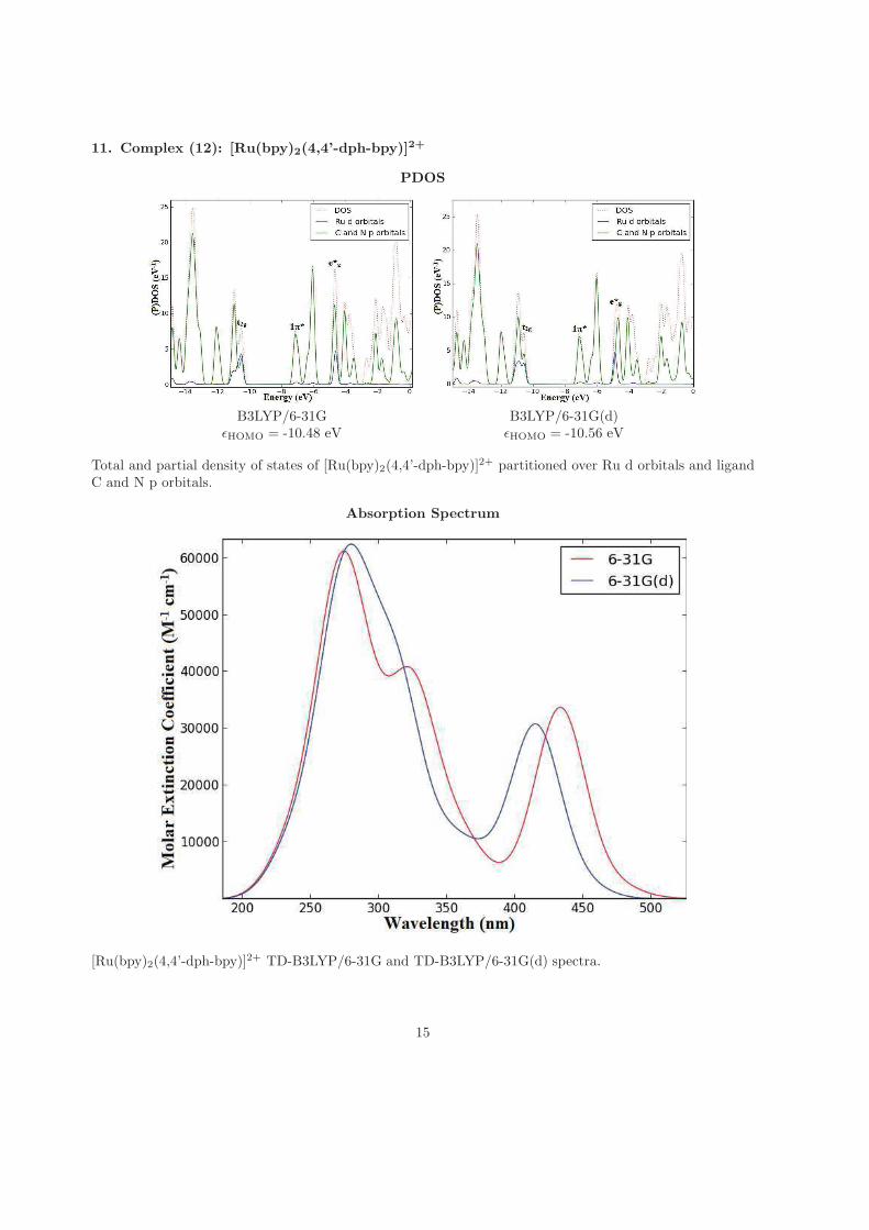
11. Complex (12): [Ru(bpy)2(4,4’-dph-bpy)]2+
PDOS
B3LYP/6-31G B3LYP/6-31G(d)ǫHOMO = -10.48 eV ǫHOMO = -10.56 eV
Total and partial density of states of [Ru(bpy)2(4,4’-dph-bpy)]2+ partitioned over Ru d orbitals and ligand
C and N p orbitals.
Absorption Spectrum
[Ru(bpy)2(4,4’-dph-bpy)]2+ TD-B3LYP/6-31G and TD-B3LYP/6-31G(d) spectra.
15
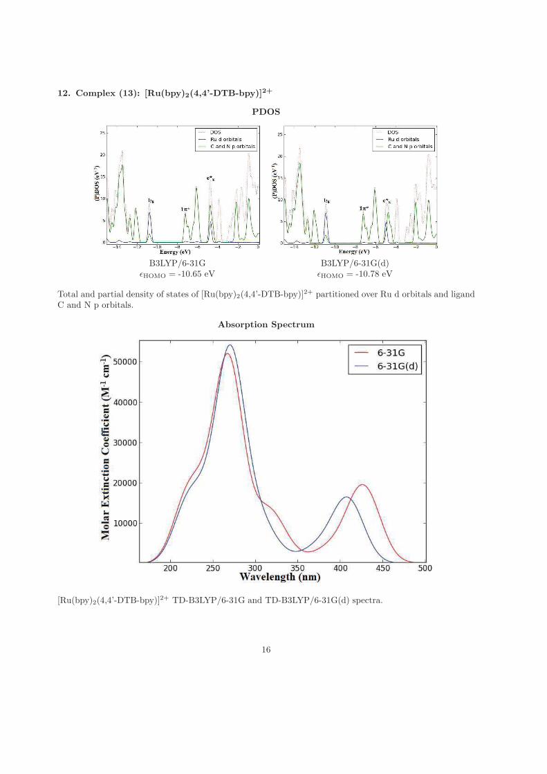
12. Complex (13): [Ru(bpy)2(4,4’-DTB-bpy)]2+
PDOS
B3LYP/6-31G B3LYP/6-31G(d)ǫHOMO = -10.65 eV ǫHOMO = -10.78 eV
Total and partial density of states of [Ru(bpy)2(4,4’-DTB-bpy)]2+ partitioned over Ru d orbitals and ligandC and N p orbitals.
Absorption Spectrum
[Ru(bpy)2(4,4’-DTB-bpy)]2+ TD-B3LYP/6-31G and TD-B3LYP/6-31G(d) spectra.
16
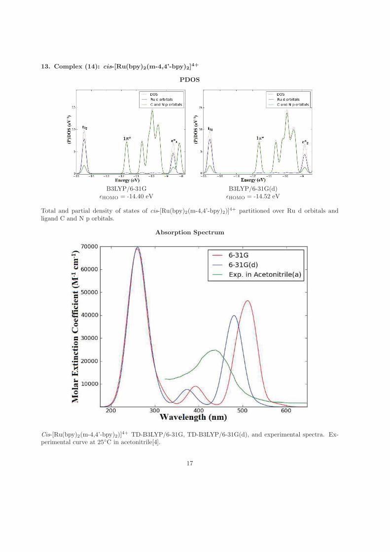
13. Complex (14): cis-[Ru(bpy)2(m-4,4’-bpy)2]4+
PDOS
B3LYP/6-31G B3LYP/6-31G(d)ǫHOMO = -14.40 eV ǫHOMO = -14.52 eV
Total and partial density of states of cis-[Ru(bpy)2(m-4,4’-bpy)2)]4+ partitioned over Ru d orbitals and
ligand C and N p orbitals.
Absorption Spectrum
Cis-[Ru(bpy)2(m-4,4’-bpy)2)]4+ TD-B3LYP/6-31G, TD-B3LYP/6-31G(d), and experimental spectra. Ex-
perimental curve at 25C in acetonitrile[4].
17
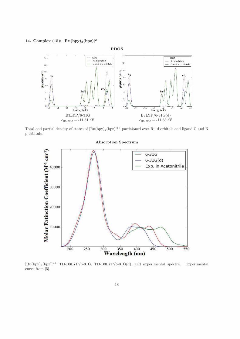
14. Complex (15): [Ru(bpy)2(bpz)]2+
PDOS
B3LYP/6-31G B3LYP/6-31G(d)ǫHOMO = -11.51 eV ǫHOMO = -11.58 eV
Total and partial density of states of [Ru(bpy)2(bpz)]2+ partitioned over Ru d orbitals and ligand C and N
p orbitals.
Absorption Spectrum
[Ru(bpy)2(bpz)]2+ TD-B3LYP/6-31G, TD-B3LYP/6-31G(d), and experimental spectra. Experimental
curve from [5].
18
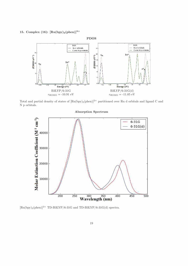
15. Complex (16): [Ru(bpy)2(phen)]2+
PDOS
B3LYP/6-31G B3LYP/6-31G(d)ǫHOMO = -10.91 eV ǫHOMO = -11.05 eV
Total and partial density of states of [Ru(bpy)2(phen)]2+ partitioned over Ru d orbitals and ligand C and
N p orbitals.
Absorption Spectrum
[Ru(bpy)2(phen)]2+ TD-B3LYP/6-31G and TD-B3LYP/6-31G(d) spectra.
19
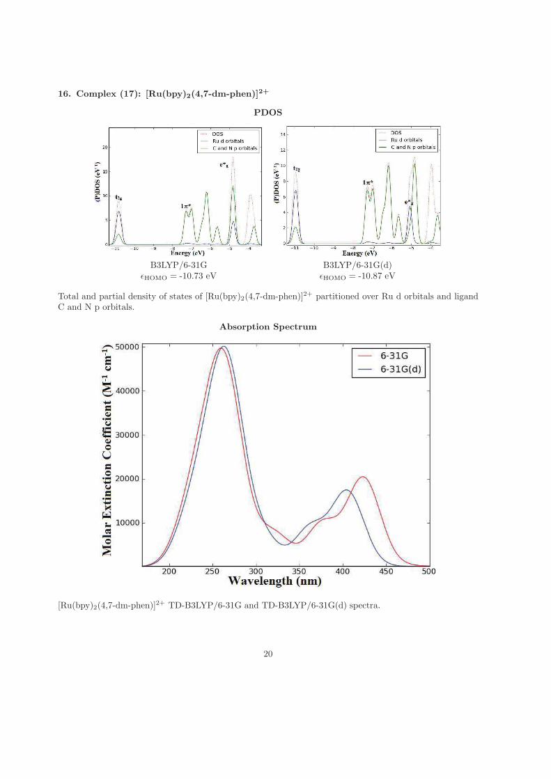
16. Complex (17): [Ru(bpy)2(4,7-dm-phen)]2+
PDOS
B3LYP/6-31G B3LYP/6-31G(d)ǫHOMO = -10.73 eV ǫHOMO = -10.87 eV
Total and partial density of states of [Ru(bpy)2(4,7-dm-phen)]2+ partitioned over Ru d orbitals and ligandC and N p orbitals.
Absorption Spectrum
[Ru(bpy)2(4,7-dm-phen)]2+ TD-B3LYP/6-31G and TD-B3LYP/6-31G(d) spectra.
20
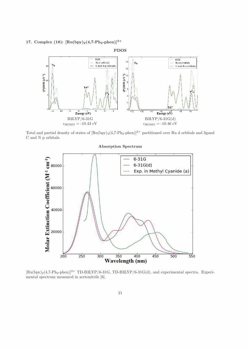
17. Complex (18): [Ru(bpy)2(4,7-Ph2-phen)]2+
PDOS
B3LYP/6-31G B3LYP/6-31G(d)ǫHOMO = -10.43 eV ǫHOMO = -10.46 eV
Total and partial density of states of [Ru(bpy)2(4,7-Ph2-phen)]2+ partitioned over Ru d orbitals and ligand
C and N p orbitals.
Absorption Spectrum
[Ru(bpy)2(4,7-Ph2-phen)]2+ TD-B3LYP/6-31G, TD-B3LYP/6-31G(d), and experimental spectra. Experi-
mental spectrum measured in acetonitrile [6].
21
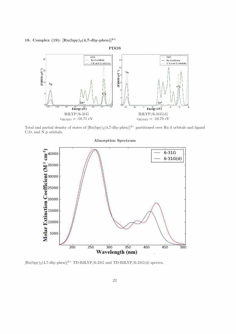
18. Complex (19): [Ru(bpy)2(4,7-dhy-phen)]2+
PDOS
B3LYP/6-31G B3LYP/6-31G(d)ǫHOMO = -10.71 eV ǫHOMO = -10.79 eV
Total and partial density of states of [Ru(bpy)2(4,7-dhy-phen)]2+ partitioned over Ru d orbitals and ligand
C,O, and N p orbitals.
Absorption Spectrum
[Ru(bpy)2(4,7-dhy-phen)]2+ TD-B3LYP/6-31G and TD-B3LYP/6-31G(d) spectra.
22
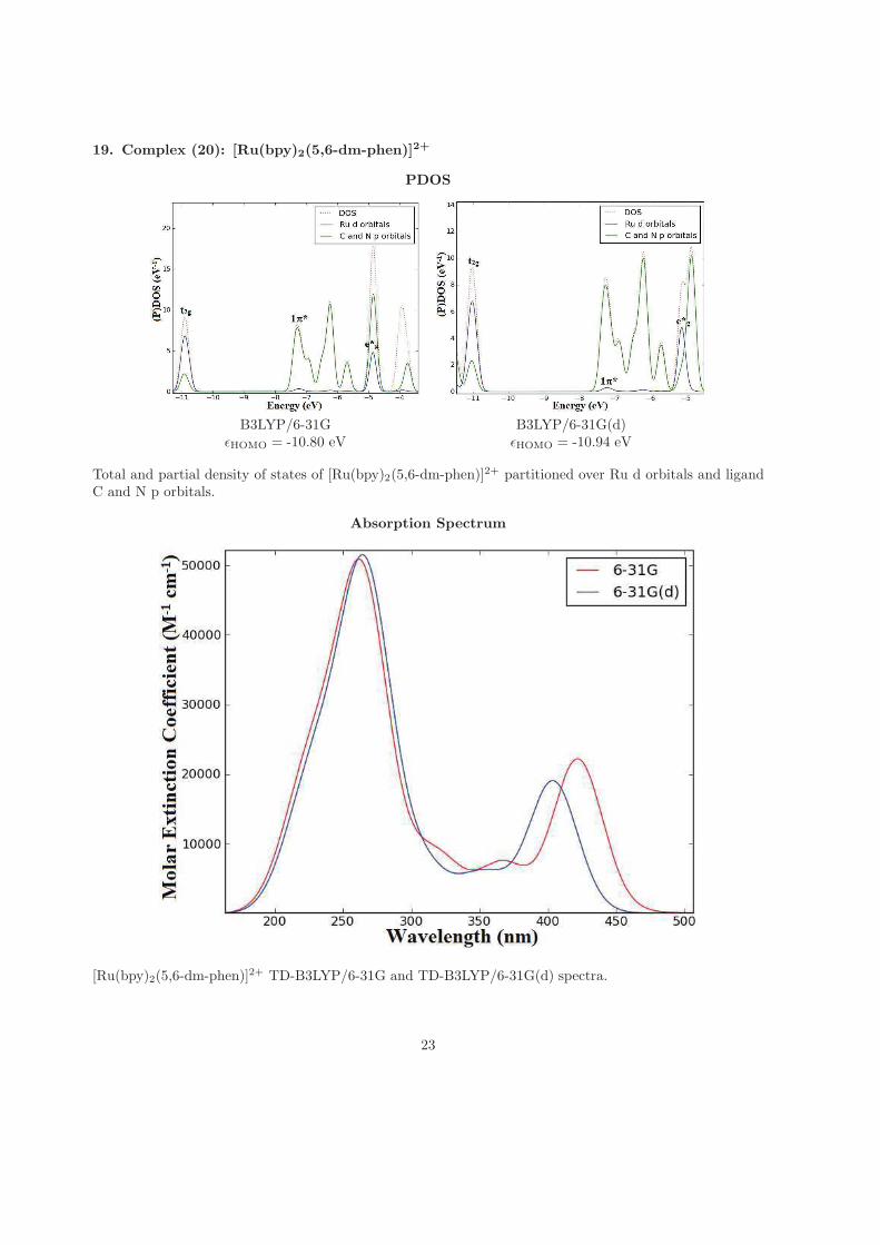
19. Complex (20): [Ru(bpy)2(5,6-dm-phen)]2+
PDOS
B3LYP/6-31G B3LYP/6-31G(d)ǫHOMO = -10.80 eV ǫHOMO = -10.94 eV
Total and partial density of states of [Ru(bpy)2(5,6-dm-phen)]2+ partitioned over Ru d orbitals and ligandC and N p orbitals.
Absorption Spectrum
[Ru(bpy)2(5,6-dm-phen)]2+ TD-B3LYP/6-31G and TD-B3LYP/6-31G(d) spectra.
23
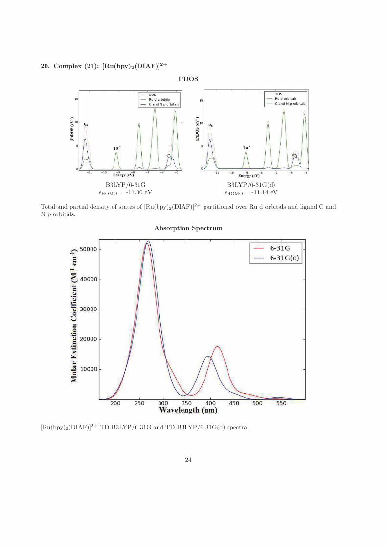
20. Complex (21): [Ru(bpy)2(DIAF)]2+
PDOS
B3LYP/6-31G B3LYP/6-31G(d)ǫHOMO = -11.00 eV ǫHOMO = -11.14 eV
Total and partial density of states of [Ru(bpy)2(DIAF)]2+ partitioned over Ru d orbitals and ligand C andN p orbitals.
Absorption Spectrum
[Ru(bpy)2(DIAF)]2+ TD-B3LYP/6-31G and TD-B3LYP/6-31G(d) spectra.
24
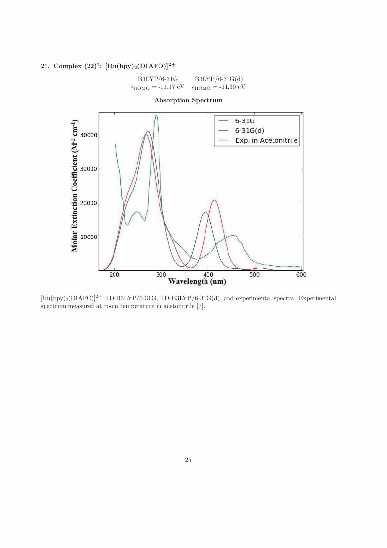
21. Complex (22)†: [Ru(bpy)2(DIAFO)]2+
B3LYP/6-31G B3LYP/6-31G(d)ǫHOMO = -11.17 eV ǫHOMO = -11.30 eV
Absorption Spectrum
[Ru(bpy)2(DIAFO)]2+ TD-B3LYP/6-31G, TD-B3LYP/6-31G(d), and experimental spectra. Experimentalspectrum measured at room temperature in acetonitrile [7].
25
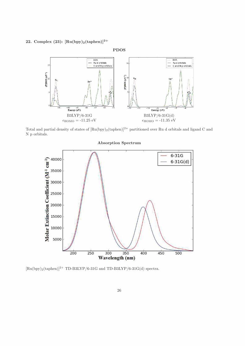
22. Complex (23): [Ru(bpy)2(taphen)]2+
PDOS
B3LYP/6-31G B3LYP/6-31G(d)ǫHOMO = -11.25 eV ǫHOMO = -11.35 eV
Total and partial density of states of [Ru(bpy)2(taphen)]2+ partitioned over Ru d orbitals and ligand C and
N p orbitals.
Absorption Spectrum
[Ru(bpy)2(taphen)]2+ TD-B3LYP/6-31G and TD-B3LYP/6-31G(d) spectra.
26
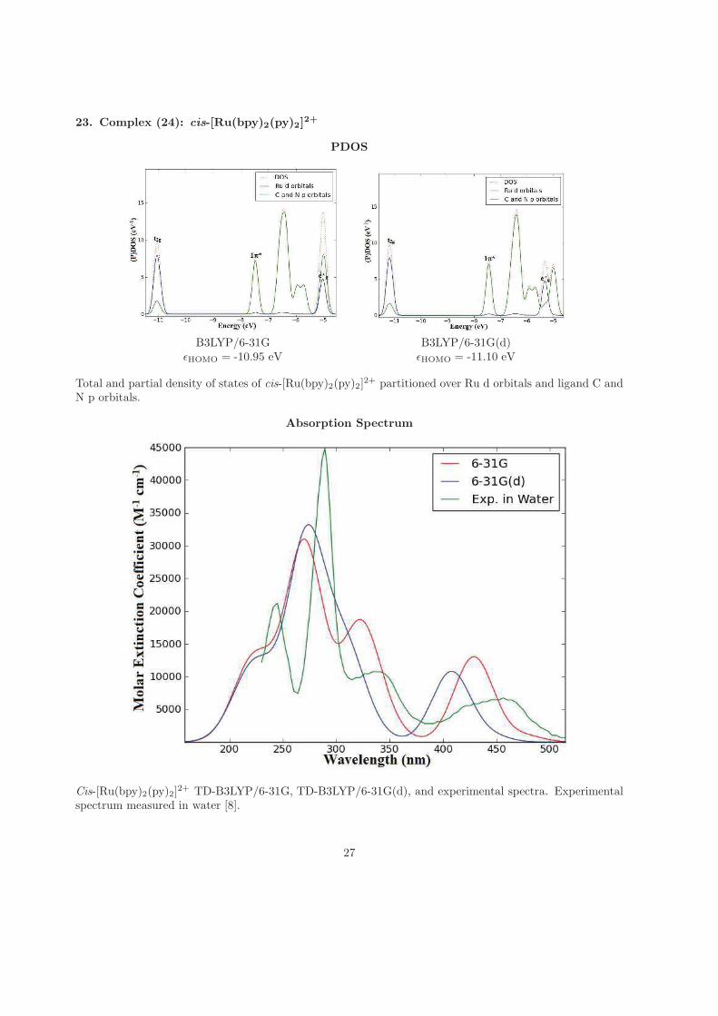
23. Complex (24): cis-[Ru(bpy)2(py)2]2+
PDOS
B3LYP/6-31G B3LYP/6-31G(d)ǫHOMO = -10.95 eV ǫHOMO = -11.10 eV
Total and partial density of states of cis-[Ru(bpy)2(py)2]2+ partitioned over Ru d orbitals and ligand C and
N p orbitals.
Absorption Spectrum
Cis-[Ru(bpy)2(py)2]2+ TD-B3LYP/6-31G, TD-B3LYP/6-31G(d), and experimental spectra. Experimental
spectrum measured in water [8].
27
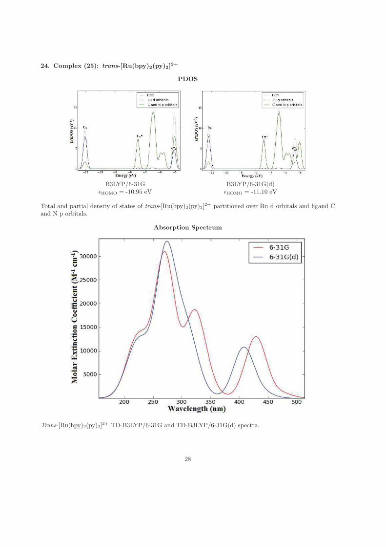
24. Complex (25): trans-[Ru(bpy)2(py)2]2+
PDOS
B3LYP/6-31G B3LYP/6-31G(d)ǫHOMO = -10.95 eV ǫHOMO = -11.10 eV
Total and partial density of states of trans-[Ru(bpy)2(py)2]2+ partitioned over Ru d orbitals and ligand C
and N p orbitals.
Absorption Spectrum
Trans-[Ru(bpy)2(py)2]2+ TD-B3LYP/6-31G and TD-B3LYP/6-31G(d) spectra.
28
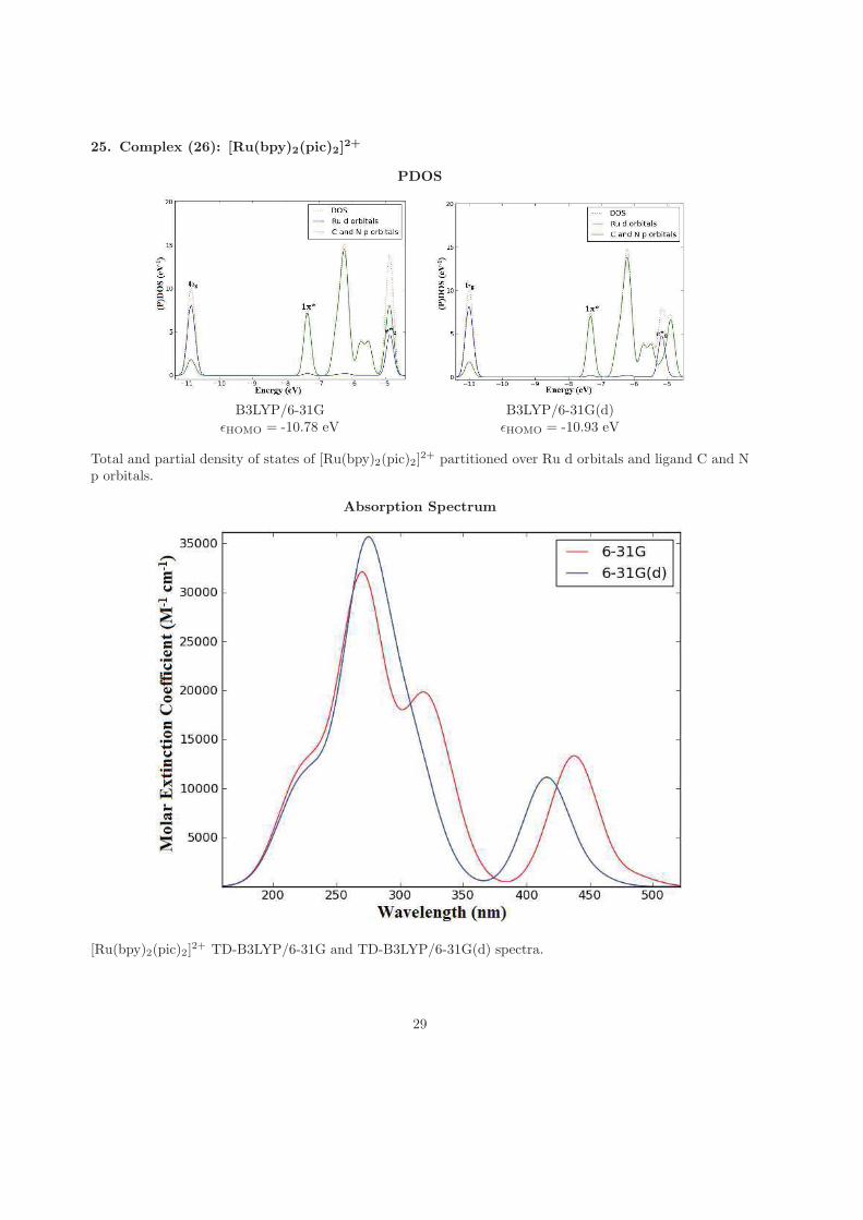
25. Complex (26): [Ru(bpy)2(pic)2]2+
PDOS
B3LYP/6-31G B3LYP/6-31G(d)ǫHOMO = -10.78 eV ǫHOMO = -10.93 eV
Total and partial density of states of [Ru(bpy)2(pic)2]2+ partitioned over Ru d orbitals and ligand C and N
p orbitals.
Absorption Spectrum
[Ru(bpy)2(pic)2]2+ TD-B3LYP/6-31G and TD-B3LYP/6-31G(d) spectra.
29
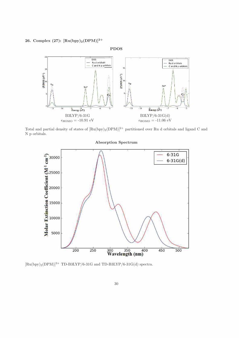
26. Complex (27): [Ru(bpy)2(DPM)]2+
PDOS
B3LYP/6-31G B3LYP/6-31G(d)ǫHOMO = -10.91 eV ǫHOMO = -11.06 eV
Total and partial density of states of [Ru(bpy)2(DPM)]2+ partitioned over Ru d orbitals and ligand C andN p orbitals.
Absorption Spectrum
[Ru(bpy)2(DPM)]2+ TD-B3LYP/6-31G and TD-B3LYP/6-31G(d) spectra.
30
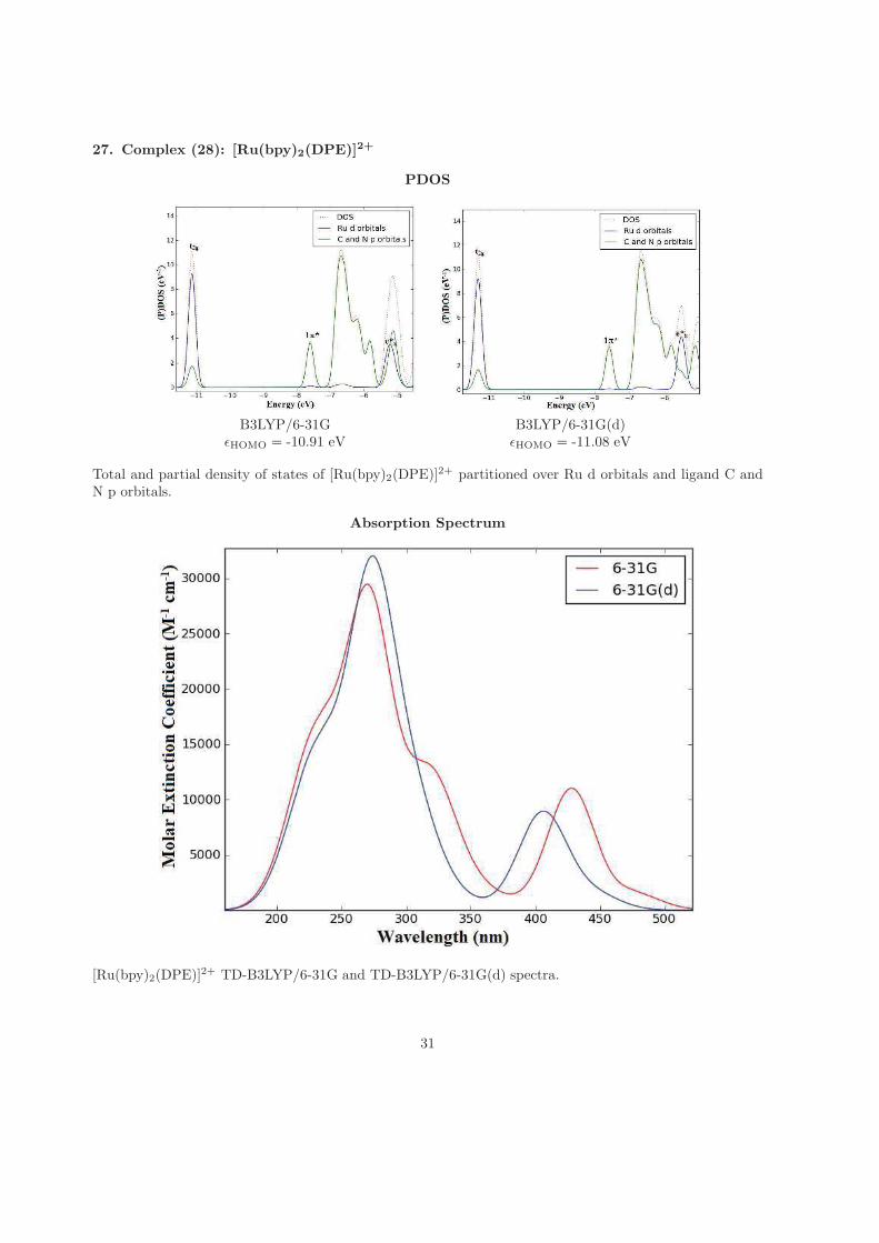
27. Complex (28): [Ru(bpy)2(DPE)]2+
PDOS
B3LYP/6-31G B3LYP/6-31G(d)ǫHOMO = -10.91 eV ǫHOMO = -11.08 eV
Total and partial density of states of [Ru(bpy)2(DPE)]2+ partitioned over Ru d orbitals and ligand C andN p orbitals.
Absorption Spectrum
[Ru(bpy)2(DPE)]2+ TD-B3LYP/6-31G and TD-B3LYP/6-31G(d) spectra.
31
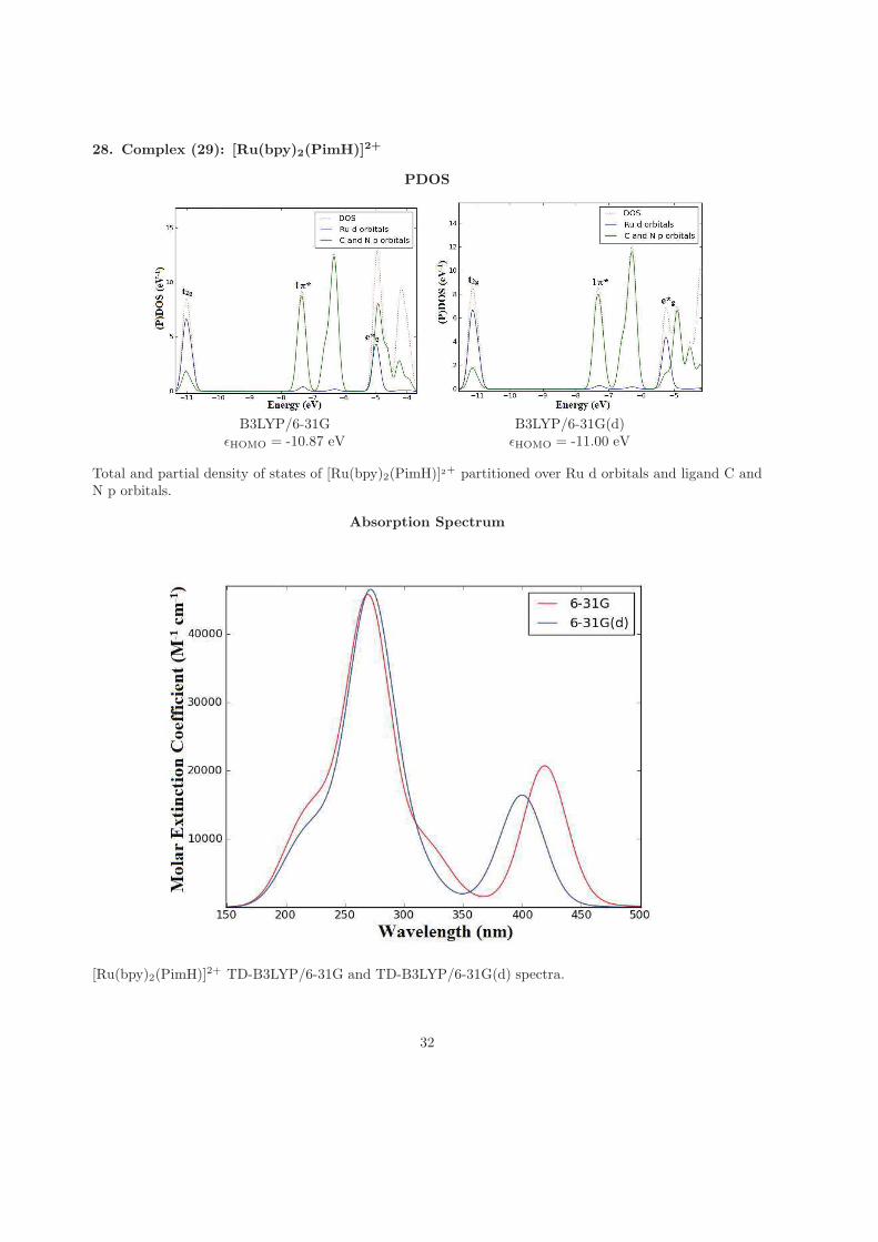
28. Complex (29): [Ru(bpy)2(PimH)]2+
PDOS
B3LYP/6-31G B3LYP/6-31G(d)ǫHOMO = -10.87 eV ǫHOMO = -11.00 eV
Total and partial density of states of [Ru(bpy)2(PimH)]2+ partitioned over Ru d orbitals and ligand C andN p orbitals.
Absorption Spectrum
[Ru(bpy)2(PimH)]2+ TD-B3LYP/6-31G and TD-B3LYP/6-31G(d) spectra.
32
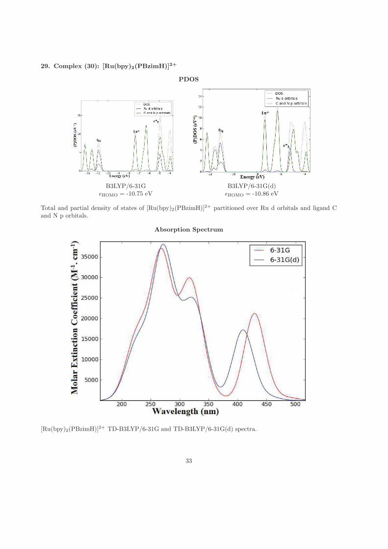
29. Complex (30): [Ru(bpy)2(PBzimH)]2+
PDOS
B3LYP/6-31G B3LYP/6-31G(d)ǫHOMO = -10.75 eV ǫHOMO = -10.86 eV
Total and partial density of states of [Ru(bpy)2(PBzimH)]2+ partitioned over Ru d orbitals and ligand Cand N p orbitals.
Absorption Spectrum
[Ru(bpy)2(PBzimH)]2+ TD-B3LYP/6-31G and TD-B3LYP/6-31G(d) spectra.
33
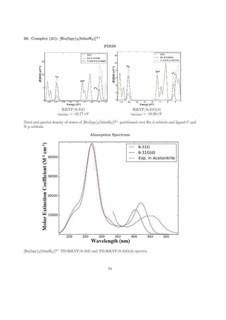
30. Complex (31): [Ru(bpy)2(biimH2)]2+
PDOS
B3LYP/6-31G B3LYP/6-31G(d)ǫHOMO = -10.77 eV ǫHOMO = -10.90 eV
Total and partial density of states of [Ru(bpy)2(biimH2)]2+ partitioned over Ru d orbitals and ligand C and
N p orbitals.
Absorption Spectrum
[Ru(bpy)2(biimH2)]2+ TD-B3LYP/6-31G and TD-B3LYP/6-31G(d) spectra.
34
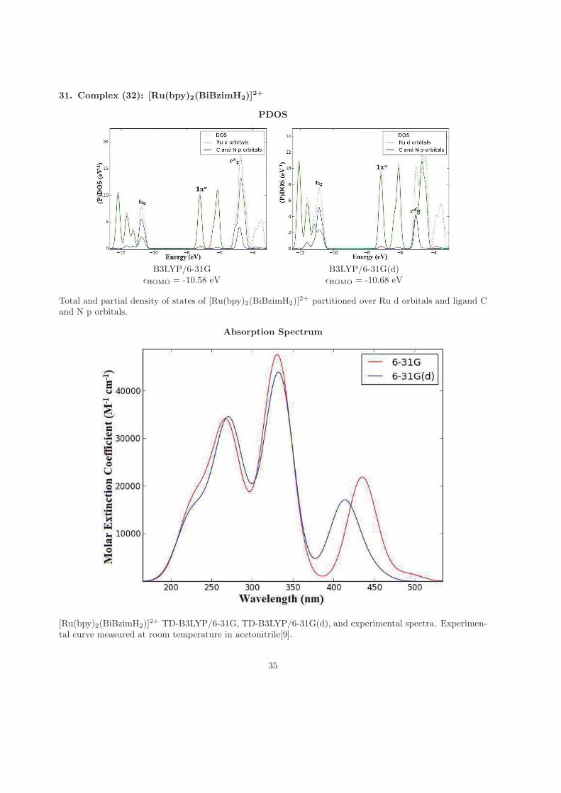
31. Complex (32): [Ru(bpy)2(BiBzimH2)]2+
PDOS
B3LYP/6-31G B3LYP/6-31G(d)ǫHOMO = -10.58 eV ǫHOMO = -10.68 eV
Total and partial density of states of [Ru(bpy)2(BiBzimH2)]2+ partitioned over Ru d orbitals and ligand C
and N p orbitals.
Absorption Spectrum
[Ru(bpy)2(BiBzimH2)]2+ TD-B3LYP/6-31G, TD-B3LYP/6-31G(d), and experimental spectra. Experimen-
tal curve measured at room temperature in acetonitrile[9].
35
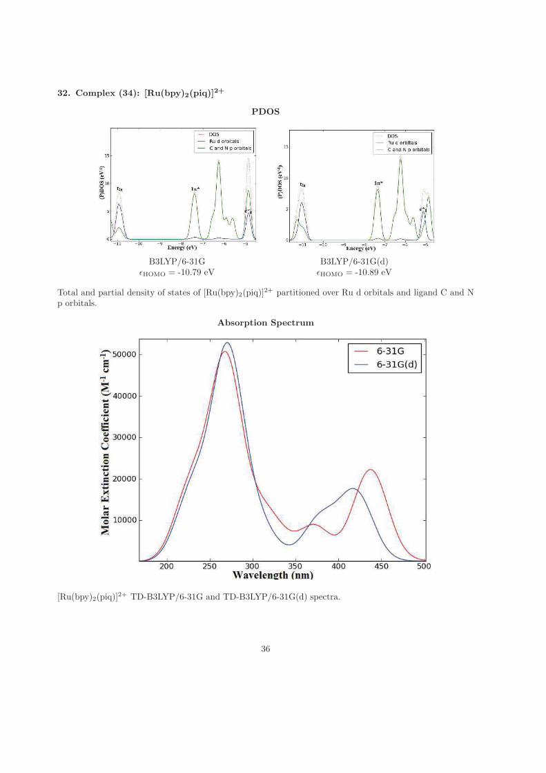
32. Complex (34): [Ru(bpy)2(piq)]2+
PDOS
B3LYP/6-31G B3LYP/6-31G(d)ǫHOMO = -10.79 eV ǫHOMO = -10.89 eV
Total and partial density of states of [Ru(bpy)2(piq)]2+ partitioned over Ru d orbitals and ligand C and N
p orbitals.
Absorption Spectrum
[Ru(bpy)2(piq)]2+ TD-B3LYP/6-31G and TD-B3LYP/6-31G(d) spectra.
36
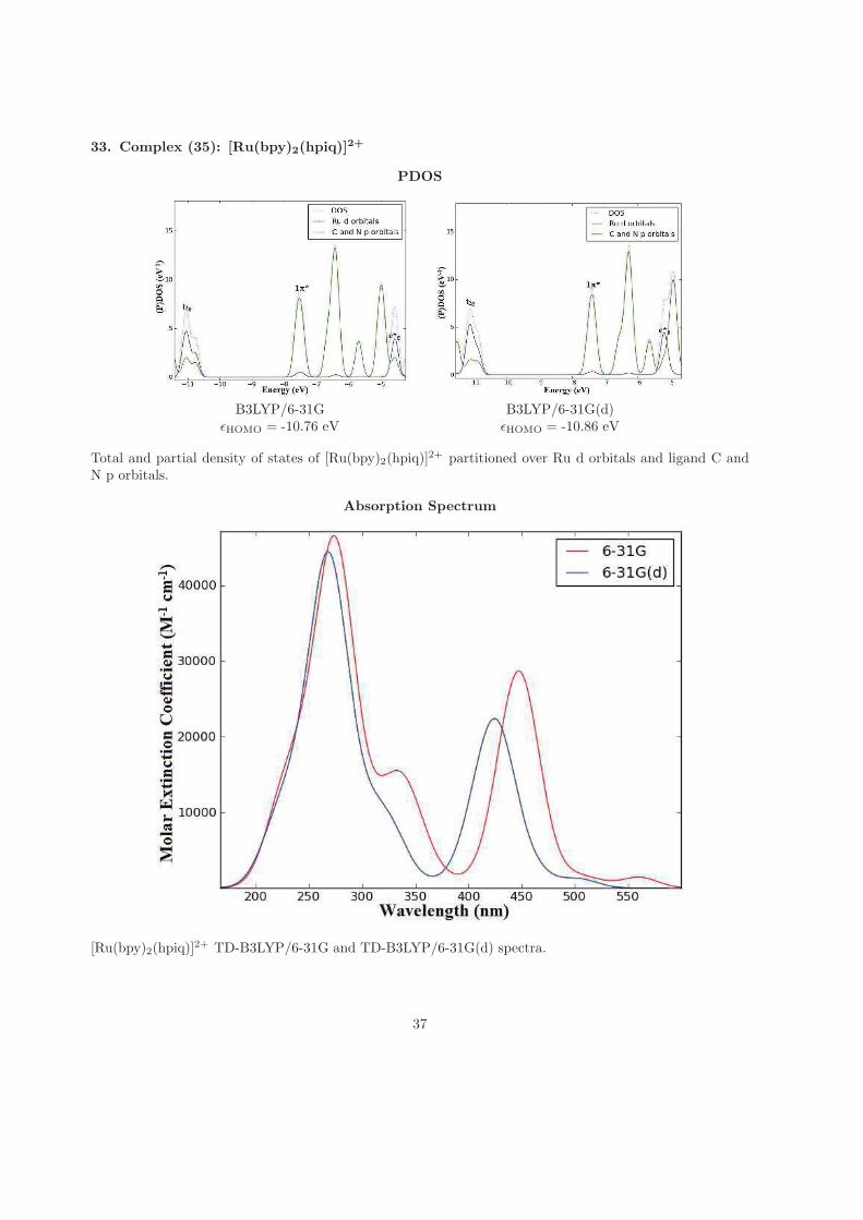
33. Complex (35): [Ru(bpy)2(hpiq)]2+
PDOS
B3LYP/6-31G B3LYP/6-31G(d)ǫHOMO = -10.76 eV ǫHOMO = -10.86 eV
Total and partial density of states of [Ru(bpy)2(hpiq)]2+ partitioned over Ru d orbitals and ligand C and
N p orbitals.
Absorption Spectrum
[Ru(bpy)2(hpiq)]2+ TD-B3LYP/6-31G and TD-B3LYP/6-31G(d) spectra.
37
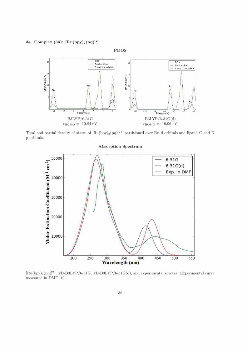
34. Complex (36): [Ru(bpy)2(pq)]2+
PDOS
B3LYP/6-31G B3LYP/6-31G(d)ǫHOMO = -10.84 eV ǫHOMO = -10.96 eV
Total and partial density of states of [Ru(bpy)2(pq)]2+ partitioned over Ru d orbitals and ligand C and N
p orbitals.
Absorption Spectrum
[Ru(bpy)2(pq)]2+ TD-B3LYP/6-31G, TD-B3LYP/6-31G(d), and experimental spectra. Experimental curve
measured in DMF [10].
38
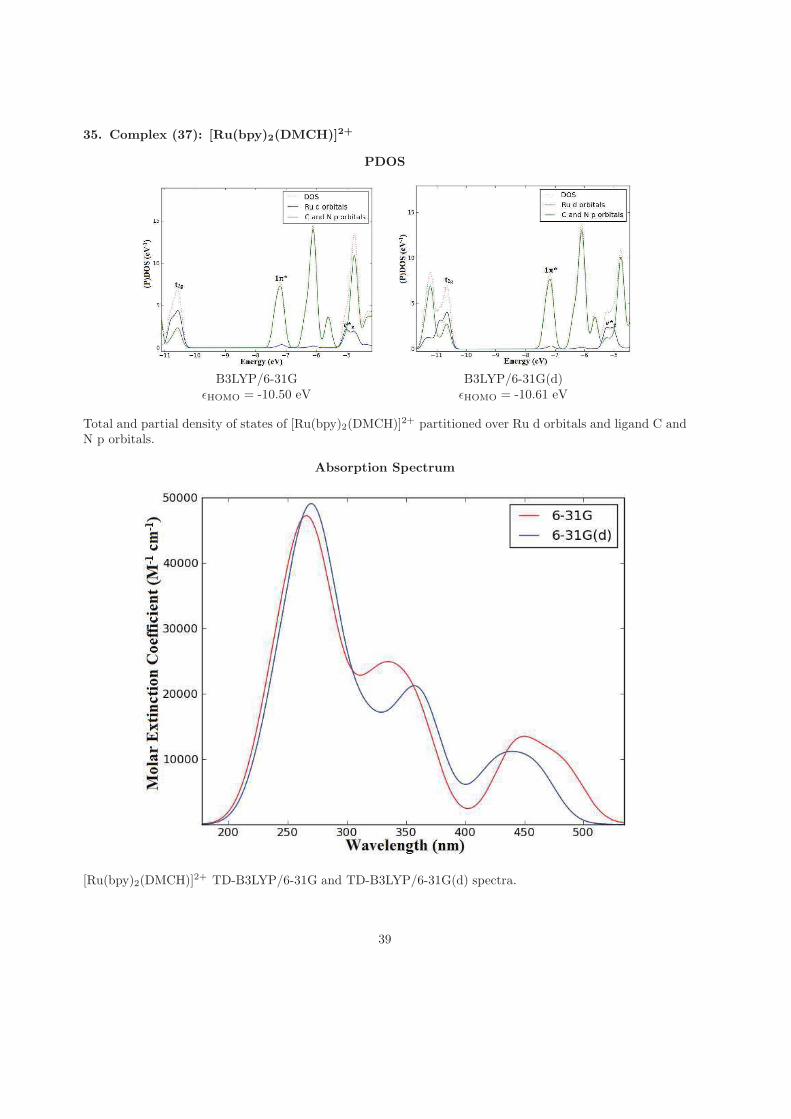
35. Complex (37): [Ru(bpy)2(DMCH)]2+
PDOS
B3LYP/6-31G B3LYP/6-31G(d)ǫHOMO = -10.50 eV ǫHOMO = -10.61 eV
Total and partial density of states of [Ru(bpy)2(DMCH)]2+ partitioned over Ru d orbitals and ligand C andN p orbitals.
Absorption Spectrum
[Ru(bpy)2(DMCH)]2+ TD-B3LYP/6-31G and TD-B3LYP/6-31G(d) spectra.
39
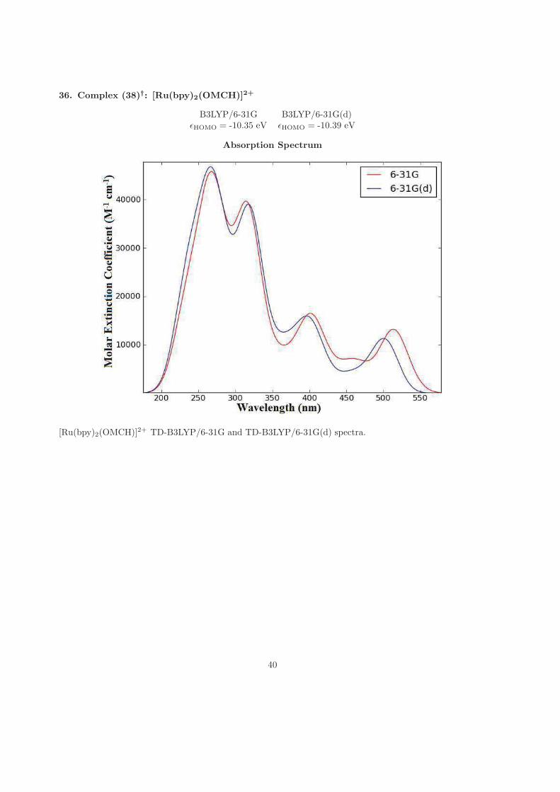
36. Complex (38)†: [Ru(bpy)2(OMCH)]2+
B3LYP/6-31G B3LYP/6-31G(d)ǫHOMO = -10.35 eV ǫHOMO = -10.39 eV
Absorption Spectrum
[Ru(bpy)2(OMCH)]2+ TD-B3LYP/6-31G and TD-B3LYP/6-31G(d) spectra.
40
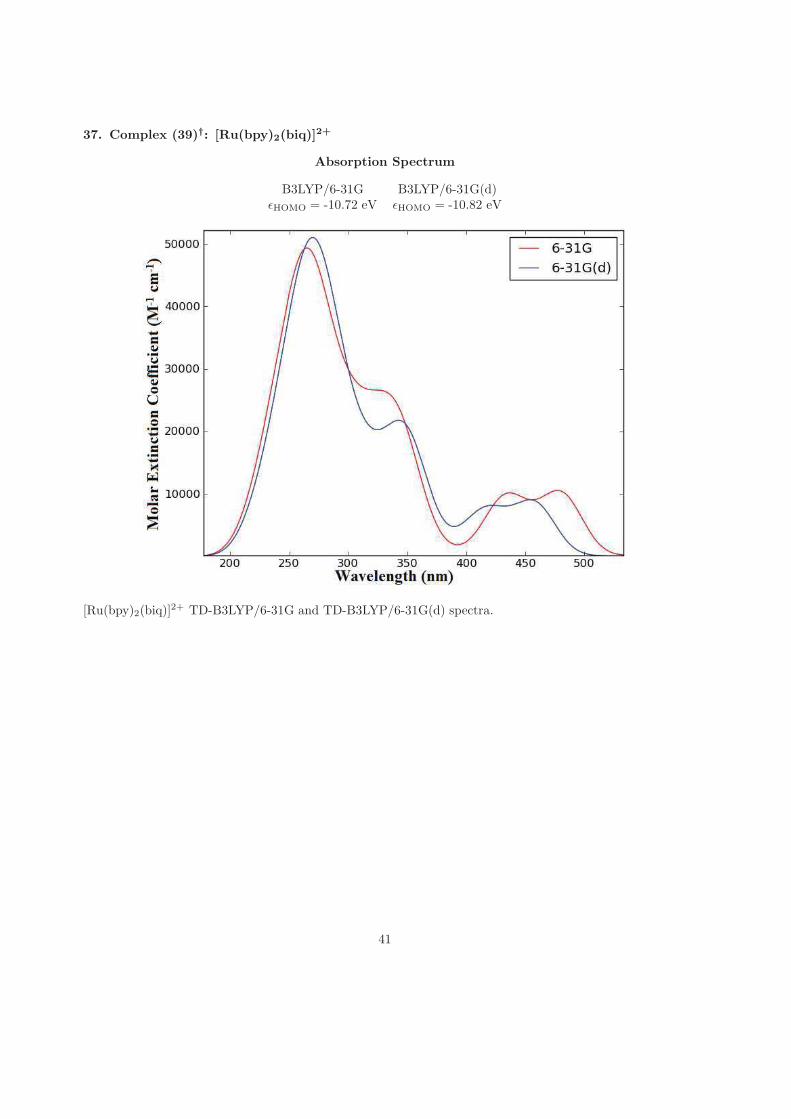
37. Complex (39)†: [Ru(bpy)2(biq)]2+
Absorption Spectrum
B3LYP/6-31G B3LYP/6-31G(d)ǫHOMO = -10.72 eV ǫHOMO = -10.82 eV
[Ru(bpy)2(biq)]2+ TD-B3LYP/6-31G and TD-B3LYP/6-31G(d) spectra.
41
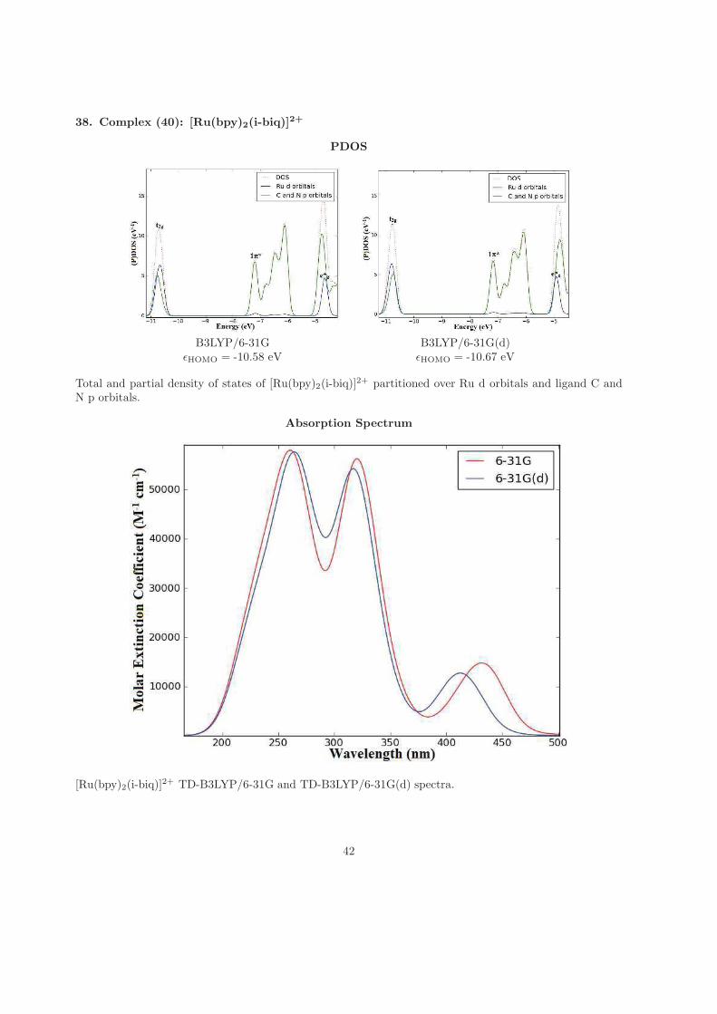
38. Complex (40): [Ru(bpy)2(i-biq)]2+
PDOS
B3LYP/6-31G B3LYP/6-31G(d)ǫHOMO = -10.58 eV ǫHOMO = -10.67 eV
Total and partial density of states of [Ru(bpy)2(i-biq)]2+ partitioned over Ru d orbitals and ligand C and
N p orbitals.
Absorption Spectrum
[Ru(bpy)2(i-biq)]2+ TD-B3LYP/6-31G and TD-B3LYP/6-31G(d) spectra.
42
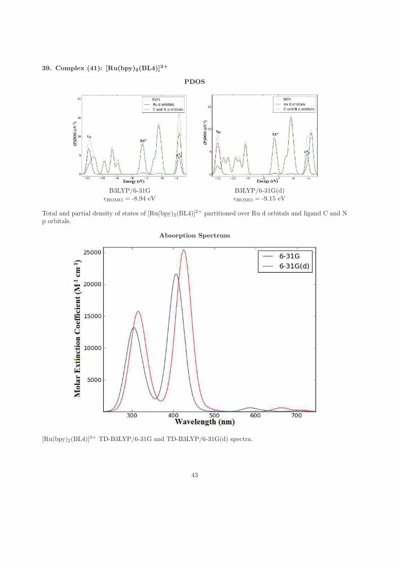
39. Complex (41): [Ru(bpy)2(BL4)]2+
PDOS
B3LYP/6-31G B3LYP/6-31G(d)ǫHOMO = -8.94 eV ǫHOMO = -9.15 eV
Total and partial density of states of [Ru(bpy)2(BL4)]2+ partitioned over Ru d orbitals and ligand C and N
p orbitals.
Absorption Spectrum
[Ru(bpy)2(BL4)]2+ TD-B3LYP/6-31G and TD-B3LYP/6-31G(d) spectra.
43
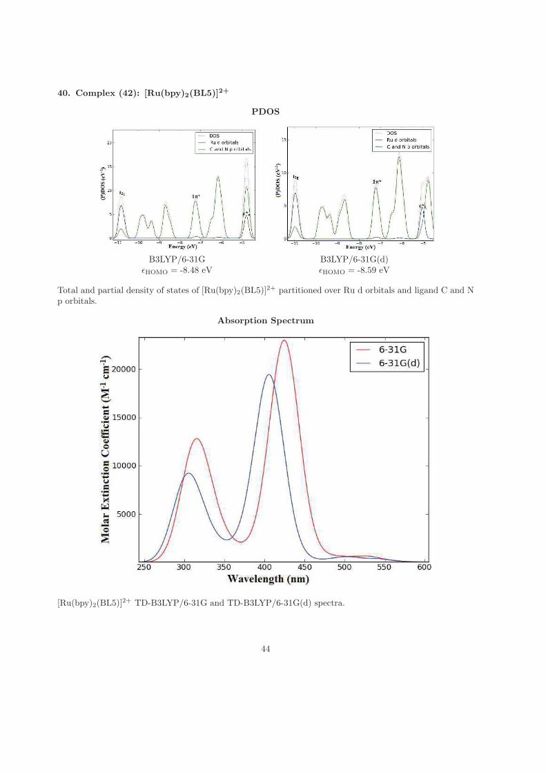
40. Complex (42): [Ru(bpy)2(BL5)]2+
PDOS
B3LYP/6-31G B3LYP/6-31G(d)ǫHOMO = -8.48 eV ǫHOMO = -8.59 eV
Total and partial density of states of [Ru(bpy)2(BL5)]2+ partitioned over Ru d orbitals and ligand C and N
p orbitals.
Absorption Spectrum
[Ru(bpy)2(BL5)]2+ TD-B3LYP/6-31G and TD-B3LYP/6-31G(d) spectra.
44
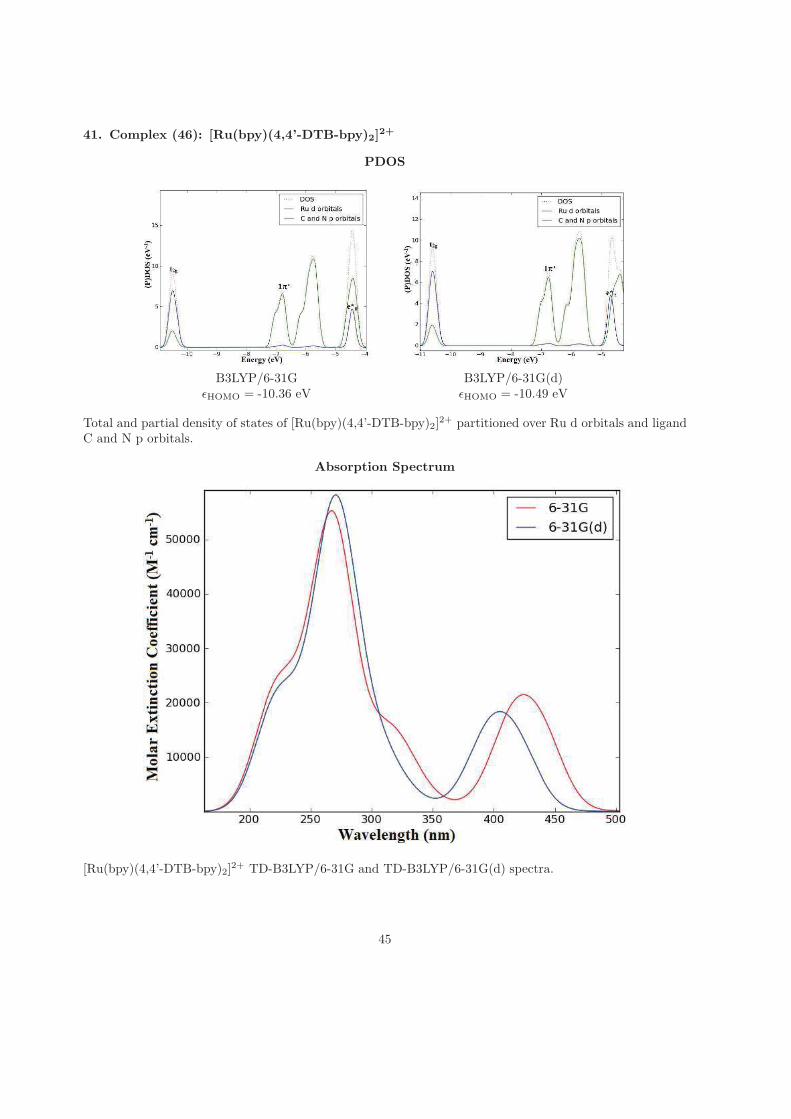
41. Complex (46): [Ru(bpy)(4,4’-DTB-bpy)2]2+
PDOS
B3LYP/6-31G B3LYP/6-31G(d)ǫHOMO = -10.36 eV ǫHOMO = -10.49 eV
Total and partial density of states of [Ru(bpy)(4,4’-DTB-bpy)2]2+ partitioned over Ru d orbitals and ligand
C and N p orbitals.
Absorption Spectrum
[Ru(bpy)(4,4’-DTB-bpy)2]2+ TD-B3LYP/6-31G and TD-B3LYP/6-31G(d) spectra.
45
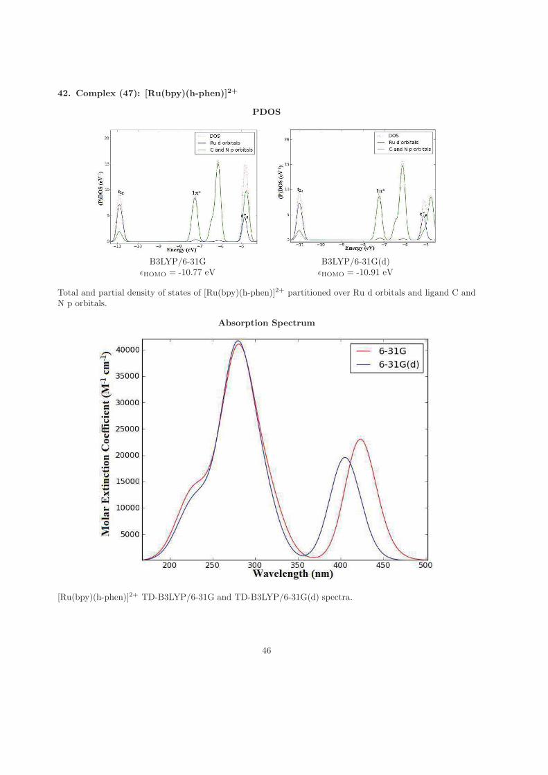
42. Complex (47): [Ru(bpy)(h-phen)]2+
PDOS
B3LYP/6-31G B3LYP/6-31G(d)ǫHOMO = -10.77 eV ǫHOMO = -10.91 eV
Total and partial density of states of [Ru(bpy)(h-phen)]2+ partitioned over Ru d orbitals and ligand C andN p orbitals.
Absorption Spectrum
[Ru(bpy)(h-phen)]2+ TD-B3LYP/6-31G and TD-B3LYP/6-31G(d) spectra.
46
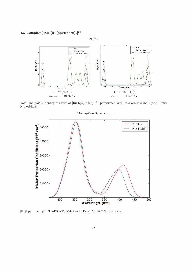
43. Complex (48): [Ru(bpy)(phen)2]2+
PDOS
B3LYP/6-31G B3LYP/6-31G(d)ǫHOMO = -10.86 eV ǫHOMO = -11.00 eV
Total and partial density of states of [Ru(bpy)(phen)2]2+ partitioned over Ru d orbitals and ligand C and
N p orbitals.
Absorption Spectrum
[Ru(bpy)(phen)2]2+ TD-B3LYP/6-31G and TD-B3LYP/6-31G(d) spectra.
47
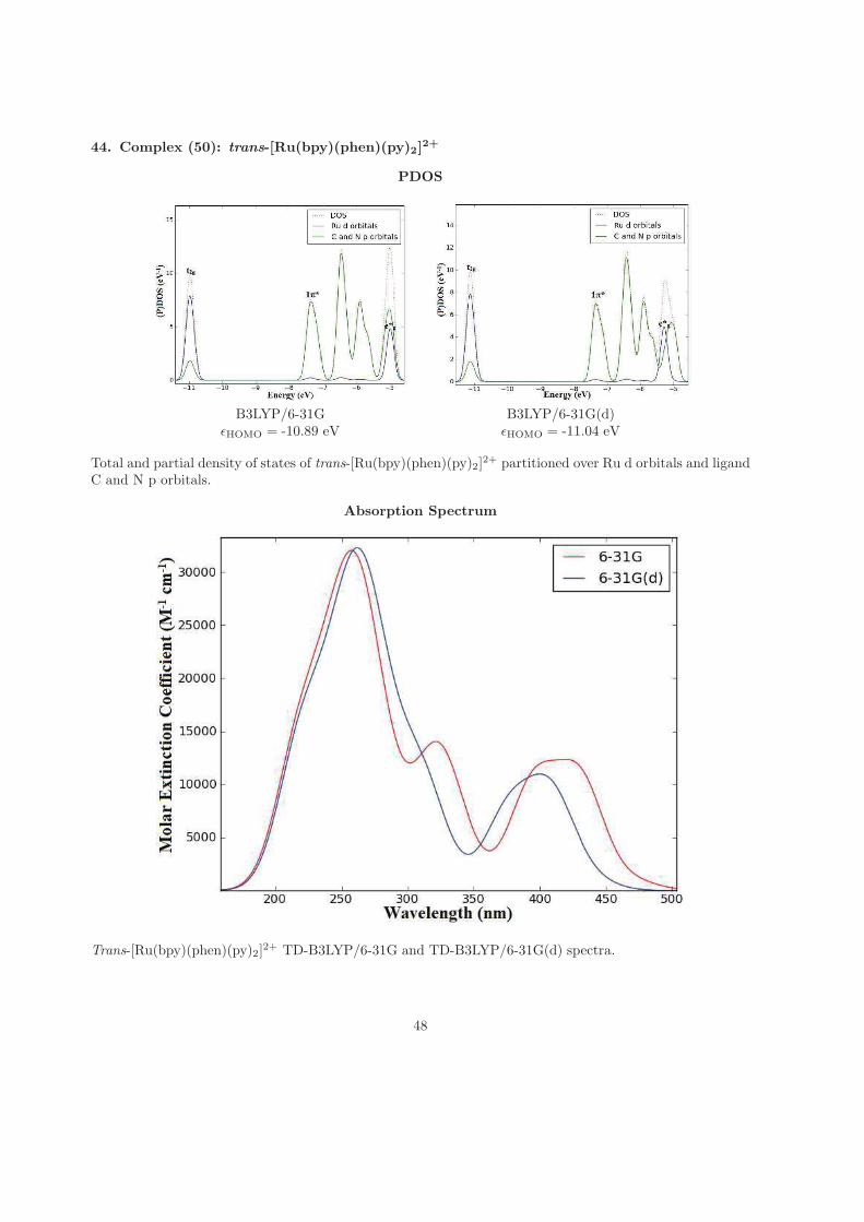
44. Complex (50): trans-[Ru(bpy)(phen)(py)2]2+
PDOS
B3LYP/6-31G B3LYP/6-31G(d)ǫHOMO = -10.89 eV ǫHOMO = -11.04 eV
Total and partial density of states of trans-[Ru(bpy)(phen)(py)2]2+ partitioned over Ru d orbitals and ligand
C and N p orbitals.
Absorption Spectrum
Trans-[Ru(bpy)(phen)(py)2]2+ TD-B3LYP/6-31G and TD-B3LYP/6-31G(d) spectra.
48
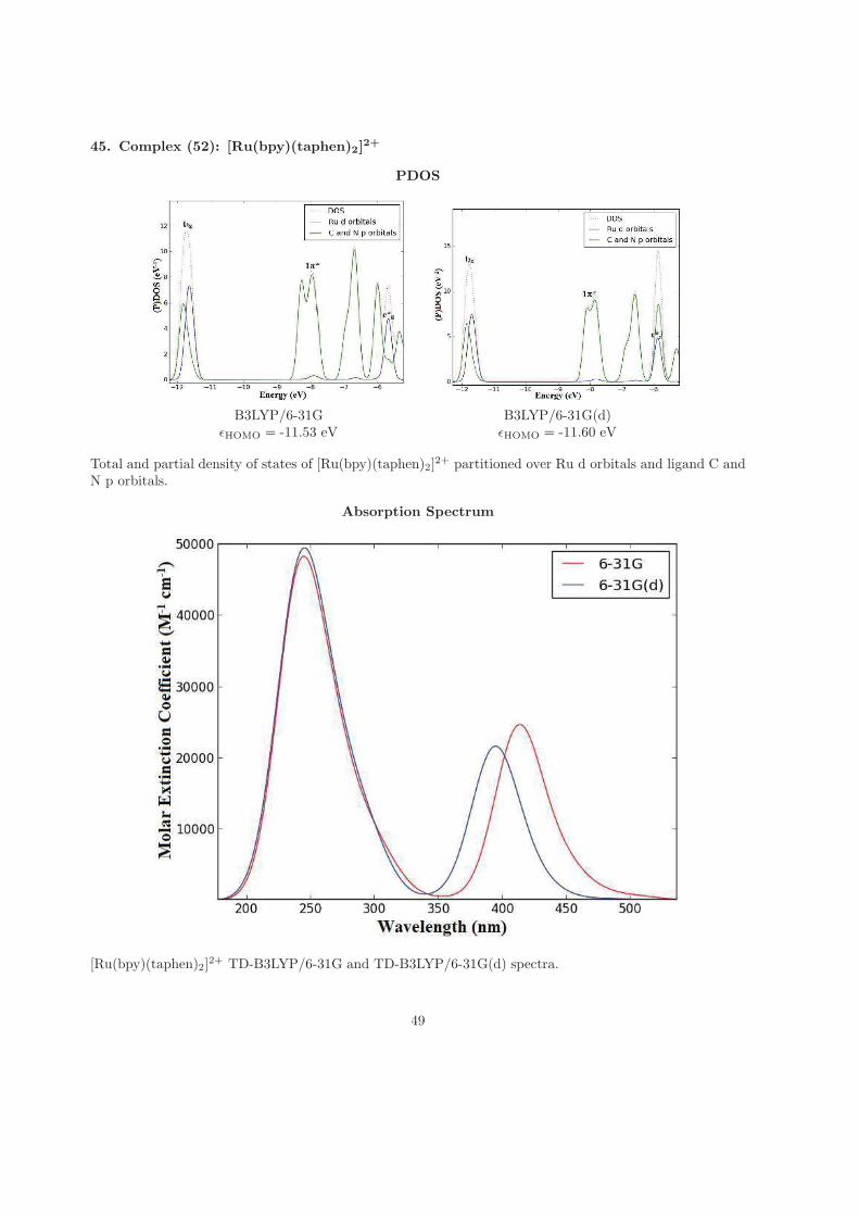
45. Complex (52): [Ru(bpy)(taphen)2]2+
PDOS
B3LYP/6-31G B3LYP/6-31G(d)ǫHOMO = -11.53 eV ǫHOMO = -11.60 eV
Total and partial density of states of [Ru(bpy)(taphen)2]2+ partitioned over Ru d orbitals and ligand C and
N p orbitals.
Absorption Spectrum
[Ru(bpy)(taphen)2]2+ TD-B3LYP/6-31G and TD-B3LYP/6-31G(d) spectra.
49
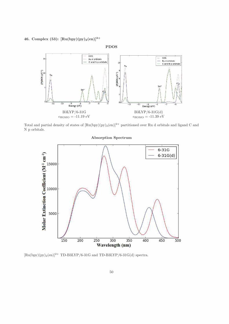
46. Complex (53): [Ru(bpy)(py)2(en)]2+
PDOS
B3LYP/6-31G B3LYP/6-31G(d)ǫHOMO = -11.19 eV ǫHOMO = -11.39 eV
Total and partial density of states of [Ru(bpy)(py)2(en)]2+ partitioned over Ru d orbitals and ligand C and
N p orbitals.
Absorption Spectrum
[Ru(bpy)(py)2(en)]2+ TD-B3LYP/6-31G and TD-B3LYP/6-31G(d) spectra.
50
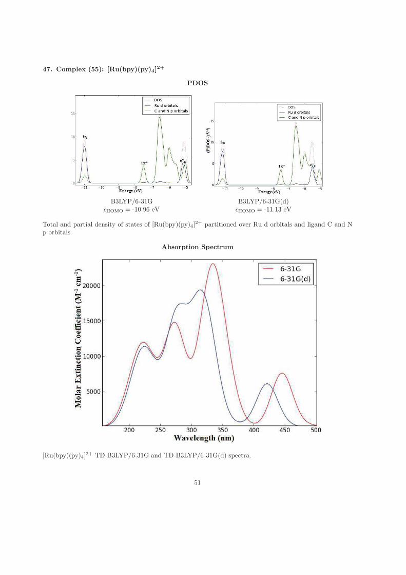
47. Complex (55): [Ru(bpy)(py)4]2+
PDOS
B3LYP/6-31G B3LYP/6-31G(d)ǫHOMO = -10.96 eV ǫHOMO = -11.13 eV
Total and partial density of states of [Ru(bpy)(py)4]2+ partitioned over Ru d orbitals and ligand C and N
p orbitals.
Absorption Spectrum
[Ru(bpy)(py)4]2+ TD-B3LYP/6-31G and TD-B3LYP/6-31G(d) spectra.
51
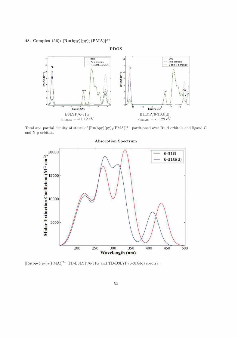
48. Complex (56): [Ru(bpy)(py)2(PMA)]2+
PDOS
B3LYP/6-31G B3LYP/6-31G(d)ǫHOMO = -11.12 eV ǫHOMO = -11.29 eV
Total and partial density of states of [Ru(bpy)(py)2(PMA)]2+ partitioned over Ru d orbitals and ligand Cand N p orbitals.
Absorption Spectrum
[Ru(bpy)(py)2(PMA)]2+ TD-B3LYP/6-31G and TD-B3LYP/6-31G(d) spectra.
52
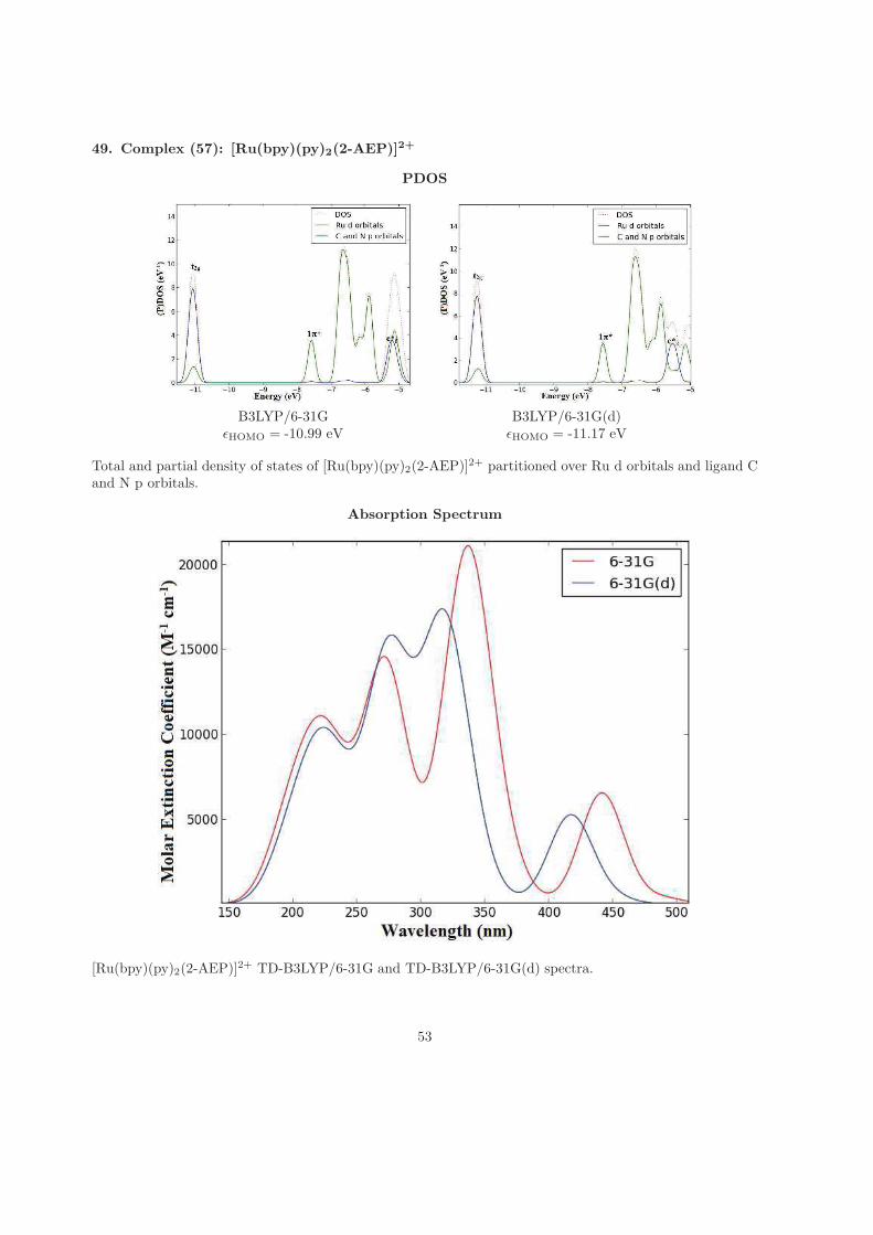
49. Complex (57): [Ru(bpy)(py)2(2-AEP)]2+
PDOS
B3LYP/6-31G B3LYP/6-31G(d)ǫHOMO = -10.99 eV ǫHOMO = -11.17 eV
Total and partial density of states of [Ru(bpy)(py)2(2-AEP)]2+ partitioned over Ru d orbitals and ligand C
and N p orbitals.
Absorption Spectrum
[Ru(bpy)(py)2(2-AEP)]2+ TD-B3LYP/6-31G and TD-B3LYP/6-31G(d) spectra.
53
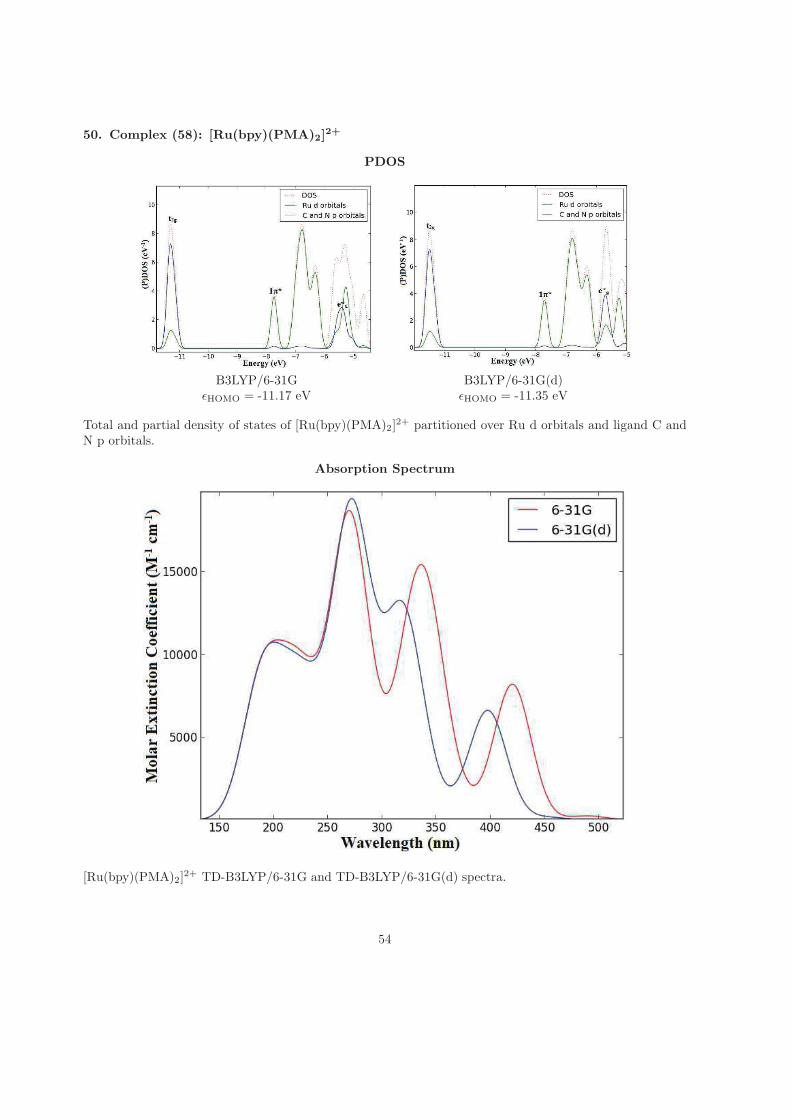
50. Complex (58): [Ru(bpy)(PMA)2]2+
PDOS
B3LYP/6-31G B3LYP/6-31G(d)ǫHOMO = -11.17 eV ǫHOMO = -11.35 eV
Total and partial density of states of [Ru(bpy)(PMA)2]2+ partitioned over Ru d orbitals and ligand C and
N p orbitals.
Absorption Spectrum
[Ru(bpy)(PMA)2]2+ TD-B3LYP/6-31G and TD-B3LYP/6-31G(d) spectra.
54
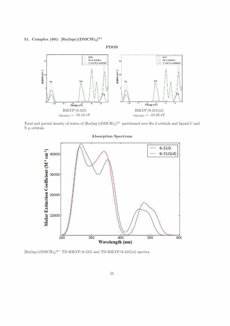
51. Complex (60): [Ru(bpy)(DMCH)2]2+
PDOS
B3LYP/6-31G B3LYP/6-31G(d)ǫHOMO = -10.13 eV ǫHOMO = -10.23 eV
Total and partial density of states of [Ru(bpy)(DMCH)2]2+ partitioned over Ru d orbitals and ligand C and
N p orbitals.
Absorption Spectrum
[Ru(bpy)(DMCH)2]2+ TD-B3LYP/6-31G and TD-B3LYP/6-31G(d) spectra.
55
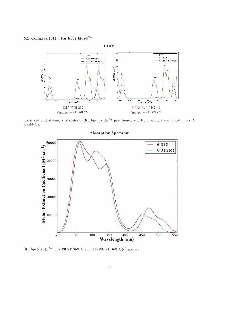
52. Complex (61): [Ru(bpy)(biq)2]2+
PDOS
B3LYP/6-31G B3LYP/6-31G(d)ǫHOMO = -10.50 eV ǫHOMO = -10.59 eV
Total and partial density of states of [Ru(bpy)(biq)2]2+ partitioned over Ru d orbitals and ligand C and N
p orbitals.
Absorption Spectrum
[Ru(bpy)(biq)2]2+ TD-B3LYP/6-31G and TD-B3LYP/6-31G(d) spectra.
56
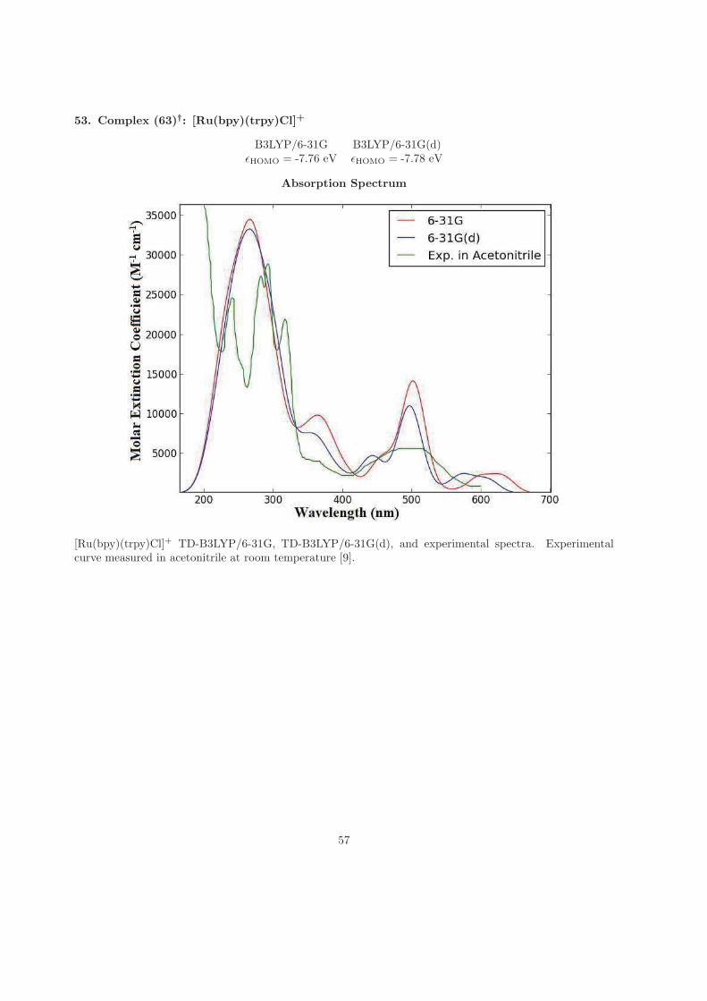
53. Complex (63)†: [Ru(bpy)(trpy)Cl]+
B3LYP/6-31G B3LYP/6-31G(d)ǫHOMO = -7.76 eV ǫHOMO = -7.78 eV
Absorption Spectrum
[Ru(bpy)(trpy)Cl]+ TD-B3LYP/6-31G, TD-B3LYP/6-31G(d), and experimental spectra. Experimentalcurve measured in acetonitrile at room temperature [9].
57
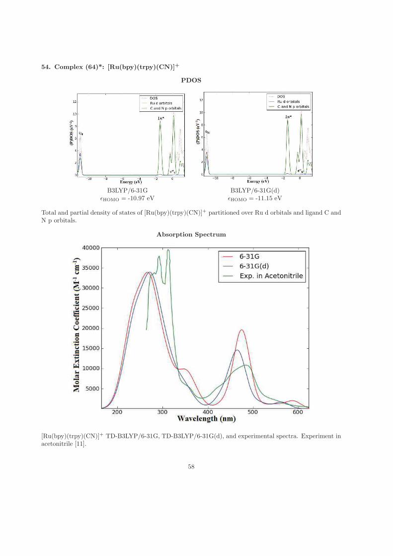
54. Complex (64)*: [Ru(bpy)(trpy)(CN)]+
PDOS
B3LYP/6-31G B3LYP/6-31G(d)ǫHOMO = -10.97 eV ǫHOMO = -11.15 eV
Total and partial density of states of [Ru(bpy)(trpy)(CN)]+ partitioned over Ru d orbitals and ligand C andN p orbitals.
Absorption Spectrum
[Ru(bpy)(trpy)(CN)]+ TD-B3LYP/6-31G, TD-B3LYP/6-31G(d), and experimental spectra. Experiment inacetonitrile [11].
58
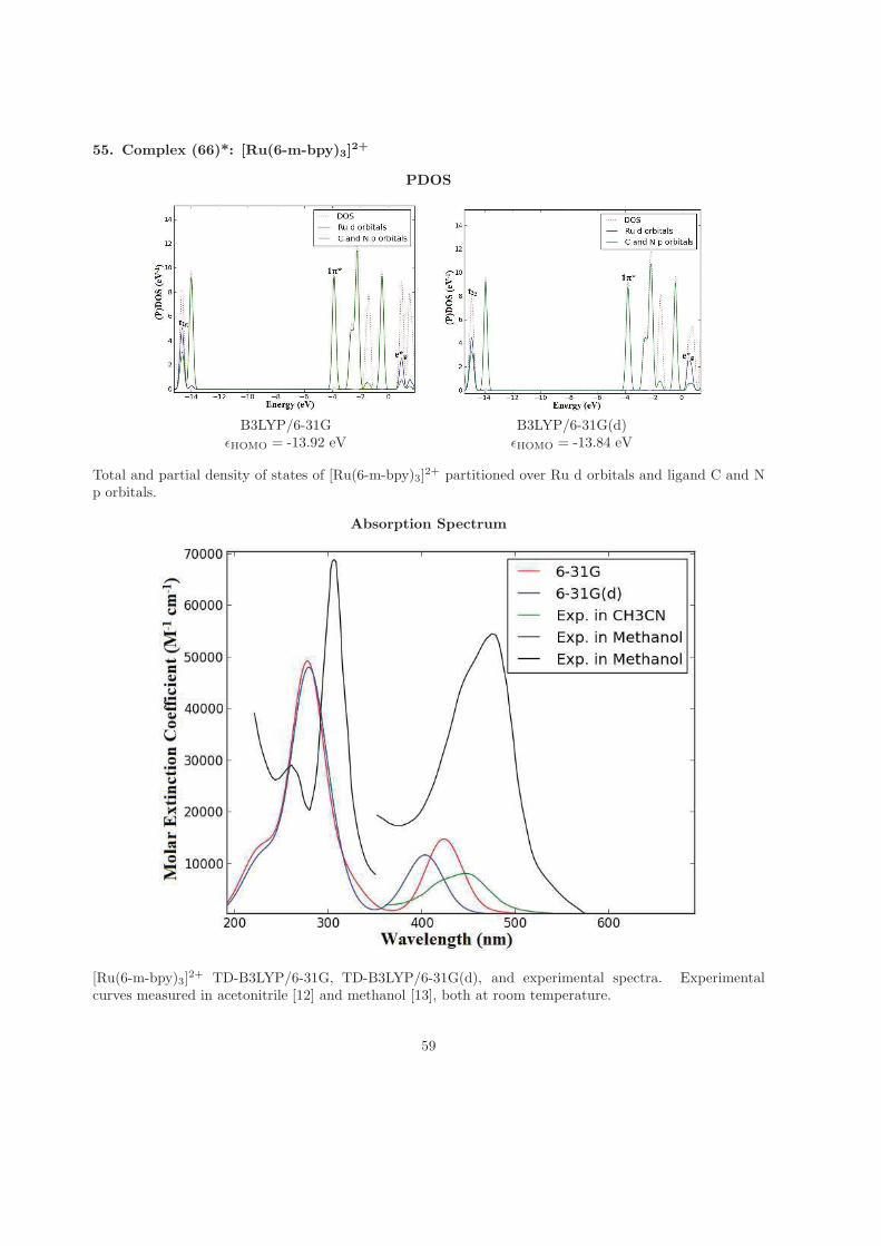
55. Complex (66)*: [Ru(6-m-bpy)3]2+
PDOS
B3LYP/6-31G B3LYP/6-31G(d)ǫHOMO = -13.92 eV ǫHOMO = -13.84 eV
Total and partial density of states of [Ru(6-m-bpy)3]2+ partitioned over Ru d orbitals and ligand C and N
p orbitals.
Absorption Spectrum
[Ru(6-m-bpy)3]2+ TD-B3LYP/6-31G, TD-B3LYP/6-31G(d), and experimental spectra. Experimental
curves measured in acetonitrile [12] and methanol [13], both at room temperature.
59
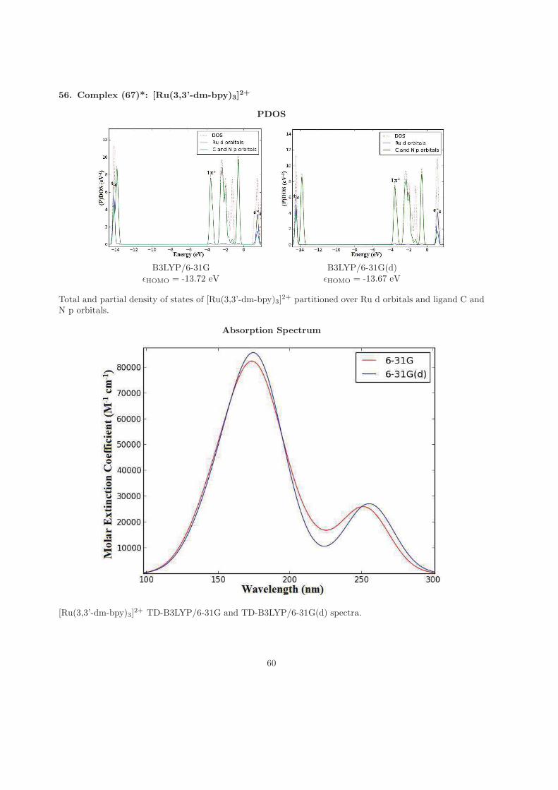
56. Complex (67)*: [Ru(3,3’-dm-bpy)3]2+
PDOS
B3LYP/6-31G B3LYP/6-31G(d)ǫHOMO = -13.72 eV ǫHOMO = -13.67 eV
Total and partial density of states of [Ru(3,3’-dm-bpy)3]2+ partitioned over Ru d orbitals and ligand C and
N p orbitals.
Absorption Spectrum
[Ru(3,3’-dm-bpy)3]2+ TD-B3LYP/6-31G and TD-B3LYP/6-31G(d) spectra.
60
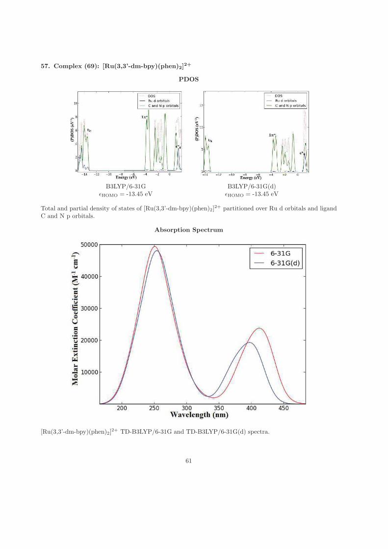
57. Complex (69): [Ru(3,3’-dm-bpy)(phen)2]2+
PDOS
B3LYP/6-31G B3LYP/6-31G(d)ǫHOMO = -13.45 eV ǫHOMO = -13.45 eV
Total and partial density of states of [Ru(3,3’-dm-bpy)(phen)2]2+ partitioned over Ru d orbitals and ligand
C and N p orbitals.
Absorption Spectrum
[Ru(3,3’-dm-bpy)(phen)2]2+ TD-B3LYP/6-31G and TD-B3LYP/6-31G(d) spectra.
61
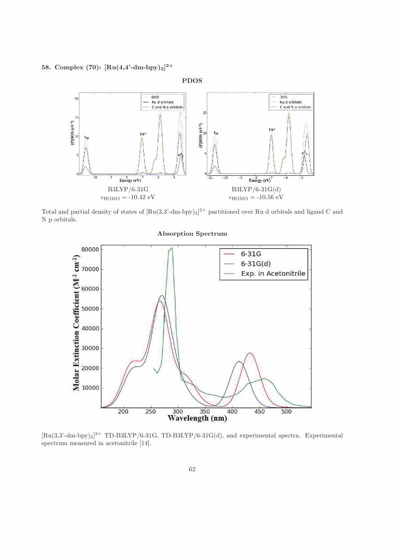
58. Complex (70): [Ru(4,4’-dm-bpy)3]2+
PDOS
B3LYP/6-31G B3LYP/6-31G(d)ǫHOMO = -10.42 eV ǫHOMO = -10.56 eV
Total and partial density of states of [Ru(3,3’-dm-bpy)3]2+ partitioned over Ru d orbitals and ligand C and
N p orbitals.
Absorption Spectrum
[Ru(3,3’-dm-bpy)3]2+ TD-B3LYP/6-31G, TD-B3LYP/6-31G(d), and experimental spectra. Experimental
spectrum measured in acetonitrile [14].
62
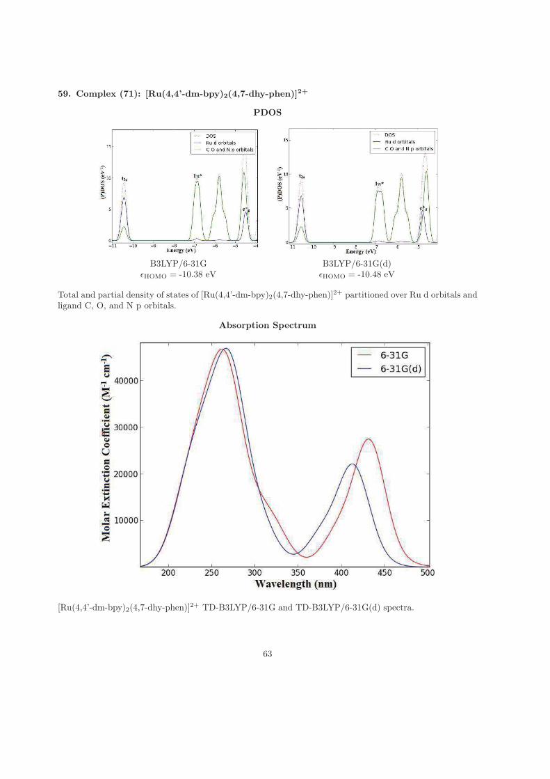
59. Complex (71): [Ru(4,4’-dm-bpy)2(4,7-dhy-phen)]2+
PDOS
B3LYP/6-31G B3LYP/6-31G(d)ǫHOMO = -10.38 eV ǫHOMO = -10.48 eV
Total and partial density of states of [Ru(4,4’-dm-bpy)2(4,7-dhy-phen)]2+ partitioned over Ru d orbitals and
ligand C, O, and N p orbitals.
Absorption Spectrum
[Ru(4,4’-dm-bpy)2(4,7-dhy-phen)]2+ TD-B3LYP/6-31G and TD-B3LYP/6-31G(d) spectra.
63
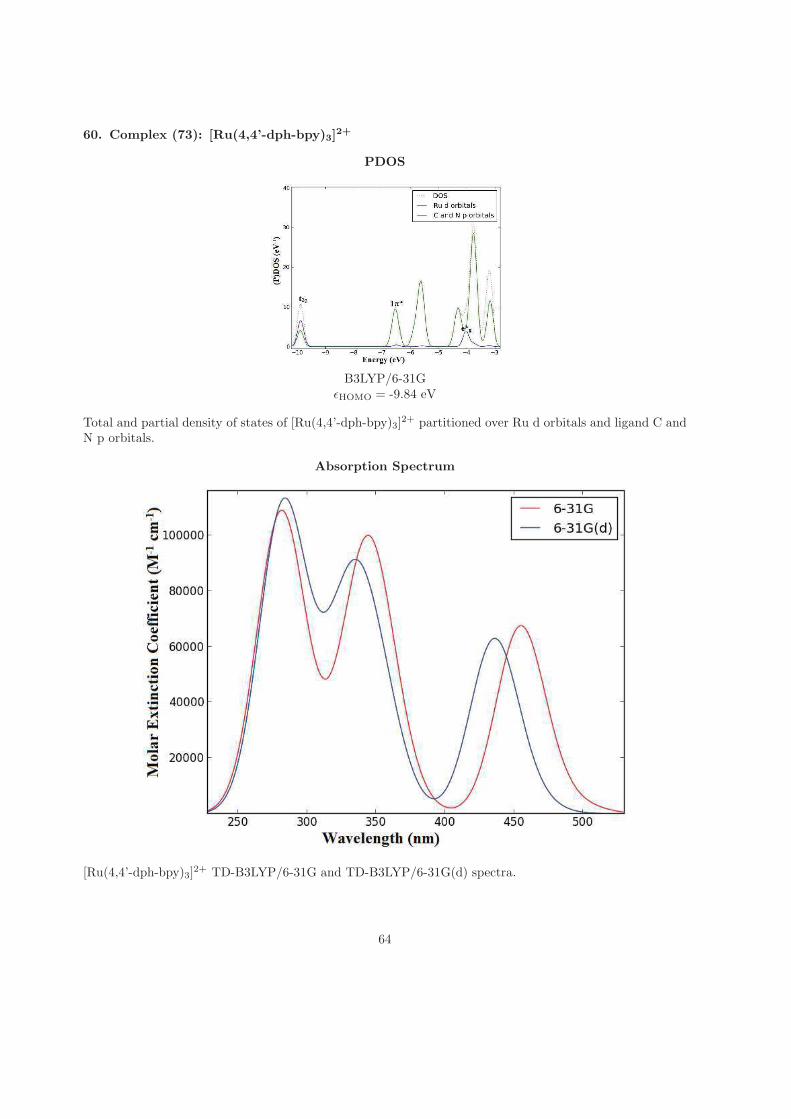
60. Complex (73): [Ru(4,4’-dph-bpy)3]2+
PDOS
B3LYP/6-31GǫHOMO = -9.84 eV
Total and partial density of states of [Ru(4,4’-dph-bpy)3]2+ partitioned over Ru d orbitals and ligand C and
N p orbitals.
Absorption Spectrum
[Ru(4,4’-dph-bpy)3]2+ TD-B3LYP/6-31G and TD-B3LYP/6-31G(d) spectra.
64
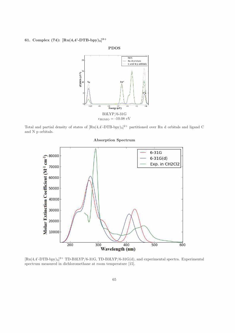
61. Complex (74): [Ru(4,4’-DTB-bpy)3]2+
PDOS
B3LYP/6-31GǫHOMO = -10.08 eV
Total and partial density of states of [Ru(4,4’-DTB-bpy)3]2+ partitioned over Ru d orbitals and ligand C
and N p orbitals.
Absorption Spectrum
[Ru(4,4’-DTB-bpy)3]2+ TD-B3LYP/6-31G, TD-B3LYP/6-31G(d), and experimental spectra. Experimental
spectrum measured in dichloromethane at room temperature [15].
65
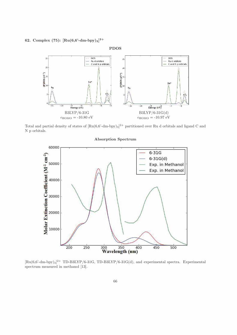
62. Complex (75): [Ru(6,6’-dm-bpy)3]2+
PDOS
B3LYP/6-31G B3LYP/6-31G(d)ǫHOMO = -10.80 eV ǫHOMO = -10.97 eV
Total and partial density of states of [Ru(6,6’-dm-bpy)3]2+ partitioned over Ru d orbitals and ligand C and
N p orbitals.
Absorption Spectrum
[Ru(6,6’-dm-bpy)3]2+ TD-B3LYP/6-31G, TD-B3LYP/6-31G(d), and experimental spectra. Experimental
spectrum measured in methanol [13].
66
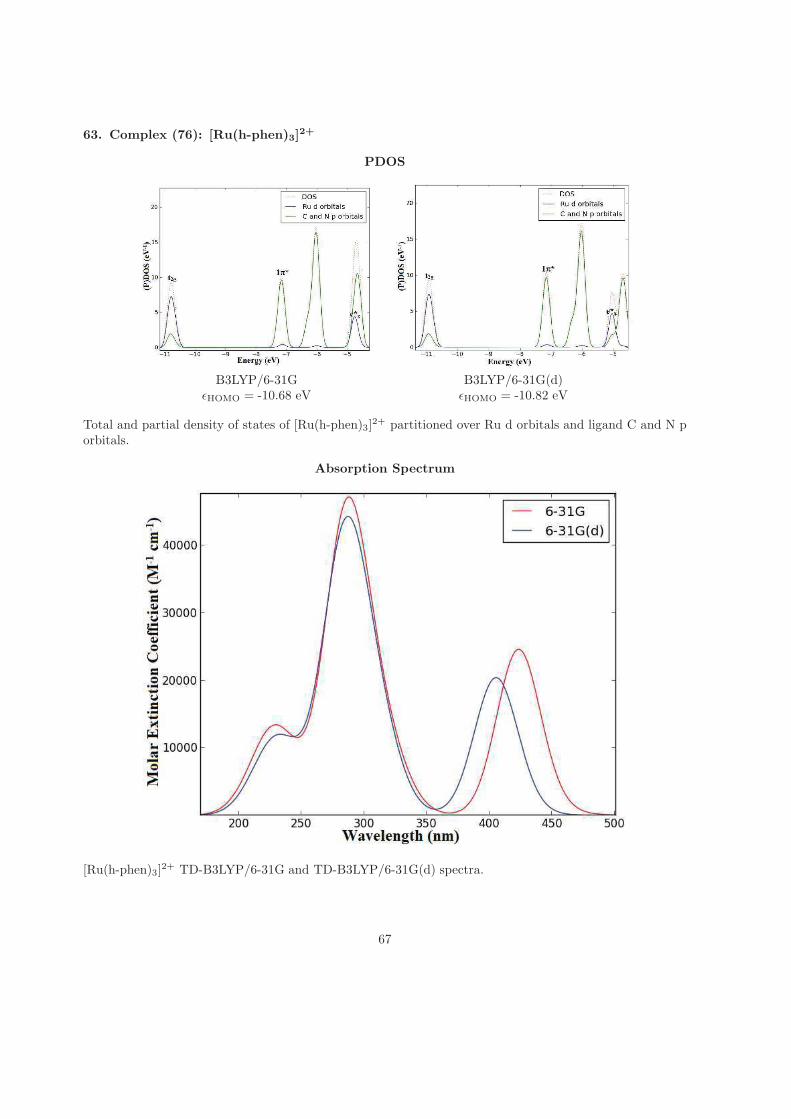
63. Complex (76): [Ru(h-phen)3]2+
PDOS
B3LYP/6-31G B3LYP/6-31G(d)ǫHOMO = -10.68 eV ǫHOMO = -10.82 eV
Total and partial density of states of [Ru(h-phen)3]2+ partitioned over Ru d orbitals and ligand C and N p
orbitals.
Absorption Spectrum
[Ru(h-phen)3]2+ TD-B3LYP/6-31G and TD-B3LYP/6-31G(d) spectra.
67
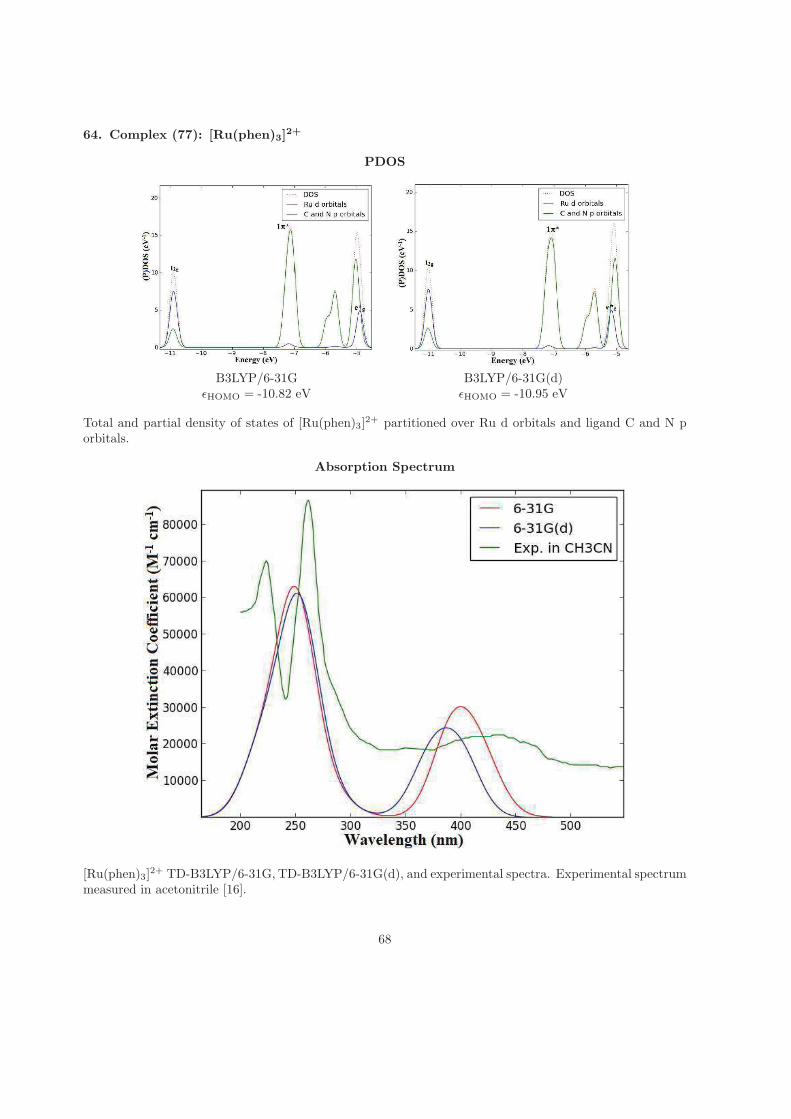
64. Complex (77): [Ru(phen)3]2+
PDOS
B3LYP/6-31G B3LYP/6-31G(d)ǫHOMO = -10.82 eV ǫHOMO = -10.95 eV
Total and partial density of states of [Ru(phen)3]2+ partitioned over Ru d orbitals and ligand C and N p
orbitals.
Absorption Spectrum
[Ru(phen)3]2+ TD-B3LYP/6-31G, TD-B3LYP/6-31G(d), and experimental spectra. Experimental spectrum
measured in acetonitrile [16].
68
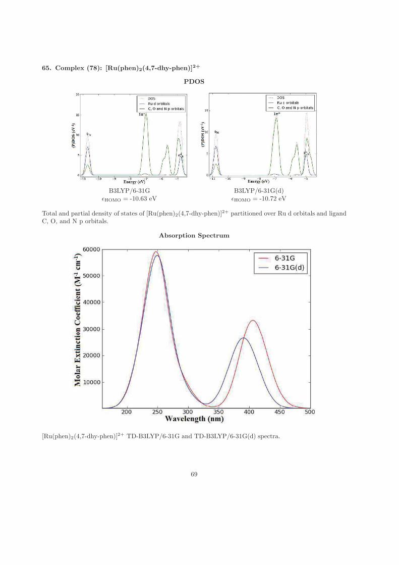
65. Complex (78): [Ru(phen)2(4,7-dhy-phen)]2+
PDOS
B3LYP/6-31G B3LYP/6-31G(d)ǫHOMO = -10.63 eV ǫHOMO = -10.72 eV
Total and partial density of states of [Ru(phen)2(4,7-dhy-phen)]2+ partitioned over Ru d orbitals and ligand
C, O, and N p orbitals.
Absorption Spectrum
[Ru(phen)2(4,7-dhy-phen)]2+ TD-B3LYP/6-31G and TD-B3LYP/6-31G(d) spectra.
69
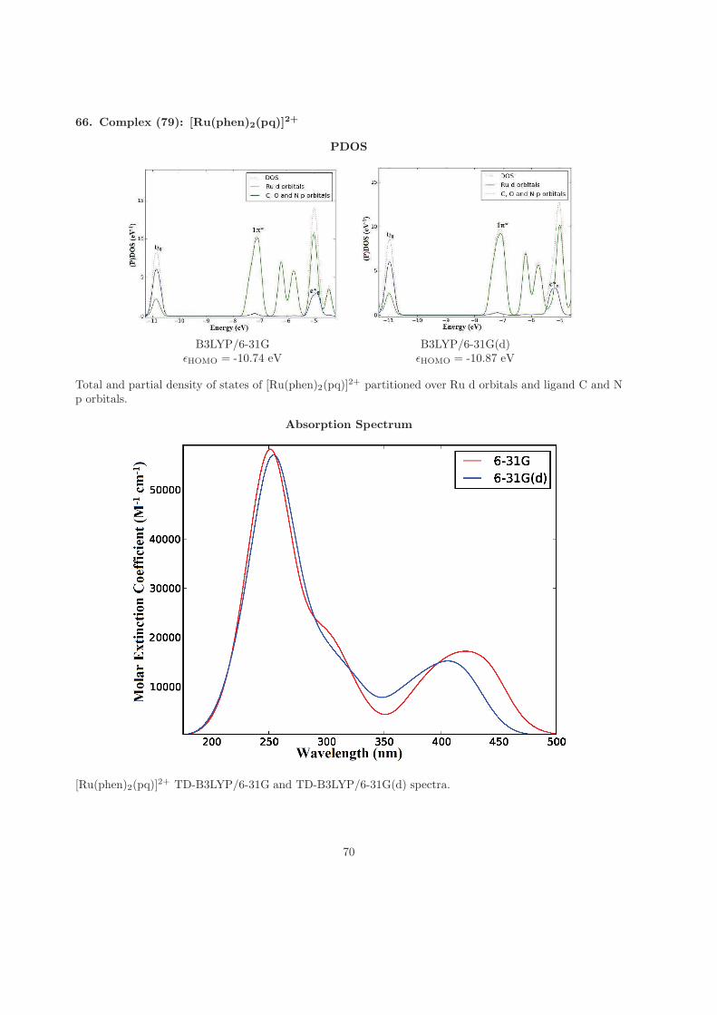
66. Complex (79): [Ru(phen)2(pq)]2+
PDOS
B3LYP/6-31G B3LYP/6-31G(d)ǫHOMO = -10.74 eV ǫHOMO = -10.87 eV
Total and partial density of states of [Ru(phen)2(pq)]2+ partitioned over Ru d orbitals and ligand C and N
p orbitals.
Absorption Spectrum
[Ru(phen)2(pq)]2+ TD-B3LYP/6-31G and TD-B3LYP/6-31G(d) spectra.
70
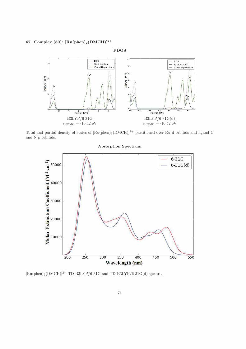
67. Complex (80): [Ru(phen)2(DMCH)]2+
PDOS
B3LYP/6-31G B3LYP/6-31G(d)ǫHOMO = -10.42 eV ǫHOMO = -10.52 eV
Total and partial density of states of [Ru(phen)2(DMCH)]2+ partitioned over Ru d orbitals and ligand Cand N p orbitals.
Absorption Spectrum
[Ru(phen)2(DMCH)]2+ TD-B3LYP/6-31G and TD-B3LYP/6-31G(d) spectra.
71
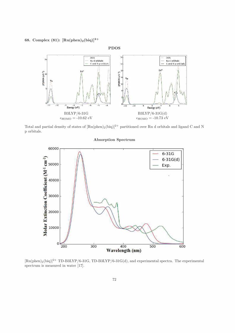
68. Complex (81): [Ru(phen)2(biq)]2+
PDOS
B3LYP/6-31G B3LYP/6-31G(d)ǫHOMO = -10.62 eV ǫHOMO = -10.73 eV
Total and partial density of states of [Ru(phen)2(biq)]2+ partitioned over Ru d orbitals and ligand C and N
p orbitals.
Absorption Spectrum
[Ru(phen)2(biq)]2+ TD-B3LYP/6-31G, TD-B3LYP/6-31G(d), and experimental spectra. The experimental
spectrum is measured in water [17].
72
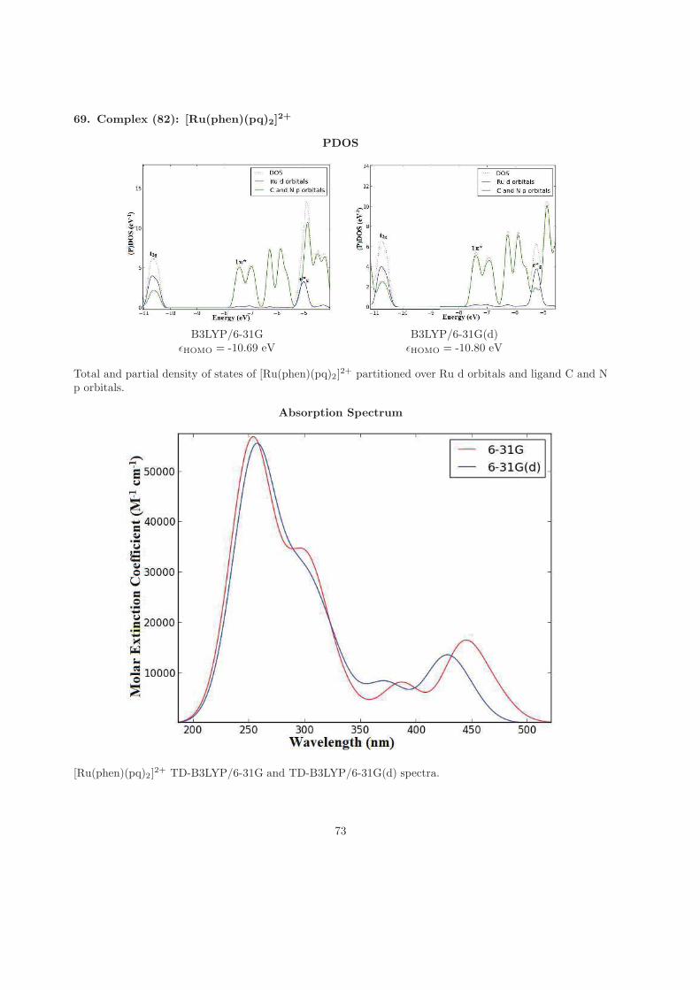
69. Complex (82): [Ru(phen)(pq)2]2+
PDOS
B3LYP/6-31G B3LYP/6-31G(d)ǫHOMO = -10.69 eV ǫHOMO = -10.80 eV
Total and partial density of states of [Ru(phen)(pq)2]2+ partitioned over Ru d orbitals and ligand C and N
p orbitals.
Absorption Spectrum
[Ru(phen)(pq)2]2+ TD-B3LYP/6-31G and TD-B3LYP/6-31G(d) spectra.
73
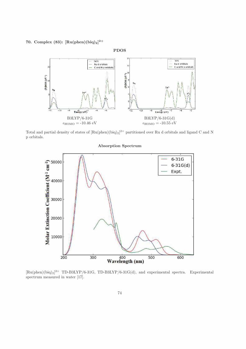
70. Complex (83): [Ru(phen)(biq)2]2+
PDOS
B3LYP/6-31G B3LYP/6-31G(d)ǫHOMO = -10.46 eV ǫHOMO = -10.55 eV
Total and partial density of states of [Ru(phen)(biq)2]2+ partitioned over Ru d orbitals and ligand C and N
p orbitals.
Absorption Spectrum
[Ru(phen)(biq)2]2+ TD-B3LYP/6-31G, TD-B3LYP/6-31G(d), and experimental spectra. Experimental
spectrum measured in water [17].
74
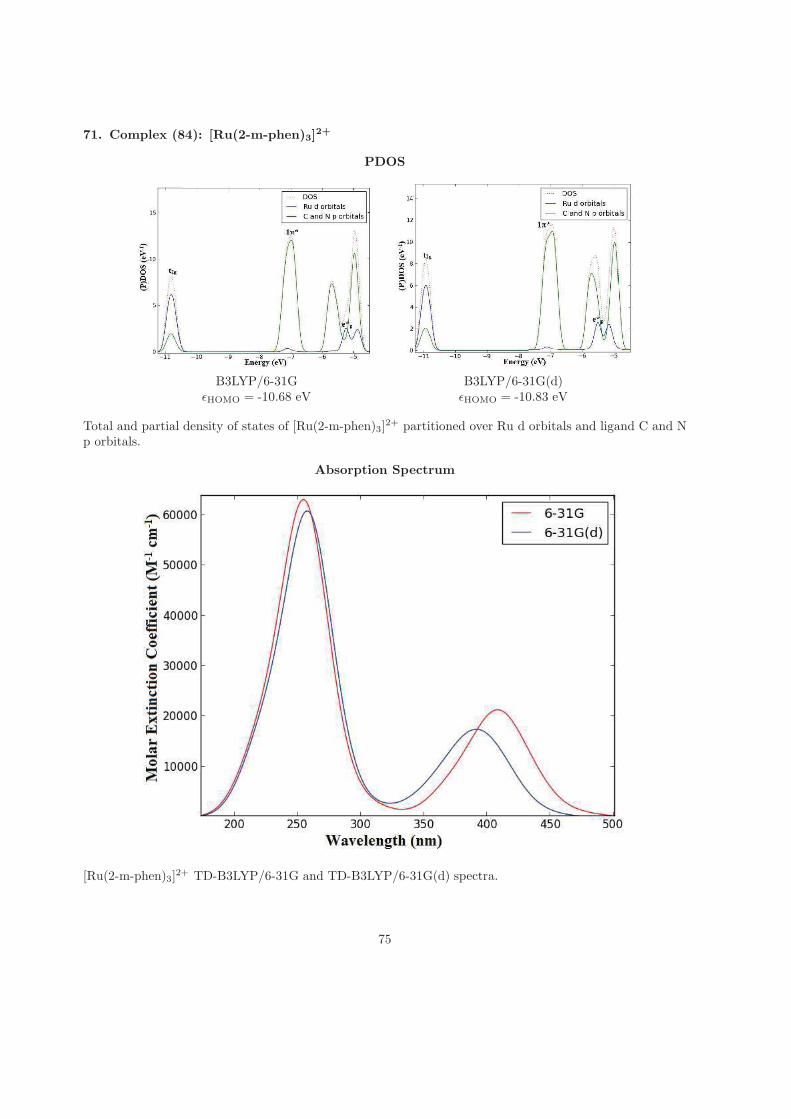
71. Complex (84): [Ru(2-m-phen)3]2+
PDOS
B3LYP/6-31G B3LYP/6-31G(d)ǫHOMO = -10.68 eV ǫHOMO = -10.83 eV
Total and partial density of states of [Ru(2-m-phen)3]2+ partitioned over Ru d orbitals and ligand C and N
p orbitals.
Absorption Spectrum
[Ru(2-m-phen)3]2+ TD-B3LYP/6-31G and TD-B3LYP/6-31G(d) spectra.
75
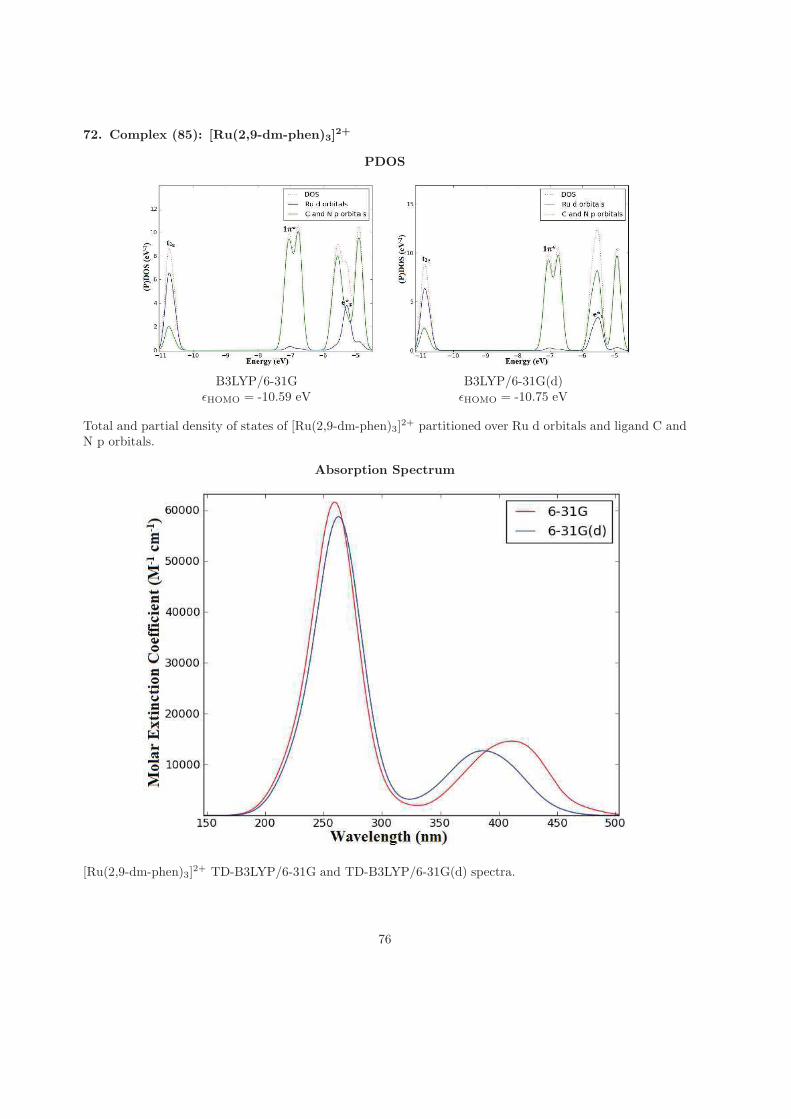
72. Complex (85): [Ru(2,9-dm-phen)3]2+
PDOS
B3LYP/6-31G B3LYP/6-31G(d)ǫHOMO = -10.59 eV ǫHOMO = -10.75 eV
Total and partial density of states of [Ru(2,9-dm-phen)3]2+ partitioned over Ru d orbitals and ligand C and
N p orbitals.
Absorption Spectrum
[Ru(2,9-dm-phen)3]2+ TD-B3LYP/6-31G and TD-B3LYP/6-31G(d) spectra.
76
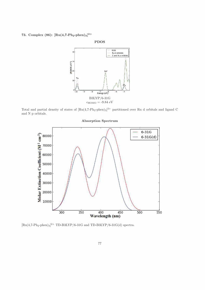
73. Complex (86): [Ru(4,7-Ph2-phen)3]2+
PDOS
B3LYP/6-31GǫHOMO = -9.84 eV
Total and partial density of states of [Ru(4,7-Ph2-phen)3]2+ partitioned over Ru d orbitals and ligand C
and N p orbitals.
Absorption Spectrum
[Ru(4,7-Ph2-phen)3]2+ TD-B3LYP/6-31G and TD-B3LYP/6-31G(d) spectra.
77
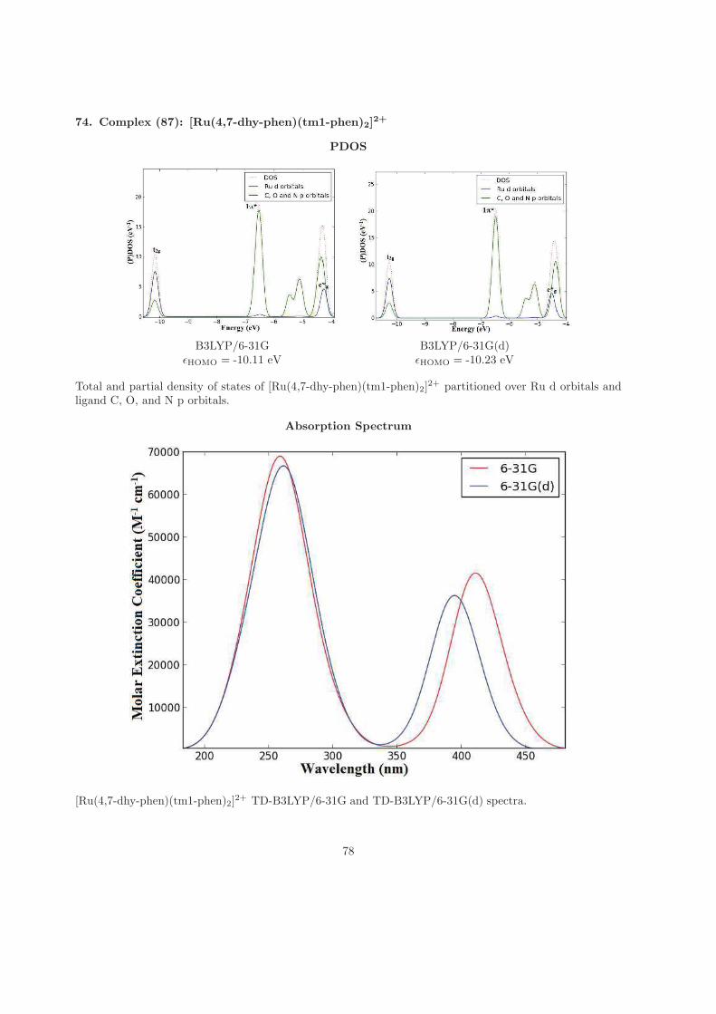
74. Complex (87): [Ru(4,7-dhy-phen)(tm1-phen)2]2+
PDOS
B3LYP/6-31G B3LYP/6-31G(d)ǫHOMO = -10.11 eV ǫHOMO = -10.23 eV
Total and partial density of states of [Ru(4,7-dhy-phen)(tm1-phen)2]2+ partitioned over Ru d orbitals and
ligand C, O, and N p orbitals.
Absorption Spectrum
[Ru(4,7-dhy-phen)(tm1-phen)2]2+ TD-B3LYP/6-31G and TD-B3LYP/6-31G(d) spectra.
78
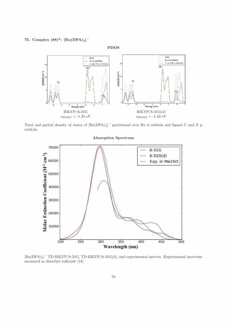
75. Complex (88)*: [Ru(DPA)3]−
PDOS
B3LYP/6-31G B3LYP/6-31G(d)ǫHOMO = -1.35 eV ǫHOMO = -1.43 eV
Total and partial density of states of [Ru(DPA)3]− partitioned over Ru d orbitals and ligand C and N p
orbitals.
Absorption Spectrum
[Ru(DPA)3]− TD-B3LYP/6-31G, TD-B3LYP/6-31G(d), and experimental spectra. Experimental spectrum
measured in dimethyl sulfoxide [18].
79
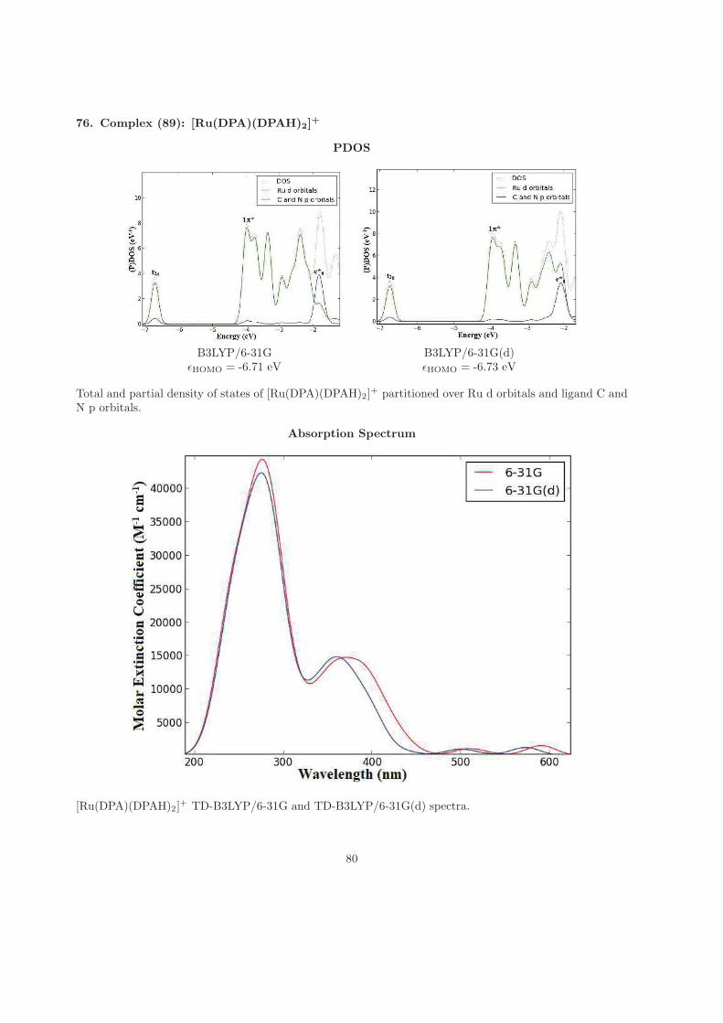
76. Complex (89): [Ru(DPA)(DPAH)2]+
PDOS
B3LYP/6-31G B3LYP/6-31G(d)ǫHOMO = -6.71 eV ǫHOMO = -6.73 eV
Total and partial density of states of [Ru(DPA)(DPAH)2]+ partitioned over Ru d orbitals and ligand C and
N p orbitals.
Absorption Spectrum
[Ru(DPA)(DPAH)2]+ TD-B3LYP/6-31G and TD-B3LYP/6-31G(d) spectra.
80
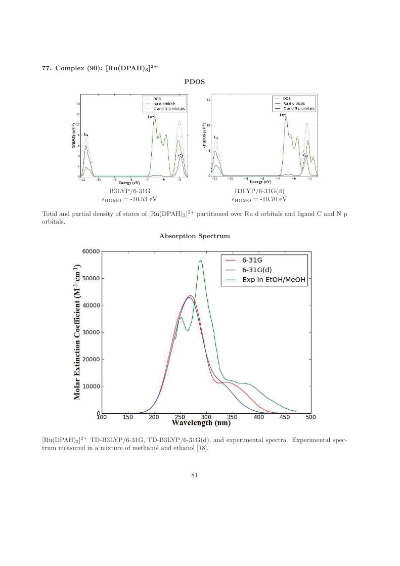
77. Complex (90): [Ru(DPAH)3]2+
PDOS
B3LYP/6-31G B3LYP/6-31G(d)ǫHOMO = -10.53 eV ǫHOMO = -10.70 eV
Total and partial density of states of [Ru(DPAH)3]2+ partitioned over Ru d orbitals and ligand C and N p
orbitals.
Absorption Spectrum
[Ru(DPAH)3]2+ TD-B3LYP/6-31G, TD-B3LYP/6-31G(d), and experimental spectra. Experimental spec-
trum measured in a mixture of methanol and ethanol [18].
81
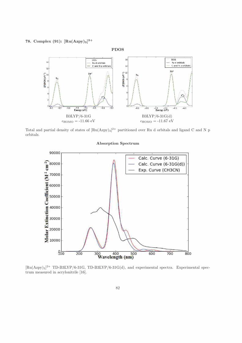
78. Complex (91): [Ru(Azpy)3]2+
PDOS
B3LYP/6-31G B3LYP/6-31G(d)ǫHOMO = -11.66 eV ǫHOMO = -11.67 eV
Total and partial density of states of [Ru(Azpy)3]2+ partitioned over Ru d orbitals and ligand C and N p
orbitals.
Absorption Spectrum
[Ru(Azpy)3]2+ TD-B3LYP/6-31G, TD-B3LYP/6-31G(d), and experimental spectra. Experimental spec-
trum measured in acrylonitrile [16].
82
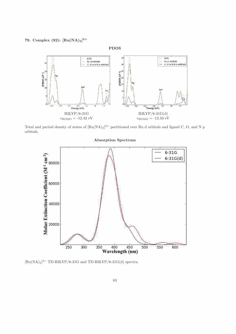
79. Complex (92): [Ru(NA)3]2+
PDOS
B3LYP/6-31G B3LYP/6-31G(d)ǫHOMO = -12.42 eV ǫHOMO = -12.33 eV
Total and partial density of states of [Ru(NA)3]2+ partitioned over Ru d orbitals and ligand C, O, and N p
orbitals.
Absorption Spectrum
[Ru(NA)3]2+ TD-B3LYP/6-31G and TD-B3LYP/6-31G(d) spectra.
83
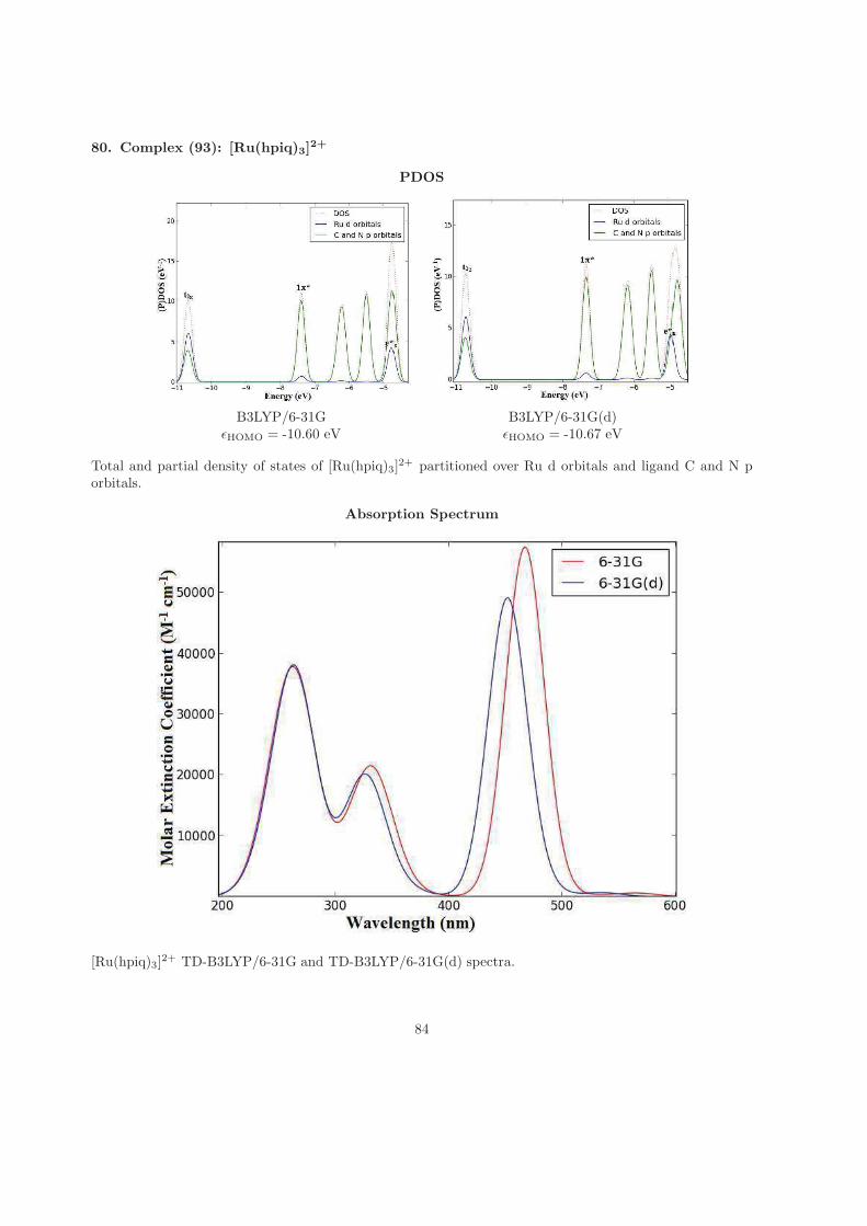
80. Complex (93): [Ru(hpiq)3]2+
PDOS
B3LYP/6-31G B3LYP/6-31G(d)ǫHOMO = -10.60 eV ǫHOMO = -10.67 eV
Total and partial density of states of [Ru(hpiq)3]2+ partitioned over Ru d orbitals and ligand C and N p
orbitals.
Absorption Spectrum
[Ru(hpiq)3]2+ TD-B3LYP/6-31G and TD-B3LYP/6-31G(d) spectra.
84
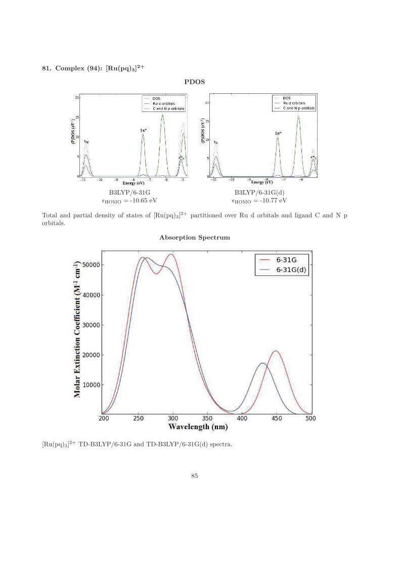
81. Complex (94): [Ru(pq)3]2+
PDOS
B3LYP/6-31G B3LYP/6-31G(d)ǫHOMO = -10.65 eV ǫHOMO = -10.77 eV
Total and partial density of states of [Ru(pq)3]2+ partitioned over Ru d orbitals and ligand C and N p
orbitals.
Absorption Spectrum
[Ru(pq)3]2+ TD-B3LYP/6-31G and TD-B3LYP/6-31G(d) spectra.
85
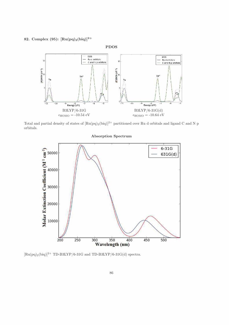
82. Complex (95): [Ru(pq)2(biq)]2+
PDOS
B3LYP/6-31G B3LYP/6-31G(d)ǫHOMO = -10.54 eV ǫHOMO = -10.64 eV
Total and partial density of states of [Ru(pq)2(biq)]2+ partitioned over Ru d orbitals and ligand C and N p
orbitals.
Absorption Spectrum
[Ru(pq)2(biq)]2+ TD-B3LYP/6-31G and TD-B3LYP/6-31G(d) spectra.
86
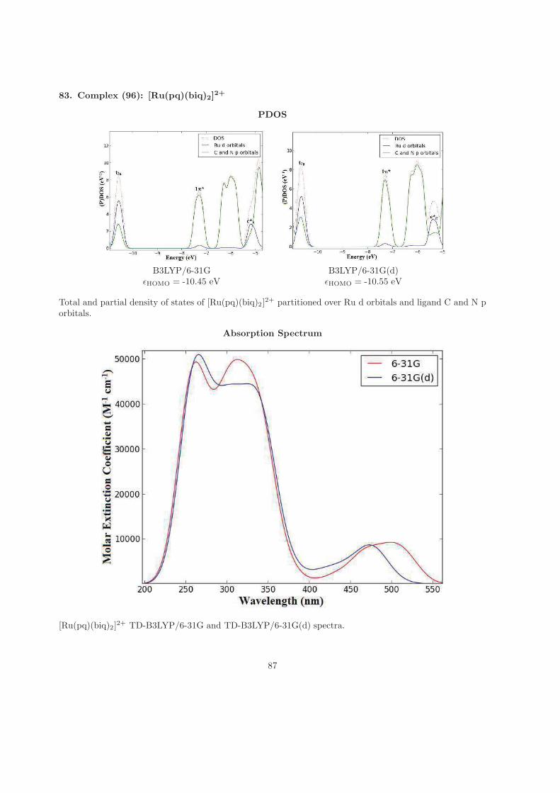
83. Complex (96): [Ru(pq)(biq)2]2+
PDOS
B3LYP/6-31G B3LYP/6-31G(d)ǫHOMO = -10.45 eV ǫHOMO = -10.55 eV
Total and partial density of states of [Ru(pq)(biq)2]2+ partitioned over Ru d orbitals and ligand C and N p
orbitals.
Absorption Spectrum
[Ru(pq)(biq)2]2+ TD-B3LYP/6-31G and TD-B3LYP/6-31G(d) spectra.
87
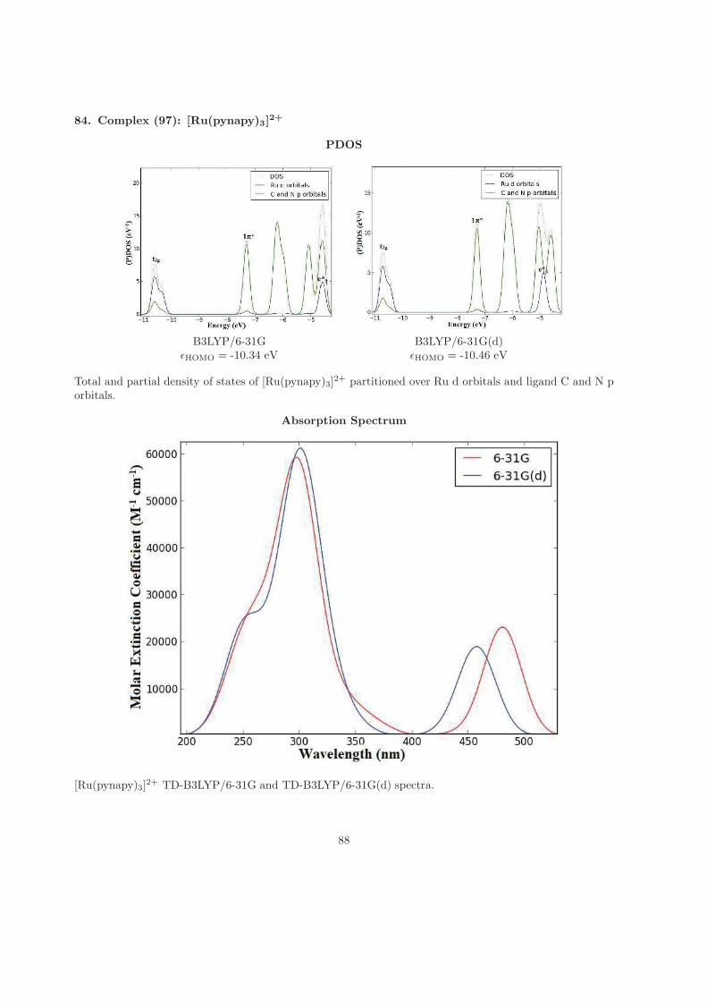
84. Complex (97): [Ru(pynapy)3]2+
PDOS
B3LYP/6-31G B3LYP/6-31G(d)ǫHOMO = -10.34 eV ǫHOMO = -10.46 eV
Total and partial density of states of [Ru(pynapy)3]2+ partitioned over Ru d orbitals and ligand C and N p
orbitals.
Absorption Spectrum
[Ru(pynapy)3]2+ TD-B3LYP/6-31G and TD-B3LYP/6-31G(d) spectra.
88
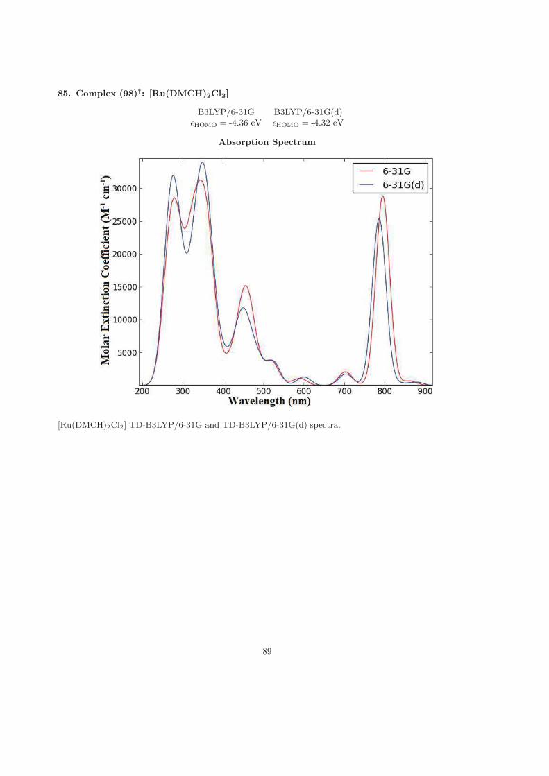
85. Complex (98)†: [Ru(DMCH)2Cl2]
B3LYP/6-31G B3LYP/6-31G(d)ǫHOMO = -4.36 eV ǫHOMO = -4.32 eV
Absorption Spectrum
[Ru(DMCH)2Cl2] TD-B3LYP/6-31G and TD-B3LYP/6-31G(d) spectra.
89
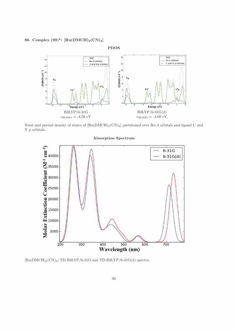
86. Complex (99)*: [Ru(DMCH)2(CN)2]
PDOS
B3LYP/6-31G B3LYP/6-31G(d)ǫHOMO = -4.56 eV ǫHOMO = -4.60 eV
Total and partial density of states of [Ru(DMCH)2(CN)2] partitioned over Ru d orbitals and ligand C andN p orbitals.
Absorption Spectrum
[Ru(DMCH)2(CN)2] TD-B3LYP/6-31G and TD-B3LYP/6-31G(d) spectra.
90
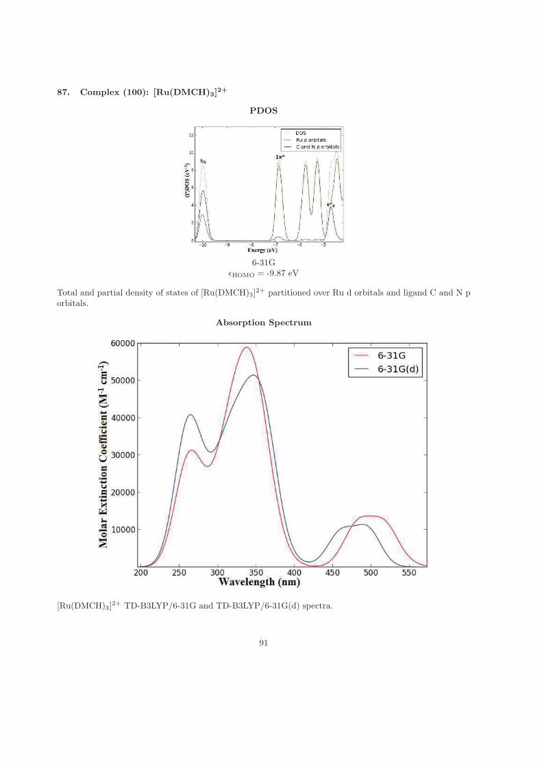
87. Complex (100): [Ru(DMCH)3]2+
PDOS
6-31GǫHOMO = -9.87 eV
Total and partial density of states of [Ru(DMCH)3]2+ partitioned over Ru d orbitals and ligand C and N p
orbitals.
Absorption Spectrum
[Ru(DMCH)3]2+ TD-B3LYP/6-31G and TD-B3LYP/6-31G(d) spectra.
91
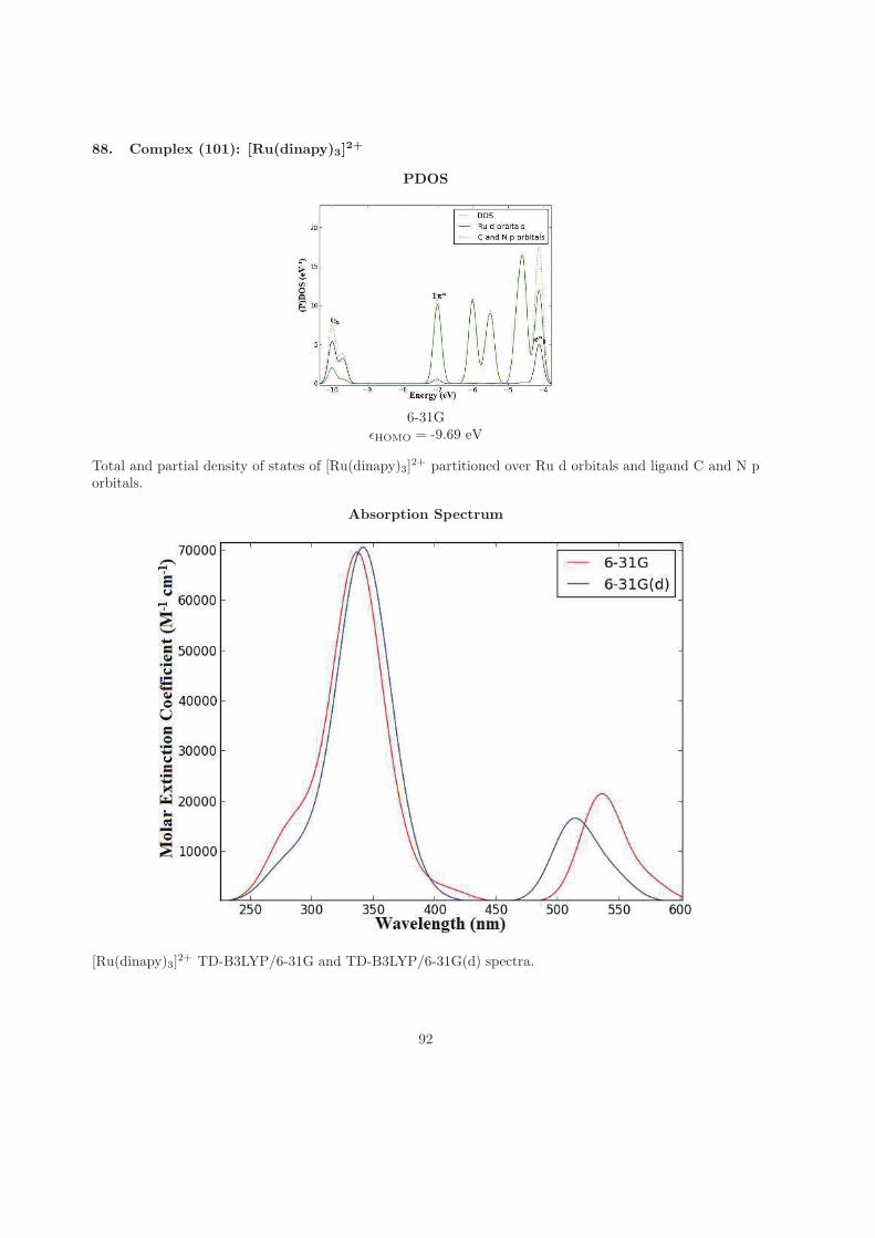
88. Complex (101): [Ru(dinapy)3]2+
PDOS
6-31GǫHOMO = -9.69 eV
Total and partial density of states of [Ru(dinapy)3]2+ partitioned over Ru d orbitals and ligand C and N p
orbitals.
Absorption Spectrum
[Ru(dinapy)3]2+ TD-B3LYP/6-31G and TD-B3LYP/6-31G(d) spectra.
92
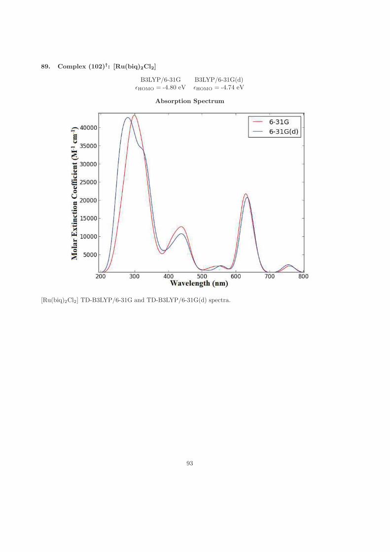
89. Complex (102)†: [Ru(biq)2Cl2]
B3LYP/6-31G B3LYP/6-31G(d)ǫHOMO = -4.80 eV ǫHOMO = -4.74 eV
Absorption Spectrum
[Ru(biq)2Cl2] TD-B3LYP/6-31G and TD-B3LYP/6-31G(d) spectra.
93
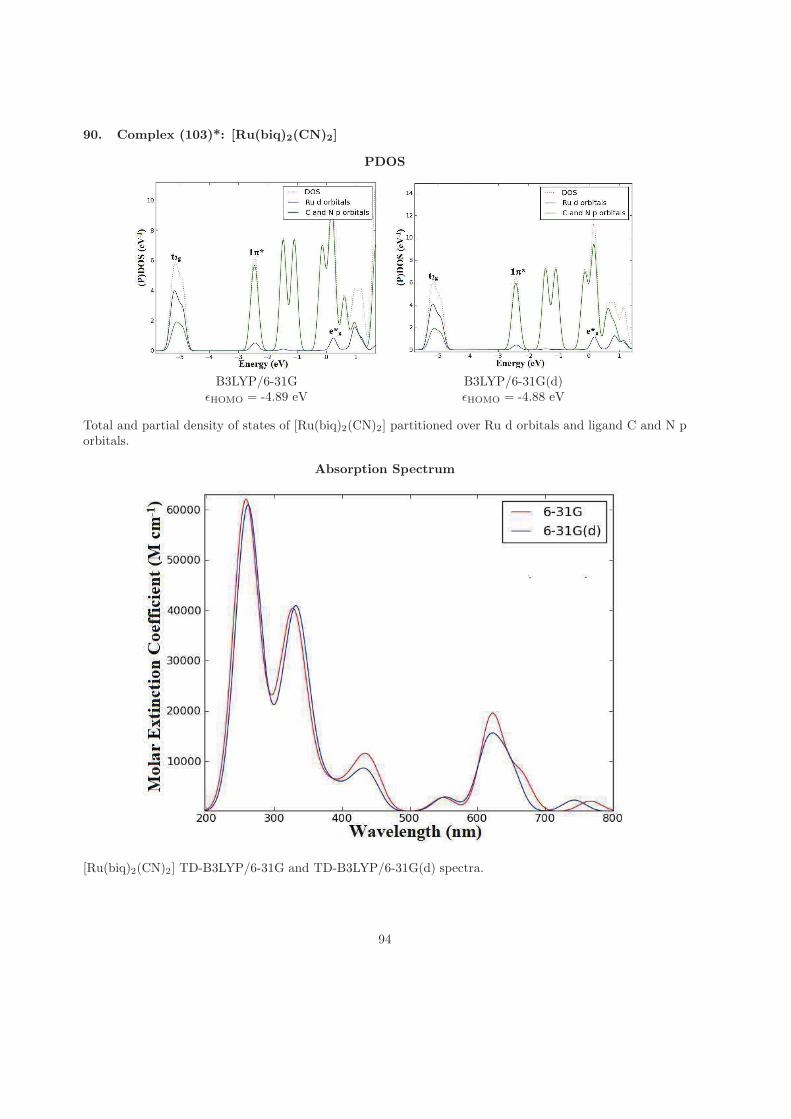
90. Complex (103)*: [Ru(biq)2(CN)2]
PDOS
B3LYP/6-31G B3LYP/6-31G(d)ǫHOMO = -4.89 eV ǫHOMO = -4.88 eV
Total and partial density of states of [Ru(biq)2(CN)2] partitioned over Ru d orbitals and ligand C and N porbitals.
Absorption Spectrum
[Ru(biq)2(CN)2] TD-B3LYP/6-31G and TD-B3LYP/6-31G(d) spectra.
94
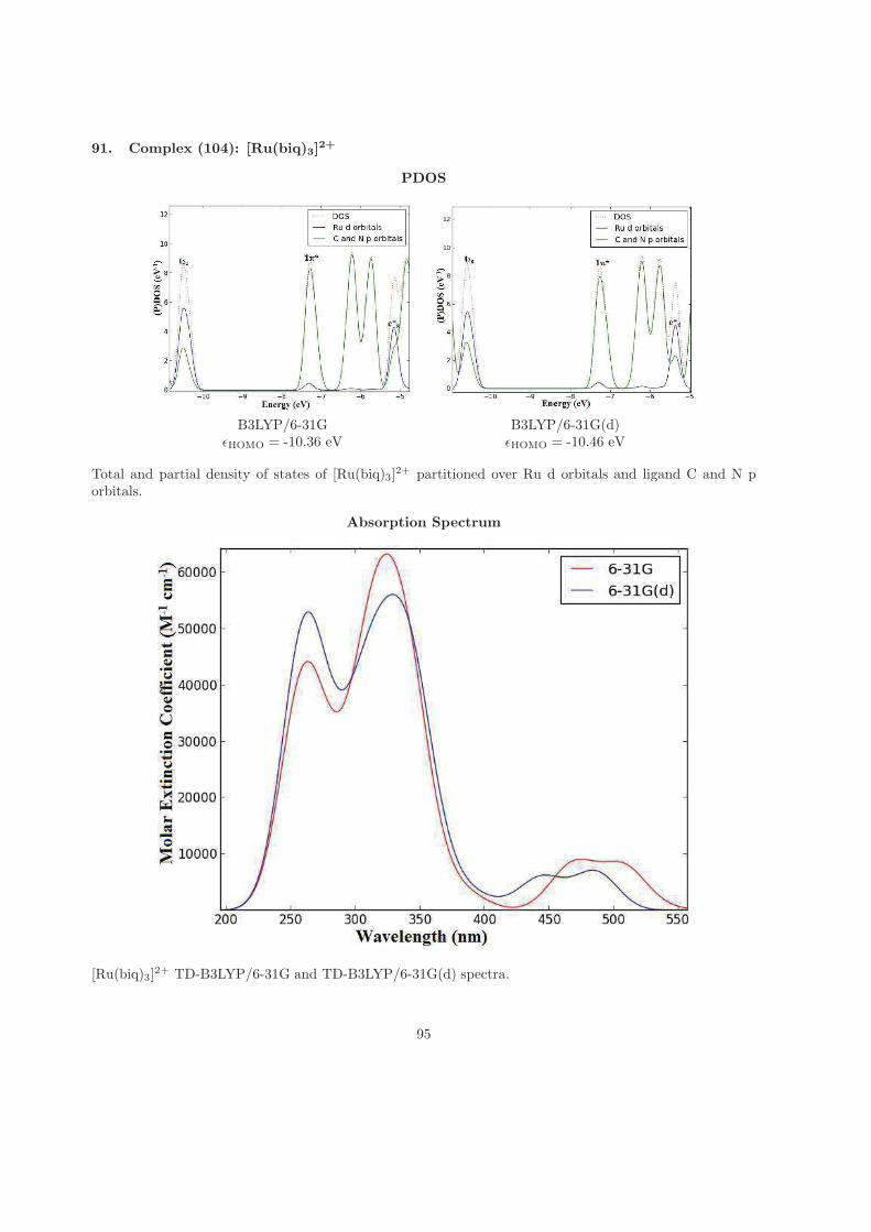
91. Complex (104): [Ru(biq)3]2+
PDOS
B3LYP/6-31G B3LYP/6-31G(d)ǫHOMO = -10.36 eV ǫHOMO = -10.46 eV
Total and partial density of states of [Ru(biq)3]2+ partitioned over Ru d orbitals and ligand C and N p
orbitals.
Absorption Spectrum
[Ru(biq)3]2+ TD-B3LYP/6-31G and TD-B3LYP/6-31G(d) spectra.
95
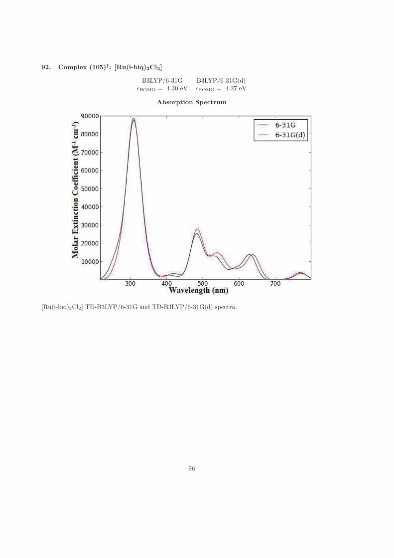
92. Complex (105)†: [Ru(i-biq)2Cl2]
B3LYP/6-31G B3LYP/6-31G(d)ǫHOMO = -4.30 eV ǫHOMO = -4.27 eV
Absorption Spectrum
[Ru(i-biq)2Cl2] TD-B3LYP/6-31G and TD-B3LYP/6-31G(d) spectra.
96
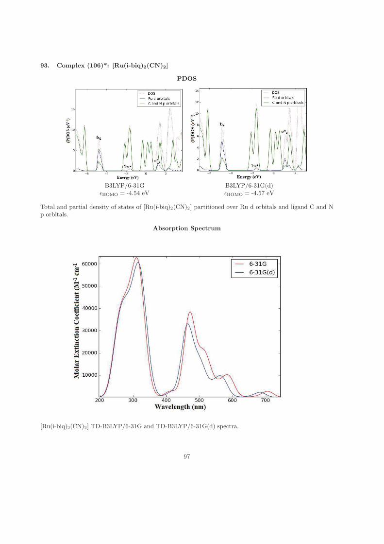
93. Complex (106)*: [Ru(i-biq)2(CN)2]
PDOS
B3LYP/6-31G B3LYP/6-31G(d)ǫHOMO = -4.54 eV ǫHOMO = -4.57 eV
Total and partial density of states of [Ru(i-biq)2(CN)2] partitioned over Ru d orbitals and ligand C and Np orbitals.
Absorption Spectrum
[Ru(i-biq)2(CN)2] TD-B3LYP/6-31G and TD-B3LYP/6-31G(d) spectra.
97
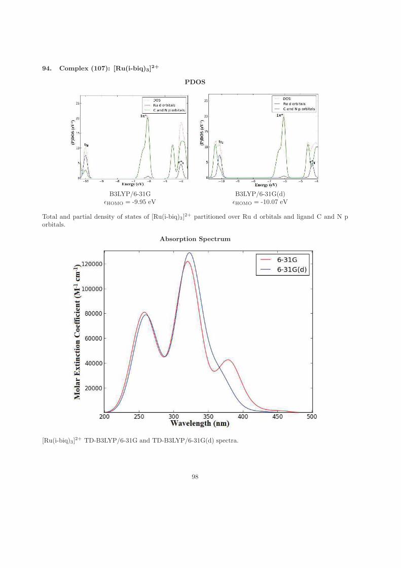
94. Complex (107): [Ru(i-biq)3]2+
PDOS
B3LYP/6-31G B3LYP/6-31G(d)ǫHOMO = -9.95 eV ǫHOMO = -10.07 eV
Total and partial density of states of [Ru(i-biq)3]2+ partitioned over Ru d orbitals and ligand C and N p
orbitals.
Absorption Spectrum
[Ru(i-biq)3]2+ TD-B3LYP/6-31G and TD-B3LYP/6-31G(d) spectra.
98
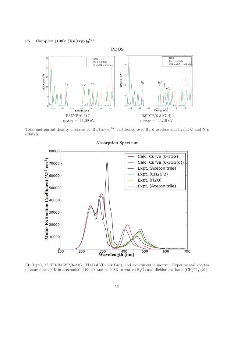
95. Complex (108): [Ru(trpy)2]2+
PDOS
14 12 10 8 6 4 2
0
5
10
15
20
25
DOS
Ru d orbitals
C and N p orbitals
14 12 10 8 6 4 2
0
5
10
15
20
DOS
Ru d orbitals
C N and O p orbitals
B3LYP/6-31G B3LYP/6-31G(d)ǫHOMO = -11.09 eV ǫHOMO = -11.19 eV
Total and partial density of states of [Ru(trpy)2]2+ partitioned over Ru d orbitals and ligand C and N p
orbitals.
Absorption Spectrum
[Ru(trpy)2]2+ TD-B3LYP/6-31G, TD-B3LYP/6-31G(d), and experimental spectra. Experimental spectra
measured at 294K in acetronitrile[19, 20] and at 298K in water (H2O) and dichloromethane (CH2Cl2)[21].
99
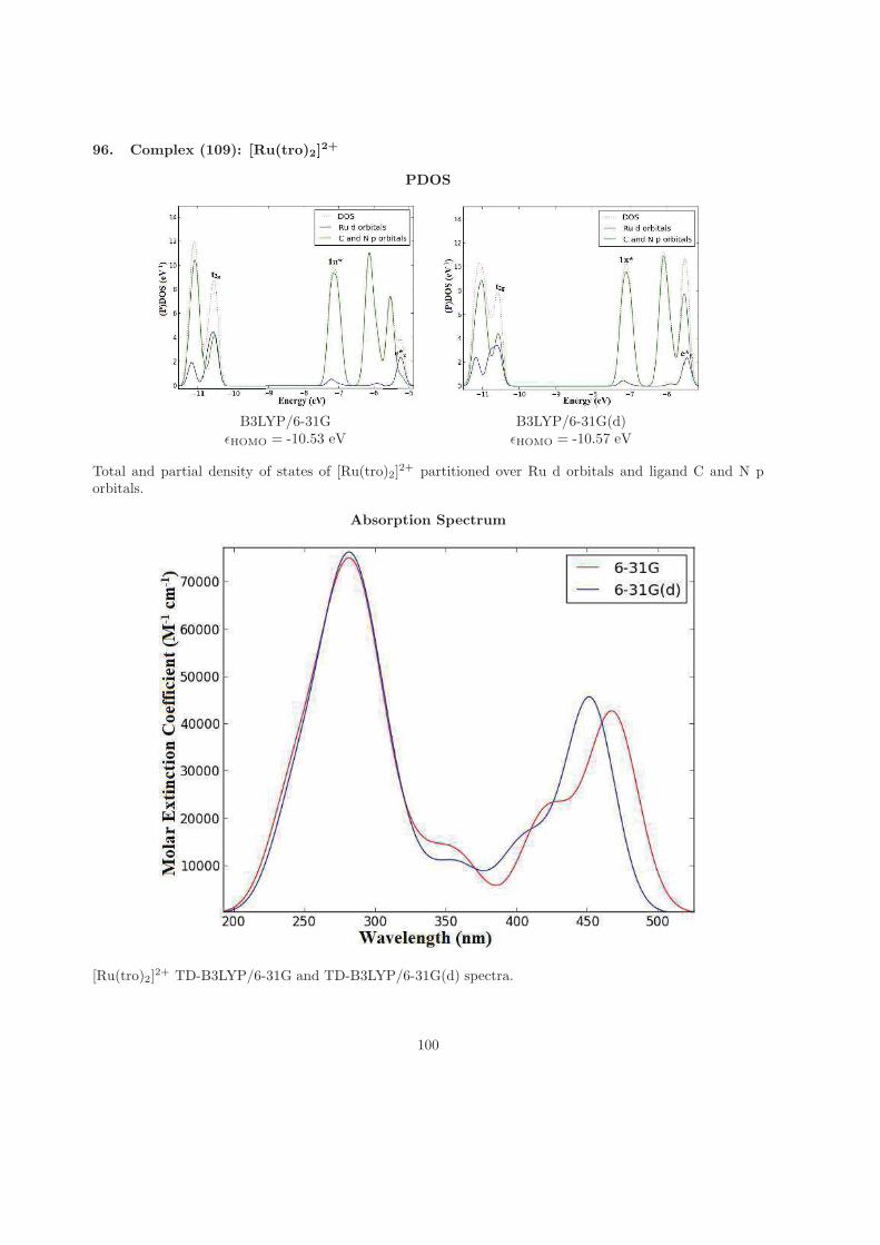
96. Complex (109): [Ru(tro)2]2+
PDOS
B3LYP/6-31G B3LYP/6-31G(d)ǫHOMO = -10.53 eV ǫHOMO = -10.57 eV
Total and partial density of states of [Ru(tro)2]2+ partitioned over Ru d orbitals and ligand C and N p
orbitals.
Absorption Spectrum
[Ru(tro)2]2+ TD-B3LYP/6-31G and TD-B3LYP/6-31G(d) spectra.
100
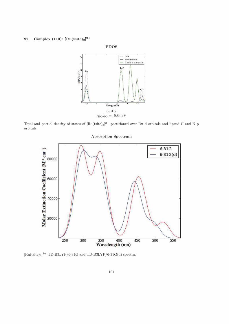
97. Complex (110): [Ru(tsite)2]2+
PDOS
6-31GǫHOMO = -9.84 eV
Total and partial density of states of [Ru(tsite)2]2+ partitioned over Ru d orbitals and ligand C and N p
orbitals.
Absorption Spectrum
[Ru(tsite)2]2+ TD-B3LYP/6-31G and TD-B3LYP/6-31G(d) spectra.
101
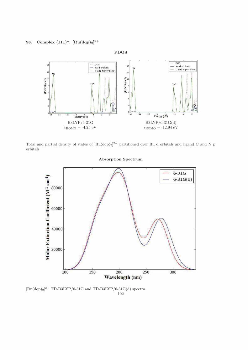
98. Complex (111)*: [Ru(dqp)2]2+
PDOS
B3LYP/6-31G B3LYP/6-31G(d)ǫHOMO = -4.25 eV ǫHOMO = -12.94 eV
Total and partial density of states of [Ru(dqp)2]2+ partitioned over Ru d orbitals and ligand C and N p
orbitals.
Absorption Spectrum
[Ru(dqp)2]2+ TD-B3LYP/6-31G and TD-B3LYP/6-31G(d) spectra.
102

REFERENCES
References
[1] J. Gu, J. Chen, and R. H. Schmehl, Using intramolecular energy transfer to transform nonphotoactive, visible-light-absorbingchromophores into sensitizers for photoredox reactions, J. Am. Chem. Soc. 132, 7338 (2010).
[2] L. Fodor, G. Lendvay, and A. Horvath, Solvent Dependence of Absorption and Emission of Ru(bpy)2(CN)2: Experiment andExplanation Based on Electronic Structure Theory, J. Phys. Chem. A 111, 12891 (2007).
[3] H. Yersin, W. Humbs, and J. Strasser, Low-lying electronic states of [Rh(bpy)3]3+, [Pt(bpy)2] 2+, and [Ru(bpy)3]2+. Acomparative study based on highly resolved and time-resolved spectra, Coord. Chem. Rev. 159, 325 (1997).
[4] B. Sullivan et al., Multiple emissions from charge transfer excited states of ruthenium (II)polypyridine complexes, Chem. Phys.Lett. 58, 389 (1978).
[5] D. P. Rillema, G. Allen, T. J. Meyer, and D. Conrad, Redox properties of ruthenium (II) tris chelate complexes containing theligands 2, 2’-bipyrazine, 2, 2’-bipyridine, and 2, 2’-bipyrimidine, Inorg. Chem. 22, 1617 (1983).
[6] N. Yoshikawa et al., Transition states of the 3 MLCT to 3 MC conversion in Ru (bpy)2(phen derivative) 2+ complexes, J. Mol.Struct. 1094, 98 (2015).
[7] W. B. Heuer et al., Reaction of RuII Diazafluorenone Compound with Nanocrystalline TiO2 Thin Film, Inorg. Chem. 49, 7726(2010).
[8] E. Borfecchia et al., X-ray transient absorption structural characterization of the 3MLCT triplet excited state of cis-[Ru(bpy)2(py)2]2+, Dalton Trans. 42, 6564 (2013).
[9] Z. Z. Li, Y. L. Niu, H. Y. Zhou, H. Y. Chao, and B. H. Ye, Visible-Light-Induced Photooxidation of Ruthenium(II) Complexwith 2,2-Biimidazole-like Ligand by Singlet Oxygen, Inorg. Chem. 52, 10087 (2013).
[10] C. D. Tait, T. M. Vess, M. K. McArmond, K. W. Hanck, and D. W. Wertz, Characterizations of the redox orbitals ofmixed-ligand 2,2’-bipyridine-2-(2’-pyridyl)quinoline ruthenium(II) complexes, J. Chem. Soc., Dalton Trans. 1987, 2467 (1987).
[11] A. A. Cadranel, P. Albores, S. Yamazaki, V. D. Klieman, and L. M. Baraldo, Efficient energy gransfer via the cyanide bridgein dinuclear complexes containing Ru(II) polypirdine moieties, Dalton Trans. 41, 5343 (2012).
[12] Q. Sun et al., Experimental Evidence of Ultrafast Quenching of the 3MLCT Luminescence in Ruthenium(II) Tris-bipyridylComplexes via a 3
dd State, J. Am. Chem. Soc. 135, 13660 (2013).[13] R. H. Fabian, D. M. Klassen, and R. W. Sonntag, Synthesis and spectroscopic characterization of ruthenium and osmium
complexes with sterically hindering ligands. 3. Tris complexes with methyl- and dimethyl-substituted 2,2’-bipyridine and 1,10-phenanthroline, Inorg. Chem. 19, 1977 (1980).
[14] B. Maubert, N. D. McClenaghan, M. T. Indelli, and S. Campagna, Absorption spectra and photophysical properties of aseries of polypyridine ligands containing appended pyrenyl and anthryl chromophores and of their ruthenium(II) complexes, J.Phys. Chem. A 107, 447 (2003).
[15] M. Schwalbe et al., Synthesis and characterisation of poly(bipyridine)ruthenium complexes as building blocks for hetero-supramolecular arrays, Euro. J. Inorg. Chem. 2008, 3310 (2008).
[16] N. Leventis et al., Synthesis and Characterization of Ru(II) Tris(1,10-phenanthroline)-Electron Acceptor Dyads Incorporating the4-Benzoyl-N-methylpyridinium Cation or N-Benzyl-N-methyl Viologen. Improving the Dynamic Range, Sensitivity, and ResponseTime of Sol-Gel-Based Optical Oxygen Sensors, Chem. Mater. 16, 1493 (2004).
[17] E. Wachter, D. K. Heidary, B. S. Howerton, S. Parkin, and E. C. Glazer, Light-activated ruthenium complexes photo bindDNA and are cytotoxic in the photodynamic therapy window, Chem. Commun. 48, 9649 (2012).
[18] D. P. Segers and M. K. DeArmond, Emission studies of transition-metal complexes of 2,2’-dipyridylamine. 2. Tris complexesof ruthenium(II), J. Phys. Chem. 86, 3768 (1982).
[19] J. T. Hewitt, P. J. Vallett, and N. H. Damrauer, Dynamics of the 3MLCT in Ru(II) Terpyridyl Complexes Probed by UltrafastSpectroscopy: Evidence of Excited-State Equilibration and Interligand Electron Transfer, J. Phys. Chem. A 116, 11536 (2012).
[20] J. Sauvage et al., Ruthenium(II) and Osmium(II) bis(terpyridine) complexes in covalently-linked multicomponent systems:Synthesis, electrochemical behavior, absorption spectra, and photochemical and photophysical properties, Chem. Rev. 94, 993(1994).
[21] E. Jakubikova et al., Electronic Structure and Spectroscopy of [Ru(tpy)2]2+, [Ru(tpy)(bpy)(H2O)]2+, and [Ru(tpy)(bpy)(Cl)]+ ,Inorg. Chem. 48, 10720 (2009).
103

Appendix B
Curriculum Vitae
296