BV Solutions for a Class of

Viscous Hyperbolic Systems

Stefano Bianchini and Alberto Bressan

S.I.S.S.A., Via Beirut 4, Trieste 34014 Italy.

Abstract. The paper is concerned with the Cauchy problem for a nonlinear, strictly hyperbolic

system with small viscosity:

ut +A(u)ux = ε uxx, u(0, x) = u(x). (∗)

We assume that the integral curves of the eigenvectors ri of the matrix A are straight lines. On

the other hand, we do not require the system (∗) to be in conservation form, nor do we make any

assumption on genuine linearity or linear degeneracy of the characteristic fields.

In this setting we prove that, for some small constant η0 > 0 the following holds. For every

initial data u ∈ L1 with Tot.Var.u < η0, the solution uε of (∗) is well defined for all t > 0. The

total variation of uε(t, ·) satisfies a uniform bound, independent of t, ε. Moreover, as ε → 0+, the

solutions uε(t, ·) converge to a unique limit u(t, ·). The map (t, u) 7→ Stu.= u(t, ·) is a Lipschitz

continuous semigroup on a closed domain D ⊂ L1 of functions with small total variation. This

semigroup is generated by a particular Riemann Solver, which we explicitly determine.

The above results can also be applied to strictly hyperbolic systems on a Riemann manifold.

Although these equations cannot be written in conservation form, we show that the Riemann struc-

ture uniquely determines a Lipschitz semigroup of “entropic” solutions, within a class of (possibly

discontinuous) functions with small total variation. The semigroup trajectories can be obtained

as the unique limits of solutions to a particular parabolic system, as the viscosity coefficient ap-

proaches zero.

The proofs rely on some new a priori estimates on the total variation of solutions for a parabolic

system whose components drift with strictly different speeds.

0

1 - Introduction

Consider a strictly hyperbolic n× n system of conservation laws in one space dimension:

ut + f(u)x = 0. (1.1)

For initial data with small total variation, the global existence of weak solutions was proved in [8].

Moreover, the uniqueness and stability of entropy admissible BV solutions was recently established

in a series of papers [3,4,5,6]. A long standing open question is whether these discontinuous

solutions can be obtained as vanishing viscosity limits. More precisely, given a smooth initial data

u : IR 7→ IRn with small total variation, consider the parabolic Cauchy problem

u(0, x) = u(x). (1.2)

ut +A(u)ux = ε uxx. (1.3)

Here A(u).= Df(u) is the Jacobian matrix of f and ε > 0. It is then natural to expect that, as

ε→ 0, the solution uε of (1.2)-(1.3) converges to the unique entropy weak solution u of (1.1)-(1.2).

Unfortunately, no general theorem in this direction is yet known. Some of the main results available

in the literature are listed below.

1) In the case of a scalar conservation law, the entropic solutions of (1.1) determine a semigroup

which is contractive w.r.t. the L1-distance. In this case, a general convergence theorem for

vanishing viscosity approximations was proved in the classical work of Kruzhkov [12].

2) For various 2 × 2 systems, if a uniform L∞–bound on all functions uε is available, one can

consider a weak limit uε u. By a compensated compactness argument introduced by

DiPerna [7], it then follows that u is actually a weak solution of the nonlinear system (1.1).

For a comprehensive discussion of the compensated compactness method and its applications

to conservation laws, see [18].

3) For n × n Temple class systems, a proof of the convergence of the viscous solutions uε to a

solution of (1.1) can be found in [17,18].

4) Assume that all characteristic fields of the system (1.1) are linearly degenerate. Then every

solution with small total variation which is initially smooth remains smooth for all positive

times [2]. Clearly such solution can be obtained as limit of vanishing viscosity approximations.

By a density argument it follows that every weak solution of (1.1) with sufficiently small total

variation is a limit of viscous approximations.

5) For a general n× n strictly hyperbolic system, let u be a piecewise smooth entropic solution

of (1.1) with jumps along a finite number of smooth curves in the t-x plane. Thanks to this

1

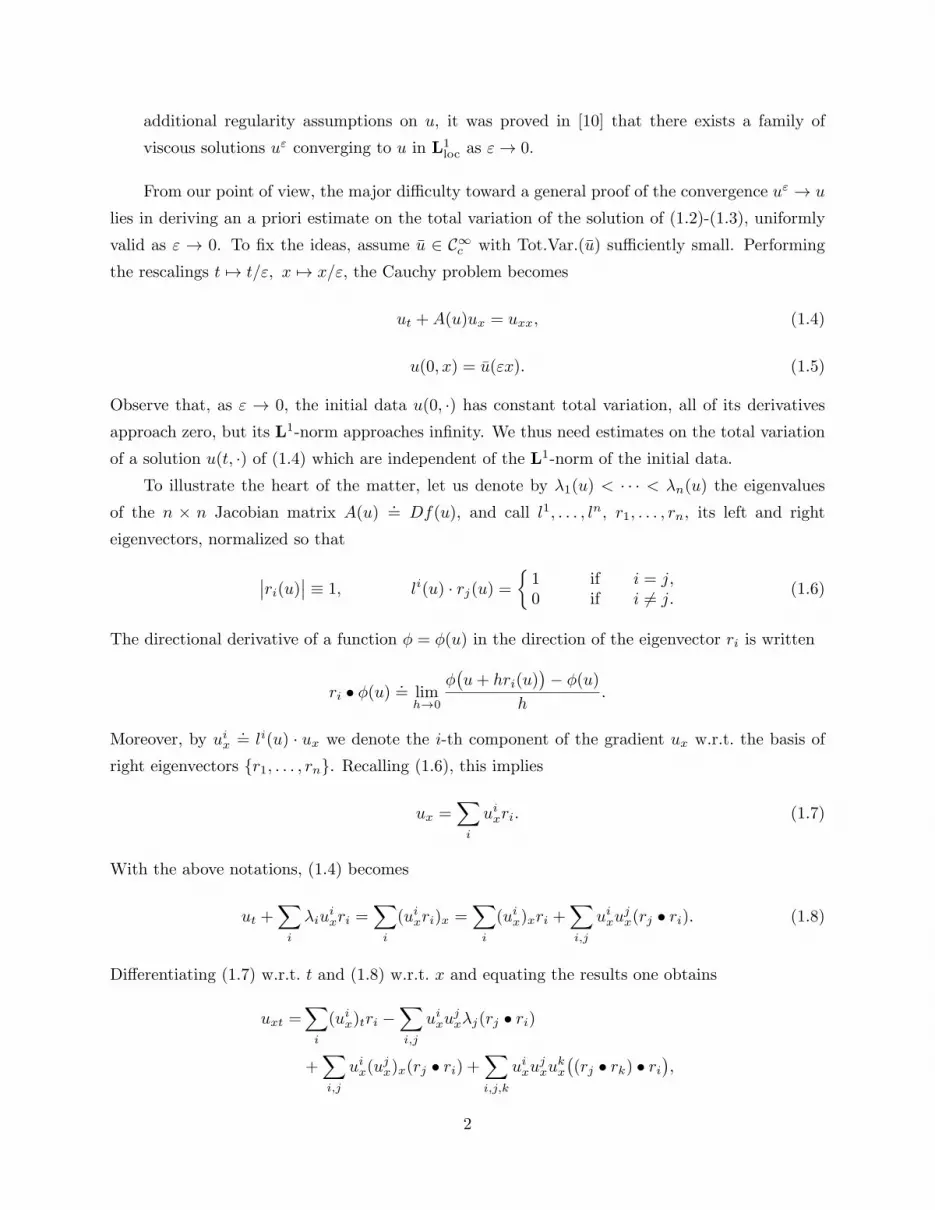
additional regularity assumptions on u, it was proved in [10] that there exists a family of

viscous solutions uε converging to u in L1loc as ε→ 0.

From our point of view, the major difficulty toward a general proof of the convergence uε → u

lies in deriving an a priori estimate on the total variation of the solution of (1.2)-(1.3), uniformly

valid as ε → 0. To fix the ideas, assume u ∈ C∞c with Tot.Var.(u) sufficiently small. Performing

the rescalings t 7→ t/ε, x 7→ x/ε, the Cauchy problem becomes

ut +A(u)ux = uxx, (1.4)

u(0, x) = u(εx). (1.5)

Observe that, as ε → 0, the initial data u(0, ·) has constant total variation, all of its derivatives

approach zero, but its L1-norm approaches infinity. We thus need estimates on the total variation

of a solution u(t, ·) of (1.4) which are independent of the L1-norm of the initial data.

To illustrate the heart of the matter, let us denote by λ1(u) < · · · < λn(u) the eigenvalues

of the n × n Jacobian matrix A(u).= Df(u), and call l1, . . . , ln, r1, . . . , rn, its left and right

eigenvectors, normalized so that

∣∣ri(u)∣∣ ≡ 1, li(u) · rj(u) =1 if i = j,0 if i 6= j.

(1.6)

The directional derivative of a function φ = φ(u) in the direction of the eigenvector ri is written

ri • φ(u).= lim

h→0

φ(u+ hri(u)

)− φ(u)

h.

Moreover, by uix.= li(u) · ux we denote the i-th component of the gradient ux w.r.t. the basis of

right eigenvectors r1, . . . , rn. Recalling (1.6), this implies

ux =∑i

uixri. (1.7)

With the above notations, (1.4) becomes

ut +∑i

λiuixri =

∑i

(uixri)x =∑i

(uix)xri +∑i,j

uixujx(rj • ri). (1.8)

Differentiating (1.7) w.r.t. t and (1.8) w.r.t. x and equating the results one obtains

uxt =∑i

(uix)tri −∑i,j

uixujxλj(rj • ri)

+∑i,j

uix(ujx)x(rj • ri) +

∑i,j,k

uixujxu

kx

((rj • rk) • ri

),

2

utx+∑i

(λiuix)xri +

∑i,j

λiuixu

jx(rj • ri)

=∑i

(uix)xxri +∑i,j

(uix)xujx(rj • ri) +

∑i,j

(uix)xujx(rj • ri)

+∑i,j

uix(ujx)x(rj • ri) +

∑i,j,k

uixujxu

kx

(rk • (rj • ri)

),

∑i

(uix)tri +∑i

(λiuix)xri +

∑j 6=k

λjujxu

kx[rk, rj ]

=∑i

(uix)xxri + 2∑i,j

(uix)xujx(rj • ri) +

∑i,j,k

uixujxu

kx

(rk • (rj • ri)− (rj • rk) • ri

).

(1.9)

Here [rk, rj ].= rk • rj − rj • rk is the usual Lie bracket. Taking the inner product of (1.9) with li(u)

one obtains

(uix)t + (λiuix)x − (uix)xx

= li ·

∑j 6=k

λk[rk, rj ]ujxu

kx + 2

∑j,k

(rk • rj)(ujx)xukx +∑j,k,`

(r` • (rk • rj)− (r` • rk) • rj

)ujxu

kxu

`x

=∑j 6=k

Gij,k(u)u

jxu

kx +

∑j,k

Hij,k(u)(u

jx)xu

kx +

∑j,k,`

Kij,k,`(u)u

jxu

kxu

`x.

(1.10)

Setting vi.= uix, we thus seek an estimate on the L1-norm of solutions to

vit +(λi(u)v

i)x− vixx =

∑j 6=k

Gij,k(u)v

jvk +∑j,k

Hij,k(u)v

jxv

k +∑j,k,`

Kij,k,`(u)v

jvkv`

.= φi(u, v1, . . . , vn).

(1.11)

We regard (1.11) as a parabolic system of n scalar equations, coupled through the terms G,H,K.

These coupling terms can be split in two groups:

– Transversal terms involving at least two distinct components, such as vjvk, vjxvk, vjvkv` with

j 6= k,

– Non-transversal terms involving one single component, such as vjvjx, vjvjvj .

In the present paper we perform a careful study of transversal terms, and show that their total

contribution is of quadratic order. Hence, for small initial data, they cannot produce a substantial

amplification of the solution of (1.11). As a consequence, if the geometry of the system is such

that the diffusion operator yields only transversal terms, then the total variation of solutions to

(1.3) remains uniformly bounded as ε → 0. This is the case of systems, not necessarily of Temple

class or not even in conservation form, where the integral curves of the eigenvectors ri are straight

lines, namely:

ri • ri(u) = 0 for all i, u. (1.12)

3

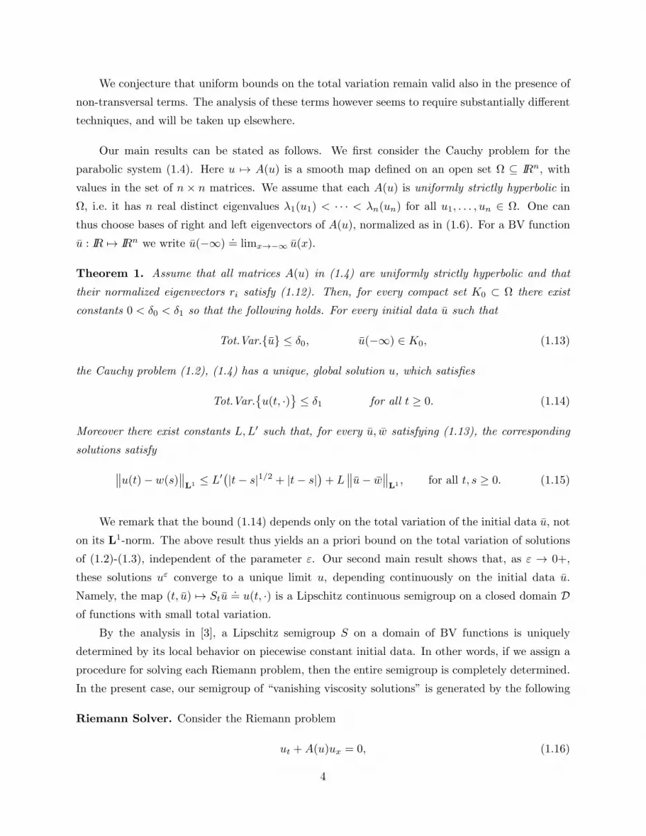
We conjecture that uniform bounds on the total variation remain valid also in the presence of

non-transversal terms. The analysis of these terms however seems to require substantially different

techniques, and will be taken up elsewhere.

Our main results can be stated as follows. We first consider the Cauchy problem for the

parabolic system (1.4). Here u 7→ A(u) is a smooth map defined on an open set Ω ⊆ IRn, with

values in the set of n × n matrices. We assume that each A(u) is uniformly strictly hyperbolic in

Ω, i.e. it has n real distinct eigenvalues λ1(u1) < · · · < λn(un) for all u1, . . . , un ∈ Ω. One can

thus choose bases of right and left eigenvectors of A(u), normalized as in (1.6). For a BV function

u : IR 7→ IRn we write u(−∞).= limx→−∞ u(x).

Theorem 1. Assume that all matrices A(u) in (1.4) are uniformly strictly hyperbolic and that

their normalized eigenvectors ri satisfy (1.12). Then, for every compact set K0 ⊂ Ω there exist

constants 0 < δ0 < δ1 so that the following holds. For every initial data u such that

Tot.Var.u ≤ δ0, u(−∞) ∈ K0, (1.13)

the Cauchy problem (1.2), (1.4) has a unique, global solution u, which satisfies

Tot.Var.u(t, ·)

≤ δ1 for all t ≥ 0. (1.14)

Moreover there exist constants L,L′ such that, for every u, w satisfying (1.13), the corresponding

solutions satisfy∥∥u(t)− w(s)∥∥L1 ≤ L′(|t− s|1/2 + |t− s|

)+ L

∥∥u− w∥∥L1 , for all t, s ≥ 0. (1.15)

We remark that the bound (1.14) depends only on the total variation of the initial data u, not

on its L1-norm. The above result thus yields an a priori bound on the total variation of solutions

of (1.2)-(1.3), independent of the parameter ε. Our second main result shows that, as ε → 0+,

these solutions uε converge to a unique limit u, depending continuously on the initial data u.

Namely, the map (t, u) 7→ Stu.= u(t, ·) is a Lipschitz continuous semigroup on a closed domain D

of functions with small total variation.

By the analysis in [3], a Lipschitz semigroup S on a domain of BV functions is uniquely

determined by its local behavior on piecewise constant initial data. In other words, if we assign a

procedure for solving each Riemann problem, then the entire semigroup is completely determined.

In the present case, our semigroup of “vanishing viscosity solutions” is generated by the following

Riemann Solver. Consider the Riemann problem

ut +A(u)ux = 0, (1.16)

4

u(0, x) =

u+ if x > 0,u− if x < 0,

(1.17)

with |u+−u−| suitably small. For u ∈ Ω, i = 1, . . . , n, define the i-rarefaction curve σ 7→ Ri(σ)(u)

as the integral curve of ri through u, parametrized so that

Ri(0)(u) = u,d

dσRi(σ)(u) = ri

(Ri(σ)(u)

). (1.18)

By the implicit function theorem there exist unique states ω0 = u−, ω1, . . . , ωn = u+ and wave

sizes σi such that

ωi = Ri(σi)(ωi−1) i = 1, . . . , n. (1.19)

Moreover, by strict hyperbolicity, there exist constants λ1 < . . . < λn−1 such that

λi(Ri(θσi)(ωi−1)

)∈ ]λi−1, λi[ θ ∈ [0, 1], i = 1, . . . , n.

with the convention λ0.= −∞, λn

.= ∞. For each i, consider the scalar function

Fi(σ).=

∫ σ

0

λi(Ri(s)(ωi−1)

)ds, (1.20)

and let zi(t, x) be the unique entropic solution to the Riemann problem for the scalar conservation

law

zt + Fi(z)x = 0, z(0, x) =

0 if x < 0,σi if x > 0.

(1.21)

A “solution” of the Riemann problem (1.16)-(1.17) is now defined by the assignment

u(t, x).= Ri

(zi(t, x)

)(ωi−1) if

x

t∈ [λi−1, λi]. (1.22)

We remark that, in general, the function in (1.22) is not a classical solution of (1.16). If

the system is not in conservation form, this function cannot even be regarded as a solution in

distributional sense. Yet, motivated by our next result it is appropriate to regard (1.22) as the

unique solution of (1.16)-(1.17) in the vanishing viscosity sense.

Theorem 2. Assume that all matrices A(u) in (1.4) are unifomly strictly hyperbolic and that their

eigenvectors satisfy (1.12). Then, for every compact set K0 ⊂ Ω there exist constants L,L′, δ0 > 0,

a closed domain D ⊂ L1loc and a continuous semigroup S : D × [0,∞[ 7→ D with the following

properties.

(i) Every function u satisfying (1.13) lies in the domain D of the semigroup.

(ii) For every u, w ∈ D with u− w ∈ L1 and every t, s ≥ 0 one has

‖Stu− Ssw‖L1 ≤ L′|t− s|+ L‖u− w‖L1 . (1.23)

5

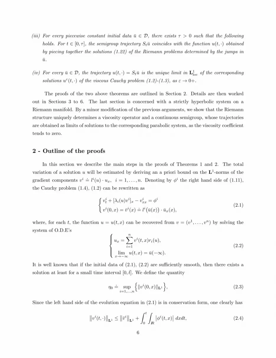
(iii) For every piecewise constant initial data u ∈ D, there exists τ > 0 such that the following

holds. For t ∈ [0, τ ], the semigroup trajectory Stu coincides with the function u(t, ·) obtained

by piecing together the solutions (1.22) of the Riemann problems determined by the jumps in

u.

(iv) For every u ∈ D, the trajectory u(t, ·) = Stu is the unique limit in L1loc of the corresponding

solutions uε(t, ·) of the viscous Cauchy problem (1.2)-(1.3), as ε→ 0+.

The proofs of the two above theorems are outlined in Section 2. Details are then worked

out in Sections 3 to 6. The last section is concerned with a strictly hyperbolic system on a

Riemann manifold. By a minor modification of the previous arguments, we show that the Riemann

structure uniquely determines a viscosity operator and a continuous semigroup, whose trajectories

are obtained as limits of solutions to the corresponding parabolic system, as the viscosity coefficient

tends to zero.

2 - Outline of the proofs

In this section we describe the main steps in the proofs of Theorems 1 and 2. The total

variation of a solution u will be estimated by deriving an a priori bound on the L1-norms of the

gradient components vi.= li(u) · ux, i = 1, . . . , n. Denoting by φi the right hand side of (1.11),

the Cauchy problem (1.4), (1.2) can be rewritten asvit + [λi(u)v

i]x − vixx = φi

vi(0, x) = vi(x).= li

(u(x)

)· ux(x),

(2.1)

where, for each t, the function u = u(t, x) can be recovered from v = (v1, . . . , vn) by solving the

system of O.D.E’s ux =

n∑i=1

vi(t, x)ri(u),

limx→−∞

u(t, x) = u(−∞).

(2.2)

It is well known that if the initial data of (2.1), (2.2) are sufficiently smooth, then there exists a

solution at least for a small time interval [0, t]. We define the quantity

η0.= sup

i=1,...,n

‖vi(0, x)‖L1

, (2.3)

Since the left hand side of the evolution equation in (2.1) is in conservation form, one clearly has

∥∥vi(t, ·)∥∥L1 ≤

∥∥vi∥∥L1 +

∫ t

0

∫IR

∣∣φi(t, x)∣∣ dxdt, (2.4)

6

therefore ∥∥vi(t, ·)∥∥L1 ≤ η0 + sup

i=1,...,n

∫ t

0

∫IR

∣∣φi(s, x)∣∣ dxds .= η(t). (2.5)

Therefore, if the total strength of the source term φi is bounded and of quadratic order w.r.t. η(t),

the solution of (2.1) is well defined for all t ≥ 0 if η0 is sufficiently small. The main goal of this

section is then to prove an a priori bound on the terms φi of the form

supi=1,...,n

∫ t

0

∫IR

∣∣φi(s, x)∣∣ dxds ≤ κη(t)2, (2.6)

for some constant κ > 0.

We start by choosing constants c, δ1 > 0 small enough so that the compact set

K1.=u ∈ IRn; dist(u, K0) ≤ δ1

(2.7)

is entirely contained inside Ω, and moreover

λj(u)− λi(v) ≥ c whenever i < j, u, v ∈ K1, |u− v| ≤ δ1. (2.8)

We also choose constants C0, C such that∣∣rj • λi(u)∣∣ ≤ C0,∣∣Gi

j,k(u)∣∣, ∣∣Hi

j,k(u)∣∣, ∣∣Ki

j,k,`(u)∣∣ ≤ C0 for all u ∈ K1 (2.9)

C ≥ max

2(n+ 1)2C0,

8√π

. (2.10)

In the first part of our analysis we shall assume that, for all i = 1, . . . , n, the initial data vi in (2.1)

satisfy ∫IR

∣∣vi(x)∣∣ dx ≤ η0, (2.11)∫IR

∣∣vix(x)∣∣ dx ≤ 4√πC2η20 , (2.12)

for some η0 > 0. We choose the constant η0 small enough so that

η0 ≤ min

c

4C,δ12n

. (2.13)

At a later stage, using standard smoothing properties of parabolic equations, we will remove the

assumption (2.12).

If η(t) > 2η0 for some t, by continuity there exists a time t > 0 such that η(t) < 2η0 for all

t ∈ [0, t[ and moreover η(t) = 2η0. We will show that for all 0 ≤ t ≤ t we have the estimates∫IR

∣∣φi(t, x)∣∣ dx < 8√πC3(2η0)

3 0 ≤ t ≤ t, (2.14)

7

∫ t

0

∫IR

∣∣φi(t, x)∣∣ dxdt < C

c

(2η0)2, (2.15)

so that it follows

η(t) < η0 +C

c

(2η0)2 ≤ 2η0. (2.16)

The above formula implies that η(t) < 2η0 for all t ≥ 0, i.e. the solution of (2.1) exists and has

bounded L1 norm for all t ≥ 0. In fact, recalling that the eigenvectors ri were chosen with unit

length, by (2.2) and the choice of η0 this yields∣∣u(t, x)− u(−∞)∣∣ ≤ Tot.Var.

u(t, ·)

≤

n∑i=1

∥∥v(t, x)∥∥L1 < n · 2η0 ≤ δ1.

(2.17)

Hence the function u takes values inside the compact set K1, and the bounds (2.8)-(2.9) hold.

A detailed proof of (2.13)-(2.14) will be worked out in Section 3, providing a priori bounds

on the L1 norms of the terms vjvk, vjxvk, vjvkv` in (1.11), for j 6= k. By (2.5), using (2.14) and

(2.15) we conclude ∫IR

∣∣vi(t, x)∣∣ dx ≤ η0 +C

c

(η(t)

)2 ≤ 2η0, (2.18)

∫IR

∣∣vix(t, x)∣∣ dx ≤ 8√πC2(η(t)

)2 ≤ 8√πC2(2η0)2. (2.19)

The second inequality provides a regularity estimate on the solution to (2.1).

The bounds (2.18)–(2.19) thus yield an a uniform bound on the total variation of u(t, ·).Indeed, for every t ≥ 0 one has

Tot.Var.u(t)

≤ δ1. (2.20)

This establishes global BV bounds on every solution u of (1.2), (1.4) whose initial data lies in the

domain

D∗ .=

u :IR 7→ IRn ; u is absolutely continuous, u(−∞) ∈ K0,∥∥li(u) · ux∥∥L1 ≤ η0,

∥∥(li(u) · ux)x∥∥L1 ≤ 4√πC2η20 , i = 1, . . . , n

.

(2.21)

In Section 4 we then observe that, by the smoothing properties of the parabolic system (1.4), one

can choose t0, δ0 > 0 so that the following holds. For every initial data u satisfying (1.13), the

corresponding solution of (1.2), (1.4) satisfies

u(t0) ∈ D∗, Tot.Var.u(t)

≤ δ1 for all t ∈ [0, t0]. (2.22)

8

The previous analysis can thus be applied to the corresponding Cauchy problem on [t0, ∞[ . This

yields the bounds (1.14), proving the first part of Theorem 1.

Concerning the estimates (1.15), the continuity of a BV solution as a function of time is a

well known result for parabolic equations. To prove the Lipschitz continuous dependence w.r.t. the

initial data, in Section 5 we first study the linearized equation describing the evolution of an

infinitesimal perturbation. Replacing u by u + εh in (1.4), letting ε → 0 and retaining terms of

order ε we obtain

ht +[DA(u) · h

]ux +A(u)hx = hxx, (2.23)

If the total variation of the reference solution u remains small, we show that every solution h =

h(t, x) of the linearized system (2.23) satisfies∫IR

∣∣h(t, x)∣∣ dx ≤ L ·∫IR

∣∣h(0, x)∣∣ dx for all t ≥ 0, (2.24)

for some uniform constant L. If now two initial data u, w are given, following [2] we construct the

smooth path

θ 7→ uθ.= θu+ (1− θ)w, θ ∈ [0, 1]. (2.25)

Calling t 7→ uθ(t, ·) the solution of (1.4) with initial data uθ, we can write

∥∥u(t)− w(t)∥∥L1 ≤

∫ 1

0

∥∥∥∥duθ(t)dθ

∥∥∥∥L1

dθ

≤ L ·∫ 1

0

∥∥∥∥duθ(0)dθ

∥∥∥∥L1

dθ

= L · ‖u− w‖L1 .

(2.26)

Indeed, the tangent vector

hθ(t, x).=duθ

dθ(t, x)

is a solution of the linearized Cauchy problem

hθt +[DA(uθ) · hθ

]uθx +A(uθ)hθx = hθxx, (2.27)

hθ(0, x) = hθ(x) = u(x)− w(x), (2.28)

hence it satisfies (2.24) for every θ. This completes the proof of Theorem 1.

We now give a proof of Theorem 2. For a fixed ε > 0, thanks to the coordinate rescaling

t 7→ t/ε, x 7→ x/ε, the solution uε of (1.2)-(1.3) can be written in the form

uε(t, x) = Uε(t/ε, x/ε),

9

where Uε is the solution of (1.4)-(1.5). Clearly, for all t ≥ 0 one has

Tot.Var.uε(t, ·)

= Tot.Var.

Uε(t, ·)

.

Therefore, by Theorem 1, for each initial condition u in the set

D0.=u ∈ L1

loc ; Tot.Var.u ≤ δ0, u(−∞) ∈ K0

(2.29)

the corresponding solution of (1.3) satisfies (1.14). Moreover, given two initial data u, w, from

(1.15) we deduce∥∥u(t)− w(s)∥∥L1 ≤ L′(√ε|t− s|+ |t− s|

)+ L

∥∥u− w∥∥L1 for all t, s ≥ 0. (2.30)

For each u ∈ D0 we can thus use Helly’s compactness theorem and deduce the existence of a

subsequence εν → 0 such that the corresponding solutions uεν converge to some function u, namely

limν→∞

uεν (t) = u(t) in L1loc , for all t ≥ 0. (2.31)

By a diagonalization argument, we can assume that, with the same sequence εν , the convergence

(2.31) holds for all solutions starting from a countable dense set of initial data in D0. In order to

characterize this limit and show that the whole sequence uε converges as ε → 0, we first derive

a bound on the propagation speed of perturbations. By studying again the linear variational

equation (2.23), in Section 6 we show that, for any interval [a, b] and any two initial data u, w, the

corresponding vanishing viscosity limit solutions satisfy∫ b−λt

a+λt

∣∣u(t, x)− w(t, x)∣∣ dx ≤ L ·

∫ b

a

∣∣u(x)− w(x)∣∣ dx . (2.32)

Here λ is a suitably large constant providing an upper bound for all wave speeds, so that∣∣λi(ω)∣∣ ≤ λ

for all ω ∈ K1, i = 1, . . . , n. We can now define

limν→∞

uεν (t, ·) = u(t, ·) .= Stu u ∈ D0. (2.33)

Indeed, since the limit (2.31) exists for a dense set of initial data u, the uniform continuity property

(2.32) implies the existence of the limit in (2.33) for all initial data in D0. By restricting this

definition to a smaller, positively invariant domain D ⊂ D0 we obtain a continuous semigroup

S : D × [0,∞[ 7→ D. In the case where ‖u− w‖L1 <∞, from (2.30) and (2.32) it follows (1.23).

It remains to show that the flow of S is compatible with the Riemann Solver defined in Section

1. By the property (2.32), it suffices to consider the case where the initial data has a single jump

as in (1.17), and show that the limit of viscous approximations converge to the solution defined at

(1.22).

10

Consider first the case where the initial datum u lies on a single i-rarefaction curve, say

u(x) = u(−∞) + z(x)ri(u(−∞)

).

Define the scalar function Fi as in (1.20). By the standard theory of scalar conservation laws [12],

it is well known that, as ε→ 0, the solution zε of the viscous Cauchy problem

zεt + Fi(zε)x = ε zεxx, zε(0, x) = z(x), (2.34)

converges to the unique entropic solution z of the scalar conservation law

zt + Fi(z)x = 0, zε(0, x) = z(x). (2.34′)

Since, by assumptions, all rarefaction curves are straight lines, the solution of (1.3) with initial

data (1.17) is given by

uε(t, x) = u(−∞) + zε(t, x)ri(u(−∞)

),

and thus converges as ε→ 0 to the function u given by

u(t, x) = u(−∞) + z(t, x)ri(u(−∞)

).

In particular, if u−, u+ in (1.17) lie on the same rarefaction curve, then uε converges to the solution

u defined in (1.22).

Since the semigroup S can be constructed using wave front tracking, it can be shown that

this case is sufficient to determine uniquely the semigroup. However, since we have in (2.32) a L1loc

dependence, it is easy to handle the general case.

Consider in fact a perturbed initial data of the form

uδ(x).=

u− if x < δ,ωi if iδ < x < (i+ 1)δ, i = 1, . . . , n− 1,u+ if x > nδ.

(2.35)

Keeping δ > 0 fixed and letting ε → 0, by the property (2.32) and the analysis of the previous

case, the corresponding viscous solutions uδ,ε converge to the function

uδ(t, x).= Ri

(zi(t, x− iδ)

)(ωi−1) if iδ + tλ ≤ x ≤ (i+ 1)δ − tλ,

with zi, λi as in (1.22). Note that, by the assumption (2.8) on the hyperbolicity of A(u), at time

t0 = δ/2λ the waves of the solution u(t0) have disjoint support at least of ct0, where c is the

constant in (2.8). Thus by the property (2.32) and the previous analysis we can extend uδ to all

t ≥ 0, and letting δ → 0 we obtain the desired result.

Since a Lipschitz continuous semigroup is entirely determined by its local behavior on piecewise

constant initial data, the previous analysis uniquely characterizes the limit of viscous approxima-

tions. In particular, this limit does not depend on the choice of the particular sequence εν in (2.33).

This completes the proof of Theorem 2.

11

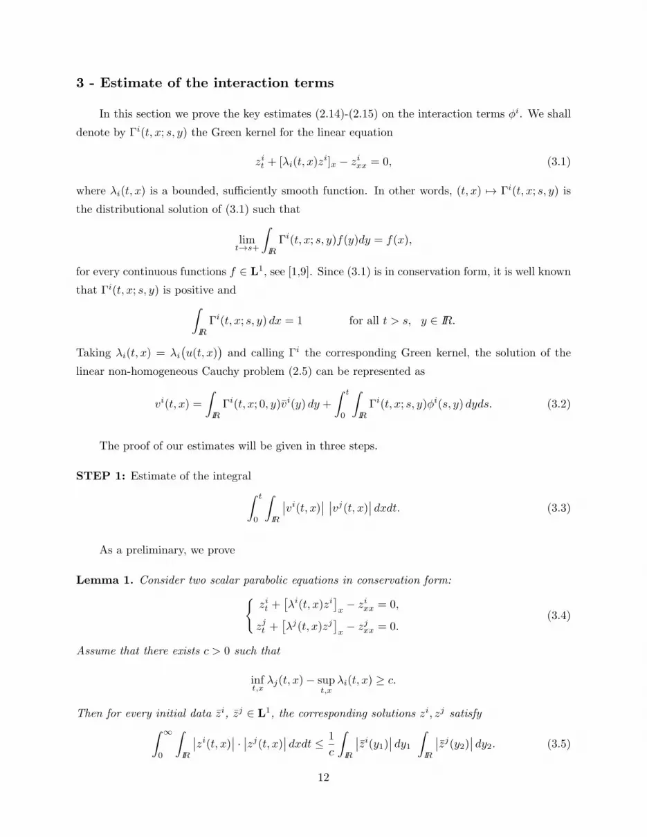
3 - Estimate of the interaction terms

In this section we prove the key estimates (2.14)-(2.15) on the interaction terms φi. We shall

denote by Γi(t, x; s, y) the Green kernel for the linear equation

zit + [λi(t, x)zi]x − zixx = 0, (3.1)

where λi(t, x) is a bounded, sufficiently smooth function. In other words, (t, x) 7→ Γi(t, x; s, y) is

the distributional solution of (3.1) such that

limt→s+

∫IR

Γi(t, x; s, y)f(y)dy = f(x),

for every continuous functions f ∈ L1, see [1,9]. Since (3.1) is in conservation form, it is well known

that Γi(t, x; s, y) is positive and∫IR

Γi(t, x; s, y) dx = 1 for all t > s, y ∈ IR.

Taking λi(t, x) = λi(u(t, x)

)and calling Γi the corresponding Green kernel, the solution of the

linear non-homogeneous Cauchy problem (2.5) can be represented as

vi(t, x) =

∫IR

Γi(t, x; 0, y)vi(y) dy +

∫ t

0

∫IR

Γi(t, x; s, y)φi(s, y) dyds. (3.2)

The proof of our estimates will be given in three steps.

STEP 1: Estimate of the integral∫ t

0

∫IR

∣∣vi(t, x)∣∣ ∣∣vj(t, x)∣∣ dxdt. (3.3)

As a preliminary, we prove

Lemma 1. Consider two scalar parabolic equations in conservation form:zit +

[λi(t, x)zi

]x− zixx = 0,

zjt +[λj(t, x)zj

]x− zjxx = 0.

(3.4)

Assume that there exists c > 0 such that

inft,xλj(t, x)− sup

t,xλi(t, x) ≥ c.

Then for every initial data zi, zj ∈ L1, the corresponding solutions zi, zj satisfy∫ ∞

0

∫IR

∣∣zi(t, x)∣∣ · ∣∣zj(t, x)∣∣ dxdt ≤ 1

c

∫IR

∣∣zi(y1)∣∣ dy1 ∫IR

∣∣zj(y2)∣∣ dy2. (3.5)

12

Proof. We first establish the bound

sup(y1,y2)∈IR2

y1 6=y2

∫ ∞

0

∫IR

Γi(t, x; 0, y1) · Γj(t, x; 0, y2) dxdt

≤ 1

c, (3.6)

where Γi, Γj denote the Green kernels corresponding to the two equations in (3.4). By possibly

performing a change of variable of the form x 7→ x − λt, which does not affect the value of the

integral (3.6), we can assume

λi(t, x) ≤ − c2< 0 <

c

2≤ λj(t, x).

This implies

λi(t, x).= λi(t, x) +

c

2≤ 0, λj(t, x)

.= λj(t, x)−

c

2≥ 0. (3.7)

We now observe that the product function K(t, x1, x2; s, y1, y2).= Γi(t, x1; s, y1) · Γj(t, x2; s, y2)

provides the Green kernel for the linear equation in two space variables:

Zt +[λi(t, x1)Z

]x1

+[λj(t, x2)Z

]x2

−∆Z = 0. (3.8)

In the following we denote by Gλ(t, x) the standard Gaussian kernel with constant drift λ and by

Gλx(t, x) its derivative w.r.t. x, i.e.

Gλ(t, x).=

1

2√πt

exp

− (x− λt)2

4t

, Gλ

x(t, x).=

−(x− λt)

4t√πt

exp

− (x− λt)2

4t

.

Writing (3.8) in the form

Zt −c

2Zx1 +

c

2Zx2 −∆Z = −

[λi(t, x1)Z

]x1

−[λj(t, x2)Z

]x2,

the corresponding Green kernel can be represented as

K(t, x1, x2; 0, y1, y2) = G−c/2(t, x1 − y1)Gc/2(t, x2 − y2)

−∫ t

0

∫∫IR2

G−c/2

x (t− s, x1 − z1)Gc/2(t− s, x2 − z2)

·K(s, z1, z2; 0, y1, y2)λi(s, z1)

dz1dz2 ds

−∫ t

0

∫∫IR2

G−c/2(t− s, x1 − z1)G

c/2x (t− s, x2 − z2)

·K(s, z1, z2; 0, y1, y2)λj(s, z2)

dz1dz2 ds.

13

We now compute

−∫IR+

∫IR

G−c/2(t, x− z1)Gc/2x (t, x− z2) dxdt =

∫IR+

∫IR

G−c/2x (t, x− z1)G

c/2(t, x− z2) dxdt

=

−12 e

(z1−z2)c/2 if z1 < z2,

0 if z1 > z2.

Using the above formula and assuming that y1 6= y2 (in this case we can change the order of

integration), recalling (3.7) and the fact that the kernel K is positive, we conclude∫IR+

∫IR

Γi(t, x; 0, y1)Γj(t, x; 0, y2) dxdt =

∫IR+

∫IR

K(t, x, x; 0, y1, y2) dxdt

≤ 1

c+

∫IR+

∫∫z1<z2

e(z1−z2)c/2K(s, z1, z2; 0, y1, y2)(λi(s, z1)− λj(s, z2)

)dz1dz2 ds

≤ 1

c.

This establishes (3.6).

Given any two initial conditions zi, zj , the corresponding solutions of (3.4) satisfy∫IR+

∫IR

∣∣zi(t, x)∣∣ ∣∣zj(t, x)∣∣ dxdt≤∫IR+

∫IR

∫∫IR2

∣∣zi(y1)∣∣Γi(t, x; 0, y1) ·∣∣zj(y2)∣∣Γj(t, x; 0, y2) dy1dy2 dxdt

≤∫IR

∣∣zi(y1)∣∣ dy1 · ∫IR

∣∣zj(y2)∣∣ dy2 · sup(y1,y2)∈IR2

y1 6=y2

∫IR+

∫IR

Γi(t, x; 0, y1) · Γj(t, x; 0, y2) dxdt

.

By (3.6) this yields (3.5), proving the lemma.

Consider now two equations of the form (2.1). The solutions vi(t, x), vj(t, x) can be written

in the form

vi(t, x) =

∫IR

Γi(t, x; 0, y)vi(y) dy +

∫ t

0

∫IR

Γi(t, x; s, y) φi(s, y) dyds,

vj(t, x) =

∫IR

Γj(t, x; 0, y)vj(y) dy +

∫ t

0

∫IR

Γj(t, x; s, y) φj(s, y) dyds.

(3.9)

Using (2.10) and the inductive assumptions (2.17), by (3.5) and (3.9) with easy calculations we

obtain ∫ t

0

∫IR

∣∣vi(t, x)∣∣ ∣∣vj(t, x)∣∣ dxdt ≤ 1

c

(η0 + max

i=1,...,n

∫ t

0

∫IR

∣∣φi(s, x)∣∣dxds)2

=1

c

(η(t)

)2 ≤ 1

c

(2η0)2.

(3.10)

14

STEP 2: Estimate of the integral∥∥vix(t)∥∥L1 =

∫IR

∣∣vix(t, x)∣∣ dx. (3.11)

Define the quantity

ξ(t).= sup

i=1,...,n0≤s≤t

∥∥vix(s)∥∥L1 . (3.12)

Using (2.9), (2.10), we have∫IR

∣∣φi(t, x)∣∣ dx ≤ n2C0η(t)ξ(t) + n2C0

(ξ(t)

)2+ n3C0η(t)

(ξ(t)

)2≤ C

2

(η(t)ξ(t) + ξ2(t) + nη(t)ξ2(t)

).

(3.13)

For convenience, for i = 1, . . . , n, introduce the quantities

λ∗i.= λi

(u(−∞)

), ‖λi‖∞

.= max

u∈K1

∣∣λi(u)− λ∗i∣∣, ‖λ′i‖∞

.= max

1≤j≤n,u∈K1

∣∣rj • λi(u)∣∣, (3.14)

Gi(t, x).= Gλ∗

i (t, x) =1

2√πt

exp

− (x− λ∗i t)

2

4t

. (3.15)

By (2.9 ), ‖λ′i‖∞ ≤ C0. We also observe that the heat kernel Gi(t, x) satisfies∫IR

∣∣Gix(t, x)

∣∣ dx =1√πt,

∫IR

∣∣Gixx(t, x)

∣∣ dx =

√2

πe· 1t. (3.16)

Define the time t by √t.= min

√π

32n‖λ′i‖∞η0,

√π

16Cη0

=

√π

16Cη0. (3.17)

Assume for simplicity that t ≤ t, where t is defined in section 2, the other case being completely

similar. For 0 ≤ t ≤ t we can write the solution as

vix(t, x) =

∫IR

Gi(t, x− y)viy(y) dy

−∫ t

0

∫IR

Gix(t− s, x− y)

∂

∂y

((λi(u)− λ∗i

)vi(s, y)

)dyds

+

∫ t

0

∫IR

Gix(t− s, x− y)φi(s, y) dyds.

Using (3.14), (3.16) and the assumption η(t) ≤ 2η0, the L1-norm of the second integral on the

right hand side of the above formula can be estimated as∫IR

∣∣∣∣∫ t

0

∫IR

Gix(t− s, x− y)

∂

∂y

((λi(u)− λ∗i

)vi(s, y)

)dy ds

∣∣∣∣ dx≤∫ t

0

∥∥Gix(t− s, ·)

∥∥L1 ·

∥∥∥∥ ∂∂y((λi(u)− λ∗i)vi(s, ·)

)∥∥∥∥L1

ds

≤∫ t

0

1√π(t− s)

·

[‖λi‖∞ξ(s) + ‖λ′i‖∞

(∑k

∥∥vk(s)∥∥L1

)∥∥vi(s)∥∥L∞

]ds

≤ 4n√π

√t‖λ′i‖∞η(t)ξ(t) ≤

2√π

√tC(2η0)ξ(t).

15

Using the above estimate together with η0 ≤ η(t) ≤ 2η0, for t ∈ [0, t] we obtain

supt∈[0, t ]

∥∥vix(t)∥∥L1 ≤ ‖vix‖L1 +1

4ξ(t) +

2√π

√tC

2

(η(t)ξ(t) + ξ2(t) + nη(t)ξ2(t)

),

so that

ξ(t) ≤ 4√πC2η20 +

1

4ξ(t) +

1

16η0

(η(t)ξ(t) + ξ2(t) + nη(t)ξ2(t)

).

By possibly reducing the value of η0, we can assume that(1 + 2

20√πC 2η0 +

8n√πC2 (2η0)

2

)< 2. (3.18)

Using (3.18) and a comparison argument, it is easy to conclude that

ξ(t) <8√πC2η2(t), (3.19)

if 0 ≤ t ≤ t.

Consider now the case t ≤ t ≤ t, and assume that (3.19) holds in the interval [t− t, t). Assume

moreover that t is the first time such that equality holds is (3.19). The x-derivative of the solution

vi of (2.1) can be written in the form

vix(t, x) =

∫IR

Gix(t, x− y)vi(t− t, y) dy

−∫ t

t−t

∫IR

Gix(t− s, x− y)

∂

∂y

((λi(u)− λ∗i

)vi(s, y)

)dy ds

+

∫ t

t−t

∫IR

Gix(t− s, x− y)φi(s, y) dy ds.

With a computation similar to the one above and using (2.9), (2.10), (3.18) and the assumption

η0 ≤ η(t) ≤ 2η0, for t ∈ [0, t] we obtain

sups∈[t−t,t]

∥∥vix(s)∥∥L1 ≤ 2√πtη(t) +

1

4sup

s∈[t−t,t]

∥∥vix(s)∥∥L1 +2√π

√tC

2

(η(t)ξ(t) + ξ2(t) + nη(t)ξ2(t)

)≤ 4√

πC2η2(t) +

1

4ξ(t) +

1

16η0

(η(t)ξ(t) + ξ2(t) + nη(t)ξ2(t)

),

hence a comparison argument shows that

ξ(t) <8√πC2η2(t). (3.20)

Using (3.19) and (3.20) we conclude that, for all 0 ≤ t ≤ t,

‖vix(t)‖L1 <8√πC2η2(t) ≤ 8√

πC2(2η0)2.

16

In particular, substituting (3.19), (3.20) in (3.13) we recover (2.14) for 0 ≤ t ≤ t.

STEP 3: Evaluation of the double integral∫ t

0

∫IR

∣∣vix(t, x)∣∣ ∣∣vj(t, x)∣∣ dxdt. (3.21)

The idea is to use the representations of the first derivative vix in terms of the heat kernel given

in the previous step to show that the quantity in (3.21) can be bounded in terms of the product of

L1-norms of vi and vj . Since these representations contain a convolution of vi with the heat kernel

G, we consider the family of functions vj(t+ τ, x+ z), with (τ, z) ∈ [0, t]× IR and we estimate the

quantity

I(σ) .= sup(τ,z)∈[0,σ]×IR

∫ σ−τ

0

∫IR

∣∣vix(t, x)∣∣ ∣∣vj(t+ τ, x+ z)∣∣ dxdt, (3.22)

where σ ≥ 0. As in the previous step, we compute the L1 norm of the source term: for all 0 ≤ t ≤ t

we have

Q(t).=

∫ t

0

∫IR

∣∣φi(t, x)∣∣dxdt ≤ n2C0

cη2(t) + n2C0I(t) +

n3C0

c

8√πC2(2η0)2η2(t)

≤ C

2η2(t)

(1 +

8n√πC2(2η0)2)

+C

cI(t).

(3.23)

We first study the case σ ≤ t, with t defined at (3.17). We write the solution of (2.1) as

vix(t, x) =

∫IR

Gi(t, x− y)viy(y) dy −∫ t

0

∫IR

Gix(s, y)

(λi(u)− λ∗i

)vix(t− s, x− y) dyds

−∫ t

0

∫IR

Gix(s, y)

(n∑

k=1

rk • λi(u)vk)vi(t− s, x− y) dyds

+

∫ t

0

∫IR

Gix(s, y)φ

i(t− s, x− y) dyds.

We first estimate the following integrals, whose computation is carried out in appendix A:∫ σ−τ

0

∫∫IR2

∣∣∣Gi(t, x− y)vix(y)vj(t+ τ, x+ z)

∣∣∣dxdydt ≤ 4

c√πC2η3(σ), (3.24)

∫ σ−τ

0

∫ t

0

∫∫IR2

∣∣∣Gix(s, y)

(λi(u)− λ∗i

)vix(t− s, x− y)vj(t+ τ, x+ z)

∣∣∣ dxdy dsdt ≤ 1

8I(σ), (3.25)

∫ σ−τ

0

∫ t

0

∫∫IR2

∣∣∣Gix(s, y)(rk • λi)vkvi(t− s, x− y)vj(t+ τ, x+ z)

∣∣∣ dxdy dsdt≤ 16

cπ

√t‖λ′i‖∞C2η4(σ),

(3.26)

17

∫ σ−τ

0

∫ t

0

∫∫IR2

∣∣∣Gix(s, y)φ

i(t− s, x− y)vj(t+ τ, x+ z)∣∣∣ dxdy dsdt

≤ 2√πCη(σ)

∫ σ

0

∫IR

∣∣φi(t, x)∣∣dxdt. (3.27)

Using the above estimates we obtain

I(σ) ≤ 6

c√πC2η3(σ) +

1

8I(σ) + 2√

πCη(σ)Q(σ). (3.28)

Using (3.23), (3.18) and a comparison argument, this shows that I(σ) is uniformly bounded, in

the case σ ≤ t by

I(σ) ≤ 8

c√πC2η3(σ).

If t ≤ σ ≤ t, we split the integrals in (3.22) in two parts:∫ σ

0

∫IR

∣∣vix(t, x)∣∣ ∣∣vj(t+ τ, x+ z)∣∣ dxdt

=

∫ t

0

+

∫ σ

t

∫IR

∣∣vix(t, x)∣∣ ∣∣vj(t+ τ, x+ z)∣∣ dxdt,

and write vix(t, x), t ≥ t, using the integral representation

vix(t, x) =

∫IR

Gix(t, y)v

i(t− t, x− y) dy

−∫ t

0

∫IR

Gix(s, y)

(λi(u)− λ∗i

)vix(t− s, x− y) dyds

−∫ t

0

∫IR

Gix(s, y)

(n∑

k=1

rk • λi(u)vk)vi(t− s, x− y) dyds

+

∫ t

0

∫IR

Gix(s, y)φ

i(t− s, x− y) dyds.

We now use the further estimates proved in Appendix A if σ− τ > t, the other case being entirely

similar: ∫ σ−τ

t

∫ ∫IR2

∣∣∣Gix(t, y)v

i(t− t, x− y)vj(t+ τ, x+ z)∣∣∣ dxdy dt ≤ 8

cπCη3(σ), (3.29)

∫ σ−τ

t

∫ t

0

∫∫IR2

∣∣∣Gix(s, y)

[λi(u)− λ∗i

]vix(t− s, x− y)vj(t+ τ, x+ z)

∣∣∣ dxdy dsdt ≤ 1

8I(σ), (3.30)

∫ σ−τ

t

∫ t

0

∫∫IR2

∣∣∣Gix(s, y)

((rk • λi)vk

)vi(t− s, x− y)vj(t+ τ, x+ z)

∣∣∣ dxdy dsdt≤ 16

cπ

√t‖λ′i‖∞C2η4(σ),

(3.31)

18

∫ σ−τ

t

∫ t

0

∫∫IR2

∣∣∣Gix(s, y)φ

i(t− s, x− y)vj(t+ τ, x+ z)∣∣∣ dxdy dsdt ≤ 2√

πCη(σ)Q(σ). (3.32)

Using the above estimates, for all (τ, z) ∈ [0, t]× IR we obtain∫ σ−τ

t

∫IR

∣∣vix(t, x)∣∣ ∣∣vj(t+τ, x+z)∣∣ dxdt ≤ 8

πCη3(σ)

c+

2

c√πC2η3(σ)+

1

8Iσ+

2√πCη(σ)Q(σ). (3.33)

Adding the two expressions (3.28), (3.33), and recalling (2.10), we obtain

I(σ) ≤ 1

c

(8

πC +

8√πC2

)η3(σ) +

I(σ)4

+2√πCη(σ)Q(σ)

≤ 10√π

C2

cη3(σ) +

I(σ)4

+2√πCη3(σ)Q(σ),

from which using a comparison argument we deduce

I(σ) ≤ 20√π

C2

cη3(σ). (3.34)

Note that (3.34) holds for every σ ≤ t. This yields the desired bound for (3.22), namely∫ t

0

∫IR

∣∣vix(t, x)∣∣ ∣∣vj(t, x)∣∣ dxdt ≤ lim supσ→t

I(σ) ≤ 20√π

C2

cη3(t). (3.35)

Using (3.10), (3.18), (3.19)–(3.20) and (3.35), we now prove the estimates (2.6)∫ t

0

∫IR

∣∣φi(t, x)∣∣ dxdt ≤ n2C0

cη2(t)

(1 + 2

20√πC(2η0)+

8n√πC2(2η0)2)

<n2C0

cη2(t) · 2 ≤ C

cη2(t),

(3.37)

4 - Nonsmooth initial data

The estimate (3.37) proves that if t is the first time such that η(t) = 2η0, then (2.5) implies

that

2η0 = η(t) < η0 +C

c

(2η0)2 ≤ 2η0, (4.1)

generating a contradiction. Thus, if u(0, x) lies in the set

D∗ .=u : IR 7→ IRn ; u(−∞) ∈ K0,

∥∥li(u) · ux∥∥L1 ≤ η0,∥∥(li(u) · ux)x∥∥L1 ≤ 4√πC2η20 , i = 1, . . . , n

,

(4.2)

19

the solution can be extended for all t ≥ 0 and it has bounded variation: namely

‖vi(t)‖L1 ≤ 2η0. (4.3)

In this section we prove that the domain can be extended to all functions with suitably small

total variation. The main argument in this last step of the proof is quite simple: If the total

variation of the initial data u is very small, after a short interval of time the corresponding solution

of (1.4) will be inside the domain D∗, thanks to the smoothing properties of the parabolic system.

Hence our previous analysis can be applied.

With a linear change of coordinates, we can assume that A∗ .= A

(u(−∞)

)= diag(λ∗1, . . . , λ

∗n).

Denoting with ei the i-th unit vector and writing ui.= ei · u, we can write the solutions of (1.4) in

the form

ui(t, x) =

∫IR

Gi(t, x− y)ui(y) dy −∫ t

0

∫IR

Gi(t− s, x− y) ei ·(A(u)−A∗)ux(s, y) dyds, (4.4)

uix(t, x) =

∫IR

Gi(t, x− y)dui(y)−∫ t

0

∫IR

Gix(t− s, x− y) ei ·

(A(u)−A∗)ux(s, y) dyds, (4.5)

uixx(t, x) =

∫IR

Gix(t, x− y)dui(y)−

∫ t

0

∫IR

Gix(t− s, x− y) ei ·

[(A(u)−A∗)ux(s, y)]

xdyds, (4.6)

with obvious meaning of notations. Recall that Gi .= Gλ∗

i is the Green kernel defined at (3.15).

We look for an estimate of the form

‖uxx(t)‖L1 ≤ CTot.Var.u√

t. (4.7)

Defining the time t0 and the constant C as

√t0

.=

√π

32n‖DA‖∞ · Tot.Var.u, C

.= max

9√π, ‖DA‖∞

,

we claim that (4.7) holds for t ≤ t0 if the initial datum is enough smooth. Clearly (4.7) is a strict

inequality for t sufficiently small. Using the same techniques as in Section 3, step 2, if 0 < t < t0

we can estimate the L1 norms of (4.5) and (4.6) as∥∥ux(t)∥∥L1 ≤ Tot.Var.u+ 2n√π

√t∥∥A−A∗∥∥

∞ sup0<s≤t

∥∥ux(s)∥∥L1 ≤ 2Tot.Var.u

∥∥uxx(t)∥∥L1 <Tot.Var.u√

πt+

8n√πC‖DA‖∞ · Tot.Var.u · sup

0<s≤t

∥∥ux(s)∥∥L1

≤ CTot.Var.u√

t,

(4.8)

where

‖A−A∗‖∞.= max

u∈K1

∣∣A(u)−A∗∣∣, ‖DA‖∞.= max

u∈K1

∣∣∣∣ dduA(u)∣∣∣∣ . (4.9)

20

Here the matrices A(u) are regarded as linear operators in L(IRn, IRn), and IRn has the norm

‖v‖ .=∑n

i=1 |vi|. This concludes the proof if the initial datum is sufficiently smooth. Since the

estimates (4.7)-(4.8) depend only on the BV norm of u, by a density argument it follows that (4.7)

holds for any enough small BV function. In particular, at time t0 form (4.7) we have∥∥uxx(t0)∥∥L1 ≤ 32n√πC2(Tot.Var.u

)2. (4.10)

With easy computations, from (1.7) it follows that the components vix are given by

vi =n∑

j=1

(li · ej) ujx, vix =n∑

j=1

(li · ej) ujxx +n∑

j,k=1

(ek • li) · ej ujxukx. (4.11)

Therefore, for a suitable constant C ′ depending on ‖DA‖∞, by (4.10)-(4.11) we have∥∥vi(t0)∥∥L1 ≤ nC ′∥∥ux(t0)∥∥L1 ≤ 2nC ′ · Tot.Var.u ≤ η0,∥∥vix(t0)∥∥L1 ≤ nC ′(1 + n

∥∥ux(t0)∥∥L1

)∥∥uxx(t0)∥∥L1

≤ nC ′(1 + 2n · Tot.Var.u

)32n√πC2(Tot.Var.u

)2≤ 4√

πC2η20 ,

(4.12)

provided that Tot.Var.u is sufficiently small and C big enough. All previous arguments can now

be applied to the solution u on the interval [t0, ∞[ . This completes the proof of the first part of

Theorem 1.

5 - L1 stability of viscous solutions

In this section we prove the stability estimate (1.15) for solutions u of (1.4). Toward this goal,

we first study the linear variational equation satisfied by infinitesimal perturbations. The evolution

equation (2.23) can be more conveniently written as

ht + [A(u)h]x + (h •A(u))ux − (ux •A(u))h = hxx . (5.1)

We first consider the case in which the initial data u is in DW . Defining the components of h and

u as

h =∑

hjrj(u), ux =∑

vjrj(u), (5.2)

with computations entirely similar to (1.7)–(1.10) we obtain

ht +n∑

j=1

(λjhj)xrj +

n∑j,k=1

λjhjvkrk • rj

+n∑

j,k=1

(vjhk − hjvk)

(λjrk • rj + (rk • λj)rj −

n∑`=1

λ`

(l` · (rk • rj)

)r`

)

=n∑

j=1

hjxxrj + 2n∑

j,k=1

hjxvkrk • rj +

n∑j,k=1

hjvkxrk • rj +n∑

j,k,`=1

hjvkv`r` • (rk • rj),

21

ht =n∑

j=1

hjtrj −n∑

j,k=1

λkhjvk(rk • rj) +

n∑j,k=1

hjvkx(rk • rj)

+n∑

j,k,`=1

hjvkv`(r` • rk) • rj ,

n∑j=1

hjtrj +

n∑j=1

(λjhj)xrj +

n∑j,k=1

(λj − λk)hjvk(rk • rj)

+n∑

j,k=1

(vjhk − hjvk)

(λjrk • rj + (rk • λj)rj −

n∑`=1

λ`

(l` · (rk • rj)

)r`

)

=n∑

j=1

hjxxrj + 2n∑

j,k=1

hjxvkrk • rj +

n∑j,k,`=1

hjvkv`(r` • (rk • rj)− (r` • rk) • rj

),

(5.3)

The inner product of (5.3) with li(u) yields

hit + [λihi]x − hixx =

n∑j,k=1

(λk − λi)li · [rk, rj ]hjvk + 2

n∑j,k=1

li · (rk • rj)hjxvk

+n∑

j,k,`=1

li ·(rl • (rk • rj)− (r` • rk) • rj

)hjvkv` +

n∑k=1

(hivk − hkvi)(rk • λi)

.=

n∑j,k=1j 6=k

Gij,k(u)h

jvk +n∑

j,k=1j 6=k

Hij,k(u)h

jxv

k +n∑

j,k,`=1k 6=`

Kij,k,`(u)h

jvkv`

+n∑

j,k=1j 6=k

J ij,k(u)h

j(vk)2 +n∑

k=1k 6=i

Lik(u)(h

ivk − hkvi)

.= ψi(u, v, h).

(5.4)

The following estimates are quite similar to those in Sections 2 - 3.

Let the constant C0 provide an upper bound for the absolute values of all functions Gij,k, H

ij,k,

Kij,k,l, J

ij,k, L

ik, as u ranges over the compact set K1. For a given initial data h, the functions hi

satisfy the equations hit +

[λi(u)h

i]x− hixx = ψi(t, x)

hi(0, x) = hi(x).= li

(u(x)

)· h(x).

(5.5)

Here ψi .= ψi(u, v, h) is the right hand side of (5.4). We assume that there exists a constant ξ0

such that

‖hi‖L1 ≤ ξ0,

∫IR

∣∣hx(x)∣∣ dx ≤ 4√πC2(2η0)ξ0, i = 1, . . . , n. (5.6)

Since the right hand side of (5.5) is in conservation form, we have

‖hi(t)‖L1 ≤ ξ0 + maxi=1,...,n

∫ t

0

∫IR

∣∣φi(s, x)∣∣dxds .= ξ(t), (5.7)

22

so that if we can prove that for some constant κ′ < 1

maxi=1,...,n

∫ t

0

∫IR

∣∣φi(s, x)∣∣dxds ≤ κ′ξ(t), (5.8)

we are done.

The proof involves three steps, entirely similar to the ones in Section 3.

1. Writing the solutions hi(t, x), vj(t, x) in the integral form

hi(t, x) =

∫IR

Γi(t, x; 0, y)hi(y) +

∫ t

0

∫IR

Γi(t, x; s, y)ψi(s, y) dyds,

vj(t, x) =

∫IR

Γj(t, x; 0, y)vj(y) dy +

∫ t

0

∫IR

Γj(t, x; s, y)φj(s, y) dyds,

after some calculations we obtain∫ ∞

0

∫IR

∣∣hi(t, x)∣∣ ∣∣vj(t, x)∣∣ dxdt ≤ 1

c

(η0 +

C

c(2η0)

2

)(ξ0 +

∫ t

0

∫IR

∣∣φ(s, x)∣∣dxds)≤ 1

c2η0ξ(t),

(5.9)

because η(t) ≤ 2η0.

2. Concerning∥∥hix(t)∥∥L1 , for every t ≥ 0 the same calculations as in Section 3, step 2, yield∫

IR

∣∣hix(t, x)∣∣ dx ≤ 8√πC22η0ξ(t), (5.10)

∫IR

∣∣ψ(t, x)∣∣dx ≤ 8√πC3(2η0)2ξ(t). (5.11)

3. Furthermore, the same computation as in Section 3, step 3 yields∫ ∞

0

∫IR

∣∣hix(t, x)∣∣ ∣∣vj(t, x)∣∣ dxdt ≤ 20√π

C2

c(2η0)

2ξ(t). (5.12)

Using the above estimates (5.8)–(5.12) and recalling that η0 also satisfies (3.18), we obtain∫ t

0

∫IR

∣∣ψi(s, x)∣∣ dxds ≤ C0

c2η0ξ(t)

[n2(1 + 2

20√πC (2η0) +

8n√πC2 (2η0)

2

)+ 2n

]≤ C

c2η0ξ(t),

(5.13)

By (2.13), the quantity ξ(t) is bounded by

limt→+∞

ξ(t) =

(1− C

c2η0

)−1

ξ0 ≤ 2ξ0, (5.14)

23

so that the functions hi have uniformly bounded L1 norm:

‖h(t)‖L1 ≤ 2ξ0. (5.15)

We consider now the case u ∈ D and h ∈ BV . Denoting the components hi.= ei · h, we can

write the solution of (5.1) in the form

hi(t, x) =

∫IR

Gi(t, x− y)dhi(y)−∫ t

0

∫IR

Gix(t− s, x− y)ei ·

[(A(u)−A∗)h(s, y)] dyds

+

∫ t

0

∫IR

Gi(t− s, x− y)ei ·[(ux •A(u)

)h(s, y)−

(h •A(u)

)ux(s, y)

]dyds,

(5.16)

hix(t, x) =

∫IR

Gix(t, x− y) dhi −

∫ t

0

∫IR

Gix(t− s, x− y)ei ·

[(A(u)−A∗)h(s, y)]

xdyds

+

∫ t

0

∫IR

Gix(t− s, x− y)ei ·

[(ux •A(u)

)h(s, y)−

(h •A(u)

)ux(s, y)

]dyds.

(5.17)

Using the same techniques of Section 4, in this case relying on the assumptions

∥∥hx(t)∥∥L1 ≤ C‖h‖L1√

t, C = max

9√π, ‖DA‖∞

,

√t <

√t0

.=

1

9nC‖DA‖∞ · Tot.Var.u,

(5.18)

for h, and recalling (4.17), we can estimate the L1-norms of (5.16) and (5.17) as

∥∥h(t)∥∥L1 ≤ ‖h‖L1 +

(4C +

4√π

)n√t‖DA‖∞ · Tot.Var.u · sup

0<s≤t

∥∥h(s)∥∥L1 ≤ 2‖h‖L1 ,

∥∥hx(t)∥∥L1 <‖h‖L1√πt

+16n√πC‖DA‖∞ · Tot.Var.u · sup

0<s≤t

∥∥h(s)∥∥L1 ≤ C

‖h‖L1√t.

In particular at time t0, repeating the arguments at (4.22), for some constant C ′ we have∥∥hi(t0)∥∥L1 ≤ nC ′ ∥∥h(t0)∥∥L1 ≤ 2nC ′ · ‖h‖L1 ≤ ξ0,∥∥hix(t0)∥∥L1 ≤ nC ′ (1 + 2nTot.Var.u)‖hx(t0)‖L1

≤ nC ′ (1 + 2nTot.Var.u)9nC3Tot.Var.u‖h‖L1 ≤ 4√

πC2 2η0ξ0,

(5.19)

provided that C is big enough and the total variation of u sufficiently small. The previous estimates

on the norms∥∥hi(t)∥∥ can thus be applied for t ∈ [t0, ∞[ , proving the estimates (2.24) on tangent

vectors. By (2.26), this completes the proof of Theorem 1.

24

6 - The vanishing viscosity limit

To complete the proof of Theorem 2 given in Section 2, it only remains to prove the bound

(2.32), for some constants L, λ. Toward this goal, we first establish an estimates on the size of a

solution h to the linear variational equation (5.1). Using the integral representation

h(t, x) =

∫IR

G(t, x− y)h(y) dy −∫ t

0

∫IR

Gx(t− s, x− y)A(u)h(s, y) dyds

+

∫ t

0

∫IR

G(t− s, x− y)[(ux •A(u)

)h(s, y)−

(h •A(u)

)ux(s, y)

]dyds,

(6.1)

we obtain the bound∣∣h(t, x)∣∣ ≤∫IR

G(t, x− y)∣∣h(y)∣∣ dy + ‖A‖∞

∫ t

0

∫IR

∣∣Gx(t− s, x− y)∣∣ ∣∣h(s, y)∣∣ dyds

+ 2‖DA‖∞∫ t

0

∫IR

∥∥ux(s)∥∥L∞ ·G(t− s, x− y)∣∣h(s, y)∣∣ dyds . (6.2)

Assuming that the initial data satisfies∣∣h(0, x)∣∣ ≤ e−x for all x ∈ IR, (6.3)

we claim that ∣∣h(t, x)∣∣ ≤ E+(t, x).= f(t) exp

4‖DA‖∞ ·

∫ t

0

∥∥ux(s)∥∥L∞ ds+ t− x

(6.4)

for all t ≥ 0, x ∈ IR, where f is an increasing function such that

f(t) ≥ 1 +

∫ t

0

2‖A‖∞f(s)(

1√t− s

+√π

)ds, f(0) = 1.

It is easy to show that we can take a function f(t) satisfying f(t) ≤ 2expCt, if the constant C

is big enough. The bound (6.4) follows from the estimates (see appendix B)∫IR

G(t, x− y)E+(0, y) dy ≤ et−x, (6.5)

‖A‖∞ ·∫ t

0

∫IR

∣∣Gx(t− s, x− y)∣∣E+(s, y) dyds ≤ 1

2E+(t, x)− 1

2et−x, (6.6)

2‖DA‖∞ ·∫ t

0

∫IR

∥∥ux(s)∥∥L∞ ·G(t− s, x− y)E+(s, y) dyds ≤ 1

2E+(t, x)− 1

2et−x, (6.7)

by a standard comparison argument. An entirely similar computation shows that, if∣∣h(0, x)∣∣ ≤ ex,

then for all t, x one has

∣∣h(t, x)∣∣ ≤ E−(t, x).= f(t) exp

4‖DA‖∞ ·

∫ t

0

∥∥ux(s)∥∥L∞ ds+ t+ x

. (6.8)

25

Observe that, by (4.19), we can choose a constant λ large enough so that

E+(t, x) ≤ 2eλ(√t+t)−x, E−(t, x) ≤ 2eλ(

√t+t)+x . (6.9)

The estimates (6.9) are very rough bounds on the solutions of (6.1): in fact we just need a bound

on the speed of propagation of perturbation. Now consider any two initial data u, w satisfying the

assumption (1.13) of Theorem 1. For every interval [a, b] and any λ > λ, defining the path θ 7→ uθ

as in (2.25), we compute∫ b−λt

a+λt

∣∣u(t, x)− w(t, x)∣∣ dx ≤

∫ 1

0

∫ b−λt

a+λt

∣∣∣∣duθdθ (t, x)

∣∣∣∣ dx dθ=

∫ 1

0

∫ b−λt

a+λt

∣∣hθ(t, x)∣∣ dx dθ , (6.10)

where hθ is the solution of the Cauchy problem (2.27)-(2.28). By linearity, we can write this

solution as a sum:

hθ = hθ1 + hθ2 + hθ3,

where hθj , j = 1, 2, 3 denote respectively the solutions of (2.27) with initial data

hθ1(0, x) =

u(x)− w(x) if x ∈ [a, b],

0 otherwise,

hθ2(0, x) =

u(x)− w(x) if x < a,

0 otherwise,hθ3(0, x) =

u(x)− w(x) if x > b,0 otherwise.

Applying the estimates (2.24) to hθ1, (6.4) to hθ2 and (6.8) to hθ3 we obtain∫ b−λt

a+λt

∣∣u(t, x)− w(t, x)∣∣ dx ≤

∫ 1

0

∫ b−λt

a+λt

(∣∣hθ1(t, x)∣∣+ ∣∣hθ2(t, x)∣∣+ ∣∣hθ3(t, x)∣∣) dxdθ≤ L · ‖hθ1(0)‖L1 + 2(b− a− 2λ)

∥∥hθ(0, ·)∥∥L∞ ·

(sup

x<b−λteλ(

√t+t)−b+x + sup

x>a+λtea+λ(

√t+t)−x

)≤ L ·

∫ b

a

∣∣u(x)− w(x)∣∣ dx+ 2(b− a)‖u− w‖L∞ · e(λ−λ)t+λ

√t.

(6.11)

Given ε > 0, consider now two solutions uε, wε of (1.3), with initial data u, w. Applying the

previous estimates to the corresponding solutions obtained via the rescalings t 7→ t/ε, x 7→ x/ε,

and observing that the distance∣∣u(x)− w(x)

∣∣ is always bounded by the diameter of the compact

set K1, from (6.11) we deduce∫ b−λt

a+λt

∣∣uε(t, x)− wε(t, x)∣∣ dx ≤ L ·

∫ b

a

∣∣u(x)− w(x)∣∣ dx+ 2(b− a) · diam(K1) · e(λ−λ)t/ε+λ

√t/ε.

Letting ε→ 0, the vanishing viscosity limits uε → u, wε → w thus satisfy∫ b−λt

a+λt

∣∣u(t, x)− w(t, x)∣∣ dx ≤ L ·

∫ b

a

∣∣u(x)− w(x)∣∣ dx. (6.12)

Since (6.12) is valid for every λ > λ, it implies (2.32).

26

7 - Hyperbolic systems on manifolds

Let M be a smooth n-dimensional Riemann and call Tu the tangent space at u ∈ M. At

each point u, let A(u) : Tu 7→ Tu be a linear mapping, smoothly depending on u ∈ M. Assume

that each A(u) is strictly hyperbolic, i.e. it has n real distinct eigenvalues λ1(u) < · · · < λn(u). If

u : [0,∞[×IR 7→ M is a smooth map, at any given (t, x) the partial derivatives ut, ux are vectors

in Tu(t,x). It is thus meaningful to consider the system

ut +A(u)ux = 0 (7.1)

In a given set of coordinates, this yields a standard quasilinear hyperbolic system. Smooth solutions

are thus well defined. On the other hand. since the equations are not in conservation form, there

is no canonical way for defining discontinuous solutions.

Toward this goal, a possible approach is to consider a Riemannian structure onM. In this case,

one can choose bases of right and left eigenvectors r1(u), . . . , rn(u) ∈ Tu and l1(u), . . . , ln(u) ∈ T ∗u

normalized as in (1.6):

⟨ri, ri

⟩= 1, li · rj =

1 if i = j,0 if i 6= j.

(7.2)

For any ε > 0 we can now consider the parabolic system

ut +A(u)ux = ε∑i

(li(u) · ux

)xri(u). (7.3)

Definition. If there exists a sequence of solutions uε of (7.3) which converges to a function

u = u(t, x) in L1loc, we say that u is a vanishing viscosity solution of (7.1).

The same computations as in (1.7)–(1.9) now yield

∑i

(uix)tri +∑i

(λiuix)xri +

∑j 6=k

λjujxu

kx[rk, rj ] = ε

∑i

(uix)xxri + 2∑j 6=k

(ujx)xukx[rk, rj ]

. (7.4)

Taking the products of (7.4) with li(u) and calling vi.= li(u) · uix, i = 1, . . . , n, we obtain a system

similar to (1.11), where the quadratic terms involve only products of waves of distinct families:

vit + (λivi)x − vixx =

∑j 6=k

Gijkvjvk +

∑j 6=k

Hijkvjxv

k. (7.5)

All of our previous analysis can thus be applied. In the following, for simplicity we assume that

a compact K0 ⊂ M is given, which lies in the domain of a single chart. In this case, the total

variation of a function u : IR 7→ M and its L1-norm can be referred to one particular system of

coordinates. The extension to the general case is straightforward.

27

Theorem 3. Let (7.1) be a strictly hyperbolic system on a Riemannian manifold M. For every

compact set K0 ⊂ M, there exist constants L,L′, η0 > 0, a closed domain D ⊂ L1loc and a

continuous semigroup S : D × [0,∞[ 7→ D with the following properties.

(i) Every function u satisfying (1.13) lies in the domain D of the semigroup.

(ii) For every u, w ∈ D with u− w ∈ L1 and every t, s ≥ 0 one has

‖Stu− Ssw‖L1 ≤ L′|t− s|+ L‖u− w‖L1 . (1.23)

(iii) For every piecewise constant initial data u ∈ D, there exists τ > 0 such that the following

holds. For t ∈ [0, τ ], the semigroup trajectory Stu coincides with the function u(t, ·) obtained

by piecing together the solutions of the Riemann problems determined by the jumps in u,

constructed by the Riemann Solver at (1.16)–(1.22).

(iv) Every trajectory of the semigroup is a vanishing viscosity solution of (7.1).

Observe that all steps in the construction of the Riemann Solver at (1.18)–(1.22) remain

meaningful also in the case of a Riemann manifold.

To prove the theorem, we observe that all the estimates derived in the previous sections

remain valid in this case. In particular, for any smooth initial data u : IR 7→ M with small total

variation, the corresponding solution of (7.3) is well defined for all t ≥ 0, and its total variation

remains uniformly small. Moreover, by the analysis in Sections 5-6, these solutions depend Lipschitz

continuously on the initial data, with a Lipschitz constant independent of ε > 0, and converge to

a limit as ε→ 0.

On the other hand, by the results in [14], the Riemann Solver described at (1.18)–(1.22)

generates a unique Lipschitz semigroup S. To show that the trajectories of this semigroup coincide

with our vanishing viscosity limits, by [3] it suffices to check the case of a Riemann initial data.

Assume first that both states u−, u+ in (1.17) lie on a single i-rarefaction curve, say

u+ = Ri(σi)(u−).

Then the particular form of the diffusion operator implies that the solution of (7.3) remains on the

same i-rarefaction curve for all positive times. We can thus write

u(t, x) = Ri

(z(t, x)

)(u−),

where z is the solution of the scalar Cauchy problem (1.21).

The general case is proved by considering small perturbations uδ of the initial data, as in

(2.35), and using the Lipschitz continuous dependence of vanishing viscosity solutions.

28

Appendix A

By the same computations as in Section 3, step 1, it follows that (3.10) holds also if we

translate vj : ∫ σ−u

0

∫IR

∣∣vi(t, x)∣∣ ∣∣vj(t+ u, x+ y)∣∣dxdt ≤ 1

c

(η(t)

)2 ≤ 1

c

(2η0)2. (A.1)

A.1. Estimation of (3.24): from (2.10) and (A.1) it follows

∫ σ−τ

0

∫∫IR2

∣∣∣Gi(t, x− y) vix(y) vj(t+ τ, x+ z)

∣∣∣ dxdy dt≤∫IR

∣∣vix(y)∣∣ ∫ σ−τ

0

∫IR

Gi(t, x− y)∣∣vj(t+ τ, x+ z)

∣∣ dx dt dy≤ 4√

πC2η20

η(σ)

c≤ 4√

πC2 η

3(σ)

c.

A.2. Estimation of (3.25): the definitions of Iσ in (3.22) and of t in (3.17) yield

∫ σ−τ

0

∫ t

0

∫∫IR2

∣∣∣Gix(s, y)

[λi(u)− λ∗i

]vix(t− s, x− y)vj(t+ τ, x+ z)

∣∣∣ dxdy dsdt≤ ‖λi‖∞

∫ σ−τ

0

∫IR

∣∣Gix(s, y)

∣∣ ∫ σ−τ

s

∫IR

∣∣vix(t− s, x− y)vj(t+ τ, x+ z)∣∣ dxdt dyds

≤ ‖λi‖∞∫ σ−τ

0

∫IR

∣∣Gix(s, y)

∣∣ ∫ σ−τ−s

0

∫IR

∣∣vix(t, x)vj(t+ τ + s, x+ z + y)∣∣ dxdt dyds

≤ 2√π

√σ − τ ‖λi‖∞I(σ) ≤ 2√

π

√t‖λi‖∞I(σ) ≤ 2n√

π

√t‖λ′i‖∞η(σ)I(σ) ≤ 1

8I(σ).

A.3. Evaluation of (3.26): by (3.19)–(3.20) and (A.1) we have

∫ σ−τ

0

∫ t

0

∫∫IR2

∣∣∣Gix(s, y)

((rk • λi)vk

)vi(t− s, x− y)vj(t+ τ, x+ z)

∣∣∣ dydx dsdt≤ ‖λ′i‖∞ sup

0≤t≤t

∥∥vk(t)∥∥L∞

·∫ σ−τ

0

∫IR

∣∣Gix(s, y)

∣∣ ∫ σ−τ

s

∫IR

∣∣vi(t− s, x− y) · vj(t+ τ, x+ z)∣∣ dxdt dyds

≤ ‖λ′i‖∞ sup0≤t≤t

∥∥vkx(t)∥∥L1

·∫ σ−τ

0

∫IR

∣∣Gix(s, y)

∣∣ ∫ σ−τ−s

0

∫IR

∣∣vi(t, x) · vj(t+ s+ τ, x+ z)∣∣ dxdt dyds

≤ ‖λ′i‖∞8√πC2η2(σ)

2√π

√σ

(1

cη2(σ)

)≤ 16

cπ

√t‖λ′i‖∞C2η4(σ) .

29

A.4. Estimation of (3.27): using (3.19)–(3.20) we obtain∫ σ−τ

0

∫ t

0

∫∫IR2

∣∣∣Gix(s, y)φ

i(t− s, x− y)vj(t+ τ, x+ z)∣∣∣ dydx dsdt

≤ sup0≤t≤t

∥∥vi(t)∥∥L∞

∫ σ−τ

0

∫IR

∣∣Gix(s, y)

∣∣ ∫ σ−τ

s

∫IR

∣∣φi(t− s, x− y)∣∣ dxdt dyds

≤ 8√πC2η2(σ)

2√π

√σ − τ

∫ σ−s−τ

0

∫IR

∣∣φi(t, x)∣∣ dxdt ≤ 2√πCη(σ)

∫ σ

0

∫IR

∣∣φi(t, x)∣∣ dxdt.A.5. Estimation of (3.29): from (2.10) and (A.1) it follows∫ σ−τ

t

∫∫IR2

∣∣∣Gix(t, y)v

i(t− t, x− y)vj(t+ τ, x+ z)∣∣∣ dydx dt

=

∫IR

∣∣Gix(t, y)

∣∣ ∫ σ−τ−t

0

∫IR

∣∣vi(t, x− y)∣∣ ∣∣vj(t+ τ + t, x+ z)

∣∣ dxdt dy≤ 1√

πt

η2(σ)

c=

8

cπCη3(σ) .

A.6. Estimation of (3.30): the definitions of I(σ) in (3.22) and of t in (3.17) yield∫ σ−τ

t

∫ t

0

∫∫IR2

dxdy∣∣∣Gi

x(s, y)[λi(u)− λ∗i

]vix(t− s, x− y)vj(t+ τ, x+ z)

∣∣∣ dxdy dsdt≤ ‖λi‖∞

∫ t

0

∫IR

∣∣Gix(s, y)

∣∣ ∫ σ−τ−s

t−s

∫IR

∣∣vix(t, x)∣∣ ∣∣vj(t+ τ + s, x+ z + y)∣∣ dxdt dyds

≤ 2n√π

√t‖λ′i‖∞

(2η0)I(σ) ≤ 1

8I(σ).

A.7. Estimation of (3.31): by (3.19)–(3.20) and (A.1) we have∫ σ−τ

t

∫ t

0

∫∫IR2

∣∣∣Gix(s, y)

((rk • λi)vk

)vi(t− s, x− y)vj(t+ τ, x+ z)

∣∣∣ dxdy dsdt≤ ‖λ′i‖∞ sup

0≤t≤t

∥∥vk(t)∥∥L∞

·∫ t

0

∫IR

∣∣Gix(s, y)

∣∣ ∫ σ−τ

t

∫IR

∣∣vi(t− s, x− y)∣∣ ∣∣vj(t+ τ, x+ z)

∣∣ dxdt dyds≤ 2√

π

√t‖λ′i‖∞

8√πC2η2(σ)

(1

cη2(t)

)=

16

cπ

√t‖λ′i‖∞C2η4(σ).

A.8. Estimation of (3.32): using (3.19)–(3.20) we obtain∫ σ−τ

t

∫ t

0

∫∫IR2

∣∣∣Gix(s, y)φ

i(t− s, x− y)vj(t+ τ, x+ z)∣∣∣ dxdy dsdt

≤ sup0≤t≤t

∥∥vi(t)∥∥L∞

∫ t

0

∫IR

∣∣Gix(s, y)

∣∣ ∫ σ−τ

t

∫IR

∣∣φi(t− s, x− y)∣∣ dxdt dyds

≤ 8√πC2η2(σ)

2√π

√t Q(σ) ≤ 2√

πCη(σ)

∫ σ

0

∫IR

∣∣φi(t, x)∣∣ dxdt.30

Appendix B

B.1. Estimation of (6.5):∫IR

G(t, x− y)E+(0, y) dy ≤ 1

2√πt

∫IR

exp

(y + 2t− x)2

4t+ t− x

dy = et−x .

B.2. Estimation of (6.6):

‖A‖∞ ·∫ t

0

∫IR

∣∣Gx(t− s, x− y)∣∣E+(s, y) dy ds

= ‖A‖∞∫ t

0

∫IR

|x− y|4(t− s)

√π(t− s)

f(s)

· exp− (x− y)2

4(t− s)+ 4‖DA‖∞

∫ s

0

∥∥ux(ς)∥∥L∞dς + s− y

dyds

≤ ‖A‖∞ exp

4‖DA‖∞

∫ t

0

∥∥ux(ς)∥∥L∞dς + t− x

·∫ t

0

f(s)

4(t− s)√π(t− s)

·∫IR

|x− y| exp− (y + 2(t− s)− x)2

4(t− s)

dyds

= exp

4‖DA‖∞

∫ t

0

∥∥ux(ς)∥∥L∞dς + t− x

·∫ t

0

‖A‖∞f(s)√π(t− s)

∫IR

∣∣ζ −√t− s

∣∣e−ζ2

dζds

≤ exp

4‖DA‖∞

∫ t

0

∥∥ux(ς)∥∥L∞dς + t− x

·∫ t

0

‖A‖∞f(s)(

1√t− s

+√π

)ds

≤ exp

4‖DA‖∞

∫ t

0

∥∥ux(ς)∥∥L∞dς + t− x

·

(f(t)

2− 1

2

)

=1

2E+(t, x)− 1

2exp

4‖DA‖∞

∫ t

0

∥∥ux(ς)∥∥L∞dς + t− x

≤ 1

2E+(t, x)− 1

2et−x .

B.3. Estimation of (6.7):

2‖DA‖∞ ·∫ t

0

∥∥ux(s)∥∥L∞

∫IR

G(t− s, x− y)E+(s, y) dyds

= 2‖DA‖∞ ·∫ t

0

f(s) · exp4‖DA‖∞

∫ s

0

∥∥ux(ς)∥∥L∞ dς + s

·∥∥ux(s)∥∥L∞

2√π(t− s)

∫IR

exp

− (x− y)2

4(t− s)− y

dy ds

≤ f(t) · et−x ·∫ t

0

2‖DA‖∞∥∥ux(s)∥∥L∞ · exp

4‖DA‖∞ ·

∫ s

0

∥∥ux(ς)∥∥L∞dς

ds

≤ 1

2E+(t, x)− 1

2f(t) · et−x

≤ 1

2E+(t, x)− 1

2et−x.

31

Acknowledgment. This research was partially supported by the European TMR Network on

Hyperbolic Conservation Laws ERBFMRXCT960033.

References

[1] D. G. Aronson, Non-negative solutions of linear parabolic equations, Ann. Scuola Norm. Sup.

Pisa 22 (1968), 607-694.

[2] A. Bressan, Contractive metrics for nonlinear hyperbolic systems, Indiana Univ. Math. J. 37

(1988), 409-421.

[3] A. Bressan, The unique limit of the Glimm scheme, Arch. Rational Mech. Anal. 130 (1995),

205-230.

[4] A. Bressan and R. M. Colombo, The semigroup generated by 2 × 2 conservation laws, Arch.

Rational Mech. Anal. 133 (1995), 1-75.

[5] A. Bressan, G. Crasta, and B. Piccoli, Well posedness of the Cauchy problem for n×n systems

of conservation laws, Memoir A.M.S., to appear.

[6] A. Bressan, T. P. Liu and T. Yang, L1 stability estimates for n× n conservation laws, Arch.

Rat. Mech. Anal., to appear.

[7] R. J. DiPerna, Convergence of approximate solutions to conservation laws, Arch. Rational

Mech. Anal. 82 (1983), 27-70.

[8] J. Glimm, Solutions in the large for nonlinear hyperbolic systems of equations, Comm. Pure

Appl. Math. 18 (1965), 697-715.

[9] A. Friedman, Partial Differential Equations of Parabolic Type, Prentice-Hall, Englewood Cliffs,

1964.

[10] J. Goodman and Z. Xin, Viscous limits for piecewise smooth solutions to systems of conser-

vation laws, Arch. Rational Mech. Anal. 121 (1992), 235-265.

[11] A. Heibig, Existence and uniqueness of solutions for some hyperbolic systems of conservation

laws, Arch. Rational Mech. Anal. 126 (1994), 79-101.

[12] S. Kruzhkov, First-order quasilinear equations with several space variables, Mat. Sb. 123

32

(1970), 228–255. English transl. in Math. USSR Sb. 10 (1970), 217–273.

[13] P.D. Lax, Hyperbolic systems of conservation laws II, Comm. Pure Appl. Math. 10 (1957),

537-566.

[14] T.-P. Liu and T. Yang, L1 stability of conservation laws with coinciding Hugoniot and char-

acteristic curves, Indiana Univ. Math. J., to appear.

[15] T.-P. Liu and T. Yang, L1 stability of weak solutions for 2× 2 systems of hyperbolic conser-

vation laws, J. Amer. Math. Soc., to appear.

[16] A. Lunardi, Analytic semigroup and optimal regularity in parabolic problems, Birkhauser, Basel

1995.

[17] D. Serre, Solutions a variation bornee pour certains systemes hyperboliques de lois de conser-

vation, J. Differential Equations 67 (1983), 137-168.

[18] D. Serre, Systemes de lois de conservation, Diderot Editor, Paris 1996.

[19] J. Smoller, Shock Waves and Reaction-Diffusion Equations, Springer-Verlag, New York, 1983.

[20] B. Temple, Systems of conservation laws with invariant submanifolds, Trans. Amer. Math.

Soc. 280 (1983), 781–795.

33