Embed Size (px)
Citation preview
HAL Id: tel-02614938https://hal.archives-ouvertes.fr/tel-02614938
Submitted on 26 May 2020
HAL is a multi-disciplinary open accessarchive for the deposit and dissemination of sci-entific research documents, whether they are pub-lished or not. The documents may come fromteaching and research institutions in France orabroad, or from public or private research centers.
L’archive ouverte pluridisciplinaire HAL, estdestinée au dépôt et à la diffusion de documentsscientifiques de niveau recherche, publiés ou non,émanant des établissements d’enseignement et derecherche français ou étrangers, des laboratoirespublics ou privés.
BSP Algorithms for LTL & CTL* Model Checking ofSecurity Protocols
Michael Guedj
To cite this version:Michael Guedj. BSP Algorithms for LTL & CTL* Model Checking of Security Protocols. Computationand Language [cs.CL]. Université de Paris-Est/Créteil, 2012. English. �tel-02614938�
Université Paris-Est École Doctorale SIMME
Numéro attribué par la bibliothèque : . . . . . . . . . . . . .
Thèsepour obtenir le grade de
Docteur de l’université de Paris-Estdiscipline : Informatique
présentée et soutenue publiquement par
Michael Guedj
le 11 octobre 2012
BSP Algorithms for LTL & CTL*Model Checking of Security Protocols
Composition du juryPrésident : Pr. Catalin Dima Univ. of Paris-EastRapporteurs : Pr. Frédéric Loulergue Univ. of Orléans
Pr. Jean-François Prada-Peyre Univ. of Paris-WestExaminateur : Pr. Laure Petrucci Univ. of Paris-North
Pr. Hanna Klaudel Univ. of ÉvryDirecteurs Scientifiques : Dr. Frédéric Gava Univ. of Paris-East
Pr. Franck Pommereau Univ. of ÉvryDirecteur : Pr. Gaétan Hains Univ. of Paris-East


Acknowledgements
The research thesis was done under the supervision of A/Prof Frédéric Gava, Prof. FranckPommereau, and Prof. Gaetan Hains, in the University Paris-Est Creteil – UPEC.
The generous financial help of Digiteo and the Ile-de-france region is gratefully acknowledged.
To my family.
To Frédéric and Franck, for been the most dedicated supervisors anyone could hope for. Forholding my hand and standing behind me all the way through. I thank you from my bottom ofmy heart.
My thanks go also to all the members of our Algorithmic, Complexity and Logic Laboratory(LACL) Laboratory.

Contents
1 Introduction 11.1 Security Protocols . . . . . . . . . . . . . . . . . . . . . . . . . . . . . . . . . . . 2
1.1.1 Generalities . . . . . . . . . . . . . . . . . . . . . . . . . . . . . . . . . . . 21.1.2 Example . . . . . . . . . . . . . . . . . . . . . . . . . . . . . . . . . . . . . 31.1.3 Motivations . . . . . . . . . . . . . . . . . . . . . . . . . . . . . . . . . . . 41.1.4 Informal definition of security protocols . . . . . . . . . . . . . . . . . . . 41.1.5 Security Properties and possible “attacks” . . . . . . . . . . . . . . . . . . 51.1.6 Why cryptographic protocols go wrong? . . . . . . . . . . . . . . . . . . . 8
1.2 Modelisation . . . . . . . . . . . . . . . . . . . . . . . . . . . . . . . . . . . . . . 81.2.1 High-level Petri nets . . . . . . . . . . . . . . . . . . . . . . . . . . . . . . 81.2.2 A syntactical layer for Petri nets with control flow: ABCD . . . . . . . . 13
1.3 Parallelisation . . . . . . . . . . . . . . . . . . . . . . . . . . . . . . . . . . . . . . 181.3.1 What is parallelism? . . . . . . . . . . . . . . . . . . . . . . . . . . . . . . 181.3.2 Bulk-Synchronous Parallelism . . . . . . . . . . . . . . . . . . . . . . . . . 211.3.3 Other models of parallel computation . . . . . . . . . . . . . . . . . . . . 23
1.4 Verifying security protocols . . . . . . . . . . . . . . . . . . . . . . . . . . . . . . 261.4.1 Verifying security protocols through theorem proving . . . . . . . . . . . . 261.4.2 Verifying security protocols by model checking . . . . . . . . . . . . . . . 271.4.3 Dedicated tools . . . . . . . . . . . . . . . . . . . . . . . . . . . . . . . . . 28
1.5 Model checking . . . . . . . . . . . . . . . . . . . . . . . . . . . . . . . . . . . . . 301.5.1 Local (on-the-fly) and global model-checking . . . . . . . . . . . . . . . . 301.5.2 Temporal logics . . . . . . . . . . . . . . . . . . . . . . . . . . . . . . . . . 301.5.3 Reduction techniques . . . . . . . . . . . . . . . . . . . . . . . . . . . . . 301.5.4 Distributed state space generation . . . . . . . . . . . . . . . . . . . . . . 35
1.6 Outline . . . . . . . . . . . . . . . . . . . . . . . . . . . . . . . . . . . . . . . . . 38
2 Stace space 412.1 Security protocols as Label Transition System . . . . . . . . . . . . . . . . . . . . 42
2.1.1 Label Transition System and the marking (state) graph . . . . . . . . . . 422.1.2 LTS representation of security protocols . . . . . . . . . . . . . . . . . . . 422.1.3 From LTS to high-level Petri nets . . . . . . . . . . . . . . . . . . . . . . . 422.1.4 Sequential state space algorithm . . . . . . . . . . . . . . . . . . . . . . . 44
2.2 A naive parallel algorithm . . . . . . . . . . . . . . . . . . . . . . . . . . . . . . . 442.3 Dedicated parallel algorithms . . . . . . . . . . . . . . . . . . . . . . . . . . . . . 46
2.3.1 Our generic protocols model . . . . . . . . . . . . . . . . . . . . . . . . . . 462.3.2 Having those structural informations from ABCD models . . . . . . . . . 472.3.3 Increasing local computation time . . . . . . . . . . . . . . . . . . . . . . 472.3.4 Decreasing local storage: sweep-line reduction . . . . . . . . . . . . . . . . 492.3.5 Balancing the computations . . . . . . . . . . . . . . . . . . . . . . . . . . 49
2.4 Formal explanations of the LTS hypothesis . . . . . . . . . . . . . . . . . . . . . 512.4.1 General assumptions . . . . . . . . . . . . . . . . . . . . . . . . . . . . . . 512.4.2 Slices . . . . . . . . . . . . . . . . . . . . . . . . . . . . . . . . . . . . . . 53
iii
iv CONTENTS
2.4.3 Receptions and classes . . . . . . . . . . . . . . . . . . . . . . . . . . . . . 542.4.4 Termination of the algorithms . . . . . . . . . . . . . . . . . . . . . . . . . 552.4.5 Balance considerations . . . . . . . . . . . . . . . . . . . . . . . . . . . . . 55
3 Model checking 573.1 Tarjan . . . . . . . . . . . . . . . . . . . . . . . . . . . . . . . . . . . . . . . . . . 57
3.1.1 Recursive Tarjan algorithm . . . . . . . . . . . . . . . . . . . . . . . . . . 583.1.2 Iterative Tarjan algorithm . . . . . . . . . . . . . . . . . . . . . . . . . . . 59
3.2 Temporal logics LTL and CTL* . . . . . . . . . . . . . . . . . . . . . . . . . . . . 603.2.1 Notations . . . . . . . . . . . . . . . . . . . . . . . . . . . . . . . . . . . . 613.2.2 CTL* syntax and semantics . . . . . . . . . . . . . . . . . . . . . . . . . . 613.2.3 Proof-structures for verifying a LTL formula . . . . . . . . . . . . . . . . 63
3.3 LTL checking . . . . . . . . . . . . . . . . . . . . . . . . . . . . . . . . . . . . . . 653.3.1 Sequential recursive algorithm for LTL . . . . . . . . . . . . . . . . . . . . 653.3.2 Sequential iterative algorithm for LTL . . . . . . . . . . . . . . . . . . . . 673.3.3 Parallel algorithm for LTL . . . . . . . . . . . . . . . . . . . . . . . . . . . 68
3.4 CTL* checking . . . . . . . . . . . . . . . . . . . . . . . . . . . . . . . . . . . . . 703.4.1 Sequential algorithms for CTL* . . . . . . . . . . . . . . . . . . . . . . . . 733.4.2 Naive parallel algorithm for CTL* . . . . . . . . . . . . . . . . . . . . . . 783.4.3 Parallel algorithm for CTL* . . . . . . . . . . . . . . . . . . . . . . . . . . 85
4 Case study 954.1 Specification of some security protocols using ABCD . . . . . . . . . . . . . . . . 95
4.1.1 Modelisation of the security protocols . . . . . . . . . . . . . . . . . . . . 954.1.2 Full example: the Needham-Schroeder protocol . . . . . . . . . . . . . . . 994.1.3 Other examples of protocols . . . . . . . . . . . . . . . . . . . . . . . . . . 102
4.2 Implementation of the algorithms . . . . . . . . . . . . . . . . . . . . . . . . . . . 1054.2.1 BSP programming in Python . . . . . . . . . . . . . . . . . . . . . . . . . 1054.2.2 SNAKES toolkit and syntactic layers . . . . . . . . . . . . . . . . . . . . . 1104.2.3 Parallel algorithms . . . . . . . . . . . . . . . . . . . . . . . . . . . . . . . 113
4.3 State space generation’s benchmarks . . . . . . . . . . . . . . . . . . . . . . . . . 1174.4 LTL and CTL*’s benchmarks . . . . . . . . . . . . . . . . . . . . . . . . . . . . . 119
5 Conclusion 1315.1 Summary of contributions . . . . . . . . . . . . . . . . . . . . . . . . . . . . . . . 1325.2 Future works . . . . . . . . . . . . . . . . . . . . . . . . . . . . . . . . . . . . . . 133
Bibliography 135
1 Introduction
Contents1.1 Security Protocols . . . . . . . . . . . . . . . . . . . . . . . . . . . . . . 2
1.1.1 Generalities . . . . . . . . . . . . . . . . . . . . . . . . . . . . . . . . . . 21.1.2 Example . . . . . . . . . . . . . . . . . . . . . . . . . . . . . . . . . . . . 31.1.3 Motivations . . . . . . . . . . . . . . . . . . . . . . . . . . . . . . . . . . 41.1.4 Informal definition of security protocols . . . . . . . . . . . . . . . . . . 41.1.5 Security Properties and possible “attacks” . . . . . . . . . . . . . . . . . 51.1.6 Why cryptographic protocols go wrong? . . . . . . . . . . . . . . . . . . 8
1.2 Modelisation . . . . . . . . . . . . . . . . . . . . . . . . . . . . . . . . . 81.2.1 High-level Petri nets . . . . . . . . . . . . . . . . . . . . . . . . . . . . . 81.2.2 A syntactical layer for Petri nets with control flow: ABCD . . . . . . . 13
1.3 Parallelisation . . . . . . . . . . . . . . . . . . . . . . . . . . . . . . . . 181.3.1 What is parallelism? . . . . . . . . . . . . . . . . . . . . . . . . . . . . . 181.3.2 Bulk-Synchronous Parallelism . . . . . . . . . . . . . . . . . . . . . . . . 211.3.3 Other models of parallel computation . . . . . . . . . . . . . . . . . . . 23
1.4 Verifying security protocols . . . . . . . . . . . . . . . . . . . . . . . . 261.4.1 Verifying security protocols through theorem proving . . . . . . . . . . . 261.4.2 Verifying security protocols by model checking . . . . . . . . . . . . . . 271.4.3 Dedicated tools . . . . . . . . . . . . . . . . . . . . . . . . . . . . . . . . 28
1.5 Model checking . . . . . . . . . . . . . . . . . . . . . . . . . . . . . . . . 301.5.1 Local (on-the-fly) and global model-checking . . . . . . . . . . . . . . . 301.5.2 Temporal logics . . . . . . . . . . . . . . . . . . . . . . . . . . . . . . . . 301.5.3 Reduction techniques . . . . . . . . . . . . . . . . . . . . . . . . . . . . 301.5.4 Distributed state space generation . . . . . . . . . . . . . . . . . . . . . 35
1.6 Outline . . . . . . . . . . . . . . . . . . . . . . . . . . . . . . . . . . . . . 38
In a world strongly dependent on distributed data communication, the design of secure in-frastructures is a crucial task. Distributed systems and networks are becoming increasinglyimportant, as most of the services and opportunities that characterise the modern society arebased on these technologies. Communication among agents over networks has therefore acquireda great deal of research interest. In order to provide effective and reliable means of communica-tion, more and more communication protocols are invented, and for most of them, security is asignificant goal.It has long been a challenge to determine conclusively whether a given protocol is secure or
not. The development of formal techniques that can check various security properties is animportant tool to meet this challenge. This document contributes to the development of suchtechniques by model security protocols using an algebra of coloured Petri net call ABCD andreduce time to checked the protocols using parallel computations. This allow parallel machinesto apply automated reasoning techniques for performing a formal analysis of security protocols.
1
2 CHAPTER 1. INTRODUCTION
1.1 Security Protocols
1.1.1 Generalities
Cryptographic protocols are communication protocols that use cryptography to achieve securitygoals such as secrecy, authentication, and agreement in the presence of adversaries.Designing security protocols is complex and often error prone: various attacks are reported
in the literature to protocols thought to be “correct” for many years. These attacks exploitweaknesses in the protocol that are due to the complex and unexpected interleavings of differentprotocol sessions as well as to the possible interference of malicious participants.Furthermore, they are not as easy that they appear [20]: the attacker is powerful enough to
perform a number of potentially dangerous actions as intercepting messages flowing over thenetwork, or replacing them by new ones using the knowledge he has previously gained; or is ableto perform encryption and decryption using the keys within his knowledge [77]. Consequentlythe number of possible testing attacks generally growing exponentially of the size of the session.Formal methods offer a promising approach for automated security analysis of protocols:
the intuitive notions are translated into formal specifications, which is essential for a carefuldesign and analysis, and protocol executions can be simulated, making it easier to verify certainsecurity properties. Formally verifying security protocols is now an old subject but still relevant.Different approach exist as [10,12,101] and tools were dedicated for this work as [11,68].To establish the correctness of a security protocol, we first need to define a model in which
such protocol is going to be analyzed. An analysis model consists of three submodels: a prop-erty model, an attacker model, and an environment model. The environment model enclosesthe attacker model, while the property model is separate. The property model allows the for-malization of the goals of the protocol, that is the security guarantees it is supposed to provide.The security goals are also known as the protocol requirements or the security properties. Theattacker model describes a participant, called the attacker (or intruder) which does not neces-sarily follow the rules of the protocol. Actually, its main interest is in breaking the protocol,by subverting the intended goal — specified using the property model described above. In theattacker model, we detail which abilities are available to the attacker, that is, which operationsthe attacker is able to perform when trying to accomplish its goal. The attacker model is alsosometimes called the threat model.The environment model is a representation of all the surrounding world of the attacker —
described above in the attacker model. The environment model includes honest principals whichfaithfully follow the steps prescribed by the security protocol. By modelling these principals, theenvironment model also encodes the security protocol under consideration. Furthermore, theenvironment model describes the communication mechanisms available between participants.Alternatively, the environment model may also describe any quality of interest from the realworld which may influence the behaviour (or security assurances) of the protocol. Examplesinclude modelling explicitly the passage of time, or modelling intrinsic network characteristicssuch as noise or routing details.The attacker is assumed to have complete network control. Thus, the attacker can intercept,
block or redirect any communication action executed by an honest principal. The attacker canalso synthesize new messages from the knowledge it has, and communicate these messages tohonest participants. This synthesis, which is the ability to create new messages, is preciselydefined. However, if the attacker does not know the correct decryption key of a given ciphertext(i.e. an encrypted message), then it can not gain any information from the ciphertext. Thisassumption is crucial, and it is known as perfect or ideal encryption. Hence, the attacker is notassumed to be able to cryptanalyse the underlying encryption scheme, but simply treat it asperfect. As with encryption, every cryptographic primitive available to the attacker (e.g. hashingor signature) is similarly idealized, arriving at perfect cryptography.
3 1.1. SECURITY PROTOCOLS
Alice Bob〈A,Na〉Kb
〈Na, Nb〉Ka
〈Nb〉Kb
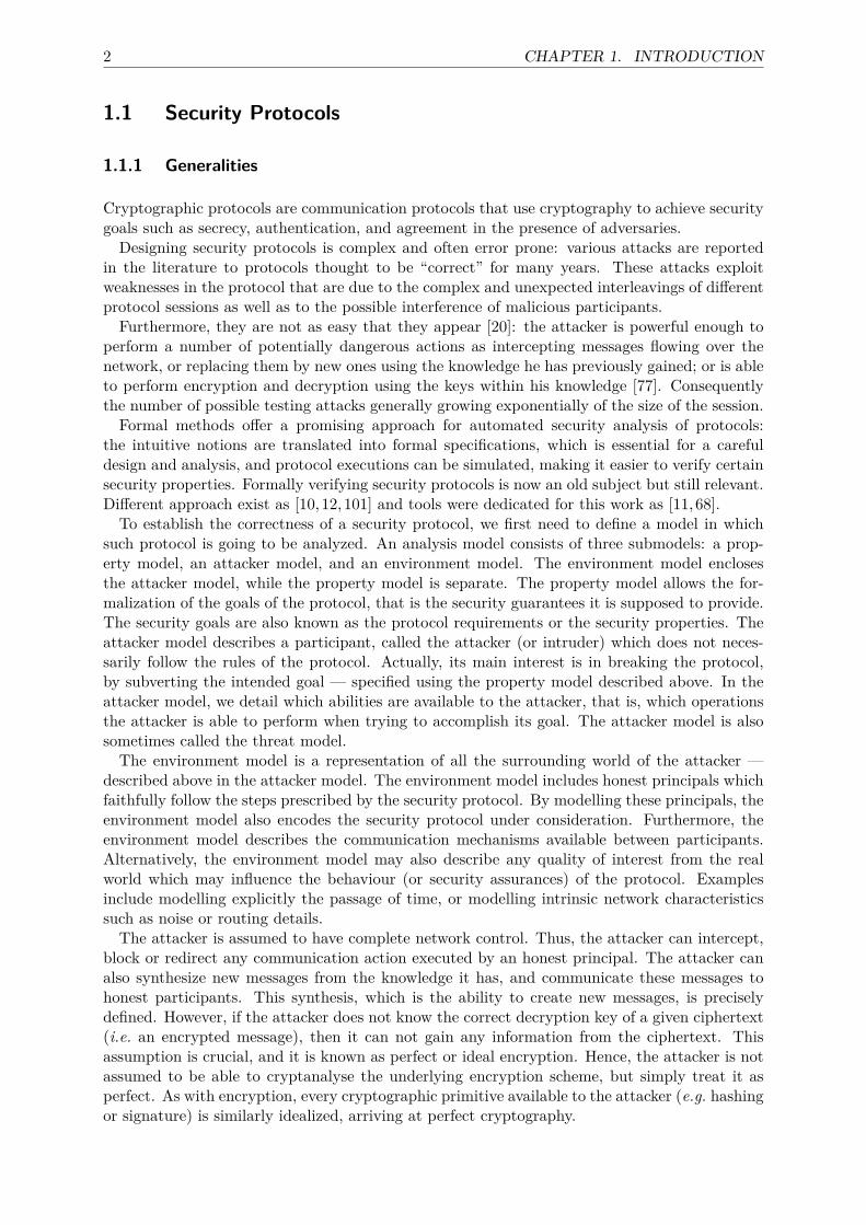
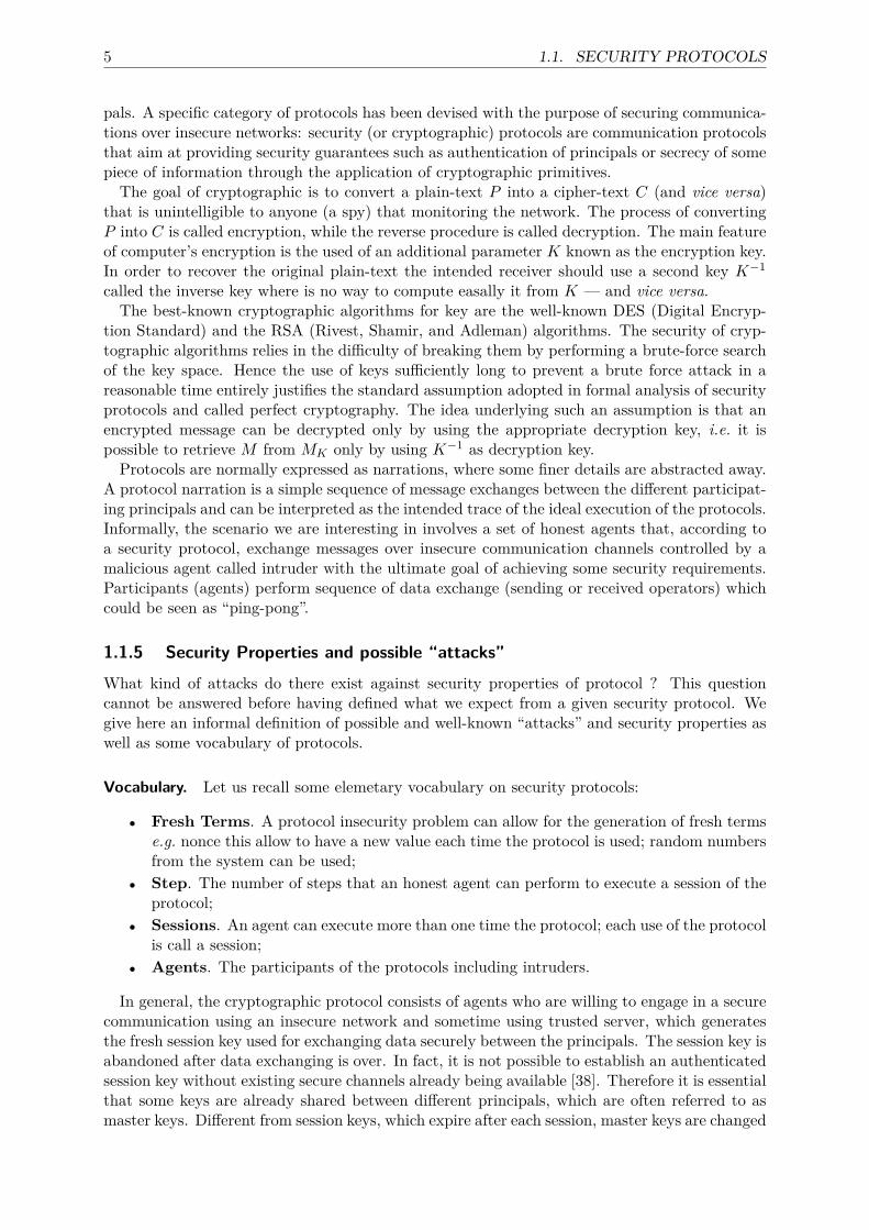
Figure 1.1. An informal specification of ns protocol, where Na and Nb are nonces and Ka, Kb
are the public keys of respectively Alice and Bob.
1.1.2 Example
The protocol ns involves two agents Alice (A) and Bob (B) who want to mutually authenticate.This is performed through the exchange of three messages as illustrated in Figure 1.1. In thisspecification, a message m is denoted by 〈m〉 and a message encrypted by a key k is denoted by〈m〉k — we use the same notation for secret key and public key encryption. The three steps ofthe protocol can be understood as follows:
1. Alice sends her identity A to Bob, together with a nonce Na; The message is encryptedwith Bob’s public key Kb so that only Bob can read it; Na thus constitutes a challengethat allows Bob to prove his identity; Bob is the only one who can read the nonce andsend it back to Alice;
2. Bob solves the challenge by sending Na to Alice, together with another nonce Nb that isa new challenge to authenticate Alice;
3. Alice solves Bob’s challenge, which results in mutual authentication.
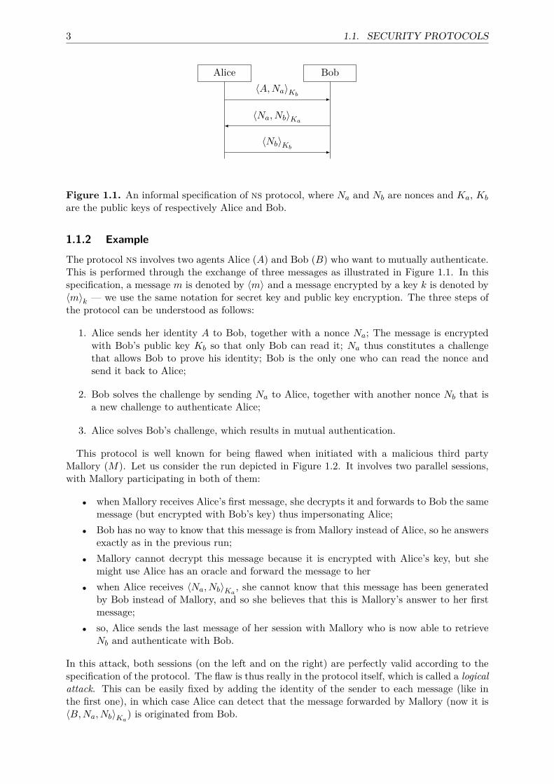
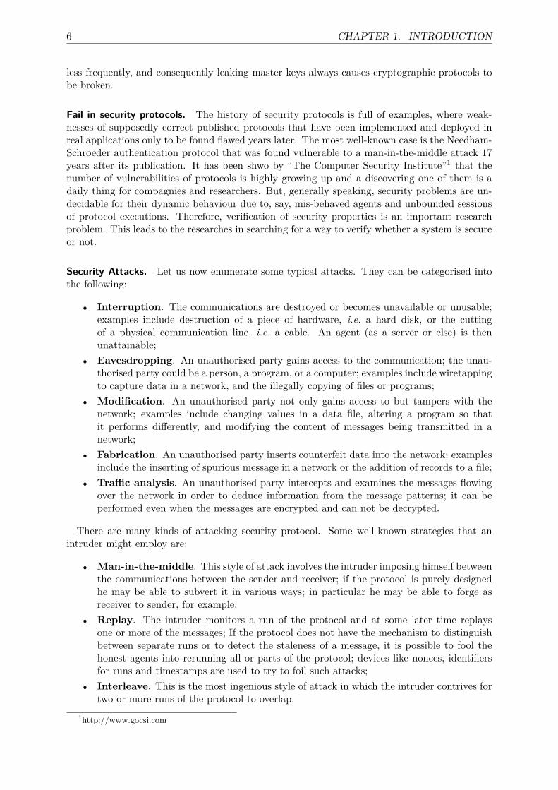
This protocol is well known for being flawed when initiated with a malicious third partyMallory (M). Let us consider the run depicted in Figure 1.2. It involves two parallel sessions,with Mallory participating in both of them:
• when Mallory receives Alice’s first message, she decrypts it and forwards to Bob the samemessage (but encrypted with Bob’s key) thus impersonating Alice;
• Bob has no way to know that this message is from Mallory instead of Alice, so he answersexactly as in the previous run;
• Mallory cannot decrypt this message because it is encrypted with Alice’s key, but shemight use Alice has an oracle and forward the message to her
• when Alice receives 〈Na, Nb〉Ka, she cannot know that this message has been generated
by Bob instead of Mallory, and so she believes that this is Mallory’s answer to her firstmessage;
• so, Alice sends the last message of her session with Mallory who is now able to retrieveNb and authenticate with Bob.
In this attack, both sessions (on the left and on the right) are perfectly valid according to thespecification of the protocol. The flaw is thus really in the protocol itself, which is called a logicalattack. This can be easily fixed by adding the identity of the sender to each message (like inthe first one), in which case Alice can detect that the message forwarded by Mallory (now it is〈B,Na, Nb〉Ka
) is originated from Bob.
4 CHAPTER 1. INTRODUCTION
Alice Mallory Bob〈A,Na〉Km
〈A,Na〉Kb
〈Na, Nb〉Ka
〈Na, Nb〉Ka
〈Nb〉Km
〈Nb〉Kb
Figure 1.2. An attack on ns protocol where Mallory authenticates as Alice with Bob.
1.1.3 Motivations
The possibility of violations and attacks of security protocols sometimes stems from subtlemisconceptions in the design of the protocols. Typically, these attacks are simply overlooked,as it is difficult for humans, even by careful inspection of simple protocols, to determine allthe complex ways that different protocol sessions could be interleaved together, with possibleinterference of a malicious intruder, the attacker.The question of whether a protocol indeed achieves its security requirements or not is, in the
general case, undecidable [4,82,90]. This has been proved by showing that a well-known undecid-able problem (e.g. the Post Correspondence Problem, the halting problem for Turing machines,etc.) can be reduced to a protocol insecurity problem. Despite this strong undecidability result,the problem of deciding whether a protocol is correct or not it is still worthwhile to be tackledby the introduction of some restrictions can lead to identify decidable subclasses: by focusing onverification of a bounded number of sessions the problem is known to be NP-complete. This canbe done by simply enumerating and exploring all traces of the protocol’s state transition systemlooking for a violation to some of the requirements. However the specific nature of securityprotocols that make them particularly suited to be checked by specific tools. That also needhow formalise those protocols to be latter checked.Although, if the general verification problem is undecidable, for many protocols, verification
can be reduced to verification of a bounded number of sessions. Moreover, even for thoseprotocols that should theorically be checked under a unbounded number of concurrent protocolexecutions, violations in their security requirements often exploit only a small number of sessions.For these reasons, in many cases of interest it is sufficient to consider a finite number of sessionsin which each agent performs a fixed number of steps. For instance all the attacks on the well-know SPORE and Clark-Jacob’s libraries [51] can be discovered by modelling each protocol withonly two protocol sessions.
1.1.4 Informal definition of security protocols
Communication protocols specify an exchange of messages between principals, i.e. the agentsparticipating in a protocol execution — e.g. users, hosts, or processes. Messages are sent overopen networks, such as the Internet, that cannot be considered secure. As a consequence, pro-tocols should be designed “robust” enough to work even under worst-case assumptions, namelymessages may be eavesdropped or tampered with by an intruder or dishonest or careless princi-
5 1.1. SECURITY PROTOCOLS
pals. A specific category of protocols has been devised with the purpose of securing communica-tions over insecure networks: security (or cryptographic) protocols are communication protocolsthat aim at providing security guarantees such as authentication of principals or secrecy of somepiece of information through the application of cryptographic primitives.The goal of cryptographic is to convert a plain-text P into a cipher-text C (and vice versa)
that is unintelligible to anyone (a spy) that monitoring the network. The process of convertingP into C is called encryption, while the reverse procedure is called decryption. The main featureof computer’s encryption is the used of an additional parameter K known as the encryption key.In order to recover the original plain-text the intended receiver should use a second key K−1
called the inverse key where is no way to compute easally it from K — and vice versa.The best-known cryptographic algorithms for key are the well-known DES (Digital Encryp-
tion Standard) and the RSA (Rivest, Shamir, and Adleman) algorithms. The security of cryp-tographic algorithms relies in the difficulty of breaking them by performing a brute-force searchof the key space. Hence the use of keys sufficiently long to prevent a brute force attack in areasonable time entirely justifies the standard assumption adopted in formal analysis of securityprotocols and called perfect cryptography. The idea underlying such an assumption is that anencrypted message can be decrypted only by using the appropriate decryption key, i.e. it ispossible to retrieve M from MK only by using K−1 as decryption key.Protocols are normally expressed as narrations, where some finer details are abstracted away.
A protocol narration is a simple sequence of message exchanges between the different participat-ing principals and can be interpreted as the intended trace of the ideal execution of the protocols.Informally, the scenario we are interesting in involves a set of honest agents that, according toa security protocol, exchange messages over insecure communication channels controlled by amalicious agent called intruder with the ultimate goal of achieving some security requirements.Participants (agents) perform sequence of data exchange (sending or received operators) whichcould be seen as “ping-pong”.
1.1.5 Security Properties and possible “attacks”
What kind of attacks do there exist against security properties of protocol ? This questioncannot be answered before having defined what we expect from a given security protocol. Wegive here an informal definition of possible and well-known “attacks” and security properties aswell as some vocabulary of protocols.
Vocabulary. Let us recall some elemetary vocabulary on security protocols:
• Fresh Terms. A protocol insecurity problem can allow for the generation of fresh termse.g. nonce this allow to have a new value each time the protocol is used; random numbersfrom the system can be used;
• Step. The number of steps that an honest agent can perform to execute a session of theprotocol;
• Sessions. An agent can execute more than one time the protocol; each use of the protocolis call a session;
• Agents. The participants of the protocols including intruders.
In general, the cryptographic protocol consists of agents who are willing to engage in a securecommunication using an insecure network and sometime using trusted server, which generatesthe fresh session key used for exchanging data securely between the principals. The session key isabandoned after data exchanging is over. In fact, it is not possible to establish an authenticatedsession key without existing secure channels already being available [38]. Therefore it is essentialthat some keys are already shared between different principals, which are often referred to asmaster keys. Different from session keys, which expire after each session, master keys are changed
6 CHAPTER 1. INTRODUCTION
less frequently, and consequently leaking master keys always causes cryptographic protocols tobe broken.
Fail in security protocols. The history of security protocols is full of examples, where weak-nesses of supposedly correct published protocols that have been implemented and deployed inreal applications only to be found flawed years later. The most well-known case is the Needham-Schroeder authentication protocol that was found vulnerable to a man-in-the-middle attack 17years after its publication. It has been shwo by “The Computer Security Institute”1 that thenumber of vulnerabilities of protocols is highly growing up and a discovering one of them is adaily thing for compagnies and researchers. But, generally speaking, security problems are un-decidable for their dynamic behaviour due to, say, mis-behaved agents and unbounded sessionsof protocol executions. Therefore, verification of security properties is an important researchproblem. This leads to the researches in searching for a way to verify whether a system is secureor not.
Security Attacks. Let us now enumerate some typical attacks. They can be categorised intothe following:
• Interruption. The communications are destroyed or becomes unavailable or unusable;examples include destruction of a piece of hardware, i.e. a hard disk, or the cuttingof a physical communication line, i.e. a cable. An agent (as a server or else) is thenunattainable;
• Eavesdropping. An unauthorised party gains access to the communication; the unau-thorised party could be a person, a program, or a computer; examples include wiretappingto capture data in a network, and the illegally copying of files or programs;
• Modification. An unauthorised party not only gains access to but tampers with thenetwork; examples include changing values in a data file, altering a program so thatit performs differently, and modifying the content of messages being transmitted in anetwork;
• Fabrication. An unauthorised party inserts counterfeit data into the network; examplesinclude the inserting of spurious message in a network or the addition of records to a file;
• Traffic analysis. An unauthorised party intercepts and examines the messages flowingover the network in order to deduce information from the message patterns; it can beperformed even when the messages are encrypted and can not be decrypted.
There are many kinds of attacking security protocol. Some well-known strategies that anintruder might employ are:
• Man-in-the-middle. This style of attack involves the intruder imposing himself betweenthe communications between the sender and receiver; if the protocol is purely designedhe may be able to subvert it in various ways; in particular he may be able to forge asreceiver to sender, for example;
• Replay. The intruder monitors a run of the protocol and at some later time replaysone or more of the messages; If the protocol does not have the mechanism to distinguishbetween separate runs or to detect the staleness of a message, it is possible to fool thehonest agents into rerunning all or parts of the protocol; devices like nonces, identifiersfor runs and timestamps are used to try to foil such attacks;
• Interleave. This is the most ingenious style of attack in which the intruder contrives fortwo or more runs of the protocol to overlap.
1http://www.gocsi.com
7 1.1. SECURITY PROTOCOLS
There are many other known styles of attack and presumably many more that have yet tobe discovered. Many involve combinations of these themes. This demonstrates the difficulty indesigning security protocols and emphasizes the need for a formal and rigorous analysis of theseprotocols.A protocol execution is considered as involving honest (participants) principals and active
attackers. The abilities of the attackers and relationship between participants and attackerstogether constitute a threat model and the almost exclusively used threat model is the oneproposed by Dolev and Yao [77]. The Dolev-Yao threat model is a worst-case model in thesense that the network, over which the participants communicate, is thought as being totallycontrolled by an omnipotent attacker with all the capabilities listed above. Therefore, there isno need to assume the existence of multiple attackers, because they together do not have moreabilities than the single omnipotent one. Dishonest principals do not need to be consideredeither: they can be viewed as an unique Dolev-Yao intruder. Furthermore, it is generally notinteresting to consider an attacker with less abilities than the omnipotent one except to verifyless properties and to accelerate the formal verification of a protocol.
Security properties. Each cryptographic protocol is designed to achieve one or more security-related goals after a successful execution, in other words, the principals involved may reasonabout certain properties; for example, only certain principals have access to particular secretinformation. They may then use this information to verify claims about subsequent communi-cation, e.g. an encrypted message can only be decrypted by the principals who have access tothe corresponding encryption key. The most commonly considered security properties include:
• Authentication. It is concerned with assuring that a communication is authentic; inthe case of an ongoing interaction, such as the connection of a host to another host, twoaspects are involved; first, at the time of connection initiation, the two entities have tobe authentic, i.e. each is the entity that he claims to be; second, during the connection,there is no third party who interferes in such a way that he can masquerade as one ofthe two legitimate parties for the purposes of unauthorized transmission or reception; forexample, fabrication is an attack on authenticity;
• Confidentiality. It is the protection of transmitted data from attacks; with respect tothe release of message contents, several levels of protection can be identified, includingthe protection of a single message or even specificfields within a message; for example,interception is an attack on confidentiality;
• Integrity. Integrity assures that messages are received as sent, with no duplication,insertion, modification, reordering, or replays; as with confidenfitiality, integrity can applyto a stream of messages, a single message, or selected fields within a message; modificationis an attack on integrity;
• Availability. Availability assures that a service or a piece of information is accessibleto legitimate users or receivers upon request; there are two common ways to specifyavailability; an approach is to specify failure factors (factors that could cause the systemor the communication to fail) [185], for example, the minimum number of host failuresneeded to bring down the system or the communication; interruption is, for example, anattack on availability;
• Non-repudiation. Non-repudiation prevents either sender or receiver from denyinga transmitted message; thus, when a message is sent, the receiver can prove that themessage was in fact sent by the alleged sender; similarly, when a message is received, thesender can prove that the message was in fact received by the alleged receiver.
8 CHAPTER 1. INTRODUCTION
1.1.6 Why cryptographic protocols go wrong?The first reason for the security protocols easily go wrong is that protocols were first usuallyexpressed as narrations and most of the details of the actual deployment are ignored. And thislittle details and ambiguities may be the reason of an attack.Second, as mentioned before, cryptographic protocols are mainly deployed over an open net-
work such that everyone can join it, exceptions are where wireless or routing protocols attackercontrol only a subpart of the network and where agents only communicate with their neigh-bors [13, 27, 121, 197, 198]. One reason for security protocols easily going wrong is the existenceof the attacker: he can start sending and receiving messages to and from the principals acrossit without the need of authorization or permission. In such an open environment, we mushanticipate that the attacker will do all sorts of actions, not just passively eavesdropping, butalso actively altering, forging, duplicating, re-directing, deleting or injecting messages. Thesefault messages can be malicious and cause a destructive effect to the protocol. Consequently,any message received from the network is treated to have been received from the attacker afterhis disposal. In other words, the attacker is considered to have the complete control of theentire network and could be considered to be the network. And it is easy for humans to forget apossible combination of the attacker. Instead, automatic verification (model-checking), which isthe subject of this document, would not forget one possible attack. And this number of attackgrowing exponentially and reduce the time of computation of generating all these attacks usingparallel machine is the main goal of this document.It is notice to say that nowadays a considerable number of cryptographic protocols have been
specified, implemented and verified. Consequently analysing cryptographic protocols in order tofind various kinds of attacks and to prevent them has received a lot of attention. As mentionedbefore, the area is remarkably subtle and a very large portion of proposed protocols have beenshown to be flawed a long time after they were published. This has naturally encouraged researchin this area.
1.2 Modelisation
A more complete presentation is available at [181].
1.2.1 High-level Petri nets
(a) Definition of classical Petri nets
A Petri net (also known as a place/transition net or P/T net) is a simple model of distributedsystems [175, 176]. A P/T net is a directed bipartite graph consists of places, transitions, anddirected arcs.Intuitivelly transitions represent events that may occur, directed arcs (also called edges) the
data and control flow; and places are the ressources. Arcs run from a place to a transition (orvice versa, never between places or between transitions. The places from which an arc runs toa transition are called the input places of the transition; the places to which arcs run from atransition are called the output places of the transition.One thing that makes Petri nets interesting is that they provide a balance between modeling
power and analyzability: it is “easy” to modelised many distributed system and many proper-ties about the concurrency of the modelised system can be automatically determined. This iscommonly called model-checking — we will give a better definition in the former.It is standard to a use a graphical representation of the P/T nets. We used the following one:
• places are represented by circles;• transitions are denoted by squares;• arcs are denoted by arrows.

9 1.2. MODELISATION
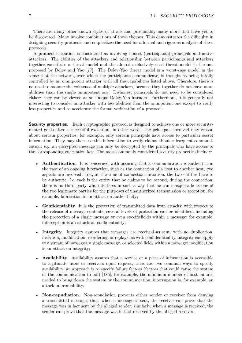
Sequence: Choice: Parallelism: Infinit loop:
init action1 action2 end
choice1
choice2
process1 process2
Figure 1.3. Petri Nets for sequence, choice, iteration and parallelism
It is common to give name to transitions and places for a better read of the net. As showin Figure 1.3, Petri nets can easally model classical structure of distributed system such assequence, choice, iteration or parallelism. Now, we give here a formal definition of Petri nets:
Definition 1 (Petri nets (P/T)).A Petri net is a tuple (S, T, `) where:
• S is the finite set of places;
• T , disjoint from S ( i.e. T ∩ S = ∅), is the finite set of transitions;
• ` is a labelling function such that for all (x, y) ∈ (S × T ) ∪ (T × S), `(x, y) is a multisetover E and defines the arc from x toward y.
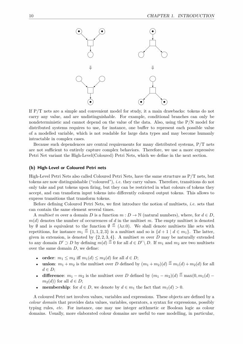
Each place can hold a number of individual tokens that represent data items flowing throughthe net. A transition is called enabled if there are tokens present at each of its input places, andif all output places have not reached their capacity. Enabled transitions can fire by consuminga specified number of tokens from each of the input places and putting a number of new tokenon each of the output places.The number of tokens held at each place is specified by themarking of the net, which represents
the current state of the net. Consecutive markings are obtained by firing transitions. Informally,starting from an initial marking, computing the marking graph of a Petri net consist to computeall the consecutive markings. This problem is known to be EXPSPACE-hard and thus decidable.Papers continue to be published on how to do it efficiently which is in certain manner also thegoal of this thesis. It is common to had bullets into places to represent markings.Formally, a marking m is represented as a vector N|S| with element m[p] denoting the number
of tokens on place p in markingm. Markingm0 is the initial marking, i.e. it contains the numberof tokens on each place at the beginning. A new marking m′ that is obtained from marking mby firing transition t, noted m[t〉m′ can be computed if m has enough tokens, i.e. for all s ∈ S,`(s, t) ≤ m(s). Then m′ is defined for all s ∈ S as m′(s) df= m(s)− `(s, t) + `(t, s).
For example, two markings of two different P/T nets, each one firing on transition which givetwo new markings:
10 CHAPTER 1. INTRODUCTION
• • •
⇓ ⇓
• • •
If P/T nets are a simple and convenient model for study, it a main drawbacks: tokens do notcarry any value, and are undistinguishable. For example, conditional branches can only benondeterministic and cannot depend on the value of the data. Also, using the P/N model fordistributed systems requires to use, for instance, one buffer to represent each possible valueof a modelled variable, which is not readable for large data types and may become humanlyintractable in complex cases.Because such dependences are central requirements for many distributed systems, P/T nets
are not sufficient to entirely capture complex behaviors. Therefore, we use a more expressivePetri Net variant the High-Level(Coloured) Petri Nets, which we define in the next section.
(b) High-Level or Coloured Petri nets
High-Level Petri Nets also called Coloured Petri Nets, have the same structure as P/T nets, buttokens are now distinguishable (“coloured”), i.e. they carry values. Therefore, transitions do notonly take and put tokens upon firing, but they can be restricted in what colours of tokens theyaccept, and can transform input tokens into differently coloured output tokens. This allows toexpress transitions that transform tokens.Before defining Coloured Petri Nets, we first introduce the notion of multisets, i.e. sets that
can contain the same element several times.A multiset m over a domain D is a function m : D → N (natural numbers), where, for d ∈ D,
m(d) denotes the number of occurrences of d in the multiset m. The empty multiset is denotedby ∅ and is equivalent to the function ∅ df= (λx.0). We shall denote multisets like sets withrepetitions, for instance m1
df= {1, 1, 2, 3} is a multiset and so is {d + 1 | d ∈ m1}. The latter,given in extension, is denoted by {2, 2, 3, 4}. A multiset m over D may be naturally extendedto any domain D′ ⊃ D by defining m(d) df= 0 for all d ∈ D′ \D. If m1 and m2 are two multisetsover the same domain D, we define:
• order: m1 ≤ m2 iff m1(d) ≤ m2(d) for all d ∈ D;• union: m1 +m2 is the multiset over D defined by (m1 +m2)(d) df= m1(d) +m2(d) for all
d ∈ D;• difference: m1 −m2 is the multiset over D defined by (m1 −m2)(d) df= max(0,m1(d)−
m2(d)) for all d ∈ D;• membership: for d ∈ D, we denote by d ∈ m1 the fact that m1(d) > 0.
A coloured Petri net involves values, variables and expressions. These objects are defined by acolour domain that provides data values, variables, operators, a syntax for expressions, possiblytyping rules, etc. For instance, one may use integer arithmetic or Boolean logic as colourdomains. Usually, more elaborated colour domains are useful to ease modelling, in particular,
11 1.2. MODELISATION
one may consider a functional programming language or the functional fragment (expressions)of an imperative programming language. In most of this document, we consider an abstractcolour domain with the following elements:
• D is the set of data values; it may include in particular the Petri net black token •, integervalues, Boolean values True and False, and a special “undefined” value ⊥;
• V is the set of variables, usually denoted as single letters x, y, . . . , or as subscribed letterslike x1, yk, . . . ;
• E is the set of expressions, involving values, variables and appropriate operators. Lete ∈ E, we denote by vars(e) the set of variables from V involved in e. Moreover, variablesor values may be considered as (simple) expressions, i.e. we assume that D ∪ V ⊂ E.
We make no assumption about the typing or syntactical correctness of values or expressions;instead, we assume that any expression can be evaluated, possibly to ⊥ (undefined). Moreprecisely, a binding is a partial function β : V→ D. Let e ∈ E and β be a binding, we denote byβ(e) the evaluation of e under β; if the domain of β does not include vars(e) then β(e) df= ⊥. Theapplication of a binding to evaluate an expression is naturally extended to sets and multisets ofexpressions.For instance, if β df= {x 7→ 1, y 7→ 2}, we have β(x + y) = 3. With β
df= {x 7→ 1, y 7→ ”2“},depending on the colour domain, we may have β(x+ y) = ⊥ (no coercion), or β(x+ y) = ”12“(coercion of integer 1 to string 1), or β(x + y) = 3 (coercion of string 2 to integer 2), or evenother values as defined by the concrete colour domain.Two expressions e1, e2 ∈ E are equivalent, which is denoted by e1 ≡ e2, iff for all possible
binding β we have β(e1) = β(e2). For instance, x+1, 1+x and 2+x−1 are pairwise equivalentexpressions for the usual integer arithmetic.Definition 2 (Coloured Petri nets).A Petri net is a tuple (S, T, `) where:
• S is the finite set of places;• T , disjoint from S, is the finite set of transitions;• ` is a labelling function such that:
◦ for all s ∈ S, `(s) ⊆ D is the type of s, i.e. the set of values that s is allowed tocarry,
◦ for all t ∈ T , `(t) ∈ E is the guard of t, i.e. a condition for its execution,◦ for all (x, y) ∈ (S × T ) ∪ (T × S), `(x, y) is a multiset over E and defines the arc
from x toward y.
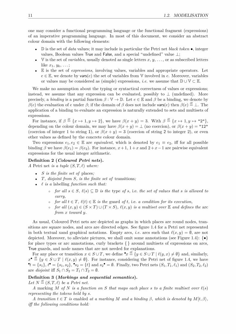
As usual, Coloured Petri nets are depicted as graphs in which places are round nodes, tran-sitions are square nodes, and arcs are directed edges. See figure 1.4 for a Petri net representedin both textual xand graphical notations. Empty arcs, i.e. arcs such that `(x, y) = ∅, are notdepicted. Moreover, to alleviate pictures, we shall omit some annotations (see Figure 1.4): {•}for place types or arc annotations, curly brackets { } around multisets of expressions on arcs,True guards, and node names that are not needed for explanations.For any place or transition x ∈ S ∪ T , we define •x df= {y ∈ S ∪ T | `(y, x) 6= ∅} and, similarly,
x•df= {y ∈ S ∪ T | `(x, y) 6= ∅}. For instance, considering the Petri net of figure 1.4, we have
•t = {s1}, t• = {s1, s2}, •s2 = {t} and s2• = ∅. Finally, two Petri nets (S1, T1, `1) and (S2, T2, `2)
are disjoint iff S1 ∩ S2 = T1 ∩ T2 = ∅.Definition 3 (Markings and sequential semantics).Let N df= (S, T, `) be a Petri net.A marking M of N is a function on S that maps each place s to a finite multiset over `(s)
representing the tokens held by s.A transition t ∈ T is enabled at a marking M and a binding β, which is denoted by M [t, β〉,
iff the following conditions hold:
12 CHAPTER 1. INTRODUCTION
Ns1
t
x > 0{•}
s2{x}
{x− 1}
{•}S
df= {s1, s2}T
df= {t}`
df= {s1 7→ N, s2 7→ {•}, t 7→ x > 0, (s1, t) 7→ {x},(s2, t) 7→ ∅, (t, s1) 7→ {x− 1}, (t, s2) 7→ {•}}
Ns1
t
x > 0 s2{x}
{x− 1}
Figure 1.4. A simple Petri net, with both full (top) and simplified annotations (below).
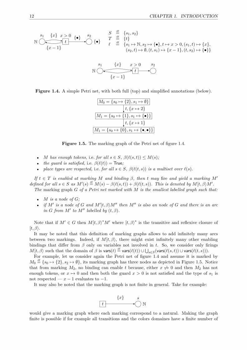
M0 = {s0 7→ {2}, s1 7→ ∅}
M1 = {s0 7→ {1}, s1 7→ {•}}
M1 = {s0 7→ {0}, s1 7→ {•, •}}
t, {x 7→ 2}
t, {x 7→ 1}
Figure 1.5. The marking graph of the Petri net of figure 1.4.
• M has enough tokens, i.e. for all s ∈ S, β(`(s, t)) ≤M(s);• the guard is satisfied, i.e. β(`(t)) = True;• place types are respected, i.e. for all s ∈ S, β(`(t, s)) is a multiset over `(s).
If t ∈ T is enabled at marking M and binding β, then t may fire and yield a marking M ′defined for all s ∈ S as M ′(s) df= M(s)− β(`(s, t)) + β(`(t, s)). This is denoted by M [t, β〉M ′.The marking graph G of a Petri net marked with M is the smallest labelled graph such that:
• M is a node of G;• if M ′ is a node of G and M ′[t, β〉M ′′ then M ′′ is also an node of G and there is an arc
in G from M ′ to M ′′ labelled by (t, β).
Note that if M ′ ∈ G then M [t, β〉∗M ′ where [t, β〉∗ is the transitive and reflexive closure of[t, β〉.It may be noted that this definition of marking graphs allows to add infinitely many arcs
between two markings. Indeed, if M [t, β〉, there might exist infinitely many other enablingbindings that differ from β only on variables not involved in t. So, we consider only firingsM [t, β〉 such that the domain of β is vars(t) df= vars(`(t)) ∪⋃
s∈S(vars(`(s, t)) ∪ vars(`(t, s))).For example, let us consider again the Petri net of figure 1.4 and assume it is marked by
M0df= {s0 7→ {2}, s2 7→ ∅}, its marking graph has three nodes as depicted in Figure 1.5. Notice
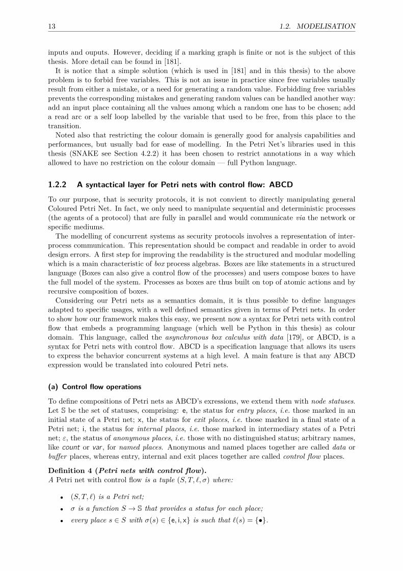
that from marking M2, no binding can enable t because, either x 67→ 0 and then M2 has notenough tokens, or x 7→ 0 and then both the guard x > 0 is not satisfied and the type of s1 isnot respected — x− 1 evaluates to −1.It may also be noted that the marking graph is not finite in general. Take for example:
t Ns{x}
would give a marking graph where each marking correspond to a natural. Making the graphfinite is possible if for example all transitions and the colors domaines have a finite number of
13 1.2. MODELISATION
inputs and ouputs. However, deciding if a marking graph is finite or not is the subject of thisthesis. More detail can be found in [181].It is notice that a simple solution (which is used in [181] and in this thesis) to the above
problem is to forbid free variables. This is not an issue in practice since free variables usuallyresult from either a mistake, or a need for generating a random value. Forbidding free variablesprevents the corresponding mistakes and generating random values can be handled another way:add an input place containing all the values among which a random one has to be chosen; adda read arc or a self loop labelled by the variable that used to be free, from this place to thetransition.Noted also that restricting the colour domain is generally good for analysis capabilities and
performances, but usually bad for ease of modelling. In the Petri Net’s libraries used in thisthesis (SNAKE see Section 4.2.2) it has been chosen to restrict annotations in a way whichallowed to have no restriction on the colour domain — full Python language.
1.2.2 A syntactical layer for Petri nets with control flow: ABCD
To our purpose, that is security protocols, it is not convient to directly manipulating generalColoured Petri Net. In fact, we only need to manipulate sequential and deterministic processes(the agents of a protocol) that are fully in parallel and would communicate via the network orspecific mediums.The modelling of concurrent systems as security protocols involves a representation of inter-
process communication. This representation should be compact and readable in order to avoiddesign errors. A first step for improving the readability is the structured and modular modellingwhich is a main characteristic of box process algebras. Boxes are like statements in a structuredlanguage (Boxes can also give a control flow of the processes) and users compose boxes to havethe full model of the system. Processes as boxes are thus built on top of atomic actions and byrecursive composition of boxes.Considering our Petri nets as a semantics domain, it is thus possible to define languages
adapted to specific usages, with a well defined semantics given in terms of Petri nets. In orderto show how our framework makes this easy, we present now a syntax for Petri nets with controlflow that embeds a programming language (which well be Python in this thesis) as colourdomain. This language, called the asynchronous box calculus with data [179], or ABCD, is asyntax for Petri nets with control flow. ABCD is a specification language that allows its usersto express the behavior concurrent systems at a high level. A main feature is that any ABCDexpression would be translated into coloured Petri nets.
(a) Control flow operations
To define compositions of Petri nets as ABCD’s exressions, we extend them with node statuses.Let S be the set of statuses, comprising: e, the status for entry places, i.e. those marked in aninitial state of a Petri net; x, the status for exit places, i.e. those marked in a final state of aPetri net; i, the status for internal places, i.e. those marked in intermediary states of a Petrinet; ε, the status of anonymous places, i.e. those with no distinguished status; arbitrary names,like count or var , for named places. Anonymous and named places together are called data orbuffer places, whereas entry, internal and exit places together are called control flow places.
Definition 4 (Petri nets with control flow).A Petri net with control flow is a tuple (S, T, `, σ) where:
• (S, T, `) is a Petri net;• σ is a function S → S that provides a status for each place;• every place s ∈ S with σ(s) ∈ {e, i, x} is such that `(s) = {•}.
14 CHAPTER 1. INTRODUCTION
e
i
x
t#1
t#2
e
x
t�1 t�2
e
x
t~1
t~2
e e
x x
t‖1 t
‖2
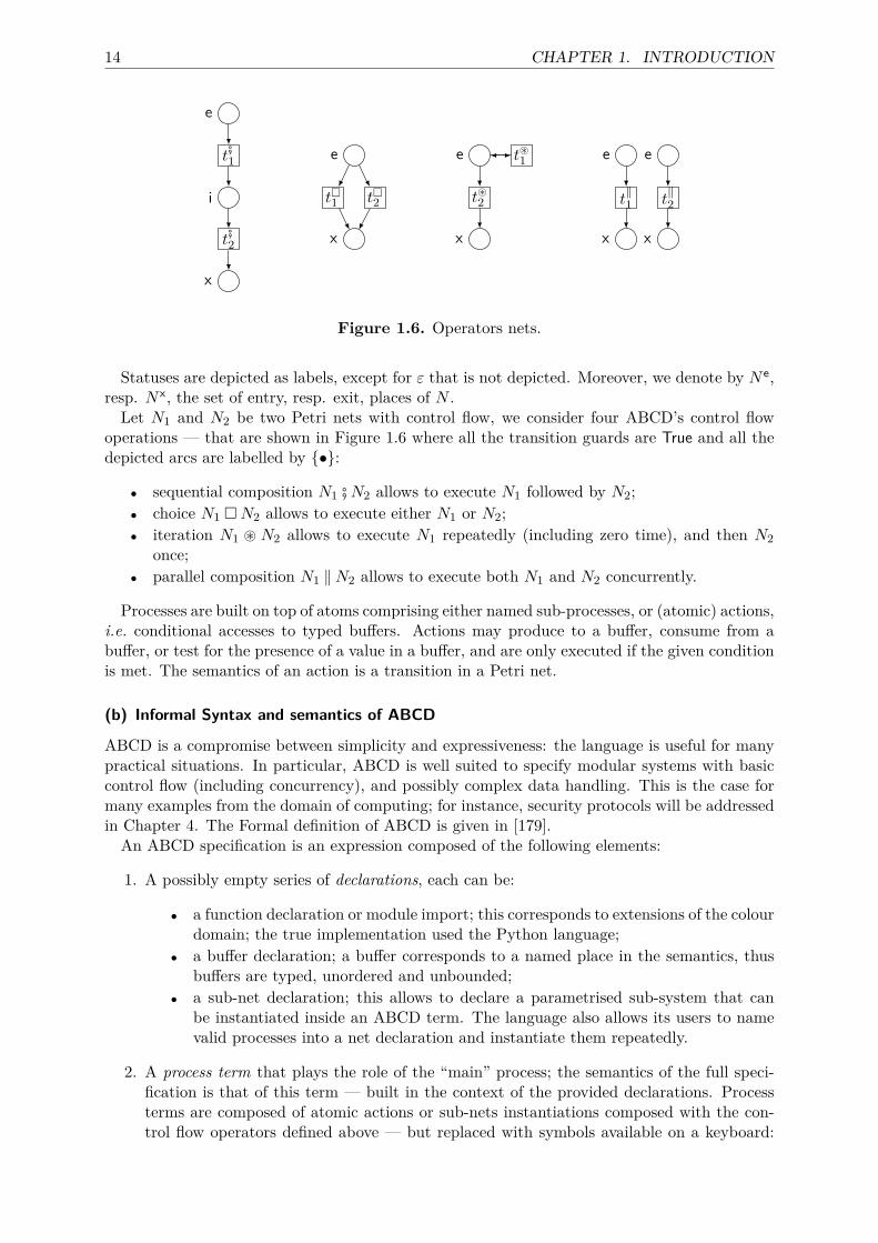
Figure 1.6. Operators nets.
Statuses are depicted as labels, except for ε that is not depicted. Moreover, we denote by N e,resp. N x, the set of entry, resp. exit, places of N .Let N1 and N2 be two Petri nets with control flow, we consider four ABCD’s control flow
operations — that are shown in Figure 1.6 where all the transition guards are True and all thedepicted arcs are labelled by {•}:
• sequential composition N1 #N2 allows to execute N1 followed by N2;• choice N1 �N2 allows to execute either N1 or N2;• iteration N1 ~ N2 allows to execute N1 repeatedly (including zero time), and then N2
once;• parallel composition N1 ‖N2 allows to execute both N1 and N2 concurrently.
Processes are built on top of atoms comprising either named sub-processes, or (atomic) actions,i.e. conditional accesses to typed buffers. Actions may produce to a buffer, consume from abuffer, or test for the presence of a value in a buffer, and are only executed if the given conditionis met. The semantics of an action is a transition in a Petri net.
(b) Informal Syntax and semantics of ABCD
ABCD is a compromise between simplicity and expressiveness: the language is useful for manypractical situations. In particular, ABCD is well suited to specify modular systems with basiccontrol flow (including concurrency), and possibly complex data handling. This is the case formany examples from the domain of computing; for instance, security protocols will be addressedin Chapter 4. The Formal definition of ABCD is given in [179].An ABCD specification is an expression composed of the following elements:
1. A possibly empty series of declarations, each can be:
• a function declaration or module import; this corresponds to extensions of the colourdomain; the true implementation used the Python language;
• a buffer declaration; a buffer corresponds to a named place in the semantics, thusbuffers are typed, unordered and unbounded;
• a sub-net declaration; this allows to declare a parametrised sub-system that canbe instantiated inside an ABCD term. The language also allows its users to namevalid processes into a net declaration and instantiate them repeatedly.
2. A process term that plays the role of the “main” process; the semantics of the full speci-fication is that of this term — built in the context of the provided declarations. Processterms are composed of atomic actions or sub-nets instantiations composed with the con-trol flow operators defined above — but replaced with symbols available on a keyboard:
15 1.2. MODELISATION
[True]e
True
x
[False]e
False
x
[count−(x), count+(x+1), shift?(j), buf+(j+x) if x<10]e
x < 10
x
count
intx 7→ x+ 1
shift
intj
buf
intj + x
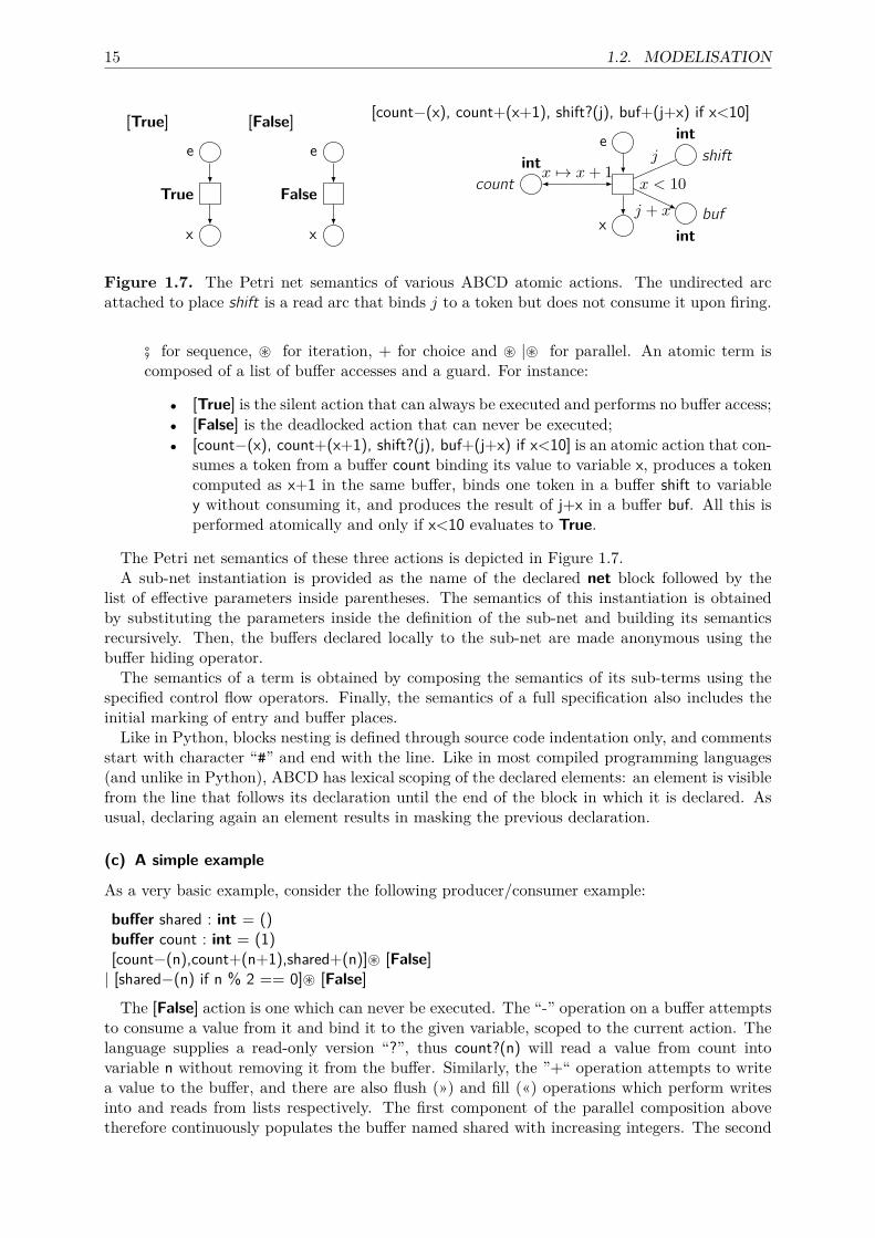
Figure 1.7. The Petri net semantics of various ABCD atomic actions. The undirected arcattached to place shift is a read arc that binds j to a token but does not consume it upon firing.
# for sequence, ~ for iteration, + for choice and ~ |~ for parallel. An atomic term iscomposed of a list of buffer accesses and a guard. For instance:
• [True] is the silent action that can always be executed and performs no buffer access;• [False] is the deadlocked action that can never be executed;• [count−(x), count+(x+1), shift?(j), buf+(j+x) if x<10] is an atomic action that con-
sumes a token from a buffer count binding its value to variable x, produces a tokencomputed as x+1 in the same buffer, binds one token in a buffer shift to variabley without consuming it, and produces the result of j+x in a buffer buf. All this isperformed atomically and only if x<10 evaluates to True.
The Petri net semantics of these three actions is depicted in Figure 1.7.A sub-net instantiation is provided as the name of the declared net block followed by the
list of effective parameters inside parentheses. The semantics of this instantiation is obtainedby substituting the parameters inside the definition of the sub-net and building its semanticsrecursively. Then, the buffers declared locally to the sub-net are made anonymous using thebuffer hiding operator.The semantics of a term is obtained by composing the semantics of its sub-terms using the
specified control flow operators. Finally, the semantics of a full specification also includes theinitial marking of entry and buffer places.Like in Python, blocks nesting is defined through source code indentation only, and comments
start with character “#” and end with the line. Like in most compiled programming languages(and unlike in Python), ABCD has lexical scoping of the declared elements: an element is visiblefrom the line that follows its declaration until the end of the block in which it is declared. Asusual, declaring again an element results in masking the previous declaration.
(c) A simple example
As a very basic example, consider the following producer/consumer example:
buffer shared : int = ()buffer count : int = (1)[count−(n),count+(n+1),shared+(n)]~ [False]| [shared−(n) if n % 2 == 0]~ [False]
The [False] action is one which can never be executed. The “-” operation on a buffer attemptsto consume a value from it and bind it to the given variable, scoped to the current action. Thelanguage supplies a read-only version “?”, thus count?(n) will read a value from count intovariable n without removing it from the buffer. Similarly, the ”+“ operation attempts to writea value to the buffer, and there are also flush (») and fill («) operations which perform writesinto and reads from lists respectively. The first component of the parallel composition abovetherefore continuously populates the buffer named shared with increasing integers. The second
16 CHAPTER 1. INTRODUCTION
sub-process just pulls the even ones out of the shared buffer. The Petri net resulting from thisABCD specification is draw in Figure 1.7. Note that for the example shown above, compute thestate marking of the generated Petri net with its initial marking would not terminate becausethe marking graph is infinite. Therefore care must be taken by the ABCD user to ensure thathis system has finitely many markings.As explain before, the declaration of net is modulare. It is thus possible to declare different
nets and compose them. A sub-process may be declared as a “net” and reused later in a processexpression. That is:
net process1():buffer state: int = ()...
net process2():buffer state: int = ()...
then a full system can be specified by running in parallel two instance (in sequence) of the firstprocess and one of the second one:
(process1# process1) ‖ process2
Typed buffers may also be declared globally to a specification or locally to net processes. Forillustring this, we we take another time for example the producer/consumers specification. Theproducer puts in a buffer “bag” the integers ranging from 0 to 9. To do so, it uses a counter“count” that is repeatedly incremented until it reaches value 10, which allows to exit the loop.The first consumer consumes only odd values from the buffer, the second one consumes onlyeven values. Both never stop looping.
def bag : int = () # buffer of integers declared empty
net prod :def count : int = 0 # buffer of integers initialised with the single value 0[count−(x), count+(x+1), bag+(x) if x < 10] ~ [count−(x) if x == 10]
net odd :[bag−(x) if (x % 2) == 1] ~ [False]
net even :[bag−(x) if (x % 2) == 0] ~ [False]
prod ‖ odd ‖ even
A sub-part of the Petri net resulting from this ABCD specification is draw in Figure. 1.7. It isinteresting to note that parts of this ABCD specification are actually Python code and couldbe arbitrarily complex: initial values of buffers (“()” and “0”); buffer accesses parameters (“x”and “x+1”); actions guards (“x<10”, “(x%2)==1”, etc.).
(d) From ABCD to Coloured Petri nets
To transform ABCD expressions into Coloured Petri nets, the control flow operators are definedby two successive phases given below. Their formal definitions is given in [179].The first one is a gluing phase that combines operand nets and atomic actions; in order to
provide a unique definition of this phase for all the operators, we use the operator nets depictedin Figure 1.6 to guide the gluing. These operator nets are themselves Petri nets with control
17 1.2. MODELISATION
N1s1e
t1
s2x s3x
N2s4e s5e
t2 t3
s6x s7x
N1 #N2s1e
t1
t2 t3
s6x s7x
s2,4i s2,5i s3,4i s3,5i
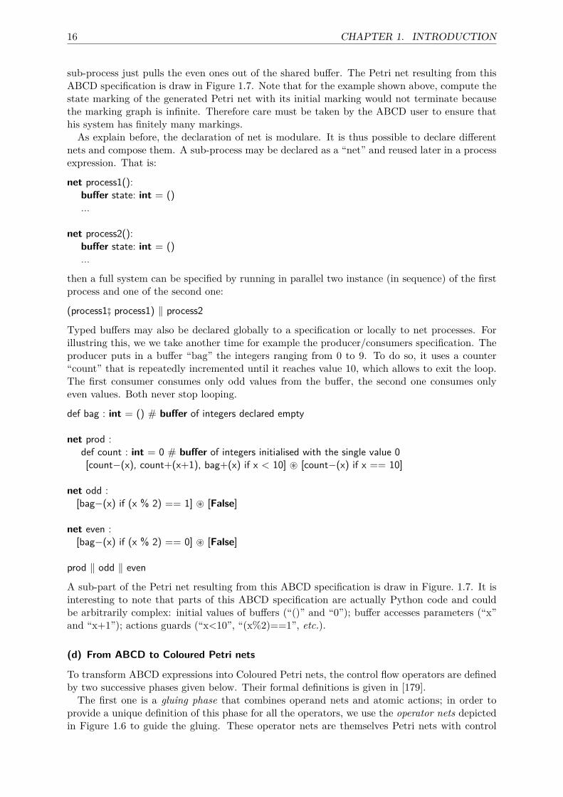
Figure 1.8. On the left: two Petri nets with control flow N1, N2. On the right: the result ofthe gluing phase of the sequential composition N1 #N2. Place names are indicated inside places.Dotted lines indicate how control flow places are paired by the Cartesian product during thegluing phase. Notice that, because no named place is present, the right net is exactly N1 #N2.
e
x x
i i i i
•buffer
•buffer other
• ε
e
x x
i i i i••buffer
other
• ε
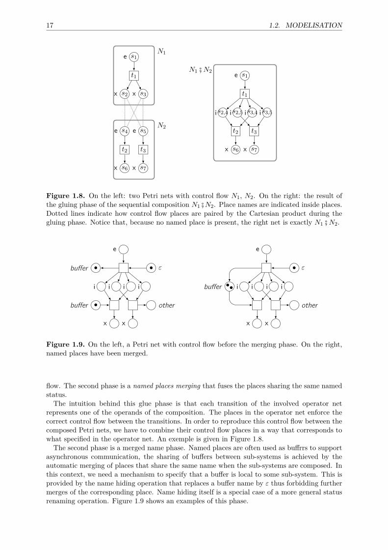
Figure 1.9. On the left, a Petri net with control flow before the merging phase. On the right,named places have been merged.
flow. The second phase is a named places merging that fuses the places sharing the same namedstatus.The intuition behind this glue phase is that each transition of the involved operator net
represents one of the operands of the composition. The places in the operator net enforce thecorrect control flow between the transitions. In order to reproduce this control flow between thecomposed Petri nets, we have to combine their control flow places in a way that corresponds towhat specified in the operator net. An exemple is given in Figure 1.8.The second phase is a merged name phase. Named places are often used as buffrrs to support
asynchronous communication, the sharing of buffers between sub-systems is achieved by theautomatic merging of places that share the same name when the sub-systems are composed. Inthis context, we need a mechanism to specify that a buffer is local to some sub-system. This isprovided by the name hiding operation that replaces a buffer name by ε thus forbidding furthermerges of the corresponding place. Name hiding itself is a special case of a more general statusrenaming operation. Figure 1.9 shows an examples of this phase.
18 CHAPTER 1. INTRODUCTION
(e) Structural Information for verification
Providing structural information about the Petri nets to analyse is usually either left to the userof a tool, or obtained by static analysis (e.g. place invariants may be computed automatically).However, in our framework, Petri nets are usually constructed by composing smaller partsinstead of being provided as a whole. This is the case in particular when the Petri net isobtained as the semantics of a syntax. In such a case, we can derive automatically manystructural information about the Petri nets.For instance, when considering the modelling and verification of security protocols, systems
mainly consist of a set of sequential processes composed in parallel and communicating througha shared buffer that models the network. In such a system, we known that, by construction,the set of control flow places of each parallel component forms a 1-invariant, i.e. there existeverytime at most one entry place and one exit place. This property comes from the fact thatthe process is sequential and that the Petri net is control-safe2 by construction. Moreover, wealso know that control flow places are 1-bounded, so we can implement their marking with aBoolean instead of an integer to count the tokens as explained above. It is also possible toanalyse buffer accesses at a syntactical level and discover buffers that are actually 1-bounded,for instance if any access is always composed either of a put and a get, or of a test, in the sameatomic action.
1.3 Parallelisation
1.3.1 What is parallelism?
A more complete presentation is available at [204].Many applications require more compute power than provided by sequential computers, like
for example, numerical simulations in industry and research, commercial applications such asquery processing, data mining and multi-media applications. One option to improve performanceis parallel processing.A parallel computer or multi-processor system is a computer utilizing more than one processor.
It’s commom to classify parallel computers by distinguishing them by the way how processors canaccess the system’s main memory. Indeed, this influences heavily the usage and programmingof the system. Two major classes of distributed memory computers can be distinguished:thedistributed memory and the shared memory systems.
(a) Flynn
Flynn defines a classification of computer architectures, based upon the number of concurrentinstruction (or control) and data streams available in the architecture [80,95].
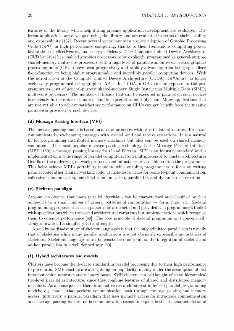
Single Instruction Multiple InstructionsSingle datum SISD MISDMultiple data SIMD MIMD
where:
• SISD is “Single Instruction, Single Data stream” that is a sequential machine;• SIMD is “Single Instruction, Multiple Data streams” that is mostly array processors and
GPU;2Let us call control-safe a Petri net with control flow whose control flow places remain marked by at most
one token under any evolution. Then, if two Petri nets are control-safe, their composition by any of the controlflow operations is also control-safe. This property holds assuming a restriction about how operators may benested [179].
19 1.3. PARALLELISATION
• MISD is “Multiple Instruction, Single Data stream” that is pipeline of data (pipe skele-ton);
• MIMD is “Multiple Instruction, Multiple Data streams” that is clusters of CPUs.
The distributed memory called No Remote Memory Access (NORMA) computers do not haveany special hardware support to access another node’s local memory directly. The nodes areonly connected through a computer network. Processors obtain data from remote memory onlyby exchanging messages over this network between processes on the requesting and the supplyingnode. Computers in this class are sometimes also called Network Of Workstations (NOW). Andin case of shared memory systems, Remote Memory Access (RMA) computers allow to accessremote memory via specialized operations implemented by hardware, however the hardwaredoes not provide a global address space. The major advantage of distributed memory systems istheir ability to scale to a very large number of nodes. In contrast, a shared memory architectureprovides (in hardware) a global address space, i.e. all memory locations can be accessed viausual load and store operations. Thereby, such a system is much easier to program. Also notethat the shared memory systems can only be scaled to moderate numbers of processors.We concentrate on Multiple Instruction, Multiple Data streams (MIMD) model, and especially
on one of its subcategory, the so-called Single Program Multiple Data (SPMD) model, wich isthe most current for the programmation of parallel computers.
(b) SPMD model
In the SPMD model, the same program runs on each processor but it computes on differentparts of the data which were distributed over the processors.There are two main programming models, message passing and shared memory, offering dif-
ferent features for implementing applications parallelized by domain decomposition. Sharedmemory allows multiple processes to read and write data from the same location. Messagepassing is another way for processes to communicate: each process can send messages to otherprocesses
(c) Shared Memory Model
In shared memory model, programs start as a single process known as a master thread thatexecutes on a single processor. The programmer designates parallel regions in the program.When the master thread reaches a parallel region, a fork operation is executed that creates ateam of threads, which execute the parallel region on multiple processors. At the end of theparallel region, a join operation terminates the team of threads, leaving only the master threadto continue on a single processor.In the shared memory model, a first parallel version is relatively easy to implement and can
be incrementally tuned. In the message passing model instead, the program can be tested onlyafter finishing the full implementation. Subsequent tuning by adapting the domain decompo-sition is usually time consuming. We give some well known examples of library for the sharedmemory programmaing model. OpenMP1 [24, 47] is a directive-based programming interfacefor the shared memory programming model. It consists of a set of directives and runtime rou-tines for Fortran, and a corresponding set of pragmas for C and C++ (1998). Directives arespecial comments that are interpreted by the compiler. Directives have the advantage that thecode is still a sequential code that can be executed on sequential machines (by ignoring thedirectives/pragmas) and therefore there is no need to maintain separate sequential and parallelversions.Intel Threading Building Blocks (Intel TBB2) library [144] which is a library in C++ language
that supports scalable parallel programming. The evaluation is done specifically for the pipelineapplications that are implemented using filter and pipeline class provided by the library. Various
20 CHAPTER 1. INTRODUCTION
features of the library which help during pipeline application development are evaluated. Dif-ferent applications are developed using the library and are evaluated in terms of their usabilityand expressibility [137]. Recent several years have seen a quick adoption of Graphic ProcessingUnits (GPU) in high performance computing, thanks to their tremendous computing power,favorable cost effectiveness, and energy efficiency. The Compute Unified Device Architecture(CUDA)3 [164] has enabled graphics processors to be explicitly programmed as general-purposeshared-memory multi-core processors with a high level of parallelism. In recent years, graphicsprocessing units (GPUs) have been progressively and rapidly advancing from being specializedfixed-function to being highly programmable and incredibly parallel computing devices. Withthe introduction of the Compute Unified Device Architecture (CUDA), GPUs are no longerexclusively programmed using graphics APIs. In CUDA, a GPU can be exposed to the pro-grammer as a set of general-purpose shared-memory Single Instruction Multiple Data (SIMD)multi-core processors. The number of threads that can be executed in parallel on such devicesis currently in the order of hundreds and is expected to multiply soon. Many applications thatare not yet able to achieve satisfactory performance on CPUs can get benefit from the massiveparallelism provided by such devices.
(d) Message Passing Interface (MPI)
The message passing model is based on a set of processes with private data structures. Processescommunicate by exchanging messages with special send and receive operations. It is a naturalfit for programming distributed memory machines but also can be used on shared memorycomputers. The most popular message passing technology is the Message Passing Interface(MPI) [189], a message passing library for C and Fortran. MPI is an industry standard and isimplemented on a wide range of parallel computers, from multiprocessor to cluster architecturesDetails of the underlying network protocols and infrastructure are hidden from the programmer.This helps achieve MPI’s portability mandate while enabling programmers to focus on writingparallel code rather than networking code. It includes routines for point-to-point communication,collective communication, one-sided communication, parallel IO, and dynamic task creation.
(e) Skeleton paradigm
Anyone can observe that many parallel algorithms can be characterised and classified by theiradherence to a small number of generic patterns of computation — farm, pipe, etc. Skeletalprogramming proposes that such patterns be abstracted and provided as a programmer’s toolkitwith specifications which transcend architectural variations but implementations which recognisethem to enhance performance [60]. The core principle of skeletal programming is conceptuallystraightforward. Its simplicity is its strength.A well know disadvantage of skeleton languages is that the only admitted parallelism is usually
that of skeletons while many parallel applications are not obviously expressible as instances ofskeletons. Skeletons languages must be constructed as to allow the integration of skeletal andad-hoc parallelism in a well defined way [60].
(f) Hybrid architecures and models
Clusters have become the de-facto standard in parallel processing due to their high performanceto price ratio. SMP clusters are also gaining on popularity, mainly under the assumption of fastinterconnection networks and memory buses. SMP clusters can be thought of as an hierarchicaltwo-level parallel architecture, since they combine features of shared and distributed memorymachines. As a consequence, there is an active research interest in hybrid parallel programmingmodels, e.g. models that perform communication both through message passing and memoryaccess. Intuitively, a parallel paradigm that uses memory access for intra-node communicationand message passing for internode communication seems to exploit better the characteristics of
21 1.3. PARALLELISATION
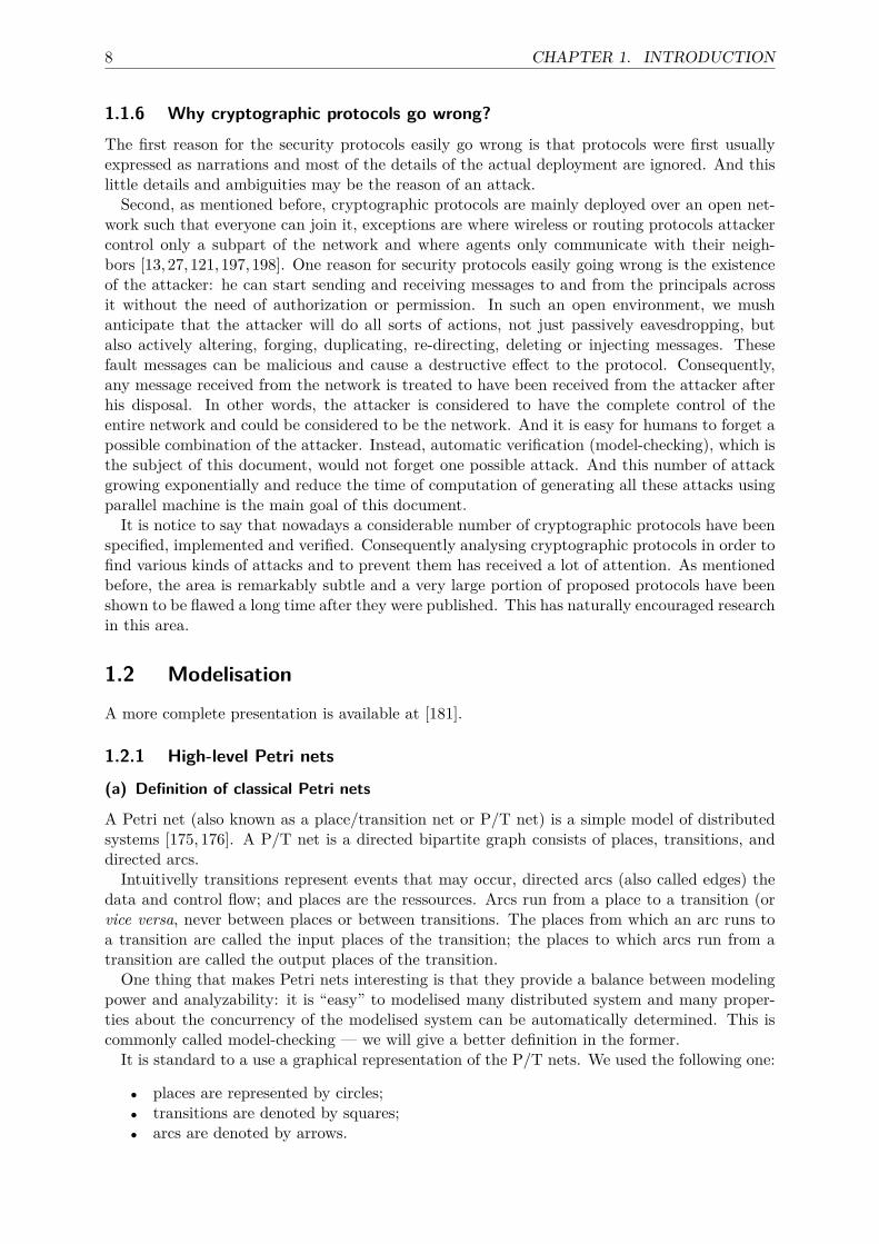
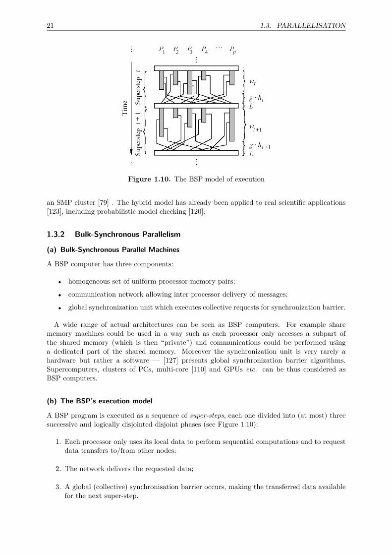
Figure 1.10. The BSP model of execution
an SMP cluster [79] . The hybrid model has already been applied to real scientific applications[123], including probabilistic model checking [120].
1.3.2 Bulk-Synchronous Parallelism
(a) Bulk-Synchronous Parallel Machines
A BSP computer has three components:
• homogeneous set of uniform processor-memory pairs;
• communication network allowing inter processor delivery of messages;
• global synchronization unit which executes collective requests for synchronization barrier.
A wide range of actual architectures can be seen as BSP computers. For example sharememory machines could be used in a way such as each processor only accesses a subpart ofthe shared memory (which is then “private”) and communications could be performed usinga dedicated part of the shared memory. Moreover the synchronization unit is very rarely ahardware but rather a software — [127] presents global synchronization barrier algorithms.Supercomputers, clusters of PCs, multi-core [110] and GPUs etc. can be thus considered asBSP computers.
(b) The BSP’s execution model
A BSP program is executed as a sequence of super-steps, each one divided into (at most) threesuccessive and logically disjointed disjoint phases (see Figure 1.10):
1. Each processor only uses its local data to perform sequential computations and to requestdata transfers to/from other nodes;
2. The network delivers the requested data;
3. A global (collective) synchronisation barrier occurs, making the transferred data availablefor the next super-step.
22 CHAPTER 1. INTRODUCTION
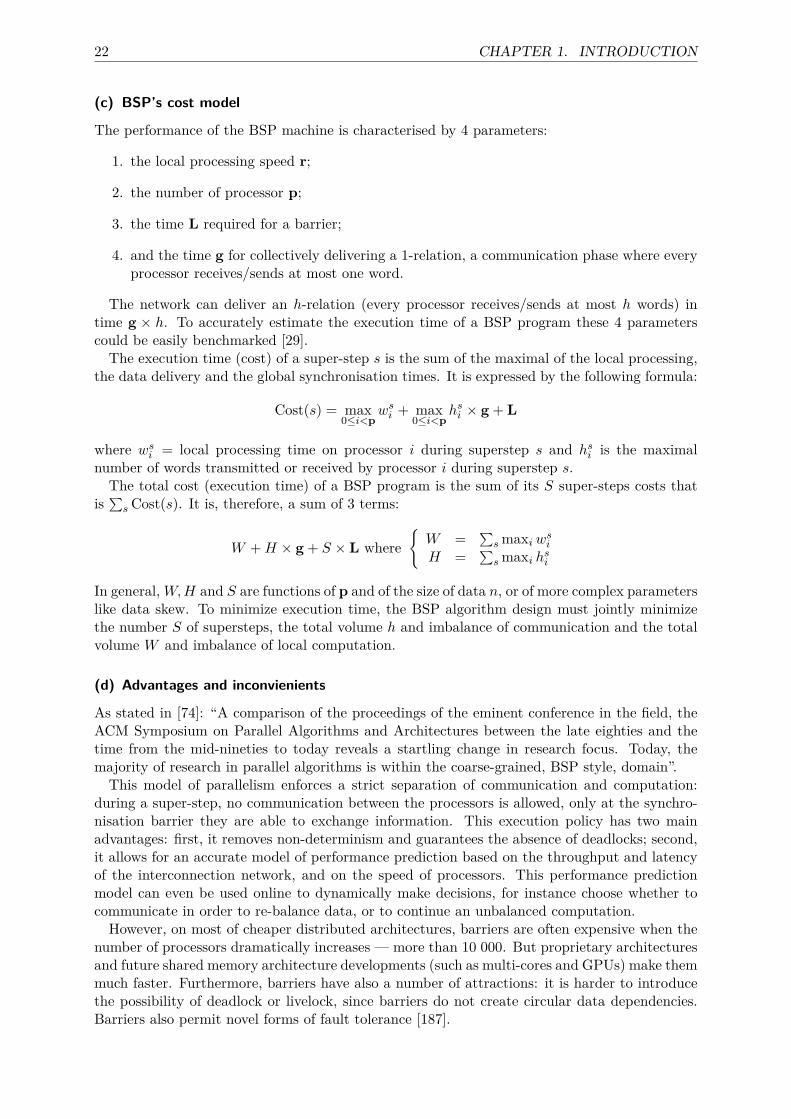
(c) BSP’s cost model
The performance of the BSP machine is characterised by 4 parameters:
1. the local processing speed r;
2. the number of processor p;
3. the time L required for a barrier;
4. and the time g for collectively delivering a 1-relation, a communication phase where everyprocessor receives/sends at most one word.
The network can deliver an h-relation (every processor receives/sends at most h words) intime g × h. To accurately estimate the execution time of a BSP program these 4 parameterscould be easily benchmarked [29].The execution time (cost) of a super-step s is the sum of the maximal of the local processing,
the data delivery and the global synchronisation times. It is expressed by the following formula:
Cost(s) = max0≤i<p
wsi + max0≤i<p
hsi × g + L
where wsi = local processing time on processor i during superstep s and hsi is the maximalnumber of words transmitted or received by processor i during superstep s.The total cost (execution time) of a BSP program is the sum of its S super-steps costs that
is ∑sCost(s). It is, therefore, a sum of 3 terms:
W +H × g + S × L where{W = ∑
s maxiwsiH = ∑
s maxi hsi
In general,W,H and S are functions of p and of the size of data n, or of more complex parameterslike data skew. To minimize execution time, the BSP algorithm design must jointly minimizethe number S of supersteps, the total volume h and imbalance of communication and the totalvolume W and imbalance of local computation.
(d) Advantages and inconvienients
As stated in [74]: “A comparison of the proceedings of the eminent conference in the field, theACM Symposium on Parallel Algorithms and Architectures between the late eighties and thetime from the mid-nineties to today reveals a startling change in research focus. Today, themajority of research in parallel algorithms is within the coarse-grained, BSP style, domain”.
This model of parallelism enforces a strict separation of communication and computation:during a super-step, no communication between the processors is allowed, only at the synchro-nisation barrier they are able to exchange information. This execution policy has two mainadvantages: first, it removes non-determinism and guarantees the absence of deadlocks; second,it allows for an accurate model of performance prediction based on the throughput and latencyof the interconnection network, and on the speed of processors. This performance predictionmodel can even be used online to dynamically make decisions, for instance choose whether tocommunicate in order to re-balance data, or to continue an unbalanced computation.However, on most of cheaper distributed architectures, barriers are often expensive when the
number of processors dramatically increases — more than 10 000. But proprietary architecturesand future shared memory architecture developments (such as multi-cores and GPUs) make themmuch faster. Furthermore, barriers have also a number of attractions: it is harder to introducethe possibility of deadlock or livelock, since barriers do not create circular data dependencies.Barriers also permit novel forms of fault tolerance [187].
23 1.3. PARALLELISATION
The BSP model considers communication actions en masse. This is less flexible than asyn-chronous messages, but easier to debug since there are many simultaneous communication ac-tions in a parallel program, and their interactions are typically complex. Bulk sending alsoprovides better performances since, from an implementation point of view, grouping communi-cation together in a seperate program phase permits a global optimization of the data exchangeby the communications library.The simplicity and yet efficiency of the BSP model makes it a good framework for teaching
(few hours are needed to teach BSP programming and algorithms), low level model for multi-cores/GPUs system optimisations [110], etc., since it has been conceived has a bridging modelfor parallel computation.This is also merely the most visible aspects of a parallel model that shifts the responsibility
for timing and synchronization issues from the applications to the communications library3. Aswith other low/high level design decisions, the applications programmer gains simplicity butgives up some flexibility and performance. In fact, the performance issue is not as simple as itseems: while a skilled programmer can in principle always produce more efficient code with alow-level tool (be it message passing or assembly language), it is not at all evident that a real-lifeprogram, produced in a finite amount of time, can actually realize that theoretical advantage,especially when the program is to be used on a wide range of machines [114,147].Last advantage of BSP is that it greatly facilitates debugging. The computations going on
during a superstep are completely independent and can thus be debugged independently. More-over, it is easy to measure during the execution of a BSP program, time speding to communicateand to synchronise by just adding chronos before and after the primitive of synchronisation. Thisfacility will be used here to compare differents algorithms.All this capacities are is possibles only because the runtime system knows precisely which com-
putations are independent. In a asynchronous message-passing system as MPI, the independentsections tend to be smaller, and identifying them is much harder. But, using BSP, programersand designer have to keep in mind that some parallelism patterns are not really BSP friendly.For example, BSP does not enjoy in an optimist manner pipeline and master/slave (also knowedas farm of processes) schemes even if it is possible to have not too inefficient BSP programs fromthese schemes [103]. Thus, some parallel computations and optmisations would never be BSP.This is the drawback of all the restricted models of computations as well.The BSP model has been used with success in a wide variety of problems such scientific
computing [14, 29, 30, 76, 134, 196], parallel data-structure [108, 116], genetic algorithms [39]and genetic programming [78], neural network [182], parallel data-bases [15–17], constraintssolver [115], graphs [46, 94, 146, 196], geometry [75], string search [93, 143], implementation oftree skeletons [156], etc.
1.3.3 Other models of parallel computation
We survey here, other groups of parallel abstract machines than BSP: the PRAM and derivedfamily, the LogP and extensions of the BSP models.
(a) PRAM
The PRAM (Parallel Random Access Machine) model [97] was introduced as a model for generalpurpose computations. A PRAM is made by an unbounded number P of processors, each onebeing a RAM [99] with set of registers rather than a memory. There is only one memoryspace shared by the processors. In every cycle each processor can perform one of the followingactions; read a value from a global memory, write a value from its register to the memoryor compute an operation on its local registers. The cost of a random access to the global
3BSP libraries are generally implemented using MPI [188] or low level routines of the given specifics architec-tures
24 CHAPTER 1. INTRODUCTION
memory is a unit-time independently from the access pattern. The PRAM model can be definedaccording to the politics to the simultaneously access the same memory localtion, the possiblechoices are: EREW (Exclusive Read Exclusive Write), CREW (Concurrent Read ConcurrentWrite), CRCW (Concurrent Read Concurrent Write). When a concurrent write is allowed someoptions are distinguished. The idealization provided by the PRAM completely hides aspectssuch as synchronization, data locality etc. This facilitated the acceptance of the model amongsttheorists of algorithms and many parallel algorithms are expressed by using such a abstraction.In practice PRAM has only the P parameter (the number of processors) and the measure ofthe work performed by an algorithm is simply the time per processor product. Issues such asthe communication latency or brandwidth are not considered and this leads to a completelyunreliable prediction of execution costs.The only possibility for hiding (partially) this problem is the exploitation of a certain amount
of parallelism to mask the wait for messages. This method is named parallel slackness. Manyworks has been done to emulate PRAM and, even if, optical technology may turn out a decisivehelp etc.
(b) APRAM
The asynchronous variant of PRAM [111] is intended to be closer to the MIMD architectures.All the models belonging to this family share the needs for an explicit synchronization to ensurethat a memory access has been completed. There are two groups of asynchronous PRAM: thephase and the subset. The models of the first group require that all of the processors participateto the synchronization while the models of the second require only a subset. The LPRAM isa variant of the APRAM wich introduces, for the first time the notion of synchronization anlatency costs. The cost of synchronizing is considered a nondecreasing function of the processorscount: B(P ). The latency introduces by the LPRAM is simply a constant d.
(c) HPRAM
The Hierarchical PRAM [125] proposed by Heywood is given by a collection of synchronousPRAM that operate asynchronously from each other. HPRAM can execute a partition instruc-tion to create disjoint subsets of a P processors PRAM. Each subset receives an algorithm to beexecuted and the partition controls the asynchrony of the model. The model has two variants:(1) Private HPRAM where partition divides memory among processors. In this case, each subsethas its own private block of shared memory. Each block is disjoint from the others belonging tothe other sub-PRAMs. (2) Shared HPRAM where partition does not divide the shared memoryand each sub-PRAM can access the global memory. The parameters of HPRAM are latency l()and the synchronization s(). The crucial point is that latency is proportional ot the diameter ofthe sub-network. In HPRAM there are two different synchronizations: α synchronization wichoccurs between processors within a (sub)-PRAM computation and β synchronization wich takesplace at the end of a partition. Costs of synchronization are often dominated by communicationsand computations.
(d) LogP
The LogP [71] model is an asynchronous (or loosely synchronous) framework to describe dis-tributed memory multicomputers which communicate point-to-point. The model provides avision of the communication costs without taking into account the topology of the interconnec-tion network. The parameters for a LogP machine are: L( latency): the upper bound on thelatency of the interconnection network, o (overhead): the overhead for transmission or reception(the processor can not overlap this time with other operations), g (gap): the minimum gap be-tween consecutive messages (the reciprocal of g is the bandwidth per processor), P (processors)the number of processors (every local operation is computed in a unit-time named cycle).
25 1.3. PARALLELISATION
(e) CLUMPS
The CLUMPS [41–43] model has been introduced by Campbell as an architectural model (in theMcColl [157] classification) wich unifies the characteristic of HPRAM and LogP. The architec-tural elements used to model a generaliez parallel hardware are: a set of processor-memory pairs,a partionable interconnection network and a flexible control among SIMD and MIMD. Since itspartitionable nature, CLUMPS complicates the LogP model by introducing a “regional” ruleto compute the values of its main parameters. CLUMPS is the first model which claims to beskeletons-oriented. Unfortunately its cost model fails in providing manageable prediction andthe complexity of its performance equations is very high.Models as HPRAM or CLUMPS can be considered as too “realistic” and this means that
they can not be a useful platform for an optimizing tool which aims to be also simple. Moreovermany of the current parallel machines do not require such a fine-grain model.
(f) LoPC
The LoPC model [98] has been introduced with the aim of extending the LogP model to accountfor node-contention. The authors claim that for both fine-grain message passing algorithms andshared memory, the cost due to accesses contention dominates the cost of handlers service timeand network latency. The main assumption in the LoPC model are that hardware messagebuffers at the nodes are infinitely large and that the interconnect is contention free. The modelassumes fixed size of the message even if it recalls the LogGP model is made for a possible exten-sion for long messages. The goal of LoPC is to generate a contention efficient runtime schedulingof communications exploiting a limitede set of algorithmic and architectural parameters.
(g) E-BSP
The E-BSP [138] extends the basic BSP model to deal with unbalanced communication patternsi.e. patterns in which the amount of data sent or received by each node is different. The costfunction supplied by E-BSP is a nonlinear function that strongly depends on the network topol-ogy. The model essentially differentiates between communication patterns that are insensitiveto the bisection bandwidth and those that are not.
(h) D-BSP
The Decomposable-BSP model [73] extends the BSP model by introducing the possibility ofsubmachine synchronizations. A D-BSP computer is basically a BSP computer where the syn-chronization device allows subgroup of processors to synchronize independently. The D-BSPremembers the HPRAM and CLUMPS model in which the cost are expressed in terms of BSPsupersteps. In this framework network locality can be exploited assuming that submachinesparameters are a decreasing functions of the diameter of the subset of processors involved incommunication and synchronization.
(i) QSM
Gibbons et al. considered the possibility of providing a bridging model based on a sharedmemory abstraction, in analogy to the message passing based BSP model. The paper introducesthe Queuing Shared Model (QSM) [112] wich accounts for bandwidth limitation in the contextof a shared memory architecture. The processors execute a sequence of synchronized phases,each consisting of an arbitrary interleaving of the following operations: shared-memory reads,shared-memory writes and local computation.
26 CHAPTER 1. INTRODUCTION
(j) Multi-BSP
Multi-core architectures, based on many processors and associated local caches or memories,are attractive devices given current technological possibilities, and known physical limitations.Multi-BSP model [200] is a multi-level model that has explicit parameters for processor num-bers, memory/cache sizes, communication costs, and syn- chronization costs. The lowest levelcorresponds to shared memory or the PRAM, acknowledging the relevance of that model forwhatever limitations on memory and processor numbers it may be efficacious to emulate it. TheMulti-BSP model which extends BSP in two ways. First, it is a hierarchical model, with an ar-bitrary number of levels. It recognizes the physical realities of multiple memory and cache levelsboth within single chips as well as in multi-chip architectures. The aim is to model all levels ofan architecture together, even possibly for whole datacenters. Second, at each level, Multi-BSPincorporates memory size as a further parameter. After all, it is the physical limitation on theamount of memory that can be accessed in a fixed amount of time from the physical locationof a processor that creates the need for multiple levels. An instance of a Multi-BSP is a treestructure of nested components where the lowest level or leaf components are processors andevery other level contains some storage capacity. The model does not distinguish memory fromcache as such, but does assume certain properties of it.
(k) HiHCoHP
We interest now in a recent model: the Hierarchical Hyper Clusters of Heterogeneous Processors(HiHCoHP) model [44, 45]. It is a successor of the homogeneous LogP model and its long-message extension LogGP. It strives to incorporate enough architectural detail to produce resultsthat are relevant to users of actual (hyper)clusters, while abstracting away enough detail to bealgorithmically and mathematically tractable. It intends to be a general-purpose algorithmicmodel — like logP and logGP.The HiHCoHP model is rather detailed, exposing architectural features such as the bandwidth
and transit costs of both networks and their ports.Our choice in favor BSP forthe ease of use. Our implementation take into account at this time
the architectures NOW in SPMD but scheduled optimizations are easy for hybrid architectures.
1.4 Verifying security protocolsThe first class of tools, which focus on verification, typically rely on encoding protocols as Hornclauses and applying resolution-based theorem proving to them (without termination guarantee).Analysis tools of this kind include NRL4 [158] and ProVerif [31].We recall that the problem of whether a protocol actually provides the security properties it
has been designed for is undecidable [81]. Despite this fact, over the last two decades a widevariety of security protocol analysis tools have been developed that are able to detect attackson protocols or, in some cases, establish their correctness. We distinguish three classes: toolsthat attempt verification (proving a protocol correct), those that attempt falsification (findingattacks), and hybrids that attempt to provide both proofs and counterexamples.
1.4.1 Verifying security protocols through theorem proving
One type of mechanized verification process is theorem proving using a higher-order logic the-orem prover such as Isabelle/HOL5 [166, 202] or PVS6 [169]. Using a theorem prover, oneformalizes the system (the agents running the protocol along with the attacker) as a set ofpossible communication traces. Afterwards, one states and proves theorems expressing that thesystem in question has certain desirable properties, The proofs are usually carried out understrong restrictions, e.g. that all variables are strictly typed and that all keys are atomic.
27 1.4. VERIFYING SECURITY PROTOCOLS
The main drawback of this approach is that verification is quite time consuming and requiresconsiderable expertise. Moreover, theorem provers provide poor support for error detectionwhen the protocols are flawed.
1.4.2 Verifying security protocols by model checking
The second kind of verification centers around the use of model checkers, which are fully auto-matic.In contrast to verification, the second class of tools detects protocol errors (i.e. attacks) using
model checking [153, 161] or constraint solving [48, 162]. Model checking attempts to find areachable state where some supposedly secret term is learnt by the intruder, or in which anauthentication property fails. Constraint solving uses symbolic representations of classes of suchstates, using variables that have to satisfy certain constraints. To ensure termination, these toolsusually bound the maximum number of runs of the protocol that can be involved in an attack.Therefore, they can only detect attacks that involve no more runs of the protocol than thestated maximum. In the third class, attempts to combine model checking with elements fromtheorem proving have resulted in backward-search-based model checkers. These use pruningtheorems, resulting in hybrid tools that in some cases can establish correctness of a protocol (foran unbounded number of sessions) or yield a counterexample, but for which termination cannotbe guaranteed [190].Model Checking offers a promising approach for automated security analysis of protocols:
the intuitive notions are translated into formal specifications, which is essential for a carefuldesign and analysis, and protocol executions can be simulated, making it easier to verify certainsecurity properties. As Model Checking becomes increasingly used in the industry as a partof the design process, there is a constant need for efficient tool support to deal with real-size applications. Model checking [55] is a successful verification method based on reachabilityanalysis (state space exploration) and allows an automatic detection of early design errors infinite-state systems. Model checking works by constructing a model (state space) of the systemunder design, on which the desired correctness properties are verified.Model checking is a powerful and automatic technique for verifying finite state concurrent
systems. Introduced in early 1980s, it has been applied widely and successfully in practice toverify digital sequential circuit designs and communication protocols. Model checking has beenproved to be particularly suited in finding counter-examples, i.e. to return paths through thetransition system that violate one of the specified system requirements.At the core of computer security-sensitive applications are security protocols i.e. a sequence
of message exchanges aiming at distributing data in a cryptographic way to the intended usersand providing security guarantees. This leads to the researches in searching for a way to verifywhether a system is secure or not. Enumerative model checking is well-adapted to for this kindof asynchronous, non-deterministic systems containing complex data types.Let us recall that the state space generation problem is the problem of computing the explicit
representation of a given model from the implicit one. This space is constructed by exploring allthe states (from a function of successor) starting from the initial state. Generally, during thisoperation, all explored states must be kept in memory in order to avoid multiple exploration of asame state. Once the space is constructed or while an on-the-fly construction, it can be used asinput for various verification procedures, such as Linear Temporal Logic (LTL) model-checking.A specialisation of the LTL logic (defined later) to protocols have also be done in [12]. In thisdocument, we will consider the more general problematic of the CTL* logic (defined later) modelchecking.State space construction may be very consuming both in terms of memory and execution time:
this is the so-called state explosion problem. The generation of large discrete state spaces is soa computationally intensive activity with extreme memory demands, highly irregular behavior,and poor locality of references. This is especially true when complex data-structures are used
28 CHAPTER 1. INTRODUCTION
in the model as the knowledge of an intruder in security protocols.During the last decade, different techniques for handling state explosion have been proposed,
among which partial orders and symmetries. However these optimizations are not always suffi-cient. Moreover, most of the currently available verification tools work on sequential machines,which limits the amount of memory and therefore the use of clusters or parallel machines isdesirable and is a great challenge of research. As this generation can cause memory thrash-ing on single or multiple processor systems, it has been lead to consider exploiting the largermemory space available in distributed systems [86,165]. Parallelize the state space constructionon several machines is thus done in order to benefit from all the local memories, cpu resourcesand disks of each machine. This allows to reduce both the amount of memory needed on eachmachine and the overall execution time.A distributed memory algorithm with its tool for verification of security protocols is described
in [192]. They used buffering principle and also employ a cache of recently sent states in theirimplementation which task is to decrease the number of sent messages. Unfortunately, theverification of temporal properties is not supported due to the difficulties of combining theparallel checking with the symmetry reduction. We think that extend our algorithm to verifytemporal properties would be easy to do.There are also many “model-checker like” tools dedicated for verifying security protocols
as [8, 10, 107]. The most known is certainly the one of [11]. Our approach has the avantage ofbeing general using an algebra of coloured Petri nets and can take into account “protocols withloop” and any data structure using Python.
[101] allows to verify some properties about the protocols for an infinite number of sessionsand with some possibility of replay using an algebra of processes. But no logic (LTL or else)can be used here and each time a new property is needed, a new theorem is need to be proved.That can be complicated for the maintenance of the method.
1.4.3 Dedicated tools
A more complete presentation is available at [68].We firstly recall some earlier approaches relying on general purpose verification tools: Isabelle.
Paulson [173] has proposed to state security properties such as secrecy as predicates (formalizedin higher-order logic) over execution traces of the protocol, without limitations on the numberof agents. These predicates can be verified by induction with automated support provided bythe Isabelle proof assistant [166, 202]. Casper7/FDR8. FDR is a model checker for the CSPprocess algebra. Roughly speaking, FDR checks whether the behaviors of a CSP process associ-ated with a protocol implementation are included in the behaviors allowed by its specification.FDR is provided with a user-friendly interface for security protocol analysis, Casper [153] thatautomatically translates protocols in an “Alice & Bob-notation” (with possible annotations) toCSP code. Gavin Lowe has discovered the now well-known attack on the Needham-SchroederPublic-Key Protocol using FDR [152]. Similarly, many protocol-specific case studies have beenperformed in various general-purpose model checkers. We mention µCRL9 [34] as used in [35],UPPAAL10 [25] as used in [63], and SPIN11 [132] as used in [155].
(a) NRL
In the NRL Protocol Analyzer [158], the protocol steps are represented as conditional rewritingrules. NRL invokes a backward search strategy from some specified insecure state to see if itcan be reached from an initial state. It has been used for verification of e.g. the Internet KeyExchange protocol [159]. Unfortunately, NRL is not publicly available and it is not clear whichcondition makes a protocol safe or not.
29 1.4. VERIFYING SECURITY PROTOCOLS
(b) Athena
The Athena [190] tool is an automatic checking algorithm for security protocols. It is basedon the Strand Spaces model [117, 195] and, when terminating, provides either a counterexam-ple if the formula under examination is false, or establishes a proof that the formula is true.Alternatively, Athena can be used with a bound (e.g. on the number of runs), in which casetermination is guaranteed, but it can guarantee at best that there exist no attacks within thebound. Unfortunately, Athena is also not publicly available.
(c) ProVerif
In ProVerif12 [31], protocol steps are represented by Horn clauses. The system can handlean unbounded number of sessions of the protocol but performs some approximations — onrandom numbers. As a consequence, when the system claims that the protocol preserves thesecrecy of some value, this is correct; this tool is thus need when no flaw has been found in theprotocol (with a bounded number of sessions) and we want to have a test for an unboundednumber of sessions. However it can generates false attacks too. Recently an algorithm wasdeveloped [1] that attempts to reconstruct attacks, in case the verification procedure fails, addingthe possibility of falsification to ProVerif.
(d) LySatool
The LySatool13 [36] implements security protocol analysis based on a process algebra enhancedwith cryptographic constructs. The approach is based on over-approximation techniques andcan verify confidentiality and authentication properties.
(e) Constraint solver
Based on [160], in which verification in the Strand Spaces model is translated into a constraintsolving problem, an efficient constraint solving method was developed in [64]. The methoduses constraint solving, optimized for protocol analysis, and a minimal form of partial orderreduction, similar to the one used in [57]. A second version of this tool does not use partialorder reduction, enabling it to verify properties of the logic PS-LTL [64].
(f) OFMC
The On-the-Fly Model Checker (OFMC [23]) is part of the AVISPA14 tool set [11], and is amodel checker for security protocols. It combines infinite state forward model checking withthe concept of a lazy intruder [21], where terms are generated on-demand during the forwardmodel checking process. A technique called constraint differentiation [162] is employed to avoidexploring similar states in different branches of the search, which is similar to the ideas in [70].It furthermore supports user-defined algebraic theories [22], allowing for correct modeling ofe.g. Diffie-Hellman exponentiation.
(g) Scyther
Scyther15 [68,69] is state-of-the-art in terms of verification speed and provides a number of novelfeatures. (1) It can verify most protocols for an unbounded number of sessions in less than asecond. Because no approximation methods are used, all attacks found are actual attacks on themodel. (2) In cases where unbounded correctness cannot be determined, the algorithm functionsas a classical bounded verification tool, and yields results for a bounded number of sessions. (3)Scyther can give a “complete characterization” of protocol roles, allowing protocol designers tospot unexpected possible behaviours early. (4) Contrary to most other verification tools, the useris not required to provide so-called scenarios for property verification, as all possible protocol
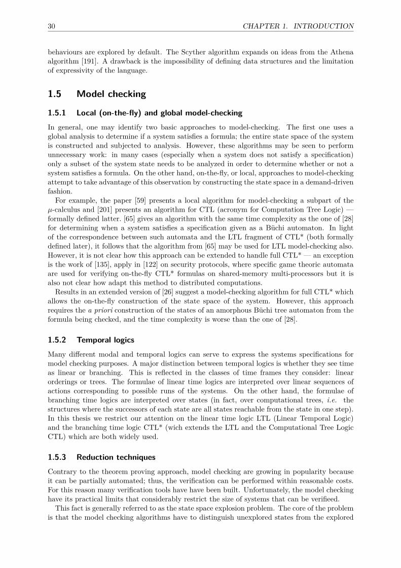
30 CHAPTER 1. INTRODUCTION
behaviours are explored by default. The Scyther algorithm expands on ideas from the Athenaalgorithm [191]. A drawback is the impossibility of defining data structures and the limitationof expressivity of the language.
1.5 Model checking
1.5.1 Local (on-the-fly) and global model-checking
In general, one may identify two basic approaches to model-checking. The first one uses aglobal analysis to determine if a system satisfies a formula; the entire state space of the systemis constructed and subjected to analysis. However, these algorithms may be seen to performunnecessary work: in many cases (especially when a system does not satisfy a specification)only a subset of the system state needs to be analyzed in order to determine whether or not asystem satisfies a formula. On the other hand, on-the-fly, or local, approaches to model-checkingattempt to take advantage of this observation by constructing the state space in a demand-drivenfashion.For example, the paper [59] presents a local algorithm for model-checking a subpart of the
µ-calculus and [201] presents an algorithm for CTL (acronym for Computation Tree Logic) —formally defined latter. [65] gives an algorithm with the same time complexity as the one of [28]for determining when a system satisfies a specification given as a Büchi automaton. In lightof the correspondence between such automata and the LTL fragment of CTL* (both formallydefined later), it follows that the algorithm from [65] may be used for LTL model-checking also.However, it is not clear how this approach can be extended to handle full CTL* — an exceptionis the work of [135], apply in [122] on security protocols, where specific game theoric automataare used for verifying on-the-fly CTL* formulas on shared-memory multi-processors but it isalso not clear how adapt this method to distributed computations.Results in an extended version of [26] suggest a model-checking algorithm for full CTL* which
allows the on-the-fly construction of the state space of the system. However, this approachrequires the a priori construction of the states of an amorphous Büchi tree automaton from theformula being checked, and the time complexity is worse than the one of [28].
1.5.2 Temporal logics
Many different modal and temporal logics can serve to express the systems specifications formodel checking purposes. A major distinction between temporal logics is whether they see timeas linear or branching. This is reflected in the classes of time frames they consider: linearorderings or trees. The formulae of linear time logics are interpreted over linear sequences ofactions corresponding to possible runs of the systems. On the other hand, the formulae ofbranching time logics are interpreted over states (in fact, over computational trees, i.e. thestructures where the successors of each state are all states reachable from the state in one step).In this thesis we restrict our attention on the linear time logic LTL (Linear Temporal Logic)and the branching time logic CTL* (wich extends the LTL and the Computational Tree LogicCTL) which are both widely used.
1.5.3 Reduction techniques
Contrary to the theorem proving approach, model checking are growing in popularity becauseit can be partially automated; thus, the verification can be performed within reasonable costs.For this reason many verification tools have have been built. Unfortunately, the model checkinghave its practical limits that considerably restrict the size of systems that can be verifieed.This fact is generally referred to as the state space explosion problem. The core of the problem
is that the model checking algorithms have to distinguish unexplored states from the explored
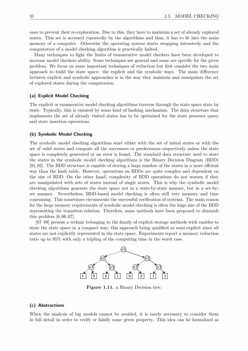
31 1.5. MODEL CHECKING
ones to prevent their re-exploration. Due to this, they have to maintain a set of already exploredstates. This set is accessed repeatedly by the algorithms and thus, it has to fit into the mainmemory of a computer. Otherwise the operating system starts swapping intensively and thecomputation of a model checking algorithm is practically halted.Many techniques to fight the limits of enumerative model checkers have been developed to
increase model checkers ability. Some techniques are general and some are specific for the givenproblem. We focus on some important techniques of reduction but first consider the two mainapproach to build the state space: the explicit and the symbolic ways. The main differencebetween explicit and symbolic approaches is in the way they maintain and manipulate the setof explored states during the computation.
(a) Explicit Model Checking
The explicit or enumerative model checking algorithms traverse through the state space state bystate. Typically, this is ensured by some kind of hashing mechanism. The data structure thatimplements the set of already visited states has to be optimized for the state presence queryand state insertion operations.
(b) Symbolic Model Checking
The symbolic model checking algorithms start either with the set of initial states or with theset of valid states and compute all the successors or predecessors respectively unless the statespace is completely generated or an error is found. The standard data structure used to storethe states in the symbolic model checking algorithms is the Binary Decision Diagram (BDD)[91,92]. The BDD structure is capable of storing a large number of the states in a more effcientway than the hash table. However, operations on BDDs are quite complex and dependent onthe size of BDD. On the other hand, complexity of BDD operations do not worsen if theyare manipulated with sets of states instead of single states. This is why the symbolic modelchecking algorithms generate the state space not in a state-by-state manner, but in a set-by-set manner. Nevertheless, BDD-based model checking is often still very memory and timeconsuming. This sometimes circumvents the successful verification of systems. The main reasonfor the large memory requirements of symbolic model checking is often the huge size of the BDDrepresenting the transition relation. Therefore, some methods have been proposed to diminishthis problem [6,66,67].
[87–89] present a technic belonging to the family of explicit storage methods wich enables tostore the state space in a compact way; this approach being qualified as semi-explicit since allstates are not explicitly represented in the state space. Experiments report a memory reductionratio up to 95% with only a tripling of the computing time in the worst case.
Figure 1.11. a Binary Decision tree.
(c) Abstractions
When the analysis of big models cannot be avoided, it is rarely necessary to consider themin full detail in order to verify or falsify some given property. This idea can be formalized as
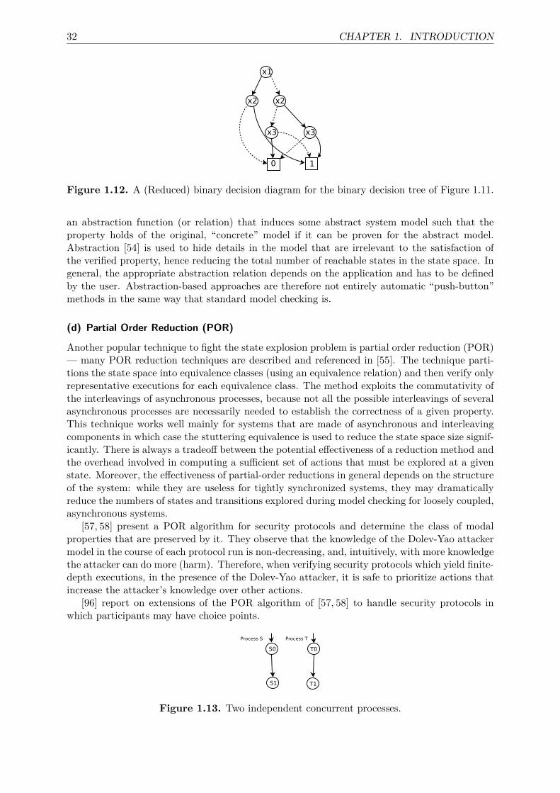
32 CHAPTER 1. INTRODUCTION
Figure 1.12. A (Reduced) binary decision diagram for the binary decision tree of Figure 1.11.
an abstraction function (or relation) that induces some abstract system model such that theproperty holds of the original, “concrete” model if it can be proven for the abstract model.Abstraction [54] is used to hide details in the model that are irrelevant to the satisfaction ofthe verified property, hence reducing the total number of reachable states in the state space. Ingeneral, the appropriate abstraction relation depends on the application and has to be definedby the user. Abstraction-based approaches are therefore not entirely automatic “push-button”methods in the same way that standard model checking is.
(d) Partial Order Reduction (POR)
Another popular technique to fight the state explosion problem is partial order reduction (POR)— many POR reduction techniques are described and referenced in [55]. The technique parti-tions the state space into equivalence classes (using an equivalence relation) and then verify onlyrepresentative executions for each equivalence class. The method exploits the commutativity ofthe interleavings of asynchronous processes, because not all the possible interleavings of severalasynchronous processes are necessarily needed to establish the correctness of a given property.This technique works well mainly for systems that are made of asynchronous and interleavingcomponents in which case the stuttering equivalence is used to reduce the state space size signif-icantly. There is always a tradeoff between the potential effectiveness of a reduction method andthe overhead involved in computing a sufficient set of actions that must be explored at a givenstate. Moreover, the effectiveness of partial-order reductions in general depends on the structureof the system: while they are useless for tightly synchronized systems, they may dramaticallyreduce the numbers of states and transitions explored during model checking for loosely coupled,asynchronous systems.
[57, 58] present a POR algorithm for security protocols and determine the class of modalproperties that are preserved by it. They observe that the knowledge of the Dolev-Yao attackermodel in the course of each protocol run is non-decreasing, and, intuitively, with more knowledgethe attacker can do more (harm). Therefore, when verifying security protocols which yield finite-depth executions, in the presence of the Dolev-Yao attacker, it is safe to prioritize actions thatincrease the attacker’s knowledge over other actions.
[96] report on extensions of the POR algorithm of [57, 58] to handle security protocols inwhich participants may have choice points.
Figure 1.13. Two independent concurrent processes.
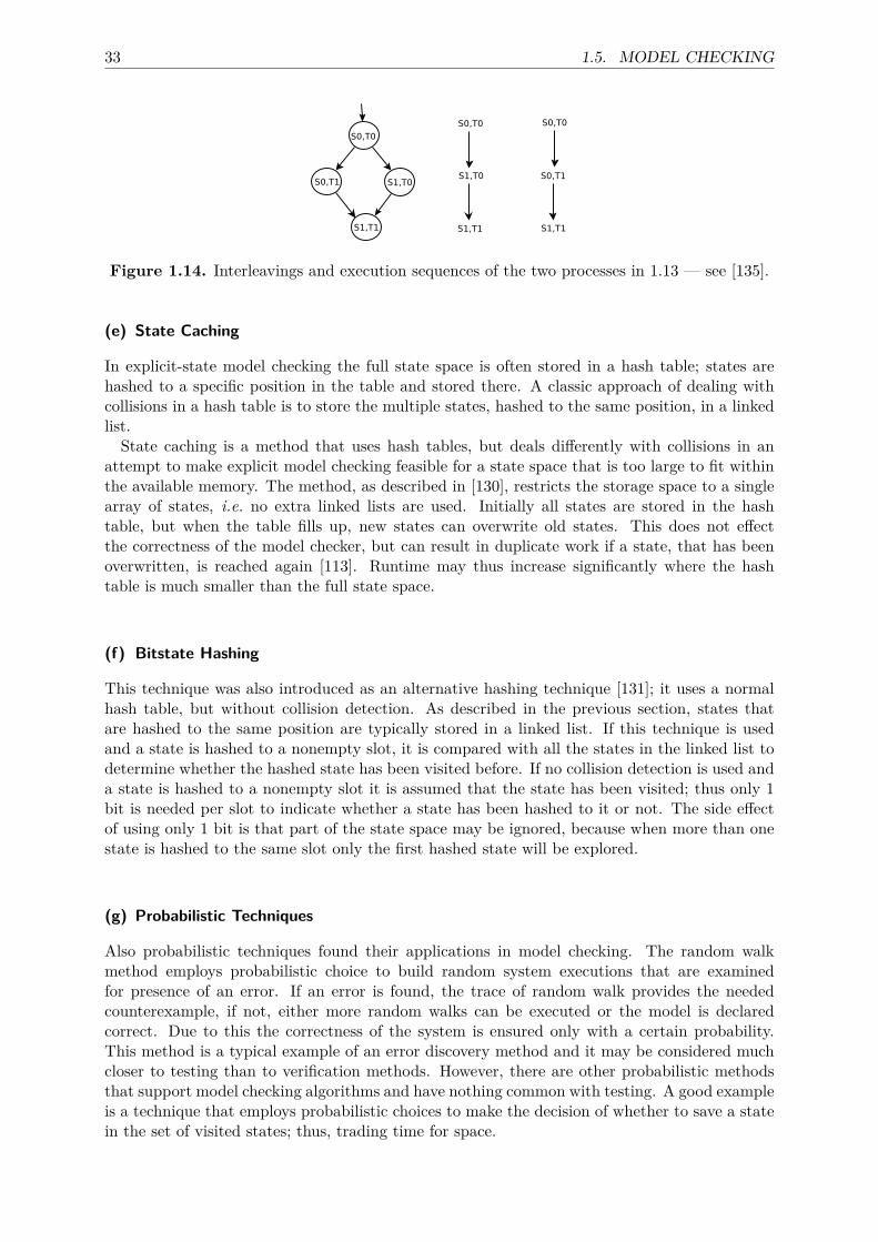
33 1.5. MODEL CHECKING
Figure 1.14. Interleavings and execution sequences of the two processes in 1.13 — see [135].
(e) State Caching
In explicit-state model checking the full state space is often stored in a hash table; states arehashed to a specific position in the table and stored there. A classic approach of dealing withcollisions in a hash table is to store the multiple states, hashed to the same position, in a linkedlist.State caching is a method that uses hash tables, but deals differently with collisions in an
attempt to make explicit model checking feasible for a state space that is too large to fit withinthe available memory. The method, as described in [130], restricts the storage space to a singlearray of states, i.e. no extra linked lists are used. Initially all states are stored in the hashtable, but when the table fills up, new states can overwrite old states. This does not effectthe correctness of the model checker, but can result in duplicate work if a state, that has beenoverwritten, is reached again [113]. Runtime may thus increase significantly where the hashtable is much smaller than the full state space.
(f) Bitstate Hashing
This technique was also introduced as an alternative hashing technique [131]; it uses a normalhash table, but without collision detection. As described in the previous section, states thatare hashed to the same position are typically stored in a linked list. If this technique is usedand a state is hashed to a nonempty slot, it is compared with all the states in the linked list todetermine whether the hashed state has been visited before. If no collision detection is used anda state is hashed to a nonempty slot it is assumed that the state has been visited; thus only 1bit is needed per slot to indicate whether a state has been hashed to it or not. The side effectof using only 1 bit is that part of the state space may be ignored, because when more than onestate is hashed to the same slot only the first hashed state will be explored.
(g) Probabilistic Techniques
Also probabilistic techniques found their applications in model checking. The random walkmethod employs probabilistic choice to build random system executions that are examinedfor presence of an error. If an error is found, the trace of random walk provides the neededcounterexample, if not, either more random walks can be executed or the model is declaredcorrect. Due to this the correctness of the system is ensured only with a certain probability.This method is a typical example of an error discovery method and it may be considered muchcloser to testing than to verification methods. However, there are other probabilistic methodsthat support model checking algorithms and have nothing common with testing. A good exampleis a technique that employs probabilistic choices to make the decision of whether to save a statein the set of visited states; thus, trading time for space.
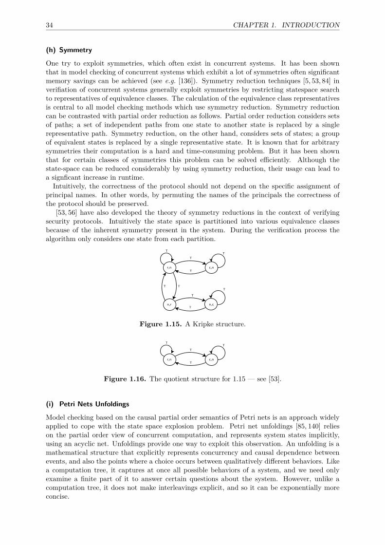
34 CHAPTER 1. INTRODUCTION
(h) Symmetry
One try to exploit symmetries, which often exist in concurrent systems. It has been shownthat in model checking of concurrent systems which exhibit a lot of symmetries often significantmemory savings can be achieved (see e.g. [136]). Symmetry reduction techniques [5, 53, 84] inverifiation of concurrent systems generally exploit symmetries by restricting statespace searchto representatives of equivalence classes. The calculation of the equivalence class representativesis central to all model checking methods which use symmetry reduction. Symmetry reductioncan be contrasted with partial order reduction as follows. Partial order reduction considers setsof paths; a set of independent paths from one state to another state is replaced by a singlerepresentative path. Symmetry reduction, on the other hand, considers sets of states; a groupof equivalent states is replaced by a single representative state. It is known that for arbitrarysymmetries their computation is a hard and time-consuming problem. But it has been shownthat for certain classes of symmetries this problem can be solved efficiently. Although thestate-space can be reduced considerably by using symmetry reduction, their usage can lead toa signficant increase in runtime.Intuitively, the correctness of the protocol should not depend on the specific assignment of
principal names. In other words, by permuting the names of the principals the correctness ofthe protocol should be preserved.
[53, 56] have also developed the theory of symmetry reductions in the context of verifyingsecurity protocols. Intuitively the state space is partitioned into various equivalence classesbecause of the inherent symmetry present in the system. During the verification process thealgorithm only considers one state from each partition.
Figure 1.15. A Kripke structure.
Figure 1.16. The quotient structure for 1.15 — see [53].
(i) Petri Nets Unfoldings
Model checking based on the causal partial order semantics of Petri nets is an approach widelyapplied to cope with the state space explosion problem. Petri net unfoldings [85, 140] relieson the partial order view of concurrent computation, and represents system states implicitly,using an acyclic net. Unfoldings provide one way to exploit this observation. An unfolding is amathematical structure that explicitly represents concurrency and causal dependence betweenevents, and also the points where a choice occurs between qualitatively different behaviors. Likea computation tree, it captures at once all possible behaviors of a system, and we need onlyexamine a finite part of it to answer certain questions about the system. However, unlike acomputation tree, it does not make interleavings explicit, and so it can be exponentially moreconcise.
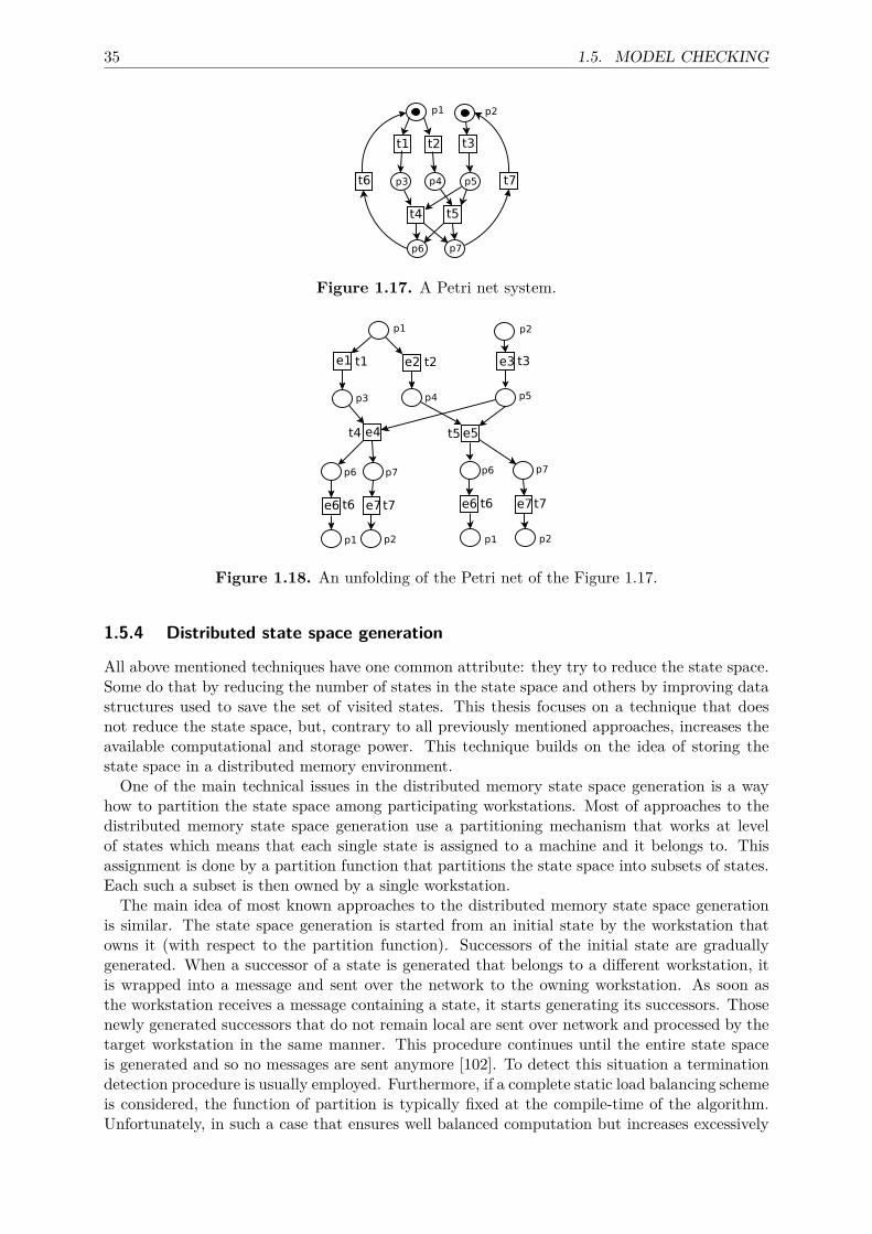
35 1.5. MODEL CHECKING
Figure 1.17. A Petri net system.
Figure 1.18. An unfolding of the Petri net of the Figure 1.17.
1.5.4 Distributed state space generation
All above mentioned techniques have one common attribute: they try to reduce the state space.Some do that by reducing the number of states in the state space and others by improving datastructures used to save the set of visited states. This thesis focuses on a technique that doesnot reduce the state space, but, contrary to all previously mentioned approaches, increases theavailable computational and storage power. This technique builds on the idea of storing thestate space in a distributed memory environment.One of the main technical issues in the distributed memory state space generation is a way
how to partition the state space among participating workstations. Most of approaches to thedistributed memory state space generation use a partitioning mechanism that works at levelof states which means that each single state is assigned to a machine and it belongs to. Thisassignment is done by a partition function that partitions the state space into subsets of states.Each such a subset is then owned by a single workstation.The main idea of most known approaches to the distributed memory state space generation
is similar. The state space generation is started from an initial state by the workstation thatowns it (with respect to the partition function). Successors of the initial state are graduallygenerated. When a successor of a state is generated that belongs to a different workstation, itis wrapped into a message and sent over the network to the owning workstation. As soon asthe workstation receives a message containing a state, it starts generating its successors. Thosenewly generated successors that do not remain local are sent over network and processed by thetarget workstation in the same manner. This procedure continues until the entire state spaceis generated and so no messages are sent anymore [102]. To detect this situation a terminationdetection procedure is usually employed. Furthermore, if a complete static load balancing schemeis considered, the function of partition is typically fixed at the compile-time of the algorithm.Unfortunately, in such a case that ensures well balanced computation but increases excessively
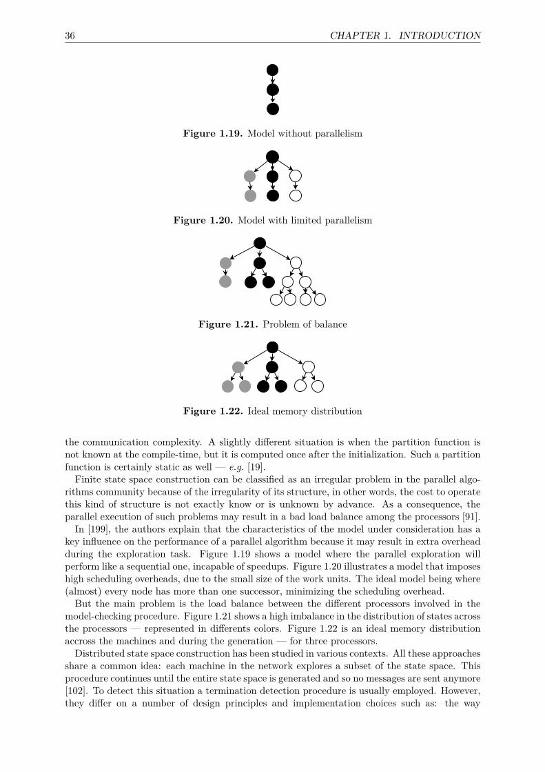
36 CHAPTER 1. INTRODUCTION
Figure 1.19. Model without parallelism
Figure 1.20. Model with limited parallelism
Figure 1.21. Problem of balance
Figure 1.22. Ideal memory distribution
the communication complexity. A slightly different situation is when the partition function isnot known at the compile-time, but it is computed once after the initialization. Such a partitionfunction is certainly static as well — e.g. [19].
Finite state space construction can be classified as an irregular problem in the parallel algo-rithms community because of the irregularity of its structure, in other words, the cost to operatethis kind of structure is not exactly know or is unknown by advance. As a consequence, theparallel execution of such problems may result in a bad load balance among the processors [91].In [199], the authors explain that the characteristics of the model under consideration has a
key influence on the performance of a parallel algorithm because it may result in extra overheadduring the exploration task. Figure 1.19 shows a model where the parallel exploration willperform like a sequential one, incapable of speedups. Figure 1.20 illustrates a model that imposeshigh scheduling overheads, due to the small size of the work units. The ideal model being where(almost) every node has more than one successor, minimizing the scheduling overhead.But the main problem is the load balance between the different processors involved in the
model-checking procedure. Figure 1.21 shows a high imbalance in the distribution of states acrossthe processors — represented in differents colors. Figure 1.22 is an ideal memory distributionaccross the machines and during the generation — for three processors.Distributed state space construction has been studied in various contexts. All these approaches
share a common idea: each machine in the network explores a subset of the state space. Thisprocedure continues until the entire state space is generated and so no messages are sent anymore[102]. To detect this situation a termination detection procedure is usually employed. However,they differ on a number of design principles and implementation choices such as: the way
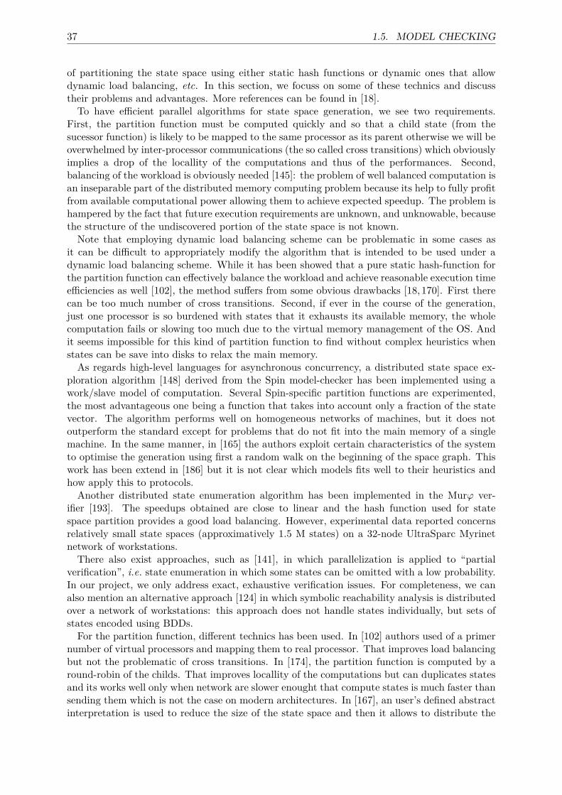
37 1.5. MODEL CHECKING
of partitioning the state space using either static hash functions or dynamic ones that allowdynamic load balancing, etc. In this section, we focuss on some of these technics and discusstheir problems and advantages. More references can be found in [18].To have efficient parallel algorithms for state space generation, we see two requirements.
First, the partition function must be computed quickly and so that a child state (from thesucessor function) is likely to be mapped to the same processor as its parent otherwise we will beoverwhelmed by inter-processor communications (the so called cross transitions) which obviouslyimplies a drop of the locallity of the computations and thus of the performances. Second,balancing of the workload is obviously needed [145]: the problem of well balanced computation isan inseparable part of the distributed memory computing problem because its help to fully profitfrom available computational power allowing them to achieve expected speedup. The problem ishampered by the fact that future execution requirements are unknown, and unknowable, becausethe structure of the undiscovered portion of the state space is not known.Note that employing dynamic load balancing scheme can be problematic in some cases as
it can be difficult to appropriately modify the algorithm that is intended to be used under adynamic load balancing scheme. While it has been showed that a pure static hash-function forthe partition function can effectively balance the workload and achieve reasonable execution timeefficiencies as well [102], the method suffers from some obvious drawbacks [18, 170]. First therecan be too much number of cross transitions. Second, if ever in the course of the generation,just one processor is so burdened with states that it exhausts its available memory, the wholecomputation fails or slowing too much due to the virtual memory management of the OS. Andit seems impossible for this kind of partition function to find without complex heuristics whenstates can be save into disks to relax the main memory.As regards high-level languages for asynchronous concurrency, a distributed state space ex-
ploration algorithm [148] derived from the Spin model-checker has been implemented using awork/slave model of computation. Several Spin-specific partition functions are experimented,the most advantageous one being a function that takes into account only a fraction of the statevector. The algorithm performs well on homogeneous networks of machines, but it does notoutperform the standard except for problems that do not fit into the main memory of a singlemachine. In the same manner, in [165] the authors exploit certain characteristics of the systemto optimise the generation using first a random walk on the beginning of the space graph. Thiswork has been extend in [186] but it is not clear which models fits well to their heuristics andhow apply this to protocols.Another distributed state enumeration algorithm has been implemented in the Murϕ ver-
ifier [193]. The speedups obtained are close to linear and the hash function used for statespace partition provides a good load balancing. However, experimental data reported concernsrelatively small state spaces (approximatively 1.5 M states) on a 32-node UltraSparc Myrinetnetwork of workstations.There also exist approaches, such as [141], in which parallelization is applied to “partial
verification”, i.e. state enumeration in which some states can be omitted with a low probability.In our project, we only address exact, exhaustive verification issues. For completeness, we canalso mention an alternative approach [124] in which symbolic reachability analysis is distributedover a network of workstations: this approach does not handle states individually, but sets ofstates encoded using BDDs.
For the partition function, different technics has been used. In [102] authors used of a primernumber of virtual processors and mapping them to real processor. That improves load balancingbut not the problematic of cross transitions. In [174], the partition function is computed by around-robin of the childs. That improves locallity of the computations but can duplicates statesand its works well only when network are slower enought that compute states is much faster thansending them which is not the case on modern architectures. In [167], an user’s defined abstractinterpretation is used to reduce the size of the state space and then it allows to distribute the
38 CHAPTER 1. INTRODUCTION
abstract graph following by computing real states fully in parallel. A tool is given for helpingthe users to find this abstraction. We have not find how this technic can be apply to securityprotocols.In [32,33,133] authors used complex distributed file system or shared database to optimise the
sending of the states especially when complex data-structure are used internally in the states —as ours. That can improve the implementation but not the idea of our algorithms. The use ofsaturation for parallel generation is defined in [50] but improve only memory use and does notachieve a clear speedup with respect to a sequential implementation.For load balacing technics we can cite [2] when remaping is initiated by the master node
when the memory utilization of one node differs more than a given percentage from the averageutilization of all the others. In the same way, [150] presented a new dynamic partition functionscheme that builds a dynamic remapping, based on the fact that the state space is partitionedinto more pieces than the number of involved machines. When load on a machine is too high,the machine releases one of the partitions it is assigned and if it is the last machine owning thepartition it sends the partition to a less loaded machine. This mechanism reduces the numberof messages sent which is done to the detriment of redundant works if a partition is owned byseveral machines and a partial inconsistence may occur when a partition is moved unless all theother machines are informed about its movement.In [170, 171] extended differents technics of the literature that tries avoid sending a state
away from the current network node if its 2nd-generation successors are local and a mechanismthat prevents re-sending already sent states. The idea is to compute latter the state for model-cheking which can be faster than sending it. That clearly improves communications but ourtechnic performs the same job without ignoring any of the states.In [118, 119] present a generic multithreaded and distributed infrastructure library designed
to allow distribution of the model checking procedure over a cluster of machines. This libraryis generic, and is designed to allow encapsulation of any model checker in order to make itdistributed.
1.6 OutlineSince these protocols are at the core of security-sensitive applications in a variety of domains,their proper functioning is crucial as a failure may undermine the customer and, more generally,the public trust in these applications. Designing secure protocols is a challenging problem [20,61].In spite of their apparent simplicity, they are notoriously error-prone. Surprisingly, severe attackscan be conducted even without breaking cryptography, but by exploiting weaknesses in theprotocols themselves, for instance by carrying out man-in-the-middle attacks, where an attackerplays off one protocol participant against another, or replay attacks, where messages from onesession (i.e. execution of an instance of the protocol) are used in another session. It is thus ofutmost importance to have tools and specification languages that support the activity of findingflaws in protocols.
(a) State Space
In this Chapter 2, we exploit the well-structured nature of security protocols and match it tothe BSP [29, 187] model of parallel computation. This allows us to simplify the writing of anefficient algorithm for computing the state space of finite protocol sessions. The structure of theprotocols is exploited to partition the state space and reduce cross transitions while increasingcomputation locality. At the same time, the BSP model allows to simplify the detection of thealgorithm termination and to load balance the computations.
First, we briefly review in Section 2.1 the context of our work that is models of securityprotocols and their state space representation as LTS. Section 2.2 describes first attempt of par-allelisation that is a naive parallel algorithm for the state space construction. Then, Section 2.3
39 1.6. OUTLINE
is dedicated to, in a first time, the hypothesis concerning our protocols model, then in moresubtle algorithms increasing local computation time, decreasing local storage by a sweep-linereduction and balancing the computations. Finally, explanations on the appropriateness of ourapproach are discussed in Section 2.4.
(b) Model Checking
Checking if a cryptographic protocol is secure or not is an undecidable problem [81] and even aNP problem restricted to a bounded number of agents and sessions [183]. However, enumerativemodel-checking is well-adapted for finding flaws [11] and some results exist by extending boundto unbound number of sessions [7]. In the following, we consider the problem of checking aLTL and CTL* formulas over labelled transition systems (LTS) that model security protocols.Checking a LTL or CTL* formula over a protocol is not new [9, 23, 100, 122, 122] and have theadvantage over dedicated tools for protocols to be easily extensible to non standard behaviour ofhonest principals (e.g. contract-signing protocols: participants required to make progress) or tocheck some security goals that cannot be expressed as reachability properties, e.g. fair exchange.A specialisation of LTL to protocols have also be done in [62]. We consider also the more generalproblematic of CTL* model checking.The peculiarity of our work concerns the parallel computation. In this Chapter 3, we recall the
well known Tarjan algorithm which is the underlying structure of the work on a local approachused by [28] for CTL* model checking. [28] is our working basis and our main contributionsin the following sections are essentially the adaptation of the algorithms found in [28] for theparallel case of security protocols.
(c) Case Study
This Chapter 4 concerns the practical part of our work. In a first time, we present the speci-fication of security Protocols by the langage ABCD and we give several examples of protocolswith their modelisation in this langage. Then, we describe the important technologies we useto implement our algorithms: the BSP Python Programming library and the SNAKES toolkitand syntactic layers wich is a Python library to define, manipulate and execute coloured Petrinets [178]. Then we give the features of the implementation of our parallel algorithms and atlast the benchmarks on our differents algoritms.

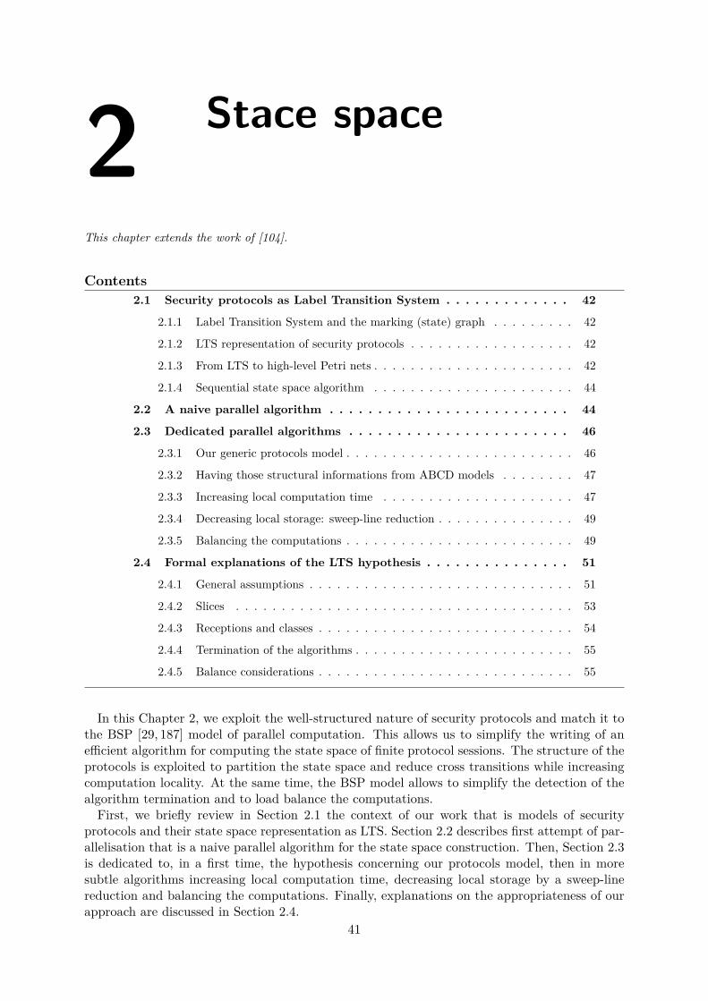
2 Stace space
This chapter extends the work of [104].
Contents2.1 Security protocols as Label Transition System . . . . . . . . . . . . . 42
2.1.1 Label Transition System and the marking (state) graph . . . . . . . . . 42
2.1.2 LTS representation of security protocols . . . . . . . . . . . . . . . . . . 42
2.1.3 From LTS to high-level Petri nets . . . . . . . . . . . . . . . . . . . . . . 42
2.1.4 Sequential state space algorithm . . . . . . . . . . . . . . . . . . . . . . 44
2.2 A naive parallel algorithm . . . . . . . . . . . . . . . . . . . . . . . . . 44
2.3 Dedicated parallel algorithms . . . . . . . . . . . . . . . . . . . . . . . 46
2.3.1 Our generic protocols model . . . . . . . . . . . . . . . . . . . . . . . . . 46
2.3.2 Having those structural informations from ABCD models . . . . . . . . 47
2.3.3 Increasing local computation time . . . . . . . . . . . . . . . . . . . . . 47
2.3.4 Decreasing local storage: sweep-line reduction . . . . . . . . . . . . . . . 49
2.3.5 Balancing the computations . . . . . . . . . . . . . . . . . . . . . . . . . 49
2.4 Formal explanations of the LTS hypothesis . . . . . . . . . . . . . . . 51
2.4.1 General assumptions . . . . . . . . . . . . . . . . . . . . . . . . . . . . . 51
2.4.2 Slices . . . . . . . . . . . . . . . . . . . . . . . . . . . . . . . . . . . . . 53
2.4.3 Receptions and classes . . . . . . . . . . . . . . . . . . . . . . . . . . . . 54
2.4.4 Termination of the algorithms . . . . . . . . . . . . . . . . . . . . . . . . 55
2.4.5 Balance considerations . . . . . . . . . . . . . . . . . . . . . . . . . . . . 55
In this Chapter 2, we exploit the well-structured nature of security protocols and match it tothe BSP [29, 187] model of parallel computation. This allows us to simplify the writing of anefficient algorithm for computing the state space of finite protocol sessions. The structure of theprotocols is exploited to partition the state space and reduce cross transitions while increasingcomputation locality. At the same time, the BSP model allows to simplify the detection of thealgorithm termination and to load balance the computations.First, we briefly review in Section 2.1 the context of our work that is models of security
protocols and their state space representation as LTS. Section 2.2 describes first attempt of par-allelisation that is a naive parallel algorithm for the state space construction. Then, Section 2.3is dedicated to, in a first time, the hypothesis concerning our protocols model, then in moresubtle algorithms increasing local computation time, decreasing local storage by a sweep-linereduction and balancing the computations. Finally, explanations on the appropriateness of ourapproach are discussed in Section 2.4.
41
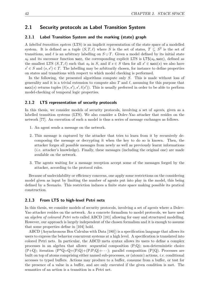
42 CHAPTER 2. STACE SPACE
2.1 Security protocols as Label Transition System
2.1.1 Label Transition System and the marking (state) graphA labelled transition system (LTS) is an implicit representation of the state space of a modelledsystem. It is defined as a tuple (S, T, `) where S is the set of states, T ⊆ S2 is the set oftransitions, and ` is an arbitrary labelling on S ∪ T . Given a model defined by its initial states0 and its successor function succ, the corresponding explicit LTS is LTS(s0, succ), defined asthe smallest LTS (S, T, `) such that s0 in S, and if s ∈ S then for all s′ ∈ succ(s) we also haves′ ∈ S and (s, s′) ∈ T . The labelling may be arbitrarily chosen, for instance to define propertieson states and transitions with respect to which model checking is performed.
In the following, the presented algorithms compute only S. This is made without loss ofgenerality and it is a trivial extension to compute also T and `, assuming for this purpose thatsucc(s) returns tuples (`(s, s′), s′, `(s′)). This is usually preferred in order to be able to performmodel-checking of temporal logic properties.
2.1.2 LTS representation of security protocolsIn this thesis, we consider models of security protocols, involving a set of agents, given as alabelled transition systems (LTS). We also consider a Dolev-Yao attacker that resides on thenetwork [77]. An execution of such a model is thus a series of message exchanges as follows.
1. An agent sends a message on the network.
2. This message is captured by the attacker that tries to learn from it by recursively de-composing the message or decrypting it when the key to do so is known. Then, theattacker forges all possible messages from newly as well as previously learnt informations(i.e. attacker’s knowledge). Finally, these messages (including the original one) are madeavailable on the network.
3. The agents waiting for a message reception accept some of the messages forged by theattacker, according to the protocol rules.
Because of undecidability or efficiency concerns, one apply some restrictions on the consideringmodel given as input by limiting the number of agents put into play in the model, this beingdefined by a Scenario. This restriction induces a finite state space making possible its praticalconstruction.
2.1.3 From LTS to high-level Petri netsIn this thesis, we consider models of security protocols, involving a set of agents where a Dolev-Yao attacker resides on the network. As a concrete formalism to model protocols, we have usedan algebra of coloured Petri nets called ABCD [181] allowing for easy and structured modelling.However, our approach is largely independent of the chosen formalism and it is enough to assumethat some properties define in [104] hold.ABCD (Asynchronous Box Calculus with Data [180]) is a specification language that allows its
users to express the behavior concurrent systems at a high level. A specification is translated intocolored Petri nets. In particular, the ABCD meta syntax allows its users to define a complexprocesses in an algebra that allows: sequential composition (P;Q); non-deterministic choice(P+Q); iteration (P*Q=Q+(P;Q)+(P;P;Q)+· · · ); parallel composition (P‖Q). Processes arebuilt on top of atoms comprising either named sub-processes, or (atomic) actions, i.e. conditionalaccesses to typed buffers. Actions may produce to a buffer, consume from a buffer, or test forthe presence of a value in a buffer, and are only executed if the given condition is met. Thesemantics of an action is a transition in a Petri net.
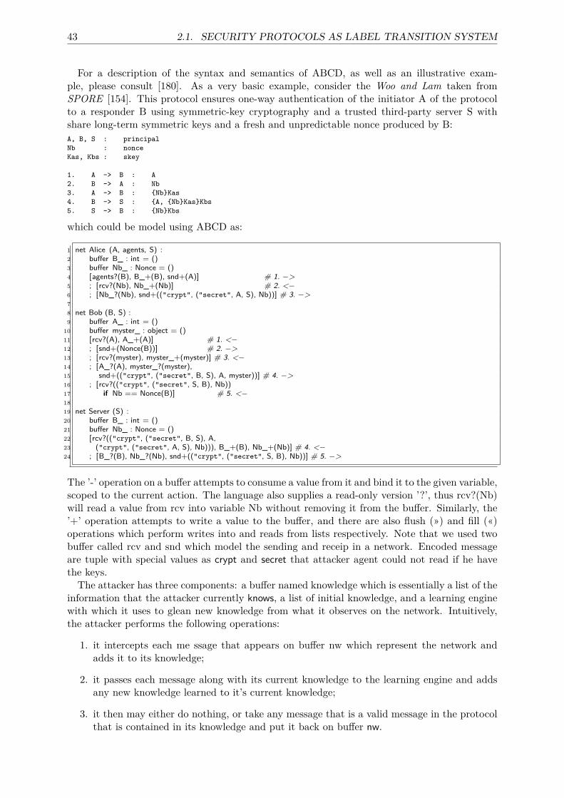
43 2.1. SECURITY PROTOCOLS AS LABEL TRANSITION SYSTEM
For a description of the syntax and semantics of ABCD, as well as an illustrative exam-ple, please consult [180]. As a very basic example, consider the Woo and Lam taken fromSPORE [154]. This protocol ensures one-way authentication of the initiator A of the protocolto a responder B using symmetric-key cryptography and a trusted third-party server S withshare long-term symmetric keys and a fresh and unpredictable nonce produced by B:A, B, S : principalNb : nonceKas, Kbs : skey
1. A -> B : A2. B -> A : Nb3. A -> B : {Nb}Kas4. B -> S : {A, {Nb}Kas}Kbs5. S -> B : {Nb}Kbs
which could be model using ABCD as:
1 net Alice (A, agents, S) :2 buffer B_ : int = ()3 buffer Nb_ : Nonce = ()4 [agents?(B), B_+(B), snd+(A)] # 1. −>5 ; [rcv?(Nb), Nb_+(Nb)] # 2. <−6 ; [Nb_?(Nb), snd+(("crypt", ("secret", A, S), Nb))] # 3. −>78 net Bob (B, S) :9 buffer A_ : int = ()
10 buffer myster_ : object = ()11 [rcv?(A), A_+(A)] # 1. <−12 ; [snd+(Nonce(B))] # 2. −>13 ; [rcv?(myster), myster_+(myster)] # 3. <−14 ; [A_?(A), myster_?(myster),15 snd+(("crypt", ("secret", B, S), A, myster))] # 4. −>16 ; [rcv?(("crypt", ("secret", S, B), Nb))17 if Nb == Nonce(B)] # 5. <−1819 net Server (S) :20 buffer B_ : int = ()21 buffer Nb_ : Nonce = ()22 [rcv?(("crypt", ("secret", B, S), A,23 ("crypt", ("secret", A, S), Nb))), B_+(B), Nb_+(Nb)] # 4. <−24 ; [B_?(B), Nb_?(Nb), snd+(("crypt", ("secret", S, B), Nb))] # 5. −>
The ’-’ operation on a buffer attempts to consume a value from it and bind it to the given variable,scoped to the current action. The language also supplies a read-only version ’?’, thus rcv?(Nb)will read a value from rcv into variable Nb without removing it from the buffer. Similarly, the’+’ operation attempts to write a value to the buffer, and there are also flush (») and fill («)operations which perform writes into and reads from lists respectively. Note that we used twobuffer called rcv and snd which model the sending and receip in a network. Encoded messageare tuple with special values as crypt and secret that attacker agent could not read if he havethe keys.The attacker has three components: a buffer named knowledge which is essentially a list of the
information that the attacker currently knows, a list of initial knowledge, and a learning enginewith which it uses to glean new knowledge from what it observes on the network. Intuitively,the attacker performs the following operations:
1. it intercepts each me ssage that appears on buffer nw which represent the network andadds it to its knowledge;
2. it passes each message along with its current knowledge to the learning engine and addsany new knowledge learned to it’s current knowledge;
3. it then may either do nothing, or take any message that is a valid message in the protocolthat is contained in its knowledge and put it back on buffer nw.
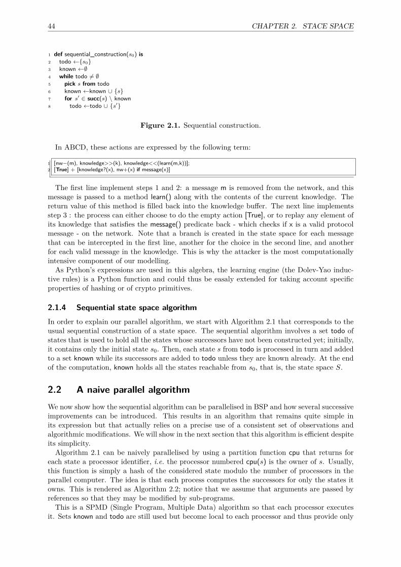
44 CHAPTER 2. STACE SPACE
1 def sequential_construction(s0) is2 todo ←{s0}3 known ←∅4 while todo 6= ∅5 pick s from todo6 known ←known ∪ {s}7 for s′ ∈ succ(s) \ known8 todo ←todo ∪ {s′}
Figure 2.1. Sequential construction.
In ABCD, these actions are expressed by the following term:
1 [nw−(m), knowledge>>(k), knowledge<<(learn(m,k))];2 [True] + [knowledge?(x), nw+(x) if message(x)]
The first line implement steps 1 and 2: a message m is removed from the network, and thismessage is passed to a method learn() along with the contents of the current knowledge. Thereturn value of this method is filled back into the knowledge buffer. The next line implementsstep 3 : the process can either choose to do the empty action [True], or to replay any element ofits knowledge that satisfies the message() predicate back - which checks if x is a valid protocolmessage - on the network. Note that a branch is created in the state space for each messagethat can be intercepted in the first line, another for the choice in the second line, and anotherfor each valid message in the knowledge. This is why the attacker is the most computationallyintensive component of our modelling.As Python’s expressions are used in this algebra, the learning engine (the Dolev-Yao induc-
tive rules) is a Python function and could thus be easaly extended for taking account specificproperties of hashing or of crypto primitives.
2.1.4 Sequential state space algorithmIn order to explain our parallel algorithm, we start with Algorithm 2.1 that corresponds to theusual sequential construction of a state space. The sequential algorithm involves a set todo ofstates that is used to hold all the states whose successors have not been constructed yet; initially,it contains only the initial state s0. Then, each state s from todo is processed in turn and addedto a set known while its successors are added to todo unless they are known already. At the endof the computation, known holds all the states reachable from s0, that is, the state space S.
2.2 A naive parallel algorithmWe now show how the sequential algorithm can be parallelised in BSP and how several successiveimprovements can be introduced. This results in an algorithm that remains quite simple inits expression but that actually relies on a precise use of a consistent set of observations andalgorithmic modifications. We will show in the next section that this algorithm is efficient despiteits simplicity.Algorithm 2.1 can be naively parallelised by using a partition function cpu that returns for
each state a processor identifier, i.e. the processor numbered cpu(s) is the owner of s. Usually,this function is simply a hash of the considered state modulo the number of processors in theparallel computer. The idea is that each process computes the successors for only the states itowns. This is rendered as Algorithm 2.2; notice that we assume that arguments are passed byreferences so that they may be modified by sub-programs.This is a SPMD (Single Program, Multiple Data) algorithm so that each processor executes
it. Sets known and todo are still used but become local to each processor and thus provide only
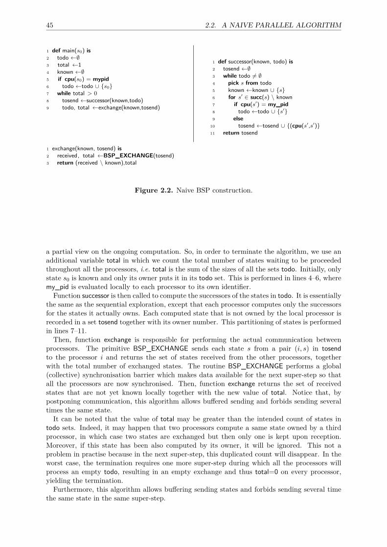
45 2.2. A NAIVE PARALLEL ALGORITHM
1 def main(s0) is2 todo ←∅3 total ←14 known ←∅5 if cpu(s0) = mypid6 todo ←todo ∪ {s0}7 while total > 08 tosend ←successor(known,todo)9 todo, total ←exchange(known,tosend)
1 def successor(known, todo) is2 tosend ←∅3 while todo 6= ∅4 pick s from todo5 known ←known ∪ {s}6 for s′ ∈ succ(s) \ known7 if cpu(s′) = my_pid8 todo ←todo ∪ {s′}9 else
10 tosend ←tosend ∪ {(cpu(s′,s′)}11 return tosend
1 exchange(known, tosend) is2 received, total ←BSP_EXCHANGE(tosend)3 return (received \ known),total
Figure 2.2. Naive BSP construction.
a partial view on the ongoing computation. So, in order to terminate the algorithm, we use anadditional variable total in which we count the total number of states waiting to be proceededthroughout all the processors, i.e. total is the sum of the sizes of all the sets todo. Initially, onlystate s0 is known and only its owner puts it in its todo set. This is performed in lines 4–6, wheremy_pid is evaluated locally to each processor to its own identifier.Function successor is then called to compute the successors of the states in todo. It is essentially
the same as the sequential exploration, except that each processor computes only the successorsfor the states it actually owns. Each computed state that is not owned by the local processor isrecorded in a set tosend together with its owner number. This partitioning of states is performedin lines 7–11.
Then, function exchange is responsible for performing the actual communication betweenprocessors. The primitive BSP_EXCHANGE sends each state s from a pair (i, s) in tosendto the processor i and returns the set of states received from the other processors, togetherwith the total number of exchanged states. The routine BSP_EXCHANGE performs a global(collective) synchronisation barrier which makes data available for the next super-step so thatall the processors are now synchronised. Then, function exchange returns the set of receivedstates that are not yet known locally together with the new value of total. Notice that, bypostponing communication, this algorithm allows buffered sending and forbids sending severaltimes the same state.It can be noted that the value of total may be greater than the intended count of states in
todo sets. Indeed, it may happen that two processors compute a same state owned by a thirdprocessor, in which case two states are exchanged but then only one is kept upon reception.Moreover, if this state has been also computed by its owner, it will be ignored. This not aproblem in practise because in the next super-step, this duplicated count will disappear. In theworst case, the termination requires one more super-step during which all the processors willprocess an empty todo, resulting in an empty exchange and thus total=0 on every processor,yielding the termination.Furthermore, this algorithm allows buffering sending states and forbids sending several time
the same state in the same super-step.
46 CHAPTER 2. STACE SPACE
2.3 Dedicated parallel algorithms
2.3.1 Our generic protocols model
In this thesis, we consider models of security protocols involving a set of agents and we assumethat any state can be represented by a function from a set L of locations to an arbitrarydata domain D. For instance, locations may correspond to local variables of agents, sharedcommunication buffers, etc.
As a concrete formalism to model protocols, we have used an algebra of coloured Petrinets [180] allowing for easy and structured modelling. However, our approach is largely in-dependent of the chosen formalism and it is enough to assume that the following propertieshold:
(P0) there exists a subset LR ⊆ L of reception locations corresponding to the information learnt(and stored) by agents from their communication with others;
(P1) LTS’s function succ can be partitioned into two successor functions succR and succL thatcorrespond respectively to transitions upon which an agent receives information (and storesit) and to transitions that make progress any agent (including the intruder); (that corre-spond respectively to the successors that change states or not on the locations from LR;)
(P2) there is an initial state s0 and there exists a function slice from state to natural (a measure)such that if s′ ∈ succR(s) then there is no path from s′ to any state s′′ such that slice(s) =slice(s′′) and slice(s′) = slice(s) + 1 (it is often call a sweep-line progression [49]);
(P3) there exists a function cpu from state to natural numbers (a hashing) such that for allstate s if s′ ∈ succL(s) then cpu(s) = cpu(s′); mainly, the knowledge of the intruder is nottaken into account to compute the hash of a state;
(P4) if s1, s2 ∈ succR(s) and cpu(s1) 6= cpu(s2) then there is no possible path from s1 to s2 andvice versa.
More precisely: for all state s and all s′ ∈ succ(s), if s′|LR= s|LR
then s′ ∈ succL(s), elses′ ∈ succR(s); where s|LR
denotes the state s whose domain is restricted to the locations inLR. Intuitively, succR corresponds to transitions upon which an agent receives information andstores it.Here again, concrete models generally make easy to distinguish these two kind of transition.On concrete models, it is generally easy to distinguish syntactically the transitions that cor-
respond to a message reception in the protocol with information storage. Thus, is it easy topartition succ as above and, for most protocol models, it is also easy to check that the aboveproperties are satisfied. This is the case in particular for the algebra of Petri nets that we haveused (see below). Thus, is it easy to partition succ as above. This is the case in particular forthe algebra of Petri nets that we have used: the ABCD formalism.In the following, the presented algorithms compute only S. This is made without loss of
generality and it is a trivial extension to compute also T and `, assuming for this purpose thatsucc(s) returns tuples (`(s, s′), s′, `(s′)). This is usually preferred in order to be able to performmodel-checking of temporal logic properties.We now show how several successive improvement can be introduced. This results in an
algorithm that remains quite simple in its expression but actually efficient and relies on a preciseuse of a consistent set of observations and algorithmic modifications.
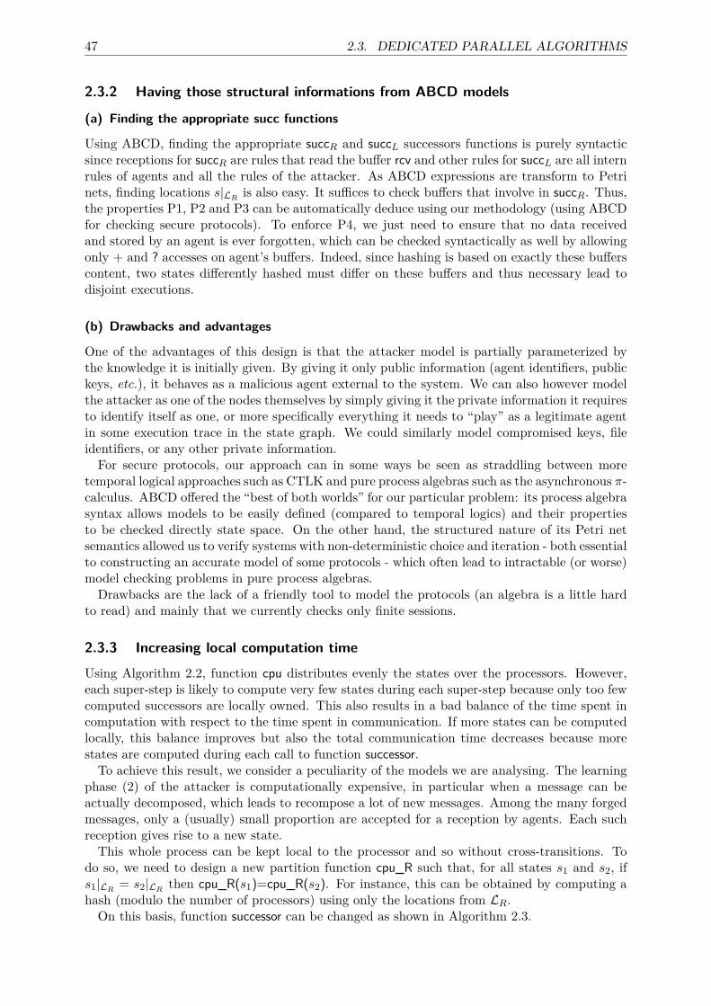
47 2.3. DEDICATED PARALLEL ALGORITHMS
2.3.2 Having those structural informations from ABCD models
(a) Finding the appropriate succ functions
Using ABCD, finding the appropriate succR and succL successors functions is purely syntacticsince receptions for succR are rules that read the buffer rcv and other rules for succL are all internrules of agents and all the rules of the attacker. As ABCD expressions are transform to Petrinets, finding locations s|LR
is also easy. It suffices to check buffers that involve in succR. Thus,the properties P1, P2 and P3 can be automatically deduce using our methodology (using ABCDfor checking secure protocols). To enforce P4, we just need to ensure that no data receivedand stored by an agent is ever forgotten, which can be checked syntactically as well by allowingonly + and ? accesses on agent’s buffers. Indeed, since hashing is based on exactly these bufferscontent, two states differently hashed must differ on these buffers and thus necessary lead todisjoint executions.
(b) Drawbacks and advantages
One of the advantages of this design is that the attacker model is partially parameterized bythe knowledge it is initially given. By giving it only public information (agent identifiers, publickeys, etc.), it behaves as a malicious agent external to the system. We can also however modelthe attacker as one of the nodes themselves by simply giving it the private information it requiresto identify itself as one, or more specifically everything it needs to “play” as a legitimate agentin some execution trace in the state graph. We could similarly model compromised keys, fileidentifiers, or any other private information.For secure protocols, our approach can in some ways be seen as straddling between more
temporal logical approaches such as CTLK and pure process algebras such as the asynchronous π-calculus. ABCD offered the “best of both worlds” for our particular problem: its process algebrasyntax allows models to be easily defined (compared to temporal logics) and their propertiesto be checked directly state space. On the other hand, the structured nature of its Petri netsemantics allowed us to verify systems with non-deterministic choice and iteration - both essentialto constructing an accurate model of some protocols - which often lead to intractable (or worse)model checking problems in pure process algebras.Drawbacks are the lack of a friendly tool to model the protocols (an algebra is a little hard
to read) and mainly that we currently checks only finite sessions.
2.3.3 Increasing local computation time
Using Algorithm 2.2, function cpu distributes evenly the states over the processors. However,each super-step is likely to compute very few states during each super-step because only too fewcomputed successors are locally owned. This also results in a bad balance of the time spent incomputation with respect to the time spent in communication. If more states can be computedlocally, this balance improves but also the total communication time decreases because morestates are computed during each call to function successor.To achieve this result, we consider a peculiarity of the models we are analysing. The learning
phase (2) of the attacker is computationally expensive, in particular when a message can beactually decomposed, which leads to recompose a lot of new messages. Among the many forgedmessages, only a (usually) small proportion are accepted for a reception by agents. Each suchreception gives rise to a new state.This whole process can be kept local to the processor and so without cross-transitions. To
do so, we need to design a new partition function cpu_R such that, for all states s1 and s2, ifs1|LR
= s2|LRthen cpu_R(s1)=cpu_R(s2). For instance, this can be obtained by computing a
hash (modulo the number of processors) using only the locations from LR.On this basis, function successor can be changed as shown in Algorithm 2.3.
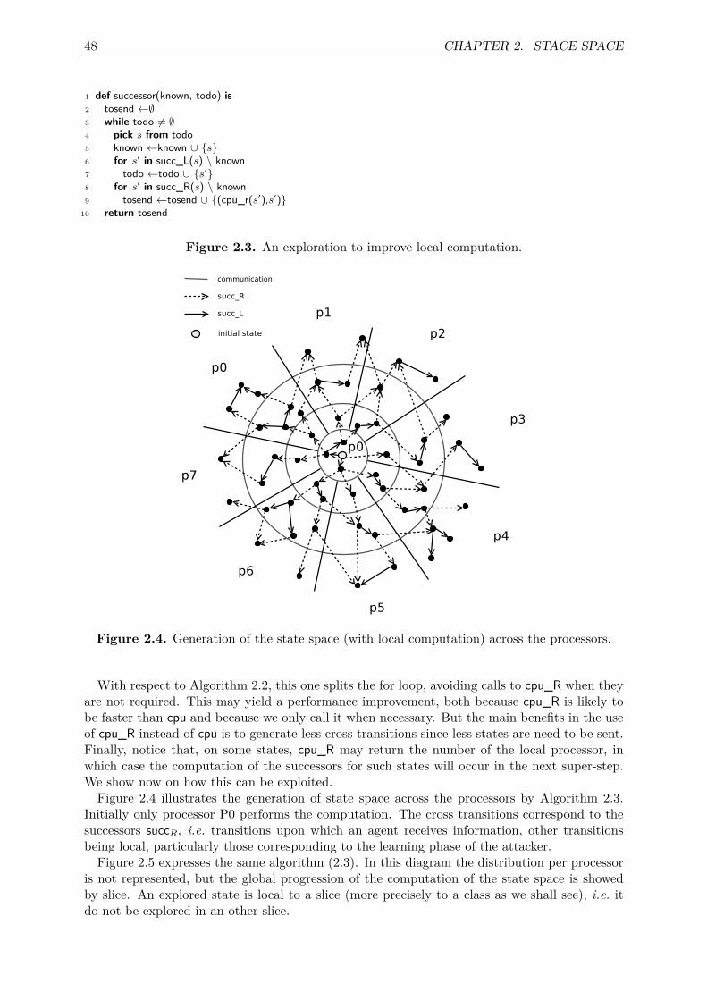
48 CHAPTER 2. STACE SPACE
1 def successor(known, todo) is2 tosend ←∅3 while todo 6= ∅4 pick s from todo5 known ←known ∪ {s}6 for s′ in succ_L(s) \ known7 todo ←todo ∪ {s′}8 for s′ in succ_R(s) \ known9 tosend ←tosend ∪ {(cpu_r(s′),s′)}
10 return tosend
Figure 2.3. An exploration to improve local computation.
Figure 2.4. Generation of the state space (with local computation) across the processors.
With respect to Algorithm 2.2, this one splits the for loop, avoiding calls to cpu_R when theyare not required. This may yield a performance improvement, both because cpu_R is likely tobe faster than cpu and because we only call it when necessary. But the main benefits in the useof cpu_R instead of cpu is to generate less cross transitions since less states are need to be sent.Finally, notice that, on some states, cpu_R may return the number of the local processor, inwhich case the computation of the successors for such states will occur in the next super-step.We show now on how this can be exploited.Figure 2.4 illustrates the generation of state space across the processors by Algorithm 2.3.
Initially only processor P0 performs the computation. The cross transitions correspond to thesuccessors succR, i.e. transitions upon which an agent receives information, other transitionsbeing local, particularly those corresponding to the learning phase of the attacker.
Figure 2.5 expresses the same algorithm (2.3). In this diagram the distribution per processoris not represented, but the global progression of the computation of the state space is showedby slice. An explored state is local to a slice (more precisely to a class as we shall see), i.e. itdo not be explored in an other slice.
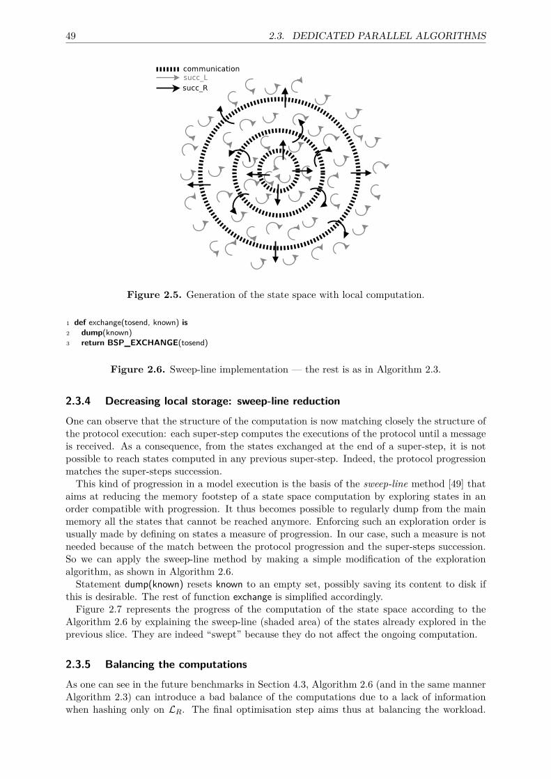
49 2.3. DEDICATED PARALLEL ALGORITHMS
Figure 2.5. Generation of the state space with local computation.
1 def exchange(tosend, known) is2 dump(known)3 return BSP_EXCHANGE(tosend)
Figure 2.6. Sweep-line implementation — the rest is as in Algorithm 2.3.
2.3.4 Decreasing local storage: sweep-line reduction
One can observe that the structure of the computation is now matching closely the structure ofthe protocol execution: each super-step computes the executions of the protocol until a messageis received. As a consequence, from the states exchanged at the end of a super-step, it is notpossible to reach states computed in any previous super-step. Indeed, the protocol progressionmatches the super-steps succession.This kind of progression in a model execution is the basis of the sweep-line method [49] that
aims at reducing the memory footstep of a state space computation by exploring states in anorder compatible with progression. It thus becomes possible to regularly dump from the mainmemory all the states that cannot be reached anymore. Enforcing such an exploration order isusually made by defining on states a measure of progression. In our case, such a measure is notneeded because of the match between the protocol progression and the super-steps succession.So we can apply the sweep-line method by making a simple modification of the explorationalgorithm, as shown in Algorithm 2.6.Statement dump(known) resets known to an empty set, possibly saving its content to disk if
this is desirable. The rest of function exchange is simplified accordingly.Figure 2.7 represents the progress of the computation of the state space according to the
Algorithm 2.6 by explaining the sweep-line (shaded area) of the states already explored in theprevious slice. They are indeed “swept” because they do not affect the ongoing computation.
2.3.5 Balancing the computations
As one can see in the future benchmarks in Section 4.3, Algorithm 2.6 (and in the same mannerAlgorithm 2.3) can introduce a bad balance of the computations due to a lack of informationwhen hashing only on LR. The final optimisation step aims thus at balancing the workload.
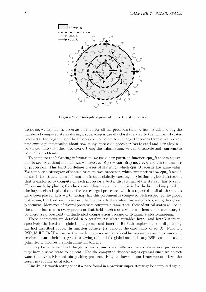
50 CHAPTER 2. STACE SPACE
Figure 2.7. Sweep-line generation of the state space.
To do so, we exploit the observation that, for all the protocols that we have studied so far, thenumber of computed states during a super-step is usually closely related to the number of statesreceived at the beginning of the super-step. So, before to exchange the states themselves, we canfirst exchange information about how many state each processor has to send and how they willbe spread onto the other processors. Using this information, we can anticipate and compensatebalancing problems.To compute the balancing information, we use a new partition function cpu_B that is equiva-
lent to cpu_R without modulo, i.e. we have cpu_R(s) = cpu_B(s) mod p, where p is the numberof processors. This function defines classes of states for which cpu_B returns the same value.We compute a histogram of these classes on each processor, which summarises how cpu_R woulddispatch the states. This information is then globally exchanged, yielding a global histogramthat is exploited to compute on each processor a better dispatching of the states it has to send.This is made by placing the classes according to a simple heuristic for the bin packing problem:the largest class is placed onto the less charged processor, which is repeated until all the classeshave been placed. It is worth noting that this placement is computed with respect to the globalhistogram, but then, each processor dispatches only the states it actually holds, using this globalplacement. Moreover, if several processors compute a same state, these identical states will be inthe same class and so every processor that holds such states will send them to the same target.So there is no possibility of duplicated computation because of dynamic states remapping.These operations are detailed in Algorithm 2.8 where variables histoL and histoG store re-
spectively the local and global histograms, and function BinPack implements the dispatchingmethod described above. In function balance, ]X denotes the cardinality of set X. FunctionBSP_MULTICAST is used so that each processor sends its local histogram to every processor andreceives in turn their histograms, allowing to build the global one. Like any BSP communicationprimitive it involves a synchronisation barrier.It may be remarked that the global histogram is not fully accurate since several processors
may have a same state to be sent. Nor the computed dispatching is optimal since we do notwant to solve a NP-hard bin packing problem. But, as shown in our benchmarks below, theresult is yet fully satisfactory.Finally, it is worth noting that if a state found in a previous super-step may be computed again,
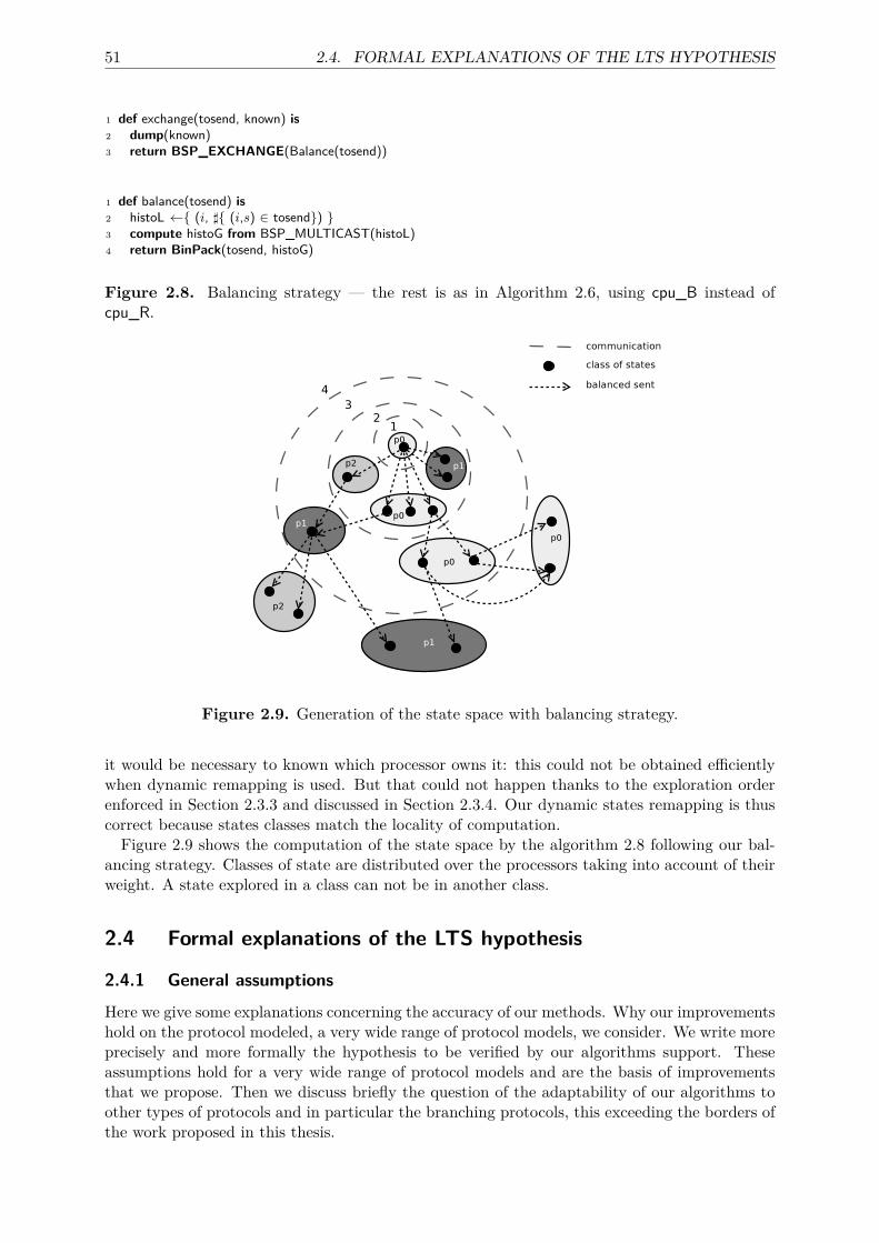
51 2.4. FORMAL EXPLANATIONS OF THE LTS HYPOTHESIS
1 def exchange(tosend, known) is2 dump(known)3 return BSP_EXCHANGE(Balance(tosend))
1 def balance(tosend) is2 histoL ←{ (i, ]{ (i,s) ∈ tosend}) }3 compute histoG from BSP_MULTICAST(histoL)4 return BinPack(tosend, histoG)
Figure 2.8. Balancing strategy — the rest is as in Algorithm 2.6, using cpu_B instead ofcpu_R.
Figure 2.9. Generation of the state space with balancing strategy.
it would be necessary to known which processor owns it: this could not be obtained efficientlywhen dynamic remapping is used. But that could not happen thanks to the exploration orderenforced in Section 2.3.3 and discussed in Section 2.3.4. Our dynamic states remapping is thuscorrect because states classes match the locality of computation.Figure 2.9 shows the computation of the state space by the algorithm 2.8 following our bal-
ancing strategy. Classes of state are distributed over the processors taking into account of theirweight. A state explored in a class can not be in another class.
2.4 Formal explanations of the LTS hypothesis
2.4.1 General assumptions
Here we give some explanations concerning the accuracy of our methods. Why our improvementshold on the protocol modeled, a very wide range of protocol models, we consider. We write moreprecisely and more formally the hypothesis to be verified by our algorithms support. Theseassumptions hold for a very wide range of protocol models and are the basis of improvementsthat we propose. Then we discuss briefly the question of the adaptability of our algorithms toother types of protocols and in particular the branching protocols, this exceeding the borders ofthe work proposed in this thesis.
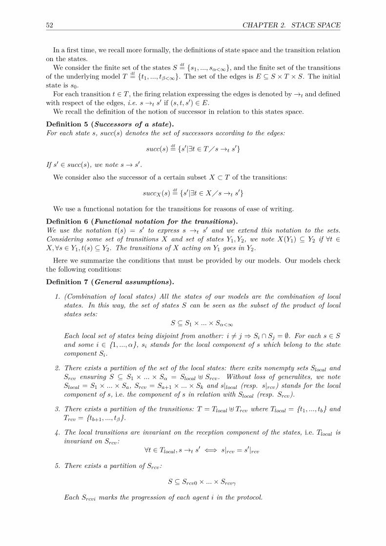
52 CHAPTER 2. STACE SPACE
In a first time, we recall more formally, the definitions of state space and the transition relationon the states.We consider the finite set of the states S df= {s1, ..., sα<∞}, and the finite set of the transitions
of the underlying model T df= {t1, ..., tβ<∞}. The set of the edges is E ⊆ S × T × S. The initialstate is s0.For each transition t ∈ T , the firing relation expressing the edges is denoted by→t and defined
with respect of the edges, i.e. s→t s′ if (s, t, s′) ∈ E.
We recall the definition of the notion of successor in relation to this states space.
Definition 5 (Successors of a state).For each state s, succ(s) denotes the set of successors according to the edges:
succ(s) df= {s′|∃t ∈ T�s→t s′}
If s′ ∈ succ(s), we note s→ s′.
We consider also the successor of a certain subset X ⊂ T of the transitions:
succX(s) df= {s′|∃t ∈ X�s→t s′}
We use a functional notation for the transitions for reasons of ease of writing.
Definition 6 (Functional notation for the transitions).We use the notation t(s) = s′ to express s →t s
′ and we extend this notation to the sets.Considering some set of transitions X and set of states Y1, Y2, we note X(Y1) ⊆ Y2 if ∀t ∈X,∀s ∈ Y1, t(s) ⊆ Y2. The transitions of X acting on Y1 goes in Y2.
Here we summarize the conditions that must be provided by our models. Our models checkthe following conditions:
Definition 7 (General assumptions).
1. (Combination of local states) All the states of our models are the combination of localstates. In this way, the set of states S can be seen as the subset of the product of localstates sets:
S ⊆ S1 × ...× Sα<∞Each local set of states being disjoint from another: i 6= j ⇒ Si ∩ Sj = ∅. For each s ∈ Sand some i ∈ {1, ..., α}, si stands for the local component of s which belong to the statecomponent Si.
2. There exists a partition of the set of the local states: there exits nonempty sets Slocal andSrcv ensuring S ⊆ S1 × ... × Sα = Slocal ] Srcv. Without loss of generalites, we noteSlocal = S1 × ... × Sa, Srcv = Sa+1 × ... × Sk and s|local (resp. s|rcv) stands for the localcomponent of s, i.e. the component of s in relation with Slocal (resp. Srcv).
3. There exists a partition of the transitions: T = Tlocal ] Trcv where Tlocal = {t1, ..., tb} andTrcv = {tb+1, ..., tβ}.
4. The local transitions are invariant on the reception component of the states, i.e. Tlocal isinvariant on Srcv:
∀t ∈ Tlocal, s→t s′ ⇐⇒ s|rcv = s′|rcv
5. There exists a partition of Srcv:
S ⊆ Srcv0 × ...× Srcvγ
Each Srcvi marks the progression of each agent i in the protocol.
53 2.4. FORMAL EXPLANATIONS OF THE LTS HYPOTHESIS
6. We assume that each Srcvi = {si1, ..., siδ} is totally ordered by ≺i. Without loss of gener-ality, one supposes forall i si1 ≺i ... ≺i siδ.
7. Trcv changes necessarily a single component of Srcv. Formally,
∀t ∈ Trcv,∀s, s′ ∈ S, s→t s′ ⇒
∃!i ∈ {0, ..., γ}�s|rcvi 6= s′|rcvi and ∀j 6= i, s|rcvj = s′|rcvjMoreover, we consider (hypothesis of strict progression of agents): s|rcvi ≺i s′|rcvi.
8. A set of function {progress0, ..., progressγ} such as:
• progressi : Srcvi → N;• ∀i ∈ {0, ..., γ}, progressi(si1) = 0;• and progressi(si(j+1)) = progressi(sij) + 1.
9. We consider that the firing of a transition t from Trcv “follows” the strict order of a certaincomponent reception, we consider Srcvi:
s→t s′ ⇒ s and s|rcvi = sij then
s|rcvi = si(j+1)
10. We note progress : S → N defined forall s by
progress(s) df=∑
i∈{0,...,γ}progressi(s|receptioni)
The items 1 and 2 implie the property (P0) of our generic protocols model.By item items 3, 4 and 7 we give (P1).We consier our cpu function acts on Sreception. By items 4 and 7 it follows (P3) and (P4).We consider the function progress as the function slice of the part 2.3.1. It follows by items
7, 8, 9 and 10 the property (P2) and we add slice(s0)=0.
2.4.2 SlicesThe progress mesure is the fundamental concept underlying the sweep-line method. The keyproperty of a progress measure is that for a given state s, all states reachable from s have aprogress measure which is greater or equal than the progress measure of s. A progress measuremakes it possible to delete certain states on-the-fly during state space generation, since it ensuresthat these states can never be reached again. We recall the definition from [49].Definition 8 (Progress mesure [49]).A progress mesure is a tuple (O,v, ϕ) such that (O,v) is a partial order and ϕ : S → O is amapping from states into O satisfying:
∀s, s′ ∈ S, s→∗ s′ ⇒ ϕ(s) v ϕ(s′)
Our previous assumptions provide a progress mesure (N,≤,slice) for the states of the system:∀s, s′ ∈ S, s→∗ s′ ⇒ slice(s) ≤ slice(s′)
Our algorithms send only the states fired by reception transition and involve:∀s, s′ ∈ S, ∀t ∈ Trcv, s→t s′ ⇒ slice(s′) = slice(s) + 1
It is correct to dump the states computed before the new reception states (corresponding to thereceptions by reception transitions), the strict progression by reception transitions ensuring thatwe will do not find them in the future.We obtain, thus, an exploration by slice, each slice defined as follows:
54 CHAPTER 2. STACE SPACE
Definition 9 (Slices).We define the slices: slice1, ..., slice$<∞ of S by:
sliceidf= {s|slice(s) = i}.
We note that one can know a priori the number of super step involved in the generation ofthe state space making easiest the problem of the termination of the algorithm (not used inpractice because of the simplicity of writing and understanding provided by the BSP model).Indeed, each process-agent consist as a certain number of strict progression point in the protocolrepresented by some places of reception, LR, (i.e. taking value in Srcv). The number of theseplaces gives the number of super-steps.We followed the approach proposed by [149] to distribute the states accross the machines by
selecting a certain processus: the designated process with some relevance unstead of hashingon the complete state (i.e. all the components of the state). More exactly the more generalapproach advocated by [142] by selecting some relevant places.
2.4.3 Receptions and classesHere we make a clear choice concerning the designated places: the reception location LR cor-responding to the progress steps of each agent (and not the attacker) and thus to the advanceof the protocol, making behavior of the attacker merely local. The set of the local transitions(Tlocal) maintaining this set we do not need to test the localization (by cpu) of states obtainedby Tlocal.The computation of the state space, during the super steps can be thus be seen by a class
concept with respect to the reception states.We define the states of reception as those received by the machine:
Definition 10 (Reception state).A state s ∈ S is a reception state if it is the initial state s = s0 or if it is fired by a receptiontransition, formally: ∃s′ ∈ S�s′ →t s∧ ∈ Trcv.
We can differentiate these reception states, by distinction of the reception component. Wegroup the reception states relatively to a homogeneous component of reception. These statesgenerate a set of states by local transitions, all state forming a reception class.Definition 11 (Reception class).A reception class C of S is defined from a set of reception states {s1, ..., sk} by:
• s1|rcv = ... = sk|rcv;• {s1, ..., sk} ⊆ C;• (s′ ∈ C and s′′ ∈ succlocal(s′)) ⇒ s′′ ∈ C.
By items 4, 7 of general assumptions and the definition succ, it follows that the states of asame reception class have the same reception component, and that two different classes do notshare no states. This provides better locality in the computation.We note that only the reception component is used for the distribution on the machines, this
corresponding to the designation of the places of receptions of the model for the distributionfunction cpu. The conservation of this component following local transitions provides a non-duplication of the states accross the machines.
The relation R notes the fact that two states belong to the same reception class. R is anequivalence relation. It follows by the point 4 of the general assumptions that:
∀s, s′ ∈ S, sRs′ ⇒ s|rcv = s′|rcv
where |rcv denotes the local component relatively to the reception places to the state to whichit applies.
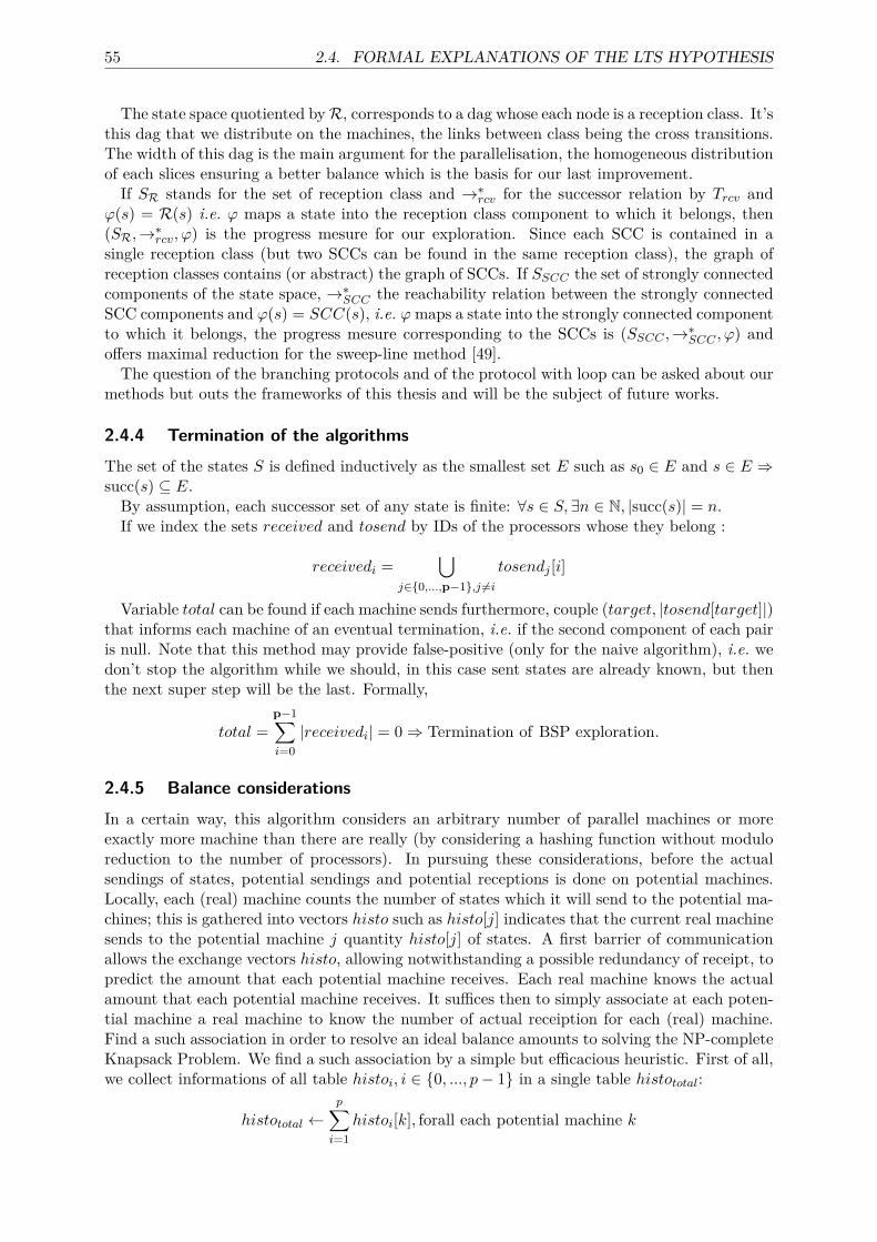
55 2.4. FORMAL EXPLANATIONS OF THE LTS HYPOTHESIS
The state space quotiented byR, corresponds to a dag whose each node is a reception class. It’sthis dag that we distribute on the machines, the links between class being the cross transitions.The width of this dag is the main argument for the parallelisation, the homogeneous distributionof each slices ensuring a better balance which is the basis for our last improvement.If SR stands for the set of reception class and →∗rcv for the successor relation by Trcv and
ϕ(s) = R(s) i.e. ϕ maps a state into the reception class component to which it belongs, then(SR,→∗rcv, ϕ) is the progress mesure for our exploration. Since each SCC is contained in asingle reception class (but two SCCs can be found in the same reception class), the graph ofreception classes contains (or abstract) the graph of SCCs. If SSCC the set of strongly connectedcomponents of the state space, →∗SCC the reachability relation between the strongly connectedSCC components and ϕ(s) = SCC(s), i.e. ϕmaps a state into the strongly connected componentto which it belongs, the progress mesure corresponding to the SCCs is (SSCC ,→∗SCC , ϕ) andoffers maximal reduction for the sweep-line method [49].The question of the branching protocols and of the protocol with loop can be asked about our
methods but outs the frameworks of this thesis and will be the subject of future works.
2.4.4 Termination of the algorithmsThe set of the states S is defined inductively as the smallest set E such as s0 ∈ E and s ∈ E ⇒succ(s) ⊆ E.By assumption, each successor set of any state is finite: ∀s ∈ S, ∃n ∈ N, |succ(s)| = n.If we index the sets received and tosend by IDs of the processors whose they belong :
receivedi =⋃
j∈{0,...,p−1},j 6=itosendj [i]
Variable total can be found if each machine sends furthermore, couple (target, |tosend[target]|)that informs each machine of an eventual termination, i.e. if the second component of each pairis null. Note that this method may provide false-positive (only for the naive algorithm), i.e. wedon’t stop the algorithm while we should, in this case sent states are already known, but thenthe next super step will be the last. Formally,
total =p−1∑i=0|receivedi| = 0⇒ Termination of BSP exploration.
2.4.5 Balance considerationsIn a certain way, this algorithm considers an arbitrary number of parallel machines or moreexactly more machine than there are really (by considering a hashing function without moduloreduction to the number of processors). In pursuing these considerations, before the actualsendings of states, potential sendings and potential receptions is done on potential machines.Locally, each (real) machine counts the number of states which it will send to the potential ma-chines; this is gathered into vectors histo such as histo[j] indicates that the current real machinesends to the potential machine j quantity histo[j] of states. A first barrier of communicationallows the exchange vectors histo, allowing notwithstanding a possible redundancy of receipt, topredict the amount that each potential machine receives. Each real machine knows the actualamount that each potential machine receives. It suffices then to simply associate at each poten-tial machine a real machine to know the number of actual receiption for each (real) machine.Find a such association in order to resolve an ideal balance amounts to solving the NP-completeKnapsack Problem. We find a such association by a simple but efficacious heuristic. First of all,we collect informations of all table histoi, i ∈ {0, ..., p− 1} in a single table histototal:
histototal ←p∑i=1
histoi[k], forall each potential machine k
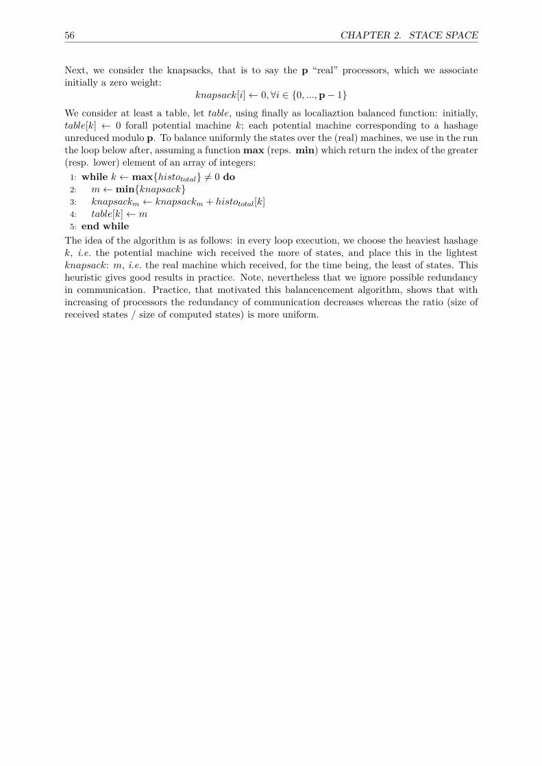
56 CHAPTER 2. STACE SPACE
Next, we consider the knapsacks, that is to say the p “real” processors, which we associateinitially a zero weight:
knapsack[i]← 0,∀i ∈ {0, ...,p− 1}
We consider at least a table, let table, using finally as localiaztion balanced function: initially,table[k] ← 0 forall potential machine k; each potential machine corresponding to a hashageunreduced modulo p. To balance uniformly the states over the (real) machines, we use in the runthe loop below after, assuming a functionmax (reps. min) which return the index of the greater(resp. lower) element of an array of integers:1: while k ←max{histototal} 6= 0 do2: m←min{knapsack}3: knapsackm ← knapsackm + histototal[k]4: table[k]← m5: end while
The idea of the algorithm is as follows: in every loop execution, we choose the heaviest hashagek, i.e. the potential machine wich received the more of states, and place this in the lightestknapsack: m, i.e. the real machine which received, for the time being, the least of states. Thisheuristic gives good results in practice. Note, nevertheless that we ignore possible redundancyin communication. Practice, that motivated this balancencement algorithm, shows that withincreasing of processors the redundancy of communication decreases whereas the ratio (size ofreceived states / size of computed states) is more uniform.
3 Model checking
This chapter extends the work of [105].
Contents3.1 Tarjan . . . . . . . . . . . . . . . . . . . . . . . . . . . . . . . . . . . . . 57
3.1.1 Recursive Tarjan algorithm . . . . . . . . . . . . . . . . . . . . . . . . . 583.1.2 Iterative Tarjan algorithm . . . . . . . . . . . . . . . . . . . . . . . . . . 59
3.2 Temporal logics LTL and CTL* . . . . . . . . . . . . . . . . . . . . . . 60
3.2.1 Notations . . . . . . . . . . . . . . . . . . . . . . . . . . . . . . . . . . . 613.2.2 CTL* syntax and semantics . . . . . . . . . . . . . . . . . . . . . . . . . 613.2.3 Proof-structures for verifying a LTL formula . . . . . . . . . . . . . . . 63
3.3 LTL checking . . . . . . . . . . . . . . . . . . . . . . . . . . . . . . . . . 65
3.3.1 Sequential recursive algorithm for LTL . . . . . . . . . . . . . . . . . . . 653.3.2 Sequential iterative algorithm for LTL . . . . . . . . . . . . . . . . . . . 673.3.3 Parallel algorithm for LTL . . . . . . . . . . . . . . . . . . . . . . . . . . 68
3.4 CTL* checking . . . . . . . . . . . . . . . . . . . . . . . . . . . . . . . . 70
3.4.1 Sequential algorithms for CTL* . . . . . . . . . . . . . . . . . . . . . . . 733.4.2 Naive parallel algorithm for CTL* . . . . . . . . . . . . . . . . . . . . . 783.4.3 Parallel algorithm for CTL* . . . . . . . . . . . . . . . . . . . . . . . . . 85
In what follow, we recall the well known Tarjan algorithm which is the underlying algorithmof the work on a on-the-fly approach used by [28] for CTL* model checking. But the peculiarityof our work concerns parallel computation: our main contributions in the following sections arethus essentially the parallel adaptation of the algorithms found in [28] for the case of securityprotocols.In a first time, we recall the Tarjan algorithm for finding the SCCs components of a directed
graph. Then we recall the LTL and CTL* logics and give and discuss our relatives parallelalgorithms.
3.1 Tarjan
Tarjan’s well known algorithm (named from its author, Robert Tarjan [194]) is a graph algorithmfor finding the strongly connected components of a graph which requires one depth-first search.A strongly connected components or SCC of a directed graph is a maximal component in whichevery vertex can be reached from each other — maximal in the sense that if we add any othernode we breaks the mutual reachability propertyNotice that in the following, we call succ the successor function in the LTS.
57
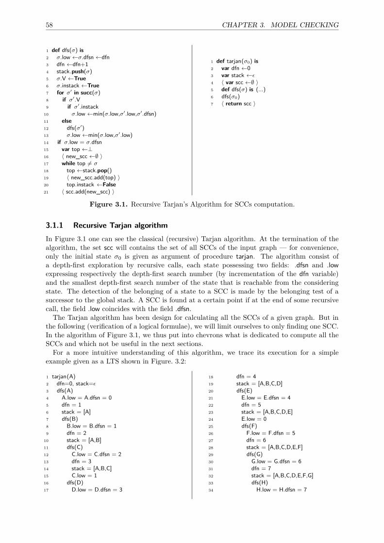
58 CHAPTER 3. MODEL CHECKING
1 def dfs(σ) is2 σ.low ←σ.dfsn ←dfn3 dfn ←dfn+14 stack.push(σ)5 σ.V ←True6 σ.instack ←True7 for σ′ in succ(σ)8 if σ′.V9 if σ′.instack
10 σ.low ←min(σ.low,σ′.low,σ′.dfsn)11 else12 dfs(σ′)13 σ.low ←min(σ.low,σ′.low)14 if σ.low = σ.dfsn15 var top ←⊥16 〈 new_scc ←∅ 〉17 while top 6= σ18 top ←stack.pop()19 〈 new_scc.add(top) 〉20 top.instack ←False21 〈 scc.add(new_scc) 〉
1 def tarjan(σ0) is2 var dfn ←03 var stack ←ε4 〈 var scc ←∅ 〉5 def dfs(σ) is (...)6 dfs(σ0)7 〈 return scc 〉
Figure 3.1. Recursive Tarjan’s Algorithm for SCCs computation.
3.1.1 Recursive Tarjan algorithmIn Figure 3.1 one can see the classical (recursive) Tarjan algorithm. At the termination of thealgorithm, the set scc will contains the set of all SCCs of the input graph — for convenience,only the initial state σ0 is given as argument of procedure tarjan. The algorithm consist ofa depth-first exploration by recursive calls, each state possessing two fields: .dfsn and .lowexpressing respectively the depth-first search number (by incrementation of the dfn variable)and the smallest depth-first search number of the state that is reachable from the consideringstate. The detection of the belonging of a state to a SCC is made by the belonging test of asuccessor to the global stack. A SCC is found at a certain point if at the end of some recursivecall, the field .low coincides with the field .dfsn.
The Tarjan algorithm has been design for calculating all the SCCs of a given graph. But inthe following (verification of a logical formulae), we will limit ourselves to only finding one SCC.In the algorithm of Figure 3.1, we thus put into chevrons what is dedicated to compute all theSCCs and which not be useful in the next sections.For a more intuitive understanding of this algorithm, we trace its execution for a simple
example given as a LTS shown in Figure. 3.2:
1 tarjan(A)2 dfn=0, stack=ε3 dfs(A)4 A.low = A.dfsn = 05 dfn = 16 stack = [A]7 dfs(B)8 B.low = B.dfsn = 19 dfn = 2
10 stack = [A,B]11 dfs(C)12 C.low = C.dfsn = 213 dfn = 314 stack = [A,B,C]15 C.low = 116 dfs(D)17 D.low = D.dfsn = 3
18 dfn = 419 stack = [A,B,C,D]20 dfs(E)21 E.low = E.dfsn = 422 dfn = 523 stack = [A,B,C,D,E]24 E.low = 025 dfs(F)26 F.low = F.dfsn = 527 dfn = 628 stack = [A,B,C,D,E,F]29 dfs(G)30 G.low = G.dfsn = 631 dfn = 732 stack = [A,B,C,D,E,F,G]33 dfs(H)34 H.low = H.dfsn = 7
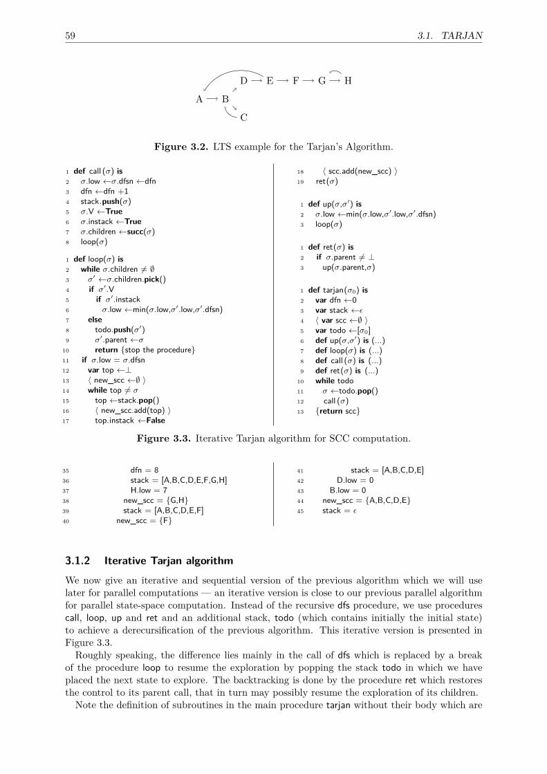
59 3.1. TARJAN
A B
C
D E F G H
Figure 3.2. LTS example for the Tarjan’s Algorithm.
1 def call (σ) is2 σ.low ←σ.dfsn ←dfn3 dfn ←dfn +14 stack.push(σ)5 σ.V ←True6 σ.instack ←True7 σ.children ←succ(σ)8 loop(σ)
1 def loop(σ) is2 while σ.children 6= ∅3 σ′ ←σ.children.pick()4 if σ′.V5 if σ′.instack6 σ.low ←min(σ.low,σ′.low,σ′.dfsn)7 else8 todo.push(σ′)9 σ′.parent ←σ
10 return {stop the procedure}11 if σ.low = σ.dfsn12 var top ←⊥13 〈 new_scc ←∅ 〉14 while top 6= σ15 top ←stack.pop()16 〈 new_scc.add(top) 〉17 top.instack ←False
18 〈 scc.add(new_scc) 〉19 ret(σ)
1 def up(σ,σ′) is2 σ.low ←min(σ.low,σ′.low,σ′.dfsn)3 loop(σ)
1 def ret(σ) is2 if σ.parent 6= ⊥3 up(σ.parent,σ)
1 def tarjan(σ0) is2 var dfn ←03 var stack ←ε4 〈 var scc ←∅ 〉5 var todo ←[σ0]6 def up(σ,σ′) is (...)7 def loop(σ) is (...)8 def call (σ) is (...)9 def ret(σ) is (...)
10 while todo11 σ ←todo.pop()12 call (σ)13 {return scc}
Figure 3.3. Iterative Tarjan algorithm for SCC computation.
35 dfn = 836 stack = [A,B,C,D,E,F,G,H]37 H.low = 738 new_scc = {G,H}39 stack = [A,B,C,D,E,F]40 new_scc = {F}
41 stack = [A,B,C,D,E]42 D.low = 043 B.low = 044 new_scc = {A,B,C,D,E}45 stack = ε
3.1.2 Iterative Tarjan algorithm
We now give an iterative and sequential version of the previous algorithm which we will uselater for parallel computations — an iterative version is close to our previous parallel algorithmfor parallel state-space computation. Instead of the recursive dfs procedure, we use procedurescall, loop, up and ret and an additional stack, todo (which contains initially the initial state)to achieve a derecursification of the previous algorithm. This iterative version is presented inFigure 3.3.Roughly speaking, the difference lies mainly in the call of dfs which is replaced by a break
of the procedure loop to resume the exploration by popping the stack todo in which we haveplaced the next state to explore. The backtracking is done by the procedure ret which restoresthe control to its parent call, that in turn may possibly resume the exploration of its children.Note the definition of subroutines in the main procedure tarjan without their body which are
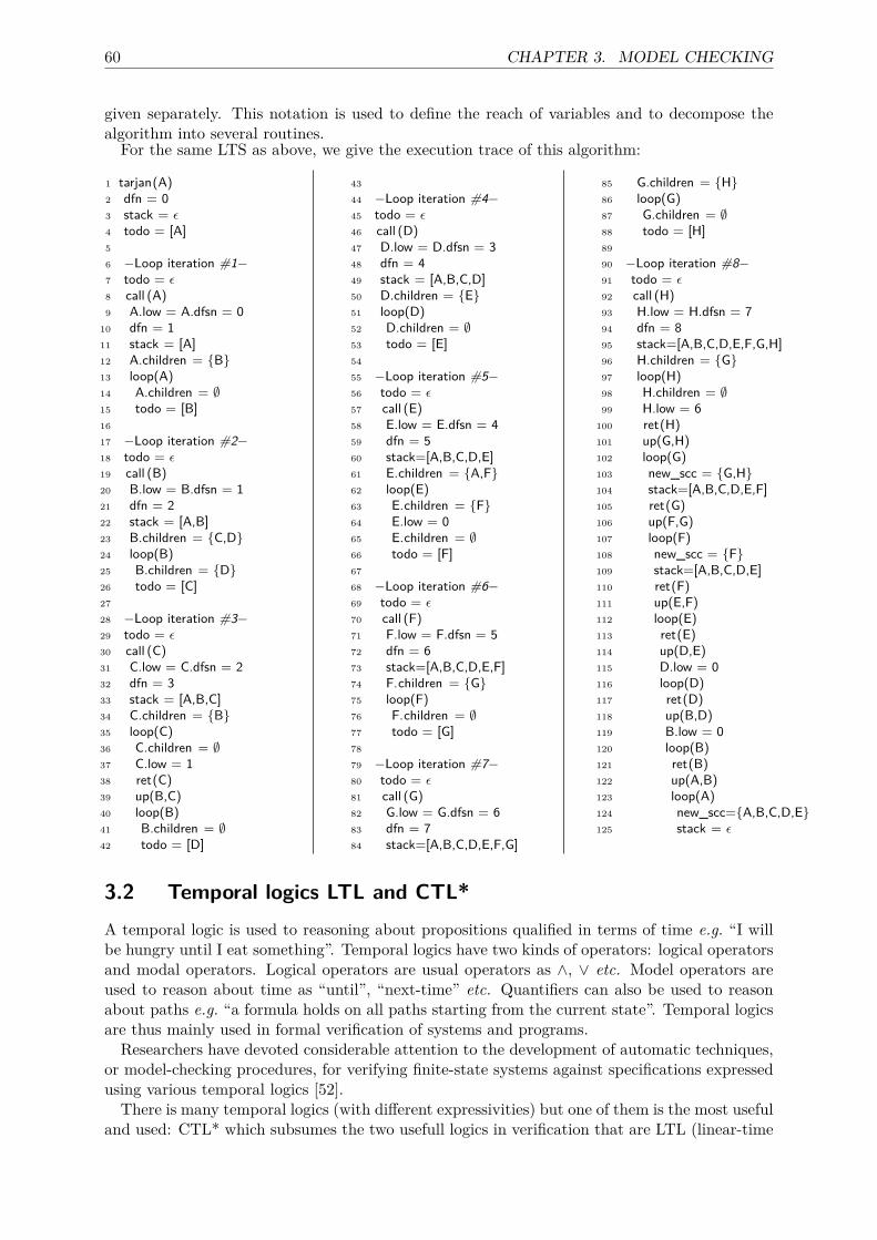
60 CHAPTER 3. MODEL CHECKING
given separately. This notation is used to define the reach of variables and to decompose thealgorithm into several routines.For the same LTS as above, we give the execution trace of this algorithm:
1 tarjan(A)2 dfn = 03 stack = ε4 todo = [A]5
6 −Loop iteration #1−7 todo = ε8 call (A)9 A.low = A.dfsn = 0
10 dfn = 111 stack = [A]12 A.children = {B}13 loop(A)14 A.children = ∅15 todo = [B]16
17 −Loop iteration #2−18 todo = ε19 call (B)20 B.low = B.dfsn = 121 dfn = 222 stack = [A,B]23 B.children = {C,D}24 loop(B)25 B.children = {D}26 todo = [C]27
28 −Loop iteration #3−29 todo = ε30 call (C)31 C.low = C.dfsn = 232 dfn = 333 stack = [A,B,C]34 C.children = {B}35 loop(C)36 C.children = ∅37 C.low = 138 ret(C)39 up(B,C)40 loop(B)41 B.children = ∅42 todo = [D]
43
44 −Loop iteration #4−45 todo = ε46 call (D)47 D.low = D.dfsn = 348 dfn = 449 stack = [A,B,C,D]50 D.children = {E}51 loop(D)52 D.children = ∅53 todo = [E]54
55 −Loop iteration #5−56 todo = ε57 call (E)58 E.low = E.dfsn = 459 dfn = 560 stack=[A,B,C,D,E]61 E.children = {A,F}62 loop(E)63 E.children = {F}64 E.low = 065 E.children = ∅66 todo = [F]67
68 −Loop iteration #6−69 todo = ε70 call (F)71 F.low = F.dfsn = 572 dfn = 673 stack=[A,B,C,D,E,F]74 F.children = {G}75 loop(F)76 F.children = ∅77 todo = [G]78
79 −Loop iteration #7−80 todo = ε81 call (G)82 G.low = G.dfsn = 683 dfn = 784 stack=[A,B,C,D,E,F,G]
85 G.children = {H}86 loop(G)87 G.children = ∅88 todo = [H]89
90 −Loop iteration #8−91 todo = ε92 call (H)93 H.low = H.dfsn = 794 dfn = 895 stack=[A,B,C,D,E,F,G,H]96 H.children = {G}97 loop(H)98 H.children = ∅99 H.low = 6
100 ret(H)101 up(G,H)102 loop(G)103 new_scc = {G,H}104 stack=[A,B,C,D,E,F]105 ret(G)106 up(F,G)107 loop(F)108 new_scc = {F}109 stack=[A,B,C,D,E]110 ret(F)111 up(E,F)112 loop(E)113 ret(E)114 up(D,E)115 D.low = 0116 loop(D)117 ret(D)118 up(B,D)119 B.low = 0120 loop(B)121 ret(B)122 up(A,B)123 loop(A)124 new_scc={A,B,C,D,E}125 stack = ε
3.2 Temporal logics LTL and CTL*A temporal logic is used to reasoning about propositions qualified in terms of time e.g. “I willbe hungry until I eat something”. Temporal logics have two kinds of operators: logical operatorsand modal operators. Logical operators are usual operators as ∧, ∨ etc. Model operators areused to reason about time as “until”, “next-time” etc. Quantifiers can also be used to reasonabout paths e.g. “a formula holds on all paths starting from the current state”. Temporal logicsare thus mainly used in formal verification of systems and programs.
Researchers have devoted considerable attention to the development of automatic techniques,or model-checking procedures, for verifying finite-state systems against specifications expressedusing various temporal logics [52].There is many temporal logics (with different expressivities) but one of them is the most useful
and used: CTL* which subsumes the two usefull logics in verification that are LTL (linear-time
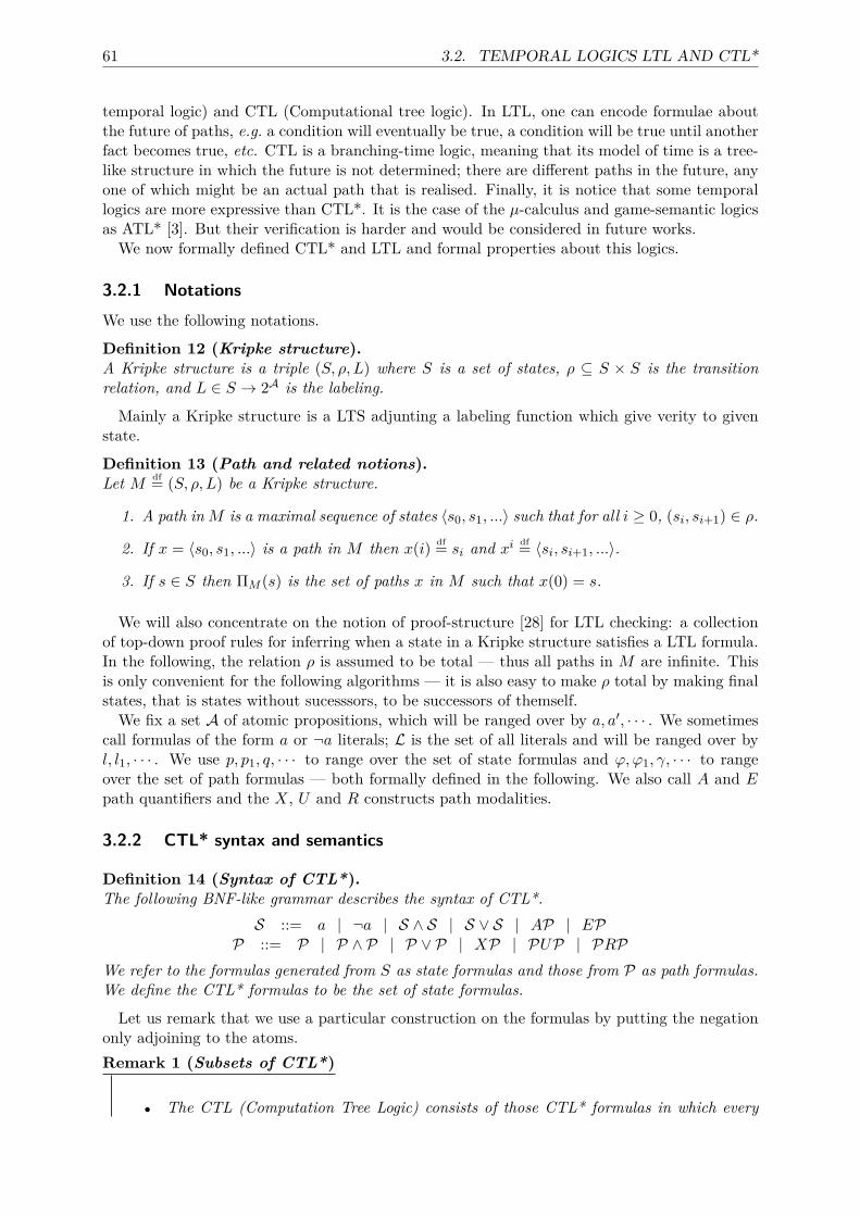
61 3.2. TEMPORAL LOGICS LTL AND CTL*
temporal logic) and CTL (Computational tree logic). In LTL, one can encode formulae aboutthe future of paths, e.g. a condition will eventually be true, a condition will be true until anotherfact becomes true, etc. CTL is a branching-time logic, meaning that its model of time is a tree-like structure in which the future is not determined; there are different paths in the future, anyone of which might be an actual path that is realised. Finally, it is notice that some temporallogics are more expressive than CTL*. It is the case of the µ-calculus and game-semantic logicsas ATL* [3]. But their verification is harder and would be considered in future works.We now formally defined CTL* and LTL and formal properties about this logics.
3.2.1 NotationsWe use the following notations.
Definition 12 (Kripke structure).A Kripke structure is a triple (S, ρ, L) where S is a set of states, ρ ⊆ S × S is the transitionrelation, and L ∈ S → 2A is the labeling.
Mainly a Kripke structure is a LTS adjunting a labeling function which give verity to givenstate.
Definition 13 (Path and related notions).Let M df= (S, ρ, L) be a Kripke structure.
1. A path inM is a maximal sequence of states 〈s0, s1, ...〉 such that for all i ≥ 0, (si, si+1) ∈ ρ.
2. If x = 〈s0, s1, ...〉 is a path in M then x(i) df= si and xidf= 〈si, si+1, ...〉.
3. If s ∈ S then ΠM (s) is the set of paths x in M such that x(0) = s.
We will also concentrate on the notion of proof-structure [28] for LTL checking: a collectionof top-down proof rules for inferring when a state in a Kripke structure satisfies a LTL formula.In the following, the relation ρ is assumed to be total — thus all paths in M are infinite. Thisis only convenient for the following algorithms — it is also easy to make ρ total by making finalstates, that is states without sucesssors, to be successors of themself.We fix a set A of atomic propositions, which will be ranged over by a, a′, · · · . We sometimes
call formulas of the form a or ¬a literals; L is the set of all literals and will be ranged over byl, l1, · · · . We use p, p1, q, · · · to range over the set of state formulas and ϕ,ϕ1, γ, · · · to rangeover the set of path formulas — both formally defined in the following. We also call A and Epath quantifiers and the X, U and R constructs path modalities.
3.2.2 CTL* syntax and semantics
Definition 14 (Syntax of CTL*).The following BNF-like grammar describes the syntax of CTL*.
S ::= a | ¬a | S ∧ S | S ∨ S | AP | EPP ::= P | P ∧ P | P ∨ P | XP | PUP | PRP
We refer to the formulas generated from S as state formulas and those from P as path formulas.We define the CTL* formulas to be the set of state formulas.
Let us remark that we use a particular construction on the formulas by putting the negationonly adjoining to the atoms.Remark 1 (Subsets of CTL*)
• The CTL (Computation Tree Logic) consists of those CTL* formulas in which every
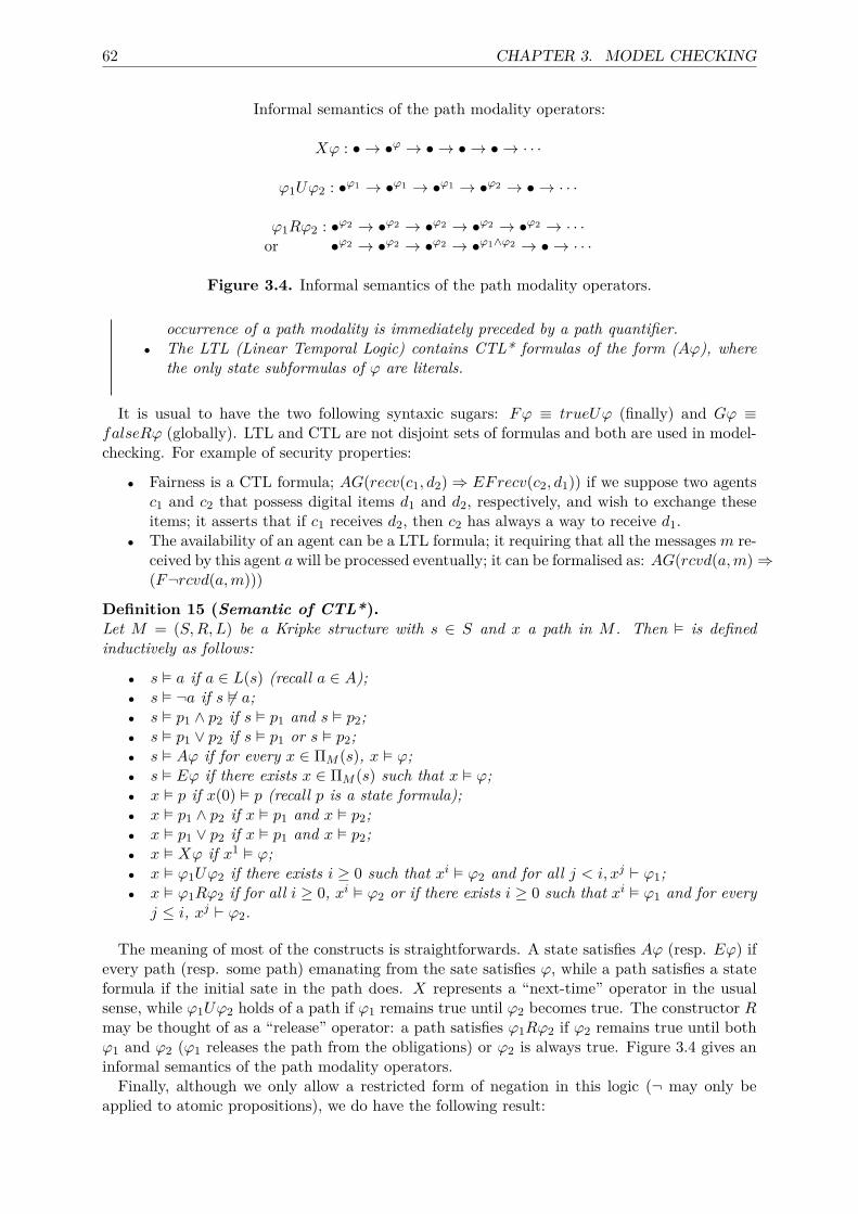
62 CHAPTER 3. MODEL CHECKING
Informal semantics of the path modality operators:
Xϕ : • → •ϕ → • → • → • → · · ·
ϕ1Uϕ2 : •ϕ1 → •ϕ1 → •ϕ1 → •ϕ2 → • → · · ·
ϕ1Rϕ2 : •ϕ2 → •ϕ2 → •ϕ2 → •ϕ2 → •ϕ2 → · · ·or •ϕ2 → •ϕ2 → •ϕ2 → •ϕ1∧ϕ2 → • → · · ·
Figure 3.4. Informal semantics of the path modality operators.
occurrence of a path modality is immediately preceded by a path quantifier.• The LTL (Linear Temporal Logic) contains CTL* formulas of the form (Aϕ), where
the only state subformulas of ϕ are literals.
It is usual to have the two following syntaxic sugars: Fϕ ≡ trueUϕ (finally) and Gϕ ≡falseRϕ (globally). LTL and CTL are not disjoint sets of formulas and both are used in model-checking. For example of security properties:
• Fairness is a CTL formula; AG(recv(c1, d2)⇒ EFrecv(c2, d1)) if we suppose two agentsc1 and c2 that possess digital items d1 and d2, respectively, and wish to exchange theseitems; it asserts that if c1 receives d2, then c2 has always a way to receive d1.
• The availability of an agent can be a LTL formula; it requiring that all the messages m re-ceived by this agent a will be processed eventually; it can be formalised as: AG(rcvd(a,m)⇒(F¬rcvd(a,m)))
Definition 15 (Semantic of CTL*).Let M = (S,R,L) be a Kripke structure with s ∈ S and x a path in M . Then � is definedinductively as follows:
• s � a if a ∈ L(s) (recall a ∈ A);• s � ¬a if s 6� a;• s � p1 ∧ p2 if s � p1 and s � p2;• s � p1 ∨ p2 if s � p1 or s � p2;• s � Aϕ if for every x ∈ ΠM (s), x � ϕ;• s � Eϕ if there exists x ∈ ΠM (s) such that x � ϕ;• x � p if x(0) � p (recall p is a state formula);• x � p1 ∧ p2 if x � p1 and x � p2;• x � p1 ∨ p2 if x � p1 and x � p2;• x � Xϕ if x1 � ϕ;• x � ϕ1Uϕ2 if there exists i ≥ 0 such that xi � ϕ2 and for all j < i, xj ` ϕ1;• x � ϕ1Rϕ2 if for all i ≥ 0, xi � ϕ2 or if there exists i ≥ 0 such that xi � ϕ1 and for every
j ≤ i, xj ` ϕ2.
The meaning of most of the constructs is straightforwards. A state satisfies Aϕ (resp. Eϕ) ifevery path (resp. some path) emanating from the sate satisfies ϕ, while a path satisfies a stateformula if the initial sate in the path does. X represents a “next-time” operator in the usualsense, while ϕ1Uϕ2 holds of a path if ϕ1 remains true until ϕ2 becomes true. The constructor Rmay be thought of as a “release” operator: a path satisfies ϕ1Rϕ2 if ϕ2 remains true until bothϕ1 and ϕ2 (ϕ1 releases the path from the obligations) or ϕ2 is always true. Figure 3.4 gives aninformal semantics of the path modality operators.Finally, although we only allow a restricted form of negation in this logic (¬ may only be
applied to atomic propositions), we do have the following result:
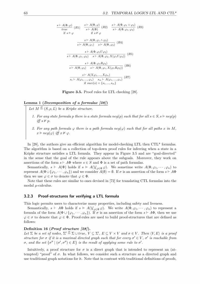
63 3.2. TEMPORAL LOGICS LTL AND CTL*
s ` A(Φ, ϕ)true
(R1)s ` A(Φ, ϕ)s ` A(Φ)
(R2)s ` A(Φ, ϕ1 ∨ ϕ2)s ` A(Φ, ϕ1, ϕ2)
(R3)
if s � ϕ if s 2 ϕ
s ` A(Φ, ϕ1 ∧ ϕ2)s ` A(Φ, ϕ1) s ` A(Φ, ϕ2)
(R4)
s ` A(Φ, ϕ1Uϕ2)s ` A(Φ, ϕ1, ϕ2) s ` A(Φ, ϕ2, X(ϕ1Uϕ2))
(R5)
s ` A(Φ, ϕ1Rϕ2)s ` A(Φ, ϕ2) s ` A(Φ, ϕ1, X(ϕ1Rϕ2))
(R6)
s ` A(Xϕ1, ..., Xϕn)s1 ` A(ϕ1, ..., ϕn) sm ` A(ϕ1, ..., ϕn)
(R7)
if succ(s) = {s1, ..., sm}
Figure 3.5. Proof rules for LTL checking [28].
Lemma 1 (Decomposition of a formulae [28])Let M df= (S, ρ, L) be a Kripke structure.
1. For any state formula p there is a state formula neg(p) such that for all s ∈ S, s � neg(p)iff s 2 p.
2. For any path formula ϕ there is a path formula neg(ϕ) such that for all paths x in M ,x � neg(ϕ) iff x 2 ϕ.
In [28], the authors give an efficient algorithm for model-checking LTL then CTL* formulas.The algorithm is based on a collection of top-down proof rules for inferring when a state in aKripke structure satisfies a LTL formula. They appear in Figure 3.5 and are “goal-directed”in the sense that the goal of the rule appears above the subgoals. Moreover, they work onassertions of the form s ` AΦ where s ∈ S and Φ is a set of path formulas.
Semantically, s ` A(Φ) holds if s � A(∨ϕ∈Φ ϕ). We sometime write A(Φ, ϕ1, · · · , ϕn) torepresent A(Φ∪{ϕ1, · · · , ϕn}) and we consider A(∅) = ∅. If σ is an assertion of the form s ` AΦthen we use ϕ ∈ σ to denote that ϕ ∈ Φ.Note that these rules are similar to ones devised in [72] for translating CTL formulas into the
modal µ-calculus.
3.2.3 Proof-structures for verifying a LTL formula
This logic permits users to characterize many properties, including safety and liveness.Semantically, s ` AΦ holds if s � A(∨ϕ∈Φ ϕ). We write A(Φ, ϕ1, · · · , ϕn) to represent a
formula of the form A(Φ ∪ {ϕ1, · · · , ϕn}). If σ is an assertion of the form s ` AΦ, then we useϕ ∈ σ to denote that ϕ ∈ Φ. Proof-rules are used to build proof-structures that are defined asfollows:
Definition 16 (Proof structure [28]).Let Σ be a set of nodes, Σ′ df= Σ ∪ true, V ⊆ Σ′, E ⊆ V × V and σ ∈ V . Then 〈V,E〉 is a proofstructure for σ if it is a maximal directed graph such that for every σ′ ∈ V , σ′ is reachable fromσ, and the set {σ′′ | (σ′, σ′′) ∈ E} is the result of applying some rule to σ′.
Intuitively, a proof structure for σ is a direct graph that is intended to represent an (at-tempted) “proof” of σ. In what follows, we consider such a structure as a directed graph anduse traditional graph notations for it. Note that in contrast with traditional definitions of proofs,
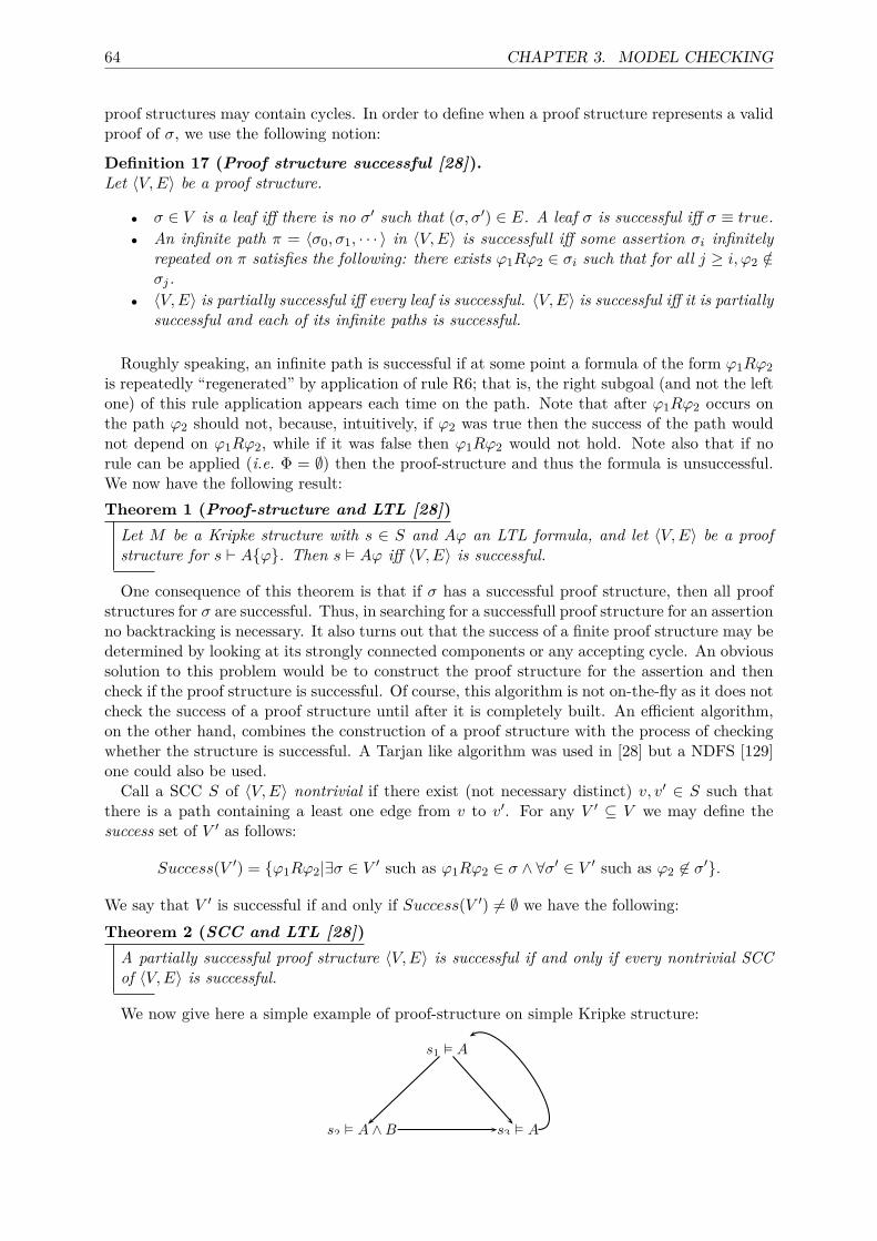
64 CHAPTER 3. MODEL CHECKING
proof structures may contain cycles. In order to define when a proof structure represents a validproof of σ, we use the following notion:
Definition 17 (Proof structure successful [28]).Let 〈V,E〉 be a proof structure.
• σ ∈ V is a leaf iff there is no σ′ such that (σ, σ′) ∈ E. A leaf σ is successful iff σ ≡ true.• An infinite path π = 〈σ0, σ1, · · · 〉 in 〈V,E〉 is successfull iff some assertion σi infinitely
repeated on π satisfies the following: there exists ϕ1Rϕ2 ∈ σi such that for all j ≥ i, ϕ2 /∈σj.
• 〈V,E〉 is partially successful iff every leaf is successful. 〈V,E〉 is successful iff it is partiallysuccessful and each of its infinite paths is successful.
Roughly speaking, an infinite path is successful if at some point a formula of the form ϕ1Rϕ2is repeatedly “regenerated” by application of rule R6; that is, the right subgoal (and not the leftone) of this rule application appears each time on the path. Note that after ϕ1Rϕ2 occurs onthe path ϕ2 should not, because, intuitively, if ϕ2 was true then the success of the path wouldnot depend on ϕ1Rϕ2, while if it was false then ϕ1Rϕ2 would not hold. Note also that if norule can be applied (i.e. Φ = ∅) then the proof-structure and thus the formula is unsuccessful.We now have the following result:Theorem 1 (Proof-structure and LTL [28])Let M be a Kripke structure with s ∈ S and Aϕ an LTL formula, and let 〈V,E〉 be a proofstructure for s ` A{ϕ}. Then s � Aϕ iff 〈V,E〉 is successful.
One consequence of this theorem is that if σ has a successful proof structure, then all proofstructures for σ are successful. Thus, in searching for a successfull proof structure for an assertionno backtracking is necessary. It also turns out that the success of a finite proof structure may bedetermined by looking at its strongly connected components or any accepting cycle. An obvioussolution to this problem would be to construct the proof structure for the assertion and thencheck if the proof structure is successful. Of course, this algorithm is not on-the-fly as it does notcheck the success of a proof structure until after it is completely built. An efficient algorithm,on the other hand, combines the construction of a proof structure with the process of checkingwhether the structure is successful. A Tarjan like algorithm was used in [28] but a NDFS [129]one could also be used.
Call a SCC S of 〈V,E〉 nontrivial if there exist (not necessary distinct) v, v′ ∈ S such thatthere is a path containing a least one edge from v to v′. For any V ′ ⊆ V we may define thesuccess set of V ′ as follows:
Success(V ′) = {ϕ1Rϕ2|∃σ ∈ V ′ such as ϕ1Rϕ2 ∈ σ ∧ ∀σ′ ∈ V ′ such as ϕ2 6∈ σ′}.
We say that V ′ is successful if and only if Success(V ′) 6= ∅ we have the following:Theorem 2 (SCC and LTL [28])A partially successful proof structure 〈V,E〉 is successful if and only if every nontrivial SCCof 〈V,E〉 is successful.
We now give here a simple example of proof-structure on simple Kripke structure:
s1 � A
s2 � A ∧B s3 � A
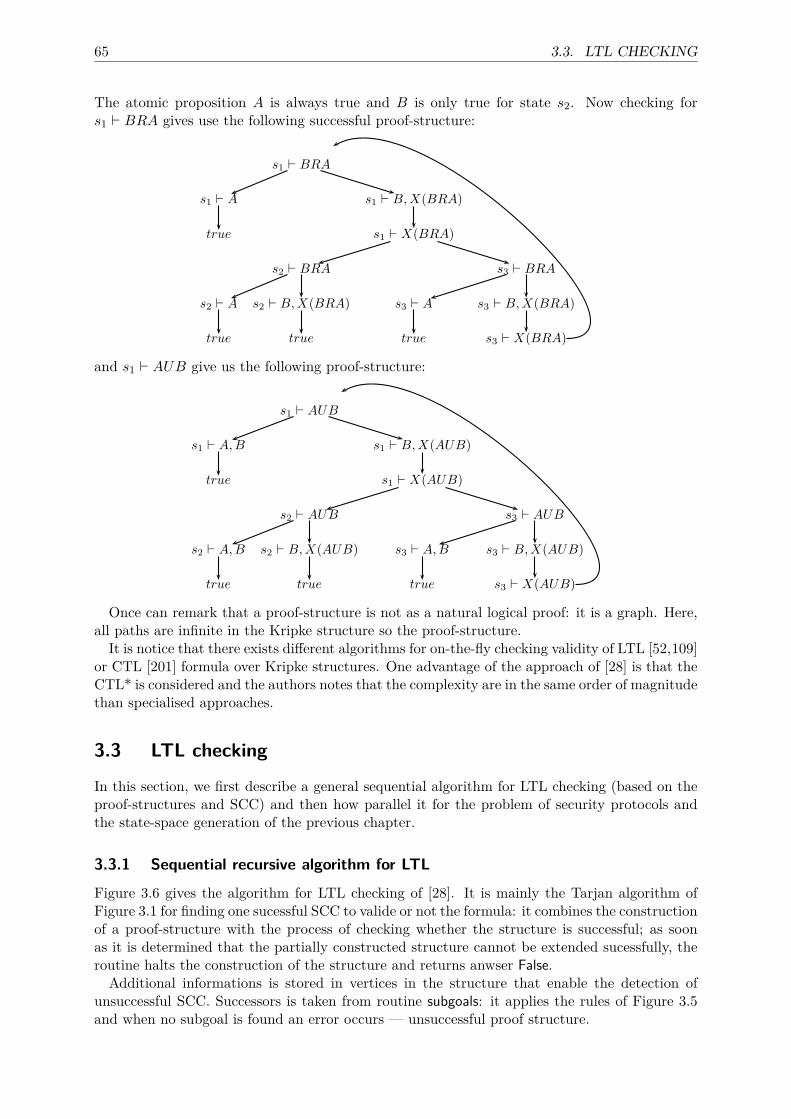
65 3.3. LTL CHECKING
The atomic proposition A is always true and B is only true for state s2. Now checking fors1 ` BRA gives use the following successful proof-structure:
s1 ⊢ BRA
s1 ⊢ A s1 ⊢ B,X(BRA)
true s1 ⊢ X(BRA)
s2 ⊢ BRA s3 ⊢ BRA
s2 ⊢ A s2 ⊢ B,X(BRA) s3 ⊢ A s3 ⊢ B,X(BRA)
true true true s3 ⊢ X(BRA)
and s1 ` AUB give us the following proof-structure:
s1 ⊢ AUB
s1 ⊢ A,B s1 ⊢ B,X(AUB)
true s1 ⊢ X(AUB)
s2 ⊢ AUB s3 ⊢ AUB
s2 ⊢ A,B s2 ⊢ B,X(AUB) s3 ⊢ A,B s3 ⊢ B,X(AUB)
true true true s3 ⊢ X(AUB)
Once can remark that a proof-structure is not as a natural logical proof: it is a graph. Here,all paths are infinite in the Kripke structure so the proof-structure.It is notice that there exists different algorithms for on-the-fly checking validity of LTL [52,109]
or CTL [201] formula over Kripke structures. One advantage of the approach of [28] is that theCTL* is considered and the authors notes that the complexity are in the same order of magnitudethan specialised approaches.
3.3 LTL checking
In this section, we first describe a general sequential algorithm for LTL checking (based on theproof-structures and SCC) and then how parallel it for the problem of security protocols andthe state-space generation of the previous chapter.
3.3.1 Sequential recursive algorithm for LTL
Figure 3.6 gives the algorithm for LTL checking of [28]. It is mainly the Tarjan algorithm ofFigure 3.1 for finding one sucessful SCC to valide or not the formula: it combines the constructionof a proof-structure with the process of checking whether the structure is successful; as soonas it is determined that the partially constructed structure cannot be extended sucessfully, theroutine halts the construction of the structure and returns anwser False.Additional informations is stored in vertices in the structure that enable the detection of
unsuccessful SCC. Successors is taken from routine subgoals: it applies the rules of Figure 3.5and when no subgoal is found an error occurs — unsuccessful proof structure.
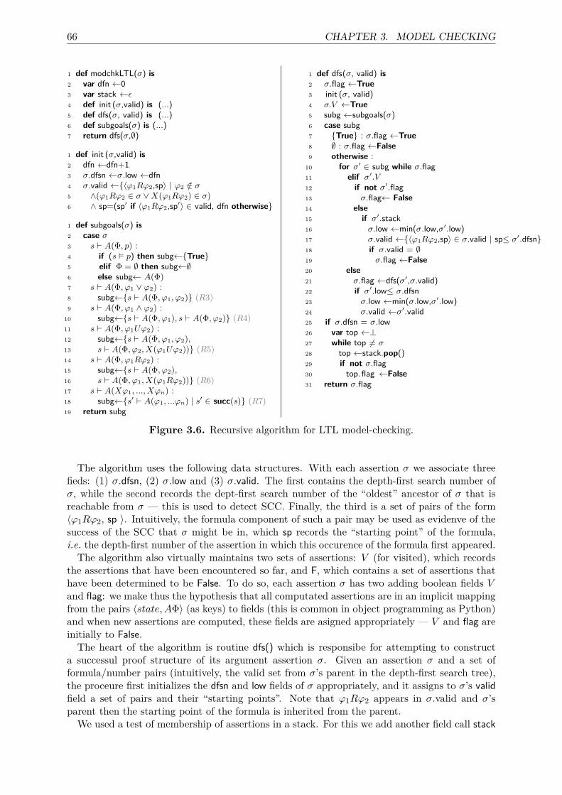
66 CHAPTER 3. MODEL CHECKING
1 def modchkLTL(σ) is2 var dfn ←03 var stack ←ε4 def init (σ,valid) is (...)5 def dfs(σ, valid) is (...)6 def subgoals(σ) is (...)7 return dfs(σ,∅)
1 def init (σ,valid) is2 dfn ←dfn+13 σ.dfsn ←σ.low ←dfn4 σ.valid ←{〈ϕ1Rϕ2,sp〉 | ϕ2 /∈ σ5 ∧(ϕ1Rϕ2 ∈ σ ∨X(ϕ1Rϕ2) ∈ σ)6 ∧ sp=(sp′ if 〈ϕ1Rϕ2,sp′〉 ∈ valid, dfn otherwise}
1 def subgoals(σ) is2 case σ3 s ` A(Φ, p) :4 if (s � p) then subg←{True}5 elif Φ = ∅ then subg←∅6 else subg← A(Φ)7 s ` A(Φ, ϕ1 ∨ ϕ2) :8 subg←{s ` A(Φ, ϕ1, ϕ2)} (R3)9 s ` A(Φ, ϕ1 ∧ ϕ2) :
10 subg←{s ` A(Φ, ϕ1), s ` A(Φ, ϕ2)} (R4)11 s ` A(Φ, ϕ1Uϕ2) :12 subg←{s ` A(Φ, ϕ1, ϕ2),13 s ` A(Φ, ϕ2, X(ϕ1Uϕ2))} (R5)14 s ` A(Φ, ϕ1Rϕ2) :15 subg←{s ` A(Φ, ϕ2),16 s ` A(Φ, ϕ1, X(ϕ1Rϕ2))} (R6)17 s ` A(Xϕ1, ..., Xϕn) :18 subg←{s′ ` A(ϕ1, ...ϕn) | s′ ∈ succ(s)} (R7)19 return subg
1 def dfs(σ, valid) is2 σ.flag ←True3 init (σ, valid)4 σ.V ←True5 subg ←subgoals(σ)6 case subg7 {True} : σ.flag ←True8 ∅ : σ.flag ←False9 otherwise :
10 for σ′ ∈ subg while σ.flag11 elif σ′.V12 if not σ′.flag13 σ.flag← False14 else15 if σ′.stack16 σ.low ←min(σ.low,σ′.low)17 σ.valid ←{〈ϕ1Rϕ2,sp〉 ∈ σ.valid | sp≤ σ′.dfsn}18 if σ.valid = ∅19 σ.flag ←False20 else21 σ.flag ←dfs(σ′,σ.valid)22 if σ′.low≤ σ.dfsn23 σ.low ←min(σ.low,σ′.low)24 σ.valid ←σ′.valid25 if σ.dfsn = σ.low26 var top ←⊥27 while top 6= σ28 top ←stack.pop()29 if not σ.flag30 top.flag ←False31 return σ.flag
Figure 3.6. Recursive algorithm for LTL model-checking.
The algorithm uses the following data structures. With each assertion σ we associate threefieds: (1) σ.dfsn, (2) σ.low and (3) σ.valid. The first contains the depth-first search number ofσ, while the second records the dept-first search number of the “oldest” ancestor of σ that isreachable from σ — this is used to detect SCC. Finally, the third is a set of pairs of the form〈ϕ1Rϕ2, sp 〉. Intuitively, the formula component of such a pair may be used as evidenve of thesuccess of the SCC that σ might be in, which sp records the “starting point” of the formula,i.e. the depth-first number of the assertion in which this occurence of the formula first appeared.The algorithm also virtually maintains two sets of assertions: V (for visited), which records
the assertions that have been encountered so far, and F, which contains a set of assertions thathave been determined to be False. To do so, each assertion σ has two adding boolean fields Vand flag: we make thus the hypothesis that all computated assertions are in an implicit mappingfrom the pairs 〈state, AΦ〉 (as keys) to fields (this is common in object programming as Python)and when new assertions are computed, these fields are asigned appropriately — V and flag areinitially to False.
The heart of the algorithm is routine dfs() which is responsibe for attempting to constructa successul proof structure of its argument assertion σ. Given an assertion σ and a set offormula/number pairs (intuitively, the valid set from σ’s parent in the depth-first search tree),the proceure first initializes the dfsn and low fields of σ appropriately, and it assigns to σ’s validfield a set of pairs and their “starting points”. Note that ϕ1Rϕ2 appears in σ.valid and σ’sparent then the starting point of the formula is inherited from the parent.We used a test of membership of assertions in a stack. For this we add another field call stack
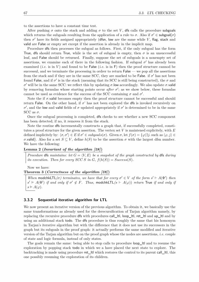
67 3.3. LTL CHECKING
to the assertions to have a constant time test.After pushing σ onto the stack and adding σ to the set V , dfs calls the procedure subgoals
which returns the subgoals resulting from the application of a rule to σ. Also if σ′ ∈ subgoal(σ)then σ′ have its fields assigned appropriately (dfsn, low are the same while V , flag, stack andvalid are False or empty set except if the assertion is already in the implicit map.Procedure dfs then processes the subgoal as follows. First, if the only subgoal has the form
True, dfs should return True, while is the set of subgoal is empty, then σ is an unsuccessfulleaf, and False should be returned. Finally, suppose the set of subgoals is a nonempty set ofassertions, we examine each of there in the following fashion. If subgoal σ′ has already beenexamined (i.e. is in V ) and found to be False (i.e. is in F) then the proof structure cannod besuccessul, and we terminate the processing in ordrer to return False — we pop all the assertionsfrom the stack and if they are in the same SCC, they are marked to be False. if σ′ has not beenfound False, and if σ′ is in the stack (meaning that its SCC is still being constructed), the σ andσ′ will be in the same SCC: we reflect this by updating σ.low accordingly. We also update σ.validby removing formulas whose starting points occur after σ′; as we show below, these formulascannot be used as evidence for the success of the SCC containing σ and σ′.
Note the if σ.valid becomes empty then the proof structure cannot be successful and shouldreturn False. On the other hand, if σ’ has not been explored the dfs is invoked recursively onσ′, and the low and valid fields of σ updated appropriately if σ′ is determined to be in the sameSCC as σ.Once the subgoal processing is completed, dfs checks to see whether a new SCC component
has been detected; if no, it removes it from the stack.Note the routine dfs incrementally constructs a graph that, if successfully completed, consti-
tutes a proof structure for the given assertion. The vertex set V is maintened explicitely, with Edefined implicitely by: 〈σ, σ′〉 ∈ E if σ′ ∈ subgoals(σ). Given σ, let f(σ) = {ϕ|∃j. such as 〈ϕ, j〉 ∈σ.valid}. Also for a set S ⊆ V , define h(S) to be the assertion σ with the largest dfsn number.We have the following:Lemma 2 (Invariant of the algorithm [28])Procedure dfs maintains: let G = 〈V,E〉 be a snapshot of the graph constructed by dfs duringits execution. Then for every SCC S in G, f(h(S)) = Success(S).
Now we have:Theorem 3 (Correctness of the algorithm [28])When modchkLTL(σ) terminates, we have that for every σ′ ∈ V of the form s′ ` A(Φ′) thens′ � A(Φ′) if and only if σ′ 6∈ F . Thus, modchkLTL(s ` A(ϕ)) return True if and only ifs � A(ϕ).
3.3.2 Sequential iterative algorithm for LTLWe now present an iterative version of the previous algorithm. To obtain it, we basically use thesame transformations as already used for the derecursification of Tarjan algorithm namely, byreplacing the recursive procedure dfs with procedures call_ltl, loop_ltl, ret_ltl and up_ltl and byusing an additional stack todo. The dfs procedure is thus roughly the same that his homonymin Tarjan’s iterative algorithm but with the difference that it does not use its successors in thegraph but its subgoals in the proof graph: it actually performs the same modified and iterativeversion of the Tarjan algorithm but on the proof graph whose the nodes are assertions, i.e. coupleof state and logic formula, instead of only states.The goals remain the same: being able to stop calls to procedure loop_ltl and to resume the
exploration by popping stack todo in which we a have placed the next state to explore. Thebacktracking is made using procedure ret_ltl which restores the control to its parent call_ltl, thisone possibly resuming the exploration of its children.
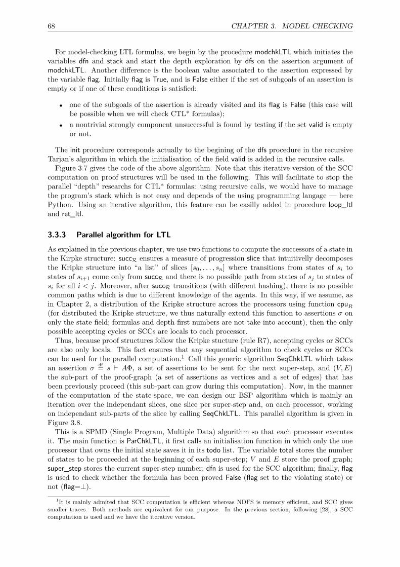
68 CHAPTER 3. MODEL CHECKING
For model-checking LTL formulas, we begin by the procedure modchkLTL which initiates thevariables dfn and stack and start the depth exploration by dfs on the assertion argument ofmodchkLTL. Another difference is the boolean value associated to the assertion expressed bythe variable flag. Initially flag is True, and is False either if the set of subgoals of an assertion isempty or if one of these conditions is satisfied:
• one of the subgoals of the assertion is already visited and its flag is False (this case willbe possible when we will check CTL* formulas);
• a nontrivial strongly component unsuccessful is found by testing if the set valid is emptyor not.
The init procedure corresponds actually to the begining of the dfs procedure in the recursiveTarjan’s algorithm in which the initialisation of the field valid is added in the recursive calls.Figure 3.7 gives the code of the above algorithm. Note that this iterative version of the SCC
computation on proof structures will be used in the following. This will facilitate to stop theparallel “depth” researchs for CTL* formulas: using recursive calls, we would have to managethe program’s stack which is not easy and depends of the using programming langage — herePython. Using an iterative algorithm, this feature can be easilly added in procedure loop_ltland ret_ltl.
3.3.3 Parallel algorithm for LTL
As explained in the previous chapter, we use two functions to compute the successors of a state inthe Kirpke structure: succR ensures a measure of progression slice that intuitivelly decomposesthe Kripke structure into “a list” of slices [s0, . . . , sn] where transitions from states of si tostates of si+1 come only from succR and there is no possible path from states of sj to states ofsi for all i < j. Moreover, after succR transitions (with different hashing), there is no possiblecommon paths which is due to different knowledge of the agents. In this way, if we assume, asin Chapter 2, a distribution of the Kripke structure across the processors using function cpuR(for distributed the Kripke structure, we thus naturally extend this function to assertions σ ononly the state field; formulas and depth-first numbers are not take into account), then the onlypossible accepting cycles or SCCs are locals to each processor.Thus, because proof structures follow the Kripke stucture (rule R7), accepting cycles or SCCs
are also only locals. This fact ensures that any sequential algorithm to check cycles or SCCscan be used for the parallel computation.1 Call this generic algorithm SeqChkLTL which takesan assertion σ
df= s ` AΦ, a set of assertions to be sent for the next super-step, and (V,E)the sub-part of the proof-graph (a set of assertions as vertices and a set of edges) that hasbeen previously proceed (this sub-part can grow during this computation). Now, in the mannerof the computation of the state-space, we can design our BSP algorithm which is mainly aniteration over the independant slices, one slice per super-step and, on each processor, workingon independant sub-parts of the slice by calling SeqChkLTL. This parallel algorithm is given inFigure 3.8.This is a SPMD (Single Program, Multiple Data) algorithm so that each processor executes
it. The main function is ParChkLTL, it first calls an initialisation function in which only the oneprocessor that owns the initial state saves it in its todo list. The variable total stores the numberof states to be proceeded at the beginning of each super-step; V and E store the proof graph;super_step stores the current super-step number; dfn is used for the SCC algorithm; finally, flagis used to check whether the formula has been proved False (flag set to the violating state) ornot (flag=⊥).
1It is mainly admited that SCC computation is efficient whereas NDFS is memory efficient, and SCC givessmaller traces. Both methods are equivalent for our purpose. In the previous section, following [28], a SCCcomputation is used and we have the iterative version.
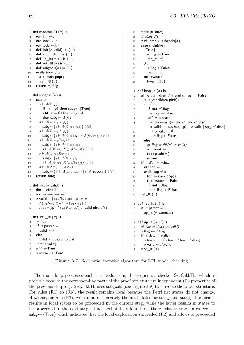
69 3.3. LTL CHECKING
1 def modchkLTL(σ) is2 var dfn ←03 var stack ←ε4 var todo ←[σ0]5 def init (σ,valid) is (...)6 def loop_ltl(σ) is (...)7 def up_ltl(σ,σ′) is (...)8 def ret_ltl (σ) is (...)9 def subgoals(σ) is (...)
10 while todo 6= ε11 σ ←todo.pop()12 call_ltl (σ)13 return σ0.flag
1 def subgoals(σ) is2 case σ3 s ` A(Φ, p) :4 if (s � p) then subg←{True}5 elif Φ = ∅ then subg←∅6 else subg← A(Φ)7 s ` A(Φ, ϕ1 ∨ ϕ2) :8 subg←{s ` A(Φ, ϕ1, ϕ2)} (R3)9 s ` A(Φ, ϕ1 ∧ ϕ2) :
10 subg←{s ` A(Φ, ϕ1), s ` A(Φ, ϕ2)} (R4)11 s ` A(Φ, ϕ1Uϕ2) :12 subg←{s ` A(Φ, ϕ1, ϕ2),13 s ` A(Φ, ϕ2, X(ϕ1Uϕ2))} (R5)14 s ` A(Φ, ϕ1Rϕ2) :15 subg←{s ` A(Φ, ϕ2),16 s ` A(Φ, ϕ1, X(ϕ1Rϕ2))} (R6)17 s ` A(Xϕ1, ..., Xϕn) :18 subg←{s′ ` A(ϕ1, ...ϕn) | s′ ∈ succ(s)} (R7)19 return subg
1 def init (σ,valid) is2 dfn ←dfn+13 σ.dfsn ←σ.low ←dfn4 σ.valid ←{〈ϕ1Rϕ2,sp〉 | ϕ2 /∈ σ5 ∧(ϕ1Rϕ2 ∈ σ ∨X(ϕ1Rϕ2) ∈ σ)6 ∧ sp=(sp′ if 〈ϕ1Rϕ2,sp′〉 ∈ valid else dfn)
1 def call_ltl (σ) is2 # init3 if σ.parent = ⊥4 valid ←∅5 else6 valid ←σ.parent.valid7 init (σ,valid)8 σ.V ←True9 σ.instack ←True
10 stack.push(σ)11 # start dfs12 σ.children ←subgoals(σ)13 case σ.children14 {True} :15 σ.flag ←True16 ret_ltl (σ)17 ∅ :18 σ.flag ←False19 ret_ltl (σ)20 otherwise :21 loop_ltl(σ)
1 def loop_ltl(σ) is2 while σ.children 6= ∅ and σ.flag != False3 σ′ ←σ.children.pick()4 if σ′.V5 if not σ′.flag6 σ.flag ←False7 elif σ′.instack8 σ.low ←min(σ.low, σ′.low, σ′.dfsn)9 σ.valid ←{〈ϕ1Rϕ2,sp〉 ∈ σ.valid | sp≤ σ′.dfsn}
10 if σ.valid = ∅11 σ.flag ←False12 else13 # flag = dfs(σ′, σ.valid)14 σ′.parent ←σ15 todo.push(σ′)16 return17 if σ.dfsn = σ.low18 var top ←⊥19 while top 6= σ20 top ←stack.pop()21 top.instack ←False22 if not σ.flag23 top.flag ←False24 ret_ltl (σ)
1 def ret_ltl (σ) is2 if σ.parent 6= ⊥3 up_ltl(σ.parent,σ)
1 def up_ltl(σ,σ′) is2 # flag = dfs(σ′,σ.valid)3 σ.flag ←σ′.flag4 if σ′.low ≤ σ.dfsn5 σ.low ←min(σ.low, σ′.low, σ′.dfsn)6 σ.valid ←σ′.valid7 loop_ltl(σ)
Figure 3.7. Sequential iterative algorithm for LTL model checking.
The main loop processes each σ in todo using the sequential checker SeqChkLTL, which ispossible because the corresponding parts of the proof structure are independent (P4 properties ofthe previous chapter). SeqChkLTL uses subgoals (see Figure 3.9) to traverse the proof structure.For rules (R1) to (R6), the result remains local because the Petri net states do not change.However, for rule (R7), we compute separately the next states for succL and succR: the formerresults in local states to be proceeded in the current step, while the latter results in states tobe proceeded in the next step. If no local state is found but there exist remote states, we setsubg←{True} which indicates that the local exploration succeeded (P2) and allows to proceeded
70 CHAPTER 3. MODEL CHECKING
1 def Init_main() is2 super_step,dfn,V ,E,todo←0,0,∅,∅,∅3 if cpu(σinit)=mypid4 todo←todo ∪ {σinit}5 flag , total←⊥,16
7 def Exchange(tosend,flag) is8 dump (V,E) at super_step9 super_step←super_step+1
10 tosend←tosend ∪ {(i,flag) | 0 ≤ i < p}11 rcv, total←BSP_EXCHANGE(Balance(tosend))12 flag ,rcv←filter_flag(rcv)13 return flag, rcv, total
1 def ParChkLTL((s ` Φ) as σ) is2 def Init_main() is (...)3 def Exchange(tosend,flag) is (...)4 def subgoals(σ,send) is (...)5 def Build_trace(σ) is (...)6 Init_main()7 while flag=⊥ ∧ total>08 send←∅9 # In parallel thread,
10 # on per independent sub−part,11 # on multi−core architectures12 while todo 6= ∅ ∧ flag=⊥13 pick σ from todo14 if σ /∈ V15 flag←SeqChkLTL(σ,send,E,V )16 if flag 6= ⊥17 send←∅18 flag ,todo,total←Exchange(send,flag)19 case flag20 ⊥ : print "OK"21 σ : Build_trace(σ)
Figure 3.8. A BSP algorithm for LTL checking.
to the next super-step in the main loop. When all the local states have been proceeded, statesare exchanged, which leads to the next slice (i.e. the next super-step). In order to terminate thealgorithm as soon as one processor discovers a counterexample, each locally computed flag issent to all the processors and the received values are then aggregated using function filter_flagthat selects the flag with the lowest dfsn value computed on the processor with the lower number,which ensures that every processor chooses the same flag and then computes the same trace.To balance computation, we use the number of states as well as the size of the formula to beverified for each state (on which the number of subgoals directly depends).Notice also that at each super-step, each processor dumps V and E to its local disk, recording
the super-step number, in order to be able to reconstruct a trace. When a state that invalidatesthe formula is found, a trace from the initial state to the current σ is constructed. Figure 3.10gives this algorithm.The data to do so is distributed among processors and dumped into local files, one per super-
step. We thus use exactly as many steps to rebuild the trace as we used to discover the erroneousstate. The algorithm is presented in Figure 3.10: a trace π whose “oldest” state is σ is recon-structed following the proof graph backward. The processor that owns σ invokes Local_trace tofind a path from a state σ′, that was in todo at the beginning of the super-state, to σ. Thenit sends σ′ to its owner to let the reconstruction continue. To simplify things, we print partsof the reconstructed trace as they are locally computed. Among the predecessors of a state, wealways choose those that are not yet in the trace π (set_of_trace(π) returns the set of states inπ) and selects one with the minimal dfsn value (using function min_dfsn), which allows to selectshorter traces.
3.4 CTL* checkingAs for LTL, we first present a general algorithm and them specialised parallel algorithms forsecurity protocols. The first one called “naive” is a first attempt to extend the parallel algorithmfor LTL checking to CTL* formula whereas the second optimises (balances) the communicationsand reduces the number of super-steps.
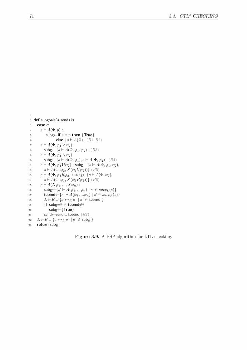
71 3.4. CTL* CHECKING
1
2 def subgoals(σ,send) is3 case σ4 s ` A(Φ, p) :5 subg←if s � p then {True}6 else {s ` A(Φ)} (R1, R2)7 s ` A(Φ, ϕ1 ∨ ϕ2) :8 subg←{s ` A(Φ, ϕ1, ϕ2)} (R3)9 s ` A(Φ, ϕ1 ∧ ϕ2)
10 subg←{s ` A(Φ, ϕ1), s ` A(Φ, ϕ2)} (R4)11 s ` A(Φ, ϕ1Uϕ2) : subg←{s ` A(Φ, ϕ1, ϕ2),12 s ` A(Φ, ϕ2, X(ϕ1Uϕ2))} (R5)13 s ` A(Φ, ϕ1Rϕ2) : subg←{s ` A(Φ, ϕ2),14 s ` A(Φ, ϕ1, X(ϕ1Rϕ2))} (R6)15 s ` A(Xϕ1, ..., Xϕn) :16 subg←{s′ ` A(ϕ1, ...ϕn) | s′ ∈ succL(s)}17 tosend←{s′ ` A(ϕ1, ...ϕn) | s′ ∈ succR(s)}18 E←E ∪ {σ 7→R σ′ | σ′ ∈ tosend }19 if subg=∅ ∧ tosend6=∅20 subg←{True}21 send←send ∪ tosend (R7)22 E←E ∪ {σ 7→L σ′ | σ′ ∈ subg }23 return subg
Figure 3.9. A BSP algorithm for LTL checking.
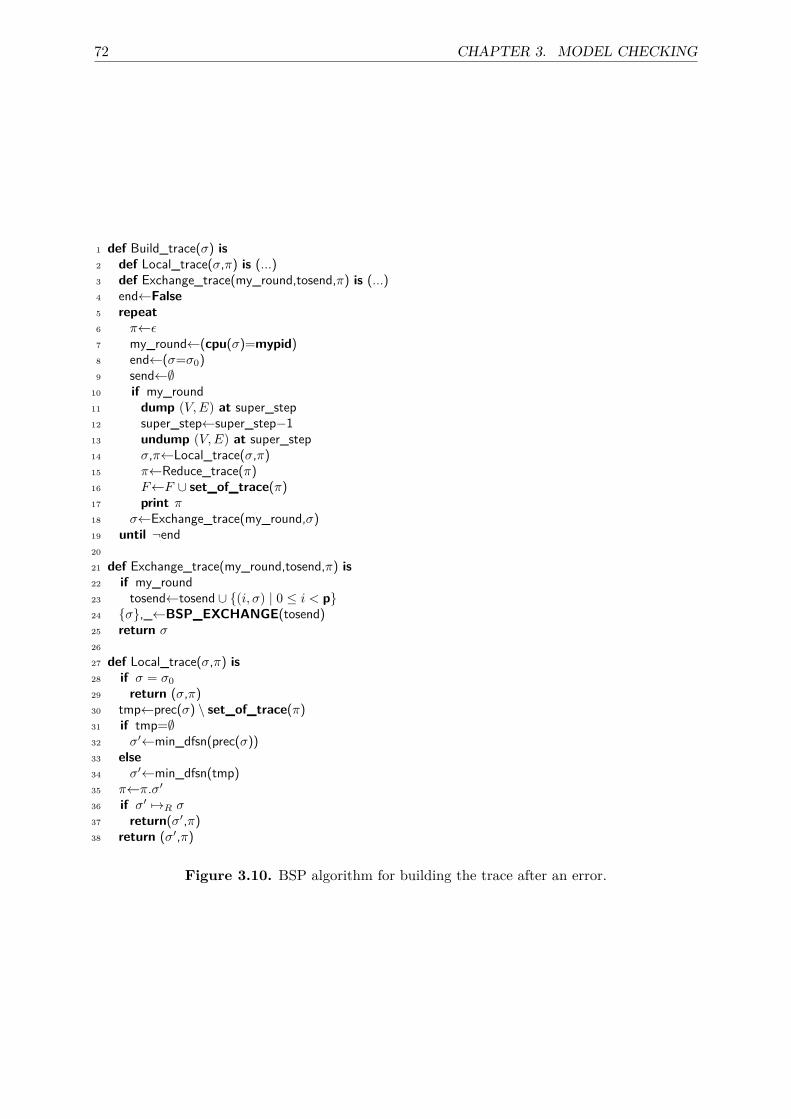
72 CHAPTER 3. MODEL CHECKING
1 def Build_trace(σ) is2 def Local_trace(σ,π) is (...)3 def Exchange_trace(my_round,tosend,π) is (...)4 end←False5 repeat6 π←ε7 my_round←(cpu(σ)=mypid)8 end←(σ=σ0)9 send←∅
10 if my_round11 dump (V,E) at super_step12 super_step←super_step−113 undump (V,E) at super_step14 σ,π←Local_trace(σ,π)15 π←Reduce_trace(π)16 F←F ∪ set_of_trace(π)17 print π18 σ←Exchange_trace(my_round,σ)19 until ¬end20
21 def Exchange_trace(my_round,tosend,π) is22 if my_round23 tosend←tosend ∪ {(i, σ) | 0 ≤ i < p}24 {σ},_←BSP_EXCHANGE(tosend)25 return σ26
27 def Local_trace(σ,π) is28 if σ = σ029 return (σ,π)30 tmp←prec(σ) \ set_of_trace(π)31 if tmp=∅32 σ′←min_dfsn(prec(σ))33 else34 σ′←min_dfsn(tmp)35 π←π.σ′
36 if σ′ 7→R σ37 return(σ′,π)38 return (σ′,π)
Figure 3.10. BSP algorithm for building the trace after an error.
73 3.4. CTL* CHECKING
3.4.1 Sequential algorithms for CTL*
(a) Recursive algorithm [28]
The global model-checking algorithm for CTL* (named modchkCTL∗ and presented in Fig-ure 3.11) processes a formulae P by recursively calls modchkLTL appropriately when it encoun-ters assertions of the form s ` AΦ or s ` EΦ or by decomposing the formulae P into subformulaswhose it applies to itself. The modchkCTL∗ procedure thus matches the pattern of the formulaeand acts accordingly. The key idea is to use the equivalence rule of an exits-formulae with thenegation of the corresponding forall-formulae to check these latter. Indeed, we already have arecursive algorithm to check LTL formula, and one can see a forall-formulae like a LTL formulaby masking all elements beginning by exists or forall (let’s recall that by the hypothesis, thenegation precede only the atoms). Thus, when we encounter elements beginning by exists orforall, we call modchkCTL∗ to proceed in the following manner:
• if the formulae is a forall-formulae, we recursively call modchkLTL to check the validityof the subformula;
• otherwise, we use modchkLTL to check the negation of the exists-formula, the final resultbeing the negation of the answer, in accordance to the equivalence rule between an exists-formula and its negation (the Lemma 1 ensuring this fact).
Notice that in the case of CTL* model checking, the cases of pattern of an Or-formulae and aAnd-formulae will be matched only at the beginning of the algorithm: indeed, otherwise thesecases will be covered by the rules of the proof graph construction in subgoals (rules R3 and R4).Note also a slight but important modification to procedure subgoals: when it encounters
an assertion of the form s ` A(p,Φ) (notably where p is Aϕ or Eϕ), it recursively invokesmodchkCTL∗(s ` p) to determine if s � p and then decides if rule R1 or rule R2 (of Fig-ure 3.5) needs to be applied. In other words, one extends the atomic test in subgoals by usingmodchkCTL∗ procedure in the case of these subformula. We have thus a double-recursively ofmodchkCTL∗ and modchkLTL.
Also note, that each call to modchkLTL creates a new empty stack and a new dfn (depth-firstnumber) since a new LTL checking is run: by abuse of language, we will named them “LTLsessions”. These sessions can shared assertions which thus shared their validity (is in F ornot). Take for example the following formulae: A(pU(E(rUp))); there will be two LTL sessions,one for the global formulae and one for the subformula E(rUp))). It is clear that the atomicproposition p would be thus test twice on the states of the Kripke structure. It can also happenfor the following formulae: A(pUq) ∨ E(pUq). And in this second case the two sessions wouldalso share only atomic propositions.Thus, more subtly, LTL sessions do not shared their depth-first numbers (low and dfsn fields),
their valid fields and thus their membership to stacks of LTL sessions. This is due because ofassertions are of the form s ` (ϕ1 ∨ϕn) and also by means of the rules of Figure 3.5: these rulesforce that call to modchkCTL∗ within a LTL session (for checking a subforma that is not LTLand thus to have another LTL session) is perform only on a subpart of the original assertionand which is strictly smaller hence ensuring no intersection of the proof-structures (graph) ofthe LTL sessions ensuring that SCC are disjoints.
(b) Iterative algorithm
As previously, we now give an iterative version of the above recursive algorithm. This allow usto have only one main loop and no side-effects within recursive calls. We thus extend the LTLiterative algorithm of Section 3.3. Considering only one main loop for parallel computationshas also the advantage to easily stop the computation whereas results of other processors areexpected. Figure 3.12 gives this main loop.
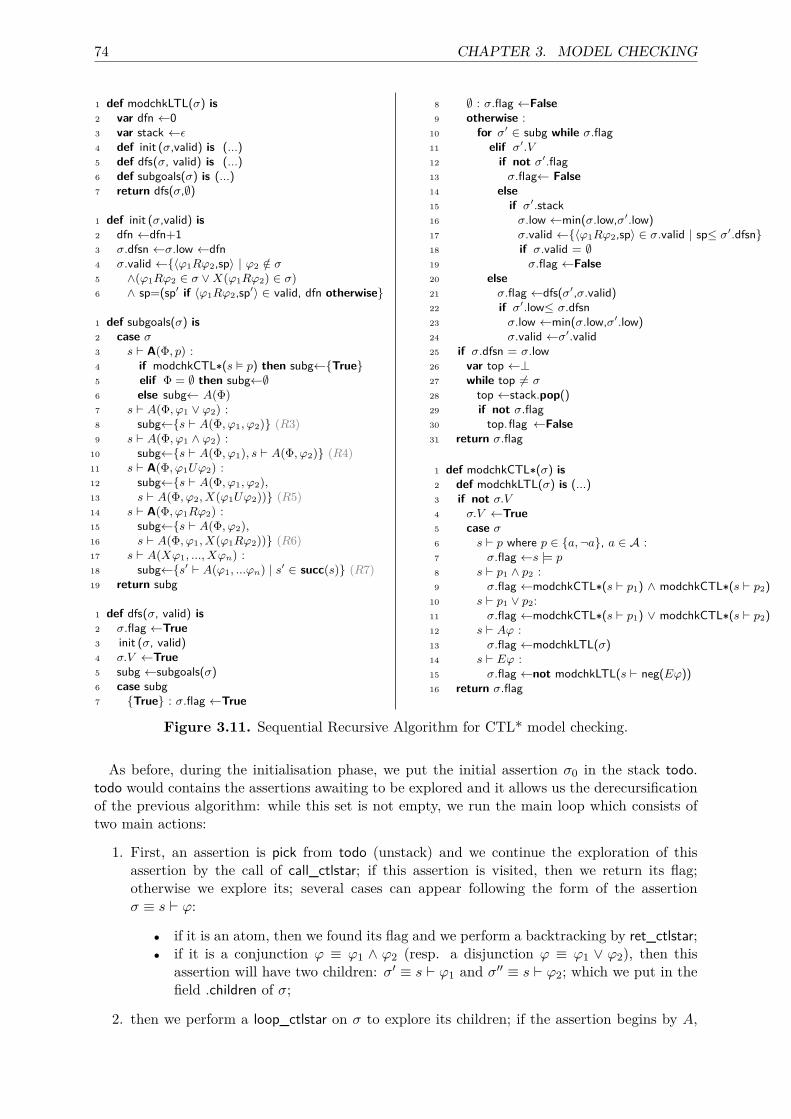
74 CHAPTER 3. MODEL CHECKING
1 def modchkLTL(σ) is2 var dfn ←03 var stack ←ε4 def init (σ,valid) is (...)5 def dfs(σ, valid) is (...)6 def subgoals(σ) is (...)7 return dfs(σ,∅)
1 def init (σ,valid) is2 dfn ←dfn+13 σ.dfsn ←σ.low ←dfn4 σ.valid ←{〈ϕ1Rϕ2,sp〉 | ϕ2 /∈ σ5 ∧(ϕ1Rϕ2 ∈ σ ∨X(ϕ1Rϕ2) ∈ σ)6 ∧ sp=(sp′ if 〈ϕ1Rϕ2,sp′〉 ∈ valid, dfn otherwise}
1 def subgoals(σ) is2 case σ3 s ` A(Φ, p) :4 if modchkCTL∗(s � p) then subg←{True}5 elif Φ = ∅ then subg←∅6 else subg← A(Φ)7 s ` A(Φ, ϕ1 ∨ ϕ2) :8 subg←{s ` A(Φ, ϕ1, ϕ2)} (R3)9 s ` A(Φ, ϕ1 ∧ ϕ2) :
10 subg←{s ` A(Φ, ϕ1), s ` A(Φ, ϕ2)} (R4)11 s ` A(Φ, ϕ1Uϕ2) :12 subg←{s ` A(Φ, ϕ1, ϕ2),13 s ` A(Φ, ϕ2, X(ϕ1Uϕ2))} (R5)14 s ` A(Φ, ϕ1Rϕ2) :15 subg←{s ` A(Φ, ϕ2),16 s ` A(Φ, ϕ1, X(ϕ1Rϕ2))} (R6)17 s ` A(Xϕ1, ..., Xϕn) :18 subg←{s′ ` A(ϕ1, ...ϕn) | s′ ∈ succ(s)} (R7)19 return subg
1 def dfs(σ, valid) is2 σ.flag ←True3 init (σ, valid)4 σ.V ←True5 subg ←subgoals(σ)6 case subg7 {True} : σ.flag ←True
8 ∅ : σ.flag ←False9 otherwise :
10 for σ′ ∈ subg while σ.flag11 elif σ′.V12 if not σ′.flag13 σ.flag← False14 else15 if σ′.stack16 σ.low ←min(σ.low,σ′.low)17 σ.valid ←{〈ϕ1Rϕ2,sp〉 ∈ σ.valid | sp≤ σ′.dfsn}18 if σ.valid = ∅19 σ.flag ←False20 else21 σ.flag ←dfs(σ′,σ.valid)22 if σ′.low≤ σ.dfsn23 σ.low ←min(σ.low,σ′.low)24 σ.valid ←σ′.valid25 if σ.dfsn = σ.low26 var top ←⊥27 while top 6= σ28 top ←stack.pop()29 if not σ.flag30 top.flag ←False31 return σ.flag
1 def modchkCTL∗(σ) is2 def modchkLTL(σ) is (...)3 if not σ.V4 σ.V ←True5 case σ6 s ` p where p ∈ {a,¬a}, a ∈ A :7 σ.flag ←s |= p8 s ` p1 ∧ p2 :9 σ.flag ←modchkCTL∗(s ` p1) ∧ modchkCTL∗(s ` p2)
10 s ` p1 ∨ p2:11 σ.flag ←modchkCTL∗(s ` p1) ∨ modchkCTL∗(s ` p2)12 s ` Aϕ :13 σ.flag ←modchkLTL(σ)14 s ` Eϕ :15 σ.flag ←not modchkLTL(s ` neg(Eϕ))16 return σ.flag
Figure 3.11. Sequential Recursive Algorithm for CTL* model checking.
As before, during the initialisation phase, we put the initial assertion σ0 in the stack todo.todo would contains the assertions awaiting to be explored and it allows us the derecursificationof the previous algorithm: while this set is not empty, we run the main loop which consists oftwo main actions:
1. First, an assertion is pick from todo (unstack) and we continue the exploration of thisassertion by the call of call_ctlstar; if this assertion is visited, then we return its flag;otherwise we explore its; several cases can appear following the form of the assertionσ ≡ s ` ϕ:
• if it is an atom, then we found its flag and we perform a backtracking by ret_ctlstar;• if it is a conjunction ϕ ≡ ϕ1 ∧ ϕ2 (resp. a disjunction ϕ ≡ ϕ1 ∨ ϕ2), then this
assertion will have two children: σ′ ≡ s ` ϕ1 and σ′′ ≡ s ` ϕ2; which we put in thefield .children of σ;
2. then we perform a loop_ctlstar on σ to explore its children; if the assertion begins by A,
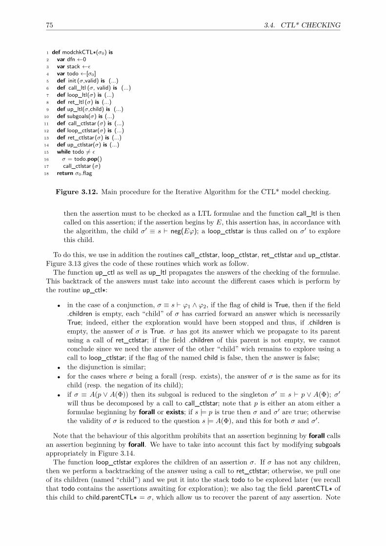
75 3.4. CTL* CHECKING
1 def modchkCTL∗(σ0) is2 var dfn ←03 var stack ←ε4 var todo ←[σ0]5 def init (σ,valid) is (...)6 def call_ltl (σ, valid) is (...)7 def loop_ltl(σ) is (...)8 def ret_ltl (σ) is (...)9 def up_ltl(σ,child) is (...)
10 def subgoals(σ) is (...)11 def call_ctlstar (σ) is (...)12 def loop_ctlstar(σ) is (...)13 def ret_ctlstar(σ) is (...)14 def up_ctlstar(σ) is (...)15 while todo 6= ε16 σ = todo.pop()17 call_ctlstar (σ)18 return σ0.flag
Figure 3.12. Main procedure for the Iterative Algorithm for the CTL* model checking.
then the assertion must to be checked as a LTL formulae and the function call_ltl is thencalled on this assertion; if the assertion begins by E, this assertion has, in accordance withthe algorithm, the child σ′ ≡ s ` neg(Eϕ); a loop_ctlstar is thus called on σ′ to explorethis child.
To do this, we use in addition the routines call_ctlstar, loop_ctlstar, ret_ctlstar and up_ctlstar.Figure 3.13 gives the code of these routines which work as follow.The function up_ctl as well as up_ltl propagates the answers of the checking of the formulae.
This backtrack of the answers must take into account the different cases which is perform bythe routine up_ctl∗:
• in the case of a conjunction, σ ≡ s ` ϕ1 ∧ ϕ2, if the flag of child is True, then if the field.children is empty, each “child” of σ has carried forward an answer which is necessarilyTrue; indeed, either the exploration would have been stopped and thus, if .children isempty, the answer of σ is True. σ has got its answer which we propagate to its parentusing a call of ret_ctlstar; if the field .children of this parent is not empty, we cannotconclude since we need the answer of the other “child” wich remains to explore using acall to loop_ctlstar; if the flag of the named child is false, then the answer is false;
• the disjunction is similar;• for the cases where σ being a forall (resp. exists), the answer of σ is the same as for its
child (resp. the negation of its child);• if σ ≡ A(p ∨ A(Φ)) then its subgoal is reduced to the singleton σ′ ≡ s ` p ∨ A(Φ); σ′
will thus be decomposed by a call to call_ctlstar; note that p is either an atom either aformulae beginning by forall or exists; if s |= p is true then σ and σ′ are true; otherwisethe validity of σ is reduced to the question s |= A(Φ), and this for both σ and σ′.
Note that the behaviour of this algorithm prohibits that an assertion beginning by forall callsan assertion beginning by forall. We have to take into account this fact by modifying subgoalsappropriately in Figure 3.14.The function loop_ctlstar explores the children of an assertion σ. If σ has not any children,
then we perform a backtracking of the answer using a call to ret_ctlstar; otherwise, we pull oneof its children (named “child”) and we put it into the stack todo to be explored later (we recallthat todo contains the assertions awaiting for exploration); we also tag the field .parentCTL∗ ofthis child to child.parentCTL∗ = σ, which allow us to recover the parent of any assertion. Note
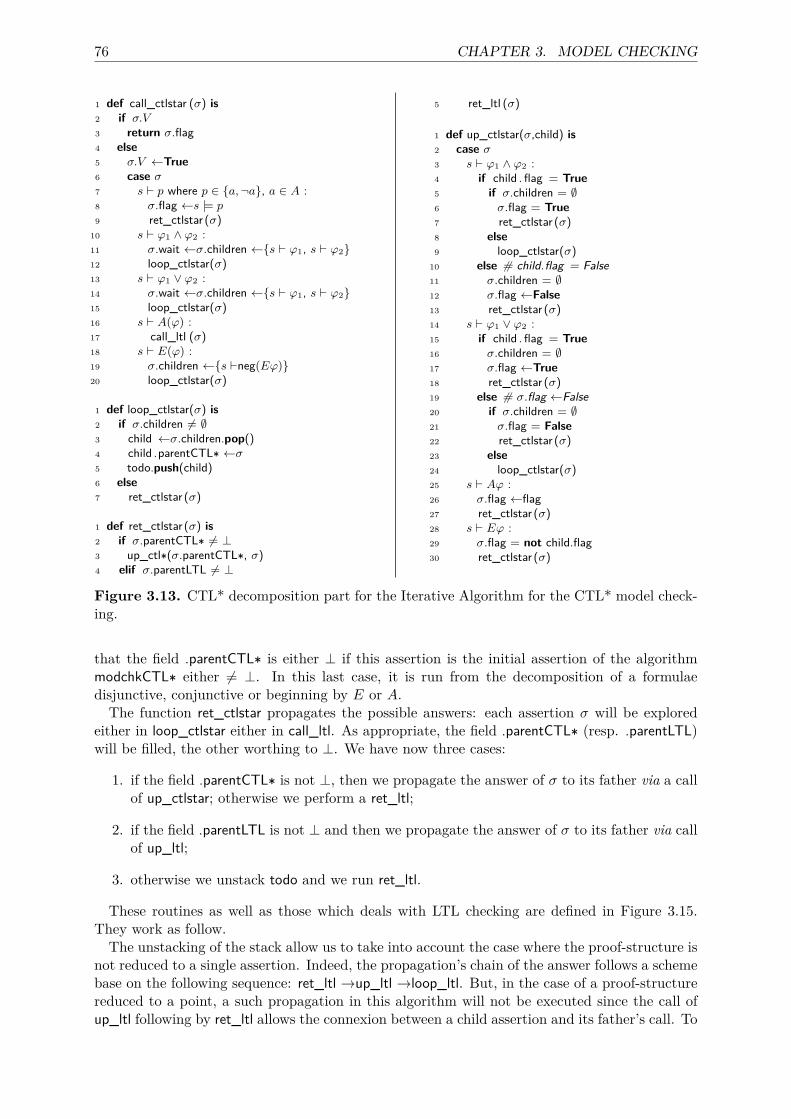
76 CHAPTER 3. MODEL CHECKING
1 def call_ctlstar (σ) is2 if σ.V3 return σ.flag4 else5 σ.V ←True6 case σ7 s ` p where p ∈ {a,¬a}, a ∈ A :8 σ.flag ←s |= p9 ret_ctlstar (σ)
10 s ` ϕ1 ∧ ϕ2 :11 σ.wait ←σ.children ←{s ` ϕ1, s ` ϕ2}12 loop_ctlstar(σ)13 s ` ϕ1 ∨ ϕ2 :14 σ.wait ←σ.children ←{s ` ϕ1, s ` ϕ2}15 loop_ctlstar(σ)16 s ` A(ϕ) :17 call_ltl (σ)18 s ` E(ϕ) :19 σ.children ←{s `neg(Eϕ)}20 loop_ctlstar(σ)
1 def loop_ctlstar(σ) is2 if σ.children 6= ∅3 child ←σ.children.pop()4 child .parentCTL∗ ←σ5 todo.push(child)6 else7 ret_ctlstar (σ)
1 def ret_ctlstar(σ) is2 if σ.parentCTL∗ 6= ⊥3 up_ctl∗(σ.parentCTL∗, σ)4 elif σ.parentLTL 6= ⊥
5 ret_ltl (σ)
1 def up_ctlstar(σ,child) is2 case σ3 s ` ϕ1 ∧ ϕ2 :4 if child . flag = True5 if σ.children = ∅6 σ.flag = True7 ret_ctlstar (σ)8 else9 loop_ctlstar(σ)
10 else # child.flag = False11 σ.children = ∅12 σ.flag ←False13 ret_ctlstar (σ)14 s ` ϕ1 ∨ ϕ2 :15 if child . flag = True16 σ.children = ∅17 σ.flag ←True18 ret_ctlstar (σ)19 else # σ.flag ←False20 if σ.children = ∅21 σ.flag = False22 ret_ctlstar (σ)23 else24 loop_ctlstar(σ)25 s ` Aϕ :26 σ.flag ←flag27 ret_ctlstar (σ)28 s ` Eϕ :29 σ.flag = not child.flag30 ret_ctlstar (σ)
Figure 3.13. CTL* decomposition part for the Iterative Algorithm for the CTL* model check-ing.
that the field .parentCTL∗ is either ⊥ if this assertion is the initial assertion of the algorithmmodchkCTL∗ either 6= ⊥. In this last case, it is run from the decomposition of a formulaedisjunctive, conjunctive or beginning by E or A.
The function ret_ctlstar propagates the possible answers: each assertion σ will be exploredeither in loop_ctlstar either in call_ltl. As appropriate, the field .parentCTL∗ (resp. .parentLTL)will be filled, the other worthing to ⊥. We have now three cases:
1. if the field .parentCTL∗ is not ⊥, then we propagate the answer of σ to its father via a callof up_ctlstar; otherwise we perform a ret_ltl;
2. if the field .parentLTL is not ⊥ and then we propagate the answer of σ to its father via callof up_ltl;
3. otherwise we unstack todo and we run ret_ltl.
These routines as well as those which deals with LTL checking are defined in Figure 3.15.They work as follow.The unstacking of the stack allow us to take into account the case where the proof-structure is
not reduced to a single assertion. Indeed, the propagation’s chain of the answer follows a schemebase on the following sequence: ret_ltl →up_ltl →loop_ltl. But, in the case of a proof-structurereduced to a point, a such propagation in this algorithm will not be executed since the call ofup_ltl following by ret_ltl allows the connexion between a child assertion and its father’s call. To
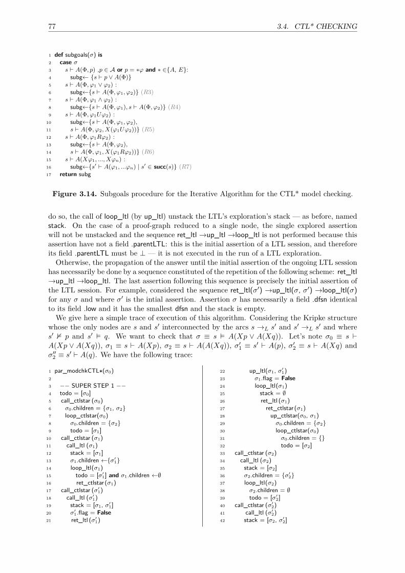
77 3.4. CTL* CHECKING
1 def subgoals(σ) is2 case σ3 s ` A(Φ, p) ,p ∈ A or p = ∗ϕ and ∗ ∈{A, E}:4 subg← {s ` p ∨A(Φ)}5 s ` A(Φ, ϕ1 ∨ ϕ2) :6 subg←{s ` A(Φ, ϕ1, ϕ2)} (R3)7 s ` A(Φ, ϕ1 ∧ ϕ2) :8 subg←{s ` A(Φ, ϕ1), s ` A(Φ, ϕ2)} (R4)9 s ` A(Φ, ϕ1Uϕ2) :
10 subg←{s ` A(Φ, ϕ1, ϕ2),11 s ` A(Φ, ϕ2, X(ϕ1Uϕ2))} (R5)12 s ` A(Φ, ϕ1Rϕ2) :13 subg←{s ` A(Φ, ϕ2),14 s ` A(Φ, ϕ1, X(ϕ1Rϕ2))} (R6)15 s ` A(Xϕ1, ..., Xϕn) :16 subg←{s′ ` A(ϕ1, ...ϕn) | s′ ∈ succ(s)} (R7)17 return subg
Figure 3.14. Subgoals procedure for the Iterative Algorithm for the CTL* model checking.
do so, the call of loop_ltl (by up_ltl) unstack the LTL’s exploration’s stack — as before, namedstack. On the case of a proof-graph reduced to a single node, the single explored assertionwill not be unstacked and the sequence ret_ltl →up_ltl →loop_ltl is not performed because thisassertion have not a field .parentLTL: this is the initial assertion of a LTL session, and thereforeits field .parentLTL must be ⊥ — it is not executed in the run of a LTL exploration.Otherwise, the propagation of the answer until the initial assertion of the ongoing LTL session
has necessarily be done by a sequence constituted of the repetition of the following scheme: ret_ltl→up_ltl →loop_ltl. The last assertion following this sequence is precisely the initial assertion ofthe LTL session. For example, considered the sequence ret_ltl(σ′) →up_ltl(σ, σ′) →loop_ltl(σ)for any σ and where σ′ is the intial assertion. Assertion σ has necessarily a field .dfsn identicalto its field .low and it has the smallest dfsn and the stack is empty.
We give here a simple trace of execution of this algorithm. Considering the Kripke structurewhose the only nodes are s and s′ interconnected by the arcs s →L s
′ and s′ →L s′ and where
s′ 2 p and s′ � q. We want to check that σ ≡ s � A(Xp ∨ A(Xq)). Let’s note σ0 ≡ s `A(Xp ∨ A(Xq)), σ1 ≡ s ` A(Xp), σ2 ≡ s ` A(A(Xq)), σ′1 ≡ s′ ` A(p), σ′2 ≡ s ` A(Xq) andσ′′2 ≡ s′ ` A(q). We have the following trace:
1 par_modchkCTL∗(σ0)2
3 −− SUPER STEP 1 −−4 todo = [σ0]5 call_ctlstar (σ0)6 σ0.children = {σ1, σ2}7 loop_ctlstar(σ0)8 σ0.children = {σ2}9 todo = [σ1]
10 call_ctlstar (σ1)11 call_ltl (σ1)12 stack = [σ1]13 σ1.children ←{σ′
1}14 loop_ltl(σ1)15 todo = [σ′
1] and σ1.children ←∅16 ret_ctlstar (σ1)17 call_ctlstar (σ′
1)18 call_ltl (σ′
1)19 stack = [σ1, σ′
1]20 σ′
1.flag = False21 ret_ltl (σ′
1)
22 up_ltl(σ1, σ′1)
23 σ1.flag = False24 loop_ltl(σ1)25 stack = ∅26 ret_ltl (σ1)27 ret_ctlstar (σ1)28 up_ctlstar(σ0, σ1)29 σ0.children = {σ2}30 loop_ctlstar(σ0)31 σ0.children = {}32 todo = [σ2]33 call_ctlstar (σ2)34 call_ltl (σ2)35 stack = [σ2]36 σ2.children = {σ′
2}37 loop_ltl(σ2)38 σ2.children = ∅39 todo = [σ′
2]40 call_ctlstar (σ′
2)41 call_ltl (σ′
2)42 stack = [σ2, σ′
2]
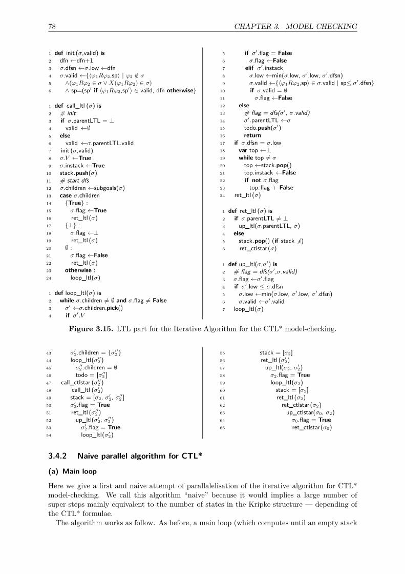
78 CHAPTER 3. MODEL CHECKING
1 def init (σ,valid) is2 dfn ←dfn+13 σ.dfsn ←σ.low ←dfn4 σ.valid ←{〈ϕ1Rϕ2,sp〉 | ϕ2 /∈ σ5 ∧(ϕ1Rϕ2 ∈ σ ∨X(ϕ1Rϕ2) ∈ σ)6 ∧ sp=(sp′ if 〈ϕ1Rϕ2,sp′〉 ∈ valid, dfn otherwise}
1 def call_ltl (σ) is2 # init3 if σ.parentLTL = ⊥4 valid ←∅5 else6 valid ←σ.parentLTL.valid7 init (σ,valid)8 σ.V ←True9 σ.instack ←True
10 stack.push(σ)11 # start dfs12 σ.children ←subgoals(σ)13 case σ.children14 {True} :15 σ.flag ←True16 ret_ltl (σ)17 {⊥} :18 σ.flag ←⊥19 ret_ltl (σ)20 ∅ :21 σ.flag ←False22 ret_ltl (σ)23 otherwise :24 loop_ltl(σ)
1 def loop_ltl(σ) is2 while σ.children 6= ∅ and σ.flag 6= False3 σ′ ←σ.children.pick()4 if σ′.V
5 if σ′.flag = False6 σ.flag ←False7 elif σ′.instack8 σ.low ←min(σ.low, σ′.low, σ′.dfsn)9 σ.valid ←{〈ϕ1Rϕ2,sp〉 ∈ σ.valid | sp≤ σ′.dfsn}
10 if σ.valid = ∅11 σ.flag ←False12 else13 # flag = dfs(σ′, σ.valid)14 σ′.parentLTL ←σ15 todo.push(σ′)16 return17 if σ.dfsn = σ.low18 var top ←⊥19 while top 6= σ20 top ←stack.pop()21 top.instack ←False22 if not σ.flag23 top.flag ←False24 ret_ltl (σ)
1 def ret_ltl (σ) is2 if σ.parentLTL 6= ⊥3 up_ltl(σ.parentLTL, σ)4 else5 stack.pop() (if stack 6 ε)6 ret_ctlstar (σ)
1 def up_ltl(σ,σ′) is2 # flag = dfs(σ′,σ.valid)3 σ.flag ←σ′.flag4 if σ′.low ≤ σ.dfsn5 σ.low ←min(σ.low, σ′.low, σ′.dfsn)6 σ.valid ←σ′.valid7 loop_ltl(σ)
Figure 3.15. LTL part for the Iterative Algorithm for the CTL* model-checking.
43 σ′2.children = {σ′′
2 }44 loop_ltl(σ′′
2 )45 σ′′
2 .children = ∅46 todo = [σ′′
2 ]47 call_ctlstar (σ′′
2 )48 call_ltl (σ′
2)49 stack = [σ2, σ′
2, σ′′2 ]
50 σ′2.flag = True
51 ret_ltl (σ′′2 )
52 up_ltl(σ′2, σ′′
2 )53 σ′
2.flag = True54 loop_ltl(σ′
2)
55 stack = [σ2]56 ret_ltl (σ′
2)57 up_ltl(σ2, σ′
2)58 σ2.flag = True59 loop_ltl(σ2)60 stack = [σ2]61 ret_ltl (σ2)62 ret_ctlstar (σ2)63 up_ctlstar(σ0, σ2)64 σ0.flag = True65 ret_ctlstar (σ0)
3.4.2 Naive parallel algorithm for CTL*
(a) Main loop
Here we give a first and naive attempt of parallalelisation of the iterative algorithm for CTL*model-checking. We call this algorithm “naive” because it would implies a large number ofsuper-steps mainly equivalent to the number of states in the Kripke structure — depending ofthe CTL* formulae.The algorithm works as follow. As before, a main loop (which computes until an empty stack
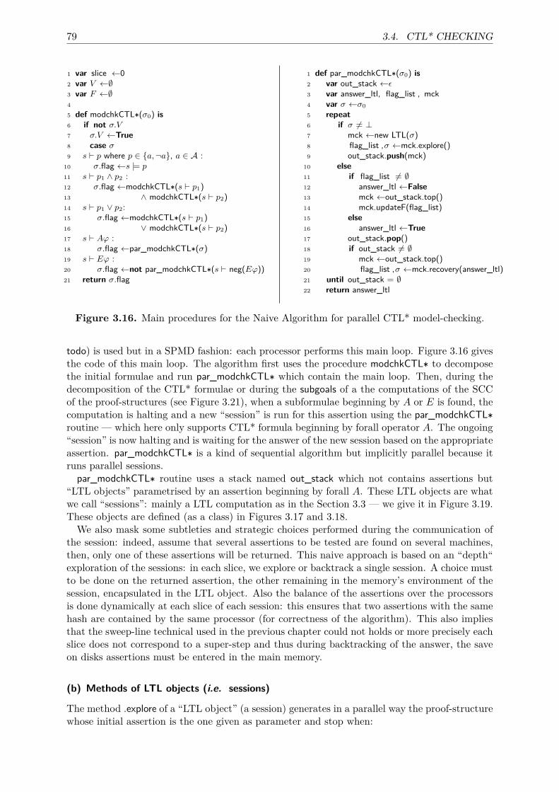
79 3.4. CTL* CHECKING
1 var slice ←02 var V ←∅3 var F ←∅4
5 def modchkCTL∗(σ0) is6 if not σ.V7 σ.V ←True8 case σ9 s ` p where p ∈ {a,¬a}, a ∈ A :
10 σ.flag ←s |= p11 s ` p1 ∧ p2 :12 σ.flag ←modchkCTL∗(s ` p1)13 ∧ modchkCTL∗(s ` p2)14 s ` p1 ∨ p2:15 σ.flag ←modchkCTL∗(s ` p1)16 ∨ modchkCTL∗(s ` p2)17 s ` Aϕ :18 σ.flag ←par_modchkCTL∗(σ)19 s ` Eϕ :20 σ.flag ←not par_modchkCTL∗(s ` neg(Eϕ))21 return σ.flag
1 def par_modchkCTL∗(σ0) is2 var out_stack ←ε3 var answer_ltl, flag_list , mck4 var σ ←σ05 repeat6 if σ 6= ⊥7 mck ←new LTL(σ)8 flag_list ,σ ←mck.explore()9 out_stack.push(mck)
10 else11 if flag_list 6= ∅12 answer_ltl ←False13 mck ←out_stack.top()14 mck.updateF(flag_list)15 else16 answer_ltl ←True17 out_stack.pop()18 if out_stack 6= ∅19 mck ←out_stack.top()20 flag_list ,σ ←mck.recovery(answer_ltl)21 until out_stack = ∅22 return answer_ltl
Figure 3.16. Main procedures for the Naive Algorithm for parallel CTL* model-checking.
todo) is used but in a SPMD fashion: each processor performs this main loop. Figure 3.16 givesthe code of this main loop. The algorithm first uses the procedure modchkCTL∗ to decomposethe initial formulae and run par_modchkCTL∗ which contain the main loop. Then, during thedecomposition of the CTL* formulae or during the subgoals of a the computations of the SCCof the proof-structures (see Figure 3.21), when a subformulae beginning by A or E is found, thecomputation is halting and a new “session” is run for this assertion using the par_modchkCTL∗routine — which here only supports CTL* formula beginning by forall operator A. The ongoing“session” is now halting and is waiting for the answer of the new session based on the appropriateassertion. par_modchkCTL∗ is a kind of sequential algorithm but implicitly parallel because itruns parallel sessions.par_modchkCTL∗ routine uses a stack named out_stack which not contains assertions but
“LTL objects” parametrised by an assertion beginning by forall A. These LTL objects are whatwe call “sessions”: mainly a LTL computation as in the Section 3.3 — we give it in Figure 3.19.These objects are defined (as a class) in Figures 3.17 and 3.18.We also mask some subtleties and strategic choices performed during the communication of
the session: indeed, assume that several assertions to be tested are found on several machines,then, only one of these assertions will be returned. This naive approach is based on an “depth“exploration of the sessions: in each slice, we explore or backtrack a single session. A choice mustto be done on the returned assertion, the other remaining in the memory’s environment of thesession, encapsulated in the LTL object. Also the balance of the assertions over the processorsis done dynamically at each slice of each session: this ensures that two assertions with the samehash are contained by the same processor (for correctness of the algorithm). This also impliesthat the sweep-line technical used in the previous chapter could not holds or more precisely eachslice does not correspond to a super-step and thus during backtracking of the answer, the saveon disks assertions must be entered in the main memory.
(b) Methods of LTL objects (i.e. sessions)
The method .explore of a “LTL object” (a session) generates in a parallel way the proof-structurewhose initial assertion is the one given as parameter and stop when:
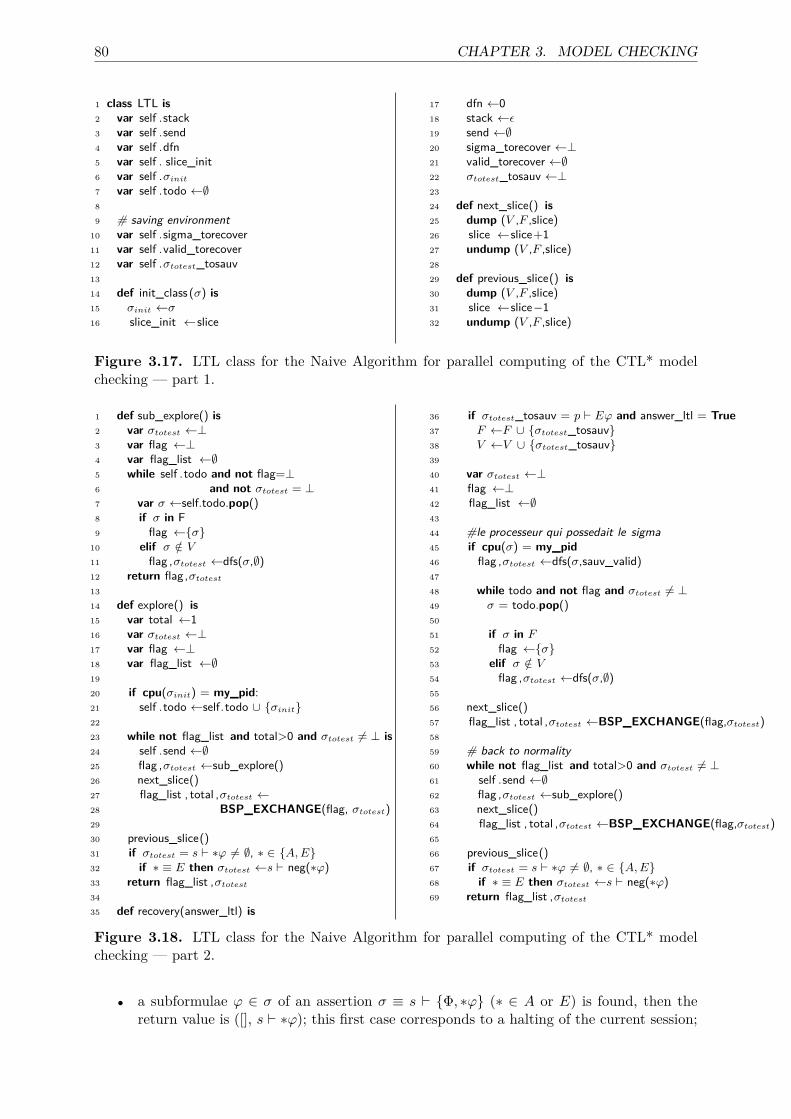
80 CHAPTER 3. MODEL CHECKING
1 class LTL is2 var self .stack3 var self .send4 var self .dfn5 var self . slice_init6 var self .σinit
7 var self .todo ←∅8
9 # saving environment10 var self .sigma_torecover11 var self .valid_torecover12 var self .σtotest_tosauv13
14 def init_class (σ) is15 σinit ←σ16 slice_init ←slice
17 dfn ←018 stack ←ε19 send ←∅20 sigma_torecover ←⊥21 valid_torecover ←∅22 σtotest_tosauv ←⊥23
24 def next_slice() is25 dump (V ,F ,slice)26 slice ←slice+127 undump (V ,F ,slice)28
29 def previous_slice() is30 dump (V ,F ,slice)31 slice ←slice−132 undump (V ,F ,slice)
Figure 3.17. LTL class for the Naive Algorithm for parallel computing of the CTL* modelchecking — part 1.
1 def sub_explore() is2 var σtotest ←⊥3 var flag ←⊥4 var flag_list ←∅5 while self .todo and not flag=⊥6 and not σtotest = ⊥7 var σ ←self.todo.pop()8 if σ in F9 flag ←{σ}
10 elif σ /∈ V11 flag ,σtotest ←dfs(σ,∅)12 return flag,σtotest
13
14 def explore() is15 var total ←116 var σtotest ←⊥17 var flag ←⊥18 var flag_list ←∅19
20 if cpu(σinit) = my_pid:21 self .todo ←self.todo ∪ {σinit}22
23 while not flag_list and total>0 and σtotest 6= ⊥ is24 self .send ←∅25 flag ,σtotest ←sub_explore()26 next_slice()27 flag_list , total ,σtotest ←28 BSP_EXCHANGE(flag, σtotest)29
30 previous_slice()31 if σtotest = s ` ∗ϕ 6= ∅, ∗ ∈ {A,E}32 if ∗ ≡ E then σtotest ←s ` neg(∗ϕ)33 return flag_list ,σtotest
34
35 def recovery(answer_ltl) is
36 if σtotest_tosauv = p ` Eϕ and answer_ltl = True37 F ←F ∪ {σtotest_tosauv}38 V ←V ∪ {σtotest_tosauv}39
40 var σtotest ←⊥41 flag ←⊥42 flag_list ←∅43
44 #le processeur qui possedait le sigma45 if cpu(σ) = my_pid46 flag ,σtotest ←dfs(σ,sauv_valid)47
48 while todo and not flag and σtotest 6= ⊥49 σ = todo.pop()50
51 if σ in F52 flag ←{σ}53 elif σ /∈ V54 flag ,σtotest ←dfs(σ,∅)55
56 next_slice()57 flag_list , total ,σtotest ←BSP_EXCHANGE(flag,σtotest)58
59 # back to normality60 while not flag_list and total>0 and σtotest 6= ⊥61 self .send ←∅62 flag ,σtotest ←sub_explore()63 next_slice()64 flag_list , total ,σtotest ←BSP_EXCHANGE(flag,σtotest)65
66 previous_slice()67 if σtotest = s ` ∗ϕ 6= ∅, ∗ ∈ {A,E}68 if ∗ ≡ E then σtotest ←s ` neg(∗ϕ)69 return flag_list ,σtotest
Figure 3.18. LTL class for the Naive Algorithm for parallel computing of the CTL* modelchecking — part 2.
• a subformulae ϕ ∈ σ of an assertion σ ≡ s ` {Φ, ∗ϕ} (∗ ∈ A or E) is found, then thereturn value is ([], s ` ∗ϕ); this first case corresponds to a halting of the current session;
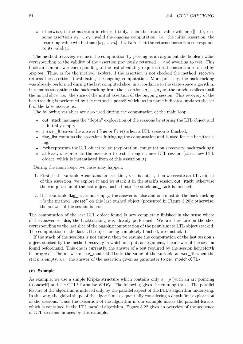
81 3.4. CTL* CHECKING
• otherwise, if the assertion is checked truly, then the return value will be ([], ⊥), elsesome assertions σ1, ..., σk invalid the ongoing computation, i.e. the initial assertion; thereturning value will be thus ([σ1, ..., σk], ⊥). Note that the returned assertion correspondsto its validity.
The method .recovery resumes the computation by passing as an argument the boolean valuecorresponding to the validity of the assertion previously returned — and awaiting to test. Thisboolean is an answer corresponding to the test of validity required on the assertion returned by.explore. Thus, as for the method .explore, if the assertion is not checked the method .recoveryreturns the assertions invalidating the ongoing computation. More precisely, the backtrackingwas already performed during the last computed slice, in accordance to the state-space algorithm.It remains to continue the backtracking from the assertions σ1, ..., σk on the previous slices untilthe initial slice, i.e. the slice of the initial assertion of the ongoing session. This recovery of thebacktracking is performed by the method .updateF which, as its name indicates, updates the setF of the false assertions.The following variables are also used during the computation of the main loop:
• out_stack manages the “depth” exploration of the sessions by storing the LTL object andis initially empty;
• answer_ltl saves the answer (True or False) when a LTL session is finished;• flag_list contains the assertions infringing the computation and is used for the backtrack-
ing;• mck represents the LTL object to use (exploration, computation’s recovery, backtracking);• at least, σ represents the assertion to test through a new LTL session (via a new LTL
object, which is instantiated from of this assertion σ).
During the main loop, two cases may happen.
1. First, if the variable σ contains an assertion, i.e. is not ⊥, then we create an LTL objectof this assertion, we explore it and we stack it in the stack’s session out_stack; otherwisethe computation of the last object pushed into the stack out_stack is finished.
2. If the variable flag_list is not empty, the answer is false and one must do the backtrackingvia the method .updateF on this last pushed object (presented in Figure 3.20); otherwise,the answer of the session is true.
The computation of the last LTL object found is now completely finished in the sense whereif the answer is false, the backtracking was already performed. We are therefore on the slicecorresponding to the last slice of the ongoing computation of the penultimate LTL object stacked.The computation of the last LTL object being completely finished, we unstack it.If the stack of the sessions is not empty, then we resume the computation of the last session’s
object stacked by the method .recovery in which one put, as argument, the answer of the sessionfound beforehand. This one is currently, the answer of a test required by the session henceforthin progress. The answer of par_modchkCTL∗ is the value of the variable answer_ltl when thestack is empty, i.e. the answer of the assertion given as parameter to par_modchkCTL∗.
(c) Example
As example, we use a simple Kripke structure which contains only s ` p (with an arc pointingto oneself) and the CTL* formulae EAEp. The following gives the running trace. The parallelfeature of the algorithm is induced only by the parallel aspect of the LTL’s algorithm underlying.In this way, the global shape of the algorithm is sequentially considering a depth first explorationof the sessions. Thus the execution of the algorithm in our example masks the parallel featurewhich is contained in the LTL parallel algorithm. Figure 3.22 gives an overview of the sequenceof LTL sessions induces by this example:
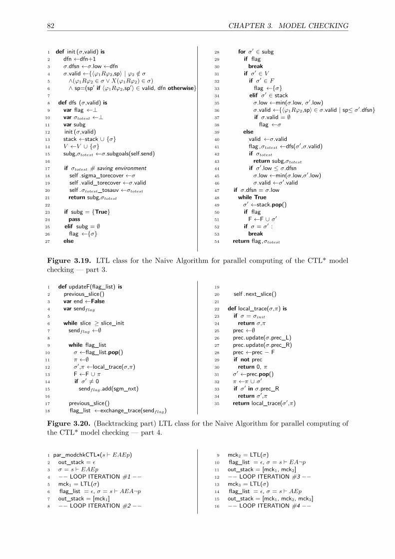
82 CHAPTER 3. MODEL CHECKING
1 def init (σ,valid) is2 dfn ←dfn+13 σ.dfsn ←σ.low ←dfn4 σ.valid ←{〈ϕ1Rϕ2,sp〉 | ϕ2 /∈ σ5 ∧(ϕ1Rϕ2 ∈ σ ∨X(ϕ1Rϕ2) ∈ σ)6 ∧ sp=(sp′ if 〈ϕ1Rϕ2,sp′〉 ∈ valid, dfn otherwise}7
8 def dfs (σ,valid) is9 var flag ←⊥
10 var σtotest ←⊥11 var subg12 init (σ,valid)13 stack ←stack ∪ {σ}14 V ←V ∪ {σ}15 subg,σtotest ←σ.subgoals(self.send)16
17 if σtotest # saving environment18 self .sigma_torecover ←σ19 self .valid_torecover ←σ.valid20 self .σtotest_tosauv ←σtotest
21 return subg,σtotest
22
23 if subg = {True}24 pass25 elif subg = ∅26 flag ←{σ}27 else
28 for σ′ ∈ subg29 if flag30 break31 if σ′ ∈ V32 if σ′ ∈ F33 flag ←{σ}34 elif σ′ ∈ stack35 σ.low ←min(σ.low, σ′.low)36 σ.valid ←{〈ϕ1Rϕ2,sp〉 ∈ σ.valid | sp≤ σ′.dfsn}37 if σ.valid = ∅38 flag ←σ39 else40 valid ←σ.valid41 flag ,σtotest ←dfs(σ′,σ.valid)42 if σtotest
43 return subg,σtotest
44 if σ′.low ≤ σ.dfsn45 σ.low ←min(σ.low,σ′.low)46 σ.valid ←σ′.valid47 if σ.dfsn = σ.low48 while True49 σ′ ←stack.pop()50 if flag51 F ←F ∪ σ′
52 if σ = σ′ :53 break54 return flag,σtotest
Figure 3.19. LTL class for the Naive Algorithm for parallel computing of the CTL* modelchecking — part 3.
1 def updateF(flag_list) is2 previous_slice()3 var end ←False4 var sendflag
5
6 while slice ≥ slice_init7 sendflag ←∅8
9 while flag_list10 σ ←flag_list.pop()11 π ←∅12 σ′,π ←local_trace(σ,π)13 F ←F ∪ π14 if σ′ 6= 015 sendflag.add(sgm_nxt)16
17 previous_slice()18 flag_list ←exchange_trace(sendflag)
19
20 self .next_slice()21
22 def local_trace(σ,π) is23 if σ = σinit
24 return σ,π25 prec ←∅26 prec.update(σ.prec_L)27 prec.update(σ.prec_R)28 prec ←prec − F29 if not prec30 return 0, π31 σ′ ←prec.pop()32 π ←π ∪ σ′
33 if σ′ in σ.prec_R34 return σ′,π35 return local_trace(σ′,π)
Figure 3.20. (Backtracking part) LTL class for the Naive Algorithm for parallel computing ofthe CTL* model checking — part 4.
1 par_modchkCTL∗(s ` EAEp)2 out_stack = ε3 σ = s ` EAEp4 −− LOOP ITERATION #1 −−5 mck1 = LTL(σ)6 flag_list = ε, σ = s ` AEA¬p7 out_stack = [mck1]8 −− LOOP ITERATION #2 −−
9 mck2 = LTL(σ)10 flag_list = ε, σ = s ` EA¬p11 out_stack = [mck1, mck2]12 −− LOOP ITERATION #3 −−13 mck3 = LTL(σ)14 flag_list = ε, σ = s ` AEp15 out_stack = [mck1, mck2, mck3]16 −− LOOP ITERATION #4 −−
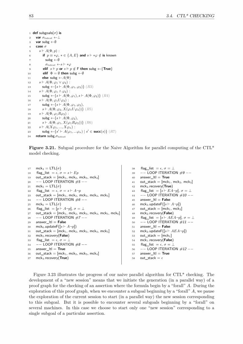
83 3.4. CTL* CHECKING
1 def subgoals(σ) is2 var σtotest ←⊥3 var subg ←∅4 case σ5 s ` A(Φ, p) :6 if p ≡ ∗ϕ, ∗ ∈ {A,E} and s ` ∗ϕ /∈ is known7 subg ←∅8 σtotest ←s ` ∗ϕ9 elif s � p or s � p /∈ F then subg ←{True}
10 elif Φ = ∅ then subg ←∅11 else subg ←A(Φ)12 s ` A(Φ, ϕ1 ∨ ϕ2) :13 subg ←{s ` A(Φ, ϕ1, ϕ2)} (R3)14 s ` A(Φ, ϕ1 ∧ ϕ2) :15 subg ←{s ` A(Φ, ϕ1), s ` A(Φ, ϕ2)} (R4)16 s ` A(Φ, ϕ1Uϕ2) :17 subg ←{s ` A(Φ, ϕ1, ϕ2),18 s ` A(Φ, ϕ2, X(ϕ1Uϕ2))} (R5)19 s ` A(Φ, ϕ1Rϕ2) :20 subg ←{s ` A(Φ, ϕ2),21 s ` A(Φ, ϕ1, X(ϕ1Rϕ2))} (R6)22 s ` A(Xϕ1, ..., Xϕn) :23 subg ←{s′ ` A(ϕ1, ...ϕn) | s′ ∈ succ(s)} (R7)24 return subg,σtotest
Figure 3.21. Subgoal procedure for the Naive Algorithm for parallel computing of the CTL*model checking.
17 mck4 = LTL(σ)18 flag_list = ε, σ = s ` Ep19 out_stack = [mck1, mck2, mck3, mck4]20 −− LOOP ITERATION #5 −−21 mck5 = LTL(σ)22 flag_list = ε, σ = s ` A¬p23 out_stack = [mck1, mck2, mck3, mck4, mck5]24 −− LOOP ITERATION #6 −−25 mck6 = LTL(σ)26 flag_list = [p ` A¬p], σ = ⊥27 out_stack = [mck1, mck2, mck3, mck4, mck5, mck6]28 −− LOOP ITERATION #7 −−29 answer_ltl = False30 mck6.updateF([s ` A¬p])31 out_stack = [mck1, mck2, mck3, mck4, mck5]32 mck5.recovery(False)33 flag_list = ε, σ = ⊥34 −− LOOP ITERATION #8 −−35 answer_ltl = True36 out_stack = [mck1, mck2, mck3, mck4]37 mck4.recovery(True)
38 flag_list = ε, σ = ⊥39 −− LOOP ITERATION #9 −−40 answer_ltl = True41 out_stack = [mck1, mck2, mck3]42 mck4.recovery(True)43 flag_list = [s ` EA¬p], σ = ⊥44 −− LOOP ITERATION #10 −−45 answer_ltl = False46 mck3.updateF([s ` A¬p])47 out_stack = [mck1, mck2]48 mck2.recovery(False)49 flag_list = [s ` AEA¬p], σ = ⊥50 −− LOOP ITERATION #11 −−51 answer_ltl = False52 mck2.updateF([s ` AEA¬p])53 out_stack = [mck1]54 mck1.recovery(False)55 flag_list = ε, σ = ⊥56 −− LOOP ITERATION #12 −−57 answer_ltl = True58 out_stack = ε
Figure 3.23 illustrates the progress of our naive parallel algorithm for CTL* checking. Thedevelopment of a “new session” means that we initiate the generation (in a parallel way) of aproof graph for the checking of an assertion where the formula begin by a “forall” A. During theexploration of this proof graph, when we encounter a subgoal beginning by a “forall” A, we pausethe exploration of the current session to start (in a parallel way) the new session correspondingto this subgoal. But it is possible to encounter several subgoals beginning by a “forall” onseveral machines. In this case we choose to start only one “new session” corresponding to asingle subgoal of a particular assertion.
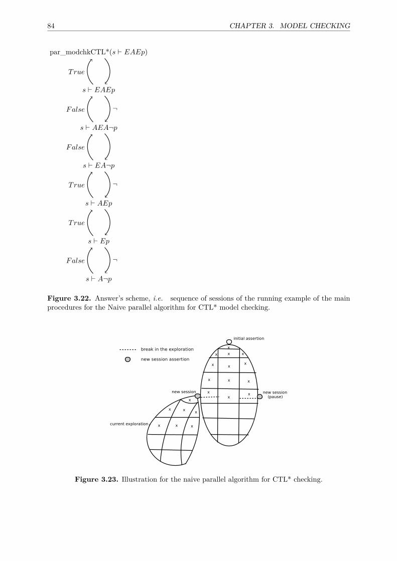
84 CHAPTER 3. MODEL CHECKING
par_modchkCTL*(s ` EAEp)
s ` EAEp
s ` AEA¬p
s ` EA¬p
s ` AEp
s ` Ep
s ` A¬p
True
¬False
False
¬True
True
¬False
Figure 3.22. Answer’s scheme, i.e. sequence of sessions of the running example of the mainprocedures for the Naive parallel algorithm for CTL* model checking.
Figure 3.23. Illustration for the naive parallel algorithm for CTL* checking.
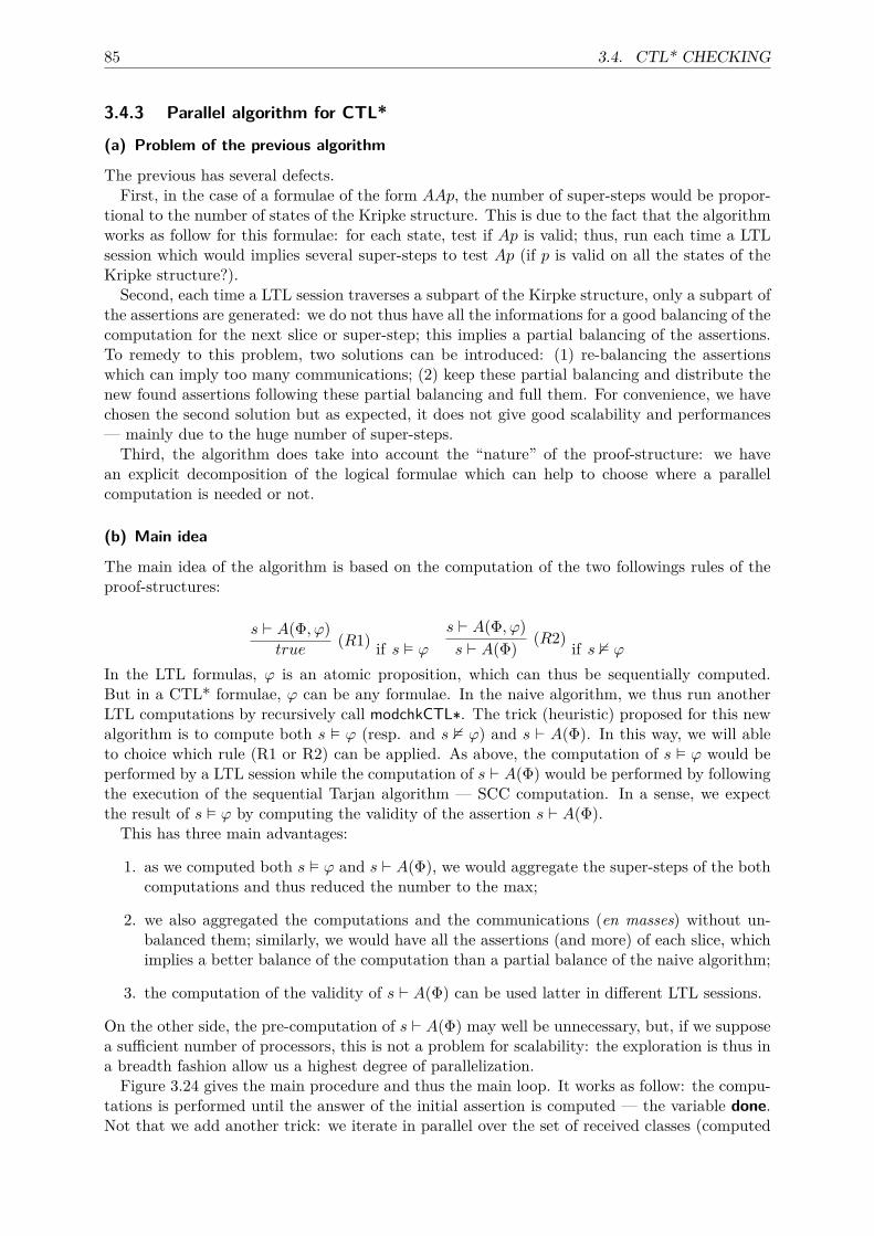
85 3.4. CTL* CHECKING
3.4.3 Parallel algorithm for CTL*
(a) Problem of the previous algorithm
The previous has several defects.First, in the case of a formulae of the form AAp, the number of super-steps would be propor-
tional to the number of states of the Kripke structure. This is due to the fact that the algorithmworks as follow for this formulae: for each state, test if Ap is valid; thus, run each time a LTLsession which would implies several super-steps to test Ap (if p is valid on all the states of theKripke structure?).Second, each time a LTL session traverses a subpart of the Kirpke structure, only a subpart of
the assertions are generated: we do not thus have all the informations for a good balancing of thecomputation for the next slice or super-step; this implies a partial balancing of the assertions.To remedy to this problem, two solutions can be introduced: (1) re-balancing the assertionswhich can imply too many communications; (2) keep these partial balancing and distribute thenew found assertions following these partial balancing and full them. For convenience, we havechosen the second solution but as expected, it does not give good scalability and performances— mainly due to the huge number of super-steps.Third, the algorithm does take into account the “nature” of the proof-structure: we have
an explicit decomposition of the logical formulae which can help to choose where a parallelcomputation is needed or not.
(b) Main idea
The main idea of the algorithm is based on the computation of the two followings rules of theproof-structures:
s ` A(Φ, ϕ)true
(R1) if s � ϕs ` A(Φ, ϕ)s ` A(Φ) (R2) if s 2 ϕ
In the LTL formulas, ϕ is an atomic proposition, which can thus be sequentially computed.But in a CTL* formulae, ϕ can be any formulae. In the naive algorithm, we thus run anotherLTL computations by recursively call modchkCTL∗. The trick (heuristic) proposed for this newalgorithm is to compute both s � ϕ (resp. and s 2 ϕ) and s ` A(Φ). In this way, we will ableto choice which rule (R1 or R2) can be applied. As above, the computation of s � ϕ would beperformed by a LTL session while the computation of s ` A(Φ) would be performed by followingthe execution of the sequential Tarjan algorithm — SCC computation. In a sense, we expectthe result of s � ϕ by computing the validity of the assertion s ` A(Φ).
This has three main advantages:
1. as we computed both s � ϕ and s ` A(Φ), we would aggregate the super-steps of the bothcomputations and thus reduced the number to the max;
2. we also aggregated the computations and the communications (en masses) without un-balanced them; similarly, we would have all the assertions (and more) of each slice, whichimplies a better balance of the computation than a partial balance of the naive algorithm;
3. the computation of the validity of s ` A(Φ) can be used latter in different LTL sessions.
On the other side, the pre-computation of s ` A(Φ) may well be unnecessary, but, if we supposea sufficient number of processors, this is not a problem for scalability: the exploration is thus ina breadth fashion allow us a highest degree of parallelization.Figure 3.24 gives the main procedure and thus the main loop. It works as follow: the compu-
tations is performed until the answer of the initial assertion is computed — the variable done.Not that we add another trick: we iterate in parallel over the set of received classes (computed
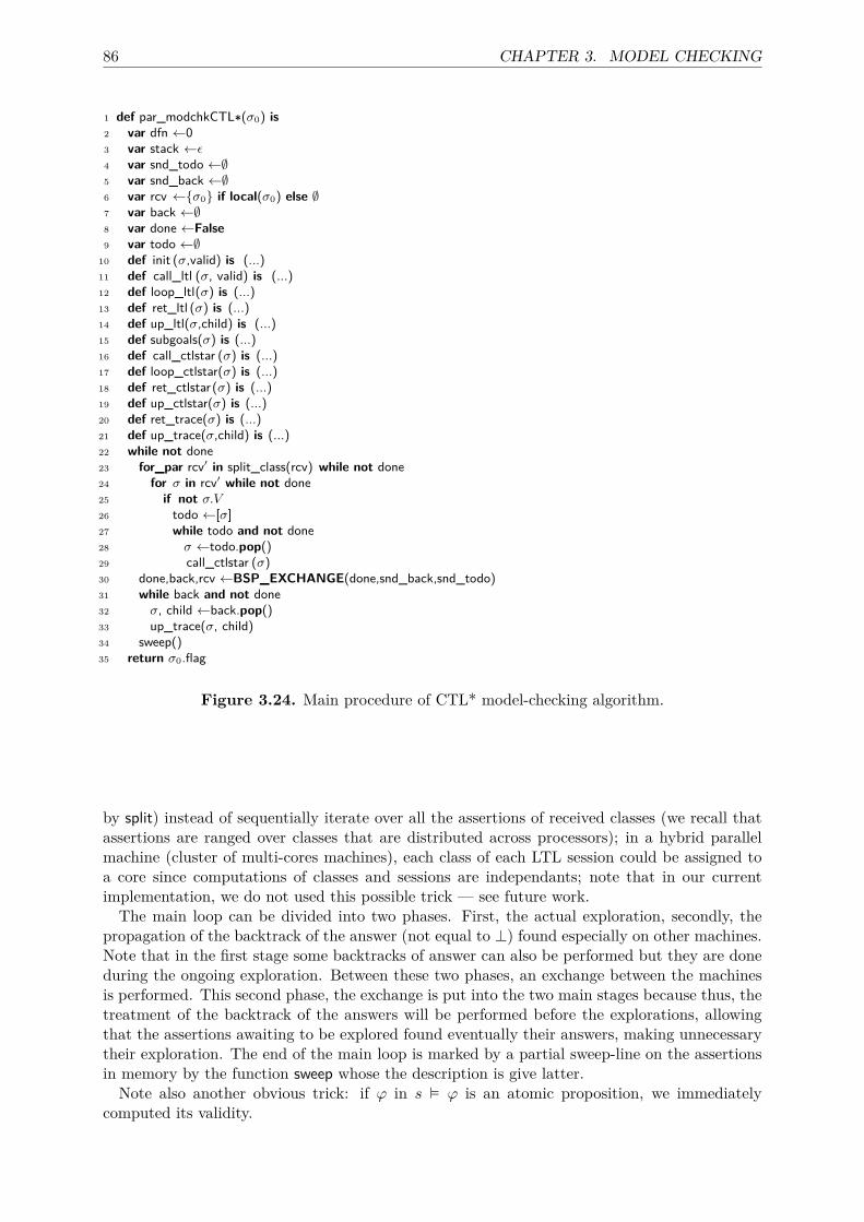
86 CHAPTER 3. MODEL CHECKING
1 def par_modchkCTL∗(σ0) is2 var dfn ←03 var stack ←ε4 var snd_todo ←∅5 var snd_back ←∅6 var rcv ←{σ0} if local(σ0) else ∅7 var back ←∅8 var done ←False9 var todo ←∅
10 def init (σ,valid) is (...)11 def call_ltl (σ, valid) is (...)12 def loop_ltl(σ) is (...)13 def ret_ltl (σ) is (...)14 def up_ltl(σ,child) is (...)15 def subgoals(σ) is (...)16 def call_ctlstar (σ) is (...)17 def loop_ctlstar(σ) is (...)18 def ret_ctlstar(σ) is (...)19 def up_ctlstar(σ) is (...)20 def ret_trace(σ) is (...)21 def up_trace(σ,child) is (...)22 while not done23 for_par rcv′ in split_class(rcv) while not done24 for σ in rcv′ while not done25 if not σ.V26 todo ←[σ]27 while todo and not done28 σ ←todo.pop()29 call_ctlstar (σ)30 done,back,rcv ←BSP_EXCHANGE(done,snd_back,snd_todo)31 while back and not done32 σ, child ←back.pop()33 up_trace(σ, child)34 sweep()35 return σ0.flag
Figure 3.24. Main procedure of CTL* model-checking algorithm.
by split) instead of sequentially iterate over all the assertions of received classes (we recall thatassertions are ranged over classes that are distributed across processors); in a hybrid parallelmachine (cluster of multi-cores machines), each class of each LTL session could be assigned toa core since computations of classes and sessions are independants; note that in our currentimplementation, we do not used this possible trick — see future work.The main loop can be divided into two phases. First, the actual exploration, secondly, the
propagation of the backtrack of the answer (not equal to ⊥) found especially on other machines.Note that in the first stage some backtracks of answer can also be performed but they are doneduring the ongoing exploration. Between these two phases, an exchange between the machinesis performed. This second phase, the exchange is put into the two main stages because thus, thetreatment of the backtrack of the answers will be performed before the explorations, allowingthat the assertions awaiting to be explored found eventually their answers, making unnecessarytheir exploration. The end of the main loop is marked by a partial sweep-line on the assertionsin memory by the function sweep whose the description is give latter.Note also another obvious trick: if ϕ in s � ϕ is an atomic proposition, we immediately
computed its validity.
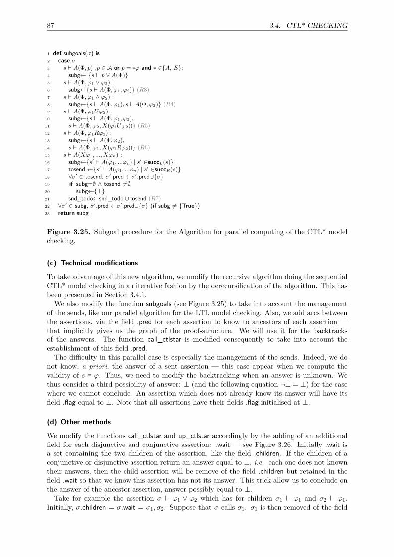
87 3.4. CTL* CHECKING
1 def subgoals(σ) is2 case σ3 s ` A(Φ, p) ,p ∈ A or p = ∗ϕ and ∗ ∈{A, E}:4 subg← {s ` p ∨A(Φ)}5 s ` A(Φ, ϕ1 ∨ ϕ2) :6 subg←{s ` A(Φ, ϕ1, ϕ2)} (R3)7 s ` A(Φ, ϕ1 ∧ ϕ2) :8 subg←{s ` A(Φ, ϕ1), s ` A(Φ, ϕ2)} (R4)9 s ` A(Φ, ϕ1Uϕ2) :
10 subg←{s ` A(Φ, ϕ1, ϕ2),11 s ` A(Φ, ϕ2, X(ϕ1Uϕ2))} (R5)12 s ` A(Φ, ϕ1Rϕ2) :13 subg←{s ` A(Φ, ϕ2),14 s ` A(Φ, ϕ1, X(ϕ1Rϕ2))} (R6)15 s ` A(Xϕ1, ..., Xϕn) :16 subg←{s′ ` A(ϕ1, ...ϕn) | s′ ∈succL(s)}17 tosend ←{s′ ` A(ϕ1, ...ϕn) | s′ ∈succR(s)}18 ∀σ′ ∈ tosend, σ′.pred ←σ′.pred∪{σ}19 if subg=∅ ∧ tosend 6=∅20 subg←{⊥}21 snd_todo←snd_todo ∪ tosend (R7)22 ∀σ′ ∈ subg, σ′.pred ←σ′.pred∪{σ} (if subg 6= {True})23 return subg
Figure 3.25. Subgoal procedure for the Algorithm for parallel computing of the CTL* modelchecking.
(c) Technical modifications
To take advantage of this new algorithm, we modify the recursive algorithm doing the sequentialCTL* model checking in an iterative fashion by the derecursification of the algorithm. This hasbeen presented in Section 3.4.1.
We also modify the function subgoals (see Figure 3.25) to take into account the managementof the sends, like our parallel algorithm for the LTL model checking. Also, we add arcs betweenthe assertions, via the field .pred for each assertion to know to ancestors of each assertion —that implicitly gives us the graph of the proof-structure. We will use it for the backtracksof the answers. The function call_ctlstar is modified consequently to take into account theestablishment of this field .pred.The difficulty in this parallel case is especially the management of the sends. Indeed, we do
not know, a priori, the answer of a sent assertion — this case appear when we compute thevalidity of s � ϕ. Thus, we need to modify the backtracking when an answer is unknown. Wethus consider a third possibility of answer: ⊥ (and the following equation ¬⊥ = ⊥) for the casewhere we cannot conclude. An assertion which does not already know its answer will have itsfield .flag equal to ⊥. Note that all assertions have their fields .flag initialised at ⊥.
(d) Other methods
We modify the functions call_ctlstar and up_ctlstar accordingly by the adding of an additionalfield for each disjunctive and conjunctive assertion: .wait — see Figure 3.26. Initially .wait isa set containing the two children of the assertion, like the field .children. If the children of aconjunctive or disjunctive assertion return an answer equal to ⊥, i.e. each one does not knowntheir answers, then the child assertion will be remove of the field .children but retained in thefield .wait so that we know this assertion has not its answer. This trick allow us to conclude onthe answer of the ancestor assertion, answer possibly equal to ⊥.Take for example the assertion σ ` ϕ1 ∨ ϕ2 which has for children σ1 ` ϕ1 and σ2 ` ϕ1.
Initially, σ.children = σ.wait = σ1, σ2. Suppose that σ calls σ1. σ1 is then removed of the field
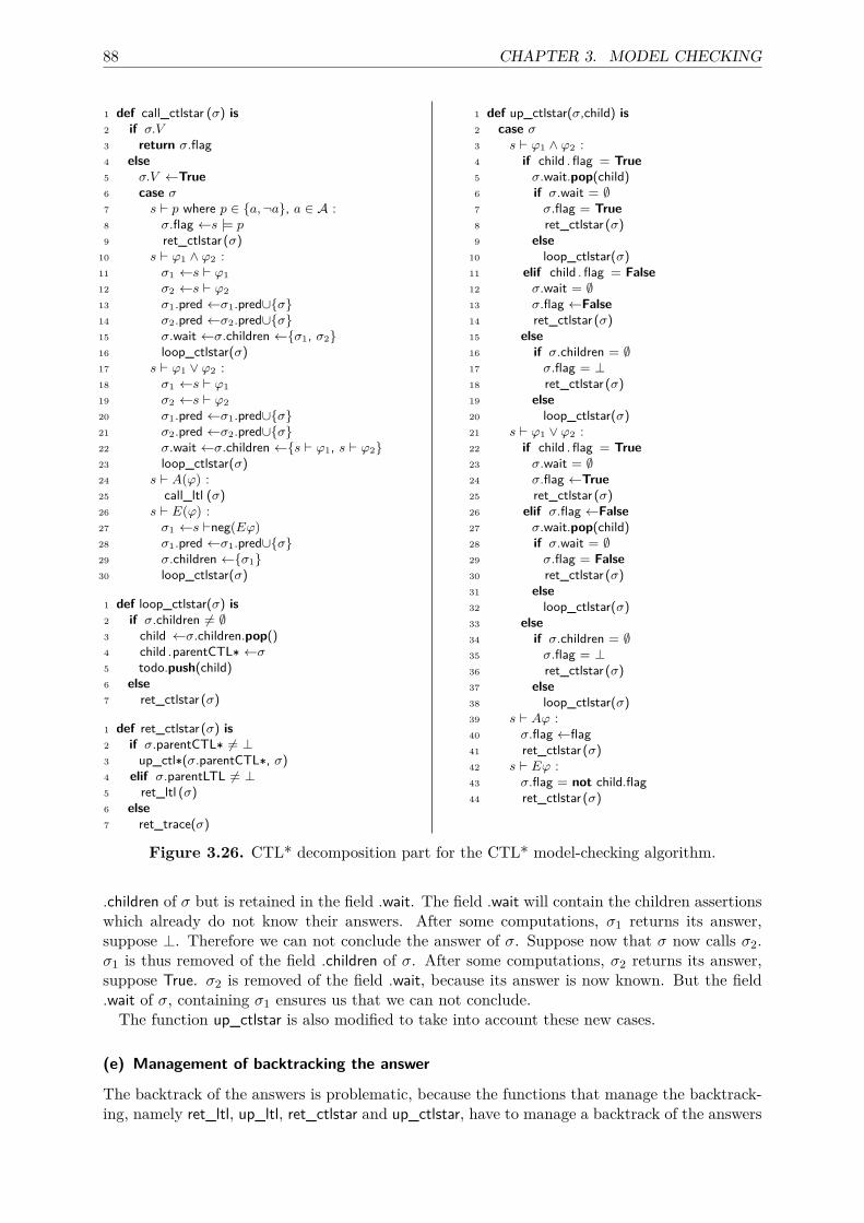
88 CHAPTER 3. MODEL CHECKING
1 def call_ctlstar (σ) is2 if σ.V3 return σ.flag4 else5 σ.V ←True6 case σ7 s ` p where p ∈ {a,¬a}, a ∈ A :8 σ.flag ←s |= p9 ret_ctlstar (σ)
10 s ` ϕ1 ∧ ϕ2 :11 σ1 ←s ` ϕ112 σ2 ←s ` ϕ213 σ1.pred ←σ1.pred∪{σ}14 σ2.pred ←σ2.pred∪{σ}15 σ.wait ←σ.children ←{σ1, σ2}16 loop_ctlstar(σ)17 s ` ϕ1 ∨ ϕ2 :18 σ1 ←s ` ϕ119 σ2 ←s ` ϕ220 σ1.pred ←σ1.pred∪{σ}21 σ2.pred ←σ2.pred∪{σ}22 σ.wait ←σ.children ←{s ` ϕ1, s ` ϕ2}23 loop_ctlstar(σ)24 s ` A(ϕ) :25 call_ltl (σ)26 s ` E(ϕ) :27 σ1 ←s `neg(Eϕ)28 σ1.pred ←σ1.pred∪{σ}29 σ.children ←{σ1}30 loop_ctlstar(σ)
1 def loop_ctlstar(σ) is2 if σ.children 6= ∅3 child ←σ.children.pop()4 child .parentCTL∗ ←σ5 todo.push(child)6 else7 ret_ctlstar (σ)
1 def ret_ctlstar(σ) is2 if σ.parentCTL∗ 6= ⊥3 up_ctl∗(σ.parentCTL∗, σ)4 elif σ.parentLTL 6= ⊥5 ret_ltl (σ)6 else7 ret_trace(σ)
1 def up_ctlstar(σ,child) is2 case σ3 s ` ϕ1 ∧ ϕ2 :4 if child . flag = True5 σ.wait.pop(child)6 if σ.wait = ∅7 σ.flag = True8 ret_ctlstar (σ)9 else
10 loop_ctlstar(σ)11 elif child . flag = False12 σ.wait = ∅13 σ.flag ←False14 ret_ctlstar (σ)15 else16 if σ.children = ∅17 σ.flag = ⊥18 ret_ctlstar (σ)19 else20 loop_ctlstar(σ)21 s ` ϕ1 ∨ ϕ2 :22 if child . flag = True23 σ.wait = ∅24 σ.flag ←True25 ret_ctlstar (σ)26 elif σ.flag ←False27 σ.wait.pop(child)28 if σ.wait = ∅29 σ.flag = False30 ret_ctlstar (σ)31 else32 loop_ctlstar(σ)33 else34 if σ.children = ∅35 σ.flag = ⊥36 ret_ctlstar (σ)37 else38 loop_ctlstar(σ)39 s ` Aϕ :40 σ.flag ←flag41 ret_ctlstar (σ)42 s ` Eϕ :43 σ.flag = not child.flag44 ret_ctlstar (σ)
Figure 3.26. CTL* decomposition part for the CTL* model-checking algorithm.
.children of σ but is retained in the field .wait. The field .wait will contain the children assertionswhich already do not know their answers. After some computations, σ1 returns its answer,suppose ⊥. Therefore we can not conclude the answer of σ. Suppose now that σ now calls σ2.σ1 is thus removed of the field .children of σ. After some computations, σ2 returns its answer,suppose True. σ2 is removed of the field .wait, because its answer is now known. But the field.wait of σ, containing σ1 ensures us that we can not conclude.The function up_ctlstar is also modified to take into account these new cases.
(e) Management of backtracking the answer
The backtrack of the answers is problematic, because the functions that manage the backtrack-ing, namely ret_ltl, up_ltl, ret_ctlstar and up_ctlstar, have to manage a backtrack of the answers
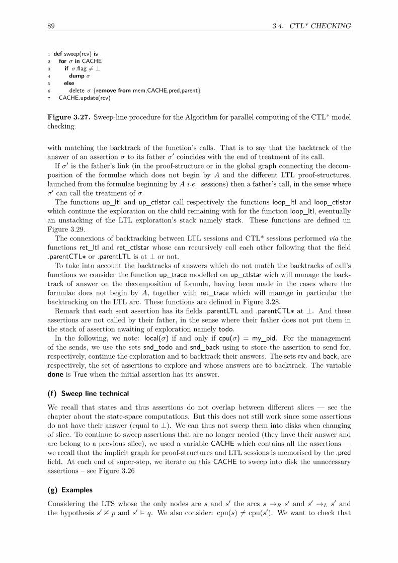
89 3.4. CTL* CHECKING
1 def sweep(rcv) is2 for σ in CACHE3 if σ.flag 6= ⊥4 dump σ5 else6 delete σ {remove from mem,CACHE,pred,parent}7 CACHE.update(rcv)
Figure 3.27. Sweep-line procedure for the Algorithm for parallel computing of the CTL* modelchecking.
with matching the backtrack of the function’s calls. That is to say that the backtrack of theanswer of an assertion σ to its father σ′ coincides with the end of treatment of its call.
If σ′ is the father’s link (in the proof-structure or in the global graph connecting the decom-position of the formulae which does not begin by A and the different LTL proof-structures,launched from the formulae beginning by A i.e. sessions) then a father’s call, in the sense whereσ′ can call the treatment of σ.The functions up_ltl and up_ctlstar call respectively the functions loop_ltl and loop_ctlstar
which continue the exploration on the child remaining with for the function loop_ltl, eventuallyan unstacking of the LTL exploration’s stack namely stack. These functions are defined unFigure 3.29.The connexions of backtracking between LTL sessions and CTL* sessions performed via the
functions ret_ltl and ret_ctlstar whose can recursively call each other following that the field.parentCTL∗ or .parentLTL is at ⊥ or not.To take into account the backtracks of answers which do not match the backtracks of call’s
functions we consider the function up_trace modelled on up_ctlstar wich will manage the back-track of answer on the decomposition of formula, having been made in the cases where theformulae does not begin by A, together with ret_trace which will manage in particular thebacktracking on the LTL arc. These functions are defined in Figure 3.28.Remark that each sent assertion has its fields .parentLTL and .parentCTL∗ at ⊥. And these
assertions are not called by their father, in the sense where their father does not put them inthe stack of assertion awaiting of exploration namely todo.In the following, we note: local(σ) if and only if cpu(σ) = my_pid. For the management
of the sends, we use the sets snd_todo and snd_back using to store the assertion to send for,respectively, continue the exploration and to backtrack their answers. The sets rcv and back, arerespectively, the set of assertions to explore and whose answers are to backtrack. The variabledone is True when the initial assertion has its answer.
(f) Sweep line technical
We recall that states and thus assertions do not overlap between different slices — see thechapter about the state-space computations. But this does not still work since some assertionsdo not have their answer (equal to ⊥). We can thus not sweep them into disks when changingof slice. To continue to sweep assertions that are no longer needed (they have their answer andare belong to a previous slice), we used a variable CACHE which contains all the assertions —we recall that the implicit graph for proof-structures and LTL sessions is memorised by the .predfield. At each end of super-step, we iterate on this CACHE to sweep into disk the unnecessaryassertions – see Figure 3.26
(g) Examples
Considering the LTS whose the only nodes are s and s′ the arcs s →R s′ and s′ →L s′ andthe hypothesis s′ 2 p and s′ � q. We also consider: cpu(s) 6= cpu(s′). We want to check that
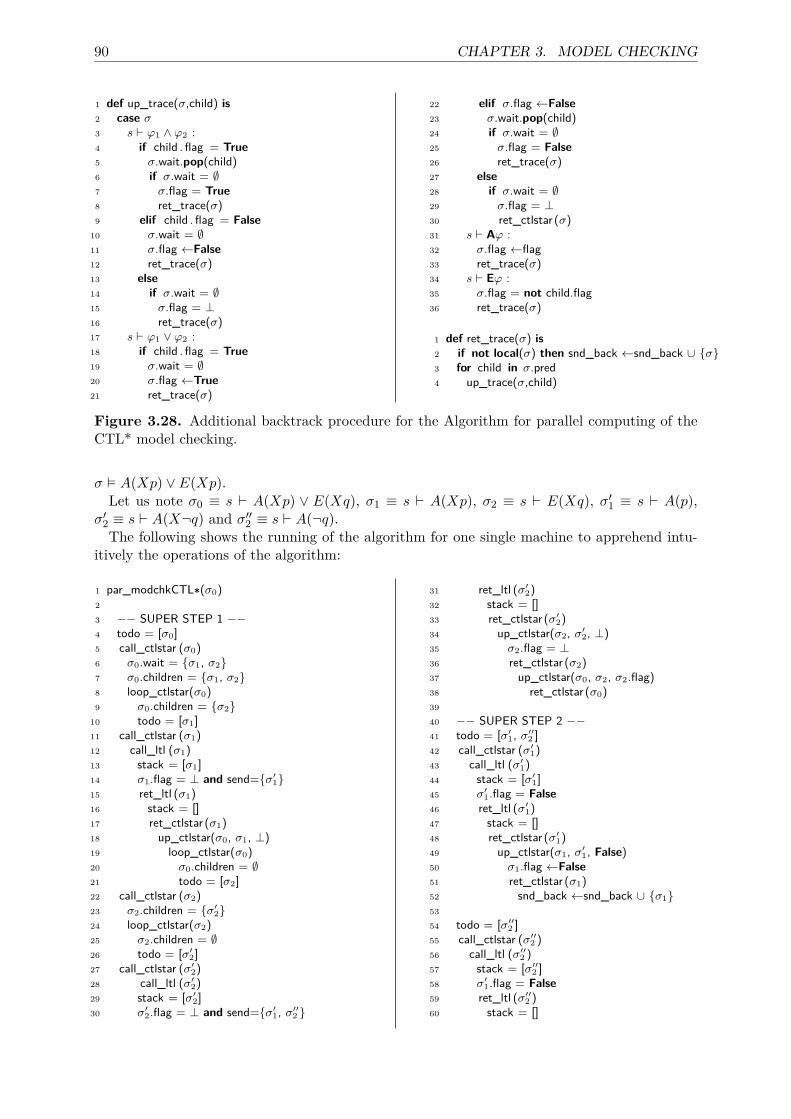
90 CHAPTER 3. MODEL CHECKING
1 def up_trace(σ,child) is2 case σ3 s ` ϕ1 ∧ ϕ2 :4 if child . flag = True5 σ.wait.pop(child)6 if σ.wait = ∅7 σ.flag = True8 ret_trace(σ)9 elif child . flag = False
10 σ.wait = ∅11 σ.flag ←False12 ret_trace(σ)13 else14 if σ.wait = ∅15 σ.flag = ⊥16 ret_trace(σ)17 s ` ϕ1 ∨ ϕ2 :18 if child . flag = True19 σ.wait = ∅20 σ.flag ←True21 ret_trace(σ)
22 elif σ.flag ←False23 σ.wait.pop(child)24 if σ.wait = ∅25 σ.flag = False26 ret_trace(σ)27 else28 if σ.wait = ∅29 σ.flag = ⊥30 ret_ctlstar (σ)31 s ` Aϕ :32 σ.flag ←flag33 ret_trace(σ)34 s ` Eϕ :35 σ.flag = not child.flag36 ret_trace(σ)
1 def ret_trace(σ) is2 if not local(σ) then snd_back ←snd_back ∪ {σ}3 for child in σ.pred4 up_trace(σ,child)
Figure 3.28. Additional backtrack procedure for the Algorithm for parallel computing of theCTL* model checking.
σ � A(Xp) ∨ E(Xp).Let us note σ0 ≡ s ` A(Xp) ∨ E(Xq), σ1 ≡ s ` A(Xp), σ2 ≡ s ` E(Xq), σ′1 ≡ s ` A(p),
σ′2 ≡ s ` A(X¬q) and σ′′2 ≡ s ` A(¬q).The following shows the running of the algorithm for one single machine to apprehend intu-
itively the operations of the algorithm:
1 par_modchkCTL∗(σ0)2
3 −− SUPER STEP 1 −−4 todo = [σ0]5 call_ctlstar (σ0)6 σ0.wait = {σ1, σ2}7 σ0.children = {σ1, σ2}8 loop_ctlstar(σ0)9 σ0.children = {σ2}
10 todo = [σ1]11 call_ctlstar (σ1)12 call_ltl (σ1)13 stack = [σ1]14 σ1.flag = ⊥ and send={σ′
1}15 ret_ltl (σ1)16 stack = []17 ret_ctlstar (σ1)18 up_ctlstar(σ0, σ1, ⊥)19 loop_ctlstar(σ0)20 σ0.children = ∅21 todo = [σ2]22 call_ctlstar (σ2)23 σ2.children = {σ′
2}24 loop_ctlstar(σ2)25 σ2.children = ∅26 todo = [σ′
2]27 call_ctlstar (σ′
2)28 call_ltl (σ′
2)29 stack = [σ′
2]30 σ′
2.flag = ⊥ and send={σ′1, σ′′
2 }
31 ret_ltl (σ′2)
32 stack = []33 ret_ctlstar (σ′
2)34 up_ctlstar(σ2, σ′
2, ⊥)35 σ2.flag = ⊥36 ret_ctlstar (σ2)37 up_ctlstar(σ0, σ2, σ2.flag)38 ret_ctlstar (σ0)39
40 −− SUPER STEP 2 −−41 todo = [σ′
1, σ′′2 ]
42 call_ctlstar (σ′1)
43 call_ltl (σ′1)
44 stack = [σ′1]
45 σ′1.flag = False
46 ret_ltl (σ′1)
47 stack = []48 ret_ctlstar (σ′
1)49 up_ctlstar(σ1, σ′
1, False)50 σ1.flag ←False51 ret_ctlstar (σ1)52 snd_back ←snd_back ∪ {σ1}53
54 todo = [σ′′2 ]
55 call_ctlstar (σ′′2 )
56 call_ltl (σ′′2 )
57 stack = [σ′′2 ]
58 σ′1.flag = False
59 ret_ltl (σ′′2 )
60 stack = []
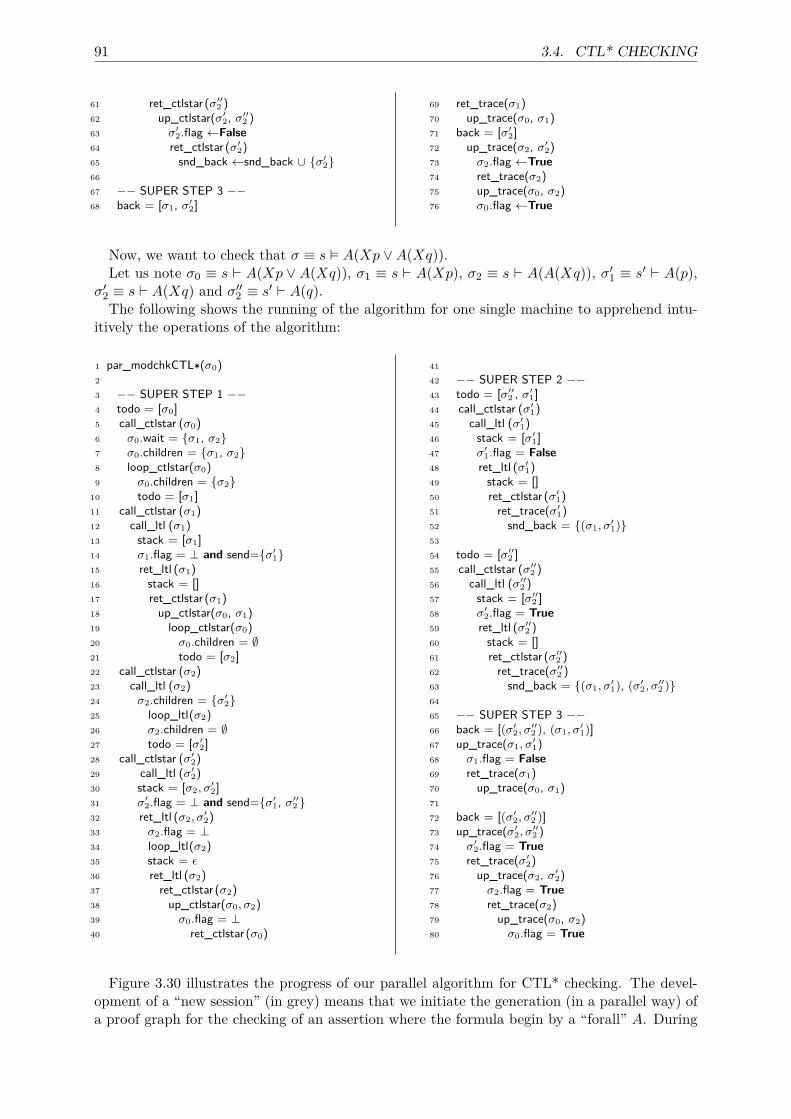
91 3.4. CTL* CHECKING
61 ret_ctlstar (σ′′2 )
62 up_ctlstar(σ′2, σ′′
2 )63 σ′
2.flag ←False64 ret_ctlstar (σ′
2)65 snd_back ←snd_back ∪ {σ′
2}66
67 −− SUPER STEP 3 −−68 back = [σ1, σ′
2]
69 ret_trace(σ1)70 up_trace(σ0, σ1)71 back = [σ′
2]72 up_trace(σ2, σ′
2)73 σ2.flag ←True74 ret_trace(σ2)75 up_trace(σ0, σ2)76 σ0.flag ←True
Now, we want to check that σ ≡ s � A(Xp ∨A(Xq)).Let us note σ0 ≡ s ` A(Xp ∨ A(Xq)), σ1 ≡ s ` A(Xp), σ2 ≡ s ` A(A(Xq)), σ′1 ≡ s′ ` A(p),
σ′2 ≡ s ` A(Xq) and σ′′2 ≡ s′ ` A(q).The following shows the running of the algorithm for one single machine to apprehend intu-
itively the operations of the algorithm:
1 par_modchkCTL∗(σ0)2
3 −− SUPER STEP 1 −−4 todo = [σ0]5 call_ctlstar (σ0)6 σ0.wait = {σ1, σ2}7 σ0.children = {σ1, σ2}8 loop_ctlstar(σ0)9 σ0.children = {σ2}
10 todo = [σ1]11 call_ctlstar (σ1)12 call_ltl (σ1)13 stack = [σ1]14 σ1.flag = ⊥ and send={σ′
1}15 ret_ltl (σ1)16 stack = []17 ret_ctlstar (σ1)18 up_ctlstar(σ0, σ1)19 loop_ctlstar(σ0)20 σ0.children = ∅21 todo = [σ2]22 call_ctlstar (σ2)23 call_ltl (σ2)24 σ2.children = {σ′
2}25 loop_ltl(σ2)26 σ2.children = ∅27 todo = [σ′
2]28 call_ctlstar (σ′
2)29 call_ltl (σ′
2)30 stack = [σ2, σ
′2]
31 σ′2.flag = ⊥ and send={σ′
1, σ′′2 }
32 ret_ltl (σ2, σ′2)
33 σ2.flag = ⊥34 loop_ltl(σ2)35 stack = ε36 ret_ltl (σ2)37 ret_ctlstar (σ2)38 up_ctlstar(σ0, σ2)39 σ0.flag = ⊥40 ret_ctlstar (σ0)
41
42 −− SUPER STEP 2 −−43 todo = [σ′′
2 , σ′1]
44 call_ctlstar (σ′1)
45 call_ltl (σ′1)
46 stack = [σ′1]
47 σ′1.flag = False
48 ret_ltl (σ′1)
49 stack = []50 ret_ctlstar (σ′
1)51 ret_trace(σ′
1)52 snd_back = {(σ1, σ
′1)}
53
54 todo = [σ′′2 ]
55 call_ctlstar (σ′′2 )
56 call_ltl (σ′′2 )
57 stack = [σ′′2 ]
58 σ′2.flag = True
59 ret_ltl (σ′′2 )
60 stack = []61 ret_ctlstar (σ′′
2 )62 ret_trace(σ′′
2 )63 snd_back = {(σ1, σ
′1), (σ′
2, σ′′2 )}
64
65 −− SUPER STEP 3 −−66 back = [(σ′
2, σ′′2 ), (σ1, σ
′1)]
67 up_trace(σ1, σ′1)
68 σ1.flag = False69 ret_trace(σ1)70 up_trace(σ0, σ1)71
72 back = [(σ′2, σ
′′2 )]
73 up_trace(σ′2, σ
′′2 )
74 σ′2.flag = True
75 ret_trace(σ′2)
76 up_trace(σ2, σ′2)
77 σ2.flag = True78 ret_trace(σ2)79 up_trace(σ0, σ2)80 σ0.flag = True
Figure 3.30 illustrates the progress of our parallel algorithm for CTL* checking. The devel-opment of a “new session” (in grey) means that we initiate the generation (in a parallel way) ofa proof graph for the checking of an assertion where the formula begin by a “forall” A. During
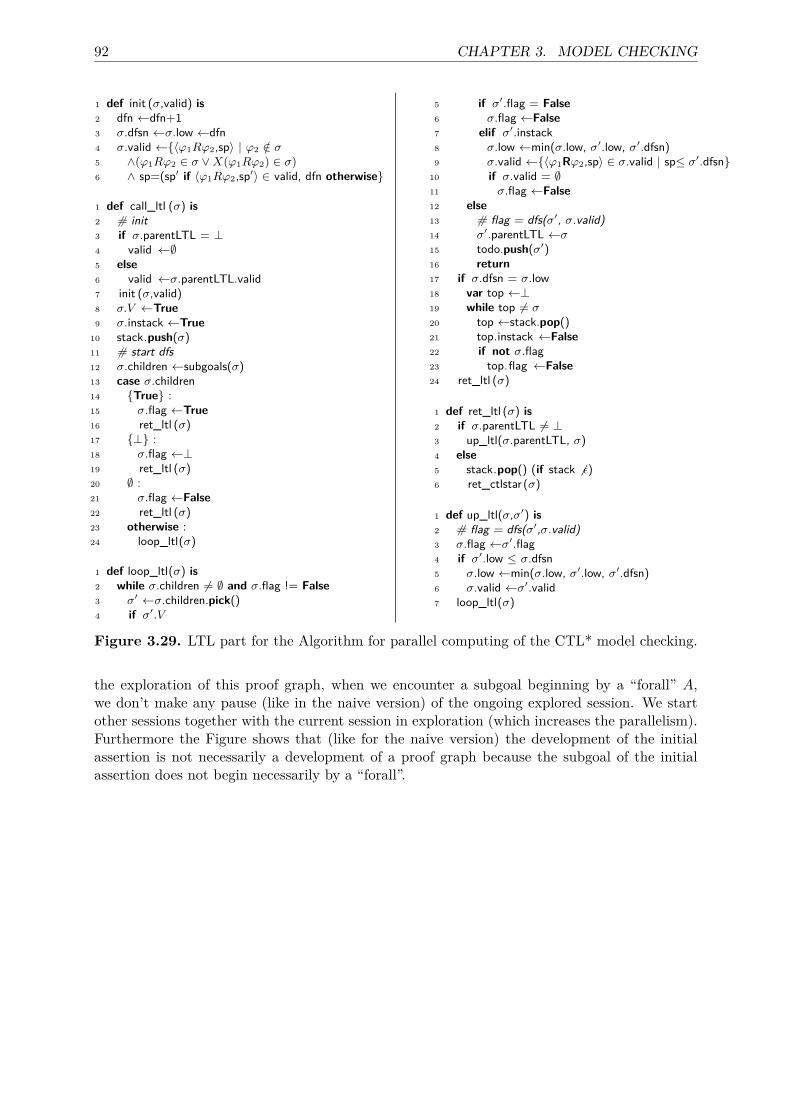
92 CHAPTER 3. MODEL CHECKING
1 def init (σ,valid) is2 dfn ←dfn+13 σ.dfsn ←σ.low ←dfn4 σ.valid ←{〈ϕ1Rϕ2,sp〉 | ϕ2 /∈ σ5 ∧(ϕ1Rϕ2 ∈ σ ∨X(ϕ1Rϕ2) ∈ σ)6 ∧ sp=(sp′ if 〈ϕ1Rϕ2,sp′〉 ∈ valid, dfn otherwise}
1 def call_ltl (σ) is2 # init3 if σ.parentLTL = ⊥4 valid ←∅5 else6 valid ←σ.parentLTL.valid7 init (σ,valid)8 σ.V ←True9 σ.instack ←True
10 stack.push(σ)11 # start dfs12 σ.children ←subgoals(σ)13 case σ.children14 {True} :15 σ.flag ←True16 ret_ltl (σ)17 {⊥} :18 σ.flag ←⊥19 ret_ltl (σ)20 ∅ :21 σ.flag ←False22 ret_ltl (σ)23 otherwise :24 loop_ltl(σ)
1 def loop_ltl(σ) is2 while σ.children 6= ∅ and σ.flag != False3 σ′ ←σ.children.pick()4 if σ′.V
5 if σ′.flag = False6 σ.flag ←False7 elif σ′.instack8 σ.low ←min(σ.low, σ′.low, σ′.dfsn)9 σ.valid ←{〈ϕ1Rϕ2,sp〉 ∈ σ.valid | sp≤ σ′.dfsn}
10 if σ.valid = ∅11 σ.flag ←False12 else13 # flag = dfs(σ′, σ.valid)14 σ′.parentLTL ←σ15 todo.push(σ′)16 return17 if σ.dfsn = σ.low18 var top ←⊥19 while top 6= σ20 top ←stack.pop()21 top.instack ←False22 if not σ.flag23 top.flag ←False24 ret_ltl (σ)
1 def ret_ltl (σ) is2 if σ.parentLTL 6= ⊥3 up_ltl(σ.parentLTL, σ)4 else5 stack.pop() (if stack 6 ε)6 ret_ctlstar (σ)
1 def up_ltl(σ,σ′) is2 # flag = dfs(σ′,σ.valid)3 σ.flag ←σ′.flag4 if σ′.low ≤ σ.dfsn5 σ.low ←min(σ.low, σ′.low, σ′.dfsn)6 σ.valid ←σ′.valid7 loop_ltl(σ)
Figure 3.29. LTL part for the Algorithm for parallel computing of the CTL* model checking.
the exploration of this proof graph, when we encounter a subgoal beginning by a “forall” A,we don’t make any pause (like in the naive version) of the ongoing explored session. We startother sessions together with the current session in exploration (which increases the parallelism).Furthermore the Figure shows that (like for the naive version) the development of the initialassertion is not necessarily a development of a proof graph because the subgoal of the initialassertion does not begin necessarily by a “forall”.
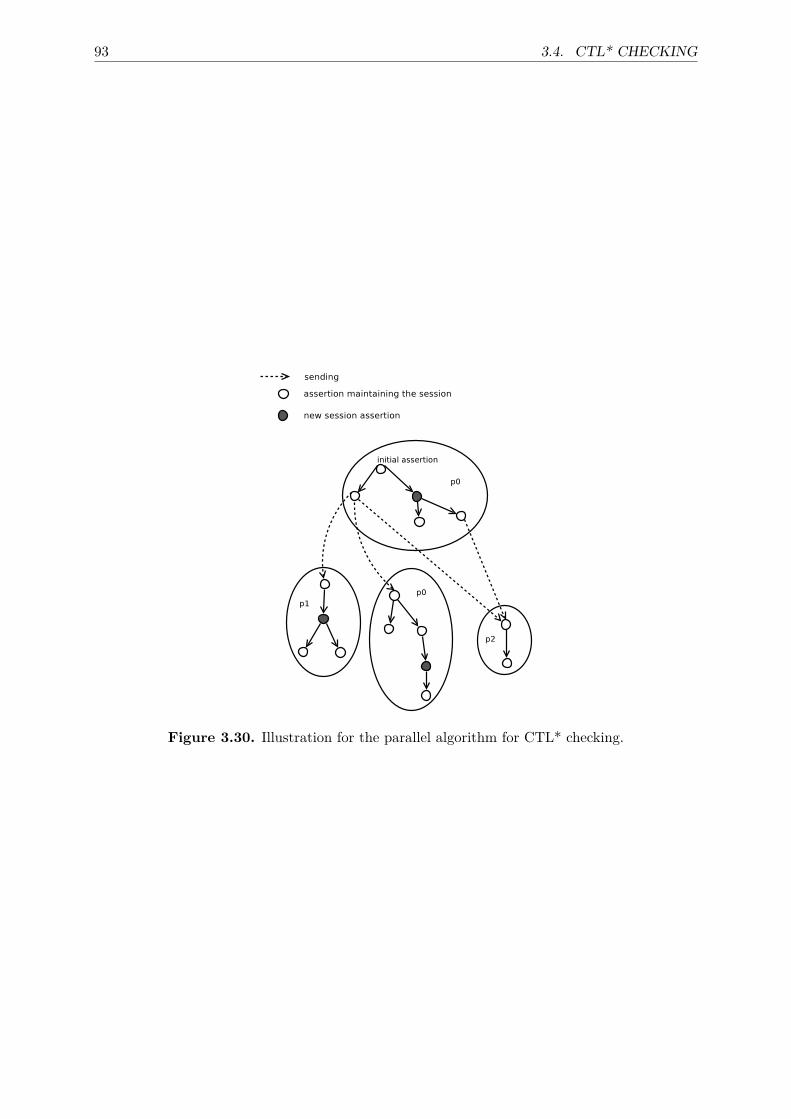
93 3.4. CTL* CHECKING
Figure 3.30. Illustration for the parallel algorithm for CTL* checking.

4 Case study
This chapter extends the works of [104,106].
Contents4.1 Specification of some security protocols using ABCD . . . . . . . . . 95
4.1.1 Modelisation of the security protocols . . . . . . . . . . . . . . . . . . . 954.1.2 Full example: the Needham-Schroeder protocol . . . . . . . . . . . . . . 994.1.3 Other examples of protocols . . . . . . . . . . . . . . . . . . . . . . . . . 102
4.2 Implementation of the algorithms . . . . . . . . . . . . . . . . . . . . 1054.2.1 BSP programming in Python . . . . . . . . . . . . . . . . . . . . . . . . 1054.2.2 SNAKES toolkit and syntactic layers . . . . . . . . . . . . . . . . . . . . 1104.2.3 Parallel algorithms . . . . . . . . . . . . . . . . . . . . . . . . . . . . . . 113
4.3 State space generation’s benchmarks . . . . . . . . . . . . . . . . . . . 1174.4 LTL and CTL*’s benchmarks . . . . . . . . . . . . . . . . . . . . . . . 119
This chapter concerns the practical part of our work. In a first time, we present the speci-fication of security Protocols by the langage ABCD and we give several examples of protocolswith their modelisation in this langage. Then, we describe the important technologies we useto implement our algorithms: the BSP Python Programming library and the SNAKES toolkitand syntactic layers wich is a Python library to define, manipulate and execute coloured Petrinets [178]. Then we give the features of the implementation of our parallel algorithms and atlast the benchmarks on our differents algoritms.
4.1 Specification of some security protocols using ABCDIn this section, we show how the ABCD language previously introduced can be used to specifyand verify security protocols. We consider models of security protocols involving a set of agentsA which exchange data (messages) using a network where there is a Dolev-Yaho attacker whichis able to read the messages, analyse them with some specific rules and generate new messagesover the network. This section is an extension of the work of [181] about security protocols.
4.1.1 Modelisation of the security protocols
(a) Modelling communication and cryptography
Using ABCD, a simple model of a network is a globally shared buffer: to send a message we putits value on the buffer and to receive a message, we get it from the buffer. As explain latter, weactually used two buffers in this document:
buffer snd : object = ()buffer rcv : object = ()
95
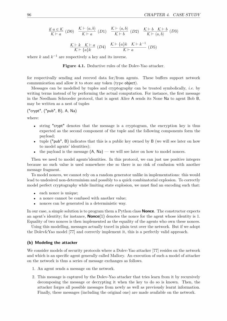
96 CHAPTER 4. CASE STUDY
if a ∈ KK ` a (D0)
K ` 〈a, b〉K ` a (D1)
K ` 〈a, b〉K ` b (D2) K ` b K ` b
K ` 〈a, b〉 (D3)
K ` k K ` aK ` {a}k (D4) K ` {a}k K ` k−1
K ` a (D5)
where k and k−1 are respectively a key and its inverse.
Figure 4.1. Deductive rules of the Dolev-Yao attacker.
for respectivally sending and receved data for/from agents. These buffers support networkcommunication and allow it to store any token (type object).Messages can be modelled by tuples and cryptography can be treated symbolically, i.e. by
writing terms instead of by performing the actual computation. For instance, the first messagein the Needham Schroeder protocol, that is agent Alice A sends its None Na to agent Bob B,may be written as a nest of tuples("crypt", ("pub", B), A, Na)where:
• string "crypt" denotes that the message is a cryptogram, the encryption key is thusexpected as the second component of the tuple and the following components form thepayload;
• tuple ("pub", B) indicates that this is a public key owned by B (we will see later on howto model agents’ identities);
• the payload is the message (A, Na) — we will see later on how to model nonces.
Then we need to model agents’identities. In this protocol, we can just use positive integersbecause no such value is used somewhere else so there is no risk of confusion with anothermessage fragment.To model nonces, we cannot rely on a random generator unlike in implementations: this would
lead to undesired non-determinism and possibly to a quick combinatorial explosion. To correctlymodel perfect cryptography while limiting state explosion, we must find an encoding such that:
• each nonce is unique;• a nonce cannot be confused with another value;• nonces can be generated in a deterministic way.
In our case, a simple solution is to program them a Python class Nonce. The constructor expectsan agent’s identity; for instance, Nonce(1) denotes the nonce for the agent whose identity is 1.Equality of two nonces is then implemented as the equality of the agents who own these nonces.Using this modelling, messages actually travel in plain text over the network. But if we adopt
the Dolev&Yao model [77] and correctly implement it, this is a perfectly valid approach.
(b) Modeling the attacker
We consider models of security protocols where a Dolev-Yao attacker [77] resides on the networkand which is an specific agent generally called Mallory. An execution of such a model of attackeron the network is thus a series of message exchanges as follows.
1. An agent sends a message on the network.
2. This message is captured by the Dolev-Yao attacker that tries learn from it by recursivelydecomposing the message or decrypting it when the key to do so is known. Then, theattacker forges all possible messages from newly as well as previously learnt information.Finally, these messages (including the original one) are made available on the network.
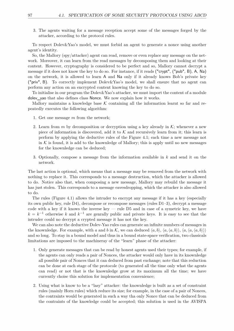
97 4.1. SPECIFICATION OF SOME SECURITY PROTOCOLS USING ABCD
3. The agents waiting for a message reception accept some of the messages forged by theattacker, according to the protocol rules.
To respect Dolev&Yao’s model, we must forbid an agent to generate a nonce using anotheragent’s identity.So, the Mallory (spy/attacker) agent can read, remove or even replace any message on the net-
work. Moreover, it can learn from the read messages by decomposing them and looking at theircontent. However, cryptography is considered to be perfect and so, Mallory cannot decrypt amessage if it does not know the key to do so. For instance, if it reads ("crypt", ("pub", B), A, Na)on the network, it is allowed to learn A and Na only if it already knows Bob’s private key("priv", B). To correctly implement Dolev&Yao’s model, we shall ensure that no agent canperform any action on an encrypted content knowing the key to do so.To initialise in our program the Dolev&Yao’s attacker, we must import the content of a module
dolev_yao that also defines class Nonce. We now explain how it works.Mallory maintains a knowledge base K containing all the information learnt so far and re-
peatedly executes the following algorithm:
1. Get one message m from the network;
2. Learn from m by decomposition or decryption using a key already in K; whenever a newpiece of information is discovered, add it to K and recursively learn from it; this learn isperform by applying the deductive rules of the Figure 4.1; each time a new message notin K is found, it is add to the knownledge of Mallory; this is apply until no new messagesfor the knownledge can be deduced;
3. Optionally, compose a message from the information available in k and send it on thenetwork.
The last action is optional, which means that a message may be removed from the network withnothing to replace it. This corresponds to a message destruction, which the attacker is allowedto do. Notice also that, when composing a new message, Mallory may rebuild the message ithas just stolen. This corresponds to a message eavesdropping, which the attacker is also allowedto do.
The rules (Figure 4.1) allows the intruder to encrypt any message if it has a key (especiallyits own public key, rule D4), decompose or recompose messages (rules D1–3), decrypt a messagecode with a key if it knows the inverse key — rule D5 and in case of a symetric key, we havek = k−1 otherwise k and k−1 are genrally public and private keys. It is easy to see that theintruder could no decrypt a crypted message it has not the key.We can also note the deductive Dolev-Yao rules can generate an infinite numbers of messages in
the knownledge. For example, with a and b in K, we can deduced 〈a, b〉, 〈a, 〈a, b〉〉, 〈a, 〈a, 〈a, b〉〉〉and so long. To stay in a bound model and thus in a bound state-space verification, two classicalslimitations are imposed to the machineray of the “learn” phase of the attacker:
1. Only generate messages that can be read by honest agents used their types; for example, ifthe agents can only reads a pair of Nonces, the attacker would only have in its knownledgeall possible pair of Nonces that it can deduced from past exchange; note that this reductioncan be done at each stage of the protocole (to generated all the time only what the agentscan read) or not that is the knownledge grow at its maximum all the time; we havecurrently choise this solution for implementation convenience;
2. Using what is know to be a “lasy” attacker: the knownledge is built as a set of constraintrules (mainly Horn rules) which reduce its size; for example, in the case of a pair of Nonces,the contraints would be generated in such a way tha only Nonce that can be deduced fromthe contraints of the knowledge could be accepted; this solution is used in the AVISPA
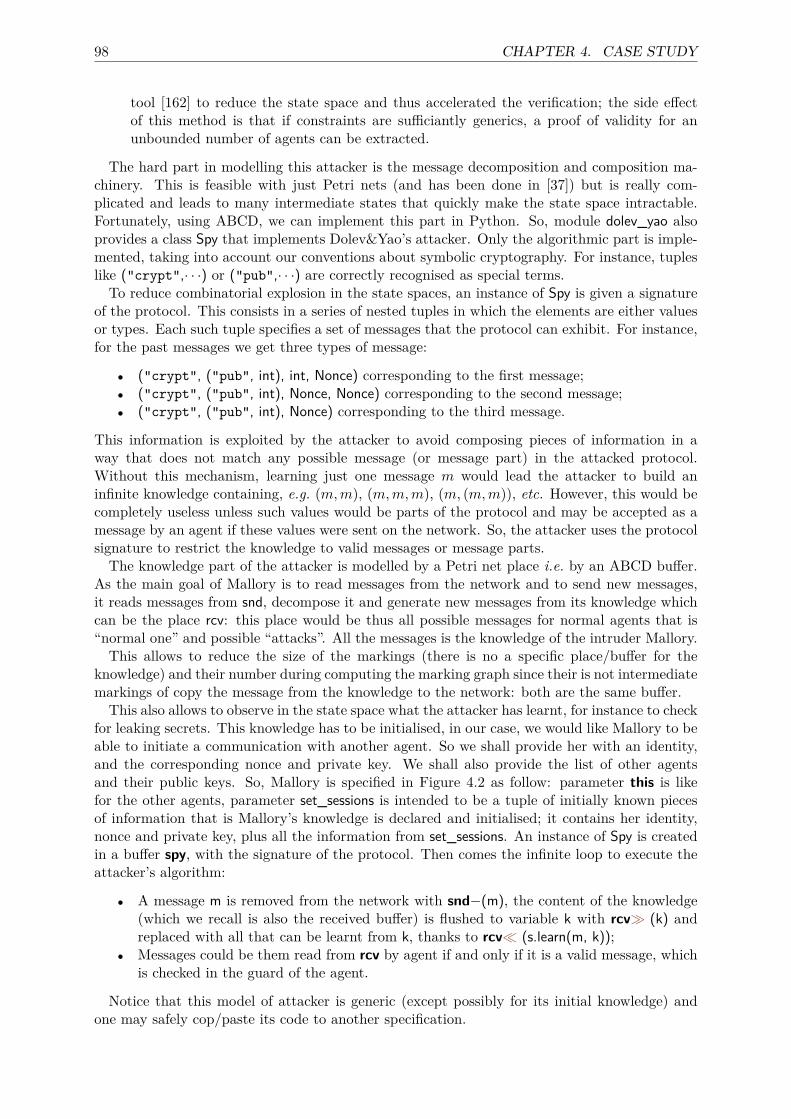
98 CHAPTER 4. CASE STUDY
tool [162] to reduce the state space and thus accelerated the verification; the side effectof this method is that if constraints are sufficiantly generics, a proof of validity for anunbounded number of agents can be extracted.
The hard part in modelling this attacker is the message decomposition and composition ma-chinery. This is feasible with just Petri nets (and has been done in [37]) but is really com-plicated and leads to many intermediate states that quickly make the state space intractable.Fortunately, using ABCD, we can implement this part in Python. So, module dolev_yao alsoprovides a class Spy that implements Dolev&Yao’s attacker. Only the algorithmic part is imple-mented, taking into account our conventions about symbolic cryptography. For instance, tupleslike ("crypt",· · ·) or ("pub",· · ·) are correctly recognised as special terms.
To reduce combinatorial explosion in the state spaces, an instance of Spy is given a signatureof the protocol. This consists in a series of nested tuples in which the elements are either valuesor types. Each such tuple specifies a set of messages that the protocol can exhibit. For instance,for the past messages we get three types of message:
• ("crypt", ("pub", int), int, Nonce) corresponding to the first message;• ("crypt", ("pub", int), Nonce, Nonce) corresponding to the second message;• ("crypt", ("pub", int), Nonce) corresponding to the third message.
This information is exploited by the attacker to avoid composing pieces of information in away that does not match any possible message (or message part) in the attacked protocol.Without this mechanism, learning just one message m would lead the attacker to build aninfinite knowledge containing, e.g. (m,m), (m,m,m), (m, (m,m)), etc. However, this would becompletely useless unless such values would be parts of the protocol and may be accepted as amessage by an agent if these values were sent on the network. So, the attacker uses the protocolsignature to restrict the knowledge to valid messages or message parts.The knowledge part of the attacker is modelled by a Petri net place i.e. by an ABCD buffer.
As the main goal of Mallory is to read messages from the network and to send new messages,it reads messages from snd, decompose it and generate new messages from its knowledge whichcan be the place rcv: this place would be thus all possible messages for normal agents that is“normal one” and possible “attacks”. All the messages is the knowledge of the intruder Mallory.This allows to reduce the size of the markings (there is no a specific place/buffer for the
knowledge) and their number during computing the marking graph since their is not intermediatemarkings of copy the message from the knowledge to the network: both are the same buffer.This also allows to observe in the state space what the attacker has learnt, for instance to check
for leaking secrets. This knowledge has to be initialised, in our case, we would like Mallory to beable to initiate a communication with another agent. So we shall provide her with an identity,and the corresponding nonce and private key. We shall also provide the list of other agentsand their public keys. So, Mallory is specified in Figure 4.2 as follow: parameter this is likefor the other agents, parameter set_sessions is intended to be a tuple of initially known piecesof information that is Mallory’s knowledge is declared and initialised; it contains her identity,nonce and private key, plus all the information from set_sessions. An instance of Spy is createdin a buffer spy, with the signature of the protocol. Then comes the infinite loop to execute theattacker’s algorithm:
• A message m is removed from the network with snd−(m), the content of the knowledge(which we recall is also the received buffer) is flushed to variable k with rcv� (k) andreplaced with all that can be learnt from k, thanks to rcv� (s.learn(m, k));
• Messages could be them read from rcv by agent if and only if it is a valid message, whichis checked in the guard of the agent.
Notice that this model of attacker is generic (except possibly for its initial knowledge) andone may safely cop/paste its code to another specification.
99 4.1. SPECIFICATION OF SOME SECURITY PROTOCOLS USING ABCD
net Mallory (this, set_sessions) :buffer spy : object = Spy(
(int, int, int, int, Nonce), #1(int, int,("crypt", ("secret", int, int),int, int, Nonce, ("secret", int, int, Nonce)),("crypt", ("secret", int, int),int, int, Nonce, ("secret", int, int, Nonce))), #2
(int, int,("crypt", ("secret", int, int),int, int, Nonce, ("secret", int, int, Nonce)),("crypt", ("secret", int, int, Nonce), Nonce),Nonce), #3(int, int,("crypt", ("secret", int, int, Nonce), Nonce)) #4)
[rcv� ((this,)+ tuple(range(1, this))+ tuple(Nonce((this, s)) for s in set_sessions))]
# ([spy?(s), snd−(m), rcv� (k), rcv� (s.learn(m, k))] ~ [False])
Figure 4.2. Typical code of Mallory.
(c) Defining a scenario
To create a complete ABCD specification, we need to provide a main term. This consists in acomposition of instances of the defined agents. By providing this, we create a scenario, i.e. aparticular situation that can then be analysed. This naturally bounced scenario with a fixnumber of agentsUsing the ABCD compiler, we can create a pnml file from this system. This file can be loaded
from a Python program using snakes to build the state space and search for a faulty.
4.1.2 Full example: the Needham-Schroeder protocolAs an illustration of the past section, we model Needham&Schroeder’s protocol for mutualauthentication [163]. This is quite a small example, but fortunately, this protocol allows to showthe most important aspects about applying ABCD to security protocols.
(a) A protocol for mutual authentication
The protocol ns involves two agents Alice (A) and Bob (B) who want to mutually authenticate.This is performed through the exchange of three messages as illustrated in Figure 4.3. In thisspecification, a message m is denoted by 〈m〉 and a message encrypted by a key k is denoted by〈m〉k (we use the same notation for secret key and public key encryption). The three steps ofthe protocol can be understood as follows:
1. Alice sends her identity A to Bob, together with a nonce Na; the message is encryptedwith Bob’s public key Kb so that only Bob can read it; Na thus constitutes a challengethat allows Bob to prove his identity: he is the only one who can read the nonce and sendit back to Alice;
2. Bob solves the challenge by sending Na to Alice, together with another nonce Nb that isa new challenge to authenticate Alice;
3. Alice solves Bob’s challenge, which results in mutual authentication.
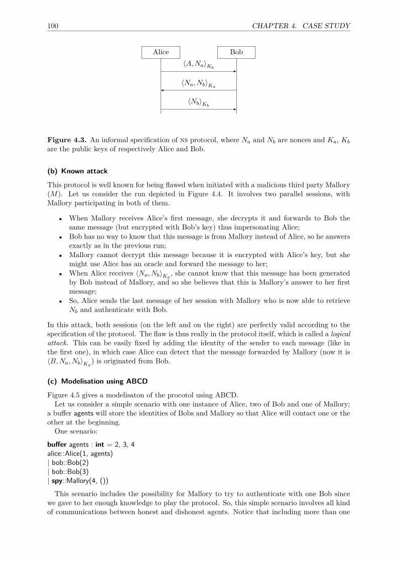
100 CHAPTER 4. CASE STUDY
Alice Bob〈A,Na〉Kb
〈Na, Nb〉Ka
〈Nb〉Kb
Figure 4.3. An informal specification of ns protocol, where Na and Nb are nonces and Ka, Kb
are the public keys of respectively Alice and Bob.
(b) Known attack
This protocol is well known for being flawed when initiated with a malicious third party Mallory(M). Let us consider the run depicted in Figure 4.4. It involves two parallel sessions, withMallory participating in both of them.
• When Mallory receives Alice’s first message, she decrypts it and forwards to Bob thesame message (but encrypted with Bob’s key) thus impersonating Alice;
• Bob has no way to know that this message is from Mallory instead of Alice, so he answersexactly as in the previous run;
• Mallory cannot decrypt this message because it is encrypted with Alice’s key, but shemight use Alice has an oracle and forward the message to her;
• When Alice receives 〈Na, Nb〉Ka, she cannot know that this message has been generated
by Bob instead of Mallory, and so she believes that this is Mallory’s answer to her firstmessage;
• So, Alice sends the last message of her session with Mallory who is now able to retrieveNb and authenticate with Bob.
In this attack, both sessions (on the left and on the right) are perfectly valid according to thespecification of the protocol. The flaw is thus really in the protocol itself, which is called a logicalattack. This can be easily fixed by adding the identity of the sender to each message (like inthe first one), in which case Alice can detect that the message forwarded by Mallory (now it is〈B,Na, Nb〉Ka
) is originated from Bob.
(c) Modelisation using ABCD
Figure 4.5 gives a modelisaton of the procotol using ABCD.Let us consider a simple scenario with one instance of Alice, two of Bob and one of Mallory;
a buffer agents will store the identities of Bobs and Mallory so that Alice will contact one or theother at the beginning.
One scenario:
buffer agents : int = 2, 3, 4alice::Alice(1, agents)| bob::Bob(2)| bob::Bob(3)| spy::Mallory(4, ())
This scenario includes the possibility for Mallory to try to authenticate with one Bob sincewe gave to her enough knowledge to play the protocol. So, this simple scenario involves all kindof communications between honest and dishonest agents. Notice that including more than one
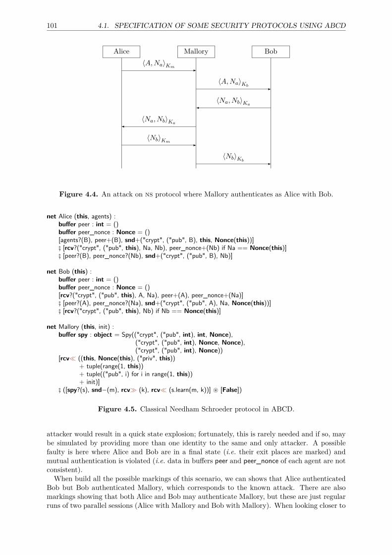
101 4.1. SPECIFICATION OF SOME SECURITY PROTOCOLS USING ABCD
Alice Mallory Bob〈A,Na〉Km
〈A,Na〉Kb
〈Na, Nb〉Ka
〈Na, Nb〉Ka
〈Nb〉Km
〈Nb〉Kb
Figure 4.4. An attack on ns protocol where Mallory authenticates as Alice with Bob.
net Alice (this, agents) :buffer peer : int = ()buffer peer_nonce : Nonce = ()[agents?(B), peer+(B), snd+("crypt", ("pub", B), this, Nonce(this))]# [rcv?("crypt", ("pub", this), Na, Nb), peer_nonce+(Nb) if Na == Nonce(this)]# [peer?(B), peer_nonce?(Nb), snd+("crypt", ("pub", B), Nb)]
net Bob (this) :buffer peer : int = ()buffer peer_nonce : Nonce = ()[rcv?("crypt", ("pub", this), A, Na), peer+(A), peer_nonce+(Na)]# [peer?(A), peer_nonce?(Na), snd+("crypt", ("pub", A), Na, Nonce(this))]# [rcv?("crypt", ("pub", this), Nb) if Nb == Nonce(this)]
net Mallory (this, init) :buffer spy : object = Spy(("crypt", ("pub", int), int, Nonce),
("crypt", ("pub", int), Nonce, Nonce),("crypt", ("pub", int), Nonce))
[rcv� ((this, Nonce(this), ("priv", this))+ tuple(range(1, this))+ tuple(("pub", i) for i in range(1, this))+ init)]
# ([spy?(s), snd−(m), rcv� (k), rcv� (s.learn(m, k))] ~ [False])
Figure 4.5. Classical Needham Schroeder protocol in ABCD.
attacker would result in a quick state explosion; fortunately, this is rarely needed and if so, maybe simulated by providing more than one identity to the same and only attacker. A possiblefaulty is here where Alice and Bob are in a final state (i.e. their exit places are marked) andmutual authentication is violated (i.e. data in buffers peer and peer_nonce of each agent are notconsistent).
When build all the possible markings of this scenario, we can shows that Alice authenticatedBob but Bob authenticated Mallory, which corresponds to the known attack. There are alsomarkings showing that both Alice and Bob may authenticate Mallory, but these are just regularruns of two parallel sessions (Alice with Mallory and Bob with Mallory). When looking closer to
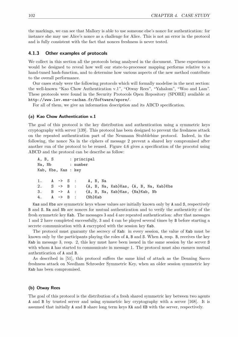
102 CHAPTER 4. CASE STUDY
the markings, we can see that Mallory is able to use someone else’s nonce for authentication: forinstance she may use Alice’s nonce as a challenge for Alice. This is not an error in the protocoland is fully consistent with the fact that nonces freshness is never tested.
4.1.3 Other examples of protocolsWe collect in this section all the protocols being analysed in the document. These experimentswould be designed to reveal how well our state-to-processor mapping performs relative to ahand-tuned hash-function, and to determine how various aspects of the new method contributeto the overall performance.Our cases study were the following protocols which will formally modelise in the next section:
the well-known “Kao Chow Authentication v.1”, “Otway Rees”, “Yahalom”, “Woo and Lam”.These protocols were found in the Security Protocols Open Repository (SPORE) available athttp://www.lsv.ens-cachan.fr/Software/spore/.
For all of them, we give an information description and its ABCD specification.
(a) Kao Chow Authentication v.1
The goal of this protocol is the key distribution and authentication using a symmetric keyscryptography with server [139]. This protocol has been designed to prevent the freshness attackon the repeated authentication part of the Neumann Stubblebine protocol. Indeed, in thefollowing, the nonce Na in the ciphers of message 2 prevent a shared key compromised afteranother run of the protocol to be reused. Figure 4.6 gives a specification of the procotol usingABCD and the protocol can be describe as follow:
A, B, S : principalNa, Nb : numberKab, Kbs, Kas : key
1. A -> S : A, B, Na2. S -> B : {A, B, Na, Kab}Kas, {A, B, Na, Kab}Kbs3. B -> A : {A, B, Na, Kab}Kas, {Na}Kab, Nb4. A -> B : {Nb}Kab
Kas and Kbs are symmetric keys whose values are initially known only by A and S, respectivelyB and S. Na and Nb are nonces for mutual authentication and to verify the authenticity of thefresh symmetric key Kab. The messages 3 and 4 are repeated authentication: after that messages1 and 2 have completed successfully, 3 and 4 can be played several times by B before starting asecrete communication with A encrypted with the session key Kab.The protocol must guaranty the secrecy of Kab: in every session, the value of Kab must be
known only by the participants playing the roles of A, B and S. When A, resp. B, receives the keyKab in message 3, resp. 2, this key must have been issued in the same session by the server Swith whom A has started to communicate in message 1. The protocol must also ensures mutualauthentication of A and B.
As described in [51], this protocol suffers the same kind of attack as the Denning Saccofreshness attack on Needham Schroeder Symmetric Key, when an older session symmetric keyKab has been compromised.
(b) Otway Rees
The goal of this protocol is the distribution of a fresh shared symmetric key between two agentsA and B by trusted server and using symmetric key cryptography with a server [168]. It isassumed that initially A and B share long term keys KA and KB with the server, respectively.
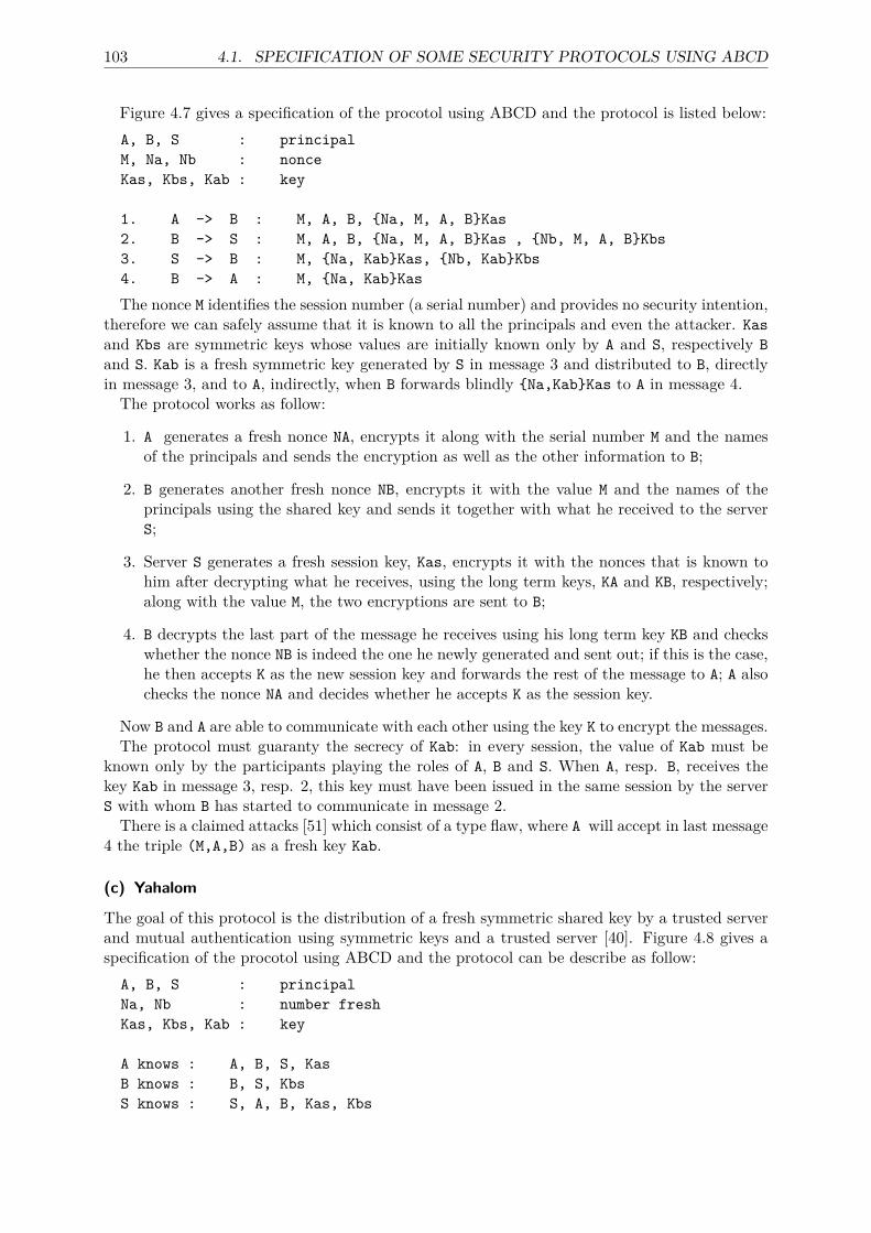
103 4.1. SPECIFICATION OF SOME SECURITY PROTOCOLS USING ABCD
Figure 4.7 gives a specification of the procotol using ABCD and the protocol is listed below:A, B, S : principalM, Na, Nb : nonceKas, Kbs, Kab : key
1. A -> B : M, A, B, {Na, M, A, B}Kas2. B -> S : M, A, B, {Na, M, A, B}Kas , {Nb, M, A, B}Kbs3. S -> B : M, {Na, Kab}Kas, {Nb, Kab}Kbs4. B -> A : M, {Na, Kab}Kas
The nonce M identifies the session number (a serial number) and provides no security intention,therefore we can safely assume that it is known to all the principals and even the attacker. Kasand Kbs are symmetric keys whose values are initially known only by A and S, respectively Band S. Kab is a fresh symmetric key generated by S in message 3 and distributed to B, directlyin message 3, and to A, indirectly, when B forwards blindly {Na,Kab}Kas to A in message 4.
The protocol works as follow:
1. A generates a fresh nonce NA, encrypts it along with the serial number M and the namesof the principals and sends the encryption as well as the other information to B;
2. B generates another fresh nonce NB, encrypts it with the value M and the names of theprincipals using the shared key and sends it together with what he received to the serverS;
3. Server S generates a fresh session key, Kas, encrypts it with the nonces that is known tohim after decrypting what he receives, using the long term keys, KA and KB, respectively;along with the value M, the two encryptions are sent to B;
4. B decrypts the last part of the message he receives using his long term key KB and checkswhether the nonce NB is indeed the one he newly generated and sent out; if this is the case,he then accepts K as the new session key and forwards the rest of the message to A; A alsochecks the nonce NA and decides whether he accepts K as the session key.
Now B and A are able to communicate with each other using the key K to encrypt the messages.The protocol must guaranty the secrecy of Kab: in every session, the value of Kab must be
known only by the participants playing the roles of A, B and S. When A, resp. B, receives thekey Kab in message 3, resp. 2, this key must have been issued in the same session by the serverS with whom B has started to communicate in message 2.There is a claimed attacks [51] which consist of a type flaw, where A will accept in last message
4 the triple (M,A,B) as a fresh key Kab.
(c) Yahalom
The goal of this protocol is the distribution of a fresh symmetric shared key by a trusted serverand mutual authentication using symmetric keys and a trusted server [40]. Figure 4.8 gives aspecification of the procotol using ABCD and the protocol can be describe as follow:
A, B, S : principalNa, Nb : number freshKas, Kbs, Kab : key
A knows : A, B, S, KasB knows : B, S, KbsS knows : S, A, B, Kas, Kbs
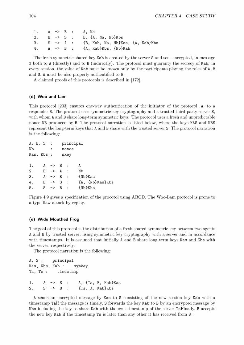
104 CHAPTER 4. CASE STUDY
1. A -> B : A, Na2. B -> S : B, {A, Na, Nb}Kbs3. S -> A : {B, Kab, Na, Nb}Kas, {A, Kab}Kbs4. A -> B : {A, Kab}Kbs, {Nb}Kab
The fresh symmetric shared key Kab is created by the server S and sent encrypted, in message3 both to A (directly) and to B (indirectly). The protocol must guaranty the secrecy of Kab: inevery session, the value of Kab must be known only by the participants playing the roles of A, Band S. A must be also properly authentified to B.A claimed proofs of this protocols is described in [172].
(d) Woo and Lam
This protocol [203] ensures one-way authentication of the initiator of the protocol, A, to aresponder B. The protocol uses symmetric-key cryptography and a trusted third-party server S,with whom A and B share long-term symmetric keys. The protocol uses a fresh and unpredictablenonce NB produced by B. The protocol narration is listed below, where the keys KAS and KBSrepresent the long-term keys that A and B share with the trusted server S. The protocol narrationis the following:
A, B, S : principalNb : nonceKas, Kbs : skey
1. A -> B : A2. B -> A : Nb3. A -> B : {Nb}Kas4. B -> S : {A, {Nb}Kas}Kbs5. S -> B : {Nb}Kbs
Figure 4.9 gives a specification of the procotol using ABCD. The Woo-Lam protocol is prone toa type flaw attack by replay.
(e) Wide Mouthed Frog
The goal of this protocol is the distribution of a fresh shared symmetric key between two agentsA and B by trusted server, using symmetric key cryptography with a server and in accordancewith timestamps. It is assumed that initially A and B share long term keys Kas and Kbs withthe server, respectively.The protocol narration is the following:
A, S : principalKas, Kbs, Kab : symkeyTa, Ts : timestamp
1. A -> S : A, {Ta, B, Kab}Kas2. S -> B : {Ts, A, Kab}Kbs
A sends an encrypted message by Kas to S consisting of the new session key Kab with atimestamp Taİf the message is timely, S forwards the key Kab to B by an encrypted message byKbs including the key to share Kab with the own timestamp of the server TsFinally, B acceptsthe new key Kab if the timestamp Ts is later than any other it has received from S .
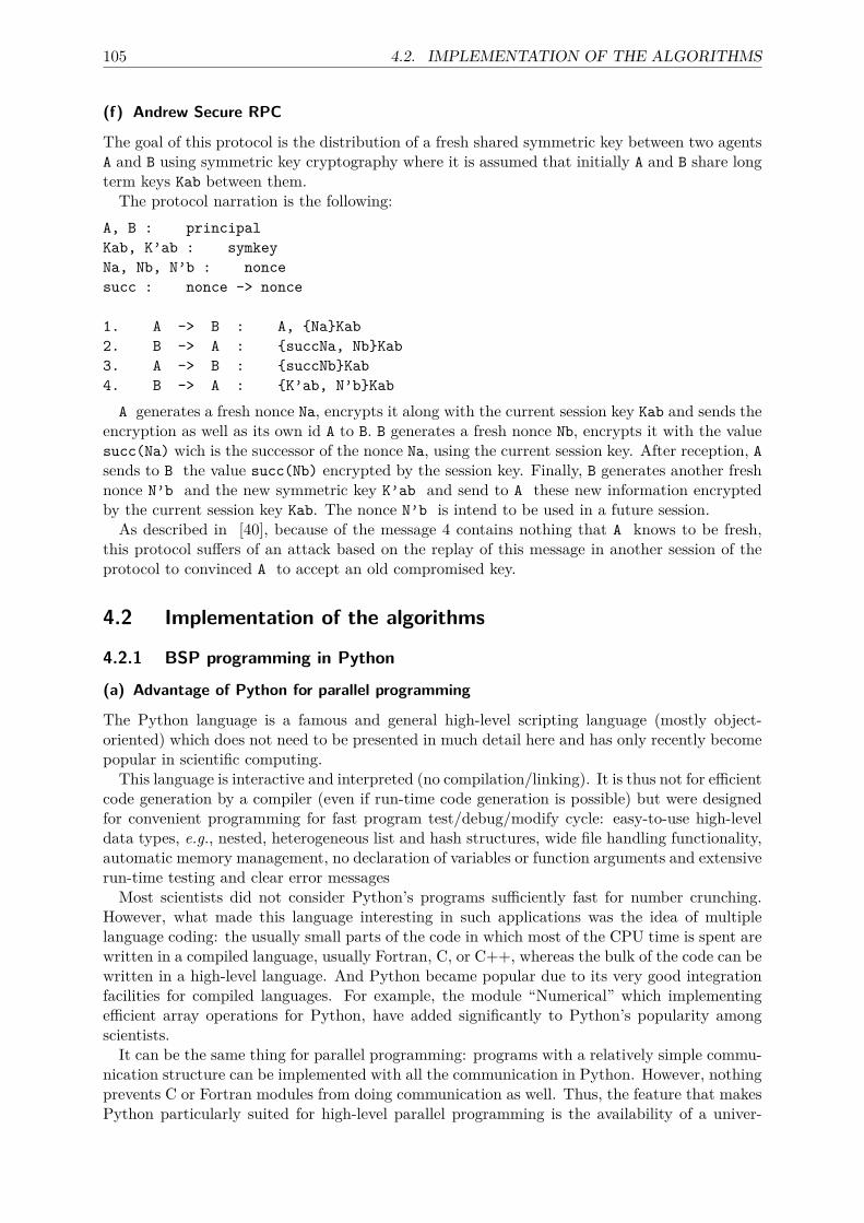
105 4.2. IMPLEMENTATION OF THE ALGORITHMS
(f) Andrew Secure RPC
The goal of this protocol is the distribution of a fresh shared symmetric key between two agentsA and B using symmetric key cryptography where it is assumed that initially A and B share longterm keys Kab between them.The protocol narration is the following:
A, B : principalKab, K’ab : symkeyNa, Nb, N’b : noncesucc : nonce -> nonce
1. A -> B : A, {Na}Kab2. B -> A : {succNa, Nb}Kab3. A -> B : {succNb}Kab4. B -> A : {K’ab, N’b}Kab
A generates a fresh nonce Na, encrypts it along with the current session key Kab and sends theencryption as well as its own id A to B. B generates a fresh nonce Nb, encrypts it with the valuesucc(Na) wich is the successor of the nonce Na, using the current session key. After reception, Asends to B the value succ(Nb) encrypted by the session key. Finally, B generates another freshnonce N’b and the new symmetric key K’ab and send to A these new information encryptedby the current session key Kab. The nonce N’b is intend to be used in a future session.
As described in [40], because of the message 4 contains nothing that A knows to be fresh,this protocol suffers of an attack based on the replay of this message in another session of theprotocol to convinced A to accept an old compromised key.
4.2 Implementation of the algorithms
4.2.1 BSP programming in Python
(a) Advantage of Python for parallel programming
The Python language is a famous and general high-level scripting language (mostly object-oriented) which does not need to be presented in much detail here and has only recently becomepopular in scientific computing.This language is interactive and interpreted (no compilation/linking). It is thus not for efficient
code generation by a compiler (even if run-time code generation is possible) but were designedfor convenient programming for fast program test/debug/modify cycle: easy-to-use high-leveldata types, e.g., nested, heterogeneous list and hash structures, wide file handling functionality,automatic memory management, no declaration of variables or function arguments and extensiverun-time testing and clear error messagesMost scientists did not consider Python’s programs sufficiently fast for number crunching.
However, what made this language interesting in such applications was the idea of multiplelanguage coding: the usually small parts of the code in which most of the CPU time is spent arewritten in a compiled language, usually Fortran, C, or C++, whereas the bulk of the code can bewritten in a high-level language. And Python became popular due to its very good integrationfacilities for compiled languages. For example, the module “Numerical” which implementingefficient array operations for Python, have added significantly to Python’s popularity amongscientists.It can be the same thing for parallel programming: programs with a relatively simple commu-
nication structure can be implemented with all the communication in Python. However, nothingprevents C or Fortran modules from doing communication as well. Thus, the feature that makesPython particularly suited for high-level parallel programming is the availability of a univer-
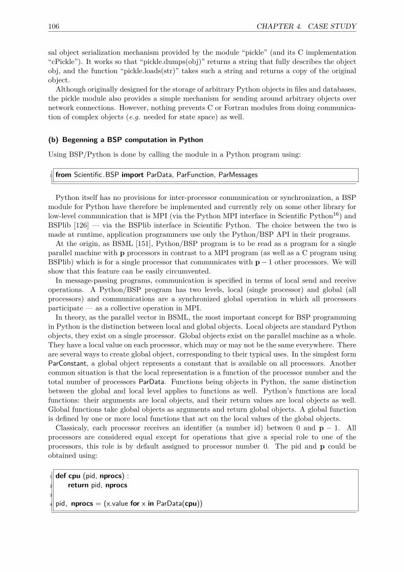
106 CHAPTER 4. CASE STUDY
sal object serialization mechanism provided by the module “pickle” (and its C implementation“cPickle”). It works so that “pickle.dumps(obj)” returns a string that fully describes the objectobj, and the function “pickle.loads(str)” takes such a string and returns a copy of the originalobject.Although originally designed for the storage of arbitrary Python objects in files and databases,
the pickle module also provides a simple mechanism for sending around arbitrary objects overnetwork connections. However, nothing prevents C or Fortran modules from doing communica-tion of complex objects (e.g. needed for state space) as well.
(b) Begenning a BSP computation in Python
Using BSP/Python is done by calling the module in a Python program using:
1 from Scientific.BSP import ParData, ParFunction, ParMessages
Python itself has no provisions for inter-processor communication or synchronization, a BSPmodule for Python have therefore be implemented and currently rely on some other library forlow-level communication that is MPI (via the Python MPI interface in Scientific Python16) andBSPlib [126] — via the BSPlib interface in Scientific Python. The choice between the two ismade at runtime, application programmers use only the Python/BSP API in their programs.At the origin, as BSML [151], Python/BSP program is to be read as a program for a single
parallel machine with p processors in contrast to a MPI program (as well as a C program usingBSPlib) which is for a single processor that communicates with p− 1 other processors. We willshow that this feature can be easily circumvented.In message-passing programs, communication is specified in terms of local send and receive
operations. A Python/BSP program has two levels, local (single processor) and global (allprocessors) and communications are a synchronized global operation in which all processorsparticipate — as a collective operation in MPI.In theory, as the parallel vector in BSML, the most important concept for BSP programming
in Python is the distinction between local and global objects. Local objects are standard Pythonobjects, they exist on a single processor. Global objects exist on the parallel machine as a whole.They have a local value on each processor, which may or may not be the same everywhere. Thereare several ways to create global object, corresponding to their typical uses. In the simplest formParConstant, a global object represents a constant that is available on all processors. Anothercommon situation is that the local representation is a function of the processor number and thetotal number of processors ParData. Functions being objects in Python, the same distinctionbetween the global and local level applies to functions as well. Python’s functions are localfunctions: their arguments are local objects, and their return values are local objects as well.Global functions take global objects as arguments and return global objects. A global functionis defined by one or more local functions that act on the local values of the global objects.Classicaly, each processor receives an identifier (a number id) between 0 and p − 1. All
processors are considered equal except for operations that give a special role to one of theprocessors, this role is by default assigned to processor number 0. The pid and p could beobtained using:
1 def cpu (pid, nprocs) :2 return pid, nprocs3
4 pid, nprocs = (x.value for x in ParData(cpu))
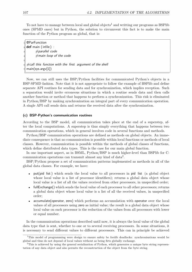
107 4.2. IMPLEMENTATION OF THE ALGORITHMS
To not have to manage between local and global objects1 and writting our programs as BSPlibones (SPMD ones) but in Python, the solution to circumvent this fact is to make the mainfunction of the Python program as global, that is:
1 @ParFunction2 def main ( infile ) :3 #parallel code4 #main loop of the code5
6 #call this functon with the first argument of the shell7 main(sys.argv[1])
Now, we can still uses the BSP/Python facilities for communicated Python’s objects in aBSP-SPMD fashion. Note that it is not appropriate to follow the example of BSPlib and defineseparate API routines for sending data and for synchronization, which implies reception. Sucha separation would invite erroneous situations in which a routine sends data and then callsanother function or method that happens to perform a synchronization. This risk is eliminatedin Python/BSP by making synchronization an integral part of every communication operation.A single API call sends data and returns the received data after the synchronization.
(c) BSP-Python’s communication routines
According to the BSP model, all communication takes place at the end of a superstep, af-ter the local computations. A superstep is thus simply everything that happens between twocommunication operations, which in general involves code in several functions and methods.Python/BSP communication operations are defined as methods on global objects. An imme-
diate consequence is that no communication is possible within local functions or methods of localclasses. However, communication is possible within the methods of global classes of functions,which define distributed data types. This is the case for our main global function.In one important aspect, as in BSML, Python/BSP is much higher-level than BSPlib for C:
communication operations can transmit almost any kind of data2.BSP/Python propose a set of communication patterns implemented as methods in all of the
global data classes. For example, we have:
• put(pid list ) which sends the local value to all processors in pid list (a global objectwhose local value is a list of processor identifiers); returns a global data object whoselocal value is a list of all the values received from other processors, in unspecified order;
• fullExchange() which sends the local value of each processor to all other processors; returnsa global data object whose local value is a list of all the received values, in unspecifiedorder;
• accumulate(operator, zero) which performs an accumulation with operator over the localvalues of all processors using zero as initial value; the result is a global data object whoselocal value on each processor is the reduction of the values from all processors with loweror equal number.
In the communication operations described until now, it is always the local value of the globaldata type that is sent, whether to one or to several receiving processors. In some situations, itis necessary to send different values to different processors. This can in principle be achieved
1This model of programming were design to ensure safety be fordib deadlocks: synchronisations would beglobal and thus do not depend of local values without as being firts globally exchange.
2This is achieved by using the general serialization of Python, which generates a unique byte string represen-tation of any data object and also permits the reconstruction of the object from the byte string.
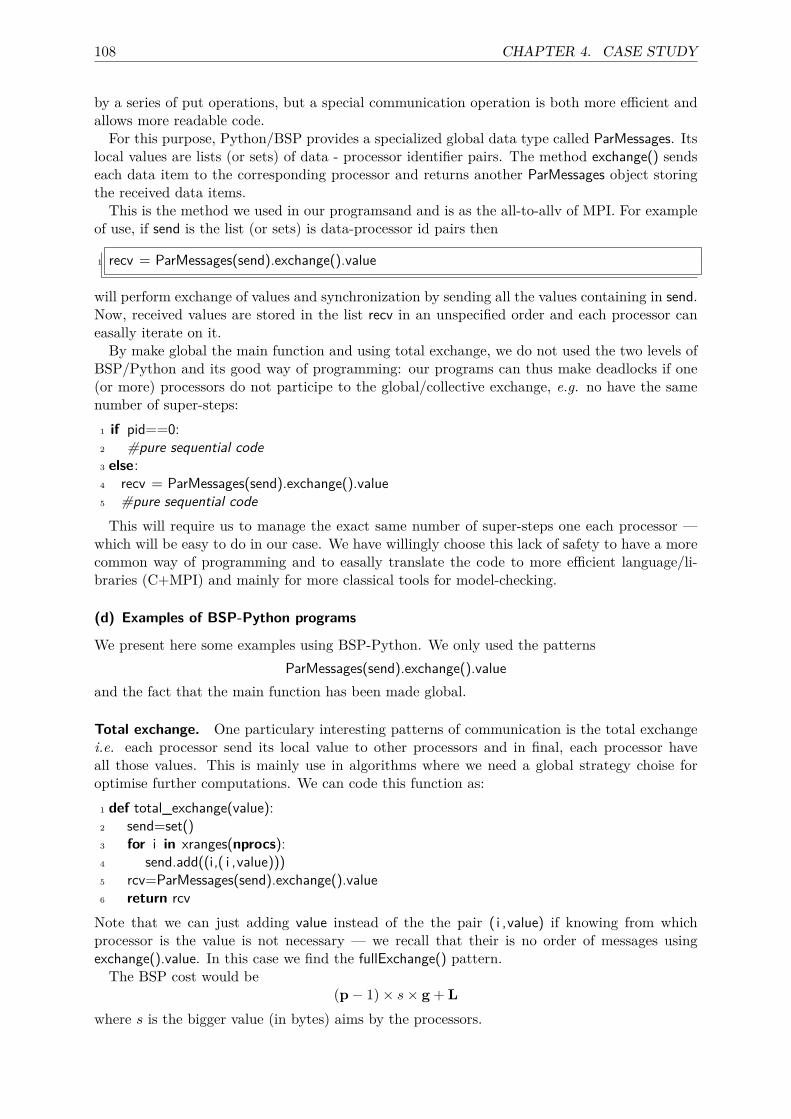
108 CHAPTER 4. CASE STUDY
by a series of put operations, but a special communication operation is both more efficient andallows more readable code.For this purpose, Python/BSP provides a specialized global data type called ParMessages. Its
local values are lists (or sets) of data - processor identifier pairs. The method exchange() sendseach data item to the corresponding processor and returns another ParMessages object storingthe received data items.This is the method we used in our programsand and is as the all-to-allv of MPI. For example
of use, if send is the list (or sets) is data-processor id pairs then
1 recv = ParMessages(send).exchange().value
will perform exchange of values and synchronization by sending all the values containing in send.Now, received values are stored in the list recv in an unspecified order and each processor caneasally iterate on it.By make global the main function and using total exchange, we do not used the two levels of
BSP/Python and its good way of programming: our programs can thus make deadlocks if one(or more) processors do not participe to the global/collective exchange, e.g. no have the samenumber of super-steps:
1 if pid==0:2 #pure sequential code3 else:4 recv = ParMessages(send).exchange().value5 #pure sequential codeThis will require us to manage the exact same number of super-steps one each processor —
which will be easy to do in our case. We have willingly choose this lack of safety to have a morecommon way of programming and to easally translate the code to more efficient language/li-braries (C+MPI) and mainly for more classical tools for model-checking.
(d) Examples of BSP-Python programs
We present here some examples using BSP-Python. We only used the patternsParMessages(send).exchange().value
and the fact that the main function has been made global.
Total exchange. One particulary interesting patterns of communication is the total exchangei.e. each processor send its local value to other processors and in final, each processor haveall those values. This is mainly use in algorithms where we need a global strategy choise foroptimise further computations. We can code this function as:
1 def total_exchange(value):2 send=set()3 for i in xranges(nprocs):4 send.add((i,( i ,value)))5 rcv=ParMessages(send).exchange().value6 return rcvNote that we can just adding value instead of the the pair ( i ,value) if knowing from whichprocessor is the value is not necessary — we recall that their is no order of messages usingexchange().value. In this case we find the fullExchange() pattern.
The BSP cost would be(p− 1)× s× g + L
where s is the bigger value (in bytes) aims by the processors.
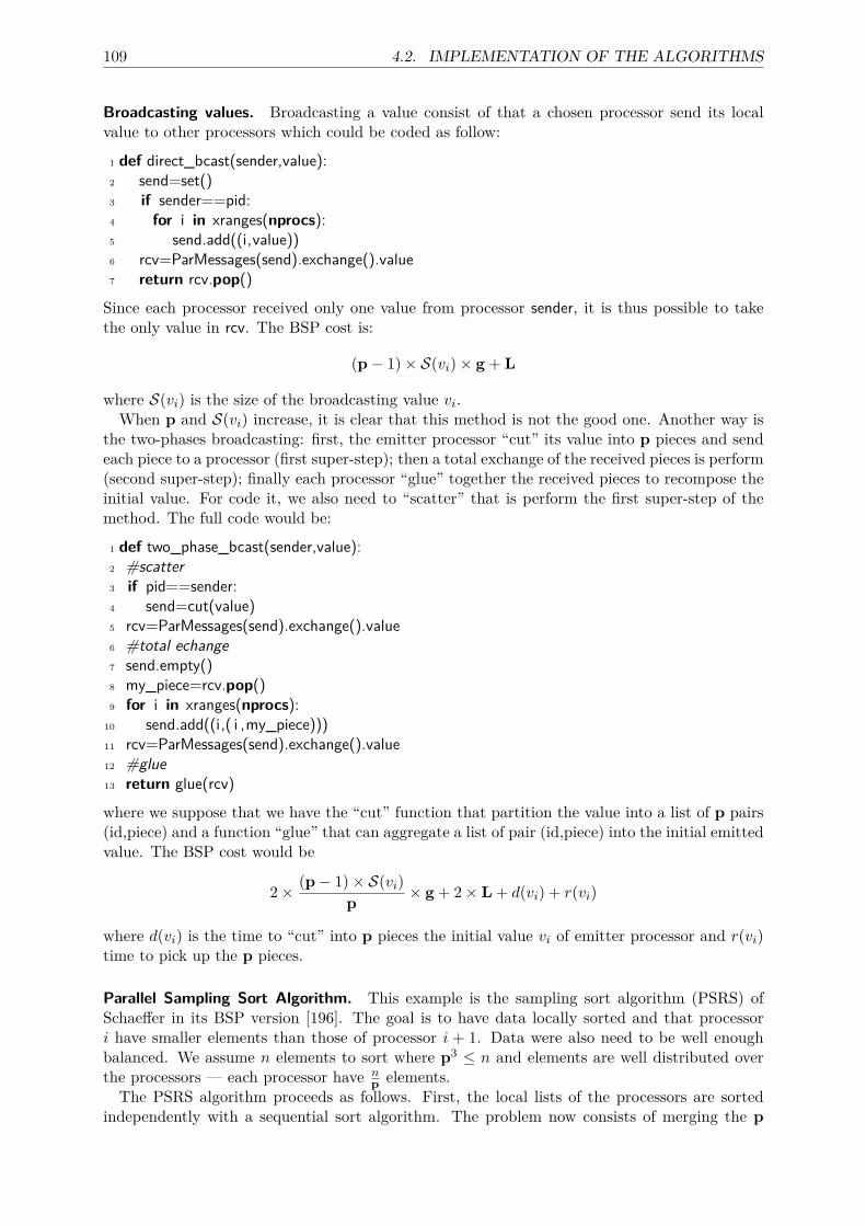
109 4.2. IMPLEMENTATION OF THE ALGORITHMS
Broadcasting values. Broadcasting a value consist of that a chosen processor send its localvalue to other processors which could be coded as follow:
1 def direct_bcast(sender,value):2 send=set()3 if sender==pid:4 for i in xranges(nprocs):5 send.add((i,value))6 rcv=ParMessages(send).exchange().value7 return rcv.pop()Since each processor received only one value from processor sender, it is thus possible to takethe only value in rcv. The BSP cost is:
(p− 1)× S(vi)× g + L
where S(vi) is the size of the broadcasting value vi.When p and S(vi) increase, it is clear that this method is not the good one. Another way is
the two-phases broadcasting: first, the emitter processor “cut” its value into p pieces and sendeach piece to a processor (first super-step); then a total exchange of the received pieces is perform(second super-step); finally each processor “glue” together the received pieces to recompose theinitial value. For code it, we also need to “scatter” that is perform the first super-step of themethod. The full code would be:
1 def two_phase_bcast(sender,value):2 #scatter3 if pid==sender:4 send=cut(value)5 rcv=ParMessages(send).exchange().value6 #total echange7 send.empty()8 my_piece=rcv.pop()9 for i in xranges(nprocs):
10 send.add((i,( i ,my_piece)))11 rcv=ParMessages(send).exchange().value12 #glue13 return glue(rcv)where we suppose that we have the “cut” function that partition the value into a list of p pairs(id,piece) and a function “glue” that can aggregate a list of pair (id,piece) into the initial emittedvalue. The BSP cost would be
2× (p− 1)× S(vi)p × g + 2× L + d(vi) + r(vi)
where d(vi) is the time to “cut” into p pieces the initial value vi of emitter processor and r(vi)time to pick up the p pieces.
Parallel Sampling Sort Algorithm. This example is the sampling sort algorithm (PSRS) ofSchaeffer in its BSP version [196]. The goal is to have data locally sorted and that processori have smaller elements than those of processor i + 1. Data were also need to be well enoughbalanced. We assume n elements to sort where p3 ≤ n and elements are well distributed overthe processors — each processor have n
p elements.The PSRS algorithm proceeds as follows. First, the local lists of the processors are sorted
independently with a sequential sort algorithm. The problem now consists of merging the p
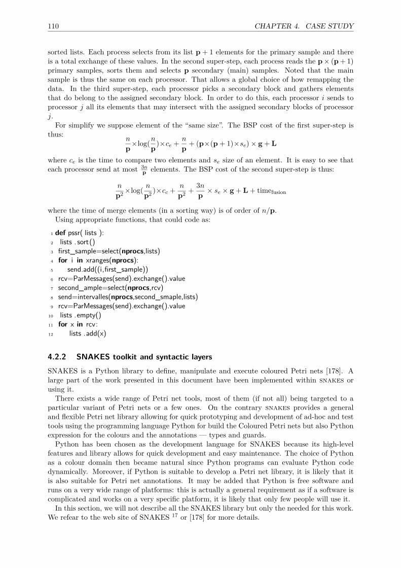
110 CHAPTER 4. CASE STUDY
sorted lists. Each process selects from its list p + 1 elements for the primary sample and thereis a total exchange of these values. In the second super-step, each process reads the p× (p + 1)primary samples, sorts them and selects p secondary (main) samples. Noted that the mainsample is thus the same on each processor. That allows a global choice of how remapping thedata. In the third super-step, each processor picks a secondary block and gathers elementsthat do belong to the assigned secondary block. In order to do this, each processor i sends toprocessor j all its elements that may intersect with the assigned secondary blocks of processorj.For simplify we suppose element of the “same size”. The BSP cost of the first super-step is
thus:n
p×log(np)×ce + n
p + (p×(p + 1)×se)× g + L
where ce is the time to compare two elements and se size of an element. It is easy to see thateach processor send at most 3n
p elements. The BSP cost of the second super-step is thus:
n
p2×log( np2 )×cc + n
p2 + 3np × se × g + L + timefusion
where the time of merge elements (in a sorting way) is of order of n/p.Using appropriate functions, that could code as:
1 def pssr( lists ):2 lists . sort()3 first_sample=select(nprocs,lists)4 for i in xranges(nprocs):5 send.add((i,first_sample))6 rcv=ParMessages(send).exchange().value7 second_ample=select(nprocs,rcv)8 send=intervalles(nprocs,second_smaple,lists)9 rcv=ParMessages(send).exchange().value
10 lists .empty()11 for x in rcv:12 lists .add(x)
4.2.2 SNAKES toolkit and syntactic layersSNAKES is a Python library to define, manipulate and execute coloured Petri nets [178]. Alarge part of the work presented in this document have been implemented within snakes orusing it.There exists a wide range of Petri net tools, most of them (if not all) being targeted to a
particular variant of Petri nets or a few ones. On the contrary snakes provides a generaland flexible Petri net library allowing for quick prototyping and development of ad-hoc and testtools using the programming language Python for build the Coloured Petri nets but also Pythonexpression for the colours and the annotations — types and guards.Python has been chosen as the development language for SNAKES because its high-level
features and library allows for quick development and easy maintenance. The choice of Pythonas a colour domain then became natural since Python programs can evaluate Python codedynamically. Moreover, if Python is suitable to develop a Petri net library, it is likely that itis also suitable for Petri net annotations. It may be added that Python is free software andruns on a very wide range of platforms: this is actually a general requirement as if a software iscomplicated and works on a very specific platform, it is likely that only few people will use it.In this section, we will not describe all the SNAKES library but only the needed for this work.
We refear to the web site of SNAKES 17 or [178] for more details.
111 4.2. IMPLEMENTATION OF THE ALGORITHMS
(a) Architecture
SNAKES is centred on a core library that defines classes related to Petri nets. Then, a setof extension modules, i.e., plugins, allow to add features to the core library or to change itsbehaviour. SNAKES is organised as a core hierarchy of modules (plus additional internal onesnot listed here):
• snakes is the top-level module and defines exceptions used throughout the library;• snakes.data defines basic data types (e.g. multisets and substitutions) and data manipu-
lation functions (e.g. Cartesian product);• snakes.typing defines a typing system used to restrict the tokens allowed in a place;• snakes.nets defines all the classes directly related to Petri nets: places, transitions, arcs,
nets, markings, reachability graphs, etc; it also exposes all the api from the modulesabove;
• snakes.plugins is the root for all the extension modules of snakes.
snakes is designed so that it can represent Petri nets in a very general fashion:
• Each transition has a guard that can be any Python Boolean expression;• Each place has a type that can be an arbitrary Python Boolean function that is used to
accept or refuse tokens;• Tokens may be arbitrary Python objects;• Input arcs (i.e. from places to transitions) can be labelled by values that can be arbitrary
Python object (to consume a known value), variables (to bind a token to a variable name),tuples of such objects (to match structured tokens, with nesting allowed), or multisets ofall these objects (to consume several tokens); new kind of arcs may be added (e.g. readand flush arcs are provided as simple extensions of existing arcs);
• Output arcs (i.e. from transitions to places) can be labelled the same way as input arcs,moreover, they can be labelled by arbitrary Python expressions to compute new valuesto be produced;
• A Petri net with these annotations is fully executable, the transition rule being that ofcoloured Petri nets: all the possible enabling bindings of a transition can be computedby snakes and used for firing.
snakes delegates all the computational aspects of Petri nets to Python. In particular, atoken is an arbitrary Python object, transitions execution can be guarded by arbitrary PythonBoolean expressions, and so on. As a result, a Petri net in snakes is mainly a skeleton withvery general behavioural rules (consume and produce tokens in places through the execution oftransitions) and with the full power of a programming language at any point where a computationis required. snakes itself is programmed in Python and uses the capability of the language todynamically evaluate arbitrary statements. Using the same programming language for snakesand its extension language is a major advantage for the generality: Petri nets in snakes can usesnakes as a library and work on Petri nets. For instance, as a token in snakes may be anyPython object, it could be an instance of the Petri net class of snakes.
(b) Main features
Apart from the possibility to handle Python-coloured Petri nets, the most noticeable otherfeatures of snakes used in this work are:
• Flexible typing system for places: a type is understood as a set defined by comprehension;so, each place is equipped with a type checker to test whether a given value can be storedor not in the place; using module snakes.typing, basic types may be defined and complextypes may be obtained using various type operations (like union, intersection, difference,complement, etc.); user-defined Boolean functions can also be used as type checkers;
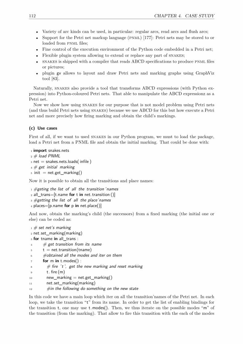
112 CHAPTER 4. CASE STUDY
• Variety of arc kinds can be used, in particular: regular arcs, read arcs and flush arcs;• Support for the Petri net markup language (pnml) [177]: Petri nets may be stored to or
loaded from pnml files;• Fine control of the execution environment of the Python code embedded in a Petri net;• Flexible plugin system allowing to extend or replace any part of snakes;• snakes is shipped with a compiler that reads ABCD specifications to produce pnml files
or pictures;• plugin gv allows to layout and draw Petri nets and marking graphs using GraphViz
tool [83].
Naturally, snakes also provide a tool that transforms ABCD expressions (with Python ex-pression) into Python-coloured Petri nets. That able to manipulate the ABCD expressionz as aPetri net.
Now we show how using snakes for our purpose that is not model problem using Petri nets(and thus build Petri nets using snakes) because we use ABCD for this but how execute a Petrinet and more precisely how firing marking and obtain the child’s markings.
(c) Use cases
First of all, if we want to used snakes in our Python program, we must to load the package,load a Petri net from a PNML file and obtain the initial marking. That could be done with:
1 import snakes.nets2 # load PNML3 net = snakes.nets.loads( infile )4 # get initial marking5 init = net.get_marking()
Now it is possible to obtain all the transitions and place names:
1 #geting the list of all the transition ’names2 all_trans=[t.name for t in net. transition ()]3 #getting the list of all the place’names4 places=[p.name for p in net.place()]
And now, obtain the marking’s child (the successors) from a fixed marking (the initial one orelse) can be coded as:
1 # set net’s marking2 net.set_marking(marking)3 for tname in all_trans :4 # get transition from its name5 t = net.transition(tname)6 #obtained all the modes and iter on them7 for m in t.modes() :8 # fire ’t ’, get the new marking and reset marking9 t . fire (m)
10 new_marking = net.get_marking()11 net.set_marking(marking)12 #in the following do something on the new state
In this code we have a main loop which iter on all the transition’names of the Petri net. In eachloop, we take the transition “t” from its name. In order to get the list of enabling bindings forthe transition t, one may use t .modes(). Then, we thus iterate on the possible modes “m” ofthe transition (from the marking). That allow to fire this transition with the each of the modes
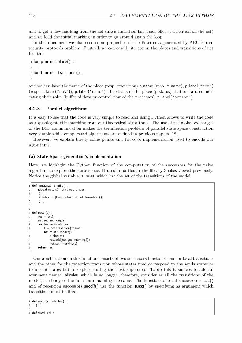
113 4.2. IMPLEMENTATION OF THE ALGORITHMS
and to get a new marking from the net (fire a transition has a side effet of execution on the net)and we load the initial marking in order to go around again the loop.In this document we also used some properties of the Petri nets generated by ABCD from
security protocols problem. First all, we can easally iterate on the places and transitions of netlike this
1 for p in net.place() :2 ...3 for t in net. transition () :4 ...and we can have the name of the place (resp. transition) p.name (resp. t .name), p. label("net")(resp. t . label("net")), p. label("name"), the status of the place (p.status) that is statuses indi-cating their roles (buffer of data or control flow of the processes), t . label("action")
4.2.3 Parallel algorithmsIt is easy to see that the code is very simple to read and using Python allows to write the codeas a quasi-syntactic matching from our theoretical algorithms. The use of the global exchangesof the BSP communication makes the termination problem of parallel state space constructionvery simple while complicated algorithms are defined in previous papers [18].However, we explain briefly some points and tricks of implementation used to encode our
algorithms.
(a) State Space generation’s implementation
Here, we highlight the Python function of the computation of the successors for the naivealgorithm to explore the state space. It uses in particular the library Snakes viewed previously.Notice the global variable allrules which list the set of the transitions of the model.
1 def initialize ( infile ) :2 global net, s0, allrules , places3 (...)4 allrules = [t.name for t in net. transition ()]5 (...)678 def succ (s) :9 res = set()
10 net.set_marking(s)11 for tname in allrules :12 t = net.transition(tname)13 for m in t.modes() :14 t . fire (m)15 res .add(net.get_marking())16 net.set_marking(s)17 return res
Our amelioration on this function consists of two successors functions: one for local transitionsand the other for the reception transition whose states fired correspond to the sends states orto unsent states but to explore during the next superstep. To do this it suffices to add anargument named allrules which is no longer, therefore, consider as all the transitions of themodel, the body of the function remaining the same. The functions of local successors succL()and of reception successors succR() use the function succ() by specifying as argument whichtransitions must be fired.
1 def succ (s, allrules ) :2 (...)34 def succL (s) :
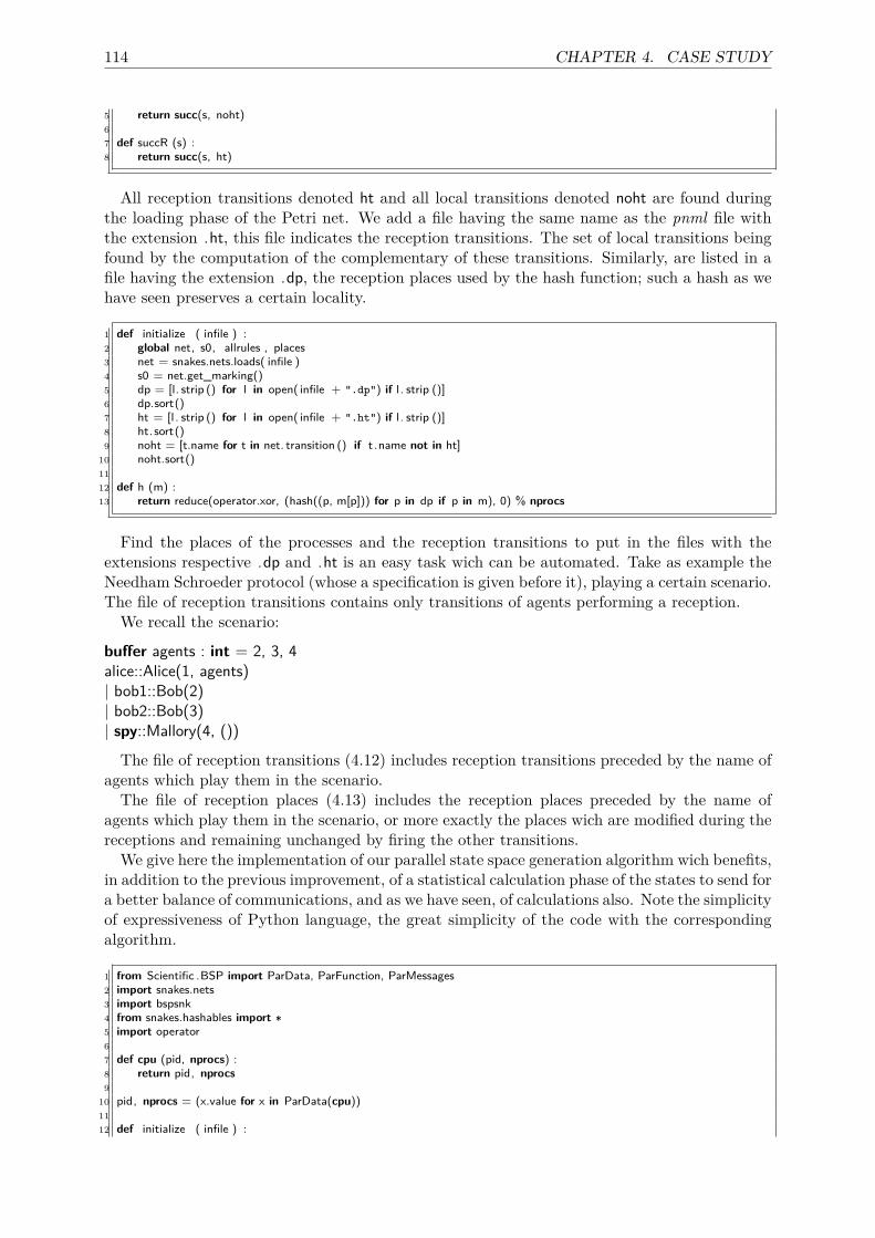
114 CHAPTER 4. CASE STUDY
5 return succ(s, noht)67 def succR (s) :8 return succ(s, ht)
All reception transitions denoted ht and all local transitions denoted noht are found duringthe loading phase of the Petri net. We add a file having the same name as the pnml file withthe extension .ht, this file indicates the reception transitions. The set of local transitions beingfound by the computation of the complementary of these transitions. Similarly, are listed in afile having the extension .dp, the reception places used by the hash function; such a hash as wehave seen preserves a certain locality.
1 def initialize ( infile ) :2 global net, s0, allrules , places3 net = snakes.nets.loads( infile )4 s0 = net.get_marking()5 dp = [l. strip () for l in open( infile + ".dp") if l. strip ()]6 dp.sort()7 ht = [l. strip () for l in open( infile + ".ht") if l. strip ()]8 ht. sort()9 noht = [t.name for t in net. transition () if t .name not in ht]
10 noht.sort()1112 def h (m) :13 return reduce(operator.xor, (hash((p, m[p])) for p in dp if p in m), 0) % nprocs
Find the places of the processes and the reception transitions to put in the files with theextensions respective .dp and .ht is an easy task wich can be automated. Take as example theNeedham Schroeder protocol (whose a specification is given before it), playing a certain scenario.The file of reception transitions contains only transitions of agents performing a reception.We recall the scenario:
buffer agents : int = 2, 3, 4alice::Alice(1, agents)| bob1::Bob(2)| bob2::Bob(3)| spy::Mallory(4, ())
The file of reception transitions (4.12) includes reception transitions preceded by the name ofagents which play them in the scenario.The file of reception places (4.13) includes the reception places preceded by the name of
agents which play them in the scenario, or more exactly the places wich are modified during thereceptions and remaining unchanged by firing the other transitions.We give here the implementation of our parallel state space generation algorithm wich benefits,
in addition to the previous improvement, of a statistical calculation phase of the states to send fora better balance of communications, and as we have seen, of calculations also. Note the simplicityof expressiveness of Python language, the great simplicity of the code with the correspondingalgorithm.
1 from Scientific .BSP import ParData, ParFunction, ParMessages2 import snakes.nets3 import bspsnk4 from snakes.hashables import ∗5 import operator67 def cpu (pid, nprocs) :8 return pid, nprocs9
10 pid, nprocs = (x.value for x in ParData(cpu))1112 def initialize ( infile ) :
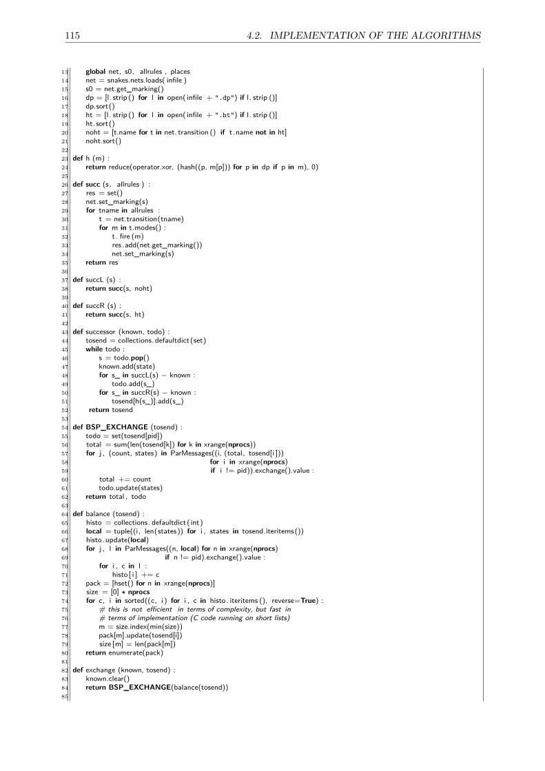
115 4.2. IMPLEMENTATION OF THE ALGORITHMS
13 global net, s0, allrules , places14 net = snakes.nets.loads( infile )15 s0 = net.get_marking()16 dp = [l. strip () for l in open( infile + ".dp") if l. strip ()]17 dp.sort()18 ht = [l. strip () for l in open( infile + ".ht") if l. strip ()]19 ht. sort()20 noht = [t.name for t in net. transition () if t .name not in ht]21 noht.sort()2223 def h (m) :24 return reduce(operator.xor, (hash((p, m[p])) for p in dp if p in m), 0)2526 def succ (s, allrules ) :27 res = set()28 net.set_marking(s)29 for tname in allrules :30 t = net.transition(tname)31 for m in t.modes() :32 t . fire (m)33 res .add(net.get_marking())34 net.set_marking(s)35 return res3637 def succL (s) :38 return succ(s, noht)3940 def succR (s) :41 return succ(s, ht)4243 def successor (known, todo) :44 tosend = collections. defaultdict(set)45 while todo :46 s = todo.pop()47 known.add(state)48 for s_ in succL(s) − known :49 todo.add(s_)50 for s_ in succR(s) − known :51 tosend[h(s_)].add(s_)52 return tosend5354 def BSP_EXCHANGE (tosend) :55 todo = set(tosend[pid])56 total = sum(len(tosend[k]) for k in xrange(nprocs))57 for j , (count, states) in ParMessages((i, (total, tosend[i ]))58 for i in xrange(nprocs)59 if i != pid)).exchange().value :60 total += count61 todo.update(states)62 return total , todo6364 def balance (tosend) :65 histo = collections. defaultdict(int)66 local = tuple((i, len(states)) for i , states in tosend.iteritems())67 histo .update(local)68 for j , l in ParMessages((n, local) for n in xrange(nprocs)69 if n != pid).exchange().value :70 for i , c in l :71 histo [ i ] += c72 pack = [hset() for n in xrange(nprocs)]73 size = [0] ∗ nprocs74 for c, i in sorted((c, i ) for i , c in histo . iteritems (), reverse=True) :75 # this is not efficient in terms of complexity, but fast in76 # terms of implementation (C code running on short lists)77 m = size.index(min(size))78 pack[m].update(tosend[i])79 size [m] = len(pack[m])80 return enumerate(pack)8182 def exchange (known, tosend) :83 known.clear()84 return BSP_EXCHANGE(balance(tosend))85
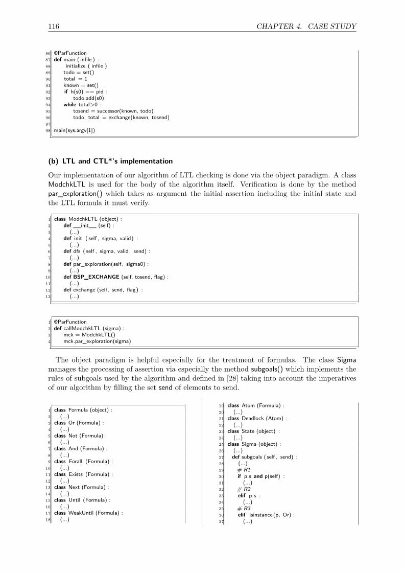
116 CHAPTER 4. CASE STUDY
86 @ParFunction87 def main ( infile ) :88 initialize ( infile )89 todo = set()90 total = 191 known = set()92 if h(s0) == pid :93 todo.add(s0)94 while total>0 :95 tosend = successor(known, todo)96 todo, total = exchange(known, tosend)9798 main(sys.argv[1])
(b) LTL and CTL*’s implementation
Our implementation of our algorithm of LTL checking is done via the object paradigm. A classModchkLTL is used for the body of the algorithm itself. Verification is done by the methodpar_exploration() which takes as argument the initial assertion including the initial state andthe LTL formula it must verify.
1 class ModchkLTL (object) :2 def __init__ (self) :3 (...)4 def init ( self , sigma, valid) :5 (...)6 def dfs ( self , sigma, valid , send) :7 (...)8 def par_exploration(self , sigma0) :9 (...)
10 def BSP_EXCHANGE (self, tosend, flag) :11 (...)12 def exchange (self, send, flag) :13 (...)
1 @ParFunction2 def callModchkLTL (sigma) :3 mck = ModchkLTL()4 mck.par_exploration(sigma)
The object paradigm is helpful especially for the treatment of formulas. The class Sigmamanages the processing of assertion via especially the method subgoals() which implements therules of subgoals used by the algorithm and defined in [28] taking into account the imperativesof our algorithm by filling the set send of elements to send.
1 class Formula (object) :2 (...)3 class Or (Formula) :4 (...)5 class Not (Formula) :6 (...)7 class And (Formula) :8 (...)9 class Forall (Formula) :
10 (...)11 class Exists (Formula) :12 (...)13 class Next (Formula) :14 (...)15 class Until (Formula) :16 (...)17 class WeakUntil (Formula) :18 (...)
19 class Atom (Formula) :20 (...)21 class Deadlock (Atom) :22 (...)23 class State (object) :24 (...)25 class Sigma (object) :26 (...)27 def subgoals ( self , send) :28 (...)29 # R130 if p.s and p(self) :31 (...)32 # R233 elif p.s :34 (...)35 # R336 elif isinstance(p, Or) :37 (...)
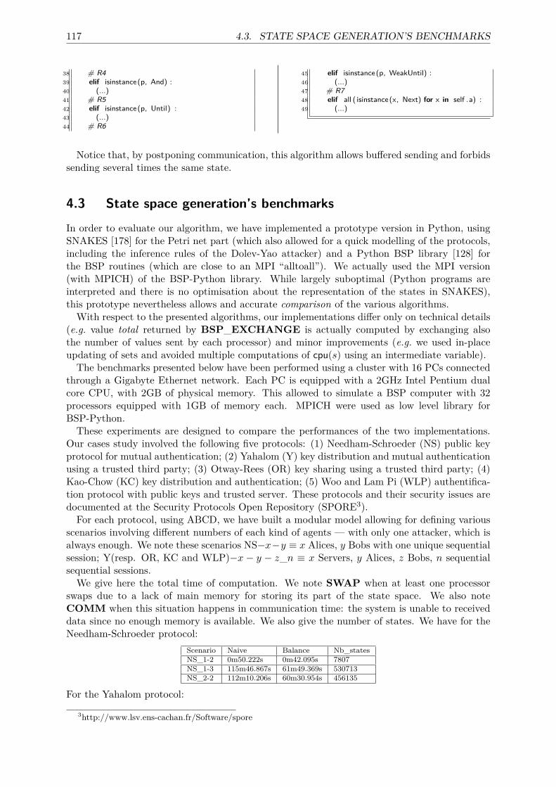
117 4.3. STATE SPACE GENERATION’S BENCHMARKS
38 # R439 elif isinstance(p, And) :40 (...)41 # R542 elif isinstance(p, Until) :43 (...)44 # R6
45 elif isinstance(p, WeakUntil) :46 (...)47 # R748 elif all ( isinstance(x, Next) for x in self .a) :49 (...)
Notice that, by postponing communication, this algorithm allows buffered sending and forbidssending several times the same state.
4.3 State space generation’s benchmarks
In order to evaluate our algorithm, we have implemented a prototype version in Python, usingSNAKES [178] for the Petri net part (which also allowed for a quick modelling of the protocols,including the inference rules of the Dolev-Yao attacker) and a Python BSP library [128] forthe BSP routines (which are close to an MPI “alltoall”). We actually used the MPI version(with MPICH) of the BSP-Python library. While largely suboptimal (Python programs areinterpreted and there is no optimisation about the representation of the states in SNAKES),this prototype nevertheless allows and accurate comparison of the various algorithms.
With respect to the presented algorithms, our implementations differ only on technical details(e.g. value total returned by BSP_EXCHANGE is actually computed by exchanging alsothe number of values sent by each processor) and minor improvements (e.g. we used in-placeupdating of sets and avoided multiple computations of cpu(s) using an intermediate variable).
The benchmarks presented below have been performed using a cluster with 16 PCs connectedthrough a Gigabyte Ethernet network. Each PC is equipped with a 2GHz Intel Pentium dualcore CPU, with 2GB of physical memory. This allowed to simulate a BSP computer with 32processors equipped with 1GB of memory each. MPICH were used as low level library forBSP-Python.These experiments are designed to compare the performances of the two implementations.
Our cases study involved the following five protocols: (1) Needham-Schroeder (NS) public keyprotocol for mutual authentication; (2) Yahalom (Y) key distribution and mutual authenticationusing a trusted third party; (3) Otway-Rees (OR) key sharing using a trusted third party; (4)Kao-Chow (KC) key distribution and authentication; (5) Woo and Lam Pi (WLP) authentifica-tion protocol with public keys and trusted server. These protocols and their security issues aredocumented at the Security Protocols Open Repository (SPORE3).For each protocol, using ABCD, we have built a modular model allowing for defining various
scenarios involving different numbers of each kind of agents — with only one attacker, which isalways enough. We note these scenarios NS−x−y ≡ x Alices, y Bobs with one unique sequentialsession; Y(resp. OR, KC and WLP)−x − y − z_n ≡ x Servers, y Alices, z Bobs, n sequentialsequential sessions.We give here the total time of computation. We note SWAP when at least one processor
swaps due to a lack of main memory for storing its part of the state space. We also noteCOMM when this situation happens in communication time: the system is unable to receiveddata since no enough memory is available. We also give the number of states. We have for theNeedham-Schroeder protocol:
Scenario Naive Balance Nb_statesNS_1-2 0m50.222s 0m42.095s 7807NS_1-3 115m46.867s 61m49.369s 530713NS_2-2 112m10.206s 60m30.954s 456135
For the Yahalom protocol:
3http://www.lsv.ens-cachan.fr/Software/spore
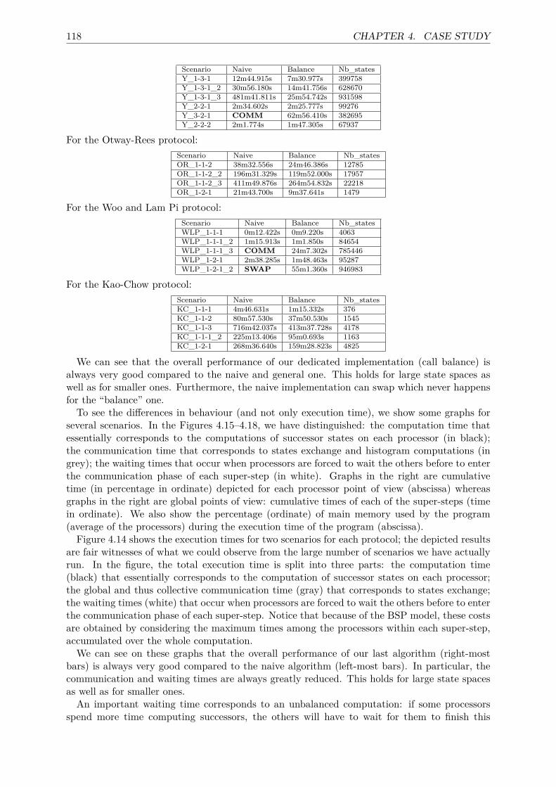
118 CHAPTER 4. CASE STUDY
Scenario Naive Balance Nb_statesY_1-3-1 12m44.915s 7m30.977s 399758Y_1-3-1_2 30m56.180s 14m41.756s 628670Y_1-3-1_3 481m41.811s 25m54.742s 931598Y_2-2-1 2m34.602s 2m25.777s 99276Y_3-2-1 COMM 62m56.410s 382695Y_2-2-2 2m1.774s 1m47.305s 67937
For the Otway-Rees protocol:Scenario Naive Balance Nb_statesOR_1-1-2 38m32.556s 24m46.386s 12785OR_1-1-2_2 196m31.329s 119m52.000s 17957OR_1-1-2_3 411m49.876s 264m54.832s 22218OR_1-2-1 21m43.700s 9m37.641s 1479
For the Woo and Lam Pi protocol:Scenario Naive Balance Nb_statesWLP_1-1-1 0m12.422s 0m9.220s 4063WLP_1-1-1_2 1m15.913s 1m1.850s 84654WLP_1-1-1_3 COMM 24m7.302s 785446WLP_1-2-1 2m38.285s 1m48.463s 95287WLP_1-2-1_2 SWAP 55m1.360s 946983
For the Kao-Chow protocol:Scenario Naive Balance Nb_statesKC_1-1-1 4m46.631s 1m15.332s 376KC_1-1-2 80m57.530s 37m50.530s 1545KC_1-1-3 716m42.037s 413m37.728s 4178KC_1-1-1_2 225m13.406s 95m0.693s 1163KC_1-2-1 268m36.640s 159m28.823s 4825
We can see that the overall performance of our dedicated implementation (call balance) isalways very good compared to the naive and general one. This holds for large state spaces aswell as for smaller ones. Furthermore, the naive implementation can swap which never happensfor the “balance” one.To see the differences in behaviour (and not only execution time), we show some graphs for
several scenarios. In the Figures 4.15–4.18, we have distinguished: the computation time thatessentially corresponds to the computations of successor states on each processor (in black);the communication time that corresponds to states exchange and histogram computations (ingrey); the waiting times that occur when processors are forced to wait the others before to enterthe communication phase of each super-step (in white). Graphs in the right are cumulativetime (in percentage in ordinate) depicted for each processor point of view (abscissa) whereasgraphs in the right are global points of view: cumulative times of each of the super-steps (timein ordinate). We also show the percentage (ordinate) of main memory used by the program(average of the processors) during the execution time of the program (abscissa).Figure 4.14 shows the execution times for two scenarios for each protocol; the depicted results
are fair witnesses of what we could observe from the large number of scenarios we have actuallyrun. In the figure, the total execution time is split into three parts: the computation time(black) that essentially corresponds to the computation of successor states on each processor;the global and thus collective communication time (gray) that corresponds to states exchange;the waiting times (white) that occur when processors are forced to wait the others before to enterthe communication phase of each super-step. Notice that because of the BSP model, these costsare obtained by considering the maximum times among the processors within each super-step,accumulated over the whole computation.We can see on these graphs that the overall performance of our last algorithm (right-most
bars) is always very good compared to the naive algorithm (left-most bars). In particular, thecommunication and waiting times are always greatly reduced. This holds for large state spacesas well as for smaller ones.An important waiting time corresponds to an unbalanced computation: if some processors
spend more time computing successors, the others will have to wait for them to finish this
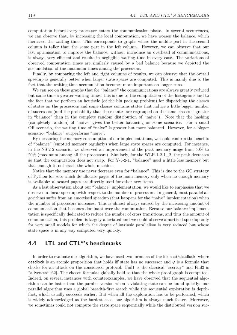
119 4.4. LTL AND CTL*’S BENCHMARKS
computation before every processor enters the communication phase. In several occurrences,we can observe that, by increasing the local computation, we have worsen the balance, whichincreased the waiting time. This corresponds to graphs where the middle part in the secondcolumn is taller than the same part in the left column. However, we can observe that ourlast optimisation to improve the balance, without introduce an overhead of communications,is always very efficient and results in negligible waiting time in every case. The variations ofobserved computation times are similarly caused by a bad balance because we depicted theaccumulation of the maximum times among the processors.Finally, by comparing the left and right columns of results, we can observe that the overall
speedup is generally better when larger state spaces are computed. This is mainly due to thefact that the waiting time accumulation becomes more important on longer runs.We can see on these graphs that for “balance” the communications are always greatly reduced
but some time a greater waiting times: this is due to the computation of the histograms and tothe fact that we perform an heuristic (of the bin packing problem) for dispatching the classesof states on the processors and some classes contains states that induce a little bigger numberof successors (and the probability that these states are regrouped on the same classes is greaterin “balance” than in the complete random distribution of “naive”). Note that the hashing(completely random) of “naive” gives the better balancing on some scenarios. For a smallOR scenario, the waiting time of “naive” is greater but more balanced. However, for a biggerscenario, “balance” outperforms “naive”.By measuring the memory consumption of our implementations, we could confirm the benefits
of “balance” (emptied memory regularly) when large state spaces are computed. For instance,in the NS-2-2 scenario, we observed an improvement of the peak memory usage from 50% to20% (maximum among all the processors). Similarly, for the WLP-1-2-1_2, the peak decreasesso that the computation does not swap. For Y-3-2-1, “balance” used a little less memory butthat enough to not crash the whole machine.Notice that the memory use never decrease even for “balance”. This is due to the GC strategy
of Python for sets which de-allocate pages of the main memory only when no enough memoryis available: allocated pages are directly used for other new items.As a last observation about our “balance” implementation, we would like to emphasise that we
observed a linear speedup with respect to the number of processors. In general, most parallel al-gorithms suffer from an amortised speedup (that happens for the “naive” implementation) whenthe number of processors increases. This is almost always caused by the increasing amount ofcommunication that becomes dominant over the computation. Because our balance implemen-tation is specifically dedicated to reduce the number of cross transitions, and thus the amount ofcommunication, this problem is largely alleviated and we could observe amortised speedup onlyfor very small models for which the degree of intrinsic parallelism is very reduced but whosestate space is in any way computed very quickly.
4.4 LTL and CTL*’s benchmarks
In order to evaluate our algorithm, we have used two formulas of the form ϕUdeadlock, wheredeadlock is an atomic proposition that holds iff state has no successor and ϕ is a formula thatchecks for an attack on the considered protocol: Fml1 is the classical ”secrecy“ and Fml2 is”aliveness“ [62]. The chosen formulas globally hold so that the whole proof graph is computed.Indeed, on several instances with counterexamples, we have observed that the sequential algo-rithm can be faster than the parallel version when a violating state can be found quickly: ourparallel algorithm uses a global breadth-first search while the sequential exploration is depth-first, which usually succeeds earlier. But when all the exploration has to be performed, whichis widely acknowledged as the hardest case, our algorithm is always much faster. Moreover,we sometimes could not compute the state space sequentially while the distributed version suc-
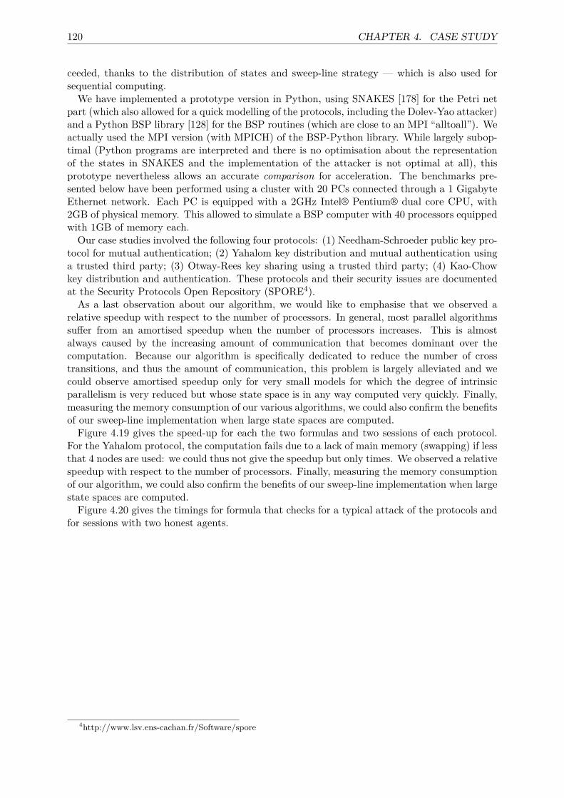
120 CHAPTER 4. CASE STUDY
ceeded, thanks to the distribution of states and sweep-line strategy — which is also used forsequential computing.We have implemented a prototype version in Python, using SNAKES [178] for the Petri net
part (which also allowed for a quick modelling of the protocols, including the Dolev-Yao attacker)and a Python BSP library [128] for the BSP routines (which are close to an MPI “alltoall”). Weactually used the MPI version (with MPICH) of the BSP-Python library. While largely subop-timal (Python programs are interpreted and there is no optimisation about the representationof the states in SNAKES and the implementation of the attacker is not optimal at all), thisprototype nevertheless allows an accurate comparison for acceleration. The benchmarks pre-sented below have been performed using a cluster with 20 PCs connected through a 1 GigabyteEthernet network. Each PC is equipped with a 2GHz Intel® Pentium® dual core CPU, with2GB of physical memory. This allowed to simulate a BSP computer with 40 processors equippedwith 1GB of memory each.Our case studies involved the following four protocols: (1) Needham-Schroeder public key pro-
tocol for mutual authentication; (2) Yahalom key distribution and mutual authentication usinga trusted third party; (3) Otway-Rees key sharing using a trusted third party; (4) Kao-Chowkey distribution and authentication. These protocols and their security issues are documentedat the Security Protocols Open Repository (SPORE4).
As a last observation about our algorithm, we would like to emphasise that we observed arelative speedup with respect to the number of processors. In general, most parallel algorithmssuffer from an amortised speedup when the number of processors increases. This is almostalways caused by the increasing amount of communication that becomes dominant over thecomputation. Because our algorithm is specifically dedicated to reduce the number of crosstransitions, and thus the amount of communication, this problem is largely alleviated and wecould observe amortised speedup only for very small models for which the degree of intrinsicparallelism is very reduced but whose state space is in any way computed very quickly. Finally,measuring the memory consumption of our various algorithms, we could also confirm the benefitsof our sweep-line implementation when large state spaces are computed.Figure 4.19 gives the speed-up for each the two formulas and two sessions of each protocol.
For the Yahalom protocol, the computation fails due to a lack of main memory (swapping) if lessthat 4 nodes are used: we could thus not give the speedup but only times. We observed a relativespeedup with respect to the number of processors. Finally, measuring the memory consumptionof our algorithm, we could also confirm the benefits of our sweep-line implementation when largestate spaces are computed.Figure 4.20 gives the timings for formula that checks for a typical attack of the protocols and
for sessions with two honest agents.
4http://www.lsv.ens-cachan.fr/Software/spore
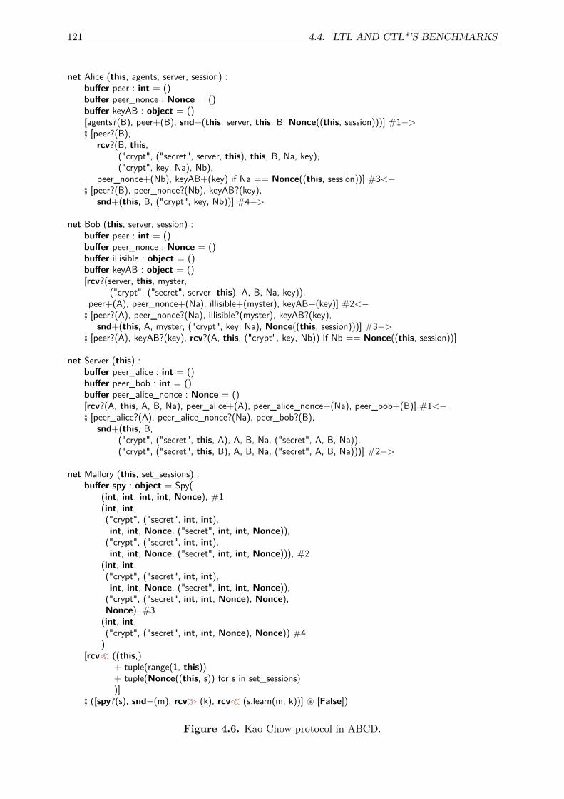
121 4.4. LTL AND CTL*’S BENCHMARKS
net Alice (this, agents, server, session) :buffer peer : int = ()buffer peer_nonce : Nonce = ()buffer keyAB : object = ()[agents?(B), peer+(B), snd+(this, server, this, B, Nonce((this, session)))] #1−># [peer?(B),
rcv?(B, this,("crypt", ("secret", server, this), this, B, Na, key),("crypt", key, Na), Nb),
peer_nonce+(Nb), keyAB+(key) if Na == Nonce((this, session))] #3<−# [peer?(B), peer_nonce?(Nb), keyAB?(key),
snd+(this, B, ("crypt", key, Nb))] #4−>
net Bob (this, server, session) :buffer peer : int = ()buffer peer_nonce : Nonce = ()buffer illisible : object = ()buffer keyAB : object = ()[rcv?(server, this, myster,
("crypt", ("secret", server, this), A, B, Na, key)),peer+(A), peer_nonce+(Na), illisible+(myster), keyAB+(key)] #2<−
# [peer?(A), peer_nonce?(Na), illisible?(myster), keyAB?(key),snd+(this, A, myster, ("crypt", key, Na), Nonce((this, session)))] #3−>
# [peer?(A), keyAB?(key), rcv?(A, this, ("crypt", key, Nb)) if Nb == Nonce((this, session))]
net Server (this) :buffer peer_alice : int = ()buffer peer_bob : int = ()buffer peer_alice_nonce : Nonce = ()[rcv?(A, this, A, B, Na), peer_alice+(A), peer_alice_nonce+(Na), peer_bob+(B)] #1<−# [peer_alice?(A), peer_alice_nonce?(Na), peer_bob?(B),
snd+(this, B,("crypt", ("secret", this, A), A, B, Na, ("secret", A, B, Na)),("crypt", ("secret", this, B), A, B, Na, ("secret", A, B, Na)))] #2−>
net Mallory (this, set_sessions) :buffer spy : object = Spy(
(int, int, int, int, Nonce), #1(int, int,("crypt", ("secret", int, int),int, int, Nonce, ("secret", int, int, Nonce)),("crypt", ("secret", int, int),int, int, Nonce, ("secret", int, int, Nonce))), #2
(int, int,("crypt", ("secret", int, int),int, int, Nonce, ("secret", int, int, Nonce)),("crypt", ("secret", int, int, Nonce), Nonce),Nonce), #3(int, int,("crypt", ("secret", int, int, Nonce), Nonce)) #4)
[rcv� ((this,)+ tuple(range(1, this))+ tuple(Nonce((this, s)) for s in set_sessions))]
# ([spy?(s), snd−(m), rcv� (k), rcv� (s.learn(m, k))] ~ [False])
Figure 4.6. Kao Chow protocol in ABCD.
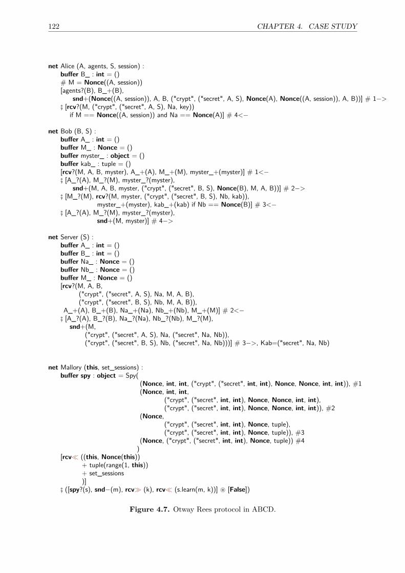
122 CHAPTER 4. CASE STUDY
net Alice (A, agents, S, session) :buffer B_ : int = ()# M = Nonce((A, session))[agents?(B), B_+(B),
snd+(Nonce((A, session)), A, B, ("crypt", ("secret", A, S), Nonce(A), Nonce((A, session)), A, B))] # 1−># [rcv?(M, ("crypt", ("secret", A, S), Na, key))
if M == Nonce((A, session)) and Na == Nonce(A)] # 4<−
net Bob (B, S) :buffer A_ : int = ()buffer M_ : Nonce = ()buffer myster_ : object = ()buffer kab_ : tuple = ()[rcv?(M, A, B, myster), A_+(A), M_+(M), myster_+(myster)] # 1<−# [A_?(A), M_?(M), myster_?(myster),
snd+(M, A, B, myster, ("crypt", ("secret", B, S), Nonce(B), M, A, B))] # 2−># [M_?(M), rcv?(M, myster, ("crypt", ("secret", B, S), Nb, kab)),
myster_+(myster), kab_+(kab) if Nb == Nonce(B)] # 3<−# [A_?(A), M_?(M), myster_?(myster),
snd+(M, myster)] # 4−>
net Server (S) :buffer A_ : int = ()buffer B_ : int = ()buffer Na_ : Nonce = ()buffer Nb_ : Nonce = ()buffer M_ : Nonce = ()[rcv?(M, A, B,
("crypt", ("secret", A, S), Na, M, A, B),("crypt", ("secret", B, S), Nb, M, A, B)),
A_+(A), B_+(B), Na_+(Na), Nb_+(Nb), M_+(M)] # 2<−# [A_?(A), B_?(B), Na_?(Na), Nb_?(Nb), M_?(M),
snd+(M,("crypt", ("secret", A, S), Na, ("secret", Na, Nb)),("crypt", ("secret", B, S), Nb, ("secret", Na, Nb)))] # 3−>, Kab=("secret", Na, Nb)
net Mallory (this, set_sessions) :buffer spy : object = Spy(
(Nonce, int, int, ("crypt", ("secret", int, int), Nonce, Nonce, int, int)), #1(Nonce, int, int,
("crypt", ("secret", int, int), Nonce, Nonce, int, int),("crypt", ("secret", int, int), Nonce, Nonce, int, int)), #2
(Nonce,("crypt", ("secret", int, int), Nonce, tuple),("crypt", ("secret", int, int), Nonce, tuple)), #3
(Nonce, ("crypt", ("secret", int, int), Nonce, tuple)) #4)
[rcv� ((this, Nonce(this))+ tuple(range(1, this))+ set_sessions)]
# ([spy?(s), snd−(m), rcv� (k), rcv� (s.learn(m, k))] ~ [False])
Figure 4.7. Otway Rees protocol in ABCD.
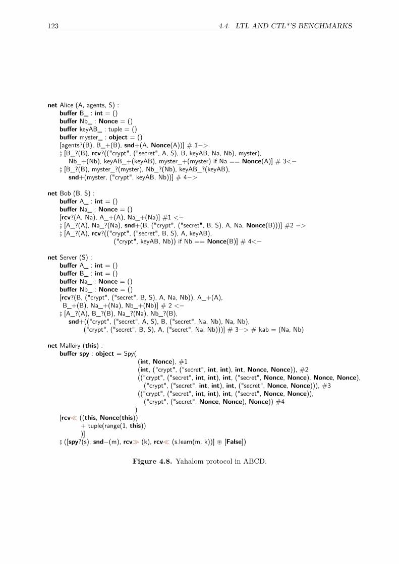
123 4.4. LTL AND CTL*’S BENCHMARKS
net Alice (A, agents, S) :buffer B_ : int = ()buffer Nb_ : Nonce = ()buffer keyAB_ : tuple = ()buffer myster_ : object = ()[agents?(B), B_+(B), snd+(A, Nonce(A))] # 1−># [B_?(B), rcv?(("crypt", ("secret", A, S), B, keyAB, Na, Nb), myster),
Nb_+(Nb), keyAB_+(keyAB), myster_+(myster) if Na == Nonce(A)] # 3<−# [B_?(B), myster_?(myster), Nb_?(Nb), keyAB_?(keyAB),
snd+(myster, ("crypt", keyAB, Nb))] # 4−>
net Bob (B, S) :buffer A_ : int = ()buffer Na_ : Nonce = ()[rcv?(A, Na), A_+(A), Na_+(Na)] #1 <−# [A_?(A), Na_?(Na), snd+(B, ("crypt", ("secret", B, S), A, Na, Nonce(B)))] #2 −># [A_?(A), rcv?(("crypt", ("secret", B, S), A, keyAB),
("crypt", keyAB, Nb)) if Nb == Nonce(B)] # 4<−
net Server (S) :buffer A_ : int = ()buffer B_ : int = ()buffer Na_ : Nonce = ()buffer Nb_ : Nonce = ()[rcv?(B, ("crypt", ("secret", B, S), A, Na, Nb)), A_+(A),B_+(B), Na_+(Na), Nb_+(Nb)] # 2 <−
# [A_?(A), B_?(B), Na_?(Na), Nb_?(B),snd+(("crypt", ("secret", A, S), B, ("secret", Na, Nb), Na, Nb),
("crypt", ("secret", B, S), A, ("secret", Na, Nb)))] # 3−> # kab = (Na, Nb)
net Mallory (this) :buffer spy : object = Spy(
(int, Nonce), #1(int, ("crypt", ("secret", int, int), int, Nonce, Nonce)), #2(("crypt", ("secret", int, int), int, ("secret", Nonce, Nonce), Nonce, Nonce),("crypt", ("secret", int, int), int, ("secret", Nonce, Nonce))), #3
(("crypt", ("secret", int, int), int, ("secret", Nonce, Nonce)),("crypt", ("secret", Nonce, Nonce), Nonce)) #4
)[rcv� ((this, Nonce(this))
+ tuple(range(1, this)))]
# ([spy?(s), snd−(m), rcv� (k), rcv� (s.learn(m, k))] ~ [False])
Figure 4.8. Yahalom protocol in ABCD.
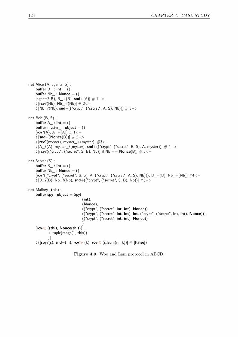
124 CHAPTER 4. CASE STUDY
net Alice (A, agents, S) :buffer B_ : int = ()buffer Nb_ : Nonce = ()[agents?(B), B_+(B), snd+(A)] # 1−># [rcv?(Nb), Nb_+(Nb)] # 2<−# [Nb_?(Nb), snd+(("crypt", ("secret", A, S), Nb))] # 3−>
net Bob (B, S) :buffer A_ : int = ()buffer myster_ : object = ()[rcv?(A), A_+(A)] # 1<−# [snd+(Nonce(B))] # 2−># [rcv?(myster), myster_+(myster)] #3<−# [A_?(A), myster_?(myster), snd+(("crypt", ("secret", B, S), A, myster))] # 4−># [rcv?(("crypt", ("secret", S, B), Nb)) if Nb == Nonce(B)] # 5<−
net Server (S) :buffer B_ : int = ()buffer Nb_ : Nonce = ()[rcv?(("crypt", ("secret", B, S), A, ("crypt", ("secret", A, S), Nb))), B_+(B), Nb_+(Nb)] #4<−# [B_?(B), Nb_?(Nb), snd+(("crypt", ("secret", S, B), Nb))] #5−>
net Mallory (this) :buffer spy : object = Spy(
(int),(Nonce),(("crypt", ("secret", int, int), Nonce)),(("crypt", ("secret", int, int), int, ("crypt", ("secret", int, int), Nonce))),(("crypt", ("secret", int, int), Nonce)))
[rcv� ((this, Nonce(this))+ tuple(range(1, this)))]
# ([spy?(s), snd−(m), rcv� (k), rcv� (s.learn(m, k))] ~ [False])
Figure 4.9. Woo and Lam protocol in ABCD.
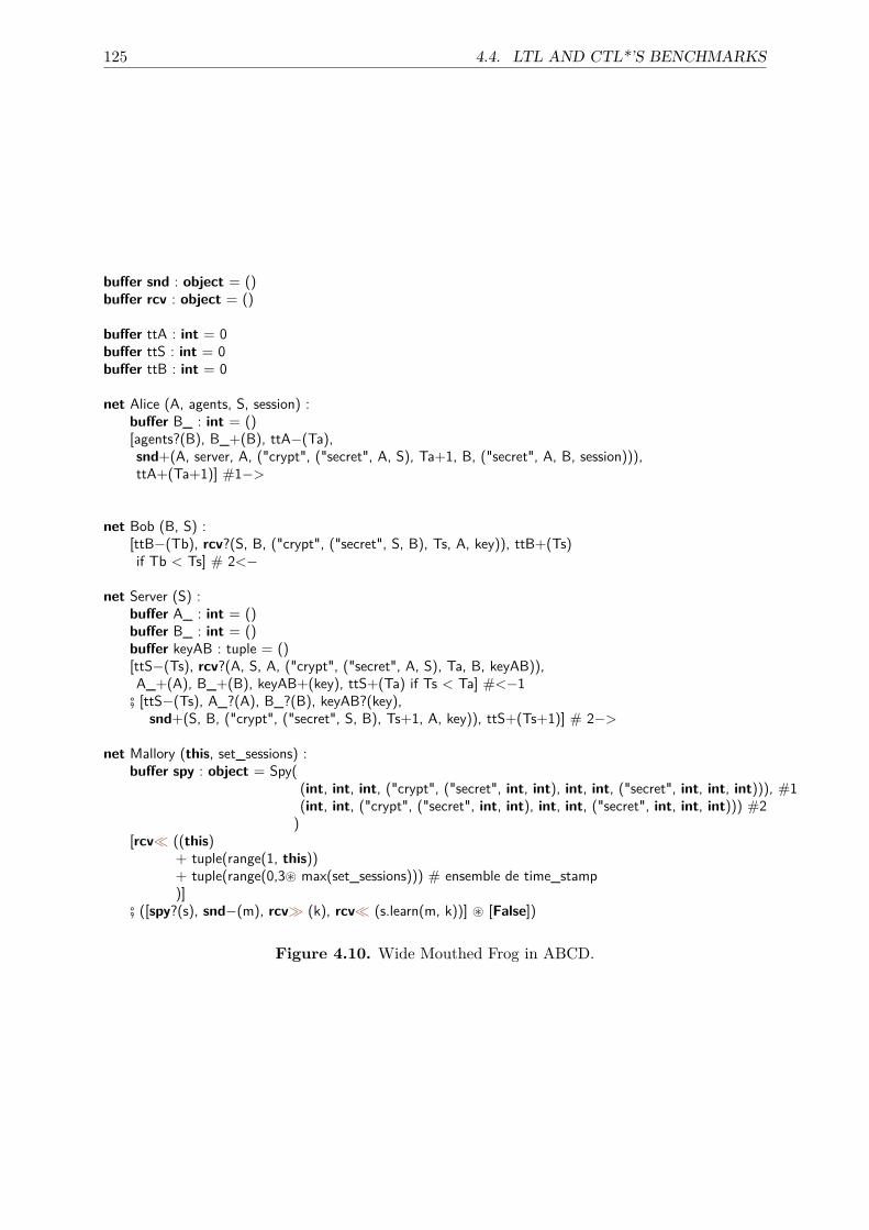
125 4.4. LTL AND CTL*’S BENCHMARKS
buffer snd : object = ()buffer rcv : object = ()
buffer ttA : int = 0buffer ttS : int = 0buffer ttB : int = 0
net Alice (A, agents, S, session) :buffer B_ : int = ()[agents?(B), B_+(B), ttA−(Ta),snd+(A, server, A, ("crypt", ("secret", A, S), Ta+1, B, ("secret", A, B, session))),ttA+(Ta+1)] #1−>
net Bob (B, S) :[ttB−(Tb), rcv?(S, B, ("crypt", ("secret", S, B), Ts, A, key)), ttB+(Ts)if Tb < Ts] # 2<−
net Server (S) :buffer A_ : int = ()buffer B_ : int = ()buffer keyAB : tuple = ()[ttS−(Ts), rcv?(A, S, A, ("crypt", ("secret", A, S), Ta, B, keyAB)),A_+(A), B_+(B), keyAB+(key), ttS+(Ta) if Ts < Ta] #<−1
# [ttS−(Ts), A_?(A), B_?(B), keyAB?(key),snd+(S, B, ("crypt", ("secret", S, B), Ts+1, A, key)), ttS+(Ts+1)] # 2−>
net Mallory (this, set_sessions) :buffer spy : object = Spy(
(int, int, int, ("crypt", ("secret", int, int), int, int, ("secret", int, int, int))), #1(int, int, ("crypt", ("secret", int, int), int, int, ("secret", int, int, int))) #2)
[rcv� ((this)+ tuple(range(1, this))+ tuple(range(0,3~ max(set_sessions))) # ensemble de time_stamp)]
# ([spy?(s), snd−(m), rcv� (k), rcv� (s.learn(m, k))] ~ [False])
Figure 4.10. Wide Mouthed Frog in ABCD.
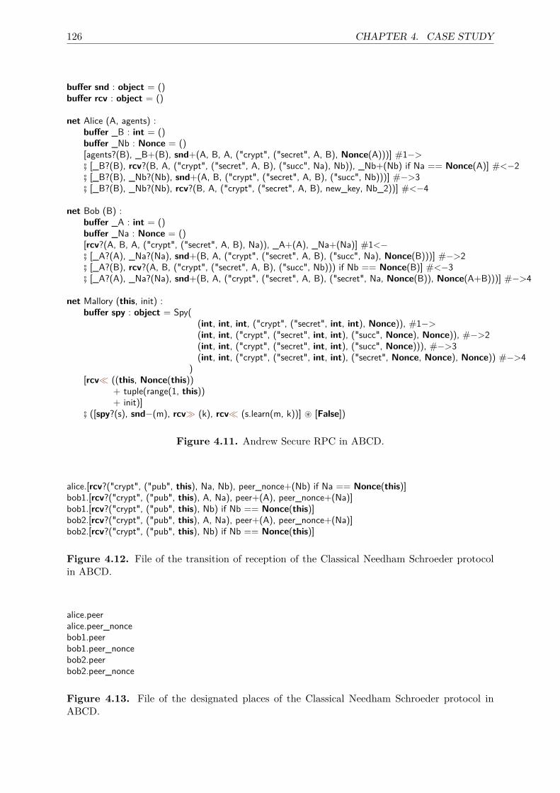
126 CHAPTER 4. CASE STUDY
buffer snd : object = ()buffer rcv : object = ()
net Alice (A, agents) :buffer _B : int = ()buffer _Nb : Nonce = ()[agents?(B), _B+(B), snd+(A, B, A, ("crypt", ("secret", A, B), Nonce(A)))] #1−># [_B?(B), rcv?(B, A, ("crypt", ("secret", A, B), ("succ", Na), Nb)), _Nb+(Nb) if Na == Nonce(A)] #<−2# [_B?(B), _Nb?(Nb), snd+(A, B, ("crypt", ("secret", A, B), ("succ", Nb)))] #−>3# [_B?(B), _Nb?(Nb), rcv?(B, A, ("crypt", ("secret", A, B), new_key, Nb_2))] #<−4
net Bob (B) :buffer _A : int = ()buffer _Na : Nonce = ()[rcv?(A, B, A, ("crypt", ("secret", A, B), Na)), _A+(A), _Na+(Na)] #1<−# [_A?(A), _Na?(Na), snd+(B, A, ("crypt", ("secret", A, B), ("succ", Na), Nonce(B)))] #−>2# [_A?(B), rcv?(A, B, ("crypt", ("secret", A, B), ("succ", Nb))) if Nb == Nonce(B)] #<−3# [_A?(A), _Na?(Na), snd+(B, A, ("crypt", ("secret", A, B), ("secret", Na, Nonce(B)), Nonce(A+B)))] #−>4
net Mallory (this, init) :buffer spy : object = Spy(
(int, int, int, ("crypt", ("secret", int, int), Nonce)), #1−>(int, int, ("crypt", ("secret", int, int), ("succ", Nonce), Nonce)), #−>2(int, int, ("crypt", ("secret", int, int), ("succ", Nonce))), #−>3(int, int, ("crypt", ("secret", int, int), ("secret", Nonce, Nonce), Nonce)) #−>4
)[rcv� ((this, Nonce(this))
+ tuple(range(1, this))+ init)]
# ([spy?(s), snd−(m), rcv� (k), rcv� (s.learn(m, k))] ~ [False])
Figure 4.11. Andrew Secure RPC in ABCD.
alice.[rcv?("crypt", ("pub", this), Na, Nb), peer_nonce+(Nb) if Na == Nonce(this)]bob1.[rcv?("crypt", ("pub", this), A, Na), peer+(A), peer_nonce+(Na)]bob1.[rcv?("crypt", ("pub", this), Nb) if Nb == Nonce(this)]bob2.[rcv?("crypt", ("pub", this), A, Na), peer+(A), peer_nonce+(Na)]bob2.[rcv?("crypt", ("pub", this), Nb) if Nb == Nonce(this)]
Figure 4.12. File of the transition of reception of the Classical Needham Schroeder protocolin ABCD.
alice.peeralice.peer_noncebob1.peerbob1.peer_noncebob2.peerbob2.peer_nonce
Figure 4.13. File of the designated places of the Classical Needham Schroeder protocol inABCD.
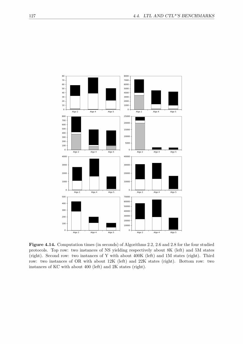
127 4.4. LTL AND CTL*’S BENCHMARKS
Algo 2 Algo 4 Algo 50
10
20
30
40
50
60
70
80
Algo 2 Algo 4 Algo 50
1000
2000
3000
4000
5000
6000
7000
8000
Algo 2 Algo 4 Algo 50
100
200
300
400
500
600
700
800
Algo 2 Algo 4 Algo 50
5000
10000
15000
20000
25000
Algo 2 Algo 4 Algo 50
1000
2000
3000
4000
Algo 2 Algo 4 Algo 50
10000
20000
30000
40000
Algo 2 Algo 4 Algo 50
100
200
300
400
500
Algo 2 Algo 4 Algo 50
10000
20000
30000
40000
50000
60000
70000
Figure 4.14. Computation times (in seconds) of Algorithms 2.2, 2.6 and 2.8 for the four studiedprotocols. Top row: two instances of NS yielding respectively about 8K (left) and 5M states(right). Second row: two instances of Y with about 400K (left) and 1M states (right). Thirdrow: two instances of OR with about 12K (left) and 22K states (right). Bottom row: twoinstances of KC with about 400 (left) and 2K states (right).
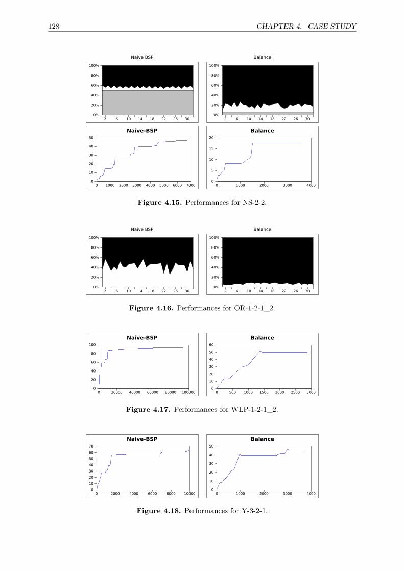
128 CHAPTER 4. CASE STUDY
2 6 10 14 18 22 26 300%
20%
40%
60%
80%
100%
Naive BSP
2 6 10 14 18 22 26 300%
20%
40%
60%
80%
100%
Balance
0 1000 2000 3000 4000 5000 6000 70000
10
20
30
40
50
Naive-BSP
0 1000 2000 3000 40000
5
10
15
20
Balance
Figure 4.15. Performances for NS-2-2.
2 6 10 14 18 22 26 300%
20%
40%
60%
80%
100%
Naive BSP
2 6 10 14 18 22 26 300%
20%
40%
60%
80%
100%
Balance
Figure 4.16. Performances for OR-1-2-1_2.
0 20000 40000 60000 80000 1000000
20
40
60
80
100
Naive-BSP
0 500 1000 1500 2000 2500 30000
10
20
30
40
50
60
Balance
Figure 4.17. Performances for WLP-1-2-1_2.
0 2000 4000 6000 8000 100000
10
20
30
40
50
60
70
Naive-BSP
0 1000 2000 3000 40000
10
20
30
40
50
Balance
Figure 4.18. Performances for Y-3-2-1.
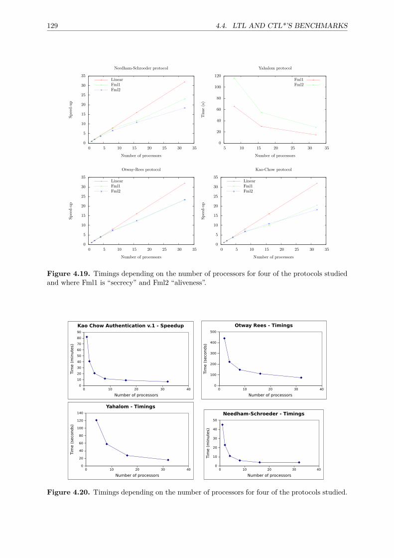
129 4.4. LTL AND CTL*’S BENCHMARKS
0
5
10
15
20
25
30
35
0 5 10 15 20 25 30 35
Speed-up
Number of processors
Needham-Schroeder protocol
LinearFml1Fml2
0
20
40
60
80
100
120
5 10 15 20 25 30 35
Tim
e(s)
Number of processors
Yahalom protocol
Fml1Fml2
0
5
10
15
20
25
30
35
0 5 10 15 20 25 30 35
Speed-up
Number of processors
Otway-Rees protocol
LinearFml1Fml2
0
5
10
15
20
25
30
35
0 5 10 15 20 25 30 35
Speed-up
Number of processors
Kao-Chow protocol
LinearFml1Fml2
Figure 4.19. Timings depending on the number of processors for four of the protocols studiedand where Fml1 is “secrecy” and Fml2 “aliveness”.
0 10 20 30 40
Number of processors
0
10
20
30
40
50
60
70
80
90
Tim
e (
min
ute
s)
Kao Chow Authentication v.1 - Speedup
0 10 20 30 40
Number of processors
0
100
200
300
400
500
Tim
e (
seconds)
Otway Rees - Timings
0 10 20 30 40
Number of processors
0
20
40
60
80
100
120
140
Tim
e (
seconds)
Yahalom - Timings
0 10 20 30 40
Number of processors
0
10
20
30
40
50
Tim
e (
min
ute
s)
Needham-Schroeder - Timings
Figure 4.20. Timings depending on the number of processors for four of the protocols studied.

5 Conclusion
Designing security protocols is complex and often error prone: various attacks are reported inthe literature to protocols thought to be “correct” for many years. This is due to the nature ofprotocols: they are executed as multiple concurrent sessions in an uncertain environment, whereall messages flowing the network could be manipulating by an attacker which does not need tobreak cryptography. Indeed, protocols are broken merely because of attackers exploiting flawsin the protocols.
Each security protocol is designed to achieve certain goals after the execution. Those goalsare called security properties. There are various security properties, for example, to ensurethat secret data is not revealed to irrelevant parties. Due to the presence of an attacker, someprotocols can not be able to preserve the expected security properties. Therefore it is veryimportant to find a formal way to find flaws and to prove their correctness with respect tosecurity properties.To check if a protocol or a session of a protocol does not contain flaw, we have proposed to
resort to model-checking, using an algebra of coloured Petri nets called ABCD to model theprotocol, together with security properties that could be expressed as reachability properties,LTL, or CTL* formulas. Reachability properties lead to construct the state space of the model(i.e. the set of its reachable states). LTL and CTL* involve the construction of the stategraph (i.e. the reachable states together with the transitions from one state to another) that iscombined with the formula under analysis into a so called proof graph. In both cases, on-the-flyanalysis allows to stop states explorations as soon as a conclusion can be drawn.However, in general, this leads to compute a number of states that may be exponentially larger
than the size of the model, which is the so called state space explosion problem. The criticalproblem of state space or state graph construction is to determine whether a newly generatedstate has been explored before. In a serial implementation this question is answered by organizingknown states in a specific data-structure, and looking for the new states in that structure. Asthis is a centralized activity, a parallel or distributed solution must find an alternative approach.The common method is to assign states to processors using a static partition function which isgenerally a hashing of the states [102]. After a state has been generated, it is sent to its assignedlocation, where a local search determines whether the state already exists. Applying this methodto security protocols fails in two points. First the number of cross-transitions (i.e. transitionsbetween two states assigned to distinct processors) is too high and leads to a too heavy networkuse. Second, memorizing all of them in the main memory is impossible without crashing thewhole parallel machine and is not clear when it is possible to put some states in disk and ifheuristics [86,148] would work well for complex protocols.Our first solution is to use the well-structured nature of the protocols to choose which part of
the state space is really needed for the partition function and to empty the data-structure in eachsuper-step of the parallel computation. Our second solution entails automated classification ofstates into classes, and dynamic mapping of classes to processors. We find that both our methodsexecute significantly faster and achieve better network use than classical method. Furthermore,we find that the method that balances states does indeed achieve better network use, memorybalance and runs faster.The fundamental message is that for parallel discrete state space generation, exploiting certain
131
132 CHAPTER 5. CONCLUSION
characteristics of the system and structuring the computation is essential. We have demonstratedtechniques that proved the feasibility of this approach and demonstrated its potential. Keyelements to our success were (1) an automated classification that reduces cross-transitions andmemory use and growth locallity of the computations (2) using global barriers (which is a low-overhead method) to compute a global remappings and thus balancing workload and achieveda good scalability for the discrete state space generation of security protocols.Then, we have shown how these ideas about state space computation could be generalized
to the computation and analysis of proof graphs. The structure of state space exploration ispreserved but enriched with the construction of the proof graph and its on-the-fly analysis. Inthe case of LTL, we could show that the required information to conclude about a formula iseither available locally to a processor (even when states are dumped from the main memory ateach super step), or is not needed anymore when a cross-transition occurs. Indeed, we have seenthat no cross-transition occurs within a strongly connected component, which are the crucialstructures in proof graphs to conclude about formulas truths. In the case of CTL* however,local conclusions can need to be delayed until a further recursive exploration is completed,which may occur on another processor. Rather than continuing such an exploration on the sameprocessor, which would limit parallelism, we could design a way to organize the computation sothat inconclusive nodes in the proof graph can be kept available until a conclusion comes froma recursive exploration, allowing to dump them immediately from the main memory. This morecomplex bookkeeping appears necessary due to the recursive nature of CTL* checking that canbe regarded as nested LTL analysis.
5.1 Summary of contributions
Throughout this thesis, we have proposed several contributions summarized thereafter.
Models of several classical security protocols. Using the ABCD algebra, have been provided,showing quite a systematic style of modeling. In particular, the same model of a Dolev-Yaoattacker can be reused in every cases. But more generally, modeling new protocols looks quitestraightforward because they are very likely to reuse the same patterns as in the protocols wehave modeled.
A parallel algorithm for state space generation. We have featuring an automated classifica-tion of states on processors, dynamic re-balancing of workload, sweep-line method to dischargeunneeded states from the processors’ memory. Experiments have also shown that this algorithmhas limited network usage as well as a good scalability.
A parallel algorithm for LTL analysis. Bsed on the algorithm for state space exploration andinherits is good characteristics.
A generalization to CTL* of the parallel LTL analysis. CTL* has been studied also. Withrespect to the previous algorithms, this one uses a more complex memory management andrequires to keep more states in memory, due to the nature of CTL* model-checking.
Prototype implementations of our algorithms. Implementations have been made and used toexperiment on the modeled protocols. We have used the Python programming language for thispurpose, which, being an interpreted language, does not allow to assess efficiency but, however,is perfectly suitable for evaluating the parallel performances of our algorithms.
133 5.2. FUTURE WORKS
A systematic performance analysis of our algorithms. Benchmarks have been conduced usingvarious instances of the modeled protocols. This allowed to confirm their good parallel behavior,in particular scalability with respect to the number of processors.
5.2 Future worksFuture works will be dedicated to build a real and efficient implementation from our prototypes.It will feature in particular a CTL* model-checker, allowing to verify non-trivial security prop-erties. Using this implementation, we would like to run benchmarks in order to compare ourapproach with existing tools. We would like also to test our algorithm on parallel computer withmore processors in order to confirm the scalability that we could observe on 40 processors.Another way to improve performances will be to consider symbolic state space representations
as well as symbolic state space computation. In the former case, we are targeting in particularrepresentations based on decision diagrams. In the latter case, we are thinking about adaptingsymmetry or partial order reduction methods to reduce the number of executions that need tobe explored. Reductions methods appear to be the simplest step because they somehow resultin exploring less states. Yet, they usually result in an exponential reduction of the number ofcomputed states or transitions. On the other hand, using symbolic representations looks morechallenging because storing large number of states in such structures is computationally efficientonly when we can also apply a symbolic successor function, i.e. compute the successors of setsof states instead of those of a single state.Moreover, we are working on the formal proofs of our algorithms. Proving a verification
algorithm is highly desirable in order to certify the truth of the diagnostics delivered by such analgorithm. Such a proof is possible because, thanks to the BSP model, our algorithm remainssimple in its structure.Finally, we would like to generalise our present results by extending the application domain.
In the security domain, we will consider more complex protocols with branching and loopingstructures, as well as complex data types manipulations. In particular, we will consider protocolsfor secure storage distributed through peer-to-peer communication [184].

Bibliography
[1] Xavier Allamigeon and Bruno Blanchet. Reconstruction of attacks against cryptographic protocols. InComputer Security Foundations Workshop (CSFW), pages 140–154. IEEE Computer Society, 2005. Page29.
[2] S. Allmaier, S. Dalibor, and D. Kreische. Parallel graph generation algorithms for shared and distributedmemory machines. In E. H. D’Hollander, G. R. Joubert, F. J. Peters, and U. Trottenberg, editors, Proceed-ings of Parallel Computing (ParCo), volume 12, pages 581–588. Elsevier, 1997. Page 38.
[3] Rajeev Alur, Thomas A. Henzinger, and Orna Kupferman. Alternating-time temporal logic. J. ACM,49(5):672–713, 2002. Page 61.
[4] R. M. Amadio and D. Lugiez. On the reachability problem in cryptographic protocols. In C. Palamidessi,editor, Concur, volume 1877 of LNCS, pages 380–394. Springer-Verla, 2000. Page 4.
[5] Christian Appold. Efficient symmetry reduction and the use of state symmetries for symbolic model check-ing. In Angelo Montanari, Margherita Napoli, and Mimmo Parente, editors, Symposium on Games, Au-tomata, Logic, and Formal Verification (GANDALF), volume 25 of EPTCS, pages 173–187, 2010. Page34.
[6] Christian Appold. Improving bdd based symbolic model checking with isomorphism exploiting transitionrelations. In Giovanna D’Agostino and Salvatore La Torre, editors, Symposium on Games, Automata, Logicsand Formal Verification (GandALF), volume 54 of EPTCS, pages 17–30, 2011. Page 31.
[7] M. Arapinis, S. Delaune, and S. Kremer. From one session to many: Dynamic tags for security protocols.In I. Cervesato, H. Veith, and A. Voronkov, editors, Logic for Programming, Artificial Intelligence, andReasoning (LPAR), volume 5330 of LNCS, pages 128–142. Springer, 2008. Page 39.
[8] A. Armando, R. Carbone, and L. Compagna. LTL model checking for security protocols. In Proceedings ofCSF, pages 385–396. IEEE Computer Society, 2007. Page 28.
[9] A. Armando, R. Carbone, and L. Compagna. Ltl model checking for security protocols. Applied Non-Classical Logics, 19(4):403–429, 2009. Page 39.
[10] A. Armando and L. Compagna. SAT-based model-checking for security protocols analysis. Int. J. Inf. Sec.,7(1):3–32, 2008. Pages 2 and 28.
[11] A. Armando and et al. The AVISPA tool for the automated validation of Internet security protocols andapplications. In K. Etessami and S. K. Rajamani, editors, Proceedings of Computer Aided Verification(CAV), volume 3576 of LNCS, pages 281–285. Springer, 2005. Pages 2, 28, 29 and 39.
[12] Alessandro Armando, Roberto Carbone, and Luca Compagna. Ltl model checking for security protocols.Journal of Applied Non-Classical Logics, 19(4):403–429, 2009. Pages 2 and 27.
[13] Mathilde Arnaud. Formal verification of secured routing protocols. PhD thesis, Laboratoire Spécification etVérification, ENS Cachan, France, 2011. Page 8.
[14] A.V.Gerbessiotis. Topics in Parallel and Distributed Computation. PhD thesis, Harvard University, 1993.Page 23.
[15] M. Bamha and M. Exbrayat. Pipelining a Skew-Insensitive Parallel Join Algorithm. Parallel ProcessingLetters, 13(3):317–328, 2003. Page 23.
[16] M. Bamha and G. Hains. Frequency-adaptive join for Shared Nothing machines. Parallel and DistributedComputing Practices, 2(3):333–345, 1999. Page 23.
[17] M. Bamha and G. Hains. An Efficient equi-semi-join Algorithm for Distributed Architectures. In V. Sun-deram, D. van Albada, and J. Dongarra, editors, International Conference on Computational Science (ICCS2005), LNCS. Springer, 2005. Page 23.
[18] J. Barnat. Distributed Memory LTL Model Checking. PhD thesis, Faculty of Informatics Masaryk UniversityBrno, 2004. Pages 37 and 113.
[19] J. Barnat, L. Brim, and I. Cëerná. Property driven distribution of nested dfs. In M. Leuschel and U. Ultes-Nitsche, editors,Workshop on Verification and Computational Logic (VCL), volume DSSE-TR-2002-5, pages1–10. Dept. of Electronics and Computer Science, University of Southampton (DSSE), UK, Technical Re-port, 2002. Page 36.
135
136 BIBLIOGRAPHY
[20] D. Basin. How to evaluate the security of real-life cryptographic protocols? The cases of ISO/IEC 29128and CRYPTREC. In Workshop on Real-life Cryptographic Protocols and Standardization, 2010. Pages 2and 38.
[21] David A. Basin. Lazy infinite-state analysis of security protocols. In Rainer Baumgart, editor, SecureNetworking - CQRE (Secure), International Exhibition and Congress Düsseldorf, volume 1740 of LNCS,pages 30–42. Springer, 1999. Page 29.
[22] David A. Basin, Sebastian Mödersheim, and Luca Viganò. Algebraic intruder deductions. In Geoff Sut-cliffe and Andrei Voronkov, editors, Logic for Programming, Artificial Intelligence, and Reasoning (LPAR),volume 3835 of LNCS, pages 549–564. Springer, 2005. Page 29.
[23] David A. Basin, Sebastian Mödersheim, and Luca Viganò. Ofmc: A symbolic model checker for securityprotocols. Int. J. Inf. Sec., 4(3):181–208, 2005. Pages 29 and 39.
[24] Ayon Basumallik, Seung-Jai Min, and Rudolf Eigenmann. Programming distributed memory sytems usingopenmp. In IPDPS, pages 1–8, 2007. Page 19.
[25] Johan Bengtsson, Kim Guldstrand Larsen, Fredrik Larsson, Paul Pettersson, and Wang Yi. Uppaal - a toolsuite for automatic verification of real-time systems. In Rajeev Alur, Thomas A. Henzinger, and Eduardo D.Sontag, editors, Hybrid Systems III: Verification and Control, Proceedings of the DIMACS/SYCON Work-shop, volume 1066 of LNCS, pages 232–243. Springer, 1995. Page 28.
[26] O. Bernholtz, M.Y. Vardi, and P. Wolper. An automata-theoretic approach to branching-time modelchecking. In D. L. Dill, editor, Computer Aided Verification (CAV), volume 818 of LNCS, pages 142–155.Springer-Verlag, 1994. Page 30.
[27] Karthikeyan Bhargavan, Ricardo Corin, Pierre-Malo Deniélou, Cédric Fournet, and James J. Leifer. Cryp-tographic protocol synthesis and verification for multiparty sessions. In omputer Security FoundationsSymposium (CSF), pages 124–140. IEEE Computer Society, 2009. Page 8.
[28] G. Bhat, R. Cleaveland, and O. Grumberg. Efficient on-the-fly model checking for ctl*. In Proceedings ofthe 10th Annual IEEE Symposium on Logic in Computer Science (LICS), pages 388–398. IEEE ComputerSociety, 1995. Pages 30, 39, 57, 61, 63, 64, 65, 67, 68, 73 and 116.
[29] R. H. Bisseling. Parallel Scientific Computation. A structured approach using BSP and MPI. OxfordUniversity Press, 2004. Pages 22, 23, 38 and 41.
[30] R. H. Bisseling and W. F. McColl. Scientific computing on bulk synchronous parallel architectures. InB. Pehrson and I. Simon, editors, Technology and Foundations: Information Processing ’94, Vol. I, vol-ume 51 of IFIP Transactions A, pages 509–514. Elsevier Science Publishers, Amsterdam, 1994. Page 23.
[31] Bruno Blanchet. An efficient cryptographic protocol verifier based on Prolog rules. In IEEE CSFW’01.IEEE Computer Society, 2001. Pages 26 and 29.
[32] S. Blom, B. Lisser, J. van de Pol, and M. Weber. A database approach to distributed state space generation.Electr. Notes Theor. Comput. Sci., 198(1):17–32, 2008. Page 38.
[33] S. Blom and S. Orzan. Distributed branching bisimulation reduction of state spaces. In ENTCS, volume 89.Elsevier, 2003. Page 38.
[34] S. C. C. Blom, W. Fokkink, J. F. Groote, I. van Langevelde, B. Lisser, and J. C. van de Pol. µ-CRL: Atoolset for analysing algebraic specifications. In Proceedings Computer Aided Verification (CAV), number2102 in LNCS, pages 250–254, 2001. Page 28.
[35] Stefan Blom, Jan Friso Groote, Sjouke Mauw, and Alexander Serebrenik. Analysing the bke-securityprotocol with µcrl. Electr. Notes Theor. Comput. Sci., 139(1):49–90, 2005. Page 28.
[36] Chiara Bodei, Mikael Buchholtz, Pierpaolo Degano, Flemming Nielson, and Hanne Riis Nielson. Staticvalidation of security protocols. Journal of Computer Security, 13(3):347–390, 2005. Page 29.
[37] R. Bouroulet, R. Devillers, H. Klaudel, E. Pelz, and F. Pommereau. Modeling and analysis of securityprotocols using role based specifications and Petri nets. In ICATPN, volume 5062 of LNCS, pages 72–91.Springer, 2008. Page 98.
[38] C. Boyd. Security architectures using formal methods. IEEE journal on Selected Areas in Communications,11(5):684–701, 1993. Page 5.
[39] A. Braud and C. Vrain. A parallel genetic algorithm based on the BSP model. In Evolutionary Computationand Parallel Processing GECCO & AAAI Workshop, Orlando (Florida), USA, 1999. Page 23.
[40] M. Burrows, M. Abadi, and R. Needham. A logic of authentication. Technical report 39, Digital SystemsResearch Center, 1989. Pages 103 and 105.
[41] Duncan Campbell. Further results with algorithmic skeletons for the clumps model of parallel computation,1996. Page 25.
[42] Duncan K. G. Campbell. On the clumps model of parallel computation. Inf. Process. Lett., 66(5):231–236,1998. Page 25.
137 BIBLIOGRAPHY
[43] Duncan K.G. Campbell. Clumps: A candidate model of efficient, general purpose parallel computation.Technical report, 1994. Page 25.
[44] F. Cappello, P. Fraigniaud, B. Mans, and A.L. Rosenberg. HiHCoHP toward a realistic communicationmodel for hierarchical hyperclusters of heterogeneous processors. In IEEE/ACM IPDPS’2001. IEEE press,2001. Page 26.
[45] Franck Cappello, Pierre Fraigniaud, Bernard Mans, and Arnold L. Rosenberg. An algorithmic model forheterogeneous hyper-clusters: rationale and experience. Int. J. Found. Comput. Sci., 16(2):195–215, 2005.Page 26.
[46] A. Chan, F. Dehne, and R. Taylor. Implementing and Testing CGM Graph Algorithms on PC Clusters andShared Memory Machines. Journal of High Performance Computing Applications, 2005. Page 23.
[47] Barbara Chapman. Using OpenMP: portable shared memory parallel programming. The MIT Press, 2008.Page 19.
[48] Yannick Chevalier and Laurent Vigneron. Automated unbounded verification of security protocols. InEd Brinksma and Kim Guldstrand Larsen, editors, Computer Aided Verification (CAV), LNCS, pages 324–337. Springer, 2002. Page 27.
[49] S. Christensen, L. M. Kristensen, and T. Mailund. A sweep-line method for state space exploration. InT. Margaria and W. Yi, editors, Proceedings of Tools and Algorithms for the Construction and Analysis ofSystems (TACAS), volume 2031 of LNCS, pages 450–464. Springer, 2001. Pages 46, 49, 53 and 55.
[50] M.-Y. Chung and G. Ciardo. A pattern recognition approach for speculative firing prediction in distributedsaturation state-space generation. In ENTCS, volume 135, pages 65–80. Elsevier, 2006. Page 38.
[51] J. Clark and J. Jacob. A survey of authentication protocol literature : Version 1.0. Available at http://www-users.cs.york.ac.uk/~jac/papers/drareview.ps.gz, 1997. Pages 4, 102 and 103.
[52] E. M. Clarke, O. Grumberg, and K. Hamaguchi. Another look at ltl model checking. In D.L. Dill, editor,Computer Aided Verification (CAV), volume 818 of LNCS, pages 415–427. Springer-Verlag, 1994. Pages 60and 65.
[53] Edmund M. Clarke, E. Allen Emerson, Somesh Jha, and A. Prasad Sistla. Symmetry reductions in modelchecking. In CAV’98, volume 1427 of LNCS. Springer, 1998. Page 34.
[54] Edmund M. Clarke, Orna Grumberg, and David E. Long. Model checking and abstraction. ACM Trans.Program. Lang. Syst., 16(5):1512–1542, 1994. Page 32.
[55] Edmund M. Clarke, Orna Grumberg, and Doron A. Peled. Model Checking. MIT Press, 2000. Pages 27and 32.
[56] Edmund M. Clarke, Somesh Jha, Reinhard Enders, and Thomas Filkorn. Exploiting symmetry in temporallogic model checking. Formal Methods in System Design, 9(1/2):77–104, 1996. Page 34.
[57] Edmund M. Clarke, Somesh Jha, and Wilfredo R. Marrero. Verifying security protocols with brutus. ACMTrans. Softw. Eng. Methodol., pages 443–487, 2000. Pages 29 and 32.
[58] Edmund M. Clarke, Somesh Jha, and Wilfredo R. Marrero. Efficient verification of security protocols usingpartial-order reductions. STTT, pages 173–188, 2003. Page 32.
[59] R. Cleaveland and B. Steffen. A linear-time model-checking algorithm for the alternation-free modal mu-calculus. Formal Methods in System Design, 2(121–147), 1993. Page 30.
[60] M. Cole. Bringing Skeletons out of the Closet: A Pragmatic Manifesto for Skeletal Parallel Programming.Parallel Computing, 30(3):389–406, 2004. Page 20.
[61] H. Comon-Lundh and V. Cortier. How to prove security of communication protocols? a discussion on thesoundness of formal models w.r.t. computational ones. In STACS, pages 29–44, 2011. Page 38.
[62] R. Corin. Analysis Models for Security Protocols. PhD thesis, University of Twente, 2006. Pages 39 and119.
[63] Ricardo Corin, Sandro Etalle, Pieter H. Hartel, and Angelika Mader. Timed model checking of securityprotocols. In Vijayalakshmi Atluri, Michael Backes, David A. Basin, and Michael Waidner, editors, FormalMethods in Security Engineering (FMSE), pages 23–32. ACM, 2004. Page 28.
[64] Ricardo Corin, Sandro Etalle, and Ari Saptawijaya. A logic for constraint-based security protocol analysis.In Symposium on Security and Privacy, pages 155–168. IEEE Computer Society, 2006. Page 29.
[65] C. Courcoubetis, M. Y. Vardi, P. Wolper, and M. Yannakakis. Memory efficient algorithms for vericationof temporal properties. Formal Methods in System design, 1:275–288, 1992. Page 30.
[66] Jean-Michel Couvreur, Emmanuelle Encrenaz, Emmanuel Paviot-Adet, Denis Poitrenaud, and Pierre-AndréWacrenier. Data decision diagrams for Petri net analysis. In ICATPN’02. Springer, 2002. Page 31.
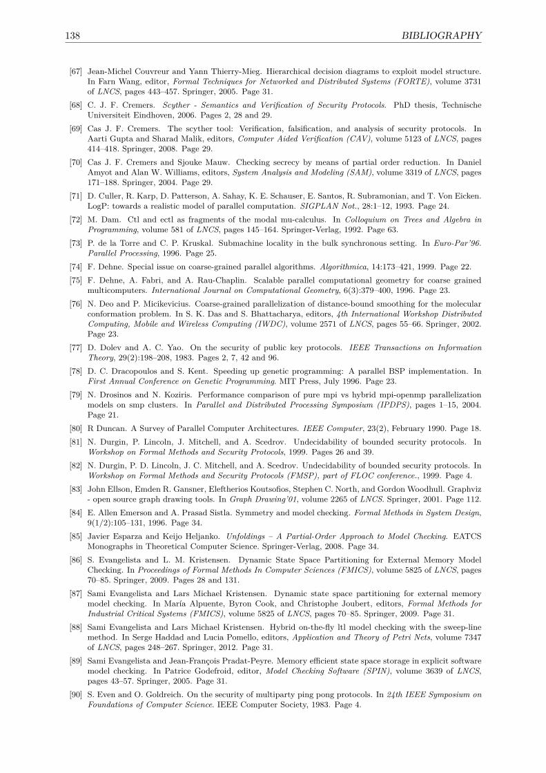
138 BIBLIOGRAPHY
[67] Jean-Michel Couvreur and Yann Thierry-Mieg. Hierarchical decision diagrams to exploit model structure.In Farn Wang, editor, Formal Techniques for Networked and Distributed Systems (FORTE), volume 3731of LNCS, pages 443–457. Springer, 2005. Page 31.
[68] C. J. F. Cremers. Scyther - Semantics and Verification of Security Protocols. PhD thesis, TechnischeUniversiteit Eindhoven, 2006. Pages 2, 28 and 29.
[69] Cas J. F. Cremers. The scyther tool: Verification, falsification, and analysis of security protocols. InAarti Gupta and Sharad Malik, editors, Computer Aided Verification (CAV), volume 5123 of LNCS, pages414–418. Springer, 2008. Page 29.
[70] Cas J. F. Cremers and Sjouke Mauw. Checking secrecy by means of partial order reduction. In DanielAmyot and Alan W. Williams, editors, System Analysis and Modeling (SAM), volume 3319 of LNCS, pages171–188. Springer, 2004. Page 29.
[71] D. Culler, R. Karp, D. Patterson, A. Sahay, K. E. Schauser, E. Santos, R. Subramonian, and T. Von Eicken.LogP: towards a realistic model of parallel computation. SIGPLAN Not., 28:1–12, 1993. Page 24.
[72] M. Dam. Ctl and ectl as fragments of the modal mu-calculus. In Colloquium on Trees and Algebra inProgramming, volume 581 of LNCS, pages 145–164. Springer-Verlag, 1992. Page 63.
[73] P. de la Torre and C. P. Kruskal. Submachine locality in the bulk synchronous setting. In Euro-Par’96.Parallel Processing, 1996. Page 25.
[74] F. Dehne. Special issue on coarse-grained parallel algorithms. Algorithmica, 14:173–421, 1999. Page 22.[75] F. Dehne, A. Fabri, and A. Rau-Chaplin. Scalable parallel computational geometry for coarse grained
multicomputers. International Journal on Computational Geometry, 6(3):379–400, 1996. Page 23.[76] N. Deo and P. Micikevicius. Coarse-grained parallelization of distance-bound smoothing for the molecular
conformation problem. In S. K. Das and S. Bhattacharya, editors, 4th International Workshop DistributedComputing, Mobile and Wireless Computing (IWDC), volume 2571 of LNCS, pages 55–66. Springer, 2002.Page 23.
[77] D. Dolev and A. C. Yao. On the security of public key protocols. IEEE Transactions on InformationTheory, 29(2):198–208, 1983. Pages 2, 7, 42 and 96.
[78] D. C. Dracopoulos and S. Kent. Speeding up genetic programming: A parallel BSP implementation. InFirst Annual Conference on Genetic Programming. MIT Press, July 1996. Page 23.
[79] N. Drosinos and N. Koziris. Performance comparison of pure mpi vs hybrid mpi-openmp parallelizationmodels on smp clusters. In Parallel and Distributed Processing Symposium (IPDPS), pages 1–15, 2004.Page 21.
[80] R Duncan. A Survey of Parallel Computer Architectures. IEEE Computer, 23(2), February 1990. Page 18.[81] N. Durgin, P. Lincoln, J. Mitchell, and A. Scedrov. Undecidability of bounded security protocols. In
Workshop on Formal Methods and Security Protocols, 1999. Pages 26 and 39.[82] N. Durgin, P. D. Lincoln, J. C. Mitchell, and A. Scedrov. Undecidability of bounded security protocols. In
Workshop on Formal Methods and Security Protocols (FMSP), part of FLOC conference., 1999. Page 4.[83] John Ellson, Emden R. Gansner, Eleftherios Koutsofios, Stephen C. North, and Gordon Woodhull. Graphviz
- open source graph drawing tools. In Graph Drawing’01, volume 2265 of LNCS. Springer, 2001. Page 112.[84] E. Allen Emerson and A. Prasad Sistla. Symmetry and model checking. Formal Methods in System Design,
9(1/2):105–131, 1996. Page 34.[85] Javier Esparza and Keijo Heljanko. Unfoldings – A Partial-Order Approach to Model Checking. EATCS
Monographs in Theoretical Computer Science. Springer-Verlag, 2008. Page 34.[86] S. Evangelista and L. M. Kristensen. Dynamic State Space Partitioning for External Memory Model
Checking. In Proceedings of Formal Methods In Computer Sciences (FMICS), volume 5825 of LNCS, pages70–85. Springer, 2009. Pages 28 and 131.
[87] Sami Evangelista and Lars Michael Kristensen. Dynamic state space partitioning for external memorymodel checking. In María Alpuente, Byron Cook, and Christophe Joubert, editors, Formal Methods forIndustrial Critical Systems (FMICS), volume 5825 of LNCS, pages 70–85. Springer, 2009. Page 31.
[88] Sami Evangelista and Lars Michael Kristensen. Hybrid on-the-fly ltl model checking with the sweep-linemethod. In Serge Haddad and Lucia Pomello, editors, Application and Theory of Petri Nets, volume 7347of LNCS, pages 248–267. Springer, 2012. Page 31.
[89] Sami Evangelista and Jean-François Pradat-Peyre. Memory efficient state space storage in explicit softwaremodel checking. In Patrice Godefroid, editor, Model Checking Software (SPIN), volume 3639 of LNCS,pages 43–57. Springer, 2005. Page 31.
[90] S. Even and O. Goldreich. On the security of multiparty ping pong protocols. In 24th IEEE Symposium onFoundations of Computer Science. IEEE Computer Society, 1983. Page 4.
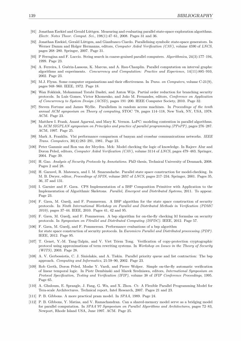
139 BIBLIOGRAPHY
[91] Jonathan Ezekiel and Gerald Lüttgen. Measuring and evaluating parallel state-space exploration algorithms.Electr. Notes Theor. Comput. Sci., 198(1):47–61, 2008. Pages 31 and 36.
[92] Jonathan Ezekiel, Gerald Lüttgen, and Gianfranco Ciardo. Parallelising symbolic state-space generators. InWerner Damm and Holger Hermanns, editors, Computer Aided Verification (CAV), volume 4590 of LNCS,pages 268–280. Springer, 2007. Page 31.
[93] P Ferragina and F. Luccio. String search in coarse-grained parallel computers. Algorithmica, 24(3):177–194,1999. Page 23.
[94] A. Ferreira, I. Guérin-Lassous, K. Marcus, and A. Rau-Chauplin. Parallel computation on interval graphs:algorithms and experiments. Concurrency and Computation: Practice and Experience, 14(11):885–910,2002. Page 23.
[95] M.J. Flynn. Some computer organizations and their effectiveness. In Trans. on Computers, volume C-21(9),pages 948–960. IEEE, 1972. Page 18.
[96] Wan Fokkink, Mohammad Torabi Dashti, and Anton Wijs. Partial order reduction for branching securityprotocols. In Luís Gomes, Victor Khomenko, and João M. Fernandes, editors, Conference on Applicationof Concurrency to System Design (ACSD), pages 191–200. IEEE Computer Society, 2010. Page 32.
[97] Steven Fortune and James Wyllie. Parallelism in random access machines. In Proceedings of the tenthannual ACM symposium on Theory of computing, STOC ’78, pages 114–118, New York, NY, USA, 1978.ACM. Page 23.
[98] Matthew I. Frank, Anant Agarwal, and Mary K. Vernon. LoPC: modeling contention in parallel algorithms.In ACM SIGPLAN symposium on Principles and practice of parallel programming (PPoPP), pages 276–287.ACM, 1997. Page 25.
[99] Mark A. Franklin. Vlsi performance comparison of banyan and crossbar communications networks. IEEETrans. Computers, 30(4):283–291, 1981. Page 23.
[100] Peter Gammie and Ron van der Meyden. Mck: Model checking the logic of knowledge. In Rajeev Alur andDoron Peled, editors, Computer Aided Verification (CAV), volume 3114 of LNCS, pages 479–483. Springer,2004. Page 39.
[101] H. Gao. Analysis of Security Protocols by Annotations. PhD thesis, Technical University of Denmark, 2008.Pages 2 and 28.
[102] H. Garavel, R. Mateescu, and I. M. Smarandache. Parallel state space construction for model-checking. InM. B. Dwyer, editor, Proceedings of SPIN, volume 2057 of LNCS, pages 217–234. Springer, 2001. Pages 35,36, 37 and 131.
[103] I. Garnier and F. Gava. CPS Implementation of a BSP Composition Primitive with Application to theImplementation of Algorithmic Skeletons. Parallel, Emergent and Distributed Systems, 2011. To appear.Page 23.
[104] F. Gava, M. Guedj, and F. Pommereau. A BSP algorithm for the state space construction of securityprotocols. In Ninth International Workshop on Parallel and Distributed Methods in Verification (PDMC2010), pages 37–44. IEEE, 2010. Pages 41, 42 and 95.
[105] F. Gava, M. Guedj, and F. Pommereau. A bsp algorithm for on-the-fly checking ltl formulas on securityprotocols. In Symposium on PArallel and Distributed Computing (ISPDC). IEEE, 2012. Page 57.
[106] F. Gava, M. Guedj, and F. Pommereau. Performance evaluations of a bsp algorithmfor state space construction of security protocols. In Euromicro Parallel and Distributed proceessing (PDP).IEEE, 2012. Page 95.
[107] T. Genet, Y.-M. Tang-Talpin, and V. Viet Triem Tong. Verification of copy-protection cryptographicprotocol using approximations of term rewriting systems. In Workshop on Issues in the Theory of Security(WITS), 2003. Page 28.
[108] A. V. Gerbessiotis, C. J. Siniolakis, and A. Tiskin. Parallel priority queue and list contraction: The bspapproach. Computing and Informatics, 21:59–90, 2002. Page 23.
[109] Rob Gerth, Doron Peled, Moshe Y. Vardi, and Pierre Wolper. Simple on-the-fly automatic verificationof linear temporal logic. In Piotr Dembinski and Marek Sredniawa, editors, International Symposium onProtocol Specification, Testing and Verification (IFIP), volume 38 of IFIP Conference Proceedings, 1995.Page 65.
[110] A. Ghuloum, E. Sprangle, J. Fang, G. Wu, and X. Zhou. Ct: A Flexible Parallel Programming Model forTera-scale Architectures. Technical report, Intel Research, 2007. Pages 21 and 23.
[111] P. B. Gibbons. A more practical pram model. In SPAA, 1989. Page 24.[112] P. B. Gibbons, Y. Matias, and V. Ramachandran. Can a shared-memory model serve as a bridging model
for parallel computation. In SPAA’97 Symposium on Parallel Algorithms and Architectures, pages 72–83,Newport, Rhode Island USA, June 1997. ACM. Page 25.
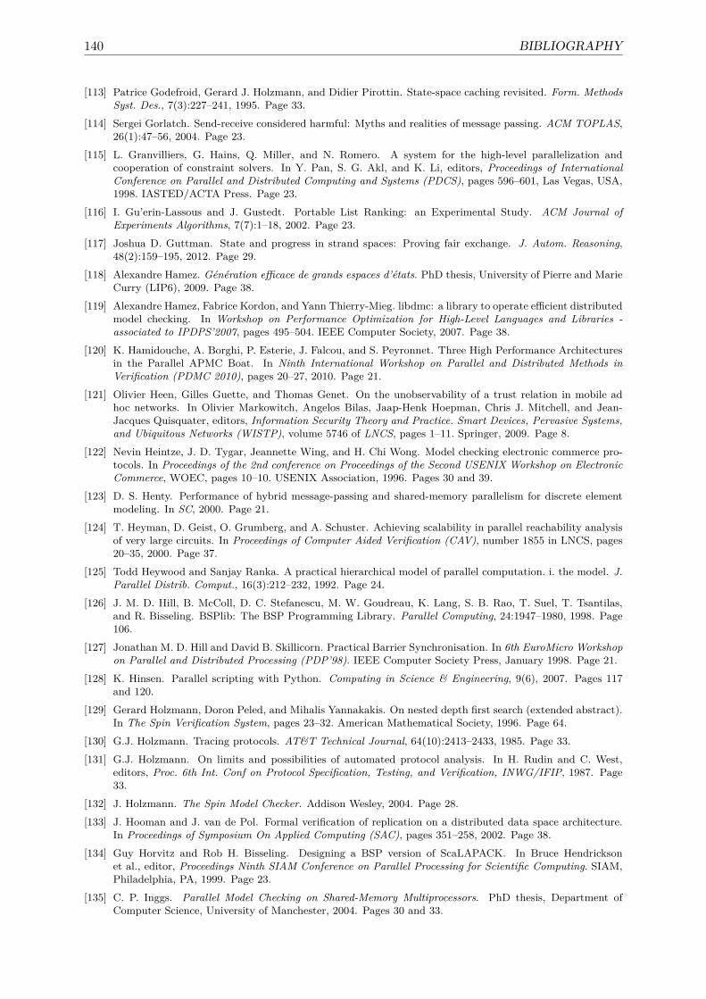
140 BIBLIOGRAPHY
[113] Patrice Godefroid, Gerard J. Holzmann, and Didier Pirottin. State-space caching revisited. Form. MethodsSyst. Des., 7(3):227–241, 1995. Page 33.
[114] Sergei Gorlatch. Send-receive considered harmful: Myths and realities of message passing. ACM TOPLAS,26(1):47–56, 2004. Page 23.
[115] L. Granvilliers, G. Hains, Q. Miller, and N. Romero. A system for the high-level parallelization andcooperation of constraint solvers. In Y. Pan, S. G. Akl, and K. Li, editors, Proceedings of InternationalConference on Parallel and Distributed Computing and Systems (PDCS), pages 596–601, Las Vegas, USA,1998. IASTED/ACTA Press. Page 23.
[116] I. Gu’erin-Lassous and J. Gustedt. Portable List Ranking: an Experimental Study. ACM Journal ofExperiments Algorithms, 7(7):1–18, 2002. Page 23.
[117] Joshua D. Guttman. State and progress in strand spaces: Proving fair exchange. J. Autom. Reasoning,48(2):159–195, 2012. Page 29.
[118] Alexandre Hamez. Génération efficace de grands espaces d’états. PhD thesis, University of Pierre and MarieCurry (LIP6), 2009. Page 38.
[119] Alexandre Hamez, Fabrice Kordon, and Yann Thierry-Mieg. libdmc: a library to operate efficient distributedmodel checking. In Workshop on Performance Optimization for High-Level Languages and Libraries -associated to IPDPS’2007, pages 495–504. IEEE Computer Society, 2007. Page 38.
[120] K. Hamidouche, A. Borghi, P. Esterie, J. Falcou, and S. Peyronnet. Three High Performance Architecturesin the Parallel APMC Boat. In Ninth International Workshop on Parallel and Distributed Methods inVerification (PDMC 2010), pages 20–27, 2010. Page 21.
[121] Olivier Heen, Gilles Guette, and Thomas Genet. On the unobservability of a trust relation in mobile adhoc networks. In Olivier Markowitch, Angelos Bilas, Jaap-Henk Hoepman, Chris J. Mitchell, and Jean-Jacques Quisquater, editors, Information Security Theory and Practice. Smart Devices, Pervasive Systems,and Ubiquitous Networks (WISTP), volume 5746 of LNCS, pages 1–11. Springer, 2009. Page 8.
[122] Nevin Heintze, J. D. Tygar, Jeannette Wing, and H. Chi Wong. Model checking electronic commerce pro-tocols. In Proceedings of the 2nd conference on Proceedings of the Second USENIX Workshop on ElectronicCommerce, WOEC, pages 10–10. USENIX Association, 1996. Pages 30 and 39.
[123] D. S. Henty. Performance of hybrid message-passing and shared-memory parallelism for discrete elementmodeling. In SC, 2000. Page 21.
[124] T. Heyman, D. Geist, O. Grumberg, and A. Schuster. Achieving scalability in parallel reachability analysisof very large circuits. In Proceedings of Computer Aided Verification (CAV), number 1855 in LNCS, pages20–35, 2000. Page 37.
[125] Todd Heywood and Sanjay Ranka. A practical hierarchical model of parallel computation. i. the model. J.Parallel Distrib. Comput., 16(3):212–232, 1992. Page 24.
[126] J. M. D. Hill, B. McColl, D. C. Stefanescu, M. W. Goudreau, K. Lang, S. B. Rao, T. Suel, T. Tsantilas,and R. Bisseling. BSPlib: The BSP Programming Library. Parallel Computing, 24:1947–1980, 1998. Page106.
[127] Jonathan M. D. Hill and David B. Skillicorn. Practical Barrier Synchronisation. In 6th EuroMicro Workshopon Parallel and Distributed Processing (PDP’98). IEEE Computer Society Press, January 1998. Page 21.
[128] K. Hinsen. Parallel scripting with Python. Computing in Science & Engineering, 9(6), 2007. Pages 117and 120.
[129] Gerard Holzmann, Doron Peled, and Mihalis Yannakakis. On nested depth first search (extended abstract).In The Spin Verification System, pages 23–32. American Mathematical Society, 1996. Page 64.
[130] G.J. Holzmann. Tracing protocols. AT&T Technical Journal, 64(10):2413–2433, 1985. Page 33.[131] G.J. Holzmann. On limits and possibilities of automated protocol analysis. In H. Rudin and C. West,
editors, Proc. 6th Int. Conf on Protocol Specification, Testing, and Verification, INWG/IFIP, 1987. Page33.
[132] J. Holzmann. The Spin Model Checker. Addison Wesley, 2004. Page 28.[133] J. Hooman and J. van de Pol. Formal verification of replication on a distributed data space architecture.
In Proceedings of Symposium On Applied Computing (SAC), pages 351–258, 2002. Page 38.[134] Guy Horvitz and Rob H. Bisseling. Designing a BSP version of ScaLAPACK. In Bruce Hendrickson
et al., editor, Proceedings Ninth SIAM Conference on Parallel Processing for Scientific Computing. SIAM,Philadelphia, PA, 1999. Page 23.
[135] C. P. Inggs. Parallel Model Checking on Shared-Memory Multiprocessors. PhD thesis, Department ofComputer Science, University of Manchester, 2004. Pages 30 and 33.
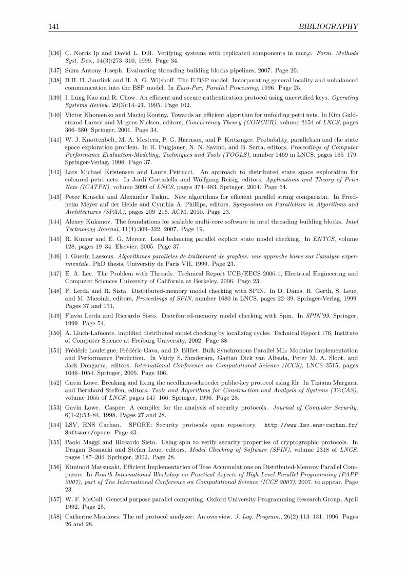
141 BIBLIOGRAPHY
[136] C. Norris Ip and David L. Dill. Verifying systems with replicated components in murϕ. Form. MethodsSyst. Des., 14(3):273–310, 1999. Page 34.
[137] Sunu Antony Joseph. Evaluating threading building blocks pipelines, 2007. Page 20.[138] B.H. H. Juurlink and H. A. G. Wijshoff. The E-BSP model: Incorporating general locality and unbalanced
communication into the BSP model. In Euro-Par, Parallel Processing, 1996. Page 25.[139] I. Lung Kao and R. Chow. An efficient and secure authentication protocol using uncertified keys. Operating
Systems Review, 29(3):14–21, 1995. Page 102.[140] Victor Khomenko and Maciej Koutny. Towards an efficient algorithm for unfolding petri nets. In Kim Guld-
strand Larsen and Mogens Nielsen, editors, Concurrency Theory (CONCUR), volume 2154 of LNCS, pages366–380. Springer, 2001. Page 34.
[141] W. J. Knottenbelt, M. A. Mestern, P. G. Harrison, and P. Kritzinger. Probability, parallelism and the statespace exploration problem. In R. Puigjaner, N. N. Savino, and B. Serra, editors, Proceedings of ComputerPerformance Evaluation-Modeling, Techniques and Tools (TOOLS), number 1469 in LNCS, pages 165–179.Springer-Verlag, 1998. Page 37.
[142] Lars Michael Kristensen and Laure Petrucci. An approach to distributed state space exploration forcoloured petri nets. In Jordi Cortadella and Wolfgang Reisig, editors, Applications and Theory of PetriNets (ICATPN), volume 3099 of LNCS, pages 474–483. Springer, 2004. Page 54.
[143] Peter Krusche and Alexander Tiskin. New algorithms for efficient parallel string comparison. In Fried-helm Meyer auf der Heide and Cynthia A. Phillips, editors, Symposium on Parallelism in Algorithms andArchitectures (SPAA), pages 209–216. ACM, 2010. Page 23.
[144] Alexey Kukanov. The foundations for scalable multi-core software in intel threading building blocks. IntelTechnology Journal, 11(4):309–322, 2007. Page 19.
[145] R. Kumar and E. G. Mercer. Load balancing parallel explicit state model checking. In ENTCS, volume128, pages 19–34. Elsevier, 2005. Page 37.
[146] I. Guerin Lassous. Algorithmes paralleles de traitement de graphes: une approche basee sur l’analyse exper-imentale. PhD thesis, University de Paris VII, 1999. Page 23.
[147] E. A. Lee. The Problem with Threads. Technical Report UCB/EECS-2006-1, Electrical Engineering andComputer Sciences University of California at Berkeley, 2006. Page 23.
[148] F. Lerda and R. Sista. Distributed-memory model checking with SPIN. In D. Dams, R. Gerth, S. Leue,and M. Massink, editors, Proceedings of SPIN, number 1680 in LNCS, pages 22–39. Springer-Verlag, 1999.Pages 37 and 131.
[149] Flavio Lerda and Riccardo Sisto. Distributed-memory model checking with Spin. In SPIN’99. Springer,1999. Page 54.
[150] A. Lluch-Lafuente. implified distributed model checking by localizing cycles. Technical Report 176, Instituteof Computer Science at Freiburg University, 2002. Page 38.
[151] Frédéric Loulergue, Frédéric Gava, and D. Billiet. Bulk Synchronous Parallel ML: Modular Implementationand Performance Prediction. In Vaidy S. Sunderam, Gaétan Dick van Albada, Peter M. A. Sloot, andJack Dongarra, editors, International Conference on Computational Science (ICCS), LNCS 3515, pages1046–1054. Springer, 2005. Page 106.
[152] Gavin Lowe. Breaking and fixing the needham-schroeder public-key protocol using fdr. In Tiziana Margariaand Bernhard Steffen, editors, Tools and Algorithms for Construction and Analysis of Systems (TACAS),volume 1055 of LNCS, pages 147–166. Springer, 1996. Page 28.
[153] Gavin Lowe. Casper: A compiler for the analysis of security protocols. Journal of Computer Security,6(1-2):53–84, 1998. Pages 27 and 28.
[154] LSV, ENS Cachan. SPORE: Security protocols open repository. http://www.lsv.ens-cachan.fr/Software/spore. Page 43.
[155] Paolo Maggi and Riccardo Sisto. Using spin to verify security properties of cryptographic protocols. InDragan Bosnacki and Stefan Leue, editors, Model Checking of Software (SPIN), volume 2318 of LNCS,pages 187–204. Springer, 2002. Page 28.
[156] Kiminori Matsuzaki. Efficient Implementation of Tree Accumulations on Distributed-Memroy Parallel Com-puters. In Fourth International Workshop on Practical Aspects of High-Level Parallel Programming (PAPP2007), part of The International Conference on Computational Science (ICCS 2007), 2007. to appear. Page23.
[157] W. F. McColl. General purpose parallel computing. Oxford University Programming Research Group, April1992. Page 25.
[158] Catherine Meadows. The nrl protocol analyzer: An overview. J. Log. Program., 26(2):113–131, 1996. Pages26 and 28.
142 BIBLIOGRAPHY
[159] Catherine Meadows. Analysis of the internet key exchange protocol using the nrl protocol analyzer. InIEEE Symposium on Security and Privacy, pages 216–231, 1999. Page 28.
[160] Jonathan K. Millen and Vitaly Shmatikov. Constraint solving for bounded-process cryptographic protocolanalysis. In Michael K. Reiter and Pierangela Samarati, editors, Computer and Communications Security(CCS), pages 166–175. ACM, 2001. Page 29.
[161] John C. Mitchell, Mark Mitchell, and Ulrich Stern. Automated analysis of cryptographic protocols usingmurphi. In IEEE Symposium on Security and Privacy, pages 141–151. IEEE Computer Society, 1997. Page27.
[162] Sebastian Mödersheim, Luca Viganò, and David A. Basin. Constraint differentiation: Search-space reduc-tion for the constraint-based analysis of security protocols. Journal of Computer Security, 18(4):575–618,2010. Pages 27, 29 and 98.
[163] R. M. Needham and M. D. Schroeder. Using encryption for authentication in large networks of computers.Communication of the ACM, 21(12), 1978. Page 99.
[164] John Nickolls, Ian Buck, Michael Garland, and Kevin Skadron. Scalable parallel programming with cuda.ACM Queue, 6(2):40–53, 2008. Page 20.
[165] D. Nicol and G. Ciardo. Automated parallelization of discrete state-space generation. Journal of Paralleland Distributed Computing, 4(2):153–167, 1997. Pages 28 and 37.
[166] T. Nipkow, L. C. Paulson, and M. Wenzel. Isabelle/HOL — A Proof Assistant for Higher-Order Logic.LNCS 2283. Springer, 2002. Pages 26 and 28.
[167] S. Orzan, J. van de Pol, and M. Espada. A state space distributed policy based on abstract interpretation.In ENTCS, volume 128, pages 35–45. Elsevier, 2005. Page 37.
[168] D. Otway and O. Rees. Efficient and timely mutual authentication. Operating Systems Review, 21(1):8–10,1987. Page 102.
[169] Sam Owre and Natarajan Shankar. A brief overview of pvs. In Otmane Aït Mohamed, César Muñoz, andSofiène Tahar, editors, Theorem Proving in Higher Order Logics (TPHOLs), volume 5170 of Lecture Notesin Computer Science, pages 22–27. Springer, 2008. Page 26.
[170] C. Pajault. Model Checking parallèle et réparti de réseaux de Petri colorés de haut-niveau. PhD thesis,Conservatoire National des Arts et Métiers, 2008. Pages 37 and 38.
[171] Christophe Pajault and Jean-François Pradat-Peyre. Distributed colored petri net model-checking withcyclades. pages 347–361, 2006. Page 38.
[172] L. C. Paulson. Relations between secrets: Two formal analyses of the yahalom protocol. J. ComputerSecurity, 2001. Page 104.
[173] Lawrence C. Paulson. The inductive approach to verifying cryptographic protocols. Journal of ComputerSecurity, 6(1-2):85–128, 1998. Page 28.
[174] D. Petcu. Parallel explicit state reachability analysis and state space construction. In Proceedings of ISPDC,pages 207–214. IEEE Computer Society, 2003. Page 37.
[175] J. L. Peterson. Petri net theory. Prentice Hall, 1981. Page 8.[176] C. A. Petri. Kommunikation mit Automaten. PhD thesis, Schriften des Instituts fur instrumentelle Mathe-
matik. Universitat Bonn, 1962. Page 8.[177] Petri net markup language. http://www.pnml.org. Page 112.[178] F. Pommereau. Quickly prototyping Petri nets tools with SNAKES. In Proc. of PNTAP’08, ACM Digital
Library, pages 1–10. ACM, 2008. Pages 39, 95, 110, 117 and 120.[179] F. Pommereau. Algebras of coloured Petri nets. Habilitation thesis, University Paris-East Creteil, 2009.
Pages 13, 14, 16 and 18.[180] F. Pommereau. Algebras of coloured Petri nets. Habilitation thesis, University Paris-East CrÃľteil, 2009.
Pages 42, 43 and 46.[181] F. Pommereau. Algebras of coloured Petri nets. Lambert Academic Publisher, 2010. ISBN 978-3-8433-6113-
2. Pages 8, 13, 42 and 95.[182] R. O. Rogers and D. B. Skillicorn. Using the BSP cost model to optimise parallel neural network training.
Future Generation Computer Systems, 14(5-6):409–424, 1998. Page 23.[183] M. Rusinowith and M. Turuani. Protocol insecurity with finite number of sessions is np-complete. In 14th
Computer Security Foundations Workshop (CSFW), pages 174–190. IEEE, 2001. Page 39.[184] S. Sanjabi and F. Pommereau. Modelling, verification, and formal analysis of security properties in a P2P
system. In Workshop on Collaboration and Security (COLSEC’10), IEEE Digital Library, pages 543–548.IEEE, 2010. Page 133.
143 BIBLIOGRAPHY
[185] F. B. Schneider. Implementing fault-tolerant services using the state machine approach: a tutorial. ACMComputing Surveys, 22(4):299–319, 1999. Page 7.
[186] H. Sivaraj and G. Gopalakrishnan. Random walk heuristic algorithms for distributed memory model check-ing. In ENTCS, volume 89. Elsevier, 2003. Page 37.
[187] D. B. Skillicorn, J. M. D. Hill, and W. F. McColl. Questions and Answers about BSP. Scientific Program-ming, 6(3):249–274, 1997. Pages 22, 38 and 41.
[188] M. Snir and W. Gropp. MPI the Complete Reference. MIT Press, 1998. Page 23.[189] M. Snir, S. W. Otto, S. Huss-Lederman, D. W. Walker, and J. Dongarra. MPI The Complete Reference.
MIT Press, 1996. Bibliothèque du LIFO. Page 20.[190] Dawn Xiaodong Song, Sergey Berezin, and Adrian Perrig. Athena: A novel approach to efficient automatic
security protocol analysis. Journal of Computer Security, 9(1/2):47–74, 2001. Pages 27 and 29.[191] Xiaodong Dawn Song. An automatic approach for building secure systems. PhD thesis, University of
California, Berkeley, 2002. Page 30.[192] U. Stern and D. L. Dill. Parallelizing the murϕ verifier. In O. Grumberg, editor, Proceedings of Computer
Aided Verification (CAV), volume 1254 of LNCS, pages 256–267. Springer, 1997. Page 28.[193] U. Stern and D. L. Hill. Parallelizing the Murϕ verifier. In O. Grumberg, editor, Proceedings of Computer-
Aided Verification (CAV), number 1254 in LNCS, pages 256–267. Springer-Verlag, 2997. Page 37.[194] R. Tarjan. Depth-first search and linear graph algorithms. SIAM journal on computing, pages 146–160,
1972. Page 57.[195] F. Javier Thayer, Jonathan C. Herzog, and Joshua D. Guttman. Strand spaces: Proving security protocols
correct. Journal of Computer Security, 7(1):191–230, 1999. Page 29.[196] A. Tiskin. The Design and Analysis of Bulk-Synchronous Parallel Algorithms. PhD thesis, Oxford University
Computing Laboratory, 1998. Pages 23 and 109.[197] M. Llanos Tobarra, Diego Cazorla, Fernando Cuartero, and Gregorio Díaz. Analysis of web services secure
conversation with formal methods. In International Conference on Internet and Web Applications andServices (ICIW), page 27. IEEE Computer Society, 2007. Page 8.
[198] M. Llanos Tobarra, Diego Cazorla, Fernando Cuartero, Gregorio Díaz, and María-Emilia Cambronero.Model checking wireless sensor network security protocols: Tinysec + leap + tinypk. TelecommunicationSystems, 40(3-4):91–99, 2009. Page 8.
[199] Ashutosh Trivedi. Techniques in symbolic model checking, 2003. Page 36.[200] L. G. Valiant. A bridging model for parallel computation. Comm. of the ACM, 33(8):103, 1990. Page 26.[201] B. Vergauwen and J. Lewi. A linear local model-checking algorithm for ctl. In E. Best, editor, CONCUR,
volume 715 of LNCS, pages 447–461. Springer-Verlag, 1993. Pages 30 and 65.[202] Makarius Wenzel, Lawrence C. Paulson, and Tobias Nipkow. The isabelle framework. In Otmane Aït
Mohamed, César Muñoz, and Sofiène Tahar, editors, Theorem Proving in Higher Order Logics (TPHOLs),volume 5170 of LNCS, pages 33–38. Springer, 2008. Pages 26 and 28.
[203] T. Y. C. Woo and S. S. Lam. A lesson on authentication protocol design. Operating Systems Review, 1994.Page 104.
[204] A. Zavanella. Skeletons and BSP : Performance Portability for Parallel Programming. PhD thesis, Universitadegli studi di Pisa, 1999. Page 18.

145 SOFTWARES
Softwares1 http://openmp.org2 http://threadingbuildingblocks.org3 http://developer.nvidia.com/category/zone/cuda-zone4 http://maude.cs.uiuc.edu/tools/Maude-NPA/5 http://www.cl.cam.ac.uk/research/hvg/isabelle/6 http://pvs.csl.sri.com7 http://www.cs.ox.ac.uk/people/gavin.lowe/Security/Casper8 http://www.cs.ox.ac.uk/projects/concurrency-tools9 http://homepages.cwi.nl/ mcrl/10 http://www.uppaal.org/11 http://spinroot.com/spin/whatispin.html12 http://www.proverif.ens.fr13 http://www2.imm.dtu.dk/cs_LySa/lysatool14 http://www.avispa-project.org15 http://people.inf.ethz.ch/cremersc/scyther/16 http://dirac.cnrs-orleans.fr/plone/software/scientificpython
17 http://snake.com

Résumé. Déterminer avec certitude si un protocole donné est sécurisé ou non est résté longtempsun défi. Le développement de techniques formelles permettant de vérifier une large gamme depropriétés de sécurité est un apport important pour relever ce défi. Ce document contribue àl’élaboration de telles techniques par la modelisation de protocole de sécurité en utilisant unealgèbre de réseaux de Petri coloré appelée ABCD et réduit le temps de vérification des proto-coles à l’aide de calculs distribués. Nous exploitons la nature “bien structurée” des protocolesde sécurité et la faison correspondre à un modèle de calcul parallèle appelé BSP. Cette struc-ture des protocoles est exploitée pour partitionner l’espace des états et réduire les transitionsinter-machines tout en augmentant la localité du calcul. Dans le même temps, le modèle BSPpermet de simplifier la détection de la terminaison de l’algorithme et l’équilibrage des chargesdes calculs. Nous considérons le problème de la vérification des formules LTL et CTL* sur dessystèmes de transitions étiquetées (LTS) qui modélisent les protocoles de sécurité. Un prototypea été développé, testé sur différents benchmarks.
Mots clefs. Parallélisme, model checking, logique temporelle, protocols de sécurité.
Abstract. It has long been a challenge to determine conclusively whether a given protocol issecure or not. The development of formal techniques that can check various security propertiesis an important tool to meet this challenge. This document contributes to the development ofsuch techniques by model security protocols using an algebra of coloured Petri net call ABCDand reduce time to checked the protocols using parallel computations. We exploit the well-structured nature of security protocols and match it to a model of parallel computation calledBSP. The structure of the protocols is exploited to partition the state space and reduce crosstransitions while increasing computation locality. At the same time, the BSP model allows tosimplify the detection of the algorithm termination and to load balance the computations. Weconsider the problem of checking a LTL and CTL* formulas over labelled transition systems(LTS) that model security protocols. A prototype implementation has been developed, allowingto run benchmarks.
Keywords. Parallelism, model checking, temporal logic, security protocols.


