Brain tumor classification based on longecho proton MRS signals

L. Lukasa, A. Devosa,*, J.A.K. Suykensa, L. Vanhammea, F.A. Howeb,C. Majosc, A. Moreno-Torresd, M. Van Der Graafe, A.R. Tateb,C. Arusf, S. Van Huffela

aSCD-SISTA, Department of Electrical Engineering, Katholieke Universiteit Leuven,Kasteelpark Arenberg 10, 3001 Heverlee (Leuven), BelgiumbCRC Biomedical Magnetic Resonance Research Group, Department of Biochemistry and Immunology,St. George’s Hospital Medical School, Cranmer Terrace, London SW17 0RE, UKcInstitut de Diagnostic per la Imatge (IDI), CSU de Bellvitge, Autovia de Castelldefels km 2.7,L’Hospitalet de Llobregat, 08907 Barcelona, SpaindCentre Diagnostic Pedralbes, Unitat Esplugues, C/Josep Anselm Clave 100, 08950 Esplugues de Llobregat,SpaineDepartment of Radiology, University Medical Center Nijmegen, PO Box 9101, 6500 HB Nijmegen,The NetherlandsfDepartament de Bioquimica i Biologia Molecular, Unitat de Ciencies, Edifici Cs,Universitat Autonoma de Barcelona, 08193 Cerdanyola del Valles, Spain

Received 28 April 2003; received in revised form 7 August 2003; accepted 17 January 2004

Artificial Intelligence in Medicine (2004) 31, 73—89

KEYWORDS

Brain tumors;

Classification;

Magnetic resonance

spectroscopy (MRS);

Linear discriminant

analysis (LDA);

Support vector

machine (SVM);

Least squares support

vector machine (LS-SVM)

Summary There has been a growing research interest in brain tumor classificationbased on proton magnetic resonance spectroscopy (1H MRS) signals. Four researchcenters within the EU funded INTERPRET project have acquired a significant number oflong echo 1H MRS signals for brain tumor classification. In this paper, we present anobjective comparison of several classification techniques applied to the discriminationof four types of brain tumors: meningiomas, glioblastomas, astrocytomas grade II andmetastases. Linear and non-linear classifiers are compared: linear discriminant ana-lysis (LDA), support vector machines (SVM) and least squares SVM (LS-SVM) with a linearkernel as linear techniques and LS-SVM with a radial basis function (RBF) kernel as anon-linear technique. Kernel-based methods can perform well in processing highdimensional data. This motivates the inclusion of SVM and LS-SVM in this study. Theanalysis includes optimal input variable selection, (hyper-) parameter estimation,followed by performance evaluation. The classification performance is evaluated over200 stratified random samplings of the dataset into training and test sets. Receiveroperating characteristic (ROC) curve analysis measures the performance of binaryclassification, while for multiclass classification, we consider the accuracy as perfor-mance measure. Based on the complete magnitude spectra, automated binary classi-fiers are able to reach an area under the ROC curve (AUC) of more than 0.9 except forthe hard case glioblastomas versus metastases. Although, based on the available long

* Corresponding author. Tel.: þ32-16-321-926; fax: þ32-16-321-970.E-mail address: andy.devos@esat.kuleuven.ac.be (A. Devos).

0933–3657/$ — see front matter � 2004 Elsevier B.V. All rights reserved.doi:10.1016/j.artmed.2004.01.001

1. Introduction

Brain tumors are the second leading cause of can-cer death in children under 15 years and youngadults up to the age of 34. These tumors are alsothe second fastest growing cause of cancer deathamong humans older than 65 years [1]. Early detec-tion and correct treatment based on accuratediagnosis are important steps to improve diseaseoutcome.

Currently, magnetic resonance spectroscopy(MRS) in combination with magnetic resonance ima-ging (MRI) are important tools to identify the loca-tion, size and type of brain tumors. So far, MRS hasbeen proven to be an accurate non-invasive tech-nique which can give detailed chemical informationof metabolites present in the suspected braintumors [2,3]. Under physiological conditions,several important metabolites are observed: NAA(N-acetyl aspartate) as a neuronal marker; Cho(choline-containing compounds) as membrane pre-cursors and degradation products; Cr (total crea-tine) as a measure of the energy status; glucose; andmI (myo-inositol). Under pathological conditions,the presence of some resonances can be indicative:a doublet of Lac (lactate); lipids and/or some lowmolecular weight proteins which might occur evenunder normal conditions; Ace (acetate) and certainamino acids, such as Ala (alanine), Gln (glutamine),Glu (glutamate) and Gly (glycine).

In comparison to in vitro spectroscopy, in vivospectroscopy signals are more difficult to analyzebecause of their broader resonances, strongly over-lapping peaks, lower signal-to-noise ratio andhigher number of artifacts. Cousins [4] discussesthe influence of the echo time TE on the spectralpattern of an MRS signal. The above-mentionedmetabolites can be detected in short echo 1H MRSsignals. However, short echo 1H MRS signals aremore difficult to analyze than long echo 1H MRSsignals due to a higher number of overlappingpeaks, a stronger baseline and a higher sensitivityto artifacts. In comparison, long echo 1H MRS sig-nals are poorer in information but they allow amore reliable analysis and testing of classificationmethods.

Many studies have been performed to classifyMRS signals. Lindon et al. [5] overviewed patternrecognition methods and their applications in

biomedical magnetic resonance. Several studies[6—11] also show some progress in automated pat-tern recognition for brain tumor classification basedon MR data. These studies are either based on MRI(e.g. [11]), MRI combined with MR spectroscopicimaging (MRSI) (e.g. [7]), long echo (e.g. [6,8,9]) orshort echo 1H MRS (e.g. [10]), but most of the papersinvestigate only one classification method andrestrict data collection to one center only. As per-formance measure either the training performanceis considered or test performance on a specificallyselected set. In our study we measure the binaryclassification performance based on the receiveroperating characteristic (ROC) curve analysis over200 stratified random samplings of training and testset. ROC analysis is commonly used in medicine [12]to objectively judge the discrimination ability ofvarious statistical methods for predictive purposes,which can be measured by the area under the ROCcurve (AUC). The AUC gives a global measure of theclinical efficiency over a range of test cut-off pointson the ROC curve. This is in contrast to performancemeasures like the accuracy, e.g. used in [11], whichis only based on a single cut-off point (e.g. for onespecific value of the false-positive rate). Variousclinical studies focus on the prediction of the malig-nancy of tumors, more specifically for brain gliomas(e.g. [6,11]). Thereby, they consider only twoclasses: low-grade and high-grade gliomas. In ourstudy, astrocytomas of grade II and glioblastomas(also called astrocytomas of grade IV) are included,which are large subtypes of, respectively, low-grade and high-grade gliomas. Additionally, we con-sider two other common brain tumor types, namelymetastases and meningiomas.

Moreover, this paper reports the results of acomparative study on a multicenter dataset ofMRS signals. This dataset was developed in theframework of the EU funded INTERPRET project[13]. Several INTERPRET partners [7,9,10,14—19]have already published results for classification ofbrain tumors based on MR data available within theproject. The papers [7,15,18] focus on the use of 1HMRSI data, while others consider the use of short orlong echo 1H MRS. Nevertheless, most of thesestudies are based on a previous version of thedataset or focus on a specific technique. For exam-ple, in [10], 144 short echo 1H MRS spectra fromthree contributing centers were used, originating

echo 1H MRS data, we did not find any statistically significant difference betweenthe performances of LDA and the kernel-based methods, the latter have thestrength that no dimensionality reduction is required to obtain such a high per-formance.� 2004 Elsevier B.V. All rights reserved.

74 L. Lukas et al.

from three groups of brain tumors; meningiomas,low-grade astrocytomas and aggressive tumors. Thelatter group includes glioblastomas and metastases.Note that these groups correspond to the same fourtumor groups as considered in this paper. But Tateet al. selects a specific training and test set; thedata from two centers formed the training set(94 spectra) and the data from the third centerwere used for testing (50 spectra). Based on thisspecific test set an accuracy of 96% was obtainedusing LDA.

In this study several methods are applied on allhistopathologically validated long echo 1H MRS datafrom four common brain tumor types as available inthe final status of the database development. Wemention three additional points differing with pre-vious classification studies within the framework ofthe INTERPRET project. First of all, we investigatewhat can be obtained as typical performance on arepresentative test set. Therefore, we construct200 different combinations of training and indepen-dent test set. Second of all, the discriminationability was judged by the AUC, which is, in contra-diction to the accuracy, a global measure. Only inone other INTERPRET study [15] ROC analysis wasalso applied to compare two diagnostic methodsfor classification based on 1H MRSI. Third of all,four different techniques are applied for classifica-tion; linear as well as non-linear techniques. Weinvestigate binary as well as multiclass classifica-tion. Moreover, this analysis includes optimalinput variable selection and (hyper-) parameterestimation.

Several classification techniques are comparedin this paper. We evaluate the performance oflinear discriminant analysis (LDA), support vectormachines (SVMs) and the least squares version ofsupport vector machines (LS-SVMs) in classifyingbrain tumors based on long echo 1H MRS spectra.The support vector machine [20,21] is a trainingalgorithm for learning classification and regressionrules from data. It applies the idea of kernel repre-sentation from mathematical analysis, for example,using either linear, polynomial, radial basis func-tions (RBF) or multi-layer perceptrons (MLP) as itslearning kernel. SVMs were first introduced by Vap-nik in the 1960s for classification and have recentlybecome an area of intense research owing to devel-opments in the techniques and theory coupled withextensions to density estimation and regression.SVMs arose from statistical learning theory; theaim being to solve only the problem of interestwithout solving a more difficult problem as an inter-mediate step. SVMs are based on the structural riskminimization principle, closely related to regular-ization theory. This principle incorporates capacity

control to prevent overfitting and is thus a partialsolution to the bias-variance trade-off dilemma.

Least squares SVM [22] uses equality constraintsand solves a set of linear equations in the dual spaceinstead of solving a quadratic programming problemas for the standard SVM. This simplifies the compu-tations and enhances the speed considerably. Thereexists a link between the LS-SVM classifier formula-tion with the well-known Fisher discriminant ana-lysis, namely by extending it to a high-dimensionalfeature space. Some parameters have to be tunedto achieve a high level performance of the (LS-)SVM,including the regularization parameter and the ker-nel parameter corresponding to the kernel type.

The paper is organized as follows. Section 2explains the material and methods used for classi-fication; description of the data and short explana-tion of the kernel based methods SVM and LS-SVM.Section 3 summarizes the results of binary classifi-cation using complete spectra, selected frequencyregions and peak integrated values, consecutively.Afterwards, results of the multiclass classificationapproach are also mentioned. In Section 4, wediscuss the classification performance of the clas-sifiers, the limitations of the dataset and the influ-ence of dimensionality reduction. Finally, Section 5presents the conclusions.

2. Material and methods

2.1. Material

The data were provided by CDP (Centre DiagnosticPedralbes, Barcelona, Spain), IDI (Institut de Diag-nostic per la Imatge, Barcelona, Spain), SGHMS (St.George’s Hospital Medical School, London, UK) andUMCN (University Medical Center Nijmegen, Nijme-gen, The Netherlands) in the framework of theINTERPRET project. It concerns long echo 1H MRSdata, acquired both with and without water sup-pression using a PRESS sequence (the repetitiontime TR is between 1500 and 2020 ms, the echotime TE ¼ 135 or 136 ms, the spectral widthSW ¼ 1000 or 2500 Hz, the number of datapointsis 512 or 2048) (Table 1).

Four main classes are considered, correspondingto four brain tumor types, i.e. glioblastomas,meningiomas, metastases and astrocytomas (gradeII). They are labeled as class 1 (glio), class 2 (meni),class 3 (meta) and class 4 (astroII), respectively. Alldata have passed a quality control and validationprocess, which was regulated by strict rules agreedon by all INTERPRET partners. After thorough exam-inations, the brain tumors were histopathologi-cally classified by three pathologists. These class

Brain tumor classification based on long echo proton MRS signals 75

assignments were based on the histological classi-fication of tumors of the central nervous system(CNS) set up by the World Health Organization(WHO).

The raw data are acquired in the time domain atthe aforementioned centers. A few preprocessingsteps are carried out: frequency alignment andphase correction with Klose’s method [23] and fil-tering of the dominating residual water peak usingHSVD [24]. The initial point of the time domainsignal was removed, because it was often affectedby artifacts. The resulting signal is transformed tothe frequency domain by a FFT. For each signal the

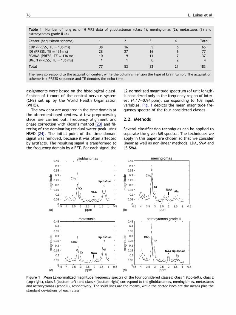
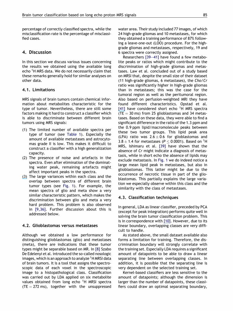
L2-normalized magnitude spectrum (of unit length)is considered only in the frequency region of inter-est (4.17—0.94 ppm), corresponding to 108 inputvariables. Fig. 1 depicts the mean magnitude fre-quency spectra of the four considered classes.

2.2. Methods

Several classification techniques can be applied toseparate the given MR spectra. The techniques weapply in this paper are chosen so that we considerlinear as well as non-linear methods: LDA, SVM andLS-SVM.

Table 1 Number of long echo 1H MRS data of glioblastomas (class 1), meningiomas (2), metastases (3) andastrocytomas grade II (4)

Center (acquisition scheme) 1 2 3 4 Total

CDP (PRESS, TE ¼ 135 ms) 38 16 5 6 65IDI (PRESS, TE ¼ 136 ms) 28 27 16 6 77SGHMS (PRESS, TE ¼ 136 ms) 10 9 11 7 37UMCN (PRESS, TE ¼ 136 ms) 1 1 0 2 4

Total 77 53 32 21 183

The rows correspond to the acquisition center, while the columns mention the type of brain tumor. The acquisitionscheme is a PRESS sequence and TE denotes the echo time.

0.511.522.533.544.50

0.05

0.1

0.15

0.2

0.25

0.3

0.35

0.4

0.45glioblastomas

ppm0.511.522.533.544.5

ppm

0.511.522.533.544.5ppm

0.511.522.533.544.5ppm

mag

nitu

de

0

0.05

0.1

0.15

0.2

0.25

0.3

0.35

0.4

0.45

mag

nitu

de

0

0.05

0.1

0.15

0.2

0.25

0.3

0.35

0.4

0.45

mag

nitu

de

0

0.05

0.1

0.15

0.2

0.25

0.3

0.35

0.4

0.45

mag

nitu

de

Cho

Cr NAA

lipids/Lac

meningiomas

Cho

Cr NAA

Ala

metastasis

Cho

Cr NAA

lipids/Lac

astrocytomas grade II

Cho Cr

NAA lipids/Lac

(a) (b)

(c) (d)

Figure 1 Mean L2-normalized magnitude frequency spectra of the four considered classes: class 1 (top-left), class 2(top-right), class 3 (bottom-left) and class 4 (bottom-right) correspond to the glioblastomas, meningiomas, metastasesand astrocytomas (grade II), respectively. The solid lines are the means, while the dotted lines are the means plus thestandard deviations of each class.

76 L. Lukas et al.

Linear discriminant analysis [25,26] basicallyprojects the data xk 2 Rn from the original inputspace into a one-dimensional variable zk 2 R andmakes a discrimination using this projected variable.This approach tries to maximize between-class var-iances and minimize the within-class variances fortwo given classes.

Linear principal component analysis (PCA) isapplied to select the input variables. It reducesthe 108 given spectral variables to a minimal setof variables which cover 75% variance of the data.

Quite often, different classes do not have equallydistributed datapoints and their distributions arealso overlapping among classes, which causes theproblem to be linearly non-separable. Here, twokernel-based classifiers SVM and LS-SVM (brieflyexplained below) are assessed. SVM and LS-SVM withlinear kernel can be regarded as regularized linearclassifiers, while LS-SVM with RBF kernel is regardedas a regularized non-linear classifier.

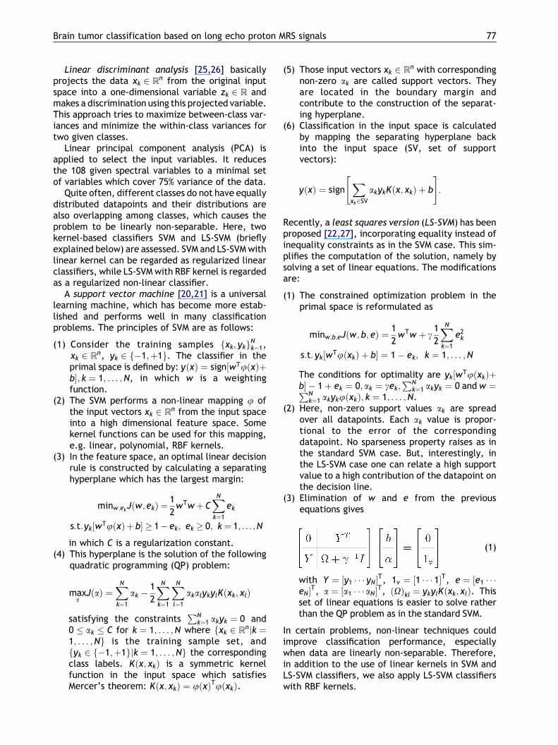
A support vector machine [20,21] is a universallearning machine, which has become more estab-lished and performs well in many classificationproblems. The principles of SVM are as follows:

(1) Consider the training samples fxk; ykgNk¼1,

xk 2 Rn, yk 2 f�1;þ1g. The classifier in theprimal space is defined by: yðxÞ ¼ sign½wTjðxÞþb; k ¼ 1; . . . ;N, in which w is a weightingfunction.

(2) The SVM performs a non-linear mapping j ofthe input vectors xk 2 Rn from the input spaceinto a high dimensional feature space. Somekernel functions can be used for this mapping,e.g. linear, polynomial, RBF kernels.

(3) In the feature space, an optimal linear decisionrule is constructed by calculating a separatinghyperplane which has the largest margin:

minw;ekJðw;ekÞ ¼

1

2wTw þC

XN

k¼1

ek

s:t:yk½wTjðxÞþ b � 1� ek; ek � 0; k ¼ 1; . . . ;N

in which C is a regularization constant.(4) This hyperplane is the solution of the following

quadratic programming (QP) problem:

maxa

JðaÞ ¼XN

k¼1

ak �1

2

XN

k¼1

XN

l¼1

akalykylKðxk; xlÞ

satisfying the constraintsPN

k¼1 akyk ¼ 0 and0 � ak � C for k ¼ 1; . . . ;N where fxk 2 Rnjk ¼1; . . . ;Ng is the training sample set, andfyk 2 f�1;þ1gjk ¼ 1; . . . ;Ng the correspondingclass labels. Kðx; xkÞ is a symmetric kernelfunction in the input space which satisfiesMercer’s theorem: Kðx; xkÞ ¼ jðxÞTjðxkÞ.

(5) Those input vectors xk 2 Rn with correspondingnon-zero ak are called support vectors. Theyare located in the boundary margin andcontribute to the construction of the separat-ing hyperplane.

(6) Classification in the input space is calculatedby mapping the separating hyperplane backinto the input space (SV, set of supportvectors):

yðxÞ ¼ signX

xk2SV

akykKðx; xkÞ þ b

" #:

Recently, a least squares version (LS-SVM) has beenproposed [22,27], incorporating equality instead ofinequality constraints as in the SVM case. This sim-plifies the computation of the solution, namely bysolving a set of linear equations. The modificationsare:

(1) The constrained optimization problem in theprimal space is reformulated as

minw;b;eJðw;b; eÞ ¼ 1

2wTw þ g

1

2

XN

k¼1

e2k

s:t: yk½wTjðxkÞ þ b ¼ 1 � ek; k ¼ 1; . . . ;N

The conditions for optimality are yk½wTjðxkÞþb � 1 þ ek ¼ 0; ak ¼ gek;

PNk¼1 akyk ¼ 0 and w ¼PN

k¼1 akykjðxkÞ; k ¼ 1; . . . ;N.(2) Here, non-zero support values ak are spread

over all datapoints. Each ak value is propor-tional to the error of the correspondingdatapoint. No sparseness property raises as inthe standard SVM case. But, interestingly, inthe LS-SVM case one can relate a high supportvalue to a high contribution of the datapoint onthe decision line.

(3) Elimination of w and e from the previousequations gives

(1)

with Y ¼ ½y1 � � � yNT, 1v ¼ ½1 � � � 1T, e ¼ ½e1 � � �eNT, a ¼ ½a1 � � � aNT, ðOÞkl ¼ ykylKðxk; xlÞ. Thisset of linear equations is easier to solve ratherthan the QP problem as in the standard SVM.

In certain problems, non-linear techniques couldimprove classification performance, especiallywhen data are linearly non-separable. Therefore,in addition to the use of linear kernels in SVM andLS-SVM classifiers, we also apply LS-SVM classifierswith RBF kernels.

Brain tumor classification based on long echo proton MRS signals 77

The MRS spectra were classified using SteveGunn’s MATLAB Support Vector Machines toolbox[28,29] and KULeuven’s MATLAB/C LS-SVMlab tool-box [27,30,31] for LS-SVM classification with bothlinear and RBF kernels.

2.3. Selected frequency regions

It is well known that characteristic peaks at cer-tain frequencies correspond to important metabo-lites in the brain [2,3,32—35]. These peaks mightbe used as discriminatory features to distinguishtumor types. In particular, when their appearanceclearly differ in size and shape in between spectraof different tumor types. Instead of using com-plete spectra as input variables to the classifier,selection of the most explanatory input featurescan be used. One approach is based on selectedfrequency regions: therefore, the input variableswithin certain regions of the magnitude spectrumwhich are assumed to contain most of the infor-mation as input features are selected. Hence, theredundancy produced by spectral noise and arte-facts in the spectrum is reduced. Characteristicmetabolites can be observed in the followingregions of the magnitude MRS spectrum: Choand Cr (2.95—3.3 ppm); NAc (1.95—2.1 ppm);Lac, Ala and lipid1 (1.15—1.55 ppm); lipid2(0.9—1.0 ppm). Note that these selected regionsare based on the metabolites that are assumed tobe most characteristic according to prior knowl-edge available from field experts participating inthis study. Nevertheless, this selection is stillsubjective as the size of the regions could bealtered or some other resonances (e.g. from meta-bolites with a typically lower intensity at a longecho time; mI, Gln, Gly, etc.) could also have beenincluded.

2.4. Peak integration

Another approach to select the most explanatoryinput is based on peak integration. The ampli-tude of a resonance is proportional to the integralof the corresponding peak in the spectrum. How-ever, precise estimation of the peak integralsis difficult due to several factors, including non-zero baseline, peak overlap, noise and also thediscrete nature of the spectrum. Peak integra-tion is performed here by using the trapezoidalrule. For each selected metabolite the areaunder the frequency peak in the magnitude spec-trum is calculated. These regions cover: Cho(3.1—3.3 ppm); Cr (2.95—3.05 ppm); NAc (1.95—2.1 ppm); Lac and Ala (1.25—1.55.ppm); and lipid1(1.1—1.25 ppm).

2.5. Training and test data

2.5.1.Binary classificationBinary classification can be used to distinguishtwo different tumor types. Instead of using a one-against-all scheme, the classes are pairwise com-pared by means of a binary classifier. Consider fourtypes of brain tumors, then six binary classifiers canbe constructed to separate the following pairs:

� glioblastomas versus meningiomas,� glioblastomas versus metastases,� glioblastomas versus astrocytomas grade II,� meningiomas versus metastases,� meningiomas versus astrocytomas grade II, and� metastases versus astrocytomas grade II.

By classifying in pairs, we obtain more informationabout:

(1) the distribution of two classes and their over-lap,

(2) the balance of the data distribution of theclasses, and

(3) the performance of the classifier which can bemeasured using ROC analysis.

The dimension of the input features to LDA isreduced by PCA. The number of principal compo-nents is determined by the number of componentsthat account for 75% of the total variance of thegiven data. Note that PCA is not used when peakintegrated values are taken as input features, aspeak integration already significantly reduces thedimension.

To achieve a high level of performance in SVMs,some hyperparameters must be tuned. These adjus-table hyperparameters include: a regularizationparameter, which determines the tradeoff betweenminimizing the training errors and minimizing themodel complexity. In case of a RBF kernel, also akernel parameter (the width s) must be selected.We choose the value of hyperparameters C for SVM,g for LS-SVM with a linear kernel and ðs; gÞ for LS-SVM with a RBF kernel through leave-one-out (LOO)cross-validation, while bounding the search to avoidoverfitting.

The experiment consists of the following steps:

(1) the data are divided in a training set (2/3 of thedata) and a test set (remainder) using stratifiedrandom sampling,

(2) train the classifiers and use the test set toevaluate the performance,

(3) the index of the misclassified spectra is noted.

This randomization is repeated 200 times to avoidbias possibly introduced by selection of a specifictraining and test set. In this way we try to obtain a

78 L. Lukas et al.

representative performance on the test set. ROC[12] analysis is used to evaluate the binary classi-fiers. The performance is then measured by themean AUC and its pooled standard error calculatedfrom 200 randomizations.

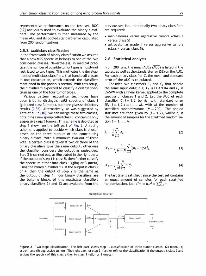
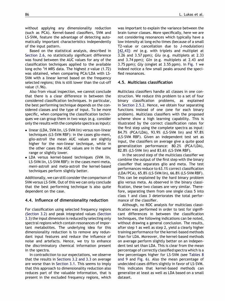
2.5.2. Multiclass classificationIn the framework of binary classification we assumethat a new MRS spectrum belongs to one of the twoconsidered classes. Nevertheless, in medical prac-tice, thenumberofpossible tumor types ismostlynotrestricted to two types. This motivates the develop-ment of multiclass classifiers, that handle all classesin one construction, which extends the classifiersmentioned in the previous section. With this setup,the classifier is expected to classify a certain spec-trum as one of the four tumor types.

Various pattern recognition techniques havebeen tried to distinguish MRS spectra of class 1(glio) and class 3 (meta), but none gives satisfactoryresults [9,36]. Alternatively, as was suggested byTate et al. in [10], we can merge these two classes,obtaining a new group called class 5, containing onlyaggressive (aggr) tumors. This scheme is depicted asstep 1 shown on the left part of Fig. 2. A votingscheme is applied to decide which class is chosenbased on the three outputs of the contributingbinary classes. With a minimum two-out-of-threevote, a certain class is taken if two or three of thebinary classifiers give the same output, otherwisethe classifier considers the output as undecided.Step 2 is carried out, as illustrated in the right part:if the output of step 1 is class 5, then further classifythe spectrum either into class 1 (glio) or 3 (meta)using the binary classifier 13. If the output is class 2or 4, then the output of step 2 is the same asthe output of step 1. Four binary classifiers arethe building blocks of this multiclass classifier:binary classifiers 24 and 13 are available from the

previous section, additionally two binary classifiersare required:

� meningiomas versus aggressive tumors (class 2versus class 5),

� astrocytomas grade II versus aggressive tumors(class 4 versus class 5).

2.6. Statistical analysis

From 200 runs, the mean AUCs (AUC) is listed in thetables, as well as the standard error (SE) on the AUC.For each binary classifier C, the mean and standarderror of the AUC is calculated.

Consider two classifiers C1 and C2 that handlethe same input data; e.g. C1 is PCA/LDA and C2 isLS-SVM with a linear kernel applied to the completespectra of classes 1 and 2. Let the AUC of eachclassifier Ci; i ¼ 1; 2 be Ai;l with standard errorSEi;l; i ¼ 1; 2; l ¼ 1; . . . ;M, with M the number ofstratified randomizations (M ¼ 200). The pooledstatistics are then given by (i ¼ 1; 2), where nl isthe amount of samples for the stratified randomiza-tion l ¼ 1; . . . ;M:

�Ai ¼1

n

XM

l¼1

Ai;l; (2)

SEi ¼

ffiffiffiffiffiffiffiffiffiffiffiffiffiffiffiffiffiffiffiffiffiffiffiffiffiffiffiffiffiffiffiffiffiffiffiffiffiffiffiffiffiffiffiffiffi1

N � M

XM

l¼1

ðnl � 1ÞSE2i;l

vuut ; (3)

SEi ¼

ffiffiffiffiffiffiffiffiffiffiffiffiffiffiffiffiffiffiffiffiffi1

M

XM

l¼1

SE2i;l

vuut : (4)

The last line is satisfied, since the test set containsan equal amount of samples for each stratifiedrandomization, i.e. 8lnl ¼ n;N ¼

PMl¼1 nl.

Multiclass Classifier

Input data

traindata24

traindata25

traindata45

binary class 24

binary class 25

binary class 45

2 or 5

2 or 4

4 or 5

Voting scheme

1 or 3

2 or 4

if 5 thenbinary class 13

if 2 or 4

2

4

5

Classifier Output

Figure 2 Two-steps classification. The left part shows step 1, classification of three tumor classes: (2) meni, (4)astroII, and (5) aggressive tumors. The right part, or step 2, further refines the classification if the output is class 5 andassigns the spectra of this class either to class 1 (glio) or 3 (meta).

Brain tumor classification based on long echo proton MRS signals 79

A general approach to statistically test whetherthe areas under two ROC curves derived from thesame samples differ significantly from each other isthen given by the critical ratio z, defined as [37]:

z ¼�A1 � �A2ffiffiffiffiffiffiffiffiffiffiffiffiffiffiffiffiffiffiffiffiffiffiffiffiffiffiffiffiffiffiffiffiffiffiffiffiffiffiffiffiffiffiffiffi

SE21 þ SE2

2 � 2rSE1SE2

qin which r is a quantity representing the correlationintroduced between the two areas by studying thesame samples. In our study we calculate the z-valuebased on the pooled statistics �Ai; SEi; i ¼ 1; 2 from200 runs as calculated in Eqs. (2)—(4). If the result-ing z-value satisfies z � 1:96, then �A1 and �A2 arestatistically different. The cut-off value 1.96 istaken as the quantity for which, under the hypoth-esis of equal AUCs (�A1 ¼ �A2), z � 1:96 occurs with aprobability of a ¼ 0:05 under a normal distribution.

This ROC analysis is performed for binary classi-fication. Although ROC analysis has been extendedto multiclass classification [38], the result is gen-erally non-intuitive and computationally expensive.This motivates the use of the correct classificationrate as performance measure for multiclass classi-fication.

3. Results

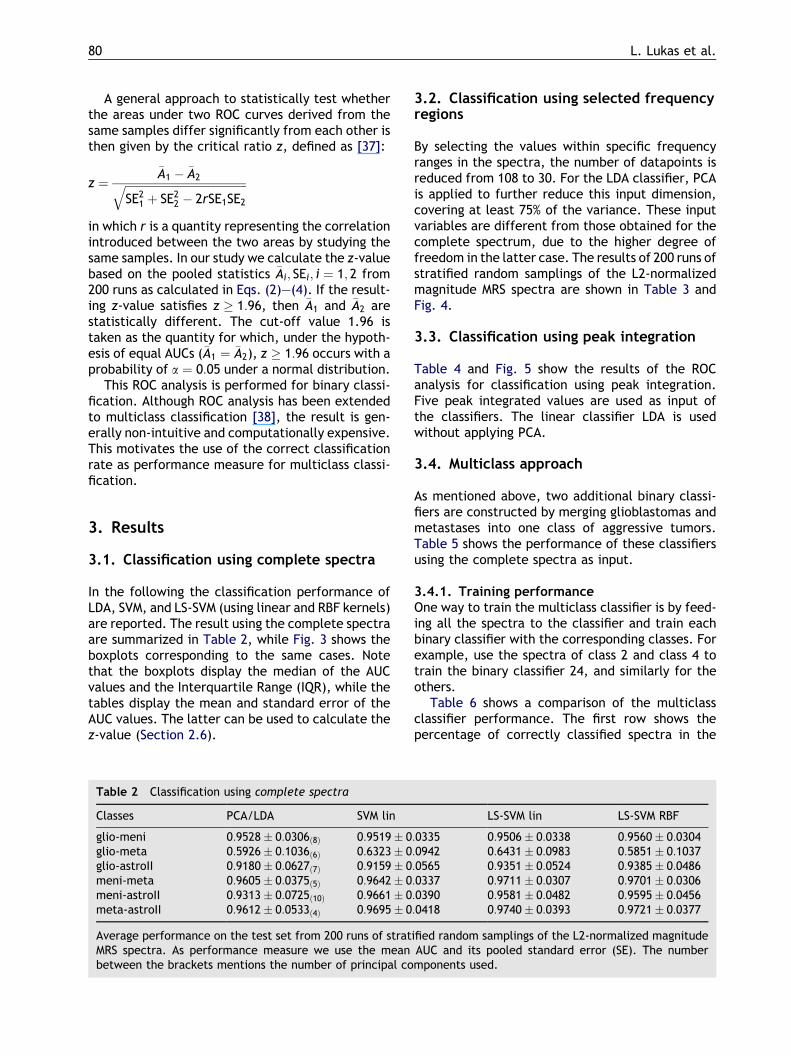
3.1. Classification using complete spectra

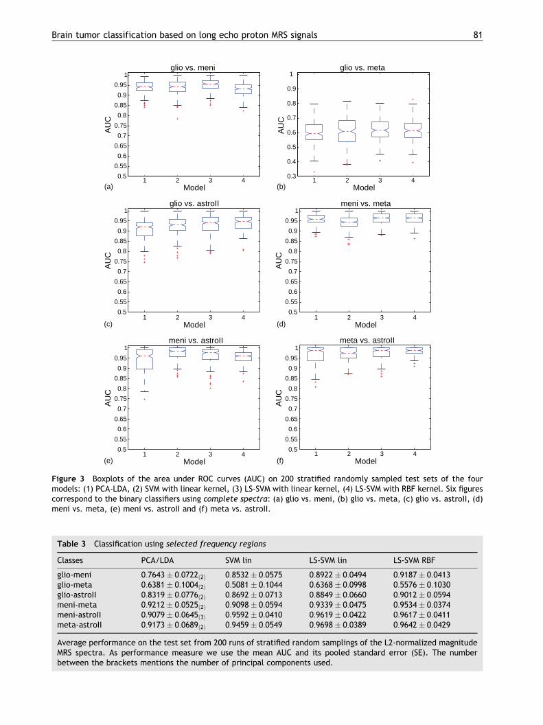
In the following the classification performance ofLDA, SVM, and LS-SVM (using linear and RBF kernels)are reported. The result using the complete spectraare summarized in Table 2, while Fig. 3 shows theboxplots corresponding to the same cases. Notethat the boxplots display the median of the AUCvalues and the Interquartile Range (IQR), while thetables display the mean and standard error of theAUC values. The latter can be used to calculate thez-value (Section 2.6).

3.2. Classification using selected frequencyregions

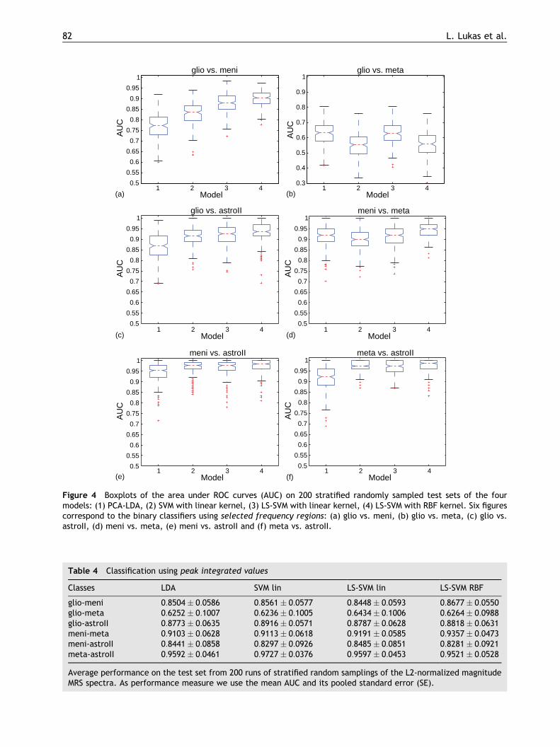
By selecting the values within specific frequencyranges in the spectra, the number of datapoints isreduced from 108 to 30. For the LDA classifier, PCAis applied to further reduce this input dimension,covering at least 75% of the variance. These inputvariables are different from those obtained for thecomplete spectrum, due to the higher degree offreedom in the latter case. The results of 200 runs ofstratified random samplings of the L2-normalizedmagnitude MRS spectra are shown in Table 3 andFig. 4.

3.3. Classification using peak integration

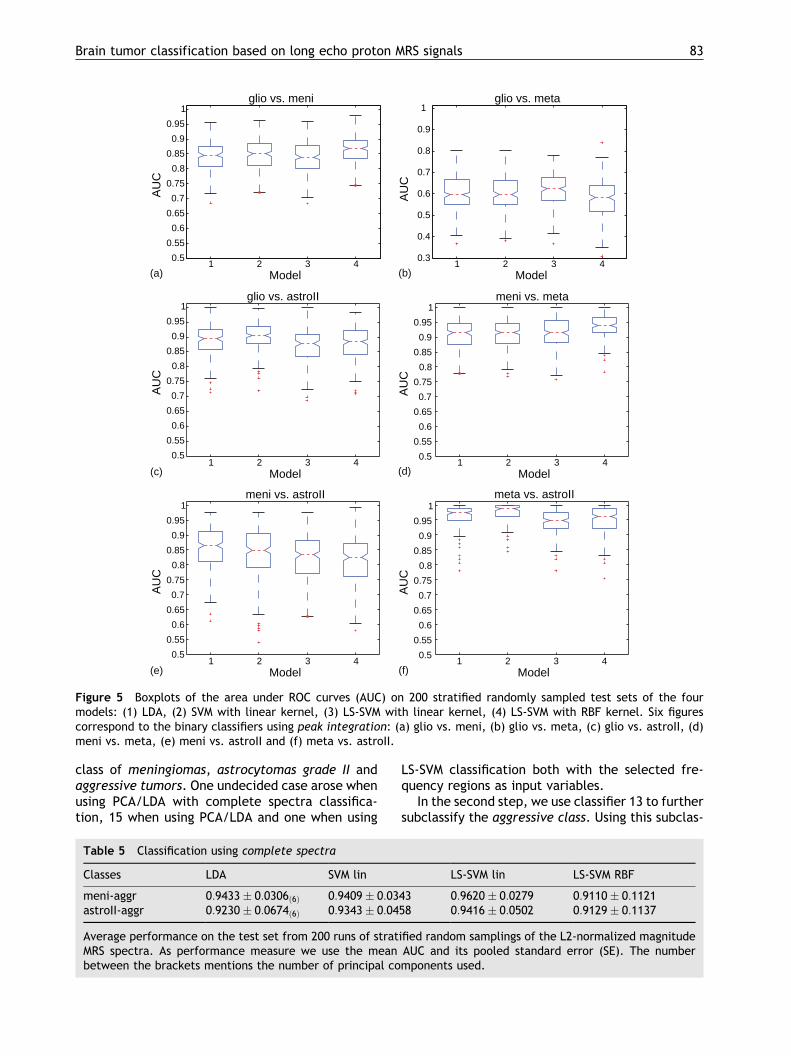
Table 4 and Fig. 5 show the results of the ROCanalysis for classification using peak integration.Five peak integrated values are used as input ofthe classifiers. The linear classifier LDA is usedwithout applying PCA.

3.4. Multiclass approach

As mentioned above, two additional binary classi-fiers are constructed by merging glioblastomas andmetastases into one class of aggressive tumors.Table 5 shows the performance of these classifiersusing the complete spectra as input.

3.4.1. Training performanceOne way to train the multiclass classifier is by feed-ing all the spectra to the classifier and train eachbinary classifier with the corresponding classes. Forexample, use the spectra of class 2 and class 4 totrain the binary classifier 24, and similarly for theothers.

Table 6 shows a comparison of the multiclassclassifier performance. The first row shows thepercentage of correctly classified spectra in the

Table 2 Classification using complete spectra

Classes PCA/LDA SVM lin LS-SVM lin LS-SVM RBF

glio-meni 0:9528 � 0:0306ð8Þ 0:9519 � 0:0335 0:9506 � 0:0338 0:9560 � 0:0304glio-meta 0:5926 � 0:1036ð6Þ 0:6323 � 0:0942 0:6431 � 0:0983 0:5851 � 0:1037glio-astroII 0:9180 � 0:0627ð7Þ 0:9159 � 0:0565 0:9351 � 0:0524 0:9385 � 0:0486meni-meta 0:9605 � 0:0375ð5Þ 0:9642 � 0:0337 0:9711 � 0:0307 0:9701 � 0:0306meni-astroII 0:9313 � 0:0725ð10Þ 0:9661 � 0:0390 0:9581 � 0:0482 0:9595 � 0:0456meta-astroII 0:9612 � 0:0533ð4Þ 0:9695 � 0:0418 0:9740 � 0:0393 0:9721 � 0:0377

Average performance on the test set from 200 runs of stratified random samplings of the L2-normalized magnitudeMRS spectra. As performance measure we use the mean AUC and its pooled standard error (SE). The numberbetween the brackets mentions the number of principal components used.

80 L. Lukas et al.

1 2 3 40.5

0.55

0.6

0.65

0.7

0.75

0.8

0.85

0.9

0.95

1glio vs. meni

AU

C

0.5

0.55

0.6

0.65

0.7

0.75

0.8

0.85

0.9

0.95

1

AU

C

0.5

0.55

0.6

0.65

0.7

0.75

0.8

0.85

0.9

0.95

1

AU

C

0.5

0.55

0.6

0.65

0.7

0.75

0.8

0.85

0.9

0.95

1

AU

C

0.5

0.55

0.6

0.65

0.7

0.75

0.8

0.85

0.9

0.95

1

AU

C

Model

1 2 3 4Model

1 2 3 4Model

1 2 3 4Model

1 2 3 4Model

1 2 3 4Model

0.3

0.4

0.5

0.6

0.7

0.8

0.9

1glio vs. meta

AU

C

glio vs. astroII meni vs. meta

meni vs. astroII meta vs. astroII

(a) (b)

(d)(c)

(e) (f)

Figure 3 Boxplots of the area under ROC curves (AUC) on 200 stratified randomly sampled test sets of the fourmodels: (1) PCA-LDA, (2) SVM with linear kernel, (3) LS-SVM with linear kernel, (4) LS-SVM with RBF kernel. Six figurescorrespond to the binary classifiers using complete spectra: (a) glio vs. meni, (b) glio vs. meta, (c) glio vs. astroII, (d)meni vs. meta, (e) meni vs. astroII and (f) meta vs. astroII.

Table 3 Classification using selected frequency regions

Classes PCA/LDA SVM lin LS-SVM lin LS-SVM RBF

glio-meni 0:7643 � 0:0722ð2Þ 0:8532 � 0:0575 0:8922 � 0:0494 0:9187 � 0:0413glio-meta 0:6381 � 0:1004ð2Þ 0:5081 � 0:1044 0:6368 � 0:0998 0:5576 � 0:1030glio-astroII 0:8319 � 0:0776ð2Þ 0:8692 � 0:0713 0:8849 � 0:0660 0:9012 � 0:0594meni-meta 0:9212 � 0:0525ð2Þ 0:9098 � 0:0594 0:9339 � 0:0475 0:9534 � 0:0374meni-astroII 0:9079 � 0:0645ð3Þ 0:9592 � 0:0410 0:9619 � 0:0422 0:9617 � 0:0411meta-astroII 0:9173 � 0:0689ð2Þ 0:9459 � 0:0549 0:9698 � 0:0389 0:9642 � 0:0429

Average performance on the test set from 200 runs of stratified random samplings of the L2-normalized magnitudeMRS spectra. As performance measure we use the mean AUC and its pooled standard error (SE). The numberbetween the brackets mentions the number of principal components used.

Brain tumor classification based on long echo proton MRS signals 81

1 2 3 40.5

0.55

0.6

0.65

0.7

0.75

0.8

0.85

0.9

0.95

1glio vs. meni

AU

C

0.5

0.55

0.6

0.65

0.7

0.75

0.8

0.85

0.9

0.95

1

AU

C

0.5

0.55

0.6

0.65

0.7

0.75

0.8

0.85

0.9

0.95

1

AU

C

0.5

0.55

0.6

0.65

0.7

0.75

0.8

0.85

0.9

0.95

1

AU

C

0.5

0.55

0.6

0.65

0.7

0.75

0.8

0.85

0.9

0.95

1

AU

C

Model1 2 3 4

Model

1 2 3 4Model

1 2 3 4Model

1 2 3 4Model

1 2 3 4Model

0.3

0.4

0.5

0.6

0.7

0.8

0.9

1glio vs. meta

AU

C

glio vs. astroII meni vs. meta

meni vs. astroII meta vs. astroII

(a) (b)

(c) (d)

(e) (f)

Figure 4 Boxplots of the area under ROC curves (AUC) on 200 stratified randomly sampled test sets of the fourmodels: (1) PCA-LDA, (2) SVM with linear kernel, (3) LS-SVM with linear kernel, (4) LS-SVM with RBF kernel. Six figurescorrespond to the binary classifiers using selected frequency regions: (a) glio vs. meni, (b) glio vs. meta, (c) glio vs.astroII, (d) meni vs. meta, (e) meni vs. astroII and (f) meta vs. astroII.

Table 4 Classification using peak integrated values

Classes LDA SVM lin LS-SVM lin LS-SVM RBF

glio-meni 0:8504 � 0:0586 0:8561 � 0:0577 0:8448 � 0:0593 0:8677 � 0:0550glio-meta 0:6252 � 0:1007 0:6236 � 0:1005 0:6434 � 0:1006 0:6264 � 0:0988glio-astroII 0:8773 � 0:0635 0:8916 � 0:0571 0:8787 � 0:0628 0:8818 � 0:0631meni-meta 0:9103 � 0:0628 0:9113 � 0:0618 0:9191 � 0:0585 0:9357 � 0:0473meni-astroII 0:8441 � 0:0858 0:8297 � 0:0926 0:8485 � 0:0851 0:8281 � 0:0921meta-astroII 0:9592 � 0:0461 0:9727 � 0:0376 0:9597 � 0:0453 0:9521 � 0:0528

Average performance on the test set from 200 runs of stratified random samplings of the L2-normalized magnitudeMRS spectra. As performance measure we use the mean AUC and its pooled standard error (SE).

82 L. Lukas et al.

class of meningiomas, astrocytomas grade II andaggressive tumors. One undecided case arose whenusing PCA/LDA with complete spectra classifica-tion, 15 when using PCA/LDA and one when using

LS-SVM classification both with the selected fre-quency regions as input variables.

In the second step, we use classifier 13 to furthersubclassify the aggressive class. Using this subclas-

1 2 3 40.5

0.55

0.6

0.65

0.7

0.75

0.8

0.85

0.9

0.95

1glio vs. meni

AU

C

0.5

0.55

0.6

0.65

0.7

0.75

0.8

0.85

0.9

0.95

1

AU

C

0.5

0.55

0.6

0.65

0.7

0.75

0.8

0.85

0.9

0.95

1

AU

C

0.5

0.55

0.6

0.65

0.7

0.75

0.8

0.85

0.9

0.95

1

AU

C

0.5

0.55

0.6

0.65

0.7

0.75

0.8

0.85

0.9

0.95

1

AU

C

Model

1 2 3 4Model

1 2 3 4Model

1 2 3 4Model

1 2 3 4Model

1 2 3 4Model

0.3

0.4

0.5

0.6

0.7

0.8

0.9

1glio vs. meta

AU

C

glio vs. astroII meni vs. meta

meni vs. astroII meta vs. astroII

(a) (b)

(c) (d)

(e) (f)

Figure 5 Boxplots of the area under ROC curves (AUC) on 200 stratified randomly sampled test sets of the fourmodels: (1) LDA, (2) SVM with linear kernel, (3) LS-SVM with linear kernel, (4) LS-SVM with RBF kernel. Six figurescorrespond to the binary classifiers using peak integration: (a) glio vs. meni, (b) glio vs. meta, (c) glio vs. astroII, (d)meni vs. meta, (e) meni vs. astroII and (f) meta vs. astroII.

Table 5 Classification using complete spectra

Classes LDA SVM lin LS-SVM lin LS-SVM RBF

meni-aggr 0:9433 � 0:0306ð6Þ 0:9409 � 0:0343 0:9620 � 0:0279 0:9110 � 0:1121astroII-aggr 0:9230 � 0:0674ð6Þ 0:9343 � 0:0458 0:9416 � 0:0502 0:9129 � 0:1137

Average performance on the test set from 200 runs of stratified random samplings of the L2-normalized magnitudeMRS spectra. As performance measure we use the mean AUC and its pooled standard error (SE). The numberbetween the brackets mentions the number of principal components used.

Brain tumor classification based on long echo proton MRS signals 83

sification, the multiclass classifier’s performance isshown in Table 7.

3.4.2. Test performanceBesides using all the spectra to choose the hyper-parameters and to train the classifiers, one can alsoselect 2/3 of the dataset as training set and use theremainder as test set. This stratified random sam-pling is repeated for 200 runs. The results are shownin Table 8 for one-step classification, which assigns

the spectra to one of the three following classes: 2, 4or 5. Table 9 shows the classifier performance aftertwo-steps classification, which assigns the spectra to1 of the 4 following classes: 1, 2, 3 or 4. Eachspectrum of class 5 in step 1, is either assigned toclass 1 or class 3 in step 2. In Tables 8 and 9 wemention the mean correct classification rate, themean misclassification rate and the mean percen-tage of undecided cases and their standard devia-tion. The correct classification rate is defined as the

Table 6 One-step classification using complete spectra

PCA/LDA (%) LS-SVM lin (%) LS-SVM RBF (%)

Compl. spec. 84.6995 93.9891 97.8142Disc. feat. 65.0273 84.6995 90.1639Peak integ. 75.9563 77.0492 80.8743

Percentage of correctly classified spectra using all L2-normalized magnitude MRS spectra to assess the trainingperformance.

Table 7 Two-steps classification using complete spectra

PCA/LDA (%) LS-SVM lin (%) LS-SVM RBF (%)

Compl. spec. 71.0383 78.1421 83.6066Disc. feat. 50.2732 68.8525 74.8634Peak integ. 61.7486 62.2951 67.7596

Percentage of correctly classified spectra using all L2-normalized magnitude MRS spectra to assess the trainingperformance.

Table 8 One-step classification using complete spectra

PCA/LDA (%) LS-SVM lin (%) LS-SVM RBF (%)

Correct 80:1855 � 4:2853 82:7823 � 3:3449 83:5726 � 3:5058Misclass 14:0887 � 4:0665 13:6532 � 3:1140 12:5565 � 3:3290Undecided 05:7258 � 2:6110 03:5645 � 2:0870 03:8710 � 2:1144

Average performance on the test set from 200 runs of stratified random samplings (2/3 of the data used for training,1/3 for testing). The first, second and third rows give, respectively, the mean correct classification rate, the meanmisclassification rate and the mean percentage of undecided cases, each with their standard deviation.

Table 9 Two-steps classification using complete spectra

PCA/LDA (%) LS-SVM lin (%) LS-SVM RBF (%)

Correct 63:1532 � 4:7255 65:7984 � 3:3449 66:8145 � 3:5058Misclass 31:1210 � 4:6858 30:6371 � 3:1706 29:3145 � 3:5954Undecided 05:7258 � 2:6110 03:5645 � 2:0870 03:8710 � 2:1144

Average performance on the test set from 200 runs of stratified random samplings (2/3 of the data used for training,1/3 for testing). The first, second and third rows give, respectively, the mean correct classification rate, the meanmisclassification rate and the mean percentage of undecided cases, each with their standard deviation. Note thatthe number of undecided cases is equal to that for the one-step classifier.

84 L. Lukas et al.

percentage of correctly classified spectra, while themisclassification rate is the percentage of misclassi-fied cases.

4. Discussion

In this section we discuss various issues concerningthe results we obtained using the available longecho 1H MRS data. We do not necessarily claim thatthese remarks generally hold for similar analyses onother data.

4.1. Limitations

MRS signals of brain tumors contain chemical infor-mation about metabolites characteristic for thetype of tumor. Nevertheless, there are still somefactors making it hard to construct a classifier whichis able to discriminate between different braintumors using MRS signals:

(1) The limited number of available spectra pertype of tumor (see Table 1). Especially theamount of available metastases and astrocyto-mas grade II is low. This makes it difficult toconstruct a classifier with a high generalizationcapacity.

(2) The presence of noise and artefacts in thespectra. Even after elimination of the dominat-ing water peak, remaining artefacts mightaffect important peaks in the spectra.

(3) The large variances within each class and theoverlap between spectra of different braintumor types (see Fig. 1). For example, themean spectra of glio and meta show a verysimilar characteristic pattern, which makes thediscrimination between glio and meta a veryhard problem. This problem is also observedin [9,36]. Further discussion about this isaddressed below.

4.2. Glioblastomas versus metastases

Although we obtained a low performance fordistinguishing glioblastomas (glio) and metastases(meta), there are indications that these tumortypes might be separable based on MR. In [8] SzaboDe Edelenyi et al. introduced the so-called nosologicimages, which is an approach to analyze 1H MRSI dataof brain tumors. It is a tool that assigns the spectro-scopic data of each voxel in the spectroscopicimage to a histopathological class. Classificationwas carried out by LDA applied on six metabolitevalues obtained from long echo 1H MRSI spectra(TE ¼ 272 ms), together with the unsuppressed

water area. Their study included 77 images, of which24 high-grade gliomas and 10 metastases, for whichthey obtained a training performance of 87% follow-ing a leave-one-out (LOO) procedure. For the high-grade gliomas and metastases, respectively, 19 and6 spectra were correctly assigned.

Researchers [39—41] have found a few metabo-lite peaks or ratios which might contribute to thediscrimination of high-grade gliomas and metas-tases. Law et al. concluded out of a study basedon MRSI that, despite the small size of their dataset(11 high-grade gliomas, 6 metastases), the Cho/Crratio was significantly higher in high-grade gliomasthan in metastases; this was the case for thetumoral region as well as the peritumoral region.Also based on perfusion-weighted MRI they havefound different characteristics. Opstad et al.[41] have considered short echo 1H MRS spectra(TE ¼ 30 ms) from 25 glioblastomas and 34 metas-tases. Based on these data, they were able to find asignificant difference in the ratio of the 1.3 ppm andthe 0.9 ppm lipid/macromolecule peaks betweenthese two tumor groups. This lipid peak area(LPA) ratio was 2:6 � 0:6 for glioblastomas and3:8 � 1:4 for metastases (P � 0:0001). Based on 1HMRS, Ishimaru et al. [39] have shown that theabsence of Cr might indicate a diagnosis of metas-tasis, while in short echo the absence of lipids mayexclude metastasis. In Fig. 1 we do indeed notice alarge mean lipid peak in metastases, but also inglioblastomas. This latter might be due to theoccurrence of necrotic tissue in part of the glio-blastomas. This partially explains the large varia-tion we especially observe within this class and thesimilarity with the class of metastases.

4.3. Classification techniques

In general, LDA as linear classifier, preceded by PCA(except for peak integration) performs quite well insolving the brain tumor classification problem. Thisis in correspondence with [10]. However, due to itslinear boundary, overlapping classes are very diffi-cult to handle.

As stated above, the small dataset available alsoforms a limitation for training. Therefore, the dis-crimination boundary will strongly correlate withthe training set. Especially LDA requires a significantamount of datapoints to be able to draw a linearseparating line between overlapping classes. Inaddition, it is possible that the separating line isvery dependent on the selected training set.

Kernel-based classifiers are less sensitive to theamount of datapoints; although the dimension islarger than the number of datapoints, these classi-fiers could draw an optimal separating boundary,

Brain tumor classification based on long echo proton MRS signals 85

without applying any dimensionality reduction(such as PCA). Kernel-based classifiers, SVM andLS-SVM, feature the advantage of detecting auto-matically important characteristics independentlyof the input pattern.

Based on the statistical analysis, described inSection 2.6, no statistically significant differencewas found between the AUC values for any of theclassification techniques applied to the availablelong echo 1H MRS data. The highest z-value (1.72)was obtained, when comparing PCA/LDA with LS-SVM with a linear kernel based on the frequencyselected regions; this is still lower than the cut-offvalue (1.96).

Also from visual inspection, we cannot concludethat there is a clear difference in between theconsidered classification techniques. In particular,the best performing technique depends on the con-sidered classes and the type of input. To be morespecific, when comparing the classification techni-ques we can group them in two ways (e.g. consideronly the results with the complete spectra as input):

� linear (LDA, SVM lin, LS-SVM lin) versus non-lineartechniques (LS-SVM RBF): in the cases glio-meni,glio-astroII the mean AUC values are slightlyhigher for the non-linear technique, while inthe other cases the AUC values are in the samerange or slightly lower.

� LDA versus kernel-based techniques (SVM lin,LS-SVM lin, LS-SVM RBF): in the cases meni-meta,meni-astroII and meta-astroII the kernel-basedtechniques perform slightly better.

Additionally, we can still consider the comparison ofSVM versus LS-SVM. Out of this we can only concludethat the best performing technique is also quitedependent on the case.

4.4. Influence of dimensionality reduction

For classification using selected frequency regions(Section 3.2) and peak integrated values (Section3.3) the input dimension is reduced by selecting onlyspectral regions which contain resonances of impor-tant metabolites. The underlying idea for thisdimensionality reduction is to remove any redun-dant input features and reduce the influence ofnoise and artefacts. Hence, we try to enhancethe discriminatory chemical information presentin the spectra.

In contradiction to our expectations, we observethat the results in Sections 3.2 and 3.3 on averageare worse than in Section 3.1. This seems to implythat this approach to dimensionality reduction alsoreduces part of the valuable information, that ispresent in the excluded frequency regions, which

was important to explain the variance between thebrain tumor classes. More specifically, here we arenot considering resonances which typically have alow intensity at long echo times (because of a smallT2-value or cancellation due to J-modulation)[42,43]: mI (e.g. with triplets and multiplet at3.26 and 3.57 ppm); Glu (e.g. multiplets at 2.33and 3.74 ppm); Gln (e.g. multiplets at 2.43 and3.75 ppm); Gly (singlet at 3.55 ppm). In Fig. 1 weindeed notice a few small peaks around the speci-fied resonances.

4.5. Multiclass classification

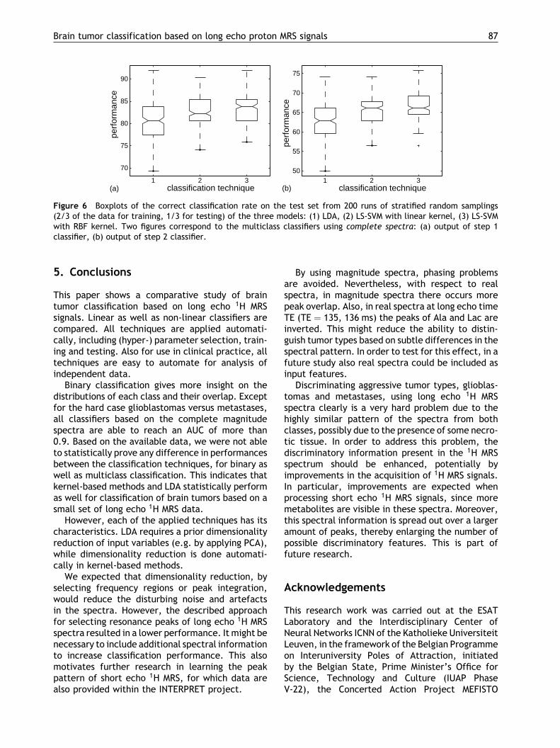
Multiclass classifiers handle all classes in one con-struction. We reduce this problem to a set of fourbinary classification problems, as explainedin Section 2.5.2. Hence, we obtain four separatingfunctions instead of one (one for each binaryproblem). Multiclass classifiers with the proposedscheme show a high learning capability. This isillustrated by the correct classification rates forthe first step using the complete spectra as input:84.7% (PCA/LDA), 93.9% (LS-SVM lin) and 97.8%(LS-SVM RBF). Given an independent test set asinput, the classifiers on average give a quite goodgeneralization performance: 80.2% (PCA/LDA),82.8% (LS-SVM lin) and 83.6% (LS-SVM RBF).

In the second step of the multiclass classifier wecombine the output of the first step with the binaryclassifier that separates glio and meta. The testperformances reduce to 63.1% correct classification(LDA/PCA), 65.8% (LS-SVM lin), 66.8% (LS-SVM RBF).This can be explained by the hard binary problemglio versus meta. As observed in the binary classi-fication, these two classes are very similar. There-fore, separating them from one single class 5 intoclass 1 and class 3 deteriorates the total perfor-mance of the classifier.

Although, no ROC analysis for multiclass classi-fication was performed in order to test for signifi-cant differences in between the classificationtechniques, the following indications can be noted,without drawing a general conclusion. The results,after step 1 as well as step 2, yield a clearly highertraining performance for the kernel-based methodsthan for LDA. Moreover, the kernel-based methodson average perform slightly better on an indepen-dent test set than LDA. This is clear from the meanpercentage of correctly classified spectra which is afew percentages higher for LS-SVM (see Tables 8and 9 and Fig. 6). Also the mean percentage ofundecided cases differs slightly in favor of LS-SVM.This indicates that kernel-based methods cangeneralize at least as well as LDA based on a smalldataset.

86 L. Lukas et al.

5. Conclusions

This paper shows a comparative study of braintumor classification based on long echo 1H MRSsignals. Linear as well as non-linear classifiers arecompared. All techniques are applied automati-cally, including (hyper-) parameter selection, train-ing and testing. Also for use in clinical practice, alltechniques are easy to automate for analysis ofindependent data.

Binary classification gives more insight on thedistributions of each class and their overlap. Exceptfor the hard case glioblastomas versus metastases,all classifiers based on the complete magnitudespectra are able to reach an AUC of more than0.9. Based on the available data, we were not ableto statistically prove any difference in performancesbetween the classification techniques, for binary aswell as multiclass classification. This indicates thatkernel-based methods and LDA statistically performas well for classification of brain tumors based on asmall set of long echo 1H MRS data.

However, each of the applied techniques has itscharacteristics. LDA requires a prior dimensionalityreduction of input variables (e.g. by applying PCA),while dimensionality reduction is done automati-cally in kernel-based methods.

We expected that dimensionality reduction, byselecting frequency regions or peak integration,would reduce the disturbing noise and artefactsin the spectra. However, the described approachfor selecting resonance peaks of long echo 1H MRSspectra resulted in a lower performance. It might benecessary to include additional spectral informationto increase classification performance. This alsomotivates further research in learning the peakpattern of short echo 1H MRS, for which data arealso provided within the INTERPRET project.

By using magnitude spectra, phasing problemsare avoided. Nevertheless, with respect to realspectra, in magnitude spectra there occurs morepeak overlap. Also, in real spectra at long echo timeTE (TE ¼ 135, 136 ms) the peaks of Ala and Lac areinverted. This might reduce the ability to distin-guish tumor types based on subtle differences in thespectral pattern. In order to test for this effect, in afuture study also real spectra could be included asinput features.

Discriminating aggressive tumor types, glioblas-tomas and metastases, using long echo 1H MRSspectra clearly is a very hard problem due to thehighly similar pattern of the spectra from bothclasses, possibly due to the presence of some necro-tic tissue. In order to address this problem, thediscriminatory information present in the 1H MRSspectrum should be enhanced, potentially byimprovements in the acquisition of 1H MRS signals.In particular, improvements are expected whenprocessing short echo 1H MRS signals, since moremetabolites are visible in these spectra. Moreover,this spectral information is spread out over a largeramount of peaks, thereby enlarging the number ofpossible discriminatory features. This is part offuture research.

Acknowledgements

This research work was carried out at the ESATLaboratory and the Interdisciplinary Center ofNeural Networks ICNN of the Katholieke UniversiteitLeuven, in the framework of the Belgian Programmeon Interuniversity Poles of Attraction, initiatedby the Belgian State, Prime Minister’s Office forScience, Technology and Culture (IUAP PhaseV-22), the Concerted Action Project MEFISTO

1 2 3

70

75

80

85

90

perf

orm

ance

classification technique1 2 3

50

55

60

65

70

75

perf

orm

ance

classification technique(a) (b)

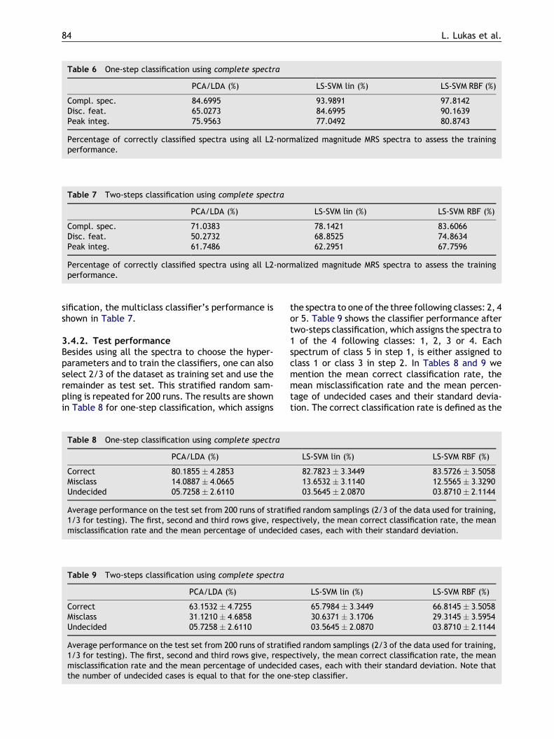
Figure 6 Boxplots of the correct classification rate on the test set from 200 runs of stratified random samplings(2/3 of the data for training, 1/3 for testing) of the three models: (1) LDA, (2) LS-SVM with linear kernel, (3) LS-SVMwith RBF kernel. Two figures correspond to the multiclass classifiers using complete spectra: (a) output of step 1classifier, (b) output of step 2 classifier.

Brain tumor classification based on long echo proton MRS signals 87

of the Flemish Community, the FWO projectsG.0407.02 and G.0269.02 and the IDO/99/03 pro-ject. AD research financed by IWT grant of theFlemish Institute for the promotion of scientific-technological research in the industry. LVH is apostdoctoral researcher with the National Fundfor Scientific Research FWO, Flanders. Use ofthe data provided by the EU funded INTERPRETproject (IST-1999-10310; http://carbon.uab.es/INTERPRET/) is gratefully acknowledged.

References

[1] The Brain Tumor Society. http://www.tbts.org.[2] Mukherji SK, editor. Clinical applications of magnetic

resonance spectroscopy. Wiley-Liss, 1998.[3] Smith ICP, Stewart LC. Magnetic resonance spectroscopy

in medicine: clinical impact. Prog Nucl Mag Res Sp 2002;40:1—34.

[4] Cousins JP. Clinical MR spectroscopy: fundamentals,current applications, and future potential. AJR Am JRoentgenol 1995;164:1337—47.

[5] Lindon JC, Holmes E, Nicholson JK. Pattern recognitionmethods and applications in biomedical magnetic reso-nance. Prog Nucl Mag Res Sp 2001;39:1—40.

[6] Herminghaus S, Dierks T, Pilatus U, Moller-Hartmann W,Wittsack J, Marquardt G, et al. Determination of histo-pathological tumor grade in neuroepithelial brain tumorsby using spectral pattern analysis of in vivo spectroscopicdata. J Neurosurg 2003;98:74—81.

[7] Simonetti AW, Melssen WJ, van der Graaf M, Heerschap A,Buydens LMC. Brain tumor classification and probabilitymaps using MRI and MRSI data. Anal Chem 2003;75(20):5352—61.

[8] Szabo De Edelenyi F, Rubin C, Esteve F, Grand S, Decorps M,Lefournier V, et al. Nature Med. 2000;6:1287—9.

[9] Tate AR, Griffiths JR, Mart½nez-Perez I, Moreno A, Barba I,Cabanas ME, et al. Towards a method for automatedclassification of 1H MRS spectra from brain tumours. NMRBiomed 1998;11:177—91.

[10] Tate AR, Majos C, Moreno A, Howe FA, Griffiths JR, Arus C.Automated classification of short echo time in vivo 1H braintumor spectra: a multicenter study. Magn Reson Med2003;49:29—36.

[11] Ye C-Z, Yang J, Geng D-Y, Zhou Y, Chen N-Y. Fuzzy rules topredict degree of malignancy in brain glioma. Med Biol EngComput 2002;40:145—52.

[12] Swets JA. ROC analysis applied to the evaluation of medicalimaging techniques. Invest Radiol 1979;14(2):109—21.

[13] International network for pattern recognition of tumoursusing magnetic resonance. http://carbon.uab.es/INTER-PRET/.

[14] Ladroue C, Tate AR, Howe FA, Griffiths JR. Exploringmagnetic resonance data with independent componentanalysis. In: Proceedings of the 19th Annual Meeting of theEuropean Society for Magnetic Resonance in Medicine andBiology (ESMRMB02), Cannes, France, August 22—25, 2002.p. 147—8.

[15] Lefournier V, Szabo De Edelenyi F, Esteve F, Grand S, BessouP, Boubagra K, et al. Nosologic images for classification ofbrain tumors with 1H MRSI: clinical performance. In:Proceedings of the 19th Annual Meeting of the EuropeanSociety for Magnetic Resonance in Medicine and Biology(ESMRMB02), Cannes, France, August 22—25, 2002. p. 91—2.

[16] Lukas L, Devos A, Suykens JAK, Vanhamme L, Van Huffel S,Tate AR, et al. The use of LS-SVM in the classification ofbrain tumors based on magnetic resonance spectroscopysignals. In: Proceedings of the European Symposium forArtifical Neural Networks (ESANN), Bruges, Belgium, April24—26, 2002. p. 131—5.

[17] Lukas L, Devos A, Suykens JAK, Vanhamme L, Van Huffel S,Tate AR, et al. The use of LS-SVM in the classification ofbrain tumors based on 1H-MR spectroscopy signals. In:Proceedings of the IEE Symposium on Medical Applicationsof Signal Processing, Savoy Place, London, UK, October 7,2002. p. 15/1—5.

[18] Szabo De Edelenyi F, Esteve F, Remy C, Buydens L.Proceedings of the 19th Annual Meeting of the EuropeanSociety for Magnetic Resonance in Medicine and Biology(ESMRMB02), Cannes, France, August 22—25, 2002. p. 91.

[19] Tate AR, Griffiths JR, Howe FA, Pujol J, Arus C.Differentiating types of human brain tumours by MRS. Acomparison of pre-processing methods and echo times. In:Proceedings of the Ninth Scientific Meeting & Exhibition(ISMRM01), Glasgow, Scotland, April 21—27, 2001. p. 2284.

[20] Vapnik V. The nature of statistical learning theory. NewYork: Springer, 1995.

[21] Vapnik V. Statistical learning theory. New York: Wiley,1998.

[22] Suykens JAK, Vandewalle J. Least squares support vectormachine classifiers. Neur Proc Lett 1999;9(3):293—300.

[23] Klose U. In vivo proton spectroscopy in presence of eddycurrents. Magn Reson Med 1990;14:26—30.

[24] Barkhuijsen H, De Beer R, Van Ormondt D. Improvedalgorithm for noniterative time-domain model fitting toexponentially damped magnetic resonance signals. J MagnReson 1987;73:553—7.

[25] Duda RO, Hart PE, Stork DG. Pattern classification. 2nd ed.New York: Wiley, 2001.

[26] Ripley BD. Pattern recognition and neural networks. Cam-bridge: Cambridge University Press, 1996.

[27] Suykens JAK, Van Gestel T, De Brabanter J, De Moor B,Vandewalle J. Least squares support vector machines.Singapore: World Scientific, 2002.

[28] Gunn SR. Support vector machines for classification andregression. Technical Report. Image Speech and IntelligentSystems Research Group, University of Southampton, 1997.

[29] MATLAB support vector machines toolbox. http://www.isis.ecs.soton.ac.uk/isystems/kernel.

[30] MATLAB/C LS-SVMlab toolbox. http://www.esat.kuleuve-n.ac.be/sista/lssvmlab.

[31] Pelckmans K, Suykens JAK, Van Gestel T, De Brabanter J,Lukas L, Hamers B, et al. LS-SVMlab Toolbox User’s Guide.Internal Report 02-145. ESAT-SISTA, K. U. Leuven, Leuven,Belgium, 2002.

[32] Howe FA, Barton SJ, Cudlip SA, Stubbs M, Saunders DE,Murphy M, et al. Metabolic profiles of human brain tumorsusing quantitative in vivo 1H magnetic resonance spectro-scopy. Magn Reson Med 2003;49:223—32.

[33] Lecrerc X, Huisman TAGM, Sorensen AG. The potential ofproton magnetic resonance spectroscopy (1H) in thediagnosis and management of patients with brain tumors.Curr Opin Oncol 2002;14:292—8.

[34] Majos C, Alonso J, Aguilera C, Serrallonga M, Acebes JJ,Arus C, et al. Adult primitive neuroectodermal tumor:proton MR spectroscopic findings with possible applicationfor differential diagnosis. Radiology 2002;225:556—66.

[35] Murphy M, Loosemore A, Clifton AG, Howe FA, Tate AR,Cudlip SA, et al. The contribution of proton magneticresonance spectroscopy (1H MRS) to clinical brain tumourdiagnosis. Br J Neurosurg 2002;16(4):329—34.

88 L. Lukas et al.

[36] Poptani H, Kaartinen J, Gupta RK, Niemitz M, Hiltunen Y,Kauppinen RA. Diagnostic assessment of brain tumours andnon-neoplastic brain disorders in vivo using proton nuclearmagnetic resonance spectroscopy and artificial neuralnetworks. J Cancer Res Clin Oncol 1999;125:343—9.

[37] Hanley JA, McNeil BJ. A method of comparing the areasunder receiver operating characteristic curves derivedfrom the same cases. Radiology 1983;148:839—43.

[38] Srinivasan A. Note on the location of optimal classifiers inn-dimensional ROC space. Technical Report PRG-TR-2-99.Oxford University Computing Laboratory, Oxford, England,1999.

[39] Ishimaru H, Morikawa M, Iwanaga S, Kaminogo M, Ochi M,Hayashi K. Differentiation between high-grade glioma andmetastastic brain tumor using single-voxel proton MRspectroscopy. Eur Radiol 2001;11:1784—91.

[40] Law M, Cha S, Knopp EA, Johnson G, Arnett J, Litt AW.High-grade gliomas and solitary metastases: differentiationby using perfusion and proton spectroscopic MR imaging.Radiology 2002;222:715—21.

[41] Opstad KS, Griffiths JR, Bell BA, Howe FA. In vivo lipidT2 relaxation time measurements in high-grade tumors:differentiation of glioblastomas and metastases. In:Proceedings of the 11th Scientific Meeting and Exhibi-tion (ISMRM 03), Toronto, Canada, July 10—16, 2003,p. 754.

[42] Ernst T, Hennig J. Coupling effects in volume selective 1Hspectroscopy of major brain metabolites. Magn Reson Med1991;21:82—96.

[43] Govindaraju V, Young K, Maudsley AA. Proton NMRchemical shifts and coupling constants for brain metabo-lites. NMR Biomed 2000;13:129—53.

Brain tumor classification based on long echo proton MRS signals 89