Bounds for present value functionswith stochastic interest rates

and stochastic volatility

Ann De Schepper1, Marc Goovaerts2,3, Jan Dhaene2,3,Rob Kaas2,3, David Vyncke2

Abstract

The distribution of the present value of a series of cash flows under stochasticinterest rates has been investigated by many researchers. One of the mainproblems in this context is the fact that the calculation of exact analyticalresults for this type of distributions turns out to be rather complicated, and isknown only for special cases. An interesting solution to this difficulty consistsof determining computable upper bounds, as close as possible to the realdistribution.

In the present contribution, we want to show how it is possible to computesuch bounds for the present value of cash flows when not only the interestrates but also volatilities are stochastic. We derive results for the stop losspremium and distribution of these bounds.

1 Introduction

When investigating sums of dependent variables, one of the main problemsthat arise is the fact that due to the dependencies it is almost impossible tofind the real distribution of such a sum. In some recent papers, we suggestedto solve this problem by calculating upper bounds. Using the concept of

1 University of Antwerp, Belgium2 University of Leuven, Belgium3 University of Amsterdam, the Netherlands

1

comonotonicity, we are able to determine bounds in convexity order that arerather close to the original variable, and much easier to compute. For themeaning and consequences of this approach, we refer to section 2.

One of the applications of this kind of problems is the investigation of thepresent value of a series of non-negative payments at times 1 up to n

A =n∑

t=1

αte−Y1 − Y2 − ...− Yt, (1)

where Yt represents the stochastic continuous compounded rate of return overthe period [t− 1, t] (see also [4]).In the classical assumption, prices are log-normally distributed, and thus thevariables Yt are independent and normally distributed. In other words,

Yt ∼ N(µt, σ

2t

)(2)

where µt and σt are constants.

In the present contribution, we will generalize this classical assumption byreplacing the constant σt by a random variable σt, where we assume that thevolatilities σt for the periods [t−1, t] are mutually independent variables. Forany realization σt we then have that

Yt | σt = σt ∼ N(µt, σ

2t

). (3)

This idea has been borrowed from [6].

In correspondence with the financial paradigma, in equation (1) we shouldcorrect the variables Yt by means of their volatility, or

A =n∑

t=1

αte−(Y1 −

12σ2

1)− (Y2 −12σ2

2)− ...− (Yt −12σ2

t ) (4)

=n∑

t=1

αte−Y (t)+ 1

2Σ(t), (5)

where Y (t) = Y1 + Y2 + ... + Yt is used to denote the total compoundedrate of return over the period [0, t], and where Σ(t) is defined as Σ(t) =σ2

1 + σ22 + ... + σ2

t . The reason for this change by means of the volatility as

2

suggested in equations (4) and (5) has to be found in the fact that with thisadaptation, for the (new) accumulated values we then have the identity

E[e(Yt− 1

2σ2

t )]· e−µt = 1. (6)

Note that for the variable Y (t) we have the obvious (conditional) moments

E[Y (t)|σ1, ..., σt] = µ1 + ...+ µt (7)V ar[Y (t)|σ1, ..., σt] = σ2

1 + ...+ σ2t = Σ(t). (8)

For the distributions of the variables Y (t) and Σ(t), we will use the notationsFt(x) and Gt(x), or

Ft(x) = Prob[Y (t) ≤ x] ft(x) =d

dxFt(x) (9)

andGt(x) = Prob[Σ(t) ≤ x] gt(x) =

d

dxGt(x). (10)

Since we already fixed the model for Y (t), the function Ft(x) is known. For thecalculation of Gt(x), we need to specify a model for the stochastic volatilities.

In order to study the distribution of the present value (5), we will use recentresults concerning bounds for sums of stochastic variables. In the followingsection, we will explain the methodology we used for finding the desired ans-wers. We will briefly repeat the most important results. Section 3 containsan expression for the function Gt(x) for a few volatility models. The concreteboundary results for the quantity A of equation (5) are presented in section 4and 5. Finally in section 6, we will give some numerical illustrations.

2 Methodology

2.1. Looking at the structure of the variable A in (5), we see that thisquantity belongs to the class of variables

A =n∑

t=1

φt(Y (t),Σ(t)). (11)

For the present problem the functions φt : �2 → � : (x, s) �→ φt(x, s) aremainly exponential.

3

Even in case the distributions of the random variables Y (t) and Σ(t) areknown, the calculation of the distribution function for random variables inthis form is far from self-evident. The most important difficulty arises fromthe fact that neither the random variables Y (t) nor the variables Σ(t) aremutually independent. A “simple” convolution of the different individualdistribution functions thus is not correct, since also the dependency structuresof the random vectors (Y (1), ..., Y (n)) and (Σ(1), ...,Σ(n)) have to be takeninto account. And this, unfortunately, is almost impossible to obtain in mostcases.

Instead of calculating the exact distribution of the variable A, we therefore willlook for bounds, in the sense of “less favourable / more dangerous” variables,with a simpler structure and as close as possible to the original variable. Webriefly repeat the meaning and most important results of this technique. Forproofs and more details, we refer to recent publications e.g. [1, 2, 4].

2.2. The notion “less favourable” or “more dangerous” variable can beformalized by means of the convex ordering, see [5], with the following defini-tion :

Definition 2.1 If two random variables V and W are such that for eachconvex function u : � → � : x �→ u(x) the expected values (provided theyexist) are ordered as

E [u(V )] ≤ E [u(W )] , (12)

the variable V is said to be smaller in convex ordering than a variable W ,which is denoted as

V ≤cx W. (13)

Since convex functions are functions that take on their largest values in thetails, this means that the variable W is more likely to take on extreme valuesthan the variable V , and thus it can be considered to be more dangerous.

Condition (12) on the expectations can be rewritten as

E [u(−V )] ≥ E [u(−W )] (14)

for arbitrary concave utility functions u : � → � : x �→ u(x). Thus, for anyrisk averse decision maker, the expected utility of the loss W is smaller than

4

the expected utility of the loss V . This means that replacing the unknowndistribution function of the variable V by the distribution function of thevariable W is a prudent stategy.

The functions u(x) = x, u(x) = −x and u(x) = x2 are all convex functions,and thus it follows immediately that V ≤cx W implies E[V ] = E[W ] as wellas V ar[V ] ≤ V ar[W ].

An equivalent characterisation of convex order is formulated in the followinglemma, a proof of which can be found in [5] :

Lemma 2.1 If two variables V and W are such that E[V ] = E[W ], then

V ≤cx W ⇔ E[(V − k)+] ≤ E[(W − k)+] for all k, (15)

with (x)+ = max(0, x).

Since more dangerous risks will correspond to higher (so-called) stop-loss pre-miums E[(V − k)+], again it can be seen that the notion of convex order isvery adequate to describe an ordering in dangerousness. Indeed, E[(V − k)+]denotes the expected loss (in financial terms) of realizations exceeding k.

2.3. The notion of convex ordering can be extended from two single variablesto two sums of variables, as is proved in [1, 2, 4]. In the following results, weuse the notation

FX(x) = Prob(X ≤ x) (16)

for the distribution of a random variable X, where x ∈ �, and

F−1X (p) = inf{x ∈ � : FX(x) ≥ p} (17)

for the inverse distribution of X, where p ∈ [0, 1].We will start by presenting bounds in convexity for ‘ordinary’ sums of vari-ables, and continue with bounds for sums of functions of variables.

Proposition 2.1 Consider an arbitrary sum of random variables

V = X1 + ...+Xn, (18)

5

and define the related stochastic quantities

Vupp = F−1X1(U) + ...+ F−1

Xn(U) (19)

Vupp∗ = F−1X1|Z(U) + ...+ F−1

Xn|Z(U) , (20)

with U an arbitrary random variable that is uniformly distributed on [0, 1],and with Z an arbitrary random variable that is independent of U .

We then haveV ≤cx Vupp∗ ≤cx Vupp (21)

and thus the stop-loss premiums satisfy the relation

E[(V − k)+] ≤cx E[(Vupp∗ − k)+] ≤cx E[(Vupp − k)+]. (22)

The corresponding terms in the original variable V and in the upper boundsVupp and Vupp∗ are all mutually identically distributed, or

Xjd= F−1

Xj(U) d

= F−1Xj |Z(U) . (23)

In fact, by construction the upper bound Vupp is the most dangerous combi-nation of variables with the same marginal distributions as the original termsXj in V . Indeed, the sum now consists of a sum of comonotonous variables alldepending on the same stochastic U , and thus not usable as hedges againsteach other. The upper bound Vupp∗ is an improved bound, which is closer toV due to the extra information through conditioning.

The second proposition extends the previous results from ordinary sums ofvariables to sums of functions of variables.

Proposition 2.2 Consider a sum of functions of random variables

V = φ1(X1) + ...+ φn(Xn). (24)

For an arbitrary random variable U that is uniformly distributed on [0, 1], andan arbitrary random variable Z which is independent of U , define the relatedstochastic quantities

Vupp = φ1(F−1X1(U)) + ...+ φn(F−1

Xn(U)) (25)

Vupp∗ = φ1(F−1X1|Z(U)) + ...+ φn(F−1

Xn|Z(U)) (26)

6

in case each function φt : � → � : x �→ φt(x) is increasing, and

Vupp = φ1(F−1X1(1− U)) + ...+ φn(F−1

Xn(1− U)) (27)

Vupp∗ = φ1(F−1X1|Z(1− U)) + ...+ φn(F−1

Xn|Z(1− U)) (28)

in case each function φt : � → � : x �→ φt(x) is decreasing.

We then haveV ≤cx Vupp∗ ≤cx Vupp (29)

and thus also

E[(V − k)+] ≤cx E[(Vupp∗ − k)+] ≤cx E[(Vupp − k)+]. (30)

Both results are mainly based on the first proposition, combined with theproperty that for any increasing function φ and for any p ∈ [0, 1] it is truethat

F−1φ(X)(p) = φ(F−1

X (p)), (31)

and that for any decreasing function φ and for any p ∈ [0, 1] we have theequality

F−1φ(X)(p) = φ(F−1

X (1− p)). (32)

Finally, once the boundary values for the investigated quantity and their stop-loss premiums are found, the distribution function follows immediately whenuse is made of lemma 2.2.

Lemma 2.2 Consider an arbitrary variable A with distribution function

FA(k) = Prob[A ≤ k] . (33)

Provided the expectations exist, the relation between stop-loss premiums anddistribution function is given by

d

dkE[(A− k)+

]= FA(k)− 1 . (34)

7

3 Distribution of Σ(t)

For the numerical illustration, we will need to know the concrete distributionof Σ(t), which can be calculated if a model for the distribution of the stochasticvolatilities σt is specified.As mentioned before, we assume the volatilities to be all independent andidentically distributed. We suggest the following two models :

• an exponential distribution for σ2t , or

σ2t ∼ exp (α) , (35)

where α is chosen large enough to minimize the chance of too large andunrealistic values for σ2

t ;

• a normal distribution for σt, or

σt ∼ N(σ, ξ2

), (36)

where again ξ is chosen small enough to minimize the risk of negativevalues for σt.

The results for the distribution Gt(x) are formulated in the following lemmas.

Lemma 3.1 Define Σ(t) as the sum Σ(t) = σ21 + σ2

2 + ... + σ2t , with the

variables σ2j independent and identically exponentially distributed,

σ2j ∼ exp (α) . (37)

Then the distribution of Σ(t) can be written as

Gt(x) = 1− e−αxt−1∑k=0

(αx)k

k!= 1− Γ(t, αx)

Γ(t)(38)

with Γ(t, z) =∫+∞z yt−1e−y dy the incomplete Gamma-function.

Proof. Trivial.

8

Lemma 3.2 Define Σ(t) as the sum Σ(t) = σ21 + σ2

2 + ... + σ2t , with the

variables σj independent and identically normally distributed,

σj ∼ N(σ, ξ2

). (39)

Then the distribution of Σ(t) is a convolution of

(i) a Gamma distribution with parameters α = t2 and β = 2ξ2, and

(ii) a compound Poisson distribution with parameter λ = tσ2

2ξ2 and with claimsize exponentially distributed with parameter 2ξ2.

For the probability density, we have

gt(x) =12ξ2

e− tσ2

2ξ2− x

2ξ2(

x

tσ2

)t/4−1/2

It/2−1

(√xtσ2

ξ2

). (40)

Proof. We start by calculating the Laplace transform Lt(u) of gt(x). Astraightforward calculation gives

E

[e−u σ2

1

]=

∫ +∞

−∞e−u s2

dΦ(s− σ

ξ

)

=1√

1 + 2uξ2exp

{σ2

2ξ2

(1

1 + 2uξ2− 1

)}, (41)

and thus

Lt(u) =(

11 + 2uξ2

)t/2exp

{tσ2

2ξ2

(1

1 + 2uξ2− 1

)}, (42)

which proves the convolution.

Next, in order to find the denstiy function, we work out the Laplace inversion.At this stage, use can be made of the integral identity∫ +∞

0e−uxxβI2β

(2√λx)

= λβu−1− 2βeλ/β. (43)

A few transformations now lead to expression (40).Q.E.D.

9

Combining the methods as described in section 2 with these distributionalresults, we will be able to calculate the bounds for the present value of aseries of payments with stochastic interest rates and with stochastic volatility.Where needed, we will use the classical notation Φ(x) for the cumulativeprobabilities of the standard normal distribution.

4 Upper bound

We now return to the real problem of this contribution, the present value ofa stochastic cash flow

A =n∑

t=1

αte−(Y1 −

12σ2

1)− (Y2 −12σ2

2)− ...− (Yt −12σ2

t ) (44)

=n∑

t=1

αte−Y (t)+ 1

2Σ(t), (45)

where all payments αj (j = 1, ..., n) are non-negative, and with the variablesmodeled as specified in the introduction.

Since both interest rate and volatility are stochastic, we will need two suc-cessive applications of the results of the previous sections when calculatingupper bounds. Indeed, in the first step we calculate an upper bound conditi-onally on all volatilities ; the second step is needed in order to eliminate thisconditioning.The results seem to be interesting even if the models of the volatility are notrealistic in practical situations (see [6]), and they represent a first result oncomonotonic bounds for scalar products of stochastic vectors.

4.1 General result

We will start by presenting the boundary variable for the present value A,and continue by calculating the stop-loss premiums and distribution.

Proposition 4.1 Let U and V be independent variables which are uniformlydistributed on [0, 1], and define the variable

Wupp(t) =12Σ(t) + Φ−1(U)

√Σ(t) (46)

10

with conditional distribution

Ht,upp(x|u) = Prob [Wupp(t) ≤ x|U = u] . (47)

We then have

A ≤cx Aupp =def

n∑t=1

αte− (µ1 + ...+ µt) +Xt,upp(U, V ) (48)

with Xt,upp(U, V ) defined by its realizations Xt,upp(u, v) = H−1t,upp(v|u).

Proof. We first apply proposition 2.2 (decreasing functions) to A, with res-pect to the variables Y (t) and conditionally on the volatilities σ1, ..., σn. Thisgives

A ≤cx A =def

n∑t=1

αte−F−1

t (1− U)+ 12Σ(t), (49)

where U is a uniformly distributed variable on [0, 1], and where

Ft(x) = Φ

(x− (µ1 + ...+ µt)√

Σ(t)

). (50)

The sum A can be rewritten as

A =n∑

t=1

αte−(µ1 + ...+ µt) +

√Σ(t)Φ−1(U)+ 1

2Σ(t)

, (51)

or

A =n∑

t=1

αte−(µ1 + ...+ µt) +Wupp(t), (52)

where we defined Wupp(t) as in equation (46).

A second application of proposition 2.2 (increasing functions), now for A withrespect to the variables Wupp(t) gives the result displayed in (48).

Q.E.D.

Starting from the previous result, we arrive at the stop-loss premiums anddistribution, as summarized in the following proposition.

11

Proposition 4.2 Consider the quantity Aupp as mentioned in proposition 4.1.The stop-loss premium for this variable can be calculated as

E[(Aupp − k)+

](53)

=∫ 1

0du

∫ 1

0dv

(n∑

t=1

αte−(µ1 + ...+ µt) +Xt,upp(u, v) − k

)+

;

the distribution follows as

Fupp(k) = Prob [Aupp ≤ k] = area(R(k)) , (54)

where the region R(k) ⊂ {(u, v)|0 ≤ u ≤ 1, 0 ≤ v ≤ 1} is the collection of allcombinations of u and v for which

n∑t=1

αte−(µ1 + ...+ µt) +Xt,upp(u, v) ≤ k . (55)

4.2 Calculation of the values Xt,upp(u, v)

In order to find an expression for the values Xt,upp(u, v), we first have to de-termine the distribution function Ht,upp(x|u) of the variable Wupp(t) of equa-tion (46). Since this variable Wupp(t) is a specific transformation of the vari-able Σ(t), the distribution Ht,upp(x|u) of the first variable can be deduced bymeans of the distribution Gt(x) of the second one (see section 3).

The following result can be applied :

Proposition 4.3 Consider a non-negative variable X for which the distribu-tion F (x) = Prob[X ≤ x] is known. For positive constants a and b, define thevariables {

Z1 = aX + b√X

Z2 = aX − b√X

(56)

with distribution functions denoted by{H1(z) = Prob[Z1 ≤ z]H2(z) = Prob[Z2 ≤ z].

(57)

12

Then

H1(z) =

0 if z ≤ 0

F

((√za +

b2

4a2 − b2a

)2)

if z > 0 ,(58)

and

H2(z) =

0 if z ≤ − b2

4a

F

((√za +

b2

4a2 + b2a

)2)

−F

((√za +

b2

4a2 − b2a

)2)

if − b2

4a < z ≤ 0

F

((√za +

b2

4a2 + b2a

)2)

if z > 0 .

(59)

Proof. Both results can be found in a straightforward way, making use ofthe probability identity

Prob[aX ± b

√X ≤ z

]= Prob

[(√X ± b

2a

)2

≤ z

a+

b2

4a2

]. (60)

Q.E.D.

Making use of the results of this proposition, with a = 12 , b = ±Φ−1(u), and

F (x) = Gt(x), the distribution Ht,upp(x|u) can be written down immediately :

• if u ≥ 1/2,

Ht,upp(x|u) =

0if x ≤ 0

Gt

((√2x+Φ−1(u)2 − Φ−1(u)

)2)

if x > 0 ;

(61)

13

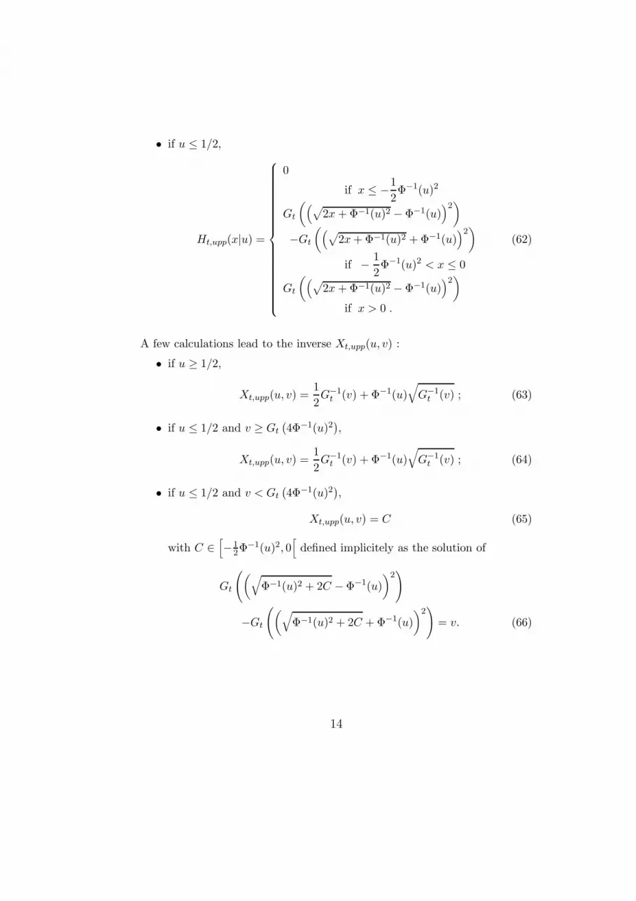
• if u ≤ 1/2,

Ht,upp(x|u) =

0

if x ≤ −12Φ−1(u)2

Gt

((√2x+Φ−1(u)2 − Φ−1(u)

)2)

−Gt

((√2x+Φ−1(u)2 +Φ−1(u)

)2)

if − 12Φ−1(u)2 < x ≤ 0

Gt

((√2x+Φ−1(u)2 − Φ−1(u)

)2)

if x > 0 .

(62)

A few calculations lead to the inverse Xt,upp(u, v) :

• if u ≥ 1/2,

Xt,upp(u, v) =12G−1

t (v) + Φ−1(u)√G−1

t (v) ; (63)

• if u ≤ 1/2 and v ≥ Gt

(4Φ−1(u)2

),

Xt,upp(u, v) =12G−1

t (v) + Φ−1(u)√G−1

t (v) ; (64)

• if u ≤ 1/2 and v < Gt(4Φ−1(u)2

),

Xt,upp(u, v) = C (65)

with C ∈[−1

2Φ−1(u)2, 0

[defined implicitely as the solution of

Gt

((√Φ−1(u)2 + 2C − Φ−1(u)

)2)

−Gt

((√Φ−1(u)2 + 2C +Φ−1(u)

)2)= v. (66)

14

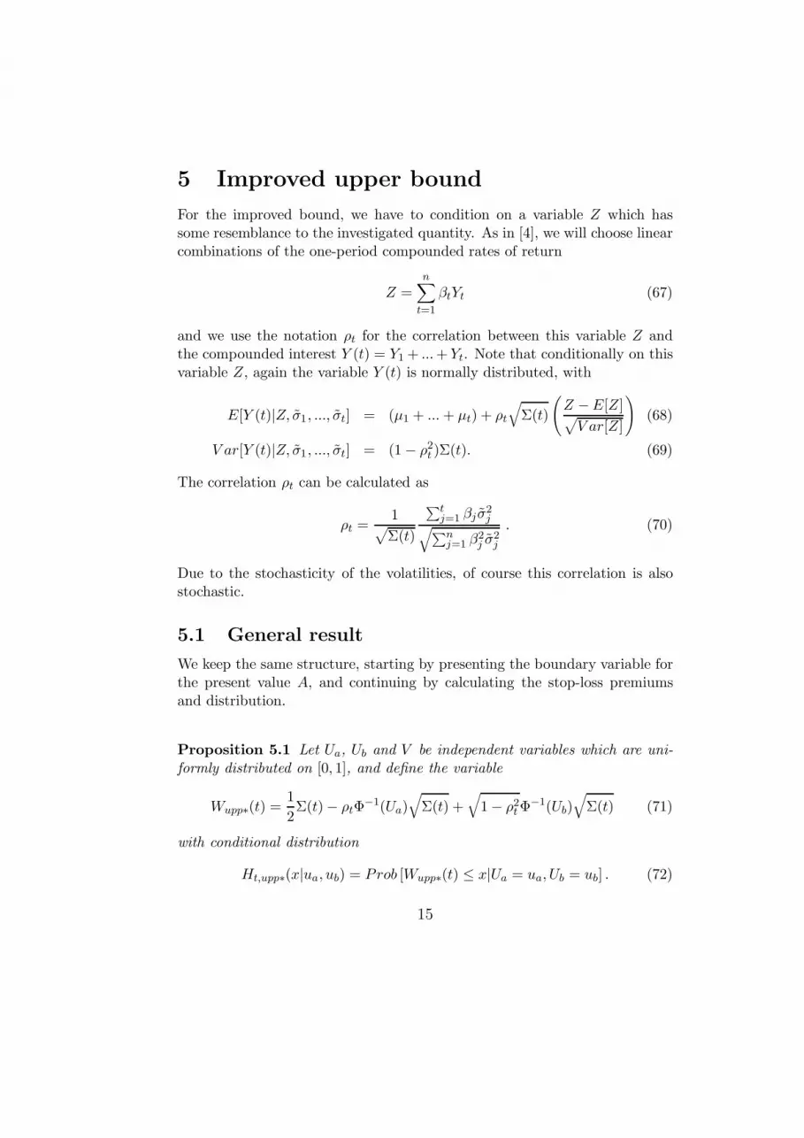
5 Improved upper bound

For the improved bound, we have to condition on a variable Z which hassome resemblance to the investigated quantity. As in [4], we will choose linearcombinations of the one-period compounded rates of return

Z =n∑

t=1

βtYt (67)

and we use the notation ρt for the correlation between this variable Z andthe compounded interest Y (t) = Y1+ ...+ Yt. Note that conditionally on thisvariable Z, again the variable Y (t) is normally distributed, with

E[Y (t)|Z, σ1, ..., σt] = (µ1 + ...+ µt) + ρt

√Σ(t)

(Z −E[Z]√V ar[Z]

)(68)

V ar[Y (t)|Z, σ1, ..., σt] = (1− ρ2t )Σ(t). (69)

The correlation ρt can be calculated as

ρt =1√Σ(t)

∑tj=1 βj σ

2j√∑n

j=1 β2j σ

2j

. (70)

Due to the stochasticity of the volatilities, of course this correlation is alsostochastic.

5.1 General result

We keep the same structure, starting by presenting the boundary variable forthe present value A, and continuing by calculating the stop-loss premiumsand distribution.

Proposition 5.1 Let Ua, Ub and V be independent variables which are uni-formly distributed on [0, 1], and define the variable

Wupp∗(t) =12Σ(t)− ρtΦ−1(Ua)

√Σ(t) +

√1− ρ2

tΦ−1(Ub)

√Σ(t) (71)

with conditional distribution

Ht,upp∗(x|ua, ub) = Prob [Wupp∗(t) ≤ x|Ua = ua, Ub = ub] . (72)

15

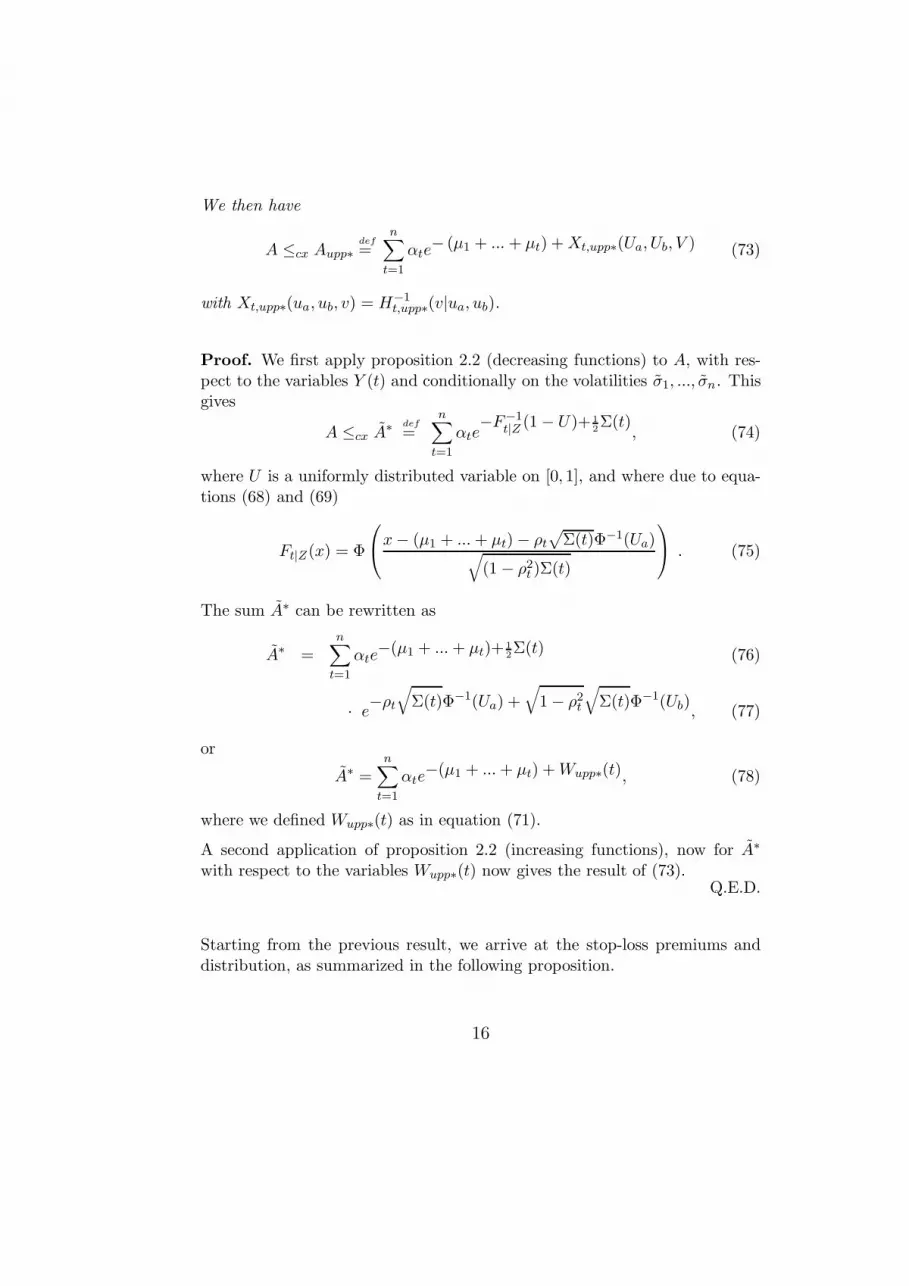
We then have

A ≤cx Aupp∗ =def

n∑t=1

αte− (µ1 + ...+ µt) +Xt,upp∗(Ua, Ub, V ) (73)

with Xt,upp∗(ua, ub, v) = H−1t,upp∗(v|ua, ub).

Proof. We first apply proposition 2.2 (decreasing functions) to A, with res-pect to the variables Y (t) and conditionally on the volatilities σ1, ..., σn. Thisgives

A ≤cx A∗ =def

n∑t=1

αte−F−1

t|Z (1− U)+ 12Σ(t)

, (74)

where U is a uniformly distributed variable on [0, 1], and where due to equa-tions (68) and (69)

Ft|Z(x) = Φ

x− (µ1 + ...+ µt)− ρt

√Σ(t)Φ−1(Ua)√

(1− ρ2t )Σ(t)

. (75)

The sum A∗ can be rewritten as

A∗ =n∑

t=1

αte−(µ1 + ...+ µt)+ 1

2Σ(t) (76)

· e−ρt

√Σ(t)Φ−1(Ua) +

√1− ρ2

t

√Σ(t)Φ−1(Ub), (77)

or

A∗ =n∑

t=1

αte−(µ1 + ...+ µt) +Wupp∗(t), (78)

where we defined Wupp∗(t) as in equation (71).

A second application of proposition 2.2 (increasing functions), now for A∗

with respect to the variables Wupp∗(t) now gives the result of (73).Q.E.D.

Starting from the previous result, we arrive at the stop-loss premiums anddistribution, as summarized in the following proposition.

16

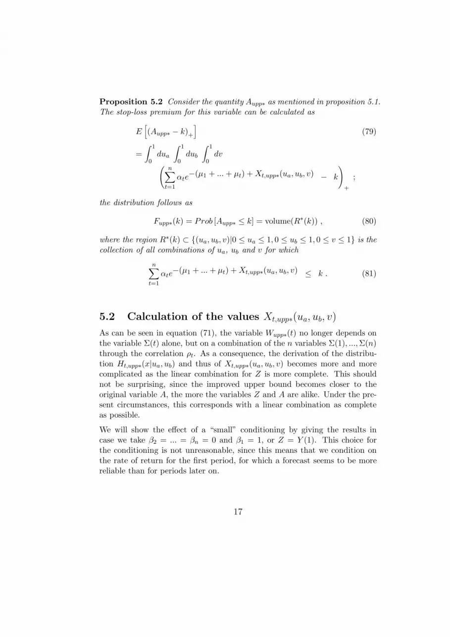
Proposition 5.2 Consider the quantity Aupp∗ as mentioned in proposition 5.1.The stop-loss premium for this variable can be calculated as

E[(Aupp∗ − k)+

](79)

=∫ 1

0dua

∫ 1

0dub

∫ 1

0dv(

n∑t=1

αte−(µ1 + ...+ µt) +Xt,upp∗(ua, ub, v) − k

)+

;

the distribution follows as

Fupp∗(k) = Prob [Aupp∗ ≤ k] = volume(R∗(k)) , (80)

where the region R∗(k) ⊂ {(ua, ub, v)|0 ≤ ua ≤ 1, 0 ≤ ub ≤ 1, 0 ≤ v ≤ 1} is thecollection of all combinations of ua, ub and v for which

n∑t=1

αte−(µ1 + ...+ µt) +Xt,upp∗(ua, ub, v) ≤ k . (81)

5.2 Calculation of the values Xt,upp∗(ua, ub, v)

As can be seen in equation (71), the variable Wupp∗(t) no longer depends onthe variable Σ(t) alone, but on a combination of the n variables Σ(1), ...,Σ(n)through the correlation ρt. As a consequence, the derivation of the distribu-tion Ht,upp∗(x|ua, ub) and thus of Xt,upp∗(ua, ub, v) becomes more and morecomplicated as the linear combination for Z is more complete. This shouldnot be surprising, since the improved upper bound becomes closer to theoriginal variable A, the more the variables Z and A are alike. Under the pre-sent circumstances, this corresponds with a linear combination as completeas possible.

We will show the effect of a “small” conditioning by giving the results incase we take β2 = ... = βn = 0 and β1 = 1, or Z = Y (1). This choice forthe conditioning is not unreasonable, since this means that we condition onthe rate of return for the first period, for which a forecast seems to be morereliable than for periods later on.

17

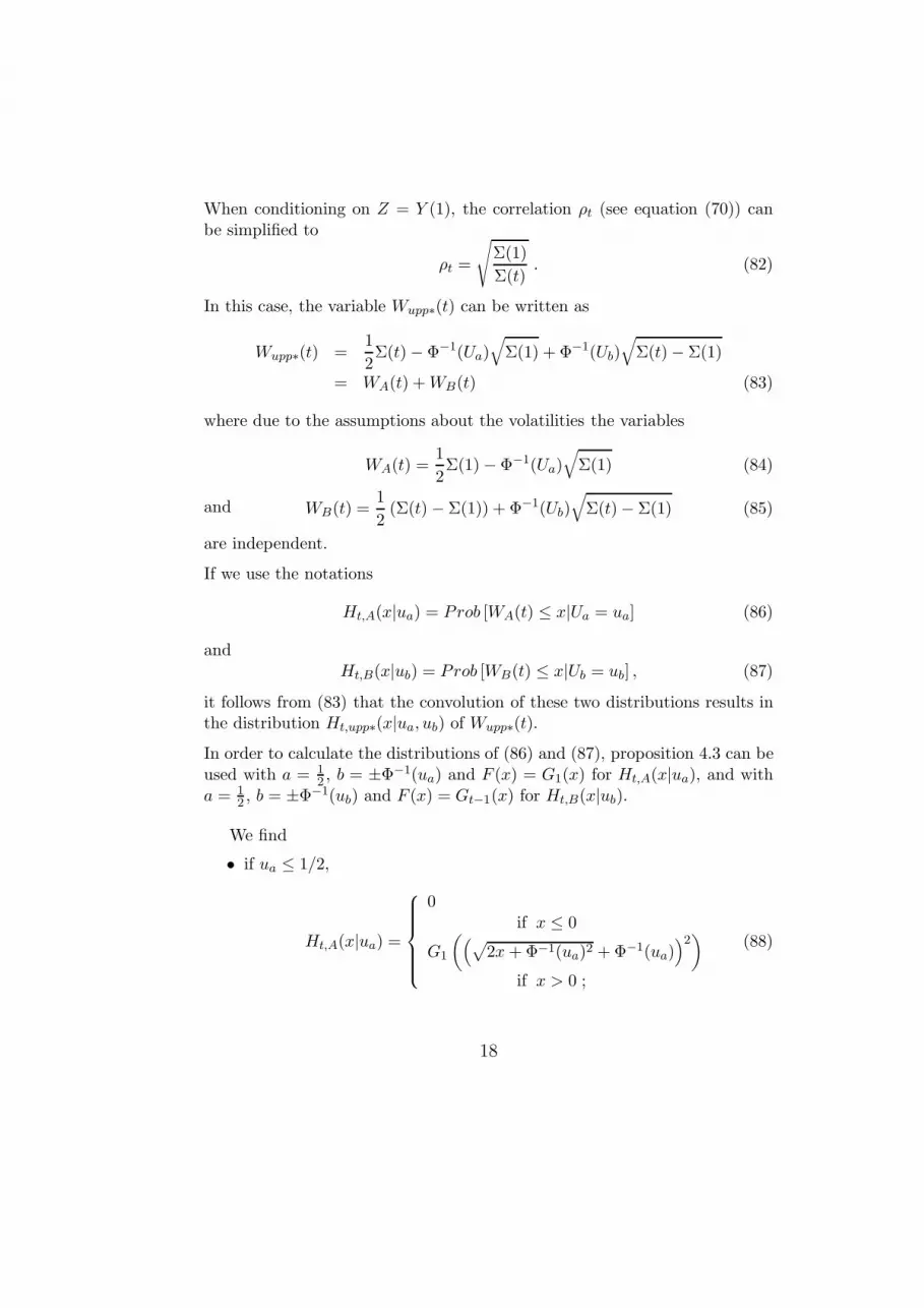
When conditioning on Z = Y (1), the correlation ρt (see equation (70)) canbe simplified to

ρt =

√Σ(1)Σ(t)

. (82)

In this case, the variable Wupp∗(t) can be written as

Wupp∗(t) =12Σ(t)− Φ−1(Ua)

√Σ(1) + Φ−1(Ub)

√Σ(t)− Σ(1)

= WA(t) +WB(t) (83)

where due to the assumptions about the volatilities the variables

WA(t) =12Σ(1)− Φ−1(Ua)

√Σ(1) (84)

and WB(t) =12(Σ(t)− Σ(1)) + Φ−1(Ub)

√Σ(t)− Σ(1) (85)

are independent.

If we use the notations

Ht,A(x|ua) = Prob [WA(t) ≤ x|Ua = ua] (86)

andHt,B(x|ub) = Prob [WB(t) ≤ x|Ub = ub] , (87)

it follows from (83) that the convolution of these two distributions results inthe distribution Ht,upp∗(x|ua, ub) of Wupp∗(t).

In order to calculate the distributions of (86) and (87), proposition 4.3 can beused with a = 1

2 , b = ±Φ−1(ua) and F (x) = G1(x) for Ht,A(x|ua), and witha = 1

2 , b = ±Φ−1(ub) and F (x) = Gt−1(x) for Ht,B(x|ub).

We find

• if ua ≤ 1/2,

Ht,A(x|ua) =

0if x ≤ 0

G1

((√2x+Φ−1(ua)2 +Φ−1(ua)

)2)

if x > 0 ;

(88)

18

• if ua ≥ 1/2,

Ht,A(x|ua) =

0

if x ≤ −12Φ−1(ua)2

G1

((√2x+Φ−1(ua)2 +Φ−1(ua)

)2)

−G1

((√2x+Φ−1(ua)2 − Φ−1(ua)

)2)

if − 12Φ−1(ua)2 < x ≤ 0

G1

((√2x+Φ−1(ua)2 +Φ−1(ua)

)2)

if x > 0 ;

(89)

• if ub ≤ 1/2,

Ht,B(x|ub) =

0

if x ≤ −12Φ−1(ub)2

Gt−1

((√2x+Φ−1(ub)2 − Φ−1(ub)

)2)

−Gt−1

((√2x+Φ−1(ub)2 +Φ−1(ub)

)2)

if − 12Φ−1(ub)2 < x ≤ 0

Gt−1

((√2x+Φ−1(ub)2 − Φ−1(ub)

)2)

if x > 0 ;

(90)

• if ub ≥ 1/2,

Ht,B(x|ub) =

0if x ≤ 0

Gt−1

((√2x+Φ−1(ub)2 −Φ−1(ub)

)2)

if x > 0 .

(91)

6 Numerical illustration

In this last section, we want to examine the accuracy of the upper bounds incomparison with the exact present value. In order to do so, we will investigate

19

the first upper bound (the bound with the smallest precision) for three cash-flows with different structure :

• αt = 10 for t = 1, ..., 10 ;

• αt = t for t = 1, ..., 10 ;

• αt = 11− t for t = 1, ..., 10.

For the normal distribution of the stochastic interest rate (see equation (3)),we choose µt = 0.07 for each time point t ; the squared stochastic volatility(see equation (35)) is assumed to be exponentially distributed with parameter20, i.e. with mean 0.05.

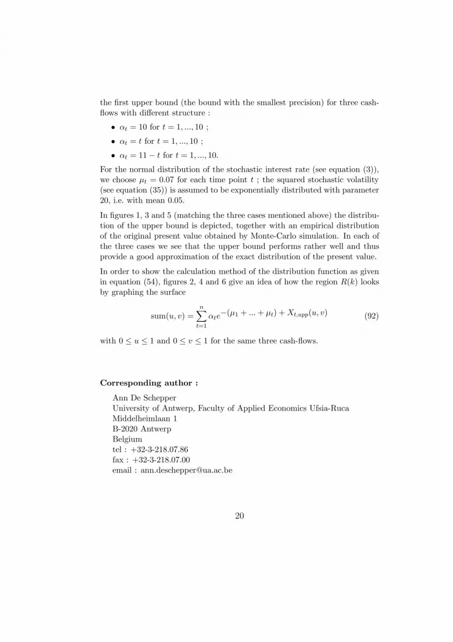
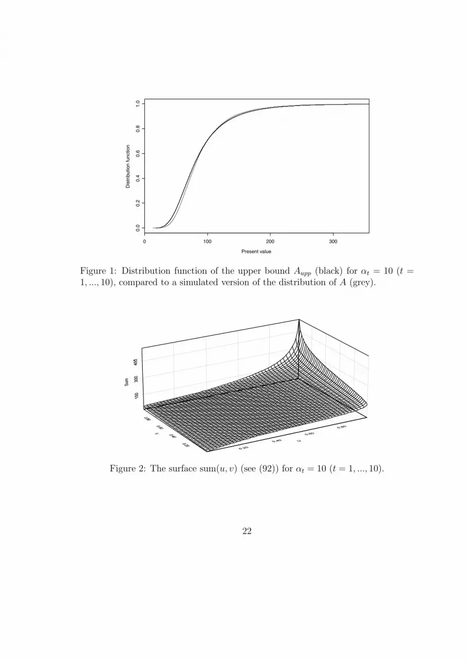
In figures 1, 3 and 5 (matching the three cases mentioned above) the distribu-tion of the upper bound is depicted, together with an empirical distributionof the original present value obtained by Monte-Carlo simulation. In each ofthe three cases we see that the upper bound performs rather well and thusprovide a good approximation of the exact distribution of the present value.

In order to show the calculation method of the distribution function as givenin equation (54), figures 2, 4 and 6 give an idea of how the region R(k) looksby graphing the surface

sum(u, v) =n∑

t=1

αte−(µ1 + ...+ µt) +Xt,upp(u, v) (92)

with 0 ≤ u ≤ 1 and 0 ≤ v ≤ 1 for the same three cash-flows.

Corresponding author :

Ann De SchepperUniversity of Antwerp, Faculty of Applied Economics Ufsia-RucaMiddelheimlaan 1B-2020 AntwerpBelgiumtel : +32-3-218.07.86fax : +32-3-218.07.00email : ann.deschepper@ua.ac.be

20

References

[1] Dhaene J. & Denuit M. (1999). “The safest dependence structure amongrisks”, Insurance: Mathematics and Economics, vol.25(1), p.11-22.

[2] Goovaerts M., Dhaene J., & De Schepper A. (2000). “Stochastic up-per bounds for present value functions”, Journal of Risk and Insurance,vol.67(1), p.1-14.

[3] Goovaerts M., Kaas R. (2001). “Some problems in actuarial finance in-volving sums of financial risks”, Statistica Neerlandica, to be published.

[4] Kaas R., Dhaene J., & Goovaerts M. (2000). “Upper and lower bounds forsums of variables”, Insurance: Mathematics and Economics, vol.27(2),p.151-168.

[5] Shaked M. & Shanthikumar J.G. (1994). Stochastic orders and their ap-plications, Academic Press, pp.545.

[6] Taylor S.J. (1994). “Modeling stochastic volatility : a review and com-parative study”, Mathematical Finance, vol.4(2), p.183-204.

[7] Vyncke D., Goovaerts M. & Dhaene J. (2000). “Convex upper and lowerbounds for present value functions”, Onderzoeksrapport KUL. Departe-ment toegepaste economische wetenschappen, vol.0025, pp.17.

21

Present value

Dis

trib

utio

n fu

nctio

n

0 100 200 300

0.0

0.2

0.4

0.6

0.8

1.0

Figure 1: Distribution function of the upper bound Aupp (black) for αt = 10 (t =1, ..., 10), compared to a simulated version of the distribution of A (grey).

Figure 2: The surface sum(u, v) (see (92)) for αt = 10 (t = 1, ..., 10).

22

Present value

Dis

trib

utio

n fu

nctio

n

0 50 100 150 200

0.0

0.2

0.4

0.6

0.8

1.0

Figure 3: Distribution function of the upper bound Aupp (black) for αt = t (t =1, ..., 10), compared to a simulated version of the distribution of A (grey).

Figure 4: The surface sum(u, v) (see (92)) for αt = t (t = 1, ..., 10).

23

Present value

Dis

trib

utio

n fu

nctio

n

0 50 100 150

0.0

0.2

0.4

0.6

0.8

1.0

Figure 5: Distribution function of the upper bound Aupp (black) for αt = 11 − t(t = 1, ..., 10), compared to a simulated version of the distribution of A (grey).

Figure 6: The surface sum(u, v) (see (92)) for αt = 11− t (t = 1, ..., 10).

24