Embed Size (px)
Citation preview

Booms, Busts, and Fraud
Paul PovelCarlson School of Management, University of Minnesota
Rajdeep SinghCarlson School of Management, University of Minnesota
Andrew WintonCarlson School of Management, University of Minnesota
Forthcoming, Review of Financial Studies
Abstract
Firms sometimes commit fraud by altering publicly reported information to bemore favorable, and investors can monitor firms to obtain more accurate informa-tion. We study equilibrium fraud and monitoring decisions. Fraud is most likely tooccur in relatively good times, and the link between fraud and good times becomesstronger as monitoring costs decrease. Nevertheless, improving business conditionsmay sometimes diminish fraud. We provide an explanation for why fraud peakstowards the end of a boom and is then revealed in the ensuing bust. We also showthat fraud can increase if firms make more information available to the public.
We would like to thank an anonymous referee for very helpful comments. We are also indebted to Ulf Axelson,Markus Brunnermeier, Sudipto Dasgupta, Eitan Goldman, Charlie Hadlock, Andrew Hertzberg, Simi Kedia,Tom Nohel, Oguzhan Ozbas, Javier Suarez, and seminar participants at Columbia University, Duke University,Goteborg University, McGill University, Michigan State University, the University of Alberta, the Universityof Iowa, the University of Minnesota, the University of Pennsylvania, the 2005 American Finance Associationmeeting in Philadelphia, the 15th Annual Conference on Financial Economics and Accounting at USC, the JFIconference “Corporate Governance: Present and Future” at Washington University St. Louis, the CEPR/SITEconference “Understanding Financial Architecture: On the Economics and Politics of Corporate Governance” atStockholm School of Economics, the conference “People and Money: The Human Factor in Financial Decision-Making” at DePaul University, the RFS-IU conference “The Causes and Consequences of Recent FinancialMarket Bubbles”, and the 2005 HKUST Finance Symposium for helpful comments.

Introduction
Booms and busts are a common feature of market economies. Almost as common is the belief
that a boom encourages and conceals financial fraud and misrepresentation by firms, which are
then revealed by the ensuing bust. Examples in the last century include the 1920s (Galbraith,
1955), the “go-go” market of the 1960s and early 1970s (Labaton, 2002, Schilit, 2002), and
the use of junk bonds and LBOs in the 1980s (Kaplan and Stein, 1993). Most recently, the
long boom of the 1990s has been followed, first by recession, then by revelations of financial
chicanery at many of America’s largest companies.
Despite this widespread belief, there is considerable disagreement as to why this pattern
occurs and what should be done about it. Some argue that tougher regulation is needed,
forcing firms to disclose more information and to restructure their governance procedures.1
Others argue that, during booms, investors are excessively optimistic and do not scrutinize the
firms they finance as carefully as they should.2
In this paper, we take a closer look at these arguments, using a simple model of financing
and investment. We show that, even when investors are perfectly rational, firms’ incentives
to commit fraud are highest in relatively good times. Nevertheless, tougher regulation may
sometimes have unintended consequences; in particular, making disclosure of firm results more
precise can actually increase incentives to commit fraud.
In our model, investors receive financing requests from firms that may have attractive
(“good”) or unattractive (“bad”) investment opportunities. When deciding whether to finance
a firm, investors can either base their decision on publicly available (but noisy) information
about the firm’s investment opportunity, or they may invest time and money in monitoring a
firm to learn its true situation. Managers of firms with poor prospects may decide to commit
fraud; such fraud is costly to them, but it makes the publicly available information look better
than it should be, and this may induce an investor to provide funds without monitoring.
Our model highlights two key determinants of a firm’s fraud decision. The first is investors’
1 Thus, in the 1930s saw the establishment of the SEC, and a stiffened regulation of financial institutionsand markets; in the early 1990s, anti-takeover legislation was enacted; and the most recent crisis led to theSarbanes-Oxley Act.
2 For example, the Economist (2002) suggests: “The remedy is disclosure, honest accounting, non-executivedirectors empowered to do their job — and, as always, skeptical shareholders looking out for their own interests.Without doubt, the last of these is most important of all. Alas, it is beyond the reach of regulators and legislators.. . . The most important lesson of this bust, like every bust, is: buyer beware.”
1

prior beliefs about the state of the economy, measured by the proportion of “good” firms among
firms seeking financing.3 When investors’ priors reflect low or average numbers of good firms,
there is little or no fraud. Intuitively, even if a firm’s public information is positive, enough
uncertainty remains that investors find it worthwhile to monitor the firm carefully, and so fraud
has little upside. When priors are fairly optimistic, however, investors do not monitor a firm
with positive public information carefully, because this merely confirms their view that the firm
is very likely to be good, but they do monitor firms with negative public information. Here,
incentives for fraud are high.
Of course, it is possible that investors’ prior beliefs are so optimistic that investors don’t
even monitor firms with negative public information. In this case, investors think that the
negative information is likely to reflect a basically good firm having bad luck rather than a bad
firm per se. Paradoxically, incentives for fraud are low, because fraud is not necessary for bad
firms to get funding.4
These predictions are consistent with some stylized facts from the most recent boom. In-
ternet firms were undoubtedly the “hottest” sector during the 1990s, getting huge inflows of
money from investors who were increasingly willing to finance early and untested business
ideas. The telecommunications industry also attracted large inflows, yet here, investors seemed
more critical, studying the financial information more carefully and staying clear of firms that
were tainted by negative news. Thus, although investors were certainly optimistic about both
sectors, they seem to have been more optimistic about the Internet than telecoms. Consistent
with our model’s predictions, little fraudulent reporting was uncovered among Internet firms,
whereas a large number of prominent cases of fraud are from telecom firms: WorldCom, Qwest,
Nortel, Global Crossing, and Lucent.
We also highlight the role of investors’ costs of monitoring firms. Although intuition suggests
that lowering such costs would reduce fraud, we show that this is not always the case. In fact,
reduced monitoring costs can actually lead to more fraud, not less: this happens if investors
have relatively optimistic priors, so that their monitoring focuses on firms with negative public
3 As noted at the end of Section 2, we obtain similar results if the state is measured instead by the returnthat firms earn when investments are successful.
4 This hump-shaped relation between investors’ prior beliefs and the probability of fraud occurs even ifmonitoring is prohibitively costly. However, as noted below, the possibility of monitoring shifts the regionwhere fraud occurs to better priors. In other words, the association between fraud and good times is linked toinvestors’ ability to monitor.
2
information.5 Moreover, the correlation of fraud incentives with good prior beliefs actually
increases as monitoring costs fall. Intuitively, lower monitoring costs increase the range of
priors over which investors are always vigilant, regardless of public information; thus, priors
have to be especially good before investors lower their guard at all and fraud begins to pay.
Again, the boom of the 1990s is consistent with these results. Throughout the 1990s, improved
computing and communication technologies greatly reduced investors’ costs of examining firms’
prospects, yet at the end of the decade — a period of very high investor expectations — a wave
of frauds occurred.
In reality, neither firms nor investors are perfectly informed about the state of the econ-
omy. Instead, they form beliefs given the recent history, e.g., the financing patterns, and how
many firms were profitable or failed. As a consequence, these beliefs adapt to changes in the
fundamentals of an economy, but only with a lag. For example, at the end of a prolonged
boom, firms and investors may take a while to realize that the tide has turned, i.e., that the
proportion of good firms has decreased; and that consequently, their fraud, monitoring and
financing decisions should change.
This delayed response to a changing environment affects the pattern of fraud over the
business cycle. In particular, fraud peaks at the end of a boom, when the economy goes into a
tailspin. This argument is based on the different roles played by the true (but unobservable)
state of the economy and the state as perceived by firms and investors. Again, the true state
may deteriorate abruptly at the end of a boom, while firms and investors believe that the
boom is continuing. Given these beliefs, bad firms decide to commit fraud (to attract funding),
and investors decide not to invest too many resources in monitoring firms with positive public
information (because, given their optimistic beliefs, the benefits of such monitoring seem small).
Both firms and investors expect that it is likely that a small number of firms will turn out to
have been financed even though their type was bad, and that only a small number of firms
will have received funding only because they committed fraud. These expectations, however,
are based on the perceived state of the economy, which is much better than the true state.
And the true state determines how many firms are bad and end up committing fraud. Thus,
both firms and investors will be “surprised” by a large number of poorly performing firms, and
5 In this case, fraud gives bad firms a chance to leave the pool of firms with negative public information,which are monitored intensively, and join the pool of firms with good public information, which are more likelyto be financed without monitoring.
3

investigations may reveal that a surprisingly large number of firms committed fraud to improve
their financial situation.6
Such a dynamic setup may explain the pattern observed in many boom-bust cycles, that
fraud peaks towards the end of a boom, often reaching surprising levels. Some have argued
that this pattern is a sign of over-optimism on the side of investors, who are either naive
or careless when deciding how to invest their funds. Even though this may be a driving
force behind these patterns, our analysis suggests that they may equally well be generated by
perfectly rational agents, who make self-interested decisions about whether to commit fraud
or whether to monitor. In fact, the two ideas go hand-in-hand: If investors are inclined to
waves of excessive optimism and pessimism, this will further exacerbate the effects that we just
discussed. However, limited rationality is not a necessary factor to explain the patterns that
we observe.
In sum, our model with rational behavior can reproduce many features of the boom-bust-
fraud pattern, explaining (amongst other things) why long booms often seem to end in a wave
of failures and fraud. Although we do not claim that investors are always perfectly rational, the
fact that rationality does not rule out this pattern suggests limits to the “buyer beware” school
of policy response. Moreover, our most critical result — that fraud incentives are highest in
good (but not exceptionally good) states of the economy — actually requires a certain amount
of “buyer beware” behavior: specifically, investors must be able to monitor and must decide
whether to monitor in a rational fashion.
This adds a new perspective to the debate on how regulation can optimally deter fraud.
Investors can use publicly available information to make their investment decisions, and they
can also monitor, i.e., analyze firms and investment opportunities in more detail. At first glance,
forcing firms to disclose more information to the public might reduce the incidence of fraud;
similarly, reducing the costs of monitoring by giving investors more rights and more power
might help fight fraud. As we show, however, these arguments are incomplete, and such policy
changes may backfire. We have already seen that lower monitoring costs sometimes lead to
more fraud. Increased disclosure may have the same effect. Suppose that improved disclosure
makes investors trust public information more, so that they are more likely to fund firms with
6 A surprisingly high incidence of fraud may actually slow the learning process, since fraud artificially makespublicly available information look more positive than it really is.
4

positive information and deny funding to firms with negative information; then bad firms are
more likely to resort to fraud so that they can produce such positive public information. To be
effective against fraud, disclosure standards must directly make fraud more difficult.7
The plan of the rest of the paper is as follows. We discuss the relevant literature in Section .
In Section 1 we introduce our model and key assumptions. In Section 2 we analyze the behavior
of investors and firms in a setting where all agents know the underlying distribution of good
and bad firms in the economy. In Section 3 we show how our results are affected by changes in
the underlying parameters and how these can motivate actual behavior by firms and investors.
We also show how agents’ beliefs can be grounded in a framework in which the underlying state
of the economy is unknown, leading to “surprising” volumes of fraud in certain circumstances.
In Section 4 we extend our model to deal with good firms’ incentives to commit fraud, and in
Section 5 we conclude. All proofs are in the Appendix.
Literature Review
Several recent papers in the finance literature also focus on managerial incentives to commit
fraud. Bebchuk and Bar-Gill (2002) present a model in which firms may commit fraud so as to
obtain better terms when issuing shares to raise funds for further investments; this incentive
to commit fraud increases if managers can sell some of their own shares in the short run or if
accounting and legal rules are lax. Goldman and Slezak (2005) present a model where optimal
managerial pay-for-performance contracts balance incentives to exert effort against incentives to
commit fraud; increased regulatory penalties for fraud can sometimes increase the equilibrium
incidence of fraud, and rules that reduce auditor incentives to collude with managers decrease
the incidence of fraud but paradoxically reduce firm value. Subrahmanyam (2005) presents a
model where more intelligent managers are better both at running firms and at committing
successful (undetected) fraud; as a result, investors may prefer more intelligent managers and
a higher incidence of fraud in exchange for higher average performance. Noe (2003) analyzes a
different type of fraud, in which a firm’s manager “tunnels” value from the firm into her own
pocket. He focuses on providing the manager with incentives to perform rather than steal the
7 This is not to say that improved disclosure has no beneficial effects. We discuss the impact of improveddisclosure in more detail in Section 3.
5

funds that she has raised. Unlike our paper, these four papers do not examine how changes in
economic conditions affect manager’s incentives to commit fraud and investor’s incentives to
monitor managers, which is our primary focus.8
Closer to our paper is Hertzberg (2003). He examines a setting in which investors are more
likely to give short-term incentives to firm managers in good times. Since short-term incentives
exacerbate financial misreporting, such misreporting tends to be correlated with good times.
Although this paper can explain a link between good times and fraud, it relies critically on
the dynamic link between compensation contracts and business prospects. Since the recent
move to link executive compensation to shareholder performance began in the recession of the
early 1990s, this cannot be a complete explanation for the links between booms and fraud.
Moreover, his model does not explain the relative absence of misreporting in the Internet
sector as compared with the telecom sector during the late 1990s. Thus, Hertzberg’s model is
complementary to ours.
There are a number of studies in the accounting literature that focus on fraud incentives in
the relationships between firms and their auditors. Some of these examine incentives to under-
report earnings in order to hide managerial perquisite consumption; see for example Morton
(1993). Closer to our focus are papers that examine the incentive to over-report ; examples
include Newman and Noel (1989), Shibano (1990), and Caplan (1999). Empirical work on SEC
enforcement actions aimed at violations of Generally Accepted Accounting Principles (GAAP)
suggests that over-reporting aimed at boosting share prices and improving access to additional
capital is in fact the more frequent source of firm-wide financial misrepresentation.9 Unlike
our paper, these auditing papers on over-reporting focus on the impact of control systems
and auditor incentives; they do not examine how fraud incentives change with overall business
conditions. A further distinction is that auditors are typically penalized for failing to detect
fraud. By focusing on the incentives of investors, we emphasize the fact that investors are not
concerned with finding fraud per se, but rather with finding good investment opportunities.
As already noted, this can lead to counterintuitive results when investors rationally focus their
8 Goldman and Slezak (2005) do show that an influx of naive, overly optimistic investors into the stockmarket increases the equilibrium incidence of fraud. Again, our model shows that such fluctuations can occureven when all investors are perfectly rational.
9 For example, Peroz et al. (1991) find that fraud usually takes the form of earnings overstatement, and thatnews of an SEC enforcement action depresses stock price. Dechow et al. (1996) find that firms that commitfraud tend to have higher ex ante needs for additional funds.
6

scrutiny on low signals rather than high ones.
Although ours is the first paper that we are aware of that ties fraudulent behavior by firms
to changing investor actions over the business cycle, there are a number of papers that are
related to the tenor of our analysis. For example, a growing body of work examines “credit
cycles” — the idea that banks and other credit suppliers engage in behavior that exacerbates
business cycle effects, making credit even tighter in recessions, and looser in expansions, than
pure demand-side effects would suggest. Among these, the closest to our paper is Ruckes (2004),
who models how competing bank lenders’ incentives to screen potential borrowers exacerbate
cyclical variations in credit standards. Dow, Gorton and Krishnamurthy (2005) how the impact
of managerial empire-building incentives changes over the business cycle, and how this affects
asset prices. None of these papers address borrower incentives to commit fraud, which is our
key focus.
Our discussion of the dynamic implications of our model is related to Persons and Warther’s
(1997) model of booms and busts in the adoption of financial innovations. In their model,
individual firms decide whether to adopt a new financial technique based on the information
that earlier adopters’ experience noisily reveals. They show that such waves of adoption always
end on a sour note, in the sense that the most recent adopters always lose money. Ex post,
the information that ends the wave is always negative, but the timing of the end is ex ante
random, and the latest adopters were behaving rationally based on the information available
at the time. Although Persons and Warther focus on social learning about a static innovation
rather than investor monitoring in the face of potential fraud, the result that busts may be
surprising yet still rational has some similarities to our discussion.
Finally, our work contrasts with the growing literature that examines how bounded ra-
tionality can cause market overreactions. The critical difference is that our model relies on
rational behavior throughout. As noted earlier, to the extent that deviations from rationality
do lead investors’ priors to overreact to recent information, they will exacerbate the effects we
describe. Similarly, we assume that firms are run by self-interested rational managers who act
opportunistically if doing so is beneficial for them. Noe and Rebello (1994) present a model
in which ethical and unethical managers coexist, where “ethical” managers are unable to act
opportunistically. The likelihood that a manager is ethical depends on past opportunity losses
to behaving in an ethical fashion; in some cases, this leads to cyclical behavior in the proportion
7

of ethical and unethical managers.
1 Basic Model and Assumptions
In this section we lay out the basic model that provides the framework for analyzing the
incidence of fraud in Section 2. The economy consists of equal numbers of firm managers and
investors, each of whom lives for one period. The sequence of events is summarized in Figure
1.
-time
Firms j and
investors imatchedrandomly
Commitfraudor not
Free signals ∈ {h, `};monitoror not
Contractwritten
RevenueR or zero;
rent C
Figure 1: Time line
1.1 Firms and Managers
Each manager controls a firm that requires an investment of I units of cash at the start of the
period. At the end of the period, the firm returns a random contractable cash flow that equals
R > I with probability θi and zero with probability 1− θi, where i ∈ {g, b} is the firm’s type.
We assume that 0 ≤ θb < θg < 1. We also assume that
Ng = θgR− I > 0 Nb = −(θbR− I) > 0; (1)
i.e., g firms are positive net present value investments (“good”), whereas b firms are negative
NPV investments (“bad”). Note that Nb is the absolute value of the expected loss from investing
in a bad firm.
In addition to generating contractable cash flows, a funded firm generates C in noncon-
tractable control benefits which the manager consumes.10 This implies that, all else equal, a
10 This could represent nonpecuniary benefits of control or pecuniary benefits that have to be given to themanager in order to elicit reasonable efforts (see for example Diamond (1993)). Moskowitz and Vissing-Jorgensen(2002) give empirical evidence that is consistent with large nonpecuniary benefits; Fee and Hadlock (2004) giveevidence on the net pecuniary benefits that CEOs lose if they are dismissed and forced to seek employmentelsewhere.
8

manager prefers to get her project funded, regardless of her firm’s type.
Managers know their own firm’s type, but outsiders can discover this only by monitoring
the firm at a cost, as we discuss below. The prior probability that any given firm is good is
given by µ, where µ ∈ (0, 1). This prior is common knowledge. For the moment, we take this
prior as exogenously given; in Section 3 we discuss how this can be embedded in a multi-period
framework.11
1.2 Investors
Investors are each endowed with I units of the generic good. At the beginning of the period,
each investor is randomly matched with a manager and her firm. After being matched, the
investor receives a free but noisy signal of the firm’s type, and may then decide whether or not
to expend additional effort and learn the firm’s type more precisely. Based on any information
that she has, the investor then can make a take-it-or-leave-it investment offer to the manager.
The manager does not have time to approach another investor, so if the investor does not make
her an offer, the manager cannot get funding for her firm.12
Our assumptions of random matching and take-it-or-leave-it offers are made for simplicity;
altering them would not change the essentials of our analysis. For simplicity, we also assume
that investors cannot pay off bad firms to reveal their type; in practice, doing so is likely to be
prohibitively expensive since a large number of incompetent managers would start firms and
apply to investors for the sole purpose of receiving that payment. (In Section 4 we return to
this issue of entry.)
Thus, in equilibrium, if the investor does fund the firm, she receives all of the contractable
cash flows that it produces. Nevertheless, since the manager receives control benefits C if the
firm is funded and nothing if the firm is not funded, she will take any offer that she is given.
11 An earlier version of this paper also discussed the possibility of entry and exit of firms, depending on thestate of the economy µ. Allowing for entry and exit does not change the results qualitatively.
12 We abstract from the possibility that firms may be competing for scarce funding and may therefore berationed. This seems reasonable if better states of the economy (higher values of µ) imply a larger availabilityof funds (investment increases with µ).
9
1.3 Signals, Fraud, and Monitoring
As just mentioned, right after managers and investors are matched, each investor receives a
free but noisy signal of the type of the manager’s firm. This signal should be thought of as a
financial report or a related public news release by the firm. We assume that this signal takes
on one of two values, h (“high”) and ` (“low”). We also assume that, absent fraud, the signal
is positively correlated with the firm’s true type:
Pr {h|g} = γ >1
2> β = Pr {h|b, no fraud} .
The free signal is subject to manipulation by the manager (“fraud”). The manager decides
whether or not to commit fraud right after she and the investor are matched. Fraud costs the
manager an amount f , where f reflects both any effort involved in committing fraud and the
chance that the manager is later caught and punished.13 Fraud increases the probability that a
bad firm generates a high signal by δ < γ−β; that is, Pr {h |b, fraud } = β+δ < γ. Thus, fraud
reduces the free signal’s correlation with the firm’s type, but the free signal remains somewhat
informative.14 Fraud is beneficial to the manager to the extent it increases the manager’s chance
of collecting control benefits C. It follows that fraud will never be attractive unless the cost of
fraud f is less than the maximum possible benefit, i.e., f < δC. Henceforth, we assume that
this condition holds.
In practical terms, fraud should be thought of as deliberate misstatement of the firm’s
results, either through altered financial reports or a misleading news release. Such an effort
increases the odds that a casual glance at the firm’s results will lead investors to think that
the firm is in good shape — in terms of our model, it increases the probability that the public
signal is high.
For simplicity, we assume that only bad firms commit fraud. As we discuss in Section 4,
allowing good firms to commit fraud leaves most of our results qualitatively unchanged, so long
as bad firms have relatively more to gain from fraud.
Suppose that the bad firm commits fraud with probability φ. Let µs (φ) be the investor’s
13 An earlier version of this paper discussed the case in which the probability of being caught committing fraud(and punished) depended on the probability of being funded. This does not change our results qualitatively.
14 Allowing δ to exceed γ−β would have little effect on our qualitative results; bad firms would never commitfraud with certainty, but comparative statics would be unchanged.
10

posterior probability that the firm is good after she sees the free signal s. Applying Bayes’
Rule, we have
µh (φ) = Pr [g|h] =Pr {g}Pr {h|g}
Pr {g}Pr {h|g}+ Pr {b}Pr {h|b} =µ
µ + (1− µ) β+φδγ
µ` (φ) = Pr [g|`] =Pr {g}Pr {`|g}
Pr {g}Pr {`|g}+ Pr {b}Pr {`|b} =µ
µ + (1− µ) 1−β−φδ1−γ
.
Notice that ∀φ ∈ (0, 1),
µ` (0) < µ` (φ) < µ` (1) < µ < µh (1) < µh (φ) < µh (0) . (2)
As expected, the posterior probability that the firm is good is higher after observing a high
signal than it is after observing a low signal, and fraud makes the signal less precise, i.e. the
posterior approaches the prior as either δ or φ increase.
After receiving the free signal, the investor can choose to investigate the firm further (“mon-
itor”). Monitoring has an effort cost of m > 0 and perfectly reveals the firm’s type. Once more,
the assumption that monitoring is perfect is not essential; the key point is that monitoring gives
more precise information about the firm’s type, and that fraud distorts the information from
monitoring relatively less than it distorts the free signal.
1.4 An Alternative Interpretation
Although our model assumes that firms are seeking initial financing, it extends easily to the
case of firms that are already in business. Suppose that firms have risky ongoing operations or
investment opportunities that can be good or bad. If a manager remains in charge, she receives
control rents; if she is fired or constrained from pursuing additional investment, she loses these
rents. A firm’s investor (say, a large shareholder) can either allow the manager to remain in
charge, or else fire or otherwise constrain the manager to avoid wasting the firm’s resources.
Finally, the investor can either make her decision based on her prior beliefs about the firm’s
type or else monitor the firm more closely before making her decision. It is easy to see that
this alternative interpretation uses essentially the same model that we have already presented.
11

2 Investor and Firm Behavior
In this section, we analyze the equilibrium actions of the firm’s manager (henceforth, “firm”)
and of the investor. As we will see, the incidence of fraud is hump-shaped, first increasing in
the prior probability that firms are good, then decreasing. When this prior probability is below
the point at which fraud reaches its peak, fraud increases as monitoring decreases; when the
prior is above this peak, fraud and monitoring decrease together. Most importantly, whenever
monitoring is feasible, the peak in fraud occurs for good priors — those for which the average
net present value of a firm’s project is positive — and this peak shifts towards higher priors as
monitoring costs decrease. In this sense, fraud is associated with “good times.”
Our analysis proceeds via backwards induction. We begin with the investor’s problem once
she has observed the free signal; then we examine the firm’s decision on whether to commit
fraud before the free signal is sent. We conclude by characterizing the equilibrium levels of
fraud and monitoring as functions of the prior probability that firms are good.
2.1 The Investor’s Ex-Post Problem
After receiving the free signal s, the investor has three possible actions: she can choose not to
invest (action “N”); she can monitor and then invest if the firm is good (action “M”);15 or
she can invest without further monitoring (action “U” for unmonitored). Defining VA as the
expected payoff to action A, the actions’ expected payoffs are as follows.
VN = 0
VM = µNg −m
VU = µNg − (1− µ) Nb
It is immediate that the investor’s decision depends only on the net present values Ng and −Nb
of the two types of firms, the cost of monitoring m, and the investor’s posterior belief on the
probability µ that the firm is good. For expositional ease, we define the following threshold
probabilities: If µ = mNg
≡ µ1(m) then VN = VM ; if µ = Nb
Nb+Ng≡ µ2 then VN = VU ; and if
µ = 1 − mNb≡ µ3(m) then VM = VU . The next proposition describes the parameter regions in
15 Note that, given (1), it never pays to invest in a bad firm.
12

which the various actions are optimal.
Proposition 1 Suppose that, after observing the free signal, the investor believes that the firm
is good with probability µ. The investor’s optimal action is as follows:
1. Do not invest if µ < min (µ1(m), µ2).
2. Invest without monitoring if µ ≥ max (µ2, µ3(m)).
3. Monitor and invest if the firm is good if µ1 < µ ≤ µ3(m) and m < NbNg
Nb+Ng≡ m.
-µ
6m
0 1
m
µ2
Do notinvest
Investwithout
monitoring
Monitor,
investif type g
m′
µ1(m′) µ3(m
′)
Figure 2: Posterior probabilities and optimal investor decisions.
Figure 2 displays key elements of the investor’s decision problem. Given the realization of
the free signal, the investor updates her beliefs about the firm’s type. Together, the posterior µ
and the cost of monitoring m determine the optimal decision. If the cost of monitoring is above
m, then min (µ1(m), µ2) = max (µ2, µ3(m)) = µ2 and monitoring is always dominated either
by not investing at all or by unmonitored financing. Here, the investor provides unmonitored
finance if and only if the posterior is above the threshold µ2, which determines where the
investor is indifferent between not investing and providing unmonitored financing.
For monitoring costs below m, it is possible that the expected benefit from monitoring
(avoiding investing in bad firms and losing Nb) may exceed the cost of monitoring m. If µ is
13

such that m = µNg (the upward sloping line in Figure 2, we have VN = VM , and the investor is
indifferent between monitored finance and not investing. For example, if m = m′, the threshold
for µ is µ1 (m′). If µ is such that m = (1− µ) Nb (the downward sloping line), we have VM = VU ,
and the investor is indifferent between monitored finance and unmonitored finance. For the
example m = m′, this defines the threshold µ3 (m′). It follows that monitoring is optimal for
intermediate posteriors, and the range of posteriors for which it is optimal increases as the cost
of monitoring m decreases.
Note that the investor’s decision depends only on the posterior µ, and not on how she forms
this posterior; different combinations of the prior µ and the probability of fraud φ that lead to
the same posterior µ lead to the same action.
2.2 The Manager’s Decision to Commit Fraud
Having solved the investor’s problem, we now examine the bad firm’s decision on whether to
commit fraud. This decision depends on the cost of fraud versus the expected benefit of fraud,
which in turn depends on the investor’s response as described in Proposition 1. Since monitoring
detects bad firms, the firm only benefits from fraud if fraud increases the firm’s probability
of receiving unmonitored funding. This requires two conditions: (i) after a high signal, the
investor’s posterior leads her to provide unmonitored funding with positive probability, and
(ii) after a low signal, the investor’s posterior leads her to provide unmonitored funding with
strictly lower probability than in the high-signal case. On the other hand, as mentioned in the
previous section, in equilibrium, fraud makes the signal less precise; this lessens the difference
in impact between high and low signals, reducing the gains from fraud.
In equilibrium, the incidence of fraud must be consistent with incentives. Thus, if the
manager’s expected benefit strictly exceeds the cost f , she undertakes fraud with certainty
(φ = 1). If the benefit equals the cost, she is willing to commit fraud with positive probability
(0 < φ < 1). Otherwise, she does not commit fraud at all.
We first describe five different ‘regimes’ which characterize the equilibrium; which regime is
relevant depends on the prior µ and on the cost of monitoring m. Define
µUF
= max {µ3 (m) , µ2} .
14

¿From Proposition 1, µUF
is the posterior at which the investor is indifferent between investing
without monitoring and some other action. As noted above, unmonitored investment is critical
to fraud. If the posterior is always above µUF
, there is no point to committing fraud; bad firms
always get funding regardless of the signals they send. Similarly, if the posterior is always below
µUF
, there is also no point to committing fraud; because firms never get funding without being
monitored, bad firms cannot get funding regardless of the signals they send. Thus µUF
is the
key to equilibrium behavior, as we now show.
The regimes are defined as follows (the names are motivated by the results of Proposition
2 below).
1. The Fund-Everything Regime:(1 +
1−µUF
µUF
1−γ1−β
)−1
≤ µ < 1.
2. The Optimistic Regime:(1 +
1−µUF
µUF
1−γ1−β−δ
)−1
≤ µ <(1 +
1−µUF
µUF
1−γ1−β
)−1
.
3. The Trust-Signals Regime:(1 +
1−µUF
µUF
γβ+δ
)−1
≤ µ <(1 +
1−µUF
µUF
1−γ1−β−δ
)−1
.
4. The Skeptical Regime:(1 +
1−µUF
µUF
γβ
)−1
≤ µ <(1 +
1−µUF
µUF
γβ+δ
)−1
.
5. The No-Trust Regime: 0 < µ <(1 +
1−µUF
µUF
γβ
)−1
.
There are two cases. In one case, monitoring is prohibitively costly, i.e. m > m; in the
other, m < m, and the investor may monitor in equilibrium. We begin with the case where
monitoring is possible.
Proposition 2 Assume that the monitoring cost m ≤ m = NbNg
Nb+Ng. Denote by λs the probability
of monitoring with a signal s, by κs the probability of unmonitored finance with a signal s, and
by φ the bad firm’s probability of committing fraud. The equilibrium decisions are as follows:
1. Fund-Everything Regime. The investor never monitors (λh = λ` = 0), all firms are funded
regardless of the signal (κh = κ` = 1), and there is no fraud (φ = 0).
2. Optimistic Regime. High-signal firms are always funded without monitoring (λh = 0 and
κh = 1). Low-signal firms are funded without monitoring with probability κ` = 1 − fδC
and are monitored otherwise (λ` = fδC
). Bad firms commit fraud with probability φ =
1δ
(1− β − µ
1−µm
Nb−m(1− γ)
).
15
3. Trust-Signals Regime. High-signal firms are always funded without monitoring (λh = 0
and κh = 1). Low-signal firms are never funded without monitoring (κ` = 0). Bad firms
always commit fraud (φ = 1).
4. Skeptical Regime. High-signal firms are funded without monitoring with probability κh =
fδC
and are monitored otherwise (λh = 1− fδC
). Low-signal firms are never funded without
monitoring (κ` = 0). Bad firms commit fraud with probability φ = 1δ
(µ
1−µm
Nb−mγ − β
).
5. No-Trust Regime. Firms are never funded without being monitored (κh = κ` = 0) and
there is no fraud (φ = 0).
0 Prior (µ)
m = NgNb
Ng+Nb
Skeptical Regim
eTrust-Signals
Regim
e
Optim
isticRegim
e
No-Trust R
egime
Mon
itor
ing
Cos
t(m
)
Monitor All Firms
No Finance
Monitor High Signals
µ2 = Nb
Ng+Nb
Fund-Everything
Regim
e
1
Figure 3: Five Regimes.
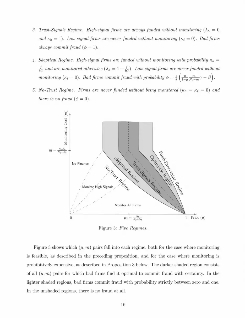
Figure 3 shows which (µ,m) pairs fall into each regime, both for the case where monitoring
is feasible, as described in the preceding proposition, and for the case where monitoring is
prohibitively expensive, as described in Proposition 3 below. The darker shaded region consists
of all (µ,m) pairs for which bad firms find it optimal to commit fraud with certainty. In the
lighter shaded regions, bad firms commit fraud with probability strictly between zero and one.
In the unshaded regions, there is no fraud at all.
16

Figure 3 is related to Figure 2, which shows the details of the investor’s ex-post decision
problem; the dashed lines in Figure 3 correspond to the solid lines in Figure 2. From the figure,
it is clear that fraud takes place in a region centered on µUF = max {µ3 (m) , µ2}, the posterior
belief at which the investor is just indifferent to providing unmonitored finance. Intuitively, if
the prior is close to this indifference point, the prior uncertainty over whether the firm should
receive unmonitored finance or not is greatest. This means that the signal’s outcome has the
greatest effect on whether the investor provides unmonitored finance or not: a high signal is
most likely to lead to a different outcome from a low signal, which is when incentives for fraud
are highest.
Analytically, the results in Proposition 2 follow from the regime definitions that precede
the proposition; these are given in terms of the prior µ and µUF . (Note that in the case of
Proposition 2, µUF equals µ3(m); i.e., when the investor is indifferent to providing unmonitored
finance, her relevant choice is between monitoring and not monitoring.) The expressions for the
boundaries of the regimes are derived from critical values of µs (φ), which again is the investor’s
posterior belief that the firm is good after seeing the free signal s and assuming that the bad
firm commits fraud with probability φ.
As an example, in the Fund-Everything regime, the prior µ is so high that even a low signal
is very likely to have come from a good firm. Specifically, we have µUF = µ3(m) ≤ µ` (1):
even after seeing a low signal, and even if bad firms commit fraud with probability one, the
investor is willing to extend unmonitored finance to the firm. Using the definition of µ` (1) and
rearranging yields the condition given in the definition. Since all firms receive unmonitored
finance regardless of the public signal, there is no benefit from committing fraud in this regime.
In the Optimistic regime, either the prior µ or the cost of monitoring m is somewhat lower,
so that µ` (0) < µ3 (m) < µ` (1). Here, a high signal still leaves the investor choosing to fund
the firm without monitoring, but a low signal is bad enough that the investor prefers to monitor
with some probability.16 In this regime, monitoring actually encourages fraud, since bad firms
that produce a low signal may be monitored and denied funding.
In the Trust-Signals regime, µ` (1) < µ3 (m) < µh (1). Here, only high signals receive
16 More precisely, if there were no chance of fraud in equilibrium, the investor would strictly prefer to monitorafter a low signal; if there were fraud with certainty, the investor would strictly prefer to not monitor; thus, inequilibrium, the investor monitors with probability between 0 and 1.
17
unmonitored finance; low signals are either monitored or rejected.17 Either way, bad firms have
no chance of being financed if they produce a low signal, so their incentive to commit fraud is
higher than it would be in the Optimistic regime. In this regime, bad firms commit fraud with
certainty.
With lower values of µ or m, we enter the Skeptical regime, where µh (1) < µ3 (m) < µh (0).
The priors in this regime are low enough that the investor finds it optimal to monitor even
high signals with positive probability. Because the bad firm may not get financing even if it
manages to obtain a high signal, the gains from fraud are lower than those in the Trust-Signals
regime. Thus, bad firms commit fraud with probability strictly less than one.
Finally, for very low values of µ, we have µh (0) < µ3 (m). In this No-Trust regime, the
investor’s prior is so low that all firms are either monitored or rejected, regardless of the signal.
Since there is no unmonitored finance, there is no gain to committing fraud, and so there is no
fraud in equilibrium.
Next, we turn to the case where monitoring costs are so high that monitoring never pays
(that is, m > m). The regimes described in Proposition 2 extend to this case in a natural way
(see Figure 3):
Proposition 3 Assume that the monitoring cost m > m = NbNg
Nb+Ng, so that the investor never
monitors. Denote by κs the probability of unmonitored finance with a signal s, and by φ the
bad firm’s probability of committing fraud. The equilibrium decisions are as follows:
1. Fund-Everything Regime. All firms are funded regardless of the signal (κh = κ` = 1), and
there is no fraud (φ = 0).
2. Optimistic Regime. High-signal firms are always funded (κh = 1). Low-signal firms are
funded with probability κ` = 1− fδC
and denied funding otherwise. Bad firms commit fraud
with probability φ = 1δ
(1− β − µ
1−µ
Ng
Nb(1− γ)
).
3. Trust-Signals Regime. High-signal firms are always funded (κh = 1). Low-signal firms
are never funded (κ` = 0). Bad firms always commit fraud (φ = 1).
4. Skeptical Regime: High-signal firms are funded without monitoring with probability κh =
fδC
and denied funding otherwise. Low-signal firms are never funded (κ` = 0). Bad firms
17 The choice depends on whether or not µ` (0) exceeds µ1 (m).
18

commit fraud with probability φ = 1δ
(µ
1−µ
Ng
Nbγ − β
).
5. No-Trust Regime: firms are never funded (κh = κ` = 0) and there is no fraud (φ = 0).
If m > m, monitoring is prohibitively expensive, and the investor either rejects the firm
or provides unmonitored financing. The five regimes are analogous to those in Proposition 2.
One key difference is that if a regime calls for monitoring when m ≤ m, it calls for denying
funding when m > m. Another key difference is that when m > m, the critical level µUF equals
µ2, which does not depend on the monitoring cost m. As a result, the boundaries of the five
regimes are constant in m, as can be seen from Figure 3. We will return to the implications of
this shortly.
Our next result is a straightforward consequence of Propositions 2 and 3.
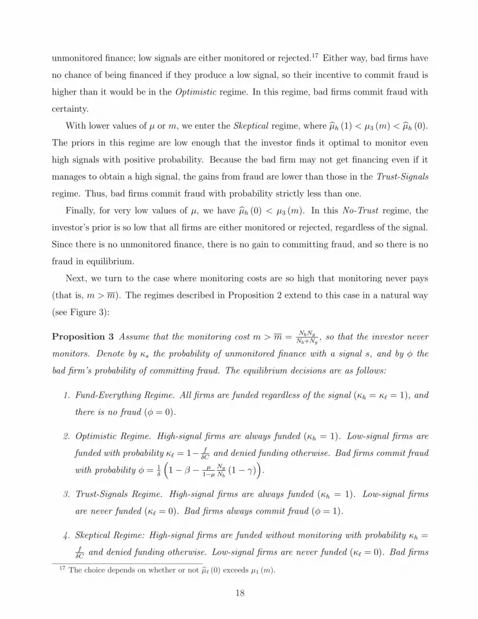
Proposition 4 Both the probability of fraud φ conditional on the firm being bad, and the ex-
ante probability of fraud (1− µ) φ are hump-shaped in the prior µ. There is no fraud for the
highest and lowest levels of µ, the Fund-Everything and No-Trust regimes. In the Skeptical
regime the probabilities of fraud are increasing in µ, while in the Optimistic regime they are
decreasing. In the Trust-Signals regime, the conditional probability is constant, while the ex-ante
probability is decreasing in µ.
0
1
1Prior (µ)
Pro
b.of
Fra
ud
(φ)
Figure 4: Fraud probability: ex-ante (dashed line) and conditional (solid line).
Figure 4 shows the conditional and ex-ante probabilities of fraud. The graphs consist of
five parts, corresponding to the five regimes described above. In the Skeptical regime, the
19
probabilities increase with µ. High-signal firms are monitored or denied funding with positive
probability, low-signal firms with certainty. Thus the investor is indifferent between monitoring
(or denying funding to) high-signal firms and funding them without any further information.
All else equal, an increase in the prior µ makes the investor strictly unwilling to monitor (or
deny funding to) high-signal firms — but then the bad firm would prefer to commit fraud with
certainty, worsening the pool of high-signal firms and destroying equilibrium. In equilibrium,
the probability of fraud must increase so as to restore balance.
In the Optimistic regime, the probability of fraud decreases with µ. The investor strictly
prefers to fund high-signal firms, and is indifferent between monitoring (or denying funding
to) low-signal firms and funding them without further information. Here, an increase in the
prior makes the investor strictly prefer to fund low-signal firms without monitoring — but
then bad firms would have no reason to commit fraud, worsening the pool of low-signal firms
and destroying equilibrium. In equilibrium, the probability of fraud decreases so as to restore
balance.
The preceding discussion accounts for the results on the bad firms’ conditional probability
of fraud φ. The results on the ex ante probability of fraud (1− µ) φ follow immediately.
The last issue we consider in this section has to do with where fraud is most likely —
i.e., where the “hump” has its peak. As we discussed following Proposition 2, the region in
(µ,m) space where fraud incentives are highest centers around the line given by µ = µUF .
When monitoring costs exceed m, so that monitoring is not feasible, this is a vertical line at
µ2, the prior at which the investor is indifferent between not financing the firm and extending
unmonitored financing. But this indifference means that the ex ante expected net present value
of a firm is zero. Thus, when monitoring is not feasible, fraud is most prevalent in “so-so” times.
Matters are very different when monitoring costs are low enough that monitoring is some-
times feasible. In this case, µUF equals µ3(m), which is a downward-sloping line. This means
that when monitoring costs fall, the region where fraud is highest shifts towards higher and
higher priors. In other words, an association between fraud and “good times” depends on
investors being able to monitor, and this association is stronger as monitoring costs are lower.
Finally, although our analysis focuses on how fraud changes as the prior probability that a
firm is good changes, we obtain similar results if this prior is held fixed and instead the return
of a successful firm R changes. It is easy to show that when R is so low that a good firm’s net
20
present value Ng is only slightly positive (and so a bad firm’s negative net present value Nb is
large), investors will be cautious even after a high signal. As R increases, eventually investors
begin to fund high-signal firms without monitoring, at which point fraud starts to occur; further
increases in R lead to the same hump-shaped pattern of fraud that we have already described.18
Thus, even if one defines “bad times” and “good times” in terms of the expected return to any
given firm rather than the relative numbers of good and bad firms, our predictions still hold.
3 Determinants of Fraud
Having established the properties of equilibria in the various regimes, we now turn to the
question of how various parameters affect the incidence of fraud. We show that, while certain
results are constant across regimes, others depend heavily on whether the regime is Skeptical
or Optimistic. In particular, the Skeptical regime is the more intuitive case; here, monitoring
discourages fraud, and other parameter effects are as one would expect. By contrast, the
Optimistic regime is counterintuitive; here, monitoring encourages fraud, and several parameter
effects are the reverse of what one would expect. We discuss the practical implications of these
results. Finally, we discuss how our model’s implications are affected by dynamic considerations.
We begin with the comparative statics of the Skeptical regime.
Proposition 5 In the Skeptical regime,
(i) The equilibrium probability that bad firms commit fraud (φ) is increasing in the prior µ,
weakly increasing in the cost of monitoring m, and decreasing in the efficacy of fraud δ.
(ii) If the monitoring cost is low (m ≤ m), then the equilibrium probability that high-signal
firms are monitored (λh) is decreasing in the cost of fraud f and increasing in both the efficacy
of fraud δ and in the level of private benefits C. If the monitoring cost is high (m > m), then
the equilibrium probability that high-signal firms are denied funding is decreasing in the cost of
fraud f and increasing in both the efficacy of fraud δ and in the level of private benefits C.
18 Briefly, an increase in R decreases µ2 and µ3(m), and thus µUF as well. From the definitions of the fiveregimes preceding Proposition 2, the boundaries of the regimes are all increasing in µUF . Thus, an increase inR shifts all regimes to the left in (µ,m) space, which means that for a fixed prior µ, the regime “improves.” Forexample, if initially the equilibrium is No-Trust, increasing R leads first to the Skeptical regime, then to theTrust-Signals regime, and so forth.
21

The intuition for part (i) of the proposition follows from the effects of parameter changes on
the investor’s incentives to monitor the pool of firms that generate high signals. An increase in
the prior probability that firms are good improves the pool, lowering the investor’s incentives
to monitor or deny funding. This allows the probability that bad firms commit fraud (φ) to
increase until equilibrium is restored. An increase in the efficacy of fraud has the opposite
effect. Finally, if monitoring costs are sufficiently low (m ≤ m), an increase in the cost of
monitoring directly lowers the investor’s monitoring incentives, again allowing the probability
of fraud to increase. (If m > m, the investor never monitors, so changes in m have no effect on
the probability of fraud.)
The intuition for part (ii) of the proposition is straightforward. The probability of mon-
itoring or funding denial is determined by the bad firm’s incentive condition — the point at
which it is indifferent between committing fraud and not committing fraud. If the cost of fraud
increases, then fraud is less attractive, and less intensive monitoring or less frequent funding
denial suffices to deter fraud to the point of indifference. Higher private benefits make getting
funded more attractive. Because generating a high signal is the only way that a bad firm
has a chance of getting funded, fraud is more attractive, and again more intensive monitoring
or funding denial is needed. Finally, if fraud is more effective, the pool of high-signal firms
worsens, all else equal, and more intensive monitoring or funding denial is needed to restore
balance.
As noted above, the Skeptical regime is the intuitive case. The investor’s decision about
partial monitoring or funding denial focuses on firms with high signals, and fraud gives a bad
firm a higher chance of entering this pool and getting funding. This leads to a direct link
between the intensity of monitoring or funding denial and fraud incentives. By contrast, the
Optimistic case is less intuitive. Here, partial monitoring or funding denial focuses on firms
with low signals, and fraud gives a bad firm a higher chance of exiting this pool by generating a
high signal and getting automatic funding. Thus, the link between the intensity of monitoring
and fraud incentives is now less direct. This can be seen in the following proposition.
Proposition 6 In the Optimistic regime,
(i) The equilibrium probability that bad firms commit fraud (φ) is decreasing in the prior µ and
the efficacy of fraud δ, and weakly decreasing in the cost of monitoring m.
22

(ii) If the monitoring cost is low (m ≤ m), then the equilibrium probability that low-signal firms
are monitored (λ`) is increasing in the cost of fraud f and decreasing in both the efficacy of
fraud δ and in the level of private benefits C. If the monitoring cost is high (m > m), then the
equilibrium probability that low-signal firms are denied funding is increasing in the cost of fraud
f and decreasing in both the efficacy of fraud δ and the level of private benefits C.
As before, part (i) of the proposition follows from the effects of parameter changes on the
investor’s incentives to tighten funding (i.e., monitor or deny funding, depending on whether
or not m ≤ m) for the pool of firms with low signals. An increase in the prior probability that
a firm is good increases the fraction of low-signal firms that are good, reducing the investor’s
incentives to tighten funding. Since a reduction in monitoring or funding denial makes fraud less
attractive (bad firms are more likely to be funded even if they get a low signal), the probability
of fraud falls until incentives are restored. An increase in the probability that bad firms can
generate high signals through fraud (δ) also increases the fraction of low-signal firms that are
good, discouraging fraud. Finally, if monitoring costs are sufficiently low (m ≤ m), an increase
in the cost of monitoring directly lowers the investor’s monitoring incentives, discouraging fraud.
Part (ii) follows from the effects of parameter changes on the bad firm’s incentives to commit
fraud. The difference is that now, more intensive monitoring or more frequent funding denial
decreases the probability that a bad firm with a low signal gets funded, and so tighter funding
encourages bad firms to commit fraud so as to improve their odds of generating high signals.
When fraud is more costly, fraud is less attractive, so more of the low-signal firms are in fact bad
firms, and tighter funding is required to restore equilibrium. Conversely, since more effective
fraud or higher private control benefits increase the quality of the pool of low-signal firms,
looser funding is required to restore equilibrium.
Thus far, we have not addressed the impact of changes in the base signal’s precision (that is,
the signal’s precision in the absence of fraud). The following proposition shows that an increase
in this precision always tends to increase the incidence of fraud.
Proposition 7 Suppose that the precision of the base signal improves, so that the probability
that good firms send high signals (γ) increases, or the base probability that bad firms send high
signals (β) decreases, or both.
(i) In both the Skeptical and the Optimistic regimes, the equilibrium probability that bad firms
23

commit fraud (φ) increases.
(ii) The regimes in which fraud occurs expand, encompassing more prior beliefs µ. Specifically,
the maximal fraud (Trust-Signals) regime expands, beginning at a lower µ and ending at a
higher µ. The Skeptical regime also begins at a lower prior µ, and the Optimistic regime ends
at a higher prior µ.
These results follow from the effect of improved signal precision on investor behavior and
thus on bad firms’ incentives to commit fraud. An increase in the probability that good firms
generate high signals improves the pool of firms that have high signals and worsens the pool
of firms that have low signals. A decrease in the base probability that bad firms generate
low signals has similar effects. All else equal, such a change decreases investors’ incentives to
monitor or deny funding to high-signal firms and increases their incentives to monitor or deny
funding to low-signal firms. This in turn tends to increase bad firms’ incentives to commit
fraud. Intuitively, a more precise signal means that the bad firm has more chance of generating
a bad signal and then losing funding, but more chance of getting funding if it does generate a
high signal; this gives it more incentive to try to commit fraud, “noising up” the signal.
In the Trust-Signals regime, the change in investor incentives does not affect behavior; in-
vestors already fund all high-signal firms and never fund low-signal firms without monitoring,
so the fraud incentives of bad firms are already maximized (probability of fraud φ equals 1).
By contrast, in the Skeptical regime, the probability that high-signal firms are funded without
monitoring increases; this makes generating a high signal through fraud strictly more attrac-
tive, and the probability that bad firms commit fraud increases until equilibrium is restored.
Similarly, in the Optimistic regime, the probability that low-signal firms are given funding
without monitoring decreases; this too makes generating a high signal through fraud strictly
more attractive. This explains the results in part (i) of the proposition.
The results in part (ii) follow similar logic. At the outer boundaries of the fraud regimes,
improved signal precision introduces a difference in investors’ willingness to extend unmoni-
tored funding to high-signal firms versus low-signal firms, creating an incentive for fraud where
none previously existed. Similarly, within the Skeptical and Optimistic regimes, the increase in
incentives for fraud expands the set of priors for which these incentives are maximized, expand-
ing the Trust-Signals regime. The upshot is that improved signal precision increases both the
24
set of economic conditions under which fraud occurs and the probability with which it occurs.19
Of course, our results on signal precision obtain in a very simple setting. In a more complex
model, improving signal precision might also make some types of fraud harder to commit,
increasing the cost of fraud f . If so, then for some firms or managers, fraud might now be
prohibitively costly.
3.1 Implications for the Incidence of Fraud
Our model predicts that the incidence of fraud is non-monotonic in µ, the proportion of good
firms, peaking for high (but not too high) values of µ. We may observe different values of µ
across different industries at a given time, or different values over time as a consequence of
business cycles.
Consider the internet and telecoms sectors in the late 1990s. Internet or “dot-com” firms
were viewed as “can’t miss” opportunities, because of a widespread conviction that much con-
ventional business would migrate to the Internet in a relatively short period of time. Investors
were willing to finance many start-ups with untested business models, and to keep providing
funds. By contrast, the telecoms sector, though viewed very positively, was not the subject
of such strong optimism in the 1990s20 There have been few accusations of fraud directed at
the Internet firms, but numerous large telecoms firms (including WorldCom, Qwest, Global
Crossing, Nortel, and Lucent) have been accused of fraudulent or misleading accounting. This
difference is consistent with our model: Internet firms may have fallen into or close to the Fund-
Everything regime, in which case there was no need to commit fraud, whereas the telecoms may
have fallen into the lower Optimistic regime, in which case fraud should have been expected.
The nonmonotonicity of fraud with respect to µ is just one example of how many parameter
changes have opposite effects depending on whether the fraud regime is Skeptical or Optimistic.
The reason for this is that investors do not monitor to detect fraud per se; instead, their goal
is to find good investment opportunities and avoid bad ones. In the Skeptical regime, investors
19 Although our focus is on how increased signal precision increases the incidence of fraud (φ), it is worthnoting that, overall, bad firms may be more or less likely to get funded. Within a given regime, an increase in γweakly increases the overall probability that a bad firm is funded, whereas a decrease in β weakly decreases this.If the increase in precision causes a regime shift, however, matters are more complex, because the probabilityκs that a firm with signal s gets unmonitored funding shifts discontinuously.
20 During the 1990s, telecom firms raised hundreds of billions of dollars for investment, based on optimisticprojections of future demand for their services. For discussion of their financing and the frauds which subse-quently came to light, see Morgenson (2000, 2002).
25

strictly prefer to be “tough” with low-signal firms (monitor or deny funding), but they are
somewhat “looser” with high-signal firms. As a result, changes in parameters affect investors’
behavior with high-signal firms but not with low-signal firms. The opposite is true in the
Optimistic regime: now, investors strictly prefer to fund high-signal firms, but they apply
somewhat tougher standards to low-signal firms. In this case, changes in parameters affect
investors’ behavior with low-signal firms but not with high-signal firms, and so the effects of
many parameter changes switch sign. In particular, a change that causes investors to loosen
standards for low firms reduces fraud because bad firms see less need for it — why commit
fraud when you can get funded without it?
As another example of this nonmonotonicity, consider the impact of a change in the cost
of monitoring. Consider again the 1990s. Arguably, as information technology improved, it
became easier for analysts and others to “kick the tires”. Recall that as the cost of monitoring
m decreases, the region where fraud occurs shifts towards better prior beliefs — if during the
boom these monitoring efforts were concentrated on firms that were known as poor performers,
then perversely, this may have increased the prevalence of fraud.
The comparative statics for other parameters of our model are more intuitive. In particular,
the probability of fraud increases with the quality of the free signal (cf. Propositions 5 and 6).
If the informativeness of the free signal increases (higher γ, lower β), bad firms have a stronger
incentive to add noise to it (by committing fraud); and if fraud is more effective (higher δ), a
bad firm can compensate by committing fraud with a lower probability (to achieve the same
expected effect).
This has implications for the use of disclosure requirements, and their use as a tool to
combat fraud. During the 1990s, the trend was for annual reports to include more and more
details, partly in response to stricter demands from the Financial Accounting Standards Board
(FASB). In the absence of fraud or misrepresentation, investors could now do a better job of
assessing a firm’s situation — and so a number of firms began to game the system, in many
cases crossing the line into fraud. Thus, tougher disclosure laws may have the perverse effect of
increasing fraud.21 Our results suggest that, to be effective against fraud, disclosure laws must
directly make fraud more difficult.
21 Furthermore, as noted above, increased precision does not necessarily reduce the overall probability withwhich a bad firm is funded, so the overall effect of tougher disclosure on funding efficiency can be mixed.
26

3.2 Implications for Investment Across the Business Cycle
We now examine how the possibility of fraud affects the behavior of investors and, in turn,
which types of firms get funding. As we will see, these effects depend heavily on the nature of
the fraud regime, but in a certain sense the effect of fraud is to amplify the impact of business
conditions on firm funding.
First, we note that if fraud is impossible, there are only three regimes: No Trust, Trust
Signals, and Fund Everything. Intuitively, once fraud is ruled out, firms no longer have any
choice variable to randomize over, so the mixed strategy equilibria — Skeptical and Optimistic
— disappear. A more technical way of seeing this is to take the definitions of the regimes
given before Proposition 2 and let the efficacy of fraud δ go to zero. It also follows that the
boundaries of the No Trust and Fund Everything regimes are precisely as before, whereas the
Trust Signals regime expands to take in the two regions in which mixed strategies prevail if
fraud is possible. Briefly, removing the possibility of fraud means that investors can now fully
rely on a firm’s signal without concern that bad firms will try to change the quality of that
signal. As a result, even if investors would choose a mixed strategy in the presence of fraud,
when fraud is ruled out they choose to fund all high signal firms without monitoring.
Since fraud has no impact in the No Trust and Fund Everything regimes, we focus our atten-
tion on the impact of fraud on investment in the other regimes. Suppose first that monitoring is
not feasible (m ≥ m). With no fraud, we are in a Trust Signals regime where high signal firms
are funded and low signal firms are not. If the possibility of fraud leads to the Skeptical regime,
high signal firms are less likely to be funded, and low signal firms are still not funded. This
unambiguously decreases the number of good firms that get funded. However, it is possible
that the number of bad firms that get funded increases; this occurs when fδC
(β + δ) > β, which
requires that the increased chance that bad firms generate high signals outweighs the decreased
chance that high signals are funded. If the possibility of fraud causes the regime to remain
Trust Signals, high signal firms are funded whereas low signal firms are not. It follows that
the number of bad firms funded increases whereas the number of good firms funded does not
change. Finally, in the Optimistic regime, high signals are funded and low signals now have a
chance of being funded. As a result, the number of good firms and bad firms that are funded
both increase. Thus, in this case, one can unambiguously say that business cycle effects are
27
amplified: fraud makes investors more stringent in the Skeptical regime (despite which more
bad firms may be funded), no more stringent in the Trust Signals regime, and less stringent in
the Optimistic regime. Also, as one would expect, more bad firms relative to good firms are
funded when there is fraud.
Suppose instead that monitoring is feasible (m < m). The effects just mentioned continue
to hold, but now there is a complicating effect: fraud affects the probability of monitoring,
which affects good and bad firms differently — good firms receive funding if monitored whereas
bad firms do not. If the possibility of fraud leads to the Skeptical regime, again, the number of
bad firms funded may increase, but now the number of good firms funded does not decrease —
though more good firms are now monitored. If fraud leads to the Trust Signals regime, more
bad firms are funded, but the monitoring of low signals may increase because the pool of low
signals is of higher quality when there is fraud. If such monitoring increases, more good firms
are monitored and funded. Finally, if fraud leads to the Optimistic regime, more bad firms are
funded, and weakly more good firms are funded; again, the last occurs when the probability
of monitoring low signals increases. In summary, once monitoring is feasible, the impact of
fraud may be to increase monitoring efforts; if so, this actually helps the good firms get funded.
Nevertheless, it remains the case that fraud means that bad firms are more likely to get funded
when conditions are good.
3.3 Dynamic Considerations
Up until now, we have assumed that investors and firms know the prior distribution of firm
types without uncertainty. In practice, such priors are likely to be uncertain, since the “true”
state of the economy can only be known ex post, if at all. Moreover, the true state of the
economy is dynamic, which can complicate the inference problems of investors and managers.
As suggested in the introduction, these considerations can exacerbate the links between fraud,
booms, and busts.
To model these issues in a simple way, we assume that there are two possible true states
of the economy, one in which there are relatively many good firms (fraction µu of all firms)
and one in which there are relatively few good firms (fraction µd of all firms, with µd < µu).
Furthermore, we assume that µu falls into the Fund-Everything regime, and µd falls into the
28

No-Trust regime. The true state cannot be observed, and all agents share common beliefs: the
probability that the state is µu is p0. It follows that the overall prior that any given firm is
good is µ = p0µu + (1− p0)µd.
First suppose that p0 is low. In this case, the ex-ante prior µ is low, corresponding to either
the No-Trust or (low) Skeptical regime. Bad firms are unlikely to commit fraud in this case,
since even high-signal firms are usually monitored before they are financed. If, ex post, the true
state of the economy proves to be µd, there will be slightly more bad firms than expected, but
the overall incidence of fraud will still be low or nonexistent. If instead the true state proves
to be µu, there will be even fewer cases of fraud, funded projects will be relatively successful,
and investors’ conservatism may seem overblown, as more monitored projects than expected
will prove to be good.
Now suppose p0 is high, so that the ex-ante prior µ falls within the Trust-Signals or Opti-
mistic regime. Although bad firms will be committing fraud, if the true state later proves to
be µu, there will not be many bad firms, and the actual incidence of fraud will be somewhat
lower than expected. By contrast, if the true state proves to be µd, the numbers of bad firms
and fraud cases will be much higher than expected.
If the prior is higher still, of course, the equilibrium will fall into the upper end of the
Optimistic regime or even the Fund-Everything regime. In this case, fraud will be low or
nonexistent, even if the state proves to be µd, but in this last case many more funded projects
than expected will perform poorly.
All of this has taken p0 as given. In reality, p0 will arise from investors getting signals from
various firms and from some “actual” realizations (e.g., realized cash flows in our model). Note
that the presence of fraud slows down updating in both directions: both high and low signals
become noisier. Thus, priors will be slower to shift in the “middle,” where bad firms are likely
to commit fraud. If beliefs begin with a p0 so high that the regime is Fund-Everything, and then
some bad realizations of the free signal shift p0 and thus µ into the Optimistic or Trust-Signals
regime, further updating will be slowed.
If there were no change in the underlying state, then over time, investor beliefs would find
their way to the true state. A more realistic assumption is that there is always some chance
that the underlying state governing the returns on new projects can shift — some chance of
transitioning from µd to µu, and another chance of transitioning the other way. If by some
29
chance beliefs do find their way close to one or the other extreme, there will always be some
chance that the beliefs are “very wrong” due to a transition. Of course, these transition
probabilities limit how high or low p0 can go, but there is still a chance that beliefs will be
heavily weighted towards one extreme or the other, in which case “surprises” of the sort already
discussed will still be possible. In particular, once p0 and thus µ are in the Optimistic regime,
a period of slow updating from “free” signals (interim results) could be followed either by a
reassuring string of high cash flows or a spate of low cash flows that suddenly reveal that the
economy is in recession — followed in the last instance by a wave of revelations of fraud.
In short, the agents in an economy may be “surprised” by changes in the economy’s fun-
damentals. Although this notion is not especially surprising, it has strong implications for the
incidence and prevalence of fraud across the business cycle. As noted, when times are bad — in
terms of our model, in the No-Trust or Skeptical regimes — positive surprises will lead to lower
amounts of fraud than expected. The opposite is true when times are good; now surprises lead
to higher-than-expected fraud.
It is also important to note that, in the last case, even fraudulent firms are surprised by the
extent of fraud. Although they have private information that they are in bad shape, which is a
somewhat negative signal for the economy as a whole, this is not the same as knowing that many
firms are in bad shape. In a more complex model, this can lead to negative spillovers as firms
with weak prospects who see others post high results feel more pressure to do so themselves,
precisely because neither they nor investors know whether the others are committing fraud.
Something of this sort seems to have happened in the case of WorldCom, whose fraudulent
reporting in the 1990s increased the pressure on its rivals (Schiesel, 2002).
4 Fraud Committed by Good Firms
We have assumed that good firms cannot commit fraud. We now discuss this assumption, and
what results we would obtain if we relax it. The motivation for the assumption is that investors
may discover whether a firm committed fraud. In our model, the detection of fraud itself is
of no consequence, since investors will not finance a firm anyway if they know its type is bad.
But in a more realistic and more complex model, committing fraud may well be taken as a
sign that the firm’s management may misbehave in future, and an investor may reject a good
30

firm if there is evidence that the firm committed fraud. This may deter the managers of good
firms from committing fraud, in particular if they are easily replaced once their firm is up and
running.
On the other hand, even if firms commit the type of fraud that is the focus of our analysis,
that does not necessarily imply that investors will worry about future misbehavior. In our
model, fraud makes firms look more attractive to investors, but it does not fool investors who
monitor before providing funds. Fraud committed by good firms improves the odds that a firm
with a high signal is actually a good firm. If it is hard to tell apart good and bad firms, investors
may therefore tolerate fraud by good firms: after all, investors care only about making good
investments and avoiding bad investments. If investors do not object to fraud committed by
good firms, then it is reasonable to expect that other agents in the economy will not object,
either. For example, the media may show little interest in such cases, because they do not make
for spectacular headlines; and regulators and enforcement agencies may show little interest, too,
because no harm was done.22
Nevertheless, it is interesting to explore the consequences of allowing for good-firm fraud.
We now provide a sketch of the analysis, which provides three insights about the role of good-
firm fraud. First, good and bad firms commit fraud for different reasons: good firms may
commit fraud to increase their chances of being monitored instead of being rejected; while bad
firms commit fraud to reduce their chances of being monitored. Second, good-firm fraud makes
the signal more informative and therefore leads to better investment decisions, while bad-firm
fraud has the opposite effect. Third, good-firm fraud tends to happen when the economy is in
poorer shape than it is when bad-firm fraud is more likely to happen.
To analyze a good firm’s incentive to commit fraud, we need to extend our model. Assume
that good firms can commit fraud at a cost f ′, and that fraud increases the probability of a
high signal from γ to γ + δ′ < 1. Given that γ > β, it is reasonable to assume that fraud is
less effective for the good firms, i.e., δ′ < δ. Also, we assume that δ′1−γ
< δ1−β
, which implies
that the costless signal is more informative if there is no fraud at all than it is if both types
commit fraud with certainty. Finally, we assume that f ′ < δ′C, since otherwise a good firm
22 The same may be true even if outsiders are unable to observe the firm’s type. In this case, they may onlypunish fraud at firms that subsequently fail, under the same reasoning as above — why punish fraud that hasnot harmed anyone? Since good firms are less likely to fail then bad firms, good firms again will be less likelyto be punished for fraud.
31
would never commit fraud. It can easily be verified that given a signal h or `, the conditional
probability of facing a good firm is
µh(φ′, φ) =
µ(γ + φ′δ′)µ(γ + φ′δ′) + (1− µ)(β + φδ)
µ`(φ′, φ) =
µ(1− γ − φ′δ′)µ(1− γ − φ′δ′) + (1− µ)(1− β − φδ)
,
where φ′ is the probability with which the good firm commits fraud. Notice that µh(φ′, φ)
is increasing in φ′ and decreasing in φ, while µ`(φ′, φ) is decreasing in φ′ and increasing in φ
(good-firm fraud improves the quality of the costless signal, while bad-firm fraud worsens it).
The two firm types’ incentives for committing fraud are not the same. While both may
commit fraud to obtain unmonitored funding instead of being rejected, a good firm may also
commit fraud in order to induce the investor to monitor (instead of rejecting), which a bad
firm would not want; also, a bad firm may commit fraud to induce the investor to provide
unmonitored funding instead of monitoring, whereas a good firm is indifferent between the two.
Hence, we focus on the case of lower monitoring costs m in what follows, since monitoring affects
the two types of firm differently and is more likely to happen if m is low. Considering lower
values of m also simplifies the analysis considerably, since the various motives for committing
fraud can be separated.
Lemma 1 Define m implicitly as the value of m which satisfies both m = Ngµ`(1, 0) and
m = Nb (1− µh(1, 0)). If m < m, then in equilibrium, either only bad firms commit fraud, or
only good firms commit fraud, or there is no fraud at all.
If m < m, then the incentives to commit fraud are driven uniquely by the desire to be
monitored or not, which is when good and bad firms differ most in their incentives to commit
fraud. The two functions that define m describe pairs (µ,m) for which the investor is indifferent
between two alternatives, assuming that only good firms commit fraud (φ′ = 1 and φ = 0).
The equation m = Ngµ`(1, 0) is equivalent to µ`(1, 0) = µ1(m), i.e., the investor is indifferent
between rejecting and monitoring a firm with a low signal; since µh(1, 0) > µ`(1, 0), a firm
with a high signal will certainly not be rejected. And m = Nb (1− µh(1, 0)) is equivalent
to µh(1, 0) = µ3(m), i.e., the investor is indifferent between monitoring a firm with a high
signal and funding it without monitoring; since µh(1, 0) > µ`(1, 0), a firm with a low signal
32

will certainly not be funded without monitoring. It is readily verified that m = Ngµ`(1, 0) is
upward sloping and that m = Nb (1− µh(1, 0)) is downward sloping. If Ngµ`(1, 0) < m < m,
the good firm may commit fraud, but the bad firm certainly does not commit fraud (it does
not benefit from being monitored, the only alternative outcome to being rejected). And if
Nb (1− µh(1, 0)) < m < m, the bad firm may commit fraud, but the good firm certainly does
not commit fraud (it is indifferent between being monitored and obtaining funds without being
monitored). Hence, for all pairs (µ,m) below both curves, there is no fraud at all. In sum,
good firms commit fraud only if the state of the economy is low enough, and bad firms only if
it is high enough.
The next question is under what circumstances good firms will commit fraud. For notational
convenience define
µGF (m) =m (1− β)
m (1− β) + (1− γ − δ′) (Ng −m)
µGF
(m) =mβ
mβ + (γ + δ′) (Ng −m),
where µGF
(m) is the value of µ such that the investor (assuming that only good firms commit
fraud) is indifferent between rejecting and monitoring a firm with a high signal and similarly
µGF (m) is the indifference value of µ conditional on a low signal. For all m < m, if µ > µGF (m)
the good firm does not commit fraud in equilibrium, so our earlier analysis is not affected if
we allow for good-firm fraud. In other words, our earlier analysis carries over to this more
general model. Analyzing the good firm’s decision is simplified by the fact that good-firm fraud
happens only if µ ≤ µGF (m), i.e., if there is certainly no bad-firm fraud.
Proposition 8 Assume m < m. Then
(1) if µ < µGF
(m), the good firm does not commit fraud;
(2) if µGF
(m) < µ < µGF (m), the good firm commits fraud; and
(3) if µ > µGF (m), the good firm does not commit fraud.
For low levels of µ the investor rejects all firms even if they obtain a high signal, and there
is no benefit from committing fraud (case 1). For high enough levels of µ, the investor monitors
even if a low signal is realized, so a good firm will be financed with certainty and thus gets no
benefit from committing fraud (case 3). It is only for intermediate values of µ that the good
33
firm benefits from committing fraud: if the investor monitors only high-signal firms, then fraud
helps the good firm because it increases the chances of producing a high signal (case 2), being
monitored, and therefore financed.
These results demonstrate that the incentives for committing fraud are very different for the
two types of firms. While both may commit fraud in order to improve their chances of obtaining
funding without monitoring instead of being rejected, their motives disagree when monitoring
is involved. Bad firms commit fraud only to increase their chances of obtaining unmonitored
funding, instead of being monitored or rejected. Good firms commit fraud to attract attention
and be monitored, if the chances of being rejected are sufficiently high. This is quite intuitive,
and it provides a reason why investors should not be worried if they discover that a good firm
committed fraud to make itself look more attractive to investors. It is also consistent with the
result that good-firm fraud tends to happen when the economy is in poorer shape than it is
when bad-firm fraud is more likely to happen. Bad-firm fraud happens to noise up the costless
signal and to convince investors to fund without monitoring; this happens only in the better
states of the economy. In contrast, good firms commit fraud in order to be monitored instead
of being rejected, which investors consider as alternatives only in poor states of the economy.
5 Conclusion
We have presented a simple model in which firms commit fraud in order to get funds from
investors. Despite its simplicity, the model can motivate several patterns of behavior that are
observed in practice and that may seem hard to explain, for example the high incidence of
fraud towards the end of the most recent stock market boom, and the prevalence of fraud in
certain industries and its near absence in others.
Our model shows which factors determine whether firms commit fraud or not. One such
factor is how carefully investors can be expected to scrutinize the firms in which they may
invest. The extent of monitoring, in turn, depends on investors’ expectations about the state
of the economy, and their expectations about firms’ fraud decisions. Our analysis reveals that
the incidence of fraud does not always respond as expected to changes in circumstances. While
it is natural to assume that improved business conditions lead to less fraud and reduced costs
of monitoring also lead to less fraud, the opposite may be true. Similarly, improvements in the
34
informativeness of publicly available information may have counterintuitive effects, since they
may increase the incidence of fraud.
These results were derived using a model with firms seeking funds for their investments, and
investors who may trust noisy information or pay for superior information about the firms. The
same information structure arises in completely different settings, and our results will apply in
these settings, too. For example, labor markets for skilled workers face a similar information
problem: employers may trust information that is easily available, such as a worker’s resume,
or they can make their own costly inquiries; and workers seeking jobs may embellish the details
listed on their resume in order to get a better job. Other examples include the used car and the
housing markets: buyers may trust their own eyes and experience, or they may hire professional
help to discover fatal flaws of what is being offered for sale; and sellers may find that a fresh
coat of paint can cover up signs of damage, fooling inexperienced buyers into thinking that
they are being offered a house or car of high quality.
Coming back to fraud and investment, our results have implications for public policy: legis-
lators and the media alike have called for new or changed regulation aimed at preventing future
waves of fraud. The Sarbanes-Oxley Act was introduced to improve the public disclosure of
financial information; the consequence may well be that investors monitor less (instead relying
more on the publicly available information), and more firms commit fraud. In other words, the
effectiveness of the new constraints that were imposed on businesses to prevent fraud may be
more limited than expected, and they may even have unintended consequences. At the same
time, our analysis suggests that it is pointless to blame investors for the abuses by arguing that
they were careless or naive when making their decisions. Such judgments are easy with the
benefit of hindsight; but given the information that was available to investors at the time, it
may have been fully rational for them to trust publicly available information in many cases,
instead of carefully monitoring firms that requested funds.
35

Appendix
Proof of Proposition 1
Investing without monitoring dominates not investing iff VU > VN ⇐⇒ µNg − (1− µ) Nb >
0 ⇐⇒ µ > Nb
Nb+Ng. Monitoring and investing in the good firm dominates not investing iff VM >
VN ⇐⇒ µNg−m > 0 ⇐⇒ µ > mNg
. Investing without monitoring dominates monitoring and
investing in the good firm iff VU > VM ⇐⇒ µNg − (1− µ) Nb > µNg −m ⇐⇒ µ > 1− mNb
.
Threshold for m: monitoring is dominated if µ ≤ mNg
and µ ≥ 1 − mNb
; combine µ = mNg
and
µ = 1− mNb
, which yields 1− mNb
= mNg
, and the definition of m.
Proof of Proposition 2
The cut-offs for the five regimes can equivalently be defined using cut-offs for the posterior
beliefs. Recall from (2) that
µ` (0) < µ` (1) < µh (1) < µh (0) .
These four cut-offs in the interval [0, 1] define the five regimes, depending on the location of
µ3 (m) in relation to the four cut-offs (for example, the Fund-Everything regime has µ` (0) >
µ3 (m)).
• The proofs for the Fund-Everything and No-Trust regimes are straightforward.
• The Optimistic regime: φ ∈ (0, 1] such that µ3 (m) < µ` (φ) cannot be an equilibrium. If
it was, ` signals would not be monitored, so there would be no benefit from committing
fraud, i.e. φ = 0. Similarly, φ ∈ [0, 1) such that µ3 (m) > µ` (φ) cannot be an equilibrium.
If it was, ` signals would be either monitored or rejected, while h signals receive unmon-
itored financing; so there would be an incentive to increase φ. So in equilibrium, the bad
firm chooses φ ∈ (0, 1) such that with a signal `,
VU = VM ⇐⇒ µ` (φ) = µ3 (m) ⇐⇒ φ =1
δ
(1− β − (1− γ)
µ
1− µ
m
Nb −m
). (A1)
36

Next, κh < 1 cannot be an equilibrium, since µ3 (m) < µh (φ) ∀φ. Therefore, κh = 1 and
λh = 0.
κ` = 1 cannot be an equilibrium. If it was, there would be no incentive for bad firms
to commit fraud, and therefore firms with a signal ` should not receive unmonitored
financing. Similarly, κ` + λ` < 1 cannot be an equilibrium. If it was, ` signals would
be rejected with positive probability. But that is not optimal for the investor since
µ` (φ) = µ3 > µ1, i.e. she strictly prefers monitoring an ` signal to rejecting it. Next,
λ` = 1, κ` = 0 cannot be an equilibrium. If it was, bad firms would commit fraud
with certainty. So in equilibrium, the investor chooses λ` and κ` such that λ` ∈ (0, 1),
λ` + κ` = 1, and
(β + δ) C + (1− β − δ) κ`C − f = βC + (1− β) κ`C ⇐⇒ κ` = 1− f
δC.
• The Trust-Signals regime: µ` (0) < µ` (1) < µ3 (m) < µh (1) < µh (0), so ` signals are
rejected or monitored while h signals are financed without monitoring. By assumption,
δC > f , so it pays for a bad firm to increase φ up to one. Signals ` are monitored iff
µ` (1) ≥ µ1 (m) ⇐⇒ µ
µ + (1− µ) 1−β−δ1−γ
≥ m
Ng
⇐⇒ µ ≥mNg
1−β−δ1−γ
1 + γ−β−δ1−γ
mNg
.
• The Skeptical regime: φ ∈ (0, 1] such that µ3 (m) > µh (φ) cannot be an equilibrium. If
it was, all firms would be either monitored or rejected, and there would be no benefit
from committing fraud. Similarly, φ ∈ [0, 1) such that µ3 (m) < µh (φ) cannot be an
equilibrium. If it was, h signals would receive unmonitored financing, while ` signals
would be either monitored or rejected, giving bad firms an incentive to increase φ. So in
equilibrium, the bad firm chooses φ such that with a signal h,
VU = VM ⇐⇒ µh (φ) = µ3 (m) ⇐⇒ φ =1
δ
(µ
1− µ
m
Nb −mγ − β
). (A2)
If φ is such that µh (φ) = µ3 (m), the investor is indifferent between monitored and
unmonitored finance for h signals, and she prefers either option to rejecting an h signal;
therefore λh + κh = 1. The investor mixes between monitored and unmonitored finance
37

for h signals, such that a bad firm is indifferent between committing fraud and not:
(β + δ) κhC − f = βCκh ⇐⇒ κh =f
δC.
So λh = 1 − κh = 1 − fδC
. Finally, κ` > 0 cannot be an equilibrium. If it was, then
µ` (φ) ≥ µ3 (m) = µh (φ), contradiction. So bad firms with an ` signal cannot expect to
get financing at all. In equilibrium, ` signals are monitored iff
µ` (φ) ≥ µ1 (m) ⇐⇒ µ ≥mNg
1− γ(1− Nb
Ng
mNb−m
) .
(and rejected otherwise).
Proof of Proposition 3
• The proofs for the Fund-Everything, Trust-Signals and No-Trust regimes are straightfor-
ward.
• The Optimistic regime: κh = 1 since µ2 < µh (1) < µh (0). Next, φ = 0 can not be an
equilibrium. The investor would not finance with a signal `, since µ` (0) < µ2. But then
a bad would firm prefer to increase φ2 above zero, since δC > f . Similarly, φ = 1 can
not be an equilibrium. The investor would finance with any signal, so there would be no
need to invest f . Next, κ` = 0 cannot be an equilibrium. All bad firms would commit
fraud with certainty, and the investor should then provide unmonitored finance for either
signal, since µ2 < µ` (1). Finally, κ` = 1 cannot be an equilibrium. Bad firms would not
commit fraud, and the investor should then reject ` signals, since µ` (0) < µ2. So the
equilibrium must be in mixed strategies for both players. The bad firm chooses φ such
that with a signal `,
VU = VN ⇐⇒ µ` (φ) Ng − (1− µ` (φ)) Nb = 0 ⇐⇒ φ =1
δ
(1− β − (1− γ)
µ
1− µ
Ng
Nb
).
The investor chooses κ` such that
(β + δ) C + (1− β − δ) κ`C − f = βC + (1− β) κ`C ⇐⇒ κ` = 1− f
δC.
38

• The Skeptical regime: φ = 0 can not be an equilibrium. The investor would not finance
with a signal `, since µ` (0) < µ2. But then a bad would firm prefer to increase φ2 above
zero, since δC > f . Similarly, φ = 1 can not be an equilibrium. If it was, the investor
would not finance any firm, so there would be no need to commit fraud. Next, κh = 0
cannot be an equilibrium. No firm would be financed, and therefore bad firms would
not commit fraud; but then the investor should finance all h signals, since µ2 < µh (0).
Finally, κh = 1 cannot be an equilibrium. Bad firms would have an incentive to commit
fraud with probability 1; but then the investor should reject all signals, since µh (1) < µ2.
So the equilibrium must be in mixed strategies for both players. The bad firm chooses φ
such that with a signal h,
VU = VN ⇐⇒ µh (φ) Ng − (1− µh (φ)) Nb = 0 ⇐⇒ φ =1
δ
(µγ
1− µ
Ng
Nb
− β
).
The investor chooses κ` such that
(β + δ) κhC − f = βκhC ⇐⇒ κh =f
δC.
Proof of Proposition 4
The conditional probabilities are derived in Proposition 2. The ex-ante probability of fraud is
calculated as (1− µ) φ in each regime.
Proof of Proposition 5
Follows immediately from (A2).
Proof of Proposition 6
Follows immediately from (A1).
Proof of Proposition 7
Part (i) follows immediately from (A1) and (A2). Part (ii) follows from an inspection of the
regime boundaries as defined in Section 4.2 (immediately before Proposition 2).
39
Proof of Lemma 1
Consider cases m < Ngµ`(1, 0). Rearrange as µ`(1, 0) > mNg
, which is equivalent to µ`(1, 0) >
µ1(m). Since µ`(φ′, φ) is decreasing in φ′ and increasing in φ, this implies that µ` (φ′, φ) > µ1(m)
∀φ′, φ, i.e., the investor is prefers to monitor firm with a signal ` rather than rejecting it. Since
µh (φ′, φ) > µ` (φ′, φ) ∀φ′, φ, a firm with a signal h will be either monitored or funded without
monitoring. So the good firm has no incentive to commit fraud.
Now consider m < Nb (1− µh(1, 0)). Rearrange as µh(1, 0) < 1 − mNb
, which is equivalent
to µh(1, 0) < µ3(m). Since µh(φ′, φ) is increasing in φ′ and decreasing in φ, this implies that
µh (φ′, φ) < µ3(m) ∀φ′, φ, i.e., the investor is prefers to monitor a firm with a high signal to
funding it without monitoring. Since µh (φ′, φ) > µ` (φ′, φ) ∀φ′, φ, a firm with a signal ` will be
either monitored or rejected. So the bad firm has no incentive to commit fraud.
Proof of Proposition 8
(1) This condition is equivalent to µh(1, 0) < µ1(m), which implies that µh (φ′, φ) < µ1(m)
∀φ′, φ, so even if the good firm commits fraud, the investor rejects all firms; hence, the good
firm will not commit fraud in equilibrium. (2) This condition is equivalent to µ`(1, 0) < µ1(m) <
µh(1, 0), so high signals are monitored and low signals are rejected. The good firm commits
fraud if (γ + δ′)C− f ′ > γC, which is satisfied given our assumption that f ′ < δ′C. (3) Follows
from Lemma 1.
40
References
Bebchuk, L., and O. Bar-Gill, 2002, “Misreporting Corporate Performance,” working paper,
Harvard University.
Caplan, D., 1999, “Internal Controls and the Detection of Management Fraud,” Journal of
Accounting Research, 37, 101-117.
Dechow, P., R. Sloan, and A. Sweeney, 1996, “Causes and Consequences of Earnings Manipu-
lation: An Analysis of Firms Subject to Enforcement Actions by the SEC,” Contemporary
Accounting Research, 13, 1-36.
Diamond, D., 1993, “Seniority and Maturity of Debt Claims,” Journal of Financial Economics,
33, 341-368.
Dow, J., G. Gorton, and A. Krishnamurthy, 2005, “Equilibrium Investment and Asset Prices
under Imperfect Corporate Control,” American Economic Review, 95, 659-681.
Economist, 2002, “Thumped,” Economist, July 13, 2002.
Fee, C. E., and C. Hadlock, 2004, “Management Turnover across the Corporate Hierarchy,”
Journal of Accounting and Economics, 37, 3-38.
Feroz, E., K. Park, and V. Pastena, 1991, “The Financial and Market Effects of the SEC’s
Accounting and Auditing Enforcement Releases,” Journal of Accounting Research, Sup-
plement, 29, 107-142.
Galbraith, J. K., 1955, The Great Crash: 1929. Riverside Press, Cambridge, Massachusetts.
Goldman, Eitan, and Steve Slezak, 2005, “An equilibrium model of incentive contracts in the
presence of information manipulation,” Journal of Financial Economics, forthcoming.
Hertzberg, A., 2003, “Managerial Incentives, Misreporting, and the Timing of Social Learning:
A Theory of Slow Booms and Rapid Recessions,” Working paper, Northwestern Univer-
sity.
Kaplan, S., and J. Stein, 1993, “The Evolution of Buyout Pricing and Financial Structure in
the 1980s,” Quarterly Journal of Economics, 108, 313-357.
41
Labaton, S., 2002, “Downturn and Shift in Population Feed Boom in White-Collar Crime,”
New York Times, June 2, 2002.
Morgenson, G., 2000, “How Easy Money Became Hard Debts,” New York Times, November
19, 2000.
Morgenson, G., 2002, “Telecom, Tangled in Its Own Web,” New York Times, March 24, 2002.
Morton, S., 1993, “Strategic Auditing for Fraud,” Accounting Review, 68, 825-839.
Moskowitz, T., and A. Vissing-Jorgensen, 2002, “The Returns to Entrepreneurial Investment:
A Private Equity Premium Puzzle?” American Economic Review, 92, 745-778.
Newman, D. P., and J. Noel, 1989, “Error Rates, Detection Rates, and Payoff Functions in
Auditing,” Auditing: A Journal of Practice and Theory, Supplement, 1989, 50-63.
Noe, T., 2003, “Tunnel-Proofing the Executive Suite: Transparency, Temptation, and the
Design of Executive Compensation,” working Paper, Tulane University.
Noe, T., and M. Rebello, 1994, “The dynamics of business ethics and economic activity,”
American Economic Review, 84, 531-547.
Persons, J., and V. Warther, 1997, “Boom and Bust Patterns in the Adoption of Financial
Innovations,” Review of Financial Studies, 10, 939-967.
Ruckes, M., 2004, “Bank competition and credit standards,” Review of Financial Studies, 17,
1073-1102.
Schiesel, S., 2002, “Trying to Catch WorldCom’s Mirage,” New York Times, June 30, 2002.
Schilit, H., 2002, Financial Shenanigans. McGraw-Hill, New York.
Shibano, T., 1990, “Assessing Audit Risk from Errors and Irregularities,” Journal of Account-
ing Research, Supplement, 28, 110-140.
Subrahmanyam, A., 2005, “A Cognitive Theory of Corporate Disclosures,” Financial Man-
agement, 34, 5-33.
42


