Preparation for lane change manoeuvres:  

Behavioural indicators and underlying cognitive processes 

 

D i s s e r t a t i o n 

 

zur Erlangung des akademischen Grades 

doctor rerum naturalium (Dr. rer. nat.) 

 

vorgelegt der Fakultät für Human‐ und Sozialwissenschaften der 

Technischen Universität Chemnitz 

 

von Matthias Johannes Henning, geboren am 08.04.1972 in Berlin 

Eingereicht am: 10.12.2009                    Tag der Disputation: 19.03.2010 

Online verfügbar unter http://archiv.tu‐chemnitz.de/pub/2010/0103 

Für

Franziska, Antonia und meine Eltern Barbara und Werner

Danksagung Zum Entstehen dieser Arbeit haben einige Personen beigetragen, denen ich für ihre Unterstützung danken möchte.

Allen voran danke ich meinem Doktorvater Prof. Dr. Josef Krems, der mir die Möglichkeit gab, dieses aus der Praxis inspirierte Thema an der Universität weiter erforschen zu können. Ich danke für die eingeräumten Freiräume, die Fragestellung aus verschiedenen Blickwinkeln heraus anzugehen, und für die durch ihn bereitgestellten technischen Forschungsinstrumente, ohne die solch eine Arbeit unmöglich gewesen wäre. Er gab mir die Gelegenheit, einen Teil meiner Forschung im Ausland durchführen zu können und zahlreiche Möglichkeiten, mich auf Tagungen und Workshops mit anderen Wissenschaftlern auszutauschen.

Ich danke meinen Kolleginnen und Kollegen in Lyon, die an der Feldstudie beteiligt waren, allen voran Olivier Georgeon, mit dem ich die Studie plante und die Daten erhob. Des Weiteren danke ich Arnaud Bonnard und Philippe Deleurence für die technische Betreuung des Versuchsfahrzeugs, Anna Mikolajetz für die Versuchsleitertätigkeit und das Drücken des magischen Knopfes und Nicolas Dapzol für das Synchronisieren und Bändigen der riesigen Datenmengen. Philipp Lindner und Stephan Blokzyl danke ich für eine nachträgliche automatisierte Auswertung von Videodaten sowie Frederik Haarig, Sylvia Langer und Annekatrin Kutzner für das Kodieren.

Ich danke meinen Kollegen in Chemnitz, die an der Simulatorstudie beteiligt waren. Für die technische Unterstützung danke ich Jaroslav Dousa, Thomas Franke, Enrico Kienel, Martin Schneider und Samuel Paterek, und ich danke meinen Diplomanden Susi Beyreuther und Nils Kroemer für die Versuchsdurchführung.

Auch danke ich meinen Doktorschwestern und -brüdern Katja Mehlhorn, Michela Schröder-Abé, Tibor Petzoldt, Thomas Schäfer, Thomas Franke, Bettina Kämpfe, Anke Popken und Diana Rösler für immer neue Motivation, konstruktives Feedback und ein angenehmes Arbeitsklima. Ein weiterer Dank gilt Manfred Schweigert, der mich vor vielen Jahren auf dieses Thema gebracht hat.

Besonderer Dank gilt meiner Familie für die Unterstützung auf diesem langen Weg. Zuallererst möchte ich meiner Frau Franziska danken, die mich immer kompromisslos unterstützte und mir durch ihre emotionale Wärme den nötigen Rückhalt und Ausgleich gegeben hat. Ich danke meinen Eltern Barbara und Werner, die mich auf diesem langen Weg in mein neues Leben immer und in jeglicher Hinsicht unterstützten. Und ich danke auch den Potsdamer Mitgliedern der Familie Henning, die mir in schlechten Zeiten auch finanziell unter die Arme griffen.

Nicht zuletzt danke ich Prof. Dr. Peter Sedlmeier für seine Bereitschaft, diese Arbeit zu begutachten und Peter Tornau für ein finales Editieren.

Inhaltsverzeichnis

1 Einführung und Integration ........................................................................................... 1

1.1 Der Spurwechsel ..................................................................................................... 3

1.1.1 Verhaltensmodelle .......................................................................................... 3

1.1.2 Kognitive Modelle ............................................................................................ 5

1.1.3 Indikatoren des Spurwechsels ......................................................................... 7

1.2 Zugrundeliegende kognitive Prozesse .................................................................... 8

1.2.1 Automatisierte Kontrollprozesse der Längs- und Querführung ...................... 9

1.2.2 Die Repräsentation der Verkehrssituation ...................................................... 9

1.2.3 Entscheidungsprozesse ................................................................................. 12

1.3 Unterstützung des Fahrers beim Spurwechsel ..................................................... 13

1.3.1 Assistenzbedarf beim Spurwechsel ............................................................... 13

1.3.2 Algorithmen zur Erkennung der Spurwechselabsicht ................................... 13

1.3.3 Kopplung von Assistenzsystemen und Fahrerabsicht ................................... 19

1.4 Kritische Bemerkungen, offene Fragen und zukünftiger Forschungsbedarf ........ 20

1.4.1 Blicke in den linken Außenspiegel und ihr Potential für die

Fahrerabsichtserkennung ............................................................................................ 20

1.4.2 Adaptationsprozesse durch die Nutzung der Fahrerabsichtserkennung ...... 21

1.4.3 Dynamische Repräsentationen ..................................................................... 22

1.5 Fazit ....................................................................................................................... 23

1.6 Literatur ................................................................................................................ 24

2 Manuskripte ................................................................................................................ 31

Einführung 1

1 Einführung und Integration

In den letzten Jahren wurde die Forschung, die das Zusammenspiel zwischen Fahrer1 und

Fahrzeug untersucht, stark vorangetrieben. Dies geschah vor allem im Zusammenhang mit

der Entwicklung und Verbesserung von Fahrerassistenz- und Informationssystemen, die den

Fahrer bei der Bewältigung der Fahraufgabe unterstützen sollen.

Ein besonderes Augenmerk galt dabei der Erkennung von Fahrerverhalten, durch die

Fahrerassistenz- und Informationssysteme Informationen über die Absichten des Fahrers

gewinnen können (Kopf, 2005). Mit Hilfe dieser Informationen kann ein System dann an das

zukünftige Fahrerverhalten angepasst werden, um so die Funktionalität und damit das

Sicherheitspotential des Gesamtsystems zu erhöhen. Zusätzlich können mit dieser

Information auch unerwünschte Systemeingriffe unterdrückt werden, die den Fahrer stören

und so zu einer Minderung der Akzeptanz des jeweiligen Fahrerassistenz- und

Informationssystems führen könnten.

Die vorliegende Arbeit widmet sich der Erforschung der Fahrer-Fahrzeug-Interaktion mit

dem Ziel der Fahrerabsichtserkennung bei Spurwechselmanövern. Diese Fahrmanöver sind

mit einer überproportionalen Unfallhäufigkeit verbunden, die sich in den Unfallstatistiken

widerspiegelt. Laut Statistischem Bundesamt (2008) kamen im Jahr 2007 12,0% (1857)

aller Unfälle mit schwerem Sachschaden auf Autobahnen in Deutschland aufgrund von

Zusammenstößen mit seitlich in die gleiche Richtung fahrenden Fahrzeugen zustande (S. 65).

Der Anteil an allen Unfällen mit leicht verletzten Personen in der gleichen Kategorie lag bei

rund 13,7%, der an allen Unfällen mit Schwerverletzten bei rund 10,6%. 48 Personen wurden

2007 auf deutschen Autobahnen bei Zusammenstößen mit seitlich in die gleiche Richtung

fahrenden Fahrzeugen getötet. Chandraratna und Stamatiadis (2003) berichten auch, dass

der Spurwechsel eines der drei „Problem-Fahrmanöver“ für ältere Kraftfahrer darstellt, da

dieses Manöver hohe kognitive und motorische Ansprüche stellt (Brackstone, McDonald, &

Wu, 1998) und mit einem erhöhten „Workload“ verbunden ist (Schiessl, 2008).

Informationen über einen bevorstehenden Spurwechsel können zweierlei Zwecken dienen.

Zum ersten kann so ein Assistenzsystem eingeschaltet werden, das den Spurwechsel

1 Wenn im Text nur die männliche Form verwendet wird, so sind weibliche Personen ausdrücklich

eingeschlossen. Die Verwendung der männlichen Form dient ausschließlich der besseren Lesbarkeit.

Einführung 2

erleichtert (z.B. Side Blind Zone Alert, Kiefer & Hankey, 2008). Zum zweiten kann ein

Assistenzsystem abgeschaltet werden, das den Fahrer irrtümlich warnen würde, wie zum

Beispiel ein Spurverlassenswarner im Falle eines beabsichtigten Überfahrens der Fahrspur

(Henning, Beyreuther et al., 2007).

In diesem Zusammenhang bilden drei Untersuchungen das Herzstück der vorliegenden

Arbeit. In einer Feldstudie untersuchten Henning, Georgeon, Dapzol und Krems (2009)

Indikatoren, die auf die Vorbereitung eines Spurwechsels hindeuten und fanden dabei vor

allem Blickverhalten in den linken Außenspiegel als einen geeigneten und sehr frühen

Indikator. Dieser dient wahrscheinlich vor allem dem Aufbau einer mentalen Repräsentation

des rückwärtigen Verkehrs. In einer anschließenden Fahrsimulatorstudie wurde

experimentell erforscht, wie diese mentale Repräsentation beschaffen ist und in welchen

Komponenten des Arbeitsgedächtnisses sie gespeichert wird (Henning, Beyreuther, & Krems,

2009). In einer dritten Studie, bestehend aus zwei Laborexperimenten, wurde nach einer

Schwelle für den Übergang von einer statischen in eine dynamische mentale Repräsentation

sich nähernder Fahrzeuge mit Hilfe des Paradigmas des Representational Momentum (Freyd

& Finke, 1984) gesucht und ebenfalls deren Lokalisation im Arbeitsgedächtnis erforscht

(Henning & Krems, 2009).

Die den drei Manuskripten vorangestellte Einleitung dient der allgemeinen Einführung in das

Thema und der Einordnung der Befunde. Dabei wird zuerst der Spurwechselprozess

dargestellt, gefolgt von einer Diskussion der zugrundeliegenden kognitiven Prozesse und

einem Exkurs über die Möglichkeiten der Spurwechselabsichtserkennung und deren

Verbesserung im Lichte der Befunde.

Einführung 3

1.1 Der Spurwechsel

Für die Beschreibung von Spurwechseln lässt sich eine Reihe von Modellen finden, die in

zwei Gruppen unterteilbar sind. Einerseits existieren Modelle, die das beobachtbare

Verhalten in Form von idealisierten Abläufen beschreiben (Chovan, Tijerina, Alexander, &

Hendricks, 1994; Fastenmeier, Hinderer, Lehnig, & Gstalter, 2001; Gipps, 1986; Halati, Lieu,

& Walker, 1997; Olsen, 2003), andererseits Modelle, die die zugrundeliegenden kognitiven

Prozesse in die Beschreibung mit einbeziehen (Michon, 1985; Salvucci, 2006). In den

folgenden zwei Abschnitten werden beide Modellansätze beschrieben. Der dritte Abschnitt

widmet sich den daraus abgeleiteten Indikatoren zu einer möglichst frühzeitigen Erkennung

der Spurwechselbsicht.

1.1.1 Verhaltensmodelle

Eine erste Beschreibung von urbanen Spurwechseln lieferte Gipps (1986), der ein

mathematisches Modell über den Entscheidungsprozess vor einem Spurwechsel aufstellte.

Er identifizierte verschiedene Faktoren, die das Auftreten eines Spurwechsels beeinflussen

können. Dazu zählt zum Beispiel die Voraussetzung, dass ein Spurwechsel überhaupt

physikalisch möglich ist, ob sich der Fahrer vor eine Kreuzung befindet, an der er abbiegen

möchte, ob sich große Fahrzeuge auf der Nachbarspur befinden und wie schnell sich die

Fahrzeuge bewegen. Seine Erkenntnisse bildeten die Grundlage für verschiedene

Verkehrsmodelle, unter anderem auch für das CORSIM Modell (Halati et al., 1997). In diesem

Modell wurden Spurwechsel in obligatorische Spurwechsel (Mandatory Lane Changes –

MLC) und Spurwechsel nach freiem Ermessen (Discretionary Lane Changes – DLC)

unterschieden. MLC müssen unternommen werden, um z.B. eine Abfahrt zu benutzen oder

eine endende Fahrspur zu verlassen. DLC werden ausgeführt, wenn Fahrer erkennen, dass

die Fahrbedingungen in der Zielspur besser sind, ein Spurwechsel aber eigentlich nicht nötig

ist.

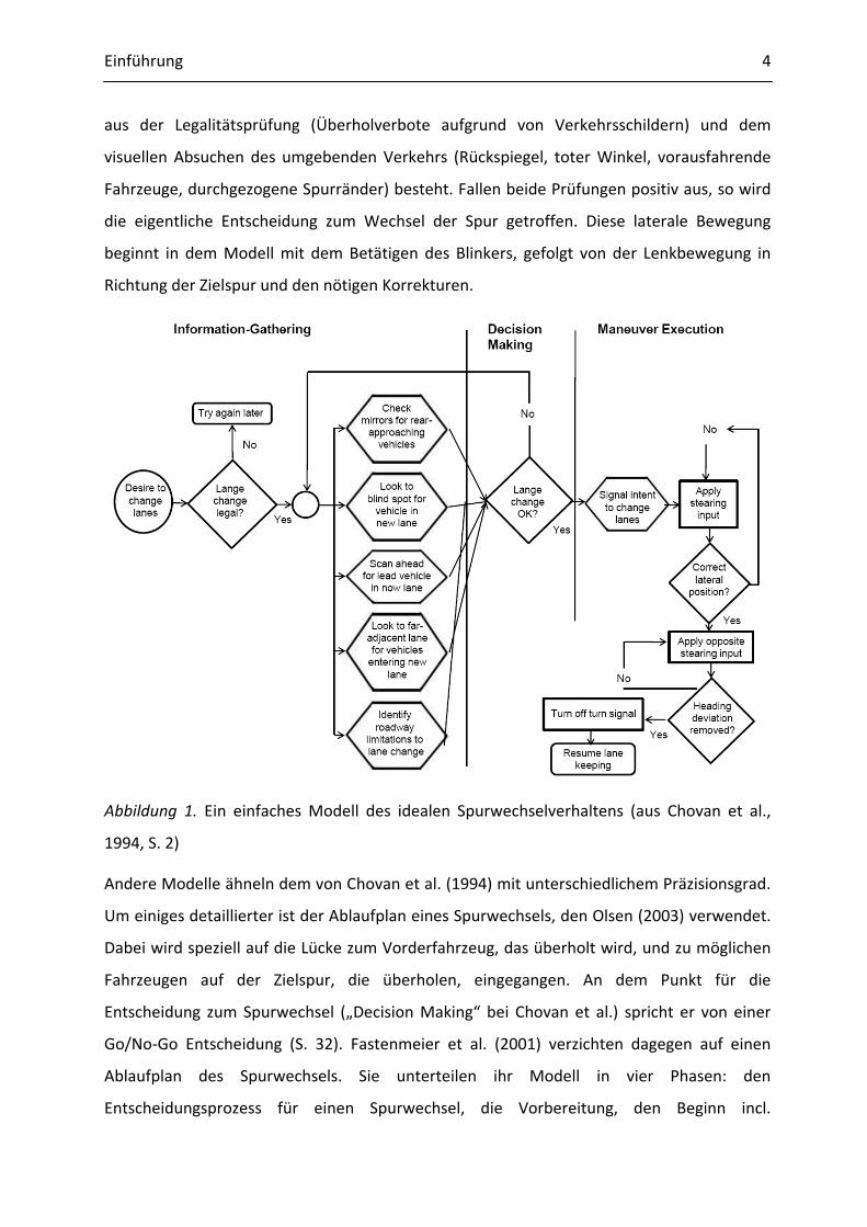
Andere Modelle lieferten eine detailliertere Beschreibung des Fahrerverhaltens bei einem

Spurwechsel. So lieferten Chovan, Tijerina, Alexander und Hendricks (1994) einen

idealisierten Ablaufplan einer Spurwechselentscheidung (siehe Abbildung 1) basierend auf

Arbeiten von McNight und Adams (1970). Ausgehend von einem Spurwechselwunsch (desire

to change lanes) wird zuerst eine Phase der Informationsaufnahme postuliert, die vor allem

Einführung 4

aus der Legalitätsprüfung (Überholverbote aufgrund von Verkehrsschildern) und dem

visuellen Absuchen des umgebenden Verkehrs (Rückspiegel, toter Winkel, vorausfahrende

Fahrzeuge, durchgezogene Spurränder) besteht. Fallen beide Prüfungen positiv aus, so wird

die eigentliche Entscheidung zum Wechsel der Spur getroffen. Diese laterale Bewegung

beginnt in dem Modell mit dem Betätigen des Blinkers, gefolgt von der Lenkbewegung in

Richtung der Zielspur und den nötigen Korrekturen.

Abbildung 1. Ein einfaches Modell des idealen Spurwechselverhaltens (aus Chovan et al.,

1994, S. 2)

Andere Modelle ähneln dem von Chovan et al. (1994) mit unterschiedlichem Präzisionsgrad.

Um einiges detaillierter ist der Ablaufplan eines Spurwechsels, den Olsen (2003) verwendet.

Dabei wird speziell auf die Lücke zum Vorderfahrzeug, das überholt wird, und zu möglichen

Fahrzeugen auf der Zielspur, die überholen, eingegangen. An dem Punkt für die

Entscheidung zum Spurwechsel („Decision Making“ bei Chovan et al.) spricht er von einer

Go/No-Go Entscheidung (S. 32). Fastenmeier et al. (2001) verzichten dagegen auf einen

Ablaufplan des Spurwechsels. Sie unterteilen ihr Modell in vier Phasen: den

Entscheidungsprozess für einen Spurwechsel, die Vorbereitung, den Beginn incl.

Einführung 5

Durchführung und den Abschluss eines Spurwechsels. Einzelne Komponenten überlappen

teilweise mit den Phasen von Chovan et al., zusätzlich werden aber noch die

Voraussetzungen von Halati et al. (1997, geschlossene Fahrspuren, etc.) übernommen. Den

einzelnen Phasen ordnen Fastenmeier und Kollegen dann verbale Beschreibungen zu, wie

z.B. „Herstellung der erforderlichen Geschwindigkeit für den Spurwechsel …“ (S. 17).

All diese Modelle können aber nur einen idealisierten Ablauf darstellen, der den komplexen

kognitiven Prozessen, die bei der Vorbereitung und Durchführung eines Spurwechsels eine

Rolle spielen, nicht gerecht wird.

1.1.2 Kognitive Modelle

Ein sehr bekanntes Modell zur Beschreibung der Fahraufgabe und ihren zugrundeliegenden

kognitiven Prozessen lieferte Michon (1985). Es beschreibt darin die Fahraufgabe als einen

Prozess, der auf drei Ebenen abläuft. Die Routenplanungs- oder Navigationsebene

(strategical level) bildet die höchste Ebene mit den Aufgaben Routenwahl, Ziel der Fahrt und

Kosten-Nutzen-Abwägungen. Hierbei handelt es sich in einem kognitiven Sinne um generelle

Pläne die eine eher langfristige zeitliche Perspektive besitzen (Minuten- bis Stundenbereich).

Die mittlere Ebene, Stabilisierungs-, Manöver- oder Bahnführungsebene (tactical level)

benannt, beinhaltet die Umsetzung der allgemeinen Pläne in konkrete Fahrmanöver, wie z.B.

Überholvorgänge oder Abbiegesituationen. Hier werden gespeicherte Handlungsmuster

eher bewusst umgesetzt, wobei die zeitliche Perspektive im Sekundenbereich zu finden ist.

Die niedrigste Ebene bildet die Stabilisierungs- oder Kontrollebene (operational level), die

sich mit der reinen Längs- und Querführung des Fahrzeuges beschäftigt. Dabei werden

Manöver aus der mittleren Ebene in direkte Steuerprozesse umgesetzt, wie beispielsweise

Lenkbewegungen, Beschleunigung, Verzögerung oder die Wahl des Ganges. In dieser Ebene

werden ebenfalls gespeicherte Handlungsmuster umgesetzt, allerdings eher automatisiert

und mit einer zeitlichen Perspektive im Millisekundenbereich.

Das Drei-Ebenen-Modell von Michon (1985) beschreibt zwar die allgemeinen Aufgaben der

Fahraufgaben und gibt erste Ansätze für die zugrundeliegenden kognitiven Prozesse, es ist

aber wenig detailliert und lässt keine Aussagen über einzelne Prozesse in bestimmten

Fahrsituationen zu. Eine Quelle für ein weitergehendes Modell mit detaillierten Annahmen

über die kognitives Prozesse beim Fahren bildet hier eine Arbeit von Dario Salvucci (2006). Er

Einführung 6

modelliert Fahrerverhalten in der kognitiven Architektur ACT-R (Adaptive Control of Thought

– Rational, Anderson et al., 2004), wobei er unter anderem die drei Ebenen von Michon

einbezieht. Im Folgenden werden eine kognitive Architektur und das darin eingebettete

Fahrmodell von Salvucci näher beschrieben.

Eine kognitive Architektur bildet einen allgemeiner Rahmen, in dem computerbasierte

Verhaltensmodelle menschlicher Informationsverarbeitung erstellt werden können (Salvucci,

2006). Die Architektur enthält sowohl die Fähigkeiten als auch die Grenzen des menschlichen

Systems, z.B. die Fähigkeiten zu Speicherung von Informationen im Gedächtnis und deren

Abruf, Lernen, Wahrnehmung und motorische Aktivität. Enthaltene Grenzen der

menschlichen Informationsverarbeitung bilden z.B. der Zerfall von Gedächtnisspuren,

foveale versus periphäre visuelle Wahrnehmung und limitierte motorische Performanz.

Damit stellt eine kognitive Architektur sicher, dass die in ihr entwickelten Modelle strikt die

kognitiven Grenzen einhalten und damit „kognitiv wahr“ sind.

In seinem Fahrermodell beschreibt Salvucci das Befahren einer zweispurigen Autobahn mit

einem PKW mittlerer Größe mit der Möglichkeit, der Spur zu folgen, Kurven zu durchfahren

und die Spur nach rechts oder links zu wechseln. Das Modell enthält drei

Hauptkomponenten: Kontrolle, Überwachung und Entscheidung, die sich in das Modell von

Michon (1985) integrieren lassen. Die Kontroll-Komponente von Salvucci entspricht der

Kontrollebene bei Michon und beinhaltet die Wahrnehmung visueller Reize zur lateralen und

longitudinalen Steuerung des Fahrzeuges via Gas, Bremse und Lenkung. Die

Überwachungskomponente von Salvuccis Fahrermodell ist ein Teil der Manöverebene von

Michon, die der Aufrechterhaltung von Situationsbewusstsein durch visuelles Überwachen

des eigenen und des Nachbarfahrstreifens dient. Dies geschieht durch zufällige

Blickzuwendungen in die Bereiche vor und hinter dem Fahrzeug (mit Hilfe der Spiegel). Die

gewonnen Informationen über andere Fahrzeuge werden dann in Form von Spur, Richtung

und Abstand im Gedächtnis von ACT-R gespeichert. Den zweiten Teil der Manöverebene von

Michon bildet die Entscheidungskomponente von Salvucci, die aufgrund der gesammelten

Informationen taktische Entscheidungen fällt. Eine solche taktische Entscheidung ist

beispielsweise ein Spurwechsel nach links. Der gesamte Entscheidungsprozess setzt sich hier

aus mehreren Teilkomponenten zusammen. Auslöser für den gesamten Prozess ist ein

Fahrzeug, das sich mit einem zeitlichen Abstand von 2 Sekunden vor dem eigenen Fahrzeug

Einführung 7

befindet. Das Fahrermodell setzt nun sein Ziel auf „Spurwechsel“. Es ruft den

Gedächtnisinhalt ab und überprüft, ob sich Fahrzeuge in einem Abstand von 40 m oder

weniger neben oder hinter dem eigenen Fahrzeug befinden. Ist dies der Fall, so prüft es den

Bereich neben und hinter dem Fahrzeug, ob sich das Fahrzeug noch immer dort befindet.

Findet es dort keine Fahrzeuge mehr, so wird der Spurwechsel initiiert. Sollte kein Fahrzeug

im Gedächtnis abrufbar sein, so scannt das Fahrermodell den Bereich neben und hinter dem

Fahrzeug, da es aufgrund von Zerfallsprozessen im Gedächtnis zu einem „Vergessen“ des

rückwärtigen Verkehrs gekommen sein kann. Werden keine Fahrzeuge in diesem Bereich

mehr festgestellt, so wird der eigentliche Spurwechselprozess initiiert. Das Fahrermodell

startet den Lenkprozess und leitet das Fahrzeug, bis es in der Mitte der Zielspur angelangt

ist.

1.1.3 Indikatoren des Spurwechsels

Aus den Spurwechselmodellen lassen sich nun Indikatoren zur Erkennung der

Spurwechselabsicht ableiten. Geht man wie die meisten Modelle davon aus, dass sich der

Spurwechsel grundlegend in eine Vorbereitungs- und eine Durchführungsphase einteilen

lässt, so können auch die Indikatoren den beiden Phasen zugeteilt werden. Henning,

Georgeon, et al. (2009) untersuchten in einer Feldstudie mit 22 Fahrern vor allem

Indikatoren, die in der Vorbereitungshase einen Spurwechsel nach links vorhersagen. Nach

eingehender Analyse des zeitlichen Verlaufes der Werte einzelner Parameter, deuten die

Befunde auf die Zunahme von Blicken in den linken Außenspiegel und die damit verbundene

Abnahme von Blicken zu anderen Blickorten (incl. der Frontscheibe) als frühesten Indikator

hin. Die Autoren unterteilten die 194 aufgezeichneten Spurwechsel auch in Spurwechsel, bei

denen die Fahrer erst den rückwärtigen Verkehr passieren ließen, und in Spurwechsel, bei

denen kein rückwärtiger Verkehr vorhanden war. Die Befunde zeigen, dass vor allem

Spurwechsel mit der Anwesenheit von rückwärtigem Verkehr einerseits durch Indikatoren

der Längsführung, wie z.B. der Betätigung von Gas- und Bremspedal oder der Varianz der

Geschwindigkeit, gekennzeichnet sind. Zum Zweiten zeigt die Studie das Potential auf, das in

der höheren Dauer der Blicke in den Außenspiegel liegt, wenn man die maximalen

Blicklängen bei Spurwechselabsicht und rückwärtigem Verkehr mit denen bei

Spurwechselabsicht und ohne rückwärtigen Verkehr vergleicht. Hinweise darauf fanden sich

auch schon in früheren Arbeiten von Henning und Kollegen (Henning, 2004; Henning,

Einführung 8

Schweigert, Baumann, & Krems, 2006). Es konnte auch gezeigt werden, dass der oft genutzte

Indikator Blinker sehr spät auftritt und nicht geeignet ist, die Vorbereitung eines

Spurwechsels vorherzusagen, genauso wie Schulterblicke eher selten und wenn dann sehr

spät anzutreffen sind. Die von Salvucci, Liu und Boer (2001) im Fahrsimulator gefundene

laterale Varianz vor Beginn des Spurwechsels konnte in der Feldstudie nicht repliziert

werden. Ein möglicher Indikator, die Anwesenheit eines langsamen vorausfahrenden

Fahrzeugs auf der gleichen Spur, konnte mit Hilfe von menschlichen Sensoren

(Versuchsleiter im Fahrzeug) als geeignet eingestuft werden, allerdings schränkt eine immer

noch nicht voll ausgereifte maschinelle Sensorik den Gebrauch dieses Indikators ein (Zehang,

Beibs, & Miller, 2006).

Indikatoren für die Durchführung des Spurwechsels waren nicht Gegenstand der

Untersuchung von Henning, Georgeon, et al. (2009), wurden aber in früheren

Untersuchungen schon auf ihre Eignung hin überprüft. Klassisch ist die Nutzung des Blinkers,

die in der Durchführungsphase höher ausfällt als in der Vorbereitungsphase des

Spurwechsels (Henning, Georgeon, & Krems, 2007), allerdings liegen gefundene Werte in

Feldstudien mit natürlicher Verhaltensbeobachtung (Naturalistic Driving Studies, z.B., Dingus

et al., 2006) bei nur 64% Blinkernutzung zum Zeitpunkt des Beginns der

Spurwechseldurchführung (Olsen, 2003). Weitere geeignete Indikatoren bilden Parameter

der lateralen Bewegung, wie zum Beispiel die Zeit bis zur Spurrandüberschreitung (Time to

Line Crossing, TTC, Hetrick, 1997) oder der Verlauf des Lenkwinkels (Pentland & Liu, 1999;

Tezuka, Soma, & Tanifuji, 2006). Wie in der Vorbereitungsphase bietet das Blickverhalten

auch in der Durchführungsphase großes Potential zur Vorhersage von Spurwechselverhalten

(Henning, 2004; McCall, Wipf, Trivedi, & Rao, 2007; Olsen, 2003; Salvucci et al., 2001).

Hervorzuheben ist hier der Blick in den linken Außenspiegel und der Schulterblick, der auch

als reine Kopfdrehung messbar ist (Doshi & Trivedi, 2008; Robinson, Erickson, Thurston, &

Clark, 1972).

1.2 Zugrundeliegende kognitive Prozesse

Die möglichen Indikatoren für die Vorbereitung und Durchführung eines Spurwechsels

bilden nur die external messbaren Verhaltenskorrelate innerer kognitiver Prozesse. Salvucci

(2006) postulierte in seinem Modell in Anlehnung an das Drei-Ebenen-Modell von Michon

(1985) drei basale kognitive Prozesse, auf die im Folgenden näher eingegangen wird.

Einführung 9

1.2.1 Automatisierte Kontrollprozesse der Längs- und Querführung

Der eher automatisierte Kontrollprozess, der aufgrund von visuellen Informationen die

laterale und longitudinale Steuerung des Fahrzeuges übernimmt, ist auch beim Spurwechsel

von Bedeutung. Zum einen wird der Abstand zum vorausfahrenden Fahrzeug mit Hilfe einer

Schätzung über die Größe des retinalen Abbildes und deren Änderung (DeLucia &

Tharanathan, 2005) ermittelt und via Gas und Bremse kontrolliert. Zum anderen wird der

physikalische Prozess des Wechselns der Fahrspur so geregelt, dass das Modell (Salvucci,

2006) die visuelle Aufmerksamkeit von der Start- auf die Zielspur verschiebt und dadurch die

Regelmechanismen des Lenkens von der Mitte der ersten bis zur Mitte der zweiten Spur

ausgelöst, gesteuert und abgeschlossen werden. Die Steuerung dieses Prozesses erfolgt

durch peripher-visuelle Wahrnehmung, das heißt, es muss keine direkte Blickzuwendung zu

den Begrenzungslinien der Spur geben (Summala, Nieminen, & Punto, 1996), sondern nur,

wie in Salvuccis Modell, zur Mitte der Fahrspur.

1.2.2 Die Repräsentation der Verkehrssituation

Der zweite kognitive Prozess bezieht sich auf die Aufrechterhaltung von

Situationsbewusstsein durch visuelles Überwachen der Fahrzeugumgebung, entweder direkt

oder über die Rückspiegel. Der Begriff Situationsbewusstsein ist vor allem durch die Arbeiten

von Mica Endley (1988) geprägt worden, die ihn beschreibt als ‘the perception of the

elements in the environment within a volume of time and space, the comprehension of their

meaning, and the projection of their status in the near future’ (S. 97) oder kürzer ‘knowing

what is going on’ (Endsley, 1995, S.36). Sie leitete ihre Befunde aus Untersuchungen im

Bereich der Luftfahrt ab, wobei andere Autoren das Konzept auch auf den Bereich des

Autofahrens übertrugen (Baumann & Krems, 2007; Gugerty, 1997).

Bei dem Prozess der Aufrechterhaltung von Situationsbewusstsein postuliert Salvucci

Gedächtnisprozesse, die Informationen über fremde Fahrzeuge rund um das eigene Auto im

Gedächtnis repräsentieren. Auch andere Autoren binden Gedächtnisprozesse in ihre

Theorien über Situationsbewusstsein ein (Adams, Tenney, & Pew, 1995; Baumann & Krems,

2007; Gugerty, 1997). So spricht Gugerty (1997) von einem dynamischen räumlichen

Arbeitsgedächtnis (dynamic spatial working memory, S. 43.), das für die mentale

Repräsentation des umgebenden Verkehrs eine Rolle spielt. Baumann und Krems (2007)

Einführung 10

postulieren den Aufbau einer mentalen Repräsentation des Umgebungsverkehrs, auf dessen

Grundlage dann Verstehens- und Vorhersageprozesse über die Verkehrssituation möglich

sind (Kintsch, 1998). Bei dem Aufbau der mentalen Repräsentation gehen Baumann und

Krems von einer Involviertheit des Arbeitsgedächtnisses aus, was sie experimentell

bestätigen konnten (Baumann, Franke, & Krems, 2008; Franke, 2008).

An diesem Punkt liefert die vorliegende Arbeit Befunde zur Art und Lokalisation der

beteiligten Gedächtnisprozesse bei der Vorbereitung eines Spurwechsels (Henning,

Beyreuther et al., 2009). In einer Studie im Chemnitzer Fahrsimulator wurde die Beteiligung

bestimmter Gedächtnisstrukturen beim Aufbau der Repräsentation des umgebenden

Verkehrs, in diesem Falle vor allem der rückwärtigen Fahrzeuge auf der Zielspur, untersucht.

Als theoretische Grundlage diente das Arbeitsgedächtnismodell von Baddeley und Hitch

(1974), das die drei Hauptkomponenten Zentrale Exekutive, Phonologische Schleife und

Räumlich-Visueller Notizblock postuliert. Es wurde angenommen, dass die Informationen

über den umgebenden Verkehr mit anderen räumlich-visuellen Informationen interferieren.

Diese Annahmen wurden über Befunde zur möglichen Unterteilung des Räumlich-Visuellen

Notizblocks erweitert, zum einen in einen eher räumlichen und einen eher visuellen Teil

(Gugerty, 1997; Klauer & Zhao, 2004), zum anderen in eine eher statische und eine eher

dynamische Komponente (Pickering, 2001; Pickering, Gathercole, Hall, & Lloyd, 2001). Zu

diesem Zweck wurde ein Zweitaufgabenparadigma mit einfacher Dissoziation entwickelt, das

es ermöglicht, das Arbeitsgedächtnis kurz vor Beginn der Vorbereitung eines Spurwechsels

mit einer bestimmten Art von Gedächtnisinhalt zu belasten, die dann nach dem Spurwechsel

abgefragt wird. Es gab vier Zweitaufgaben zur Belastung des Räumlich-Visuellen Notizblocks,

die eher räumlich-statisch, räumlich-dynamisch, visuell-statisch oder visuell-dynamisch

gestaltet wurden. Zur Kontrolle wurde eine phonologische Zweitaufgabe genutzt. Außerdem

wurde die Geschwindigkeit des rückwärtigen Verkehrs variiert, wobei die Annahme bestand,

dass höhere Geschwindigkeiten eher mit den dynamischen Zweitaufgaben interferieren,

niedrigere eher mit den statischen Aufgaben. Die Befunde konnten zeigen, dass alle visuell-

räumlichen Zweitaufgaben mit dem Prozess der Vorbereitung des Spurwechsels

interferierten, entgegen der Annahmen aber vor allem die visuell-statische Aufgabe. Auch

konnte die Hypothese einer Interferenz mit eher dynamischen Zweitaufgaben nur teilweise

bestätigt werden. Diese Befunde führten zu der Annahme, dass der rückwärtige Verkehr in

der Untersuchung eher statisch als dynamisch repräsentiert wird.

Einführung 11

In einer Folgestudie stellten sich Henning und Krems (2009) nun die Frage, ab welcher

Geschwindigkeit denn der rückwärtige Verkehr, wie er durch den Rückspiegel aufgenommen

wird, dynamisch gespeichert ist. Dazu wurde das Paradigma des Representational

Momentum (Freyd & Finke, 1984) benutzt. Dieses Paradigma beschreibt Befunde zur

Verzerrung einer im Kurzzeitgedächtnis gespeicherten Bewegung in Bewegungsrichtung. In

einem Laborexperiment zeigten Freyd und Finke Probanden nacheinander drei Rechtecke,

die durch Rotationen um jeweils 17° eine Drehbewegung implizierten. Sie baten die

Probanden, sich die Position des letzten Rechtecks zu merken und mit der Position eines

vierten Rechtecks zu vergleichen, das ein wenig versetzt oder identisch zum dritten Rechteck

war. Es konnte gezeigt werden, dass Probanden immer eine Position memorierten, die sich

einige Winkel-Grad weiter in Richtung der Drehbewegung befand (meisten +2°). Diese

Befunde waren unabhängig von der Bewegungsrichtung und konnten auch auf andere

Bewegungsarten und sogar Töne übertragen werden (Kelly & Freyd, 1987).

Henning und Krems (2009) übertrugen nun das Paradigma auf die Darbietung von

Fahrzeugen im Rückspiegel und entwarfen kleine Videosequenzen, die der Darbietung eines

sich nähernden Fahrzeuges im linken Außenspiegel in Größe und Größenänderung (Tau)

ähnelten. Im ersten Experiment wurde untersucht, bei welcher Annäherungsgeschwindigkeit

sich der Effekt des Representational Momentum zeigt. Die Befunde zeigen eindeutig, dass

sich der Effekt erst bei einer Annäherungsgeschwindigkeit von 75 km/h und nicht schon bei

50 km/h zeigt, was darauf hindeutet, dass sich erst ab einer Annäherungsgeschwindigkeit

über 50 km/h die Repräsentation des Rückwärtigen Verkehrs dynamisch zu sein scheint. In

einem zweiten Experiment wurde die Lokalisation dieser Repräsentation im

Arbeitsgedächtnis analog zur Studie von Henning, Beyreuther et al. (2009) detailliert

betrachtet (Patzelt, 2009). Die Untersuchung erfolgte mit den Videos, die eine

Annäherungsgeschwindigkeit von 75 km/h darstellen. Diese mussten, eingebettet in die

Präsentation und den Abruf der schon bekannten Zweitaufgaben, bearbeitet werden. Die

Befunde zeigen, dass es eher zu Interferenzen zwischen der Bearbeitung des

Representational Momemtums und den eher dynamischen Zweitaufgaben kommt, wobei

die räumlich-dynamische Zweitaufaufgabe eine größere Interferenz zeigt als die visuell-

dynamische Zweitaufgabe. Dies entspricht den eigentlichen Vorhersagen über die

Speicherung von dynamischen Informationen im Arbeitsgedächtnis und zeigt auch, dass eine

Unterteilung des Räumlich-Visuellen Notizblocks, wie ihn Pickering et al. (2001) vorschlagen,

Einführung 12

sinnvoll erscheint. Es erklärt auch die Befunde aus der Studie von Henning, Beyreuther, et al.

(2009), da in besagter Studie wahrscheinlich keine dynamische Repräsentation des

rückwärtigen Verkehrs möglich war. Die gewählten Differenzgeschwindigkeiten waren

kleiner als oder gleich 50 km/h.

1.2.3 Entscheidungsprozesse

Der dritte kognitive Prozess, den Salvucci (2006) postuliert, ist der Entscheidungsprozess für

einen Spurwechsel. Dabei gibt es zwei Punkte, an denen das Fahrermodell eine Entscheidung

trifft. Der erste Punkt betrifft die Entscheidung zu einem Spurwechsel aufgrund eines

langsameren Vorausfahrzeuges, im Modell das Setzen des Zieles auf „Spurwechsel“. Die

Annahme, dass langsamere Vorausfahrzeuge den Wunsch zu einem Spurwechsel auslösen,

ist durch zahlreiche Befunde gestützt. So konnte auch in der Untersuchung von Henning,

Georgeon, et al. (2009) gezeigt werden, dass ein langsameres Fahrzeug fast immer zu einem

Spurwechsel führt (87%). Bar-Gera und Shinar (2005) gehen noch weiter und konnten in

einer Simulatorstudie sogar zeigen, dass vorausfahrende Fahrzeuge, die ursprünglich etwas

schneller als das eigene Fahrzeug sind, in 50% der Fälle überholt wurden. Einen kognitiven

Ansatz dazu liefern Norman und Shallice (1986) mit ihrer Schema-Aktivierungs-Theorie. Sie

postulieren dabei eine automatische (contention scheduling) und einen bewusste

Handlungssteuerung (supervisory attentional system) aufgrund von Umweltreizen.

Übertragen auf den Spurwechsel dient also ein Umweltreiz in Form eines langsameren,

manchmal auch leicht schnelleren Vorausfahrzeugs, als automatischer Auslöser für ein

Handlungsschema, das in diesem Fall die Vorbereitung eines Spurwechsels beinhaltet. Dieses

Schema kann auch willentlich beeinflusst werden, z. B. indem der Beifahrer den Wunsch

äußert, dass er doch an der nächsten Autobahnraststätte anhalten möchte, und der Fahrer

die Vorbereitung zum Spurwechsel abbricht.

Die zweite Entscheidung im Zusammenhang mit einem Spurwechsel muss dann getroffen

werden, wenn der Fahrer die Spur wechseln will und kontrolliert hat, ob die Lücke in der

Zielspur groß genug ist bzw. ob sich dort überhaupt Fahrzeuge befinden. Über diese

Entscheidung gibt es keine kognitive Theorie, aber der Prozess scheint in verschiedenen

Fahrermodellen über eine detaillierte Annahme zur Wahl einer Lücke abgebildet worden zu

sein (Toledo, Koutsopoulos, & Ben-Akiva, 2003)

Einführung 13

1.3 Unterstützung des Fahrers beim Spurwechsel

Die bisherigen Befunde zum Spurwechsel und zu den zugrundeliegenden kognitiven

Prozessen bilden die Grundlage für eine mögliche Unterstützung des Fahrers in drei

Bereichen. Zuerst lässt sich Assistenzbedarf beim Spurwechsel ableiten. Zum Zweiten

können Erkennungsalgorithmen, die auf die Spurwechselabsicht schließen lassen,

beschrieben und Verbesserungspotential anhand der Befunde begründet werden. Der dritte

Komplex dient einer Kategorisierung der Kopplung eines möglichen

Spurwechselabsichtserkenners mit Fahrerassistenz- und Informationssystemen der Längs-

und Querführung.

1.3.1 Assistenzbedarf beim Spurwechsel

Aus der Beschreibung der kognitiven Prozesse lassen sich nun drei mögliche Ansatzpunkte

für den Assistenzbedarf ableiten, die schon teilweise in der Realität umgesetzt sind. Bei der

Kontrolle der Längs- und Querführung gibt es den Ansatz, den Fahrer beim Wunsch eines

Spurwechsels auf einer idealen Trajektorie von der Start- auf die Zielspur zu führen

(Hatipoglu, Ozguner, & Redmill, 2003). Die visuelle Kontrolle des rückwärtigen Verkehrs kann

durch eine sensorische Überwachung des Raumes neben und hinter dem Fahrzeug gelöst

werden, deren Ergebnis dem Fahrer angezeigt wird (Kiefer & Hankey, 2008). Diese

Assistenzfunktion geht entweder einher mit einer Handlungsempfehlung, die dem Fahrer die

Größe der Lücke mit Hilfe z.B. einer grafischen Anzeige darbietet (Hegeman, van der Horst,

Brookhuis, & Hoogendoorn, 2007), oder mit einer Warnung, die den Fahrer vor einem sich

seitlich befindenden oder von hinten nähernden Fahrzeug warnt (Tijerina, 1999).

1.3.2 Algorithmen zur Erkennung der Spurwechselabsicht

All die beschriebenen Systeme und Funktionalitäten beruhen auf einer sensorischen

Erkennung der Fahrzeugumgebung. Um den Fahrer in der Spurwechselsituation zu

unterstützen, benötigt das System Informationen über die bevorstehende

Spurwechselabsicht, anhand derer es dann aktiviert wird. Zur Erkennung dieser Absicht gibt

es einige Studien aus dem Fahrsimulator oder dem Feld, die in Tabelle 1 systematisiert

werden. Dabei kann nach verschiedenen Arten der Modellierung der Algorithmen und der

kognitiven Grundlage unterschieden werden. Es gab teilweise Algorithmen, die mehr

Fahrmanöver als nur den Spurwechsel unterschieden. Des Weiteren wird der Umfang der

Einführung 14

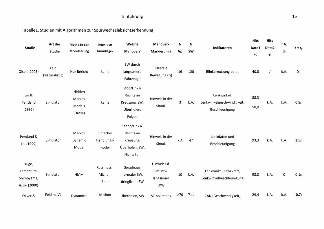
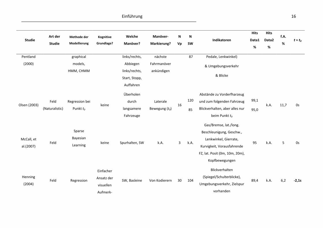
Studie in Anzahl an Probanden und Anzahl an analysierten Spurwechseln dargestellt. Die

letzten vier Spalten sind der Performanz der eigentlichen Algorithmen gewidmet. Es wird die

Anzahl an Treffern (Hits) des eigentlichen Datensatzes für die Modellbildung berichtet

(Prozentsatz erkannter Spurwechsel in Data1) sowie die Validierung des Algorithmus an

einem zweiten Datensatz (Prozentsatz erkannter Spurwechsel in Data2) sowie die Anzahl

falscher Alarme (irrtümlich erkannter Spurwechsel), sofern die Studie diese beinhaltete. Die

letzte Spalte berichtet dann den Zeitpunkt, für den die Performanzwerte gelten, im Bezug

zum Zeitpunkt t0, der den Beginn der lateralen Bewegung, also des eigentlichen Wechselns

der Fahrspur, markiert.

Einführung 15

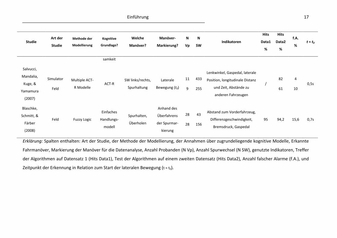
Tabelle1. Studien mit Algorithmen zur Spurwechselabsichtserkennung

Studie Art der

Studie

Methode der

Modellierung

Kognitive

Grundlage?

Welche

Manöver?

Manöver-

Markierung?

N

Vp

N

SW Indikatoren

Hits

Data1

%

Hits

Data2

%

f.A.

% t ≈ t0

Olsen (2003) Feld

(Naturalistic) Nur Bericht keine

SW durch

langsamere

Fahrzeuge

Laterale

Bewegung (t0) 16 120 Blinkernutzung bei t0 40,8 / k.A. 0s

Liu &

Pentland

(1997)

Simulator

Hidden

Markov

Models

(HMM)

keine

Stop/Links/

Rechts an

Kreuzung, SW,

Überholen,

Folgen

Hinweis in der

Simul. 3 k.A.

Lenkwinkel,

Lenkwinkelgeschwindigkeit,

Beschleunigung

88,3

50,0 k.A. k.A. 0,5s

Pentland &

Liu (1999) Simulator

Markov

Dynamic

Model

Einfaches

Handlungs-

modell

Stopp/Links/

Rechts an

Kreuzung,

Überholen, SW,

Nichts tun

Hinweis in der

Simul. k.A 47

Lenkdaten und

Beschleunigung 93,3 k.A. k.A. 1,5s

Kuge,

Yamamura,

Shimoyama,

& Liu (2000)

Simulator HMM

Rassmuss.,

Michon,

Boer

Geradeaus,

normaler SW,

dringlicher SW

Hinweis i.d.

Sim. bzw.

langsamer

LKW

10 k.A. Lenkwinkel, Lenkkraft,

Lenkwinkelbeschleunigung 98,3 k.A. 0 0,1s

Oliver & Feld m. VL Dynamical Michon Überholen, SW VP sollte das >70 711 CAN (Geschwindigkeit, 29,4 k.A. k.A. -0,7s

Einführung 16

Studie Art der

Studie

Methode der

Modellierung

Kognitive

Grundlage?

Welche

Manöver?

Manöver-

Markierung?

N

Vp

N

SW Indikatoren

Hits

Data1

%

Hits

Data2

%

f.A.

% t ≈ t0

Pentland

(2000)

graphical

models,

HMM, CHMM

links/rechts,

Abbiegen

links/rechts,

Start, Stopp,

Auffahren

nächste

Fahrmanöver

ankündigen

87 Pedale, Lenkwinkel)

& Umgebungsverkehr

& Blicke

Olsen (2003) Feld

(Naturalistic)

Regression bei

Punkt t0

keine

Überholen

durch

langsamere

Fahrzeuge

Laterale

Bewegung (t0) 16

120

85

Abstände zu Vorderfharzeug

und zum folgenden Fahrzeug

Blickverhalten, aber alles nur

beim Punkt t0

99,1

95,0 k.A. 11,7 0s

McCall, et

al.(2007) Feld

Sparse

Bayesian

Learning

keine Spurhalten, SW k.A. 3 k.A.

Gas/Bremse, lat./long.

Beschleunigung, Geschw.,

Lenkwinkel, Gierrate,

Kurvigkeit, Vorausfahrende

FZ, lat. Posit (0m, 10m, 20m),

Kopfbewegungen

95 k.A. 5 0s

Henning

(2004) Feld Regression

Einfacher

Ansatz der

visuellen

Aufmerk-

SW, Basleine Von Kodierern 30 104

Blickverhalten

(Spiegel/Schulterblicke),

Umgebungsverkehr, Zielspur

vorhanden

89,4 k.A. 6,2 -2,1s

Einführung 17

Studie Art der

Studie

Methode der

Modellierung

Kognitive

Grundlage?

Welche

Manöver?

Manöver-

Markierung?

N

Vp

N

SW Indikatoren

Hits

Data1

%

Hits

Data2

%

f.A.

% t ≈ t0

samkeit

Salvucci,

Mandalia,

Kuge, &

Yamamura

(2007)

Simulator

Feld

Multiple ACT-

R Modelle ACT-R

SW links/rechts,

Spurhaltung

Laterale

Bewegung (t0)

11

9

433

255

Lenkwinkel, Gaspedal, laterale

Position, longitudinale Distanz

und Zeit, Abstände zu

anderen Fahrzeugen

/ 82

61

4

10 0,5s

Blaschke,

Schmitt, &

Färber

(2008)

Feld Fuzzy Logic

Einfaches

Handlungs-

modell

Spurhalten,

Überholen

Anhand des

Überfahrens

der Spurmar-

kierung

28

28

43

156

Abstand zum Vorderfahrzeug,

Differenzgeschwindigkeit,

Bremsdruck, Gaspedal

95 94,2 15,6 0,7s

Erklärung: Spalten enthalten: Art der Studie, der Methode der Modellierung, der Annahmen über zugrundeliegende kognitive Modelle, Erkannte

Fahrmanöver, Markierung der Manöver für die Datenanalyse, Anzahl Probanden (N Vp), Anzahl Spurwechsel (N SW), genutzte Indikatoren, Treffer

der Algorithmen auf Datensatz 1 (Hits Data1), Test der Algorithmen auf einem zweiten Datensatz (Hits Data2), Anzahl falscher Alarme (f.A.), und

Zeitpunkt der Erkennung in Relation zum Start der lateralen Bewegung (t ≈ t0).

Einführung 18

Die Methoden der Modellierung variieren zwischen den einzelnen Studien und werden im

Folgenden kurz erläutert. Eine Reihe von Untersuchungen nutzt Hidden Markov Modelle

(Kuge et al., 2000; Liu & Pentland, 1997; Oliver & Pentland, 2000), die eine Subgruppe

Dynamische Bayesscher Netze darstellen (Rabiner, 1989). Sie haben das Potential, auf

verborgene Zustände eines Systems (Hidden States) mit Hilfe von beobachtbarem Verhalten

zu schließen. In die gleiche Gruppe fallen Markov Dynamic Models und Coupled Hidden

Markov Models, die nur Abwandlungen von Hidden Markov Models darstellen (Oliver &

Pentland, 2000; Pentland & Liu, 1999). Sparse Bayesian Learning (McCall et al., 2007) ist ein

Subtyp von probabilistischem Bayesianischem Lernen (Tipping, 2001). Salvucci et al. (2007)

nutzten verschiedene Modelle, die in der kognitiven Architektur ACT-R (Anderson et al.,

2004) implementiert wurden (s.a. Abschnitt zu kognitiven Modellen). Blaschle et al. (2008)

verwenden den Ansatz Fuzzy Logic, der einen Prozess probabilistischen Schließens darstellt,

basierend auf unscharfen Annahmen. Einige Autoren nutzten auch klassische statistische

Verfahren, wie z.B. eine Regression (Henning, 2004; Olsen, 2003).

Wie in den rechten vier Spalten der Tabelle 1 zur Performanz dargestellt, konnten einzelne

Studien gute Erkennungsleistungen demonstrieren. Bei kritischer Betrachtung zeigen sich

allerdings einige Limitationen:

• Viele Studien zeigen gute Resultate, allerdings nur im Fahrsimulator (Kuge et al.,

2000; Liu & Pentland, 1997; Pentland & Liu, 1999; Salvucci et al., 2007).

• Einige Studien zeigen gute Erkennungsleistungen, basieren aber auf Daten von nur

wenigen Probanden (Kuge et al., 2000; McCall et al., 2007; Pentland & Liu, 1999;

Salvucci et al., 2007). Werden Studien mit vielen Probanden unternommen, so ist die

Erkennungsleitsung eher gering (Oliver & Pentland, 2000).

• Viele Studien geben den Zeitpunkt ihrer optimalen Erkennung erst mit oder nach

dem Beginn der lateralen Bewegung an (positive Zeitwerte), nur zwei Studien bilden

da eine Ausnahme (Henning, 2004; Oliver & Pentland, 2000). Die letztgenannten

Studien integrieren das Blickverhalten in ihren Erkennungsalgorithmus.

Wie die Zusammenstellung verdeutlicht, gibt es einen Forschungsbedarf, der zu einer

erhöhten und früheren Erkennungsleistung auf Basis einer breiteren Stichprobe führen

sollte. Einen Beitrag dazu lieferte die Studie von Henning, Georgeon, et al., (2009). Sie

konnte zeigen, dass es auch geeignete Indikatoren in der Vorbereitungsphase des

Einführung 19

Spurwechsels gibt, die nun in einem weiteren Schritt algorithmisch integriert werden

müssen. Diese Umsetzung könnte dann, auch alternativ zu anderen Ansätzen, verschiedenen

Assistenzsystemen der Längs- und Querführung zur Verfügung stehen.

1.3.3 Kopplung von Assistenzsystemen und Fahrerabsicht

Wie im Abschnitt zum Assistenzbedarf beim Spurwechsel verdeutlicht wurde, dient die

Spurwechselabsichtserkennung Systemen zur Unterstützung dieses Fahrmanövers als

Startpunkt für ihre Assistenz. Diese Unterstützung ist abhängig von der Art des Systems. Soll

das System dem Fahrer Informationen über die Möglichkeit zum Wechseln der Fahrspur

geben, so wünscht er diese Informationen so früh wie möglich, also schon mit Beginn der

Vorbereitung des Spurwechsels. Sollte er aber vor einer Kollision mit einem seitwärts

fahrenden Fahrzeug gewarnt werden, so ist eine Erkennung der Absicht kurz nach

Manöverstart, aber vor dem Überfahrens des Spurrandes nötig, wozu bisherige Algorithmen

durchaus in der Lage sind.

Es gibt aber auch andere Assistenzsysteme, die von der Spurwechselabsichtserkennung

profitieren. Zum Beispiel sogenannte Workload-Manager (Amditis, Kubmann,

Polychronopoulos, Engstrom, & Andreone, 2006), die im Falle einer Fahrsituation mit hohem

Workload nur bestimmte Informationen an den Fahrer herantragen, andere aber verzögern.

So können zum Beispiel bei einem Spurwechsel Informationen über Fahrzeuge im toten

Winkel an den Fahrer herangetragen werden, eingehende Anrufe oder Navigationshinweise

auf den Zeitpunkt nach dem Fahrmanöver verschoben werden (Piechulla, Mayser, Gehrke, &

König, 2003).

Neben dem Spurwechselassistenten (Kiefer & Hankey, 2008) existiert ein weiteres System

der Querführung, das von der Spurwechselabsicht profitieren kann. Dies ist der eingangs

schon erwähnte Spurverlassenswarner (Lane Departure Warning, Joon Woong, 2002). Dieser

kann durch die Informationen über einen bevorstehenden Spurwechsel abgeschaltet

werden, um störende Alarme zu vermeiden. Der Nutzen dieser Kopplung konnte in einer

Expertenstudie bestätigt werden (Henning, Beyreuther et al., 2007), die Teil der Dissertation

von Stefan Hoch (2009) ist.

Ähnlich wie die Systeme der Querführung können auch die Systeme der Längsführung von

der Information über den Spurwechsel profitieren. Zu nennen sind dort zwei Systeme: der

Einführung 20

adaptive Tempomat (Adaptive Cruise Control, ACC, Moon, Yi, Kang, & Yoon, 2009) und

Systeme zur Kollisionsverminderung bzw. -vermeidung (Collision Mitigation/Avoidance,

Ferrara & Vecchio, 2007). Beide Systeme würden im Falle eines beabsichtigten Spurwechsels

unterdrückt bzw. in einen anderen Modus wechseln, meist um den sonst eingeleiteten

Bremsvorgang zu vermeiden und den Fahrer nicht zu irritieren (Smith & Zhang, 2004).

1.4 Kritische Bemerkungen, offene Fragen und zukünftiger Forschungsbedarf

1.4.1 Blicke in den linken Außenspiegel und ihr Potential für die

Fahrerabsichtserkennung

Vor allem die Feldstudie von Henning, Georgeon, et al. (2009) hat gezeigt, dass der Blick in

den linken Außenspiegel großes Potential für eine frühe Erkennung eines Spurwechsels

besitzt. Dieser Indikator ist aber mit einigen Problemen behaftet, auf die jetzt näher

eingegangen wird.

Ein Problem ist die Blickmessung, die trotz jahrzehnterlanger Forschung noch immer nicht

problemlos funktioniert (Duchowski, 2007). Vor allem stellen Sonnenbrillen ein schwer

lösbares Problem dar, aber auch schnell wechselnde Lichtverhältnisse oder einfach nur die

Hände der Fahrer am Lenkrad, die die Kamera verdecken. Eine mögliche Lösung hierbei ist

das Messen der Kopfbewegungen, die ab einem bestimmten Blickwinkel eine hohe

Korrelation zu den Blickbewegungen aufweisen (Doshi & Trivedi, 2008; Robinson et al.,

1972). Dazu sollten auch Blicke in den linken Außenspiegel und über die Schulter zählen.

Eine bekannte Marke, die solch eine Technologie schon in Autos einsetzt, ist Lexus mit dem

sogenannten „Driver Monitoring“ (Linder, Kircher, Vadeby, & Nygardhs, 2007). Hat das Auto

ein Hindernis auf der eigenen Trajektorie erkannt und der Fahrer dreht in diesem Moment

seinen Kopf zur Seite, so gibt das Fahrzeug einen kurzen Hinweis auf die Gefahrensituation.

Ein weiterer Aspekt der Blickmessung, die bisher immer mit einer Kamera im Fahrzeug

verbunden ist, sind ethische Bedenken. Oft fürchten die Hersteller, dass die Kunden sich

durch diese Kamera unwohl und überwacht fühlen. Möglicherweise wird ihr Verhalten sogar

aufgezeichnet und unbemerkt in größere Datenbanken, z.B. der Hersteller, eingespeist.

Diesem Aspekt kann man nicht ohne weiteres begegnen, wahrscheinlich ist hier

Vertrauensarbeit vonnöten sowie eine Verdeutlichung des Nutzens solch einer Applikation.

Einführung 21

Ein weiteres Problem stellen die Änderungen des Blickverhaltens durch Zweitaufgaben dar.

Wie schon Schweigert (2003) in seiner Dissertation feststellte, vermindern Fahrer bei der

aktiven Bearbeitung von Zweitaufgaben die Blickzuwendungen zu den Rückspiegeln massiv.

Auch rein kognitive Aufgaben, wie das Memorieren von visuell-räumlichen Mustern, führte

bei Henning, Beyreuther, et al. (2009) zu einer Verringerung der Anzahl der Spiegelblicke.

Dies war vor allem auf ein späteres Einsetzen des Blickverhaltens zurückzuführen. Dieser

Aspekt sollte unbedingt in die Entwicklung eines Algorithmus mit einfließen.

Problematisch sind auch die Blicke in den linken Außenspiegel, die während der Phase ohne

Vorbereitung und Durchführung von Spurwechseln nach links auftreten. Diese wurden in der

Studie von Henning, Georgeon, et al. (2009) gefunden und konnten teilweise durch die

Anwesenheit von anderen Fahrzeugen erklärt werden. Diese führen zu falschen Alarmen,

sollte ein Assistenzsystem die Spurwechselabsicht nur aus diesen Blicken schließen. Eine

Lösung bietet hier die Analyse der Blickdauer in den Spiegel, der ein gewisses Potential zur

Erkennung der Spurwechselabsicht zugeschrieben werden kann. Es scheint, dass bei der

Vorbereitung von Spurwechseln die Blicke in den linken Außenspiegel länger sind, als wenn

kein Spurwechsel vorbereitet wird. Allerdings ist auch anzumerken, dass sich die Blickdauer

auch durch die Anwesenheit von Objekten im Spiegel verlängert. Auch variieren die

Blickdauer stark, und diese Varianz kann teilweise durch Persönlichkeitsmerkmale, wie z.B.

die „Inspection-Time“, aufgeklärt werden (Garaas & Pomplun, 2008).

Zusammenfasend lässt sich sagen, dass Blicke in den linken Außenspiegel ein großes

Potential zur Erkennung von Spurwechseln besitzen, allerdings bedarf es für eine

Praxistauglichkeit noch weiterer Forschung.

1.4.2 Adaptationsprozesse durch die Nutzung der Fahrerabsichtserkennung

Neuartige Fahrerassistenzsysteme bergen die Gefahr, dass sich die Fahrer an sie anpassen

und somit den möglichen Nutzen und Sicherheitsgewinn durch ein riskanteres Fahrverahlten

aufheben (Stichwort Risikohomöostase, Gelau, 1997; Saad, 2006). Bisher ist aber unklar, wie

Fahrer mit adaptiven Assistenzsystemen im Straßenverkehr umgehen, bzw. wie sich diese

Systeme allgemein auf das Fahrverhalten und die Akzeptanz auswirken. Eine Möglichkeit,

diese Einflüsse zu untersuchen, bieten sogenannte Field Operational Tests, bei denen Fahrer

über einen längeren Zeitraum mit solch einem System ausgestattet werden (z. B. Sayer,

Einführung 22

LeBlanc, Mefford, & Devonshire, 2007). Sie können dann ohne Versuchsleiter (Stichwort

„Naturalistic Driving“) die Fahrzeuge mit den Systemen in ihren alltäglichen Fahrsituationen

nutzen. Dabei werden Daten aufgezeichnet und später analysiert. Diese lassen dann Schlüsse

über mögliche Anpassungen des Verhaltens aufgrund der Assistenzfunktion oder eben der

zusätzlichen Fahrerabsichtserkennung durch den zeitlich kontrollierten Beginn der Nutzung

zu.

1.4.3 Dynamische Repräsentationen

Einen zweiten Schwerpunkt der Arbeit bildete die Untersuchung über den Aufbaus eines

mentalen Modells des rückwärtigen Verkehrs (Henning, Beyreuther et al., 2009; Henning &

Krems, 2009). Hierbei stand vor allem die Frage im Raum, ob diese Repräsentation

dynamisch oder statisch ist, bzw. wo die mögliche Schwelle für den Übergang von statischer

zu dynamischer Repräsentation zu suchen ist. Aus den Studien geht hervor, dass die

Speicherung dieser Prozesse im visuell-räumlichen Teil des Arbeitsgedächtnisses stattfindet.

Welche Praxisrelevanz haben nun diese Befunde? Die nachgewiesenen Interferenzen

zwischen den eher visuell-statischen Gedächtnisinhalten und der Repräsentation des

rückwärtigen Verkehrs bei einer Annäherungsgeschwindigkeit bis zu 50 km/h, bzw. den eher

räumlich-dynamischen Gedächtnisinhalten bei Geschwindigkeiten darüber, sollten

Beachtung finden. So können gerade komplizierte Navigationsangaben im Gedächtnis

möglicherweise die Repräsentation des umgebenden Verkehrs beeinflussen und so zu

Fehlentscheidungen führen. Auch hier könnte eine entsprechende Fahrsimulatorstudie mit

realitätsnahen Zweitaufgaben aufschlussreich sein.

Auch kann der Ansatz des Representational Momentum weiterverfolgt werden. Eine

interessante Frage wäre zum Beispiel, ob Probanden bei sich schnell nähernden Fahrzeugen

(75 km/h Bedingung) und gleichzeitigem Memorieren räumlich-dynamischer Zweitaufgaben

die Position des sich nähernden Fahrzeuges überschätzen, also weiter fortgeschritten in der

Trajektorie schätzen. Darauf deuten die Befunde aus Henning und Krems (2009) hin, wobei

die Aufgabe ja das Memorieren der letzten Position in der Bewegung ist. Eine etwas

abgewandelte Aufgabe ist die Bewegungsvorhersage (Prediction Motion Task, Gottsdanker,

1952), die eine Bewegung vorgibt, diese dann verdeckt und den Probanden die Position des

Stimulus zu einer bestimmten Zeit schätzen lässt. DeLucia und Mather (2006) nutzten diese

Einführung 23

Aufgabe und verwendeten sie zusammen mit einer Representational Momemtum Task in

einer einfachen Fahrsimulatorstudie. Dabei ging es um die Unterschiede in der

Bewegungsextrapolation zwischen älteren und jüngeren Fahrern. Ähnlich könnte auch ein

Experiment zum Einfluss der Zweitaufgaben auf die Güte der Bewegungsextrapolation

rückwärtiger Fahrzeuge gestaltet sein.

1.5 Fazit

Die im vorigen Abschnitt diskutierten Ansätze für zukünftigen Forschungsbedarf zeigen, dass

auf dem Gebiet der Spurwechselabsichtserkennung und der kognitiven Grundlagen des

Verhaltens beim Wechseln der Fahrspur noch einige Fragen unbeantwortet sind. Die

vorliegende Arbeit hat ihren Beitrag geleistet, um dem Ziel von sicherem und

komfortablerem Fahren mit adaptiven Assistenzsystemen näher zu kommen und Anstoß für

weitere Entwicklungen zu liefern. Auch konnte die Arbeit zeigen, wie eng die doch sehr

angewandten Themen mit denen der Grundlagenforschung verknüpft sind, und ich freue

mich schon darauf, diesen Verbund weiter zu beforschen.

Einführung 24

1.6 Literatur

Adams, M. J., Tenney, Y. J., & Pew, R. W. (1995). Situation awareness and the cognitive

management of complex systems. Human Factors, 37(1), 85-104.

Amditis, A., Kubmann, H., Polychronopoulos, A., Engstrom, J., & Andreone, L. (2006). System

architecture for integrated adaptive HMI solutions. Paper presented at the Intelligent

Vehicles Symposium, 2006 IEEE.

Anderson, J. R., Bothell, D., Byrne, M. D., Douglass, S., Lebiere, C., & Qin, Y. (2004). An

integrated theory of the mind. Psychological Review, 111(4), 1036-1060.

Baddeley, A., & Hitch, G. (1974). Working memory. In G. H. Bower (Ed.), The psychology of

learning and motivation: Advances in research and theory (Vol. 8, pp. 47--89). New

York: Academic Press.

Bar-Gera, H., & Shinar, D. (2005). The tendency of drivers to pass other vehicles.

Transportation Research Part F, 8, 429-439.

Baumann, M., Franke, T., & Krems, J. F. (2008). The effect of experience, relevance and

interruption duration on drivers' mental representation of a traffic situation. In D. d.

Waard, F. O. Flemisch, B. Lorenz, H. Oberheid & K. A. Brookhuis (Eds.), Human

Factors for Assistance and Automation (pp. 141-152). Maastricht: Shaker.

Baumann, M., & Krems, J. F. (2007). Situation awareness and driving: A cognitive model. In C.

Cacciabue & C. Re (Eds.), Modelling driver behaviour in automotive environments.

Critical issues in advanced automotive systems and human-centred design (pp. 253-

265). London: Springer.

Blaschke, C., Schmitt, J., & Färber, B. (2008). Überholmanöver-Prädiktion über CAN-Bus-

Daten. Automobiltechnische Zeitschrift, 11, 1022-1028.

Brackstone, M., McDonald, M., & Wu, J. (1998). Lane changing on the motorway: Factors

affecting its occurrence, and their implications. Paper presented at the Road

Transport Information and Control, 1998. 9th International Conference on (Conf.

Publ. No. 454).

Chandraratna, S., & Stamatiadis, N. (2003). Problem driving maneuvers of elderly drivers.

Transportation Research Record: Journal of the Transportation Research Board,

1843(-1), 89-95.

Chovan, J. D., Tijerina, L., Alexander, G., & Hendricks, D. L. (1994). Examination of lane

change crashes and potential IVHS countermeasures. (DOT HS 808 071). Washington,

Einführung 25

DC: U.S. Department of Transportation, National Highway Traffic Safety

Administration.

DeLucia, P. R., & Mather, R. D. (2006). Motion extrapolation of car-following scenes in

younger and older drivers. Human Factors: The Journal of the Human Factors and

Ergonomics Society, 48(4), 666-674.

DeLucia, P. R., & Tharanathan, A. (2005). Effects of optical flow and discrete warnings on

deceleration detection during car following. Human Factors and Ergonomics Society

Annual Meeting Proceedings, 49, 1673-1676.

Dingus, T. A., Klauer, S. G., Neale, V. L., Petersen, A., Lee, S. E., Sudweeks, J., et al. (2006). The

100-car naturalistic driving study, phase II - Results of the 100-car field experiment.

DOT HS 810 593, National Highway Traffic Safety Administration.

Doshi, A., & Trivedi, M. (2008). A comparative exploration of eye gaze and head motion cues

for lane change intent prediction. Paper presented at the Intelligent Vehicles

Symposium, 2008 IEEE.

Duchowski, A. (2007). Eye tracking methodology - Theory and practice. London: Springer.

Endsley, M. R. (1988). Design and evaluation for situation awareness enhancement

Proceedings of the Human Factors Society 32nd Annual Meeting (pp. 97-101).

Anaheim, CA.

Endsley, M. R. (1995). Toward a theory of situation awareness in dynamic systems. Human

Factors, 37(1), 32-64.

Fastenmeier, W., Hinderer, J., Lehnig, U., & Gstalter, H. (2001). Analyse von

Spurwechselvorgängen im Verkehr. Zeitschrift für Arbeitswissenschaft, 55, 15-23.

Ferrara, A., & Vecchio, C. (2007). Collision avoidance strategies and coordinated control of

passenger vehicles. Nonlinear Dynamics, 49(4), 475-492.

Franke, T. (2008). Involvement of long-term working memory in situation awareness in the

driving domain. Diploma Thesis, Chemnitz University of Technology, Chemnitz,

Germany.

Freyd, J. J., & Finke, R. A. (1984). Representational momentum. Journal of Experimental

Psychology: Learning, Memory, and Cognition, 10(1), 126-132.

Garaas, T. W., & Pomplun, M. (2008). Inspection time and visual-perceptual processing.

Vision Research, 48(4), 523-537.

Einführung 26

Gelau, C. (1997). Aktuelle Entwicklungen der Risikohomöostasetheorie. In U. Schulz (Ed.),

Wahrnehmungs-, Entscheidungs- und Handlungsprozesse beim Führen eines

Kraftfahrzeugs (pp. 41-71). Münster: LIT Verlag.

Gipps, P. G. (1986). A model for the structure of lane-changing decisions. Transportation

Research Part B: Methodological, 20(5), 403-414.

Gottsdanker, R. M. (1952). The accuracy of prediction motion. Journal of Experimental

Psychology, 43(1), 26-36.

Gugerty, L. J. (1997). Situation awareness during driving: explicit and implicit knowledge in

dynamic spatial memory. Journal of experimental Psychology: Applied, 3(1), 42-66.

Halati, A., Lieu, H., & Walker, S. (1997). CORSIM – Corridor traffic simulation model

Proceedings of the Traffic Congestion and Traffic Safety in the 21st Century

Conference (pp. 570-576).

Hatipoglu, C., Ozguner, U., & Redmill, K. A. (2003). Automated lane change controller design.

Intelligent Transportation Systems, IEEE Transactions on, 4(1), 13-22.

Hegeman, G., van der Horst, R., Brookhuis, K., & Hoogendoorn, S. (2007). Functioning and

Acceptance of Overtaking Assistant Design Tested in Driving Simulator Experiment.

Transportation Research Record: Journal of the Transportation Research Board,

2018(-1), 45-52.

Henning, M. J. (2004). Indikatoren zur Fahrerabsichtserkennung - Das Blickverhalten bei

Spurwechselvorgängen. Diploma Thesis, Chemnitz University of Technology,

Chemnitz.

Henning, M. J., Beyreuther, S., & Krems, J. F. (2009). Is mental representation of rearward

traffic in visuo-spatial working memory static or dynamic in lane changing?

Manuscript in preparation.

Henning, M. J., Beyreuther, S., Kroemer, N., Wipplinger, S., Krems., J. F., & Schaller, J. (2007).

Expertenevaluation eines Fahrerassistenzsystems mit Spurwechselabsichtserkennung.

Projektbericht, BMW Group Forschung und Technik GmbH, München.

Henning, M. J., Georgeon, O., Dapzol, N., & Krems, J. F. (2009). How early can the car know

that the driver would like to change lanes? An analysis of early indicators selected by

underlying cognitive processes. Manuscript in preparation.

Henning, M. J., Georgeon, O., & Krems, J. F. (2007). The quality of behavioral and

environmental indicators used to infer the intention to change lanes Proceedings of

Einführung 27

the International Driving Symposium on Human Factors in Driver Assessment,

Training, and Vehicle Design (pp. 231-237). Stevenson, Washington.

Henning, M. J., & Krems, J. F. (2009). Thru the mirror – On the localisation of rearward traffic

in dynamic visuo-spatial working memory using the representational momentum

paradigm. Manuscript in preparation.

Henning, M. J., Schweigert, M., Baumann, M., & Krems, J. F. (2006). Eye-glance patterns

during lane change manoeuvres. Paper presented at the Vision in Vehicles 11, Dublin,

Ireland.

Hetrick, S. (1997). Examination of driver lane change behavior and the potential effectiveness

of warning onset rules for lane change or "side" crash avoidance systems. Thesis,

Virginia Polytechnic Institute & State University, Blacksburg, VA.

Hoch, S. (2009). Kontextmanagement und Wissensanalyse im kognitiven Automobil der

Zukunft. Dissertation, Technische Universität München, München.

Joon Woong, L. (2002). A machine vision system for lane-departure detection. Comput. Vis.

Image Underst., 86(1), 52-78. doi: http://dx.doi.org/10.1006/cviu.2002.0958

Kelly, M. H., & Freyd, J. J. (1987). Explorations of representational momentum. Cognitive

Psychology, 19(3), 369-401.

Kiefer, R. J., & Hankey, J. M. (2008). Lane change behavior with a side blind zone alert

system. Accident Analysis & Prevention, 40(2), 683-690.

Kintsch, W. (1998). Comprehension: A paradigm for cognition. New York, NY US: Cambridge

University Press.

Klauer, K. C., & Zhao, Z. (2004). Double dissociations in visual and spatial short-term

memory. Journal of Experimental Psychology: General, 133(3), 355-381.

Kopf, M. (2005). Was nützt es dem Fahrer, wenn Fahrerinformations- und -assistenzsysteme

etwas über ihn wissen? In M. Maurer & C. Stiller (Eds.), Fahrerassistenzsysteme mit

maschineller Wahrnehmung (pp. 117-139). Berlin: Springer Verlag.

Kuge, N., Yamamura, T., Shimoyama, O., & Liu, A. (2000). A driver behavior recognition

method based on a drive model framework. Paper presented at the SAE World

Congress, Detroit, MI.

Linder, A., Kircher, A., Vadeby, A., & Nygardhs, S. (2007). Intelligent trasport systems (ITS) in

passenger cars and methods for assessment of safety impact. A literature review. (VTI

report 604A). Linköping: VTI.

Einführung 28

Liu, A., & Pentland, A. P. (1997, November 9-12). Towards real-time recognition of driver

intention. Paper presented at the IEEE Intelligent Transportation Systems

Conference, Boston, MA.

McCall, J. C., Wipf, D. P., Trivedi, M. M., & Rao, B. D. (2007). Lane change intent analysis

using robust operators and sparse bayseian learning. IEEE Transactions on Intelligent

Transportation Systems (IST), 8, 431-440.

McKnight, J., & Adams, B. (1970). Driver education and task analysis volume 1: Task

descriptions. Department of Transportation, National Highway Safety Bureau.

Michon, J. A. (1985). A critical view of driver behavior models: What do we know, what

should we do? In L. Evans & R. C. Schwing (Eds.), Human behavior and traffic safety

(pp. 485-520): New York: Plenum Press.

Moon, S., Yi, K., Kang, H., & Yoon, P. (2009). Adaptive Cruise Control with Collision Avoidance

in Multi-Vehicle Traffic Situations. SAE International Journal of Passenger Cars -

Mechanical Systems, 2(1), 653-660.

Norman, D. A., & Shallice, T. (1986). Attention to action: Willed and automatic control of

behavior. In R. J. Davidson, G. E. Schwartz & D. Shapiro (Eds.), Consciousness and Self-

Regulation, Advances in Research and Theory (pp. 1-18).

Oliver, N., & Pentland, A. P. (2000). Graphical models for driver behavior recognition in a

smartcar. Paper presented at the IEEE Intelligent Vehicles Symposium 2000,

Dearborn (MI), USA.

Olsen, E. C. B. (2003). Modeling slow lead vehicle lane changing. Dissertation, Virginia

Polytechnic Institute and State University, Blacksburg VA.

Patzelt, M. (2009). Das "Representational Momentum" des rückwärtigen Verkehrs und

dessen Lokalisation im Arbeitsgedächtnis. Bachelor Thesis, Technische Universität

Chemnitz, Chemnitz.

Pentland, A., & Liu, A. (1999). Modeling and prediction of human behavior. Neural

Computation, 11(1), 229-242.

Pickering, S. J. (2001). Cognitive approaches to the fractionation of visuo-spatial working

memory. Cortex, 37(4), 457-473.

Pickering, S. J., Gathercole, S. E., Hall, M., & Lloyd, S. A. (2001). Development of memory for

pattern and path: Further evidence for the fractionation of visuo-spatial memory. The

Einführung 29

Quarterly Journal of Experimental Psychology A: Human Experimental Psychology,

54(2), 397-420.

Piechulla, W., Mayser, C., Gehrke, H., & König, W. (2003). Reducing drivers' mental workload

by means of an adaptive man-machine interface. Transportation Research Part F:

Traffic Psychology and Behaviour, 6(4), 233-248.

Rabiner, L. R. (1989). A tutorial on hidden markov models and selected applications in

speech recognition. Proceedings of the IEEE 77(2), 257-285.

Robinson, G. H., Erickson, D., Thurston, G., & Clark, R. (1972). Visual search by automobile

drivers. Human Factors, 14(4), 315-323.

Saad, F. (2006). Some critical issues when studying behavioural adaptations to new driver

support systems. Cognition, Technology & Work, 8(3), 175-181.

Salvucci, D. D. (2006). Modeling driver behavior in a cognitive architecture. Human Factors,

48(2), 362-380.

Salvucci, D. D., Liu, A., & Boer, E. R. (2001). Control and monitoring during lane changes.

Paper presented at the Vision in Vehicles IX, Brisbane, Australia.

Salvucci, D. D., Mandalia, H. M., Kuge, N., & Yamamura, T. (2007). Lane-change detection

using a computational driver model. Human Factors, 49(3), 532-542.

Sayer, J. R., LeBlanc, D. J., Mefford, M. L., & Devonshire, J. (2007). Field test results of a road

departure crash warning system: driver acceptance, perceived utility and willingness

to purchase. Ann Arbor: Transportation Research Inst.

Schiessl, C. (2008). Continuous subjective strain measurement. IET Intelligent Transport

Systems, 2(2), 161-169.

Schweigert, M. (2003). Fahrerblickverhalten und Nebenaufgaben. Dissertation, Technische

Universität München, München.

Smith, M., & Zhang, H. (2004). Safety vehicles using adaptive interface technology (Task 8): A

literature review of intent inference. Washington D.C.: National Highway Traffic

Safety Administration.

Statistisches Bundesamt. (2008). Verkehr - Verkehrsunfälle. (Fachserie 8 Reihe 7).

Wiesbaden: Statistisches Bundesamt.

Summala, H., Nieminen, T., & Punto, M. (1996). Maintaining lane position with peripheral

vision during in-vehicle tasks. Human Factors, 38, 442-451.

Einführung 30

Tezuka, S., Soma, H., & Tanifuji, K. (2006). A study of driver behavior inference model at time

of lane change using bayesian networks. Paper presented at the Industrial

Technology, 2006. ICIT 2006. IEEE International Conference on.

Tijerina, L. (1999). Operational and behavioral issues in the comprehensive evaluation of

lane change crash avoidance systems. Journal of Transportation Human Factors, 1(2),

159-175.

Tipping, M. E. (2001). Sparse bayesian learning and the relevance vector machine. J. Mach.

Learn. Res., 1, 211-244.

Toledo, T., Koutsopoulos, H., & Ben-Akiva, M. (2003). Modeling integrated lane-changing

behavior. Transportation Research Record: Journal of the Transportation Research

Board, 1857(-1), 30-38.

Zehang, S., Beibs, G., & Miller, R. (2006). On-road vehicle detection: A review. IEEE

Transactions on Pattern Analysis and Machine Intelligence, 28(5), 694-711.

Einführung 31

2 Manuskripte

Im diesem Abschnitt befinden sich die drei Manuskripte, die das Kernstück der vorliegenden

Arbeit bilden. Sie sind in der zur Einreichung vorbereiteten Form eingefügt. Zur besseren

Lesbarkeit wurden die Abbildungen in den Text integriert.

Henning, M. J., Georgeon, O., Dapzol, N., & Krems, J. F. (2009). How early can the car know

that the driver would like to change lanes? An analysis of early indicators selected by

underlying cognitive processes. Manuscript in preparation……………………………………..32

Henning, M. J., Beyreuther, S., & Krems, J. F. (2009). Is mental representation of rearward

traffic in visuo-spatial working memory static or dynamic in lane changing?

Manuscript in preparation……………………………………………………………………………………….91

Henning, M. J., & Krems, J. F. (2009). Thru the mirror — On the localisation of rearward

traffic in dynamic visual-spatial working memory using the representational

momentum paradigm. Manuscript in preparation…………………………………………………123

Early indicators selected by underlying cognitive processes   32 

  

 

 

 

 

How Early can the Car Know That the Driver Would Like to Change Lanes? An Analysis 

of Early Indicators Selected by Underlying Cognitive Processes 

 

 

 

 

 

Matthias J. Henning1, Olivier L. Georgeon2, Nicolas Dapzol³, and Josef F. Krems1 

 

1 Chemnitz University of Technology, Germany 

2 Penn State University, U.S.A. 

³ Institut National de Recherche sur les Transports et leur Sécurité, France 

Early indicators selected by underlying cognitive processes   33 

Abstract 

The  present  study  examines  potential  indicators  to  predict  the  preparation  for  a  lane 

change. We conducted a field study on multi‐lane highways in central France with 22 drivers. 

194 preparations for lane changes to the left were recorded and categorised by presence or 

absence  of  rearward  traffic.  Additionally,  we  randomly  selected  sequences  with  normal 

driving  (no  lane change  intention). For analysis, we selected candidate  indicators based on 

cognitive  theories  and  results  of  previous  findings  from  the  field  of  eye movements,  car 

controls  (accelerator,  brake,  steering  wheel),  and  car  characteristics  (velocity  and  lane 

position).  In  a  first  step  we  analysed  differences  between  lane  change  preparation  and 

normal  driving,  as well  as  the  presences  and  absence  of  rearward  traffic  using  classical 

statistical methods.  The  analysis was  accomplished  either  for  the  entire  sequence  or  for 

certain points in time (first, medium, and last two seconds) to examine the evolution in time. 

Indicators with  significant  differences  and  high  effect  sizes  (d > 0.8) were  then  tested  to 

predict  the  preparation  for  a  lane  change.  It  was  realised  either  based  on  the  entire 

sequence or based on the first 2 seconds using the signal detection theory. Results show that 

an  increasing  in  frequency and duration of glances  to  the  left outside mirror as well as a 

decreasing  in frequency and duration of glances to the outside are the earliest behavioural 

indicators. Additionally, the information about a slow leading vehicle itself strongly indicates 

the intention to change lanes, but to date such information is not measurable as precise as it 

is required. 

Early indicators selected by underlying cognitive processes   34 

How Early can the Car Know That the Driver Would Like to Change Lanes? An Analysis 

of Early Indicators Selected by Underlying Cognitive Processes 

Lane  changes  on  multi‐lane  highways  are  frequently  performed  while  driving 

manoeuvres with high cognitive and motoric demands (Brackstone, McDonald, & Wu, 1998; 

Gipps, 1986). This strain is directly measurable in an increased workload (e.g., Schiessl, 2008) 

and  indirectly  reflected  in a  raised  crash  risk  in  connection with  lane  change manoeuvres 

(Statistisches  Bundesamt,  2008).  For  instance  in  2007,  on German  highways  12.0%  of  all 

severe  accidents  without  injuries,  13.7%  of  crashes  with  light  injuries,  and  8.2%  of  all 

accidents with deaths were related to a  lane change manoeuvre. Furthermore, high‐speed 

lane  changes  on  limited‐access  highways  are  one  of  the  problem  driving manoeuvres  for 

elderly drivers (Chandraratna & Stamatiadis, 2003).  

A novel approach to lower the workload during a lane change manoeuvre is to assist 

the  driver  by  using  advanced  driver  assistant  systems  (ADAS)  and  In‐vehicle  Information 

Systems  (IVIS).  For  instance,  a  lane  change  support  assistant  provides  information  to  the 

driver  about  either  the  oncoming  rearward  traffic  or  vehicles  in  the  blind  spot  (Kiefer & 

Hankey, 2008). Another system is a workload manger that filters out unwanted information 

in  high‐workload  situations  and  keeps  them  away  from  the  driver  (Piechulla,  Mayser, 

Gehrke, & König, 2003). The  information  to  filter out  could be an  incoming phone  call. A 

third way to lower the workload is an adaptation of other kinds of ADAS to the lane change 

situation  in order  to  suppress nuisance alarms  (Kopf, 2005). These unwanted alarms have 

the potential to raise the workload in a situation where the level of workload is already high. 

An example is a Lane Departure Warning system, warning the driver if he is unintentionally 

crossing  the  lane edge  (Joon Woong, 2002). This system could be suppressed  if  the driver 

has the intention of changing lanes. 

It  is  important  for  the  mentioned  systems  to  receive  the  information  about  an 

intended  lane change to work properly, but they have different requirements on how early 

the  information  about  an  intended  lane  change  is  given  to  perform  adequately.  A  lane 

departure warning system needs the information very late, shortly before crossing the line, 

whereas a Lane Change Assistant or a Workload Manager need this  information as early as 

Early indicators selected by underlying cognitive processes   35 

possible,  starting  from  the mental  involvement  of  the  driver  in  the  preparation  the  lane 

change manoeuvre.  

To date,  the  systems  integrate  the  information about driver’s  intentions  to  change 

lanes mostly by using the turn signal as an indicator (e.g., Brandt, Sattel, & Bohm, 2007). This 

is an easy and cost‐efficient way, but it has two disadvantages: The turn signal is not used in 

every  lane change situation and  if  it  is used,  it  is used very  late. For  instance, Olsen (2003) 

could show in a naturalistic driving study that the turn signal was switched on in only 64.2% 

of all  lane  changes. At  the onset of  the  lateral movement  to  the  target  lane,  it was even 

activated  in  only  40.8%  of  cases.  Due  to  the  disadvantages  of  the  turn  signal  to  deliver 

reliable  information  about  the  driver’s  intention  to  change  lanes,  research  on  alternative 

indicators has  increased  in  the  last decade. Several studies demonstrated  the  feasibility of 

other sources of  information  from the car, the driving environment, or the driver  itself, to 

infer  the  intention  to change  lanes  to a certain extend  (e.g., McCall, Wipf, Trivedi, & Rao, 

2007; Oliver & Pentland, 2000; Salvucci, Mandalia, Kuge, & Yamamura, 2007).  

All these studies on  lane change prediction used different techniques to  implement 

the  intent  inference. For  instance, Oliver and Pentland (2000) used coupled hidden Markov 

models, a special application of hidden Markov models  (HMM, Rabiner, 1989). HMM have 

the potential to infer unobservable (hidden) states from observable actions. Henning (2004) 

used a classical regression analysis; Salvucci et al. (2007) used a cognitive architecture (ACT‐

R; see Anderson et al., 2004), which is discussed in more detail later in this article. Blaschke 

et al. (2008) used fuzzy logic systems to develop their modelling, based on fuzzy sets (Zadeh, 

1965). Fuzzy logic systems are built on a probabilistic reasoning process that uses fuzzy input 

parameters. Finally, McCall et al. (2007) used sparse Bayesian learning (Tipping, 2001), which 

is a subtype of probabilistic Bayesian learning.  

All these techniques allow the creation of algorithms, which differentiate between a 

lane  change  and  other  driving  manoeuvres  (e.g.,  straight  driving).  The  algorithms’ 

performance can be benchmarked using the signal detection theory by means of hit rate and 

false alarm rate, or sensitivity and 1 ‐ specifity respectively (Egan, 1975). A perfect classifier 

would have a hit rate of 100% (sensitivity = 1) and a false alarm rate of 0% (specifity = 1). A 

third  important benchmark  is the time of recognition, which  is measured using one out of 

two different anchors,  the action onset and  the  line crossing. The  second point  is  the  last 

point in time to predict the lane change manoeuvre, after that point the car is located in the 

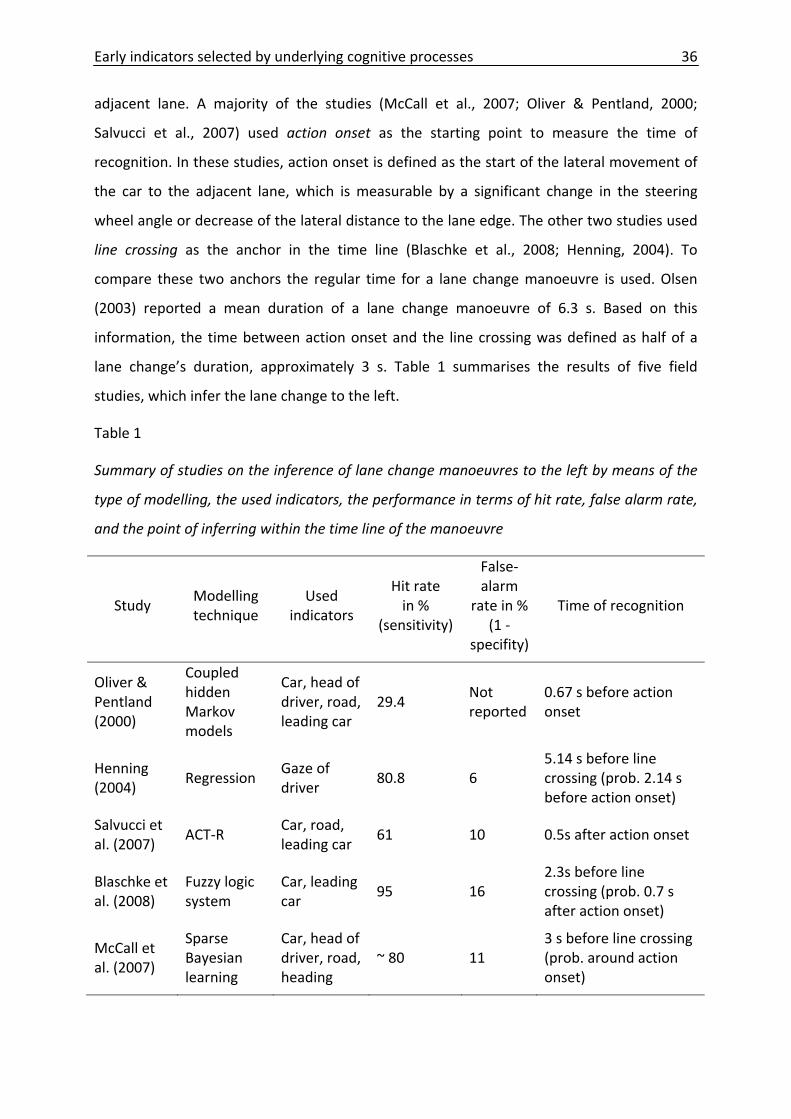
Early indicators selected by underlying cognitive processes   36 

adjacent  lane.  A  majority  of  the  studies  (McCall  et  al.,  2007;  Oliver  &  Pentland,  2000; 

Salvucci  et  al.,  2007)  used  action  onset  as  the  starting  point  to  measure  the  time  of 

recognition. In these studies, action onset is defined as the start of the lateral movement of 

the  car  to  the  adjacent  lane, which  is measurable  by  a  significant  change  in  the  steering 

wheel angle or decrease of the lateral distance to the lane edge. The other two studies used 

line  crossing  as  the  anchor  in  the  time  line  (Blaschke  et  al.,  2008;  Henning,  2004).  To 

compare  these  two anchors  the  regular  time  for a  lane change manoeuvre  is used. Olsen 

(2003)  reported  a mean  duration  of  a  lane  change manoeuvre  of  6.3  s.  Based  on  this 

information,  the  time between action onset and  the  line crossing was defined as half of a 

lane  change’s  duration,  approximately  3  s.  Table  1  summarises  the  results  of  five  field 

studies, which infer the lane change to the left.  

Table 1  

Summary of studies on the inference of lane change manoeuvres to the left by means of the 

type of modelling, the used indicators, the performance in terms of hit rate, false alarm rate, 

and the point of inferring within the time line of the manoeuvre 

Study Modelling technique 

Used indicators 

Hit rate in % 

(sensitivity) 

False‐alarm 

rate in % (1 ‐ 

specifity) 

Time of recognition 

Oliver & Pentland (2000) 

Coupled hidden Markov models 

Car, head of driver, road, leading car 

29.4 Not reported 

0.67 s before action onset 

Henning (2004) 

Regression Gaze of driver 

80.8  6 5.14 s before line crossing (prob. 2.14 s before action onset) 

Salvucci et al. (2007) 

ACT‐R Car, road, leading car 

61  10  0.5s after action onset 

Blaschke et al. (2008) 

Fuzzy logic system 

Car, leading car 

95  16 2.3s before line crossing (prob. 0.7 s after action onset) 

McCall et al. (2007) 

Sparse Bayesian learning 

Car, head of driver, road, heading 

~ 80  11 3 s before line crossing (prob. around action onset) 

 

Early indicators selected by underlying cognitive processes   37 

Table 1  indicates  that briefly after action onset  (start of  the  lateral movement)  the 

algorithms were  able  to predict up  to 95% of  lane  changes  to  the  left  in  the  field. These 

results are sufficient  for assistant systems  that need  the  information very  late,  like a Lane 

Departure Warning  system. However,  the  results are  inadequate  for  systems  that  require 

the  information  as  early  as  the  driver  starts  the  preparation  for  a  lane  change,  like  a 

Workload Manger  or  a  Lane  Change Assistant.  In  Table  1,  only  two  studies were  able  to 

predict  lane changes before action onset, both  included eye or head movements  into their 

modelling  (Henning,  2004;  Oliver  &  Pentland,  2000).  There  are  similar  findings  in  other 

studies, for example Chattington, Wilson, Ashford, and Marple‐Horvat (2007) reported that 

typical  eye  movements  to  both  sides  precede  curve  negotiation  by  several  seconds. 

However, to understand which eye movements are typical for certain driving manoeuvres it 

is necessary  to understand  the underlying  cognitive processes,  like  information gathering, 

storage,  and  usage  as  a  basis  for  the  oncoming  action.  To  highlight  cognitive  processes 

connected  to  lane change manoeuvres, common  lane change models are discussed  in  the 

next chapter. 

Common Lane Change Models 

Possible sources of behavioural descriptions and their underlying cognitive processes 

during lane change manoeuvres are models. Several of these lane change models have been 

proposed (Chovan, Tijerina, Alexander, & Hendricks, 1994; Fastenmeier, Hinderer, Lehnig, & 

Gstalter, 2001; Olsen, 2003; Salvucci, 2006). They divide the lane change process into at least 

two  phases.  These  are  a  preparation  phase  (sometimes  called  decision  phase)  and  an 

execution phase. As the inference of drivers’ intentions needs to be made in the preparation 

phase, we will now take a closer look at this phase. 

The preparation phase starts with a desire to change lanes, mostly by a slow leading 

vehicle  or merging  lanes  (see Olsen,  2003,  for  a  detailed  analysis).  If  there  is  a  desire  to 

change  lanes  the driver scans  the mirrors, blind spots, and  target  lane  to check  if  there  is 

traffic (Chovan et al., 1994). Depending on the density of the traffic, the driver then decides 

if the gap in the target lane is sufficient enough to start the lateral movement, or to wait and 

scan again. The left part of Figure 1 illustrates this process in a flowchart.  

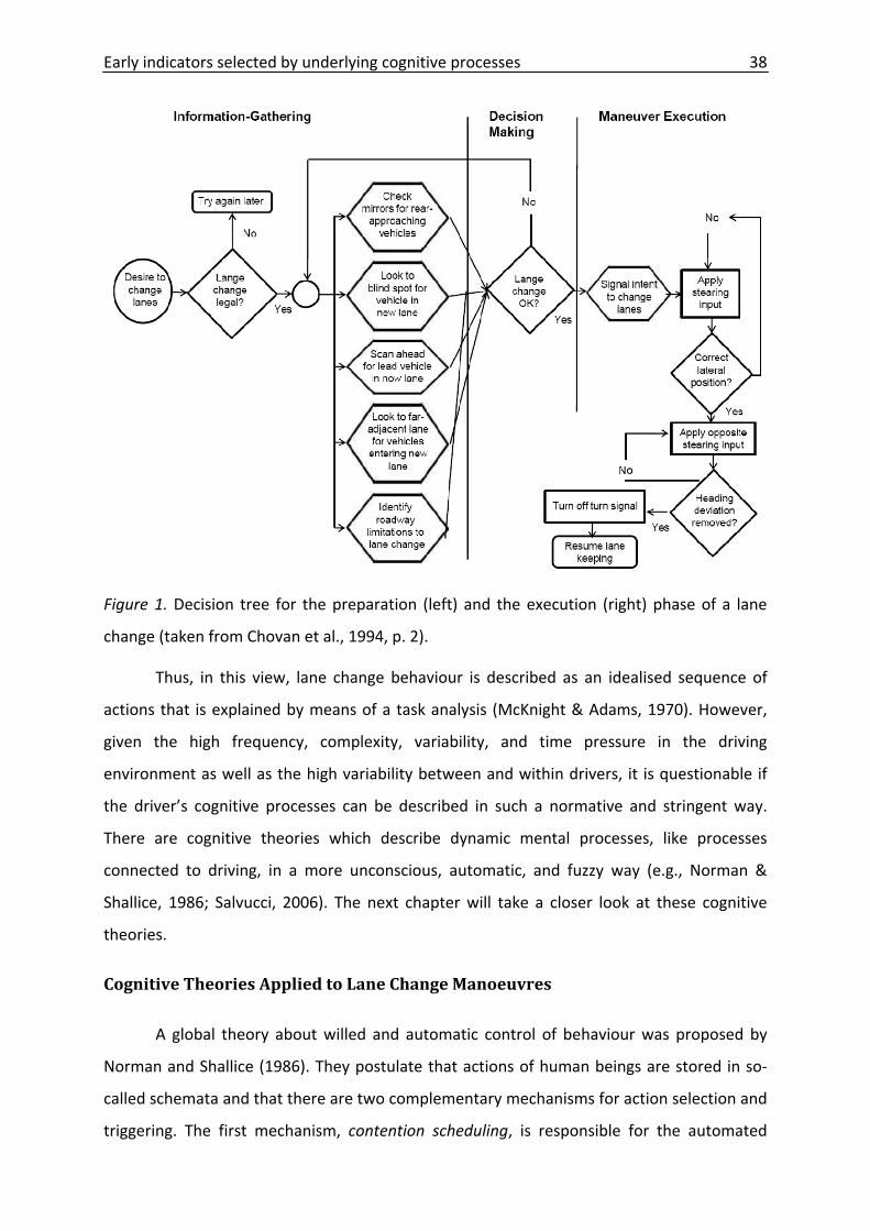
Early indicators selected by underlying cognitive processes   38 

 

Figure 1. Decision  tree  for  the preparation  (left) and  the execution  (right) phase of a  lane 

change (taken from Chovan et al., 1994, p. 2). 

Thus,  in  this  view,  lane  change behaviour  is described as an  idealised  sequence of  

actions that  is explained by means of a task analysis  (McKnight & Adams, 1970). However, 

given  the  high  frequency,  complexity,  variability,  and  time  pressure  in  the  driving 

environment as well as the high variability between and within drivers,  it  is questionable  if 

the driver’s  cognitive processes  can be described  in  such  a normative  and  stringent way. 

There  are  cognitive  theories  which  describe  dynamic  mental  processes,  like  processes 

connected  to  driving,  in  a more  unconscious,  automatic,  and  fuzzy way  (e.g., Norman & 

Shallice, 1986;  Salvucci, 2006). The next  chapter will  take a  closer  look at  these  cognitive 

theories.  

Cognitive Theories Applied to Lane Change Manoeuvres 

A global  theory about willed and automatic  control of behaviour was proposed by 

Norman and Shallice (1986). They postulate that actions of human beings are stored  in so‐

called schemata and that there are two complementary mechanisms for action selection and 

triggering.  The  first mechanism,  contention  scheduling,  is  responsible  for  the  automated 

Early indicators selected by underlying cognitive processes   39 

selection and coordination of different well‐learned habitual tasks. The second mechanism is 

the  supervisory attentional  system  that  is a more  conscious  selection of action  schemata, 

which are used especially when tasks are new or complex. Transferred to the field of driving, 

these  two mechanisms  can  both  activate  and  suppress  several  schemata  (sequentially  as 

well as parallel),  for example a “drive curve” schema can be activated and a drive straight 

schema  can  be  suppressed.  Corresponding  triggers  and  the  goals  of  the  driver  handle 

activation and suppression of schemata. For example, the perception of an oncoming curve 

can  trigger a  schema  that  incorporates passing  through a curve.  It  starts  the behaviour of 

adapting the speed to the slope of the curve and looking for the best trajectory to negotiate 

through the curve. At the same time, it suppresses the former activated schema of straight 

driving.  

Transferring this mechanism to  lane changing, triggers can be more diverse than for 

passing a  curve,  like a  slow  leading vehicle, an oncoming off‐ramp, or merging  lanes. The 

following example explains the process. Assume one is driving on a highway and encounters 

a slow vehicle directly ahead  in the  lane. This slow  leading vehicle would serve as a trigger 

that  activates  the  lane  change  schema  by  the  contention  scheduler.  It  activates  typical 

behaviour  connected  to  the  preparation  for  a  lane  change,  for  example  scanning  the 

rearward  traffic  for  oncoming  cars.  If  there  is  a  sufficient  gap,  the  driver  changes  to  the 

adjacent  lane. However,  in the event that a  lane change  is not possible due to a solid  line, 

this would serve as another trigger for the contention scheduler. It would then stop the lane 

change schema and activate the schema for car following. If there were someone sitting  in 

the  car  prohibiting  the  driver  from  overtaking  the  car  ahead,  the  supervisory  attentional 

system would suppress the lane change schema.  

The  theory  of  Norman  and  Shallice  (1986)  explains  the  interaction  of  drivers’ 

behaviour and the environment in terms of triggering a certain behaviour automatically with 

a  stimulus  in  the  environment.  This  potential  trigger  does  not  always  lead  to  the  certain 

behaviour  due  to  other  triggers  in  the  environment  (the  example  of  the  solid  line)  or 

involvement of higher cognitive processes, like the intervention of a passenger who is urging 

the driver to stay in the lane. However, it neither accounts for the content of a schema nor 

provides the connection between cognition and behaviour  in a measurable way. Hence, to 

derive potential  indicators,  a  theory  that describes  the  cognitive processes during driving 

Early indicators selected by underlying cognitive processes   40 

and their relationship to observable behaviour in terms of glance behaviour, steering wheel, 

and pedal use should be cited. 

One approach  that provides such a  fine grained account of  the cognitive processes 

has been proposed by Salvucci (2006). He developed a driver model that is implemented in a 

cognitive  architecture  (ACT‐R,  for  further  information  see  Anderson  et  al.,  2004).  In  his 

paper, he describes  a  cognitive  architecture  as  follows:  ‘[it] …  is  a  general  framework  for 

specifying  computational  behavioural  models  of  human  cognitive  performance.  The 

architecture embodies both the abilities and constraints of the human system—for instance, 

abilities  such  as memory  storage  and  recall,  learning,  perception,  and motor  action;  and 

constraints  such  as memory  decay,  foveal  versus  peripheral  visual  encoding,  and  limited 

motor performance. As such, a cognitive architecture helps to ensure that cognitive models 

developed  in  the  framework are  rigorous and psychologically valid,  thus abiding by all  the 

limitations of the human system.’ (p. 364).  

In  his  driver model,  Salvucci  (2006)  describes  the  behaviour  of  driving  a  standard 

midsize vehicle on a two‐lane highway with moderate traffic and distinguishes between lane 

keeping,  curve negotiation  and  lane  changing  to  left  and  right.  The model  contains  three 

main  components:  control,  monitoring,  and  decision  making.  The  control  component 

manages all perception of visual cues and manipulation of vehicle controls  for  lateral and 

longitudinal control  (steering, acceleration, and braking). The monitoring component deals 

with the continual maintenance of situation awareness by visually sampling the  lanes (own 

and other) to the front and via mirrors to the back (altogether four positions) randomly with 

a  certain probability. The  information  gathered by  these monitoring  activities  is  stored  in 

facts  in  ACT‐R’s  memory.  The  third  component  decision  making  uses  the  information 

gathered during monitoring  to determine  if  any  tactical decision  should be made.  Such  a 

decision could for example be whether and when to undertake a lane change. When there is 

a slow leading vehicle (2 s headway), the driver model sets its goal to undergo a lane change. 

If  the  goal  is  set  to  change  lanes,  information  about  the  traffic on  the  target  lane  that  is 

available in memory, is used to decide whether or not the lane change can be accomplished. 

If  the model  finds any  information about a near car  in  the target  lane  in memory and  this 

vehicle is within a distance of 40 m, it aborts the lane change process and starts to check if 

the  car  is  still  there.  If  there  is  no  information  on  traffic  in  the  target  lane  available  in 

memory, the model checks also the target lane again (to the front and via the mirrors to the 

Early indicators selected by underlying cognitive processes   41 

back). This double‐checking  is necessary as, due to decay processes  in memory, the model 

might  have  “forgotten”  that  there  are  cars  in  the  target  lane.  After  perceiving  the 

information about the traffic in the target lane, two alternatives remain. If there is no car in 

the  target  lane,  the model  initialises a  lane change by  switching visual attention  from  the 

current  lane  to  the adjacent  lane and  then begins  the actual steering process.  If  there are 

cars in the other lane, the model keeps checking the mirrors until the gap in the target lane 

is sufficient enough (40 m) to initialise a lane change as described before.  

Previous Findings on Eye Movements 

Salvucci’s driver model within the ACT‐R cognitive architecture generates measurable 

behaviour on  the basis of  the computer‐generated cognitive processes  in  terms of glances 

and manual controls. This measurable behaviour can then show possible indicators of a lane 

change manoeuvre. The advantage of  the cognitive driver model over conventional driver 

models (e.g., Chovan et al., 1994; Olsen, 2003) is that the cognitive model delivers not only 

the  information  that  drivers  show  a  certain  behaviour,  it  also  predicts when  they  do  it. 

Findings  in  field studies that  focus on eye‐movement behaviour during driving support the 

predictions of the driving studies. For instance, Olsen (2003) reported that there are higher 

proportions of  glances  to  the mirrors  and blind  spots when drivers  start  to  change  lanes 

versus  when  they  drive  straight.  These  findings  reflect  the  increased  information 

requirements  due  to  the  decision  to  undertake  a  lane  change  (have  the  goal  to  change 

lanes). Moreover, the two options to either change  lanes  immediately (free target  lane) or 

wait until a sufficient gap  in the target  lane appears are also reflected  in the  literature. For 

instance,  Bhise  et  al.  (1981)  show  that  increasing  traffic  in  the  target  lane  leads  to  an 

increasing number and duration of glances  to  the mirrors during  lane changes  (and  longer 

preparation  for  lane changes). Robinson, Erickson, Thurston, and Clark  (1972) and Tijerina, 

Garrott,  Stoltzfus,  and  Parmer  (2005)  reported  that  lane  changes  to  the  left  are  more 

connected  to glances  into  the  left outside mirror and  lane  changes  to  the  right are more 

associated  to  the use of  the  interior and right mirror. Henning, Schweigert, Baumann, and 

Krems (2006) found evidence that there  is a timely order of glance  locations before a  lane 

change; glances to the  left outside mirror precede glances to the  left blind spot by several 

seconds. However, there is also always a small proportion of glances to the left outside and 

to  the  interior mirror  if  there  is  no  lane  change  following  (Henning  et  al.,  2006).  These 

Early indicators selected by underlying cognitive processes   42 

findings  support  the  ACT‐R  driver  model  (Salvucci,  2006),  which  proposes  scanning  the 

mirrors without  the  intention of  changing  lanes. These  findings were  complemented by a 

study of Nunes and Recarte (2005), who describe that the percentage of fixations to mirrors 

almost doubles  in the presence of traffic on the target  lane without a slow  leading vehicle; 

and it is even higher with a slow leading vehicle.  

To summarise, lane changes to the left are probably connected to glances to the left 

outside mirror  and  later  to  glances  to  the  left blind  spot. Glances  to  the  interior or  right 

outside mirror should be more connected to lane changes to the right, but they are not the 

focus of this study. However, there is always a proportion of glances to the mirrors without a 

lane change  intention. This  is describes as  the monitoring component of  the driver model 

(Salvucci, 2006), and  it  seems  that  it  is  further  influenced by  the amount of  traffic on  the 

other lane (Nunes & Recarte, 2005). 

Candidate Indicators From Eye Movements 

Based on  the  theoretical assumptions of Salvucci  (2006) and according  to previous 

findings  (Bhise  et  al.,  1981;  Henning  et  al.,  2006;  Nunes  &  Recarte,  2005;  Olsen,  2003; 

Robinson  et  al.,  1972;  Tijerina  et  al.,  2005),  a  precise  description  of  all  glance‐based 

indicators  is delivered  in Table 2. The findings are categorised by two different factors. The 

first  factor  is  lane  change  preparation  or  not  (intention  to  change  lanes  [yes  vs.  no]). 

According  to  results of Bhise et al.  (1981) and Nunes & Recarte  (2005),  the  second  factor 

concerns the presence or absence of rearward traffic on the target lane (rearward traffic on 

target lane [yes vs. no]).  

 

   

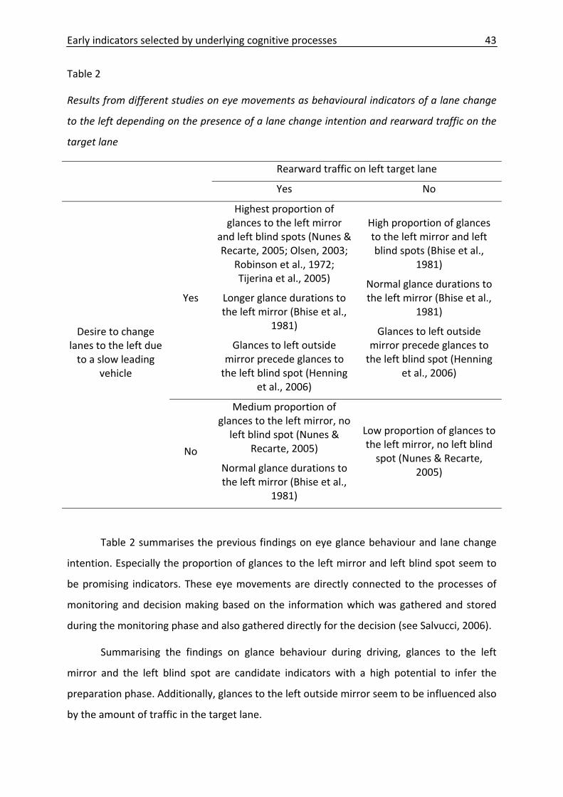
Early indicators selected by underlying cognitive processes   43 

Table 2 

Results from different studies on eye movements as behavioural indicators of a lane change 

to the left depending on the presence of a lane change intention and rearward traffic on the 

target lane 

    Rearward traffic on left target lane 

    Yes  No 

Desire to change lanes to the left due to a slow leading 

vehicle 

Yes 

Highest proportion of glances to the left mirror 

and left blind spots (Nunes & Recarte, 2005; Olsen, 2003; 

Robinson et al., 1972; Tijerina et al., 2005) 

Longer glance durations to the left mirror (Bhise et al., 

1981) 

Glances to left outside mirror precede glances to the left blind spot (Henning 

et al., 2006) 

High proportion of glances to the left mirror and left blind spots (Bhise et al., 

1981) 

Normal glance durations to the left mirror (Bhise et al., 

1981) 

Glances to left outside mirror precede glances to the left blind spot (Henning 

et al., 2006) 

No 

Medium proportion of glances to the left mirror, no left blind spot (Nunes & 

Recarte, 2005) 

Normal glance durations to the left mirror (Bhise et al., 

1981) 

Low proportion of glances to the left mirror, no left blind spot (Nunes & Recarte, 

2005) 

 

Table 2 summarises the previous findings on eye glance behaviour and  lane change 

intention. Especially the proportion of glances to the left mirror and left blind spot seem to 

be promising  indicators. These eye movements are directly connected  to  the processes of 

monitoring and decision making based on  the  information which was gathered and stored 

during the monitoring phase and also gathered directly for the decision (see Salvucci, 2006).  

Summarising  the  findings  on  glance  behaviour  during  driving,  glances  to  the  left 

mirror  and  the  left  blind  spot  are  candidate  indicators with  a  high  potential  to  infer  the 

preparation phase. Additionally, glances to the left outside mirror seem to be influenced also 

by the amount of traffic in the target lane. 

Early indicators selected by underlying cognitive processes   44 

Candidate Indicators from Car Controls 

Up until now, an eye tracking system has been an expensive sensor that has to deal 

with  problems  such  as  noisy  data  due  to  changing  light  conditions,  sunglasses,  etc. 

(Duchowski, 2007). One  solution  to overcome  these problems  could be  to use only head‐

motions, which  are  closely  related  to  glances  to  the  side mirror  or  blind  spots  (Doshi & 

Trivedi, 2008; Robinson et al., 1972). An additional solution could be the use of sensors from 

the  car  to  serve  as  indicators,  which  is  a  common  procedure  for  reducing  costs.  Car 

manufacturers  and  suppliers  would  welcome  the  use  of  indicators  which  are  already 

available inside the car, usually accessible via the controller area network (CAN bus), like the 

steering wheel angle, the pedal‐course of accelerator and brake, and the turn signal (Farsi, 

Ratcliff, & Barbosa, 1999).  

The  cognitive  driver model  (Salvucci,  2006)  delivers  information  about  the  use  of 

these  potential  indicators  as  well.  They  are  connected  to  the  control  and  decision 

components of the cognitive processes. In case of straight driving (no lane change) the driver 

model stays at a constant speed in the middle of the lane. If there is traffic in the target lane 

the model adapts the speed to maintain a safe gap to the slow leading vehicle (deceleration) 

and  stays  in  the middle of  the original  lane.  If  the gap  in  the  target  lane  is  sufficient,  the 

model accelerates and starts the action by steering. 

Unfortunately,  there  are  no  results  from  field  studies  on  the  longitudinal  velocity 

adjustment  in  terms  of  deceleration  and  braking  while  preparing  a  lane  change. 

Nevertheless,  the  first  seconds  of  this  behaviour  are  very  similar  to  approaching  a  slow 

leading vehicle  in car‐following studies, which has been examined and modelled for almost 

half  a  century  (for  an  overview  and  a  critical  discussion,  see  Boer,  1999;  Brackstone  & 

McDonald,  1999).  Car‐following  models  are  based  on  assumptions  about  speed  and 

acceleration to adapt the car’s speed to the speed of the car in front by using the gas pedal 

(accelerator) and brake.  

Another  candidate  indicator  from  the  CAN  bus  is  the  turn  signal.  As  previously 

described, naturalistic driving studies indicate that drivers start to use it either late or not at 

all to indicate a lane change (Olsen, 2003). 

Table  3  summarises  the  assumptions  derived  from  the  cognitive  driver  model 

(Salvucci, 2006) and car‐following models (Boer, 1999; Brackstone & McDonald, 1999) on the 

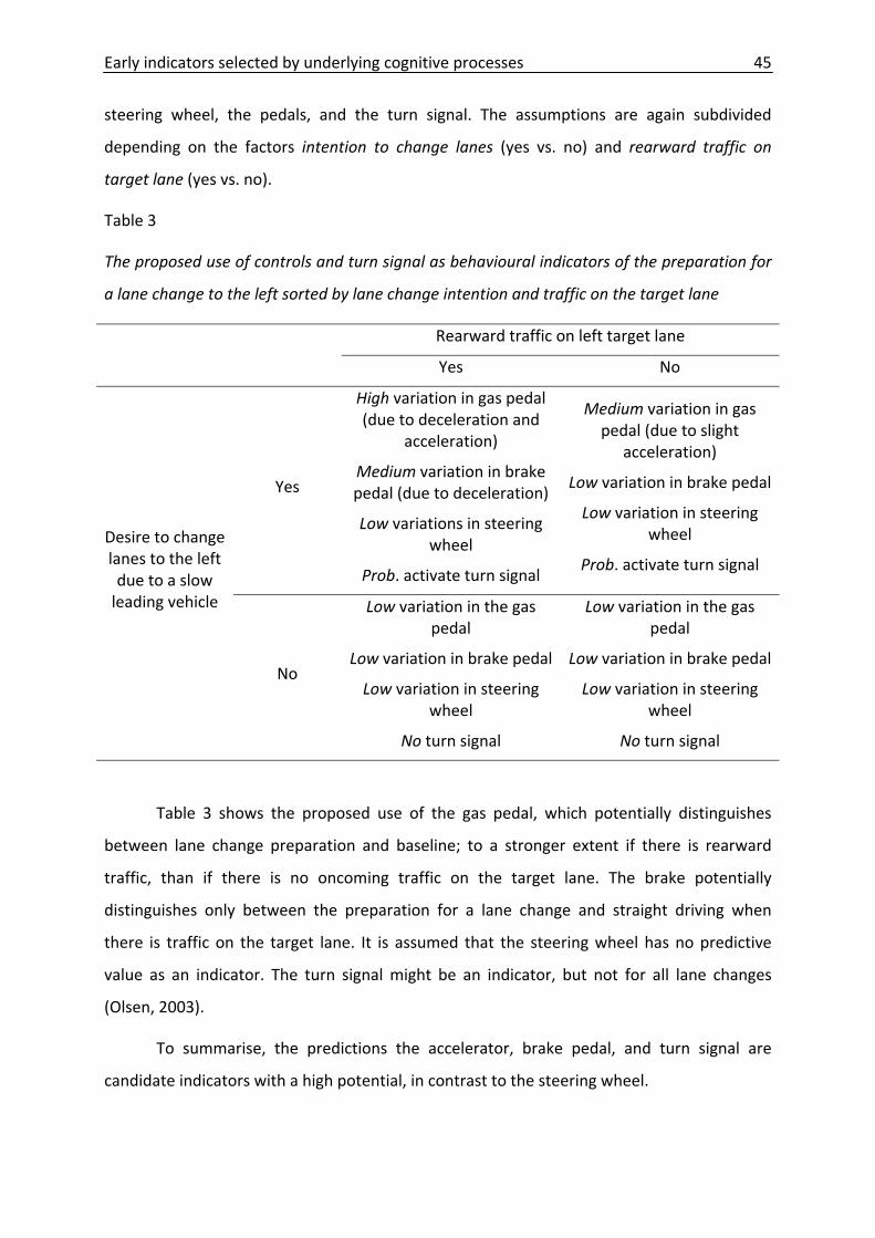
Early indicators selected by underlying cognitive processes   45 

steering  wheel,  the  pedals,  and  the  turn  signal.  The  assumptions  are  again  subdivided 

depending  on  the  factors  intention  to  change  lanes  (yes  vs.  no)  and  rearward  traffic  on 

target lane (yes vs. no). 

Table 3 

The proposed use of controls and turn signal as behavioural indicators of the preparation for 

a lane change to the left sorted by lane change intention and traffic on the target lane 

    Rearward traffic on left target lane 

    Yes  No 

Desire to change lanes to the left due to a slow leading vehicle 

Yes 

High variation in gas pedal (due to deceleration and 

acceleration) 

Medium variation in brake pedal (due to deceleration) 

Low variations in steering wheel 

Prob. activate turn signal 

Medium variation in gas pedal (due to slight 

acceleration) 

Low variation in brake pedal

Low variation in steering wheel 

Prob. activate turn signal 

No 

Low variation in the gas pedal 

Low variation in brake pedal

Low variation in steering wheel 

No turn signal 

Low variation in the gas pedal 

Low variation in brake pedal

Low variation in steering wheel 

No turn signal 

 

Table  3  shows  the  proposed  use  of  the  gas  pedal, which  potentially  distinguishes 

between  lane  change  preparation  and  baseline;  to  a  stronger  extent  if  there  is  rearward 

traffic,  than  if  there  is  no  oncoming  traffic  on  the  target  lane.  The  brake  potentially 

distinguishes  only  between  the  preparation  for  a  lane  change  and  straight  driving when 

there  is  traffic on  the  target  lane.  It  is assumed  that  the  steering wheel has no predictive 

value  as  an  indicator.  The  turn  signal might be  an  indicator, but not  for  all  lane  changes 

(Olsen, 2003).  

To  summarise,  the  predictions  the  accelerator,  brake  pedal,  and  turn  signal  are 

candidate indicators with a high potential, in contrast to the steering wheel.  

Early indicators selected by underlying cognitive processes   46 

Candidate Indicators from the Car’s Characteristics 

Supplementary  to  the  above  described  indicators  that  measure  the  drivers’ 

behaviour  directly  (accelerator  pedal,  brake  pedal,  turn  signal),  there  are  other  possible 

sources  of  information  such  as  the  car  characteristics  in  terms  of  lane  position  and 

movement. A variety of measures for this task are known, but they can be roughly classified 

by  longitudinal and  lateral position and motion. Both directions can be determined by  lane 

position, velocity, and its first derivation, acceleration.  

The movement of the car  is closely related to the car controls. Whereas the  lateral 

position  and movement  are  connected  to  the  steering wheel,  the  longitudinal motion  is 

strongly correlated to the use of the pedals. Due to this strong correlation all assumptions 

derived  from  the  driver model  (Salvucci,  2006)  on  accelerator,  brake  pedal,  and  steering 

wheel can be applied here, too. Therefore, connected to assumptions made  in Table 3, the 

longitudinal  velocity  and  all  connected measures  should  have more power  to predict  the 

preparation for a lane change than the lateral motion. 

Research Questions 

Whereas  all  candidate  indicators  (see  table  2  and  3)  seem  to  be  involved  in  lane 

change behaviour,  it  is not clear  to what extent and when. This study aims  to answer  the 

following questions: 

- Are some candidate indicators better then others? 

- Are some candidate indicators better for predicting lane changes earlier on whereas 

others for predicting them later on?  

To answer the questions we conducted a field study  in order to record driving data 

on  lane change behaviour  in a naturalistic driving environment. The data were recorded by 

means  of  an  instrumented  car,  labelled,  and  finally  analysed  in  two  steps.  First,  we 

compared  all  candidate  indicators  using methods  from  inferential  statistics  to  find  out  if 

there are significant differences between the  lane change preparation and a corresponding 

baseline sequence. Candidate  indicators with a high potential to  infer the desire to change 

lanes are the following: from eye movements, glances to the  left mirror and the  left blind; 

from car controls, the variance of the accelerator and the brake pedal, and the turn signal; 

and  from  car  dynamics,  the  longitudinal  velocity. Additionally,  glances  to  the  left  outside 

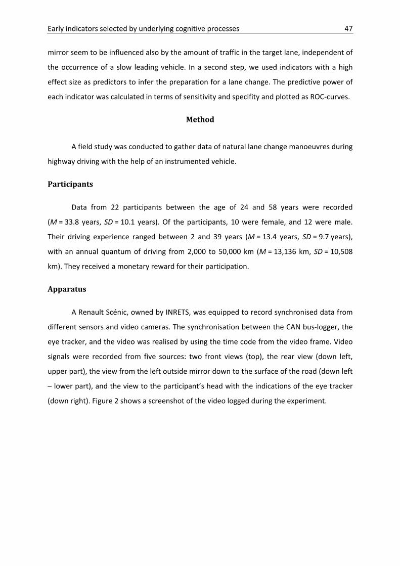
Early indicators selected by underlying cognitive processes   47 

mirror seem to be influenced also by the amount of traffic in the target lane, independent of 

the occurrence of a slow  leading vehicle.  In a second step, we used  indicators with a high 

effect size as predictors to infer the preparation for a lane change. The predictive power of 

each indicator was calculated in terms of sensitivity and specifity and plotted as ROC‐curves.  

Method  

A field study was conducted to gather data of natural lane change manoeuvres during 

highway driving with the help of an instrumented vehicle. 

Participants 

Data  from  22  participants  between  the  age  of  24  and  58  years  were  recorded 

(M = 33.8 years, SD = 10.1 years). Of  the participants, 10 were  female, and 12 were male. 

Their  driving  experience  ranged  between  2  and  39  years  (M = 13.4  years,  SD = 9.7 years), 

with an annual quantum of driving  from 2,000  to 50,000 km  (M = 13,136 km, SD = 10,508 

km). They received a monetary reward for their participation. 

Apparatus 

A Renault Scénic, owned by INRETS, was equipped to record synchronised data from 

different sensors and video cameras. The synchronisation between the CAN bus‐logger, the 

eye tracker, and the video was realised by using the time code from the video frame. Video 

signals were  recorded  from  five  sources:  two  front  views  (top),  the  rear  view  (down  left, 

upper part), the view from the left outside mirror down to the surface of the road (down left 

– lower part), and the view to the participant’s head with the indications of the eye tracker 

(down right). Figure 2 shows a screenshot of the video logged during the experiment.  

 

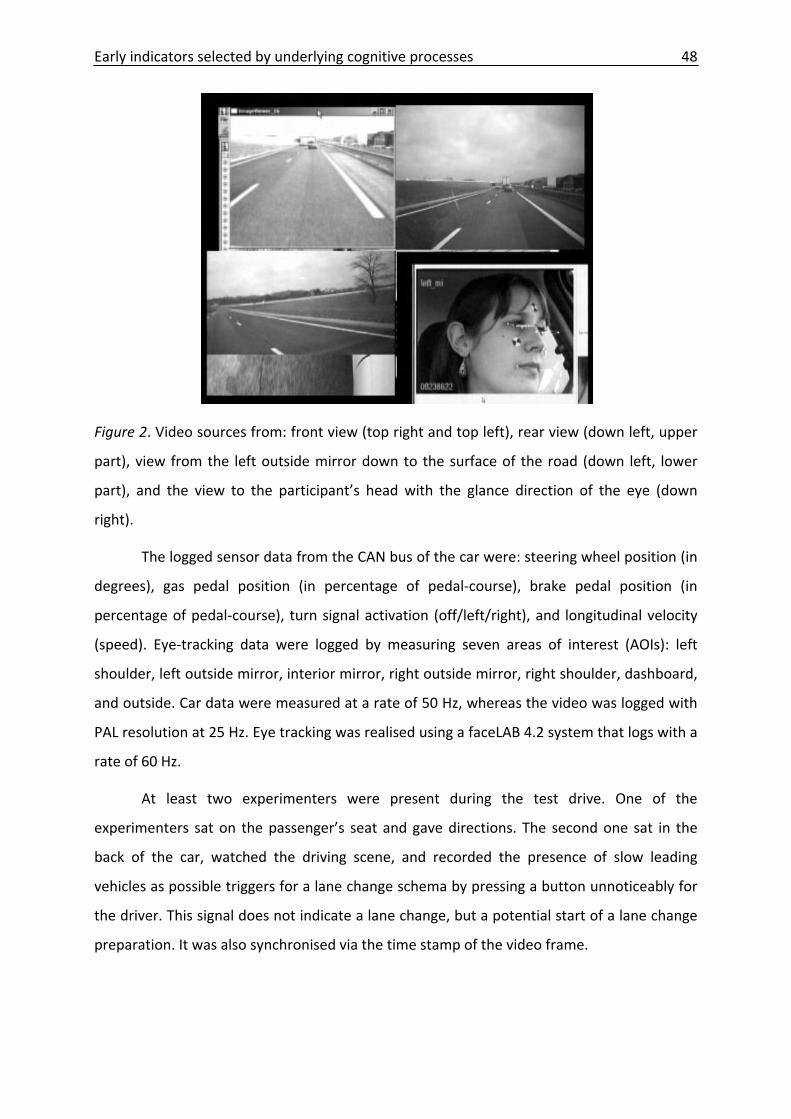
Early indicators selected by underlying cognitive processes   48 

 

Figure 2. Video sources from: front view (top right and top left), rear view (down left, upper 

part), view  from  the  left outside mirror down  to  the surface of  the road  (down  left,  lower 

part),  and  the  view  to  the  participant’s  head with  the  glance  direction  of  the  eye  (down 

right). 

The logged sensor data from the CAN bus of the car were: steering wheel position (in 

degrees),  gas  pedal  position  (in  percentage  of  pedal‐course),  brake  pedal  position  (in 

percentage of pedal‐course), turn signal activation  (off/left/right), and  longitudinal velocity 

(speed).  Eye‐tracking  data were  logged  by measuring  seven  areas  of  interest  (AOIs):  left 

shoulder, left outside mirror, interior mirror, right outside mirror, right shoulder, dashboard, 

and outside. Car data were measured at a rate of 50 Hz, whereas the video was logged with 

PAL resolution at 25 Hz. Eye tracking was realised using a faceLAB 4.2 system that logs with a 

rate of 60 Hz.  

At  least  two  experimenters  were  present  during  the  test  drive.  One  of  the 

experimenters  sat on  the passenger’s  seat and gave directions. The  second one  sat  in  the 

back  of  the  car, watched  the  driving  scene,  and  recorded  the  presence  of  slow  leading 

vehicles as possible triggers for a lane change schema by pressing a button unnoticeably for 

the driver. This signal does not indicate a lane change, but a potential start of a lane change 

preparation. It was also synchronised via the time stamp of the video frame. 

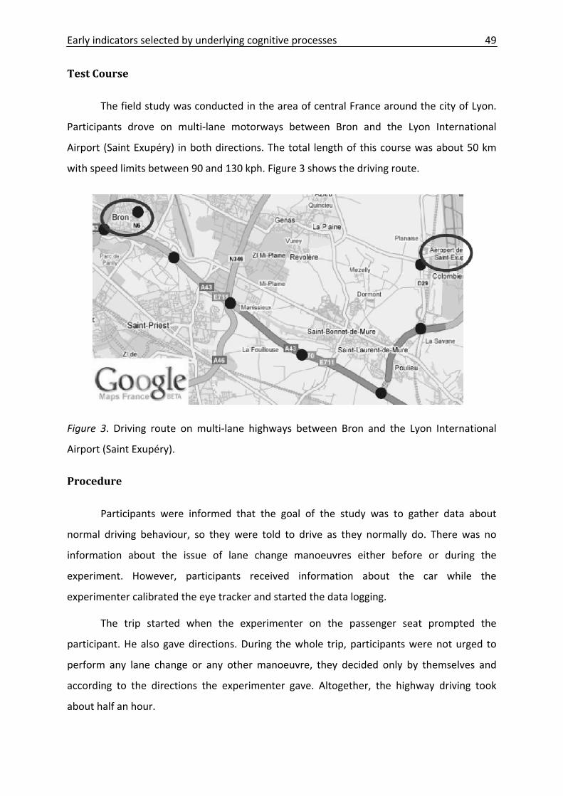
Early indicators selected by underlying cognitive processes   49 

Test Course 

The field study was conducted in the area of central France around the city of Lyon. 

Participants  drove  on  multi‐lane  motorways  between  Bron  and  the  Lyon  International 

Airport  (Saint Exupéry)  in both directions. The total  length of this course was about 50 km 

with speed limits between 90 and 130 kph. Figure 3 shows the driving route. 

 

Figure  3. Driving  route  on multi‐lane  highways  between  Bron  and  the  Lyon  International 

Airport (Saint Exupéry). 

Procedure 

Participants were  informed  that  the  goal  of  the  study was  to  gather  data  about 

normal  driving  behaviour,  so  they were  told  to  drive  as  they  normally  do.  There was  no 

information  about  the  issue  of  lane  change  manoeuvres  either  before  or  during  the 

experiment.  However,  participants  received  information  about  the  car  while  the 

experimenter calibrated the eye tracker and started the data logging.  

The  trip  started  when  the  experimenter  on  the  passenger  seat  prompted  the 

participant. He also gave directions. During  the whole  trip, participants were not urged  to 

perform  any  lane  change  or  any  other manoeuvre,  they decided  only  by  themselves  and 

according  to  the  directions  the  experimenter  gave.  Altogether,  the  highway  driving  took 

about half an hour.  

Early indicators selected by underlying cognitive processes   50 

After  driving,  the  data  was  immediately  processed  to  find  the  sequences  with 

reasonable circumstances for changing  lanes  in the video (they were  identified by the time 

stamps  associated  to  the  button  pressed  by  the  experimenter).  Participants were  shown 

these video sequences and were asked about whether they had thought about executing a 

lane  change  or  not.  In  situations  with  a  lane  change  following  the  pressed  button,  the 

participants were  asked  to  indicate  the  point  in  the  video where  they  had  started  to  be 

mentally engaged  in the preparation for the  lane change. In situations with no  lane change 

following the pressed button, the participants were asked if there had been any lane change 

intention at all, and  if so, about the cause of the withdrawal. Finally, the participants filled 

out a questionnaire on demographic data; then they were debriefed and thanked. After each 

run, all sensor and video data were checked for plausibility to identify malfunctions. 

Post Experimental Data Processing and Coding 

Due  to  the  lack  of  an  appropriate  sensor,  the  position  of  the  car  in  the  lane was 

automatically derived from the  lower  left hand side of the video via  image processing (see 

Figure 2). To make  this possible, a measuring  tape was  located orthogonally  to  the  car  in 

sight of the camera before each run. For the automatic detection, the computer estimated 

the distance from the left side of the car to the lane markers. If there was no lane marker, an 

algorithm estimated the distance based on the last and next true distance. 

Afterwards, trained human coders watched the video scenes with highway sections 

and marked all lane change manoeuvres to the left in terms of start of the preparation and 

start  of  the  lateral  movement  of  the  car  as  start  and  end  points  of  the  lane  change 

preparation.  For  the definition of  the  starting point,  they used  three  sources: a.  the  time 

stamp from the button pressed by the experimenter to mark a slow  leading vehicle, b. the 

post‐driving statements of the participants about the start of the mental engagement for a 

lane change in the video, and c. the coder’s own estimation on the basis of the video and all 

data sources. Three different coders coded these starting points of the preparation for a lane 

change  in  parallel  to  calculate  an  interrater  reliability  using  the  Kendalls  W  procedure 

(normal  distribution  was  not  given;  Kolmogorov‐Smirnov  at  p < .001).  For  all  194  cases, 

Kendalls W was at W = .92.  

All  lane  change  sequences  were  also  classified  depending  on  whether  there  was 

traffic on the target  lane to the  left that required a delay  in the execution of a  lane change 

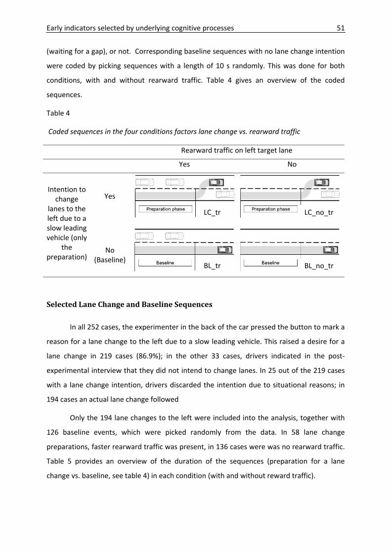
Early indicators selected by underlying cognitive processes   51 

(waiting for a gap), or not.  Corresponding baseline sequences with no lane change intention 

were coded by picking sequences with a  length of 10  s  randomly. This was done  for both 

conditions,  with  and  without  rearward  traffic.  Table  4  gives  an  overview  of  the  coded 

sequences. 

Table 4 

 Coded sequences in the four conditions factors lane change vs. rearward traffic  

    Rearward traffic on left target lane 

    Yes  No 

Intention to change 

lanes to the left due to a slow leading vehicle (only 

the preparation) 

Yes 

 

No (Baseline) 

 

Selected Lane Change and Baseline Sequences 

In all 252 cases, the experimenter in the back of the car pressed the button to mark a 

reason for a  lane change to the  left due to a slow  leading vehicle. This raised a desire for a 

lane  change  in  219  cases  (86.9%);  in  the  other  33  cases,  drivers  indicated  in  the  post‐

experimental interview that they did not intend to change lanes. In 25 out of the 219 cases 

with a  lane change  intention, drivers discarded the  intention due to situational reasons;  in 

194 cases an actual lane change followed 

Only the 194  lane changes to the  left were  included  into the analysis, together with 

126  baseline  events,  which  were  picked  randomly  from  the  data.  In  58  lane  change 

preparations, faster rearward traffic was present, in 136 cases were was no rearward traffic. 

Table  5  provides  an  overview  of  the  duration  of  the  sequences  (preparation  for  a  lane 

change vs. baseline, see table 4) in each condition (with and without reward traffic). 

LC_tr 

BL_tr 

LC_no_tr 

BL_no_tr 

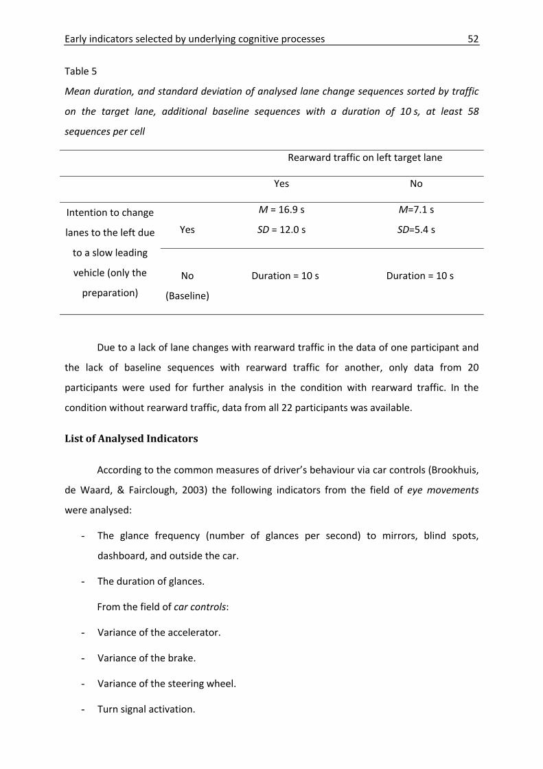
Early indicators selected by underlying cognitive processes   52 

Table 5 

Mean duration, and standard deviation of analysed lane change sequences sorted by traffic 

on  the  target  lane,  additional  baseline  sequences  with  a  duration  of  10 s,  at  least  58 

sequences per cell 

    Rearward traffic on left target lane 

    Yes  No 

Intention to change 

lanes to the left due 

to a slow leading 

vehicle (only the 

preparation) 

   

Yes 

M = 16.9 s                

SD = 12.0 s 

M=7.1 s                     

SD=5.4 s 

 

No 

(Baseline) 

Duration = 10 s  Duration = 10 s 

 

Due to a lack of lane changes with rearward traffic in the data of one participant and 

the  lack  of  baseline  sequences  with  rearward  traffic  for  another,  only  data  from  20 

participants were  used  for  further  analysis  in  the  condition with  rearward  traffic.  In  the 

condition without rearward traffic, data from all 22 participants was available. 

List of Analysed Indicators 

According to the common measures of driver’s behaviour via car controls (Brookhuis, 

de Waard, &  Fairclough,  2003)  the  following  indicators  from  the  field  of  eye movements 

were analysed: 

- The  glance  frequency  (number  of  glances  per  second)  to  mirrors,  blind  spots, 

dashboard, and outside the car. 

- The duration of glances. 

From the field of car controls: 

- Variance of the accelerator. 

- Variance of the brake. 

- Variance of the steering wheel. 

- Turn signal activation. 

Early indicators selected by underlying cognitive processes   53 

In addition, from the field of car characteristics: 

- Mean and variance of longitudinal velocity. 

- Mean and variance of lateral position. 

Results 

Analysis of Indicators Based on Inferential Statistics 

This part of the analysis compares mean lane change preparation with corresponding 

mean baseline  sequence  for all  indicators using methods  from  inferential  statistics  to  find 

out if there are significant differences.  

Analysis based on the entire sequence. 

Eye movements.  

In  the  first  step,  eye  movements  as  a  behavioural  measure  were  analysed.  The 

statistical  testing  involved  the  following  indicators  from  the  field  of  eye  movements 

(according to Brookhuis et al., 2003): 

- The frequency of glances to mirrors, blind spots, dashboard, and outside the car. 

- The duration of glances. 

Therefore, glances to the different AOI were analysed. A glance is defined spatially by 

the direction of the visual attention to an AOI. Temporally,  it  lasts  from entering a specific 

AOI  until  entering  the  next  AOI.  One  glance  consists  of  at  least  one  fixation,  but  it  can 

enclose more. 

Glance frequencies.  

Figure 4 shows the glance frequencies to the seven AOIs (outside,  left shoulder,  left 

mirror, interior mirror, right mirror, right shoulder, and dashboard). The means are grouped 

by the two factors lane change and rearward traffic and classified by AOIs.   

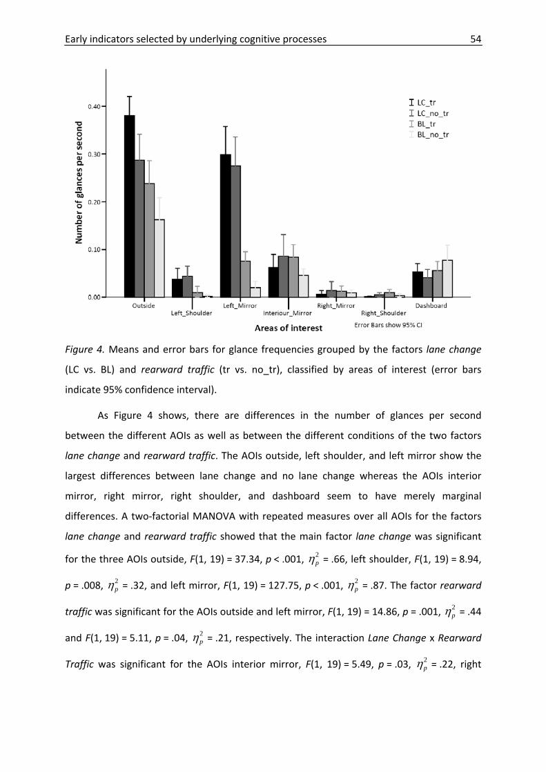
Early indicators selected by underlying cognitive processes   54 

 

Figure 4. Means and error bars  for glance  frequencies grouped by  the  factors  lane change 

(LC  vs.  BL)  and  rearward  traffic  (tr  vs.  no_tr),  classified  by  areas  of  interest  (error  bars 

indicate 95% confidence interval). 

As  Figure  4  shows,  there  are  differences  in  the  number  of  glances  per  second 

between  the different AOIs as well as between  the different conditions of  the  two  factors 

lane change and rearward traffic. The AOIs outside,  left shoulder, and  left mirror show the 

largest  differences  between  lane  change  and  no  lane  change whereas  the  AOIs  interior 

mirror,  right  mirror,  right  shoulder,  and  dashboard  seem  to  have  merely  marginal 

differences. A two‐factorial MANOVA with repeated measures over all AOIs  for the  factors 

lane change and  rearward  traffic showed  that  the main  factor  lane change was significant 

for the three AOIs outside, F(1, 19) = 37.34, p < .001,  2pη  = .66, left shoulder, F(1, 19) = 8.94, 

p = .008,  2pη  = .32, and  left mirror, F(1, 19) = 127.75, p < .001,  2

pη  = .87. The factor rearward 

traffic was significant for the AOIs outside and left mirror, F(1, 19) = 14.86, p = .001,  2pη  = .44 

and F(1, 19) = 5.11, p = .04,  2pη  = .21, respectively. The  interaction Lane Change x Rearward 

Traffic was  significant  for  the  AOIs  interior mirror,  F(1,  19) = 5.49,  p = .03,  2pη  = .22,  right 

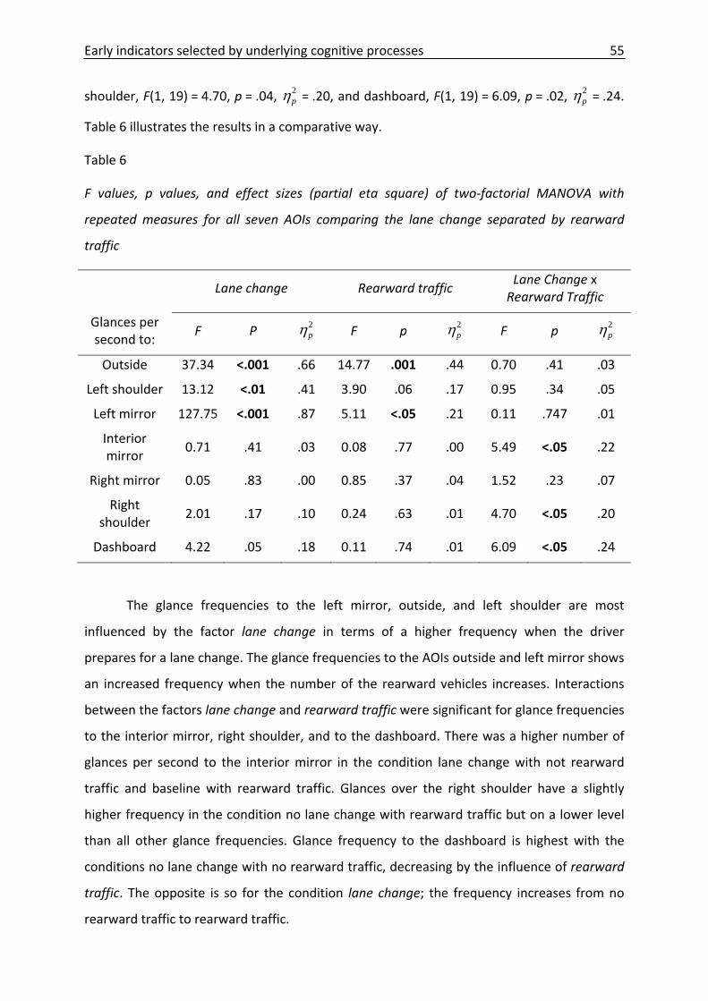
Early indicators selected by underlying cognitive processes   55 

shoulder, F(1, 19) = 4.70, p = .04,  2pη  = .20, and dashboard, F(1, 19) = 6.09, p = .02,  2

pη  = .24. 

Table 6 illustrates the results in a comparative way. 

Table 6 

F  values,  p  values,  and  effect  sizes  (partial  eta  square)  of  two‐factorial  MANOVA  with 

repeated measures  for  all  seven AOIs  comparing  the  lane  change  separated  by  rearward 

traffic 

  Lane change  Rearward traffic Lane Change x Rearward Traffic 

Glances per second to: 

F  P  2pη   F  p  2

pη   F  p  2pη  

Outside  37.34  <.001  .66  14.77 .001  .44  0.70  .41  .03 

Left shoulder  13.12  <.01  .41  3.90  .06  .17  0.95  .34  .05 

Left mirror  127.75 <.001  .87  5.11  <.05  .21  0.11  .747  .01 

Interior mirror 

0.71  .41  .03  0.08  .77  .00  5.49  <.05  .22 

Right mirror  0.05  .83  .00  0.85  .37  .04  1.52  .23  .07 

Right shoulder 

2.01  .17  .10  0.24  .63  .01  4.70  <.05  .20 

Dashboard  4.22  .05  .18  0.11  .74  .01  6.09  <.05  .24 

 

The  glance  frequencies  to  the  left  mirror,  outside,  and  left  shoulder  are  most 

influenced  by  the  factor  lane  change  in  terms  of  a  higher  frequency  when  the  driver 

prepares for a lane change. The glance frequencies to the AOIs outside and left mirror shows 

an  increased  frequency when  the number of  the  rearward vehicles  increases.  Interactions 

between the factors lane change and rearward traffic were significant for glance frequencies 

to the  interior mirror, right shoulder, and to the dashboard. There was a higher number of 

glances per  second  to  the  interior mirror  in  the  condition  lane  change with not  rearward 

traffic  and  baseline with  rearward  traffic. Glances  over  the  right  shoulder  have  a  slightly 

higher frequency in the condition no lane change with rearward traffic but on a lower level 

than  all other  glance  frequencies. Glance  frequency  to  the dashboard  is highest with  the 

conditions no lane change with no rearward traffic, decreasing by the influence of rearward 

traffic. The opposite  is  so  for  the condition  lane change;  the  frequency  increases  from no 

rearward traffic to rearward traffic.  

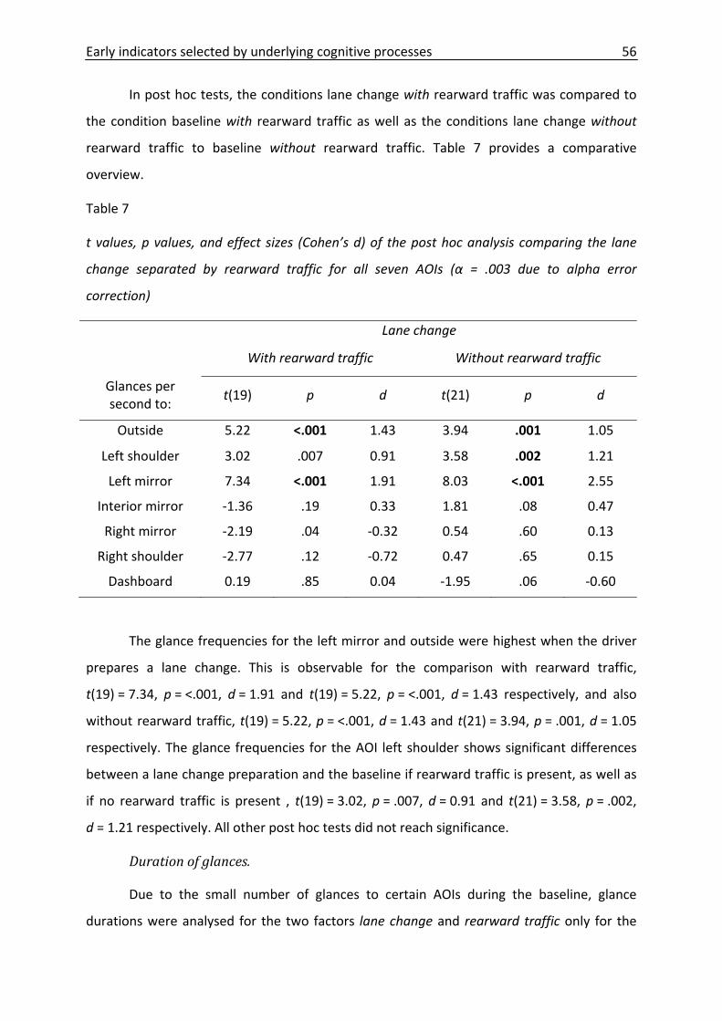
Early indicators selected by underlying cognitive processes   56 

In post hoc tests, the conditions  lane change with rearward traffic was compared to 

the condition baseline with  rearward  traffic as well as  the conditions  lane change without 

rearward  traffic  to  baseline  without  rearward  traffic.  Table  7  provides  a  comparative 

overview. 

Table 7 

t values, p values, and effect sizes  (Cohen’s d) of  the post hoc analysis comparing the  lane 

change  separated  by  rearward  traffic  for  all  seven  AOIs  (α  =  .003  due  to  alpha  error 

correction) 

  Lane change 

  With rearward traffic 

Without rearward traffic 

Glances per second to: 

t(19)  p  d 

t(21)  p  d 

Outside  5.22  <.001  1.43  3.94  .001  1.05 

Left shoulder  3.02  .007  0.91  3.58  .002  1.21 

Left mirror  7.34  <.001  1.91  8.03  <.001  2.55 

Interior mirror  ‐1.36  .19  0.33  1.81  .08  0.47 

Right mirror  ‐2.19  .04  ‐0.32  0.54  .60  0.13 

Right shoulder  ‐2.77  .12  ‐0.72  0.47  .65  0.15 

Dashboard  0.19  .85  0.04  ‐1.95  .06  ‐0.60 

 

The glance frequencies for the  left mirror and outside were highest when the driver 

prepares  a  lane  change.  This  is  observable  for  the  comparison  with  rearward  traffic, 

t(19) = 7.34,  p = <.001,  d = 1.91  and  t(19) = 5.22,  p = <.001,  d = 1.43  respectively,  and  also 

without rearward traffic, t(19) = 5.22, p = <.001, d = 1.43 and t(21) = 3.94, p = .001, d = 1.05 

respectively. The glance  frequencies  for the AOI  left shoulder shows significant differences 

between a lane change preparation and the baseline if rearward traffic is present, as well as 

if no  rearward  traffic  is present  ,  t(19) = 3.02, p = .007, d = 0.91  and  t(21) = 3.58, p = .002, 

d = 1.21 respectively. All other post hoc tests did not reach significance.  

Duration of glances. 

Due  to  the  small  number  of  glances  to  certain  AOIs  during  the  baseline,  glance 

durations were analysed  for  the  two  factors  lane change and  rearward  traffic only  for  the 

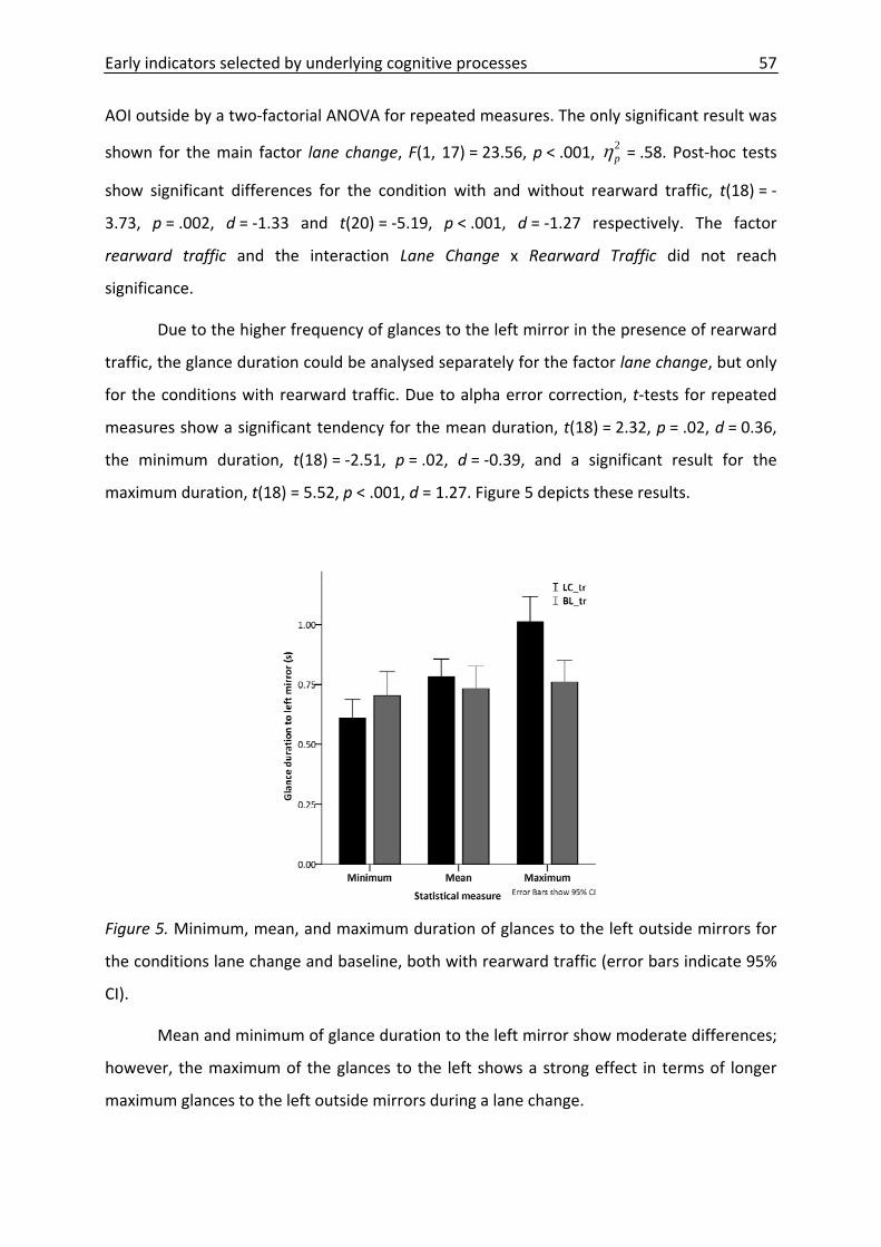
Early indicators selected by underlying cognitive processes   57 

AOI outside by a two‐factorial ANOVA for repeated measures. The only significant result was 

shown  for  the main  factor  lane change, F(1, 17) = 23.56, p < .001,  2pη  = .58. Post‐hoc  tests 

show  significant  differences  for  the  condition with  and without  rearward  traffic,  t(18) = ‐

3.73,  p = .002,  d = ‐1.33  and  t(20) = ‐5.19,  p < .001,  d = ‐1.27  respectively.  The  factor 

rearward  traffic  and  the  interaction  Lane  Change  x  Rearward  Traffic  did  not  reach 

significance.  

Due to the higher frequency of glances to the left mirror in the presence of rearward 

traffic, the glance duration could be analysed separately for the factor lane change, but only 

for the conditions with rearward traffic. Due to alpha error correction, t‐tests for repeated 

measures show a significant tendency for the mean duration, t(18) = 2.32, p = .02, d = 0.36, 

the  minimum  duration,  t(18) = ‐2.51,  p = .02,  d = ‐0.39,  and  a  significant  result  for  the 

maximum duration, t(18) = 5.52, p < .001, d = 1.27. Figure 5 depicts these results. 

 

 

Figure 5. Minimum, mean, and maximum duration of glances to the left outside mirrors for 

the conditions lane change and baseline, both with rearward traffic (error bars indicate 95% 

CI). 

Mean and minimum of glance duration to the left mirror show moderate differences; 

however, the maximum of the glances to the  left shows a strong effect  in terms of  longer 

maximum glances to the left outside mirrors during a lane change. 

Early indicators selected by underlying cognitive processes   58 

To prove the assumption that glance durations of glances to the left outside mirror in 

preparation for a  lane change are  longer  if there  is traffic than  if there  is no traffic present 

(see  Table  2),  both  lane  change  conditions  (with  and  without  rearward  traffic)  were 

compared.  Due  to  alpha  error  correction,  t‐tests  for  repeated  measures  show  only  a 

significant  results  for  the mean  duration,  t(19) = 2.72,  p < .05,  d = 0.50  and  the maximum 

duration, t(19) = 5.62, p < .001, d = 1.23.  

Car controls. 

According to the common measures of driver’s behaviour via car controls (Brookhuis 

et al., 2003) the following indicators were analysed: 

- Variance of the accelerator. 

- Variance of the brake. 

- Variance of the steering wheel. 

- Turn signal activation. 

Data of the pedals were available in terms of percentage of pedal‐course, and data of 

the  steering wheel  in  terms of degrees  in each direction. The activation of  the  turn  signal 

was measured in terms of off/left/right. 

Accelerator, brake pedal, and steering wheel. 

Figure  6  illustrates  the  variance  of  the  car  controls  accelerator,  brake  pedal,  and 

steering wheel. The accelerator shows a higher variance for all conditions compared to the 

brake and steering wheel. For the  indicators accelerator and brake, the highest variance  is 

observable in the condition lane change with rearward traffic and especially the accelerator 

shows a variance above 100%.  In  contrast,  the  steering wheel  shows only a variance of 2 

degrees, whereas it can span up to 360 degree. 

  

   

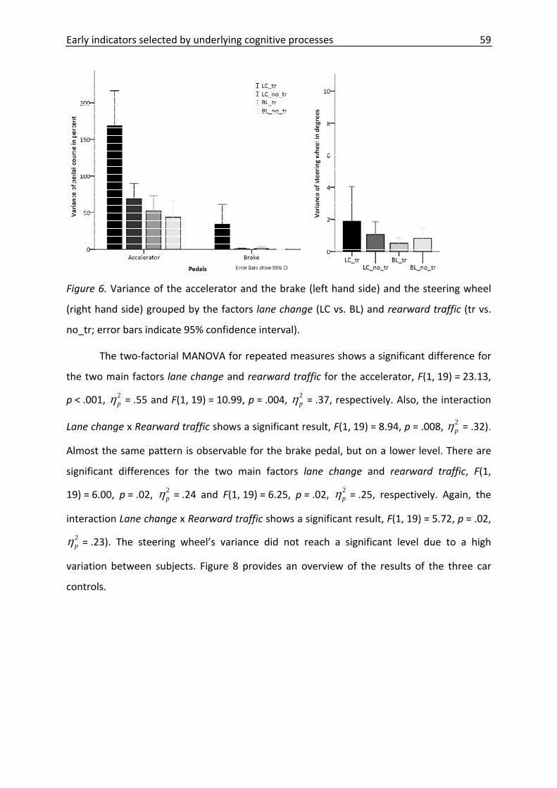
Early indicators selected by underlying cognitive processes   59 

   

Figure 6. Variance of the accelerator and the brake (left hand side) and the steering wheel 

(right hand side) grouped by the factors  lane change (LC vs. BL) and rearward traffic (tr vs. 

no_tr; error bars indicate 95% confidence interval). 

The two‐factorial MANOVA for repeated measures shows a significant difference for 

the two main factors  lane change and rearward traffic for the accelerator, F(1, 19) = 23.13, 

p < .001,  2pη  = .55 and F(1, 19) = 10.99, p = .004,  2

pη  = .37, respectively. Also, the  interaction 

Lane change x Rearward traffic shows a significant result, F(1, 19) = 8.94, p = .008,  2pη  = .32). 

Almost the same pattern  is observable for the brake pedal, but on a  lower  level. There are 

significant  differences  for  the  two  main  factors  lane  change  and  rearward  traffic,  F(1, 

19) = 6.00,  p = .02,  2pη  = .24  and  F(1, 19) = 6.25,  p = .02,  2

pη  = .25,  respectively.  Again,  the 

interaction Lane change x Rearward traffic shows a significant result, F(1, 19) = 5.72, p = .02, 

2pη  = .23).  The  steering  wheel’s  variance  did  not  reach  a  significant  level  due  to  a  high 

variation between  subjects.  Figure 8 provides  an overview of  the  results of  the  three  car 

controls. 

   

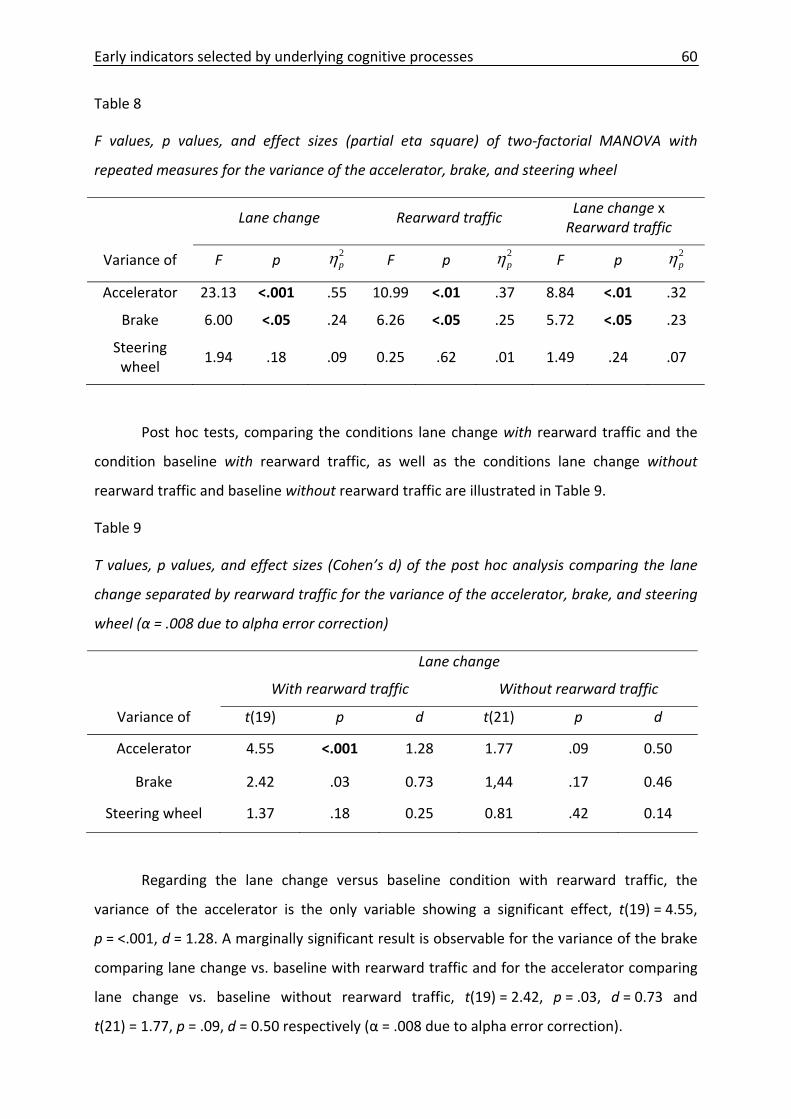
Early indicators selected by underlying cognitive processes   60 

Table 8 

F  values,  p  values,  and  effect  sizes  (partial  eta  square)  of  two‐factorial  MANOVA  with 

repeated measures for the variance of the accelerator, brake, and steering wheel  

  Lane change  Rearward traffic Lane change x Rearward traffic 

Variance of  F  p  2pη   F  p  2

pη   F  p  2pη  

Accelerator  23.13 <.001  .55  10.99 <.01  .37  8.84  <.01  .32 

Brake  6.00  <.05  .24  6.26  <.05  .25  5.72  <.05  .23 

Steering wheel 

1.94  .18  .09  0.25  .62  .01  1.49  .24  .07 

 

Post hoc  tests, comparing  the conditions  lane change with rearward  traffic and  the 

condition  baseline  with  rearward  traffic,  as  well  as  the  conditions  lane  change  without 

rearward traffic and baseline without rearward traffic are illustrated in Table 9. 

Table 9 

T values, p values, and effect sizes (Cohen’s d) of the post hoc analysis comparing the  lane 

change separated by rearward traffic for the variance of the accelerator, brake, and steering 

wheel (α = .008 due to alpha error correction) 

  Lane change 

  With rearward traffic Without rearward traffic

Variance of  t(19)  p  d t(21)  p  d 

Accelerator  4.55  <.001  1.28  1.77  .09  0.50 

Brake  2.42  .03  0.73  1,44  .17  0.46 

Steering wheel  1.37  .18  0.25  0.81  .42  0.14 

 

Regarding  the  lane  change  versus  baseline  condition  with  rearward  traffic,  the 

variance  of  the  accelerator  is  the  only  variable  showing  a  significant  effect,  t(19) = 4.55, 

p = <.001, d = 1.28. A marginally significant result is observable for the variance of the brake 

comparing lane change vs. baseline with rearward traffic and for the accelerator comparing 

lane  change  vs.  baseline  without  rearward  traffic,  t(19) = 2.42,  p = .03,  d = 0.73  and 

t(21) = 1.77, p = .09, d = 0.50 respectively (α = .008 due to alpha error correction).  

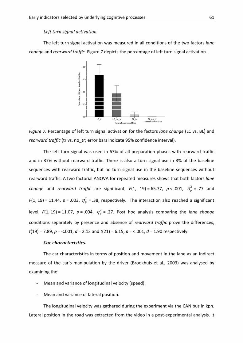
Early indicators selected by underlying cognitive processes   61 

Left turn signal activation. 

The left turn signal activation was measured in all conditions of the two factors lane 

change and rearward traffic. Figure 7 depicts the percentage of left turn signal activation. 

 

Figure 7. Percentage of left turn signal activation for the factors lane change (LC vs. BL) and 

rearward traffic (tr vs. no_tr; error bars indicate 95% confidence interval). 

The  left turn signal was used  in 67% of all preparation phases with rearward traffic 

and  in 37% without  rearward  traffic. There  is also a  turn  signal use  in 3% of  the baseline 

sequences with  rearward  traffic, but no  turn  signal use  in  the baseline sequences without 

rearward traffic. A two factorial ANOVA for repeated measures shows that both factors lane 

change  and  rearward  traffic  are  significant,  F(1,  19) = 65.77,  p < .001,  2pη  = .77  and 

F(1, 19) = 11.44, p = .003,  2pη  = .38,  respectively.   The  interaction also  reached a  significant 

level,  F(1, 19) = 11.07,  p = .004,  2pη  = .27.  Post  hoc  analysis  comparing  the  lane  change 

conditions  separately  by  presence  and  absence  of  rearward  traffic  prove  the  differences, 

t(19) = 7.89, p = <.001, d = 2.13 and t(21) = 6.15, p = <.001, d = 1.90 respectively. 

Car characteristics. 

The car characteristics  in terms of position and movement  in the  lane as an  indirect 

measure of  the  car’s manipulation by  the driver  (Brookhuis et al., 2003) was analysed by 

examining the: 

- Mean and variance of longitudinal velocity (speed). 

- Mean and variance of lateral position. 

The longitudinal velocity was gathered during the experiment via the CAN bus in kph. 

Lateral position in the road was extracted from the video in a post‐experimental analysis. It 

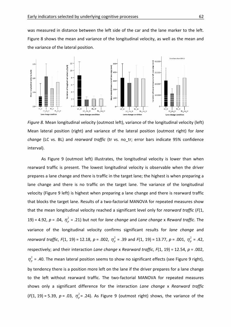
Early indicators selected by underlying cognitive processes   62 

was measured  in distance between the  left side of the car and the  lane marker to the  left. 

Figure 8 shows the mean and variance of the longitudinal velocity, as well as the mean and 

the variance of the lateral position.  

         

Figure 8. Mean longitudinal velocity (outmost left), variance of the longitudinal velocity (left) 

Mean  lateral  position  (right)  and  variance  of  the  lateral  position  (outmost  right)  for  lane 

change  (LC  vs.  BL)  and  rearward  traffic  (tr  vs.  no_tr;  error  bars  indicate  95%  confidence 

interval). 

As  Figure  9  (outmost  left)  illustrates,  the  longitudinal  velocity  is  lower  than when 

rearward  traffic  is present. The  lowest  longitudinal velocity  is observable when  the driver 

prepares a lane change and there is traffic in the target lane; the highest is when preparing a 

lane  change  and  there  is  no  traffic  on  the  target  lane.  The  variance  of  the  longitudinal 

velocity (Figure 9 left) is highest when preparing a lane change and there is rearward traffic 

that blocks the target lane. Results of a two‐factorial MANOVA for repeated measures show 

that the mean longitudinal velocity reached a significant level only for rearward traffic (F(1, 

19) = 4.92, p = .04,  2pη  = .21) but not for lane change and Lane change x Reward traffic. The 

variance  of  the  longitudinal  velocity  confirms  significant  results  for  lane  change  and 

rearward traffic, F(1, 19) = 12.18, p = .002,  2pη  = .39 and F(1, 19) = 13.77, p = .001,  2

pη  = .42, 

respectively; and their interaction Lane change x Rearward traffic, F(1, 19) = 12.54, p = .002, 

2pη  = .40. The mean lateral position seems to show no significant effects (see Figure 9 right), 

by tendency there is a position more left on the lane if the driver prepares for a lane change 

to  the  left  without  rearward  traffic.  The  two‐factorial MANOVA  for  repeated measures 

shows  only  a  significant  difference  for  the  interaction  Lane  change  x  Rearward  traffic 

(F(1, 19) = 5.39,  p = .03,  2pη = .24).  As  Figure  9  (outmost  right)  shows,  the  variance  of  the 

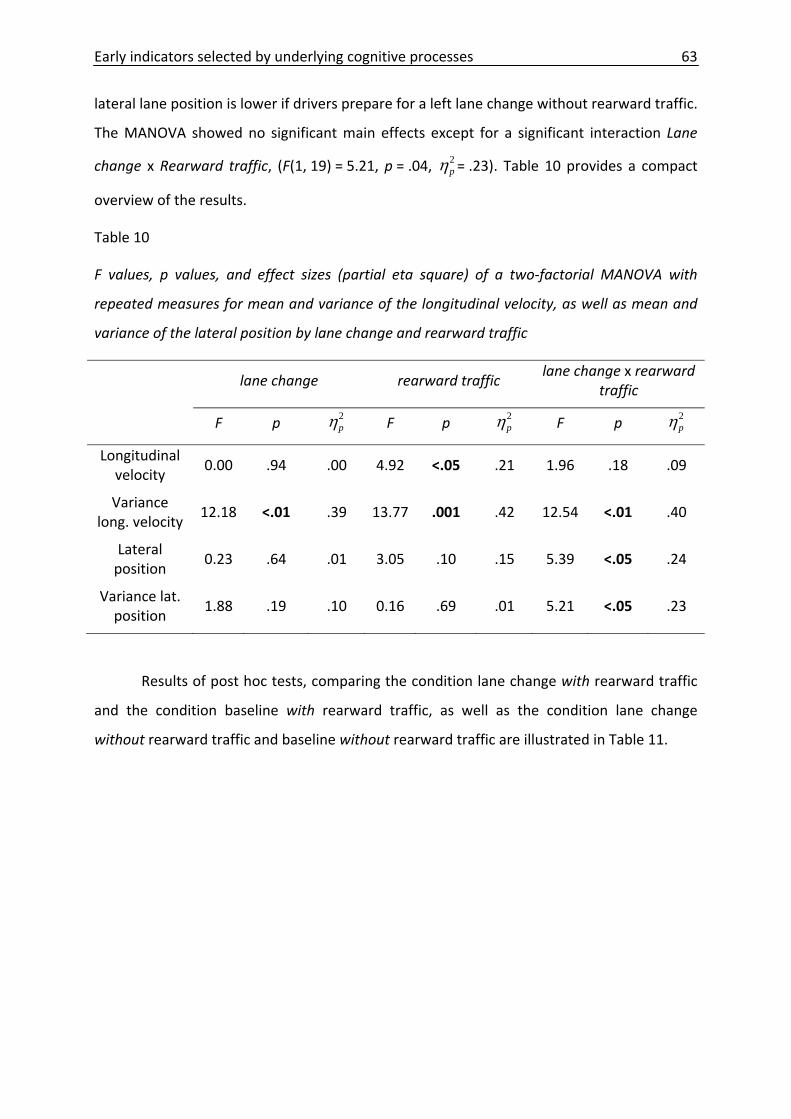
Early indicators selected by underlying cognitive processes   63 

lateral lane position is lower if drivers prepare for a left lane change without rearward traffic. 

The MANOVA  showed no  significant main effects except  for a  significant  interaction  Lane 

change  x Rearward  traffic,  (F(1, 19) = 5.21, p = .04,  2pη = .23). Table 10 provides a  compact 

overview of the results.  

Table 10 

F  values,  p  values,  and  effect  sizes  (partial  eta  square)  of  a  two‐factorial MANOVA with 

repeated measures for mean and variance of the  longitudinal velocity, as well as mean and 

variance of the lateral position by lane change and rearward traffic 

  lane change  rearward traffic lane change x rearward 

traffic 

  F  p  2pη   F  p  2

pη   F  p  2pη  

Longitudinal velocity 

0.00  .94  .00  4.92  <.05  .21  1.96  .18  .09 

Variance long. velocity 

12.18 <.01  .39  13.77 .001  .42  12.54  <.01  .40 

Lateral position 

0.23  .64  .01  3.05  .10  .15  5.39  <.05  .24 

Variance lat. position 

1.88  .19  .10  0.16  .69  .01  5.21  <.05  .23 

 

Results of post hoc tests, comparing the condition lane change with rearward traffic 

and  the  condition  baseline  with  rearward  traffic,  as  well  as  the  condition  lane  change 

without rearward traffic and baseline without rearward traffic are illustrated in Table 11. 

   

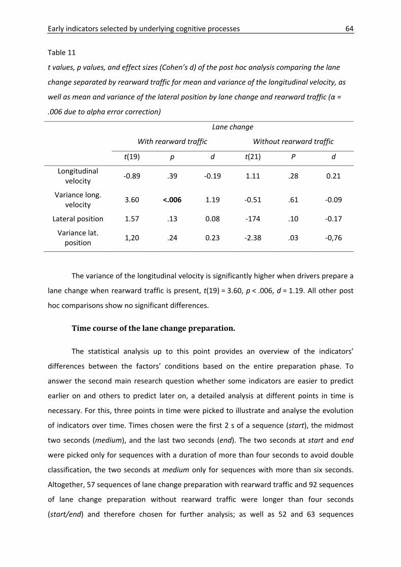
Early indicators selected by underlying cognitive processes   64 

Table 11 

t values, p values, and effect sizes (Cohen’s d) of the post hoc analysis comparing the lane 

change separated by rearward traffic for mean and variance of the longitudinal velocity, as 

well as mean and variance of the lateral position by lane change and rearward traffic (α = 

.006 due to alpha error correction) 

  Lane change 

  With rearward traffic 

Without rearward traffic 

  t(19)  p  d t(21)  P  d 

Longitudinal velocity 

‐0.89  .39  ‐0.19  1.11  .28  0.21 

Variance long. velocity 

3.60  <.006  1.19  ‐0.51  .61  ‐0.09 

Lateral position  1.57  .13  0.08  ‐174  .10  ‐0.17 

Variance lat. position 

1,20  .24  0.23  ‐2.38  .03  ‐0,76 

 

The variance of the longitudinal velocity is significantly higher when drivers prepare a 

lane change when rearward traffic  is present, t(19) = 3.60, p < .006, d = 1.19. All other post 

hoc comparisons show no significant differences. 

Time course of the lane change preparation.  

The  statistical  analysis  up  to  this  point  provides  an  overview  of  the  indicators’ 

differences  between  the  factors’  conditions  based  on  the  entire  preparation  phase.  To 

answer  the  second main  research question whether  some  indicators are easier  to predict 

earlier on  and others  to predict  later on,  a detailed  analysis at different points  in  time  is 

necessary. For this, three points  in time were picked to  illustrate and analyse the evolution 

of  indicators over time. Times chosen were the first 2 s of a sequence (start), the midmost 

two seconds  (medium), and  the  last  two seconds  (end). The  two seconds at start and end 

were picked only for sequences with a duration of more than four seconds to avoid double 

classification,  the  two seconds at medium only  for sequences with more  than six seconds. 

Altogether, 57 sequences of lane change preparation with rearward traffic and 92 sequences 

of  lane  change  preparation  without  rearward  traffic  were  longer  than  four  seconds 

(start/end)  and  therefore  chosen  for  further  analysis;  as  well  as  52  and  63  sequences 

Early indicators selected by underlying cognitive processes   65 

respectively of each category that were more than six seconds in length (medium). All two‐

second  sequences  at  the  start,  medium,  and  end  were  compared  with  corresponding 

baseline sequences of also two seconds in length, either with or without rearward traffic. 

To describe  the  three points  in  time,  the duration between  the  finish of each  two‐

second sequence (start/medium/end) and the beginning of the  lane change’s execution are 

summarised. The start sequence with rearward traffic finishes in mean 15.42 s (SD = 11.91 s) 

before the beginning of the  lane change’s execution, the  finish of a  lane change execution 

without  rearward  traffic  is  in mean  7.45 s  (SD = 4.94 s)  before  the  beginning  of  the  lane 

change’s execution. Medium  sequence of a  lane  change preparation with  rearward  traffic 

finish  in mean  8.2 s  (SD = 5.9 s)  before  the  beginning  of  the  lane  change’s  execution,  the 

finish of a  lane change execution without rearward traffic  in mean 4.78 s  (SD = 2.32 s). The 

end sequences finished directly before the execution’s starting point. 

Due  to  the  focus  of  the  timeline,  to  simplify  analysis,  and  to  avoid  repetition, 

statistical  comparisons were  only  calculated  between  the  factors  lance  change  and  time, 

separately for both types of the factor rearward traffic. Results are reported for the factor 

time,  the  interaction Time x Lane change, and  the post hoc comparisons  for each point  in 

time.  

Eye movements. 

Glance frequencies. 

A two‐factorial MANOVA for repeated measures and post hoc tests were computed 

to analyse differences between the three points in time. Figure 9 illustrates the time course 

for all seven AOIs. 

 

 

 

   

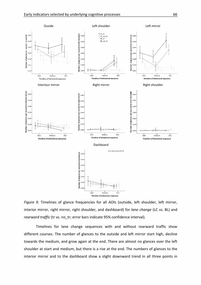
Early indicators selected by underlying cognitive processes   66 

Ouside  Left shoulder Left mirror 

 

Interiour mirror Right mirror Right shoulder 

 

  Dashboard  

   

Figure  9.  Timelines  of  glance  frequencies  for  all  AOIs  (outside,  left  shoulder,  left mirror, 

interior mirror, right mirror, right shoulder, and dashboard) for  lane change (LC vs. BL) and 

rearward traffic (tr vs. no_tr; error bars indicate 95% confidence interval). 

Timelines  for  lane  change  sequences  with  and  without  rearward  traffic  show 

different courses. The number of glances  to  the outside and  left mirror start high, decline 

towards the medium, and grow again at the end. There are almost no glances over the  left 

shoulder at start and medium, but there is a rise at the end. The numbers of glances to the 

interior mirror and  to  the dashboard  show a  slight downward  trend  in all  three points  in 

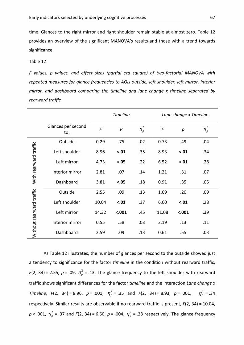
Early indicators selected by underlying cognitive processes   67 

time. Glances to the right mirror and right shoulder remain stable at almost zero. Table 12 

provides an overview of  the significant MANOVA’s  results and  those with a  trend  towards 

significance. 

Table 12 

F  values,  p  values,  and  effect  sizes  (partial  eta  square)  of  two‐factorial  MANOVA  with 

repeated measures for glance frequencies to AOIs outside,  left shoulder,  left mirror,  interior 

mirror,  and  dashboard  comparing  the  timeline  and  lane  change  x  timeline  separated  by 

rearward traffic 

    Timeline  Lane change x Timeline 

 Glances per second 

to: F  P  2

pη   F  p  2pη  

With

 rearw

ard traffic  Outside  0.29  .75  .02  0.73  .49  .04 

Left shoulder  8.96  <.01  .35  8.93  <.01  .34 

Left mirror  4.73  <.05  .22  6.52  <.01  .28 

Interior mirror  2.81  .07  .14  1.21  .31  .07 

Dashboard  3.81  <.05  .18  0.91  .35  .05 

With

out rearw

ard traffic 

Outside  2.55  .09  .13  1.69  .20  .09 

Left shoulder  10.04  <.01  .37  6.60  <.01  .28 

Left mirror  14.32  <.001  .45  11.08  <.001  .39 

Interior mirror  0.55  .58  .03  2.19  .13  .11 

Dashboard  2.59  .09  .13  0.61  .55  .03 

 

As Table 12 illustrates, the number of glances per second to the outside showed just 

a tendency to significance  for the  factor timeline  in the condition without rearward traffic, 

F(2, 34) = 2.55, p = .09,  2pη  = .13. The  glance  frequency  to  the  left  shoulder with  rearward 

traffic shows significant differences for the factor timeline and the interaction Lane change x 

Timeline,  F(2,  34) = 8.96,  p = .001,  2pη  = .35  and  F(2,  34) = 8.93,  p = .001,    2

pη  = .34 

respectively. Similar results are observable if no rearward traffic is present, F(2, 34) = 10.04, 

p < .001,  2pη  = .37 and F(2, 34) = 6.60, p = .004,  2

pη  = .28 respectively. The glance  frequency 

Early indicators selected by underlying cognitive processes   68 

to  the  left mirror  shows  the highest effect  size  for  the  factor  timeline and  the  interaction 

Lane change x Timeline  if no rearward traffic  is present, F(2, 34) = 14.32, p < .001,  2pη  = .45 

and  F(2,  34) = 11.08,  p < .001,  2pη  = .39  respectively.  If  rearward  traffic  is present  timeline 

and  Lane  change  x  Timeline  are  also  significant,  F(2,  34) = 4.73,  p = .02,  2pη  = .22  and 

F(2, 34) = 6.52, p = .004,  2pη  = .28 respectively. The number of glances to the  interior mirror 

show only a tendency to significance for the factor timeline with the presence of rearward 

traffic,  F(2,  34) = 2.81,  p = .07,  2pη  = .14.  Finally,  the  number  of  glances  to  the  dashboard 

show  a  significant  difference  for  the  factor  timeline  if  rearward  traffic  is  present  and  a 

significant  tendency  if no  rearward  traffic  is present,  F(2, 34) = 3.81, p = .03,  2pη  = .18 and 

F(2, 34) = 6.52, p = .09,  2pη  = .13.  

To prove  if there are reliable differences at the particular points  in time, post hoc t 

tests with corrected α‐error  (α = .001) were calculated. Table 13  illustrates  the results  in a 

comparative way. 

   

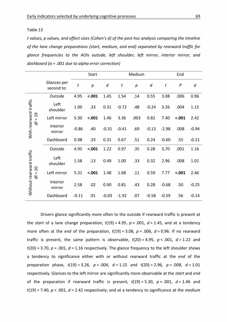
Early indicators selected by underlying cognitive processes   69 

Table 13 

t values, p values, and effect sizes (Cohen’s d) of the post hoc analysis comparing the timeline 

of the  lane change preparations (start, medium, and end) separated by rearward traffic for 

glance  frequencies  to  the  AOIs  outside,  left  shoulder,  left  mirror,  interior  mirror,  and 

dashboard (α = .001 due to alpha error correction) 

    Start  Medium  End 

 Glances per second to: 

t  p  d 

t  p  d 

t  P  d 

With

 rearw

ard traffic 

df = 19 

Outside  4.95  <.001 1.45  1.54  .14  0.55  3.08  .006  0.96 

Left shoulder 

1.00  .33  0.31  ‐0.72  .48  ‐0.24  3.26  .004  1.15 

Left mirror  5.30  <.001 1.46  3.36  .003  0.82  7.40  <.001  2.42 

Interior mirror 

‐0.86  .40  ‐0.31  ‐0.41  .69  ‐0.13  ‐2.98  .008  ‐0.94 

Dashboard  0.98  .33  0.31  0.67  .51  0.24  ‐0.60  .55  ‐0.21 

With

out rearw

ard traffic 

df = 20 

Outside  4.95  <.001 1.22  0.97  .35  0.28  3,70  .001  1.16 

Left shoulder 

1.58  .13  0.49  1.00  .33  0.32  2.96  .008  1.01 

Left mirror  5.31  <.001 1.48  1.68  .11  0.59  7.77  <.001  2.46 

Interior mirror 

2.58  .02  0.90  0.81  .43  0.28  ‐0.68  .50  ‐0.25 

Dashboard  ‐0.11  .91  ‐0.03  ‐1.92  .07  ‐0.58  ‐0.59  .56  ‐0.14 

 

Drivers glance significantly more often to the outside if rearward traffic is present at 

the  start  of  a  lane  change  preparation,  t(19) = 4.95,  p < .001,  d = 1.45,  and  at  a  tendency 

more  often  at  the  end  of  the  preparation,  t(19) = 3.08,  p = .006,  d = 0.96.  If  no  rearward 

traffic  is  present,  the  same  pattern  is  observable,  t(20) = 4.95,  p < .001,  d = 1.22  and 

t(20) = 3.70, p = .001, d = 1.16 respectively. The glance frequency to the left shoulder shows 

a  tendency  to  significance  either  with  or  without  rearward  traffic  at  the  end  of  the 

preparation  phase,  t(19) = 3.26,  p = .004,  d = 1.15  and  t(20) = 2.96,  p = .008,  d = 1.01 

respectively. Glances to the left mirror are significantly more observable at the start and end 

of  the  preparation  if  rearward  traffic  is  present,  t(19) = 5.30,  p < .001,  d = 1.46  and 

t(19) = 7.40, p < .001, d = 2.42 respectively; and at a tendency to significance at the medium 

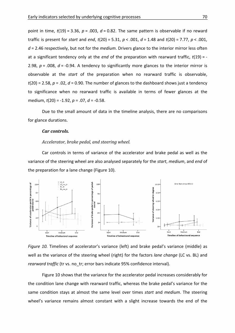
Early indicators selected by underlying cognitive processes   70 

point  in  time,  t(19) = 3.36, p = .003, d = 0.82. The  same pattern  is observable  if no  reward 

traffic  is present for start and end, t(20) = 5.31, p < .001, d = 1.48 and t(20) = 7.77, p < .001, 

d = 2.46 respectively, but not for the medium. Drivers glance to the interior mirror less often 

at a significant  tendency only at  the end of  the preparation with  rearward  traffic,  t(19) = ‐

2.98, p = .008, d = ‐0.94. A  tendency  to  significantly more glances  to  the  interior mirror  is 

observable  at  the  start  of  the  preparation  when  no  rearward  traffic  is  observable, 

t(20) = 2.58, p = .02, d = 0.90. The number of glances to the dashboard shows just a tendency 

to  significance  when  no  rearward  traffic  is  available  in  terms  of  fewer  glances  at  the 

medium, t(20) = ‐1.92, p = .07, d = ‐0.58. 

Due to the small amount of data  in the timeline analysis, there are no comparisons 

for glance durations. 

Car controls. 

Accelerator, brake pedal, and steering wheel. 

Car controls  in  terms of variance of  the accelerator and brake pedal as well as  the 

variance of the steering wheel are also analysed separately for the start, medium, and end of 

the preparation for a lane change (Figure 10).  

 

Figure 10. Timelines of accelerator’s variance  (left) and brake pedal’s variance  (middle) as 

well as the variance of the steering wheel (right) for the factors lane change (LC vs. BL) and 

rearward traffic (tr vs. no_tr; error bars indicate 95% confidence interval). 

Figure 10 shows that the variance for the accelerator pedal increases considerably for 

the condition lane change with rearward traffic, whereas the brake pedal’s variance for the 

same condition  stays at almost  the  same  level over  times start and medium. The  steering 

wheel’s  variance  remains  almost  constant with  a  slight  increase  towards  the  end  of  the 

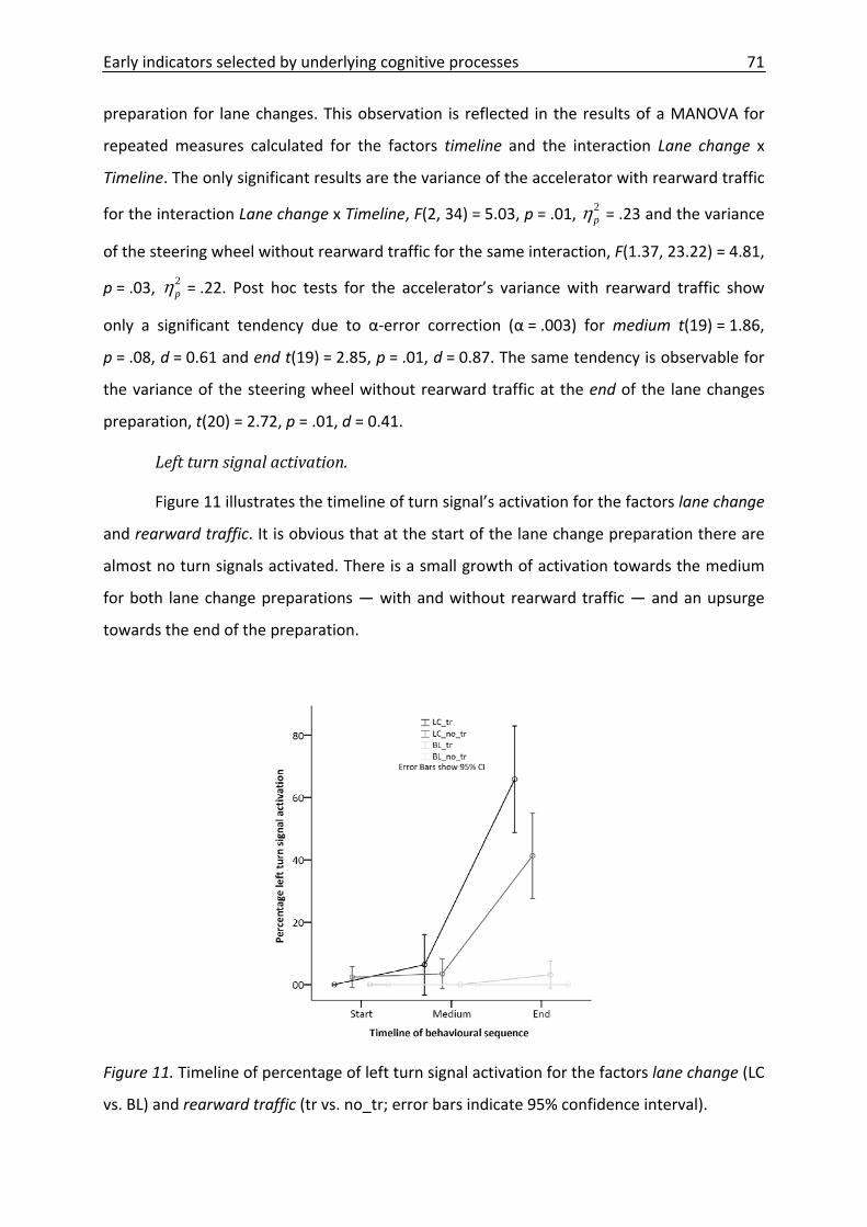
Early indicators selected by underlying cognitive processes   71 

preparation  for  lane changes. This observation  is reflected  in the results of a MANOVA  for 

repeated measures  calculated  for  the  factors  timeline  and  the  interaction  Lane  change  x 

Timeline. The only significant results are the variance of the accelerator with rearward traffic 

for the interaction Lane change x Timeline, F(2, 34) = 5.03, p = .01,  2pη  = .23 and the variance 

of the steering wheel without rearward traffic for the same interaction, F(1.37, 23.22) = 4.81, 

p = .03,  2pη  = .22.  Post  hoc  tests  for  the  accelerator’s  variance with  rearward  traffic  show 

only  a  significant  tendency  due  to  α‐error  correction  (α = .003)  for medium  t(19) = 1.86, 

p = .08, d = 0.61 and end t(19) = 2.85, p = .01, d = 0.87. The same tendency is observable for 

the variance of the steering wheel without rearward traffic at the end of the  lane changes 

preparation, t(20) = 2.72, p = .01, d = 0.41. 

Left turn signal activation. 

Figure 11 illustrates the timeline of turn signal’s activation for the factors lane change 

and rearward traffic. It is obvious that at the start of the lane change preparation there are 

almost no turn signals activated. There  is a small growth of activation towards the medium 

for both  lane change preparations — with and without rearward traffic — and an upsurge 

towards the end of the preparation.  

 

 

Figure 11. Timeline of percentage of left turn signal activation for the factors lane change (LC 

vs. BL) and rearward traffic (tr vs. no_tr; error bars indicate 95% confidence interval). 

Early indicators selected by underlying cognitive processes   72 

An  ANOVA  for  repeated measures  shows  significant  results  in  the  condition with 

rearward traffic for timeline and Lane change x Timeline, F(2, 34) = 29.15, p < .001,  2pη  = .63 

and F(2, 34) = 27.71, p < .001,  2pη  = .62  respectively. Post hoc  tests show significant  results 

only  for  the end of  the preparation with  rearward  traffic,  t(19) = 7.10, p = <.001, d = 1.92. 

Almost the same pattern  is observable  for turn signal’s activation  in the condition without 

rearward traffic for timeline and  lane change x timeline, F(2, 34) = 24.14, p < .001,  2pη  = .59 

and  F(2, 34) = 24.14,  p < .001,  2pη  = .59  respectively.  Post‐hoc  tests  again  show  only 

significant differences for end, t(20) = 5.92, p = <.001, d = 1.83. 

Car characteristics. 

A MANOVA  for  repeated measures  analysing  the mean  longitudinal  velocity,  the 

variation  of  the  longitudinal  velocity,  the mean  lateral  position,  and  the  variation  of  the 

lateral  position  showed  no  significant  differences  for  either  the  factor  timeline  or  the 

interaction lane change x timeline. 

Selection of candidate indicators for prediction of lane change preparation. 

After analysing all potential  indicators,  the  final candidate  indicators were  selected 

based on the results of either the whole sequence of lane change preparation or for the first 

2 s.  The  latter  selection  is  important  for  knowing  which  indicator  is  able  to  infer  the 

preparation  for  a  lane  change  at  the  onset  of  the  cognitive  involvement  of  the  driver. 

Selection criterion  is an effect size  ≥ 0.8  (≤  ‐0.8), which  is  regarded as “high” according  to 

common conventions (e.g., Sedlmeier & Renkewitz, 2007). Selected candidate indicators are 

listed  in Table 14 and ordered by the effect size d either for the whole sequence or for the 

first two seconds.  

   

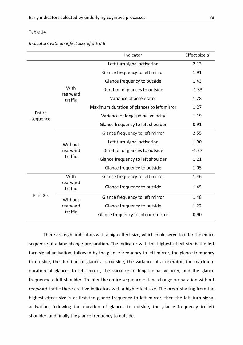
Early indicators selected by underlying cognitive processes   73 

Table 14 

Indicators with an effect size of d ≥ 0.8 

    Indicator  Effect size d 

Entire sequence 

With rearward traffic 

Left turn signal activation  2.13 

Glance frequency to left mirror  1.91 

Glance frequency to outside  1.43 

Duration of glances to outside  ‐1.33 

Variance of accelerator  1.28 

Maximum duration of glances to left mirror  1.27 

Variance of longitudinal velocity  1.19 

Glance frequency to left shoulder  0.91 

Without rearward traffic 

Glance frequency to left mirror  2.55 

Left turn signal activation  1.90 

Duration of glances to outside  ‐1.27 

Glance frequency to left shoulder  1.21 

Glance frequency to outside  1.05 

First 2 s 

With rearward traffic 

Glance frequency to left mirror  1.46 

Glance frequency to outside  1.45 

Without rearward traffic 

Glance frequency to left mirror  1.48 

Glance frequency to outside  1.22 

Glance frequency to interior mirror  0.90 

 

There are eight indicators with a high effect size, which could serve to infer the entire 

sequence of a  lane change preparation. The  indicator with the highest effect size  is the  left 

turn signal activation, followed by the glance frequency to left mirror, the glance frequency 

to outside,  the duration of  glances  to outside,  the  variance of  accelerator,  the maximum 

duration  of  glances  to  left mirror,  the  variance  of  longitudinal  velocity,  and  the  glance 

frequency to left shoulder. To infer the entire sequence of lane change preparation without 

rearward traffic there are five indicators with a high effect size. The order starting from the 

highest  effect  size  is  at  first  the  glance  frequency  to  left mirror,  then  the  left  turn  signal 

activation,  following  the  duration  of  glances  to  outside,  the  glance  frequency  to  left 

shoulder, and finally the glance frequency to outside.  

Early indicators selected by underlying cognitive processes   74 

To infer only the start of the preparation for a lane change, there are only indicators 

from the  field of eye movements.  If there  is rearward traffic, only the glance  frequency to 

the left mirror and outside show a high effect size. If there is no rearward traffic the glance 

frequency to the left mirror, outside, and the interior mirror show a high effect size. 

The  next  chapter  of  this  article  tests  these  indicators  as  predictors  to  infer  lane 

change preparation either based on the entire sequence or based on the first two seconds. 

Prediction of the Lane change Preparation Based on Potential Candidate 

Indicators 

The aim of the second part of this analysis is to prove the benefit of all pre‐selected 

indicators to  infer the preparation for a  lane change. This  is feasible  in two different ways. 

On the one hand, so‐called “offline” detection performs the  inference based on the entire 

behavioural  sequence.  This  procedure  proves  the  power  of  each  indicator,  but  it  is  not 

capable of inferring in real‐time. On the other hand, “online” detection infers the behaviour 

at an early stage of the behavioural sequence, in this case based on the first 2 s.  

To determine the quality of each indicator to infer the preparation for a lane change, 

the receiver operating characteristic (ROC curve) from signal detection theory is used (Egan, 

1975). The ROC curve plots  the sensitivity  (true positive  rate, hit  rate) versus 1 – specifity 

(false alarm rate, 1 – true negative rate, false positive rate) for a binary classifier system (see 

Figure 13). If the classifier is perfect, sensitivity and specifity reach 1 (100%).  The ROC curve 

then  crosses  the  point  0,  1  and  the  area  below  the  curve  is  equal  to  one. A  completely 

random  guess  would  give  a  point  along  a  diagonal  line  (the  so‐called  line  of  no‐

discrimination) from the left bottom to the top right corners (ROC area of .5). ROC curves for 

all indicators with a high effect size (see table 14) are plotted and the size of the area below 

the curve is reported.  

Predicting Power Based on the Entire Sequence (Offline) 

At first, indicators with a high effect sizes were used to predict the whole sequence, 

the  offline  detection.  They  are  plotted  separately  for  the  conditions  with  and  without 

rearward traffic. 

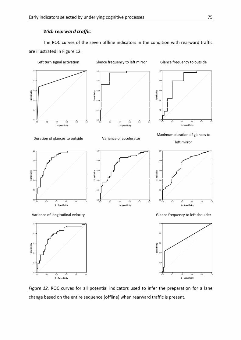
Early indicators selected by underlying cognitive processes   75 

With rearward traffic. 

The ROC curves of the seven offline  indicators in the condition with rearward traffic 

are illustrated in Figure 12.  

Left turn signal activation  Glance frequency to left mirror Glance frequency to outside

 

Duration of glances to outside  Variance of accelerator Maximum duration of glances to 

left mirror 

 

Variance of longitudinal velocity  Glance frequency to left shoulder

 

 

Figure 12. ROC  curves  for  all potential  indicators used  to  infer  the preparation  for  a  lane 

change based on the entire sequence (offline) when rearward traffic is present. 

 

Early indicators selected by underlying cognitive processes   76 

All indicators are able to predict the entire preparation sequence to a certain extent 

with different hit‐rate (sensitivity) and false alarm rates (1 – specifity). Table 15 summarises 

all seven indicators, sorted by the size of the area below the ROC curve.  

Table 15 

ROC area, threshold, sensitivity, and 1 – specifity for all potential indicators used to infer the 

preparation for a lane change based on the entire sequence (offline) when rearward traffic is 

present 

Indicator  ROC area  Threshold  Sensitivity  1 ‐ Specifity 

Glance frequency to left mirror  .93  > 0.20 s‐1  .72  .02 

Duration of glances to outside  .84  < 1.88 s  .69  .18 

Left turn signal activation  .82  on/off  .67  .03 

Glance frequency to outside  .80  > 0.30 s‐1 .79  .20 

Variance of longitudinal velocity  .77  > 1.67 kph  .69  .23 

Variance of accelerator  .76  > 6.35%  .71  .28 

Maximum duration of glances to left mirror 

.72  > 0.82 s  .76  .37 

Glance frequency to left shoulder  .69  > 0.01 s‐1  .43  .03 

 

The  glance  frequency  to  the  left  outside mirror  is  the most  valuable  indicator  for 

inferring  the  preparation  for  a  lane  change  based  on  the  entire  behavioural  sequence.  It 

exceeds all other  indicators  in  terms of  sensitivity and  specifity. An analysis of alternative 

thresholds showed that all lane change preparations to the left are connected to at least one 

glance  to  the  left outside mirror  (threshold > 0.03  s‐1,  sensitivity = 1.00, 1 – Specifity = .53) 

and  97%  of  all  lane  change  preparations  can  be  inferred with  a  false  alarm  rate  of  18% 

(threshold > 0.10  s‐1).  The  duration  of  glances  to  the  outside,  left  turn  signal  activation, 

glance  frequency  to outside, variance of  longitudinal velocity, variance of accelerator, and 

maximum duration of glances to left mirror follow. Left turn signal activation has the lowest 

sensitivity  (.67),  but  also  the  lowest  false  alarm  rate  (1  –  Specifity = .03).  The  highest 

sensitivity has the number of glances per second to outside (.79), but also a high 1 – Specifity 

(.20).  The  highest  false  alarm  rate  is  observable  at  the  indicator maximum  duration  of 

glances to left mirror (1 – Specifity = .37). 

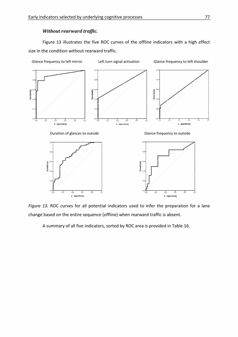
Early indicators selected by underlying cognitive processes   77 

Without rearward traffic. 

Figure 13  illustrates  the  five ROC curves of  the offline  indicators with a high effect 

size in the condition without rearward traffic. 

Glance frequency to left mirror  Left turn signal activation Glance frequency to left shoulder

 

Duration of glances to outside Glance frequency to outside 

   

Figure 13. ROC  curves  for  all potential  indicators used  to  infer  the preparation  for  a  lane 

change based on the entire sequence (offline) when rearward traffic is absent. 

A summary of all five indicators, sorted by ROC area is provided in Table 16. 

   

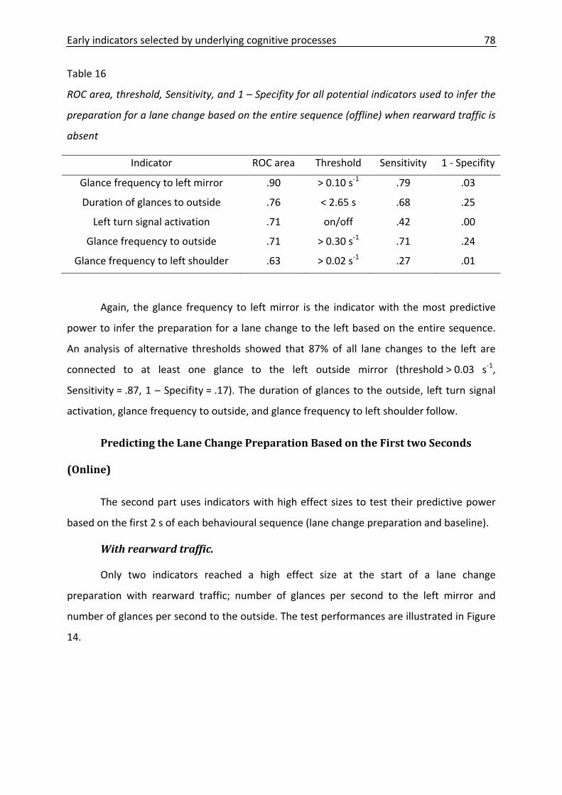
Early indicators selected by underlying cognitive processes   78 

Table 16 

ROC area, threshold, Sensitivity, and 1 – Specifity for all potential indicators used to infer the 

preparation for a lane change based on the entire sequence (offline) when rearward traffic is 

absent 

Indicator  ROC area  Threshold  Sensitivity  1 ‐ Specifity 

Glance frequency to left mirror  .90  > 0.10 s‐1  .79  .03 

Duration of glances to outside  .76  < 2.65 s  .68  .25 

Left turn signal activation  .71  on/off  .42  .00 

Glance frequency to outside  .71  > 0.30 s‐1 .71  .24 

Glance frequency to left shoulder  .63  > 0.02 s‐1  .27  .01 

  

Again,  the glance  frequency  to  left mirror  is  the  indicator with  the most predictive 

power to  infer the preparation for a  lane change to the  left based on the entire sequence. 

An  analysis of  alternative  thresholds  showed  that  87% of  all  lane  changes  to  the  left  are 

connected  to  at  least  one  glance  to  the  left  outside  mirror  (threshold > 0.03  s‐1, 

Sensitivity = .87, 1 – Specifity = .17). The duration of glances to the outside,  left turn signal 

activation, glance frequency to outside, and glance frequency to left shoulder follow. 

Predicting the Lane Change Preparation Based on the First two Seconds 

(Online)  

The second part uses  indicators with high effect sizes to test their predictive power 

based on the first 2 s of each behavioural sequence (lane change preparation and baseline).  

With rearward traffic. 

Only  two  indicators  reached  a  high  effect  size  at  the  start  of  a  lane  change 

preparation with  rearward  traffic;  number  of  glances  per  second  to  the  left mirror  and 

number of glances per second to the outside. The test performances are illustrated in Figure 

14.  

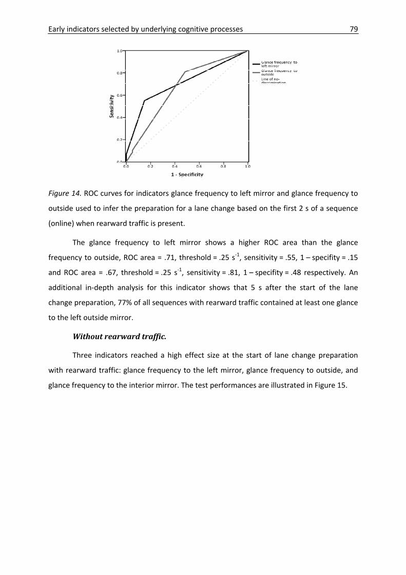
Early indicators selected by underlying cognitive processes   79 

 

Figure 14. ROC curves for indicators glance frequency to left mirror and glance frequency to 

outside used to infer the preparation for a lane change based on the first 2 s of a sequence 

(online) when rearward traffic is present. 

The  glance  frequency  to  left  mirror  shows  a  higher  ROC  area  than  the  glance 

frequency to outside, ROC area =  .71, threshold = .25 s‐1, sensitivity = .55, 1 – specifity = .15 

and ROC area =  .67,  threshold = .25  s‐1,  sensitivity = .81, 1 – specifity = .48  respectively. An 

additional  in‐depth  analysis  for  this  indicator  shows  that  5  s  after  the  start  of  the  lane 

change preparation, 77% of all sequences with rearward traffic contained at least one glance 

to the left outside mirror.  

Without rearward traffic. 

Three  indicators  reached a high effect  size at  the  start of  lane  change preparation 

with rearward traffic: glance frequency to the  left mirror, glance frequency to outside, and 

glance frequency to the interior mirror. The test performances are illustrated in Figure 15. 

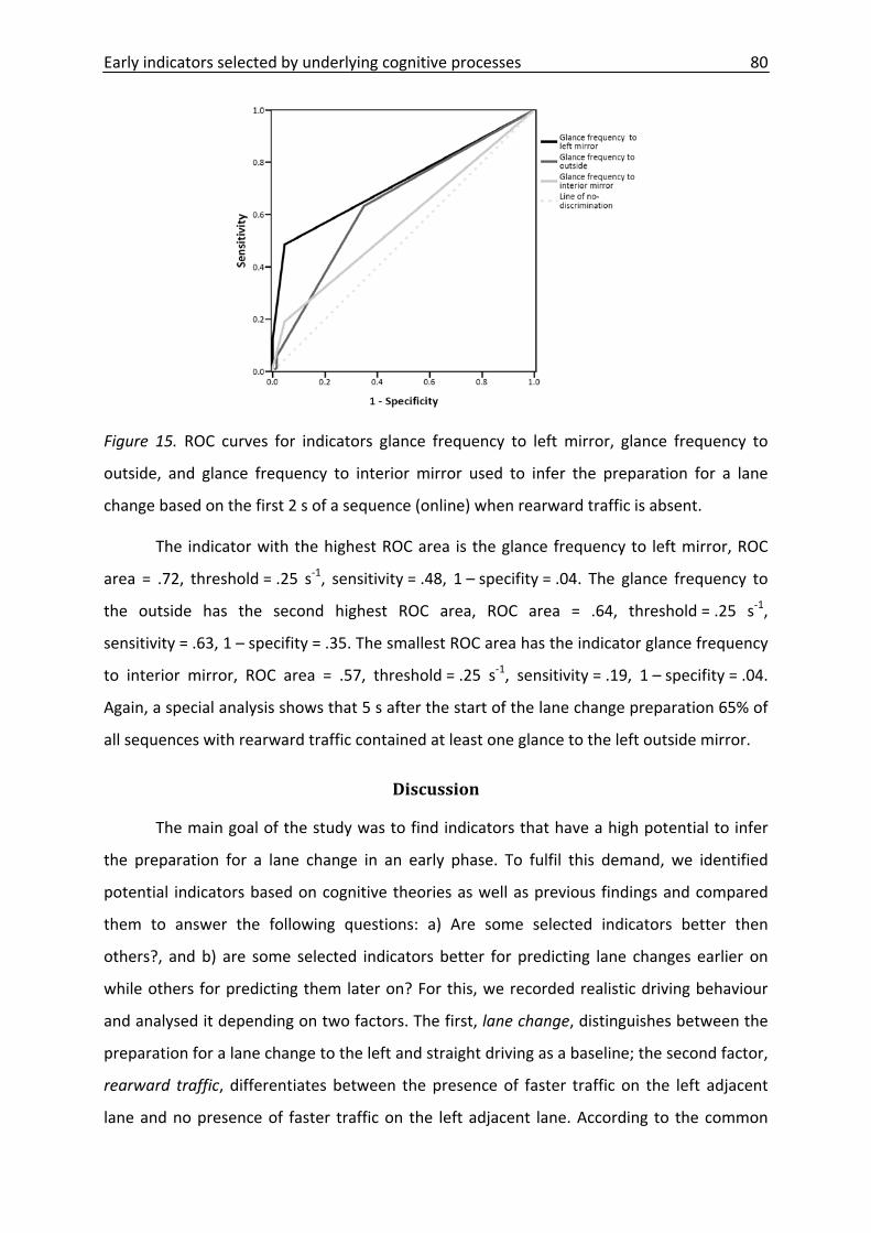
Early indicators selected by underlying cognitive processes   80 

 

Figure  15.  ROC  curves  for  indicators  glance  frequency  to  left mirror,  glance  frequency  to 

outside,  and  glance  frequency  to  interior mirror  used  to  infer  the  preparation  for  a  lane 

change based on the first 2 s of a sequence (online) when rearward traffic is absent. 

The  indicator with the highest ROC area  is the glance  frequency to  left mirror, ROC 

area =  .72,  threshold = .25  s‐1,  sensitivity = .48, 1 – specifity = .04.  The  glance  frequency  to 

the  outside  has  the  second  highest  ROC  area,  ROC  area  =  .64,  threshold = .25  s‐1, 

sensitivity = .63, 1 – specifity = .35. The smallest ROC area has the indicator glance frequency 

to  interior mirror,  ROC  area  =  .57,  threshold = .25  s‐1,  sensitivity = .19,  1 – specifity = .04. 

Again, a special analysis shows that 5 s after the start of the lane change preparation 65% of 

all sequences with rearward traffic contained at least one glance to the left outside mirror. 

Discussion  

The main goal of the study was to find  indicators that have a high potential to  infer 

the  preparation  for  a  lane  change  in  an  early  phase.  To  fulfil  this  demand, we  identified 

potential  indicators based on cognitive theories as well as previous  findings and compared 

them  to  answer  the  following  questions:  a)  Are  some  selected  indicators  better  then 

others?, and b) are  some  selected  indicators better  for predicting  lane  changes earlier on 

while others for predicting them  later on? For this, we recorded realistic driving behaviour 

and analysed it depending on two factors. The first, lane change, distinguishes between the 

preparation for a lane change to the left and straight driving as a baseline; the second factor, 

rearward  traffic, differentiates between  the presence of  faster  traffic on  the  left adjacent 

lane and no presence of  faster  traffic on  the  left adjacent  lane. According  to  the common 

Early indicators selected by underlying cognitive processes   81 

measures  of  driver  behaviour,  we  preselected  potential  indicators  from  three  different 

sources  for  analysis: eye movements,  car  controls, and  car  characteristics. The process of 

analysis was sub‐divided  into  two steps: At  first, we used  typical methods  from  inferential 

statistics to discover indicators which differentiate between lane change and no lane change 

with high effect sizes, separated by the presence or absence of rearward traffic. In a second 

step,  we  used  the  indicators  with  a  high  effect  size  as  predictors  for  a  lane  change 

preparation.  Both  analyses  were  carried  out  based  on  an  average  over  the  entire 

behavioural  sequence  (lane  change  preparation  or  baseline),  as well  as  based  on  several 

specific points in time during the sequence (the first, medium, and last 2 s).  

A General Description of Driving Behaviour Preparing a Lane Change Manoeuvre 

Based on our data, we can describe the whole process of the preparation as follows: 

A slow leading vehicle caused a desire to change lanes in 87% of all cases. In some of these 

cases the desire ends due to situational reasons (11%). The first behavioural reflection of the 

desire  is measurable  though  increasing  glance  frequencies  to  the  left  outside mirror,  the 

outside,  and  the  interior mirror  (the  final AOI only without  rearward  traffic)  and  through 

decreasing  duration  of  glances  to  the  outside.  At  the  end  of  the  preparation  for  a  lane 

change manoeuvre (before the start of the lateral movement to the adjacent lane) the turn 

signal is used in 67% of all lane change preparations with and 37% without rearward traffic. 

Around the same time, drivers start to look over their shoulder to check for vehicles directly 

beside  their own car  (43% with and 27% without rearward  traffic).  If drivers prepare  for a 

lane  change  and  the  left  adjacent  lane  (target  lane)  is  blocked  by  rearward  traffic,  the 

pressure  to  adapt  their  speed  to  that  of  the  slow  leading  vehicle  is measurable  by  an 

increased variance of the accelerator pedal (release and press), a slightly increased variance 

in  the  brake  pedal  (press  and  release)  resulting  in  a  reduced  longitudinal  velocity.  In  the 

similar situation but without rearward traffic, the driver moves faster than in normal driving 

situations (baseline) and there are no significant differences in the use of the accelerator and 

brake pedal.  

In addition to what  is mentioned above, there  is an  influence of rearward traffic on 

glance behaviour. Drivers tend to glance to the  left mirror and to the  interior mirror more 

often if there is oncoming rearward traffic on the left adjacent lane, even if there is no desire 

to change  lanes. Finally, glances  to  the  left outside mirror  seem  to have  longer maximum 

Early indicators selected by underlying cognitive processes   82 

durations  if  there  is  a  desire  to  change  lanes  compared  to  the  baseline  condition, when 

rearward traffic is present.  

Indicators to Predict the Entire Sequence 

Based on cognitive theories  (Norman & Shallice, 1986; Salvucci, 2006) and previous 

findings  (Bhise  et  al.,  1981;  Henning  et  al.,  2006;  Nunes  &  Recarte,  2005;  Olsen,  2003; 

Robinson et al., 1972; Tijerina et al., 2005) several  indicators were assumed to have a high 

potential to predict the preparation for a lane change manoeuvre. Such a high potential was 

assumed for glances to the left mirror and the left blind spot from eye movements; from car 

controls the variances of the accelerator and brake pedal and the turn signal; and from car 

dynamics the longitudinal velocity.  

We  were  able  to  prove  these  assumptions  by  conducting  the  present  study.  To 

predict  the  lane  change  preparation,  the  indicator with  the most  power  is  the  increased 

glance frequency to the  left mirror, which could predict between 87% and 97% of all cases 

with a false alarm rate of around 18%. Following this are the decreased duration of glances 

to  the  outside,  the  left  turn  signal  activation,  and  the  increased  glance  frequency  to  the 

outside.  In driving  situations with  the presence of  rearward  traffic on  the  adjacent  lanes, 

there  is a higher variance of the  longitudinal velocity, a higher variance of the accelerator, 

and  the  higher  maximum  duration  of  glances  to  left  mirror.  All  of  these  are  powerful 

indicators.  The  glance  frequency  to  the  left  blind  spot  increased  so  that  43%  of  all  lane 

change preparations with and 27% without rearward traffic can be inferred with a very low 

false alarm rate (around 2%). In general, eye glance behaviour seems to be more powerful to 

predict  a  lane  change  preparation  than  indicators  from  the  sources  car  control  and  car 

characteristics. An exception is turn signal activation; however, it predicts only about half to 

two‐thirds of all cases and it is only used at a very late point in the preparation phase. 

Indicators to Predict Within the First Two Seconds 

If the task is to predict the lane change within the first two seconds, indicators merely 

from the field of eye glance behaviour have the power to predict a lane change preparation. 

There is an increased glance frequency to the left mirror, to the outside, and in the case of 

an absence of rearward traffic, there is also an increasing frequency of glances to the interior 

mirror when drivers start to prepare for a lane change. After two seconds, there was at least 

Early indicators selected by underlying cognitive processes   83 

one  glance  to  the  left outside mirror  in 55% of  all  cases with  and 48% without  rearward 

traffic. Moreover,  after  five  seconds,  in  77%  of  lane  change  preparations with  and  65% 

without rearward traffic drivers glanced to the left mirror at least one time. False alarms for 

glances to the left mirror are at 15% for the condition with rearward traffic and 4% without 

rearward traffic. 

Indicators with Potential for Later Prediction 

Some indicators are usable to predict lane change preparations later than within the 

first  two seconds. For  instance,  the  turn signal  is used by  the driver mostly within  the  last 

two  seconds;  glances  to  the  left  blind  spot  are  also  observable  in  that  time.  Figure  10 

indicates that in the lane change condition with rearward traffic, drivers use the brake pedal 

first  and  later  the  accelerator,  but  only  the  accelerator  shows  significant  differences  in 

variance compared to the baseline conditions.   

Ineffective Indicators 

The  analysis  reveals  that  there  are  two  indicators with  no  potential  to  infer  lane 

change preparation, the steering wheel and the lateral position in the lane. These indicators 

might have their potential to infer the execution of a lane change manoeuvre (e.g., Hetrick, 

1997), but not during the preparation for a lane change.  

An  indicator which  seems  to have  some potential  (d = 0.73) but  failed  to meet  the 

criteria to test the prediction (d ≥ .8) is the variance of the brake pedal. This indicator could 

be useful in connection with the accelerator pedal in the condition with rearward traffic.  

Influence of Rearward Traffic on Glance Behaviour 

Traffic  in the  left adjacent  lane (target  lane)  influenced the glance behaviour to the 

left outside mirror in two ways. If there was traffic, and there was no desire to change lanes, 

the  glance  frequency was  higher  than  if  there  was  no  traffic.  The  same  is  true  for  the 

comparison  between  presence  and  absence  of  rearward  traffic  if  there  is  a  slow  leading 

vehicle.  The  second  influence  is  the  glance  duration.  If  the  driver  is  preparing  for  a  lane 

change with rearward traffic, the mean and maximum glance duration is significantly higher 

than if drivers are preparing for a lane change and there is no rearward traffic present. 

Early indicators selected by underlying cognitive processes   84 

Results in the Light of Cognitive Theories  

Cognitive theories were the basis for describing and selecting  indicators which were 

tested  in  this  study.  The  assumptions  of  the  theories  could  be  proved  by means  of  the 

results. Furthermore, there are some results that could potentially  improve the theories  in 

some points.  

Concerning the SAS theory of Norman and Shallice (1986) of action selection, there 

are  a  few  results  from  human  observers  that  support  their  predictions.  A  slow  leading 

vehicle  can  serve  as  a  trigger  for  a  lane  change  in  around  87%  of  all  cases, which  is  an 

indicator  of  contention  scheduling.  The  observation  that  drivers  discarded  the  desire  to 

change lanes due to situational reasons in 11% of cases, which also means an experimenter 

asking the driver to abort the lane change and to use the next exit, supports the supervisory 

attentional system.  

The  predictions  based  on  the  driver  model  from  Salvucci  (2006)  could  all  be 

confirmed. This is the case for the glance behaviour during the preparation for a lane change 

as well as for the mirror‐glances during the baseline. Also, the adaptation of the longitudinal 

velocity to the slow leading vehicle in the case of the target lane being blocked is predicted 

by the model. Moreover, there are  links to extend the model. The  first point concerns the 

diversity  of  glance  locations;  the model  should  be  able  to  differentiate  between  the  left, 

interior,  and  right mirrors.  Additionally,  glances  to  the  blind  spots  are  eligible  for  being 

considered. Another link concerns the glance behaviour to the left outside mirror in terms of 

bottom up and top down processes. During the preparation for a lane change to the left with 

no rearward traffic the glances are more characterisable as top down processes (information 

seeking), whereas the glance behaviour to the left outside mirror during the period with no 

lane  change  intention  but  rearward  traffic  points more  for  bottom  up  processes.  These 

processes  are  implemented  to  a  certain  degree  via  the  random  sampling  of  the mirrors 

(monitoring). This  leads  to mirror glances during  the baseline, but  it  is  independent of  the 

occurrence of rearward traffic in the target lane. Thus, the model should somehow react to 

an  increase  in surrounding  traffic by an  increase  in  random mirror sampling. A  third point 

concerns the differences in glance durations. Drivers glance in the left outside mirror if they 

want to prepare for a lane change and there is rearward traffic on the adjacent lane longer 

than  if  there  is  rearward  traffic but  they do not prepare  for a  lane  change. A meaningful 

Early indicators selected by underlying cognitive processes   85 

implementation  in  the  driver  model  should  provide  a  theoretical  explanation  for  these 

findings.  

Limitation of the Study 

The  study  has  some  limitations  which  will  be  discussed  in  this  paragraph.  One 

limitation  of  the  study  is  the measure  of  a  slow  leading  vehicle  by means  of  a  “human 

sensor” This procedure is not as objective as a “real” sensor could be. However, the distance 

to the leading vehicle is not a common signal in cars (CAN) and up until now, these systems 

have not been as reliable as they should be, especially when detecting cars in far distances in 

real‐time (for an overview, see Zehang, Bebis, & Miller, 2006). Another limitation, associated 

with the previous one, could be the nature of the data as not “naturalistic” enough. A real 

“naturalistic driving study” means that there is no experimenter in the car (e.g., Dingus et al., 

2006).  However,  the  marking  of  the  slow  leading  vehicle  was  only  possible  due  to  an 

experimenter. Nevertheless, driving behaviour with the presence of an observer can still be 

regarded  as  “normal”  behaviour.  Research  has  shown  that  results with  an  experimenter 

joining the driver are comparable to normal driving (Hjälmdahl & Várhelyi, 2004).  

Further Research 

Looking  forward,  further  research could be concentrated  towards  two directions. A 

more  technical  one would  be  to  combine  the  indicators with  the  help  of  an  appropriate 

algorithm  (e.g., Hidden Markov Models, Rabiner, 1989). The  findings of  the present  study 

could also be applied to a technical system, which should be able to predict the preparation 

for a slow leading lane change as early as possible. This system should highly rely on an eye 

tracking or head tracking system to track glances to at least the left outside mirror (Doshi & 

Trivedi,  2008;  Robinson  et  al.,  1972).  Another way  of  building  an  algorithm  to  infer  the 

preparation for a  lane change  is to use the cognitive driver model (Salvucci, 2006). Salvucci 

et al. (2007) already developed an algorithm to infer the lane change execution based on the 

cognitive driver model. The  system  simulates  a  set of possible driver  intentions  and  their 

resulting behaviours using a simplification of the cognitive driver model that was based on 

sensor data only (glance behaviour was unconsidered). A first step could be to improve the 

model  as previously described  and use  it  similarly  to  Salvucci et  al.  (2007). Another  issue 

concerns  the use of a  slow  leading  vehicle  itself  (see also Bar‐Gera &  Shinar, 2005). New 

Early indicators selected by underlying cognitive processes   86 

technologies  like car  to car communication might  improve  the  reliability of detecting slow 

leading vehicles and the information could be used as another early indicator to predict the 

preparation for a lane change (e.g., van Arem, van Driel, & Visser, 2006). 

Another research  issue concerns  the use of  the glances  to  the  left mirror. They are 

the  earliest  behavioural  indicator  of  the  lane  change  preparation.  Is  there  some  hidden 

potential  in the glance duration? What  influences their occurrence and their duration? Are 

there parts of the process to establish situational awareness,  like some authors propose as 

an essential part of the driving task (Baumann & Krems, 2007; Gugerty, 1997)?  

Acknowledgment   

This  project  was  granted  by  the  European  Union  and  was  part  of  Network  of 

Excellence  (NOE) HUMANIST  (human  centred  design  for  information  society  technologies 

applied to road transport). Gratitude to the team at INRETS, Lyon for the maintenance of the 

instrumented  vehicle  and  the  support  in  conducting  the  study,  the  coders  at  Chemnitz 

University of Technology,  and  the  team  that was  responsible  for  the  image processing. A 

special thank‐you to Katja Mehlhorn for her fruitful comments on the paper.   

Early indicators selected by underlying cognitive processes   87 

References  

Anderson,  J.  R.,  Bothell,  D.,  Byrne, M.  D.,  Douglass,  S.,  Lebiere,  C., & Qin,  Y.  (2004).  An 

integrated theory of the mind. Psychological Review, 111(4), 1036‐1060.  

Bar‐Gera,  H.,  &  Shinar,  D.  (2005).  The  tendency  of  drivers  to  pass  other  vehicles. 

Transportation Research Part F, 8, 429‐439.  

Baumann, M., & Krems, J. F. (2007). Situation awareness and driving: A cognitive model. In C. 

Cacciabue &  C.  Re  (Eds.), Modelling  driver  behaviour  in  automotive  environments. 

Critical  issues  in advanced automotive systems and human‐centred design  (pp. 253‐

265). London: Springer.  

Bhise, V. D., Meldrum, J., Jack, D., Troell, G., Hoffmeister, D., & Forbes, L. (1981). Driver head 

movements  in  left  outside mirror  sampling  (SAE  paper  810761). Warrendale,  PA: 

Society of Automotive Engineers. 

Blaschke,  C.,  Schmitt,  J.,  &  Färber,  B.  (2008).  Überholmanöver‐Prädiktion  über  CAN‐Bus‐

Daten. Automobiltechnische Zeitschrift, 11, 1022‐1028.  

Boer, E. R. (1999). Car following from the driver's perspective. Transportation Research Part 

F: Traffic Psychology and Behaviour, 2(4), 201‐206.  

Brackstone, M., & McDonald, M.  (1999). Car‐following: A historical  review. Transportation 

Research Part F: Traffic Psychology and Behaviour, 2(4), 181‐196.  

Brackstone, M., McDonald, M., & Wu,  J.  (1998).  Lane  changing on  the motorway: Factors 

affecting  its  occurrence,  and  their  implications.  Paper  presented  at  the  Road 

Transport  Information  and  Control,  1998.  9th  International  Conference  on  (Conf. 

Publ. No. 454). 

Brandt, T., Sattel, T., & Bohm, M. (2007). Combining haptic human‐machine interaction with 

predictive  path  planning  for  lane‐keeping  and  collision  avoidance  systems.  Paper 

presented at the Intelligent Vehicles Symposium, 2007 IEEE. 

Brookhuis, K. A., de Waard, D., &  Fairclough,  S. H.  (2003). Criteria  for driver  impairment. 

Ergonomics, 46(5), 433.  

Chandraratna,  S., &  Stamatiadis, N.  (2003). Problem driving maneuvers of elderly drivers. 

Transportation  Research  Record:  Journal  of  the  Transportation  Research  Board, 

1843(‐1), 89‐95.  

Chattington,  M.,  Wilson,  M.,  Ashford,  D.,  &  Marple‐Horvat,  D.  (2007).  Eye–steering 

coordination in natural driving. Experimental Brain Research, 180(1), 1‐14.  

Early indicators selected by underlying cognitive processes   88 

Chovan,  J.  D.,  Tijerina,  L.,  Alexander,  G.,  &  Hendricks,  D.  L.  (1994).  Examination  of  lane 

change crashes and potential IVHS countermeasures. (DOT HS 808 071). Washington, 

DC:  U.S.  Department  of  Transportation,  National  Highway  Traffic  Safety 

Administration. 

Dingus, T. A., Klauer, S. G., Neale, V. L., Petersen, A., Lee, S. E., Sudweeks, J., et al. (2006). The 

100‐car naturalistic driving study, phase  II  ‐ Results of  the 100‐car  field experiment. 

DOT HS 810 593, National Highway Traffic Safety Administration. 

Doshi, A., & Trivedi, M. (2008). A comparative exploration of eye gaze and head motion cues 

for  lane  change  intent  prediction.  Paper  presented  at  the  Intelligent  Vehicles 

Symposium, 2008 IEEE. 

Duchowski, A. (2007). Eye tracking methodology ‐ Theory and practice. London: Springer. 

Egan, J. P. (1975). Signal detection theory and ROC‐analysis. New York: Academic Press. 

Farsi,  M.,  Ratcliff,  K.,  &  Barbosa,  M.  (1999).  An  overview  of  controller  area  network. 

Computing & Control Engineering Journal, 10(3), 113‐120.  

Fastenmeier,  W.,  Hinderer,  J.,  Lehnig,  U.,  &  Gstalter,  H.  (2001).  Analyse  von 

Spurwechselvorgängen im Verkehr. Zeitschrift für Arbeitswissenschaft, 55, 15‐23.  

Gipps,  P. G.  (1986). A model  for  the  structure  of  lane‐changing  decisions.  Transportation 

Research Part B: Methodological, 20(5), 403‐414.  

Gugerty, L. J.  (1997). Situation awareness during driving: explicit and  implicit knowledge  in 

dynamic spatial memory. Journal of experimental Psychology: Applied, 3(1), 42‐66.  

Henning, M.  J.  (2004).  Indikatoren  zur  Fahrerabsichtserkennung  ‐  Das  Blickverhalten  bei 

Spurwechselvorgängen.  Diploma  Thesis,  Chemnitz  University  of  Technology, 

Chemnitz.    

Henning, M.  J.,  Schweigert, M.,  Baumann, M., &  Krems,  J.  F.  (2006).  Eye‐glance  patterns 

during lane change manoeuvres. Paper presented at the Vision in Vehicles 11, Dublin, 

Ireland. 

Hetrick, S. (1997). Examination of driver lane change behavior and the potential effectiveness 

of warning  onset  rules  for  lane  change  or  "side"  crash  avoidance  systems.  Thesis, 

Virginia Polytechnic Institute & State University, Blacksburg, VA.    

Hjälmdahl, M., & Várhelyi, A. (2004). Validation of  in‐car observations, a method for driver 

assessment. Transportation Research Part A, 38(2), 127‐142.  

Early indicators selected by underlying cognitive processes   89 

Joon Woong, L. (2002). A machine vision system for  lane‐departure detection. Comput. Vis. 

Image Underst., 86(1), 52‐78. doi: http://dx.doi.org/10.1006/cviu.2002.0958 

Kiefer,  R.  J., &  Hankey,  J. M.  (2008).  Lane  change  behavior with  a  side  blind  zone  alert 

system. Accident Analysis & Prevention, 40(2), 683‐690.  

Kopf, M. (2005). Was nützt es dem Fahrer, wenn Fahrerinformations‐ und ‐assistenzsysteme 

etwas über  ihn wissen?  In M. Maurer & C. Stiller (Eds.), Fahrerassistenzsysteme mit 

maschineller Wahrnehmung (pp. 117‐139). Berlin: Springer Verlag.  

McCall,  J. C., Wipf, D. P., Trivedi, M. M., & Rao, B. D.  (2007).  Lane  change  intent analysis 

using robust operators and sparse bayseian learning. IEEE Transactions on Intelligent 

Transportation Systems (IST), 8, 431‐440.  

McKnight,  J.,  &  Adams,  B.  (1970).  Driver  education  and  task  analysis  volume  1:  Task 

descriptions. Department of Transportation, National Highway Safety Bureau. 

Norman, D. A., &  Shallice, T.  (1986). Attention  to action: Willed and automatic  control of 

behavior. In R. J. Davidson, G. E. Schwartz & D. Shapiro (Eds.), Consciousness and Self‐

Regulation, Advances in Research and Theory (pp. 1‐18).  

Nunes, L. M., & Recarte, L. A.  (2005). Speed,  traffic complexity, and visual performance: a 

study on open road. In G. Underwood (Ed.), Traffic and transport psychology: Theory 

and application (pp. 339‐354). Amsterdam: Elsevier.  

Oliver, N., & Pentland, A. P.  (2000). Graphical models  for driver behavior  recognition  in a 

smartcar.  Paper  presented  at  the  IEEE  Intelligent  Vehicles  Symposium  2000, 

Dearborn (MI), USA. 

Olsen,  E.  C.  B.  (2003).  Modeling  slow  lead  vehicle  lane  changing.  Dissertation,  Virginia 

Polytechnic Institute and State University, Blacksburg VA.    

Piechulla, W., Mayser, C., Gehrke, H., & König, W. (2003). Reducing drivers' mental workload 

by means  of  an  adaptive man‐machine  interface.  Transportation  Research  Part  F: 

Traffic Psychology and Behaviour, 6(4), 233‐248.  

Rabiner,  L.  R.  (1989).  A  tutorial  on  hidden markov models  and  selected  applications  in 

speech recognition. Proceedings of the IEEE 77(2), 257‐285.  

Robinson, G. H., Erickson, D., Thurston, G., & Clark, R.  (1972). Visual search by automobile 

drivers. Human Factors, 14(4), 315‐323.  

Salvucci, D. D. (2006). Modeling driver behavior  in a cognitive architecture. Human Factors, 

48(2), 362‐380.  

Early indicators selected by underlying cognitive processes   90 

Salvucci, D. D., Mandalia, H. M., Kuge, N., & Yamamura, T.  (2007).  Lane‐change detection 

using a computational driver model. Human Factors, 49(3), 532‐542.  

Schiessl,  C.  (2008).  Continuous  subjective  strain  measurement.  IET  Intelligent  Transport 

Systems, 2(2), 161‐169.  

Sedlmeier, P., & Renkewitz, F. (2007). Forschungsmethoden und Statistik in der Psychologie. 

München: Pearson. 

Statistisches  Bundesamt.  (2008).  Verkehr  ‐  Verkehrsunfälle.  (Fachserie  8  Reihe  7). 

Wiesbaden: Statistisches Bundesamt. 

Tijerina, L., Garrott, W. R., Stoltzfus, D., & Parmer, E. (2005). Eye glance behavior of van and 

passenger car drivers during  lange change decision phase. Transportation Research 

Record, 1937, 37‐43.  

Tipping, M. E. (2001). Sparse bayesian  learning and the relevance vector machine. J. Mach. 

Learn. Res., 1, 211‐244.  

van Arem, B.,  van Driel, C.  J. G., & Visser, R.  (2006).  The  impact  of  cooperative  adaptive 

cruise control on traffic‐flow characteristics. Intelligent Transportation Systems, IEEE 

Transactions on, 7(4), 429‐436.  

Zadeh, L. A. (1965). Fuzzy sets. Information control, 8, 338‐353.  

Zehang,  S.,  Bebis,  G.,  &  Miller,  R.  (2006).  On‐road  vehicle  detection:  a  review.  Pattern 

Analysis and Machine Intelligence, IEEE Transactions on, 28(5), 694‐711.  

 

 

Mental representation of rearward traffic in visuo‐spatial working memory   91 

 

 

 

 

 

Is Mental Representation of Rearward Traffic in Visuo‐spatial Working Memory Static 

or Dynamic in Lane Changing? 

 

 

Matthias J. Henning, Susi Beyreuther, and Josef F. Krems 

Chemnitz University of Technology 

 

 

 

 

 

   

Mental representation of rearward traffic in visuo‐spatial working memory   92 

Abstract 

The  goal  of  the  study  is  to  examine  processes  involved  in  holding  information  about 

rearward  traffic  in  working  memory.  It  was  proposed  that  rearward  traffic  information 

(rather spatial), should interfere most with spatial tasks. The more dynamic rearward traffic 

is in terms of higher speed, the more dynamic the mental representation of rearward traffic 

should be, and the more  it should  interfere with the dynamic version of secondary tasks. A 

driving simulator study was conducted where 30 participants carried out  lane changes with 

rearward traffic in the target lane. Before lane change preparation, participants memorised 

one of  five  secondary  tasks  (visual‐static, visual‐dynamic,  spatial‐static, or  spatial‐dynamic, 

phonological).  After  lane  change  execution,  they  were  asked  to  recall  the  memorised 

material.  In  contrast  to  the  hypotheses,  results  indicate  that  information  about  rearward 

traffic  interfered most with  visual  tasks. A  possible  explanation  could  be  that  the  driving 

scenario was too predictable and participants memorised information about rearward traffic 

more in terms of a picture (car vs. no car). Further research could work with a more dynamic 

and unpredictable driving scenario. 

Mental representation of rearward traffic in visuo‐spatial working memory   93 

Is Mental Representation of Rearward Traffic in Visuo‐spatial Working Memory Static or 

Dynamic in Lane Changing? 

Imagine driving on a crowded highway with a slow‐moving vehicle in front of you. In 

approaching the vehicle, you consider overtaking it via the left lane. However, a high number 

of  faster  cars  travelling  in  the  left  lane  require  you  to  decide  immediately  if  a  safe  lane 

change is possible. If a gap of sufficient dimension opens in the adjacent lane, you can then 

initiate a lane change. If not, you memorise observed rearward vehicles in the left lane and 

wait until they have passed.  

The  lane  change  scenario  described  above  is  a  common  situation  on  multi‐lane 

highways (Brackstone, McDonald, & Wu, 1998). Statistically, it carries with it an inherent risk 

of accidents,  for example,  in 2007 12% of all severe accidents without  injuries on German 

highways were  associated with  lane  change manoeuvres  (Statistisches Bundesamt,  2008), 

13.7% with light injuries, 10.6% with severe injuries, and 8.2% with deaths. Chovan, Tijerina, 

Alexander,  and  Hendricks  (1994)  reported  that  the major  cause  of  lane  change  related 

accidents  is  driver  unawareness  of  vehicles  in  the  adjacent  lane.  In  the  process  of 

maintaining  awareness  of  the  driving  situation,  Baumann  and  Krems  (2007)  argue  that 

working memory might play a key role.  

Currently,  it  is  not  fully  understood  which  components  of  working  memory  are 

involved  in memorising  information  about  vehicles  in  the  left  lane  (i.e.,  rearward  traffic) 

temporarily, and if the storage and recall process can be disrupted by other information that 

is similar in modality.  

Lane Change Manoeuvres 

The process of lane change manoeuvring is described by several lane change models 

(Chovan et al., 1994; Fastenmeier, Hinderer, Lehnig, & Gstalter, 2001; Olsen, 2003; Salvucci, 

2006).  It  is  normally  divided  into  at  least  two  steps:  preparation  and  execution. When 

preparing  a  lane  change,  drivers  scan  their mirrors  and  blind  spots  to  check  for  faster 

rearward and adjacent traffic. If the available gap in the adjacent lane is sufficient, the driver 

switches on the turn signal and starts the lane change by turning the steering wheel. If not, 

he waits for a sufficient gap. All  lane change models  include scanning behaviour to mirrors 

and blind spots. Early research has shown that  lane changes to the  left are associated with 

Mental representation of rearward traffic in visuo‐spatial working memory   94 

glances  to  the  left outside mirror  (e.g., Robinson, Erickson, Thurston, & Clark, 1972). Only 

one model  includes  the memory  processes  involved  in  the  preparation  of  a  lane  change 

(Salvucci, 2006), which  is  implemented  in a cognitive architecture  (ACT‐R, Anderson et al., 

2004). In his model, Salvucci simulates the behaviour of driving a standard mid‐sized vehicle 

on a two‐lane highway with moderate traffic and distinguishes between lane keeping, curve 

negotiation  and  lane  changing  (both  left  and  right).  The  model  contains  three  main 

components: control, monitoring and decision making. The control component manages the 

perception of  low‐level visual cues and the manipulation of vehicle controls for  lateral and 

longitudinal  control  (steering, acceleration and braking). The monitoring  component deals 

with the continued maintenance of situation awareness by visually sampling lanes (own and 

other) to the front and via mirrors to the back (i.e., four positions in total) randomly, with a 

certain probability. The information gathered by these monitoring activities is stored in ACT‐

R memory and  is defined as an unspecified chunk  in declarative memory  that decays over 

time.  The  third  component  decision  making  uses  the  information  gathered  during 

monitoring  to determine  if  any  tactical decision  should be made,  such  as  the decision  to 

change  lanes.  If  the  goal  is  to  change  lanes,  information  about  traffic  on  the  target  lane 

available in memory is used to decide whether the lane change can be accomplished or not. 

If the model finds any information about a nearby car in the target lane in memory, it aborts 

the lane change process. If there is no information about traffic in the target lane available in 

declarative memory, the model rechecks the target lane (to the front and via mirrors to the 

back).  This  double‐checking  is  necessary  due  to  decay  processes  in memory;  that  is,  the 

model might have  “forgotten”  that  there are any  cars  in  the  target  lane. After perceiving 

information about traffic on the target lane, two alternatives remain. If there is no car in the 

target  lane,  the  model  starts  a  lane  change  by  adjusting  visual  attention  from  the 

participant’s own lane to the other lane and begins the actual steering process. If there are 

cars in the target lane, the model keeps checking the mirrors until the gap in the target lane 

is sufficient to initiate a lane change as described previously. 

Salvucci’s  (2006) model provides a theoretical  framework, which postulates the use 

of mental representation  in the display of rearward traffic while changing  lanes  in working 

memory to maintain situational awareness.  

   

Mental representation of rearward traffic in visuo‐spatial working memory   95 

Situational Awareness and Working Memory  

According to Endsley (1988), situation awareness is defined as “he perception of the 

elements in the environment within a volume of time and space, the comprehension of their 

meaning, and the projection of their status in the near future” (p. 97), or shorter, ‘knowing 

what  is going on’  (Endsley, 1995, p. 36). Originally developed  in  the aviation domain,  the 

idea  of  situation  awareness was  recently  introduced  to  the  field  of  driving  (Baumann & 

Krems, 2007;  L. Gugerty,  in press). Most  theoretical  frameworks associated with  situation 

awareness  involve working memory  as  a  critical  part  of maintaining  situation  awareness 

(Adams, Tenney, & Pew, 1995; Baumann & Krems, 2007; Endsley, 1995; L. J. Gugerty, 1997). 

For instance, Baumann and Krems (2007) emphasise the role of long‐term working memory, 

a  concept  introduced  by  Ericsson  and  Kintsch  (1995) who  postulate  the  use  of working 

memory  based  on  long‐term memory  in maintaining  situational  awareness.  In  a  recent 

simulator study that employed a high‐density driving scenario, Baumann, Franke, and Krems 

(2008; Franke, 2008) were able to show that experienced drivers can overcome limitations in 

working memory by using  long‐term working memory  structures  to  store  information. An 

approach to the study of the connection between situation awareness in the driving domain 

and the concept of working memory (Baddeley & Hitch, 1974)  is provided by Jóhannsdóttir 

(2005).  The  Baddeley  and  Hitch  (1974)  model  consists  of  three  components:  the 

phonological  loop,  the  central  executive,  and  the  visuo‐spatial  sketchpad.  Jóhannsdóttir 

(2005)  used  secondary  tasks  to  load  the  different  components  of  working  memory  to 

examine  interferences  with  the  representation  of  the  surrounding  traffic.  In  her  study, 

participants had to maintain a central lane position (lateral tracking) while driving in a driving 

simulator.  After  each  trial,  participants  had  to  recall  the  positions  of  surrounding  cars. 

Simultaneously, they performed one of three secondary tasks continuously: verbal rhyming, 

spatial  tapping, and  random  tapping. These  three  tasks were  supposed  to  load either  the 

phonological  loop,  the  spatial part of  the visuo‐spatial  sketchpad, or  the central executive 

component. Jóhannsdóttir found that the mental representation of cars in front of the driver 

was  correlated  to  the  spatial part of  the  visuo‐spatial  sketchpad  (and  interfered with  the 

spatial tapping task), whereas the mental representation of rearward cars was correlated to 

the phonological loop (and interfered with the verbal rhyming task).  

Gugerty  (1997)  analysed  situation  awareness  by  measuring  explicit  and  implicit 

knowledge during driving. Participants had to drive safely on a crowded highway and avoid 

Mental representation of rearward traffic in visuo‐spatial working memory   96 

possible  hazards,  such  as  suddenly  merging  cars,  by  either  braking  or  changing  lanes. 

Occasionally,  the  driving  scene  was  interrupted  and  they  had  to  recall  the  positions  of 

surrounding  cars  as  an  explicit measure.  In  contrast,  implicit measures  consisted  of  the 

reaction either  to  suddenly merging cars  in  the  front or  to cars  in  the blind  spots  (hazard 

detection).  Gugerty  varied  working  memory  load  by  increasing  the  number  of  cars 

surrounding  the  driver.  Results  show  that  when memory  load  was  higher,  the  recall  of 

vehicle locations declined markedly and participants used cues such as car location to focus 

attention to potentially hazardous cars. Based on his results he proposed a dynamic spatial 

working memory for rearward vehicles to maintain safe situational awareness.  

The theoretical foundation of dynamic spatial working memory was  laid by Gugerty 

(1997) and is based on the model of working memory (Baddeley & Hitch, 1974), with current 

modifications.  

Dynamic Spatial Working Memory 

Baddeley  and  Hitch  (1974)  describe  three  subsystems:  the  central  executive,  the 

phonological loop, and the visuo‐spatial sketchpad. The central executive controls attention 

and the two slave systems. The first slave system, the phonological loop, deals with acoustic 

and  verbal  information, whereas  the  visuo‐spatial  sketchpad  (the  second  slave  system)  is 

capable of  temporarily maintaining  and manipulating  visuo‐spatial  information.  The  latter 

plays an  important role  in spatial orientation and  in the solution of visuo‐spatial problems. 

Klauer and Zhao (2004) argue that the visuo‐spatial sketchpad  is the system where a driver 

temporarily stores distances, shapes and movements of cars as seen in the rearview mirror 

in working memory, while driving. This system is therefore discussed more detailed. 

There  is  ongoing  debate  concerning  the  question  as  to whether  the  visuo‐spatial 

sketchpad  consists  of  different  subcomponents  with  special  functions  (Baddeley,  2003a; 

Klauer &  Zhao,  2004;  Pickering,  2001).  In  an  early  discussion,  Logie  (1995)  argued  for  a 

fractioning between  visual  and  spatial  subcomponents,  also  referred  as  the  ‘what’  versus 

‘where’  distinction.  He  claimed  that  the  visual  component  is  closely  related  to  visual 

properties  of  the  items,  like  shape,  color,  and  brightness.  In  contrast,  the  spatial 

subcomponent  stores  information  about  the  location of  items,  the geometric  relationship 

between  items, and  their movement  through  space. Della Sala, Gray, Baddeley, Allamano, 

and Wilson  (1999) used  two primary  tasks and  two  secondary  tasks  to examine a double 

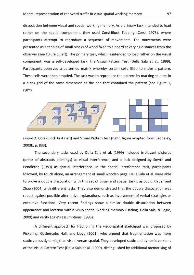
Mental representation of rearward traffic in visuo‐spatial working memory   97 

dissociation between visual and spatial working memory. As a primary task intended to load 

rather  on  the  spatial  component,  they  used  Corsi‐Block  Tapping  (Corsi,  1973),  where 

participants  attempt  to  reproduce  a  sequence  of  movements.  The  movements  were 

presented as a tapping of small blocks of wood fixed to a board at varying distances from the 

observer (see Figure 1, left). The primary task, which is intended to load rather on the visual 

component, was  a  self‐developed  task,  the  Visual  Pattern  Test  (Della  Sala  et  al.,  1999). 

Participants  observed  a  patterned matrix whereby  certain  cells  filled  to make  a  pattern. 

These cells were then emptied. The task was to reproduce the pattern by marking squares in 

a blank  grid of  the  same dimension  as  the one  that  contained  the pattern  (see  Figure 1, 

right). 

 

Figure 1. Corsi‐Block test (left) and Visual Pattern test (right, figure adapted from Baddeley, 

2003b, p. 833). 

The  secondary  tasks  used  by  Della  Sala  et  al.  (1999)  included  irrelevant  pictures 

(prints  of  abstracts  paintings)  as  visual  interference,  and  a  task  designed  by  Smyth  and 

Pendleton  (1989)  as  spatial  interference.  In  the  spatial  interference  task,  participants 

followed, by touch alone, an arrangement of small wooden pegs. Della Sala et al. were able 

to prove a double dissociation with this set of visual and spatial tasks, as could Klauer and 

Zhao  (2004) with different tasks. They also demonstrated that the double dissociation was 

robust against possible alternative explanations, such as involvement of verbal strategies or 

executive  functions.  Very  recent  findings  show  a  similar  double  dissociation  between 

appearance and  location within visuo‐spatial working memory (Darling, Della Sala, & Logie, 

2009) and verify Logie’s assumptions (1995). 

A  different  approach  for  fractioning  the  visuo‐spatial  sketchpad was  proposed  by 

Pickering,  Gathercole,  Hall,  and  Lloyd  (2001), who  argued  that  fragmentation was more 

static versus dynamic, than visual versus spatial. They developed static and dynamic versions 

of the Visual Pattern Test (Della Sala et al., 1999), distinguished by additional memorising of 

Mental representation of rearward traffic in visuo‐spatial working memory   98 

order of appearance instead of simply remembering location of black squares (see Figure 1, 

right). Pickering et al. elaborated the segmentation of the visuo‐spatial sketchpad into static 

and  dynamic  subcomponents  and  defended  their  findings  in  the  face  of  a  possible 

alternative explanation  in  the dynamic version of  the  task –  the use of a verbal encoding 

strategy. 

To summarise, there are two approaches  in the debate on the fragmentation of the 

visuo‐spatial sketchpad. Logie (1995) and other colleagues (Della Sala et al., 1999; Klauer & 

Zhao,  2004)  argue  for  a  segmentation  in  a  visual  and  a  spatial  subcomponent. However, 

Pickering  et  al.  (2001)  propose  a  fragmentation  into  either  a  static  or  a  dynamic 

subcomponent. 

Approach of the Study 

The goal of  the present  study  is  to examine memory processes  involved  in holding 

information about rearward  traffic  in working memory. Therefore, we conducted a driving 

simulator  study where  participants  carried  out  lane  changes with  rearward  traffic  in  the 

target  lane. Before  lane change preparation, participants memorised one of five secondary 

tasks. After  lane  change execution,  they were  asked  to  recall  the memorised material.  In 

contrast to Gugerty (1997) and Jóhannsdóttir (2005), the driving scene was not  interrupted 

due to the reactivity of such a method (Franke, 2008). 

The secondary tasks in this study are designed to load on the two subsystems of the 

initial model  of working memory;  the  visuo‐spatial  sketchpad  and  the  phonological  loop 

(Baddeley & Hitch,  1974).  The  design  of  these  tasks  follows  findings  generated  from  the 

debate  surrounding  fragmentation  of  the  visuo‐spatial  sketchpad  (Baddeley,  2003b; Della 

Sala  et  al.,  1999;  Pickering  et  al.,  2001).  Hence,  to  a  certain  extent,  the  tasks  are 

characteristically  visual‐static,  visual‐dynamic,  spatial‐static,  or  spatial‐dynamic.  The 

character of the fifth task  is phonological. All five tasks are pure memory  load tasks, which 

are memorised before  the onset of  the primary  task and recalled after  the primary  task  is 

completed. This diminishes task switching costs, and therefore minimises the involvement of 

the central executive (Baddeley, Chincotta, & Adlam, 2001; Emerson & Miyake, 2003). 

Mental representation of rearward traffic in visuo‐spatial working memory   99 

Hypothesis 

There are three types of hypotheses connected to the type of dependent variables. 

The first type of hypotheses (H1‐x) concerns the data of the primary task, the lane changing. 

The  second  type of hypotheses  (H2‐x)  refers  to  the  secondary  tasks and  the  third  type  to 

information gathering through the mirrors (H3). 

Due  to  the design of  the dual‐task paradigm, we propose  that  lane  changing  itself 

leads  to differences  in  the  longitudinal  and  lateral driving parameters  (speed, distance  to 

leading  vehicle,  lateral  distance,  lateral  velocity,  etc; H1‐1). Additionally,  due  to  the  pure 

memory character of  the secondary  task  there should be no  influence  in  the primary  task 

(H1‐2).  In  contrast,  the  influence  on  the  driving  task  (especially  the  representation  of 

rearward traffic) should be measurable in the secondary tasks. According to the modality of 

rearward traffic information (rather spatial), the first hypothesis in this block (H2‐1) suggests 

that it should interfere most with spatial tasks (L. J. Gugerty, 1997; Klauer & Zhao, 2004). The 

second hypothesis (H2‐2) concerns dynamics of rearward traffic; the more dynamic traffic is 

in  terms of higher speed,  the more dynamic  the mental representation of rearward  traffic 

should be,  and  the more  it  should  interfere with  the dynamic  version of  secondary  tasks 

(Pickering  et  al.,  2001).  The  third  hypothesis  (H2‐3)  states  that  there  should  be  no 

interference  between  the mental  representation  of  rearward  traffic  and  the  verbal  task 

because both types of information differ in nature and therefore use different subsystems of 

the working memory system. Finally, we propose that there should be an influence of both 

tasks  (primary  and  secondary)  on  glance  behaviour  to  the  left mirror. We  predict  that  if 

there  is a high memory  load due to  interference between representations from both tasks 

(the  driving  scene  and  the  secondary  task),  there  should  be  a  blocking  for  information 

gathering due  to  glances  to  the mirror.  This  should defend participants  from overloading 

memory and should be measurable by means of less glance‐allocation to the mirror (H3).  

Method 

Participants 

Thirty  students  and  staff  members  of  the  Chemnitz  University  of  Technology 

participated (average age 23.2 years). Nineteen participants were female (average age 22.5 

years; SD = 3.5 years) and 11 participants were male (average age 24.4 years; SD = 5.6 years). 

Mental representation of rearward traffic in visuo‐spatial working memory   100 

They held a valid driver’s  license, had at  least one year of driving experience, and did not 

have  any  experience with  the  secondary  tasks  used  in  this  experiment.  Average  driving 

experience was  characterised by  average  car usage of 3.6 days per week  (SD = 2.5 days), 

median kilometrage of 10.000 km per year, median of all kilometers driven of 52,500 km, 

and median  duration  of  holding  a  driver’s  license  of  54 months.  One  participant  drove 

100,000 km per year, had a total kilometrage of 2,500,000 km, held a driver’s license for 264 

months  and  thus  distorts  driving  experience  data  accordingly. Most  students  got  course 

credit  for  their  attendance,  but  some  participants  also  took  part without  any  promise  of 

payoff. 

Apparatus 

The experiment was conducted using a medium‐fidelity fixed‐base driving simulator 

with STISIM Drive software (System Technology Inc, 2008). It consisted of a BMW driving cab 

with automatic transmission and a three‐screen projection providing a 135° horizontal field‐

of‐view. Screens were set at a distance of 260 cm from the average position of drivers’ eyes. 

Only  the  left  mirror  was  projected  on  the  left  screens  in  its  appropriate  positions. 

Additionally, a remote eye‐tracking system (Seeingmachines, 2008) was used to collect eye 

movement data for glances to the left mirror only. 

The secondary tasks were provided and recalled using E‐Prime software (Psychology 

Software Tools Inc, 2007), which was running on a different personal computer. Both visual 

tasks  (visual‐static  and  visual‐dynamic)  and  the  phonological  task  were  presented 

simultaneously on the front screen and via a touchpad in the centre console (see Figure 2). 

The  transparency  of  the  presentation  ensured  that  the  driver  could  recognise  both  the 

driving  scene  and  the  secondary  task  by  looking  straight  ahead.  The  two  spatial  tasks 

(spatial‐static and spatial‐dynamic) were presented auditorily via four speakers mounted  in 

locations  around  the  driver:  Two  speakers were  positioned  approx.  68  cm  left  and  right 

(front), and  two  speakers approx. 24 cm  left and  right  (behind),  in  relation  to  the driver’s 

head,  to ensure optimal audibility of spatial material. The recall of all  five secondary  tasks 

was recorded on the touchpad located in the centre console (see Figure 2).  

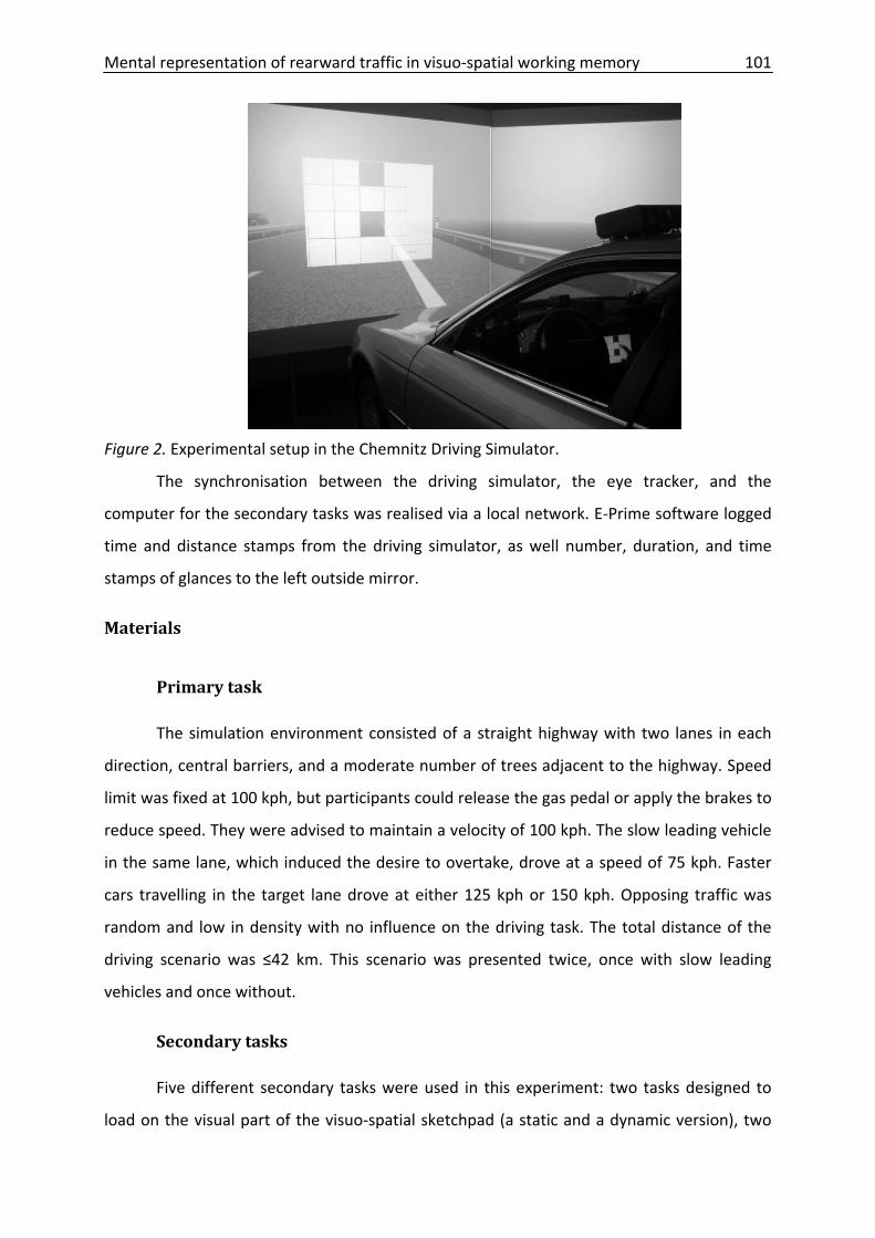
Mental representation of rearward traffic in visuo‐spatial working memory   101 

 

Figure 2. Experimental setup in the Chemnitz Driving Simulator. 

The  synchronisation  between  the  driving  simulator,  the  eye  tracker,  and  the 

computer for the secondary tasks was realised via a local network. E‐Prime software logged 

time and distance  stamps  from  the driving  simulator, as well number, duration, and  time 

stamps of glances to the left outside mirror. 

Materials   

Primary task 

The simulation environment consisted of a straight highway with  two  lanes  in each 

direction, central barriers, and a moderate number of trees adjacent to the highway. Speed 

limit was fixed at 100 kph, but participants could release the gas pedal or apply the brakes to 

reduce speed. They were advised to maintain a velocity of 100 kph. The slow leading vehicle 

in the same  lane, which  induced the desire to overtake, drove at a speed of 75 kph. Faster 

cars  travelling  in  the  target  lane drove at either 125 kph or 150 kph. Opposing  traffic was 

random and  low  in density with no  influence on the driving task. The total distance of the 

driving  scenario was  ≤42  km.  This  scenario was  presented  twice,  once with  slow  leading 

vehicles and once without. 

Secondary tasks 

Five different secondary  tasks were used  in  this experiment:  two  tasks designed  to 

load on the visual part of the visuo‐spatial sketchpad (a static and a dynamic version), two 

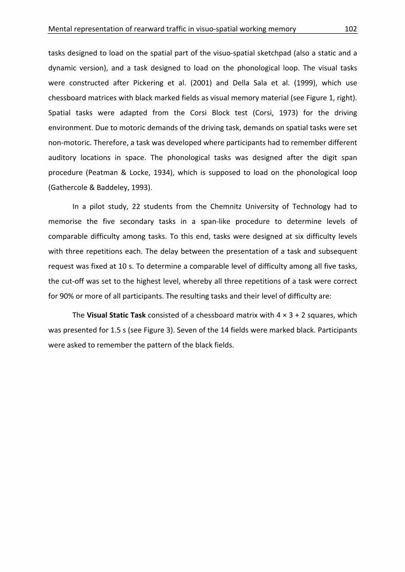
Mental representation of rearward traffic in visuo‐spatial working memory   102 

tasks designed to load on the spatial part of the visuo‐spatial sketchpad (also a static and a 

dynamic  version),  and  a  task designed  to  load  on  the phonological  loop.  The  visual  tasks 

were  constructed  after  Pickering  et  al.  (2001)  and  Della  Sala  et  al.  (1999),  which  use 

chessboard matrices with black marked fields as visual memory material (see Figure 1, right). 

Spatial  tasks  were  adapted  from  the  Corsi  Block  test  (Corsi,  1973)  for  the  driving 

environment. Due to motoric demands of the driving task, demands on spatial tasks were set 

non‐motoric. Therefore, a task was developed where participants had to remember different 

auditory  locations  in  space.  The  phonological  tasks  was  designed  after  the  digit  span 

procedure  (Peatman &  Locke, 1934), which  is  supposed  to  load on  the phonological  loop 

(Gathercole & Baddeley, 1993). 

In  a  pilot  study,  22  students  from  the  Chemnitz  University  of  Technology  had  to 

memorise  the  five  secondary  tasks  in  a  span‐like  procedure  to  determine  levels  of 

comparable difficulty among  tasks. To  this end,  tasks were designed at  six difficulty  levels 

with three repetitions each. The delay between the presentation of a task and subsequent 

request was fixed at 10 s. To determine a comparable level of difficulty among all five tasks, 

the cut‐off was set to the highest level, whereby all three repetitions of a task were correct 

for 90% or more of all participants. The resulting tasks and their level of difficulty are: 

The Visual Static Task consisted of a chessboard matrix with 4 × 3 + 2 squares, which 

was presented for 1.5 s (see Figure 3). Seven of the 14 fields were marked black. Participants 

were asked to remember the pattern of the black fields. 

   

Mental representation of rearward traffic in visuo‐spatial working memory   103 

 

Figure 3. An example of the visual‐static task (VisStat). 

The Visual Dynamic Task consisted of five 3 × 2 + 2 chessboard squares, which were 

presented one after another, each for 500 ms (see Figure 4). The sequence started with an 

empty matrix; with every new matrix one white square turned black. It was not possible for 

the same field to be black twice. The task was to remember the sequence of black fields  in 

the correct order. 

 

Figure 4. An example of the order of appearance of the visual‐dynamic task (VisDyn). 

The  Spatial  Static  Task was  presented  via  four  speakers  inside  the  car  that were 

positioned  around  the  driver’s  head  (see  Figure  5).  Two  different  sounds  were  played 

simultaneously on  two of  the  four speakers  for 2 s. After a short brake of 500 ms, a  third 

sound was presented on a third speaker for 2 s as well. It was also possible, that the single 

sound preceded the two different parallel sounds, temporally. Participants were required to 

memorise  the  positions  of  activated  speakers  in  space,  independent  of  their  order  of 

presentation. 

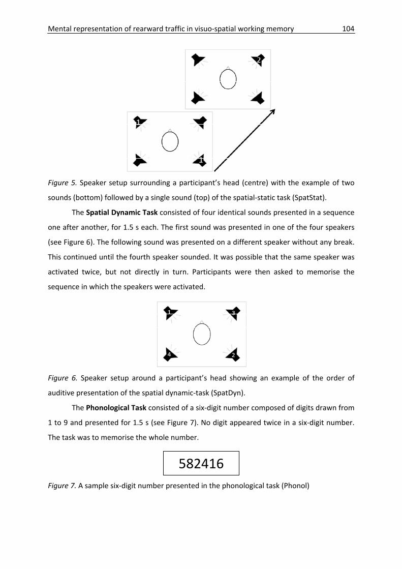
Mental representation of rearward traffic in visuo‐spatial working memory   104 

 

Figure 5. Speaker setup surrounding a participant’s head  (centre) with the example of two 

sounds (bottom) followed by a single sound (top) of the spatial‐static task (SpatStat). 

The Spatial Dynamic Task consisted of four identical sounds presented in a sequence 

one after another, for 1.5 s each. The first sound was presented in one of the four speakers 

(see Figure 6). The following sound was presented on a different speaker without any break. 

This continued until the fourth speaker sounded. It was possible that the same speaker was 

activated  twice,  but  not  directly  in  turn.  Participants were  then  asked  to memorise  the 

sequence in which the speakers were activated. 

 

Figure  6.  Speaker  setup  around  a participant’s head  showing  an  example of  the order of 

auditive presentation of the spatial dynamic‐task (SpatDyn). 

The Phonological Task consisted of a six‐digit number composed of digits drawn from 

1 to 9 and presented for 1.5 s (see Figure 7). No digit appeared twice in a six‐digit number. 

The task was to memorise the whole number. 

 582416

Figure 7. A sample six‐digit number presented in the phonological task (Phonol) 

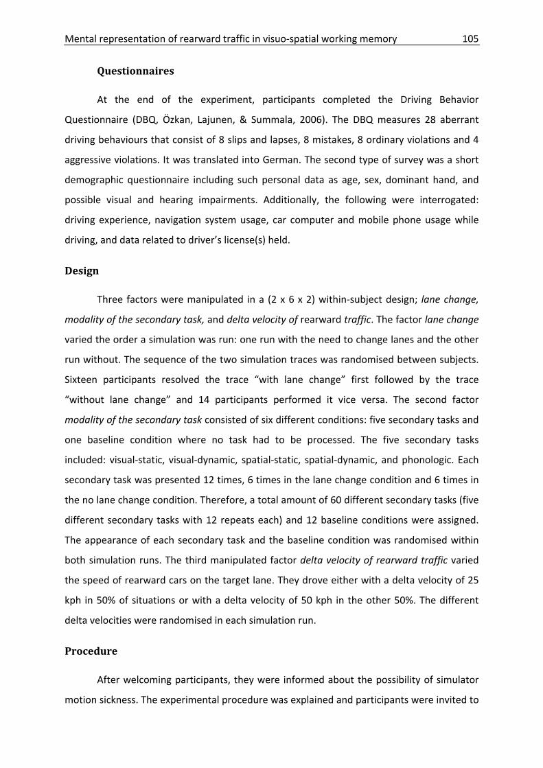
Mental representation of rearward traffic in visuo‐spatial working memory   105 

Questionnaires  

At  the  end  of  the  experiment,  participants  completed  the  Driving  Behavior 

Questionnaire  (DBQ, Özkan,  Lajunen, &  Summala,  2006).  The DBQ measures  28  aberrant 

driving behaviours that consist of 8 slips and lapses, 8 mistakes, 8 ordinary violations and 4 

aggressive violations. It was translated into German. The second type of survey was a short 

demographic questionnaire  including  such personal data as age,  sex, dominant hand, and 

possible  visual  and  hearing  impairments.  Additionally,  the  following  were  interrogated: 

driving experience, navigation  system usage, car computer and mobile phone usage while 

driving, and data related to driver’s license(s) held. 

Design 

Three  factors were manipulated  in a  (2 x 6 x 2) within‐subject design;  lane change, 

modality of the secondary task, and delta velocity of rearward traffic. The factor lane change 

varied the order a simulation was run: one run with the need to change lanes and the other 

run without. The sequence of the two simulation traces was randomised between subjects. 

Sixteen  participants  resolved  the  trace  “with  lane  change”  first  followed  by  the  trace 

“without  lane  change”  and  14  participants  performed  it  vice  versa.  The  second  factor 

modality of the secondary task consisted of six different conditions: five secondary tasks and 

one  baseline  condition  where  no  task  had  to  be  processed.  The  five  secondary  tasks 

included: visual‐static, visual‐dynamic,  spatial‐static,  spatial‐dynamic, and phonologic. Each 

secondary task was presented 12 times, 6 times in the lane change condition and 6 times in 

the no lane change condition. Therefore, a total amount of 60 different secondary tasks (five 

different secondary tasks with 12 repeats each) and 12 baseline conditions were assigned. 

The appearance of each secondary task and the baseline condition was randomised within 

both simulation runs. The third manipulated factor delta velocity of rearward traffic varied 

the speed of rearward cars on the target lane. They drove either with a delta velocity of 25 

kph  in 50% of situations or with a delta velocity of 50 kph  in the other 50%. The different 

delta velocities were randomised in each simulation run. 

Procedure 

After welcoming participants, they were  informed about the possibility of simulator 

motion sickness. The experimental procedure was explained and participants were invited to 

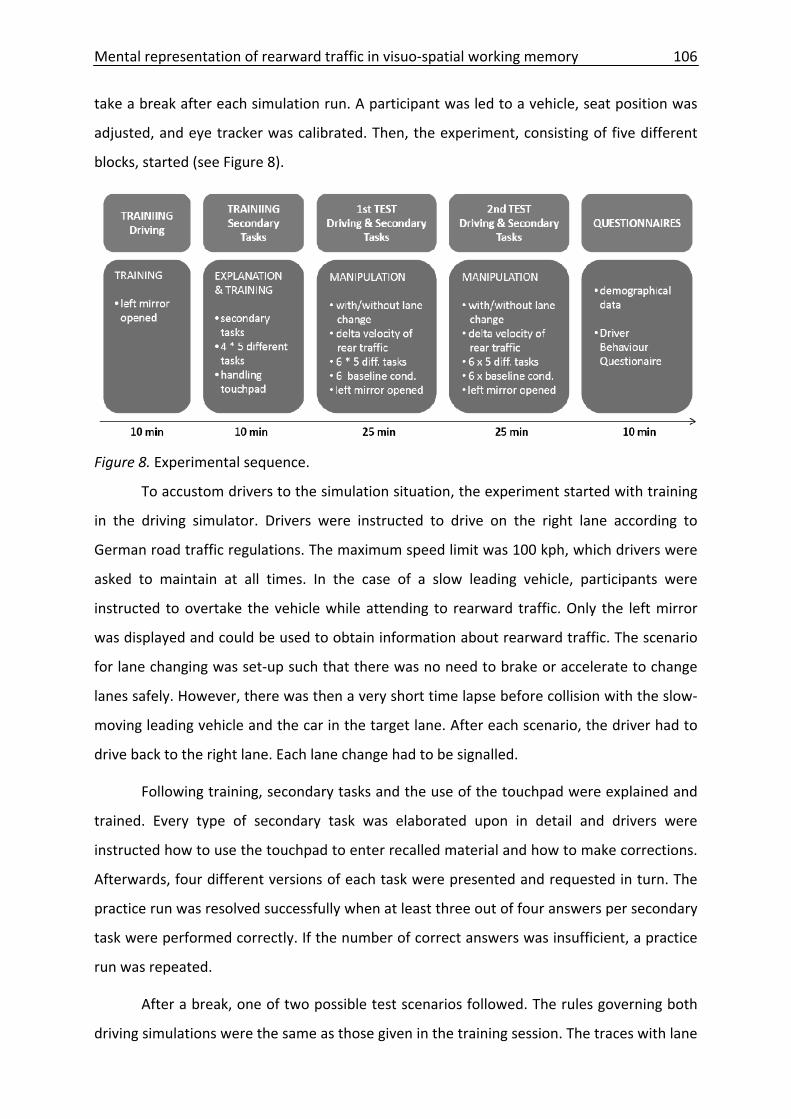
Mental representation of rearward traffic in visuo‐spatial working memory   106 

take a break after each simulation run. A participant was led to a vehicle, seat position was 

adjusted, and eye tracker was calibrated. Then, the experiment, consisting of five different 

blocks, started (see Figure 8). 

 

Figure 8. Experimental sequence. 

To accustom drivers to the simulation situation, the experiment started with training 

in  the  driving  simulator.  Drivers were  instructed  to  drive  on  the  right  lane  according  to 

German road traffic regulations. The maximum speed limit was 100 kph, which drivers were 

asked  to maintain  at  all  times.  In  the  case  of  a  slow  leading  vehicle,  participants  were 

instructed  to overtake  the vehicle while attending  to  rearward  traffic. Only  the  left mirror 

was displayed and could be used to obtain information about rearward traffic. The scenario 

for lane changing was set‐up such that there was no need to brake or accelerate to change 

lanes safely. However, there was then a very short time lapse before collision with the slow‐

moving leading vehicle and the car in the target lane. After each scenario, the driver had to 

drive back to the right lane. Each lane change had to be signalled. 

Following training, secondary tasks and the use of the touchpad were explained and 

trained.  Every  type  of  secondary  task  was  elaborated  upon  in  detail  and  drivers  were 

instructed how to use the touchpad to enter recalled material and how to make corrections. 

Afterwards, four different versions of each task were presented and requested  in turn. The 

practice run was resolved successfully when at least three out of four answers per secondary 

task were performed correctly. If the number of correct answers was insufficient, a practice 

run was repeated. 

After a break, one of two possible test scenarios followed. The rules governing both 

driving simulations were the same as those given in the training session. The traces with lane 

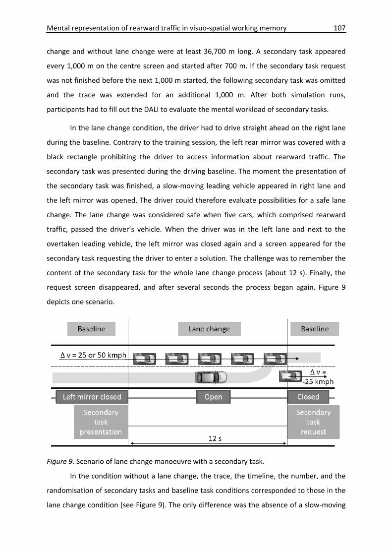
Mental representation of rearward traffic in visuo‐spatial working memory   107 

change

th a 

black  r

Figure 9. Scenario of lane change manoeuvre with a secondary task. 

In the condition without a lane change, the trace, the timeline, the number, and the

sponded to those in the 

lane change condition (see Figure 9). The only difference was the absence of a slow‐moving 

 and without  lane change were at  least 36,700 m  long. A  secondary  task appeared 

every 1,000 m on the centre screen and started after 700 m.  If the secondary task request 

was not finished before the next 1,000 m started, the following secondary task was omitted 

and  the  trace  was  extended  for  an  additional  1,000  m.  After  both  simulation  runs, 

participants had to fill out the DALI to evaluate the mental workload of secondary tasks. 

In the lane change condition, the driver had to drive straight ahead on the right lane 

during the baseline. Contrary to the training session, the left rear mirror was covered wi

ectangle  prohibiting  the  driver  to  access  information  about  rearward  traffic.  The 

secondary task was presented during the driving baseline. The moment the presentation of 

the secondary  task was  finished, a slow‐moving  leading vehicle appeared  in right  lane and 

the  left mirror was opened. The driver could therefore evaluate possibilities for a safe  lane 

change.  The  lane  change was  considered  safe when  five  cars, which  comprised  rearward 

traffic,  passed  the  driver’s  vehicle. When  the  driver was  in  the  left  lane  and  next  to  the 

overtaken  leading vehicle,  the  left mirror was closed again and a  screen appeared  for  the 

secondary task requesting the driver to enter a solution. The challenge was to remember the 

content of  the secondary  task  for  the whole  lane change process  (about 12 s). Finally,  the 

request  screen  disappeared,  and  after  several  seconds  the  process  began  again.  Figure  9 

depicts one scenario. 

 

 

randomisation of secondary tasks and baseline task conditions corre

Mental representation of rearward traffic in visuo‐spatial working memory   108 

lead ve

Results 

ween 90 and 120 minutes, depending 

on the occurrence on errors in the simulation and the duration of the calibration process of 

the eye tracker. 

erformance (Hypotheses H2‐x), and eye glance behaviour (Hypothesis H3). 

The ma

Driving Task Performance 

g behaviour  (e.g., Brookhuis, de Waard, & 

Fairclough, 2003),  variables  from  the  field of  longitudinal  and  lateral driving performance 

of a  three‐factor multiple analysis of variance  (MANOVA)  for 

repeat

hicle. Therefore, there was no need to overtake in this condition. The task of no lane 

change required the driver to drive straight ahead and solve secondary tasks every 1,000 m. 

The driving part of the experiment was finished when both simulation runs were resolved. 

During  the  last  10  minutes  of  the  experiment,  participants  completed  the 

questionnaire about demographic data and the DBQ. 

On average, each experimental run  lasted bet

The  statistical  analysis  was  subdivided  into  three  parts  of  dependent  measures: 

primary  task  performance  in  terms  of  lane  change  performance  (Hypotheses  H1‐x), 

secondary task p

in factors in the analysis are: lane change (yes vs. no), modality of the secondary task 

(visual‐static  [VisStat],  visual‐dynamic  [VisDyn],  spatial‐static  [SpatStat],  spatial‐dynamic 

[SpatDyn], phonological [Phonol], and no secondary task [Baseline]), and delta velocity of the 

rearward traffic (delta speed 25 kph vs. 50 kph). 

According  to common measures of drivin

were analysed with  the help 

ed measures.  Longitudinal performance measures  included: mean  speed, minimum 

speed,  standard  deviation  of  speed, minimum  acceleration,  maximum  acceleration,  and 

standard  deviation  of  acceleration.  Lateral  performance  measures  included:  standard 

deviation of steering wheel position, standard deviation of steering wheel rate, mean lateral 

lane  position,  minimum  lateral  lane  position,  maximum  lateral  lane  position,  standard 

deviation  of  lateral  lane  position, maximum  lateral  speed,  standard  deviation  of  lateral 

speed,  maximum  lateral  acceleration,  and  standard  deviation  of  lateral  acceleration.  A 

MANOVA  for  repeated measures  resulted  in  significant  results  for  the main  factor  lane 

change,  F(16,  13) = 10.83, p <  .001,  η²p = .93.  The  majority  of  the  measures  showed 

significant results for the factor  lane change, with the exception of maximum (longitudinal) 

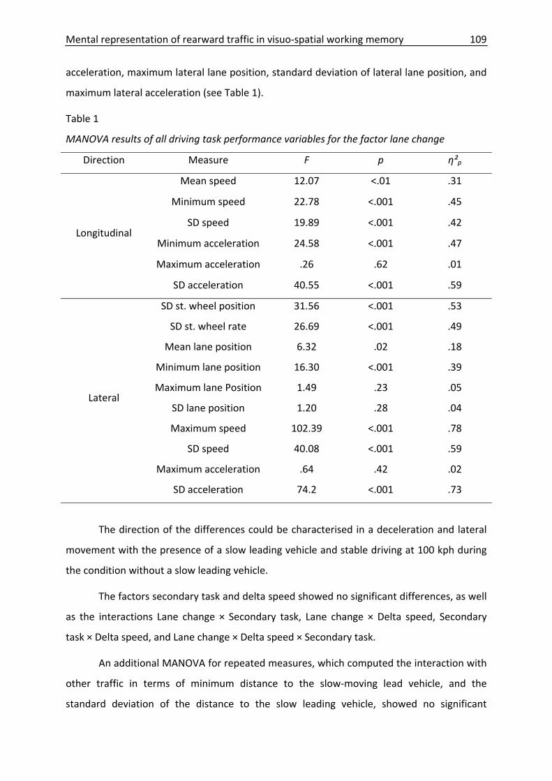
Mental representation of rearward traffic in visuo‐spatial working memory   109 

acceleration, maximum lateral lane position, standard deviation of lateral lane position, and 

maximum lateral acceleration (see Table 1). 

Table 1 

MANOVA results of all driving task performance variables for the factor lane change 

Direction  Measure  F  p  η²p 

Longitudinal 

Mean speed  12.07  <.01  .31 

Minimum speed  22.78  <.001  .45 

19.89  <.001 

Mini tion 

Ma  

SD  

Lateral 

SD speed  .42 

mum accelera 24.58  <.001  .47 

ximum acceleration .26  .62  .01 

 acceleration 40.55  <.001  .59 

SD st. wheel position  31.56  <.001  .53 

SD st. wheel rate  26.69  <.001 

M  

M  

Ma n 

<.001 

Ma  

.49 

ean lane position 6.32  .02  .18 

inimum lane position 16.30  <.001  .39 

ximum lane Positio 1.49  .23  .05 

SD lane position  1.20  .28  .04 

Maximum speed  102.39  <.001  .78 

SD speed  40.08  .59 

ximum acceleration .64  .42  .02 

SD acceleration  74.2  <.001  .73 

 

The directio ld be characterised  in a eleration an eral 

movement with the pre leading ve and stable  at 100 kp ring 

the condition without a slow leading vehicle. 

eed × Secondary task.  

  no  significant 

n of the differences cou  dec d  lat

sence of a slow  hicle   driving h du

The factors secondary task and delta speed showed no significant differences, as well 

as  the  interactions  Lane  change ×  Secondary  task,  Lane  change × Delta  speed,  Secondary 

task × Delta speed, and Lane change × Delta sp

An additional MANOVA for repeated measures, which computed the interaction with 

other  traffic  in  terms  of  minimum  distance  to  the  slow‐moving  lead  vehicle,  and  the 

standard  deviation  of  the  distance  to  the  slow  leading  vehicle,  showed

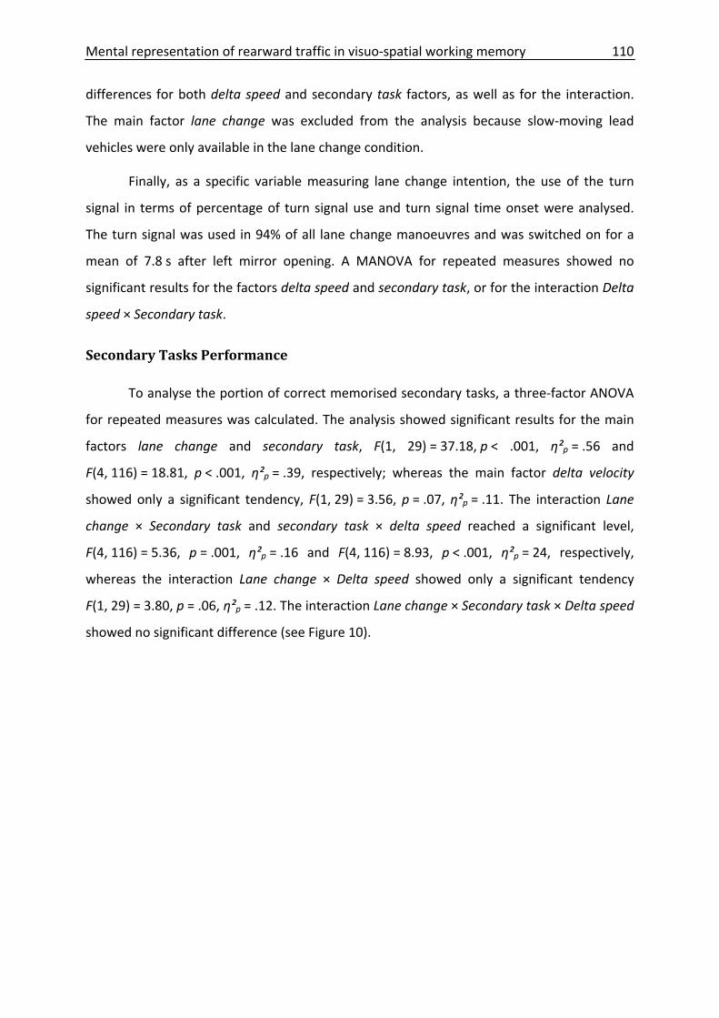
Mental representation of rearward traffic in visuo‐spatial working memory   110 

differe

uvres and was switched on for a 

mean 

Secondary Tasks Performance 

rtion of correct memorised secondary tasks, a three‐factor ANOVA 

for repeated measures was calculated. The analysis showed significant results for the main 

  task,  F(1,  29) = 37.18, p <  .001,  η²p = .56  and 

F(4, 11

  e

nces  for both delta speed and secondary  task  factors, as well as  for  the  interaction. 

The main  factor  lane  change was  excluded  from  the  analysis  because  slow‐moving  lead 

vehicles were only available in the lane change condition.  

Finally,  as  a  specific  variable measuring  lane  change  intention,  the use of  the  turn 

signal  in  terms of percentage of  turn signal use and  turn signal  time onset were analysed. 

The turn signal was used  in 94% of all  lane change manoe

of  7.8 s  after  left mirror  opening.  A MANOVA  for  repeated measures  showed  no 

significant results for the factors delta speed and secondary task, or for the interaction Delta 

speed × Secondary task.  

To analyse the po

factors  lane  change  and  secondary

6) = 18.81,  p < .001,  η²p = .39,  respectively;  whereas  the main  factor  delta  velocity 

showed only a  significant  tendency,  F(1, 29) = 3.56, p = .07, η²p = .11. The  interaction  Lane 

change  ×  Secondary  task  and  secondary  task ×  delta  speed  reached  a  significant  l vel, 

F(4, 116) = 5.36,  p = .001,  η²p = .16  and  F(4, 116) = 8.93,  p < .001,  η²p = 24,  respectively, 

whereas  the  interaction  Lane  change  ×  Delta  speed  showed  only  a  significant  tendency 

F(1, 29) = 3.80, p = .06, η²p = .12. The interaction Lane change × Secondary task × Delta speed 

showed no significant difference (see Figure 10). 

   

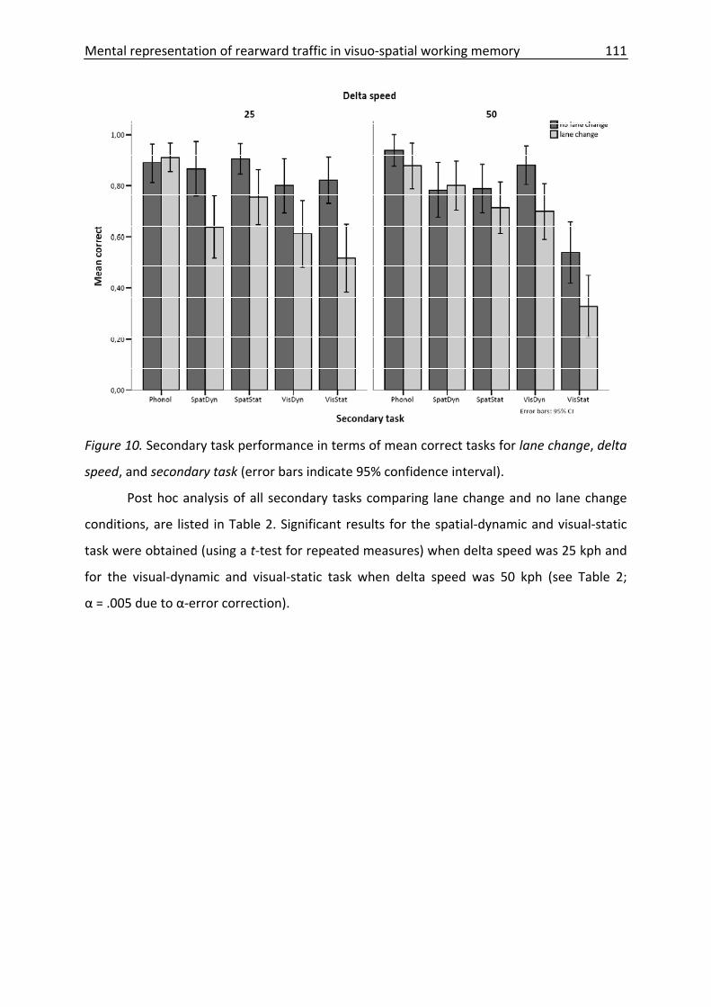
Mental representation of rearward traffic in visuo‐spatial working memory   111 

 

Figure 10. Secondary task performance in terms of mean correct tasks for lane change, delta 

speed, and secondary task (error bars indicate 95% confidence interval). 

Post hoc analysis of all secondary tasks comparing  lane change and no  lane change 

conditions, are  listed  in Table 2. Significant results  for the spatial‐dynamic and visual‐static 

task were obtained (using a t‐test for repeated measures) when delta speed was 25 kph and 

for  the  visual‐dynamic  and  visual‐static  task when  delta  speed was  50  kph  (see  Table  2; 

α = .005 due to α‐error correction). 

 

   

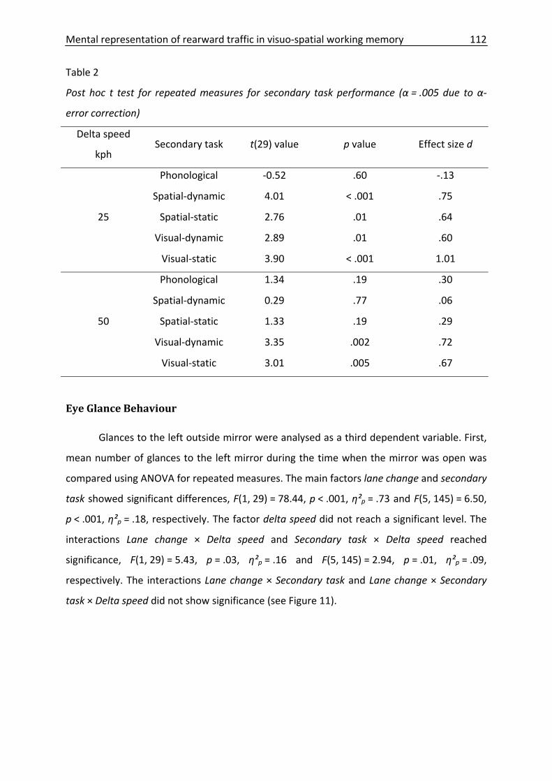
Mental representation of rearward traffic in visuo‐spatial working memory   112 

Table 2 

Post hoc  t  test  for  repeated measures  for  secondary  task performance  (α = .005 due  to  α‐

error correction) 

Delta speed 

kph Secondary task  t(29) value  p value  Effect size d 

25 

Phonological  ‐0.52  .60  ‐.13 

Spatial‐dynamic  4.01  < .001  .75 

Spatial‐static  2.76  .01  .64 

Visual‐dynamic  2.89  .01  .60 

Visual‐static  3.90  < .001  1.01 

50 

Phonological  1.34  .19  .30 

Spatial‐dynamic  0.29  .77  .06 

Spatial‐static  1.33  .19  .29 

Visual‐dynamic  3.35  .002  .72 

Visual‐static  3.01  .005  .67 

 

Eye Glance Behaviour 

Glances to the left outside mirror were analysed as a third dependent variable. First, 

mean number of glances to the  left mirror during the time when the mirror was open was 

compared using ANOVA for repeated measures. The main factors lane change and secondary 

task showed significant differences, F(1, 29) = 78.44, p < .001, η²p = .73 and F(5, 145) = 6.50, 

p < .001, η²p = .18, respectively. The factor delta speed did not reach a significant  level. The 

interactions  Lane  change  ×  Delta  speed  and  Secondary  task  ×  Delta  speed  reached 

significance,  F(1, 29) = 5.43,  p = .03,  η²p = .16  and  F(5, 145) = 2.94,  p = .01,  η²p = .09, 

respectively. The  interactions Lane change × Secondary  task and Lane change × Secondary 

task × Delta speed did not show significance (see Figure 11).  

 

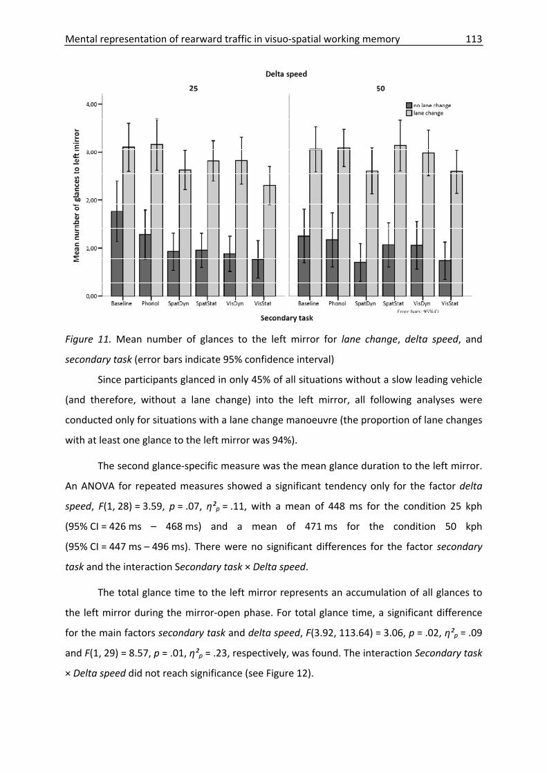
Mental representation of rearward traffic in visuo‐spatial working memory   113 

 

Figure  11. Mean  number  of  glances  to  the  left mirror  for  lane  change,  delta  speed,  and 

secondary task (error bars indicate 95% confidence interval) 

Since participants glanced in only 45% of all situations without a slow leading vehicle 

(and  therefore,  without  a  lane  change)  into  the  left mirror,  all  following  analyses  were 

conducted only for situations with a lane change manoeuvre (the proportion of lane changes 

with at least one glance to the left mirror was 94%). 

The second glance‐specific measure was the mean glance duration to the left mirror. 

An ANOVA  for  repeated measures  showed a  significant  tendency only  for  the  factor delta 

speed,  F(1, 28) = 3.59,  p = .07,  η²p = .11, with  a mean  of  448 ms  for  the  condition  25  kph 

(95% CI = 426 ms  –  468 ms)  and  a  mean  of  471 ms  for  the  condition  50  kph 

(95% CI = 447 ms – 496 ms). There were no  significant differences  for  the  factor  secondary 

task and the interaction Secondary task × Delta speed. 

The total glance time to the  left mirror represents an accumulation of all glances to 

the  left mirror during the mirror‐open phase. For total glance time, a significant difference 

for the main factors secondary task and delta speed, F(3.92, 113.64) = 3.06, p = .02, η²p = .09 

and F(1, 29) = 8.57, p = .01, η²p = .23, respectively, was found. The interaction Secondary task 

× Delta speed did not reach significance (see Figure 12).  

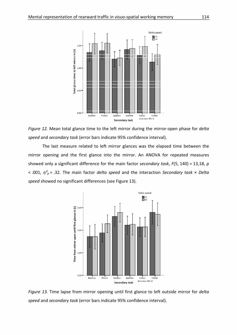
Mental representation of rearward traffic in visuo‐spatial working memory   114 

 

Figure 12. Mean total glance time to the  left mirror during the mirror‐open phase for delta 

speed and secondary task (error bars indicate 95% confidence interval). 

The  last measure  related  to  left mirror glances was  the elapsed  time between  the 

mirror  opening  and  the  first  glance  into  the mirror.  An  ANOVA  for  repeated measures 

showed only a significant difference for the main factor secondary task, F(5, 140) = 13,18, p 

< .001,  η²p = .32.  The main  factor  delta  speed  and  the  interaction  Secondary  task  × Delta 

speed showed no significant differences (see Figure 13). 

 

Figure 13. Time  lapse  from mirror opening until  first glance to  left outside mirror  for delta 

speed and secondary task (error bars indicate 95% confidence interval). 

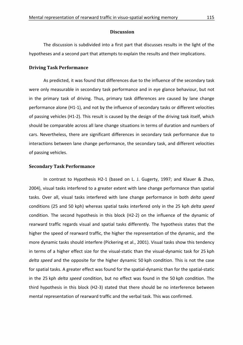
Mental representation of rearward traffic in visuo‐spatial working memory   115 

 Discussion 

The discussion  is subdivided  into a first part that discusses results  in the  light of the 

hypotheses and a second part that attempts to explain the results and their implications. 

Driving Task Performance  

As predicted, it was found that differences due to the influence of the secondary task 

were only measurable  in secondary task performance and  in eye glance behaviour, but not 

in  the  primary  task  of  driving.  Thus,  primary  task  differences  are  caused  by  lane  change 

performance alone (H1‐1), and not by the influence of secondary tasks or different velocities 

of passing vehicles (H1‐2). This result is caused by the design of the driving task itself, which 

should be comparable across all lane change situations in terms of duration and numbers of 

cars. Nevertheless,  there are  significant differences  in  secondary  task performance due  to 

interactions between lane change performance, the secondary task, and different velocities 

of passing vehicles. 

Secondary Task Performance 

In  contrast  to Hypothesis H2‐1  (based  on  L.  J. Gugerty,  1997;  and  Klauer &  Zhao, 

2004), visual tasks interfered to a greater extent with lane change performance than spatial 

tasks. Over  all,  visual  tasks  interfered with  lane  change  performance  in  both  delta  speed 

conditions  (25 and 50 kph) whereas spatial tasks  interfered only  in the 25 kph delta speed 

condition.  The  second hypothesis  in  this block  (H2‐2) on  the  influence of  the dynamic of 

rearward  traffic  regards visual and  spatial  tasks differently. The hypothesis  states  that  the 

higher the speed of rearward traffic, the higher the representation of the dynamic, and  the 

more dynamic tasks should interfere (Pickering et al., 2001). Visual tasks show this tendency 

in terms of a higher effect size for the visual‐static than the visual‐dynamic task for 25 kph 

delta speed and the opposite for the higher dynamic 50 kph condition. This  is not the case 

for spatial tasks. A greater effect was found for the spatial‐dynamic than for the spatial‐static 

in  the 25 kph delta  speed condition, but no effect was  found  in  the 50 kph condition. The 

third hypothesis  in  this block  (H2‐3)  stated  that  there  should be no  interference between 

mental representation of rearward traffic and the verbal task. This was confirmed.  

Mental representation of rearward traffic in visuo‐spatial working memory   116 

Eye Glance Behaviour 

Glances  to  the  left  mirror  during  the  period  it  was  activated  showed  significant 

differences for several parameters. The mean number of glances to the  left outside mirror 

was larger when participants had to undertake a lane change. In 45% of all situations with no 

lane  change  participants  glanced  to  the  left  outside mirror,  even  if  it was  not  necessary. 

Additionally, the number of glances to the  left outside mirror was  lower when they had to 

memorise  a  spatial‐dynamic  or  a  visual‐static  task,  especially  in  the  50 kph  delta  speed 

condition. This confirmed hypothesis H3. There was no influence of secondary task on glance 

duration.  However,  faster  rearward  traffic  in  the  adjacent  lane  tended  to  cause  longer 

glances  into  the  mirror.  Total  glance  time  reflects  the  influence  of  secondary  task  on 

numbers of glances and influence of the velocity of rearward traffic on glance duration. The 

time  elapsed  from  opening  of  the  left  outside  mirror  to  first  glance  can  serve  as  an 

explanation for the  lower number of glances during performance of the spatial‐dynamic or 

the visual‐static task. In other words, when participants first look at the mirror at a later time 

point, they have less time remaining to glance at the mirror before it closes.  

Possible Explanations of the Results and Implications 

The  results  suggest  that  information  about  rearward  traffic  in  this  study  is  visual 

rather  than  spatial, and  static more  than dynamic  (i.e.,  largest effect  size  found  in  visual‐

static  condition),  in  nature.  A  possible  explanation  for  these  findings  could  be  that 

information  about  rearward  traffic was not memorised  as  a moving  vehicle  in  space, but 

more as a picture. This could be caused due to the fact that rearward traffic was too slow, or 

that  the  situation was  too predictable, and participants  just memorised an  image of a car 

versus  looking at an empty mirror and  initiating a  lane change. The  implications  for  future 

studies  include making the  lane change situations  less predictable and more demanding so 

that drivers are forced to memorise positions of rearward traffic in terms of moving objects 

in space.  

Nevertheless, our results have important implications for applications in traffic, as well as for 

the  debate  on  fragmentation  of  the  visuo‐spatial  sketchpad.  This  is  if  the  mental 

representation of rearward traffic in such situations is more visual‐static, then presentation 

of the same kind of information should be avoided. For instance, it might be suboptimal if an 

in‐vehicle  information  system  (IVIS)  urges  a  driver  to  memorise  an  image,  such  as  a 

Mental representation of rearward traffic in visuo‐spatial working memory   117 

navigation system showing a  landmark, upon which a driver should orient himself. Another 

example could be a very vivid description of an image given by the passenger (e.g., a messy 

kitchen). Another crucial implication of this study is the change in glance behaviour in terms 

of  delayed  first  glances  to  the mirror,  especially  due  to  spatial‐dynamic  and  visual‐static 

secondary tasks. This  is relevant for systems that rely on glances to the mirror, such as the 

Lane Change Assist that warns the driver when a vehicle  is detected  in the blind spot via a 

display  in  the  side  mirror  (Kiefer  &  Hankey,  2008).  Moreover,  some  systems  obtain 

information  about  driver  intention  to  change  lanes  via  glances  to  the  left  outside mirror 

(Doshi & Trivedi, 2008; Henning, 2004; Henning, Georgeon, Dapzol, & Krems, 2009; Oliver & 

Pentland,  2000).  These  early  glances  can  trigger  a  workload  manager  (Green,  2004; 

Piechulla, Mayser, Gehrke, & König, 2003), which aims  to  lower driver workload  in a high‐

demand  situation  such  as  a  lane  change,  by  suppressing  incoming  phone  calls  during 

preparation of a lane change (de Waard, Kruizinga, & Brookhuis, 2008). 

The  implication  of  this  study  for  the  debate  on  fragmentation  of  the  visuo‐spatial 

sketchpad is not very clear. Results of visual tasks seem to support the static‐dynamic split of 

the visuo‐spatial sketchpad (Pickering et al., 2001), but not spatial tasks. Another supportive 

result can be inferred based on the glance behaviour. There is a later onset of glances to the 

mirror for spatial‐dynamic or visual‐static secondary tasks. A clear result is suggested in the 

lack of  interference with the phonological task. This  is contrary to findings of Jóhannsdóttir 

(2005) and can be explained in terms of methodology.  First, verbal and spatial memory tasks 

use different perceptual  resources. Whereas participants obtain visual  information  for  the 

verbal  task on  a  continuous basis  via projection onto  a  frontal  screen,  the motoric‐based 

tapping task (non‐visual) requires participants to press a learned (and therefore automated) 

pattern.  Thus,  it  is  difficult  to  compare  these  tasks.  Jóhannsdóttir  also  reported  no  pilot 

testing  of  secondary  tasks  to  adapt  participants  to  task  difficulty.  A  second  argument 

concerns the verbal task’s front screen projection. Whereas the distance between the verbal 

stimuli and the cars  in front was about 4 degrees, the distance to the rearview mirror was 

located about 6 degrees above and 2 degrees to the right of verbal stimuli. This may have 

made  it  harder  to  obtain  information  from  the  rearview mirror when  accomplishing  the 

verbal task and therefore may explain differences between study findings. 

A future study should investigate lane change manoeuvres using more unpredictable 

and  challenging  situations  in higher density  traffic.  In  contrast  to  the  current  study  there 

Mental representation of rearward traffic in visuo‐spatial working memory   118 

might be measurable differences in driving performance, such as in the study of Salvucci and 

Beltowska (2008). However, such a design makes it harder for participants to work with pure 

memory  tasks  and  to  keep  memory  content  constant  across  different  experimental 

situations.  

An alternative method would be  to work only with memory content of  the mirror, 

which might be made possible by employing short videos of an approaching car in a mirror. 

This  approach  is  similar  to  the  paradigm  of  representational momentum  (Freyd &  Finke, 

1984), which relies on a dynamic mental representation in visual‐spatial short‐term memory.

Mental representation of rearward traffic in visuo‐spatial working memory   119 

References 

Adams, M.  J.,  Tenney,  Y.  J., &  Pew,  R. W.  (1995).  Situation  awareness  and  the  cognitive 

management of complex systems. Human Factors, 37(1), 85‐104.  

Anderson,  J.  R.,  Bothell,  D.,  Byrne, M.  D.,  Douglass,  S.,  Lebiere,  C., & Qin,  Y.  (2004).  An 

integrated theory of the mind. Psychological Review, 111(4), 1036‐1060.  

Baddeley, A. (2003a). Double dissociations: Not magic but still useful. Cortex, 39(1), 129‐131.  

Baddeley, A. (2003b). Working memory: Looking back and  looking forward. Nature Reviews 

Neuroscience, 4(10), 829‐839.  

Baddeley, A., Chincotta, D., & Adlam, A. (2001). Working memory and the control of action: 

Evidence  from  task  switching.  Journal of Experimental Psychology: General, 130(4), 

641‐657.  

Baddeley, A., & Hitch, G. (1974). Working memory.  In G. H. Bower (Ed.), The psychology of 

learning and motivation: Advances  in  research and  theory  (Vol. 8, pp. 47‐‐89). New 

York: Academic Press.  

Baumann, M.,  Franke,  T., &  Krems,  J.  F.  (2008).  The  effect  of  experience,  relevance  and 

interruption duration on drivers' mental representation of a traffic situation. In D. d. 

Waard,  F.  O.  Flemisch,  B.  Lorenz,  H.  Oberheid  &  K.  A.  Brookhuis  (Eds.),  Human 

Factors for Assistance and Automation (pp. 141‐152). Maastricht: Shaker.  

Baumann, M., & Krems, J. F. (2007). Situation awareness and driving: A cognitive model. In C. 

Cacciabue &  C.  Re  (Eds.), Modelling  driver  behaviour  in  automotive  environments. 

Critical  issues  in advanced automotive systems and human‐centred design  (pp. 253‐

265). London: Springer.  

Brackstone, M., McDonald, M., & Wu,  J.  (1998).  Lane  changing on  the motorway: Factors 

affecting  its  occurrence,  and  their  implications.  Paper  presented  at  the  Road 

Transport  Information  and  Control,  1998.  9th  International  Conference  on  (Conf. 

Publ. No. 454). 

Brookhuis, K. A., de Waard, D., &  Fairclough,  S. H.  (2003). Criteria  for driver  impairment. 

Ergonomics, 46(5), 433.  

Chovan,  J.  D.,  Tijerina,  L.,  Alexander,  G.,  &  Hendricks,  D.  L.  (1994).  Examination  of  lane 

change crashes and potential IVHS countermeasures. (DOT HS 808 071). Washington, 

DC:  U.S.  Department  of  Transportation,  National  Highway  Traffic  Safety 

Administration. 

Mental representation of rearward traffic in visuo‐spatial working memory   120 

Corsi,  P.  M.  (1973).  Human  memory  and  the  medial  temporal  region  of  the  brain.  34, 

ProQuest  Information & Learning, US. Retrieved  from http://search.ebscohost.com/ 

login.aspx?direct=true&db=psyh&AN=1976‐04900‐001&site=ehost‐live   

Darling,  S.,  Della  Sala,  S.,  &  Logie,  R.  H.  (2009).  Dissociation  between  appearance  and 

location within visuo‐spatial working memory. The Quarterly Journal of Experimental 

Psychology, 62(3), 417‐425.  

de Waard, D., Kruizinga, A., & Brookhuis, K. A.  (2008). The consequences of an  increase  in 

heavy goods vehicles  for passenger  car drivers' mental workload and behaviour: A 

simulator study. Accident Analysis & Prevention, 40(2), 818‐828.  

Della Sala, S., Gray, C., Baddeley, A., Allamano, N., & Wilson, L. (1999). Pattern span: A tool 

for unwelding visuo‐spatial memory. Neuropsychologia, 37(10), 1189‐1199.  

Doshi, A., & Trivedi, M. (2008). A comparative exploration of eye gaze and head motion cues 

for  lane  change  intent  prediction.  Paper  presented  at  the  Intelligent  Vehicles 

Symposium, 2008 IEEE. 

Emerson, M. J., & Miyake, A. (2003). The role of  inner speech in task switching: A dual‐task 

investigation. Journal of Memory and Language, 48(1), 148‐168.  

Endsley,  M.  R.  (1988).  Design  and  evaluation  for  situation  awareness  enhancement 

Proceedings  of  the  Human  Factors  Society  32nd  Annual  Meeting  (pp.  97‐101). 

Anaheim, CA.  

Endsley, M. R. (1995). Toward a theory of situation awareness  in dynamic systems. Human 

Factors, 37(1), 32‐64.  

Ericsson,  K.  A., &  Kintsch, W.  (1995).  Long‐term working memory.  Psychological  Review, 

102(2), 211‐245.  

Fastenmeier,  W.,  Hinderer,  J.,  Lehnig,  U.,  &  Gstalter,  H.  (2001).  Analyse  von 

Spurwechselvorgängen im Verkehr. Zeitschrift für Arbeitswissenschaft, 55, 15‐23.  

Franke, T.  (2008).  Involvement of  long‐term working memory  in situation awareness  in  the 

driving  domain.  Diploma  Thesis,  Chemnitz  University  of  Technology,  Chemnitz, 

Germany.    

Freyd,  J.  J., &  Finke,  R.  A.  (1984).  Representational momentum.  Journal  of  Experimental 

Psychology: Learning, Memory, and Cognition, 10(1), 126‐132.  

Gathercole,  S.  E., & Baddeley, A. D.  (1993). Working memory  and  language. Hillsdale, NJ 

England: Lawrence Erlbaum Associates, Inc. 

Mental representation of rearward traffic in visuo‐spatial working memory   121 

Green, P. (2004). Driver distraction, telematics design, and workload managers: Safety issues 

and  solutions  (SAE  paper  2004‐21‐0022).  Paper  presented  at  the  International 

Congress on Transportation Electronics. 

Gugerty, L. (in press). Situation awareness in driving. In J. Lee, M. Rizzo, D. Fisher & J. Caird. 

(Eds.), Handbook for driving simulation in engineering, medicine and psychology: CRC 

Press.  Retrieved  from  http://www.clemson.edu/psych/gugerty/Gugerty‐SAdriving‐

Lee‐etal.pdf 

Gugerty, L. J.  (1997). Situation awareness during driving: explicit and  implicit knowledge  in 

dynamic spatial memory. Journal of experimental Psychology: Applied, 3(1), 42‐66.  

Henning, M.  J.  (2004).  Indikatoren  zur  Fahrerabsichtserkennung  ‐  Das  Blickverhalten  bei 

Spurwechselvorgängen.  Diploma  Thesis,  Chemnitz  University  of  Technology, 

Chemnitz.    

Henning, M. J., Georgeon, O., Dapzol, N., & Krems, J. F. (2009). How early can the car know 

that the driver would like to change lanes? An analysis of early indicators selected by 

underlying cognitive processes. Manuscript in preparation.   

Jóhannsdóttir, K. R. (2005). Situation awareness and working memory: An  integration of an 

applied concept with a  fundamental cognitive process. 65, ProQuest  Information & 

Learning,  US.  Retrieved  from  http://search.ebscohost.com/login.aspx?direct=true 

&db=psyh&AN=2005‐99012‐266&site=ehost‐live   

Kiefer,  R.  J., &  Hankey,  J. M.  (2008).  Lane  change  behavior with  a  side  blind  zone  alert 

system. Accident Analysis & Prevention, 40(2), 683‐690.  

Klauer,  K.  C.,  &  Zhao,  Z.  (2004).  Double  dissociations  in  visual  and  spatial  short‐term 

memory. Journal of Experimental Psychology: General, 133(3), 355‐381.  

Logie, R. H. (1995). Visuo‐spatial working memory. Hillsdale, NJ England: Lawrence Erlbaum 

Associates, Inc. 

Oliver, N., & Pentland, A. P.  (2000). Graphical models  for driver behavior  recognition  in a 

smartcar.  Paper  presented  at  the  IEEE  Intelligent  Vehicles  Symposium  2000, 

Dearborn (MI), USA. 

Olsen,  E.  C.  B.  (2003).  Modeling  slow  lead  vehicle  lane  changing.  Dissertation,  Virginia 

Polytechnic Institute and State University, Blacksburg VA.    

Özkan, T., Lajunen, T., & Summala, H.  (2006). Driver behaviour questionnaire: A  follow‐up 

study. Accident Analysis & Prevention, 38(2), 386‐395.  

Mental representation of rearward traffic in visuo‐spatial working memory   122 

Peatman,  J. G., &  Locke, N. M.  (1934).  Studies  in  the methodology of  the digit‐span  test. 

Archives of Psychology, 167, 35‐35.  

Pickering,  S.  J.  (2001).  Cognitive  approaches  to  the  fractionation  of  visuo‐spatial working 

memory. Cortex, 37(4), 457‐473.  

Pickering, S. J., Gathercole, S. E., Hall, M., & Lloyd, S. A. (2001). Development of memory for 

pattern and path: Further evidence for the fractionation of visuo‐spatial memory. The 

Quarterly  Journal  of  Experimental  Psychology  A:  Human  Experimental  Psychology, 

54(2), 397‐420.  

Piechulla, W., Mayser, C., Gehrke, H., & König, W. (2003). Reducing drivers' mental workload 

by means  of  an  adaptive man‐machine  interface.  Transportation  Research  Part  F: 

Traffic Psychology and Behaviour, 6(4), 233‐248.  

Psychology Software Tools Inc. (2007). E‐Prime 2 (Version 2.0.8.22). Pittsburgh, PA.  

Robinson, G. H., Erickson, D., Thurston, G., & Clark, R.  (1972). Visual search by automobile 

drivers. Human Factors, 14(4), 315‐323.  

Salvucci, D. D. (2006). Modeling driver behavior  in a cognitive architecture. Human Factors, 

48(2), 362‐380.  

Salvucci, D. D., & Beltowska, J. (2008). Effects of memory rehearsal on driver performance: 

Experiment  and  theoretical  account.  Human  Factors:  The  Journal  of  the  Human 

Factors and Ergonomics Society, 50(5), 834‐844.  

Seeingmachines. (2008). faceLAB (Version 4.6). Canberra.  

Smyth, M. M., & Pendleton, L. R.  (1989). Working memory  for movements. The Quarterly 

Journal of Experimental Psychology A: Human Experimental Psychology, 41(2), 235‐

250.  

Statistisches  Bundesamt.  (2008).  Verkehr  ‐  Verkehrsunfälle.  (Fachserie  8  Reihe  7). 

Wiesbaden: Statistisches Bundesamt. 

System Technology Inc. (2008). STISIM drive (Version Build 2.10.03). Hawthorne, CA.  

 

 

Rearward traffic and representational momentum  123 

 

 

 

 

Thru the Mirror – On the Localisation of Rearward Traffic in Dynamic Visuo‐Spatial Working 

Memory Using the Representational Momentum Paradigm 

 

 

Matthias J. Henning and Josef F. Krems 

Chemnitz University of Technology 

 

 

 

 

Rearward traffic and representational momentum  124 

Abstract 

The present study aims to  investigate whether the presentation of rearward traffic  is static 

or dynamic  in nature depending on different velocities of  the approaching  car. Therefore, 

the  paradigm  of  representational  momentum  (Freyd  &  Finke,  1984)  was  used  in  2 

experiments.  In  a  first  experiment,  20  participants  watched  short  videos  similar  to  an 

approaching  car  observed  via  the  left  wing  mirror.  The  representational  momentum 

paradigm was able to provide evidence that the short‐term representation  in memory was 

dynamic  in  nature  starting  from  an  approaching  speed  faster  than  50  kph.  In  a  second 

experiment, visuo‐spatial secondary tasks were used to investigate whether the influence of 

the  representational momentum  is also  reflected  in  secondary  task performance. Twenty‐

five  participants memorised  1  of  5  secondary  tasks  (visual‐static,  visual‐dynamic,  spatial‐

static, or spatial‐dynamic, phonological). Afterwards, they had to fulfil three representational 

momentum  tasks  and  finally  they  were  asked  to  recall  the  memorised  secondary  task 

material.  Results  proved  that  representational momentum  showed  higher  effect  sizes  for 

both  dynamic  secondary  task  conditions.  The  same  pattern  was  observable  for  the 

secondary task performance.  

Rearward traffic and representational momentum  125 

Thru the Mirror – On the Localisation of Rearward Traffic in Dynamic Visuo‐spatial 

Working Memory Using the Representational Momentum Paradigm 

Around  two  percent  of  all  fixations made  by  drivers  are  located  on  the  rearview 

mirrors (Nunes & Recarte, 2005). These glances are performed in order to monitor rearward 

traffic and maintain situational awareness (Baumann, Franke, & Krems, 2008; Gugerty, 1997; 

Salvucci, 2006). Especially during a lane change manoeuvre on a highway, where information 

about  rearward  traffic  is  essential  for  safety,  glances  to  the mirrors  increase  (Henning, 

Schweigert,  Baumann,  &  Krems,  2006;  Olsen,  Lee,  &  Wierwille,  2005;  Tijerina,  Garrott, 

Stoltzfus, & Parmer, 2005). If drivers want to change to the left lane, they glance at the left 

outside  mirror  (wing  mirror)  to  a  higher  extent  than  at  other  mirror  locations  in  total 

(Robinson, Erickson, Thurston, & Clark, 1972). Additionally, glances at the left mirrors are the 

earliest behavioural  indicators of a  lane change manoeuvre to the  left (Henning, Georgeon, 

Dapzol, & Krems, 2009).  

Glances  towards  the  left  wing mirror  in  conjunction  with  a  lane  change  provide 

information about rearward cars  in the adjacent  lane or to a certain degree  in the driver’s 

own  lane  (Bhise et al., 1981). What the driver actually sees  in the  left outside mirror  is an 

approaching  car,  if  there  is  one.  If  a  car  is  approaching,  the  driver  has  to memorise  the 

position and speed of the car for a short time  in order to utilise this  information as a basis 

for  the  decision  whether  to  change  lanes  or  not.  Gugerty  (1997)  proposed  that  this 

information  is  represented  in dynamic spatial working memory, because  it  is dynamic and 

spatial in nature. However, Henning, Beyreuther, and Krems (2009) found evidence that it is 

more visual and static in nature, more like a static picture.  

The present study aims to investigate whether the presentation of rearward traffic is 

static  or  dynamic  in  nature  depending  on  different  velocities  of  the  approaching  car. 

Therefore we use  the paradigm of representational momentum  (Freyd & Finke, 1984)  in a 

first  experiment.  This  paradigm  is  able  to  provide  evidence  as  to whether  a  short‐term 

representation in memory is dynamic in nature. In a second experiment, we use visuo‐spatial 

secondary tasks from Henning, Beyreuther, et al. (2009) to investigate whether the influence 

from the representational momentum is also reflected in secondary task performance. 

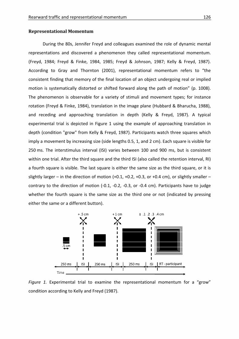
Rearward traffic and representational momentum  126 

Representational Momentum 

During the 80s, Jennifer Freyd and colleagues examined the role of dynamic mental 

representations  and  discovered  a  phenomenon  they  called  representational momentum. 

(Freyd,  1984;  Freyd  &  Finke,  1984,  1985;  Freyd  &  Johnson,  1987;  Kelly  &  Freyd,  1987). 

According  to  Gray  and  Thornton  (2001),  representational  momentum  refers  to  “the 

consistent finding that memory of the final location of an object undergoing real or implied 

motion  is  systematically distorted or  shifted  forward along  the path of motion”  (p. 1008). 

The phenomenon  is observable  for a variety of  stimuli and movement  types;  for  instance 

rotation (Freyd & Finke, 1984), translation in the image plane (Hubbard & Bharucha, 1988), 

and  receding  and  approaching  translation  in  depth  (Kelly  &  Freyd,  1987).  A  typical 

experimental  trial  is depicted  in  Figure 1 using  the example of  approaching  translation  in 

depth (condition "grow" from Kelly & Freyd, 1987). Participants watch three squares which 

imply a movement by increasing size (side lengths 0.5, 1, and 2 cm). Each square is visible for 

250 ms.  The  interstimulus  interval  (ISI)  varies between 100  and 900 ms, but  is  consistent 

within one trial. After the third square and the third ISI (also called the retention interval, RI) 

a fourth square is visible. The last square is either the same size as the third square, or it is 

slightly larger – in the direction of motion (+0.1, +0.2, +0.3, or +0.4 cm), or slightly smaller – 

contrary to the direction of motion  (‐0.1,  ‐0.2,  ‐0.3, or  ‐0.4 cm). Participants have to  judge 

whether  the  fourth  square  is  the  same  size as  the  third one or not  (indicated by pressing 

either the same or a different button).  

 

Figure  1.  Experimental  trial  to  examine  the  representational  momentum  for  a  “grow” 

condition according to Kelly and Freyd (1987). 

 

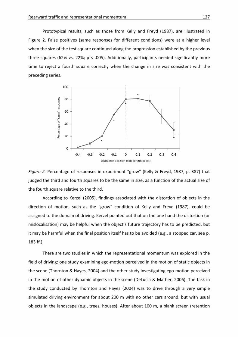
Rearward traffic and representational momentum  127 

Prototypical  results,  such  as  those  from  Kelly  and  Freyd  (1987),  are  illustrated  in 

Figure  2.  False  positives  (same  responses  for  different  conditions) were  at  a  higher  level 

when the size of the test square continued along the progression established by the previous 

three squares  (62% vs. 22%; p <  .005). Additionally, participants needed significantly more 

time  to  reject  a  fourth  square  correctly when  the  change  in  size was  consistent with  the 

preceding series.  

 

Figure 2. Percentage of responses  in experiment “grow”  (Kelly & Freyd, 1987, p. 387)  that 

judged the third and fourth squares to be the same in size, as a function of the actual size of 

the fourth square relative to the third. 

According  to Kerzel  (2005),  findings associated with  the distortion of objects  in  the 

direction  of  motion,  such  as  the  “grow”  condition  of  Kelly  and  Freyd  (1987),  could  be 

assigned to the domain of driving. Kerzel pointed out that on the one hand the distortion (or 

mislocalisation) may be helpful when the object’s future trajectory has to be predicted, but 

it may be harmful when the final position itself has to be avoided (e.g., a stopped car, see p. 

183 ff.).  

There are two studies in which the representational momentum was explored in the 

field of driving: one study examining ego‐motion perceived in the motion of static objects in 

the scene (Thornton & Hayes, 2004) and the other study investigating ego‐motion perceived 

in the motion of other dynamic objects  in the scene (DeLucia & Mather, 2006). The task  in 

the  study  conducted  by  Thornton  and  Hayes  (2004) was  to  drive  through  a  very  simple 

simulated driving environment  for about 200 m with no other cars around, but with usual 

objects  in the  landscape (e.g., trees, houses). After about 100 m, a blank screen (retention 

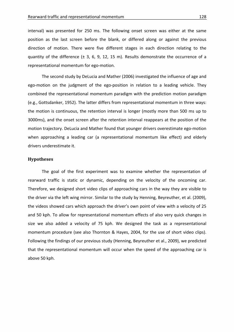
Rearward traffic and representational momentum  128 

interval) was  presented  for  250 ms.  The  following  onset  screen was  either  at  the  same 

position  as  the  last  screen  before  the  blank,  or  differed  along  or  against  the  previous 

direction  of  motion.  There  were  five  different  stages  in  each  direction  relating  to  the 

quantity of  the difference  (± 3, 6, 9, 12, 15 m). Results demonstrate  the occurrence of  a 

representational momentum for ego‐motion.  

The second study by DeLucia and Mather (2006) investigated the influence of age and 

ego‐motion  on  the  judgment  of  the  ego‐position  in  relation  to  a  leading  vehicle.  They 

combined the representational momentum paradigm with the prediction motion paradigm 

(e.g., Gottsdanker, 1952). The latter differs from representational momentum in three ways: 

the motion  is continuous, the retention  interval  is  longer  (mostly more than 500 ms up to 

3000ms), and the onset screen after the retention  interval reappears at the position of the 

motion trajectory. DeLucia and Mather found that younger drivers overestimate ego‐motion 

when  approaching  a  leading  car  (a  representational momentum  like  effect)  and  elderly 

drivers underestimate it. 

Hypotheses 

The  goal  of  the  first  experiment  was  to  examine  whether  the  representation  of 

rearward  traffic  is  static  or  dynamic,  depending  on  the  velocity  of  the  oncoming  car. 

Therefore, we designed short video clips of approaching cars  in the way they are visible to 

the driver via the left wing mirror. Similar to the study by Henning, Beyreuther, et al. (2009), 

the videos showed cars which approach the driver’s own point of view with a velocity of 25 

and 50 kph. To allow for representational momentum effects of also very quick changes  in 

size  we  also  added  a  velocity  of  75  kph.  We  designed  the  task  as  a  representational 

momentum procedure (see also Thornton & Hayes, 2004,  for the use of short video clips). 

Following the findings of our previous study (Henning, Beyreuther et al., 2009), we predicted 

that  the  representational momentum will occur when  the speed of  the approaching car  is 

above 50 kph. 

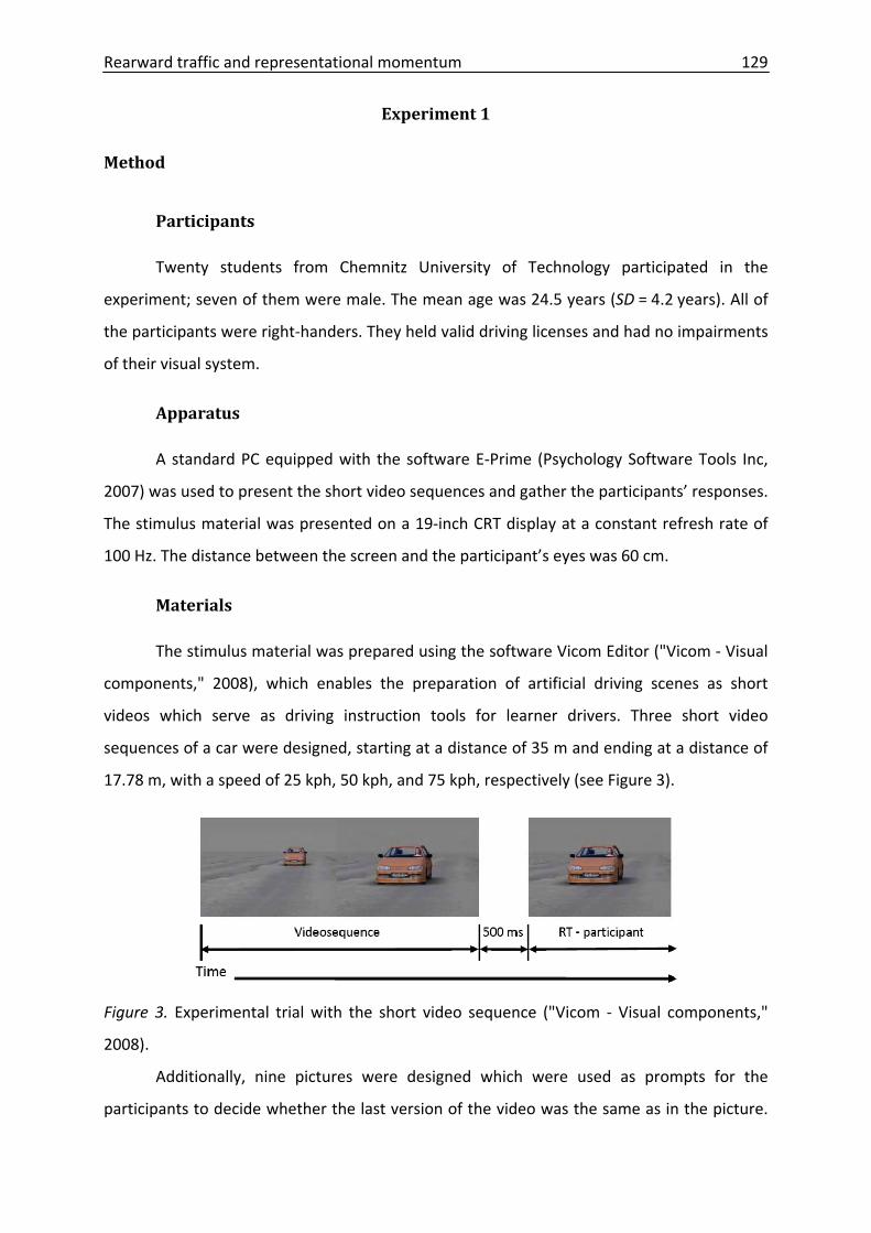
Rearward traffic and representational momentum  129 

Experiment 1  

Method 

Participants 

Twenty  students  from  Chemnitz  University  of  Technology  participated  in  the 

experiment; seven of them were male. The mean age was 24.5 years (SD = 4.2 years). All of 

the participants were right‐handers. They held valid driving licenses and had no impairments 

of their visual system.  

Apparatus 

A standard PC equipped with  the software E‐Prime  (Psychology Software Tools  Inc, 

2007) was used to present the short video sequences and gather the participants’ responses. 

The stimulus material was presented on a 19‐inch CRT display at a constant refresh rate of 

100 Hz. The distance between the screen and the participant’s eyes was 60 cm. 

Materials 

The stimulus material was prepared using the software Vicom Editor ("Vicom ‐ Visual 

components,"  2008),  which  enables  the  preparation  of  artificial  driving  scenes  as  short 

videos  which  serve  as  driving  instruction  tools  for  learner  drivers.  Three  short  video 

sequences of a car were designed, starting at a distance of 35 m and ending at a distance of 

17.78 m, with a speed of 25 kph, 50 kph, and 75 kph, respectively (see Figure 3). 

 

Figure 3. Experimental  trial with  the  short  video  sequence  ("Vicom  ‐ Visual  components," 

2008). 

Additionally,  nine  pictures  were  designed  which  were  used  as  prompts  for  the 

participants to decide whether the last version of the video was the same as in the picture. 

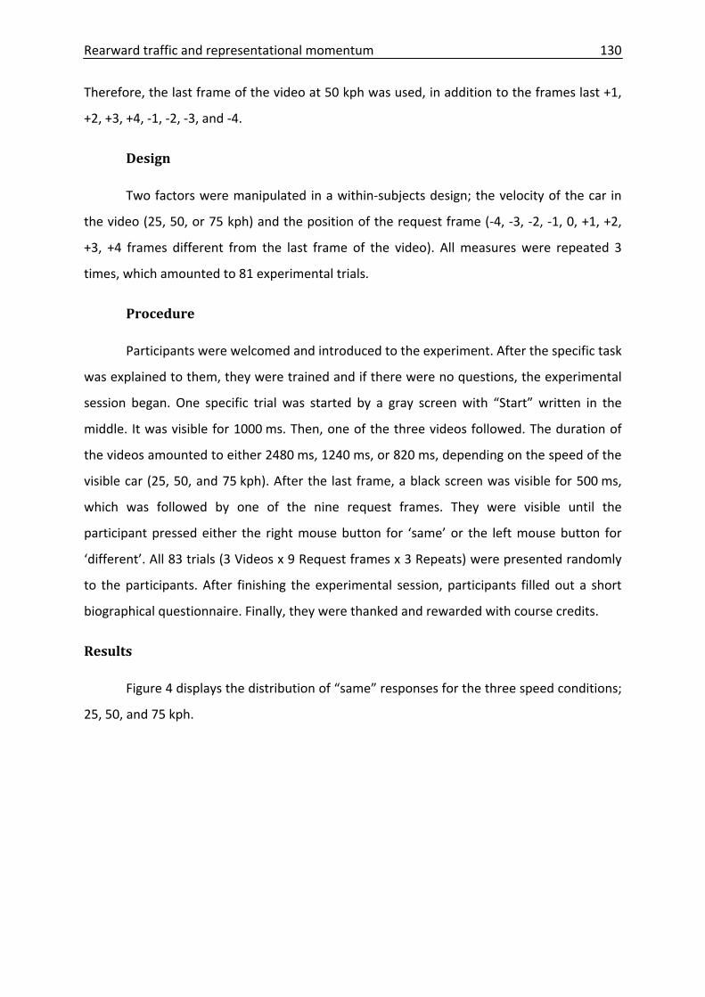
Rearward traffic and representational momentum  130 

Therefore, the last frame of the video at 50 kph was used, in addition to the frames last +1, 

+2, +3, +4, ‐1, ‐2, ‐3, and ‐4. 

Design 

Two factors were manipulated  in a within‐subjects design; the velocity of the car  in 

the video (25, 50, or 75 kph) and the position of the request frame (‐4, ‐3, ‐2, ‐1, 0, +1, +2, 

+3,  +4  frames different  from  the  last  frame of  the  video). All measures were  repeated  3 

times, which amounted to 81 experimental trials.  

Procedure 

Participants were welcomed and introduced to the experiment. After the specific task 

was explained to them, they were trained and if there were no questions, the experimental 

session began. One  specific  trial was  started by  a  gray  screen with  “Start” written  in  the 

middle.  It was visible for 1000 ms. Then, one of the three videos followed. The duration of 

the videos amounted to either 2480 ms, 1240 ms, or 820 ms, depending on the speed of the 

visible car (25, 50, and 75 kph). After the  last frame, a black screen was visible for 500 ms, 

which  was  followed  by  one  of  the  nine  request  frames.  They  were  visible  until  the 

participant pressed either  the  right mouse button  for  ‘same’ or  the  left mouse button  for 

‘different’. All 83 trials (3 Videos x 9 Request frames x 3 Repeats) were presented randomly 

to  the participants. After  finishing  the experimental  session, participants  filled out a  short 

biographical questionnaire. Finally, they were thanked and rewarded with course credits. 

Results 

Figure 4 displays the distribution of “same” responses for the three speed conditions; 

25, 50, and 75 kph. 

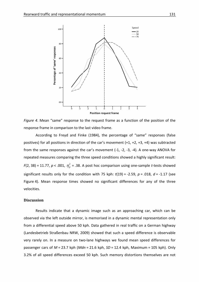
Rearward traffic and representational momentum  131 

 

Figure 4. Mean “same” response  to  the request  frame as a  function of  the position of  the 

response frame in comparison to the last video frame. 

According  to  Freyd  and  Finke  (1984),  the  percentage  of  “same”  responses  (false 

positives) for all positions in direction of the car’s movement (+1, +2, +3, +4) was subtracted 

from the same responses against the car’s movement (‐1, ‐2, ‐3, ‐4). A one‐way ANOVA for 

repeated measures comparing the three speed conditions showed a highly significant result: 

F(2, 38) = 11.77, p < .001,   = .38. A post hoc comparison using one‐sample t‐tests showed 

significant  results only  for  the  condition with 75 kph:  t(19) = ‐2.59, p = .018, d = ‐1.17  (see 

Figure 4).  Mean  response  times  showed  no  significant  differences  for  any  of  the  three 

velocities.  

2pη

Discussion 

Results  indicate  that  a  dynamic  image  such  as  an  approaching  car, which  can  be 

observed via the left outside mirror, is memorised in a dynamic mental representation only 

from a differential speed above 50 kph. Data gathered  in real traffic on a German highway 

(Landesbetrieb Straßenbau NRW, 2009) showed that such a speed difference  is observable 

very  rarely on.  In a measure on  two‐lane highways we  found mean  speed differences  for 

passenger cars of M = 23.7 kph (Mdn = 21.6 kph, SD = 12.4 kph, Maximum = 105 kph). Only 

3.2% of all speed differences exceed 50 kph. Such memory distortions  themselves are not 

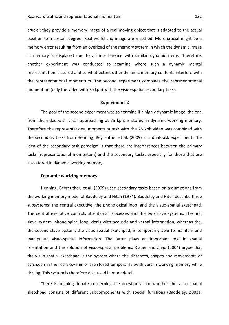
Rearward traffic and representational momentum  132 

crucial; they provide a memory  image of a real moving object that  is adapted to the actual 

position  to a certain degree. Real world and  image are matched. More crucial might be a 

memory error resulting from an overload of the memory system in which the dynamic image 

in  memory  is  displaced  due  to  an  interference  with  similar  dynamic  items.  Therefore, 

another  experiment  was  conducted  to  examine  where  such  a  dynamic  mental 

representation is stored and to what extent other dynamic memory contents interfere with 

the  representational momentum.  The  second  experiment  combines  the  representational 

momentum (only the video with 75 kph) with the visuo‐spatial secondary tasks. 

Experiment 2  

The goal of the second experiment was to examine if a highly dynamic image, the one 

from  the  video with  a  car  approaching  at  75  kph,  is  stored  in dynamic working memory. 

Therefore the representational momentum task with the 75 kph video was combined with 

the secondary tasks  from Henning, Beyreuther et al.  (2009)  in a dual‐task experiment. The 

idea of  the  secondary  task paradigm  is  that  there  are  interferences between  the primary 

tasks  (representational momentum) and  the  secondary  tasks, especially  for  those  that are 

also stored in dynamic working memory. 

Dynamic working memory 

Henning, Beyreuther, et al. (2009) used secondary tasks based on assumptions from 

the working memory model of Baddeley and Hitch (1974). Baddeley and Hitch describe three 

subsystems:  the central executive,  the phonological  loop, and  the visuo‐spatial  sketchpad. 

The  central  executive  controls  attentional  processes  and  the  two  slave  systems.  The  first 

slave  system, phonological  loop, deals with acoustic and verbal  information, whereas  the, 

the  second  slave  system,  the  visuo‐spatial  sketchpad,  is  temporarily able  to maintain and 

manipulate  visuo‐spatial  information.  The  latter  plays  an  important  role  in  spatial 

orientation and  the  solution of visuo‐spatial problems. Klauer and Zhao  (2004) argue  that 

the  visuo‐spatial  sketchpad  is  the  system where  the distances,  shapes and movements of 

cars seen in the rearview mirror are stored temporarily by drivers in working memory while 

driving. This system is therefore discussed in more detail. 

There  is  ongoing  debate  concerning  the  question  as  to whether  the  visuo‐spatial 

sketchpad  consists  of  different  subcomponents  with  special  functions  (Baddeley,  2003a; 

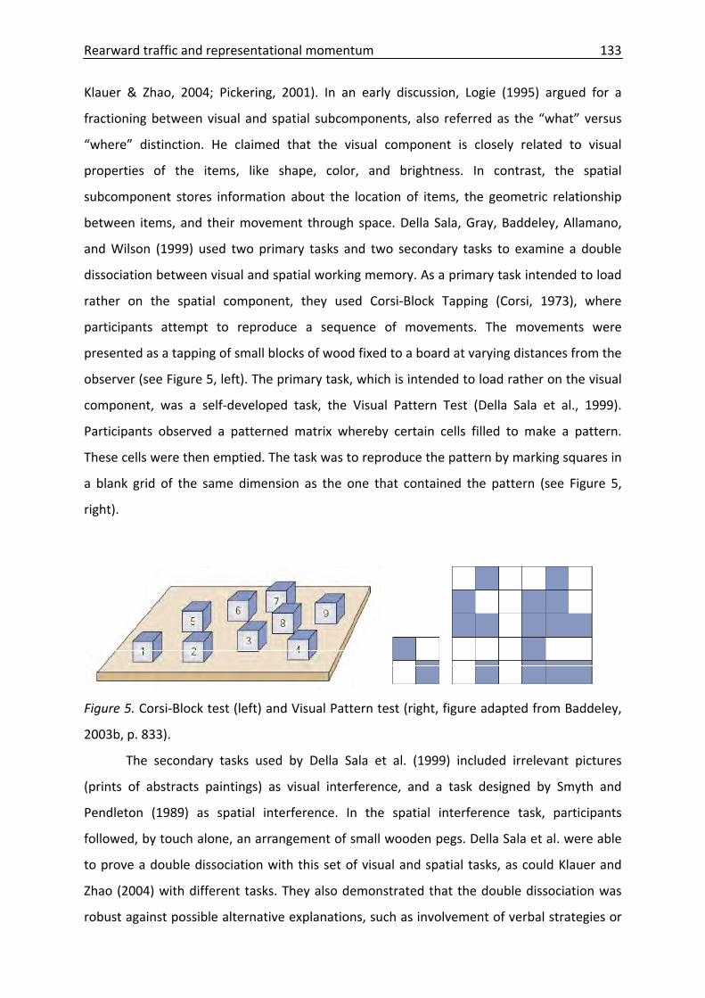
Rearward traffic and representational momentum  133 

Klauer &  Zhao,  2004;  Pickering,  2001).  In  an  early  discussion,  Logie  (1995)  argued  for  a 

fractioning between visual and  spatial  subcomponents, also  referred as  the “what” versus 

“where”  distinction.  He  claimed  that  the  visual  component  is  closely  related  to  visual 

properties  of  the  items,  like  shape,  color,  and  brightness.  In  contrast,  the  spatial 

subcomponent  stores  information  about  the  location of  items,  the geometric  relationship 

between  items, and  their movement  through  space. Della Sala, Gray, Baddeley, Allamano, 

and Wilson  (1999) used  two primary  tasks and  two  secondary  tasks  to examine a double 

dissociation between visual and spatial working memory. As a primary task intended to load 

rather  on  the  spatial  component,  they  used  Corsi‐Block  Tapping  (Corsi,  1973),  where 

participants  attempt  to  reproduce  a  sequence  of  movements.  The  movements  were 

presented as a tapping of small blocks of wood fixed to a board at varying distances from the 

observer (see Figure 5, left). The primary task, which is intended to load rather on the visual 

component, was  a  self‐developed  task,  the  Visual  Pattern  Test  (Della  Sala  et  al.,  1999). 

Participants  observed  a  patterned matrix whereby  certain  cells  filled  to make  a  pattern. 

These cells were then emptied. The task was to reproduce the pattern by marking squares in 

a blank  grid of  the  same dimension  as  the one  that  contained  the pattern  (see  Figure 5, 

right). 

 

 

Figure 5. Corsi‐Block test (left) and Visual Pattern test (right, figure adapted from Baddeley, 

2003b, p. 833). 

The  secondary  tasks  used  by  Della  Sala  et  al.  (1999)  included  irrelevant  pictures 

(prints  of  abstracts  paintings)  as  visual  interference,  and  a  task  designed  by  Smyth  and 

Pendleton  (1989)  as  spatial  interference.  In  the  spatial  interference  task,  participants 

followed, by touch alone, an arrangement of small wooden pegs. Della Sala et al. were able 

to prove a double dissociation with this set of visual and spatial tasks, as could Klauer and 

Zhao  (2004) with different tasks. They also demonstrated that the double dissociation was 

robust against possible alternative explanations, such as involvement of verbal strategies or 

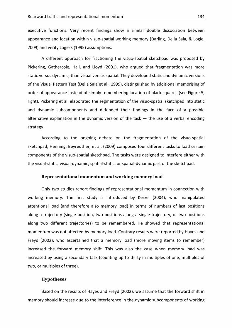
Rearward traffic and representational momentum  134 

executive  functions.  Very  recent  findings  show  a  similar  double  dissociation  between 

appearance and  location within visuo‐spatial working memory (Darling, Della Sala, & Logie, 

2009) and verify Logie’s (1995) assumptions. 

A  different  approach  for  fractioning  the  visuo‐spatial  sketchpad was  proposed  by 

Pickering,  Gathercole,  Hall,  and  Lloyd  (2001), who  argued  that  fragmentation was more 

static versus dynamic, than visual versus spatial. They developed static and dynamic versions 

of the Visual Pattern Test (Della Sala et al., 1999), distinguished by additional memorising of 

order of appearance instead of simply remembering location of black squares (see Figure 5, 

right). Pickering et al. elaborated the segmentation of the visuo‐spatial sketchpad into static 

and  dynamic  subcomponents  and  defended  their  findings  in  the  face  of  a  possible 

alternative explanation  in  the dynamic version of  the  task —  the use of a verbal encoding 

strategy. 

According  to  the  ongoing  debate  on  the  fragmentation  of  the  visuo‐spatial 

sketchpad, Henning, Beyreuther, et al. (2009) composed four different tasks to load certain 

components of the visuo‐spatial sketchpad. The tasks were designed to interfere either with 

the visual‐static, visual‐dynamic, spatial‐static, or spatial‐dynamic part of the sketchpad. 

Representational momentum and working memory load 

Only two studies report  findings of representational momentum  in connection with 

working  memory.  The  first  study  is  introduced  by  Kerzel  (2004),  who  manipulated 

attentional  load  (and  therefore  also memory  load)  in  terms  of  numbers  of  last  positions 

along a trajectory  (single position, two positions along a single trajectory, or two positions 

along  two  different  trajectories)  to  be  remembered.  He  showed  that  representational 

momentum was not affected by memory load. Contrary results were reported by Hayes and 

Freyd  (2002),  who  ascertained  that  a memory  load  (more moving  items  to  remember) 

increased  the  forward  memory  shift.  This  was  also  the  case  when  memory  load  was 

increased by using a secondary task (counting up to thirty  in multiples of one, multiples of 

two, or multiples of three).  

Hypotheses 

Based on the results of Hayes and Freyd (2002), we assume that the forward shift in 

memory should increase due to the interference in the dynamic subcomponents of working 

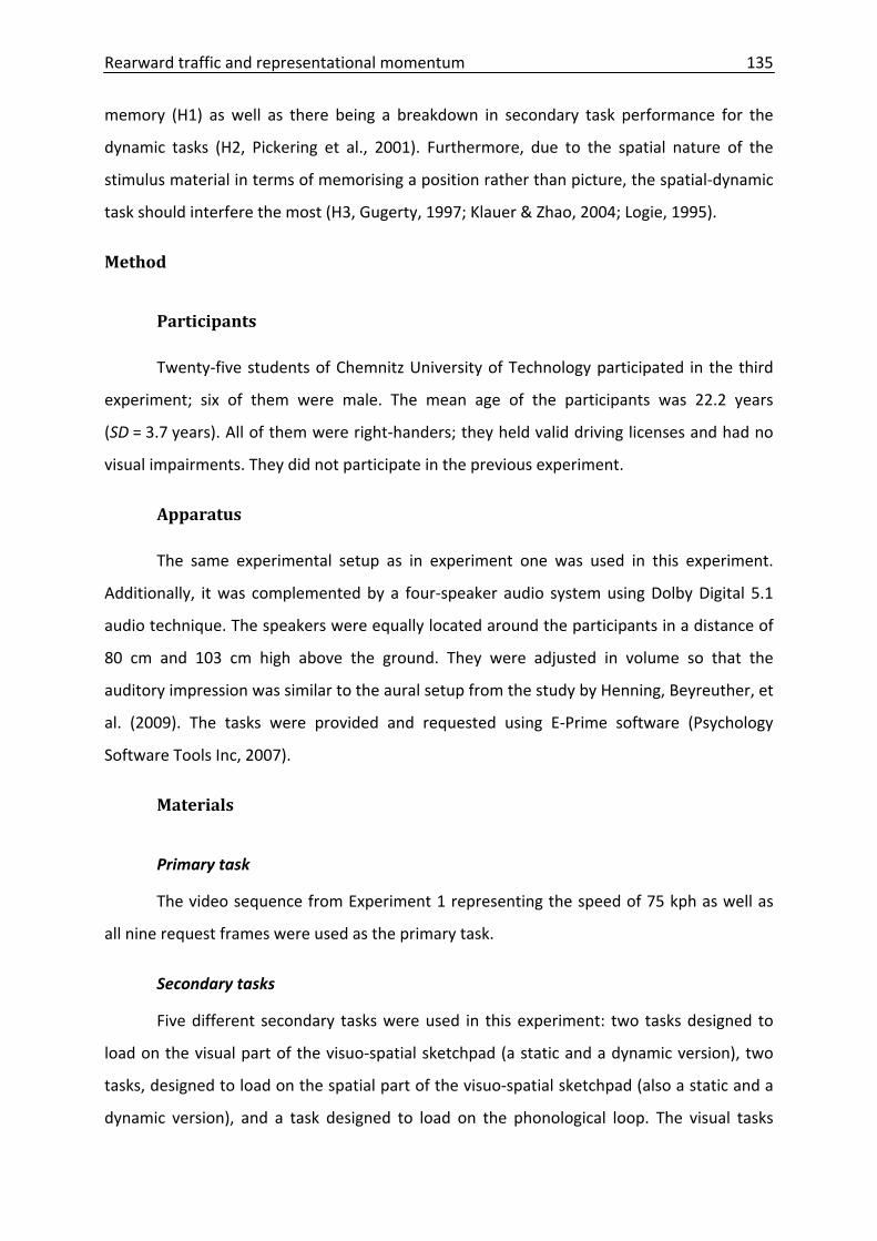
Rearward traffic and representational momentum  135 

memory  (H1)  as well  as  there being  a breakdown  in  secondary  task performance  for  the 

dynamic  tasks  (H2,  Pickering  et  al.,  2001).  Furthermore,  due  to  the  spatial  nature  of  the 

stimulus material in terms of memorising a position rather than picture, the spatial‐dynamic 

task should interfere the most (H3, Gugerty, 1997; Klauer & Zhao, 2004; Logie, 1995).   

Method 

Participants 

Twenty‐five students of Chemnitz University of Technology participated  in the third 

experiment;  six  of  them  were  male.  The  mean  age  of  the  participants  was  22.2  years 

(SD = 3.7 years). All of them were right‐handers; they held valid driving  licenses and had no 

visual impairments. They did not participate in the previous experiment. 

Apparatus 

The  same  experimental  setup  as  in  experiment  one was  used  in  this  experiment. 

Additionally,  it was complemented by a  four‐speaker audio  system using Dolby Digital 5.1 

audio technique. The speakers were equally located around the participants in a distance of 

80  cm  and  103  cm  high  above  the  ground.  They  were  adjusted  in  volume  so  that  the 

auditory impression was similar to the aural setup from the study by Henning, Beyreuther, et 

al.  (2009).  The  tasks  were  provided  and  requested  using  E‐Prime  software  (Psychology 

Software Tools Inc, 2007). 

Materials 

Primary task 

The video sequence from Experiment 1 representing the speed of 75 kph as well as 

all nine request frames were used as the primary task.  

Secondary tasks 

Five different secondary  tasks were used  in  this experiment:  two  tasks designed  to 

load on the visual part of the visuo‐spatial sketchpad (a static and a dynamic version), two 

tasks, designed to load on the spatial part of the visuo‐spatial sketchpad (also a static and a 

dynamic  version),  and  a  task designed  to  load  on  the phonological  loop.  The  visual  tasks 

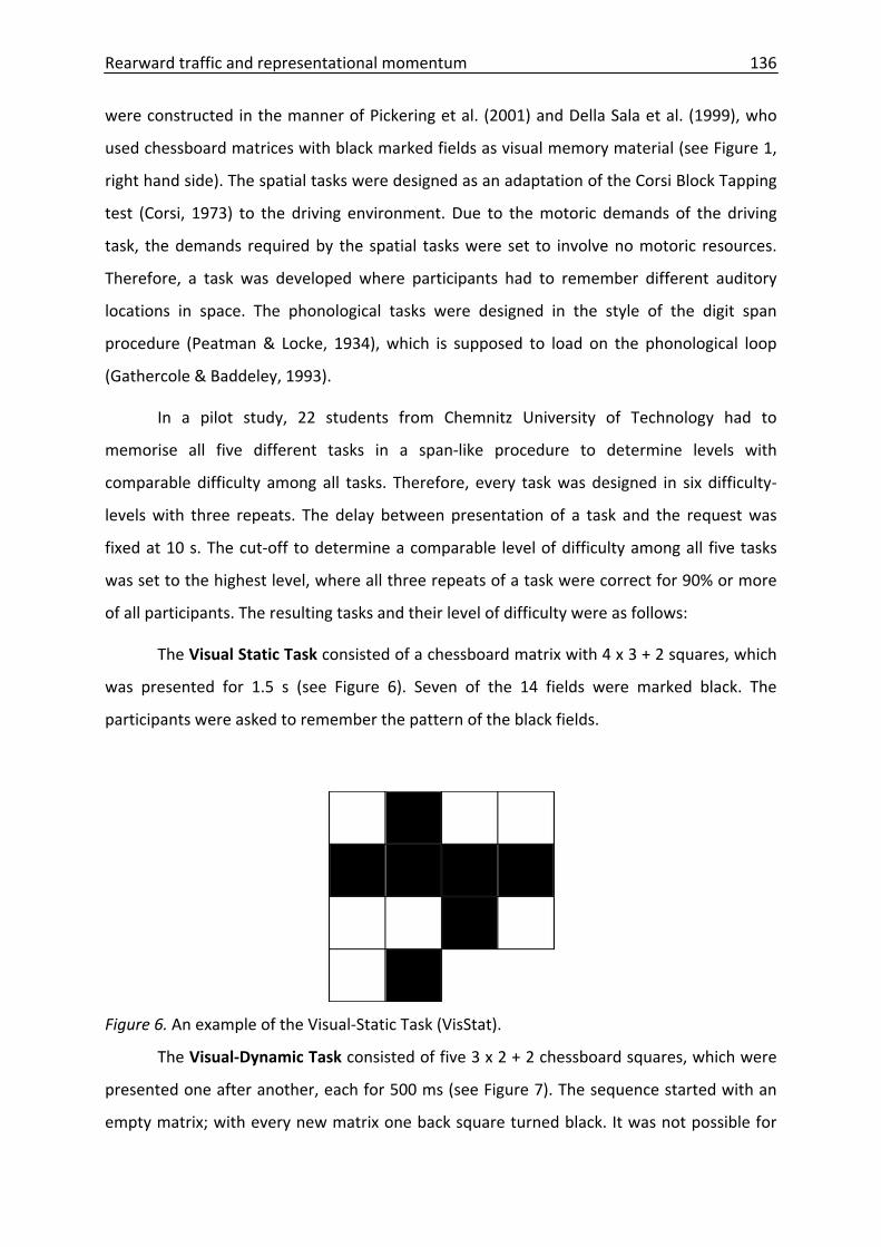
Rearward traffic and representational momentum  136 

were constructed  in the manner of Pickering et al. (2001) and Della Sala et al. (1999), who 

used chessboard matrices with black marked fields as visual memory material (see Figure 1, 

right hand side). The spatial tasks were designed as an adaptation of the Corsi Block Tapping 

test  (Corsi, 1973)  to  the driving environment. Due  to  the motoric demands of  the driving 

task,  the demands  required by  the spatial  tasks were set  to  involve no motoric  resources. 

Therefore,  a  task was  developed where  participants  had  to  remember  different  auditory 

locations  in  space.  The  phonological  tasks  were  designed  in  the  style  of  the  digit  span 

procedure  (Peatman &  Locke, 1934), which  is  supposed  to  load on  the phonological  loop 

(Gathercole & Baddeley, 1993). 

In  a  pilot  study,  22  students  from  Chemnitz  University  of  Technology  had  to 

memorise  all  five  different  tasks  in  a  span‐like  procedure  to  determine  levels  with 

comparable difficulty among all  tasks. Therefore, every  task was designed  in  six difficulty‐

levels with  three  repeats. The delay between presentation of a  task and  the  request was 

fixed at 10 s. The cut‐off to determine a comparable  level of difficulty among all  five tasks 

was set to the highest level, where all three repeats of a task were correct for 90% or more 

of all participants. The resulting tasks and their level of difficulty were as follows: 

The Visual Static Task consisted of a chessboard matrix with 4 x 3 + 2 squares, which 

was  presented  for  1.5  s  (see  Figure  6).  Seven  of  the  14  fields  were marked  black.  The 

participants were asked to remember the pattern of the black fields. 

 

 

Figure 6. An example of the Visual‐Static Task (VisStat). 

The Visual‐Dynamic Task consisted of five 3 x 2 + 2 chessboard squares, which were 

presented one after another, each for 500 ms (see Figure 7). The sequence started with an 

empty matrix; with every new matrix one back square turned black. It was not possible for 

Rearward traffic and representational momentum  137 

the  same  field  to  turn black  twice. The  task was  to  remember  the  sequence of  the black 

fields in the correct order. 

 

Figure 7. An example of the order of appearance of the Visual‐Dynamic Task (VisDyn). 

The Spatial‐Static Task was presented via  four speakers  inside  the car, which were 

positioned  around  the  driver’s  head  (see  Figure  8).  Two  different  sounds  were  played 

simultaneously on two of the four speakers at the same time for 2 s. After a short break of 

500 ms, a third sound was presented on a single speaker, for 2 s as well. It was also possible 

that  the  single  sound  preceded  the  two  different  concurrent  sounds.  The  task  for  the 

participants  was  to  memorise  the  positions  of  the  activated  speakers  in  space, 

independently of their order. 

 

Figure  8.  The  speaker  setup  around  the  participant’s  head with  an  example  of  the  two 

sounds followed by a single sound in the Spatial‐Static Task (SpatStat). 

The Spatial‐Dynamic Task consisted of four identical sounds which were presented in 

a sequence one after another, each of them for 1.5 s. The first sound was presented by one 

of  the  four  speakers  (see  Figure  9).  The  following  sound  was  presented  on  a  different 

speaker without any break. This  continued until  the  fourth  sound.  It was possible  for  the 

same speaker to be activated twice, but not in immediate succession. The participants were 

asked to memorise the sequence in which the speakers were activated. 

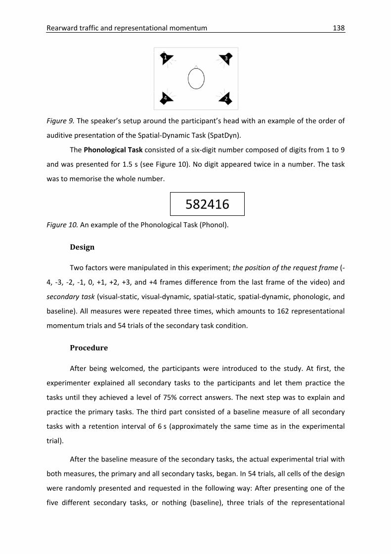
Rearward traffic and representational momentum  138 

 

Figure 9. The speaker’s setup around the participant’s head with an example of the order of 

auditive presentation of the Spatial‐Dynamic Task (SpatDyn). 

The Phonological Task consisted of a six‐digit number composed of digits from 1 to 9 

and was presented for 1.5 s (see Figure 10). No digit appeared twice  in a number. The task 

was to memorise the whole number. 

 582416

Figure 10. An example of the Phonological Task (Phonol). 

Design 

Two factors were manipulated in this experiment; the position of the request frame (‐

4,  ‐3,  ‐2,  ‐1, 0, +1, +2, +3, and +4  frames difference  from  the  last  frame of  the video) and 

secondary task (visual‐static, visual‐dynamic, spatial‐static, spatial‐dynamic, phonologic, and 

baseline). All measures were repeated three times, which amounts to 162 representational 

momentum trials and 54 trials of the secondary task condition. 

Procedure 

After being welcomed,  the participants were  introduced  to  the  study. At  first,  the 

experimenter  explained  all  secondary  tasks  to  the  participants  and  let  them  practice  the 

tasks until they achieved a  level of 75% correct answers. The next step was to explain and 

practice the primary tasks. The third part consisted of a baseline measure of all secondary 

tasks with a  retention  interval of 6 s  (approximately  the same  time as  in  the experimental 

trial).  

After the baseline measure of the secondary tasks, the actual experimental trial with 

both measures, the primary and all secondary tasks, began. In 54 trials, all cells of the design 

were randomly presented and requested  in the following way: After presenting one of the 

five  different  secondary  tasks,  or  nothing  (baseline),  three  trials  of  the  representational 

Rearward traffic and representational momentum  139 

momentum  procedure  followed,  as  in  experiment  two.  All  representational  momentum 

trials were presented with  the  video of  an  approaching  car  travelling  at 75 kph, but with 

different request frames. Participants had to estimate whether the last picture was the same 

as the  last frame of the video sequence (equivalent to Experiment 1). The number of three 

representational momentum trials were chosen according to the mean number of glances at 

the  left  wing  mirror  during  a  lane  change  trial  in  Experiment  1.  After  the  third 

representational momentum trial, the request of the secondary task was presented and the 

participant had  to enter  the memorised stimulus. Figure 11 sketches  the sequence of one 

trial.  

 

Figure 11. Experimental trial with the presentation and request of a visual‐dynamic task and 

presentation and request of three representational momentum trials in‐between. 

At the end, participants had to fill out a biographical questionnaire. 

Results 

Primary tasks 

Figure  12  depicts  the  distribution  of  “same”  responses  for  all  representational 

momentum trials under the influence of the five secondary tasks and without the influence 

(baseline).  

 

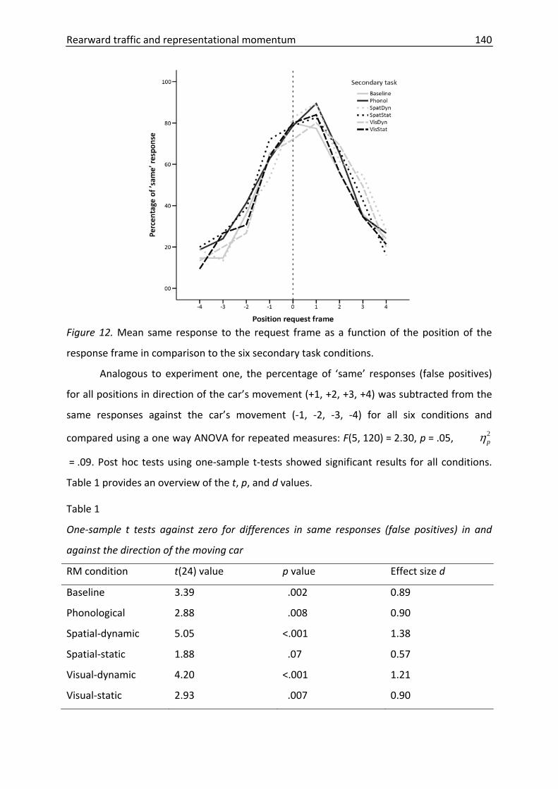
Rearward traffic and representational momentum  140 

 Figure 12. Mean  same  response  to  the  request  frame as a  function of  the position of  the 

response frame in comparison to the six secondary task conditions. 

Analogous  to experiment one,  the percentage of  ‘same’  responses  (false positives) 

for all positions in direction of the car’s movement (+1, +2, +3, +4) was subtracted from the 

same  responses  against  the  car’s  movement  (‐1,  ‐2,  ‐3,  ‐4)  for  all  six  conditions  and 

compared using a one way ANOVA for repeated measures: F(5, 120) = 2.30, p = .05,        

 = .09. Post hoc  tests using one‐sample  t‐tests showed significant results  for all conditions. 

Table 1 provides an overview of the t, p, and d values. 

2pη

Table 1 

One‐sample  t  tests  against  zero  for  differences  in  same  responses  (false  positives)  in  and 

against the direction of the moving car 

RM condition  t(24) value  p value  Effect size d 

Baseline  3.39    .002  0.89 

Phonological  2.88    .008  0.90 

Spatial‐dynamic  5.05  <.001  1.38 

Spatial‐static  1.88    .07  0.57 

Visual‐dynamic  4.20  <.001  1.21 

Visual‐static  2.93    .007  0.90 

 

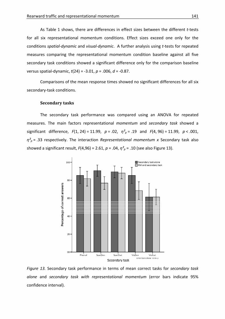
Rearward traffic and representational momentum  141 

As Table 1 shows, there are differences  in effect sizes between the different t‐tests 

for  all  six  representational momentum  conditions.  Effect  sizes  exceed  one  only  for  the 

conditions spatial‐dynamic and visual‐dynamic.  A further analysis using t‐tests for repeated 

measures  comparing  the  representational momentum  condition  baseline  against  all  five 

secondary task conditions showed a significant difference only for the comparison baseline 

versus spatial‐dynamic, t(24) = ‐3.01, p = .006, d = ‐0.87. 

Comparisons of the mean response times showed no significant differences for all six 

secondary‐task conditions. 

Secondary tasks 

The  secondary  task  performance  was  compared  using  an  ANOVA  for  repeated 

measures.  The  main  factors  representational  momentum  and  secondary  task  showed  a 

significant  difference,  F(1, 24) = 11.99,  p = .02,  η²p = .19  and  F(4, 96) = 11.99,  p < .001, 

η²p = .33  respectively.  The  interaction  Representational momentum  x  Secondary  task  also 

showed a significant result, F(4,96) = 2.61, p = .04, η²p = .10 (see also Figure 13). 

 

Figure 13. Secondary  task performance  in  terms of mean  correct  tasks  for  secondary  task 

alone  and  secondary  task  with  representational  momentum  (error  bars  indicate  95% 

confidence interval). 

 

Rearward traffic and representational momentum  142 

Post  hoc  tests  showed  a  significant  result  only  for  the  differences  in  the  Spatial‐

Dynamic  Task,  t(24) = 3.97,  p = .001,  d = 0.85,  and  a  tendency  toward  significance  for 

differences  in  the  visual‐dynamic  task  (α‐level  at  α = .01,  due  to  α‐level  correction), 

t(24) = 2.33, p = .03, d = 0.74. 

 Discussion 

All  hypotheses  could  be  proved  by  the  results.  The  representational momentum 

showed higher effect  sizes  for both dynamic  secondary  task conditions  (H1);  furthermore, 

the only  significant difference  in  comparison  to  the baseline  showed  the  representational 

momentum under  the memory  load of  the spatial‐dynamic secondary task  (H3). The same 

pattern was observable for the secondary task performance. Both dynamic secondary tasks 

show either a significant result or a tendency towards significance (H2).  

The results support the findings of Hayes and Freyd (2002). We showed that there is 

a forward shift in memory position for the final position of the dynamic item due to memory 

interference,  which  is  beyond  the  “normal”  memory  shift.  We  also  supported  the 

fragmentation hypothesis of Pickering et al. (2001) who proposed a dissociation in the visuo‐

spatial sketchpad that  is static versus dynamic  instead of visual versus spatial.  It somehow 

also supports Logie  (1995) who argued  for the where versus what distinction analogous to 

the  visual  versus  spatial  one.  The  representational  momentum  paradigm  asked  the 

participant to remember the  last position, which  is where  information and therefore more 

spatial. 

General Discussion 

Our  experiments  demonstrated  that  representational momentum  is  applicable  to 

rearward  traffic which  is  visible  in  the  left  outside mirror. As  Experiment  1  showed,  it  is 

applicable only for speed differences of above 50 kph. However, if such a situation appears 

on a highway,  it seems to be dangerous  if drivers hold spatial‐dynamic content  in memory 

simultaneously, like a route description. The consequence could be the further displacement 

of the car’s representation in memory that leads to inadequate decisions. One such decision 

with a positive outcome might be the abortion of a lane change due to the feeling that the 

oncoming car might be too close. In addition, the opposite scenario  is  imaginable,  in which 

the driver might be visually distracted in a high‐density driving situation and might think that 

Rearward traffic and representational momentum  143 

the car has already passed and therefore might start the lane change too early, with all the 

negative  consequences.  A  first  step  for  further  research  could  be  the  identification  of 

potentially  interfering  tasks  and  their  influence  on  the  lane  change  behavior  under  high 

workload of the driver. 

There is also an impact of the results on basic research. First, these finding supports 

the position of Pickering et al.  (2001)  in  the ongoing debate on  the  fragmentation of  the 

visuo‐spatial sketchpad. Nevertheless, a proof of her assumptions due to double dissociation 

is  still  outstanding  (Klauer &  Zhao,  2004).  A  second  issue  concerns  the  representational 

momentum.  It might  be  possible  that  the  there  are  other  effects  that  are  in  diametrical 

opposition to the representational momentum effect, so called motion aftereffects (Regan & 

Beverley, 1978).  It  is not  clear  to what extend both effects are  influencing each other, or 

cancel each other out, and  it could be a drawback of the present study. For  instance Freyd 

and Finke (1984) used three rotated static objects which only imply a motion to avoid these 

effects. However, when driver  look  in  their mirror,  they  see  an  approaching  car,  like  in  a 

small video. 

To conclude, the discussion showed that there are several starting points for further 

research with interesting topics to examine.   

Acknowledgement 

We would like to thank Nils Kroemer and Milena Patzelt for their help in conducting 

the experiments.   

Rearward traffic and representational momentum  144 

References 

Baddeley, A. (2003a). Double dissociations: Not magic but still useful. Cortex, 39(1), 129‐131.  

Baddeley, A. (2003b). Working memory: Looking back and  looking forward. Nature Reviews 

Neuroscience, 4(10), 829‐839.  

Baddeley, A., & Hitch, G. (1974). Working memory.  In G. H. Bower (Ed.), The psychology of 

learning and motivation: Advances  in  research and  theory  (Vol. 8, pp. 47‐‐89). New 

York: Academic Press.  

Baumann, M.,  Franke,  T., &  Krems,  J.  F.  (2008).  The  effect  of  experience,  relevance  and 

interruption duration on drivers' mental representation of a traffic situation. In D. d. 

Waard,  F.  O.  Flemisch,  B.  Lorenz,  H.  Oberheid  &  K.  A.  Brookhuis  (Eds.),  Human 

Factors for Assistance and Automation (pp. 141‐152). Maastricht: Shaker.  

Bhise, V. D., Meldrum, J., Jack, D., Troell, G., Hoffmeister, D., & Forbes, L. (1981). Driver head 

movements  in  left  outside mirror  sampling  (SAE  paper  810761). Warrendale,  PA: 

Society of Automotive Engineers. 

Corsi,  P.  M.  (1973).  Human  memory  and  the  medial  temporal  region  of  the  brain.  34, 

ProQuest  Information  &  Learning,  US.  Retrieved  from 

http://search.ebscohost.com/login.aspx?direct=true&db=psyh&AN=1976‐04900‐

001&site=ehost‐live   

Darling,  S.,  Della  Sala,  S.,  &  Logie,  R.  H.  (2009).  Dissociation  between  appearance  and 

location within visuo‐spatial working memory. The Quarterly Journal of Experimental 

Psychology, 62(3), 417‐425.  

Della Sala, S., Gray, C., Baddeley, A., Allamano, N., & Wilson, L. (1999). Pattern span: A tool 

for unwelding visuo‐spatial memory. Neuropsychologia, 37(10), 1189‐1199.  

DeLucia,  P.  R.,  & Mather,  R.  D.  (2006). Motion  extrapolation  of  car‐following  scenes  in 

younger  and older drivers. Human  Factors:  The  Journal of  the Human  Factors and 

Ergonomics Society, 48(4), 666‐674.  

Freyd,  J.  J.  (1984). Dynamic mental  representations and apparent accelerated motion. 44, 

ProQuest  Information  &  Learning,  US.  Retrieved  from 

http://search.ebscohost.com/login.aspx?direct=true&db=psyh&AN=1984‐54292‐

001&site=ehost‐live   

Freyd,  J.  J., &  Finke,  R.  A.  (1984).  Representational momentum.  Journal  of  Experimental 

Psychology: Learning, Memory, and Cognition, 10(1), 126‐132.  

Rearward traffic and representational momentum  145 

Freyd, J. J., & Finke, R. A. (1985). A velocity effect for representational momentum. Bulletin 

of the Psychonomic Society, 23(6), 443‐446.  

Freyd, J. J., & Johnson, J. Q. (1987). Probing the time course of representational momentum. 

Journal  of  Experimental  Psychology:  Learning, Memory,  and  Cognition,  13(2),  259‐

268.  

Gathercole,  S.  E., & Baddeley, A. D.  (1993). Working memory  and  language. Hillsdale, NJ 

England: Lawrence Erlbaum Associates, Inc. 

Gottsdanker,  R.  M.  (1952).  The  accuracy  of  prediction  motion.  Journal  of  Experimental 

Psychology, 43(1), 26‐36.  

Gray,  R.,  &  Thornton,  I.  M.  (2001).  Exploring  the  link  between  time  to  collision  and 

representational momentum. Perception, 30(8), 1007‐1022.  

Gugerty, L. J.  (1997). Situation awareness during driving: explicit and  implicit knowledge  in 

dynamic spatial memory. Journal of experimental Psychology: Applied, 3(1), 42‐66.  

Hayes, A. E., & Freyd,  J.  J.  (2002). Representational momentum when attention  is divided. 

Visual Cognition, 9(1), 8‐27.  

Henning, M.  J., Beyreuther, S., & Krems,  J. F.  (2009).  Is mental  representation of  rearward 

traffic  in  visuo‐spatial  working  memory  static  or  dynamic  in  lane  changing? 

Manuscript in preparation.   

Henning, M. J., Georgeon, O., Dapzol, N., & Krems, J. F. (2009). How early can the car know 

that the driver would like to change lanes? An analysis of early indicators selected by 

underlying cognitive processes. Manuscript in preparation.   

Henning, M.  J.,  Schweigert, M.,  Baumann, M., &  Krems,  J.  F.  (2006).  Eye‐glance  patterns 

during lane change manoeuvres. Paper presented at the Vision in Vehicles 11, Dublin, 

Ireland. 

Hubbard,  T.  L.,  &  Bharucha,  J.  J.  (1988).  Judged  displacement  in  apparent  vertical  and 

horizontal motion. Perception & Psychophysics, 44(3), 211‐221.  

Kelly, M. H., &  Freyd,  J.  J.  (1987).  Explorations  of  representational momentum.  Cognitive 

Psychology, 19(3), 369‐401.  

Kerzel, D. (2004). Attentional load modulates mislocalization of moving stimuli, but does not 

eliminate the error. Psychonomic Bulletin & Review, 11(5), 848‐853.  

Rearward traffic and representational momentum  146 

Kerzel,  D.  (2005).  Representational  momentum  beyond  internalized  physics:  Embodied 

mechanisms  of  anticipation  cause  errors  in  visual  short‐term  memory.  Current 

Directions in Psychological Science, 14(4), 180‐184.  

Klauer,  K.  C.,  &  Zhao,  Z.  (2004).  Double  dissociations  in  visual  and  spatial  short‐term 

memory. Journal of Experimental Psychology: General, 133(3), 355‐381.  

Landesbetrieb  Straßenbau  NRW.  (2009).  Messdaten  über  fahrstreifenbezogene 

Geschwindigkeiten auf Autobahnen.   

Logie, R. H. (1995). Visuo‐spatial working memory. Hillsdale, NJ England: Lawrence Erlbaum 

Associates, Inc. 

Nunes, L. M., & Recarte, L. A.  (2005). Speed,  traffic complexity, and visual performance: a 

study on open road. In G. Underwood (Ed.), Traffic and transport psychology: Theory 

and application (pp. 339‐354). Amsterdam: Elsevier.  

Olsen, E. C. B., Lee, S. E., & Wierwille, W. W. (2005). Eye glance behavior during lane changes 

and  straight‐ahead driving. Paper presented  at  the Transportation Research Board 

Meeting. 

Peatman,  J. G., &  Locke, N. M.  (1934).  Studies  in  the methodology of  the digit‐span  test. 

Archives of Psychology, 167, 35‐35.  

Pickering,  S.  J.  (2001).  Cognitive  approaches  to  the  fractionation  of  visuo‐spatial working 

memory. Cortex, 37(4), 457‐473.  

Pickering, S. J., Gathercole, S. E., Hall, M., & Lloyd, S. A. (2001). Development of memory for 

pattern and path: Further evidence for the fractionation of visuo‐spatial memory. The 

Quarterly  Journal  of  Experimental  Psychology  A:  Human  Experimental  Psychology, 

54(2), 397‐420.  

Psychology Software Tools Inc. (2007). E‐Prime 2 (Version 2.0.8.22). Pittsburgh, PA.  

Regan, D., & Beverley,  K.  I.  (1978).  Illusory motion  in  depth: Aftereffect  of  adaptation  to 

changing size. Vision Research, 18(2), 209‐212.  

Robinson, G. H., Erickson, D., Thurston, G., & Clark, R.  (1972). Visual search by automobile 

drivers. Human Factors, 14(4), 315‐323.  

Salvucci, D. D. (2006). Modeling driver behavior  in a cognitive architecture. Human Factors, 

48(2), 362‐380.  

Rearward traffic and representational momentum  147 

Smyth, M. M., & Pendleton, L. R.  (1989). Working memory  for movements. The Quarterly 

Journal of Experimental Psychology A: Human Experimental Psychology, 41(2), 235‐

250.  

Thornton,  I.  M.,  &  Hayes,  A.  E.  (2004).  Anticipating  action  in  complex  scenes.  Visual 

Cognition, 11(2), 341‐370.  

Tijerina, L., Garrott, W. R., Stoltzfus, D., & Parmer, E. (2005). Eye glance behavior of van and 

passenger car drivers during  lange change decision phase. Transportation Research 

Record, 1937, 37‐43.  

Vicom ‐ Visual components (Version 0.71). (2008). arge tp 21.  

 

 

Lebenslauf    148  

Lebenslauf Matthias Johannes Henning  

 ZUR PERSON 

 geboren am    08.04.1972  Geburtsort    Berlin Familienstand   verheiratet, eine Tochter Staatsangehörigkeit  deutsch  

 ANSCHRIFT 

       Technische Universität Chemnitz 

Institut für Psychologie Allgemeine und Arbeitpsychologie Wilhelm‐Raabe‐Straße 43 09120 Chemnitz Tel.: 0371‐531‐36405 E‐Mail: matthias.henning@psychologie.tu‐chemnitz.de 

  AKADEMISCHER WERDEGANG  

01.2006 – 12.2009  Dissertation: „Preparation for lane change manoeuvres: Behavioural indicators and underlying cognitive processes.“, 9/2006 – 11/2006 Feldversuch zur Datengewinnung in Lyon/Frankreich, 1/2009 bis 8/2009 Laborstudien in Chemnitz, 8/2008 bis 01/2009 Fahrsimulatorversuch in Chemnitz (erfolgreiche Verteidigung am 19.03.2010, Gesamtnote: magna cum laude) 

 seit 04.2004  Wissenschaftlicher Mitarbeiter am Lehrstuhl für Allgemeine 

und Arbeitspsychologie der TU Chemnitz  02.2003 – 05.2003  Praktikum bei der BMW Forschung und Technik GmbH – Team 

MMI – Schwerpunkt Eye‐Tracking (München)  02.2002 – 04.2002  Praktikum beim Fraunhofer Institut für Produktionsanalgen und 

Konstruktionstechnik (IPK) – Abteilung Wissensmanagement (Berlin) 

 04.1999 – 08.2003   Studentische Hilfskraft, am Lehrstuhl für 

Allgemeine und Arbeitspsychologie der TU Chemnitz und an der Valdosta State University (08.2000 ‐ 04.2001) 

 

  

Lebenslauf    149  

08.2000 – 05.2001  Auslandsstudium an der Valdosta State University (Valdosta, GA, USA), Schwerpunkt: Industrial and Organizational Psychology 

 10.1998 – 03.2004  Studium der Psychologie an der TU Chemnitz (Diplomnote 1,4), 

Schwerpunkt: Arbeits‐ und Ingenieurspsychologie,   Diplomarbeit: „Indikatoren der Fahrerabsichtserkennung – Das 

Blickverhalten bei Spurwechselvorgängen“ im Auftrag der BMW Forschung und Technik GmbH (München) 

  FORSCHUNGSINTERESSEN 

 Gestaltung und Evaluation der MMS, Fokus Fahrerassistenz‐ und Fahrerinformationssysteme (FAS/FIS)  Erkennung der Handlungsintention (Fahrerabsichtserkennung) Fahrermodellierung (ACT‐R)  Usability Visuell‐räumliches Arbeitsgedächtnis Representational Momentum 

 Eye‐Tracking  

      Fahrsimulation Naturalistic Driving Studies, Field Operational Tests 

  PROJEKTE 

 seit 11.2009  Akquise und Bearbeitung – Forschungsprojekt  

„Fahrerakzeptanz von aktiver Gefahrenbremsung“ als Teilprojekt der Forschungsinitiative AKTIV (Adaptive und Kooperative Technologien für den Intelligenten Verkehr) 

 seit 09.2009  Akquise und Leitung – Forschungsprojekt für Honda R&D 

Europe  07.2008 – 12.2009  Akquise und Bearbeitung  – Methodenprojekt „Methodische 

Aspekte von sogenannten Naturalistic Driving Studies und Feldstudien“ für die Forschungsvereinigung Automobiltechnik 

 11.2007 – 05.2008  Akquise – „Kompetenzinitiative Usabilty“. Preisträger des 

Wettbewerbs „Wirtschaft trifft Wissenschaft“ des Ministeriums für Verkehr, Bau und Stadtentwicklung 

 10.2006 – 01.2007  Akquise und Leitung – Evaluationsprojekt „Bewertung eines 

Fahrerassistenzsystems“ für die BMW Forschung und Technik GmbH 

   

Lebenslauf    150  

seit 03.2006  Gründung und Forschung am Interdisziplinären Zentrum für Fahrerassistenzsysteme der TU Chemnitz (I‐FAS) 

 10.2005 – 03.2007   Akquise und Leitung – Forschungsprojekt 

„Reisezeitinformationen auf Autobahnwegweisern“ für die Bundesanstalt für Straßenwesen 

 11.2004 – 09.2005  Akquise und Leitung – Forschungsprojekt  

„Spurwechselabsichtserkennung“ für die BMW Forschung und Technik GmbH 

 11.2004 – 03.2008  Young Researcher im EU‐Network of Excellence HUMANIST    11.2004 – 06.2008  Konzeptionierung und Aufbau des Fahrsimulators der TU 

Chemnitz  04.2004 – 09.2004  Leitung – Forschungsprojekt „Reliabilität der 

Okklusionsmethode“ für die Bundesanstalt für Straßenwesen  08.2002 – 10.2002  Mitarbeit im Projekt – Evaluation eines Fahrer‐Information‐

Systems im Fahrversuch für die BMW Forschung und Technik GmbH (als stud. Hilfskraft) 

 06.2001 – 08.2003  Mitarbeit im Forschungsprojekt „Benutzerorientierte 

Präsentation und   von Informationen im Internet“, gefördert von der 

04.1999 – 07.2000 Deutschen Forschungsgemeinschaft, Fokus Eye‐Tracking (als stud. Hilfskraft) 

  

LEHRTÄTIGKEIT  SS 2010  Seminar Ergonomie  WS 2009/10   Empirisch‐Experimentelles Forschen  SS 2009  Seminar Ingenieurpsychologie: Ergonomie  WS 2008/09   Empirisch‐Experimentelles Forschen  SS 2008   Seminar Ingenieurpsychologie: Ergonomie und Design  WS 2007/08   Empirisch‐Experimentelles Forschen  SS 2007   Seminar Kognitive Ergonomie  SS 2007   Proseminar Gedächtnis  

  

Lebenslauf    151  

SS 2006   Proseminar Gedächtnis   WS 2005/06   Experimentalpsychologisches Praktikum  SS 2005   Proseminar Gedächtnis  WS 2004/05   Experimentalpsychologisches Praktikum   

BETREUUNG VON DIPLOM‐ UND BACHELORARBEITEN  seit 2009  Nils Kroemer, Julia Wichmann – Blicklängen bei 

Spurwechselvorgängen – Zusammenhänge mit der individuellen „Inspection Time“ und deren Modellierung in einer kognitiven Architektur (ACT‐R)  

 seit 2009  Matthias Rölz, Mario Simon – Explorationen des klassischen 

„Represenational Momentum“ und deren Lokalisation im Arbeitsgedächtnis 

 seit 2008  Susi Beyreuther – Repräsentation räumlich‐dynamischer 

Informationen bei Spurwechselvorgängen  2009  Milena Patzelt – Das „Represenational Momentum“ des 

rückwärtigen Verkehrs und dessen Lokalisation im Arbeitsgedächtnis 

 2006 – 2008  Anna Mikolajetz – Fahrerverhalten in Kurven. Ermittlung von 

Kenngrößen zur Parametrisierung von Kurvenassistenz (für die Volkswagen AG, Wolfsburg) 

 2006 – 2008  Ulrike Thiemer – Wahrnehmung und Akzeptanz von 

Reisezeitangaben in dynamischen Wegweisern auf Bundesautobahnen. Eine experimentelle Untersuchung zur Bewertung verschiedener Anzeigekonzepte 

  

MITGLIEDSCHAFTEN        

Society for Human Resource Management, VSU local chapter         International Association of Applied Psychology         Deutsche Gesellschaft für Psychologie  

    

  

Lebenslauf    152  

ANDERE TÄTIGKEITEN UND SCHULBILDUNG    

11.2008  Trainer für Eye‐Tracking Anwendungen (faceLAB) im Fahrsimulator, für CIDAUT, Valladolid, Spanien 

 01.2001 – 04.2001  Mitarbeiter des campusweiten IT‐Support an der Valdosta State 

University (Valdosta, GA, USA)  02.1995 – 07.1998  Erwerb der Hochschulreife am Treptow‐Kolleg, Berlin  12.1994 – 01.1995  Fahrer für Lastkraftwagen mit mehr als 7,5t zulässigem 

Gesamtgewicht für die Firma Weiss, Berlin  02.1993 – 07.1994  Elektronik‐Facharbeiter bei der Deutschen Bahn, Berlin, 

Schwerpunkt Fernmeldemontage  02.1991 – 10.1991  Elektronik‐Facharbeiter bei der Deutschen Reichsbahn, Berlin, 

Schwerpunkt Instandhaltung von Computersystemen  09‐1988 – 02.1991  Berufsausbildung zum Elektronikfacharbeiter bei der Deutschen 

Reichsbahn, Berlin, Schwerpunkt Instandhaltung von Computersystemen 

 09.1978 – 08.1988  Polytechnische Oberschule, Berlin 

  KENNTNISSE UND FÄHIGKEITEN  

Trainings  Workshop zur Nutzung und Analyse von Elektrookulografie (EOG) bei Prof. Niels Galley, Köln 

   Training zum Systemadministrator (Windows 2000) 

 EDV      MS Office (Word, Powerpoint, Excel, Project) 

        SPSS, R         Diadem (aus LabVIEW von National Instruments)         Matlab         Mangold Interact         Noldus Observer      Experimente    E‐Prime         PxLab    Modellierung    ACT‐R         Hidden Markov Models (via Matlab)    Programmierung  Visual Basic for Applications (Excel, E‐Prime und Diadem)          HTML  

  

Lebenslauf    153  

  

        Einstieg Lisp         Einstieg in C++    Hardware    Eye‐Tracker (ASL, faceLAB, SMI)         Fahrsimulator (STISIM)    Sprachen    Englisch (fließend in Wort und Schrift)         Französisch (Grundkenntnisse)         Russisch (Grundkenntnisse)    Fahrerlaubnis für  PKW (B, BE) 

LKW (C, CE, C1E, T)         Motorrad (A, A1)  

Publikationsliste    154  

Publikationsliste Matthias Johannes Henning  Beiträge in Zeitschriften  Gelau, C., Henning, M. J., & Krems, J. F. (2009). On the reliability of the occlusion technique 

as a tool for the assessment of the HMI of in‐vehicle information and communication systems. Applied Ergonomics, 40, 181‐184. 

 Lebherz, C., Mohr, C., Henning, M. & Sedlmeier, P. (2005). Wie brauchbar sind Hochschul‐

Rankings? Eine empirische Analyse. In Teichler, U. & Tippelt, R. (Eds.) Hochschullandschaft im Wandel (Zeitschrift für Pädagogik ‐ 50. Beiheft), 

 Beiträge in Tagungsbänden  Henning, M. J., Schweigert., M., Baumann, M., & Krems, J. F. (in press). Eye‐glance patterns 

during lane change manoeuvres. In A.G. Gale et al. (Eds.) Proceedings of Vision in Vehicles 11. 

 Lietz, H., Henning, M. J., Petzoldt, T., Krems, J. F., & Wanielik, G. (2010). A software tool for 

the visualization and annotations of naturalistic driving data stored in relational databases. In J. Krems, T. Petzoldt, & M. Henning (Eds.), Proceedings of European Conference on Human Centred Design for Intelligent Transport Systems (pp. 427‐433). Lyon: HUMANIST publications. 

 Henning, M. J., Mikolajetz, A., Tenzer, A., Zobel, R. & Krems, J. F. (2009). Fahrerverhalten in 

Kurven: Ermittlung von Kenngrößen zur Parametrisierung von Kurvenassistenz. In A. Lichtenstein, C. Stößel & C. Clemens (Eds.). Der Mensch im Mittelpunkt technischer Systeme, Tagungsband der 8. Berliner Werkstatt Mensch‐Maschine‐Systeme (S. 200‐205). Düsseldorf: VDI Verlag. 

 Jentsch, M., Kienast, H., Lindner, P., Weigel, H., Henning, M. J., Petzoldt, T., Wanielik, G., 

Krems, J. F. & Spanner‐Ulmer, B. (2009). Vernetzt Forschen – das I‐FAS der TU Chemnitz. In Tagungsband Vernetzt Planen und Produzieren (S. 113‐122). 

 Lindner, P., Weigel, H., Fardi, B., Henning, M. J., Kienast, H., Wanielik, G., Krems, J. F. & 

Spanner‐Ulmer, B. (2009). Räumlich gerichtete Anzeigen im Fahrzeug: Realisierung einer Mensch‐Maschine‐Schnittstelle für ein Fußgängererkennungssystem. In Tagungsband (CD 1) des 1. Automobiltechnischen Kolloquiums, München. 

 Mikolajetz, A., Henning, M. J., Tenzer, A., Zobel, R., Krems, J. F., & Petzoldt, T. (2009). Curve 

Negotiation: Identifying Driver Behavior Around Curves with the Driver Performance Database. In Proceedings of the 5th International Driving Symposium on Human Factors in Driver Assessment, Training, and Vehicle Design , Big Sky, Montana (pp. 391‐397). 

 

  

Publikationsliste    155  

Weigel, H., Lindner, P., Henning, M. J., Kienast, H., Wanielik, G., Krems, J. F., & Spanner‐Ulmer, B. (2009) A novel head up display for driver assistance systems. In Proceedings of ITS 2009, 16th World Congress on Intelligent Transport Systems. 

 Henning, M. J., Georgeon, O., Wynn, T., & Krems, J. F. (2008). Modeling driver behaviour in 

order to infer the intention to change lanes. In C. Brusque (Ed.), Proceedings of the European Conference on Human Interface Design for Intelligent Transport Systems (pp. 113‐120). Lyon: Humanist Publications. 

 Henning, M. J., Kienast, H., Lindner, P., Weigel, H., Krems, J. F., Spanner‐Ulmer, B. & 

Wanielik, G. (2008). Multifunktionale Mensch‐Maschine‐Schnittstelle. In Maurer, M. und Stiller, C. (Hrsg.), Tagungsband des 5. Workshops Fahrerassistenzsysteme FAS2008 (S. 151‐158). Karlsruhe: fmrt e.V. 

 Kienast, H., Henning, M. J., Lindner, P., Weigel, H., Krems, J. F., Spanner‐Ulmer, B. & 

Wanielik, G. (2008). Fußgängerwarnung mit einer Multifunktionalen Mensch‐Maschine‐Schnittstelle. In: Gesellschaft für Arbeitswissenschaft (Hrsg.). Produkt‐ und Produktions‐Ergonomie ‐ Aufgabe für Entwickler und Planer (S. 137‐140). Dortmund: GfA Press. 

 Kienast, H., Henning, M. J., Lindner, P., Weigel, H., Krems, J. F., Wanielik, G. & Spanner‐

Ulmer, B. (2008). Aufmerksamkeitssteuerung mit räumlich gerichteten Anzeigen bei Fahrerassistenzsystemen. In: Tagungsband zur 24. VW/VDI‐Gemeinschaftstagung "Fahrerassistenzsysteme und Integrierte Sicherheit" (S. 413‐424). VDI Bericht 2048. 

 Wynn, T., Richardson, J. H., Georgeon, O., Bellet, T., Henning, M. J., & Krems, J. F. (2008). 

Cognitive activity modelling: A case study of lane change schemas and sensation seeking. In C. Brusque (Ed.), Proceedings of the European Conference on Human Interface Design for Intelligent Transport Systems (pp. 277‐285). Lyon: Humanist Publications. 

 Georgeon, O., Henning, M. J., Bellet, T., & Mille, A. (2007). Creating cognitive models from 

activity analysis: A knowledge engineering approach to car driver modeling. Proceedings of the International Conference on Cognitive Modeling, Ann Arbor, Michigan (pp. 43‐48).  

 Henning, M. J., Georgeon, O., & Krems, J. F. (2007). The quality of behavioral and 

environmental indicators used to infer the intention to change lanes. In Proceedings of the International Driving Symposium on Human Factors in Driver Assessment, Training, and Vehicle Design, Stevenson, Washington (pp. 231‐237). 

 Henning, M. J., Georgeon, O., & Krems, J. F. (2007). Verhaltensindikatoren zur 

Fahrerabsichtserkennung am Beispiel des Spurwechsels. In M. Rötting, G. Wozny, A. Klostermann & J. Huss (Hrsg.), Prospektive Gestaltung von Mensch‐Technik‐Interaktion, Tagungsband der 7. Berliner Werkstatt Mensch‐Maschine‐Systeme (S. 185‐190). Düsseldorf: VDI Verlag. 

  

  

Publikationsliste    156  

Buchkapitel  Krems, J. F., Henning, M., & Petzoldt, T. (2009). Methoden zur Messung von Fahrerverhalten: 

Vom Labor bis zur Feldstudie. In H. Winner & R. Buder (Hrsg.), Wie realitätsnah lässt sich Fahrerverhalten messen? (S. 103 ‐ 111). Stuttgart: Ergonomia. 

 Editionen  Krems, J., Petzoldt, T., & Henning, M. (Eds.) (2010). Proceedings of European Conference on 

Human Centred Design for Intelligent Transport Systems. Lyon: HUMANIST publications. 

 Vorträge/Poster auf wissenschaftlichen Tagungen  Metzner, M., Wichmann, J., Henning, M. J. & Krems, J. F. (2010, März). Auswirkungen der 

Überlagerung mehrerer dynamischer Objekte im Arbeitsgedächtnisses auf den Representational‐Momentum‐Effekt. Poster auf der 52. Tagung experimentell arbeitender Psychologen, Saarbrücken. 

 Henning, M. J., Georgeon, O., & Krems, J. F. (2008, September). The stability of behavioral 

indicators used to infer the intention to change lanes. Presentation given at the 4th International Conference on Traffic & Transport Psychology, Washington DC. 

 Henning, M. J., Thiemer, U. & Krems, J. F. (2008, März). Die Bewertung unterschiedlicher 

Anzeigeformen von Reisezeitinformationen auf Autobahnwegweisern. Präsentation auf der 50. Tagung experimentell arbeitender Psychologen, Marburg. 

 Wynn, T., Richardson, J., Georgeon, O., Bellet, T., Henning, M.J., & Krems, J.F. (2007, 

September). Cognitive activity modelling: A case study of lane change schemas and sensation seeking. Presentation at the TFC Conference, Humanist Framework, Vienna, Austria. 

 Henning, M. J., Baumann, M. & Krems, J. F. (2006, September). Blickverhalten zur Vorhersage 

von Spurwechselvorgängen . Präsentation auf dem 45. Kongress der Deutschen Gesellschaft für Psychologie, Nürnberg. 

 Henning, M., Schweigert M. & Krems, J. F. (2006, März). Der Einfluss der Geschwindigkeit auf 

das Blickverhalten bei Spurwechselvorgängen. Präsentation auf der 48. Tagung experimentell arbeitender Psychologen, Mainz. 

 Krems, J. F., Henning, M. J., Baumann, R. K. M., & Schweigert, M., (2006, November). 

Inferring driver’s intention by using eye‐movement behaviour. Presentation at the 2nd conference on Driver Needs, Humanist Framework, Turku, Finnland. 

 Krems, J. F., Baumann, M., Henning M. & Schweigert M. (2005, July). Lane‐change 

assistance: Predicting drivers intentions by eye‐movement. Presentation at the 11. Conference on Human‐Computer Interaction, Las Vegas. 

 

  

Publikationsliste    157  

Henning, M., Schweigert, M., Baumann M. & Krems J. F. (2005). Blickverhalten bei Spurwechselvorgängen. Präsentation auf der 47. Tagung experimentell arbeitender Psychologen, Regensburg. 

 Baumann, M., Henning, M., Schweigert, M., Rösler D., & Krems J. F. (2004, September). Eye‐

Movement behaviour during lane change manoeuvres. Presentation given at the 3rd International Conference on Traffic & Transport Psychology, Nottingham, UK. 

 Eingeladene Vorträge und Diskussionen  Henning, M. (2009, August). Das dynamische Arbeitsgedächtnis beim Spurwechsel. 

Präsentation beim Deutschen Zentrum für Luft‐ und Raumfahrt, Institut für Verkehrssystemtechnik, Braunschweig. 

 Henning, M. (2008, April). Ganzheitliche Anzeigekonzepte für multifunktionale FAS. 

Präsentation auf dem 4. TecDay, Aschaffenburg.   Henning, M. (2008, März). Fahrerabsichtserkennung ‐ Indikatoren des Spurwechsels. 

Präsentation für die Volkswagen Konzernforschung, Wolfsburg.  Henning, M. (2007, Januar). Das Blickverhalten als Indikator der Fahrerintention am Beispiel 

des Spurwechsels. Präsentation im Rahmen des ZMMS Eyes‐Tea, Berlin.  Henning, M, Schaap, N., & Turetschek, C. (2006, April). From driving behaviour to driver 

models and back. Presentation at the Tandem Learning Session within the Humanist Framework, Madrid, Spain.  

 Henning, M. (2006, January). Eye‐movement behavior during lane changing manoeuvres. . 

Presentation at a Meeting within the Humanist Framework in Lyon, France.  Berichte  Hülsemann, U., Krems, J. F., Henning, M. J., & Thiemer, U. (2009). Voraussetzungen für 

dynamische Wegweisung mit integrierten Stau‐ und Reisezeitinformationen. In Berichte der Bundesanstalt für Straßenwesen, Verkehrstechnik, Heft V 181: Bundesanstalt für Straßenwesen. 

 Henning, M. J., Beyreuther, S., Kroemer, N., Wipplinger, S., Krems. J. F. & Schaller, J. (2007). 

Expertenevaluation eines Fahrerassistenzsystems mit Spurwechselabsichtserkennung. Projektbericht für die BMW Group Forschung und Technik GmbH, München. 

 Henning, M. & Krems, J. F. (2005). Spurwechselabsichtserkennung. Projektbericht für die 

BMW Group Forschung und Technik GmbH, München.   Henning, M. & Krems, J. F. (2004). Die Relaibilität der Okklusionsmethode beim Einsatz als 

Verfahren zur Messung visueller Ablenkung durch Fahrerassistenz‐ und Informationssysteme. Projektbericht für die Bundesanstalt für Straßenwesen, Bergisch‐Gladbach.   

  

Publikationsliste    158  

  

Rezensionen  Jahn, G., & Henning, M. (2007). Two new textbooks on applied cognitive psychology. Applied 

Cognitive Psychology, 21, 551‐556.  Sonstiges  Petzoldt, T. & Henning, M. (2008). 4. International conference on traffic & transport 

psychology (Tagungsbericht). Zeitschrift für Verkehrssicherheit, 54, 219‐220.   Qualifikationsschrift  Henning, M. (2004). Indikatoren der Fahrerabsichtserkennung – Das Blickverhalten bei 

Spurwechselvorgängen. Unveröffentlichte Diplomarbeit: TU Chemnitz.   

Eidesstattliche Erklärung 

 

 

 

Die vorliegende Arbeit wurde von mir selbstständig verfasst. Ich habe keine anderen als die 

angegeben Hilfsmittel benutzt. 

 

 

 

 

Matthias Henning 

Chemnitz, den 10.12.1009