arX

iv:1

202.

1696

v1 [

q-bi

o.N

C]

8 F

eb 2

012

Bayesian Inference of Whole-Brain Networks

M. Hinne1,2,*, T. Heskes2, and M.A.J. van Gerven1

1Donders Institute for Brain, Cognition and Behaviour: Centre for Cognition.

Radboud University, Nijmegen, The Netherlands2Institute for Computing and Information Sciences. Radboud University,

Nijmegen, The Netherlands*mhinne@cs.ru.nl

February 9, 2012

Abstract

In structural brain networks the connections of interest consist of white-matter fibre bun-dles between spatially segregated brain regions. The presence, location and orientation ofthese white matter tracts can be derived using diffusion MRI in combination with probabilis-tic tractography. Unfortunately, as of yet no approaches have been suggested that providean undisputed way of inferring brain networks from tractography. In this paper, we providea computational framework which we refer to as Bayesian connectomics. Rather than apply-ing an arbitrary threshold to obtain a single network, we consider the posterior distributionof networks that are supported by the data, combined with an exponential random graph(ERGM) prior that captures a priori knowledge concerning the graph-theoretical propertiesof whole-brain networks. We show that, on simulated probabilistic tractography data, ourapproach is able to reconstruct whole-brain networks. In addition, our approach directlysupports multi-model data fusion and group-level network inference.

1 Introduction

Human behaviour ultimately arises through the interactions between multiple brain regions thattogether form a network that can be characterized in terms of structural, functional and effectiveconnectivity (Penny et al., 2006). The science of characterizing neural connectivity, that is, toelucidate the wiring diagram of the human brain, has come to be known as connectomics and isseen as one of the great challenges in neuroscience (Sporns et al., 2005).

Structural connectivity presupposes the presence of white-matter tracts that connect spatiallysegregated brain regions which constrain the functional and effective connectivity between theseregions. Hence, structural connectivity provides the scaffolding that is required to shape neu-ronal dynamics. Furthermore, structural connectivity has been related to several diseases, suchas Alzheimer’s disease, attention deficit hyperactivity disorder and multiple sclerosis (He et al.,2008, 2009; Konrad and Eickhoff, 2010), and is therefore also of major importance in clinicalneuroscience (Catani, 2007).

Currently, the only way to estimate structural connectivity of whole-brain networks in vivois through the use of diffusion imaging; a variant of magnetic resonance imaging which measuresthe restricted diffusion of water molecules, thereby providing an indirect measure of the presenceand orientation of white-matter tracts. By following the principal diffusion direction in individualvoxels, streamlines can be drawn that represent the structure of fibre bundles connecting sepa-rate regions of grey matter. This process is known as deterministic tractography (Chung et al.,2010; Zhang et al., 2005). There are however several problems associated with this deterministic

1

approach as it cannot easily deal with various ambiguous but common fiber configurations suchas kissing, crossing and splaying fibre bundles (Jbabdi and Johansen-Berg, 2011).

As a solution to this problem, probabilistic tractography has been introduced (Behrens et al.,2007, 2003; Friman et al., 2006; Jbabdi et al., 2007). By repeating the streamlining process multi-ple times, probabilistic tractography ultimately produces for each voxel a measure of uncertaintyabout in which other voxel a hypothesized connection will terminate. A benefit of the proba-bilistic approach is that it can deal with ambiguous fiber configurations by taking streamlininguncertainty into account and produces probability estimates concerning the presence or absenceof particular white-matter tracts.

Often, one is not interested so much in particular tracts but rather in whole-brain struc-tural connectivity. Several approaches have been suggested to derive whole-brain networks fromprobabilistic tractography results (Chung et al., 2011; Hagmann et al., 2007; Iturria-Medina et al.,2008; Skudlarski et al., 2008). The resulting networks are all reported to exhibit certain graph-theoretical properties, such as a characteristic short path length, clustering, the existence of hubsand modular structure (Bassett et al., 2011; Bassett and Bullmore, 2006; Bullmore and Sporns,2009; Gong et al., 2009; Sporns, 2006). Unfortunately, the inference of whole-brain networks fromprobabilistic tractography estimates remains somewhat ad hoc. Networks are often constructedby counting the number of streamlines that connect regions of interest and interpreting this as anundirected, weighted graph (e.g. (Zalesky et al., 2010)). Alternatively, a binary graph is obtainedby simply adding an edge for each pair of regions that have one or more streamlines between them(e.g. (Bassett et al., 2011; Hagmann et al., 2007; Vaessen et al., 2010)). It is hard, however, tomaintain a direct correspondence between connection strength and the probability distributionover tracts that is produced by probabilistic tractography (Jbabdi and Johansen-Berg, 2011).

Another important observation is that the mentioned approaches do not easily support theintegration of probabilistic streamlining data with other datasets. This is a particularly relevanttopic in contemporary neuroscience since it is assumed by multi-modal data fusion, where dataacquired via different recording modalities is integrated to provide a coherent picture of brainfunction (Horwitz and Poeppel, 2002), and required by group-level inference, where the interest isin estimating a network that characterizes a particular population, e.g. when comparing patientswith controls in a clinical setting (Simpson et al., 2011b).

In the following, we provide for the first time a computational framework for the estimation ofwhole-brain networks from probabilistic tractography outcomes. In our approach, which we referto as Bayesian connectomics, we consider the posterior distribution of graphs that are supportedby our data, instead of a generating a single network based on an arbitrary threshold. Ourapproach relies on defining a generative model for whole-brain networks which is inspired byrecent work on network inference in systems biology (Mukherjee and Speed, 2008) and consistsof two ingredients. First, a likelihood model based on a multivariate distribution which viewsthe streamline distributions produced by probabilistic tractography as noisy data. Second, anexponential random graph prior which models prior knowledge concerning the graph-theoreticalproperties of whole-brain networks. The extension to multi-modal data fusion or group-levelinference follows by defining the likelihood model as a product of multivariate distributions. Inorder to validate our methodology we make use of simulated data which allows us to compare theestimates produced by Bayesian connectomics with ground truth. We show that our approachis able to reconstruct whole-brain networks from simulated data as produced by probabilistictractography.

2 Bayesian inference of whole-brain networks

In this section we derive our Bayesian approach to the inference of whole-brain networks, referredto as Bayesian connectomics. We start by defining the likelihood term for our generative model.Subsequently, an exponential random graph prior will be defined which can be used to capture theessential graph-theoretical properties of whole-brain networks. Finally, we derive a Markov chainMonte-Carlo algorithm to sample from the posterior distribution of whole-brain networks.

2

2.1 Likelihood model

Assume we want to infer the connectivity between K brain regions. That is, we want to find agraph G ∈ G where G is the family of undirected graphs. The graph G = (V,E) consists of verticesV = {V1, . . . , VK} and edges E ⊆ V ×V where loops (Vi, Vi) for i ∈ {1, . . . ,K} are excluded fromthe edge set. We use eij = 1 when (Vi, Vj) ∈ E and eij = 0 when (Vi, Vj) /∈ E.

We start by considering one region and the possible targets in which a postulated tractmay terminate. Probabilistic tractography will produce a distribution over target regions ni =(ni1, . . . , niK)T by drawing S streamlines, Ni =

∑Kk=1 nik ≤ S of them ending up in a target

region. Let nii = 0 and assume that all streamlines are drawn independently. The probability offinding a particular distribution ni is expressed as a multinomial distribution

P (ni | xi) ∝

K∏

j=1

xnij

ij , (1)

in which xij with∑

j xij = 1 represents the probability of drawing a streamline from region i toregion j. This streamlining probability itself depends on whether or not there actually exists atract between region i and region j. We model the distribution of streamlining probabilities usinga Dirichlet distribution

P (xi | ai) ∝

K∏

j=1

xaij−1ij (2)

where theaij = eija+ (1− eij)a (3)

can be interpreted as pseudo-counts that determine the probability of streamlining from regioni to region j when an edge eij in the underlying graph G is either present (a) or absent (a).Because the Dirichlet prior with parameters ai = (ai1, . . . , aiK) is conjugate to the multinomialdistribution, the posterior distribution of tract probabilities is again Dirichlet such that

P (xi | ni, ai) ∝ P (ni | xi)P (xi | ai) ∝K∏

j=1

xnij+aij−1ij . (4)

Let N = (n1; . . . ;nK) represent the probabilistic tractography data, X = (x1; . . . ;xK) thestreamlining probabilities, and A = (a1; . . . ; aK) the parameters of the Dirichlet distribution, forall brain regions 1 ≤ i ≤ K combined. The likelihood of the graph G is then expressed as

P (N | G) =

∫

P (N | X)P (X | A) dX

=∏

i

Ni!∏

j nij !

Γ(

∑

j aij

)

Γ(

∑

j (aij + nij))

∏

j

Γ (aij + nij)

Γ (aij)

, (5)

where we have replaced A with G on the left-hand side to emphasize that we are interested in aprobability distribution over a set of graphs. Note that A and G are easily exchanged throughEq. (3). The second step in Eq. (5) follows by recognizing P (N | G) as a product of compoundDirichlet-Multinomial distributions, also known as multivariate Polya distributions (Minka, 2003).This leads to the log-likelihood

L ≡ logP (N | G) =∑

i

logNi!

∏

j nij !+ log

Γ(

∑

j aij

)

Γ(

∑

j(aij + nij)) +

∑

j

logΓ (aij + nij)

Γ (aij)

. (6)

3

2.2 Exponential random graph prior

We would like to define a prior such that, when sampling from the prior, we generate reasonablewhole-brain networks. Here, reasonable is taken to mean that the networks should respect graph-theoretical properties that have been inferred by previous studies in connectomics. One way toconstruct a prior that has this property is using the theory of exponential random graph models(ERGMs) (Frank and Strauss, 1986; Holland and Leinhardt, 1981; Wasserman, 1996). ERGMs,developed in the context of social network analysis (Snijders et al., 2006; Snijders, 2002) andsystems biology (Mukherjee and Speed, 2008), have recently been used to fit models of whole-brain networks (Simpson et al., 2011a,b). However, they have not been used before as priors in agenerative model of whole-brain networks.

The exponential random graph prior is defined as a log-linear distribution

P (G) ∝ exp(

λ∑

i

wifi(G))

, (7)

in which λ is a strength parameter and the parameters wi tune the relative strengths of theindividual concordance functions fi : G → R that capture several graph-theoretical properties ofwhole-brain networks.

For illustrative purposes, we will use the prior in order to capture the small-world phenomenonthat occurs so frequently in brain networks (Sporns, 2010). That is, we wish to generate networksthat have short average path length and a large clustering coefficient. This can be achieved bystarting with a graph whose neighboring vertices are connected and rewiring edges at random witha certain probability (Watts and Strogatz, 1998). The choice of functions fi is restricted howeverby the Markov chain Monte Carlo sampling algorithm since, as we will note in Section 2.3, thechange after each sampling step must be calculated efficiently. Unfortunately, this prevents us fromusing average path length as as a concordance function since the change in path length due to anedge mutation cannot be calculated locally. It requires an all-pairs shortest paths algorithm, forwhich the fastest – Dijkstra’s algorithm – is known to have time complexity O(|E|·|V |+|V |2 log |V |)on sparse graphs (Dijkstra, 1959). Instead, as a surrogate model, we use a prior that prefers graphswhich are characterized by a small number of short edges. Let dij be the Euclidian distancebetween vertices i and j, then the prior is defined as

P (G) ∝ exp (βf(G)) (8)

with β = λ ·w and concordance function f(G) = −∑

i,j eijdij which assumes that the edge lengthfollows an exponential distribution. In Section 3, we will show that this prior prefers graphs whichexhibit the small-world property.

2.3 Sampling from the posterior distribution

By using the likelihood and the prior in conjunction with Bayes’ rule, we obtain the followingposterior distribution over whole-brain networks:

P (G | N) ∝ P (N | G)P (G) . (9)

Since the posterior P (G | N) cannot be calculated analytically, we use Metropolis Markov chainMonte Carlo (MCMC) sampling to approximate this distribution (Mukherjee and Speed, 2008).The acceptance of each sample G′ in the sampling chain is determined by the ratio

α =P (G′ | N)

P (G | N). (10)

A proposed graph becomes a new sample with probability min(1, α). The acceptance probabilityof a suggested sample can be calculated as

logα = ∆Lkl + λ∑

i

wi∆fi(G) , (11)

4

with ∆Lkl the change in log-likelihood after flipping edge ekl and ∆fi(G) = fi(G′)− fi(G). This

requires that we can efficiently update both the likelihood and the prior for new samples in theMarkov chain.

The change in log-likelihood as a consequence of the flipping of an edge ekl to 1− ekl is definedas

∆Lkl = logP (N | G′)− logP (N | G) , (12)

with the sole difference that the parameter akl associated with G′ and denoted by akl is given byakl = alk = (1− ekl)a+ ekla with ekl the edge as defined in G. Plugging (6) into (12) yields

∆Lkl = log

[

Γ (akl + nkl)

Γ (akl + nkl)

]

+ log

[

Γ (alk + nlk)

Γ (alk + nlk)

]

+ log

Γ(

∑

j akj

)

Γ(

∑

j akj

)

+ log

Γ(

∑

j alj

)

Γ(

∑

j alj

)

− log

Γ(

∑

j(akj + nkj))

Γ(

∑

j(akj + nkj))

− log

Γ(

∑

j(alj + nlj))

Γ(

∑

j(alj + nlj))

− 2 log

[

Γ (alk)

Γ (alk)

]

. (13)

The change in the log prior as a consequence of the flipping of an edge ekl to 1− ekl dependson the employed concordance function(s). The concordance function used in (8) factorizes overindividual edges:

P (G) ∝∏

i,j

exp [−βeijdij ] (14)

such that ∆f(G) = (2ekl − 1)dkl.All configurations of the 2N(N−1)/2 possible graphs have a probability greater than zero to be

constructed thus guaranteeing that the Markov chain is irreducible. The collection of acceptedsamples {G(1), . . . , G(T )} forms an approximation of the posterior P (G | N). When we desire togenerate a whole-brain network, the maximum a posterior graph

GMAP = argmaxG

{

logP (N | G) + logP (G)}

(15)

can be used. Alternatively, the samples can be used to estimate posterior probabilities of networkfeatures, such as the existence of a tract. Assuming the Markov chain has converged, the posteriorprobability of a single tract is given by

E [eij |N] =1

T

T∑

t=1

e(t)ij . (16)

Other quantities may be estimated in a similar fashion.

2.4 Dealing with multiple datasets

As pointed out previously, probabilistic streamlining data need not be collected in isolation. It maybe collected in conjunction with other data such as resting-state fMRI or MEG data or it may becollected for multiple subjects. We show that our approach quite naturally supports multi-modaldata fusion and/or group-level inference.

Suppose we have acquired M datasets Y1, . . . ,YM . The goal is to derive the graph G whichbest explains these data. The posterior for G will be of the form

P (G | Y1, . . . ,YM ) ∝ P (Y1, . . . ,YM | G)P (G) . (17)

Conditional on G, we assume that the datasets are independent, such that we have the followingfactorized representation of the posterior:

P (G | Y1, . . . ,YM ) ∝

[

M∏

i=1

P (Yi | G)

]

P (G) . (18)

5

In case of multi-modal data fusion this requires that we are able to write down a likelihoodmodel for each of the datasets Yi. In case of group-level inference, Yi represents probabilisticstreamlining data for subject i. Note that this is not the same as simply summing the streamlines,by virtue of Eq. (5). It follows from the factorization implied by (18) that, in order to run theMCMC algorithm at the group level, all that is required is to use the following term for the changein log-likelihood when computing the acceptance probability:

∆Lkl =

M∑

i=1

[

logP (Ni | G′)− logP (Ni | G)

]

. (19)

3 Simulation study

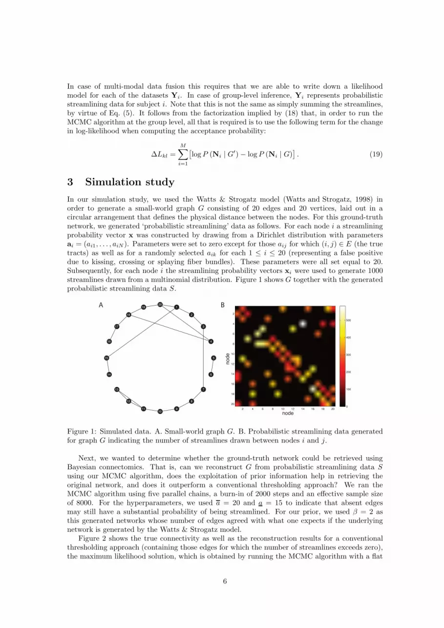
In our simulation study, we used the Watts & Strogatz model (Watts and Strogatz, 1998) inorder to generate a small-world graph G consisting of 20 edges and 20 vertices, laid out in acircular arrangement that defines the physical distance between the nodes. For this ground-truthnetwork, we generated ‘probabilistic streamlining’ data as follows. For each node i a streamliningprobability vector x was constructed by drawing from a Dirichlet distribution with parametersai = (ai1, . . . , aiN ). Parameters were set to zero except for those aij for which (i, j) ∈ E (the truetracts) as well as for a randomly selected aik for each 1 ≤ i ≤ 20 (representing a false positivedue to kissing, crossing or splaying fiber bundles). These parameters were all set equal to 20.Subsequently, for each node i the streamlining probability vectors xi were used to generate 1000streamlines drawn from a multinomial distribution. Figure 1 shows G together with the generatedprobabilistic streamlining data S.

1

2

3

4

5

6

7

8

910

11

12

13

14

15

16

17

18

1920

2 4 6 8 10 12 14 16 18 20

2

4

6

8

10

12

14

16

18

200

100

200

300

400

500

node

no

de

A B

Figure 1: Simulated data. A. Small-world graph G. B. Probabilistic streamlining data generatedfor graph G indicating the number of streamlines drawn between nodes i and j.

Next, we wanted to determine whether the ground-truth network could be retrieved usingBayesian connectomics. That is, can we reconstruct G from probabilistic streamlining data Susing our MCMC algorithm, does the exploitation of prior information help in retrieving theoriginal network, and does it outperform a conventional thresholding approach? We ran theMCMC algorithm using five parallel chains, a burn-in of 2000 steps and an effective sample sizeof 8000. For the hyperparameters, we used a = 20 and a = 15 to indicate that absent edgesmay still have a substantial probability of being streamlined. For our prior, we used β = 2 asthis generated networks whose number of edges agreed with what one expects if the underlyingnetwork is generated by the Watts & Strogatz model.

Figure 2 shows the true connectivity as well as the reconstruction results for a conventionalthresholding approach (containing those edges for which the number of streamlines exceeds zero),the maximum likelihood solution, which is obtained by running the MCMC algorithm with a flat

6

node

no

de

2 4 6 8 10 12 14 16 18 20

2

4

6

8

10

12

14

16

18

20

node

no

de

2 4 6 8 10 12 14 16 18 20

2

4

6

8

10

12

14

16

18

20

node

no

de

2 4 6 8 10 12 14 16 18 20

2

4

6

8

10

12

14

16

18

20

node

no

de

2 4 6 8 10 12 14 16 18 20

2

4

6

8

10

12

14

16

18

20

true connectivity thresholding

ML solution MAP solution

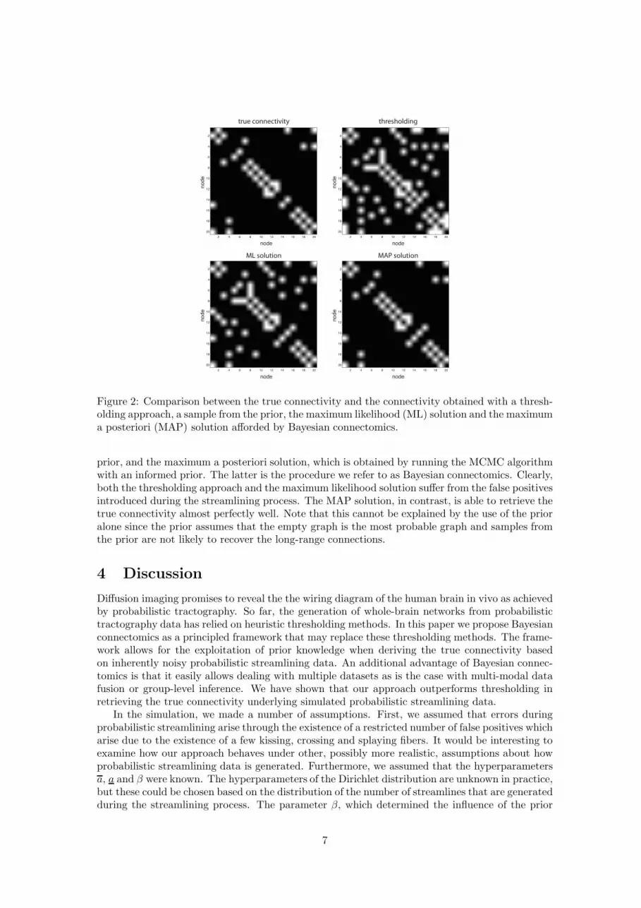
Figure 2: Comparison between the true connectivity and the connectivity obtained with a thresh-olding approach, a sample from the prior, the maximum likelihood (ML) solution and the maximuma posteriori (MAP) solution afforded by Bayesian connectomics.

prior, and the maximum a posteriori solution, which is obtained by running the MCMC algorithmwith an informed prior. The latter is the procedure we refer to as Bayesian connectomics. Clearly,both the thresholding approach and the maximum likelihood solution suffer from the false positivesintroduced during the streamlining process. The MAP solution, in contrast, is able to retrieve thetrue connectivity almost perfectly well. Note that this cannot be explained by the use of the prioralone since the prior assumes that the empty graph is the most probable graph and samples fromthe prior are not likely to recover the long-range connections.

4 Discussion

Diffusion imaging promises to reveal the the wiring diagram of the human brain in vivo as achievedby probabilistic tractography. So far, the generation of whole-brain networks from probabilistictractography data has relied on heuristic thresholding methods. In this paper we propose Bayesianconnectomics as a principled framework that may replace these thresholding methods. The frame-work allows for the exploitation of prior knowledge when deriving the true connectivity basedon inherently noisy probabilistic streamlining data. An additional advantage of Bayesian connec-tomics is that it easily allows dealing with multiple datasets as is the case with multi-modal datafusion or group-level inference. We have shown that our approach outperforms thresholding inretrieving the true connectivity underlying simulated probabilistic streamlining data.

In the simulation, we made a number of assumptions. First, we assumed that errors duringprobabilistic streamlining arise through the existence of a restricted number of false positives whicharise due to the existence of a few kissing, crossing and splaying fibers. It would be interesting toexamine how our approach behaves under other, possibly more realistic, assumptions about howprobabilistic streamlining data is generated. Furthermore, we assumed that the hyperparametersa, a and β were known. The hyperparameters of the Dirichlet distribution are unknown in practice,but these could be chosen based on the distribution of the number of streamlines that are generatedduring the streamlining process. The parameter β, which determined the influence of the prior

7

was chosen such that samples from the prior corresponded to the small-world networks we wereinterested in. In order to construct priors which work well in practice, various other concordancefunctions can be employed, whose parameters can be estimated on existing data using maximumlikelihood approaches (Hunter et al., 2008; Simpson et al., 2011a).

In this paper, we have laid the foundations for a Bayesian approach to connectivity analysis.What remains is to validate the approach not only on simulated data but also on empirical data.This not only requires the reconstruction of whole-brain networks from diffusion imaging data, butalso an assessment of their validity on independent data. One may think here of determining howwell reconstructed networks correspond to networks estimated from resting-state fMRI or fromtracer data (Jbabdi and Johansen-Berg, 2011). Eventually, we would like to use our approach todetermine how differences between (groups of) people can be understood in terms of variations intheir underlying wiring diagrams.

References

Bassett, D., Brown, J., Deshpande, V., Carlson, J., and Grafton, S. (2011). Conserved and variablearchitecture of human white matter connectivity. NeuroImage, 54(2):1262–1279.

Bassett, D. and Bullmore, E. (2006). Small-world brain networks. Neuroscientist, 12(6):512–523.

Behrens, T., Johansen-Berg, H., Jbabdi, S., Rushworth, M., and Woolrich, M. (2007). Probabilis-tic diffusion tractography with multiple fibre orientations: What can we gain? NeuroImage,34(1):144–155.

Behrens, T., Woolrich, M., Jenkinson, M., Johansen-Berg, H., Nunes, R., Clare, S., Matthews, P.,Brady, J., and Smith, S. (2003). Characterization and propagation of uncertainty in diffusion-weighted MR imaging. Magnet. Reson. Med., 50(5):1077–1088.

Bullmore, E. and Sporns, O. (2009). Complex brain networks: graph theoretical analysis ofstructural and functional systems. Nature Rev. Neurosci., 10(3):186–198.

Catani, M. (2007). From hodology to function. Brain, 130(3):602–605.

Chung, H.-W., Chou, M.-C., and Chen, C.-Y. (2010). Principles and Limitations of ComputationalAlgorithms in Clinical Diffusion Tensor MR Tractography. A. J. Neuroradiol., 32:3–13.

Chung, M., Adluru, N., Dalton, K., Alexander, A., and Davidson, R. (2011). Scalable brainnetwork construction on white matter fibers. In SPIE Med. Imaging, volume 7962, pages 1–6.

Dijkstra, E. (1959). A note on two problems in connexion with graphs. Numer. Math., 1:269–271.

Frank, O. and Strauss, D. (1986). Markov graphs. J. Amer. Statistical Assoc., 81(395):832–842.

Friman, O., Farneback, G., and Westin, C.-F. (2006). A Bayesian approach for stochastic whitematter tractography. IEEE T. Med. Imaging, 25(8):965–978.

Gong, G., He, Y., Concha, L., Lebel, C., Gross, D., Evans, A., and Beaulieu, C. (2009). Mappinganatomical connectivity patterns of human cerebral cortex using in vivo diffusion tensor imagingtractography. Cereb. Cortex, 19(3):524–536.

Hagmann, P., Kurant, M., Gigandet, X., Thiran, P., Wedeen, V., Meuli, R., and Thiran, J. (2007).Mapping human whole-brain structural networks with diffusion MRI. PLoS ONE, 2(7):e597.

He, Y., Chen, Z., and Evans, A. (2008). Structural insights into aberrant topological patterns oflarge-scale cortical networks in Alzheimer’s disease. J. Neurosci, 28(18):4756–4766.

He, Y., Dagher, A., Chen, Z., Charil, A., Zijdenbos, A., Worsley, K., and Evans, A. (2009).Impaired small-world efficiency in structural cortical networks in multiple sclerosis associatedwith white matter lesion load. Brain, 132(12):3366–3379.

8

Holland, P. and Leinhardt, S. (1981). An exponential family of probability distributions fordirected graphs. J. Amer. Stat. Assoc., 76(373):33–50.

Horwitz, B. and Poeppel, D. (2002). How can EEG/MEG and fMRI/PET data be combined?Hum. Brain Mapp., 17:1–3.

Hunter, D., Goodreau, S., and Handcock, M. (2008). Goodness of fit of social network models. JAm. Stat. Assoc, 103(481):248–258.

Iturria-Medina, Y., Sotero, R., Canales-Rodrıguez, E., Aleman-Gomez, Y., and Melie-Garcıa, L.(2008). Studying the human brain anatomical network via diffusion-weighted MRI and GraphTheory. NeuroImage, 40(3):1064–1076.

Jbabdi, S. and Johansen-Berg, H. (2011). Tractography: Where Do We Go from Here? Brain

Connect., 1(3):169–183.

Jbabdi, S., Woolrich, M., Andersson, J., and Behrens, T. (2007). A Bayesian framework for globaltractography. NeuroImage, 37(1):116–129.

Konrad, K. and Eickhoff, S. (2010). Is the ADHD brain wired differently? A review on structuraland functional connectivity in attention deficit hyperactivity disorder. Hum. Brain Mapp.,31(6):904–916.

Minka, T. (2003). Estimating a Dirichlet distribution. Technical report, M.I.T.

Mukherjee, S. and Speed, T. (2008). Network inference using informative priors. Proc. Natl. Acad.Sci., 105(38):14313–8.

Penny, W., Friston, K., Ashburner, J., Kiebel, S., and Nichols, T., editors (2006). Statistical

Parametric Mapping: The Analysis of Functional Brain Images. Academic Press, 1st edition.

Simpson, S., Hayasaka, S., and Laurienti, P. (2011a). Exponential Random Graph Modeling forComplex Brain Networks. PLoS ONE, 6(5):–.

Simpson, S., Moussa, M., and Laurienti, P. (2011b). An exponential random graph modelingapproach to creating group-based representative whole-brain connectivity networks. arXiv,stat.AP.

Skudlarski, P., Jagannathan, K., Calhoun, V., Hampson, M., Skudlarska, B., and Pearlson, G.(2008). Measuring brain connectivity: diffusion tensor imaging validates resting state temporalcorrelations. NeuroImage, 43(3):554–561.

Snijders, T., Pattison, P., Robins, G., and Handcock, M. (2006). New Specifications for Exponen-tial Random Graph Models. Sociol. Methodol., 36(1):99–153.

Snijders, T. A. B. (2002). Markov chain Monte Carlo estimation of exponential random graphmodels. J. of Soc. Struct., 3.

Sporns, O. (2006). Small-world connectivity, motif composition, and complexity of fractal neuronalconnections. Biosystems, 85(1):55–64.

Sporns, O. (2010). Networks of the Brain. M.I.T. Press.

Sporns, O., Tononi, G., and Kotter, R. (2005). The human connectome: A structural descriptionof the human brain. PLoS Comput. Biol., 1(4):e42.

Vaessen, M., Hofman, P., Tijssen, H., Aldenkamp, A., Jansen, J., and Backes, W. (2010). Theeffect and reproducibility of different clinical DTI gradient sets on small world brain connectivitymeasures. NeuroImage, 51(3):1106–1116.

9

Wasserman, S. (1996). Logit models and logistic regressions for social networks: I. An introductionto Markov graphs and p∗. Psychometrika, 61(3):401–425.

Watts, D. J. and Strogatz, S. H. (1998). Collective dynamics of ’small-world’ networks. Nature,393(6684):440–442.

Zalesky, A., Fornito, A., Harding, I., Cocchi, L., Yucel, M., Pantelis, C., and Bullmore, E. (2010).Whole-brain anatomical networks: does the choice of nodes matter? NeuroImage, 50(3):970–983.

Zhang, J., Ji, H., Kang, N., and Cao, N. (2005). Fiber Tractography in Diffusion Tensor MagneticResonance Imaging: A Survey and Beyond. Technical report, Dept. of Comp. Sci., Uni. ofKentucky.

10