Bayesian Estimation of Motion Vector Fields

Ii I I I I 1’ 1” ’ I ’ II I 1

910 IEEE TRANSACTIONS ON PATTERN ANALYSIS AND MACHINE INTELLIGENCE, VOL. 14, NO. 9, SEPTEMBER 1992

Bayesian Estima tion of Mo tion Vector F ields Janusz Konrad and Eric Dubois, Senior Member, IEEE

Abstract-This paper presents a new approach to the estimation of 2-D motion vector fields from time-varying images. The approach is stochastic both in its formulation and in the solution method. The formulation involves the specification of a deterministic structural model along ivith stochastic observation and motion field models. Two motion models are proposed: a globally smooth model based on vector Markov random fields and a piecewise smooth model derived from coupled vector-binary Markov random fields. Two estimation criteria are studied. In the max imum a posteriori probability (MAP) estimation, the a posteriori probability of motion given data is maximized, whereas in the min imum expected cost (MEC) estimation, the expectation of a certain cost function is minimized. The MAP estimation is performed via simulated annealing, whereas the MEC algorithm performs iteration-wise averaging. Both algorithms generate sample fields by means of stochustic relaxation implemented via the Gibbs sampler. Two versions are developed: one for a discrete state space and the other for a continuous state space. The MAP estimation is incorporated into a hierarchical environment to deal efficiently with large displacements. Numerous experimental results of application of these algorithms to natural and computer-generated images with natural and synthetic motion are shown.

Index Terms- Bayesian estimation, Markov random fields, motion estimation, motion modeling, optical flow, simulated annealing, stochastic relaxation, 2-D motion.

I. INTRODUCTION

M OTION computat ion has long been known as one of the fundamental and difficult problems in computer vision.

It has been tackled from various angles with variable success. This paper introduces a stochastic approach to the computat ion of motion. The approach stems from well-known concepts used in stochastic model ing and reconstruction of images such as Bayesian estimation criteria [lo], [27], Markov random field (MRF) models for images [35], [lo], [7], simulated annealing, and iterated conditional modes (ICM) as solution methods [20], [lo], [4]. In this paper, we extend these criteria, models, and solution methods to cont inuous and discrete motion vector fields, we discuss similarities and differences with existing algorithms, and we present numerous motion estimates for synthetic and natural motion.

There are two main aspects to motion estimation: computa- tion of 3-D motion in space and computat ion of 2-D motion in the image plane, which is also called optical flow. In this paper, we are concerned with the latter problem. Knowledge of

Manuscript received March 13,199O; revised February 21, 1992. This work was supported by the Natural Sciences and Engineering Research Council of Canada under Strategic Grant STROO40524. Recommended for acceptance by Associate Editor N. Ahuja.

The authors are with the Institut National de la Recherche Scientifique INRS-T&communications, Verdun Quebec, Canada, H3E lH6.

IEEE Log Number 9201771.

2-D motion in a t ime-varying image can be used to infer 3-D motion, e.g., of a camera with respect to the environment, or to compute structure from motion; however, it can also be used directly in mot ion-compensated processing (e.g., interpolation, noise reduction) or compression of image sequences.

The existing approaches to estimating 2-D motion from dy- namic images can be classified as either low-level or high-level computer vision algorithms. The class of algorithms presented here belongs to the former group, a long with such methods as block matching, spatio-temporal gradient, or Fourier techniques, and is character ized by computat ion of motion based only on simple low-level image descriptors like intensity. The high-level methods, which are not considered here, rely on image analysis to extract high-level features of the data, such as edges, object boundaries, or complete objects, and use them to solve the cor respondence problem.

The problem of motion computat ion has proved to be difficult due to two factors: ill posedness and complexity. The problem is ill posed since many different vector fields can explain the same data (images). The complexity of the problem is dependent on its dimensionality, which is high since typically, several thousand unknowns have to be computed simultaneously.

Simple estimation algorithms like block matching frequently fail to produce good results because they rely on the data only and do not attempt to explicitly model motion fields. Consequent ly, every motion vector is computed from local intensity values, disregarding the motion of neighbor ing picture elements. To overcome this deficiency, instead of minimizing a local objective function, global formulations over the complete motion field have been used. Horn and Schunck [17] p roposed a global criterion as a compromise between an error der ived from the motion constraint equat ion and a motion smoothness error. Hildreth [16] used the difference between the measured and the estimated velocity component orthogonal to an intensity contour and al lowed smoothing only a long such a contour. Nagel and Enkelmann [31] ex tended the Horn-Schunck method by using image structure in the smoothness term, thus allowing space-variant smoothing.

All three approaches can be classified as regularization (of the original i l l-posed cor respondence problem), where the smoothness term expresses a priori assumptions about the propert ies of motion. The major drawback of the Horn- Schunck and Nagel-Enkelmann methods is that the motion vectors are conf ined to fixed spatio-temporal positions; hence, to perform sampling structure conversion through motion- compensated interpolation, motion fields have to be interpolated as well. In addition, the formulation using the motion constraint equat ion requires evaluation of image derivatives,

0162-8828/92$03.00 0 1992 IEEE

KONRAD AND DUBOIS: BAYESlAN ESTIMATION OF MOTION VECTOR FIELDS 911

which is an il l-posed problem itself. Horn and Schunck have used a space-invariant smoothing operator, but it causes substantial oversmoothing at motion boundaries. This problem has been partially solved by the Nagel and Enkelmann“‘oriented smoothness” operator. Both methods have been extended to handle large displacements via a hierarchical approach [12], [9]. The major drawback of Hildreth’s approach is the need to know intensity contours, e.g., edges, before performing motion estimation, which is especially cumbersome if the method is to be appl ied to a wide class of images (e.g., video). In addition, it is not clear how the boundary, estimates are propagated, especially if the contours are not closed.

Most motion estimation techniques to date, including the three examples above, have been exclusively deterministic. There are a few notable exceptions, however. Schunck [33] and Martinez [28] p roposed maximum likelihood estimation of motion based on a statistical model relating observat ions and unknowns. Murray and Buxton [30] used a Markov random field model for optical flow segmentat ion and solved it using simulated annealing. More recently, Bouthemy and Lalande [5] and Heitz and Bouthemy [ 141, [15] appl ied Markov random field models to motion detection and segmentat ion and solved the problem using Besag’s ICM method [4].

In that which follows, a Bayesian approach to motion estimation derived from the Bayesian reconstruction of images as proposed by Geman and Geman [lo] and Marroquin [27] is proposed. In Section II, estimation criteria are formulated, suitable models are proposed, and the resulting a posteriori probability is derived. In Section III, solutions to the stochastic formulations are proposed via stochastic relaxation. Section IV covers hierarchical extension of the maximum a posteriori (MAP) probability estimation, whereas Section IV presents numerous experimental results for natural images with synthetic and natural motion.

II. FORMULATION

A. Terminology

Let u denote the true underlying time-varying image understood as an i l luminance pattern in some image plane obtained from the observed scene via an ideal optical system. The observed image g, which is related to the underlying image IL via some random transformation, is considered to be a sample of a random field G. The image g is assumed to be quant ized in ampli tude and sampled on lattice A, in R3 (horizontal, vertical, and temporal directions). Such a lattice is a collection of sites (s,t) E R3 [8], where z and t denote spatial and temporal positions, respectively.

Let u at t imes t = t- and t = t+ be called the preceding and the following images, respectively. Disregarding the occlusion and newly exposed areas, for every point in the preceding image, there exists a corresponding point in the following image such that both arise from the projection of the same scene point. Every such pair of points can be connected by a straight line. Since u is def ined over cont inuous (z, t), these lines will intersect a p lane located at t (t- < t < t+) over a dense set of locations. In other words, for each (z, t), there exists a line joining corresponding image points at t imes t-

and t+. Note that these lines coincide with the true motion trajectory at the end points and not necessari ly between them. The true motion trajectory will intersect (in general) the plane at time t at a location different from (z, t). It is also possible that more than one such linear trajectory will pass through (x, t).

Let the 2-D projections of line segments between t- and t+ on the plane at time t be referred to as the unknown (true) displacement field d associated with the underlying image U. It is not feasible to compute displacement vectors on a cont inuum of spatial positions; hence, d is assumed to be an array of vectors def ined over the lattice Ad in R3. In the literature, the cases where Ad is a sublattice of A, : Ad C A,, or Ad is identical to A, : Ad = A,, have been most frequently considered. In this paper, a more general situation, where Ad and A, are arbitrary, will be investigated. Consequent ly, a displacement vector may be def ined at a spatio-temporal position that does not belong to A9. For Ad = A, (e.g., for mot ion-compensated prediction), the linear trajectories introduce no errors because only the endpoints are of interest. In the case where Ad # A, (e.g., for mot ion-compensated interpolation), however, there are three points of interest, and consequent ly, there will be an error introduced due to a departure of the motion trajectory from linearity in the interval (t-, t+). If this interval is small, such an error is expected to be minor.

The investigations that follow are valid for any lattices A9 and Ad, but for simplicity, it is assumed that they are rectangular lattices with horizontal, vertical, and temporal sampling periods (T! , T; , Tg ) and ( Th , T; , Td) , respectively. Consequent ly, consecut ive image fie ds 4 are spaced by Tg seconds, whereas motion fields are spaced by Td seconds. Each field of the image sequence contains Mg picture elements (pixels), and each motion field consists of A’fd vectors. Let the horizontal and vertical dimensions of motion fields be A$ and Mi, respectively (A$ = i’&‘$ x A!$). W ith the above assumptions, a site si = [kT,h, 1T;, mT,] E A, (for some integer i, Ic, 1, m) is an image pixel in the mth field with spatial coordinate (Ic, 1).

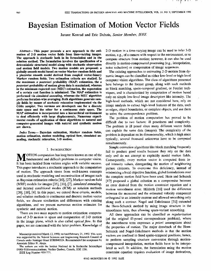
The true displacement field 2 is assumed-to be a sample (realization) from random field (RF) D. Let d be an estimate of d, and let d denote any sample field from D. Assuming a linear motion trajectory between two images, as discussed above, the definition of the displacement field is given below and is illustrated in Fig. 1.

Definition: The displacement field a def ined over Ad is a set of 2-D vectors such that for all (zi, t) E Ad, the preceding image point (xi - At. &xi, t), t-) has moved to the following point (xi + (1.0 - At) . d(xi, t), t+), where t- = t - At. T,, t+ = t + (1.0 - At) . T,,-and At = t/T, - [t/Tg].

The displacement field d may not be def ined at all points in Ad, for example, due to occlusions and may not be unique, as in the case of a rotating uniform disk. Note that this definition places a displacement vector at any spatio-temporal position. The limiting cases when At=O.O and At=l.O correspond to forward and backward predictive-type estimation, respectively.

Since we impose no constraints on images, it can be

912 IEEE TRANSACTIONS ON PA’ITERN ANALYSIS AND MACHINE INTELLIGENCE, VOL. 14, NO. 9, SEPTEMBER 1992

At. T, I

Fig. 1. Definition of the displacement field dt for motion estimation from two image fields (only one vector is displayed). Sites of lattice i\d (0) are pivoting points for the displacement vectors, and thus, every vector d(z,. t) crosses site (z,, t), whereas its ends are “free” to move and do not necessarily belong to lattice -is.

expected that motion fields associated with such images will contain discontinuities at the boundar ies of objects with different motion. To model sudden changes in motion vector length and/or orientation, we use the concept of motion discontinuity. The true motion discontinuities are curves in the image plane def ined over cont inuous spatio-temporal coordinates (z, t) and are unobservable like the true motion fields. They are just a means of describing motion in an image and can be understood as indicator functions (e.g., binary) for each (x, t). Let the true (unknown) field of such discontinuities be denoted by i. Since the computat ion of i over a cont inuum of spatial posit ions is not feasible, i will be represented by a discrete discontinuity field over a union of cosets (shifted lattices) [8] Qr =T+!J~U&, where $~h and $v are orthogonal cosets def ined as follows (superscript T denotes a transposition):

$‘I, = Ad + [o! T;/2, olT, +v = Ad + [Ti/2,0, OIT.

Cosets ?/& and ?,L+, identify posit ions at which Ml= M$x(M~ 1)+(&Q-l)xMi motion discontinuities or line elements are estimated. The line elements are located midway between sites of Ad and take on the value 1 if a motion boundary intersects the line joining the neighbor ing displacement vector sites and 0 otherwise.

W e assume that i is a sample field from RF L. Let rbe an estimate of i. In addition, let 1 be any sample field drawn from L. The RF L will be called a line process, and its sample 1 will be called a line field.

Let the subscript t denote restriction of a random field or of its realization to time t. Thus, dt will s tand for a realization of random field Dt (D at time t).

It is assumed that the random field Gt is def ined over the discrete state space S, = (Si)“., where Si is the single pixel state space corresponding to quant ized image intensities, and (.)M denotes an M-fold Cartesian product. Similarly, the random field Dt is def ined over the state space Sd = (Si)“d, where Sk is the single vector state space. Two cases are considered:

1. Sb is a discrete state space, i.e., a square 2-D grid over the range [-d,,,, d,,,] with Nd possible levels in each direction.

2. Sb = R2 is a cont inuous state space. It is also assumed that the random field L is def ined over the discrete state space Sl = (Sf)*[l, where Sf is the single line element state space. For the purpose of this work, it is assumed that RF L is binary and that S,l consists of two states: 0 (no motion discontinuity) and 1 (motion discontinuity “on”). Possible extensions of this state space to nonbinary spaces (e.g., incorporating the directionality of line elements) are not considered in this paper but can be found in [lo] in the context of image modeling.

B. Estimation Criteria

The objective is to jointly estimate the pair (&i) of true displacement and line fields at time t corresponding to an underlying image u on the basis of observat ions g.

I) MAP EstimatioE* The “best” or “most likely” displacement field estimate dt E Sd and line field estimate 2 E Sz given the observat ions gt- , gt+ must satisfy the relationship:

P(Dt =;it+,Lt =ht-,gt+) 2

P(-Dt=&,Lt=illgt-,gt+) ~&E$&E&

where P is the conditional discrete probability distribution of the motion and line fields given the observations. Applying the Bayes rule for discrete random variables, the above posterior distribution can be factored as follows:

P(Dt = 4, Lt = Llgt-, gt+ > = Wt, =gt+ldt,zt,gt-)P(Dt=dt,Lt =ltjgt-). (1)

Wt, = gt+ Ia- >

Note that since P(Gt+ = gt+ ]gt- ) is not a function of (ot, L,), it can be ignored w_hen-maximizing P(Dt = 2, Lt = Ztlgt- , St+_) with respect to (4, It). Thus, the MAP estimate of the pair (4, 2,) is the solution to the following optimization

KONRAD AND DUBOIS: BAYESIAN ESTIMATION OF MOTION VECTOR FIELDS 913

problem:

ma P(Gt+ &,x, [ = gt+ I&,;, gt- )P(Dt = 2, Lt = i&m)].

If displacement vectors are def ined over the cont inuous state space s, = R2, then by using the Bayes rule for mixed random variables, the discrete probability distribution P(Dt = &,Lt =z I St-) is replaced by the mixed continuous/discrete probability distribution p(&, Lt = zjg,-).

2) Min imum Expected Cost (MEC) Estimation: Another approach to the estimation of motion is based on Bayesian criteria developed by Marroquin for reconstruction of images [27]. The goal is to minimize the ensemble average with respect to Dt , Gt- , Gt, of some positive definite cost functional measur ing the error between the true and estimated motion fields (minimum expected cost (MEC) estimation). Here, we will only discuss the MEC estimation for the globally smooth motion model, i.e., without discontinuity process Lt. Let the cost functional have the following form:

Md O(d;, d;) = c O(d’(x;, t), d”(x;, t))

i=l

where 0 is a positive definite function, and 6, 6’ are two motion vector fields. The cost asso$ated with_ approximating the true motion field & by estimate 4 is O(&, 4). The optimal Bayesian estimate 21 E sd is def ined as follows:

E ~t,Gt- Gt+ P(dt,~~)l = m inED,,ct-,~,+ [@(A,&)] (2) 2,

where EDt ,G*- ,Gt+ 1.1 stands for the ensemble expectat ion over all configurations of Dt , Gt- and Gt,. Note that the estimates & and ;it’ are functions of gt- and gt+ and can be thought of as mappings from R2Mg to R2Md. Expressing the expectat ion as a sum and using the positive definiteness of 8, it can be shown [24] that (2) is equivalent to

I c W t = dtlg t- , a+)] Vi. (3) d,:d(x,,t)=r

This means that the minimization with respect to 2 can be achieved by minimizing the individual marginal expected costs at each position (xi, t).

Further simplification of (3) requires explicit knowledge of the function 0. This function must reflect “goodness” of an estimate, i.e., a worse estimate should increase the value of 8, and a better one should reduce it. W e use the following 8:

e(ii(xi, t),^d(xi, t)) = Ild(Xiy t) - ^d(Xi, t)ll’ (4)

where II . I( is the L2 norm for mathematical tractability. The solution to minimization (3) with r9 def ined in (4) is the minimum mean squared error (MMSE) estimate expressed

through the marginal conditional expectat ion of D(xi, t):

;i*(x;,t) = c r[ c P(Dt =dtlgt-,gt+)] Vi. l-es; d, :d(x, ,t)=r

(5)

The cont inuous state space case is identical except for integrals replacing the summations and probability density replacing the discrete probability distribution. To compute the conditional expectat ion from (5), the a posteriori discrete probability distribution P(Dt = dt I gt- ,gt+) or density ~(4 I gt- ,gt+> is needed.

C. Models

In order to solve the MAP and MEC estimation problems, the posterior distribution from (1) must be known explicitly. In this section, we determine the constituent probabilit ies from (1) by formulating appropriate models. First, from a structural model relating motion to the underlying image and from a model for the observat ion process, we propose the likelihood PG, = gt+ I 4, lt, gt- ). Then, we directly postulate a displacement field model for P(Dt = dt, Lt = Ztlgt-).

1) Structural Model: To facilitate inference of motion from images, it is fundamental to specify a structural model relating motion vectors and image intensity values. It is usually assumed that image intensity or its spatial gradient is constant a long motion trajectories. Applying the intensity constancy assumption to the true underlying image u along the true motion trajectories 2 in time interval [t-, t+] results in the following relationship:

u(x - At .2(x, t), t-) = U(Z + (1.0 - At) . ;1(~, t), t+). (6)

A more complex model incorporating linear variation of intensity has been devised in [34] and [ll]; however, it will not be considered here.

2) Observation Model: The true underlying image u results from the “ideal” projection of a scene onto an image plane. In reality, images are acquired with a video camera and discretized using electronic circuitry. Hence, the observed image g is a transformed copy of u after such operat ions as filtering, sampling, y correction, and quantization, and it also incorporates image sensor noise, quantization noise, distortion due to aliasing, etc.

Extrapolating the relationship (6) to the observed image g, we model the displaced pixel differences (DPD’s)

F(:(;i(xi,t),xi,t) =s(xi + (1.0~ At) .;I(xi,t),t+) -g(xi-At.d(zi,t),t-)

for (zi, t) E Ad by independent Gaussian random variables. g(z, t) above denotes an intensity value at (z, t) @A9 obtained by interpolation. W e have investigated various interpolation schemes [23] and have concluded that a l though matching algorithms are relatively insensitive to the type of interpolator, spatio-temporal gradient methods require interpolators that provide continuity of both the intensity and its first derivative. W e thus use a third-order (bicubic) separable interpolator, as proposed by Keys [19], which has this property.

914 IEEE TRANSACTIONS ON PATTERN ANALYSIS AND MACHINE INTELLIGENCE, VOL. 14, NO. 9, SEPTEMBER 1992

Given these assumptions, we can write’

P(Gt+ = iit+ I dt,lt,gt-) =

(2aa2)-Md/2. e -Q&+ iha- )/202 (7)

where energy U, is def ined as

i=l

and where ct+ and ct+ denote the random and sample image fields at time t+ spatially interpolated at posit ions pointed to by displacement vectors. W e need, however, U, (gt+ I 4, gt- ), i.e., energy at locations of the image sampling lattice A, at time t+ . W e could account for this d iscrepancy by interpolating the motion field dt to get a field of motion vectors terminating on the lattice points at t+; however, this will not significantly change the energy U,, and thus, we simply assume that ugbt, I &,a-) = UgGt+ I dt,gt- ).

3) Displacement Field Model: It can be observed that in most scenes, motion is the result of a change of position of near rigid bodies. After projection onto the image plane, that 3-D motion becomes a 2-D motion of 2-D objects. The motion field in such an image consists of patches of similar (orientation and length) vectors with possible discontinuities at motion boundaries. Therefore, it will be assumed here that motion fields are smooth functions of spatial position x (fixed t) except for occasional abrupt changes in vector length and/or orientation. In fact, displacement fields are significantly smoother than the images themselves. Based on this observat ion and on successful application of MRF’s to image model ing [13], [lo], here, we propose to jointly model the motion and motion discontinuity fields by a pair (Dt, Lt) of coupled vector and binary MRF’s.

The traditional approach to characterization of MRF’s via the finite-dimensional joint distributions is cumbersome and does not provide a simple and clear relationship between the distribution parameters and the propert ies of a MRF. Due to the Hammersley-Clifford theorem [3], however, a MRF with respect to ne ighborhood system JV is uniquely character ized by a Gibbs distribution with respect to ni. Since a vector MRF (VMRF) differs from a scalar MRF only by the definition of a state (in R2 instead of R), the propert ies of scalar MRF’s hold for VMRF’s as well.

Recall that the propert ies of a motion model are descr ibed by the discrete probability distribution P(Dt = dt, Lt = Zt I gt-) from (l), which can be factored using the Bayes rule:

P(Dt=dt,Lt=ltlgt-)= P(Dt = dt I Lst-) . P(Lt = it I St-).

If P(Dt = & I Zt,gt-) and P(Lt = Ztlgt-) are Gibbsian, then P(Dt = 4, Lt = It I gt-) is also Gibbsian, and the pair (44) has M ar k ovian properties. Since a single image field is expected to contribute little information to the motion vector

‘Note that dt constitutes a complete description of motion, and line field It is only an aid in estimation of dt. Hence, the condit ioning on It can be dropped, thus giving U(&+ Idt, gt- ).

model, the condit ioning on gt- in P(Dt = 4 I It, gt- ) is omit- ted as an approximation. However, motion discontinuities will most likely occur at the posit ions of intensity discontinuities at object boundaries, which is expressed through condit ioning on gt- in P(Lt = 4 I St-).

Under assumed Markov properties, the probability govern- ing the displacement RF Dt can be expressed by the Gibbs distribution

P(Dt = & I it) = $emud(& I ft)/Pd (9)

where zd is a normalizing constant (partition function), pd is a constant controll ing characteristic propert ies of Dt, and the (conditional) energy function Ud(dt I Zt) is def ined as

u&t 1 it) = c vd(dt,cd)[l - l(@i,xj),t)].

Cd={x,,xj}ECd (10)

cd is a clique of vectors, whereas cd is a set of all such cl iques derived from a ne ighborhood system Nd def ined over lattice Ad. (@;, xj) , t) E Ql denotes a site of line element located between vector sites Zi and xj. vd is a potential function crucial to characterization of the propert ies of displacement process Dt. This is a straightforward extension of the scalar MRF model for images as proposed by Geman and Geman POl*

The energy function (10) can be understood as follows. There exists a cost Vd(dt, cd) associated with each vector cl ique cd that increases if a motion field sample locally departs from the assumed a priori model character ized by pd and vd. If, however, the line element separat ing the displacement vectors from clique cd is “turned on” (Z( &i, zj), t) = l), there is no cost associated with the clique cd. In this way, there is no penalty for introducing an abrupt change in length or orientation of a displacement vector. The ability to zero the cost associated with vector cl iques by inserting a line element must be penalized, however. Otherwise, a line field with all e lements “on” would give the zero displacement energy (10). This penalty is provided by the line field model descr ibed in the next section.

To specify the a priori displacement model, the potential function v,+ the ne ighborhood system J%& and the cl iques cd have to be specified. Bearing in mind the assumed smoothness of dt, we define the potential function vd as follows:

cd = {Zi,Xj} E cd (11)

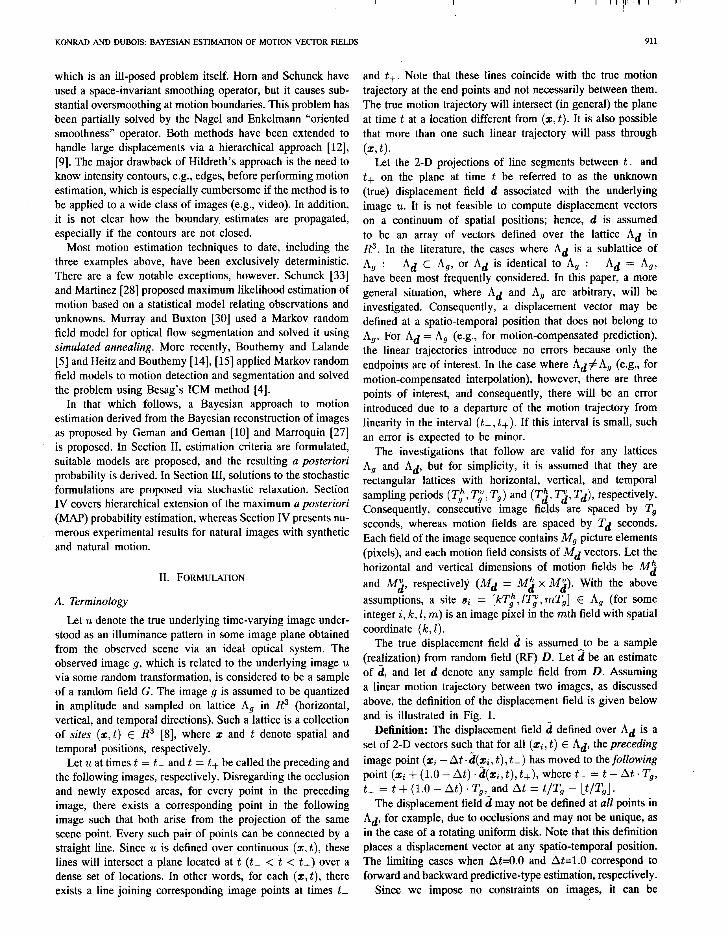
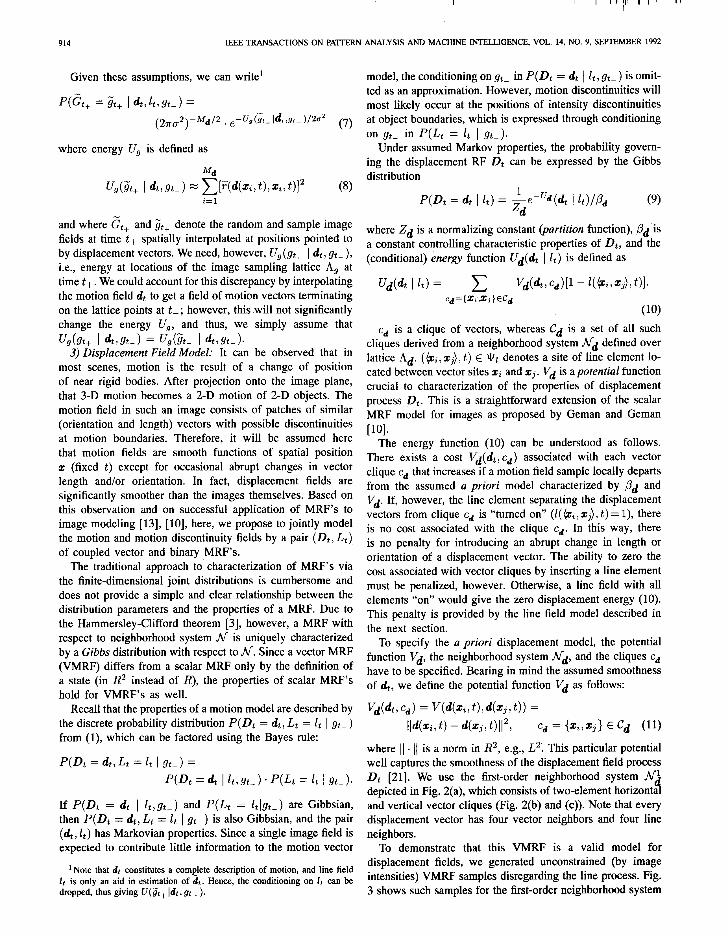
where II . 11 is a norm in R2, e.g., L2: This particular potential well captures the smoothness of the displacement field process Dt [21]. W e use the first-order ne ighborhood system N1

4 depicted in Fig. 2(a), which consists of two-element horizonta and vertical vector cl iques (Fig. 2(b) and (c)). Note that every displacement vector has four vector neighbors and four line neighbors.

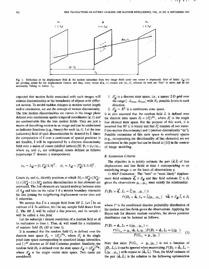
To demonstrate that this VMRF is a valid model for displacement fields, we generated unconstrained (by image intensities) VMRF samples disregarding the line process. Fig. 3 shows such samples for the first-order ne ighborhood system


(k.7.I) X .

(k-;.I) ’ (I$) ’ (k:l.l) l ’ ’ X

X .

(k.;+l)

(4 (b) (4

Fig. 2. (a) First-order neighborhood system ,%: for vector field dt defined over Ad with discontinuities It defined over @r; (b) horizontal cliques; (c) vertical cliques (o-center vector site, r-vector site, x-line site).

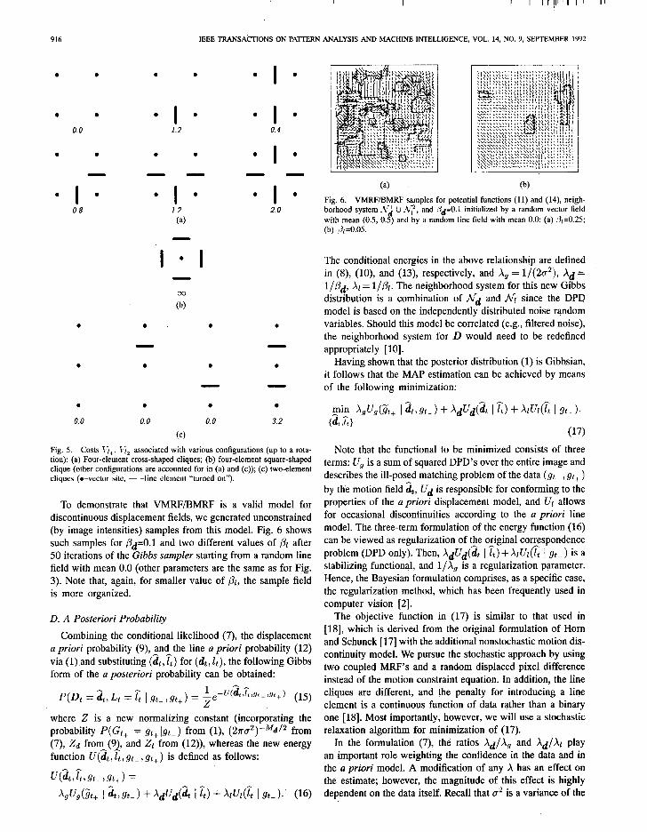
(4 (b) Fig. 3. VMRF samples for potential function (11) and neighborhood system -ki initialized by a random vector field with mean (0.5, 0.5): (a) .jd=l.O; (b) &=B.l.

and two different values of pd after 50 iterations of the Gibbs sampler (Section III) starting from random initial configuration with mean (0.5, 0.5). Note that for smaller value of ,8& the sample field is less “chaotic.” The value of ,6d can be viewed as an “activity” or “ordering” measure. Thus, to model a slowly varying motion pd of the order of 0.1 seems to be appropriate; however, an exact value cannot be established.

4) Line Field Model: The line field model is based on a binary MRF (BMRF) Lt and is described by the Gibbs probability distribution

P(Lt = lt 1 gt-) = +w~L, (12)

with Zr and ,L?r as the usual constants. Ul is the line energy function, which is defined as follows:

Uz& I St- > = 1 wt, St- 1 cz)

where cl is a line clique, and Cl is a set of all line cliques derived from a neighborhood system h/ defined over Ql. The line potential function K provides a penalty associated with the introduction of a line element.

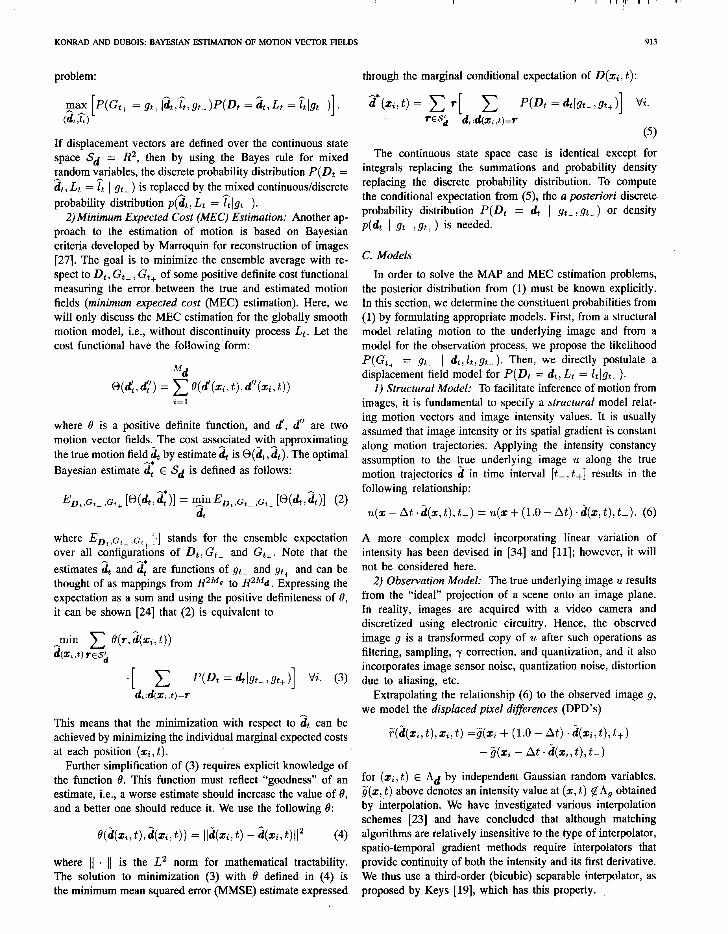
The second-order neighborhood system J$: for the “dual” sampling structure Pl is shown in Fig. 4. Note that since the union of cosets !IJz = ?/& &,!I, identifies positions of horizontal and vertical line elements, two neighborhood systems are defined (Figs. 4(a) and (b)). Every line element has eight line neighbors and two vector neighbors. There are two types of four-element line cliques. The cross-shaped cliques from Fig. 4(c) are the same as those used in [lo] and aim at modeling the shape of motion boundaries (small penalty for straight lines and high penalty for intersections; see Fig. 5(a)). The

X X

x l x X X

X 63 X x 0 cg l x

x l x X X

X X

(4 W

.

X

0 x 0 X . 0 x 0 x l

X X x 0 x X

0 x l .

Cc) cd; (e) (9

Fig. 4. Second-order neighborhood system .‘1;’ for line field It defined over +l: (a) Horizontal line element; (b) vertical line element; (c), (d) four-element cliques; (e), (f) two-element cliques (‘:,-center line site, x-line site, e-vector site).

square-shaped cliques from Fig. 4(d) are employed in order to exclude isolated vectors (I$ = 00; see Fig. 5(b)) when all four line elements are “on.” The two-element vertical cliques of horizontal line elements (Fig. 4(e)) and the horizontal cliques of vertical line elements (Fig. 4(f)) are used following Marroquin [27] to prevent formation of double edges (Fig. 5(c)). Fig. 5 shows possible configurations (up to a rotation) as well as related costs, which were chosen experimentally. Only one configuration of the square-shaped four-element clique (Fig. 5(b)) is shown since other configurations are accounted for in the cross-shaped and two-element cliques.

Note that the a priori probability of the line process (12) is conditioned on the observations. It means that image information gt- should be considered when computing the line samples lt. In general, a 3-D scene giving rise to a motion discontinuity will also contribute to an intensity edge. Only under specific circumstances will a motion discontinuity not correspond to an edge of intensity. Hence, similarly to Hutchinson et al. [18], we assume that an introduction of a line element should coincide with an intensity edge. We use the following potential function for one-element cliques:

6, (k, St-, cz) =

i

(vUg”t- I* Eh(+z;,zj), t) for horizontal cr = {zi,zj} &$-+(&,z.j),t) for vertical cr = {z;,zj}

where lh, 1, are horizontal and vertical line elements, Vh, V, are horizontal and vertical components of the spatial gradient at position (@i, zj), t), and a is a constant. The above potential introduces a penalty only if a line element is “on,” and the appropriate gradient is relatively small. The total potential function for the line field can be expressed as

wt, St-, cz) = ti, (4, cr> + E, (L s> + h (4, St-, s> (14)

where Vl, and Vl, are tabulated in Fig. 5, and I$, is given above.

916 IEEE TRANSACTIONS ON PAmRN ANALYSIS AND MACHINE INTELLIGENCE, VOL. 14, NO. 9, SEPTEMBER 1992

. .

. .

0.0

. I b 0.8

l

. .

. I . 1.2

. .

- B

. I . 1.2 (4

. I .

. I . 0.4

. I . - - b I .

2.0

.

. . . .

.

0.0

. .

0.0 0.0 (4

. 3.2

Fig. 5. Costs 1 i, , Ii, associated with various configurations (up to a rotation): (a) Four-element cross-shaped cliques; (b) four-element square-shaped clique (other configurations are accounted for in (a) and (c)); (c) two-element cliques (e-vector site, - -line element “turned on”).

To demonstrate that VMRF/BMRF is a valid model for discont inuous displacement fields, we generated unconstrained (by image intensities) samples from this model. Fig. 6 shows such samples for pdzO.1 and two different values of ,& after 50 iterations of the Gibbs sampler starting from a random line field with mean 0.0 (other parameters are the same as for Fig. 3). Note that, again, for smaller value of pr, the sample field is more organized.

D. A Posteriori Probability

Combining the conditional l ikelihood (7), the displacement a priori probability (9), and the line a priori probability (12) via (1) and substituting (a,;) for (4, lt), the following Gibbs form of the a posteriori probability can be obtained:

P(Dt = 2, Lt = i‘, 1 gt-,gt+) = ~~-~(~~i~l~-+) (15)

where Z is a new normalizing constant ( incorporating the probability P( Gt+ = gt+]gt-) from (l), (2rra2)-%i2 from (7) Zd from-(91, and ZZ from (12)), whereas the new energy function V(dt , It, gt- , gt+ ) is def ined as follows:

U(~,il,gt-,a+) =

~,u,(s,+ 1 a, St- > + ~&-&t j 8) + huz@i 1 St- )- (16)

Fig. 6. VMRFBMRF samples for potential functions (11) and (14) neighborhood system ,tfl U ,k;‘,

4 and ddZO.1 initialized by a random vector field

with mean (0.5, 0.5 and by a random line field with mean 0.0: (a) .9,=0.25; (b) 13~ =0.05.

The conditional energies in the above relationship are def ined in (8), (lo), and (13), respectively, and X, = 1/(2cr2), Ad = l/p,+ Xl = l//3,. The ne ighborhood system for this new Gibbs distribution is a combinat ion of JI.> and Nr since the DPD model is based on the independent ly distributed noise random variables. Should this model be correlated (e.g., filtered noise), the ne ighborhood system for D would need to be redef ined appropriately [lo].

Having shown that the posterior distribution (1) is Gibbsian, it follows that the MAP estimation can be achieved by means of the following minimization:

(17) Note that the functional to be minimized consists of three

terms: U, is a sum of squared DPD’s over the entire image and descr ibes the il l-posed matching problem of the data (St-, gt+ ) by the motion field &, ud is responsible for conforming to the propert ies of the a priori displacement model, and Ul allows for occasional discontinuities according to the a priori line model. The three-term formulation of the energy function (16) can be v iewed as regularization of the original cor respondence problem (DPD only). Then, $JUd(& I 2) +XlUl(i‘, I gt-) is a stabilizing functional, and l/X, is a regularization parameter. Hence, the Bayesian formulation comprises, as a specific case, the regularization method, which has been frequently used in computer vision [2].

The objective function in (17) is similar to that used in [18], which is der ived from the original formulation of Horn and Schunck [ 171 with the additional nonstochast ic motion discontinuity model. W e pursue the stochastic approach by using two coupled MRF’s and a random displaced pixel difference instead of the motion constraint equation. In addition, the line cl iques are different, and the penalty for introducing a line element is a cont inuous function of data rather than a binary one [18]. Most importantly, however, we will use a stochastic relaxation algorithm for minimization of (17).

In the fOmWkttiOn (7), the ratios Ad/x, and Ad/Al play an important role weighting the conf idence in the data and in the a priori model. A modification of any X has an effect on the estimate; however, the magni tude of this effect is highly dependent on the data itself. Recall that g2 is a var iance of the


displaced pixel difference (Gaussian) model; its value can be estimated given a displacement field. However, the parameters ,6d and pl, which characterize the a priori motion model, are far more difficult to compute. When MRF’s are used in estimation of such observables as images or textures, /3 can be estimated by analyzing a number of samples (training process) and then used to perform estimation on some other data. The success of the estimation is highly dependent on the similarity between the real data and the model (the training data). In the case of estimating an unobservable such as motion, it is not clear how to compute p, and thus, it is usually chosen ad hoc. Consequent ly, there is no point in estimating a2; the ratios Ad/x, and Ad/& may be chosen instead.

III. STOCHASTIC SOLUTION TO MAP AND MEC ESTIMATION

The MAP estimation expressed through optimization (17) is a very complex problem because of the number of unknowns involved (typically tens of thousands) and because of multimodality of the objective function, which depends on & through the observat ions g. The MEC estimation problem is also character ized by a large number of unknowns and by the necessity to compute the marginal conditional distributions in (5).

A. Solving the MAP Estimation: Simulated Annealing

To solve the optimization problem (17) we use the method of simulated annealing [20], [lo], which is based on the analogy with the process of annealing of solids. In simulated anneal ing, the behavior of a solid is simulated by generat ing sample configurations from a Gibbs distribution with the energy function suitably crafted for the given optimization problem. A “temperature” parameter T, which replaces the true temperature in chemical anneal ing, is introduced into the a posteriori probability (15) as follows:

P(Dt = 2, L = L I gt- , a+) = Fe 1 -~&,L~J~+)/T

&3) The sample configurations are produced using stochastic re-

laxation (e.g., the Metropolis algorithm or the Gibbs sampler), which will be descr ibed in Section III-C. Similarly to Geman and Geman, we incorporate the Gibbs sampler into the inhomogeneous simulated anneal ing algorithm2 with the anneal ing schedule specif ied by the initial and final temperatures Ta and Tf and the temperature change rule Tk = (P(T~, Ic) at iteration /c.~ In [lo], it was proved (Theorem B) that if a sufficiently high initial temperature Ta is used, if the temperature TI, attains 0 with at most logarithmic rate, and if every site is visited infinitely often, then with time t + 00, the system will converge to the global opt imum for any starting configuration.

The theoretical value of Ta is usually impractically high, and therefore, it is typically establ ished through experimentation. Another practical problem is posed by the logarithmic

2Simulated anneal ing is called homogeneous if the Markov chain it generates can be decomposed into a sequence of stationary chains, i.e., with constant temperatures. It is called inhomogeneous if such decomposit ion does not exist, i.e., transition probabilities are t ime dependent through the temperature.

3An iteration is understood here as a complete scan of the unknown field, i.e., Md or Md -I- Mr attempted modifications of individual unknowns.

anneal ing schedule. In order to obtain a “very organized” solution, the final temperature Tf after N iterations must be quite small. Unfortunately, the required number of iterations to attain the final temperature Tf from Tu grows exponential ly with Tu/Tf. If the initial temperature cannot be lowered more without affecting the quality of the solution, then only the anneal ing schedule can be modified. In the experiments descr ibed in Section V, we have used the exponential schedule cp(T,,, Ic) = To . a(“-‘), where a is slightly less than 1.0. Such a schedule reaches a low temperature in fewer iterations than the logarithmic one with the same number of iterations [lo] but has to be used with caution since a large temperature decrement between iterations may trap the chain in a local minimum.

B. Solving the MEC Estimation: LLN for Markov Chains

The propert ies of a Markov chain constructed by the Metropolis algorithm or the Gibbs sampler are such that it is a regenerative process, and the time instants of the returns to a given state constitute a renewal process. Hence, the law of large numbers (LLN) for Markov chains [32] can be applied, and the marginal conditional expectat ion (5) can be approximated as follows:

^d*(zi,t) M $d*(zi,t) k=O

where d”(z;, t) is a displacement vector estimate at iteration number Ic, and N is the total number of iterations.

The advantage of the above approach over simulated anneal ing is that it requires no anneal ing schedule since the generat ion of samples occurs at a constant temperature T. This temperature controls the state-rejection rate of the generat ion algorithm. If the parameter T is higher, the lower the rejection rate and the more chaotic the generated samples. If the T is lower, the higher the rejection rate and the more orderly the structure of generated realizations. To choose optimal T, Marroquin proposed a method that maximizes the likelihood of a solution with respect to T [27].

C. Stochastic Relaxation

To implement the MAP and MEC estimation algorithms discussed above, samples from MRF’s Dt and Lt are needed. Such samples can be provided by stochastic relaxation such as the Metropolis algorithm [29] or the Gibbs sampler [lo]. A very important feature of stochastic relaxation methods is that they produce states according to probabilit ies of their occurrence, i.e., the unlikely states are also generated (less frequently, however). When incorporated into simulated annealing, this property allows local minima to be escaped, unlike the case of descent methods. W e will use the Gibbs sampler since, despite its high complexity per iteration, in our tests, it provided a lower overall computat ional burden than the Metropolis algorithm [24].

The Gibbs sampler for discrete displacement process Dt is a site-replacement procedure that generates a new vector at every position (zi, t) E Ad according to the following marginal


conditional discrete probability distribution [25] der ived from probability (18):

with the local displacement energy function Ui def ined as

Ad c k^d(zj,t)l12[1 -ii( (21) j:xjETd(Zz)

where vd(Zi) is a spatial ne ighborhood of displacement vector at zi, and 2: denotes a displacement field identical to field &, except for spatial location CC;, where the vector is z. Similarly, it can be demonstrated [24] that the conditional probability driving the Gibbs sampler for displacement discontinuities can be expressed at spatio-temporal location (y;, t) E 91 as follows:

P(L(Y,,G =iiyd) I iiYjA.7. # &,gt-)

,-a;(~;^dt,st-j/T =

c ZES; e -u;(&i.st-j/T

(22)

where the local line energy function IJ: is def ined as

u,;@,&,k, =xd c Il&m,~) - &d)l12[1 - zl+ Cd={%,z,b (2, .3&l) =y,

Xl c K@,gt-, Cl) (23) ct :y, ECl

and 2 denotes a line field that is identical to field z, except for spatial location yi =< 2,) zn >, where the line element is Z.

1) Discrete State Space Gibbs Sampler: The discrete state space Gibbs sampler scans the displacement and line fields and generates new states according to the Gibbs marginal probability distributions (20) and (22) respectively.

At each spatial location of random field Dt, a complete bivariate discrete probability distribution is computed (probability for all possible displacement vector states). Then, the 2-D distribution is accumulated along one direction (e.g., horizontal) to obtain a 1-D marginal cumulative distribution, and a random state is generated from this univariate distribution. The vertical state is generated by sampling the univariate cumulative distribution obtained from the 2-D discrete probability

distribution for the known horizontal state. The calculation of the complete probability distribution at each location results in a high computat ional load per iteration of the discrete state space Gibbs sampler. However, this is offset by faster convergence than the Metropolis algorithm, which samples the states from a uniform discrete probability distribution and only then rejects the unlikely ones.

Since the random field Lt is binary, only the probabilit ies for “on” and “off” states have to be computed. A new line state is generated based on those two probabilities.

2) Continuous State Space Gibbs Sampler for Dt: Recall that in the case of the cont inuous state space (sd = R2), the marginal conditional discrete probability distribution de- f ined in (20) bzcomes the probability density p(^d(zi, t) ] +j,W # iJt,gt~,gt+) with the same local energy Ui as def ined in (21). Note that the first term in this energy is quadrat ic with respect to F, whereas the second term is quadrat ic in &. If &he first term could be approximated by a quadrat ic form in d,, then Ui would be quadratic, and the conditional density would be Gaussian. There exist efficient techniques for generat ing normal bivariates, which would significantly speed up the estimation.

Assume that an approximate estimate ht of the displacement field is known and that the image intensity is locally approximately linear. Then, using the first-order terms of the Taylor expansion, the displaced pixel difference F can be expressed as follows:

iy(^d(z;, t), 5; ) t) M F((h(Zi,t),Zi,t) + (2(3J;,t) -i(zi,t))TVd~(:(b(s;,t),si,t)

(24)

where the spatial gradient of F at (i(Zi, t), 2;) t) is def ined as shown at the bottom of this page. Incorporating the linearization (24) into the local energy Ui (21) we obtain approximation (25) (which is shown at R t e bottom of the next page), where & is fixed. To simplify the subsequent derivation, we temporari ly use Fi, 2, &, and & to denote F((i(z;, t), zi, t), ^d(zi, t), ;I(%;, t), and ii@;, zJ, t), respectively. W ith this simplification, the energy (see (25)) can be written as follows:

&et us fit the-condit ional probability density p(^d(Zi, t) ] d(zj, t), j # i, It, gt- , gt+ ) with energy approximated as above

v&2(&, t),zi> t, = I, =

~~(Z,-A~~(Zi,t).t-)at + a;;(z,+(l.o-aazt).d(z,,t).t+) (1.0 - At)

$((z;-At$Zi,t),t-) At + ~~(~,+(l.o-~~).d(~,,t),t+) (1.0 - At) 1 ’

KONRAD AND DUBOIS: BAYESIAN ESTIMATION OF MOTION VECI-OR FIELDS 919

into the following 2-D Gaussian distribution:

P(Z) = 1 2rr(det M) 4 e

-3(Z-myM-‘(z-m)

where m is the mean vector, and the covar iance matrix A4 is def ined as follows:

By complet ing the squares, we obtain the following equat ions (note that the temperature T from (20) must be taken into account):

kZTM-‘Z =$ (XgZTvdFiviFiZ + /!dZTZ C (1 - lij)), j:jel,

1 - 5ZTM-‘m = f

( XgzTv#i

(Fi - $vdFi) - XdZT C 2j(l - lij))

which can be simplified to

where I is the identity matrix, and &, & are def ined below. Comput ing appropriate inverses, the following parameters of the Gaussian distribution can be obtained:

where PL;, the average vector Ji, and the scaling factor <i are computed as follows:

pi ++vT-. dr ,vdk

9

<i= C (1 -xj).

Note that this definition of averaging takes into account the line elements and simply does not allow performance of such operat ion across a motion boundary. The horizontal and vertical component var iances a$, ai, as well as the correlation

coefficient p, which comprise the covar iance matrix M, have the following form:

The initial vector h, can be assumed zero throughout the estimation process, but with increasing 4, the error due to intensity nonlinearity would significantly increase. Hence, it is better to “track” an intensity pattern by modifying & accordingly. An interesting result can be obtained when it is assumed that at every iteration of the Gibbs sampler, & = &, i.e., the approximate displacement field is equal to the average from the previous iteration. Then, returning to the original notation, the estimation process can be descr ibed by the following iterative equation:

;i”+‘(Zi, t) =

Pi v#(dk(zi, t),Z;, t) + ni

(27)

where Ic is the iteration number. n; is a Gaussian bivariate with the covar iance matrix M, which along with pi is def ined as before except for 2: replacing &.

The cont inuous state space Gibbs sampler descr ibed above results in a spatio-temporal gradient estimation method, whereas the discrete state space Gibbs sampler from the previous section is an example of an explicit (pixel) matching algorithm. This important difference is due to the Taylor expansion used in approximating the displaced pixel difference P by the linear form (24).

Note the similarity of the iterative update equat ion (27) to the update equat ion of the Horn-Schunck algorithm [17]. Except for the displaced pixel difference replacing the motion constraint equat ion and the inclusion of the random vector tzi, they are identical. It is interesting that similar update equat ions result from two different approaches: Horn and Schunck establish a necessary condit ion for optimality and solve a linear system by deterministic relaxation, whereas here, a 2- D Gaussian distribution is fitted into the conditional marginal probability density to obtain the Gibbs sampler update formula. For T=O and & = &, the cont inuous state space Gibbs sampler is equivalent to a variation of the Horn-Schunck algorithm, or in other words, their algorithm can be v iewed as an instantly “frozen” simulated anneal ing.

Note that at the beginning, when the temperature is high, the random term )Zi has large variance, and the estimates assume

U~(;i~.C,gt-,gt+) MXg[F(h(Zirt), zi,t) + (Z-d(zi,t))TVd~(~(zi,t),zi,t)]2+

c llz - 2(q, t>ll”[1 -Q+i,tj)7 t>l,

j:zjEVd(zs) (25)

II I ’


quite random values. As the temperature T is reduced to zero, the variances and the correlation coefficient get smaller, thus reducing the random term of the estimate. In the limit, the algorithm performs a deterministic update. In addition, observe that the variance g2 in (26) for fixed Ad/X, and P decreases with growing P. It means that if there is a significant horizontal gradient (detail) in the image structure, the uncertainty of the estimate in the horizontal direction is small. The same relationship applies to ui. Hence, the algorithm takes into account image structure in order to determine the amount of randomness allowed at a given temperature.

As stated at the beginning of this section, the continuous state space approach should be more efficient computationally due to generation of Gaussian bivariates, as opposed to generation of bivariates with arbitrary discrete probability distribution (Section 111-C-l). Due to the complexity of both approaches, it is very difficult to calculate the number of multiplications and additions needed. We have found, however, that for a maximum displacement of two pixels and a quarter-pel precision (typical values for slow motion in broadcast applications), the computational cost for the continuous state space Gibbs sampler should be at least two orders of magnitude smaller than that for the discrete state space case. This finding has been confirmed experimentally and is discussed in Section V-B-2.

IV. BAYESIAN ESTIMATION OVER A HIERARCHY OF RESOLUTIONS

There are two major reasons for carrying out motion com- putation over a hierarchy of resolutions: to speed up the estimation process and to reduce violation of underlying assumptions. The discrete state space Gibbs sampler, because it is a stochastic exhaustive search method, requires a computational effort proportional to the size of the state space searched. When incorporated into simulated annealing at one resolution level, it is capable of locating the global optimum but at a substantial computational cost. In the case of the continuous state space Gibbs sampler, however, the major reason for the hierarchical approach is to minimize the violation of the assumed locally linear intensity variation.

The basic operation in a hierarchical algorithm is data prefiltering, which, when applied in a cascaded fashion, results in an even or odd4 data pyramid [12]. Usually, after each stage of filtering, the data are subsampled [6] to provide a more compact representation at a given resolution level. In motion estimation with subpixel accuracy, however, such subsampling leads to unnecessary interpolation errors. Hence, we will use a constant-width odd pyramid for images. A similar pyramid is constructed for the displacement fields. Subsampling in such a pyramid is not obligatory, but since the data lack high- frequency content at lower resolution levels, it is reasonable to specify displacement vectors on a subsampled grid. Such subsampling will cause faster convergence of the estimation

41n even pyramids, lower resolution pixels are half-pixel shifted with respect to the preceding higher resolution pixels, whereas in odd pyramids, they are aligned.

algorithm because of fewer vectors at the top of the pyramid and because of faster propagation of smoothness constraints over increased absolute distances.

Let the sequence of sample fields {gt”, ,K = 0, 1, . . . , Kl - l} denote a constant-width odd pyramid of images with Kl being the number of resolution levels and subscript th denoting either t- or t+. gF* denotes the full resolution image, whereas the image g& is obtained by filtering the image g:;‘. The Gaussian (low-pass) [9] and Laplacian (bandpass) [l] pyramids of images have previously been used in hierarchical motion estimation. We used Nyquist-like low-pass 2-D separable FIR filters [24] to allow 2:l subsampling with minimal aliasing.

Letthesequences{;i,“,n=O,l,...,K~-l}and{@,K= O,l,..., Kl - 1) denote an odd pyramid of displacement field estimates and an even pyramid of discontinuity field estimates, respectively.

Once an estimate is obtained at level 6, it must be transformed to the next higher resolution level for subsequent improvement. The interpolation 2, between levels ri and IE - 1 can be expressed as follows:

where b,“-’ and m,“-‘, here known as the base displacement and line fields at level (6 - l), are the results of interpolation 27,. For displacement interpolation, we use the neighbor repetition of K-level estimates at the missing positions of level (6 - 1). The interpolation of discontinuities defined over an even pyramid is less straightforward. Since, at lower resolution levels, the motion discontinuity estimates may be somewhat unreliable, it may not be useful to use them explicitly at the subsequent resolution level (m;=O). Instead, they can be used implicitly through the motion field, i.e., the discontinuities “encoded” into the motion field are passed through the displacement interpolation stage. The line process is absent for a number of iterations and is turned on once a coarse displacement estimate is known (other possibilities are discussed in [24]).

Usually, hierarchical motion-estimation algorithms use the previous-level estimate as the initial state at a subsequent level and allow arbitrary estimates (within a given state space) thereafter. This strategy is not suitable for the discrete state space Gibbs sampler since the key problem is to speed up the computations or, equivalently, to restrict the size of Sb for IF. > 0. If the solution from the previous level is close to the optimal one, a limited spatial area around this initial solution can be searched for the new estimate.

Hence, the base displacement field b: will not be used at level n merely as the initial state but as a coarse solution that is fine tuned at subsequent levels. The field b: is a fixed array of vectors and is used to identify the centers of new single-vector state spaces at level IE. Application of the MAP estimation algorithm yields an incremental displacement field z,” so that the final estimate at level K is given by x = ^h,” + br . Similarly, the final line field estimate at level K. is @ = @ $ rn; where z; is an incremental line field, and $ is a nonlinear (e.g., mod&o 2) operator combining two line elements.

KONRAD AND DUBOIS:BAYESIAN ESTIMATIONOFMOTION VECTORFIELDS

With the above notation, the new energy function for the hierarchical MAP estimation can be expressed as follows:

xg” CB(j&, t) + bn(zi,t),%t)12+

where the incremental estimates i” and @ are variable, whereas the base estimates b,” and rn; are fixed for given K. ? is the displaced pixel difference as before but evaluated for images gt”, .

V. EXPERIMENTAL RESULTS

A. Test Images

The algorithms described above have been tested on a number of images with both synthetic and natural motion. The images, which are either captured by a video camera or computer generated, have been stored in a displayable line-interlaced format with interfield distance 760 = l/60 s.

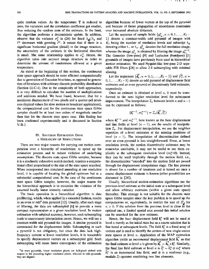
To provide a quantitative test, we used two image sequences with synthetic motion. Fig. 7(a) shows a pattern based on the concept of a random dot stereogram. The 0th field of the sequence consists of random, uniformly distributed numbers from the range [40 2001. The subsequent even fields are exact copies of the 0th field, except for a 50 by 20 pixel rectangle R E A, in the center of the outlined area, which has been moved by d,=(2.0, 1.0) with respect to the previous even field. The odd fields are exact replicas of the preceding even fields. Fig. 7(b) shows the test image 2, which provides a synthetic motion of natural data obtained from a video camera. The background is provided by the test image 3, whereas the 45 by 20 pixel rectangle R E A, in the center is obtained from another image through low-pass filtering and subsampling. In subsequent fields, the same background image is used, whereas the moving pixels in the rectangle (d, =(lS, 0.5)) are obtained from appropriately shifted pixels in the prefiltered image. Unlike in the case of test image 1, this test pattern permits noninteger displacements, which is a more realistic situation since there is no perfect data matching. In both images, the white frame outlines the area of 77 by 49 pixels used in the estimation.

Fig. 8 shows the 0th field of a natural sequence obtained with a video camera. The acquisition process included, as usual, camera filtering, sampling, and quantization, as described in Section 11-C-2. There is some aliasing present in the data due to insufficient vertical filtering before sampling (as is typical in most camera-captured imagery with interlace). No filtering or any other processing has been applied to the sequence after acquisition. The white frame outlines the area of 221 by 69 pixels used in estimation.

B. Estimation Results

The motion estimates presented below have been obtained

921

(4 (b) Fig. 7. Test images with synthetic motion and a 77 by 49 pel window used in estimation: (a) Test image 1, [RI = .SO x 20 pixels, d,=(2.0, 1.0); (b) test image 2, IRI = 45 x 20 pixels, d,=(1.5, 0.5).

Fig. 8. Test 3 with natural motion and in estimation.

a 221 by 69 pel window used

forward estimation), and Ad = As. Estimates for other At and Ad can be found in [24].

The discrete state space stochastic relaxation used in sim- ulations was based on S’ with d,,,=2.0 and Nd=17 levels in each direction. This c I! oice of parameters gives the upper bound of a quarter pixel on the predicted accuracy of motion vectors in the absence of such unaccounted effects as occlusions or .illumination change. The continuous state space estimation, however, can, in principle, give finer accuracy if all underlying assumptions are satisfied. In practice, the observed accuracy in both cases depends on the extent to which assumptions are violated, which is difficult to assess, and on such parameters as annealing schedule, motion, and image models, etc. The annealing schedule is particularly difficult to establish since its parameters (initial temperature, number of iterations) are highly dependent on the data. At the moment, we do not know how to choose parameters of the algorithms in order to obtain given accuracy in practice, although we have been able to establish, through experimentation on synthetic-motion sequences, those models and parameter ranges that give lower mean square errors than others [24].

To model the motion, neighborhood systems from Figs. 2 and 4 with notentials (11) and (14) were used. Since the from pairs of fields separated by Tg = 2760, with At=O.O (i.e., 1 \ I \ I

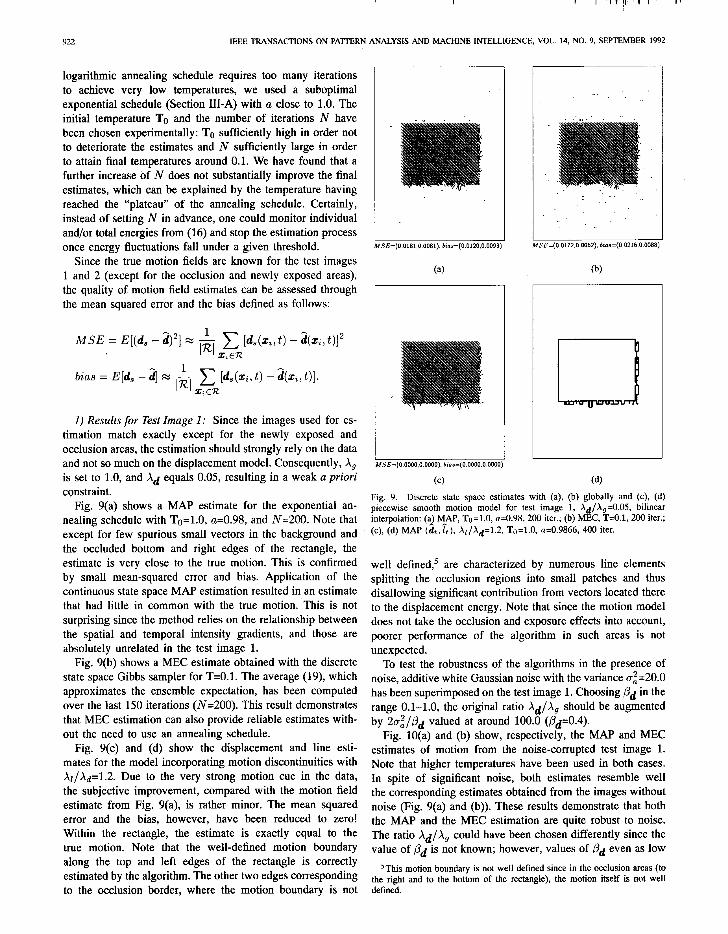
922 IEEE TRANSACTIONS ON PAmRN ANALYSIS AND MACHINE INTELLIGENCE, VOL. 14, NO. 9, SEPTEMBER 1992

logarithmic anneal ing schedule requires too many iterations to achieve very low temperatures, we used a suboptimal exponential schedule (Section III-A) with a close to 1.0. The initial temperature TO and the number of iterations N have been chosen experimentally: To sufficiently high in order not to deteriorate the estimates and N sufficiently large in order to attain final temperatures around 0.1. W e have found that a further increase of N does not substantially improve the final estimates, which can be explained by the temperature having reached the “plateau” of the anneal ing schedule. Certainly, instead of setting N in advance, one could monitor individual and/or total energies from (16) and stop the estimation process once energy fluctuations fall under a given threshold.

Since the true motion fields are known for the test images 1 and 2 (except for the occlusion and newly exposed areas), the quality of motion field estimates can be assessed through the mean squared error and the bias def ined as follows:

MSE = E[(dS - ^d)2] = & c [d&i, t) - &%t)12 X,ER

bias = E[ds - 4 M L ,R, c [d&i, t) - ^d(xi, t)l. X,ER

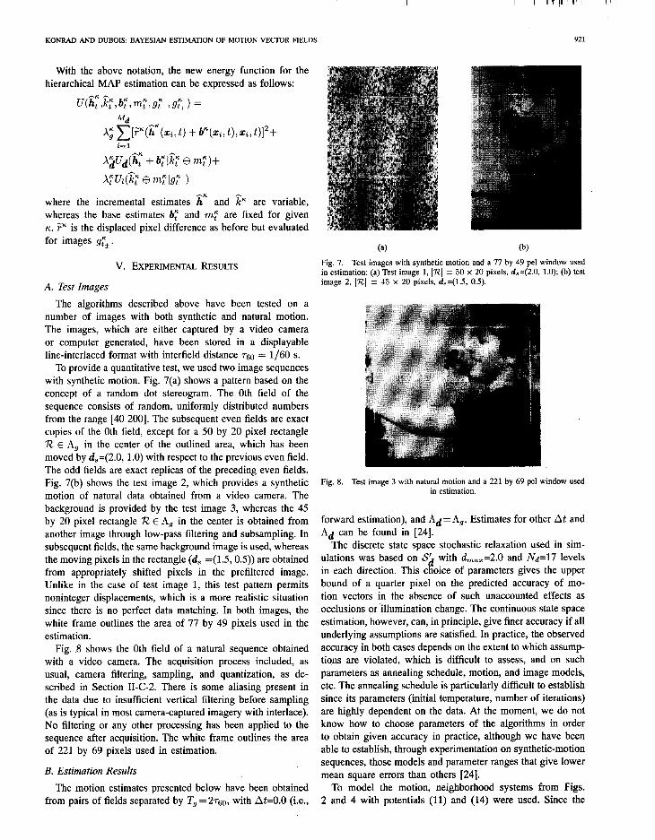
1) Results for Test Image 1: Since the images used for estimation match exactly except for the newly exposed and occlusion areas, the estimation should strongly rely on the data and not so much on the displacement model. Consequent ly, X, is set to 1.0, and Ad equals 0.05, resulting in a weak a priori constraint.

Fig. 9(a) shows a MAP estimate for the exponential anneal ing schedule with Tu=l.O, a=0.98, and N=200. Note that except for few spurious small vectors in the background and the occluded bottom and right edges of the rectangle, the estimate is very close to the true motion. This is confirmed by small mean-squared error and bias. Application of the cont inuous state space MAP estimation resulted in an estimate that had little in common with the true motion. This is not surprising since the method relies on the relationship between the spatial and temporal intensity gradients, and those are absolutely unrelated in the test image 1.

Fig. 9(b) shows a MEC estimate obtained with the discrete state space Gibbs sampler for T=O.l. The average (19), which approximates the ensemble expectation, has been computed over the last 150 iterations (N=200). This result demonstrates that MEC estimation can also provide reliable estimates without the need to use an anneal ing schedule.

Fig. 9(c) and (d) show the displacement and line estimates for the model incorporating motion discontinuities with xr/&=l.2. Due to the very strong motion cue in the data, the subjective improvement, compared with the motion field estimate from Fig. 9(a), is rather minor. The mean squared error and the bias, however, have been reduced to zero! W ithin the rectangle, the estimate is exactly equal to the true motion. Note that the well-defined motion boundary a long the top and left edges of the rectangle is correctly est imated by the algorithm. The other two edges corresponding to the occlusion border, where the motion boundary is not

MSE=(0.0181,0 0081) . b ios=(O 0120 .0 0093 )

(4

I

/ MSE=(O 0000 .0 0000) . b ios=(O 0000 .0 .0000

Cc)

M. SE=(O 0172 .0 0062) ,b tos=(O 0216 .00088 )

(4 Fig. 9. Discrete state space estimates with (a), (b) globally and (c), (d) piecewise smooth motion model for test image 1, xd/xs=O.O& bilinear interpolation: (al MAAP, Tc=l.O, a=0.98, 200 iter.; (b) MEC, T=O.l, 200 iter.; (c), (d) MAP (dt. It), &/+1.2, Ta=l.O, a=0.9866, 400 iter.

well defined,’ are character ized by numerous line elements splitting the occlusion regions into small patches and thus disallowing significant contribution from vectors located there to the displacement energy. Note that since the motion model does not take the occlusion and exposure effects into account, poorer per formance of the algorithm in such areas is not unexpected.

To test the robustness of the algorithms in the presence of noise, additive white Gaussian noise with the var iance az=20.0 has been super imposed on the test image 1. Choosing @d in the range 0.1-1.0, the original ratio Ad/x, should be augmented by 2Uz/Pd valued at a round 100.0 (pdZO.4).

Fig. 10(a) and (b) show, respectively, the MAP and MEC estimates of motion from the noise-corrupted test image 1. Note that higher temperatures have been used in both cases. In spite of significant noise, both estimates resemble well the corresponding estimates obtained from the images without noise (Fig. 9(a) and (b)). These results demonstrate that both the MAP and the MEC estimation are quite robust to noise. The ratio Ad/&, could have been chosen differently since the value of pd is not known; however, values of /Id even as low

5This motion boundary is not well def ined since in the occlusion areas (to the right and to the bottom of the rectangle), the motion itself is not well defined.

KONRAD AND DUBOIS: BAYESIAN ESTIMATION OF MOTION VECTOR FIELDS

:_

; I_,. .:; .;. . . . . ” -: : : :

SE=(0.1684.0 0698) . b ios=(O 1483 .0 0808 :

(4

ISE=(O 2612 .00606) . b ios=(03607 .00932 ]

(b)

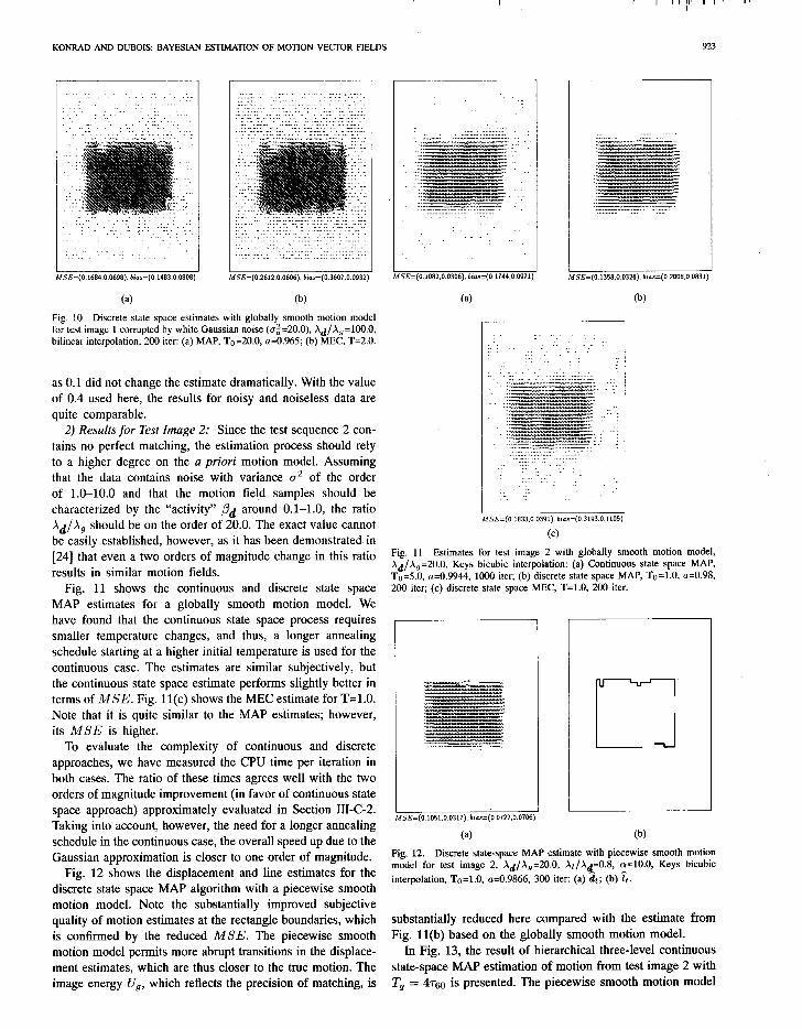
Fig. 10 Discrete state space estimates with globally smooth motion model for test image 1 corrupted by white Gaussian noise (0,2=20.0), X~/X,=lOO.O, bilinear interpolation, 200 iter: (a) MAP, To=20.0, a=0.965; (b) MEC, T=2.0.

as 0.1 did not change the estimate dramatically. W ith the value of 0.4 used here, the results for noisy and noiseless data are quite comparable.

2) Results for Test Image 2: Since the test sequence 2 contains no perfect matching, the estimation process should rely to a higher degree on the a priori motion model. Assuming that the data contains noise with var iance u2 of the order of 1.0-10.0 and that the motion field samples should be character ized by the “activity” ,8d around 0.1-1.0, the ratio Ad/x, should be on the order of 20.0. The exact value cannot be easily established, however, as it has been demonstrated in [24] that even a two orders of magni tude change in this ratio results in similar motion fields.

Fig. 11 shows the cont inuous and discrete state space MAP estimates for a globally smooth motion model. W e have found that the cont inuous state space process requires smaller temperature changes, and thus, a longer anneal ing schedule starting at a higher initial temperature is used for the cont inuous case. The estimates are similar subjectively, but the cont inuous state space estimate performs slightly better in terms of MSE. Fig. 11(c) shows the MEC estimate for T-1.0. Note that it is quite similar to the MAP estimates; however, its MSE is higher.

To evaluate the complexity of cont inuous and discrete approaches, we have measured the CPU time per iteration in both cases. The ratio of these times agrees well with the two orders of magni tude improvement (in favor of cont inuous state space approach) approximately evaluated in Section 11X-C-2. Taking into account, however, the need for a longer anneal ing schedule in the cont inuous case, the overall speed up due to the Gaussian approximation is closer to one order of magnitude.

Fig. 12 shows the displacement and line estimates for the discrete state space MAP algorithm with a piecewise smooth motion model. Note the substantially improved subjective quality of motion estimates at the rectangle boundaries, which is confirmed by the reduced MSE. The piecewise smooth motion model permits more abrupt transitions in the displacement estimates, which are thus closer to the true motion. The image energy V,, which reflects the precision of matching, is

._: ”

SE=(0.1082,0 .0306) . b ios=(O 1744 .0 .0971 :

(4

M SE=(O.l358.0.0326), bios=(O 2008 .0 0 8 3 1

923

(b)

_:: ::

:_. : :. : : ..::

: .:

I MSE=(O 1833 .0 0391) . b ios=(O 3193 .0 1 1 0 5

Cc)

Fig. 11 Estimates for test image 2 with globally smooth motion model, Xd/X,=20.0, Keys bicubic interpolation: (a) Cont inuous state space MAP, To=5.0, rr=O.9944, 1000 iter; (b) discrete state space MAP, To=l.O, (r=O.98, 200 iter; (c) discrete state space MEC, T=l.O, 200 iter.

M. SE=(0.1051.0 0317) . b ias=(O 0722 .0 0 7 0 1

(4

L-7 J Fig. 12. Discrete state-space MAP estimate with piecewise smooth motion model for test image 2, Xd/X,=20.0, X,/X4=0.8, ,=lO.O, Keys bicubic interpolation, To=l.O, a=0.9866, 300 iter: (a) dt ; (b) It.

substantially reduced here compared with the estimate from Fig. 11(b) based on the globally smooth motion model.

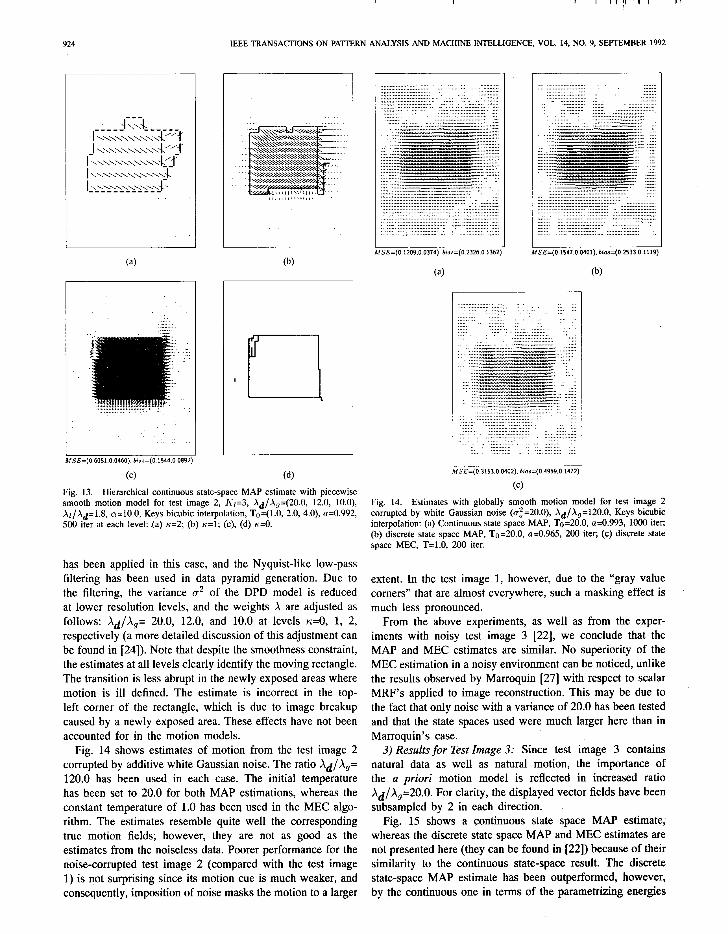
In Fig. 13, the result of hierarchical three-level cont inuous state-space MAP estimation of motion from test image 2 with Tg = 49-60 is presented. The piecewise smooth motion model

924 IEEE TRANSACTIONS ON PAlTERN ANALYSIS AND MACHINE INTELLIGENCE, VOL. 14, NO. 9, SEPTEMBER 1992

(4

MSE=(O 6051 .00460) . b iasz (0 .1544 .00892)

Cc) (4 Fig. 13. Hierarchical continuous state-space MAP estimate with piecewise smooth motion model for test image 2, 1<r=3, Xd/X,=(20.0, 12.0, 10.0) Xr/Xd=1.8, a=lO.O, Keys bicubic interpolation, To=(l.O, 2.0, 4.0), r/=0.992, 500 iter at each level: (a) s-=2; (b) ri=l; (c), (d) ~=0.

has been appl ied in this case, and the Nyquist-like low-pass filtering has been used in data pyramid generat ion. Due to the filtering, the var iance u2 of the DPD model is reduced at lower resolution levels, and the weights X are adjusted as follows: Ad/&= 20.0, 12.0, and 10.0 at levels n=O, 1, 2, respectively (a more detailed discussion of this adjustment can be found in [24]). Note that despite the smoothness constraint, the estimates at all levels clearly identify the moving rectangle. The transition is less abrupt in the newly exposed areas where motion is ill defined. The estimate is incorrect in the top- left corner of the rectangle, which is due to image breakup caused by a newly exposed area. These effects have not been accounted for in the motion models.

Fig. 14 shows estimates of motion from the test image 2 corrupted by additive white Gaussian noise. The ratio Ad/&= 120.0 has been used in each case. The initial temperature has been set to 20.0 for both MAP estimations, whereas the constant temperature of 1.0 has been used in the MEC algorithm. The estimates resemble quite well the corresponding true motion fields; however, they are not as good as the estimates from the noiseless data. Poorer per formance for the noise-corrupted test image 2 (compared with the test image 1) is not surprising since its motion cue is much weaker, and consequent ly, imposition of noise masks the motion to a larger

'SE=(O 1209 .0 0374) . b ias=(O 2326 .0 1362 )

(4

M SE=(O 1547 .0 .0401) . b ios=(O 2533 .0 1119 :

(b)

fSE=(O 3153 .00402) . b ias=(04959.0 1472 :

(4

Fig. 14. Estimates with globally smooth motion model for test image 2 corrupted by white Gaussian noise ((~2=20.0), Xd/X,=120.0, Keys bicubic interpolation: (a) Cont inuous state space MAP, To=20.0, a=0.993, 1000 iter; (b) discrete state space MAP, Tn=20.0, rr=O.965, 200 iter; (c) discrete state space MEC, T=l.O, 200 iter.

extent. In the test image 1, however, due to the “gray value corners” that are almost everywhere, such a masking effect is much less pronounced.

From the above experiments, as well as from the experiments with noisy test image 3 [22], we conclude that the MAP and MEC estimates are similar. No superiority of the MEC estimation in a noisy environment can be noticed, unlike the results observed by Marroquin [27] with respect to scalar MRF’s appl ied to image reconstruction. This may be due to the fact that only noise with a var iance of 20.0 has been tested and that the state spaces used were much larger here than in Marroquin’s case.

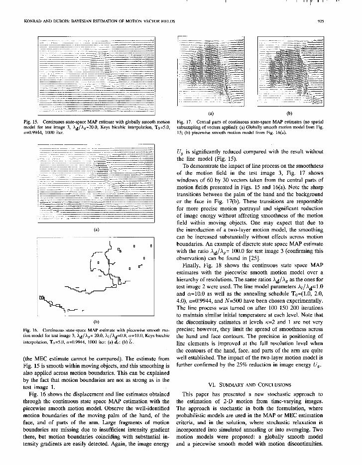
3) Results for Test Image 3: Since test image 3 contains natural data as well as natural motion, the importance of the a priori motion model is reflected in increased ratio x,J/&=20.0. For clarity, the displayed vector fields have been subsampled by 2 in each direction.

Fig. 15 shows a cont inuous state space MAP estimate, whereas the discrete state space MAP and MEC estimates are not presented here (they can be found in [22]) because of their similarity to the cont inuous state-space result. The discrete state-space MAP estimate has been outperformed, however, by the cont inuous one in terms of the parametrizing energies

KONRADANDDUBOIS: BAYESIANESTIMATlONOFMOTIONVECTORFIELDS 925

Fig. 15. Continuous state-space MAP estimate with globally smooth motion model for test image 3, Xd/X,=20.0, Keys bicubic interpolation, To=5.0, a=0.9944. 1000 iter.

(4

0 0

(b) Fig. 16. Continuous state-space MAP estimate with piecewise smooth motion model for test image 3, Ad/X,= 20.0, X,/A~=O.S, n=lO.O, Keys bicubic interpolation, Tu=5.0, a=0.9944, 1000 iter: (a) dt; (b) 6.

(the MEC estimate cannot be compared). The estimate from Fig. 15 is smooth within moving objects, and this smoothing is also applied across motion boundaries. This can be explained by the fact that motion boundaries are not as strong as in the test image 1.

Fig. 16 shows the displacement and line estimates obtained through the continuous state space MAP estimation with the piecewise smooth motion model. Observe the well-identified motion boundaries of the moving palm of the hand, of the face, and of parts of the arm. Large fragments of motion boundaries are missing due to insufficient intensity gradient there, but motion boundaries coinciding with substantial in- tensitv gradients are easilv detected. Again. the image eneruv

(4 (b)

Fig. 17. Central parts of continuous state-space MAT’ estimates (no spatial subsampling of vectors applied): (a) Globally smooth motion model from Fig. 15; (b) piecewise smooth motion model from Fig. 16(a).

U, is significantly reduced compared with the result without the line model (Fig. 15).

To demonstrate the impact of line process on the smoothness of the motion field in the test image 3, Fig. 17 shows windows of 60 by 30 vectors taken from the central parts of motion fields presented in Figs. 15 and 16(a). Note the sharp transitions between the palm of the hand and the background or the face in Fig. 17(b). These transitions are responsible for more precise motion portrayal and significant reduction of image energy without affecting smoothness of the motion field within moving objects. One may expect that due to the introduction of a two-layer motion model, the smoothing can be increased substantially without effects across motion boundaries. An example of discrete state space MAP estimate with the ratio Ad/X,= 100.0 for test image 3 (confirming this observation) can be found in [25].

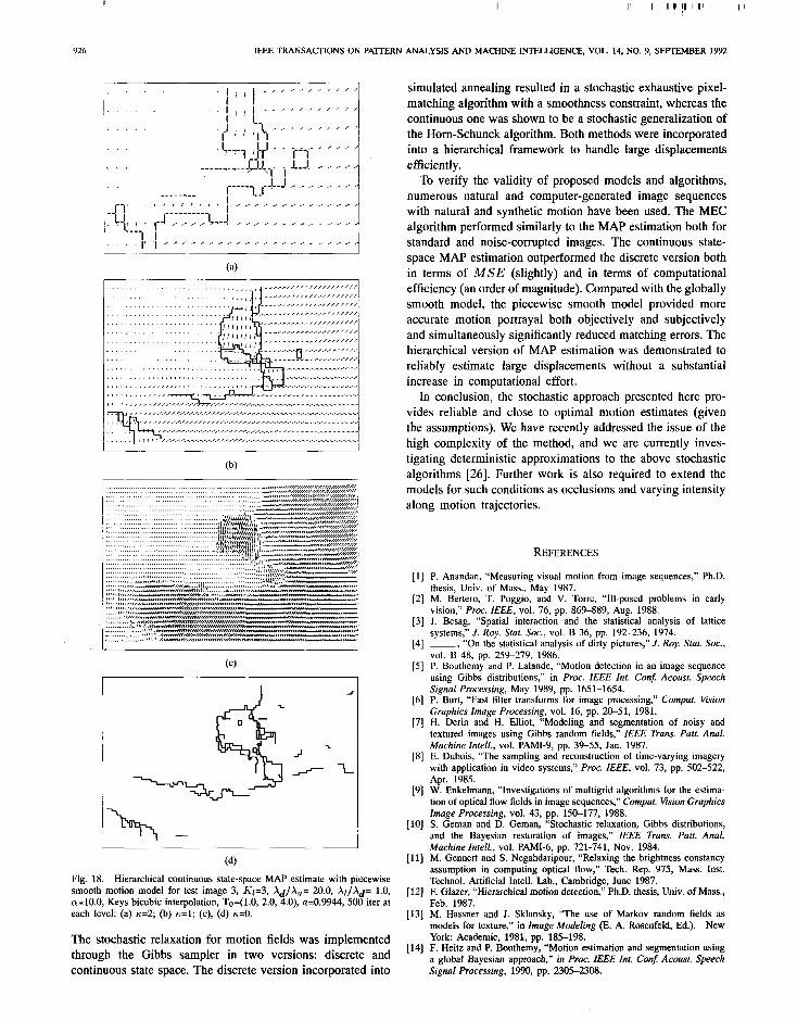
Finally, Fig. 18 shows the continuous state space MAP estimates with the piecewise smooth motion model over a hierarchy of resolutions. The same ratios Ad/X, as the ones for test image 2 were used. The line model parameters &/Xd=l.O and a=lO.O as well as the annealing schedule Ta=(l.O, 2.0, 4.0) a=0:9944, and N=500 have been chosen experimentally. The line process was turned on after 100 150 200 iterations to maintain similar initial temperature at each level. Note that the discontinuity estimates at levels rc=2 and 1 are not very precise; however, they limit the spread of smoothness across the hand and face contours. The precision in positioning of line elements is improved at the full resolution level when the contours of the hand, face, and parts of the arm are quite well established. The impact of the two-layer motion model is further confirmed by the 25% reduction in image energy U,.

VI. SUMMARY AND CONCLUSIONS

This paper has presented a new stochastic approach to the estimation of 2-D motion from time-varying images. The approach is stochastic in both the formulation, where probabilistic models are used in the MAP or MEC estimation criteria, and in the solution, where stochastic relaxation is incorporated into simulated annealing or into averaging. Two motion models were proposed: a globally smooth model and a niecewise smooth model with motion discontinuities.

926 IEEE TRANSACDONS ON PATTERN ANALYSIS AND MACHINE INTELLIGENCE, VOL. 14, NO. 9, SEPTEMBER 1992

i

(4

N -

-I

-L

(4 Fig. 18. Hierarchical continuous state-space MAP estimate with piecewise smooth motion model for test image 3, Kl=3, X&X,= 20.0, X,/X,= 1.0, a=lO.O, Keys bicubic interpolation, To=(l.O, 2.0, 4.0), a=0.9944, 500 iter at each level: (a) ~=2; (b) r;=l; (c), (d) n=O.

The stochastic relaxation for motion fields was implemented through the Gibbs sampler in two versions: discrete and cont inuous state suace. The discrete version incornorated into

simulated anneal ing resulted in a stochastic exhaust ive pixel- matching algorithm with a smoothness constraint, whereas the cont inuous one was shown to be a stochastic general ization of the Horn-Schunck algorithm. Both methods were incorporated into a hierarchical f ramework to handle large displacements efficiently.

To verify the validity of p roposed models and algorithms, numerous natural and computer-generated image sequences with natural and synthetic motion have been used. The MEC algorithm performed similarly to the MAP estimation both for s tandard and noise-corrupted images. The cont inuous state- space MAP estimation outperformed the discrete version both in terms of MSE (slightly) and in terms of computat ional efficiency (an order of magnitude). Compared with the globally smooth model, the piecewise smooth model provided more accurate motion portrayal both objectively and subjectively and simultaneously significantly reduced matching errors. The hierarchical version of MAP estimation was demonstrated to reliably estimate large displacements without a substantial increase in computat ional effort.

In conclusion, the stochastic approach presented here provides reliable and close to optimal motion estimates (given the assumptions). W e have recently addressed the issue of the high complexity of the method, and we are currently inves- tigating deterministic approximations to the above stochastic algorithms [26]. Further work is also required to extend the models for such condit ions as occlusions and varying intensity a long motion trajectories.

REFERENCES

[l] P. Anandan, “Measuring visual motion from image sequences,” Ph.D. thesis, Univ. of Mass., May 1987.

[2] M. Bertero, T. Poggio, and V. Torre, “Ill-posed problems in early vision,” Proc. IEEE, vol. 76, pp. 869-889, Aug. 1988.

[3] J. Besag, “Spatial interaction and the statistical analysis of lattice systems,” .I. Roy. Stat. Sot., vol. B 36, pp. 192-236, 1974.

[4] -, “On the statistical analysis of dirty pictures,” J. Roy. Stat. Sot., vol. B 48, pp. 259-279, 1986.

[5] P. Bouthemy and P. Lalande, “Motion detection in an image sequence using Gibbs distributions,” in Proc. IEEE Int. Conj Acoust. Speech Signal Processing, May 1989, pp. 1651-1654.

[6] P. Burt, “Fast filter transforms for image processing,” Comput. Ksion Graphics Image Processing, vol. 16, pp. 2&51, 1981.

[7] H. Derin and H. Elliot, “Model ing and segmentat ion of noisy and textured images using Gibbs random fields,” IEEE Trans. Patt. Anal. Machine Intell., vol. PAMI-9, pp. 39-55, Jan. 1987.

IS] E. Dubois, “The sampling and reconstruction of time-varying imagery with application in video systems,” Proc. IEEE, vol. 73, pp. 502-522, Apr. 1985.

[9] W. Enkelmann, “Investigations of multigrid algorithms for the estimation of optical flow fields in image sequences,” Comput. vision Graphics Image Processing, vol. 43, pp. 150-177, 1988.

[lo] S. Geman and D. Geman, “Stochastic relaxation, Gibbs distributions, and the Bayesian restoration of images,” IEEE Trans. Part. Anal. Machine Intell., vol. PAMI-6, pp. 721-741, Nov. 1984.

[ll] M. Gennert and S. Negahdaripour, “Relaxing the brightness constancy assumption in comput ing optical flow,” Tech. Rep. 975, Mass. Inst. Technol. Artificial Intell. Lab., Cambridge, June 1987.

[12] F. Glazer, “Hierarchical motion detection,” Ph.D. thesis, Univ. of Mass., Feb. 1987.

1131 M. Hassner and J. Sklansky, “The use of Markov random fields as models for texture,” in Image Model ing (E. A. Rosenfeld, Ed.). New York: Academic, I981, pp.-185-198. -

[14] F. Heitz and P. Bouthemy, “Motion estimation and segmentat ion using a global Bayesian approach,” in Proc. IEEE Inf. ConjI Acoust. Speech Sipnal Processinp. 1990. DO. 2305-2308.

KONRAD AND DUBOIS: BAYESIAN ESTIMA’TlON OF MOTION VECTOR FIELDS 927

[15] -, “Mult imodal motion estimation and segmentat ion using Markov random fields,” in Proc. IEEE Int. Conf Part. Recogn., June 1990, pp. 378-383.

[16] E. Hildreth, “Computat ions underlying the measurement of visuai motion,” Artificial Intell., vol. 23, pp. 309-354, 1984.

[17] B. P. Horn and B. Schunck, “Determining optical flow,“Arti&ial Intell., vol. 17, pp. 185-203, 1981.

[18] J. Hutchinson, C. Koch, J. Luo, and C. Mead, “Comput ing motion using analog and binary resistive networks,” Comput., vol. 21, pp. 52-63, Mar. 1988.

[19] R. Keys, “Cubic convolution interpolation for digital image processing,” IEEE Trans. Acoust. Speech Signal Processing, vol. ASSP-29, pp. 115>1160, Dec. 1981.

[20] S. Kirkpatrick, C. Gelatt, Jr., and M. Vecchi, “Optimization by simulated anneal ing,” Sci., vol. 220, pp. 671-680, May 1983.

[21] J. Konrad and E. Dubois, “Estimation of image motion fields: Bayesian formulation and stochastic solution,” . m Proc. IEEE Int. Conf Acoust. Speech Signal Processing, Apr. 1988, pp. 1072-1075.

[22] -, “Multigrid Bayesian estimation of image motion fields using stochastic relaxation,” m Proc. IEEE Int. Cant: Comma. Vision. Dec. 1988, pp. 354-362.

1231 .I. Konrad, “Motion-comuensated intemolation for TV frame-rate con- _ _ version,” Tech. Rep. 26,INRS-Telecommunications, Oct. 1988.

[24] -, “Bayesian estimation of motion fields from image sequences,” Ph.D. thesis, Dept. of Elect. Eng., McGill Univ., Montreal, June 1989.

[25] J. Konrad and E. Dubois, “Bayesian estimation of discontinuous motion in images using simulated anneal ing,” m Proc. Conj Vision Interface VI’89 June 1989, pp. 51-60.

[26] -, “Comparison of stochastic and deterministic solution methods in Bayesian estimation of 2-D motion,” Image Vision Comput., vol. 9, pp. 215-228, Aug. 1991.

1271 J. Marroquin, “Probablistic solution of inverse problems,” Ph.D. thesis, Mass. Inst. Technol., Cambridge, Sept. 1985. .

1281 D. Martinez, “Model-based motion estimation and its aoolication to _ _ . . restoration and interpolation of motion pictures,” Ph.D. thesis, Mass. Inst. Technol., Cambridge, Aug. 1986.

[29] N. Metropolis, A. Rosenbluth, M. Rosenbluth, H. Teller, and E. Teller, “Equat ion of state calculations by fast comput ing machines,” J. Chem. Phys., vol. 21, pp. 1087-1092, June 1953.

[30] D. Murray and B. Buxton, “Scene segmentat ion from visual motion using global optimization,” IEEE Trans. Part. Anal. Machine Intell., vol. PAMI-9, pp. 220-228, Mar. 1987.

[31] H. -H. Nagel and W. Enkelmann, “An investigation of smoothness constraints for the estimation of displacement vector fields from image sequences,” IEEE Trans. Part. Anal. Machine Intell., vol. PAMI-8, pp. 565-593, Sept. 1986.

[32] S. Ross, Appl ied Probability Models with Optimization Applications. San Francisco: Holden-Day, 1970.

1331 B. Schunck, “Motion segmentat ion and estimation,” Ph.D. thesis, Mass. Inst. Technol., Cambridge, May 1983.

[341 0. Tretiak and L. Pastor, “Velocity estimation from image sequences with second order differential operators,” in Proc. IEEE Int. Cant: Part. Recogn., July 1984, pp. 16-19:

[35] J. Woods, “Two-dimensional discrete Markovian fields,” IEEE Trans. Inform Theory, vol. IT-18, pp. 232-240, Mar. 1972.

Janusz Konrad was born in Szczecin, Poland, on Nov. 15, 1956. He received the M.Eng. degree with distinction from the Technical University of Szczecin, Poland, in 1980 and the Ph.D. degree, also with distinction, from McGill University, Montreal, Canada, in 1989, both in electrical engineering.

In July 1989, he joined the Institut National de la Recherche Scientifique, University of Quebec as a research associate at the INRS-TCICcommunications Centre in Montreal, Canada, where he worked on transmission of HDTV images. In May 1991, he

became an Assistant Professor at INRS-T&communications. He has collaborated with the Visual Communicat ions Group of Bell-Northern Research. His interests are in the areas of mult idimensional signal processing, computer vision, and image sequence transmission.

Eric Dubois (S’72-M’77-SM’85) received the B.Eng. (honors) degree with great distinction and the M.Eng. degree from McGill University, Montreal, Canada in 1972 and 1974, respectively, and the Ph.D. degree from the University of Toronto, Toronto, Canada, in 1978, all in electrical engineering.

He joined the Institut National de la Recherche Scientifique (University of Quebec) in 1977, where he currently holds the position of Professor in the INRS-Telecommunicat ions Centre, Montreal, Canada. He has also been an Auxiliary Professor in the Department of Electrical Engineering, McGill University, since 1981. In 1986, he was on sabbatical leave with the Advanced Television Research Program at the Media Laboratory, Massachusetts Institute of Technology, Cambridge. His research has centered on the source coding and processing of still and moving images and in mult idimensional digital signal processing. He has collaborated extensively with the Image Services Depart- ment of Bell-Northern Research, the Engineering Department of the Canadian Broadcasting Corporation, and the Communicat ions Research Center, Ottawa, Canada. His current work is in enhanced and high-definition television systems and in motion estimation with application to television signal processing.

Dr. Dubois was the co-recipient of the 1988 Journal Award from the Society of Motion Picture and Television Engineeers. He is a member of the Order of Engineers of Quebec.

Documents

Bayesian Estimation of Motion Vector Fields