ARTICLE IN PRESS

0925-5273/$ - se

doi:10.1016/j.ijp

�Correspondifax: +90312 23

E-mail addre

Int. J. Production Economics 103 (2006) 600–609

www.elsevier.com/locate/ijpe

Balancing of parallel assembly lines

Hadi Gokc-ena,�, Kurs-ad Agpakb, Recep Benzera

aDepartment of Industrial Engineering, Faculty of Engineering and Architecture, Gazi University, Maltepe, 06570, Ankara, TurkeybDepartment of Industrial Engineering, Faculty of Engineering, Gaziantep University, Gaziantep, Turkey

Received 13 June 2003; accepted 2 December 2005

Available online 14 February 2006

Abstract

Productivity improvement in assembly lines is very important because it increases capacity and reduces cost. If the

capacity of the line is insufficient, one possible way to increase the capacity is to construct parallel lines. In this study, new

procedures and a mathematical model on the single model assembly line balancing problem with parallel lines are

proposed. The procedures are illustrated with numerical examples. Lastly, active case procedure and the mathematical

model are tested on well-known problems in the line balancing literature.

r 2006 Elsevier B.V. All rights reserved.

Keywords: Assembly line balancing; Parallel lines

1. Introduction

Manufacturers mostly use assembly lines toproduce a high volume product. An assembly lineis a sequence of workstations connected together bya material handling system. It is used to assemblecomponents into a final product. The problem ofbalancing an assembly line is a classic IndustrialEngineering problem. Even though much of thework in this area goes back to the mid-1950s andearly 1960s, the basic structure of the problem isrelevant to the design of production systems today,even in automated plants (Nahmias, 1993). Theassembly line balancing problem is assigning tasksto workstations that minimize the amount of idletime of the line while satisfying specific conditions.The first condition is that the total task time

e front matter r 2006 Elsevier B.V. All rights reserved

e.2005.12.001

ng author. Tel.: +90 312 231 74 00 2859;

0 84 34.

ss: hgokcen@gazi.edu.tr (H. Gokc-en).

assigned to each workstation should be less thanor equal to the cycle time (the time interval betweentwo successive outputs). The second is that the taskassignments should follow the sequential processingorder of the tasks.

Assembly lines can be classified into two generalgroups: traditional assembly lines (with single andmulti/mixed products) and U-type assembly lines(with single and multi/mixed products). The litera-ture on assembly line balancing is rather extensive.For literature on traditional assembly line balan-cing, the review papers of Baybars (1986), Ghoshand Gagnon (1989), and Erdal and Sarin (1998) canbe seen. In addition, the papers of Miltenburg andWijngaard (1994), Urban (1998), Scholl and Klein(1999), Ohno and Nakade (1997), Miltenburg(1998), Sparling and Miltenburg (1998), Miltenburg(2001), Guerriero and Miltenburg (2003), can alsobe investigated for U-type line balancing. However,studies on parallel lines are quite few. In designingthe parallel assembly lines, Suer and Dagli (1994)

.

ARTICLE IN PRESSH. Gokc-en et al. / Int. J. Production Economics 103 (2006) 600–609 601

suggested heuristic procedures and algorithms todynamically determine the number of lines and theline configuration. Also, Suer (1998) studied alter-native assembly line design strategies for a singleproduct. The objective was to determine the numberof assembly lines with minimum total manpower.For this purpose he proposed a 3-phase methodol-ogy: assembly line balancing, determining theparallel workstations and parallel lines. Otherresearches involving parallel workstation havefocused on the simple assembly line balancingproblem (Simaria and Vilarinho, 2001), mixed-model production line balancing problem (Askinand Zhou, 1997; McMullen and Frazier, 1997;Vilarinho and Simaria, 2002).

Most manufacturing plants consist of one ormore assembly lines. When the demand is highenough, it is not uncommon to duplicate the entireassembly line. This provides the advantage ofshortening the assembly line, but may require moreequipment and tools. Another advantage of parallelassembly lines is seen during workstation break-downs. If equipment problems occur at a work-station, other lines can continue to run. A singleserial line must be shutdown whenever there is afailure at any workstation.

The approach presented here is quite differentfrom Suer’s (1998) approach. In this paper, thenumber of lines to be parallelized is not consideredand is not important to be determined as in Suer’s(1998) study. The goal is to balance more than oneassembly line together. That is, it will be possible toassign task(s) from each line to a multi-skilledoperator. As a result, it is inevitable to minimize thetotal idle time of the lines.

2. Notation

The following notations are used in this paper:

C cycle timeCard{F} cardinality of set F, i.e. number of tasks in

set F.Card{Z} cardinality of set Z, i.e. number of tasks

in set Z.x number of trials, x ¼ 1; . . . ;Xh line number, h ¼ 1; . . . ;Hk station number, k ¼ 1; . . . ;Kdk the idle time of station k (C-sum of task

times-walking time)RN random number from array of (1, m)

JMhkJ total number of tasks (that can be) assignedto station k in line h

Lh line h

nh number of tasks in line h

tih performance time of task i in line h

Kmin theoretical minimum number of stationsKmax maximum number of stationsPh set of precedence relationships in prece-

dence diagram of line h

xhik 1 if task i in line h is assigned to station k; 0otherwise

Uhk 1 if station k is utilized in line h; 0 otherwisezk 1 if station k is utilized; 0 otherwise

3. Proposed procedures

It is a most common case in industry that morethan one line (especially two or three lines) producesthe same product or different types of products atthe same time independently. Working of the linessimultaneously with a common resource is veryimportant in terms of resource minimization. Thisprocedure makes this situation possible.

The common assumptions of the procedures arelisted below:

(i)

Only one product is produced on each assemblyline.

(ii)

Precedence diagrams for each product areknown.

(iii)

Task performance times of each product areknown.

(iv)

Operators working in each workstation of theeach line are multi-skilled (flexible workers).

(v)

It can also be worked each side of any line.

In this study, productivity improvement of theassembly system by parallel lines can be realized intwo ways: A passive way and an active way.3.1. Passive case procedure

In the passive case, same products are assembledwith the same cycle time in two different assemblylines. In other words, we have assumed that thenumber of lines is two. This case can be appliedwhen there is a workstation with an idle time, whichis equal or more than the half of the cycle time afterline is balanced. For the passive case, the followingsteps should be carried out:

(i)

Balance each assembly line by using any singlemodel assembly line balancing method.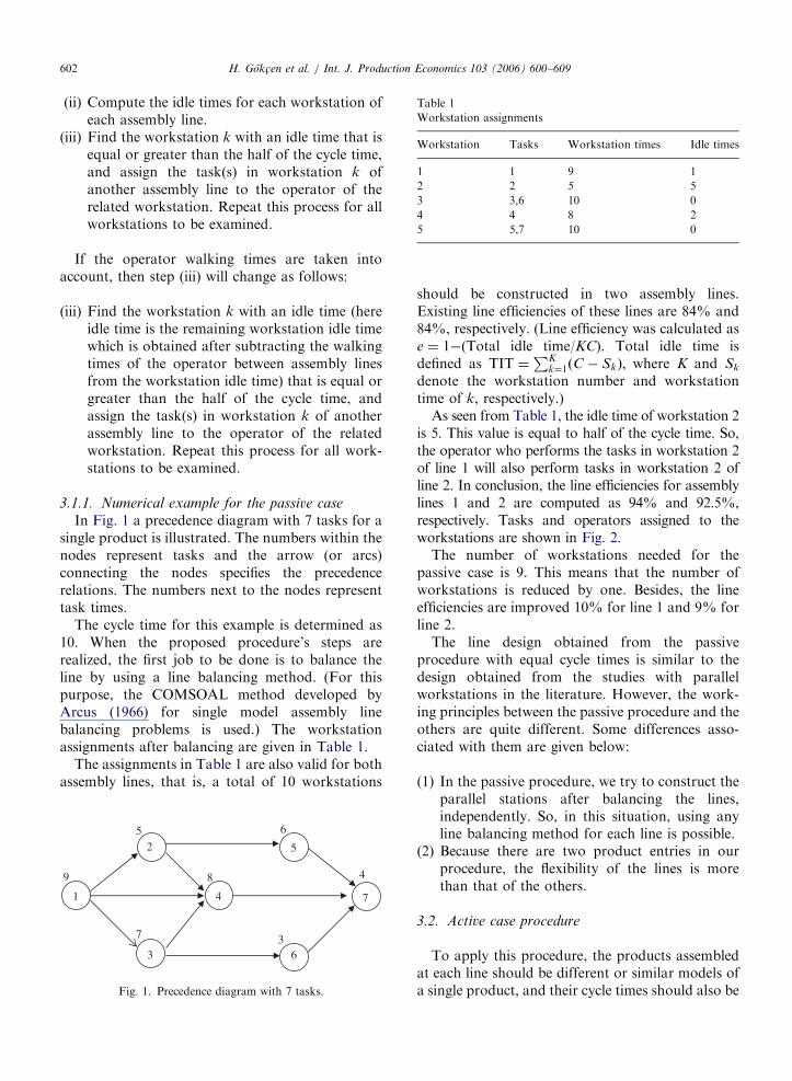

ARTICLE IN PRESS

Table 1

H. Gokc-en et al. / Int. J. Production Economics 103 (2006) 600–609602

(ii)

1

9

Workstation assignments

Compute the idle times for each workstation ofeach assembly line.

Workstation Tasks Workstation times Idle times

(iii)

1 1 9 1

2 2 5 5

3 3,6 10 0

4 4 8 2

5 5,7 10 0

Find the workstation k with an idle time that isequal or greater than the half of the cycle time,and assign the task(s) in workstation k ofanother assembly line to the operator of therelated workstation. Repeat this process for allworkstations to be examined.

If the operator walking times are taken intoaccount, then step (iii) will change as follows:

(iii)

Find the workstation k with an idle time (hereidle time is the remaining workstation idle timewhich is obtained after subtracting the walkingtimes of the operator between assembly linesfrom the workstation idle time) that is equal orgreater than the half of the cycle time, andassign the task(s) in workstation k of anotherassembly line to the operator of the relatedworkstation. Repeat this process for all work-stations to be examined.

3.1.1. Numerical example for the passive case

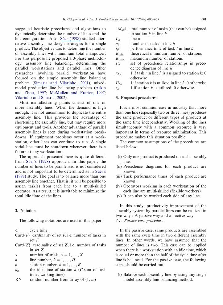
In Fig. 1 a precedence diagram with 7 tasks for asingle product is illustrated. The numbers within thenodes represent tasks and the arrow (or arcs)connecting the nodes specifies the precedencerelations. The numbers next to the nodes representtask times.

The cycle time for this example is determined as10. When the proposed procedure’s steps arerealized, the first job to be done is to balance theline by using a line balancing method. (For thispurpose, the COMSOAL method developed byArcus (1966) for single model assembly linebalancing problems is used.) The workstationassignments after balancing are given in Table 1.

The assignments in Table 1 are also valid for bothassembly lines, that is, a total of 10 workstations

5

3

2

7

6

4

5

7

8

6

3

4

Fig. 1. Precedence diagram with 7 tasks.

should be constructed in two assembly lines.Existing line efficiencies of these lines are 84% and84%, respectively. (Line efficiency was calculated ase ¼ 1�(Total idle time/KC). Total idle time isdefined as TIT ¼

PKk¼1ðC � SkÞ; where K and Sk

denote the workstation number and workstationtime of k, respectively.)

As seen from Table 1, the idle time of workstation 2is 5. This value is equal to half of the cycle time. So,the operator who performs the tasks in workstation 2of line 1 will also perform tasks in workstation 2 ofline 2. In conclusion, the line efficiencies for assemblylines 1 and 2 are computed as 94% and 92.5%,respectively. Tasks and operators assigned to theworkstations are shown in Fig. 2.

The number of workstations needed for thepassive case is 9. This means that the number ofworkstations is reduced by one. Besides, the lineefficiencies are improved 10% for line 1 and 9% forline 2.

The line design obtained from the passiveprocedure with equal cycle times is similar to thedesign obtained from the studies with parallelworkstations in the literature. However, the work-ing principles between the passive procedure and theothers are quite different. Some differences asso-ciated with them are given below:

(1)

In the passive procedure, we try to construct theparallel stations after balancing the lines,independently. So, in this situation, using anyline balancing method for each line is possible.

(2)

Because there are two product entries in ourprocedure, the flexibility of the lines is morethan that of the others.

3.2. Active case procedure

To apply this procedure, the products assembledat each line should be different or similar models ofa single product, and their cycle times should also be

ARTICLE IN PRESS

(1) (2)

(2)

(3,6)

(3,6)

(4)

(4)(1) (5,7)

(5,7)Assembly Line I

Assembly Line II

Fig. 2. Operator allocations.

H. Gokc-en et al. / Int. J. Production Economics 103 (2006) 600–609 603

same. The task assignment logic of this procedure issimilar to that of the COMSOAL. The proposedprocedure can be applied to more than one parallelline. The steps that should be carried out for thiscase are listed below:

(i)

Initialization step (set x ¼ 0, h ¼ 0, k ¼ 0). (ii) Start new trial; set x ¼ xþ 1. (iii) h ¼ hþ 1 until H�1, set k ¼ k þ 1 (open new

workstation).

(iv) For all tasks i 2 fLh;Lhþ1g, a set of assignable

tasks (F list) to workstation k is determined (iftihpdk, then add i to the F list).

(v)

For all tasks iAF, if tih ¼ dk, then add i to theZ list.

(vi)

If Za+, then set m ¼ Card{Z}. Randomlygenerate RNAUniform(1, m). Assign theRNth task to the relating station and removethe RNth task from the relating precedencediagram and update the dk and F list.

(vii)

If Z ¼+ and Fa+, set m ¼ Card{F}.Randomly generate RNAUniform(1, m). As-sign the RNth task to the relating station andremove the RNth task from the relatingprecedence diagram and update the dk and F

list.

(viii) If (F ¼+) and unassigned tasks are avail-

able, then go to step (iii); if Fa+, then go to(iv).

(ix)

If the number of stations is less than theprevious trial, update the best assignments. Ifx ¼ X , then STOP, otherwise go to step (ii).

The procedure is run for all different line sequences(1,2,3ym; 2,1,3,y,m; 3,1,2,y, m;yyyy). Thebalance with the lower number of workstations will beselected from among all the line sequencing combina-tions. This balance will be accepted as the commonbalance of the parallel lines.

If the operator walking times are taken intoaccount, then step (iv) will change as follows:

(iv)

For all tasks i 2 fLh;Lhþ1g, a set of assignabletasks (F list) to workstation k is determined

(if any task(s) from the Lh+1 will be assigned tothe workstation k in Lh, then the suitable tasksfor (tih+1+walking timepdk) condition areadded to the F list).

3.2.1. Numerical example for the active case

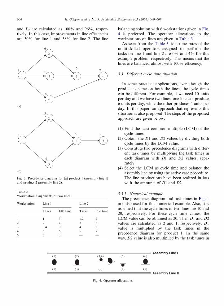
In Fig. 3, precedence diagrams for two differentproducts are illustrated (h ¼ 2). The tasks (nodes)on the precedence diagram of product 1 are not thesame as the tasks on the other diagram. Forexample, task 1 of product (or line) 1 is differentfrom task 1 of product (or line) 2.

The cycle times are determined as 10. Theworkstation assignments obtained when each pro-duct in the problem was balanced independently aregiven in Table 2.

As seen from Table 2, the number of workstationsneeded for two lines is 9. The efficiencies of each lineare 70% and 58%, respectively.

When the proposed active case procedure is used,the workstation assignment will be different fromthe previous one. The working system of theproposed procedure for one station is given below.

Assignable tasks list (F list) for station 1 is task 1on line 1 and line 2. No tasks in the F list are addedto the Z list due to tih6¼dk. Any task in the F list isselected randomly. Let the task be on line 1. Initiallyd1 was 10. After assignment, d1 is obtained as10� 7 ¼ 3; the remaining time is 3. In L1, there areno feasible tasks to meet the remaining time of 3.For this reason, the tasks on L2 should be examinedThere is only task 1 on line 2 in the F list. This taskshould be added to the Z list because its time isequal to the remaining time. Then, task 1 in the Z

list is also assigned to workstation 1. In thissituation, the updated F list is empty, so the relatedworkstation is closed and a new one is opened. In asimilar manner, steps are repeated until all the tasksare assigned.

As a result of working the proposed active caseprocedure, the number of workstations obtained is6. Number of workstations for two lines isdecreased from 9 to 6; thus, the number ofworkstations saved is 3. Besides, efficiencies of L1

ARTICLE IN PRESSH. Gokc-en et al. / Int. J. Production Economics 103 (2006) 600–609604

and L2 are calculated as 100% and 96%, respec-tively. In this case, improvements in line efficienciesare 30% for line 1 and 38% for line 2. The line

Table 2

Workstation assignments of two lines

Workstation Line 1 Line 2

Tasks Idle time Tasks Idle time

1 1 3 1,2 2

2 2 4 3 6

3 3,4 0 4 2

4 5 5 5 7

5 6 3 — —

1

4

2

5

5

3

7 7

6

5

56

1

3

2

4

3 3

5

4

5

(a)

(b)

8

Fig. 3. Precedence diagrams for (a) product 1 (assembly line 1)

and product 2 (assembly line 2).

(1) (2)

(3)

(3,4)

(1) (2)

Fig. 4. Operator

balancing solution with 6 workstations given in Fig.4 is preferred. The operator allocations to theworkstations on lines are given in Table 3.

As seen from the Table 3, idle time rates of themulti-skilled operators assigned to perform thetasks on line 1 and line 2 are 0% and 4% for thisexample problem, respectively. This means that thelines are balanced almost with 100% efficiency.

3.3. Different cycle time situation

In some practical applications, even though theproduct is same on both the lines, the cycle timescan be different. For example, if we need 10 unitsper day and we have two lines, one line can produce6 units per day, while the other produces 4 units perday. In this paper, an approach that represents thissituation is also proposed. The steps of the proposedapproach are given below:

(1)

(5

(4

alloc

Find the least common multiple (LCM) of thecycle times.

(2)

Obtain the D1 and D2 values by dividing bothcycle times by the LCM value.

(3)

Constitute two precedence diagrams with differ-ent task times by multiplying the task times ineach diagram with D1 and D2 values, sepa-rately.

(4)

Select the LCM as cycle time and balance theassembly line by using the active case procedure.The line productions have been realized in lotswith the amounts of D1 and D2.

3.3.1. Numerical example

The precedence diagram and task times in Fig. 1are also used for this numerical example. Also, it isassumed that the cycle times of two lines are 10 and20, respectively. For these cycle time values, theLCM value can be obtained as 20. Then D1 and D2values are calculated as 2 and 1, respectively. D1value is multiplied by the task times in theprecedence diagram for product 1. In the sameway, D2 value is also multiplied by the task times in

)

)

(6)

(5)

Assembly Line I

Assembly Line II

ations.

ARTICLE IN PRESSH. Gokc-en et al. / Int. J. Production Economics 103 (2006) 600–609 605

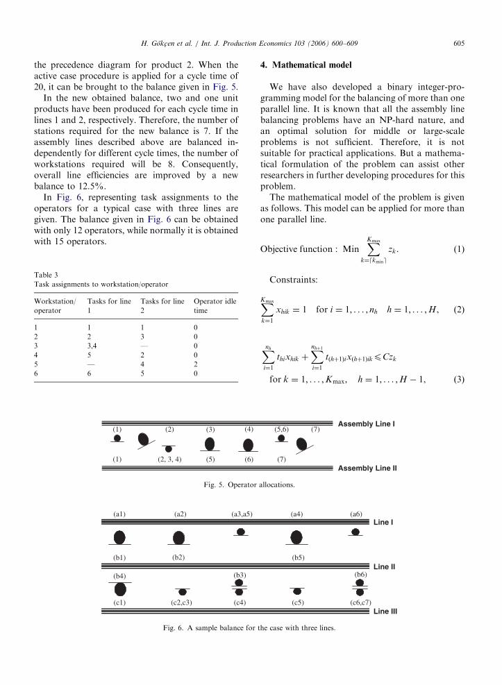
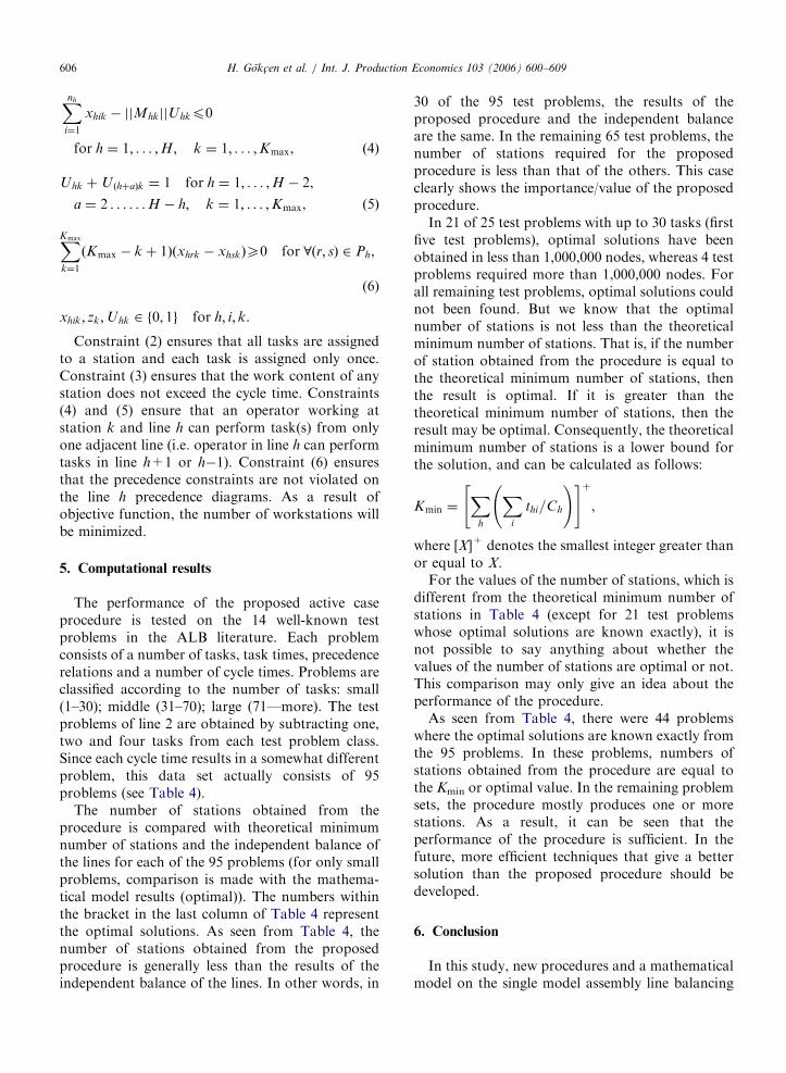
the precedence diagram for product 2. When theactive case procedure is applied for a cycle time of20, it can be brought to the balance given in Fig. 5.

In the new obtained balance, two and one unitproducts have been produced for each cycle time inlines 1 and 2, respectively. Therefore, the number ofstations required for the new balance is 7. If theassembly lines described above are balanced in-dependently for different cycle times, the number ofworkstations required will be 8. Consequently,overall line efficiencies are improved by a newbalance to 12.5%.

In Fig. 6, representing task assignments to theoperators for a typical case with three lines aregiven. The balance given in Fig. 6 can be obtainedwith only 12 operators, while normally it is obtainedwith 15 operators.

Table 3

Task assignments to workstation/operator

Workstation/

operator

Tasks for line

1

Tasks for line

2

Operator idle

time

1 1 1 0

2 2 3 0

3 3,4 — 0

4 5 2 0

5 — 4 2

6 6 5 0

(1) (2)

(1) (5)

(4)(3)

(6)(2, 3, 4)

Fig. 5. Operator

(a1) (a2) (a3,a5)

(b2)(b1)

(b4) (b3)

(c1) (c4)(c2,c3)

Fig. 6. A sample balance for

4. Mathematical model

We have also developed a binary integer-pro-gramming model for the balancing of more than oneparallel line. It is known that all the assembly linebalancing problems have an NP-hard nature, andan optimal solution for middle or large-scaleproblems is not sufficient. Therefore, it is notsuitable for practical applications. But a mathema-tical formulation of the problem can assist otherresearchers in further developing procedures for thisproblem.

The mathematical model of the problem is givenas follows. This model can be applied for more thanone parallel line.

Objective function : MinXKmax

k¼dkmine

zk. (1)

Constraints:

XKmax

k¼1

xhik ¼ 1 for i ¼ 1; . . . ; nh h ¼ 1; . . . ;H, (2)

Xnh

i¼1

thixhik þXnhþ1

i¼1

tðhþ1Þixðhþ1ÞikpCzk

for k ¼ 1; . . . ;Kmax; h ¼ 1; . . . ;H � 1, ð3Þ

(5,6) (7)

(7)

Assembly Line I

Assembly Line II

allocations.

Line I(a4) (a6)

(b5)

(b6)

(c5) (c6,c7)

Line II

Line III

the case with three lines.

ARTICLE IN PRESSH. Gokc-en et al. / Int. J. Production Economics 103 (2006) 600–609606

Xnh

i¼1

xhik � jjMhkjjUhkp0

for h ¼ 1; . . . ;H; k ¼ 1; . . . ;Kmax, ð4Þ

Uhk þU ðhþaÞk ¼ 1 for h ¼ 1; . . . ;H � 2,

a ¼ 2 . . . . . .H � h; k ¼ 1; . . . ;Kmax, ð5Þ

XKmax

k¼1

ðKmax � k þ 1Þðxhrk � xhskÞX0 for 8ðr; sÞ 2 Ph,

(6)

xhik; zk;Uhk 2 f0; 1g for h; i; k.

Constraint (2) ensures that all tasks are assignedto a station and each task is assigned only once.Constraint (3) ensures that the work content of anystation does not exceed the cycle time. Constraints(4) and (5) ensure that an operator working atstation k and line h can perform task(s) from onlyone adjacent line (i.e. operator in line h can performtasks in line h+1 or h�1). Constraint (6) ensuresthat the precedence constraints are not violated onthe line h precedence diagrams. As a result ofobjective function, the number of workstations willbe minimized.

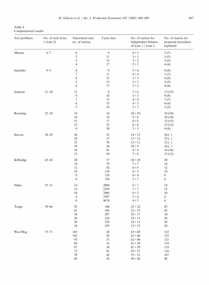
5. Computational results

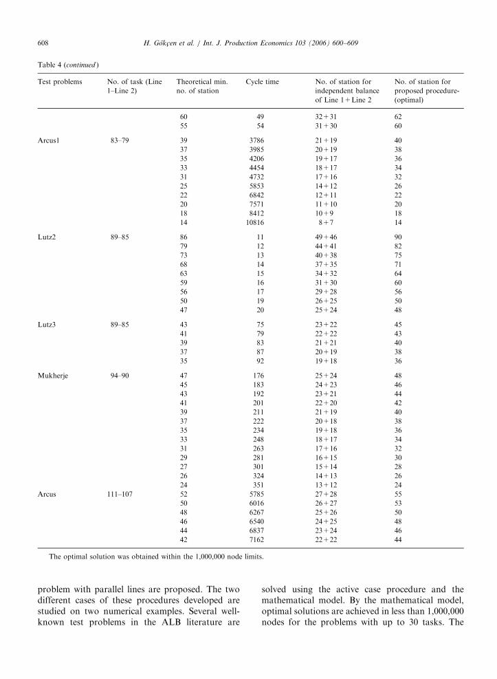
The performance of the proposed active caseprocedure is tested on the 14 well-known testproblems in the ALB literature. Each problemconsists of a number of tasks, task times, precedencerelations and a number of cycle times. Problems areclassified according to the number of tasks: small(1–30); middle (31–70); large (71—more). The testproblems of line 2 are obtained by subtracting one,two and four tasks from each test problem class.Since each cycle time results in a somewhat differentproblem, this data set actually consists of 95problems (see Table 4).

The number of stations obtained from theprocedure is compared with theoretical minimumnumber of stations and the independent balance ofthe lines for each of the 95 problems (for only smallproblems, comparison is made with the mathema-tical model results (optimal)). The numbers withinthe bracket in the last column of Table 4 representthe optimal solutions. As seen from Table 4, thenumber of stations obtained from the proposedprocedure is generally less than the results of theindependent balance of the lines. In other words, in

30 of the 95 test problems, the results of theproposed procedure and the independent balanceare the same. In the remaining 65 test problems, thenumber of stations required for the proposedprocedure is less than that of the others. This caseclearly shows the importance/value of the proposedprocedure.

In 21 of 25 test problems with up to 30 tasks (firstfive test problems), optimal solutions have beenobtained in less than 1,000,000 nodes, whereas 4 testproblems required more than 1,000,000 nodes. Forall remaining test problems, optimal solutions couldnot been found. But we know that the optimalnumber of stations is not less than the theoreticalminimum number of stations. That is, if the numberof station obtained from the procedure is equal tothe theoretical minimum number of stations, thenthe result is optimal. If it is greater than thetheoretical minimum number of stations, then theresult may be optimal. Consequently, the theoreticalminimum number of stations is a lower bound forthe solution, and can be calculated as follows:

Kmin ¼X

h

Xi

thi=Ch

!" #þ,

where [X]+ denotes the smallest integer greater thanor equal to X.

For the values of the number of stations, which isdifferent from the theoretical minimum number ofstations in Table 4 (except for 21 test problemswhose optimal solutions are known exactly), it isnot possible to say anything about whether thevalues of the number of stations are optimal or not.This comparison may only give an idea about theperformance of the procedure.

As seen from Table 4, there were 44 problemswhere the optimal solutions are known exactly fromthe 95 problems. In these problems, numbers ofstations obtained from the procedure are equal tothe Kmin or optimal value. In the remaining problemsets, the procedure mostly produces one or morestations. As a result, it can be seen that theperformance of the procedure is sufficient. In thefuture, more efficient techniques that give a bettersolution than the proposed procedure should bedeveloped.

6. Conclusion

In this study, new procedures and a mathematicalmodel on the single model assembly line balancing

ARTICLE IN PRESS

Table 4

Computational results

Test problems No. of task (Line

1–Line 2)

Theoretical min.

no. of station

Cycle time No. of station for

independent balance

of Line 1+Line 2

No. of station for

proposed procedure-

(optimal)

Merten 6–7 6 9 4+3 7-(7)

5 11 3+3 5-(5)

5 13 3+2 5-(5)

4 17 2+2 4-(4)

Jaeschke 9–8 8 9 5+4 8-(8)

7 11 4+4 7-(7)

6 13 3+3 6-(6)

5 15 3+3 5-(5)

4 17 3+2 4-(4)

Jackson 11–10 11 8 7+6 13-(13)

9 10 5+5 9-(9)

7 13 4+4 7-(7)

6 15 4+3 6-(6)

5 19 3+3 5-(5)

Roszieng 25–24 18 14 10+10 18-(18)

16 16 8+8 16-(16)

15 17 8+8 15-(15)

12 22 6+6 12-(12)

9 30 5+5 9-(9)

Sawyer 30–28 26 25 14+13 26-(�)24 27 13+12 25-(�)22 30 12+11 22-(�)18 36 10+9 18-(�)16 41 8+8 16-(16)

12 54 7+6 12-(12)

Kilbridge 45–43 20 57 10+10 20

14 79 7+7 14

12 92 6+6 12

10 110 6+5 10

8 138 4+4 8

6 184 3+3 6

Hahn 53–51 14 2004 8+7 14

12 2338 7+7 12

10 2806 6+5 10

8 3507 5+4 8

6 4676 4+3 6

Tonge 70–66 43 160 23+22 45

41 168 22+22 43

34 207 18+17 34

30 234 16+15 30

26 270 14+13 26

24 293 13+12 24

Wee-Mag 75–71 105 28 63+60 123

102 29 63+60 123

95 31 62+60 121

89 33 61+59 119

87 34 61+59 119

72 41 59+57 116

70 42 55+53 107

69 43 50+48 98

H. Gokc-en et al. / Int. J. Production Economics 103 (2006) 600–609 607

ARTICLE IN PRESS

Table 4 (continued )

Test problems No. of task (Line

1–Line 2)

Theoretical min.

no. of station

Cycle time No. of station for

independent balance

of Line 1+Line 2

No. of station for

proposed procedure-

(optimal)

60 49 32+31 62

55 54 31+30 60

Arcus1 83–79 39 3786 21+19 40

37 3985 20+19 38

35 4206 19+17 36

33 4454 18+17 34

31 4732 17+16 32

25 5853 14+12 26

22 6842 12+11 22

20 7571 11+10 20

18 8412 10+9 18

14 10816 8+7 14

Lutz2 89–85 86 11 49+46 90

79 12 44+41 82

73 13 40+38 75

68 14 37+35 71

63 15 34+32 64

59 16 31+30 60

56 17 29+28 56

50 19 26+25 50

47 20 25+24 48

Lutz3 89–85 43 75 23+22 45

41 79 22+22 43

39 83 21+21 40

37 87 20+19 38

35 92 19+18 36

Mukherje 94–90 47 176 25+24 48

45 183 24+23 46

43 192 23+21 44

41 201 22+20 42

39 211 21+19 40

37 222 20+18 38

35 234 19+18 36

33 248 18+17 34

31 263 17+16 32

29 281 16+15 30

27 301 15+14 28

26 324 14+13 26

24 351 13+12 24

Arcus 111–107 52 5785 27+28 55

50 6016 26+27 53

48 6267 25+26 50

46 6540 24+25 48

44 6837 23+24 46

42 7162 22+22 44

�The optimal solution was obtained within the 1,000,000 node limits.

H. Gokc-en et al. / Int. J. Production Economics 103 (2006) 600–609608

problem with parallel lines are proposed. The twodifferent cases of these procedures developed arestudied on two numerical examples. Several well-known test problems in the ALB literature are

solved using the active case procedure and themathematical model. By the mathematical model,optimal solutions are achieved in less than 1,000,000nodes for the problems with up to 30 tasks. The

ARTICLE IN PRESSH. Gokc-en et al. / Int. J. Production Economics 103 (2006) 600–609 609

results obtained from the procedure are comparedwith the optimal solutions (for only small pro-blems), the theoretical minimum number of stationsand the independent balance of the lines for eachproblem. Comparison results show that the perfor-mance of the procedure is sufficient. The proposedmodels provide a significant improvement in assem-bly line efficiency when more than one line isnecessary. Finally, this study is a new approach andprovides a different perspective for interestedassembly line balancing researchers.

References

Arcus, A.L., 1966. COMSOAL: A computer method of sequen-

cing operations for assembly lines. International Journal of

Production Research 4, 259–277.

Askin, R.G., Zhou, M., 1997. Parallel station heuristic for the

mixed-model production line balancing problem. Interna-

tional Journal of Production Research 35 (11), 3095–3105.

Baybars, I., 1986. A survey of exact algorithms for the simple

assembly line balancing problem. Management Science 32 (8),

909–932.

Erdal, E., Sarin, S.C., 1998. A survey of the assembly line

balancing procedures. Production Planning and Control 9 (5),

414–434.

Ghosh, S., Gagnon, J., 1989. A comprehensive literature review

and analysis of the design, balancing and scheduling of

assembly systems. International Journal of Production

Research 27 (4), 637–670.

Guerriero, F., Miltenburg, J., 2003. The stochastic U-line

balancing problem. Naval Research Logistics 50, 31–57.

McMullen, P.R., Frazier, G.V., 1997. Heuristic for solving

mixed-model line balancing problems with stochastic task

durations and parallel stations. International Journal of

Production Economics 51 (3), 177–190.

Miltenburg, J., 1998. Balancing U-lines in a multiple U-line

facility. European Journal of Operational Research 109, 1–23.

Miltenburg, J., 2001. U-shaped production lines: A review of

theory and practice. International Journal of Production

Economics 70, 201–214.

Miltenburg, J., Wijngaard, J., 1994. The U-line balancing

problem. Management Science 40 (10), 1378–1388.

Nahmias, S., 1993. Production and Operations Analysis. second

ed. Irwin, Homewood, IL.

Ohno, K., Nakade, K., 1997. Analysis and optimization of

U-shaped production line. Journal of the Operations Re-

search Society of Japan 40 (1), 90–104.

Scholl, A., Klein, R., 1999. ULINO: Optimally balancing U-

shaped JIT assembly lines. International Journal of Produc-

tion Research 37 (4), 721–736.

Simaria, A.S., Vilarinho, P.M., 2001. The simple assembly line

balancing problem with parallel workstations—a simulated

annealing approach. International Journal of Industrial

Engineering: Theory Applications and Practice 8 (3), 230–240.

Sparling, D., Miltenburg, J., 1998. The mixed-model U-line

balancing problem. International Journal of Production

Research 36 (2), 485–501.

Suer, G.A., 1998. Designing parallel assembly lines. Computers

and Industrial Engineering 35 (3–4), 467–470.

Suer, G.A., Dagli, C., 1994. A knowledge-based system

for selection of resource allocation rules and algorithms.

In: Mital, A., Anand, S. (Eds.), Handbook of Expert

System Applications in Manufacturing; Structures and Rules.

Chapman & Hall, London, pp. 108–147.

Urban, T.L., 1998. Note: Optimal balancing of U-shaped

assembly lines. Management Science 44 (5), 738–741.

Vilarinho, P.M., Simaria, A.S., 2002. A two-stage heuristic

method for balancing mixed-model assembly lines with

parallel workstations. International Journal of Production

Research 40 (6), 1405–1420.