©1991-2020 Inter-CAD Kft. All rights reserved

USER’S MANUAL

Copyright Copyright © 1991-2020 Inter-CAD Kft. of Hungary. All rights reserved. No part of this publication may be

reproduced, stored in a retrieval system, or transmitted in any form or by any means, electronic, mechan-

ical, photocopying, recording or otherwise, for any purposes.

Trademarks AxisVM is a registered trademark of Inter-CAD Kft.

All other trademarks are owned by their respective owners.

Inter-CAD Kft. is not affiliated with INTERCAD PTY. Ltd. of Australia.

Disclaimer The material presented in this text is for illustrative and educational purposes only and is not intended to

be exhaustive or to apply to any particular engineering problem for design. While reasonable efforts had

been made in the preparation of this text to assure its accuracy, Inter-CAD Kft. assumes no liability or

responsibility to any person or company for direct or indirect damages resulting from the use of any in-

formation contained herein.

Changes Inter-CAD Kft. reserves the right to revise and improve its product as it sees fit. This publication describes

the state of this product at the time of its publication and may not reflect the product at all times in the

future.

Version This is an International Version of the product that may not conform to corresponding standards in a

respective country and is available solely on an “as is” basis.

Limited warranty Inter-CAD Kft. makes no warranty, either expressed or implied, including but not limited to any implied

warranties of merchantability or fitness for a particular purpose, regarding these materials.

In no event shall Inter-CAD Kft. be liable to anyone for special, collateral, incidental, or consequential

damages in connection with or arising out of purchase or use of these materials. The sole and exclusive

liability to Inter-CAD KFT., regardless of the form of action, shall not exceed the purchase price of the

material described herein.

Technical support

and services

If you have questions about installing or using the AxisVM, check this User’s Manual first - you will find

answers to most of your questions here. If you need further assistance, please contact your software pro-

vider.

User’s Manual X5 Release4 e2 3

C O N T E N T S

1. New features of Version X5 ................................................................................................................................................. 11

2. How to use AxisVM ................................................................................................................................................................ 15 2.1. Hardware requirements................................................................................................................................................................. 15 2.2. Protection and installation ............................................................................................................................................................. 16

2.2.1. Hardware key ........................................................................................................................................................................ 16 2.2.2. Software key ......................................................................................................................................................................... 17 2.2.3. Installation ............................................................................................................................................................................ 19

2.3. Getting started ............................................................................................................................................................................... 24 2.4. AxisVM user interface .................................................................................................................................................................... 25 2.5. Using the cursor, the keyboard, the mouse ................................................................................................................................... 26 2.6. Keyboard shortcuts ........................................................................................................................................................................ 28 2.7. Quick Menu .................................................................................................................................................................................... 32 2.8. Dialog boxes ................................................................................................................................................................................... 32 2.9. Table Browser ................................................................................................................................................................................ 32 2.10. Report Maker ............................................................................................................................................................................... 38

2.10.1. Report toolbar .................................................................................................................................................................... 40 2.10.2. Report ................................................................................................................................................................................. 40 2.10.3. Edit ...................................................................................................................................................................................... 42

2.10.3.1. Template-based reports ............................................................................................................................................ 43 2.10.3.2. Editing a template ..................................................................................................................................................... 44 2.10.3.3. Filter-based report .................................................................................................................................................... 47

2.10.4. Drawings ............................................................................................................................................................................. 47 2.10.5. Gallery................................................................................................................................................................................. 48 2.10.6. Gallery and Drawings Library Toolbars ............................................................................................................................... 48 2.10.7. Text Editor .......................................................................................................................................................................... 48

2.11. storeys ......................................................................................................................................................................................... 50 2.12. Layer Manager ............................................................................................................................................................................. 50 2.13. Drawings Library .......................................................................................................................................................................... 50 2.14. Save to Drawings Library .............................................................................................................................................................. 50 2.15. Export current view as 3D PDF ..................................................................................................................................................... 50 2.16. The Icon bar ................................................................................................................................................................................. 51

2.16.1. Selection ............................................................................................................................................................................. 52 2.16.2. Zoom icon bar ..................................................................................................................................................................... 54 2.16.3. Views .................................................................................................................................................................................. 55 2.16.4. Display mode ...................................................................................................................................................................... 56 2.16.5. Color coding ........................................................................................................................................................................ 60 2.16.6. Geometric transformations on objects ............................................................................................................................... 62

2.16.6.1. Translate .................................................................................................................................................................... 62 2.16.6.2. Rotate ........................................................................................................................................................................ 64 2.16.6.3. Mirror ........................................................................................................................................................................ 65 2.16.6.4. Scale .......................................................................................................................................................................... 65

2.16.7. Workplanes ......................................................................................................................................................................... 66 2.16.8. Structural grid ..................................................................................................................................................................... 66 2.16.9. Guidelines ........................................................................................................................................................................... 69 2.16.10. Geometry tools ................................................................................................................................................................. 70 2.16.11. Dimension lines, symbols and labels ................................................................................................................................ 71

2.16.11.1. Orthogonal dimension lines .................................................................................................................................... 71 2.16.11.2. Aligned dimension lines ........................................................................................................................................... 73 2.16.11.3. Angle dimension ...................................................................................................................................................... 74 2.16.11.4. Arc length ................................................................................................................................................................ 75 2.16.11.5. Arc radius................................................................................................................................................................. 75 2.16.11.6. Level and elevation marks ....................................................................................................................................... 75 2.16.11.7. Text box ................................................................................................................................................................... 76 2.16.11.8. Object info and result text boxes ............................................................................................................................ 78 2.16.11.9. Isoline labels ............................................................................................................................................................ 80 2.16.11.10. Dimension lines for footing ................................................................................................................................... 80

2.16.12. Editing background layers ................................................................................................................................................. 80 2.16.13. Renaming/renumbering ................................................................................................................................................... 82 2.16.14. Parts .................................................................................................................................................................................. 82 2.16.15. Sections ............................................................................................................................................................................ 84 2.16.16. Virtual beams .................................................................................................................................................................... 88 2.16.17. Find ................................................................................................................................................................................... 91 2.16.18. Display options ................................................................................................................................................................. 91

4

2.16.19. Options ............................................................................................................................................................................. 96 2.16.19.1. Grid and cursor ........................................................................................................................................................ 96 2.16.19.2. Editing...................................................................................................................................................................... 96 2.16.19.3. Drawing ................................................................................................................................................................... 97

2.16.20. Model info ........................................................................................................................................................................ 98 2.17. Speed Buttons .............................................................................................................................................................................. 98 2.18. Information windows ................................................................................................................................................................... 99

2.18.1. Coordinate window ............................................................................................................................................................ 99 2.18.2. Info window ........................................................................................................................................................................ 99 2.18.3. Color coding ...................................................................................................................................................................... 100 2.18.4. Color legend window ........................................................................................................................................................ 100 2.18.5. Perspective window tool .................................................................................................................................................. 103

3. The Main Menu .................................................................................................................................................................... 105 3.1. File .. ............................................................................................................................................................................................ 105

3.1.1. New model ......................................................................................................................................................................... 105 3.1.2. Previous revisions… ............................................................................................................................................................ 106 3.1.3. Open ................................................................................................................................................................................... 107 3.1.4. Save .................................................................................................................................................................................... 107 3.1.5. Save as ................................................................................................................................................................................ 107 3.1.6. Export ................................................................................................................................................................................. 107

3.1.6.1. Export to DXF ............................................................................................................................................................. 107 3.1.6.2. Export to IFC .............................................................................................................................................................. 108 3.1.6.3. Export to Revit ........................................................................................................................................................... 109 3.1.6.4. Export to Tekla Structures ......................................................................................................................................... 112 3.1.6.5. Export to Nemetschek Allplan ................................................................................................................................... 113 3.1.6.6. Export to SAF file format ........................................................................................................................................... 114 3.1.6.7. Export to other applications ...................................................................................................................................... 114 3.1.6.8. Export to AxisVM ....................................................................................................................................................... 114

3.1.7. Import ................................................................................................................................................................................. 115 3.1.7.1. Importing DXF files .................................................................................................................................................... 115 3.1.7.2. Importing IFC files...................................................................................................................................................... 116 3.1.7.3. Importing Revit RAE files ........................................................................................................................................... 117 3.1.7.4. Importing PDF files .................................................................................................................................................... 123 3.1.7.5. Importing SAF files..................................................................................................................................................... 123 3.1.7.6. Importing AxisVM AXS files ....................................................................................................................................... 124 3.1.7.7. Importing files from other applications ..................................................................................................................... 125

3.1.8. Parametric design ............................................................................................................................................................... 125 3.1.8.1. Grasshopper/Rhinoceros plugin ................................................................................................................................ 126 3.1.8.2. Dynamo/Autodesk plugin .......................................................................................................................................... 126

3.1.9. Tekla Structures – AxisVM connection – TI module............................................................................................................ 127 3.1.9.1. Two-way connection for Tekla Structures versions 2019 and later........................................................................... 127

3.1.9.1.1. Transferring model from AxisVM to Tekla Structures ............................................................................................................... 127 3.1.9.1.2. Transferring analysis model from Tekla Structures to AxisVM ............................................................................................... 130 3.1.9.1.3. Workflow between AxisVM and Tekla Structures ...................................................................................................................... 134 3.1.9.2. One-way connection for Tekla Structures versions before 2019 .............................................................................. 135

3.1.10. Page header ...................................................................................................................................................................... 139 3.1.11. Print setup ........................................................................................................................................................................ 139 3.1.12. Print .................................................................................................................................................................................. 139 3.1.13. Printing from file ............................................................................................................................................................... 141 3.1.14. Model Library ................................................................................................................................................................... 142 3.1.15. Material Library ................................................................................................................................................................ 143 3.1.16. Cross-Section Library ........................................................................................................................................................ 148

3.1.16.1. Cross-Section Editor ................................................................................................................................................ 151 3.1.17. Spring characteristics library............................................................................................................................................. 162

3.1.17.1. Node-to-node spring ............................................................................................................................................... 163 3.1.17.2. Seismic isolators ...................................................................................................................................................... 166

3.1.18. Exit .................................................................................................................................................................................... 167 3.2. Edit .. ............................................................................................................................................................................................ 168

3.2.1. Undo ................................................................................................................................................................................... 168 3.2.2. Redo .................................................................................................................................................................................... 168 3.2.3. Repeat last command ......................................................................................................................................................... 168 3.2.4. Select All ............................................................................................................................................................................. 168 3.2.5. Restore previous selection ................................................................................................................................................. 169 3.2.6. Copy .................................................................................................................................................................................... 169 3.2.7. Paste ................................................................................................................................................................................... 169 3.2.8. Copy / paste options ........................................................................................................................................................... 169

User’s Manual X5 Release4 e2 5

3.2.9. Delete ................................................................................................................................................................................. 170 3.2.10. Table Browser ................................................................................................................................................................... 171 3.2.11. Report Maker .................................................................................................................................................................... 171 3.2.12. Saving drawings and design result tables ......................................................................................................................... 171 3.2.13. Weight Report .................................................................................................................................................................. 172 3.2.14. Assemble structural members .......................................................................................................................................... 172 3.2.15. Break apart structural members ....................................................................................................................................... 172 3.2.16. Convert surface loads distributed over beams ................................................................................................................. 172 3.2.17. Convert beams to shell model .......................................................................................................................................... 172 3.2.18. Create shell model for nodal connection .......................................................................................................................... 173 3.2.19. Convert loads of the selected load panels to individual loads .......................................................................................... 173 3.2.20. Convert automatic references .......................................................................................................................................... 173

3.3. Settings ........................................................................................................................................................................................ 174 3.3.1. Display options ................................................................................................................................................................... 174 3.3.2. Options ............................................................................................................................................................................... 174 3.3.3. Layer Manager .................................................................................................................................................................... 175 3.3.4. storeys ................................................................................................................................................................................ 176 3.3.5. Guidelines ........................................................................................................................................................................... 178 3.3.6. Structural Grid .................................................................................................................................................................... 178 3.3.7. Design codes ....................................................................................................................................................................... 178 3.3.8. Units and Formats .............................................................................................................................................................. 179 3.3.9. Gravitation .......................................................................................................................................................................... 179 3.3.10. Stiffness reduction ............................................................................................................................................................ 180 3.3.11. Preferences ....................................................................................................................................................................... 181 3.3.12. Keyboard shortcuts ........................................................................................................................................................... 194 3.3.13. Language ........................................................................................................................................................................... 195 3.3.14. Report language ............................................................................................................................................................... 195 3.3.15. Toolbars to default position ............................................................................................................................................. 196 3.3.16. Dialog boxes to default position ....................................................................................................................................... 196

3.4. View ............................................................................................................................................................................................ 196 3.5. Plugins .......................................................................................................................................................................................... 197 3.6. Window ........................................................................................................................................................................................ 197

3.6.1. Property Editor ................................................................................................................................................................... 198 3.6.2. Information Windows ......................................................................................................................................................... 198 3.6.3. Background picture............................................................................................................................................................. 198 3.6.4. Split Horizontally ................................................................................................................................................................. 199 3.6.5. Split Vertically ..................................................................................................................................................................... 200 3.6.6. Close Window ..................................................................................................................................................................... 200 3.6.7. Changing label font size ...................................................................................................................................................... 200 3.6.8. Preventing labels from overlapping .................................................................................................................................... 200 3.6.9. Drawings Library ................................................................................................................................................................. 201

3.6.9.1. Export drawings to a 3D PDF file - PDF module ........................................................................................................ 202 3.6.10. Save to Drawings Library .................................................................................................................................................. 202

3.7. Help . ............................................................................................................................................................................................ 203 3.7.1. Contents ............................................................................................................................................................................. 203 3.7.2. Guides ................................................................................................................................................................................. 203 3.7.3. AxisVM Home Page ............................................................................................................................................................. 203 3.7.4. AxisVM Update ................................................................................................................................................................... 203 3.7.5. About .................................................................................................................................................................................. 203 3.7.6. Release information............................................................................................................................................................ 204

3.8. Main toolbar ................................................................................................................................................................................ 204

4. The Preprocessor ................................................................................................................................................................. 205 4.1. Geometry ..................................................................................................................................................................................... 205 4.2. The Model Editor ......................................................................................................................................................................... 206

4.2.1. Multi-window mode ........................................................................................................................................................... 206 4.3. Coordinate systems ..................................................................................................................................................................... 207

4.3.1. Cartesian coordinate system .............................................................................................................................................. 207 4.3.2. Polar coordinates ................................................................................................................................................................ 207

4.4. Coordinate window...................................................................................................................................................................... 208 4.5. Grid . ............................................................................................................................................................................................ 209 4.6. Cursor step ................................................................................................................................................................................... 209 4.7. Editing tools ................................................................................................................................................................................. 209

4.7.1. Cursor identification .......................................................................................................................................................... 209 4.7.2. Entering coordinates numerically ....................................................................................................................................... 210 4.7.3. Measuring distance ............................................................................................................................................................ 211 4.7.4. Constrained cursor movements.......................................................................................................................................... 211

6

4.7.5. Locking coordinates ............................................................................................................................................................ 212 4.7.6. Auto intersect ..................................................................................................................................................................... 212

4.8. Geometry Toolbar ........................................................................................................................................................................ 212 4.8.1. Node (Point) ....................................................................................................................................................................... 212 4.8.2. Line ..................................................................................................................................................................................... 213 4.8.3. Arc....................................................................................................................................................................................... 213 4.8.4. Horizontal division .............................................................................................................................................................. 214 4.8.5. Vertical division .................................................................................................................................................................. 214 4.8.6. Quad/triangle division ........................................................................................................................................................ 215 4.8.7. Intersect .............................................................................................................................................................................. 216 4.8.8. Remove node ...................................................................................................................................................................... 216 4.8.9. Remove intermediate nodes .............................................................................................................................................. 216 4.8.10. Extend lines to meet another line or plane ...................................................................................................................... 216 4.8.11. Trim lines to meet another line or plane .......................................................................................................................... 217 4.8.12. Extend/cut lines to their point of intersection ................................................................................................................. 217 4.8.13. Line division ...................................................................................................................................................................... 218 4.8.14. Normal transversal ........................................................................................................................................................... 218 4.8.15. Intersect plane with the model ........................................................................................................................................ 218 4.8.16. Intersect plane with the model and remove half space ................................................................................................... 218 4.8.17. Domain intersection ......................................................................................................................................................... 218 4.8.18. Purge unnecessary lines and nodes .................................................................................................................................. 219 4.8.19. Geometry check ................................................................................................................................................................ 219 4.8.20. Surface .............................................................................................................................................................................. 219 4.8.21. Modify, transform............................................................................................................................................................. 220 4.8.22. Delete ............................................................................................................................................................................... 221

4.9. Finite Elements ............................................................................................................................................................................ 221 4.9.1. Materials ............................................................................................................................................................................. 222 4.9.2. Cross-sections ..................................................................................................................................................................... 223

4.9.2.1. Browse cross-section libraries ................................................................................................................................... 224 4.9.3. Spring characteristics .......................................................................................................................................................... 226 4.9.4. Direct drawing of objects .................................................................................................................................................... 227 4.9.5. Direct drawing of supports ................................................................................................................................................. 228 4.9.6. Domain ............................................................................................................................................................................... 228

4.9.6.1. Defining a normal domain ......................................................................................................................................... 229 4.9.6.2. Composite ribbed domain ......................................................................................................................................... 232 4.9.6.3. Hollow core domain .................................................................................................................................................. 233 4.9.6.4. Parametric ribbed plates ........................................................................................................................................... 234 4.9.6.5. Trapezoidal steel deck ............................................................................................................................................... 234 4.9.6.6. Domain with custom stiffness matrix ........................................................................................................................ 235 4.9.6.7. XLAM domain ............................................................................................................................................................ 236

4.9.7. Hole .................................................................................................................................................................................... 237 4.9.8. Domain operations ............................................................................................................................................................. 238 4.9.9. Line elements ..................................................................................................................................................................... 239 4.9.10. Surface elements .............................................................................................................................................................. 247 4.9.11. Nodal support ................................................................................................................................................................... 251 4.9.12. Line support ...................................................................................................................................................................... 254 4.9.13. Surface support ................................................................................................................................................................ 255 4.9.14. Edge hinge ........................................................................................................................................................................ 256 4.9.15. Rigid elements .................................................................................................................................................................. 256 4.9.16. Diaphragm ........................................................................................................................................................................ 257 4.9.17. Spring ................................................................................................................................................................................ 258 4.9.18. Gap ................................................................................................................................................................................... 259 4.9.19. Seismic isolators ............................................................................................................................................................... 260 4.9.20. Link ................................................................................................................................................................................... 262 4.9.21. Nodal DOF (degrees of freedom) ...................................................................................................................................... 266 4.9.22. References ........................................................................................................................................................................ 267 4.9.23. Creating model framework from an architectural model ................................................................................................. 271 4.9.24. Modify .............................................................................................................................................................................. 274 4.9.25. Delete ............................................................................................................................................................................... 275

4.10. Loads .......................................................................................................................................................................................... 275 4.10.1. Load cases, load groups .................................................................................................................................................... 275 4.10.2. Load combinations ........................................................................................................................................................... 282 4.10.3. Nodal loads ....................................................................................................................................................................... 286 4.10.4. Concentrated load on beam ............................................................................................................................................. 286 4.10.5. Point load on domain or load panel ................................................................................................................................. 287 4.10.6. Distributed line load on beam/rib .................................................................................................................................... 288

User’s Manual X5 Release4 e2 7

4.10.7. Edge load .......................................................................................................................................................................... 289 4.10.8. Domain / Load panel line load .......................................................................................................................................... 291 4.10.9. Surface load ...................................................................................................................................................................... 293 4.10.10. Domain / Load panel area load ....................................................................................................................................... 294 4.10.11. Surface load distributed over line elements ................................................................................................................... 296 4.10.12. Load panels ..................................................................................................................................................................... 297 4.10.13. Snow load – SWG module............................................................................................................................................... 299 4.10.14. Wind load – SWG module ............................................................................................................................................... 307 4.10.15. Fluid load ........................................................................................................................................................................ 317 4.10.16. Self-weight ...................................................................................................................................................................... 317 4.10.17. Fault in length (fabrication error) ................................................................................................................................... 318 4.10.18. Tension/compression ..................................................................................................................................................... 318 4.10.19. Thermal load on line elements ....................................................................................................................................... 318 4.10.20. Thermal load on surface elements ................................................................................................................................. 319 4.10.21. Forced support displacement ......................................................................................................................................... 319 4.10.22. Influence line .................................................................................................................................................................. 320 4.10.23. Seismic loads – SE1 module ............................................................................................................................................ 321

4.10.23.1. Seismic load calculation according to Eurocode 8 ................................................................................................. 322 4.10.23.2. Seismic load calculation according to Swiss SIA 261 ............................................................................................. 327 4.10.23.3. Seismic load calculation according to German EC8-1 NA ...................................................................................... 327 4.10.23.4. Seismic load calculation according to Italian NTC 2018 ........................................................................................ 327 4.10.23.5. Seismic load calculation according to Romanian P100-1 ...................................................................................... 327 4.10.23.6. Seismic load calculation according to Dutch NPR 9998:2018 ................................................................................ 328

4.10.24. Pushover loads – SE2 module ......................................................................................................................................... 328 4.10.25. Global imperfection ........................................................................................................................................................ 330 4.10.26. Tensioning - PS1 module ................................................................................................................................................ 331

4.10.26.1. Post-tensioning of beam and rib elements ........................................................................................................... 331 4.10.26.2. Post-tensioning of domains ................................................................................................................................... 339

4.10.27. Moving loads .................................................................................................................................................................. 342 4.10.27.1. Moving loads on line elements.............................................................................................................................. 342 4.10.27.2. Moving loads on domains ..................................................................................................................................... 343

4.10.28. Dynamic loads (for time-history analysis) – DYN module ............................................................................................... 344 4.10.28.1. Dynamic nodal load ............................................................................................................................................... 349 4.10.28.2. Dynamic support acceleration ............................................................................................................................... 350 4.10.28.3. Dynamic nodal acceleration .................................................................................................................................. 350 4.10.28.4. Dynamic point load on domain or load panel ....................................................................................................... 351 4.10.28.5. Dynamic area load on domain or load panel ......................................................................................................... 351

4.10.29. Fire effect on steel elements – SD8 module ................................................................................................................... 351 4.10.30. Fire effect on timber elements – TD8 module ................................................................................................................ 358 4.10.31. Split loads in separate load cases ................................................................................................................................... 361 4.10.32. Nodal mass ..................................................................................................................................................................... 362 4.10.33. Modify ............................................................................................................................................................................ 362 4.10.34. Delete ............................................................................................................................................................................. 362

4.11. Mesh .......................................................................................................................................................................................... 363 4.11.1. Mesh generation .............................................................................................................................................................. 363

4.11.1.1. Meshing of line elements ........................................................................................................................................ 363 4.11.1.2. Meshing of domains ................................................................................................................................................ 363

4.11.2. Mesh refinement .............................................................................................................................................................. 364 4.11.3. Checking finite elements .................................................................................................................................................. 366 4.11.4. Delete all meshes .............................................................................................................................................................. 366

5. Analysis ................................................................................................................................................................................... 367 5.1. Static analysis ............................................................................................................................................................................... 369 5.2. Vibration ...................................................................................................................................................................................... 374

5.2.1. Vibration response factor ................................................................................................................................................... 376 5.3. Dynamic analysis .......................................................................................................................................................................... 378 5.4. Buckling ........................................................................................................................................................................................ 381 5.5. Finite elements ............................................................................................................................................................................ 382 5.6. Main steps of an analysis ............................................................................................................................................................. 384 5.7. Error messages ............................................................................................................................................................................. 385

6. The Postprocessor ............................................................................................................................................................... 387 6.1. Static ............................................................................................................................................................................................ 387

6.1.1. Minimum and maximum values ......................................................................................................................................... 393 6.1.2. Animation ........................................................................................................................................................................... 394 6.1.3. Diagram display .................................................................................................................................................................. 395 6.1.4. Pushover capacity curves.................................................................................................................................................... 399

8

6.1.4.1. Capacity curves according to Eurocode 8 .................................................................................................................. 400 6.1.4.2. Acceleration-Displacement Response Spectrum (ADRS) ........................................................................................... 400 6.1.4.3. Drift ........................................................................................................................................................................... 401

6.1.5. Result tables ....................................................................................................................................................................... 401 6.1.5.1. Section segment result tables ................................................................................................................................... 402

6.1.6. Displacements .................................................................................................................................................................... 403 6.1.6.1. Nonlinear calculation of total deflection (wtot) for RC plates ................................................................................... 405 6.1.6.2. Relative displacements .............................................................................................................................................. 406

6.1.7. Nodal velocities .................................................................................................................................................................. 407 6.1.8. Nodal accelerations ............................................................................................................................................................ 407 6.1.9. Truss/beam internal forces ................................................................................................................................................. 407 6.1.10. Rib internal forces ............................................................................................................................................................. 409 6.1.11. Virtual beam internal forces ............................................................................................................................................. 410 6.1.12. Surface element internal forces ....................................................................................................................................... 411 6.1.13. Support internal forces ..................................................................................................................................................... 413 6.1.14. Internal forces of line to line link elements and edge hinges ........................................................................................... 414 6.1.15. Spring element internal forces ......................................................................................................................................... 414 6.1.16. Truss, beam and rib element strains ................................................................................................................................ 415 6.1.17. Truss, beam and rib element strains at stress points ....................................................................................................... 416 6.1.18. Surface element strains .................................................................................................................................................... 416 6.1.19. Surface element strains at stress points ........................................................................................................................... 418 6.1.20. Spring element deformations ........................................................................................................................................... 418 6.1.21. Truss/beam/rib stresses ................................................................................................................................................... 418 6.1.22. Surface element stresses .................................................................................................................................................. 423 6.1.23. Spring element nonlinear results ...................................................................................................................................... 427 6.1.24. Spring element dynamic results ....................................................................................................................................... 428 6.1.25. Influence lines ................................................................................................................................................................... 428 6.1.26. Unbalanced loads ............................................................................................................................................................. 429

6.2. Buckling ........................................................................................................................................................................................ 430 6.3. Vibration ...................................................................................................................................................................................... 430 6.4. Dynamic ....................................................................................................................................................................................... 432 6.5. R.C. Design ................................................................................................................................................................................... 432

6.5.1. Surface reinforcement parameters and reinforcement calculation - RC1 module ............................................................. 432 6.5.1.1. Calculation of orthogonal x/y reinforcement according to Eurocode 2 .................................................................... 435 6.5.1.2. Calculation of orthogonal x/y reinforcement according to DIN EN, DIN 1045-1 and SIA 262 ................................... 436 6.5.1.3. Calculation of skew reinforcement according to Eurocode 2 and SIA 262 ................................................................ 437

6.5.2. Actual reinforcement .......................................................................................................................................................... 439 6.5.2.1. Reinforcement for surface elements and domains ................................................................................................... 440 6.5.2.2. Mesh-independent reinforcement ............................................................................................................................ 441

6.5.3. Beam reinforcement parameters (uniaxial bending) .......................................................................................................... 442 6.5.4. Actual reinforcement against biaxial bending (column) ..................................................................................................... 446 6.5.5. Nonlinear analysis of reinforced concrete beam and column elements ............................................................................ 449 6.5.6. Nonlinear analysis of RC surfaces ....................................................................................................................................... 451 6.5.7. Cracking .............................................................................................................................................................................. 452

6.5.7.1. Cracking calculation according to Eurocode 2 ........................................................................................................... 453 6.5.7.2. Cracking calculation according to DIN 1045-1 ........................................................................................................... 454

6.5.8. Shear resistance and reinforcement calculation for plates and shells ............................................................................... 454 6.5.8.1. Calculation according to Eurocode 2 ......................................................................................................................... 455 6.5.8.2. Calculation according to SIA 262 ............................................................................................................................... 455

6.5.9. Column reinforcement – RC2 module ................................................................................................................................ 456 6.5.9.1. Eccentricity calculation .............................................................................................................................................. 461 6.5.9.2. Check of reinforced columns according to Eurocode 2 (bending with axial force) ................................................... 463 6.5.9.3. Check of reinforced columns according to DIN1045-1 (bending with axial force) .................................................... 465 6.5.9.4. Check of reinforced columns according to SIA 262 (bending with axial force) ......................................................... 466 6.5.9.5. Shear and torsion check of reinforced concrete columns ......................................................................................... 467 6.5.9.6. Shear and torsion check according to Eurocode 2 and DIN 1045-1 .......................................................................... 469 6.5.9.7. Shear and torsion check according to SIA 262........................................................................................................... 470 6.5.9.8. Capacity design: calculation the design value of shear force according to Eurocode and SIA .................................. 471

6.5.10. Composite column design – RC2 module ......................................................................................................................... 473 6.5.10.1. Design check according to Eurocode and SIA standards ......................................................................................... 474

6.5.11. Beam reinforcement design – RC2 module ...................................................................................................................... 475 6.5.11.1. Steps of beam reinforcement design ...................................................................................................................... 477 6.5.11.2. Checking calculated beam reinforcement ............................................................................................................... 479 6.5.11.3. Checking actual beam reinforcement...................................................................................................................... 481 6.5.11.4. Beam reinforcement according to Eurocode2 ........................................................................................................ 484 6.5.11.5. Beam reinforcement according to DIN 1045-1 ........................................................................................................ 486

User’s Manual X5 Release4 e2 9

6.5.11.6. Beam reinforcement according to SIA 262:2003 ..................................................................................................... 487 6.5.12. Punching analysis – RC3 module ...................................................................................................................................... 489

6.5.12.1. Punching analysis according to Eurocode ............................................................................................................... 490 6.5.12.1.1. Punching analysis of columns according to Eurocode ............................................................................................................ 490 6.5.12.1.2. Punching analysis of wall ends and corners according to Eurocode ................................................................................... 495 6.5.12.2. Punching analysis according to SIA 262 ................................................................................................................... 496

6.5.12.2.1. Punching analysis of columns according to SIA 262 ................................................................................................................ 496 6.5.12.2.2. Punching analysis of wall ends and wall corners according to SIA 262 .............................................................................. 500

6.5.13. Footing design – RC4 module ........................................................................................................................................... 501 6.5.13.1. Pad footing design ................................................................................................................................................... 501 6.5.13.2. Strip footing design ................................................................................................................................................. 512

6.5.14. Design of reinforced concrete cores and walls – RC5 module .......................................................................................... 513 6.5.14.1. Defining reinforcement ........................................................................................................................................... 517 6.5.14.2. Check reinforcement ............................................................................................................................................... 520 6.5.14.3. Calculation of eccentricity ....................................................................................................................................... 521

6.5.14.3.1. Check reinforcement according to Eurocode 2 ........................................................................................................................ 522 6.5.14.3.2. Check reinforcement according to SIA 262 ................................................................................................................................ 523 6.5.14.4. Results ..................................................................................................................................................................... 525

6.5.15. Stress-strain analysis of reinforced concrete sections – RC6 module ............................................................................... 527 6.5.15.1. Stress-strain analysis parameters ............................................................................................................................ 529 6.5.15.2. Stress-strain analysis ............................................................................................................................................... 530 6.5.15.3. Results ..................................................................................................................................................................... 531

6.6. Steel design .................................................................................................................................................................................. 533 6.6.1. Steel beam design according to Eurocode 3 – SD1 module ................................................................................................ 533

6.6.1.1. ULS design parameters .............................................................................................................................................. 539 6.6.1.2. SLS design parameters............................................................................................................................................... 545 6.6.1.3. Diagrams and design calculations ............................................................................................................................. 546 6.6.1.4. Steel cross-section optimization - SD9 module ......................................................................................................... 548

6.6.2. Steel beam fire design according to Eurocode 3 – SD8 module ......................................................................................... 551 6.6.3. Bolted joint design of steel beams...................................................................................................................................... 559

6.7. Timber design .............................................................................................................................................................................. 564 6.7.1. Timber beam design – TD1 module .................................................................................................................................... 564 6.7.2. Timber beam fire design – TD8 module .............................................................................................................................. 572 6.7.3. Timber cross-section optimization – TD9 module .............................................................................................................. 575

6.8. Design of XLAM domains – XLM modul ....................................................................................................................................... 575 6.9. Masonry wall design – MD1 module ........................................................................................................................................... 579

6.9.1. Complex analysis of unreinforced masonry walls ............................................................................................................... 579 6.9.1.1. Definition of masonry walls and their parameters .................................................................................................... 579 6.9.1.2. Parameters of a masonry wall strip ........................................................................................................................... 582 6.9.1.3. Check domain as a masonry wall ............................................................................................................................... 584 6.9.1.4. Design check of masonry walls, definition of design- and joint parameters ............................................................. 584 6.9.1.5. Display of masonry walls in the model ...................................................................................................................... 591 6.9.1.6. Results ....................................................................................................................................................................... 592 6.9.1.7. Principles of checking ................................................................................................................................................ 597 6.9.1.8. Design check according to Eurocode 6 ...................................................................................................................... 597 6.9.1.9. Design check according to NTC.................................................................................................................................. 601 6.9.1.10. Design check according to SIA ................................................................................................................................. 604

7. AxisVM Viewer and Viewer Expert .................................................................................................................................. 609

8. Programming AxisVM – COM module ............................................................................................................................ 609

9. Examples ................................................................................................................................................................................ 611 9.1. Linear static analysis of a steel plane frame ................................................................................................................................ 611 9.2. Geometric nonlinear static analysis of a steel plane frame ......................................................................................................... 612 9.3. Buckling analysis of a steel plane frame ...................................................................................................................................... 613 9.4. Vibration analysis (I-Order) of a steel plane frame ...................................................................................................................... 614 9.5. Vibration analysis (II-Order) of a steel plane frame ..................................................................................................................... 615 9.6. Linear static analysis of a reinforced concrete cantilever ............................................................................................................ 616 9.7. Linear static analysis of a simply supported reinforced concrete plate ....................................................................................... 617 9.8. Linear static analysis of a clamped reinforced concrete plate ..................................................................................................... 618

10. References ........................................................................................................................................................................... 619

10

This page is intentionally left blank.

User’s Manual X5 Release4 e2 11

1. New features of Version X5

General

Optional Sentinel SL software licensing 2.2.2 Software key

Customizable default names for new models, load cases and load groups 3.3.11 Preferences

Keyboard shortcuts can be assigned to Deformed shape, show non-visible parts

grayed (see Menu.View category) and several rotation control commands (see

Speed buttons category).

3.3.12 Keyboard shortcuts

Automatic dimensioning of structural gridlines 2.16.9 Guidelines

Labeling options can be set for library drawings as well 2.16.18 Display options

3.6.9 Drawings Library

Displaying applied reinforcement in rendered view (plates, beams, columns, walls

and wall cores)

2.16.4 Display mode

Displaying Object contours in 3D also makes the solid view of the element visible. 2.16.4 Display mode

Export of actual reinforcement to 3D PDF files 2.15 Export current view as 3D PDF

Editing

Parametric thick-walled C, L and T shapes 3.1.16.1 Cross-Section Editor

Outline and hole polygons of thick-walled cross-sections can be edited or deleted

BIM and connectivity

XLSX based structural model data exchange format, e.g. for

ArchiCAD- new SAF module 3.1.6.6 Export to SAF file format

3.1.7.5 Importing SAF files

Improved Tekla Structures – AxisVM connection for Tekla Structures versions 2019

and later (Import to / Export from AxisVM)

3.1.9.1 Two-way connection for Tekla Structures versions 2019 and later

Export of applied reinforcement to TEKLA Structures (TI module) 3.1.9.1.1 Transferring model from AxisVM to Tekla Structures

Improvements of reinforcement export to IFC, now including column and beam

stirrups

3.1.6.2 Export to IFC

Import/export of tapered walls to IFC (Open BIM connection) 3.1.6.2 Export to IFC

3.1.7.2 Importing IFC files

Export of eccentric walls and slabs to IFC, including reinforcement 3.1.6.2 Export to IFC

Export of selected elements from Revit to AxisVM

3.1.7.3 Importing Revit RAE files Tracking changes in the workflow between Revit and AxisVM (Close BIM connec-

tion)

REV module supports Revit 2021

Plugin to import parametric structures generated in Grasshopper 3.1.8.1 Grasshopper/Rhinoceros plugin

Plugin to import parametric structures generated in Dynamo 3.1.8.2 Dynamo/Autodesk plugin

Elements

Composite cross-sections 3.1.16.1 Cross-Section Editor

Custom stiffness and resistance for beam end releases in each direction 4.9.9 Line elements

Semi-rigid connection defined by spring characteristic

12

Plastic hinges on beam ends are available in x direction as well

Swap start and end cross-sections or end releases of the selected beams / ribs

New type of spring elements with plastic behavior defined by nonsymmetric force-

displacement function and hysteresis for nonlinear and dynamic analysis

3.1.17 Spring characteristics library Damping coefficient is in spring characteristic library.

Bilinear damping function

Dashpot elements

Maxwell or Kelvin-Voigt damping to model dynamic behaviour of spring element

or nodal support components.

Nodal support in a custom local system 4.9.11 Nodal support

Line support in reference direction 4.9.12 Line support

High grade concrete materials 4.9.1 Materials

Element-based stiffness reduction for response spectrum analysis 3.3.10 Stiffness reduction

Trapezoidal steel plate and trapezoidal composite domains 4.9.6.5 Trapezoidal steel deck

Springs and nodal supports can be defined as seismic isolators 3.1.17.2 Seismic isolators

Loads

Mesh independent dynamic loads on domains 4.10.28 Dynamic loads (for time-history analysis) – DYN module

Custom load combination in seismic analysis 4.10.23.1 Seismic load calculation accord-ing to Eurocode 8

Multiple (mutually exclusive) seismic actions can be applied to the structure. 4.10.23.1 Seismic load calculation accord-ing to Eurocode 8

Resampling the original function with equidistant sampling 4.10.28 Dynamic loads (for time-history analysis) – DYN module

Correcting of the dynamic acceleration function for zero final displacement and

velocity

4.10.28 Dynamic loads (for time-history analysis) – DYN module

5.3 Dynamic analysis

User-defined parametric fire curves for steel design (SD8 module) 6.6.2 Steel beam fire design according to Eurocode 3 – SD8 module

Fire design of timber structures according to EC5 (TD8 module) 6.7.2 Timber beam fire design – TD8 module

Optional new tendon geometry editor using linear or circular or parabolic arc seg-

ments (PS1 module)

4.10.26 Tensioning - PS1 module

Tensioning of domains 4.10.26.2 Post-tensioning of domains

Dynamic point loads and area loads for domains and load panels 4.10.28.4 Dynamic point load on domain or load panel

4.10.28.5 Dynamic area load on domain or load panel

Analysis

Iteration control (constraint for strain & displacement increments)

5.1 Static analysis

5.3 Dynamic analysis

Interpolation and correcting method at dynamic load functions 5.3 Dynamic analysis

Point of application is calculated for unbalanced loads 6.1.26 Unbalanced loads

User’s Manual X5 Release4 e2 13

Results

Extension of an existing section segment group is also possible 2.16.15 Sections

Surface element stresses 6.1.22 Surface element stresses

Dynamic results (relative velocity, damping force, total force) of spring ele-

ments are displayed 6.1.24 Spring element dynamic results

Automatic scaling of displacements 6.1 Static

Dropdown lists displaying load cases / combinations, result components

and result display modes on the main window and on design dialogs are

directly resizable.

It is easier to compare critical combinations as their numeric identifier

can also be displayed

3.3.11 Preferences

New result component α derived from support forces showing the ratio of

horizontal and vertical forces

6.1.13 Support internal forces

New principal surface force components: an1, an2, am1, am2, αvRz 6.1.12 Surface element internal forces

Table of buckling of steel design members 6.6.1.1 ULS design parameters

Design

Stress-strain analysis of reinforced concrete cross-sections –

new RC6 module 6.5.15 Stress-strain analysis of reinforced concrete sections – RC6 module

Post-tensioning of tapered domains or adjacent domains with different

thickness (PS1 module)

4.10.26.2 Post-tensioning of domains

Taking into account the second-order effects due to imperfections and geo-

metric nonlinearity in steel design (SD1 module) 6.6.1.1 ULS design parameters

Steel design module checks Class 4 T sections ( (SD1 module) 6.6.1 Steel beam design according to Eurocode 3 – SD1 module

Design of masonry walls according to Eurocode 6 & SIA –

Verification of shear resistance for masonry walls

Extended material parameters for masonry walls and strength calculator

new MD1 module

6.9 Masonry wall design – MD1 module

Composite column design (RC2 module) 6.5.10 Composite column design – RC2 module

Verification of punching resistance of base plates along control perimeters

within 2d from the column edge (RC3 module)

6.5.12.1.1

Punching analysis with a custom reinforcement ratio (RC3 module) 6.5.12 Punching analysis – RC3 module

Punching analysis of wall ends and corners according to EC & SIA

Punching of base plates

Surface reinforcement parameters: Concrete cover can be specified for the

secondary (inner) layer of reinforcement as well

6.5.1 Surface reinforcement parameters and reinfor-cement calculation - RC1 module

Limiting crack width for surface reinforcement calculation can be defined

both for the axis of rebars (wk,max) and at the extreme concrete fiber

(wk2,max)

Diameter of side rebars can be defined for reinforced concrete beams

(RC2 module) 6.5.3 Beam reinforcement parameters (uniaxial bending)

6.5.11 Beam reinforcement design – RC2 module User-defined actual stirrup spacing for reinforced concrete beams

Punching analysis according to calculated/actual reinforcement or with a

custom reinforcement ratio (RC3 module)

6.5.12 Punching analysis – RC3 module

14

Configurable slope of the load spread under the footing (for layered sub-

soil) (RC4 module)

6.5.13.1 Pad footing design

Footing design for seismic combinations (RC4 module) 6.5.13 Footing design – RC4 module

Pad footing design for circular footings (RC4 module)

Design of reinforced concrete walls and - new RC5 module 6.5.14 Design of reinforced concrete cores and walls – RC5 module

Approximate design of U and C steel cross-sections against lateral tor-

sional buckling for bending in the symmetry plane (SD1 module)

6.6 Steel design

Improving detection of lateral supports for the AutoMcr method (SD1

module)

Fire design of timber structures – new TD8 module 6.7.2 Timber beam fire design – TD8 module

Reports

Table of parameters for imperfection load cases

New tables made available in report templates (rebar steel grades, seis-

mic parameters, modal mass factors, fire loads, snow load parameters)

2.10.3.1 Template-based reports

Reinforced concrete beam design calculation report 6.5.11 Beam reinforcement design – RC2 module

User’s Manual X5 Release4 e2 15

2. How to use AxisVM

Welcome to AxisVM!

AxisVM is a finite-element program for the static, vibration, and buckling analysis of structures. It was

developed by and especially for civil engineers. AxisVM combines powerful analysis capabilities with an

easy to use graphical user interface.

Preprocessing Modeling: geometry tools (point, lines, surfaces); automatic meshing; material and cross-section

libraries; element and load tools, import/export CAD geometry (DXF); interface to architectural design

software products like Graphisoft’s ArchiCAD via IFC to create model framework directly.

At every step of the modeling process, you will receive graphical verification of your progress. Multi-

level undo/redo command and on-line help is available.

Analysis Static, vibration, and buckling

Postprocessing Displaying the results: deformed/undeformed shape display; diagram, and iso-line/surface plots;

animation; customizable tabular reports.

After your analysis, AxisVM provides powerful visualization tools that let you quickly interpret your

results, and numerical tools to search, report, and perform further calculations using those results. The

results can be used to display the deformed or animated shape of your geometry or the isoline/surface

plots. AxisVM can linearly combine or envelope the results.

Reporting Reporting is always part of the analysis, and a graphical user interface enhances the process and

simplifies the effort. AxisVM provides direct, high quality printing of both text and graphics data to

document your model and results. In addition data and graphics can be easily exported (DXF, BMP, JPG,

WMF, EMF, RTF, HTML, TXT, DBF).

2.1. Hardware requirements

The table below shows the minimum/recommended hardware and software requirements, so you can

experience maximum productivity with AxisVM.

Recommended configuration

8 GB RAM

50 GB of free hard disk space

17” color monitor (or larger), at least 1920x1080 pixels

A dual or multi-core processor over 2 GHz

Windows10 64-bit operating system

Mouse or other pointing devices

Windows compatible laser or inkjet printer

Minimal configuration

4 GB RAM

10 GB of free hard disk space

15” color monitor, at least 1024x768 resolution

Mouse

Windows 7

Supported operat-ing systems

Windows 10, Windows 8.1, Windows 8, Windows 7, Windows Server 2008 (32 or 64 bit operating

systems)

Partially supported (some add-ons or plugins may fail): Windows Vista, Windows XP/ SP3, Windows

Server 2003/SP1

Memory access 64-bit and 32-bit

versions

To reach more memory is very important as it speeds up the analysis considerably.

The native 64-bit version of AxisVM X5 runs only on 64 bit operating systems. It has direct access to

the physical memory so no further settings are required.

The 32-bit version of AxisVM X5 runs on both 32 and 64 bit operating systems. It has direct access to

the lower 2 GB of the physical memory.

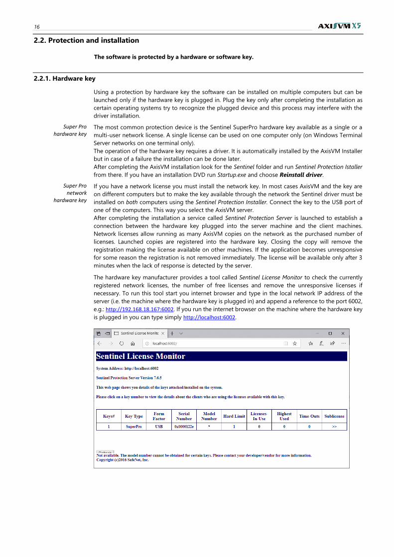
16

2.2. Protection and installation

The software is protected by a hardware or software key.

2.2.1. Hardware key

Using a protection by hardware key the software can be installed on multiple computers but can be

launched only if the hardware key is plugged in. Plug the key only after completing the installation as

certain operating systems try to recognize the plugged device and this process may interfere with the

driver installation.

Super Pro hardware key

The most common protection device is the Sentinel SuperPro hardware key available as a single or a

multi-user network license. A single license can be used on one computer only (on Windows Terminal

Server networks on one terminal only).

The operation of the hardware key requires a driver. It is automatically installed by the AxisVM Installer

but in case of a failure the installation can be done later.

After completing the AxisVM installation look for the Sentinel folder and run Sentinel Protection Istaller

from there. If you have an installation DVD run Startup.exe and choose Reinstall driver.

Super Pro network

hardware key

If you have a network license you must install the network key. In most cases AxisVM and the key are

on different computers but to make the key available through the network the Sentinel driver must be

installed on both computers using the Sentinel Protection Installer. Connect the key to the USB port of

one of the computers. This way you select the AxisVM server.

After completing the installation a service called Sentinel Protection Server is launched to establish a

connection between the hardware key plugged into the server machine and the client machines.

Network licenses allow running as many AxisVM copies on the network as the purchased number of

licenses. Launched copies are registered into the hardware key. Closing the copy will remove the

registration making the license available on other machines. If the application becomes unresponsive

for some reason the registration is not removed immediately. The license will be available only after 3

minutes when the lack of response is detected by the server.

The hardware key manufacturer provides a tool called Sentinel License Monitor to check the currently

registered network licenses, the number of free licenses and remove the unresponsive licenses if

necessary. To run this tool start you internet browser and type in the local network IP address of the

server (i.e. the machine where the hardware key is plugged in) and append a reference to the port 6002,

e.g.: http://192.168.18.167:6002. If you run the internet browser on the machine where the hardware key

is plugged in you can type simply http://localhost:6002.

User’s Manual X5 Release4 e2 17

Speeding up the ac-cess of network

keys

If AxisVM is launched on a client machine it begins to search the network for available network keys

checking each computer running Sentinel Pro Server regardless if the key is plugged or not. It may slow

down the search process. To improve the connection speed it is recommended to create an NSP_HOST

environment variable on the client machine, specifying the local network IP address of the computer

with the key, e.g.: NSP_HOST = 192.168.0.23.

In case of more than one network key it is possible to set the NSP_HOST1, ...., NSP_HOST5 environment

variables identifying computers with keys. The maximum number of keys that can be handled this way

is five.

To run AxisVM on any computer on the network SuperPro Server must be running on the server. If it

stops all running AxisVM programs stop.

Sentinel HL hardware key

The Sentinel HL key is a new kind of protection device that does not require driver installation. Plugging

it into the USB port the Windows operating system identifies it as a HID (Human Interface Device).

Sentinel HL keys also have single user and network models. A single license can be used on one

computer only (on Windows Terminal Server networks on one terminal only).

Sentinel HL network

hardware key

Network licenses allow running as many AxisVM copies on the network as the purchased number of

licenses. Sentinel HL network keys require installation of the HASP runtime environment. To do this find

the Sentinel LDK folder within the AxisVM installation folder and run the HASPUserSetup application

from there. The HASP runtime environment provides a connection between the hardware key plugged

into the server machine and the client machines. If the environment is not running AxisVM cannot be

launched on the client machines.

To purchase further licenses for a network key run the Admin Control Center (see below), choose Sentinel

Keys from the menu on the left and choose the appropriate network key from the list. Click on the C2V

icon on the right to save a c2v file. Send this file to your distributor with your license order. Your

distributor will send a v2c file with the additional licenses. Save it to your machine. To update the number

of licenses choose Update/Attach from the menu on the left then browse for the v2c file you saved. Click

the Open button to transfer license information to the network key. The new licenses will become

available.

2.2.2. Software key

Software key protection allows launching the program on the machine where the software key is in-

stalled. Software keys can be transferred to another machine using a tool (see later). After transferring

a software license the program will run only on the other machine and fails to run on the first one.

Software license is linked to the hardware elements of the computer, therefore any change in the

hardware (replacement of the motherboard, CPU, Ethernet card, hard drive, optical drive or other

built-in peripherals) will invalidate the license.

To prevent such loss the license must be transferred temporarily to another machine before changing

the hardware, replace the hardware element then transfer the license from the other machine.

Sentinel SL software key

Sentinel SL is not a physical device attached to a port but a software key specific to the given hardware.

It cannot be copied directly but can be transferred to another machine using the RUS tool of the pro-

tection package (see details below).

Software key may be a reasonable solution if storage, connection or protection of the physical key raises

problems.

As the software key is stored on the hard drive / SSD of the machine, viruses, malware or flaws in the

update of the operating system may corrupt the key. In this case another software key must be pur-

chased.

Installing Sentinel

HASP Run-time En-

vironment

A software key requires the installation of the Sentinel HASP Run-time Environment.

Download it from www.axisvm.eu (find it under Downloads / Software Updates / Sentinel driver) or look

for InstallSentinelRuntime.exe in the Sentinel LDK folder of your AxisVM installation.

Sentinel Admin Control Center

To check the status of the environment run your internet browser on the server then type http://lo-

calhost:1947. The Sentinel Admin Control Center will be displayed.

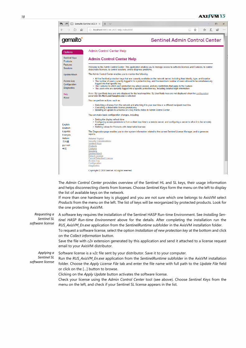
18

The Admin Control Center provides overview of the Sentinel HL and SL keys, their usage information

and helps disconnecting clients from licenses. Choose Sentinel Keys form the menu on the left to display

the list of available keys on the network.

If more than one hardware key is plugged and you are not sure which one belongs to AxisVM select

Products from the menu on the left. The list of keys will be reorganized by protected products. Look for

the one protecting AxisVM.

Requesting a Sentinel SL

software license

A software key requires the installation of the Sentinel HASP Run-time Environment. See Installing Sen-

tinel HASP Run-time Environment above for the details. After completing the installation run the

RUS_AxisVM_En.exe application from the SentinelRuntime subfolder in the AxisVM installation folder.

To request a software license, select the option Installation of new protection key at the bottom and click

on the Collect information button.

Save the file with c2v extension generated by this application and send it attached to a license request

email to your AxisVM distributor.

Applying a Sentinel SL

software license

Software license is a v2c file sent by your distributor. Save it to your computer.

Run the RUS_AxisVM_En.exe application from the SentinelRuntime subfolder in the AxisVM installation

folder. Choose the Apply License File tab and enter the file name with full path to the Update File field

or click on the […] button to browse.

Clicking on the Apply Update button activates the software license.

Check your license using the Admin Control Center tool (see above). Choose Sentinel Keys from the

menu on the left, and check if your Sentinel SL license appears in the list.

User’s Manual X5 Release4 e2 19

Sentinel SL License transfer

A software license can be transferred to another machine. After completing the transfer AxisVM will run

only on the other machine (works just like a hardware protection key removed and plugged into the

other machine). To transfer the license run the RUS_AxisVM_En.exe application on the other machine

too, select the Transfer License tab and generate a recipient information file (*.id) and copy that file to

the first machine. Go back to the first machine, select the Transfer License tab, go to the Read the recip-

ient information file from field, click on the […] button and load the *.id file you have copied from the

other machine, fill out the Generate the license transfer file to field then click on the Generate License

Transfer File button. Copy the generated file with h2h extension to the other machine, go there, select

the Apply License File tab, go to the Update File field, browse for the h2h file you have copied and click

on Apply Update.

2.2.3. Installation

Preparing AxisVM

installation

on a Mac

Most professional structural analysis software programs support only Windows. The following methods

will enable AxisVM use on a Mac:

1. Boot Camp

Apple’s Boot Camp allows for installing Windows on a Mac. This will provide the best performance for

running AxisVM on a Mac.

2. Virtual Machines

Software such as Parallels or VMWare Fusion use virtual machines to install Windows on a Mac, allowing

AxisVM to run.

3. Remote Desktop

The Remote Desktop software on a Mac computer allows for remote access of a Windows computer

running AxisVM.

Installation

If you have downloaded the installer application from our website, run it. Otherwise insert the AxisVM

installation DVD into the DVD drive. The Startup program starts automatically if the autoplay option is

enabled. If autoplay is not enabled, click the Start button, and select Run.... Open the Startup.exe

program on your AxisVM DVD. Select AxisVM X5 Setup and follow the instructions.

Installation under Windows Vista/Windows 7/Windows 8/Windows 10 operating systems:

• You need the latest Sentinel driver. You can download it from www.axisvm.eu / Downloads –

Software updates / Sentinel Driver update on the right tab)

• Right click on the program icon after the installation of AxisVM

• Choose the Properties menu item from the Quick Menu.

• Select the Compatibility tab on the appearing dialog and turn on the Run as administrator

checkbox.

By default the application and the example models will be installed on drive C: in

C:\AxisVM_X5 and C:\AxisVM_X5\Examples

folders. You can specify the drive and the folders during the installation process. The setup program

creates the AxisVM program group that includes the AxisVM application icon.

The application can be installed to the usual C: \ Program Files \ AxisVM_X5 folder (C: \ Program Files

(x86) \ AxisVM_X5 under 64-bit operating systems). However in this case the Run as administrator pro-

perty must be set for AxisVM.exe, AxisVM_x64.exe \ IDTFConverter \ DTFConverter.exe. Find these files

through Start Menu / Computer, right click on the files and choose Properties from the popup menu, go

to the Compatibility tab, find Privilege level and turn on the above option. Users without administrative

rights has to ask the administrator to set write access to the C: \ Program Files \ AxisVM_X5 folder (see

Permissions under the Security tab).

32/64-bit versions On 64 bit operating systems the user can choose to install either the 32-bit or the 64-bit version of

AxisVM. Installing the 64-bit version also copies the 32-bit version to the hard disk but no shortcut is

created on the desktop for this file. On 32-bit operating systems only the 32-bit version is installed.

It is not recommended to install AxisVM under the c:\Program Files folder as the program placed

there can be started only with administrative rights and there may be failures in running libraries

like the 3D PDF generator.

20

Silent installation

The software can be installed in silent mode using command line. The Setup program accepts optional

command line parameters. These can be useful to system administrators, and to other programs calling

the Setup program.

Two typical examples are shown below considering 32 and 64-bit versions:

In case of 64-bit version:

setup.exe /VERYSILENT /SUPPRESSMSGBOXES /NORESTART /Dir="C:\AxisVMX5" lang=nl NoIcons=0

types=64bits Tasks=extensions1,extensions2

In case of 32-bit version:

setup.exe /VERYSILENT /SUPPRESSMSGBOXES /NORESTART /Dir="C:\AxisVMX5" lang=nl NoIcons=0

types=32bits Tasks=extensions1,extensions2

AxisVM setup is made by Inno Setup installer. The most important optional command line parameters

are listed below. For more information please see the Inno Setup help.

/SP-

Disables the This will install... Do you wish to continue? prompt at the beginning of Setup. Of course,

this will have no effect if the DisableStartupPrompt [Setup] section directive was set to yes.

/SILENT, /VERYSILENT

Instructs Setup to be silent or very silent. When Setup is silent the wizard and the background window

are not displayed but the installation progress window is. When a setup is very silent this installation

progress window is not displayed. Everything else is normal so for example error messages during in-

stallation are displayed and the startup prompt is (if you haven't disabled it with DisableStartupPrompt

or the '/SP-' command line option explained above).

If a restart is necessary and the '/NORESTART' command isn't used (see below) and Setup is silent, it

will display a Reboot now? message box. If it's very silent it will reboot without asking.

/SUPPRESSMSGBOXES

Instructs Setup to suppress message boxes. Only has an effect when combined with '/SILENT' and

'/VERYSILENT'.

The default response in situations where there's a choice is:

• Yes in a 'Keep newer file?' situation.

• No in a 'File exists, confirm overwrite.' situation.

• Abort in Abort/Retry situations.

• Cancel in Retry/Cancel situations.

• Yes (=continue) in a DiskSpaceWarning/DirExists/DirDoesntExist/NoUninstallWar-

ning/ExitSetupMessage/ConfirmUninstall situation.

• Yes (=restart) in a FinishedRestartMessage/UninstalledAndNeedsRestart situation.

5 message boxes are not suppressible:

• The About Setup message box.

• The Exit Setup? message box.

• The FileNotInDir2 message box displayed when Setup requires a new disk to be inserted

and the disk was not found.

• Any (error) message box displayed before Setup (or Uninstall) could read the command

line parameters.

• Any message box displayed by [Code] support function MsgBox.

/LOG

Causes Setup to create a log file in the user's TEMP directory detailing file installation and [Run]

actions taken during the installation process. This can be a helpful debugging aid. For example, if you

suspect a file isn't being replaced when you believe it should be (or vice versa), the log file will tell you

if the file was really skipped, and why.

The log file is created with a unique name based on the current date. (It will not overwrite or append

to existing files.)

User’s Manual X5 Release4 e2 21

The information contained in the log file is technical in nature and therefore not intended to be

understandable by end users. Nor is it designed to be machine-parsable; the format of the file is subject

to change without notice.

/LOG="filename"

Same as /LOG, except it allows you to specify a fixed path/filename to use for the log file. If a file with

the specified name already exists it will be overwritten. If the file cannot be created, Setup will abort

with an error message.

/NOCANCEL

Prevents the user from cancelling during the installation process, by disabling the Cancel button and

ignoring clicks on the close button. Useful along with '/SILENT' or '/VERYSILENT'.

/NORESTART

Instructs Setup not to reboot even if it's necessary.

/LANG=language

Specifies the language to use. language specifies the internal name of the language as specified in a

[Languages] section entry.

When a valid /LANG parameter is used, the Select Language dialog will be suppressed.

/DIR="x:\dirname"

Overrides the default directory name displayed on the Select Destination Location wizard page. A

fully qualified pathname must be specified.

/GROUP="folder name"

Overrides the default folder name displayed on the Select Start Menu Folder wizard page. If the

[Setup] section directive DisableProgramGroupPage was set to yes, this command line parameter is

ignored.

/NOICONS

Instructs Setup to initially check the Don't create a Start Menu folder check box on the Select Start

Menu Folder wizard page.

/TYPE=type name

Overrides the default setup type.

If the specified type exists and isn't a custom type, then any /COMPONENTS parameter will be ig-

nored.

/COMPONENTS="comma separated list of component names"

Overrides the default component settings. Using this command line parameter causes Setup to au-

tomatically select a custom type. If no custom type is defined, this parameter is ignored.

Only the specified components will be selected; the rest will be deselected.

If a component name is prefixed with a "*" character, any child components will be selected as well

(except for those that include the dontinheritcheck flag). If a component name is prefixed with a "!"

character, the component will be deselected.

This parameter does not change the state of components that include the fixed flag.

Example:

Deselect all components, then select the "help" and "plugins" components:

/COMPONENTS="help,plugins"

Example:

Deselect all components, then select a parent component and all of its children with the exception of

one:

/COMPONENTS="*parent,!parent\child"

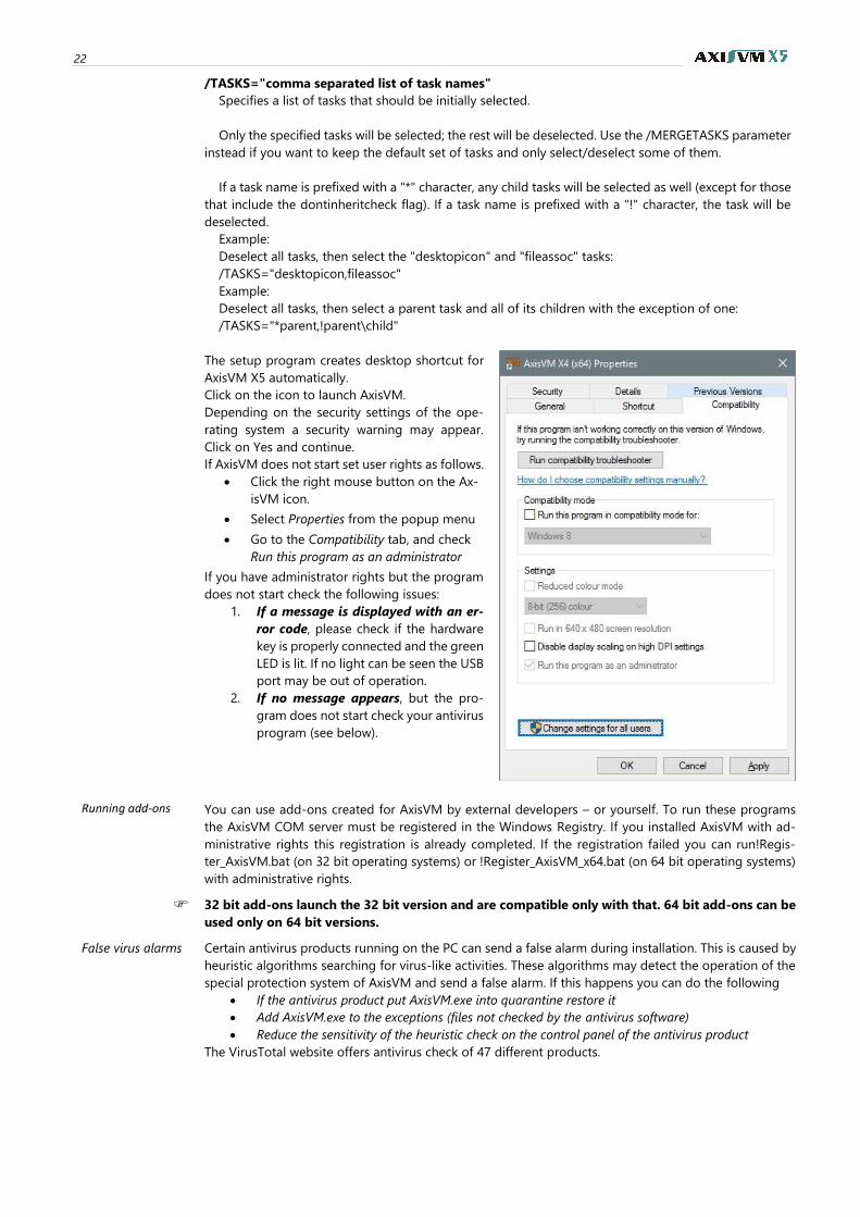
22

/TASKS="comma separated list of task names"

Specifies a list of tasks that should be initially selected.

Only the specified tasks will be selected; the rest will be deselected. Use the /MERGETASKS parameter

instead if you want to keep the default set of tasks and only select/deselect some of them.

If a task name is prefixed with a "*" character, any child tasks will be selected as well (except for those

that include the dontinheritcheck flag). If a task name is prefixed with a "!" character, the task will be

deselected.

Example:

Deselect all tasks, then select the "desktopicon" and "fileassoc" tasks:

/TASKS="desktopicon,fileassoc"

Example:

Deselect all tasks, then select a parent task and all of its children with the exception of one:

/TASKS="*parent,!parent\child"

The setup program creates desktop shortcut for

AxisVM X5 automatically.

Click on the icon to launch AxisVM.

Depending on the security settings of the ope-

rating system a security warning may appear.

Click on Yes and continue.

If AxisVM does not start set user rights as follows.

• Click the right mouse button on the Ax-

isVM icon.

• Select Properties from the popup menu

• Go to the Compatibility tab, and check

Run this program as an administrator

If you have administrator rights but the program

does not start check the following issues:

1. If a message is displayed with an er-

ror code, please check if the hardware

key is properly connected and the green

LED is lit. If no light can be seen the USB

port may be out of operation.

2. If no message appears, but the pro-

gram does not start check your antivirus

program (see below).

Running add-ons You can use add-ons created for AxisVM by external developers – or yourself. To run these programs

the AxisVM COM server must be registered in the Windows Registry. If you installed AxisVM with ad-

ministrative rights this registration is already completed. If the registration failed you can run!Regis-

ter_AxisVM.bat (on 32 bit operating systems) or !Register_AxisVM_x64.bat (on 64 bit operating systems)

with administrative rights.

32 bit add-ons launch the 32 bit version and are compatible only with that. 64 bit add-ons can be

used only on 64 bit versions.

False virus alarms Certain antivirus products running on the PC can send a false alarm during installation. This is caused by

heuristic algorithms searching for virus-like activities. These algorithms may detect the operation of the

special protection system of AxisVM and send a false alarm. If this happens you can do the following

• If the antivirus product put AxisVM.exe into quarantine restore it

• Add AxisVM.exe to the exceptions (files not checked by the antivirus software)

• Reduce the sensitivity of the heuristic check on the control panel of the antivirus product

The VirusTotal website offers antivirus check of 47 different products.

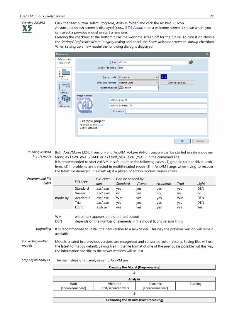
User’s Manual X5 Release4 e2 23

Starting AxisVM

Click the Start button, select Programs, AxisVM folder, and click the AxisVM X5 icon.

At startup a splash screen is displayed (see... 3.7.5 About) then a welcome screen is shown where you

can select a previous model or start a new one.

Clearing the checkbox at the bottom turns the welcome screen off for the future. To turn it on choose

the Settings\Preferences\Data Integrity dialog and check the Show welcome screen on startup checkbox.

When setting up a new model the following dialog is displayed.

Running AxisVM in safe mode

Both AxisVM.exe (32-bit version) and AxisVM_x64.exe (64-bit version) can be started in safe mode en-

tering axisvm.exe /SAFE or axisvm_x64.exe /SAFE in the command line.

It is recommended to start AxisVM in safe mode in the following cases: (1) graphic card or driver prob-

lems, (2) if problems are detected in multithreaded mode (3) if AxisVM hangs when trying to recover

the latest file damaged in a crash (4) if a plugin or addon module causes errors.

Program and file types

File type

File exten-

sion

Can be opened by

Standard Viewer Academic Trial Light

made by

Standard .axs/.axe yes yes yes yes DEN

Viewer .axv/.axw no yes no no no

Academic .axs/.axe WM yes yes WM DEN

Trial .axs/.axe yes yes yes yes DEN

Light .axd/.axr yes yes yes yes yes WM watermark appears on the printed output DEN depends on the number of elements in the model (Light version limit)

Upgrading It is recommended to install the new version to a new folder. This way the previous version will remain

available.

Converting earlier models

Models created in a previous versions are recognized and converted automatically. Saving files will use

the latest format by default. Saving files in the file format of one of the previous is possible but this way

the information specific to the newer versions will be lost.

Steps of an analysis The main steps of an analysis using AxisVM are:

Creating the Model (Preprocessing)

Analysis

Static (linear/nonlinear)

Vibration (first/second-order)

Dynamic (linear/nonlinear)

Buckling

Evaluating the Results (Postprocessing)

24

Capacity Practically, the model size is limited by the amount of free space on your hard disk.

The restrictions on the model size and on the parameters of an analysis are as follows:

Professional

Entity Maximum

Nodes Unlimited

Materials Unlimited

Elements Truss Unlimited

Beam Unlimited

Rib Unlimited

Membrane Unlimited

Plate Unlimited

Shell Unlimited

Support Unlimited

Gap Unlimited

Diaphragm Unlimited

Spring Unlimited

Rigid Unlimited

Link Unlimited

Load cases Unlimited

Load combinations Unlimited

Frequencies Unlimited

Small Business

Entity Maximum

Nodes Unlimited

Materials Unlimited

Elements Only trusses 500

Truss+Beam+Rib * 250

Rib on the edge of a surface 1500

Any combination of membrane,

plate or shell

2000

Support Unlimited

Gap Unlimited

Diaphragm Unlimited

Spring Unlimited

Rigid Unlimited

Link Unlimited

Load cases Unlimited

Load combinations Unlimited

* If there are beams or/and ribs in the structure

2.3. Getting started

The best way to discover AxisVM is to build a simple model, analyse it and evaluate the results.

The steps of model building are described in the AxisVM Step by step tutorial.

There are three major steps in a modeling process:

Geometry The first step is to create the geometry model of the structure (in 2D or 3D).

Geometry can be drawn by hand or can be imported from other CAD programs. It is also possible to

draw elements (columns, beams, walls, slabs) directly.

Elements If you chose to draw the geometry first you must specify material and element properties, mesh the

geometry into elements (assigning the properties and a mesh, to the wire-frame model), and define the

support conditions.

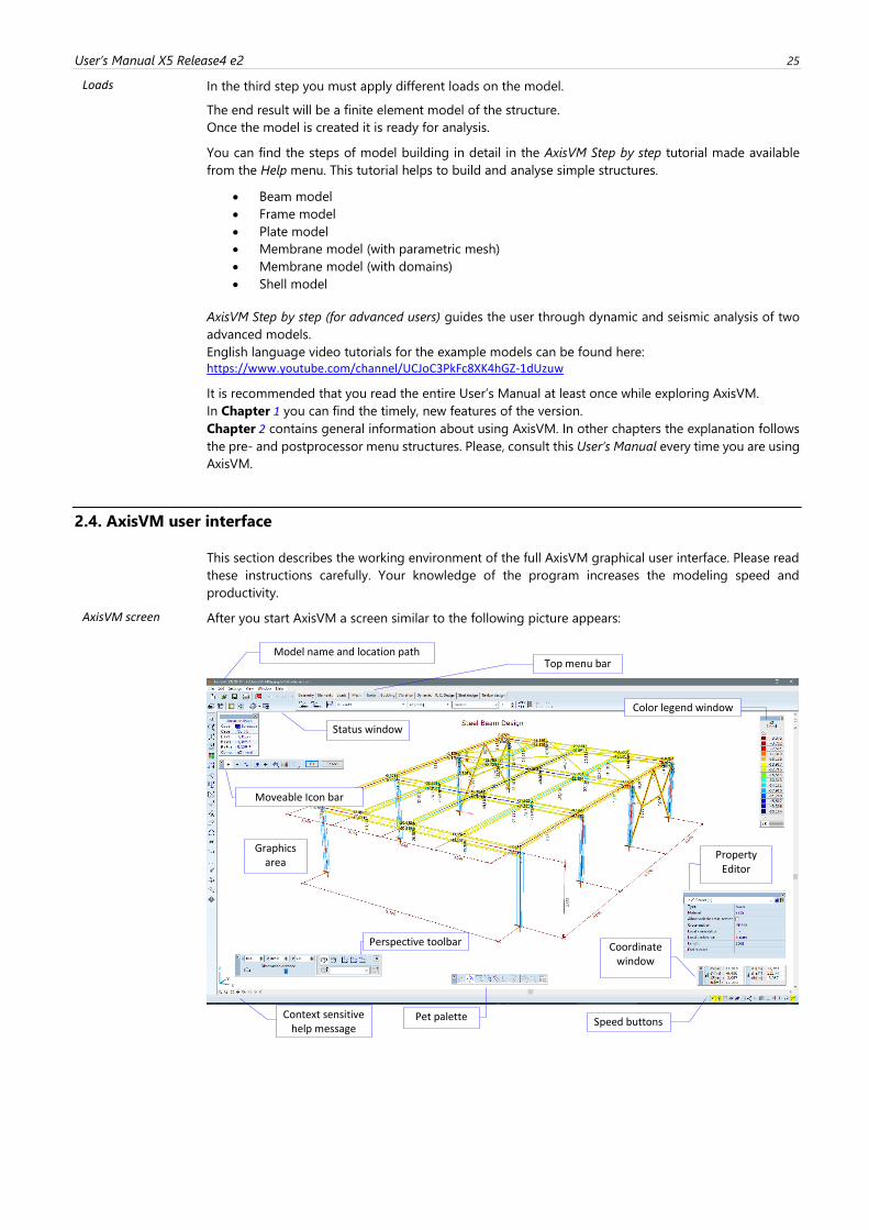
User’s Manual X5 Release4 e2 25

Loads

In the third step you must apply different loads on the model.

The end result will be a finite element model of the structure.

Once the model is created it is ready for analysis.

You can find the steps of model building in detail in the AxisVM Step by step tutorial made available

from the Help menu. This tutorial helps to build and analyse simple structures.

• Beam model

• Frame model

• Plate model

• Membrane model (with parametric mesh)

• Membrane model (with domains)

• Shell model

AxisVM Step by step (for advanced users) guides the user through dynamic and seismic analysis of two

advanced models.

English language video tutorials for the example models can be found here:

https://www.youtube.com/channel/UCJoC3PkFc8XK4hGZ-1dUzuw

It is recommended that you read the entire User’s Manual at least once while exploring AxisVM.

In Chapter 1 you can find the timely, new features of the version.

Chapter 2 contains general information about using AxisVM. In other chapters the explanation follows

the pre- and postprocessor menu structures. Please, consult this User’s Manual every time you are using

AxisVM.

2.4. AxisVM user interface

This section describes the working environment of the full AxisVM graphical user interface. Please read

these instructions carefully. Your knowledge of the program increases the modeling speed and

productivity.

AxisVM screen After you start AxisVM a screen similar to the following picture appears:

Context sensitive help message

Status window

Color legend window

Pet palette

Moveable Icon bar

Graphics area

Property Editor

Speed buttons

Coordinate window

Perspective toolbar

Top menu bar

Model name and location path

26

The parts of the AxisVM screen are briefly described below.

Graphics area The area on the screen where you create your model.

Graphics cursor The screen cursor is used to draw, select entities, and pick from menus and dialog boxes. Depending

on the current state of AxisVM, it can appear as a pick-box, crosshairs with pick-box, or pointer.

Top menu bar Each item of the top menu bar has its own dropdown menu list. To use the top menu bar, move the

cursor up to the menu bar. The cursor will change to a pointer. To select a menu bar item, move the

pointer over it, and press the pick button to select the item. Its associated sub-menu will appear.

Active icon The active icon represents the command that is currently selected.

Icon bar The icons represent working tools in a pictorial form. These tools are accessible during any stage of

work. The icon bar and flyout toolbars are draggable and dockable.

Coordinate window The window on the graphics area displaying the graphics cursor coordinates.

Color legend win-dow

The window shows the color legend used in the display of the results. Appears only in the post-

processing session.

Info window The window shows the status of the model and results display.

Context sensitive help

Provides a help message that depends on the topic under process.

Property Editor The Property Editor offers a simple way to change certain properties of the selected elements or loads.

Pet palette Pet palettes appear when modifying geometry according to the type of the dragged entity (node,

straight line, arc). See... 4.8.21 Modify, transform

Speed buttons Speed buttons in the bottom right provide the fastest access to certain switches (parts, sections,

symbols, numbering, workplanes, etc.)

The model With AxisVM you can create and analyze finite element models of civil engineering structures. Thus the

program operates on a model that is an approximate of the actual structure.

To each model you must assign a name. That name will be used as a file name when it is saved. You

may assign only names that are valid Windows file names. The model consists of all data that you specify

using AxisVM. The model’s data are stored in two files: the input data in the filename.axs and the

results in the filename.axe file.

AxisVM checks if AXS and AXE files belong to the same version of the model.

2.5. Using the cursor, the keyboard, the mouse

Unicode is a computing industry standard for the consistent encoding, representation and handling of

text expressed in most of the world's writing systems. AxisVM X5 provides full Unicode support.

All windows appear according to the current Windows theme.

Graphics cursor

As you move your mouse, the graphics cursor symbol tracks the movement on the screen. To select an

entity, an icon or menu item, move the cursor over it and click the left mouse button. The shape of the

cursor will change accordingly (see... 4.7.1 Cursor identification), and will appear on the screen in one of

the following forms:

Crosshairs: Pointer: Crosshairs/zoom mode:

If you pick an entity when the cursor is in its default mode (info mode), the properties of that entity will

be displayed as a tooltip.

Tooltip Depending on the menu your cursor is on, you may get the properties of the following entities:

Geometry node (point) coordinates, line length

Elements finite element, reference, degree-of-freedom, support, length, mass, material,

cross-section

Loads element load, nodal mass

Mesh meshing parameters

Static displacement, internal force, stress, reinforcement, influence line ordinate

User’s Manual X5 Release4 e2 27

Vibration mode shape ordinate

Dynamic displacement, velocity, acceleration, internal force, stress

R.C. Design specific reinforcement values

Steel Design displacement, internal force, utilization results and resistances

Timber Design displacement, internal force, utilization factor results and resistances

The keyboard You can also use the keyboard to move the cursor:

Arrow keys, Moves the graphics cursor in the current plane.

[Ctrl] +

Arrow keys,

Moves the graphics cursor in the current plane with a step size enlarged/reduced by a factor set in the

Settings dialog box.

[Shift]+

[][][][→],

Moves the graphics cursor in the current plane on a line of angle n· , custom or +n·90°.

[Home] [End] Moves the graphics cursor perpendicular to the current plane.

[Ctrl]+ [Home], [End]

Moves the graphics cursor perpendicular to the current plane with a step size enlarged/reduced by a

factor set in the Settings dialog box.

[Esc] or

right button

Interrupts the command and/or returns to an upper menu level.

[Enter]+[Space]

left button

Selects an item from a menu, executes a command, and selects entities.

These are termed command buttons.

[Alt] Activates the main menu

[Tab] Moves the focus from control to control in a dialog.

[+] [-]

Performs fast zoom in/out and pan. The zoom and pan parameters are defined by the current position

of the graphics cursor in the graphics area, and by the magnification factor set in Settings / Options /

Zoom Factor. Center of the fast zoom in/out is always the current graphics cursor position.

[Insert] or [Alt]+[Shift]

Moves the relative origin (i.e. the reference point of the relative coordinates) to the current graphics

cursor position.

wheel Roll forward to zoom in

Roll backwards to zoom out

Press the wheel and drag to drag the drawing area

Centre of zoom in and zoom out is the current position of the cursor.

Hot Keys Keyboard combinations to access frequently used functions faster.

See... 2.6 Keyboard shortcuts

right button Displays the Quick Menu. See... 2.7 Quick Menu

28

2.6. Keyboard shortcuts

Keyboard shortcuts can be assigned to common operations, toolbar buttons, menu items. The default settings of AxisVM are

the following. The main toolbar button shortcuts are context-sensitive, i.e. the same shortcut can perform different tasks on

different tabs (Geometry, Elements, Loads, etc.).

General commands Open ............................................. Ctrl+O Save ............................................. Ctrl+S Print ............................................ Ctrl+P Undo ............................................. Alt+BkSp Redo ............................................. Shift+Alt+BkSp Layer Manager .................................... F11 storeys .......................................... F7 Table Browser .................................... F12 Report Maker ..................................... F10 Drawings Library ................................. F6 Save to Drawings Library ......................... F9 Delete ........................................... Del Set relative origin .............................. Ins Previous load case ............................... Ctrl+PgUp Next load case ................................... Ctrl+PgDn Icon bar Selection ........................................ S Color coding ..................................... Shift+C Translate / Copy ................................. Shift+T Rotate ........................................... Shift+R Mirror ........................................... Shift+M Scale ............................................ Shift+S Dimension lines .................................. Ctrl+Alt+D Edit background layers ........................... Ctrl+Alt+E Part ............................................. Shift+P Section lines .................................... Shift+Ctrl+X Find ............................................. F3 Display options .................................. Ctrl+Y Model information ................................ Shift+I View Zoom in ........................................ Ctrl+ü Zoom out ....................................... Shift+Ctrl+ü Fit in window .................................. Ctrl+W Pan ............................................ Ctrl+M Rotate ......................................... Ctrl+R Front view ..................................... Ctrl+1 Side view ...................................... Ctrl+3 Top view ....................................... Ctrl+2 Perspective .................................... Ctrl+4 Wireframe ...................................... Alt+F5 Hidden line removal ............................ Alt+F6 Rendered ....................................... Alt+F7 Texture ........................................ Alt+F8 Guidelines Structural grid ................................ Shift+G Perpendicular .................................. Alt+V Parallel ....................................... Alt+P Bisector ....................................... Alt+B Dividing point ................................. Alt+M Intersection point of two lines ................ Alt+I Toolbar [Geometry] ....................................... Shift+F1 [Elements] ....................................... Shift+F2 [Loads] .......................................... Shift+F3 [Mesh] ........................................... Shift+F4 [Static] ......................................... Shift+F5 [Buckling] ....................................... Shift+F6 [Vibration] ...................................... Shift+F7 [Dynamic] ........................................ Shift+F8 [R. C. Design] ................................... Shift+F9 [Steel design] ................................... Shift+F10 [Timber design] .................................. Shift+F11 Geometry Node ........................................... N Line ........................................... L Polygon ........................................ P Rectangle ...................................... R Arc ............................................ A Arc based on three points ...................... B

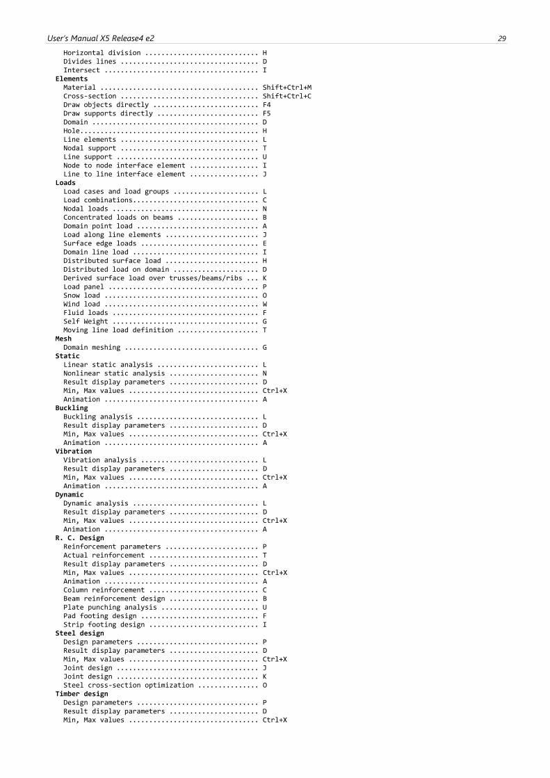
User’s Manual X5 Release4 e2 29

Horizontal division ............................ H Divides lines .................................. D Intersect ...................................... I Elements Material ....................................... Shift+Ctrl+M Cross-section .................................. Shift+Ctrl+C Draw objects directly .......................... F4 Draw supports directly ......................... F5 Domain ......................................... D Hole............................................ H Line elements .................................. L Nodal support .................................. T Line support ................................... U Node to node interface element ................. I Line to line interface element ................. J Loads Load cases and load groups ..................... L Load combinations............................... C Nodal loads .................................... N Concentrated loads on beams .................... B Domain point load .............................. A Load along line elements ....................... J Surface edge loads ............................. E Domain line load ............................... I Distributed surface load ....................... H Distributed load on domain ..................... D Derived surface load over trusses/beams/ribs ... K Load panel ..................................... P Snow load ...................................... O Wind load ...................................... W Fluid loads .................................... F Self Weight .................................... G Moving line load definition .................... T Mesh Domain meshing ................................. G Static Linear static analysis ......................... L Nonlinear static analysis ...................... N Result display parameters ...................... D Min, Max values ................................ Ctrl+X Animation ...................................... A Buckling Buckling analysis .............................. L Result display parameters ...................... D Min, Max values ................................ Ctrl+X Animation ...................................... A Vibration Vibration analysis ............................. L Result display parameters ...................... D Min, Max values ................................ Ctrl+X Animation ...................................... A Dynamic Dynamic analysis ............................... L Result display parameters ...................... D Min, Max values ................................ Ctrl+X Animation ...................................... A R. C. Design Reinforcement parameters ....................... P Actual reinforcement ........................... T Result display parameters ...................... D Min, Max values ................................ Ctrl+X Animation ...................................... A Column reinforcement ........................... C Beam reinforcement design ...................... B Plate punching analysis ........................ U Pad footing design ............................. F Strip footing design ........................... I Steel design Design parameters .............................. P Result display parameters ...................... D Min, Max values ................................ Ctrl+X Joint design ................................... J Joint design ................................... K Steel cross-section optimization ............... O Timber design Design parameters .............................. P Result display parameters ...................... D Min, Max values ................................ Ctrl+X

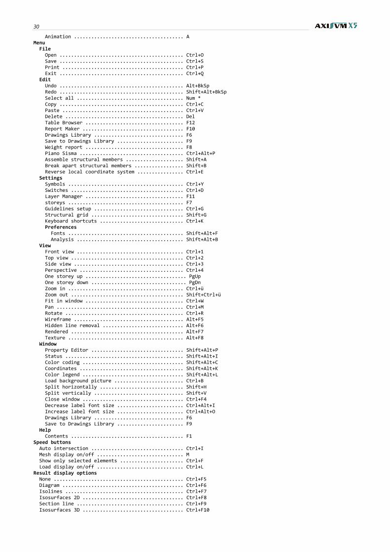
30

Animation ...................................... A Menu File Open ........................................... Ctrl+O Save ........................................... Ctrl+S Print .......................................... Ctrl+P Exit ........................................... Ctrl+Q Edit Undo ........................................... Alt+BkSp Redo ........................................... Shift+Alt+BkSp Select all ..................................... Num * Copy ........................................... Ctrl+C Paste .......................................... Ctrl+V Delete ......................................... Del Table Browser .................................. F12 Report Maker ................................... F10 Drawings Library ............................... F6 Save to Drawings Library ....................... F9 Weight report .................................. F8 Piano Sisma .................................... Ctrl+Alt+P Assemble structural members .................... Shift+A Break apart structural members ................. Shift+B Reverse local coordinate system ................ Ctrl+E Settings Symbols ........................................ Ctrl+Y Switches ....................................... Ctrl+D Layer Manager .................................. F11 storeys ........................................ F7 Guidelines setup ............................... Ctrl+G Structural grid ................................ Shift+G Keyboard shortcuts ............................. Ctrl+K Preferences Fonts ........................................ Shift+Alt+F Analysis ..................................... Shift+Alt+B View Front view ..................................... Ctrl+1 Top view ....................................... Ctrl+2 Side view ...................................... Ctrl+3 Perspective .................................... Ctrl+4 One storey up ................................... PgUp One storey down ................................. PgDn Zoom in ........................................ Ctrl+ü Zoom out ....................................... Shift+Ctrl+ü Fit in window .................................. Ctrl+W Pan ............................................ Ctrl+M Rotate ......................................... Ctrl+R Wireframe ...................................... Alt+F5 Hidden line removal ............................ Alt+F6 Rendered ....................................... Alt+F7 Texture ........................................ Alt+F8 Window Property Editor ................................ Shift+Alt+P Status ......................................... Shift+Alt+I Color coding ................................... Shift+Alt+C Coordinates .................................... Shift+Alt+K Color legend ................................... Shift+Alt+L Load background picture ........................ Ctrl+B Split horizontally ............................. Shift+H Split vertically ............................... Shift+V Close window ................................... Ctrl+F4 Decrease label font size ....................... Ctrl+Alt+I Increase label font size ....................... Ctrl+Alt+O Drawings Library ............................... F6 Save to Drawings Library ....................... F9 Help Contents ....................................... F1 Speed buttons Auto intersection ................................ Ctrl+I Mesh display on/off .............................. M Show only selected elements ...................... Ctrl+F Load display on/off .............................. Ctrl+L Result display options None ............................................. Ctrl+F5 Diagram .......................................... Ctrl+F6 Isolines ......................................... Ctrl+F7 Isosurfaces 2D ................................... Ctrl+F8 Section line ..................................... Ctrl+F9 Isosurfaces 3D ................................... Ctrl+F10

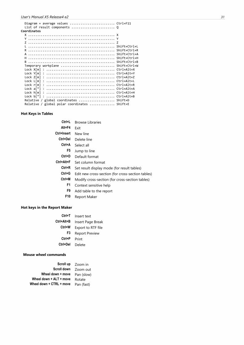
User’s Manual X5 Release4 e2 31

Diagram + average values ......................... Ctrl+F11 List of result components ........................ Q Coordinates X ................................................ X Y ................................................ Y Z ................................................ Z L ................................................ Shift+Ctrl+L R ................................................ Shift+Ctrl+R A ................................................ Shift+Ctrl+A H ................................................ Shift+Ctrl+H B ................................................ Shift+Ctrl+B Temporary workplane .............................. Shift+Ctrl+W Lock X[m] : ...................................... Ctrl+Alt+X Lock Y[m] : ...................................... Ctrl+Alt+Y Lock Z[m] : ...................................... Ctrl+Alt+Z Lock L[m] : ...................................... Ctrl+Alt+L Lock r[m] : ...................................... Ctrl+Alt+R Lock a[°] : ...................................... Ctrl+Alt+A Lock h[m] : ...................................... Ctrl+Alt+H Lock b[°] : ...................................... Ctrl+Alt+B Relative / global coordinates .................... Shift+D Relative / global polar coordinates .............. Shift+E

Hot Keys in Tables

Ctrl+L Browse Libraries

Alt+F4 Exit

Ctrl+Insert New line

Ctrl+Del Delete line

Ctrl+A Select all

F5 Jump to line

Ctrl+D Default format

Ctrl+Alt+F Set column format

Ctrl+R Set result display mode (for result tables)

Ctrl+G Edit new cross-section (for cross-section tables)

Ctrl+M Modify cross-section (for cross-section tables)

F1 Context sensitive help

F9 Add table to the report

F10 Report Maker

Hot keys in the Report Maker

Ctrl+T Insert text

Ctrl+Alt+B Insert Page Break

Ctrl+W Export to RTF file

F3 Report Preview

Ctrl+P Print

Ctrl+Del Delete

Mouse wheel commands

Scroll up Zoom in

Scroll down Zoom out

Wheel down + move Pan (slow)

Wheel down + ALT + move Rotate

Wheel down + CTRL + move Pan (fast)

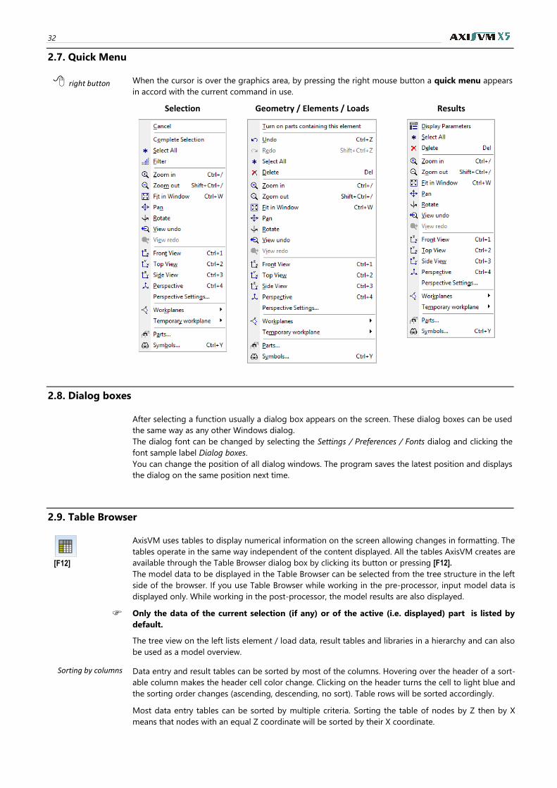
32

2.7. Quick Menu

right button When the cursor is over the graphics area, by pressing the right mouse button a quick menu appears

in accord with the current command in use.

Selection Geometry / Elements / Loads Results

2.8. Dialog boxes

After selecting a function usually a dialog box appears on the screen. These dialog boxes can be used

the same way as any other Windows dialog.

The dialog font can be changed by selecting the Settings / Preferences / Fonts dialog and clicking the

font sample label Dialog boxes.

You can change the position of all dialog windows. The program saves the latest position and displays

the dialog on the same position next time.

2.9. Table Browser

[F12]

AxisVM uses tables to display numerical information on the screen allowing changes in formatting. The

tables operate in the same way independent of the content displayed. All the tables AxisVM creates are

available through the Table Browser dialog box by clicking its button or pressing [F12].

The model data to be displayed in the Table Browser can be selected from the tree structure in the left

side of the browser. If you use Table Browser while working in the pre-processor, input model data is

displayed only. While working in the post-processor, the model results are also displayed.

Only the data of the current selection (if any) or of the active (i.e. displayed) part is listed by

default.

The tree view on the left lists element / load data, result tables and libraries in a hierarchy and can also

be used as a model overview.

Sorting by columns Data entry and result tables can be sorted by most of the columns. Hovering over the header of a sort-

able column makes the header cell color change. Clicking on the header turns the cell to light blue and

the sorting order changes (ascending, descending, no sort). Table rows will be sorted accordingly.

Most data entry tables can be sorted by multiple criteria. Sorting the table of nodes by Z then by X

means that nodes with an equal Z coordinate will be sorted by their X coordinate.

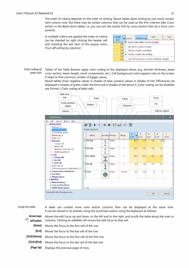
User’s Manual X5 Release4 e2 33

The order of criteria depends on the order of clicking. Result tables allow sorting by one result compo-

nent column only. But there may be certain columns that can be used as the first criterion (like Cross-

section in the Beam force tables, i.e. you can sort the results first by cross-section then by a force com-

ponent).

In multiple criteria are applied the order of criteria

can be checked by right clicking the header cell

and checking the last item of the popup menu

(Turn off sorting by columns):

Color coding of table cells

Tables of the Table Browser apply color coding to the displayed values (e.g. domain thickness, beam

cross-section, beam length, result components, etc.). Cell background colors appear only on the screen.

It helps to find common, smaller of bigger values.

Result tables show negative values in shades of blue, positive values in shades of red. Efficiencies are

displayed in shades of green under the limit and in shades of red above it. Color coding can be disabled,

see Format / Color coding of table cells.

Using the table A table can contain more rows and/or columns than can be displayed at the same time.

It can be viewed in its entirety using the scroll bars and/or using the keyboard as follows:

Arrow keys left button

Moves the edit focus up and down, to the left and to the right, and scrolls the table along the rows or

columns. Clicking an editable cell moves the edit focus to that cell.

[Home] Moves the focus to the first cell of the row.

[End] Moves the focus to the last cell of the row.

[Ctrl]+[Home] Moves the focus to the first cell of the first row

[Ctrl]+[End] Moves the focus to the last cell of the last row.

[Page Up] Displays the previous page of rows.

Fit

Print

Cross-Section Editor

Paste Copy

Delete

Library

Add new row

Columns

Add to report

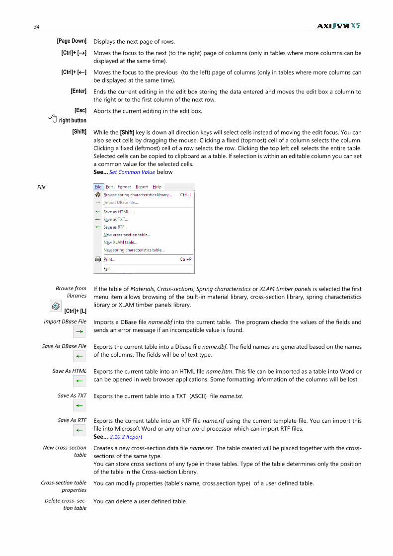
34

[Page Down] Displays the next page of rows.

[Ctrl]+ [→] Moves the focus to the next (to the right) page of columns (only in tables where more columns can be

displayed at the same time).

[Ctrl]+ [] Moves the focus to the previous (to the left) page of columns (only in tables where more columns can

be displayed at the same time).

[Enter] Ends the current editing in the edit box storing the data entered and moves the edit box a column to

the right or to the first column of the next row.

[Esc]

right button

Aborts the current editing in the edit box.

[Shift] While the [Shift] key is down all direction keys will select cells instead of moving the edit focus. You can

also select cells by dragging the mouse. Clicking a fixed (topmost) cell of a column selects the column.

Clicking a fixed (leftmost) cell of a row selects the row. Clicking the top left cell selects the entire table.

Selected cells can be copied to clipboard as a table. If selection is within an editable column you can set

a common value for the selected cells.

See... Set Common Value below

File

Browse from libraries

[Ctrl]+ [L]

If the table of Materials, Cross-sections, Spring characteristics or XLAM timber panels is selected the first

menu item allows browsing of the built-in material library, cross-section library, spring characteristics

library or XLAM timber panels library.

Import DBase File

Imports a DBase file name.dbf into the current table. The program checks the values of the fields and

sends an error message if an incompatible value is found.

Save As DBase File

Exports the current table into a Dbase file name.dbf. The field names are generated based on the names

of the columns. The fields will be of text type.

Save As HTML

Exports the current table into an HTML file name.htm. This file can be imported as a table into Word or

can be opened in web browser applications. Some formatting information of the columns will be lost.

Save As TXT

Exports the current table into a TXT (ASCII) file name.txt.

Save As RTF

Exports the current table into an RTF file name.rtf using the current template file. You can import this

file into Microsoft Word or any other word processor which can import RTF files.

See... 2.10.2 Report

New cross-section table

Creates a new cross-section data file name.sec. The table created will be placed together with the cross-

sections of the same type.

You can store cross sections of any type in these tables. Type of the table determines only the position

of the table in the Cross-section Library.

Cross-section table properties

You can modify properties (table’s name, cross.section type) of a user defined table.

Delete cross- sec-tion table

You can delete a user defined table.

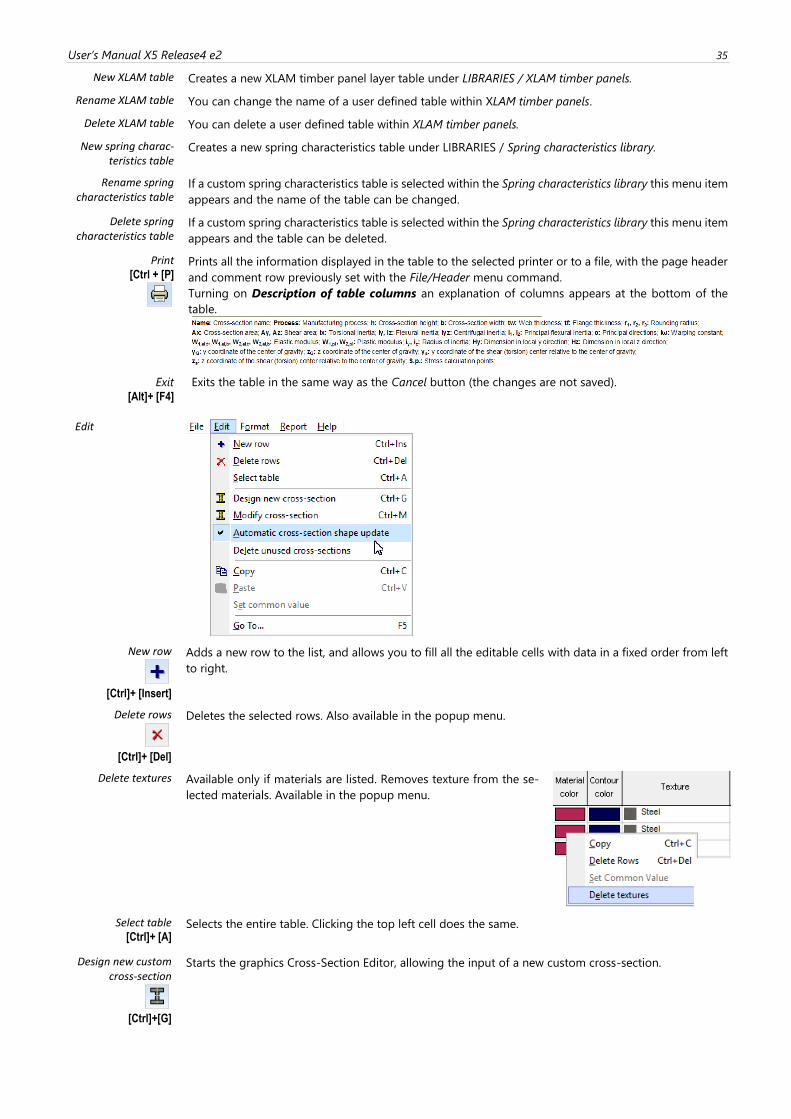
User’s Manual X5 Release4 e2 35

New XLAM table Creates a new XLAM timber panel layer table under LIBRARIES / XLAM timber panels.

Rename XLAM table You can change the name of a user defined table within XLAM timber panels.

Delete XLAM table You can delete a user defined table within XLAM timber panels.

New spring charac-teristics table

Creates a new spring characteristics table under LIBRARIES / Spring characteristics library.

Rename spring characteristics table

If a custom spring characteristics table is selected within the Spring characteristics library this menu item

appears and the name of the table can be changed.

Delete spring characteristics table

If a custom spring characteristics table is selected within the Spring characteristics library this menu item

appears and the table can be deleted.

Print [Ctrl + [P]

Prints all the information displayed in the table to the selected printer or to a file, with the page header

and comment row previously set with the File/Header menu command.

Turning on Description of table columns an explanation of columns appears at the bottom of the

table.

Exit

[Alt]+ [F4]

Exits the table in the same way as the Cancel button (the changes are not saved).

Edit

New row

[Ctrl]+ [Insert]

Adds a new row to the list, and allows you to fill all the editable cells with data in a fixed order from left

to right.

Delete rows

[Ctrl]+ [Del]

Deletes the selected rows. Also available in the popup menu.

Delete textures

Available only if materials are listed. Removes texture from the se-

lected materials. Available in the popup menu.

Select table [Ctrl]+ [A]

Selects the entire table. Clicking the top left cell does the same.

Design new custom cross-section

[Ctrl]+[G]

Starts the graphics Cross-Section Editor, allowing the input of a new custom cross-section.

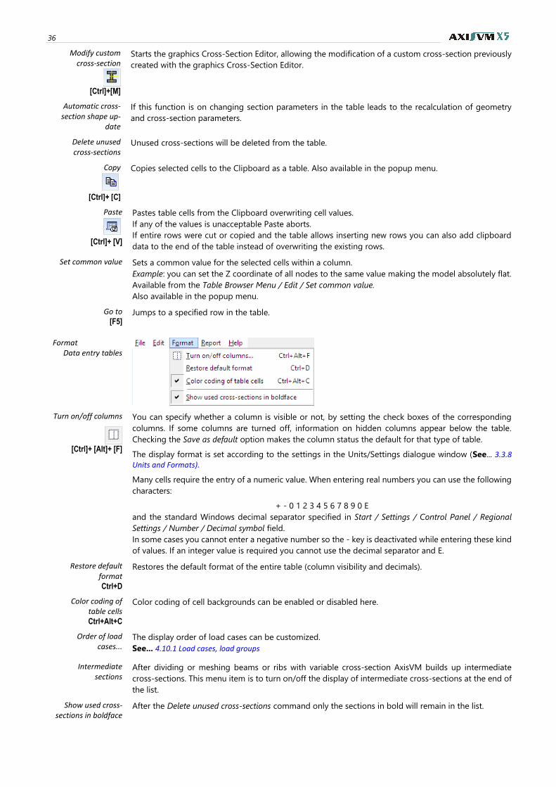
36

Modify custom cross-section

[Ctrl]+[M]

Starts the graphics Cross-Section Editor, allowing the modification of a custom cross-section previously

created with the graphics Cross-Section Editor.

Automatic cross-section shape up-

date

If this function is on changing section parameters in the table leads to the recalculation of geometry

and cross-section parameters.

Delete unused cross-sections

Unused cross-sections will be deleted from the table.

Copy

[Ctrl]+ [C]

Copies selected cells to the Clipboard as a table. Also available in the popup menu.

Paste

[Ctrl]+ [V]

Pastes table cells from the Clipboard overwriting cell values.

If any of the values is unacceptable Paste aborts.

If entire rows were cut or copied and the table allows inserting new rows you can also add clipboard

data to the end of the table instead of overwriting the existing rows.

Set common value Sets a common value for the selected cells within a column.

Example: you can set the Z coordinate of all nodes to the same value making the model absolutely flat.

Available from the Table Browser Menu / Edit / Set common value.

Also available in the popup menu.

Go to [F5]

Jumps to a specified row in the table.

Format Data entry tables

Turn on/off columns

[Ctrl]+ [Alt]+ [F]

You can specify whether a column is visible or not, by setting the check boxes of the corresponding

columns. If some columns are turned off, information on hidden columns appear below the table.

Checking the Save as default option makes the column status the default for that type of table.

The display format is set according to the settings in the Units/Settings dialogue window (See... 3.3.8 Units and Formats).

Many cells require the entry of a numeric value. When entering real numbers you can use the following

characters:

+ - 0 1 2 3 4 5 6 7 8 9 0 E

and the standard Windows decimal separator specified in Start / Settings / Control Panel / Regional

Settings / Number / Decimal symbol field.

In some cases you cannot enter a negative number so the - key is deactivated while entering these kind

of values. If an integer value is required you cannot use the decimal separator and E.

Restore default format Ctrl+D

Restores the default format of the entire table (column visibility and decimals).

Color coding of table cells Ctrl+Alt+C

Color coding of cell backgrounds can be enabled or disabled here.

Order of load cases...

The display order of load cases can be customized.

See... 4.10.1 Load cases, load groups

Intermediate sections

After dividing or meshing beams or ribs with variable cross-section AxisVM builds up intermediate

cross-sections. This menu item is to turn on/off the display of intermediate cross-sections at the end of

the list.

Show used cross-sections in boldface

After the Delete unused cross-sections command only the sections in bold will remain in the list.

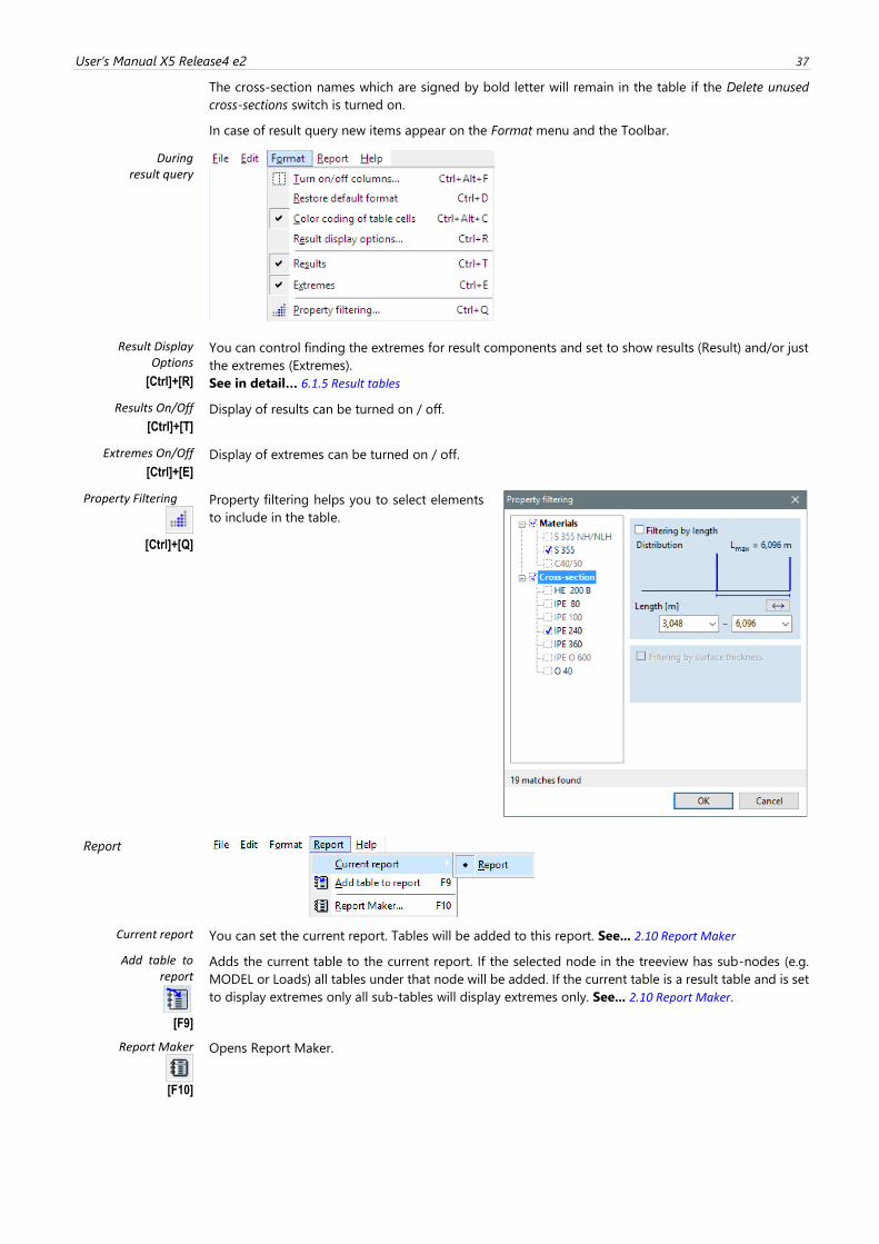
User’s Manual X5 Release4 e2 37

The cross-section names which are signed by bold letter will remain in the table if the Delete unused

cross-sections switch is turned on.

In case of result query new items appear on the Format menu and the Toolbar.

During result query

Result Display Options

[Ctrl]+[R]

You can control finding the extremes for result components and set to show results (Result) and/or just

the extremes (Extremes).

See in detail… 6.1.5 Result tables

Results On/Off

[Ctrl]+[T]

Display of results can be turned on / off.

Extremes On/Off

[Ctrl]+[E]

Display of extremes can be turned on / off.

Property Filtering

[Ctrl]+[Q]

Property filtering helps you to select elements

to include in the table.

Report

Current report You can set the current report. Tables will be added to this report. See... 2.10 Report Maker

Add table to report

[F9]

Adds the current table to the current report. If the selected node in the treeview has sub-nodes (e.g.

MODEL or Loads) all tables under that node will be added. If the current table is a result table and is set

to display extremes only all sub-tables will display extremes only. See... 2.10 Report Maker.

Report Maker

[F10]

Opens Report Maker.

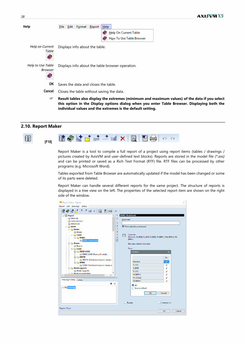
38

Help

Help on Current Table

Displays info about the table.

Help to Use Table Browser

Displays info about the table browser operation.

OK Saves the data and closes the table.

Cancel Closes the table without saving the data.

Result tables also display the extremes (minimum and maximum values) of the data if you select

this option in the Display options dialog when you enter Table Browser. Displaying both the

individual values and the extremes is the default setting.

2.10. Report Maker

[F10]

Report Maker is a tool to compile a full report of a project using report items (tables / drawings /

pictures created by AxisVM and user-defined text blocks). Reports are stored in the model file (*.axs)

and can be printed or saved as a Rich Text Format (RTF) file. RTF files can be processed by other

programs (e.g. Microsoft Word).

Tables exported from Table Browser are automatically updated if the model has been changed or some

of its parts were deleted.

Report Maker can handle several different reports for the same project. The structure of reports is

displayed in a tree view on the left. The properties of the selected report item are shown on the right

side of the window.

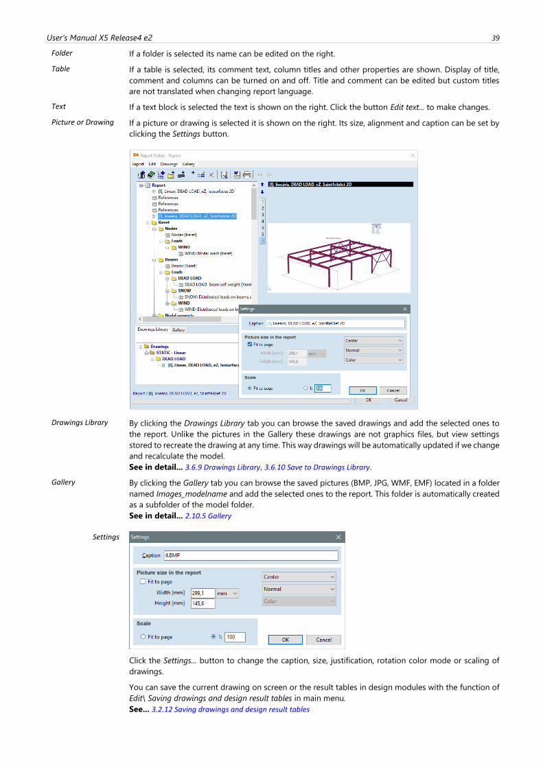
User’s Manual X5 Release4 e2 39

Folder If a folder is selected its name can be edited on the right.

Table If a table is selected, its comment text, column titles and other properties are shown. Display of title,

comment and columns can be turned on and off. Title and comment can be edited but custom titles

are not translated when changing report language.

Text If a text block is selected the text is shown on the right. Click the button Edit text... to make changes.

Picture or Drawing If a picture or drawing is selected it is shown on the right. Its size, alignment and caption can be set by

clicking the Settings button.

Drawings Library By clicking the Drawings Library tab you can browse the saved drawings and add the selected ones to

the report. Unlike the pictures in the Gallery these drawings are not graphics files, but view settings

stored to recreate the drawing at any time. This way drawings will be automatically updated if we change

and recalculate the model.

See in detail... 3.6.9 Drawings Library, 3.6.10 Save to Drawings Library.

Gallery By clicking the Gallery tab you can browse the saved pictures (BMP, JPG, WMF, EMF) located in a folder

named Images_modelname and add the selected ones to the report. This folder is automatically created

as a subfolder of the model folder.

See in detail... 2.10.5 Gallery

Settings

Click the Settings... button to change the caption, size, justification, rotation color mode or scaling of

drawings.

You can save the current drawing on screen or the result tables in design modules with the function of

Edit\ Saving drawings and design result tables in main menu.

See... 3.2.12 Saving drawings and design result tables

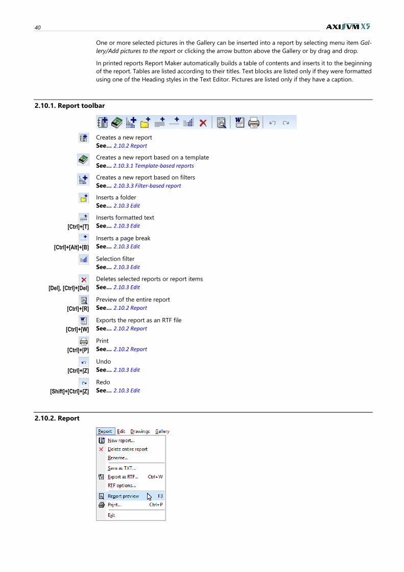
40

One or more selected pictures in the Gallery can be inserted into a report by selecting menu item Gal-

lery/Add pictures to the report or clicking the arrow button above the Gallery or by drag and drop.

In printed reports Report Maker automatically builds a table of contents and inserts it to the beginning

of the report. Tables are listed according to their titles. Text blocks are listed only if they were formatted

using one of the Heading styles in the Text Editor. Pictures are listed only if they have a caption.

2.10.1. Report toolbar

Creates a new report

See… 2.10.2 Report

Creates a new report based on a template

See… 2.10.3.1 Template-based reports

Creates a new report based on filters

See… 2.10.3.3 Filter-based report

Inserts a folder

See… 2.10.3 Edit

[Ctrl]+[T]

Inserts formatted text

See… 2.10.3 Edit

[Ctrl]+[Alt]+[B]

Inserts a page break

See… 2.10.3 Edit

Selection filter

See… 2.10.3 Edit

[Del], [Ctrl]+[Del]

Deletes selected reports or report items

See… 2.10.3 Edit

[Ctrl]+[R]

Preview of the entire report

See… 2.10.2 Report

[Ctrl]+[W]

Exports the report as an RTF file

See… 2.10.2 Report

[Ctrl]+[P]

Print

See… 2.10.2 Report

[Ctrl]+[Z]

Undo

See… 2.10.3 Edit

[Shift]+[Ctrl]+[Z]

Redo

See… 2.10.3 Edit

2.10.2. Report

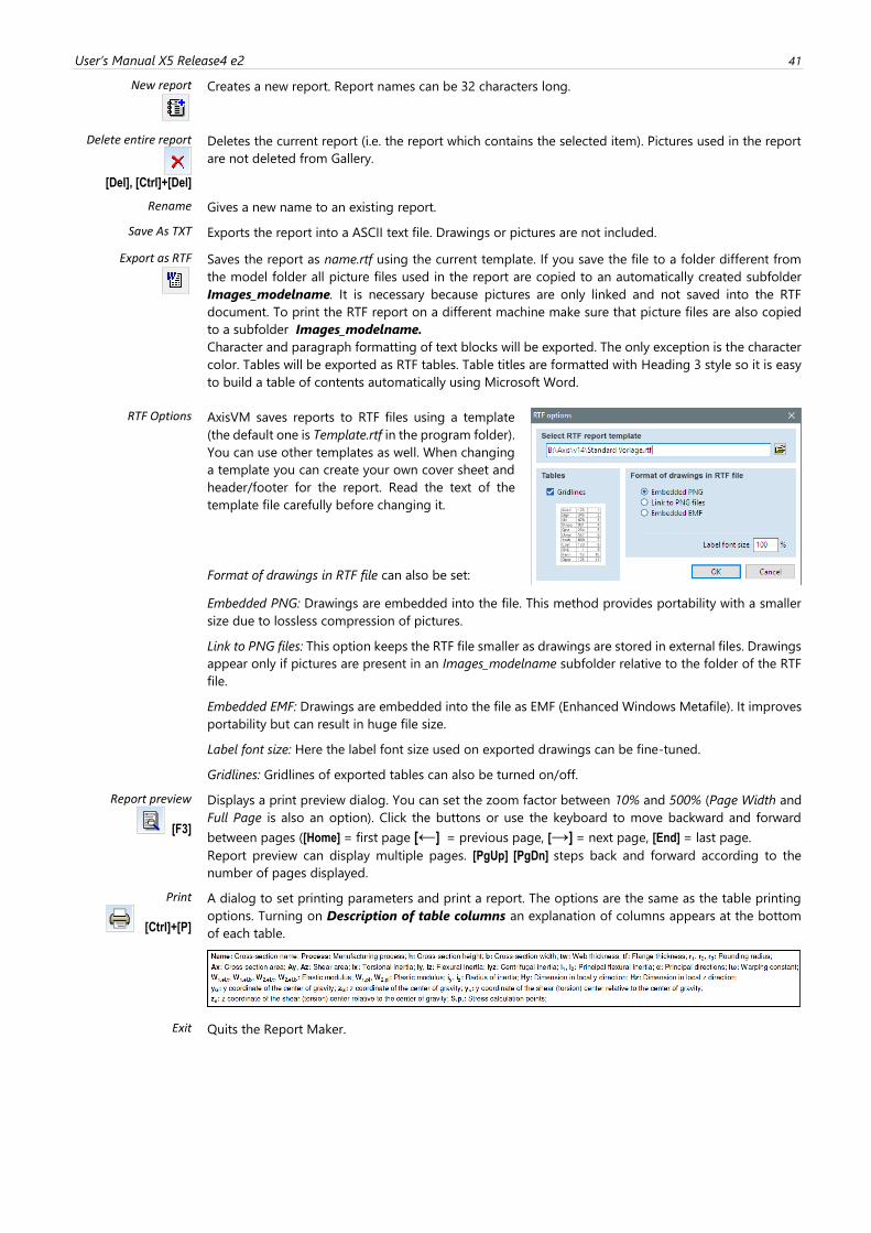
User’s Manual X5 Release4 e2 41

New report

Creates a new report. Report names can be 32 characters long.

Delete entire report

[Del], [Ctrl]+[Del]

Deletes the current report (i.e. the report which contains the selected item). Pictures used in the report

are not deleted from Gallery.

Rename Gives a new name to an existing report.

Save As TXT Exports the report into a ASCII text file. Drawings or pictures are not included.

Export as RTF

Saves the report as name.rtf using the current template. If you save the file to a folder different from

the model folder all picture files used in the report are copied to an automatically created subfolder

Images_modelname. It is necessary because pictures are only linked and not saved into the RTF

document. To print the RTF report on a different machine make sure that picture files are also copied

to a subfolder Images_modelname.

Character and paragraph formatting of text blocks will be exported. The only exception is the character

color. Tables will be exported as RTF tables. Table titles are formatted with Heading 3 style so it is easy

to build a table of contents automatically using Microsoft Word.

RTF Options

AxisVM saves reports to RTF files using a template

(the default one is Template.rtf in the program folder).

You can use other templates as well. When changing

a template you can create your own cover sheet and

header/footer for the report. Read the text of the

template file carefully before changing it.

Format of drawings in RTF file can also be set:

Embedded PNG: Drawings are embedded into the file. This method provides portability with a smaller

size due to lossless compression of pictures.

Link to PNG files: This option keeps the RTF file smaller as drawings are stored in external files. Drawings

appear only if pictures are present in an Images_modelname subfolder relative to the folder of the RTF

file.

Embedded EMF: Drawings are embedded into the file as EMF (Enhanced Windows Metafile). It improves

portability but can result in huge file size.

Label font size: Here the label font size used on exported drawings can be fine-tuned.

Gridlines: Gridlines of exported tables can also be turned on/off.

Report preview

[F3]

Displays a print preview dialog. You can set the zoom factor between 10% and 500% (Page Width and

Full Page is also an option). Click the buttons or use the keyboard to move backward and forward

between pages ([Home] = first page [←] = previous page, [→] = next page, [End] = last page.

Report preview can display multiple pages. [PgUp] [PgDn] steps back and forward according to the

number of pages displayed.

Print

[Ctrl]+[P]

A dialog to set printing parameters and print a report. The options are the same as the table printing

options. Turning on Description of table columns an explanation of columns appears at the bottom

of each table.

Exit Quits the Report Maker.

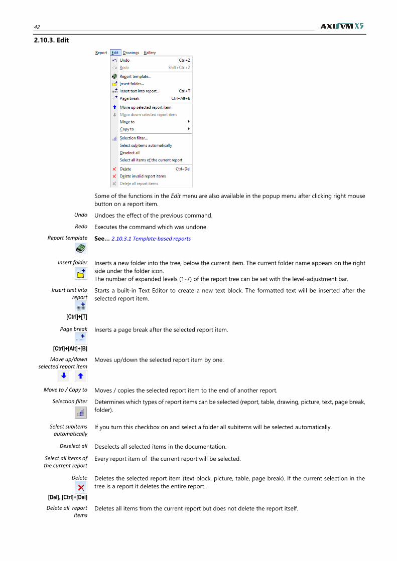
42

2.10.3. Edit

Some of the functions in the Edit menu are also available in the popup menu after clicking right mouse

button on a report item.

Undo Undoes the effect of the previous command.

Redo Executes the command which was undone.

Report template

See… 2.10.3.1 Template-based reports

Insert folder

Inserts a new folder into the tree, below the current item. The current folder name appears on the right

side under the folder icon.

The number of expanded levels (1-7) of the report tree can be set with the level-adjustment bar.

Insert text into report

[Ctrl]+[T]

Starts a built-in Text Editor to create a new text block. The formatted text will be inserted after the

selected report item.

Page break

[Ctrl]+[Alt]+[B]

Inserts a page break after the selected report item.

Move up/down selected report item

Moves up/down the selected report item by one.

Move to / Copy to Moves / copies the selected report item to the end of another report.

Selection filter

Determines which types of report items can be selected (report, table, drawing, picture, text, page break,

folder).

Select subitems automatically

If you turn this checkbox on and select a folder all subitems will be selected automatically.

Deselect all Deselects all selected items in the documentation.

Select all items of the current report

Every report item of the current report will be selected.

Delete

[Del], [Ctrl]+[Del]

Deletes the selected report item (text block, picture, table, page break). If the current selection in the

tree is a report it deletes the entire report.

Delete all report items

Deletes all items from the current report but does not delete the report itself.

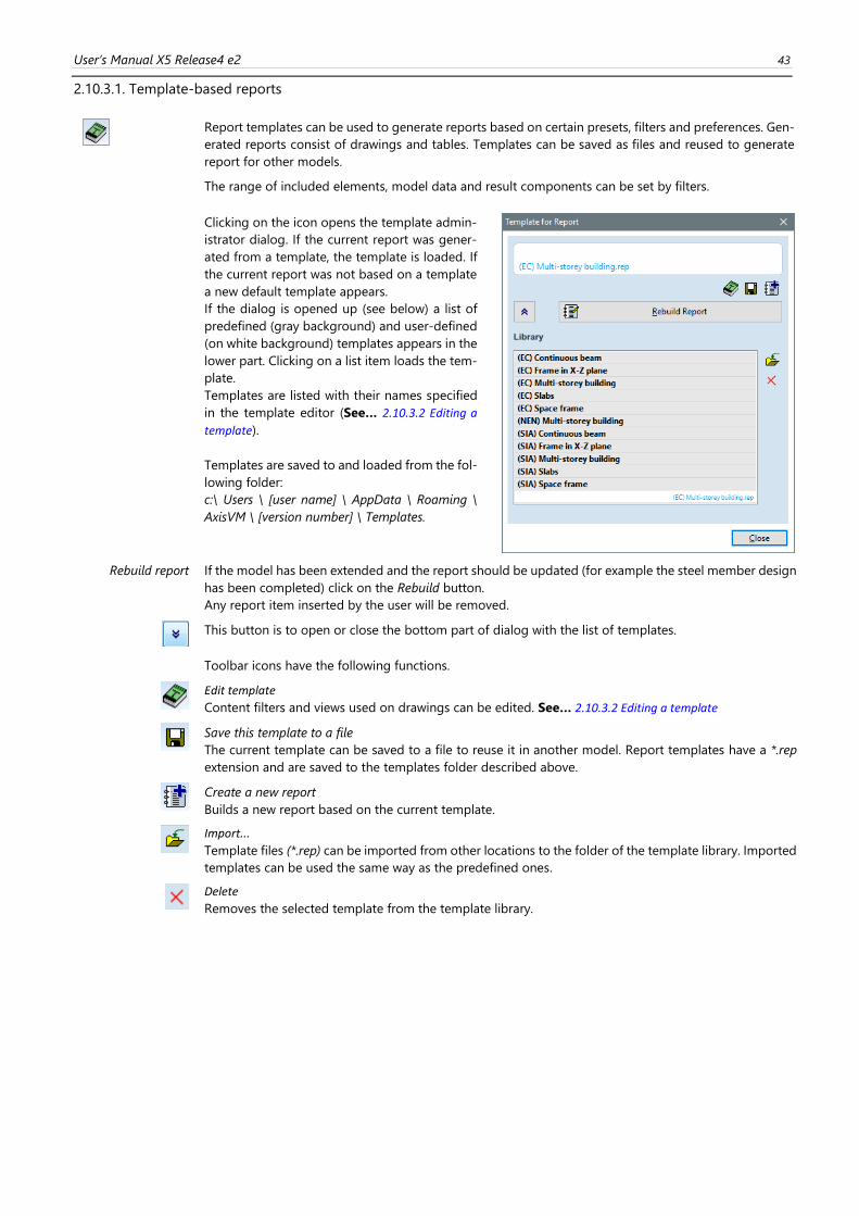
User’s Manual X5 Release4 e2 43

2.10.3.1. Template-based reports

Report templates can be used to generate reports based on certain presets, filters and preferences. Gen-

erated reports consist of drawings and tables. Templates can be saved as files and reused to generate

report for other models.

The range of included elements, model data and result components can be set by filters.

Clicking on the icon opens the template admin-

istrator dialog. If the current report was gener-

ated from a template, the template is loaded. If

the current report was not based on a template

a new default template appears.

If the dialog is opened up (see below) a list of

predefined (gray background) and user-defined

(on white background) templates appears in the

lower part. Clicking on a list item loads the tem-

plate.

Templates are listed with their names specified

in the template editor (See… 2.10.3.2 Editing a

template).

Templates are saved to and loaded from the fol-

lowing folder:

c:\ Users \ [user name] \ AppData \ Roaming \

AxisVM \ [version number] \ Templates.

Rebuild report If the model has been extended and the report should be updated (for example the steel member design

has been completed) click on the Rebuild button.

Any report item inserted by the user will be removed.

This button is to open or close the bottom part of dialog with the list of templates.

Toolbar icons have the following functions.

Edit template

Content filters and views used on drawings can be edited. See… 2.10.3.2 Editing a template

Save this template to a file

The current template can be saved to a file to reuse it in another model. Report templates have a *.rep

extension and are saved to the templates folder described above.

Create a new report

Builds a new report based on the current template.

Import...

Template files (*.rep) can be imported from other locations to the folder of the template library. Imported

templates can be used the same way as the predefined ones.

Delete

Removes the selected template from the template library.

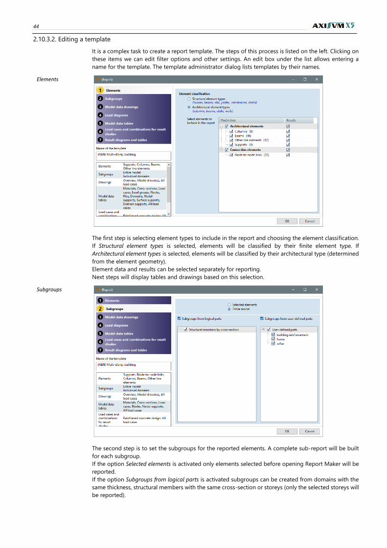
44

2.10.3.2. Editing a template

It is a complex task to create a report template. The steps of this process is listed on the left. Clicking on

these items we can edit filter options and other settings. An edit box under the list allows entering a

name for the template. The template administrator dialog lists templates by their names.

Elements

The first step is selecting element types to include in the report and choosing the element classification.

If Structural element types is selected, elements will be classified by their finite element type. If

Architectural element types is selected, elements will be classified by their architectural type (determined

from the element geometry).

Element data and results can be selected separately for reporting.

Next steps will display tables and drawings based on this selection.

Subgroups

The second step is to set the subgroups for the reported elements. A complete sub-report will be built

for each subgroup.

If the option Selected elements is activated only elements selected before opening Report Maker will be

reported.

If the option Subgroups from logical parts is activated subgroups can be created from domains with the

same thickness, structural members with the same cross-section or storeys (only the selected storeys will

be reported).

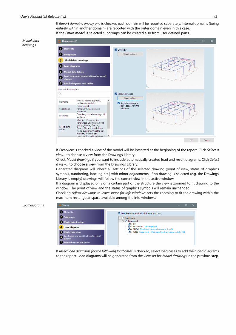
User’s Manual X5 Release4 e2 45

If Report domains one by one is checked each domain will be reported separately. Internal domains (being

entirely within another domain) are reported with the outer domain even in this case.

If the Entire model is selected subgroups can be created also from user defined parts.

Model data drawings

If Overview is checked a view of the model will be insterted at the beginning of the report. Click Select a

view... to choose a view from the Drawings Library.

Check Model drawings if you want to include automatically created load and result diagrams. Click Select

a view... to choose a view from the Drawings Library.

Generated diagrams will inherit all settings of the selected drawing (point of view, status of graphics

symbols, numbering, labeling etc.) with minor adjustments. If no drawing is selected (e.g. the Drawings

Library is empty) drawings will follow the current view in the active window.

If a diagram is displayed only on a certain part of the structure the view is zoomed to fit drawing to the

window. The point of view and the status of graphics symbols will remain unchanged.

Checking Adjust drawings to leave space for info windows sets the zooming to fit the drawing within the

maximum rectangular space available among the info windows.

Load diagrams

If Insert load diagrams for the following load cases is checked, select load cases to add their load diagrams

to the report. Load diagrams will be generated from the view set for Model drawings in the previous step.

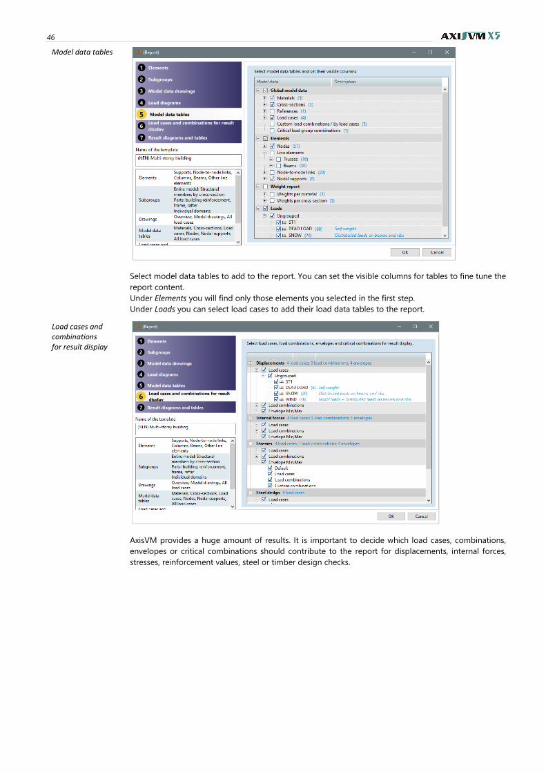
46

Model data tables

Select model data tables to add to the report. You can set the visible columns for tables to fine tune the

report content.

Under Elements you will find only those elements you selected in the first step.

Under Loads you can select load cases to add their load data tables to the report.

Load cases and combinations for result display

AxisVM provides a huge amount of results. It is important to decide which load cases, combinations,

envelopes or critical combinations should contribute to the report for displacements, internal forces,

stresses, reinforcement values, steel or timber design checks.

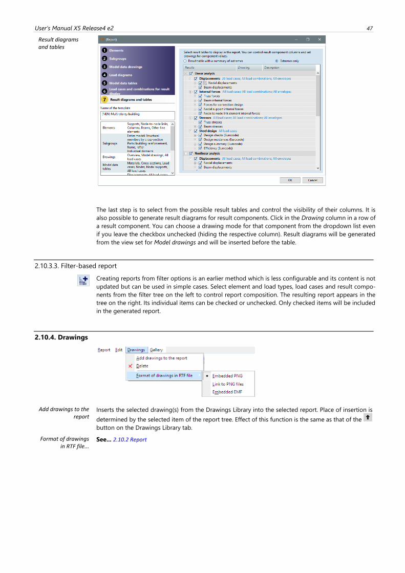
User’s Manual X5 Release4 e2 47

Result diagrams and tables

The last step is to select from the possible result tables and control the visibility of their columns. It is

also possible to generate result diagrams for result components. Click in the Drawing column in a row of

a result component. You can choose a drawing mode for that component from the dropdown list even

if you leave the checkbox unchecked (hiding the respective column). Result diagrams will be generated

from the view set for Model drawings and will be inserted before the table.

2.10.3.3. Filter-based report

Creating reports from filter options is an earlier method which is less configurable and its content is not

updated but can be used in simple cases. Select element and load types, load cases and result compo-

nents from the filter tree on the left to control report composition. The resulting report appears in the

tree on the right. Its individual items can be checked or unchecked. Only checked items will be included

in the generated report.

2.10.4. Drawings

Add drawings to the report

Inserts the selected drawing(s) from the Drawings Library into the selected report. Place of insertion is

determined by the selected item of the report tree. Effect of this function is the same as that of the

button on the Drawings Library tab.

Format of drawings in RTF file...

See... 2.10.2 Report

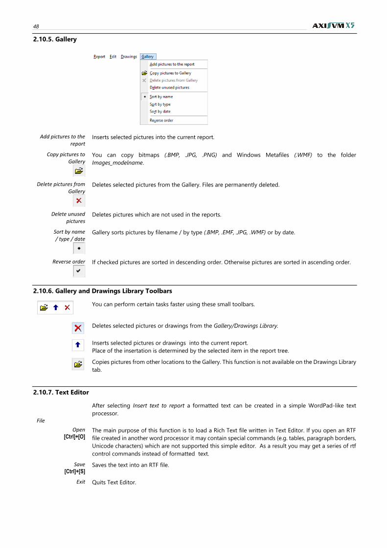
48

2.10.5. Gallery

Add pictures to the report

Inserts selected pictures into the current report.

Copy pictures to Gallery

You can copy bitmaps (.BMP, .JPG, .PNG) and Windows Metafiles (.WMF) to the folder

Images_modelname.

Delete pictures from Gallery

Deletes selected pictures from the Gallery. Files are permanently deleted.

Delete unused pictures

Deletes pictures which are not used in the reports.

Sort by name / type / date

Gallery sorts pictures by filename / by type (.BMP, .EMF, .JPG, .WMF) or by date.

Reverse order

If checked pictures are sorted in descending order. Otherwise pictures are sorted in ascending order.

2.10.6. Gallery and Drawings Library Toolbars

You can perform certain tasks faster using these small toolbars.

Deletes selected pictures or drawings from the Gallery/Drawings Library.

Inserts selected pictures or drawings into the current report.

Place of the insertation is determined by the selected item in the report tree.

Copies pictures from other locations to the Gallery. This function is not available on the Drawings Library

tab.

2.10.7. Text Editor

After selecting Insert text to report a formatted text can be created in a simple WordPad-like text

processor.

File

Open [Ctrl]+[O]

The main purpose of this function is to load a Rich Text file written in Text Editor. If you open an RTF

file created in another word processor it may contain special commands (e.g. tables, paragraph borders,

Unicode characters) which are not supported this simple editor. As a result you may get a series of rtf

control commands instead of formatted text.

Save [Ctrl]+[S]

Saves the text into an RTF file.

Exit Quits Text Editor.

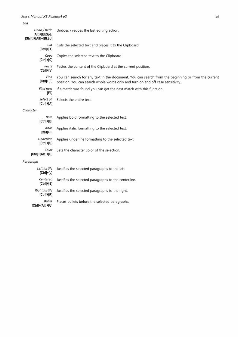
User’s Manual X5 Release4 e2 49

Edit

Undo / Redo [Alt]+[BkSp] /

[Shift]+[Alt]+[BkSp]

Undoes / redoes the last editing action.

Cut [Ctrl]+[X]

Cuts the selected text and places it to the Clipboard.

Copy [Ctrl]+[C]

Copies the selected text to the Clipboard.

Paste [Ctrl]+[V]

Pastes the content of the Clipboard at the current position.

Find [Ctrl]+[F]

You can search for any text in the document. You can search from the beginning or from the current

position. You can search whole words only and turn on and off case sensitivity.

Find next [F3]

If a match was found you can get the next match with this function.

Select all [Ctrl]+[A]

Selects the entire text.

Character

Bold [Ctrl]+[B]

Applies bold formatting to the selected text.

Italic [Ctrl]+[I]

Applies italic formatting to the selected text.

Underline [Ctrl]+[U]

Applies underline formatting to the selected text.

Color [Ctrl]+[Alt ]+[C]

Sets the character color of the selection.

Paragraph

Left justify [Ctrl]+[L]

Justifies the selected paragraphs to the left.

Centered [Ctrl]+[E]

Justifies the selected paragraphs to the centerline.

Right justify [Ctrl]+[R]

Justifies the selected paragraphs to the right.

Bullet [Ctrl]+[Alt]+[U]

Places bullets before the selected paragraphs.

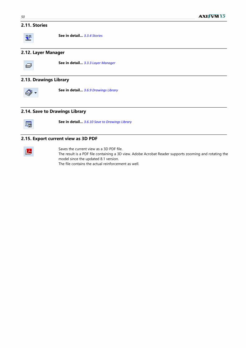
50

2.11. Stories

See in detail... 3.3.4 Stories

2.12. Layer Manager

See in detail... 3.3.3 Layer Manager

2.13. Drawings Library

See in detail... 3.6.9 Drawings Library

2.14. Save to Drawings Library

See in detail... 3.6.10 Save to Drawings Library

2.15. Export current view as 3D PDF

Saves the current view as a 3D PDF file.

The result is a PDF file containing a 3D view. Adobe Acrobat Reader supports zooming and rotating the

model since the updated 8.1 version.

The file contains the actual reinforcement as well.

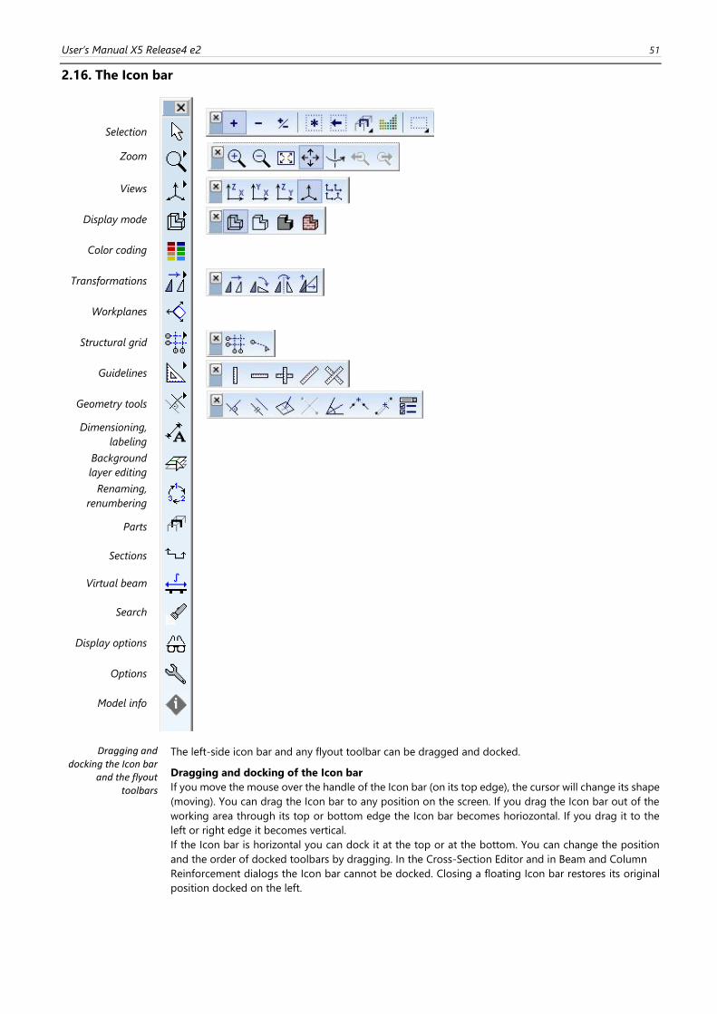
User’s Manual X5 Release4 e2 51

2.16. The Icon bar

Selection

*

Zoom

Views

Display mode

Color coding

Transformations

Workplanes

Structural grid

Guidelines

Geometry tools

Dimensioning,

labeling

Background

layer editing

Renaming,

renumbering

Parts

Sections

Virtual beam

Search

Display options

Options

Model info

Dragging and docking the Icon bar

and the flyout toolbars

The left-side icon bar and any flyout toolbar can be dragged and docked.

Dragging and docking of the Icon bar

If you move the mouse over the handle of the Icon bar (on its top edge), the cursor will change its shape

(moving). You can drag the Icon bar to any position on the screen. If you drag the Icon bar out of the

working area through its top or bottom edge the Icon bar becomes horiozontal. If you drag it to the

left or right edge it becomes vertical.

If the Icon bar is horizontal you can dock it at the top or at the bottom. You can change the position

and the order of docked toolbars by dragging. In the Cross-Section Editor and in Beam and Column

Reinforcement dialogs the Icon bar cannot be docked. Closing a floating Icon bar restores its original

position docked on the left.

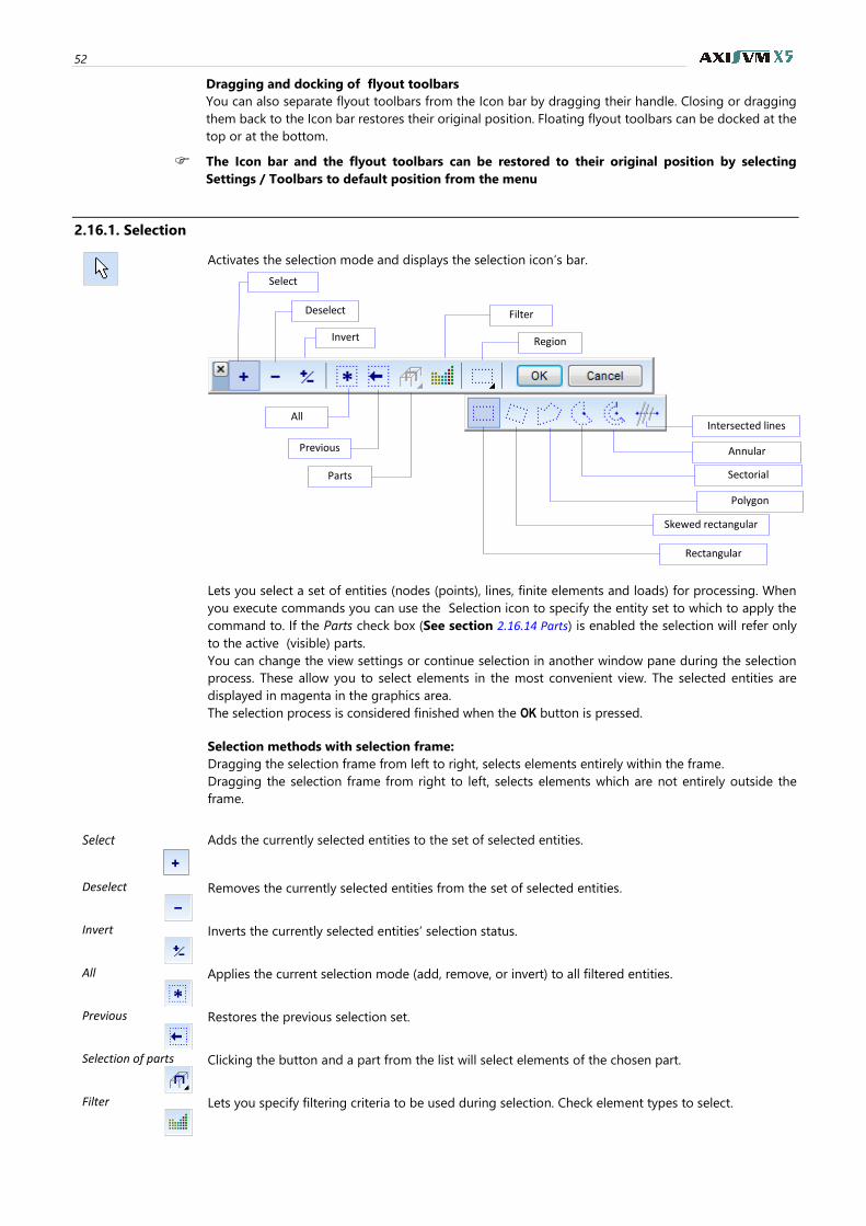
52

Dragging and docking of flyout toolbars

You can also separate flyout toolbars from the Icon bar by dragging their handle. Closing or dragging

them back to the Icon bar restores their original position. Floating flyout toolbars can be docked at the

top or at the bottom.

The Icon bar and the flyout toolbars can be restored to their original position by selecting

Settings / Toolbars to default position from the menu

2.16.1. Selection

Activates the selection mode and displays the selection icon’s bar.

Lets you select a set of entities (nodes (points), lines, finite elements and loads) for processing. When

you execute commands you can use the Selection icon to specify the entity set to which to apply the

command to. If the Parts check box (See section 2.16.14 Parts) is enabled the selection will refer only

to the active (visible) parts.

You can change the view settings or continue selection in another window pane during the selection

process. These allow you to select elements in the most convenient view. The selected entities are

displayed in magenta in the graphics area.

The selection process is considered finished when the OK button is pressed.

Selection methods with selection frame:

Dragging the selection frame from left to right, selects elements entirely within the frame.

Dragging the selection frame from right to left, selects elements which are not entirely outside the

frame.

Select

Adds the currently selected entities to the set of selected entities.

Deselect

Removes the currently selected entities from the set of selected entities.

Invert

Inverts the currently selected entities’ selection status.

All

Applies the current selection mode (add, remove, or invert) to all filtered entities.

Previous

Restores the previous selection set.

Selection of parts

Clicking the button and a part from the list will select elements of the chosen part.

Filter

Lets you specify filtering criteria to be used during selection. Check element types to select.

Deselect

All

Select

Region Invert

Parts

Previous Annular

Skewed rectangular

Sectorial

Rectangular

Filter

Polygon

Intersected lines

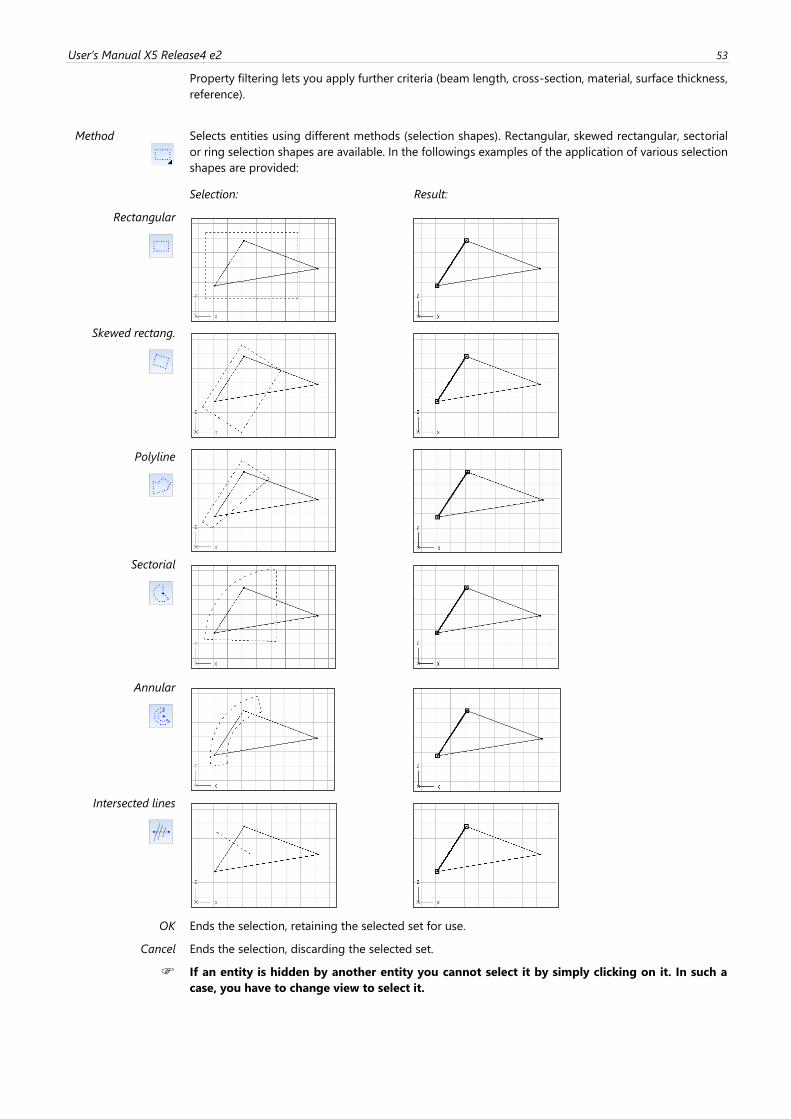
User’s Manual X5 Release4 e2 53

Property filtering lets you apply further criteria (beam length, cross-section, material, surface thickness,

reference).

Method

Selects entities using different methods (selection shapes). Rectangular, skewed rectangular, sectorial

or ring selection shapes are available. In the followings examples of the application of various selection

shapes are provided:

Selection: Result:

Rectangular

Skewed rectang.

Polyline

Sectorial

Annular

Intersected lines

OK Ends the selection, retaining the selected set for use.

Cancel Ends the selection, discarding the selected set.

If an entity is hidden by another entity you cannot select it by simply clicking on it. In such a

case, you have to change view to select it.

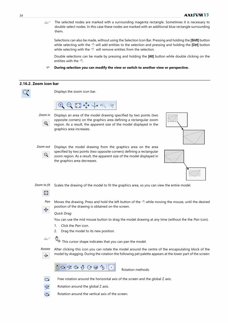
54

The selected nodes are marked with a surrounding magenta rectangle. Sometimes it is necessary to

double-select nodes. In this case these nodes are marked with an additional blue rectangle surrounding

them.

Selections can also be made, without using the Selection Icon Bar. Pressing and holding the [Shift] button

while selecting with the will add entities to the selection and pressing and holding the [Ctrl] button

while selecting with the will remove entities from the selection.

Double selections can be made by pressing and holding the [Alt] button while double clicking on the

entities with the .

During selection you can modify the view or switch to another view or perspective.

2.16.2. Zoom icon bar

Displays the zoom icon bar.

Zoom in

Displays an area of the model drawing specified by two points (two

opposite corners) on the graphics area defining a rectangular zoom

region. As a result, the apparent size of the model displayed in the

graphics area increases.

Zoom out

Displays the model drawing from the graphics area on the area

specified by two points (two opposite corners) defining a rectangular

zoom region. As a result, the apparent size of the model displayed in

the graphics area decreases.

Zoom to fit

Scales the drawing of the model to fit the graphics area, so you can view the entire model.

Pan

Moves the drawing. Press and hold the left button of the while moving the mouse, until the desired

position of the drawing is obtained on the screen.

Quick Drag:

You can use the mid mouse button to drag the model drawing at any time (without the the Pan icon).

1. Click the Pan icon.

2. Drag the model to its new position.

This cursor shape indicates that you can pan the model.

Rotate

After clicking this icon you can rotate the model around the centre of the encapsulating block of the

model by dragging. During the rotation the following pet palette appears at the lower part of the screen:

Rotation methods:

Free rotation around the horizontal axis of the screen and the global Z axis.

Rotation around the global Z axis.

Rotation around the vertical axis of the screen.

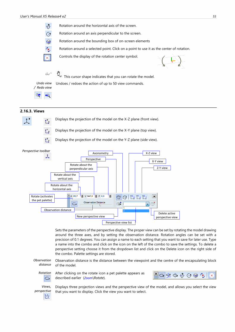
User’s Manual X5 Release4 e2 55

Rotation around the horizontal axis of the screen.

Rotation around an axis perpendicular to the screen.

Rotation around the bounding box of on-screen elements

Rotation around a selected point. Click on a point to use it as the center of rotation.

Controls the display of the rotation center symbol.

This cursor shape indicates that you can rotate the model.

Undo view / Redo view

Undoes / redoes the action of up to 50 view commands.

2.16.3. Views

Displays the projection of the model on the X-Z plane (front view).

Displays the projection of the model on the X-Y plane (top view).

Displays the projection of the model on the Y-Z plane (side view).

Perspective toolbar

Sets the parameters of the perspective display. The proper view can be set by rotating the model drawing

around the three axes, and by setting the observation distance. Rotation angles can be set with a

precision of 0.1 degrees. You can assign a name to each setting that you want to save for later use. Type

a name into the combo and click on the icon on the left of the combo to save the settings. To delete a

perspective setting choose it from the dropdown list and click on the Delete icon on the right side of

the combo. Palette settings are stored.

Observation distance

Observation distance is the distance between the viewpoint and the centre of the encapsulating block

of the model.

Rotation

After clicking on the rotate icon a pet palette appears as

described earlier (Zoom\Rotate).

Views, perspective

Displays three projection views and the perspective view of the model, and allows you select the view

that you want to display. Click the view you want to select.

Axonometry X-Z view

Perspective

Rotate about the perpendicular axis

X-Y view

Rotate about the vertical axis

Z-Y view

Rotate about the horizontal axis

Rotate (activates the pet palette)

Observation distance Delete active

perspective view New perspective view

Perspective view list

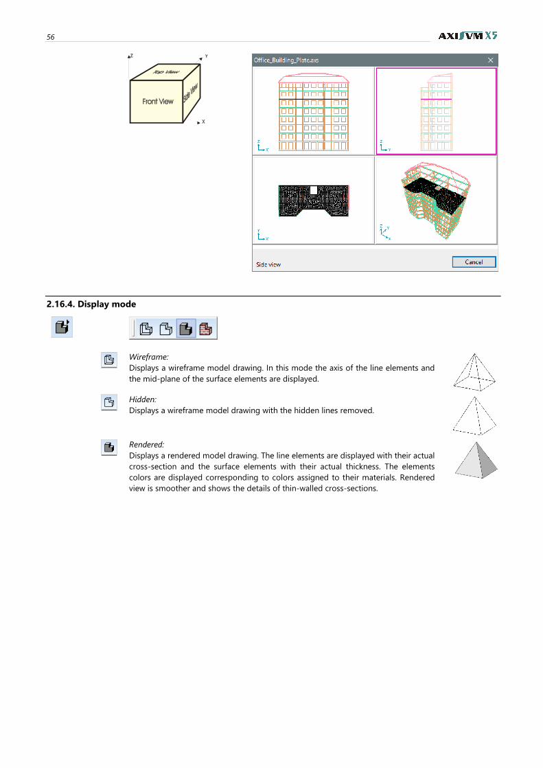
56

2.16.4. Display mode

Wireframe:

Displays a wireframe model drawing. In this mode the axis of the line elements and

the mid-plane of the surface elements are displayed.

Hidden:

Displays a wireframe model drawing with the hidden lines removed.

Rendered:

Displays a rendered model drawing. The line elements are displayed with their actual

cross-section and the surface elements with their actual thickness. The elements

colors are displayed corresponding to colors assigned to their materials. Rendered

view is smoother and shows the details of thin-walled cross-sections.

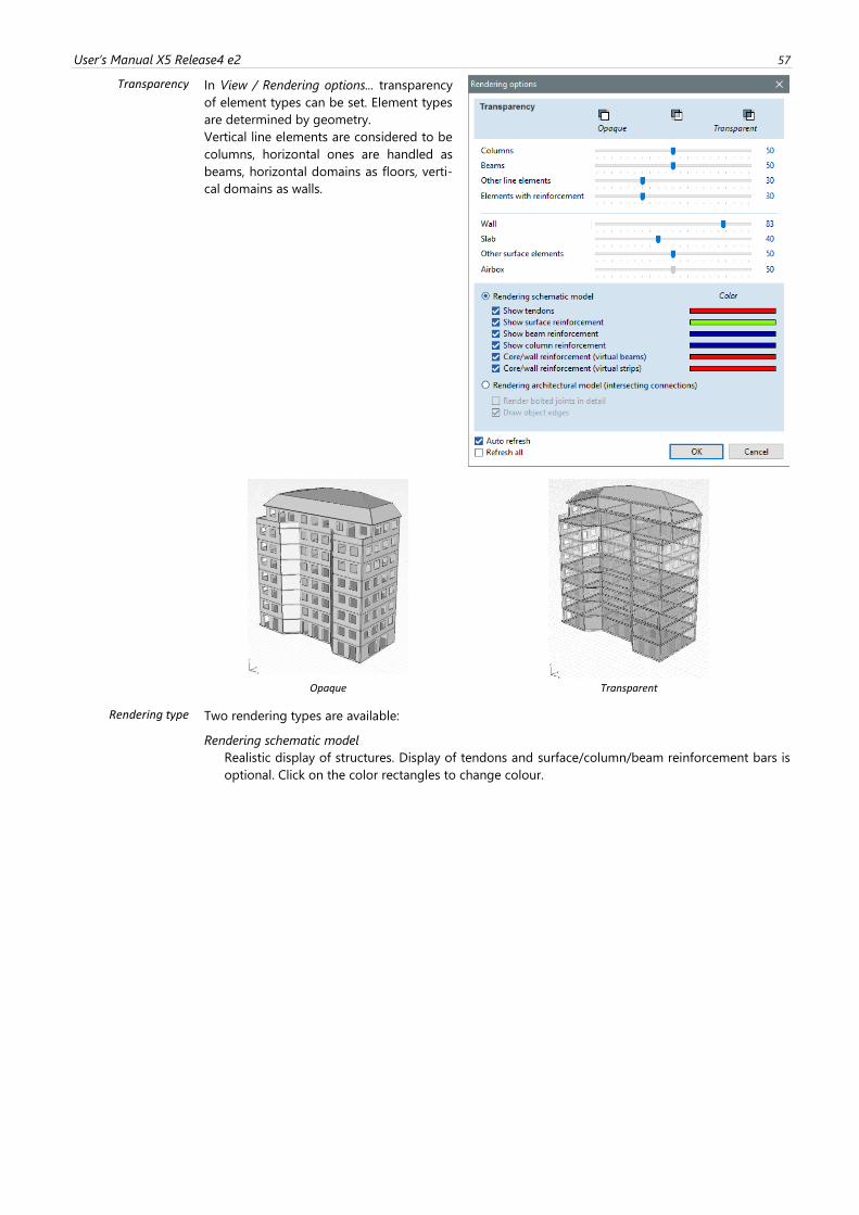
User’s Manual X5 Release4 e2 57

Transparency

In View / Rendering options... transparency

of element types can be set. Element types

are determined by geometry.

Vertical line elements are considered to be

columns, horizontal ones are handled as

beams, horizontal domains as floors, verti-

cal domains as walls.

Opaque Transparent

Rendering type

Two rendering types are available:

Rendering schematic model

Realistic display of structures. Display of tendons and surface/column/beam reinforcement bars is

optional. Click on the color rectangles to change colour.

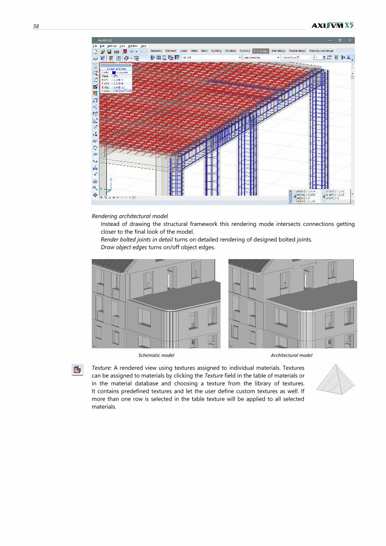
58

Rendering architectural model

Instead of drawing the structural framework this rendering mode intersects connections getting

closer to the final look of the model.

Render bolted joints in detail turns on detailed rendering of designed bolted joints.

Draw object edges turns on/off object edges.

Schematic model Architectural model

Texture: A rendered view using textures assigned to individual materials. Textures

can be assigned to materials by clicking the Texture field in the table of materials or

in the material database and choosing a texture from the library of textures.

It contains predefined textures and let the user define custom textures as well. If

more than one row is selected in the table texture will be applied to all selected

materials.

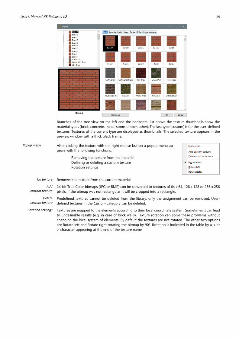
User’s Manual X5 Release4 e2 59

Branches of the tree view on the left and the horizontal list above the texture thumbnails show the

material types (brick, concrete, metal, stone, timber, other). The last type (custom) is for the user-defined

textures. Textures of the current type are displayed as thumbnails. The selected texture appears in the

preview window with a thick black frame.

Popup menu

After clicking the texture with the right mouse button a popup menu ap-

pears with the following functions:

Removing the texture from the material

Defining or deleting a custom texture

Rotation settings

No texture Removes the texture from the current material

Add custom texture

24-bit True Color bitmaps (JPG or BMP) can be converted to textures of 64 x 64, 128 x 128 or 256 x 256

pixels. If the bitmap was not rectangular it will be cropped into a rectangle.

Delete custom texture

Predefined textures cannot be deleted from the library, only the assignment can be removed. User-

defined textures in the Custom category can be deleted.

Rotation settings Textures are mapped to the elements according to their local coordinate system. Sometimes it can lead

to undesirable results (e.g. in case of brick walls). Texture rotation can solve these problems without

changing the local system of elements. By default the textures are not rotated. The other two options

are Rotate left and Rotate right rotating the bitmap by 90°. Rotation is indicated in the table by a < or

> character appearing at the end of the texture name.

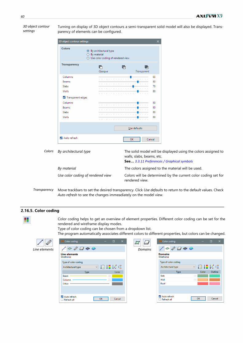
60

3D object contour settings

Turning on display of 3D object contours a semi-transparent solid model will also be displayed. Trans-

parency of elements can be configured.

Colors By architectural type The solid model will be displayed using the colors assigned to

walls, slabs, beams, etc.

See… 3.3.11 Preferences / Graphical symbols

By material The colors assigned to the material will be used.

Use color coding of rendered view Colors will be determined by the current color coding set for

rendered view.

Transparency Move trackbars to set the desired transparency. Click Use defaults to return to the default values. Check

Auto refresh to see the changes immeadiately on the model view.

2.16.5. Color coding

Color coding helps to get an overview of element properties. Different color coding can be set for the

rendered and wireframe display modes.

Type of color coding can be chosen from a dropdown list.

The program automatically associates different colors to different properties, but colors can be changed.

Line elements

Domains

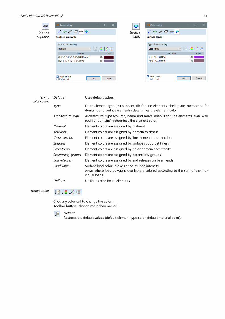
User’s Manual X5 Release4 e2 61

Surface

supports

Surface

loads

Type of color coding

Default Uses default colors.

Type Finite element type (truss, beam, rib for line elements, shell, plate, membrane for

domains and surface elements) determines the element color.

Architectural type Architectural type (column, beam and miscellaneous for line elements, slab, wall,

roof for domains) determines the element color.

Material Element colors are assigned by material

Thickness Element colors are assigned by domain thickness

Cross-section Element colors are assigned by line element cross-section

Stiffness Element colors are assigned by surface support stiffness

Eccentricity Element colors are assigned by rib or domain eccentricity

Eccentricity groups Element colors are assigned by eccentricity groups

End releases Element colors are assigned by end releases on beam ends

Load value Surface load colors are assigned by load intensity.

Areas where load polygons overlap are colored according to the sum of the indi-

vidual loads.

Uniform Uniform color for all elements

Setting colors

Click any color cell to change the color.

Toolbar buttons change more than one cell.

Default

Restores the default values (default element type color, default material color).

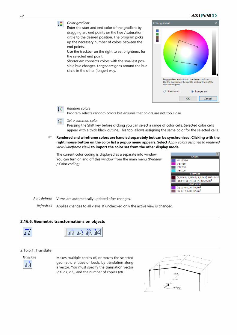
62

Color gradient

Enter the start and end color of the gradient by

dragging arc end points on the hue / saturation

circle to the desired position. The program picks

up the necessary number of colors between the

end points.

Use the trackbar on the right to set brightness for

the selected end point.

Shorter arc connects colors with the smallest pos-

sible hue changes. Longer arc goes around the hue

circle in the other (longer) way.

Random colors

Program selects random colors but ensures that colors are not too close.

Set a common color

Pressing the Shift key before clicking you can select a range of color cells. Selected color cells

appear with a thick black outline. This tool allows assigning the same color for the selected cells.

Rendered and wireframe colors are handled separately but can be synchronized. Clicking with the

right mouse button on the color list a popup menu appears. Select Apply colors assigned to rendered

view (wireframe view) to import the color set from the other display mode.

The current color coding is displayed as a separate info window.

You can turn on and off this window from the main menu (Window

/ Color coding)

Auto Refresh Views are automatically updated after changes.

Refresh all Applies changes to all views. If unchecked only the active view is changed.

2.16.6. Geometric transformations on objects

2.16.6.1. Translate

Translate

Makes multiple copies of, or moves the selected

geometric entities or loads, by translation along

a vector. You must specify the translation vector

(dX, dY, dZ), and the number of copies (N).

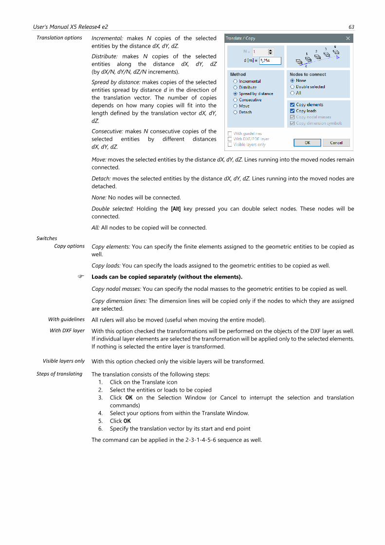
User’s Manual X5 Release4 e2 63

Translation options

Incremental makes N copies of the selected

entities by the distance dX, dY, dZ.

Distribute makes N copies of the selected

entities along the distance dX, dY, dZ

(by dX/N, dY/N, dZ/N increments).

Spread by distance: makes copies of the selected

entities spread by distance d in the direction of

the translation vector. The number of copies

depends on how many copies will fit into the

length defined by the translation vector dX, dY,

dZ.

Consecutive: makes N consecutive copies of the

selected entities by different distances

dX, dY, dZ.

Move: moves the selected entities by the distance dX, dY, dZ. Lines running into the moved nodes remain

connected.

Detach: moves the selected entities by the distance dX, dY, dZ. Lines running into the moved nodes are

detached.

None: No nodes will be connected.

Double selected: Holding the [Alt] key pressed you can double select nodes. These nodes will be

connected.

All: All nodes to be copied will be connected.

Switches

Copy options Copy elements: You can specify the finite elements assigned to the geometric entities to be copied as

well.

Copy loads: You can specify the loads assigned to the geometric entities to be copied as well.

Loads can be copied separately (without the elements).

Copy nodal masses: You can specify the nodal masses to the geometric entities to be copied as well.

Copy dimension lines: The dimension lines will be copied only if the nodes to which they are assigned

are selected.

With guidelines All rulers will also be moved (useful when moving the entire model).

With DXF layer With this option checked the transformations will be performed on the objects of the DXF layer as well.

If individual layer elements are selected the transformation will be applied only to the selected elements.

If nothing is selected the entire layer is transformed.

Visible layers only With this option checked only the visible layers will be transformed.

Steps of translating The translation consists of the following steps:

1. Click on the Translate icon

2. Select the entities or loads to be copied

3. Click OK on the Selection Window (or Cancel to interrupt the selection and translation

commands)

4. Select your options from within the Translate Window.

5. Click OK

6. Specify the translation vector by its start and end point

The command can be applied in the 2-3-1-4-5-6 sequence as well.

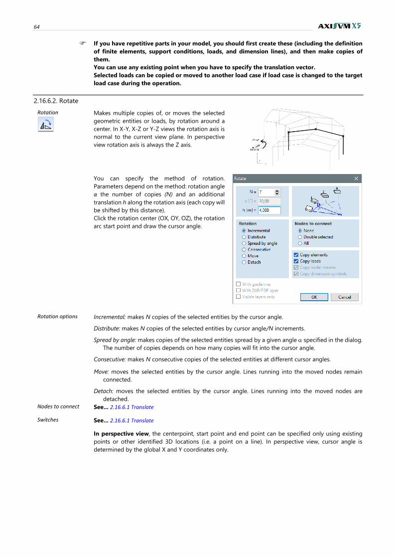
64

If you have repetitive parts in your model, you should first create these (including the definition

of finite elements, support conditions, loads, and dimension lines), and then make copies of

them.

You can use any existing point when you have to specify the translation vector.

Selected loads can be copied or moved to another load case if load case is changed to the target

load case during the operation.

2.16.6.2. Rotate

Rotation

Makes multiple copies of, or moves the selected

geometric entities or loads, by rotation around a

center. In X-Y, X-Z or Y-Z views the rotation axis is

normal to the current view plane. In perspective

view rotation axis is always the Z axis.

You can specify the method of rotation.

Parameters depend on the method: rotation angle

α the number of copies (N) and an additional

translation h along the rotation axis (each copy will

be shifted by this distance).

Click the rotation center (OX, OY, OZ), the rotation

arc start point and draw the cursor angle.

Rotation options Incremental: makes N copies of the selected entities by the cursor angle.

Distribute: makes N copies of the selected entities by cursor angle/N increments.

Spread by angle: makes copies of the selected entities spread by a given angle specified in the dialog.

The number of copies depends on how many copies will fit into the cursor angle.

Consecutive: makes N consecutive copies of the selected entities at different cursor angles.

Move: moves the selected entities by the cursor angle. Lines running into the moved nodes remain

connected.

Detach: moves the selected entities by the cursor angle. Lines running into the moved nodes are

detached.

Nodes to connect See... 2.16.6.1 Translate

Switches See... 2.16.6.1 Translate

In perspective view, the centerpoint, start point and end point can be specified only using existing

points or other identified 3D locations (i.e. a point on a line). In perspective view, cursor angle is

determined by the global X and Y coordinates only.

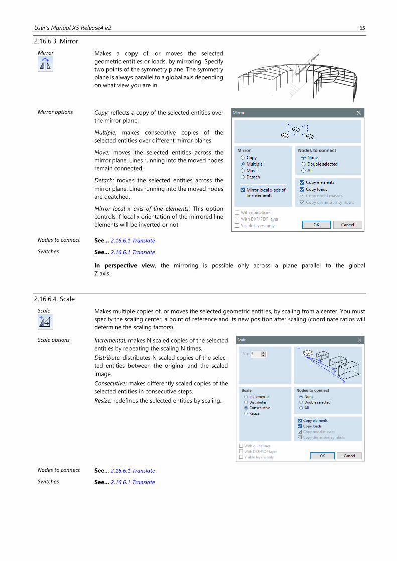
User’s Manual X5 Release4 e2 65

2.16.6.3. Mirror

Mirror

Makes a copy of, or moves the selected

geometric entities or loads, by mirroring. Specify

two points of the symmetry plane. The symmetry

plane is always parallel to a global axis depending

on what view you are in.

Mirror options

Copy: reflects a copy of the selected entities over

the mirror plane.

Multiple: makes consecutive copies of the

selected entities over different mirror planes.

Move: moves the selected entities across the

mirror plane. Lines running into the moved nodes

remain connected.

Detach: moves the selected entities across the

mirror plane. Lines running into the moved nodes

are deatched.

Mirror local x axis of line elements: This option

controls if local x orientation of the mirrored line

elements will be inverted or not.

Nodes to connect See... 2.16.6.1 Translate

Switches See... 2.16.6.1 Translate

In perspective view, the mirroring is possible only across a plane parallel to the global

Z axis.

2.16.6.4. Scale

Scale

Makes multiple copies of, or moves the selected geometric entities, by scaling from a center. You must

specify the scaling center, a point of reference and its new position after scaling (coordinate ratios will

determine the scaling factors).

Scale options

Incremental: makes N scaled copies of the selected

entities by repeating the scaling N times.

Distribute: distributes N scaled copies of the selec-

ted entities between the original and the scaled

image.

Consecutive: makes differently scaled copies of the

selected entities in consecutive steps.

Resize: redefines the selected entities by scaling.

Nodes to connect See... 2.16.6.1 Translate

Switches See... 2.16.6.1 Translate

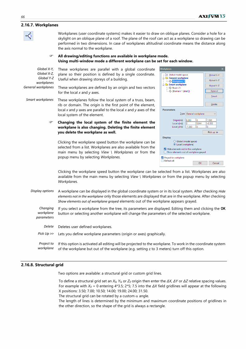
66

2.16.7. Workplanes

Workplanes (user coordinate systems) makes it easier to draw on oblique planes. Consider a hole for a

skylight on an oblique plane of a roof. The plane of the roof can act as a workplane so drawing can be

performed in two dimensions. In case of workplanes altitudinal coordinate means the distance along

the axis normal to the workplane.

All drawing/editing functions are available in workplane mode.

Using multi-window mode a different workplane can be set for each window.

Global X-Y, Global X-Z, Global Y-Z

workplanes

These workplanes are parallel with a global coordinate

plane so their position is defined by a single coordinate.

Useful when drawing storeys of a building.

General workplanes These workplanes are defined by an origin and two vectors

for the local x and y axes.

Smart workplanes These workplanes follow the local system of a truss, beam,

rib or domain. The origin is the first point of the element,

local x and y axes are parallel to the local x and y axes of the

local system of the element.

Changing the local system of the finite element the

workplane is also changing. Deleting the finite element

you delete the workplane as well.

Clicking the workplane speed button the workplane can be

selected from a list. Workplanes are also available from the

main menu by selecting View \ Workplanes or from the

popup menu by selecting Workplanes.

Clicking the workplane speed button the workplane can be selected from a list. Workplanes are also

available from the main menu by selecting View \ Workplanes or from the popup menu by selecting

Workplanes.

Display options A workplane can be displayed in the global coordinate system or in its local system. After checking Hide

elements not in the workplane only those elements are displayed that are in the workplane. After checking

Show elements out of workplane grayed elements out of the workplane appears grayed.

Changing workplane

parameters

If you select a workplane from the tree, its parameters are displayed. Editing them and clicking the OK

button or selecting another workplane will change the parameters of the selected workplane.

Delete Deletes user defined workplanes.

Pick Up >> Lets you define workplane parameters (origin or axes) graphically.

Project to workplane

If this option is activated all editing will be projected to the workplane. To work in the coordinate system

of the workplane but out of the workplane (e.g. setting z to 3 meters) turn off this option.

2.16.8. Structural grid

Two options are available: a structural grid or custom grid lines.

To define a structural grid set an X0, Y0, or Z0 origin then enter the ΔX, ΔY or ΔZ relative spacing values.

For example with X0 = 0 entering 4*3.5; 2*5; 7.5 into the ΔX field gridlines will appear at the following

X positions: 3.50; 7.00; 10.50; 14.00; 19.00; 24.00; 31.50.

The structural grid can be rotated by a custom angle.

The length of lines is determined by the minimum and maximum coordinate positions of gridlines in

the other direction, so the shape of the grid is always a rectangle.

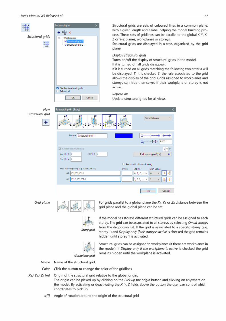
User’s Manual X5 Release4 e2 67

Structural grids

Structural grids are sets of coloured lines in a common plane,

with a given length and a label helping the model building pro-

cess. These sets of gridlines can be parallel to the global X-Y, X-

Z or Y-Z planes, workplanes or storeys.

Structural grids are displayed in a tree, organized by the grid

plane.

Display structural grids

Turns on/off the display of structural grids in the model.

If it is turned off all grids disappear.

If it is turned on all grids matching the following two criteria will

be displayed: 1) it is checked 2) the rule associated to the grid

allows the display of the grid. Grids assigned to workplanes and

storeys can hide themselves if their workplane or storey is not

active.

Refresh all

Update structural grids for all views.

New

structural grid

Grid plane

For grids parallel to a global plane the X0, Y0, or Z0 distance between the

grid plane and the global plane can be set

Story grid

If the model has storeys different structural grids can be assigned to each

storey. The grid can be associated to all storeys by selecting On all storeys

from the dropdown list. If the grid is associated to a specific storey (e.g.

storey 1) and Display only if the storey is active is checked the grid remains

hidden until storey 1 is activated.

Workplane grid

Structural grids can be assigned to workplanes (if there are workplanes in

the model). If Display only if the workplane is active is checked the grid

remains hidden until the workplane is activated.

Name Name of the structural grid

Color Click the button to change the color of the gridlines.

X0 / Y0 / Z0 [m]

Origin of the structural grid relative to the global origin.

The origin can be picked up by clicking on the Pick up the origin button and clicking on anywhere on

the model. By activating or deactivating the X, Y, Z fields above the button the user can control which

coordinates to pick up.

α[°] Angle of rotation around the origin of the structural grid

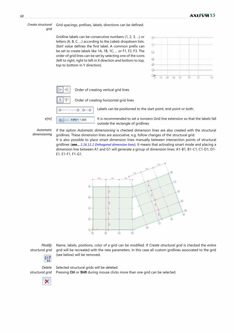
68

Create structural grid

Grid spacings, prefixes, labels, directions can be defined.

Gridline labels can be consecutive numbers (1, 2, 3, ...) or

letters (A, B, C, ...) according to the Labels dropdown lists.

Start value defines the first label. A common prefix can

be set to create labels like 1A, 1B, 1C, ... or F1, F2, F3. The

order of grid lines can be set by selecting one of the icons

(left to right, right to left in X direction and bottom to top,

top to bottom in Y direction).

Order of creating vertical grid lines

Order of creating horizontal grid lines

Labels can be positioned to the start point, end point or both.

e[m] It is recommended to set a nonzero Grid line extension so that the labels fall

outside the rectangle of gridlines

Automatic dimensioning

If the option Automatic dimensioning is checked dimension lines are also created with the structural

gridlines. These dimension lines are associative, e.g. follow changes of the structural grid.

It is also possible to place smart dimension lines manually between intersection points of structural

gridlines (see… 2.16.11.1 Orthogonal dimension lines). It means that activating smart mode and placing a

dimension line between A1 and G1 will generate a group of dimension lines: A1-B1, B1-C1, C1-D1, D1-

E1, E1-F1, F1-G1.

Modify

structural grid

Name, labels, positions, color of a grid can be modified. If Create structural grid is checked the entire

grid will be recreated with the new parameters. In this case all custom gridlines associated to the grid

(see below) will be removed.

Delete

structural grid

Selected structural grids will be deleted.

Pressing Ctrl or Shift during mouse clicks more than one grid can be selected.

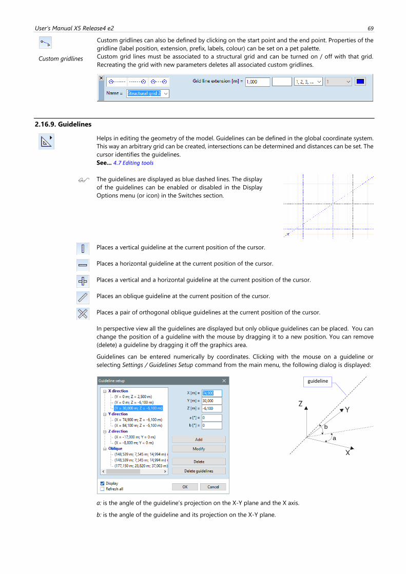
User’s Manual X5 Release4 e2 69

Custom gridlines

Custom gridlines can also be defined by clicking on the start point and the end point. Properties of the

gridline (label position, extension, prefix, labels, colour) can be set on a pet palette.

Custom grid lines must be associated to a structural grid and can be turned on / off with that grid.

Recreating the grid with new parameters deletes all associated custom gridlines.

2.16.9. Guidelines

Helps in editing the geometry of the model. Guidelines can be defined in the global coordinate system.

This way an arbitrary grid can be created, intersections can be determined and distances can be set. The

cursor identifies the guidelines.

See... 4.7 Editing tools

The guidelines are displayed as blue dashed lines. The display

of the guidelines can be enabled or disabled in the Display

Options menu (or icon) in the Switches section.

Places a vertical guideline at the current position of the cursor.

Places a horizontal guideline at the current position of the cursor.

Places a vertical and a horizontal guideline at the current position of the cursor.

Places an oblique guideline at the current position of the cursor.

Places a pair of orthogonal oblique guidelines at the current position of the cursor.

In perspective view all the guidelines are displayed but only oblique guidelines can be placed. You can

change the position of a guideline with the mouse by dragging it to a new position. You can remove

(delete) a guideline by dragging it off the graphics area.

Guidelines can be entered numerically by coordinates. Clicking with the mouse on a guideline or

selecting Settings / Guidelines Setup command from the main menu, the following dialog is displayed:

a: is the angle of the guideline’s projection on the X-Y plane and the X axis.

b: is the angle of the guideline and its projection on the X-Y plane.

a

b

guideline

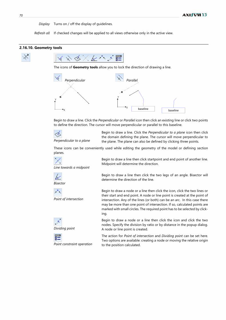
70

Display Turns on / off the display of guidelines.

Refresh all If checked changes will be applied to all views otherwise only in the active view.

2.16.10. Geometry tools

The icons of Geometry tools allow you to lock the direction of drawing a line.

Perpendicular Parallel

Begin to draw a line. Click the Perpendicular or Parallel icon then click an existing line or click two points

to define the direction. The cursor will move perpendicular or parallel to this baseline.

Perpendicular to a plane

Begin to draw a line. Click the Perpendicular to a plane icon then click

the domain defining the plane. The cursor will move perpendicular to

the plane. The plane can also be defined by clicking three points.

These icons can be conveniently used while editing the geometry of the model or defining section

planes.

Line towards a midpoint

Begin to draw a line then click startpoint and end point of another line.

Midpoint will determine the direction.

Bisector

Begin to draw a line then click the two legs of an angle. Bisector will

determine the direction of the line.

Point of intersection

Begin to draw a node or a line then click the icon, click the two lines or

their start and end point. A node or line point is created at the point of

intersection. Any of the lines (or both) can be an arc. In this case there

may be more than one point of intersection. If so, calculated points are

marked with small circles. The required point has to be selected by click-

ing.

Dividing point

Begin to draw a node or a line then click the icon and click the two

nodes. Specify the division by ratio or by distance in the popup dialog.

A node or line point is created.

Point constraint operation

The action for Point of intersection and Dividing point can be set here.

Two options are available: creating a node or moving the relative origin

to the position calculated.

baseline baseline

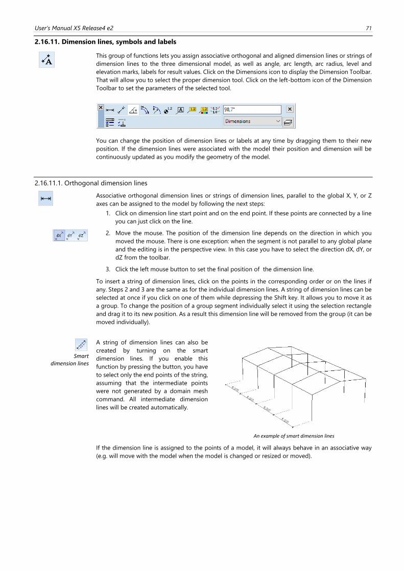
User’s Manual X5 Release4 e2 71

2.16.11. Dimension lines, symbols and labels

This group of functions lets you assign associative orthogonal and aligned dimension lines or strings of

dimension lines to the three dimensional model, as well as angle, arc length, arc radius, level and

elevation marks, labels for result values. Click on the Dimensions icon to display the Dimension Toolbar.

That will allow you to select the proper dimension tool. Click on the left-bottom icon of the Dimension

Toolbar to set the parameters of the selected tool.

You can change the position of dimension lines or labels at any time by dragging them to their new

position. If the dimension lines were associated with the model their position and dimension will be

continuously updated as you modify the geometry of the model.

2.16.11.1. Orthogonal dimension lines

Associative orthogonal dimension lines or strings of dimension lines, parallel to the global X, Y, or Z

axes can be assigned to the model by following the next steps:

1. Click on dimension line start point and on the end point. If these points are connected by a line

you can just click on the line.

2. Move the mouse. The position of the dimension line depends on the direction in which you

moved the mouse. There is one exception: when the segment is not parallel to any global plane

and the editing is in the perspective view. In this case you have to select the direction dX, dY, or

dZ from the toolbar.

3. Click the left mouse button to set the final position of the dimension line.

To insert a string of dimension lines, click on the points in the corresponding order or on the lines if

any. Steps 2 and 3 are the same as for the individual dimension lines. A string of dimension lines can be

selected at once if you click on one of them while depressing the Shift key. It allows you to move it as

a group. To change the position of a group segment individually select it using the selection rectangle

and drag it to its new position. As a result this dimension line will be removed from the group (it can be

moved individually).

Smart

dimension lines

A string of dimension lines can also be

created by turning on the smart

dimension lines. If you enable this

function by pressing the button, you have

to select only the end points of the string,

assuming that the intermediate points

were not generated by a domain mesh

command. All intermediate dimension

lines will be created automatically.

An example of smart dimension lines

If the dimension line is assigned to the points of a model, it will always behave in an associative way

(e.g. will move with the model when the model is changed or resized or moved).

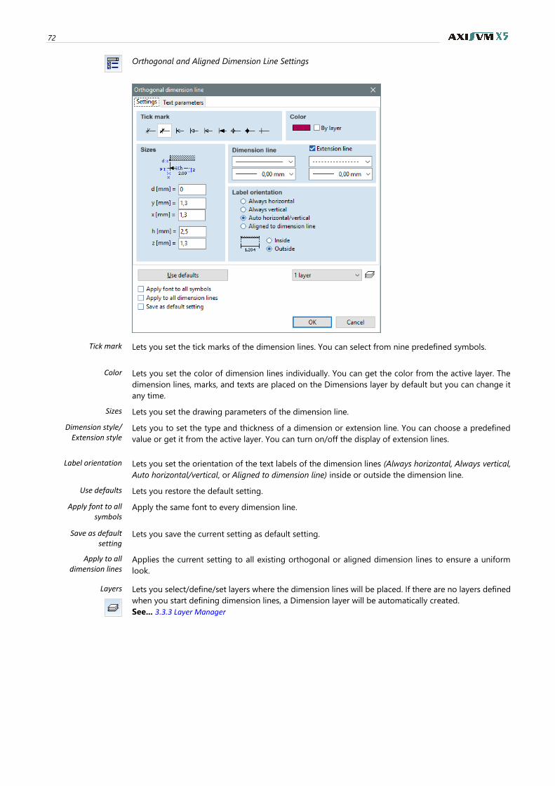
72

Orthogonal and Aligned Dimension Line Settings

Tick mark

Lets you set the tick marks of the dimension lines. You can select from nine predefined symbols.

Color

Lets you set the color of dimension lines individually. You can get the color from the active layer. The

dimension lines, marks, and texts are placed on the Dimensions layer by default but you can change it

any time.

Sizes Lets you set the drawing parameters of the dimension line.

Dimension style/ Extension style

Lets you to set the type and thickness of a dimension or extension line. You can choose a predefined

value or get it from the active layer. You can turn on/off the display of extension lines.

Label orientation

Lets you set the orientation of the text labels of the dimension lines (Always horizontal, Always vertical,

Auto horizontal/vertical, or Aligned to dimension line) inside or outside the dimension line.

Use defaults Lets you restore the default setting.

Apply font to all symbols

Apply the same font to every dimension line.

Save as default setting

Lets you save the current setting as default setting.

Apply to all dimension lines

Applies the current setting to all existing orthogonal or aligned dimension lines to ensure a uniform

look.

Layers

Lets you select/define/set layers where the dimension lines will be placed. If there are no layers defined

when you start defining dimension lines, a Dimension layer will be automatically created.

See... 3.3.3 Layer Manager

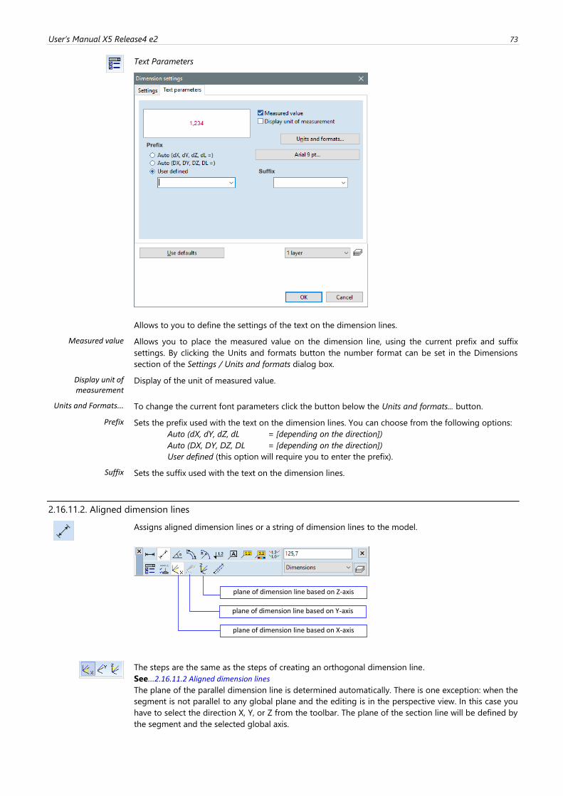
User’s Manual X5 Release4 e2 73

Text Parameters

Allows to you to define the settings of the text on the dimension lines.

Measured value Allows you to place the measured value on the dimension line, using the current prefix and suffix

settings. By clicking the Units and formats button the number format can be set in the Dimensions

section of the Settings / Units and formats dialog box.

Display unit of measurement

Display of the unit of measured value.

Units and Formats... To change the current font parameters click the button below the Units and formats... button.

Prefix

Sets the prefix used with the text on the dimension lines. You can choose from the following options:

Auto (dX, dY, dZ, dL = [depending on the direction])

Auto (DX, DY, DZ, DL = [depending on the direction])

User defined (this option will require you to enter the prefix).

Suffix Sets the suffix used with the text on the dimension lines.

2.16.11.2. Aligned dimension lines

Assigns aligned dimension lines or a string of dimension lines to the model.

The steps are the same as the steps of creating an orthogonal dimension line.

See...2.16.11.2 Aligned dimension lines

The plane of the parallel dimension line is determined automatically. There is one exception: when the

segment is not parallel to any global plane and the editing is in the perspective view. In this case you

have to select the direction X, Y, or Z from the toolbar. The plane of the section line will be defined by

the segment and the selected global axis.

plane of dimension line based on X-axis

plane of dimension line based on Y-axis

plane of dimension line based on Z-axis

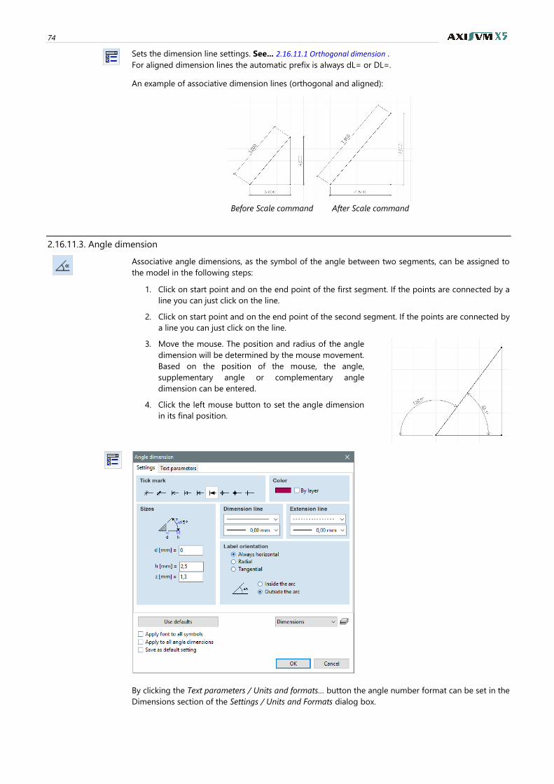
74

Sets the dimension line settings. See... 2.16.11.1 Orthogonal dimension .

For aligned dimension lines the automatic prefix is always dL= or DL=.

An example of associative dimension lines (orthogonal and aligned):

Before Scale command After Scale command

2.16.11.3. Angle dimension

Associative angle dimensions, as the symbol of the angle between two segments, can be assigned to

the model in the following steps:

1. Click on start point and on the end point of the first segment. If the points are connected by a

line you can just click on the line.

2. Click on start point and on the end point of the second segment. If the points are connected by

a line you can just click on the line.

3. Move the mouse. The position and radius of the angle

dimension will be determined by the mouse movement.

Based on the position of the mouse, the angle,

supplementary angle or complementary angle

dimension can be entered.

4. Click the left mouse button to set the angle dimension

in its final position.

By clicking the Text parameters / Units and formats… button the angle number format can be set in the

Dimensions section of the Settings / Units and Formats dialog box.

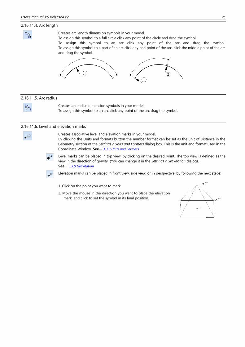
User’s Manual X5 Release4 e2 75

2.16.11.4. Arc length

Creates arc length dimension symbols in your model.

To assign this symbol to a full circle click any point of the circle and drag the symbol.

To assign this symbol to an arc click any point of the arc and drag the symbol.

To assign this symbol to a part of an arc click any end point of the arc, click the middle point of the arc

and drag the symbol.

2.16.11.5. Arc radius

Creates arc radius dimension symbols in your model.

To assign this symbol to an arc click any point of the arc drag the symbol.

2.16.11.6. Level and elevation marks

Creates associative level and elevation marks in your model.

By clicking the Units and formats button the number format can be set as the unit of Distance in the

Geometry section of the Settings / Units and Formats dialog box. This is the unit and format used in the

Coordinate Window. See... 3.3.8 Units and Formats

Level marks can be placed in top view, by clicking on the desired point. The top view is defined as the

view in the direction of gravity (You can change it in the Settings / Gravitation dialog).

See... 3.3.9 Gravitation

Elevation marks can be placed in front view, side view, or in perspective, by following the next steps:

1. Click on the point you want to mark.

2. Move the mouse in the direction you want to place the elevation

mark, and click to set the symbol in its final position.

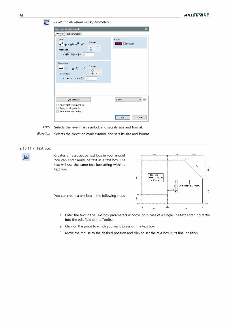
76

Level and elevation mark parameters

Level Selects the level mark symbol, and sets its size and format.

Elevation Selects the elevation mark symbol, and sets its size and format.

2.16.11.7. Text box

Creates an associative text box in your model.

You can enter multiline text in a text box. The

text will use the same text formatting within a

text box.

You can create a text box in the following steps:

1. Enter the text in the Text box parameters window, or in case of a single line text enter it directly

into the edit field of the Toolbar.

2. Click on the point to which you want to assign the text box.

3. Move the mouse to the desired position and click to set the text box in its final position.

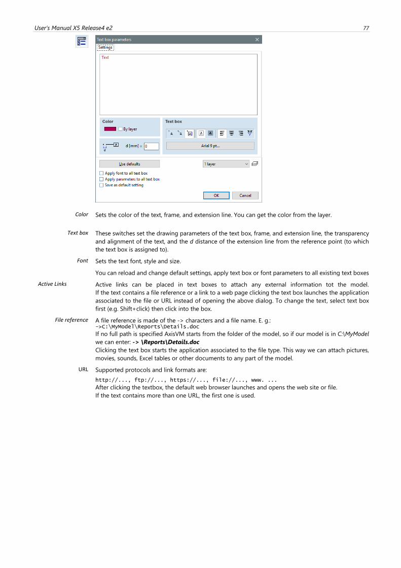
User’s Manual X5 Release4 e2 77

Color

Sets the color of the text, frame, and extension line. You can get the color from the layer.

Text box

These switches set the drawing parameters of the text box, frame, and extension line, the transparency

and alignment of the text, and the d distance of the extension line from the reference point (to which

the text box is assigned to).

Font Sets the text font, style and size.

You can reload and change default settings, apply text box or font parameters to all existing text boxes

Active Links Active links can be placed in text boxes to attach any external information tot the model.

If the text contains a file reference or a link to a web page clicking the text box launches the application

associated to the file or URL instead of opening the above dialog. To change the text, select text box

first (e.g. Shift+click) then click into the box.

File reference A file reference is made of the -> characters and a file name. E. g.: ->C:\MyModel\Reports\Details.doc

If no full path is specified AxisVM starts from the folder of the model, so if our model is in C:\MyModel

we can enter: -> \Reports\Details.doc

Clicking the text box starts the application associated to the file type. This way we can attach pictures,

movies, sounds, Excel tables or other documents to any part of the model.

URL Supported protocols and link formats are:

http://..., ftp://..., https://..., file://..., www. ...

After clicking the textbox, the default web browser launches and opens the web site or file.

If the text contains more than one URL, the first one is used.

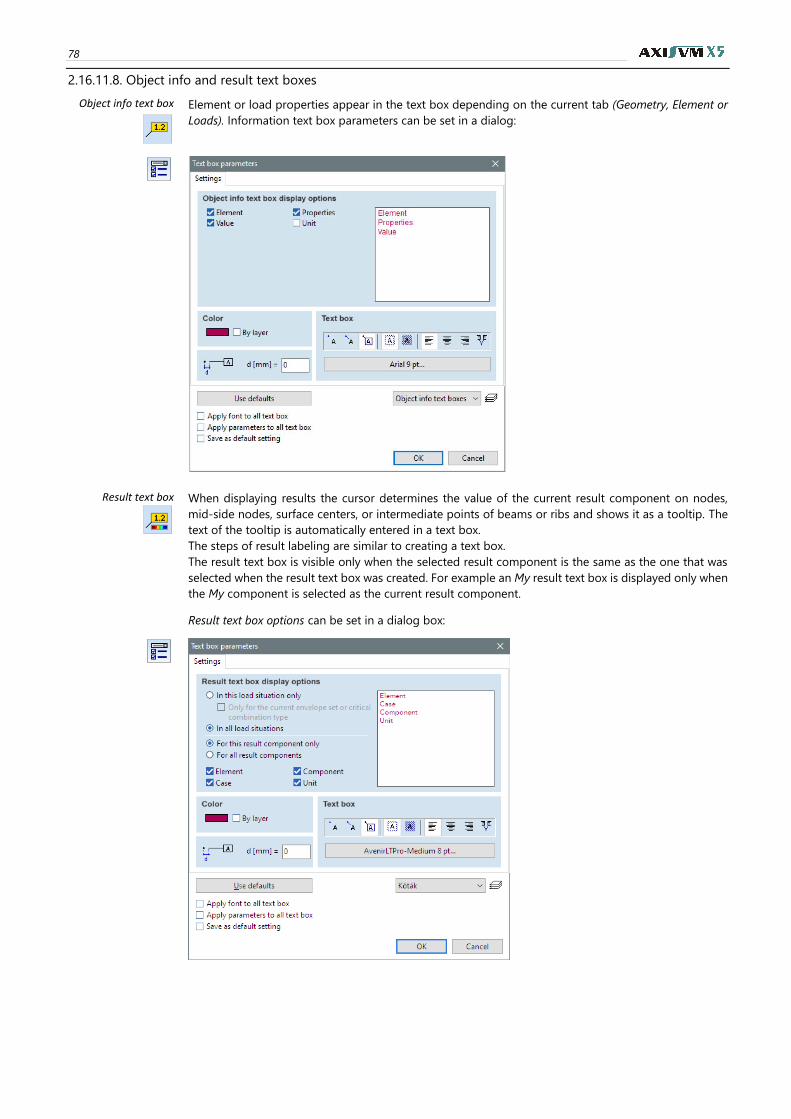
78

2.16.11.8. Object info and result text boxes

Object info text box

Element or load properties appear in the text box depending on the current tab (Geometry, Element or

Loads). Information text box parameters can be set in a dialog:

Result text box

When displaying results the cursor determines the value of the current result component on nodes,

mid-side nodes, surface centers, or intermediate points of beams or ribs and shows it as a tooltip. The

text of the tooltip is automatically entered in a text box.

The steps of result labeling are similar to creating a text box.

The result text box is visible only when the selected result component is the same as the one that was

selected when the result text box was created. For example an My result text box is displayed only when

the My component is selected as the current result component.

Result text box options can be set in a dialog box:

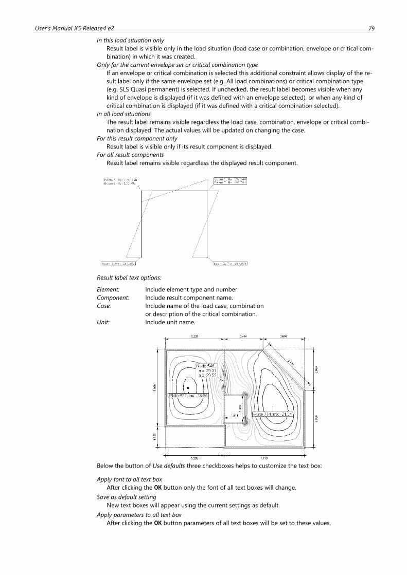
User’s Manual X5 Release4 e2 79

In this load situation only

Result label is visible only in the load situation (load case or combination, envelope or critical com-

bination) in which it was created.

Only for the current envelope set or critical combination type

If an envelope or critical combination is selected this additional constraint allows display of the re-

sult label only if the same envelope set (e.g. All load combinations) or critical combination type

(e.g. SLS Quasi permanent) is selected. If unchecked, the result label becomes visible when any

kind of envelope is displayed (if it was defined with an envelope selected), or when any kind of

critical combination is displayed (if it was defined with a critical combination selected).

In all load situations

The result label remains visible regardless the load case, combination, envelope or critical combi-

nation displayed. The actual values will be updated on changing the case.

For this result component only

Result label is visible only if its result component is displayed.

For all result components

Result label remains visible regardless the displayed result component.

Result label text options:

Element: Include element type and number.

Component: Include result component name.

Case: Include name of the load case, combination

or description of the critical combination.

Unit: Include unit name.

Below the button of Use defaults three checkboxes helps to customize the text box:

Apply font to all text box

After clicking the OK button only the font of all text boxes will change.

Save as default setting

New text boxes will appear using the current settings as default.

Apply parameters to all text box

After clicking the OK button parameters of all text boxes will be set to these values.

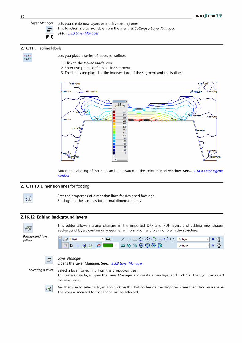
80

Layer Manager

[F11]

Lets you create new layers or modify existing ones.

This function is also available from the menu as Settings / Layer Manager.

See... 3.3.3 Layer Manager

2.16.11.9. Isoline labels

Lets you place a series of labels to isolines.

1. Click to the Isoline labels icon

2. Enter two points defining a line segment

3. The labels are placed at the intersections of the segment and the isolines

Automatic labeling of isolines can be activated in the color legend window. See… 2.18.4 Color legend window

2.16.11.10. Dimension lines for footing

Sets the properties of dimension lines for designed footings.

Settings are the same as for normal dimension lines.

2.16.12. Editing background layers

Background layer editor

This editor allows making changes in the imported DXF and PDF layers and adding new shapes.

Background layers contain only geometry information and play no role in the structure.

Layer Manager

Opens the Layer Manager. See… 3.3.3 Layer Manager

Selecting a layer Select a layer for editing from the dropdown tree.

To create a new layer open the Layer Manager and create a new layer and click OK. Then you can select

the new layer.

Another way to select a layer is to click on this button beside the dropdown tree then click on a shape.

The layer associated to that shape will be selected.

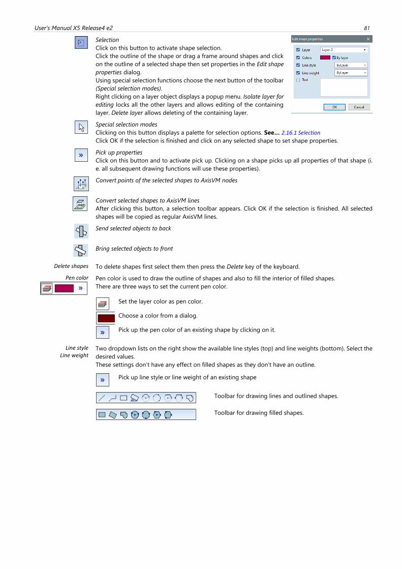
User’s Manual X5 Release4 e2 81

Selection

Click on this button to activate shape selection.

Click the outline of the shape or drag a frame around shapes and click

on the outline of a selected shape then set properties in the Edit shape

properties dialog.

Using special selection functions choose the next button of the toolbar

(Special selection modes).

Right clicking on a layer object displays a popup menu. Isolate layer for

editing locks all the other layers and allows editing of the containing

layer. Delete layer allows deleting of the containing layer.

Special selection modes

Clicking on this button displays a palette for selection options. See… 2.16.1 Selection

Click OK if the selection is finished and click on any selected shape to set shape properties.

Pick up properties

Click on this button and to activate pick up. Clicking on a shape picks up all properties of that shape (i.

e. all subsequent drawing functions will use these properties).

Convert points of the selected shapes to AxisVM nodes

Convert selected shapes to AxisVM lines

After clicking this button, a selection toolbar appears. Click OK if the selection is finished. All selected

shapes will be copied as regular AxisVM lines.

Send selected objects to back

Bring selected objects to front

Delete shapes To delete shapes first select them then press the Delete key of the keyboard.

Pen color

Pen color is used to draw the outline of shapes and also to fill the interior of filled shapes.

There are three ways to set the current pen color.

Set the layer color as pen color.

Choose a color from a dialog.

Pick up the pen color of an existing shape by clicking on it.

Line style Two dropdown lists on the right show the available line styles (top) and line weights (bottom). Select the

desired values.

These settings don’t have any effect on filled shapes as they don’t have an outline.

Line weight

Pick up line style or line weight of an existing shape

Toolbar for drawing lines and outlined shapes.

Toolbar for drawing filled shapes.

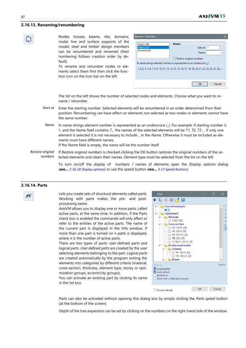
82

2.16.13. Renaming/renumbering

Nodes, trusses, beams, ribs, domains,

nodal, line and surface supports of the

model, steel and timber design members

can be renumbered and renamed (their

numbering follows creation order by de-

fault).

To rename and renumber nodes or ele-

ments select them first then click the func-

tion icon on the Icon bar on the left.

The list on the left shows the number of selected nodes and elements. Choose what you want to re-

name / renumber.

Start at Enter the starting number. Selected elements will be renumbered in an order determined from their

position. Renumbering can have effect on elements not selected as two nodes or elements cannot have

the same number.

Name In name strings element number is represented as an underscore (_). For example: if starting number is

1, and the Name field contains T_, the names of the selected elements will be T1, T2, T3 … If only one

element is selected it is not necessary to include _ in the Name. Otherwise it must be included as ele-

ments must have different names.

If the Name field is empty, the name will be the number itself.

Restore original numbers

If Restore original numbers is checked clicking the OK button restores the original numbers of the se-

lected elements and clears their names. Element type must be selected from the list on the left.

To turn on/off the display of numbers / names of elements open the Display options dialog

(see... 2.16.18 Display options) or use the speed button (see... 2.17 Speed Buttons)

2.16.14. Parts

Lets you create sets of structural elements called parts.

Working with parts makes the pre- and post-

processing easier.

AxisVM allows you to display one or more parts, called

active parts, at the same time. In addition, if the Parts

check box is enabled the commands will only affect or

refer to the entities of the active parts. The name of

the current part is displayed in the Info window. If

more than one part is turned on n parts is displayed,

where n is the number of active parts.

There are two types of parts: user-defined parts and

logical parts. User defined parts are created by the user

selecting elements belonging to the part. Logical parts

are created automatically by the program sorting the

elements into categories by different criteria (material,

cross-section, thickness, element type, storey or opti-

mization groups, eccentricity groups).

You can activate an existing part by clicking its name

in the list box.

Parts can also be activated without opening this dialog box by simply clicking the Parts speed button

(at the bottom of the screen).

Depth of the tree expansion can be set by clicking on the numbers on the right-hand side of the window.

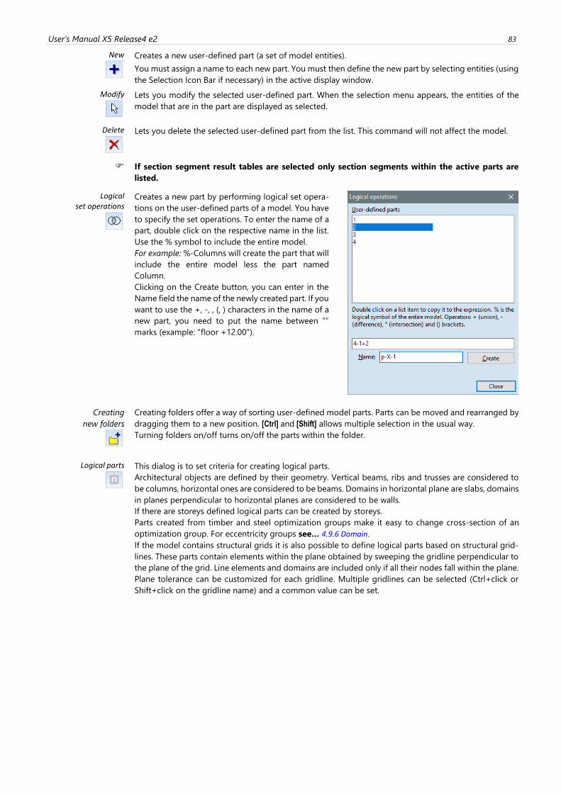
User’s Manual X5 Release4 e2 83

New

Creates a new user-defined part (a set of model entities).

You must assign a name to each new part. You must then define the new part by selecting entities (using

the Selection Icon Bar if necessary) in the active display window.

Modify

Lets you modify the selected user-defined part. When the selection menu appears, the entities of the

model that are in the part are displayed as selected.

Delete

Lets you delete the selected user-defined part from the list. This command will not affect the model.

If section segment result tables are selected only section segments within the active parts are

listed.

Logical set operations

Creates a new part by performing logical set opera-

tions on the user-defined parts of a model. You have

to specify the set operations. To enter the name of a

part, double click on the respective name in the list.

Use the % symbol to include the entire model.

For example: %-Columns will create the part that will

include the entire model less the part named

Column.

Clicking on the Create button, you can enter in the

Name field the name of the newly created part. If you

want to use the +, -, , (, ) characters in the name of a

new part, you need to put the name between “”

marks (example: "floor +12.00").

Creating

new folders

Creating folders offer a way of sorting user-defined model parts. Parts can be moved and rearranged by

dragging them to a new position. [Ctrl] and [Shift] allows multiple selection in the usual way.

Turning folders on/off turns on/off the parts within the folder.

Logical parts

This dialog is to set criteria for creating logical parts.

Architectural objects are defined by their geometry. Vertical beams, ribs and trusses are considered to

be columns, horizontal ones are considered to be beams. Domains in horizontal plane are slabs, domains

in planes perpendicular to horizontal planes are considered to be walls.

If there are storeys defined logical parts can be created by storeys.

Parts created from timber and steel optimization groups make it easy to change cross-section of an

optimization group. For eccentricity groups see… 4.9.6 Domain.

If the model contains structural grids it is also possible to define logical parts based on structural grid-

lines. These parts contain elements within the plane obtained by sweeping the gridline perpendicular to

the plane of the grid. Line elements and domains are included only if all their nodes fall within the plane.

Plane tolerance can be customized for each gridline. Multiple gridlines can be selected (Ctrl+click or

Shift+click on the gridline name) and a common value can be set.

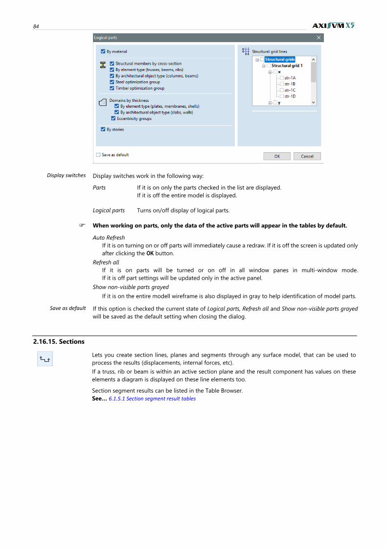
84

Display switches Display switches work in the following way:

Parts

If it is on only the parts checked in the list are displayed.

If it is off the entire model is displayed.

Logical parts Turns on/off display of logical parts.

When working on parts, only the data of the active parts will appear in the tables by default.

Auto Refresh

If it is on turning on or off parts will immediately cause a redraw. If it is off the screen is updated only

after clicking the OK button.

Refresh all

If it is on parts will be turned or on off in all window panes in multi-window mode.

If it is off part settings will be updated only in the active panel.

Show non-visible parts grayed

If it is on the entire modell wireframe is also displayed in gray to help identification of model parts.

Save as default If this option is checked the current state of Logical parts, Refresh all and Show non-visible parts grayed

will be saved as the default setting when closing the dialog.

2.16.15. Sections

Lets you create section lines, planes and segments through any surface model, that can be used to

process the results (displacements, internal forces, etc).

If a truss, rib or beam is within an active section plane and the result component has values on these

elements a diagram is displayed on these line elements too.

Section segment results can be listed in the Table Browser.

See… 6.1.5.1 Section segment result tables

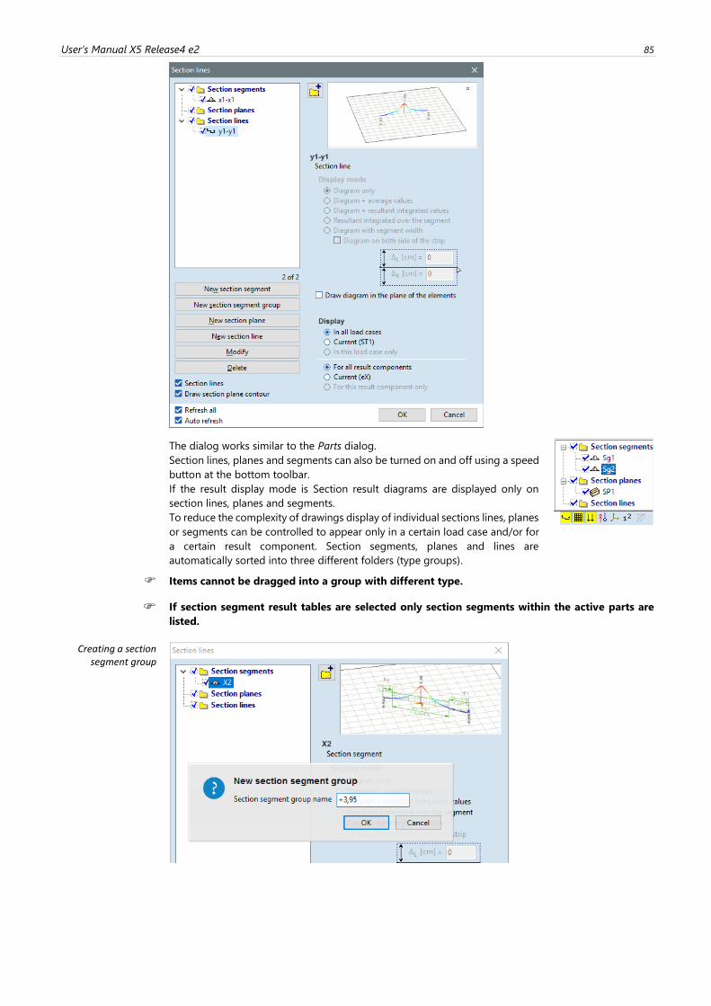
User’s Manual X5 Release4 e2 85

The dialog works similar to the Parts dialog.

Section lines, planes and segments can also be turned on and off using a speed

button at the bottom toolbar.

If the result display mode is Section result diagrams are displayed only on

section lines, planes and segments.

To reduce the complexity of drawings display of individual sections lines, planes

or segments can be controlled to appear only in a certain load case and/or for

a certain result component. Section segments, planes and lines are

automatically sorted into three different folders (type groups).

Items cannot be dragged into a group with different type.

If section segment result tables are selected only section segments within the active parts are

listed.

Creating a section segment group

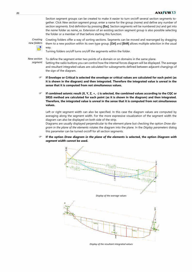
86

Section segment groups can be created to make it easier to turn on/off several section segments to-

gether. Click New section segment group, enter a name for the group (name) and define any number of

section segments. End definition by pressing [Esc]. Section segments will be numbered (xx) and get into

the name folder as name_xx. Extension of an existing section segment group is also possible selecting

the folder or a member of that before starting this function.

Creating new folders

Creating folders offer a way of sorting sections. Segments can be moved and rearranged by dragging

them to a new position within its own type group. [Ctrl] and [Shift] allows multiple selection in the usual

way.

Turning folders on/off turns on/off the segments within the folder.

New section segment

To define the segment enter two points of a domain or on domains in the same plane.

Setting the radio buttons you can control how the internal forces diagram will be displayed. The average

and resultant integrated values are calculated for subsegments defined between adjacent changings of

the sign of the diagram.

If Envelope or Critical is selected the envelope or critical values are calculated for each point (as

it is shown in the diagram) and then integrated. Therefore the integrated value is unreal in the

sense that it is computed from not simultaneous values.

If combined seismic result (X, Y, Z, +, -) is selected, the combined values according to the CQC or

SRSS method are calculated for each point (as it is shown in the diagram) and then integrated.

Therefore, the integrated value is unreal in the sense that it is computed from not simultaneous

values.

Left or right segment width can also be specified. In this case the diagram values are computed by

averaging along the segment width. For the more expressive visualization of the segment width the

diagram can also be displayed on both side of the strip.

Diagrams are usually displayed perpendicular to the element plane but checking the option Draw dia-

gram in the plane of the elements rotates the diagram into the plane. In the Display parameters dialog

this parameter can be turned on/off for all section segments.

If the option Draw diagram in the plane of the elements is selected, the option Diagram with

segment width cannot be used.

Display of the average values

Display of the resultant integrated values

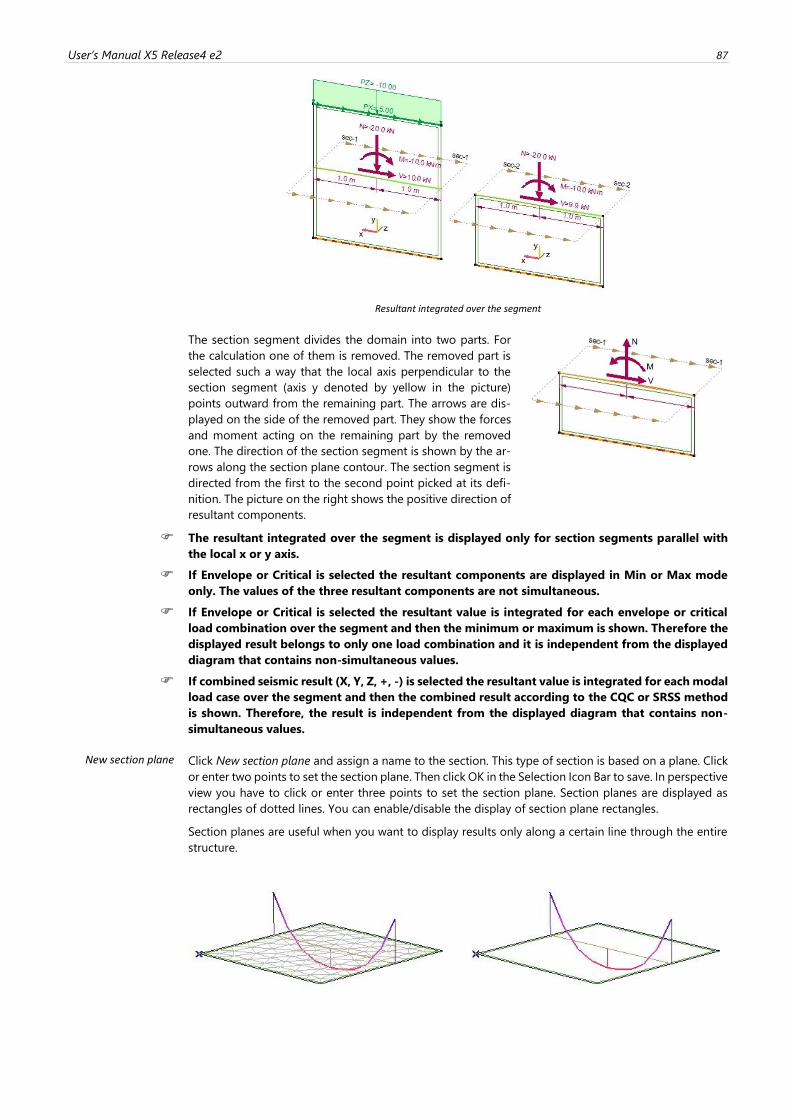
User’s Manual X5 Release4 e2 87

Resultant integrated over the segment

The section segment divides the domain into two parts. For

the calculation one of them is removed. The removed part is

selected such a way that the local axis perpendicular to the

section segment (axis y denoted by yellow in the picture)

points outward from the remaining part. The arrows are dis-

played on the side of the removed part. They show the forces

and moment acting on the remaining part by the removed

one. The direction of the section segment is shown by the ar-

rows along the section plane contour. The section segment is

directed from the first to the second point picked at its defi-

nition. The picture on the right shows the positive direction of

resultant components.

The resultant integrated over the segment is displayed only for section segments parallel with

the local x or y axis.

If Envelope or Critical is selected the resultant components are displayed in Min or Max mode

only. The values of the three resultant components are not simultaneous.

If Envelope or Critical is selected the resultant value is integrated for each envelope or critical

load combination over the segment and then the minimum or maximum is shown. Therefore the

displayed result belongs to only one load combination and it is independent from the displayed

diagram that contains non-simultaneous values.

If combined seismic result (X, Y, Z, +, -) is selected the resultant value is integrated for each modal

load case over the segment and then the combined result according to the CQC or SRSS method

is shown. Therefore, the result is independent from the displayed diagram that contains non-

simultaneous values.

New section plane Click New section plane and assign a name to the section. This type of section is based on a plane. Click

or enter two points to set the section plane. Then click OK in the Selection Icon Bar to save. In perspective

view you have to click or enter three points to set the section plane. Section planes are displayed as

rectangles of dotted lines. You can enable/disable the display of section plane rectangles.

Section planes are useful when you want to display results only along a certain line through the entire

structure.

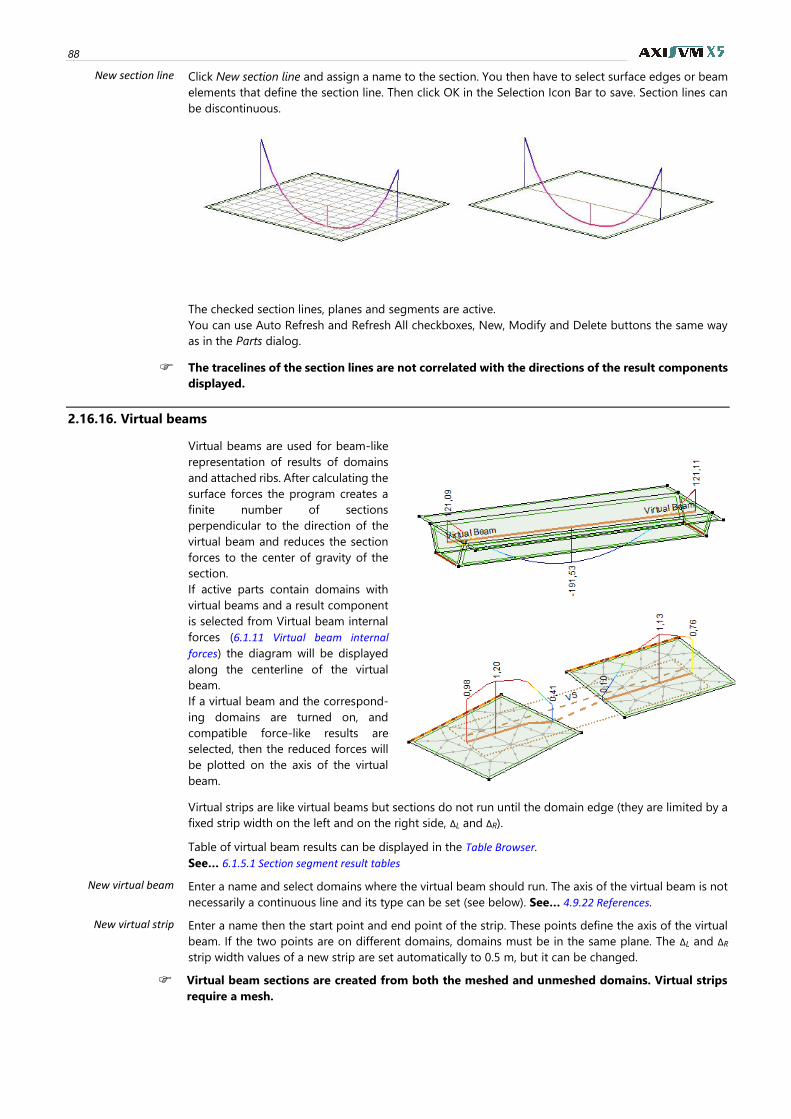
88

New section line Click New section line and assign a name to the section. You then have to select surface edges or beam

elements that define the section line. Then click OK in the Selection Icon Bar to save. Section lines can

be discontinuous.

The checked section lines, planes and segments are active.

You can use Auto Refresh and Refresh All checkboxes, New, Modify and Delete buttons the same way

as in the Parts dialog.

The tracelines of the section lines are not correlated with the directions of the result components

displayed.

2.16.16. Virtual beams

Virtual beams are used for beam-like

representation of results of domains

and attached ribs. After calculating the

surface forces the program creates a

finite number of sections

perpendicular to the direction of the

virtual beam and reduces the section

forces to the center of gravity of the

section.

If active parts contain domains with

virtual beams and a result component

is selected from Virtual beam internal

forces (6.1.11 Virtual beam internal

forces) the diagram will be displayed

along the centerline of the virtual

beam.

If a virtual beam and the correspond-

ing domains are turned on, and

compatible force-like results are

selected, then the reduced forces will

be plotted on the axis of the virtual

beam.

Virtual strips are like virtual beams but sections do not run until the domain edge (they are limited by a

fixed strip width on the left and on the right side, ΔL and ΔR).

Table of virtual beam results can be displayed in the Table Browser.

See… 6.1.5.1 Section segment result tables

New virtual beam Enter a name and select domains where the virtual beam should run. The axis of the virtual beam is not

necessarily a continuous line and its type can be set (see below). See… 4.9.22 References.

New virtual strip Enter a name then the start point and end point of the strip. These points define the axis of the virtual

beam. If the two points are on different domains, domains must be in the same plane. The ΔL and ΔR

strip width values of a new strip are set automatically to 0.5 m, but it can be changed.

Virtual beam sections are created from both the meshed and unmeshed domains. Virtual strips

require a mesh.

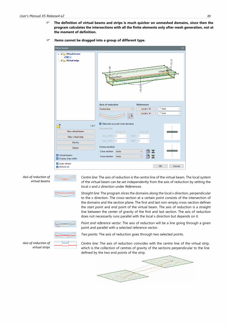
User’s Manual X5 Release4 e2 89

The definition of virtual beams and strips is much quicker on unmeshed domains, since then the

program calculates the intersections with all the finite elements only after mesh generation, not at

the moment of definition.

Items cannot be dragged into a group of different type.

Axis of reduction of virtual beams

Centre line: The axis of reduction is the centre line of the virtual beam. The local system

of the virtual beam can be set independently from the axis of reduction by setting the

local x and z direction under References.

Straight line: The program slices the domains along the local x direction, perpendicular

to the x direction. The cross-section at a certain point consists of the intersection of

the domains and the section plane. The first and last non-empty cross-section defines

the start point and end point of the virtual beam. The axis of reduction is a straight

line between the center of gravity of the first and last section. The axis of reduction

does not necessarily runs parallel with the local x direction but depends on it.

Point and reference vector: The axis of reduction will be a line going through a given

point and parallel with a selected reference vector.

Two points: The axis of reduction goes through two selected points.

Axis of reduction of virtual strips

Centre line: The axis of reduction coincides with the centre line of the virtual strip,

which is the collection of centres of gravity of the sections perpendicular to the line

defined by the two end points of the strip.

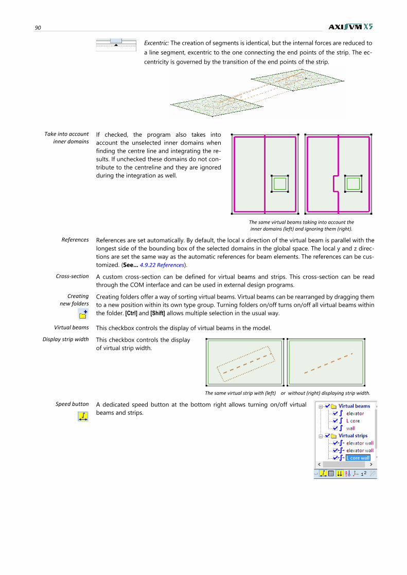
90

Excentric: The creation of segments is identical, but the internal forces are reduced to

a line segment, excentric to the one connecting the end points of the strip. The ec-

centricity is governed by the transition of the end points of the strip.

Take into account inner domains

If checked, the program also takes into

account the unselected inner domains when

finding the centre line and integrating the re-

sults. If unchecked these domains do not con-

tribute to the centreline and they are ignored

during the integration as well.

The same virtual beams taking into account the inner domains (left) and ignoring them (right).

References References are set automatically. By default, the local x direction of the virtual beam is parallel with the

longest side of the bounding box of the selected domains in the global space. The local y and z direc-

tions are set the same way as the automatic references for beam elements. The references can be cus-

tomized. (See... 4.9.22 References).

Cross-section A custom cross-section can be defined for virtual beams and strips. This cross-section can be read

through the COM interface and can be used in external design programs.

Creating new folders

Creating folders offer a way of sorting virtual beams. Virtual beams can be rearranged by dragging them

to a new position within its own type group. Turning folders on/off turns on/off all virtual beams within

the folder. [Ctrl] and [Shift] allows multiple selection in the usual way.

Virtual beams This checkbox controls the display of virtual beams in the model.

Display strip width This checkbox controls the display

of virtual strip width.

The same virtual strip with (left) or without (right) displaying strip width.

Speed button

A dedicated speed button at the bottom right allows turning on/off virtual

beams and strips.

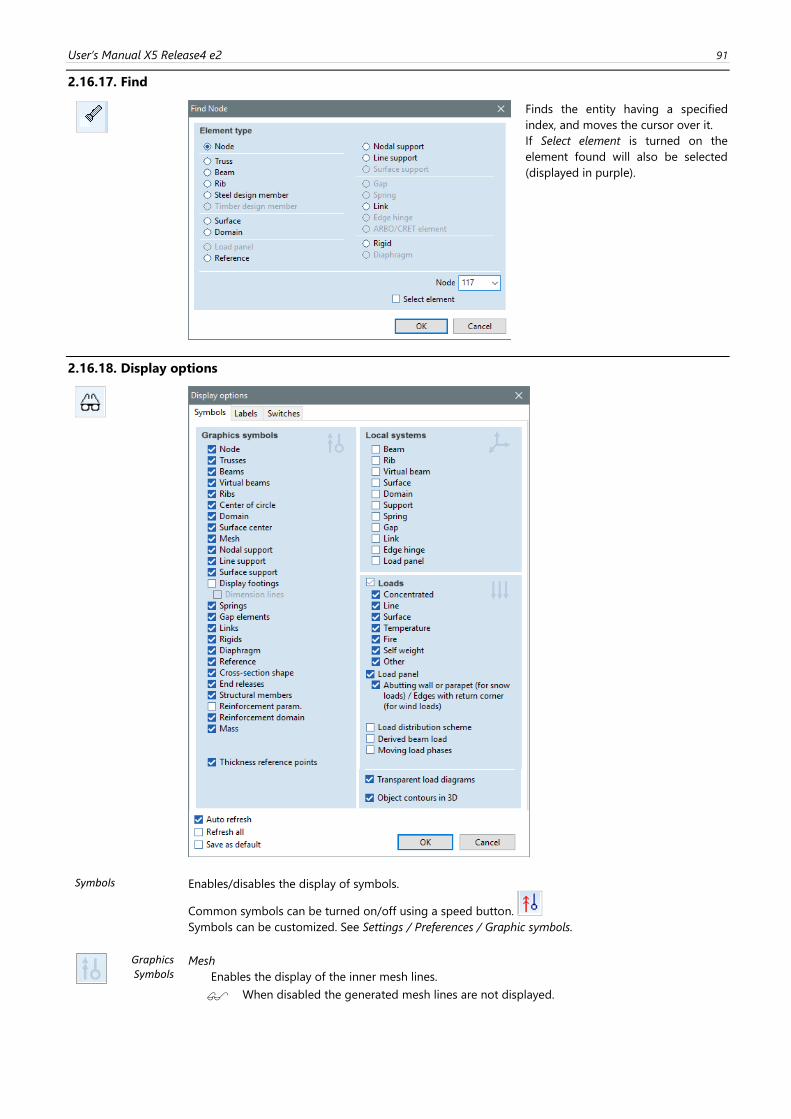
User’s Manual X5 Release4 e2 91

2.16.17. Find

Finds the entity having a specified

index, and moves the cursor over it.

If Select element is turned on the

element found will also be selected

(displayed in purple).

2.16.18. Display options

Symbols Enables/disables the display of symbols.

Common symbols can be turned on/off using a speed button. Symbols can be customized. See Settings / Preferences / Graphic symbols.

Graphics Symbols

Mesh

Enables the display of the inner mesh lines. When disabled the generated mesh lines are not displayed.

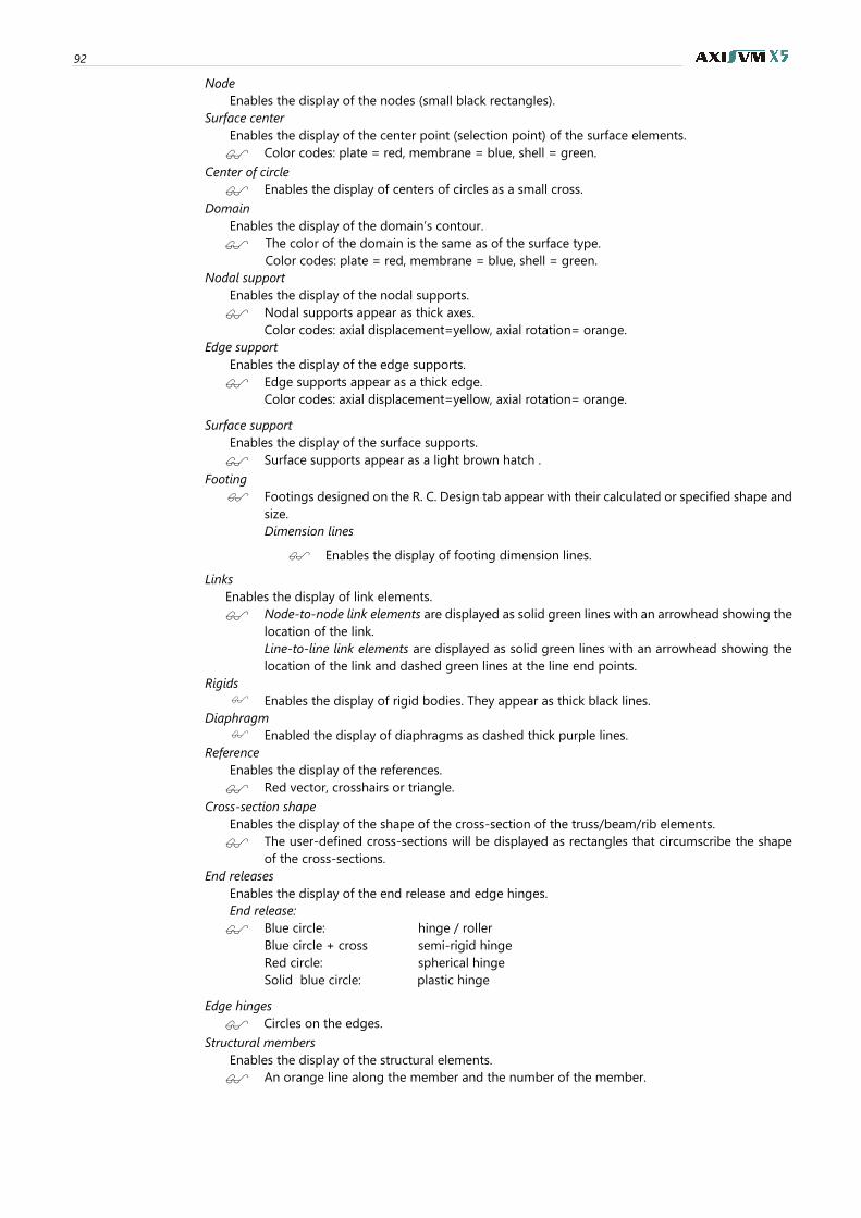
92

Node

Enables the display of the nodes (small black rectangles).

Surface center

Enables the display of the center point (selection point) of the surface elements.

Color codes: plate = red, membrane = blue, shell = green.

Center of circle

Enables the display of centers of circles as a small cross.

Domain

Enables the display of the domain’s contour.

The color of the domain is the same as of the surface type.

Color codes: plate = red, membrane = blue, shell = green.

Nodal support

Enables the display of the nodal supports.

Nodal supports appear as thick axes.

Color codes: axial displacement=yellow, axial rotation= orange.

Edge support

Enables the display of the edge supports.

Edge supports appear as a thick edge.

Color codes: axial displacement=yellow, axial rotation= orange.

Surface support

Enables the display of the surface supports.

Surface supports appear as a light brown hatch .

Footing

Footings designed on the R. C. Design tab appear with their calculated or specified shape and

size.

Dimension lines

Enables the display of footing dimension lines.

Links

Enables the display of link elements.

Node-to-node link elements are displayed as solid green lines with an arrowhead showing the

location of the link.

Line-to-line link elements are displayed as solid green lines with an arrowhead showing the

location of the link and dashed green lines at the line end points.

Rigids

Enables the display of rigid bodies. They appear as thick black lines.

Diaphragm

Enabled the display of diaphragms as dashed thick purple lines.

Reference

Enables the display of the references.

Red vector, crosshairs or triangle.

Cross-section shape

Enables the display of the shape of the cross-section of the truss/beam/rib elements.

The user-defined cross-sections will be displayed as rectangles that circumscribe the shape

of the cross-sections.

End releases

Enables the display of the end release and edge hinges.

End release:

Blue circle: hinge / roller

Blue circle + cross semi-rigid hinge

Red circle: spherical hinge

Solid blue circle: plastic hinge

Edge hinges

Circles on the edges.

Structural members

Enables the display of the structural elements.

An orange line along the member and the number of the member.

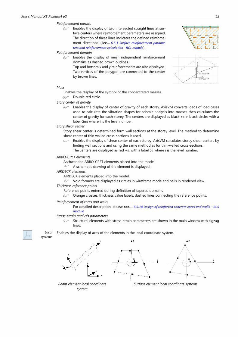
User’s Manual X5 Release4 e2 93

Reinforcement param.

Enables the display of two intersected straight lines at sur-

face centers where reinforcement parameters are assigned.

The direction of these lines indicates the defined reinforce-

ment directions. (See... 6.5.1 Surface reinforcement parame-

ters and reinforcement calculation - RC1 module).

Reinforcement domain

Enables the display of mesh independent reinforcement

domains as dashed brown outlines.

Top and bottom x and y reinforcements are also displayed.

Two vertices of the polygon are connected to the center

by brown lines.

Mass

Enables the display of the symbol of the concentrated masses.

Double red circle.

Story center of gravity

Enables the display of center of gravity of each storey. AxisVM converts loads of load cases

used to calculate the vibration shapes for seismic analysis into masses then calculates the

center of gravity for each storey. The centers are displayed as black +s in black circles with a

label Gmi where i is the level number.

Story shear center

Story shear center is determined form wall sections at the storey level. The method to determine

shear center of thin walled cross-sections is used. Enables the display of shear center of each storey. AxisVM calculates storey shear centers by

finding wall sections and using the same method as for thin-walled cross-sections.

The centers are displayed as red +s, with a label Si, where i is the level number.

ARBO-CRET elements

Aschwanden ARBO-CRET elements placed into the model.

A schematic drawing of the element is displayed.

AIRDECK elements

AIRDECK elements placed into the model.

Void formers are displayed as circles in wireframe mode and balls in rendered view.

Thickness reference points

Reference points entered during definition of tapered domains Orange crosses, thickness value labels, dashed lines connecting the reference points.

Reinforcement of cores and walls

For detailed description, please see… 6.5.14 Design of reinforced concrete cores and walls – RC5 module

Stress-strain analysis parameters

Structural elements with stress-strain parameters are shown in the main window with zigzag

lines.

Local systems

Enables the display of axes of the elements in the local coordinate system.

Beam element local coordinate

system

Surface element local coordinate systems

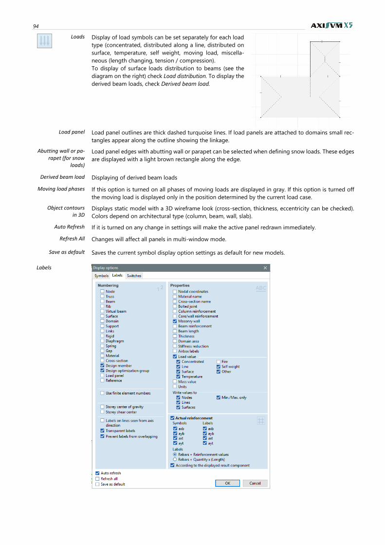
94

Loads Display of load symbols can be set separately for each load

type (concentrated, distributed along a line, distributed on

surface, temperature, self weight, moving load, miscella-

neous (length changing, tension / compression).

To display of surface loads distribution to beams (see the

diagram on the right) check Load distribution. To display the

derived beam loads, check Derived beam load.

Load panel Load panel outlines are thick dashed turquoise lines. If load panels are attached to domains small rec-

tangles appear along the outline showing the linkage.

Abutting wall or pa-rapet (for snow

loads)

Load panel edges with abutting wall or parapet can be selected when defining snow loads. These edges

are displayed with a light brown rectangle along the edge.

Derived beam load Displaying of derived beam loads

Moving load phases If this option is turned on all phases of moving loads are displayed in gray. If this option is turned off

the moving load is displayed only in the position determined by the current load case.

Object contours in 3D

Displays static model with a 3D wireframe look (cross-section, thickness, eccentricity can be checked).

Colors depend on architectural type (column, beam, wall, slab).

Auto Refresh If it is turned on any change in settings will make the active panel redrawn immediately.

Refresh All Changes will affect all panels in multi-window mode.

Save as default Saves the current symbol display option settings as default for new models.

Labels

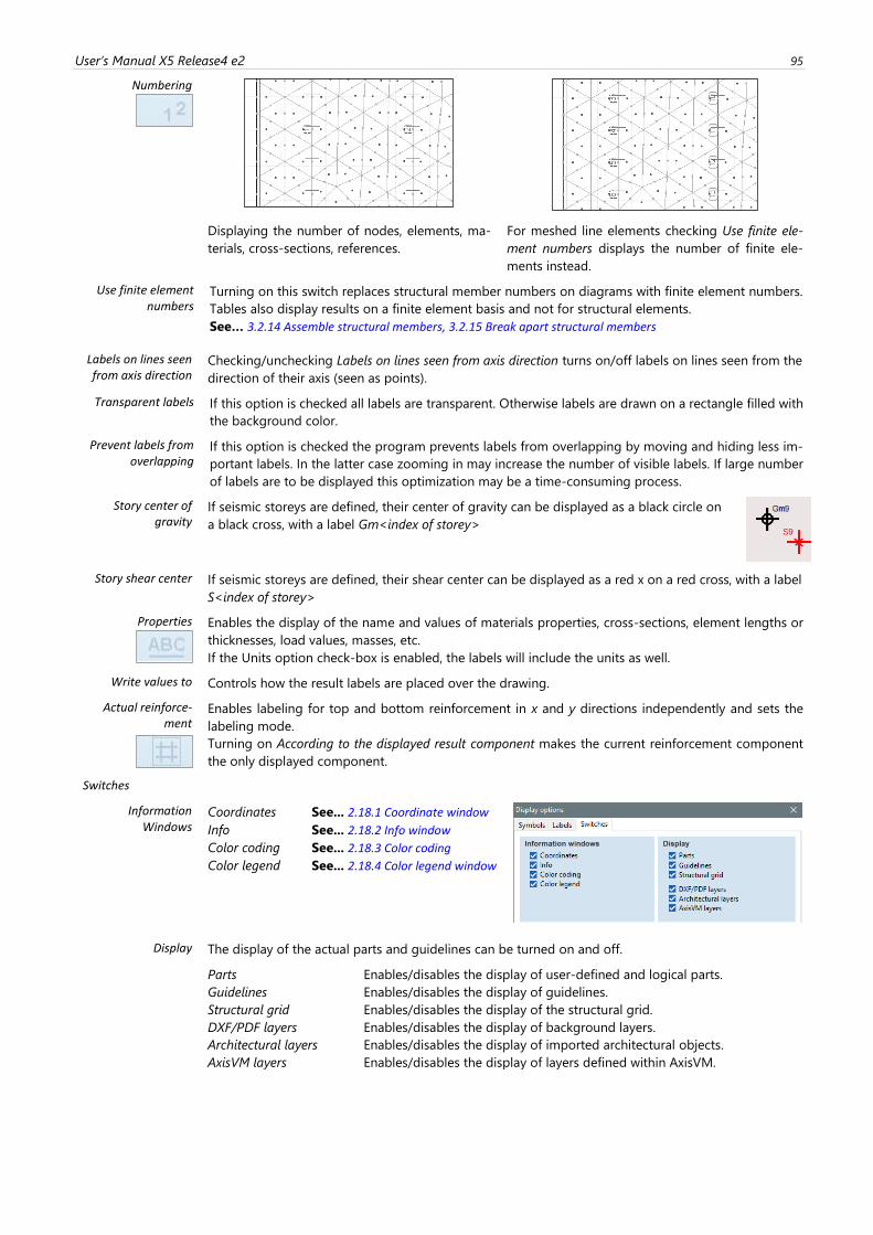
User’s Manual X5 Release4 e2 95

Numbering

Displaying the number of nodes, elements, ma-

terials, cross-sections, references.

For meshed line elements checking Use finite ele-

ment numbers displays the number of finite ele-

ments instead.

Use finite element numbers

Turning on this switch replaces structural member numbers on diagrams with finite element numbers.

Tables also display results on a finite element basis and not for structural elements.

See… 3.2.14 Assemble structural members, 3.2.15 Break apart structural members

Labels on lines seen from axis direction

Checking/unchecking Labels on lines seen from axis direction turns on/off labels on lines seen from the

direction of their axis (seen as points).

Transparent labels If this option is checked all labels are transparent. Otherwise labels are drawn on a rectangle filled with

the background color.

Prevent labels from overlapping

If this option is checked the program prevents labels from overlapping by moving and hiding less im-

portant labels. In the latter case zooming in may increase the number of visible labels. If large number

of labels are to be displayed this optimization may be a time-consuming process.

Story center of gravity

If seismic storeys are defined, their center of gravity can be displayed as a black circle on

a black cross, with a label Gm<index of storey>

Story shear center If seismic storeys are defined, their shear center can be displayed as a red x on a red cross, with a label

S<index of storey>

Properties

Enables the display of the name and values of materials properties, cross-sections, element lengths or

thicknesses, load values, masses, etc.

If the Units option check-box is enabled, the labels will include the units as well.

Write values to Controls how the result labels are placed over the drawing.

Actual reinforce-ment

Enables labeling for top and bottom reinforcement in x and y directions independently and sets the

labeling mode.

Turning on According to the displayed result component makes the current reinforcement component

the only displayed component.

Switches

Information Windows

Coordinates See... 2.18.1 Coordinate window

Info See... 2.18.2 Info window

Color coding See... 2.18.3 Color coding

Color legend See... 2.18.4 Color legend window

Display The display of the actual parts and guidelines can be turned on and off.

Parts Enables/disables the display of user-defined and logical parts.

Guidelines Enables/disables the display of guidelines.

Structural grid Enables/disables the display of the structural grid.

DXF/PDF layers Enables/disables the display of background layers.

Architectural layers Enables/disables the display of imported architectural objects.

AxisVM layers Enables/disables the display of layers defined within AxisVM.

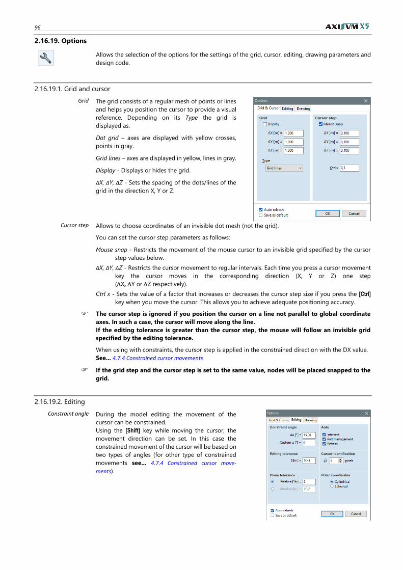
96

2.16.19. Options

Allows the selection of the options for the settings of the grid, cursor, editing, drawing parameters and

design code.

2.16.19.1. Grid and cursor

Grid

The grid consists of a regular mesh of points or lines

and helps you position the cursor to provide a visual

reference. Depending on its Type the grid is

displayed as:

Dot grid – axes are displayed with yellow crosses,

points in gray.

Grid lines – axes are displayed in yellow, lines in gray.

Display - Displays or hides the grid.

ΔX, ΔY, ΔZ - Sets the spacing of the dots/lines of the

grid in the direction X, Y or Z.

Cursor step Allows to choose coordinates of an invisible dot mesh (not the grid).

You can set the cursor step parameters as follows:

Mouse snap - Restricts the movement of the mouse cursor to an invisible grid specified by the cursor

step values below.

ΔX, ΔY, ΔZ - Restricts the cursor movement to regular intervals. Each time you press a cursor movement

key the cursor moves in the corresponding direction (X, Y or Z) one step

(X, Y or Z respectively).

Ctrl x - Sets the value of a factor that increases or decreases the cursor step size if you press the [Ctrl]

key when you move the cursor. This allows you to achieve adequate positioning accuracy.

The cursor step is ignored if you position the cursor on a line not parallel to global coordinate

axes. In such a case, the cursor will move along the line.

If the editing tolerance is greater than the cursor step, the mouse will follow an invisible grid

specified by the editing tolerance.

When using with constraints, the cursor step is applied in the constrained direction with the DX value.

See... 4.7.4 Constrained cursor movements

If the grid step and the cursor step is set to the same value, nodes will be placed snapped to the

grid.

2.16.19.2. Editing

Constraint angle During the model editing the movement of the

cursor can be constrained.

Using the [Shift] key while moving the cursor, the

movement direction can be set. In this case the

constrained movement of the cursor will be based on

two types of angles (for other type of constrained

movements see... 4.7.4 Constrained cursor move-

ments).

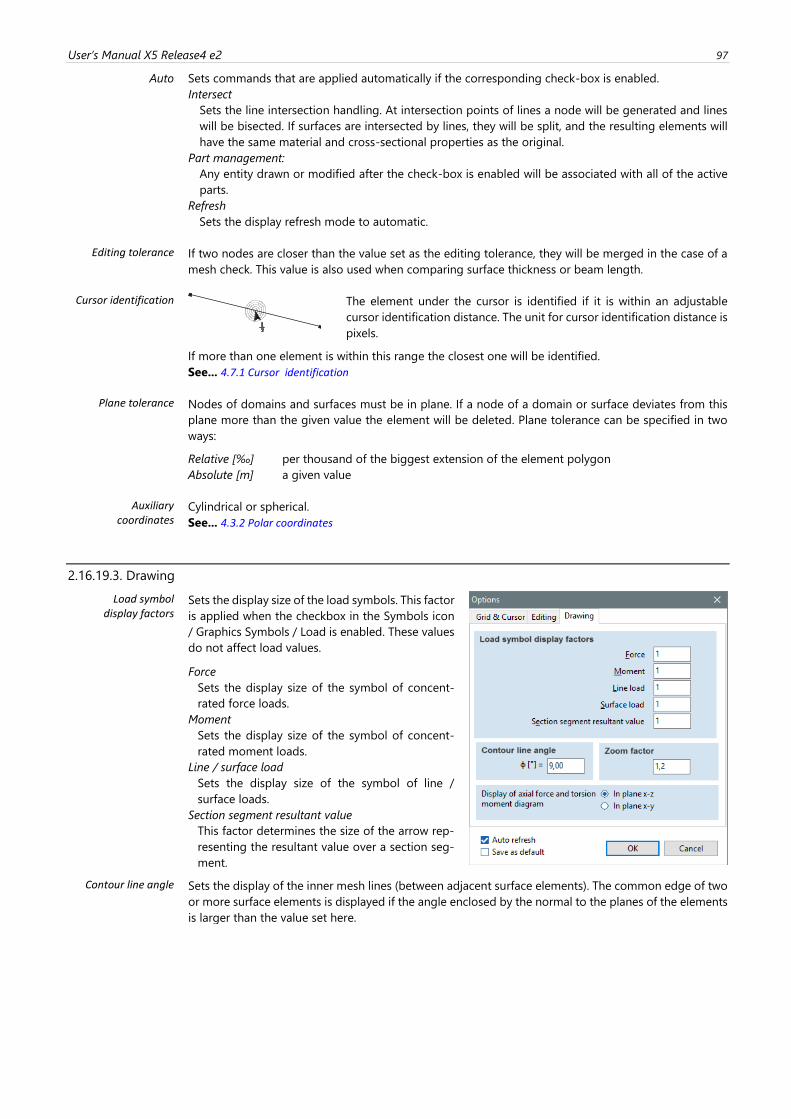
User’s Manual X5 Release4 e2 97

Auto Sets commands that are applied automatically if the corresponding check-box is enabled.

Intersect

Sets the line intersection handling. At intersection points of lines a node will be generated and lines

will be bisected. If surfaces are intersected by lines, they will be split, and the resulting elements will

have the same material and cross-sectional properties as the original.

Part management:

Any entity drawn or modified after the check-box is enabled will be associated with all of the active

parts.

Refresh

Sets the display refresh mode to automatic.

Editing tolerance If two nodes are closer than the value set as the editing tolerance, they will be merged in the case of a

mesh check. This value is also used when comparing surface thickness or beam length.

Cursor identification

The element under the cursor is identified if it is within an adjustable

cursor identification distance. The unit for cursor identification distance is

pixels.

If more than one element is within this range the closest one will be identified.

See... 4.7.1 Cursor identification

Plane tolerance Nodes of domains and surfaces must be in plane. If a node of a domain or surface deviates from this

plane more than the given value the element will be deleted. Plane tolerance can be specified in two

ways:

Relative [‰] per thousand of the biggest extension of the element polygon

Absolute [m] a given value

Auxiliary coordinates

Cylindrical or spherical.

See... 4.3.2 Polar coordinates

2.16.19.3. Drawing

Load symbol display factors

Sets the display size of the load symbols. This factor

is applied when the checkbox in the Symbols icon

/ Graphics Symbols / Load is enabled. These values

do not affect load values.

Force

Sets the display size of the symbol of concent-

rated force loads.

Moment

Sets the display size of the symbol of concent-

rated moment loads.

Line / surface load

Sets the display size of the symbol of line /

surface loads.

Section segment resultant value

This factor determines the size of the arrow rep-

resenting the resultant value over a section seg-

ment.

Contour line angle Sets the display of the inner mesh lines (between adjacent surface elements). The common edge of two

or more surface elements is displayed if the angle enclosed by the normal to the planes of the elements

is larger than the value set here.

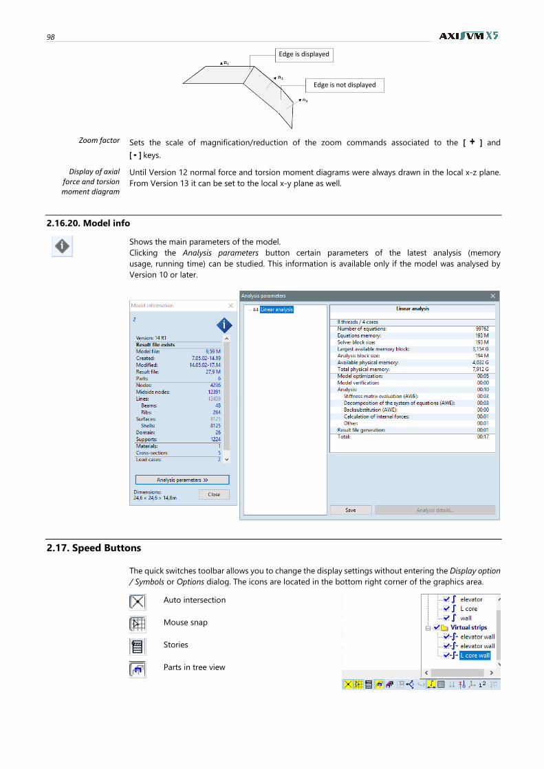
98

Zoom factor Sets the scale of magnification/reduction of the zoom commands associated to the [ + ] and

[ - ] keys.

Display of axial force and torsion moment diagram

Until Version 12 normal force and torsion moment diagrams were always drawn in the local x-z plane.

From Version 13 it can be set to the local x-y plane as well.

2.16.20. Model info

Shows the main parameters of the model.

Clicking the Analysis parameters button certain parameters of the latest analysis (memory

usage, running time) can be studied. This information is available only if the model was analysed by

Version 10 or later.

2.17. Speed Buttons

The quick switches toolbar allows you to change the display settings without entering the Display option

/ Symbols or Options dialog. The icons are located in the bottom right corner of the graphics area.

Auto intersection

Mouse snap

Stories

Parts in tree view

Edge is displayed

Edge is not displayed

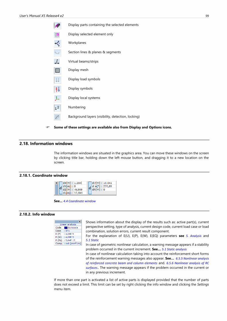
User’s Manual X5 Release4 e2 99

Display parts containing the selected elements

Display selected element only

Workplanes

Section lines & planes & segments

Virtual beams/strips

Display mesh

Display load symbols

Display symbols

Display local systems

Numbering

Background layers (visibility, detection, locking)

Some of these settings are available also from Display and Options icons.

2.18. Information windows

The information windows are situated in the graphics area. You can move these windows on the screen

by clicking title bar, holding down the left mouse button, and dragging it to a new location on the

screen.

2.18.1. Coordinate window

See... 4.4 Coordinate window

2.18.2. Info window

Shows information about the display of the results such as: active part(s), current

perspective setting, type of analysis, current design code, current load case or load

combination, solution errors, current result component.

For the explanation of E(U), E(P), E(W), E(EQ) parameters see 5. Analysis and

5.1 Static

In case of geometric nonlinear calculation, a warning message appears if a stability

problem occurred in the current increment. See… 5.1 Static analysis

In case of nonlinear calculation taking into account the reinforcement short forms

of the reinforcement warning messages also appear. See… 6.5.5 Nonlinear analysis

of reinforced concrete beam and column elements and. 6.5.6 Nonlinear analysis of RC

surfaces.. The warning message appears if the problem occurred in the current or

in any previous increment.

If more than one part is activated a list of active parts is displayed provided that the number of parts

does not exceed a limit. This limit can be set by right clicking the info window and clicking the Settings

menu item.

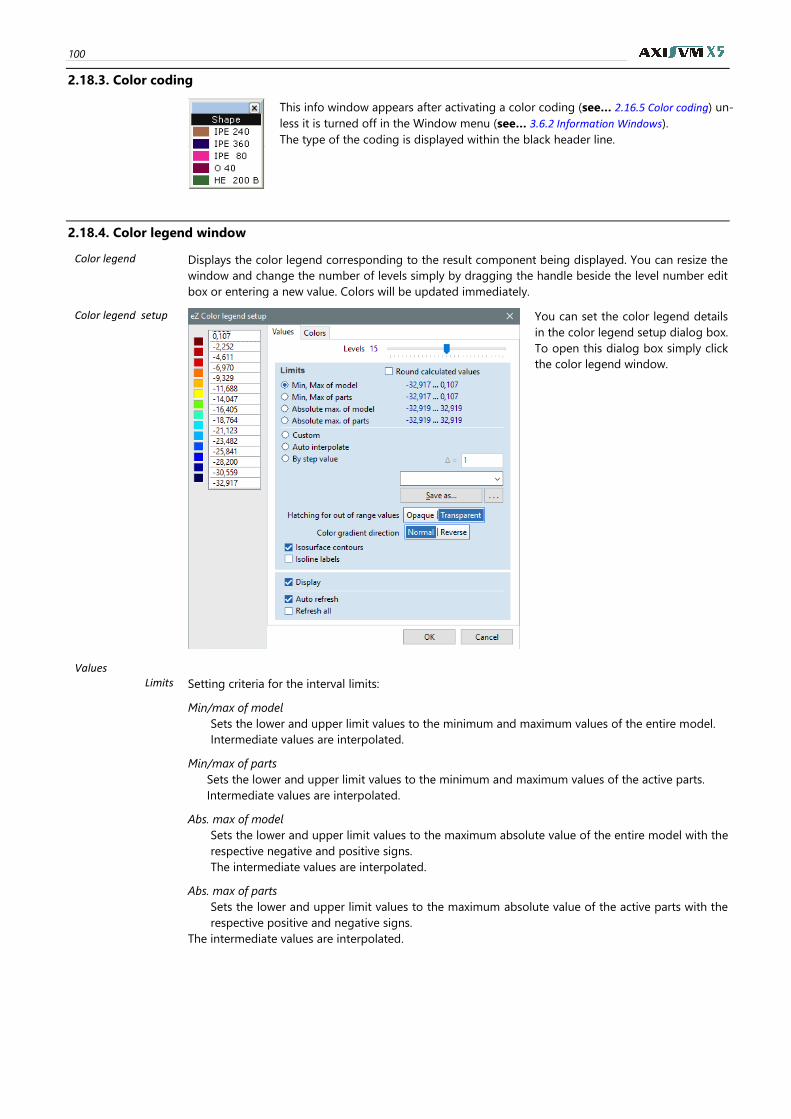
100

2.18.3. Color coding

This info window appears after activating a color coding (see… 2.16.5 Color coding) un-

less it is turned off in the Window menu (see… 3.6.2 Information Windows).

The type of the coding is displayed within the black header line.

2.18.4. Color legend window

Color legend

Displays the color legend corresponding to the result component being displayed. You can resize the

window and change the number of levels simply by dragging the handle beside the level number edit

box or entering a new value. Colors will be updated immediately.

Color legend setup

You can set the color legend details

in the color legend setup dialog box.

To open this dialog box simply click

the color legend window.

Values

Limits Setting criteria for the interval limits:

Min/max of model

Sets the lower and upper limit values to the minimum and maximum values of the entire model.

Intermediate values are interpolated.

Min/max of parts

Sets the lower and upper limit values to the minimum and maximum values of the active parts.

Intermediate values are interpolated.

Abs. max of model

Sets the lower and upper limit values to the maximum absolute value of the entire model with the

respective negative and positive signs.

The intermediate values are interpolated.

Abs. max of parts

Sets the lower and upper limit values to the maximum absolute value of the active parts with the

respective positive and negative signs.

The intermediate values are interpolated.

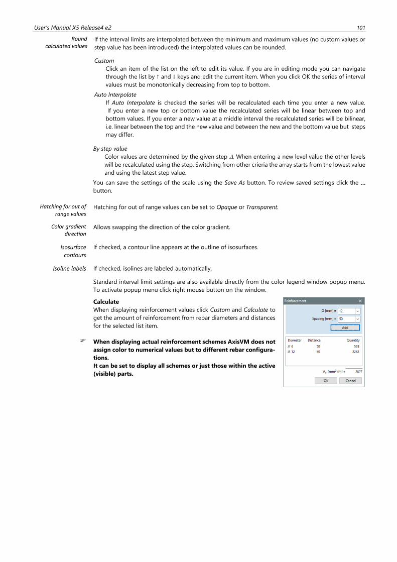
User’s Manual X5 Release4 e2 101

Round calculated values

If the interval limits are interpolated between the minimum and maximum values (no custom values or

step value has been introduced) the interpolated values can be rounded.

Custom

Click an item of the list on the left to edit its value. If you are in editing mode you can navigate

through the list by ↑ and ↓ keys and edit the current item. When you click OK the series of interval

values must be monotonically decreasing from top to bottom.

Auto Interpolate

If Auto Interpolate is checked the series will be recalculated each time you enter a new value.

If you enter a new top or bottom value the recalculated series will be linear between top and

bottom values. If you enter a new value at a middle interval the recalculated series will be bilinear,

i.e. linear between the top and the new value and between the new and the bottom value but steps

may differ.

By step value

Color values are determined by the given step . When entering a new level value the other levels

will be recalculated using the step. Switching from other crieria the array starts from the lowest value

and using the latest step value.

You can save the settings of the scale using the Save As button. To review saved settings click the ...

button.

Hatching for out of range values

Hatching for out of range values can be set to Opaque or Transparent.

Color gradient direction

Allows swapping the direction of the color gradient.

Isosurface

contours

If checked, a contour line appears at the outline of isosurfaces.

Isoline labels If checked, isolines are labeled automatically.

Standard interval limit settings are also available directly from the color legend window popup menu.

To activate popup menu click right mouse button on the window.

Calculate

When displaying reinforcement values click Custom and Calculate to

get the amount of reinforcement from rebar diameters and distances

for the selected list item.

When displaying actual reinforcement schemes AxisVM does not

assign color to numerical values but to different rebar configura-

tions.

It can be set to display all schemes or just those within the active

(visible) parts.

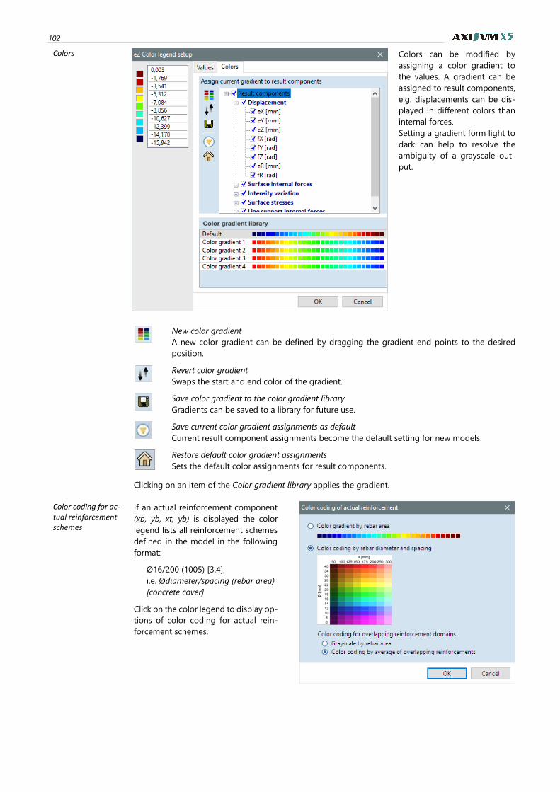
102

Colors

Colors can be modified by

assigning a color gradient to

the values. A gradient can be

assigned to result components,

e.g. displacements can be dis-

played in different colors than

internal forces.

Setting a gradient form light to

dark can help to resolve the

ambiguity of a grayscale out-

put.

New color gradient

A new color gradient can be defined by dragging the gradient end points to the desired

position.

Revert color gradient

Swaps the start and end color of the gradient.

Save color gradient to the color gradient library

Gradients can be saved to a library for future use.

Save current color gradient assignments as default

Current result component assignments become the default setting for new models.

Restore default color gradient assignments

Sets the default color assignments for result components.

Clicking on an item of the Color gradient library applies the gradient.

Color coding for ac-tual reinforcement schemes

If an actual reinforcement component

(xb, yb, xt, yb) is displayed the color

legend lists all reinforcement schemes

defined in the model in the following

format:

Ø16/200 (1005) [3.4],

i.e. Ødiameter/spacing (rebar area)

[concrete cover]

Click on the color legend to display op-

tions of color coding for actual rein-

forcement schemes.

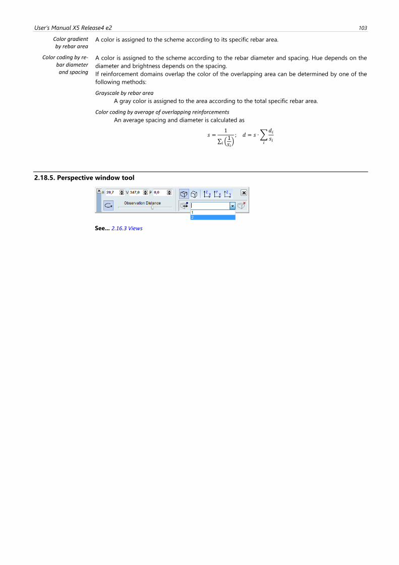
User’s Manual X5 Release4 e2 103

Color gradient by rebar area

A color is assigned to the scheme according to its specific rebar area.

Color coding by re-bar diameter and spacing

A color is assigned to the scheme according to the rebar diameter and spacing. Hue depends on the

diameter and brightness depends on the spacing.

If reinforcement domains overlap the color of the overlapping area can be determined by one of the

following methods:

Grayscale by rebar area

A gray color is assigned to the area according to the total specific rebar area.

Color coding by average of overlapping reinforcements

An average spacing and diameter is calculated as

𝑠 =1

∑ (1𝑠𝑖)𝑖

; 𝑑 = 𝑠 ∙∑𝑑𝑖𝑠𝑖

𝑖

2.18.5. Perspective window tool

See... 2.16.3 Views

104

This page is intentionally left blank.

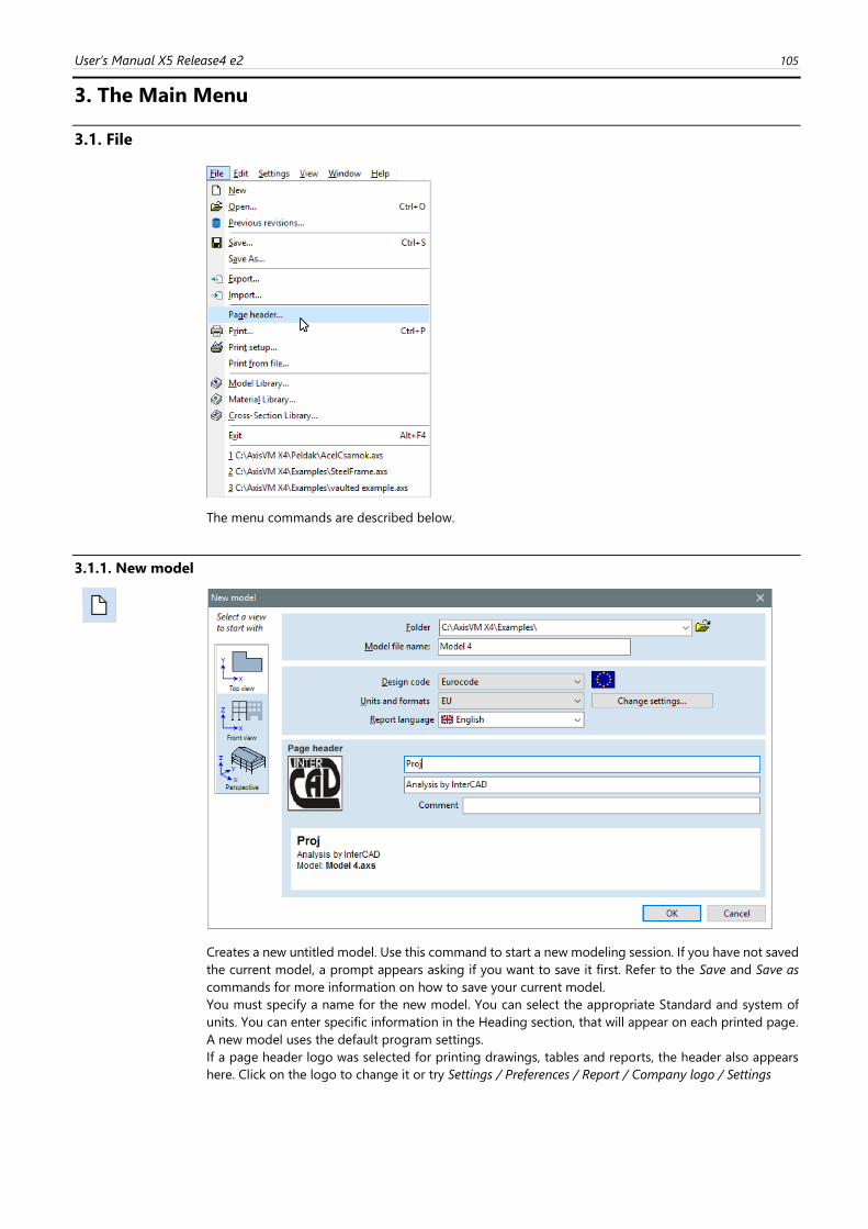
User’s Manual X5 Release4 e2 105

3. The Main Menu

3.1. File

The menu commands are described below.

3.1.1. New model

Creates a new untitled model. Use this command to start a new modeling session. If you have not saved

the current model, a prompt appears asking if you want to save it first. Refer to the Save and Save as

commands for more information on how to save your current model.

You must specify a name for the new model. You can select the appropriate Standard and system of

units. You can enter specific information in the Heading section, that will appear on each printed page.

A new model uses the default program settings.

If a page header logo was selected for printing drawings, tables and reports, the header also appears

here. Click on the logo to change it or try Settings / Preferences / Report / Company logo / Settings

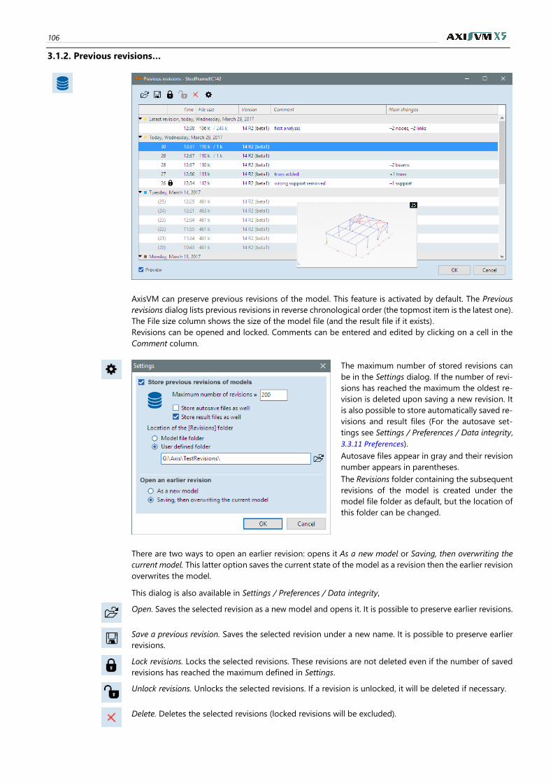
106

3.1.2. Previous revisions…

AxisVM can preserve previous revisions of the model. This feature is activated by default. The Previous

revisions dialog lists previous revisions in reverse chronological order (the topmost item is the latest one).

The File size column shows the size of the model file (and the result file if it exists).

Revisions can be opened and locked. Comments can be entered and edited by clicking on a cell in the

Comment column.

The maximum number of stored revisions can

be in the Settings dialog. If the number of revi-

sions has reached the maximum the oldest re-

vision is deleted upon saving a new revision. It

is also possible to store automatically saved re-

visions and result files (For the autosave set-

tings see Settings / Preferences / Data integrity,

3.3.11 Preferences).

Autosave files appear in gray and their revision

number appears in parentheses.

The Revisions folder containing the subsequent

revisions of the model is created under the

model file folder as default, but the location of

this folder can be changed.

There are two ways to open an earlier revision: opens it As a new model or Saving, then overwriting the

current model. This latter option saves the current state of the model as a revision then the earlier revision

overwrites the model.

This dialog is also available in Settings / Preferences / Data integrity,

Open. Saves the selected revision as a new model and opens it. It is possible to preserve earlier revisions.

Save a previous revision. Saves the selected revision under a new name. It is possible to preserve earlier

revisions.

Lock revisions. Locks the selected revisions. These revisions are not deleted even if the number of saved

revisions has reached the maximum defined in Settings.

Unlock revisions. Unlocks the selected revisions. If a revision is unlocked, it will be deleted if necessary.

Delete. Deletes the selected revisions (locked revisions will be excluded).

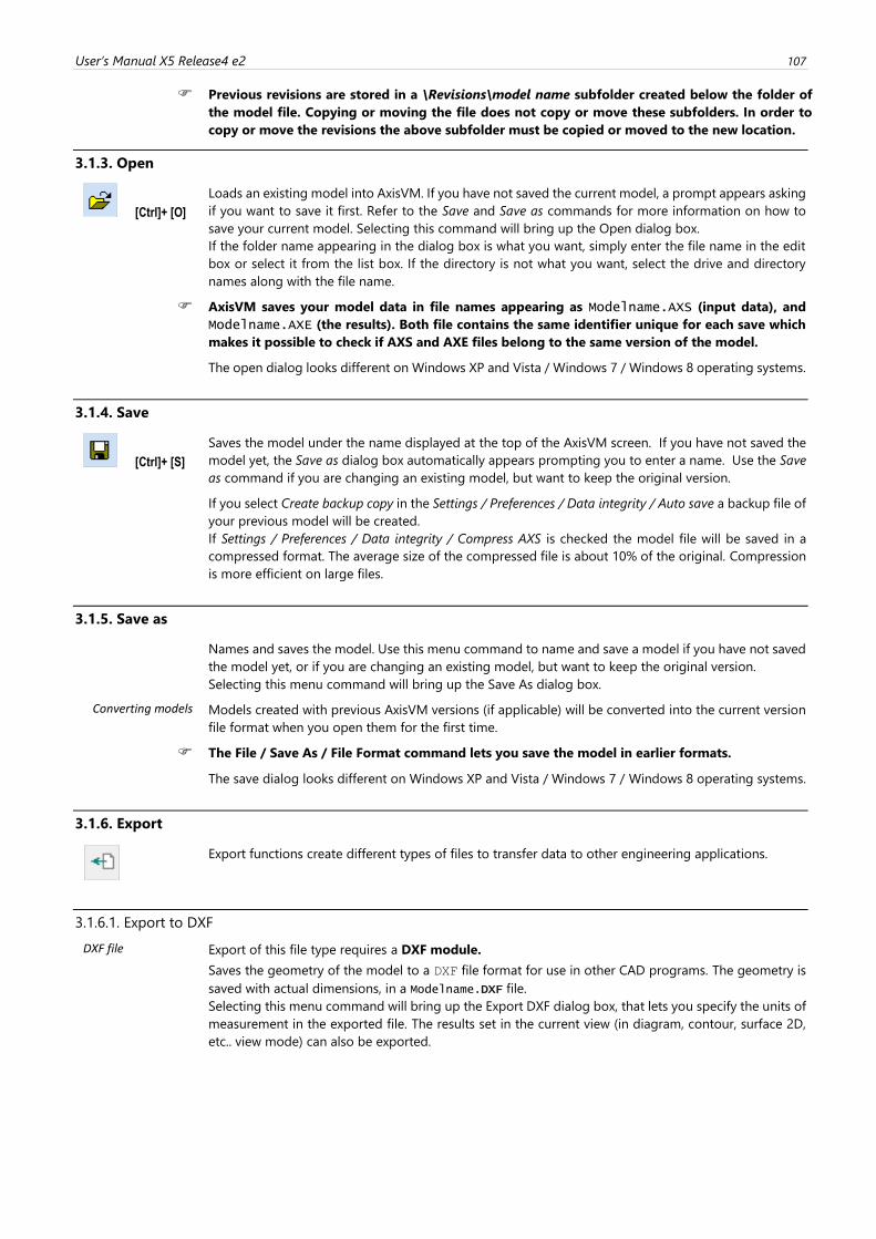
User’s Manual X5 Release4 e2 107

Previous revisions are stored in a \Revisions\model name subfolder created below the folder of

the model file. Copying or moving the file does not copy or move these subfolders. In order to

copy or move the revisions the above subfolder must be copied or moved to the new location.

3.1.3. Open

[Ctrl]+ [O]

Loads an existing model into AxisVM. If you have not saved the current model, a prompt appears asking

if you want to save it first. Refer to the Save and Save as commands for more information on how to

save your current model. Selecting this command will bring up the Open dialog box.

If the folder name appearing in the dialog box is what you want, simply enter the file name in the edit

box or select it from the list box. If the directory is not what you want, select the drive and directory

names along with the file name.

AxisVM saves your model data in file names appearing as Modelname.AXS (input data), and

Modelname.AXE (the results). Both file contains the same identifier unique for each save which

makes it possible to check if AXS and AXE files belong to the same version of the model.

The open dialog looks different on Windows XP and Vista / Windows 7 / Windows 8 operating systems.

3.1.4. Save

[Ctrl]+ [S]

Saves the model under the name displayed at the top of the AxisVM screen. If you have not saved the

model yet, the Save as dialog box automatically appears prompting you to enter a name. Use the Save

as command if you are changing an existing model, but want to keep the original version.

If you select Create backup copy in the Settings / Preferences / Data integrity / Auto save a backup file of

your previous model will be created.

If Settings / Preferences / Data integrity / Compress AXS is checked the model file will be saved in a

compressed format. The average size of the compressed file is about 10% of the original. Compression

is more efficient on large files.

3.1.5. Save as

Names and saves the model. Use this menu command to name and save a model if you have not saved

the model yet, or if you are changing an existing model, but want to keep the original version.

Selecting this menu command will bring up the Save As dialog box.

Converting models Models created with previous AxisVM versions (if applicable) will be converted into the current version

file format when you open them for the first time.

The File / Save As / File Format command lets you save the model in earlier formats.

The save dialog looks different on Windows XP and Vista / Windows 7 / Windows 8 operating systems.

3.1.6. Export

Export functions create different types of files to transfer data to other engineering applications.

3.1.6.1. Export to DXF

DXF file Export of this file type requires a DXF module.

Saves the geometry of the model to a DXF file format for use in other CAD programs. The geometry is

saved with actual dimensions, in a Modelname.DXF file.

Selecting this menu command will bring up the Export DXF dialog box, that lets you specify the units of

measurement in the exported file. The results set in the current view (in diagram, contour, surface 2D,

etc.. view mode) can also be exported.

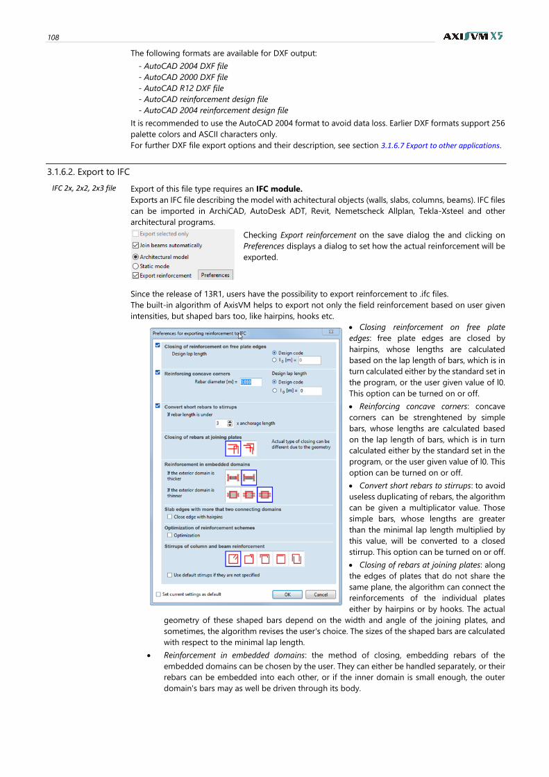
108

The following formats are available for DXF output:

- AutoCAD 2004 DXF file

- AutoCAD 2000 DXF file

- AutoCAD R12 DXF file

- AutoCAD reinforcement design file

- AutoCAD 2004 reinforcement design file

It is recommended to use the AutoCAD 2004 format to avoid data loss. Earlier DXF formats support 256

palette colors and ASCII characters only.

For further DXF file export options and their description, see section 3.1.6.7 Export to other applications.

3.1.6.2. Export to IFC

IFC 2x, 2x2, 2x3 file

Export of this file type requires an IFC module.

Exports an IFC file describing the model with achitectural objects (walls, slabs, columns, beams). IFC files

can be imported in ArchiCAD, AutoDesk ADT, Revit, Nemetscheck Allplan, Tekla-Xsteel and other

architectural programs.

Checking Export reinforcement on the save dialog the and clicking on

Preferences displays a dialog to set how the actual reinforcement will be

exported.

Since the release of 13R1, users have the possibility to export reinforcement to .ifc files.

The built-in algorithm of AxisVM helps to export not only the field reinforcement based on user given

intensities, but shaped bars too, like hairpins, hooks etc.

• Closing reinforcement on free plate

edges: free plate edges are closed by

hairpins, whose lengths are calculated

based on the lap length of bars, which is in

turn calculated either by the standard set in

the program, or the user given value of l0.

This option can be turned on or off.

• Reinforcing concave corners: concave

corners can be strenghtened by simple

bars, whose lengths are calculated based

on the lap length of bars, which is in turn

calculated either by the standard set in the

program, or the user given value of l0. This

option can be turned on or off.

• Convert short rebars to stirrups: to avoid

useless duplicating of rebars, the algorithm

can be given a multiplicator value. Those

simple bars, whose lengths are greater

than the minimal lap length multiplied by

this value, will be converted to a closed

stirrup. This option can be turned on or off.

• Closing of rebars at joining plates: along

the edges of plates that do not share the

same plane, the algorithm can connect the

reinforcements of the individual plates

either by hairpins or by hooks. The actual

geometry of these shaped bars depend on the width and angle of the joining plates, and

sometimes, the algorithm revises the user's choice. The sizes of the shaped bars are calculated

with respect to the minimal lap length.

• Reinforcement in embedded domains: the method of closing, embedding rebars of the

embedded domains can be chosen by the user. They can either be handled separately, or their

rebars can be embedded into each other, or if the inner domain is small enough, the outer

domain's bars may as well be driven through its body.

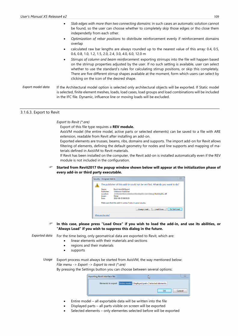
User’s Manual X5 Release4 e2 109

• Slab edges with more than two connecting domains: in such cases an automatic solution cannot

be found, so the user can choose whether to completely skip those edges or tho close them

independetly from each other.

• Optimization of rebar positions to distribute reinforcement evenly if reinforcement domains

overlap

• calculated raw bar lengths are always rounded up to the nearest value of this array: 0.4, 0.5,

0.6, 0.8, 1.0, 1.2, 1.5, 2.0, 2.4, 3.0, 4.0, 6.0, 12.0 m

• Stirrups of column and beam reinforcement: exporting strirrups into the file will happen based

on the strirrup properties adjusted by the user. If no such setting is available, user can select

whether to use the standard’s rules for calculating stirrup positions, or skip this completely.

There are five different stirrup shapes available at the moment, form which users can select by

clicking on the icon of the desired shape.

Export model data

If the Architectural model option is selected only architectural objects will be exported. If Static model

is selected, finite element meshes, loads, load cases, load groups and load combinations will be included

in the IFC file. Dynamic, influence line or moving loads will be excluded.

3.1.6.3. Export to Revit

Export to Revit (*.are)

Export of this file type requires a REV module.

AxisVM model (the entire model, active parts or selected elements) can be saved to a file with ARE

extension, readable from Revit after installing an add-on.

Exported elements are trusses, beams, ribs, domains and supports. The import add-on for Revit allows

filtering of elements, defining the default geometry for nodes and line supports and mapping of ma-

terials defined in AxisVM to Revit materials.

If Revit has been installed on the computer, the Revit add-on is installed automatically even if the REV

module is not included in the configuration.

Started from Revit2017 the popup window shown below will appear at the initialization phase of

every add-in or third party executable.

In this case, please press "Load Once" if you wish to load the add-in, and use its abilities, or

"Always Load" if you wish to suppress this dialog in the future.

Exported data For the time being, only geomatrical data are exported to Revit, which are:

• linear elements with their materials and sections

• regions and their materials

• supports

Usage Export process must always be started from AxisVM, the way mentioned below:

File menu -> Export -> Export to revit (*.are)

By pressing the Settings button you can choose between several options:

• Entire model – all exportable data will be written into the file

• Displayed parts – all parts visible on screen will be exported

• Selected elements – only elementes selected before will be exported

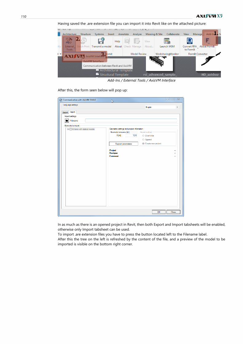
110

Having saved the .are extension file you can import it into Revit like on the attached picture:

Add-Ins / External Tools / AxisVM Interface

After this, the form seen below will pop up:

In as much as there is an opened project in Revit, then both Export and Import tabsheets will be enabled,

otherwise only Import tabsheet can be used.

To import .are extension files you have to press the button located left to the Filename label.

After this the tree on the left is refreshed by the content of the file, and a preview of the model to be

imported is visible on the bottom right corner.

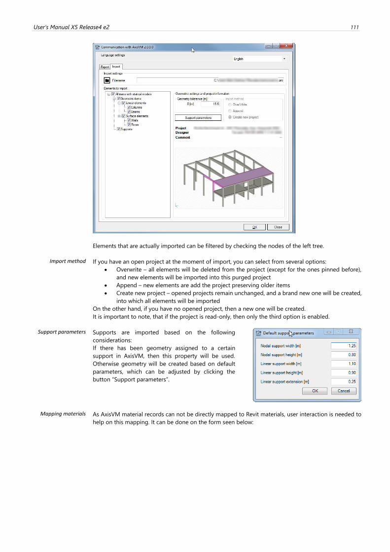
User’s Manual X5 Release4 e2 111

Elements that are actually imported can be filtered by checking the nodes of the left tree.

Import method If you have an open project at the moment of import, you can select from several options:

• Overwrite – all elements will be deleted from the project (except for the ones pinned before),

and new elements will be imported into this purged project

• Append – new elements are add the project preserving older items

• Create new project – opened projects remain unchanged, and a brand new one will be created,

into which all elements will be imported

On the other hand, if you have no opened project, then a new one will be created.

It is important to note, that if the project is read-only, then only the third option is enabled.

Support parameters Supports are imported based on the following

considerations:

If there has been geometry assigned to a certain

support in AxisVM, then this property will be used.

Otherwise geometry will be created based on default

parameters, which can be adjusted by clicking the

button “Support parameters”.

Mapping materials As AxisVM material records can not be directly mapped to Revit materials, user interaction is needed to

help on this mapping. It can be done on the form seen below:

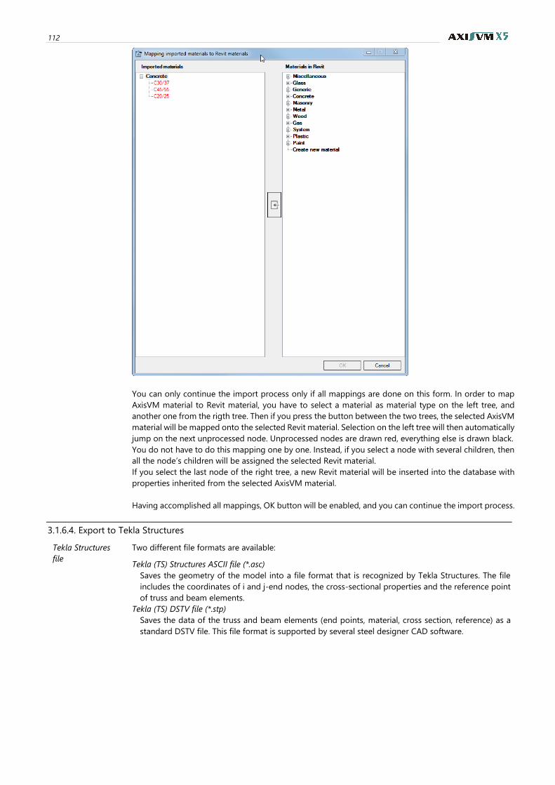
112

You can only continue the import process only if all mappings are done on this form. In order to map

AxisVM material to Revit material, you have to select a material as material type on the left tree, and

another one from the rigth tree. Then if you press the button between the two trees, the selected AxisVM

material will be mapped onto the selected Revit material. Selection on the left tree will then automatically

jump on the next unprocessed node. Unprocessed nodes are drawn red, everything else is drawn black.

You do not have to do this mapping one by one. Instead, if you select a node with several children, then

all the node’s children will be assigned the selected Revit material.

If you select the last node of the right tree, a new Revit material will be inserted into the database with

properties inherited from the selected AxisVM material.

Having accomplished all mappings, OK button will be enabled, and you can continue the import process.

3.1.6.4. Export to Tekla Structures

Tekla Structures

file

Two different file formats are available:

Tekla (TS) Structures ASCII file (*.asc)

Saves the geometry of the model into a file format that is recognized by Tekla Structures. The file

includes the coordinates of i and j-end nodes, the cross-sectional properties and the reference point

of truss and beam elements.

Tekla (TS) DSTV file (*.stp)

Saves the data of the truss and beam elements (end points, material, cross section, reference) as a

standard DSTV file. This file format is supported by several steel designer CAD software.

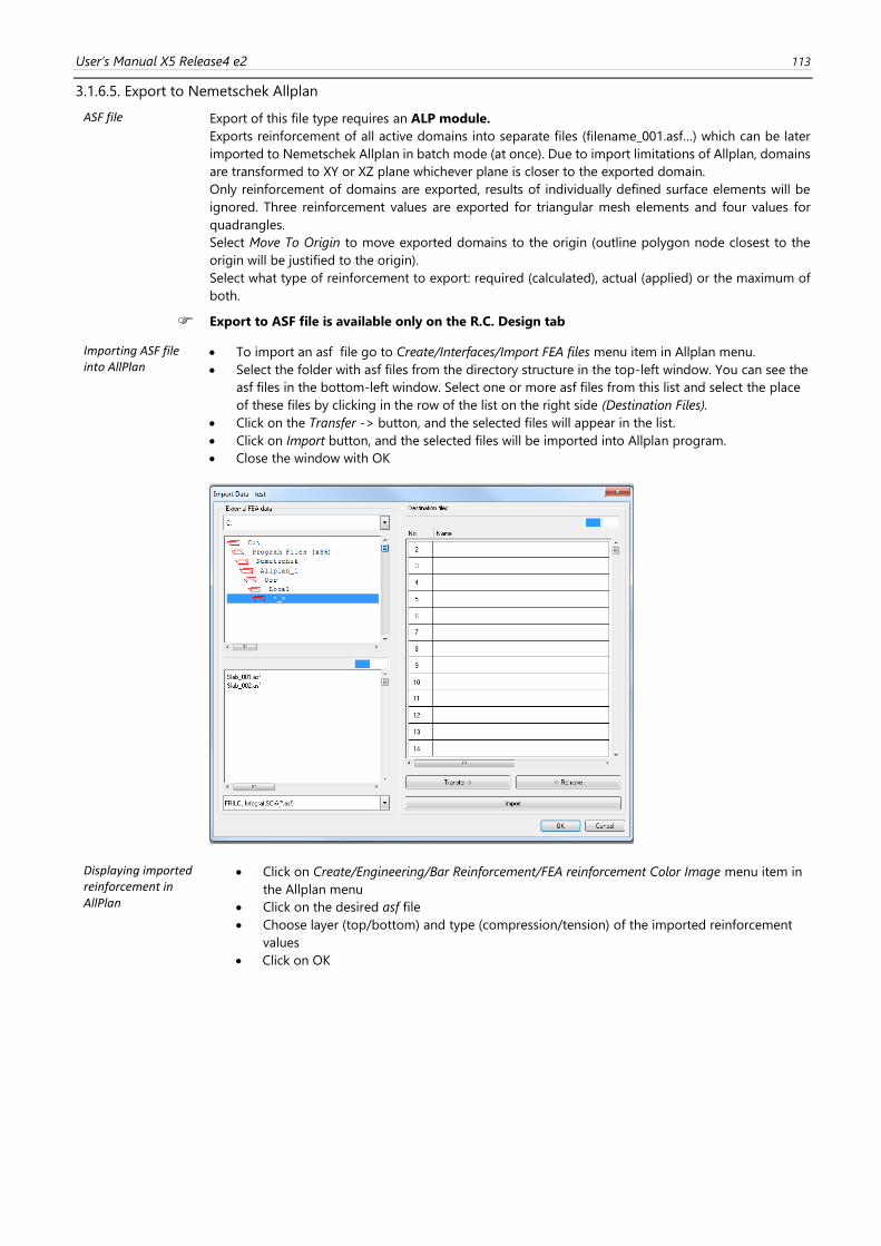
User’s Manual X5 Release4 e2 113

3.1.6.5. Export to Nemetschek Allplan

ASF file Export of this file type requires an ALP module.

Exports reinforcement of all active domains into separate files (filename_001.asf…) which can be later

imported to Nemetschek Allplan in batch mode (at once). Due to import limitations of Allplan, domains

are transformed to XY or XZ plane whichever plane is closer to the exported domain.

Only reinforcement of domains are exported, results of individually defined surface elements will be

ignored. Three reinforcement values are exported for triangular mesh elements and four values for

quadrangles.

Select Move To Origin to move exported domains to the origin (outline polygon node closest to the

origin will be justified to the origin).

Select what type of reinforcement to export: required (calculated), actual (applied) or the maximum of

both.

Export to ASF file is available only on the R.C. Design tab

Importing ASF file into AllPlan

• To import an asf file go to Create/Interfaces/Import FEA files menu item in Allplan menu.

• Select the folder with asf files from the directory structure in the top-left window. You can see the

asf files in the bottom-left window. Select one or more asf files from this list and select the place

of these files by clicking in the row of the list on the right side (Destination Files).

• Click on the Transfer -> button, and the selected files will appear in the list.

• Click on Import button, and the selected files will be imported into Allplan program.

• Close the window with OK

Displaying imported reinforcement in AllPlan

• Click on Create/Engineering/Bar Reinforcement/FEA reinforcement Color Image menu item in

the Allplan menu

• Click on the desired asf file

• Choose layer (top/bottom) and type (compression/tension) of the imported reinforcement

values

• Click on OK

114

3.1.6.6. Export to SAF file format

Export of this file type requires an SAF module.

This Excel-based file format supports exchange of structural model data with other applications support-

ing this protocol. The file consists of standardized spreadsheets with the geometry, structural and load

properties of the model, thus can be viewed and/or edited with Excel. SAF protocol is supported by

ArchiCAD, AllPlan, SCIA and RFEM.

Entities exported to the resulting file are

• trusses, beams, columns, ribs, supports, regions and connection elements (hinges, joints)

• cross-sections

• support stiffnesses

• load, load combinations

Usage Select File menu / Export / SAF export (*.xlsx), select the location and filename for the export and press

Save.

3.1.6.7. Export to other applications

Bocad file Saves the geometry of the model into a file format that is recognized by the Bocad software. The file

includes the coordinates of i and j-end nodes, the cross-sectional properties and the reference point of

truss and beam elements.

StatikPlan file For StatikPlan AxisVM exports a DXF file including the contour of the reinforced concrete plate, the

calculated reinforcements as isolines and the result legends on different layers.

PianoCA file Generates a *.pia interface file for PianoCA. It includes the data, supports, loads and the calculated

results of the selected beam elements.

CADWork file Creates a DXF file to use in CADWork reinforcement detailing software.

Only selected domains will be exported.

As CADWork works in 2D, selected domains must be in the same plane. Each domain in the DXF file is

transformed to a local X-Y coordinate system, Z coordinate represents the calculated amount of rein-

forcement.

SDNF 2.0, 3.0 file Saves the model in SDNF (Steel Detailing Neutral Format) file readable by steel detailing products (Ad-

vance Steel, SDS/2, Tekla Structures, PDMS).

Glaser -isb cad- *.fem fájl

Exports reinforcement domains to the Glaser -isb cad-program.

3.1.6.8. Export to AxisVM

AxisVM Viewer Saves the model in AxisVM Viewer format (*.axv).

See… 7 AxisVM Viewer and Viewer Expert

AXS file The following groups of elements can be

exported: the entire structure, displayed

parts or selected elements.

To select export options similar to those

of the Copy options (see… 3.2.8 Copy /

paste options ) click the Settings button of

the Export dialog.

Export selected only Exports the selected elements only.

Coordinate units The coordinate units of the exported file

can be selected here.

The default unit is meter [m].

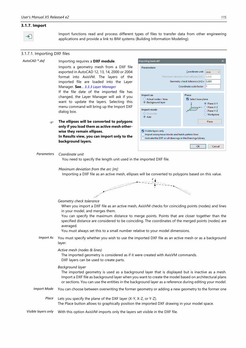
User’s Manual X5 Release4 e2 115

3.1.7. Import

Import functions read and process different types of files to transfer data from other engineering

applications and provide a link to BIM systems (Building Information Modeling).

3.1.7.1. Importing DXF files

AutoCAD *.dxf

Importing requires a DXF module.

Imports a geometry mesh from a DXF file

exported in AutoCAD 12, 13, 14, 2000 or 2004

format into AxisVM. The layers of the

imported file are loaded into the Layer

Manager. See... 3.3.3 Layer Manager

If the file date of the imported file has

changed, the Layer Manager will ask if you

want to update the layers. Selecting this

menu command will bring up the Import DXF

dialog box.

The ellipses will be converted to polygons

only if you load them as active mesh other-

wise they remain ellipses.

In Results view, you can import only to the

background layers.

Parameters Coordinate unit

You need to specify the length unit used in the imported DXF file.

Maximum deviation from the arc [m]:

Importing a DXF file as an active mesh, ellipses will be converted to polygons based on this value.

Geometry check tolerance

When you import a DXF file as an active mesh, AxisVM checks for coinciding points (nodes) and lines

in your model, and merges them.

You can specify the maximum distance to merge points. Points that are closer together than the

specified distance are considered to be coinciding. The coordinates of the merged points (nodes) are

averaged.

You must always set this to a small number relative to your model dimensions.

Import As You must specify whether you wish to use the imported DXF file as an active mesh or as a background

layer.

Active mesh (nodes & lines)

The imported geometry is considered as if it were created with AxisVM commands.

DXF layers can be used to create parts.

Background layer

The imported geometry is used as a background layer that is displayed but is inactive as a mesh.

Import a DXF file as background layer when you want to create the model based on architectural plans

or sections. You can use the entities in the background layer as a reference during editing your model.

Import Mode You can choose between overwriting the former geometry or adding a new geometry to the former one

Place

Lets you specify the plane of the DXF layer (X-Y, X-Z, or Y-Z).

The Place button allows to graphically position the imported DXF drawing in your model space.

Visible layers only With this option AxisVM imports only the layers set visible in the DXF file.

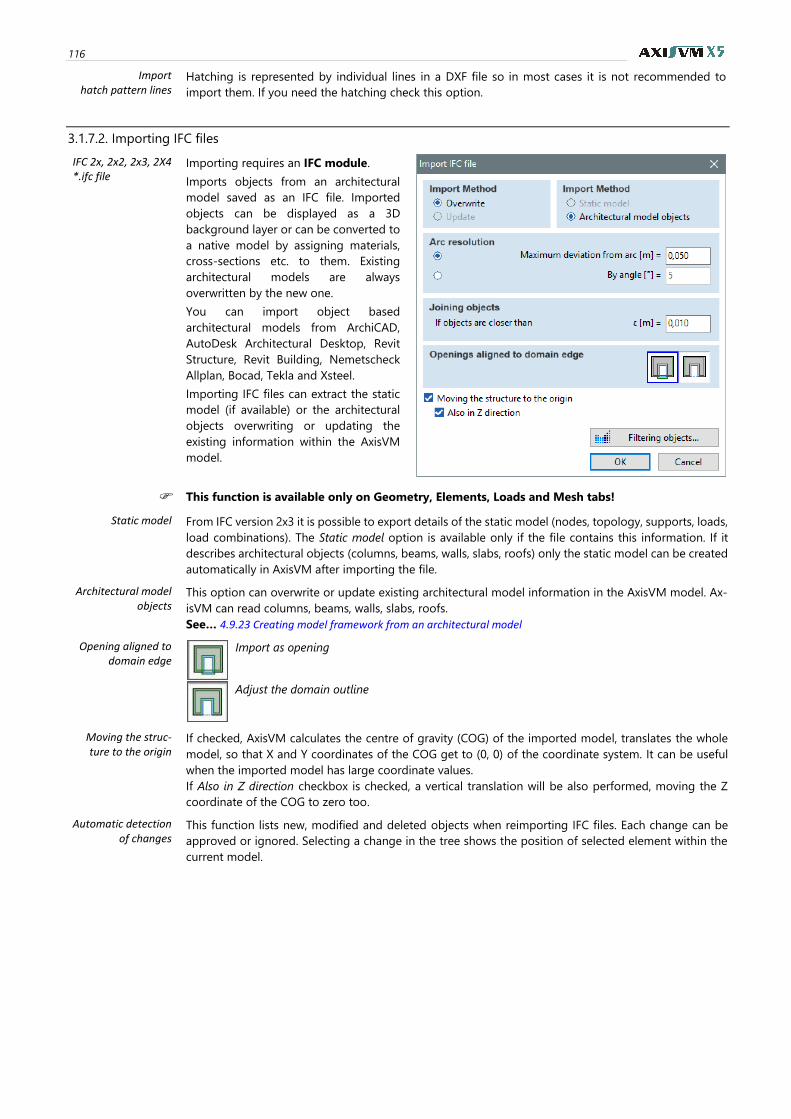
116

Import hatch pattern lines

Hatching is represented by individual lines in a DXF file so in most cases it is not recommended to

import them. If you need the hatching check this option.

3.1.7.2. Importing IFC files

IFC 2x, 2x2, 2x3, 2X4 *.ifc file

Importing requires an IFC module.

Imports objects from an architectural

model saved as an IFC file. Imported

objects can be displayed as a 3D

background layer or can be converted to

a native model by assigning materials,

cross-sections etc. to them. Existing

architectural models are always

overwritten by the new one.

You can import object based

architectural models from ArchiCAD,

AutoDesk Architectural Desktop, Revit

Structure, Revit Building, Nemetscheck

Allplan, Bocad, Tekla and Xsteel.

Importing IFC files can extract the static

model (if available) or the architectural

objects overwriting or updating the

existing information within the AxisVM

model.

This function is available only on Geometry, Elements, Loads and Mesh tabs!

Static model From IFC version 2x3 it is possible to export details of the static model (nodes, topology, supports, loads,

load combinations). The Static model option is available only if the file contains this information. If it

describes architectural objects (columns, beams, walls, slabs, roofs) only the static model can be created

automatically in AxisVM after importing the file.

Architectural model objects

This option can overwrite or update existing architectural model information in the AxisVM model. Ax-

isVM can read columns, beams, walls, slabs, roofs.

See… 4.9.23 Creating model framework from an architectural model

Opening aligned to domain edge

Import as opening

Adjust the domain outline

Moving the struc-ture to the origin

If checked, AxisVM calculates the centre of gravity (COG) of the imported model, translates the whole

model, so that X and Y coordinates of the COG get to (0, 0) of the coordinate system. It can be useful

when the imported model has large coordinate values.

If Also in Z direction checkbox is checked, a vertical translation will be also performed, moving the Z

coordinate of the COG to zero too.

Automatic detection of changes

This function lists new, modified and deleted objects when reimporting IFC files. Each change can be

approved or ignored. Selecting a change in the tree shows the position of selected element within the

current model.

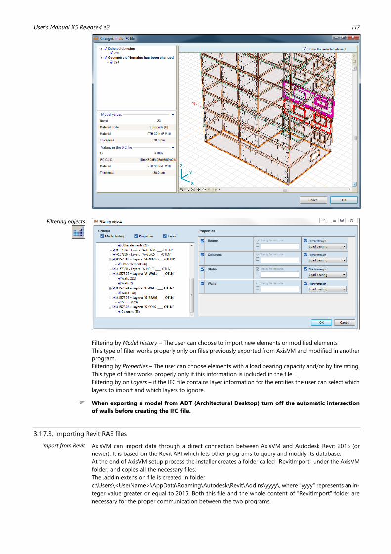
User’s Manual X5 Release4 e2 117

Filtering objects

Filtering by Model history – The user can choose to import new elements or modified elements

This type of filter works properly only on files previously exported from AxisVM and modified in another

program.

Filtering by Properties – The user can choose elements with a load bearing capacity and/or by fire rating.

This type of filter works properly only if this information is included in the file.

Filtering by on Layers – if the IFC file contains layer information for the entities the user can select which

layers to import and which layers to ignore.

When exporting a model from ADT (Architectural Desktop) turn off the automatic intersection

of walls before creating the IFC file.

3.1.7.3. Importing Revit RAE files

Import from Revit

AxisVM can import data through a direct connection between AxisVM and Autodesk Revit 2015 (or

newer). It is based on the Revit API which lets other programs to query and modify its database.

At the end of AxisVM setup process the installer creates a folder called "RevitImport" under the AxisVM

folder, and copies all the necessary files.

The .addin extension file is created in folder

c:\Users\<UserName>\AppData\Roaming\Autodesk\Revit\Addins\yyyy\, where "yyyy" represents an in-

teger value greater or equal to 2015. Both this file and the whole content of "RevitImport" folder are

necessary for the proper communication between the two programs.

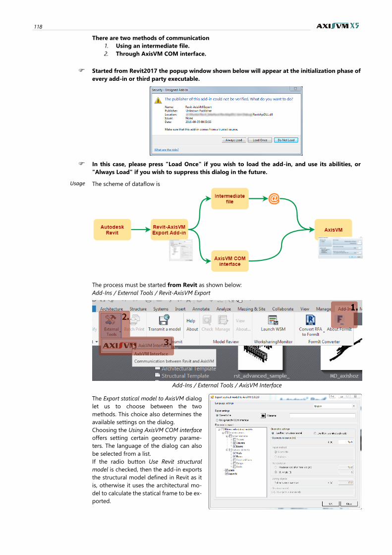
118

There are two methods of communication

1. Using an intermediate file.

2. Through AxisVM COM interface.

Started from Revit2017 the popup window shown below will appear at the initialization phase of

every add-in or third party executable.

In this case, please press "Load Once" if you wish to load the add-in, and use its abilities, or

"Always Load" if you wish to suppress this dialog in the future.

Usage The scheme of dataflow is

The process must be started from Revit as shown below:

Add-Ins / External Tools / Revit-AxisVM Export

Add-Ins / External Tools / AxisVM Interface

The Export statical model to AxisVM dialog

let us to choose between the two

methods. This choice also determines the

available settings on the dialog.

Choosing the Using AxisVM COM interface

offers setting certain geometry parame-

ters. The language of the dialog can also

be selected from a list.

If the radio button Use Revit structural

model is checked, then the add-in exports

the structural model defined in Revit as it

is, otherwise it uses the architectural mo-

del to calculate the statical frame to be ex-

ported.

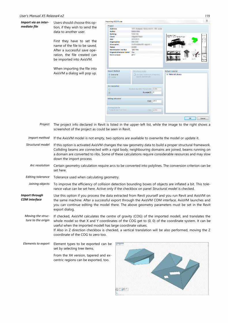
User’s Manual X5 Release4 e2 119

Import via an inter-mediate file

Users should choose this op-

tion, if they wish to send the

data to another user.

First they have to set the

name of the file to be saved.

After a successful save ope-

ration, the file created can

be imported into AxisVM.

When importing the file into

AxisVM a dialog will pop up.

Project The project info declared in Revit is listed in the upper-left list, while the image to the right shows a

screenshot of the project as could be seen in Revit.

Import method If the AxisVM model is not empty, two options are available to overwrite the model or update it.

Structural model If this option is activated AxisVM changes the raw geometry data to build a proper structural framework.

Colliding beams are connected with a rigid body, neighbouring domains are joined, beams running on

a domain are converted to ribs. Some of these calculations require considerable resources and may slow

down the import process.

Arc resolution Certain geometry calculation require arcs to be converted into polylines. The conversion criterion can be

set here.

Editing tolerance Tolerance used when calculating geometry.

Joining objects To improve the efficiency of collision detection bounding boxes of objects are inflated a bit. This tole-

rance value can be set here. Active only if the checkbox on panel Structural model is checked.

Import through COM interface

Use this option if you process the data extracted from Revit yourself and you run Revit and AxisVM on

the same machine. After a successful export through the AxisVM COM interface, AxisVM launches and

you can continue editing the model there. The above geometry parameters must be set in the Revit

export dialog.

Moving the struc-ture to the origin

If checked, AxisVM calculates the centre of gravity (COG) of the imported modell, and translates the

whole model so that X and Y coordinates of the COG get to (0, 0) of the coordinate system. It can be

useful when the imported modell has large coordinate values.

If Also in Z direction checkbox is checked, a vertical translation will be also performed, moving the Z

coordinate of the COG to zero too.

Elements to export Element types to be exported can be

set by selecting tree items.

From the X4 version, tapered and ex-

centric regions can be exported, too.

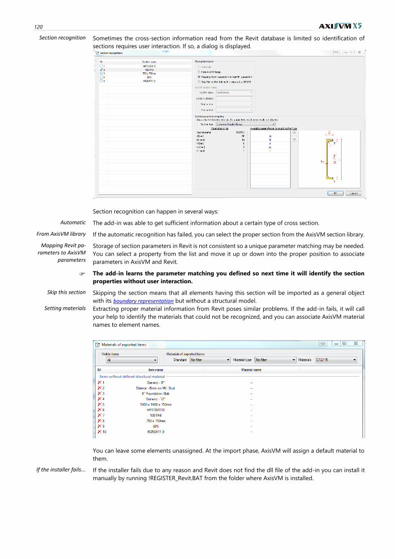
120

Section recognition Sometimes the cross-section information read from the Revit database is limited so identification of

sections requires user interaction. If so, a dialog is displayed.

Section recognition can happen in several ways:

Automatic The add-in was able to get sufficient information about a certain type of cross section.

From AxisVM library If the automatic recognition has failed, you can select the proper section from the AxisVM section library.

Mapping Revit pa-rameters to AxisVM

parameters

Storage of section parameters in Revit is not consistent so a unique parameter matching may be needed.

You can select a property from the list and move it up or down into the proper position to associate

parameters in AxisVM and Revit.

The add-in learns the parameter matching you defined so next time it will identify the section

properties without user interaction.

Skip this section Skipping the section means that all elements having this section will be imported as a general object

with its boundary representation but without a structural model.

Setting materials Extracting proper material information from Revit poses similar problems. If the add-in fails, it will call

your help to identify the materials that could not be recognized, and you can associate AxisVM material

names to element names.

You can leave some elements unassigned. At the import phase, AxisVM will assign a default material to

them.

If the installer fails... If the installer fails due to any reason and Revit does not find the dll file of the add-in you can install it

manually by running !REGISTER_Revit.BAT from the folder where AxisVM is installed.

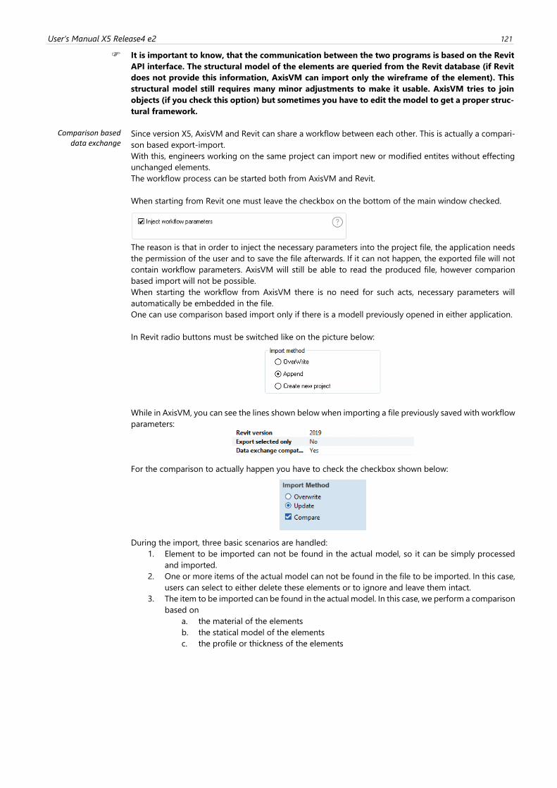
User’s Manual X5 Release4 e2 121

It is important to know, that the communication between the two programs is based on the Revit

API interface. The structural model of the elements are queried from the Revit database (if Revit

does not provide this information, AxisVM can import only the wireframe of the element). This

structural model still requires many minor adjustments to make it usable. AxisVM tries to join

objects (if you check this option) but sometimes you have to edit the model to get a proper struc-

tural framework.

Comparison based data exchange

Since version X5, AxisVM and Revit can share a workflow between each other. This is actually a compari-

son based export-import.

With this, engineers working on the same project can import new or modified entites without effecting

unchanged elements.

The workflow process can be started both from AxisVM and Revit.

When starting from Revit one must leave the checkbox on the bottom of the main window checked.

The reason is that in order to inject the necessary parameters into the project file, the application needs

the permission of the user and to save the file afterwards. If it can not happen, the exported file will not

contain workflow parameters. AxisVM will still be able to read the produced file, however comparion

based import will not be possible.

When starting the workflow from AxisVM there is no need for such acts, necessary parameters will

automatically be embedded in the file.

One can use comparison based import only if there is a modell previously opened in either application.

In Revit radio buttons must be switched like on the picture below:

While in AxisVM, you can see the lines shown below when importing a file previously saved with workflow

parameters:

For the comparison to actually happen you have to check the checkbox shown below:

During the import, three basic scenarios are handled:

1. Element to be imported can not be found in the actual model, so it can be simply processed

and imported.

2. One or more items of the actual model can not be found in the file to be imported. In this case,

users can select to either delete these elements or to ignore and leave them intact.

3. The item to be imported can be found in the actual model. In this case, we perform a comparison

based on

a. the material of the elements

b. the statical model of the elements

c. the profile or thickness of the elements

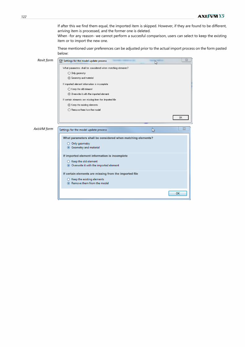
122

If after this we find them equal, the imported item is skipped. However, if they are found to be different,

arriving item is processed, and the former one is deleted.

When -for any reason- we cannot perform a succesful comparison, users can select to keep the existing

item or to import the new one.

These mentioned user preferences can be adjusted prior to the actual import process on the form pasted

below:

Revit form

AxisVM form

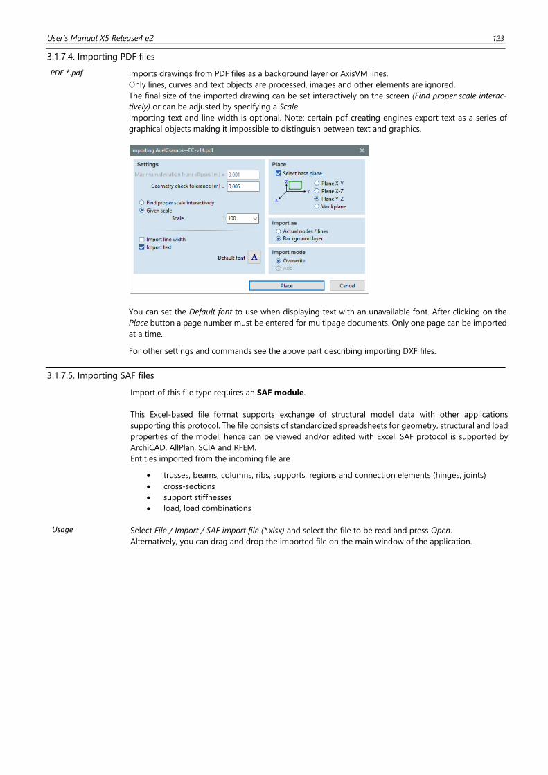
User’s Manual X5 Release4 e2 123

3.1.7.4. Importing PDF files

PDF *.pdf Imports drawings from PDF files as a background layer or AxisVM lines.

Only lines, curves and text objects are processed, images and other elements are ignored.

The final size of the imported drawing can be set interactively on the screen (Find proper scale interac-

tively) or can be adjusted by specifying a Scale.

Importing text and line width is optional. Note: certain pdf creating engines export text as a series of

graphical objects making it impossible to distinguish between text and graphics.

You can set the Default font to use when displaying text with an unavailable font. After clicking on the

Place button a page number must be entered for multipage documents. Only one page can be imported

at a time.

For other settings and commands see the above part describing importing DXF files.

3.1.7.5. Importing SAF files

Import of this file type requires an SAF module.

This Excel-based file format supports exchange of structural model data with other applications

supporting this protocol. The file consists of standardized spreadsheets for geometry, structural and load

properties of the model, hence can be viewed and/or edited with Excel. SAF protocol is supported by

ArchiCAD, AllPlan, SCIA and RFEM.

Entities imported from the incoming file are

• trusses, beams, columns, ribs, supports, regions and connection elements (hinges, joints)

• cross-sections

• support stiffnesses

• load, load combinations

Usage Select File / Import / SAF import file (*.xlsx) and select the file to be read and press Open.

Alternatively, you can drag and drop the imported file on the main window of the application.

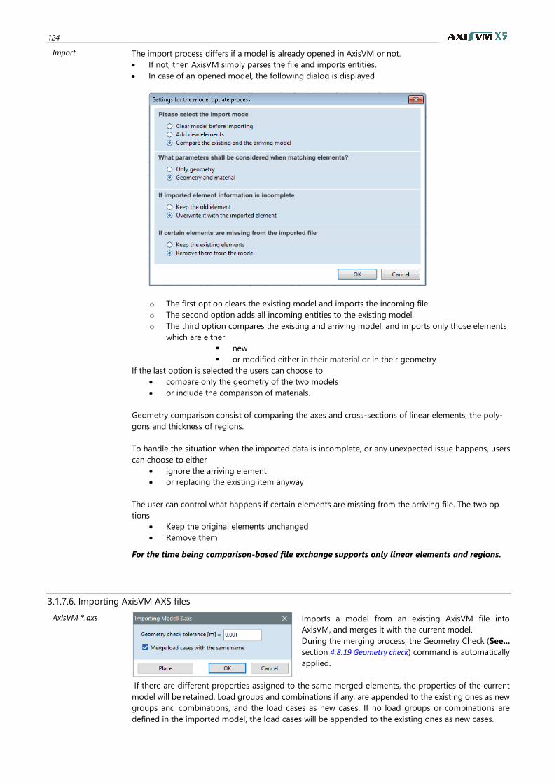
124

Import The import process differs if a model is already opened in AxisVM or not.

• If not, then AxisVM simply parses the file and imports entities.

• In case of an opened model, the following dialog is displayed

o The first option clears the existing model and imports the incoming file

o The second option adds all incoming entities to the existing model

o The third option compares the existing and arriving model, and imports only those elements

which are either

▪ new

▪ or modified either in their material or in their geometry

If the last option is selected the users can choose to

• compare only the geometry of the two models

• or include the comparison of materials.

Geometry comparison consist of comparing the axes and cross-sections of linear elements, the poly-

gons and thickness of regions.

To handle the situation when the imported data is incomplete, or any unexpected issue happens, users

can choose to either

• ignore the arriving element

• or replacing the existing item anyway

The user can control what happens if certain elements are missing from the arriving file. The two op-

tions

• Keep the original elements unchanged

• Remove them

For the time being comparison-based file exchange supports only linear elements and regions.

3.1.7.6. Importing AxisVM AXS files

AxisVM *.axs Imports a model from an existing AxisVM file into

AxisVM, and merges it with the current model.

During the merging process, the Geometry Check (See...

section 4.8.19 Geometry check) command is automatically

applied.

If there are different properties assigned to the same merged elements, the properties of the current

model will be retained. Load groups and combinations if any, are appended to the existing ones as new

groups and combinations, and the load cases as new cases. If no load groups or combinations are

defined in the imported model, the load cases will be appended to the existing ones as new cases.

User’s Manual X5 Release4 e2 125

If the same load case exists in both models, loads will be merged if the Merge load cases with the same

name checkbox is checked.

If both models contains loads that are limited to one occurrence (e.g. thermal) in the same load case,

the load in the current model will be retained.

The Section Lines/Planes Parts with the same name are merged, otherwise they are appended.

When importing an AxisVM file a dialog is displayed.

Use the Place button to graphically position the imported model in your model’s space.

3.1.7.7. Importing files from other applications

Stereo Lithography *.stl file

Reads the triangular mesh describing the surface of a model from a file in STL format (binary or text).

Multiple nodes and degenerated triangles are filtered out. Import can be transferred to a background

layer as well.

Bocad interface *.sc1 file

Opens a data file created by Bocad steel construction software (*.sc1) and imports beam cross-sections

and geometry.

Glaser -isb cad- *.geo file

Imports *.geo files exported by Glaser -isb cad- describing beam or surface models.

SDNF file (Steel Detailing Ne-utral Format)

Imports a file exported in Steel Detailing Neutral Format used in data exchange between steel detailing

programs.

DSTV format *.stp file

In its current version AxisVM is capable of importing stp files implementing "PSS_2000_04" file scheme

based on "Standard Description for Product Interface Steel Construction 4/2000". This filetype is de-

signed for storing steel structures' data, and can describe linear structures as well as planar regions.

Even statical calculations can be imported through this interface, though with limited capabilities.

If static calculations and an architectural model are both embedded in the file, the user can choose

importing either the calculation or the architectural model. When trying to import data onto an existing

modell, the user can select between overwriting or just supplementing it.

3.1.8. Parametric design

„Parametric design is based on the idea, that specific numbers, i.e., parameters control the geometry.

To fully exploit its potentials, these parameters are linked to each other, and these links form a system.

Thus, it is possible that by modifying only one parameter, the whole geometry changes. This idea is

regularly used in structural design. Imagine that by modifying only the span of a truss, the height and

the truss layout are automatically updated both in the 3D model and in the shop drawings. To build a

system capable of doing this requires time, and therefore it is essential to think it over whether it is

worth the time to create a parametric model. However, once we have built such a system of parameters,

links, and a dynamically changing model, we have a highly flexible tool.”

Based on the article of Péter Romvári: Parametric design in practice in epiteszforum.hu

AxisVM Export plugins

The most commonly used parametric design software in structural design are Grasshopper and Dy-

namo. These are often referred to as graphical algorithm editors that can be used to create parametric

models easily. By using the AxisVM Export plugins, the parametric models created in Grasshopper/Dy-

namo can be exported to AxisVM. First, the AxisVM Export plugin should be installed in Grasshop-

per/Dynamo. The AxisVM Export plugin communicates with AxisVM through its API (COM inter-

face). The export requires that AxisVM and a version of Grasshopper/Dynamo are all installed on the

same computer. After starting the export, AxisVM automatically launches, showing the exported model.

One advantage of this interface is that it is easy to create parametric models and even templates in

Grasshopper/Dynamo. For example, the parameters of a truss may be the span, height, layout, and

cross-section sizes. The other advantage is that in in the Grasshopper/Dynamo there are a lot of geo-

metric functions, that enables creating complex spatial models.

126

Currently, models with straight lines can be exported to AxisVM. There are two available exporting op-

tions:

• export lines;

• export elements, for which the type of the element (truss, beam, rib), the material properties,

and the cross-section have to be defined.

Currently, only the following properties can be used:

• material property: according to the Eurocodes (from AxisVM material library);

• cross-section: I, hollow (pipe, box), solid round and rectangular cross-sections (from AxisVM

cross-section library).

3.1.8.1. Grasshopper/Rhinoceros plugin

*.gh, *.3dm files

Grasshopper is the parametric design tool of the Rhinoceros CAD software. Grasshopper can be started

from within Rhinoceros. To export a file with *.gh extension, the AxisVM Export plugin shall be installed

in Grasshopper in Rhinoceros version 6. After installation, the modeling and exporting functions (com-

ponents) are available in the Grasshopper menu, in the AxisVM tab. Rhinoceros files (*.3dm) shall be

loaded into Grasshopper before exporting to AxisVM.

After exporting, the AxisVM model is independent of the parametric model. Starting a new export (e.g.,

with modified geometric parameters) launches a new AxisVM model in a separate window.

The AxisVM Export plugin can be downloaded from https://www.food4rhino.com/app/axisvm-export.

For further details, example files, and installation guide see: https://github.com/AxisVM/Grasshop-

perToAxisVM/wiki

3.1.8.2. Dynamo/Autodesk plugin

*.dyn, *.rvt files

Dynamo is a parametric design tool of the Autodesk Revit software. Dynamo can either be started from

within Revit or as an independent software (Dynamo Studio, Dynamo Sandbox). To export a file with

*.dyn extension, the AxisVM Export plugin shall be installed in Dynamo. After installation, the modeling

and exporting functions (nodes) are available on the left-hand side menu of Dynamo, at the AxisVM

drop-down menu. Revit files (*.rvt) shall be loaded into Dynamo before exporting to AxisVM.

In Dynamo, before starting the export, first, a new model shall be created using the AxModel node. Self-

weight, nodal load, and nodal supports can be added to the parametric structural model. After starting

the export, a one-directional link is created between the parametric model and the AxisVM model. This

means, that modifying a (geometrical or structural) parameter in Dynamo automatically updates the

structural model in AxisVM. In AxisVM, further structural elements can be added, but these do not in-

fluence the Dynamo parametric model. In Dynamo, it is possible to start an AxisVM linear static analysis.

The link between the models is destroyed by closing any of the models.

The simplest way to download the AxisVM Export plugin is from within the Dynamo software: go to

Packages in the Dynamo menu, then choose Search for a Package... and type AxisVM Export. For further

details, example files, and installation guide see:

https://github.com/AxisVM/DynamoToAxisVM/wiki

AxisVM is able to communicate with Tekla Structures software different ways in case of

• version 2019 and later,

• version before 2019.

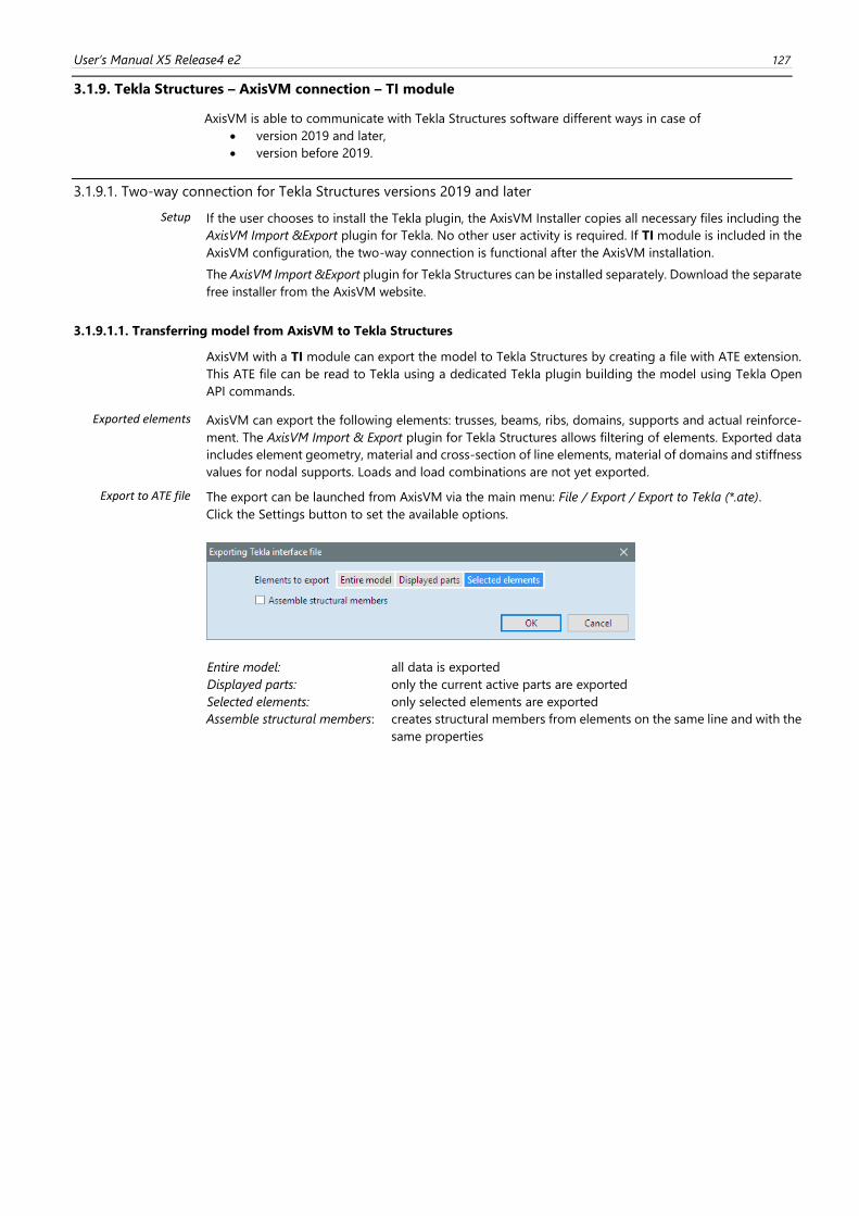
User’s Manual X5 Release4 e2 127

3.1.9. Tekla Structures – AxisVM connection – TI module

AxisVM is able to communicate with Tekla Structures software different ways in case of

• version 2019 and later,

• version before 2019.

3.1.9.1. Two-way connection for Tekla Structures versions 2019 and later

Setup If the user chooses to install the Tekla plugin, the AxisVM Installer copies all necessary files including the

AxisVM Import &Export plugin for Tekla. No other user activity is required. If TI module is included in the

AxisVM configuration, the two-way connection is functional after the AxisVM installation.

The AxisVM Import &Export plugin for Tekla Structures can be installed separately. Download the separate

free installer from the AxisVM website.

3.1.9.1.1. Transferring model from AxisVM to Tekla Structures

AxisVM with a TI module can export the model to Tekla Structures by creating a file with ATE extension.

This ATE file can be read to Tekla using a dedicated Tekla plugin building the model using Tekla Open

API commands.

Exported elements AxisVM can export the following elements: trusses, beams, ribs, domains, supports and actual reinforce-

ment. The AxisVM Import & Export plugin for Tekla Structures allows filtering of elements. Exported data

includes element geometry, material and cross-section of line elements, material of domains and stiffness

values for nodal supports. Loads and load combinations are not yet exported.

Export to ATE file The export can be launched from AxisVM via the main menu: File / Export / Export to Tekla (*.ate).

Click the Settings button to set the available options.

Entire model: all data is exported

Displayed parts: only the current active parts are exported

Selected elements: only selected elements are exported

Assemble structural members: creates structural members from elements on the same line and with the

same properties

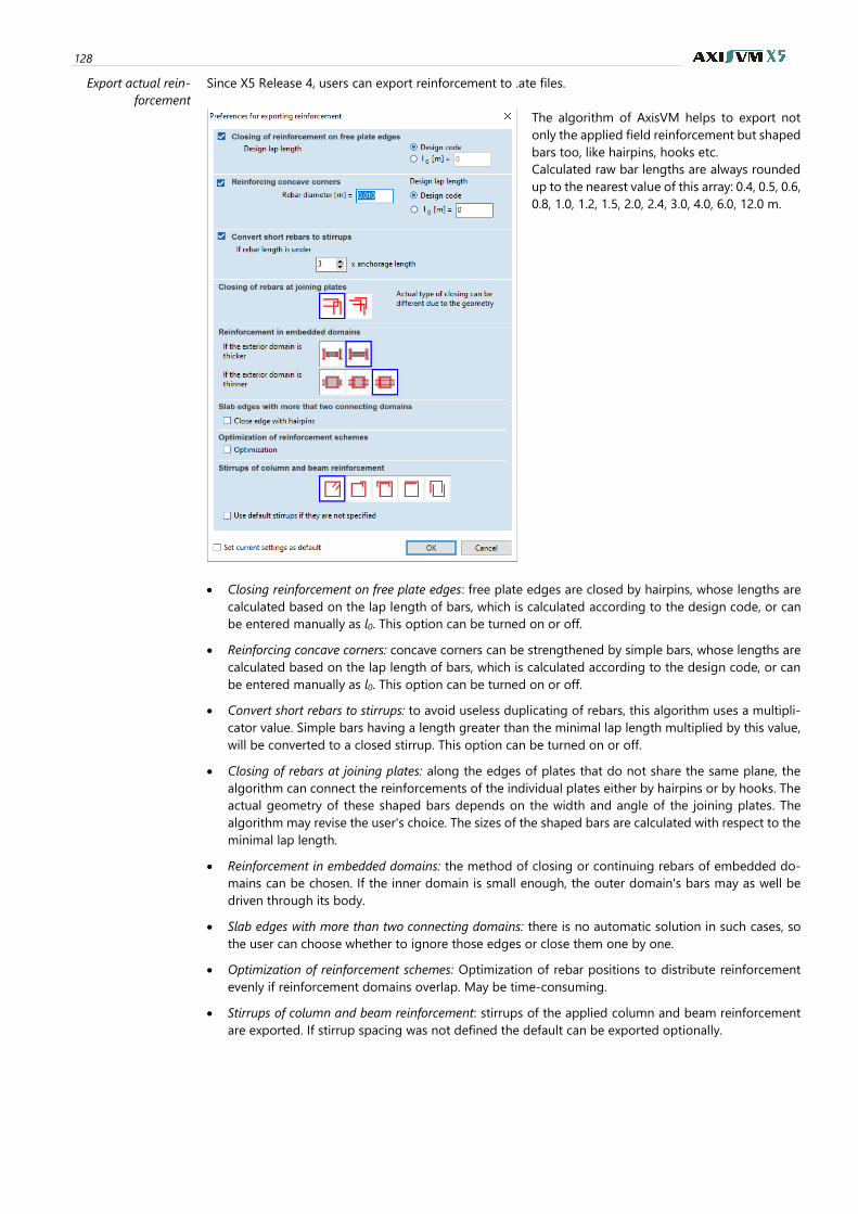
128

Export actual rein-

forcement

Since X5 Release 4, users can export reinforcement to .ate files.

The algorithm of AxisVM helps to export not

only the applied field reinforcement but shaped

bars too, like hairpins, hooks etc.

Calculated raw bar lengths are always rounded

up to the nearest value of this array: 0.4, 0.5, 0.6,

0.8, 1.0, 1.2, 1.5, 2.0, 2.4, 3.0, 4.0, 6.0, 12.0 m.

• Closing reinforcement on free plate edges: free plate edges are closed by hairpins, whose lengths are

calculated based on the lap length of bars, which is calculated according to the design code, or can

be entered manually as l0. This option can be turned on or off.

• Reinforcing concave corners: concave corners can be strengthened by simple bars, whose lengths are

calculated based on the lap length of bars, which is calculated according to the design code, or can

be entered manually as l0. This option can be turned on or off.

• Convert short rebars to stirrups: to avoid useless duplicating of rebars, this algorithm uses a multipli-

cator value. Simple bars having a length greater than the minimal lap length multiplied by this value,

will be converted to a closed stirrup. This option can be turned on or off.

• Closing of rebars at joining plates: along the edges of plates that do not share the same plane, the

algorithm can connect the reinforcements of the individual plates either by hairpins or by hooks. The

actual geometry of these shaped bars depends on the width and angle of the joining plates. The

algorithm may revise the user's choice. The sizes of the shaped bars are calculated with respect to the

minimal lap length.

• Reinforcement in embedded domains: the method of closing or continuing rebars of embedded do-

mains can be chosen. If the inner domain is small enough, the outer domain's bars may as well be

driven through its body.

• Slab edges with more than two connecting domains: there is no automatic solution in such cases, so

the user can choose whether to ignore those edges or close them one by one.

• Optimization of reinforcement schemes: Optimization of rebar positions to distribute reinforcement

evenly if reinforcement domains overlap. May be time-consuming.

• Stirrups of column and beam reinforcement: stirrups of the applied column and beam reinforcement

are exported. If stirrup spacing was not defined the default can be exported optionally.

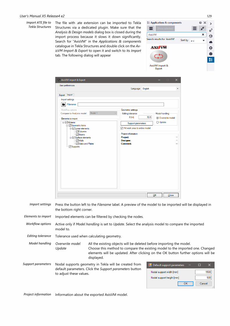
User’s Manual X5 Release4 e2 129

Import ATE file to Tekla Structures

The file with .ate extension can be imported to Tekla

Structures via a dedicated plugin. Make sure that the

Analysis & Design models dialog box is closed during the

import process because it slows it down significantly.

Search for “AxisVM” in the Applications & components

catalogue in Tekla Structures and double click on the Ax-

isVM Import & Export to open it and switch to its Import

tab. The following dialog will appear

Import settings Press the button left to the Filename label. A preview of the model to be imported will be displayed in

the bottom right corner.

Elements to import Imported elements can be filtered by checking the nodes.

Workflow options Active only if Model handling is set to Update. Select the analysis model to compare the imported

model to.

Editing tolerance Tolerance used when calculating geometry.

Model handling Overwrite model All the existing objects will be deleted before importing the model.

Update Choose this method to compare the existing model to the imported one. Changed

elements will be updated. After clicking on the OK button further options will be

displayed.

Support parameters Nodal supports geometry in Tekla will be created from

default parameters. Click the Support parameters button

to adjust these values.

Project information Information about the exported AxisVM model.

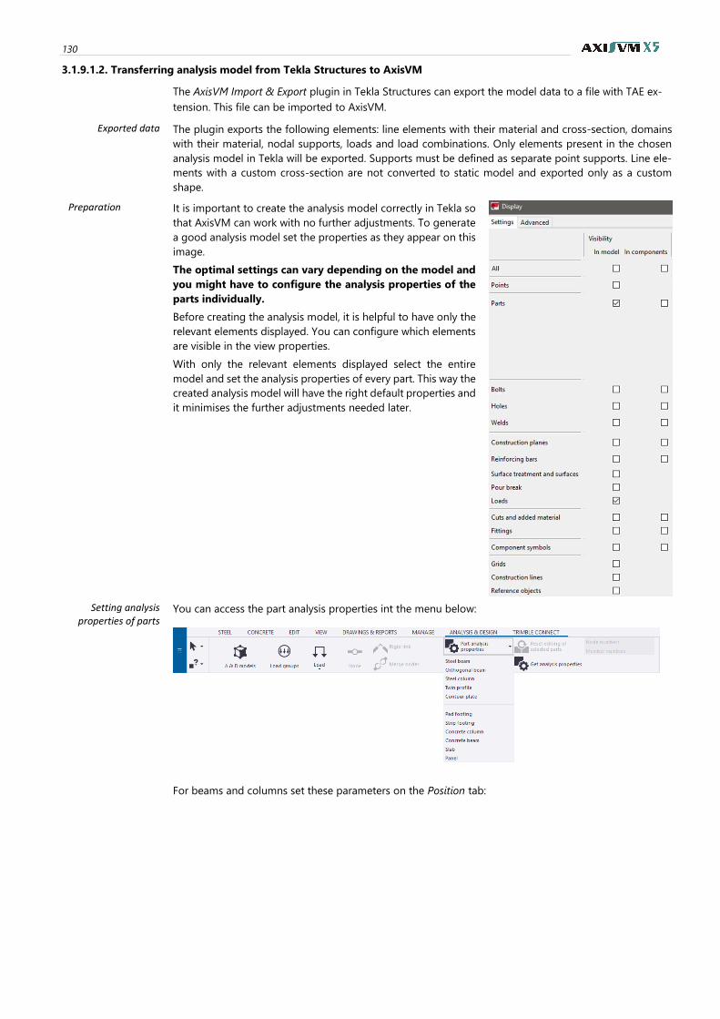
130

3.1.9.1.2. Transferring analysis model from Tekla Structures to AxisVM

The AxisVM Import & Export plugin in Tekla Structures can export the model data to a file with TAE ex-

tension. This file can be imported to AxisVM.

Exported data The plugin exports the following elements: line elements with their material and cross-section, domains

with their material, nodal supports, loads and load combinations. Only elements present in the chosen

analysis model in Tekla will be exported. Supports must be defined as separate point supports. Line ele-

ments with a custom cross-section are not converted to static model and exported only as a custom

shape.

Preparation It is important to create the analysis model correctly in Tekla so

that AxisVM can work with no further adjustments. To generate

a good analysis model set the properties as they appear on this

image.

The optimal settings can vary depending on the model and

you might have to configure the analysis properties of the

parts individually.

Before creating the analysis model, it is helpful to have only the

relevant elements displayed. You can configure which elements

are visible in the view properties.

With only the relevant elements displayed select the entire

model and set the analysis properties of every part. This way the

created analysis model will have the right default properties and

it minimises the further adjustments needed later.

Setting analysis properties of parts

You can access the part analysis properties int the menu below:

For beams and columns set these parameters on the Position tab:

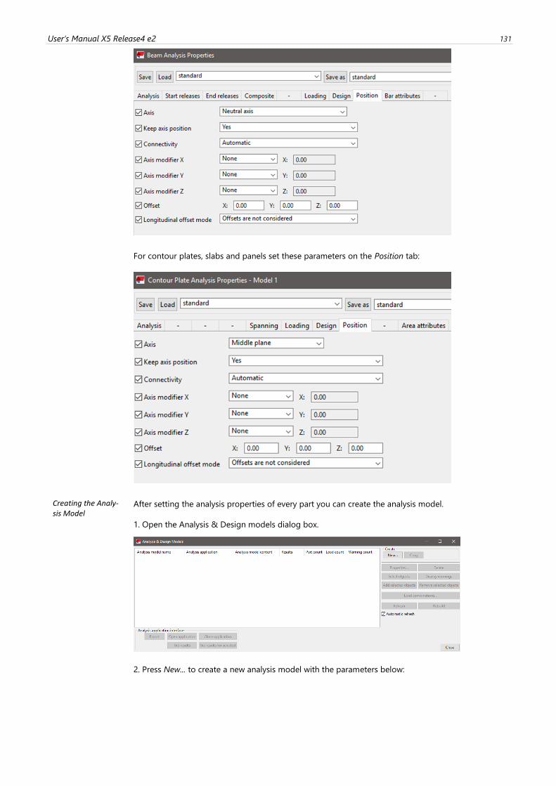
User’s Manual X5 Release4 e2 131

For contour plates, slabs and panels set these parameters on the Position tab:

Creating the Analy-sis Model

After setting the analysis properties of every part you can create the analysis model.

1. Open the Analysis & Design models dialog box.

2. Press New... to create a new analysis model with the parameters below:

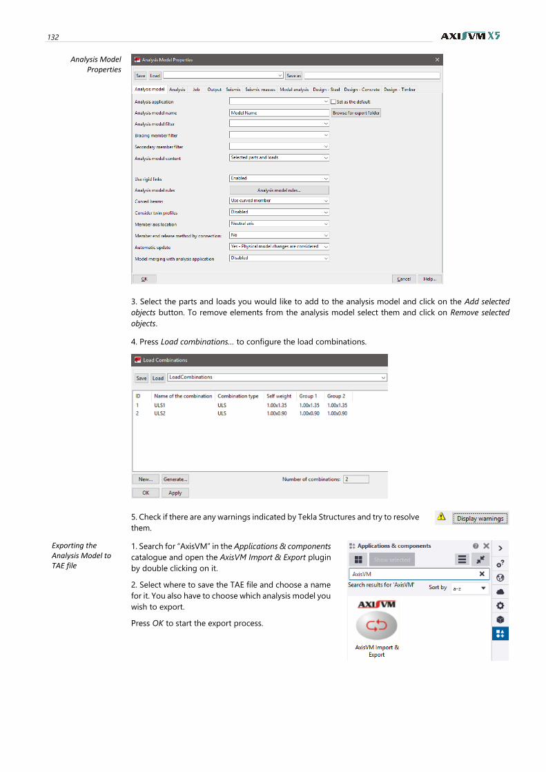
132

Analysis Model Properties

3. Select the parts and loads you would like to add to the analysis model and click on the Add selected

objects button. To remove elements from the analysis model select them and click on Remove selected

objects.

4. Press Load combinations… to configure the load combinations.

5. Check if there are any warnings indicated by Tekla Structures and try to resolve

them.

Exporting the Analysis Model to TAE file

1. Search for “AxisVM” in the Applications & components

catalogue and open the AxisVM Import & Export plugin

by double clicking on it.

2. Select where to save the TAE file and choose a name

for it. You also have to choose which analysis model you

wish to export.

Press OK to start the export process.

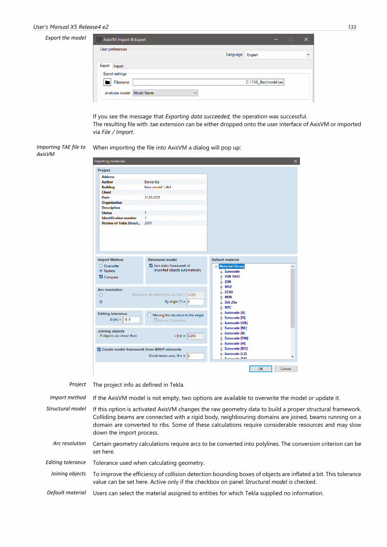
User’s Manual X5 Release4 e2 133

Export the model

If you see the message that Exporting data succeeded, the operation was successful.

The resulting file with .tae extension can be either dropped onto the user interface of AxisVM or imported

via File / Import.

Importing TAE file to AxisVM

When importing the file into AxisVM a dialog will pop up:

Project The project info as defined in Tekla.

Import method If the AxisVM model is not empty, two options are available to overwrite the model or update it.

Structural model If this option is activated AxisVM changes the raw geometry data to build a proper structural framework.

Colliding beams are connected with a rigid body, neighbouring domains are joined, beams running on a

domain are converted to ribs. Some of these calculations require considerable resources and may slow

down the import process.

Arc resolution Certain geometry calculations require arcs to be converted into polylines. The conversion criterion can be

set here.

Editing tolerance Tolerance used when calculating geometry.

Joining objects To improve the efficiency of collision detection bounding boxes of objects are inflated a bit. This tolerance

value can be set here. Active only if the checkbox on panel Structural model is checked.

Default material Users can select the material assigned to entities for which Tekla supplied no information.

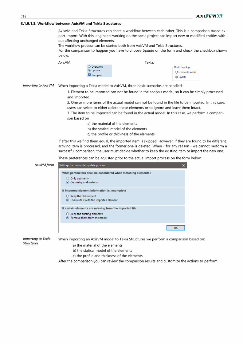
134

3.1.9.1.3. Workflow between AxisVM and Tekla Structures

AxisVM and Tekla Structures can share a workflow between each other. This is a comparison based ex-

port-import. With this, engineers working on the same project can import new or modified entities with-

out affecting unchanged elements.

The workflow process can be started both from AxisVM and Tekla Structures.

For the comparison to happen you have to choose Update on the form and check the checkbox shown

below:

AxisVM:

Tekla:

Importing to AxisVM When importing a Tekla model to AxisVM, three basic scenarios are handled:

1. Element to be imported can not be found in the analysis model, so it can be simply processed

and imported.

2. One or more items of the actual model can not be found in the file to be imported. In this case,

users can select to either delete these elements or to ignore and leave them intact.

3. The item to be imported can be found in the actual model. In this case, we perform a compari-

son based on

a) the material of the elements

b) the statical model of the elements

c) the profile or thickness of the elements.

If after this we find them equal, the imported item is skipped. However, if they are found to be different,

arriving item is processed, and the former one is deleted. When - for any reason - we cannot perform a

successful comparison, the user must decide whether to keep the existing item or import the new one.

These preferences can be adjusted prior to the actual import process on the form below:

AxisVM form

Importing to Tekla Structures

When importing an AxisVM model to Tekla Structures we perform a comparison based on:

a) the material of the elements

b) the statical model of the elements

c) the profile and thickness of the elements

After the comparison you can review the comparison results and customize the actions to perform.

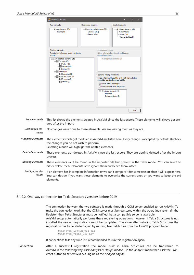
User’s Manual X5 Release4 e2 135

New elements This list shows the elements created in AxisVM since the last export. These elements will always get cre-

ated after the import.

Unchanged ele-ments

No changes were done to these elements. We are leaving them as they are.

Modified elements The elements which got modified in AxisVM are listed here. Every change is accepted by default. Uncheck

the changes you do not wish to perform.

Selecting a node will highlight the related elements.

Deleted elements These elements got deleted in AxisVM since the last export. They are getting deleted after the import

process.

Missing elements These elements can’t be found in the imported file but present in the Tekla model. You can select to

either delete these elements or to ignore them and leave them intact.

Ambiguous ele-ments

If an element has incomplete information or we can’t compare it for some reason, then it will appear here.

You can decide if you want these elements to overwrite the current ones or you want to keep the old

elements.

3.1.9.2. One-way connection for Tekla Structures versions before 2019

The connection between the two software is made through a COM server enabled to run AxisVM. To

make the connection work first the COM server must be registered within the operating system (in the

Registry) then Tekla Structures must be notified that a compatible server is available.

AxisVM setup automatically performs these registering operations, however if Tekla Structures is not

installed the second registration cannot be completed. Therefore after installing Tekla Structures the

registration has to be started again by running two batch files from the AxisVM program folder:

!REGISTER_AXISVM_X64.BAT

!REGISTER_TEKLA_X64.BAT

If connections fails any time it is recommended to run this registration again.

Connection After a successful registration the model built in Tekla Structures can be transferred to

AxisVM in the following way: click Analysis & Design models... in the Analysis menu then click the Prop-

erties button to set AxisVM AD Engine as the Analysis engine.

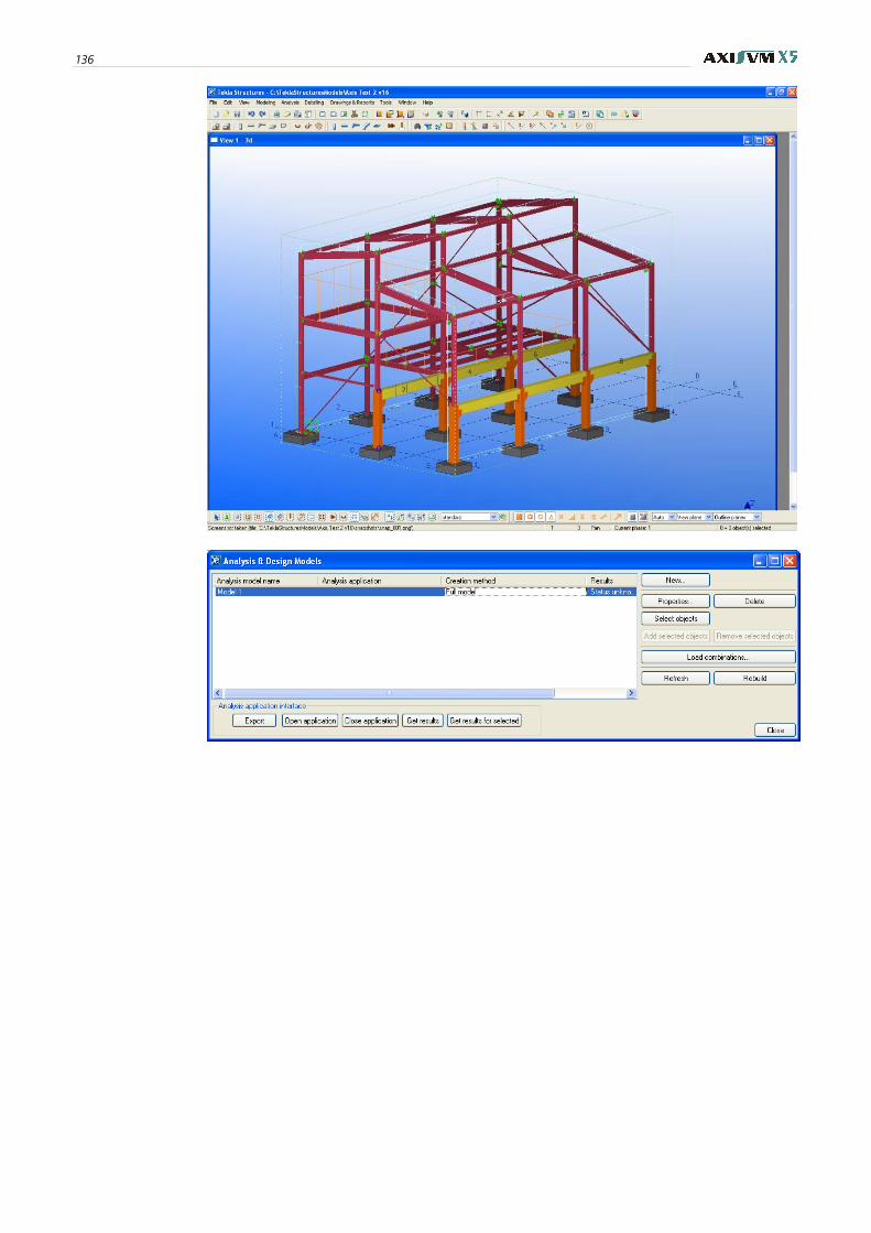
136

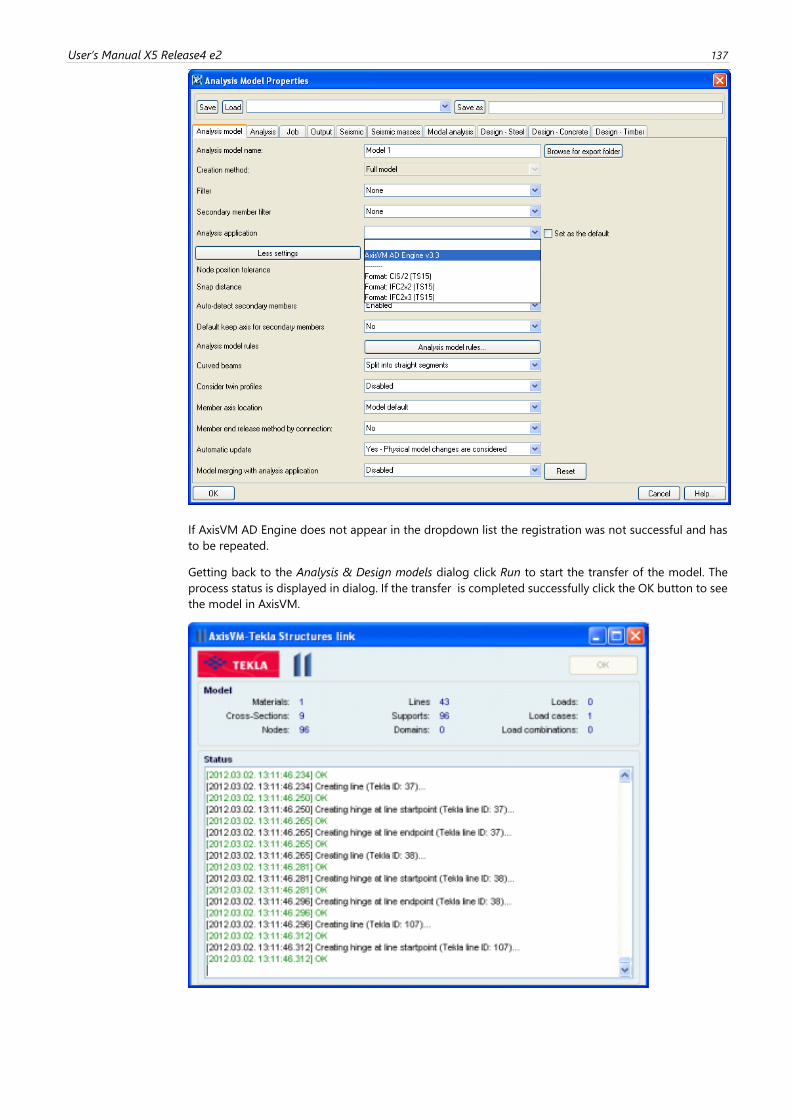
User’s Manual X5 Release4 e2 137

If AxisVM AD Engine does not appear in the dropdown list the registration was not successful and has

to be repeated.

Getting back to the Analysis & Design models dialog click Run to start the transfer of the model. The

process status is displayed in dialog. If the transfer is completed successfully click the OK button to see

the model in AxisVM.

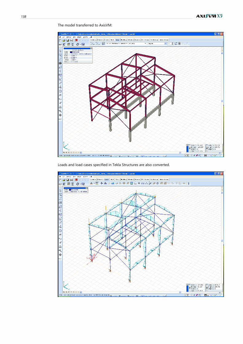
138

The model transferred to AxisVM:

Loads and load cases specified in Tekla Structures are also converted.

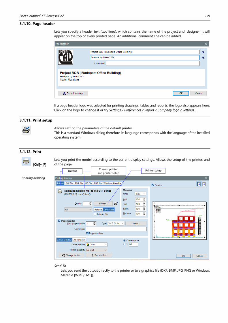
User’s Manual X5 Release4 e2 139

3.1.10. Page header

Lets you specify a header text (two lines), which contains the name of the project and designer. It will

appear on the top of every printed page. An additional comment line can be added.

If a page header logo was selected for printing drawings, tables and reports, the logo also appears here.

Click on the logo to change it or try Settings / Preferences / Report / Company logo / Settings…

3.1.11. Print setup

Allows setting the parameters of the default printer.

This is a standard Windows dialog therefore its language corresponds with the language of the installed

operating system.

3.1.12. Print

[Ctrl]+ [P]

Lets you print the model according to the current display settings. Allows the setup of the printer, and

of the page.

Printing drawing

Send To

Lets you send the output directly to the printer or to a graphics file (DXF, BMP, JPG, PNG or Windows

Metafile [WMF/EMF]).

Current printer and printer setup

Printer setup Output

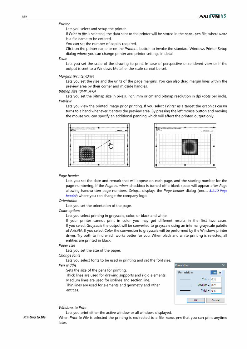
140

Printer

Lets you select and setup the printer.

If Print to file is selected, the data sent to the printer will be stored in the Name.prn file, where Name

is a file name to be entered.

You can set the number of copies required.

Click on the printer name or on the Printer… button to invoke the standard Windows Printer Setup

dialog where you can change printer and printer settings in detail.

Scale

Lets you set the scale of the drawing to print. In case of perspective or rendered view or if the

output is sent to a Windows Metafile the scale cannot be set.

Margins (Printer/DXF)

Lets you set the size and the units of the page margins. You can also drag margin lines within the

preview area by their corner and midside handles.

Bitmap size (BMP, JPG)

Lets you set the bitmap size in pixels, inch, mm or cm and bitmap resolution in dpi (dots per inch).

Preview

Lets you view the printed image prior printing. If you select Printer as a target the graphics cursor

turns to a hand whenever it enters the preview area. By pressing the left mouse button and moving

the mouse you can specify an additional panning which will affect the printed output only.

Page header

Lets you set the date and remark that will appear on each page, and the starting number for the

page numbering. If the Page numbers checkbox is turned off a blank space will appear after Page

allowing handwritten page numbers. Setup… displays the Page header dialog (see… 3.1.10 Page

header) where you can change the company logo.

Orientation

Lets you set the orientation of the page.

Color options

Lets you select printing in grayscale, color, or black and white.

If your printer cannot print in color you may get different results in the first two cases.

If you select Grayscale the output will be converted to grayscale using an internal grayscale palette

of AxisVM. If you select Color the conversion to grayscale will be performed by the Windows printer

driver. Try both to find which works better for you. When black and white printing is selected, all

entities are printed in black.

Paper size

Lets you set the size of the paper.

Change fonts

Lets you select fonts to be used in printing and set the font size.

Pen widths

Sets the size of the pens for printing.

Thick lines are used for drawing supports and rigid elements.

Medium lines are used for isolines and section line.

Thin lines are used for elements and geometry and other

entities.

Windows to Print

Lets you print either the active window or all windows displayed.

Printing to file When Print to File is selected the printing is redirected to a file, name.prn that you can print anytime

later.

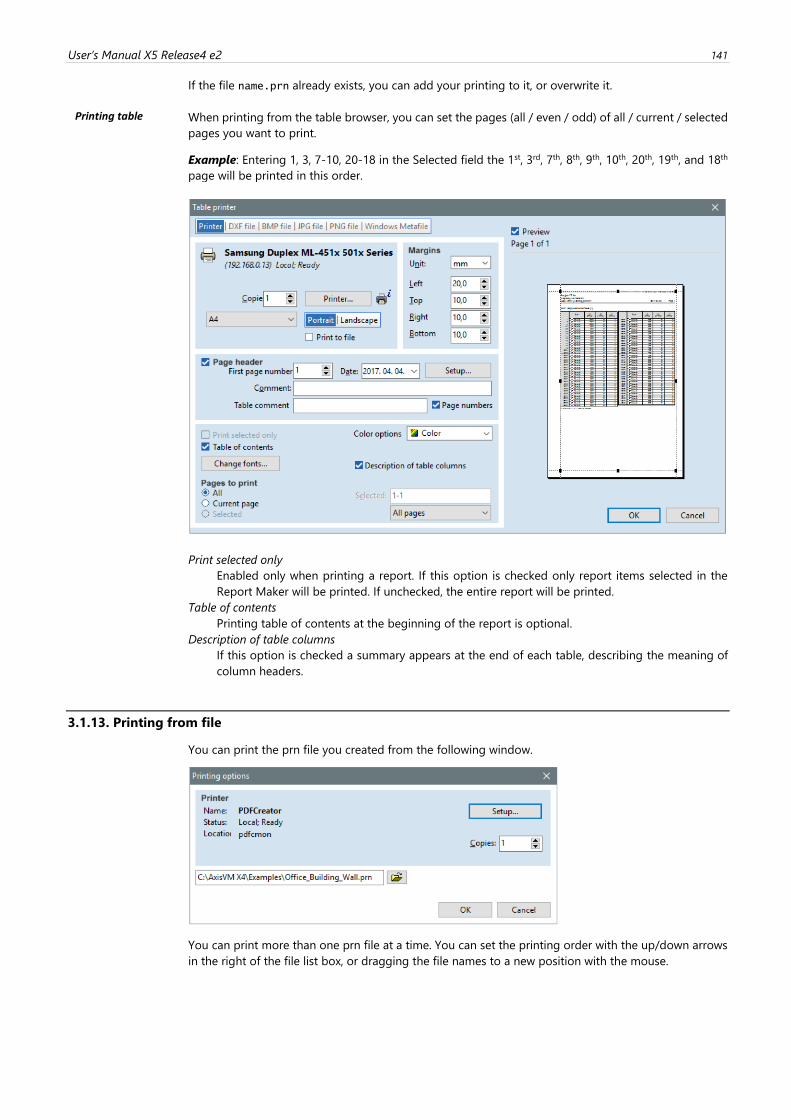
User’s Manual X5 Release4 e2 141

If the file name.prn already exists, you can add your printing to it, or overwrite it.

Printing table When printing from the table browser, you can set the pages (all / even / odd) of all / current / selected

pages you want to print.

Example: Entering 1, 3, 7-10, 20-18 in the Selected field the 1st, 3rd, 7th, 8th, 9th, 10th, 20th, 19th, and 18th

page will be printed in this order.

Print selected only

Enabled only when printing a report. If this option is checked only report items selected in the

Report Maker will be printed. If unchecked, the entire report will be printed.

Table of contents

Printing table of contents at the beginning of the report is optional.

Description of table columns

If this option is checked a summary appears at the end of each table, describing the meaning of

column headers.

3.1.13. Printing from file

You can print the prn file you created from the following window.

You can print more than one prn file at a time. You can set the printing order with the up/down arrows

in the right of the file list box, or dragging the file names to a new position with the mouse.

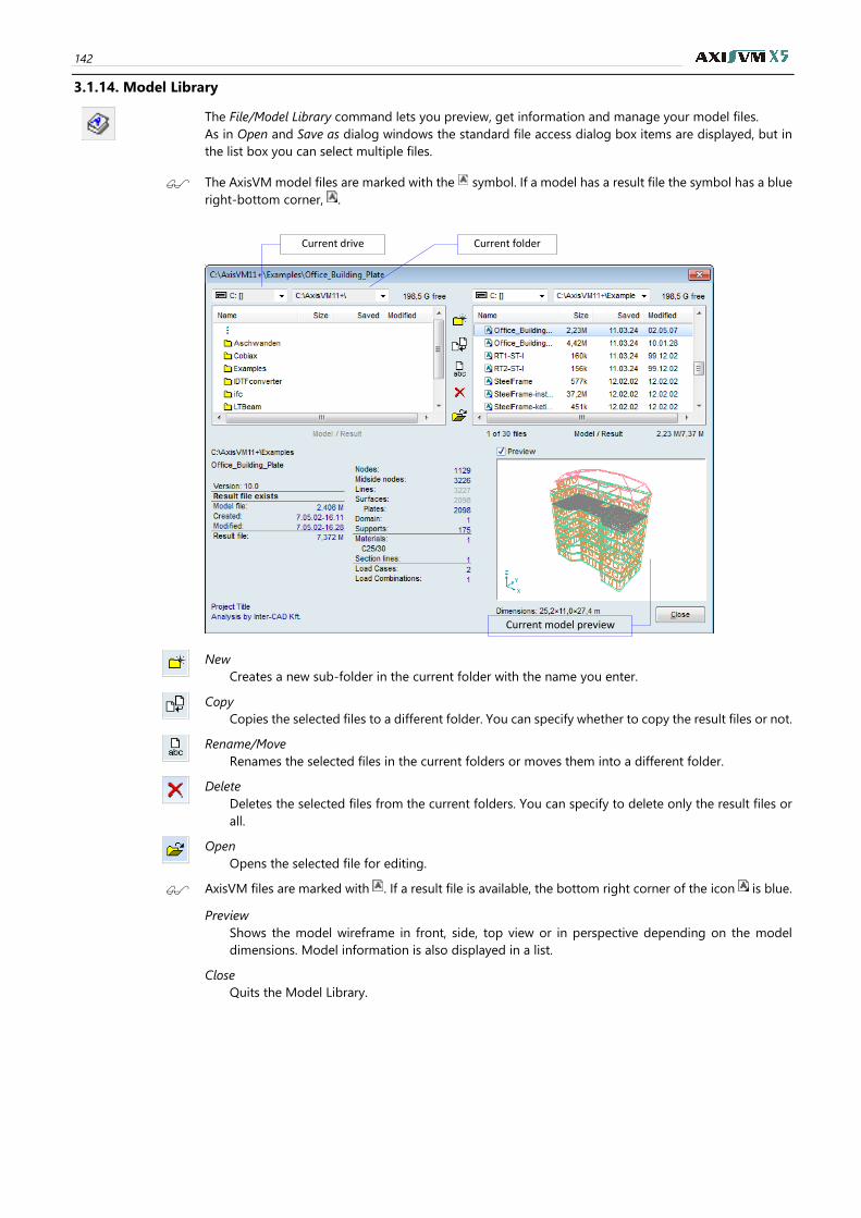
142

3.1.14. Model Library

The File/Model Library command lets you preview, get information and manage your model files.

As in Open and Save as dialog windows the standard file access dialog box items are displayed, but in

the list box you can select multiple files.

The AxisVM model files are marked with the symbol. If a model has a result file the symbol has a blue

right-bottom corner, .

New

Creates a new sub-folder in the current folder with the name you enter.

Copy

Copies the selected files to a different folder. You can specify whether to copy the result files or not.

Rename/Move

Renames the selected files in the current folders or moves them into a different folder.

Delete

Deletes the selected files from the current folders. You can specify to delete only the result files or

all.

Open

Opens the selected file for editing.

AxisVM files are marked with . If a result file is available, the bottom right corner of the icon is blue.

Preview

Shows the model wireframe in front, side, top view or in perspective depending on the model

dimensions. Model information is also displayed in a list.

Close

Quits the Model Library.

Current model preview

Current folder Current drive

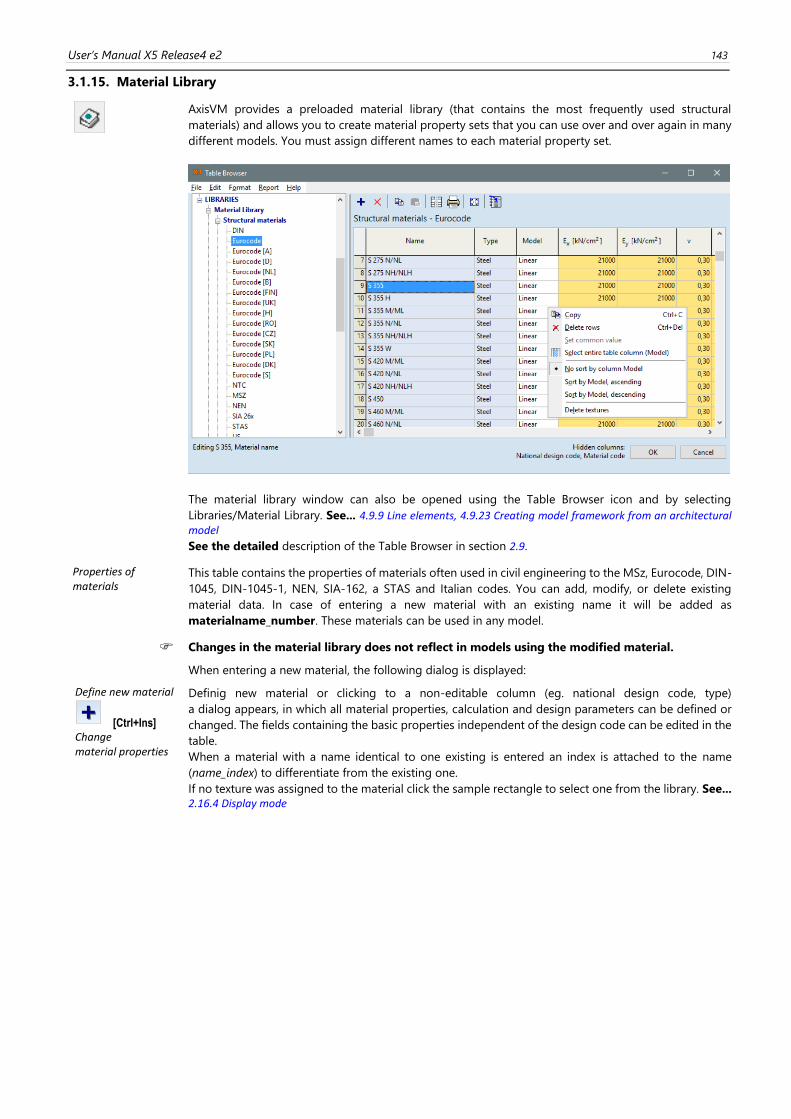
User’s Manual X5 Release4 e2 143

3.1.15. Material Library

AxisVM provides a preloaded material library (that contains the most frequently used structural

materials) and allows you to create material property sets that you can use over and over again in many

different models. You must assign different names to each material property set.

The material library window can also be opened using the Table Browser icon and by selecting

Libraries/Material Library. See... 4.9.9 Line elements, 4.9.23 Creating model framework from an architectural model

See the detailed description of the Table Browser in section 2.9.

Properties of materials

This table contains the properties of materials often used in civil engineering to the MSz, Eurocode, DIN-

1045, DIN-1045-1, NEN, SIA-162, a STAS and Italian codes. You can add, modify, or delete existing

material data. In case of entering a new material with an existing name it will be added as

materialname_number. These materials can be used in any model.

Changes in the material library does not reflect in models using the modified material.

When entering a new material, the following dialog is displayed:

Define new material

[Ctrl+Ins] Change material properties

Definig new material or clicking to a non-editable column (eg. national design code, type)

a dialog appears, in which all material properties, calculation and design parameters can be defined or

changed. The fields containing the basic properties independent of the design code can be edited in the

table.

When a material with a name identical to one existing is entered an index is attached to the name

(name_index) to differentiate from the existing one.

If no texture was assigned to the material click the sample rectangle to select one from the library. See...

2.16.4 Display mode

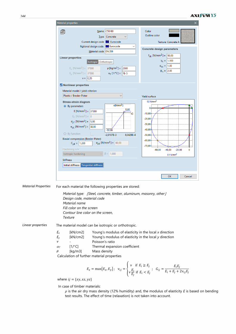
144

Material Properties For each material the following properties are stored:

Material type: Steel, concrete, timber, aluminum, masonry, other

Design code, material code

Material name

Fill color on the screen

Contour line color on the screen,

Texture

Linear properties The material model can be isotropic or orthotropic.

Ex [kN/cm2] Young’s modulus of elasticity in the local x direction

Ey [kN/cm2] Young’s modulus of elasticity in the local y direction

ν - Poisson’s ratio

T [1/C] Thermal expansion coefficient

ρ [kg/m3] Mass density

Calculation of further material properties

𝐸𝑧 = max{𝐸𝑥, 𝐸𝑦} ; 𝜈𝑖𝑗 = {

𝜈 if 𝐸𝑖 ≥ 𝐸𝑗

𝜈𝐸𝑖𝐸𝑗 if 𝐸𝑖 < 𝐸𝑗

; 𝐺𝑖𝑗 =𝐸𝑖𝐸𝑗

𝐸𝑖 + 𝐸𝑗 + 2𝜈𝑖𝑗𝐸𝑗

where 𝑖𝑗 = {𝑥𝑦, 𝑥𝑧, 𝑦𝑧}

In case of timber materials:

𝜌 is the air dry mass density (12% humidity) and, the modulus of elasticity E is based on bending

test results. The effect of time (relaxation) is not taken into account.

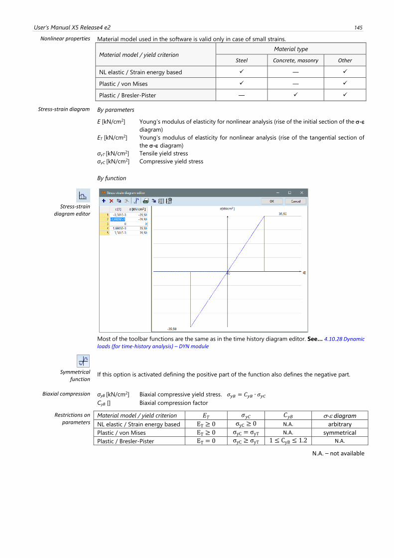
User’s Manual X5 Release4 e2 145

Nonlinear properties Material model used in the software is valid only in case of small strains.

Material model / yield criterion

Material type

Steel Concrete, masonry Other

NL elastic / Strain energy based ✓ — ✓

Plastic / von Mises ✓ — ✓

Plastic / Bresler-Pister — ✓ ✓

Stress-strain diagram By parameters

E [kN/cm2] Young’s modulus of elasticity for nonlinear analysis (rise of the initial section of the -

diagram)

ET [kN/cm2] Young’s modulus of elasticity for nonlinear analysis (rise of the tangential section of

the - diagram)

σyT [kN/cm2] Tensile yield stress

σyC [kN/cm2] Compressive yield stress

By function

Stress-strain

diagram editor

Most of the toolbar functions are the same as in the time history diagram editor. See… 4.10.28 Dynamic loads (for time-history analysis) – DYN module

Symmetrical

function

If this option is activated defining the positive part of the function also defines the negative part.

Biaxial compression σyB [kN/cm2] Biaxial compressive yield stress. 𝜎𝑦𝐵 = 𝐶𝑦𝐵 ∙ 𝜎𝑦𝐶

CyB [] Biaxial compression factor

Restrictions on parameters

Material model / yield criterion 𝐸𝑇 𝜎𝑦𝐶 𝐶𝑦𝐵 - diagram

NL elastic / Strain energy based ET ≥ 0 σyC ≥ 0 N.A. arbitrary

Plastic / von Mises ET ≥ 0 σyC = σyT N.A. symmetrical

Plastic / Bresler-Pister ET = 0 σyC ≥ σyT 1 ≤ CyB ≤ 1.2 N.A.

N.A. – not available

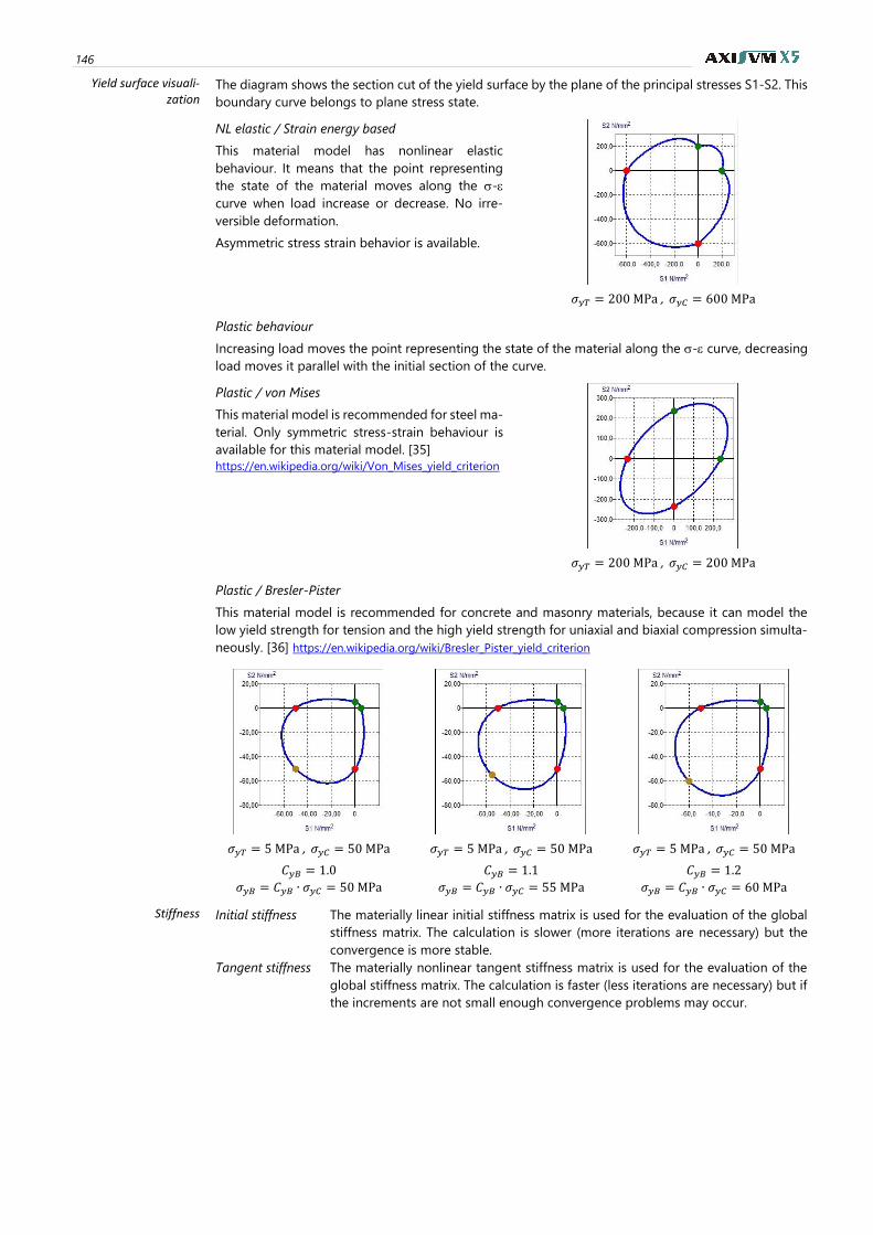
146

Yield surface visuali-zation

The diagram shows the section cut of the yield surface by the plane of the principal stresses S1-S2. This

boundary curve belongs to plane stress state.

NL elastic / Strain energy based

This material model has nonlinear elastic

behaviour. It means that the point representing

the state of the material moves along the -

curve when load increase or decrease. No irre-

versible deformation.

Asymmetric stress strain behavior is available.

𝜎𝑦𝑇 = 200 MPa , 𝜎𝑦𝐶 = 600 MPa

Plastic behaviour

Increasing load moves the point representing the state of the material along the - curve, decreasing

load moves it parallel with the initial section of the curve.

Plastic / von Mises

This material model is recommended for steel ma-

terial. Only symmetric stress-strain behaviour is

available for this material model. [35]

https://en.wikipedia.org/wiki/Von_Mises_yield_criterion

𝜎𝑦𝑇 = 200 MPa , 𝜎𝑦𝐶 = 200 MPa

Plastic / Bresler-Pister

This material model is recommended for concrete and masonry materials, because it can model the

low yield strength for tension and the high yield strength for uniaxial and biaxial compression simulta-

neously. [36] https://en.wikipedia.org/wiki/Bresler_Pister_yield_criterion

𝜎𝑦𝑇 = 5 MPa , 𝜎𝑦𝐶 = 50 MPa

𝐶𝑦𝐵 = 1.0 𝜎𝑦𝐵 = 𝐶𝑦𝐵 ∙ 𝜎𝑦𝐶 = 50 MPa

𝜎𝑦𝑇 = 5 MPa , 𝜎𝑦𝐶 = 50 MPa

𝐶𝑦𝐵 = 1.1 𝜎𝑦𝐵 = 𝐶𝑦𝐵 ∙ 𝜎𝑦𝐶 = 55 MPa

𝜎𝑦𝑇 = 5 MPa , 𝜎𝑦𝐶 = 50 MPa

𝐶𝑦𝐵 = 1.2 𝜎𝑦𝐵 = 𝐶𝑦𝐵 ∙ 𝜎𝑦𝐶 = 60 MPa

Stiffness Initial stiffness The materially linear initial stiffness matrix is used for the evaluation of the global

stiffness matrix. The calculation is slower (more iterations are necessary) but the

convergence is more stable.

Tangent stiffness The materially nonlinear tangent stiffness matrix is used for the evaluation of the

global stiffness matrix. The calculation is faster (less iterations are necessary) but if

the increments are not small enough convergence problems may occur.

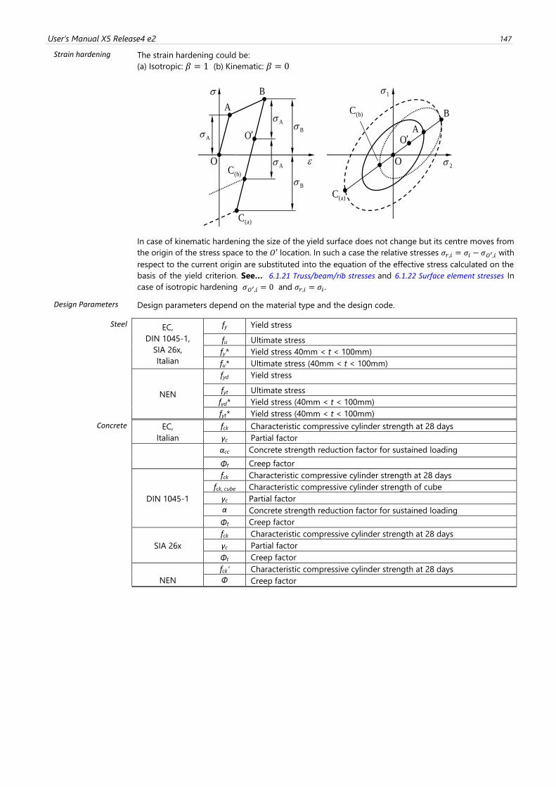
User’s Manual X5 Release4 e2 147

Strain hardening The strain hardening could be:

(a) Isotropic: 𝛽 = 1 (b) Kinematic: 𝛽 = 0

In case of kinematic hardening the size of the yield surface does not change but its centre moves from

the origin of the stress space to the 𝑂′ location. In such a case the relative stresses 𝜎𝑟,𝑖 = 𝜎𝑖 − 𝜎𝑂′,𝑖 with

respect to the current origin are substituted into the equation of the effective stress calculated on the

basis of the yield criterion. See… 6.1.21 Truss/beam/rib stresses and 6.1.22 Surface element stresses In

case of isotropic hardening 𝜎𝑂′,𝑖 = 0 and 𝜎𝑟,𝑖 = 𝜎𝑖 .

Design Parameters Design parameters depend on the material type and the design code.

Steel EC,

DIN 1045-1,

SIA 26x,

Italian

fy Yield stress

fu Ultimate stress

fy* Yield stress 40mm < t < 100mm)

fu* Ultimate stress (40mm < t < 100mm)

NEN

fyd Yield stress

fyt Ultimate stress

fyd* Yield stress (40mm < t < 100mm)

fyt* Yield stress (40mm < t < 100mm)

Concrete EC,

Italian

fck Characteristic compressive cylinder strength at 28 days

γc Partial factor

αcc Concrete strength reduction factor for sustained loading

Φt Creep factor

DIN 1045-1

fck Characteristic compressive cylinder strength at 28 days

fck, cube Characteristic compressive cylinder strength of cube

γc Partial factor

α Concrete strength reduction factor for sustained loading

Φt Creep factor

SIA 26x

fck Characteristic compressive cylinder strength at 28 days

γc Partial factor

Φt Creep factor

NEN

fck’ Characteristic compressive cylinder strength at 28 days

Φ Creep factor

1

A

B

O

A

B

(a)C

(b)C

(a)C

(b)CA

A

B

B

A

2O

OO

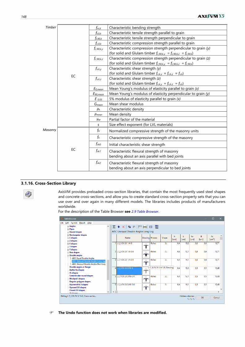
148

Timber

EC

fm,k Characteristic bending strength

ft,0,k Characteristic tensile strength parallel to grain

ft,90,k Characteristic tensile strength perpendicular to grain

fc,0,k Characteristic compression strength parallel to grain

fc,90,k,y Characteristic compression strength perpendicular to grain (y)

(for solid and Glulam timber fc,90,k,y = fc,90,k,z = fc,90,k)

fc,90,k,z Characteristic compression strength perpendicular to grain (z)

(for solid and Glulam timber fc,90,k,y = fc,90,k,z = fc,90,k)

fv,k,y Characteristic shear strength (y)

(for solid and Glulam timber fv,k,y = fv,k,z = fv,k)

fv,k,z Characteristic shear strength (z)

(for solid and Glulam timber fv,k,y = fv,k,z = fv,k)

E0,mean Mean Young’s modulus of elasticity parallel to grain (x)

E90,mean Mean Young’s modulus of elasticity perpendicular to grain (y)

E 0.05 5% modulus of elasticity parallel to grain (x)

Gmean Mean shear modulus

ρk Characteristic density

ρmean Mean density

γM Partial factor of the material

s Size effect exponent (for LVL materials)

Masonry

EC

fb Normalized compressive strength of the masonry units

fk Characteristic compressive strength of the masonry

fvk0 Initial characteristic shear strength

fxk1 Characteristic flexural strength of masonry

bending about an axis parallel with bed joints

fxk2 Characteristic flexural strength of masonry

bending about an axis perpendicular to bed joints

3.1.16. Cross-Section Library

AxisVM provides preloaded cross-section libraries, that contain the most frequently used steel shapes

and concrete cross-sections, and allow you to create standard cross-section property sets that you can

use over and over again in many different models. The libraries includes products of manufacturers

worldwide.

For the description of the Table Browser see 2.9 Table Browser.

The Undo function does not work when libraries are modified.

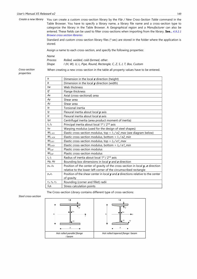
User’s Manual X5 Release4 e2 149

Create a new library

You can create a custom cross-section library by the File / New Cross-Section Table command in the

Table Browser. You have to specify a library name, a library file name and a cross-section type to

categorize the library in the Table Browser. A Geographical region and a Manufacturer can also be

entered. These fields can be used to filter cross-sections when importing from the library. See… 4.9.2.1 Browse cross-section libraries

Standard and custom cross-section library files (*.sec) are stored in the folder where the application is

stored.

Assign a name to each cross-section, and specify the following properties:

Name

Process Rolled, welded, cold-formed, other.

Shape I (H, W), U, L, Pipe, Round, Rectangle, C, Z, S, J, T, Box, Custom

Cross-section properties

When creating a new cross-section in the table all property values have to be entered.

h Dimension in the local z direction (height)

b Dimension in the local y direction (width)

tw Web thickness

tf Flange thickness

Ax Axial (cross-sectional) area

Ay Shear area

Az Shear area

Ix Torsional inertia

Iy Flexural inertia about local y axis

Iz Flexural inertia about local z axis

Iyz Centrifugal inertia (area product moment of inertia)

I1, I2 Principal inertia about local 1st / 2nd axis

Iω Warping modulus (used for the design of steel shapes)

W1, el,t Elastic cross-section modulus, top = I1 / e2_max (see diagram below)

W1, el,b Elastic cross-section modulus, bottom = I1 / e2_min

W2,el,t Elastic cross-section modulus, top = I2 / e1_max

W2,el,b Elastic cross-section modulus, bottom = I2 / e1_min

W1,pl Plastic cross-section modulus

W2,pl Plastic cross-section modulus

iy, iz Radius of inertia about local 1st / 2nd axis

Hy, Hz Bounding box dimensions in local y and z direction

yG, zG Position of the center of gravity of the cross-section in local y, z direction

relative to the lower-left corner of the circumscribed rectangle

ys,zs Position of the shear center in local y and z directions relative to the center

of gravity

r1, r2, r3 Rounding (corner and fillet) radii

S.p. Stress calculation points

The Cross-section Library contains different type of cross-sections:

Steel cross-section

Hot rolled parallel flange

I beam Hot rolled tapered flange I beam

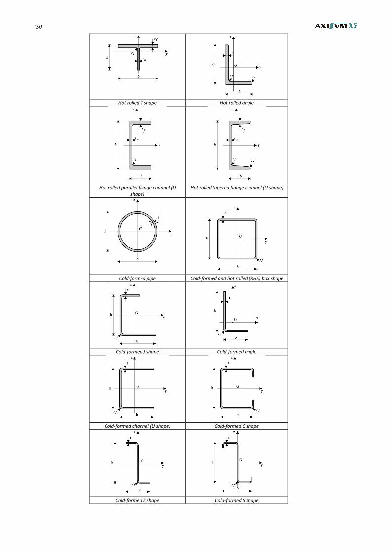
150

Hot rolled T shape Hot rolled angle

Hot rolled parallel flange channel (U

shape) Hot rolled tapered flange channel (U shape)

Cold-formed pipe Cold-formed and hot rolled (RHS) box shape

Cold-formed J shape Cold-formed angle

Cold-formed channel (U shape) Cold-formed C shape

Cold-formed Z shape Cold-formed S shape

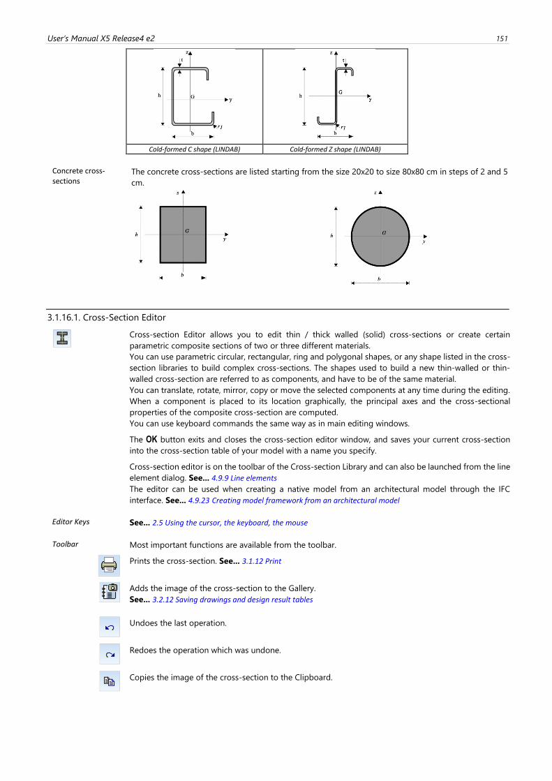
User’s Manual X5 Release4 e2 151

Cold-formed C shape (LINDAB) Cold-formed Z shape (LINDAB)

Concrete cross-sections

The concrete cross-sections are listed starting from the size 20x20 to size 80x80 cm in steps of 2 and 5

cm.

3.1.16.1. Cross-Section Editor

Cross-section Editor allows you to edit thin / thick walled (solid) cross-sections or create certain

parametric composite sections of two or three different materials.

You can use parametric circular, rectangular, ring and polygonal shapes, or any shape listed in the cross-

section libraries to build complex cross-sections. The shapes used to build a new thin-walled or thin-

walled cross-section are referred to as components, and have to be of the same material.

You can translate, rotate, mirror, copy or move the selected components at any time during the editing.

When a component is placed to its location graphically, the principal axes and the cross-sectional

properties of the composite cross-section are computed.

You can use keyboard commands the same way as in main editing windows.

The OK button exits and closes the cross-section editor window, and saves your current cross-section

into the cross-section table of your model with a name you specify.

Cross-section editor is on the toolbar of the Cross-section Library and can also be launched from the line

element dialog. See... 4.9.9 Line elements

The editor can be used when creating a native model from an architectural model through the IFC

interface. See... 4.9.23 Creating model framework from an architectural model

Editor Keys See... 2.5 Using the cursor, the keyboard, the mouse

Toolbar Most important functions are available from the toolbar.

Prints the cross-section. See... 3.1.12 Print

Adds the image of the cross-section to the Gallery.

See... 3.2.12 Saving drawings and design result tables

Undoes the last operation.

Redoes the operation which was undone.

Copies the image of the cross-section to the Clipboard.

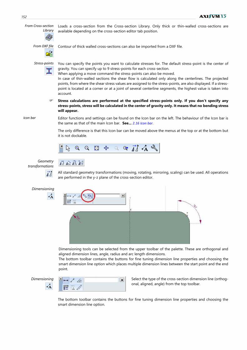
152

From Cross-section Library

Loads a cross-section from the Cross-section Library. Only thick or thin-walled cross-sections are

available depending on the cross-section editor tab position.

From DXF file

Contour of thick walled cross-sections can also be imported from a DXF file.

Stress-points

You can specify the points you want to calculate stresses for. The default stress-point is the center of

gravity. You can specify up to 9 stress-points for each cross-section.

When applying a move command the stress-points can also be moved.

In case of thin-walled sections the shear flow is calculated only along the centerlines. The projected

points, from where the shear stress values are assigned to the stress-points, are also displayed. If a stress-

point is located at a corner or at a joint of several centerline segments, the highest value is taken into

account.

Stress calculations are performed at the specified stress-points only. If you don’t specify any

stress-points, stress will be calculated in the center of gravity only. It means that no bending stress

will appear.

Icon bar Editor functions and settings can be found on the Icon bar on the left. The behaviour of the Icon bar is

the same as that of the main Icon bar. See... 2.16 Icon bar.

The only difference is that this Icon bar can be moved above the menus at the top or at the bottom but

it is not dockable.

Geometry

transformations

All standard geometry transformations (moving, rotating, mirroring, scaling) can be used. All operations

are performed in the y-z plane of the cross-section editor.

Dimensioning

Dimensioning tools can be selected from the upper toolbar of the palette. These are orthogonal and

aligned dimension lines, angle, radius and arc length dimensions.

The bottom toolbar contains the buttons for fine tuning dimension line properties and choosing the

smart dimension line option which places multiple dimension lines between the start point and the end

point.

Dimensioning

Select the type of the cross-section dimension line (orthog-

onal, aligned, angle) from the top toolbar.

The bottom toolbar contains the buttons for fine tuning dimension line properties and choosing the

smart dimension line option.

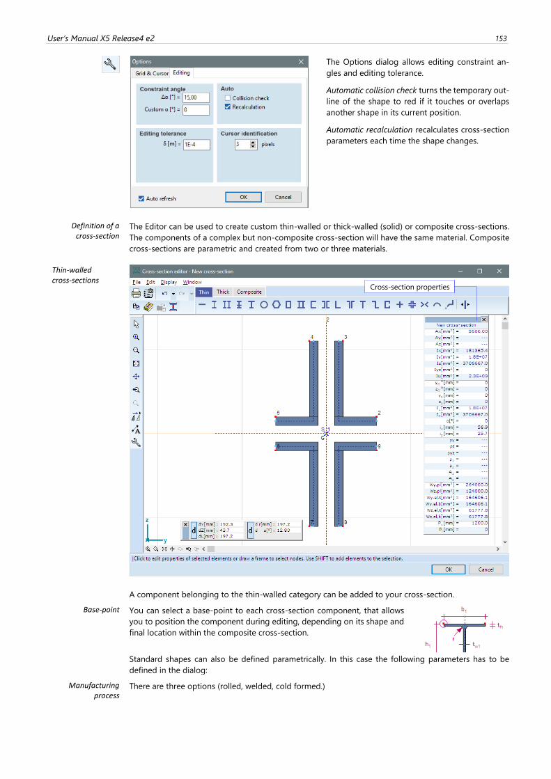
User’s Manual X5 Release4 e2 153

The Options dialog allows editing constraint an-

gles and editing tolerance.

Automatic collision check turns the temporary out-

line of the shape to red if it touches or overlaps

another shape in its current position.

Automatic recalculation recalculates cross-section

parameters each time the shape changes.

Definition of a cross-section

The Editor can be used to create custom thin-walled or thick-walled (solid) or composite cross-sections.

The components of a complex but non-composite cross-section will have the same material. Composite

cross-sections are parametric and created from two or three materials.

Thin-walled cross-sections

A component belonging to the thin-walled category can be added to your cross-section.

Base-point You can select a base-point to each cross-section component, that allows

you to position the component during editing, depending on its shape and

final location within the composite cross-section.

Standard shapes can also be defined parametrically. In this case the following parameters has to be

defined in the dialog:

Manufacturing process

There are three options (rolled, welded, cold formed.)

Cross-section properties

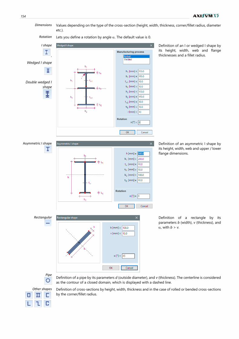
154

Dimensions Values depending on the type of the cross-section (height, width, thickness, corner/fillet radius, diameter

etc.).

Rotation Lets you define a rotation by angle . The default value is 0.

I shape

,

Wedged I shape

Double wedged I

shape

Definition of an I or wedged I shape by

its height, width, web and flange

thicknesses and a fillet radius.

Asymmetric I shape

Definition of an asymmetric I shape by

its height, width, web and upper / lower

flange dimensions.

Rectangular

Definition of a rectangle by its

parameters b (width), v (thickness), and

, with b > v.

Pipe

Definition of a pipe by its parameters d (outside diameter), and v (thickness). The centerline is considered

as the contour of a closed domain, which is displayed with a dashed line.

Other shapes

Definition of cross-sections by height, width, thickness and in the case of rolled or bended cross-sections

by the corner/fillet radius.

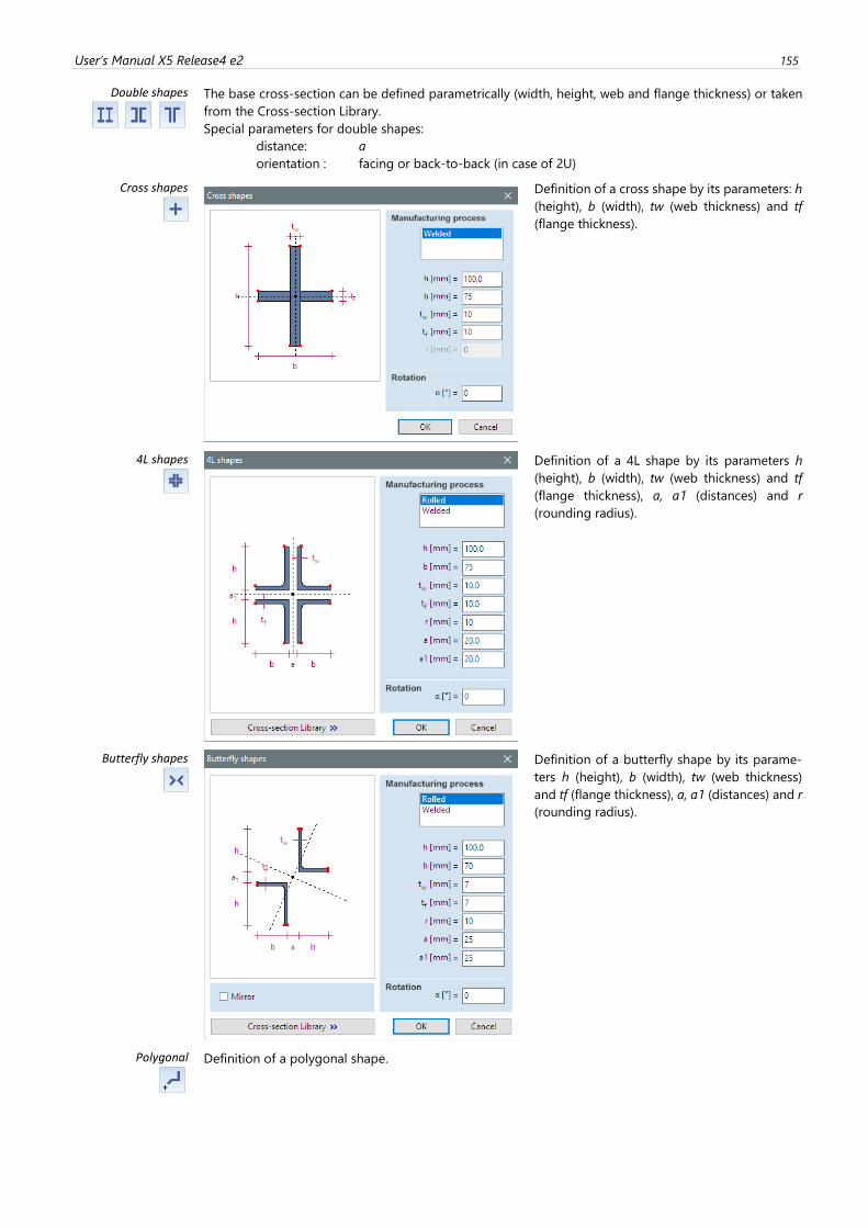
User’s Manual X5 Release4 e2 155

Double shapes

The base cross-section can be defined parametrically (width, height, web and flange thickness) or taken

from the Cross-section Library.

Special parameters for double shapes:

distance: a

orientation : facing or back-to-back (in case of 2U)

Cross shapes

Definition of a cross shape by its parameters: h

(height), b (width), tw (web thickness) and tf

(flange thickness).

4L shapes

Definition of a 4L shape by its parameters h

(height), b (width), tw (web thickness) and tf

(flange thickness), a, a1 (distances) and r

(rounding radius).

Butterfly shapes

Definition of a butterfly shape by its parame-

ters h (height), b (width), tw (web thickness)

and tf (flange thickness), a, a1 (distances) and r

(rounding radius).

Polygonal

Definition of a polygonal shape.

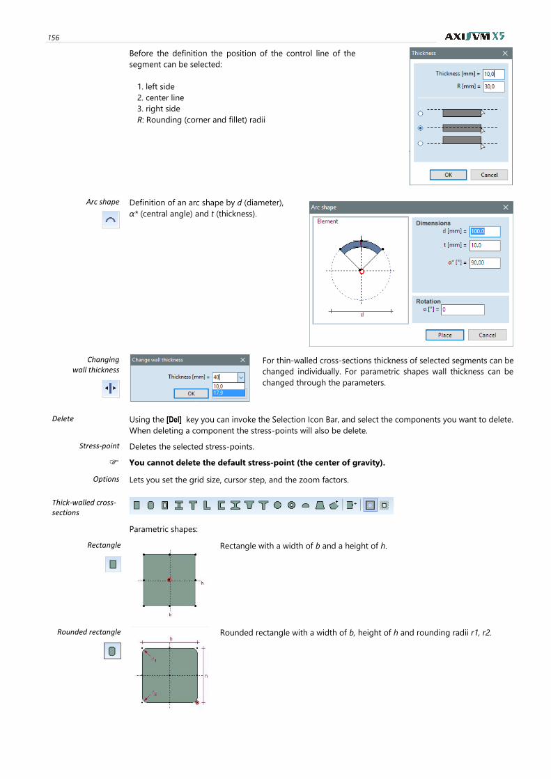
156

Before the definition the position of the control line of the

segment can be selected:

1. left side

2. center line

3. right side

R: Rounding (corner and fillet) radii

Arc shape

Definition of an arc shape by d (diameter),

α* (central angle) and t (thickness).

Changing wall thickness

For thin-walled cross-sections thickness of selected segments can be

changed individually. For parametric shapes wall thickness can be

changed through the parameters.

Delete Using the [Del] key you can invoke the Selection Icon Bar, and select the components you want to delete.

When deleting a component the stress-points will also be delete.

Stress-point Deletes the selected stress-points.

You cannot delete the default stress-point (the center of gravity).

Options Lets you set the grid size, cursor step, and the zoom factors.

Thick-walled cross-sections

Parametric shapes:

Rectangle

Rectangle with a width of b and a height of h.

Rounded rectangle

Rounded rectangle with a width of b, height of h and rounding radii r1, r2.

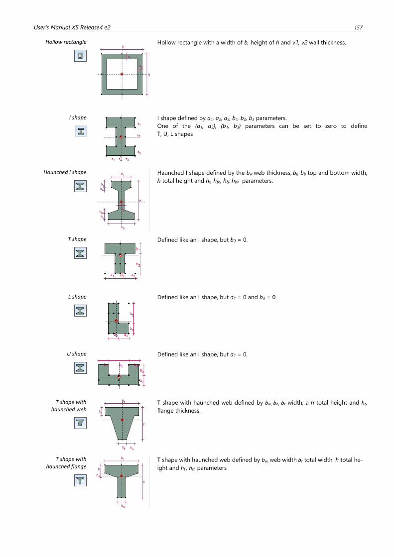
User’s Manual X5 Release4 e2 157

Hollow rectangle

Hollow rectangle with a width of b, height of h and v1, v2 wall thickness.

I shape

I shape defined by a1, a2, a3, b1, b2, b3 parameters.

One of the (a1, a3), (b1, b3) parameters can be set to zero to define

T, U, L shapes

Haunched I shape

Haunched I shape defined by the bw web thickness, bt, bb top and bottom width,

h total height and ht, hth, hb, hbh parameters.

T shape

Defined like an I shape, but b3 = 0.

L shape

Defined like an I shape, but a1 = 0 and b3 = 0.

U shape

Defined like an I shape, but a1 = 0.

T shape with haunched web

T shape with haunched web defined by bw, bb, bt width, a h total height and ht,

flange thickness.

T shape with haunched flange

T shape with haunched web defined by bw, web width bt total width, h total he-

ight and ht , hth parameters

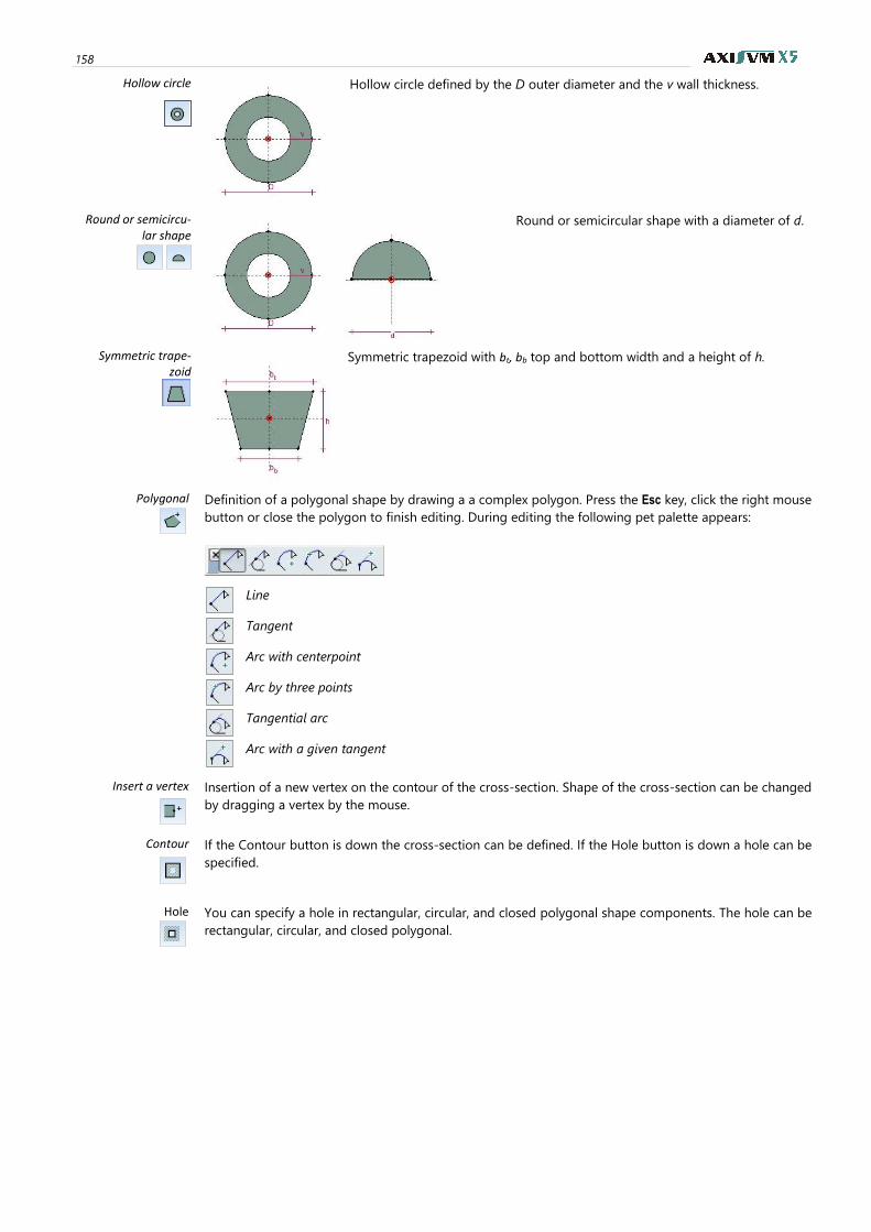
158

Hollow circle

Hollow circle defined by the D outer diameter and the v wall thickness.

Round or semicircu-lar shape

Round or semicircular shape with a diameter of d.

Symmetric trape-zoid

Symmetric trapezoid with bt, bb top and bottom width and a height of h.

Polygonal

Definition of a polygonal shape by drawing a a complex polygon. Press the Esc key, click the right mouse

button or close the polygon to finish editing. During editing the following pet palette appears:

Line

Tangent

Arc with centerpoint

Arc by three points

Tangential arc

Arc with a given tangent

Insert a vertex

Insertion of a new vertex on the contour of the cross-section. Shape of the cross-section can be changed

by dragging a vertex by the mouse.

Contour

If the Contour button is down the cross-section can be defined. If the Hole button is down a hole can be

specified.

Hole

You can specify a hole in rectangular, circular, and closed polygonal shape components. The hole can be

rectangular, circular, and closed polygonal.

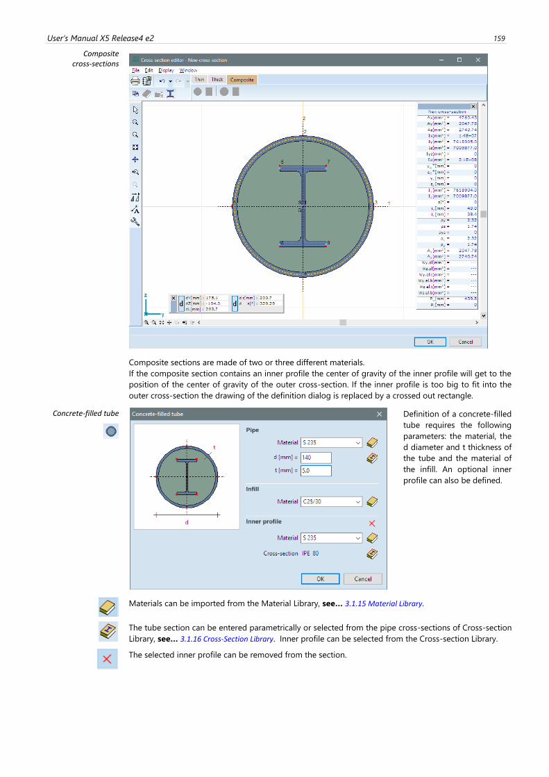
User’s Manual X5 Release4 e2 159

Composite cross-sections

Composite sections are made of two or three different materials.

If the composite section contains an inner profile the center of gravity of the inner profile will get to the

position of the center of gravity of the outer cross-section. If the inner profile is too big to fit into the

outer cross-section the drawing of the definition dialog is replaced by a crossed out rectangle.

Concrete-filled tube

Definition of a concrete-filled

tube requires the following

parameters: the material, the

d diameter and t thickness of

the tube and the material of

the infill. An optional inner

profile can also be defined.

Materials can be imported from the Material Library, see… 3.1.15 Material Library.

The tube section can be entered parametrically or selected from the pipe cross-sections of Cross-section

Library, see… 3.1.16 Cross-Section Library. Inner profile can be selected from the Cross-section Library.

The selected inner profile can be removed from the section.

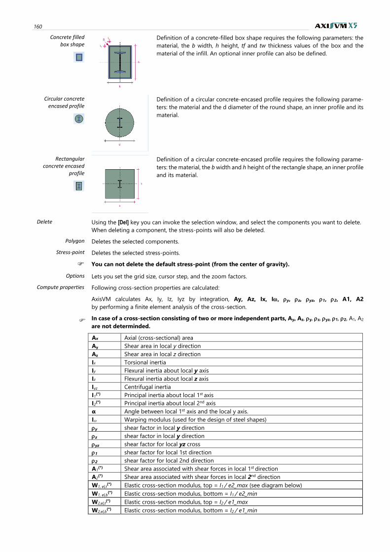
160

Concrete filled box shape

Definition of a concrete-filled box shape requires the following parameters: the

material, the b width, h height, tf and tw thickness values of the box and the

material of the infill. An optional inner profile can also be defined.

Circular concrete encased profile

Definition of a circular concrete-encased profile requires the following parame-

ters: the material and the d diameter of the round shape, an inner profile and its

material.

Rectangular concrete encased

profile

Definition of a circular concrete-encased profile requires the following parame-

ters: the material, the b width and h height of the rectangle shape, an inner profile

and its material.

Delete Using the [Del] key you can invoke the selection window, and select the components you want to delete.

When deleting a component, the stress-points will also be deleted.

Polygon Deletes the selected components.

Stress-point Deletes the selected stress-points.

You can not delete the default stress-point (from the center of gravity).

Options Lets you set the grid size, cursor step, and the zoom factors.

Compute properties Following cross-section properties are calculated:

AxisVM calculates Ax, Iy, Iz, Iyz by integration, Ay, Az, Ix, I, y, z, yz, 1, 2, A1, A2

by performing a finite element analysis of the cross-section.

In case of a cross-section consisting of two or more independent parts, Ay, Az, y, z, yz, 1, 2, A1, A2

are not determinded.

Ax Axial (cross-sectional) area

Ay Shear area in local y direction

Az Shear area in local z direction

Ix Torsional inertia

Iy Flexural inertia about local y axis

Iz Flexural inertia about local z axis

Iyz Centrifugal inertia

I1(*) Principal inertia about local 1st axis

I2(*) Principal inertia about local 2nd axis

α Angle between local 1st axis and the local y axis.

I Warping modulus (used for the design of steel shapes)

y shear factor in local y direction

z shear factor in local y direction

yz shear factor for local yz cross

1 shear factor for local 1st direction

2 shear factor for local 2nd direction

A1(*) Shear area associated with shear forces in local 1st direction

A2(*) Shear area associated with shear forces in local 2nd direction

W1, el,t(*) Elastic cross-section modulus, top = I1 / e2_max (see diagram below)

W1, el,b(*) Elastic cross-section modulus, bottom = I1 / e2_min

W2,el,t(*) Elastic cross-section modulus, top = I2 / e1_max

W2,el,b(*) Elastic cross-section modulus, bottom = I2 / e1_min

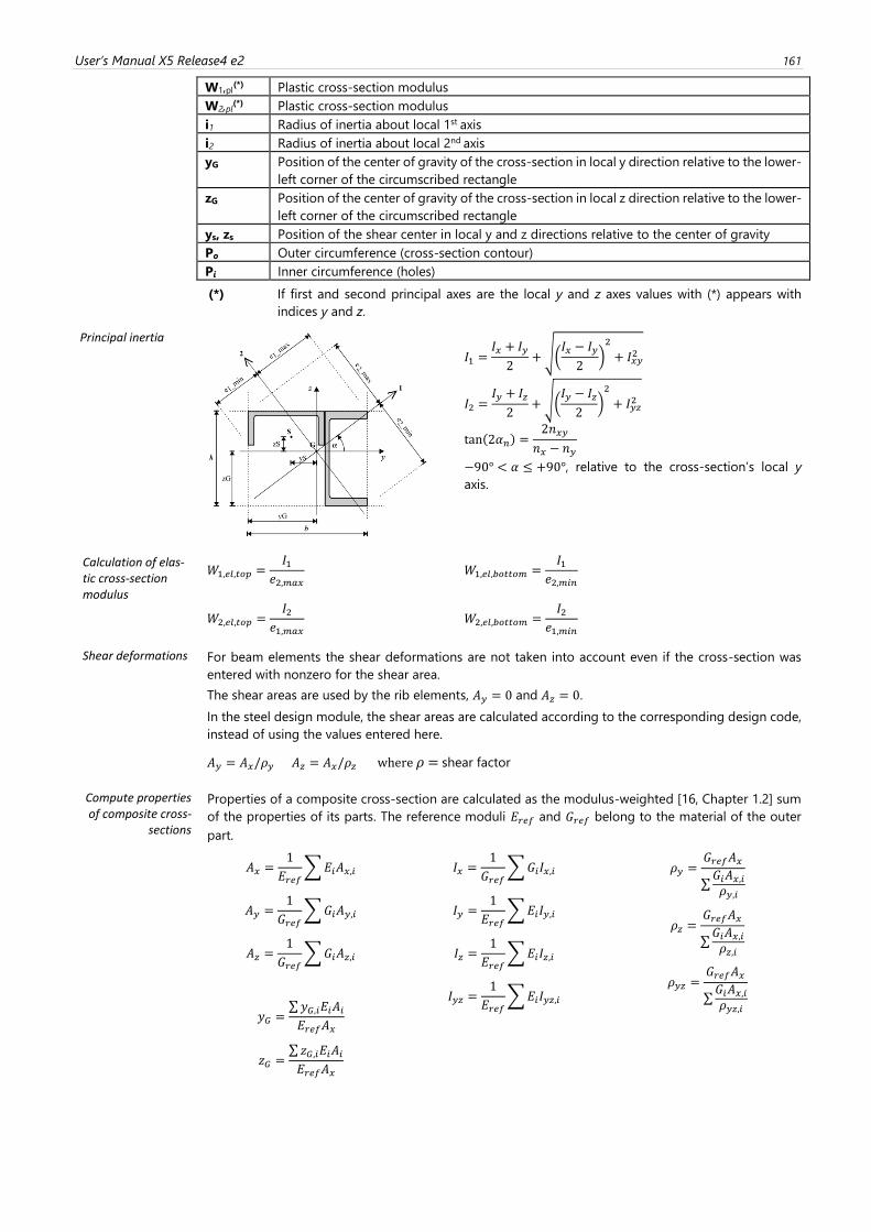
User’s Manual X5 Release4 e2 161

W1,pl(*) Plastic cross-section modulus

W2,pl(*) Plastic cross-section modulus

i1 Radius of inertia about local 1st axis

i2 Radius of inertia about local 2nd axis

yG Position of the center of gravity of the cross-section in local y direction relative to the lower-

left corner of the circumscribed rectangle

zG Position of the center of gravity of the cross-section in local z direction relative to the lower-

left corner of the circumscribed rectangle

ys, zs Position of the shear center in local y and z directions relative to the center of gravity

Po Outer circumference (cross-section contour)

Pi Inner circumference (holes)

(*) If first and second principal axes are the local y and z axes values with (*) appears with

indices y and z.

Principal inertia

𝐼1 =𝐼𝑥 + 𝐼𝑦

2+ √(

𝐼𝑥 − 𝐼𝑦

2)2

+ 𝐼𝑥𝑦2

𝐼2 =𝐼𝑦 + 𝐼𝑧

2+ √(

𝐼𝑦 − 𝐼𝑧

2)2

+ 𝐼𝑦𝑧2

tan(2𝛼𝑛) =2𝑛𝑥𝑦

𝑛𝑥 − 𝑛𝑦

−90° < 𝛼 ≤ +90°, relative to the cross-section’s local y

axis.

Calculation of elas-tic cross-section modulus

𝑊1,𝑒𝑙,𝑡𝑜𝑝 =𝐼1

𝑒2,𝑚𝑎𝑥 𝑊1,𝑒𝑙,𝑏𝑜𝑡𝑡𝑜𝑚 =

𝐼1𝑒2,𝑚𝑖𝑛

𝑊2,𝑒𝑙,𝑡𝑜𝑝 =𝐼2

𝑒1,𝑚𝑎𝑥 𝑊2,𝑒𝑙,𝑏𝑜𝑡𝑡𝑜𝑚 =

𝐼2𝑒1,𝑚𝑖𝑛

Shear deformations For beam elements the shear deformations are not taken into account even if the cross-section was

entered with nonzero for the shear area.

The shear areas are used by the rib elements, 𝐴𝑦 = 0 and 𝐴𝑧 = 0.

In the steel design module, the shear areas are calculated according to the corresponding design code,

instead of using the values entered here.

𝐴𝑦 = 𝐴𝑥/𝜌𝑦 𝐴𝑧 = 𝐴𝑥/𝜌𝑧 where 𝜌 = shear factor

Compute properties of composite cross-

sections

Properties of a composite cross-section are calculated as the modulus-weighted [16, Chapter 1.2] sum

of the properties of its parts. The reference moduli 𝐸𝑟𝑒𝑓 and 𝐺𝑟𝑒𝑓 belong to the material of the outer

part.

𝐴𝑥 =

1

𝐸𝑟𝑒𝑓∑𝐸𝑖𝐴𝑥,𝑖

𝐴𝑦 =1

𝐺𝑟𝑒𝑓∑𝐺𝑖𝐴𝑦,𝑖

𝐴𝑧 =1

𝐺𝑟𝑒𝑓∑𝐺𝑖𝐴𝑧,𝑖

𝑦𝐺 =∑𝑦𝐺,𝑖𝐸𝑖𝐴𝑖𝐸𝑟𝑒𝑓𝐴𝑥

𝑧𝐺 =∑𝑧𝐺,𝑖𝐸𝑖𝐴𝑖𝐸𝑟𝑒𝑓𝐴𝑥

𝐼𝑥 =1

𝐺𝑟𝑒𝑓∑𝐺𝑖𝐼𝑥,𝑖

𝐼𝑦 =1

𝐸𝑟𝑒𝑓∑𝐸𝑖𝐼𝑦,𝑖

𝐼𝑧 =1

𝐸𝑟𝑒𝑓∑𝐸𝑖𝐼𝑧,𝑖

𝐼𝑦𝑧 =1

𝐸𝑟𝑒𝑓∑𝐸𝑖𝐼𝑦𝑧,𝑖

𝜌𝑦 =𝐺𝑟𝑒𝑓𝐴𝑥

∑𝐺𝑖𝐴𝑥,𝑖𝜌𝑦,𝑖

𝜌𝑧 =𝐺𝑟𝑒𝑓𝐴𝑥

∑𝐺𝑖𝐴𝑥,𝑖𝜌𝑧,𝑖

𝜌𝑦𝑧 =𝐺𝑟𝑒𝑓𝐴𝑥

∑𝐺𝑖𝐴𝑥,𝑖𝜌𝑦𝑧,𝑖

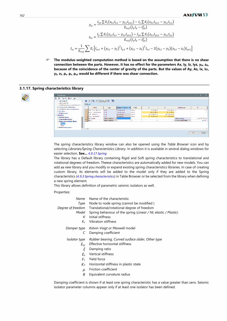
162

𝑦𝜔 =𝐼𝑦𝑧 ∑𝐸𝑖(𝑧𝑆,𝑖𝐼𝑧,𝑖 − 𝑦𝑆,𝑖𝐼𝑦𝑧,𝑖) − 𝐼𝑧 ∑𝐸𝑖(𝑧𝑆,𝑖𝐼𝑦𝑧,𝑖 − 𝑦𝑆,𝑖𝐼𝑦,𝑖)

𝐸𝑟𝑒𝑓(𝐼𝑦𝐼𝑧 − 𝐼𝑦𝑧2 )

𝑧𝜔 =𝐼𝑦 ∑𝐸𝑖(𝑧𝑆,𝑖𝐼𝑧,𝑖 − 𝑦𝑆,𝑖𝐼𝑦𝑧,𝑖) − 𝐼𝑦𝑧 ∑𝐸𝑖(𝑧𝑆,𝑖𝐼𝑦𝑧,𝑖 − 𝑦𝑆,𝑖𝐼𝑦,𝑖)

𝐸𝑟𝑒𝑓(𝐼𝑦𝐼𝑧 − 𝐼𝑦𝑧2 )

𝐼𝜔 =1

𝐸𝑟𝑒𝑓∑𝐸𝑖 [𝐼𝜔,𝑖 + (𝑦𝑆,𝑖 − 𝑦𝑆)

2𝐼𝑦,𝑖 + (𝑧𝑆,𝑖 − 𝑧𝑆)

2𝐼𝑧,𝑖 − 2(𝑦𝑆,𝑖 − 𝑦𝑆)(𝑧𝑆,𝑖 − 𝑧𝑆)𝐼𝑦𝑧,𝑖]

The modulus-weighted computation method is based on the assumption that there is no shear

connection between the parts. However, it has no effect for the parameters Ax, Iy, Iz, Iyz, yG, zG,

because of the coincidence of the center of gravity of the parts. But the values of Ay, Az, Ix, I,

yS, zS, ρy, ρz, ρyz would be different if there was shear connection.

3.1.17. Spring characteristics library

The spring characteristics library window can also be opened using the Table Browser icon and by

selecting Libraries/Spring Characteristics Library. In addition it is available in several dialog windows for

easier selection. See... 4.9.17 Spring

The library has a Default library containing Rigid and Soft spring characteristics to translational and

rotational degrees of freedom. Theese characteristics are automatically added for new models. You can

add aa new library and you modify or expand existing spring characteristics libraries. In case of creating

custom library, its elements will be added to the model only if they are added to the Spring

characteristics (4.9.3 Spring characteristics) in Table Browser or be selected from the library when defining

a new spring element.

This library allows definition of parametric seismic isolators as well.

Properties:

Name Name of the characteristic

Type Node to node spring (cannot be modified )

Degree of freedom Translational/rotational degree of freedom

Model Spring behaviour of the spring (Linear / NL elastic / Plastic)

K Initial stiffness

Kv Vibration stiffness

Damper type Kelvin-Voigt or Maxwell model

C Damping coefficient

Isolator type Rubber bearing, Curved surface slider, Other type

Exy Effective horizontal stiffness

ξ Damping ratio

Ez Vertical stiffness

F1 Yield force

KT Horizontal stiffness in plastic state

µ Friction coefficient

R Equivalent curvature radius

Damping coefficient is shown if at least one spring characteristic has a value greater than zero. Seismic

isolator parameter columns appear only if at least one isolator has been defined.

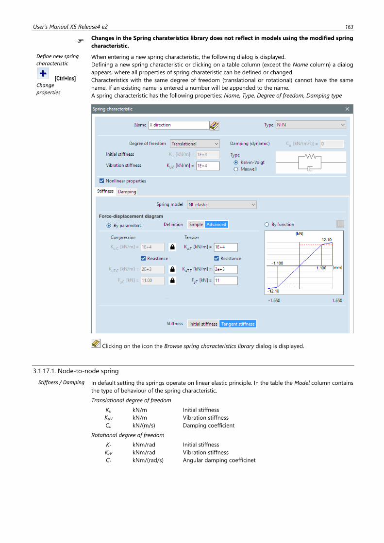
User’s Manual X5 Release4 e2 163

Changes in the Spring charateristics library does not reflect in models using the modified spring

characteristic.

Define new spring characteristic

[Ctrl+Ins] Change properties

When entering a new spring characteristic, the following dialog is displayed.

Defining a new spring characteristic or clicking on a table column (except the Name column) a dialog

appears, where all properties of spring charateristic can be defined or changed.

Characteristics with the same degree of freedom (translational or rotational) cannot have the same

name. If an existing name is entered a number will be appended to the name.

A spring characteristic has the following properties: Name, Type, Degree of freedom, Damping type

Clicking on the icon the Browse spring characteristics library dialog is displayed.

3.1.17.1. Node-to-node spring

Stiffness / Damping In default setting the springs operate on linear elastic principle. In the table the Model column contains

the type of behaviour of the spring characteristic.

Translational degree of freedom

Ku kN/m Initial stiffness

KuV kN/m Vibration stiffness

Cu kN/(m/s) Damping coefficient

Rotational degree of freedom

Kr kNm/rad Initial stiffness

KrV kNm/rad Vibration stiffness

Cr kNm/(rad/s) Angular damping coefficinet

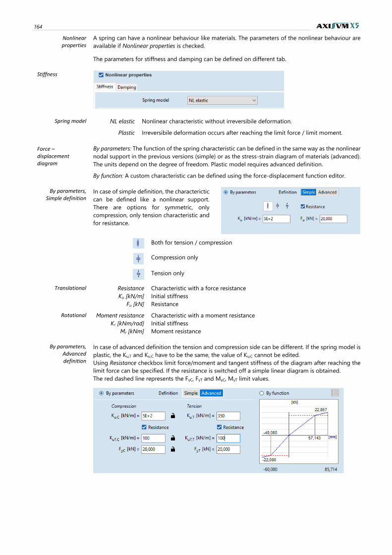
164

Nonlinear properties

A spring can have a nonlinear behaviour like materials. The parameters of the nonlinear behaviour are

available if Nonlinear properties is checked.

The parameters for stiffness and damping can be defined on different tab.

Stiffness

Spring model NL elastic Nonlinear characteristic without irreversibile deformation.

Plastic Irreversibile deformation occurs after reaching the limit force / limit moment.

Force – displacement diagram

By parameters: The function of the spring characteristic can be defined in the same way as the nonlinear

nodal support in the previous versions (simple) or as the stress-strain diagram of materials (advanced).

The units depend on the degree of freedom. Plastic model requires advanced definition.

By function: A custom characteristic can be defined using the force-displacement function editor.

By parameters, Simple definition

In case of simple definition, the characterictic

can be defined like a nonlinear support.

There are options for symmetric, only

compression, only tension characteristic and

for resistance.

Both for tension / compression

Compression only

Tension only

Translational Resistance Characteristic with a force resistance

Ku [kN/m] Initial stiffness

Fu [kN] Resistance

Rotational Moment resistance Characteristic with a moment resistance

Kr [kNm/rad] Initial stiffness

Mr [kNm] Moment resistance

By parameters, Advanced definition

In case of advanced definition the tension and compression side can be different. If the spring model is

plastic, the Ku,T and Ku,C have to be the same, the value of Ku,C cannot be edited.

Using Resistance checkbox limit force/moment and tangent stiffness of the diagram after reaching the

limit force can be specified. If the resistance is switched off a simple linear diagram is obtained.

The red dashed line represents the FyC, FyT and MyC, MyT limit values.

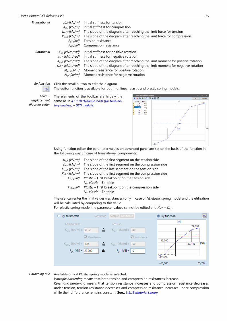
User’s Manual X5 Release4 e2 165

Translational Ku,T [kN/m] Initial stiffness for tension

Ku,T [kN/m] Initial stiffness for compression

KuT,T [kN/m] The slope of the diagram after reaching the limit force for tension

KuT,C [kN/m] The slope of the diagram after reaching the limit force for compression

FyT [kN] Tension resistance

FyC [kN] Compression resistance

Rotational Kr,T [kNm/rad] Initial stiffness for positive rotation

Kr,C [kNm/rad] Initial stiffness for negative rotation

KrT,T [kNm/rad] The slope of the diagram after reaching the limit moment for positive rotation

KrT,C [kNm/rad] The slope of the diagram after reaching the limit moment for negative rotation

MyT [kNm] Moment resistance for positive rotation

MyC [kNm] Moment resistance for negative rotation

By function

Click the small button to edit the diagram.

The editor function is available for both nonlinear elastic and plastic spring models.

Force – displacement

diagram editor

The elements of the toolbar are largely the

same as in 4.10.28 Dynamic loads (for time-his-tory analysis) – DYN module.

Using function editor the parameter values on advanced panel are set on the basis of the function in

the following way (in case of translational components)

Ku,T [kN/m] The slope of the first segment on the tension side

Ku,c [kN/m] The slope of the first segment on the compression side

KuT,T [kN/m] The slope of the last segment on the tension side

KuT,C [kN/m] The slope of the first segment on the compression side

Fy,T [kN] Plastic – First breakpoint on the tension side

NL elastic – Editable

Fy,C [kN] Plastic – First breakpoint on the compression side

NL elastic – Editable

The user can enter the limit values (resistances) only in case of NL elastic spring model and the utilization

will be calculated by comparing to this value.

For plastic spring model the parameter values cannot be edited and Ku,T = Ku,c.

Hardening rule Available only if Plastic spring model is selected.

Isotropic hardening means that both tension and compression resistances increase.

Kinematic hardening means that tension resistance increases and compression resistance decreases

under tension, tension resistance decreases and compression resistance increases under compression

while their differerence remains constant. See.. 3.1.15 Material Library

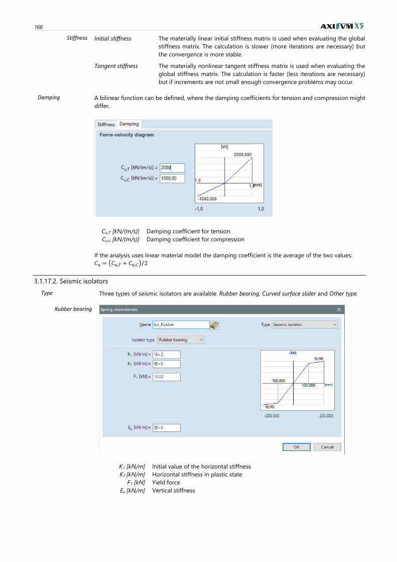
166

Stiffness Initial stiffness The materially linear initial stiffness matrix is used when evaluating the global

stiffness matrix. The calculation is slower (more iterations are necessary) but

the convergence is more stable.

Tangent stiffness The materially nonlinear tangent stiffness matrix is used when evaluating the

global stiffness matrix. The calculation is faster (less iterations are necessary)

but if increments are not small enough convergence problems may occur.

Damping A bilinear function can be defined, where the damping coefficients for tension and compression might

differ.

Cu,T [kN/(m/s)] Damping coefficient for tension

Cu,c [kN/(m/s)] Damping coefficient for compression

If the analysis uses linear material model the damping coefficient is the average of the two values:

𝐶𝑢 = (𝐶𝑢,𝑇 + 𝐶𝑢,𝐶)/2

3.1.17.2. Seismic isolators

Type Three types of seismic isolators are available: Rubber bearing, Curved surface slider and Other type.

Rubber bearing

K1 [kN/m] Initial value of the horizontal stiffness

KT [kN/m] Horizontal stiffness in plastic state

F1 [kN] Yield force

Ez [kN/m] Vertical stiffness

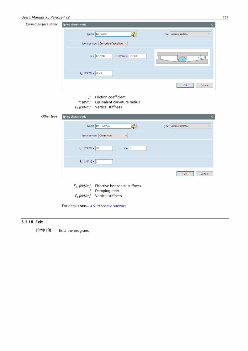
User’s Manual X5 Release4 e2 167

Curved surface slider

µ Friction coefficient

R [mm] Equivalent curvature radius

Ez [kN/m] Vertical stiffness

Other type

Exy [kN/m] Effective horizontal stiffness

ξ Damping ratio

Ez [kN/m] Vertical stiffness

For details see… 4.9.19 Seismic isolators

3.1.18. Exit

[Ctrl]+ [Q] Exits the program.

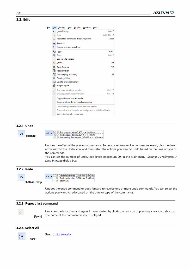
168

3.2. Edit

3.2.1. Undo

Alt+BkSp

Undoes the effect of the previous commands. To undo a sequence of actions (more levels), click the down

arrow next to the Undo icon, and then select the actions you want to undo based on the time or type of

the commands.

You can set the number of undo/redo levels (maximum 99) in the Main menu Settings / Preferences /

Data integrity dialog box.

3.2.2. Redo

Shift+Alt+BkSp

Undoes the undo command or goes forward to reverse one or more undo commands. You can select the

actions you want to redo based on the time or type of the commands.

3.2.3. Repeat last command

[Space]

Launches the last command again if it was started by clicking on an icon or pressing a keyboard shortcut.

The name of the command is also displayed.

3.2.4. Select All

Num *

See... 2.16.1 Selection

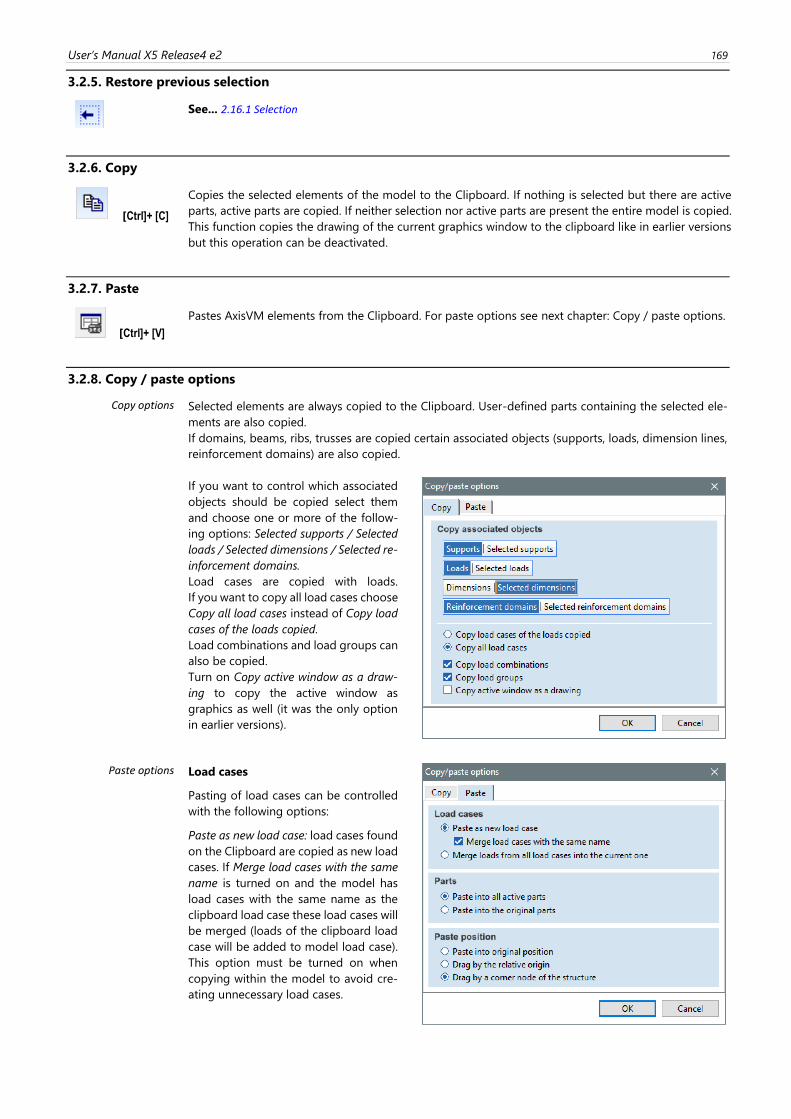
User’s Manual X5 Release4 e2 169

3.2.5. Restore previous selection

See... 2.16.1 Selection

3.2.6. Copy

[Ctrl]+ [C]

Copies the selected elements of the model to the Clipboard. If nothing is selected but there are active

parts, active parts are copied. If neither selection nor active parts are present the entire model is copied.

This function copies the drawing of the current graphics window to the clipboard like in earlier versions

but this operation can be deactivated.

3.2.7. Paste

[Ctrl]+ [V]

Pastes AxisVM elements from the Clipboard. For paste options see next chapter: Copy / paste options.

3.2.8. Copy / paste options

Copy options

Selected elements are always copied to the Clipboard. User-defined parts containing the selected ele-

ments are also copied.

If domains, beams, ribs, trusses are copied certain associated objects (supports, loads, dimension lines,

reinforcement domains) are also copied.

If you want to control which associated

objects should be copied select them

and choose one or more of the follow-

ing options: Selected supports / Selected

loads / Selected dimensions / Selected re-

inforcement domains.

Load cases are copied with loads.

If you want to copy all load cases choose

Copy all load cases instead of Copy load

cases of the loads copied.

Load combinations and load groups can

also be copied.

Turn on Copy active window as a draw-

ing to copy the active window as

graphics as well (it was the only option

in earlier versions).

Paste options

Load cases

Pasting of load cases can be controlled

with the following options:

Paste as new load case: load cases found

on the Clipboard are copied as new load

cases. If Merge load cases with the same

name is turned on and the model has

load cases with the same name as the

clipboard load case these load cases will

be merged (loads of the clipboard load

case will be added to model load case).

This option must be turned on when

copying within the model to avoid cre-

ating unnecessary load cases.

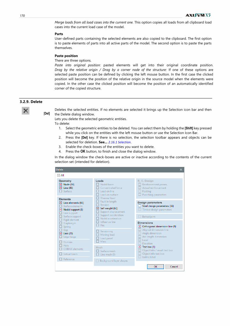
170

Merge loads from all load cases into the current one. This option copies all loads from all clipboard load

cases into the current load case of the model.

Parts

User-defined parts containing the selected elements are also copied to the clipboard. The first option

is to paste elements of parts into all active parts of the model. The second option is to paste the parts

themselves.

Paste position

There are three options.

Paste into original position: pasted elements will get into their original coordinate position.

Drag by the relative origin / Drag by a corner node of the structure: If one of these options are

selected paste position can be defined by clicking the left mouse button. In the first case the clicked

position will become the position of the relative origin in the source model when the elements were

copied. In the other case the clicked position will become the position of an automatically identified

corner of the copied structure.

3.2.9. Delete

[Del] Deletes the selected entities. If no elements are selected it brings up the Selection icon bar and then

the Delete dialog window.

Lets you delete the selected geometric entities.

To delete:

1. Select the geometric entities to be deleted. You can select them by holding the [Shift] key pressed

while you click on the entities with the left mouse button or use the Selection Icon Bar.

2. Press the [Del] key. If there is no selection, the selection toolbar appears and objects can be

selected for deletion. See... 2.16.1 Selection.

3. Enable the check-boxes of the entities you want to delete.

4. Press the OK button, to finish and close the dialog window.

In the dialog window the check-boxes are active or inactive according to the contents of the current

selection set (intended for deletion).

User’s Manual X5 Release4 e2 171

Geometry Lets you select geometric entities for deletion. Deleting geometric entities that have assigned finite

elements, will result in the deletion of its finite elements and of the associated loads.

Elements Lets you select finite elements for deletion. Deleting finite elements will not delete the respective

geometric entity, but will delete the loads.

References Lets you select references for deletion. All finite elements that use the deleted references, and the

associated loads will be deleted too.

Mesh Lets you remove mesh from domains.

R.C. Design Lets you select the reinforcement parameters attached to the selected elements for deletion. Footing

parameters are also deleted.

Steel / Timber design

Lets you select the steel / timber design parameters attached to the selected elements for deletion.

Dimensions Lets you select the dimension lines, text boxes etc. for deletion.

3.2.10. Table Browser

[F12]

See... 2.9 Table Browser

3.2.11. Report Maker

[F10]

See... 2.10 Report Maker

3.2.12. Saving drawings and design result tables

Add drawing to Gallery [F9]

You can save drawings from AxisVM in many different contexts: you can save AxisVM main windows,

beam displacement and internal forces diagrams, steel design results, nonlinear calculation results,

reinforced concrete column and beam design diagrams, bolted joint diagrams. In case of a divided view

you can select to save all windows or the active one only.

Drawings Library is another way to store diagrams. While Gallery contains static image files, the

Drawings Library uses associative drawings following changes in the model.

See... 2.13 Drawings Library

Which file format to use?

Bitmap formats (.BMP, .JPG) store the pixels of the diagram, so Windows metafiles provide higher

resolution when printed. JPG is a compressed format with a slight loss of quality but these files are much

smaller than BMPs.

Windows metafiles (.WMF, .EMF) store a series of drawing commands so they can be scaled and printed

in any size in the same quality. However if you choose hidden line removal or a rendered view drawn

by OpenGL technology metafiles will contain only bitmaps.

To get a high resolution rendered view print the picture directly.

Drawings will be saved to a subfolder Images_modelname automatically created under the folder of the

model file. These pictures can be inserted into a report. Do not modify the name of the subfolder

Images_modelname.

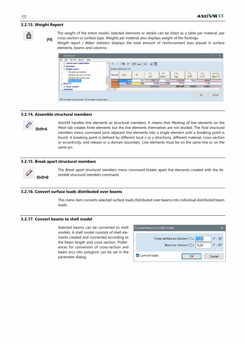
172

3.2.13. Weight Report

[F8]

The weight of the entire model, selected elements or details can be listed as a table per material, per

cross-section or surface type. Weights per material also displays weight of the footings.

Weight report / Rebar statistics displays the total amount of reinforcement bars placed in surface

elements, beams and columns.

3.2.14. Assemble structural members

Shift+A

AxisVM handles line elements as structural members. It means that Meshing of line elements on the

Mesh tab creates finite elements but the line elements themselves are not divided. The Find structural

members menu command joins adjacent line elements into a single element until a breaking point is

found. A breaking point is defined by different local x or z directions, different material, cross-section

or eccentricity, end release or a domain boundary. Line elements must be on the same line or on the

same arc.

3.2.15. Break apart structural members

Shift+B

The Break apart structural members menu command breaks apart line elements created with the As-

semble structural members command.

3.2.16. Convert surface loads distributed over beams

This menu item converts selected surface loads distributed over beams into individual distributed beam

loads.

3.2.17. Convert beams to shell model

Selected beams can be converted to shell

models. A shell model consists of shell ele-

ments created and connected according to

the beam length and cross-section. Prefer-

ences for conversion of cross-section and

beam arcs into polygons can be set in the

parameter dialog.

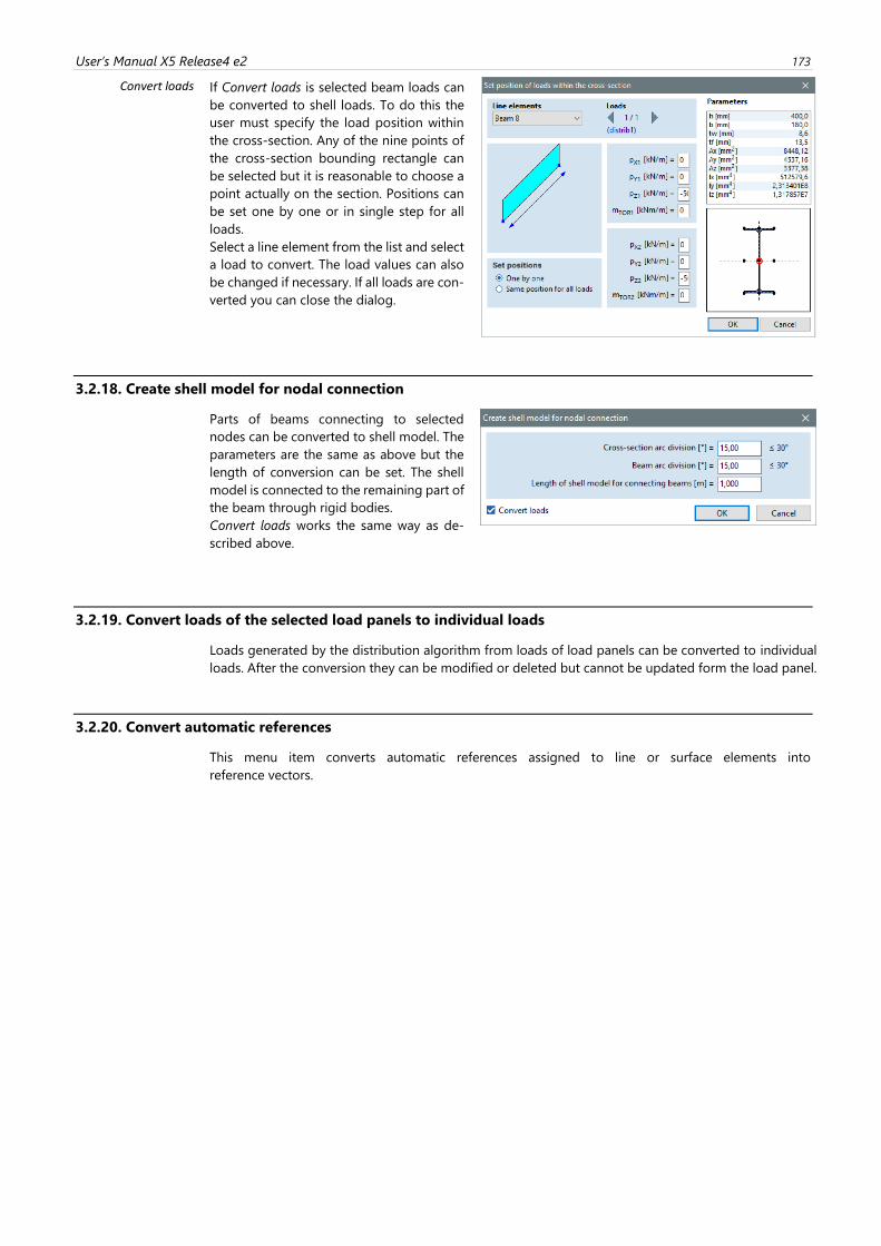
User’s Manual X5 Release4 e2 173

Convert loads If Convert loads is selected beam loads can

be converted to shell loads. To do this the

user must specify the load position within

the cross-section. Any of the nine points of

the cross-section bounding rectangle can

be selected but it is reasonable to choose a

point actually on the section. Positions can

be set one by one or in single step for all

loads.

Select a line element from the list and select

a load to convert. The load values can also

be changed if necessary. If all loads are con-

verted you can close the dialog.

3.2.18. Create shell model for nodal connection

Parts of beams connecting to selected

nodes can be converted to shell model. The

parameters are the same as above but the

length of conversion can be set. The shell

model is connected to the remaining part of

the beam through rigid bodies.

Convert loads works the same way as de-

scribed above.

3.2.19. Convert loads of the selected load panels to individual loads

Loads generated by the distribution algorithm from loads of load panels can be converted to individual

loads. After the conversion they can be modified or deleted but cannot be updated form the load panel.

3.2.20. Convert automatic references

This menu item converts automatic references assigned to line or surface elements into

reference vectors.

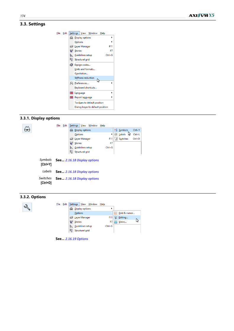
174

3.3. Settings

3.3.1. Display options

Symbols See... 2.16.18 Display options [Ctrl+Y]

Labels See... 2.16.18 Display options

Switches See... 2.16.18 Display options [Ctrl+D]

3.3.2. Options

See... 2.16.19 Options

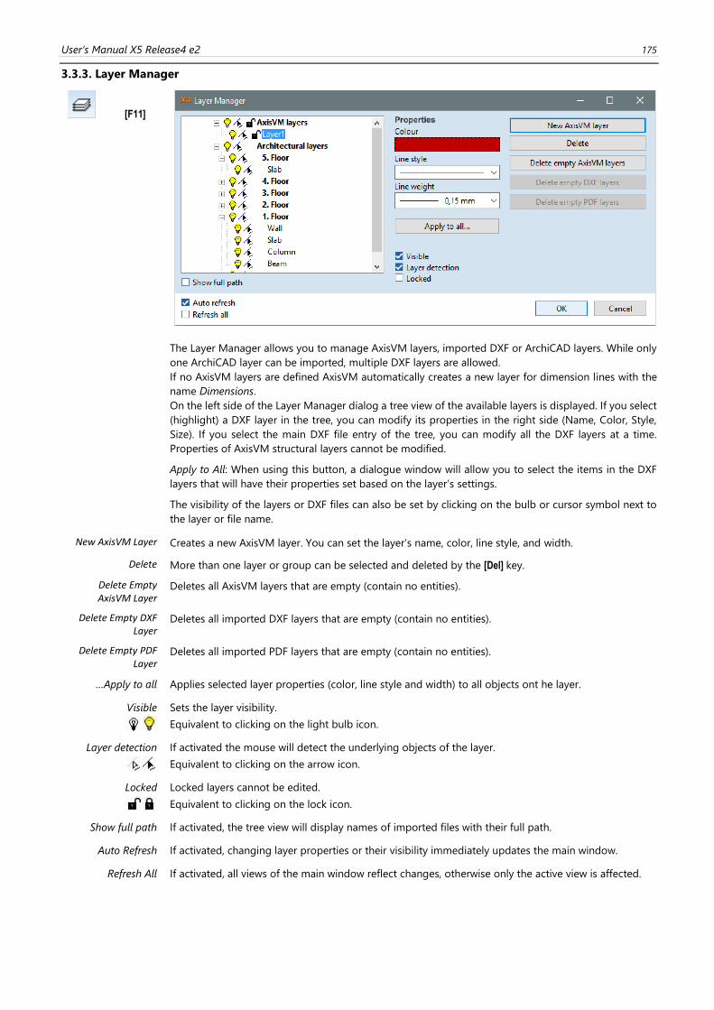
User’s Manual X5 Release4 e2 175

3.3.3. Layer Manager

[F11]

The Layer Manager allows you to manage AxisVM layers, imported DXF or ArchiCAD layers. While only

one ArchiCAD layer can be imported, multiple DXF layers are allowed.

If no AxisVM layers are defined AxisVM automatically creates a new layer for dimension lines with the

name Dimensions. On the left side of the Layer Manager dialog a tree view of the available layers is displayed. If you select

(highlight) a DXF layer in the tree, you can modify its properties in the right side (Name, Color, Style,

Size). If you select the main DXF file entry of the tree, you can modify all the DXF layers at a time.

Properties of AxisVM structural layers cannot be modified.

Apply to All: When using this button, a dialogue window will allow you to select the items in the DXF

layers that will have their properties set based on the layer’s settings.

The visibility of the layers or DXF files can also be set by clicking on the bulb or cursor symbol next to

the layer or file name.

New AxisVM Layer Creates a new AxisVM layer. You can set the layer’s name, color, line style, and width.

Delete More than one layer or group can be selected and deleted by the [Del] key.

Delete Empty AxisVM Layer

Deletes all AxisVM layers that are empty (contain no entities).

Delete Empty DXF Layer

Deletes all imported DXF layers that are empty (contain no entities).

Delete Empty PDF Layer

Deletes all imported PDF layers that are empty (contain no entities).

…Apply to all Applies selected layer properties (color, line style and width) to all objects ont he layer.

Visible

Sets the layer visibility.

Equivalent to clicking on the light bulb icon.

Layer detection

If activated the mouse will detect the underlying objects of the layer.

Equivalent to clicking on the arrow icon.

Locked

Locked layers cannot be edited.

Equivalent to clicking on the lock icon.

Show full path If activated, the tree view will display names of imported files with their full path.

Auto Refresh If activated, changing layer properties or their visibility immediately updates the main window.

Refresh All If activated, all views of the main window reflect changes, otherwise only the active view is affected.

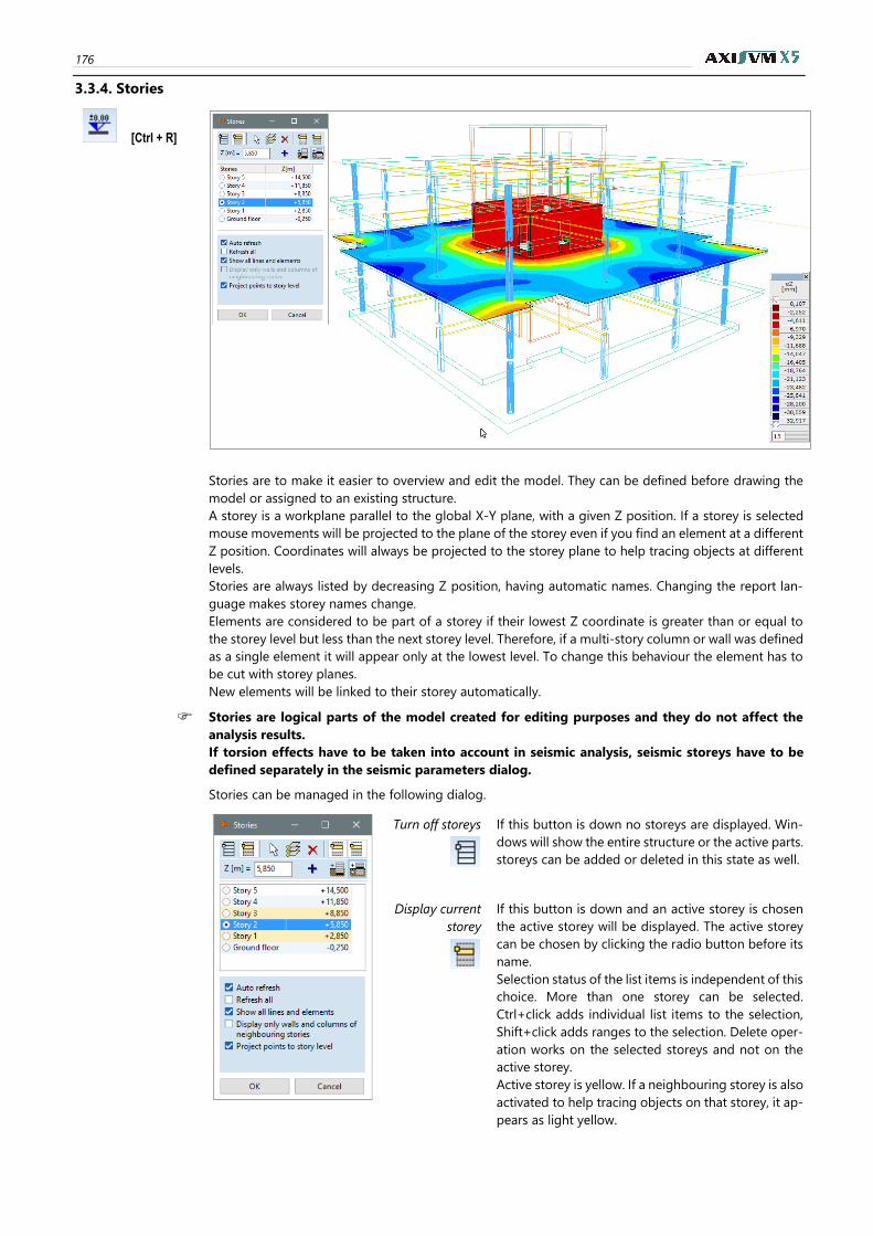
176

3.3.4. Stories

[Ctrl + R]

Stories are to make it easier to overview and edit the model. They can be defined before drawing the

model or assigned to an existing structure.

A storey is a workplane parallel to the global X-Y plane, with a given Z position. If a storey is selected

mouse movements will be projected to the plane of the storey even if you find an element at a different

Z position. Coordinates will always be projected to the storey plane to help tracing objects at different

levels.

Stories are always listed by decreasing Z position, having automatic names. Changing the report lan-

guage makes storey names change.

Elements are considered to be part of a storey if their lowest Z coordinate is greater than or equal to

the storey level but less than the next storey level. Therefore, if a multi-story column or wall was defined

as a single element it will appear only at the lowest level. To change this behaviour the element has to

be cut with storey planes.

New elements will be linked to their storey automatically.

Stories are logical parts of the model created for editing purposes and they do not affect the

analysis results.

If torsion effects have to be taken into account in seismic analysis, seismic storeys have to be

defined separately in the seismic parameters dialog.

Stories can be managed in the following dialog.

Turn off storeys

If this button is down no storeys are displayed. Win-

dows will show the entire structure or the active parts.

storeys can be added or deleted in this state as well.

Display current

storey

If this button is down and an active storey is chosen

the active storey will be displayed. The active storey

can be chosen by clicking the radio button before its

name.

Selection status of the list items is independent of this

choice. More than one storey can be selected.

Ctrl+click adds individual list items to the selection,

Shift+click adds ranges to the selection. Delete oper-

ation works on the selected storeys and not on the

active storey.

Active storey is yellow. If a neighbouring storey is also

activated to help tracing objects on that storey, it ap-

pears as light yellow.

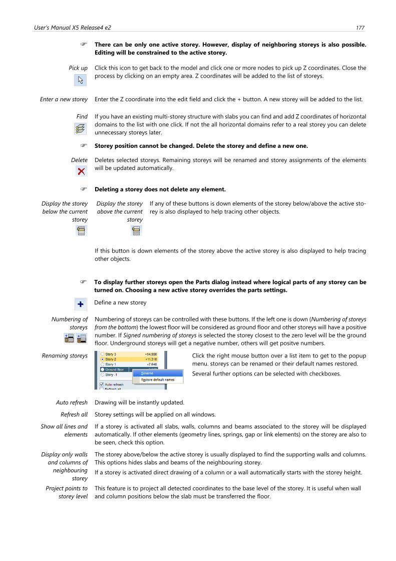
User’s Manual X5 Release4 e2 177

There can be only one active storey. However, display of neighboring storeys is also possible.

Editing will be constrained to the active storey.

Pick up

Click this icon to get back to the model and click one or more nodes to pick up Z coordinates. Close the

process by clicking on an empty area. Z coordinates will be added to the list of storeys.

Enter a new storey Enter the Z coordinate into the edit field and click the + button. A new storey will be added to the list.

Find

If you have an existing multi-storey structure with slabs you can find and add Z coordinates of horizontal

domains to the list with one click. If not the all horizontal domains refer to a real storey you can delete

unnecessary storeys later.

Storey position cannot be changed. Delete the storey and define a new one.

Delete

Deletes selected storeys. Remaining storeys will be renamed and storey assignments of the elements

will be updated automatically.

Deleting a storey does not delete any element.

Display the storey

below the current

storey

Display the storey

above the current

storey

If any of these buttons is down elements of the storey below/above the active sto-

rey is also displayed to help tracing other objects.

If this button is down elements of the storey above the active storey is also displayed to help tracing

other objects.

To display further storeys open the Parts dialog instead where logical parts of any storey can be

turned on. Choosing a new active storey overrides the parts settings.

Define a new storey

Numbering of

storeys

Numbering of storeys can be controlled with these buttons. If the left one is down (Numbering of storeys

from the bottom) the lowest floor will be considered as ground floor and other storeys will have a positive

number. If Signed numbering of storeys is selected the storey closest to the zero level will be the ground

floor. Underground storeys will get a negative number, others will get positve numbers.

Renaming storeys

Click the right mouse button over a list item to get to the popup

menu. storeys can be renamed or their default names restored.

Several further options can be selected with checkboxes.

Auto refresh Drawing will be instantly updated.

Refresh all Storey settings will be applied on all windows.

Show all lines and

elements

If a storey is activated all slabs, walls, columns and beams associated to the storey will be displayed

automatically. If other elements (geometry lines, springs, gap or link elements) on the storey are also to

be seen, check this option.

Display only walls

and columns of

neighbouring

storey

The storey above/below the active storey is usually displayed to find the supporting walls and columns.

This options hides slabs and beams of the neighbouring storey.

If a storey is activated direct drawing of a column or a wall automatically starts with the storey height.

Project points to

storey level

This feature is to project all detected coordinates to the base level of the storey. It is useful when wall

and column positions below the slab must be transferred the floor.

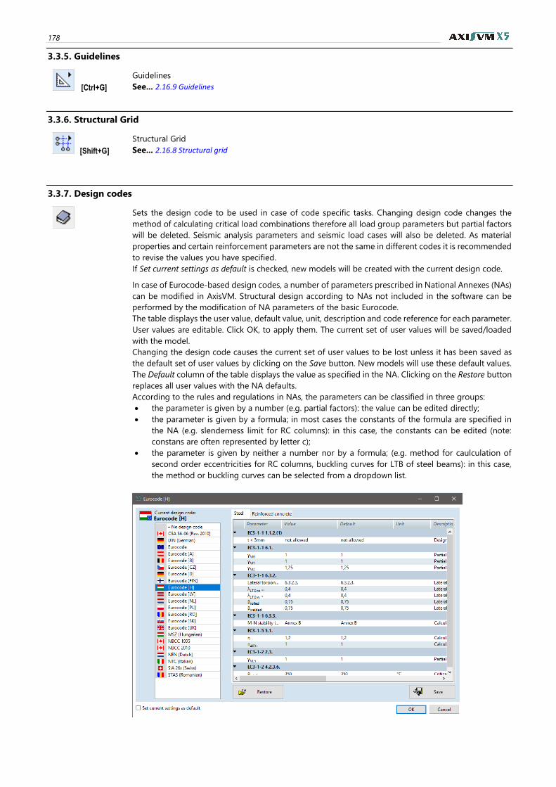
178

3.3.5. Guidelines

[Ctrl+G]

Guidelines

See... 2.16.9 Guidelines

3.3.6. Structural Grid

[Shift+G]

Structural Grid

See... 2.16.8 Structural grid

3.3.7. Design codes

Sets the design code to be used in case of code specific tasks. Changing design code changes the

method of calculating critical load combinations therefore all load group parameters but partial factors

will be deleted. Seismic analysis parameters and seismic load cases will also be deleted. As material

properties and certain reinforcement parameters are not the same in different codes it is recommended

to revise the values you have specified.

If Set current settings as default is checked, new models will be created with the current design code.

In case of Eurocode-based design codes, a number of parameters prescribed in National Annexes (NAs)

can be modified in AxisVM. Structural design according to NAs not included in the software can be

performed by the modification of NA parameters of the basic Eurocode.

The table displays the user value, default value, unit, description and code reference for each parameter.

User values are editable. Click OK, to apply them. The current set of user values will be saved/loaded

with the model.

Changing the design code causes the current set of user values to be lost unless it has been saved as

the default set of user values by clicking on the Save button. New models will use these default values.

The Default column of the table displays the value as specified in the NA. Clicking on the Restore button

replaces all user values with the NA defaults.

According to the rules and regulations in NAs, the parameters can be classified in three groups:

• the parameter is given by a number (e.g. partial factors): the value can be edited directly;

• the parameter is given by a formula; in most cases the constants of the formula are specified in

the NA (e.g. slenderness limit for RC columns): in this case, the constants can be edited (note:

constans are often represented by letter c);

• the parameter is given by neither a number nor by a formula; (e.g. method for caulculation of

second order eccentricities for RC columns, buckling curves for LTB of steel beams): in this case,

the method or buckling curves can be selected from a dropdown list.

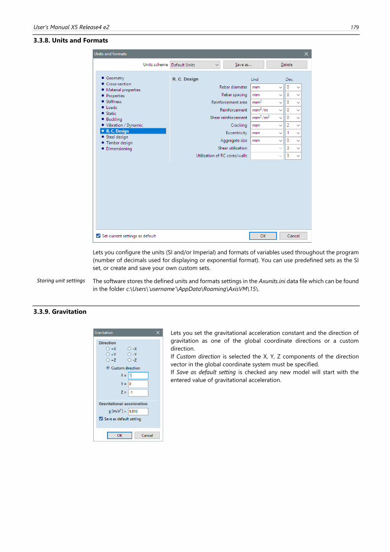
User’s Manual X5 Release4 e2 179

3.3.8. Units and Formats

Lets you configure the units (SI and/or Imperial) and formats of variables used throughout the program

(number of decimals used for displaying or exponential format). You can use predefined sets as the SI

set, or create and save your own custom sets.

Storing unit settings The software stores the defined units and formats settings in the Axunits.ini data file which can be found

in the folder c:\Users\'username'\AppData\Roaming\AxisVM\15\.

3.3.9. Gravitation

Lets you set the gravitational acceleration constant and the direction of

gravitation as one of the global coordinate directions or a custom

direction.

If Custom direction is selected the X, Y, Z components of the direction

vector in the global coordinate system must be specified.

If Save as default setting is checked any new model will start with the

entered value of gravitational acceleration.

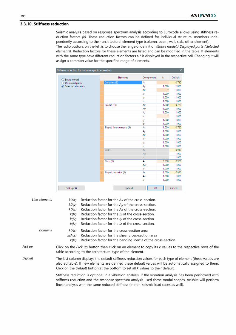
180

3.3.10. Stiffness reduction

Seismic analysis based on response spectrum analysis according to Eurocode allows using stiffness re-

duction factors (k). These reduction factors can be defined for individual structural members inde-

pendently according to their architectural element type (column, beam, wall, slab, other element).

The radio buttons on the left is to choose the range of definition (Entire model / Displayed parts / Selected

elements). Reduction factors for these elements are listed and can be modified in the table. If elements

with the same type have different reduction factors a * is displayed in the respective cell. Changing it will

assign a common value for the specified range of elements.

Line elements k(Ax) Reduction factor for the Ax of the cross-section.

k(Ay) Reduction factor for the Ay of the cross-section.

k(Az) Reduction factor for the Az of the cross-section.

k(Ix) Reduction factor for the Ix of the cross-section.

k(Iy) Reduction factor for the Iy of the cross-section.

k(Iz) Reduction factor for the Iz of the cross-section.

Domains k(Ac) Reduction factor for the cross-section area

k(Acs) Reduction factor for the shear cross-section area

k(Ic) Reduction factor for the bending inertia of the cross-section

Pick up Click on the Pick up button then click on an element to copy its k values to the respective rows of the

table according to the architectural type of the element.

Default The last column displays the default stiffness reduction values for each type of element (these values are

also editable). If new elements are defined these default values will be automatically assigned to them.

Click on the Default button at the bottom to set all k values to their default.

Stiffness reduction is optional in a vibration analysis. If the vibration analysis has been performed with

stiffness reduction and the response spectrum analysis used these modal shapes, AxisVM will perform

linear analysis with the same reduced stiffness (in non-seismic load cases as well).

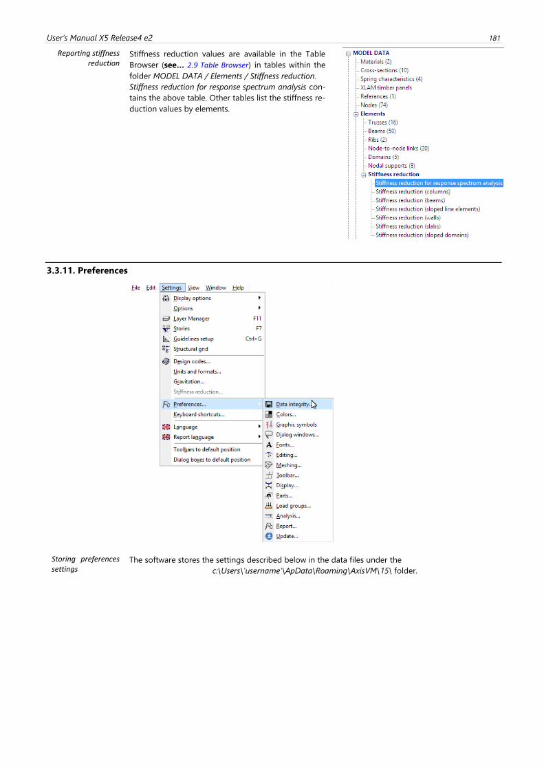
User’s Manual X5 Release4 e2 181

Reporting stiffness reduction

Stiffness reduction values are available in the Table

Browser (see… 2.9 Table Browser) in tables within the

folder MODEL DATA / Elements / Stiffness reduction.

Stiffness reduction for response spectrum analysis con-

tains the above table. Other tables list the stiffness re-

duction values by elements.

3.3.11. Preferences

Storing preferences settings

The software stores the settings described below in the data files under the

c:\Users\'username'\ApData\Roaming\AxisVM\15\ folder.

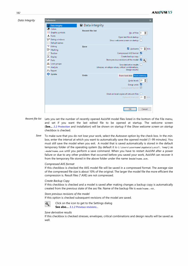
182

Data Integrity

Recent file list

Lets you set the number of recently opened AxisVM model files listed in the bottom of the File menu,

and set if you want the last edited file to be opened at startup. The welcome screen

(See... 2.2 Protection and installation) will be shown on startup if the Show welcome screen on startup

checkbox is checked.

Save

To make sure that you do not lose your work, select the Autosave option by the check box. In the min.

box, enter the interval at which you want to automatically save the opened model (1-99 minutes). You

must still save the model when you exit. A model that is saved automatically is stored in the default

temporary folder of the operating system (by default it is C:\Users\username\AppData\Local\ Temp\) as

~modelname.avm until you perform a save command. When you have to restart AxisVM after a power

failure or due to any other problem that occurred before you saved your work, AxisVM can recover it

from the temporary file stored in the above folder under the name $modelname.avm.

Compressed AXS format

If this checkbox is checked the AXS model file will be saved in a compressed format. The average size

of the compressed file size is about 10% of the original. The larger the model file the more efficient the

compression is. Result files (*.AXE) are not compressed.

Create Backup Copy

If this checkbox is checked and a model is saved after making changes a backup copy is automatically

created from the previous state of the axs file. Name of the backup file is modelname.~AX.

Store previous revisions of the model

If this option is checked subsequent revisions of the model are saved.

Click on the icon to get to the Settings dialog

See also… 3.1.2 Previous revisions…

Save derivative results

If this checkbox is checked stresses, envelopes, critical combinations and design results will be saved as

well.

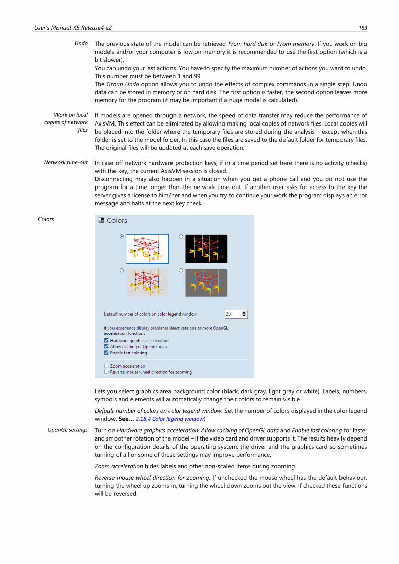
User’s Manual X5 Release4 e2 183

Undo

The previous state of the model can be retrieved From hard disk or From memory. If you work on big

models and/or your computer is low on memory it is recommended to use the first option (which is a

bit slower).

You can undo your last actions. You have to specify the maximum number of actions you want to undo.

This number must be between 1 and 99.

The Group Undo option allows you to undo the effects of complex commands in a single step. Undo

data can be stored in memory or on hard disk. The first option is faster, the second option leaves more

memory for the program (it may be important if a huge model is calculated).

Work on local copies of network

files

If models are opened through a network, the speed of data transfer may reduce the performance of

AxisVM. This effect can be eliminated by allowing making local copies of network files. Local copies will

be placed into the folder where the temporary files are stored during the analysis – except when this

folder is set to the model folder. In this case the files are saved to the default folder for temporary files.

The original files will be updated at each save operation.

Network time-out

In case off network hardware protection keys, if in a time period set here there is no activity (checks)

with the key, the current AxisVM session is closed.

Disconnecting may also happen in a situation when you get a phone call and you do not use the

program for a time longer than the network time-out. If another user asks for access to the key the

server gives a license to him/her and when you try to continue your work the program displays an error

message and halts at the next key check.

Colors

Lets you select graphics area background color (black, dark gray, light gray or white). Labels, numbers,

symbols and elements will automatically change their colors to remain visible

Default number of colors on color legend window: Set the number of colors displayed in the color legend

window. See… 2.18.4 Color legend window)

OpenGL settings Turn on Hardware graphics acceleration, Allow caching of OpenGL data and Enable fast coloring for faster

and smoother rotation of the model – if the video card and driver supports it. The results heavily depend

on the configuration details of the operating system, the driver and the graphics card so sometimes

turning of all or some of these settings may improve performance.

Zoom acceleration hides labels and other non-scaled items during zooming.

Reverse mouse wheel direction for zooming. If unchecked the mouse wheel has the default behaviour:

turning the wheel up zooms in, turning the wheel down zooms out the view. If checked these functions

will be reversed.

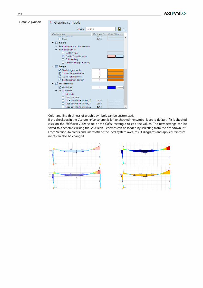
184

Graphic symbols

Color and line thickness of graphic symbols can be customized.

If the checkbox in the Custom value column is left unchecked the symbol is set to default. If it is checked

click on the Thickness / size value or the Color rectangle to edit the values. The new settings can be

saved to a scheme clicking the Save icon. Schemes can be loaded by selecting from the dropdown list.

From Version X4 colors and line width of the local system axes, result diagrams and applied reinforce-

ment can also be changed.

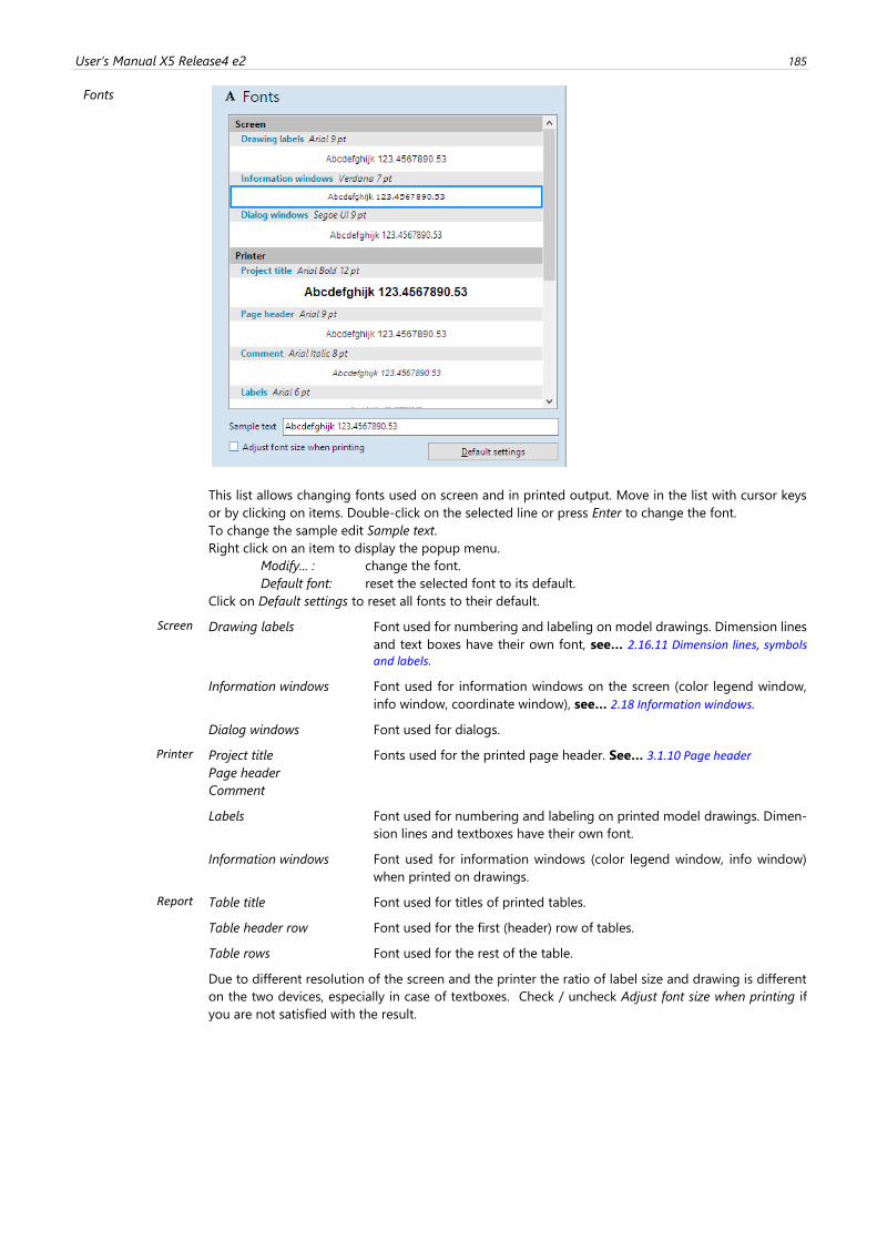
User’s Manual X5 Release4 e2 185

Fonts

This list allows changing fonts used on screen and in printed output. Move in the list with cursor keys

or by clicking on items. Double-click on the selected line or press Enter to change the font.

To change the sample edit Sample text.

Right click on an item to display the popup menu.

Modify... : change the font.

Default font: reset the selected font to its default.

Click on Default settings to reset all fonts to their default.

Screen Drawing labels Font used for numbering and labeling on model drawings. Dimension lines

and text boxes have their own font, see… 2.16.11 Dimension lines, symbols and labels.

Information windows Font used for information windows on the screen (color legend window,

info window, coordinate window), see… 2.18 Information windows.

Dialog windows Font used for dialogs.

Printer Project title

Page header

Comment

Fonts used for the printed page header. See… 3.1.10 Page header

Labels Font used for numbering and labeling on printed model drawings. Dimen-

sion lines and textboxes have their own font.

Information windows Font used for information windows (color legend window, info window)

when printed on drawings.

Report Table title Font used for titles of printed tables.

Table header row Font used for the first (header) row of tables.

Table rows Font used for the rest of the table.

Due to different resolution of the screen and the printer the ratio of label size and drawing is different

on the two devices, especially in case of textboxes. Check / uncheck Adjust font size when printing if

you are not satisfied with the result.

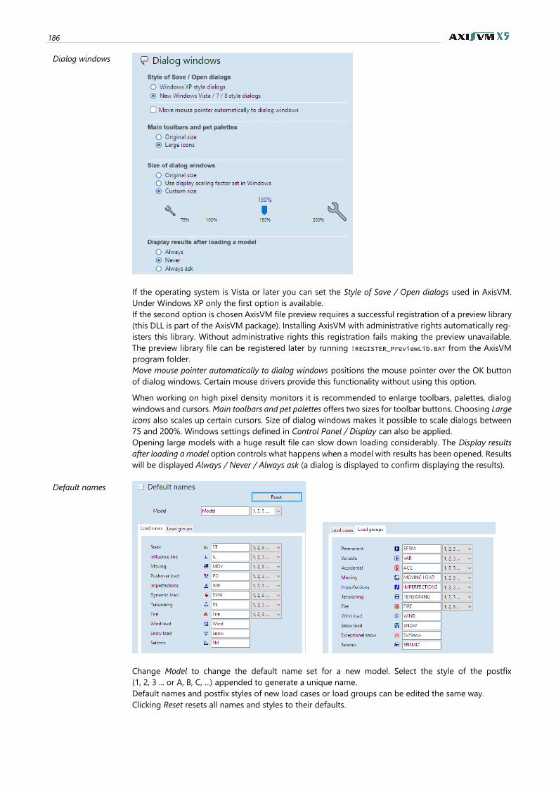
186

Dialog windows

If the operating system is Vista or later you can set the Style of Save / Open dialogs used in AxisVM.

Under Windows XP only the first option is available.

If the second option is chosen AxisVM file preview requires a successful registration of a preview library

(this DLL is part of the AxisVM package). Installing AxisVM with administrative rights automatically reg-

isters this library. Without administrative rights this registration fails making the preview unavailable.

The preview library file can be registered later by running !REGISTER_PreviewLib.BAT from the AxisVM

program folder.

Move mouse pointer automatically to dialog windows positions the mouse pointer over the OK button

of dialog windows. Certain mouse drivers provide this functionality without using this option.

When working on high pixel density monitors it is recommended to enlarge toolbars, palettes, dialog

windows and cursors. Main toolbars and pet palettes offers two sizes for toolbar buttons. Choosing Large

icons also scales up certain cursors. Size of dialog windows makes it possible to scale dialogs between

75 and 200%. Windows settings defined in Control Panel / Display can also be applied.

Opening large models with a huge result file can slow down loading considerably. The Display results

after loading a model option controls what happens when a model with results has been opened. Results

will be displayed Always / Never / Always ask (a dialog is displayed to confirm displaying the results).

Default names

Change Model to change the default name set for a new model. Select the style of the postfix

(1, 2, 3 ... or A, B, C, ...) appended to generate a unique name.

Default names and postfix styles of new load cases or load groups can be edited the same way.

Clicking Reset resets all names and styles to their defaults.

User’s Manual X5 Release4 e2 187

Editing

Circle Closing Angle Parameter for drawing arcs. If the center angle of the arc is smaller than this angle or it is closer to 360°

than this angle then a whole circle will be drawn.

Projection line to workplane

Display of projection lines can be turned on/off. Its shows the distance of the cursor from the current

workplane.

Delete unnecessary contour lines after automatic domain intersection

Controls if contour lines are automatically deleted after domain intersection. If this function is turned

off contour lines became internal lines of the union.

Break unmeshed structural members whenever a node is inserted

By default AxisVM uses structural members. These are line elements consisting of one or more finite

elements. Unmeshed members contain one finite element only. If a new node is inserted on an

unmeshed member or the line is divided the structural member remains unaffected but will contain

more than one finite element. Clicking on a structural member selects all finite elements belonging to

the member. This behaviour can be changed by checking this option. Then new nodes inserted on

structural members will break apart the member. To break apart existing structural members use Edit

/ Break apart structural members.

Enable selection of finite elements on lines

If activated, finite elements of a structural member can be selected individually. Otherwise only the

whole structural member can be selected.

Enable selection of design members

If activated, design members can be selected instead of structural members. Design members consists

of a group of lines with the same design parameters handled as one entity for steel or timber design

purposes.

Elements of a hidden mesh can be selected

If display of mesh is turned off this field controls if the hidden nodes / lines / surface elements can be

selected or not. This switch also controls if these nodes and elements appear in tables or not.

Show instructions at the cursor

Controls the display of a small tooltip window at the cursor with instructions for the next step of the

current task. If unchecked, instruction messages appear only at the bottom status line.

Make all layers editable when entering the layer editor

If activated, all locked layers will be unlocked when entering the background layer editor.

See… 2.16.12 Editing background layers. Otherwise locked layers must be unlocked manually.

See… 2.12 Layer Manager and 2.17 Speed Buttons.

Geometry check before running an analysis

If activated a geometry check is automatically performed before analysis.

See… 4.8.19 Geometry check

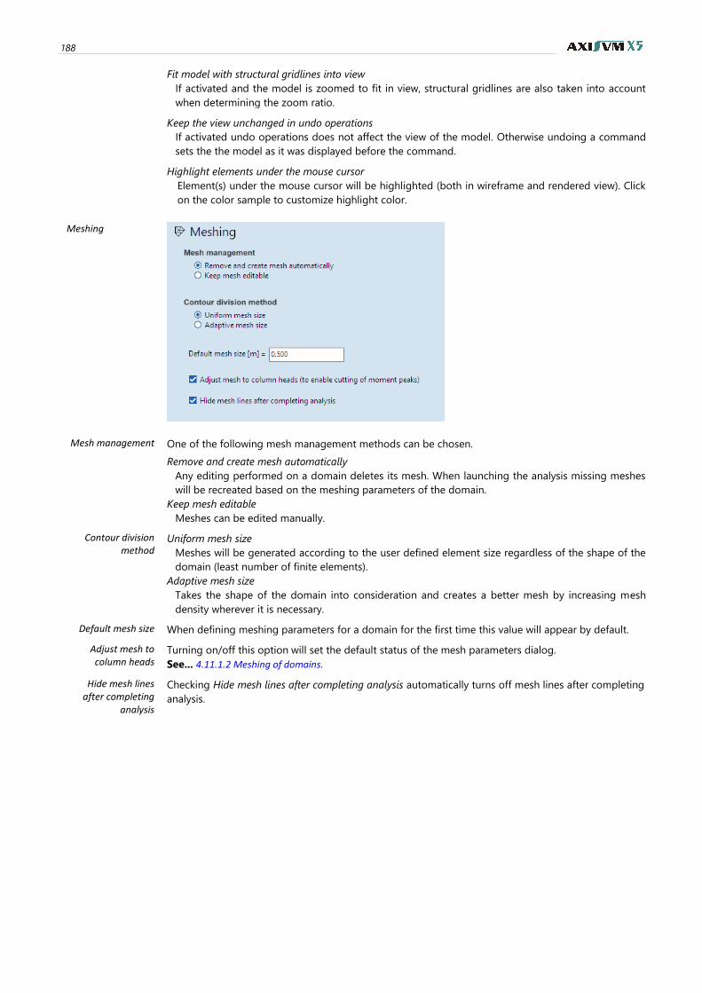
188

Fit model with structural gridlines into view

If activated and the model is zoomed to fit in view, structural gridlines are also taken into account

when determining the zoom ratio.

Keep the view unchanged in undo operations

If activated undo operations does not affect the view of the model. Otherwise undoing a command

sets the the model as it was displayed before the command.

Highlight elements under the mouse cursor

Element(s) under the mouse cursor will be highlighted (both in wireframe and rendered view). Click

on the color sample to customize highlight color.

Meshing

Mesh management

One of the following mesh management methods can be chosen.

Remove and create mesh automatically

Any editing performed on a domain deletes its mesh. When launching the analysis missing meshes

will be recreated based on the meshing parameters of the domain.

Keep mesh editable

Meshes can be edited manually.

Contour division method

Uniform mesh size

Meshes will be generated according to the user defined element size regardless of the shape of the

domain (least number of finite elements).

Adaptive mesh size

Takes the shape of the domain into consideration and creates a better mesh by increasing mesh

density wherever it is necessary.

Default mesh size When defining meshing parameters for a domain for the first time this value will appear by default.

Adjust mesh to column heads

Turning on/off this option will set the default status of the mesh parameters dialog.

See... 4.11.1.2 Meshing of domains.

Hide mesh lines after completing

analysis

Checking Hide mesh lines after completing analysis automatically turns off mesh lines after completing

analysis.

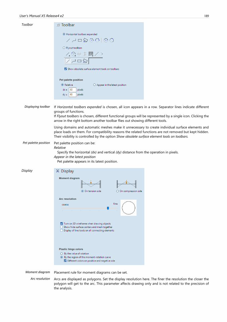
User’s Manual X5 Release4 e2 189

Toolbar

Displaying toolbar If Horizontal toolbars expanded is chosen, all icon appears in a row. Separator lines indicate different

groups of functions.

If Flyout toolbars is chosen, different functional groups will be represented by a single icon. Clicking the

arrow in the right bottom another toolbar flies out showing different tools.

Using domains and automatic meshes make it unnecessary to create individual surface elements and

place loads on them. For compatibility reasons the related functions are not removed but kept hidden.

Their visibility is controlled by the option Show obsolete surface element tools on toolbars.

Pet palette position Pet palette position can be:

Relative

Specify the horizontal (dx) and vertical (dy) distance from the operation in pixels.

Appear in the latest position

Pet palette appears in its latest position.

Display

Moment diagram Placement rule for moment diagrams can be set.

Arc resolution

Arcs are displayed as polygons. Set the display resolution here. The finer the resolution the closer the

polygon will get to the arc. This parameter affects drawing only and is not related to the precision of

the analysis.

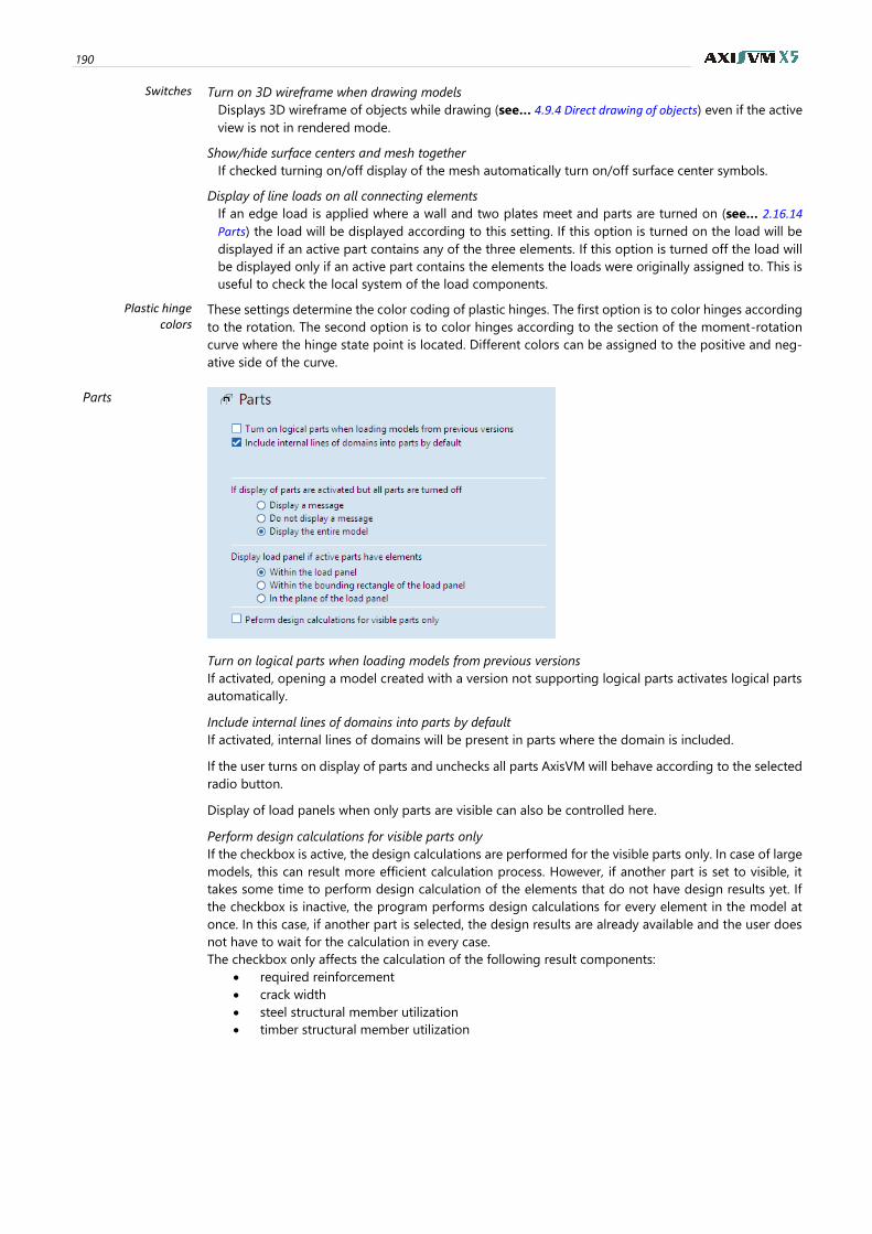
190

Switches Turn on 3D wireframe when drawing models

Displays 3D wireframe of objects while drawing (see… 4.9.4 Direct drawing of objects) even if the active

view is not in rendered mode.

Show/hide surface centers and mesh together

If checked turning on/off display of the mesh automatically turn on/off surface center symbols.

Display of line loads on all connecting elements

If an edge load is applied where a wall and two plates meet and parts are turned on (see… 2.16.14

Parts) the load will be displayed according to this setting. If this option is turned on the load will be

displayed if an active part contains any of the three elements. If this option is turned off the load will

be displayed only if an active part contains the elements the loads were originally assigned to. This is

useful to check the local system of the load components.

Plastic hinge colors

These settings determine the color coding of plastic hinges. The first option is to color hinges according

to the rotation. The second option is to color hinges according to the section of the moment-rotation

curve where the hinge state point is located. Different colors can be assigned to the positive and neg-

ative side of the curve.

Parts

Turn on logical parts when loading models from previous versions

If activated, opening a model created with a version not supporting logical parts activates logical parts

automatically.

Include internal lines of domains into parts by default

If activated, internal lines of domains will be present in parts where the domain is included.

If the user turns on display of parts and unchecks all parts AxisVM will behave according to the selected

radio button.

Display of load panels when only parts are visible can also be controlled here.

Perform design calculations for visible parts only If the checkbox is active, the design calculations are performed for the visible parts only. In case of large

models, this can result more efficient calculation process. However, if another part is set to visible, it

takes some time to perform design calculation of the elements that do not have design results yet. If

the checkbox is inactive, the program performs design calculations for every element in the model at

once. In this case, if another part is selected, the design results are already available and the user does

not have to wait for the calculation in every case.

The checkbox only affects the calculation of the following result components:

• required reinforcement

• crack width

• steel structural member utilization

• timber structural member utilization

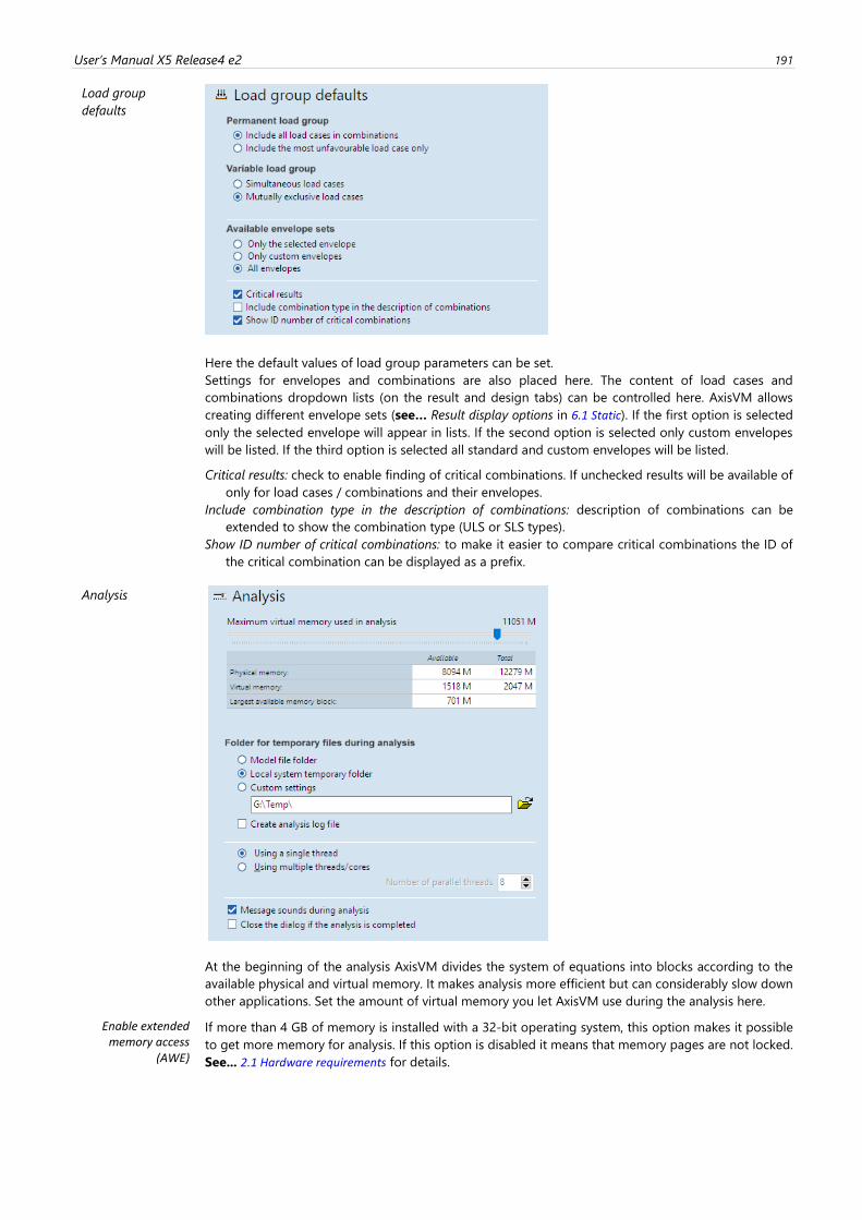
User’s Manual X5 Release4 e2 191

Load group

defaults

Here the default values of load group parameters can be set.

Settings for envelopes and combinations are also placed here. The content of load cases and

combinations dropdown lists (on the result and design tabs) can be controlled here. AxisVM allows

creating different envelope sets (see… Result display options in 6.1 Static). If the first option is selected

only the selected envelope will appear in lists. If the second option is selected only custom envelopes

will be listed. If the third option is selected all standard and custom envelopes will be listed.

Critical results: check to enable finding of critical combinations. If unchecked results will be available of

only for load cases / combinations and their envelopes.

Include combination type in the description of combinations: description of combinations can be

extended to show the combination type (ULS or SLS types).

Show ID number of critical combinations: to make it easier to compare critical combinations the ID of

the critical combination can be displayed as a prefix.

Analysis

At the beginning of the analysis AxisVM divides the system of equations into blocks according to the

available physical and virtual memory. It makes analysis more efficient but can considerably slow down

other applications. Set the amount of virtual memory you let AxisVM use during the analysis here.

Enable extended memory access

(AWE)

If more than 4 GB of memory is installed with a 32-bit operating system, this option makes it possible

to get more memory for analysis. If this option is disabled it means that memory pages are not locked.

See... 2.1 Hardware requirements for details.

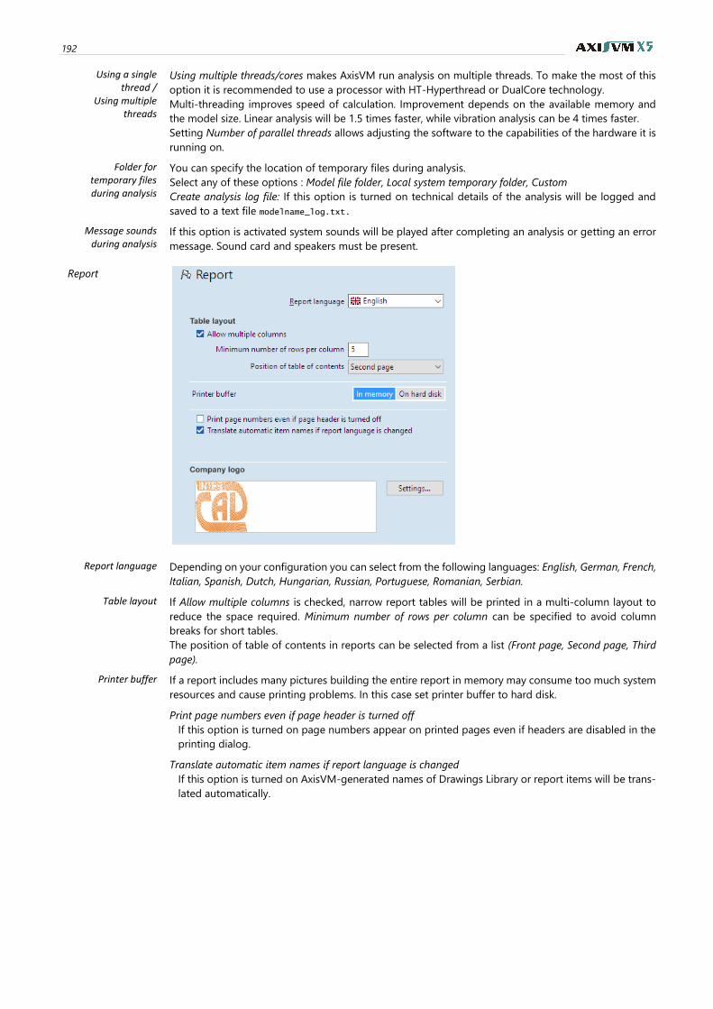
192

Using a single thread /

Using multiple threads

Using multiple threads/cores makes AxisVM run analysis on multiple threads. To make the most of this

option it is recommended to use a processor with HT-Hyperthread or DualCore technology.

Multi-threading improves speed of calculation. Improvement depends on the available memory and

the model size. Linear analysis will be 1.5 times faster, while vibration analysis can be 4 times faster.

Setting Number of parallel threads allows adjusting the software to the capabilities of the hardware it is

running on.

Folder for temporary files during analysis

You can specify the location of temporary files during analysis.

Select any of these options : Model file folder, Local system temporary folder, Custom

Create analysis log file: If this option is turned on technical details of the analysis will be logged and

saved to a text file modelname_log.txt.

Message sounds during analysis

If this option is activated system sounds will be played after completing an analysis or getting an error

message. Sound card and speakers must be present.

Report

Report language Depending on your configuration you can select from the following languages: English, German, French,

Italian, Spanish, Dutch, Hungarian, Russian, Portuguese, Romanian, Serbian.

Table layout If Allow multiple columns is checked, narrow report tables will be printed in a multi-column layout to

reduce the space required. Minimum number of rows per column can be specified to avoid column

breaks for short tables.

The position of table of contents in reports can be selected from a list (Front page, Second page, Third

page).

Printer buffer If a report includes many pictures building the entire report in memory may consume too much system

resources and cause printing problems. In this case set printer buffer to hard disk.

Print page numbers even if page header is turned off

If this option is turned on page numbers appear on printed pages even if headers are disabled in the

printing dialog.

Translate automatic item names if report language is changed

If this option is turned on AxisVM-generated names of Drawings Library or report items will be trans-

lated automatically.

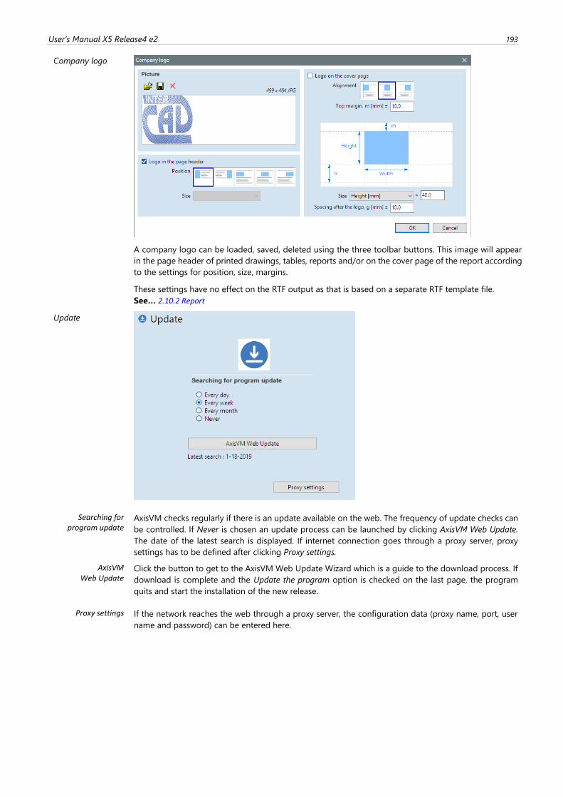
User’s Manual X5 Release4 e2 193

Company logo

A company logo can be loaded, saved, deleted using the three toolbar buttons. This image will appear

in the page header of printed drawings, tables, reports and/or on the cover page of the report according

to the settings for position, size, margins.

These settings have no effect on the RTF output as that is based on a separate RTF template file.

See… 2.10.2 Report

Update

Searching for program update

AxisVM checks regularly if there is an update available on the web. The frequency of update checks can

be controlled. If Never is chosen an update process can be launched by clicking AxisVM Web Update.

The date of the latest search is displayed. If internet connection goes through a proxy server, proxy

settings has to be defined after clicking Proxy settings.

AxisVM Web Update

Click the button to get to the AxisVM Web Update Wizard which is a guide to the download process. If

download is complete and the Update the program option is checked on the last page, the program

quits and start the installation of the new release.

Proxy settings If the network reaches the web through a proxy server, the configuration data (proxy name, port, user

name and password) can be entered here.

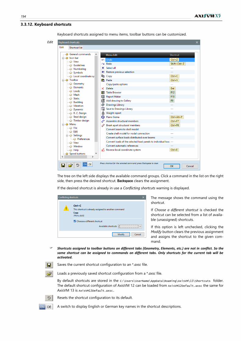
194

3.3.12. Keyboard shortcuts

Keyboard shortcuts assigned to menu items, toolbar buttons can be customized.

Edit

The tree on the left side displays the available command groups. Click a command in the list on the right

side, then press the desired shortcut. Backspace clears the assignment.

If the desired shortcut is already in use a Conflicting shortcuts warning is displayed.

The message shows the command using the

shortcut.

If Choose a different shortcut is checked the

shortcut can be selected from a list of availa-

ble (unassigned) shortcuts.

If this option is left unchecked, clicking the

Modify button clears the previous assignment

and assigns the shortcut to the given com-

mand.

Shortcuts assigned to toolbar buttons on different tabs (Geometry, Elements, etc.) are not in conflict. So the same shortcut can be assigned to commands on different tabs. Only shortcuts for the current tab will be activated.

Saves the current shortcut configuration to an *.axsc file.

Loads a previously saved shortcut configuration from a *.axsc file.

By default shortcuts are stored in the C:\Users\UserName\AppData\Roaming\AxisVM\13\Shortcuts folder.

The default shortcut configuration of AxisVM 12 can be loaded from AxisVM12Default.axsc the same for

AxisVM 13 is AxisVM13Default.axsc.

Resets the shortcut configuration to its default.

A switch to display English or German key names in the shortcut descriptions.

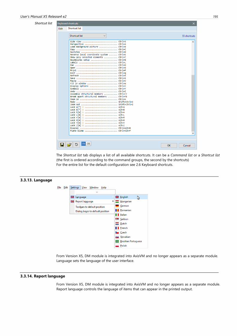
User’s Manual X5 Release4 e2 195

Shortcut list

The Shortcut list tab displays a list of all available shortcuts. It can be a Command list or a Shortcut list

(the first is ordered according to the command groups, the second by the shortcuts)

For the entire list for the default configuration see 2.6 Keyboard shortcuts.

3.3.13. Language

From Version X5, DM module is integrated into AxisVM and no longer appears as a separate module.

Language sets the language of the user interface.

3.3.14. Report language

From Version X5, DM module is integrated into AxisVM and no longer appears as a separate module.

Report language controls the language of items that can appear in the printed output.

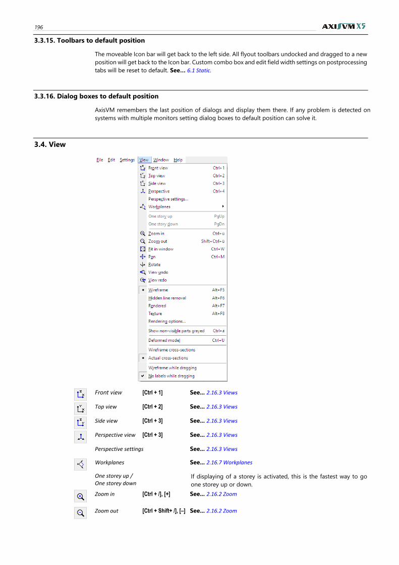
196

3.3.15. Toolbars to default position

The moveable Icon bar will get back to the left side. All flyout toolbars undocked and dragged to a new

position will get back to the Icon bar. Custom combo box and edit field width settings on postprocessing

tabs will be reset to default. See… 6.1 Static.

3.3.16. Dialog boxes to default position

AxisVM remembers the last position of dialogs and display them there. If any problem is detected on

systems with multiple monitors setting dialog boxes to default position can solve it.

3.4. View

Front view [Ctrl + 1] See... 2.16.3 Views

Top view [Ctrl + 2] See... 2.16.3 Views

Side view [Ctrl + 3] See... 2.16.3 Views

Perspective view [Ctrl + 3] See... 2.16.3 Views

Perspective settings See... 2.16.3 Views

Workplanes See... 2.16.7 Workplanes

One storey up / One storey down

If displaying of a storey is activated, this is the fastest way to go

one storey up or down.

Zoom in [Ctrl + /], [+] See... 2.16.2 Zoom

Zoom out [Ctrl + Shift+ /], [–] See... 2.16.2 Zoom

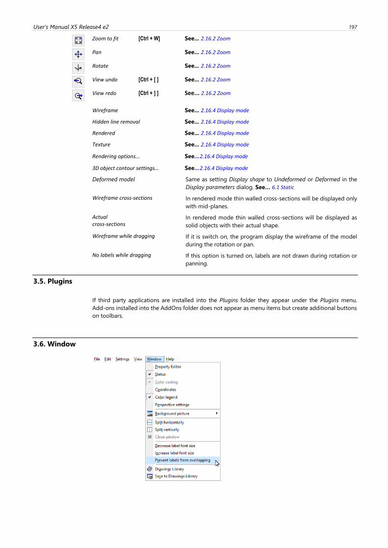
User’s Manual X5 Release4 e2 197

Zoom to fit [Ctrl + W] See... 2.16.2 Zoom

Pan See... 2.16.2 Zoom

Rotate See... 2.16.2 Zoom

View undo [Ctrl + [ ] See... 2.16.2 Zoom

View redo [Ctrl + ] ] See... 2.16.2 Zoom

Wireframe See... 2.16.4 Display mode

Hidden line removal See... 2.16.4 Display mode

Rendered See... 2.16.4 Display mode

Texture See... 2.16.4 Display mode

Rendering options... See... 2.16.4 Display mode

3D object contour settings… See... 2.16.4 Display mode

Deformed model Same as setting Display shape to Undeformed or Deformed in the

Display parameters dialog. See… 6.1 Static

Wireframe cross-sections In rendered mode thin walled cross-sections will be displayed only

with mid-planes.

Actual cross-sections

In rendered mode thin walled cross-sections will be displayed as

solid objects with their actual shape.

Wireframe while dragging If it is switch on, the program display the wireframe of the model

during the rotation or pan.

No labels while dragging If this option is turned on, labels are not drawn during rotation or

panning.

3.5. Plugins

If third party applications are installed into the Plugins folder they appear under the Plugins menu.

Add-ons installed into the AddOns folder does not appear as menu items but create additional buttons

on toolbars.

3.6. Window

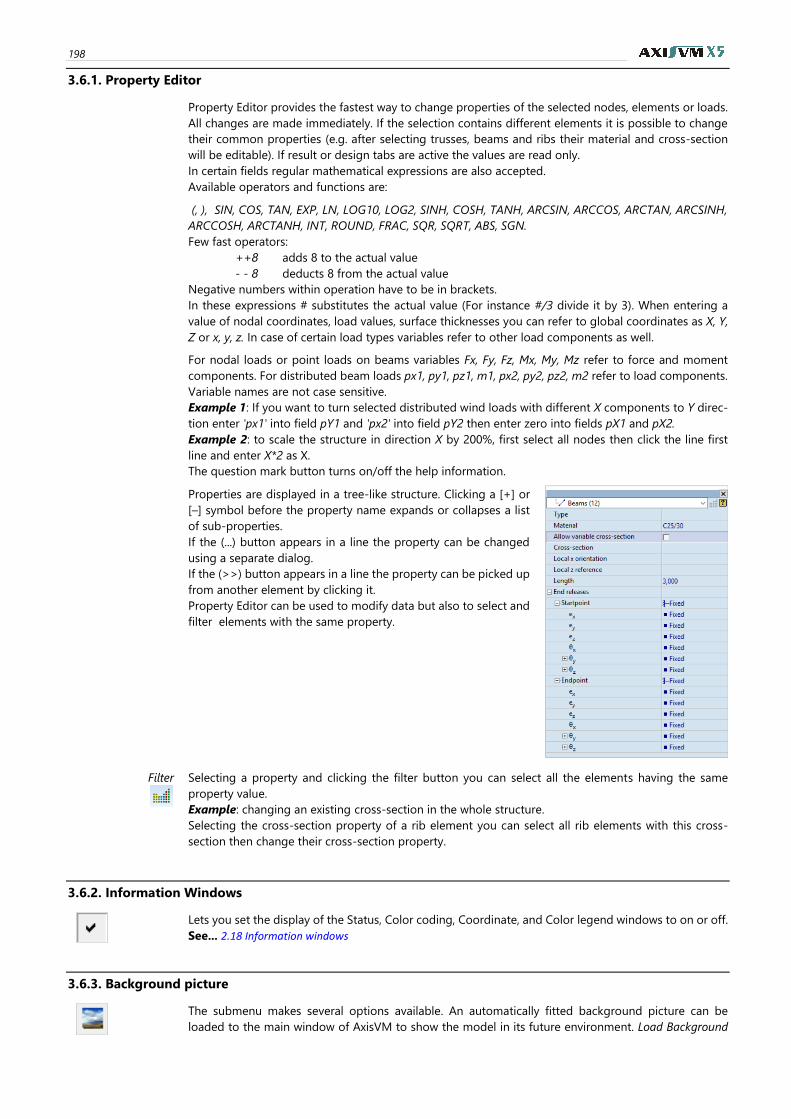
198

3.6.1. Property Editor

Property Editor provides the fastest way to change properties of the selected nodes, elements or loads.

All changes are made immediately. If the selection contains different elements it is possible to change

their common properties (e.g. after selecting trusses, beams and ribs their material and cross-section

will be editable). If result or design tabs are active the values are read only.

In certain fields regular mathematical expressions are also accepted.

Available operators and functions are:

(, ), SIN, COS, TAN, EXP, LN, LOG10, LOG2, SINH, COSH, TANH, ARCSIN, ARCCOS, ARCTAN, ARCSINH,

ARCCOSH, ARCTANH, INT, ROUND, FRAC, SQR, SQRT, ABS, SGN.

Few fast operators:

++8 adds 8 to the actual value

- - 8 deducts 8 from the actual value

Negative numbers within operation have to be in brackets.

In these expressions # substitutes the actual value (For instance #/3 divide it by 3). When entering a

value of nodal coordinates, load values, surface thicknesses you can refer to global coordinates as X, Y,

Z or x, y, z. In case of certain load types variables refer to other load components as well.

For nodal loads or point loads on beams variables Fx, Fy, Fz, Mx, My, Mz refer to force and moment

components. For distributed beam loads px1, py1, pz1, m1, px2, py2, pz2, m2 refer to load components.

Variable names are not case sensitive.

Example 1: If you want to turn selected distributed wind loads with different X components to Y direc-

tion enter 'px1' into field pY1 and 'px2' into field pY2 then enter zero into fields pX1 and pX2.

Example 2: to scale the structure in direction X by 200%, first select all nodes then click the line first

line and enter X*2 as X.

The question mark button turns on/off the help information.

Properties are displayed in a tree-like structure. Clicking a [+] or

[–] symbol before the property name expands or collapses a list

of sub-properties.

If the (...) button appears in a line the property can be changed

using a separate dialog.

If the (>>) button appears in a line the property can be picked up

from another element by clicking it.

Property Editor can be used to modify data but also to select and

filter elements with the same property.

Filter

Selecting a property and clicking the filter button you can select all the elements having the same

property value.

Example: changing an existing cross-section in the whole structure.

Selecting the cross-section property of a rib element you can select all rib elements with this cross-

section then change their cross-section property.

3.6.2. Information Windows

Lets you set the display of the Status, Color coding, Coordinate, and Color legend windows to on or off.

See... 2.18 Information windows

3.6.3. Background picture

The submenu makes several options available. An automatically fitted background picture can be

loaded to the main window of AxisVM to show the model in its future environment. Load Background

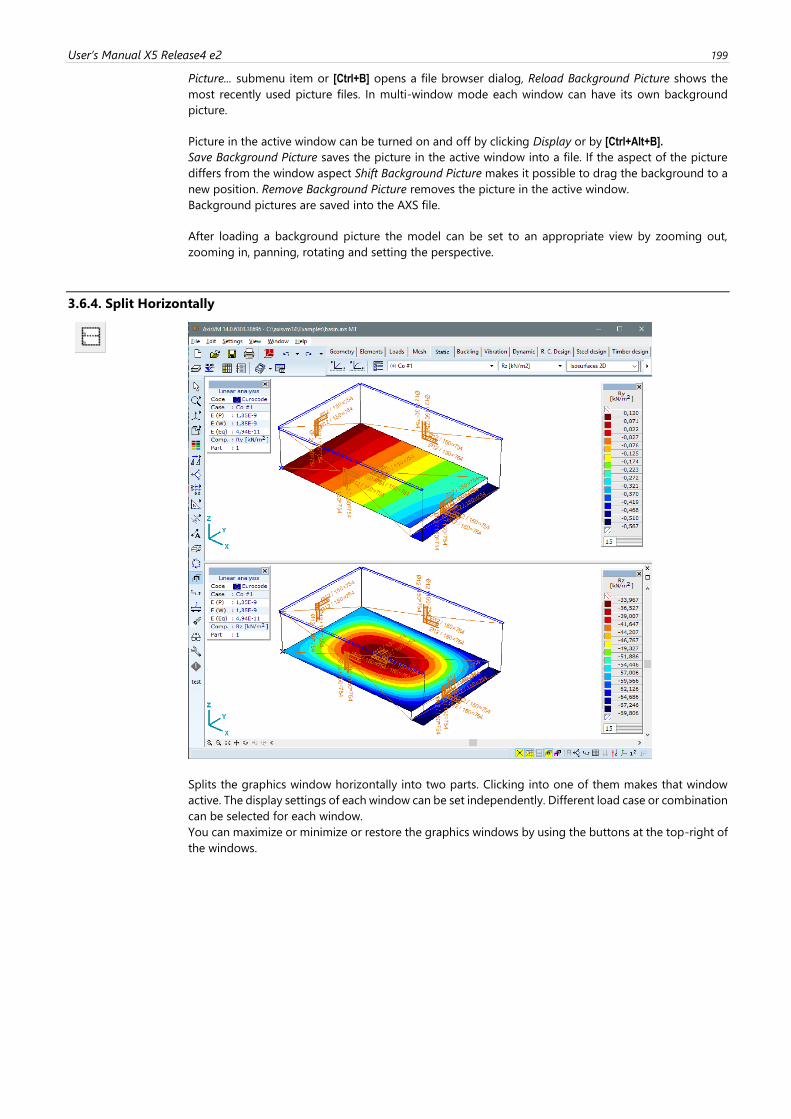
User’s Manual X5 Release4 e2 199

Picture... submenu item or [Ctrl+B] opens a file browser dialog, Reload Background Picture shows the

most recently used picture files. In multi-window mode each window can have its own background

picture.

Picture in the active window can be turned on and off by clicking Display or by [Ctrl+Alt+B].

Save Background Picture saves the picture in the active window into a file. If the aspect of the picture

differs from the window aspect Shift Background Picture makes it possible to drag the background to a

new position. Remove Background Picture removes the picture in the active window.

Background pictures are saved into the AXS file.

After loading a background picture the model can be set to an appropriate view by zooming out,

zooming in, panning, rotating and setting the perspective.

3.6.4. Split Horizontally

Splits the graphics window horizontally into two parts. Clicking into one of them makes that window

active. The display settings of each window can be set independently. Different load case or combination

can be selected for each window.

You can maximize or minimize or restore the graphics windows by using the buttons at the top-right of

the windows.

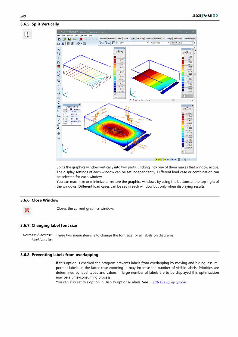
200

3.6.5. Split Vertically

Splits the graphics window vertically into two parts. Clicking into one of them makes that window active.

The display settings of each window can be set independently. Different load case or combination can

be selected for each window.

You can maximize or minimize or restore the graphics windows by using the buttons at the top-right of

the windows. Different load cases can be set in each window but only when displaying results.

3.6.6. Close Window

Closes the current graphics window.

3.6.7. Changing label font size

Decrease / Increase label font size

These two menu items is to change the font size for all labels on diagrams.

3.6.8. Preventing labels from overlapping

If this option is checked the program prevents labels from overlapping by moving and hiding less im-

portant labels. In the latter case zooming in may increase the number of visible labels. Priorities are

determined by label types and values. If large number of labels are to be displayed this optimization

may be a time-consuming process.

You can also set this option in Display options/Labels. See… 2.16.18 Display options

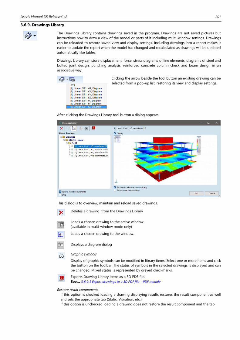
User’s Manual X5 Release4 e2 201

3.6.9. Drawings Library

The Drawings Library contains drawings saved in the program. Drawings are not saved pictures but

instructions how to draw a view of the model or parts of it including multi-window settings. Drawings

can be reloaded to restore saved view and display settings. Including drawings into a report makes it

easier to update the report when the model has changed and recalculated as drawings will be updated

automatically like tables.

Drawings Library can store displacement, force, stress diagrams of line elements, diagrams of steel and

bolted joint design, punching analysis, reinforced concrete column check and beam design in an

associative way.

Clicking the arrow beside the tool button an existing drawing can be

selected from a pop-up list, restoring its view and display settings.

After clicking the Drawings Library tool button a dialog appears.

This dialog is to overview, maintain and reload saved drawings.

Deletes a drawing from the Drawings Library

Loads a chosen drawing to the active window.

(available in multi-window mode only)

Loads a chosen drawing to the window.

Displays a diagram dialog

Graphic symbols

Display of graphic symbols can be modified in library items. Select one or more items and click

the button on the toolbar. The status of symbols in the selected drawings is displayed and can

be changed. Mixed status is represented by greyed checkmarks.

Exports Drawing Library items as a 3D PDF file.

See… 3.6.9.1 Export drawings to a 3D PDF file - PDF module

Restore result components

If this option is checked loading a drawing displaying results restores the result component as well

and sets the appropriate tab (Static, Vibration, etc.).

If this option is unchecked loading a drawing does not restore the result component and the tab.

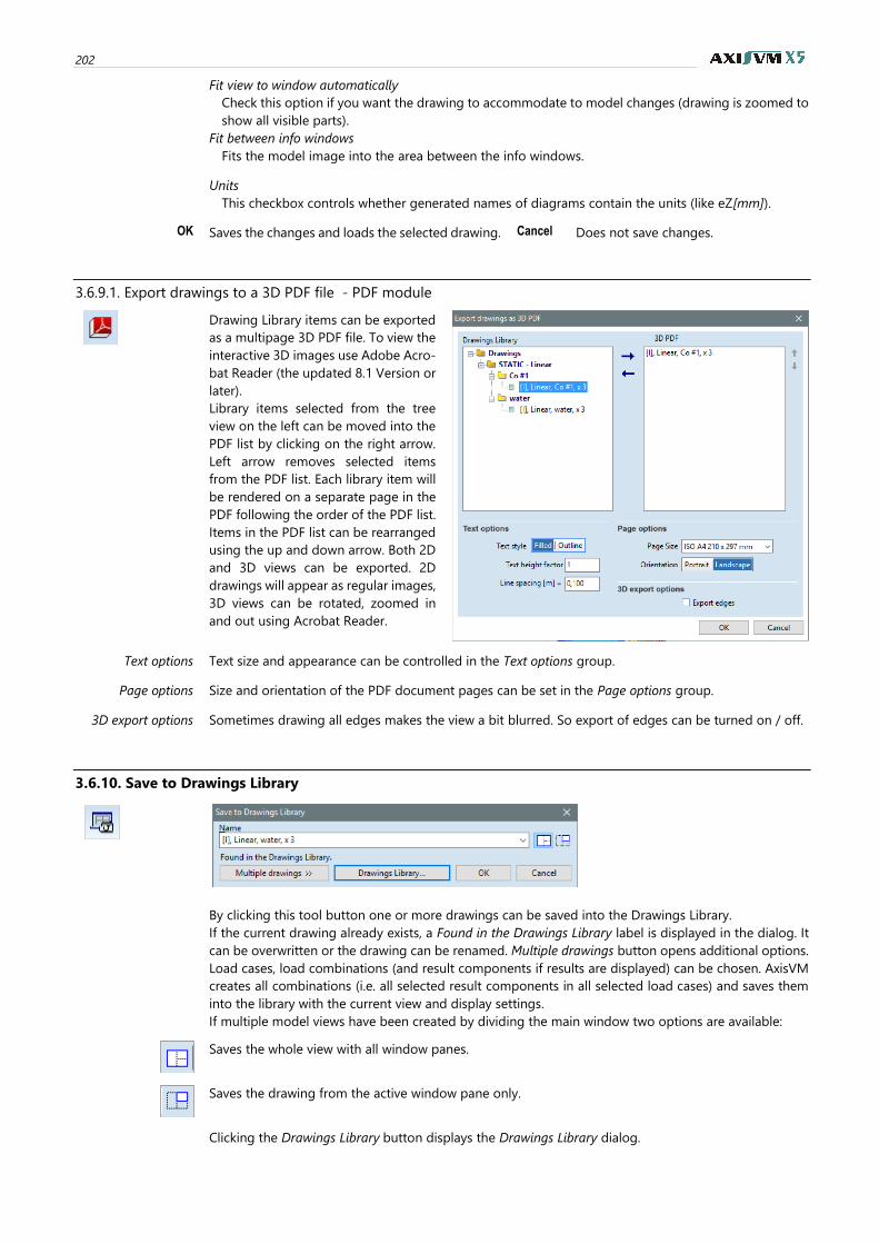
202

Fit view to window automatically

Check this option if you want the drawing to accommodate to model changes (drawing is zoomed to

show all visible parts).

Fit between info windows

Fits the model image into the area between the info windows.

Units

This checkbox controls whether generated names of diagrams contain the units (like eZ[mm]).

OK Saves the changes and loads the selected drawing. Cancel Does not save changes.

3.6.9.1. Export drawings to a 3D PDF file - PDF module

Drawing Library items can be exported

as a multipage 3D PDF file. To view the

interactive 3D images use Adobe Acro-

bat Reader (the updated 8.1 Version or

later).

Library items selected from the tree

view on the left can be moved into the

PDF list by clicking on the right arrow.

Left arrow removes selected items

from the PDF list. Each library item will

be rendered on a separate page in the

PDF following the order of the PDF list.

Items in the PDF list can be rearranged

using the up and down arrow. Both 2D

and 3D views can be exported. 2D

drawings will appear as regular images,

3D views can be rotated, zoomed in

and out using Acrobat Reader.

Text options Text size and appearance can be controlled in the Text options group.

Page options Size and orientation of the PDF document pages can be set in the Page options group.

3D export options Sometimes drawing all edges makes the view a bit blurred. So export of edges can be turned on / off.

3.6.10. Save to Drawings Library

By clicking this tool button one or more drawings can be saved into the Drawings Library.

If the current drawing already exists, a Found in the Drawings Library label is displayed in the dialog. It

can be overwritten or the drawing can be renamed. Multiple drawings button opens additional options.

Load cases, load combinations (and result components if results are displayed) can be chosen. AxisVM

creates all combinations (i.e. all selected result components in all selected load cases) and saves them

into the library with the current view and display settings.

If multiple model views have been created by dividing the main window two options are available:

Saves the whole view with all window panes.

Saves the drawing from the active window pane only.

Clicking the Drawings Library button displays the Drawings Library dialog.

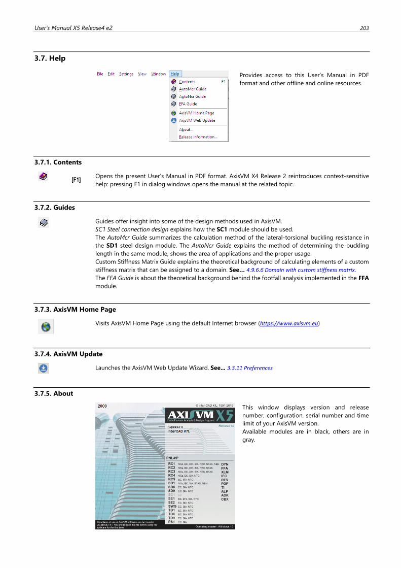
User’s Manual X5 Release4 e2 203

3.7. Help

Provides access to this User’s Manual in PDF

format and other offline and online resources.

3.7.1. Contents

[F1] Opens the present User’s Manual in PDF format. AxisVM X4 Release 2 reintroduces context-sensitive

help: pressing F1 in dialog windows opens the manual at the related topic.

3.7.2. Guides

Guides offer insight into some of the design methods used in AxisVM.

SC1 Steel connection design explains how the SC1 module should be used.

The AutoMcr Guide summarizes the calculation method of the lateral-torsional buckling resistance in

the SD1 steel design module. The AutoNcr Guide explains the method of determining the buckling

length in the same module, shows the area of applications and the proper usage.

Custom Stiffness Matrix Guide explains the theoretical background of calculating elements of a custom

stiffness matrix that can be assigned to a domain. See… 4.9.6.6 Domain with custom stiffness matrix.

The FFA Guide is about the theoretical background behind the footfall analysis implemented in the FFA

module.

3.7.3. AxisVM Home Page

Visits AxisVM Home Page using the default Internet browser (https://www.axisvm.eu)

3.7.4. AxisVM Update

Launches the AxisVM Web Update Wizard. See... 3.3.11 Preferences

3.7.5. About

This window displays version and release

number, configuration, serial number and time

limit of your AxisVM version.

Available modules are in black, others are in

gray.

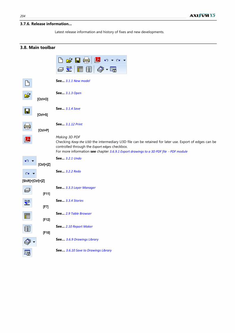
204

3.7.6. Release information...

Latest release information and history of fixes and new developments.

3.8. Main toolbar

See... 3.1.1 New model

[Ctrl+O]

See... 3.1.3 Open

[Ctrl+S]

See... 3.1.4 Save

[Ctrl+P]

See... 3.1.12 Print

Making 3D PDF

Checking Keep the U3D the intermediary U3D file can be retained for later use. Export of edges can be

controlled through the Export edges checkbox.

For more information see chapter 3.6.9.1 Export drawings to a 3D PDF file - PDF module

[Ctrl]+[Z]

See... 3.2.1 Undo

[Shift]+[Ctrl]+[Z]

See... 3.2.2 Redo

[F11]

See... 3.3.3 Layer Manager

[F7]

See... 3.3.4 Stories

[F12]

See... 2.9 Table Browser

[F10]

See... 2.10 Report Maker

See… 3.6.9 Drawings Library

See… 3.6.10 Save to Drawings Library

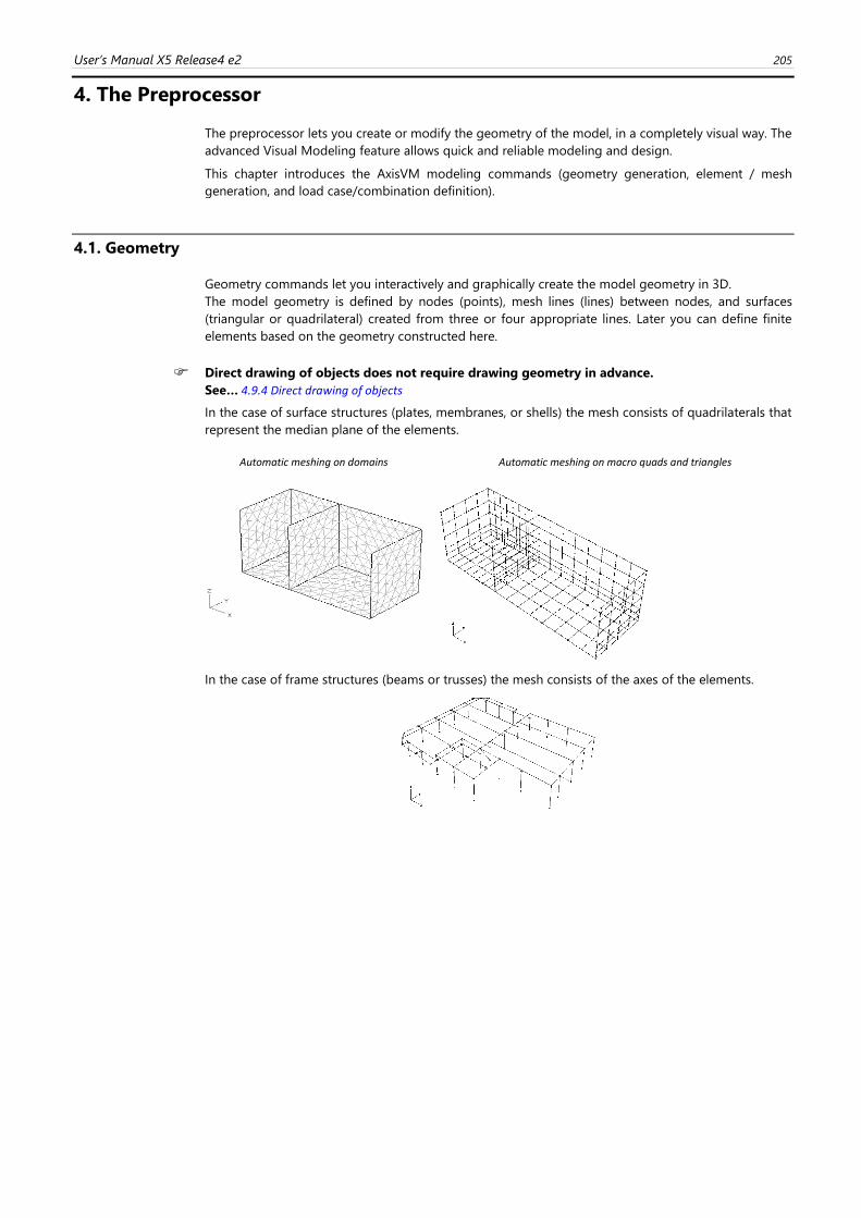
User’s Manual X5 Release4 e2 205

4. The Preprocessor

The preprocessor lets you create or modify the geometry of the model, in a completely visual way. The

advanced Visual Modeling feature allows quick and reliable modeling and design.

This chapter introduces the AxisVM modeling commands (geometry generation, element / mesh

generation, and load case/combination definition).

4.1. Geometry

Geometry commands let you interactively and graphically create the model geometry in 3D.

The model geometry is defined by nodes (points), mesh lines (lines) between nodes, and surfaces

(triangular or quadrilateral) created from three or four appropriate lines. Later you can define finite

elements based on the geometry constructed here.

Direct drawing of objects does not require drawing geometry in advance.

See… 4.9.4 Direct drawing of objects

In the case of surface structures (plates, membranes, or shells) the mesh consists of quadrilaterals that

represent the median plane of the elements.

Automatic meshing on domains Automatic meshing on macro quads and triangles

In the case of frame structures (beams or trusses) the mesh consists of the axes of the elements.

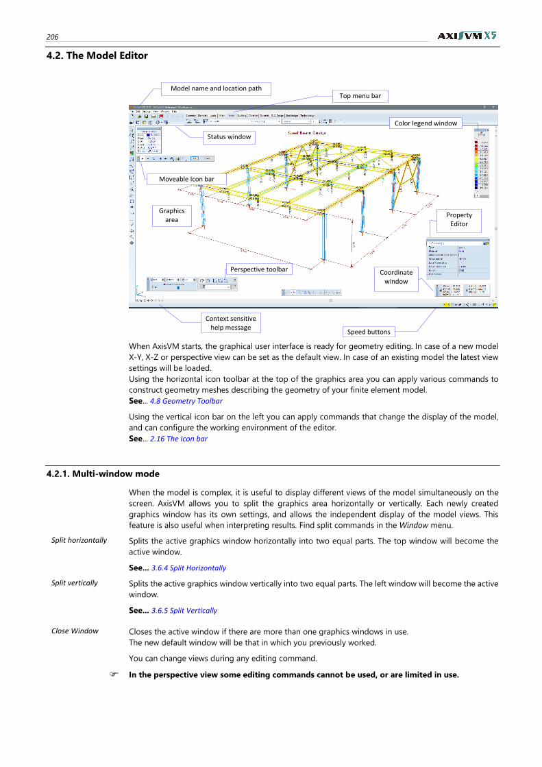
206

4.2. The Model Editor

When AxisVM starts, the graphical user interface is ready for geometry editing. In case of a new model

X-Y, X-Z or perspective view can be set as the default view. In case of an existing model the latest view

settings will be loaded.

Using the horizontal icon toolbar at the top of the graphics area you can apply various commands to

construct geometry meshes describing the geometry of your finite element model.

See... 4.8 Geometry Toolbar

Using the vertical icon bar on the left you can apply commands that change the display of the model,

and can configure the working environment of the editor.

See... 2.16 The Icon bar

4.2.1. Multi-window mode

When the model is complex, it is useful to display different views of the model simultaneously on the

screen. AxisVM allows you to split the graphics area horizontally or vertically. Each newly created

graphics window has its own settings, and allows the independent display of the model views. This

feature is also useful when interpreting results. Find split commands in the Window menu.

Split horizontally Splits the active graphics window horizontally into two equal parts. The top window will become the

active window.

See... 3.6.4 Split Horizontally

Split vertically Splits the active graphics window vertically into two equal parts. The left window will become the active

window.

See... 3.6.5 Split Vertically

Close Window Closes the active window if there are more than one graphics windows in use.

The new default window will be that in which you previously worked.

You can change views during any editing command.

In the perspective view some editing commands cannot be used, or are limited in use.

Context sensitive help message

Speed buttons

Status window

Color legend window

Moveable Icon bar

Graphics area

Property Editor

Coordinate window

Perspective toolbar

Top menu bar

Model name and location path

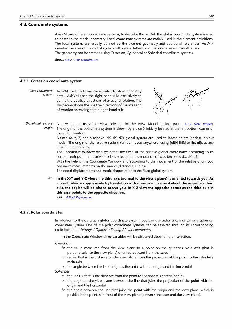
User’s Manual X5 Release4 e2 207

4.3. Coordinate systems

AxisVM uses different coordinate systems, to describe the model. The global coordinate system is used

to describe the model geometry. Local coordinate systems are mainly used in the element definitions.

The local systems are usually defined by the element geometry and additional references. AxisVM

denotes the axes of the global system with capital letters, and the local axes with small letters.

The geometry can be created using Cartesian, Cylindrical or Spherical coordinate systems.

See... 4.3.2 Polar coordinates

4.3.1. Cartesian coordinate system

Base coordinate system

AxisVM uses Cartesian coordinates to store geometry

data. AxisVM uses the right-hand rule exclusively to

define the positive directions of axes and rotation. The

illustration shows the positive directions of the axes and

of rotation according to the right-hand rule.

Global and relative origin

A new model uses the view selected in the New Model dialog (see... 3.1.1 New model).

The origin of the coordinate system is shown by a blue X initially located at the left bottom corner of

the editor window.

A fixed (X, Y, Z) and a relative (dX, dY, dZ) global system are used to locate points (nodes) in your

model. The origin of the relative system can be moved anywhere (using [Alt]+[Shift] or [Insert]), at any

time during modeling.

The Coordinate Window displays either the fixed or the relative global coordinates according to its

current settings. If the relative mode is selected, the denotation of axes becomes dX, dY, dZ.

With the help of the Coordinate Window, and according to the movement of the relative origin you

can make measurements on the model (distances, angles).

The nodal displacements and mode shapes refer to the fixed global system.

In the X-Y and Y-Z views the third axis (normal to the view’s plane) is oriented towards you. As

a result, when a copy is made by translation with a positive increment about the respective third

axis, the copies will be placed nearer you. In X-Z view the opposite occurs as the third axis in

this case points to the opposite direction.

See... 4.9.22 References

4.3.2. Polar coordinates

In addition to the Cartesian global coordinate system, you can use either a cylindrical or a spherical

coordinate system. One of the polar coordinate systems can be selected through its corresponding

radio button in Settings / Options / Editing / Polar coordinates.

In the Coordinate Window three variables will be displayed depending on selection:

Cylindrical

h: the value measured from the view plane to a point on the cylinder’s main axis (that is

perpendicular to the view plane) oriented outward from the screen

r: radius that is the distance on the view plane from the projection of the point to the cylinder’s

main axis

a: the angle between the line that joins the point with the origin and the horizontal

Spherical

r: the radius, that is the distance from the point to the sphere’s center (origin)

a: the angle on the view plane between the line that joins the projection of the point with the

origin and the horizontal

b: the angle between the line that joins the point with the origin and the view plane, which is

positive if the point is in front of the view plane (between the user and the view plane).

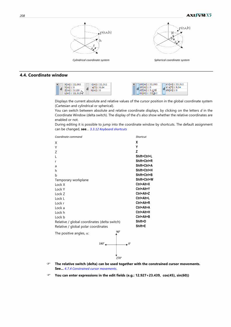
208

Cylindrical coordinate system Spherical coordinate system

4.4. Coordinate window

Displays the current absolute and relative values of the cursor position in the global coordinate system

(Cartesian and cylindrical or spherical).

You can switch between absolute and relative coordinate displays, by clicking on the letters d in the

Coordinate Window (delta switch). The display of the d’s also show whether the relative coordinates are

enabled or not.

During editing it is possible to jump into the coordinate window by shortcuts. The default assignment

can be changed, see… 3.3.12 Keyboard shortcuts

Coordinate command Shortcut

X X

Y Y

Z Z

L Shift+Ctrl+L

r Shift+Ctrl+R

a Shift+Ctrl+A

h Shift+Ctrl+H

b Shift+Ctrl+B

Temporary workplane Shift+Ctrl+W

Lock X Ctrl+Alt+X

Lock Y Ctrl+Alt+Y

Lock Z Ctrl+Alt+Z

Lock L Ctrl+Alt+L

Lock r Ctrl+Alt+R

Lock a Ctrl+Alt+A

Lock h Ctrl+Alt+H

Lock b Ctrl+Alt+B

Relative / global coordinates (delta switch) Shift+D

Relative / global polar coordinates Shift+E

The positive angles, :

The relative switch (delta) can be used together with the constrained cursor movements.

See... 4.7.4 Constrained cursor movements.

You can enter expressions in the edit fields (e.g.: 12.927+23.439, cos(45), sin(60))

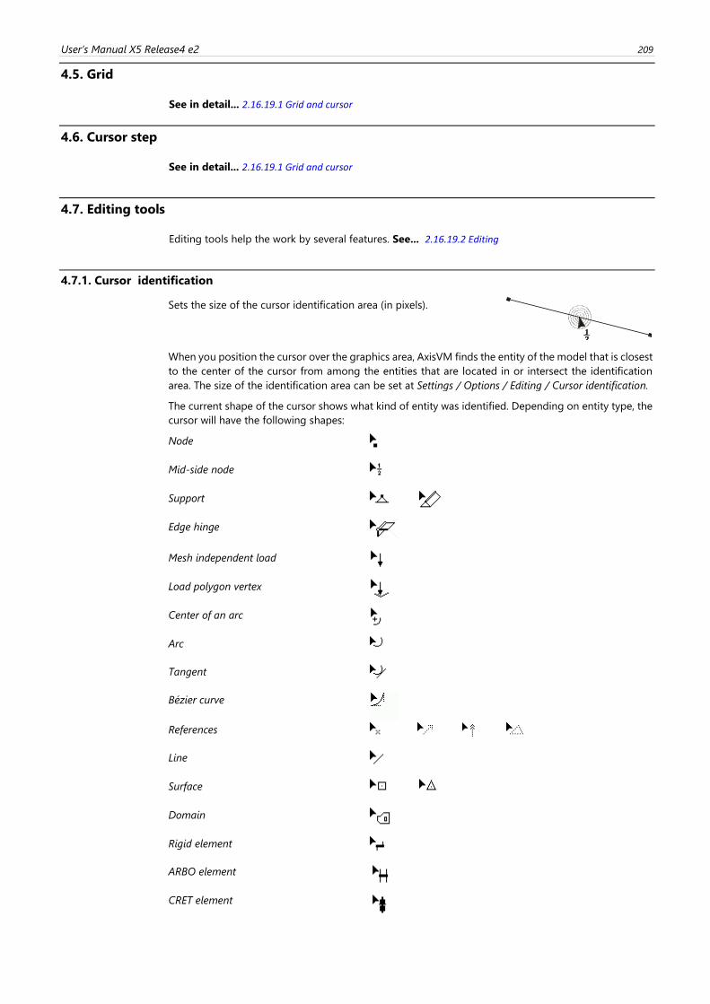
User’s Manual X5 Release4 e2 209

4.5. Grid

See in detail... 2.16.19.1 Grid and cursor

4.6. Cursor step

See in detail... 2.16.19.1 Grid and cursor

4.7. Editing tools

Editing tools help the work by several features. See... 2.16.19.2 Editing

4.7.1. Cursor identification

Sets the size of the cursor identification area (in pixels).

When you position the cursor over the graphics area, AxisVM finds the entity of the model that is closest

to the center of the cursor from among the entities that are located in or intersect the identification

area. The size of the identification area can be set at Settings / Options / Editing / Cursor identification.

The current shape of the cursor shows what kind of entity was identified. Depending on entity type, the

cursor will have the following shapes:

Node

Mid-side node

Support

Edge hinge

Mesh independent load

Load polygon vertex

Center of an arc

Arc

Tangent

Bézier curve

References

Line

Surface

Domain

Rigid element

ARBO element

CRET element

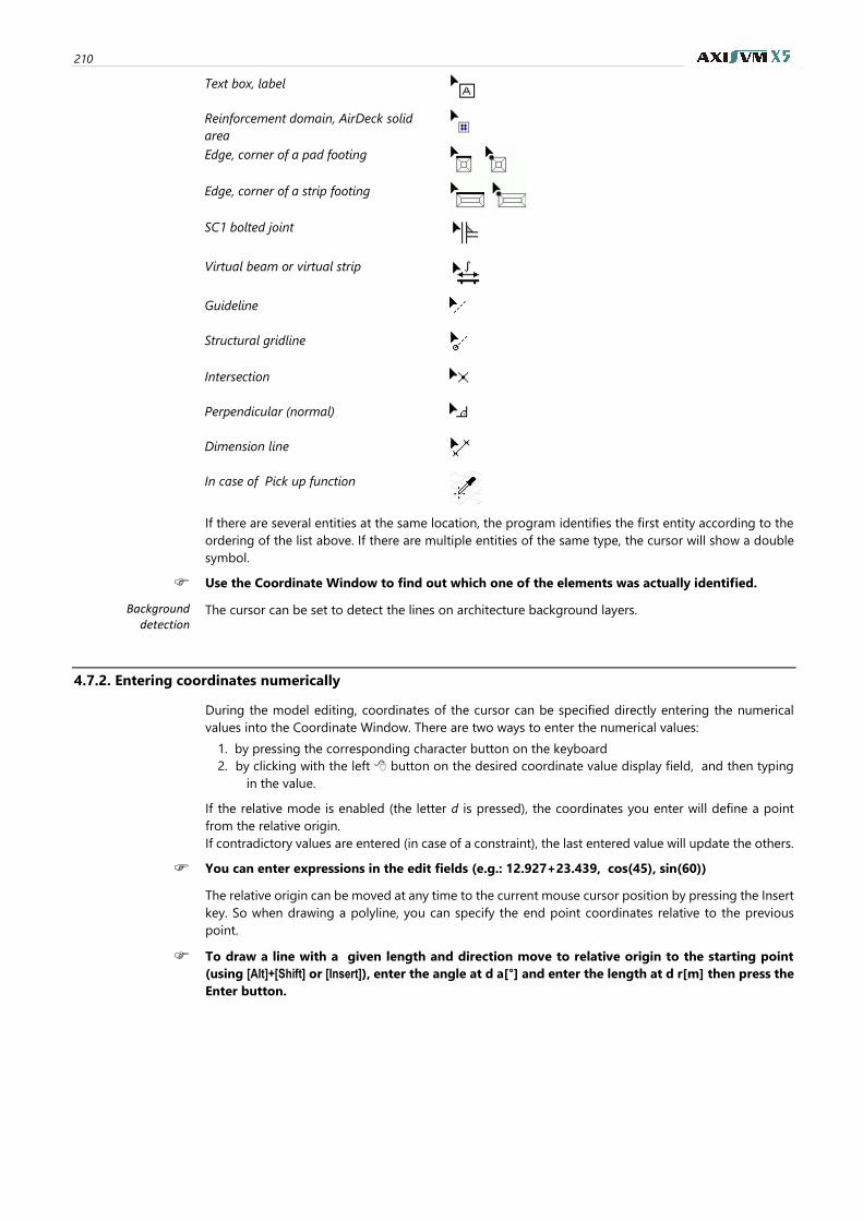
210

Text box, label

Reinforcement domain, AirDeck solid

area

Edge, corner of a pad footing

Edge, corner of a strip footing

SC1 bolted joint

Virtual beam or virtual strip

Guideline

Structural gridline

Intersection

Perpendicular (normal)

Dimension line

In case of Pick up function

If there are several entities at the same location, the program identifies the first entity according to the

ordering of the list above. If there are multiple entities of the same type, the cursor will show a double

symbol.

Use the Coordinate Window to find out which one of the elements was actually identified.

Background detection

The cursor can be set to detect the lines on architecture background layers.

4.7.2. Entering coordinates numerically

During the model editing, coordinates of the cursor can be specified directly entering the numerical

values into the Coordinate Window. There are two ways to enter the numerical values:

1. by pressing the corresponding character button on the keyboard

2. by clicking with the left button on the desired coordinate value display field, and then typing

in the value.

If the relative mode is enabled (the letter d is pressed), the coordinates you enter will define a point

from the relative origin.

If contradictory values are entered (in case of a constraint), the last entered value will update the others.

You can enter expressions in the edit fields (e.g.: 12.927+23.439, cos(45), sin(60))

The relative origin can be moved at any time to the current mouse cursor position by pressing the Insert

key. So when drawing a polyline, you can specify the end point coordinates relative to the previous

point.

To draw a line with a given length and direction move to relative origin to the starting point

(using [Alt]+[Shift] or [Insert]), enter the angle at d a[°] and enter the length at d r[m] then press the

Enter button.

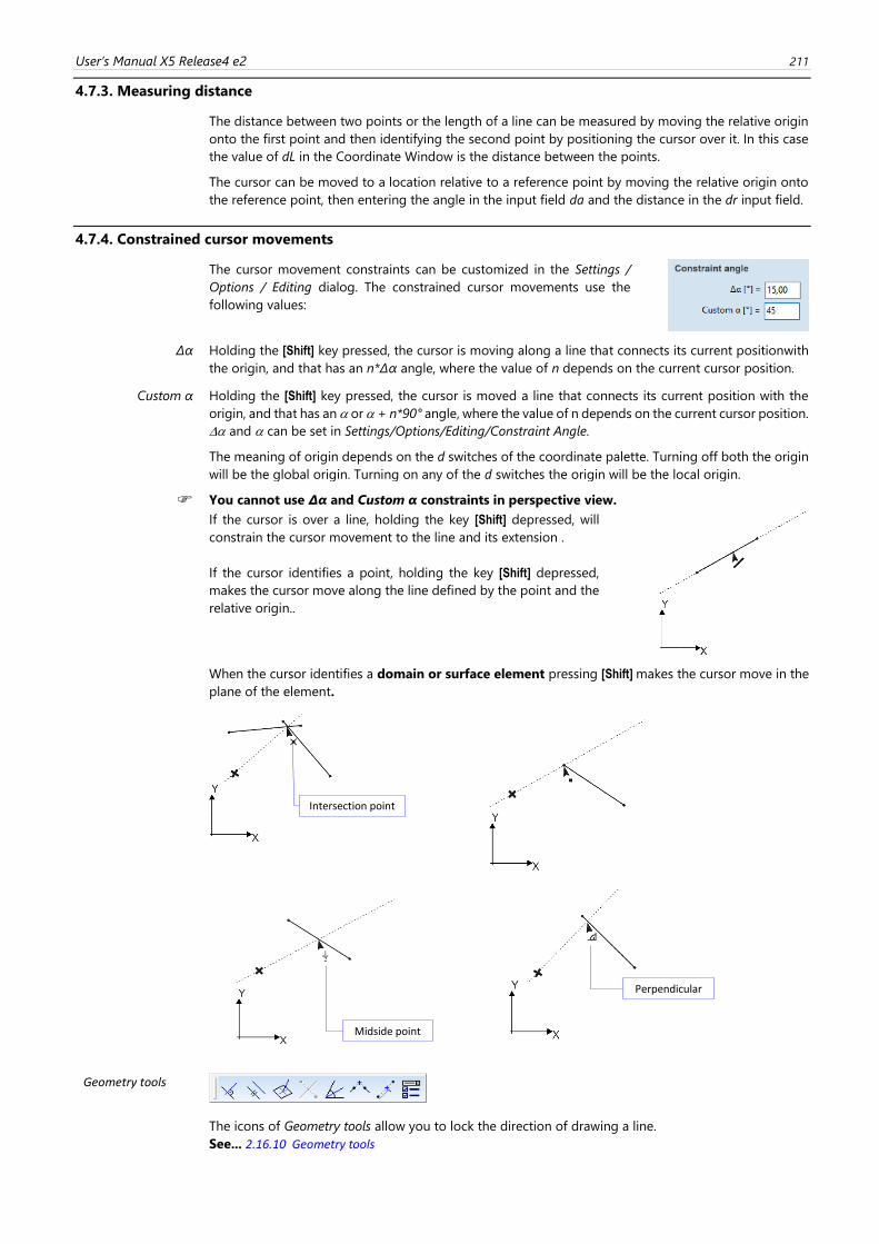
User’s Manual X5 Release4 e2 211

4.7.3. Measuring distance

The distance between two points or the length of a line can be measured by moving the relative origin

onto the first point and then identifying the second point by positioning the cursor over it. In this case

the value of dL in the Coordinate Window is the distance between the points.

The cursor can be moved to a location relative to a reference point by moving the relative origin onto

the reference point, then entering the angle in the input field da and the distance in the dr input field.

4.7.4. Constrained cursor movements

The cursor movement constraints can be customized in the Settings /

Options / Editing dialog. The constrained cursor movements use the

following values:

Δα

Holding the [Shift] key pressed, the cursor is moving along a line that connects its current positionwith

the origin, and that has an n*Δα angle, where the value of n depends on the current cursor position.

Custom α

Holding the [Shift] key pressed, the cursor is moved a line that connects its current position with the

origin, and that has an or + n*90° angle, where the value of n depends on the current cursor position.

and can be set in Settings/Options/Editing/Constraint Angle.

The meaning of origin depends on the d switches of the coordinate palette. Turning off both the origin

will be the global origin. Turning on any of the d switches the origin will be the local origin.

You cannot use Δα and Custom α constraints in perspective view.

If the cursor is over a line, holding the key [Shift] depressed, will

constrain the cursor movement to the line and its extension .

If the cursor identifies a point, holding the key [Shift] depressed,

makes the cursor move along the line defined by the point and the

relative origin..

When the cursor identifies a domain or surface element pressing [Shift] makes the cursor move in the

plane of the element.

Geometry tools

The icons of Geometry tools allow you to lock the direction of drawing a line.

See... 2.16.10 Geometry tools

Perpendicular

Intersection point

Midside point

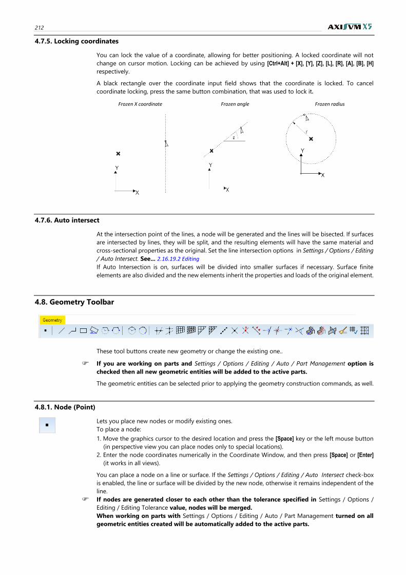
212

4.7.5. Locking coordinates

You can lock the value of a coordinate, allowing for better positioning. A locked coordinate will not

change on cursor motion. Locking can be achieved by using [Ctrl+Alt] + [X], [Y], [Z], [L], [R], [A], [B], [H]

respectively.

A black rectangle over the coordinate input field shows that the coordinate is locked. To cancel

coordinate locking, press the same button combination, that was used to lock it.

Frozen X coordinate

Frozen angle

Frozen radius

4.7.6. Auto intersect

At the intersection point of the lines, a node will be generated and the lines will be bisected. If surfaces

are intersected by lines, they will be split, and the resulting elements will have the same material and

cross-sectional properties as the original. Set the line intersection options in Settings / Options / Editing

/ Auto Intersect. See... 2.16.19.2 Editing

If Auto Intersection is on, surfaces will be divided into smaller surfaces if necessary. Surface finite

elements are also divided and the new elements inherit the properties and loads of the original element.

4.8. Geometry Toolbar

These tool buttons create new geometry or change the existing one..

If you are working on parts and Settings / Options / Editing / Auto / Part Management option is

checked then all new geometric entities will be added to the active parts.

The geometric entities can be selected prior to applying the geometry construction commands, as well.

4.8.1. Node (Point)

Lets you place new nodes or modify existing ones.

To place a node:

1. Move the graphics cursor to the desired location and press the [Space] key or the left mouse button

(in perspective view you can place nodes only to special locations).

2. Enter the node coordinates numerically in the Coordinate Window, and then press [Space] or [Enter]

(it works in all views).

You can place a node on a line or surface. If the Settings / Options / Editing / Auto Intersect check-box

is enabled, the line or surface will be divided by the new node, otherwise it remains independent of the

line.

If nodes are generated closer to each other than the tolerance specified in Settings / Options /

Editing / Editing Tolerance value, nodes will be merged.

When working on parts with Settings / Options / Editing / Auto / Part Management turned on all

geometric entities created will be automatically added to the active parts.

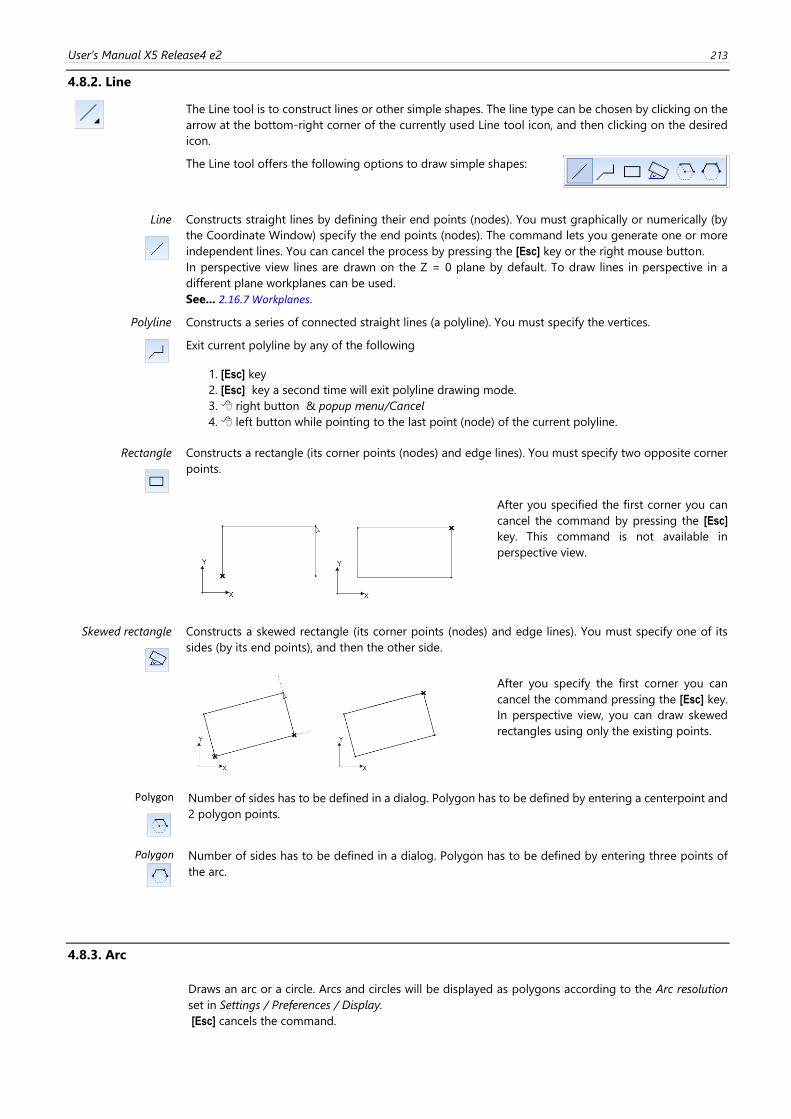
User’s Manual X5 Release4 e2 213

4.8.2. Line

The Line tool is to construct lines or other simple shapes. The line type can be chosen by clicking on the

arrow at the bottom-right corner of the currently used Line tool icon, and then clicking on the desired

icon.

The Line tool offers the following options to draw simple shapes:

Line

Constructs straight lines by defining their end points (nodes). You must graphically or numerically (by

the Coordinate Window) specify the end points (nodes). The command lets you generate one or more

independent lines. You can cancel the process by pressing the [Esc] key or the right mouse button.

In perspective view lines are drawn on the Z = 0 plane by default. To draw lines in perspective in a

different plane workplanes can be used.

See... 2.16.7 Workplanes.

Polyline

Constructs a series of connected straight lines (a polyline). You must specify the vertices.

Exit current polyline by any of the following

1. [Esc] key

2. [Esc] key a second time will exit polyline drawing mode.

3. right button & popup menu/Cancel

4. left button while pointing to the last point (node) of the current polyline.

Rectangle

Constructs a rectangle (its corner points (nodes) and edge lines). You must specify two opposite corner

points.

After you specified the first corner you can

cancel the command by pressing the [Esc]

key. This command is not available in

perspective view.

Skewed rectangle

Constructs a skewed rectangle (its corner points (nodes) and edge lines). You must specify one of its

sides (by its end points), and then the other side.

After you specify the first corner you can

cancel the command pressing the [Esc] key.

In perspective view, you can draw skewed

rectangles using only the existing points.

Polygon

Number of sides has to be defined in a dialog. Polygon has to be defined by entering a centerpoint and

2 polygon points.

Polygon

Number of sides has to be defined in a dialog. Polygon has to be defined by entering three points of

the arc.

4.8.3. Arc

Draws an arc or a circle. Arcs and circles will be displayed as polygons according to the Arc resolution

set in Settings / Preferences / Display.

[Esc] cancels the command.

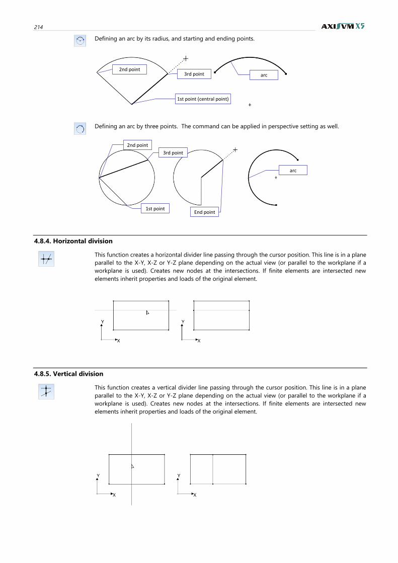
214

Defining an arc by its radius, and starting and ending points.

Defining an arc by three points. The command can be applied in perspective setting as well.

4.8.4. Horizontal division

This function creates a horizontal divider line passing through the cursor position. This line is in a plane

parallel to the X-Y, X-Z or Y-Z plane depending on the actual view (or parallel to the workplane if a

workplane is used). Creates new nodes at the intersections. If finite elements are intersected new

elements inherit properties and loads of the original element.

4.8.5. Vertical division

This function creates a vertical divider line passing through the cursor position. This line is in a plane

parallel to the X-Y, X-Z or Y-Z plane depending on the actual view (or parallel to the workplane if a

workplane is used). Creates new nodes at the intersections. If finite elements are intersected new

elements inherit properties and loads of the original element.

3rd point

1st point (central point)

1st point

2nd point

3rd point

arc

2nd point arc

End point

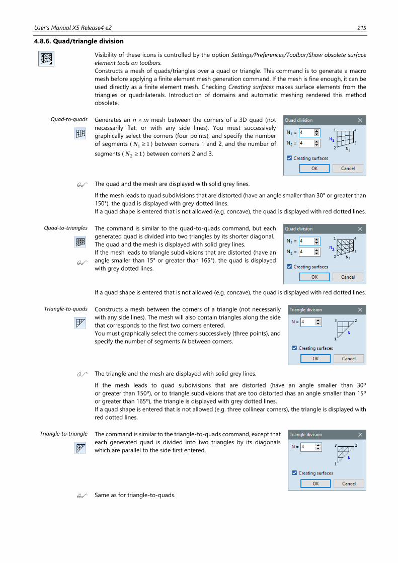
User’s Manual X5 Release4 e2 215

4.8.6. Quad/triangle division

Visibility of these icons is controlled by the option Settings/Preferences/Toolbar/Show obsolete surface

element tools on toolbars.

Constructs a mesh of quads/triangles over a quad or triangle. This command is to generate a macro

mesh before applying a finite element mesh generation command. If the mesh is fine enough, it can be

used directly as a finite element mesh. Checking Creating surfaces makes surface elements from the

triangles or quadrilaterals. Introduction of domains and automatic meshing rendered this method

obsolete.

Quad-to-quads

Generates an n m mesh between the corners of a 3D quad (not

necessarily flat, or with any side lines). You must successively

graphically select the corners (four points), and specify the number

of segments ( 11 N ) between corners 1 and 2, and the number of

segments ( 12 N ) between corners 2 and 3.

The quad and the mesh are displayed with solid grey lines.

If the mesh leads to quad subdivisions that are distorted (have an angle smaller than 30° or greater than

150°), the quad is displayed with grey dotted lines.

If a quad shape is entered that is not allowed (e.g. concave), the quad is displayed with red dotted lines.

Quad-to-triangles

The command is similar to the quad-to-quads command, but each

generated quad is divided into two triangles by its shorter diagonal.

The quad and the mesh is displayed with solid grey lines.

If the mesh leads to triangle subdivisions that are distorted (have an

angle smaller than 15° or greater than 165°), the quad is displayed

with grey dotted lines.

If a quad shape is entered that is not allowed (e.g. concave), the quad is displayed with red dotted lines.

Triangle-to-quads

Constructs a mesh between the corners of a triangle (not necessarily

with any side lines). The mesh will also contain triangles along the side

that corresponds to the first two corners entered.

You must graphically select the corners successively (three points), and

specify the number of segments N between corners.

The triangle and the mesh are displayed with solid grey lines.

If the mesh leads to quad subdivisions that are distorted (have an angle smaller than 30º

or greater than 150º), or to triangle subdivisions that are too distorted (has an angle smaller than 15º

or greater than 165º), the triangle is displayed with grey dotted lines.

If a quad shape is entered that is not allowed (e.g. three collinear corners), the triangle is displayed with

red dotted lines.

Triangle-to-triangle

The command is similar to the triangle-to-quads command, except that

each generated quad is divided into two triangles by its diagonals

which are parallel to the side first entered.

Same as for triangle-to-quads.

216

4.8.7. Intersect

If the Settings / Options / Editing / Auto / Intersect checkbox was not enabled in the dialog window at

the time of creating the geometric entity, using this command you can intersect the selected lines.

Intersection can be filtered by element types in a dialog. Selected lines will be divided by creating nodes

(points) at their intersections.

If finite elements are assigned to the lines, finite elements are also divided and inherit the properties

and loads of the original element..

You can select elements for intersection beforehand.

4.8.8. Remove node

Removes the selected nodes at the intersections of lines. It makes it easier to construct trusses crossing

but not intersecting each other or to remove unnecessary division points along a line.

Intersection nodes can be removed only if the number of connecting lines are even and lines can

be joined.

4.8.9. Remove intermediate nodes

Removes unnecessary intermediate nodes on lines. Nodes with two connecting lines are removed

provided they can be joined.

4.8.10. Extend lines to meet another line or plane

Extends existing straight lines or arcs to meet another straight line, arc or plane.

Extension modes

Extend lines to meet another line

The first step is to specify the boundary: click on an existing line or arc or enter two points of

an imaginary boundary line. Click on lines near their end point to extend.

Extend lines to meet more than one line

The first step is to click on multiple lines defining the boundary. Click OK on the selection

toolbar or press Enter. Select the lines to extend. Click OK on the selection toolbar or press

Enter. Both ends of the lines will be extended to meet the boundary.

Extend lines to meet a plane

The first step is the specify the boundary plane: click on an existing domain or enter three non-

collinear points of an imaginary boundary plane. Click on lines near their end point to extend.

Extend lines to meet more than one plane

The first step is to click on multiple domains defining the boundary. Click OK on the selection

toolbar or press Enter. Select the lines to extend. Click OK on the selection toolbar or press

Enter. Both ends of the lines will be extended to meet the boundary.

Settings

Extend lines even if there is no actual intersection

This is a two-state button. If it is down (its background turns white) lines will be extended even

if the point of intersection does not fall between the start and end point of the boundary line.

If it is up (its background is blue) lines will be extended only if the point of intersection is on

the boundary line.

The last three buttons control the behaviour of lines connected to the extended point.

Move free ends, add splice if other elements are connected

The program automatically chooses from the two options listed below. If no lines are con-

nected to the extended point, it chooses the first option, otherwise it chooses the second one.

Always move line ends

The node of the extended point is moved to the point of intersection. The direction of lines

connected to this node will change.

User’s Manual X5 Release4 e2 217

Always splice line ends

The node of the extended point is not moved. A new node will be created at the point of

intersection and a new line (a splice) is inserted between the two nodes. Connected lines re-

main unchanged.

4.8.11. Trim lines to meet another line or plane

Trims existing straight lines or arcs to meet other straight lines, arcs or planes.

Trimming modes

Trim lines to meet another line

The first step is to specify the cutting line: click on an existing line or arc or enter two points

of an imaginary cutting line. Click on the line segments to be removed.

Trim lines to meet other lines

The first step is to click on multiple lines defining the cutting lines. Click OK on the selection

toolbar or press Enter. Select the lines to trim. Click OK on the selection toolbar or press Enter.

Click on that side of the cutting lines where you want to remove the line segments.

Trim lines to meet a plane

The first step is the specify the cutting plane: click on an existing domain or enter three non-

collinear points of an imaginary cutting plane. If the cutting plane intersects the lines click on

the line segments to be removed.

Trim lines to meet more than one plane

The first step is to click on multiple domains defining the cutting planes. Click OK on the se-

lection toolbar or press Enter. Select the lines to trim. Click OK on the selection toolbar or press

Enter. Click on that side of the cutting planes where you want to remove the line segments.

Settings

Trim lines even if there is no actual intersection

This is a two-state button. If it is down (its background turns white) lines will be trimmed even

if the point of intersection does not fall between the start and end point of the boundary line.

If it is up (its background is blue) lines will be trimmed only if the point of intersection is on

the boundary line.

The last three buttons control the behaviour of lines connected to end point of trimmed lines.

The trimmed line always get a new end point at the point of intersection.

Move free ends, remove segment if other elements are connected

The program automatically chooses from the two options listed below. If lines are connected

to the extended point, it chooses the second option.

Always move line ends

The end point of connected lines will move to the new end point. The old end point is removed.

Always remove line segment

The original end point and connected lines remains unchanged.

4.8.12. Extend/cut lines to their point of intersection

Modes

Extend/trim two selected lines to their point of intersection

Extends/trims pairs of consecutively selected lines to their point of intersection.

Extend/trim selected lines to the point of intersection with the first one

Extends/trims consecutively selected lines to their point of intersection with the first line.

The next two buttons control the behaviour of arcs where there may be two points of intersection.

Settings

Extend the arc end where the extension is shorter

The program always chooses the end where the point of intersection is closer.

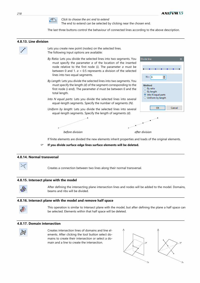
218

Click to choose the arc end to extend

The end to extend can be selected by clicking near the chosen end.

The last three buttons control the behaviour of connected lines according to the above description.

4.8.13. Line division

Lets you create new point (nodes) on the selected lines.

The following input options are available:

By Ratio: Lets you divide the selected lines into two segments. You

must specify the parameter a of the location of the inserted

node relative to the first node (i). The parameter a must be

between 0 and 1. a = 0.5 represents a division of the selected

lines into two equal segments.

By Length: Lets you divide the selected lines into two segments. You

must specify the length (d) of the segment corresponding to the

first node (i end). The parameter d must be between 0 and the

total length.

Into N equal parts: Lets you divide the selected lines into several

equal-length segments. Specify the number of segments (N).

Uniform by length: Lets you divide the selected lines into several

equal-length segments. Specify the length of segments (d).

before division after division

If finite elements are divided the new elements inherit properties and loads of the original elements.

If you divide surface edge lines surface elements will be deleted.

4.8.14. Normal transversal

Creates a connection between two lines along their normal transversal.

4.8.15. Intersect plane with the model

After defining the intersecting plane intersection lines and nodes will be added to the model. Domains,

beams and ribs will be divided.

4.8.16. Intersect plane with the model and remove half space

This operation is similar to Intersect plane with the model, but after defining the plane a half space can

be selected. Elements within that half space will be deleted.

4.8.17. Domain intersection

Creates intersection lines of domains and line el-

ements. After clicking the tool button select do-

mains to create their intersection or select a do-

main and a line to create the intersection.

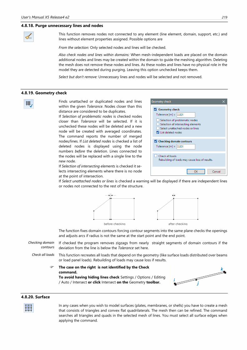
User’s Manual X5 Release4 e2 219

4.8.18. Purge unnecessary lines and nodes

This function removes nodes not connected to any element (line element, domain, support, etc.) and

lines without element properties assigned. Possible options are

From the selection: Only selected nodes and lines will be checked.

Also check nodes and lines within domains: When mesh-independent loads are placed on the domain

additional nodes and lines may be created within the domain to guide the meshing algorithm. Deleting

the mesh does not remove these nodes and lines. As these nodes and lines have no physical role in the

model they are detected during purging. Leaving this option unchecked keeps them.

Select but don’t remove: Unnecessary lines and nodes will be selected and not removed.

4.8.19. Geometry check

Finds unattached or duplicated nodes and lines

within the given Tolerance. Nodes closer than this

distance are considered to be duplicates.

If Selection of problematic nodes is checked nodes

closer than Tolerance will be selected. If it is

unchecked these nodes will be deleted and a new

node will be created with averaged coordinates.

The command reports the number of merged

nodes/lines. If List deleted nodes is checked a list of

deleted nodes is displayed using the node

numbers before the deletion. Lines connected to

the nodes will be replaced with a single line to the

new node.

If Selection of intersecting elements is checked it se-

lects intersecting elements where there is no node

at the point of intersection.

If Select unattached nodes or lines is checked a warning will be displayed if there are independent lines

or nodes not connected to the rest of the structure.

The function fixes domain contours forcing contour segments into the same plane checks the openings

and adjusts arcs if radius is not the same at the start point and the end point.

Checking domain contours

If checked the program removes zigzags from nearly straight segments of domain contours if the

deviation from the line is below the Tolerance set here.

Check all loads This function recreates all loads that depend on the geometry (like surface loads distributed over beams

or load panel loads). Rebuilding of loads may cause loss if results.

The case on the right is not identified by the Check

command.

To avoid having hiding lines check Settings / Options / Editing

/ Auto / Intersect or click Intersect on the Geometry toolbar.

4.8.20. Surface

In any cases when you wish to model surfaces (plates, membranes, or shells) you have to create a mesh

that consists of triangles and convex flat quadrilaterals. The mesh then can be refined. The command

searches all triangles and quads in the selected mesh of lines. You must select all surface edges when

applying the command.

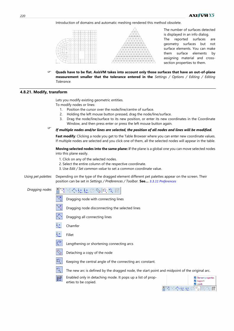
220

Introduction of domains and automatic meshing rendered this method obsolete.

The number of surfaces detected

is displayed in an info dialog.

The reported surfaces are

geometry surfaces but not

surface elements. You can make

them surface elements by

assigning material and cross-

section properties to them.

Quads have to be flat. AxisVM takes into account only those surfaces that have an out-of-plane

measurement smaller that the tolerance entered in the Settings / Options / Editing / Editing

Tolerance.

4.8.21. Modify, transform

Lets you modify existing geometric entities.

To modify nodes or lines:

1. Position the cursor over the node/line/centre of surface.

2. Holding the left mouse button pressed, drag the node/line/surface.

3. Drag the node/line/surface to its new position, or enter its new coordinates in the Coordinate

Window, and then press enter or press the left mouse button again.

If multiple nodes and/or lines are selected, the position of all nodes and lines will be modified.

Fast modify: Clicking a node you get to the Table Browser where you can enter new coordinate values.

If multiple nodes are selected and you click one of them, all the selected nodes will appear in the table.

Moving selected nodes into the same plane: if the plane is a global one you can move selected nodes

into this plane easily.

1. Click on any of the selected nodes.

2. Select the entire column of the respective coordinate.

3. Use Edit / Set common value to set a common coordinate value.

Using pet palettes

Depending on the type of the dragged element different pet palettes appear on the screen. Their

position can be set in Settings / Preferences / Toolbar. See… 3.3.11 Preferences

Dragging nodes

Dragging node with connecting lines

Dragging node disconnecting the selected lines

Dragging all connecting lines

Chamfer

Fillet

Lengthening or shortening connecting arcs

Detaching a copy of the node

Keeping the central angle of the connecting arc constant.

The new arc is defined by the dragged node, the start point and midpoint of the original arc.

Enabled only in detaching mode. It pops up a list of prop-

erties to be copied.

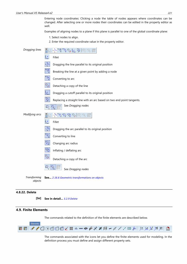
User’s Manual X5 Release4 e2 221

Entering node coordinates: Clicking a node the table of nodes appears where coordinates can be

changed. After selecting one or more nodes their coordinates can be edited in the property editor as

well.

Examples of aligning nodes to a plane if this plane is parallel to one of the global coordinate plane:

1. Select nodes to align.

2. Enter the required coordinate value in the property editor.

Dragging lines

Fillet

Dragging the line parallel to its original position

Breaking the line at a given point by adding a node

Converting to arc

Detaching a copy of the line

Dragging a cutoff parallel to its original position

Replacing a straight line with an arc based on two end point tangents.

See Dragging nodes

Modifying arcs

Fillet

Dragging the arc parallel to its original position

Converting to line

Changing arc radius

Inflating / deflating arc

Detaching a copy of the arc

See Dragging nodes

Transforming objects

See... 2.16.6 Geometric transformations on objects

4.8.22. Delete

[Del] See in detail... 3.2.9 Delete

4.9. Finite Elements

The commands related to the definition of the finite elements are described below.

The commands associated with the icons let you define the finite elements used for modeling. In the

definition process you must define and assign different property sets.

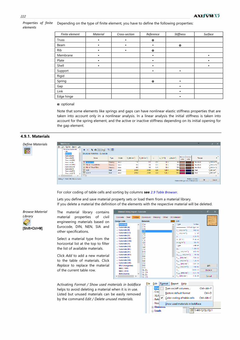
222

Properties of finite elements

Depending on the type of finite element, you have to define the following properties:

Finite element Material Cross-section Reference Stiffness Surface

Truss • • o

Beam • • • o

Rib • • o

Membrane • • •

Plate • • •

Shell • • •

Support • •

Rigid

Spring o •

Gap •

Link •

Edge hinge •

o: optional

Note that some elements like springs and gaps can have nonlinear elastic stiffness properties that are

taken into account only in a nonlinear analysis. In a linear analysis the initial stiffness is taken into

account for the spring element, and the active or inactive stiffness depending on its initial opening for

the gap element.

4.9.1. Materials

Define Materials

For color coding of table cells and sorting by columns see 2.9 Table Browser.

Lets you define and save material property sets or load them from a material library.

If you delete a material the definition of the elements with the respective material will be deleted.

Browse Material Library

[Shift+Ctrl+M]

The material library contains

material properties of civil

engineering materials based on

Eurocode, DIN, NEN, SIA and

other specifications.

Select a material type from the

horizontal list at the top to filter

the list of available materials.

Click Add to add a new material

to the table of materials. Click

Replace to replace the material

of the current table row.

Activating Format / Show used materials in boldface

helps to avoid deleting a material when it is in use.

Listed but unused materials can be easily removed

by the command Edit / Delete unused materials.

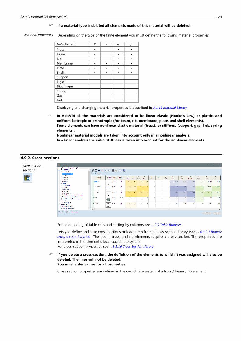
User’s Manual X5 Release4 e2 223

If a material type is deleted all elements made of this material will be deleted.

Material Properties Depending on the type of the finite element you must define the following material properties:

Finite Element E ν α ρ

Truss • • •

Beam • • •

Rib • • •

Membrane • • • •

Plate • • • •

Shell • • • •

Support

Rigid

Diaphragm

Spring

Gap

Link

Displaying and changing material properties is described in 3.1.15 Material Library

In AxisVM all the materials are considered to be linear elastic (Hooke’s Law) or plastic, and

uniform isotropic or orthotropic (for beam, rib, membrane, plate, and shell elements).

Some elements can have nonlinear elastic material (truss), or stiffness (support, gap, link, spring

elements).

Nonlinear material models are taken into account only in a nonlinear analysis.

In a linear analysis the initial stiffness is taken into account for the nonlinear elements.

4.9.2. Cross-sections

Define Cross-sections

For color coding of table cells and sorting by columns see… 2.9 Table Browser.

Lets you define and save cross-sections or load them from a cross-section library (see… 4.9.2.1 Browse

cross-section libraries). The beam, truss, and rib elements require a cross-section. The properties are

interpreted in the element’s local coordinate system.

For cross-section properties see... 3.1.16 Cross-Section Library

If you delete a cross-section, the definition of the elements to which it was assigned will also be

deleted. The lines will not be deleted.

You must enter values for all properties.

Cross section properties are defined in the coordinate system of a truss / beam / rib element.

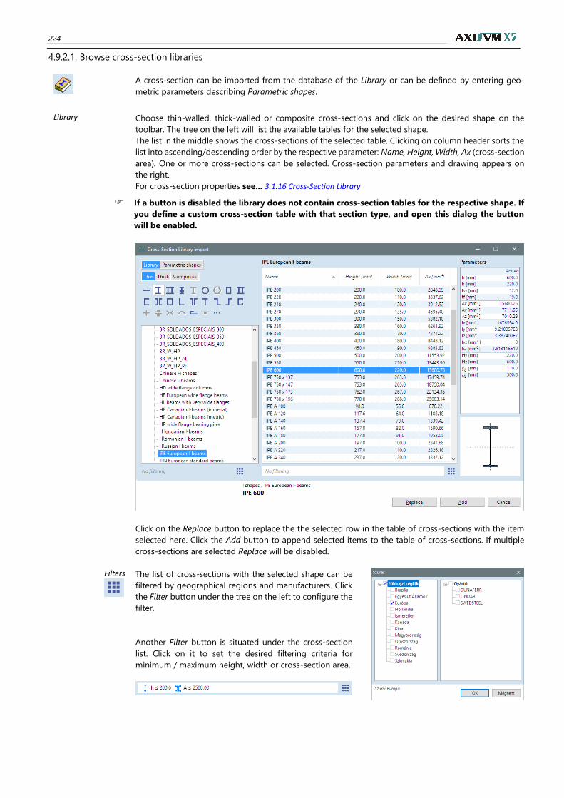
224

4.9.2.1. Browse cross-section libraries

A cross-section can be imported from the database of the Library or can be defined by entering geo-

metric parameters describing Parametric shapes.

Library Choose thin-walled, thick-walled or composite cross-sections and click on the desired shape on the

toolbar. The tree on the left will list the available tables for the selected shape.

The list in the middle shows the cross-sections of the selected table. Clicking on column header sorts the

list into ascending/descending order by the respective parameter: Name, Height, Width, Ax (cross-section

area). One or more cross-sections can be selected. Cross-section parameters and drawing appears on

the right.

For cross-section properties see... 3.1.16 Cross-Section Library

If a button is disabled the library does not contain cross-section tables for the respective shape. If

you define a custom cross-section table with that section type, and open this dialog the button

will be enabled.

Click on the Replace button to replace the the selected row in the table of cross-sections with the item

selected here. Click the Add button to append selected items to the table of cross-sections. If multiple

cross-sections are selected Replace will be disabled.

Filters

The list of cross-sections with the selected shape can be

filtered by geographical regions and manufacturers. Click

the Filter button under the tree on the left to configure the

filter.

Another Filter button is situated under the cross-section

list. Click on it to set the desired filtering criteria for

minimum / maximum height, width or cross-section area.

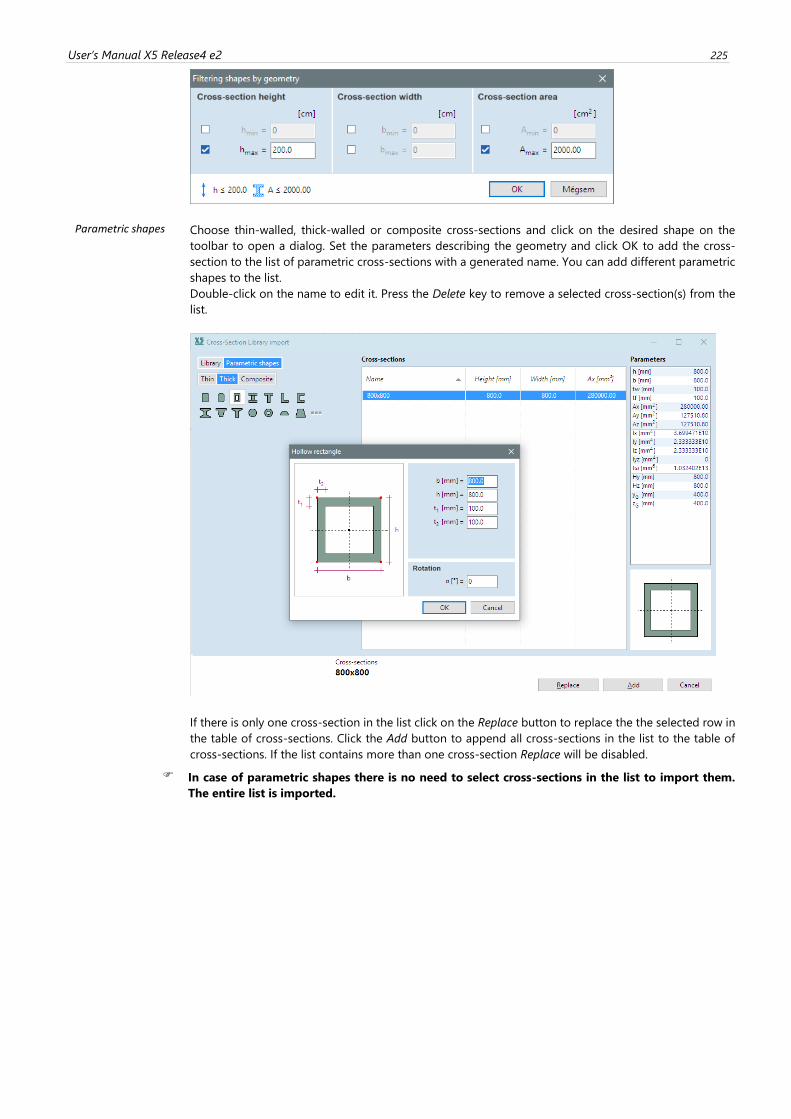
User’s Manual X5 Release4 e2 225

Parametric shapes Choose thin-walled, thick-walled or composite cross-sections and click on the desired shape on the

toolbar to open a dialog. Set the parameters describing the geometry and click OK to add the cross-

section to the list of parametric cross-sections with a generated name. You can add different parametric

shapes to the list.

Double-click on the name to edit it. Press the Delete key to remove a selected cross-section(s) from the

list.

If there is only one cross-section in the list click on the Replace button to replace the the selected row in

the table of cross-sections. Click the Add button to append all cross-sections in the list to the table of

cross-sections. If the list contains more than one cross-section Replace will be disabled.

In case of parametric shapes there is no need to select cross-sections in the list to import them.

The entire list is imported.

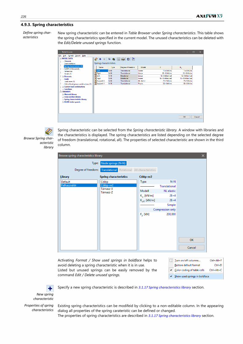
226

4.9.3. Spring characteristics

Define spring char-acteristics

New spring characteristic can be entered in Table Browser under Spring characteristics. This table shows

the spring characteristics specified in the current model. The unused characteristics can be deleted with

the Edit/Delete unused springs function.

Browse Spring char-

acteristic library

Spring characteristic can be selected from the Spring characteristic library. A window with libraries and

the characteristics is displayed. The spring characteristics are listed depending on the selected degree

of freedom (translational, rotational, all). The properties of selected characteristic are shown in the third

column.

Activating Format / Show used springs in boldface helps to

avoid deleting a spring characteristic when it is in use.

Listed but unused springs can be easily removed by the

command Edit / Delete unused springs.

New spring

characteristic

Specify a new spring characteristic is described in 3.1.17 Spring characteristics library section.

Properties of spring characteristics

Existing spring characteristics can be modifeid by clicking to a non-editable column. In the appearing

dialog all properties of the spring carateristic can be defined or changed.

The properties of spring characteristics are described in 3.1.17 Spring characteristics library section.

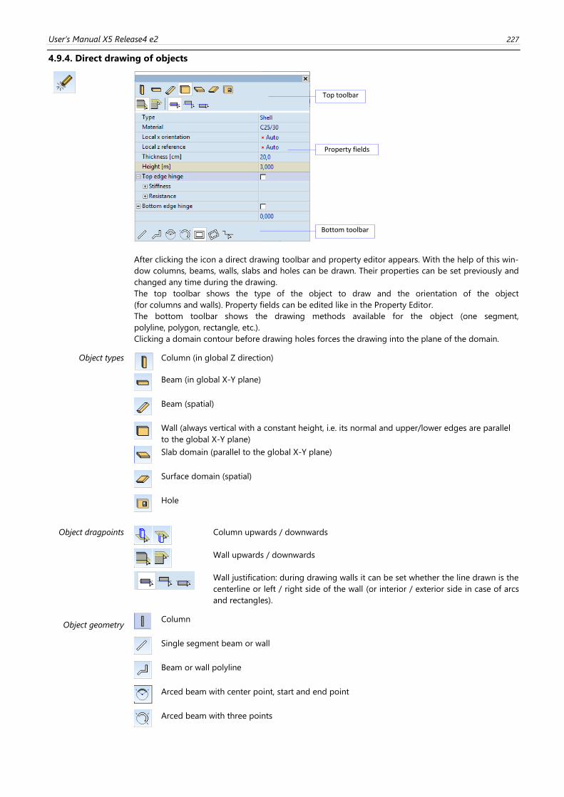
User’s Manual X5 Release4 e2 227

4.9.4. Direct drawing of objects

After clicking the icon a direct drawing toolbar and property editor appears. With the help of this win-

dow columns, beams, walls, slabs and holes can be drawn. Their properties can be set previously and

changed any time during the drawing.

The top toolbar shows the type of the object to draw and the orientation of the object

(for columns and walls). Property fields can be edited like in the Property Editor.

The bottom toolbar shows the drawing methods available for the object (one segment,

polyline, polygon, rectangle, etc.).

Clicking a domain contour before drawing holes forces the drawing into the plane of the domain.

Object types

Column (in global Z direction)

Beam (in global X-Y plane)

Beam (spatial)

Wall (always vertical with a constant height, i.e. its normal and upper/lower edges are parallel

to the global X-Y plane)

Slab domain (parallel to the global X-Y plane)

Surface domain (spatial)

Hole

Object dragpoints

Column upwards / downwards

Wall upwards / downwards

Wall justification: during drawing walls it can be set whether the line drawn is the

centerline or left / right side of the wall (or interior / exterior side in case of arcs

and rectangles).

Object geometry Column

Single segment beam or wall

Beam or wall polyline

Arced beam with center point, start and end point

Arced beam with three points

Top toolbar

Bottom toolbar

Property fields

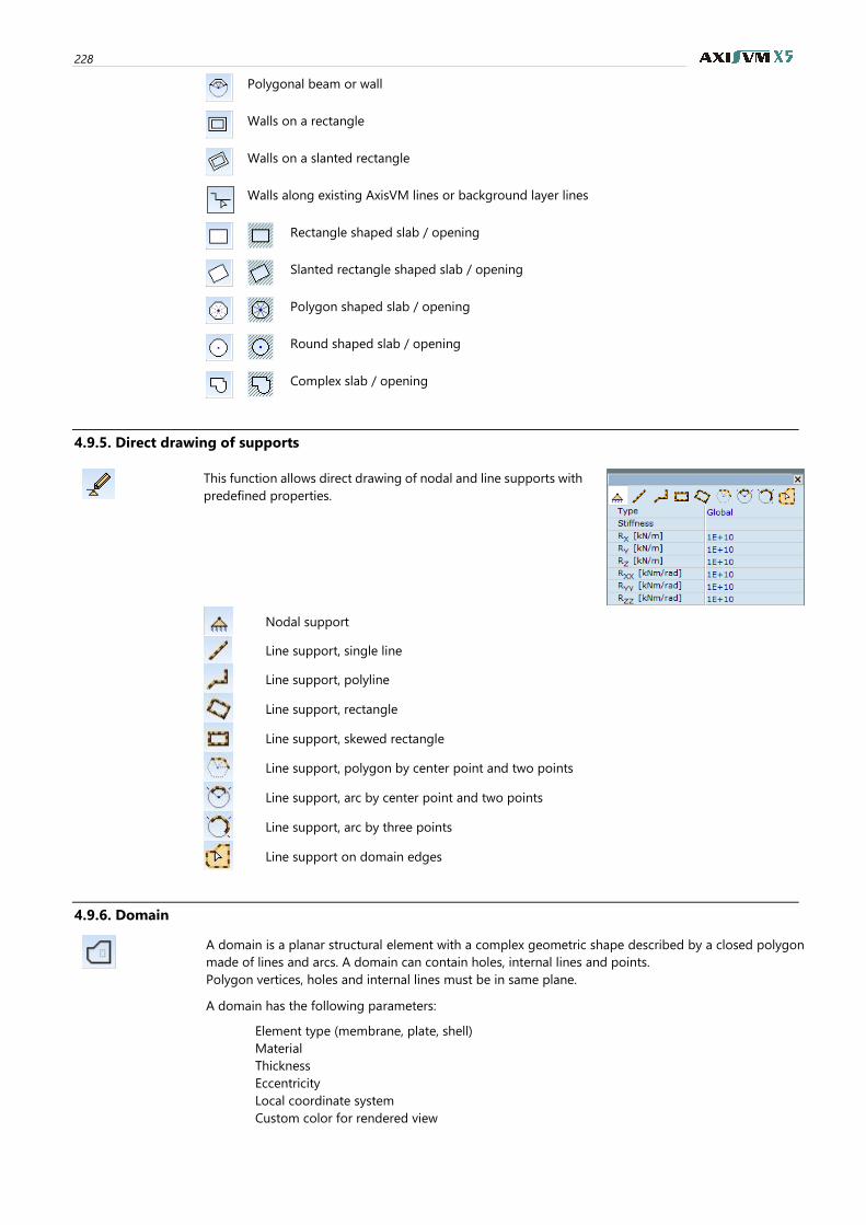
228

Polygonal beam or wall

Walls on a rectangle

Walls on a slanted rectangle

Walls along existing AxisVM lines or background layer lines

Rectangle shaped slab / opening

Slanted rectangle shaped slab / opening

Polygon shaped slab / opening

Round shaped slab / opening

Complex slab / opening

4.9.5. Direct drawing of supports

This function allows direct drawing of nodal and line supports with

predefined properties.

Nodal support

Line support, single line

Line support, polyline

Line support, rectangle

Line support, skewed rectangle

Line support, polygon by center point and two points

Line support, arc by center point and two points

Line support, arc by three points

Line support on domain edges

4.9.6. Domain

A domain is a planar structural element with a complex geometric shape described by a closed polygon

made of lines and arcs. A domain can contain holes, internal lines and points.

Polygon vertices, holes and internal lines must be in same plane.

A domain has the following parameters:

Element type (membrane, plate, shell)

Material

Thickness

Eccentricity

Local coordinate system

Custom color for rendered view

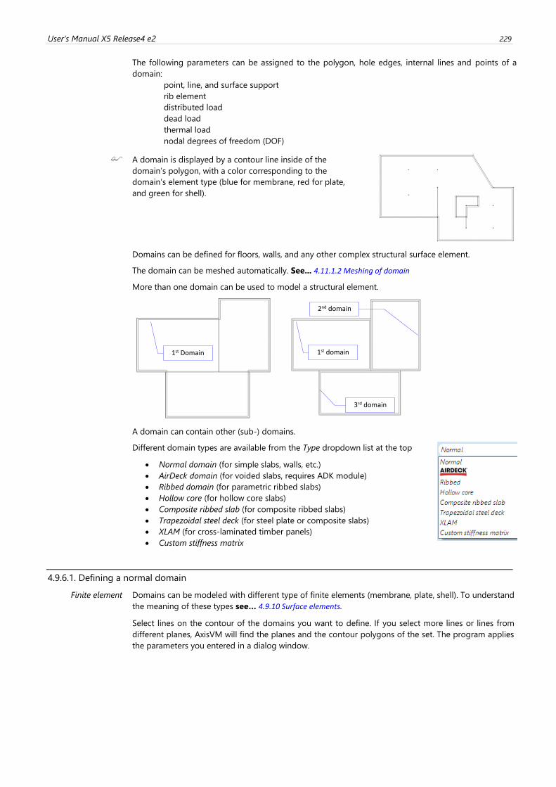
User’s Manual X5 Release4 e2 229

The following parameters can be assigned to the polygon, hole edges, internal lines and points of a

domain:

point, line, and surface support

rib element

distributed load

dead load

thermal load

nodal degrees of freedom (DOF)

A domain is displayed by a contour line inside of the

domain’s polygon, with a color corresponding to the

domain’s element type (blue for membrane, red for plate,

and green for shell).

Domains can be defined for floors, walls, and any other complex structural surface element.

The domain can be meshed automatically. See... 4.11.1.2 Meshing of domain

More than one domain can be used to model a structural element.

A domain can contain other (sub-) domains.

Different domain types are available from the Type dropdown list at the top

• Normal domain (for simple slabs, walls, etc.)

• AirDeck domain (for voided slabs, requires ADK module)

• Ribbed domain (for parametric ribbed slabs)

• Hollow core (for hollow core slabs)

• Composite ribbed slab (for composite ribbed slabs)

• Trapezoidal steel deck (for steel plate or composite slabs)

• XLAM (for cross-laminated timber panels)

• Custom stiffness matrix

4.9.6.1. Defining a normal domain

Finite element Domains can be modeled with different type of finite elements (membrane, plate, shell). To understand

the meaning of these types see… 4.9.10 Surface elements.

Select lines on the contour of the domains you want to define. If you select more lines or lines from

different planes, AxisVM will find the planes and the contour polygons of the set. The program applies

the parameters you entered in a dialog window.

1st Domain 1st domain

3rd domain

2nd domain

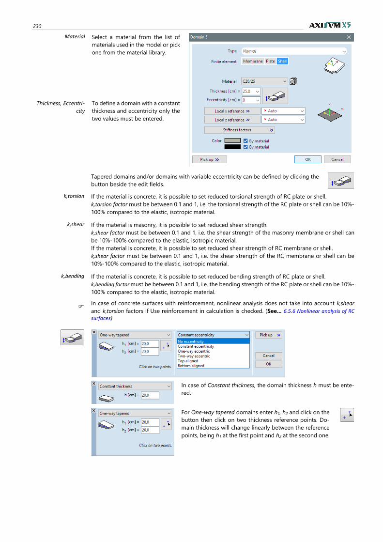
230

Material Select a material from the list of

materials used in the model or pick

one from the material library.

Thickness, Eccentri-

city

To define a domain with a constant

thickness and eccentricity only the

two values must be entered.

Tapered domains and/or domains with variable eccentricity can be defined by clicking the

button beside the edit fields.

k,torsion

If the material is concrete, it is possible to set reduced torsional strength of RC plate or shell.

k,torsion factor must be between 0.1 and 1, i.e. the torsional strength of the RC plate or shell can be 10%-

100% compared to the elastic, isotropic material.

k,shear If the material is masonry, it is possible to set reduced shear strength.

k,shear factor must be between 0.1 and 1, i.e. the shear strength of the masonry membrane or shell can

be 10%-100% compared to the elastic, isotropic material.

If the material is concrete, it is possible to set reduced shear strength of RC membrane or shell.

k,shear factor must be between 0.1 and 1, i.e. the shear strength of the RC membrane or shell can be

10%-100% compared to the elastic, isotropic material.

k,bending If the material is concrete, it is possible to set reduced bending strength of RC plate or shell.

k,bending factor must be between 0.1 and 1, i.e. the bending strength of the RC plate or shell can be 10%-

100% compared to the elastic, isotropic material.

In case of concrete surfaces with reinforcement, nonlinear analysis does not take into account k,shear

and k,torsion factors if Use reinforcement in calculation is checked. (See... 6.5.6 Nonlinear analysis of RC surfaces)

In case of Constant thickness, the domain thickness h must be ente-

red.

For One-way tapered domains enter h1, h2 and click on the

button then click on two thickness reference points. Do-

main thickness will change linearly between the reference

points, being h1 at the first point and h2 at the second one.

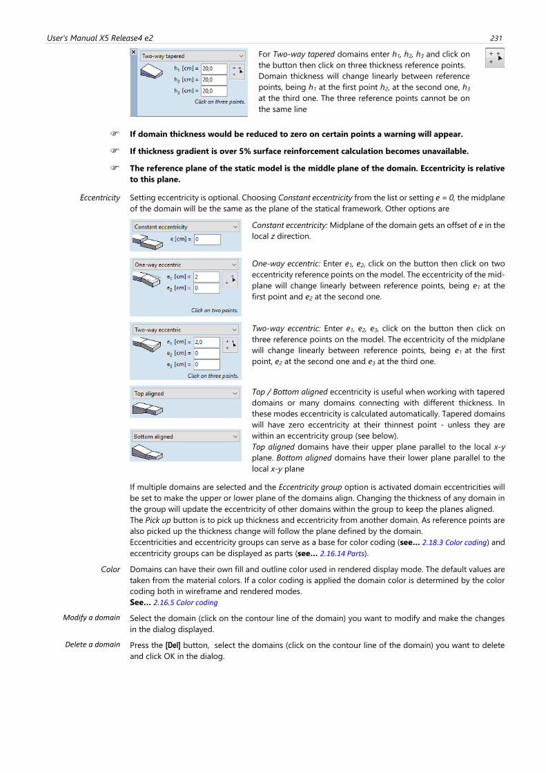
User’s Manual X5 Release4 e2 231

For Two-way tapered domains enter h1, h2, h3 and click on

the button then click on three thickness reference points.

Domain thickness will change linearly between reference

points, being h1 at the first point h2, at the second one, h3

at the third one. The three reference points cannot be on

the same line

If domain thickness would be reduced to zero on certain points a warning will appear.

If thickness gradient is over 5% surface reinforcement calculation becomes unavailable.

The reference plane of the static model is the middle plane of the domain. Eccentricity is relative

to this plane.

Eccentricity Setting eccentricity is optional. Choosing Constant eccentricity from the list or setting e = 0, the midplane

of the domain will be the same as the plane of the statical framework. Other options are

Constant eccentricity: Midplane of the domain gets an offset of e in the

local z direction.

One-way eccentric: Enter e1, e2, click on the button then click on two

eccentricity reference points on the model. The eccentricity of the mid-

plane will change linearly between reference points, being e1 at the

first point and e2 at the second one.

Two-way eccentric: Enter e1, e2, e3, click on the button then click on

three reference points on the model. The eccentricity of the midplane

will change linearly between reference points, being e1 at the first

point, e2 at the second one and e3 at the third one.

Top / Bottom aligned eccentricity is useful when working with tapered

domains or many domains connecting with different thickness. In

these modes eccentricity is calculated automatically. Tapered domains

will have zero eccentricity at their thinnest point - unless they are

within an eccentricity group (see below).

Top aligned domains have their upper plane parallel to the local x-y

plane. Bottom aligned domains have their lower plane parallel to the

local x-y plane

If multiple domains are selected and the Eccentricity group option is activated domain eccentricities will

be set to make the upper or lower plane of the domains align. Changing the thickness of any domain in

the group will update the eccentricity of other domains within the group to keep the planes aligned.

The Pick up button is to pick up thickness and eccentricity from another domain. As reference points are

also picked up the thickness change will follow the plane defined by the domain.

Eccentricities and eccentricity groups can serve as a base for color coding (see… 2.18.3 Color coding) and

eccentricity groups can be displayed as parts (see… 2.16.14 Parts).

Color Domains can have their own fill and outline color used in rendered display mode. The default values are

taken from the material colors. If a color coding is applied the domain color is determined by the color

coding both in wireframe and rendered modes.

See… 2.16.5 Color coding

Modify a domain Select the domain (click on the contour line of the domain) you want to modify and make the changes

in the dialog displayed.

Delete a domain Press the [Del] button, select the domains (click on the contour line of the domain) you want to delete

and click OK in the dialog.

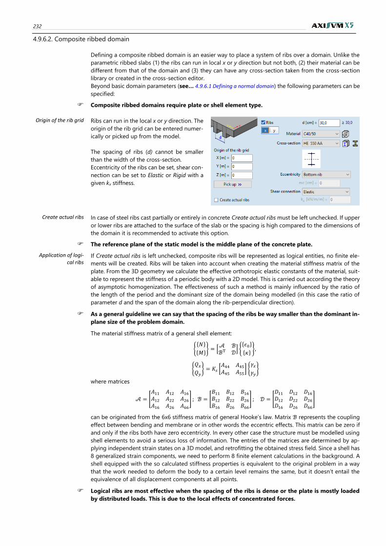
232

4.9.6.2. Composite ribbed domain

Defining a composite ribbed domain is an easier way to place a system of ribs over a domain. Unlike the

parametric ribbed slabs (1) the ribs can run in local x or y direction but not both, (2) their material can be

different from that of the domain and (3) they can have any cross-section taken from the cross-section

library or created in the cross-section editor.

Beyond basic domain parameters (see… 4.9.6.1 Defining a normal domain) the following parameters can be

specified:

Composite ribbed domains require plate or shell element type.

Origin of the rib grid

Ribs can run in the local x or y direction. The

origin of the rib grid can be entered numer-

ically or picked up from the model.

The spacing of ribs (d) cannot be smaller

than the width of the cross-section.

Eccentricity of the ribs can be set, shear con-

nection can be set to Elastic or Rigid with a

given kx stiffness.

Create actual ribs In case of steel ribs cast partially or entirely in concrete Create actual ribs must be left unchecked. If upper

or lower ribs are attached to the surface of the slab or the spacing is high compared to the dimensions of

the domain it is recommended to activate this option.

The reference plane of the static model is the middle plane of the concrete plate.

Application of logi-cal ribs

If Create actual ribs is left unchecked, composite ribs will be represented as logical entities, no finite ele-

ments will be created. Ribs will be taken into account when creating the material stiffness matrix of the

plate. From the 3D geometry we calculate the effective orthotropic elastic constants of the material, suit-

able to represent the stiffness of a periodic body with a 2D model. This is carried out according the theory

of asymptotic homogenization. The effectiveness of such a method is mainly influenced by the ratio of

the length of the period and the dominant size of the domain being modelled (in this case the ratio of

parameter d and the span of the domain along the rib-perpendicular direction).

As a general guideline we can say that the spacing of the ribs be way smaller than the dominant in-

plane size of the problem domain.

The material stiffness matrix of a general shell element:

{{𝑁}

{𝑀}} = [

𝒜 ℬℬT 𝒟

] {{𝜖0}

{𝜅}},

{𝑄𝑥𝑄𝑦} = 𝐾𝑠 [

𝐴44 𝐴45𝐴45 𝐴55

] {𝛾𝑥𝛾𝑦}

where matrices

𝒜 = [

𝐴11 𝐴12 𝐴16𝐴12 𝐴22 𝐴26𝐴16 𝐴26 𝐴66

] ; ℬ = [

𝐵11 𝐵12 𝐵16𝐵12 𝐵22 𝐵26𝐵16 𝐵26 𝐵66

] ; 𝒟 = [

𝐷11 𝐷12 𝐷16𝐷12 𝐷22 𝐷26𝐷16 𝐷26 𝐷66

]

can be originated from the 6x6 stiffness matrix of general Hooke’s law. Matrix ℬ represents the coupling

effect between bending and membrane or in other words the eccentric effects. This matrix can be zero if

and only if the ribs both have zero eccentricity. In every other case the structure must be modelled using

shell elements to avoid a serious loss of information. The entries of the matrices are determined by ap-

plying independent strain states on a 3D model, and retrofitting the obtained stress field. Since a shell has

8 generalized strain components, we need to perform 8 finite element calculations in the background. A

shell equipped with the so calculated stiffness properties is equivalent to the original problem in a way

that the work needed to deform the body to a certain level remains the same, but it doesn’t entail the

equivalence of all displacement components at all points.

Logical ribs are most effective when the spacing of the ribs is dense or the plate is mostly loaded

by distributed loads. This is due to the local effects of concentrated forces.

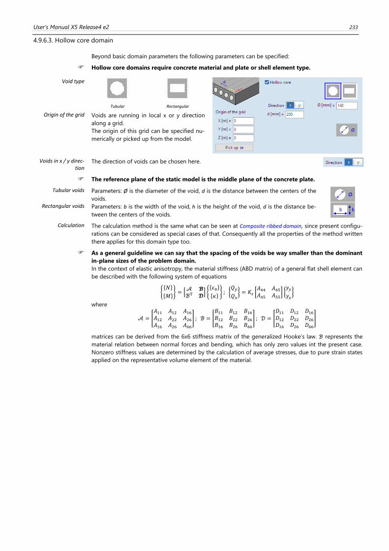
User’s Manual X5 Release4 e2 233

4.9.6.3. Hollow core domain

Beyond basic domain parameters the following parameters can be specified:

Hollow core domains require concrete material and plate or shell element type.

Void type

Tubular Rectangular

Origin of the grid

Voids are running in local x or y direction

along a grid.

The origin of this grid can be specified nu-

merically or picked up from the model.

Voids in x / y direc-tion

The direction of voids can be chosen here.

The reference plane of the static model is the middle plane of the concrete plate.

Tubular voids Parameters: Ø is the diameter of the void, d is the distance between the centers of the

voids. Rectangular voids Parameters: b is the width of the void, h is the height of the void, d is the distance be-

tween the centers of the voids.

Calculation The calculation method is the same what can be seen at Composite ribbed domain, since present configu-

rations can be considered as special cases of that. Consequently all the properties of the method written

there applies for this domain type too.

As a general guideline we can say that the spacing of the voids be way smaller than the dominant

in-plane sizes of the problem domain.

In the context of elastic anisotropy, the material stiffness (ABD matrix) of a general flat shell element can

be described with the following system of equations

{{𝑁}

{𝑀}} = [

𝒜 𝓑ℬT 𝓓

] {{𝜖0}

{𝜅}} ; {

𝑄𝑦𝑄𝑥} = 𝐾𝑠 [

𝐴44 𝐴45𝐴45 𝐴55

] {𝛾𝑦𝛾𝑥}

where

𝒜 = [

𝐴11 𝐴12 𝐴16𝐴12 𝐴22 𝐴26𝐴16 𝐴26 𝐴66

] ; ℬ = [

𝐵11 𝐵12 𝐵16𝐵12 𝐵22 𝐵26𝐵16 𝐵26 𝐵66

] ; 𝒟 = [

𝐷11 𝐷12 𝐷16𝐷12 𝐷22 𝐷26𝐷16 𝐷26 𝐷66

]

matrices can be derived from the 6x6 stiffness matrix of the generalized Hooke’s law. ℬ represents the

material relation between normal forces and bending, which has only zero values int the present case.

Nonzero stiffness values are determined by the calculation of average stresses, due to pure strain states

applied on the representative volume element of the material.

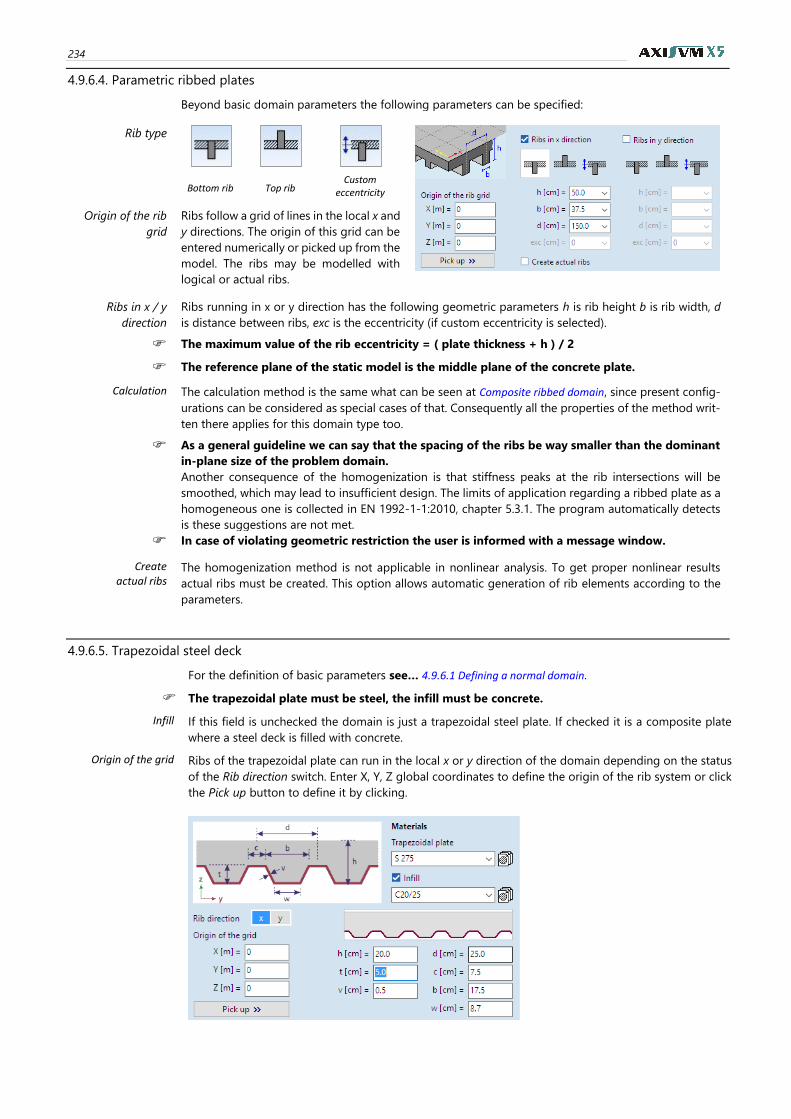
234

4.9.6.4. Parametric ribbed plates

Beyond basic domain parameters the following parameters can be specified:

Rib type

Bottom rib Top rib

Custom eccentricity

Origin of the rib

grid

Ribs follow a grid of lines in the local x and

y directions. The origin of this grid can be

entered numerically or picked up from the

model. The ribs may be modelled with

logical or actual ribs.

Ribs in x / y

direction

Ribs running in x or y direction has the following geometric parameters h is rib height b is rib width, d

is distance between ribs, exc is the eccentricity (if custom eccentricity is selected).

The maximum value of the rib eccentricity = ( plate thickness + h ) / 2

The reference plane of the static model is the middle plane of the concrete plate.

Calculation The calculation method is the same what can be seen at Composite ribbed domain, since present config-

urations can be considered as special cases of that. Consequently all the properties of the method writ-

ten there applies for this domain type too.

As a general guideline we can say that the spacing of the ribs be way smaller than the dominant

in-plane size of the problem domain.

Another consequence of the homogenization is that stiffness peaks at the rib intersections will be

smoothed, which may lead to insufficient design. The limits of application regarding a ribbed plate as a

homogeneous one is collected in EN 1992-1-1:2010, chapter 5.3.1. The program automatically detects

is these suggestions are not met.

In case of violating geometric restriction the user is informed with a message window.

Create actual ribs

The homogenization method is not applicable in nonlinear analysis. To get proper nonlinear results

actual ribs must be created. This option allows automatic generation of rib elements according to the

parameters.

4.9.6.5. Trapezoidal steel deck

For the definition of basic parameters see… 4.9.6.1 Defining a normal domain.

The trapezoidal plate must be steel, the infill must be concrete.

Infill If this field is unchecked the domain is just a trapezoidal steel plate. If checked it is a composite plate

where a steel deck is filled with concrete.

Origin of the grid

Ribs of the trapezoidal plate can run in the local x or y direction of the domain depending on the status

of the Rib direction switch. Enter X, Y, Z global coordinates to define the origin of the rib system or click

the Pick up button to define it by clicking.

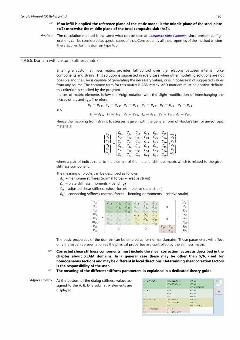
User’s Manual X5 Release4 e2 235

If no infill is applied the reference plane of the static model is the middle plane of the steel plate

(t/2) otherwise the middle plane of the total composite slab (h/2).

Analysis The calculation method is the same what can be seen at Composite ribbed domain, since present config-

urations can be considered as special cases of that. Consequently all the properties of the method written

there applies for this domain type too.

4.9.6.6. Domain with custom stiffness matrix

Entering a custom stiffness matrix provides full control over the relations between internal force

components and strains. This solution is suggested in every case when other modelling solutions are not

possible and the user is capable of generating the necessary values, or is in posession of suggested values

from any source. The common term for this matrix is ABD matrix. ABD matrices must be positive definite,

this criterion is checked by the program.

Indices of matrix elements follow the Voigt notation with the slight modification of interchanging the

incices of 𝜏𝑥𝑧 and 𝜏𝑦𝑧 . Therefore

𝜎1 = 𝜎11, 𝜎2 = 𝜎22, 𝜎3 = 𝜎33, 𝜎4 = 𝜎23, 𝜎5 = 𝜎13, 𝜎6 = 𝜎12 and

휀1 = 휀11, 휀2 = 휀22, 휀3 = 휀33, 휀4 = 휀23, 휀5 = 휀13, 휀6 = 휀12.

Hence the mapping from strains to stresses is given with the general form of Hooke’s law for anysotropic

materials:

{

𝜎1𝜎2𝜎3𝜎4𝜎5𝜎6}

=

[ 𝐶11 𝐶12 𝐶13𝐶21 𝐶22 𝐶23𝐶31 𝐶32 𝐶33

𝐶14 𝐶15 𝐶16𝐶24 𝐶25 𝐶26𝐶34 𝐶35 𝐶36

𝐶41 𝐶42 𝐶43𝐶51 𝐶52 𝐶53𝐶61 𝐶62 𝐶63

𝐶44 𝐶45 𝐶46𝐶54 𝐶55 𝐶56𝐶64 𝐶65 𝐶66]

{

휀1휀2휀3휀4휀5휀6}

where a pair of indices refer to the element of the material stiffness matrix which is related to the given

stiffness component.

The meaning of blocks can be described as follows

𝐴𝑖𝑗 – membrane stiffness (normal forces – relative strain)

𝐷𝑖𝑗 – plate stiffness (moments – bending)

𝑆𝑖𝑗 – adjusted shear stiffness (shear forces – relative shear strain)

𝐵𝑖𝑗 – connecting stiffness (normal forces – bending or moments – relative strain)

The basic properties of the domain can be entered as for normal domains. Those parameters will affect

only the visual representation as the physical properties are controlled by the stiffness matrix.

Corrected shear stiffness components must include the shear correction factors as described in the

chapter about XLAM domains. In a general case these may be other than 5/6, used for

homogeneous sections and may be different in local directions. Determining shear corretion factors

is the responsibility of the user.

The meaning of the different stiffness parameters is explained in a dedicated theory guide.

Stiffness matrix

At the bottom of the dialog stiffness values as-

signed to the A, B, D, S submatrix elements are

displayed.

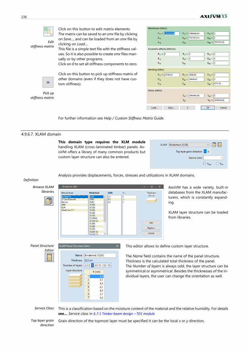
236

Edit stiffness matrix

Pick up stiffness matrix

Click on this button to edit matrix elements.

The matrix can be saved to an smx file by clicking

on Save..., and can be loaded from an smx file by

clicking on Load....

This file is a simple text file with the stiffness val-

ues. So it is also possible to create smx files man-

ually or by other programs.

Click on 0 to set all stiffness components to zero.

Click on this button to pick up stiffness matrix of

other domains (even if they does not have cus-

tom stiffness).

For further information see Help / Custom Stiffness Matrix Guide.

4.9.6.7. XLAM domain

This domain type requires the XLM module

handling XLAM (cross-laminated timber) panels. Ax-

isVM offers a library of many common products but

custom layer structure can also be entered.

Analysis provides displacements, forces, stresses and utilizations in XLAM domains.

Definition

Browse XLAM libraries

AxisVM has a wide variety, built-in

databases from the XLAM manufac-

turers, which is constantly expand-

ing.

XLAM layer structure can be loaded

from libraries.

Panel Structure Editor

This editor allows to define custom layer structure.

The Name field contains the name of the panel structure.

Thickness is the calculated total thickness of the panel.

The Number of layers is always odd, the layer structure can be

symmetrical or asymmetrical. Besides the thicknesses of the in-

dividual layers, the user can change the orientation as well.

Service Class This is a classification based on the moisture content of the material and the relative humidity. For details

see… Service class in 6.7.1 Timber beam design – TD1 module

Top layer grain direction

Grain direction of the topmost layer must be specified it can be the local x or y direction.

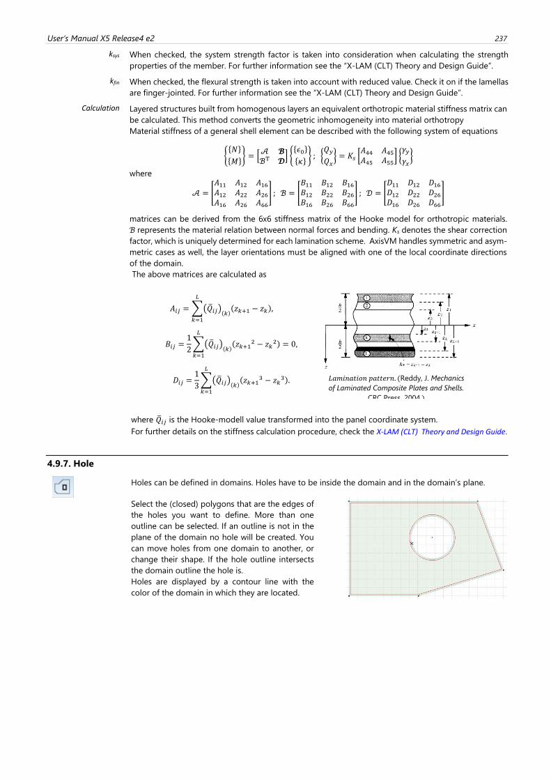
User’s Manual X5 Release4 e2 237

ksys When checked, the system strength factor is taken into consideration when calculating the strength

properties of the member. For further information see the “X-LAM (CLT) Theory and Design Guide”.

kfin When checked, the flexural strength is taken into account with reduced value. Check it on if the lamellas

are finger-jointed. For further information see the “X-LAM (CLT) Theory and Design Guide”.

Calculation Layered structures built from homogenous layers an equivalent orthotropic material stiffness matrix can

be calculated. This method converts the geometric inhomogeneity into material orthotropy

Material stiffness of a general shell element can be described with the following system of equations

{{𝑁}

{𝑀}} = [

𝒜 𝓑ℬT 𝓓

] {{𝜖0}

{𝜅}} ; {

𝑄𝑦𝑄𝑥} = 𝐾𝑠 [

𝐴44 𝐴45𝐴45 𝐴55

] {𝛾𝑦𝛾𝑥}

where

𝒜 = [

𝐴11 𝐴12 𝐴16𝐴12 𝐴22 𝐴26𝐴16 𝐴26 𝐴66

] ; ℬ = [

𝐵11 𝐵12 𝐵16𝐵12 𝐵22 𝐵26𝐵16 𝐵26 𝐵66

] ; 𝒟 = [

𝐷11 𝐷12 𝐷16𝐷12 𝐷22 𝐷26𝐷16 𝐷26 𝐷66

]

matrices can be derived from the 6x6 stiffness matrix of the Hooke model for orthotropic materials.

ℬ represents the material relation between normal forces and bending. Ks denotes the shear correction

factor, which is uniquely determined for each lamination scheme. AxisVM handles symmetric and asym-

metric cases as well, the layer orientations must be aligned with one of the local coordinate directions

of the domain.

The above matrices are calculated as

where �̅�𝑖𝑗 is the Hooke-modell value transformed into the panel coordinate system.

For further details on the stiffness calculation procedure, check the X-LAM (CLT) Theory and Design Guide.

4.9.7. Hole

Holes can be defined in domains. Holes have to be inside the domain and in the domain’s plane.

Select the (closed) polygons that are the edges of

the holes you want to define. More than one

outline can be selected. If an outline is not in the

plane of the domain no hole will be created. You

can move holes from one domain to another, or

change their shape. If the hole outline intersects

the domain outline the hole is.

Holes are displayed by a contour line with the

color of the domain in which they are located.

𝐴𝑖𝑗 = ∑(�̅�𝑖𝑗)(𝑘)(𝑧𝑘+1 − 𝑧𝑘),

𝐿

𝑘=1

𝐵𝑖𝑗 =1

2∑(�̅�𝑖𝑗)(𝑘)

(𝑧𝑘+12 − 𝑧𝑘

2) = 0,

𝐿

𝑘=1

𝐷𝑖𝑗 =1

3∑(�̅�𝑖𝑗)(𝑘)

(𝑧𝑘+13 − 𝑧𝑘

3).

𝐿

𝑘=1

𝐿𝑎𝑚𝑖𝑛𝑎𝑡𝑖𝑜𝑛 𝑝𝑎𝑡𝑡𝑒𝑟𝑛. (Reddy, J. Mechanics

of Laminated Composite Plates and Shells.

CRC Press, 2004.)

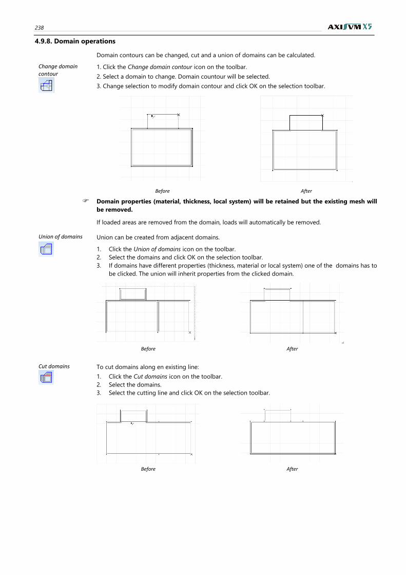
238

4.9.8. Domain operations

Domain contours can be changed, cut and a union of domains can be calculated.

Change domain contour

1. Click the Change domain contour icon on the toolbar.

2. Select a domain to change. Domain countour will be selected.

3. Change selection to modify domain contour and click OK on the selection toolbar.

Before After

Domain properties (material, thickness, local system) will be retained but the existing mesh will

be removed.

If loaded areas are removed from the domain, loads will automatically be removed.

Union of domains

Union can be created from adjacent domains.

1. Click the Union of domains icon on the toolbar.

2. Select the domains and click OK on the selection toolbar.

3. If domains have different properties (thickness, material or local system) one of the domains has to

be clicked. The union will inherit properties from the clicked domain.

Before After

Cut domains

To cut domains along en existing line:

1. Click the Cut domains icon on the toolbar.

2. Select the domains.

3. Select the cutting line and click OK on the selection toolbar.

Before After

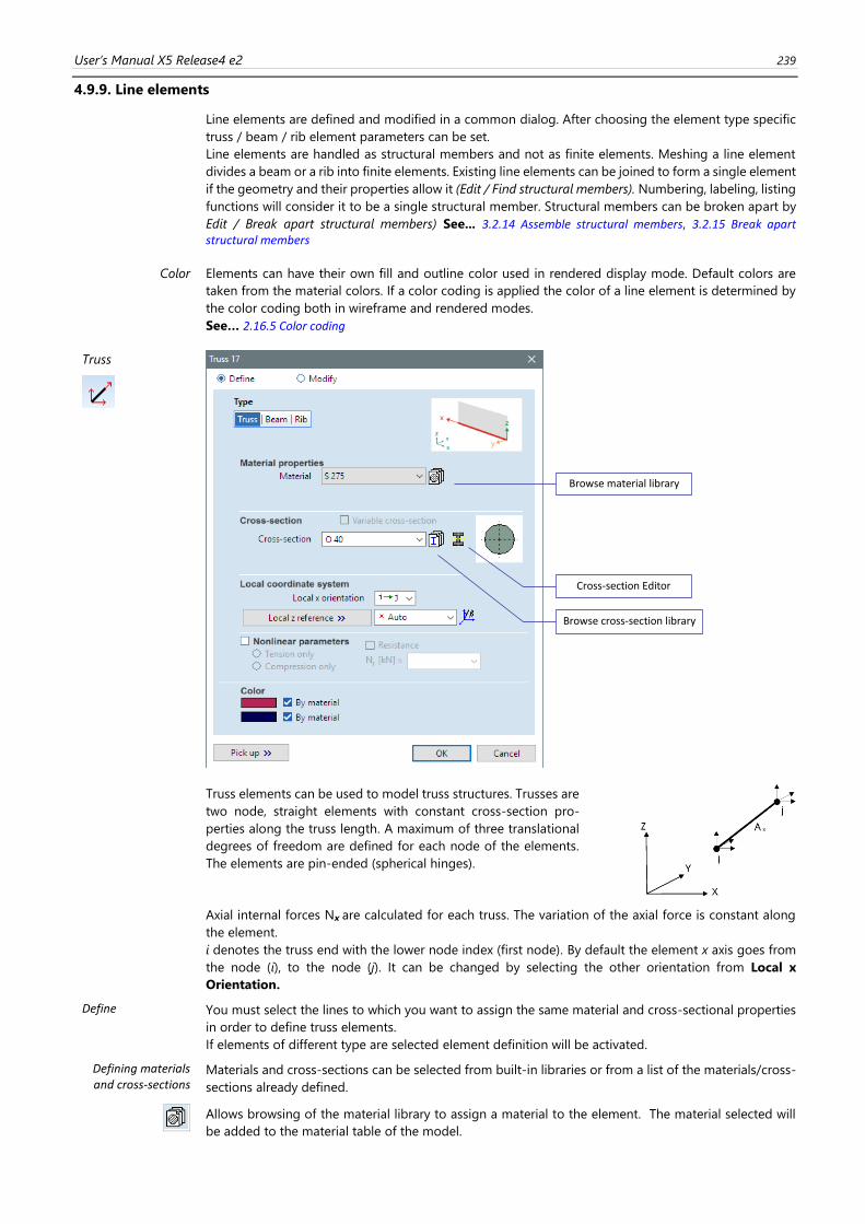
User’s Manual X5 Release4 e2 239

4.9.9. Line elements

Line elements are defined and modified in a common dialog. After choosing the element type specific

truss / beam / rib element parameters can be set.

Line elements are handled as structural members and not as finite elements. Meshing a line element

divides a beam or a rib into finite elements. Existing line elements can be joined to form a single element

if the geometry and their properties allow it (Edit / Find structural members). Numbering, labeling, listing

functions will consider it to be a single structural member. Structural members can be broken apart by

Edit / Break apart structural members) See... 3.2.14 Assemble structural members, 3.2.15 Break apart structural members

Color Elements can have their own fill and outline color used in rendered display mode. Default colors are

taken from the material colors. If a color coding is applied the color of a line element is determined by

the color coding both in wireframe and rendered modes.

See… 2.16.5 Color coding

Truss

Truss elements can be used to model truss structures. Trusses are

two node, straight elements with constant cross-section pro-

perties along the truss length. A maximum of three translational

degrees of freedom are defined for each node of the elements.

The elements are pin-ended (spherical hinges).

Axial internal forces Nx are calculated for each truss. The variation of the axial force is constant along

the element.

i denotes the truss end with the lower node index (first node). By default the element x axis goes from

the node (i), to the node (j). It can be changed by selecting the other orientation from Local x

Orientation.

Define You must select the lines to which you want to assign the same material and cross-sectional properties

in order to define truss elements.

If elements of different type are selected element definition will be activated.

Defining materials and cross-sections

Materials and cross-sections can be selected from built-in libraries or from a list of the materials/cross-

sections already defined.

Allows browsing of the material library to assign a material to the element. The material selected will

be added to the material table of the model.

Browse material library

Browse cross-section library

Cross-section Editor

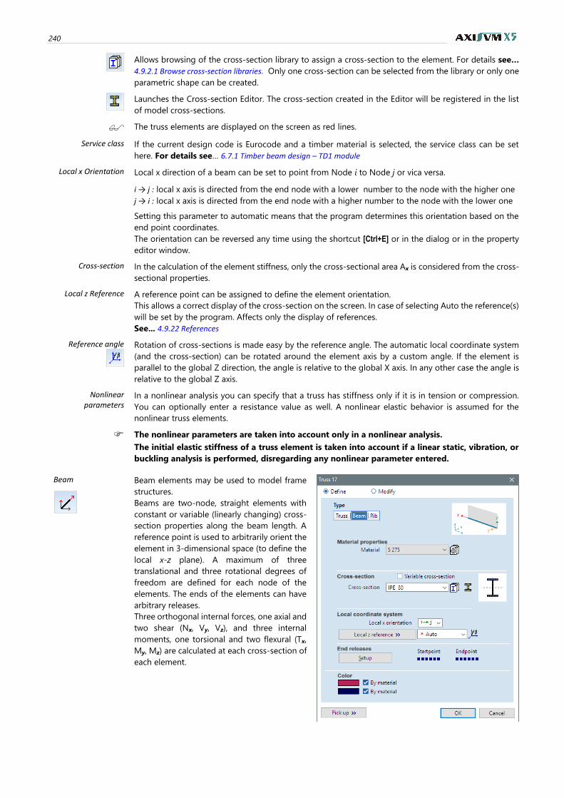
240

Allows browsing of the cross-section library to assign a cross-section to the element. For details see…

4.9.2.1 Browse cross-section libraries. Only one cross-section can be selected from the library or only one

parametric shape can be created.

Launches the Cross-section Editor. The cross-section created in the Editor will be registered in the list

of model cross-sections.

The truss elements are displayed on the screen as red lines.

Service class

If the current design code is Eurocode and a timber material is selected, the service class can be set

here. For details see… 6.7.1 Timber beam design – TD1 module

Local x Orientation Local x direction of a beam can be set to point from Node i to Node j or vica versa.

i → j : local x axis is directed from the end node with a lower number to the node with the higher one

j → i : local x axis is directed from the end node with a higher number to the node with the lower one

Setting this parameter to automatic means that the program determines this orientation based on the

end point coordinates.

The orientation can be reversed any time using the shortcut [Ctrl+E] or in the dialog or in the property

editor window.

Cross-section In the calculation of the element stiffness, only the cross-sectional area Ax is considered from the cross-

sectional properties.

Local z Reference A reference point can be assigned to define the element orientation.

This allows a correct display of the cross-section on the screen. In case of selecting Auto the reference(s)

will be set by the program. Affects only the display of references.

See... 4.9.22 References

Reference angle

Rotation of cross-sections is made easy by the reference angle. The automatic local coordinate system

(and the cross-section) can be rotated around the element axis by a custom angle. If the element is

parallel to the global Z direction, the angle is relative to the global X axis. In any other case the angle is

relative to the global Z axis.

Nonlinear parameters

In a nonlinear analysis you can specify that a truss has stiffness only if it is in tension or compression.

You can optionally enter a resistance value as well. A nonlinear elastic behavior is assumed for the

nonlinear truss elements.

The nonlinear parameters are taken into account only in a nonlinear analysis.

The initial elastic stiffness of a truss element is taken into account if a linear static, vibration, or

buckling analysis is performed, disregarding any nonlinear parameter entered.

Beam

Beam elements may be used to model frame

structures.

Beams are two-node, straight elements with

constant or variable (linearly changing) cross-

section properties along the beam length. A

reference point is used to arbitrarily orient the

element in 3-dimensional space (to define the

local x-z plane). A maximum of three

translational and three rotational degrees of

freedom are defined for each node of the

elements. The ends of the elements can have

arbitrary releases.

Three orthogonal internal forces, one axial and

two shear (Nx, Vy, Vz), and three internal

moments, one torsional and two flexural (Tx,

My, Mz) are calculated at each cross-section of

each element.

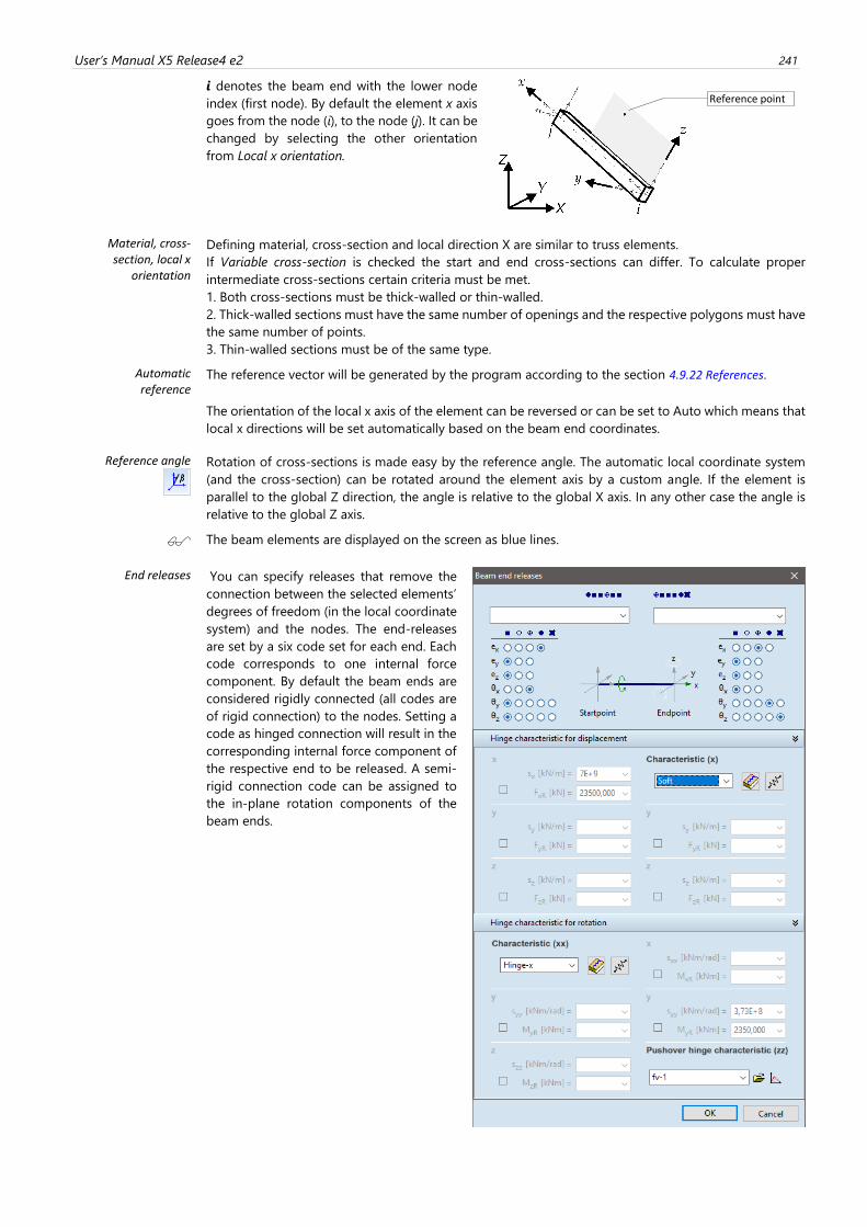
User’s Manual X5 Release4 e2 241

i denotes the beam end with the lower node

index (first node). By default the element x axis

goes from the node (i), to the node (j). It can be

changed by selecting the other orientation

from Local x orientation.

Material, cross-section, local x

orientation

Defining material, cross-section and local direction X are similar to truss elements.

If Variable cross-section is checked the start and end cross-sections can differ. To calculate proper

intermediate cross-sections certain criteria must be met.

1. Both cross-sections must be thick-walled or thin-walled.

2. Thick-walled sections must have the same number of openings and the respective polygons must have

the same number of points.

3. Thin-walled sections must be of the same type.

Automatic reference

The reference vector will be generated by the program according to the section 4.9.22 References.

The orientation of the local x axis of the element can be reversed or can be set to Auto which means that

local x directions will be set automatically based on the beam end coordinates.

Reference angle

Rotation of cross-sections is made easy by the reference angle. The automatic local coordinate system

(and the cross-section) can be rotated around the element axis by a custom angle. If the element is

parallel to the global Z direction, the angle is relative to the global X axis. In any other case the angle is

relative to the global Z axis.

The beam elements are displayed on the screen as blue lines.

End releases You can specify releases that remove the

connection between the selected elements’

degrees of freedom (in the local coordinate

system) and the nodes. The end-releases

are set by a six code set for each end. Each

code corresponds to one internal force

component. By default the beam ends are

considered rigidly connected (all codes are

of rigid connection) to the nodes. Setting a

code as hinged connection will result in the

corresponding internal force component of

the respective end to be released. A semi-

rigid connection code can be assigned to

the in-plane rotation components of the

beam ends.

Reference point

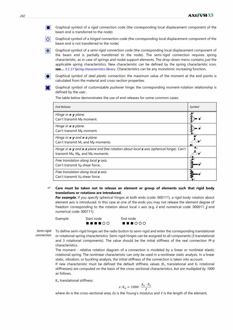
242

Graphical symbol of a rigid connection code (the corresponding local displacement component of the

beam end is transferred to the node)

Graphical symbol of a hinged connection code (the corresponding local displacement component of the

beam end is not transferred to the node)

Graphical symbol of a semi-rigid connection code (the corresponding local displacement component of

the beam end is partially transferred to the node). The semi-rigid connection requires spring

characteristic, as in case of springs and nodal support elements. The drop-down menu contains just the

applicable spring characteristics. New characteristic can be defined by the spring characteristic icon,

see… 3.1.17 Spring characteristics library. Characteristics can be any monotonic increasing function.

Graphical symbol of steel plastic connection: the maximum value of the moment at the end points is

calculated from the material and cross-section properties.

Graphical symbol of customizable pushover hinge: the corresponding moment-rotation relationship is

defined by the user..

The table below demonstrates the use of end releases for some common cases:

End Release Symbol

Hinge in x-y plane.

Can’t transmit Mz moment.

Hinge in x-z plane.

Can’t transmit My moment.

Hinge in x-y and x-z plane.

Can’t transmit Mz and My moments.

Hinge in x-y and x-z plane and free rotation about local x axis (spherical hinge). Can’t

transmit Mx, My, and Mz moments.

Free translation along local y axis.

Can’t transmit Vy shear force.

Free translation along local z axis.

Can’t transmit Vz shear force.

Care must be taken not to release an element or group of elements such that rigid body

translations or rotations are introduced.

For example, if you specify spherical hinges at both ends (code: 000111), a rigid body rotation about

element axis is introduced. In this case at one of the ends you may not release the element degree of

freedom corresponding to the rotation about local x axis (e.g. i end numerical code: 000011; j end

numerical code: 000111).

Example: Start node End node

Semi-rigid connection

To define semi-rigid hinges set the radio button to semi-rigid and enter the corresponding translational

or rotational spring characteristics. Semi-rigid hinges can be assigned to all components (3 translational

and 3 rotational components). The value should be the initial stiffness of the real connection M-

characteristics.

The moment - relative rotation diagram of a connection is modeled by a linear or nonlinear elastic

rotational spring. The nonlinear characteristic can only be used in a nonlinear static analysis. In a linear

static, vibration, or buckling analysis, the initial stiffness of the connection is taken into account.

If new characteristic must be defined the default stiffness values (Ku translational and Kr rotational

stiffnesses) are computed on the basis of the cross-sectional characteristics, but are multiplied by 1000

as follows.

Ku translational stiffness:

𝑥: 𝐾𝑢 = 1000 ∙𝐴𝑥 ∙ 𝐸𝑥ℓ

where Ax is the cross-sectional area, Ex is the Young’s modulus and ℓ is the length of the element,

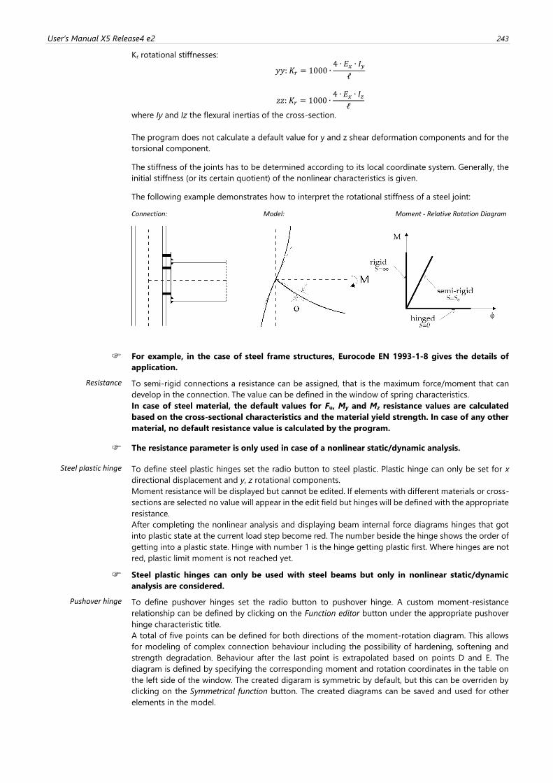
User’s Manual X5 Release4 e2 243

Kr rotational stiffnesses:

𝑦𝑦: 𝐾𝑟 = 1000 ∙4 ∙ 𝐸𝑥 ∙ 𝐼𝑦

ℓ

𝑧𝑧: 𝐾𝑟 = 1000 ∙4 ∙ 𝐸𝑥 ∙ 𝐼𝑧

ℓ

where Iy and Iz the flexural inertias of the cross-section.

The program does not calculate a default value for y and z shear deformation components and for the

torsional component.

The stiffness of the joints has to be determined according to its local coordinate system. Generally, the

initial stiffness (or its certain quotient) of the nonlinear characteristics is given.

The following example demonstrates how to interpret the rotational stiffness of a steel joint:

Connection: Model: Moment - Relative Rotation Diagram

For example, in the case of steel frame structures, Eurocode EN 1993-1-8 gives the details of

application.

Resistance To semi-rigid connections a resistance can be assigned, that is the maximum force/moment that can

develop in the connection. The value can be defined in the window of spring characteristics.

In case of steel material, the default values for Fu, My and Mz resistance values are calculated

based on the cross-sectional characteristics and the material yield strength. In case of any other

material, no default resistance value is calculated by the program.

The resistance parameter is only used in case of a nonlinear static/dynamic analysis.

Steel plastic hinge

To define steel plastic hinges set the radio button to steel plastic. Plastic hinge can only be set for x

directional displacement and y, z rotational components.

Moment resistance will be displayed but cannot be edited. If elements with different materials or cross-

sections are selected no value will appear in the edit field but hinges will be defined with the appropriate

resistance.

After completing the nonlinear analysis and displaying beam internal force diagrams hinges that got

into plastic state at the current load step become red. The number beside the hinge shows the order of

getting into a plastic state. Hinge with number 1 is the hinge getting plastic first. Where hinges are not

red, plastic limit moment is not reached yet.

Steel plastic hinges can only be used with steel beams but only in nonlinear static/dynamic

analysis are considered.

Pushover hinge

To define pushover hinges set the radio button to pushover hinge. A custom moment-resistance

relationship can be defined by clicking on the Function editor button under the appropriate pushover

hinge characteristic title.

A total of five points can be defined for both directions of the moment-rotation diagram. This allows

for modeling of complex connection behaviour including the possibility of hardening, softening and

strength degradation. Behaviour after the last point is extrapolated based on points D and E. The

diagram is defined by specifying the corresponding moment and rotation coordinates in the table on

the left side of the window. The created digaram is symmetric by default, but this can be overriden by

clicking on the Symmetrical function button. The created diagrams can be saved and used for other

elements in the model.

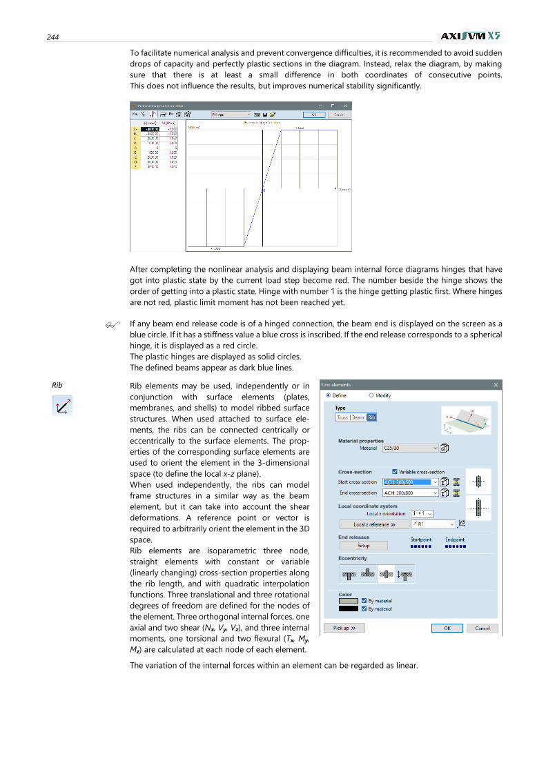
244

To facilitate numerical analysis and prevent convergence difficulties, it is recommended to avoid sudden

drops of capacity and perfectly plastic sections in the diagram. Instead, relax the diagram, by making

sure that there is at least a small difference in both coordinates of consecutive points.

This does not influence the results, but improves numerical stability significantly.

After completing the nonlinear analysis and displaying beam internal force diagrams hinges that have

got into plastic state by the current load step become red. The number beside the hinge shows the

order of getting into a plastic state. Hinge with number 1 is the hinge getting plastic first. Where hinges

are not red, plastic limit moment has not been reached yet.

If any beam end release code is of a hinged connection, the beam end is displayed on the screen as a

blue circle. If it has a stiffness value a blue cross is inscribed. If the end release corresponds to a spherical

hinge, it is displayed as a red circle.

The plastic hinges are displayed as solid circles.

The defined beams appear as dark blue lines.

Rib

Rib elements may be used, independently or in

conjunction with surface elements (plates,

membranes, and shells) to model ribbed surface

structures. When used attached to surface ele-

ments, the ribs can be connected centrically or

eccentrically to the surface elements. The prop-

erties of the corresponding surface elements are

used to orient the element in the 3-dimensional

space (to define the local x-z plane).

When used independently, the ribs can model

frame structures in a similar way as the beam

element, but it can take into account the shear

deformations. A reference point or vector is

required to arbitrarily orient the element in the 3D

space.

Rib elements are isoparametric three node,

straight elements with constant or variable

(linearly changing) cross-section properties along

the rib length, and with quadratic interpolation

functions. Three translational and three rotational

degrees of freedom are defined for the nodes of

the element. Three orthogonal internal forces, one

axial and two shear (Nx, Vy, Vz), and three internal

moments, one torsional and two flexural (Tx, My,

Mz) are calculated at each node of each element.

The variation of the internal forces within an element can be regarded as linear.

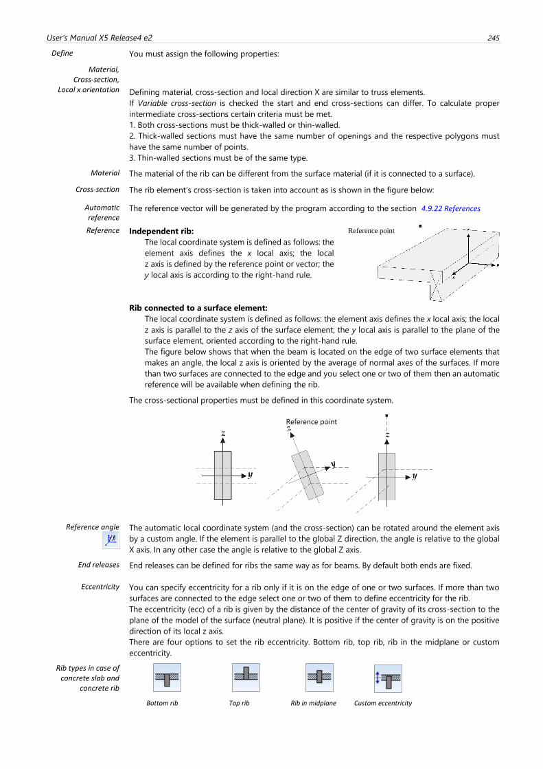
User’s Manual X5 Release4 e2 245

Define You must assign the following properties:

Material, Cross-section,

Local x orientation

Defining material, cross-section and local direction X are similar to truss elements.

If Variable cross-section is checked the start and end cross-sections can differ. To calculate proper

intermediate cross-sections certain criteria must be met.

1. Both cross-sections must be thick-walled or thin-walled.

2. Thick-walled sections must have the same number of openings and the respective polygons must

have the same number of points.

3. Thin-walled sections must be of the same type.

Material The material of the rib can be different from the surface material (if it is connected to a surface).

Cross-section The rib element’s cross-section is taken into account as is shown in the figure below:

Automatic reference

The reference vector will be generated by the program according to the section 4.9.22 References

Reference

Independent rib:

The local coordinate system is defined as follows: the

element axis defines the x local axis; the local

z axis is defined by the reference point or vector; the

y local axis is according to the right-hand rule.

Rib connected to a surface element:

The local coordinate system is defined as follows: the element axis defines the x local axis; the local

z axis is parallel to the z axis of the surface element; the y local axis is parallel to the plane of the

surface element, oriented according to the right-hand rule.

The figure below shows that when the beam is located on the edge of two surface elements that

makes an angle, the local z axis is oriented by the average of normal axes of the surfaces. If more

than two surfaces are connected to the edge and you select one or two of them then an automatic

reference will be available when defining the rib.

The cross-sectional properties must be defined in this coordinate system.

Reference angle

The automatic local coordinate system (and the cross-section) can be rotated around the element axis

by a custom angle. If the element is parallel to the global Z direction, the angle is relative to the global

X axis. In any other case the angle is relative to the global Z axis.

End releases End releases can be defined for ribs the same way as for beams. By default both ends are fixed.

Eccentricity You can specify eccentricity for a rib only if it is on the edge of one or two surfaces. If more than two

surfaces are connected to the edge select one or two of them to define eccentricity for the rib.

The eccentricity (ecc) of a rib is given by the distance of the center of gravity of its cross-section to the

plane of the model of the surface (neutral plane). It is positive if the center of gravity is on the positive

direction of its local z axis.

There are four options to set the rib eccentricity. Bottom rib, top rib, rib in the midplane or custom

eccentricity.

Rib types in case of concrete slab and

concrete rib

Bottom rib Top rib Rib in midplane Custom eccentricity

Reference point

Reference point

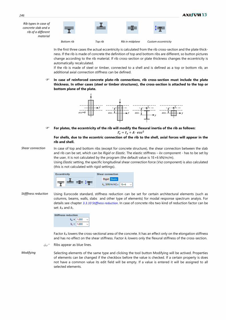
246

Rib types in case of concrete slab and a

rib of a different material

Bottom rib Top rib Rib in midplane Custom eccentricity

In the first three cases the actual eccentricity is calculated from the rib cross-section and the plate thick-

ness. If the rib is made of concrete the definition of top and bottom ribs are different, so button pictures

change according to the rib material. If rib cross-section or plate thickness changes the eccentricity is

automatically recalculated.

If the rib is made of steel or timber, connected to a shell and is defined as a top or bottom rib, an

additional axial connection stiffness can be defined.

In case of reinforced concrete plate-rib connections, rib cross-section must include the plate

thickness. In other cases (steel or timber structures), the cross-section is attached to the top or

bottom plane of the plate.

For plates, the eccentricity of the rib will modify the flexural inertia of the rib as follows:

𝑰𝒚∗ = 𝑰𝒚 + 𝑨 ⋅ 𝒆𝒙𝒄

𝟐

For shells, due to the eccentric connection of the rib to the shell, axial forces will appear in the

rib and shell.

Shear connection In case of top and bottom ribs (except for concrete structure), the shear connection between the slab

and rib can be set, which can be Rigid or Elastic. The elastic stiffness – kx component - has to be set by

the user, it is not calculated by the program (the default value is 1E+6 kN/m/m).

Using Elastic setting, the specific longitudinal shear connection force (Vxz component) is also calculated

(this is not calculated with rigid settings).

Stifffness reduction Using Eurocode standard, stiffness reduction can be set for certain architectural elements (such as

columns, beams, walls, slabs and other type of elements) for modal response spectrum analyis. For

details see chapter 3.3.10 Stiffness reduction. In case of concrete ribs two kind of reduction factor can be

set: kA and kI.

Factor kA lowers the cross-sectional area of the concrete. It has an effect only on the elongation stiffness

and has no effect on the shear stiffness. Factor kI lowers only the flexural stiffness of the cross-section.

Ribs appear as blue lines.

Modifying Selecting elements of the same type and clicking the tool button Modifying will be actived. Properties

of elements can be changed if the checkbox before the value is checked. If a certain property is does

not have a common value its edit field will be empty. If a value is entered it will be assigned to all

selected elements.

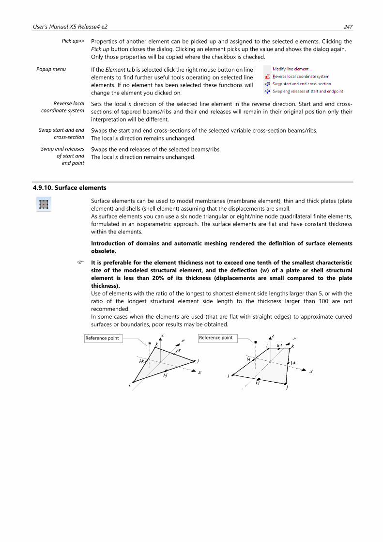
User’s Manual X5 Release4 e2 247

Pick up>> Properties of another element can be picked up and assigned to the selected elements. Clicking the

Pick up button closes the dialog. Clicking an element picks up the value and shows the dialog again.

Only those properties will be copied where the checkbox is checked.

Popup menu If the Element tab is selected click the right mouse button on line

elements to find further useful tools operating on selected line

elements. If no element has been selected these functions will

change the element you clicked on.

Reverse local coordinate system

Sets the local x direction of the selected line element in the reverse direction. Start and end cross-

sections of tapered beams/ribs and their end releases will remain in their original position only their

interpretation will be different.

Swap start and end cross-section

Swaps the start and end cross-sections of the selected variable cross-section beams/ribs.

The local x direction remains unchanged.

Swap end releases of start and

end point

Swaps the end releases of the selected beams/ribs.

The local x direction remains unchanged.

4.9.10. Surface elements

Surface elements can be used to model membranes (membrane element), thin and thick plates (plate

element) and shells (shell element) assuming that the displacements are small.

As surface elements you can use a six node triangular or eight/nine node quadrilateral finite elements,

formulated in an isoparametric approach. The surface elements are flat and have constant thickness

within the elements.

Introduction of domains and automatic meshing rendered the definition of surface elements

obsolete.

It is preferable for the element thickness not to exceed one tenth of the smallest characteristic

size of the modeled structural element, and the deflection (w) of a plate or shell structural

element is less than 20% of its thickness (displacements are small compared to the plate

thickness).

Use of elements with the ratio of the longest to shortest element side lengths larger than 5, or with the

ratio of the longest structural element side length to the thickness larger than 100 are not

recommended.

In some cases when the elements are used (that are flat with straight edges) to approximate curved

surfaces or boundaries, poor results may be obtained.

Reference point Reference point

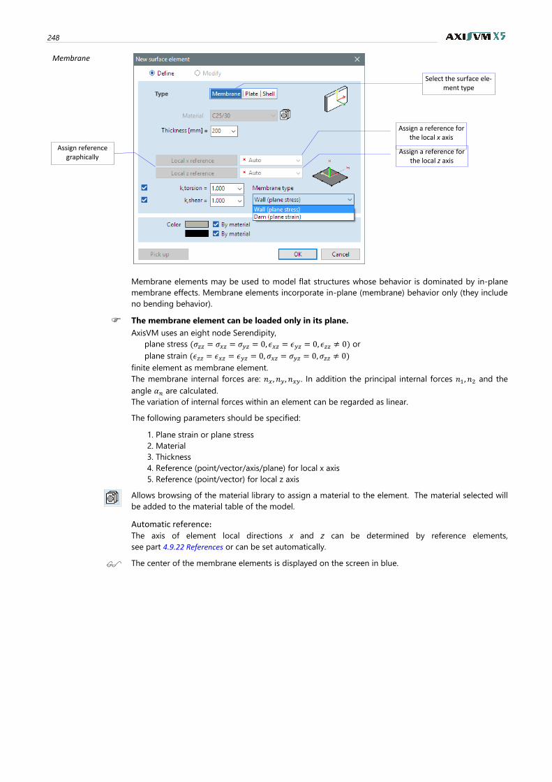
248

Membrane

Membrane elements may be used to model flat structures whose behavior is dominated by in-plane

membrane effects. Membrane elements incorporate in-plane (membrane) behavior only (they include

no bending behavior).

The membrane element can be loaded only in its plane.

AxisVM uses an eight node Serendipity,

plane stress (𝜎𝑧𝑧 = 𝜎𝑥𝑧 = 𝜎𝑦𝑧 = 0, 𝜖𝑥𝑧 = 𝜖𝑦𝑧 = 0, 𝜖𝑧𝑧 ≠ 0) or

plane strain (𝜖𝑧𝑧 = 𝜖𝑥𝑧 = 𝜖𝑦𝑧 = 0, 𝜎𝑥𝑧 = 𝜎𝑦𝑧 = 0, 𝜎𝑧𝑧 ≠ 0)

finite element as membrane element.

The membrane internal forces are: 𝑛𝑥 , 𝑛𝑦, 𝑛𝑥𝑦. In addition the principal internal forces 𝑛1, 𝑛2 and the

angle 𝛼𝑛 are calculated.

The variation of internal forces within an element can be regarded as linear.

The following parameters should be specified:

1. Plane strain or plane stress

2. Material

3. Thickness

4. Reference (point/vector/axis/plane) for local x axis

5. Reference (point/vector) for local z axis

Allows browsing of the material library to assign a material to the element. The material selected will

be added to the material table of the model.

Automatic reference:

The axis of element local directions x and z can be determined by reference elements,

see part 4.9.22 References or can be set automatically.

The center of the membrane elements is displayed on the screen in blue.

Select the surface ele-ment type

Assign reference graphically

Assign a reference for the local z axis

Assign a reference for the local x axis

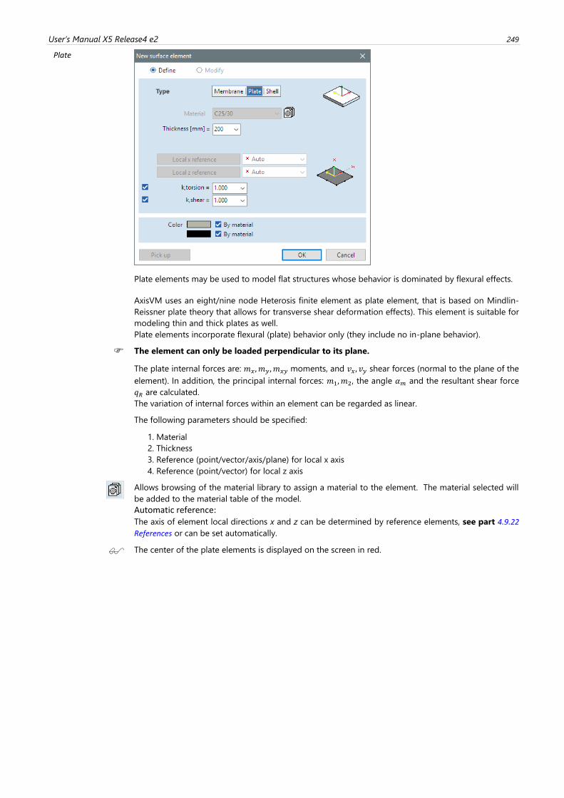
User’s Manual X5 Release4 e2 249

Plate

Plate elements may be used to model flat structures whose behavior is dominated by flexural effects.

AxisVM uses an eight/nine node Heterosis finite element as plate element, that is based on Mindlin-

Reissner plate theory that allows for transverse shear deformation effects). This element is suitable for

modeling thin and thick plates as well.

Plate elements incorporate flexural (plate) behavior only (they include no in-plane behavior).

The element can only be loaded perpendicular to its plane.

The plate internal forces are: 𝑚𝑥, 𝑚𝑦 , 𝑚𝑥𝑦 moments, and 𝑣𝑥, 𝑣𝑦 shear forces (normal to the plane of the

element). In addition, the principal internal forces: 𝑚1, 𝑚2, the angle 𝛼𝑚 and the resultant shear force

𝑞𝑅 are calculated.

The variation of internal forces within an element can be regarded as linear.

The following parameters should be specified:

1. Material

2. Thickness

3. Reference (point/vector/axis/plane) for local x axis

4. Reference (point/vector) for local z axis

Allows browsing of the material library to assign a material to the element. The material selected will

be added to the material table of the model.

Automatic reference: The axis of element local directions x and z can be determined by reference elements, see part 4.9.22

References or can be set automatically.

The center of the plate elements is displayed on the screen in red.

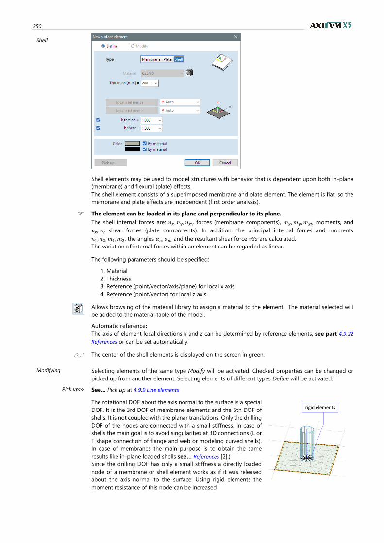
250

Shell

Shell elements may be used to model structures with behavior that is dependent upon both in-plane

(membrane) and flexural (plate) effects.

The shell element consists of a superimposed membrane and plate element. The element is flat, so the

membrane and plate effects are independent (first order analysis).

The element can be loaded in its plane and perpendicular to its plane.

The shell internal forces are: 𝑛𝑥 , 𝑛𝑦 , 𝑛𝑥𝑦 forces (membrane components), 𝑚𝑥 , 𝑚𝑦, 𝑚𝑥𝑦 moments, and

𝑣𝑥, 𝑣𝑦 shear forces (plate components). In addition, the principal internal forces and moments

𝑛1, 𝑛2, 𝑚1, 𝑚2, the angles 𝛼𝑛, 𝛼𝑚 and the resultant shear force 𝑣𝑆𝑧 are calculated.

The variation of internal forces within an element can be regarded as linear.

The following parameters should be specified:

1. Material

2. Thickness

3. Reference (point/vector/axis/plane) for local x axis

4. Reference (point/vector) for local z axis

Allows browsing of the material library to assign a material to the element. The material selected will

be added to the material table of the model.

Automatic reference:

The axis of element local directions x and z can be determined by reference elements, see part 4.9.22

References or can be set automatically.

The center of the shell elements is displayed on the screen in green.

Modifying Selecting elements of the same type Modify will be activated. Checked properties can be changed or

picked up from another element. Selecting elements of different types Define will be activated.

Pick up>> See... Pick up at 4.9.9 Line elements

The rotational DOF about the axis normal to the surface is a special

DOF. It is the 3rd DOF of membrane elements and the 6th DOF of

shells. It is not coupled with the planar translations. Only the drilling

DOF of the nodes are connected with a small stiffness. In case of

shells the main goal is to avoid singularities at 3D connections (L or

T shape connection of flange and web or modeling curved shells).

In case of membranes the main purpose is to obtain the same

results like in-plane loaded shells see… References [2].)

Since the drilling DOF has only a small stiffness a directly loaded

node of a membrane or shell element works as if it was released

about the axis normal to the surface. Using rigid elements the

moment resistance of this node can be increased.

rigid elements

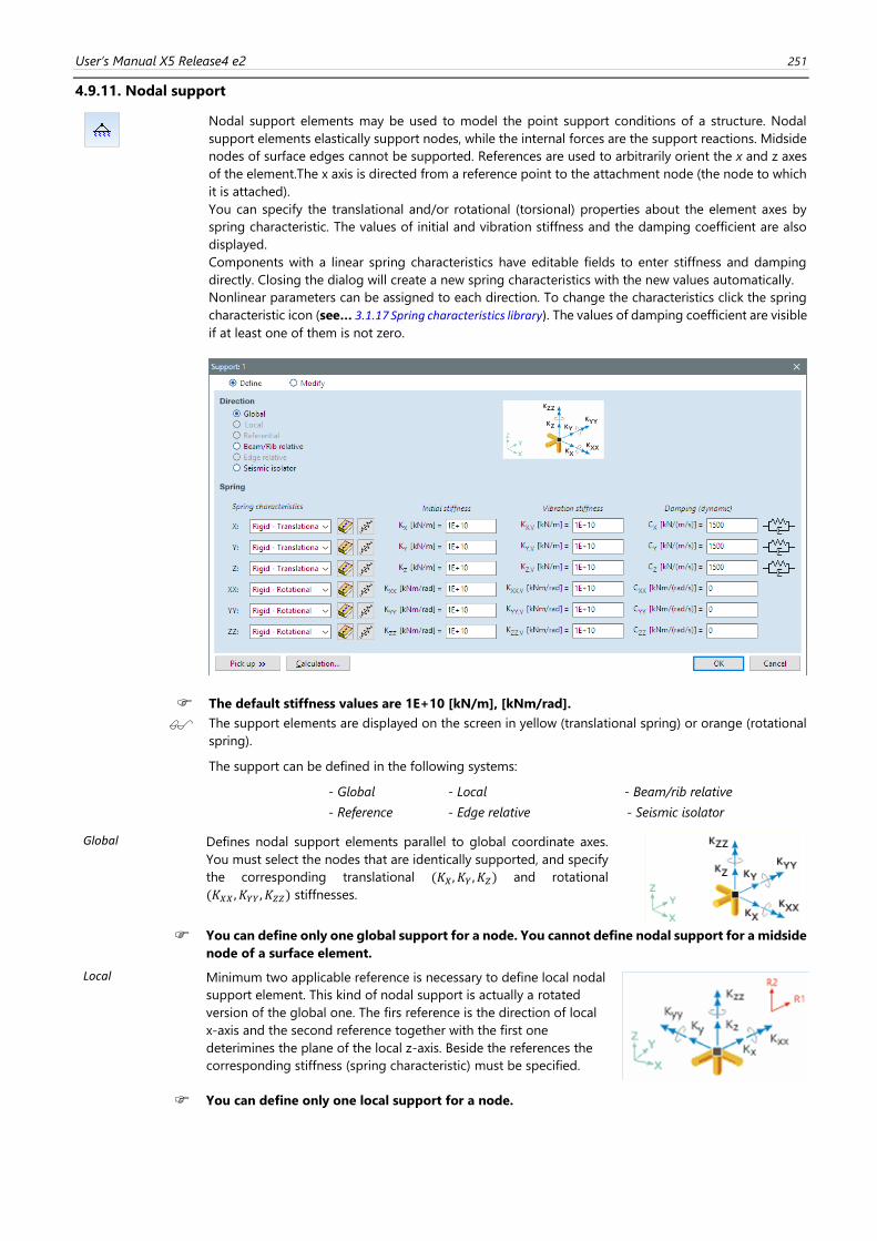
User’s Manual X5 Release4 e2 251

4.9.11. Nodal support

Nodal support elements may be used to model the point support conditions of a structure. Nodal

support elements elastically support nodes, while the internal forces are the support reactions. Midside

nodes of surface edges cannot be supported. References are used to arbitrarily orient the x and z axes

of the element.The x axis is directed from a reference point to the attachment node (the node to which

it is attached).

You can specify the translational and/or rotational (torsional) properties about the element axes by

spring characteristic. The values of initial and vibration stiffness and the damping coefficient are also

displayed.

Components with a linear spring characteristics have editable fields to enter stiffness and damping

directly. Closing the dialog will create a new spring characteristics with the new values automatically.

Nonlinear parameters can be assigned to each direction. To change the characteristics click the spring

characteristic icon (see… 3.1.17 Spring characteristics library). The values of damping coefficient are visible

if at least one of them is not zero.

The default stiffness values are 1E+10 [kN/m], [kNm/rad].

The support elements are displayed on the screen in yellow (translational spring) or orange (rotational

spring).

The support can be defined in the following systems:

- Global - Local - Beam/rib relative

- Reference - Edge relative - Seismic isolator

Global Defines nodal support elements parallel to global coordinate axes.

You must select the nodes that are identically supported, and specify

the corresponding translational (𝐾𝑋, 𝐾𝑌 , 𝐾𝑍) and rotational

(𝐾𝑋𝑋 , 𝐾𝑌𝑌, 𝐾𝑍𝑍) stiffnesses.

You can define only one global support for a node. You cannot define nodal support for a midside

node of a surface element.

Local Minimum two applicable reference is necessary to define local nodal

support element. This kind of nodal support is actually a rotated

version of the global one. The firs reference is the direction of local

x-axis and the second reference together with the first one

deterimines the plane of the local z-axis. Beside the references the

corresponding stiffness (spring characteristic) must be specified.

You can define only one local support for a node.

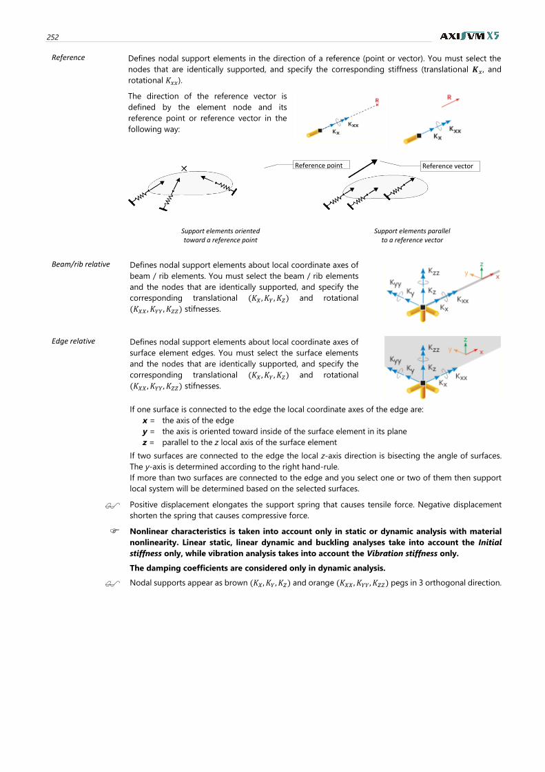
252

Reference Defines nodal support elements in the direction of a reference (point or vector). You must select the

nodes that are identically supported, and specify the corresponding stiffness (translational 𝑲𝑥, and

rotational 𝐾𝑥𝑥).

The direction of the reference vector is

defined by the element node and its

reference point or reference vector in the

following way:

Support elements oriented toward a reference point

Support elements parallel to a reference vector

Beam/rib relative Defines nodal support elements about local coordinate axes of

beam / rib elements. You must select the beam / rib elements

and the nodes that are identically supported, and specify the

corresponding translational (𝐾𝑋 , 𝐾𝑌 , 𝐾𝑍) and rotational

(𝐾𝑋𝑋 , 𝐾𝑌𝑌, 𝐾𝑍𝑍) stifnesses.

Edge relative Defines nodal support elements about local coordinate axes of

surface element edges. You must select the surface elements

and the nodes that are identically supported, and specify the

corresponding translational (𝐾𝑋 , 𝐾𝑌 , 𝐾𝑍) and rotational

(𝐾𝑋𝑋 , 𝐾𝑌𝑌, 𝐾𝑍𝑍) stifnesses.

If one surface is connected to the edge the local coordinate axes of the edge are:

x = the axis of the edge

y = the axis is oriented toward inside of the surface element in its plane

z = parallel to the z local axis of the surface element

If two surfaces are connected to the edge the local z-axis direction is bisecting the angle of surfaces.

The y-axis is determined according to the right hand-rule.

If more than two surfaces are connected to the edge and you select one or two of them then support

local system will be determined based on the selected surfaces.

Positive displacement elongates the support spring that causes tensile force. Negative displacement

shorten the spring that causes compressive force.

Nonlinear characteristics is taken into account only in static or dynamic analysis with material

nonlinearity. Linear static, linear dynamic and buckling analyses take into account the Initial

stiffness only, while vibration analysis takes into account the Vibration stiffness only.

The damping coefficients are considered only in dynamic analysis.

Nodal supports appear as brown (𝐾𝑋, 𝐾𝑌 , 𝐾𝑍) and orange (𝐾𝑋𝑋 , 𝐾𝑌𝑌, 𝐾𝑍𝑍) pegs in 3 orthogonal direction.

Reference point Reference vector

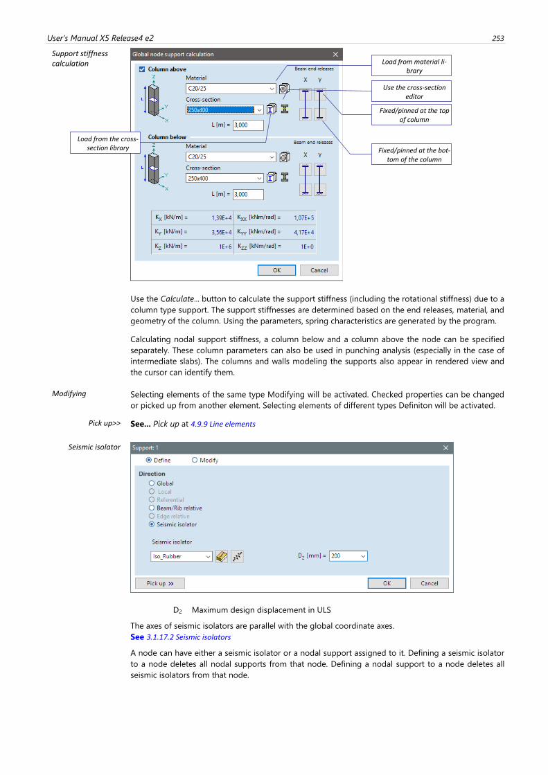
User’s Manual X5 Release4 e2 253

Support stiffness calculation

Use the Calculate... button to calculate the support stiffness (including the rotational stiffness) due to a

column type support. The support stiffnesses are determined based on the end releases, material, and

geometry of the column. Using the parameters, spring characteristics are generated by the program.

Calculating nodal support stiffness, a column below and a column above the node can be specified

separately. These column parameters can also be used in punching analysis (especially in the case of

intermediate slabs). The columns and walls modeling the supports also appear in rendered view and

the cursor can identify them.

Modifying Selecting elements of the same type Modifying will be activated. Checked properties can be changed

or picked up from another element. Selecting elements of different types Definiton will be activated.

Pick up>> See... Pick up at 4.9.9 Line elements

Seismic isolator

D2 Maximum design displacement in ULS

The axes of seismic isolators are parallel with the global coordinate axes.

See 3.1.17.2 Seismic isolators

A node can have either a seismic isolator or a nodal support assigned to it. Defining a seismic isolator

to a node deletes all nodal supports from that node. Defining a nodal support to a node deletes all

seismic isolators from that node.

Load from the cross-section library

Load from material li-brary

Use the cross-section editor

Fixed/pinned at the top of column

Fixed/pinned at the bot-tom of the column

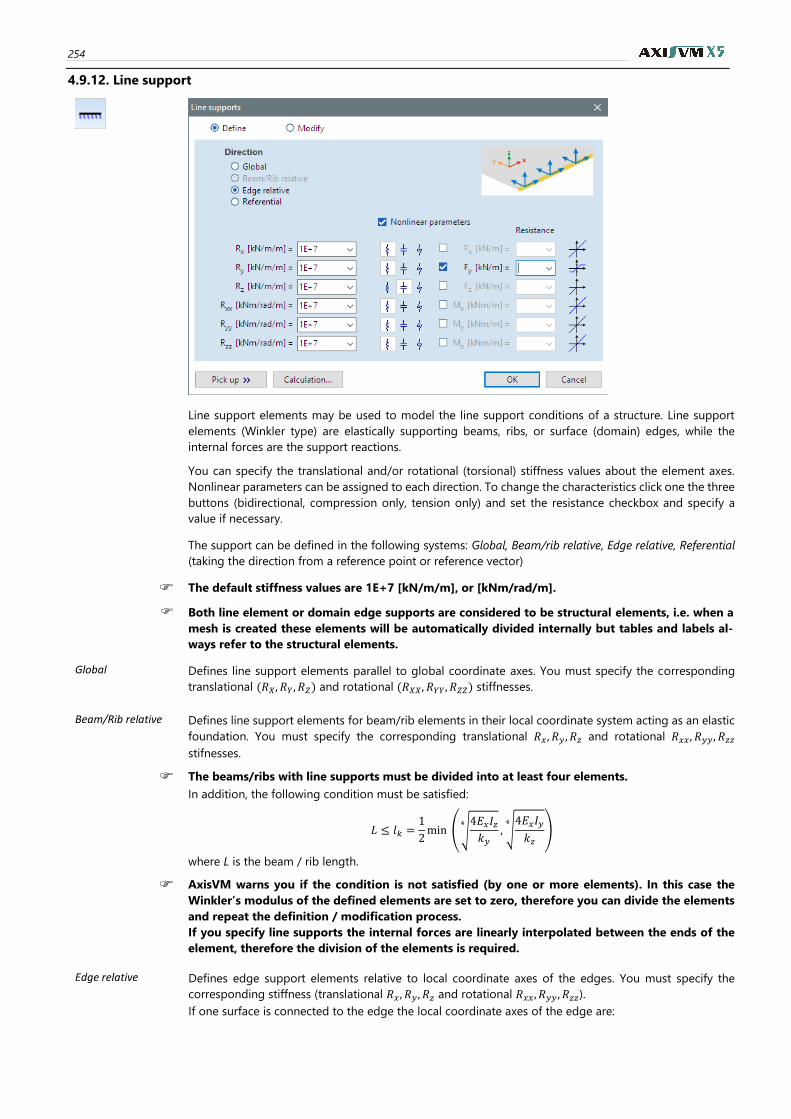
254

4.9.12. Line support

Line support elements may be used to model the line support conditions of a structure. Line support

elements (Winkler type) are elastically supporting beams, ribs, or surface (domain) edges, while the

internal forces are the support reactions.

You can specify the translational and/or rotational (torsional) stiffness values about the element axes.

Nonlinear parameters can be assigned to each direction. To change the characteristics click one the three

buttons (bidirectional, compression only, tension only) and set the resistance checkbox and specify a

value if necessary.

The support can be defined in the following systems: Global, Beam/rib relative, Edge relative, Referential

(taking the direction from a reference point or reference vector)

The default stiffness values are 1E+7 [kN/m/m], or [kNm/rad/m].

Both line element or domain edge supports are considered to be structural elements, i.e. when a

mesh is created these elements will be automatically divided internally but tables and labels al-

ways refer to the structural elements.

Global Defines line support elements parallel to global coordinate axes. You must specify the corresponding

translational (𝑅𝑋, 𝑅𝑌, 𝑅𝑍) and rotational (𝑅𝑋𝑋, 𝑅𝑌𝑌, 𝑅𝑍𝑍) stiffnesses.

Beam/Rib relative Defines line support elements for beam/rib elements in their local coordinate system acting as an elastic

foundation. You must specify the corresponding translational 𝑅𝑥, 𝑅𝑦 , 𝑅𝑧 and rotational 𝑅𝑥𝑥, 𝑅𝑦𝑦 , 𝑅𝑧𝑧

stifnesses.

The beams/ribs with line supports must be divided into at least four elements.

In addition, the following condition must be satisfied:

𝐿 ≤ 𝑙𝑘 =1

2min (√

4𝐸𝑥𝐼𝑧𝑘𝑦

4

, √4𝐸𝑥𝐼𝑦

𝑘𝑧

4

)

where L is the beam / rib length.

AxisVM warns you if the condition is not satisfied (by one or more elements). In this case the

Winkler’s modulus of the defined elements are set to zero, therefore you can divide the elements

and repeat the definition / modification process.

If you specify line supports the internal forces are linearly interpolated between the ends of the

element, therefore the division of the elements is required.

Edge relative Defines edge support elements relative to local coordinate axes of the edges. You must specify the

corresponding stiffness (translational 𝑅𝑥, 𝑅𝑦, 𝑅𝑧 and rotational 𝑅𝑥𝑥, 𝑅𝑦𝑦 , 𝑅𝑧𝑧).

If one surface is connected to the edge the local coordinate axes of the edge are:

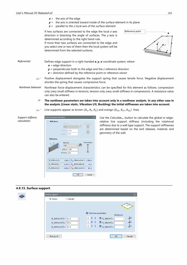
User’s Manual X5 Release4 e2 255

x = the axis of the edge

y = the axis is oriented toward inside of the surface element in its plane

z = parallel to the z local axis of the surface element

If two surfaces are connected to the edge the local z-axis

direction is bisecting the angle of surfaces. The y-axis is

determined according to the right hand-rule.

If more than two surfaces are connected to the edge and

you select one or two of them then the local system will be

determined from the selected surfaces.

Referential Defines edge support in a right-handed x, y, z coordinate system, where

x = edge direction

y = perpendicular both to the edge and the z reference direction

z = direction defined by the reference point or reference vector

Positive displacement elongates the support spring that causes tensile force. Negative displacement

shorten the spring that causes compressive force.

Nonlinear behavior Nonlinear force-displacement characteristics can be specified for this element as follows: compression

only (very small stiffness in tension), tension only (very small stiffness in compression). A resistance value

can also be entered.

The nonlinear parameters are taken into account only in a nonlinear analysis. In any other case in

the analysis (Linear static, Vibration I/II, Buckling) the initial stiffnesses are taken into account.

Line supports appear as brown (𝑅𝑋, 𝑅𝑌, 𝑅𝑍) and orange (𝑅𝑋𝑋, 𝑅𝑌𝑌, 𝑅𝑍𝑍) lines.

Support stiffness calculation

Use the Calculate... button to calculate the global or edge-

relative line support stiffness (including the rotational

stiffness) due to a wall type support. The support stiffnesses

are determined based on the end releases, material, and

geometry of the wall.

4.9.13. Surface support

Reference point

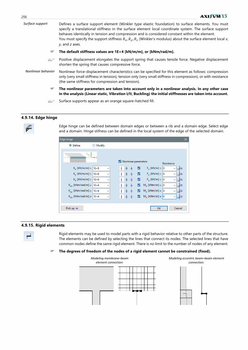
256

Surface support Defines a surface support element (Winkler type elastic foundation) to surface elements. You must

specify a translational stiffness in the surface element local coordinate system. The surface support

behaves identically in tension and compression and is considered constant within the element.

You must specify the support stiffness 𝑅𝑥, 𝑅𝑦, 𝑅𝑧 (Winkler’s modulus) about the surface element local x,

y, and z axes.

The default stiffness values are 1E+4 [kN/m/m], or [kNm/rad/m].

Positive displacement elongates the support spring that causes tensile force. Negative displacement

shorten the spring that causes compressive force.

Nonlinear behavior Nonlinear force-displacement characteristics can be specified for this element as follows: compression

only (very small stiffness in tension), tension only (very small stiffness in compression), or with resistance

(the same stiffness for compression and tension).

The nonlinear parameters are taken into account only in a nonlinear analysis. In any other case

in the analysis (Linear static, Vibration I/II, Buckling) the initial stiffnesses are taken into account.

Surface supports appear as an orange square-hatched fill.

4.9.14. Edge hinge

Edge hinge can be defined between domain edges or between a rib and a domain edge. Select edge

and a domain. Hinge stifness can be defined in the local system of the edge of the selected domain.

4.9.15. Rigid elements

Rigid elements may be used to model parts with a rigid behavior relative to other parts of the structure.

The elements can be defined by selecting the lines that connect its nodes. The selected lines that have

common nodes define the same rigid element. There is no limit to the number of nodes of any element.

The degrees of freedom of the nodes of a rigid element cannot be constrained (fixed).

Modeling membrane–beam element connection:

Modeling eccentric beam–beam element connection:

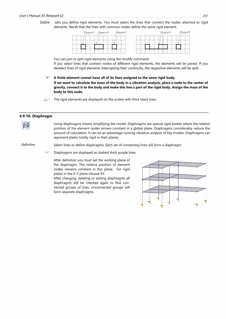
User’s Manual X5 Release4 e2 257

Define Lets you define rigid elements. You must select the lines that connect the nodes attached to rigid

elements. Recall that the lines with common nodes define the same rigid element.

You can join or split rigid elements using the modify command.

If you select lines that connect nodes of different rigid elements, the elements will be joined. If you

deselect lines of rigid elements interrupting their continuity, the respective elements will be split.

A finite element cannot have all of its lines assigned to the same rigid body.

If we want to calculate the mass of the body in a vibration analysis, place a node to the center of

gravity, connect it to the body and make this line a part of the rigid body. Assign the mass of the

body to this node.

The rigid elements are displayed on the screen with thick black lines.

4.9.16. Diaphragm

Using diaphragms means simplifying the model. Diaphragms are special rigid bodies where the relative

position of the element nodes remain constant in a global plane. Diaphragms considerably reduce the

amount of calculation. It can be an advantage running vibration analysis of big models. Diaphragms can

represent plates totally rigid in their planes.

Definition Select lines to define diaphragms. Each set of connecting lines will form a diaphragm.

Diaphragms are displayed as dashed thick purple lines.

After definition you must set the working plane of

the diaphragm. The relative position of element

nodes remains constant in this plane. For rigid

plates in the X-Y plane choose XY.

After changing, deleting or adding diaphragms all

diaphragms will be checked again to find con-

nected groups of lines. Unconnected groups will

form separate diaphragms.

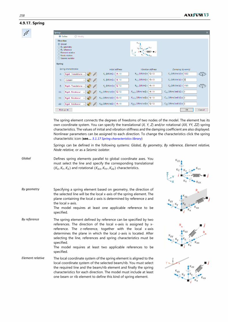
258

4.9.17. Spring

The spring element connects the degrees of freedoms of two nodes of the model. The element has its

own coordinate system. You can specify the translational (X, Y, Z) and/or rotational (XX, YY, ZZ) spring

characteristics. The values of initial and vibration stiffness and the damping coefficient are also displayed.

Nonlinear parameters can be assigned to each direction. To change the characteristics click the spring

characteristic icon (see… 3.1.17 Spring characteristics library)

Springs can be defined in the following systems: Global, By geometry, By reference, Element relative,

Node relative, or as a Seismic isolator.

Global Defines spring elements parallel to global coordinate axes. You

must select the line and specify the corresponding translational

(𝐾𝑋 , 𝐾𝑌, 𝐾𝑍) and rotational (𝐾𝑋𝑋 , 𝐾𝑌𝑌 , 𝐾𝑍𝑍) characteristics.

By geometry Specifying a spring element based on geometry, the direction of

the selected line will be the local x-axis of the spring element. The

plane containing the local z-axis is determined by reference z and

the local x-axis.

The model requires at least one applicable reference to be

specified.

By reference The spring element defined by reference can be specified by two

references. The direction of the local x-axis is assigned by x-

reference. The z-reference, together with the local x-axis

determines the plane in which the local z-axis is located. After

selecting the line, references and spring characteristics must be

specified.

The model requires at least two applicable references to be

specified.

Element relative The local coordinate system of the spring element is aligned to the

local coordinate system of the selected beam/rib. You must select

the required line and the beam/rib element and finally the spring

characteristics for each direction. The model must include at least

one beam or rib element to define this kind of spring element.

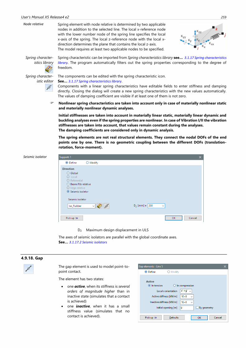
User’s Manual X5 Release4 e2 259

Node relative Spring element with node relative is determined by two applicable

nodes in addition to the selected line. The local x-reference node

with the lower number node of the spring line specifies the local

x-axis of the spring. The local z-reference node with the local x-

direction determines the plane that contains the local z-axis.

The model requires at least two applicable nodes to be specified.

Spring character-

istics library

Spring characteristic can be imported from Spring characteristics library see… 3.1.17 Spring characteristics

library. The program automatically filters out the spring properties corresponding to the degree of

freedom.

Spring character-

istic editor

The components can be edited with the spring characteristic icon.

See… 3.1.17 Spring characteristics library.

Components with a linear spring characteristics have editable fields to enter stiffness and damping

directly. Closing the dialog will create a new spring characteristics with the new values automatically.

The values of damping coefficient are visible if at least one of them is not zero.

Nonlinear spring characteristics are taken into account only in case of materially nonlinear static

and materially nonlinear dynamic analyses.

Initial stiffnesses are taken into account in materially linear static, materially linear dynamic and

buckling analyses even if the spring properties are nonlinear. In case of Vibration I/II the vibration

stiffnesses are taken into account, that values remain constant during the analyses.

The damping coefficients are considered only in dynamic analysis.

The spring elements are not real structural elements. They connect the nodal DOFs of the end

points one by one. There is no geometric coupling between the different DOFs (translation-

rotation, force-moment).

Seismic isolator

D2 Maximum design displacement in ULS

The axes of seismic isolators are parallel with the global coordinate axes.

See… 3.1.17.2 Seismic isolators

4.9.18. Gap

The gap element is used to model point-to-

point contact.

The element has two states:

• one active, when its stiffness is several

orders of magnitude higher than in

inactive state (simulates that a contact

is achieved)

• one inactive, when it has a small

stiffness value (simulates that no

contact is achieved).

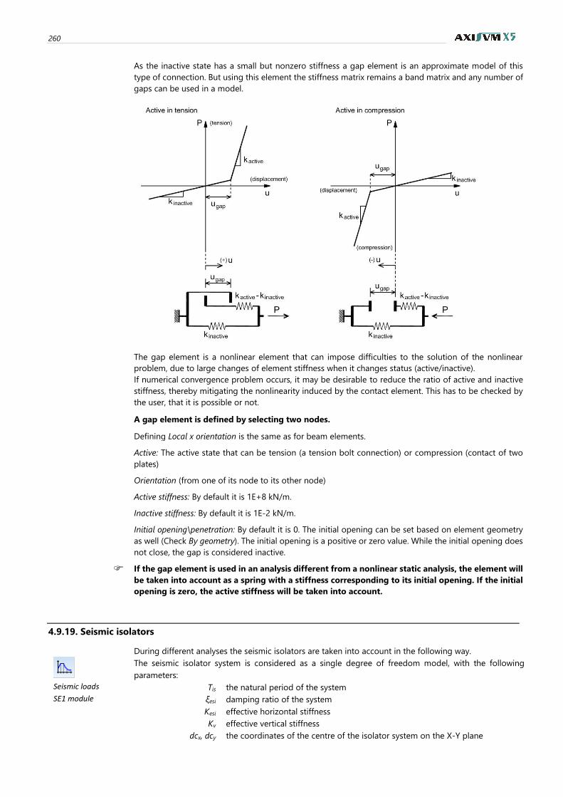
260

As the inactive state has a small but nonzero stiffness a gap element is an approximate model of this

type of connection. But using this element the stiffness matrix remains a band matrix and any number of

gaps can be used in a model.

The gap element is a nonlinear element that can impose difficulties to the solution of the nonlinear

problem, due to large changes of element stiffness when it changes status (active/inactive).

If numerical convergence problem occurs, it may be desirable to reduce the ratio of active and inactive

stiffness, thereby mitigating the nonlinearity induced by the contact element. This has to be checked by

the user, that it is possible or not.

A gap element is defined by selecting two nodes.

Defining Local x orientation is the same as for beam elements.

Active: The active state that can be tension (a tension bolt connection) or compression (contact of two

plates)

Orientation (from one of its node to its other node)

Active stiffness: By default it is 1E+8 kN/m.

Inactive stiffness: By default it is 1E-2 kN/m.

Initial opening\penetration: By default it is 0. The initial opening can be set based on element geometry

as well (Check By geometry). The initial opening is a positive or zero value. While the initial opening does

not close, the gap is considered inactive.

If the gap element is used in an analysis different from a nonlinear static analysis, the element will

be taken into account as a spring with a stiffness corresponding to its initial opening. If the initial

opening is zero, the active stiffness will be taken into account.

4.9.19. Seismic isolators

During different analyses the seismic isolators are taken into account in the following way.

The seismic isolator system is considered as a single degree of freedom model, with the following

parameters:

Seismic loads Tis the natural period of the system

SE1 module ξesi damping ratio of the system

Kesi effective horizontal stiffness

Kv effective vertical stiffness

dcx, dcy the coordinates of the centre of the isolator system on the X-Y plane

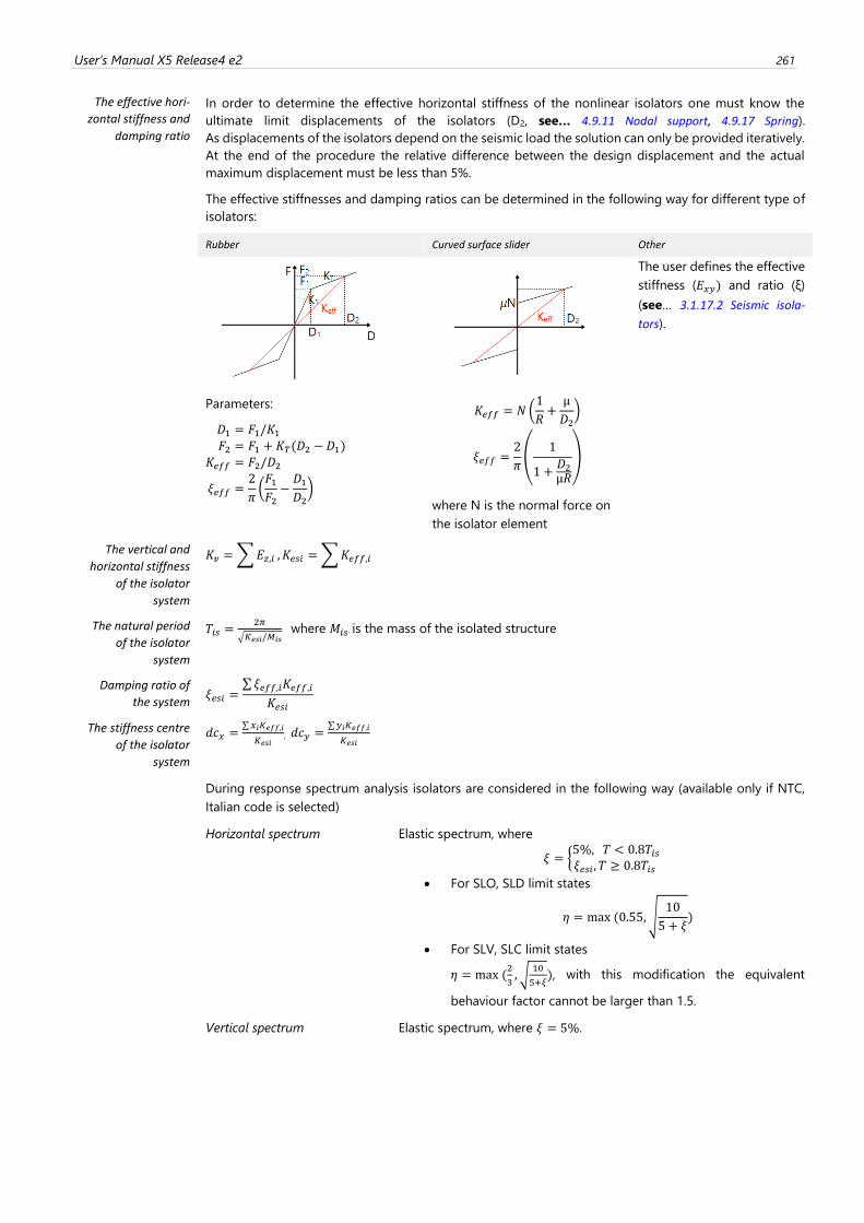
User’s Manual X5 Release4 e2 261

The effective hori-

zontal stiffness and

damping ratio

In order to determine the effective horizontal stiffness of the nonlinear isolators one must know the

ultimate limit displacements of the isolators (D2, see… 4.9.11 Nodal support, 4.9.17 Spring).

As displacements of the isolators depend on the seismic load the solution can only be provided iteratively.

At the end of the procedure the relative difference between the design displacement and the actual

maximum displacement must be less than 5%.

The effective stiffnesses and damping ratios can be determined in the following way for different type of

isolators:

Rubber Curved surface slider Other

Parameters:

𝐷1 = 𝐹1/𝐾1

𝐹2 = 𝐹1 + 𝐾𝑇(𝐷2 −𝐷1)

𝐾𝑒𝑓𝑓 = 𝐹2/𝐷2

𝜉𝑒𝑓𝑓 =2

𝜋(𝐹1𝐹2−𝐷1𝐷2)

𝐾𝑒𝑓𝑓 = 𝑁 (1

𝑅+µ

𝐷2)

𝜉𝑒𝑓𝑓 =2

𝜋(

1

1 +𝐷2µ𝑅

)

where N is the normal force on

the isolator element

The user defines the effective

stiffness (𝐸𝑥𝑦) and ratio (ξ)

(see… 3.1.17.2 Seismic isola-

tors).

The vertical and

horizontal stiffness

of the isolator

system

𝐾𝑣 =∑𝐸𝑧,𝑖 , 𝐾𝑒𝑠𝑖 =∑𝐾𝑒𝑓𝑓,𝑖

The natural period

of the isolator

system

𝑇𝑖𝑠 =2𝜋

√𝐾𝑒𝑠𝑖/𝑀𝑖𝑠 where 𝑀𝑖𝑠 is the mass of the isolated structure

Damping ratio of

the system 𝜉𝑒𝑠𝑖 =

∑𝜉𝑒𝑓𝑓,𝑖𝐾𝑒𝑓𝑓,𝑖

𝐾𝑒𝑠𝑖

The stiffness centre

of the isolator

system

𝑑𝑐𝑥 =∑𝑥𝑖𝐾𝑒𝑓𝑓,𝑖

𝐾𝑒𝑠𝑖, 𝑑𝑐𝑦 =

∑𝑦𝑖𝐾𝑒𝑓𝑓,𝑖

𝐾𝑒𝑠𝑖

During response spectrum analysis isolators are considered in the following way (available only if NTC,

Italian code is selected)

Horizontal spectrum Elastic spectrum, where

𝜉 = {5%, 𝑇 < 0.8𝑇𝑖𝑠𝜉𝑒𝑠𝑖 , 𝑇 ≥ 0.8𝑇𝑖𝑠

• For SLO, SLD limit states

휂 = max (0.55,√10

5 + 𝜉)

• For SLV, SLC limit states

휂 = max (2

3, √

10

5+𝜉), with this modification the equivalent

behaviour factor cannot be larger than 1.5.

Vertical spectrum Elastic spectrum, where 𝜉 = 5%.

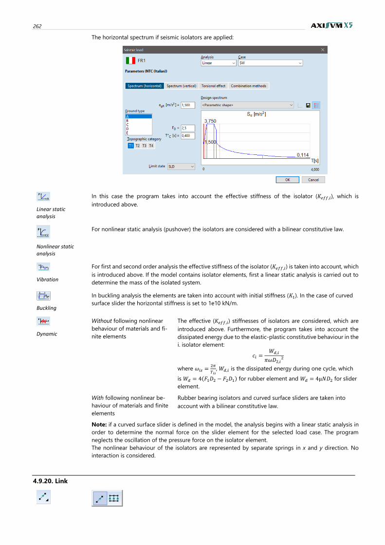
262

The horizontal spectrum if seismic isolators are applied:

Linear static analysis

In this case the program takes into account the effective stiffness of the isolator (𝐾𝑒𝑓𝑓,𝑖), which is

introduced above.

Nonlinear static analysis

For nonlinear static analysis (pushover) the isolators are considered with a bilinear constitutive law.

Vibration

For first and second order analysis the effective stiffness of the isolator (𝐾𝑒𝑓𝑓,𝑖) is taken into account, which

is introduced above. If the model contains isolator elements, first a linear static analysis is carried out to

determine the mass of the isolated system.

Buckling

In buckling analysis the elements are taken into account with initial stiffness (𝐾1). In the case of curved

surface slider the horizontal stiffness is set to 1e10 kN/m.

Dynamic

Without following nonlinear

behaviour of materials and fi-

nite elements

The effective (𝐾𝑒𝑓𝑓,𝑖) stiffnesses of isolators are considered, which are

introduced above. Furthermore, the program takes into account the

dissipated energy due to the elastic-plastic constitutive behaviour in the

i. isolator element:

𝑐𝑖 =𝑊𝑑,𝑖

𝜋𝜔𝐷2,𝑖2

where 𝜔𝑖𝑠 =2𝜋

𝑇𝑖𝑠, 𝑊𝑑,𝑖 is the dissipated energy during one cycle, which

is 𝑊𝑑 = 4(𝐹1𝐷2 − 𝐹2𝐷1) for rubber element and 𝑊𝑑 = 4µ𝑁𝐷2 for slider

element.

With following nonlinear be-

haviour of materials and finite

elements

Rubber bearing isolators and curved surface sliders are taken into

account with a bilinear constitutive law.

Note: if a curved surface slider is defined in the model, the analysis begins with a linear static analysis in

order to determine the normal force on the slider element for the selected load case. The program

neglects the oscillation of the pressure force on the isolator element.

The nonlinear behaviour of the isolators are represented by separate springs in x and y direction. No

interaction is considered.

4.9.20. Link

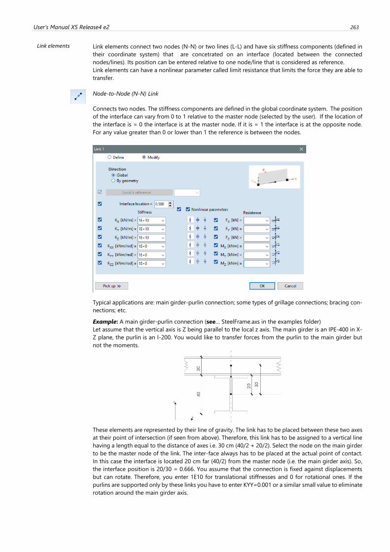
User’s Manual X5 Release4 e2 263

Link elements Link elements connect two nodes (N-N) or two lines (L-L) and have six stiffness components (defined in

their coordinate system) that are concetrated on an interface (located between the connected

nodes/lines). Its position can be entered relative to one node/line that is considered as reference.

Link elements can have a nonlinear parameter called limit resistance that limits the force they are able to

transfer.

Node-to-Node (N-N) Link

Connects two nodes. The stiffness components are defined in the global coordinate system. The position

of the interface can vary from 0 to 1 relative to the master node (selected by the user). If the location of

the interface is = 0 the interface is at the master node. If it is = 1 the interface is at the opposite node.

For any value greater than 0 or lower than 1 the reference is between the nodes.

Typical applications are: main girder-purlin connection; some types of grillage connections; bracing con-

nections; etc.

Example: A main girder-purlin connection (see… SteelFrame.axs in the examples folder)

Let assume that the vertical axis is Z being parallel to the local z axis. The main girder is an IPE-400 in X-

Z plane, the purlin is an I-200. You would like to transfer forces from the purlin to the main girder but

not the moments.

These elements are represented by their line of gravity. The link has to be placed between these two axes

at their point of intersection (if seen from above). Therefore, this link has to be assigned to a vertical line

having a length equal to the distance of axes i.e. 30 cm (40/2 + 20/2). Select the node on the main girder

to be the master node of the link. The inter-face always has to be placed at the actual point of contact.

In this case the interface is located 20 cm far (40/2) from the master node (i.e. the main girder axis). So,

the interface position is 20/30 = 0.666. You assume that the connection is fixed against displacements

but can rotate. Therefore, you enter 1E10 for translational stiffnesses and 0 for rotational ones. If the

purlins are supported only by these links you have to enter KYY=0.001 or a similar small value to eliminate

rotation around the main girder axis.

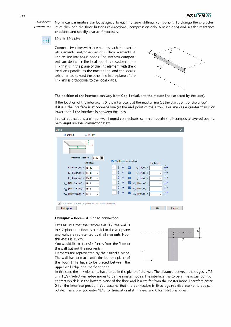
264

Nonlinear parameters

Nonlinear parameters can be assigned to each nonzero stiffness component. To change the character-

istics click one the three buttons (bidirectional, compression only, tension only) and set the resistance

checkbox and specify a value if necessary.

Line-to-Line Link

Connects two lines with three nodes each that can be

rib elements and/or edges of surface elements. A

line-to-line link has 6 nodes. The stiffness compon-

ents are defined in the local coordinate system of the

link that is in the plane of the link element with the x

local axis parallel to the master line, and the local z

axis oriented toward the other line in the plane of the

link and is orthogonal to the local x axis.

The position of the interface can vary from 0 to 1 relative to the master line (selected by the user).

If the location of the interface is 0, the interface is at the master line (at the start point of the arrow).

If it is 1 the interface is at opposite line (at the end point of the arrow). For any value greater than 0 or

lower than 1 the interface is between the lines.

Typical applications are: floor-wall hinged connections; semi-composite / full-composite layered beams;

Semi-rigid rib-shell connections; etc.

Example: A floor-wall hinged connection.

Let’s assume that the vertical axis is Z, the wall is

in Y-Z plane, the floor is parallel to the X-Y plane

and walls are represented by shell elements. Floor

thickness is 15 cm.

You would like to transfer forces from the floor to

the wall but not the moments.

Elements are represented by their middle plane.

The wall has to reach until the bottom plane of

the floor. Links have to be placed between the

upper wall edge and the floor edge.

In this case the link elements have to be in the plane of the wall. The distance between the edges is 7.5

cm (15/2). Select wall edge nodes to be the master nodes. The interface has to be at the actual point of

contact which is in the bottom plane of the floor and is 0 cm far from the master node. Therefore enter

0 for the interface position. You assume that the connection is fixed against displacements but can

rotate. Therefore, you enter 1E10 for translational stiffnesses and 0 for rotational ones.

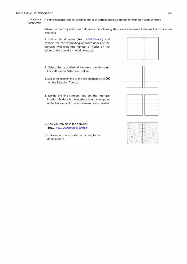
User’s Manual X5 Release4 e2 265

Nonlinear parameters

A limit resistance can be specified for each corresponding component with non-zero stiffness.

When used in conjunction with domains the following steps can be followed to define line-to-line link

elements:

1. Define the domains (See... 4.9.6 Domain) and

connect the cor-responding opposite nodes of the

domains with lines (the number of nodes on the

edges of the domains should be equal).

2. Select the quadrilateral between the domains.

Click OK on the Selection Toolbar.

3. Select the master line of the link element. Click OK

on the Selection Toolbar.

4. Define the link stiffness, and set the interface

location. By default the interface is in the midpoint

of the link element. The link element(s) are created.

5. Now you can mesh the domains.

See... 4.11.1.2 Meshing of domain

6. Link elements are divided according to the

domain mesh.

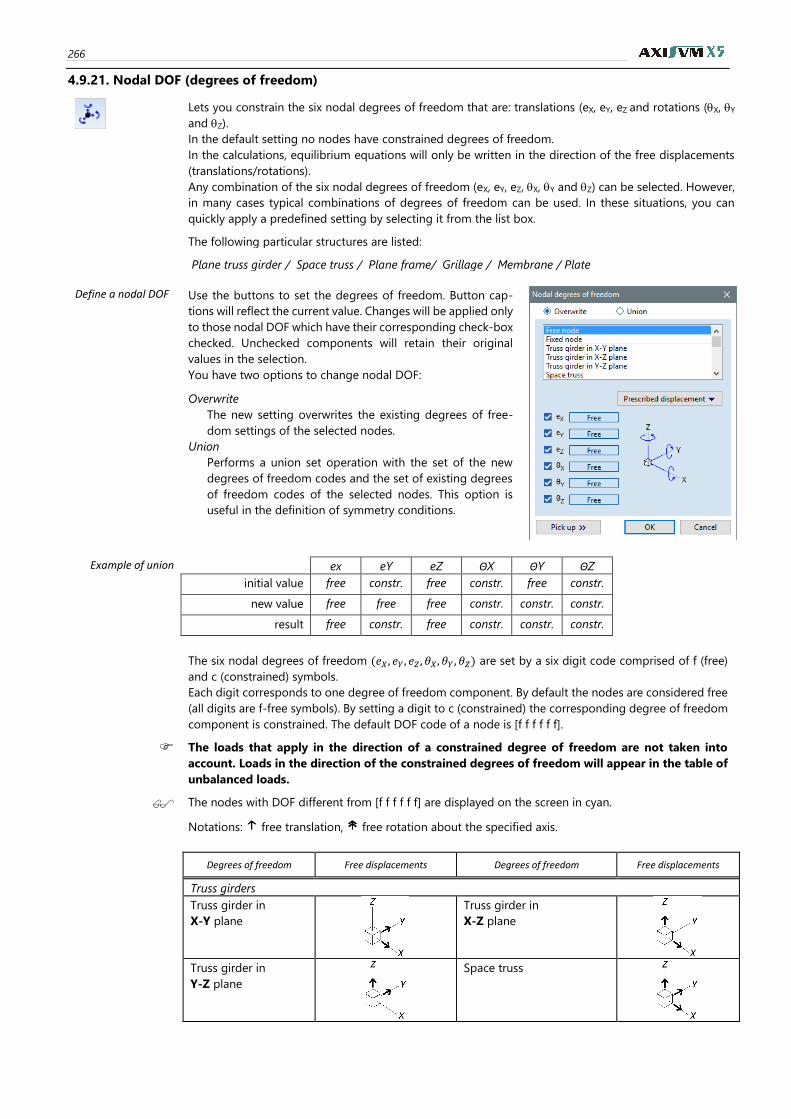
266

4.9.21. Nodal DOF (degrees of freedom)

Lets you constrain the six nodal degrees of freedom that are: translations (eX, eY, eZ and rotations (X, Y

and Z).

In the default setting no nodes have constrained degrees of freedom.

In the calculations, equilibrium equations will only be written in the direction of the free displacements

(translations/rotations).

Any combination of the six nodal degrees of freedom (eX, eY, eZ, X, Y and Z) can be selected. However,

in many cases typical combinations of degrees of freedom can be used. In these situations, you can

quickly apply a predefined setting by selecting it from the list box.

The following particular structures are listed:

Plane truss girder / Space truss / Plane frame/ Grillage / Membrane / Plate

Define a nodal DOF Use the buttons to set the degrees of freedom. Button cap-

tions will reflect the current value. Changes will be applied only

to those nodal DOF which have their corresponding check-box

checked. Unchecked components will retain their original

values in the selection.

You have two options to change nodal DOF:

Overwrite

The new setting overwrites the existing degrees of free-

dom settings of the selected nodes.

Union

Performs a union set operation with the set of the new

degrees of freedom codes and the set of existing degrees

of freedom codes of the selected nodes. This option is

useful in the definition of symmetry conditions.

Example of union ex eY eZ ΘX ΘY ΘZ

initial value free constr. free constr. free constr.

new value free free free constr. constr. constr.

result free constr. free constr. constr. constr.

The six nodal degrees of freedom (𝑒𝑋, 𝑒𝑌, 𝑒𝑍, 휃𝑋, 휃𝑌 , 휃𝑍) are set by a six digit code comprised of f (free)

and c (constrained) symbols.

Each digit corresponds to one degree of freedom component. By default the nodes are considered free

(all digits are f-free symbols). By setting a digit to c (constrained) the corresponding degree of freedom

component is constrained. The default DOF code of a node is [f f f f f f].

The loads that apply in the direction of a constrained degree of freedom are not taken into

account. Loads in the direction of the constrained degrees of freedom will appear in the table of

unbalanced loads.

The nodes with DOF different from [f f f f f f] are displayed on the screen in cyan.

Notations: free translation, free rotation about the specified axis.

Degrees of freedom Free displacements Degrees of freedom Free displacements

Truss girders

Truss girder in

X-Y plane

Truss girder in

X-Z plane

Truss girder in

Y-Z plane

Space truss

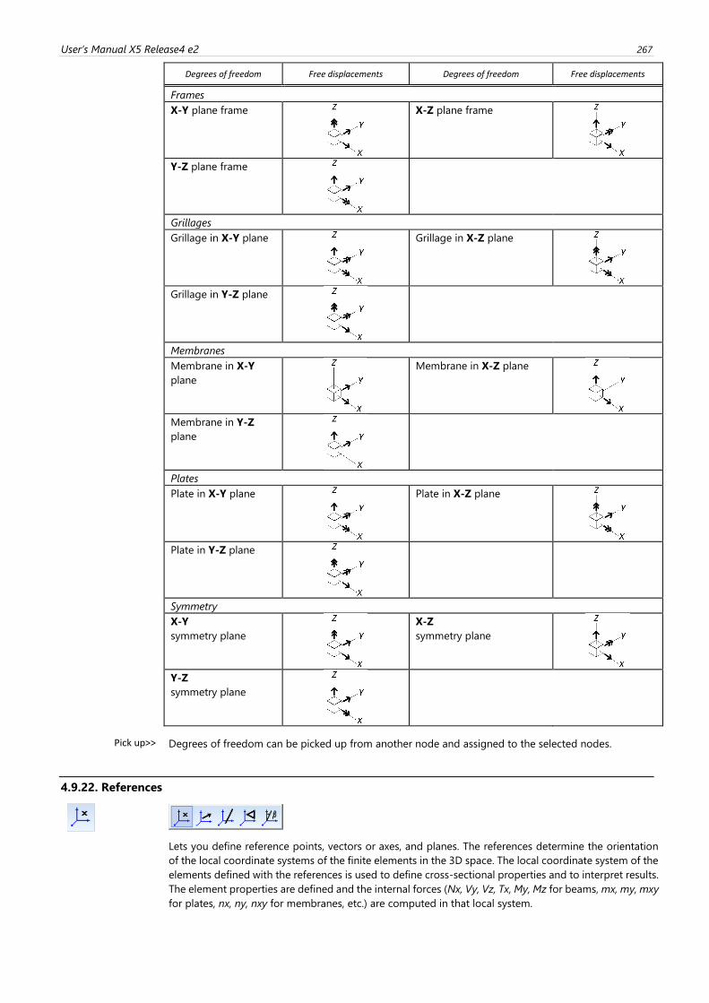
User’s Manual X5 Release4 e2 267

Degrees of freedom Free displacements Degrees of freedom Free displacements

Frames

X-Y plane frame

X-Z plane frame

Y-Z plane frame

Grillages

Grillage in X-Y plane

Grillage in X-Z plane

Grillage in Y-Z plane

Membranes

Membrane in X-Y

plane

Membrane in X-Z plane

Membrane in Y-Z

plane

Plates

Plate in X-Y plane

Plate in X-Z plane

Plate in Y-Z plane

Symmetry

X-Y

symmetry plane

X-Z

symmetry plane

Y-Z

symmetry plane

Pick up>>

Degrees of freedom can be picked up from another node and assigned to the selected nodes.

4.9.22. References

Lets you define reference points, vectors or axes, and planes. The references determine the orientation

of the local coordinate systems of the finite elements in the 3D space. The local coordinate system of the

elements defined with the references is used to define cross-sectional properties and to interpret results.

The element properties are defined and the internal forces (Nx, Vy, Vz, Tx, My, Mz for beams, mx, my, mxy

for plates, nx, ny, nxy for membranes, etc.) are computed in that local system.

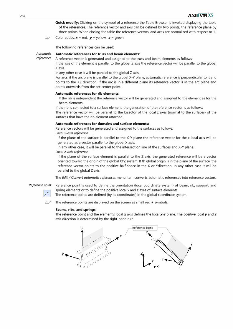
268

Quick modify: Clicking on the symbol of a reference the Table Browser is invoked displaying the table

of the references. The reference vector and axis can be defined by two points, the reference plane by

three points. When closing the table the reference vectors, and axes are normalized with respect to 1.

Color codes: x = red, y = yellow, z = green.

The following references can be used:

Automatic references

Automatic references for truss and beam elements:

A reference vector is generated and assigned to the truss and beam elements as follows:

If the axis of the element is parallel to the global Z axis the reference vector will be parallel to the global

X axis.

In any other case it will be parallel to the global Z axis.

For arcs: if the arc plane is parallel to the global X-Y plane, automatic reference is perpendicular to it and

points to the +Z direction. If the arc is in a different plane its reference vector is in the arc plane and

points outwards from the arc center point.

Automatic references for rib elements:

If the rib is independent the reference vector will be generated and assigned to the element as for the

beam elements.

If the rib is connected to a surface element, the generation of the reference vector is as follows:

The reference vector will be parallel to the bisector of the local z axes (normal to the surfaces) of the

surfaces that have the rib element attached.

Automatic references for domains and surface elements:

Reference vectors will be generated and assigned to the surfaces as follows:

Local x-axis reference

If the plane of the surface is parallel to the X-Y plane the reference vector for the x local axis will be

generated as a vector parallel to the global X axis.

In any other case, it will be parallel to the intersection line of the surfaces and X-Y plane.

Local z-axis reference

If the plane of the surface element is parallel to the Z axis, the generated reference will be a vector

oriented toward the origin of the global XYZ system. If th global origin is in the plane of the surface, the

reference vector points to the positive half space in the X or Ydirection. In any other case it will be

parallel to the global Z axis.

The Edit / Convert automatic references menu item converts automatic references into reference vectors.

Reference point

Reference point is used to define the orientation (local coordinate system) of beam, rib, support, and

spring elements or to define the positive local x and z axes of surface elements.

The reference points are defined (by its coordinates) in the global coordinate system.

The reference points are displayed on the screen as small red + symbols.

Beams, ribs, and springs:

The reference point and the element’s local x axis defines the local x-z plane. The positive local y and z

axis direction is determined by the right-hand rule.

Reference point Reference point

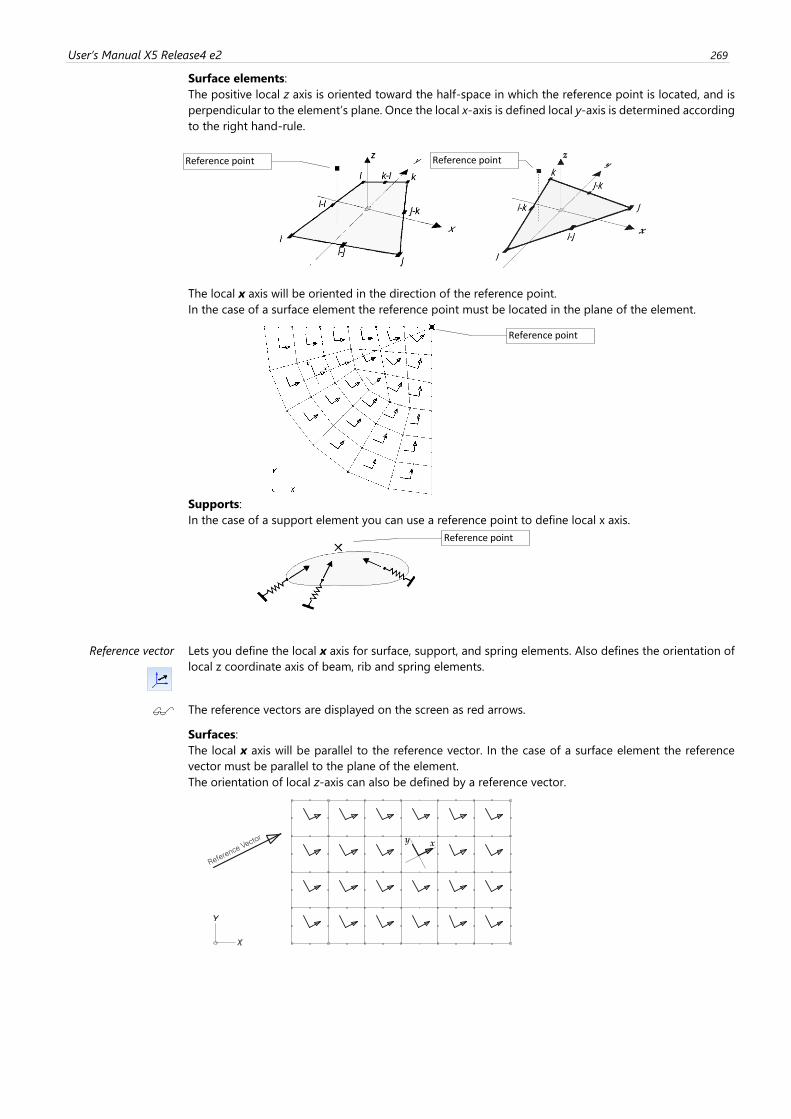
User’s Manual X5 Release4 e2 269

Surface elements:

The positive local z axis is oriented toward the half-space in which the reference point is located, and is

perpendicular to the element’s plane. Once the local x-axis is defined local y-axis is determined according

to the right hand-rule.

The local x axis will be oriented in the direction of the reference point.

In the case of a surface element the reference point must be located in the plane of the element.

Supports:

In the case of a support element you can use a reference point to define local x axis.

Reference vector

Lets you define the local x axis for surface, support, and spring elements. Also defines the orientation of

local z coordinate axis of beam, rib and spring elements.

The reference vectors are displayed on the screen as red arrows.

Surfaces:

The local x axis will be parallel to the reference vector. In the case of a surface element the reference

vector must be parallel to the plane of the element.

The orientation of local z-axis can also be defined by a reference vector.

Reference point Reference point

Reference point

Reference point

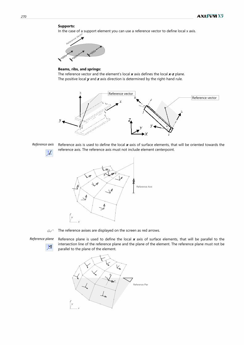
270

Supports:

In the case of a support element you can use a reference vector to define local x axis.

Beams, ribs, and springs:

The reference vector and the element’s local x axis defines the local x-z plane.

The positive local y and z axis direction is determined by the right-hand rule.

Reference axis

Reference axis is used to define the local x-axis of surface elements, that will be oriented towards the

reference axis. The reference axis must not include element centerpoint.

The reference axises are displayed on the screen as red arrows.

Reference plane

Reference plane is used to define the local x axis of surface elements, that will be parallel to the

intersection line of the reference plane and the plane of the element. The reference plane must not be

parallel to the plane of the element.

Reference vector

Reference vector

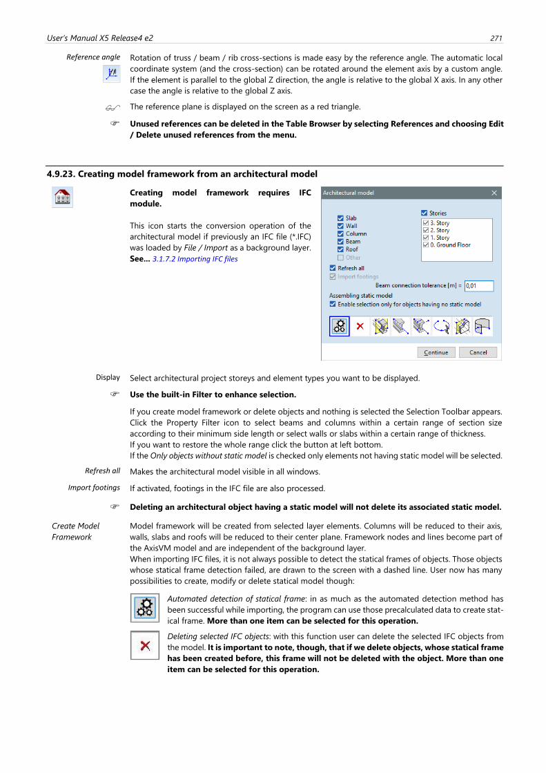
User’s Manual X5 Release4 e2 271

Reference angle

Rotation of truss / beam / rib cross-sections is made easy by the reference angle. The automatic local

coordinate system (and the cross-section) can be rotated around the element axis by a custom angle.

If the element is parallel to the global Z direction, the angle is relative to the global X axis. In any other

case the angle is relative to the global Z axis.

The reference plane is displayed on the screen as a red triangle.

Unused references can be deleted in the Table Browser by selecting References and choosing Edit

/ Delete unused references from the menu.

4.9.23. Creating model framework from an architectural model

Creating model framework requires IFC

module.

This icon starts the conversion operation of the

architectural model if previously an IFC file (*.IFC)

was loaded by File / Import as a background layer.

See... 3.1.7.2 Importing IFC files

Display Select architectural project storeys and element types you want to be displayed.

Use the built-in Filter to enhance selection.

If you create model framework or delete objects and nothing is selected the Selection Toolbar appears.

Click the Property Filter icon to select beams and columns within a certain range of section size

according to their minimum side length or select walls or slabs within a certain range of thickness.

If you want to restore the whole range click the button at left bottom.

If the Only objects without static model is checked only elements not having static model will be selected.

Refresh all Makes the architectural model visible in all windows.

Import footings If activated, footings in the IFC file are also processed.

Deleting an architectural object having a static model will not delete its associated static model.

Create Model

Framework

Model framework will be created from selected layer elements. Columns will be reduced to their axis,

walls, slabs and roofs will be reduced to their center plane. Framework nodes and lines become part of

the AxisVM model and are independent of the background layer.

When importing IFC files, it is not always possible to detect the statical frames of objects. Those objects

whose statical frame detection failed, are drawn to the screen with a dashed line. User now has many

possibilities to create, modify or delete statical model though:

Automated detection of statical frame: in as much as the automated detection method has

been successful while importing, the program can use those precalculated data to create stat-

ical frame. More than one item can be selected for this operation.

Deleting selected IFC objects: with this function user can delete the selected IFC objects from

the model. It is important to note, though, that if we delete objects, whose statical frame

has been created before, this frame will not be deleted with the object. More than one

item can be selected for this operation.

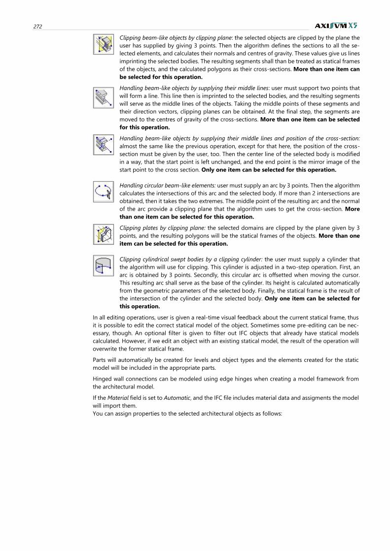
272

Clipping beam-like objects by clipping plane: the selected objects are clipped by the plane the

user has supplied by giving 3 points. Then the algorithm defines the sections to all the se-

lected elements, and calculates their normals and centres of gravity. These values give us lines

imprinting the selected bodies. The resulting segments shall than be treated as statical frames

of the objects, and the calculated polygons as their cross-sections. More than one item can

be selected for this operation.

Handling beam-like objects by supplying their middle lines: user must support two points that

will form a line. This line then is imprinted to the selected bodies, and the resulting segments

will serve as the middle lines of the objects. Taking the middle points of these segments and

their direction vectors, clipping planes can be obtained. At the final step, the segments are

moved to the centres of gravity of the cross-sections. More than one item can be selected

for this operation.

Handling beam-like objects by supplying their middle lines and position of the cross-section:

almost the same like the previous operation, except for that here, the position of the cross-

section must be given by the user, too. Then the center line of the selected body is modified

in a way, that the start point is left unchanged, and the end point is the mirror image of the

start point to the cross section. Only one item can be selected for this operation.

Handling circular beam-like elements: user must supply an arc by 3 points. Then the algorithm

calculates the intersections of this arc and the selected body. If more than 2 intersections are

obtained, then it takes the two extremes. The middle point of the resulting arc and the normal

of the arc provide a clipping plane that the algorithm uses to get the cross-section. More

than one item can be selected for this operation.

Clipping plates by clipping plane: the selected domains are clipped by the plane given by 3

points, and the resulting polygons will be the statical frames of the objects. More than one

item can be selected for this operation.

Clipping cylindrical swept bodies by a clipping cylinder: the user must supply a cylinder that

the algorithm will use for clipping. This cylinder is adjusted in a two-step operation. First, an

arc is obtained by 3 points. Secondly, this circular arc is offsetted when moving the cursor.

This resulting arc shall serve as the base of the cylinder. Its height is calculated automatically

from the geometric parameters of the selected body. Finally, the statical frame is the result of

the intersection of the cylinder and the selected body. Only one item can be selected for

this operation.

In all editing operations, user is given a real-time visual feedback about the current statical frame, thus

it is possible to edit the correct statical model of the object. Sometimes some pre-editing can be nec-

essary, though. An optional filter is given to filter out IFC objects that already have statical models

calculated. However, if we edit an object with an existing statical model, the result of the operation will

overwrite the former statical frame.

Parts will automatically be created for levels and object types and the elements created for the static

model will be included in the appropriate parts.

Hinged wall connections can be modeled using edge hinges when creating a model framework from

the architectural model.

If the Material field is set to Automatic, and the IFC file includes material data and assigments the model

will import them.

You can assign properties to the selected architectural objects as follows:

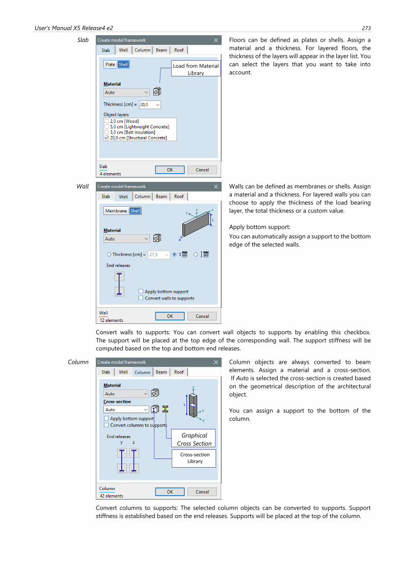
User’s Manual X5 Release4 e2 273

Slab

Floors can be defined as plates or shells. Assign a

material and a thickness. For layered floors, the

thickness of the layers will appear in the layer list. You

can select the layers that you want to take into

account.

Wall

Walls can be defined as membranes or shells. Assign

a material and a thickness. For layered walls you can

choose to apply the thickness of the load bearing

layer, the total thickness or a custom value.

Apply bottom support:

You can automatically assign a support to the bottom

edge of the selected walls.

Convert walls to supports: You can convert wall objects to supports by enabling this checkbox.

The support will be placed at the top edge of the corresponding wall. The support stiffness will be

computed based on the top and bottom end releases.

Column

Column objects are always converted to beam

elements. Assign a material and a cross-section.

If Auto is selected the cross-section is created based

on the geometrical description of the architectural

object.

You can assign a support to the bottom of the

column.

Convert columns to supports: The selected column objects can be converted to supports. Support

stiffness is established based on the end releases. Supports will be placed at the top of the column.

Load from Material

Library

Cross-section Library

Graphical

Cross Section

Editor

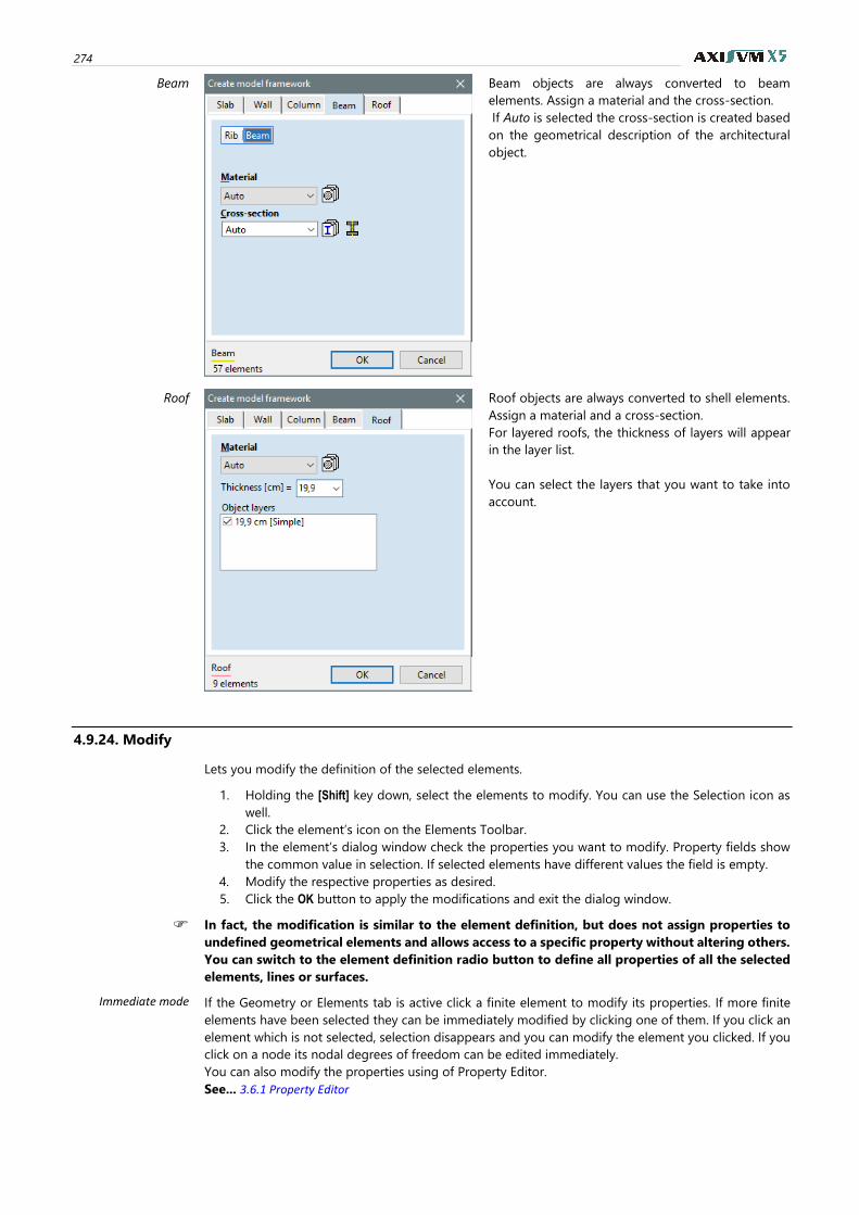
274

Beam

Beam objects are always converted to beam

elements. Assign a material and the cross-section.

If Auto is selected the cross-section is created based

on the geometrical description of the architectural

object.

Roof

Roof objects are always converted to shell elements.

Assign a material and a cross-section.

For layered roofs, the thickness of layers will appear

in the layer list.

You can select the layers that you want to take into

account.

4.9.24. Modify

Lets you modify the definition of the selected elements.

1. Holding the [Shift] key down, select the elements to modify. You can use the Selection icon as

well.

2. Click the element’s icon on the Elements Toolbar.

3. In the element’s dialog window check the properties you want to modify. Property fields show

the common value in selection. If selected elements have different values the field is empty.

4. Modify the respective properties as desired.

5. Click the OK button to apply the modifications and exit the dialog window.

In fact, the modification is similar to the element definition, but does not assign properties to

undefined geometrical elements and allows access to a specific property without altering others.

You can switch to the element definition radio button to define all properties of all the selected

elements, lines or surfaces.

Immediate mode If the Geometry or Elements tab is active click a finite element to modify its properties. If more finite

elements have been selected they can be immediately modified by clicking one of them. If you click an

element which is not selected, selection disappears and you can modify the element you clicked. If you

click on a node its nodal degrees of freedom can be edited immediately.

You can also modify the properties using of Property Editor.

See... 3.6.1 Property Editor

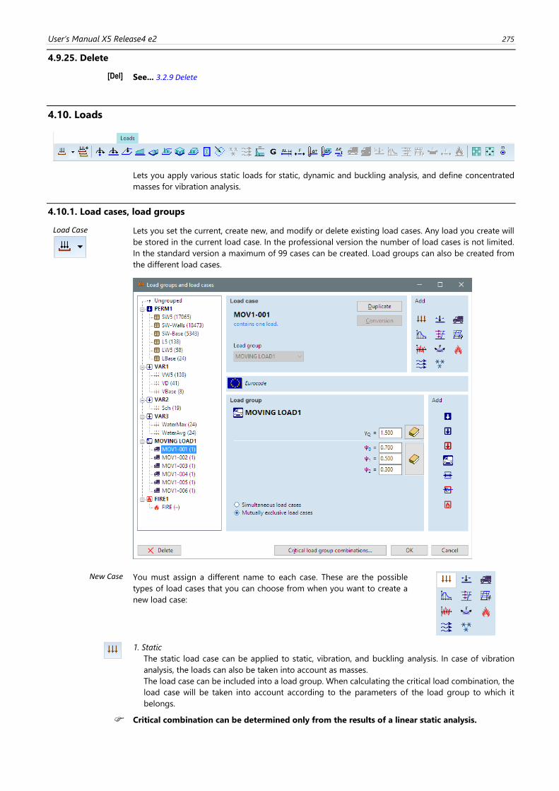
User’s Manual X5 Release4 e2 275

4.9.25. Delete

[Del] See... 3.2.9 Delete

4.10. Loads

Lets you apply various static loads for static, dynamic and buckling analysis, and define concentrated

masses for vibration analysis.

4.10.1. Load cases, load groups

Load Case

Lets you set the current, create new, and modify or delete existing load cases. Any load you create will

be stored in the current load case. In the professional version the number of load cases is not limited.

In the standard version a maximum of 99 cases can be created. Load groups can also be created from

the different load cases.

New Case You must assign a different name to each case. These are the possible

types of load cases that you can choose from when you want to create a

new load case:

1. Static

The static load case can be applied to static, vibration, and buckling analysis. In case of vibration

analysis, the loads can also be taken into account as masses.

The load case can be included into a load group. When calculating the critical load combination, the

load case will be taken into account according to the parameters of the load group to which it

belongs.

Critical combination can be determined only from the results of a linear static analysis.

276

2. Influence line

Lets you apply a relative displacement load to obtain the influence line of a result component, of a

truss or beam element.

When the influence line load case type is selected you can apply only the influence line load.

3. Moving load

In this type of load case only moving (line or surface) loads can be defined. When defining a moving

load a group of new load cases will be created. The number of these load cases is equal to the number

of steps specified in the moving load definition dialog. Their name is created automatically like

MOV_xx. As they get into a load group the most unfavorable effect of the moving load can be checked

displaying the result of the critical combination. These auto-created load cases can be moved to-

gether only and only into another moving load group.

If more than one moving load is applied in the same load case the number of steps (and auto-created

load cases) will be equal to the maximum number of steps specified. If the maximum number of steps

is k, and another moving load has i steps (i < k), then this load will remain at the end of the path in

steps i+1, i+2, …, k.

See details... 4.10.27 Moving loads

Moving load cases can be placed only in moving load groups. Static loads can also be defined in

moving load cases. They will be present in all steps but only in moving load cases.

4. Seismic (SE1 module is required)

When selecting seismic load case type you can specify the parameters for calculation of earthquake

loads. Prior to creating an seismic load case, you must perform a vibration analysis. Based on the

mode shapes, and on the structural masses, AxisVM generates seismic loads case, in a k+2 number,

where k is the number of available smallest frequencies. The two additional cases corresponds to

the signs +, and -, that contain the critical combinations.

Multiple seismic actions can be defined for the structure. Seismic actions cannot be combined.

See details... 4.10.23 Seismic loads – SE1 module

When selecting seismic load case the only icon available on the Toolbar will be Seismic para-

meters.

5. Pushover (SE2 module is required)

When selecting pushover load case type you can specify parameters for generating load distributions

that can be used in pushover analyses. Prior to creating a pushover load case, you must perform

vibration analysis. Based on specified mode shapes AxisVM generates nodal forces on each node of

the model. A total of four load cases are generated initially. They represent a uniform (U) and a modal

(M) distribution in the direction of each of the horizontal axes (X and Y by default). The uniform load

distribution option generates nodal forces proportional to the masses assigned to each node in the

model. The modal load distribution uses the mode shape weighed by the masses at each node to

generate the nodal force distribution. In both cases the sum of forces generated is 1 kN in the same

horizontal direction.

See details… 4.10.24 Pushover loads – SE2 module

When selecting pushover load case the only icon available on the Toolbar will be Pushover

parameters.

6. Global imperfection

If an imperfection load case is created it is automatically placed into an imperfection load group

which can contain only imperfection load cases. This load group has no parameters and is automati-

cally deleted if their load cases are deleted. Imperfection load cases can be used in nonlinear analysis

with geometric nonlinearity. When generating critical ULS load combinations in the load combination

table imperfection load cases can be included. Load combinations including an imperfection load

case require nonlinear analysis with geometric nonlinearity.

See details … 4.10.25 Global imperfection

Imperfection load cases does not contribute to critical combinations of linear analysis results.

7. Tensioning (PS1 module is required)

If tensioning calculation according to the current design code is supported, tensioning load cases can

be created. These load cases always get into a tensioning load group. After defining a load case with

the name name, two load cases will be created. name-T0 will contain the equivalent load calculated

for the end of tensioning process, name-TI will contain long term values of the equivalent load. Any

of these load cases can be selected to define tensioning. After definition just loads for name-T0 will

User’s Manual X5 Release4 e2 277

be calculated as static analysis results are required to determine the long term equivalent loads. See

details… 4.10.26 Tensioning - PS1 module

When selecting tensioning load case the only icon available on the Toolbar will be Tensioning.

8. Dynamic load case (DYN module is required)

After defining a dynamic load case and selecting it the Loads tab will allow definition of dynamic

loads and nodal acceleration.

See details…4.10.28 Dynamic loads (for time-history analysis) – DYN module

Dynamic load cases cannot be included in load groups and load combinations. Loads within dy-

namic load cases will be applied only in Dynamic analysis.

9. Snow load cases (SWG module is required)

AxisVM can calculate and apply snow loads on the structure. The limits of automatic snow load gen-

eration in the program are explained in 4.10.13 Snow load – SWG module.

Snow loads can be placed on flat load panels in arbitrary planes. As a first step a temporary snow

load case is created in the snow load group and its name can be set. If the design code requires

verification for exceptional snow load, an exceptional snow load case is also created in an exceptional

snow load group (except for exceptional snow loads as per Annex B of Eurocode 1-3). After defining

load panels and setting the snow load parameters the program replaces the temporary load case

with automatically generated snow load cases.

The undrifted load case receives a UD suffix. Drifted load cases receive a D suffix with 2-4 extra char-

acters. These characters indicate the wind direction (X+, X–, Y+, Y–). Besides winds parallel to the

coordinate axes, winds in 45°+n*90° directions (where n = 0, 1, 2, 3) are also taken into account and

are indicated by the quadrant where the wind speed vector points to. X+Y– refers to a wind in the

315° direction for example (0° being defined by the positive X axis, and angles measured counter-

clockwise).

Only the necessary load cases are created by the algorithm, therefore the number of load cases and

their type depends on the type of structure under consideration and the snow load parameters given

by the user. Load parameters shall be defined after closing the Load Cases Dialogue by clicking on

the Snow Load icon in the Toolbar. Before this step it is recommended to define load panels of the

roof using the Load Panels icon in the Toolbar.

For details of snow load generation see… 4.10.13 Snow load – SWG module.

If a snow load case is selected only two buttons are enabled on the Loads toolbar. These are the

the load panel and snow load definition.

10. Wind load cases (SWG module is required)

During parametric definition of wind loads it is necessary define one or more substructures exposed

to wind. If Separate load cases for each substructure is checked wind loads of different substructures

will be generated into different load cases. Otherwise load cases will contain wind loads for more

substructures.

Calculated wind loads are reliable only for certain building types as described in the design code. It

is recommended to use these automatic methods only for geometries within the limits explained in

detail at 4.10.14 Wind load – SWG module. Wind loads can be placed on flat load panels in arbitrary

planes. As a first step a temporary wind load case is created in the wind load group and the name of

the wind load case can be set. After defining load panels and setting the wind load parameters the

program replaces the temporary load case with automatically generated wind load cases.

Wind load cases are generated with a name code corresponding to the loading situation.

The first two characters after the name of the load case describe the wind direction (X+, X–, Y+, Y–).

The logic behind this notation is the same as for snow loads. The next one or two characters denote

the type of wind action.

P and S denote pressure and suction, respectively. For pitched roofs the design code requires to check

all possible combinations of wind actions on the two sides of the roof. Therefore, for pitched roofs

Pp, Ps, Sp and Ss load cases are created. Here the first character refers to the windswept side, the

second one refers to the sheltered side. For special torsion actions T+ and T– are used referring to

the two different torsion directions.

The last character denotes the type of internal action. The internal wind actions are ignored for O; P

stands for internal pressure, S stands for internal suction. These load cases are needed only if no

further information is available on internal pressure so a positive and a negative critical value must

be used as an approximation on the conservative side. If the last character is C, the load case was

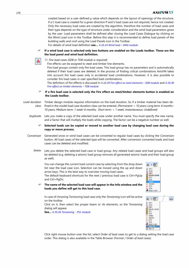
278

created based on a user-defined μ value which depends on the layout of openings of the structure.

If a C load case is created for a given direction P and S load cases are not required, hence not created.

Only the necessary load cases are created by the algorithm, therefore the number of load cases and

their type depends on the type of structure under consideration and the wind load parameters given

by the user. Load parameters shall be defined after closing the Load Cases Dialogue by clicking on

the Wind Load icon in the Toolbar. Before this step it is recommended to define load panels of the

building walls and roof using the Load Panels icon in the Toolbar.

For details of wind load definition see… 4.10.14 Wind load – SWG module.

If a wind load case is selected only two buttons are enabled on the Loads toolbar. These are the

the load panel and wind load definition.

11. Fire load cases (SD8 or TD8 module is required)

Fire effects can be assigned to steel and timber line elements.

Fire load groups contain only fire load cases. This load group has no parameters and is automatically

deleted if their load cases are deleted. In the process of finding critical combinations AxisVM takes

into account fire load cases only in accidental load combinations. However, it is also possible to

consider fire load cases in user specified load combinations.

The definition of fire effects is discussed in 4.10.29 Fire effect on steel elements – SD8 module and 4.10.30 Fire effect on timber elements – TD8 module

If a fire load case is selected only the Fire effect on steel/timber elements button is enabled on

the Loads toolbar.

Load-duration

class

Timber design module requires information on the load duration. So if a timber material has been de-

fined in the model load case duration class can be entered. (Permanent: > 10 years; Long term: 6 months–

10 years; Medium term: 1 week–6 months; Short term: < 1 week; Instantaneous; Undefined)

Duplicate Lets you make a copy of the selected load case under another name. You must specify the new name,

and a factor that will multiply the loads while copying. The factor can be a negative number as well.

Selected loads can be copied or moved to another load case by changing load case during the

copy or move process.

Conversion Generated snow or wind load cases can be converted to regular load cases by clicking the Conversion

button. All load cases of the selected type will be converted. After conversion converted loads and load

cases can be deleted and modified.

Delete Lets you delete the selected load case or load group. Any related load cases and load groups will also

be deleted (e.g. deleting a seismic load group removes all generated seismic loads and their load group

as well).

You can change the current load current case by selecting from the drop down

list near the load case icon. Selection can be moved using the up and down

arrow keys. This is the best way to overview moving load cases.

The default keyboard shortcuts for the next / previous load case is Ctrl+PgUp

and Ctrl+PgDn.

The name of the selected load case will appear in the Info window and the

loads you define will get to this load case.

In case of choosing Tensioning load case only the Tensioning icon will be active

on the toolbar.

Click on it, then select the proper beam or rib elements, so the Tensioning

dialog will appear.

See... 4.10.26 Tensioning - PS1 module

Click right mouse button over the list, select Order of load cases to get to a dialog setting the load case

order. This dialog is also available in the Table Browser (Format / Order of load cases).

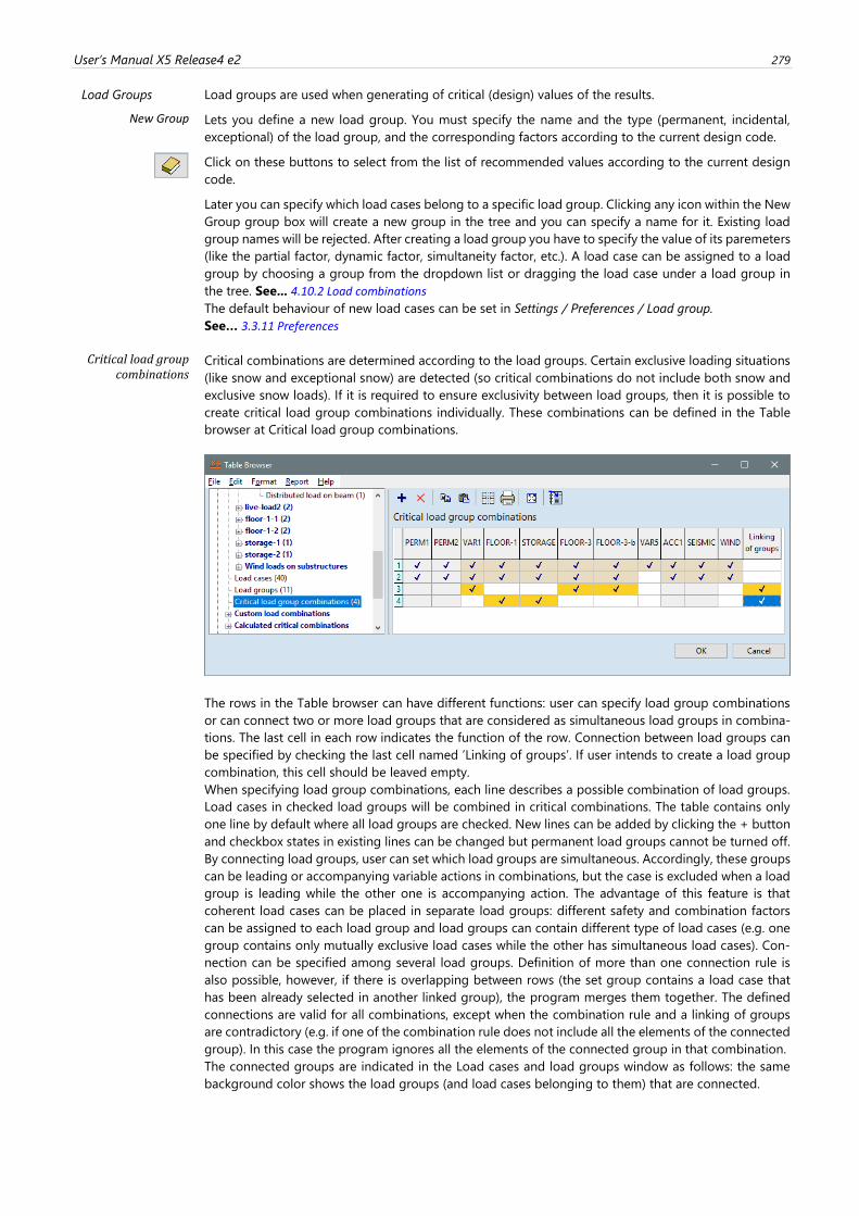
User’s Manual X5 Release4 e2 279

Load Groups Load groups are used when generating of critical (design) values of the results.

New Group

Lets you define a new load group. You must specify the name and the type (permanent, incidental,

exceptional) of the load group, and the corresponding factors according to the current design code.

Click on these buttons to select from the list of recommended values according to the current design

code.

Later you can specify which load cases belong to a specific load group. Clicking any icon within the New

Group group box will create a new group in the tree and you can specify a name for it. Existing load

group names will be rejected. After creating a load group you have to specify the value of its paremeters

(like the partial factor, dynamic factor, simultaneity factor, etc.). A load case can be assigned to a load

group by choosing a group from the dropdown list or dragging the load case under a load group in

the tree. See... 4.10.2 Load combinations

The default behaviour of new load cases can be set in Settings / Preferences / Load group.

See… 3.3.11 Preferences

Critical load group combinations

Critical combinations are determined according to the load groups. Certain exclusive loading situations

(like snow and exceptional snow) are detected (so critical combinations do not include both snow and

exclusive snow loads). If it is required to ensure exclusivity between load groups, then it is possible to

create critical load group combinations individually. These combinations can be defined in the Table

browser at Critical load group combinations.

The rows in the Table browser can have different functions: user can specify load group combinations

or can connect two or more load groups that are considered as simultaneous load groups in combina-

tions. The last cell in each row indicates the function of the row. Connection between load groups can

be specified by checking the last cell named ’Linking of groups’. If user intends to create a load group

combination, this cell should be leaved empty. When specifying load group combinations, each line describes a possible combination of load groups.

Load cases in checked load groups will be combined in critical combinations. The table contains only

one line by default where all load groups are checked. New lines can be added by clicking the + button

and checkbox states in existing lines can be changed but permanent load groups cannot be turned off.

By connecting load groups, user can set which load groups are simultaneous. Accordingly, these groups

can be leading or accompanying variable actions in combinations, but the case is excluded when a load

group is leading while the other one is accompanying action. The advantage of this feature is that

coherent load cases can be placed in separate load groups: different safety and combination factors

can be assigned to each load group and load groups can contain different type of load cases (e.g. one

group contains only mutually exclusive load cases while the other has simultaneous load cases). Con-

nection can be specified among several load groups. Definition of more than one connection rule is

also possible, however, if there is overlapping between rows (the set group contains a load case that

has been already selected in another linked group), the program merges them together. The defined

connections are valid for all combinations, except when the combination rule and a linking of groups

are contradictory (e.g. if one of the combination rule does not include all the elements of the connected

group). In this case the program ignores all the elements of the connected group in that combination.

The connected groups are indicated in the Load cases and load groups window as follows: the same

background color shows the load groups (and load cases belonging to them) that are connected.

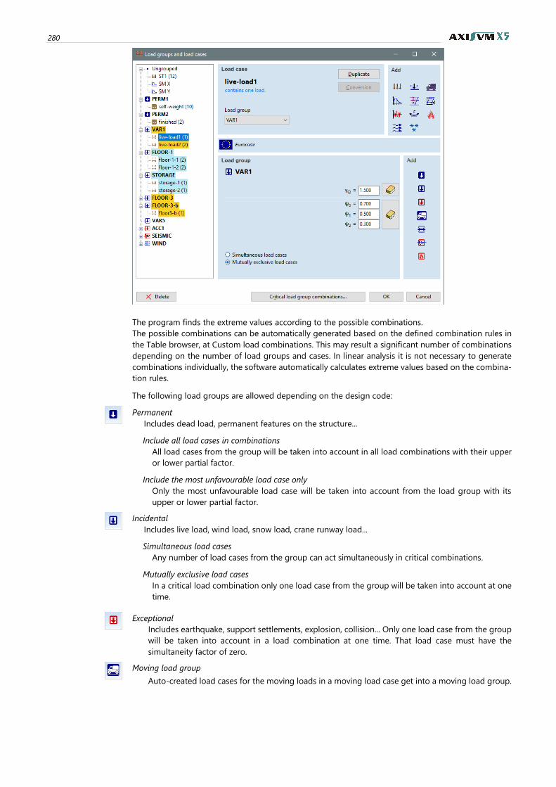
280

The program finds the extreme values according to the possible combinations. The possible combinations can be automatically generated based on the defined combination rules in

the Table browser, at Custom load combinations. This may result a significant number of combinations

depending on the number of load groups and cases. In linear analysis it is not necessary to generate

combinations individually, the software automatically calculates extreme values based on the combina-

tion rules.

The following load groups are allowed depending on the design code:

Permanent

Includes dead load, permanent features on the structure...

Include all load cases in combinations

All load cases from the group will be taken into account in all load combinations with their upper

or lower partial factor.

Include the most unfavourable load case only

Only the most unfavourable load case will be taken into account from the load group with its

upper or lower partial factor.

Incidental

Includes live load, wind load, snow load, crane runway load...

Simultaneous load cases

Any number of load cases from the group can act simultaneously in critical combinations.

Mutually exclusive load cases

In a critical load combination only one load case from the group will be taken into account at one

time.

Exceptional

Includes earthquake, support settlements, explosion, collision... Only one load case from the group

will be taken into account in a load combination at one time. That load case must have the

simultaneity factor of zero.

Moving load group

Auto-created load cases for the moving loads in a moving load case get into a moving load group.

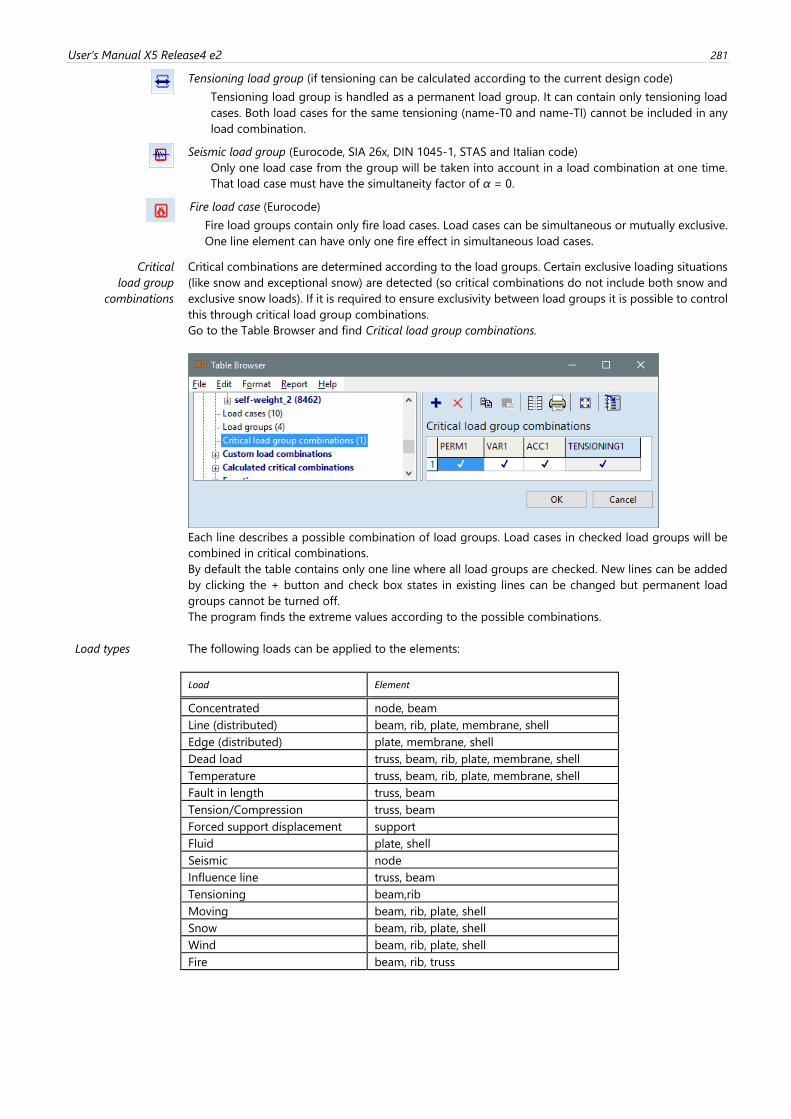
User’s Manual X5 Release4 e2 281

Tensioning load group (if tensioning can be calculated according to the current design code)

Tensioning load group is handled as a permanent load group. It can contain only tensioning load

cases. Both load cases for the same tensioning (name-T0 and name-TI) cannot be included in any

load combination.

Seismic load group (Eurocode, SIA 26x, DIN 1045-1, STAS and Italian code)

Only one load case from the group will be taken into account in a load combination at one time.

That load case must have the simultaneity factor of α = 0.

Fire load case (Eurocode)

Fire load groups contain only fire load cases. Load cases can be simultaneous or mutually exclusive.

One line element can have only one fire effect in simultaneous load cases.

Critical

load group

combinations

Critical combinations are determined according to the load groups. Certain exclusive loading situations

(like snow and exceptional snow) are detected (so critical combinations do not include both snow and

exclusive snow loads). If it is required to ensure exclusivity between load groups it is possible to control

this through critical load group combinations.

Go to the Table Browser and find Critical load group combinations.

Each line describes a possible combination of load groups. Load cases in checked load groups will be

combined in critical combinations.

By default the table contains only one line where all load groups are checked. New lines can be added

by clicking the + button and check box states in existing lines can be changed but permanent load

groups cannot be turned off.

The program finds the extreme values according to the possible combinations.

Load types The following loads can be applied to the elements:

Load Element

Concentrated node, beam

Line (distributed) beam, rib, plate, membrane, shell

Edge (distributed) plate, membrane, shell

Dead load truss, beam, rib, plate, membrane, shell

Temperature truss, beam, rib, plate, membrane, shell

Fault in length truss, beam

Tension/Compression truss, beam

Forced support displacement support

Fluid plate, shell

Seismic node

Influence line truss, beam

Tensioning beam,rib

Moving beam, rib, plate, shell

Snow beam, rib, plate, shell

Wind beam, rib, plate, shell

Fire beam, rib, truss

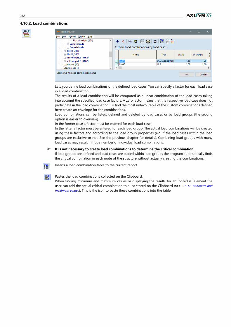
282

4.10.2. Load combinations

Lets you define load combinations of the defined load cases. You can specify a factor for each load case

in a load combination.

The results of a load combination will be computed as a linear combination of the load cases taking

into account the specified load case factors. A zero factor means that the respective load case does not

participate in the load combination. To find the most unfavourable of the custom combinations defined

here create an envelope for the combinations.

Load combinations can be listed, defined and deleted by load cases or by load groups (the second

option is easier to overview).

In the former case a factor must be entered for each load case.

In the latter a factor must be entered for each load group. The actual load combinations will be created

using these factors and according to the load group properties (e.g. if the load cases within the load

groups are exclusive or not. See the previous chapter for details). Combining load groups with many

load cases may result in huge number of individual load combinations.

It is not necessary to create load combinations to determine the critical combination.

If load groups are defined and load cases are placed within load groups the program automatically finds

the critical combination in each node of the structure without actually creating the combinations.

Inserts a load combination table to the current report.

Pastes the load combinations collected on the Clipboard.

When finding minimum and maximum values or displaying the results for an individual element the

user can add the actual critical combination to a list stored on the Clipboard (see… 6.1.1 Minimum and

maximum values). This is the icon to paste these combinations into the table.

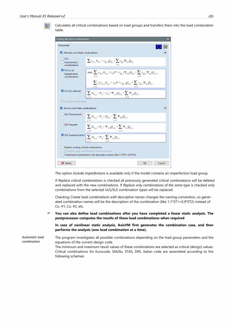
User’s Manual X5 Release4 e2 283

Calculates all critical combinations based on load groups and transfers them into the load combination

table.

The option Include imperfections is available only if the model contains an imperfection load group.

If Replace critical combinations is checked all previously generated critical combinations will be deleted

and replaced with the new combinations. If Replace only combinations of the same type is checked only

combinations from the selected ULS/SLS combination types will be replaced.

Checking Create load combinations with descriptive names changes the naming convention, so gener-

ated combination names will be the description of the combination (like 1.1*ST1+0.9*ST2) instead of

Co. #1, Co. #2, etc.

You can also define load combinations after you have completed a linear static analysis. The

postprocessor computes the results of these load combinations when required

In case of nonlinear static analysis, AxisVM first generates the combination case, and then

performs the analysis (one load combination at a time).

Automatic load combination

The program investigates all possible combinations depending on the load group parameters and the

equations of the current design code.

The minimum and maximum result values of these combinations are selected as critical (design) values.

Critical combinations for Eurocode, SIA26x, STAS, DIN, Italian code are assembled according to the

following schemes:

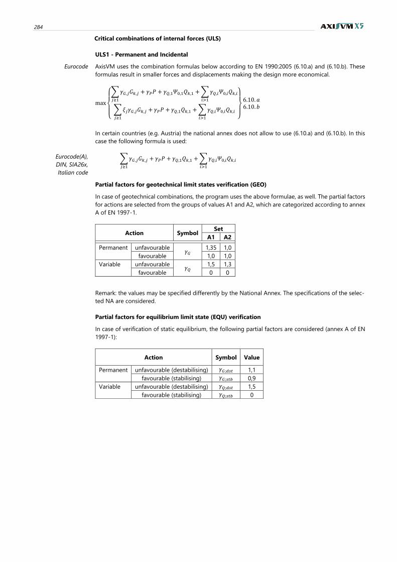
284

Critical combinations of internal forces (ULS)

ULS1 - Permanent and Incidental

Eurocode AxisVM uses the combination formulas below according to EN 1990:2005 (6.10.a) and (6.10.b). These

formulas result in smaller forces and displacements making the design more economical.

max

{

∑𝛾𝐺,𝑗𝐺𝑘,𝑗 + 𝛾𝑃𝑃 + 𝛾𝑄,1𝛹0,1𝑄𝑘,1 +∑𝛾𝑄,𝑖𝛹0,𝑖𝑄𝑘,𝑖

𝑖>1𝑗≥1

∑𝜉𝑗𝛾𝐺,𝑗𝐺𝑘,𝑗 + 𝛾𝑃𝑃 + 𝛾𝑄,1𝑄𝑘,1 +∑𝛾𝑄,𝑖𝛹0,𝑖𝑄𝑘,𝑖𝑖>1𝑗≥1 }

6.10. 𝑎6.10. 𝑏

In certain countries (e.g. Austria) the national annex does not allow to use (6.10.a) and (6.10.b). In this

case the following formula is used:

Eurocode(A),

DIN, SIA26x,

Italian code

∑𝛾𝐺,𝑗𝐺𝑘,𝑗 + 𝛾𝑃𝑃 + 𝛾𝑄,1𝑄𝑘,1 +∑𝛾𝑄,𝑖𝛹0,𝑖𝑄𝑘,𝑖𝑖>1𝑗≥1

Partial factors for geotechnical limit states verification (GEO)

In case of geotechnical combinations, the program uses the above formulae, as well. The partial factors

for actions are selected from the groups of values A1 and A2, which are categorized according to annex

A of EN 1997-1.

Action Symbol Set

A1 A2

Permanent unfavourable 𝛾𝐺

1,35 1,0

favourable 1,0 1,0

Variable unfavourable 𝛾𝑄

1,5 1,3

favourable 0 0

Remark: the values may be specified differently by the National Annex. The specifications of the selec-

ted NA are considered.

Partial factors for equilibrium limit state (EQU) verification

In case of verification of static equilibrium, the following partial factors are considered (annex A of EN

1997-1):

Action Symbol Value

Permanent unfavourable (destabilising) 𝛾𝐺;𝑑𝑠𝑡 1,1

favourable (stabilising) 𝛾𝐺;𝑠𝑡𝑏 0,9

Variable unfavourable (destabilising) 𝛾𝑄;𝑑𝑠𝑡 1,5

favourable (stabilising) 𝛾𝑄;𝑠𝑡𝑏 0

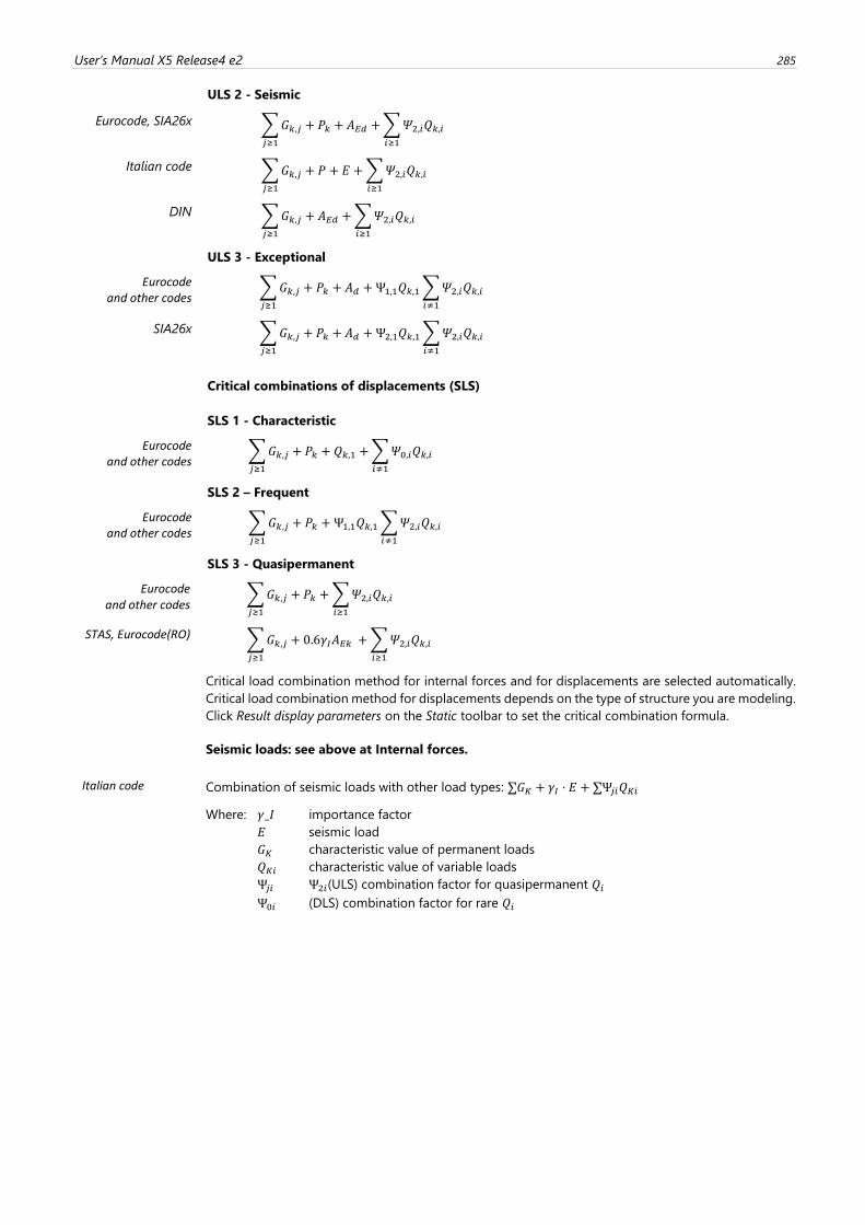
User’s Manual X5 Release4 e2 285

ULS 2 - Seismic

Eurocode, SIA26x ∑𝐺𝑘,𝑗 + 𝑃𝑘 + 𝐴𝐸𝑑 +∑𝛹2,𝑖𝑄𝑘,𝑖𝑖≥1𝑗≥1

Italian code ∑𝐺𝑘,𝑗 + 𝑃 + 𝐸 +∑𝛹2,𝑖𝑄𝑘,𝑖𝑖≥1𝑗≥1

DIN ∑𝐺𝑘,𝑗 + 𝐴𝐸𝑑 +∑𝛹2,𝑖𝑄𝑘,𝑖𝑖≥1𝑗≥1

ULS 3 - Exceptional

Eurocode and other codes

∑𝐺𝑘,𝑗 + 𝑃𝑘 + 𝐴𝑑 +Ψ1,1𝑄𝑘,1∑𝛹2,𝑖𝑄𝑘,𝑖𝑖≠1𝑗≥1

SIA26x ∑𝐺𝑘,𝑗 + 𝑃𝑘 + 𝐴𝑑 +Ψ2,1𝑄𝑘,1∑𝛹2,𝑖𝑄𝑘,𝑖𝑖≠1𝑗≥1

Critical combinations of displacements (SLS)

SLS 1 - Characteristic

Eurocode and other codes

∑𝐺𝑘,𝑗 + 𝑃𝑘 + 𝑄𝑘,1 +∑𝛹0,𝑖𝑄𝑘,𝑖𝑖≠1𝑗≥1

SLS 2 – Frequent

Eurocode and other codes

∑𝐺𝑘,𝑗 + 𝑃𝑘 +Ψ1,1𝑄𝑘,1∑𝛹2,𝑖𝑄𝑘,𝑖𝑖≠1𝑗≥1

SLS 3 - Quasipermanent

Eurocode and other codes

∑𝐺𝑘,𝑗 + 𝑃𝑘 +∑𝛹2,𝑖𝑄𝑘,𝑖𝑖≥1𝑗≥1

STAS, Eurocode(RO) ∑𝐺𝑘,𝑗 + 0.6𝛾𝐼𝐴𝐸𝑘 +∑𝛹2,𝑖𝑄𝑘,𝑖𝑖≥1𝑗≥1

Critical load combination method for internal forces and for displacements are selected automatically.

Critical load combination method for displacements depends on the type of structure you are modeling.

Click Result display parameters on the Static toolbar to set the critical combination formula.

Seismic loads: see above at Internal forces.

Italian code Combination of seismic loads with other load types: ∑𝐺𝐾 + 𝛾𝐼 ⋅ 𝐸 + ∑Ψ𝑗𝑖𝑄𝐾𝑖

Where: 𝛾_𝐼 importance factor

𝐸 seismic load

𝐺𝐾 characteristic value of permanent loads

𝑄𝐾𝑖 characteristic value of variable loads

Ψ𝑗𝑖 Ψ2𝑖(ULS) combination factor for quasipermanent 𝑄𝑖

Ψ0𝑖 (DLS) combination factor for rare 𝑄𝑖

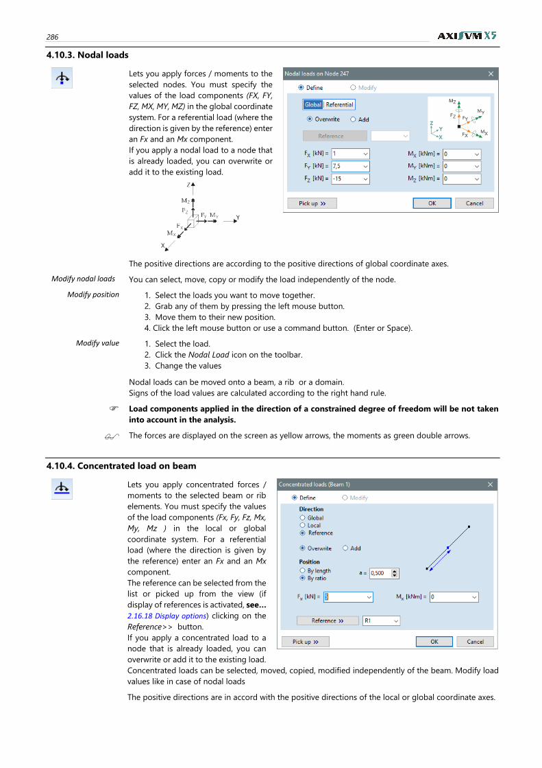
286

4.10.3. Nodal loads

Lets you apply forces / moments to the

selected nodes. You must specify the

values of the load components (FX, FY,

FZ, MX, MY, MZ) in the global coordinate

system. For a referential load (where the

direction is given by the reference) enter

an Fx and an Mx component.

If you apply a nodal load to a node that

is already loaded, you can overwrite or

add it to the existing load.

The positive directions are according to the positive directions of global coordinate axes.

Modify nodal loads You can select, move, copy or modify the load independently of the node.

Modify position 1. Select the loads you want to move together.

2. Grab any of them by pressing the left mouse button.

3. Move them to their new position.

4. Click the left mouse button or use a command button. (Enter or Space).

Modify value 1. Select the load.

2. Click the Nodal Load icon on the toolbar.

3. Change the values

Nodal loads can be moved onto a beam, a rib or a domain.

Signs of the load values are calculated according to the right hand rule.

Load components applied in the direction of a constrained degree of freedom will be not taken

into account in the analysis.

The forces are displayed on the screen as yellow arrows, the moments as green double arrows.

4.10.4. Concentrated load on beam

Lets you apply concentrated forces /

moments to the selected beam or rib

elements. You must specify the values

of the load components (Fx, Fy, Fz, Mx,

My, Mz ) in the local or global

coordinate system. For a referential

load (where the direction is given by

the reference) enter an Fx and an Mx

component.

The reference can be selected from the

list or picked up from the view (if

display of references is activated, see…

2.16.18 Display options) clicking on the

Reference>> button.

If you apply a concentrated load to a

node that is already loaded, you can

overwrite or add it to the existing load.

Concentrated loads can be selected, moved, copied, modified independently of the beam. Modify load

values like in case of nodal loads

The positive directions are in accord with the positive directions of the local or global coordinate axes.

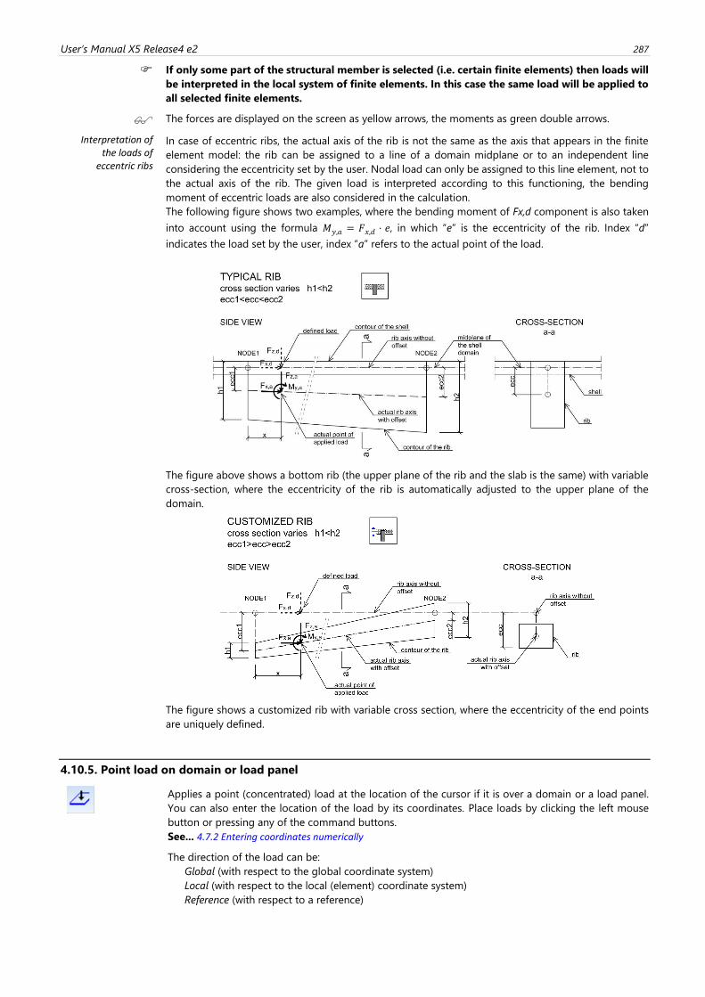
User’s Manual X5 Release4 e2 287

If only some part of the structural member is selected (i.e. certain finite elements) then loads will

be interpreted in the local system of finite elements. In this case the same load will be applied to

all selected finite elements.

The forces are displayed on the screen as yellow arrows, the moments as green double arrows.

Interpretation of the loads of

eccentric ribs

In case of eccentric ribs, the actual axis of the rib is not the same as the axis that appears in the finite

element model: the rib can be assigned to a line of a domain midplane or to an independent line

considering the eccentricity set by the user. Nodal load can only be assigned to this line element, not to

the actual axis of the rib. The given load is interpreted according to this functioning, the bending

moment of eccentric loads are also considered in the calculation.

The following figure shows two examples, where the bending moment of Fx,d component is also taken

into account using the formula 𝑀𝑦,𝑎 = 𝐹𝑥,𝑑 ⋅ 𝑒, in which “e” is the eccentricity of the rib. Index “d”

indicates the load set by the user, index “a” refers to the actual point of the load.

The figure above shows a bottom rib (the upper plane of the rib and the slab is the same) with variable

cross-section, where the eccentricity of the rib is automatically adjusted to the upper plane of the

domain.

The figure shows a customized rib with variable cross section, where the eccentricity of the end points

are uniquely defined.

4.10.5. Point load on domain or load panel

Applies a point (concentrated) load at the location of the cursor if it is over a domain or a load panel.

You can also enter the location of the load by its coordinates. Place loads by clicking the left mouse

button or pressing any of the command buttons.

See... 4.7.2 Entering coordinates numerically

The direction of the load can be:

Global (with respect to the global coordinate system)

Local (with respect to the local (element) coordinate system)

Reference (with respect to a reference)

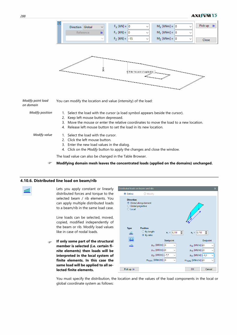
288

Modify point load on domain

You can modify the location and value (intensity) of the load:

Modify position 1. Select the load with the cursor (a load symbol appears beside the cursor).

2. Keep left mouse button depressed.

3. Move the mouse or enter the relative coordinates to move the load to a new location.

4. Release left mouse button to set the load in its new location.

Modify value 1. Select the load with the cursor.

2. Click the left mouse button.

3. Enter the new load values in the dialog.

4. Click on the Modify button to apply the changes and close the window.

The load value can also be changed in the Table Browser.

Modifying domain mesh leaves the concentrated loads (applied on the domains) unchanged.

4.10.6. Distributed line load on beam/rib

Lets you apply constant or linearly

distributed forces and torque to the

selected beam / rib elements. You

can apply multiple distributed loads

to a beam/rib in the same load case.

Line loads can be selected, moved,

copied, modified independently of

the beam or rib. Modify load values

like in case of nodal loads.

If only some part of the structural

member is selected (i.e. certain fi-

nite elements) then loads will be

interpreted in the local system of

finite elements. In this case the

same load will be applied to all se-

lected finite elements.

You must specify the distribution, the location and the values of the load components in the local or

global coordinate system as follows:

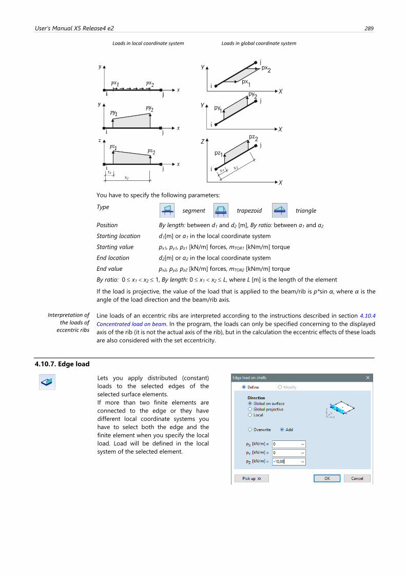
User’s Manual X5 Release4 e2 289

Loads in local coordinate system Loads in global coordinate system

You have to specify the following parameters:

Type

segment

trapezoid

triangle

Position By length: between d1 and d2 [m], By ratio: between a1 and a2

Starting location d1[m] or a1 in the local coordinate system

Starting value px1, py1, pz1 [kN/m] forces, mTOR1 [kNm/m] torque

End location d2[m] or a2 in the local coordinate system

End value px2, py2, pz2 [kN/m] forces, mTOR2 [kNm/m] torque

By ratio: 0 x1 x2 1, By length: 0 x1 x2 L, where L [m] is the length of the element

If the load is projective, the value of the load that is applied to the beam/rib is p*sin α, where α is the

angle of the load direction and the beam/rib axis.

Interpretation of the loads of

eccentric ribs

Line loads of an eccentric ribs are interpreted according to the instructions described in section 4.10.4

Concentrated load on beam. In the program, the loads can only be specified concerning to the displayed

axis of the rib (it is not the actual axis of the rib), but in the calculation the eccentric effects of these loads

are also considered with the set eccentricity.

4.10.7. Edge load

Lets you apply distributed (constant)

loads to the selected edges of the

selected surface elements.

If more than two finite elements are

connected to the edge or they have

different local coordinate systems you

have to select both the edge and the

finite element when you specify the local

load. Load will be defined in the local

system of the selected element.

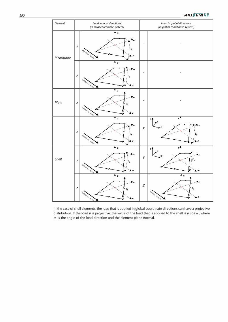
290

Element Load in local directions (in local coordinate system)

Load in global directions (in global coordinate system)

Membrane

x

-

-

y

-

-

Plate z

-

-

Shell

x

X

y

Y

z

Z

In the case of shell elements, the load that is applied in global coordinate directions can have a projective

distribution. If the load p is projective, the value of the load that is applied to the shell is p cos , where

is the angle of the load direction and the element plane normal.

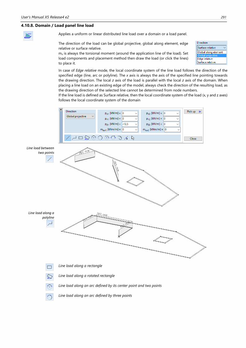
User’s Manual X5 Release4 e2 291

4.10.8. Domain / Load panel line load

Applies a uniform or linear distributed line load over a domain or a load panel.

The direction of the load can be global projective, global along element, edge

relative or surface relative.

mx is always the torsional moment (around the application line of the load). Set

load components and placement method then draw the load (or click the lines)

to place it.

In case of Edge relative mode, the local coordinate system of the line load follows the direction of the

specified edge (line, arc or polyline). The x axis is always the axis of the specified line pointing towards

the drawing direction. The local z axis of the load is parallel with the local z axis of the domain. When

placing a line load on an existing edge of the model, always check the direction of the resulting load, as

the drawing direction of the selected line cannot be determined from node numbers.

If the line load is defined as Surface relative, then the local coordinate system of the load (x, y and z axes)

follows the local coordinate system of the domain

Line load between two points

Line load along a polyline

Line load along a rectangle

Line load along a rotated rectangle

Line load along an arc defined by its center point and two points

Line load along an arc defined by three points

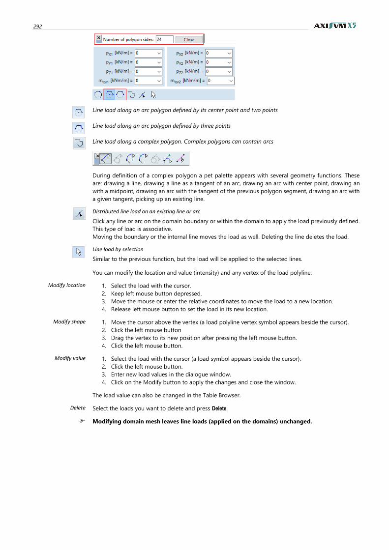
292

Line load along an arc polygon defined by its center point and two points

Line load along an arc polygon defined by three points

Line load along a complex polygon. Complex polygons can contain arcs

During definition of a complex polygon a pet palette appears with several geometry functions. These

are: drawing a line, drawing a line as a tangent of an arc, drawing an arc with center point, drawing an

with a midpoint, drawing an arc with the tangent of the previous polygon segment, drawing an arc with

a given tangent, picking up an existing line.

Distributed line load on an existing line or arc

Click any line or arc on the domain boundary or within the domain to apply the load previously defined.

This type of load is associative.

Moving the boundary or the internal line moves the load as well. Deleting the line deletes the load.

Line load by selection

Similar to the previous function, but the load will be applied to the selected lines.

You can modify the location and value (intensity) and any vertex of the load polyline:

Modify location 1. Select the load with the cursor.

2. Keep left mouse button depressed.

3. Move the mouse or enter the relative coordinates to move the load to a new location.

4. Release left mouse button to set the load in its new location.

Modify shape 1. Move the cursor above the vertex (a load polyline vertex symbol appears beside the cursor).

2. Click the left mouse button

3. Drag the vertex to its new position after pressing the left mouse button.

4. Click the left mouse button.

Modify value 1. Select the load with the cursor (a load symbol appears beside the cursor).

2. Click the left mouse button.

3. Enter new load values in the dialogue window.

4. Click on the Modify button to apply the changes and close the window.

The load value can also be changed in the Table Browser.

Delete Select the loads you want to delete and press Delete.

Modifying domain mesh leaves line loads (applied on the domains) unchanged.

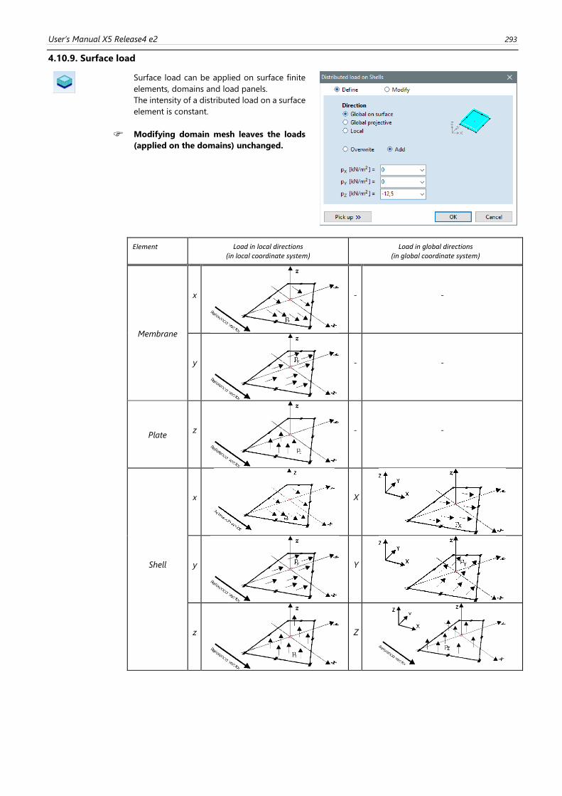
User’s Manual X5 Release4 e2 293

4.10.9. Surface load

Surface load can be applied on surface finite

elements, domains and load panels.

The intensity of a distributed load on a surface

element is constant.

Modifying domain mesh leaves the loads

(applied on the domains) unchanged.

Element Load in local directions (in local coordinate system)

Load in global directions (in global coordinate system)

Membrane

x

-

-

y

-

-

Plate

z

-

-

Shell

x

X

y

Y

z

Z

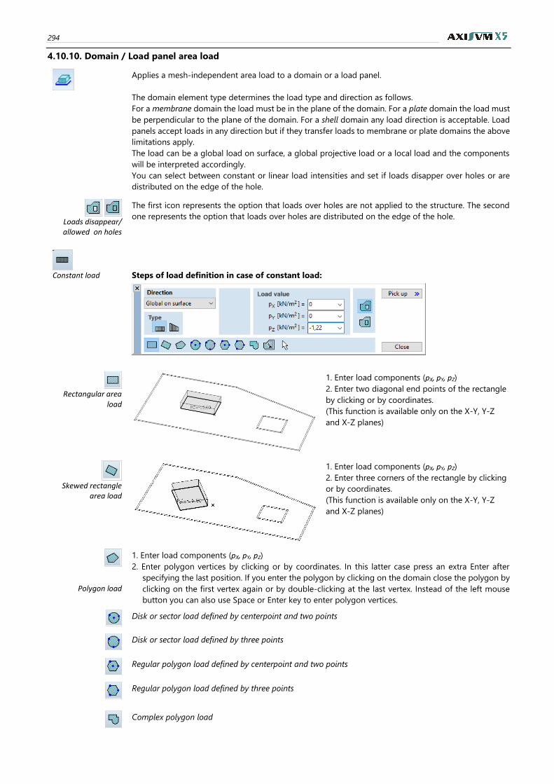
294

4.10.10. Domain / Load panel area load

Applies a mesh-independent area load to a domain or a load panel.

The domain element type determines the load type and direction as follows.

For a membrane domain the load must be in the plane of the domain. For a plate domain the load must

be perpendicular to the plane of the domain. For a shell domain any load direction is acceptable. Load

panels accept loads in any direction but if they transfer loads to membrane or plate domains the above

limitations apply.

The load can be a global load on surface, a global projective load or a local load and the components

will be interpreted accordingly.

You can select between constant or linear load intensities and set if loads disapper over holes or are

distributed on the edge of the hole.

Loads disappear/ allowed on holes

The first icon represents the option that loads over holes are not applied to the structure. The second

one represents the option that loads over holes are distributed on the edge of the hole.

Constant load Steps of load definition in case of constant load:

Rectangular area

load

1. Enter load components (pX, pY, pZ)

2. Enter two diagonal end points of the rectangle

by clicking or by coordinates.

(This function is available only on the X-Y, Y-Z

and X-Z planes)

Skewed rectangle

area load

1. Enter load components (pX, pY, pZ)

2. Enter three corners of the rectangle by clicking

or by coordinates.

(This function is available only on the X-Y, Y-Z

and X-Z planes)

Polygon load

1. Enter load components (pX, pY, pZ)

2. Enter polygon vertices by clicking or by coordinates. In this latter case press an extra Enter after

specifying the last position. If you enter the polygon by clicking on the domain close the polygon by

clicking on the first vertex again or by double-clicking at the last vertex. Instead of the left mouse

button you can also use Space or Enter key to enter polygon vertices.

Disk or sector load defined by centerpoint and two points

Disk or sector load defined by three points

Regular polygon load defined by centerpoint and two points

Regular polygon load defined by three points

Complex polygon load

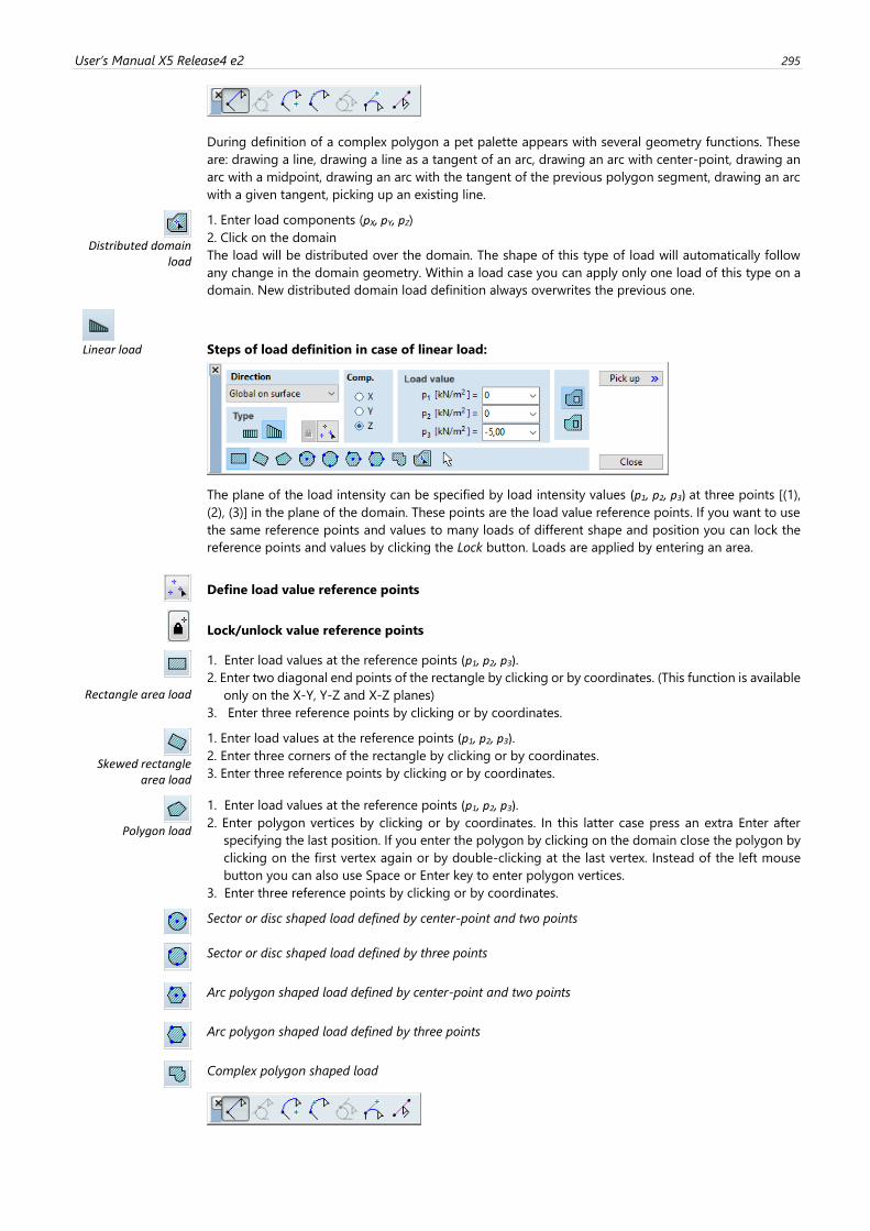
User’s Manual X5 Release4 e2 295

During definition of a complex polygon a pet palette appears with several geometry functions. These

are: drawing a line, drawing a line as a tangent of an arc, drawing an arc with center-point, drawing an

arc with a midpoint, drawing an arc with the tangent of the previous polygon segment, drawing an arc

with a given tangent, picking up an existing line.

Distributed domain

load

1. Enter load components (pX, pY, pZ)

2. Click on the domain

The load will be distributed over the domain. The shape of this type of load will automatically follow

any change in the domain geometry. Within a load case you can apply only one load of this type on a

domain. New distributed domain load definition always overwrites the previous one.

Linear load Steps of load definition in case of linear load:

The plane of the load intensity can be specified by load intensity values (p1, p2, p3) at three points [(1),

(2), (3)] in the plane of the domain. These points are the load value reference points. If you want to use

the same reference points and values to many loads of different shape and position you can lock the

reference points and values by clicking the Lock button. Loads are applied by entering an area.

Define load value reference points

Lock/unlock value reference points

Rectangle area load

1. Enter load values at the reference points (p1, p2, p3).

2. Enter two diagonal end points of the rectangle by clicking or by coordinates. (This function is available

only on the X-Y, Y-Z and X-Z planes)

3. Enter three reference points by clicking or by coordinates.

Skewed rectangle

area load

1. Enter load values at the reference points (p1, p2, p3).

2. Enter three corners of the rectangle by clicking or by coordinates.

3. Enter three reference points by clicking or by coordinates.

Polygon load

1. Enter load values at the reference points (p1, p2, p3).

2. Enter polygon vertices by clicking or by coordinates. In this latter case press an extra Enter after

specifying the last position. If you enter the polygon by clicking on the domain close the polygon by

clicking on the first vertex again or by double-clicking at the last vertex. Instead of the left mouse

button you can also use Space or Enter key to enter polygon vertices.

3. Enter three reference points by clicking or by coordinates.

Sector or disc shaped load defined by center-point and two points

Sector or disc shaped load defined by three points

Arc polygon shaped load defined by center-point and two points

Arc polygon shaped load defined by three points

Complex polygon shaped load

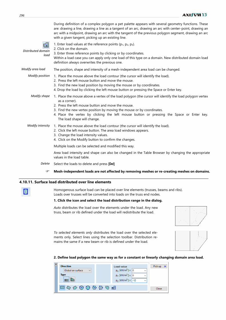
296

During definition of a complex polygon a pet palette appears with several geometry functions. These

are: drawing a line, drawing a line as a tangent of an arc, drawing an arc with center-point, drawing an

arc with a midpoint, drawing an arc with the tangent of the previous polygon segment, drawing an arc

with a given tangent, picking up an existing line.

Distributed domain

load

1. Enter load values at the reference points (p1, p2, p3).

2. Click on the domain.

3. Enter three reference points by clicking or by coordinates.

Within a load case you can apply only one load of this type on a domain. New distributed domain load

definition always overwrites the previous one.

Modify area load The position, shape and intensity of a mesh-independent area load can be changed.

Modify position 1. Place the mouse above the load contour (the cursor will identify the load).

2. Press the left mouse button and move the mouse.

3. Find the new load position by moving the mouse or by coordinates.

4. Drop the load by clicking the left mouse button or pressing the Space or Enter key.

Modify shape 1. Place the mouse above a vertex of the load polygon (the cursor will identify the load polygon vertex

as a corner).

2. Press the left mouse button and move the mouse.

3. Find the new vertex position by moving the mouse or by coordinates.

4. Place the vertex by clicking the left mouse button or pressing the Space or Enter key.

The load shape will change.

Modify intensity 1. Place the mouse above the load contour (the cursor will identify the load).

2. Click the left mouse button. The area load windows appears.

3. Change the load intensity values.

4. Click on the Modify button to confirm the changes.

Multiple loads can be selected and modified this way.

Area load intensity and shape can also be changed in the Table Browser by changing the appropriate

values in the load table.

Delete Select the loads to delete and press [Del]

Mesh-independent loads are not affected by removing meshes or re-creating meshes on domains.

4.10.11. Surface load distributed over line elements

Homogenous surface load can be placed over line elements (trusses, beams and ribs).

Loads over trusses will be converted into loads on the truss end nodes.

1. Click the icon and select the load distribution range in the dialog.

Auto distributes the load over the elements under the load. Any new

truss, beam or rib defined under the load will redistribute the load.

To selected elements only distributes the load over the selected ele-

ments only. Select lines using the selection toolbar. Distribution re-

mains the same if a new beam or rib is defined under the load.

2. Define load polygon the same way as for a constant or linearly changing domain area load.

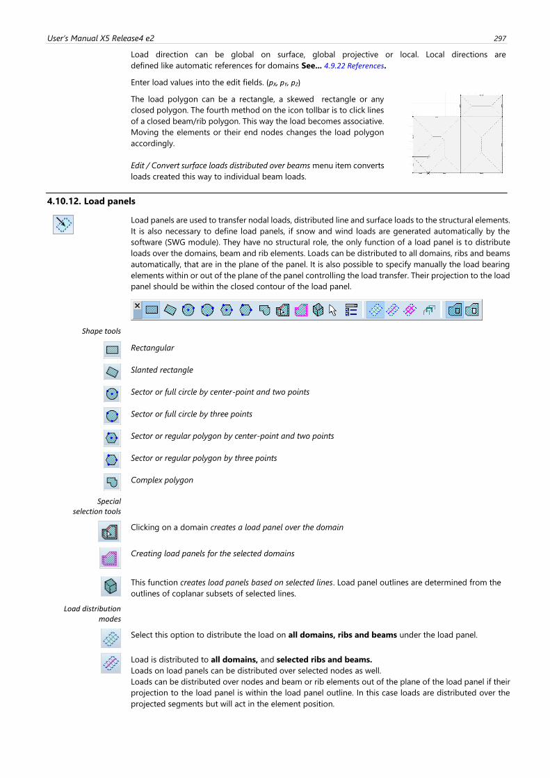
User’s Manual X5 Release4 e2 297

Load direction can be global on surface, global projective or local. Local directions are

defined like automatic references for domains See... 4.9.22 References.

Enter load values into the edit fields. (pX, pY, pZ)

The load polygon can be a rectangle, a skewed rectangle or any

closed polygon. The fourth method on the icon tollbar is to click lines

of a closed beam/rib polygon. This way the load becomes associative.

Moving the elements or their end nodes changes the load polygon

accordingly.

Edit / Convert surface loads distributed over beams menu item converts

loads created this way to individual beam loads.

4.10.12. Load panels

Load panels are used to transfer nodal loads, distributed line and surface loads to the structural elements.

It is also necessary to define load panels, if snow and wind loads are generated automatically by the

software (SWG module). They have no structural role, the only function of a load panel is to distribute

loads over the domains, beam and rib elements. Loads can be distributed to all domains, ribs and beams

automatically, that are in the plane of the panel. It is also possible to specify manually the load bearing

elements within or out of the plane of the panel controlling the load transfer. Their projection to the load

panel should be within the closed contour of the load panel.

Shape tools

Rectangular

Slanted rectangle

Sector or full circle by center-point and two points

Sector or full circle by three points

Sector or regular polygon by center-point and two points

Sector or regular polygon by three points

Complex polygon

Special selection tools

Clicking on a domain creates a load panel over the domain

Creating load panels for the selected domains

This function creates load panels based on selected lines. Load panel outlines are determined from the

outlines of coplanar subsets of selected lines.

Load distribution modes

Select this option to distribute the load on all domains, ribs and beams under the load panel.

Load is distributed to all domains, and selected ribs and beams.

Loads on load panels can be distributed over selected nodes as well.

Loads can be distributed over nodes and beam or rib elements out of the plane of the load panel if their

projection to the load panel is within the load panel outline. In this case loads are distributed over the

projected segments but will act in the element position.

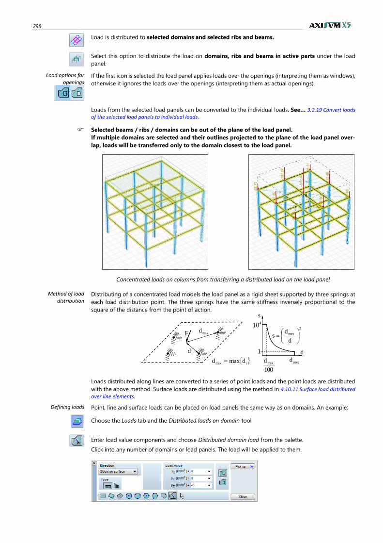
298

Load is distributed to selected domains and selected ribs and beams.

Select this option to distribute the load on domains, ribs and beams in active parts under the load

panel.

Load options for openings

If the first icon is selected the load panel applies loads over the openings (interpreting them as windows),

otherwise it ignores the loads over the openings (interpreting them as actual openings).

Loads from the selected load panels can be converted to the individual loads. See… 3.2.19 Convert loads of the selected load panels to individual loads.

Selected beams / ribs / domains can be out of the plane of the load panel.

If multiple domains are selected and their outlines projected to the plane of the load panel over-

lap, loads will be transferred only to the domain closest to the load panel.

Concentrated loads on columns from transferring a distributed load on the load panel

Method of load distribution

Distributing of a concentrated load models the load panel as a rigid sheet supported by three springs at

each load distribution point. The three springs have the same stiffness inversely proportional to the

square of the distance from the point of action.

Loads distributed along lines are converted to a series of point loads and the point loads are distributed

with the above method. Surface loads are distributed using the method in 4.10.11 Surface load distributed over line elements.

Defining loads Point, line and surface loads can be placed on load panels the same way as on domains. An example:

Choose the Loads tab and the Distributed loads on domain tool

Enter load value components and choose Distributed domain load from the palette.

Click into any number of domains or load panels. The load will be applied to them.

id

F maxd

maxd

d

100

dmax

410

s

2

max

d

ds

=

1

imax dmaxd =

User’s Manual X5 Release4 e2 299

4.10.13. Snow load – SWG module

Design codes Snow load is generated automatically in the program according to the regulations of several national

standards and their applicable annexes. The standards in the program for which snow load generation

is available are listed below. The national design standards that served as the basis of calculation for the

given standard in the program are also listed.

Eurocode general EN 1991-1-3:2003 (EC 1-3)

Eurocode 1 Action on Structures

Part 1-3 General Actions – Snow loads

EC German EN 1991-1-3:2003

DIN EN 1991-1-3/NA December 2010

NTC Italian EN 1991-1-3:2003

UNI EN 1991-1-3/NA July 2007

NTC 2018

EC Dutch EN 1991-1-3:2003

NEN EN 1991-1-3/NB November 2007

EC Hungarian EN 1991-1-3:2003

MSZ EN 1991-1-3:2016/NA September 2016

EC Romanian CR 1-1-3/2012

conform with SR EN 1991-1-3

EC Czech EN 1991-1-3:2003

CSN EN 1991-1-3/NA July 2012

EC Slovakian EN 1991-1-3:2003

STN EN 1991-1-3/NA December 2004

EC Polish EN 1991-1-3:2003

PN EN 1991-1-3/NA September 2005

EC Danish EN 1991-1-3:2003

DS/EN 1991-1-3 DK NA October 2015

EC Belgian EC 1991-1-3:2003

NBN EN 1991-1-3/ANB October 2007

EC Austrian EN 1991-1-3:2003

ÖNORM B 1991-1-3 September 2013

EC Finnish EN 1991-1-3:2003

SFS-EN 1990-1-3/NA November 2007

Swiss SIA261:2003 Einwirkungen auf Tragwerke

SIA261/1:2003 Ergänzende Festlegungen

Assumptions Application limits

Applicability of the algorithm in the program is limited by the applicability of the specifications in the

standards it is based on. Following is a list of such limitations for each standard in the program.

Eurocode

general

• The algorithm generates snow loads on building roofs. It is not recommended for

snow load generation on other types of structures, such as bridges.

• The algorithm is applicable to various roof geometries. It takes the effect of ridges

and troughs on snow accumulation into account when calculating the snow effect

on roof panels adjacent to the ridge or trough. It does not take into account the

effect of local snow accumulation on distant (i.e. not adjacent) roof panels, there-

fore, it is not recommended for complex roof geometries where such effect is ex-

pected to have significant influence on the characteristic snow load. Note that ne-

ither does EC 1-3 specify snow load calculation for the latter cases.

• Building altitude shall be less than 1500 m.

• Snow impact when snow falls off a higher roof is not considered; snow load is

always classified as static action.

• Ice loading is not considered.

300

• Lateral loading from snow is not considered.

• Exceptional snow drifts as per Annex B are not considered.

• Exceptional snow loads are not considered.

• Sliding of snow off the roof is assumed not to be prevented.

• Local snow accumulation in the vicinity of taller construction works and smaller

projections on the roof are taken into account.

• Snow overhanging the edge of the roof is considered.

• Snow load on snowguards is not considered.

• The program can generate snow load corresponding to any arbitrary return period.

EC German • Because calculation is based on the general Eurocode, the limits presented there

apply for this standard as well with the extensions/modifications listed below.

• The methodology in 5.3.4 for multi-span roofs is not implemented, because it leads

to ambiguous load generation in 3D cases.

• Exceptional snow load with the same distribution is taken into account

NTC Italian • Because calculation is based on the general Eurocode, the limits presented there

apply for this standard as well.

EC Dutch • Because calculation is based on the general Eurocode, the limits presented there

apply for this standard as well with the extensions/modifications listed below.

• No altitudes above 1500 m can be found in the Netherlands, thus the limit on alti-

tude is not applicable.

EC Hungarian • Because calculation is based on the general Eurocode, the limits presented there

apply for this standard as well.

EC Belgian • Because calculation is based on the general Eurocode, the limits presented there

apply for this standard as well with the extensions/modifications listed below.

• No altitudes above 1500 m can be found in Belgium, thus the limit on altitude is

not applicable.

EC Romanian • Because calculation is based on the general Eurocode, the limits presented there

apply for this standard as well.

EC Czech • Because calculation is based on the general Eurocode, the limits presented there

apply for this standard as well.

EC Slovak • Because calculation is based on the general Eurocode, the limits presented there

apply for this standard as well.

• Exceptional snow load with the same distribution is taken into account.

EC Polish • Because calculation is based on the general Eurocode, the limits presented there

apply for this standard as well.

EC Danish • Because calculation is based on the general Eurocode, the limits presented there

apply for this standard as well.

EC Austrian • Because calculation is based on the general Eurocode, the limits presented there

apply for this standard as well with the extensions/modifications listed below.

• The algorithm provides reliable results only for altitudes below 1500 m.

For higher altitudes the snow load shall be calculated as per 5.1 in EC 1-3 NA.

• The effect of solar panels as per Annex B in EC 1-3 NA is not considered.

• The influence area for snow load is assumed to be greater than 10 m2. For structural

members affected by snow from smaller areas see 9.2.1.1 in EC 1-3 NA and use an

increased value of sk for the analysis.

• The total area of the roof is assumed to be less than 2000 m2. For larger roof areas

see 9.2.1.2 in EC 1-3 NA and apply an appropriate increase in sk for the analysis.

• The effect of short eaves (h < 0.5 m) as per 9.2.1.3 in EC 1-3 NA is not considered

automatically. This effect can be considered by an appropriately extended model

that includes the ground surface around building as an extension of the roof.

• The effect of graves (as per 9.2.5.4 in EC 1-3 NA) is not considered.

EC Finnish • Because calculation is based on the general Eurocode, the limits presented there

apply for this standard as well.

User’s Manual X5 Release4 e2 301

Swiss • The algorithm generates snow loads on building roofs. It is not recommended for

snow load generation on other types of structures, such as bridges.

• The algorithm is applicable to various roof geometries. It takes the effect of ridges

and troughs on snow accumulation into account when calculating the snow effect

on roof panels adjacent to the ridge or trough. It does not take into account the

effect of local snow accumulation on distant (i.e. not adjacent) roof panels, there-

fore, it is not recommended for complex roof geometries where such effect is ex-

pected to have significant influence on the characteristic snow load. Note that ne-

ither does SIA261 specify snow load calculation for the latter cases.

• Building altitude shall be less than 2000 m.

• Exceptional snow loads are not considered.

• Sliding of snow off the roof is assumed not to be prevented.

• Local snow accumulation in the vicinity of taller construction works and smaller

projections on the roof are taken into account.

• Snow overhanging the edge of the roof is considered.

Calculation details The logic of snow load calculation is explained below for each standard in the program

Eurocode

general

• The recommended values are assumed for all coefficients unless specified other-

wise by the user. None of the recommendations in National Annexes is assumed.

• The factors for combination value, frequent value and quasi-permanent value of

the snow load are taken according to Table 4.1 of EC 1-3.

• The characteristic value of snow load on the ground shall be specified by the user.

• Snow load on the roof is calculated using Eq. (5.1) in EC 1-3.

• The exposure coefficient is based on the topography selected by the user. The Ce

values that correspond to each topography type are taken from Table 5.1 in EC 1-

3.

• The thermal coefficient is taken as 1.0 by default and shall be modified by the user

if the application of a different value is justified.

• The snow load shape coefficient for roofs composed of planar panels is calculated

as per Section 5.3.1 - 5.3.4 in EC 1-3.

• Snow load shape coefficients for the undrifted load case are based on μ1 in Table

5.2 in EC 1-3. Each panel has its own μ1 value that is calculated using the slope of

the panel.

• Snow load shape coefficients for the drifted load case are based on μ2 in Table 5.2.

μ2 coefficients for troughs are calculated as per Figure 5.4 in EC 1-3 using the slopes

of the connecting roof panels in the wind direction of the given drifted snow load

case. (e.g.: A horizontal trough in the X direction results in no snow accumulation

when the wind blows in the X direction because the slopes of the connecting roof

panels in the X direction are 0°.) When there are no troughs on a roof, the drifted

load arrangements in Figure 5.3 in EC 1-3 are considered. The reduced snow inten-

sity is always assumed on the windswept side of the roof.

• Snow load shape coefficients for cylindrical roofs are calculated as per 5.3.5. in EC

1-3. In order to achieve sufficient accuracy in the load shape, it is recommended to

approximate the cylindrical roof with at least 20 planar segments.

• The effect of taller construction works and obstructions on the roof are considered

as per 5.3.6 and 6.2 in EC 1-3. Their influence is only taken into account in the drifted

load cases. Snow is assumed to be drifted only if the wall or obstacle is not parallel

to the wind direction.

• Snow load overhanging the edge of the roof is considered as per 6.3 in EC 1-3.

• Snow load corresponding to a user-defined return period is calculated using the

procedure in Annex D of EC 1-3.

302

EC German • Because calculation is based on the general Eurocode, the procedure presented

there is applied for this standard as well with the modifications/extensions listed

below

• The characteristic value of snow load on the ground is automatically calculated

based on 4.1 in EC 1-3 NA using the zone and the altitude specified by the user.

• Exceptional snow load is generated. The exceptional snow load coefficient is as-

sumed 2.0 by default, but it shall be overwritten by the appropriate value by the

user for Northern Germany as per 4.3 in EC 1-3 NA.

• The effect of taller construction works is calculated as per 5.3.6 in EC 1-3 NA.

NTC Italian • Because calculation is based on the general Eurocode, the procedure presented

there is applied for this standard as well with the modifications/extensions listed

below.

• The characteristic value of snow load on the ground is automatically calculated

based on 4.1 in EC 1-3 NA using the zone and the altitude specified by the user.

• The value of the exposure coefficient is based on 5.2 (7) in EC 1-3 NA.

EC Dutch • Because calculation is based on the general Eurocode, the procedure presented

there is applied for this standard as well with the modifications/extensions listed

below.

• The characteristic value of snow load on the ground is taken as 0.7 kN/m2 as per

4.1 (1) in EC 1-3 NA.

• The factors for combination value, frequent value and quasi-permanent value of

the snow load are taken as 0, 0.2, and 0, respectively as per 4.2 (1) in EC 1-3 NA.

EC Belgian • Because calculation is based on the general Eurocode, the procedure presented

there is applied for this standard as well with the modifications/extensions listed

below.

• The characteristic value of snow load on the ground is automatically calculated

based on 4.1 (1) in EC 1-3 NA as a function of the altitude specified by the user.

• The combination factors for frequent and quasi-permanent load combinations are

based on EC 1-3 NA 4.2 (1).

• The exposure and temperature coefficients are taken as 1.0 according to the regu-

lations in EC 1-3 NA 5.2 (7) and (8).

• When calculating the effect of taller construction works, the upper limit of μw is 2.0

as per EC 1-3 NA 5.3.6 (1).

• The effect of snow overhanging the roof is not considered (EC 1-3 NA 6.3).

EC Hungarian • Because calculation is based on the general Eurocode, the procedure presented

there is applied for this standard as well with the modifications/extensions listed

below.

• The characteristic value of snow load ont he ground is automatically calculated

based on NA1.6 in EC 1-3 NA using the altitude specified by the user.

• Exceptional snow load is generated. An exceptional snow load coefficient of 2.0 is

used as per NA1.8 in EC 1-3 NA.

User’s Manual X5 Release4 e2 303

EC Romanian • Because calculation is based on the general Eurocode, the procedure presented

there is applied for this standard as well with the modifications/extensions listed

below

• The characteristic value of snow load on the ground is calculated automatically

based on 3.1 in CR 1-3 using the basic sk value and the altitude specified by the

user.

• Snow load on the roof is calculated using Eq. (4.1) in CR 1-3.

• The importance factor shall be selected by the user; the list of recommended values

is based on Table 4.2 in CR 1-3.

• The factors for combination value, frequent value and quasi-permanent value of

the snow load are taken as 0.7, 0.5, and 0.4, respectively as per Table 4.4 in CR 1-3.

EC Czech • Because calculation is based on the general Eurocode, the procedure presented

there is applied for this standard as well with the modifications/extensions listed

below

• The characteristic value of snow load on the ground is based on the map cited in

2.7 in EC 1-3 NA (www.snehovamapa.cz)

• Snow load shape coefficients for cylindrical roofs are calculated as per 2.19 and

Figure NA.1 in EC 1-3 NA

• The effect of taller construction works is taken into account as per 2.20 in EC 1-3

NA with the following assumption: b1,s = 0.5b1.

EC Polish • Because calculation is based on the general Eurocode, the procedure presented

there is applied for this standard as well with the modifications/extensions listed

below

• The characteristic value of snow load on the ground is calculated automatically

based on 1.7, Figure 1 and Table 1 in EC 1-3 NA using the zone and altitude speci-

fied by the user.

EC Danish • Because calculation is based on the general Eurocode, the procedure presented

there is applied for this standard as well with the modifications/extensions listed

below.

• The characteristic value of snow load on the ground is taken as 1.0 kN/m2 as per

4.1 (1) NOTE 1 in EC 1-3 NA.

• Default snow load exposure coefficients are based on the assumption of Cs = 1.0

as per 5.2(7) in EC 1-3 NA. When a different size coefficient needs the be applied,

the user shall calculate the resulting exposure coefficient and define it as custom.

• The additional snow load arrangement in 5.3.3(4) in EC 1-3 NA is not considered.

• Snow load shape coefficients for cylindrical roofs are calculated as per 5.3.5. (3) in

EC 1-3 NA

• The effect of taller construction works is taken into account as per 5.3.6 in EC 1-3

NA with the following assumptions: (i) the shelter is global; (ii) bsl = 0.5b1; (iii) the

shelter is on the leeward side.

EC Austrian • Because calculation is based on the general Eurocode, the procedure presented

there is applied for this standard as well with the modifications/extensions listed

below.

• The characteristic value of snow load on the ground is calculated automatically

based on Eq. (C.1) in EC 1-3 NA using the zone and altitude specified by the user.

• Snow load shape coefficients for multi-span roofs are calculated as per 9.2.3 in EC

1-3 NA.

• Snow load shape coefficients for vaulted roofs are calculated as per 9.2.4.3 in EC 1-

3 NA.

• The modifications for calculating the effect of taller construction works in 9.2.5.1 in

EC 1-3 NA are taken into account.

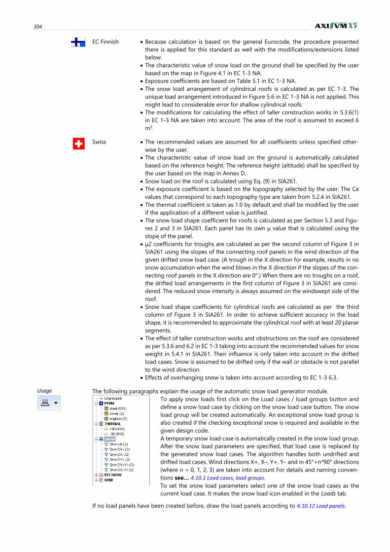
304

EC Finnish • Because calculation is based on the general Eurocode, the procedure presented

there is applied for this standard as well with the modifications/extensions listed

below.

• The characteristic value of snow load on the ground shall be specified by the user

based on the map in Figure 4.1 in EC 1-3 NA.

• Exposure coefficients are based on Table 5.1 in EC 1-3 NA.

• The snow load arrangement of cylindrical roofs is calculated as per EC 1-3. The

unique load arrangement introduced in Figure 5.6 in EC 1-3 NA is not applied. This

might lead to considerable error for shallow cylindrical roofs.

• The modifications for calculating the effect of taller construction works in 5.3.6(1)

in EC 1-3 NA are taken into account. The area of the roof is assumed to exceed 6

m2.

Swiss • The recommended values are assumed for all coefficients unless specified other-

wise by the user.

• The characteristic value of snow load on the ground is automatically calculated

based on the reference height. The reference height (altitude) shall be specified by

the user based on the map in Annex D.

• Snow load on the roof is calculated using Eq. (9) in SIA261.

• The exposure coefficient is based on the topography selected by the user. The Ce

values that correspond to each topography type are taken from 5.2.4 in SIA261.

• The thermal coefficient is taken as 1.0 by default and shall be modified by the user

if the application of a different value is justified.

• The snow load shape coefficient for roofs is calculated as per Section 5.3 and Figu-

res 2 and 3 in SIA261. Each panel has its own μ value that is calculated using the

slope of the panel.

• μ2 coefficients for troughs are calculated as per the second column of Figure 3 in

SIA261 using the slopes of the connecting roof panels in the wind direction of the

given drifted snow load case. (A trough in the X direction for example, results in no

snow accumulation when the wind blows in the X direction if the slopes of the con-

necting roof panels in the X direction are 0°.) When there are no troughs on a roof,

the drifted load arrangements in the first column of Figure 3 in SIA261 are consi-

dered. The reduced snow intensity is always assumed on the windswept side of the

roof.

• Snow load shape coefficients for cylindrical roofs are calculated as per the third

column of Figure 3 in SIA261. In order to achieve sufficient accuracy in the load

shape, it is recommended to approximate the cylindrical roof with at least 20 planar

segments.

• The effect of taller construction works and obstructions on the roof are considered

as per 5.3.6 and 6.2 in EC 1-3 taking into account the recommended values for snow

weight in 5.4.1 in SIA261. Their influence is only taken into account in the drifted

load cases. Snow is assumed to be drifted only if the wall or obstacle is not parallel

to the wind direction.

• Effects of overhanging snow is taken into account according to EC 1-3 6.3.

Usage The following paragraphs explain the usage of the automatic snow load generator module.

To apply snow loads first click on the Load cases / load groups button and

define a snow load case by clicking on the snow load case button. The snow

load group will be created automatically. An exceptional snow load group is

also created if the checking exceptional snow is required and available in the

given design code.

A temporary snow load case is automatically created in the snow load group.

After the snow load parameters are specified, that load case is replaced by

the generated snow load cases. The algorithm handles both undrifted and

drifted load cases. Wind directions X+, X–, Y+, Y– and in 45°+n*90° directions

(where n = 0, 1, 2, 3) are taken into account For details and naming conven-

tions see… 4.10.1 Load cases, load groups.

To set the snow load parameters select one of the snow load cases as the

current load case. It makes the snow load icon enabled in the Loads tab.

If no load panels have been created before, draw the load panels according to 4.10.12 Load panels.

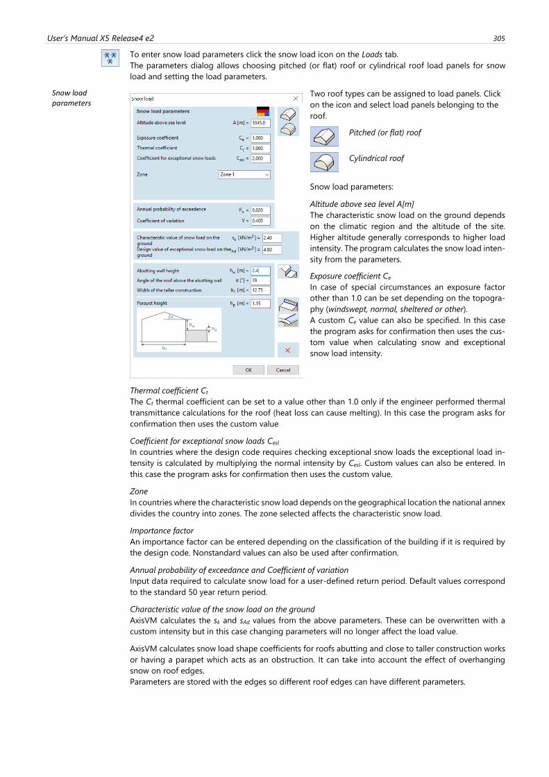
User’s Manual X5 Release4 e2 305

To enter snow load parameters click the snow load icon on the Loads tab.

The parameters dialog allows choosing pitched (or flat) roof or cylindrical roof load panels for snow

load and setting the load parameters.

Snow load parameters

Two roof types can be assigned to load panels. Click

on the icon and select load panels belonging to the

roof.

Pitched (or flat) roof

Cylindrical roof

Snow load parameters:

Altitude above sea level A[m]

The characteristic snow load on the ground depends

on the climatic region and the altitude of the site.

Higher altitude generally corresponds to higher load

intensity. The program calculates the snow load inten-

sity from the parameters.

Exposure coefficient Ce

In case of special circumstances an exposure factor

other than 1.0 can be set depending on the topogra-

phy (windswept, normal, sheltered or other).

A custom Ce value can also be specified. In this case

the program asks for confirmation then uses the cus-

tom value when calculating snow and exceptional

snow load intensity.

Thermal coefficient Ct

The Ct thermal coefficient can be set to a value other than 1.0 only if the engineer performed thermal

transmittance calculations for the roof (heat loss can cause melting). In this case the program asks for

confirmation then uses the custom value

Coefficient for exceptional snow loads Cesl

In countries where the design code requires checking exceptional snow loads the exceptional load in-

tensity is calculated by multiplying the normal intensity by Cesl. Custom values can also be entered. In

this case the program asks for confirmation then uses the custom value.

Zone

In countries where the characteristic snow load depends on the geographical location the national annex

divides the country into zones. The zone selected affects the characteristic snow load.

Importance factor

An importance factor can be entered depending on the classification of the building if it is required by

the design code. Nonstandard values can also be used after confirmation.

Annual probability of exceedance and Coefficient of variation

Input data required to calculate snow load for a user-defined return period. Default values correspond

to the standard 50 year return period.

Characteristic value of the snow load on the ground

AxisVM calculates the sk and sAd values from the above parameters. These can be overwritten with a

custom intensity but in this case changing parameters will no longer affect the load value.

AxisVM calculates snow load shape coefficients for roofs abutting and close to taller construction works

or having a parapet which acts as an obstruction. It can take into account the effect of overhanging

snow on roof edges.

Parameters are stored with the edges so different roof edges can have different parameters.

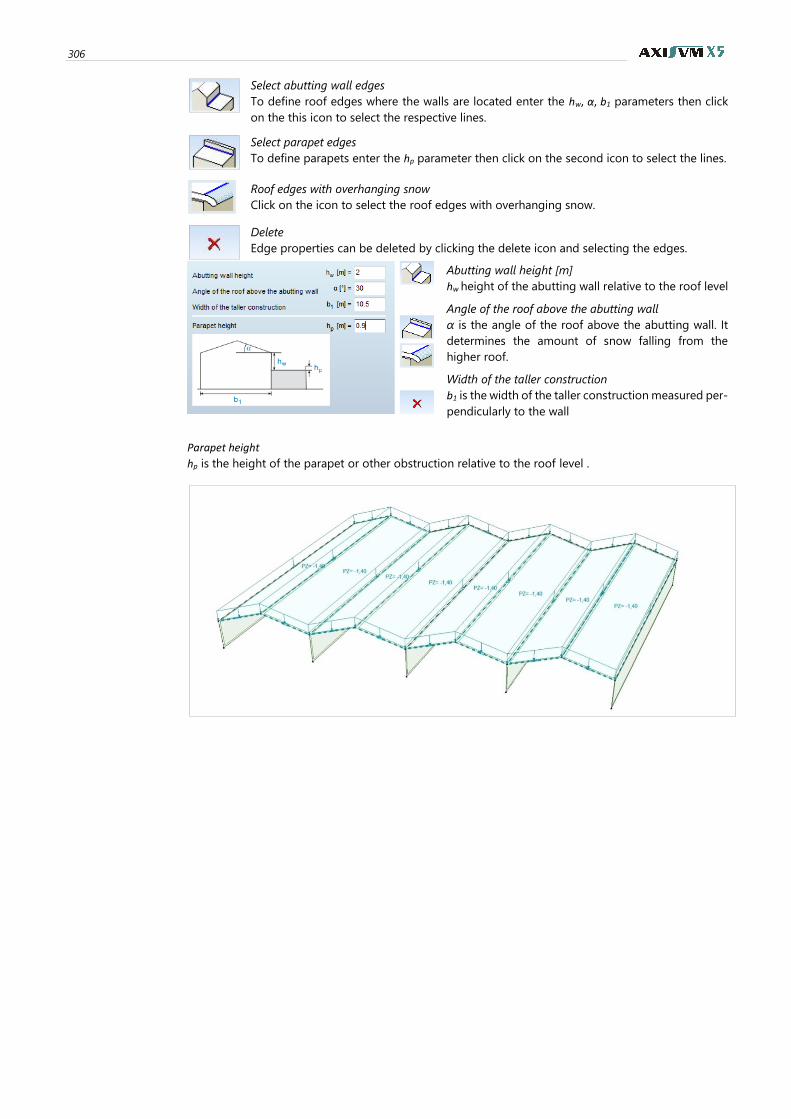
306

Select abutting wall edges

To define roof edges where the walls are located enter the hw, α, b1 parameters then click

on the this icon to select the respective lines.

Select parapet edges

To define parapets enter the hp parameter then click on the second icon to select the lines.

Roof edges with overhanging snow

Click on the icon to select the roof edges with overhanging snow.

Delete

Edge properties can be deleted by clicking the delete icon and selecting the edges.

Abutting wall height [m]

hw height of the abutting wall relative to the roof level

Angle of the roof above the abutting wall

α is the angle of the roof above the abutting wall. It

determines the amount of snow falling from the

higher roof.

Width of the taller construction

b1 is the width of the taller construction measured per-

pendicularly to the wall

Parapet height

hp is the height of the parapet or other obstruction relative to the roof level .

User’s Manual X5 Release4 e2 307

4.10.14. Wind load – SWG module

Design codes Wind load is generated automatically in the program according to the regulations of several national

standards and their applicable annexes. The standards in the program for which wind load generation is

available are listed below. The national design standards that served as the basis of calculation for the

given standard in the program are also listed.

Eurocode

general

EN 1991-1-4:2005 (EC 1-4)

Eurocode 1 Action on Structures

Part 1-4 General Actions – Wind Actions

EC German EC 1991-1-4:2005

DIN EN 1991-1-4/NA December 2010

NTC Italian EC 1991-1-4:2005

UNI EN 1991-1-4/NA July 2007

NTC 2018

EC Dutch EC 1991-1-4:2005

NEN EN 1991-1-4/NB November 2007

EC Hungarian EC 1991-1-4:2005

MSZ EN 1991-1-4/NA January 2016

EC Romanian CR 1-1-4/2012

conform with SR EN 1991-1-4

EC Czech EC 1991-1-4:2005

CSN EN 1991-1-4/NA July 2013

EC Slovakian EC 1991-1-4:2005

STN EN 1991-1-4/NA July 2008

EC Belgian EC 1991-1-4:2005

NBN EN 1991-1-4/ANB December 2010

EC Polish EC 1991-1-4:2005

PN EN 1991-1-4/NA October 2008

EC Danish EC 1991-1-4:2005

DS/EN 1991-1-4 DK NA July 2015

EC Austrian EN 1991-1-4:2005

ÖNORM B 1991-1-4 May 2013

EC Finnish EN 1991-1-4:2005

SFS-EN 1991-1-4/NA November 2007

Swiss SIA261:2003 Einwirkungen auf Tragwerke

SIA261/1:2003 Ergänzende Festlegungen

308

Assumptions Application limits

Applicability of the algorithm in the program is limited by the applicability of the specifications in the

standards it is based on. Following is a list of such limitations for each standard in the program.

Eurocode

general • The algorithm can determine the wind load of rectangular-plan buildings, rectangu-

lar-plan canopies, free-standing walls and signboards. Buildings are structures with an

internal empty space surrounded by a closed line of walls and covered by a roof.

• The following types of roofs are handled by the algorithm for buildings: flat, mono-

pitch, duopitch, hipped, vaulted.

• The following types of canopy roofs are handled by the algorithm: monopitch and

duopitch.

• The height and the width of the building shall not exceed 200 m.

• The global wind effect is determined for the structure. Hence, pressure coefficients

are calculated with the assumption of at least 10 m2 of loaded area for buildings. The

wind load of canopies and free-standing objects is based on force coefficients.

• The influence of neighboring structures and obstacles is assumed negligible.

• When calculating the internal pressure coefficients, the building is assumed not to

have a dominant external opening. Internal pressure is only calculated for buildings.

• The structural factor cscd is taken as 1.0 (corresponding applicability limits are listed

in 6.2 (1) of EC 1-4).

• the influence of ice and snow on wind load is assumed negligible

EC German • because calculation is based on the general Eurocode, the limits presented there apply

for this standard as well with the extensions/modifications listed below

• building height < 300 m

• building altitude < 1100 m

NTC Italian • because calculation is based on the general Eurocode, the limits presented there apply

for this standard as well with the extensions/modifications listed below

• building altitude < 1500 m

EC Dutch • because calculation is based on the general Eurocode, the limits presented there apply

for this standard as well

EC Hungarian • because calculation is based on the general Eurocode, the limits presented there apply

for this standard as well

EC Romanian • because calculation is based on the general Eurocode, the limits presented there apply

for this standard as well with the extensions/modifications listed below

• building altitude < 1000 m (for buildings in southwest Banat and in areas with an

altitude above 1000 m special consideration is required and the basic wind velocity

shall be specified by the user)

EC Czech • because calculation is based on the general Eurocode, the limits presented there apply

for this standard as well

EC Slovakian • because calculation is based on the general Eurocode, the limits presented there apply

for this standard as well

EC Belgian • because calculation is based on the general Eurocode, the limits presented there apply

for this standard as well

EC Polish • because calculation is based on the general Eurocode, the limits presented there apply

for this standard as well

EC Danish • because calculation is based on the general Eurocode, the limits presented there apply

for this standard as well

EC Austrian • because calculation is based on the general Eurocode, the limits presented there apply

for this standard as well

EC Finnish • because calculation is based on the general Eurocode, the limits presented there apply

for this standard as well

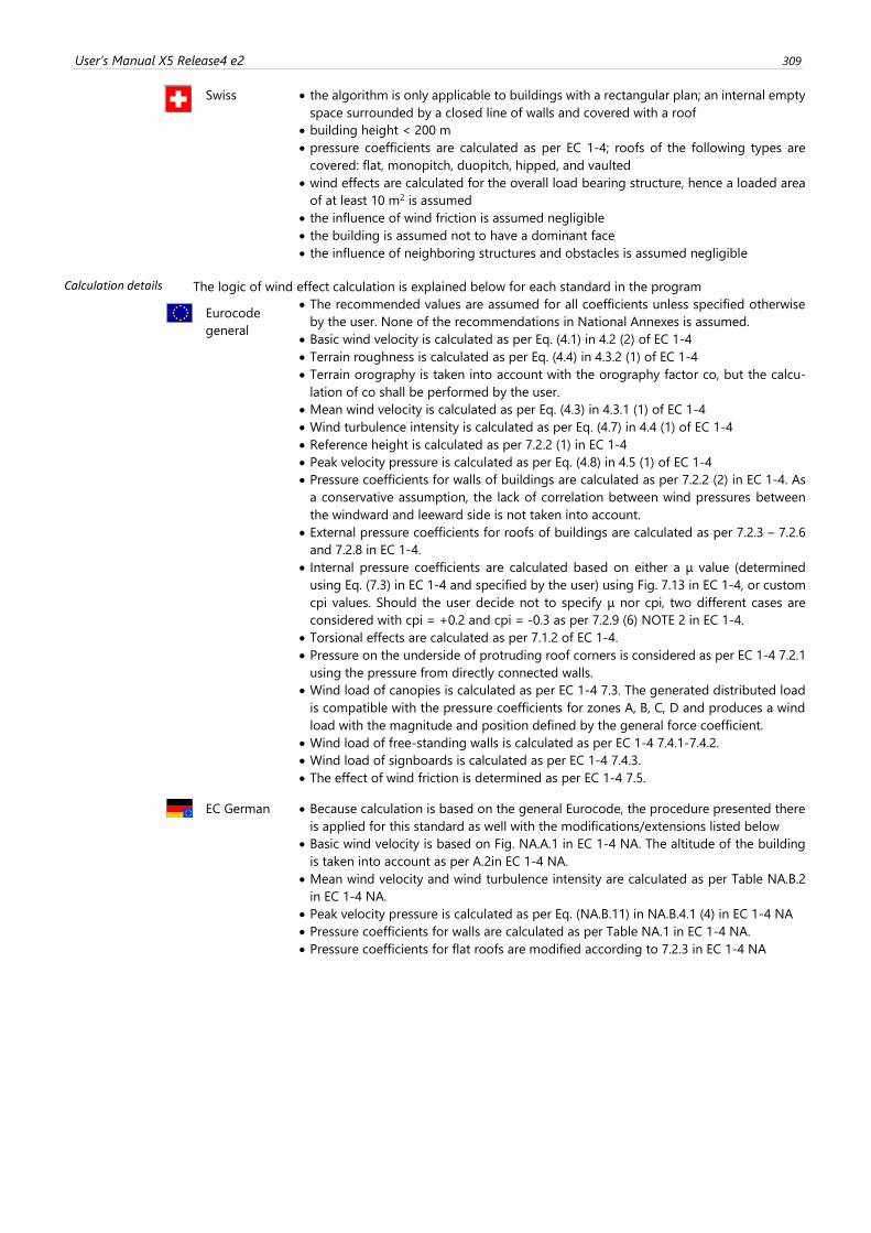
User’s Manual X5 Release4 e2 309

Swiss • the algorithm is only applicable to buildings with a rectangular plan; an internal empty

space surrounded by a closed line of walls and covered with a roof

• building height < 200 m

• pressure coefficients are calculated as per EC 1-4; roofs of the following types are

covered: flat, monopitch, duopitch, hipped, and vaulted

• wind effects are calculated for the overall load bearing structure, hence a loaded area

of at least 10 m2 is assumed

• the influence of wind friction is assumed negligible

• the building is assumed not to have a dominant face

• the influence of neighboring structures and obstacles is assumed negligible

Calculation details The logic of wind effect calculation is explained below for each standard in the program

Eurocode

general

• The recommended values are assumed for all coefficients unless specified otherwise

by the user. None of the recommendations in National Annexes is assumed.

• Basic wind velocity is calculated as per Eq. (4.1) in 4.2 (2) of EC 1-4

• Terrain roughness is calculated as per Eq. (4.4) in 4.3.2 (1) of EC 1-4

• Terrain orography is taken into account with the orography factor co, but the calcu-

lation of co shall be performed by the user.

• Mean wind velocity is calculated as per Eq. (4.3) in 4.3.1 (1) of EC 1-4

• Wind turbulence intensity is calculated as per Eq. (4.7) in 4.4 (1) of EC 1-4

• Reference height is calculated as per 7.2.2 (1) in EC 1-4

• Peak velocity pressure is calculated as per Eq. (4.8) in 4.5 (1) of EC 1-4

• Pressure coefficients for walls of buildings are calculated as per 7.2.2 (2) in EC 1-4. As

a conservative assumption, the lack of correlation between wind pressures between

the windward and leeward side is not taken into account.

• External pressure coefficients for roofs of buildings are calculated as per 7.2.3 – 7.2.6

and 7.2.8 in EC 1-4.

• Internal pressure coefficients are calculated based on either a μ value (determined

using Eq. (7.3) in EC 1-4 and specified by the user) using Fig. 7.13 in EC 1-4, or custom

cpi values. Should the user decide not to specify μ nor cpi, two different cases are

considered with cpi = +0.2 and cpi = -0.3 as per 7.2.9 (6) NOTE 2 in EC 1-4.

• Torsional effects are calculated as per 7.1.2 of EC 1-4.

• Pressure on the underside of protruding roof corners is considered as per EC 1-4 7.2.1

using the pressure from directly connected walls.

• Wind load of canopies is calculated as per EC 1-4 7.3. The generated distributed load

is compatible with the pressure coefficients for zones A, B, C, D and produces a wind

load with the magnitude and position defined by the general force coefficient.

• Wind load of free-standing walls is calculated as per EC 1-4 7.4.1-7.4.2.

• Wind load of signboards is calculated as per EC 1-4 7.4.3.

• The effect of wind friction is determined as per EC 1-4 7.5.

EC German • Because calculation is based on the general Eurocode, the procedure presented there

is applied for this standard as well with the modifications/extensions listed below

• Basic wind velocity is based on Fig. NA.A.1 in EC 1-4 NA. The altitude of the building

is taken into account as per A.2in EC 1-4 NA.

• Mean wind velocity and wind turbulence intensity are calculated as per Table NA.B.2

in EC 1-4 NA.

• Peak velocity pressure is calculated as per Eq. (NA.B.11) in NA.B.4.1 (4) in EC 1-4 NA

• Pressure coefficients for walls are calculated as per Table NA.1 in EC 1-4 NA.

• Pressure coefficients for flat roofs are modified according to 7.2.3 in EC 1-4 NA

310

NTC Italian • Because calculation is based on the general Eurocode, the procedure presented there

is applied for this standard as well with the modifications/extensions listed below.

• Basic wind velocity is calculated using the parameters in Table N.A.1 in EC 1-4 NA.

• Terrain roughness is calculated using 3.3.7 in NTC 2018.

• The wind load distribution for walls of slender buildings is not variable as per EC 1-4,

but uniform according to the regulations in 3.3 in NTC 2018.

• Pressure coefficients for walls are based on Table IV. in 3.3 in NTC 2018.

• Load zone geometry and corresponding pressure coefficients for roofs are based on

3.3 in NTC 2018.

• Global pressure coefficients as per NTC 2018 are not considered.

• Automatic internal pressure calculation is based on 3.3 in NTC 2018 using cpi =±0.2.

EC Dutch • Because calculation is based on the general Eurocode, the procedure presented there

is applied for this standard as well with the modifications/extensions listed below.

• Basic wind velocity is proposed based on the zones in Figure NB.1 and the corres-

ponding values in Table NB.1 in EC 1-4 NA.

• Terrain roughness is calculated as per Eq. (4.5) and Table 4.1 in EC 1-4 NA

• Pressure coefficients for walls are calculated as per Table 7.1 in EC 1-4 NA.

The lack of correlation between wind pressures between the windward and leeward

side is always taken into account by multiplying the pressure intensities with 0.85.

• External pressure coefficients for roofs are calculated as per Tables 7.2, 7.3a, 7.3b, 7.4a,

7.4b, and 7.5 in EC 1-4 NA.

EC Hungarian • Because calculation is based on the general Eurocode, the procedure presented there

is applied for this standard as well with the modifications/extensions listed below

• Basic wind velocity is taken as 23.6 m/s2 as per NA4.1 in EC 1-4 NA.

• The recommended value of cdir = 1.00 in NA4.2 in EC 1-4 NA is taken into account.

EC Romanian • Because calculation is based on the general Eurocode, the procedure presented there

is applied for this standard as well with the modifications/extensions listed below

• Basic wind velocity is calculated using Eq. (2.2) and Fig. 2.1 in CR 1-4.

• The importance factor is taken into account when calculating the wind pressure inten-

sity as per Eq. (3.1) and (3.2) in CR 1-4.

EC Czech • Because calculation is based on the general Eurocode, the procedure presented there

is applied for this standard as well with the modifications/extensions listed below

• Basic wind velocity is based on the wind map of the Czech Republic in Fig. NA.4.1 in

EC 1-4 NA.

EC Slovakian • Because calculation is based on the general Eurocode, the procedure presented there

is applied for this standard as well with the modifications/extensions listed below

• Basic wind velocity is calculated as per Table EC 1-4 NA NB1.

• External pressure coefficients for roofs are modified as per EC 1-4 NA 2.27–2.30.

EC Belgian • Because calculation is based on the general Eurocode, the procedure presented there

is applied for this standard as well with the modifications/extensions listed below.

• Basic wind velocity is based on the wind map of Belgium in Fig. 4.3 in EC 1-4 NA.

• The cdir and cseason coefficients recommended in EC 1-4 NA can be taken into account

by the user, but the default values for both parameters are 1.0.

• The turbulence factor kl is calculated as per 4.4 in EC 1-4 NA.

EC Polish • Because calculation is based on the general Eurocode, the procedure presented there

is applied for this standard as well with the modifications/extensions listed below

• Basic wind velocity is calculated as per Table NA.1 in EC 1-4 NA.

• The cdir coefficients recommended in Table NA.2 in EC 1-4 NA can be taken into ac-

count by the user, but the default values for the parameter is 1.0.

• Terrain roughness is calculated as per Table NA.3 in EC 1-4 NA.

User’s Manual X5 Release4 e2 311

EC Danish • Because calculation is based on the general Eurocode, the procedure presented there

is applied for this standard as well with the modifications/extensions listed below.

• Basic wind velocity is taken as 24 m/s as per 4.2 (1)P NOTE 2 in EC 1-4 NA. Different

values (such as for areas less than 25 km from the North Sea) shall be specified by the

user.

• The cdir and cseason coefficients recommended in 4.2 (2)P in EC 1-4 NA can be taken

into account by the user. The default values for both parameters are 1.0.

• The pressure coefficient for zone I of flat roofs is calculated as per 7.2.3(4) in

EC 1-4 NA.

EC Austrian • Because calculation is based on the general Eurocode, the procedure presented there

is applied for this standard as well with the modifications/extensions listed below

• Basic velocity pressure (qb) shall be specified by the user based on Annex A of

EC 1-4 NA.

• Peak velocity pressure is calculated as per Table 1 in EC 1-4 NA

• The simplified approaches for pressure coefficients in EC 1-4 NA are not applied. The

pressure coefficients are calculated with the more accurate complex approaches at all

times.

EC Austrian • Pressure coefficients for walls are calculated as per Table 3a, 3b and 4 in

EC 1-4 NA.

• Zones F and G are not used for roofs when their cumulative area is less than 20% of

the total roof area as per 9.2 in EC 1-4 NA.

EC Finnish • Because calculation is based on the general Eurocode, the procedure presented there

is applied for this standard as well with the modifications/extensions listed below.

• Basic wind velocity for various parts of the country is based on 4.2(1)P in EC 1-4 NA.

• The unique value for kr in 4.3.2(1) in EC 1-4 NA is taken into consideration when terrain

roughness is calculated.

Swiss • The recommended values are assumed for all coefficients unless specified otherwise

by the user.

• The basic value of velocity pressure (qp0) shall be determined by the user based on

Appendix E of SIA 261

• Peak velocity pressure is calculated as per Eq. (11) in 6.2.1.1 in SIA 261

• The wind profile coefficient ch is calculated as per Eq. (12) in 6.2.1.2 in SIA 261 accor-

ding to parameters in Table 4 corresponding to the terrain category selected by the

user.

• Wind pressure is calculated as per Eq. (13) (external) and Eq. (14) (internal) in 6.2.2.1 in

SIA 261. The corresponding pressure coefficients are not taken from Appendix C, but

from Tables 7.2.3 – 7.2.6 and 7.2.8 in EC 1-4 to provide a more generally applicable

solution that is also in line with Swiss design practice.

• The cred reduction factor is assumed 1.0 in all cases.

• The cd dynamic factor is assumed 1.0 in all cases. The corresponding limitations are

listed in 6.3.5 in SIA 261.

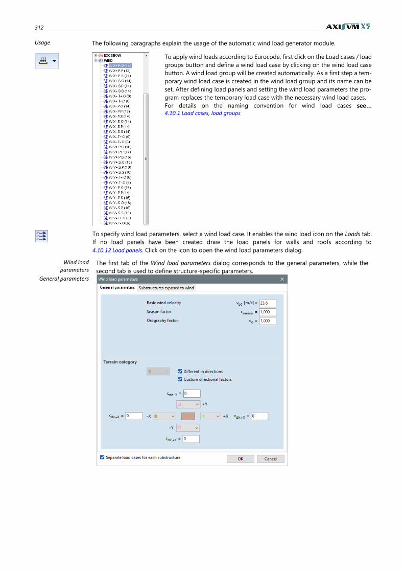
312

Usage The following paragraphs explain the usage of the automatic wind load generator module.

To apply wind loads according to Eurocode, first click on the Load cases / load

groups button and define a wind load case by clicking on the wind load case

button. A wind load group will be created automatically. As a first step a tem-

porary wind load case is created in the wind load group and its name can be

set. After defining load panels and setting the wind load parameters the pro-

gram replaces the temporary load case with the necessary wind load cases.

For details on the naming convention for wind load cases see…

4.10.1 Load cases, load groups

To specify wind load parameters, select a wind load case. It enables the wind load icon on the Loads tab.

If no load panels have been created draw the load panels for walls and roofs according to

4.10.12 Load panels. Click on the icon to open the wind load parameters dialog.

Wind load parameters

The first tab of the Wind load parameters dialog corresponds to the general parameters, while the

second tab is used to define structure-specific parameters.

General parameters

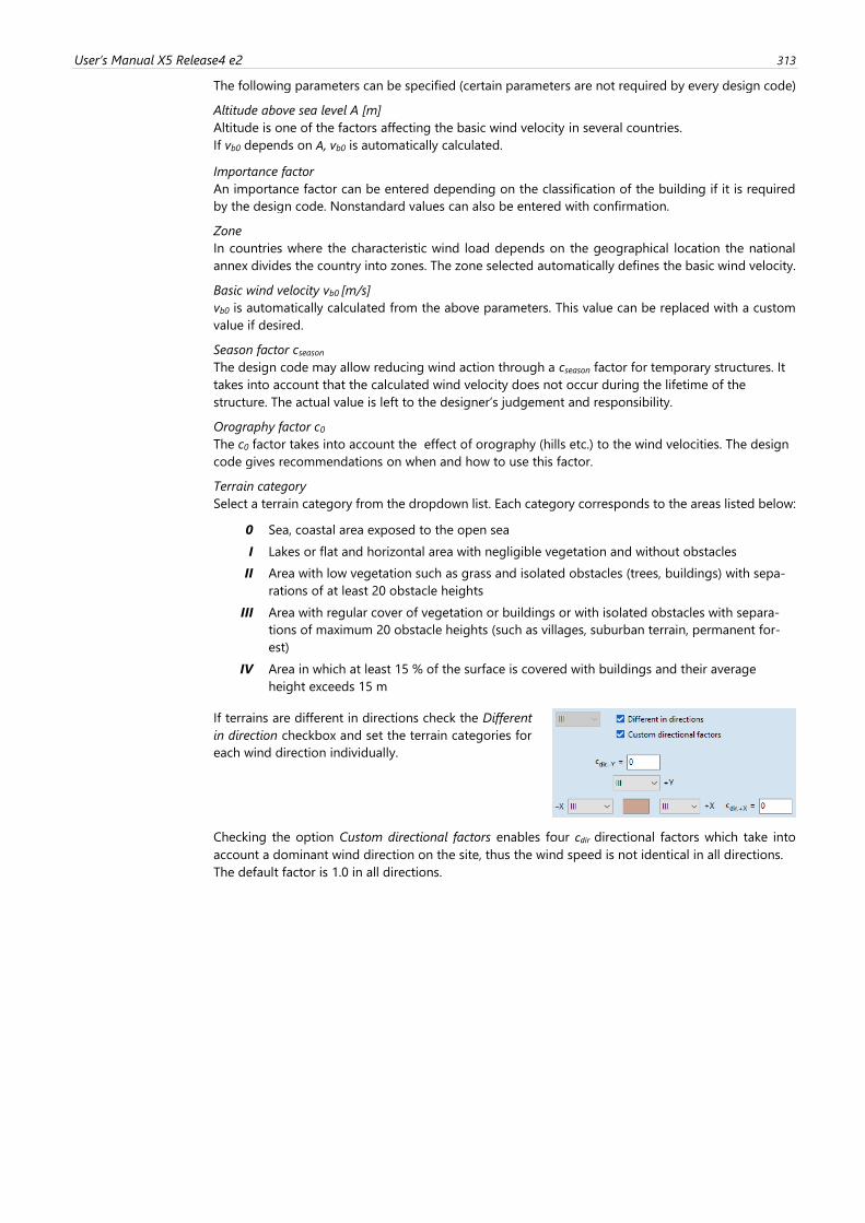
User’s Manual X5 Release4 e2 313

The following parameters can be specified (certain parameters are not required by every design code)

Altitude above sea level A [m]

Altitude is one of the factors affecting the basic wind velocity in several countries.

If vb0 depends on A, vb0 is automatically calculated.

Importance factor

An importance factor can be entered depending on the classification of the building if it is required

by the design code. Nonstandard values can also be entered with confirmation.

Zone

In countries where the characteristic wind load depends on the geographical location the national

annex divides the country into zones. The zone selected automatically defines the basic wind velocity.

Basic wind velocity vb0 [m/s]

vb0 is automatically calculated from the above parameters. This value can be replaced with a custom

value if desired.

Season factor cseason

The design code may allow reducing wind action through a cseason factor for temporary structures. It

takes into account that the calculated wind velocity does not occur during the lifetime of the

structure. The actual value is left to the designer’s judgement and responsibility.

Orography factor c0

The c0 factor takes into account the effect of orography (hills etc.) to the wind velocities. The design

code gives recommendations on when and how to use this factor.

Terrain category

Select a terrain category from the dropdown list. Each category corresponds to the areas listed below:

0 Sea, coastal area exposed to the open sea

I Lakes or flat and horizontal area with negligible vegetation and without obstacles

II Area with low vegetation such as grass and isolated obstacles (trees, buildings) with sepa-

rations of at least 20 obstacle heights

III Area with regular cover of vegetation or buildings or with isolated obstacles with separa-

tions of maximum 20 obstacle heights (such as villages, suburban terrain, permanent for-

est)

IV Area in which at least 15 % of the surface is covered with buildings and their average

height exceeds 15 m

If terrains are different in directions check the Different

in direction checkbox and set the terrain categories for

each wind direction individually.

Checking the option Custom directional factors enables four cdir directional factors which take into

account a dominant wind direction on the site, thus the wind speed is not identical in all directions.

The default factor is 1.0 in all directions.

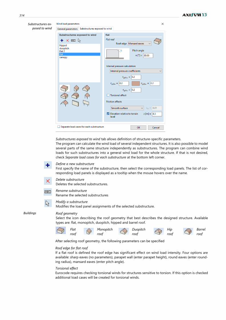
314

Substructures ex-posed to wind

Substructures exposed to wind tab allows definition of structure-specific parameters.

The program can calculate the wind load of several independent structures. It is also possible to model

several parts of the same structure independently as substructures. The program can combine wind

loads for such substructures into a general wind load for the whole structure. If that is not desired,

check Separate load cases for each substructure at the bottom left corner.

Define a new substructure

First specify the name of the substructure, then select the corresponding load panels. The list of cor-

responding load panels is displayed as a tooltip when the mouse hovers over the name.

Delete substructure

Deletes the selected substructures.

Rename substructure

Rename the selected substructures

Modify a substructure

Modifies the load panel assignments of the selected substructure.

Buildings Roof geometry

Select the icon describing the roof geometry that best describes the designed structure. Available

types are: flat, monopitch, duopitch, hipped and barrel roof.

Flat

roof

Monopitch

roof

Duopitch

roof

Hip

roof

Barrel

roof

After selecting roof geometry, the following parameters can be specified

Roof edge for flat roof

If a flat roof is defined the roof edge has significant effect on wind load intensity. Four options are

available: sharp eaves (no parameters), parapet wall (enter parapet height), round eaves (enter round-

ing radius), mansard eaves (enter pitch angle).

Torsional effect

Eurocode requires checking torsional winds for structures sensitive to torsion. If this option is checked

additional load cases will be created for torsional winds.

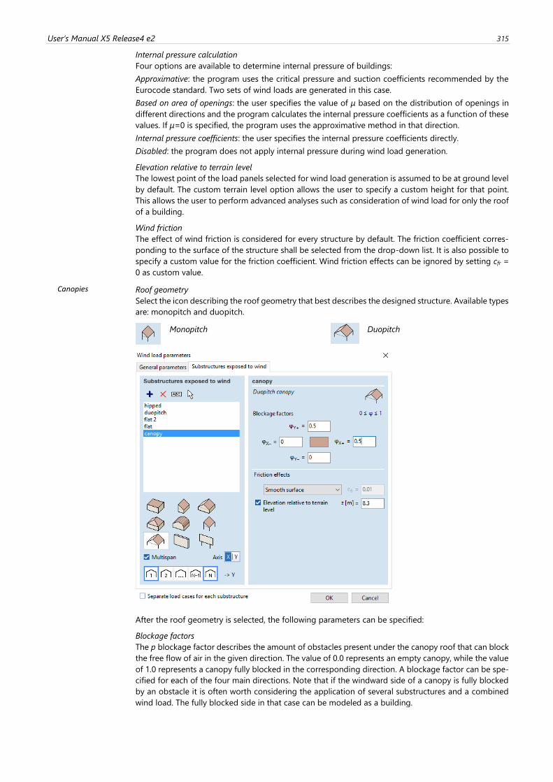
User’s Manual X5 Release4 e2 315

Internal pressure calculation

Four options are available to determine internal pressure of buildings:

Approximative: the program uses the critical pressure and suction coefficients recommended by the

Eurocode standard. Two sets of wind loads are generated in this case.

Based on area of openings: the user specifies the value of μ based on the distribution of openings in

different directions and the program calculates the internal pressure coefficients as a function of these

values. If μ=0 is specified, the program uses the approximative method in that direction.

Internal pressure coefficients: the user specifies the internal pressure coefficients directly.

Disabled: the program does not apply internal pressure during wind load generation.

Elevation relative to terrain level

The lowest point of the load panels selected for wind load generation is assumed to be at ground level

by default. The custom terrain level option allows the user to specify a custom height for that point.

This allows the user to perform advanced analyses such as consideration of wind load for only the roof

of a building.

Wind friction

The effect of wind friction is considered for every structure by default. The friction coefficient corres-

ponding to the surface of the structure shall be selected from the drop-down list. It is also possible to

specify a custom value for the friction coefficient. Wind friction effects can be ignored by setting cfr =

0 as custom value.

Canopies Roof geometry

Select the icon describing the roof geometry that best describes the designed structure. Available types

are: monopitch and duopitch.

Monopitch

Duopitch

After the roof geometry is selected, the following parameters can be specified:

Blockage factors

The p blockage factor describes the amount of obstacles present under the canopy roof that can block

the free flow of air in the given direction. The value of 0.0 represents an empty canopy, while the value

of 1.0 represents a canopy fully blocked in the corresponding direction. A blockage factor can be spe-

cified for each of the four main directions. Note that if the windward side of a canopy is fully blocked

by an obstacle it is often worth considering the application of several substructures and a combined

wind load. The fully blocked side in that case can be modeled as a building.

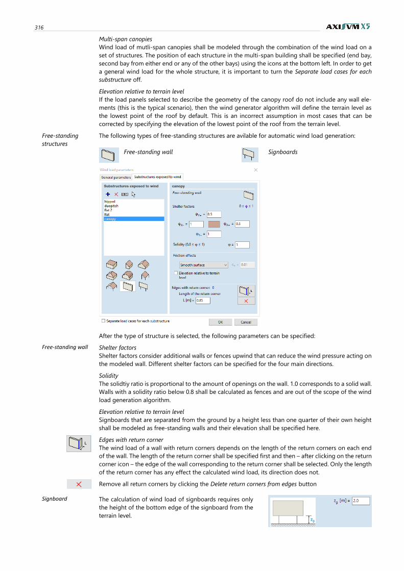
316

Multi-span canopies

Wind load of mutli-span canopies shall be modeled through the combination of the wind load on a

set of structures. The position of each structure in the multi-span building shall be specified (end bay,

second bay from either end or any of the other bays) using the icons at the bottom left. In order to get

a general wind load for the whole structure, it is important to turn the Separate load cases for each

substructure off.

Elevation relative to terrain level

If the load panels selected to describe the geometry of the canopy roof do not include any wall ele-

ments (this is the typical scenario), then the wind generator algorithm will define the terrain level as

the lowest point of the roof by default. This is an incorrect assumption in most cases that can be

corrected by specifying the elevation of the lowest point of the roof from the terrain level.

Free-standing

structures

The following types of free-standing structures are avilable for automatic wind load generation:

Free-standing wall

Signboards

After the type of structure is selected, the following parameters can be specified:

Free-standing wall Shelter factors

Shelter factors consider additional walls or fences upwind that can reduce the wind pressure acting on

the modeled wall. Different shelter factors can be specified for the four main directions.

Solidity

The solidtiy ratio is proportional to the amount of openings on the wall. 1.0 corresponds to a solid wall.

Walls with a solidity ratio below 0.8 shall be calculated as fences and are out of the scope of the wind

load generation algorithm.

Elevation relative to terrain level

Signboards that are separated from the ground by a height less than one quarter of their own height

shall be modeled as free-standing walls and their elevation shall be specified here.

Edges with return corner

The wind load of a wall with return corners depends on the length of the return corners on each end

of the wall. The length of the return corner shall be specified first and then – after clicking on the return

corner icon – the edge of the wall corresponding to the return corner shall be selected. Only the length

of the return corner has any effect the calculated wind load, its direction does not.

Remove all return corners by clicking the Delete return corners from edges button

Signboard The calculation of wind load of signboards requires only

the height of the bottom edge of the signboard from the

terrain level.

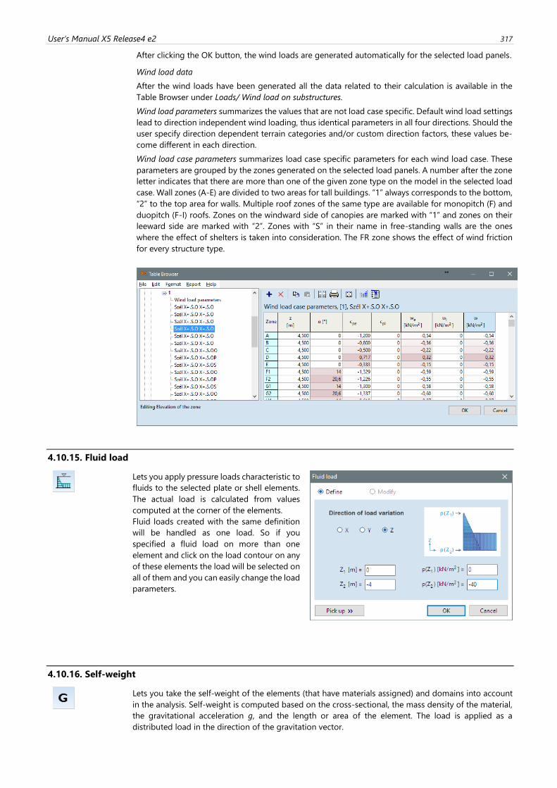
User’s Manual X5 Release4 e2 317

After clicking the OK button, the wind loads are generated automatically for the selected load panels.

Wind load data

After the wind loads have been generated all the data related to their calculation is available in the

Table Browser under Loads/ Wind load on substructures.

Wind load parameters summarizes the values that are not load case specific. Default wind load settings

lead to direction independent wind loading, thus identical parameters in all four directions. Should the

user specify direction dependent terrain categories and/or custom direction factors, these values be-

come different in each direction.

Wind load case parameters summarizes load case specific parameters for each wind load case. These

parameters are grouped by the zones generated on the selected load panels. A number after the zone

letter indicates that there are more than one of the given zone type on the model in the selected load

case. Wall zones (A-E) are divided to two areas for tall buildings. “1” always corresponds to the bottom,

“2” to the top area for walls. Multiple roof zones of the same type are available for monopitch (F) and

duopitch (F-I) roofs. Zones on the windward side of canopies are marked with “1” and zones on their

leeward side are marked with “2”. Zones with “S” in their name in free-standing walls are the ones

where the effect of shelters is taken into consideration. The FR zone shows the effect of wind friction

for every structure type.

4.10.15. Fluid load

Lets you apply pressure loads characteristic to

fluids to the selected plate or shell elements.

The actual load is calculated from values

computed at the corner of the elements.

Fluid loads created with the same definition

will be handled as one load. So if you

specified a fluid load on more than one

element and click on the load contour on any

of these elements the load will be selected on

all of them and you can easily change the load

parameters.

4.10.16. Self-weight

Lets you take the self-weight of the elements (that have materials assigned) and domains into account

in the analysis. Self-weight is computed based on the cross-sectional, the mass density of the material,

the gravitational acceleration g, and the length or area of the element. The load is applied as a

distributed load in the direction of the gravitation vector.

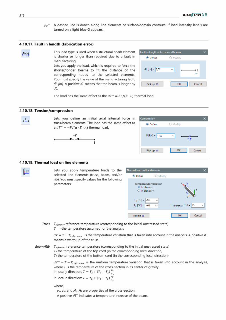
318

A dashed line is drawn along line elements or surface/domain contours. If load intensity labels are

turned on a light blue G appears.

4.10.17. Fault in length (fabrication error)

This load type is used when a structural beam element

is shorter or longer than required due to a fault in

manufacturing.

Lets you apply the load, which is required to force the

shorter/longer beams to fit the distance of the

corresponding nodes, to the selected elements.

You must specify the value of the manufacturing fault,

dL [m]. A positive dL means that the beam is longer by

dL.

The load has the same effect as the 𝑑𝑇= = 𝑑𝐿/(𝛼 ⋅ 𝐿) thermal load.

4.10.18. Tension/compression

Lets you define an initial axial internal force in

truss/beam elements. The load has the same effect as

a 𝑑𝑇= = −𝑃/(𝛼 ⋅ 𝐸 ⋅ 𝐴) thermal load.

4.10.19. Thermal load on line elements

Lets you apply temperature loads to the

selected line elements (truss, beam, and/or

rib). You must specify values for the following

parameters:

Truss Treference reference temperature (corresponding to the initial unstressed state)

T -the temperature assumed for the analysis

𝑑𝑇 = 𝑇 − 𝑇𝑟𝑒𝑓𝑒𝑟𝑒𝑛𝑐𝑒 is the temperature variation that is taken into account in the analysis. A positive dT

means a warm up of the truss.

Beam/Rib Treference reference temperature (corresponding to the initial unstressed state)

T1 the temperature of the top cord (in the corresponding local direction)

T2 the temperature of the bottom cord (in the corresponding local direction)

𝑑𝑇= = 𝑇 − 𝑇𝑟𝑒𝑓𝑒𝑟𝑒𝑛𝑐𝑒 is the uniform temperature variation that is taken into account in the analysis,

where T is the temperature of the cross-section in its center of gravity.

in local y direction: 𝑇 = 𝑇2 + (𝑇1 − 𝑇2)𝑦𝐺

𝐻𝑦

in local z direction: 𝑇 = 𝑇2 + (𝑇1 − 𝑇2)𝑧𝐺

𝐻𝑧

where,

yG, zG, and Hy, Hz are properties of the cross-section.

A positive dT= indicates a temperature increase of the beam.

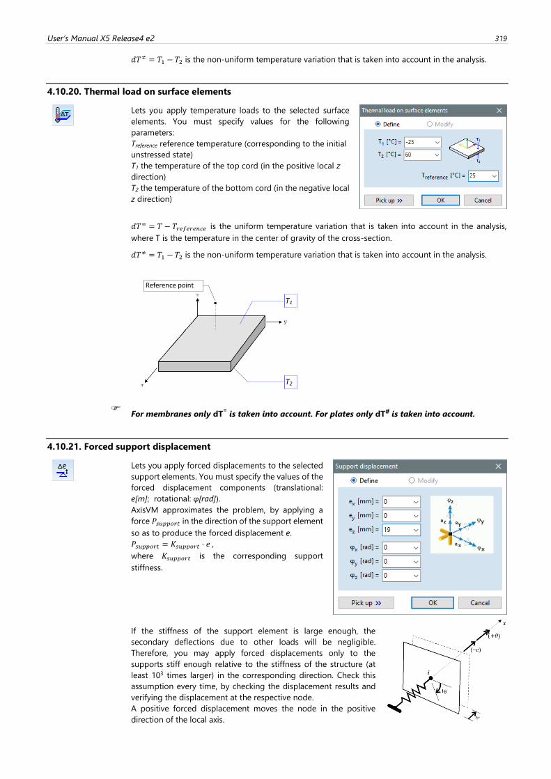
User’s Manual X5 Release4 e2 319

𝑑𝑇≠ = 𝑇1 − 𝑇2 is the non-uniform temperature variation that is taken into account in the analysis.

4.10.20. Thermal load on surface elements

Lets you apply temperature loads to the selected surface

elements. You must specify values for the following

parameters:

Treference reference temperature (corresponding to the initial

unstressed state)

T1 the temperature of the top cord (in the positive local z

direction)

T2 the temperature of the bottom cord (in the negative local

z direction)

𝑑𝑇= = 𝑇 − 𝑇𝑟𝑒𝑓𝑒𝑟𝑒𝑛𝑐𝑒 is the uniform temperature variation that is taken into account in the analysis,

where T is the temperature in the center of gravity of the cross-section.

𝑑𝑇≠ = 𝑇1 − 𝑇2 is the non-uniform temperature variation that is taken into account in the analysis.

For membranes only dT

= is taken into account. For plates only dT# is taken into account.

4.10.21. Forced support displacement

Lets you apply forced displacements to the selected

support elements. You must specify the values of the

forced displacement components (translational:

e[m]; rotational: φ[rad]).

AxisVM approximates the problem, by applying a

force 𝑃𝑠𝑢𝑝𝑝𝑜𝑟𝑡 in the direction of the support element

so as to produce the forced displacement e.

𝑃𝑠𝑢𝑝𝑝𝑜𝑟𝑡 = 𝐾𝑠𝑢𝑝𝑝𝑜𝑟𝑡 ⋅ 𝑒 ,

where 𝐾𝑠𝑢𝑝𝑝𝑜𝑟𝑡 is the corresponding support

stiffness.

If the stiffness of the support element is large enough, the

secondary deflections due to other loads will be negligible.

Therefore, you may apply forced displacements only to the

supports stiff enough relative to the stiffness of the structure (at

least 103 times larger) in the corresponding direction. Check this

assumption every time, by checking the displacement results and

verifying the displacement at the respective node.

A positive forced displacement moves the node in the positive

direction of the local axis.

T2

T1

Reference point

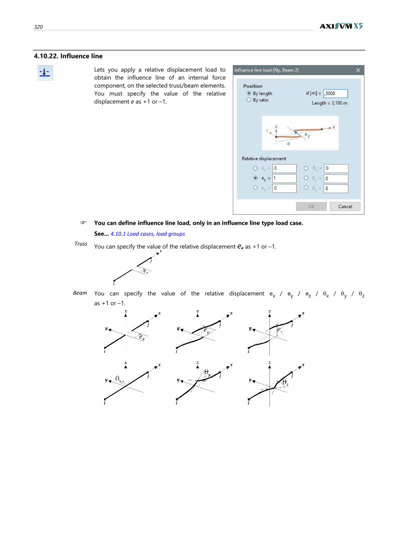
320

4.10.22. Influence line

Lets you apply a relative displacement load to

obtain the influence line of an internal force

component, on the selected truss/beam elements.

You must specify the value of the relative

displacement e as +1 or –1.

You can define influence line load, only in an influence line type load case.

See... 4.10.1 Load cases, load groups

Truss You can specify the value of the relative displacement ex as +1 or –1.

Beam You can specify the value of the relative displacement ex / ey / ez / x / y / z

as +1 or –1.

User’s Manual X5 Release4 e2 321

4.10.23. Seismic loads – SE1 module

The SE1 module includes several tools that facilitate the execution of Modal Response Spectrum

Analysis (MRSA) in AxisVM. The tools automatically perform seismic load generation in three orthogonal

directions for each vibration mode; calculation of structural response for each vibration mode and

combination of modal responses into a governing seismic effect. The following guide provides

information on the settings and options available in the program and explains how to use them. Due to

the vast literature of MRSA it is not possible to provide a step-by-step theoretical explanation to the

application of such an analysis here.

Design Codes Calculations are performed according to regulations in the general Eurocode standards (particularly

Eurocode 8) complemented by the National Annex that corresponds to the Design Code selected by

the user. Exceptions to this approach are the Swiss and Hungarian National Standards, which are not

based on the Eurocodes. The standards in the program for which MRSA calculation is available are listed

below.

Eurocode general EN 1998-1:2004 (EC 8-1)

Eurocode 8 Design of structures for earthquake resistance

Part 1: General rules, seismic actions and rules for buildings

EC German

EN 1998-1:2004 DIN EN 1998-1/NA:2011-01

EC Dutch

NPR 9998:2018

EC Hungarian

EN 1998-1:2004

EC Romanian

P100-1-2013

EC Czech

EN 1998-1:2004

EC Slovakian

EN 1998-1:2004

EC Polish

EN 1998-1:2004

EC Danish

EN 1998-1:2004

EC Austrian

EN 1998-1:2004

EC British EN 1998-1:2004

EC Finnish EN 1998-1:2004

EC Belgian EN 1998-1:2004

EC Swedish EN 1998-1:2004

NTC Italian

NTC 2018

Swiss

SIA 261:2003

Hungarian National Standard (MSZ)

Romanian STAS

German DIN 1045-1 DIN 4149:2005-04

MRSA procedure Seismic loads are generated based on the vibration mode shapes in all design codes. Loads are applied

in linear static analysis and the effects of several mode shapes are combined to get the design internal

forces and displacements of the structure.

Multiple seismic actions can be defined for the structure. These actions cannot be combined.

The following parts provide details on the calculation process. First, the general Eurocode procedure is

presented followed by a summary of country-specific modifications.

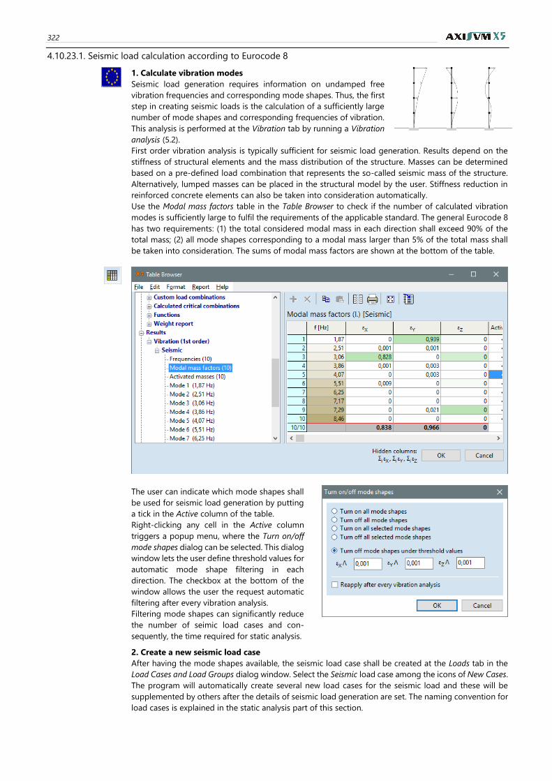
322

4.10.23.1. Seismic load calculation according to Eurocode 8

1. Calculate vibration modes

Seismic load generation requires information on undamped free

vibration frequencies and corresponding mode shapes. Thus, the first

step in creating seismic loads is the calculation of a sufficiently large

number of mode shapes and corresponding frequencies of vibration.

This analysis is performed at the Vibration tab by running a Vibration

analysis (5.2).

First order vibration analysis is typically sufficient for seismic load generation. Results depend on the

stiffness of structural elements and the mass distribution of the structure. Masses can be determined

based on a pre-defined load combination that represents the so-called seismic mass of the structure.

Alternatively, lumped masses can be placed in the structural model by the user. Stiffness reduction in

reinforced concrete elements can also be taken into consideration automatically.

Use the Modal mass factors table in the Table Browser to check if the number of calculated vibration

modes is sufficiently large to fulfil the requirements of the applicable standard. The general Eurocode 8

has two requirements: (1) the total considered modal mass in each direction shall exceed 90% of the

total mass; (2) all mode shapes corresponding to a modal mass larger than 5% of the total mass shall

be taken into consideration. The sums of modal mass factors are shown at the bottom of the table.

The user can indicate which mode shapes shall

be used for seismic load generation by putting

a tick in the Active column of the table.

Right-clicking any cell in the Active column

triggers a popup menu, where the Turn on/off

mode shapes dialog can be selected. This dialog

window lets the user define threshold values for

automatic mode shape filtering in each

direction. The checkbox at the bottom of the

window allows the user the request automatic

filtering after every vibration analysis.

Filtering mode shapes can significantly reduce

the number of seimic load cases and con-

sequently, the time required for static analysis.

2. Create a new seismic load case

After having the mode shapes available, the seismic load case shall be created at the Loads tab in the

Load Cases and Load Groups dialog window. Select the Seismic load case among the icons of New Cases.

The program will automatically create several new load cases for the seismic load and these will be

supplemented by others after the details of seismic load generation are set. The naming convention for

load cases is explained in the static analysis part of this section.

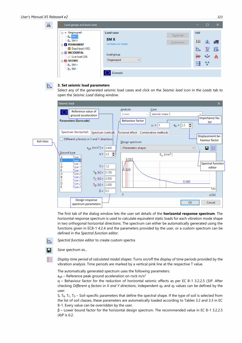
User’s Manual X5 Release4 e2 323

3. Set seismic load parameters

Select any of the generated seismic load cases and click on the Seismic load icon in the Loads tab to

open the Seismic Load dialog window.

The first tab of the dialog window lets the user set details of the horizontal response spectrum. The

horizontal response spectrum is used to calculate equivalent static loads for each vibration mode shape

in two orthogonal horizontal directions. The spectrum can either be automatically generated using the

functions given in EC8-1 4.2.4 and the parameters provided by the user, or a custom spectrum can be

defined in the Spectral function editor.

Spectral function editor to create custom spectra

Save spectrum as...

Display time period of calculated modal shapes: Turns on/off the display of time periods provided by the

vibration analysis. Time periods are marked by a vertical pink line at the respective T value.

The automatically generated spectrum uses the following parameters:

agR – Reference peak ground acceleration on rock m/s2

q – Behaviour factor for the reduction of horizontal seismic effects as per EC 8-1 3.2.2.5 (3)P. After

checking Different q factors in X and Y directions, independent qX and qY values can be defined by the

user.

S, TB, TC, TD – Soil-specific parameters that define the spectral shape. If the type of soil is selected from

the list of soil classes, these parameters are automatically loaded according to Tables 3.2 and 3.3 in EC

8-1. Every value can be overridden by the user.

β – Lower bound factor for the horizontal design spectrum. The recommended value in EC 8-1 3.2.2.5

(4)P is 0.2.

Spectral function editor

Soil class

Reference value of ground acceleration

Design response spectrum parameters

Displacement be-haviour factor

Importance fac-tor Behaviour factor

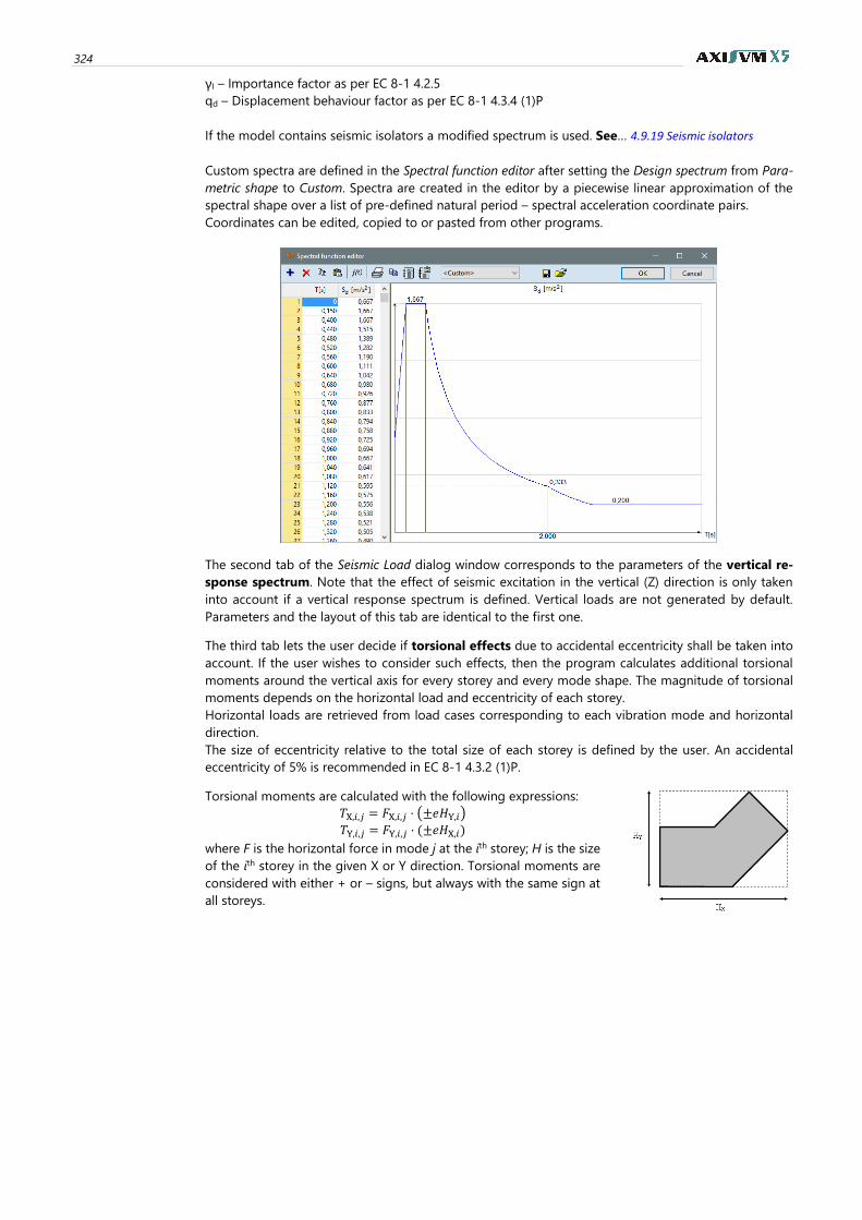
324

γI – Importance factor as per EC 8-1 4.2.5

qd – Displacement behaviour factor as per EC 8-1 4.3.4 (1)P

If the model contains seismic isolators a modified spectrum is used. See… 4.9.19 Seismic isolators

Custom spectra are defined in the Spectral function editor after setting the Design spectrum from Para-

metric shape to Custom. Spectra are created in the editor by a piecewise linear approximation of the

spectral shape over a list of pre-defined natural period – spectral acceleration coordinate pairs.

Coordinates can be edited, copied to or pasted from other programs.

The second tab of the Seismic Load dialog window corresponds to the parameters of the vertical re-

sponse spectrum. Note that the effect of seismic excitation in the vertical (Z) direction is only taken

into account if a vertical response spectrum is defined. Vertical loads are not generated by default.

Parameters and the layout of this tab are identical to the first one.

The third tab lets the user decide if torsional effects due to accidental eccentricity shall be taken into

account. If the user wishes to consider such effects, then the program calculates additional torsional

moments around the vertical axis for every storey and every mode shape. The magnitude of torsional

moments depends on the horizontal load and eccentricity of each storey.

Horizontal loads are retrieved from load cases corresponding to each vibration mode and horizontal

direction.

The size of eccentricity relative to the total size of each storey is defined by the user. An accidental

eccentricity of 5% is recommended in EC 8-1 4.3.2 (1)P.

Torsional moments are calculated with the following expressions:

𝑇X,𝑖,𝑗 = 𝐹X,𝑖,𝑗 ⋅ (±𝑒𝐻Y,𝑖)

𝑇Y,𝑖,𝑗 = 𝐹Y,𝑖,𝑗 ⋅ (±𝑒𝐻X,𝑖)

where F is the horizontal force in mode j at the ith storey; H is the size

of the ith storey in the given X or Y direction. Torsional moments are

considered with either + or – signs, but always with the same sign at

all storeys.

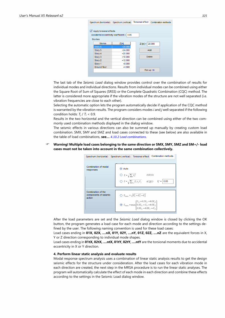
User’s Manual X5 Release4 e2 325

The last tab of the Seismic Load dialog window provides control over the combination of results for

individual modes and individual directions. Results from individual modes can be combined using either

the Square Root of Sum of Squares (SRSS) or the Complete Quadratic Combination (CQC) method. The

latter is considered more appropriate if the vibration modes of the structure are not well separated (i.e.

vibration frequencies are close to each other).

Selecting the automatic option lets the program automatically decide if application of the CQC method

is warranted by the vibration results. The program considers modes i and j well separated if the following

condition holds: Tj / Ti < 0.9.

Results in the two horizontal and the vertical direction can be combined using either of the two com-

monly used combination methods displayed in the dialog window.

The seismic effects in various directions can also be summed up manually by creating custom load

combination. SMX, SMY and SMZ and load cases connected to these (see below) are also available in

the table of load combinations, see… 4.10.2 Load combinations.

Warning! Multiple load cases belonging to the same direction or SMX, SMY, SMZ and SM+/- load

cases must not be taken into account in the same combination collectively.

After the load parameters are set and the Seismic Load dialog window is closed by clicking the OK

button, the program generates a load case for each mode and direction according to the settings de-

fined by the user. The following naming convention is used for these load cases:

Load cases ending in 01X, 02X, ....nX, 01Y, 02Y, ....nY, 01Z, 02Z, ....nZ are the equivalent forces in X,

Y or Z direction corresponding to individual mode shapes.

Load cases ending in 01tX, 02tX, ....ntX, 01tY, 02tY, ....ntY are the torsional moments due to accidental

eccentricity in X or Y direction.

4. Perform linear static analysis and evaluate results

Modal response spectrum analysis uses a combination of linear static analysis results to get the design

seismic effects for the structure under consideration. After the load cases for each vibration mode in

each direction are created, the next step in the MRSA procedure is to run the linear static analyses. The

program will automatically calculate the effect of each mode in each direction and combine these effects

according to the settings in the Seismic Load dialog window.

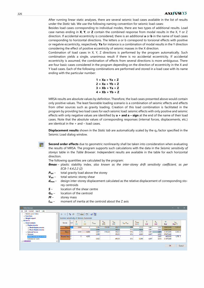
326

After running linear static analyses, there are several seismic load cases available in the list of results

under the Static tab. We use the following naming convention for seismic load cases:

Besides load cases corresponding to individual modes, there are two types of additional results. Load

case names ending in X, Y, or Z contain the combined response from modal results in the X, Y or Z

direction. If accidental eccentricity is considered, there is an additional a or b in the name of load cases

corresponding to horizontal directions. The letters a or b correspond to torsional effects with positive

or negatvie eccentricity, respectively. Ya for instance is a combination of modal results in the Y direction

considering the effect of positive eccentricity of seismic masses in the X direction.

Combination of load cases in X, Y, Z directions is performed by the program automatically. Such

combination yields a single, unanimous result if there is no accidental eccentricity. If accidental

eccentricity is assumed, the combination of effects from several directions is more ambiguous. There

are four basic cases considered in the program depending on the direction of eccentricity in the X and

Y load cases. Each of the following combinations are performed and stored in a load case with its name

ending with the particular number:

1 = Xa + Ya + Z

2 = Xa + Yb + Z

3 = Xb + Ya + Z

4 = Xb + Yb + Z

MRSA results are absolute values by definition. Therefore, the load cases presented above would contain

only positive values. The least favorable loading scenario is a combination of seismic effects and effects

from other sources such as gravity loading. Creation of this load combination is facilitated in the

program by providing two load cases for each seismic load: seismic effects with only positive and seismic

effects with only negative values are identified by a + and a – sign at the end of the name of their load

cases. Note that the absolute values of corresponding responses (internal forces, displacements, etc.)

are identical in the + and – load cases.

Displacement results shown in the Static tab are automatically scaled by the qd factor specified in the

Seismic Load dialog window.

Second order effects due to geometric nonlinearity shall be taken into consideration when evaluating

the results of MRSA. The program supports such calculations with the data in the Seismic sensitivity of

storeys table in the Table Browser. Independent results are available in the table for each horizontal

direction.

The following quantities are calculated by the program:

θmax – plastic stability index, also known as the inter-storey drift sensitivity coefficient, as per

EC8-1 4.4.2.2 (2)

Ptot – total gravity load above the storey

Vtot – total seismic storey shear

dmax – design inter-storey displacement calculated as the relative displacement of corresponding sto-

rey centroids

S – location of the shear centre

Gm – location of the centroid

M – storey mass

Imz – moment of inertia at the centroid about the Z axis

User’s Manual X5 Release4 e2 327

AxisVM does not consider the influence of second order effects automatically through internal force

amplification. The user shall evaluate the sensitivity of the structure to such effects. If the influence of

second order effects can be taken into consideration through force amplification, then the user shall

determine the appropriate value of the amplification factor as per EC8-1 4.4.2.2 (3). That amplification

factor can be specified in the program as the fse factor in the following design tools:

6.5.1 Surface reinforcement parameters and reinforcement calculation - RC1 module

6.5.9.2 Check of reinforced columns according to Eurocode 2

6.5.11.3 Checking actual beam reinforcement

6.5.12.1.1 Punching analysis of columns according to Eurocode

6.5.13 Footing design – RC4 module

6.6.1 Steel beam design according to Eurocode 3 – SD1 module

6.6.3 Bolted joint design of steel

The fse factor scales only the internal forces from seismic load.

4.10.23.2. Seismic load calculation according to Swiss SIA 261

The calculation procedure, dialog windows, assumptions and features are identical to those presented

in the general Eurocode 8 section. The following paragraphs list only the modifications that are

unique to the SIA 261 standard.

3. Set seismic load parameters

The following modifications are applied at the Seismic Load dialog window:

- Horizontal and vertical response spectra are based on SIA261 16.2.4.

- Soil-specific parameters are set according to Table 25 in SIA261.

4.10.23.3. Seismic load calculation according to German EC8-1 NA

The calculation procedure, dialog windows, assumptions and features are identical to those presented

in the general Eurocode 8 section. The following paragraphs list only the modifications that are

unique to the DIN EN 1998-1/NA (EC8-1 NA)standard.

3. Set seismic load parameters

The following modifications are applied at the Seismic Load dialog window:

- Horizontal and vertical response spectra are based on EC8-1 NA NDP 3.2.2.5(4)P.

- Soil-specific parameters are set according to Tables NA.4 and NA.5 in EC8-1 NA.

4.10.23.4. Seismic load calculation according to Italian NTC 2018

The calculation procedure, dialog windows, assumptions and features are identical to those presented

in the general Eurocode 8 section. The following paragraphs list only the modifications that are

unique to the latest NTC standard.

3. Set seismic load parameters

The following modifications are applied at the Seismic Load dialog window:

- Horizontal and vertical response spectra are based on NTC 2018 3.2.3.2.

- Soil-specific parameters are set according to Tables 3.2.V-VII in NTC 2018 3.2.3.2.

- If the model contains seismic isolators a modified spectrum is used, depending on the limit

state (SLO, SLD, SLV, SLC) set in the seismic parameters dialog according to NTC 2018 3.2.1.

See… 4.9.19 Seismic isolators. As multiple seismic actions can be defined for the same model,

seismic results obtained for different limit states can be compared.

- Results of the seismic isolator system are available in a separate table.

4.10.23.5. Seismic load calculation according to Romanian P100-1

The calculation procedure, dialog windows, assumptions and features are identical to those presented

in the general Eurocode 8 section. The following paragraphs list only the modifications that are

unique to the P100-1 standard.

3. Set seismic load parameters

The following modifications are applied at the Seismic Load dialog window:

- Horizontal and vertical response spectra are based on P100-1 3.1(7), 3.1(13), and 3.2(1).

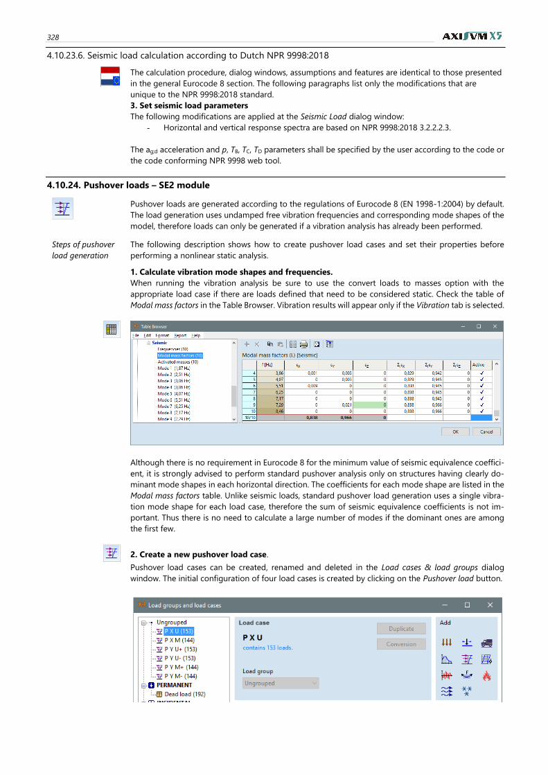
328

4.10.23.6. Seismic load calculation according to Dutch NPR 9998:2018

The calculation procedure, dialog windows, assumptions and features are identical to those presented

in the general Eurocode 8 section. The following paragraphs list only the modifications that are

unique to the NPR 9998:2018 standard.

3. Set seismic load parameters

The following modifications are applied at the Seismic Load dialog window:

- Horizontal and vertical response spectra are based on NPR 9998:2018 3.2.2.2.3.

The ag;d acceleration and p, TB, TC, TD parameters shall be specified by the user according to the code or

the code conforming NPR 9998 web tool.

4.10.24. Pushover loads – SE2 module

Pushover loads are generated according to the regulations of Eurocode 8 (EN 1998-1:2004) by default.

The load generation uses undamped free vibration frequencies and corresponding mode shapes of the

model, therefore loads can only be generated if a vibration analysis has already been performed.

Steps of pushover

load generation

The following description shows how to create pushover load cases and set their properties before

performing a nonlinear static analysis.

1. Calculate vibration mode shapes and frequencies.

When running the vibration analysis be sure to use the convert loads to masses option with the

appropriate load case if there are loads defined that need to be considered static. Check the table of

Modal mass factors in the Table Browser. Vibration results will appear only if the Vibration tab is selected.

Although there is no requirement in Eurocode 8 for the minimum value of seismic equivalence coeffici-

ent, it is strongly advised to perform standard pushover analysis only on structures having clearly do-

minant mode shapes in each horizontal direction. The coefficients for each mode shape are listed in the

Modal mass factors table. Unlike seismic loads, standard pushover load generation uses a single vibra-

tion mode shape for each load case, therefore the sum of seismic equivalence coefficients is not im-

portant. Thus there is no need to calculate a large number of modes if the dominant ones are among

the first few.

2. Create a new pushover load case.

Pushover load cases can be created, renamed and deleted in the Load cases & load groups dialog

window. The initial configuration of four load cases is created by clicking on the Pushover load button.

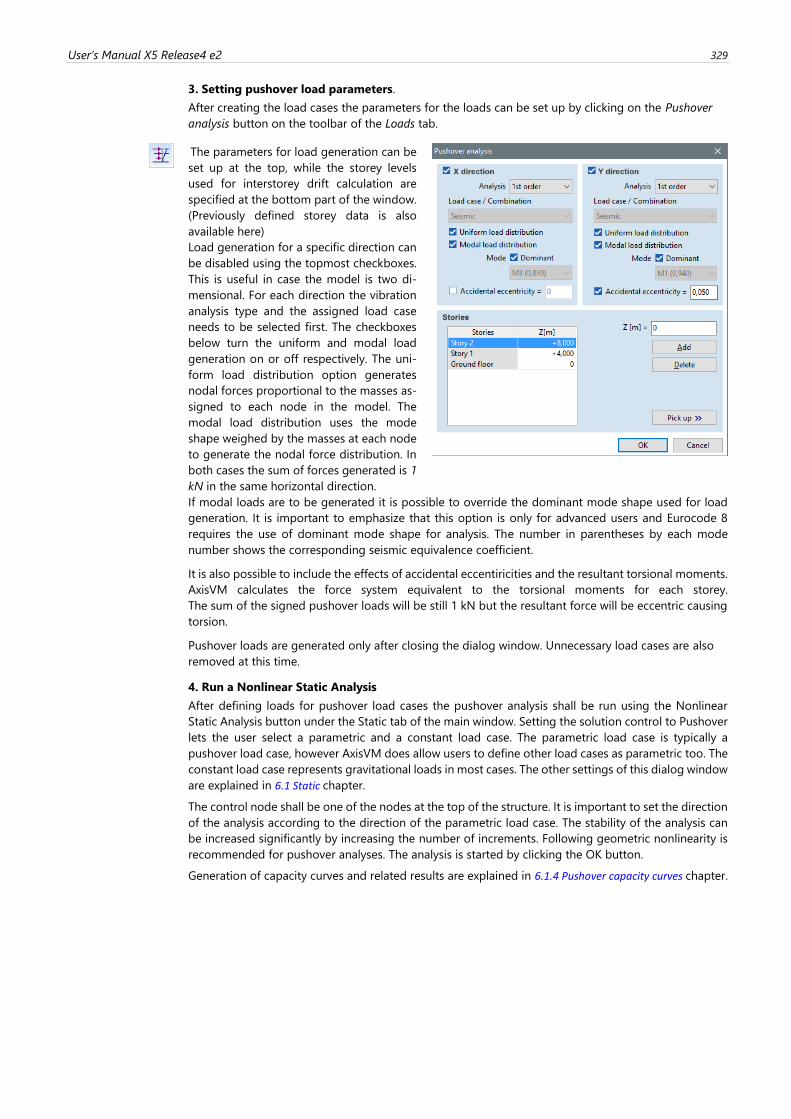
User’s Manual X5 Release4 e2 329

3. Setting pushover load parameters.

After creating the load cases the parameters for the loads can be set up by clicking on the Pushover

analysis button on the toolbar of the Loads tab.

The parameters for load generation can be

set up at the top, while the storey levels

used for interstorey drift calculation are

specified at the bottom part of the window.

(Previously defined storey data is also

available here)

Load generation for a specific direction can

be disabled using the topmost checkboxes.

This is useful in case the model is two di-

mensional. For each direction the vibration

analysis type and the assigned load case

needs to be selected first. The checkboxes

below turn the uniform and modal load

generation on or off respectively. The uni-

form load distribution option generates

nodal forces proportional to the masses as-

signed to each node in the model. The

modal load distribution uses the mode

shape weighed by the masses at each node

to generate the nodal force distribution. In

both cases the sum of forces generated is 1

kN in the same horizontal direction.

If modal loads are to be generated it is possible to override the dominant mode shape used for load

generation. It is important to emphasize that this option is only for advanced users and Eurocode 8

requires the use of dominant mode shape for analysis. The number in parentheses by each mode

number shows the corresponding seismic equivalence coefficient.

It is also possible to include the effects of accidental eccentiricities and the resultant torsional moments.

AxisVM calculates the force system equivalent to the torsional moments for each storey.

The sum of the signed pushover loads will be still 1 kN but the resultant force will be eccentric causing

torsion.

Pushover loads are generated only after closing the dialog window. Unnecessary load cases are also

removed at this time.

4. Run a Nonlinear Static Analysis

After defining loads for pushover load cases the pushover analysis shall be run using the Nonlinear

Static Analysis button under the Static tab of the main window. Setting the solution control to Pushover

lets the user select a parametric and a constant load case. The parametric load case is typically a

pushover load case, however AxisVM does allow users to define other load cases as parametric too. The

constant load case represents gravitational loads in most cases. The other settings of this dialog window

are explained in 6.1 Static chapter.

The control node shall be one of the nodes at the top of the structure. It is important to set the direction

of the analysis according to the direction of the parametric load case. The stability of the analysis can

be increased significantly by increasing the number of increments. Following geometric nonlinearity is

recommended for pushover analyses. The analysis is started by clicking the OK button.

Generation of capacity curves and related results are explained in 6.1.4 Pushover capacity curves chapter.

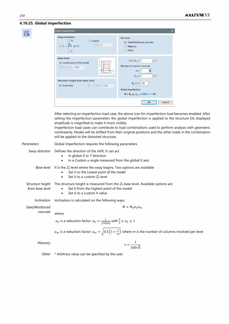
330

4.10.25. Global imperfection

After selecting an imperfection load case, the above icon for imperfection load becomes enabled. After

setting the imperfection parameters the global imperfection is applied to the structure (its displayed

amplitude is magnified to make it more visible).

Imperfection load cases can contribute to load combinations used to perform analysis with geometric

nonlinearity. Nodes will be shifted from their original positions and the other loads in the combination

will be applied to the distorted structure.

Parameters Global imperfection requires the following parameters.

Sway direction Defines the direction of the shift. It can act

• in global X or Y direction

• in a Custom angle measured from the global X axis

Base level It is the Z0 level where the sway begins. Two options are available

• Set it to the Lowest point of the model

• Set it to a custom Z0 level

Structure height

from base level

The structure height is measured from the Z0 base level. Available options are

• Set it from the highest point of the model

• Set it to a custom h value

Inclination Inclination is calculated on the following ways:

Steel/Reinforced

concrete

Φ = Φ0𝛼ℎ𝛼𝑚

where

𝛼ℎ is a reduction factor: 𝛼ℎ =2

√(ℎ[𝑚]) with

2

3≤ 𝛼ℎ ≤ 1

𝛼𝑚 is a reduction factor: 𝛼𝑚 = √0.5 (1 +1

𝑚) where m is the number of columns involved per level

Masonry ν =1

100√ℎ

Other * Arbitrary value can be specified by the user.

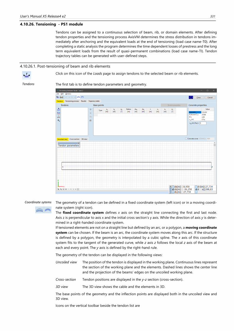
User’s Manual X5 Release4 e2 331

4.10.26. Tensioning - PS1 module

Tendons can be assigned to a continuous selection of beam, rib, or domain elements. After defining

tendon properties and the tensioning process AxisVM determines the stress distribution in tendons im-

mediately after anchoring and the equivalent loads at the end of tensioning (load case name-T0). After

completing a static analysis the program determines the time dependent losses of prestress and the long

term equivalent loads from the result of quasi-permanent combinations (load case name-TI). Tendon

trajectory tables can be generated with user-defined steps.

4.10.26.1. Post-tensioning of beam and rib elements

Click on this icon of the Loads page to assign tendons to the selected beam or rib elements.

Tendons The first tab is to define tendon parameters and geometry.

Coordinate sytems

The geometry of a tendon can be defined in a fixed coordinate system (left icon) or in a moving coordi-

nate system (right icon).

The fixed coordinate system defines x axis on the straight line connecting the first and last node.

Axis z is perpendicular to axis x and the initial cross section’s y axis. While the direction of axis y is deter-

mined in a right-handed coordinate system.

If tensioned elements are not on a straight line but defined by an arc, or a polygon, a moving coordinate

system can be chosen. If the beam is an arc, the coordinate system moves along this arc. If the structure

is defined by a polygon, the geometry is interpolated by a cubic spline. The x axis of this coordinate

system fits to the tangent of the generated curve, while z axis z follows the local z axis of the beam at

each and every point. The y axis is defined by the right-hand rule.

The geometry of the tendon can be displayed in the following views:

Uncoiled view The position of the tendon is displayed in the working plane. Continuous lines represent

the section of the working plane and the elements. Dashed lines shows the center line

and the projection of the beams’ edges on the uncoiled working plane.

Cross-section Tendon positions are displayed in the y-z section (cross-section).

3D view The 3D view shows the cable and the elements in 3D.

The base points of the geometry and the inflection points are displayed both in the uncoiled view and

3D view.

Icons on the vertical toolbar beside the tendon list are

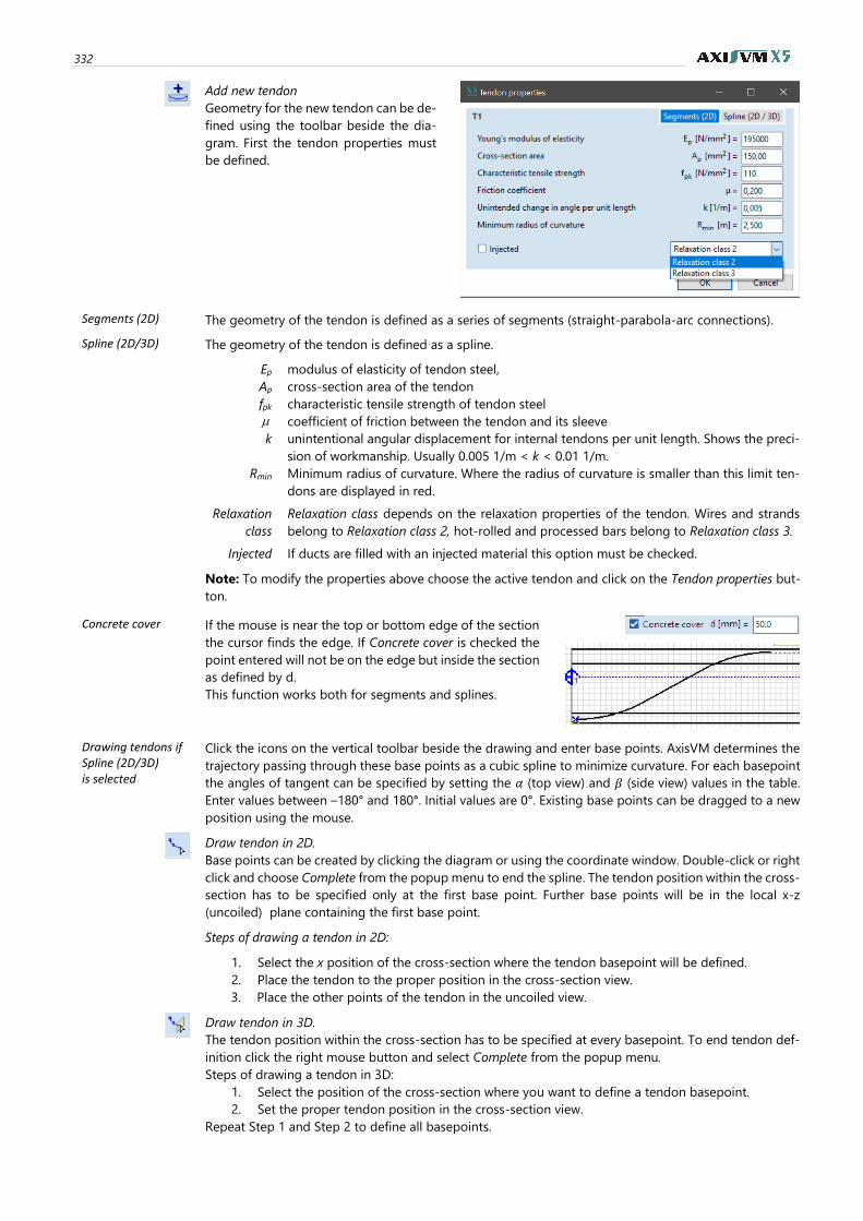
332

Add new tendon

Geometry for the new tendon can be de-

fined using the toolbar beside the dia-

gram. First the tendon properties must

be defined.

Segments (2D) The geometry of the tendon is defined as a series of segments (straight-parabola-arc connections).

Spline (2D/3D) The geometry of the tendon is defined as a spline.

Ep modulus of elasticity of tendon steel,

Ap cross-section area of the tendon

fpk characteristic tensile strength of tendon steel

coefficient of friction between the tendon and its sleeve

k unintentional angular displacement for internal tendons per unit length. Shows the preci-

sion of workmanship. Usually 0.005 1/m < k < 0.01 1/m.

Rmin Minimum radius of curvature. Where the radius of curvature is smaller than this limit ten-

dons are displayed in red.

Relaxation

class

Relaxation class depends on the relaxation properties of the tendon. Wires and strands

belong to Relaxation class 2, hot-rolled and processed bars belong to Relaxation class 3.

Injected If ducts are filled with an injected material this option must be checked.

Note: To modify the properties above choose the active tendon and click on the Tendon properties but-

ton.

Concrete cover If the mouse is near the top or bottom edge of the section

the cursor finds the edge. If Concrete cover is checked the

point entered will not be on the edge but inside the section

as defined by d.

This function works both for segments and splines.

Drawing tendons if Spline (2D/3D) is selected

Click the icons on the vertical toolbar beside the drawing and enter base points. AxisVM determines the

trajectory passing through these base points as a cubic spline to minimize curvature. For each basepoint

the angles of tangent can be specified by setting the 𝛼 (top view) and 𝛽 (side view) values in the table.

Enter values between –180° and 180°. Initial values are 0°. Existing base points can be dragged to a new

position using the mouse.

Draw tendon in 2D.

Base points can be created by clicking the diagram or using the coordinate window. Double-click or right

click and choose Complete from the popup menu to end the spline. The tendon position within the cross-

section has to be specified only at the first base point. Further base points will be in the local x-z

(uncoiled) plane containing the first base point.

Steps of drawing a tendon in 2D:

1. Select the x position of the cross-section where the tendon basepoint will be defined.

2. Place the tendon to the proper position in the cross-section view.

3. Place the other points of the tendon in the uncoiled view.

Draw tendon in 3D.

The tendon position within the cross-section has to be specified at every basepoint. To end tendon def-

inition click the right mouse button and select Complete from the popup menu.

Steps of drawing a tendon in 3D:

1. Select the position of the cross-section where you want to define a tendon basepoint.

2. Set the proper tendon position in the cross-section view.

Repeat Step 1 and Step 2 to define all basepoints.

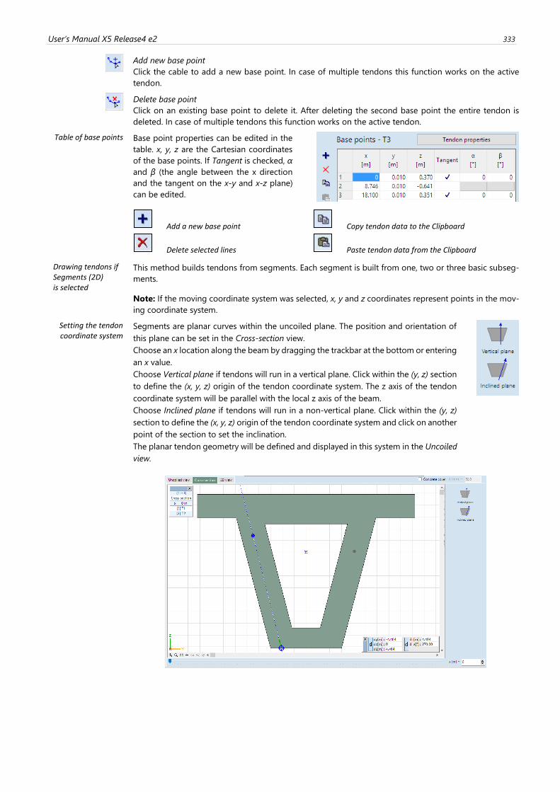
User’s Manual X5 Release4 e2 333

Add new base point

Click the cable to add a new base point. In case of multiple tendons this function works on the active

tendon.

Delete base point

Click on an existing base point to delete it. After deleting the second base point the entire tendon is

deleted. In case of multiple tendons this function works on the active tendon.

Table of base points Base point properties can be edited in the

table. x, y, z are the Cartesian coordinates

of the base points. If Tangent is checked, α

and β (the angle between the x direction

and the tangent on the x-y and x-z plane)

can be edited.

Add a new base point Copy tendon data to the Clipboard

Delete selected lines Paste tendon data from the Clipboard

Drawing tendons if Segments (2D) is selected

This method builds tendons from segments. Each segment is built from one, two or three basic subseg-

ments.

Note: If the moving coordinate system was selected, x, y and z coordinates represent points in the mov-

ing coordinate system.

Setting the tendon coordinate system

Segments are planar curves within the uncoiled plane. The position and orientation of

this plane can be set in the Cross-section view.

Choose an x location along the beam by dragging the trackbar at the bottom or entering

an x value.

Choose Vertical plane if tendons will run in a vertical plane. Click within the (y, z) section

to define the (x, y, z) origin of the tendon coordinate system. The z axis of the tendon

coordinate system will be parallel with the local z axis of the beam.

Choose Inclined plane if tendons will run in a non-vertical plane. Click within the (y, z)

section to define the (x, y, z) origin of the tendon coordinate system and click on another

point of the section to set the inclination.

The planar tendon geometry will be defined and displayed in this system in the Uncoiled

view.

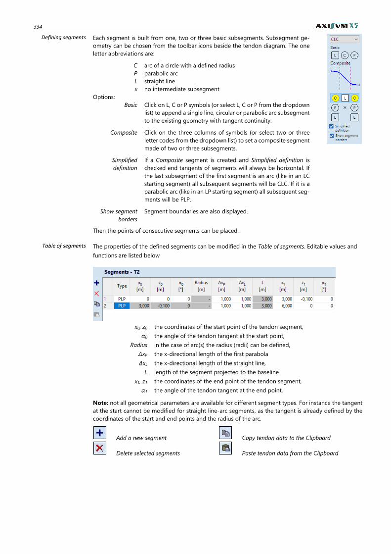
334

Defining segments Each segment is built from one, two or three basic subsegments. Subsegment ge-

ometry can be chosen from the toolbar icons beside the tendon diagram. The one

letter abbreviations are:

C arc of a circle with a defined radius

P parabolic arc

L straight line

x no intermediate subsegment

Options:

Basic Click on L, C or P symbols (or select L, C or P from the dropdown

list) to append a single line, circular or parabolic arc subsegment

to the existing geometry with tangent continuity.

Composite Click on the three columns of symbols (or select two or three

letter codes from the dropdown list) to set a composite segment

made of two or three subsegments.

Simplified

definition

If a Composite segment is created and Simplified definition is

checked end tangents of segments will always be horizontal. If

the last subsegment of the first segment is an arc (like in an LC

starting segment) all subsequent segments will be CLC. If it is a

parabolic arc (like in an LP starting segment) all subsequent seg-

ments will be PLP.

Show segment

borders

Segment boundaries are also displayed.

Then the points of consecutive segments can be placed.

Table of segments The properties of the defined segments can be modified in the Table of segments. Editable values and

functions are listed below

x0, z0 the coordinates of the start point of the tendon segment,

α0 the angle of the tendon tangent at the start point,

Radius in the case of arc(s) the radius (radii) can be defined,

ΔxP the x-directional length of the first parabola

ΔxL the x-directional length of the straight line,

L length of the segment projected to the baseline

x1, z1 the coordinates of the end point of the tendon segment,

α1 the angle of the tendon tangent at the end point.

Note: not all geometrical parameters are available for different segment types. For instance the tangent

at the start cannot be modified for straight line-arc segments, as the tangent is already defined by the

coordinates of the start and end points and the radius of the arc.

Add a new segment Copy tendon data to the Clipboard

Delete selected segments Paste tendon data from the Clipboard

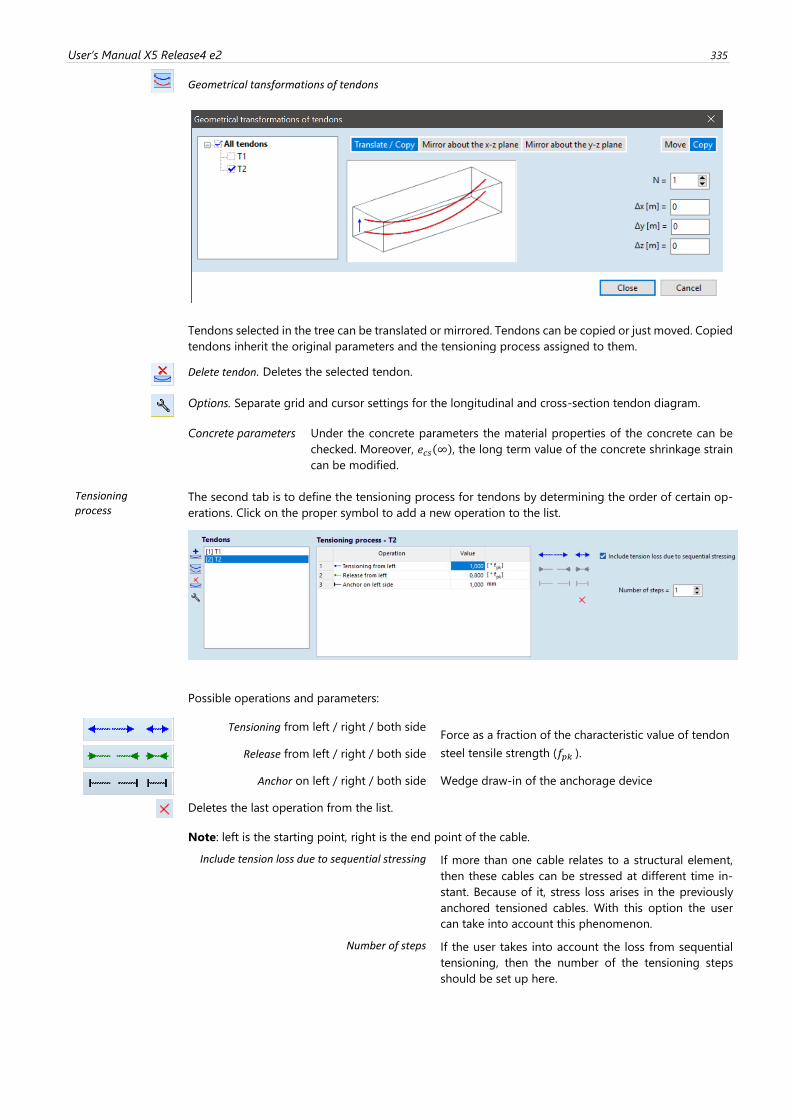
User’s Manual X5 Release4 e2 335

Geometrical tansformations of tendons

Tendons selected in the tree can be translated or mirrored. Tendons can be copied or just moved. Copied

tendons inherit the original parameters and the tensioning process assigned to them.

Delete tendon. Deletes the selected tendon.

Options. Separate grid and cursor settings for the longitudinal and cross-section tendon diagram.

Concrete parameters Under the concrete parameters the material properties of the concrete can be

checked. Moreover, 𝑒𝑐𝑠(∞), the long term value of the concrete shrinkage strain

can be modified.

Tensioning process

The second tab is to define the tensioning process for tendons by determining the order of certain op-

erations. Click on the proper symbol to add a new operation to the list.

Possible operations and parameters:

Tensioning from left / right / both side Force as a fraction of the characteristic value of tendon

steel tensile strength (𝑓𝑝𝑘 ).

Release from left / right / both side

Anchor on left / right / both side Wedge draw-in of the anchorage device

Deletes the last operation from the list.

Note: left is the starting point, right is the end point of the cable.

Include tension loss due to sequential stressing If more than one cable relates to a structural element,

then these cables can be stressed at different time in-

stant. Because of it, stress loss arises in the previously

anchored tensioned cables. With this option the user

can take into account this phenomenon.

Number of steps If the user takes into account the loss from sequential

tensioning, then the number of the tensioning steps

should be set up here.

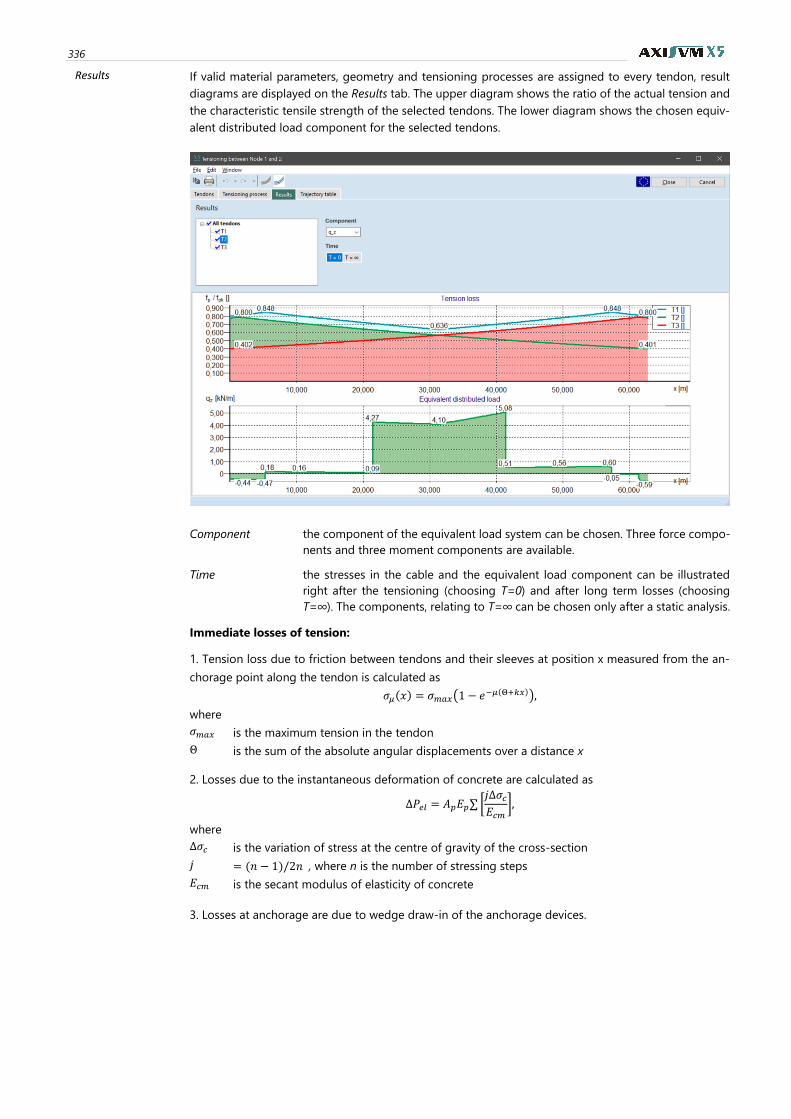
336

Results If valid material parameters, geometry and tensioning processes are assigned to every tendon, result

diagrams are displayed on the Results tab. The upper diagram shows the ratio of the actual tension and

the characteristic tensile strength of the selected tendons. The lower diagram shows the chosen equiv-

alent distributed load component for the selected tendons.

Component the component of the equivalent load system can be chosen. Three force compo-

nents and three moment components are available.

Time the stresses in the cable and the equivalent load component can be illustrated

right after the tensioning (choosing T=0) and after long term losses (choosing

T=∞). The components, relating to T=∞ can be chosen only after a static analysis.

Immediate losses of tension:

1. Tension loss due to friction between tendons and their sleeves at position x measured from the an-

chorage point along the tendon is calculated as

𝜎𝜇(𝑥) = 𝜎𝑚𝑎𝑥(1 − 𝑒−𝜇(Θ+𝑘𝑥)),

where

𝜎𝑚𝑎𝑥 is the maximum tension in the tendon

Θ is the sum of the absolute angular displacements over a distance x

2. Losses due to the instantaneous deformation of concrete are calculated as

Δ𝑃𝑒𝑙 = 𝐴𝑝𝐸𝑝∑ [𝑗Δ𝜎𝑐𝐸𝑐𝑚

],

where

Δ𝜎𝑐 is the variation of stress at the centre of gravity of the cross-section

𝑗 = (𝑛 − 1)/2𝑛 , where n is the number of stressing steps

𝐸𝑐𝑚 is the secant modulus of elasticity of concrete

3. Losses at anchorage are due to wedge draw-in of the anchorage devices.

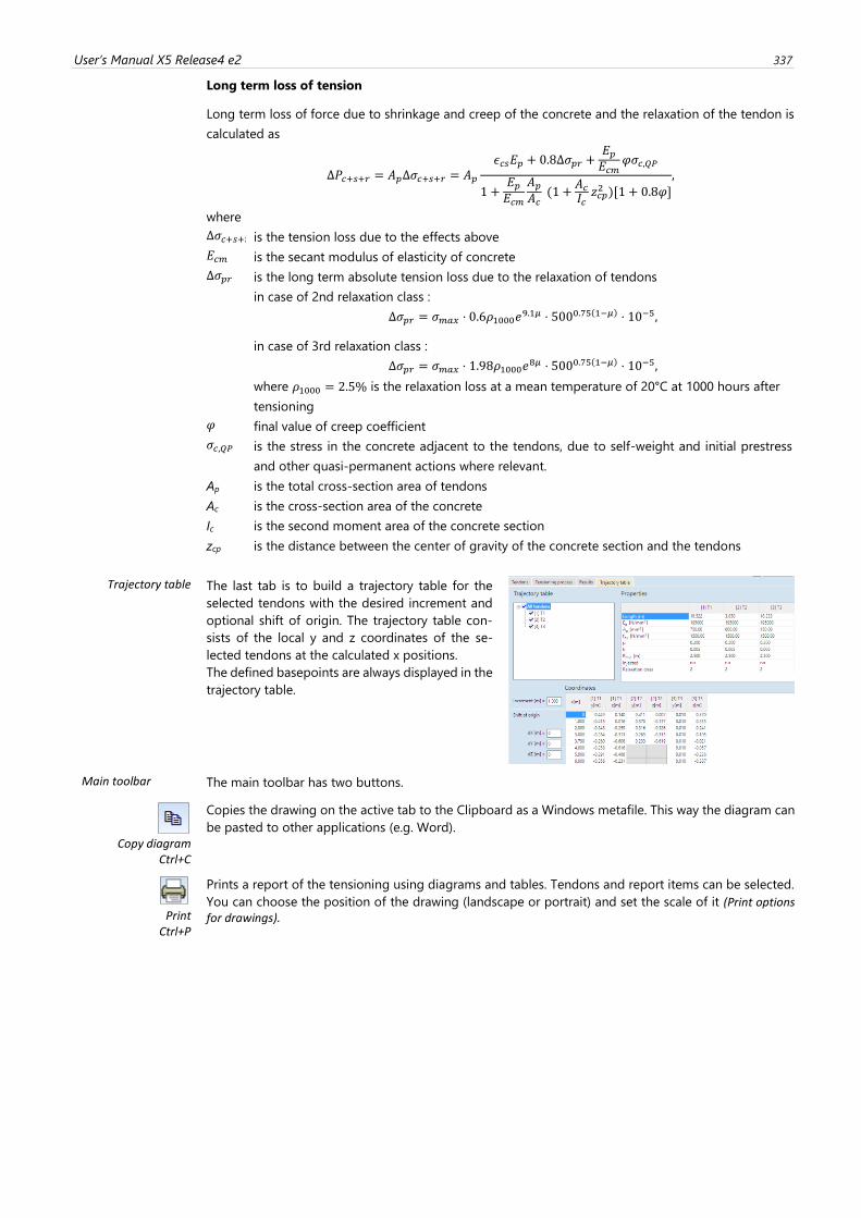
User’s Manual X5 Release4 e2 337

Long term loss of tension

Long term loss of force due to shrinkage and creep of the concrete and the relaxation of the tendon is

calculated as

Δ𝑃𝑐+𝑠+𝑟 = 𝐴𝑝Δ𝜎𝑐+𝑠+𝑟 = 𝐴𝑝

𝜖𝑐𝑠𝐸𝑝 + 0.8Δ𝜎𝑝𝑟 +𝐸𝑝𝐸𝑐𝑚

𝜑𝜎𝑐,𝑄𝑃

1 +𝐸𝑝𝐸𝑐𝑚

𝐴𝑝𝐴𝑐 (1 +

𝐴𝑐𝐼𝑐𝑧𝑐𝑝2 )[1 + 0.8𝜑]

,

where

Δ𝜎𝑐+𝑠+𝑟 is the tension loss due to the effects above

𝐸𝑐𝑚 is the secant modulus of elasticity of concrete

Δ𝜎𝑝𝑟 is the long term absolute tension loss due to the relaxation of tendons

in case of 2nd relaxation class :

Δ𝜎𝑝𝑟 = 𝜎𝑚𝑎𝑥 ⋅ 0.6𝜌1000𝑒9.1𝜇 ⋅ 5000.75(1−𝜇) ⋅ 10−5,

in case of 3rd relaxation class :

Δ𝜎𝑝𝑟 = 𝜎𝑚𝑎𝑥 ⋅ 1.98𝜌1000𝑒8𝜇 ⋅ 5000.75(1−𝜇) ⋅ 10−5,

where 𝜌1000 = 2.5% is the relaxation loss at a mean temperature of 20°C at 1000 hours after

tensioning

𝜑 final value of creep coefficient

𝜎𝑐,𝑄𝑃 is the stress in the concrete adjacent to the tendons, due to self-weight and initial prestress

and other quasi-permanent actions where relevant.

Ap is the total cross-section area of tendons

Ac is the cross-section area of the concrete

Ic is the second moment area of the concrete section

zcp is the distance between the center of gravity of the concrete section and the tendons

Trajectory table The last tab is to build a trajectory table for the

selected tendons with the desired increment and

optional shift of origin. The trajectory table con-

sists of the local y and z coordinates of the se-

lected tendons at the calculated x positions.

The defined basepoints are always displayed in the

trajectory table.

Main toolbar The main toolbar has two buttons.

Copy diagram

Ctrl+C

Copies the drawing on the active tab to the Clipboard as a Windows metafile. This way the diagram can

be pasted to other applications (e.g. Word).

Print

Ctrl+P

Prints a report of the tensioning using diagrams and tables. Tendons and report items can be selected.

You can choose the position of the drawing (landscape or portrait) and set the scale of it (Print options for drawings).

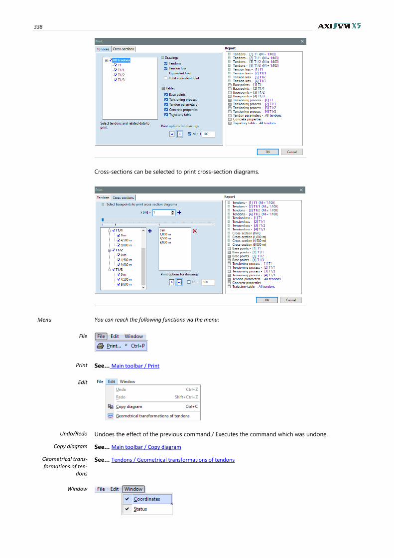
338

Cross-sections can be selected to print cross-section diagrams.

Menu You can reach the following functions via the menu:

File

Print See… Main toolbar / Print

Edit

Undo/Redo Undoes the effect of the previous command./ Executes the command which was undone.

Copy diagram See… Main toolbar / Copy diagram

Geometrical trans-formations of ten-

dons

See… Tendons / Geometrical transformations of tendons

Window

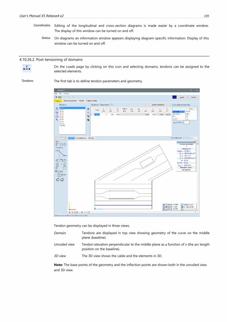
User’s Manual X5 Release4 e2 339

Coordinates Editing of the longitudinal and cross-section diagrams is made easier by a coordinate window.

The display of this window can be turned on and off.

Status On diagrams an information window appears displaying diagram-specific information. Display of this

window can be turned on and off.

4.10.26.2. Post-tensioning of domains

On the Loads page by clicking on this icon and selecting domains, tendons can be assigned to the

selected elements.

Tendons The first tab is to define tendon parameters and geometry.

Tendon geometry can be displayed in three views.

Domain Tendons are displayed in top view showing geometry of the curve on the middle

plane (baseline).

Uncoiled view Tendon elevation perpendicular to the middle plane as a function of x (the arc length

position on the baseline).

3D view The 3D view shows the cable and the elements in 3D.

Note: The base points of the geometry and the inflection points are shown both in the uncoiled view

and 3D view.

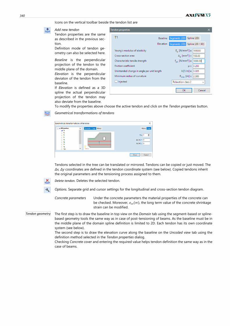
340

Icons on the vertical toolbar beside the tendon list are

Add new tendon

Tendon properties are the same

as described in the previous sec-

tion.

Definition mode of tendon ge-

ometry can also be selected here.

Baseline is the perpendicular

projection of the tendon to the

middle plane of the domain.

Elevation is the perpendicular

deviaton of the tendon from the

baseline.

If Elevation is defined as a 3D

spline the actual perpendicular

projection of the tendon may

also deviate from the baseline.

To modify the properties above choose the active tendon and click on the Tendon properties button.

Geometrical transformations of tendons

Tendons selected in the tree can be translated or mirrored. Tendons can be copied or just moved. The

Δx, Δy coordinates are defined in the tendon coordinate system (see below). Copied tendons inherit

the original parameters and the tensioning process assigned to them.

Delete tendon. Deletes the selected tendon.

Options. Separate grid and cursor settings for the longitudinal and cross-section tendon diagram.

Concrete parameters Under the concrete parameters the material properties of the concrete can

be checked. Moreover, 𝑒𝑐𝑠(∞), the long term value of the concrete shrinkage

strain can be modified.

Tendon geometry The first step is to draw the baseline in top view on the Domain tab using the segment-based or spline-

based geometry tools the same way as in case of post-tensioning of beams. As the baseline must be in

the middle plane of the domain spline definition is limited to 2D. Each tendon has its own coordinate

system (see below).

The second step is to draw the elevation curve along the baseline on the Uncoiled view tab using the

definition method selected in the Tendon properties dialog.

Checking Concrete cover and entering the required value helps tendon definition the same way as in the

case of beams.

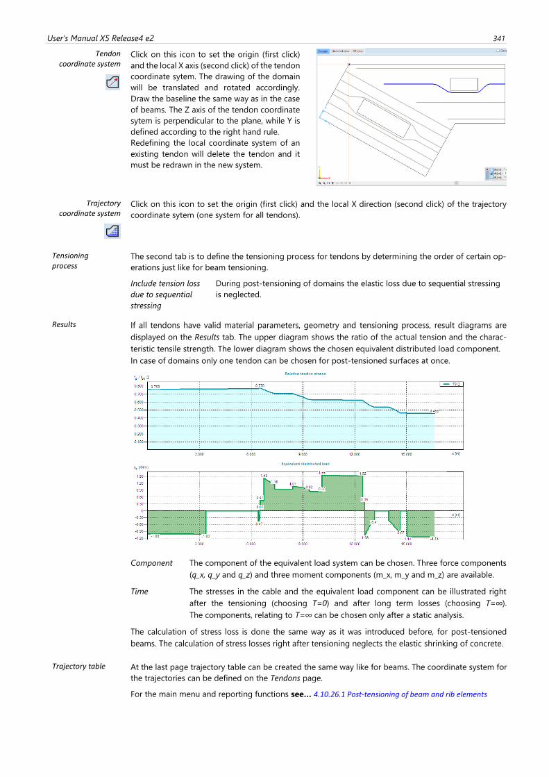
User’s Manual X5 Release4 e2 341

Tendon coordinate system

Click on this icon to set the origin (first click)

and the local X axis (second click) of the tendon

coordinate sytem. The drawing of the domain

will be translated and rotated accordingly.

Draw the baseline the same way as in the case

of beams. The Z axis of the tendon coordinate

sytem is perpendicular to the plane, while Y is

defined according to the right hand rule.

Redefining the local coordinate system of an

existing tendon will delete the tendon and it

must be redrawn in the new system.

Trajectory coordinate system

Click on this icon to set the origin (first click) and the local X direction (second click) of the trajectory

coordinate sytem (one system for all tendons).

Tensioning process

The second tab is to define the tensioning process for tendons by determining the order of certain op-

erations just like for beam tensioning.

Include tension loss

due to sequential

stressing

During post-tensioning of domains the elastic loss due to sequential stressing

is neglected.

Results If all tendons have valid material parameters, geometry and tensioning process, result diagrams are

displayed on the Results tab. The upper diagram shows the ratio of the actual tension and the charac-

teristic tensile strength. The lower diagram shows the chosen equivalent distributed load component.

In case of domains only one tendon can be chosen for post-tensioned surfaces at once.

Component The component of the equivalent load system can be chosen. Three force components

(q_x, q_y and q_z) and three moment components (m_x, m_y and m_z) are available.

Time The stresses in the cable and the equivalent load component can be illustrated right

after the tensioning (choosing T=0) and after long term losses (choosing T=∞).

The components, relating to T=∞ can be chosen only after a static analysis.

The calculation of stress loss is done the same way as it was introduced before, for post-tensioned

beams. The calculation of stress losses right after tensioning neglects the elastic shrinking of concrete.

Trajectory table At the last page trajectory table can be created the same way like for beams. The coordinate system for

the trajectories can be defined on the Tendons page.

For the main menu and reporting functions see… 4.10.26.1 Post-tensioning of beam and rib elements

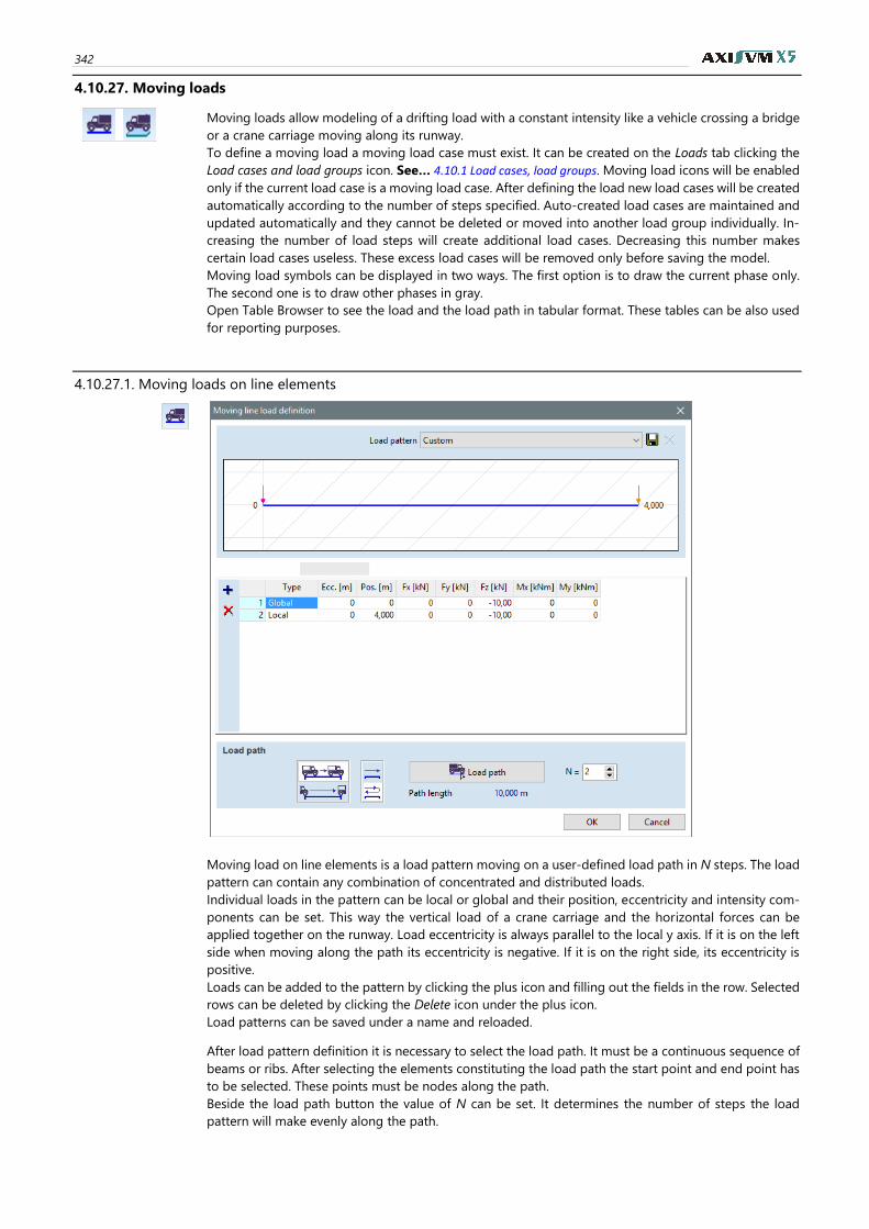
342

4.10.27. Moving loads

Moving loads allow modeling of a drifting load with a constant intensity like a vehicle crossing a bridge

or a crane carriage moving along its runway.

To define a moving load a moving load case must exist. It can be created on the Loads tab clicking the

Load cases and load groups icon. See… 4.10.1 Load cases, load groups. Moving load icons will be enabled

only if the current load case is a moving load case. After defining the load new load cases will be created

automatically according to the number of steps specified. Auto-created load cases are maintained and

updated automatically and they cannot be deleted or moved into another load group individually. In-

creasing the number of load steps will create additional load cases. Decreasing this number makes

certain load cases useless. These excess load cases will be removed only before saving the model.

Moving load symbols can be displayed in two ways. The first option is to draw the current phase only.

The second one is to draw other phases in gray.

Open Table Browser to see the load and the load path in tabular format. These tables can be also used

for reporting purposes.

4.10.27.1. Moving loads on line elements

Moving load on line elements is a load pattern moving on a user-defined load path in N steps. The load

pattern can contain any combination of concentrated and distributed loads.

Individual loads in the pattern can be local or global and their position, eccentricity and intensity com-

ponents can be set. This way the vertical load of a crane carriage and the horizontal forces can be

applied together on the runway. Load eccentricity is always parallel to the local y axis. If it is on the left

side when moving along the path its eccentricity is negative. If it is on the right side, its eccentricity is

positive.

Loads can be added to the pattern by clicking the plus icon and filling out the fields in the row. Selected

rows can be deleted by clicking the Delete icon under the plus icon.

Load patterns can be saved under a name and reloaded.

After load pattern definition it is necessary to select the load path. It must be a continuous sequence of

beams or ribs. After selecting the elements constituting the load path the start point and end point has

to be selected. These points must be nodes along the path.

Beside the load path button the value of N can be set. It determines the number of steps the load

pattern will make evenly along the path.

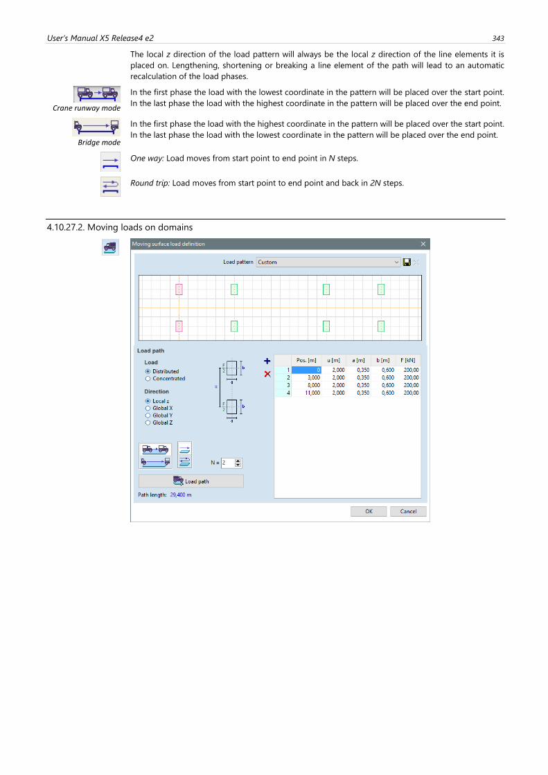
User’s Manual X5 Release4 e2 343

The local z direction of the load pattern will always be the local z direction of the line elements it is

placed on. Lengthening, shortening or breaking a line element of the path will lead to an automatic

recalculation of the load phases.

Crane runway mode

In the first phase the load with the lowest coordinate in the pattern will be placed over the start point.

In the last phase the load with the highest coordinate in the pattern will be placed over the end point.

Bridge mode

In the first phase the load with the highest coordinate in the pattern will be placed over the start point.

In the last phase the load with the lowest coordinate in the pattern will be placed over the end point.

One way: Load moves from start point to end point in N steps.

Round trip: Load moves from start point to end point and back in 2N steps.

4.10.27.2. Moving loads on domains

344

This load type is convenient when vehicle loads has to be defined. The load pattern consists of concen-

trated or rectangular surface loads pairs representing the wheels on the axles.

u is the vehicle gauge, a and b refer to the rectangle dimensions. Axle load F will be distributed evenly

on the two wheels. Load patterns can be saved under a name and reloaded.

The load type and direction switches on the left determines the properties of all loads

entered into the table.

Loads can be added to the pattern by clicking the plus icon and filling out the fields in the row. Selected

rows can be deleted by clicking the Delete icon under the plus icon.

After load pattern definition it is necessary to select the load path. It must be a continuous polyline

running through domains.

The load path does not have to stay in the same plane and can cross holes or empty areas

between domains.

Path start point and end point is the first and last point of the polyline.

Each phase will contain only the loads actually falling on a domain. The local z direction of the load

pattern will be the local z direction of the domain it is placed on. In case of a path running along the

edge of two or more domains in different planes only the domains in the active parts are taken into

account. The local z direction will be chosen finding the domain with the minimum angle between local

z and global Z directions.

Beside the load path button the value of N can be set. It determines the number of steps the load pattern

will make evenly along the path.

In the first phase the load with the lowest coordinate in the pattern will be placed over the start point. In

the last phase the load with the highest coordinate in the pattern will be placed over the end point.

Changing domain geometry will lead to an automatic recalculation of the load phases.

Crane runway

mode

In the first phase the load with the lowest coordinate in the pattern will be placed over the start point. In

the last phase the load with the highest coordinate in the pattern will be placed over the end point.

Bridge mode

In the first phase the load with the highest coordinate in the pattern will be placed over the start point.

In the last phase the load with the lowest coordinate in the pattern will be placed over the end point.

One way: Load moves from start point to end point in N steps.

Round trip: Load moves from start point to end point and back in 2N steps.

4.10.28. Dynamic loads (for time-history analysis) – DYN module

Dynamic nodal loads and acceleration functions can be defined for time-history analysis.

Acceleration functions can be used for seismic analysis. In this case it is recommended to

obtain proper seismic accelerograms and assign these functions to support nodes to analyse the effects

of the earthquake. This method provides more exact results than the response spectrum analysis and

can be used even if nonlinear elements are defined in the model (nonlinear supports, tension-only

trusses, etc.). Its disadvantage is that it cannot be combined with other load types automatically.

To define nodal loads or acceleration functions the current load case must be a dynamic load case.

See… 4.10.1 Load cases, load groups

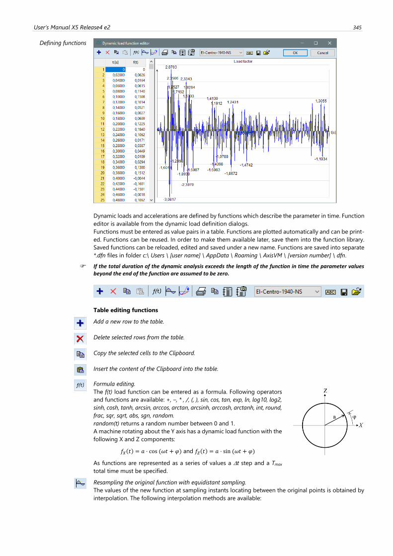
User’s Manual X5 Release4 e2 345

Defining functions

Dynamic loads and accelerations are defined by functions which describe the parameter in time. Function

editor is available from the dynamic load definition dialogs.

Functions must be entered as value pairs in a table. Functions are plotted automatically and can be print-

ed. Functions can be reused. In order to make them available later, save them into the function library.

Saved functions can be reloaded, edited and saved under a new name. Functions are saved into separate

*.dfn files in folder c:\ Users \ [user name] \ AppData \ Roaming \ AxisVM \ [version number] \ dfn.

If the total duration of the dynamic analysis exceeds the length of the function in time the parameter values beyond the end of the function are assumed to be zero.

Table editing functions

Add a new row to the table.

Delete selected rows from the table.

Copy the selected cells to the Clipboard.

Insert the content of the Clipboard into the table.

Formula editing.

The f(t) load function can be entered as a formula. Following operators

and functions are available: +, –, * , /, (, ), sin, cos, tan, exp, ln, log10, log2,

sinh, cosh, tanh, arcsin, arccos, arctan, arcsinh, arccosh, arctanh, int, round,

frac, sqr, sqrt, abs, sgn, random.

random(t) returns a random number between 0 and 1.

A machine rotating about the Y axis has a dynamic load function with the

following X and Z components:

𝑓𝑋(𝑡) = 𝑎 ⋅ cos (𝜔𝑡 + 𝜑) and 𝑓𝑍(𝑡) = 𝑎 ⋅ sin (𝜔𝑡 + 𝜑)

As functions are represented as a series of values a t step and a Tmax

total time must be specified.

Resampling the original function with equidistant sampling.

The values of the new function at sampling instants locating between the original points is obtained by

interpolation. The following interpolation methods are available:

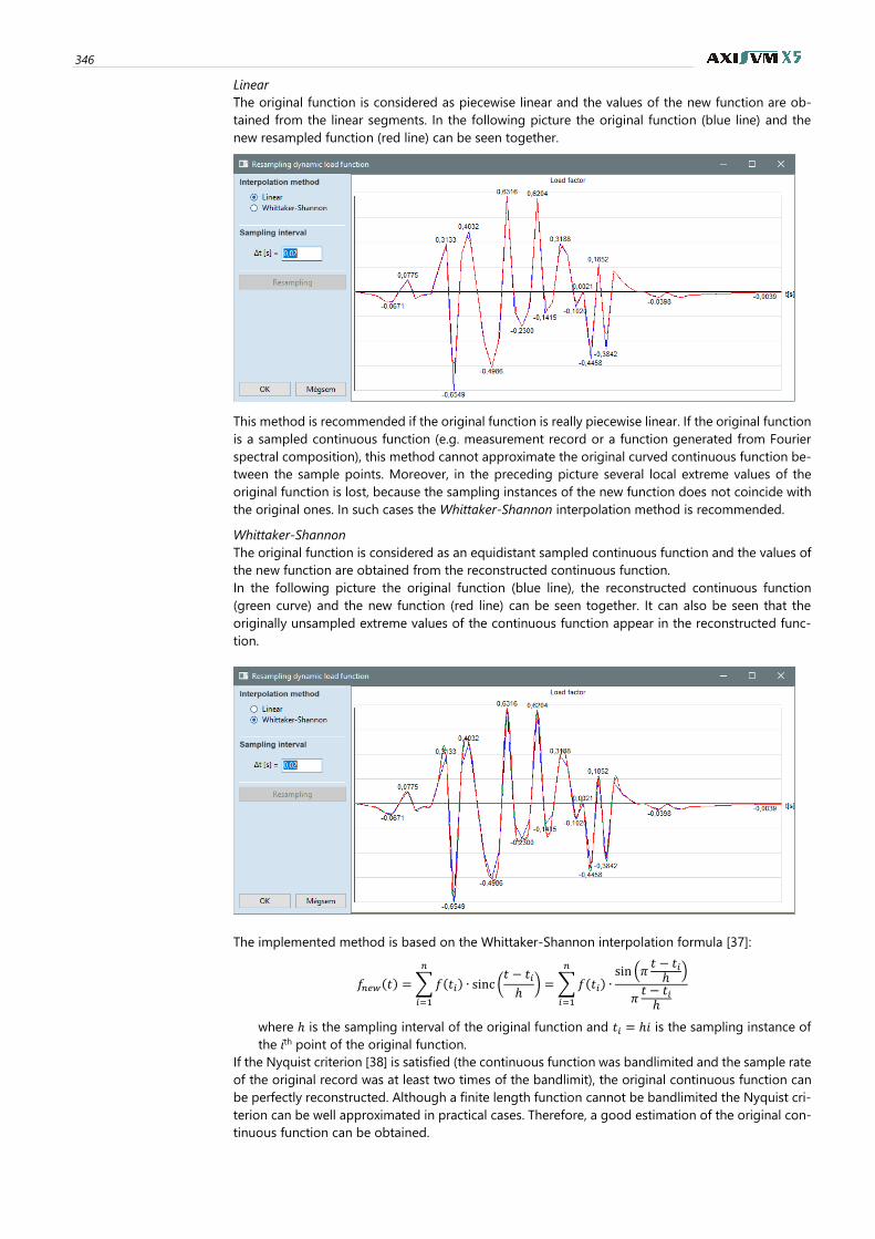
346

Linear

The original function is considered as piecewise linear and the values of the new function are ob-

tained from the linear segments. In the following picture the original function (blue line) and the

new resampled function (red line) can be seen together.

This method is recommended if the original function is really piecewise linear. If the original function

is a sampled continuous function (e.g. measurement record or a function generated from Fourier

spectral composition), this method cannot approximate the original curved continuous function be-

tween the sample points. Moreover, in the preceding picture several local extreme values of the

original function is lost, because the sampling instances of the new function does not coincide with

the original ones. In such cases the Whittaker-Shannon interpolation method is recommended.

Whittaker-Shannon

The original function is considered as an equidistant sampled continuous function and the values of

the new function are obtained from the reconstructed continuous function.

In the following picture the original function (blue line), the reconstructed continuous function

(green curve) and the new function (red line) can be seen together. It can also be seen that the

originally unsampled extreme values of the continuous function appear in the reconstructed func-

tion.

The implemented method is based on the Whittaker-Shannon interpolation formula [37]:

𝑓𝑛𝑒𝑤(𝑡) =∑𝑓(𝑡𝑖) ∙ sinc (𝑡 − 𝑡𝑖ℎ

)

𝑛

𝑖=1

=∑𝑓(𝑡𝑖) ∙sin (𝜋

𝑡 − 𝑡𝑖ℎ

)

𝜋𝑡 − 𝑡𝑖ℎ

𝑛

𝑖=1

where ℎ is the sampling interval of the original function and 𝑡𝑖 = ℎ𝑖 is the sampling instance of

the ith point of the original function.

If the Nyquist criterion [38] is satisfied (the continuous function was bandlimited and the sample rate

of the original record was at least two times of the bandlimit), the original continuous function can

be perfectly reconstructed. Although a finite length function cannot be bandlimited the Nyquist cri-

terion can be well approximated in practical cases. Therefore, a good estimation of the original con-

tinuous function can be obtained.

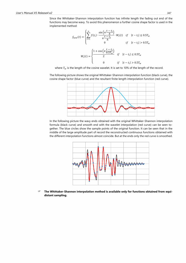
User’s Manual X5 Release4 e2 347

Since the Whittaker-Shannon interpolation function has infinite length the fading out end of the

functions may become wavy. To avoid this phenomenon a further cosine shape factor is used in the

implemented method:

𝑓𝑛𝑒𝑤(𝑡) =

{

∑𝑓(𝑡𝑖) ∙

sin (𝜋𝑡 − 𝑡𝑖ℎ

)

𝜋𝑡 − 𝑡𝑖ℎ

𝑛

𝑖=1

∙ 𝑊𝑖(𝑡) 𝑖𝑓 |𝑡 − 𝑡𝑖| ≤ 0.5𝑇𝑤

0 𝑖𝑓 |𝑡 − 𝑡𝑖| > 0.5𝑇𝑤

𝑊𝑖(𝑡) =

{

1 + cos (𝜋

𝑡 − 𝑡𝑖0.5𝑇𝑤

)

2𝑖𝑓 |𝑡 − 𝑡𝑖| ≤ 0.5𝑇𝑤

0 𝑖𝑓 |𝑡 − 𝑡𝑖| > 0.5𝑇𝑤

where 𝑇𝑤 is the length of the cosine wavelet. It is set to 10% of the length of the record.

The following picture shows the original Whittaker-Shannon interpolation function (black curve), the

cosine shape factor (blue curve) and the resultant finite length interpolation function (red curve).

In the following picture the wavy ends obtained with the original Whittaker-Shannon interpolation

formula (black curve) and smooth end with the wavelet interpolation (red curve) can be seen to-

gether. The blue circles show the sample points of the original function. It can be seen that in the

middle of the large amplitude part of record the reconstructed continuous functions obtained with

the different interpolation functions almost coincide. But at the ends only the red curve is smoothed.

The Whittaker-Shannon interpolation method is available only for functions obtained from equi-

distant sampling.

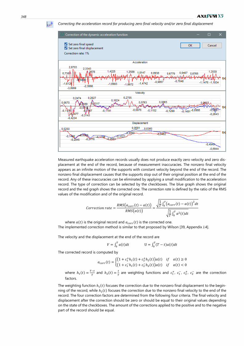
348

Correcting the acceleration record for producing zero final velocity and/or zero final displacement

Measured earthquake acceleration records usually does not produce exactly zero velocity and zero dis-

placement at the end of the record, because of measurement inaccuracies. The nonzero final velocity

appears as an infinite motion of the supports with constant velocity beyond the end of the record. The

nonzero final displacement causes that the supports stop out of their original position at the end of the

record. Any of these inaccuracies can be eliminated by applying a small modification to the acceleration

record. The type of correction can be selected by the checkboxes. The blue graph shows the original

record and the red graph shows the corrected one. The correction rate is defined by the ratio of the RMS

values of the modification and of the original record.

𝐶𝑜𝑟𝑟𝑒𝑐𝑡𝑖𝑜𝑛 𝑟𝑎𝑡𝑒 =𝑅𝑀𝑆(𝑎𝑐𝑜𝑟𝑟(𝑡) − 𝑎(𝑡))

𝑅𝑀𝑆(𝑎(𝑡))=

√1𝑇 ∫

(𝑎𝑐𝑜𝑟𝑟(𝑡) − 𝑎(𝑡))2𝑑𝑡

𝑇

0

√1𝑇 ∫

𝑎2(𝑡)𝑑𝑡𝑇

0

where 𝑎(𝑡) is the original record and 𝑎𝑐𝑜𝑟𝑟(𝑡) is the corrected one.

The implemented correction method is similar to that proposed by Wilson [39, Appendix J.4].

The velocity and the displacement at the end of the record are

𝑉 = ∫ 𝑎(𝑡)𝑑𝑡𝑇

0 U = ∫ (𝑇 − 𝑡)𝑎(𝑡)𝑑𝑡

𝑇

0

The corrected record is computed by

𝑎𝑐𝑜𝑟𝑟(𝑡) = {(1 + 𝑐1

+ℎ1(𝑡) + 𝑐2+ℎ2(𝑡))𝑎(𝑡) 𝑖𝑓 𝑎(𝑡) ≥ 0

(1 + 𝑐1−ℎ1(𝑡) + 𝑐2

−ℎ2(𝑡))𝑎(𝑡) 𝑖𝑓 𝑎(𝑡) < 0

where ℎ1(𝑡) =𝑇−𝑡

𝑇 and ℎ2(𝑡) =

𝑡

𝑇 are weighting functions and 𝑐1

+, 𝑐1−, 𝑐2

+, 𝑐2− are the correction

factors.

The weighting function ℎ1(𝑡) focuses the correction due to the nonzero final displacement to the begin-

ning of the record, while ℎ2(𝑡) focuses the correction due to the nonzero final velocity to the end of the

record. The four correction factors are determined from the following four criteria. The final velocity and

displacement after the correction should be zero or should be equal to their original values depending

on the state of the checkboxes. The amount of the corrections applied to the positive and to the negative

part of the record should be equal.

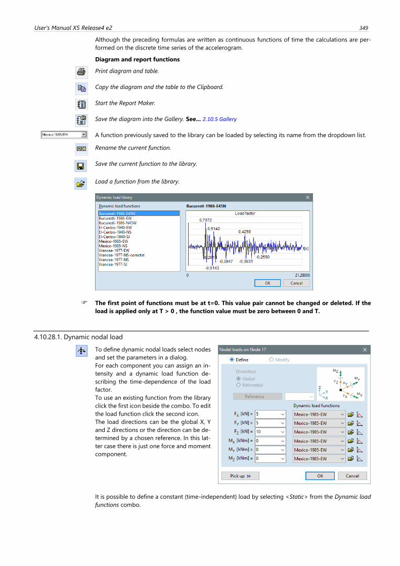
User’s Manual X5 Release4 e2 349

Although the preceding formulas are written as continuous functions of time the calculations are per-

formed on the discrete time series of the accelerogram.

Diagram and report functions

Print diagram and table.

Copy the diagram and the table to the Clipboard.

Start the Report Maker.

Save the diagram into the Gallery. See... 2.10.5 Gallery

A function previously saved to the library can be loaded by selecting its name from the dropdown list.

Rename the current function.

Save the current function to the library.

Load a function from the library.

The first point of functions must be at t=0. This value pair cannot be changed or deleted. If the

load is applied only at T > 0 , the function value must be zero between 0 and T.

4.10.28.1. Dynamic nodal load

To define dynamic nodal loads select nodes

and set the parameters in a dialog.

For each component you can assign an in-

tensity and a dynamic load function de-

scribing the time-dependence of the load

factor.

To use an existing function from the library

click the first icon beside the combo. To edit

the load function click the second icon.

The load directions can be the global X, Y

and Z directions or the direction can be de-

termined by a chosen reference. In this lat-

ter case there is just one force and moment

component.

It is possible to define a constant (time-independent) load by selecting <Static> from the Dynamic load

functions combo.

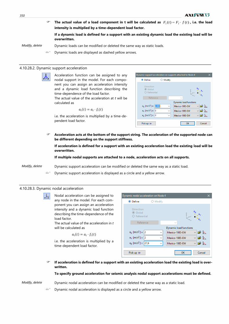
350

The actual value of a load component in t will be calculated as )()( tfFtF ii = , i.e. the load

intensity is multiplied by a time-dependent load factor.

If a dynamic load is defined for a support with an existing dynamic load the existing load will be

overwritten.

Modify, delete Dynamic loads can be modified or deleted the same way as static loads.

Dynamic loads are displayed as dashed yellow arrows.

4.10.28.2. Dynamic support acceleration

Acceleration function can be assigned to any

nodal support in the model. For each compo-

nent you can assign an acceleration intensity

and a dynamic load function describing the

time-dependence of the load factor.

The actual value of the acceleration at t will be

calculated as

𝑎𝑖(𝑡) = 𝑎𝑖 ⋅ 𝑓𝑖(𝑡)

i.e. the acceleration is multiplied by a time-de-

pendent load factor.

Acceleration acts at the bottom of the support string. The acceleration of the supported node can

be different depending on the support stiffness.

If acceleration is defined for a support with an existing acceleration load the existing load will be

overwritten.

If multiple nodal supports are attached to a node, acceleration acts on all supports.

Modify, delete Dynamic support acceleration can be modified or deleted the same way as a static load.

Dynamic support acceleration is displayed as a circle and a yellow arrow.

4.10.28.3. Dynamic nodal acceleration

Nodal acceleration can be assigned to

any node in the model. For each com-

ponent you can assign an acceleration

intensity and a dynamic load function

describing the time-dependence of the

load factor.

The actual value of the acceleration in t

will be calculated as

𝑎𝑖(𝑡) = 𝑎𝑖 ⋅ 𝑓𝑖(𝑡)

i.e. the acceleration is multiplied by a

time-dependent load factor.

If acceleration is defined for a support with an existing acceleration load the existing load is over-

written.

To specify ground acceleration for seismic analysis nodal support accelerations must be defined.

Modify, delete Dynamic nodal acceleration can be modified or deleted the same way as a static load.

Dynamic nodal acceleration is displayed as a circle and a yellow arrow.

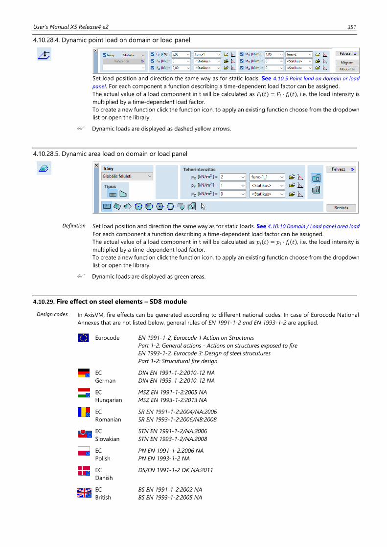
User’s Manual X5 Release4 e2 351

4.10.28.4. Dynamic point load on domain or load panel

Set load position and direction the same way as for static loads. See 4.10.5 Point load on domain or load

panel. For each component a function describing a time-dependent load factor can be assigned.

The actual value of a load component in t will be calculated as 𝐹𝑖(𝑡) = 𝐹𝑖 ⋅ 𝑓𝑖(𝑡), i.e. the load intensity is

multiplied by a time-dependent load factor.

To create a new function click the function icon, to apply an existing function choose from the dropdown

list or open the library.

Dynamic loads are displayed as dashed yellow arrows.

4.10.28.5. Dynamic area load on domain or load panel

Definition Set load position and direction the same way as for static loads. See 4.10.10 Domain / Load panel area load

For each component a function describing a time-dependent load factor can be assigned.

The actual value of a load component in t will be calculated as 𝑝𝑖(𝑡) = 𝑝𝑖 ⋅ 𝑓𝑖(𝑡), i.e. the load intensity is

multiplied by a time-dependent load factor.

To create a new function click the function icon, to apply an existing function choose from the dropdown

list or open the library.

Dynamic loads are displayed as green areas.

4.10.29. Fire effect on steel elements – SD8 module

Design codes In AxisVM, fire effects can be generated according to different national codes. In case of Eurocode National

Annexes that are not listed below, general rules of EN 1991-1-2 and EN 1993-1-2 are applied.

Eurocode EN 1991-1-2, Eurocode 1 Action on Structures

Part 1-2: General actions - Actions on structures exposed to fire

EN 1993-1-2, Eurocode 3: Design of steel strucutures

Part 1-2: Strucutural fire design

EC

German

DIN EN 1991-1-2:2010-12 NA

DIN EN 1993-1-2:2010-12 NA

EC

Hungarian

MSZ EN 1991-1-2:2005 NA

MSZ EN 1993-1-2:2013 NA

EC

Romanian

SR EN 1991-1-2:2004/NA:2006

SR EN 1993-1-2:2006/NB:2008

EC

Slovakian

STN EN 1991-1-2/NA:2006

STN EN 1993-1-2/NA:2008

EC

Polish

PN EN 1991-1-2:2006 NA

PN EN 1993-1-2 NA

EC

Danish

DS/EN 1991-1-2 DK NA:2011

EC

British

BS EN 1991-1-2:2002 NA

BS EN 1993-1-2:2005 NA

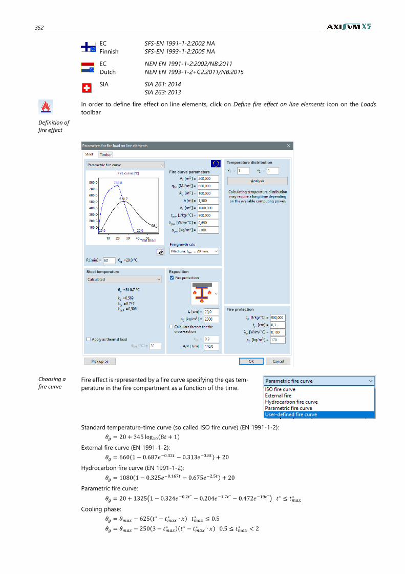
352

EC

Finnish

SFS-EN 1991-1-2:2002 NA

SFS-EN 1993-1-2:2005 NA

EC

Dutch

NEN EN 1991-1-2:2002/NB:2011

NEN EN 1993-1-2+C2:2011/NB:2015

SIA SIA 261: 2014

SIA 263: 2013

Definition of fire effect

In order to define fire effect on line elements, click on Define fire effect on line elements icon on the Loads

toolbar

Choosing a fire curve

Fire effect is represented by a fire curve specifying the gas tem-

perature in the fire compartment as a function of the time.

Standard temperature-time curve (so called ISO fire curve) (EN 1991-1-2):

휃𝑔 = 20 + 345 log10(8𝑡 + 1)

External fire curve (EN 1991-1-2):

휃𝑔 = 660(1 − 0.687𝑒−0.32𝑡 − 0.313𝑒−3.8𝑡) + 20

Hydrocarbon fire curve (EN 1991-1-2):

휃𝑔 = 1080(1 − 0.325𝑒−0.167𝑡 − 0.675𝑒−2.5𝑡) + 20

Parametric fire curve:

휃𝑔 = 20 + 1325(1 − 0.324𝑒−0.2𝑡∗ − 0.204𝑒−1.7𝑡

∗− 0.472𝑒−19𝑡

∗) 𝑡∗ ≤ 𝑡𝑚𝑎𝑥

∗

Cooling phase:

휃𝑔 = 휃𝑚𝑎𝑥 − 625(𝑡∗ − 𝑡𝑚𝑎𝑥

∗ ∙ 𝑥) 𝑡𝑚𝑎𝑥∗ ≤ 0.5

휃𝑔 = 휃𝑚𝑎𝑥 − 250(3 − 𝑡𝑚𝑎𝑥∗ )(𝑡∗ − 𝑡𝑚𝑎𝑥

∗ ∙ 𝑥) 0.5 ≤ 𝑡𝑚𝑎𝑥∗ < 2

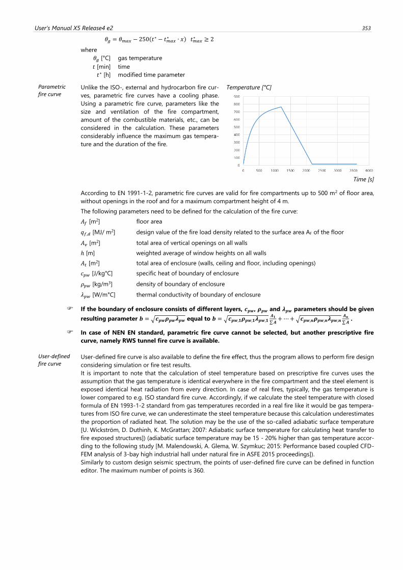
User’s Manual X5 Release4 e2 353

휃𝑔 = 휃𝑚𝑎𝑥 − 250(𝑡∗ − 𝑡𝑚𝑎𝑥

∗ ∙ 𝑥) 𝑡𝑚𝑎𝑥∗ ≥ 2

where

휃𝑔 [°C] gas temperature

𝑡 [min] time

𝑡∗ [h] modified time parameter

Parametric fire curve

Unlike the ISO-, external and hydrocarbon fire cur-

ves, parametric fire curves have a cooling phase.

Using a parametric fire curve, parameters like the

size and ventilation of the fire compartment,

amount of the combustible materials, etc., can be

considered in the calculation. These parameters

considerably influence the maximum gas tempera-

ture and the duration of the fire.

Temperature [°C]

Time [s]

According to EN 1991-1-2, parametric fire curves are valid for fire compartments up to 500 m2 of floor area,

without openings in the roof and for a maximum compartment height of 4 m.

The following parameters need to be defined for the calculation of the fire curve:

𝐴𝑓 [m2] floor area

𝑞𝑓,𝑑 [MJ/ m2] design value of the fire load density related to the surface area Af of the floor

𝐴𝑣 [m2] total area of vertical openings on all walls

ℎ [m] weighted average of window heights on all walls

𝐴𝑡 [m2] total area of enclosure (walls, ceiling and floor, including openings)

𝑐𝑝𝑤 [J/kg°C] specific heat of boundary of enclosure

𝜌𝑝𝑤 [kg/m3] density of boundary of enclosure

𝜆𝑝𝑤 [W/m°C] thermal conductivity of boundary of enclosure

If the boundary of enclosure consists of different layers, 𝒄𝒑𝒘, 𝝆𝒑𝒘 and 𝝀𝒑𝒘 parameters should be given

resulting parameter 𝒃 = √𝒄𝒑𝒘𝝆𝒑𝒘𝝀𝒑𝒘 equal to 𝒃 = √𝒄𝒑𝒘,𝟏𝝆𝒑𝒘,𝟏𝝀𝒑𝒘,𝟏𝑨𝟏

∑𝑨+⋯+√𝒄𝒑𝒘,𝒏𝝆𝒑𝒘,𝒏𝝀𝒑𝒘,𝒏

𝑨𝒏

∑𝑨 .

In case of NEN EN standard, parametric fire curve cannot be selected, but another prescriptive fire

curve, namely RWS tunnel fire curve is available.

User-defined fire curve

User-defined fire curve is also available to define the fire effect, thus the program allows to perform fire design

considering simulation or fire test results.

It is important to note that the calculation of steel temperature based on prescriptive fire curves uses the

assumption that the gas temperature is identical everywhere in the fire compartment and the steel element is

exposed identical heat radiation from every direction. In case of real fires, typically, the gas temperature is

lower compared to e.g. ISO standard fire curve. Accordingly, if we calculate the steel temperature with closed

formula of EN 1993-1-2 standard from gas temperatures recorded in a real fire like it would be gas tempera-

tures from ISO fire curve, we can underestimate the steel temperature because this calculation underestimates

the proportion of radiated heat. The solution may be the use of the so-called adiabatic surface temperature

[U. Wickström, D. Duthinh, K. McGrattan; 2007: Adiabatic surface temperature for calculating heat transfer to

fire exposed structures]) (adiabatic surface temperature may be 15 - 20% higher than gas temperature accor-

ding to the following study [M. Malendowski, A. Glema, W. Szymkuc; 2015: Performance based coupled CFD-

FEM analysis of 3-bay high industrial hall under natural fire in ASFE 2015 proceedings]).

Similarly to custom design seismic spectrum, the points of user-defined fire curve can be defined in function

editor. The maximum number of points is 360.

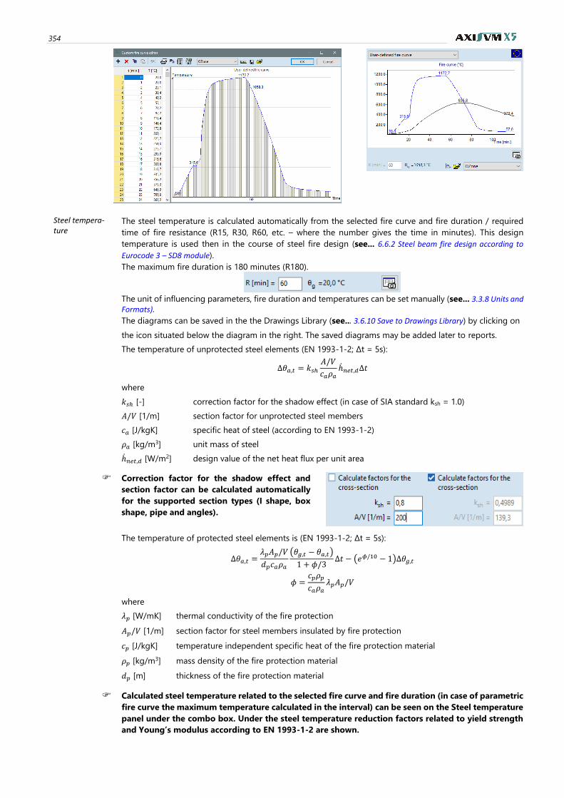
354

Steel tempera-ture

The steel temperature is calculated automatically from the selected fire curve and fire duration / required

time of fire resistance (R15, R30, R60, etc. – where the number gives the time in minutes). This design

temperature is used then in the course of steel fire design (see... 6.6.2 Steel beam fire design according to

Eurocode 3 – SD8 module).

The maximum fire duration is 180 minutes (R180).

The unit of influencing parameters, fire duration and temperatures can be set manually (see... 3.3.8 Units and Formats).

The diagrams can be saved in the the Drawings Library (see... 3.6.10 Save to Drawings Library) by clicking on

the icon situated below the diagram in the right. The saved diagrams may be added later to reports.

The temperature of unprotected steel elements (EN 1993-1-2; ∆t = 5s):

Δ휃𝑎,𝑡 = 𝑘𝑠ℎ𝐴/𝑉

𝑐𝑎𝜌𝑎ℎ̇𝑛𝑒𝑡,𝑑Δ𝑡

where

𝑘𝑠ℎ [-] correction factor for the shadow effect (in case of SIA standard ksh = 1.0)

𝐴/𝑉 [1/m] section factor for unprotected steel members

𝑐𝑎 [J/kgK] specific heat of steel (according to EN 1993-1-2)

𝜌𝑎 [kg/m3] unit mass of steel

ℎ̇𝑛𝑒𝑡,𝑑 [W/m2] design value of the net heat flux per unit area

Correction factor for the shadow effect and

section factor can be calculated automatically

for the supported section types (I shape, box

shape, pipe and angles).

The temperature of protected steel elements is (EN 1993-1-2; ∆t = 5s):

Δ휃𝑎,𝑡 =𝜆𝑝𝐴𝑝/𝑉

𝑑𝑝𝑐𝑎𝜌𝑎

(휃𝑔,𝑡 − 휃𝑎,𝑡)

1 + 𝜙/3Δ𝑡 − (𝑒𝜙/10 − 1)Δ휃𝑔,𝑡

𝜙 =𝑐𝑝𝜌𝑝

𝑐𝑎𝜌𝑎𝜆𝑝𝐴𝑝/𝑉

where

𝜆𝑝 [W/mK] thermal conductivity of the fire protection

𝐴𝑝/𝑉 [1/m] section factor for steel members insulated by fire protection

𝑐𝑝 [J/kgK] temperature independent specific heat of the fire protection material

𝜌𝑝 [kg/m3] mass density of the fire protection material

𝑑𝑝 [m] thickness of the fire protection material

Calculated steel temperature related to the selected fire curve and fire duration (in case of parametric

fire curve the maximum temperature calculated in the interval) can be seen on the Steel temperature

panel under the combo box. Under the steel temperature reduction factors related to yield strength

and Young’s modulus according to EN 1993-1-2 are shown.

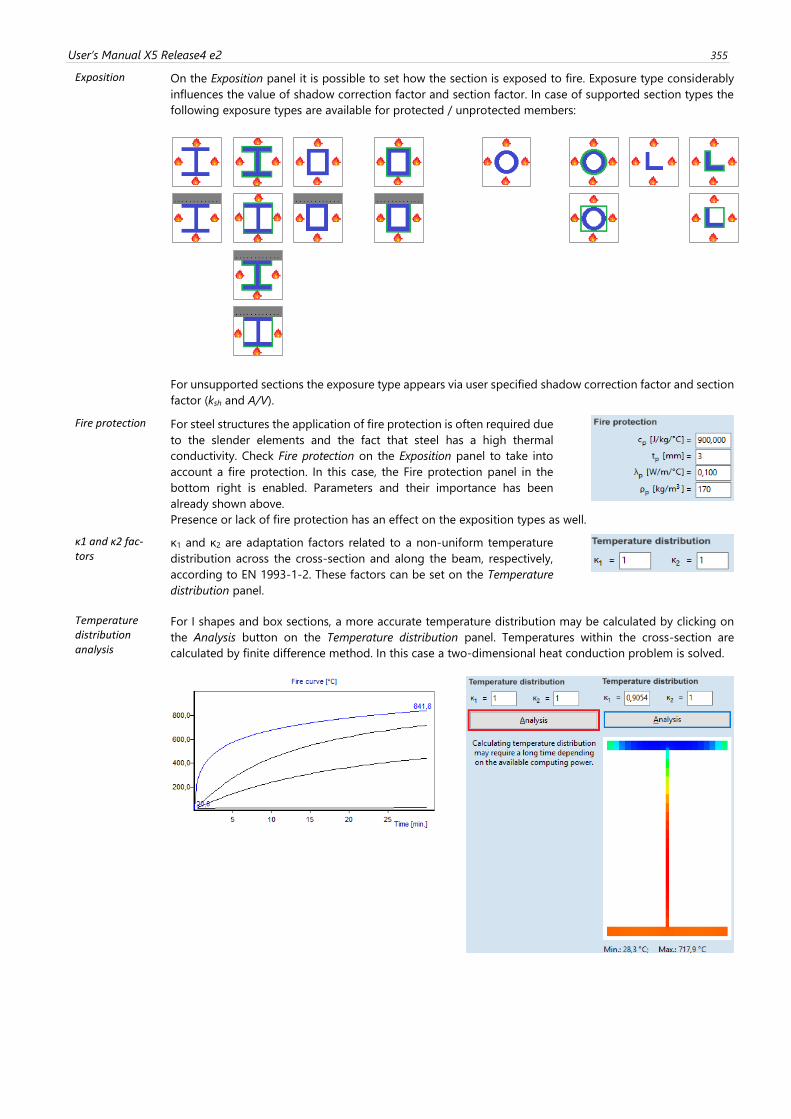
User’s Manual X5 Release4 e2 355

Exposition On the Exposition panel it is possible to set how the section is exposed to fire. Exposure type considerably

influences the value of shadow correction factor and section factor. In case of supported section types the

following exposure types are available for protected / unprotected members:

For unsupported sections the exposure type appears via user specified shadow correction factor and section

factor (ksh and A/V).

Fire protection For steel structures the application of fire protection is often required due

to the slender elements and the fact that steel has a high thermal

conductivity. Check Fire protection on the Exposition panel to take into

account a fire protection. In this case, the Fire protection panel in the

bottom right is enabled. Parameters and their importance has been

already shown above.

Presence or lack of fire protection has an effect on the exposition types as well.

κ1 and κ2 fac-tors

κ1 and κ2 are adaptation factors related to a non-uniform temperature

distribution across the cross-section and along the beam, respectively,

according to EN 1993-1-2. These factors can be set on the Temperature

distribution panel.

Temperature distribution analysis

For I shapes and box sections, a more accurate temperature distribution may be calculated by clicking on

the Analysis button on the Temperature distribution panel. Temperatures within the cross-section are

calculated by finite difference method. In this case a two-dimensional heat conduction problem is solved.

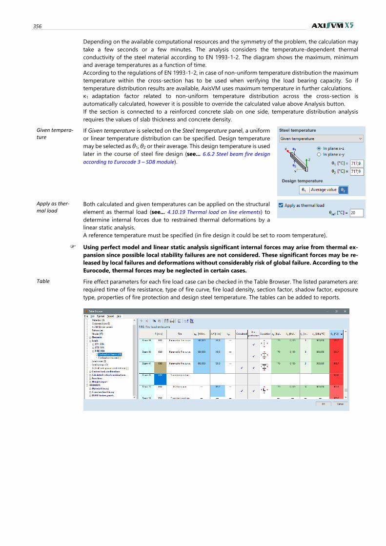
356

Depending on the available computational resources and the symmetry of the problem, the calculation may

take a few seconds or a few minutes. The analysis considers the temperature-dependent thermal

conductivity of the steel material according to EN 1993-1-2. The diagram shows the maximum, minimum

and average temperatures as a function of time.

According to the regulations of EN 1993-1-2, in case of non-uniform temperature distribution the maximum

temperature within the cross-section has to be used when verifying the load bearing capacity. So if

temperature distribution results are available, AxisVM uses maximum temperature in further calculations.

κ1 adaptation factor related to non-uniform temperature distribution across the cross-section is

automatically calculated, however it is possible to override the calculated value above Analysis button.

If the section is connected to a reinforced concrete slab on one side, temperature distribution analysis

requires the values of slab thickness and concrete density.

Given tempera-ture

If Given temperature is selected on the Steel temperature panel, a uniform

or linear temperature distribution can be specified. Design temperature

may be selected as θ1, θ2 or their average. This design temperature is used

later in the course of steel fire design (see... 6.6.2 Steel beam fire design

according to Eurocode 3 – SD8 module).

Apply as ther-mal load

Both calculated and given temperatures can be applied on the structural

element as thermal load (see... 4.10.19 Thermal load on line elements) to

determine internal forces due to restrained thermal deformations by a

linear static analysis.

A reference temperature must be specified (in fire design it could be set to room temperature).

Using perfect model and linear static analysis significant internal forces may arise from thermal ex-

pansion since possible local stability failures are not considered. These significant forces may be re-

leased by local failures and deformations without considerably risk of global failure. According to the

Eurocode, thermal forces may be neglected in certain cases.

Table Fire effect parameters for each fire load case can be checked in the Table Browser. The listed parameters are:

required time of fire resistance, type of fire curve, fire load density, section factor, shadow factor, exposure

type, properties of fire protection and design steel temperature. The tables can be added to reports.

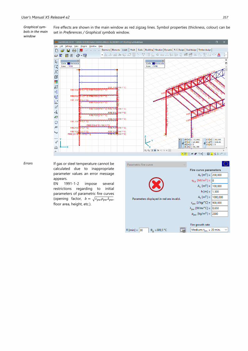
User’s Manual X5 Release4 e2 357

Graphical sym-bols in the main window

Fire effects are shown in the main window as red zigzag lines. Symbol properties (thickness, colour) can be

set in Preferences / Graphical symbols window.

Errors If gas or steel temperature cannot be

calculated due to inappropriate

parameter values an error message

appears.

EN 1991-1-2 impose several

restrictions regarding to initial

parameters of parametric fire curves

(opening factor, 𝑏 = √𝑐𝑝𝑤𝜌𝑝𝑤𝜆𝑝𝑤 ,

floor area, height, etc.).

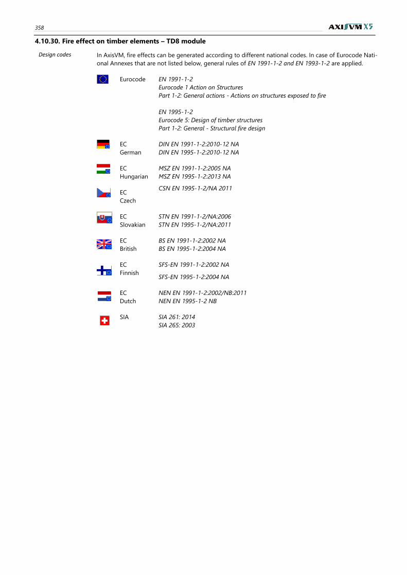
358

4.10.30. Fire effect on timber elements – TD8 module

Design codes In AxisVM, fire effects can be generated according to different national codes. In case of Eurocode Nati-

onal Annexes that are not listed below, general rules of EN 1991-1-2 and EN 1993-1-2 are applied.

Eurocode EN 1991-1-2

Eurocode 1 Action on Structures

Part 1-2: General actions - Actions on structures exposed to fire

EN 1995-1-2

Eurocode 5: Design of timber structures

Part 1-2: General - Structural fire design

EC

German

DIN EN 1991-1-2:2010-12 NA

DIN EN 1995-1-2:2010-12 NA

EC

Hungarian

MSZ EN 1991-1-2:2005 NA

MSZ EN 1995-1-2:2013 NA

EC

Czech

CSN EN 1995-1-2/NA 2011

EC

Slovakian

STN EN 1991-1-2/NA:2006

STN EN 1995-1-2/NA:2011

EC

British

BS EN 1991-1-2:2002 NA

BS EN 1995-1-2:2004 NA

EC

Finnish

SFS-EN 1991-1-2:2002 NA

SFS-EN 1995-1-2:2004 NA

EC

Dutch

NEN EN 1991-1-2:2002/NB:2011

NEN EN 1995-1-2 NB

SIA SIA 261: 2014

SIA 265: 2003

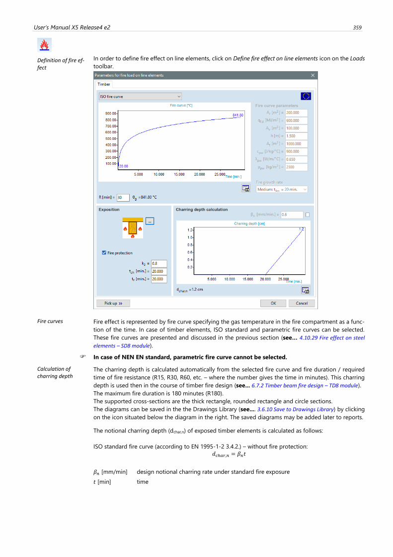
User’s Manual X5 Release4 e2 359

Definition of fire ef-fect

In order to define fire effect on line elements, click on Define fire effect on line elements icon on the Loads

toolbar.

Fire curves Fire effect is represented by fire curve specifying the gas temperature in the fire compartment as a func-

tion of the time. In case of timber elements, ISO standard and parametric fire curves can be selected.

These fire curves are presented and discussed in the previous section (see… 4.10.29 Fire effect on steel

elements – SD8 module).

In case of NEN EN standard, parametric fire curve cannot be selected.

Calculation of charring depth

The charring depth is calculated automatically from the selected fire curve and fire duration / required

time of fire resistance (R15, R30, R60, etc. – where the number gives the time in minutes). This charring

depth is used then in the course of timber fire design (see... 6.7.2 Timber beam fire design – TD8 module).

The maximum fire duration is 180 minutes (R180).

The supported cross-sections are the thick rectangle, rounded rectangle and circle sections.

The diagrams can be saved in the the Drawings Library (see.... 3.6.10 Save to Drawings Library) by clicking

on the icon situated below the diagram in the right. The saved diagrams may be added later to reports.

The notional charring depth (dchar,n) of exposed timber elements is calculated as follows:

ISO standard fire curve (according to EN 1995-1-2 3.4.2.) – without fire protection:

𝑑𝑐ℎ𝑎𝑟,𝑛 = 𝛽𝑛𝑡

𝛽𝑛 [mm/min] design notional charring rate under standard fire exposure

𝑡 [min] time

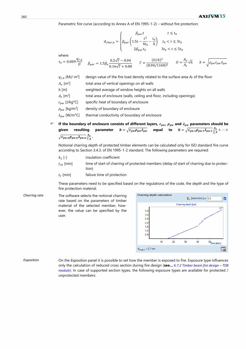
360

Parametric fire curve (according to Annex A of EN 1995-1-2) – without fire protection:

𝑑𝑐ℎ𝑎𝑟,𝑛 =

{

𝛽𝑝𝑎𝑟𝑡 𝑡 ≤ 𝑡0

𝛽𝑝𝑎𝑟 (1.5𝑡 −𝑡2

4𝑡0−𝑡04) 𝑡0 < 𝑡 ≤ 3𝑡0

2𝛽𝑝𝑎𝑟𝑡0 3𝑡0 < 𝑡 ≤ 5𝑡0

where

𝑡0 = 0.009𝑞𝑓,𝑑

𝑂

𝛽𝑝𝑎𝑟 = 1.5𝛽𝑛0.2√Γ − 0.04

0.16√Γ + 0.08

Γ =(𝑂/𝑏)2

(0.04/1160)2 𝑂 =

𝐴𝑣𝐴𝑡√ℎ

𝑏 = √𝜌𝑝𝑤𝑐𝑝𝑤𝜆𝑝𝑤

𝑞𝑓,𝑑 [MJ/ m2] design value of the fire load density related to the surface area Af of the floor

𝐴𝑣 [m2] total area of vertical openings on all walls

ℎ [m] weighted average of window heights on all walls

𝐴𝑡 [m2] total area of enclosure (walls, ceiling and floor, including openings)

𝑐𝑝𝑤 [J/kg°C] specific heat of boundary of enclosure

𝜌𝑝𝑤 [kg/m3] density of boundary of enclosure

𝜆𝑝𝑤 [W/m°C] thermal conductivity of boundary of enclosure

If the boundary of enclosure consists of different layers, 𝒄𝒑𝒘, 𝝆𝒑𝒘 and 𝝀𝒑𝒘 parameters should be

given resulting parameter 𝒃 = √𝒄𝒑𝒘𝝆𝒑𝒘𝝀𝒑𝒘 equal to 𝒃 = √𝒄𝒑𝒘,𝟏𝝆𝒑𝒘,𝟏𝝀𝒑𝒘,𝟏𝑨𝟏

∑𝑨+⋯+

√𝒄𝒑𝒘,𝒏𝝆𝒑𝒘,𝒏𝝀𝒑𝒘,𝒏𝑨𝒏

∑𝑨 .

Notional charring depth of protected timber elements can be calculated only for ISO standard fire curve

according to Section 3.4.3. of EN 1995-1-2 standard. The following parameters are required:

𝑘2 [-] insulation coefficient

𝑡𝑐ℎ [min] time of start of charring of protected members (delay of start of charring due to protec-

tion)

𝑡𝑓 [min] failure time of protection

These parameters need to be specified based on the regulations of the code, the depth and the type of

fire protection material.

Charring rate The software selects the notional charring

rate based on the parameters of timber

material of the selected member, how-

ever, the value can be specified by the

user.

Exposition On the Exposition panel it is possible to set how the member is exposed to fire. Exposure type influences

only the calculation of reduced cross section during fire design (see... 6.7.2 Timber beam fire design – TD8

module). In case of supported section types, the following exposure types are available for protected /

unprotected members:

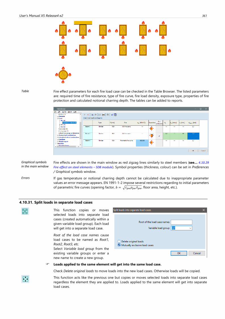
User’s Manual X5 Release4 e2 361

Table Fire effect parameters for each fire load case can be checked in the Table Browser. The listed parameters

are: required time of fire resistance, type of fire curve, fire load density, exposure type, properties of fire

protection and calculated notional charring depth. The tables can be added to reports.

Graphical symbols in the main window

Fire effects are shown in the main window as red zigzag lines similarly to steel members (see… 4.10.29

Fire effect on steel elements – SD8 module). Symbol properties (thickness, colour) can be set in Preferences

/ Graphical symbols window.

Errors If gas temperature or notional charring depth cannot be calculated due to inappropriate parameter

values an error message appears. EN 1991-1-2 impose several restrictions regarding to initial parameters

of parametric fire curves (opening factor, 𝑏 = √𝑐𝑝𝑤𝜌𝑝𝑤𝜆𝑝𝑤 , floor area, height, etc.).

4.10.31. Split loads in separate load cases

This function copies or moves

selected loads into separate load

cases (created automatically within a

given variable load group). Each load

will get into a separate load case.

Root of the load case names cause

load cases to be named as Root1,

Root2, Root3, etc.

Select Variable load group from the

existing variable groups or enter a

new name to create a new group.

Loads applied to the same element will get into the same load case.

Check Delete original loads to move loads into the new load cases. Otherwise loads will be copied.

This function acts like the previous one but copies or moves selected loads into separate load cases

regardless the element they are applied to. Loads applied to the same element will get into separate

load cases.

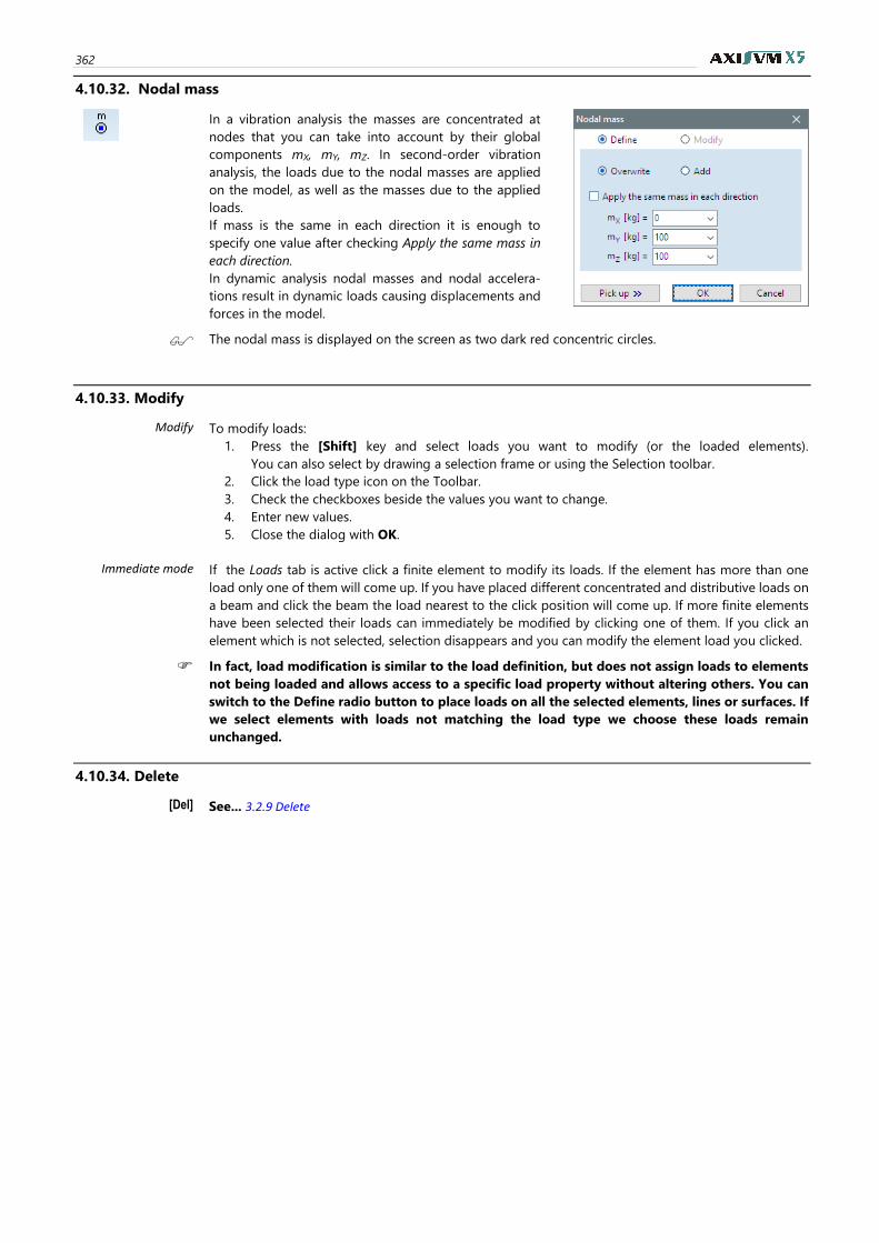
362

4.10.32. Nodal mass

In a vibration analysis the masses are concentrated at

nodes that you can take into account by their global

components mX, mY, mZ. In second-order vibration

analysis, the loads due to the nodal masses are applied

on the model, as well as the masses due to the applied

loads.

If mass is the same in each direction it is enough to

specify one value after checking Apply the same mass in

each direction.

In dynamic analysis nodal masses and nodal accelera-

tions result in dynamic loads causing displacements and

forces in the model.

The nodal mass is displayed on the screen as two dark red concentric circles.

4.10.33. Modify

Modify To modify loads:

1. Press the [Shift] key and select loads you want to modify (or the loaded elements).

You can also select by drawing a selection frame or using the Selection toolbar.

2. Click the load type icon on the Toolbar.

3. Check the checkboxes beside the values you want to change.

4. Enter new values.

5. Close the dialog with OK.

Immediate mode If the Loads tab is active click a finite element to modify its loads. If the element has more than one

load only one of them will come up. If you have placed different concentrated and distributive loads on

a beam and click the beam the load nearest to the click position will come up. If more finite elements

have been selected their loads can immediately be modified by clicking one of them. If you click an

element which is not selected, selection disappears and you can modify the element load you clicked.

In fact, load modification is similar to the load definition, but does not assign loads to elements

not being loaded and allows access to a specific load property without altering others. You can

switch to the Define radio button to place loads on all the selected elements, lines or surfaces. If

we select elements with loads not matching the load type we choose these loads remain

unchanged.

4.10.34. Delete

[Del] See... 3.2.9 Delete

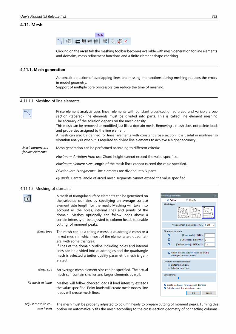
User’s Manual X5 Release4 e2 363

4.11. Mesh

Clicking on the Mesh tab the meshing toolbar becomes available with mesh generation for line elements

and domains, mesh refinement functions and a finite element shape checking.

4.11.1. Mesh generation

Automatic detection of overlapping lines and missing intersections during meshing reduces the errors

in model geometry.

Support of multiple core processors can reduce the time of meshing.

4.11.1.1. Meshing of line elements

Finite element analysis uses linear elements with constant cross-section so arced and variable cross-

section (tapered) line elements must be divided into parts. This is called line element meshing.

The accuracy of the solution depens on the mesh density.

This mesh can be removed or modified just like a domain mesh. Removing a mesh does not delete loads

and properties assigned to the line element.

A mesh can also be defined for linear elements with constant cross-section. It is useful in nonlinear or

vibration analysis when it is required to divide line elements to achieve a higher accuracy.

Mesh parameters for line elements

Mesh generation can be performed according to different criteria:

Maximum deviation from arc: Chord height cannot exceed the value specified.

Maximum element size: Length of the mesh lines cannot exceed the value specified.

Division into N segments: Line elements are divided into N parts.

By angle: Central angle of arced mesh segments cannot exceed the value specified.

4.11.1.2. Meshing of domains

A mesh of triangular surface elements can be generated on

the selected domains by specifying an average surface

element side length for the mesh. Meshing will take into

account all the holes, internal lines and points of the

domain. Meshes optionally can follow loads above a

certain intensity or be adjusted to column heads to enable

cutting of moment peaks.

Mesh type The mesh can be a triangle mesh, a quadrangle mesh or a

mixed mesh, in which most of the elements are quadrilat-

eral with some triangles.

If lines of the domain outline including holes and internal

lines can be divided into quadrangles and the quadrangle

mesh is selected a better quality parametric mesh is gen-

erated.

Mesh size An average mesh element size can be specified. The actual

mesh can contain smaller and larger elements as well.

Fit mesh to loads Meshes will follow checked loads if load intensity exceeds

the value specified. Point loads will create mesh nodes, line

loads will create mesh lines.

Adjust mesh to col-umn heads

The mesh must be properly adjusted to column heads to prepare cutting of moment peaks. Turning this

option on automatically fits the mesh according to the cross-section geometry of connecting columns.

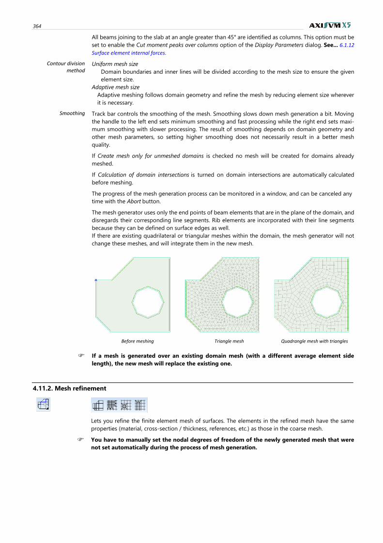
364

All beams joining to the slab at an angle greater than 45° are identified as columns. This option must be

set to enable the Cut moment peaks over columns option of the Display Parameters dialog. See... 6.1.12

Surface element internal forces.

Contour division method

Uniform mesh size

Domain boundaries and inner lines will be divided according to the mesh size to ensure the given

element size.

Adaptive mesh size

Adaptive meshing follows domain geometry and refine the mesh by reducing element size wherever

it is necessary.

Smoothing Track bar controls the smoothing of the mesh. Smoothing slows down mesh generation a bit. Moving

the handle to the left end sets minimum smoothing and fast processing while the right end sets maxi-

mum smoothing with slower processing. The result of smoothing depends on domain geometry and

other mesh parameters, so setting higher smoothing does not necessarily result in a better mesh

quality.

If Create mesh only for unmeshed domains is checked no mesh will be created for domains already

meshed.

If Calculation of domain intersections is turned on domain intersections are automatically calculated

before meshing.

The progress of the mesh generation process can be monitored in a window, and can be canceled any

time with the Abort button.

The mesh generator uses only the end points of beam elements that are in the plane of the domain, and

disregards their corresponding line segments. Rib elements are incorporated with their line segments

because they can be defined on surface edges as well.

If there are existing quadrilateral or triangular meshes within the domain, the mesh generator will not

change these meshes, and will integrate them in the new mesh.

Before meshing Triangle mesh Quadrangle mesh with triangles

If a mesh is generated over an existing domain mesh (with a different average element side

length), the new mesh will replace the existing one.

4.11.2. Mesh refinement

Lets you refine the finite element mesh of surfaces. The elements in the refined mesh have the same

properties (material, cross-section / thickness, references, etc.) as those in the coarse mesh.

You have to manually set the nodal degrees of freedom of the newly generated mesh that were

not set automatically during the process of mesh generation.

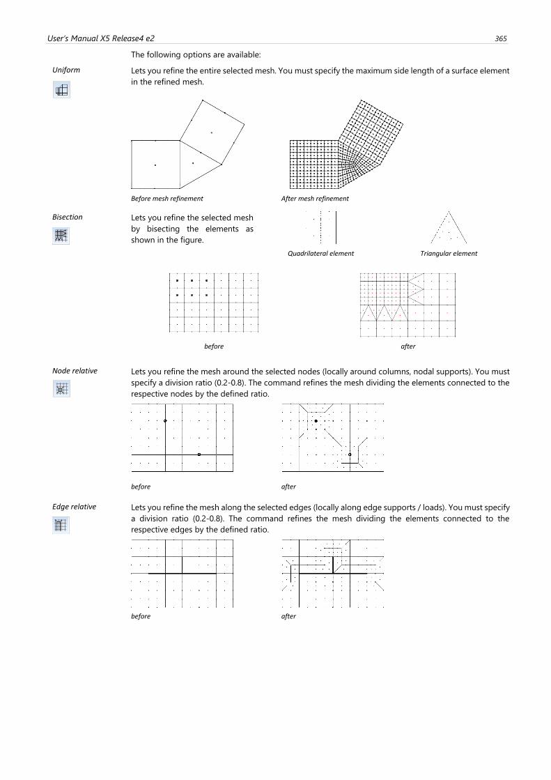
User’s Manual X5 Release4 e2 365

The following options are available:

Uniform

Lets you refine the entire selected mesh. You must specify the maximum side length of a surface element

in the refined mesh.

Before mesh refinement After mesh refinement

Bisection

Lets you refine the selected mesh

by bisecting the elements as

shown in the figure.

Quadrilateral element Triangular element

before after

Node relative

Lets you refine the mesh around the selected nodes (locally around columns, nodal supports). You must

specify a division ratio (0.2-0.8). The command refines the mesh dividing the elements connected to the

respective nodes by the defined ratio.

before after

Edge relative

Lets you refine the mesh along the selected edges (locally along edge supports / loads). You must specify

a division ratio (0.2-0.8). The command refines the mesh dividing the elements connected to the

respective edges by the defined ratio.

before after

366

4.11.3. Checking finite elements

Program checks the minimum angle of surface finite elements ().

A triangular finite element is distorted if ≤ 15.

A qudrilateral finite element is distorted if ≤ 30.

4.11.4. Delete all meshes

Deletes all meshes from line elements

Deletes all domain meshes from domains

Deletes all (line or domain) meshes of the model.

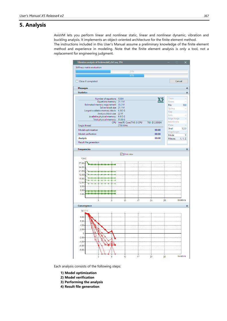
User’s Manual X5 Release4 e2 367

5. Analysis

AxisVM lets you perform linear and nonlinear static, linear and nonlinear dynamic, vibration and

buckling analysis. It implements an object-oriented architecture for the finite element method.

The instructions included in this User’s Manual assume a preliminary knowledge of the finite element

method and experience in modeling. Note that the finite element analysis is only a tool, not a

replacement for engineering judgment.

Each analysis consists of the following steps:

1) Model optimization

2) Model verification

3) Performing the analysis

4) Result file generation

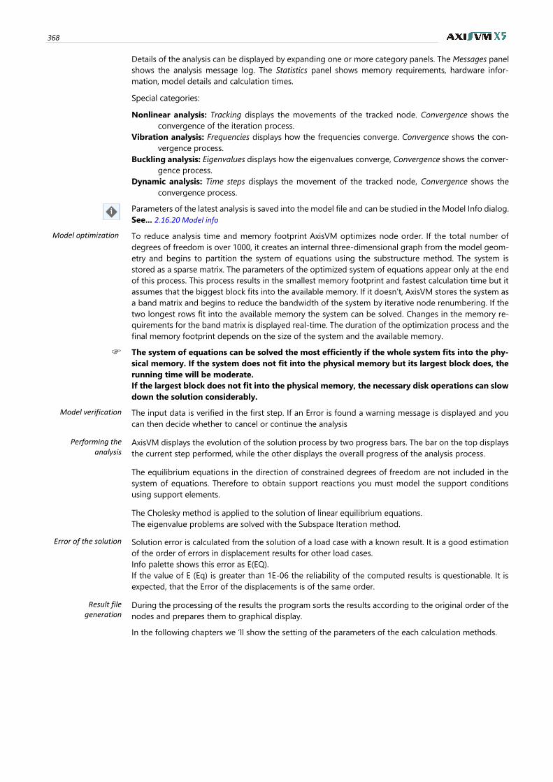
368

Details of the analysis can be displayed by expanding one or more category panels. The Messages panel

shows the analysis message log. The Statistics panel shows memory requirements, hardware infor-

mation, model details and calculation times.

Special categories:

Nonlinear analysis: Tracking displays the movements of the tracked node. Convergence shows the

convergence of the iteration process.

Vibration analysis: Frequencies displays how the frequencies converge. Convergence shows the con-

vergence process.

Buckling analysis: Eigenvalues displays how the eigenvalues converge, Convergence shows the conver-

gence process.

Dynamic analysis: Time steps displays the movement of the tracked node, Convergence shows the

convergence process.

Parameters of the latest analysis is saved into the model file and can be studied in the Model Info dialog.

See... 2.16.20 Model info

Model optimization To reduce analysis time and memory footprint AxisVM optimizes node order. If the total number of

degrees of freedom is over 1000, it creates an internal three-dimensional graph from the model geom-

etry and begins to partition the system of equations using the substructure method. The system is

stored as a sparse matrix. The parameters of the optimized system of equations appear only at the end

of this process. This process results in the smallest memory footprint and fastest calculation time but it

assumes that the biggest block fits into the available memory. If it doesn’t, AxisVM stores the system as

a band matrix and begins to reduce the bandwidth of the system by iterative node renumbering. If the

two longest rows fit into the available memory the system can be solved. Changes in the memory re-

quirements for the band matrix is displayed real-time. The duration of the optimization process and the

final memory footprint depends on the size of the system and the available memory.

The system of equations can be solved the most efficiently if the whole system fits into the phy-

sical memory. If the system does not fit into the physical memory but its largest block does, the

running time will be moderate.

If the largest block does not fit into the physical memory, the necessary disk operations can slow

down the solution considerably.

Model verification The input data is verified in the first step. If an Error is found a warning message is displayed and you

can then decide whether to cancel or continue the analysis

Performing the analysis

AxisVM displays the evolution of the solution process by two progress bars. The bar on the top displays

the current step performed, while the other displays the overall progress of the analysis process.

The equilibrium equations in the direction of constrained degrees of freedom are not included in the

system of equations. Therefore to obtain support reactions you must model the support conditions

using support elements.

The Cholesky method is applied to the solution of linear equilibrium equations.

The eigenvalue problems are solved with the Subspace Iteration method.

Error of the solution Solution error is calculated from the solution of a load case with a known result. It is a good estimation

of the order of errors in displacement results for other load cases.

Info palette shows this error as E(EQ).

If the value of E (Eq) is greater than 1E-06 the reliability of the computed results is questionable. It is

expected, that the Error of the displacements is of the same order.

Result file generation

During the processing of the results the program sorts the results according to the original order of the

nodes and prepares them to graphical display.

In the following chapters we ‘ll show the setting of the parameters of the each calculation methods.

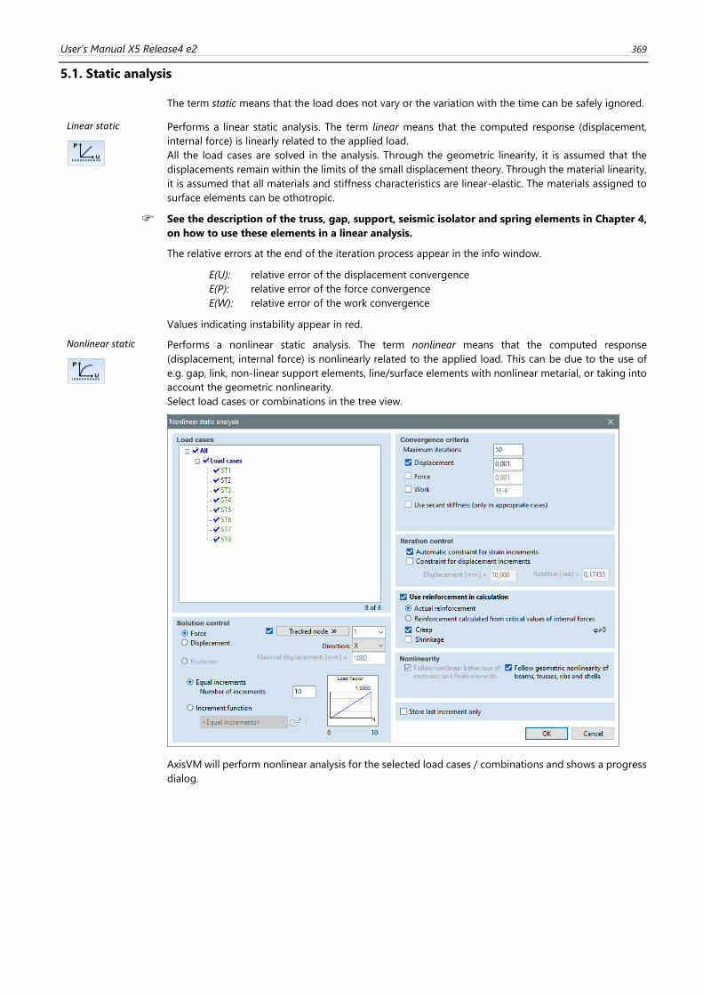
User’s Manual X5 Release4 e2 369

5.1. Static analysis

The term static means that the load does not vary or the variation with the time can be safely ignored.

Linear static

Performs a linear static analysis. The term linear means that the computed response (displacement,

internal force) is linearly related to the applied load.

All the load cases are solved in the analysis. Through the geometric linearity, it is assumed that the

displacements remain within the limits of the small displacement theory. Through the material linearity,

it is assumed that all materials and stiffness characteristics are linear-elastic. The materials assigned to

surface elements can be othotropic.

See the description of the truss, gap, support, seismic isolator and spring elements in Chapter 4,

on how to use these elements in a linear analysis.

The relative errors at the end of the iteration process appear in the info window.

E(U): relative error of the displacement convergence

E(P): relative error of the force convergence

E(W): relative error of the work convergence

Values indicating instability appear in red.

Nonlinear static

Performs a nonlinear static analysis. The term nonlinear means that the computed response

(displacement, internal force) is nonlinearly related to the applied load. This can be due to the use of

e.g. gap, link, non-linear support elements, line/surface elements with nonlinear metarial, or taking into

account the geometric nonlinearity.

Select load cases or combinations in the tree view.

AxisVM will perform nonlinear analysis for the selected load cases / combinations and shows a progress

dialog.

370

Solution control

Force

When Force control is selected, the increments are applied as fractions of the loads (as one

parameter load). It is possible to track the displacement of a node in a given direction. A graph

of this displacement versus increments will be plotted during the analysis.

Displacement

When displacement control is selected, the increments are applied as fractions of the

displacement component of the node specified.

Pushover

Pushover control is a special type of displacement control that allows the use of a constant load

case while having another parametric load case that is increased incrementally. This is essential

for pushover analyses to model P-Δ effects appropriately.

After selecting pushover control, the top of the dialog changes to accommodate the drop-down

boxes for parametric and constant load cases. See... 4.10.24 Pushover loads – SE2 module for details

on load definition and recommended analysis settings.

Tracked node, Direction, maximum displacement

In case of displacement or pushover control a control node and a degree of freedom must be

selected. Maximum displacement is the maximum allowed displacement of the control node in the

given direction.

Number of increments

There are two methods to define the number of increments:

1. Equal increments. Specify the number of increments. The default value is 10. When highly

nonlinear behavior is analyzed, you may specify a greater value in order to achieve

convergence.

2. Increment function. Loads are not increasing in a linear way but follow a predefined function.

Using an increment function it is possible to reduce the number of increments where the

behaviour of the structure is linear and increase the number of increments where the

behaviour is nonlinear. Saved functions can be reloaded, edited and saved under a new name

(see… 4.10.28 Dynamic loads (for time-history analysis) – DYN module). Functions are saved into

separate *.inc files in folder c:\ Users \ [user name] \ AppData \ Roaming \ AxisVM \ [version

number] \ inc.

Convergence criteria

Based on the convergence tolerances you specify, AxisVM will determine if the nonlinear solution

has reached the required accuracy (convergence). Therefore it is important that the convergence

tolerances to be set properly. During the iteration process, the norm of the unequilibrated load

and/or of the iterational displacement increment vector must vanish (to approach zero).

Maximum iterations

You can set the maximum number of the iterations based on the specifics of your model, and of

the incremental solution parameters. By default the value is set to 20. If the convergence is not

achieved within the maximum number of iterations, no results will be obtained.

Displacement / Force / Work / Convergence criteria

In case of a nonlinear calculation you can specify multiple criteria, in terms of load, displacement,

and work, for monitoring the convergence of the nonlinear solution. At least one criteria has to

be selected. The criteria expressed in terms of work can be adequate for most problems.

However, you may encounter a small Error in your unequilibrated load while the Error in

displacements is still large, or vice-versa.

Factors of convergence criteria has the following default values: 0.001 for displacements, 0.001

for force, and 0.000001 for work.

The relative errors at the end of the iteration process appear in the info window.

E(U): relative error of the displacement convergence

E(P): relative error of the force convergence

E(W): relative error of the work convergence

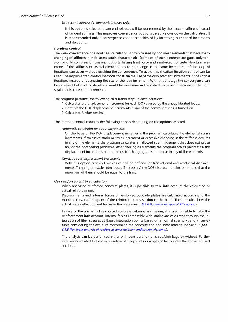
User’s Manual X5 Release4 e2 371

Use secant stiffness (in appropriate cases only)

If this option is selected beam end releases will be represented by their secant stiffness instead

of tangent stiffness. This improves convergence but considerably slows down the calculation. It

is recommended only if convergence cannot be achieved by increasing number of increments

and iterations.

Iteration control

The weak convergence of a nonlinear calculation is often caused by nonlinear elements that have sharp

changing of stiffness in their stress-strain characteristic. Examples of such elements are gaps, only ten-

sion or only compression trusses, supports having limit force and reinforced concrete structural ele-

ments. If the stiffness of several elements has to be change in the same increment, infinite loop of

iterations can occur without reaching the convergence. To avoid this situation iteration control can be

used. The implemented control methods constrain the size of the displacement increments in the critical

iterations instead of decreasing the size of the load increment. With this strategy the convergence can

be achieved but a lot of iterations would be necessary in the critical increment, because of the con-

strained displacement increments.

The program performs the following calculation steps in each iteration:

1. Calculates the displacement increment for each DOF caused by the unequilibrated loads.

2. Controls the DOF displacement increments if any of the control options is turned on.

3. Calculates further results…

The iteration control contains the following checks depending on the options selected.

Automatic constraint for strain increments

On the basis of the DOF displacement increments the program calculates the elemental strain

increments. If excessive strain or stress increment or excessive changing in the stiffness occures

in any of the elements, the program calculates an allowed strain increment that does not cause

any of the opreceding problems. After cheking all elements the program scales (decreases) the

displacement increments so that excessive changing does not occur in any of the elements.

Constraint for displacement increments

With this option custom limit values can be defined for translational and rotational displace-

ments. The program scales (decreases if necessary) the DOF displacement increments so that the

maximum of them should be equal to the limit.

Use reinforcement in calculation

When analyzing reinforced concrete plates, it is possible to take into account the calculated or

actual reinforcement.

Displacements and internal forces of reinforced concrete plates are calculated according to the

moment-curvature diagram of the reinforced cross-section of the plate. These results show the

actual plate deflection and forces in the plate (see… 6.5.6 Nonlinear analysis of RC surfaces).

In case of the analysis of reinforced concrete columns and beams, it is also possible to take the

reinforcement into account. Internal forces compatible with strains are calculated through the in-

tegration of fiber stresses at Gauss integration points based on ε normal strains, κy and κz curva-

tures considering the actual reinforcement, the concrete and nonlinear material behaviour (see...

6.5.5 Nonlinear analysis of reinforced concrete beam and column elements).

The analysis can be performed either with consideration of creep/shrinkage or without. Further

information related to the consideration of creep and shrinkage can be found in the above referred

sections.

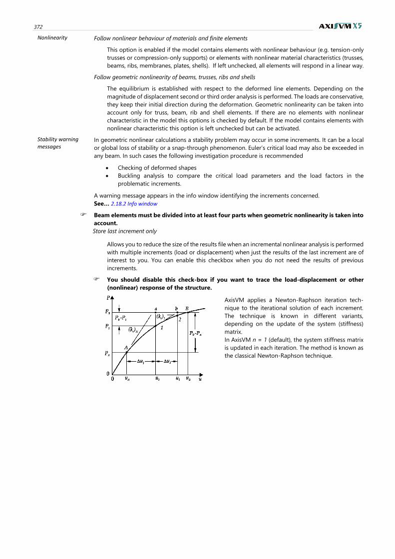
372

Nonlinearity Follow nonlinear behaviour of materials and finite elements

This option is enabled if the model contains elements with nonlinear behaviour (e.g. tension-only

trusses or compression-only supports) or elements with nonlinear material characteristics (trusses,

beams, ribs, membranes, plates, shells). If left unchecked, all elements will respond in a linear way.

Follow geometric nonlinearity of beams, trusses, ribs and shells

The equilibrium is established with respect to the deformed line elements. Depending on the

magnitude of displacement second or third order analysis is performed. The loads are conservative,

they keep their initial direction during the deformation. Geometric nonlinearity can be taken into

account only for truss, beam, rib and shell elements. If there are no elements with nonlinear

characteristic in the model this options is checked by default. If the model contains elements with

nonlinear characteristic this option is left unchecked but can be activated.

Stability warning messages

In geometric nonlinear calculations a stability problem may occur in some increments. It can be a local

or global loss of stability or a snap-through phenomenon. Euler’s critical load may also be exceeded in

any beam. In such cases the following investigation procedure is recommended

• Checking of deformed shapes

• Buckling analysis to compare the critical load parameters and the load factors in the

problematic increments.

A warning message appears in the info window identifying the increments concerned.

See… 2.18.2 Info window

Beam elements must be divided into at least four parts when geometric nonlinearity is taken into

account.

Store last increment only

Allows you to reduce the size of the results file when an incremental nonlinear analysis is performed

with multiple increments (load or displacement) when just the results of the last increment are of

interest to you. You can enable this checkbox when you do not need the results of previous

increments.

You should disable this check-box if you want to trace the load-displacement or other

(nonlinear) response of the structure.

AxisVM applies a Newton-Raphson iteration tech-

nique to the iterational solution of each increment.

The technique is known in different variants,

depending on the update of the system (stiffness)

matrix.

In AxisVM n = 1 (default), the system stiffness matrix

is updated in each iteration. The method is known as

the classical Newton-Raphson technique.

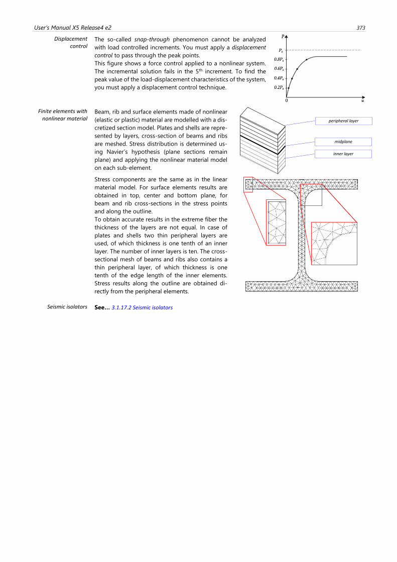
User’s Manual X5 Release4 e2 373

Displacement control

The so-called snap-through phenomenon cannot be analyzed

with load controlled increments. You must apply a displacement

control to pass through the peak points.

This figure shows a force control applied to a nonlinear system.

The incremental solution fails in the 5th increment. To find the

peak value of the load-displacement characteristics of the system,

you must apply a displacement control technique.

Finite elements with nonlinear material

Beam, rib and surface elements made of nonlinear

(elastic or plastic) material are modelled with a dis-

cretized section model. Plates and shells are repre-

sented by layers, cross-section of beams and ribs

are meshed. Stress distribution is determined us-

ing Navier’s hypothesis (plane sections remain

plane) and applying the nonlinear material model

on each sub-element.

Stress components are the same as in the linear

material model. For surface elements results are

obtained in top, center and bottom plane, for

beam and rib cross-sections in the stress points

and along the outline.

To obtain accurate results in the extreme fiber the

thickness of the layers are not equal. In case of

plates and shells two thin peripheral layers are

used, of which thickness is one tenth of an inner

layer. The number of inner layers is ten. The cross-

sectional mesh of beams and ribs also contains a

thin peripheral layer, of which thickness is one

tenth of the edge length of the inner elements.

Stress results along the outline are obtained di-

rectly from the peripheral elements.

Seismic isolators See… 3.1.17.2 Seismic isolators

midplane

peripheral layer

inner layer

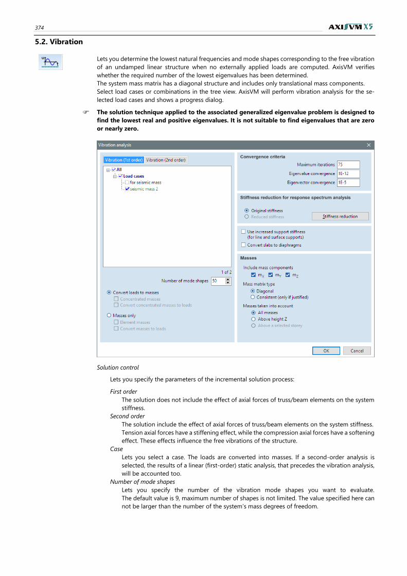
374

5.2. Vibration

Lets you determine the lowest natural frequencies and mode shapes corresponding to the free vibration

of an undamped linear structure when no externally applied loads are computed. AxisVM verifies

whether the required number of the lowest eigenvalues has been determined.

The system mass matrix has a diagonal structure and includes only translational mass components.

Select load cases or combinations in the tree view. AxisVM will perform vibration analysis for the se-

lected load cases and shows a progress dialog.

The solution technique applied to the associated generalized eigenvalue problem is designed to

find the lowest real and positive eigenvalues. It is not suitable to find eigenvalues that are zero

or nearly zero.

Solution control

Lets you specify the parameters of the incremental solution process:

First order

The solution does not include the effect of axial forces of truss/beam elements on the system

stiffness.

Second order

The solution include the effect of axial forces of truss/beam elements on the system stiffness.

Tension axial forces have a stiffening effect, while the compression axial forces have a softening

effect. These effects influence the free vibrations of the structure.

Case

Lets you select a case. The loads are converted into masses. If a second-order analysis is

selected, the results of a linear (first-order) static analysis, that precedes the vibration analysis,

will be accounted too.

Number of mode shapes

Lets you specify the number of the vibration mode shapes you want to evaluate.

The default value is 9, maximum number of shapes is not limited. The value specified here can

not be larger than the number of the system’s mass degrees of freedom.

User’s Manual X5 Release4 e2 375

Convert loads to masses

You can enable the conversion of the load components parallel with the gravitation into

masses, and take these concentrated masses into account. The generated nodal masses can

be checked in the Table Browser (Results / Vibration / [load case or combination name] / Nodal

masses).

Concentrated masses: If nodal masses have been defined (see… 4.10.32 Nodal mass) they can

be included in or excluded from the analysis.

Convert concentrated masses to loads: If nodal masses have been defined they can be

converted to loads.

Masses only

You can analyze models without loads, but with masses, and take Element masses into account.

You can even Convert nodal masses to loads.

Convergence criteria

Based on the convergence tolerances you specify, AxisVM will determine if the calculated

eigenvalues and eigenvectors have the required accuracy. Therefore it is important that the

convergence tolerances be set properly.

Maximum number of iterations

You can set the maximum number of the iterations based on the specifics of your model, and

the number of eigenvalues requested (more iterations for more eigenvalues). By default the

value is set to 20. If the convergence is not achieved within the maximum number of iterations,

no results will be obtained.

Eigenvalue convergence

Lets you specify the convergence tolerance for the eigenvalues.

The default value is 1E-10.

Eigenvector convergence

Lets you specify the convergence tolerance for the eigenvectors.

The default value is 1E-5.

Diaphragm

When running a vibration analysis with the option Convert slabs to diaphragms checked, all

slabs (horizontal plates) will be temporarily replaced by diaphragms.

The running time is reduced if the model contains only columns and slabs. If structural walls

are included, the number of equations will be reduced but the bandwidth will be increased.

The resultant running time may be greater than without diaphragms.

Stiffness reduction for response spectrum analysis

Further information in chapter 3.3.10 Stiffness reduction.

Use increased support stiffness

Supports act in a different way during vibrations. Using increased support stiffness (107 kN/m/m

for line supports, 104 kN/m2 for surface supports) may help to get more realistic vibration results.

For nodal support components the vibration stiffness of the spring is applied. See… 4.9.11 Nodal support.

Masses

Include mass components

Only checked mass components will be used in the analysis. It is useful when calculating modal

shapes only in a certain direction.

Mass matrix type

Diagonal: smaller mass matrix but without centrifugal intertias

Consistent (only if justified): complete mass matrix with centrifugal intertias

Masses taken into account

Here the masses taken into account during vibration analysis can be configured. Beside

All masses it is possible to reduce the masses to those above a given Z height or a given level

(if the model contains levels). An example could be the exclusion of the basement from the

vibration analysis.

For details about the behaviour of seismic isolators see… 3.1.17.2 Seismic isolators

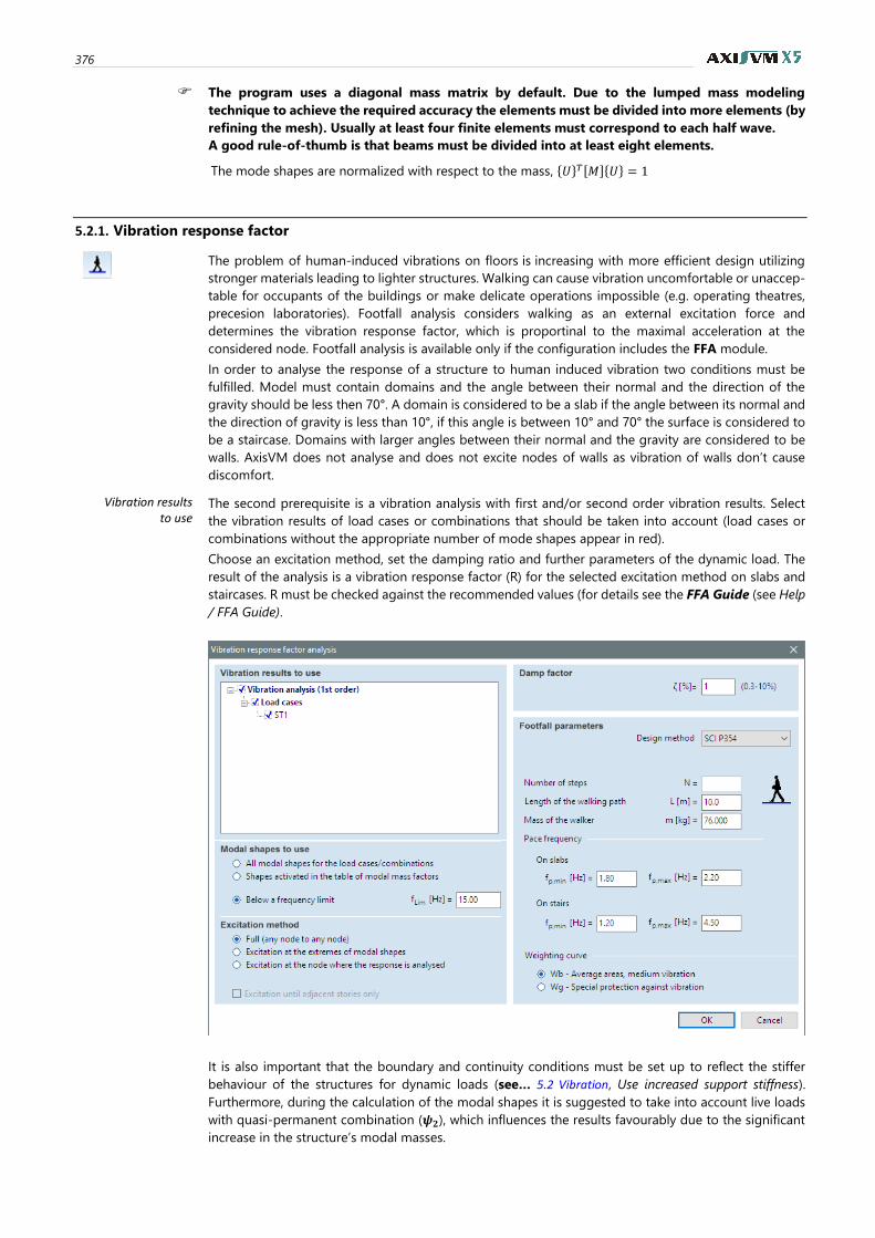
376

The program uses a diagonal mass matrix by default. Due to the lumped mass modeling

technique to achieve the required accuracy the elements must be divided into more elements (by

refining the mesh). Usually at least four finite elements must correspond to each half wave.

A good rule-of-thumb is that beams must be divided into at least eight elements.

The mode shapes are normalized with respect to the mass, {𝑈}𝑇[𝑀]{𝑈} = 1

5.2.1. Vibration response factor

The problem of human-induced vibrations on floors is increasing with more efficient design utilizing

stronger materials leading to lighter structures. Walking can cause vibration uncomfortable or unaccep-

table for occupants of the buildings or make delicate operations impossible (e.g. operating theatres,

precesion laboratories). Footfall analysis considers walking as an external excitation force and

determines the vibration response factor, which is proportinal to the maximal acceleration at the

considered node. Footfall analysis is available only if the configuration includes the FFA module.

In order to analyse the response of a structure to human induced vibration two conditions must be

fulfilled. Model must contain domains and the angle between their normal and the direction of the

gravity should be less then 70°. A domain is considered to be a slab if the angle between its normal and

the direction of gravity is less than 10°, if this angle is between 10° and 70° the surface is considered to

be a staircase. Domains with larger angles between their normal and the gravity are considered to be

walls. AxisVM does not analyse and does not excite nodes of walls as vibration of walls don’t cause

discomfort.

Vibration results to use

The second prerequisite is a vibration analysis with first and/or second order vibration results. Select

the vibration results of load cases or combinations that should be taken into account (load cases or

combinations without the appropriate number of mode shapes appear in red).

Choose an excitation method, set the damping ratio and further parameters of the dynamic load. The

result of the analysis is a vibration response factor (R) for the selected excitation method on slabs and

staircases. R must be checked against the recommended values (for details see the FFA Guide (see Help

/ FFA Guide).

It is also important that the boundary and continuity conditions must be set up to reflect the stiffer

behaviour of the structures for dynamic loads (see… 5.2 Vibration, Use increased support stiffness).

Furthermore, during the calculation of the modal shapes it is suggested to take into account live loads

with quasi-permanent combination (𝝍𝟐), which influences the results favourably due to the significant

increase in the structure’s modal masses.

User’s Manual X5 Release4 e2 377

Modal shapes to use

All modal shapes for the load cases/combinations: All shapes of the selected load cases/combinations

will be taken into account.

Shapes activated in the table of modal mass factors: Shapes can be made inactive in the table of Modal

mass factors (see… 4.10.23.1 Seismic load calculation according to Eurocode 8).

Below frequency limit let the user to set a limit for the eigenfrequencies, which will appear in the

calculation. Only modes with a smaller frequency will be taken into account.

Excitation method Three excitation methods are available. Each one creates a separate R result component.

Full: All nodes of slabs or staircases can excite any other node (R full). This is the most robust method.

Excitation at the extremes of the modal shapes: Excitation takes place only at the two global extrema of

the eigenshapes (R extr.).

Excitation at the node where the response is analysed: The analysed node is only excited by itself (R self).

Excitation until adjacent storeys only: This option is enabled if the model contains at least three storeys.

If checked the analysed node can only be excited with nodes on the same or adjacent storeys.

Damping The critical damping ratio of the analysed structure can be set. Suggestions can be found in [33], [34].

Footfall parameters

Design method Two approaches are available: CCIP-016 [33] and SCI P354 [34]. Their algorithms are described in the

FFA Guide (see Help / FFA Guide). Changing the approach clears the previous results.

Number of steps (CCIP-016)

The CCIP-016 design method allows resonant accelerations to be reduced due to the fact that resonance

needs time to develop. So the number of footsteps (the duration of the excitation) has effect on the

results.

Length of the wal-king path

(SCI P354)

SCI P354 also takes into account the same effect but the relevant parameter is the length of the

walking path. In this approach the most unfavourable length should be given.

Mass of the walker Both methods allow deviation from the predefined mass of the walker.

Pace frequency AxisVM analyses the effect of steps at several different pace frequencies within a given range. The lower

and upper bound of the frequency range can be set here.

Weighting curve SCI P354 allows the usage of different weighting curves. These curves take into account the fact that

the human perception of vibration varies with frequency.

Wb – Average areas, medium vibration should be used, if general comfort must be provided in the

building,

Wg – Special protection against vibration should be used if precise hand movements, steady vision

must be ensured.

In CCIP-016 design method only one weighting is applied.

For further details see Help / FFA Guide.

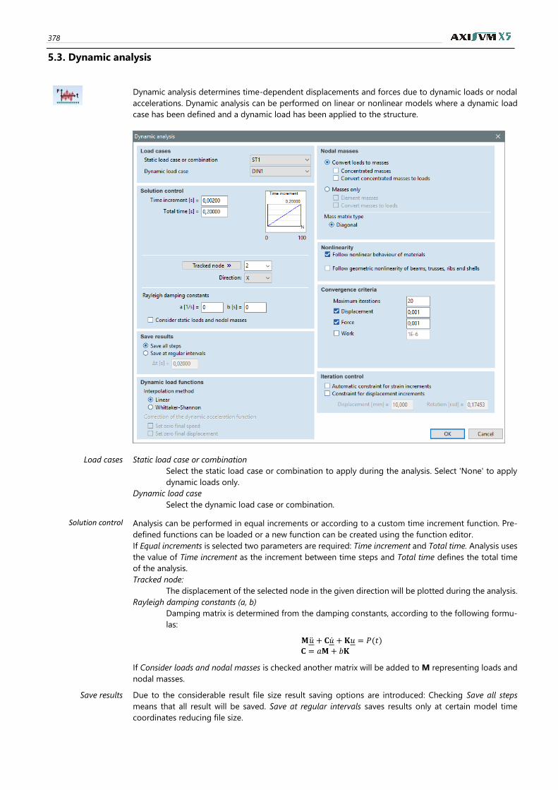
378

5.3. Dynamic analysis

Dynamic analysis determines time-dependent displacements and forces due to dynamic loads or nodal

accelerations. Dynamic analysis can be performed on linear or nonlinear models where a dynamic load

case has been defined and a dynamic load has been applied to the structure.

Load cases Static load case or combination

Select the static load case or combination to apply during the analysis. Select 'None' to apply

dynamic loads only.

Dynamic load case

Select the dynamic load case or combination.

Solution control Analysis can be performed in equal increments or according to a custom time increment function. Pre-

defined functions can be loaded or a new function can be created using the function editor.

If Equal increments is selected two parameters are required: Time increment and Total time. Analysis uses

the value of Time increment as the increment between time steps and Total time defines the total time

of the analysis.

Tracked node:

The displacement of the selected node in the given direction will be plotted during the analysis.

Rayleigh damping constants (a, b)

Damping matrix is determined from the damping constants, according to the following formu-

las:

𝐌 �̈� + 𝐂�̇� + 𝐊𝑢 = 𝑃(𝑡)

𝐂 = 𝑎𝐌+ 𝑏𝐊

If Consider loads and nodal masses is checked another matrix will be added to M representing loads and

nodal masses.

Save results Due to the considerable result file size result saving options are introduced: Checking Save all steps

means that all result will be saved. Save at regular intervals saves results only at certain model time

coordinates reducing file size.

User’s Manual X5 Release4 e2 379

Dynamic load

functions

Interpolation method

The solver has to evaluate the dynamic load functions at every time step of the calculation. If there

are missing sample points at any of the time steps, interpolation is necessary. This option is available

only in this case. The selected interpolation method is performed for all dynamic load functions used

in the selected load case. The interpolated functions are not saved into the model. They are available

only for the solver. The following interpolation methods can be selected:

Linear

Simple linear sampling (see… 4.10.28 Dynamic loads (for time-history analysis) – DYN module). This

method is recommended if the dynamic load functions in the selected load case are piecewise linear.

Whittaker-Shannon

This method is based on the Whittaker-Shannon interpolation formula (see… 4.10.28 Dynamic loads (for

time-history analysis) – DYN module). It is recommended if the dynamic load functions in the selected load

case are sampled continuous functions (e.g. measurement records or functions generated from Fourier

spectral composition).

The Whittaker-Shannon interpolation method is available only for functions obtained from equi-

distant sampling.

Correction of the dynamic acceleration function

The selected corrections performed for all dynamic acceleration functions belonging to the selected load

case. These options are available if there are dynamic accelerations in the selected load case. The cor-

rected functions are not saved into the model. They are available only for the solver. The correction

method is described in section 4.10.28 Dynamic loads (for time-history analysis) – DYN module

Nodal masses Nodal masses will be taken into account like in a vibration analysis.

Mass matrix type Dynamic analysis uses Diagonal matrix type.

Nonlinearity Follow nonlinear behaviour of materials and finite elements

If nonlinear elements are defined (e.g. a tension-only truss) here you can activate or deactivate

the nonlinear behaviour.

Follow geometric nonlinearity of beams, trusses, ribs and shells

If this option is activated loads will be applied to the displaced structure in each step.

Convergence crite-ria

If any of the nonlinearity options is checked convergence criteria has to be set and will be taken into

account like in a nonlinear static analysis. Otherwise the actual E(U), E(P) and E(W) values (their final

values appear in the Info window) are compared to the reference values set here.

Iteration control These options are described in section 5.1 Static analysis

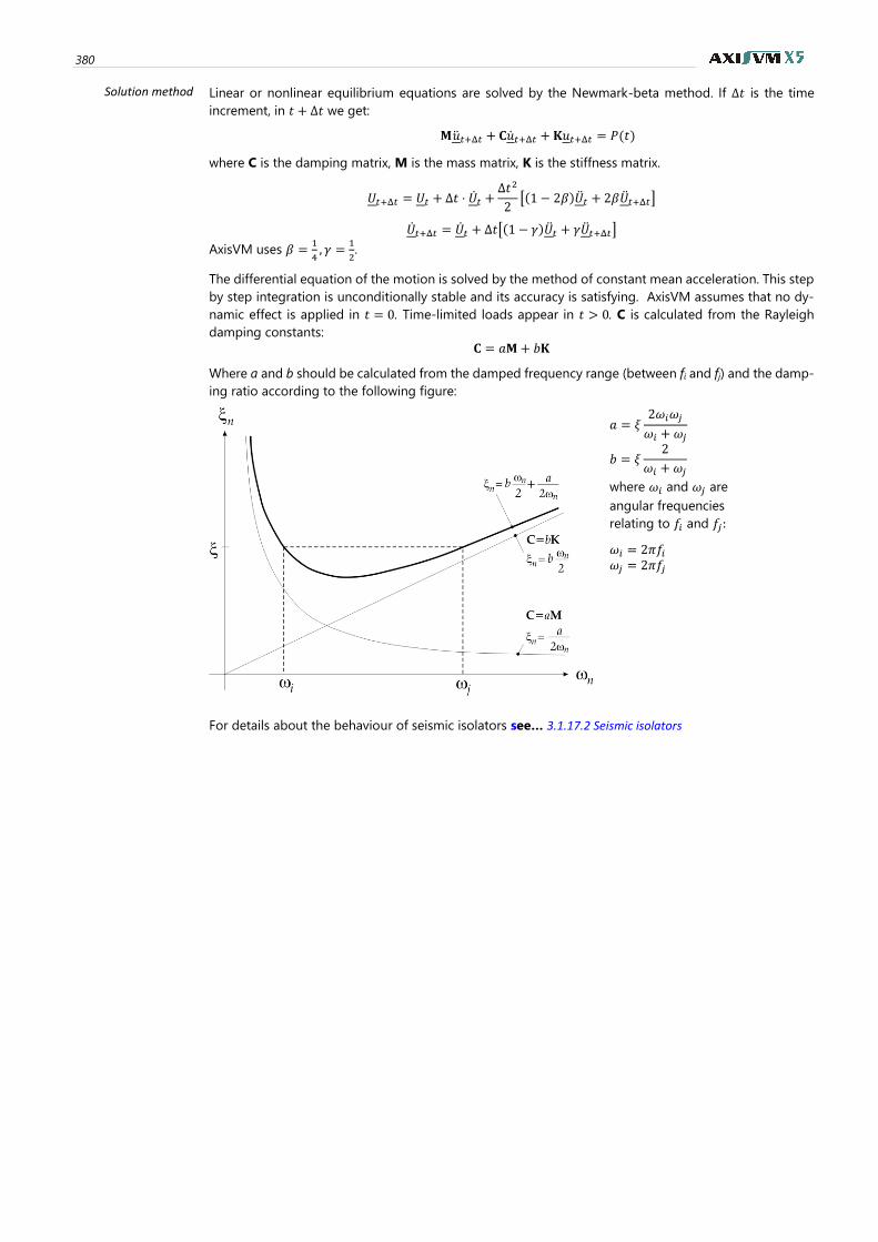
380

Solution method Linear or nonlinear equilibrium equations are solved by the Newmark-beta method. If Δ𝑡 is the time

increment, in 𝑡 + Δ𝑡 we get:

𝐌 �̈�𝑡+Δ𝑡 + 𝐂�̇�𝑡+Δ𝑡 +𝐊𝑢𝑡+Δ𝑡 = 𝑃(𝑡)

where C is the damping matrix, M is the mass matrix, K is the stiffness matrix.

𝑈𝑡+Δ𝑡 = 𝑈𝑡 + Δ𝑡 ⋅ �̇�𝑡 +Δ𝑡2

2[(1 − 2𝛽)�̈�𝑡 + 2𝛽�̈�𝑡+Δ𝑡]

�̇�𝑡+Δ𝑡 = �̇�𝑡 + Δ𝑡[(1 − 𝛾)�̈�𝑡 + 𝛾�̈�𝑡+Δ𝑡]

AxisVM uses 𝛽 =1

4, 𝛾 =

1

2.

The differential equation of the motion is solved by the method of constant mean acceleration. This step

by step integration is unconditionally stable and its accuracy is satisfying. AxisVM assumes that no dy-

namic effect is applied in 𝑡 = 0. Time-limited loads appear in 𝑡 > 0. C is calculated from the Rayleigh

damping constants:

𝐂 = 𝑎𝐌+ 𝑏𝐊

Where a and b should be calculated from the damped frequency range (between fi and fj) and the damp-

ing ratio according to the following figure:

𝑎 = 𝜉2𝜔𝑖𝜔𝑗

𝜔𝑖 + 𝜔𝑗

𝑏 = 𝜉2

𝜔𝑖 + 𝜔𝑗

where 𝜔𝑖 and 𝜔𝑗 are

angular frequencies

relating to 𝑓𝑖 and 𝑓𝑗:

𝜔𝑖 = 2𝜋𝑓𝑖 𝜔𝑗 = 2𝜋𝑓𝑗

For details about the behaviour of seismic isolators see… 3.1.17.2 Seismic isolators

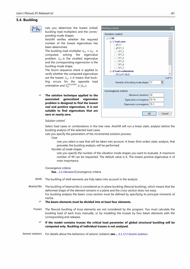
User’s Manual X5 Release4 e2 381

5.4. Buckling

Lets you determine the lowest (initial)

buckling load multipliers and the corres-

ponding mode shapes.

AxisVM verifies whether the required

number of the lowest eigenvalues has

been determined.

The buckling load multiplier 𝑛𝑐𝑟 = 𝜆𝑐𝑟 is

computed, solving the eigenvalue

problem. 𝜆𝑐𝑟 is the smallest eigenvalue

and the corresponding eigenvector is the

buckling mode shape.

The Sturm sequence check is applied to

verify whether the computed eigenvalues

are the lowest. 𝜆𝑐𝑟 < 0 means that buck-

ling occurs for the opposite load

orientation and 𝜆𝑐𝑟𝑒𝑓𝑓𝑒𝑐𝑡𝑖𝑣𝑒

≤ |𝜆𝑐𝑟|.

The solution technique applied to the

associated generalized eigenvalue

problem is designed to find the lowest

real and positive eigenvalues. It is not

suitable to find eigenvalues that are

zero or nearly zero.

Solution control

Select load cases or combinations in the tree view. AxisVM will run a linear static analysis before the

buckling analysis of the selected load cases.

Lets you specify the parameters of the incremental solution process:

Case

Lets you select a case that will be taken into account. A linear (first-order) static analysis, that

precedes the buckling analysis, will be performed.

Number of mode shapes

Lets you specify the number of the vibration mode shapes you want to evaluate. A maximum

number of 99 can be requested. The default value is 6. The lowest positive eigenvalue is of

main importance.

Convergence criteria

See... 5.2 Vibration/Convergence criteria

Shells The buckling of shell elements are fully taken into account in the analysis.

Beams/ribs The buckling of beams/ribs is considered as in-plane buckling (flexural buckling), which means that the

deformed shape of the element remains in a plane and the cross-section does not warp.

For buckling analysis the beam cross-section must be defined by specifying its principal moments of

inertia.

The beam elements must be divided into at least four elements.

Trusses The flexural buckling of truss elements are not considered by the program. You must calculate the

buckling load of each truss manually, or by modeling the trusses by four beam elements with the

corresponding end releases.

If the model contains trusses the critical load parameter of global structural buckling will be

computed only. Buckling of individual trusses is not analysed.

Seismic isolators For details about the behaviour of seismic isolators see… 3.1.17.2 Seismic isolators

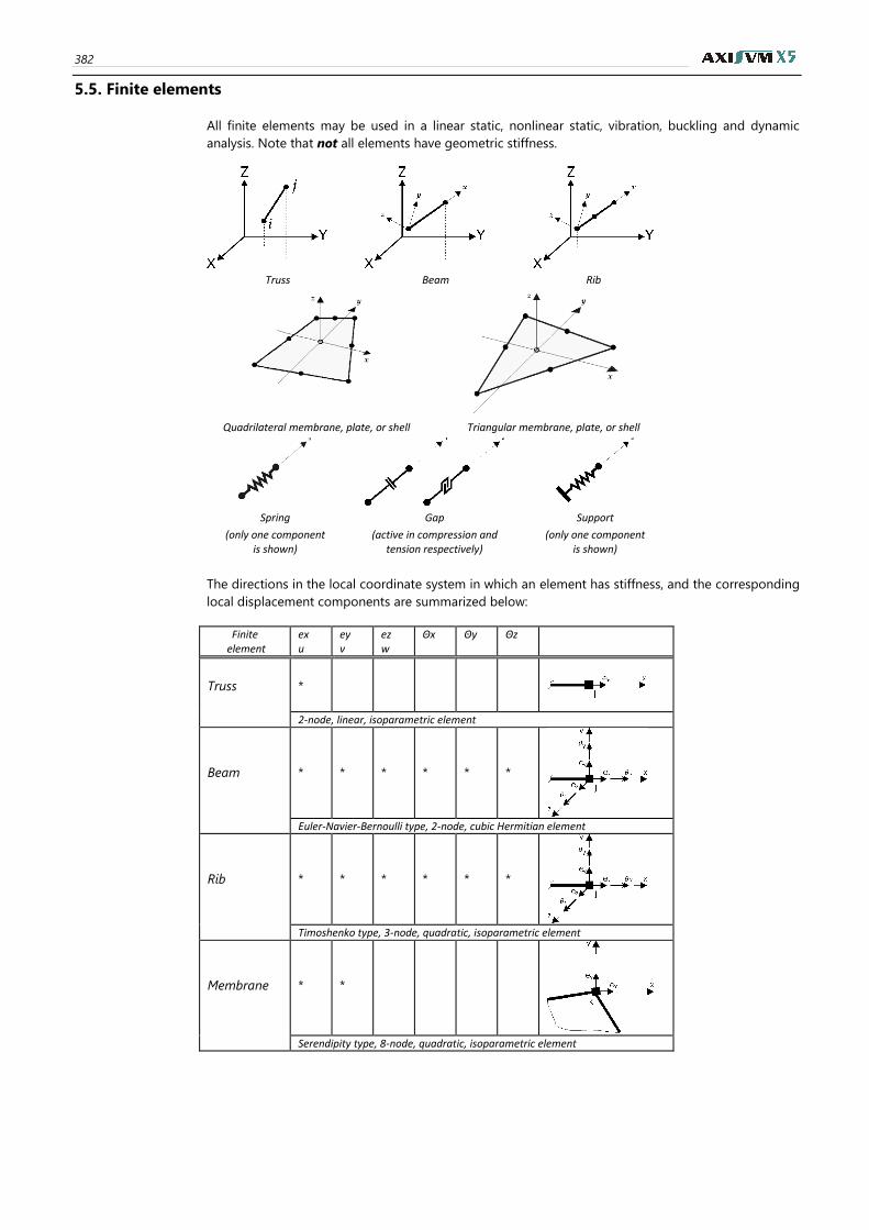
382

5.5. Finite elements

All finite elements may be used in a linear static, nonlinear static, vibration, buckling and dynamic

analysis. Note that not all elements have geometric stiffness.

Truss Beam Rib

Quadrilateral membrane, plate, or shell Triangular membrane, plate, or shell

Spring

(only one component is shown)

Gap

(active in compression and tension respectively)

Support

(only one component is shown)

The directions in the local coordinate system in which an element has stiffness, and the corresponding

local displacement components are summarized below:

Finite element

ex u

ey v

ez w

Θx Θy Θz

Truss

*

2-node, linear, isoparametric element

Beam

*

*

*

*

*

*

Euler-Navier-Bernoulli type, 2-node, cubic Hermitian element

Rib

*

*

*

*

*

*

Timoshenko type, 3-node, quadratic, isoparametric element

Membrane

*

*

Serendipity type, 8-node, quadratic, isoparametric element

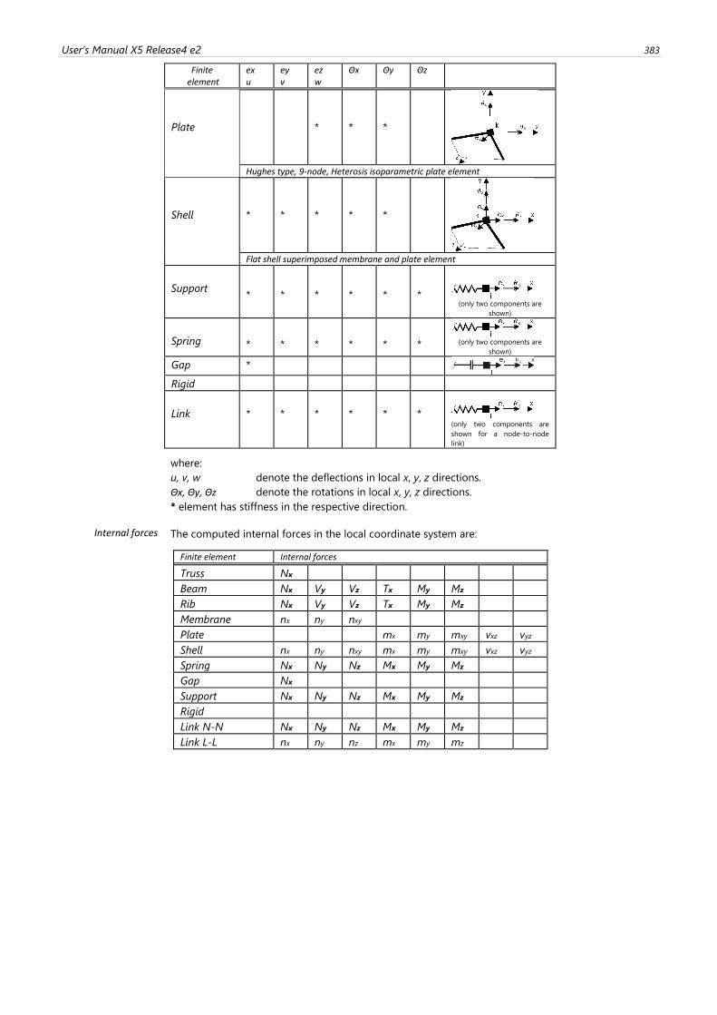
User’s Manual X5 Release4 e2 383

Finite element

ex u

ey v

ez w

Θx Θy Θz

Plate

*

*

*

Hughes type, 9-node, Heterosis isoparametric plate element

Shell

*

*

*

*

*

Flat shell superimposed membrane and plate element

Support

*

*

*

*

*

*

(only two components are

shown)

Spring *

*

*

*

*

*

(only two components are

shown)

Gap *

Rigid

Link

*

*

*

*

*

*

(only two components are

shown for a node-to-node

link)

where:

u, v, w denote the deflections in local x, y, z directions.

Θx, Θy, Θz denote the rotations in local x, y, z directions.

* element has stiffness in the respective direction.

Internal forces The computed internal forces in the local coordinate system are:

Finite element Internal forces

Truss Nx

Beam Nx Vy Vz Tx My Mz

Rib Nx Vy Vz Tx My Mz

Membrane nx ny nxy

Plate mx my mxy vxz vyz

Shell nx ny nxy mx my mxy vxz vyz

Spring Nx Ny Nz Mx My Mz

Gap Nx

Support Nx Ny Nz Mx My Mz

Rigid

Link N-N Nx Ny Nz Mx My Mz

Link L-L nx ny nz mx my mz

384

5.6. Main steps of an analysis

1. Define the geometry of the structure, the material and cross-sectional properties of the

members, the support conditions, and the loads.

2. Determine the load transfer path.

3. Determine local discontinuities such as stiffeners, gussets, holes.

4. Determine the type of finite elements that will best model the behavior of the structure. With

this step the properties of structural elements will be concentraded in their neutral axis (point,

axis, or, plane).

5. Determine a mesh type and size for the model. The size of the mesh have to correspond to the

desired accuracy of the results and with the available hardware.

6. Create the model:

a.) Equivalent geometry

b.) Equivalent properties

c.) Topology of the elements

d.) Equivalent support conditions

e.) Equivalent load (static) or masses (vibration, response-spectrum)

7. Check input data (accuracy, compatibility)

8. Run analysis

9. Select important results

10. Evaluate and check the results

a.) Accuracy and convergence of the solution

b.) Compatibility taking into account point 6.d.

c.) Uncommon structures shall be analyzed with other methods and/or software as well.

11. Restart analysis with a correspondingly updated model, if in step 10 a criteria is not satisfied.

12. Evaluate the results by the means of isoline/isosurface plots, animation, tables... Draw

conclusions on the structure’s behavior.

Modelling To build a model of a structure you have to accept many assumptions so you also have to keep the

effects of these assumptions in view when evaluating results.

The finite element method provides an approximative solution for surface models. To make the model

match the real solution you have to use finite element meshes with an appropriate density. Making

finite element meshes you have to take into account the expected stress distribution, the model

geometry and the materials, supports and loads used.

The position af nodes and mesh lines (called the topology of the finite element mesh) depends on the

geometrical discontinuities (irregular contours, line supports) and the discontinuities of loads

(concentrated loads, terraced load values for line loads).

At stress concentration points (sharp corners) you have to refine the mesh. To avoid singularities due

to concentrated effects you can distribute them on a small area around the point of effect.

Arc contours can be approximated as polygons. Using very small tolerance in this approximation leads

to polygons with extreme small sides. The very dense mesh created on this contour may cause the

model exceed the capacity of your computer.

In general if you refine the mesh you get more accurate results.

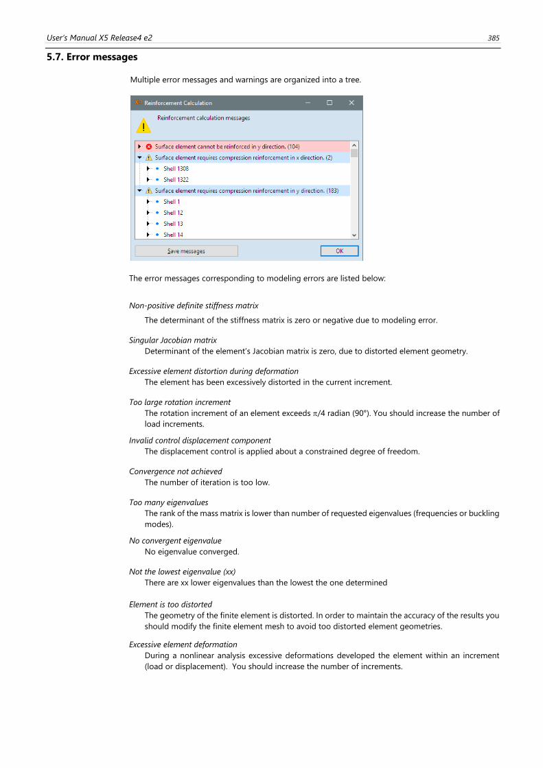
User’s Manual X5 Release4 e2 385

5.7. Error messages

Multiple error messages and warnings are organized into a tree.

The error messages corresponding to modeling errors are listed below:

Non-positive definite stiffness matrix

The determinant of the stiffness matrix is zero or negative due to modeling error.

Singular Jacobian matrix

Determinant of the element’s Jacobian matrix is zero, due to distorted element geometry.

Excessive element distortion during deformation

The element has been excessively distorted in the current increment.

Too large rotation increment

The rotation increment of an element exceeds /4 radian (90°). You should increase the number of

load increments.

Invalid control displacement component

The displacement control is applied about a constrained degree of freedom.

Convergence not achieved

The number of iteration is too low.

Too many eigenvalues

The rank of the mass matrix is lower than number of requested eigenvalues (frequencies or buckling

modes).

No convergent eigenvalue

No eigenvalue converged.

Not the lowest eigenvalue (xx)

There are xx lower eigenvalues than the lowest the one determined

Element is too distorted

The geometry of the finite element is distorted. In order to maintain the accuracy of the results you

should modify the finite element mesh to avoid too distorted element geometries.

Excessive element deformation

During a nonlinear analysis excessive deformations developed the element within an increment

(load or displacement). You should increase the number of increments.

386

No convergence achieved within maximum number of iterations

There was no convergence within the maximum number of iterations (see... Static /Nonlinear Static

Analysis/Solution Control parameters). You can increase the number of iteration. The model may

not converge at the respective load level, and you should change the Solution Control parameters

accordingly.

Divergence in the current iteration

A divergence was detected in the iteration process. Increments are too large or the convergence

criteria are too loose.

No stiffness at node ... in direction ...

There is a singularity in the system stiffness matrix corresponding to that degree of freedom. You

should check the support and degrees of freedom (DOF) settings of your model.

Other (system) er-

ror messages

In some cases, other type of error messages may also appear. Based on the system error code, more

information is provided about the error on the following link:

http://docwiki.embarcadero.com/RADStudio/Tokyo/en/Input-Output_Errors

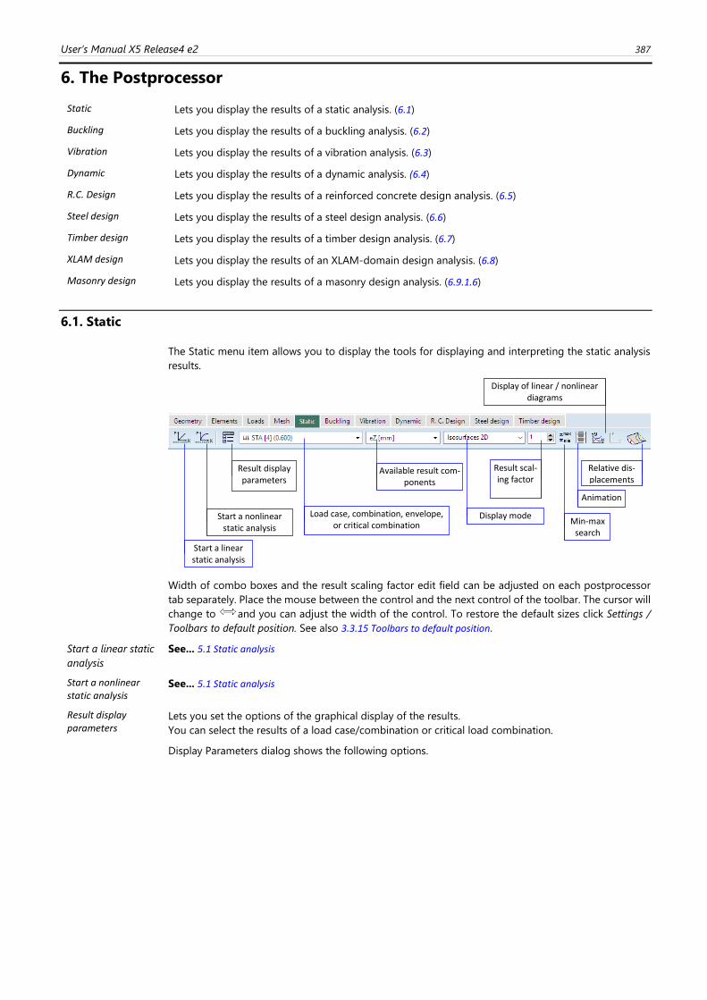
User’s Manual X5 Release4 e2 387

6. The Postprocessor

Static Lets you display the results of a static analysis. (6.1)

Buckling Lets you display the results of a buckling analysis. (6.2)

Vibration Lets you display the results of a vibration analysis. (6.3)

Dynamic Lets you display the results of a dynamic analysis. (6.4)

R.C. Design Lets you display the results of a reinforced concrete design analysis. (6.5)

Steel design Lets you display the results of a steel design analysis. (6.6)

Timber design Lets you display the results of a timber design analysis. (6.7)

XLAM design Lets you display the results of an XLAM-domain design analysis. (6.8)

Masonry design Lets you display the results of a masonry design analysis. (6.9.1.6)

6.1. Static

The Static menu item allows you to display the tools for displaying and interpreting the static analysis

results.

Width of combo boxes and the result scaling factor edit field can be adjusted on each postprocessor

tab separately. Place the mouse between the control and the next control of the toolbar. The cursor will

change to and you can adjust the width of the control. To restore the default sizes click Settings /

Toolbars to default position. See also 3.3.15 Toolbars to default position.

Start a linear static

analysis

See... 5.1 Static analysis

Start a nonlinear static analysis

See... 5.1 Static analysis

Result display parameters

Lets you set the options of the graphical display of the results.

You can select the results of a load case/combination or critical load combination.

Display Parameters dialog shows the following options.

Result display parameters

Start a nonlinear static analysis

Available result com-ponents

Result scal-ing factor

Animation

Min-max search

Load case, combination, envelope, or critical combination

Display mode

Display of linear / nonlinear diagrams

Start a linear static analysis

Relative dis-placements

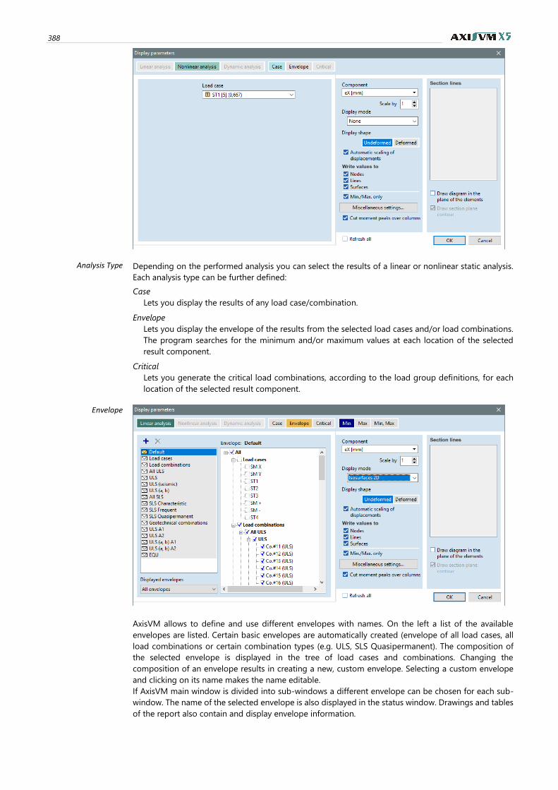
388

Analysis Type

Depending on the performed analysis you can select the results of a linear or nonlinear static analysis.

Each analysis type can be further defined:

Case

Lets you display the results of any load case/combination.

Envelope

Lets you display the envelope of the results from the selected load cases and/or load combinations.

The program searches for the minimum and/or maximum values at each location of the selected

result component.

Critical

Lets you generate the critical load combinations, according to the load group definitions, for each

location of the selected result component.

Envelope

AxisVM allows to define and use different envelopes with names. On the left a list of the available

envelopes are listed. Certain basic envelopes are automatically created (envelope of all load cases, all

load combinations or certain combination types (e.g. ULS, SLS Quasipermanent). The composition of

the selected envelope is displayed in the tree of load cases and combinations. Changing the

composition of an envelope results in creating a new, custom envelope. Selecting a custom envelope

and clicking on its name makes the name editable.

If AxisVM main window is divided into sub-windows a different envelope can be chosen for each sub-

window. The name of the selected envelope is also displayed in the status window. Drawings and tables

of the report also contain and display envelope information.

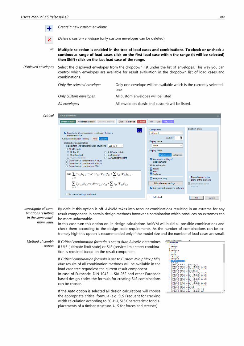
User’s Manual X5 Release4 e2 389

Create a new custom envelope

Delete a custom envelope (only custom envelopes can be deleted)

.

Multiple selection is enabled in the tree of load cases and combinations. To check or uncheck a

continuous range of load cases click on the first load case within the range (it will be selected)

then Shift+click on the last load case of the range. .

Displayed envelopes Select the displayed envelopes from the dropdown list under the list of envelopes. This way you can

control which envelopes are available for result evaluation in the dropdown list of load cases and

combinations. .

Only the selected envelope Only one envelope will be available which is the currently selected

one.

Only custom envelopes All custom envelopes will be listed

All envelopes All envelopes (basic and custom) will be listed.

Critical

Investigate all com-binations resulting in the same maxi-

mum value

By default this option is off. AxisVM takes into account combinations resulting in an extreme for any

result component. In certain design methods however a combination which produces no extremes can

be more unfavorable.

In this case turn this option on. In design calculations AxisVM will build all possible combinations and

check them according to the design code requirements. As the number of combinations can be ex-

tremely high this option is recommended only if the model size and the number of load cases are small.

Method of combi-nation

If Critical combination formula is set to Auto AxisVM determines

if ULS (ultimate limit state) or SLS (service limit state) combina-

tion is required based on the result component.

If Critical combination formula is set to Custom Min / Max / Min,

Max results of all combination methods will be available in the

load case tree regardless the current result component.

In case of Eurocode, DIN 1045-1, SIA 262 and other Eurocode

based design codes the formula for creating SLS combinations

can be chosen.

If the Auto option is selected all design calculations will choose

the appropriate critical formula (e.g. SLS Frequent for cracking

width calculation according to EC-HU, SLS Characteristic for dis-

placements of a timber structure, ULS for forces and stresses).

390

Display values

If you have selected Envelope or Critical you can choose from the following options:

Min+Max

Displays the minimum and maximum values of the current result component.

Min

Displays the minimum (sign dependent) values of the current result component.

Max

Displays the maximum (sign dependent) values of the current result component.

Display Shape Undeformed

Displays the undeformed shape (original configuration) of the model.

Deformed

Displays the deformed shape of the model.

Automatic scaling of displacements

Scales the real deformation by an automatic scale factor so that the maximum displacement is

represented as 50 pixels. This pre-scaled deformation is the basis of the further scaling by the result

scaling factor. Without this option the basis of the scaling by result scaling factor is the real

deformation.

Display Mode Diagram

Lets you display the current result component in a colored diagram form. The numerical values are

displayed if a Show value labels on option is enabled.

Filled diagram

Similar to Diagram but fills it in a customizable way (see Graphic symbols, 3.3.11 Preferences) Diagram+average values

This display mode is available only if line support forces are displayed. If this mode is selected line

support forces diagrams are enhanced with the display and labeling of the average value. Averag-

ing is made over continuos supports. Supports are considered to be continuous if they have the

same stiffness and their angle is below a small limit.

Section line

Lets you display the current result component in the active section lines and/or planes in a diagram

form. The numerical values are displayed if the Show Value Labels On option is enabled.

Filled section line

Similar to Section line but fills it in a customizable way (see settings for the Filled diagram, Graphic

symbols, 3.3.11 Preferences) Isoline (contour line)

Lets you display the current result component in a line color contour plot form.

The values that are represented by the isolines are specified in the Color Legend window. You can

set the parameters of the Color Legend window as was described in the Information Windows

paragraph. The numerical values are displayed if a Show Value Labels On option is enabled.

Isosurface 2D or 3D

Lets you display the current result component in a filled color contour plot form.

The ranges that are represented by the isosurfaces are specified in the Color Legend window. You

can set the parameters of the Color Legend window as was described in Information Windows

paragraph. The numerical values are displayed if a a Show Value Labels On option is enabled. See...

2.18.4 Color legend window

None

The current result component is not displayed.

Section lines Lets you set the active section lines, planes and segments. If display mode is set to Section line result

diagrams will be drawn only on active (checked) section lines. Symbol of the section planes can be

displayed enabling the Draw section plane contour checkbox. Turning on the Draw diagram in the plane

of elements option changes the appearance of all section diagrams. To change this parameter

individually use the Section lines dialog.

See... 2.16.15 Sections

Component Lets you select the result component to be displayed.

Scale by Lets you set the scale of a diagram drawing. The default value is 1, when the maximum ordinate is

represented as 50 pixels.

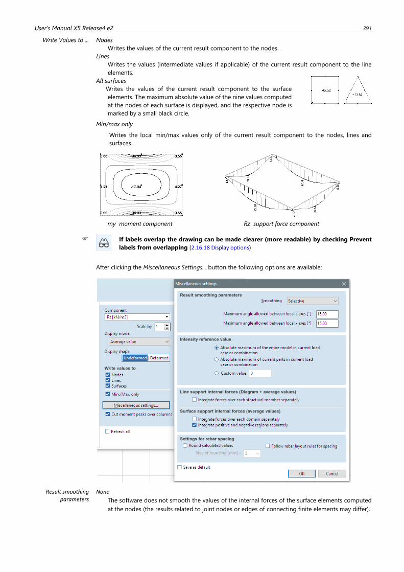
User’s Manual X5 Release4 e2 391

Write Values to ... Nodes

Writes the values of the current result component to the nodes.

Lines

Writes the values (intermediate values if applicable) of the current result component to the line

elements.

All surfaces

Writes the values of the current result component to the surface

elements. The maximum absolute value of the nine values computed

at the nodes of each surface is displayed, and the respective node is

marked by a small black circle.

Min/max only

Writes the local min/max values only of the current result component to the nodes, lines and

surfaces.

my moment component Rz support force component

If labels overlap the drawing can be made clearer (more readable) by checking Prevent

labels from overlapping (2.16.18 Display options)

After clicking the Miscellaneous Settings... button the following options are available:

Result smoothing parameters

None

The software does not smooth the values of the internal forces of the surface elements computed

at the nodes (the results related to joint nodes or edges of connecting finite elements may differ).

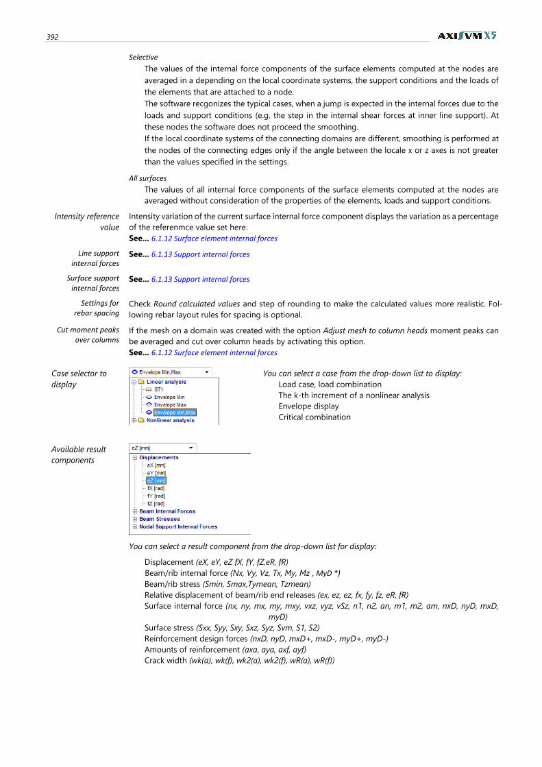
392

Selective

The values of the internal force components of the surface elements computed at the nodes are

averaged in a depending on the local coordinate systems, the support conditions and the loads of

the elements that are attached to a node.

The software recgonizes the typical cases, when a jump is expected in the internal forces due to the

loads and support conditions (e.g. the step in the internal shear forces at inner line support). At

these nodes the software does not proceed the smoothing.

If the local coordinate systems of the connecting domains are different, smoothing is performed at

the nodes of the connecting edges only if the angle between the locale x or z axes is not greater

than the values specified in the settings.

All surfaces

The values of all internal force components of the surface elements computed at the nodes are

averaged without consideration of the properties of the elements, loads and support conditions.

Intensity reference

value

Intensity variation of the current surface internal force component displays the variation as a percentage

of the referenmce value set here.

See... 6.1.12 Surface element internal forces

Line support internal forces

See... 6.1.13 Support internal forces

Surface support internal forces

See... 6.1.13 Support internal forces

Settings for rebar spacing

Check Round calculated values and step of rounding to make the calculated values more realistic. Fol-

lowing rebar layout rules for spacing is optional.

Cut moment peaks over columns

If the mesh on a domain was created with the option Adjust mesh to column heads moment peaks can

be averaged and cut over column heads by activating this option.

See... 6.1.12 Surface element internal forces

Case selector to

display

You can select a case from the drop-down list to display:

Load case, load combination

The k-th increment of a nonlinear analysis

Envelope display

Critical combination

Available result

components

You can select a result component from the drop-down list for display:

Displacement (eX, eY, eZ fX, fY, fZ,eR, fR)

Beam/rib internal force (Nx, Vy, Vz, Tx, My, Mz , MyD *) Beam/rib stress (Smin, Smax,Tymean, Tzmean)

Relative displacement of beam/rib end releases (ex, ez, ez, fx, fy, fz, eR, fR)

Surface internal force (nx, ny, mx, my, mxy, vxz, vyz, vSz, n1, n2, an, m1, m2, am, nxD, nyD, mxD,

myD)

Surface stress (Sxx, Syy, Sxy, Sxz, Syz, Svm, S1, S2)

Reinforcement design forces (nxD, nyD, mxD+, mxD-, myD+, myD-)

Amounts of reinforcement (axa, aya, axf, ayf)

Crack width (wk(a), wk(f), wk2(a), wk2(f), wR(a), wR(f))

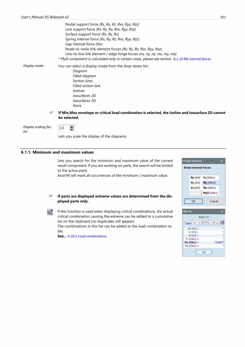
User’s Manual X5 Release4 e2 393

Nodal support force (Rx, Ry, Rz, Rxx, Ryy, Rzz)

Line support force (Rx, Ry, Rz, Rxx, Ryy, Rzz)

Surface support force (Rx, Ry, Rz)

Spring internal force (Rx, Ry, Rz, Rxx, Ryy, Rzz)

Gap internal force (Nx)

Node-to-node link element forces (Rx, Ry, Rz, Rxx, Ryy, Rzz)

Line-to-line link element / edge hinge forces (nx, ny, nz, mx, my, mz)

* MyD component is calculated only in certain cases, please see section 6.1.10 Rib internal forces

Display mode You can select a display mode from the drop-down list:

Diagram

Filled diagram

Section lines

Filled section line

Isolines

Isosurfaces 2D

Isosurfaces 3D

None

If Min,Max envelope or critical load combination is selected, the Isoline and Isosurface 2D cannot

be selected.

Display scaling fac-tor

Lets you scale the display of the diagrams.

6.1.1. Minimum and maximum values

Lets you search for the minimum and maximum value of the current

result component. If you are working on parts, the search will be limited

to the active parts.

AxisVM will mark all occurrences of the minimum / maximum value.

If parts are displayed extreme values are determined from the dis-

played parts only.

If this function is used when displaying critical combinations, the actual

critical combination causing the extreme can be added to a cumulative

list on the clipboard (no duplicates will appear).

The combinations in this list can be added to the load combination ta-

ble.

See... 4.10.2 Load combinations.

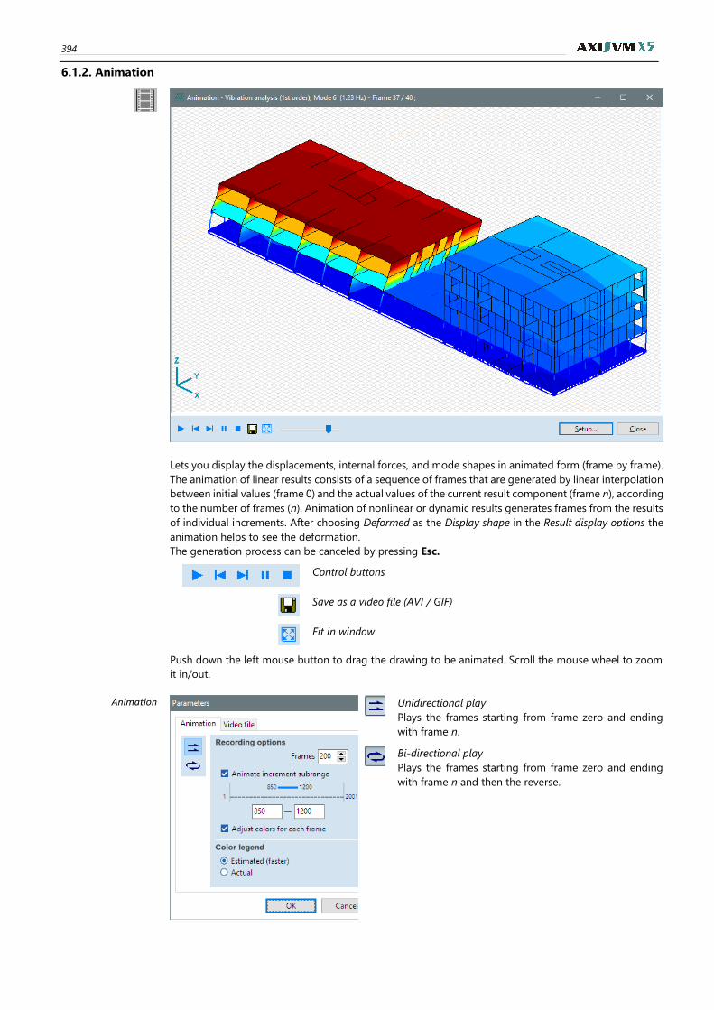
394

6.1.2. Animation

Lets you display the displacements, internal forces, and mode shapes in animated form (frame by frame).

The animation of linear results consists of a sequence of frames that are generated by linear interpolation

between initial values (frame 0) and the actual values of the current result component (frame n), according

to the number of frames (n). Animation of nonlinear or dynamic results generates frames from the results

of individual increments. After choosing Deformed as the Display shape in the Result display options the

animation helps to see the deformation.

The generation process can be canceled by pressing Esc.

Control buttons

Save as a video file (AVI / GIF)

Fit in window

Push down the left mouse button to drag the drawing to be animated. Scroll the mouse wheel to zoom

it in/out.

Animation

Unidirectional play

Plays the frames starting from frame zero and ending

with frame n.

Bi-directional play

Plays the frames starting from frame zero and ending

with frame n and then the reverse.

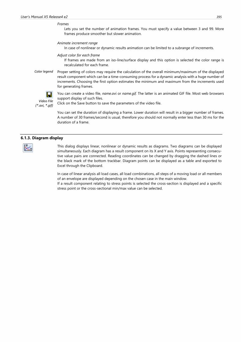
User’s Manual X5 Release4 e2 395

Frames

Lets you set the number of animation frames. You must specify a value between 3 and 99. More

frames produce smoother but slower animation.

Animate increment range

In case of nonlinear or dynamic results animation can be limited to a subrange of increments.

Adjust color for each frame

If frames are made from an iso-line/surface display and this option is selected the color range is

recalculated for each frame.

Color legend Proper setting of colors may require the calculation of the overall minimum/maximum of the displayed

result component which can be a time-consuming process for a dynamic analysis with a huge number of

increments. Choosing the first option estimates the minimum and maximum from the increments used

for generating frames.

Video File

(*.avi, *.gif)

You can create a video file, name.avi or name.gif. The latter is an animated GIF file. Most web browsers

support display of such files.

Click on the Save button to save the parameters of the video file.

You can set the duration of displaying a frame. Lower duration will result in a bigger number of frames.

A number of 30 frames/second is usual, therefore you should not normally enter less than 30 ms for the

duration of a frame.

6.1.3. Diagram display

This dialog displays linear, nonlinear or dynamic results as diagrams. Two diagrams can be displayed

simultaneously. Each diagram has a result component on its X and Y axis. Points representing consecu-

tive value pairs are connected. Reading coordinates can be changed by dragging the dashed lines or

the black mark of the bottom trackbar. Diagram points can be displayed as a table and exported to

Excel through the Clipboard.

In case of linear analysis all load cases, all load combinations, all steps of a moving load or all members

of an envelope are displayed depending on the chosen case in the main window.

If a result component relating to stress points is selected the cross-section is displayed and a specific

stress point or the cross-sectional min/max value can be selected.

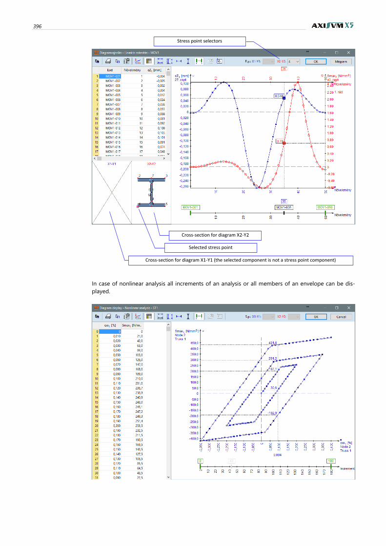
396

In case of nonlinear analysis all increments of an analysis or all members of an envelope can be dis-

played.

Cross-section for diagram X2-Y2

Selected stress point

Cross-section for diagram X1-Y1 (the selected component is not a stress point component)

Stress point selectors

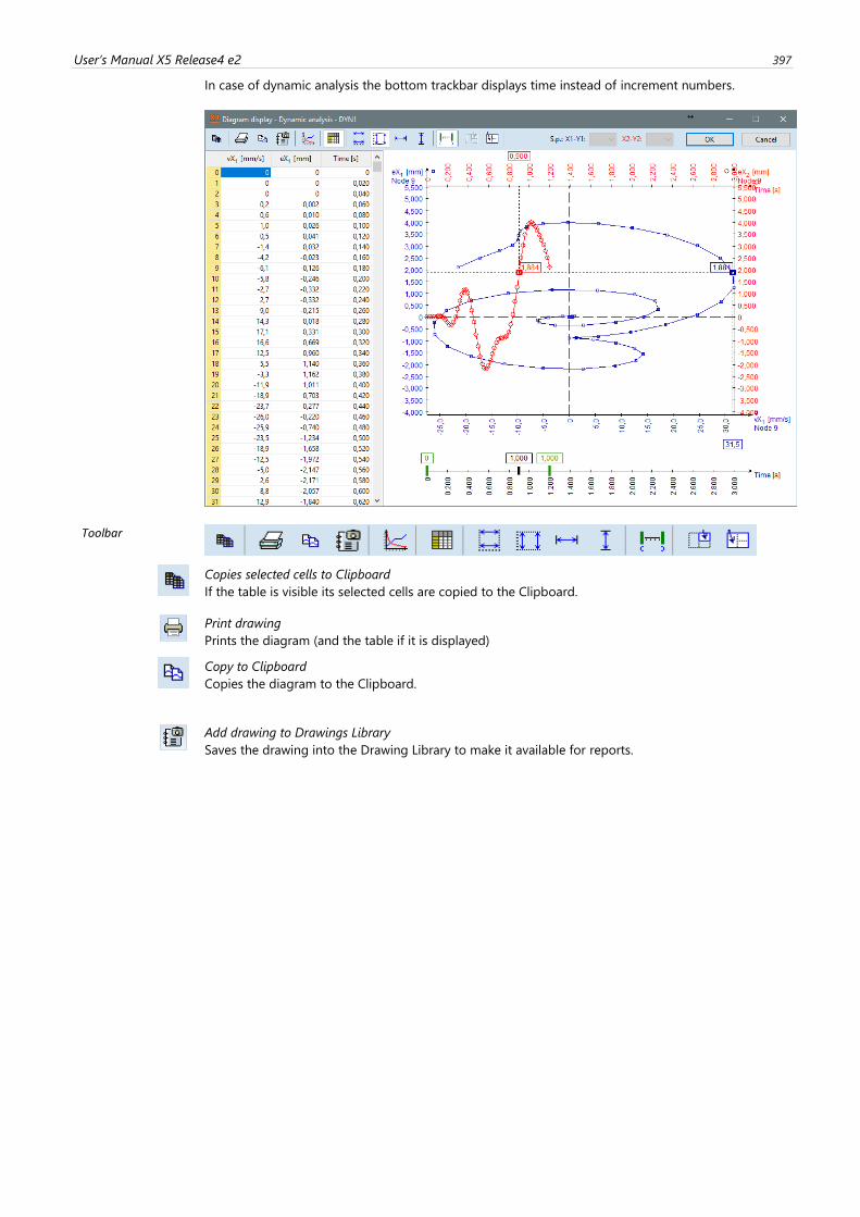
User’s Manual X5 Release4 e2 397

In case of dynamic analysis the bottom trackbar displays time instead of increment numbers.

Toolbar

Copies selected cells to Clipboard

If the table is visible its selected cells are copied to the Clipboard.

Print drawing

Prints the diagram (and the table if it is displayed)

Copy to Clipboard

Copies the diagram to the Clipboard.

Add drawing to Drawings Library

Saves the drawing into the Drawing Library to make it available for reports.

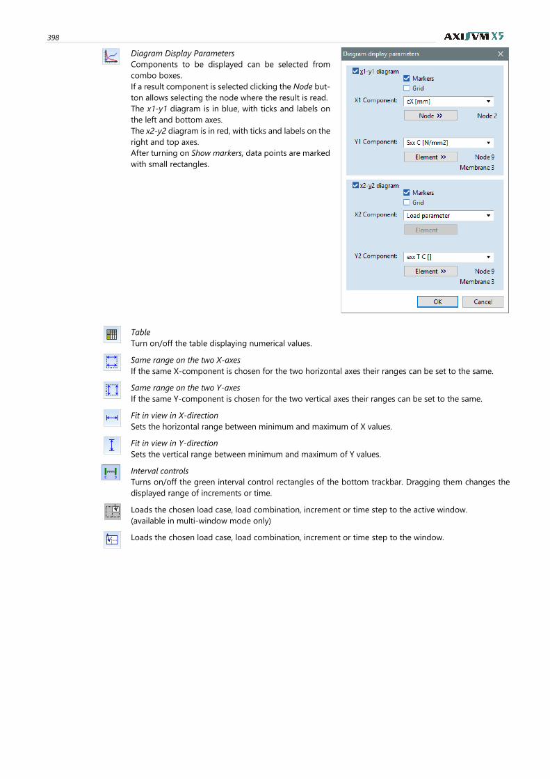
398

Diagram Display Parameters

Components to be displayed can be selected from

combo boxes.

If a result component is selected clicking the Node but-

ton allows selecting the node where the result is read.

The x1-y1 diagram is in blue, with ticks and labels on

the left and bottom axes.

The x2-y2 diagram is in red, with ticks and labels on the

right and top axes.

After turning on Show markers, data points are marked

with small rectangles.

Table

Turn on/off the table displaying numerical values.

Same range on the two X-axes

If the same X-component is chosen for the two horizontal axes their ranges can be set to the same.

Same range on the two Y-axes

If the same Y-component is chosen for the two vertical axes their ranges can be set to the same.

Fit in view in X-direction

Sets the horizontal range between minimum and maximum of X values.

Fit in view in Y-direction

Sets the vertical range between minimum and maximum of Y values.

Interval controls

Turns on/off the green interval control rectangles of the bottom trackbar. Dragging them changes the

displayed range of increments or time.

Loads the chosen load case, load combination, increment or time step to the active window.

(available in multi-window mode only)

Loads the chosen load case, load combination, increment or time step to the window.

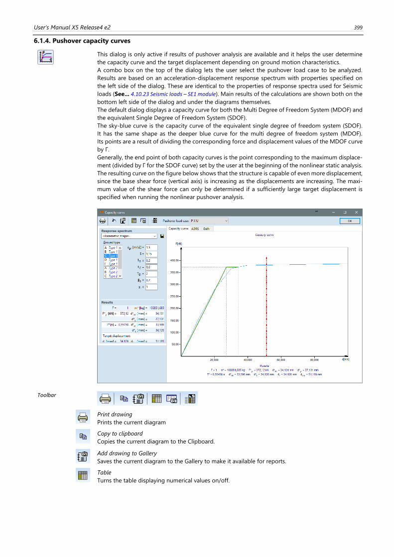
User’s Manual X5 Release4 e2 399

6.1.4. Pushover capacity curves

This dialog is only active if results of pushover analysis are available and it helps the user determine

the capacity curve and the target displacement depending on ground motion characteristics.

A combo box on the top of the dialog lets the user select the pushover load case to be analyzed.

Results are based on an acceleration-displacement response spectrum with properties specified on

the left side of the dialog. These are identical to the properties of response spectra used for Seismic

loads (See... 4.10.23 Seismic loads – SE1 module). Main results of the calculations are shown both on the

bottom left side of the dialog and under the diagrams themselves.

The default dialog displays a capacity curve for both the Multi Degree of Freedom System (MDOF) and

the equivalent Single Degree of Freedom System (SDOF).

The sky-blue curve is the capacity curve of the equivalent single degree of freedom system (SDOF).

It has the same shape as the deeper blue curve for the multi degree of freedom system (MDOF).

Its points are a result of dividing the corresponding force and displacement values of the MDOF curve

by Γ.

Generally, the end point of both capacity curves is the point corresponding to the maximum displace-

ment (divided by Γ for the SDOF curve) set by the user at the beginning of the nonlinear static analysis.

The resulting curve on the figure below shows that the structure is capable of even more displacement,

since the base shear force (vertical axis) is increasing as the displacements are increasing. The maxi-

mum value of the shear force can only be determined if a sufficiently large target displacement is

specified when running the nonlinear pushover analysis.

Toolbar

Print drawing

Prints the current diagram

Copy to clipboard

Copies the current diagram to the Clipboard.

Add drawing to Gallery

Saves the current diagram to the Gallery to make it available for reports.

Table

Turns the table displaying numerical values on/off.

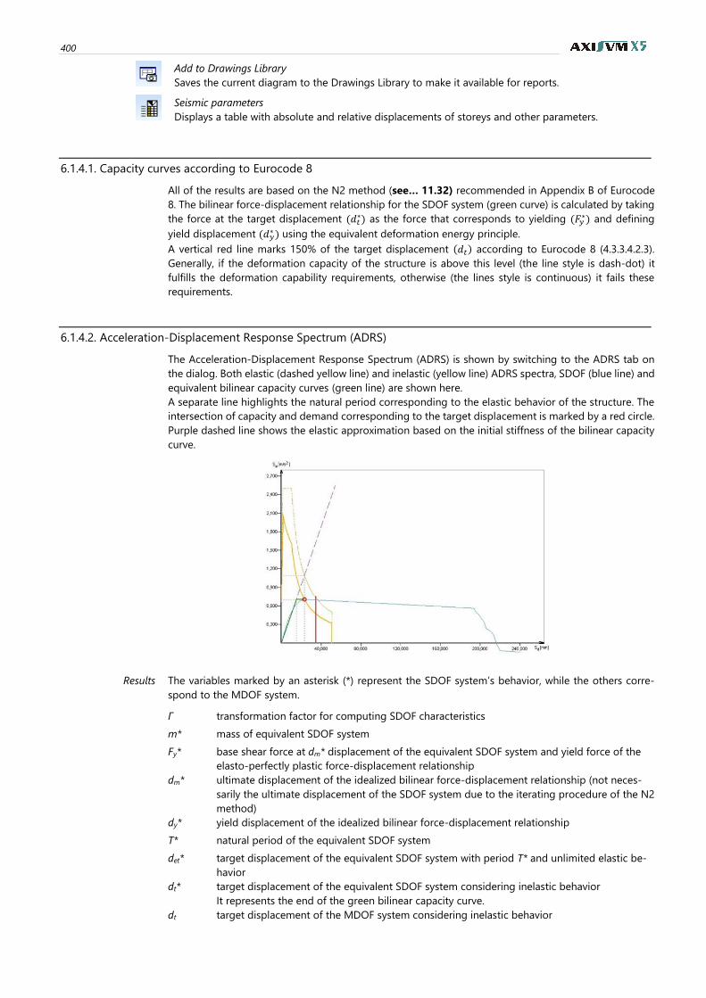
400

Add to Drawings Library

Saves the current diagram to the Drawings Library to make it available for reports.

Seismic parameters

Displays a table with absolute and relative displacements of storeys and other parameters.

6.1.4.1. Capacity curves according to Eurocode 8

All of the results are based on the N2 method (see… 11.32) recommended in Appendix B of Eurocode

8. The bilinear force-displacement relationship for the SDOF system (green curve) is calculated by taking

the force at the target displacement (𝑑𝑡∗) as the force that corresponds to yielding (𝐹𝑦

∗) and defining

yield displacement (𝑑𝑦∗ ) using the equivalent deformation energy principle.

A vertical red line marks 150% of the target displacement (𝑑𝑡) according to Eurocode 8 (4.3.3.4.2.3).

Generally, if the deformation capacity of the structure is above this level (the line style is dash-dot) it

fulfills the deformation capability requirements, otherwise (the lines style is continuous) it fails these

requirements.

6.1.4.2. Acceleration-Displacement Response Spectrum (ADRS)

The Acceleration-Displacement Response Spectrum (ADRS) is shown by switching to the ADRS tab on

the dialog. Both elastic (dashed yellow line) and inelastic (yellow line) ADRS spectra, SDOF (blue line) and

equivalent bilinear capacity curves (green line) are shown here.

A separate line highlights the natural period corresponding to the elastic behavior of the structure. The

intersection of capacity and demand corresponding to the target displacement is marked by a red circle.

Purple dashed line shows the elastic approximation based on the initial stiffness of the bilinear capacity

curve.

Results The variables marked by an asterisk (*) represent the SDOF system’s behavior, while the others corre-

spond to the MDOF system.

Γ transformation factor for computing SDOF characteristics

m* mass of equivalent SDOF system

Fy* base shear force at dm* displacement of the equivalent SDOF system and yield force of the

elasto-perfectly plastic force-displacement relationship

dm* ultimate displacement of the idealized bilinear force-displacement relationship (not neces-

sarily the ultimate displacement of the SDOF system due to the iterating procedure of the N2

method)

dy* yield displacement of the idealized bilinear force-displacement relationship

T* natural period of the equivalent SDOF system

det* target displacement of the equivalent SDOF system with period T* and unlimited elastic be-

havior

dt* target displacement of the equivalent SDOF system considering inelastic behavior

It represents the end of the green bilinear capacity curve.

dt target displacement of the MDOF system considering inelastic behavior

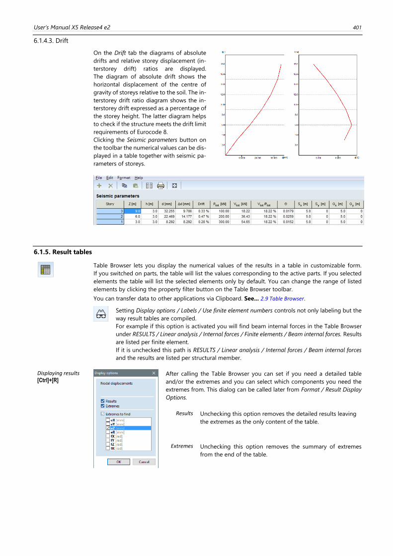
User’s Manual X5 Release4 e2 401

6.1.4.3. Drift

On the Drift tab the diagrams of absolute

drifts and relative storey displacement (in-

terstorey drift) ratios are displayed.

The diagram of absolute drift shows the

horizontal displacement of the centre of

gravity of storeys relative to the soil. The in-

terstorey drift ratio diagram shows the in-

terstorey drift expressed as a percentage of

the storey height. The latter diagram helps

to check if the structure meets the drift limit

requirements of Eurocode 8.

Clicking the Seismic parameters button on

the toolbar the numerical values can be dis-

played in a table together with seismic pa-

rameters of storeys.

6.1.5. Result tables

Table Browser lets you display the numerical values of the results in a table in customizable form.

If you switched on parts, the table will list the values corresponding to the active parts. If you selected

elements the table will list the selected elements only by default. You can change the range of listed

elements by clicking the property filter button on the Table Browser toolbar.

You can transfer data to other applications via Clipboard. See... 2.9 Table Browser.

Setting Display options / Labels / Use finite element numbers controls not only labeling but the

way result tables are compiled.

For example if this option is activated you will find beam internal forces in the Table Browser

under RESULTS / Linear analysis / Internal forces / Finite elements / Beam internal forces. Results

are listed per finite element.

If it is unchecked this path is RESULTS / Linear analysis / Internal forces / Beam internal forces

and the results are listed per structural member.

Displaying results [Ctrl]+[R]

After calling the Table Browser you can set if you need a detailed table

and/or the extremes and you can select which components you need the

extremes from. This dialog can be called later from Format / Result Display

Options.

Results Unchecking this option removes the detailed results leaving

the extremes as the only content of the table.

Extremes Unchecking this option removes the summary of extremes

from the end of the table.

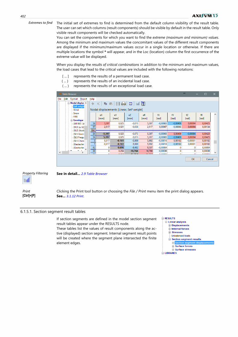
402

Extremes to find The initial set of extremes to find is determined from the default column visibility of the result table.

The user can set which columns (result components) should be visible by default in the result table. Only

visible result components will be checked automatically.

You can set the components for which you want to find the extreme (maximum and minimum) values.

Among the minimum and maximum values the concomitant values of the different result components

are displayed if the minimum/maximum values occur in a single location or otherwise. If there are

multiple locations the symbol * will appear, and in the Loc (location) column the first occurrence of the

extreme value will be displayed.

When you display the results of critical combinations in addition to the minimum and maximum values,

the load cases that lead to the critical values are included with the following notations:

[ ... ] represents the results of a permanent load case.

{ ... } represents the results of an incidental load case.

( ... ) represents the results of an exceptional load case.

Property Filtering

See in detail... 2.9 Table Browser

Print

[Ctrl]+[P]

Clicking the Print tool button or choosing the File / Print menu item the print dialog appears.

See... 3.1.12 Print.

6.1.5.1. Section segment result tables

If section segments are defined in the model section segment

result tables appear under the RESULTS node.

These tables list the values of result components along the ac-

tive (displayed) section segment. Internal segment result points

will be created where the segment plane intersected the finite

element edges.

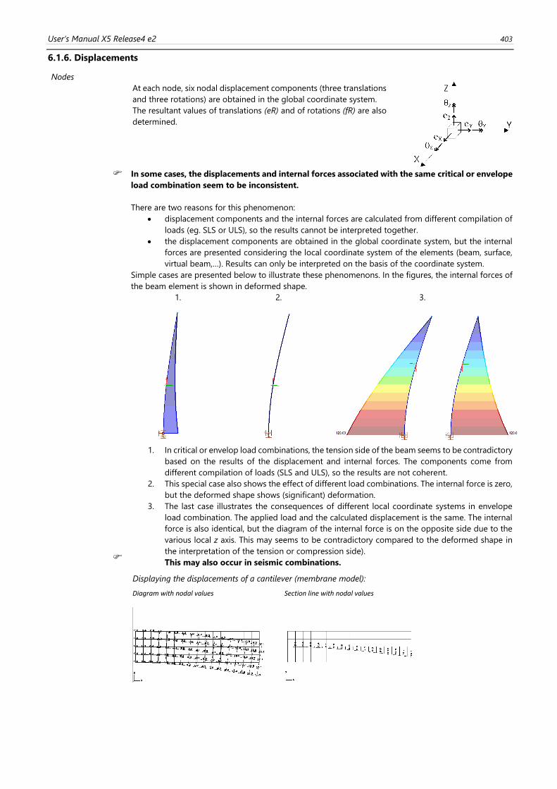
User’s Manual X5 Release4 e2 403

6.1.6. Displacements

Nodes

At each node, six nodal displacement components (three translations

and three rotations) are obtained in the global coordinate system.

The resultant values of translations (eR) and of rotations (fR) are also

determined.

In some cases, the displacements and internal forces associated with the same critical or envelope

load combination seem to be inconsistent.

There are two reasons for this phenomenon:

• displacement components and the internal forces are calculated from different compilation of

loads (eg. SLS or ULS), so the results cannot be interpreted together.

• the displacement components are obtained in the global coordinate system, but the internal

forces are presented considering the local coordinate system of the elements (beam, surface,

virtual beam,…). Results can only be interpreted on the basis of the coordinate system.

Simple cases are presented below to illustrate these phenomenons. In the figures, the internal forces of

the beam element is shown in deformed shape.

1. 2. 3.

1. In critical or envelop load combinations, the tension side of the beam seems to be contradictory

based on the results of the displacement and internal forces. The components come from

different compilation of loads (SLS and ULS), so the results are not coherent.

2. This special case also shows the effect of different load combinations. The internal force is zero,

but the deformed shape shows (significant) deformation.

3. The last case illustrates the consequences of different local coordinate systems in envelope

load combination. The applied load and the calculated displacement is the same. The internal

force is also identical, but the diagram of the internal force is on the opposite side due to the

various local z axis. This may seems to be contradictory compared to the deformed shape in

the interpretation of the tension or compression side).

This may also occur in seismic combinations.

Displaying the displacements of a cantilever (membrane model):

Diagram with nodal values Section line with nodal values

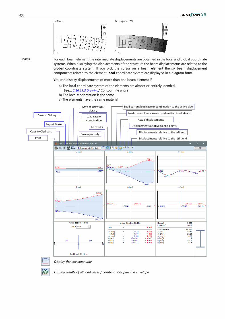
404

Isolines Isosurfaces 2D

Beams For each beam element the intermediate displacements are obtained in the local and global coordinate

systems. When displaying the displacements of the structure the beam displacements are related to the

global coordinate system. If you pick the cursor on a beam element the six beam displacement

components related to the element local coordinate system are displayed in a diagram form.

You can display displacements of more than one beam element if:

a) The local coordinate system of the elements are almost or entirely identical.

See... 2.16.19.3 Drawing/ Contour line angle

b) The local x orientation is the same.

c) The elements have the same material

Display the envelope only

Display results of all load cases / combinations plus the envelope

Print

Copy to Clipboard

Report Maker

Save to Gallery

Save to Drawings Library

Load case or combination Actual displacements

Displacements relative to end points

Load current load case or combination to the active view

Load current load case or combination to all views

All results

Envelopes only Displacements relative to the left end

Displacements relative to the right end

User’s Manual X5 Release4 e2 405

Load current load case or combination to the active view (in case of multi-window mode the load case

or combination will only be loaded to the active view)

Load current load case or combination to all views (in case of multi-window mode the load case or

combination will be loaded to all views)

Actual displacements

Displacements relative to

end points

Displacements relative to

the left end

Displacements relative to

the right end

You can display the diagrams corresponding to any load case or combination, as well as envelopes. You

can turn on and off the display of envelope functions and set the position along the member where

you want the results displayed.

Save diagrams to the Drawings Li-

brary

Associative diagrams can be saved to the Drawings Library. Drawings from this library can be inserted

into reports. After changing and recalculating the model diagrams in the library and reports change

accordingly.

Result tables See... 6.1.5 Result tables

6.1.6.1. Nonlinear calculation of total deflection (wtot) for RC plates

The following function is only available in Eurocode-NL and Eurocode-B standards and can be

used only for plates.

EN 1990:2002 A1.4.3, NEN-EN 1990 A1.4.3

To determine the total deflection of a reinforced plate different type of vertical deflections must be

calculated by running a series of nonlinear analyses for certain combinations with and without creep.

Use reinforcement in calculation must always be checked.

Calculation of total deflection requires the following values

w1 Initial part of the deflection under permanent loads

Run nonlinear analysis for 1) permanent load cases or 2) characteristic, frequent or quasi-permanent

SLS combinations without variable loads) without creep (φ = 0)

w2 Long-term part of the deflection under permanent loads

The same quasi-permanent SLS combinations must be calculated both with and without creep as w2 is

obtained as the difference between the two results.

Permanent part of the SLS combinations must include the same permanent load cases as the combina-

tion used to determine w1.

w3 Additional part of the deflection due to the variable actions of the relevant combinations

Must be calculated from the same SLS combinations as used to determine w1 but including variable

load cases as well without creep. w3 is obtained as the difference between the two results.

wbij wbij =w2+w3

wtot Total deflection

wtot = w1+w2+w3

Steps of calculation 1. Generate all SLS combinations you want to take into account. Quasipermanent SLS combinations

must always be included. See... 4.10.2 Load combinations

2. Run a nonlinear analysis for all combinations without creep. Quasipermanent SLS combinations must

also be calculated with creep.

Use reinforcement in calculation must always be checked. See... 5.1 Static analysis.

3. Select a predefined envelope of SLS Quasipermanent or a custom envelope created from a subset of

the combinations. See... 6.1 Static.

4. If the envelope contains all the needed combinations, the program finds the set of combinations that

include the same permanent load cases and determine w1, w2, w3, wbij and wtot value for each set,

calculates their envelope and makes the envelope values available as w1, w2, w3, wbij and wtot result

components.

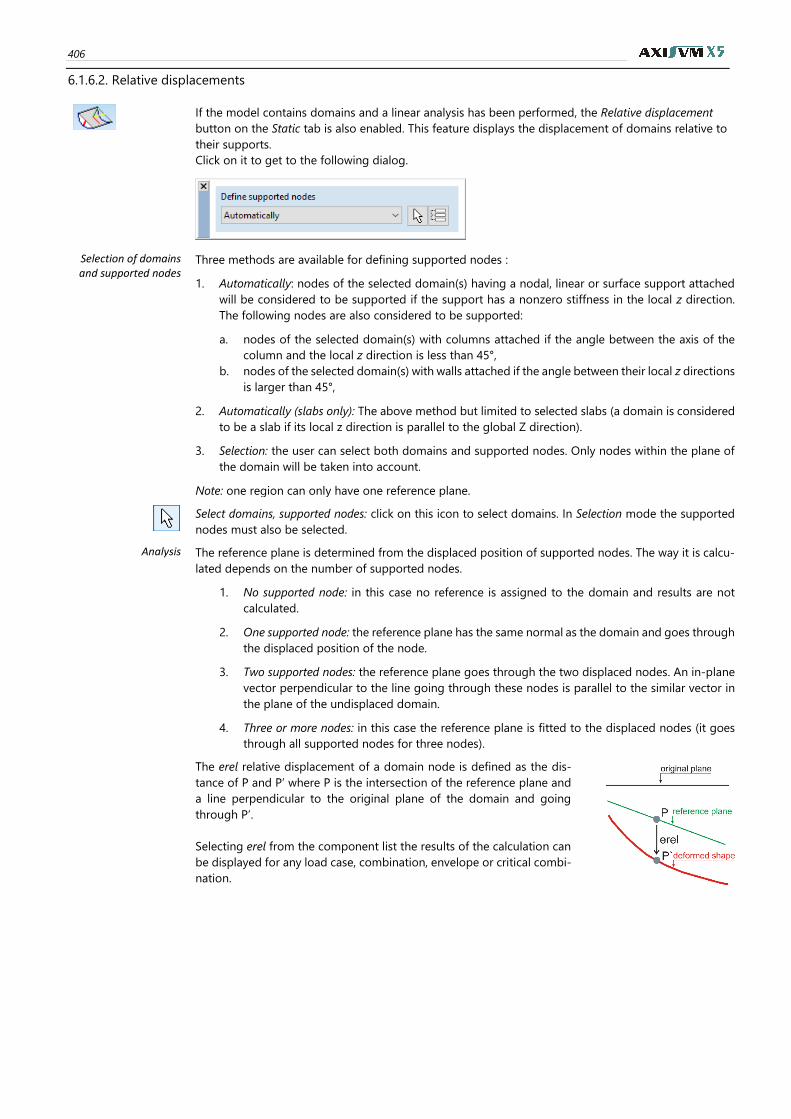
406

6.1.6.2. Relative displacements

If the model contains domains and a linear analysis has been performed, the Relative displacement

button on the Static tab is also enabled. This feature displays the displacement of domains relative to

their supports.

Click on it to get to the following dialog.

Selection of domains and supported nodes

Three methods are available for defining supported nodes :

1. Automatically: nodes of the selected domain(s) having a nodal, linear or surface support attached

will be considered to be supported if the support has a nonzero stiffness in the local z direction.

The following nodes are also considered to be supported:

a. nodes of the selected domain(s) with columns attached if the angle between the axis of the

column and the local z direction is less than 45°,

b. nodes of the selected domain(s) with walls attached if the angle between their local z directions

is larger than 45°,

2. Automatically (slabs only): The above method but limited to selected slabs (a domain is considered

to be a slab if its local z direction is parallel to the global Z direction).

3. Selection: the user can select both domains and supported nodes. Only nodes within the plane of

the domain will be taken into account.

Note: one region can only have one reference plane.

Select domains, supported nodes: click on this icon to select domains. In Selection mode the supported

nodes must also be selected.

Analysis The reference plane is determined from the displaced position of supported nodes. The way it is calcu-

lated depends on the number of supported nodes.

1. No supported node: in this case no reference is assigned to the domain and results are not

calculated.

2. One supported node: the reference plane has the same normal as the domain and goes through

the displaced position of the node.

3. Two supported nodes: the reference plane goes through the two displaced nodes. An in-plane

vector perpendicular to the line going through these nodes is parallel to the similar vector in

the plane of the undisplaced domain.

4. Three or more nodes: in this case the reference plane is fitted to the displaced nodes (it goes

through all supported nodes for three nodes).

The erel relative displacement of a domain node is defined as the dis-

tance of P and P’ where P is the intersection of the reference plane and

a line perpendicular to the original plane of the domain and going

through P’.

Selecting erel from the component list the results of the calculation can

be displayed for any load case, combination, envelope or critical combi-

nation.

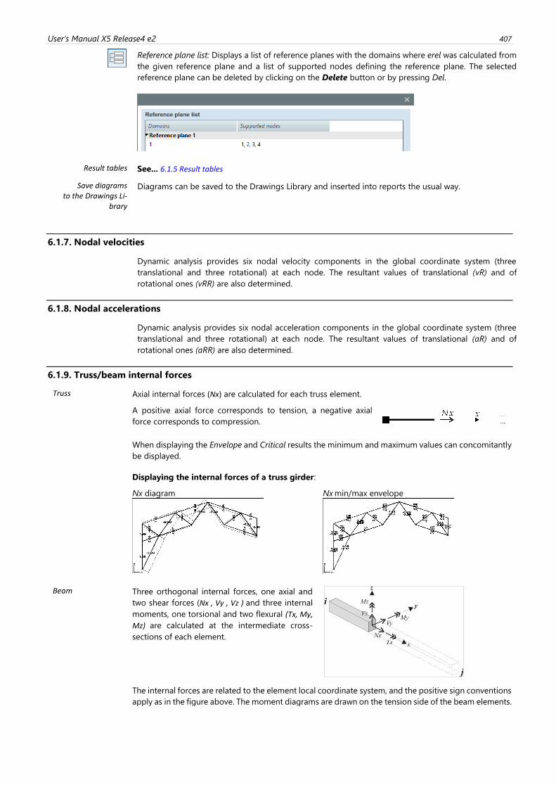
User’s Manual X5 Release4 e2 407

Reference plane list: Displays a list of reference planes with the domains where erel was calculated from

the given reference plane and a list of supported nodes defining the reference plane. The selected

reference plane can be deleted by clicking on the Delete button or by pressing Del.

Result tables See... 6.1.5 Result tables

Save diagrams to the Drawings Li-

brary

Diagrams can be saved to the Drawings Library and inserted into reports the usual way.

6.1.7. Nodal velocities

Dynamic analysis provides six nodal velocity components in the global coordinate system (three

translational and three rotational) at each node. The resultant values of translational (vR) and of

rotational ones (vRR) are also determined.

6.1.8. Nodal accelerations

Dynamic analysis provides six nodal acceleration components in the global coordinate system (three

translational and three rotational) at each node. The resultant values of translational (aR) and of

rotational ones (aRR) are also determined.

6.1.9. Truss/beam internal forces

Truss Axial internal forces (Nx) are calculated for each truss element.

A positive axial force corresponds to tension, a negative axial

force corresponds to compression.

When displaying the Envelope and Critical results the minimum and maximum values can concomitantly

be displayed.

Displaying the internal forces of a truss girder:

Nx diagram Nx min/max envelope

Beam Three orthogonal internal forces, one axial and

two shear forces (Nx , Vy , Vz ) and three internal

moments, one torsional and two flexural (Tx, My,

Mz) are calculated at the intermediate cross-

sections of each element.

The internal forces are related to the element local coordinate system, and the positive sign conventions

apply as in the figure above. The moment diagrams are drawn on the tension side of the beam elements.

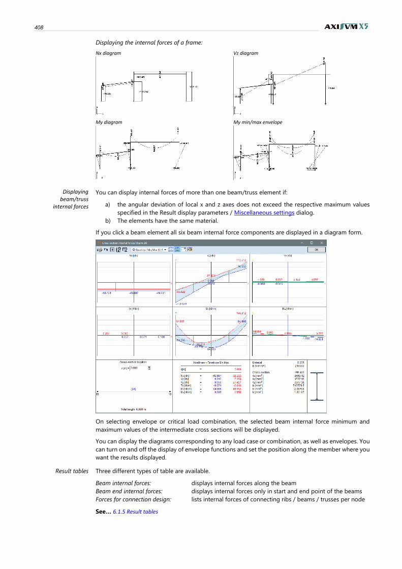
408

Displaying the internal forces of a frame:

Nx diagram Vz diagram

My diagram My min/max envelope

Displaying beam/truss

internal forces

You can display internal forces of more than one beam/truss element if:

a) the angular deviation of local x and z axes does not exceed the respective maximum values

specified in the Result display parameters / Miscellaneous settings dialog.

b) The elements have the same material.

If you click a beam element all six beam internal force components are displayed in a diagram form.

On selecting envelope or critical load combination, the selected beam internal force minimum and

maximum values of the intermediate cross sections will be displayed.

You can display the diagrams corresponding to any load case or combination, as well as envelopes. You

can turn on and off the display of envelope functions and set the position along the member where you

want the results displayed.

Result tables Three different types of table are available.

Beam internal forces: displays internal forces along the beam

Beam end internal forces: displays internal forces only in start and end point of the beams

Forces for connection design: lists internal forces of connecting ribs / beams / trusses per node

See… 6.1.5 Result tables

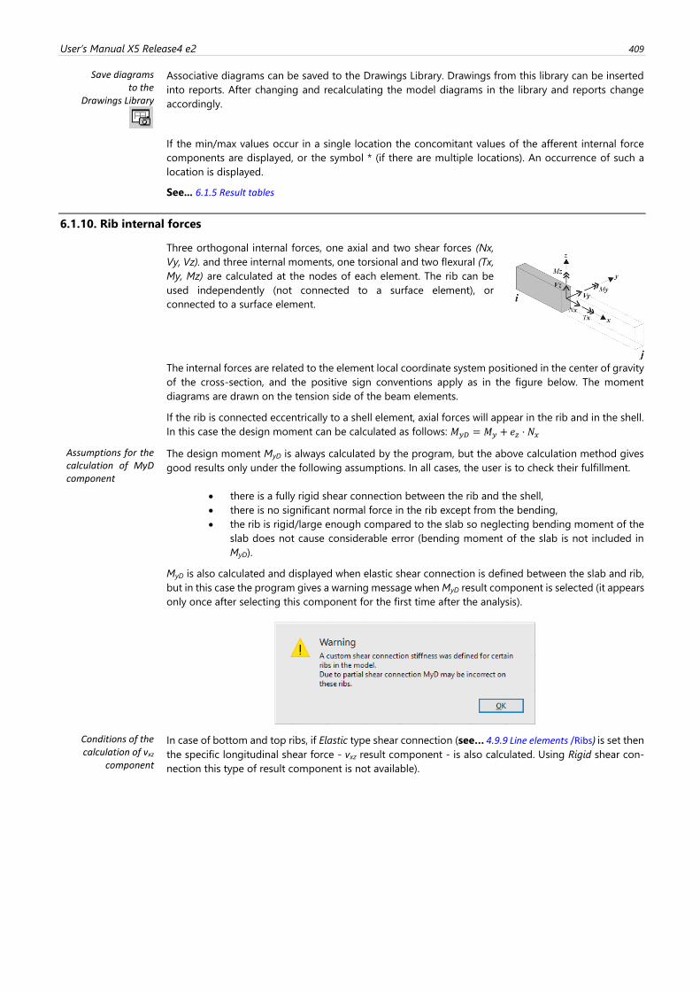
User’s Manual X5 Release4 e2 409

Save diagrams to the

Drawings Library

Associative diagrams can be saved to the Drawings Library. Drawings from this library can be inserted

into reports. After changing and recalculating the model diagrams in the library and reports change

accordingly.

If the min/max values occur in a single location the concomitant values of the afferent internal force

components are displayed, or the symbol * (if there are multiple locations). An occurrence of such a

location is displayed.

See... 6.1.5 Result tables

6.1.10. Rib internal forces

Three orthogonal internal forces, one axial and two shear forces (Nx,

Vy, Vz). and three internal moments, one torsional and two flexural (Tx,

My, Mz) are calculated at the nodes of each element. The rib can be

used independently (not connected to a surface element), or

connected to a surface element.

The internal forces are related to the element local coordinate system positioned in the center of gravity

of the cross-section, and the positive sign conventions apply as in the figure below. The moment

diagrams are drawn on the tension side of the beam elements.

If the rib is connected eccentrically to a shell element, axial forces will appear in the rib and in the shell.

In this case the design moment can be calculated as follows: 𝑀𝑦𝐷 = 𝑀𝑦 + 𝑒𝑧 ⋅ 𝑁𝑥

Assumptions for the calculation of MyD component

The design moment MyD is always calculated by the program, but the above calculation method gives

good results only under the following assumptions. In all cases, the user is to check their fulfillment.

• there is a fully rigid shear connection between the rib and the shell,

• there is no significant normal force in the rib except from the bending,

• the rib is rigid/large enough compared to the slab so neglecting bending moment of the

slab does not cause considerable error (bending moment of the slab is not included in

MyD).

MyD is also calculated and displayed when elastic shear connection is defined between the slab and rib,

but in this case the program gives a warning message when MyD result component is selected (it appears

only once after selecting this component for the first time after the analysis).

Conditions of the calculation of vxz

component

In case of bottom and top ribs, if Elastic type shear connection (see… 4.9.9 Line elements /Ribs) is set then

the specific longitudinal shear force - vxz result component - is also calculated. Using Rigid shear con-

nection this type of result component is not available).

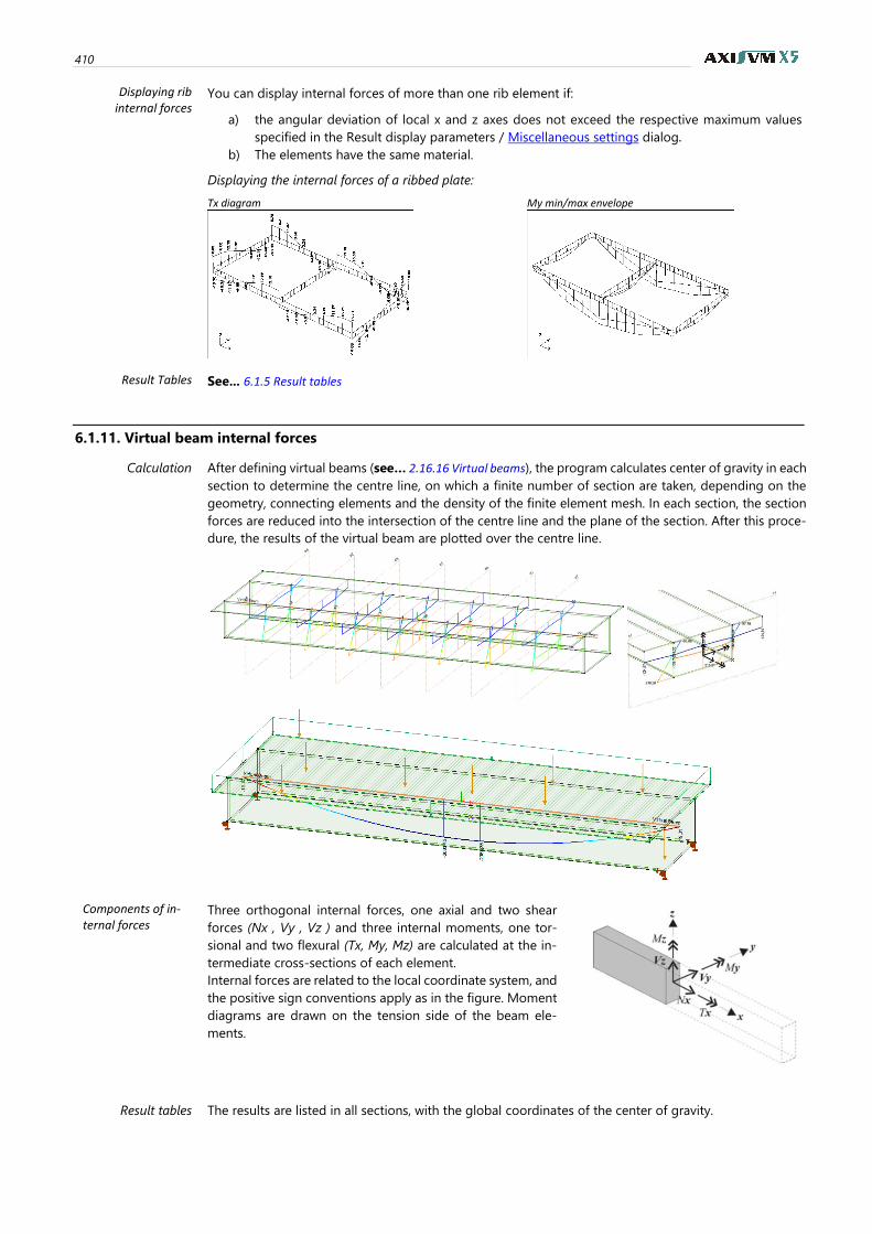
410

Displaying rib internal forces

You can display internal forces of more than one rib element if:

a) the angular deviation of local x and z axes does not exceed the respective maximum values

specified in the Result display parameters / Miscellaneous settings dialog.

b) The elements have the same material.

Displaying the internal forces of a ribbed plate:

Tx diagram My min/max envelope

Result Tables See... 6.1.5 Result tables

6.1.11. Virtual beam internal forces

Calculation After defining virtual beams (see… 2.16.16 Virtual beams), the program calculates center of gravity in each

section to determine the centre line, on which a finite number of section are taken, depending on the

geometry, connecting elements and the density of the finite element mesh. In each section, the section

forces are reduced into the intersection of the centre line and the plane of the section. After this proce-

dure, the results of the virtual beam are plotted over the centre line.

Components of in-ternal forces

Three orthogonal internal forces, one axial and two shear

forces (Nx , Vy , Vz ) and three internal moments, one tor-

sional and two flexural (Tx, My, Mz) are calculated at the in-

termediate cross-sections of each element.

Internal forces are related to the local coordinate system, and

the positive sign conventions apply as in the figure. Moment

diagrams are drawn on the tension side of the beam ele-

ments.

Result tables The results are listed in all sections, with the global coordinates of the center of gravity.

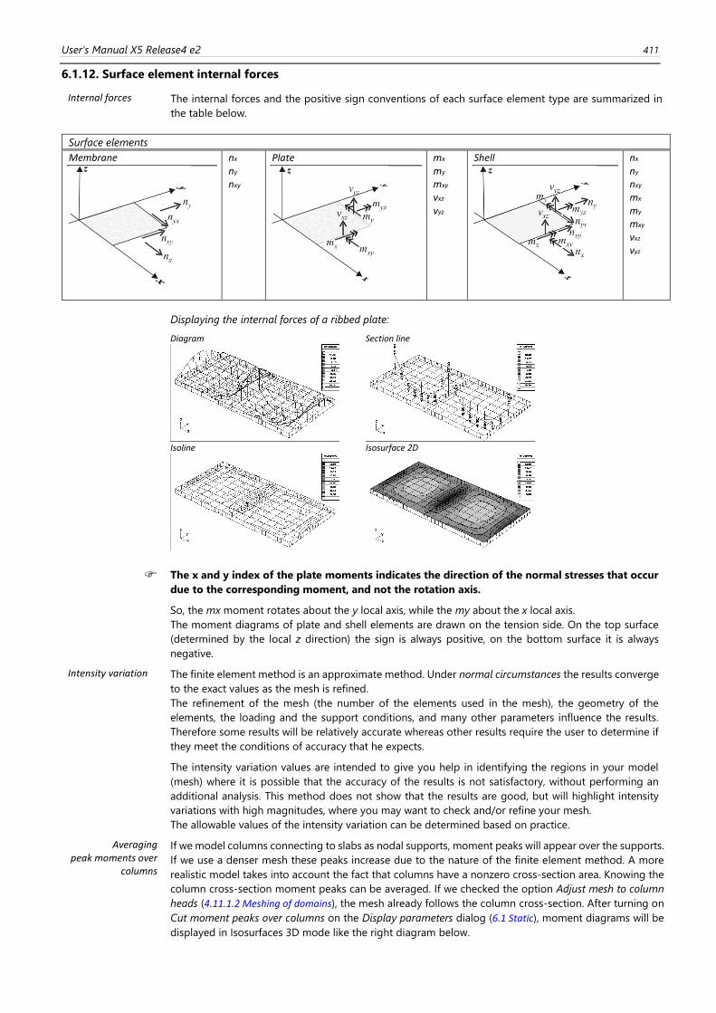
User’s Manual X5 Release4 e2 411

6.1.12. Surface element internal forces

Internal forces The internal forces and the positive sign conventions of each surface element type are summarized in

the table below.

Surface elements

Membrane

nx ny

nxy

Plate

mx my mxy vxz vyz

Shell

nx ny

nxy mx my mxy vxz vyz

Displaying the internal forces of a ribbed plate:

Diagram Section line

Isoline Isosurface 2D

The x and y index of the plate moments indicates the direction of the normal stresses that occur

due to the corresponding moment, and not the rotation axis.

So, the mx moment rotates about the y local axis, while the my about the x local axis.

The moment diagrams of plate and shell elements are drawn on the tension side. On the top surface

(determined by the local z direction) the sign is always positive, on the bottom surface it is always

negative.

Intensity variation The finite element method is an approximate method. Under normal circumstances the results converge

to the exact values as the mesh is refined.

The refinement of the mesh (the number of the elements used in the mesh), the geometry of the

elements, the loading and the support conditions, and many other parameters influence the results.

Therefore some results will be relatively accurate whereas other results require the user to determine if

they meet the conditions of accuracy that he expects.

The intensity variation values are intended to give you help in identifying the regions in your model

(mesh) where it is possible that the accuracy of the results is not satisfactory, without performing an

additional analysis. This method does not show that the results are good, but will highlight intensity

variations with high magnitudes, where you may want to check and/or refine your mesh.

The allowable values of the intensity variation can be determined based on practice.

Averaging peak moments over

columns

If we model columns connecting to slabs as nodal supports, moment peaks will appear over the supports.

If we use a denser mesh these peaks increase due to the nature of the finite element method. A more

realistic model takes into account the fact that columns have a nonzero cross-section area. Knowing the

column cross-section moment peaks can be averaged. If we checked the option Adjust mesh to column

heads (4.11.1.2 Meshing of domains), the mesh already follows the column cross-section. After turning on

Cut moment peaks over columns on the Display parameters dialog (6.1 Static), moment diagrams will be

displayed in Isosurfaces 3D mode like the right diagram below.

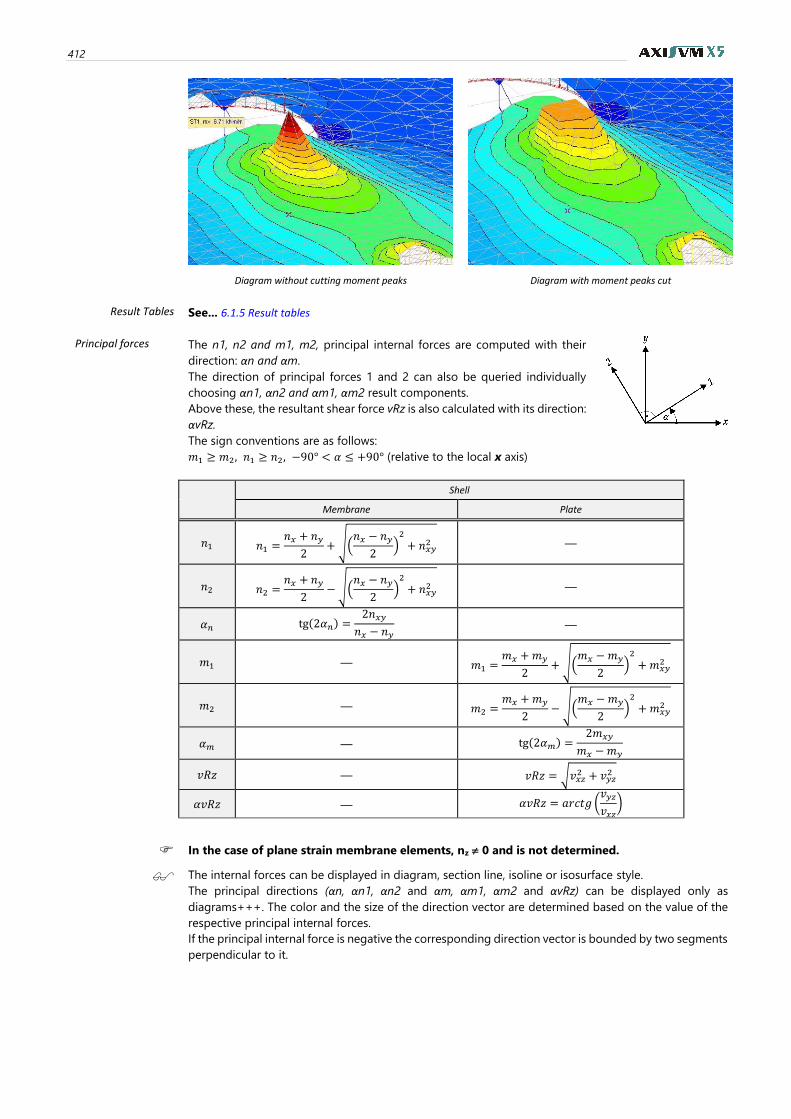
412

Diagram without cutting moment peaks Diagram with moment peaks cut

Result Tables See... 6.1.5 Result tables

Principal forces The n1, n2 and m1, m2, principal internal forces are computed with their

direction: αn and αm.

The direction of principal forces 1 and 2 can also be queried individually

choosing αn1, αn2 and αm1, αm2 result components.

Above these, the resultant shear force vRz is also calculated with its direction:

αvRz.

The sign conventions are as follows:

𝑚1 ≥ 𝑚2, 𝑛1 ≥ 𝑛2, −90° < 𝛼 ≤ +90° (relative to the local x axis)

Shell

Membrane Plate

𝑛1 𝑛1 =𝑛𝑥 + 𝑛𝑦

2+ √(

𝑛𝑥 − 𝑛𝑦

2)2

+ 𝑛𝑥𝑦2 —

𝑛2 𝑛2 =𝑛𝑥 + 𝑛𝑦

2− √(

𝑛𝑥 − 𝑛𝑦

2)2

+ 𝑛𝑥𝑦2 —

𝛼𝑛 tg(2𝛼𝑛) =2𝑛𝑥𝑦

𝑛𝑥 − 𝑛𝑦 —

𝑚1 — 𝑚1 =𝑚𝑥 +𝑚𝑦

2+ √(

𝑚𝑥 −𝑚𝑦

2)2

+𝑚𝑥𝑦2

𝑚2 — 𝑚2 =𝑚𝑥 +𝑚𝑦

2− √(

𝑚𝑥 −𝑚𝑦

2)2

+𝑚𝑥𝑦2

𝛼𝑚 — tg(2𝛼𝑚) =2𝑚𝑥𝑦

𝑚𝑥 −𝑚𝑦

𝑣𝑅𝑧 — 𝑣𝑅𝑧 = √𝑣𝑥𝑧2 + 𝑣𝑦𝑧

2

𝛼𝑣𝑅𝑧 — 𝛼𝑣𝑅𝑧 = 𝑎𝑟𝑐𝑡𝑔 (𝑣𝑦𝑧

𝑣𝑥𝑧)

In the case of plane strain membrane elements, nz 0 and is not determined.

The internal forces can be displayed in diagram, section line, isoline or isosurface style.

The principal directions (αn, αn1, αn2 and αm, αm1, αm2 and αvRz) can be displayed only as

diagrams+++. The color and the size of the direction vector are determined based on the value of the

respective principal internal forces.

If the principal internal force is negative the corresponding direction vector is bounded by two segments

perpendicular to it.

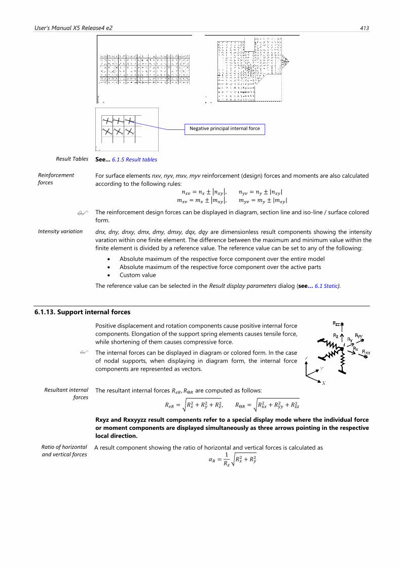
User’s Manual X5 Release4 e2 413

Result Tables See... 6.1.5 Result tables

Reinforcement forces

For surface elements nxv, nyv, mxv, myv reinforcement (design) forces and moments are also calculated

according to the following rules:

𝑛𝑥𝑣 = 𝑛𝑥 ± |𝑛𝑥𝑦|, 𝑛𝑦𝑣 = 𝑛𝑦 ± |𝑛𝑥𝑦|

𝑚𝑥𝑣 = 𝑚𝑥 ± |𝑚𝑥𝑦|, 𝑚𝑦𝑣 = 𝑚𝑦 ± |𝑚𝑥𝑦|

The reinforcement design forces can be displayed in diagram, section line and iso-line / surface colored

form.

Intensity variation dnx, dny, dnxy, dmx, dmy, dmxy, dqx, dqy are dimensionless result components showing the intensity

varation within one finite element. The difference between the maximum and minimum value within the

finite element is divided by a reference value. The reference value can be set to any of the following:

• Absolute maximum of the respective force component over the entire model

• Absolute maximum of the respective force component over the active parts

• Custom value

The reference value can be selected in the Result display parameters dialog (see… 6.1 Static).

6.1.13. Support internal forces

Positive displacement and rotation components cause positive internal force

components. Elongation of the support spring elements causes tensile force,

while shortening of them causes compressive force.

The internal forces can be displayed in diagram or colored form. In the case

of nodal supports, when displaying in diagram form, the internal force

components are represented as vectors.

Resultant internal forces

The resultant internal forces 𝑅𝑒𝑅 , 𝑅Θ𝑅 are computed as follows:

𝑅𝑒𝑅 = √𝑅𝑥2 + 𝑅𝑦

2 + 𝑅𝑧2, 𝑅Θ𝑅 = √𝑅x𝑥

2 + 𝑅y𝑦2 + 𝑅z𝑧

2

Rxyz and Rxxyyzz result components refer to a special display mode where the individual force

or moment components are displayed simultaneously as three arrows pointing in the respective

local direction.

Ratio of horizontal and vertical forces

A result component showing the ratio of horizontal and vertical forces is calculated as

𝛼𝑅 =1

𝑅𝑧√𝑅𝑥

2 + 𝑅𝑦2

Negative principal internal force

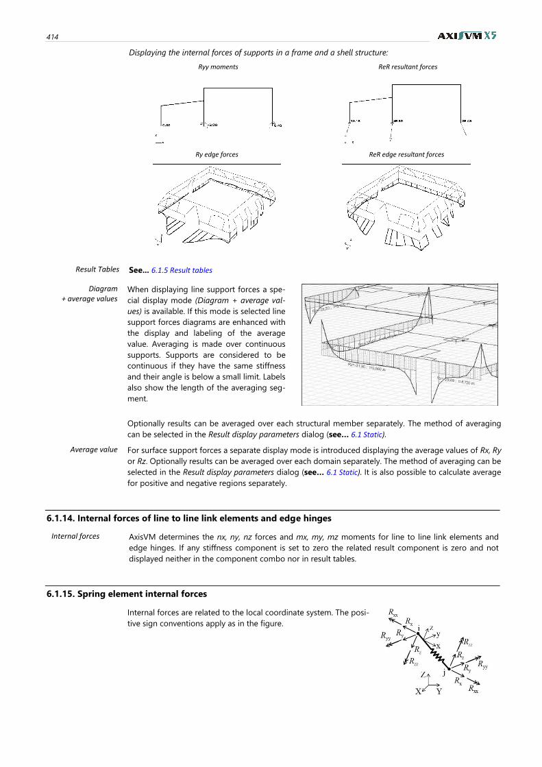
414

Displaying the internal forces of supports in a frame and a shell structure:

Ryy moments ReR resultant forces

Ry edge forces ReR edge resultant forces

Result Tables See... 6.1.5 Result tables

Diagram + average values

When displaying line support forces a spe-

cial display mode (Diagram + average val-

ues) is available. If this mode is selected line

support forces diagrams are enhanced with

the display and labeling of the average

value. Averaging is made over continuous

supports. Supports are considered to be

continuous if they have the same stiffness

and their angle is below a small limit. Labels

also show the length of the averaging seg-

ment.

Optionally results can be averaged over each structural member separately. The method of averaging

can be selected in the Result display parameters dialog (see… 6.1 Static).

Average value For surface support forces a separate display mode is introduced displaying the average values of Rx, Ry

or Rz. Optionally results can be averaged over each domain separately. The method of averaging can be

selected in the Result display parameters dialog (see… 6.1 Static). It is also possible to calculate average

for positive and negative regions separately.

6.1.14. Internal forces of line to line link elements and edge hinges

Internal forces AxisVM determines the nx, ny, nz forces and mx, my, mz moments for line to line link elements and

edge hinges. If any stiffness component is set to zero the related result component is zero and not

displayed neither in the component combo nor in result tables.

6.1.15. Spring element internal forces

Internal forces are related to the local coordinate system. The posi-

tive sign conventions apply as in the figure.

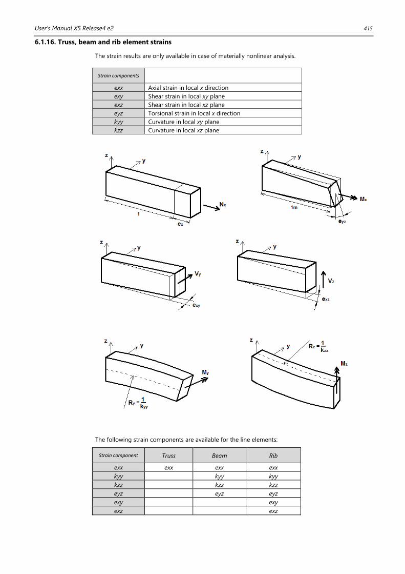
User’s Manual X5 Release4 e2 415

6.1.16. Truss, beam and rib element strains

The strain results are only available in case of materially nonlinear analysis.

Strain components

exx Axial strain in local x direction

exy Shear strain in local xy plane

exz Shear strain in local xz plane

eyz Torsional strain in local x direction

kyy Curvature in local xy plane

kzz Curvature in local xz plane

The following strain components are available for the line elements:

Strain component Truss Beam Rib

exx exx exx exx

kyy kyy kyy

kzz kzz kzz

eyz eyz eyz

exy exy

exz exz

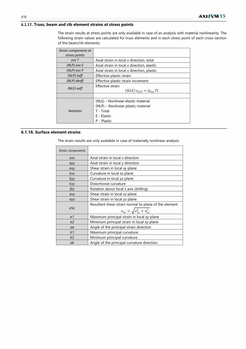
416

6.1.17. Truss, beam and rib element strains at stress points

The strain results at stress points are only available in case of an analysis with material nonlinearity. The

following strain values are calculated for truss elements and in each stress point of each cross-section

of the beam/rib elements:

Strain components at stress points

exx T Axial strain in local x direction, total

(NLP) exx E Axial strain in local x direction, elastic

(NLP) exx P Axial strain in local x direction, plastic

(NLP) eeff Effective plastic strain

(NLP) deeff Effective plastic strain increment

(NLE) eeff Effective strain

(𝑁𝐿𝐸) 𝑒𝑒𝑓𝑓 = |𝑒𝑥𝑥 𝑇|

Notation

(NLE) – Nonlinear elastic material

(NLP) – Nonlinear plastic material

T - Total

E - Elastic

P - Plastic

6.1.18. Surface element strains

The strain results are only available in case of materially nonlinear analysis.

Strain components

exx Axial strain in local x direction

eyy Axial strain in local y direction

exy Shear strain in local xy plane

kxx Curvature in local xz plane

kyy Curvature in local yz plane

kxy Distortional curvature

fzz Rotation about local z axis (drilling)

exz Shear strain in local xz plane

eyz Shear strain in local yz plane

eSz Resultant shear strain normal to plane of the element

𝑒𝑆𝑧 = √𝑒𝑥𝑧2 + 𝑒𝑦𝑧

2

e1 Maximum principal strain in local xy plane

e2 Minimum principal strain in local xy plane

ae Angle of the principal strain direction

k1 Maximum principal curvature

k2 Minimum principal curvature

ak Angle of the principal curvature direction

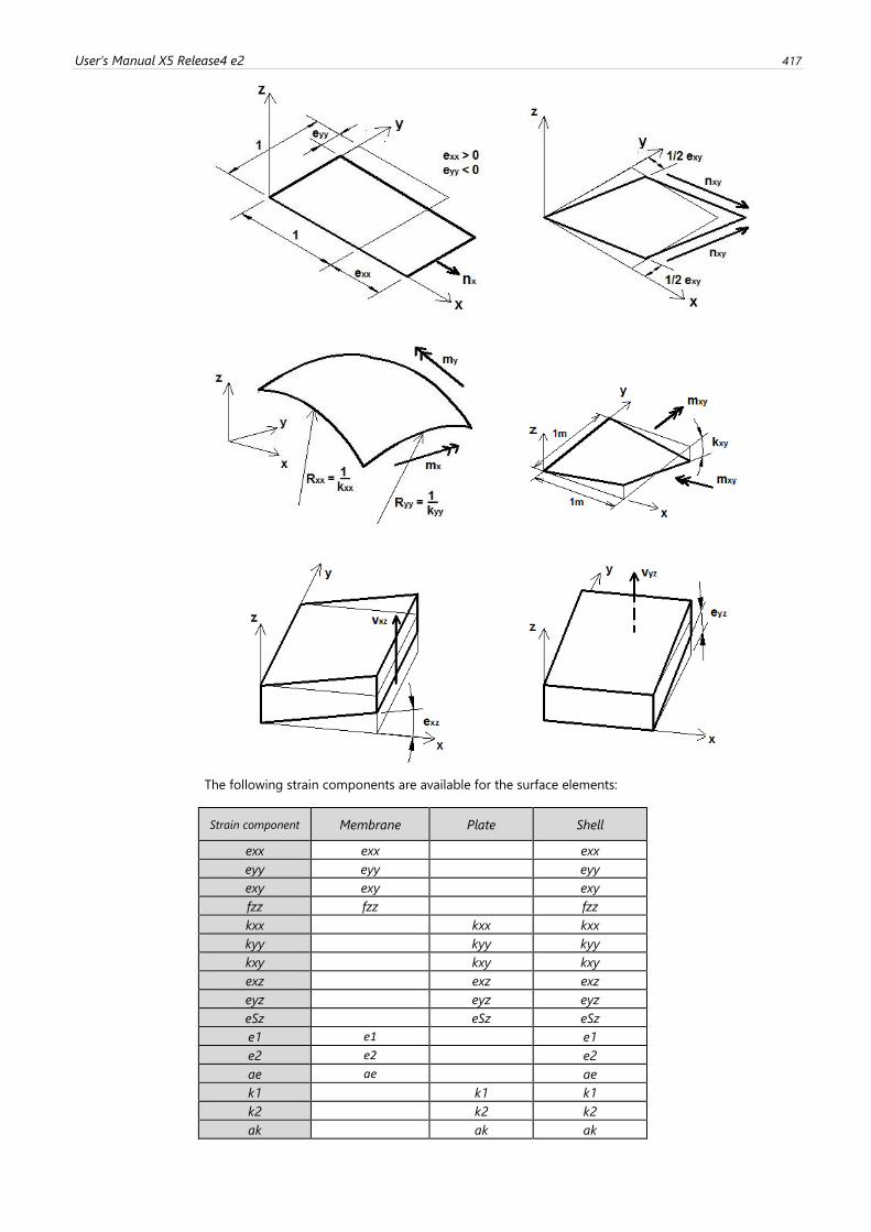
User’s Manual X5 Release4 e2 417

The following strain components are available for the surface elements:

Strain component Membrane Plate Shell

exx exx exx

eyy eyy eyy

exy exy exy

fzz fzz fzz

kxx kxx kxx

kyy kyy kyy

kxy kxy kxy

exz exz exz

eyz eyz eyz

eSz eSz eSz

e1 e1 e1

e2 e2 e2

ae ae ae

k1 k1 k1

k2 k2 k2

ak ak ak

418

6.1.19. Surface element strains at stress points

The strain results at stress points are only available in case of materially nonlinear analysis. The following

strain components are calculated at each node of the element in the top, center, and bottom fiber:

Strain components at stress points

exx T, (NLP) exx E, (NLP) exx P

Axial strain in local x direction

eyy T, (NLP) eyy E, (NLP) eyy P

Axial strain in local y direction

exy T, (NLP) exy E, (NLP) exy P

Shear strain in local xy plane

e1 T, (NLP) e1 E, (NLP) e1 P Maximum principal strain in local xy plane

e2 T, (NLP) e2 E, (NLP) e2 P Minimum principal strain in local xy plane

ae T, (NLP) ae E, (NLP) ae P Angle of the principal strain direction

(NLP) eeff Effective plastic strain

(NLP) deeff Effective plastic strain increment

(NLE) eeff Effective strain

𝑒𝑒𝑓𝑓 = √1

(1 − 2𝜈)(1 + 𝜈)[(1 − 𝜈)(𝑒𝑥𝑥2 + 𝑒𝑦𝑦2 + 𝑒𝑧𝑧2 ) + 2𝜈(𝑒𝑥𝑥𝑒𝑦𝑦 + 𝑒𝑥𝑥𝑒𝑧𝑧 + 𝑒𝑦𝑦𝑒𝑧𝑧) +

1 − 2𝜈

2𝑒𝑥𝑦2 ]

Notation

(NLE) – Nonlinear elastic material

(NLP) – Nonlinear plastic material

T – Total

E – Elastic

P – Plastic

6.1.20. Spring element deformations

Deformation

components Deformations in local directions

ex 𝑒𝑥 = 𝑒𝑥𝑗 − 𝑒𝑥𝑖

ez 𝑒𝑦 = 𝑒𝑦𝑗 − 𝑒𝑦𝑖

ez 𝑒𝑧 = 𝑒𝑧𝑗 − 𝑒𝑧𝑖

Rotational deformations about local axes

fx 𝑓𝑥 = 𝑓𝑥𝑗 − 𝑓𝑥𝑖

fy 𝑓𝑦 = 𝑓𝑦𝑗 − 𝑓𝑦𝑖

fz 𝑓𝑧 = 𝑓𝑧𝑗 − 𝑓𝑧𝑖

6.1.21. Truss/beam/rib stresses

The display modes for stress results are the same as for the internal forces. The table of the stress results

are similar to those of internal forces.

Truss The 𝑆𝑥 = 𝑁𝑥/𝐴𝑥 stress value is calculated for each truss element.

A positive value means tension.

Beams / Ribs The following stress values are calculated in each stress point of each cross-section of the beam/rib

element:

Normal stress from tension/compression and bending is calculated disregarding warping stress:

𝑆𝑥,𝑖 =𝑁𝑥𝐴𝑥+𝑀𝑦𝐼𝑧 +𝑀𝑧𝐼𝑦𝑧

𝐼𝑦𝐼𝑧 − 𝐼𝑦𝑧2 𝑧𝑖 −

𝑀𝑧𝐼𝑦 +𝑀𝑦𝐼𝑦𝑧

𝐼𝑦𝐼𝑧 − 𝐼𝑦𝑧2 𝑦𝑖

where yi , zi are the stress point coordinates. Positive stress value means tension in the cross-section.

Resultant shear stress is calculated from shear and twisting (Saint-Venant) disregarding warping shear

stress.

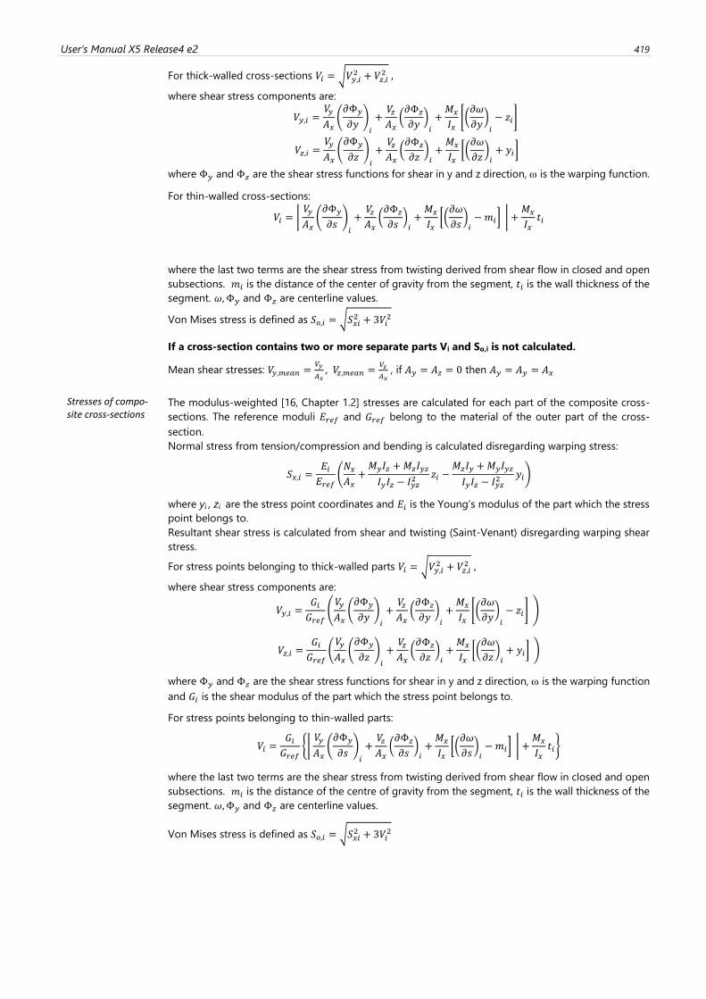
User’s Manual X5 Release4 e2 419

For thick-walled cross-sections 𝑉𝑖 = √𝑉𝑦,𝑖

2 + 𝑉𝑧,𝑖2 ,

where shear stress components are:

𝑉𝑦,𝑖 =𝑉𝑦

𝐴𝑥(𝜕Φ𝑦

𝜕𝑦)𝑖

+𝑉𝑧𝐴𝑥(𝜕Φ𝑧𝜕𝑦

)𝑖

+𝑀𝑥

𝐼𝑥[(𝜕𝜔

𝜕𝑦)𝑖

− 𝑧𝑖]

𝑉𝑧,𝑖 =𝑉𝑦

𝐴𝑥(𝜕Φ𝑦

𝜕𝑧)𝑖

+𝑉𝑧𝐴𝑥(𝜕Φ𝑧𝜕𝑧

)𝑖+𝑀𝑥

𝐼𝑥[(𝜕𝜔

𝜕𝑧)𝑖+ 𝑦𝑖]

where Φ𝑦 and Φ𝑧 are the shear stress functions for shear in y and z direction, is the warping function.

For thin-walled cross-sections:

𝑉𝑖 = | 𝑉𝑦

𝐴𝑥(𝜕Φ𝑦

𝜕𝑠)𝑖

+𝑉𝑧𝐴𝑥(𝜕Φ𝑧𝜕𝑠

)𝑖+𝑀𝑥

𝐼𝑥[(𝜕𝜔

𝜕𝑠)𝑖−𝑚𝑖]

| +𝑀𝑥

𝐼𝑥𝑡𝑖

where the last two terms are the shear stress from twisting derived from shear flow in closed and open

subsections. 𝑚𝑖 is the distance of the center of gravity from the segment, 𝑡𝑖 is the wall thickness of the

segment. 𝜔,Φ𝑦 and Φ𝑧 are centerline values.

Von Mises stress is defined as 𝑆𝑜,𝑖 = √𝑆𝑥𝑖2 + 3𝑉𝑖

2

If a cross-section contains two or more separate parts Vi and So,i is not calculated.

Mean shear stresses: 𝑉𝑦,𝑚𝑒𝑎𝑛 =𝑉𝑦

𝐴𝑥, 𝑉𝑧,𝑚𝑒𝑎𝑛 =

𝑉𝑧

𝐴𝑥 , if 𝐴𝑦 = 𝐴𝑧 = 0 then 𝐴𝑦 = 𝐴𝑦 = 𝐴𝑥

Stresses of compo-site cross-sections

The modulus-weighted [16, Chapter 1.2] stresses are calculated for each part of the composite cross-

sections. The reference moduli 𝐸𝑟𝑒𝑓 and 𝐺𝑟𝑒𝑓 belong to the material of the outer part of the cross-

section.

Normal stress from tension/compression and bending is calculated disregarding warping stress:

𝑆𝑥,𝑖 =𝐸𝑖𝐸𝑟𝑒𝑓

(𝑁𝑥𝐴𝑥+𝑀𝑦𝐼𝑧 +𝑀𝑧𝐼𝑦𝑧

𝐼𝑦𝐼𝑧 − 𝐼𝑦𝑧2 𝑧𝑖 −

𝑀𝑧𝐼𝑦 +𝑀𝑦𝐼𝑦𝑧

𝐼𝑦𝐼𝑧 − 𝐼𝑦𝑧2 𝑦𝑖)

where yi , zi are the stress point coordinates and 𝐸𝑖 is the Young’s modulus of the part which the stress

point belongs to.

Resultant shear stress is calculated from shear and twisting (Saint-Venant) disregarding warping shear

stress.

For stress points belonging to thick-walled parts 𝑉𝑖 = √𝑉𝑦,𝑖2 + 𝑉𝑧,𝑖

2 ,

where shear stress components are:

𝑉𝑦,𝑖 =𝐺𝑖𝐺𝑟𝑒𝑓

(𝑉𝑦

𝐴𝑥(𝜕Φ𝑦

𝜕𝑦)𝑖

+𝑉𝑧𝐴𝑥(𝜕Φ𝑧𝜕𝑦

)𝑖

+𝑀𝑥

𝐼𝑥[(𝜕𝜔

𝜕𝑦)𝑖

− 𝑧𝑖]

)

𝑉𝑧,𝑖 =𝐺𝑖𝐺𝑟𝑒𝑓

(𝑉𝑦

𝐴𝑥(𝜕Φ𝑦

𝜕𝑧)𝑖

+𝑉𝑧𝐴𝑥(𝜕Φ𝑧𝜕𝑧

)𝑖+𝑀𝑥

𝐼𝑥[(𝜕𝜔

𝜕𝑧)𝑖+ 𝑦𝑖]

)

where Φ𝑦 and Φ𝑧 are the shear stress functions for shear in y and z direction, is the warping function

and 𝐺𝑖 is the shear modulus of the part which the stress point belongs to.

For stress points belonging to thin-walled parts:

𝑉𝑖 =𝐺𝑖𝐺𝑟𝑒𝑓

{| 𝑉𝑦

𝐴𝑥(𝜕Φ𝑦

𝜕𝑠)𝑖

+𝑉𝑧𝐴𝑥(𝜕Φ𝑧𝜕𝑠

)𝑖+𝑀𝑥

𝐼𝑥[(𝜕𝜔

𝜕𝑠)𝑖−𝑚𝑖]

| +𝑀𝑥

𝐼𝑥𝑡𝑖}

where the last two terms are the shear stress from twisting derived from shear flow in closed and open

subsections. 𝑚𝑖 is the distance of the centre of gravity from the segment, 𝑡𝑖 is the wall thickness of the

segment. 𝜔,Φ𝑦 and Φ𝑧 are centerline values.

Von Mises stress is defined as 𝑆𝑜,𝑖 = √𝑆𝑥𝑖2 + 3𝑉𝑖

2

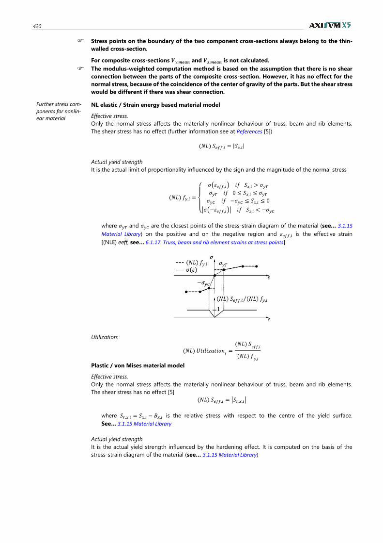
420

Stress points on the boundary of the two component cross-sections always belong to the thin-

walled cross-section.

For composite cross-sections 𝑽𝒚,𝒎𝒆𝒂𝒏 and 𝑽𝒛,𝒎𝒆𝒂𝒏 is not calculated.

The modulus-weighted computation method is based on the assumption that there is no shear

connection between the parts of the composite cross-section. However, it has no effect for the

normal stress, because of the coincidence of the center of gravity of the parts. But the shear stress

would be different if there was shear connection.

Further stress com-ponents for nonlin-ear material

NL elastic / Strain energy based material model

Effective stress.

Only the normal stress affects the materially nonlinear behaviour of truss, beam and rib elements.

The shear stress has no effect (further information see at References [5])

(𝑁𝐿) 𝑆𝑒𝑓𝑓,𝑖 = |𝑆𝑥.𝑖|

Actual yield strength

It is the actual limit of proportionality influenced by the sign and the magnitude of the normal stress

(𝑁𝐿) 𝑓𝑦,𝑖 =

{

𝜎(휀𝑒𝑓𝑓,𝑖) 𝑖𝑓 𝑆𝑥,𝑖 > 𝜎𝑦𝑇

𝜎𝑦𝑇 𝑖𝑓 0 ≤ 𝑆𝑥,𝑖 ≤ 𝜎𝑦𝑇𝜎𝑦𝐶 𝑖𝑓 −𝜎𝑦𝐶 ≤ 𝑆𝑥,𝑖 ≤ 0

|𝜎(−휀𝑒𝑓𝑓,𝑖)| 𝑖𝑓 𝑆𝑥,𝑖 < −𝜎𝑦𝐶

where 𝜎𝑦𝑇 and 𝜎𝑦𝐶 are the closest points of the stress-strain diagram of the material (see… 3.1.15

Material Library) on the positive and on the negative region and 휀𝑒𝑓𝑓,𝑖 is the effective strain

[(NLE) eeff, see… 6.1.17 Truss, beam and rib element strains at stress points]

Utilization:

(𝑁𝐿) 𝑈𝑡𝑖𝑙𝑖𝑧𝑎𝑡𝑖𝑜𝑛𝑖=(𝑁𝐿) 𝑆

𝑒𝑓𝑓,𝑖

(𝑁𝐿) 𝑓𝑦,𝑖

Plastic / von Mises material model

Effective stress.

Only the normal stress affects the materially nonlinear behaviour of truss, beam and rib elements.

The shear stress has no effect [5]

(𝑁𝐿) 𝑆𝑒𝑓𝑓,𝑖 = |𝑆𝑟,𝑥.𝑖|

where 𝑆𝑟,𝑥,𝑖 = 𝑆𝑥,𝑖 − 𝐵𝑥,𝑖 is the relative stress with respect to the centre of the yield surface.

See… 3.1.15 Material Library

Actual yield strength

It is the actual yield strength influenced by the hardening effect. It is computed on the basis of the

stress-strain diagram of the material (see… 3.1.15 Material Library)

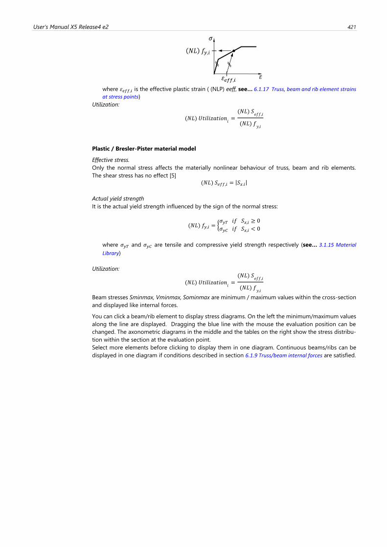
User’s Manual X5 Release4 e2 421

where 휀𝑒𝑓𝑓,𝑖 is the effective plastic strain ( (NLP) eeff, see… 6.1.17 Truss, beam and rib element strains

at stress points)

Utilization:

(𝑁𝐿) 𝑈𝑡𝑖𝑙𝑖𝑧𝑎𝑡𝑖𝑜𝑛𝑖=(𝑁𝐿) 𝑆

𝑒𝑓𝑓,𝑖

(𝑁𝐿) 𝑓𝑦,𝑖

Plastic / Bresler-Pister material model

Effective stress.

Only the normal stress affects the materially nonlinear behaviour of truss, beam and rib elements.

The shear stress has no effect [5] (𝑁𝐿) 𝑆𝑒𝑓𝑓,𝑖 = |𝑆𝑥.𝑖|

Actual yield strength

It is the actual yield strength influenced by the sign of the normal stress:

(𝑁𝐿) 𝑓𝑦,𝑖 = {𝜎𝑦𝑇 𝑖𝑓 𝑆𝑥,𝑖 ≥ 0

𝜎𝑦𝐶 𝑖𝑓 𝑆𝑥,𝑖 < 0

where 𝜎𝑦𝑇 and 𝜎𝑦𝐶 are tensile and compressive yield strength respectively (see… 3.1.15 Material

Library)

Utilization:

(𝑁𝐿) 𝑈𝑡𝑖𝑙𝑖𝑧𝑎𝑡𝑖𝑜𝑛𝑖=(𝑁𝐿) 𝑆

𝑒𝑓𝑓,𝑖

(𝑁𝐿) 𝑓𝑦,𝑖

Beam stresses Sminmax, Vminmax, Sominmax are minimum / maximum values within the cross-section

and displayed like internal forces.

You can click a beam/rib element to display stress diagrams. On the left the minimum/maximum values

along the line are displayed. Dragging the blue line with the mouse the evaluation position can be

changed. The axonometric diagrams in the middle and the tables on the right show the stress distribu-

tion within the section at the evaluation point.

Select more elements before clicking to display them in one diagram. Continuous beams/ribs can be

displayed in one diagram if conditions described in section 6.1.9 Truss/beam internal forces are satisfied.

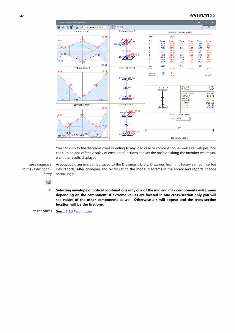
422

You can display the diagrams corresponding to any load case or combination, as well as envelopes. You

can turn on and off the display of envelope functions and set the position along the member where you

want the results displayed.

Save diagrams

to the Drawings Li-

brary

Associative diagrams can be saved to the Drawings Library. Drawings from this library can be inserted

into reports. After changing and recalculating the model diagrams in the library and reports change

accordingly.

Selecting envelope or critical combinations only one of the min and max components will appear

depending on the component. If extreme values are located in one cross-section only you will

see values of the other components as well. Otherwise a will appear and the cross-section

location will be the first one.

Result Tables See... 6.1.5 Result tables

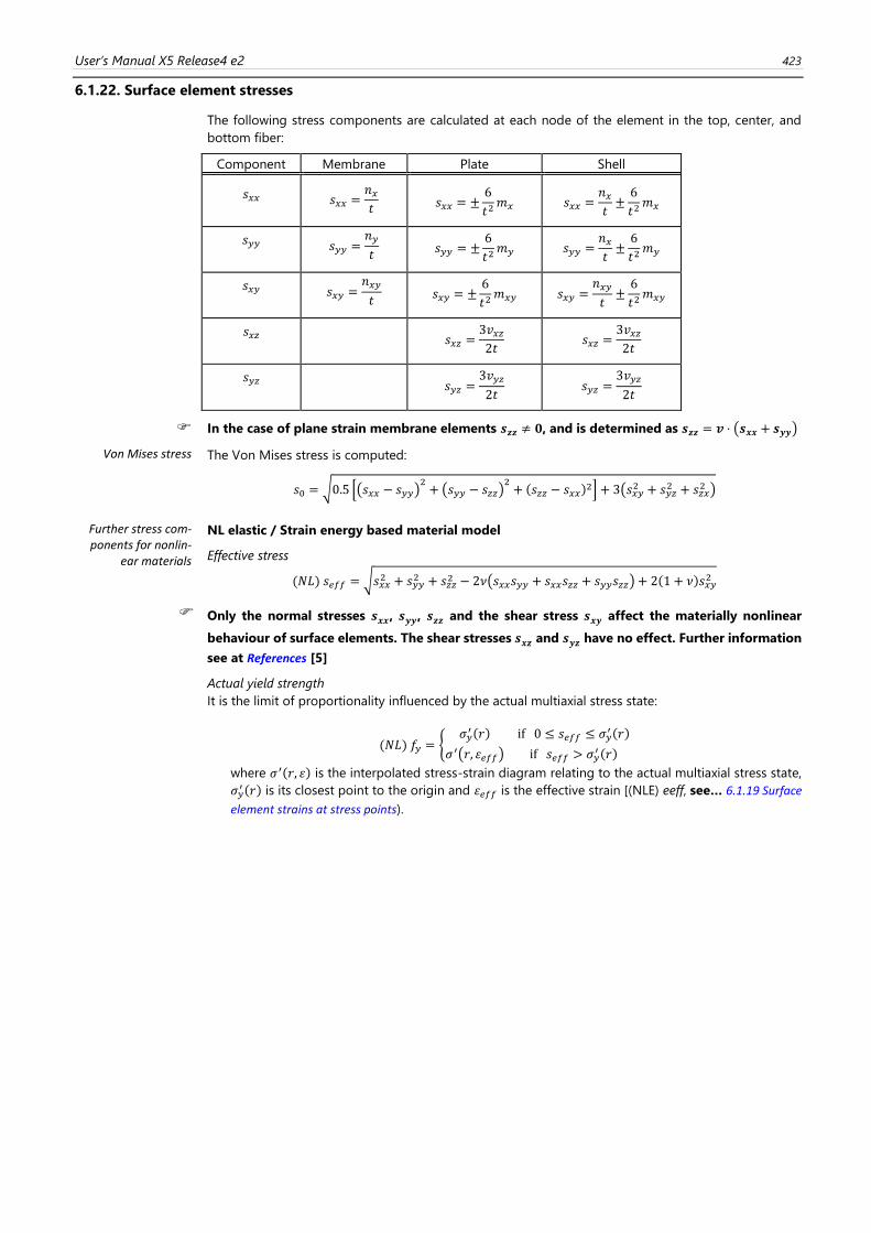
User’s Manual X5 Release4 e2 423

6.1.22. Surface element stresses

The following stress components are calculated at each node of the element in the top, center, and

bottom fiber:

Component Membrane Plate Shell

𝑠𝑥𝑥 𝑠𝑥𝑥 =𝑛𝑥𝑡

𝑠𝑥𝑥 = ±6

𝑡2𝑚𝑥 𝑠𝑥𝑥 =

𝑛𝑥𝑡±6

𝑡2𝑚𝑥

𝑠𝑦𝑦 𝑠𝑦𝑦 =𝑛𝑦

𝑡 𝑠𝑦𝑦 = ±

6

𝑡2𝑚𝑦 𝑠𝑦𝑦 =

𝑛𝑥𝑡±6

𝑡2𝑚𝑦

𝑠𝑥𝑦 𝑠𝑥𝑦 =𝑛𝑥𝑦

𝑡 𝑠𝑥𝑦 = ±

6

𝑡2𝑚𝑥𝑦 𝑠𝑥𝑦 =

𝑛𝑥𝑦

𝑡±6

𝑡2𝑚𝑥𝑦

𝑠𝑥𝑧 𝑠𝑥𝑧 =3𝑣𝑥𝑧2𝑡

𝑠𝑥𝑧 =3𝑣𝑥𝑧2𝑡

𝑠𝑦𝑧 𝑠𝑦𝑧 =

3𝑣𝑦𝑧

2𝑡 𝑠𝑦𝑧 =

3𝑣𝑦𝑧

2𝑡

In the case of plane strain membrane elements 𝒔𝒛𝒛 ≠ 𝟎, and is determined as 𝒔𝒛𝒛 = 𝒗 ⋅ (𝒔𝒙𝒙 + 𝒔𝒚𝒚)

Von Mises stress The Von Mises stress is computed:

𝑠0 = √0.5 [(𝑠𝑥𝑥 − 𝑠𝑦𝑦)2+ (𝑠𝑦𝑦 − 𝑠𝑧𝑧)

2+ (𝑠𝑧𝑧 − 𝑠𝑥𝑥)

2] + 3(𝑠𝑥𝑦2 + 𝑠𝑦𝑧

2 + 𝑠𝑧𝑥2 )

Further stress com-ponents for nonlin-

ear materials

NL elastic / Strain energy based material model

Effective stress

(𝑁𝐿) 𝑠𝑒𝑓𝑓 = √𝑠𝑥𝑥2 + 𝑠𝑦𝑦

2 + 𝑠𝑧𝑧2 − 2𝜈(𝑠𝑥𝑥𝑠𝑦𝑦 + 𝑠𝑥𝑥𝑠𝑧𝑧 + 𝑠𝑦𝑦𝑠𝑧𝑧) + 2(1 + 𝜈)𝑠𝑥𝑦

2

Only the normal stresses 𝒔𝒙𝒙, 𝒔𝒚𝒚, 𝒔𝒛𝒛 and the shear stress 𝒔𝒙𝒚 affect the materially nonlinear

behaviour of surface elements. The shear stresses 𝒔𝒙𝒛 and 𝒔𝒚𝒛 have no effect. Further information

see at References [5]

Actual yield strength

It is the limit of proportionality influenced by the actual multiaxial stress state:

(𝑁𝐿) 𝑓𝑦 = {𝜎𝑦′(𝑟) if 0 ≤ 𝑠𝑒𝑓𝑓 ≤ 𝜎𝑦

′(𝑟)

𝜎′(𝑟, 휀𝑒𝑓𝑓) if 𝑠𝑒𝑓𝑓 > 𝜎𝑦′ (𝑟)

where 𝜎′(𝑟, 휀) is the interpolated stress-strain diagram relating to the actual multiaxial stress state,

𝜎𝑦′(𝑟) is its closest point to the origin and 휀𝑒𝑓𝑓 is the effective strain [(NLE) eeff, see… 6.1.19 Surface

element strains at stress points).

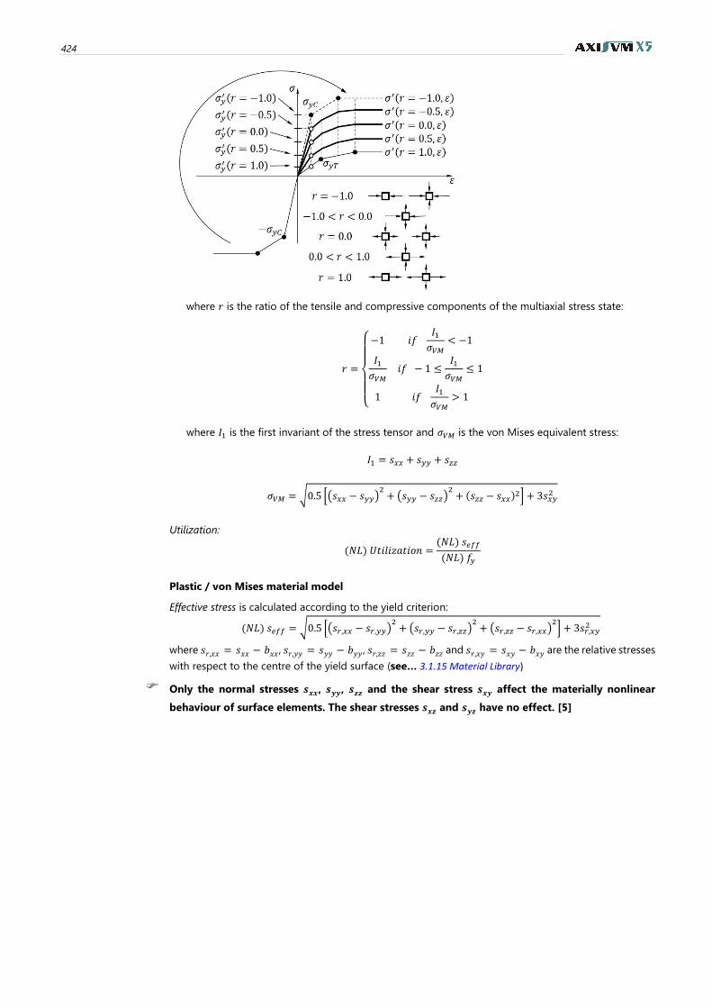
424

where 𝑟 is the ratio of the tensile and compressive components of the multiaxial stress state:

𝑟 =

{

−1 𝑖𝑓

𝐼1𝜎𝑉𝑀

< −1

𝐼1𝜎𝑉𝑀

𝑖𝑓 − 1 ≤𝐼1𝜎𝑉𝑀

≤ 1

1 𝑖𝑓 𝐼1𝜎𝑉𝑀

> 1

where 𝐼1 is the first invariant of the stress tensor and 𝜎𝑉𝑀 is the von Mises equivalent stress:

𝐼1 = 𝑠𝑥𝑥 + 𝑠𝑦𝑦 + 𝑠𝑧𝑧

𝜎𝑉𝑀 = √0.5 [(𝑠𝑥𝑥 − 𝑠𝑦𝑦)2+ (𝑠𝑦𝑦 − 𝑠𝑧𝑧)

2+ (𝑠𝑧𝑧 − 𝑠𝑥𝑥)

2] + 3𝑠𝑥𝑦2

Utilization:

(𝑁𝐿) 𝑈𝑡𝑖𝑙𝑖𝑧𝑎𝑡𝑖𝑜𝑛 =(𝑁𝐿) 𝑠𝑒𝑓𝑓

(𝑁𝐿) 𝑓𝑦

Plastic / von Mises material model

Effective stress is calculated according to the yield criterion:

(𝑁𝐿) 𝑠𝑒𝑓𝑓 = √0.5 [(𝑠𝑟,𝑥𝑥 − 𝑠𝑟,𝑦𝑦)2+ (𝑠𝑟,𝑦𝑦 − 𝑠𝑟,𝑧𝑧)

2+ (𝑠𝑟,𝑧𝑧 − 𝑠𝑟,𝑥𝑥)

2] + 3𝑠𝑟,𝑥𝑦

2

where 𝑠𝑟,𝑥𝑥 = 𝑠𝑥𝑥 − 𝑏𝑥𝑥, 𝑠𝑟,𝑦𝑦 = 𝑠𝑦𝑦 − 𝑏𝑦𝑦 , 𝑠𝑟,𝑧𝑧 = 𝑠𝑧𝑧 − 𝑏𝑧𝑧 and 𝑠𝑟,𝑥𝑦 = 𝑠𝑥𝑦 − 𝑏𝑥𝑦 are the relative stresses

with respect to the centre of the yield surface (see… 3.1.15 Material Library)

Only the normal stresses 𝒔𝒙𝒙, 𝒔𝒚𝒚, 𝒔𝒛𝒛 and the shear stress 𝒔𝒙𝒚 affect the materially nonlinear

behaviour of surface elements. The shear stresses 𝒔𝒙𝒛 and 𝒔𝒚𝒛 have no effect. [5]

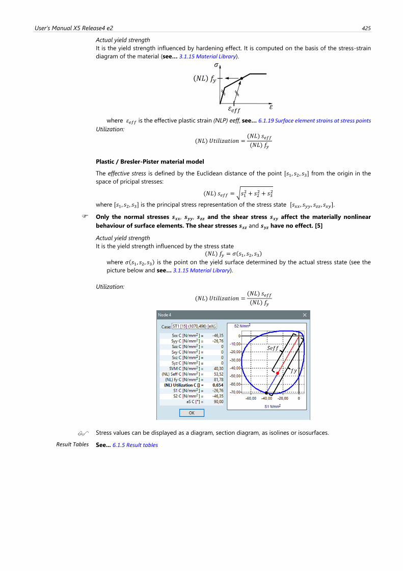
User’s Manual X5 Release4 e2 425

Actual yield strength

It is the yield strength influenced by hardening effect. It is computed on the basis of the stress-strain

diagram of the material (see… 3.1.15 Material Library).

where 휀𝑒𝑓𝑓 is the effective plastic strain (NLP) eeff, see… 6.1.19 Surface element strains at stress points

Utilization:

(𝑁𝐿) 𝑈𝑡𝑖𝑙𝑖𝑧𝑎𝑡𝑖𝑜𝑛 =(𝑁𝐿) 𝑠𝑒𝑓𝑓

(𝑁𝐿) 𝑓𝑦

Plastic / Bresler-Pister material model

The effective stress is defined by the Euclidean distance of the point [𝑠1, 𝑠2, 𝑠3] from the origin in the

space of pricipal stresses:

(𝑁𝐿) 𝑠𝑒𝑓𝑓 = √𝑠12 + 𝑠2

2 + 𝑠32

where [𝑠1, 𝑠2, 𝑠3] is the principal stress representation of the stress state [𝑠𝑥𝑥, 𝑠𝑦𝑦, 𝑠𝑧𝑧, 𝑠𝑥𝑦].

Only the normal stresses 𝒔𝒙𝒙, 𝒔𝒚𝒚, 𝒔𝒛𝒛 and the shear stress 𝒔𝒙𝒚 affect the materially nonlinear

behaviour of surface elements. The shear stresses 𝒔𝒙𝒛 and 𝒔𝒚𝒛 have no effect. [5]

Actual yield strength

It is the yield strength influenced by the stress state

(𝑁𝐿) 𝑓𝑦 = 𝜎(𝑠1, 𝑠2, 𝑠3)

where 𝜎(𝑠1, 𝑠2, 𝑠3) is the point on the yield surface determined by the actual stress state (see the

picture below and see… 3.1.15 Material Library).

Utilization:

(𝑁𝐿) 𝑈𝑡𝑖𝑙𝑖𝑧𝑎𝑡𝑖𝑜𝑛 =(𝑁𝐿) 𝑠𝑒𝑓𝑓

(𝑁𝐿) 𝑓𝑦

Stress values can be displayed as a diagram, section diagram, as isolines or isosurfaces.

Result Tables See... 6.1.5 Result tables

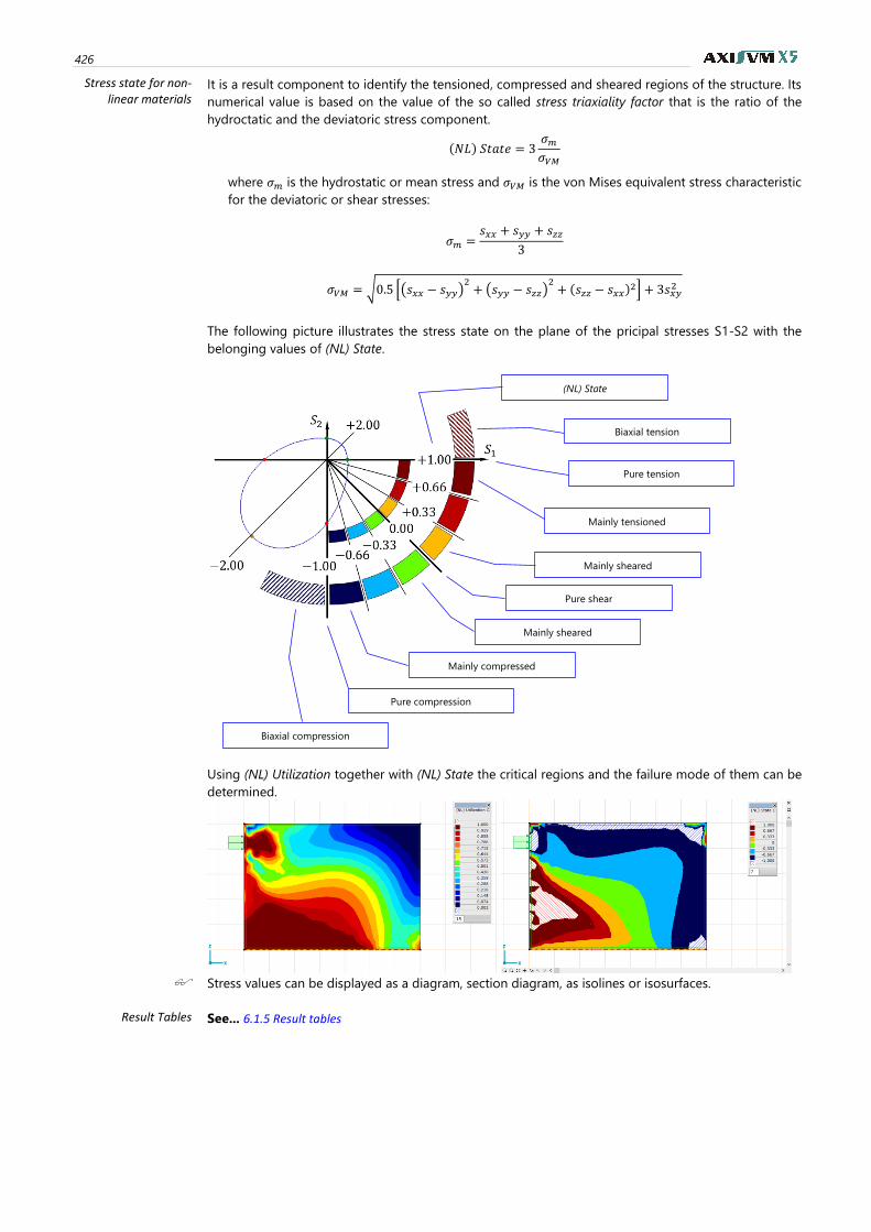
426

Stress state for non-linear materials

It is a result component to identify the tensioned, compressed and sheared regions of the structure. Its

numerical value is based on the value of the so called stress triaxiality factor that is the ratio of the

hydroctatic and the deviatoric stress component.

(𝑁𝐿) 𝑆𝑡𝑎𝑡𝑒 = 3𝜎𝑚𝜎𝑉𝑀

where 𝜎𝑚 is the hydrostatic or mean stress and 𝜎𝑉𝑀 is the von Mises equivalent stress characteristic

for the deviatoric or shear stresses:

𝜎𝑚 =𝑠𝑥𝑥 + 𝑠𝑦𝑦 + 𝑠𝑧𝑧

3

𝜎𝑉𝑀 = √0.5 [(𝑠𝑥𝑥 − 𝑠𝑦𝑦)2+ (𝑠𝑦𝑦 − 𝑠𝑧𝑧)

2+ (𝑠𝑧𝑧 − 𝑠𝑥𝑥)

2] + 3𝑠𝑥𝑦2

The following picture illustrates the stress state on the plane of the pricipal stresses S1-S2 with the

belonging values of (NL) State.

Using (NL) Utilization together with (NL) State the critical regions and the failure mode of them can be

determined.

Stress values can be displayed as a diagram, section diagram, as isolines or isosurfaces.

Result Tables See... 6.1.5 Result tables

Pure tension

Mainly tensioned

Mainly sheared

Pure shear

Pure compression

Mainly compressed

Mainly sheared

(NL) State

Biaxial tension

Biaxial compression

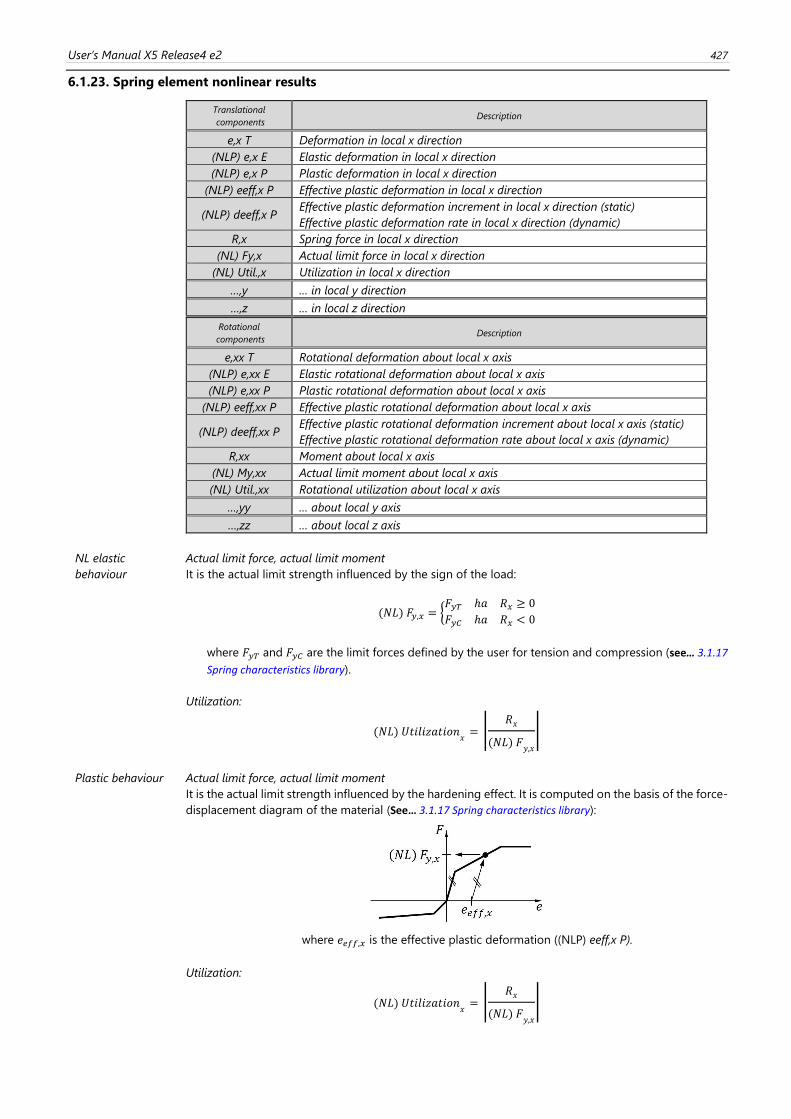
User’s Manual X5 Release4 e2 427

6.1.23. Spring element nonlinear results

Translational

components Description

e,x T Deformation in local x direction

(NLP) e,x E Elastic deformation in local x direction

(NLP) e,x P Plastic deformation in local x direction

(NLP) eeff,x P Effective plastic deformation in local x direction

(NLP) deeff,x P Effective plastic deformation increment in local x direction (static)

Effective plastic deformation rate in local x direction (dynamic)

R,x Spring force in local x direction

(NL) Fy,x Actual limit force in local x direction

(NL) Util.,x Utilization in local x direction

…,y … in local y direction

…,z … in local z direction

Rotational

components Description

e,xx T Rotational deformation about local x axis

(NLP) e,xx E Elastic rotational deformation about local x axis

(NLP) e,xx P Plastic rotational deformation about local x axis

(NLP) eeff,xx P Effective plastic rotational deformation about local x axis

(NLP) deeff,xx P Effective plastic rotational deformation increment about local x axis (static)

Effective plastic rotational deformation rate about local x axis (dynamic)

R,xx Moment about local x axis

(NL) My,xx Actual limit moment about local x axis

(NL) Util.,xx Rotational utilization about local x axis

…,yy … about local y axis

…,zz … about local z axis

NL elastic

behaviour

Actual limit force, actual limit moment

It is the actual limit strength influenced by the sign of the load:

(𝑁𝐿) 𝐹𝑦,𝑥 = {𝐹𝑦𝑇 ℎ𝑎 𝑅𝑥 ≥ 0

𝐹𝑦𝐶 ℎ𝑎 𝑅𝑥 < 0

where 𝐹𝑦𝑇 and 𝐹𝑦𝐶 are the limit forces defined by the user for tension and compression (see… 3.1.17

Spring characteristics library).

Utilization:

(𝑁𝐿) 𝑈𝑡𝑖𝑙𝑖𝑧𝑎𝑡𝑖𝑜𝑛𝑥= |

𝑅𝑥

(𝑁𝐿) 𝐹𝑦,𝑥

|

Plastic behaviour Actual limit force, actual limit moment

It is the actual limit strength influenced by the hardening effect. It is computed on the basis of the force-

displacement diagram of the material (See… 3.1.17 Spring characteristics library):

where 𝑒𝑒𝑓𝑓,𝑥 is the effective plastic deformation ((NLP) eeff,x P).

Utilization:

(𝑁𝐿) 𝑈𝑡𝑖𝑙𝑖𝑧𝑎𝑡𝑖𝑜𝑛𝑥= |

𝑅𝑥

(𝑁𝐿) 𝐹𝑦,𝑥

|

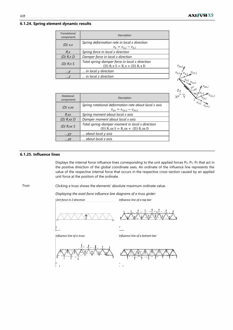
428

6.1.24. Spring element dynamic results

Translational

components Description

(D) v,x Spring deformation rate in local x direction

𝑣𝑥 = 𝑣𝑥,𝑗 − 𝑣𝑥,𝑖

R,x Spring force in local x direction

(D) R,x D Damper force in local x direction

(D) R,x S Total spring-damper force in local x direction

(D) R, x S = R, x + (D) R, x D

…,y … in local y direction

…,z … in local z direction

Rotational

components Description

(D) v,xx Spring rotational deformation rate about local x axis

𝑣𝑥𝑥 = 𝑣𝑥𝑥,𝑗 − 𝑣𝑥𝑥,𝑖

R,xx Spring moment about local x axis

(D) R,xx D Damper moment about local x axis

(D) R,xx S Total spring-damper moment in local x direction

(D) R, xx S = R, xx + (D) R, xx D

…,yy … about local y axis

…,zz … about local z axis

6.1.25. Influence lines

Displays the internal force influence lines corresponding to the unit applied forces PX, PY, PZ that act in

the positive direction of the global coordinate axes. An ordinate of the influence line represents the

value of the respective internal force that occurs in the respective cross-section caused by an applied

unit force at the position of the ordinate.

Truss Clicking a truss shows the elements’ absolute maximum ordinate value.

Displaying the axial force influence line diagrams of a truss girder:

Unit force in Z direction Influence line of a top bar

Influence line of a truss Influence line of a bottom bar

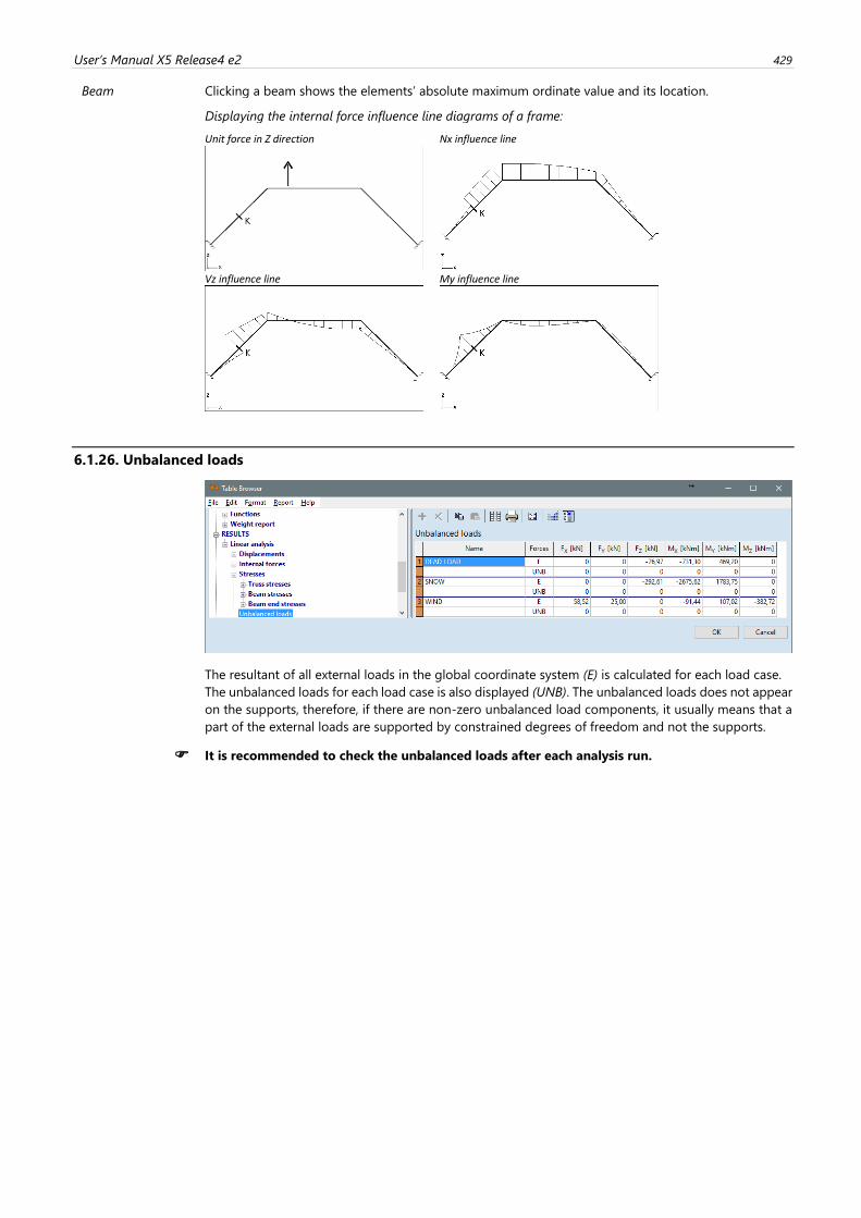
User’s Manual X5 Release4 e2 429

Beam Clicking a beam shows the elements’ absolute maximum ordinate value and its location.

Displaying the internal force influence line diagrams of a frame:

Unit force in Z direction Nx influence line

Vz influence line My influence line

6.1.26. Unbalanced loads

The resultant of all external loads in the global coordinate system (E) is calculated for each load case.

The unbalanced loads for each load case is also displayed (UNB). The unbalanced loads does not appear

on the supports, therefore, if there are non-zero unbalanced load components, it usually means that a

part of the external loads are supported by constrained degrees of freedom and not the supports.

It is recommended to check the unbalanced loads after each analysis run.

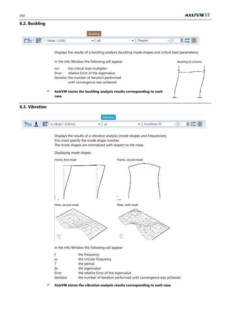
430

6.2. Buckling

Displays the results of a buckling analysis (buckling mode shapes and critical load parameters).

In the Info Window the following will appear: Buckling of a frame:

ncr the critical load multiplier

Error relative Error of the eigenvalue

Iteration the number of iteration performed

until convergence was achieved

AxisVM stores the buckling analysis results corresponding to each

case.

6.3. Vibration

Displays the results of a vibration analysis (mode shapes and frequencies).

You must specify the mode shape number.

The mode shapes are normalized with respect to the mass.

Displaying mode shapes:

Frame, first mode Frame, second mode

Plate, second mode Plate, sixth mode

In the Info Window the following will appear:

f the frequency

ω the circular frequency

T the period

Ev the eigenvalue

Error the relative Error of the eigenvalue

Iteration the number of iteration performed until convergence was achieved

AxisVM stores the vibration analysis results corresponding to each case.

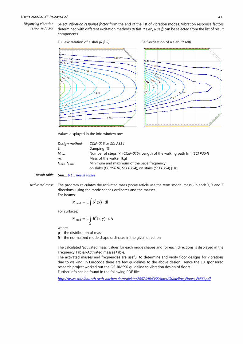
User’s Manual X5 Release4 e2 431

Displaying vibration response factor

Select Vibration response factor from the end of the list of vibration modes. Vibration response factors

determined with different excitation methods (R full, R extr., R self) can be selected from the list of result

components.

Full excitatation of a slab (R full) Self-excitation of a slab (R self)

Values displayed in the info window are:

Design method: CCIP-016 or SCI P354

ξ: Damping [%]

N, L: Number of steps [-] (CCIP-016), Length of the walking path [m] (SCI P354)

m: Mass of the walker [kg]

fp,min, fp,max Minimum and maximum of the pace frequency

on slabs (CCIP-016, SCI P354), on stairs (SCI P354) [Hz]

Result table See... 6.1.5 Result tables

Activated mass The program calculates the activated mass (some article use the term ‘modal mass’) in each X, Y and Z

directions, using the mode shapes ordinates and the masses.

For beams:

Mmod = μ∫δ2(x) ∙ dl

l

For surfaces:

Mmod = μ∫ δ2(x, y) ∙ dA

A

where:

μ – the distribution of mass

δ – the normalized mode shape ordinates in the given direction

The calculated ‘activated mass’ values for each mode shapes and for each directions is displayed in the

Frequency Tables/Activated masses table.

The activated masses and frequencies are useful to determine and verify floor designs for vibrations

due to walking. In Eurocode there are few guidelines to the above design. Hence the EU sponsored

research project worked out the OS-RMS90 guideline to vibration design of floors.

Further info can be found in the following PDF file:

http://www.stahlbau.stb.rwth-aachen.de/projekte/2007/HIVOSS/docs/Guideline_Floors_EN02.pdf

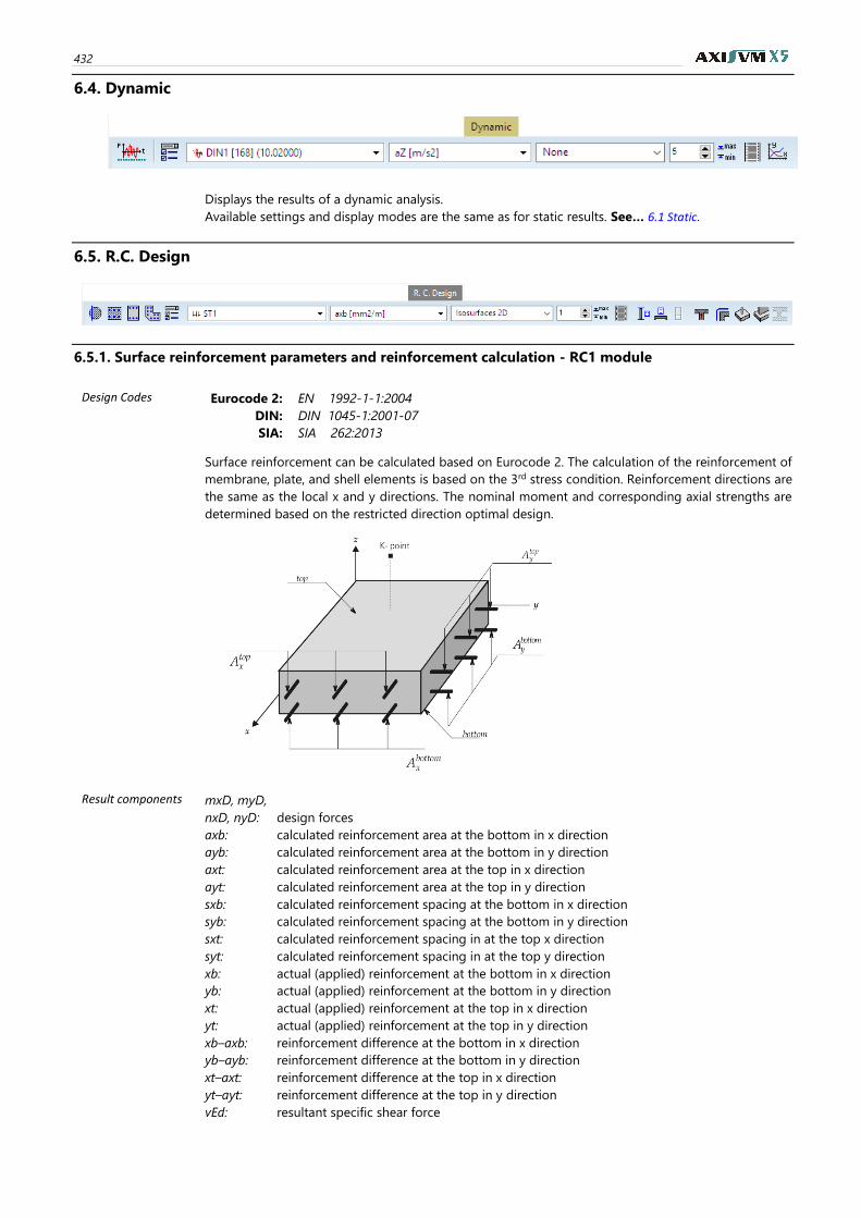
432

6.4. Dynamic

Displays the results of a dynamic analysis.

Available settings and display modes are the same as for static results. See… 6.1 Static.

6.5. R.C. Design

6.5.1. Surface reinforcement parameters and reinforcement calculation - RC1 module

Design Codes Eurocode 2: EN 1992-1-1:2004

DIN: DIN 1045-1:2001-07

SIA: SIA 262:2013

Surface reinforcement can be calculated based on Eurocode 2. The calculation of the reinforcement of

membrane, plate, and shell elements is based on the 3rd stress condition. Reinforcement directions are

the same as the local x and y directions. The nominal moment and corresponding axial strengths are

determined based on the restricted direction optimal design.

Result components mxD, myD,

nxD, nyD: design forces

axb: calculated reinforcement area at the bottom in x direction

ayb: calculated reinforcement area at the bottom in y direction

axt: calculated reinforcement area at the top in x direction

ayt: calculated reinforcement area at the top in y direction

sxb: calculated reinforcement spacing at the bottom in x direction

syb: calculated reinforcement spacing at the bottom in y direction

sxt: calculated reinforcement spacing in at the top x direction

syt: calculated reinforcement spacing in at the top y direction

xb: actual (applied) reinforcement at the bottom in x direction

yb: actual (applied) reinforcement at the bottom in y direction

xt: actual (applied) reinforcement at the top in x direction

yt: actual (applied) reinforcement at the top in y direction

xb–axb: reinforcement difference at the bottom in x direction

yb–ayb: reinforcement difference at the bottom in y direction

xt–axt: reinforcement difference at the top in x direction

yt–ayt: reinforcement difference at the top in y direction

vEd: resultant specific shear force

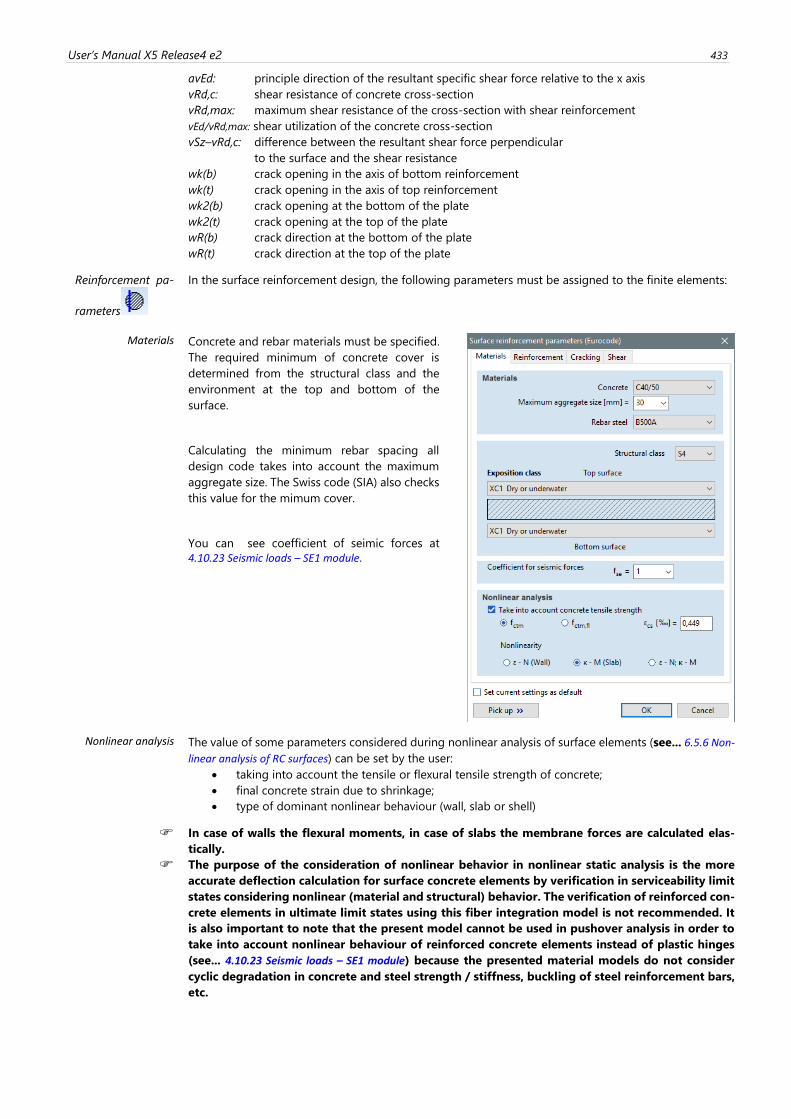
User’s Manual X5 Release4 e2 433

avEd: principle direction of the resultant specific shear force relative to the x axis

vRd,c: shear resistance of concrete cross-section

vRd,max: maximum shear resistance of the cross-section with shear reinforcement

vEd/vRd,max: shear utilization of the concrete cross-section

vSz–vRd,c: difference between the resultant shear force perpendicular

to the surface and the shear resistance

wk(b) crack opening in the axis of bottom reinforcement

wk(t) crack opening in the axis of top reinforcement

wk2(b) crack opening at the bottom of the plate

wk2(t) crack opening at the top of the plate

wR(b) crack direction at the bottom of the plate

wR(t) crack direction at the top of the plate

Reinforcement pa-

rameters

In the surface reinforcement design, the following parameters must be assigned to the finite elements:

Materials

Concrete and rebar materials must be specified.

The required minimum of concrete cover is

determined from the structural class and the

environment at the top and bottom of the

surface.

Calculating the minimum rebar spacing all

design code takes into account the maximum

aggregate size. The Swiss code (SIA) also checks

this value for the mimum cover.

You can see coefficient of seimic forces at

4.10.23 Seismic loads – SE1 module.

Nonlinear analysis The value of some parameters considered during nonlinear analysis of surface elements (see... 6.5.6 Non-

linear analysis of RC surfaces) can be set by the user:

• taking into account the tensile or flexural tensile strength of concrete;

• final concrete strain due to shrinkage;

• type of dominant nonlinear behaviour (wall, slab or shell)

In case of walls the flexural moments, in case of slabs the membrane forces are calculated elas-

tically.

The purpose of the consideration of nonlinear behavior in nonlinear static analysis is the more

accurate deflection calculation for surface concrete elements by verification in serviceability limit

states considering nonlinear (material and structural) behavior. The verification of reinforced con-

crete elements in ultimate limit states using this fiber integration model is not recommended. It

is also important to note that the present model cannot be used in pushover analysis in order to

take into account nonlinear behaviour of reinforced concrete elements instead of plastic hinges

(see... 4.10.23 Seismic loads – SE1 module) because the presented material models do not consider

cyclic degradation in concrete and steel strength / stiffness, buckling of steel reinforcement bars,

etc.

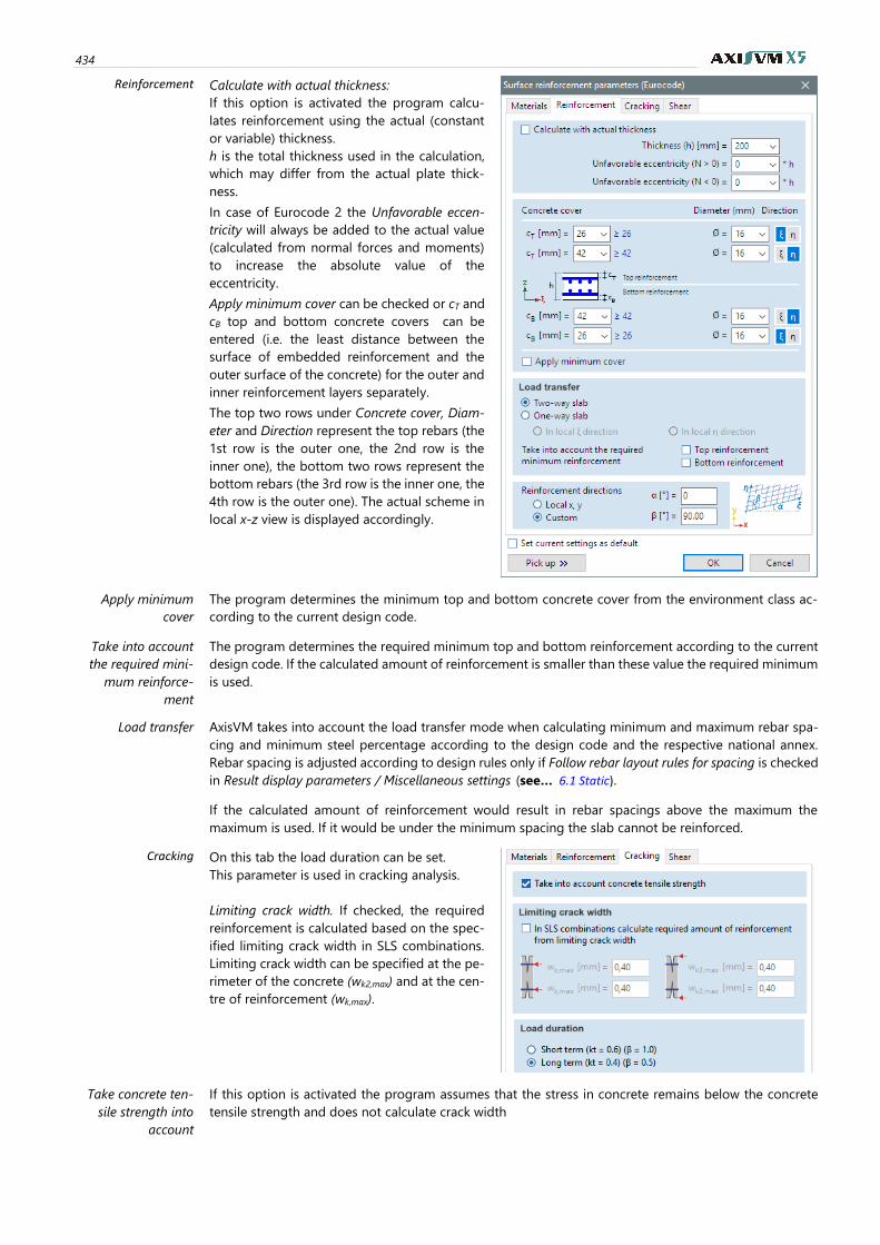
434

Reinforcement

Calculate with actual thickness:

If this option is activated the program calcu-

lates reinforcement using the actual (constant

or variable) thickness.

h is the total thickness used in the calculation,

which may differ from the actual plate thick-

ness.

In case of Eurocode 2 the Unfavorable eccen-

tricity will always be added to the actual value

(calculated from normal forces and moments)

to increase the absolute value of the

eccentricity.

Apply minimum cover can be checked or cT and

cB top and bottom concrete covers can be

entered (i.e. the least distance between the

surface of embedded reinforcement and the

outer surface of the concrete) for the outer and

inner reinforcement layers separately.

The top two rows under Concrete cover, Diam-

eter and Direction represent the top rebars (the

1st row is the outer one, the 2nd row is the

inner one), the bottom two rows represent the

bottom rebars (the 3rd row is the inner one, the

4th row is the outer one). The actual scheme in

local x-z view is displayed accordingly.

Apply minimum

cover

The program determines the minimum top and bottom concrete cover from the environment class ac-

cording to the current design code.

Take into account

the required mini-

mum reinforce-

ment

The program determines the required minimum top and bottom reinforcement according to the current

design code. If the calculated amount of reinforcement is smaller than these value the required minimum

is used.

Load transfer

AxisVM takes into account the load transfer mode when calculating minimum and maximum rebar spa-

cing and minimum steel percentage according to the design code and the respective national annex.

Rebar spacing is adjusted according to design rules only if Follow rebar layout rules for spacing is checked

in Result display parameters / Miscellaneous settings (see… 6.1 Static).

If the calculated amount of reinforcement would result in rebar spacings above the maximum the

maximum is used. If it would be under the minimum spacing the slab cannot be reinforced.

Cracking On this tab the load duration can be set.

This parameter is used in cracking analysis.

Limiting crack width. If checked, the required

reinforcement is calculated based on the spec-

ified limiting crack width in SLS combinations.

Limiting crack width can be specified at the pe-

rimeter of the concrete (wk2,max) and at the cen-

tre of reinforcement (wk,max).

Take concrete ten-

sile strength into

account

If this option is activated the program assumes that the stress in concrete remains below the concrete

tensile strength and does not calculate crack width

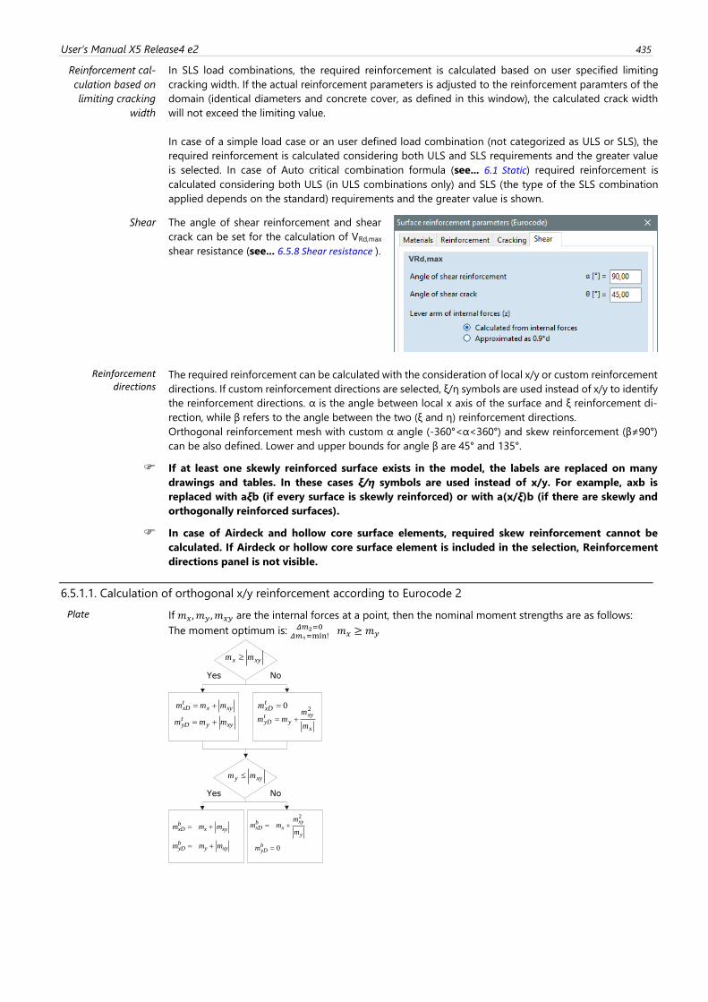
User’s Manual X5 Release4 e2 435

Reinforcement cal-

culation based on

limiting cracking

width

In SLS load combinations, the required reinforcement is calculated based on user specified limiting

cracking width. If the actual reinforcement parameters is adjusted to the reinforcement paramters of the

domain (identical diameters and concrete cover, as defined in this window), the calculated crack width

will not exceed the limiting value.

In case of a simple load case or an user defined load combination (not categorized as ULS or SLS), the

required reinforcement is calculated considering both ULS and SLS requirements and the greater value

is selected. In case of Auto critical combination formula (see... 6.1 Static) required reinforcement is

calculated considering both ULS (in ULS combinations only) and SLS (the type of the SLS combination

applied depends on the standard) requirements and the greater value is shown.

Shear

The angle of shear reinforcement and shear

crack can be set for the calculation of VRd,max

shear resistance (see... 6.5.8 Shear resistance ).

Reinforcement directions

The required reinforcement can be calculated with the consideration of local x/y or custom reinforcement

directions. If custom reinforcement directions are selected, ξ/η symbols are used instead of x/y to identify

the reinforcement directions. α is the angle between local x axis of the surface and ξ reinforcement di-

rection, while β refers to the angle between the two (ξ and η) reinforcement directions.

Orthogonal reinforcement mesh with custom α angle (-360°<α<360°) and skew reinforcement (β≠90°)

can be also defined. Lower and upper bounds for angle β are 45° and 135°.

If at least one skewly reinforced surface exists in the model, the labels are replaced on many

drawings and tables. In these cases ξ/η symbols are used instead of x/y. For example, axb is

replaced with aξb (if every surface is skewly reinforced) or with a(x/ξ)b (if there are skewly and

orthogonally reinforced surfaces).

In case of Airdeck and hollow core surface elements, required skew reinforcement cannot be

calculated. If Airdeck or hollow core surface element is included in the selection, Reinforcement

directions panel is not visible.

6.5.1.1. Calculation of orthogonal x/y reinforcement according to Eurocode 2

Plate If 𝑚𝑥, 𝑚𝑦 , 𝑚𝑥𝑦 are the internal forces at a point, then the nominal moment strengths are as follows:

The moment optimum is: 𝛥𝑚2=0𝛥𝑚1=min!

𝑚𝑥 ≥ 𝑚𝑦

xyx mm

xyxtxD mmm +=

xyytyD mmm +=

0=txDm

x

xyy

tyD

m

mmm

2

+=

xyy mm

xyxbxD mmm +=

xyybyD mmm +=

y

xyx

bxD

m

mmm

2

+=

0=byDm

Yes No

Yes

No

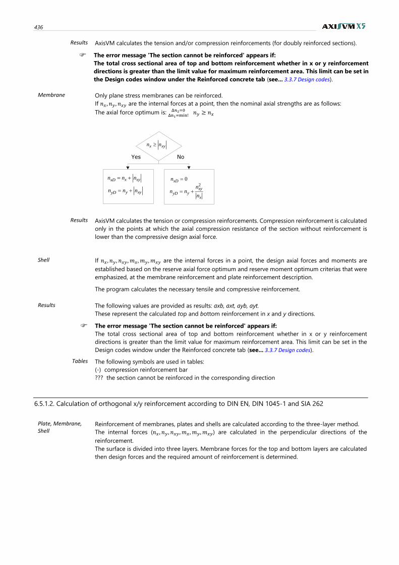
436

Results AxisVM calculates the tension and/or compression reinforcements (for doubly reinforced sections).

The error message 'The section cannot be reinforced' appears if:

The total cross sectional area of top and bottom reinforcement whether in x or y reinforcement

directions is greater than the limit value for maximum reinforcement area. This limit can be set in

the Design codes window under the Reinforced concrete tab (see... 3.3.7 Design codes).

Membrane Only plane stress membranes can be reinforced.

If 𝑛𝑥 , 𝑛𝑦 , 𝑛𝑥𝑦 are the internal forces at a point, then the nominal axial strengths are as follows:

The axial force optimum is: Δ𝑛2=0Δn1=min!

𝑛𝑦 ≥ 𝑛𝑥

xyx nn

xyxxD nnn +=

xyyyD nnn +=

0=xDn

x

xyyyD

n

nnn

2

+=

Yes No

Results AxisVM calculates the tension or compression reinforcements. Compression reinforcement is calculated

only in the points at which the axial compression resistance of the section without reinforcement is

lower than the compressive design axial force.

Shell If 𝑛𝑥 , 𝑛𝑦 , 𝑛𝑥𝑦 , 𝑚𝑥, 𝑚𝑦 , 𝑚𝑥𝑦 are the internal forces in a point, the design axial forces and moments are

established based on the reserve axial force optimum and reserve moment optimum criterias that were

emphasized, at the membrane reinforcement and plate reinforcement description.

The program calculates the necessary tensile and compressive reinforcement.

Results The following values are provided as results: axb, axt, ayb, ayt.

These represent the calculated top and bottom reinforcement in x and y directions.

The error message 'The section cannot be reinforced' appears if:

The total cross sectional area of top and bottom reinforcement whether in x or y reinforcement

directions is greater than the limit value for maximum reinforcement area. This limit can be set in the

Design codes window under the Reinforced concrete tab (see... 3.3.7 Design codes).

Tables The following symbols are used in tables:

(-) compression reinforcement bar

??? the section cannot be reinforced in the corresponding direction

6.5.1.2. Calculation of orthogonal x/y reinforcement according to DIN EN, DIN 1045-1 and SIA 262

Plate, Membrane, Shell

Reinforcement of membranes, plates and shells are calculated according to the three-layer method.

The internal forces (𝑛𝑥 , 𝑛𝑦 , 𝑛𝑥𝑦, 𝑚𝑥 , 𝑚𝑦, 𝑚𝑥𝑦) are calculated in the perpendicular directions of the

reinforcement.

The surface is divided into three layers. Membrane forces for the top and bottom layers are calculated

then design forces and the required amount of reinforcement is determined.

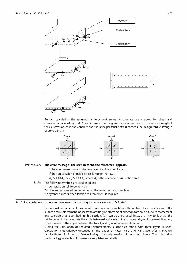
User’s Manual X5 Release4 e2 437

Besides calculating the required reinforcement zones of concrete are checked for shear and

compression according to A, B and C cases. The program considers reduced compressive strength if

tensile stress arises in the concrete and the principal tensile stress exceeds the design tensile strength

of concrete (fctd).

Case A

Case B

Case C

Error message The error message 'The section cannot be reinforced' appears.

If the compressed zone of the concrete fails due shear forces.

If the compression principal stress is higher than 𝑓𝑐𝑑 .

𝐴𝑥 > 0.04𝐴𝑐, or 𝐴𝑦 > 0.04𝐴𝑐 , where 𝐴𝑐 is the concrete cross-section area.

Tables The following symbols are used in tables:

(-) compression reinforcement bar

??? the section cannot be reinforced in the corresponding direction

No symbol appears when tension reinforcement is required.

6.5.1.3. Calculation of skew reinforcement according to Eurocode 2 and SIA 262

Orthogonal reinforcement meshes with reinforcement directions differing from local x and y axes of the

surface and reinforcement meshes with arbitrary reinforcement directions are called skew reinforcement

and calculated as described in this section. ξ/η symbols are used instead of x/y to identify the

reinforcement directions. α is the angle between local x axis of the surface and ξ reinforcement direction,

while β refers to the angle between the two (ξ and η) reinforcement directions.

During the calculation of required reinforcements, a sandwich model with three layers is used.

Calculation methodology described in the paper of Peter Marti and Hans Seelhofer is invoked

(H. Seelhofer & P. Marti: Dimensioning of skewly reinforced concrete plates). The calculation

methodology is identical for membranes, plates and shells.

Medium layer

Bottom layer

Top layer

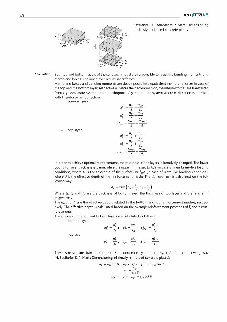
438

Reference: H. Seelhofer & P. Marti: Dimensioning

of skewly reinforced concrete plates

Calculation Both top and bottom layers of the sandwich model are responsible to resist the bending moments and

membrane forces. The inner layer resists shear forces.

Membrane forces and bending moments are decomposed into equivalent membrane forces in case of

the top and the bottom layer, respectively. Before the decomposition, the internal forces are transferred

from x-y coordinate system into an orthogonal x’-y’ coordinate system where x’ direction is identical

with ξ reinforcement direction.

- bottom layer:

𝑛𝑥′𝑏 =

𝑛𝑥′2−𝑚𝑥′

𝑑𝑣

𝑛𝑦′𝑏 =

𝑛𝑦′

2−𝑚𝑦′

𝑑𝑣

𝑛𝑥′𝑦′𝑏 =

𝑛𝑥′𝑦′

2−𝑚𝑥′𝑦′

𝑑𝑣

- top layer:

𝑛𝑥′𝑡 =

𝑛𝑥′2+𝑚𝑥′

𝑑𝑣

𝑛𝑦′𝑡 =

𝑛𝑦′

2+𝑚𝑦′

𝑑𝑣

𝑛𝑥′𝑦′𝑡 =

𝑛𝑥′𝑦′

2+𝑚𝑥′𝑦′

𝑑𝑣

In order to achieve optimal reinforcement, the thickness of the layers is iteratively changed. The lower

bound for layer thickness is 5 mm, while the upper limit is set to H/2 (in case of membrane-like loading

conditions, where H is the thickness of the surface) or ξc0d (in case of plate-like loading conditions,

where d is the effective depth of the reinforcement mesh). The 𝑑𝑣 level arm is calculated on the fol-

lowing way:

𝑑𝑣 = 𝑚𝑖𝑛 (𝑑𝑏 −𝑡𝑡2, 𝑑𝑡 −

𝑡𝑏2)

Where 𝑡𝑏, 𝑡𝑡 and 𝑑𝑣 are the thickness of bottom layer, the thickness of top layer and the level arm,

respectively.

The 𝑑𝑏 and 𝑑𝑡 are the effective depths related to the bottom and top reinforcement meshes, respec-

tively. The effective depth is calculated based on the average reinforcement positions of ξ and η rein-

forcements.

The stresses in the top and bottom layers are calculated as follows:

- bottom layer:

𝜎𝑥′𝑏 =

𝑛𝑥′𝑏

𝑡𝑏; 𝜎𝑦′

𝑏 =𝑛𝑦′𝑏

𝑡𝑏; 𝜏𝑥′𝑦′

𝑏 =𝑛𝑥′𝑦′𝑏

𝑡𝑏

- top layer:

𝜎𝑥′𝑡 =

𝑛𝑥′𝑡

𝑡𝑡; 𝜎𝑦′

𝑡 =𝑛𝑦′𝑡

𝑡𝑡; 𝜏𝑥′𝑦′

𝑡 =𝑛𝑥′𝑦′𝑡

𝑡𝑡

These stresses are transformed into ξ-η coordinate system (𝜎𝜉 , 𝜎𝜂, 𝜏𝜉𝜂) on the following way

(H. Seelhofer & P. Marti: Dimensioning of skewly reinforced concrete plates):

𝜎𝜉 = 𝜎𝑥′ sin 𝛽 + 𝜎𝑦′ cos 𝛽 cot 𝛽 − 2𝜏𝑥′𝑦′ sin 𝛽

𝜎𝜂 =𝜎𝑦′

sin 𝛽

𝜏𝜉𝜂 = 𝜏𝜂𝜉 = 𝜏𝑥′𝑦′ − 𝜎𝑦′ cot 𝛽

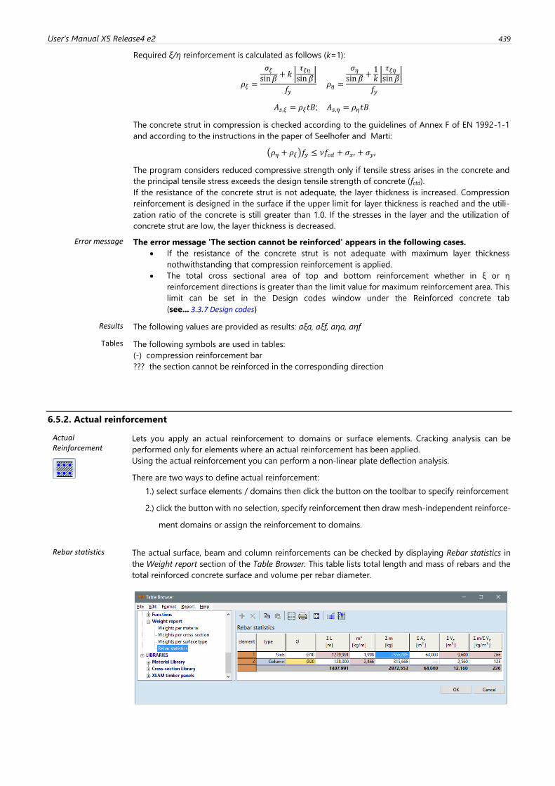
User’s Manual X5 Release4 e2 439

Required ξ/η reinforcement is calculated as follows (k=1):

𝜌𝜉 =

𝜎𝜉sin 𝛽

+ 𝑘 |𝜏𝜉𝜂sin 𝛽

|

𝑓𝑦 𝜌𝜂 =

𝜎𝜂sin 𝛽

+1𝑘|𝜏𝜉𝜂sin 𝛽

|

𝑓𝑦

𝐴𝑠,𝜉 = 𝜌𝜉𝑡𝐵; 𝐴𝑠,𝜂 = 𝜌𝜂𝑡𝐵

The concrete strut in compression is checked according to the guidelines of Annex F of EN 1992-1-1

and according to the instructions in the paper of Seelhofer and Marti:

(𝜌𝜂 + 𝜌𝜉)𝑓𝑦 ≤ 𝜈𝑓𝑐𝑑 + 𝜎𝑥′ + 𝜎𝑦′

The program considers reduced compressive strength only if tensile stress arises in the concrete and

the principal tensile stress exceeds the design tensile strength of concrete (fctd).

If the resistance of the concrete strut is not adequate, the layer thickness is increased. Compression

reinforcement is designed in the surface if the upper limit for layer thickness is reached and the utili-

zation ratio of the concrete is still greater than 1.0. If the stresses in the layer and the utilization of

concrete strut are low, the layer thickness is decreased.

Error message The error message 'The section cannot be reinforced' appears in the following cases.

• If the resistance of the concrete strut is not adequate with maximum layer thickness

nothwithstanding that compression reinforcement is applied.

• The total cross sectional area of top and bottom reinforcement whether in ξ or η

reinforcement directions is greater than the limit value for maximum reinforcement area. This

limit can be set in the Design codes window under the Reinforced concrete tab

(see... 3.3.7 Design codes)

Results The following values are provided as results: aξa, aξf, aηa, aηf

Tables The following symbols are used in tables:

(-) compression reinforcement bar

??? the section cannot be reinforced in the corresponding direction

6.5.2. Actual reinforcement

Actual Reinforcement

Lets you apply an actual reinforcement to domains or surface elements. Cracking analysis can be

performed only for elements where an actual reinforcement has been applied.

Using the actual reinforcement you can perform a non-linear plate deflection analysis.

There are two ways to define actual reinforcement:

1.) select surface elements / domains then click the button on the toolbar to specify reinforcement

2.) click the button with no selection, specify reinforcement then draw mesh-independent reinforce-

ment domains or assign the reinforcement to domains.

Rebar statistics

The actual surface, beam and column reinforcements can be checked by displaying Rebar statistics in

the Weight report section of the Table Browser. This table lists total length and mass of rebars and the

total reinforced concrete surface and volume per rebar diameter.

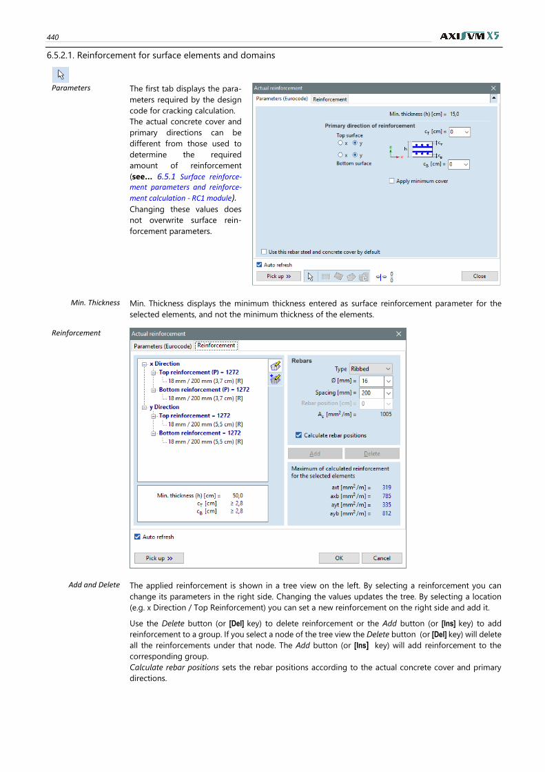
440

6.5.2.1. Reinforcement for surface elements and domains

Parameters The first tab displays the para-

meters required by the design

code for cracking calculation.

The actual concrete cover and

primary directions can be

different from those used to

determine the required

amount of reinforcement

(see… 6.5.1 Surface reinforce-

ment parameters and reinforce-

ment calculation - RC1 module). Changing these values does

not overwrite surface rein-

forcement parameters.

Min. Thickness Min. Thickness displays the minimum thickness entered as surface reinforcement parameter for the

selected elements, and not the minimum thickness of the elements.

Reinforcement

Add and Delete The applied reinforcement is shown in a tree view on the left. By selecting a reinforcement you can

change its parameters in the right side. Changing the values updates the tree. By selecting a location

(e.g. x Direction / Top Reinforcement) you can set a new reinforcement on the right side and add it.

Use the Delete button (or [Del] key) to delete reinforcement or the Add button (or [Ins] key) to add

reinforcement to a group. If you select a node of the tree view the Delete button (or [Del] key) will delete

all the reinforcements under that node. The Add button (or [Ins] key) will add reinforcement to the

corresponding group.

Calculate rebar positions sets the rebar positions according to the actual concrete cover and primary

directions.

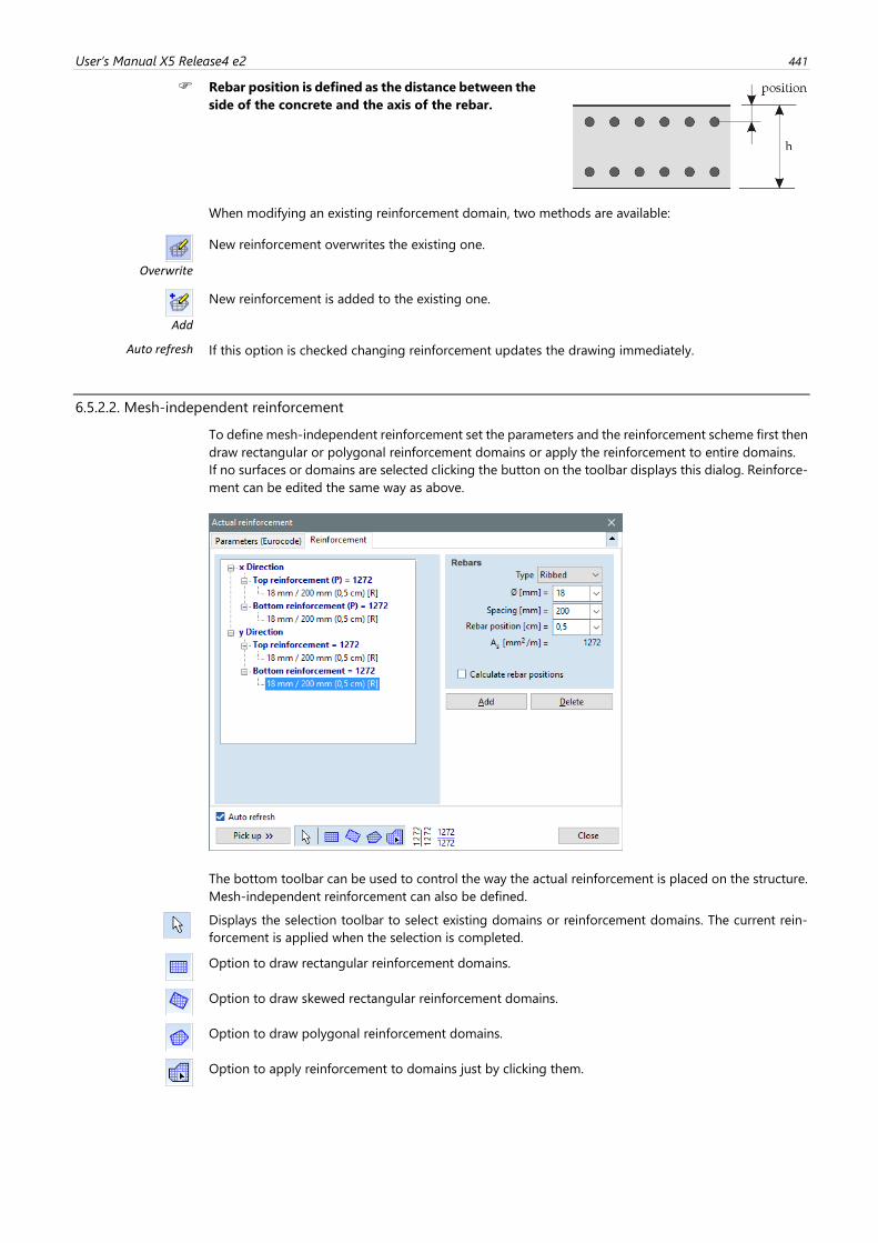
User’s Manual X5 Release4 e2 441

Rebar position is defined as the distance between the

side of the concrete and the axis of the rebar.

When modifying an existing reinforcement domain, two methods are available:

Overwrite

New reinforcement overwrites the existing one.

Add

New reinforcement is added to the existing one.

Auto refresh If this option is checked changing reinforcement updates the drawing immediately.

6.5.2.2. Mesh-independent reinforcement

To define mesh-independent reinforcement set the parameters and the reinforcement scheme first then

draw rectangular or polygonal reinforcement domains or apply the reinforcement to entire domains.

If no surfaces or domains are selected clicking the button on the toolbar displays this dialog. Reinforce-

ment can be edited the same way as above.

The bottom toolbar can be used to control the way the actual reinforcement is placed on the structure.

Mesh-independent reinforcement can also be defined.

Displays the selection toolbar to select existing domains or reinforcement domains. The current rein-

forcement is applied when the selection is completed.

Option to draw rectangular reinforcement domains.

Option to draw skewed rectangular reinforcement domains.

Option to draw polygonal reinforcement domains.

Option to apply reinforcement to domains just by clicking them.

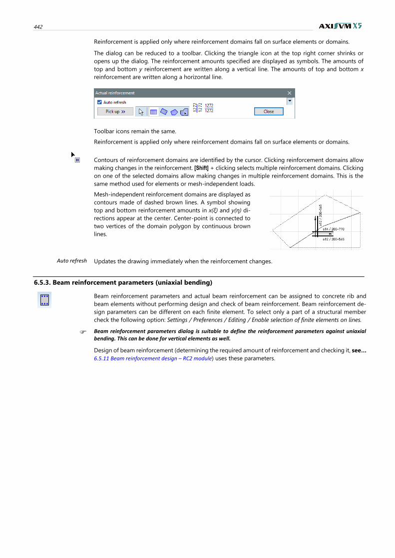
442

Reinforcement is applied only where reinforcement domains fall on surface elements or domains.

The dialog can be reduced to a toolbar. Clicking the triangle icon at the top right corner shrinks or

opens up the dialog. The reinforcement amounts specified are displayed as symbols. The amounts of

top and bottom y reinforcement are written along a vertical line. The amounts of top and bottom x

reinforcement are written along a horizontal line.

Toolbar icons remain the same.

Reinforcement is applied only where reinforcement domains fall on surface elements or domains.

Contours of reinforcement domains are identified by the cursor. Clicking reinforcement domains allow

making changes in the reinforcement. [Shift] + clicking selects multiple reinforcement domains. Clicking

on one of the selected domains allow making changes in multiple reinforcement domains. This is the

same method used for elements or mesh-independent loads.

Mesh-independent reinforcement domains are displayed as

contours made of dashed brown lines. A symbol showing

top and bottom reinforcement amounts in x(ξ) and y(η) di-

rections appear at the center. Center-point is connected to

two vertices of the domain polygon by continuous brown

lines.

Auto refresh Updates the drawing immediately when the reinforcement changes.

6.5.3. Beam reinforcement parameters (uniaxial bending)

Beam reinforcement parameters and actual beam reinforcement can be assigned to concrete rib and

beam elements without performing design and check of beam reinforcement. Beam reinforcement de-

sign parameters can be different on each finite element. To select only a part of a structural member

check the following option: Settings / Preferences / Editing / Enable selection of finite elements on lines.

Beam reinforcement parameters dialog is suitable to define the reinforcement parameters against uniaxial bending. This can be done for vertical elements as well.

Design of beam reinforcement (determining the required amount of reinforcement and checking it, see…

6.5.11 Beam reinforcement design – RC2 module) uses these parameters.

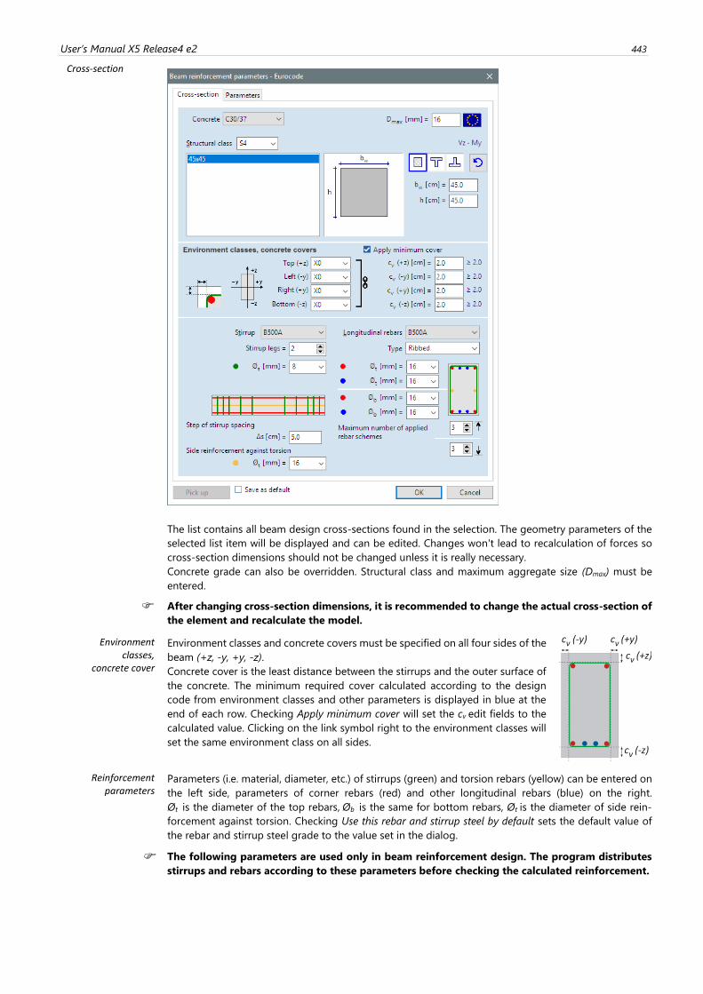
User’s Manual X5 Release4 e2 443

Cross-section

The list contains all beam design cross-sections found in the selection. The geometry parameters of the

selected list item will be displayed and can be edited. Changes won't lead to recalculation of forces so

cross-section dimensions should not be changed unless it is really necessary.

Concrete grade can also be overridden. Structural class and maximum aggregate size (Dmax) must be

entered.

After changing cross-section dimensions, it is recommended to change the actual cross-section of

the element and recalculate the model.

Environment classes,

concrete cover

Environment classes and concrete covers must be specified on all four sides of the

beam (+z, -y, +y, -z).

Concrete cover is the least distance between the stirrups and the outer surface of

the concrete. The minimum required cover calculated according to the design

code from environment classes and other parameters is displayed in blue at the

end of each row. Checking Apply minimum cover will set the cv edit fields to the

calculated value. Clicking on the link symbol right to the environment classes will

set the same environment class on all sides.

Reinforcement parameters

Parameters (i.e. material, diameter, etc.) of stirrups (green) and torsion rebars (yellow) can be entered on

the left side, parameters of corner rebars (red) and other longitudinal rebars (blue) on the right.

Øt is the diameter of the top rebars, Øb is the same for bottom rebars, Øt is the diameter of side rein-

forcement against torsion. Checking Use this rebar and stirrup steel by default sets the default value of

the rebar and stirrup steel grade to the value set in the dialog.

The following parameters are used only in beam reinforcement design. The program distributes

stirrups and rebars according to these parameters before checking the calculated reinforcement.

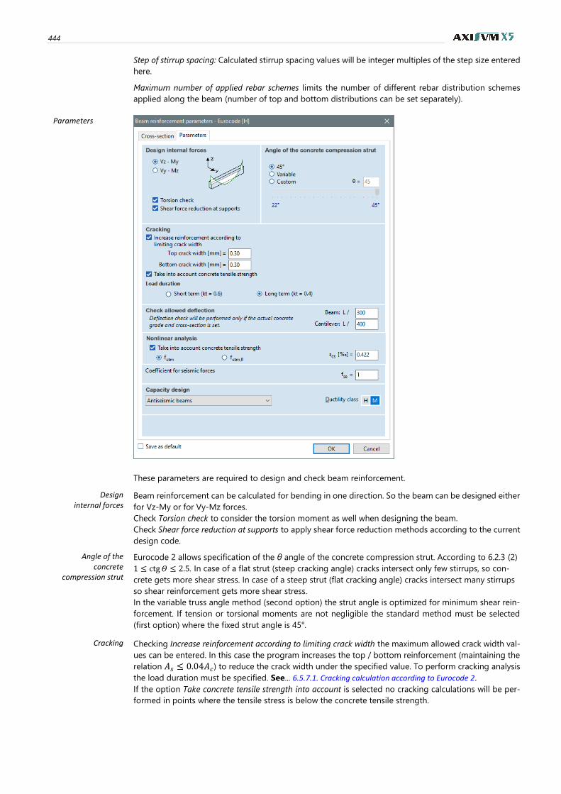
444

Step of stirrup spacing: Calculated stirrup spacing values will be integer multiples of the step size entered

here.

Maximum number of applied rebar schemes limits the number of different rebar distribution schemes

applied along the beam (number of top and bottom distributions can be set separately).

Parameters

These parameters are required to design and check beam reinforcement.

Design internal forces

Beam reinforcement can be calculated for bending in one direction. So the beam can be designed either

for Vz-My or for Vy-Mz forces.

Check Torsion check to consider the torsion moment as well when designing the beam.

Check Shear force reduction at supports to apply shear force reduction methods according to the current

design code.

Angle of the concrete

compression strut

Eurocode 2 allows specification of the θ angle of the concrete compression strut. According to 6.2.3 (2)

1 ≤ ctg 𝛩 ≤ 2.5. In case of a flat strut (steep cracking angle) cracks intersect only few stirrups, so con-

crete gets more shear stress. In case of a steep strut (flat cracking angle) cracks intersect many stirrups

so shear reinforcement gets more shear stress.

In the variable truss angle method (second option) the strut angle is optimized for minimum shear rein-

forcement. If tension or torsional moments are not negligible the standard method must be selected

(first option) where the fixed strut angle is 45°.

Cracking Checking Increase reinforcement according to limiting crack width the maximum allowed crack width val-

ues can be entered. In this case the program increases the top / bottom reinforcement (maintaining the

relation 𝐴𝑠 ≤ 0.04𝐴𝑐) to reduce the crack width under the specified value. To perform cracking analysis

the load duration must be specified. See... 6.5.7.1. Cracking calculation according to Eurocode 2.

If the option Take concrete tensile strength into account is selected no cracking calculations will be per-

formed in points where the tensile stress is below the concrete tensile strength.

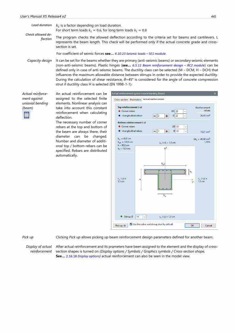
User’s Manual X5 Release4 e2 445

Load duration 𝑘𝑡 is a factor depending on load duration.

For short term loads 𝑘𝑡 = 0.6, for long term loads 𝑘𝑡 = 0.8

Check allowed de-flection The program checks the allowed deflection according to the criteria set for beams and cantilevers. L

represents the beam length. This check will be performed only if the actual concrete grade and cross-

section is set.

For coefficient of seimic forces see… 4.10.23 Seismic loads – SE1 module.

Capacity design It can be set for the beams whether they are primary (anti-seismic beams) or secondary seismic elements

(non-anti-seismic beams). Plastic hinges (see… 6.5.11 Beam reinforcement design – RC2 module) can be

defined only in case of anti-seismic beams. The ductility class can be selected (M – DCM, H – DCH) that

influences the maximum allowable distance between stirrups in order to provide the expected ductility.

During the calculation of shear resistance, θ=45° is considered for the angle of concrete compression

strut if ductility class H is selected (EN 1998-1-1).

Actual reinforce-

ment against

uniaxial bending

(beam)

An actual reinforcement can be

assigned to the selected finite

elements. Nonlinear analysis can

take into account this constant

reinforcement when calculating

deflection.

The necessary number of corner

rebars at the top and bottom of

the beam are always there, their

diameter can be changed.

Number and diameter of additi-

onal top / bottom rebars can be

specified. Rebars are distributed

automatically.

Pick up Clicking Pick up allows picking up beam reinforcement design parameters defined for another beam.

Display of actual

reinforcement

After actual reinforcement and its prameters have been assigned to the element and the display of cross-

section shapes is turned on (Display options / Symbols / Graphics symbols / Cross-section shape,

See… 2.16.18 Display options) actual reinforcement can also be seen in the model view.

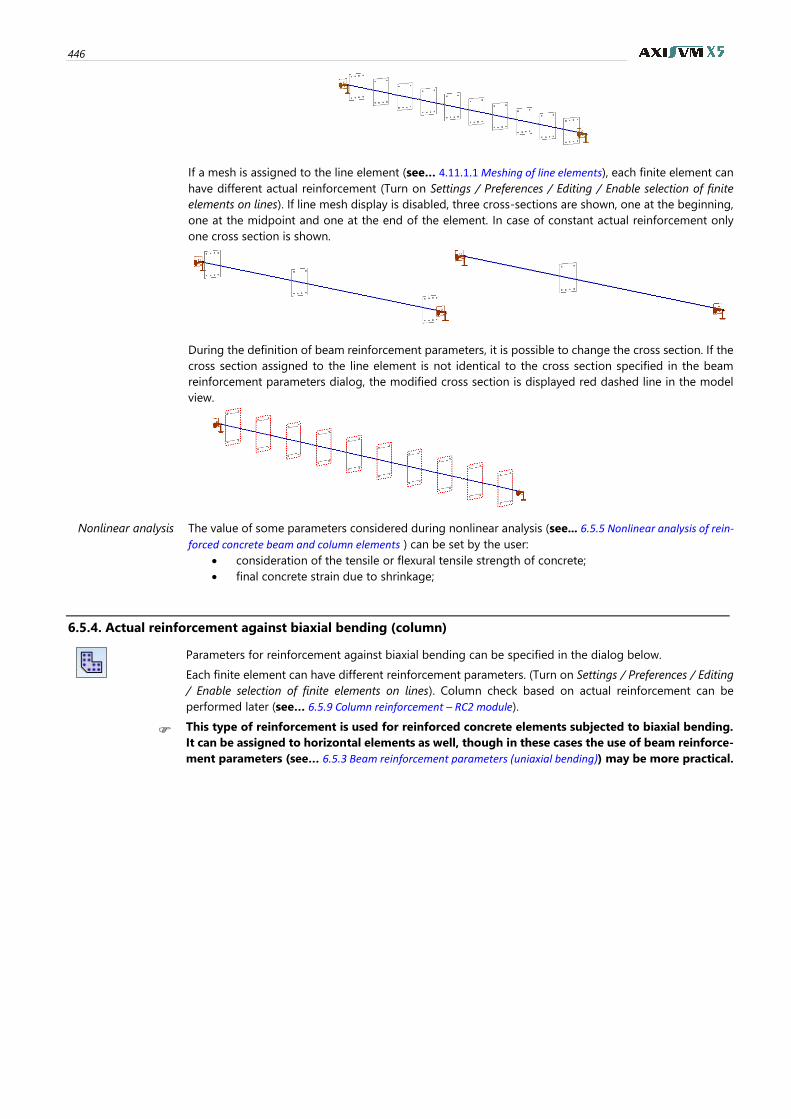
446

If a mesh is assigned to the line element (see… 4.11.1.1 Meshing of line elements), each finite element can

have different actual reinforcement (Turn on Settings / Preferences / Editing / Enable selection of finite

elements on lines). If line mesh display is disabled, three cross-sections are shown, one at the beginning,

one at the midpoint and one at the end of the element. In case of constant actual reinforcement only

one cross section is shown.

During the definition of beam reinforcement parameters, it is possible to change the cross section. If the

cross section assigned to the line element is not identical to the cross section specified in the beam

reinforcement parameters dialog, the modified cross section is displayed red dashed line in the model

view.

Nonlinear analysis The value of some parameters considered during nonlinear analysis (see... 6.5.5 Nonlinear analysis of rein-

forced concrete beam and column elements ) can be set by the user:

• consideration of the tensile or flexural tensile strength of concrete;

• final concrete strain due to shrinkage;

6.5.4. Actual reinforcement against biaxial bending (column)

Parameters for reinforcement against biaxial bending can be specified in the dialog below.

Each finite element can have different reinforcement parameters. (Turn on Settings / Preferences / Editing

/ Enable selection of finite elements on lines). Column check based on actual reinforcement can be

performed later (see… 6.5.9 Column reinforcement – RC2 module).

This type of reinforcement is used for reinforced concrete elements subjected to biaxial bending.

It can be assigned to horizontal elements as well, though in these cases the use of beam reinforce-

ment parameters (see… 6.5.3 Beam reinforcement parameters (uniaxial bending)) may be more practical.

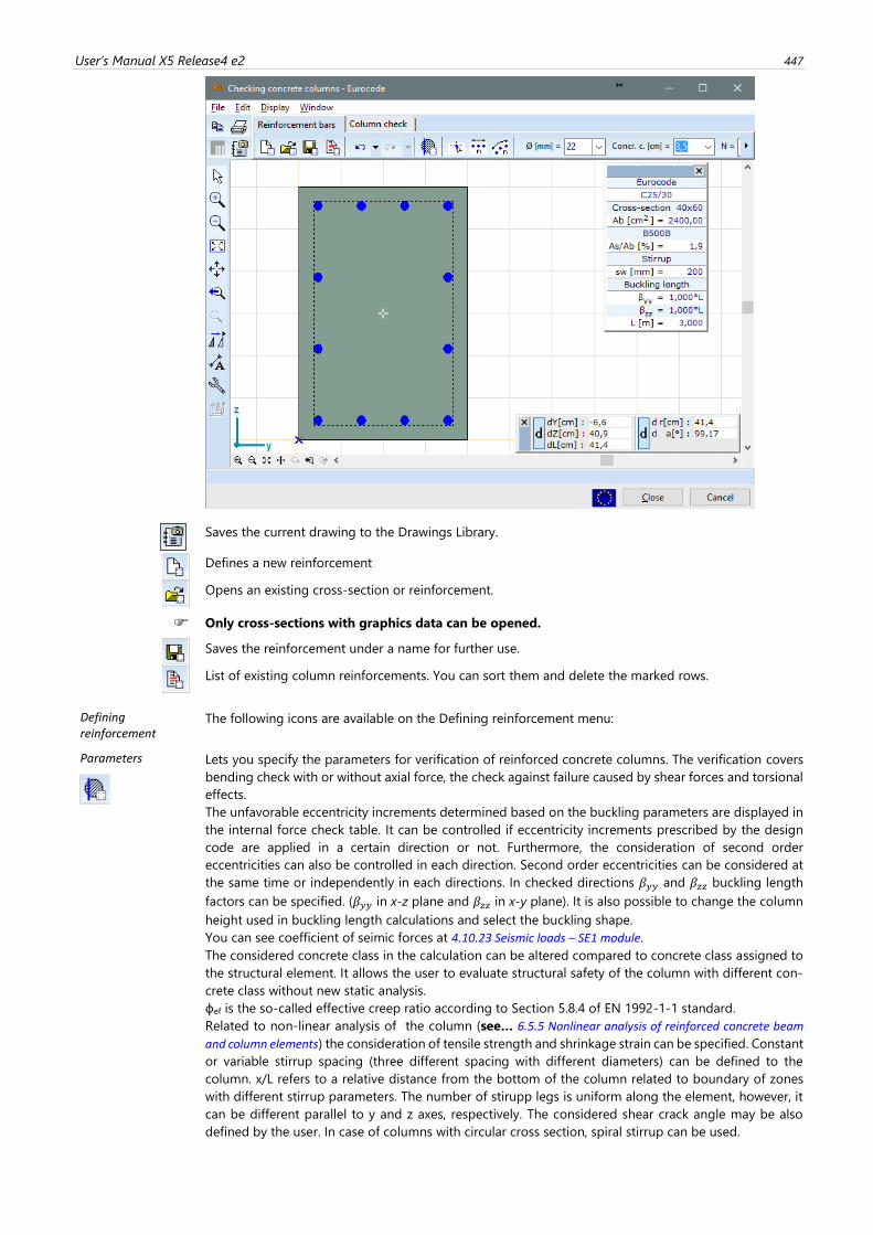
User’s Manual X5 Release4 e2 447

Saves the current drawing to the Drawings Library.

Defines a new reinforcement

Opens an existing cross-section or reinforcement.

Only cross-sections with graphics data can be opened.

Saves the reinforcement under a name for further use.

List of existing column reinforcements. You can sort them and delete the marked rows.

Defining reinforcement

The following icons are available on the Defining reinforcement menu:

Parameters

Lets you specify the parameters for verification of reinforced concrete columns. The verification covers

bending check with or without axial force, the check against failure caused by shear forces and torsional

effects.

The unfavorable eccentricity increments determined based on the buckling parameters are displayed in

the internal force check table. It can be controlled if eccentricity increments prescribed by the design

code are applied in a certain direction or not. Furthermore, the consideration of second order

eccentricities can also be controlled in each direction. Second order eccentricities can be considered at

the same time or independently in each directions. In checked directions 𝛽𝑦𝑦 and 𝛽𝑧𝑧 buckling length

factors can be specified. (𝛽𝑦𝑦 in x-z plane and 𝛽𝑧𝑧 in x-y plane). It is also possible to change the column

height used in buckling length calculations and select the buckling shape. You can see coefficient of seimic forces at 4.10.23 Seismic loads – SE1 module.

The considered concrete class in the calculation can be altered compared to concrete class assigned to

the structural element. It allows the user to evaluate structural safety of the column with different con-

crete class without new static analysis.

ϕef is the so-called effective creep ratio according to Section 5.8.4 of EN 1992-1-1 standard.

Related to non-linear analysis of the column (see… 6.5.5 Nonlinear analysis of reinforced concrete beam

and column elements) the consideration of tensile strength and shrinkage strain can be specified. Constant

or variable stirrup spacing (three different spacing with different diameters) can be defined to the

column. x/L refers to a relative distance from the bottom of the column related to boundary of zones

with different stirrup parameters. The number of stirupp legs is uniform along the element, however, it

can be different parallel to y and z axes, respectively. The considered shear crack angle may be also

defined by the user. In case of columns with circular cross section, spiral stirrup can be used.

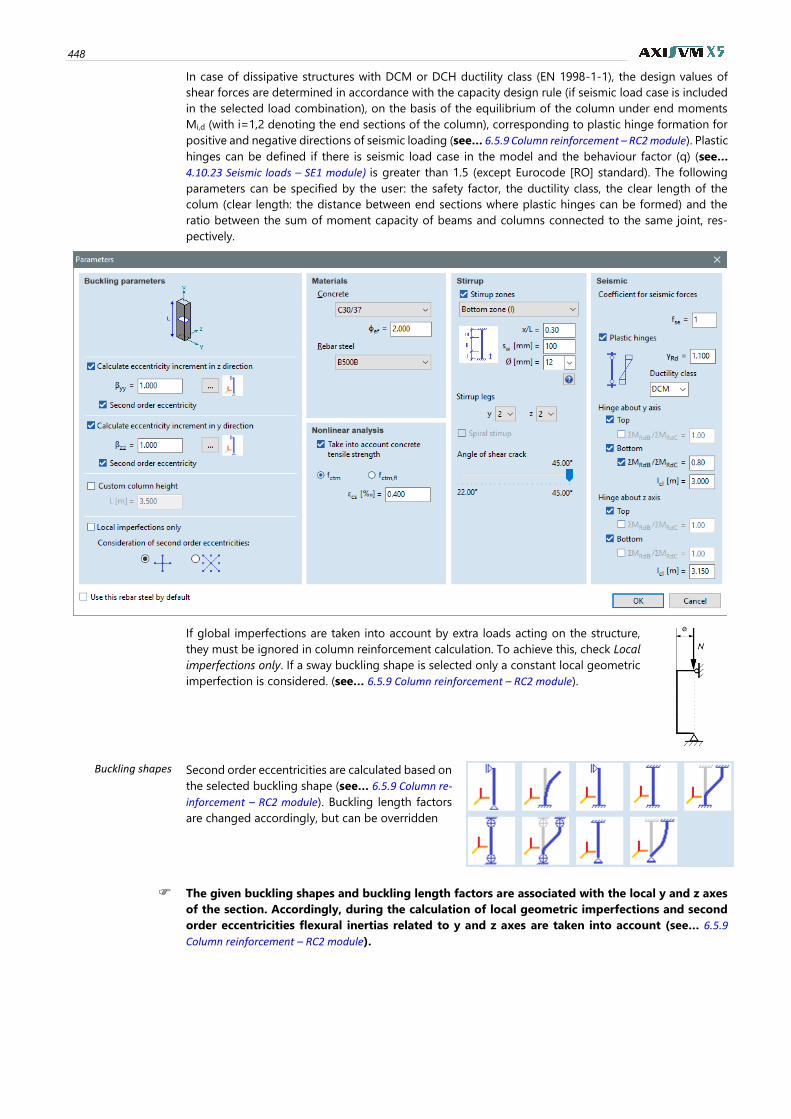
448

In case of dissipative structures with DCM or DCH ductility class (EN 1998-1-1), the design values of

shear forces are determined in accordance with the capacity design rule (if seismic load case is included

in the selected load combination), on the basis of the equilibrium of the column under end moments

Mi,d (with i=1,2 denoting the end sections of the column), corresponding to plastic hinge formation for

positive and negative directions of seismic loading (see… 6.5.9 Column reinforcement – RC2 module). Plastic

hinges can be defined if there is seismic load case in the model and the behaviour factor (q) (see…

4.10.23 Seismic loads – SE1 module) is greater than 1.5 (except Eurocode [RO] standard). The following

parameters can be specified by the user: the safety factor, the ductility class, the clear length of the

colum (clear length: the distance between end sections where plastic hinges can be formed) and the

ratio between the sum of moment capacity of beams and columns connected to the same joint, res-

pectively.

If global imperfections are taken into account by extra loads acting on the structure,

they must be ignored in column reinforcement calculation. To achieve this, check Local

imperfections only. If a sway buckling shape is selected only a constant local geometric

imperfection is considered. (see… 6.5.9 Column reinforcement – RC2 module).

Buckling shapes

Second order eccentricities are calculated based on

the selected buckling shape (see… 6.5.9 Column re-

inforcement – RC2 module). Buckling length factors

are changed accordingly, but can be overridden

The given buckling shapes and buckling length factors are associated with the local y and z axes

of the section. Accordingly, during the calculation of local geometric imperfections and second

order eccentricities flexural inertias related to y and z axes are taken into account (see… 6.5.9

Column reinforcement – RC2 module).

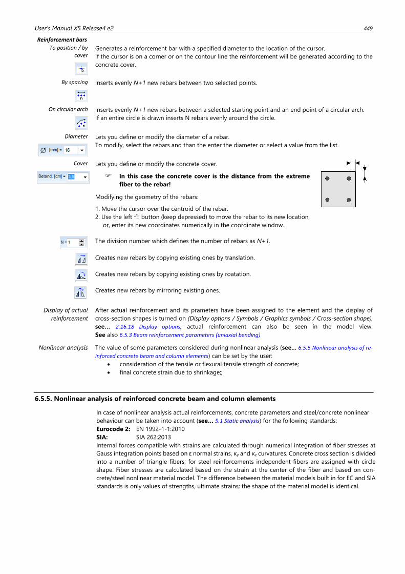
User’s Manual X5 Release4 e2 449

Reinforcement bars

To position / by cover

Generates a reinforcement bar with a specified diameter to the location of the cursor.

If the cursor is on a corner or on the contour line the reinforcement will be generated according to the

concrete cover.

By spacing

Inserts evenly N+1 new rebars between two selected points.

On circular arch

Inserts evenly N+1 new rebars between a selected starting point and an end point of a circular arch.

If an entire circle is drawn inserts N rebars evenly around the circle.

Diameter

Lets you define or modify the diameter of a rebar.

To modify, select the rebars and than the enter the diameter or select a value from the list.

Cover

Lets you define or modify the concrete cover.

In this case the concrete cover is the distance from the extreme

fiber to the rebar!

Modifying the geometry of the rebars:

1. Move the cursor over the centroid of the rebar.

2. Use the left button (keep depressed) to move the rebar to its new location,

or, enter its new coordinates numerically in the coordinate window.

The division number which defines the number of rebars as N+1.

Creates new rebars by copying existing ones by translation.

Creates new rebars by copying existing ones by roatation.

Creates new rebars by mirroring existing ones.

Display of actual

reinforcement

After actual reinforcement and its prameters have been assigned to the element and the display of

cross-section shapes is turned on (Display options / Symbols / Graphics symbols / Cross-section shape),

see… 2.16.18 Display options, actual reinforcement can also be seen in the model view.

See also 6.5.3 Beam reinforcement parameters (uniaxial bending)

Nonlinear analysis The value of some parameters considered during nonlinear analysis (see... 6.5.5 Nonlinear analysis of re-

inforced concrete beam and column elements) can be set by the user:

• consideration of the tensile or flexural tensile strength of concrete;

• final concrete strain due to shrinkage;;

6.5.5. Nonlinear analysis of reinforced concrete beam and column elements

In case of nonlinear analysis actual reinforcements, concrete parameters and steel/concrete nonlinear

behaviour can be taken into account (see… 5.1 Static analysis) for the following standards:

Eurocode 2: EN 1992-1-1:2010

SIA: SIA 262:2013

Internal forces compatible with strains are calculated through numerical integration of fiber stresses at

Gauss integration points based on ε normal strains, κy and κz curvatures. Concrete cross section is divided

into a number of triangle fibers; for steel reinforcements independent fibers are assigned with circle

shape. Fiber stresses are calculated based on the strain at the center of the fiber and based on con-

crete/steel nonlinear material model. The difference between the material models built in for EC and SIA

standards is only values of strengths, ultimate strains; the shape of the material model is identical.

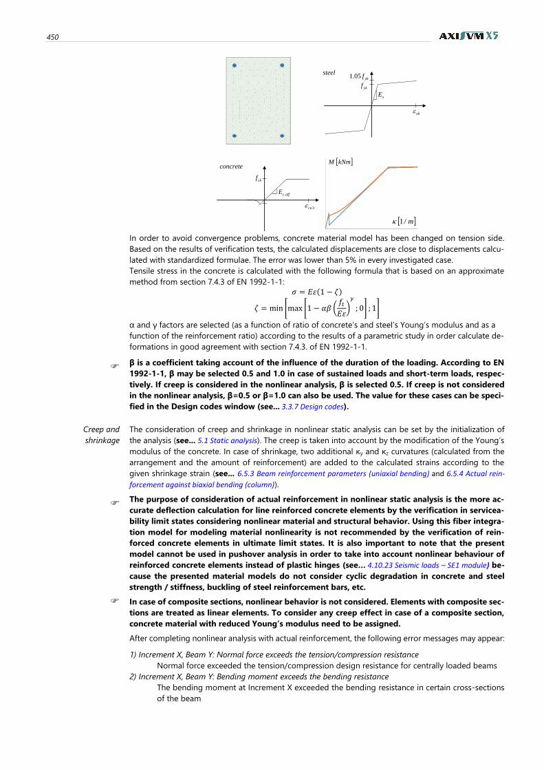
450

In order to avoid convergence problems, concrete material model has been changed on tension side.

Based on the results of verification tests, the calculated displacements are close to displacements calcu-

lated with standardized formulae. The error was lower than 5% in every investigated case.

Tensile stress in the concrete is calculated with the following formula that is based on an approximate

method from section 7.4.3 of EN 1992-1-1:

𝜎 = 𝐸휀(1 − 휁)

휁 = min [max [1 − 𝛼𝛽 (𝑓𝑡𝐸휀)𝛾

; 0] ; 1]

α and γ factors are selected (as a function of ratio of concrete’s and steel’s Young’s modulus and as a

function of the reinforcement ratio) according to the results of a parametric study in order calculate de-

formations in good agreement with section 7.4.3. of EN 1992-1-1.

β is a coefficient taking account of the influence of the duration of the loading. According to EN

1992-1-1, β may be selected 0.5 and 1.0 in case of sustained loads and short-term loads, respec-

tively. If creep is considered in the nonlinear analysis, β is selected 0.5. If creep is not considered

in the nonlinear analysis, β=0.5 or β=1.0 can also be used. The value for these cases can be speci-

fied in the Design codes window (see... 3.3.7 Design codes).

Creep and

shrinkage

The consideration of creep and shrinkage in nonlinear static analysis can be set by the initialization of

the analysis (see... 5.1 Static analysis). The creep is taken into account by the modification of the Young’s

modulus of the concrete. In case of shrinkage, two additional κy and κz curvatures (calculated from the

arrangement and the amount of reinforcement) are added to the calculated strains according to the

given shrinkage strain (see... 6.5.3 Beam reinforcement parameters (uniaxial bending) and 6.5.4 Actual rein-

forcement against biaxial bending (column)).

The purpose of consideration of actual reinforcement in nonlinear static analysis is the more ac-

curate deflection calculation for line reinforced concrete elements by the verification in servicea-

bility limit states considering nonlinear material and structural behavior. Using this fiber integra-

tion model for modeling material nonlinearity is not recommended by the verification of rein-

forced concrete elements in ultimate limit states. It is also important to note that the present

model cannot be used in pushover analysis in order to take into account nonlinear behaviour of

reinforced concrete elements instead of plastic hinges (see… 4.10.23 Seismic loads – SE1 module) be-

cause the presented material models do not consider cyclic degradation in concrete and steel

strength / stiffness, buckling of steel reinforcement bars, etc.

In case of composite sections, nonlinear behavior is not considered. Elements with composite sec-

tions are treated as linear elements. To consider any creep effect in case of a composite section,

concrete material with reduced Young’s modulus need to be assigned.

After completing nonlinear analysis with actual reinforcement, the following error messages may appear:

1) Increment X, Beam Y: Normal force exceeds the tension/compression resistance

Normal force exceeded the tension/compression design resistance for centrally loaded beams

2) Increment X, Beam Y: Bending moment exceeds the bending resistance

The bending moment at Increment X exceeded the bending resistance in certain cross-sections

of the beam

sEykf

ykf05.1

uk

steel

effcE ,

ckf

3cu

concrete kNmM

m/1

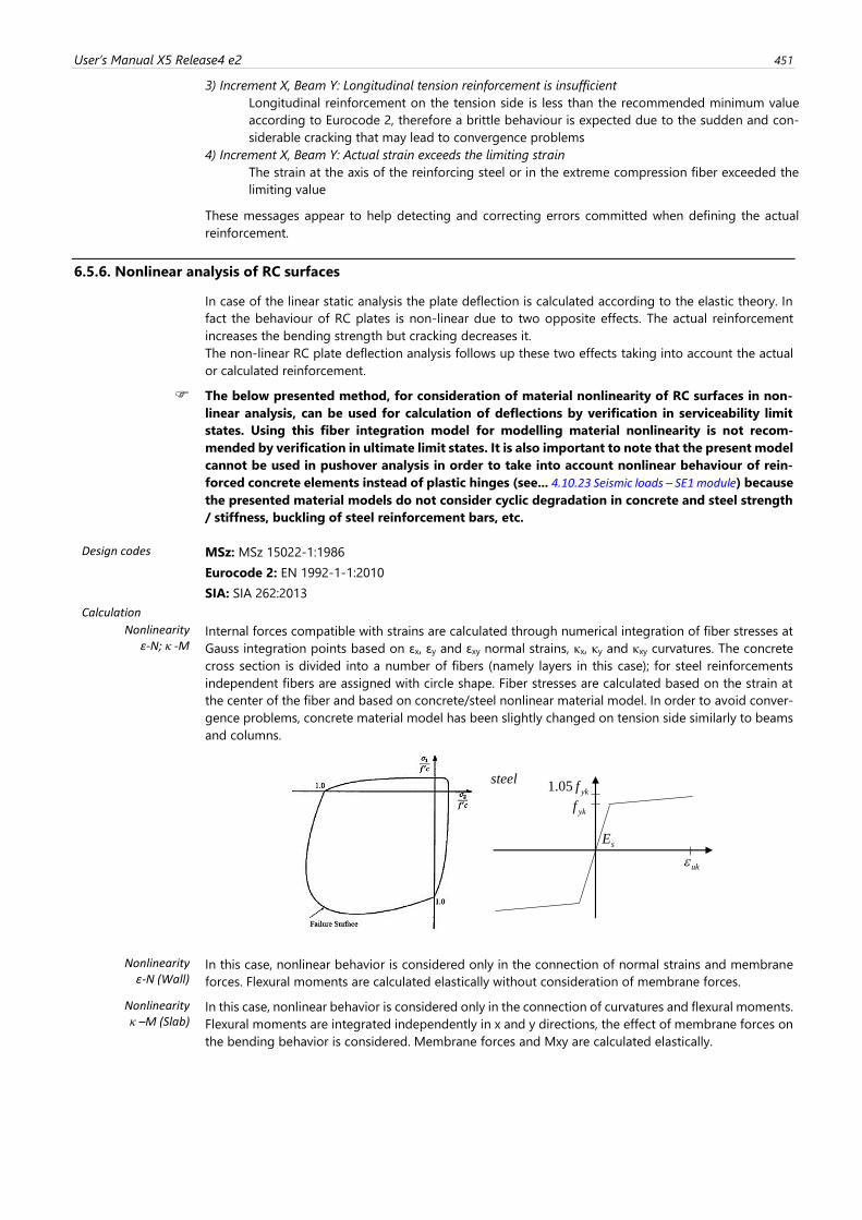
User’s Manual X5 Release4 e2 451

3) Increment X, Beam Y: Longitudinal tension reinforcement is insufficient

Longitudinal reinforcement on the tension side is less than the recommended minimum value

according to Eurocode 2, therefore a brittle behaviour is expected due to the sudden and con-

siderable cracking that may lead to convergence problems

4) Increment X, Beam Y: Actual strain exceeds the limiting strain

The strain at the axis of the reinforcing steel or in the extreme compression fiber exceeded the

limiting value

These messages appear to help detecting and correcting errors committed when defining the actual

reinforcement.

6.5.6. Nonlinear analysis of RC surfaces

In case of the linear static analysis the plate deflection is calculated according to the elastic theory. In

fact the behaviour of RC plates is non-linear due to two opposite effects. The actual reinforcement

increases the bending strength but cracking decreases it.

The non-linear RC plate deflection analysis follows up these two effects taking into account the actual

or calculated reinforcement.

The below presented method, for consideration of material nonlinearity of RC surfaces in non-

linear analysis, can be used for calculation of deflections by verification in serviceability limit

states. Using this fiber integration model for modelling material nonlinearity is not recom-

mended by verification in ultimate limit states. It is also important to note that the present model

cannot be used in pushover analysis in order to take into account nonlinear behaviour of rein-

forced concrete elements instead of plastic hinges (see... 4.10.23 Seismic loads – SE1 module) because

the presented material models do not consider cyclic degradation in concrete and steel strength

/ stiffness, buckling of steel reinforcement bars, etc.

Design codes MSz: MSz 15022-1:1986

Eurocode 2: EN 1992-1-1:2010

SIA: SIA 262:2013

Calculation

Nonlinearity ε-N; κ -M

Internal forces compatible with strains are calculated through numerical integration of fiber stresses at

Gauss integration points based on εx, εy and εxy normal strains, κx, κy and κxy curvatures. The concrete

cross section is divided into a number of fibers (namely layers in this case); for steel reinforcements

independent fibers are assigned with circle shape. Fiber stresses are calculated based on the strain at

the center of the fiber and based on concrete/steel nonlinear material model. In order to avoid conver-

gence problems, concrete material model has been slightly changed on tension side similarly to beams

and columns.

Nonlinearity ε-N (Wall)

In this case, nonlinear behavior is considered only in the connection of normal strains and membrane

forces. Flexural moments are calculated elastically without consideration of membrane forces.

Nonlinearity κ –M (Slab)

In this case, nonlinear behavior is considered only in the connection of curvatures and flexural moments.

Flexural moments are integrated independently in x and y directions, the effect of membrane forces on

the bending behavior is considered. Membrane forces and Mxy are calculated elastically.

sE

ykfykf05.1

uk

steel

effcE ,

ckf

3cu

concrete

4eff,cEctmf

452

In case of slabs with considerable torsion a nonlinear analysis based only on κx-Mx and κy-My

bending behaviour may underestimate the deflection, so it is recommended to use the first ε-

N; κ-M complex model. That can follow nonlinear behaviour related to the six strain and internal

force components.

In case of κ-M nonlinearity model, in order to calculate more realistic deformations, torsion

stiffness in the stiffness matrix is considered on a reduced value if the surface is cracked at a

specific point in both x and y main directions. If the height of cracked zone is considerable

(>0.5H), torsion stiffness is considered on 15% of the original elastic value. Linearly interpolated

value is used between the two states.

The nonlinear analysis of skewly reinforced concrete surfaces is not allowed. These surfaces are

treated as materially linear elements without the consideration of cracking and the effect of

reinforcement. The Young’s modulus is calculated with the consideration of the defined creep

factor.

Amount of rein-forcement

Actual or calculated reinforcement can be taken into account in nonlinear static analysis by choosing

Use reinforcement in calculation in the Nonlinear static analysis dialog (see... 5.1 Static analysis). The

convergence of such nonlinear analyses is sensitive to the amount of reinforcement. In order to avoid

convergence problems, AxisVM applies the minimum reinforcement prescribed by the design code

where (top or bottom) actual reinforcement is defined only in one direction. The convergence is usually

better in case of actual reinforcement. It is recommended to use the Take into account the minimum

required reinforcement option while defining reinforcement parameters to surfaces (see... 6.5.1 Surface

reinforcement parameters and reinforcement calculation - RC1 module)

Elements within the contour of columns

If Adjust mesh to column heads option is selected by domain meshing, finite elements within the con-

tour of RC columns can be identified. In order to avoid convergence problems, nonlinear behavior of

these elements is neglected in the calculation.

Creep and shrink-age

The consideration of creep and shrinkage in nonlinear static analysis can be set by the initialization of

the analysis (see... 5.1 Static analysis). The creep is taken into account by the modification of the con-

crete’s Young’s modulus. The shrinkage is considered only in flexural deformations.

Nonlinearity ε-N; κ -M

Two calculated (based on the arrangement and the amount of reinforcement and on the state of RC

section) shrinkage induced curvatures (namely κx and κy) are added to the calculated strains according

to the given shrinkage strain (see... 6.5.1 Surface reinforcement parameters and reinforcement calculation -

RC1 module).

Nonlinearity ε-N (Wall)

The reinforcement in walls is typically symmetrical, thus shrinkage curvatures are not taken into account

in this case.

Nonlinearity κ –M (Slab)

Two calculated (based on the arrangement and the amount of reinforcement and on the state of RC

section) shrinkage induced are added to the calculated strains according to the given shrinkage strain.

Warning messages After completing nonlinear analysis with actual reinforcement, the following warning messages may

appear:

• “Normal force exceeds the resistance.”

• ”Actual strain exceeds the limiting strain.”

(Note: In case of the reinforcement or concrete in compression)

6.5.7. Cracking

Design Codes Eurocode 2:

DIN:

EN 1992-1-1:2004

DIN 1045-1:2001-07

After the assignment of the actual reinforcement the program calculates the

crack width and crack directions in the membrane, plate and shell elements.

The calculation can be perfromed with reinforcement directions relative to the

surface element’s local x and y axes or with arbitrary ξ and η reinforcement

directions. The program displays the crack openings in a color coded mode,

can draw the crack map and the crack angles.

The set of the parameters can be seen in the previous section.

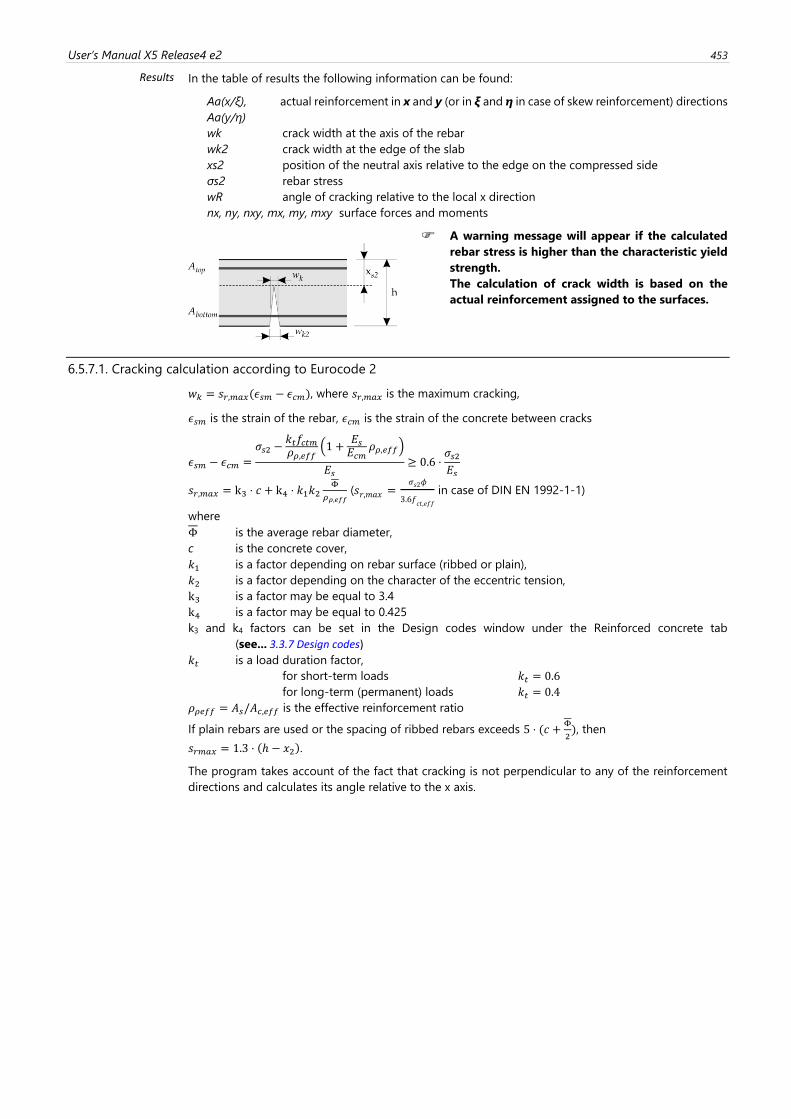
User’s Manual X5 Release4 e2 453

Results In the table of results the following information can be found:

Aa(x/ξ),

Aa(y/η)

actual reinforcement in x and y (or in ξ and η in case of skew reinforcement) directions

wk crack width at the axis of the rebar

wk2 crack width at the edge of the slab

xs2 position of the neutral axis relative to the edge on the compressed side

σs2 rebar stress

wR angle of cracking relative to the local x direction

nx, ny, nxy, mx, my, mxy surface forces and moments

A warning message will appear if the calculated

rebar stress is higher than the characteristic yield

strength.

The calculation of crack width is based on the

actual reinforcement assigned to the surfaces.

6.5.7.1. Cracking calculation according to Eurocode 2

𝑤𝑘 = 𝑠𝑟,𝑚𝑎𝑥(𝜖𝑠𝑚 − 𝜖𝑐𝑚), where 𝑠𝑟,𝑚𝑎𝑥 is the maximum cracking,

𝜖𝑠𝑚 is the strain of the rebar, 𝜖𝑐𝑚 is the strain of the concrete between cracks

𝜖𝑠𝑚 − 𝜖𝑐𝑚 =

𝜎𝑠2 −𝑘𝑡𝑓𝑐𝑡𝑚𝜌𝜌,𝑒𝑓𝑓

(1 +𝐸𝑠𝐸𝑐𝑚

𝜌𝜌,𝑒𝑓𝑓)

𝐸𝑠≥ 0.6 ⋅

𝜎𝑠2𝐸𝑠

𝑠𝑟,𝑚𝑎𝑥 = k3 ⋅ 𝑐 + k4 ⋅ 𝑘1𝑘2Φ

𝜌𝜌,𝑒𝑓𝑓 (𝑠𝑟,𝑚𝑎𝑥 =

𝜎𝑠2𝜙

3.6𝑓𝑐𝑡,𝑒𝑓𝑓

in case of DIN EN 1992-1-1)

where

Φ is the average rebar diameter,

c is the concrete cover,

𝑘1 is a factor depending on rebar surface (ribbed or plain),

𝑘2 is a factor depending on the character of the eccentric tension,

k3 is a factor may be equal to 3.4

k4 is a factor may be equal to 0.425

k3 and k4 factors can be set in the Design codes window under the Reinforced concrete tab

(see... 3.3.7 Design codes)

𝑘𝑡 is a load duration factor,

for short-term loads 𝑘𝑡 = 0.6

for long-term (permanent) loads 𝑘𝑡 = 0.4

𝜌𝜌𝑒𝑓𝑓 = 𝐴𝑠/𝐴𝑐,𝑒𝑓𝑓 is the effective reinforcement ratio

If plain rebars are used or the spacing of ribbed rebars exceeds 5 ⋅ (𝑐 +Φ

2), then

𝑠𝑟𝑚𝑎𝑥 = 1.3 ⋅ (ℎ − 𝑥2).

The program takes account of the fact that cracking is not perpendicular to any of the reinforcement

directions and calculates its angle relative to the x axis.

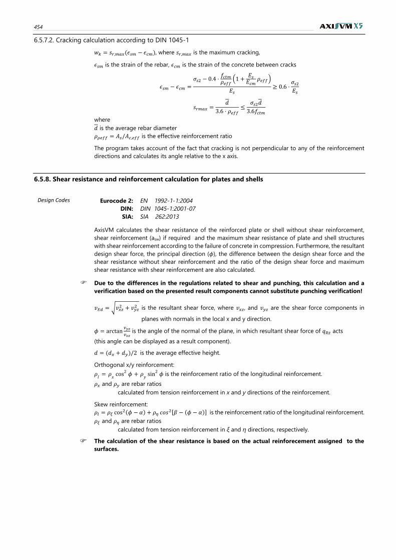
454

6.5.7.2. Cracking calculation according to DIN 1045-1

𝑤𝑘 = 𝑠𝑟,𝑚𝑎𝑥(𝜖𝑠𝑚 − 𝜖𝑐𝑚), where 𝑠𝑟,𝑚𝑎𝑥 is the maximum cracking,

𝜖𝑠𝑚 is the strain of the rebar, 𝜖𝑐𝑚 is the strain of the concrete between cracks

𝜖𝑠𝑚 − 𝜖𝑐𝑚 =

𝜎𝑠2 − 0.4 ⋅𝑓𝑐𝑡𝑚𝜌𝑒𝑓𝑓

(1 +𝐸𝑠𝐸𝑐𝑚

𝜌𝑒𝑓𝑓)

𝐸𝑠≥ 0.6 ⋅

𝜎𝑠2𝐸𝑠

𝑠𝑟𝑚𝑎𝑥 =𝑑

3.6 ⋅ 𝜌𝑒𝑓𝑓≤

𝜎𝑠2𝑑

3.6𝑓𝑐𝑡𝑚

where

𝑑 is the average rebar diameter

𝜌𝜌𝑒𝑓𝑓 = 𝐴𝑠/𝐴𝑐,𝑒𝑓𝑓 is the effective reinforcement ratio

The program takes account of the fact that cracking is not perpendicular to any of the reinforcement

directions and calculates its angle relative to the x axis.

6.5.8. Shear resistance and reinforcement calculation for plates and shells

Design Codes Eurocode 2: EN 1992-1-1:2004

DIN: DIN 1045-1:2001-07

SIA: SIA 262:2013

AxisVM calculates the shear resistance of the reinforced plate or shell without shear reinforcement,

shear reinforcement (asw) if required and the maximum shear resistance of plate and shell structures

with shear reinforcement according to the failure of concrete in compression. Furthermore, the resultant

design shear force, the principal direction (𝜙), the difference between the design shear force and the

shear resistance without shear reinforcement and the ratio of the design shear force and maximum

shear resistance with shear reinforcement are also calculated.

Due to the differences in the regulations related to shear and punching, this calculation and a

verification based on the presented result components cannot substitute punching verification!

𝑣𝐸𝑑 = √𝑣𝑥𝑧

2 + 𝑣𝑦𝑧2 is the resultant shear force, where 𝑣𝑥𝑧, and 𝑣𝑦𝑧 are the shear force components in

planes with normals in the local x and y direction.

𝜙 = arctan𝑣𝑦𝑧

𝑣𝑥𝑧 is the angle of the normal of the plane, in which resultant shear force of 𝑞𝑅𝑧 acts

(this angle can be displayed as a result component).

𝑑 = (𝑑𝑥 + 𝑑𝑦)/2 is the average effective height.

Orthogonal x/y reinforcement:

𝜌𝑙= 𝜌

𝑥cos2 𝜙 + 𝜌

𝑦sin2 𝜙 is the reinforcement ratio of the longitudinal reinforcement.

𝜌𝑥 and 𝜌𝑦 are rebar ratios

calculated from tension reinforcement in x and y directions of the reinforcement.

Skew reinforcement:

𝜌𝑙 = 𝜌𝜉 cos2(𝜙 − 𝛼) + 𝜌𝜂 𝑐𝑜𝑠

2[𝛽 − (𝜙 − 𝛼)] is the reinforcement ratio of the longitudinal reinforcement.

𝜌𝜉 and 𝜌𝜂 are rebar ratios

calculated from tension reinforcement in ξ and η directions, respectively.

The calculation of the shear resistance is based on the actual reinforecement assigned to the

surfaces.

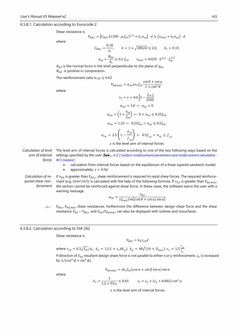
User’s Manual X5 Release4 e2 455

6.5.8.1. Calculation according to Eurocode 2

Shear resistance is

𝑉𝑅𝑑,𝑐 = [𝐶𝑅𝑑,𝑐𝑘(100 ⋅ 𝜌𝑙𝑓𝑐𝑘)1/3 + 𝑘1𝜎𝑐𝑝] ⋅ 𝑑 ≥ (𝑣𝑚𝑖𝑛 + 𝑘1𝜎𝑐𝑝) ⋅ 𝑑

where

𝐶𝑅𝑑,𝑐 =0.18

𝛾𝑐, 𝑘 = 1 + √200/𝑑 ≤ 2.0, 𝑘1 = 0.15

𝜎𝑐𝑝 =𝑁𝐸𝑑𝐴𝑐

≤ 0.2 𝑓𝑐𝑑 , 𝑣𝑚𝑖𝑛 = 0.035 ⋅ 𝑘3/2 ⋅ 𝑓𝑐𝑘1/2

𝑁𝐸𝑑 is the normal force in the shell perpendicular to the plane of 𝑞𝑅𝑧 .

𝑁𝐸𝑑 is positive in compression.

The reinforcement ratio is 𝜌𝑙 ≤ 0.02

𝑉𝑅𝑑,𝑚𝑎𝑥 = 𝛼𝑐𝑤𝑧𝜈1𝑓𝑐𝑑cot 휃 + cot 𝛼

1 + cot2 휃

where

𝜈1 = 𝜈 = 0.6 [1 −𝑓𝑐𝑘250

]

𝛼𝑐𝑤 = 1.0 ← 𝜎𝑐𝑝 = 0

𝛼𝑐𝑤 = (1 +𝜎𝑐𝑝

𝑓𝑐𝑑) ← 0 < 𝜎𝑐𝑝 ≤ 0.25𝑓𝑐𝑑

𝛼𝑐𝑤 = 1.25 ← 0.25𝑓𝑐𝑑 < 𝜎𝑐𝑝 ≤ 0.5𝑓𝑐𝑑

𝛼𝑐𝑤 = 2.5(1 −𝜎𝑐𝑝

𝑓𝑐𝑑

) ← 0.5𝑓𝑐𝑑< 𝜎𝑐𝑝 ≤ 𝑓

𝑐𝑑

𝑧 is the level arm of internal forces

Calculation of level

arm of internal

forces

The level arm of internal forces is calculated according to one of the two following ways based on the

settings specified by the user (See... 6.5.1 Surface reinforcement parameters and reinforcement calculation -

RC1 module) :

• calculation from internal forces based on the equilibrium of a three-layered sandwich model;

• approximately: 𝑧 = 0.9𝑑

Calculation of re-

quired shear rein-

forcement

If 𝑣𝐸𝑑 is greater than 𝑉𝑅𝑑,𝑐, shear reinforcement is required to resist shear forces. The required reinforce-

ment (e.g. [mm2/m2]) is calculated with the help of the following formula. If 𝑣𝐸𝑑 is greater than 𝑉𝑅𝑑,𝑚𝑎𝑥 ,

the section cannot be reinforced against shear force. In these cases, the software warns the user with a

warning message.

𝑎𝑠𝑤 =𝑣𝐸𝑑

𝑧𝑓𝑦𝑤𝑑1𝑚[(cot 휃 + cot 𝛼) sin 𝛼]

𝑉𝑅𝑑,𝑐 , 𝑉𝑅𝑑,𝑚𝑎𝑥 shear resistances, furthermore the difference between design shear force and the shear

resistance 𝑉𝐸𝑑 − 𝑉𝑅𝑑,𝑐 and 𝑉𝐸𝑑/𝑉𝑅𝑑,𝑚𝑎𝑥 can also be displayed with isolines and isosurfaces.

6.5.8.2. Calculation according to SIA 262

Shear resistance is

𝑉𝑅𝑑𝑐 = 𝑘𝑑𝜏𝑐𝑑𝑑

where 𝜏𝑐𝑑 = 0.3√𝑓𝑐𝑘/𝛾𝑐; 𝑘𝑑 = 1/(1 + 휀𝑣𝑑𝑘𝑔); 𝑘𝑔 = 48 (16 + 𝐷𝑚𝑎𝑥)⁄ ; 휀𝑣 = 1,5𝑓𝑠𝑑

𝐸𝑠.

If direction of 𝑉𝐸𝑑 resultant design share force is not parallel to either x or y reinforcement, 휀𝑣 is increased

by 1/(cos4 𝜙 + sin4 𝜙).

𝑉𝑅𝑑,𝑚𝑎𝑥 = 𝑧𝑘𝑐𝑓𝑐𝑑(cos 𝛼 + cot 𝛽 sin 𝛼) sin 𝛼

where

𝑘𝑐 =1

1.2 + 55휀1≤ 0.65 휀1 = 휀𝑥 + (휀𝑥 + 0.002) cot

2 𝛼

𝑧 is the level arm of internal forces

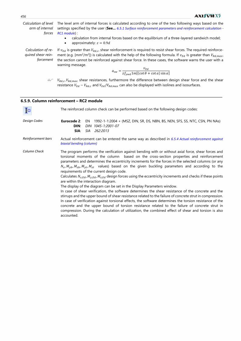
456

Calculation of level

arm of internal

forces

The level arm of internal forces is calculated according to one of the two following ways based on the

settings specified by the user (See... 6.5.1 Surface reinforcement parameters and reinforcement calculation -

RC1 module) :

• calculation from internal forces based on the equilibrium of a three-layered sandwich model;

• approximately: 𝑧 = 0.9𝑑

Calculation of re-

quired shear rein-

forcement

If 𝑣𝐸𝑑 is greater than 𝑉𝑅𝑑,𝑐, shear reinforcement is required to resist shear forces. The required reinforce-

ment (e.g. [mm2/m2]) is calculated with the help of the following formula. If 𝑣𝐸𝑑 is greater than 𝑉𝑅𝑑,𝑚𝑎𝑥 ,

the section cannot be reinforced against shear force. In these cases, the software warns the user with a

warning message.

𝑎𝑠𝑤 =𝑣𝐸𝑑

𝑧𝑓𝑦𝑤𝑑1𝑚[(cot 휃 + cot 𝛼) sin 𝛼]

𝑉𝑅𝑑,𝑐 , 𝑉𝑅𝑑,𝑚𝑎𝑥 shear resistances, furthermore the difference between design shear force and the shear

resistance 𝑉𝐸𝑑 − 𝑉𝑅𝑑,𝑐 and 𝑉𝐸𝑑/𝑉𝑅𝑑,𝑚𝑎𝑥 can also be displayed with isolines and isosurfaces.

6.5.9. Column reinforcement – RC2 module

The reinforced column check can be performed based on the following design codes:

Design Codes Eurocode 2: EN 1992-1-1:2004 + (MSZ, DIN, SR, DS, NBN, BS, NEN, SFS, SS, NTC, CSN, PN NAs)

DIN: DIN 1045-1:2001-07

SIA: SIA 262:2013

Reinforcement bars Actual reinforcement can be entered the same way as described in 6.5.4 Actual reinforcement against biaxial bending (column)

Column Check The program performs the verification against bending with or without axial force, shear forces and

torsional moments of the column based on the cross-section properties and reinforcement

parameters and determines the eccentricity increments for the forces in the selected columns (or any

𝑁𝑥, 𝑀𝑦𝑏 , 𝑀𝑧𝑏, 𝑀𝑦𝑡, 𝑀𝑧𝑡 values) based on the given buckling parameters and according to the

requirements of the current design code.

Calculates 𝑁𝑥,𝐸𝑑 ,𝑀𝑦,𝐸𝑑 ,𝑀𝑧,𝐸𝑑 design forces using the eccentricity increments and checks if these points

are within the interaction diagram.

The display of the diagram can be set in the Display Parameters window.

In case of shear verification, the software determines the shear resistance of the concrete and the

stirrups and the upper bound of shear resistance related to the failure of concrete strut in compression.

In case of verification against torsional effects, the software determines the torsion resistance of the

concrete and the upper bound of torsion resistance related to the failure of concrete strut in

compression. During the calculation of utilization, the combined effect of shear and torsion is also

accounted.

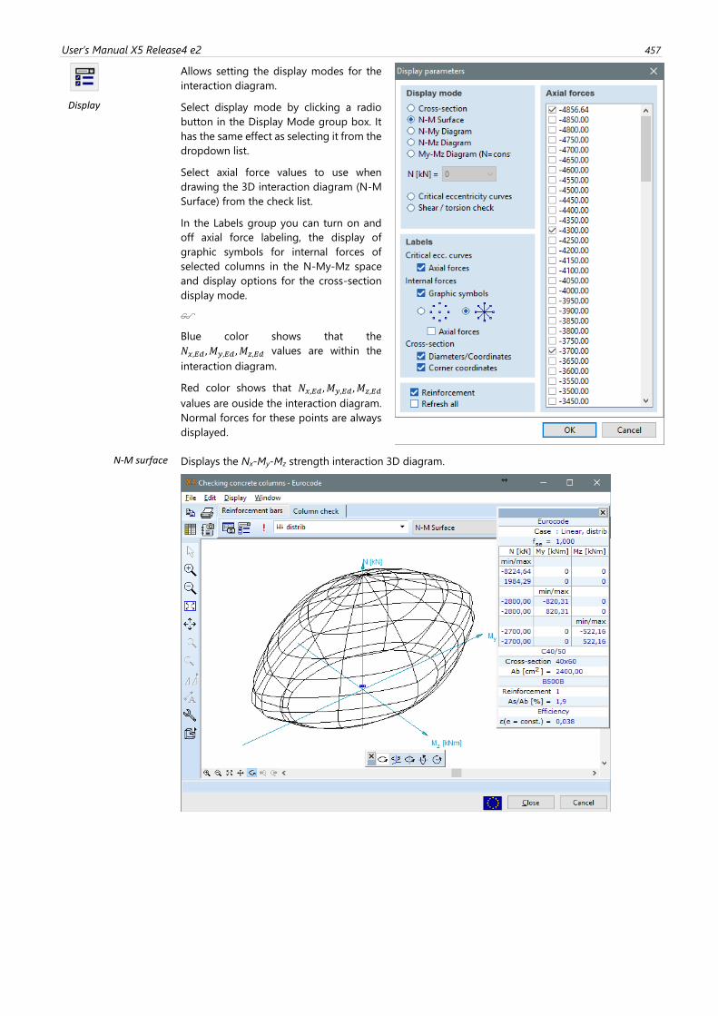
User’s Manual X5 Release4 e2 457

Display

Allows setting the display modes for the

interaction diagram.

Select display mode by clicking a radio

button in the Display Mode group box. It

has the same effect as selecting it from the

dropdown list.

Select axial force values to use when

drawing the 3D interaction diagram (N-M

Surface) from the check list.

In the Labels group you can turn on and

off axial force labeling, the display of

graphic symbols for internal forces of

selected columns in the N-My-Mz space

and display options for the cross-section

display mode.

Blue color shows that the

𝑁𝑥,𝐸𝑑 ,𝑀𝑦,𝐸𝑑 ,𝑀𝑧,𝐸𝑑 values are within the

interaction diagram.

Red color shows that 𝑁𝑥,𝐸𝑑 ,𝑀𝑦,𝐸𝑑 ,𝑀𝑧,𝐸𝑑

values are ouside the interaction diagram.

Normal forces for these points are always

displayed.

N-M surface Displays the Nx-My-Mz strength interaction 3D diagram.

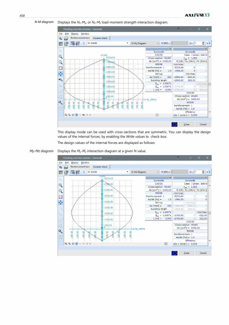
458

N-M diagram Displays the Nx-My, or Nx-Mz load-moment strength interaction diagram.

This display mode can be used with cross-sections that are symmetric. You can display the design

values of the internal forces, by enabling the Write values to check-box.

The design values of the internal forces are displayed as follows:

My-Mz diagram Displays the My-Mz interaction diagram at a given N value.

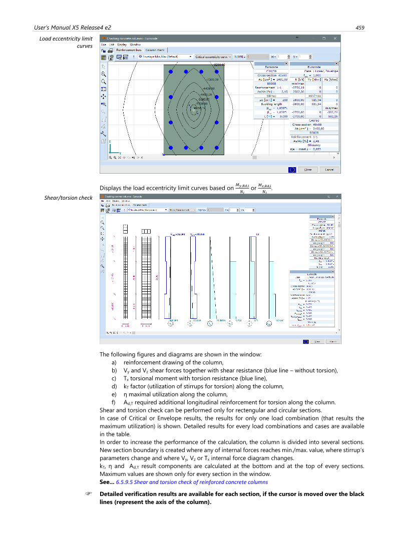
User’s Manual X5 Release4 e2 459

Load eccentricity limit curves

Displays the load eccentricity limit curves based on 𝑀𝑦,𝑅𝑑,𝑖

𝑁𝑖 or

𝑀𝑧,𝑅𝑑,𝑖

𝑁𝑖.

Shear/torsion check

The following figures and diagrams are shown in the window:

a) reinforcement drawing of the column,

b) Vy and Vz shear forces together with shear resistance (blue line – without torsion),

c) Tx torsional moment with torsion resistance (blue line),

d) kT factor (utilization of stirrups for torsion) along the column,

e) η maximal utilization along the column,

f) Asl,T required additional longitudinal reinforcement for torsion along the column.

Shear and torsion check can be performed only for rectengular and circular sections.

In case of Critical or Envelope results, the results for only one load combination (that results the

maximum utilization) is shown. Detailed results for every load combinations and cases are available

in the table.

In order to increase the performance of the calculation, the column is divided into several sections.

New section boundary is created where any of internal forces reaches min./max. value, where stirrup’s

parameters change and where Vy, Vz or Tx internal force diagram changes.

kT, η and Asl,T result components are calculated at the bottom and at the top of every sections.

Maximum values are shown only for every section in the window.

See... 6.5.9.5 Shear and torsion check of reinforced concrete columns

Detailed verification results are available for each section, if the cursor is moved over the black

lines (represent the axis of the column).

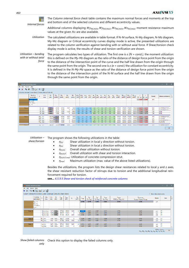
460

Internal forces

The Column internal force check table contains the maximum normal forces and moments at the top

and bottom end of the selected columns and different eccentricity values.

Additional columns displaying 𝑀𝑦𝑅𝑑,𝑚𝑖𝑛 , 𝑀𝑦𝑅𝑑,𝑚𝑎𝑥 , 𝑀𝑧𝑅𝑑,𝑚𝑖𝑛 , 𝑀𝑧𝑅𝑑,𝑚𝑎𝑥 moment resistance maximum

values at the given 𝑁𝑥 are also available.

Utilization The calculated utilizations are available in table format. If N-M surface, N-My diagram, N-Mz diagram,

My-Mz diagram or Critical eccentricity curves display mode is active, the presented utilizations are

related to the column verification against bending with or without axial force. If Shear/torsion check

display mode is active, the results of shear and torsion verification are shown.

Utilization – bending with or without axial

force

The program calculates two types of utilization. The first one is ε (N = const.), the moment utilization:

this is defined on the My-Mz diagram as the ratio of the distance of design force point from the origin

to the distance of the intersection point of the curve and the half line drawn from the origin through

the same point from the origin. The second one is ε (e = const.) the utilization for constant eccentricity.

It is defined in the N-My-Mz space as the ratio of the distance of design force point from the origin

to the distance of the intersection point of the N-M surface and the half line drawn from the origin

through the same point from the origin.

Utilization – shear/torsion

The program shows the following utilizations in the table:

• ηVy: Shear utilization in local y direction without torsion.

• ηVz: Shear utilization in local z direction without torsion.

• ηVyVz: Overall shear utilization without torsion.

• ηVyVzT: Overall utilization with shear and torsion interaction.

• ηVyVzT,max: Utilization of concrete compression strut.

• ηmax: Maximum utilization (max. value of the above listed utilizations).

Besides the utilizations, the program lists the design shear resistances related to local y and z axes,

the shear resistant reduction factor of stirrups due to torsion and the additional longitudinal rein-

forcement required for torsion.

see... 6.5.9.5 Shear and torsion check of reinforced concrete columns

Show failed columns only

Check this option to display the failed columns only.

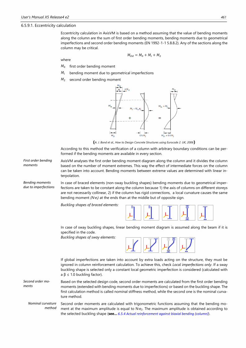
User’s Manual X5 Release4 e2 461

6.5.9.1. Eccentricity calculation

Eccentricity calculation in AxisVM is based on a method assuming that the value of bending moments

along the column are the sum of first order bending moments, bending moments due to geometrical

imperfections and second order bending moments (EN 1992-1-1 5.8.8.2). Any of the sections along the

column may be critical.

𝑀𝐸𝑑 = 𝑀0 +𝑀𝑖 +𝑀2

where

𝑀0 first order bending moment

𝑀𝑖 bending moment due to geometrical imperfections

𝑀2 second order bending moment

(A. J. Bond et al., How to Design Concrete Structures using Eurocode 2. UK, 2006)

According to this method the verification of a column with arbitrary boundary conditions can be per-

formed if the bending moments are available in every section.

First order bending moments

AxisVM analyses the first order bending moment diagram along the column and it divides the column

based on the number of moment extremes. This way the effect of intermediate forces on the column

can be taken into account. Bending moments between extreme values are determined with linear in-

terpolation.

Bending moments due to imperfections

In case of braced elements (non-sway buckling shapes) bending moments due to geometrical imper-

fections are taken to be constant along the column because 1) the axis of columns on different storeys

are not necessarily collinear, 2) if the column has rigid connections, a local curvature causes the same

bending moment (N·ei) at the ends than at the middle but of opposite sign.

Buckling shapes of braced elements:

In case of sway buckling shapes, linear bending moment diagram is assumed along the beam if it is

specified in the code.

Buckling shapes of sway elements:

If global imperfections are taken into account by extra loads acting on the structure, they must be

ignored in column reinforcement calculation. To achieve this, check Local imperfections only. If a sway

buckling shape is selected only a constant local geometric imperfection is considered (calculated with

a β ≤ 1.0 buckling factor).

Second order mo-ments

Based on the selected design code, second order moments are calculated from the first order bending

moments (extended with bending moments due to imperfections) or based on the buckling shape. The

first calculation method is called nominal stiffness method, while the second one is the nominal curva-

ture method.

Nominal curvature method

Second order moments are calculated with trigonometric functions assuming that the bending mo-

ment at the maximum amplitude is equal to N·e2. The maximum amplitude is obtained according to

the selected buckling shape (see... 6.5.4 Actual reinforcement against biaxial bending (column)).

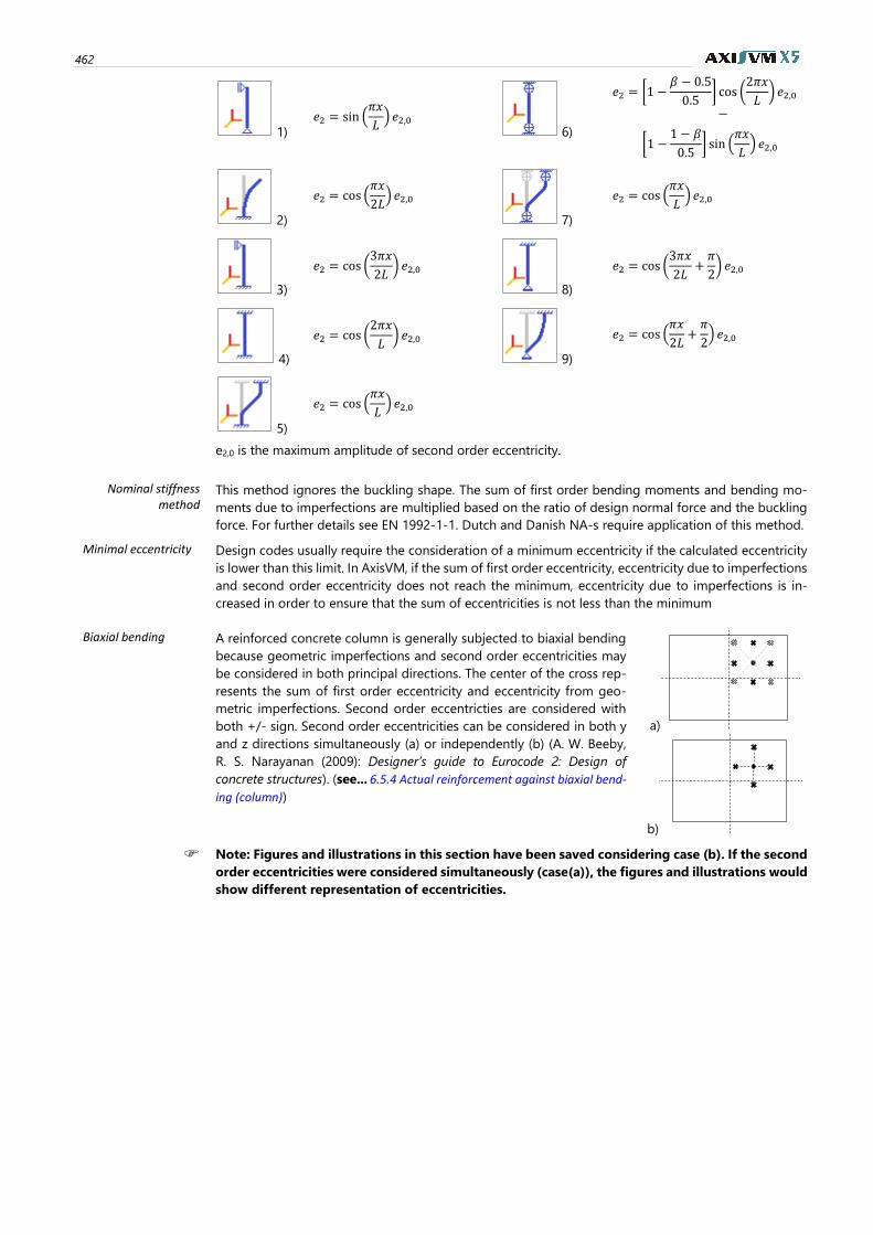
462

1) 𝑒2 = sin (

𝜋𝑥

𝐿) 𝑒2,0

6)

𝑒2 = [1 −𝛽 − 0.5

0.5] cos (

2𝜋𝑥

𝐿) 𝑒2,0

−

[1 −1 − 𝛽

0.5] sin (

𝜋𝑥

𝐿)𝑒2,0

2)

𝑒2 = cos (𝜋𝑥

2𝐿) 𝑒2,0

7)

𝑒2 = cos (𝜋𝑥

𝐿)𝑒2,0

3)

𝑒2 = cos (3𝜋𝑥

2𝐿) 𝑒2,0

8)

𝑒2 = cos (3𝜋𝑥

2𝐿+𝜋

2) 𝑒2,0

4)

𝑒2 = cos (2𝜋𝑥

𝐿) 𝑒2,0

9)

𝑒2 = cos (𝜋𝑥

2𝐿+𝜋

2) 𝑒2,0

5)

𝑒2 = cos (𝜋𝑥

𝐿) 𝑒2,0

e2,0 is the maximum amplitude of second order eccentricity.

Nominal stiffness method

This method ignores the buckling shape. The sum of first order bending moments and bending mo-

ments due to imperfections are multiplied based on the ratio of design normal force and the buckling

force. For further details see EN 1992-1-1. Dutch and Danish NA-s require application of this method.

Minimal eccentricity Design codes usually require the consideration of a minimum eccentricity if the calculated eccentricity

is lower than this limit. In AxisVM, if the sum of first order eccentricity, eccentricity due to imperfections

and second order eccentricity does not reach the minimum, eccentricity due to imperfections is in-

creased in order to ensure that the sum of eccentricities is not less than the minimum

Biaxial bending A reinforced concrete column is generally subjected to biaxial bending

because geometric imperfections and second order eccentricities may

be considered in both principal directions. The center of the cross rep-

resents the sum of first order eccentricity and eccentricity from geo-

metric imperfections. Second order eccentricties are considered with

both +/- sign. Second order eccentricities can be considered in both y

and z directions simultaneously (a) or independently (b) (A. W. Beeby,

R. S. Narayanan (2009): Designer’s guide to Eurocode 2: Design of

concrete structures). (see... 6.5.4 Actual reinforcement against biaxial bend-

ing (column))

a)

b)

Note: Figures and illustrations in this section have been saved considering case (b). If the second

order eccentricities were considered simultaneously (case(a)), the figures and illustrations would

show different representation of eccentricities.

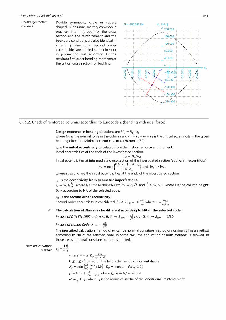
User’s Manual X5 Release4 e2 463

Double symmetric columns

Double symmetric, circle or square

shaped RC columns are very common in

practice. If Ix = Iy both for the cross

section and the reinforcement and the

boundary conditions are also identical in

x and y directions, second order

eccentricities are applied neither in x nor

in y direction but according to the

resultant first order bending moments at

the critical cross section for buckling.

6.5.9.2. Check of reinforced columns according to Eurocode 2 (bending with axial force)

Design moments in bending directions are 𝑀𝑑 = 𝑁𝑑 ⋅ 𝑒𝑑

where Nd is the normal force in the column and 𝑒𝑑 = 𝑒𝑒 + 𝑒𝑖 + 𝑒2 is the critical eccentricity in the given

bending direction. Minimal eccentricity: max (20 mm, h/30).

𝑒𝑒 is the initial eccentricity calculated from the first order force and moment.

Initial eccentricities at the ends of the investigated section:

𝑒𝑒 = 𝑀𝐼/𝑁𝑑

Initial eccentricities at intermediate cross-section of the investigated section (equivalent eccentricity):

𝑒𝑒 = max {0.6 ⋅ 𝑒𝑎 + 0.4 ⋅ 𝑒𝑏

0.4 ⋅ 𝑒𝑎} and |𝑒𝑎| ≥ |𝑒𝑏|,

where 𝑒𝑎 and 𝑒𝑏 are the initial eccentricities at the ends of the investigated section.

𝑒𝑖 is the eccentricity from geometric imperfections.

𝑒𝑖 = 𝛼ℎΘ0𝑙0

2 , where 𝑙0 is the buckling length, 𝛼ℎ = 2/√𝑙 and

2

3≤ 𝛼ℎ ≤ 1, where l is the column height.

Θ0 – according to NA of the selected code.

𝑒2 is the second order eccentricity.

Second order eccentricity is considered if 𝜆 ≥ 𝜆𝑙𝑖𝑚 = 20𝐴𝐵𝐶

√𝑛 where 𝑛 =

𝑁𝐸𝑑

𝐴𝑐𝑓𝑐𝑑

The calculation of λlim may be different according to NA of the selected code!

In case of DIN EN 1992-1-1: 𝑛 < 0.41 → 𝜆𝑙𝑖𝑚 =16

√𝑛; 𝑛 > 0.41 → 𝜆𝑙𝑖𝑚 = 25.0

In case of Italian Code: 𝜆𝑙𝑖𝑚 =25

√𝑛

The prescribed calculation method of 𝒆𝟐 can be nominal curvature method or nominal stiffness method

according to NA of the selected code. In some NAs, the application of both methods is allowed. In

these cases, nominal curvature method is applied.

Nominal curvature method 𝑒2 =

1

𝑟

𝑙02

𝑐

where 1

𝑟= 𝐾𝑟𝐾𝜑

𝑓𝑦𝑑

𝐸𝑠⋅0.45⋅𝑑′

8 ≤ 𝑐 ≤ 𝜋2 based on the first order bending moment diagram

𝐾𝑟 = min {𝑁𝑢′−𝑁𝐸𝑑

𝑁𝑢′−𝑁𝑏𝑎𝑙

; 1.0} , 𝐾𝜑 = max{1 + 𝛽𝜑𝑒𝑓; 1.0},

𝛽 = 0.35 +𝑓𝑐𝑘

200−

𝜆

150, where 𝑓𝑐𝑘 is in N/mm2 unit

𝑑′ =ℎ

2+ 𝑖𝑠 , where 𝑖𝑠 is the radius of inertia of the longitudinal reinforcement

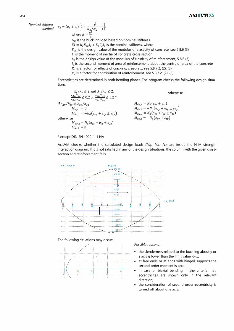
464

Nominal stiffness method

𝑒2 = (𝑒𝑒 + 𝑒𝑖) [1 +𝛽

𝑁𝐵 𝑁𝑑⁄ − 1],

where 𝛽 =𝜋2

𝑐

𝑁𝐵 is the buckling load based on nominal stiffness

𝐸𝐼 = 𝐾𝑐𝐸𝑐𝑑𝐼𝑐 + 𝐾𝑠𝐸𝑠𝐼𝑠 is the nominal stiffness, where

𝐸𝑐𝑑 is the design value of the modulus of elasticity of concrete, see 5.8.6 (3)

𝐼𝑐 is the moment of inertia of concrete cross section

𝐸𝑠 is the design value of the modulus of elasticity of reinforcement, 5.8.6 (3)

𝐼𝑠 is the second moment of area of reinforcement, about the centre of area of the concrete

𝐾𝑐 is a factor for effects of cracking, creep etc, see 5.8.7.2. (2), (3)

𝐾𝑠 is a factor for contribution of reinforcement, see 5.8.7.2. (2), (3)

Eccentricities are determined in both bending planes. The program checks the following design situa-

tions:

𝜆𝑦 𝜆𝑧⁄ ≤ 2 and 𝜆𝑧 𝜆𝑦⁄ ≤ 2, 𝑒𝑑𝑦 𝑏𝑒𝑞⁄

𝑒𝑑𝑧 ℎ𝑒𝑞⁄≤ 0,2 or

𝑒𝑑𝑧 ℎ𝑒𝑞⁄

𝑒𝑑𝑦 𝑏𝑒𝑞⁄≤ 0,2 *

otherwise

if 𝑒𝑑𝑦 𝑏𝑒𝑞⁄ > 𝑒𝑑𝑧 ℎ𝑒𝑞⁄

𝑀𝑑𝑦,1 = 0

𝑀𝑑𝑧,1 = −𝑁𝑑(𝑒𝑒𝑦 + 𝑒𝑖𝑦 ± 𝑒2𝑦)

otherwise

𝑀𝑑𝑦,2 = 𝑁𝑑(𝑒𝑒𝑧 + 𝑒𝑖𝑧 ± 𝑒2𝑧)

𝑀𝑑𝑧,2 = 0

𝑀𝑑𝑦,1 = 𝑁𝑑(𝑒𝑒𝑧 + 𝑒𝑖𝑧)

𝑀𝑑𝑧,1 = −𝑁𝑑(𝑒𝑒𝑦 + 𝑒𝑖𝑦 ± 𝑒2𝑦)

𝑀𝑑𝑦,2 = 𝑁𝑑(𝑒𝑒𝑧 + 𝑒𝑖𝑧 ± 𝑒2𝑧)

𝑀𝑑𝑧,2 = −𝑁𝑑(𝑒𝑒𝑦 + 𝑒𝑖𝑦)

* except DIN EN 1992-1-1 NA

AxisVM checks whether the calculated design loads (Mdy, Mdz, Nd) are inside the N-M strength

interaction diagram. If it is not satisfied in any of the design situations, the column with the given cross-

section and reinforcement fails.

The following situations may occur:

Possible reasons:

• the slenderness related to the buckling about y or

z axis is lower than the limit value 𝜆𝑙𝑖𝑚; • at free ends or at ends with hinged supports the

second order moment is zero;

• in case of biaxial bending, if the criteria met,

eccentricites are shown only in the relevant

direction;

• the consideration of second order eccentricity is

turned off about one axis.

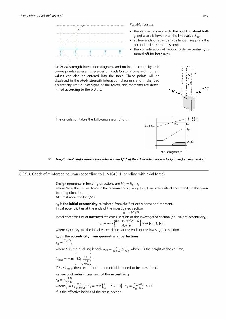
User’s Manual X5 Release4 e2 465

Possible reasons:

• the slenderness related to the buckling about both

y and z axis is lower than the limit value 𝜆𝑙𝑖𝑚; • at free ends or at ends with hinged supports the

second order moment is zero;

• the consideration of second order eccentricity is

turned off for both axes.

On N-MR strength interaction diagrams and on load eccentricity limit

curves points represent these design loads.Custom force and moment

values can also be entered into the table. These points will be

displayed in the N-MR strength interaction diagrams and in the load

eccentricity limit curves.Signs of the forces and moments are deter-

mined according to the picture.

The calculation takes the following assumptions:

, diagrams:

Longitudinal reinforcement bars thinner than 1/15 of the stirrup distance will be ignored for compression.

6.5.9.3. Check of reinforced columns according to DIN1045-1 (bending with axial force)

Design moments in bending directions are 𝑀𝑑 = 𝑁𝑑 ⋅ 𝑒𝑑

where Nd is the normal force in the column and 𝑒𝑑 = 𝑒0 + 𝑒𝑎 + 𝑒2 is the critical eccentricity in the given

bending direction.

Minimal eccentricity: h/20.

𝑒0 is the initial eccentricity calculated from the first order force and moment.

Initial eccentricities at the ends of the investigated section:

𝑒0 = 𝑀𝐼/𝑁𝑑

Initial eccentricities at intermediate cross-section of the investigated section (equivalent eccentricity):

𝑒0 = max {0.6 ⋅ 𝑒𝑎 + 0.4 ⋅ 𝑒𝑏

0.4 ⋅ 𝑒𝑎} 𝑎𝑛𝑑 |𝑒𝑎| ≥ |𝑒𝑏|,

where 𝑒𝑎 and 𝑒𝑏 are the initial eccentricities at the ends of the investigated section.

𝑒𝑎 : is the eccentricity from geometric imperfections.

𝑒𝑎 =𝛼𝑎1𝑙02

,

where 𝑙0 is the buckling length, 𝛼𝑎1 =1

100⋅√𝑙≤

1

200, where l is the height of the column,

𝜆𝑚𝑎𝑥 = max{25;16

√𝑁𝑑

𝐴𝑐𝑓𝑐𝑑

},

if 𝜆 ≥ 𝜆𝑚𝑎𝑥 , then second order eccentricitied need to be considered.

e2 : second order increment of the eccentricity.

𝑒2 = 𝐾11

𝑟

𝑙02

10,

where 1

𝑟= 𝐾2

2⋅𝑓𝑦𝑑

𝐸𝑠⋅0.9⋅𝑑 , 𝐾1 = min {

𝜆

10− 2.5; 1.0} , 𝐾2 =

𝑁𝑢𝑑 −𝑁𝑑

𝑁𝑢𝑑 −𝑁𝑏𝑎𝑙

≤ 1.0

d is the effective height of the cross-section

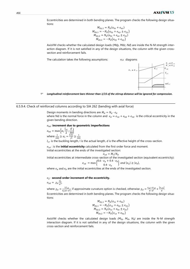
466

Eccentricities are determined in both bending planes. The program checks the following design situa-

tions:

𝑀𝑑𝑦,1 = 𝑁𝑑(𝑒0𝑧 + 𝑒𝑎𝑧)

𝑀𝑑𝑧,1 = −𝑁𝑑(𝑒0𝑦 + 𝑒𝑎𝑦 ± 𝑒2𝑦)

𝑀𝑑𝑦,2 = 𝑁𝑑(𝑒0𝑧 + 𝑒𝑎𝑧 ± 𝑒2𝑧)

𝑀𝑑𝑧,2 = −𝑁𝑑(𝑒0𝑦 + 𝑒𝑎𝑦)

AxisVM checks whether the calculated design loads (Mdy, Mdz, Nd) are inside the N-M strength inter-

action diagram. If it is not satisfied in any of the design situations, the column with the given cross-

section and reinforcement fails.

The calculation takes the following assumptions: , diagrams

Longitudinal reinforcement bars thinner than 1/15 of the stirrup distance will be ignored for compression.

6.5.9.4. Check of reinforced columns according to SIA 262 (bending with axial force)

Design moments in bending directions are 𝑀𝑑 = 𝑁𝑑 ⋅ 𝑒𝑑

where Nd is the normal force in the column and 𝑒𝑑 = 𝑒1𝑑 + 𝑒0𝑑 + 𝑒2𝑑 is the critical eccentricity in the

given bending direction.

𝑒0𝑑 : increment due to geometric imperfections

𝑒0𝑑 = max {𝛼𝑖𝑙𝑐𝑟2;𝑑

30}

where 1

200≥ 𝛼𝑖 =

0.01

√𝑙≥

1

300

𝑙𝑐𝑟 is the buckling length, l is the actual length, d is the effective height of the cross-section.

𝑒1𝑑 : is the initial eccentricity calculated from the first order force and moment.

Initial eccentricities at the ends of the investigated section:

𝑒1𝑑 = 𝑀𝐼/𝑁𝑑

Initial eccentricities at intermediate cross-section of the investigated section (equivalent eccentricity):

𝑒1𝑑 = max {0.6 ⋅ 𝑒𝑎 + 0.4 ⋅ 𝑒𝑏

0.4 ⋅ 𝑒𝑎} 𝑎𝑛𝑑 |𝑒𝑎| ≥ |𝑒𝑏|,

where 𝑒𝑎 and 𝑒𝑏 are the initial eccentricities at the ends of the investigated section.

𝑒2: second order increment of the eccentricity.

𝑒2𝑑 = 𝜒𝑑𝑙𝑐𝑟2

𝜋2,

where 𝜒𝑑 =2𝑓𝑠𝑑

𝐸𝑠(𝑑−𝑑′)

if approximate curvature option is checked, otherwise 𝜒𝑑 =𝜀𝑠𝑑−𝜀′𝑠𝑑

𝑑−𝑑′+|𝜀𝑐,∞|

𝑑.

Eccentricities are determined in both bending planes. The program checks the following design situa-

tions:

𝑀𝑑𝑦,1 = 𝑁𝑑(𝑒1𝑧 + 𝑒0𝑧)

𝑀𝑑𝑧,1 = −𝑁𝑑(𝑒1𝑦 + 𝑒0𝑦 ± 𝑒2𝑦)

𝑀𝑑𝑦,2 = 𝑁𝑑(𝑒1𝑧 + 𝑒0𝑧 ± 𝑒2𝑧)

𝑀𝑑𝑧,2 = −𝑁𝑑(𝑒1𝑦 + 𝑒0𝑦)

AxisVM checks whether the calculated design loads (Mdy, Mdz, Nd) are inside the N-M strength

interaction diagram. If it is not satisfied in any of the design situations, the column with the given

cross-section and reinforcement fails.

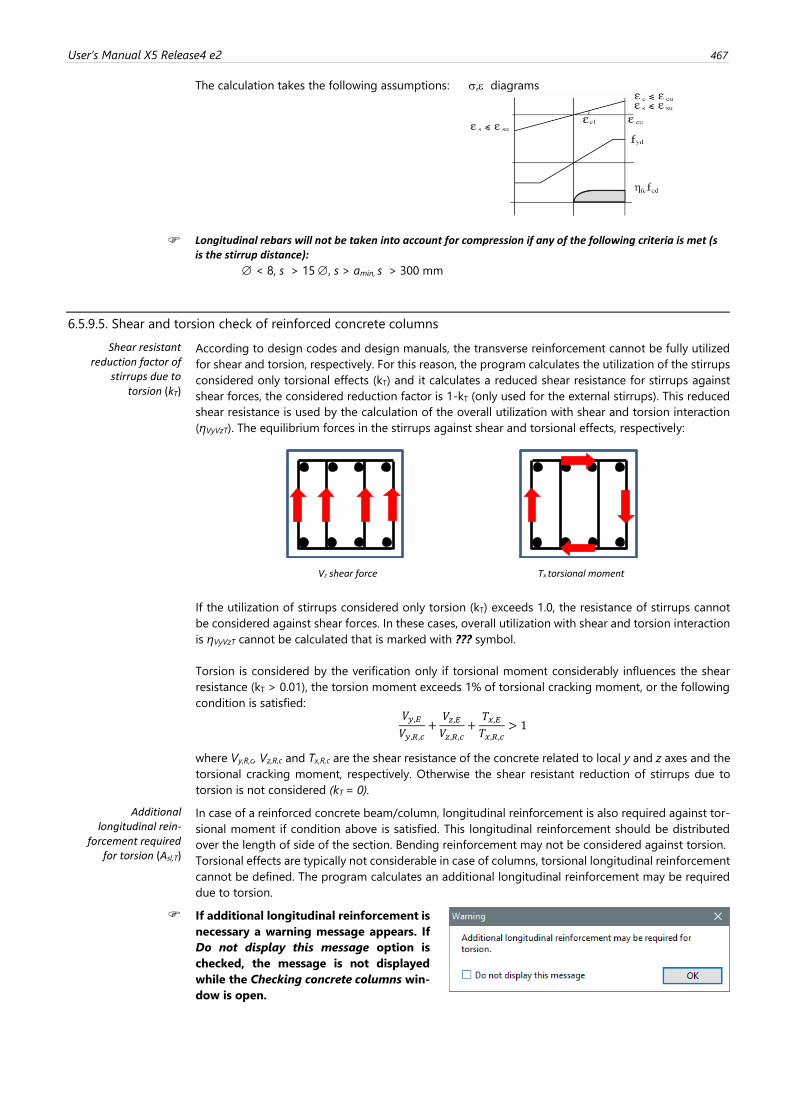
User’s Manual X5 Release4 e2 467

The calculation takes the following assumptions: , diagrams

Longitudinal rebars will not be taken into account for compression if any of the following criteria is met (s is the stirrup distance):

< 8, s > 15 , s > amin, s > 300 mm

6.5.9.5. Shear and torsion check of reinforced concrete columns

Shear resistant reduction factor of

stirrups due to torsion (kT)

According to design codes and design manuals, the transverse reinforcement cannot be fully utilized

for shear and torsion, respectively. For this reason, the program calculates the utilization of the stirrups

considered only torsional effects (kT) and it calculates a reduced shear resistance for stirrups against

shear forces, the considered reduction factor is 1-kT (only used for the external stirrups). This reduced

shear resistance is used by the calculation of the overall utilization with shear and torsion interaction

(ηVyVzT). The equilibrium forces in the stirrups against shear and torsional effects, respectively:

Vz shear force Tx torsional moment

If the utilization of stirrups considered only torsion (kT) exceeds 1.0, the resistance of stirrups cannot

be considered against shear forces. In these cases, overall utilization with shear and torsion interaction

is ηVyVzT cannot be calculated that is marked with ??? symbol.

Torsion is considered by the verification only if torsional moment considerably influences the shear

resistance (kT > 0.01), the torsion moment exceeds 1% of torsional cracking moment, or the following

condition is satisfied: 𝑉𝑦,𝐸

𝑉𝑦,𝑅,𝑐+𝑉𝑧,𝐸𝑉𝑧,𝑅,𝑐

+𝑇𝑥,𝐸𝑇𝑥,𝑅,𝑐

> 1

where Vy,R,c, Vz,R,c and Tx,R,c are the shear resistance of the concrete related to local y and z axes and the

torsional cracking moment, respectively. Otherwise the shear resistant reduction of stirrups due to

torsion is not considered (kT = 0).

Additional longitudinal rein-

forcement required for torsion (Asl,T)

In case of a reinforced concrete beam/column, longitudinal reinforcement is also required against tor-

sional moment if condition above is satisfied. This longitudinal reinforcement should be distributed

over the length of side of the section. Bending reinforcement may not be considered against torsion.

Torsional effects are typically not considerable in case of columns, torsional longitudinal reinforcement

cannot be defined. The program calculates an additional longitudinal reinforcement may be required

due to torsion.

If additional longitudinal reinforcement is

necessary a warning message appears. If

Do not display this message option is

checked, the message is not displayed

while the Checking concrete columns win-

dow is open.

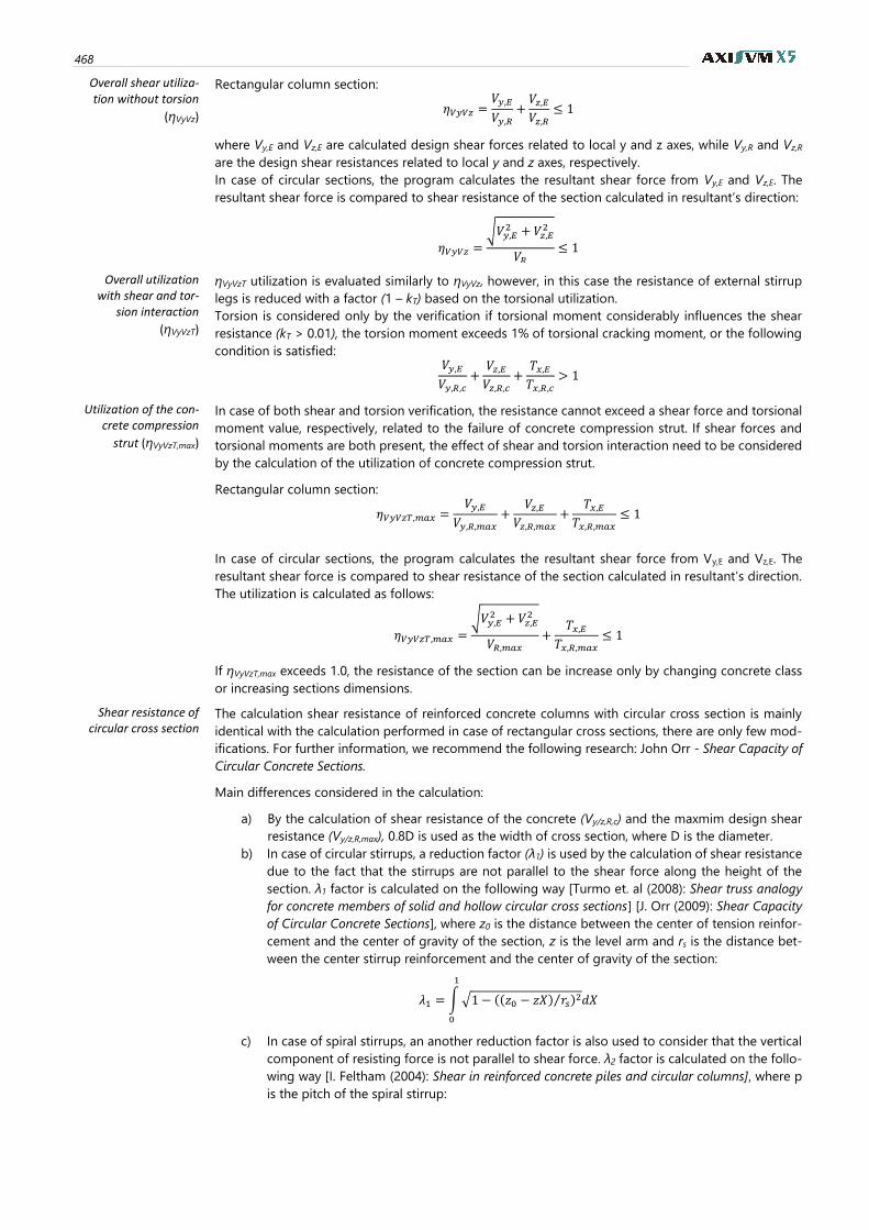
468

Overall shear utiliza-tion without torsion

(ηVyVz)

Rectangular column section:

휂𝑉𝑦𝑉𝑧 =𝑉𝑦,𝐸

𝑉𝑦,𝑅+𝑉𝑧,𝐸𝑉𝑧,𝑅

≤ 1

where Vy,E and Vz,E are calculated design shear forces related to local y and z axes, while Vy,R and Vz,R

are the design shear resistances related to local y and z axes, respectively.

In case of circular sections, the program calculates the resultant shear force from Vy,E and Vz,E. The

resultant shear force is compared to shear resistance of the section calculated in resultant’s direction:

휂𝑉𝑦𝑉𝑧 =

√𝑉𝑦,𝐸2 + 𝑉𝑧,𝐸

2

𝑉𝑅≤ 1

Overall utilization with shear and tor-

sion interaction

(ηVyVzT)

ηVyVzT utilization is evaluated similarly to ηVyVz, however, in this case the resistance of external stirrup

legs is reduced with a factor (1 – kT) based on the torsional utilization.

Torsion is considered only by the verification if torsional moment considerably influences the shear

resistance (kT > 0.01), the torsion moment exceeds 1% of torsional cracking moment, or the following

condition is satisfied: 𝑉𝑦,𝐸

𝑉𝑦,𝑅,𝑐+𝑉𝑧,𝐸𝑉𝑧,𝑅,𝑐

+𝑇𝑥,𝐸𝑇𝑥,𝑅,𝑐

> 1

Utilization of the con-crete compression

strut (ηVyVzT,max)

In case of both shear and torsion verification, the resistance cannot exceed a shear force and torsional

moment value, respectively, related to the failure of concrete compression strut. If shear forces and

torsional moments are both present, the effect of shear and torsion interaction need to be considered

by the calculation of the utilization of concrete compression strut.

Rectangular column section:

휂𝑉𝑦𝑉𝑧𝑇,𝑚𝑎𝑥 =𝑉𝑦,𝐸

𝑉𝑦,𝑅,𝑚𝑎𝑥+

𝑉𝑧,𝐸𝑉𝑧,𝑅,𝑚𝑎𝑥

+𝑇𝑥,𝐸

𝑇𝑥,𝑅,𝑚𝑎𝑥≤ 1

In case of circular sections, the program calculates the resultant shear force from Vy,E and Vz,E. The

resultant shear force is compared to shear resistance of the section calculated in resultant’s direction.

The utilization is calculated as follows:

휂𝑉𝑦𝑉𝑧𝑇,𝑚𝑎𝑥 =

√𝑉𝑦,𝐸2 + 𝑉𝑧,𝐸

2

𝑉𝑅,𝑚𝑎𝑥+

𝑇𝑥,𝐸𝑇𝑥,𝑅,𝑚𝑎𝑥

≤ 1

If ηVyVzT,max exceeds 1.0, the resistance of the section can be increase only by changing concrete class

or increasing sections dimensions.

Shear resistance of circular cross section

The calculation shear resistance of reinforced concrete columns with circular cross section is mainly

identical with the calculation performed in case of rectangular cross sections, there are only few mod-

ifications. For further information, we recommend the following research: John Orr - Shear Capacity of

Circular Concrete Sections.

Main differences considered in the calculation:

a) By the calculation of shear resistance of the concrete (Vy/z,R,c) and the maxmim design shear

resistance (Vy/z,R,max), 0.8D is used as the width of cross section, where D is the diameter.

b) In case of circular stirrups, a reduction factor (λ1) is used by the calculation of shear resistance

due to the fact that the stirrups are not parallel to the shear force along the height of the

section. λ1 factor is calculated on the following way [Turmo et. al (2008): Shear truss analogy

for concrete members of solid and hollow circular cross sections] [J. Orr (2009): Shear Capacity

of Circular Concrete Sections], where z0 is the distance between the center of tension reinfor-

cement and the center of gravity of the section, z is the level arm and rs is the distance bet-

ween the center stirrup reinforcement and the center of gravity of the section:

𝜆1 = ∫√1− ((𝑧0 − 𝑧𝑋) 𝑟𝑠⁄ )2𝑑𝑋

1

0

c) In case of spiral stirrups, an another reduction factor is also used to consider that the vertical

component of resisting force is not parallel to shear force. λ2 factor is calculated on the follo-

wing way [I. Feltham (2004): Shear in reinforced concrete piles and circular columns], where p

is the pitch of the spiral stirrup:

User’s Manual X5 Release4 e2 469

𝜆2 = ((𝑝

2𝜋𝑟𝑠)2

+ 1)

−0.5

Level arm During the calculation of shear resistance of a reinforced concrete section, the level arm (z) of internal

forces plays an important role. The level arm is interpreted as the distance between the center of ten-

sion reinforcement and the center of compression zone. In case of beams, z is approximately selected

0.9d, where d is the effective depth. However, if axial force is present, this approximation cannot be

used. The program automatically calculates the level arm of internal forces with the consideration of

the axial force in the section.

The program checks the detailing rules in the standard regarding minimum/maximum longitu-

dinal reinforcement ratios, maximum distance of stirrups and minimum diameter of stirrups.

Warning message calls the attention of the user in the information window and instantly after

the design calculations if any of these detailing rules is not fulfilled. During the definition of the

parameters, the user is informed of the fulfilment of detailing rules regarding maximum dis-

tance of stirrups and minimum diameter of stirrups by clicking button.

See... 6.5.4 Actual reinforcement against biaxial bending (column)

6.5.9.6. Shear and torsion check according to Eurocode 2 and DIN 1045-1

Design shear resistance

𝑉𝑅𝑑 = 𝑀𝑖𝑛[𝑀𝑎𝑥[𝑉𝑅𝑑,𝑐 , 𝑉𝑅𝑑,𝑠], 𝑉𝑅𝑑,𝑚𝑎𝑥]

where VRd,c is the shear resistance of concrete, VRd,s is the shear resistance of stirrups, and VRd,max is the

maximal shear resistance of the section according to the resistance of concrete compression strut.

Shear resistance of concrete

𝑉𝑅𝑑,𝑐 = [𝐶𝑅𝑑,𝑐𝑘(100𝜌𝑙𝑓𝑐𝑘)1 3⁄ + 𝑘1𝜎𝑐𝑝]𝑏𝑤𝑑 ≥ (𝑣𝑚𝑖𝑛 + 𝑘1𝜎𝑐𝑝)𝑏𝑤𝑑

where:

• ρsl ratio of tensile reinforcement,

• bw is the smallest width of the cross-section in the tensile area (circular section 0.8D),

• d is the effective depth,

• σcp the axial stress in the cross-section due to loading or prestressing (compression is positive)

<0.2fcd,

• CRd,c, vmin and k1 parameters that are regulated in the National Annex. The values of these

factors can be set in the Design codes window under the Reinforced concrete tab

(see... 3.3.7 Design codes).

In case of DIN 1045-1:

𝑉𝑅𝑑,𝑐 = [0.1𝑘(100𝜌𝑙𝑓𝑐𝑘)1 3⁄ + 0.12𝜎𝑐𝑝]𝑏𝑤𝑑

Shear resistance of stirrups

Rectangular cross section:

𝑉𝑅𝑑,𝑠 =𝐴𝑠𝑤𝑠𝑧𝑓𝑦𝑤𝑑 cot 휃

Circular cross section:

𝑉𝑅𝑑,𝑠 = 𝜆1𝜆2𝐴𝑠𝑤𝑠𝑧𝑓𝑦𝑤𝑑 cot 휃

where:

• Asw is the cross-sectional area of the shear reinforcement,

• s is the spacing of stirrups or the pitch of spiral stirrup,

• z is the level arm,

• fywd is the design yield strength of the shear reinforcement,

• θ is the angle of shear crack,

• λ1 is the reduction factor for circular stirrups,

• λ2 is the reduction factor for spiral stirrups.

Maximum design shear resistance 𝑉𝑅𝑑,𝑚𝑎𝑥 = 𝛼𝑐𝑤𝑏𝑤𝑧𝜈1𝑓𝑐𝑑

cot 휃 + cot 𝛼

1 + cot2 휃

where:

• αcw is a coefficient taking account of the state of the stress in the compression chord,

• ν1 is a strength reduction factor for concrete cracked in shear,

• α is the angle between shear reinforcement and the beam axis perpendicular to the shear

force (in case of stirrups α=90°).

470

In case of DIN 1045-1:

𝑉𝑅𝑑,𝑚𝑎𝑥 = 0.75𝑏𝑤𝑧𝑓𝑐𝑑cot 휃 + cot 𝛼

1 + cot2 휃

Torsional cracking moment – torsional

resistance of concrete

𝑇𝑅𝑑,𝑐 = 2𝐴𝑘𝑓𝑐𝑡𝑑𝑡𝑒𝑓

where:

• Ak is the area enclosed by the centre-lines of the connecting walls,

• tef is the effective wall thickness.

Maximum design tor-sional moment

The maximum torsional moment related to the resistance of concrete compression strut is calculated

as follows:

𝑇𝑅𝑑,𝑚𝑎𝑥 = 2𝜈𝛼𝑐𝑤𝑓𝑐𝑑𝐴𝑘𝑡𝑒𝑓 sin 휃 cos 휃

Calculation of kT 𝑘𝑇 =

𝑇𝐸𝑑2𝐴𝑠𝑤𝐴𝑘𝑓𝑦𝑤𝑑 cot 휃

where:

• TEd is the design torsional moment,

• Asw cross sectional area of a stirrup leg.

Calculation of Asl,T 𝐴𝑠𝑙,𝑇 =

𝑇𝐸𝑑𝑢𝑘 cot 휃

2𝐴𝑘𝑓𝑦𝑤𝑑

where:

• uk is the perimeter of the area Ak.

6.5.9.7. Shear and torsion check according to SIA 262

Shear resistance of concrete

𝑉𝑅𝑑 = 𝑘𝑑𝜏𝑐𝑑𝑏𝑤𝑑

𝑘𝑑 =1

1 + 3휀𝑣𝑑

휀𝑣 = 1.5𝑓𝑠𝑑𝐸𝑠

where:

• τcd is shear stress limit (𝜏𝑐𝑑 = 0,3√𝑓𝑐𝑘 𝛾𝑐⁄ ),

• bw is the smallest width of the cross-section in the tensile area (circular section 0.8D),

• d is the effective depth.

Shear resistance of stirrups

Rectangular cross section:

𝑉𝑅𝑑,𝑠 =𝐴𝑠𝑤𝑠𝑧𝑓𝑠𝑑 cot 𝛼

Circular cross section:

𝑉𝑅𝑑,𝑠 = 𝜆1𝜆2𝐴𝑠𝑤𝑠𝑧𝑓𝑠𝑑 cot 𝛼

where:

• Asw is the cross-sectional area of the shear reinforcement,

• s is the spacing of stirrups or the pitch of spiral stirrup,

• z is the level arm,

• fsd is the design yield strength of the shear reinforcement,

• α is the angle of shear crack,

• λ1 is the reduction factor for circular stirrups,

• λ2 is the reduction factor for spiral stirrups.

Maximum design shear resistance

𝑉𝑅𝑑,𝑐 = 𝑏𝑤𝑧𝑘𝑐𝑓𝑐𝑑 sin 𝛼 cos 𝛼

𝑘𝑐 =1

1.2 + 55휀1≤ 0.65

휀1 = 휀𝑥 + (휀1 + 0.002) cot2 𝛼

where:

• kc is a strength reduction factor for concrete cracked in shear.

Torsional cracking moment – torsional

resistance of concrete

𝑇𝑅𝑑 = 2𝐴𝑘𝑘𝑑𝜏𝑐𝑑𝑡𝑘

where:

• Ak is the area enclosed by the centre-lines of the connecting walls,

• tk is the effective wall thickness.

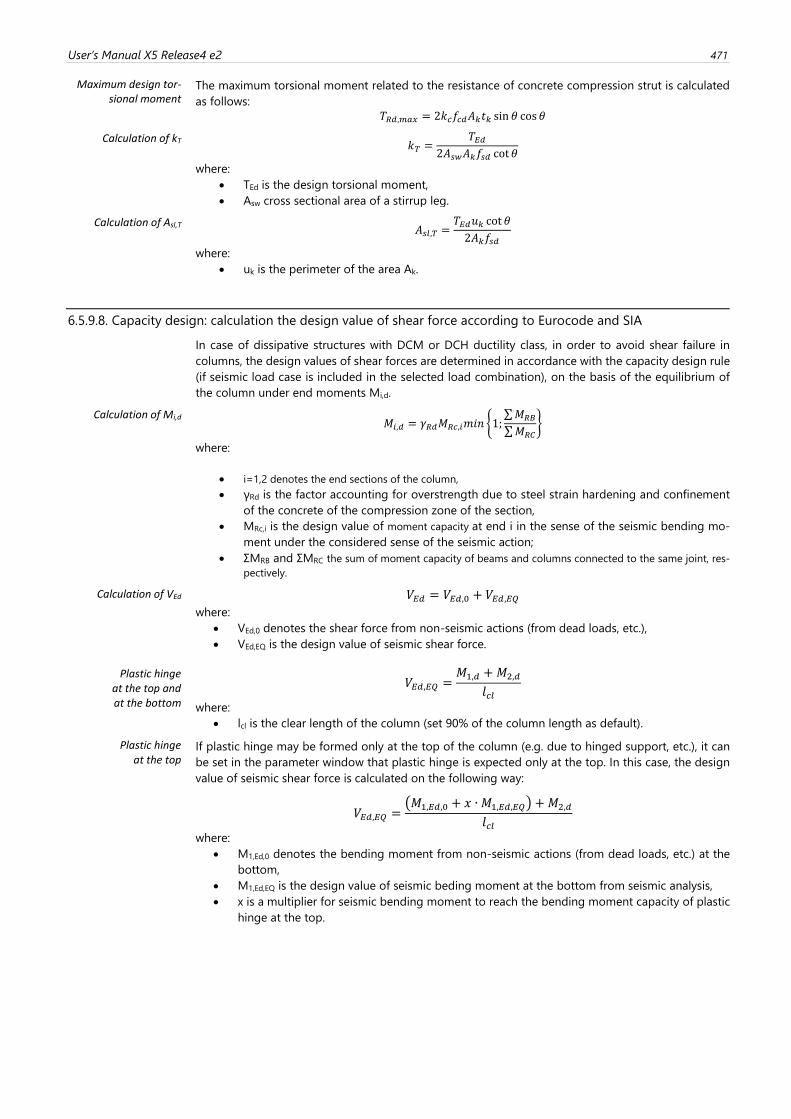
User’s Manual X5 Release4 e2 471

Maximum design tor-sional moment

The maximum torsional moment related to the resistance of concrete compression strut is calculated

as follows:

𝑇𝑅𝑑,𝑚𝑎𝑥 = 2𝑘𝑐𝑓𝑐𝑑𝐴𝑘𝑡𝑘 sin 휃 cos 휃

Calculation of kT 𝑘𝑇 =

𝑇𝐸𝑑2𝐴𝑠𝑤𝐴𝑘𝑓𝑠𝑑 cot 휃

where:

• TEd is the design torsional moment,

• Asw cross sectional area of a stirrup leg.

Calculation of Asl,T 𝐴𝑠𝑙,𝑇 =

𝑇𝐸𝑑𝑢𝑘 cot 휃

2𝐴𝑘𝑓𝑠𝑑

where:

• uk is the perimeter of the area Ak.

6.5.9.8. Capacity design: calculation the design value of shear force according to Eurocode and SIA

In case of dissipative structures with DCM or DCH ductility class, in order to avoid shear failure in

columns, the design values of shear forces are determined in accordance with the capacity design rule

(if seismic load case is included in the selected load combination), on the basis of the equilibrium of

the column under end moments Mi,d.

Calculation of Mi,d

𝑀𝑖,𝑑 = 𝛾𝑅𝑑𝑀𝑅𝑐,𝑖𝑚𝑖𝑛 {1;∑𝑀𝑅𝐵

∑𝑀𝑅𝐶}

where:

• i=1,2 denotes the end sections of the column,

• γRd is the factor accounting for overstrength due to steel strain hardening and confinement

of the concrete of the compression zone of the section,

• MRc,i is the design value of moment capacity at end i in the sense of the seismic bending mo-

ment under the considered sense of the seismic action;

• ΣMRB and ΣMRC the sum of moment capacity of beams and columns connected to the same joint, res-

pectively.

Calculation of VEd 𝑉𝐸𝑑 = 𝑉𝐸𝑑,0 + 𝑉𝐸𝑑,𝐸𝑄

where:

• VEd,0 denotes the shear force from non-seismic actions (from dead loads, etc.),

• VEd,EQ is the design value of seismic shear force.

Plastic hinge at the top and at the bottom

𝑉𝐸𝑑,𝐸𝑄 =𝑀1,𝑑 +𝑀2,𝑑

𝑙𝑐𝑙

where:

• lcl is the clear length of the column (set 90% of the column length as default).

Plastic hinge at the top

If plastic hinge may be formed only at the top of the column (e.g. due to hinged support, etc.), it can

be set in the parameter window that plastic hinge is expected only at the top. In this case, the design

value of seismic shear force is calculated on the following way:

𝑉𝐸𝑑,𝐸𝑄 =(𝑀1,𝐸𝑑,0 + 𝑥 ∙ 𝑀1,𝐸𝑑,𝐸𝑄) + 𝑀2,𝑑

𝑙𝑐𝑙

where:

• M1,Ed,0 denotes the bending moment from non-seismic actions (from dead loads, etc.) at the

bottom,

• M1,Ed,EQ is the design value of seismic beding moment at the bottom from seismic analysis,

• x is a multiplier for seismic bending moment to reach the bending moment capacity of plastic

hinge at the top.

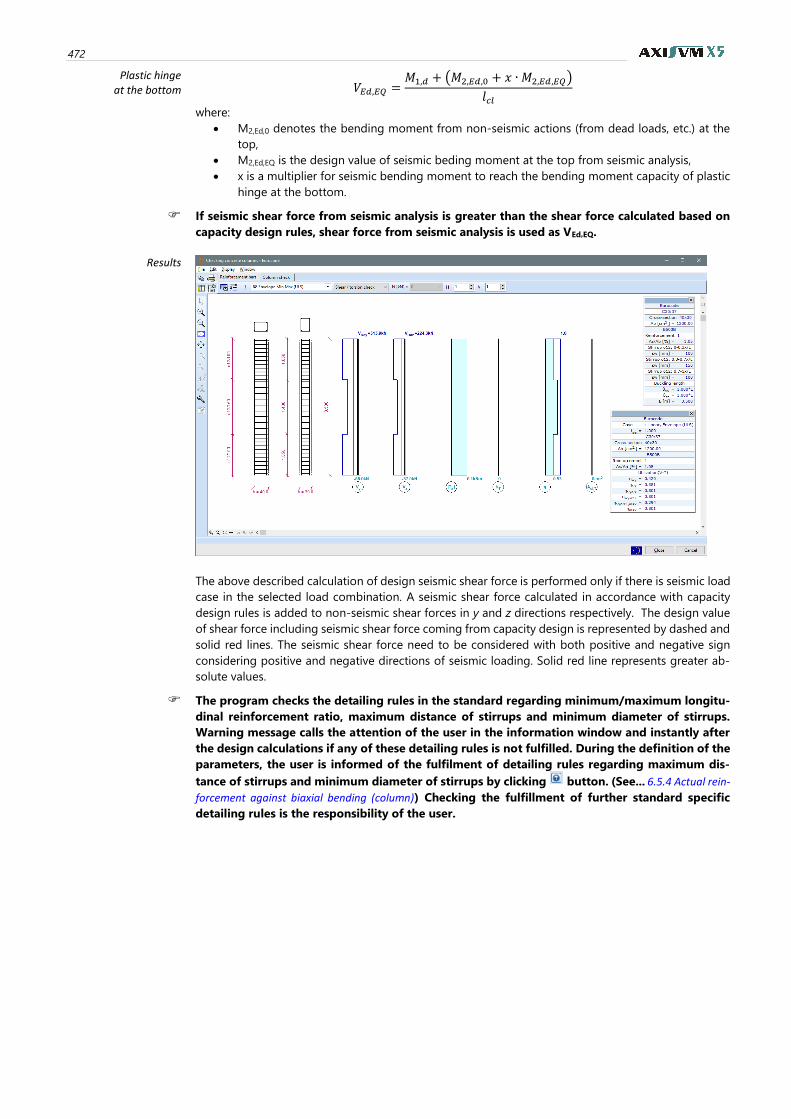
472

Plastic hinge at the bottom 𝑉𝐸𝑑,𝐸𝑄 =

𝑀1,𝑑 + (𝑀2,𝐸𝑑,0 + 𝑥 ∙ 𝑀2,𝐸𝑑,𝐸𝑄)

𝑙𝑐𝑙

where:

• M2,Ed,0 denotes the bending moment from non-seismic actions (from dead loads, etc.) at the

top,

• M2,Ed,EQ is the design value of seismic beding moment at the top from seismic analysis,

• x is a multiplier for seismic bending moment to reach the bending moment capacity of plastic

hinge at the bottom.

If seismic shear force from seismic analysis is greater than the shear force calculated based on

capacity design rules, shear force from seismic analysis is used as VEd,EQ.

Results

The above described calculation of design seismic shear force is performed only if there is seismic load

case in the selected load combination. A seismic shear force calculated in accordance with capacity

design rules is added to non-seismic shear forces in y and z directions respectively. The design value

of shear force including seismic shear force coming from capacity design is represented by dashed and

solid red lines. The seismic shear force need to be considered with both positive and negative sign

considering positive and negative directions of seismic loading. Solid red line represents greater ab-

solute values.

The program checks the detailing rules in the standard regarding minimum/maximum longitu-

dinal reinforcement ratio, maximum distance of stirrups and minimum diameter of stirrups.

Warning message calls the attention of the user in the information window and instantly after

the design calculations if any of these detailing rules is not fulfilled. During the definition of the

parameters, the user is informed of the fulfilment of detailing rules regarding maximum dis-

tance of stirrups and minimum diameter of stirrups by clicking button. (See... 6.5.4 Actual rein-

forcement against biaxial bending (column)) Checking the fulfillment of further standard specific

detailing rules is the responsibility of the user.

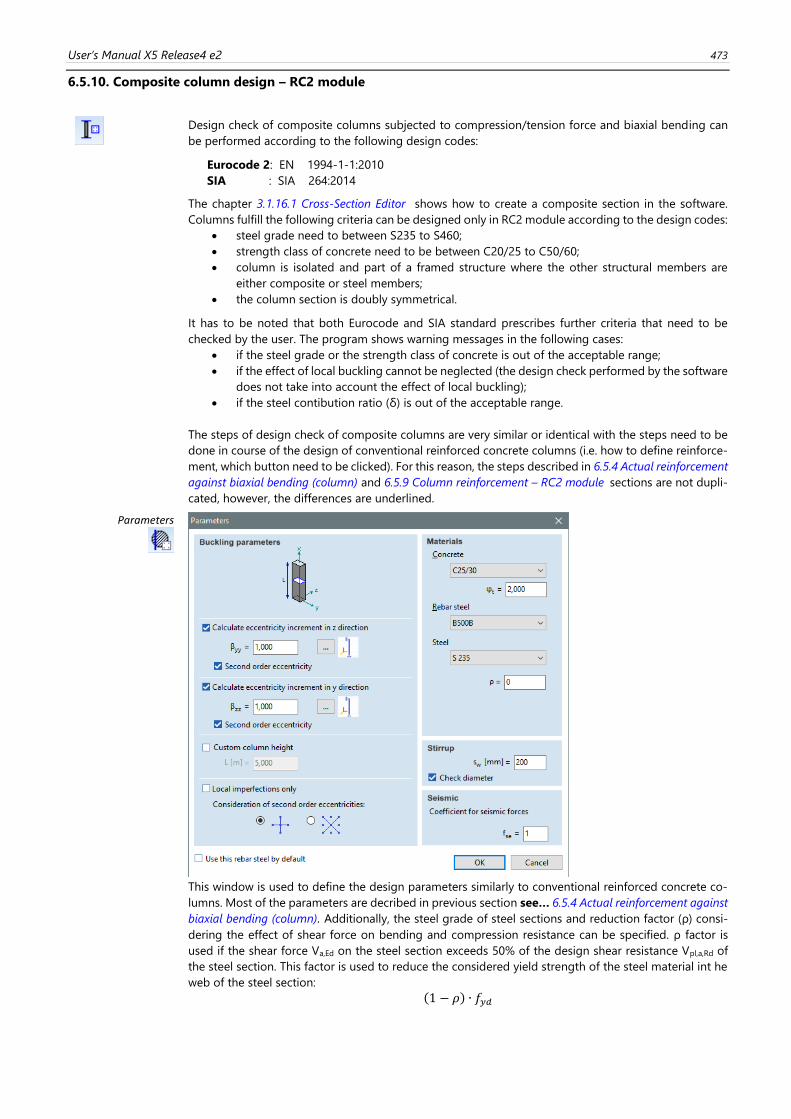
User’s Manual X5 Release4 e2 473

6.5.10. Composite column design – RC2 module

Design check of composite columns subjected to compression/tension force and biaxial bending can

be performed according to the following design codes:

Eurocode 2: EN 1994-1-1:2010

SIA : SIA 264:2014

The chapter 3.1.16.1 Cross-Section Editor shows how to create a composite section in the software.

Columns fulfill the following criteria can be designed only in RC2 module according to the design codes:

• steel grade need to between S235 to S460;

• strength class of concrete need to be between C20/25 to C50/60;

• column is isolated and part of a framed structure where the other structural members are

either composite or steel members;

• the column section is doubly symmetrical.

It has to be noted that both Eurocode and SIA standard prescribes further criteria that need to be

checked by the user. The program shows warning messages in the following cases:

• if the steel grade or the strength class of concrete is out of the acceptable range;

• if the effect of local buckling cannot be neglected (the design check performed by the software

does not take into account the effect of local buckling);

• if the steel contibution ratio (δ) is out of the acceptable range.

The steps of design check of composite columns are very similar or identical with the steps need to be

done in course of the design of conventional reinforced concrete columns (i.e. how to define reinforce-

ment, which button need to be clicked). For this reason, the steps described in 6.5.4 Actual reinforcement

against biaxial bending (column) and 6.5.9 Column reinforcement – RC2 module sections are not dupli-

cated, however, the differences are underlined.

Parameters

This window is used to define the design parameters similarly to conventional reinforced concrete co-

lumns. Most of the parameters are decribed in previous section see… 6.5.4 Actual reinforcement against

biaxial bending (column). Additionally, the steel grade of steel sections and reduction factor (ρ) consi-

dering the effect of shear force on bending and compression resistance can be specified. ρ factor is

used if the shear force Va,Ed on the steel section exceeds 50% of the design shear resistance Vpl,a,Rd of

the steel section. This factor is used to reduce the considered yield strength of the steel material int he

web of the steel section:

(1 − 𝜌) ∙ 𝑓𝑦𝑑

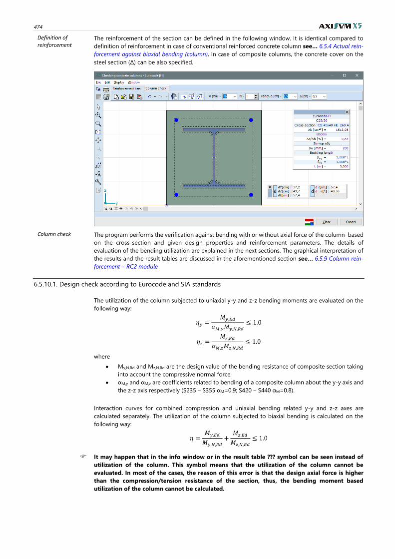
474

Definition of reinforcement

The reinforcement of the section can be defined in the following window. It is identical compared to

definition of reinforcement in case of conventional reinforced concrete column see… 6.5.4 Actual rein-

forcement against biaxial bending (column). In case of composite columns, the concrete cover on the

steel section (Δ) can be also specified.

Column check The program performs the verification against bending with or without axial force of the column based

on the cross-section and given design properties and reinforcement parameters. The details of

evaluation of the bending utilization are explained in the next sections. The graphical interpretation of

the results and the result tables are discussed in the aforementioned section see… 6.5.9 Column rein-

forcement – RC2 module

6.5.10.1. Design check according to Eurocode and SIA standards

The utilization of the column subjected to uniaxial y-y and z-z bending moments are evaluated on the

following way:

휂𝑦 =𝑀𝑦,𝐸𝑑

𝛼𝑀,𝑦𝑀𝑦,𝑁,𝑅𝑑

≤ 1.0

휂𝑧 =𝑀𝑧,𝐸𝑑

𝛼𝑀,𝑧𝑀𝑧,𝑁,𝑅𝑑

≤ 1.0

where

• My,N,Rd and Mz,N,Rd are the design value of the bending resistance of composite section taking

into account the compressive normal force,

• αM,y and αM,z are coefficients related to bending of a composite column about the y-y axis and

the z-z axis respectively (S235 – S355 αM=0.9; S420 – S440 αM=0.8).

Interaction curves for combined compression and uniaxial bending related y-y and z-z axes are

calculated separately. The utilization of the column subjected to biaxial bending is calculated on the

following way:

휂 =𝑀𝑦,𝐸𝑑

𝑀𝑦,𝑁,𝑅𝑑

+𝑀𝑧,𝐸𝑑

𝑀𝑧,𝑁,𝑅𝑑

≤ 1.0

It may happen that in the info window or in the result table ??? symbol can be seen instead of

utilization of the column. This symbol means that the utilization of the column cannot be

evaluated. In most of the cases, the reason of this error is that the design axial force is higher

than the compression/tension resistance of the section, thus, the bending moment based

utilization of the column cannot be calculated.

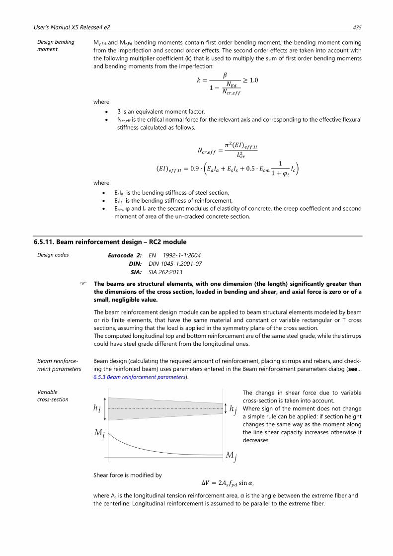
User’s Manual X5 Release4 e2 475

Design bending moment

My,Ed and Mz,Ed bending moments contain first order bending moment, the bending moment coming

from the imperfection and second order effects. The second order effects are taken into account with

the following multiplier coefficient (k) that is used to multiply the sum of first order bending moments

and bending moments from the imperfection:

𝑘 =𝛽

1 − 𝑁𝐸𝑑𝑁𝑐𝑟,𝑒𝑓𝑓

≥ 1.0

where

• β is an equivalent moment factor,

• Ncr,eff is the critical normal force for the relevant axis and corresponding to the effective flexural

stiffness calculated as follows.

𝑁𝑐𝑟,𝑒𝑓𝑓 =𝜋2(𝐸𝐼)𝑒𝑓𝑓,𝐼𝐼

𝐿𝑐𝑟2

(𝐸𝐼)𝑒𝑓𝑓,𝐼𝐼 = 0.9 ∙ (𝐸𝑎𝐼𝑎 + 𝐸𝑠𝐼𝑠 + 0.5 ∙ 𝐸𝑐𝑚1

1 + 𝜑𝑡𝐼𝑐)

where

• EaIa is the bending stiffness of steel section,

• EsIs is the bending stiffness of reinforcement,

• Ecm, φ and Ic are the secant modulus of elasticity of concrete, the creep coeffiecient and second

moment of area of the un-cracked concrete section.

6.5.11. Beam reinforcement design – RC2 module

Design codes Eurocode 2: EN 1992-1-1:2004

DIN: DIN 1045-1:2001-07

SIA: SIA 262:2013

The beams are structural elements, with one dimension (the length) significantly greater than

the dimensions of the cross section, loaded in bending and shear, and axial force is zero or of a

small, negligible value.

The beam reinforcement design module can be applied to beam structural elements modeled by beam

or rib finite elements, that have the same material and constant or variable rectangular or T cross

sections, assuming that the load is applied in the symmetry plane of the cross section.

The computed longitudinal top and bottom reinforcement are of the same steel grade, while the stirrups

could have steel grade different from the longitudinal ones.

Beam reinforce-

ment parameters

Beam design (calculating the required amount of reinforcement, placing stirrups and rebars, and check-

ing the reinforced beam) uses parameters entered in the Beam reinforcement parameters dialog (see…

6.5.3 Beam reinforcement parameters).

Variable cross-section

The change in shear force due to variable

cross-section is taken into account.

Where sign of the moment does not change

a simple rule can be applied: if section height

changes the same way as the moment along

the line shear capacity increases otherwise it

decreases.

Shear force is modified by

Δ𝑉 = 2𝐴𝑠𝑓𝑦𝑑 sin 𝛼,

where As is the longitudinal tension reinforcement area, α is the angle between the extreme fiber and

the centerline. Longitudinal reinforcement is assumed to be parallel to the extreme fiber.

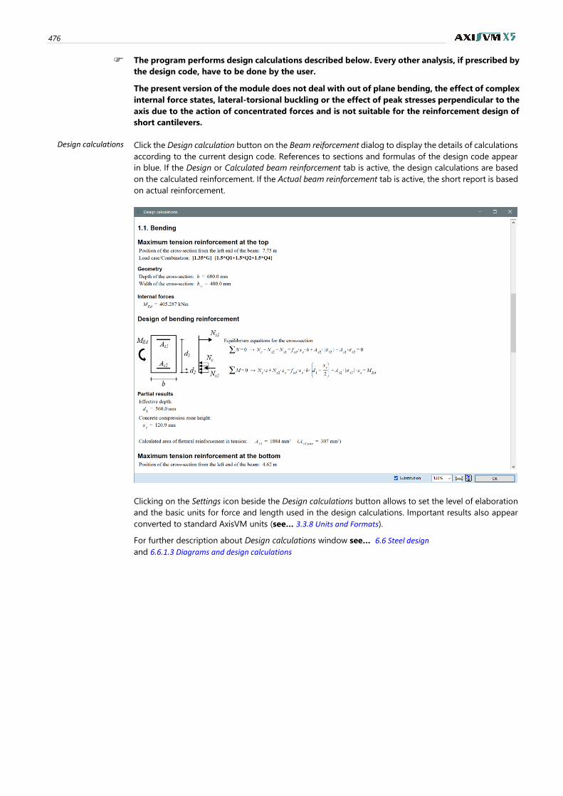
476

The program performs design calculations described below. Every other analysis, if prescribed by

the design code, have to be done by the user.

The present version of the module does not deal with out of plane bending, the effect of complex

internal force states, lateral-torsional buckling or the effect of peak stresses perpendicular to the

axis due to the action of concentrated forces and is not suitable for the reinforcement design of

short cantilevers.

Design calculations Click the Design calculation button on the Beam reiforcement dialog to display the details of calculations

according to the current design code. References to sections and formulas of the design code appear

in blue. If the Design or Calculated beam reinforcement tab is active, the design calculations are based

on the calculated reinforcement. If the Actual beam reinforcement tab is active, the short report is based

on actual reinforcement.

Clicking on the Settings icon beside the Design calculations button allows to set the level of elaboration

and the basic units for force and length used in the design calculations. Important results also appear

converted to standard AxisVM units (see… 3.3.8 Units and Formats).

For further description about Design calculations window see… 6.6 Steel design

and 6.6.1.3 Diagrams and design calculations

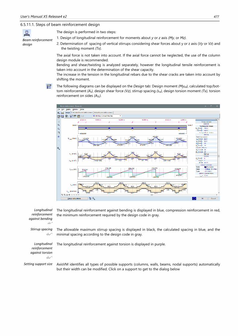
User’s Manual X5 Release4 e2 477

6.5.11.1. Steps of beam reinforcement design

Beam reinforcement design

The design is performed in two steps:

1. Design of longitudinal reinforcement for moments about y or z axis (My, or Mz).

2. Determination of spacing of vertical stirrups considering shear forces about y or z axis (Vy or Vz) and

the twisting moment (Tx).

The axial force is not taken into account. If the axial force cannot be neglected, the use of the column

design module is recommended.

Bending and shear/twisting is analyzed separately, however the longitudinal tensile reinforcement is

taken into account in the determination of the shear capacity.

The increase in the tension in the longitudinal rebars due to the shear cracks are taken into account by

shifting the moment.

The following diagrams can be displayed on the Design tab: Design moment (MyEd), calculated top/bot-

tom reinforcement (As), design shear force (Vz), stirrup spacing (sw), design torsion moment (Tx), torsion

reinforcement on sides (ASL).

Longitudinal reinforcement

against bending

The longitudinal reinforcement against bending is displayed in blue, compression reinforcement in red,

the minimum reinforcement required by the design code in gray.

Stirrup spacing

The allowable maximum stirrup spacing is displayed in black, the calculated spacing in blue, and the

minimal spacing according to the design code in gray.

Longitudinal reinforcement

against torsion

The longitudinal reinforcement against torsion is displayed in purple.

Setting support size AxisVM identifies all types of possible supports (columns, walls, beams, nodal supports) automatically

but their width can be modified. Click on a support to get to the dialog below

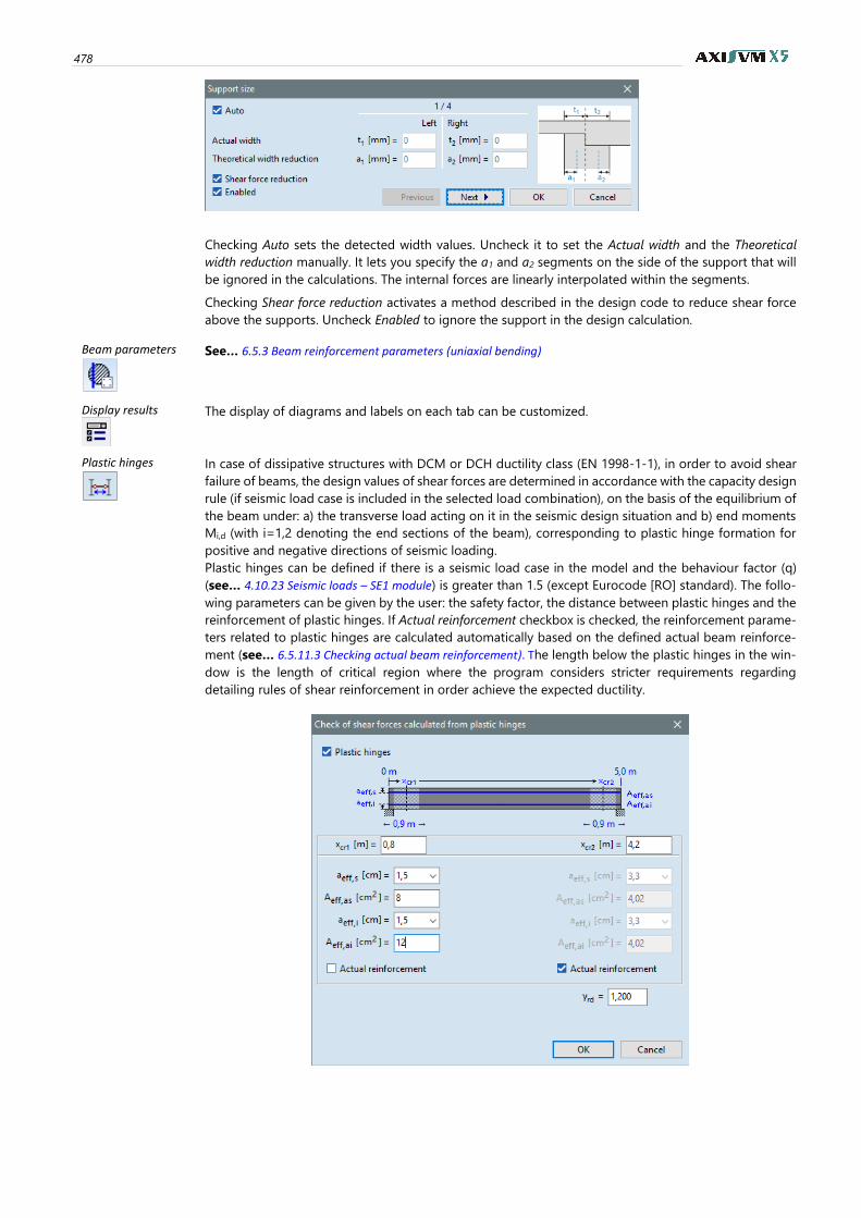
478

Checking Auto sets the detected width values. Uncheck it to set the Actual width and the Theoretical

width reduction manually. It lets you specify the a1 and a2 segments on the side of the support that will

be ignored in the calculations. The internal forces are linearly interpolated within the segments.

Checking Shear force reduction activates a method described in the design code to reduce shear force

above the supports. Uncheck Enabled to ignore the support in the design calculation.

Beam parameters

See… 6.5.3 Beam reinforcement parameters (uniaxial bending)

Display results

The display of diagrams and labels on each tab can be customized.

Plastic hinges

In case of dissipative structures with DCM or DCH ductility class (EN 1998-1-1), in order to avoid shear

failure of beams, the design values of shear forces are determined in accordance with the capacity design

rule (if seismic load case is included in the selected load combination), on the basis of the equilibrium of

the beam under: a) the transverse load acting on it in the seismic design situation and b) end moments

Mi,d (with i=1,2 denoting the end sections of the beam), corresponding to plastic hinge formation for

positive and negative directions of seismic loading.

Plastic hinges can be defined if there is a seismic load case in the model and the behaviour factor (q)

(see… 4.10.23 Seismic loads – SE1 module) is greater than 1.5 (except Eurocode [RO] standard). The follo-

wing parameters can be given by the user: the safety factor, the distance between plastic hinges and the

reinforcement of plastic hinges. If Actual reinforcement checkbox is checked, the reinforcement parame-

ters related to plastic hinges are calculated automatically based on the defined actual beam reinforce-

ment (see… 6.5.11.3 Checking actual beam reinforcement). The length below the plastic hinges in the win-

dow is the length of critical region where the program considers stricter requirements regarding

detailing rules of shear reinforcement in order achieve the expected ductility.

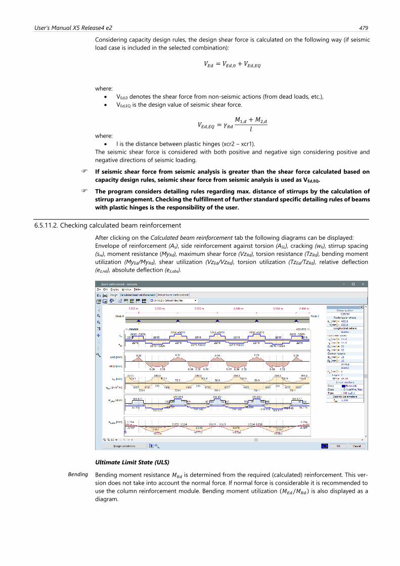
User’s Manual X5 Release4 e2 479

Considering capacity design rules, the design shear force is calculated on the following way (if seismic

load case is included in the selected combination):

𝑉𝐸𝑑 = 𝑉𝐸𝑑,0 + 𝑉𝐸𝑑,𝐸𝑄

where:

• VEd,0 denotes the shear force from non-seismic actions (from dead loads, etc.),

• VEd,EQ is the design value of seismic shear force.

𝑉𝐸𝑑,𝐸𝑄 = 𝛾𝑅𝑑𝑀1,𝑑 +𝑀2,𝑑

𝑙

where:

• l is the distance between plastic hinges (xcr2 – xcr1).

The seismic shear force is considered with both positive and negative sign considering positive and

negative directions of seismic loading.

If seismic shear force from seismic analysis is greater than the shear force calculated based on

capacity design rules, seismic shear force from seismic analysis is used as VEd,EQ.

The program considers detailing rules regarding max. distance of stirrups by the calculation of

stirrup arrangement. Checking the fulfillment of further standard specific detailing rules of beams

with plastic hinges is the responsibility of the user.

6.5.11.2. Checking calculated beam reinforcement

After clicking on the Calculated beam reinforcement tab the following diagrams can be displayed:

Envelope of reinforcement (As), side reinforcement against torsion (ASL), cracking (wk), stirrup spacing

(sw), moment resistance (MyRd), maximum shear force (VzRd), torsion resistance (TzRd), bending moment

utilization (MyEd/MyRd), shear utilization (VzEd/VzRd), torsion utilization (TzEd/TzRd), relative deflection

(ez,rel), absolute deflection (ez,abs).

Ultimate Limit State (ULS)

Bending Bending moment resistance 𝑀𝑅𝑑 is determined from the required (calculated) reinforcement. This ver-

sion does not take into account the normal force. If normal force is considerable it is recommended to

use the column reinforcement module. Bending moment utilization (𝑀𝐸𝑑/𝑀𝑅𝑑) is also displayed as a

diagram.

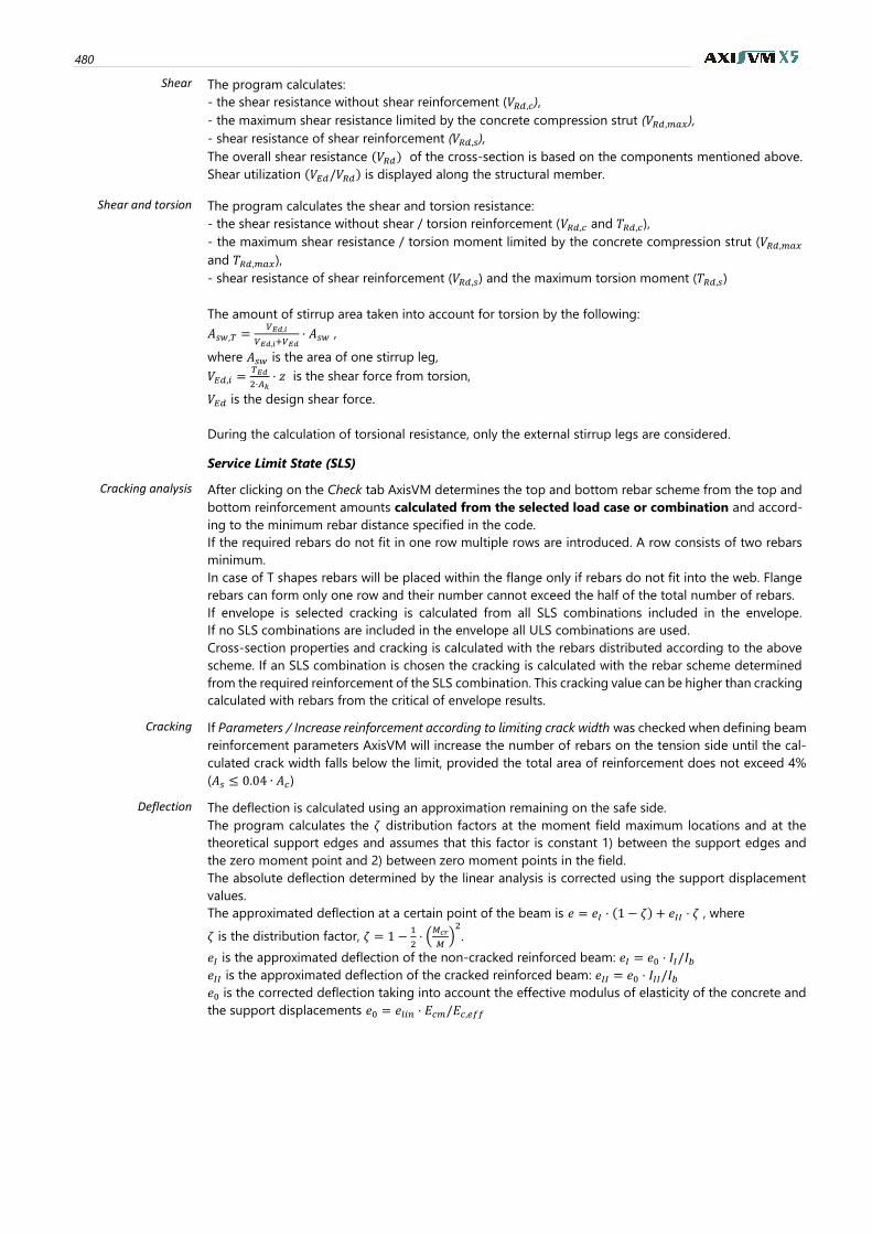
480

Shear The program calculates:

- the shear resistance without shear reinforcement (𝑉𝑅𝑑,𝑐),

- the maximum shear resistance limited by the concrete compression strut (𝑉𝑅𝑑,𝑚𝑎𝑥),

- shear resistance of shear reinforcement (𝑉𝑅𝑑,𝑠),

The overall shear resistance (𝑉𝑅𝑑) of the cross-section is based on the components mentioned above.

Shear utilization (𝑉𝐸𝑑/𝑉𝑅𝑑) is displayed along the structural member.

Shear and torsion The program calculates the shear and torsion resistance:

- the shear resistance without shear / torsion reinforcement (𝑉𝑅𝑑,𝑐 and 𝑇𝑅𝑑,𝑐),

- the maximum shear resistance / torsion moment limited by the concrete compression strut (𝑉𝑅𝑑,𝑚𝑎𝑥

and 𝑇𝑅𝑑,𝑚𝑎𝑥),

- shear resistance of shear reinforcement (𝑉𝑅𝑑,𝑠) and the maximum torsion moment (𝑇𝑅𝑑,𝑠)

The amount of stirrup area taken into account for torsion by the following:

𝐴𝑠𝑤,𝑇 =𝑉𝐸𝑑,𝑖

𝑉𝐸𝑑,𝑖+𝑉𝐸𝑑⋅ 𝐴𝑠𝑤 ,

where 𝐴𝑠𝑤 is the area of one stirrup leg,

𝑉𝐸𝑑,𝑖 =𝑇𝐸𝑑

2⋅𝐴𝑘⋅ 𝑧 is the shear force from torsion,

𝑉𝐸𝑑 is the design shear force.

During the calculation of torsional resistance, only the external stirrup legs are considered. Service Limit State (SLS)

Cracking analysis After clicking on the Check tab AxisVM determines the top and bottom rebar scheme from the top and

bottom reinforcement amounts calculated from the selected load case or combination and accord-

ing to the minimum rebar distance specified in the code.

If the required rebars do not fit in one row multiple rows are introduced. A row consists of two rebars

minimum.

In case of T shapes rebars will be placed within the flange only if rebars do not fit into the web. Flange

rebars can form only one row and their number cannot exceed the half of the total number of rebars.

If envelope is selected cracking is calculated from all SLS combinations included in the envelope.

If no SLS combinations are included in the envelope all ULS combinations are used.

Cross-section properties and cracking is calculated with the rebars distributed according to the above

scheme. If an SLS combination is chosen the cracking is calculated with the rebar scheme determined

from the required reinforcement of the SLS combination. This cracking value can be higher than cracking

calculated with rebars from the critical of envelope results.

Cracking

If Parameters / Increase reinforcement according to limiting crack width was checked when defining beam

reinforcement parameters AxisVM will increase the number of rebars on the tension side until the cal-

culated crack width falls below the limit, provided the total area of reinforcement does not exceed 4%

(𝐴𝑠 ≤ 0.04 ∙ 𝐴𝑐)

Deflection The deflection is calculated using an approximation remaining on the safe side.

The program calculates the 휁 distribution factors at the moment field maximum locations and at the

theoretical support edges and assumes that this factor is constant 1) between the support edges and

the zero moment point and 2) between zero moment points in the field.

The absolute deflection determined by the linear analysis is corrected using the support displacement

values.

The approximated deflection at a certain point of the beam is 𝑒 = 𝑒𝐼 ⋅ (1 − 휁) + 𝑒𝐼𝐼 ⋅ 휁 , where

휁 is the distribution factor, 휁 = 1 −1

2⋅ (

𝑀𝑐𝑟

𝑀)2.

𝑒𝐼 is the approximated deflection of the non-cracked reinforced beam: 𝑒𝐼 = 𝑒0 ⋅ 𝐼𝐼/𝐼𝑏

𝑒𝐼𝐼 is the approximated deflection of the cracked reinforced beam: 𝑒𝐼𝐼 = 𝑒0 ⋅ 𝐼𝐼𝐼/𝐼𝑏

𝑒0 is the corrected deflection taking into account the effective modulus of elasticity of the concrete and

the support displacements 𝑒0 = 𝑒𝑙𝑖𝑛 ⋅ 𝐸𝑐𝑚/𝐸𝑐,𝑒𝑓𝑓

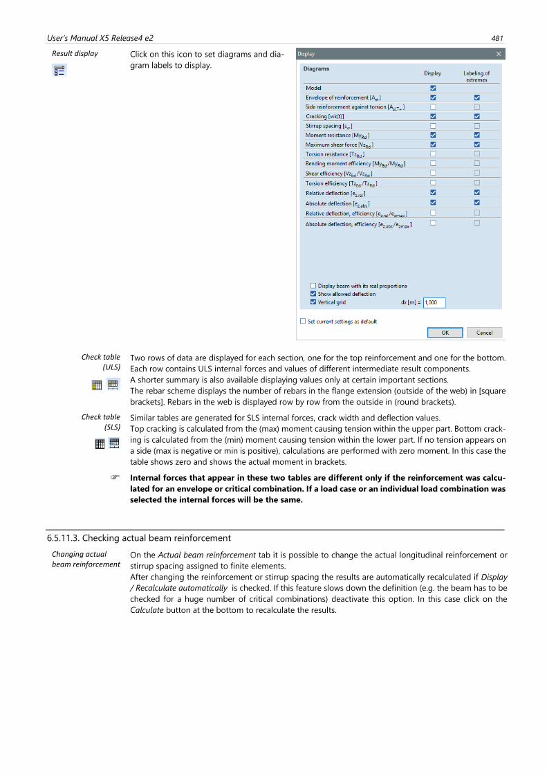
User’s Manual X5 Release4 e2 481

Result display

Click on this icon to set diagrams and dia-

gram labels to display.

Check table (ULS)

Two rows of data are displayed for each section, one for the top reinforcement and one for the bottom.

Each row contains ULS internal forces and values of different intermediate result components.

A shorter summary is also available displaying values only at certain important sections.

The rebar scheme displays the number of rebars in the flange extension (outside of the web) in [square

brackets]. Rebars in the web is displayed row by row from the outside in (round brackets).

Check table (SLS)

Similar tables are generated for SLS internal forces, crack width and deflection values.

Top cracking is calculated from the (max) moment causing tension within the upper part. Bottom crack-

ing is calculated from the (min) moment causing tension within the lower part. If no tension appears on

a side (max is negative or min is positive), calculations are performed with zero moment. In this case the

table shows zero and shows the actual moment in brackets.

Internal forces that appear in these two tables are different only if the reinforcement was calcu-

lated for an envelope or critical combination. If a load case or an individual load combination was

selected the internal forces will be the same.

6.5.11.3. Checking actual beam reinforcement

Changing actual beam reinforcement

On the Actual beam reinforcement tab it is possible to change the actual longitudinal reinforcement or

stirrup spacing assigned to finite elements.

After changing the reinforcement or stirrup spacing the results are automatically recalculated if Display

/ Recalculate automatically is checked. If this feature slows down the definition (e.g. the beam has to be

checked for a huge number of critical combinations) deactivate this option. In this case click on the

Calculate button at the bottom to recalculate the results.

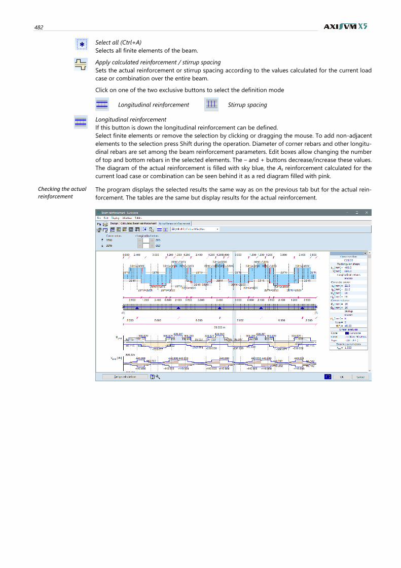
482

Select all (Ctrl+A)

Selects all finite elements of the beam.

Apply calculated reinforcement / stirrup spacing

Sets the actual reinforcement or stirrup spacing according to the values calculated for the current load

case or combination over the entire beam.

Click on one of the two exclusive buttons to select the definition mode

Longitudinal reinforcement

Stirrup spacing

Longitudinal reinforcement

If this button is down the longitudinal reinforcement can be defined.

Select finite elements or remove the selection by clicking or dragging the mouse. To add non-adjacent

elements to the selection press Shift during the operation. Diameter of corner rebars and other longitu-

dinal rebars are set among the beam reinforcement parameters. Edit boxes allow changing the number

of top and bottom rebars in the selected elements. The – and + buttons decrease/increase these values.

The diagram of the actual reinforcement is filled with sky blue, the As reinforcement calculated for the

current load case or combination can be seen behind it as a red diagram filled with pink.

Checking the actual reinforcement

The program displays the selected results the same way as on the previous tab but for the actual rein-

forcement. The tables are the same but display results for the actual reinforcement.

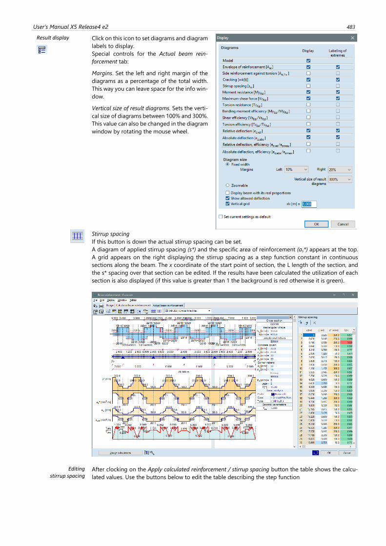
User’s Manual X5 Release4 e2 483

Result display

Click on this icon to set diagrams and diagram

labels to display.

Special controls for the Actual beam rein-

forcement tab:

Margins. Set the left and right margin of the

diagrams as a percentage of the total width.

This way you can leave space for the info win-

dow.

Vertical size of result diagrams. Sets the verti-

cal size of diagrams between 100% and 300%.

This value can also be changed in the diagram

window by rotating the mouse wheel.

Stirrup spacing

If this button is down the actual stirrup spacing can be set.

A diagram of applied stirrup spacing (s*) and the specific area of reinforcement (as*) appears at the top.

A grid appears on the right displaying the stirrup spacing as a step function constant in continuous

sections along the beam. The x coordinate of the start point of section, the L length of the section, and

the s* spacing over that section can be edited. If the results have been calculated the utilization of each

section is also displayed (if this value is greater than 1 the background is red otherwise it is green).

Editing stirrup spacing

After clocking on the Apply calculated reinforcement / stirrup spacing button the table shows the calcu-

lated values. Use the buttons below to edit the table describing the step function

484

Insert a new row before the current one

Creates a new section by dividing the row before the current one into two equal parts. s* remains the

same but can be edited separately.

Insert a new row after the current one

Creates a new section by dividing the current section into two equal parts. s* remains the same but can

be edited separately.

Delete selected rows

After deleting the selected rows the previous section will be extended.

Editing cells The x start point of a section can be changed to any value between the previous and the next x values.

Changing x will also adjust the length of the current and the previous section accordingly. x values out-

side this range will be rejected.

The L length of a section can be changed but the end point of the section must fall to the left of the end

of the next section. The length of the next section will be adjusted accordingly.

6.5.11.4. Beam reinforcement according to Eurocode2

Symbols, material properties, partial factors

fcd design value of the compressive strength of the concrete

fctd design value of the yield strength of the concrete

α = 0.85; a coefficient, that takes the sustained load and other unfavorable effects into account

γc = 1.5; partial factor of the concrete

fyd design value of flow limit of rebar steel

εsu limiting strain of rebar steel

Es (=200 kN/mm2); Young modulus of rebar steel

γs = 1.15; partial factor of the steel

Shear & torsion re-inforcement design

of stirrups

The design is based on the following values of design shear resistance:

𝑉𝑅𝑑,𝑐 Design shear resistance of the cross-section without shear reinforcement.

𝑉𝑅𝑑,𝑚𝑎𝑥 Maximum shear force that can be transmitted without the failure of the inclined

compression bars.

𝑉𝑅𝑑,𝑠 Design shear resistance of the cross-section with shear reinforcement.

𝑇𝑅𝑑,𝑐 Design torsional resistance of the cross-section without shear reinforcement.

𝑇𝑅𝑑,𝑚𝑎𝑥 Maximum torsional moment that can be transmitted without the failure of the inclined

compression bars.

AxisVM calculates the shear & torsion reinforcement assuming that shear crack inclination angle is 45.

The relation between the capacity of inclined compression concrete bars and the design values is

checked.

𝑉𝐸𝑑𝑉𝑅𝑑,𝑚𝑎𝑥

+𝑇𝐸𝑑

𝑇𝑅𝑑,𝑚𝑎𝑥≤ 1,

where

𝑉𝑅𝑑,𝑚𝑎𝑥 =𝛼𝑐𝑤𝑏𝑤𝑧𝑣1𝑓𝑐𝑑cot 휃 + tan 휃

and

𝑇𝑅𝑑,𝑚𝑎𝑥 = 2𝜈𝛼𝑐𝑤𝑓𝑐𝑡𝑑𝑡𝑒𝑓𝑖𝐴𝑘 sin 휃 cos 휃

If the cross-section does not fail it is checked if shear & torsion reinforcement is required according to

the formula 𝑉𝐸𝑑𝑉𝑅𝑑,𝑐

+𝑇𝐸𝑑𝑇𝑅𝑑,𝑐

≤ 1,

where 𝑉𝑅𝑑,𝑐 = [𝐶𝑅𝑑,𝑐𝑘(100𝜚𝑙𝑓𝑐𝑘)13⁄ + 𝑘1𝜎𝑐𝑝] 𝑏𝑤𝑑 and 𝑇𝑅𝑑,𝑐 = 2𝑓𝑐𝑡𝑑𝑡𝑒𝑓𝑖𝐴𝑘

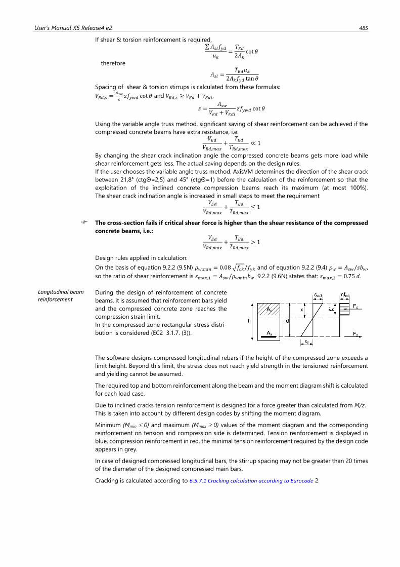
User’s Manual X5 Release4 e2 485

If shear & torsion reinforcement is required, ∑𝐴𝑠𝑙𝑓𝑦𝑑

𝑢𝑘=𝑇𝐸𝑑2𝐴𝑘

cot 휃

therefore

𝐴𝑠𝑙 =𝑇𝐸𝑑𝑢𝑘

2𝐴𝑘𝑓𝑦𝑑 tan 휃

Spacing of shear & torsion stirrups is calculated from these formulas:

𝑉𝑅𝑑,𝑠 =𝐴𝑠𝑤

𝑠𝑧𝑓𝑦𝑤𝑑 cot 휃 and 𝑉𝑅𝑑,𝑠 ≥ 𝑉𝐸𝑑 + 𝑉𝐸𝑑𝑖,

𝑠 =𝐴𝑠𝑤

𝑉𝐸𝑑 + 𝑉𝐸𝑑𝑖𝑧𝑓𝑦𝑤𝑑 cot 휃

Using the variable angle truss method, significant saving of shear reinforcement can be achieved if the

compressed concrete beams have extra resistance, i.e: 𝑉𝐸𝑑

𝑉𝑅𝑑,𝑚𝑎𝑥+

𝑇𝐸𝑑𝑇𝑅𝑑,𝑚𝑎𝑥

≪ 1

By changing the shear crack inclination angle the compressed concrete beams gets more load while

shear reinforcement gets less. The actual saving depends on the design rules.

If the user chooses the variable angle truss method, AxisVM determines the direction of the shear crack

between 21,8° (ctgΘ=2,5) and 45° (ctgΘ=1) before the calculation of the reinforcement so that the

exploitation of the inclined concrete compression beams reach its maximum (at most 100%).

The shear crack inclination angle is increased in small steps to meet the requirement 𝑉𝐸𝑑

𝑉𝑅𝑑,𝑚𝑎𝑥+

𝑇𝐸𝑑𝑇𝑅𝑑,𝑚𝑎𝑥

≤ 1

The cross-section fails if critical shear force is higher than the shear resistance of the compressed

concrete beams, i.e.: 𝑉𝐸𝑑

𝑉𝑅𝑑,𝑚𝑎𝑥+

𝑇𝐸𝑑𝑇𝑅𝑑,𝑚𝑎𝑥

> 1

Design rules applied in calculation:

On the basis of equation 9.2.2 (9.5N) 𝜌𝑤;𝑚𝑖𝑛 = 0.08 √𝑓𝑐𝑘/𝑓𝑦𝑘 and of equation 9.2.2 (9.4) 𝜌𝑤 = 𝐴𝑠𝑤/𝑠𝑏𝑤,

so the ratio of shear reinforcement is 𝑠𝑚𝑎𝑥,1 = 𝐴𝑠𝑤/𝜌𝑤𝑚𝑖𝑛𝑏𝑤 9.2.2 (9.6N) states that: 𝑠𝑚𝑎𝑥,2 = 0.75 𝑑.

Longitudinal beam reinforcement

During the design of reinforcement of concrete

beams, it is assumed that reinforcement bars yield

and the compressed concrete zone reaches the

compression strain limit. In the compressed zone rectangular stress distri-

bution is considered (EC2 3.1.7. (3)).

The software designs compressed longitudinal rebars if the height of the compressed zone exceeds a

limit height. Beyond this limit, the stress does not reach yield strength in the tensioned reinforcement

and yielding cannot be assumed.

The required top and bottom reinforcement along the beam and the moment diagram shift is calculated

for each load case.

Due to inclined cracks tension reinforcement is designed for a force greater than calculated from M/z.

This is taken into account by different design codes by shifting the moment diagram.

Minimum (Mmin 0) and maximum (Mmax 0) values of the moment diagram and the corresponding

reinforcement on tension and compression side is determined. Tension reinforcement is displayed in

blue, compression reinforcement in red, the minimal tension reinforcement required by the design code

appears in grey.

In case of designed compressed longitudinal bars, the stirrup spacing may not be greater than 20 times

of the diameter of the designed compressed main bars.

Cracking is calculated according to 6.5.7.1 Cracking calculation according to Eurocode 2

486

6.5.11.5. Beam reinforcement according to DIN 1045-1

DIN 1045-1 Symbols, material properties, partial factors

fcd design value of the compressive strength of the concrete

fctm mean value of the tensile strength of the concrete

α = 0.85; a coefficient, that takes the sustained load and other unfavorable effects into account

γc = 1.5; partial factor of the concrete

fyd design value of flow limit of rebar steel

εsu limiting strain of rebar steel

Es (=200 kN/mm2); Young modulus of rebar steel

γs = 1.15; partial factor of the steel

Shear & torsion re-inforcement design of stirrups

The design is based on the following three values of design shear resistance:

𝑉𝑅𝑑,𝑐𝑡 Design shear resistance of the cross-section without shear reinforcement.

𝑉𝑅𝑑,𝑚𝑎𝑥 Maximum shear force that can be transmitted without the failure of the inclined

compression bars.

𝑉𝑅𝑑,𝑠𝑦 Design shear resistance of the cross-section with shear reinforcement.

No shear reinforcement is required if 𝑉𝐸𝑑 ≤ 𝑉𝑅𝑑,𝑐𝑡 , DIN 1045-1 10.3.1 (2)

The cross-section does not fail if 𝑉𝐸𝑑 ≤ 𝑉𝑅𝑑,𝑚𝑎𝑥 .

If 𝑉𝐸𝑑 > 𝑉𝑅𝑑,𝑐𝑡 shear reinforcement should be applied DIN 1045-1 10.3.1 (3)

Stirrup spacing is determined to meet the requirement 𝑉𝐸𝑑 ≤ 𝑉𝑅𝑑,𝑠𝑦 .

For cross sections with shear reinforcement we can choose between the regular method (45° cracking)

and Variable Angle Truss (VAT) method.

If the assumed compression trusses have reserve (𝑉𝑅𝑑,𝑚𝑎𝑥 > 𝑉𝐸𝑑) according to the regular method, the

VAT method will lead to considerable savings in shear reinforcement.

By changing the shear crack inclination angle the compressed concrete beams gets more load while

shear reinforcement gets less.

The program is calculating the value

cot Θ =1.2 − 1.4

𝜎𝑐𝑑𝑓𝑐𝑑

𝐴𝑠𝑤

1 −𝑉𝑅𝑑,𝑐𝑉𝐸𝑑

In case of regular concrete: 0.58 ≤ cot Θ ≤ 3.0

In case of light concrete: 0.58 ≤ cot Θ ≤ 2.0 DIN 1045-1 10.3.4 (3)

The regular method assumes the angle of shear cracks to be 45, so cotΘ = 1

𝑉𝑅𝑑,𝑠𝑦 =𝐴𝑠𝑤

𝑠𝑤𝑓𝑦𝑑𝑧 cotΘ DIN 1045-1 10.3.4 (7)

is the shear resistance due to the shear reinforcement.

If torsion is considerable, AxisVM also checks the following condition:

[𝑇𝐸𝑑

𝑇𝑅𝑑,𝑚𝑎𝑥]2

+ [𝑉𝐸𝑑

𝑉𝑅𝑑,𝑚𝑎𝑥]2

≤ 1 DIN 1045-1 10.4.2 (5)

No calculated shear & torsion reinforcement has to be applied if

𝑻𝑬𝒅 ≤ 𝑽𝑬𝒅𝒃𝒘/𝟒. 𝟓 and 𝑽𝑬𝒅 [𝟏 +𝟒.𝟓𝑻𝑬𝒅

𝑽𝑬𝒅𝒃𝒘] ≤ 𝑽𝑹𝒅,𝒄𝒕 DIN 1045-1 10.4.1 (6)

Stirrup reinforce-ment from twisting moment

Resistant twisting moment on the basis of the failure of the compressed concrete bar:

𝑇𝑅𝑑,𝑠𝑦 =2𝐴𝑠𝑤𝑠𝑤

𝑓𝑦𝑑𝐴𝑘 cot Θ

The stirrup distance:

𝒔𝒘 =𝟐𝑨𝒔𝒘𝑻𝑬𝒅

𝒇𝒚𝒅𝑨𝒌 𝐜𝐨𝐭𝚯

Longitudinal reinforcement is calculated from twisting moment 𝑻𝑹𝒅,𝒔𝒚 =𝟐𝑨𝒔𝒍

𝒖𝒌𝒇𝒚𝒅𝑨𝒌 𝐭𝐚𝐧𝚯 ,

so 𝑨𝒔𝒍 = 𝑻𝑬𝒅𝒖𝒌/𝟐𝒇𝒚𝒅𝑨𝒌 𝐭𝐚𝐧𝚯, which should be placed evenly along the cross-section contour.

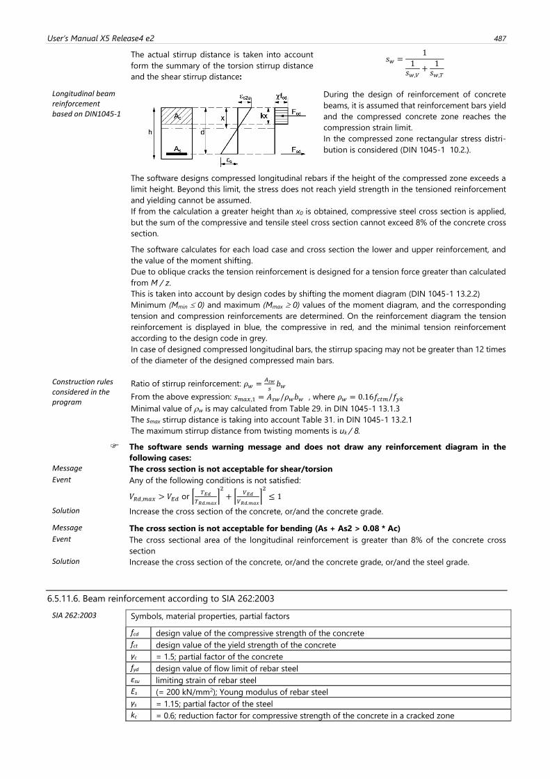
User’s Manual X5 Release4 e2 487

The actual stirrup distance is taken into account

form the summary of the torsion stirrup distance

and the shear stirrup distance:

𝑠𝑤 =1

1𝑠𝑤,𝑉

+1𝑠𝑤,𝑇

Longitudinal beam reinforcement based on DIN1045-1

During the design of reinforcement of concrete

beams, it is assumed that reinforcement bars yield

and the compressed concrete zone reaches the

compression strain limit. In the compressed zone rectangular stress distri-

bution is considered (DIN 1045-1 10.2.).

The software designs compressed longitudinal rebars if the height of the compressed zone exceeds a

limit height. Beyond this limit, the stress does not reach yield strength in the tensioned reinforcement

and yielding cannot be assumed. If from the calculation a greater height than x0 is obtained, compressive steel cross section is applied,

but the sum of the compressive and tensile steel cross section cannot exceed 8% of the concrete cross

section.

The software calculates for each load case and cross section the lower and upper reinforcement, and

the value of the moment shifting.

Due to oblique cracks the tension reinforcement is designed for a tension force greater than calculated

from M / z.

This is taken into account by design codes by shifting the moment diagram (DIN 1045-1 13.2.2)

Minimum (Mmin 0) and maximum (Mmax 0) values of the moment diagram, and the corresponding

tension and compression reinforcements are determined. On the reinforcement diagram the tension

reinforcement is displayed in blue, the compressive in red, and the minimal tension reinforcement

according to the design code in grey.

In case of designed compressed longitudinal bars, the stirrup spacing may not be greater than 12 times

of the diameter of the designed compressed main bars.

Construction rules considered in the program

Ratio of stirrup reinforcement: 𝜌𝑤 =𝐴𝑠𝑤

𝑠𝑏𝑤

From the above expression: 𝑠𝑚𝑎𝑥,1 = 𝐴𝑠𝑤/𝜌𝑤𝑏𝑤 , where 𝜌𝑤 = 0.16𝑓𝑐𝑡𝑚/𝑓𝑦𝑘

Minimal value of w is may calculated from Table 29. in DIN 1045-1 13.1.3

The smax stirrup distance is taking into account Table 31. in DIN 1045-1 13.2.1

The maximum stirrup distance from twisting moments is uk / 8.

The software sends warning message and does not draw any reinforcement diagram in the

following cases:

Message The cross section is not acceptable for shear/torsion

Event Any of the following conditions is not satisfied:

𝑉𝑅𝑑,𝑚𝑎𝑥 > 𝑉𝐸𝑑 or [𝑇𝐸𝑑

𝑇𝑅𝑑,𝑚𝑎𝑥]2

+ [𝑉𝐸𝑑

𝑉𝑅𝑑,𝑚𝑎𝑥]2

≤ 1

Solution Increase the cross section of the concrete, or/and the concrete grade.

Message The cross section is not acceptable for bending (As + As2 > 0.08 * Ac)

Event The cross sectional area of the longitudinal reinforcement is greater than 8% of the concrete cross

section

Solution Increase the cross section of the concrete, or/and the concrete grade, or/and the steel grade.

6.5.11.6. Beam reinforcement according to SIA 262:2003

SIA 262:2003 Symbols, material properties, partial factors

fcd design value of the compressive strength of the concrete

fct design value of the yield strength of the concrete

γc = 1.5; partial factor of the concrete

fyd design value of flow limit of rebar steel

εsu limiting strain of rebar steel

Es (= 200 kN/mm2); Young modulus of rebar steel

γs = 1.15; partial factor of the steel

kc = 0.6; reduction factor for compressive strength of the concrete in a cracked zone

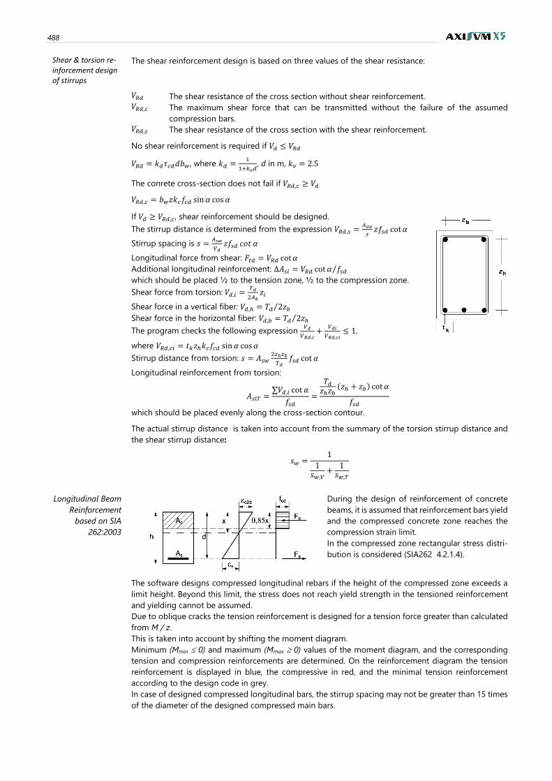
488

Shear & torsion re-inforcement design of stirrups

The shear reinforcement design is based on three values of the shear resistance:

𝑉𝑅𝑑 The shear resistance of the cross section without shear reinforcement.

𝑉𝑅𝑑,𝑐 The maximum shear force that can be transmitted without the failure of the assumed

compression bars.

𝑉𝑅𝑑,𝑠 The shear resistance of the cross section with the shear reinforcement.

No shear reinforcement is required if 𝑉𝑑 ≤ 𝑉𝑅𝑑

𝑉𝑅𝑑 = 𝑘𝑑𝜏𝑐𝑑𝑑𝑏𝑤, where 𝑘𝑑 =1

1+𝑘𝑣𝑑, d in m, 𝑘𝑣 = 2.5

The conrete cross-section does not fail if 𝑉𝑅𝑑,𝑐 ≥ 𝑉𝑑

𝑉𝑅𝑑,𝑐 = 𝑏𝑤𝑧𝑘𝑐𝑓𝑐𝑑 sin 𝛼 cos𝛼

If 𝑉𝑑 ≥ 𝑉𝑅𝑑,𝑐, shear reinforcement should be designed.

The stirrup distance is determined from the expression 𝑉𝑅𝑑,𝑠 =𝐴𝑠𝑤

𝑠𝑧𝑓𝑠𝑑 cot 𝛼

Stirrup spacing is 𝑠 =𝐴𝑠𝑤

𝑉𝑑𝑧𝑓𝑠𝑑 𝑐𝑜𝑡 𝛼

Longitudinal force from shear: 𝐹𝑡𝑑 = 𝑉𝑅𝑑 cot 𝛼

Additional longitudinal reinforcement: Δ𝐴𝑠𝑙 = 𝑉𝑅𝑑 cot 𝛼 𝑓𝑠𝑑⁄

which should be placed ½ to the tension zone, ½ to the compression zone.

Shear force from torsion: 𝑉𝑑,𝑖 =𝑇𝑑

2𝐴𝑘𝑧𝑖

Shear force in a vertical fiber: 𝑉𝑑,ℎ = 𝑇𝑑 2𝑧𝑏⁄

Shear force in the horizontal fiber: 𝑉𝑑,𝑏 = 𝑇𝑑 2𝑧ℎ⁄

The program checks the following expression 𝑉𝑑

𝑉𝑅𝑑,𝑐+

𝑉𝑑𝑖

𝑉𝑅𝑑,𝑐𝑖≤ 1,

where 𝑉𝑅𝑑,𝑐𝑖 = 𝑡𝑘𝑧ℎ𝑘𝑐𝑓𝑐𝑑 sin 𝛼 cos𝛼

Stirrup distance from torsion: 𝑠 = 𝐴𝑠𝑤2𝑧ℎ𝑧𝑏

𝑇𝑑𝑓𝑠𝑑 cot 𝛼

Longitudinal reinforcement from torsion:

𝐴𝑠𝑙𝑇 =∑𝑉𝑑,𝑖 cot 𝛼

𝑓𝑠𝑑=

𝑇𝑑𝑧ℎ𝑧𝑏

(𝑧ℎ + 𝑧𝑏) cot 𝛼

𝑓𝑠𝑑

which should be placed evenly along the cross-section contour.

The actual stirrup distance is taken into account from the summary of the torsion stirrup distance and

the shear stirrup distance:

𝑠𝑤 =1

1𝑠𝑤,𝑉

+1𝑠𝑤,𝑇

Longitudinal Beam

Reinforcement

based on SIA

262:2003

During the design of reinforcement of concrete

beams, it is assumed that reinforcement bars yield

and the compressed concrete zone reaches the

compression strain limit. In the compressed zone rectangular stress distri-

bution is considered (SIA262 4.2.1.4).

The software designs compressed longitudinal rebars if the height of the compressed zone exceeds a

limit height. Beyond this limit, the stress does not reach yield strength in the tensioned reinforcement

and yielding cannot be assumed.

Due to oblique cracks the tension reinforcement is designed for a tension force greater than calculated

from M / z.

This is taken into account by shifting the moment diagram.

Minimum (Mmin 0) and maximum (Mmax 0) values of the moment diagram, and the corresponding

tension and compression reinforcements are determined. On the reinforcement diagram the tension

reinforcement is displayed in blue, the compressive in red, and the minimal tension reinforcement

according to the design code in grey.

In case of designed compressed longitudinal bars, the stirrup spacing may not be greater than 15 times

of the diameter of the designed compressed main bars.

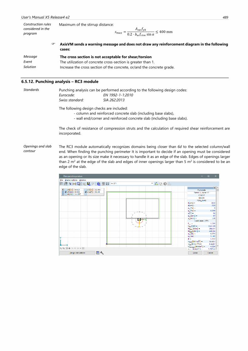
User’s Manual X5 Release4 e2 489

Construction rules considered in the program

Maximum of the stirrup distance:

𝑠𝑚𝑎𝑥 =𝐴𝑠𝑤𝑓𝑦𝑘

0.2 ⋅ 𝑏𝑤𝑓𝑐𝑡𝑚 sin 𝛼≤ 400 mm

AxisVM sends a warning message and does not draw any reinforcement diagram in the following

cases:

Message The cross section is not acceptable for shear/torsion

Event The utilization of concrete cross-section is greater than 1.

Solution Increase the cross section of the concrete, or/and the concrete grade.

6.5.12. Punching analysis – RC3 module

Standards Punching analysis can be performed according to the following design codes:

Eurocode: EN 1992-1-1:2010

Swiss standard: SIA 262:2013

The following design checks are included:

- column and reinforced concrete slab (including base slabs),

- wall end/corner and reinforced concrete slab (including base slabs).

The check of resistance of compression struts and the calculation of required shear reinforcement are

incorporated.

Openings and slab contour

The RC3 module automatically recognizes domains being closer than 6d to the selected column/wall

end. When finding the punching perimeter It is important to decide if an opening must be considered

as an opening or its size make it necessary to handle it as an edge of the slab. Edges of openings larger

than 2 m2 at the edge of the slab and edges of inner openings larger than 5 m2 is considered to be an

edge of the slab.

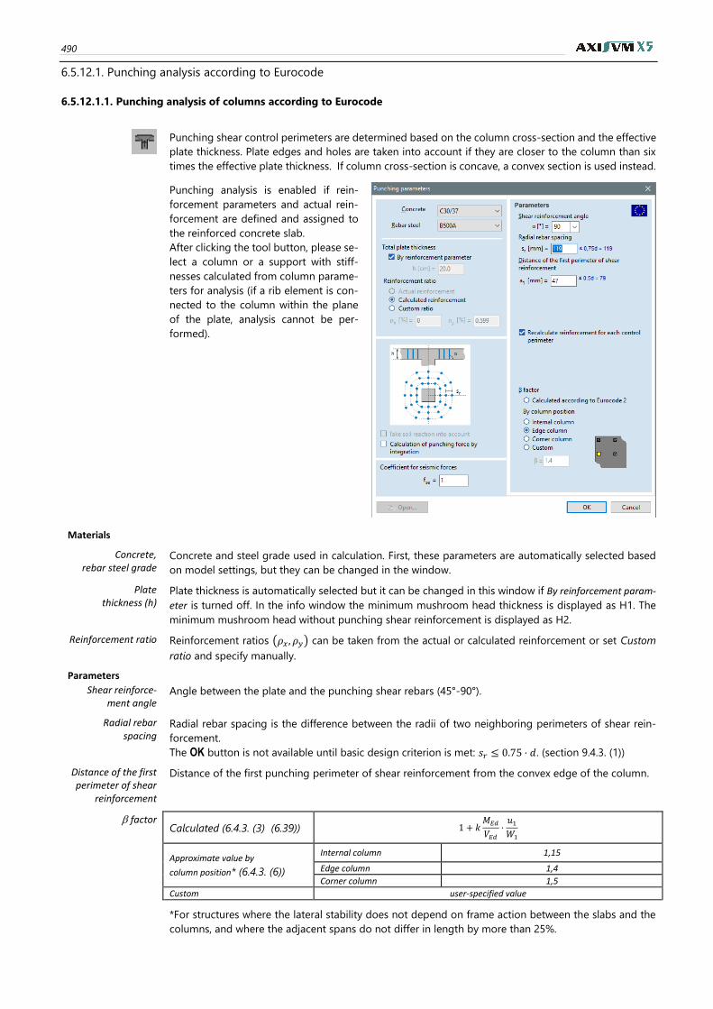
490

6.5.12.1. Punching analysis according to Eurocode

6.5.12.1.1. Punching analysis of columns according to Eurocode

Punching shear control perimeters are determined based on the column cross-section and the effective

plate thickness. Plate edges and holes are taken into account if they are closer to the column than six

times the effective plate thickness. If column cross-section is concave, a convex section is used instead.

Punching analysis is enabled if rein-

forcement parameters and actual rein-

forcement are defined and assigned to

the reinforced concrete slab.

After clicking the tool button, please se-

lect a column or a support with stiff-

nesses calculated from column parame-

ters for analysis (if a rib element is con-

nected to the column within the plane

of the plate, analysis cannot be per-

formed).

Materials

Concrete, rebar steel grade

Concrete and steel grade used in calculation. First, these parameters are automatically selected based

on model settings, but they can be changed in the window.

Plate thickness (h)

Plate thickness is automatically selected but it can be changed in this window if By reinforcement param-

eter is turned off. In the info window the minimum mushroom head thickness is displayed as H1. The

minimum mushroom head without punching shear reinforcement is displayed as H2.

Reinforcement ratio Reinforcement ratios (𝜌𝑥 , 𝜌𝑦) can be taken from the actual or calculated reinforcement or set Custom

ratio and specify manually.

Parameters

Shear reinforce-ment angle

Angle between the plate and the punching shear rebars (45°-90°).

Radial rebar spacing

Radial rebar spacing is the difference between the radii of two neighboring perimeters of shear rein-

forcement.

The OK button is not available until basic design criterion is met: 𝑠𝑟 ≤ 0.75 ⋅ 𝑑. (section 9.4.3. (1))

Distance of the first perimeter of shear

reinforcement

Distance of the first punching perimeter of shear reinforcement from the convex edge of the column.

factor Calculated (6.4.3. (3) (6.39)) 1 + 𝑘

𝑀𝐸𝑑

𝑉𝐸𝑑⋅𝑢1𝑊1

Approximate value by

column position* (6.4.3. (6))

Internal column 1,15

Edge column 1,4

Corner column 1,5

Custom user-specified value

*For structures where the lateral stability does not depend on frame action between the slabs and the

columns, and where the adjacent spans do not differ in length by more than 25%.

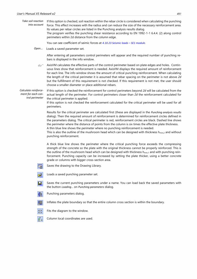
User’s Manual X5 Release4 e2 491

Take soil reaction into account

If this option is checked, soil reaction within the rebar circle is considered when calculating the punching

force. This effect increases with the radius and can reduce the size of the necessary reinforcement area.

Its values per rebar circles are listed in the Punching analysis results dialog.

The program verifies the punching shear resistance according to EN 1992-1-1 6.4.4. (2) along control

perimeters within 2d distance from the column edge.

You can see coefficient of seimic forces at 4.10.23 Seismic loads – SE1 module.

Open... Loads a saved parameter set.

After entering all parameters control perimeters will appear and the required number of punching re-

bars is displayed in the info window.

AxisVM calculates the effective parts of the control perimeter based on plate edges and holes. Contin-

uous lines show that reinforcement is needed. AxisVM displays the required amount of reinforcement

for each line. The info window shows the amount of critical punching reinforcement. When calculating

the length of the critical perimeter it is assumed that rebar spacing on the perimeter is not above 2d

but the fulfillment of this requirement is not checked. If this requirement is not met, the user should

choose a smaller diameter or place additional rebars.

Calculate reinforce-ment for each con-

trol perimeter

If this option is checked the reinforcement for control perimeters beyond 2d will be calculated from the

actual length of the perimeter. For control perimeters closer than 2d the reinforcement calculated for

the critical perimeter is applied.

If this option is not checked the reinforcement calculated for the critical perimeter will be used for all

perimeters.

Results for the critical perimeter are calculated first (these are displayed in the Punching analysis results

dialog). Then the required amount of reinforcement is determined for reinforcement circles defined in

the parameters dialog. The critical perimeter is red, reinforcement circles are black. Dashed line shows

the perimeter where the distance of points from the column is six times the effective plate thickness.

A thin blue line shows the perimeter where no punching reinforcement is needed.

This is also the outline of the mushroom head which can be designed with thickness hmin,2 and without

punching reinforcement.

A thick blue line shows the perimeter where the critical punching force exceeds the compressing

strength of the concrete so the plate with the original thickness cannot be properly reinforced. This is

the outline of the mushroom head which can be designed with thickness hmin,1 and with punching rein-

forcement. Punching capacity can be increased by setting the plate thicker, using a better concrete

grade or columns with bigger cross-section area.

Saves the drawing to the Drawing Library.

Loads a saved punching parameter set.

Saves the current punching parameters under a name. You can load back the saved parameters with

the button Loading... on Punching parameters dialog.

Punching parameters dialog.

Inflates the plate boundary so that the entire column cross section is within the boundary.

Fits the diagram to the window.

Column local coordinates are used.

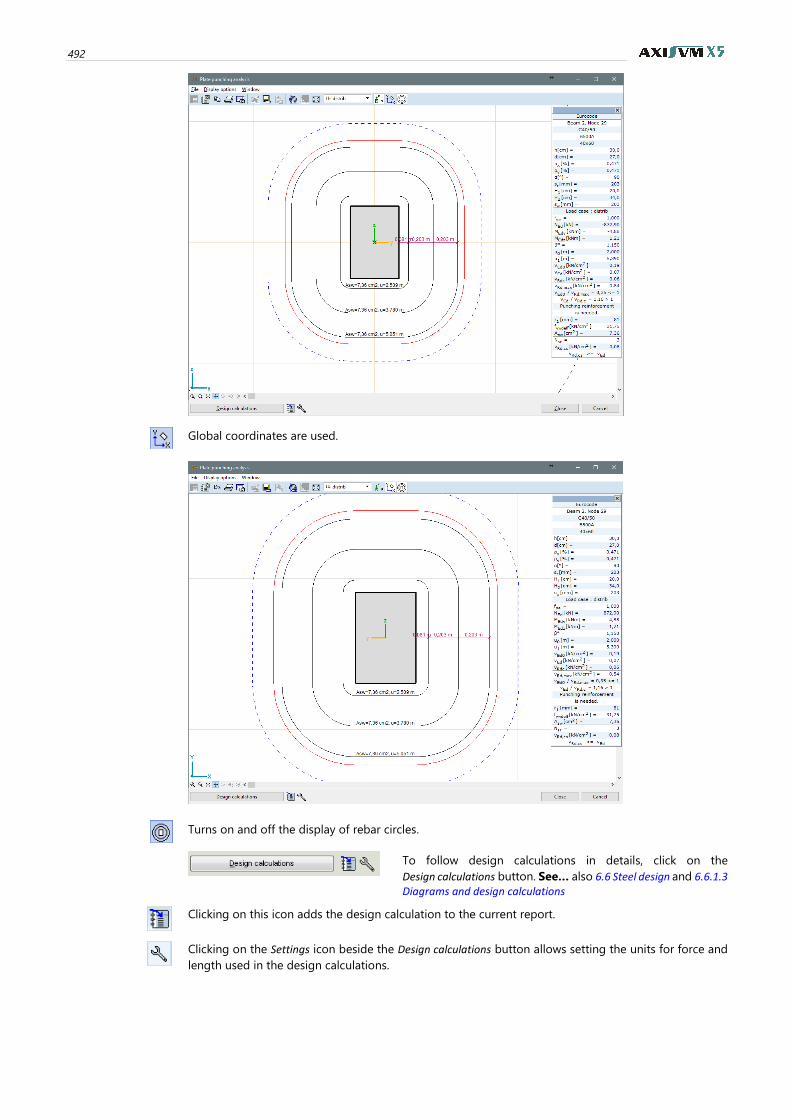
492

Global coordinates are used.

Turns on and off the display of rebar circles.

To follow design calculations in details, click on the

Design calculations button. See… also 6.6 Steel design and 6.6.1.3 Diagrams and design calculations

Clicking on this icon adds the design calculation to the current report.

Clicking on the Settings icon beside the Design calculations button allows setting the units for force and

length used in the design calculations.

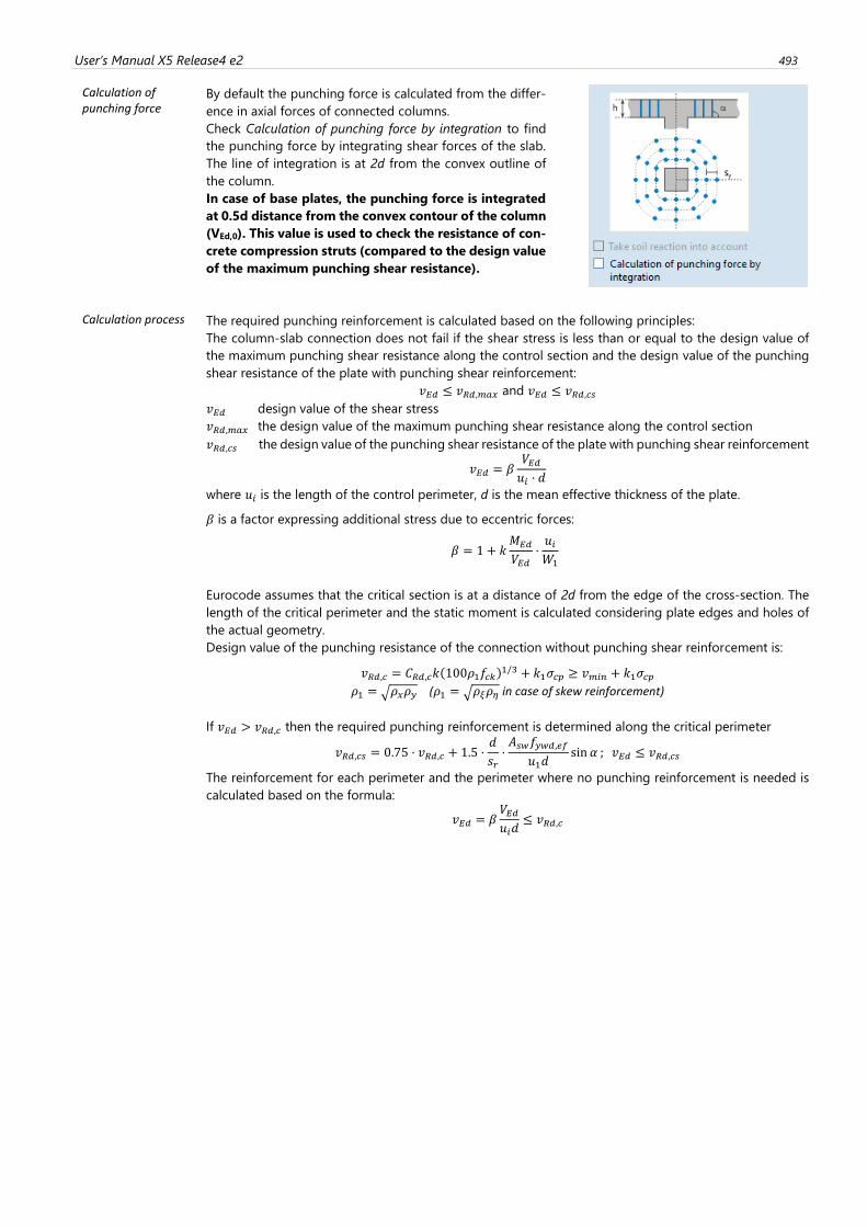
User’s Manual X5 Release4 e2 493

Calculation of punching force

By default the punching force is calculated from the differ-

ence in axial forces of connected columns.

Check Calculation of punching force by integration to find

the punching force by integrating shear forces of the slab.

The line of integration is at 2d from the convex outline of

the column.

In case of base plates, the punching force is integrated

at 0.5d distance from the convex contour of the column

(VEd,0). This value is used to check the resistance of con-

crete compression struts (compared to the design value

of the maximum punching shear resistance).

Calculation process

The required punching reinforcement is calculated based on the following principles:

The column-slab connection does not fail if the shear stress is less than or equal to the design value of

the maximum punching shear resistance along the control section and the design value of the punching

shear resistance of the plate with punching shear reinforcement:

𝑣𝐸𝑑 ≤ 𝑣𝑅𝑑,𝑚𝑎𝑥 and 𝑣𝐸𝑑 ≤ 𝑣𝑅𝑑,𝑐𝑠

𝑣𝐸𝑑 design value of the shear stress

𝑣𝑅𝑑,𝑚𝑎𝑥 the design value of the maximum punching shear resistance along the control section

𝑣𝑅𝑑,𝑐𝑠 the design value of the punching shear resistance of the plate with punching shear reinforcement

𝑣𝐸𝑑 = 𝛽𝑉𝐸𝑑𝑢𝑖 ⋅ 𝑑

where 𝑢𝑖 is the length of the control perimeter, d is the mean effective thickness of the plate.

𝛽 is a factor expressing additional stress due to eccentric forces:

𝛽 = 1 + 𝑘𝑀𝐸𝑑

𝑉𝐸𝑑⋅𝑢𝑖𝑊1

Eurocode assumes that the critical section is at a distance of 2d from the edge of the cross-section. The

length of the critical perimeter and the static moment is calculated considering plate edges and holes of

the actual geometry.

Design value of the punching resistance of the connection without punching shear reinforcement is:

𝑣𝑅𝑑,𝑐 = 𝐶𝑅𝑑,𝑐𝑘(100𝜌1𝑓𝑐𝑘)1/3 + 𝑘1𝜎𝑐𝑝 ≥ 𝑣𝑚𝑖𝑛 + 𝑘1𝜎𝑐𝑝

𝜌1 = √𝜌𝑥𝜌𝑦 (𝜌1 = √𝜌𝜉𝜌𝜂 in case of skew reinforcement)

If 𝑣𝐸𝑑 > 𝑣𝑅𝑑,𝑐 then the required punching reinforcement is determined along the critical perimeter

𝑣𝑅𝑑,𝑐𝑠 = 0.75 ⋅ 𝑣𝑅𝑑,𝑐 + 1.5 ⋅𝑑

𝑠𝑟⋅𝐴𝑠𝑤𝑓𝑦𝑤𝑑,𝑒𝑓

𝑢1𝑑sin 𝛼 ; 𝑣𝐸𝑑 ≤ 𝑣𝑅𝑑,𝑐𝑠

The reinforcement for each perimeter and the perimeter where no punching reinforcement is needed is

calculated based on the formula:

𝑣𝐸𝑑 = 𝛽𝑉𝐸𝑑𝑢𝑖𝑑

≤ 𝑣𝑅𝑑,𝑐

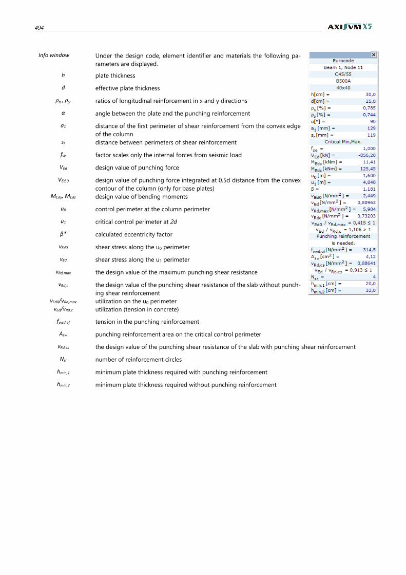
494

Info window

Under the design code, element identifier and materials the following pa-

rameters are displayed.

h plate thickness

d effective plate thickness

𝜌𝑥, 𝜌𝑦 ratios of longitudinal reinforcement in x and y directions

α angle between the plate and the punching reinforcement

a1 distance of the first perimeter of shear reinforcement from the convex edge

of the column

sr distance between perimeters of shear reinforcement

fse factor scales only the internal forces from seismic load

VEd design value of punching force

VEd,0 design value of punching force integrated at 0.5d distance from the convex

contour of the column (only for base plates)

MEdy, MEdz design value of bending moments

u0 control perimeter at the column perimeter

u1 critical control perimeter at 2d

ϐ* calculated eccentricity factor

vEd0 shear stress along the u0 perimeter

vEd shear stress along the u1 perimeter

vRd,max the design value of the maximum punching shear resistance

vRd,c the design value of the punching shear resistance of the slab without punch-

ing shear reinforcement

vEd0/vRd,max utilization on the u0 perimeter

vEd/vRd,c utilization (tension in concrete)

fywd,ef tension in the punching reinforcement

Asw punching reinforcement area on the critical control perimeter

vRd,cs the design value of the punching shear resistance of the slab with punching shear reinforcement

Nsr number of reinforcement circles

hmin,1 minimum plate thickness required with punching reinforcement

hmin,2 minimum plate thickness required without punching reinforcement

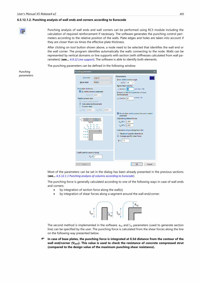
User’s Manual X5 Release4 e2 495

6.5.12.1.2. Punching analysis of wall ends and corners according to Eurocode

Punching analysis of wall ends and wall corners can be performed using RC3 module including the

calculation of required reinforcement if necessary. The software generates the punching control peri-

meters according to the relative position of the walls. Plate edges and holes are taken into account if

they are closer than six times the effective plate thickness.

After clicking on tool button shown above, a node need to be selected that identifies the wall end or

the wall corner. The program identifies automatically the walls connecting to the node. Walls can be

represented by vertical domains or line supports with section (with stiffnesses calculated from wall pa-

rameters) (see... 4.9.12 Line support). The software is able to identify both elements.

The punching parameters can be defined in the following window:

Punching parameters

Most of the parameters can be set in the dialog has been already presented in the previous sections

(see... 6.5.12.1.1 Punching analysis of columns according to Eurocode).

The punching force is generally calculated according to one of the following ways in case of wall ends

and corners:

• by integration of section force along the wall(s);

• by integration of shear forces along a segment around the wall end/corner.

The second method is implemented in the software. acp and lcp parameters (used to generate section

line) can be specified by the user. The punching force is calculated from the shear forces along the line

on the following way presented below.

In case of base plates, the punching force is integrated at 0.5d distance from the contour of the

wall end/corner (VEd,0). This value is used to check the resistance of concrete compressed strut

(compared to the design value of the maximum punching shear resistance).

acp

acp

lcp lcp

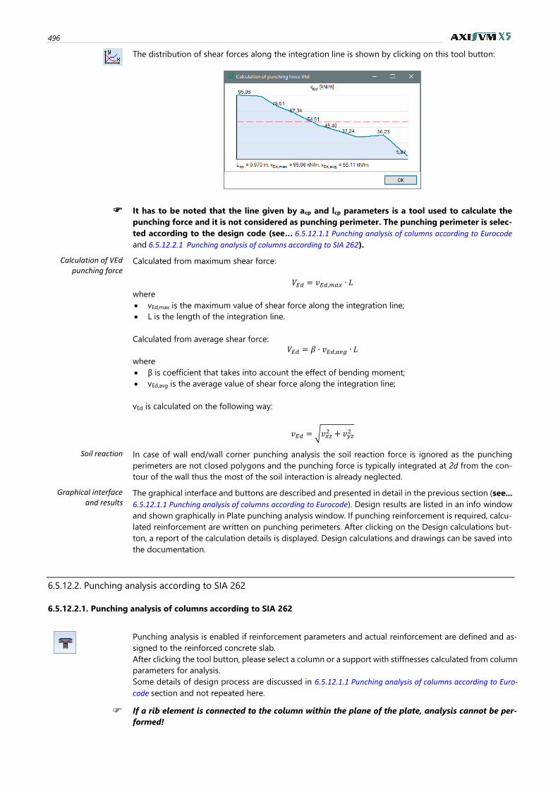
496

The distribution of shear forces along the integration line is shown by clicking on this tool button:

It has to be noted that the line given by acp and lcp parameters is a tool used to calculate the

punching force and it is not considered as punching perimeter. The punching perimeter is selec-

ted according to the design code (see… 6.5.12.1.1 Punching analysis of columns according to Eurocode

and 6.5.12.2.1 Punching analysis of columns according to SIA 262).

Calculation of VEd punching force

Calculated from maximum shear force:

𝑉𝐸𝑑 = 𝑣𝐸𝑑,𝑚𝑎𝑥 ∙ 𝐿

where

• vEd,max is the maximum value of shear force along the integration line;

• L is the length of the integration line.

Calculated from average shear force:

𝑉𝐸𝑑 = 𝛽 ∙ 𝑣𝐸𝑑,𝑎𝑣𝑔 ∙ 𝐿

where

• β is coefficient that takes into account the effect of bending moment;

• vEd,avg is the average value of shear force along the integration line;

vEd is calculated on the following way:

𝑣𝐸𝑑 = √𝑣𝑥𝑧2 + 𝑣𝑦𝑧

2

Soil reaction In case of wall end/wall corner punching analysis the soil reaction force is ignored as the punching

perimeters are not closed polygons and the punching force is typically integrated at 2d from the con-

tour of the wall thus the most of the soil interaction is already neglected.

Graphical interface and results

The graphical interface and buttons are described and presented in detail in the previous section (see...

6.5.12.1.1 Punching analysis of columns according to Eurocode). Design results are listed in an info window

and shown graphically in Plate punching analysis window. If punching reinforcement is required, calcu-

lated reinforcement are written on punching perimeters. After clicking on the Design calculations but-

ton, a report of the calculation details is displayed. Design calculations and drawings can be saved into

the documentation.

6.5.12.2. Punching analysis according to SIA 262

6.5.12.2.1. Punching analysis of columns according to SIA 262

Punching analysis is enabled if reinforcement parameters and actual reinforcement are defined and as-

signed to the reinforced concrete slab.

After clicking the tool button, please select a column or a support with stiffnesses calculated from column

parameters for analysis.

Some details of design process are discussed in 6.5.12.1.1 Punching analysis of columns according to Euro-

code section and not repeated here.

If a rib element is connected to the column within the plane of the plate, analysis cannot be per-

formed!

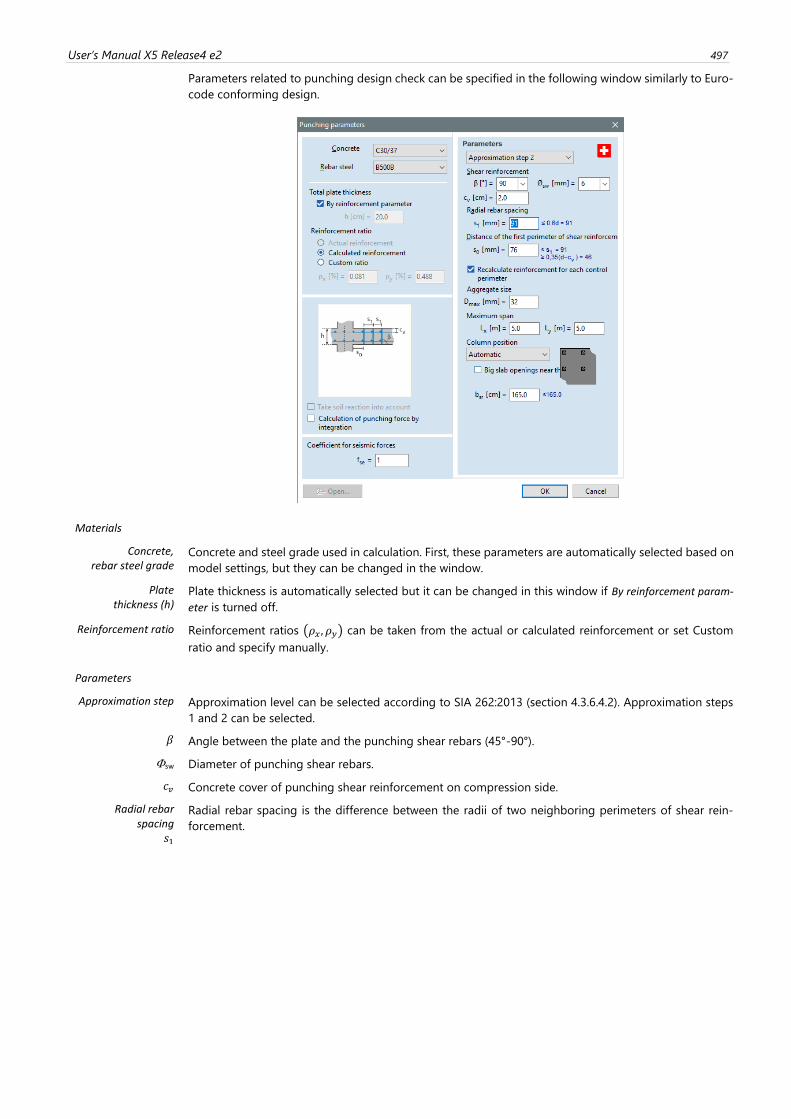
User’s Manual X5 Release4 e2 497

Parameters related to punching design check can be specified in the following window similarly to Euro-

code conforming design.

Materials

Concrete, rebar steel grade

Concrete and steel grade used in calculation. First, these parameters are automatically selected based on

model settings, but they can be changed in the window.

Plate thickness (h)

Plate thickness is automatically selected but it can be changed in this window if By reinforcement param-

eter is turned off.

Reinforcement ratio Reinforcement ratios (𝜌𝑥 , 𝜌𝑦) can be taken from the actual or calculated reinforcement or set Custom

ratio and specify manually.

Parameters

Approximation step Approximation level can be selected according to SIA 262:2013 (section 4.3.6.4.2). Approximation steps

1 and 2 can be selected.

𝛽 Angle between the plate and the punching shear rebars (45°-90°).

sw Diameter of punching shear rebars.

𝑐𝑣 Concrete cover of punching shear reinforcement on compression side.

Radial rebar spacing

𝑠1

Radial rebar spacing is the difference between the radii of two neighboring perimeters of shear rein-

forcement.

498

Distance of the first perimeter of shear

reinforcement 𝑠0

Distance of the first punching perimeter of shear reinforcement from the convex edge of the column.

𝐷𝑚𝑎𝑥 maximum grain size of aggregate

𝑙𝑥, 𝑙𝑦 span in x-, y-directions (sections 4.3.6.4.2 and 4.3.6.4.4)

bsr Limit value for width of column strips for the determination of bending resistances.

Calculation of punching force

The punching force can be calculated from the difference in axial forces of connected columns or by the

integration of shear forces of the slab (see... 6.5.12.1.1 Punching analysis of columns according to Eurocode).

Design principles

The software determines the punching perimeter at 0,5𝑑𝑣 distance (section 4.3.6.2.2) from the convex

edge of the column where punching resistance need to be checked. The resistance of compressive struts

is calculated according to section 4.3.6.5.7:

𝑉𝑅𝑑,𝑚𝑎𝑥 = 2 ∙ 𝑘𝑟 ⋅ 𝜏𝑐𝑑 ⋅ 𝑑𝑣 ⋅ 𝑢

If 𝑉𝑑 > 𝑉𝑅𝑑,𝑚𝑎𝑥, the resistance of compressive struts is not adequate. In this case, the plate thickness or

concrete strength need to be changed.

The punching shear resistance without shear reinforcement is calculated on the following way (section

4.3.6.3.1):

𝑉𝑅𝑑,𝑐 = 𝑘𝑟 ⋅ 𝜏𝑐𝑑 ⋅ 𝑑𝑣 ⋅ 𝑢

If 𝑉𝑑 ≤ 𝑉𝑅𝑑,𝑐, punching shear reinforcement is not necessary, otherwise the required shear reinforcement

is calculated as follows (sections 4.3.6.5.2 (65) and 4.3.6.5.3 (66)):

𝛴𝐴𝑠𝑤 =𝑉𝑑

𝑘𝑒 ⋅ 𝜎𝑠𝑑 ⋅ 𝑠𝑖𝑛𝛽,

where

𝜎𝑠𝑑 =𝐸𝑠 ⋅ 𝜓

6⋅ (1 +

𝑓𝑏𝑑𝑓𝑠𝑑

⋅𝑑

𝜙𝑠𝑤)

𝜓 = 1,5 ⋅𝑟𝑠

𝑑⋅𝑓𝑠𝑑

𝐸𝑠⋅ (

𝑚𝑠𝑑

𝑚𝑅𝑑)3 2⁄

and 𝑓𝑏𝑑 =1,4⋅𝑓𝑐𝑡𝑚

𝛾𝑐

This required reinforcement need to be applied between 0,35 ⋅ 𝑑𝑣 and 𝑑𝑣 according to the code. Based

on the given design parameters, the number perimeters of shear reinforcement is calculated can be

placed between 0,35 ⋅ 𝑑𝑣 and 𝑑𝑣 . Required reinforcement for a perimeter is calculated by dividing 𝛴𝐴𝑠𝑤

with the number of perimeters. This 𝐴𝑠𝑤 required reinforcement is placed (outside 𝑑𝑣 distance) on each

perimeter until it is needed.

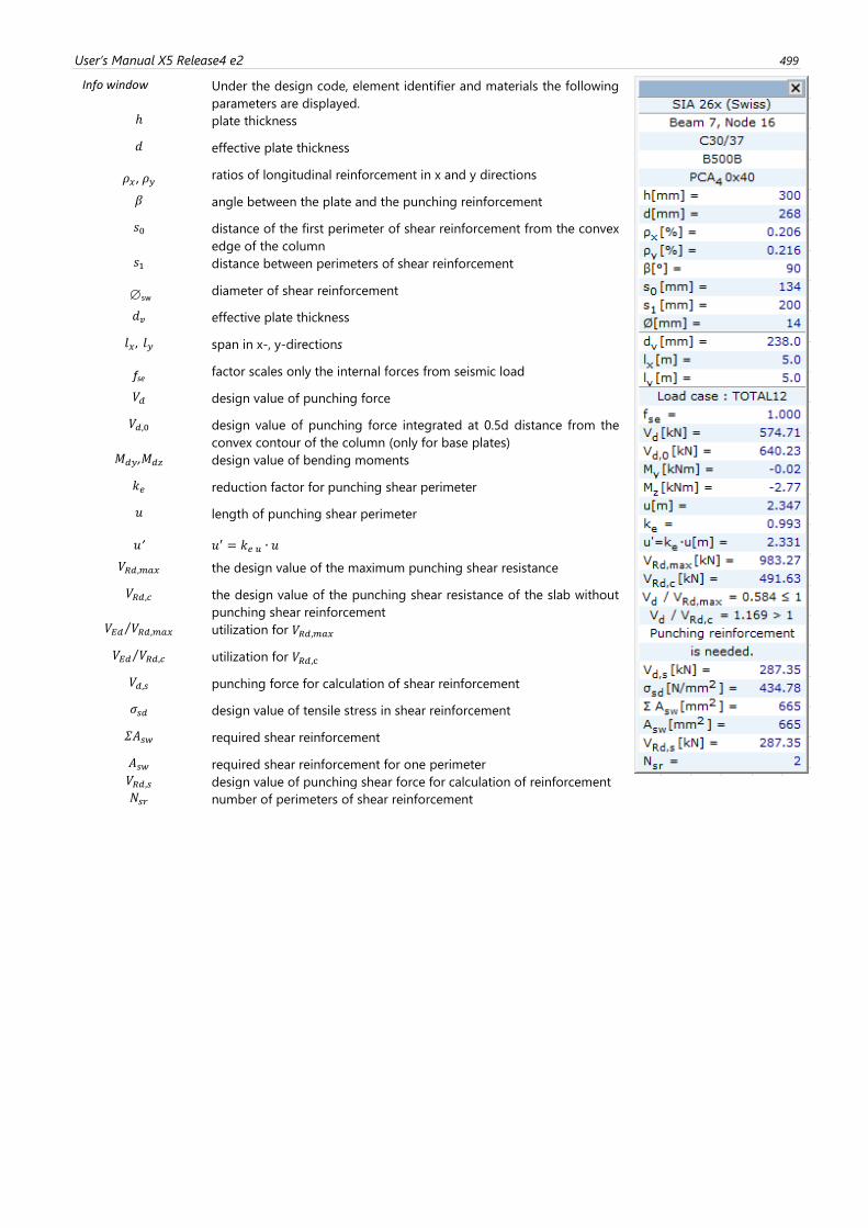
User’s Manual X5 Release4 e2 499

Info window

Under the design code, element identifier and materials the following

parameters are displayed.

ℎ plate thickness

𝑑 effective plate thickness

𝜌𝑥, 𝜌𝑦 ratios of longitudinal reinforcement in x and y directions

𝛽 angle between the plate and the punching reinforcement

𝑠0 distance of the first perimeter of shear reinforcement from the convex

edge of the column

𝑠1 distance between perimeters of shear reinforcement

sw diameter of shear reinforcement

𝑑𝑣 effective plate thickness

𝑙𝑥, 𝑙𝑦 span in x-, y-directions

fse factor scales only the internal forces from seismic load

𝑉𝑑 design value of punching force

𝑉𝑑,0 design value of punching force integrated at 0.5d distance from the

convex contour of the column (only for base plates)

𝑀𝑑𝑦,𝑀𝑑𝑧 design value of bending moments

𝑘𝑒 reduction factor for punching shear perimeter

𝑢 length of punching shear perimeter

𝑢’ 𝑢′ = 𝑘𝑒 𝑢 ∙ 𝑢

𝑉𝑅𝑑,𝑚𝑎𝑥 the design value of the maximum punching shear resistance

𝑉𝑅𝑑,𝑐 the design value of the punching shear resistance of the slab without

punching shear reinforcement

𝑉𝐸𝑑 𝑉𝑅𝑑,𝑚𝑎𝑥⁄ utilization for 𝑉𝑅𝑑,𝑚𝑎𝑥

𝑉𝐸𝑑 𝑉𝑅𝑑,𝑐⁄ utilization for 𝑉𝑅𝑑,c

𝑉𝑑,𝑠 punching force for calculation of shear reinforcement

𝜎𝑠𝑑 design value of tensile stress in shear reinforcement

𝛴𝐴𝑠𝑤 required shear reinforcement

𝐴𝑠𝑤 required shear reinforcement for one perimeter

𝑉𝑅𝑑,𝑠 design value of punching shear force for calculation of reinforcement

𝑁𝑠𝑟 number of perimeters of shear reinforcement

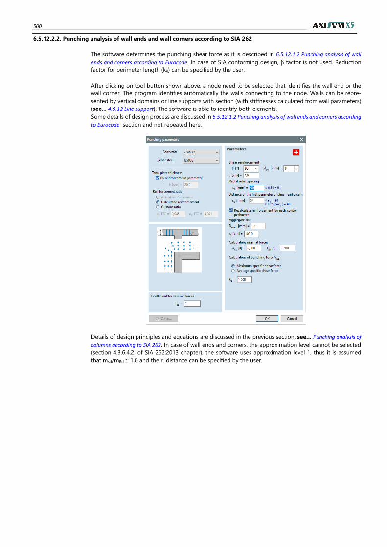
500

6.5.12.2.2. Punching analysis of wall ends and wall corners according to SIA 262

The software determines the punching shear force as it is described in 6.5.12.1.2 Punching analysis of wall

ends and corners according to Eurocode. In case of SIA conforming design, β factor is not used. Reduction

factor for perimeter length (ke) can be specified by the user.

After clicking on tool button shown above, a node need to be selected that identifies the wall end or the

wall corner. The program identifies automatically the walls connecting to the node. Walls can be repre-

sented by vertical domains or line supports with section (with stiffnesses calculated from wall parameters)

(see... 4.9.12 Line support). The software is able to identify both elements.

Some details of design process are discussed in 6.5.12.1.2 Punching analysis of wall ends and corners according

to Eurocode section and not repeated here.

Details of design principles and equations are discussed in the previous section. see… Punching analysis of

columns according to SIA 262. In case of wall ends and corners, the approximation level cannot be selected

(section 4.3.6.4.2. of SIA 262:2013 chapter), the software uses approximation level 1, thus it is assumed

that msd/mRd 1.0 and the rs distance can be specified by the user.

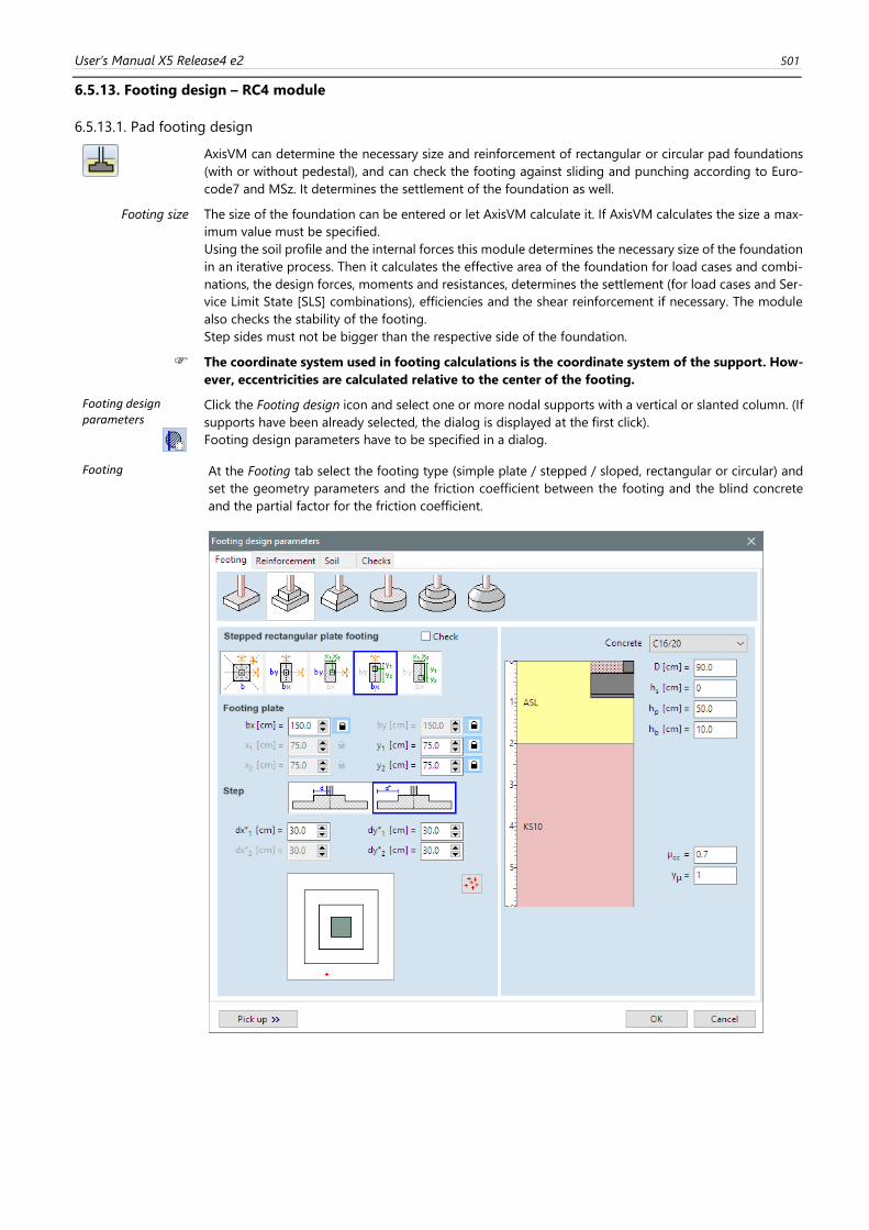
User’s Manual X5 Release4 e2 501

6.5.13. Footing design – RC4 module

6.5.13.1. Pad footing design

AxisVM can determine the necessary size and reinforcement of rectangular or circular pad foundations

(with or without pedestal), and can check the footing against sliding and punching according to Euro-

code7 and MSz. It determines the settlement of the foundation as well.

Footing size The size of the foundation can be entered or let AxisVM calculate it. If AxisVM calculates the size a max-

imum value must be specified.

Using the soil profile and the internal forces this module determines the necessary size of the foundation

in an iterative process. Then it calculates the effective area of the foundation for load cases and combi-

nations, the design forces, moments and resistances, determines the settlement (for load cases and Ser-

vice Limit State [SLS] combinations), efficiencies and the shear reinforcement if necessary. The module

also checks the stability of the footing.

Step sides must not be bigger than the respective side of the foundation.

The coordinate system used in footing calculations is the coordinate system of the support. How-

ever, eccentricities are calculated relative to the center of the footing.

Footing design parameters

Click the Footing design icon and select one or more nodal supports with a vertical or slanted column. (If

supports have been already selected, the dialog is displayed at the first click).

Footing design parameters have to be specified in a dialog.

Footing At the Footing tab select the footing type (simple plate / stepped / sloped, rectangular or circular) and

set the geometry parameters and the friction coefficient between the footing and the blind concrete

and the partial factor for the friction coefficient.

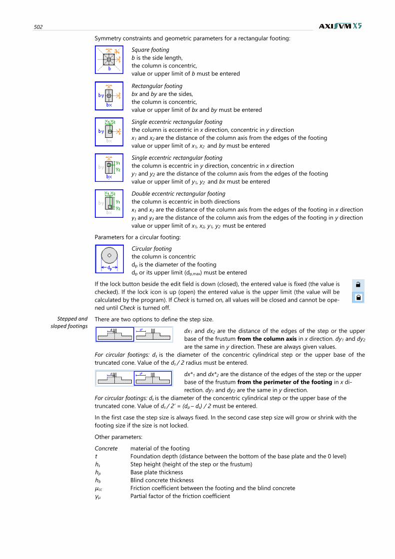
502

Symmetry constraints and geometric parameters for a rectangular footing:

Square footing

b is the side length,

the column is concentric,

value or upper limit of b must be entered

Rectangular footing

bx and by are the sides,

the column is concentric,

value or upper limit of bx and by must be entered

Single eccentric rectangular footing

the column is eccentric in x direction, concentric in y direction

x1 and x2 are the distance of the column axis from the edges of the footing

value or upper limit of x1, x2 and by must be entered

Single eccentric rectangular footing

the column is eccentric in y direction, concentric in x direction

y1 and y2 are the distance of the column axis from the edges of the footing

value or upper limit of y1, y2 and bx must be entered

Double eccentric rectangular footing

the column is eccentric in both directions

x1 and x2 are the distance of the column axis from the edges of the footing in x direction

y1 and y2 are the distance of the column axis from the edges of the footing in y direction

value or upper limit of x1, x2, y1, y2 must be entered

Parameters for a circular footing:

Circular footing

the column is concentric

dp is the diameter of the footing

dp or its upper limit (dp,max) must be entered

If the lock button beside the edit field is down (closed), the entered value is fixed (the value is

checked). If the lock icon is up (open) the entered value is the upper limit (the value will be

calculated by the program). If Check is turned on, all values will be closed and cannot be ope-

ned until Check is turned off.

Stepped and sloped footings

There are two options to define the step size.

dx1 and dx2 are the distance of the edges of the step or the upper

base of the frustum from the column axis in x direction. dy1 and dy2

are the same in y direction. These are always given values.

For circular footings: ds is the diameter of the concentric cylindrical step or the upper base of the

truncated cone. Value of the ds / 2 radius must be entered.

dx*1 and dx*2 are the distance of the edges of the step or the upper

base of the frustum from the perimeter of the footing in x di-

rection. dy1 and dy2 are the same in y direction.

For circular footings: ds is the diameter of the concentric cylindrical step or the upper base of the

truncated cone. Value of ds / 2’ = (dp – ds) / 2 must be entered.

In the first case the step size is always fixed. In the second case step size will grow or shrink with the

footing size if the size is not locked.

Other parameters:

Concrete material of the footing

t Foundation depth (distance between the bottom of the base plate and the 0 level)

hs Step height (height of the step or the frustum)

hp Base plate thickness

hb Blind concrete thickness

μcc Friction coefficient between the footing and the blind concrete

γμ Partial factor of the friction coefficient

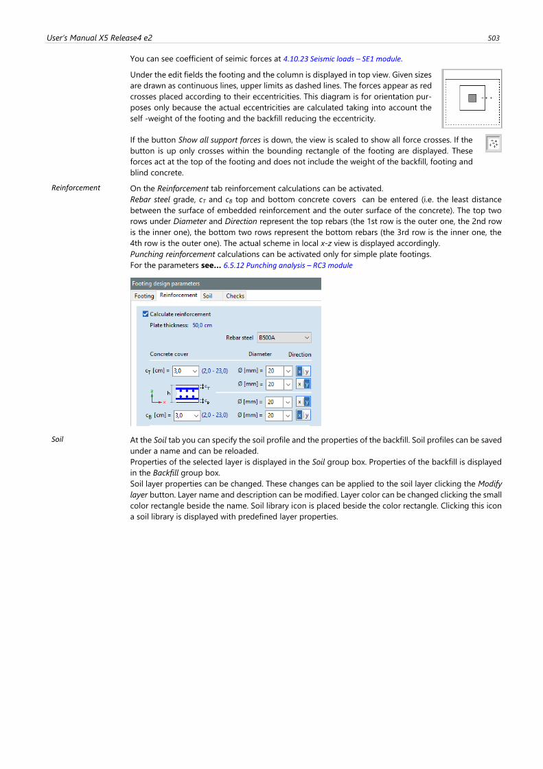
User’s Manual X5 Release4 e2 503

You can see coefficient of seimic forces at 4.10.23 Seismic loads – SE1 module.

Under the edit fields the footing and the column is displayed in top view. Given sizes

are drawn as continuous lines, upper limits as dashed lines. The forces appear as red

crosses placed according to their eccentricities. This diagram is for orientation pur-

poses only because the actual eccentricities are calculated taking into account the

self -weight of the footing and the backfill reducing the eccentricity.

If the button Show all support forces is down, the view is scaled to show all force crosses. If the

button is up only crosses within the bounding rectangle of the footing are displayed. These

forces act at the top of the footing and does not include the weight of the backfill, footing and

blind concrete.

Reinforcement On the Reinforcement tab reinforcement calculations can be activated.

Rebar steel grade, cT and cB top and bottom concrete covers can be entered (i.e. the least distance

between the surface of embedded reinforcement and the outer surface of the concrete). The top two

rows under Diameter and Direction represent the top rebars (the 1st row is the outer one, the 2nd row

is the inner one), the bottom two rows represent the bottom rebars (the 3rd row is the inner one, the

4th row is the outer one). The actual scheme in local x-z view is displayed accordingly.

Punching reinforcement calculations can be activated only for simple plate footings.

For the parameters see… 6.5.12 Punching analysis – RC3 module

Soil At the Soil tab you can specify the soil profile and the properties of the backfill. Soil profiles can be saved

under a name and can be reloaded.

Properties of the selected layer is displayed in the Soil group box. Properties of the backfill is displayed

in the Backfill group box.

Soil layer properties can be changed. These changes can be applied to the soil layer clicking the Modify

layer button. Layer name and description can be modified. Layer color can be changed clicking the small

color rectangle beside the name. Soil library icon is placed beside the color rectangle. Clicking this icon

a soil library is displayed with predefined layer properties.

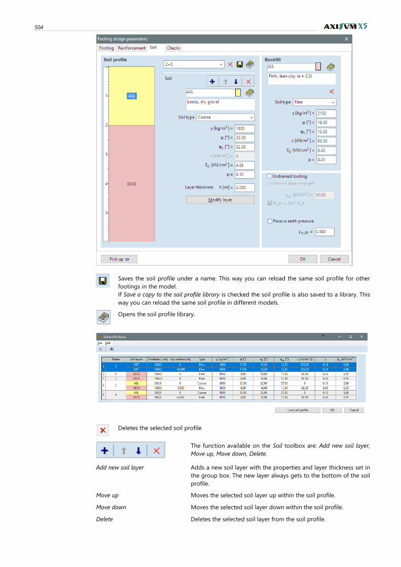
504

Saves the soil profile under a name. This way you can reload the same soil profile for other

footings in the model.

If Save a copy to the soil profile library is checked the soil profile is also saved to a library. This

way you can reload the same soil profile in different models.

Opens the soil profile library.

Deletes the selected soil profile

The function available on the Soil toolbox are: Add new soil layer,

Move up, Move down, Delete.

Add new soil layer Adds a new soil layer with the properties and layer thickness set in

the group box. The new layer always gets to the bottom of the soil

profile.

Move up Moves the selected soil layer up within the soil profile.

Move down Moves the selected soil layer down within the soil profile.

Delete Deletes the selected soil layer from the soil profile.

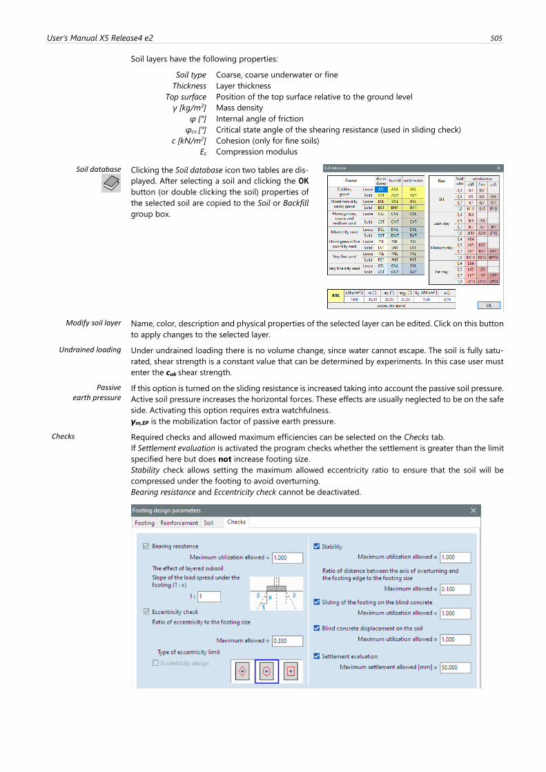
User’s Manual X5 Release4 e2 505

Soil layers have the following properties:

Soil type Coarse, coarse underwater or fine

Thickness Layer thickness

Top surface Position of the top surface relative to the ground level

γ [kg/m3] Mass density

φ [°] Internal angle of friction

φcv [°] Critical state angle of the shearing resistance (used in sliding check)

c [kN/m2] Cohesion (only for fine soils)

Es Compression modulus

Soil database

Clicking the Soil database icon two tables are dis-

played. After selecting a soil and clicking the OK

button (or double clicking the soil) properties of

the selected soil are copied to the Soil or Backfill

group box.

Modify soil layer Name, color, description and physical properties of the selected layer can be edited. Click on this button

to apply changes to the selected layer.

Undrained loading

Under undrained loading there is no volume change, since water cannot escape. The soil is fully satu-

rated, shear strength is a constant value that can be determined by experiments. In this case user must

enter the cuk shear strength.

Passive earth pressure

If this option is turned on the sliding resistance is increased taking into account the passive soil pressure.

Active soil pressure increases the horizontal forces. These effects are usually neglected to be on the safe

side. Activating this option requires extra watchfulness.

γm,EP is the mobilization factor of passive earth pressure.

Checks Required checks and allowed maximum efficiencies can be selected on the Checks tab.

If Settlement evaluation is activated the program checks whether the settlement is greater than the limit

specified here but does not increase footing size.

Stability check allows setting the maximum allowed eccentricity ratio to ensure that the soil will be

compressed under the footing to avoid overturning.

Bearing resistance and Eccentricity check cannot be deactivated.

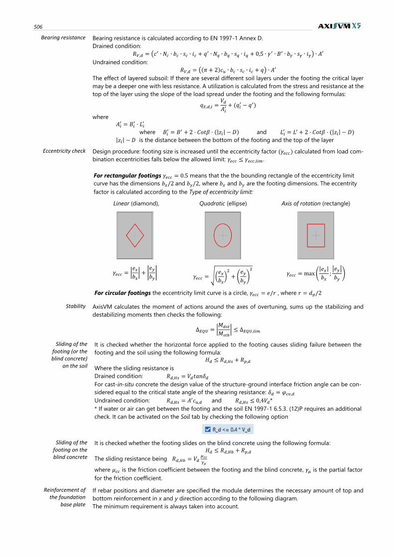
506

Bearing resistance Bearing resistance is calculated according to EN 1997-1 Annex D.

Drained condition:

𝑅𝑉,𝑑 = (𝑐′ ∙ 𝑁𝑐 ∙ 𝑏𝑐 ∙ 𝑠𝑐 ∙ 𝑖𝑐 + 𝑞

′ ∙ 𝑁𝑞 ∙ 𝑏𝑞 ∙ 𝑠𝑞 ∙ 𝑖𝑞 + 0,5 ∙ 𝛾′ ∙ 𝐵′ ∙ 𝑏𝛾 ∙ 𝑠𝛾 ∙ 𝑖𝛾) ∙ 𝐴′

Undrained condition:

𝑅𝑉,𝑑 = ((𝜋 + 2)𝑐𝑢 ∙ 𝑏𝑐 ∙ 𝑠𝑐 ∙ 𝑖𝑐 + 𝑞) ∙ 𝐴′

The effect of layered subsoil: If there are several different soil layers under the footing the critical layer

may be a deeper one with less resistance. A utilization is calculated from the stress and resistance at the

top of the layer using the slope of the load spread under the footing and the following formulas:

𝑞𝐸,𝑑,𝑖 =𝑉𝑑𝐴𝑖′ + (𝑞𝑖

′ − 𝑞′)

where

𝐴𝑖′ = 𝐵𝑖

′ · 𝐿𝑖′

where 𝐵𝑖′ = 𝐵′ + 2 · 𝐶𝑜𝑡𝛽 · (|𝑧𝑖| − 𝐷) and 𝐿𝑖

′ = 𝐿′ + 2 · 𝐶𝑜𝑡𝛽 · (|𝑧𝑖| − 𝐷)

|𝑧𝑖| − 𝐷 is the distance between the bottom of the footing and the top of the layer

Eccentricity check Design procedure: footing size is increased until the eccentricity factor (𝛾𝑒𝑐𝑐) calculated from load com-

bination eccentricities falls below the allowed limit: 𝛾𝑒𝑐𝑐 ≤ 𝛾𝑒𝑐𝑐,𝑙𝑖𝑚.

For rectangular footings 𝛾𝑒𝑐𝑐 = 0.5 means that the the bounding rectangle of the eccentricity limit

curve has the dimensions 𝑏𝑥/2 and 𝑏𝑦/2, where 𝑏𝑥 and 𝑏𝑦 are the footing dimensions. The eccentrity

factor is calculated according to the Type of eccentricity limit:

Linear (diamond), Quadratic (ellipse) Axis of rotation (rectangle)

𝛾𝑒𝑐𝑐 = |𝑒𝑥𝑏𝑥| + |

𝑒𝑦

𝑏𝑦|

𝛾𝑒𝑐𝑐 = √(𝑒𝑥𝑏𝑥)2

+ (𝑒𝑦

𝑏𝑦)

2

𝛾𝑒𝑐𝑐 = max (|𝑒𝑥|

𝑏𝑥;|𝑒𝑦|

𝑏𝑦)

For circular footings the eccentricity limit curve is a circle, 𝛾𝑒𝑐𝑐 = 𝑒/𝑟 , where 𝑟 = 𝑑𝑝/2

Stability

AxisVM calculates the moment of actions around the axes of overtuning, sums up the stabilizing and

destabilizing moments then checks the following:

Δ𝐸𝑄𝑈 = |𝑀𝑑𝑠𝑡

𝑀𝑠𝑡𝑏| ≤ Δ𝐸𝑄𝑈,𝑙𝑖𝑚

Sliding of the footing (or the blind concrete)

on the soil

It is checked whether the horizontal force applied to the footing causes sliding failure between the

footing and the soil using the following formula:

𝐻𝑑 ≤ 𝑅𝑑,𝐻𝑠 + 𝑅𝑝,𝑑

Where the sliding resistance is

Drained condition: 𝑅𝑑,𝐻𝑠 = 𝑉𝑑𝑡𝑎𝑛𝛿𝑑

For cast-in-situ concrete the design value of the structure-ground interface friction angle can be con-

sidered equal to the critical state angle of the shearing resistance: 𝛿𝑑 = 𝜑𝑐𝑣,𝑑

Undrained condition: 𝑅𝑑,𝐻𝑠 = 𝐴′𝑐𝑢,𝑑 and 𝑅𝑑,𝐻𝑠 ≤ 0,4𝑉𝑑*

* If water or air can get between the footing and the soil EN 1997-1 6.5.3. (12)P requires an additional

check. It can be activated on the Soil tab by checking the following option

Sliding of the footing on the blind concrete

It is checked whether the footing slides on the blind concrete using the following formula: 𝐻𝑑 ≤ 𝑅𝑑,𝐻𝑏 + 𝑅𝑝,𝑑

The sliding resistance being 𝑅𝑑,𝐻𝑏 = 𝑉𝑑𝜇𝑐𝑐

𝛾𝜇

where 𝜇𝑐𝑐 is the friction coefficient between the footing and the blind concrete, 𝛾𝜇 is the partial factor

for the friction coefficient.

Reinforcement of the foundation

base plate

If rebar positions and diameter are specified the module determines the necessary amount of top and

bottom reinforcement in x and y direction according to the following diagram.

The minimum requirement is always taken into account.

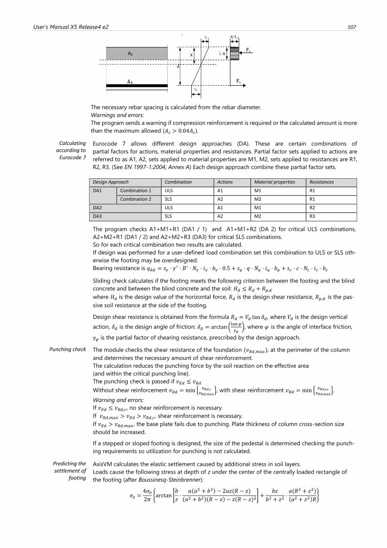
User’s Manual X5 Release4 e2 507

The necessary rebar spacing is calculated from the rebar diameter.

Warnings and errors:

The program sends a warning if compression reinforcement is required or the calculated amount is more

than the maximum allowed (𝐴𝑠 > 0.04𝐴𝑐).

Calculating according to

Eurocode 7

Eurocode 7 allows different design approaches (DA). These are certain combinations of

partial factors for actions, material properties and resistances. Partial factor sets applied to actions are

referred to as A1, A2, sets applied to material properties are M1, M2, sets applied to resistances are R1,

R2, R3. (See EN 1997-1:2004, Annex A) Each design approach combine these partial factor sets.

Design Approach Combination Actions Material properties Resistances

DA1 Combination 1 ULS A1 M1 R1

Combination 2 SLS A2 M2 R1

DA2 ULS A1 M1 R2

DA3 SLS A2 M2 R3

The program checks A1+M1+R1 (DA1 / 1) and A1+M1+R2 (DA 2) for critical ULS combinations,

A2+M2+R1 (DA1 / 2) and A2+M2+R3 (DA3) for critical SLS combinations.

So for each critical combination two results are calculated.

If design was performed for a user-defined load combination set this combination to ULS or SLS oth-

erwise the footing may be overdesigned.

Bearing resistance is 𝑞𝑅𝑑 = 𝑠𝛾 ⋅ 𝛾′ ⋅ 𝐵′ ⋅ 𝑁𝛾 ⋅ 𝑖𝛾 ⋅ 𝑏𝛾 ⋅ 0.5 + 𝑠𝑞 ⋅ 𝑞 ⋅ 𝑁𝑞 ⋅ 𝑖𝑞 ⋅ 𝑏𝑞 + 𝑠𝑐 ⋅ 𝑐 ⋅ 𝑁𝑐 ⋅ 𝑖𝑐 ⋅ 𝑏𝑐

Sliding check calculates if the footing meets the following criterion between the footing and the blind

concrete and between the blind concrete and the soil: 𝐻𝑑 ≤ 𝑅𝑑 + 𝑅𝑝,𝑑

where 𝐻𝑑 is the design value of the horizontal force, 𝑅𝑑 is the design shear resistance, 𝑅𝑝,𝑑 is the pas-

sive soil resistance at the side of the footing.

Design shear resistance is obtained from the formula 𝑅𝑑 = 𝑉𝑑 tan 𝛿𝑑, where 𝑉𝑑 is the design vertical

action, 𝛿𝑑 is the design angle of friction: 𝛿𝑑 = arctan (tan𝜑

𝛾𝜑), where 𝜑 is the angle of interface friction,

𝛾𝜑 is the partial factor of shearing resistance, prescribed by the design approach.

Punching check The module checks the shear resistance of the foundation (𝑣𝑅𝑑,𝑚𝑎𝑥), at the perimeter of the column

and determines the necessary amount of shear reinforcement.

The calculation reduces the punching force by the soil reaction on the effective area

(and within the critical punching line).

The punching check is passed if 𝑣𝐸𝑑 ≤ 𝑣𝑅𝑑

Without shear reinforcement 𝑣𝑅𝑑 = min {𝑣𝑅𝑑,𝑐

𝑣𝑅𝑑,𝑚𝑎𝑥}, with shear reinforcement 𝑣𝑅𝑑 = min {

𝑣𝑅𝑑,𝑐𝑠𝑣𝑅𝑑,𝑚𝑎𝑥

}.

Warning and errors:

If 𝑣𝐸𝑑 ≤ 𝑣𝑅𝑑,𝑐, no shear reinforcement is necessary.

If 𝑣𝑅𝑑,𝑚𝑎𝑥 > 𝑣𝐸𝑑 > 𝑣𝑅𝑑,𝑐, shear reinforcement is necessary.

If 𝑣𝐸𝑑 > 𝑣𝑅𝑑,𝑚𝑎𝑥 , the base plate fails due to punching. Plate thickness of column cross-section size

should be increased.

If a stepped or sloped footing is designed, the size of the pedestal is determined checking the punch-

ing requirements so utilization for punching is not calculated.

Predicting the settlement of

footing

AxisVM calculates the elastic settlement caused by additional stress in soil layers.

Loads cause the following stress at depth of z under the center of the centrally loaded rectangle of

the footing (after Boussinesq-Steinbrenner):

𝜎𝑧 =4𝜎02𝜋

{arctan [𝑏

𝑧⋅

𝑎(𝑎2 + 𝑏2) − 2𝑎𝑧(𝑅 − 𝑧)

(𝑎2 + 𝑏2)(𝑅 − 𝑧) − 𝑧(𝑅 − 𝑧)2] +

𝑏𝑧

𝑏2 + 𝑧2⋅𝑎(𝑅2 + 𝑧2)

(𝑎2 + 𝑧2)𝑅}

508

where the distance between the characteristic point and the central axes are 0.37B' and 0.37L'.

a and b are the dimensions of the four parts of the loaded rectangle according to the following table:

𝑎 𝑏

I. (0.5 − 0.37) ⋅ 𝐿′ (0.5 − 0.37) ⋅ 𝐵′

II. (0.5 + 0.37) ⋅ 𝐿′ (0.5 − 0.37) ⋅ 𝐵′

III. (0.5 + 0.37) ⋅ 𝐿′ (0.5 + 0.37) ⋅ 𝐵′

IV. (0.5 − 0.37) ⋅ 𝐿′ (0.5 + 0.37) ⋅ 𝐵′

If a < b, the two values are swapped. 𝜎0 is the soil stress at the footing base plane caused by loads (including the self-weight of the footing

and the backfill minus the weight of the removed soil above the base plane),

and 𝑅 = √𝑎2 + 𝑏2 + 𝑧2.

This stress calculation is valid for a homogeneous half space. In case of soil layers effective layer

thicknesses must be calculated:

ℎ𝑖,𝑒𝑞 = ℎ𝑖 ⋅ (𝐸𝑠,𝑖𝐸𝑠,𝑟𝑒𝑓

⋅𝜌𝑠,𝑟𝑒𝑓

𝜌𝑠,𝑖)

2/5

where

ℎ𝑖 ,𝑒𝑞 is the effective thickness of the soil layer i

ℎ𝑖 is the thickness of the soil layer i

𝐸𝑠,𝑟𝑒𝑓 is the Young modulus of the the reference soil layer

𝐸𝑆𝑖 is the Young modulus of the soil layer i

𝜌𝑠,𝑟𝑒𝑓 is the density of the reference soil layer

𝜌𝑠,𝑖 is the density of the soil layer i

AxisVM breaks up the user defined soil layers into 10 cm sublayers and calculates the stress due to

soil weight and the stress caused by loading at the bottom of the sublayer. The change in sublayer

thickness is calculated according to the following formulas:

Δℎ𝑖 = ℎ𝑖𝜎𝑎𝑖𝐸𝑠𝑖

; 𝜎𝑎𝑖 =𝜎𝑖−1 + 𝜎𝑖

2

𝜎𝑎𝑖 is the average stress caused by loading in sublayer i

𝜎𝑖−1 is the average stress caused by loading at the top of sublayer i

𝜎𝑖 is the average stress caused by loading at the bottom of sublayer i

𝐸𝑠𝑖 : the Young modulus of the sublayer i

The predicted settlement at a given depth is calculated as the sum of the changes in sublayer thick-

nesses for the sublayers above the level:

𝑠𝑚 =∑Δℎ𝑖

𝑚

𝑖=0

AxisVM calculates the limit depth, where 𝜎 = 0.1 ⋅ 𝜎𝑜𝑏 (i.e. the extra stress caused by loading falls un-

der the 10% of the stress due to soil self-weight.

If this condition is not met at the bottom of the layer structure a settlement estimation is made based

on the settlement at this point and the stress ratio (> 0.1) is calculated.

If the stress caused by loading at the footing base plane is smaller than the stress due to the

original soil layers settlement is not calculated.

AxisVM calculates the settlement for all load cases and SLS combinations. Stress and settlement func-

tions are displayed for the selected load case. Settlement function s(z) is the total settlement of layers

above z.

Seismic check If vibration analysis is completed and the seismic loads are generated seismic check of footings can be

performed. Enter the following parameters:

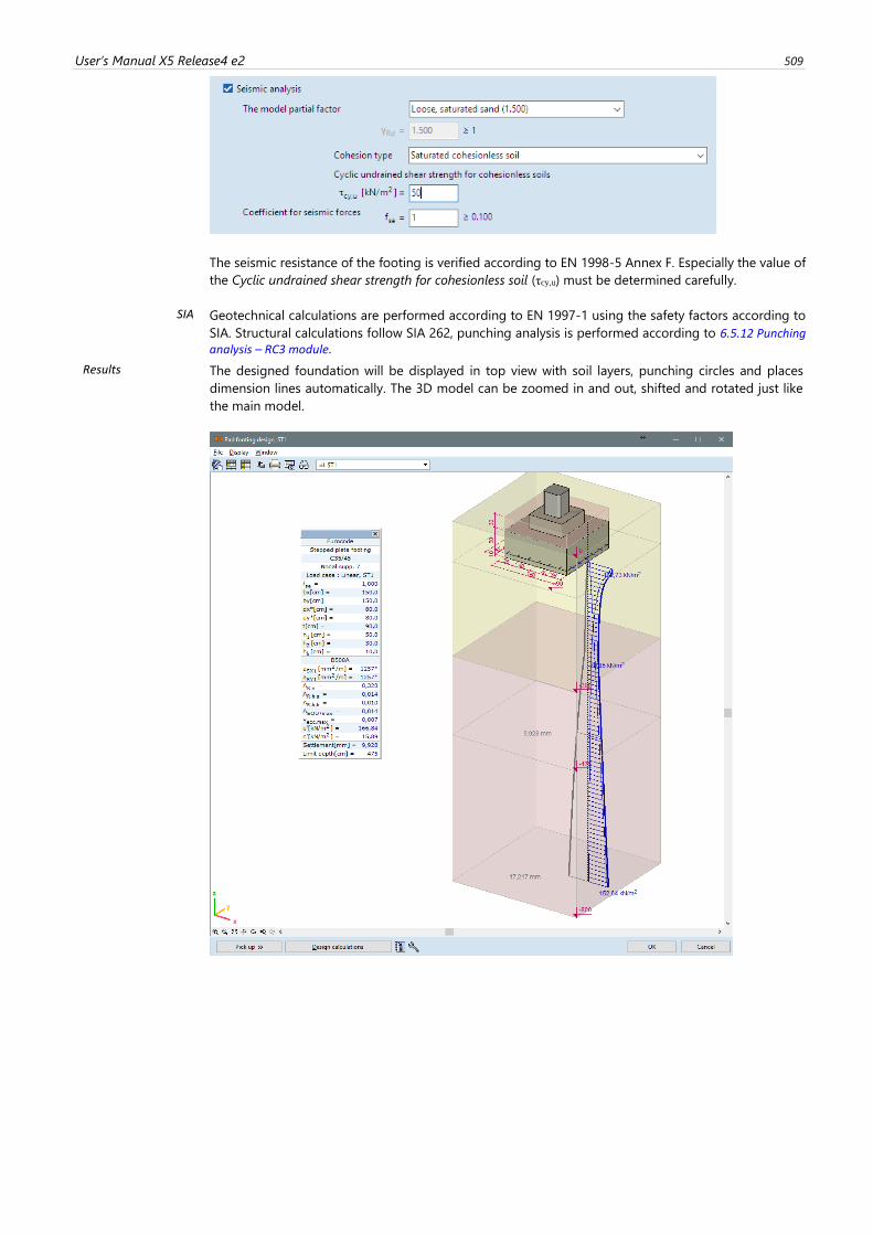
User’s Manual X5 Release4 e2 509

The seismic resistance of the footing is verified according to EN 1998-5 Annex F. Especially the value of

the Cyclic undrained shear strength for cohesionless soil (τcy,u) must be determined carefully.

SIA

Geotechnical calculations are performed according to EN 1997-1 using the safety factors according to

SIA. Structural calculations follow SIA 262, punching analysis is performed according to 6.5.12 Punching analysis – RC3 module.

Results

The designed foundation will be displayed in top view with soil layers, punching circles and places

dimension lines automatically. The 3D model can be zoomed in and out, shifted and rotated just like

the main model.

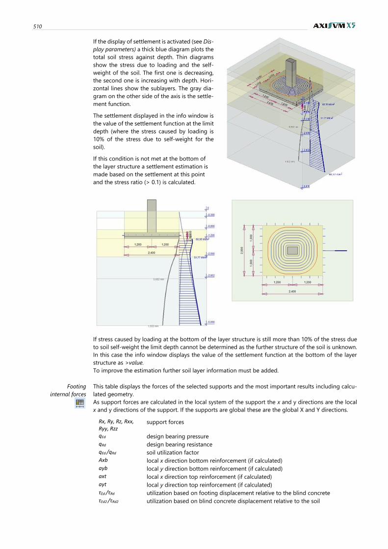
510

If the display of settlement is activated (see Dis-

play parameters) a thick blue diagram plots the

total soil stress against depth. Thin diagrams

show the stress due to loading and the self-

weight of the soil. The first one is decreasing,

the second one is increasing with depth. Hori-

zontal lines show the sublayers. The gray dia-

gram on the other side of the axis is the settle-

ment function.

The settlement displayed in the info window is

the value of the settlement function at the limit

depth (where the stress caused by loading is

10% of the stress due to self-weight for the

soil).

If this condition is not met at the bottom of

the layer structure a settlement estimation is

made based on the settlement at this point

and the stress ratio (> 0.1) is calculated.

If stress caused by loading at the bottom of the layer structure is still more than 10% of the stress due

to soil self-weight the limit depth cannot be determined as the further structure of the soil is unknown.

In this case the info window displays the value of the settlement function at the bottom of the layer

structure as >value.

To improve the estimation further soil layer information must be added.

Footing

internal forces

This table displays the forces of the selected supports and the most important results including calcu-

lated geometry.

As support forces are calculated in the local system of the support the x and y directions are the local

x and y directions of the support. If the supports are global these are the global X and Y directions.

Rx, Ry, Rz, Rxx, Ryy, Rzz

support forces

qEd design bearing pressure

qRd design bearing resistance

qEd /qRd soil utilization factor

Axb local x direction bottom reinforcement (if calculated)

ayb local y direction bottom reinforcement (if calculated)

axt local x direction top reinforcement (if calculated)

ayt local y direction top reinforcement (if calculated)

τEd /τRd utilization based on footing displacement relative to the blind concrete

τEd2 /τRd2 utilization based on blind concrete displacement relative to the soil

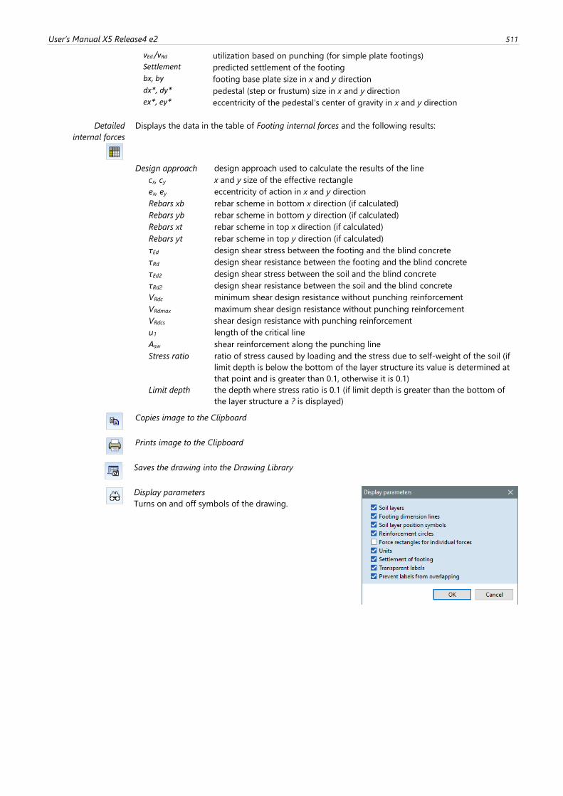
User’s Manual X5 Release4 e2 511

vEd /vRd utilization based on punching (for simple plate footings)

Settlement predicted settlement of the footing

bx, by footing base plate size in x and y direction

dx*, dy* pedestal (step or frustum) size in x and y direction

ex*, ey* eccentricity of the pedestal's center of gravity in x and y direction

Detailed

internal forces

Displays the data in the table of Footing internal forces and the following results:

Design approach design approach used to calculate the results of the line

cx, cy x and y size of the effective rectangle

ex, ey eccentricity of action in x and y direction

Rebars xb rebar scheme in bottom x direction (if calculated)

Rebars yb rebar scheme in bottom y direction (if calculated)

Rebars xt rebar scheme in top x direction (if calculated)

Rebars yt rebar scheme in top y direction (if calculated)

τEd design shear stress between the footing and the blind concrete

τRd design shear resistance between the footing and the blind concrete

τEd2 design shear stress between the soil and the blind concrete

τRd2 design shear resistance between the soil and the blind concrete

VRdc minimum shear design resistance without punching reinforcement

VRdmax maximum shear design resistance without punching reinforcement

VRdcs shear design resistance with punching reinforcement

u1 length of the critical line

Asw shear reinforcement along the punching line

Stress ratio ratio of stress caused by loading and the stress due to self-weight of the soil (if

limit depth is below the bottom of the layer structure its value is determined at

that point and is greater than 0.1, otherwise it is 0.1)

Limit depth the depth where stress ratio is 0.1 (if limit depth is greater than the bottom of

the layer structure a ? is displayed)

Copies image to the Clipboard

Prints image to the Clipboard

Saves the drawing into the Drawing Library

Display parameters

Turns on and off symbols of the drawing.

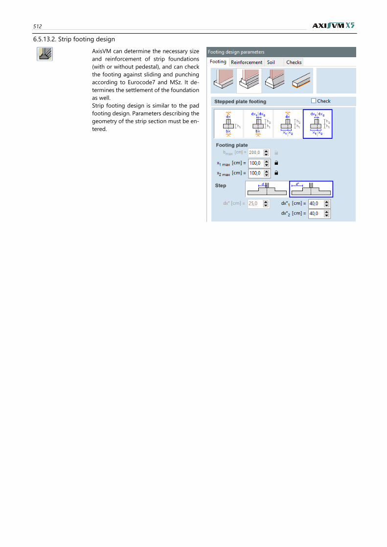
512

6.5.13.2. Strip footing design

AxisVM can determine the necessary size

and reinforcement of strip foundations

(with or without pedestal), and can check

the footing against sliding and punching

according to Eurocode7 and MSz. It de-

termines the settlement of the foundation

as well.

Strip footing design is similar to the pad

footing design. Parameters describing the

geometry of the strip section must be en-

tered.

User’s Manual X5 Release4 e2 513

6.5.14. Design of reinforced concrete cores and walls – RC5 module

Using RC5 module, reinforcement can be assigned to reinforced cores and walls and the design check

of cores/walls subjected to bending and axial force can be performed.

Reinforcement can be assigned to virtual beams or virtual strips (see… 2.16.16 Virtual beams) after

clicking the icon on the left or clicking on the axis of a virtual beam/strip. The icon is visible if there is

reinforced concrete domain, there is at least on virtual beam/strip and statical or dynamical results are

available in the model.

After clicking on the icon, one virtual beam or strip can be selected in the course of selection procedure

(see… 2.16.1 Selection). If the selection is invalid, the software warns with a warning message. The

selection may be invalid in the following cases:

• Neither virtual beam, nor virtual strip has been selected.

• More than one virtual beam/strip has been selected.

• The selected virtual beam/strip has non-concrete domain(s).

• The selected virtual beam/strip is not continuous.

• The cross section of the virtual beam/strip is not supported (e.g. variable section).

• The selected virtual beam/strip is not vertical (max. 15° deviation is allowed).

• Automatic cross section is set to the selected virtual beam/strip but a rib connected to one of

the domains is not concrete.

After a valid selection, the Reinforced concrete cores and walls window is opened where storeys and

reinforcement can be assigned to cores and walls and the design check can be performed. Altogether,

there are three tabs on the window: 1) Virtual beams; 2) Virtual strips; 3) Overall utilization.

Virtual beams can be used to design reinforced concrete cores with the assumption that sections

remain approximately plane before and after loading. This assumption is likely not valid in case of large

and short cores and in case of the presence of considerable warping torsional moment and a section

that is sensitive to warping effects.

The design check of reinforced concrete cores is performed similarly to the design check of reinforced

concrete columns. The Nx-My-Mz strength interaction diagram of the section is calculated and it is

checked whether the point representing Nx,Ed, My,Ed, Mz,Ed design forces is within the interaction diagram.

During design check of core reinforcement, buckling length coefficient cannot be defined, since

modern design codes (e.g. EN 1992-1-1) includes methods wherewith the effect of imperfections and

second order effects can be taken into account on structural level. In case of reinforced concrete

cores, it is assumed that the integrated design internal forces include the effect of imperfections

and second order effects.

Virtual strips can be used by the design check of wall ends or wall segments considering possible

buckling failures of the wall between floors. The program is able to calculate the additional eccentricities

from imperfections and second order effects regarding a storey, based on the given buckling length

coefficient. After sum with the initial eccentricities (calculated from the integrated internal forces), the

program calculates the Nx,Ed, My,Ed, Mz,Ed design forces. It is assumed that the integrated design

internal forces include the effect of imperfections and second order effects on structural level.

The design check is performed similarly to the case of reinforced concrete cores that the Nx-My-Mz

strength interaction diagram of the section is generated and it is checked whether the point

representing Nx,Ed, My,Ed, Mz,Ed design forces is within the interaction diagram.

On the overall utilization tab, design results of reinforced concrete cores calculated with virtual beams

and design results of wall ends/segments calculated with virtual strips can be summed. It may be

necessary because the Nx-My-Mz strength interaction diagram of cores is generated without

consideration the loss of stability of compressed wall ends and inner wall segments. The program

supports the use of various summation rules as it can be seen in the following figures.

In case of warping-sensitive cores and the presence of considerable warping torsional moments,

the section warps and it does not remain plane after loading. It is recommended to to perform

the design check for wall segments of the core separately in such cases because the section can-

not designed as a whole.

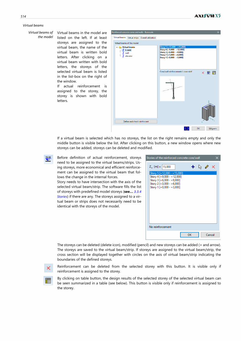
514

Virtual beams

Virtual beams of the model

Virtual beams in the model are

listed on the left. If at least

storeys are assigned to the

virtual beam, the name of the

virtual beam is written bold

letters. After clicking on a

virtual beam written with bold

letters, the storeys of the

selected virtual beam is listed

in the list-box on the right of

the window.

If actual reinforcement is

assigned to the storey, the

storey is shown with bold

letters.

If a virtual beam is selected which has no storeys, the list on the right remains empty and only the

middle button is visible below the list. After clicking on this button, a new window opens where new

storeys can be added, storeys can be deleted and modified.

Before definition of actual reinforcement, storeys

need to be assigned to the virtual beams/strips. Us-

ing storeys, more economical and efficient reinforce-

ment can be assigned to the virtual beam that fol-

lows the change in the internal forces.

Story needs to have intersection with the axis of the

selected virtual beam/strip. The software fills the list

of storeys with predefined model storeys (see… 3.3.4

Stories) if there are any. The storeys assigned to a vir-

tual beam or strips does not necessarily need to be

identical with the storeys of the model.

The storeys can be deleted (delete icon), modified (pencil) and new storeys can be added (+ and arrow).

The storeys are saved to the virtual beam/strip. If storeys are assigned to the virtual beam/strip, the

cross section will be displayed together with circles on the axis of virtual beam/strip indicating the

boundaries of the defined storeys.

Reinforcement can be deleted from the selected storey with this button. It is visible only if

reinforcement is assigned to the storey.

By clicking on table button, the design results of the selected storey of the selected virtual beam can

be seen summarized in a table (see below). This button is visible only if reinforcement is assigned to

the storey.

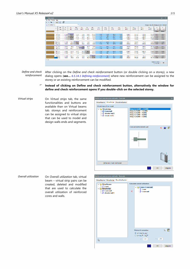
User’s Manual X5 Release4 e2 515

Define and check reinforcement

After clicking on the Define and check reinforcement button (or double clicking on a storey), a new

dialog opens (see… 6.5.14.1 Defining reinforcement) where new reinforcement can be assigned to the

storey or an existing reinforcement can be modified.

Instead of clicking on Define and check reinforcement button, alternatively the window for

define and check reinforcement opens if you double-click on the selected storey.

Virtual strips On Virtual strips tab, the same

functionalities and buttons are

available than on Virtual beams

tab. storeys and reinforcement

can be assigned to virtual strips

that can be used to model and

design walls ends and segments.

Overall utilization On Overall utilization tab, virtual

beam – virtual strip pairs can be

created, deleted and modified

that are used to calculate the

overall utilization of reinforced

cores and walls.

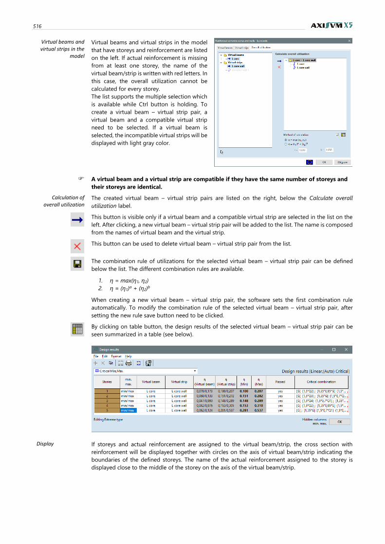
516

Virtual beams and virtual strips in the

model

Virtual beams and virtual strips in the model

that have storeys and reinforcement are listed

on the left. If actual reinforcement is missing

from at least one storey, the name of the

virtual beam/strip is written with red letters. In

this case, the overall utilization cannot be

calculated for every storey.

The list supports the multiple selection which

is available while Ctrl button is holding. To

create a virtual beam – virtual strip pair, a

virtual beam and a compatible virtual strip

need to be selected. If a virtual beam is

selected, the incompatible virtual strips will be

displayed with light gray color.

A virtual beam and a virtual strip are compatible if they have the same number of storeys and

their storeys are identical.

Calculation of overall utilization

The created virtual beam – virtual strip pairs are listed on the right, below the Calculate overall

utilization label.

This button is visible only if a virtual beam and a compatible virtual strip are selected in the list on the

left. After clicking, a new virtual beam – virtual strip pair will be added to the list. The name is composed

from the names of virtual beam and the virtual strip.

This button can be used to delete virtual beam – virtual strip pair from the list.

The combination rule of utilizations for the selected virtual beam – virtual strip pair can be defined

below the list. The different combination rules are available.

1. η = max(η1, η2)

2. η = (η1)a + (η2)b

When creating a new virtual beam – virtual strip pair, the software sets the first combination rule

automatically. To modify the combination rule of the selected virtual beam – virtual strip pair, after

setting the new rule save button need to be clicked.

By clicking on table button, the design results of the selected virtual beam – virtual strip pair can be

seen summarized in a table (see below).

Display If storeys and actual reinforcement are assigned to the virtual beam/strip, the cross section with

reinforcement will be displayed together with circles on the axis of virtual beam/strip indicating the

boundaries of the defined storeys. The name of the actual reinforcement assigned to the storey is

displayed close to the middle of the storey on the axis of the virtual beam/strip.

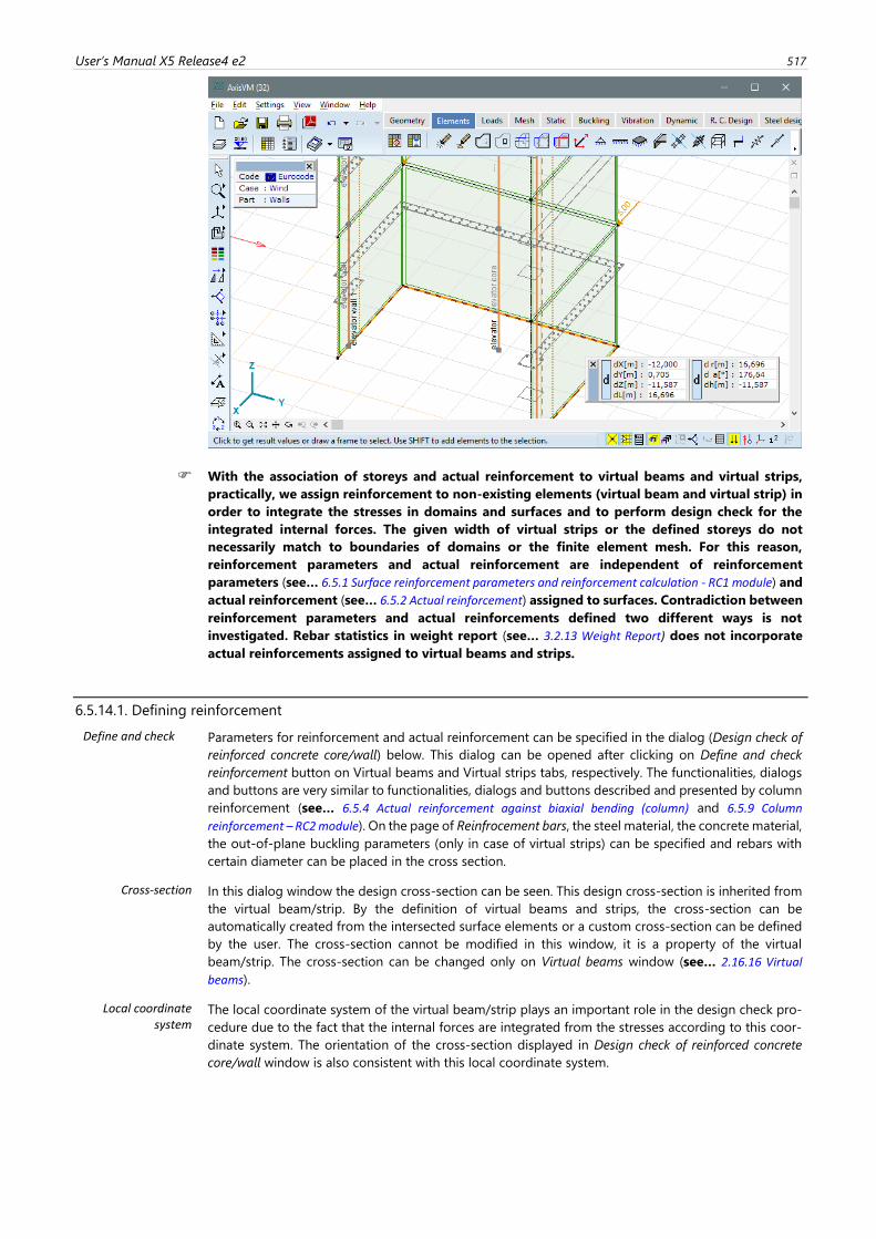
User’s Manual X5 Release4 e2 517

With the association of storeys and actual reinforcement to virtual beams and virtual strips,

practically, we assign reinforcement to non-existing elements (virtual beam and virtual strip) in

order to integrate the stresses in domains and surfaces and to perform design check for the

integrated internal forces. The given width of virtual strips or the defined storeys do not

necessarily match to boundaries of domains or the finite element mesh. For this reason,

reinforcement parameters and actual reinforcement are independent of reinforcement

parameters (see… 6.5.1 Surface reinforcement parameters and reinforcement calculation - RC1 module) and

actual reinforcement (see… 6.5.2 Actual reinforcement) assigned to surfaces. Contradiction between

reinforcement parameters and actual reinforcements defined two different ways is not

investigated. Rebar statistics in weight report (see… 3.2.13 Weight Report) does not incorporate

actual reinforcements assigned to virtual beams and strips.

6.5.14.1. Defining reinforcement

Define and check Parameters for reinforcement and actual reinforcement can be specified in the dialog (Design check of

reinforced concrete core/wall) below. This dialog can be opened after clicking on Define and check

reinforcement button on Virtual beams and Virtual strips tabs, respectively. The functionalities, dialogs

and buttons are very similar to functionalities, dialogs and buttons described and presented by column

reinforcement (see… 6.5.4 Actual reinforcement against biaxial bending (column) and 6.5.9 Column

reinforcement – RC2 module). On the page of Reinfrocement bars, the steel material, the concrete material,

the out-of-plane buckling parameters (only in case of virtual strips) can be specified and rebars with

certain diameter can be placed in the cross section.

Cross-section In this dialog window the design cross-section can be seen. This design cross-section is inherited from

the virtual beam/strip. By the definition of virtual beams and strips, the cross-section can be

automatically created from the intersected surface elements or a custom cross-section can be defined

by the user. The cross-section cannot be modified in this window, it is a property of the virtual

beam/strip. The cross-section can be changed only on Virtual beams window (see… 2.16.16 Virtual

beams).

Local coordinate system

The local coordinate system of the virtual beam/strip plays an important role in the design check pro-

cedure due to the fact that the internal forces are integrated from the stresses according to this coor-

dinate system. The orientation of the cross-section displayed in Design check of reinforced concrete

core/wall window is also consistent with this local coordinate system.

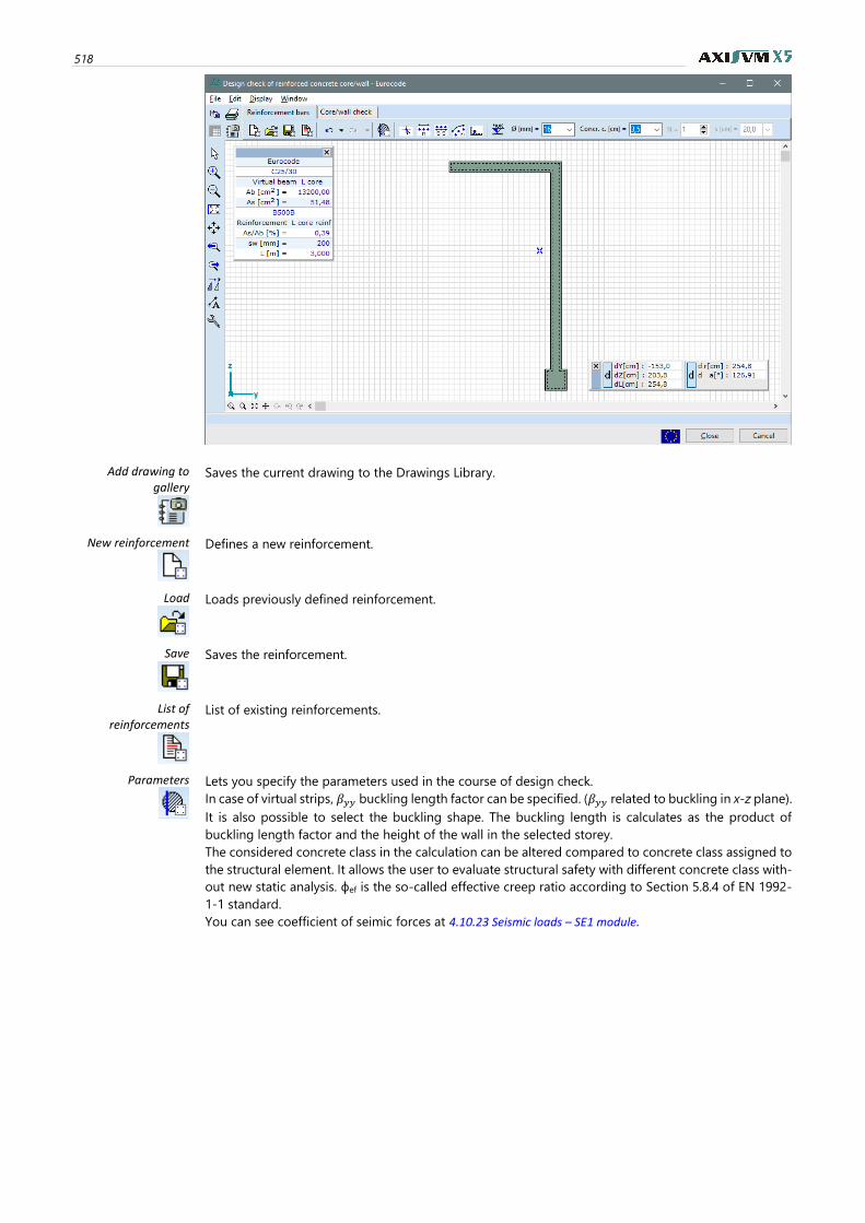
518

Add drawing to gallery

Saves the current drawing to the Drawings Library.

New reinforcement

Defines a new reinforcement.

Load

Loads previously defined reinforcement.

Save

Saves the reinforcement.

List of reinforcements

List of existing reinforcements.

Parameters

Lets you specify the parameters used in the course of design check.

In case of virtual strips, 𝛽𝑦𝑦 buckling length factor can be specified. (𝛽𝑦𝑦 related to buckling in x-z plane).

It is also possible to select the buckling shape. The buckling length is calculates as the product of

buckling length factor and the height of the wall in the selected storey.

The considered concrete class in the calculation can be altered compared to concrete class assigned to

the structural element. It allows the user to evaluate structural safety with different concrete class with-

out new static analysis. ϕef is the so-called effective creep ratio according to Section 5.8.4 of EN 1992-

1-1 standard.

You can see coefficient of seimic forces at 4.10.23 Seismic loads – SE1 module.

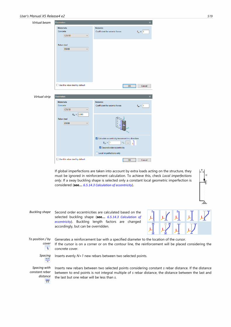
User’s Manual X5 Release4 e2 519

Virtual beam

Virtual strip

If global imperfections are taken into account by extra loads acting on the structure, they

must be ignored in reinforcement calculation. To achieve this, check Local imperfections

only. If a sway buckling shape is selected only a constant local geometric imperfection is

considered (see… 6.5.14.3 Calculation of eccentricity).

Buckling shape

Second order eccentricities are calculated based on the

selected buckling shape (see… 6.5.14.3 Calculation of

eccentricity). Buckling length factors are changed

accordingly, but can be overridden.

To position / by cover

Generates a reinforcement bar with a specified diameter to the location of the cursor.

If the cursor is on a corner or on the contour line, the reinforcement will be placed considering the

concrete cover.

Spacing

Inserts evenly N+1 new rebars between two selected points.

Spacing with constant rebar

distance

Inserts new rebars between two selected points considering constant s rebar distance. If the distance

between to end points is not integral multiple of s rebar distance, the distance between the last and

the last but one rebar will be less than s.

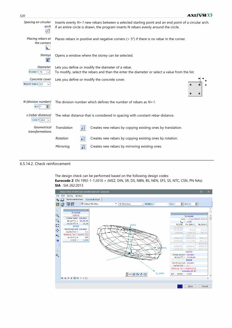
520

Spacing on circular arch

Inserts evenly N+1 new rebars between a selected starting point and an end point of a circular arch.

If an entire circle is drawn, the program inserts N rebars evenly around the circle.

Placing rebars at the corners

Places rebars in positive and negative corners (> 5°) if there is no rebar in the corner.

Storeys

Opens a window where the storey can be selected.

Diameter

Lets you define or modify the diameter of a rebar.

To modify, select the rebars and than the enter the diameter or select a value from the list.

Concrete cover

Lets you define or modify the concrete cover.

N (division number)

The division number which defines the number of rebars as N+1.

s (rebar distance)

The rebar distance that is considered in spacing with constant rebar distance.

Geometrical transformations

Translation

Creates new rebars by copying existing ones by translation.

Rotation

Creates new rebars by copying existing ones by rotation.

Mirroring

Creates new rebars by mirroring existing ones.

6.5.14.2. Check reinforcement

The design check can be performed based on the following design codes:

Eurocode 2: EN 1992-1-1:2010 + (MSZ, DIN, SR, DS, NBN, BS, NEN, SFS, SS, NTC, CSN, PN NAs)

SIA : SIA 262:2013

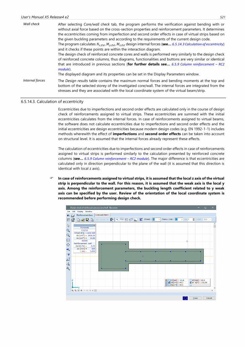
User’s Manual X5 Release4 e2 521

Wall check After selecting Core/wall check tab, the program performs the verification against bending with or

without axial force based on the cross-section properties and reinforcement parameters. It determines

the eccentricities coming from imperfection and second order effects in case of virtual strips based on

the given buckling parameters and according to the requirements of the current design code.

The program calculates 𝑁𝑥,𝐸𝑑 ,𝑀𝑦,𝐸𝑑 ,𝑀𝑧,𝐸𝑑 design internal forces (see… 6.5.14.3 Calculation of eccentricity)

and it checks if these points are within the interaction diagram.

The design check of reinforced concrete cores and walls is performed very similarly to the design check

of reinforced concrete columns, thus diagrams, functionalities and buttons are very similar or identical

that are introduced in previous sections (for further details see… 6.5.9 Column reinforcement – RC2

module).

The displayed diagram and its properties can be set in the Display Parameters window.

Internal forces The Design results table contains the maximum normal forces and bending moments at the top and

bottom of the selected storey of the invetigated core/wall. The internal forces are integrated from the

stresses and they are associated with the local coordinate system of the virtual beam/strip.

6.5.14.3. Calculation of eccentricity

Eccentricities due to imperfections and second order effects are calculated only in the course of design

check of reinforcements assigned to virtual strips. These eccentricities are summed with the initial

eccentricities calculates from the internal forces. In case of reinforcements assigned to virtual beams,

the software does not calculate eccentricities due to imperfections and second order effects and the

initial eccentricities are design eccentricities because modern design codes (e.g. EN 1992-1-1) includes

methods wherewith the effect of imperfections and second order effects can be taken into account

on structural level. It is assumed that the internal forces already represent these effects.

The calculation of eccentricities due to imperfections and second order effects in case of reinforcements

assigned to virtual strips is performed similarly to the calculation presented by reinforced concrete

columns (see… 6.5.9 Column reinforcement – RC2 module). The major difference is that eccentricities are

calculated only in direction perpendicular to the plane of the wall (it is assumed that this direction is

identical with local z axis).

In case of reinforcements assigned to virtual strips, it is assumed that the local z axis of the virtual

strip is perpendicular to the wall. For this reason, it is assumed that the weak axis is the local y

axis. Among the reinforcement parameters, the buckling length coefficient related to y weak

axis can be specified by the user. Review of the orientation of the local coordinate system is

recommended before performing design check.

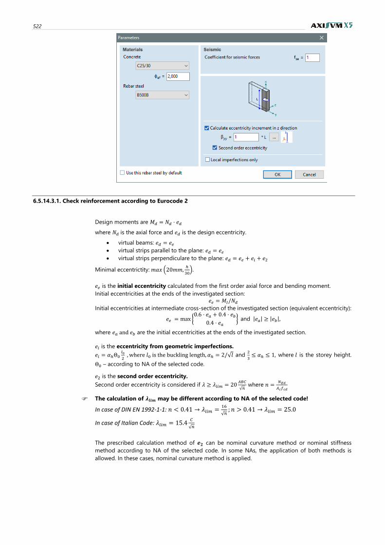
522

6.5.14.3.1. Check reinforcement according to Eurocode 2

Design moments are 𝑀𝑑 = 𝑁𝑑 ⋅ 𝑒𝑑

where 𝑁𝑑 is the axial force and 𝑒𝑑 is the design eccentricity.

• virtual beams: 𝑒𝑑 = 𝑒𝑒

• virtual strips parallel to the plane: 𝑒𝑑 = 𝑒𝑒

• virtual strips perpendiculare to the plane: 𝑒𝑑 = 𝑒𝑒 + 𝑒𝑖 + 𝑒2

Minimal eccentrictity: 𝑚𝑎𝑥 (20𝑚𝑚,ℎ

30).

𝑒𝑒 is the initial eccentricity calculated from the first order axial force and bending moment.

Initial eccentricities at the ends of the investigated section:

𝑒𝑒 = 𝑀𝐼/𝑁𝑑

Initial eccentricities at intermediate cross-section of the investigated section (equivalent eccentricity):

𝑒𝑒 = max {0.6 ⋅ 𝑒𝑎 + 0.4 ⋅ 𝑒𝑏

0.4 ⋅ 𝑒𝑎} and |𝑒𝑎| ≥ |𝑒𝑏|,

where 𝑒𝑎 and 𝑒𝑏 are the initial eccentricities at the ends of the investigated section.

𝑒𝑖 is the eccentricity from geometric imperfections.

𝑒𝑖 = 𝛼ℎΘ0𝑙0

2 , where 𝑙0 is the buckling length, 𝛼ℎ = 2/√𝑙 and

2

3≤ 𝛼ℎ ≤ 1, where 𝑙 is the storey height.

Θ0 – according to NA of the selected code.

𝑒2 is the second order eccentricity.

Second order eccentricity is considered if 𝜆 ≥ 𝜆𝑙𝑖𝑚 = 20𝐴𝐵𝐶

√𝑛 where 𝑛 =

𝑁𝐸𝑑

𝐴𝑐𝑓𝑐𝑑

The calculation of 𝝀𝒍𝒊𝒎 may be different according to NA of the selected code!

In case of DIN EN 1992-1-1: 𝑛 < 0.41 → 𝜆𝑙𝑖𝑚 =16

√𝑛; 𝑛 > 0.41 → 𝜆𝑙𝑖𝑚 = 25.0

In case of Italian Code: 𝜆𝑙𝑖𝑚 = 15.4𝐶

√𝑛

The prescribed calculation method of 𝒆𝟐 can be nominal curvature method or nominal stiffness

method according to NA of the selected code. In some NAs, the application of both methods is

allowed. In these cases, nominal curvature method is applied.

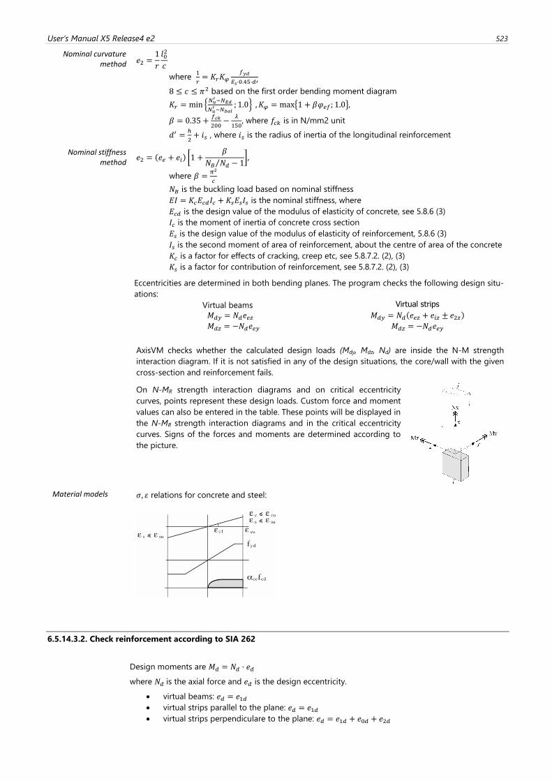
User’s Manual X5 Release4 e2 523

Nominal curvature method 𝑒2 =

1

𝑟

𝑙02

𝑐

where 1

𝑟= 𝐾𝑟𝐾𝜑

𝑓𝑦𝑑

𝐸𝑠⋅0.45⋅𝑑′

8 ≤ 𝑐 ≤ 𝜋2 based on the first order bending moment diagram

𝐾𝑟 = min {𝑁𝑢′−𝑁𝐸𝑑

𝑁𝑢′−𝑁𝑏𝑎𝑙

; 1.0} , 𝐾𝜑 = max{1 + 𝛽𝜑𝑒𝑓; 1.0},

𝛽 = 0.35 +𝑓𝑐𝑘

200−

𝜆

150, where 𝑓𝑐𝑘 is in N/mm2 unit

𝑑′ =ℎ

2+ 𝑖𝑠 , where 𝑖𝑠 is the radius of inertia of the longitudinal reinforcement

Nominal stiffness method

𝑒2 = (𝑒𝑒 + 𝑒𝑖) [1 +𝛽

𝑁𝐵 𝑁𝑑⁄ − 1],

where 𝛽 =𝜋2

𝑐

𝑁𝐵 is the buckling load based on nominal stiffness

𝐸𝐼 = 𝐾𝑐𝐸𝑐𝑑𝐼𝑐 + 𝐾𝑠𝐸𝑠𝐼𝑠 is the nominal stiffness, where

𝐸𝑐𝑑 is the design value of the modulus of elasticity of concrete, see 5.8.6 (3)

𝐼𝑐 is the moment of inertia of concrete cross section

𝐸𝑠 is the design value of the modulus of elasticity of reinforcement, 5.8.6 (3)

𝐼𝑠 is the second moment of area of reinforcement, about the centre of area of the concrete

𝐾𝑐 is a factor for effects of cracking, creep etc, see 5.8.7.2. (2), (3)

𝐾𝑠 is a factor for contribution of reinforcement, see 5.8.7.2. (2), (3)

Eccentricities are determined in both bending planes. The program checks the following design situ-

ations:

Virtual beams Virtual strips

𝑀𝑑𝑦 = 𝑁𝑑𝑒𝑒𝑧

𝑀𝑑𝑧 = −𝑁𝑑𝑒𝑒𝑦

𝑀𝑑𝑦 = 𝑁𝑑(𝑒𝑒𝑧 + 𝑒𝑖𝑧 ± 𝑒2𝑧)

𝑀𝑑𝑧 = −𝑁𝑑𝑒𝑒𝑦

AxisVM checks whether the calculated design loads (Mdy, Mdz, Nd) are inside the N-M strength

interaction diagram. If it is not satisfied in any of the design situations, the core/wall with the given

cross-section and reinforcement fails.

On N-MR strength interaction diagrams and on critical eccentricity

curves, points represent these design loads. Custom force and moment

values can also be entered in the table. These points will be displayed in

the N-MR strength interaction diagrams and in the critical eccentricity

curves. Signs of the forces and moments are determined according to

the picture.

Material models 𝜎, 휀 relations for concrete and steel:

6.5.14.3.2. Check reinforcement according to SIA 262

Design moments are 𝑀𝑑 = 𝑁𝑑 ⋅ 𝑒𝑑

where 𝑁𝑑 is the axial force and 𝑒𝑑 is the design eccentricity.

• virtual beams: 𝑒𝑑 = 𝑒1𝑑

• virtual strips parallel to the plane: 𝑒𝑑 = 𝑒1𝑑

• virtual strips perpendiculare to the plane: 𝑒𝑑 = 𝑒1𝑑 + 𝑒0𝑑 + 𝑒2𝑑

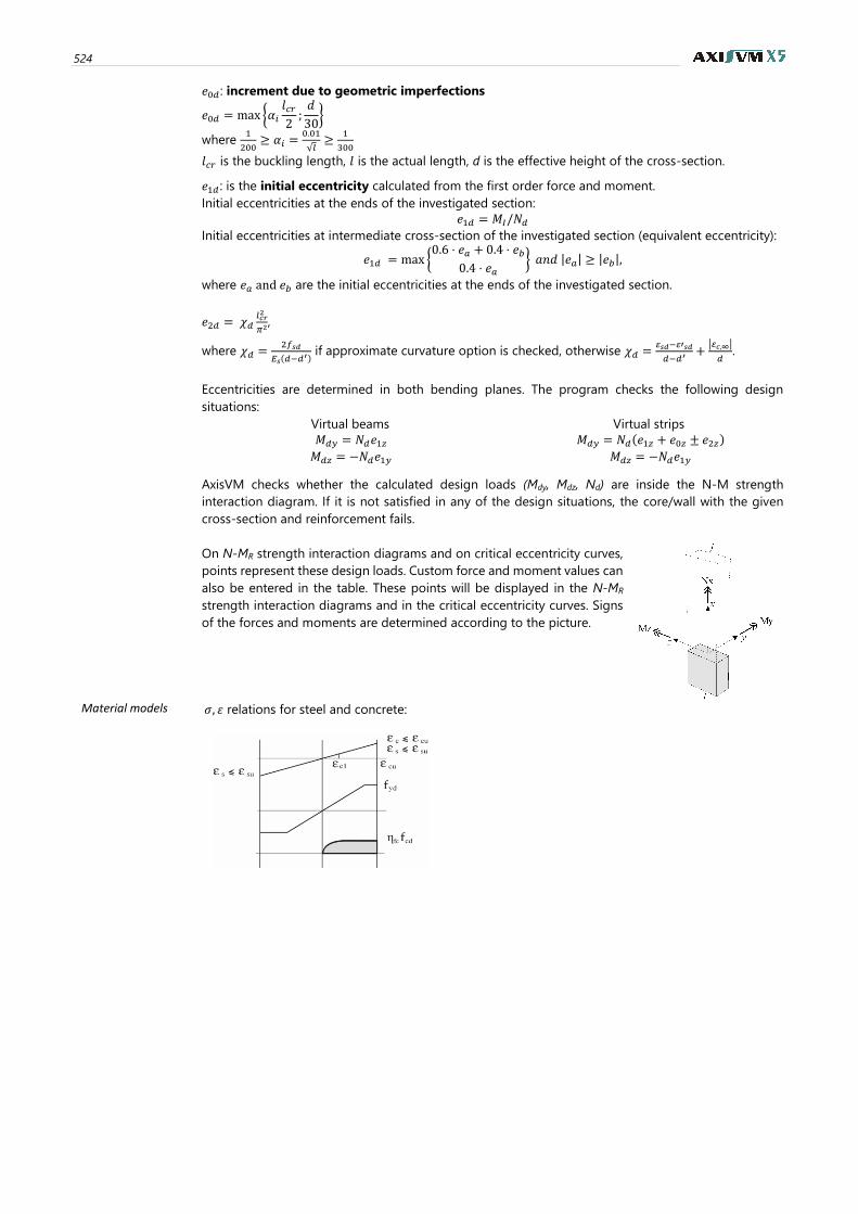
524

𝑒0𝑑 : increment due to geometric imperfections

𝑒0𝑑 = max {𝛼𝑖𝑙𝑐𝑟2;𝑑

30}

where 1

200≥ 𝛼𝑖 =

0.01

√𝑙≥

1

300

𝑙𝑐𝑟 is the buckling length, 𝑙 is the actual length, d is the effective height of the cross-section.

𝑒1𝑑 : is the initial eccentricity calculated from the first order force and moment.

Initial eccentricities at the ends of the investigated section:

𝑒1𝑑 = 𝑀𝐼/𝑁𝑑

Initial eccentricities at intermediate cross-section of the investigated section (equivalent eccentricity):

𝑒1𝑑 = max {0.6 ⋅ 𝑒𝑎 + 0.4 ⋅ 𝑒𝑏

0.4 ⋅ 𝑒𝑎} 𝑎𝑛𝑑 |𝑒𝑎| ≥ |𝑒𝑏|,

where 𝑒𝑎 and 𝑒𝑏 are the initial eccentricities at the ends of the investigated section.

𝑒2𝑑 = 𝜒𝑑𝑙𝑐𝑟2

𝜋2,

where 𝜒𝑑 =2𝑓𝑠𝑑

𝐸𝑠(𝑑−𝑑′)

if approximate curvature option is checked, otherwise 𝜒𝑑 =𝜀𝑠𝑑−𝜀′𝑠𝑑

𝑑−𝑑′+|𝜀𝑐,∞|

𝑑.

Eccentricities are determined in both bending planes. The program checks the following design

situations:

Virtual beams Virtual strips

𝑀𝑑𝑦 = 𝑁𝑑𝑒1𝑧

𝑀𝑑𝑧 = −𝑁𝑑𝑒1𝑦

𝑀𝑑𝑦 = 𝑁𝑑(𝑒1𝑧 + 𝑒0𝑧 ± 𝑒2𝑧)

𝑀𝑑𝑧 = −𝑁𝑑𝑒1𝑦

AxisVM checks whether the calculated design loads (Mdy, Mdz, Nd) are inside the N-M strength

interaction diagram. If it is not satisfied in any of the design situations, the core/wall with the given

cross-section and reinforcement fails.

On N-MR strength interaction diagrams and on critical eccentricity curves,

points represent these design loads. Custom force and moment values can

also be entered in the table. These points will be displayed in the N-MR

strength interaction diagrams and in the critical eccentricity curves. Signs

of the forces and moments are determined according to the picture.

Material models 𝜎, 휀 relations for steel and concrete:

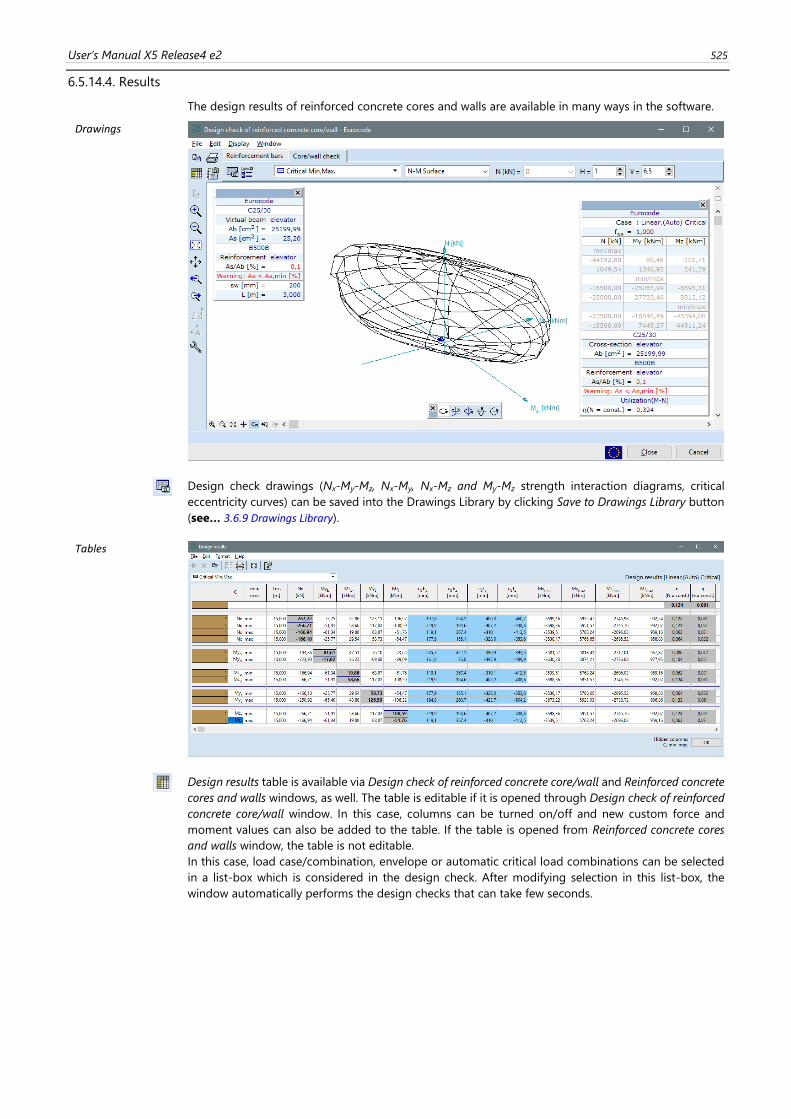
User’s Manual X5 Release4 e2 525

6.5.14.4. Results

The design results of reinforced concrete cores and walls are available in many ways in the software.

Drawings

Design check drawings (Nx-My-Mz, Nx-My, Nx-Mz and My-Mz strength interaction diagrams, critical

eccentricity curves) can be saved into the Drawings Library by clicking Save to Drawings Library button

(see… 3.6.9 Drawings Library).

Tables

Design results table is available via Design check of reinforced concrete core/wall and Reinforced concrete

cores and walls windows, as well. The table is editable if it is opened through Design check of reinforced

concrete core/wall window. In this case, columns can be turned on/off and new custom force and

moment values can also be added to the table. If the table is opened from Reinforced concrete cores

and walls window, the table is not editable.

In this case, load case/combination, envelope or automatic critical load combinations can be selected

in a list-box which is considered in the design check. After modifying selection in this list-box, the

window automatically performs the design checks that can take few seconds.

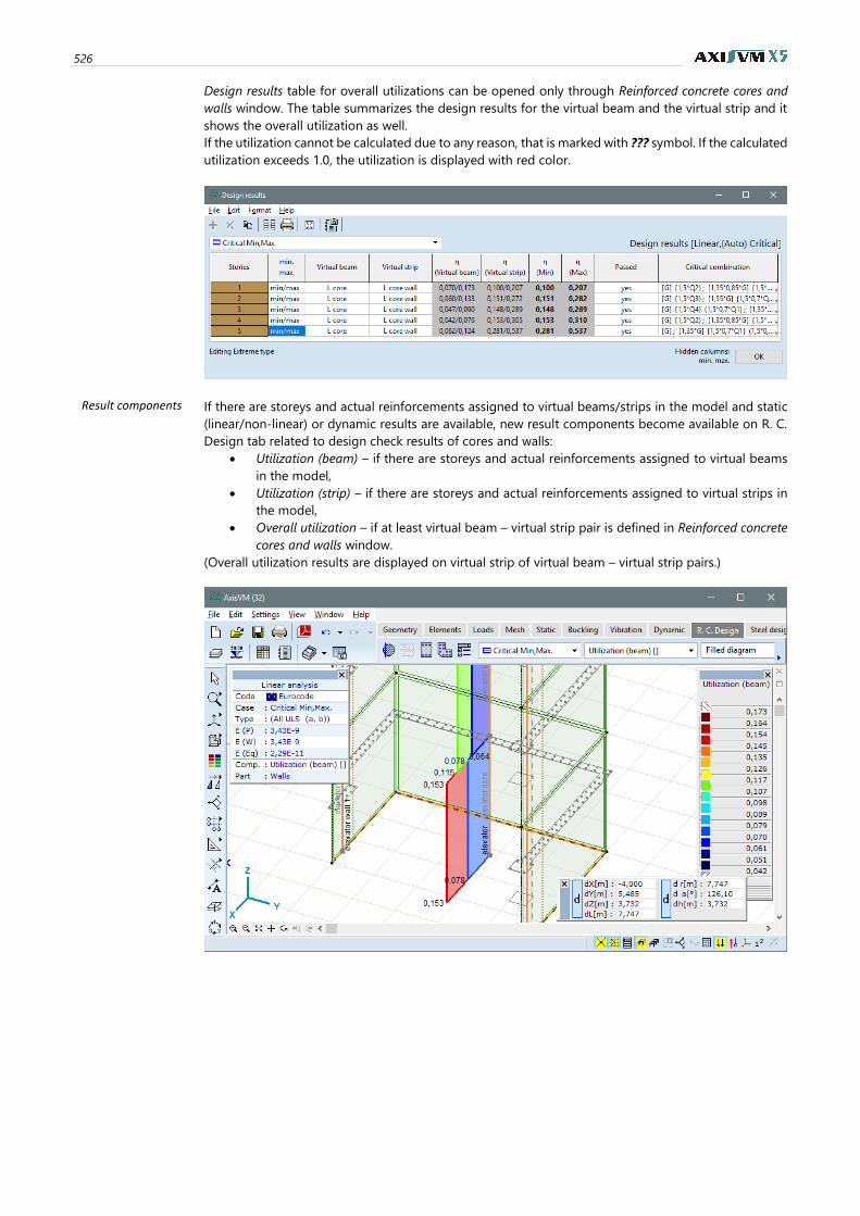
526

Design results table for overall utilizations can be opened only through Reinforced concrete cores and

walls window. The table summarizes the design results for the virtual beam and the virtual strip and it

shows the overall utilization as well.

If the utilization cannot be calculated due to any reason, that is marked with ??? symbol. If the calculated

utilization exceeds 1.0, the utilization is displayed with red color.

Result components If there are storeys and actual reinforcements assigned to virtual beams/strips in the model and static

(linear/non-linear) or dynamic results are available, new result components become available on R. C.

Design tab related to design check results of cores and walls:

• Utilization (beam) – if there are storeys and actual reinforcements assigned to virtual beams

in the model,

• Utilization (strip) – if there are storeys and actual reinforcements assigned to virtual strips in

the model,

• Overall utilization – if at least virtual beam – virtual strip pair is defined in Reinforced concrete

cores and walls window.

(Overall utilization results are displayed on virtual strip of virtual beam – virtual strip pairs.)

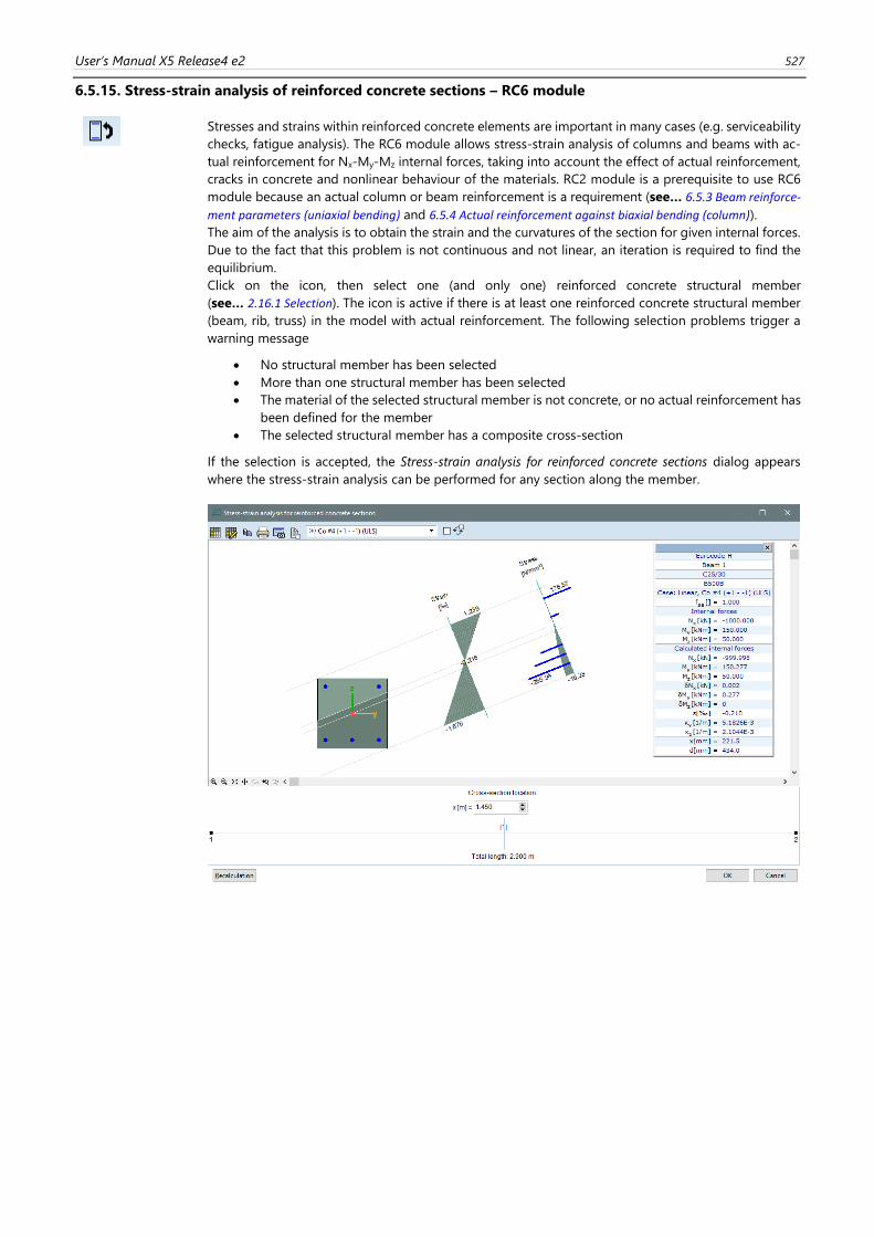
User’s Manual X5 Release4 e2 527

6.5.15. Stress-strain analysis of reinforced concrete sections – RC6 module

Stresses and strains within reinforced concrete elements are important in many cases (e.g. serviceability

checks, fatigue analysis). The RC6 module allows stress-strain analysis of columns and beams with ac-

tual reinforcement for Nx-My-Mz internal forces, taking into account the effect of actual reinforcement,

cracks in concrete and nonlinear behaviour of the materials. RC2 module is a prerequisite to use RC6

module because an actual column or beam reinforcement is a requirement (see… 6.5.3 Beam reinforce-

ment parameters (uniaxial bending) and 6.5.4 Actual reinforcement against biaxial bending (column)).

The aim of the analysis is to obtain the strain and the curvatures of the section for given internal forces.

Due to the fact that this problem is not continuous and not linear, an iteration is required to find the

equilibrium.

Click on the icon, then select one (and only one) reinforced concrete structural member

(see… 2.16.1 Selection). The icon is active if there is at least one reinforced concrete structural member

(beam, rib, truss) in the model with actual reinforcement. The following selection problems trigger a

warning message

• No structural member has been selected

• More than one structural member has been selected

• The material of the selected structural member is not concrete, or no actual reinforcement has

been defined for the member

• The selected structural member has a composite cross-section

If the selection is accepted, the Stress-strain analysis for reinforced concrete sections dialog appears

where the stress-strain analysis can be performed for any section along the member.

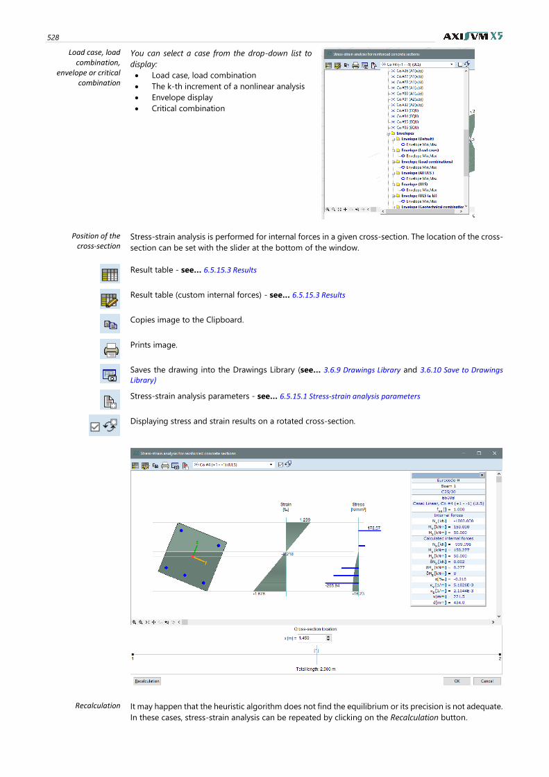
528

Load case, load combination,

envelope or critical combination

You can select a case from the drop-down list to

display:

• Load case, load combination

• The k-th increment of a nonlinear analysis

• Envelope display

• Critical combination

Position of the cross-section

Stress-strain analysis is performed for internal forces in a given cross-section. The location of the cross-

section can be set with the slider at the bottom of the window.

Result table - see… 6.5.15.3 Results

Result table (custom internal forces) - see… 6.5.15.3 Results

Copies image to the Clipboard.

Prints image.

Saves the drawing into the Drawings Library (see… 3.6.9 Drawings Library and 3.6.10 Save to Drawings Library)

Stress-strain analysis parameters - see… 6.5.15.1 Stress-strain analysis parameters

Displaying stress and strain results on a rotated cross-section.

Recalculation It may happen that the heuristic algorithm does not find the equilibrium or its precision is not adequate.

In these cases, stress-strain analysis can be repeated by clicking on the Recalculation button.

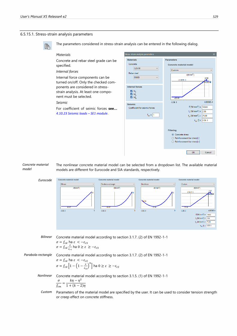
User’s Manual X5 Release4 e2 529

6.5.15.1. Stress-strain analysis parameters

The parameters considered in stress-strain analysis can be entered in the following dialog.

Materials

Concrete and rebar steel grade can be

specified.

Internal forces

Internal force components can be

turned on/off. Only the checked com-

ponents are considered in stress-

strain analysis. At least one compo-

nent must be selected.

Seismic

For coefficient of seimic forces see…

4.10.23 Seismic loads – SE1 module.

Concrete material model

The nonlinear concrete material model can be selected from a dropdown list. The available material

models are different for Eurocode and SIA standards, respectively.

Eurocode

Bilinear

Concrete material model according to section 3.1.7. (2) of EN 1992-1-1

𝜎 = 𝑓𝑐𝑑 ha 휀 < −휀𝑐3

𝜎 = 𝑓𝑐𝑑𝜀

𝜀𝑐3 ha 0 ≥ 휀 ≥ −휀𝑐3

Parabola-rectangle Concrete material model according to section 3.1.7. (2) of EN 1992-1-1

𝜎 = 𝑓𝑐𝑑 ha 휀 < −휀𝑐2

𝜎 = 𝑓𝑐𝑑 [1 − (1 −𝜀

𝜀𝑐2)𝑛] ha 0 ≥ 휀 ≥ −휀𝑐2

Nonlinear Concrete material model according to section 3.1.5. (1) of EN 1992-1-1

𝜎

𝑓𝑐𝑚=

𝑘휂 − 휂2

1 + (𝑘 − 2)휂

Custom Parameters of the material model are specified by the user. It can be used to consider tension strength

or creep effect on concrete stiffness.

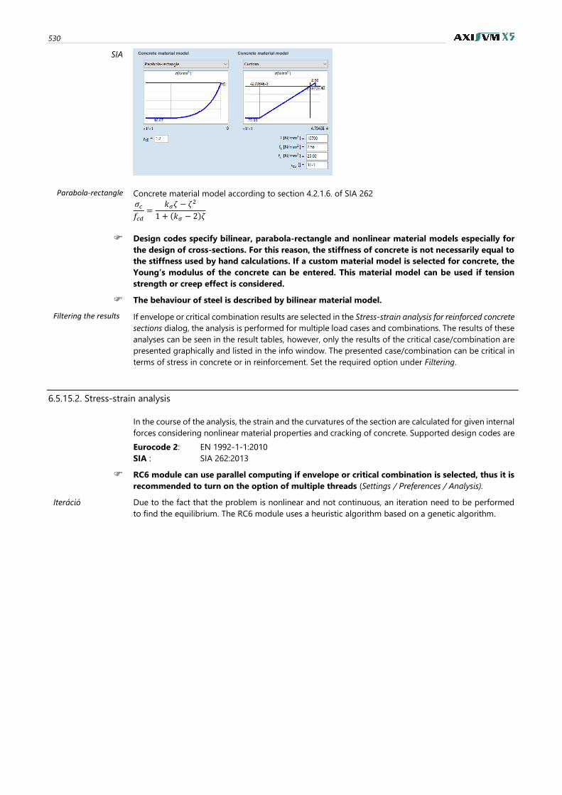
530

SIA

Parabola-rectangle Concrete material model according to section 4.2.1.6. of SIA 262

𝜎𝑐𝑓𝑐𝑑

=𝑘𝜎휁 − 휁

2

1 + (𝑘𝜎 − 2)휁

Design codes specify bilinear, parabola-rectangle and nonlinear material models especially for

the design of cross-sections. For this reason, the stiffness of concrete is not necessarily equal to

the stiffness used by hand calculations. If a custom material model is selected for concrete, the

Young’s modulus of the concrete can be entered. This material model can be used if tension

strength or creep effect is considered.

The behaviour of steel is described by bilinear material model.

Filtering the results If envelope or critical combination results are selected in the Stress-strain analysis for reinforced concrete

sections dialog, the analysis is performed for multiple load cases and combinations. The results of these

analyses can be seen in the result tables, however, only the results of the critical case/combination are

presented graphically and listed in the info window. The presented case/combination can be critical in

terms of stress in concrete or in reinforcement. Set the required option under Filtering.

6.5.15.2. Stress-strain analysis

In the course of the analysis, the strain and the curvatures of the section are calculated for given internal

forces considering nonlinear material properties and cracking of concrete. Supported design codes are

Eurocode 2: EN 1992-1-1:2010

SIA : SIA 262:2013

RC6 module can use parallel computing if envelope or critical combination is selected, thus it is

recommended to turn on the option of multiple threads (Settings / Preferences / Analysis).

Iteráció Due to the fact that the problem is nonlinear and not continuous, an iteration need to be performed

to find the equilibrium. The RC6 module uses a heuristic algorithm based on a genetic algorithm.

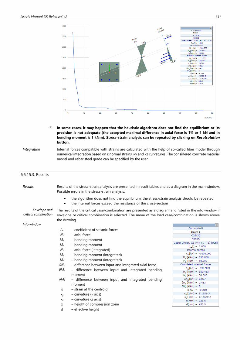
User’s Manual X5 Release4 e2 531

In some cases, it may happen that the heuristic algorithm does not find the equilibrium or its

precision is not adequate (the accepted maximal difference in axial force is 1% or 1 kN and in

bending moment is 1 kNm). Stress-strain analysis can be repeated by clicking on Recalculation

button.

Integration Internal forces compatible with strains are calculated with the help of so-called fiber model through

numerical integration based on ε normal strains, κy and κz curvatures. The considered concrete material

model and rebar steel grade can be specified by the user.

6.5.15.3. Results

Results

Results of the stress-strain analysis are presented in result tables and as a diagram in the main window.

Possible errors in the stress-strain analysis:

• the algorithm does not find the equilibrium, the stress-strain analysis should be repeated

• the internal forces exceed the resistance of the cross-section

Envelope and critical combination

The results of the critical case/combination are presented as a diagram and listed in the info window if

envelope or critical combination is selected. The name of the load case/combination is shown above

the drawing.

Info window

fse – coefficient of seismic forces

Nx – axial force

My – bending moment

Mz – bending moment

Nx – axial force (integrated)

My – bending moment (integrated)

Mz – bending moment (integrated)

δNx – difference between input and integrated axial force

δMy – difference between input and integrated bending

moment

δMz – difference between input and integrated bending

moment

ε – strain at the centroid

κy – curvature (y axis)

κz – curvature (z axis)

x – height of compression zone

d – effective height

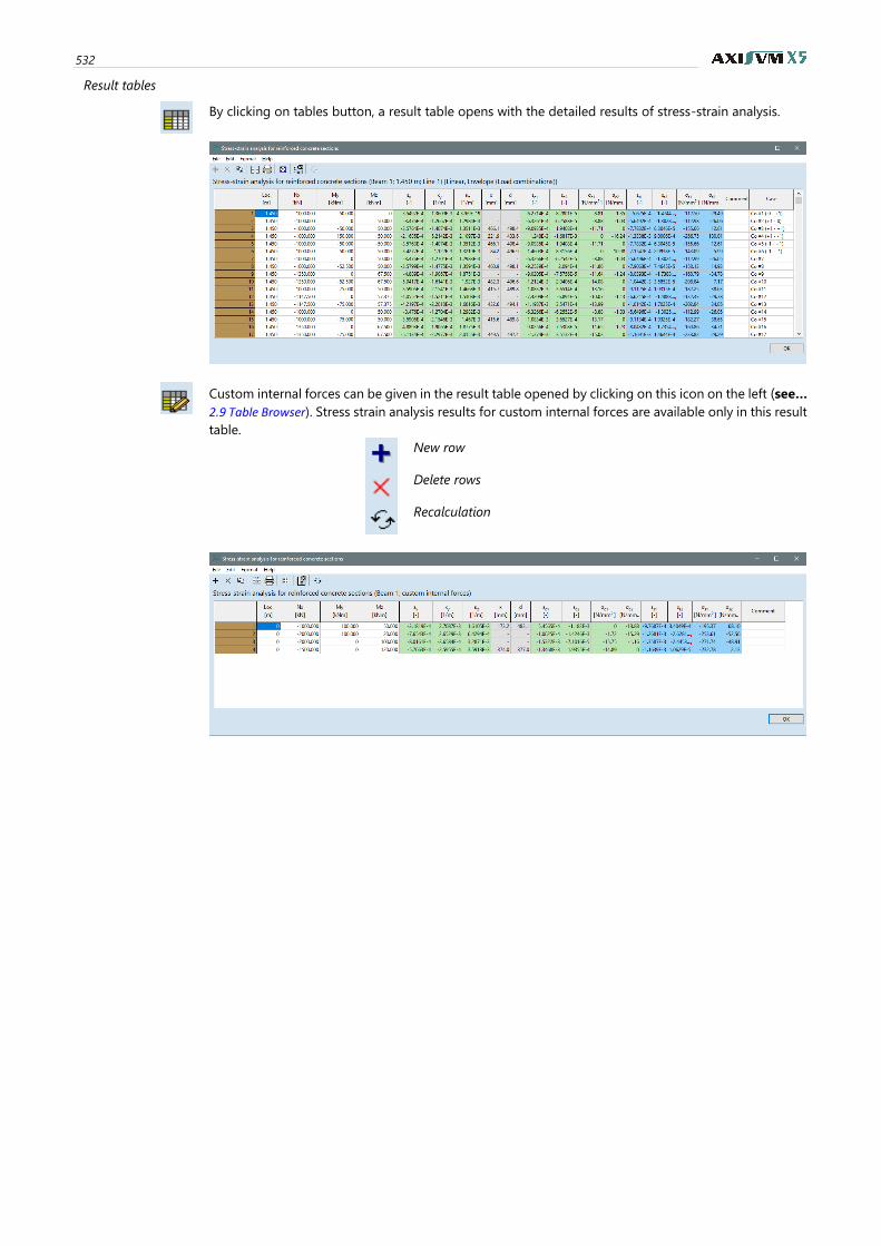
532

Result tables

By clicking on tables button, a result table opens with the detailed results of stress-strain analysis.

Custom internal forces can be given in the result table opened by clicking on this icon on the left (see…

2.9 Table Browser). Stress strain analysis results for custom internal forces are available only in this result

table.

New row

Delete rows

Recalculation

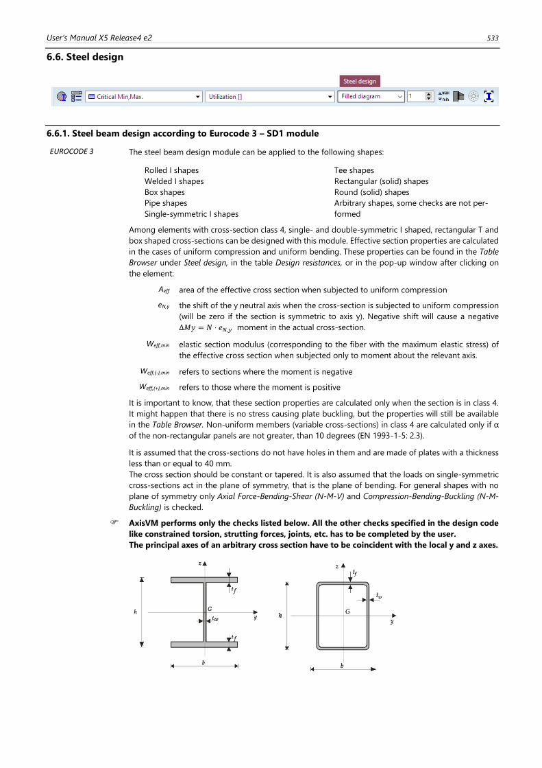
User’s Manual X5 Release4 e2 533

6.6. Steel design

6.6.1. Steel beam design according to Eurocode 3 – SD1 module

EUROCODE 3 The steel beam design module can be applied to the following shapes:

Rolled I shapes

Welded I shapes

Box shapes

Pipe shapes

Single-symmetric I shapes

Tee shapes

Rectangular (solid) shapes

Round (solid) shapes

Arbitrary shapes, some checks are not per-

formed

Among elements with cross-section class 4, single- and double-symmetric I shaped, rectangular T and

box shaped cross-sections can be designed with this module. Effective section properties are calculated

in the cases of uniform compression and uniform bending. These properties can be found in the Table

Browser under Steel design, in the table Design resistances, or in the pop-up window after clicking on

the element:

Aeff area of the effective cross section when subjected to uniform compression

eN,y the shift of the y neutral axis when the cross-section is subjected to uniform compression

(will be zero if the section is symmetric to axis y). Negative shift will cause a negative

Δ𝑀𝑦 = 𝑁 ⋅ 𝑒𝑁,𝑦 moment in the actual cross-section.

Weff,min

elastic section modulus (corresponding to the fiber with the maximum elastic stress) of

the effective cross section when subjected only to moment about the relevant axis.

Weff,(-),min refers to sections where the moment is negative

Weff,(+),min refers to those where the moment is positive

It is important to know, that these section properties are calculated only when the section is in class 4.

It might happen that there is no stress causing plate buckling, but the properties will still be available

in the Table Browser. Non-uniform members (variable cross-sections) in class 4 are calculated only if α

of the non-rectangular panels are not greater, than 10 degrees (EN 1993-1-5: 2.3).

It is assumed that the cross-sections do not have holes in them and are made of plates with a thickness

less than or equal to 40 mm.

The cross section should be constant or tapered. It is also assumed that the loads on single-symmetric

cross-sections act in the plane of symmetry, that is the plane of bending. For general shapes with no

plane of symmetry only Axial Force-Bending-Shear (N-M-V) and Compression-Bending-Buckling (N-M-

Buckling) is checked.

AxisVM performs only the checks listed below. All the other checks specified in the design code

like constrained torsion, strutting forces, joints, etc. has to be completed by the user.

The principal axes of an arbitrary cross section have to be coincident with the local y and z axes.

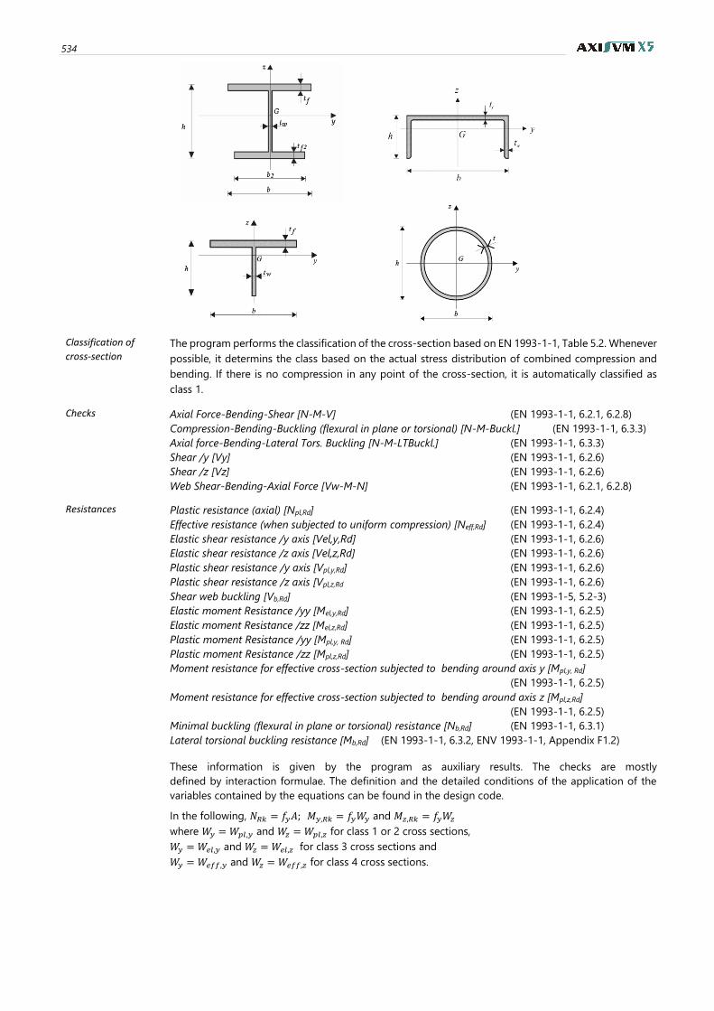
534

Classification of

cross-section The program performs the classification of the cross-section based on EN 1993-1-1, Table 5.2. Whenever

possible, it determins the class based on the actual stress distribution of combined compression and

bending. If there is no compression in any point of the cross-section, it is automatically classified as

class 1.

Checks Axial Force-Bending-Shear [N-M-V] (EN 1993-1-1, 6.2.1, 6.2.8)

Compression-Bending-Buckling (flexural in plane or torsional) [N-M-Buckl.] (EN 1993-1-1, 6.3.3)

Axial force-Bending-Lateral Tors. Buckling [N-M-LTBuckl.] (EN 1993-1-1, 6.3.3)

Shear /y [Vy] (EN 1993-1-1, 6.2.6)

Shear /z [Vz] (EN 1993-1-1, 6.2.6)

Web Shear-Bending-Axial Force [Vw-M-N] (EN 1993-1-1, 6.2.1, 6.2.8)

Resistances Plastic resistance (axial) [Npl,Rd] (EN 1993-1-1, 6.2.4)

Effective resistance (when subjected to uniform compression) [Neff,Rd] (EN 1993-1-1, 6.2.4)

Elastic shear resistance /y axis [Vel,y,Rd] (EN 1993-1-1, 6.2.6)

Elastic shear resistance /z axis [Vel,z,Rd] (EN 1993-1-1, 6.2.6)

Plastic shear resistance /y axis [Vpl,y,Rd] (EN 1993-1-1, 6.2.6)

Plastic shear resistance /z axis [Vpl,z,Rd (EN 1993-1-1, 6.2.6)

Shear web buckling [Vb,Rd] (EN 1993-1-5, 5.2-3)

Elastic moment Resistance /yy [Mel,y,Rd] (EN 1993-1-1, 6.2.5)

Elastic moment Resistance /zz [Mel,z,Rd] (EN 1993-1-1, 6.2.5)

Plastic moment Resistance /yy [Mpl,y, Rd] (EN 1993-1-1, 6.2.5)

Plastic moment Resistance /zz [Mpl,z,Rd] (EN 1993-1-1, 6.2.5)

Moment resistance for effective cross-section subjected to bending around axis y [Mpl,y, Rd]

(EN 1993-1-1, 6.2.5)

Moment resistance for effective cross-section subjected to bending around axis z [Mpl,z,Rd]

(EN 1993-1-1, 6.2.5)

Minimal buckling (flexural in plane or torsional) resistance [Nb,Rd] (EN 1993-1-1, 6.3.1)

Lateral torsional buckling resistance [Mb,Rd] (EN 1993-1-1, 6.3.2, ENV 1993-1-1, Appendix F1.2)

These information is given by the program as auxiliary results. The checks are mostly

defined by interaction formulae. The definition and the detailed conditions of the application of the

variables contained by the equations can be found in the design code.

In the following, 𝑁𝑅𝑘 = 𝑓𝑦𝐴; 𝑀𝑦,𝑅𝑘 = 𝑓𝑦𝑊𝑦 and 𝑀𝑧,𝑅𝑘 = 𝑓𝑦𝑊𝑧

where 𝑊𝑦 = 𝑊𝑝𝑙,𝑦 and 𝑊𝑧 = 𝑊𝑝𝑙,𝑧 for class 1 or 2 cross sections,

𝑊𝑦 = 𝑊𝑒𝑙,𝑦 and 𝑊𝑧 = 𝑊𝑒𝑙,𝑧 for class 3 cross sections and

𝑊𝑦 = 𝑊𝑒𝑓𝑓,𝑦 and 𝑊𝑧 = 𝑊𝑒𝑓𝑓,𝑧 for class 4 cross sections.

User’s Manual X5 Release4 e2 535

Axial Force-Bending-Shear

The member can be in tension or in compression. The check is performed on the basis of

EN 1993-1-1, 6.2.1 (7). 𝑁𝐸𝑑

𝑁𝑅𝑘/𝛾𝑀0+𝑀𝑦,𝐸𝑑 + Δ𝑀𝑦,𝐸𝑑

𝑀𝑦,𝑅𝑘/𝛾𝑀0+

𝑀𝑧,𝐸𝑑

𝑀𝑧,𝑅𝑘/𝛾𝑀0≤ 1

Δ𝑀𝑦,𝐸𝑑 = 𝑁𝐸𝑑 ⋅ 𝑒𝑁,𝑦: it differs from zero only when the cross section is in class 4 and the original cross

section is asymmetric to axis y.

High shear

If the shear force is greater than 50% of the shear resistance, the effect of shear force is considered as

detailed below.

For section class 1. and 2. allowance is made on the resistance moment accoding to EN 1993-1-1, 6.2.8.

For section class 3. and 4. stresses are calculated and the general and conservative formula in EN 1993-

1-1, 6.2.1 (5) is applied. This is done for section types: I, T, C, box and pipe. For other section types (L

shape, rectangular and round sold shapes, and user defined shapes) the effect of hight shear has to be

calculated by the user.

Plastic resistance check

For I, pipe and box shaped sections in section class 1. and 2., the resistance check is performed according

to EN 1993-1-1 6.2.10. Allowance is made for the effect of both shear force and axial force on the

resistance moment. Besides resistance check of pure axial force and pure shear force, the following

criteria should be satisfied:

𝑀𝑦,𝐸𝑑

𝑀𝑁,𝑦,𝑅𝑑≤ 1;

𝑀𝑧,𝐸𝑑

𝑀𝑁,𝑧,𝑅𝑑≤ 1

where 𝑀𝑁,𝑦,𝑅𝑑 , 𝑀𝑁,𝑧,𝑅𝑑 are reduced moment resistances based on the effect of shear force and axial force

(EN 1993-1-1 6.2.8. and 6.2.9.1). For pipe sections, the reduced moment is calculated as follows:

𝑀𝑁,𝑦,𝑅𝑑 = 1.04 ⋅ (1 − 𝜌 −𝑛1.7

(1 − 𝜌)0.7) ; 𝑛 =

𝑁𝐸𝑑𝑁𝑝𝑙,𝑅𝑑

; 𝜌 = (2𝑉𝐸𝑑

𝑉𝑝𝑙,𝑧,𝑅𝑑− 1)

2

𝑀𝑁,𝑧,𝑅𝑑 = 1.04 ⋅ (1 − 𝜌 −𝑛1.7

(1 − 𝜌)0.7) ; 𝑛 =

𝑁𝐸𝑑𝑁𝑝𝑙,𝑅𝑑

; 𝜌 = (2𝑉𝐸𝑑

𝑉𝑝𝑙,𝑦,𝑅𝑑− 1)

2

For bi-axial bending the criterion in EN 1993-1-1 6.2.9.1. (6) should be satisfied:

[𝑀𝑦,𝐸𝑑

𝑀𝑁,𝑦,𝑅𝑑]

𝛼

+ [𝑀𝑧,𝐸𝑑

𝑀𝑁,𝑧,𝑅𝑑]

𝛽

≤ 1

Compression-

Bending-Buckling

The check is based on EN 1993-1-1, 6.3.3 (6.61) and (6.62):

𝑁𝐸𝑑𝜒𝑦𝑁𝑅𝑘/𝛾𝑀1

+ 𝑘𝑦𝑦𝑀𝑦,𝐸𝑑 + Δ𝑀𝑦,𝐸𝑑

𝑀𝑦,𝑅𝑘/𝛾𝑀1+ 𝑘𝑦𝑧

𝑀𝑧,𝐸𝑑

𝑀𝑧,𝑅𝑘/𝛾𝑀1≤ 1

𝑁𝐸𝑑𝜒𝑧𝑁𝑅𝑘/𝛾𝑀1

+ 𝑘𝑧𝑦𝑀𝑦,𝐸𝑑 + Δ𝑀𝑦,𝐸𝑑

𝑀𝑦,𝑅𝑘/𝛾𝑀1+ 𝑘𝑧𝑧

𝑀𝑧,𝐸𝑑

𝑀𝑧,𝑅𝑘/𝛾𝑀1≤ 1

(𝜒𝐿𝑇 = 1.0)

∆𝑀𝑦,𝐸𝑑 = 𝑁𝐸𝑑 ∙ 𝑒𝑁 ,𝑦 differs from zero only when the cross section is in class 4 and the original cross

section is asymmetric to axis y.

Axial Force-Bending-Lateral

Torsional Buckling

When determining the lateral-torsional buckling resistance, it is assumed that the cross section is

constant and symmetric to the local z axis. It is also assumed the the loads act in the plane of symmetry,

that is the plane of bending (except for C/U cross sections, see below). The value of k (ENV 1993-1-1,

F1.2) is taken equal to 𝐾𝑧 (buckling length factor). The weak axis should be the local z axis.

The check is based on the form of equations (6.61) and (6.62) of EN 1993-1-1, 6.3.3 :

𝑁𝐸𝑑

𝜒𝑦𝑁𝑅𝑘/𝛾

𝑀1

+ 𝑘𝑦𝑦𝑀𝑦,𝐸𝑑 + Δ𝑀𝑦,𝐸𝑑

𝜒𝐿𝑇𝑀𝑦,𝑅𝑘/𝛾𝑀1

+ 𝑘𝑦𝑧𝑀𝑧,𝐸𝑑

𝑀𝑧,𝑅𝑘/𝛾𝑀1

≤ 1

𝑁𝐸𝑑

𝜒𝑧𝑁𝑅𝑘/𝛾

𝑀1

+ 𝑘𝑧𝑦𝑀𝑦,𝐸𝑑 + Δ𝑀𝑦,𝐸𝑑

𝜒𝐿𝑇𝑀𝑦,𝑅𝑘

/𝛾𝑀1

+ 𝑘𝑧𝑧𝑀𝑧,𝐸𝑑

𝑀𝑧,𝑅𝑘/𝛾𝑀1

≤ 1

𝛥𝑀𝑦,𝐸𝑑 = 𝑁𝐸𝑑 ⋅ 𝑒𝑁,𝑦: it differs from zero only when the cross section is in class 4 and the original cross

section is asymmetric to axis y.

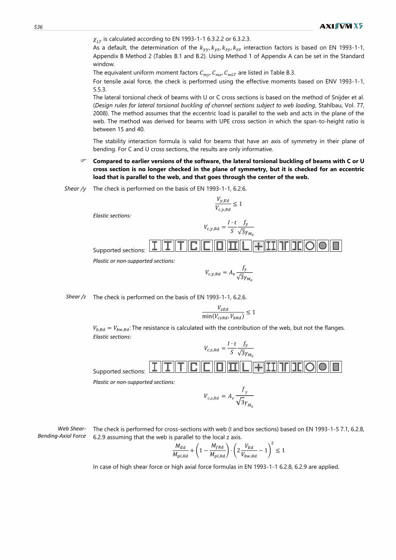
536

𝜒𝐿𝑇

is calculated according to EN 1993-1-1 6.3.2.2 or 6.3.2.3.

As a default, the determination of the 𝑘𝑦𝑦 , 𝑘𝑦𝑧, 𝑘𝑧𝑦 , 𝑘𝑧𝑧 interaction factors is based on EN 1993-1-1,

Appendix B Method 2 (Tables B.1 and B.2). Using Method 1 of Appendix A can be set in the Standard

window.

The equivalent uniform moment factors 𝐶𝑚𝑦, 𝐶𝑚𝑧, 𝐶𝑚𝐿𝑇 are listed in Table B.3.

For tensile axial force, the check is performed using the effective moments based on ENV 1993-1-1,

5.5.3.

The lateral torsional check of beams with U or C cross sections is based on the method of Snijder et al.

(Design rules for lateral torsional buckling of channel sections subject to web loading, Stahlbau, Vol. 77,

2008). The method assumes that the eccentric load is parallel to the web and acts in the plane of the

web. The method was derived for beams with UPE cross section in which the span-to-height ratio is

between 15 and 40.

The stability interaction formula is valid for beams that have an axis of symmetry in their plane of

bending. For C and U cross sections, the results are only informative.

Compared to earlier versions of the software, the lateral torsional buckling of beams with C or U

cross section is no longer checked in the plane of symmetry, but it is checked for an eccentric

load that is parallel to the web, and that goes through the center of the web.

Shear /y The check is performed on the basis of EN 1993-1-1, 6.2.6.

𝑉𝑦,𝐸𝑑

𝑉𝑐,𝑦,𝑅𝑑≤ 1

Elastic sections:

𝑉𝑐,𝑦,𝑅𝑑 =𝐼 ∙ 𝑡

𝑆

𝑓𝑦

√3𝛾𝑀0

Supported sections:

Plastic or non-supported sections:

𝑉𝑐,𝑦,𝑅𝑑 = 𝐴𝑣𝑓𝑦

√3𝛾𝑀0

Shear /z The check is performed on the basis of EN 1993-1-1, 6.2.6.

𝑉𝑧𝐸𝑑min(𝑉𝑐𝑧𝑅𝑑 , 𝑉𝑏𝑅𝑑)

≤ 1

𝑉𝑏,𝑅𝑑 = 𝑉𝑏𝑤,𝑅𝑑 : The resistance is calculated with the contribution of the web, but not the flanges.

Elastic sections:

𝑉𝑐,𝑧,𝑅𝑑 =𝐼 ∙ 𝑡

𝑆

𝑓𝑦

√3𝛾𝑀0

Supported sections:

Plastic or non-supported sections:

𝑉𝑐,𝑧,𝑅𝑑 = 𝐴𝑣

𝑓𝑦

√3𝛾𝑀0

Web Shear-Bending-Axial Force

The check is performed for cross-sections with web (I and box sections) based on EN 1993-1-5 7.1, 6.2.8,

6.2.9 assuming that the web is parallel to the local z axis.

𝑀𝐸𝑑

𝑀𝑝𝑙,𝑅𝑑+ (1 −

𝑀𝑓𝑅𝑑

𝑀𝑝𝑙,𝑅𝑑) ⋅ (2

𝑉𝐸𝑑𝑉𝑏𝑤,𝑅𝑑

− 1)

2

≤ 1

In case of high shear force or high axial force formulas in EN 1993-1-1 6.2.8, 6.2.9 are applied.

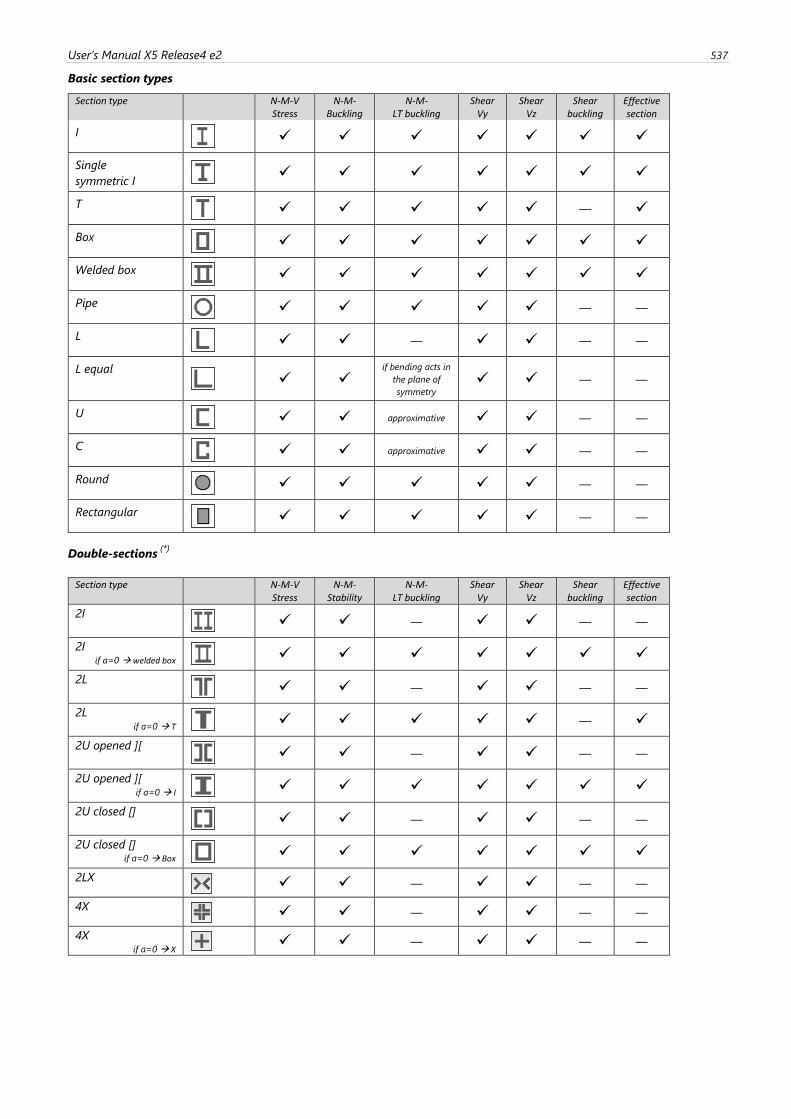
User’s Manual X5 Release4 e2 537

Basic section types

Section type N-M-V Stress

N-M-Buckling

N-M- LT buckling

Shear Vy

Shear Vz

Shear buckling

Effective section

I

✓ ✓ ✓ ✓ ✓ ✓ ✓

Single

symmetric I ✓ ✓ ✓ ✓ ✓ ✓ ✓

T

✓ ✓ ✓ ✓ ✓ — ✓

Box

✓ ✓ ✓ ✓ ✓ ✓ ✓

Welded box

✓ ✓ ✓ ✓ ✓ ✓ ✓

Pipe

✓ ✓ ✓ ✓ ✓ — —

L

✓ ✓ — ✓ ✓ — —

L equal

✓ ✓

if bending acts in

the plane of

symmetry ✓ ✓ — —

U

✓ ✓ approximative ✓ ✓ — —

C

✓ ✓ approximative ✓ ✓ — —

Round

✓ ✓ ✓ ✓ ✓ — —

Rectangular

✓ ✓ ✓ ✓ ✓ — —

Double-sections (*)

Section type N-M-V

Stress N-M-

Stability N-M-

LT buckling Shear

Vy Shear

Vz Shear

buckling Effective section

2I

✓ ✓ — ✓ ✓ — —

2I if a=0 → welded box

✓ ✓ ✓ ✓ ✓ ✓ ✓

2L

✓ ✓ — ✓ ✓ — —

2L if a=0 → T

✓ ✓ ✓ ✓ ✓ — ✓

2U opened ][

✓ ✓ — ✓ ✓ — —

2U opened ][ if a=0 → I

✓ ✓ ✓ ✓ ✓ ✓ ✓

2U closed []

✓ ✓ — ✓ ✓ — —

2U closed [] if a=0 → Box

✓ ✓ ✓ ✓ ✓ ✓ ✓

2LX

✓ ✓ — ✓ ✓ — —

4X

✓ ✓ — ✓ ✓ — —

4X if a=0 → X

✓ ✓ — ✓ ✓ — —

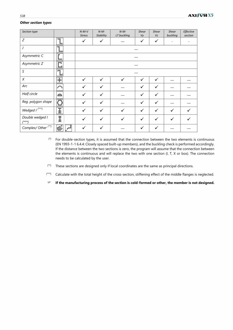
538

Other section types

Section type N-M-V

Stress N-M-

Stability N-M-

LT buckling Shear

Vy Shear

Vz Shear

buckling Effective section

Z

✓ ✓ — ✓ ✓ - -

J

—

Asymmetric C

—

Asymmetric Z

—

S

—

X ✓ ✓ ✓ ✓ ✓ — —

Arc

✓ ✓ — ✓ ✓ — —

Half circle

✓ ✓ — ✓ ✓ — —

Reg. polygon shape

✓ ✓ — ✓ ✓ — —

Wedged I (***)

✓ ✓ ✓ ✓ ✓ ✓ ✓

Double wedged I

(***) ✓ ✓ ✓ ✓ ✓ ✓ ✓

Complex/ Other (**)

✓ ✓ — ✓ ✓ — —

(*) For double-section types, it is assumed that the connection between the two elements is continuous

(EN 1993-1-1 6.4.4: Closely spaced built-up members), and the buckling check is performed accordingly.

If the distance between the two sections is zero, the program will assume that the connection between

the elements is continuous and will replace the two with one section (I, T, X or box). The connection

needs to be calculated by the user.

(**) These sections are designed only if local coordinates are the same as principal directions.

(***) Calculate with the total height of the cross-section, stiffening effect of the middle flanges is neglected.

If the manufacturing process of the section is cold-formed or other, the member is not designed.

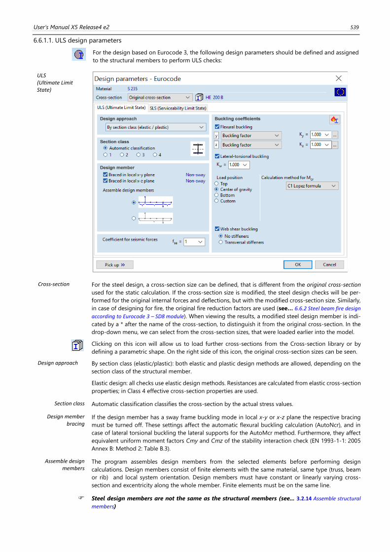
User’s Manual X5 Release4 e2 539

6.6.1.1. ULS design parameters

For the design based on Eurocode 3, the following design parameters should be defined and assigned

to the structural members to perform ULS checks:

ULS (Ultimate Limit State)

5Cross-section For the steel design, a cross-section size can be defined, that is different from the original cross-section

used for the static calculation. If the cross-section size is modified, the steel design checks will be per-

formed for the original internal forces and deflections, but with the modified cross-section size. Similarly,

in case of designing for fire, the original fire reduction factors are used (see… 6.6.2 Steel beam fire design

according to Eurocode 3 – SD8 module). When viewing the results, a modified steel design member is indi-

cated by a * after the name of the cross-section, to distinguish it from the original cross-section. In the

drop-down menu, we can select from the cross-section sizes, that were loaded earlier into the model.

Clicking on this icon will allow us to load further cross-sections from the Cross-section library or by

defining a parametric shape. On the right side of this icon, the original cross-section sizes can be seen.

Design approach By section class (elastic/plastic): both elastic and plastic design methods are allowed, depending on the

section class of the structural member.

Elastic design: all checks use elastic design methods. Resistances are calculated from elastic cross-section

properties; in Class 4 effective cross-section properties are used.

Section class Automatic classification classifies the cross-section by the actual stress values.

Design member bracing

If the design member has a sway frame buckling mode in local x-y or x-z plane the respective bracing

must be turned off. These settings affect the automatic flexural buckling calculation (AutoNcr), and in

case of lateral torsional buckling the lateral supports for the AutoMcr method. Furthermore, they affect

equivalent uniform moment factors Cmy and Cmz of the stability interaction check (EN 1993-1-1: 2005

Annex B: Method 2: Table B.3).

Assemble design members

The program assembles design members from the selected elements before performing design

calculations. Design members consist of finite elements with the same material, same type (truss, beam

or rib) and local system orientation. Design members must have constant or linearly varying cross-

section and excentricity along the whole member. Finite elements must be on the same line.

Steel design members are not the same as the structural members (see... 3.2.14 Assemble structural

members)

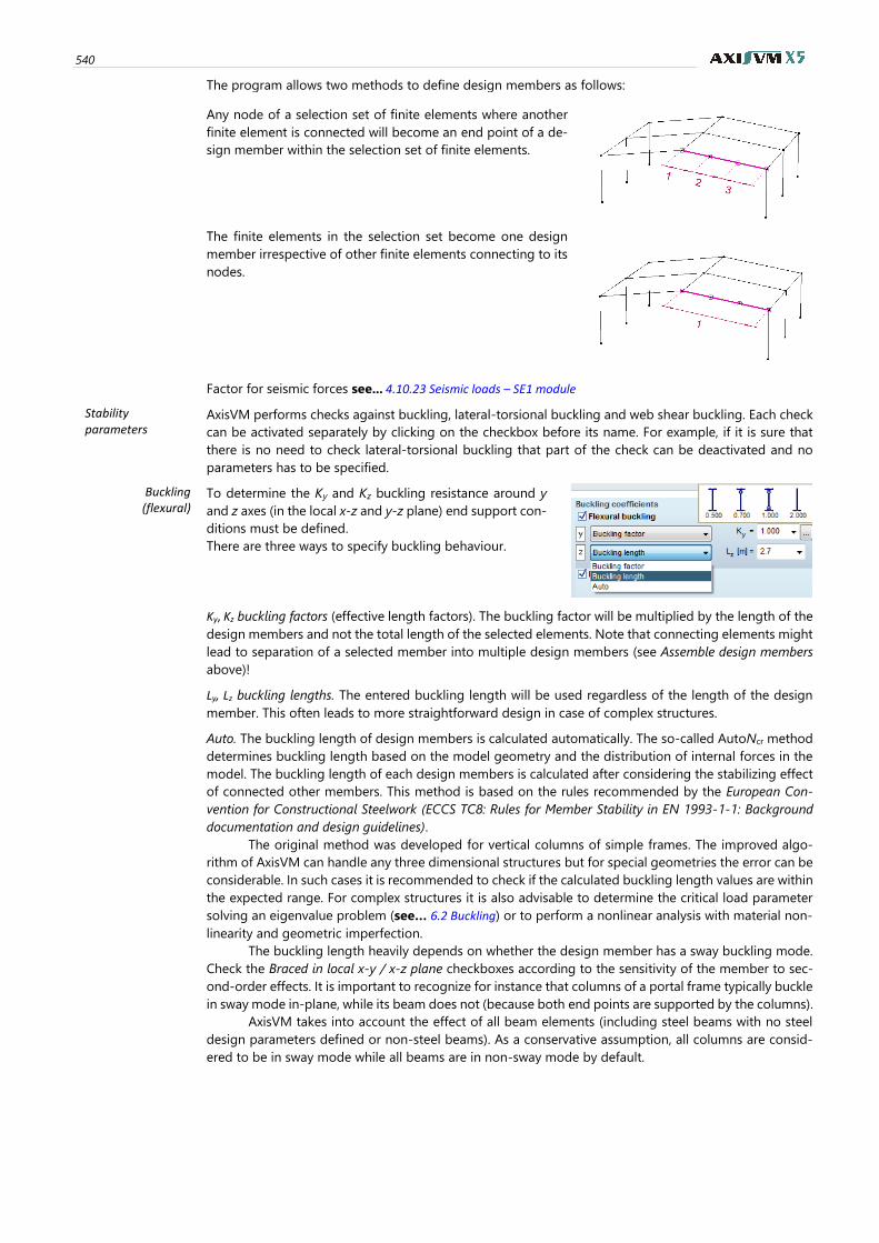
540

The program allows two methods to define design members as follows:

Any node of a selection set of finite elements where another

finite element is connected will become an end point of a de-

sign member within the selection set of finite elements.

The finite elements in the selection set become one design

member irrespective of other finite elements connecting to its

nodes.

Factor for seismic forces see... 4.10.23 Seismic loads – SE1 module

Stability parameters

AxisVM performs checks against buckling, lateral-torsional buckling and web shear buckling. Each check

can be activated separately by clicking on the checkbox before its name. For example, if it is sure that

there is no need to check lateral-torsional buckling that part of the check can be deactivated and no

parameters has to be specified.

Buckling (flexural)

To determine the Ky and Kz buckling resistance around y

and z axes (in the local x-z and y-z plane) end support con-

ditions must be defined.

There are three ways to specify buckling behaviour.

Ky, Kz buckling factors (effective length factors). The buckling factor will be multiplied by the length of the

design members and not the total length of the selected elements. Note that connecting elements might

lead to separation of a selected member into multiple design members (see Assemble design members

above)!

Ly, Lz buckling lengths. The entered buckling length will be used regardless of the length of the design

member. This often leads to more straightforward design in case of complex structures.

Auto. The buckling length of design members is calculated automatically. The so-called AutoNcr method

determines buckling length based on the model geometry and the distribution of internal forces in the

model. The buckling length of each design members is calculated after considering the stabilizing effect

of connected other members. This method is based on the rules recommended by the European Con-

vention for Constructional Steelwork (ECCS TC8: Rules for Member Stability in EN 1993-1-1: Background

documentation and design guidelines).

The original method was developed for vertical columns of simple frames. The improved algo-

rithm of AxisVM can handle any three dimensional structures but for special geometries the error can be

considerable. In such cases it is recommended to check if the calculated buckling length values are within

the expected range. For complex structures it is also advisable to determine the critical load parameter

solving an eigenvalue problem (see… 6.2 Buckling) or to perform a nonlinear analysis with material non-

linearity and geometric imperfection.

The buckling length heavily depends on whether the design member has a sway buckling mode.

Check the Braced in local x-y / x-z plane checkboxes according to the sensitivity of the member to sec-

ond-order effects. It is important to recognize for instance that columns of a portal frame typically buckle

in sway mode in-plane, while its beam does not (because both end points are supported by the columns).

AxisVM takes into account the effect of all beam elements (including steel beams with no steel

design parameters defined or non-steel beams). As a conservative assumption, all columns are consid-

ered to be in sway mode while all beams are in non-sway mode by default.

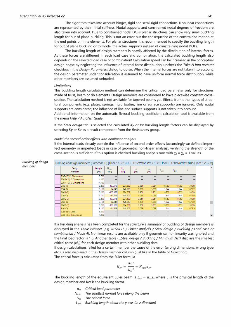
User’s Manual X5 Release4 e2 541

The algorithm takes into account hinges, rigid and semi-rigid connections. Nonlinear connections

are represented by their initial stiffness. Nodal supports and constrained nodal degrees of freedom are

also taken into account. Due to constrained nodal DOFs planar structures can show very small buckling

length for out of plane buckling. This is not an error but the consequence of the constrained motion at

the end points of finite elements. For planar structures it is recommended to specify the buckling length

for out of plane buckling or to model the actual supports instead of constraining nodal DOFs.

The buckling length of design members is heavily affected by the distribution of internal forces.

As these forces are different in each load case and combination, the calculated buckling length also

depends on the selected load case or combination! Calculation speed can be increased in the conceptual

design phase by neglecting the influence of internal force distribution; uncheck the Take N into account

checkbox in the Design Parameters dialog to do so. When the internal forces are not taken into account,

the design parameter under consideration is assumed to have uniform normal force distribution, while

other members are assumed unloaded.

Limitations

This buckling length calculation method can determine the critical load parameter only for structures

made of truss, beam or rib elements. Design members are considered to have piecewise constant cross-

section. The calculation method is not available for tapered beams yet. Effects from other types of struc-

tural components (e.g. plates, springs, rigid bodies, line or surface supports) are ignored. Only nodal

supports are considered; the influence of line and surface supports is not taken into account.

Additional information on the automatic flexural buckling coefficient calculation tool is available from

the menu Help / AutoNcr Guide.

If the Steel design tab is selected the calculated Ky or Kz buckling length factors can be displayed by

selecting Ky or Kz as a result component from the Resistances group.

Model the second order effects with nonlinear analysis

If the internal loads already contain the influence of second order effects (accordingly we defined imper-

fect geometry or imperfect loads in case of geometric non-linear analysis), verifying the strength of the

cross-section is sufficient. If this option is checked buckling analysis runs with χx = χy = 1 values.

Buckling of design members

If a buckling analysis has been completed for the structure a summary of buckling of design members is

displayed in the Table Browser (e.g. RESULTS / Linear analysis / Steel design / Buckling / Load case or

combination / Mode 4). Nonlinear results are available only if geometrical nonlinearity was ignored and

the final load factor is 1.0. Another table (…Steel design / Buckling / Minimum Ncr) displays the smallest

critical force (Ncr) for each design member with other buckling data.

If design calculations failed for a certain member the cause of the error (wrong dimensions, wrong type

etc.) is also displayed in the Design member column (just like in the table of Utilization).

The critical force is calculated from the Euler formula

𝑁𝑐𝑟 = 𝜋𝐸𝐼

𝐿𝑐𝑟2= 𝑁𝑚𝑖𝑛𝛼𝑐𝑟

The buckling length of the equivalent Euler beam is 𝐿𝑐𝑟 = 𝐾𝑐𝑟𝐿, where L is the physical length of the

design member and Kcr is the buckling factor.

αcr Critical load parameter

Nmin The smallest normal force along the beam

Ncr The critical force

Ly,cr Buckling length about the y axis (in z direction)

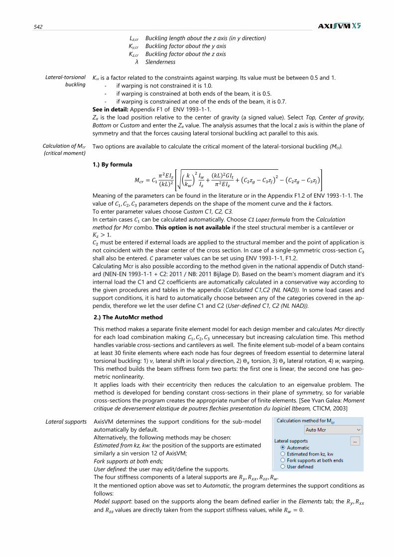
542

Lz,cr Buckling length about the z axis (in y direction)

Ky,cr Buckling factor about the y axis

Kz,cr Buckling factor about the z axis

λ Slenderness

Lateral-torsional buckling

K is a factor related to the constraints against warping. Its value must be between 0.5 and 1.

- if warping is not constrained it is 1.0.

- if warping is constrained at both ends of the beam, it is 0.5.

- if warping is constrained at one of the ends of the beam, it is 0.7.

See in detail: Appendix F1 of ENV 1993-1-1.

Za is the load position relative to the center of gravity (a signed value). Select Top, Center of gravity,

Bottom or Custom and enter the Za value. The analysis assumes that the local z axis is within the plane of

symmetry and that the forces causing lateral torsional buckling act parallel to this axis.

Calculation of Mcr (critical moment)

Two options are available to calculate the critical moment of the lateral-torsional buckling (Mcr).

1.) By formula

𝑀𝑐𝑟 = 𝐶1𝜋2𝐸𝐼𝑧(𝑘𝐿)2

[√(𝑘

𝑘𝑤)2 𝐼𝑤𝐼𝑧+(𝑘𝐿)2𝐺𝐼𝑡𝜋2𝐸𝐼𝑧

+ (𝐶2𝑧𝑔 − 𝐶3𝑧𝑗)2− (𝐶2𝑧𝑔 − 𝐶3𝑧𝑗)]

Meaning of the parameters can be found in the literature or in the Appendix F1.2 of ENV 1993-1-1. The

value of 𝐶1, 𝐶2, 𝐶3 parameters depends on the shape of the moment curve and the k factors.

To enter parameter values choose Custom C1, C2, C3.

In certain cases 𝐶1 can be calculated automatically. Choose C1 Lopez formula from the Calculation

method for Mcr combo. This option is not available if the steel structural member is a cantilever or

𝐾𝑧 > 1.

𝐶2 must be entered if external loads are applied to the structural member and the point of application is

not coincident with the shear center of the cross section. In case of a single-symmetric cross-section 𝐶3

shall also be entered. 𝐶 parameter values can be set using ENV 1993-1-1, F1.2.

Calculating Mcr is also possible according to the method given in the national appendix of Dutch stand-

ard (NEN-EN 1993-1-1 + C2: 2011 / NB: 2011 Bijlage D). Based on the beam's moment diagram and it's

internal load the C1 and C2 coefficients are automatically calculated in a conservative way according to

the given procedures and tables in the appendix (Calculated C1,C2 (NL NAD)). In some load cases and

support conditions, it is hard to automatically choose between any of the categories covered in the ap-

pendix, therefore we let the user define C1 and C2 (User-defined C1, C2 (NL NAD)).

2.) The AutoMcr method

This method makes a separate finite element model for each design member and calculates Mcr directly

for each load combination making 𝐶1, 𝐶2, 𝐶3 unnecessary but increasing calculation time. This method

handles variable cross-sections and cantilevers as well. The finite element sub-model of a beam contains

at least 30 finite elements where each node has four degrees of freedom essential to determine lateral

torsional buckling: 1) 𝜈, lateral shift in local y direction, 2) Θ𝑥 torsion, 3) Θ𝑧 lateral rotation, 4) w, warping.

This method builds the beam stiffness form two parts: the first one is linear, the second one has geo-

metric nonlinearity.

It applies loads with their eccentricity then reduces the calculation to an eigenvalue problem. The

method is developed for bending constant cross-sections in their plane of symmetry, so for variable

cross-sections the program creates the appropriate number of finite elements. [See Yvan Galea: Moment

critique de deversement elastique de poutres flechies presentation du logiciel ltbeam, CTICM, 2003]

Lateral supports AxisVM determines the support conditions for the sub-model

automatically by default.

Alternatively, the following methods may be chosen:

Estimated from kz, kw: the position of the supports are estimated

similarly a sin version 12 of AxisVM;

Fork supports at both ends;

User defined: the user may edit/define the supports.

The four stiffness components of a lateral supports are 𝑅𝑦, 𝑅𝑥𝑥, 𝑅𝑧𝑧, 𝑅𝑤.

It the mentioned option above was set to Automatic, the program determines the support conditions as

follows:

Model support: based on the supports along the beam defined earlier in the Elements tab; the 𝑅𝑦, 𝑅𝑥𝑥

and 𝑅𝑧𝑧 values are directly taken from the support stiffness values, while 𝑅𝑤 = 0.

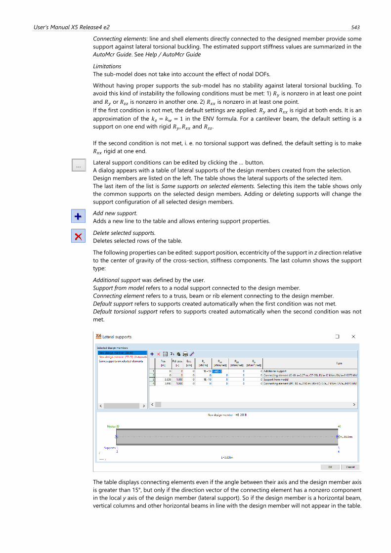
User’s Manual X5 Release4 e2 543

Connecting elements: line and shell elements directly connected to the designed member provide some

support against lateral torsional buckling. The estimated support stiffness values are summarized in the

AutoMcr Guide. See Help / AutoMcr Guide

Limitations

The sub-model does not take into account the effect of nodal DOFs.

Without having proper supports the sub-model has no stability against lateral torsional buckling. To

avoid this kind of instability the following conditions must be met: 1) 𝑅𝑦 is nonzero in at least one point

and 𝑅𝑦 or 𝑅𝑧𝑧 is nonzero in another one. 2) 𝑅𝑥𝑥 is nonzero in at least one point.

If the first condition is not met, the default settings are applied: 𝑅𝑦 and 𝑅𝑥𝑥 is rigid at both ends. It is an

approximation of the 𝑘𝑧 = 𝑘𝑤 = 1 in the ENV formula. For a cantilever beam, the default setting is a

support on one end with rigid 𝑅𝑦, 𝑅𝑥𝑥 and 𝑅𝑧𝑧.

If the second condition is not met, i. e. no torsional support was defined, the default setting is to make

𝑅𝑥𝑥 rigid at one end.

Lateral support conditions can be edited by clicking the … button.

A dialog appears with a table of lateral supports of the design members created from the selection.

Design members are listed on the left. The table shows the lateral supports of the selected item.

The last item of the list is Same supports on selected elements. Selecting this item the table shows only

the common supports on the selected design members. Adding or deleting supports will change the

support configuration of all selected design members.

Add new support.

Adds a new line to the table and allows entering support properties.

Delete selected supports.

Deletes selected rows of the table.

The following properties can be edited: support position, eccentricity of the support in z direction relative

to the center of gravity of the cross-section, stiffness components. The last column shows the support

type:

Additional support was defined by the user.

Support from model refers to a nodal support connected to the design member.

Connecting element refers to a truss, beam or rib element connecting to the design member.

Default support refers to supports created automatically when the first condition was not met.

Default torsional support refers to supports created automatically when the second condition was not

met.

The table displays connecting elements even if the angle between their axis and the design member axis

is greater than 15°, but only if the direction vector of the connecting element has a nonzero component

in the local y axis of the design member (lateral support). So if the design member is a horizontal beam,

vertical columns and other horizontal beams in line with the design member will not appear in the table.

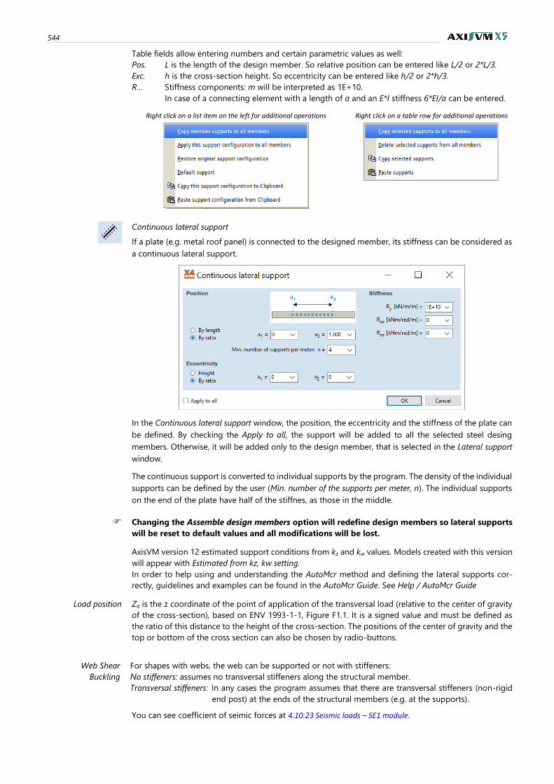
544

Table fields allow entering numbers and certain parametric values as well:

Pos. L is the length of the design member. So relative position can be entered like L/2 or 2*L/3.

Exc. h is the cross-section height. So eccentricity can be entered like h/2 or 2*h/3.

R… Stiffness components: m will be interpreted as 1E+10.

In case of a connecting element with a length of a and an E*I stiffness 6*EI/a can be entered.

Right click on a list item on the left for additional operations

Right click on a table row for additional operations

Continuous lateral support

If a plate (e.g. metal roof panel) is connected to the designed member, its stiffness can be considered as

a continuous lateral support.

In the Continuous lateral support window, the position, the eccentricity and the stiffness of the plate can

be defined. By checking the Apply to all, the support will be added to all the selected steel desing

members. Otherwise, it will be added only to the design member, that is selected in the Lateral support

window.

The continuous support is converted to individual supports by the program. The density of the individual

supports can be defined by the user (Min. number of the supports per meter, n). The individual supports

on the end of the plate have half of the stiffnes, as those in the middle.

Changing the Assemble design members option will redefine design members so lateral supports

will be reset to default values and all modifications will be lost.

AxisVM version 12 estimated support conditions from kz and kw values. Models created with this version

will appear with Estimated from kz, kw setting.

In order to help using and understanding the AutoMcr method and defining the lateral supports cor-

rectly, guidelines and examples can be found in the AutoMcr Guide. See Help / AutoMcr Guide

Load position Za is the z coordinate of the point of application of the transversal load (relative to the center of gravity

of the cross-section), based on ENV 1993-1-1, Figure F1.1. It is a signed value and must be defined as

the ratio of this distance to the height of the cross-section. The positions of the center of gravity and the

top or bottom of the cross section can also be chosen by radio-buttons.

Web Shear

Buckling

For shapes with webs, the web can be supported or not with stiffeners:

No stiffeners: assumes no transversal stiffeners along the structural member.

Transversal stiffeners: In any cases the program assumes that there are transversal stiffeners (non-rigid

end post) at the ends of the structural members (e.g. at the supports).

You can see coefficient of seimic forces at 4.10.23 Seismic loads – SE1 module.

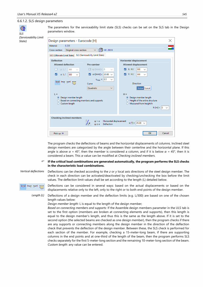
User’s Manual X5 Release4 e2 545

6.6.1.2. SLS design parameters

SLS (Serviceability Limit State)

The parameters for the serviceability limit state (SLS) checks can be set on the SLS tab in the Design

parameters window.

The program checks the deflections of beams and the horizontal displacements of columns. Inclined steel

design members are categorized by the angle between their centerline and the horizontal plane. If this

angle is above α = 45°, then the member is considered a column, and if it is below α = 45°, then it is

considered a beam. This α value can be modified at Checking inclined members.

If the critical load combinations are generated automatically, the program performs the SLS checks

in the characteristic load combinations.

Vertical deflections Deflections can be checked according to the z or y local axis directions of the steel design member. The

check in each direction can be activated/deactivated by checking/unchecking the box before the limit

values. The deflection limit values shall be set according to the length (L) detailed below.

Deflections can be considered in several ways: based on the actual displacements or based on the

displacements relative only to the left, only to the right or to both end points of the design member.

Length (L)

Deflections of a design member and the deflection limits (e.g. L/300) are based on one of the chosen

length values below:

Design member length: L is equal to the length of the design member;

Based on connecting members and supports: If the Assemble design members parameter in the ULS tab is

set to the first option (members are broken at connecting elements and supports), then this length is

equal to the design member’s length, and thus this is the same as the length above. If it is set to the

second option (the selected beams are checked as one design member), then the program checks if there

are any supports or connecting members along the design member in the direction of the deflection

check that prevents the deflection of the design member. Between these, the SLS check is performed for

each section of the member. For example, checking a 15-meter-long beam, if there are supporting

columns in the end points and at one-third of the length of the beam, then the program performs SLS

checks separately for the first 5-meter-long section and the remaining 10-meter-long section of the beam.

Custom length: any value can be entered.

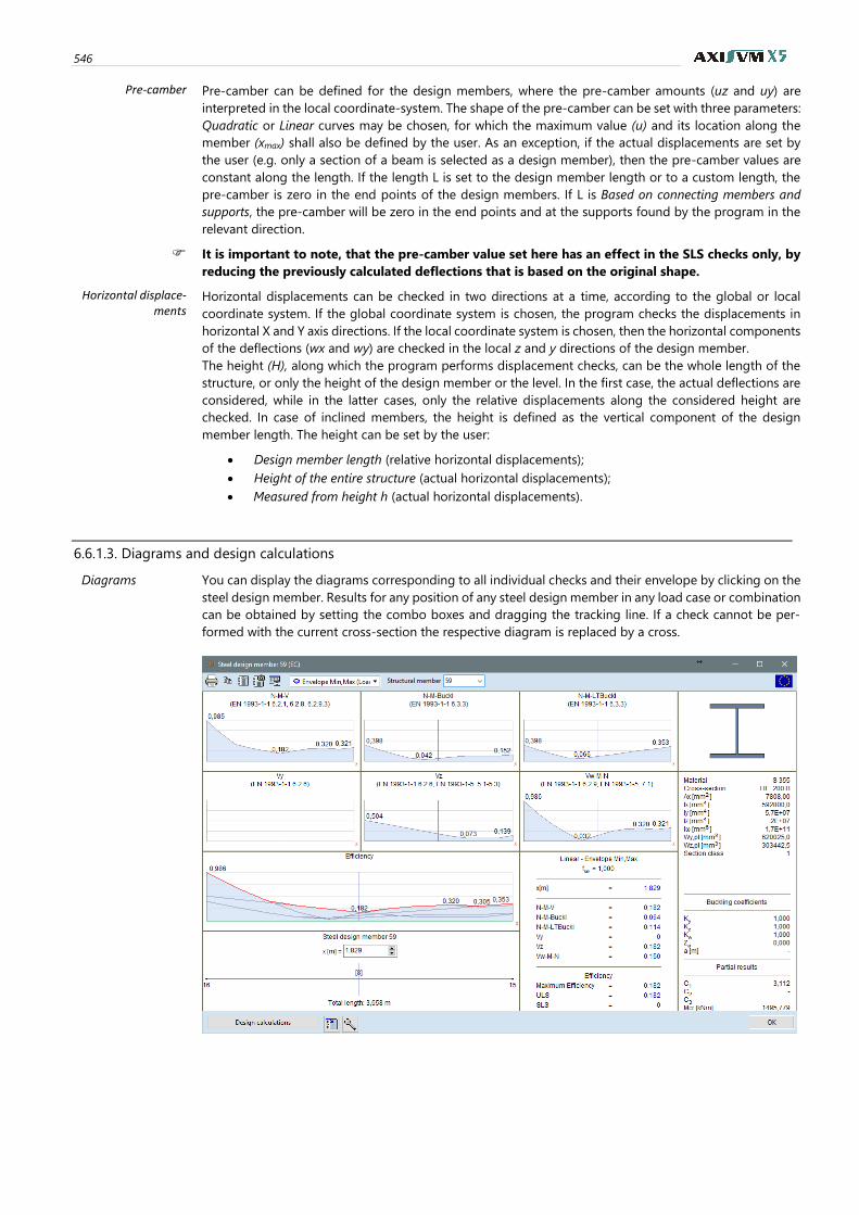
546

Pre-camber

Pre-camber can be defined for the design members, where the pre-camber amounts (uz and uy) are

interpreted in the local coordinate-system. The shape of the pre-camber can be set with three parameters:

Quadratic or Linear curves may be chosen, for which the maximum value (u) and its location along the

member (xmax) shall also be defined by the user. As an exception, if the actual displacements are set by

the user (e.g. only a section of a beam is selected as a design member), then the pre-camber values are

constant along the length. If the length L is set to the design member length or to a custom length, the

pre-camber is zero in the end points of the design members. If L is Based on connecting members and

supports, the pre-camber will be zero in the end points and at the supports found by the program in the

relevant direction.

It is important to note, that the pre-camber value set here has an effect in the SLS checks only, by

reducing the previously calculated deflections that is based on the original shape.

Horizontal displace-ments

Horizontal displacements can be checked in two directions at a time, according to the global or local

coordinate system. If the global coordinate system is chosen, the program checks the displacements in

horizontal X and Y axis directions. If the local coordinate system is chosen, then the horizontal components

of the deflections (wx and wy) are checked in the local z and y directions of the design member.

The height (H), along which the program performs displacement checks, can be the whole length of the

structure, or only the height of the design member or the level. In the first case, the actual deflections are

considered, while in the latter cases, only the relative displacements along the considered height are

checked. In case of inclined members, the height is defined as the vertical component of the design

member length. The height can be set by the user:

• Design member length (relative horizontal displacements);

• Height of the entire structure (actual horizontal displacements);

• Measured from height h (actual horizontal displacements).

6.6.1.3. Diagrams and design calculations

Diagrams

You can display the diagrams corresponding to all individual checks and their envelope by clicking on the

steel design member. Results for any position of any steel design member in any load case or combination

can be obtained by setting the combo boxes and dragging the tracking line. If a check cannot be per-

formed with the current cross-section the respective diagram is replaced by a cross.

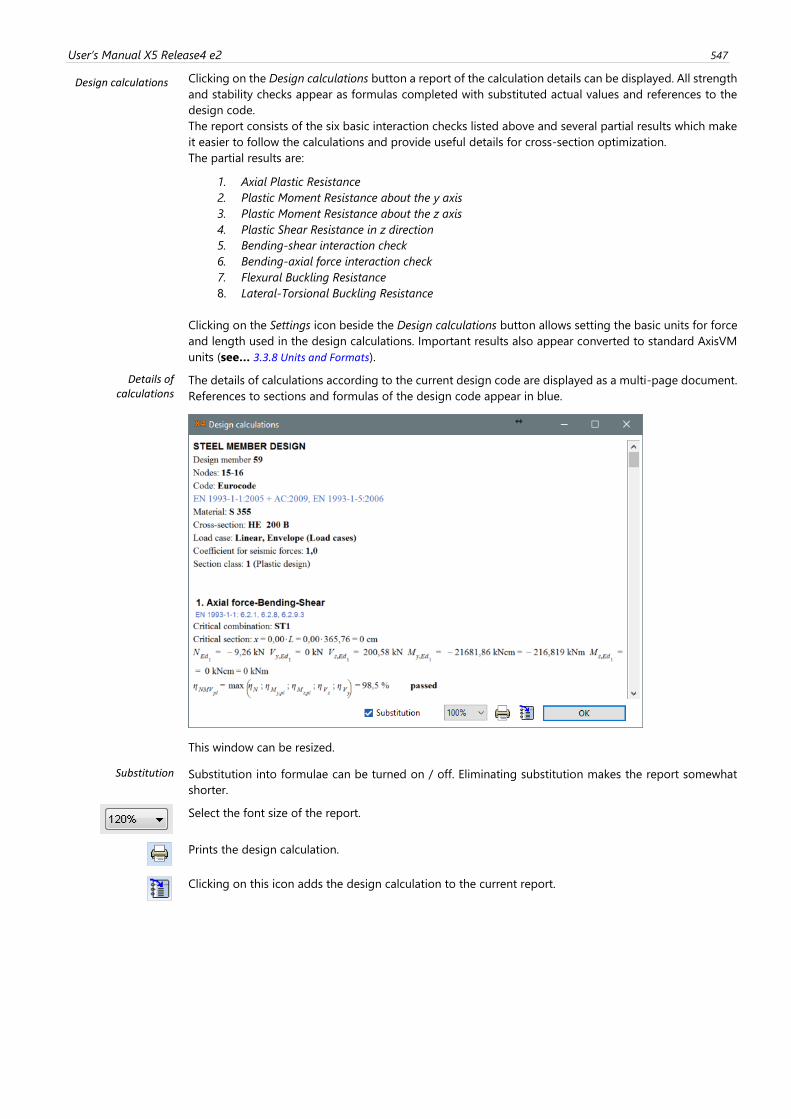
User’s Manual X5 Release4 e2 547

Design calculations

Clicking on the Design calculations button a report of the calculation details can be displayed. All strength

and stability checks appear as formulas completed with substituted actual values and references to the

design code.

The report consists of the six basic interaction checks listed above and several partial results which make

it easier to follow the calculations and provide useful details for cross-section optimization.

The partial results are:

1. Axial Plastic Resistance

2. Plastic Moment Resistance about the y axis

3. Plastic Moment Resistance about the z axis

4. Plastic Shear Resistance in z direction

5. Bending-shear interaction check

6. Bending-axial force interaction check

7. Flexural Buckling Resistance

8. Lateral-Torsional Buckling Resistance

Clicking on the Settings icon beside the Design calculations button allows setting the basic units for force

and length used in the design calculations. Important results also appear converted to standard AxisVM

units (see… 3.3.8 Units and Formats).

Details of calculations

The details of calculations according to the current design code are displayed as a multi-page document.

References to sections and formulas of the design code appear in blue.

This window can be resized.

Substitution Substitution into formulae can be turned on / off. Eliminating substitution makes the report somewhat

shorter.

Select the font size of the report.

Prints the design calculation.

Clicking on this icon adds the design calculation to the current report.

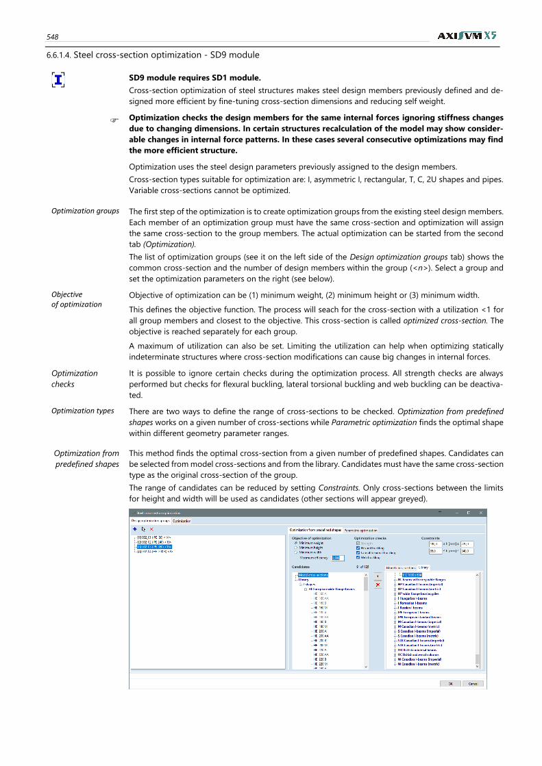
548

6.6.1.4. Steel cross-section optimization - SD9 module

SD9 module requires SD1 module.

Cross-section optimization of steel structures makes steel design members previously defined and de-

signed more efficient by fine-tuning cross-section dimensions and reducing self weight.

Optimization checks the design members for the same internal forces ignoring stiffness changes

due to changing dimensions. In certain structures recalculation of the model may show consider-

able changes in internal force patterns. In these cases several consecutive optimizations may find

the more efficient structure.

Optimization uses the steel design parameters previously assigned to the design members.

Cross-section types suitable for optimization are: I, asymmetric I, rectangular, T, C, 2U shapes and pipes.

Variable cross-sections cannot be optimized.

Optimization groups The first step of the optimization is to create optimization groups from the existing steel design members.

Each member of an optimization group must have the same cross-section and optimization will assign

the same cross-section to the group members. The actual optimization can be started from the second

tab (Optimization).

The list of optimization groups (see it on the left side of the Design optimization groups tab) shows the

common cross-section and the number of design members within the group (<n>). Select a group and

set the optimization parameters on the right (see below).

Objective of optimization

Objective of optimization can be (1) minimum weight, (2) minimum height or (3) minimum width.

This defines the objective function. The process will seach for the cross-section with a utilization <1 for

all group members and closest to the objective. This cross-section is called optimized cross-section. The

objective is reached separately for each group.

A maximum of utilization can also be set. Limiting the utilization can help when optimizing statically

indeterminate structures where cross-section modifications can cause big changes in internal forces.

Optimization

checks

It is possible to ignore certain checks during the optimization process. All strength checks are always

performed but checks for flexural buckling, lateral torsional buckling and web buckling can be deactiva-

ted.

Optimization types There are two ways to define the range of cross-sections to be checked. Optimization from predefined

shapes works on a given number of cross-sections while Parametric optimization finds the optimal shape

within different geometry parameter ranges.

Optimization from

predefined shapes

This method finds the optimal cross-section from a given number of predefined shapes. Candidates can

be selected from model cross-sections and from the library. Candidates must have the same cross-section

type as the original cross-section of the group.

The range of candidates can be reduced by setting Constraints. Only cross-sections between the limits

for height and width will be used as candidates (other sections will appear greyed).

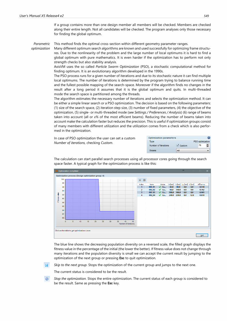
User’s Manual X5 Release4 e2 549

If a group contains more than one design member all members will be checked. Members are checked

along their entire length. Not all candidates will be checked. The program analyses only those necessary

for finding the global optimum.

Parametric

optimization

This method finds the optimal cross-section within different geometry parameter ranges.

Many different optimum search algorithms are known and used successfully for optimizing frame structu-

res. Due to the nonlinearity of the problem and the large number of local optimums it is hard to find a

global optimum with pure mathematics. It is even harder if the optimization has to perform not only

strength checks but also stability analysis.

AxisVM uses the so called Particle Swarm Optimization (PSO), a stochastic computational method for

finding optimum. It is an evolutionary algorithm developed in the 1990s.

The PSO process runs for a given number of iterations and due to its stochastic nature it can find multiple

local optimums. The number of iterations is determined by the program trying to balance running time

and the fullest possible mapping of the search-space. Moreover if the algorithm finds no changes in the

result after a long period it assumes that it is the global optimum and quits. In multi-threaded

mode the search space is partitioned among the threads.

The algorithm estimates the necessary number of iterations and selects the optimization method. It can

be either a simple linear search or a PSO optimization. The decision is based on the following parameters:

(1) size of the search space, (2) iteration step size, (3) number of fixed parameters, (4) the objective of the

optimization, (5) single- or multi-threaded mode (see Settings / Preferences / Analysis) (6) range of beams

taken into account (all or x% of the most efficient beams). Reducing the number of beams taken into

account make the calculation faster but reduces the precision. This is useful if optimization groups consist

of many members with different utilization and the utilization comes from a check which is also perfor-

med in the optimization.

In case of PSO optimization the user can set a custom

Number of iterations, checking Custom.

The calculation can start parallel search processes using all processor cores going through the search

space faster. A typical graph for the optimization process is like this:

The blue line shows the decreasing population diversity on a reversed scale, the filled graph displays the

fitness value in the percentage of the initial (the lower the better). If fitness value does not change through

many iterations and the population diversity is small we can accept the current result by jumping to the

optimization of the next group or pressing Esc to quit optimization.

Skip to the next group. Stops the optimization of the current group and jumps to the next one.

The current status is considered to be the result.

Stop the optimization. Stops the entire optimization. The current status of each group is considered to

be the result. Same as pressing the Esc key.

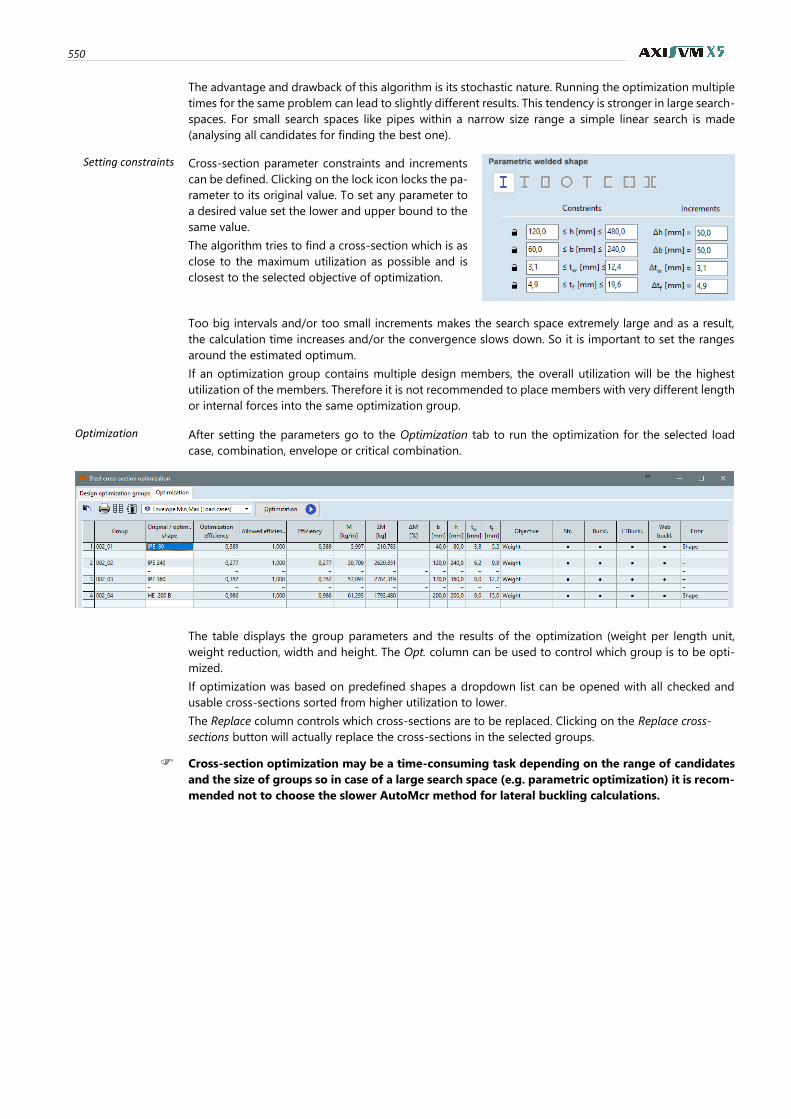
550

The advantage and drawback of this algorithm is its stochastic nature. Running the optimization multiple

times for the same problem can lead to slightly different results. This tendency is stronger in large search-

spaces. For small search spaces like pipes within a narrow size range a simple linear search is made

(analysing all candidates for finding the best one).

Setting constraints Cross-section parameter constraints and increments

can be defined. Clicking on the lock icon locks the pa-

rameter to its original value. To set any parameter to

a desired value set the lower and upper bound to the

same value.

The algorithm tries to find a cross-section which is as

close to the maximum utilization as possible and is

closest to the selected objective of optimization.

Too big intervals and/or too small increments makes the search space extremely large and as a result,

the calculation time increases and/or the convergence slows down. So it is important to set the ranges

around the estimated optimum.

If an optimization group contains multiple design members, the overall utilization will be the highest

utilization of the members. Therefore it is not recommended to place members with very different length

or internal forces into the same optimization group.

Optimization After setting the parameters go to the Optimization tab to run the optimization for the selected load

case, combination, envelope or critical combination.

The table displays the group parameters and the results of the optimization (weight per length unit,

weight reduction, width and height. The Opt. column can be used to control which group is to be opti-

mized.

If optimization was based on predefined shapes a dropdown list can be opened with all checked and

usable cross-sections sorted from higher utilization to lower.

The Replace column controls which cross-sections are to be replaced. Clicking on the Replace cross-

sections button will actually replace the cross-sections in the selected groups.

Cross-section optimization may be a time-consuming task depending on the range of candidates

and the size of groups so in case of a large search space (e.g. parametric optimization) it is recom-

mended not to choose the slower AutoMcr method for lateral buckling calculations.

User’s Manual X5 Release4 e2 551

6.6.2. Steel beam fire design according to Eurocode 3 – SD8 module

Standards AxisVM performs steel fire design according to different national codes. In case of Eurocode National

Annexes that are not listed below, general rules of EN 1993-1-2 are considered.

Eurocode EN 1993-1-2

Eurocode 3: Design of steel structures

Part 1-2: Structural fire design

EC

German

DIN EN 1993-1-2:2010-12 NA

EC

Hungarian

SZ EN 1993-1-2:2013 NA

EC

Romanian

SR EN 1993-1-2:2006/NB:2008

EC

Slovakian

STN EN 1993-1-2/NA:2008

EC

Polish

PN EN 1993-1-2 NA

EC

British

BS EN 1993-1-2:2005 NA

EC

Finnish

SFS-EN 1993-1-2:2005 NA

Fire design of steel structures according to EN 1993-1-2

Steel beam fire design (SD8 module) is based on the ”ordinary” steel beam design (SD1 module;

see… 6.6.1 Steel beam design according to Eurocode 3 – SD1 module), so SD1 module is a prerequisite to

use SD8 module.

EN 1993-1-2 (EC3-1-2) discusses fire design of steel structures. EC3-1-2 is very close to EN 1993-1-1, so

we note only the difference.

Steel beam fire design can be performed in AxisVM if 1) the selected load combination includes a fire

load case (4.10.1 Load cases, load groups) 2) if a fire effect has been assigned to any of the selected elements

(4.10.29 Fire effect on steel elements – SD8 module) in that fire load case. If different fire effects have been

assigned to elements of a design member, an error message appears and fire design cannot be perfor-

med.

If the selection contains elements without fire effect the ordinary steel design will be performed on them.

Certain steel fire design parameters also has to be assigned to the elements (see below).

Member analysis EC3-1-2 discusses different methods: member analysis, analysis of a part of the structure and analysis of

the entire structure. Member analysis is the most widespread verification method due to its simplicity.

Analysis of a part or whole of the structure usually requires complex nonlinear numerical models and

nonlinear statical analysis.

Guiding principles of member analysis according to EC3-1-2:

• Design member internal forces can be calculated with linear static analysis;

• „Only the effects of thermal deformations resulting from thermal gradients across the cross-

section need to be considered. The effects of axial or in-plain thermal expansions may be neg-

lected.” (EC3-1-2, 2.4.2 (4));

• „The boundary conditions at supports and ends of member may be assumed to remain unchan-

ged throughout the fire exposure.” (EC3-1-2, 2.4.2 (5)).

SD8 performs member analysis. It has to be checked if that structure/structural part can be verified with

member analysis according to the guidelines of EC3-1-2.

In certain cases analysis of a part of the structure can be also executed in AxisVM if 1) boundary conditions

are set carefully, 2) fire effects are taken into account as thermal load and 3) we consider the guidelines

in section 2.4.3 of EC3-1-2.

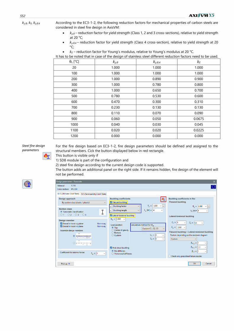
552

ky,θ, kE, ky,θ,4 According to the EC3-1-2, the following reduction factors for mechanical properties of carbon steels are

considered in steel fire design in AxisVM:

• ky,θ – reduction factor for yield strength (Class 1, 2 and 3 cross-sections), relative to yield strength

at 20 °C;

• ky,θ,4 – reduction factor for yield strength (Class 4 cross-section), relative to yield strength at 20

°C;

• kE – reduction factor for Young’s modulus, relative to Young’s modulus at 20 °C.

It has to be noted that in case of the design of stainless steel different reduction factors need to be used. θs [°C] ky,θ ky,θ,4 kE

20 1.000 1.000 1.000

100 1.000 1.000 1.000

200 1.000 0.890 0.900

300 1.000 0.780 0.800

400 1.000 0.650 0.700

500 0.780 0.530 0.600

600 0.470 0.300 0.310

700 0.230 0.130 0.130

800 0.110 0.070 0.090

900 0.060 0.050 0.0675

1000 0.040 0.030 0.045

1100 0.020 0.020 0.0225

1200 0.000 0.000 0.000

Steel fire design parameters

For the fire design based on EC3-1-2, fire design parameters should be defined and assigned to the

structural members. Cick the button displayed below in red rectangle.

This button is visible only if

1) SD8 module is part of the configuration and

2) steel fire design according to the current design code is supported.

The button adds an additional panel on the right side. If it remains hidden, fire design of the element will

not be performed.

User’s Manual X5 Release4 e2 553

Buckling coefficients in fire

Flexural buckling It is possible to define different buckling length or buckling length coefficient for the calculation of buck-

ling resistance about y and z axes in fire, as deflection of the element is often prevented by thin-walled

elements (purlins, etc.) that lose their stiffness very quickly on elevated temperature. The definition/cal-

culation of buckling length is the same as in case of normal temperature design (blue rectangle). If the

automatic buckling length calculation is selected, the fire design module uses the same buckling length

as in normal temperature design.

If Flexural buckling is checked, buckling resistance calculation and verification are performed on both

normal and elevated temperature.

Lateral-torsional buckling

𝐾_𝜔: factor related to the constraints against warping can be different on elevated temperature.

If Lateral-torsional buckling is checked, resistance calculation and verification are performed on both nor-

mal and elevated temperature.

Mcr – critical bending moment

Different parameters can be defined for the consideration and calculation of critical bending moment,

The way of calculation of critical bending moment and load position are the same as in normal tempera-

ture design (blue rectangle).

If AutoMcr is selected, automatically calculated or user defined lateral supports are taken into account by

the calculation of Mcr.

Flexural buckling + Lateral-torsional

bucklings

Verification against flexural torsional buckling is performed if Flexural buckling and Lateral-torsional buc-

kling are checked and the stability parameters are defined. The verification method is explained below.

Equivalent uniform moment factors (βM,y, βM,z and βM,LT of EC3-1-2; Fig. 4.2) need to be defined. It is pos-

sible to calculate these factors automatically based on the bending moment diagram.

Check only prescribed failure modes

EN 1993-1-1 and EN 1993-1-2 standards are similar, but EN 1993-1-2 does not discuss verification in

several failure modes (e.g. strength failure caused by internal forces in interaction with each other or shear

web buckling failure). According to the relevant literature, EN 1993-1-1 verification formulae can be used

in these cases but with reduced yield strength and Young’s modulus. Nevertheless, these verifications are

not prescribed by the code.

If Check only prescribed failure modes is checked, only EC3-1-2 design checks are performed.

Classification of cross-sections

AxisVM classifies cross-sections according to Table 5.2 of EN 1993-1-1. In case of fire design, the ε para-

meter is calculated according to EC3-1-2:

휀 = 0.85√235

𝑓𝑦

Design checks in fire SD8 performs the following design checks:

Check only pre-scribed failure

modes

Axial force-Bending-Shear [N-M-V] (EN 1993-1-1, 6.2.1, 6.2.9.3)

(EN 1993-1-2, 4.2.1-4.2.3, Annex E)

Compression-Bending-Buckling (flexural in plane or torsional) [N-M-Buck] (EN 1993-1-2, 4.2.3.5, Annex E)

Axial force-Bending-Lateral Tors. Buckling [N-M-LTBuckl] (EN 1993-1-2, 4.2.3.5, Annex E)

Shear /y [Vy] (EN 1993-1-2, 4.2.3.3, 4.2.3.4, Annex E)

Shear /z [Vz] (EN 1993-1-2, 4.2.3.3, 4.2.3.4, Annex E)

Check only

prescribed failure modes

Axial force-Bending-Shear [N-M-V] (EN 1993-1-1, 6.2.1, 6.2.8, 6.2.9.3)

(EN 1993-1-2, 4.2.1-4.2.3, Annex E)

Compression-Bending-Buckling (flexural in plane or torsional) [N-M-Buck] (EN 1993-1-2, 4.2.3.5, Annex E)

Axial force-Bending-Lateral Tors. Buckling [N-M-LTBuckl] (EN 1993-1-2, 4.2.3.5, Annex E)

Shear /y [Vy] (EN 1993-1-2, 4.2.3.3, 4.2.3.4, Annex E)

Shear /z [Vz] (EN 1993-1-5, 5.1-5.3)

(EN 1993-1-2, 4.2.3.3, 4.2.3.4, Annex E)

Web shear-Bending-Axial force [Vw-M-N]

(EN 1993-1-1, 6.2.1, 6.2.8, 6.2.9)

(EN 1993-1-5, 5.1-5.3, 7.1)

(EN 1993-1-2, 4.2.1-4.2.3, Annex E)

554

Resistances

Plastic resistance (axial) [Npl,fi,Rd] (EN 1993-1-2, 4.2.3.1, Annex E)

Effective resistance (when subjected to uniform compression) [Neff, fi,Rd] (EN 1993-1-2, 4.2.3.1, Annex E)

Elastic Shear Resistance /y axis [Vel,fi,y,Rd]

(EN 1993-1-1, 6.2.6, EN 1993-1-2, 4.2.3.3, 4.2.3.4, Annex E)

Elastic Shear Resistance /z axis [Vel,fi,z,Rd]

(EN 1993-1-1, 6.2.6, EN 1993-1-2, 4.2.3.3, 4.2.3.4, Annex E)

Plastic Shear Resistance /y axis [Vpl,fi,y,Rd]

(EN 1993-1-1, 6.2.6, EN 1993-1-2, 4.2.3.3, 4.2.3.4, Annex E) Plastic Shear Resistance /z axis [Vpl,fi,z,Rd]

(EN 1993-1-1, 6.2.6, EN 1993-1-2, 4.2.3.3, 4.2.3.4, Annex E)

Shear Web Buckling [Vb,fi,Rd] (EN 1993-1-5, 5.1-5.3, EN 1993-1-2, 4.2.3.3, 4.2.3.4, Annex E)

Elastic Moment Resistance /yy [Mel,fi,y,Rd] (EN 1993-1-2, 4.2.3.4, Annex E)

Elastic Moment Resistance /zz [Mel,fi,z,Rd] (EN 1993-1-2, 4.2.3.4, Annex E)

Plastic Moment Resistance /yy [Mpl,fi,y, Rd] (EN 1993-1-2, 4.2.3.3, Annex E)

Plastic Moment Resistance /zz [Mpl,fi,z,Rd] (EN 1993-1-2, 4.2.3.3, Annex E)

Moment Resistance for effective cross-section subjected to bending around axis y [Meff,fi,y, Rd]

(EN 1993-1-2, 4.2.3.3, 4.2.3.4, Annex E)

Moment Resistance for effective cross-section subjected to bending around axis z [Meff,fi,z,Rd]

(EN 1993-1-2, 4.2.3.3, 4.2.3.4, Annex E)

Minimal Buckling (flexural in plane or torsional) Resistance [Nb,fi,Rd] (EN 1993-1-2, 4.2.3.2, Annex E)

Lateral Torsional Buckling Resistance [Mb,fi,Rd] (EN 1993-1-2, 4.2.3.3, 4.2.3.4, Annex E)

Critical temperature [θcr] (EN 1993-1-2)

Axial force-Bending-Shear

Check only prescribed failure

modes

Elastic design check (Class 3 cross-sections)

General formula:

𝑁𝐸𝑑

𝐴𝑓𝑦𝑘𝑦,𝜃𝛾𝑀𝑓𝑖

+𝑀𝑦,𝐸𝑑

𝑊𝑒𝑙,𝑦

𝑓𝑦𝑘𝑦,𝜃𝛾𝑀𝑓𝑖

+𝑀𝑧,𝐸𝑑

𝑊𝑒𝑙,𝑧

𝑓𝑦𝑘𝑦,𝜃𝛾𝑀𝑓𝑖

≤ 1

If shear force is greater than 50% of the shear resistance or torsional moment is present, the following

yield condition is checked (only for I, T, C, box and pie sections):

(𝜎𝑥,𝐸𝑑

𝑓𝑦𝑘𝑦,𝜃 𝛾𝑀𝑓𝑖⁄

)

2

+ (𝜎𝑧,𝐸𝑑

𝑓𝑦𝑘𝑦,𝜃 𝛾𝑀𝑓𝑖⁄

)

2

− (𝜎𝑥,𝐸𝑑

𝑓𝑦𝑘𝑦,𝜃 𝛾𝑀𝑓𝑖⁄

)(𝜎𝑧,𝐸𝑑

𝑓𝑦𝑘𝑦,𝜃 𝛾𝑀𝑓𝑖⁄

) + 3(𝜏𝐸𝑑

𝑓𝑦𝑘𝑦,𝜃 𝛾𝑀𝑓𝑖⁄

)

2

≤ 1

Elastic design check (class 4 cross-sections)

General formula:

𝑁𝐸𝑑

𝐴𝑒𝑓𝑓𝑓𝑦𝑘𝑦,𝜃,4𝛾𝑀𝑓𝑖

+𝑀𝑦,𝐸𝑑 + Δ𝑀𝑦,𝐸𝑑

𝑊𝑒𝑓𝑓,𝑦

𝑓𝑦𝑘𝑦,𝜃,4𝛾𝑀𝑓𝑖

+𝑀𝑧,𝐸𝑑

𝑊𝑒𝑓𝑓,𝑧

𝑓𝑦𝑘𝑦,𝜃,4𝛾𝑀𝑓𝑖

≤ 1

If the shear force is greater than 50% of the shear resistance or torsional moment is present, the following

yield condition is checked (only for I, T, C, box and pie sections):

(𝜎𝑥,𝐸𝑑

𝑓𝑦𝑘𝑦,𝜃,4 𝛾𝑀𝑓𝑖⁄

)

2

+ (𝜎𝑧,𝐸𝑑

𝑓𝑦𝑘𝑦,𝜃,4 𝛾𝑀𝑓𝑖⁄

)

2

− (𝜎𝑥,𝐸𝑑

𝑓𝑦𝑘𝑦,𝜃,4 𝛾𝑀𝑓𝑖⁄

) (𝜎𝑧,𝐸𝑑

𝑓𝑦𝑘𝑦,𝜃,4 𝛾𝑀𝑓𝑖⁄

) + 3(𝜏𝐸𝑑

𝑓𝑦𝑘𝑦,𝜃,4 𝛾𝑀𝑓𝑖⁄

)

2

≤ 1

∆𝑀𝑦,𝐸𝑑 = 𝑁𝐸𝑑 ∙ 𝑒𝑁 ,𝑦: it differs from zero only when the cross section is in Class 4 and the original cross-

section is asymmetric to axis y.

Plastic design check

For I, pipe and box sections in section Class 1 and 2, the resistance check is performed according to EN

1993-1-1 6.2.10 and EC3-1-2. Allowance is made for the effect of both shear force and axial force on the

resistance moment. Beyond the resistance check of pure axial force and pure shear force, the following

criteria should also be satisfied:

𝑀𝑦,𝐸𝑑

𝑀𝑁,𝑓𝑖,𝑦,𝑅𝑑≤ 1;

𝑀𝑧,𝐸𝑑

𝑀𝑁,𝑓𝑖,𝑧,𝑅𝑑≤ 1

User’s Manual X5 Release4 e2 555

where MN,fi,y,Rd, MN,fi,z,Rd are reduced moment resistances based on the effect of shear force and axial force

(EN 1993-1-1 6.2.8. and 6.2.9.1). For pipe sections, the reduced moment is calculated as follows:

𝑀𝑁,𝑓𝑖,𝑦,𝑅𝑑 = 1.04 ⋅ (1 − 𝜌 −𝑛1.7

(1 − 𝜌)0.7) ; 𝑛 =

𝑁𝐸𝑑𝑁𝑝𝑙,𝑓𝑖,𝑅𝑑

; 𝜌 = (2𝑉𝐸𝑑

𝑉𝑝𝑙,𝑓𝑖,𝑧,𝑅𝑑− 1)

2

𝑀𝑁,𝑓𝑖,𝑧,𝑅𝑑 = 1.04 ⋅ (1 − 𝜌 −𝑛1.7

(1 − 𝜌)0.7) ; 𝑛 =

𝑁𝐸𝑑𝑁𝑝𝑙,𝑓𝑖,𝑅𝑑

; 𝜌 = (2𝑉𝐸𝑑

𝑉𝑝𝑙,𝑓𝑖,𝑦,𝑅𝑑− 1)

2

For bi-axial bending the criterion in EN 1993-1-1 6.2.9.1. (6) should be satisfied (I, box and pipe shaped

cross-sections):

[𝑀𝑦,𝐸𝑑

𝑀𝑁,𝑓𝑖,𝑦,𝑅𝑑]

𝛼

+ [𝑀𝑧,𝐸𝑑

𝑀𝑁,𝑓𝑖,𝑧,𝑅𝑑]

𝛽

≤ 1

Other cross-section types:

𝑁𝑝𝑙,𝑓𝑖,𝑅𝑑 =𝐴𝑓𝑦𝑘𝑦,𝜃

𝛾𝑀𝑓𝑖

;𝑀𝑝𝑙,𝑓𝑖,𝑦,𝑅𝑑 =𝑊𝑝𝑙,𝑦𝑓𝑦𝑘𝑦,𝜃

𝛾𝑀𝑓𝑖

;𝑀𝑝𝑙,𝑓𝑖,𝑧,𝑅𝑑 =𝑊𝑝𝑙,𝑧𝑓𝑦𝑘𝑦,𝜃

𝛾𝑀𝑓𝑖

𝑁𝐸𝑑𝑁𝑝𝑙,𝑓𝑖,𝑅𝑑

+𝑀𝑦,𝐸𝑑

𝑀𝑝𝑙,𝑓𝑖,𝑦,𝑅𝑑+

𝑀𝑧,𝐸𝑑

𝑀𝑝𝑙,𝑓𝑖,𝑧,𝑅𝑑≤ 1

If the shear force is greater than 50% of the shear resistance, the bending moment resistance is reduced

considering the effect of shear force according to EN 1993-1-1 6.2.8. and EC3-1-2 (MV,fi,y,Rd, MV,fi,z,Rd).

Check only prescribed failure

modes

Elastic design check (class 3 cross-sections) 𝑁𝐸𝑑

𝐴𝑓𝑦𝑘𝑦,𝜃𝛾𝑀𝑓𝑖

+𝑀𝑦,𝐸𝑑

𝑊𝑒𝑙,𝑦

𝑓𝑦𝑘𝑦,𝜃𝛾𝑀𝑓𝑖

+𝑀𝑧,𝐸𝑑

𝑊𝑒𝑙,𝑧

𝑓𝑦𝑘𝑦,𝜃𝛾𝑀𝑓𝑖

≤ 1

𝑉𝑦,𝐸𝑑

𝑉𝑒𝑙,𝑓𝑖,𝑦,𝑅𝑑≤ 1;

𝑉𝑧,𝐸𝑑𝑉𝑒𝑙,𝑓𝑖,𝑧,𝑅𝑑

≤ 1

Elastic design check (class 4 cross-sections) 𝑁𝐸𝑑

𝐴𝑒𝑓𝑓𝑓𝑦𝑘𝑦,𝜃,4𝛾𝑀𝑓𝑖

+𝑀𝑦,𝐸𝑑 + Δ𝑀𝑦,𝐸𝑑

𝑊𝑒𝑓𝑓,𝑦

𝑓𝑦𝑘𝑦,𝜃,4𝛾𝑀𝑓𝑖

+𝑀𝑧,𝐸𝑑

𝑊𝑒𝑓𝑓,𝑧

𝑓𝑦𝑘𝑦,𝜃,4𝛾𝑀𝑓𝑖

≤ 1

𝑉𝑦,𝐸𝑑

𝑉𝑒𝑙,𝑓𝑖,𝑦,𝑅𝑑≤ 1;

𝑉𝑧,𝐸𝑑𝑉𝑒𝑙,𝑓𝑖,𝑧,𝑅𝑑

≤ 1

Plastic design check 𝑁𝐸𝑑

𝑁𝑝𝑙,𝑓𝑖,𝑅𝑑+

𝑀𝑦,𝐸𝑑

𝑀𝑝𝑙,𝑓𝑖,𝑦,𝑅𝑑+

𝑀𝑧,𝐸𝑑

𝑀𝑝𝑙,𝑓𝑖,𝑧,𝑅𝑑≤ 1

𝑉𝑦,𝐸𝑑

𝑉𝑝𝑙,𝑓𝑖,𝑦,𝑅𝑑≤ 1;

𝑉𝑧,𝐸𝑑𝑉𝑝𝑙,𝑓𝑖,𝑧,𝑅𝑑

≤ 1

Compression-Bend-ing-Buckling

According to EN 1993-1-2, 4.2.3.5 (4.21a, c):

Elastic design check (class 3 cross-sections)

𝑁𝐸𝑑

𝜒𝑚𝑖𝑛,𝑓𝑖𝐴𝑘𝑦,𝜃𝑓𝑦𝛾𝑀𝑓𝑖

+ 𝑘𝑦𝑀𝑦,𝐸𝑑

𝑊𝑒𝑙,𝑦𝑘𝑦,𝜃𝑓𝑦𝛾𝑀𝑓𝑖

+ 𝑘𝑧𝑀𝑧,𝐸𝑑

𝑊𝑒𝑙,𝑧𝑘𝑦,𝜃𝑓𝑦𝛾𝑀𝑓𝑖

≤ 1

𝑘𝑦 = 1 −𝜇𝑦𝑁𝐸𝑑

𝜒𝑦,𝑓𝑖𝐴𝑘𝑦,𝜃𝑓𝑦𝛾𝑀𝑓𝑖

≤ 3; 𝑘𝑧 = 1 −𝜇𝑧𝑁𝐸𝑑

𝜒𝑧,𝑓𝑖𝐴𝑘𝑦,𝜃𝑓𝑦𝛾𝑀𝑓𝑖

≤ 3

Elastic design check (class 4 cross-sections)

𝑁𝐸𝑑

𝜒𝑚𝑖𝑛,𝑓𝑖𝐴𝑒𝑓𝑓𝑘𝑦,𝜃,4𝑓𝑦𝛾𝑀𝑓𝑖

+ 𝑘𝑦𝑀𝑦,𝐸𝑑 + Δ𝑀𝑦,𝐸𝑑

𝑊𝑒𝑓𝑓,𝑦𝑘𝑦,𝜃,4𝑓𝑦𝛾𝑀𝑓𝑖

+ 𝑘𝑧𝑀𝑧,𝐸𝑑

𝑊𝑒𝑓𝑓,𝑧𝑘𝑦,𝜃,4𝑓𝑦𝛾𝑀𝑓𝑖

≤ 1

𝑘𝑦 = 1 −𝜇𝑦𝑁𝐸𝑑

𝜒𝑦,𝑓𝑖𝐴𝑒𝑓𝑓𝑘𝑦,𝜃,4𝑓𝑦𝛾𝑀𝑓𝑖

≤ 3; 𝑘𝑧 = 1 −𝜇𝑧𝑁𝐸𝑑

𝜒𝑧,𝑓𝑖𝐴𝑒𝑓𝑓𝑘𝑦,𝜃,4𝑓𝑦𝛾𝑀𝑓𝑖

≤ 3

Plastic design check

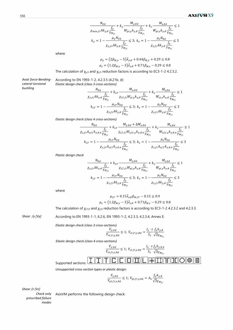
556

𝑁𝐸𝑑

𝜒𝑚𝑖𝑛,𝑓𝑖𝐴𝑘𝑦,𝜃𝑓𝑦𝛾𝑀𝑓𝑖

+ 𝑘𝑦𝑀𝑦,𝐸𝑑

𝑊𝑝𝑙,𝑦𝑘𝑦,𝜃𝑓𝑦𝛾𝑀𝑓𝑖

+ 𝑘𝑧𝑀𝑧,𝐸𝑑

𝑊𝑝𝑙,𝑧𝑘𝑦,𝜃𝑓𝑦𝛾𝑀𝑓𝑖

≤ 1

𝑘𝑦 = 1 −𝜇𝑦𝑁𝐸𝑑

𝜒𝑦,𝑓𝑖𝐴𝑘𝑦,𝜃𝑓𝑦𝛾𝑀𝑓𝑖

≤ 3; 𝑘𝑧 = 1 −𝜇𝑧𝑁𝐸𝑑

𝜒𝑧,𝑓𝑖𝐴𝑘𝑦,𝜃𝑓𝑦𝛾𝑀𝑓𝑖

≤ 3

where

𝜇𝑦 = (2𝛽𝑀,𝑦 − 5)�̅�𝑦,𝜃 + 0.44𝛽𝑀,𝑦 + 0.29 ≤ 0.8

𝜇𝑧 = (1.2𝛽𝑀,𝑦 − 3)�̅�𝑧,𝜃 + 0.71𝛽𝑀,𝑧 − 0.29 ≤ 0.8

The calculation of χy,fi and χz,fi reduction factors is according to EC3-1-2 4.2.3.2.

Axial force-Bending-Lateral-torsional buckling

According to EN 1993-1-2, 4.2.3.5 (4.21b, d):

Elastic design check (class 3 cross-sections)

𝑁𝐸𝑑

𝜒𝑧,𝑓𝑖𝐴𝑘𝑦,𝜃𝑓𝑦𝛾𝑀𝑓𝑖

+ 𝑘𝐿𝑇𝑀𝑦,𝐸𝑑

𝜒𝐿𝑇,𝑓𝑖𝑊𝑒𝑙,𝑦𝑘𝑦,𝜃𝑓𝑦𝛾𝑀𝑓𝑖

+ 𝑘𝑧𝑀𝑧,𝐸𝑑

𝑊𝑒𝑙,𝑧𝑘𝑦,𝜃𝑓𝑦𝛾𝑀𝑓𝑖

≤ 1

𝑘𝐿𝑇 = 1 −𝜇𝐿𝑇𝑁𝐸𝑑

𝜒𝑧,𝑓𝑖𝐴𝑘𝑦,𝜃𝑓𝑦𝛾𝑀𝑓𝑖

≤ 3; 𝑘𝑧 = 1 −𝜇𝑧𝑁𝐸𝑑

𝜒𝑧,𝑓𝑖𝐴𝑘𝑦,𝜃𝑓𝑦𝛾𝑀𝑓𝑖

≤ 3

Elastic design check (class 4 cross-sections)

𝑁𝐸𝑑

𝜒𝑧,𝑓𝑖𝐴𝑒𝑓𝑓𝑘𝑦,𝜃,4𝑓𝑦𝛾𝑀𝑓𝑖

+ 𝑘𝐿𝑇𝑀𝑦,𝐸𝑑 + Δ𝑀𝑦,𝐸𝑑

𝜒𝐿𝑇,𝑓𝑖𝑊𝑒𝑓𝑓,𝑦𝑘𝑦,𝜃,4𝑓𝑦𝛾𝑀𝑓𝑖

+ 𝑘𝑧𝑀𝑧,𝐸𝑑

𝑊𝑒𝑓𝑓,𝑧𝑘𝑦,𝜃,4𝑓𝑦𝛾𝑀𝑓𝑖

≤ 1

𝑘𝐿𝑇 = 1 −𝜇𝐿𝑇𝑁𝐸𝑑

𝜒𝑧,𝑓𝑖𝐴𝑒𝑓𝑓𝑘𝑦,𝜃,4𝑓𝑦𝛾𝑀𝑓𝑖

≤ 3; 𝑘𝑧 = 1 −𝜇𝑧𝑁𝐸𝑑

𝜒𝑧,𝑓𝑖𝐴𝑒𝑓𝑓𝑘𝑦,𝜃,4𝑓𝑦𝛾𝑀𝑓𝑖

≤ 3

Plastic design check

𝑁𝐸𝑑

𝜒𝑧,𝑓𝑖𝐴𝑘𝑦,𝜃𝑓𝑦𝛾𝑀𝑓𝑖

+ 𝑘𝐿𝑇𝑀𝑦,𝐸𝑑

𝜒𝐿𝑇,𝑓𝑖𝑊𝑝𝑙,𝑦𝑘𝑦,𝜃𝑓𝑦𝛾𝑀𝑓𝑖

+ 𝑘𝑧𝑀𝑧,𝐸𝑑

𝑊𝑝𝑙,𝑧𝑘𝑦,𝜃𝑓𝑦𝛾𝑀𝑓𝑖

≤ 1

𝑘𝐿𝑇 = 1 −𝜇𝐿𝑇𝑁𝐸𝑑

𝜒𝑧,𝑓𝑖𝐴𝑘𝑦,𝜃𝑓𝑦𝛾𝑀𝑓𝑖

≤ 3; 𝑘𝑧 = 1 −𝜇𝑧𝑁𝐸𝑑

𝜒𝑧,𝑓𝑖𝐴𝑘𝑦,𝜃𝑓𝑦𝛾𝑀𝑓𝑖

≤ 3

where

𝜇𝐿𝑇 = 0.15�̅�𝑧,𝜃𝛽𝑀,𝐿𝑇 − 0.15 ≤ 0.9

𝜇𝑧 = (1.2𝛽𝑀,𝑦 − 3)�̅�𝑧,𝜃 + 0.71𝛽𝑀,𝑧 − 0.29 ≤ 0.8

The calculation of χLT,fi and χz,fi reduction factors is according to EC3-1-2 4.2.3.2 and 4.2.3.3.

Shear /y [Vy] According to EN 1993-1-1, 6.2.6, EN 1993-1-2, 4.2.3.3, 4.2.3.4, Annex E: Elastic design check (class 3 cross-sections)

𝑉𝑦,𝐸𝑑

𝑉𝑒𝑙,𝑓𝑖,𝑦,𝑅𝑑≤ 1; 𝑉𝑒𝑙,𝑓𝑖,𝑦,𝑅𝑑 =

𝐼𝑧 ∙ 𝑡

𝑆𝑧

𝑓𝑦𝑘𝑦,𝜃

√3𝛾𝑀𝑓𝑖

Elastic design check (class 4 cross-sections)

𝑉𝑦,𝐸𝑑

𝑉𝑒𝑙,𝑓𝑖,𝑦,𝑅𝑑≤ 1; 𝑉𝑒𝑙,𝑓𝑖,𝑦,𝑅𝑑 =

𝐼𝑧 ∙ 𝑡

𝑆𝑧

𝑓𝑦𝑘𝑦,𝜃,4

√3𝛾𝑀𝑓𝑖

Supported sections:

Unsupported cross-section types or plastic design:

𝑉𝑦,𝐸𝑑

𝑉𝑝𝑙,𝑓𝑖,𝑦,𝑅𝑑≤ 1; 𝑉𝑝𝑙,𝑓𝑖,𝑦,𝑅𝑑 = 𝐴𝑣

𝑓𝑦𝑘𝑦,𝜃

√3𝛾𝑀𝑓𝑖

Shear /z [Vz]

Check only prescribed failure

modes

AxisVM performs the following design check:

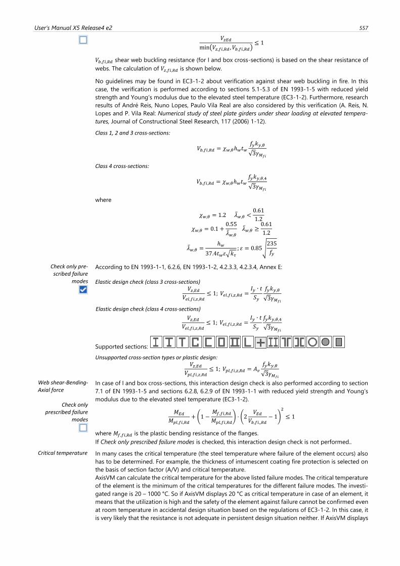
User’s Manual X5 Release4 e2 557

𝑉𝑧𝐸𝑑

min(𝑉𝑧,𝑓𝑖,𝑅𝑑 , 𝑉𝑏,𝑓𝑖,𝑅𝑑)≤ 1

𝑉𝑏,𝑓𝑖,𝑅𝑑 shear web buckling resistance (for I and box cross-sections) is based on the shear resistance of

webs. The calculation of 𝑉𝑧,𝑓𝑖,𝑅𝑑 is shown below.

No guidelines may be found in EC3-1-2 about verification against shear web buckling in fire. In this

case, the verification is performed according to sections 5.1-5.3 of EN 1993-1-5 with reduced yield

strength and Young’s modulus due to the elevated steel temperature (EC3-1-2). Furthermore, research

results of André Reis, Nuno Lopes, Paulo Vila Real are also considered by this verification (A. Reis, N.

Lopes and P. Vila Real: Numerical study of steel plate girders under shear loading at elevated tempera-

tures, Journal of Constructional Steel Research, 117 (2006) 1-12).

Class 1, 2 and 3 cross-sections:

𝑉𝑏,𝑓𝑖,𝑅𝑑 = 𝜒𝑤,𝜃ℎ𝑤𝑡𝑤𝑓𝑦𝑘𝑦,𝜃

√3𝛾𝑀𝑓𝑖

Class 4 cross-sections:

𝑉𝑏,𝑓𝑖,𝑅𝑑 = 𝜒𝑤,𝜃ℎ𝑤𝑡𝑤𝑓𝑦𝑘𝑦,𝜃,4

√3𝛾𝑀𝑓𝑖

where

𝜒𝑤,𝜃 = 1.2 �̅�𝑤,𝜃 <0.61

1.2

𝜒𝑤,𝜃 = 0.1 +0.55

�̅�𝑤,𝜃 �̅�𝑤,𝜃 ≥

0.61

1.2

�̅�𝑤,𝜃 =ℎ𝑤

37.4𝑡𝑤휀√𝑘𝜏; 휀 = 0.85√

235

𝑓𝑦

Check only pre-scribed failure

modes

According to EN 1993-1-1, 6.2.6, EN 1993-1-2, 4.2.3.3, 4.2.3.4, Annex E: Elastic design check (class 3 cross-sections)

𝑉𝑧,𝐸𝑑𝑉𝑒𝑙,𝑓𝑖,𝑧,𝑅𝑑

≤ 1; 𝑉𝑒𝑙,𝑓𝑖,𝑧,𝑅𝑑 =𝐼𝑦 ∙ 𝑡

𝑆𝑦

𝑓𝑦𝑘𝑦,𝜃

√3𝛾𝑀𝑓𝑖

Elastic design check (class 4 cross-sections)

𝑉𝑧,𝐸𝑑𝑉𝑒𝑙,𝑓𝑖,𝑧,𝑅𝑑

≤ 1; 𝑉𝑒𝑙,𝑓𝑖,𝑧,𝑅𝑑 =𝐼𝑦 ∙ 𝑡

𝑆𝑦

𝑓𝑦𝑘𝑦,𝜃,4

√3𝛾𝑀𝑓𝑖

Supported sections:

Unsupported cross-section types or plastic design: 𝑉𝑧,𝐸𝑑

𝑉𝑝𝑙,𝑓𝑖,𝑧,𝑅𝑑≤ 1; 𝑉𝑝𝑙,𝑓𝑖,𝑧,𝑅𝑑 = 𝐴𝑣

𝑓𝑦𝑘𝑦,𝜃

√3𝛾𝑀𝑓𝑖

Web shear-Bending-Axial force

Check only prescribed failure

modes

In case of I and box cross-sections, this interaction design check is also performed according to section

7.1 of EN 1993-1-5 and sections 6.2.8, 6.2.9 of EN 1993-1-1 with reduced yield strength and Young’s

modulus due to the elevated steel temperature (EC3-1-2).

𝑀𝐸𝑑

𝑀𝑝𝑙,𝑓𝑖,𝑅𝑑+ (1 −

𝑀𝑓,𝑓𝑖,𝑅𝑑

𝑀𝑝𝑙,𝑓𝑖,𝑅𝑑) ⋅ (2

𝑉𝐸𝑑𝑉𝑏,𝑓𝑖,,𝑅𝑑

− 1)

2

≤ 1

where 𝑀𝑓,𝑓𝑖,𝑅𝑑 is the plastic bending resistance of the flanges.

If Check only prescribed failure modes is checked, this interaction design check is not performed..

Critical temperature In many cases the critical temperature (the steel temperature where failure of the element occurs) also

has to be determined. For example, the thickness of intumescent coating fire protection is selected on

the basis of section factor (A/V) and critical temperature.

AxisVM can calculate the critical temperature for the above listed failure modes. The critical temperature

of the element is the minimum of the critical temperatures for the different failure modes. The investi-

gated range is 20 – 1000 °C. So if AxisVM displays 20 °C as critical temperature in case of an element, it

means that the utilization is high and the safety of the element against failure cannot be confirmed even

at room temperature in accidental design situation based on the regulations of EC3-1-2. In this case, it

is very likely that the resistance is not adequate in persistent design situation neither. If AxisVM displays

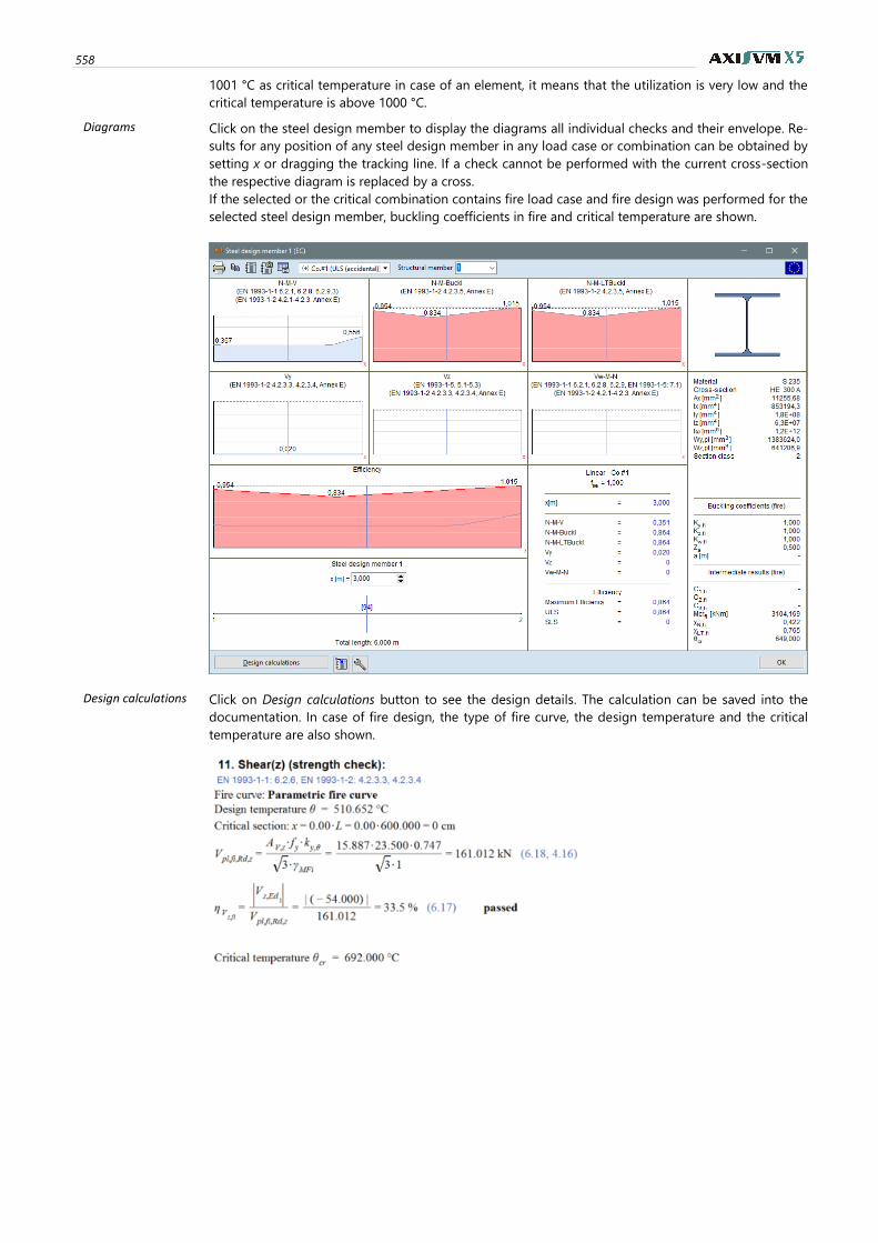
558

1001 °C as critical temperature in case of an element, it means that the utilization is very low and the

critical temperature is above 1000 °C.

Diagrams Click on the steel design member to display the diagrams all individual checks and their envelope. Re-

sults for any position of any steel design member in any load case or combination can be obtained by

setting x or dragging the tracking line. If a check cannot be performed with the current cross-section

the respective diagram is replaced by a cross.

If the selected or the critical combination contains fire load case and fire design was performed for the

selected steel design member, buckling coefficients in fire and critical temperature are shown.

Design calculations Click on Design calculations button to see the design details. The calculation can be saved into the

documentation. In case of fire design, the type of fire curve, the design temperature and the critical

temperature are also shown.

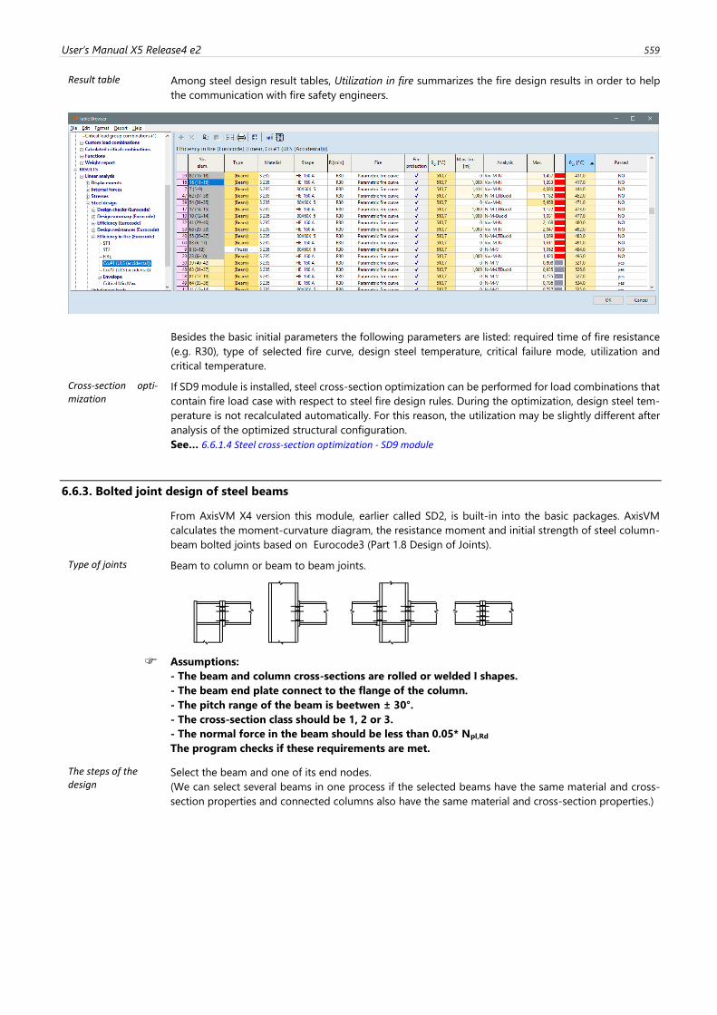
User’s Manual X5 Release4 e2 559

Result table Among steel design result tables, Utilization in fire summarizes the fire design results in order to help

the communication with fire safety engineers.

Besides the basic initial parameters the following parameters are listed: required time of fire resistance

(e.g. R30), type of selected fire curve, design steel temperature, critical failure mode, utilization and

critical temperature.

Cross-section opti-mization

If SD9 module is installed, steel cross-section optimization can be performed for load combinations that

contain fire load case with respect to steel fire design rules. During the optimization, design steel tem-

perature is not recalculated automatically. For this reason, the utilization may be slightly different after

analysis of the optimized structural configuration.

See… 6.6.1.4 Steel cross-section optimization - SD9 module

6.6.3. Bolted joint design of steel beams

From AxisVM X4 version this module, earlier called SD2, is built-in into the basic packages. AxisVM

calculates the moment-curvature diagram, the resistance moment and initial strength of steel column-

beam bolted joints based on Eurocode3 (Part 1.8 Design of Joints).

Type of joints Beam to column or beam to beam joints.

Assumptions:

- The beam and column cross-sections are rolled or welded I shapes.

- The beam end plate connect to the flange of the column.

- The pitch range of the beam is beetwen ± 30°.

- The cross-section class should be 1, 2 or 3.

- The normal force in the beam should be less than 0.05* Npl,Rd

The program checks if these requirements are met.

The steps of the design

Select the beam and one of its end nodes.

(We can select several beams in one process if the selected beams have the same material and cross-

section properties and connected columns also have the same material and cross-section properties.)

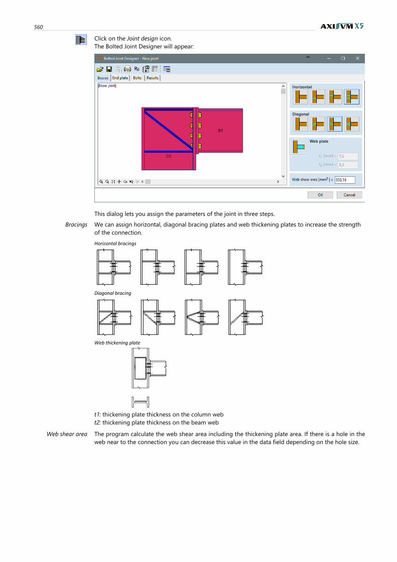
560

Click on the Joint design icon.

The Bolted Joint Designer will appear:

This dialog lets you assign the parameters of the joint in three steps.

Bracings We can assign horizontal, diagonal bracing plates and web thickening plates to increase the strength

of the connection.

Horizontal bracings

Diagonal bracing

Web thickening plate

t1: thickening plate thickness on the column web

t2: thickening plate thickness on the beam web

Web shear area The program calculate the web shear area including the thickening plate area. If there is a hole in the

web near to the connection you can decrease this value in the data field depending on the hole size.

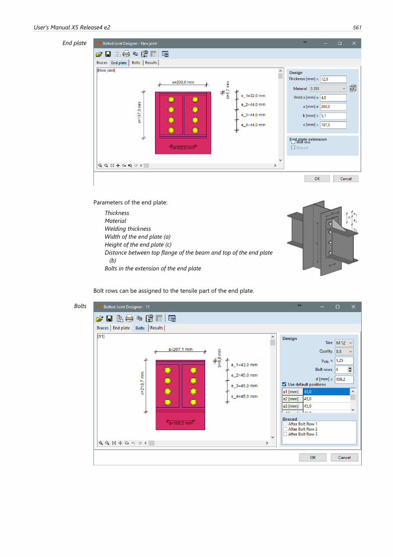
User’s Manual X5 Release4 e2 561

End plate

Parameters of the end plate:

Thickness

Material

Welding thickness

Width of the end plate (a)

Height of the end plate (c)

Distance between top flange of the beam and top of the end plate

(b)

Bolts in the extension of the end plate

Bolt rows can be assigned to the tensile part of the end plate.

Bolts

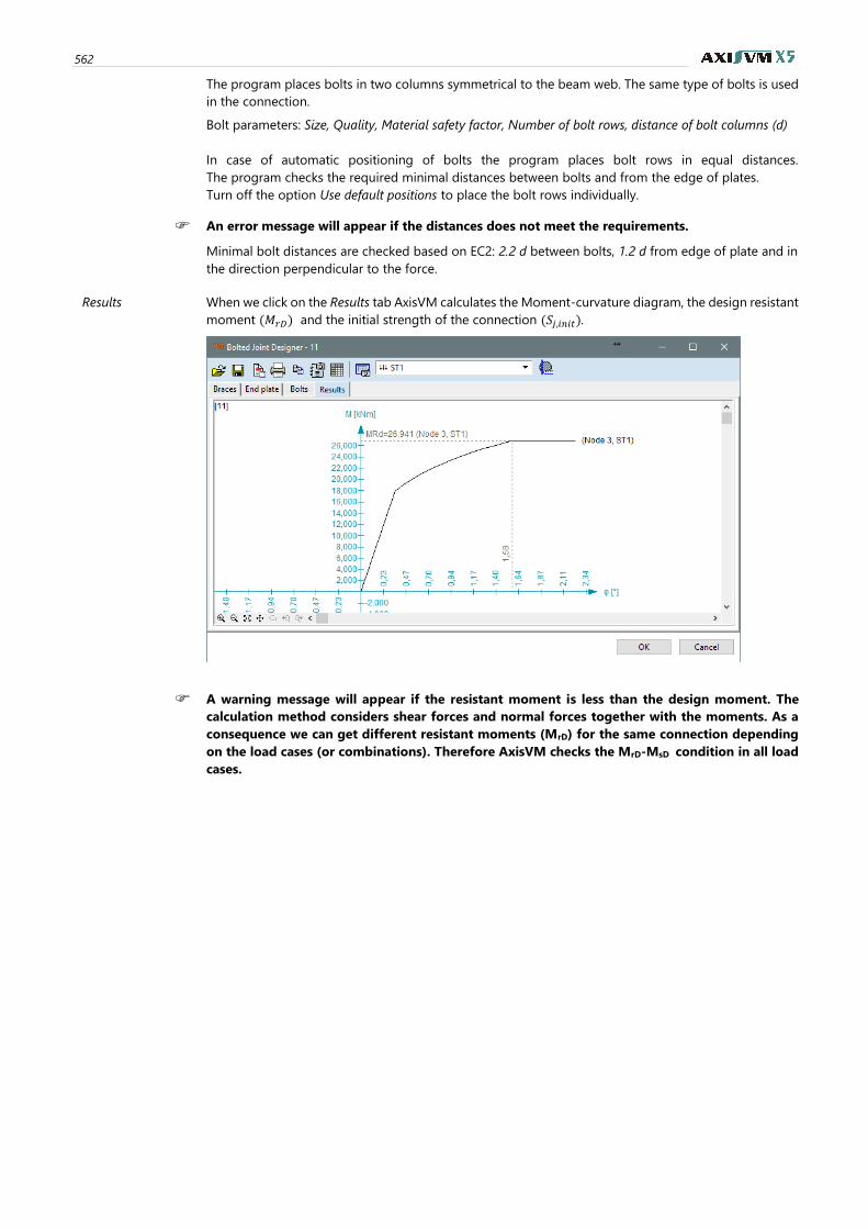
562

The program places bolts in two columns symmetrical to the beam web. The same type of bolts is used

in the connection.

Bolt parameters: Size, Quality, Material safety factor, Number of bolt rows, distance of bolt columns (d)

In case of automatic positioning of bolts the program places bolt rows in equal distances.

The program checks the required minimal distances between bolts and from the edge of plates.

Turn off the option Use default positions to place the bolt rows individually.

An error message will appear if the distances does not meet the requirements.

Minimal bolt distances are checked based on EC2: 2.2 d between bolts, 1.2 d from edge of plate and in

the direction perpendicular to the force.

Results When we click on the Results tab AxisVM calculates the Moment-curvature diagram, the design resistant

moment (𝑀𝑟𝐷) and the initial strength of the connection (𝑆𝑗,𝑖𝑛𝑖𝑡).

A warning message will appear if the resistant moment is less than the design moment. The

calculation method considers shear forces and normal forces together with the moments. As a

consequence we can get different resistant moments (MrD) for the same connection depending

on the load cases (or combinations). Therefore AxisVM checks the MrD-MsD condition in all load

cases.

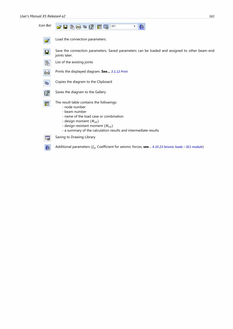
User’s Manual X5 Release4 e2 563

Icon Bar

Load the connection parameters.

Save the connection parameters. Saved parameters can be loaded and assigned to other beam-end

joints later.

List of the existing joints

Prints the displayed diagram. See... 3.1.12 Print

Copies the diagram to the Clipboard

Saves the diagram to the Gallery

The result table contains the followings:

- node number

- beam number

- name of the load case or combination

- design moment (𝑀𝑠𝐷)

- design resistant moment (𝑀𝑟𝐷)

- a summary of the calculation results and intermediate results

Saving to Drawing Library

Additional parameters (𝑓𝑠𝑒 Coefficient for seismic forces, see… 4.10.23 Seismic loads – SE1 module)

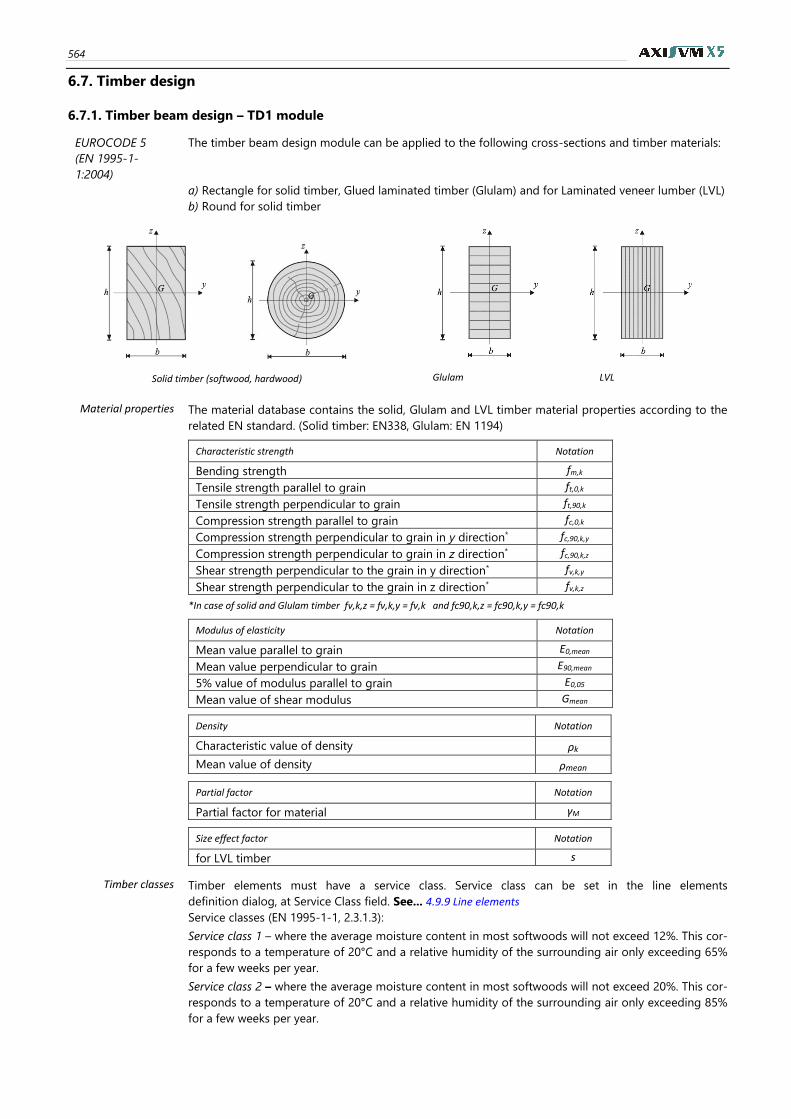
564

6.7. Timber design

6.7.1. Timber beam design – TD1 module

EUROCODE 5

(EN 1995-1-

1:2004)

The timber beam design module can be applied to the following cross-sections and timber materials:

a) Rectangle for solid timber, Glued laminated timber (Glulam) and for Laminated veneer lumber (LVL)

b) Round for solid timber

Solid timber (softwood, hardwood)

Glulam LVL

Material properties The material database contains the solid, Glulam and LVL timber material properties according to the

related EN standard. (Solid timber: EN338, Glulam: EN 1194)

Characteristic strength Notation

Bending strength fm,k

Tensile strength parallel to grain ft,0,k

Tensile strength perpendicular to grain ft,90,k

Compression strength parallel to grain fc,0,k

Compression strength perpendicular to grain in y direction* fc,90,k,y

Compression strength perpendicular to grain in z direction* fc,90,k,z

Shear strength perpendicular to the grain in y direction* fv,k,y

Shear strength perpendicular to the grain in z direction* fv,k,z

*In case of solid and Glulam timber fv,k,z = fv,k,y = fv,k and fc90,k,z = fc90,k,y = fc90,k

Modulus of elasticity Notation

Mean value parallel to grain E0,mean

Mean value perpendicular to grain E90,mean

5% value of modulus parallel to grain E0,05

Mean value of shear modulus Gmean

Density Notation

Characteristic value of density ρk

Mean value of density ρmean

Partial factor Notation

Partial factor for material γM

Size effect factor Notation

for LVL timber s

Timber classes Timber elements must have a service class. Service class can be set in the line elements

definition dialog, at Service Class field. See... 4.9.9 Line elements

Service classes (EN 1995-1-1, 2.3.1.3):

Service class 1 – where the average moisture content in most softwoods will not exceed 12%. This cor-

responds to a temperature of 20°C and a relative humidity of the surrounding air only exceeding 65%

for a few weeks per year.

Service class 2 – where the average moisture content in most softwoods will not exceed 20%. This cor-

responds to a temperature of 20°C and a relative humidity of the surrounding air only exceeding 85%

for a few weeks per year.

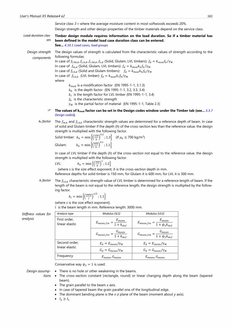
User’s Manual X5 Release4 e2 565

Service class 3 – where the average moisture content in most softwoods exceeds 20%.

Design strength and other design properties of the timber materials depend on the service class.

Load-duration clas-ses

Timber design module requires information on the load duration. So if a timber material has

been defined in the model load case duration class can be entered.

See... 4.10.1 Load cases, load groups

Design strength

components

The design values of strength is calculated from the characteristic values of strength according to the

following formulas:

In case of 𝑓𝑡,90,𝑑 , 𝑓𝑐,0,𝑑 , 𝑓𝑐,90,𝑑 , 𝑓𝑣,𝑑 (Solid, Glulam, LVL timbers): 𝑓𝑑 = 𝑘𝑚𝑜𝑑𝑓𝑘 𝛾𝑀⁄

In case of 𝑓𝑚,𝑑 (Solid, Glulam, LVL timbers): 𝑓𝑑 = 𝑘𝑚𝑜𝑑𝑘ℎ𝑓𝑘 𝛾𝑀⁄

In case of 𝑓𝑡,0,𝑑 (Solid and Glulam timbers): 𝑓𝑑 = 𝑘𝑚𝑜𝑑𝑘ℎ𝑓𝑘/𝛾𝑀

In case of 𝑓𝑡,0,𝑑 (LVL timber): 𝑓𝑑 = 𝑘𝑚𝑜𝑑𝑘𝑙𝑓𝑘/𝛾𝑀

where

𝑘𝑚𝑜𝑑 is a modification factor (EN 1995-1-1, 3.1.3)

𝑘ℎ is the depth factor (EN 1995-1-1, 3.2, 3.3, 3.4)

𝑘𝑙 is the length factor for LVL timber (EN 1995-1-1, 3.4)

𝑓𝑘 is the characteristic strength

𝛾𝑀 is the partial factor of material (EN 1995-1-1, Table 2.3)

The values of kmod factor can be set in the Design codes window under the Timber tab (see... 3.3.7 Design codes).

kh factor The 𝑓𝑚,𝑘 and 𝑓𝑡,0,𝑘 characteristic strength values are determined for a reference depth of beam. In case

of solid and Glulam timber if the depth (h) of the cross-section less than the reference value, the design

strength is multiplied with the following factor.

Solid timber: 𝑘ℎ = min {(150

ℎ)0.2; 1.3} (if 𝜌𝑘 ≤ 700 kg/m3)

Glulam: 𝑘ℎ = min {(600

ℎ)0.1; 1.1}

In case of LVL timber if the depth (h) of the cross-section not equal to the reference value, the design

strength is multiplied with the following factor.

LVL: 𝑘ℎ = min {(300

ℎ)𝑠; 1.2}

(where s is the size effect exponent, h is the cross-section depth in mm.

Reference depths for solid timber is 150 mm, for Glulam it is 600 mm, for LVL it is 300 mm.

kl factor The 𝑓𝑡,0,𝑘 characteristic strength value of LVL timber is determined for a reference length of beam. If the

length of the beam is not equal to the reference length, the design strength is multiplied by the follow-

ing factor.

𝑘𝑙 = min {(3000

𝑙)𝑠/2; 1.1}

(where s is the size effect exponent).

𝑙 is the beam length in mm. Reference length: 3000 mm.

Stiffness values for

analysis

Analysis type Modulus (SLS) Modulus (ULS)

First order,

linear elastic 𝐸𝑚𝑒𝑎𝑛,𝑓𝑖𝑛 =

𝐸𝑚𝑒𝑎𝑛1 + 𝑘𝑑𝑒𝑓

𝐸𝑚𝑒𝑎𝑛,𝑓𝑖𝑛 =𝐸𝑚𝑒𝑎𝑛

1 + 𝜓2𝑘𝑑𝑒𝑓

𝐺𝑚𝑒𝑎𝑛,𝑓𝑖𝑛 =𝐺𝑚𝑒𝑎𝑛1 + 𝑘𝑑𝑒𝑓

𝐺𝑚𝑒𝑎𝑛,𝑓𝑖𝑛 =𝐺𝑚𝑒𝑎𝑛

1 + 𝜓2𝑘𝑑𝑒𝑓

Second order,

linear elastic 𝐸𝑑 = 𝐸𝑚𝑒𝑎𝑛/𝛾𝑀 𝐸𝑑 = 𝐸𝑚𝑒𝑎𝑛/𝛾𝑀

𝐺𝑑 = 𝐺𝑚𝑒𝑎𝑛/𝛾𝑀 𝐺𝑑 = 𝐺𝑚𝑒𝑎𝑛/𝛾𝑀

Frequency 𝐸𝑚𝑒𝑎𝑛 , 𝐺𝑚𝑒𝑎𝑛 𝐸𝑚𝑒𝑎𝑛 , 𝐺𝑚𝑒𝑎𝑛

Conservative way 𝜓2 = 1 is used.

Design assump-

tions

• There is no hole or other weakening in the beams.

• The cross-section constant (rectangle, round) or linear changing depth along the beam (tapered

beam).

• The grain parallel to the beam x axis.

• In case of tapered beam the grain parallel one of the longitudinal edge.

• The dominant bending plane is the x-z plane of the beam (moment about y axis).

• 𝐼𝑦 ≥ 𝐼𝑧

566

• In case of Glulam the laminates are parallel to the y axis of the cross-section.

• in case of LVL the laminates are parallel to the z axis of the cross-section.

Checks

Normal force-Bending [N-M] (EN 1995-1-1, 6.2.3, 6.2.4)

Compression-Bending-Buckling (in plane) [N-M-Buckling] (EN 1995-1-1, 6.3.2)

Normal force-Bending-Lateral tors. buckling [N-M-LT buckling] (EN 1995-1-1, 6.3.3)

Shear /y -Torsion /x [Vy-Tx] (EN 1995-1-1, 6.1.7, 6.1.8)

Shear (y) - Shear(z) - Torsion (x) [Vy- Vz-Tx] (EN 1995-1-1, 6.1.7, 6.1.8)

Moment /y - Shear /z (tensile stress perpendicular to the grain) [My-V z] (EN 1995-1-1, 6.4.3)

Calculated parame-ters

𝜆𝑟𝑒𝑙,𝑦 Relative slenderness ratio (y) /in z-x plane of the beam/ []

𝜆𝑟𝑒𝑙,𝑧 Relative slenderness ratio (z) /in y-x plane of the beam/ []

𝑘𝑐,𝑦 Buckling (instability) factor (y) /in z-x plane of the beam/ [] (EN 1995-1-1, 6.3.2)

𝑘𝑐,𝑧 Buckling (instability) factor (z) /in x-y plane of the beam/ [] (EN 1995-1-1, 6.3.2)

𝑘𝑐𝑟𝑖𝑡 Lateral torsional buckling factor [] (EN 1995-1-1, 6.3.3)

𝑘ℎ Depth factor [] (EN 1995-1-1, 3.2, 3.3, 3.4)

𝑘𝑚𝑜𝑑 modification factor [] (EN 1995-1-1, 3.1.3)

𝜎𝑡,90,𝑑 (tensile stress perpendicular to the grain) [N/mm2] (EN 1995-1-1, 6.4.3)

AxisVM performs the following checks only. All the other checks specified in the design code like

supports, joints, etc. has to be completed by the user.

Normal force-Bend-ing

The design value of normal force can be tension or compression.

Tension and moment (EN 1995-1-1, 6.2.3)

𝜎𝑡,0,𝑑𝑓𝑡,0,𝑑

+𝜎𝑚,𝑦,𝑑

𝑓𝑚,𝑦,𝑑+ 𝑘𝑚

𝜎𝑚,𝑧,𝑑𝑓𝑚,𝑧,𝑑

≤ 1

𝜎𝑡,0,𝑑𝑓𝑡,0,𝑑

+ 𝑘𝑚𝜎𝑚,𝑦,𝑑

𝑓𝑚,𝑦,𝑑+𝜎𝑚,𝑧,𝑑𝑓𝑚,𝑧,𝑑

≤ 1

Compression and moment (EN 1995-1-1, 6.2.4)

(𝜎𝑐,0,𝑑𝑓𝑐,0,𝑑

)

2

+𝜎𝑚,𝑦,𝑑

𝑓𝑚,𝑦,𝑑+ 𝑘𝑚

𝜎𝑚,𝑧,𝑑𝑓𝑚,𝑧,𝑑

≤ 1

(𝜎𝑐,0,𝑑𝑓𝑐,0,𝑑

)

2

+ 𝑘𝑚𝜎𝑚,𝑦,𝑑

𝑓𝑚,𝑦,𝑑+𝜎𝑚,𝑧,𝑑𝑓𝑚,𝑧,𝑑

≤ 1

where 𝑘𝑚 = 0.7 in case of rectangle cross-section, 𝑘𝑚 = 1 in all other cases.

Compression-Mo-ment-Buckling

(EN 1995-1-1, 6.3.2) 𝜎𝑐,0,𝑑

𝑘𝑐,𝑦𝑓𝑐,0,𝑑+𝜎𝑚,𝑦,𝑑

𝑓𝑚,𝑦,𝑑+ 𝑘𝑚

𝜎𝑚,𝑧,𝑑𝑓𝑚,𝑧,𝑑

≤ 1

𝜎𝑐,0,𝑑𝑘𝑐,𝑧𝑓𝑐,0,𝑑

+ 𝑘𝑚𝜎𝑚,𝑦,𝑑

𝑓𝑚,𝑦,𝑑+𝜎𝑚,𝑧,𝑑𝑓𝑚,𝑧,𝑑

≤ 1

where,

𝑘𝑐,𝑦 Buckling (instability) factor (y) /in z-x plane of the beam/ (EN 1995-1-1, 6.3.2)

𝑘𝑐,𝑧 Buckling (instability) factor (z) /in x-y plane of the beam/ (EN 1995-1-1, 6.3.2)

In case of tension force the 𝑓𝑐,0,𝑑 is replaced with 𝑓𝑡,0,𝑑 and 𝑘𝑐,𝑦 = 𝑘𝑐,𝑧 = 1

User’s Manual X5 Release4 e2 567

Normal force-Bend-ing-

LT buckling

For lateral torsional buckling check the program assumptions that the beam is bending in z-x plane

(about y axis). If there is simultaneous 𝑀𝑧 moment on the beam and the compression stress from 𝑀𝑧

reach the 3% of the 𝑓𝑐,0,𝑑 a warning message appears.

Bending only (EN 1995-1-1, 6.3.3) 𝜎𝑚,𝑑

𝑘𝑐𝑟𝑖𝑡𝑓𝑚,𝑑≤ 1

Compression and moment (EN 1995-1-1, 6.3.3)

(𝜎𝑚,𝑑

𝑘𝑐𝑟𝑖𝑡𝑓𝑚,𝑑)

2

+𝜎𝑐𝑑

𝑘𝑐,𝑧𝑓𝑐,0,𝑑≤ 1

Tension and bending

In case of small tension and bending that lateral torsional buckling could be occur, however there is no

rule in EC5 for this case.

The following conservative check is used.

|𝜎𝑚𝑡,𝑑|

𝑘𝑐𝑟𝑖𝑡𝑓𝑚,𝑑≤ 1;

𝜎𝑚𝑡,𝑑 =𝑀𝑑

𝑊𝑦+𝑁𝑑𝐴< 0

where 𝑘𝑐𝑟𝑖𝑡 is the lateral buckling factor according to the following

𝜆𝑟𝑒𝑙,𝑚 ≤ 0.75 𝑘𝑐𝑟𝑖𝑡 = 1

0.75 < 𝜆𝑟𝑒𝑙,𝑚 ≤ 1.4 𝑘𝑐𝑟𝑖𝑡 = 1.56 − 0.75 ⋅ 𝜆𝑟𝑒𝑙,𝑚

1.4 < 𝜆𝑟𝑒𝑙,𝑚 𝑘𝑐𝑟𝑖𝑡 = 1/𝜆𝑟𝑒𝑙,𝑚2

Shear-Torsion There is no rule in EC5 for case of simultaneous shear force and torsional moment.

In this case the program uses the interaction formula according to DIN EN 1995-1-1/NA:2010.

Shear(y) , Shear(z) and torsion

max [𝜏𝑣,𝑦,𝑑

𝑓𝑣,𝑑;𝜏𝑣,𝑧,𝑑𝑓𝑣,𝑑

;𝜏𝑡𝑜𝑟,𝑑

𝑘𝑠ℎ𝑎𝑝𝑒𝑓𝑣,𝑑+ (

𝜏𝑣,𝑦,𝑑

𝑓𝑣,𝑑)

2

+ (𝜏𝑣,𝑧,𝑑𝑓𝑣,𝑑

)

2

] ≤ 1

where,

𝑘𝑠ℎ𝑎𝑝𝑒 is a factor for the shape of cross-section.

For round cross-section 𝑘𝑠ℎ𝑎𝑝𝑒 = 1.2,

for rectangular cross-section 𝑘𝑠ℎ𝑎𝑝𝑒 = min{1 + 0.15 ⋅ ℎ 𝑏⁄ ; 2.0}

Moment-Shear In case of curved beams the program checks the tensile stress perpendicular to the grain from My and

Vz forces. (EN 1995-1-1, 6.4.3.)

Moment(y)-Shear(z) 𝜏𝑑𝑓𝑣,𝑑

+𝜎𝑡,90,𝑑

𝑘𝑑𝑖𝑠𝑘𝑣𝑜𝑙𝑓𝑡,90,𝑑≤ 1

𝑘𝑑𝑖𝑠 is a factor which takes into account the effect of the stress distribution in the apex zone (𝑘𝑑𝑖𝑠 =

1.4 for curved beams)

𝑘𝑣𝑜𝑙 is a volume factor 𝑘𝑣𝑜𝑙 = [𝑉0 𝑉⁄ ]0.2

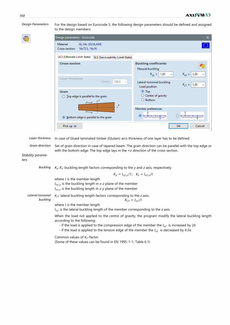
568

Design Parameters For the design based on Eurocode 5, the following design parameters should be defined and assigned

to the design members:

Layer thickness In case of Glued laminated timber (Glulam) arcs thickness of one layer has to be defined.

Grain direction Set of grain direction in case of tapered beam. The grain direction can be parallel with the top edge or

with the bottom edge. The top edge lays in the +z direction of the cross-section.

Stability parame-

ters

Buckling Ky, Kz: buckling length factors corresponding to the y and z axis, respectively.

𝐾𝑦 = 𝑙𝑒𝑓,𝑦 𝑙⁄ ; 𝐾𝑧 = 𝑙𝑒𝑓,𝑧/𝑙

where 𝑙 is the member length

𝑙𝑒𝑓,𝑦 is the buckling length in x-z plane of the member

𝑙𝑒𝑓,𝑧 is the buckling length in x-y plane of the member

Lateral torsional buckling

KLT: lateral buckling length factors corresponding to the z axis.

𝐾𝐿𝑇 = 𝑙𝑒𝑓/𝑙

where 𝑙 is the member length

𝑙𝑒𝑓 is the lateral buckling length of the member corresponding to the z axis.

When the load not applied to the centre of gravity, the program modify the lateral buckling length

according to the following:

- if the load is applied to the compression edge of the member the 𝑙𝑒𝑓 is increased by 2ℎ

- if the load is applied to the tension edge of the member the 𝑙𝑒𝑓 is decreased by 0.5ℎ

Common values of KLT factor.

(Some of these values can be found in EN 1995-1-1, Table 6.1)

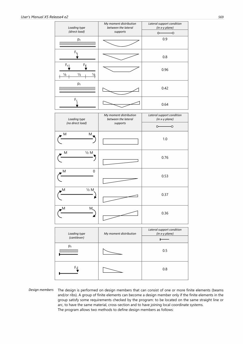
User’s Manual X5 Release4 e2 569

Loading type (direct load)

My moment distribution between the lateral

supports

Lateral support condition (in x-y plane)

pz 0.9

Fz

0.8

Fz Fz

¼ ½ ¼

0.96

pz

0.42

Fz

0.64

Loading type

(no direct load)

My moment distribution between the lateral

supports

Lateral support condition (in x-y plane)

M M

1.0

M ½ M

0.76

M 0

0.53

M ½ M

0.37

M M

0.36

Loading type (cantilever)

My moment distribution

Lateral support condition (in x-y plane)

pz

0.5

Fz

0.8

Design members The design is performed on design members that can consist of one or more finite elements (beams

and/or ribs). A group of finite elements can become a design member only if the finite elements in the

group satisfy some requirements checked by the program: to be located on the same straight line or

arc, to have the same material, cross-section and to have joining local coordinate systems.

The program allows two methods to define design members as follows:

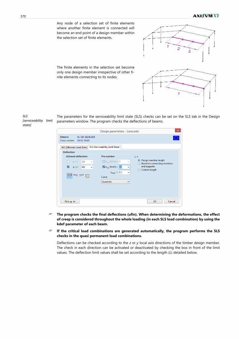
570

Any node of a selection set of finite elements

where another finite element is connected will

become an end point of a design member within

the selection set of finite elements.

The finite elements in the selection set become

only one design member irrespective of other fi-

nite elements connecting to its nodes.

SLS (serviceability limit state)

The parameters for the serviceability limit state (SLS) checks can be set on the SLS tab in the Design

parameters window. The program checks the deflections of beams.

The program checks the final deflections (ufin). When determining the deformations, the effect

of creep is considered throughout the whole loading (in each SLS load combination) by using the

kdef parameter of each beam.

If the critical load combinations are generated automatically, the program performs the SLS

checks in the quasi permanent load combinations.

Deflections can be checked according to the z or y local axis directions of the timber design member.

The check in each direction can be activated or deactivated by checking the box in front of the limit

values. The deflection limit values shall be set according to the length (L) detailed below.

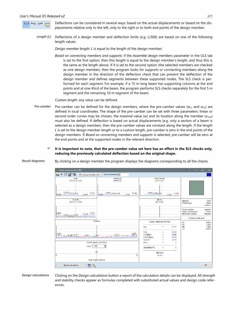
User’s Manual X5 Release4 e2 571

Deflections can be considered in several ways: based on the actual displacements or based on the dis-

placements relative only to the left, only to the right or to both end points of the design member.

Length (L)

Deflections of a design member and deflection limits (e.g. L/300) are based on one of the following

length values:

Design member length: L is equal to the length of the design member;

Based on connecting members and supports: if the Assemble design members parameter in the ULS tab

is set to the first option, then this length is equal to the design member’s length, and thus this is

the same as the length above. If it is set to the second option (the selected members are checked

as one design member), then the program looks for supports or connecting members along the

design member in the direction of the deflection check that can prevent the deflection of the

design member and defines segments between these supported nodes. The SLS check is per-

formed for each segment. For example, if a 15 m long beam has supporting columns at the end

points and at one-third of the beam, the program performs SLS checks separately for the first 5 m

segment and the remaining 10 m segment of the beam.

Custom length: any value can be defined.

Pre-camber

Pre-camber can be defined for the design members, where the pre-camber values (wcz and wcy) are

defined in local coordinates. The shape of the pre-camber can be set with three parameters: linear or

second-order curves may be chosen, the maximal value (w) and its location along the member (xmax)

must also be defined. If deflection is based on actual displacements (e.g. only a section of a beam is

selected as a design member), then the pre-camber values are constant along the length. If the length

L is set to the design member length or to a custom length, pre-camber is zero in the end points of the

design members. If Based on connecting members and supports is selected, pre-camber will be zero at

the end points and at the supported nodes in the relevant direction.

It is important to note, that the pre-camber value set here has an effect in the SLS checks only,

reducing the previously calculated deflection based on the original shape.

Result diagrams By clicking on a design member the program displays the diagrams corresponding to all the checks.

Design calculations

Clicking on the Design calculations button a report of the calculation details can be displayed. All strength

and stability checks appear as formulas completed with substituted actual values and design code refer-

ences.

572

Clicking on the Settings icon beside the Design calculations button allows setting the basic units for force

and length used in the design calculations. Important results also appear converted to standard AxisVM

units (see… 3.3.8 Units and Formats). For further details see… 6.6.1 Steel beam design according to Eurocode 3 – SD1 module

6.7.2. Timber beam fire design – TD8 module

Standards AxisVM performs timber fire design according to many national codes. In case of Eurocode National

Annexes that are not listed below, general rules of EN 1993-1-2 are considered.

Eurocode

EN 1995-1-2 Eurocode 5: Design of timber structures

Part 1-2: General - Structural fire design

EC

German

DIN EN 1995-1-2:2010-12 NA

EC

Hungarian

MSZ EN 1995-1-2:2013 NA

EC

Romanian

SR EN 1995-1-2:2004/Ac:2006

EC

Czech

CSN EN 1995-1-2/NA 2011

EC

Slovakian

STN EN 1995-1-2:2008/NA:2011

EC

British

BS EN 1995-1-2:2004 NA

EC

Dutch

NEN EN 1995-1-2/NB:2016

EC

Finnish

SFS-EN 1995-1-2:2004 NA

Fire design of timber structures according to EN 1995-1-2

Timber beam fire design (TD8 module) is based on methods of general timber beam design (TD1 module;

see… 6.7.1 Timber beam design – TD1 module), thus TD1 module is a prerequisite to use TD8.

EN 1995-1-2 (EC5-1-2) discusses fire design of timber structures. This section describes the differences

between the general design and fire design.

Timber beam fire design can be performed in AxisVM if

1) the selected load combination includes a fire load case (see… 4.10.1 Load cases, load groups)

2) if a fire effect has been assigned to any of the selected elements (see… 4.10.30 Fire effect on timber

elements – TD8 module) in that fire load case.

If different fire effects have been assigned to elements of a design member fire design cannot be per-

formed and an error message appears.

For selected elements without fire effect the general timber design will be performed. Timber fire design

parameters also has to be assigned to the elements (see below).

Member analysis EC5-1-2 discusses different methods: member analysis, analysis of a part of the structure and analysis of

the entire structure. Member analysis is the most widespread verification method due to its simplicity.

Analysis of a part or whole of the structure usually requires complex nonlinear numerical models and

nonlinear statical analysis.

Guiding principles of member analysis according to EC5-1-2:

• Design member internal forces can be calculated with linear static analysis;

• The boundary conditions at supports may be assumed to be constant with time. (EC5-1-2, 2.4.2

(4)).

TD8 module performs member analysis. It has to be checked whether the structure/structural part can be

verified with member analysis according to the guidelines of EC5-1-2.

Timber fire design parameters

Fire design based on EC5-1-2 requires fire design parameters defined and assigned to structural

members. This button is available only if 1) TD8 module is part of the configuration and 2) the current

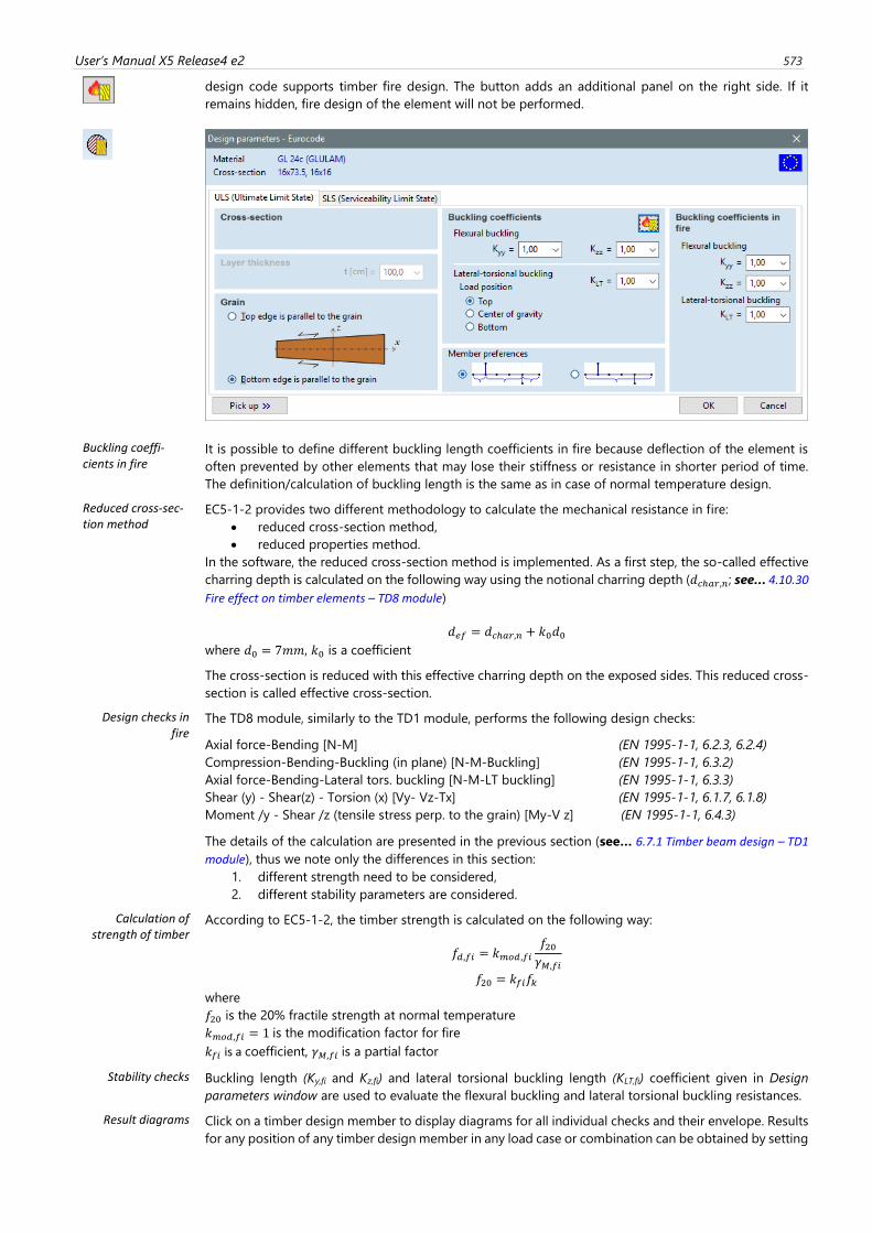
User’s Manual X5 Release4 e2 573

design code supports timber fire design. The button adds an additional panel on the right side. If it

remains hidden, fire design of the element will not be performed.

Buckling coeffi-cients in fire

It is possible to define different buckling length coefficients in fire because deflection of the element is

often prevented by other elements that may lose their stiffness or resistance in shorter period of time.

The definition/calculation of buckling length is the same as in case of normal temperature design.

Reduced cross-sec-tion method

EC5-1-2 provides two different methodology to calculate the mechanical resistance in fire:

• reduced cross-section method,

• reduced properties method.

In the software, the reduced cross-section method is implemented. As a first step, the so-called effective

charring depth is calculated on the following way using the notional charring depth (𝑑𝑐ℎ𝑎𝑟,𝑛; see… 4.10.30

Fire effect on timber elements – TD8 module)

𝑑𝑒𝑓 = 𝑑𝑐ℎ𝑎𝑟,𝑛 + 𝑘0𝑑0

where 𝑑0 = 7𝑚𝑚, 𝑘0 is a coefficient

The cross-section is reduced with this effective charring depth on the exposed sides. This reduced cross-

section is called effective cross-section.

Design checks in fire

The TD8 module, similarly to the TD1 module, performs the following design checks:

Axial force-Bending [N-M] (EN 1995-1-1, 6.2.3, 6.2.4)

Compression-Bending-Buckling (in plane) [N-M-Buckling] (EN 1995-1-1, 6.3.2)

Axial force-Bending-Lateral tors. buckling [N-M-LT buckling] (EN 1995-1-1, 6.3.3)

Shear (y) - Shear(z) - Torsion (x) [Vy- Vz-Tx] (EN 1995-1-1, 6.1.7, 6.1.8)

Moment /y - Shear /z (tensile stress perp. to the grain) [My-V z] (EN 1995-1-1, 6.4.3)

The details of the calculation are presented in the previous section (see… 6.7.1 Timber beam design – TD1

module), thus we note only the differences in this section:

1. different strength need to be considered,

2. different stability parameters are considered.

Calculation of strength of timber

According to EC5-1-2, the timber strength is calculated on the following way:

𝑓𝑑,𝑓𝑖 = 𝑘𝑚𝑜𝑑,𝑓𝑖𝑓20𝛾𝑀,𝑓𝑖

𝑓20 = 𝑘𝑓𝑖𝑓𝑘

where

𝑓20 is the 20% fractile strength at normal temperature

𝑘𝑚𝑜𝑑,𝑓𝑖 = 1 is the modification factor for fire

𝑘𝑓𝑖 is a coefficient, 𝛾𝑀,𝑓𝑖 is a partial factor

Stability checks Buckling length (Ky,fi and Kz,fi) and lateral torsional buckling length (KLT,fi) coefficient given in Design

parameters window are used to evaluate the flexural buckling and lateral torsional buckling resistances.

Result diagrams Click on a timber design member to display diagrams for all individual checks and their envelope. Results

for any position of any timber design member in any load case or combination can be obtained by setting

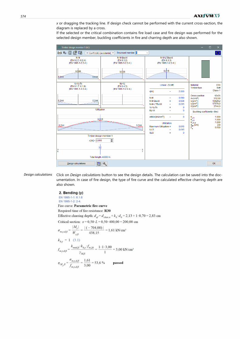
574

x or dragging the tracking line. If design check cannot be performed with the current cross-section, the

diagram is replaced by a cross.

If the selected or the critical combination contains fire load case and fire design was performed for the

selected design member, buckling coefficients in fire and charring depth are also shown.

Design calculations Click on Design calculations button to see the design details. The calculation can be saved into the doc-

umentation. In case of fire design, the type of fire curve and the calculated effective charring depth are

also shown.

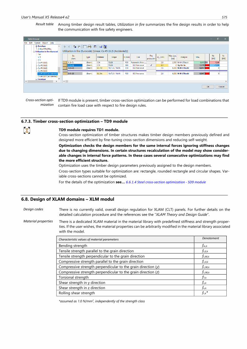
User’s Manual X5 Release4 e2 575

Result table Among timber design result tables, Utilization in fire summarizes the fire design results in order to help

the communication with fire safety engineers.

Cross-section opti-mization

If TD9 module is present, timber cross-section optimization can be performed for load combinations that

contain fire load case with respect to fire design rules.

6.7.3. Timber cross-section optimization – TD9 module

TD9 module requires TD1 module.

Cross-section optimization of timber structures makes timber design members previously defined and

designed more efficient by fine-tuning cross-section dimensions and reducing self-weight.

Optimization checks the design members for the same internal forces ignoring stiffness changes

due to changing dimensions. In certain structures recalculation of the model may show consider-

able changes in internal force patterns. In these cases several consecutive optimizations may find

the more efficient structure.

Optimization uses the timber design parameters previously assigned to the design members.

Cross-section types suitable for optimization are: rectangle, rounded rectangle and circular shapes. Var-

iable cross-sections cannot be optimized.

For the details of the optimization see… 6.6.1.4 Steel cross-section optimization - SD9 module

6.8. Design of XLAM domains – XLM modul

Design codes There is no currently valid, overall design regulation for XLAM (CLT) panels. For further details on the

detailed calculation procedure and the references see the “XLAM Theory and Design Guide”.

Material properties There is a dedicated XLAM material in the material library with predefined stiffness and strength proper-

ties. If the user wishes, the material properties can be arbitrarily modified in the material library associated

with the model.

Characteristic values of material parameters Denotement

Bending strength fm,k

Tensile strength parallel to the grain direction ft,0,k

Tensile strength perpendicular to the grain direction ft,90,k

Compressive strength parallel to the grain direction fc,0,k

Compressive strength perpendicular to the grain direction (y) fc,90,k

Compressive strength perpendicular to the grain direction (z) fc,90,k

Torsional strength fT,k

Shear strength in y direction fv,k

Shear strength in z direction fv,k

Rolling shear strength fr,k*

*assumed as 1.0 N/mm2, independently of the strength class

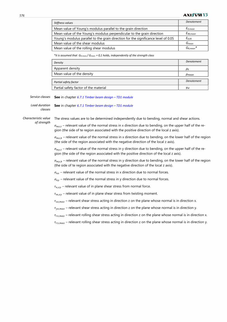
576

Stiffness values Denotement

Mean value of Young’s modulus parallel to the grain direction E0,mean

Mean value of the Young’s modulus perpendicular to the grain direction E90,mean

Young’s modulus parallel to the grain direction for the significance level of 0.05 E0,05

Mean value of the shear modulus Gmean

Mean value of the rolling shear modulus GR,mean*

*it is assumed that GR,mean / Gmean = 0,1 holds, independently of the strength class

Density Denotement

Apparent density ρk

Mean value of the density ρmean

Partial safety factor Denotement

Partial safety factor of the material γM

Service classes

See in chapter 6.7.1 Timber beam design – TD1 module

Load duration classes

See in chapter 6.7.1 Timber beam design – TD1 module

Characteristic value of strength

The stress values are to be determined independently due to bending, normal and shear actions.

𝜎𝑚𝑥,𝑡 – relevant value of the normal stress in x direction due to bending, on the upper half of the re-

gion (the side of te region associated with the positive direction of the local z axis).

𝜎𝑚𝑥,𝑏 – relevant value of the normal stress in x direction due to bending, on the lower half of the region

(the side of the region associated with the negative direction of the local z axis).

𝜎𝑚𝑦,𝑡 – relevant value of the normal stress in y direction due to bending, on the upper half of the re-

gion (the side of the region associated with the positive direction of the local z axis).

𝜎𝑚𝑦,𝑏 – relevant value of the normal stress in y direction due to bending, on the lower half of the region

(the side of te region associated with the negative direction of the local z axis).

𝜎𝑛𝑥 – relevant value of the normal stress in x direction due to normal forces.

𝜎𝑛𝑦 – relevant value of the normal stress in y direction due to normal forces.

𝜏𝑛,𝑥𝑦 – relevant value of in plane shear stress from normal force.

𝜏𝑚,𝑥𝑦 – relevant value of in plane shear stress from twisting moment.

𝜏𝑥𝑧,𝑚𝑎𝑥 – relevant shear stress acting in direction z on the plane whose normal is in direction x.

𝜏𝑦𝑧,𝑚𝑎𝑥 – relevant shear stress acting in direction z on the plane whose normal is in direction y.

𝜏𝑟𝑥,𝑚𝑎𝑥 – relevant rolling shear stress acting in direction z on the plane whose normal is in direction x.

𝜏𝑟𝑦,𝑚𝑎𝑥 – relevant rolling shear stress acting in direction z on the plane whose normal is in direction y.

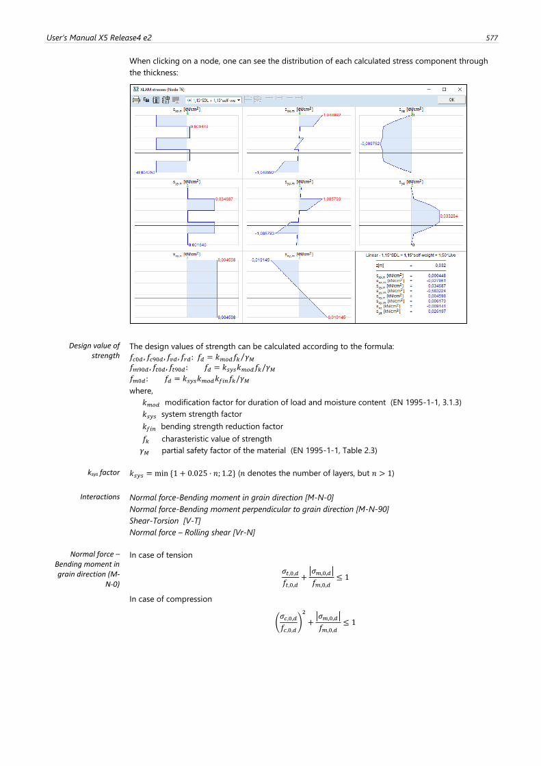
User’s Manual X5 Release4 e2 577

When clicking on a node, one can see the distribution of each calculated stress component through

the thickness:

Design value of strength

The design values of strength can be calculated according to the formula:

𝑓𝑐0𝑑 , 𝑓𝑐90𝑑 , 𝑓𝑣𝑑 , 𝑓𝑟𝑑: 𝑓𝑑 = 𝑘𝑚𝑜𝑑𝑓𝑘 𝛾𝑀⁄

𝑓𝑚90𝑑 , 𝑓𝑡0𝑑 , 𝑓𝑡90𝑑: 𝑓𝑑 = 𝑘𝑠𝑦𝑠𝑘𝑚𝑜𝑑𝑓𝑘/𝛾𝑀

𝑓𝑚0𝑑: 𝑓𝑑 = 𝑘𝑠𝑦𝑠𝑘𝑚𝑜𝑑𝑘𝑓𝑖𝑛𝑓𝑘/𝛾𝑀

where,

𝑘𝑚𝑜𝑑 modification factor for duration of load and moisture content (EN 1995-1-1, 3.1.3)

𝑘𝑠𝑦𝑠 system strength factor

𝑘𝑓𝑖𝑛 bending strength reduction factor

𝑓𝑘 charasteristic value of strength

𝛾𝑀 partial safety factor of the material (EN 1995-1-1, Table 2.3)

ksys factor 𝑘𝑠𝑦𝑠 = min {1 + 0.025 ⋅ 𝑛; 1.2} (𝑛 denotes the number of layers, but 𝑛 > 1)

Interactions Normal force-Bending moment in grain direction [M-N-0]

Normal force-Bending moment perpendicular to grain direction [M-N-90]

Shear-Torsion [V-T]

Normal force – Rolling shear [Vr-N]

Normal force – Bending moment in grain direction (M-

N-0)

In case of tension

𝜎𝑡,0,𝑑𝑓𝑡,0,𝑑

+|𝜎𝑚,0,𝑑|

𝑓𝑚,0,𝑑≤ 1

In case of compression

(𝜎𝑐,0,𝑑𝑓𝑐,0,𝑑

)

2

+|𝜎𝑚,0,𝑑|

𝑓𝑚,0,𝑑≤ 1

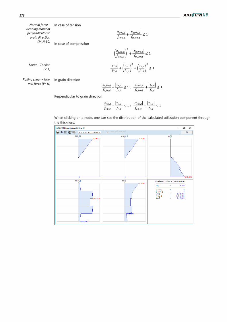
578

Normal force – Bending moment perpendicular to

grain direction (M-N-90)

In case of tension

𝜎𝑡,90,𝑑𝑓𝑡,90,𝑑

+|𝜎𝑚,90,𝑑|

𝑓𝑚,90,𝑑≤ 1

In case of compression

(𝜎𝑐,90,𝑑𝑓𝑐,90,𝑑

)

2

+|𝜎𝑚,90,𝑑|

𝑓𝑚,90,𝑑≤ 1

Shear – Torsion (V-T)

|𝜏𝑇,𝑑|

𝑓𝑇,𝑑+ (

𝜏𝑑𝑓𝑣,𝑑

)

2

+ (𝜏𝑟,𝑑𝑓𝑟,𝑑

)

2

≤ 1

Rolling shear – Nor-mal force (Vr-N)

In grain direction

𝜎𝑡,90,𝑑𝑓𝑡,90,𝑑

+|𝜏𝑟,𝑑|

𝑓𝑟,𝑑≤ 1 ;

|𝜎𝑐,90,𝑑|

𝑓𝑐,90,𝑑+|𝜏𝑟,𝑑|

𝑓𝑟,𝑑≤ 1

Perpendicular to grain direction

𝜎𝑡,0,𝑑𝑓𝑡,0,𝑑

+|𝜏𝑟,𝑑|

𝑓𝑟,𝑑≤ 1 ;

|𝜎𝑐,0,𝑑|

𝑓𝑐,0,𝑑+|𝜏𝑟,𝑑|

𝑓𝑟,𝑑≤ 1

When clicking on a node, one can see the distribution of the calculated utilization component through

the thickness:

User’s Manual X5 Release4 e2 579

6.9. Masonry wall design – MD1 module

MD1 module allows performing the typical analysis of unreinforced masonry walls and to specify their

design parameters required for the design check. An overall and complex verification process is imple-

mented for masonry walls subjected to mainly vertical and in-plane shear loading.

It provides a solution for the global analysis of one or multi-storey masonry walls with connecting joints.

Joints usually has considerable influence on the load-bearing capacity of the walls.

The verification is available for Eurocode, NTC and SIA standards.

6.9.1. Complex analysis of unreinforced masonry walls

General principles The following types of analysis are available in the module:

A) Stability analysis of walls subjected to mainly vertical loads. This check takes into account only

the eccentricities perpendicular to the plane of the wall, irrespective of the width of the wall

strip. Two-directional eccentricity cannot be analysed.

B) Complex stability check handling two-directional normal force eccentricity coupled with in-plane

shear check.

The A) and B) checks use different user-defined design sections (see… 6.9.1.3). Check type B is only

performed if shear check is requested in the Masonry wall strip parameters dialog (see… 6.9.1.2 Parameters of a masonry wall strip)

Only unreinforced masonry walls can be checked assuming that the wall has constant wall thickness along

a storey, only single leaf wall can be specified.

The masonry walls can be checked according to EN 1996-1-1 (chapter 6.1), NTC (chapter 4.5.6.2) and SIA

266 (chapter 4.3.1 and 4.4.) considering the following assumptions and application limits.

The above design codes assume that the walls are horizontally supported by the slabs, so standalone or

cantilevered walls cannot be analysed.

Various parameters can be added to the model (see Joint settings) which can result additional bending

moments on the structural model (multi-storey walls with various wall thickness, joint settings, the effect

of eccentric slab reaction force).

These effects are not negligible in the calculation of the load-bearing capacity of the elements, but accu-

rate modelling may require significantly complicated models in some cases. To facilitate the design check,

two approximative models are provided (see… Calculation of additional bending moments). In all cases, the

user should decide if these solutions are applicable.

The MD1 module works with virtual strips (see… 2.16.16 Virtual beams). Design parameters are assigned

to virtual strips and the check can only be performed on the integrated results of the strips.

Virtual strips can include multiple storeys, so the whole wall segment can be analysed as a complete

structural system, but storeys can have different design parameters.

Chapters 6.9.1.7…6.9.1.10 serves information about standard specific limitations.

6.9.1.1. Definition of masonry walls and their parameters

Design parameters

Click on the Design parameters icon, to specify the storeys of the masonry wall strip and check the wall

in the Masonry walls dialog.

Click on the icon or on the axis of a virtual strip to assign design parameters (see… 2.16.16 Virtual beams).

The icon is enabled only if there is at least one virtual strip in the model with static or dynamic results.

First the virtual strip must be selected (see… 2.16.1 Selection). Only one virtual strip can be selected, its

domains cannot have materials other than masonry, the strip must be continuous, the domains cannot

be tapered and must be vertical with a maximum deviation of 15°. If any of these criteria is not met a

warning message appears otherwise the Masonry walls dialog is displayed and the selected virtual strip

will be selected from the list of masonry virtual strips.

Masonry walls dialog opens automatically when clicking on a (valid) virtual strip in the model.

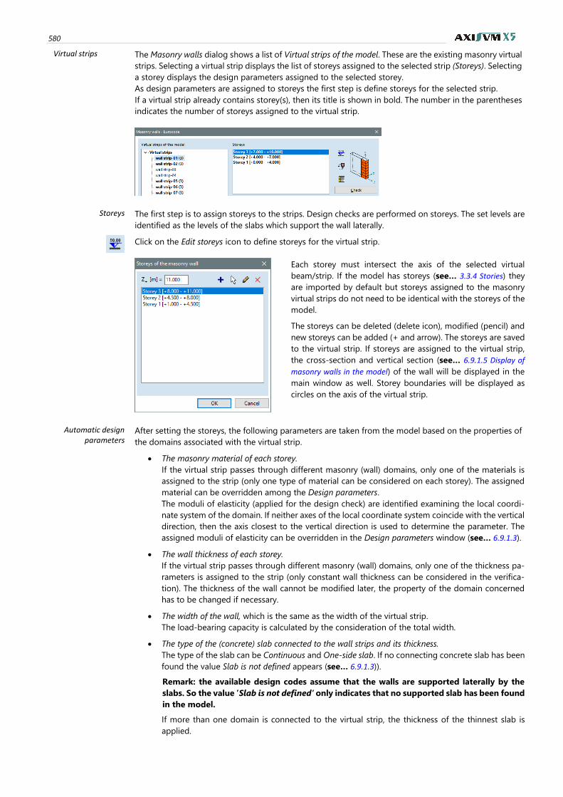
580

Virtual strips The Masonry walls dialog shows a list of Virtual strips of the model. These are the existing masonry virtual

strips. Selecting a virtual strip displays the list of storeys assigned to the selected strip (Storeys). Selecting

a storey displays the design parameters assigned to the selected storey.

As design parameters are assigned to storeys the first step is define storeys for the selected strip.

If a virtual strip already contains storey(s), then its title is shown in bold. The number in the parentheses

indicates the number of storeys assigned to the virtual strip.

Storeys The first step is to assign storeys to the strips. Design checks are performed on storeys. The set levels are

identified as the levels of the slabs which support the wall laterally.

Click on the Edit storeys icon to define storeys for the virtual strip.

Each storey must intersect the axis of the selected virtual

beam/strip. If the model has storeys (see… 3.3.4 Stories) they

are imported by default but storeys assigned to the masonry

virtual strips do not need to be identical with the storeys of the

model.

The storeys can be deleted (delete icon), modified (pencil) and

new storeys can be added (+ and arrow). The storeys are saved

to the virtual strip. If storeys are assigned to the virtual strip,

the cross-section and vertical section (see… 6.9.1.5 Display of

masonry walls in the model) of the wall will be displayed in the

main window as well. Storey boundaries will be displayed as

circles on the axis of the virtual strip.

Automatic design parameters

After setting the storeys, the following parameters are taken from the model based on the properties of

the domains associated with the virtual strip.

• The masonry material of each storey.

If the virtual strip passes through different masonry (wall) domains, only one of the materials is

assigned to the strip (only one type of material can be considered on each storey). The assigned

material can be overridden among the Design parameters.

The moduli of elasticity (applied for the design check) are identified examining the local coordi-

nate system of the domain. If neither axes of the local coordinate system coincide with the vertical

direction, then the axis closest to the vertical direction is used to determine the parameter. The

assigned moduli of elasticity can be overridden in the Design parameters window (see… 6.9.1.3).

• The wall thickness of each storey.

If the virtual strip passes through different masonry (wall) domains, only one of the thickness pa-

rameters is assigned to the strip (only constant wall thickness can be considered in the verifica-

tion). The thickness of the wall cannot be modified later, the property of the domain concerned

has to be changed if necessary.

• The width of the wall, which is the same as the width of the virtual strip.

The load-bearing capacity is calculated by the consideration of the total width.

• The type of the (concrete) slab connected to the wall strips and its thickness.

The type of the slab can be Continuous and One-side slab. If no connecting concrete slab has been

found the value Slab is not defined appears (see… 6.9.1.3)).

Remark: the available design codes assume that the walls are supported laterally by the

slabs. So the value ’Slab is not defined’ only indicates that no supported slab has been found

in the model.

If more than one domain is connected to the virtual strip, the thickness of the thinnest slab is

applied.

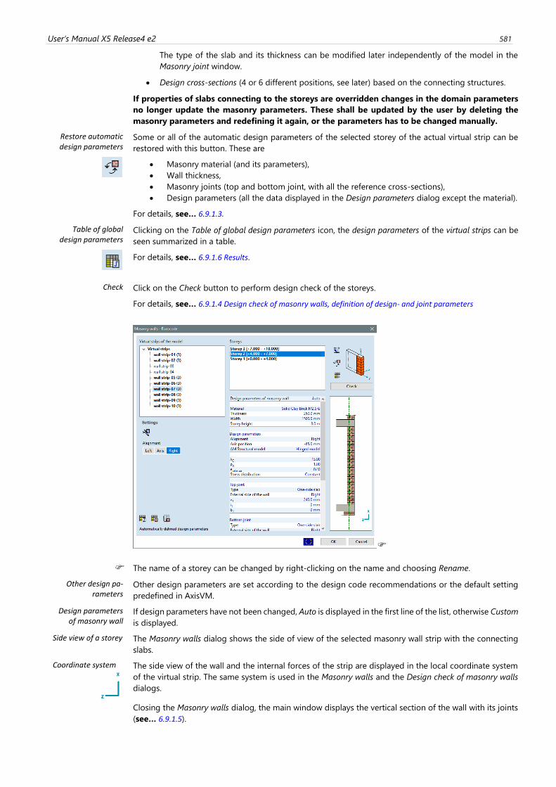
User’s Manual X5 Release4 e2 581

The type of the slab and its thickness can be modified later independently of the model in the

Masonry joint window.

• Design cross-sections (4 or 6 different positions, see later) based on the connecting structures.

If properties of slabs connecting to the storeys are overridden changes in the domain parameters

no longer update the masonry parameters. These shall be updated by the user by deleting the

masonry parameters and redefining it again, or the parameters has to be changed manually.

Restore automatic design parameters

Some or all of the automatic design parameters of the selected storey of the actual virtual strip can be

restored with this button. These are

• Masonry material (and its parameters),

• Wall thickness,

• Masonry joints (top and bottom joint, with all the reference cross-sections),

• Design parameters (all the data displayed in the Design parameters dialog except the material).

For details, see… 6.9.1.3.

Table of global design parameters

Clicking on the Table of global design parameters icon, the design parameters of the virtual strips can be

seen summarized in a table.

For details, see… 6.9.1.6 Results.

Check Click on the Check button to perform design check of the storeys.

For details, see… 6.9.1.4 Design check of masonry walls, definition of design- and joint parameters

The name of a storey can be changed by right-clicking on the name and choosing Rename.

Other design pa-rameters

Other design parameters are set according to the design code recommendations or the default setting

predefined in AxisVM.

Design parameters of masonry wall

If design parameters have not been changed, Auto is displayed in the first line of the list, otherwise Custom

is displayed.

Side view of a storey The Masonry walls dialog shows the side of view of the selected masonry wall strip with the connecting

slabs.

Coordinate system

The side view of the wall and the internal forces of the strip are displayed in the local coordinate system

of the virtual strip. The same system is used in the Masonry walls and the Design check of masonry walls

dialogs.

Closing the Masonry walls dialog, the main window displays the vertical section of the wall with its joints

(see… 6.9.1.5).

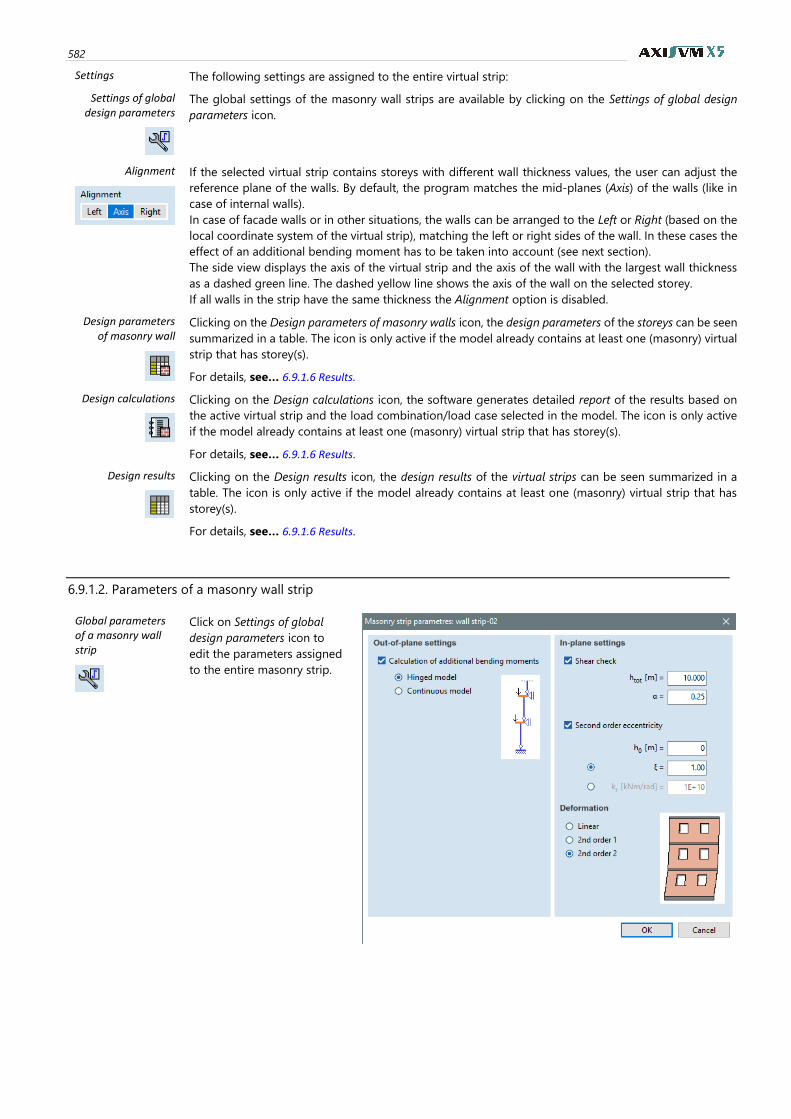
582

Settings The following settings are assigned to the entire virtual strip:

Settings of global design parameters

The global settings of the masonry wall strips are available by clicking on the Settings of global design

parameters icon.

Alignment

If the selected virtual strip contains storeys with different wall thickness values, the user can adjust the

reference plane of the walls. By default, the program matches the mid-planes (Axis) of the walls (like in

case of internal walls).

In case of facade walls or in other situations, the walls can be arranged to the Left or Right (based on the

local coordinate system of the virtual strip), matching the left or right sides of the wall. In these cases the

effect of an additional bending moment has to be taken into account (see next section).

The side view displays the axis of the virtual strip and the axis of the wall with the largest wall thickness

as a dashed green line. The dashed yellow line shows the axis of the wall on the selected storey.

If all walls in the strip have the same thickness the Alignment option is disabled.

Design parameters of masonry wall

Clicking on the Design parameters of masonry walls icon, the design parameters of the storeys can be seen

summarized in a table. The icon is only active if the model already contains at least one (masonry) virtual

strip that has storey(s).

For details, see… 6.9.1.6 Results.

Design calculations

Clicking on the Design calculations icon, the software generates detailed report of the results based on

the active virtual strip and the load combination/load case selected in the model. The icon is only active

if the model already contains at least one (masonry) virtual strip that has storey(s).

For details, see… 6.9.1.6 Results.

Design results

Clicking on the Design results icon, the design results of the virtual strips can be seen summarized in a

table. The icon is only active if the model already contains at least one (masonry) virtual strip that has

storey(s).

For details, see… 6.9.1.6 Results.

6.9.1.2. Parameters of a masonry wall strip

Global parameters of a masonry wall strip

Click on Settings of global

design parameters icon to

edit the parameters assigned

to the entire masonry strip.

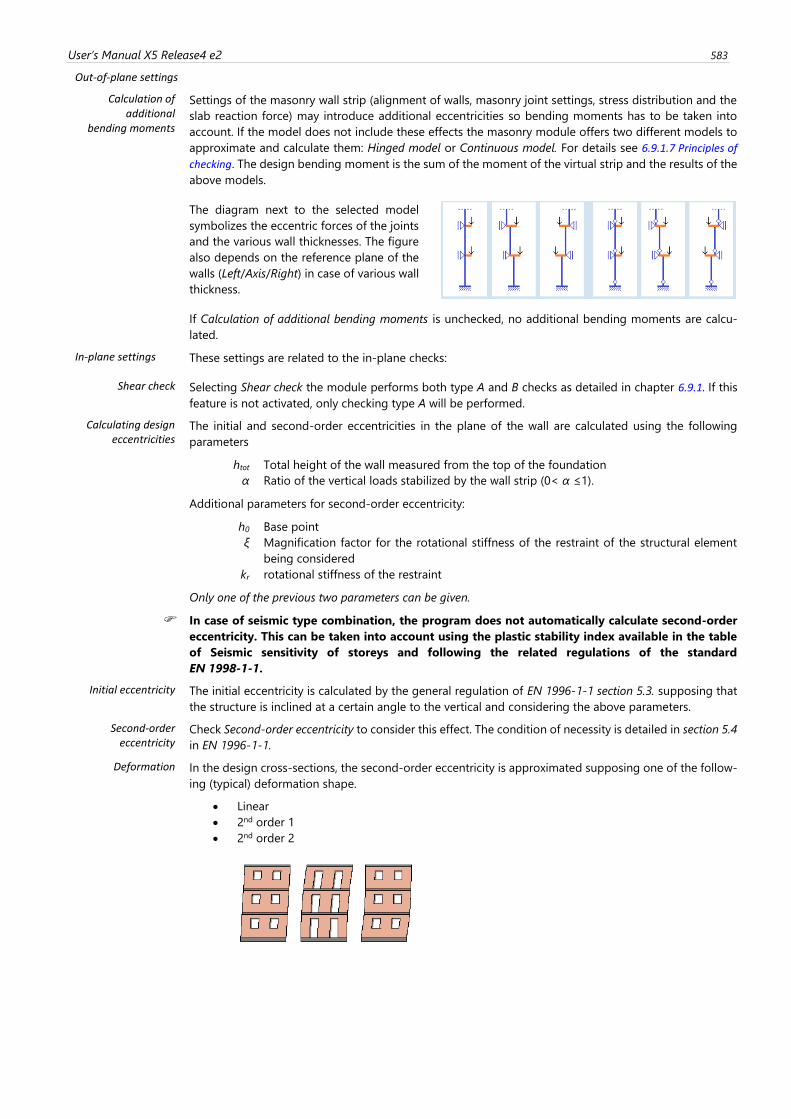
User’s Manual X5 Release4 e2 583

Out-of-plane settings

Calculation of additional

bending moments

Settings of the masonry wall strip (alignment of walls, masonry joint settings, stress distribution and the

slab reaction force) may introduce additional eccentricities so bending moments has to be taken into

account. If the model does not include these effects the masonry module offers two different models to

approximate and calculate them: Hinged model or Continuous model. For details see 6.9.1.7 Principles of

checking. The design bending moment is the sum of the moment of the virtual strip and the results of the

above models.

The diagram next to the selected model

symbolizes the eccentric forces of the joints

and the various wall thicknesses. The figure

also depends on the reference plane of the

walls (Left/Axis/Right) in case of various wall

thickness.

If Calculation of additional bending moments is unchecked, no additional bending moments are calcu-

lated.

In-plane settings

These settings are related to the in-plane checks:

Shear check Selecting Shear check the module performs both type A and B checks as detailed in chapter 6.9.1. If this

feature is not activated, only checking type A will be performed.

Calculating design eccentricities

The initial and second-order eccentricities in the plane of the wall are calculated using the following

parameters

htot Total height of the wall measured from the top of the foundation

α Ratio of the vertical loads stabilized by the wall strip (0< α ≤1).

Additional parameters for second-order eccentricity:

h0 Base point

ξ Magnification factor for the rotational stiffness of the restraint of the structural element

being considered

kr rotational stiffness of the restraint

Only one of the previous two parameters can be given.

In case of seismic type combination, the program does not automatically calculate second-order

eccentricity. This can be taken into account using the plastic stability index available in the table

of Seismic sensitivity of storeys and following the related regulations of the standard

EN 1998-1-1.

Initial eccentricity The initial eccentricity is calculated by the general regulation of EN 1996-1-1 section 5.3. supposing that

the structure is inclined at a certain angle to the vertical and considering the above parameters.

Second-order eccentricity

Check Second-order eccentricity to consider this effect. The condition of necessity is detailed in section 5.4

in EN 1996-1-1.

Deformation In the design cross-sections, the second-order eccentricity is approximated supposing one of the follow-

ing (typical) deformation shape.

• Linear

• 2nd order 1

• 2nd order 2

584

6.9.1.3. Check domain as a masonry wall

Check domain as a masonry wall

Check domain as a masonry wall is a simplified check of a single storey wall without existing virtual strips.

The virtual strip is automatically created during the process. A simple masonry region has to be selected

and a reference point for the virtual strip.

The created virtual strip is always 1 m wide, but this value can be changed any time editing the settings

of virtual strips (see… 2.16.16 Virtual beams). If the entered starting point is near to the edge of the domain,

the axis of the virtual strip is automatically shifted to ensure that the entire strip falls within the domain.

Finishing the selection, the Design check of masonry walls window opens, where the design parameters

and joints can be set and the results can be checked.

The masonry wall strip defined by the function of Check domain as a masonry wall can also be managed

by the Design parameters function like the other virtual strips.

Note: using this function the software assumes that calculation of additional bending moment (see later)

is not needed and the shear check is not marked. To change these settings click on the automatically

created virtual strip and make changes through the Masonry walls dialog.

6.9.1.4. Design check of masonry walls, definition of design- and joint parameters

Design check of masonry wall

Click on the Check button of the Masonry walls dialog to display the Design check of masonry wall dialog

where the design parameters of the wall storeys can be specified and design check is performed.

Set the first dropdown list on the top toolbar to the desired storey of the wall and set the load case or

combination.

The left side of the window displays the Vertical section or the Side view of the selected masonry storey.

(If shear check is not active, only the section of the wall can be seen.) Dimensions and joints are shown in

detail including the connecting slab, thermal insulation, etc. In the Side view of the wall, the connecting

wall domains are also visible in a pale colour, which is a help to specify the design sections (openings) for

shear design.

The coordinate system in the right/left corner (depending on the selected view) shows the coordinate

system of the virtual strip.

The green axis shows the axis of the virtual strip. If the wall thickness is not the same on all storeys, this

axis is identical with the axis of the thickest wall. The yellow axis is the axis of the storey. If wall thickness

is not the same on all storeys the yellow axis is not necessarily coincide with the green axis.

The material colour used is the same as the colour of masonry elements. Filling pattern cannot be

changed and it does not follow the type of masonry elements.

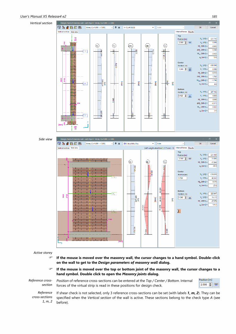
User’s Manual X5 Release4 e2 585

Vertical section

Side view

Active storey

If the mouse is moved over the masonry wall, the cursor changes to a hand symbol. Double-click

on the wall to get to the Design parameters of masonry wall dialog.

If the mouse is moved over the top or bottom joint of the masonry wall, the cursor changes to a

hand symbol. Double click to open the Masonry joints dialog.

Reference cross- section

Position of reference cross-sections can be entered at the Top / Center / Bottom. Internal

forces of the virtual strip is read in these positions for design check.

Reference cross-sections

1, m, 2

If shear check is not selected, only 3 reference cross-sections can be set (with labels 1, m, 2). They can be

specified when the Vertical section of the wall is active. These sections belong to the check type A (see

before).

586

Thick, blue lines show the positions of reference cross-sections. These lines can be dragged with the

mouse between the limits (black dashed lines).

The position of reference cross-sections is automatically adjusted to the edge of concrete slabs at the

top and the bottom if concrete slabs are present according to the joint settings. Click on the small button

right to the edit field to restore the automatic position.

In case of SIA 266 standard, the position of the middle cross-section cannot be set.

Reference cross-sections

1v, mv, 2v (position of the

openings)

If shear check is activated three more reference cross-sections can be set in the Side view of the wall.

These are the positions where design check B) is performed (complex stability and shear check). The

effects of openings and connecting domains can be considered with these positions (shear design is

performed on the wall section between the lower and upper sections). These positions are independent

of sections 1, m, 2 and are shown in green with signs 1v, mv, 2v. Only the top and bottom positions can

be set, the middle reference line is always halfway between them.

Setting the position of openings

Default positions of sections 1v, mv, 2v are determined based on the connecting domains. These can be

modified by dragging the reference lines or they can be set directly in the model after clicking on the

Position of opening icon. The icon is only available on the Internal forces panel (if Side view is selected).

Further information to the reference

cross-sections

Using the three edit boxes on Internal forces tab, the positions can be given by exact values. These values

are accepted only if they are between the limits (dashed lines).

The position of arrows above the thick blue lines represents the eccentricity of the compression force in

that specific cross-section. The colour of arrows is blue but if the resistance of the cross-section is not

adequate according to the design check the colour changes to red. If the resistance cannot be calculated

due to an error, the arrow is not shown.

If positions of reference cross-sections change both considered internal forces and design results

will change.

Internal forces In the Design check of masonry wall window, the following internal force diagrams are shown:

Vertical section

Nx Axial force (design axial force)

My Bending moment about local y axis

DMy Additional bending moment due to eccentric effects (calculated only if Calculation of additional

bending moments option is checked on Masonry walls window)

SMy Design bending moment (the sum of bending moment of the virtual strip and additional bending

moment)

Vz Shear force of the virtual strip perpendicular to the wall plane

Side view

Nx Axial force (design axial force)

Mz Bending moment about local z axis

Vy Shear force of the virtual strip within the wall plane

Thin black lines indicate the position of reference cross-sections on the internal force diagrams.

Results panel The design results are summarized in a table on the Results tab. For further information see… 6.9.1.6 Results.

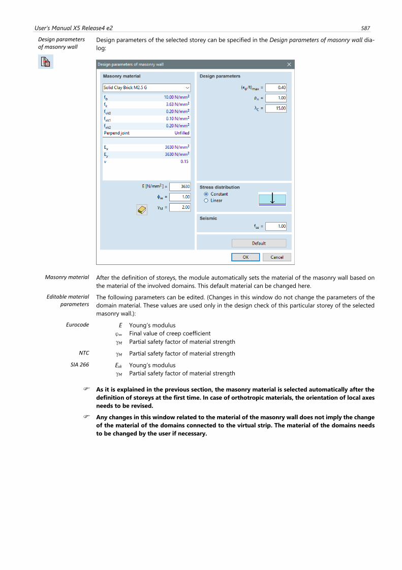
User’s Manual X5 Release4 e2 587

Design parameters of masonry wall

Design parameters of the selected storey can be specified in the Design parameters of masonry wall dia-

log:

Masonry material After the definition of storeys, the module automatically sets the material of the masonry wall based on

the material of the involved domains. This default material can be changed here.

Editable material parameters

The following parameters can be edited. (Changes in this window do not change the parameters of the

domain material. These values are used only in the design check of this particular storey of the selected

masonry wall.):

Eurocode E Young’s modulus

φ∞ Final value of creep coefficient

M Partial safety factor of material strength

NTC M Partial safety factor of material strength

SIA 266 Exk Young’s modulus

M Partial safety factor of material strength

As it is explained in the previous section, the masonry material is selected automatically after the

definition of storeys at the first time. In case of orthotropic materials, the orientation of local axes

needs to be revised.

Any changes in this window related to the material of the masonry wall does not imply the change

of the material of the domains connected to the virtual strip. The material of the domains needs

to be changed by the user if necessary.

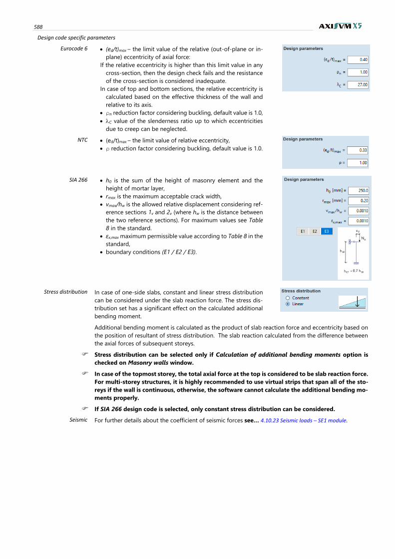
588

Design code specific parameters

Eurocode 6 • (ed/t)max – the limit value of the relative (out-of-plane or in-

plane) eccentricity of axial force:

If the relative eccentricity is higher than this limit value in any

cross-section, then the design check fails and the resistance

of the cross-section is considered inadequate.

In case of top and bottom sections, the relative eccentricity is

calculated based on the effective thickness of the wall and

relative to its axis.

• ρn reduction factor considering buckling, default value is 1.0,

• C value of the slenderness ratio up to which eccentricities

due to creep can be neglected.

NTC • (ed/t)max – the limit value of relative eccentricity,

• ρ reduction factor considering buckling, default value is 1.0.

SIA 266 • h0 is the sum of the height of masonry element and the

height of mortar layer,

• rmax is the maximum acceptable crack width,

• vmax/hw is the allowed relative displacement considering ref-

erence sections 1v and 2v (where hw is the distance between

the two reference sections). For maximum values see Table

8 in the standard.

• εx,max maximum permissible value according to Table 8 in the

standard,

• boundary conditions (E1 / E2 / E3).

Stress distribution In case of one-side slabs, constant and linear stress distribution

can be considered under the slab reaction force. The stress dis-

tribution set has a significant effect on the calculated additional

bending moment.

Additional bending moment is calculated as the product of slab reaction force and eccentricity based on

the position of resultant of stress distribution. The slab reaction calculated from the difference between

the axial forces of subsequent storeys.

Stress distribution can be selected only if Calculation of additional bending moments option is

checked on Masonry walls window.

In case of the topmost storey, the total axial force at the top is considered to be slab reaction force.

For multi-storey structures, it is highly recommended to use virtual strips that span all of the sto-

reys if the wall is continuous, otherwise, the software cannot calculate the additional bending mo-

ments properly.

If SIA 266 design code is selected, only constant stress distribution can be considered.

Seismic For further details about the coefficient of seismic forces see… 4.10.23 Seismic loads – SE1 module.

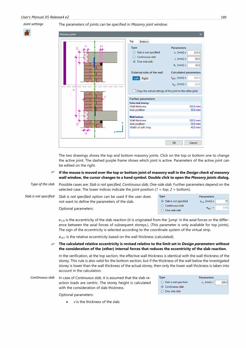
User’s Manual X5 Release4 e2 589

Joint settings

The parameters of joints can be specified in Masonry joint window:

The two drawings shows the top and bottom masonry joints. Click on the top or bottom one to change

the active joint. The dashed purple frame shows which joint is active. Parameters of the active joint can

be edited on the right.

If the mouse is moved over the top or bottom joint of masonry wall in the Design check of masonry

wall window, the cursor changes to a hand symbol. Double click to open the Masonry joints dialog.

Type of the slab

Possible cases are: Slab is not specified, Continuous slab, One-side slab. Further parameters depend on the

selected case. The lower indices indicate the joint position (1 = top; 2 = bottom).

Slab is not specified Slab is not specified option can be used if the user does

not want to define the parameters of the slab.

Optional parameters:

e1,N is the eccentricity of the slab reaction (it is originated from the ’jump’ in the axial forces or the differ-

ence between the axial forces of subsequent storeys.). (This parameter is only available for top joints).

The sign of the eccentricity is selected according to the coordinate system of the virtual strip.

erel,1 is the relative eccentricity based on the wall thickness (calculated).

The calculated relative eccentricity is revised relative to the limit set in Design parameters without

the consideration of the (other) internal forces that reduces the eccentricity of the slab reaction.

In the verification, at the top section, the effective wall thickness is identical with the wall thickness of the

storey. This rule is also valid for the bottom section, but if the thickness of the wall below the investigated

storey is lower than the wall thickness of the actual storey, then only the lower wall thickness is taken into

account in the calculation.

Continuous slab In case of Continuous slab, it is assumed that the slab re-

action loads are centric. The storey height is calculated

with the consideration of slab thickness.

Optional parameters:

• v is the thickness of the slab.

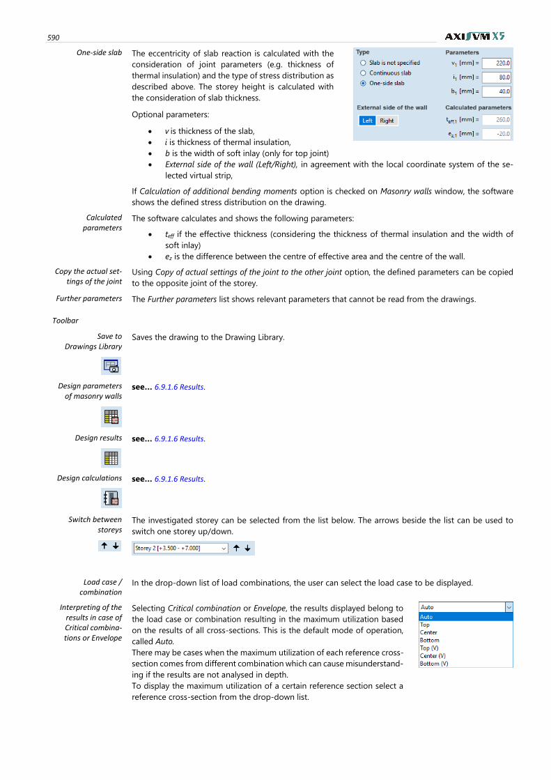
590

One-side slab The eccentricity of slab reaction is calculated with the

consideration of joint parameters (e.g. thickness of

thermal insulation) and the type of stress distribution as

described above. The storey height is calculated with

the consideration of slab thickness.

Optional parameters:

• v is thickness of the slab,

• i is thickness of thermal insulation,

• b is the width of soft inlay (only for top joint)

• External side of the wall (Left/Right), in agreement with the local coordinate system of the se-

lected virtual strip,

If Calculation of additional bending moments option is checked on Masonry walls window, the software

shows the defined stress distribution on the drawing.

Calculated parameters

The software calculates and shows the following parameters:

• teff if the effective thickness (considering the thickness of thermal insulation and the width of

soft inlay)

• ez is the difference between the centre of effective area and the centre of the wall.

Copy the actual set-tings of the joint

Using Copy of actual settings of the joint to the other joint option, the defined parameters can be copied

to the opposite joint of the storey.

Further parameters The Further parameters list shows relevant parameters that cannot be read from the drawings.

Toolbar

Save to Drawings Library

Saves the drawing to the Drawing Library.

Design parameters of masonry walls

see… 6.9.1.6 Results.

Design results

see… 6.9.1.6 Results.

Design calculations

see… 6.9.1.6 Results.

Switch between storeys

The investigated storey can be selected from the list below. The arrows beside the list can be used to

switch one storey up/down.

Load case / combination

In the drop-down list of load combinations, the user can select the load case to be displayed.

Interpreting of the results in case of Critical combina-tions or Envelope

Selecting Critical combination or Envelope, the results displayed belong to

the load case or combination resulting in the maximum utilization based

on the results of all cross-sections. This is the default mode of operation,

called Auto.

There may be cases when the maximum utilization of each reference cross-

section comes from different combination which can cause misunderstand-

ing if the results are not analysed in depth.

To display the maximum utilization of a certain reference section select a

reference cross-section from the drop-down list.

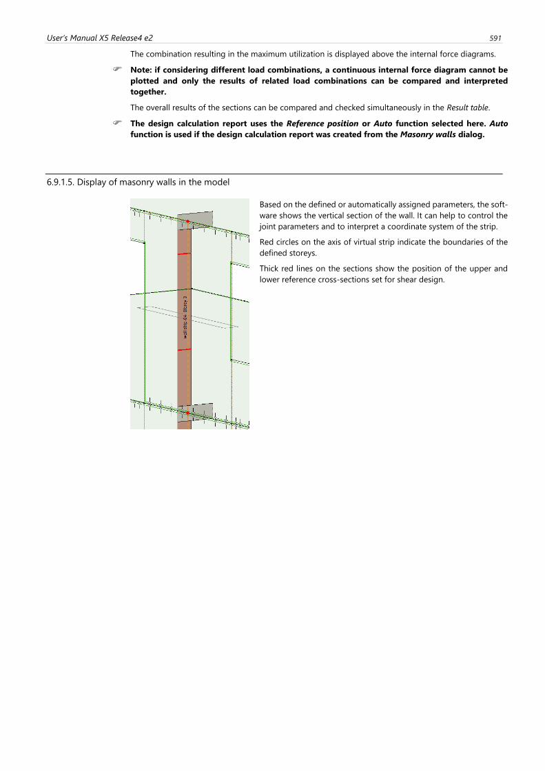
User’s Manual X5 Release4 e2 591

The combination resulting in the maximum utilization is displayed above the internal force diagrams.

Note: if considering different load combinations, a continuous internal force diagram cannot be

plotted and only the results of related load combinations can be compared and interpreted

together.

The overall results of the sections can be compared and checked simultaneously in the Result table.

The design calculation report uses the Reference position or Auto function selected here. Auto

function is used if the design calculation report was created from the Masonry walls dialog.

6.9.1.5. Display of masonry walls in the model

Based on the defined or automatically assigned parameters, the soft-

ware shows the vertical section of the wall. It can help to control the

joint parameters and to interpret a coordinate system of the strip.

Red circles on the axis of virtual strip indicate the boundaries of the

defined storeys.

Thick red lines on the sections show the position of the upper and

lower reference cross-sections set for shear design.

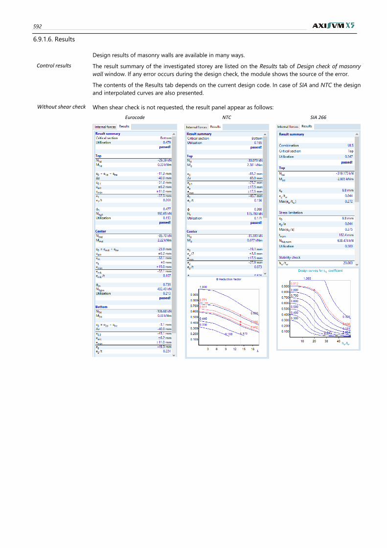
592

6.9.1.6. Results

Design results of masonry walls are available in many ways.

Control results The result summary of the investigated storey are listed on the Results tab of Design check of masonry

wall window. If any error occurs during the design check, the module shows the source of the error.

The contents of the Results tab depends on the current design code. In case of SIA and NTC the design

and interpolated curves are also presented.

Without shear check When shear check is not requested, the result panel appear as follows:

Eurocode NTC SIA 266

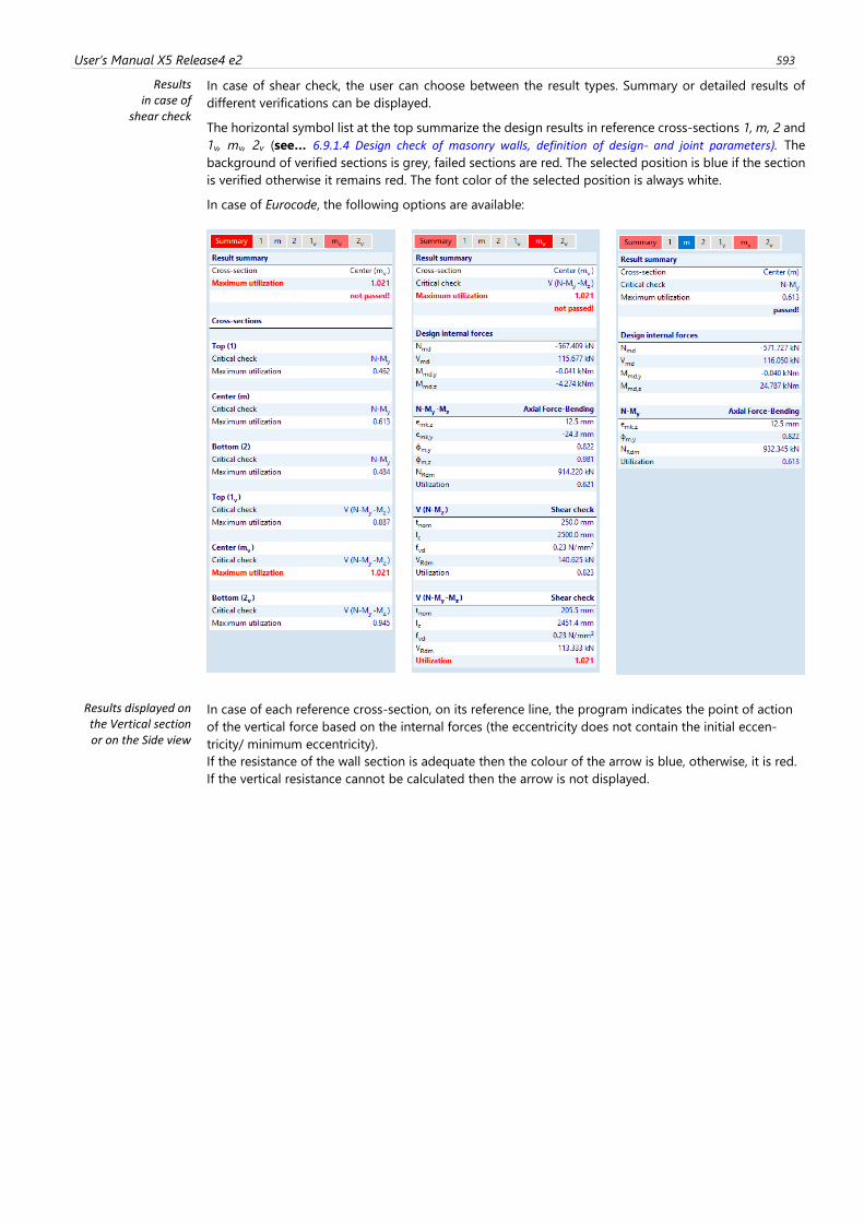
User’s Manual X5 Release4 e2 593

Results in case of

shear check

In case of shear check, the user can choose between the result types. Summary or detailed results of

different verifications can be displayed.

The horizontal symbol list at the top summarize the design results in reference cross-sections 1, m, 2 and

1v, mv, 2v (see… 6.9.1.4 Design check of masonry walls, definition of design- and joint parameters). The

background of verified sections is grey, failed sections are red. The selected position is blue if the section

is verified otherwise it remains red. The font color of the selected position is always white.

In case of Eurocode, the following options are available:

Results displayed on the Vertical section or on the Side view

In case of each reference cross-section, on its reference line, the program indicates the point of action

of the vertical force based on the internal forces (the eccentricity does not contain the initial eccen-

tricity/ minimum eccentricity).

If the resistance of the wall section is adequate then the colour of the arrow is blue, otherwise, it is red.

If the vertical resistance cannot be calculated then the arrow is not displayed.

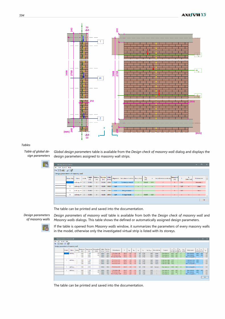
594

Tables

Table of global de-sign parameters

Global design parameters table is available from the Design check of masonry wall dialog and displays the

design parameters assigned to masonry wall strips.

The table can be printed and saved into the documentation.

Design parameters of masonry walls

Design parameters of masonry wall table is available from both the Design check of masonry wall and

Masonry walls dialogs. This table shows the defined or automatically assigned design parameters.

If the table is opened from Masonry walls window, it summarizes the parameters of every masonry walls

in the model, otherwise only the investigated virtual strip is listed with its storeys.

The table can be printed and saved into the documentation.

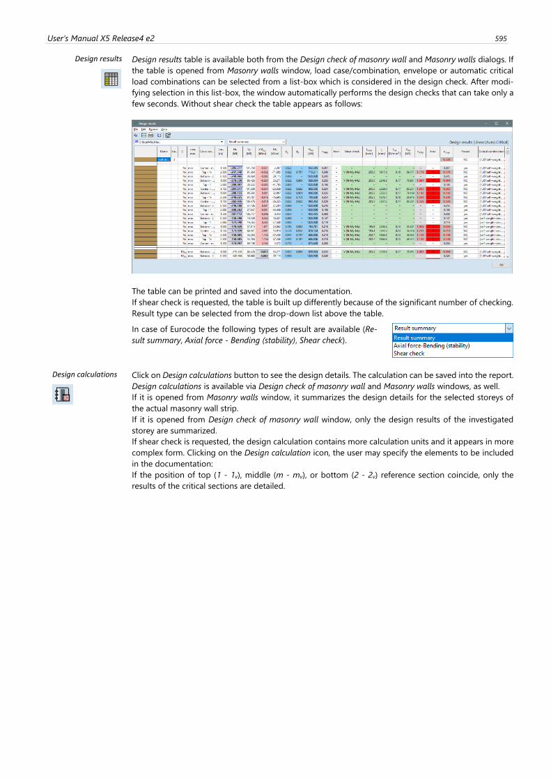
User’s Manual X5 Release4 e2 595

Design results

Design results table is available both from the Design check of masonry wall and Masonry walls dialogs. If

the table is opened from Masonry walls window, load case/combination, envelope or automatic critical

load combinations can be selected from a list-box which is considered in the design check. After modi-

fying selection in this list-box, the window automatically performs the design checks that can take only a

few seconds. Without shear check the table appears as follows:

The table can be printed and saved into the documentation.

If shear check is requested, the table is built up differently because of the significant number of checking.

Result type can be selected from the drop-down list above the table.

In case of Eurocode the following types of result are available (Re-

sult summary, Axial force - Bending (stability), Shear check).

Design calculations

Click on Design calculations button to see the design details. The calculation can be saved into the report.

Design calculations is available via Design check of masonry wall and Masonry walls windows, as well.

If it is opened from Masonry walls window, it summarizes the design details for the selected storeys of

the actual masonry wall strip.

If it is opened from Design check of masonry wall window, only the design results of the investigated

storey are summarized.

If shear check is requested, the design calculation contains more calculation units and it appears in more

complex form. Clicking on the Design calculation icon, the user may specify the elements to be included

in the documentation:

If the position of top (1 - 1v), middle (m - mv), or bottom (2 - 2v) reference section coincide, only the

results of the critical sections are detailed.

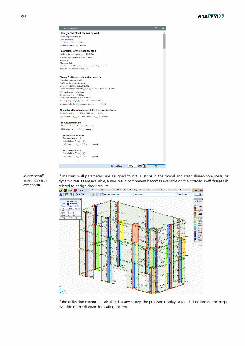
596

Masonry wall utilization result component

If masonry wall parameters are assigned to virtual strips in the model and static (linear/non-linear) or

dynamic results are available, a new result component becomes available on the Masonry wall design tab

related to design check results.

If the utilization cannot be calculated at any storey, the program displays a red dashed line on the nega-

tive side of the diagram indicating the error.

User’s Manual X5 Release4 e2 597

6.9.1.7. Principles of checking

Checking The software can perform two types of analysis with the following restrictions:

A. Design check of masonry walls subjected to mainly vertical loads.

In this checking only the out-of-plane eccentricities can be taken into account, shear check is not

included. The verification is based on the reference cross-sections signed 1, m, 2. (Only the ec-

centricities perpendicular to the plane of the wall are taken into account, irrespective of the width

of the wall strip, two-directional eccentricity cannot be analysed.)

B. Design check of masonry bracing walls, which contains a complex stability analysis consid-

ering out-of-plane and in-plane eccentricity of the axial force and an in-plane shear check

as well.

This verification is concerned to the reference cross-sections signed 1v, mv, 2v, but executed only

if shear check is requested.

• The tensile strength of masonry perpendicular to bed joints is zero.

• Only single-leaf walls can be examined with constant wall thickness along a storey.

• The additional bending moments due to the eccentric effects (alignment of the walls in case of

various wall thickness, masonry joint settings, stress distribution under the slab reaction) of the

settings can only be calculated by approximation models if the results of the model do not contain

them. The changes in the stiffness due to the eccentric effects cannot be taken into account.

Calculation of design internal forces

The internal forces of a virtual strip are calculated by the integration of the internal forces of the domain

considering the total width of the strip.

The design axial, shear force and in-plane bending moment are equal to the identical internal force of

the virtual strip (Nx, Vy and Mz).

The out-of-plane design bending moment is the sum of the moment of the virtual strip My and the ad-

ditional bending moment calculated by the approximate models.

The available approximate models are the followings:

Hinged model:

This is a simple beam model with bottom hinges.

The walls are supported laterally on each storey.

Continuous model:

The additional bending moment calculated using a

continuous beam model which involves all the walls.

The walls are supported laterally on each storey, the

bottom joint of the lower storey is supposed to be

fixed.

In these models, only the linear stiffness properties of walls are considered, and the stiffness sup-

posed to be constant for a storey. The various stiffness of connecting slabs and lateral supports

cannot be taken into account.

In SIA standard only the Hinged model is available.

Standard specifications

The specific verification rules of the available standards see… 6.9.1.8…6.9.1.10.

6.9.1.8. Design check according to Eurocode 6

Naming conventions During the design check 6 different reference cross-section are distinguished:

• the reference sections 1, m, 2 are identical to the design sections explained in chapter 6.1 in

Eurocode (top, middle and bottom sections);

• sections 1v, mv, 2v are the top, middle and bottom sections and used for shear check.

Stability check In case of reference sections signed with 1, m and 2, only the out-of-plane eccentricities of the axial force

are taken into account in the analysis. At sections 1v, mv, 2v both eccentricities (out-of-plane and in-plane)

are considered. The two cases are discussed together below.

General principles Considering the general principles of the standard (chapter 6.1.) the program executes the following

verifications:

598

The resistance of the wall section is adequate if the next criterion

𝑁𝐸𝑑 ≤ 𝑁𝑅𝑑

and the detailed rules are satisfied.

The following formula is applied to determine the vertical resistance of a wall:

N𝑅𝑑 = Φ𝑦 ∙ Φ𝑧 ∙ 𝑡 ∙ 𝑏 ∙ 𝑓𝑑

where y and z are the reduction factors related to y and z direction. (In case of reference cross-sections

1, m and 2, the capacity reduction factor z = 1 because the in-plane eccentricity is not taken into ac-

count).

At the top and bottom sections, the capacity reduction factor is calculated by the effective wall thickness

- teff (see masonry joint settings).

In case of shear check, if the top 1v or bottom 2v cross-section is adjusted to a corner of internal opening

and the distance between the reference cross-section (1v or 2v) and the top/bottom of the wall is greater

than the width of the wall, the section is considered as ‘middle’ section during the verification. Reference

cross-section mv is always considered as ‘middle’ section.

The design compressive strength is: 𝑓𝑑 = 𝑓𝑘/𝛾𝑀

If the cross-sectional area of a wall strip is less than 0,01 m2, the design compressive strength should be

lowered: f𝑑,𝑟𝑒𝑑 = 𝑓𝑑 ∙ (0,7 + 3𝐴), where A is the loaded horizontal gross cross-sectional area of the wall,

expressed in square metres.

In the module, only the cross-sectional area of the virtual strip can be considered, irrespective the total

width of the concerned domain.

Checking at the top or bottom of the wall

The design eccentricities, the reduction factors and the vertical resistance of the sections are calculated

as follows:

Out-of-plane eccentricity

The design eccentricity is calculated by the next equation:

𝑒𝑖,𝑧 =𝑀𝑖𝑑,𝑦

𝑁𝑖𝑑+ 𝑒ℎ𝑒,𝑧 + 𝑒𝑖𝑛𝑖𝑡,𝑧 ≥ 0,05 ∙ 𝑡

where ei,z is the eccentricity at the top (i=1) or the bottom (i=2) of the wall.

The program does not separate the eccentricities depending on the load type (vertical/horizontal) and

indicates the sum of them in the calculation as follows. The eccentricity based on the internal forces

calculated to the axis of the wall:

𝑒0,𝑧 =𝑀𝑖𝑑,𝑦

𝑁𝑖𝑑+ 𝑒ℎ𝑒,𝑧

In the verification, the program applies lowered wall thickness (teff), if not the whole section is working

(due to the masonry joint settings). In this case, the eccentricity is calculated to the axis of the effective

wall thickness:

𝑒0,𝑖,𝑧 = 𝑒𝑖,𝑧 − Δ𝑧

where z is the difference between the axis of the wall and effective wall thickness.

(If the wall thickness t is not reduced due to the joint settings, then 𝑡𝑒𝑓𝑓 = 𝑡 and 𝑒0,𝑖,𝑧 = 𝑒0,𝑧.)

Considering the rules of the standard and the markings above, the design eccentricity comes from the

following expression:

𝑒𝑖,𝑧 = 𝑒0,𝑖,𝑧 + 𝑒𝑖𝑛𝑖𝑡,𝑧 ≥ 0,05 ∙ 𝑡𝑒𝑓𝑓

The initial eccentricity is measured in the unfavourable direction relative to the axis of the effective thick-

ness, the minimum eccentricity is calculated by teff.

The i,y capacity reduction factor is calculated as follows:

Φ𝑖,𝑦 = 1 −2 ∙ 𝑒𝑖,𝑧𝑡𝑒𝑓𝑓

User’s Manual X5 Release4 e2 599

In-plane eccentricity

The design eccentricity is calculated by the next formula:

𝑒𝑖,𝑦 = 𝑒0,𝑖,𝑦 + 𝑒𝑖𝑛𝑖𝑡,𝑦 + 𝑒∆2,𝑦

where ei,y the in-plane eccentricity of the axial force in the y direction.

The initial eccentricity einit,y is calculated by following the rules of chapter 5.3 in EN 1996-1-1 5.3 consid-

ering initial incline of the building and the global design parameters of the masonry strip.

The second-order eccentricity e2,y is calculated using Annex B of EN 1996-1-1.

These additional eccentricities are taken into account in the unfavourable direction.

The capacity reduction factor i,z is calculated as follows:

Φ𝑖,𝑧 = 1 −2 ∙ 𝑒𝑖,𝑦

𝑏

where b is the total width of the wall (strip).

In case of seismic type combination, the program does not automatically calculate second-order eccen-

tricity. This can be taken into account using the plastic stability index available in the table of Seismic

sensitivity of storeys and following the related regulations of the standard EN 1998-1-1.

Vertical resistance

Considering the total wall width b, the vertical resistance is the following:

N𝑅𝑑,𝑖 = Φ𝑖,𝑦 ∙ Φ𝑖,𝑧 ∙ 𝑡𝑒𝑓𝑓 ∙ 𝑏 ∙ 𝑓𝑑

Checking in the middle of the wall height

The design eccentricities, the reduction factors and the vertical resistance of the middle sections are cal-

culated as follows:

Out-of-plane eccentricity

The design eccentricity is calculated by the next expression:

𝑒𝑚,𝑧 =𝑀𝑚𝑑,𝑧

𝑁𝑚𝑑+ 𝑒ℎ𝑚,𝑧 ± 𝑒𝑖𝑛𝑖𝑡,𝑧

The program does not separate the eccentricities depending on the load type (vertical/horizontal) and

indicates the sum of them in the calculation as follows. The eccentricity based on the internal forces

calculated to the axis of the wall:

𝑒0,𝑚,𝑧 =𝑀𝑚𝑑,𝑦

𝑁𝑚𝑑+ 𝑒ℎ𝑚,𝑧

and the eccentricity due to loads:

𝑒𝑚,𝑧 = 𝑒0,𝑚,𝑧 ± 𝑒𝑖𝑛𝑖𝑡,𝑧

finally, the design eccentricity comes from the following expression:

𝑒𝑚𝑘,𝑧 = 𝑒𝑚,𝑧 + 𝑒𝑘,𝑧 ≥ 0,05 ∙ 𝑡

where ek,z is the eccentricity due to creep, but it only has to be taken into account if the slenderness of

the wall exceeds the limit of C :

ℎ𝑒𝑓

𝑡𝑒𝑓> 𝜆𝑐

in this case

𝑒𝑘,𝑧 = 0,002 ∙ 𝜙∞ ∙ℎ𝑒𝑓

𝑡𝑒𝑓√𝑡 ∙ 𝑒𝑚,𝑧

C is specified in the National Annex (in the program the parameter C can be modified if necessary).

In NEN-EN 1996-1-1 (Dutch code) the following criterion is considered when calculating emk,z:

𝑒𝑚𝑘,𝑧 = 𝑚𝑎𝑥 {𝑒𝑚,𝑧 + 𝑒𝑘,𝑧; 0,05 ∙ 𝑡; ℎ𝑒𝑓

300; 10 mm}

The factor of m,y is calculated by Annex G (G1…G4) in EN 1996-1-1.

In-plane eccentricity

The design eccentricity is calculated by the next formula:

𝑒𝑚,𝑦 = 𝑒0,𝑚,𝑦 + 𝑒𝑖𝑛𝑖𝑡,𝑦 + 𝑒∆2,𝑦

where em,y the in-plane eccentricity of the axial force in the y direction.

The initial eccentricity einit,y is calculated by following the rules of chapter 5.3 in EN 1996-1-1 5.3 consid-

ering initial incline and the set global design parameters of the masonry strip.

The second-order eccentricity e2,y is calculated using Annex B of EN 1996-1-1.

600

These additional eccentricities are taken into account in the unfavourable direction.

The capacity reduction factor m,z is calculated as follows:

Φ𝑚,𝑧 = 1 −2 ∙ 𝑒𝑚,𝑦

𝑏

where b is the total width of the wall (strip).

In case of seismic type combination, the program does not automatically calculate second-order eccen-

tricity. This can be taken into account using the plastic stability index available in the table of Seismic

sensitivity of storeys and following the related regulations of the standard EN 1998-1-1.

Vertical resistance

Considering the total wall width b, the vertical resistance is the following:

N𝑅𝑑,𝑖 = Φ𝑚,𝑦 ∙ Φ𝑚,𝑧 ∙ 𝑡 ∙ 𝑏 ∙ 𝑓𝑑

Design and detailing rules

The following rules are checked:

• slenderness of the wall: ≤ 27.

• minimum wall thickness according to the National Annex. It is examined, only if a specific value

is given in the National Annex. In cases, when the minimum thickness depends on the type of

the wall, the program applies only the minimum of the given values.

• minimum area of wall: 0,04 m2.

• maximum relative eccentricity (it is not clearly regulated in EN 1996-1-1). In the program, the

limit can be set freely (see Design parameters). The default setting is: erel,max = 0,40 (only one

value can be set, and it is taken into account in all three sections).

Checking

- at the top (i=1) or bottom (i=2):

𝑒𝑟𝑒𝑙,𝑖 =𝑒𝑖𝑡𝑒𝑓𝑓

≤ 𝑒𝑟𝑒𝑙,𝑚𝑎𝑥

- in the middle of the wall height:

𝑒𝑟𝑒𝑙,𝑚 =𝑒𝑚𝑘𝑡≤ 𝑒𝑟𝑒𝑙,𝑚𝑎𝑥

The relative eccentricity is checked in both direction (y and z).

Shear check Shear capacity is calculated in sections 1v, mv, 2v at each storey considering the following principles.

In EN 1996-1-1 standard, the general formula (chapter 6.2, 6.13) for shear check does not provide clear

instructions to handle the out-of-plane eccentricity of the axial force. For this reason, two different shear

checks are executed (‘linear’ and ‘interaction’ check), of which the lower shear capacity is considered as

critical. In the design calculation, only the result of the critical check is documented.

Linear shear check

In case of Linear shear check, the capacity is calculated by the formula detailed in chapter 6.2 in EN-1996-

1-1, but the out-of-plane eccentricity of the axial force is neglected (supposed to be zero)

V𝑅𝑑,𝑖 = f𝑣𝑑 ∙ 𝑡 ∙ 𝑙𝑐

VRd,i is the shear resistant of the top (1v), middle (mv) or bottom (2v) reference cross-section (index i

indicates the position of the section 1, m, 2),

lc is the length of the compressed part of the wall assuming linear stress distribution.

fvd is the design value of the shear strength of masonry based on the average of the vertical stresses

over the compressed part of the wall.

Interaction shear check

In case of interaction shear check, eccentricities are considered in both directions and the length of the

compressed part of the section is calculated assuming constant stress distribution:

V𝑅𝑑,𝑖 = f𝑣𝑑 ∙ 𝑡𝑛𝑜𝑚 ∙ 𝑙𝑐

VRd,i is the shear resistant of top (1v), middle (mv) or bottom (2v) reference cross-section (index i indi-

cates the position of the section 1, m, 2),

tnom is the width of the compressed part of the wall considering the out-of-plane eccentricity,

lc is the length of the compressed zone calculated by in-plane eccentricity.

Based on the results of the stability test:

𝑙𝑐 = Φ𝑖,𝑧 ∙ 𝑏

𝑡𝑛𝑜𝑚 = Φ𝑖,𝑦 ∙ 𝑡

fvd is the design value of the shear strength of masonry based on the average of the vertical stresses over

the compressed part of the wall.

User’s Manual X5 Release4 e2 601

When calculating the resistance by the above methods, if the reference cross-section 1v or 2v are

considered as ‘top’ or ‘bottom’ section in the verification (the distance between the top/bottom

level and the position of the reference cross-section lower than the width of the wall), then lowered

wall thickness teff is taken into account in the calculation.

Notes to the result of the shear

check

Usually, there is only slight difference between the results of above methods but it depends on many

parameters. In case of the interaction check, the area of the compressed zone is lower, but the design

shear strength may be greater due to the greater average vertical stresses. However, the design shear

strength is limited by the maximum shear strength according to the National Annexes.

Typically, the interaction check gives the critical (lower) capacity.

Error messages The following error messages appears in the results:

Displayed error message: Interpretation of the error:

Not passed! The resistance of the wall/section is not adequate.

The force is out of the cross-section The point of action of the vertical force is out of the cross-section.

Relative eccentricity is too high. In the cross-section the relative eccentricity exceeds the limit (see

Design parameters).

The cross-section is in tension. The cross-section is in tension, the vertical resistance cannot be

calculated.

Axial compression force is zero. In the cross-section the axial compression force is negligibly

small, less than 0,1 kN.

Slenderness is too high. The slenderness of the wall exceeds the limit according to the

standard.

The wall thickness is insufficient. The wall thickness is less than the limit according to the National

Annex.

The wall section is insufficient. The cross-sectional area of the wall (cross-section of the virtual

strip) is less than the limit according to the standard.

6.9.1.9. Design check according to NTC

General principles Following the general principles of the standard (NTC 2018) a wall has to be checked at three sections

(top, mid-height of the wall, bottom) similar to Eurocode 6.

In the standard, it is supposed that the wall has hinges at the top and bottom. The user has to build such

a model with the right settings that follows the guidelines of the standard.

Signs During the design check 6 different reference cross-section are distinguished:

• the reference sections signed as 1, m, 2-es are identical to the design sections explained in

chapter 6.1 in Eurocode (top, middle and bottom sections);

• sections signed as 1v, mv, 2v are the top, middle and bottom sections and used for shear check.

Stability check In case of reference sections signed with 1, m and 2, only the out-of-plane eccentricities of the axial force

are taken into account in the analysis. At sections 1v, mv, 2v both eccentricities (out-of-plane and in-plane)

are considered. The two cases are discussed together below.

The resistance of the wall section is adequate if the following criterion

𝑁𝑑 ≤ 𝑁𝑟

and the detailed rules are satisfied.

The program uses the following formula to determine the vertical resistance of a wall:

N𝑟 = 𝑓𝑑,𝑟𝑖𝑑 ∙ 𝑡 ∙ 𝑏

and

f𝑑,𝑟𝑖𝑑 = Φ𝑦 ∙ Φ𝑧 ∙ 𝑓𝑑

where y and z are the reduction factors related to y and z direction. (In case of reference cross-sections

1, m and 2, the capacity reduction factor z=1 because the in-plane eccentricity is not taken into account).

602

At the top and bottom sections, the reduction factor is calculated by the effective wall thickness (see

masonry joint settings).

The design compressive strength is f𝑑 = 𝑓𝑘/𝛾𝑀

Checking at the top or bottom of the wall

The design eccentricities, the capacity reduction factors and the vertical resistance of the sections are

calculated as follows:

Out-of-plane eccentricity

In NTC, the design eccentricity is calculated by the following equation:

𝑒1,𝑧 = |𝑒𝑠,𝑧| + 𝑒𝑎,𝑧

where es,z is the eccentricity of vertical loads in the local z direction.

The program does not separate the eccentricities depending on the load type (vertical/horizontal) and

indicates the sum of them as e0,z.

In the verification, the program applies lowered wall thickness (teff), if not the whole section is working

(due to the masonry joint settings). In this case, the eccentricity is calculated to the axis of the effective

wall thickness:

𝑒0,1,𝑧 = 𝑒0,𝑧 − Δ𝑧

where z is the difference between the axes of the wall and effective wall thickness.

(If the wall thickness t is not reduced due to the joint settings, then 𝑡𝑒𝑓𝑓 = 𝑡 and 𝑒0,𝑖,𝑧 = 𝑒0,𝑧 .)

Finally, the design eccentricity comes from the following expression:

𝑒1,𝑧 = 𝑒0,1,𝑧 + 𝑒𝑎,𝑧

Where 𝑒𝑎,𝑧 = ℎ/200 (h is the storey height).

The initial eccentricity ea,z is measured in the unfavourable direction relative to the axis of the effective

thickness (teff).

Based on the initial parameters, the factor of i,z is calculated by linear interpolation using the table given

in the standard (see below).

The relative eccentricity: e𝑟𝑒𝑙,1,𝑧 = 𝑒1,𝑧/𝑡𝑒𝑓𝑓 , where teff is the effective wall thickness.

The eccentricity coefficient m is calculated by the following: 𝑚 = 6 ∙ 𝑒𝑟𝑒𝑙,1,𝑧,

and the slenderness: 𝜆 = ℎ0/𝑡, where ℎ0 = 𝜚 ∙ ℎ.

In-plane eccentricity

The in-plane eccentricity and the capacity reduction factor are calculated according to the principles of

EN 1996-1-1 standard (see details above).

Vertical resistance

Considering the total wall width b, the vertical resistance is the following:

N𝑟 = Φ1,𝑦 ∙ Φ1,𝑧 ∙ 𝑓𝑑 ∙ 𝑡𝑒𝑓𝑓 ∙ 𝑏

Checking in the middle of the wall height

The design eccentricities, the capacity reduction factors and the vertical resistance of the middle sections

are calculated as follows:

Out-of-plane eccentricity

The design eccentricity is calculated by the following expression:

𝑒2,𝑧 =𝑒1,𝑧2+ 𝑒𝑣,𝑧

where e2,z is the design eccentricity at the top in the local z direction, ev,z eccentricity is calculated from

horizontal loads.

The program does not separate the eccentricities depending on the load type (vertical/horizontal) and

indicates the sum of them as e0,z.

The design eccentricity comes from the following expression:

𝑒2,𝑧 = 𝑒0,𝑧 +𝑒𝑎,𝑧2≥ 𝑒𝑎,𝑧

Where 𝑒𝑎,𝑧 = ℎ/200

In the above formula, half of the ea,z is taken in the calculation considering the hinged model recom-

mended in the standard.

If the user uses hinges for the domains and also applies the model called Hinged model to determine the

additional bending moments, then this formula gives the same result as the standard. The applied models

have to be considered by the users.

User’s Manual X5 Release4 e2 603

Based on the initial parameters, the factor of 2,z is calculated by linear interpolation using the table given

in the standard (see below).

The relative eccentricity: e𝑟𝑒𝑙,2,𝑧 =𝑒2,𝑧

𝑡, where t is the total wall thickness.

The eccentricity coefficient m is calculated by the following: 𝑚 = 6 ∙ 𝑒𝑟𝑒𝑙,2,𝑧,

and the slenderness: 𝜆 =ℎ0

𝑡, where ℎ0 = 𝜚 ∙ ℎ.

In-plane eccentricity

The in-plane eccentricity and the capacity reduction factor are calculated according to the principles of

EN 1996-1-1 standard (see details above).

Vertical resistance

Considering the total wall width b, the vertical resistance is the following:

N𝑟 = Φ2,𝑦 ∙ Φ2,𝑧 ∙ 𝑓𝑑 ∙ 𝑡𝑒𝑓𝑓 ∙ 𝑏

Interpolation table for the determina-

tion of y factor

The following table (given in the standard, Tab. 4.5.III) is used to determine the factor of y.

Slenderness -

m = 6e/t

0 0,5 1,0 1,5 2,0

0 1,00 0,74 0,59 0,44 0,33

5 0,97 0,71 0,55 0,39 0,27

10 0,86 0,61 0,45 0,27 0,16

15 0,69 0,48 0,32 0,17 -

20 0,53 0,36 0,23 - -

Shear check Shear resistance is calculated according to the principles of EN 1996-1-1 standard (see details above).

Design shear strength is determined according to NTC standard.

Design and detailing rules

The following rules are checked:

• slenderness of the wall: ≤ 20.

• minimum wall thickness: t ≥ 150 mm (only this value is considered, the minimum value depend-

ing on the type of the unit is not checked).

• minimum area of wall: 0,04 m2 (applying the rule given Eurocode 6).

• maximum relative eccentricity (the default value is 0.33, but it can be modified).

Checking

- at the top or bottom:

𝑒𝑟𝑒𝑙,1 =𝑒1𝑡𝑒𝑓𝑓

≤ 0,33

- in the middle of the wall height:

𝑒𝑟𝑒𝑙,2 =𝑒2𝑡≤ 0,33

The relative eccentricity is checked in both direction (y and z).

Error messages The following error messages appears in the results:

Displayed error message: Interpretation of the error:

Not passed! The resistance of the wall/section is not adequate.

The force is out of the cross-sec-

tion.

The point of action of the vertical force is out of the cross-section.

Relative eccentricity is too high. In the cross-section the relative eccentricity exceeds the limit (see De-

sign parameters).

The cross-section is in tension. The cross-section is in tension, the vertical resistance cannot be calcu-

lated.

Axial compression force is zero. In the cross-section the axial compression force is negligibly small, less

than 0,1 kN.

604

Slenderness is too high. The slenderness of the wall exceeds the limit according to the standard.

The wall thickness is insuffi-

cient.

The wall thickness is less than the limit according to the National Annex.

The wall section is insufficient. The cross-sectional area of the wall (cross-section of the virtual strip) is

less, than the limit according to the standard.

cannot be calculated! cannot be evaluated based on the initial parameters of interpolation.

6.9.1.10. Design check according to SIA

General principles The principles of SIA 266: 2015 design code calculation method differ significantly from the procedure

described in Eurocode 6. Based on the standard, the wall has to be checked in ultimate and serviceability

limit state (ULS and SLS) as well.

The program performs ULS or SLS verification depending on the type of combination. If the type is not

known, both checking is performed, but only the result of the critical state is displayed.

The design code contains constraints on the static model, so the user should take care of the correct

choice of the static model. For the assumptions, see details below.

Calculating the additional bending moment only the Hinged model is available, and only constant stress

distribution can be applied.

The applied static model (E1, E2 and E3) has to be selected as the program cannot determine it from the

model.

Signs of design cross-sections

Four different design cross-sections are distinguished in the verification

• cross-sections with a sign of 1 (top) or 2 (bottom),

• cross-sections with a sign of 1v (top) or 2v (bottom) for shear check.

ULS verification In ULS verification, the wall is checked in two sections of the wall: at the top and the bottom of the wall.

Four different analysis are performed:

• stress limitation at cross-sections 1 and 1v,

• stability check considering the internal forces of the virtual strip at the reference position of

sections 1 and 2v,

• stress limitation at cross-sections 2 and 2v,

• shear check at the top cross-section (1v).

The verifications of cross-sections 1v and 2v are performed only if shear check is requested.

At design cross-sections 1 and 2 only the out-of-plane eccentricity of the axial force is taken into account,

but at sections 1v and 2v the in-plane eccentricity is also considered.

Stress limitation Firstly, the relative eccentricity is checked according to the standard: (ez/tw) is limited by the formula (6)

and Figure 4 (ez/tw ≤ 0,375). On the other hand, the program calculates the load-bearing capacity con-

sidering the compressed zone of the wall and it is compared to the design axial force.

The compressed width of the section considering out-of-plane eccentricity:

t𝑛𝑜𝑚 = 𝑡 − 2 ∙ 𝑒0,𝑧

In the verification, the program applies lowered wall thickness (teff), if not the whole section is working

(due to the masonry joint settings).

e0,z is the eccentricity is calculated to the axis of the effective wall thickness:

𝑁𝑅𝑑,𝑛𝑜𝑚 = 𝑙𝑐 ∙ 𝑡𝑛𝑜𝑚 ∙ 𝑓𝑥𝑑

User’s Manual X5 Release4 e2 605

where lc is equal to lw when checking cross-sections 1 and 2. In case of cross-sections 1v and 2v the

compressed length of the wall is (l=l2) lowered due to the in-plane bending moment:

𝑙2 = 𝑙𝑤 −2 ∙ 𝑀𝑧,𝑖,𝑑

𝑁𝑥𝑑

Stability check

In case of cross-section 1, the program follows the regulations of the standard (SIA 266:2015) described

in chapter 4.3.1.3 (11):

𝑁𝑥𝑑 ≤ 𝑘𝑁 ∙ 𝑙𝑤 ∙ 𝑡𝑤 ∙ 𝑓𝑥𝑑

In case of cross-section 2v, formula (17, in chapter 4.3.3.1) is used considering in-plane bending moment:

𝑁𝑥𝑑 ≤ 𝑘𝑁 ∙ 𝑙2 ∙ 𝑡𝑤 ∙ 𝑓𝑥𝑑

where

• Nxd is the design vertical force at the top of the wall,

• lw width of the wall (in the program it is equal to the width of the virtual strip)

• tw wall thickness,

• fxd is the design compressive strength, f𝑥𝑑 = 𝑓𝑥𝑘/𝛾𝑀

• l2 length of the compressed part of the wall assuming constant stress distribution:

𝑙2 = 𝑙𝑤 −2 ∙ 𝑀𝑧2𝑑

𝑁𝑥𝑑

The factor of kN is calculated by linear interpolation based on the set static model (E1, E2 and E3) using

the design curves given in the standard (SIA 266:2015, Figure 5).

The interpolation is determined by the relative slenderness of the wall (hw / tw or hcr / tw) and the relative

eccentricity (ez / tw) calculated at the top of the wall.

In case of eccentricity ez, the software assumes the followings:

- the eccentricity is originated of the eccentricity of slab reaction. The resultant of the slab reaction

force is in the axis of the effective wall thickness (lowered wall thickness considering masonry

joint settings).

- the eccentricity of the vertical force from the wall above is supposed to be zero at the investi-

gated top section (ez 0).

The user should consider whether these approximations are appropriate based on the built model and

settings.

In the standard, the relative eccentricity (ez/tw) is limited by the formula (6) and the Figure 4 (ez/tw ≤ 0,375).

But in the program, this value is limited to 0.35, because of the limits of the design curve for interpolation.

𝑒𝑧𝑡𝑤≤ 𝑚𝑖𝑛 {

1

2∙ (1 −

𝑁𝑥𝑑𝑙𝑤 ∙ 𝑡𝑤 ∙ 𝑓𝑥𝑑

) ; 0,35}

If this regulation is not satisfied then the vertical resistance of the wall cannot be calculated.

The standard does not contain a similar checking method for the mid-height section as Eurocode

6, so the wall is not checked for the internal forces in the middle section.

Shear check

The program follows the rules of section 4.3.3.1 (SIA 266:2015) and uses formula (18):

𝑉𝑑 ≤ 𝑘𝑉 ∙ 𝑙1 ∙ 𝑡𝑛𝑜𝑚 ∙ 𝑓𝑦𝑑

where

Vd is the design shear force in reference cross-section1v,

l1 is the length of the compressed part considering in-plane bending moment:

𝑙1 = 𝑙𝑤 −2 ∙ 𝑀𝑧1𝑑

𝑁𝑥𝑑

tnom is the width of the compressed zone due to the out-of-plane bending:

t𝑛𝑜𝑚 = 𝑡 − 2 ∙ 𝑒0,𝑦

(In the verification, the program applies lowered wall thickness - teff, if not the whole section is

working due to the masonry joint settings).

606

fyd is the design compressive strength in the direction parallel to the bed joints:

f𝑦𝑑 =𝑓𝑦𝑘

𝛾𝑀

The factor of kV is calculated by linear interpolation based on the design curves given in the standard (SIA

266:2015, Figure 9). hw is the height difference of cross-sections 1v and 2v. The software makes also inter-

polation between the 3 given curves depending on the ratio of fxd/fyd in the range of 0.30…0.75.

Error messages The following error messages appears in the results:

Displayed error message: Interpretation of the error:

Not passed! The resistance of the wall/section is not adequate.

The force is out of the cross-sec-

tion.

The point of action of the vertical force is out of the cross-section.

Relative eccentricity is too high. In the cross-section the relative eccentricity exceeds the limit (see De-

sign parameters).

The cross-section is in tension. The cross-section is in tension, the vertical resistance cannot be calcu-

lated.

Axial compression force is zero. In the cross-section the axial compression force is negligibly small, less

than 0,1 kN.

Slenderness is too high. The slenderness of the wall exceeds the limits of the design curves for

interpolation (hw/tw≤ 50 or hcr/tw≤ 50), the factor of kN cannot be cal-

culated.

SLS verification The program follows the regulations of the standard (SIA 266:2015) described in chapter 4.4.1.5 (21):

The maximum crack width can be calculated by the next formula:

𝑟 = 𝑘𝑟 ∙𝑁𝑥 ∙ ℎ0

𝐸𝑥𝑘 ∙ 𝑙𝑤 ∙ 𝑡𝑤

where

Nx is the vertical force on the top of the wall,

h0 is the total height of the masonry unit and mortar,

Exk moduli of elasticity,

lw width of the wall (in the program it is equal to the width of the virtual strip),

tw wall thickness,

The factor of kr is calculated by linear interpolation based on the set static model (E1, E2 and E3) using

the design curves given in the standard (SIA 266:2015, Figure 12).

The interpolation is determined by the relative slenderness of the wall (hw/hE or hcr/hE) and the relative

eccentricity (ey/tw) calculated at the top of the wall.

The parameter of hE is calculated as follows:

ℎ𝐸 = 𝜋 ∙ √𝐸𝑥𝑘 ∙ 𝑙𝑤 ∙ 𝑡𝑤

3

12 ∙ 𝑁𝑥

The wall is adequate for the SLS verifications, if 𝑟 ≤ 𝑟𝑚𝑎𝑥 , where rmax is the maximum crack width accord-

ing to 4.2.2.2. The default value of the maximum crack width is 0,2 mm, but it can be set among the

design parameters.

User’s Manual X5 Release4 e2 607

In case of shear check

If shear check is requested, then the SLS verification is extended by the followings according to 4.4.2.1 in

SIA 266:2015.

The relative displacement – the value of ’v’ according to formula (22) - between the top (1v) and bottom

(2v) sections is calculated by the relative deformation of the virtual strip.

The maximum strain εx,max is determined by the formula (23):

휀𝑥.𝑚𝑎𝑥 =6 ∙ (𝑀𝑧1 + 𝑉 ∙ ℎ𝑤)

𝐸𝑥𝑘 ∙ 𝑙𝑤2 ∙ 𝑡𝑤

−𝑁𝑥

𝐸𝑥𝑘 ∙ 𝑙𝑤 ∙ 𝑡𝑤

The relative displacement and the maximum strain are always determined by the top (2v) and bot-

tom (2v) sections defined for the shear check.

The above results are compared to the limits set among the design parameters of a storey.

Error messages The following error messages appears in the results:

Displayed error message: Interpretation of the error:

Not passed! The resistance of the wall/section is not adequate.

Relative eccentricity is too high. In the cross-section the relative eccentricity exceeds the limit of 0.35.

The cross-section is in tension. The cross-section is in tension, the vertical resistance cannot be cal-

culated.

Axial compression force is zero. In the cross-section the axial compression force is negligibly small,

less than 0,1 kN.

kr cannot be calculated! The factor of kr cannot be evaluated based on the initial parameters

of interpolation (hw/hE or hcr/hE and ez/tw)

Design and detailing rules

The following rules are checked during the verification:

• the slenderness of the wall: ≤ 50 (limit of the design curves of kN factor, =hw/tw or =hcr/tw).

• maximum relative eccentricity (limited in the design curves for the interpolation):

erel,max = 0,35.

The relative eccentricity is checked only at the top cross-section:

𝑒𝑟𝑒𝑙,𝑖 =𝑒𝑧𝑡≤ 𝑒𝑟𝑒𝑙,𝑚𝑎𝑥

where t is the effective cross-section.

608

This page is intentionally left blank.

User’s Manual X5 Release4 e2 609

7. AxisVM Viewer and Viewer Expert

AxisVM Viewer

AxisVM Viewer is a freely downloadable version of the

program for viewing models without the possibility of

making changes. Printing of drawings, tables or reports

is not available.

This programs allows a detailed presentation of a model

in an environment where AxisVM has not been installed.

If you do not want others to use your work as a basis for their models but you would like to let them

see it save the model in an AxisVM Viewer (*.AXV) file format (see File/Export). The market version cannot

read AXV files but the Viewer can. This format guarantees that your work will be protected.

AxisVM Viewer Ex-

pert

Owners of the AxisVM market version can buy the Viewer Expert version which lets the user print

diagrams, tables and reports or place temporary dimension lines and text boxes. No changes can be

saved.

8. Programming AxisVM – COM module

AxisVM COM server

AxisVM, like many other Windows application, supports Microsoft COM technology making its opera-

tions available for external programs. Programs implementing a COM server register their COM classes

in the Windows Registry providing interface information.

Any external program can get these descriptions, read object properties or call the functions provided

through the interface. A program can launch AxisVM, build models, run calculations and get the results

through the AxisVM COM server. This is the best way to

• build and analyse parametric models,

• finding solutions with iterative methods or

• build specific design extension modules.

DLL modules placed in the Plugins folder of AxisVM are automatically included in the Plugins menu

imitating the subfolder structure of the Plugins folder. The AxisVM COM server specification and pro-

gramming examples are downloadable from the AxisVM website, www.axisvm.eu

610

This page is intentionally left blank.

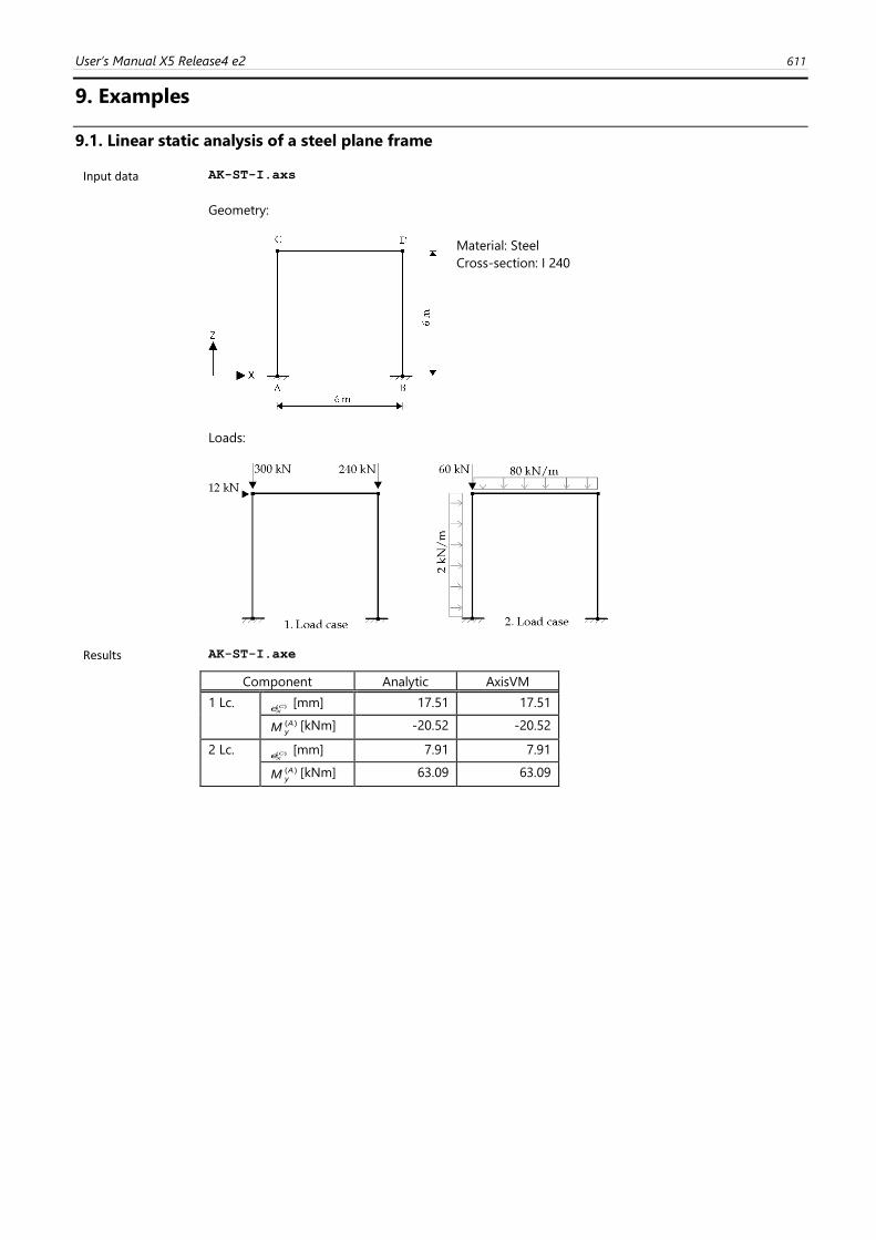
User’s Manual X5 Release4 e2 611

9. Examples

9.1. Linear static analysis of a steel plane frame

Input data AK-ST-I.axs

Geometry:

Material: Steel

Cross-section: I 240

Loads:

Results AK-ST-I.axe

Component Analytic AxisVM

1 Lc. eX

C( ) [mm] 17.51 17.51

M yA( ) [kNm] -20.52 -20.52

2 Lc. eX

C( ) [mm] 7.91 7.91

M yA( ) [kNm] 63.09 63.09

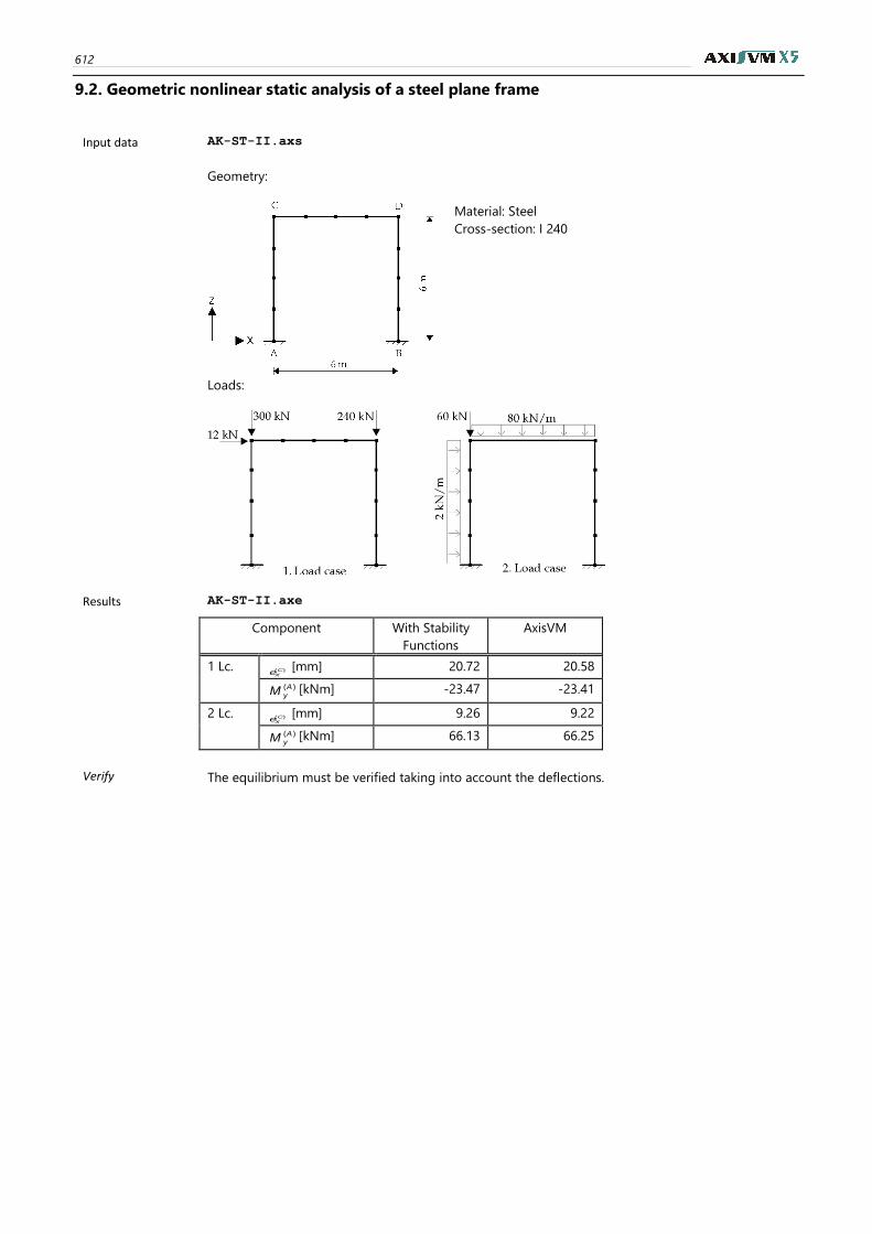
612

9.2. Geometric nonlinear static analysis of a steel plane frame

Input data AK-ST-II.axs

Geometry:

Material: Steel

Cross-section: I 240

Loads:

Results AK-ST-II.axe

Component With Stability

Functions

AxisVM

1 Lc. eX

C( ) [mm] 20.72 20.58

M yA( ) [kNm] -23.47 -23.41

2 Lc. eX

C( ) [mm] 9.26 9.22

M yA( ) [kNm] 66.13 66.25

Verify The equilibrium must be verified taking into account the deflections.

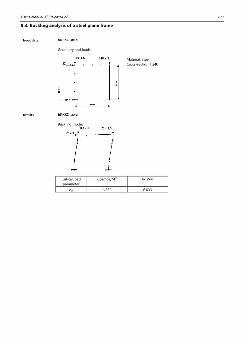
User’s Manual X5 Release4 e2 613

9.3. Buckling analysis of a steel plane frame

Input data AK-KI.axs

Geometry and loads:

Material: Steel

Cross-section: I 240

Results AK-KI.axe

Buckling mode:

Critical load

parameter

Cosmos/M AxisVM

ncr 6.632 6.633

614

9.4. Vibration analysis (I-Order) of a steel plane frame

Input data AK-RZ-I.axs

Geometry:

Material: Steel

Cross-section: I 240

Results AK-RZ-I.axe

Frequency [Hz]

Mode Cosmos/M AxisVM

1 6.957 6.957

2 27.353 27.353

3 44.692 44.692

4 48.094 48.094

5 95.714 95.714

6 118.544 118.544

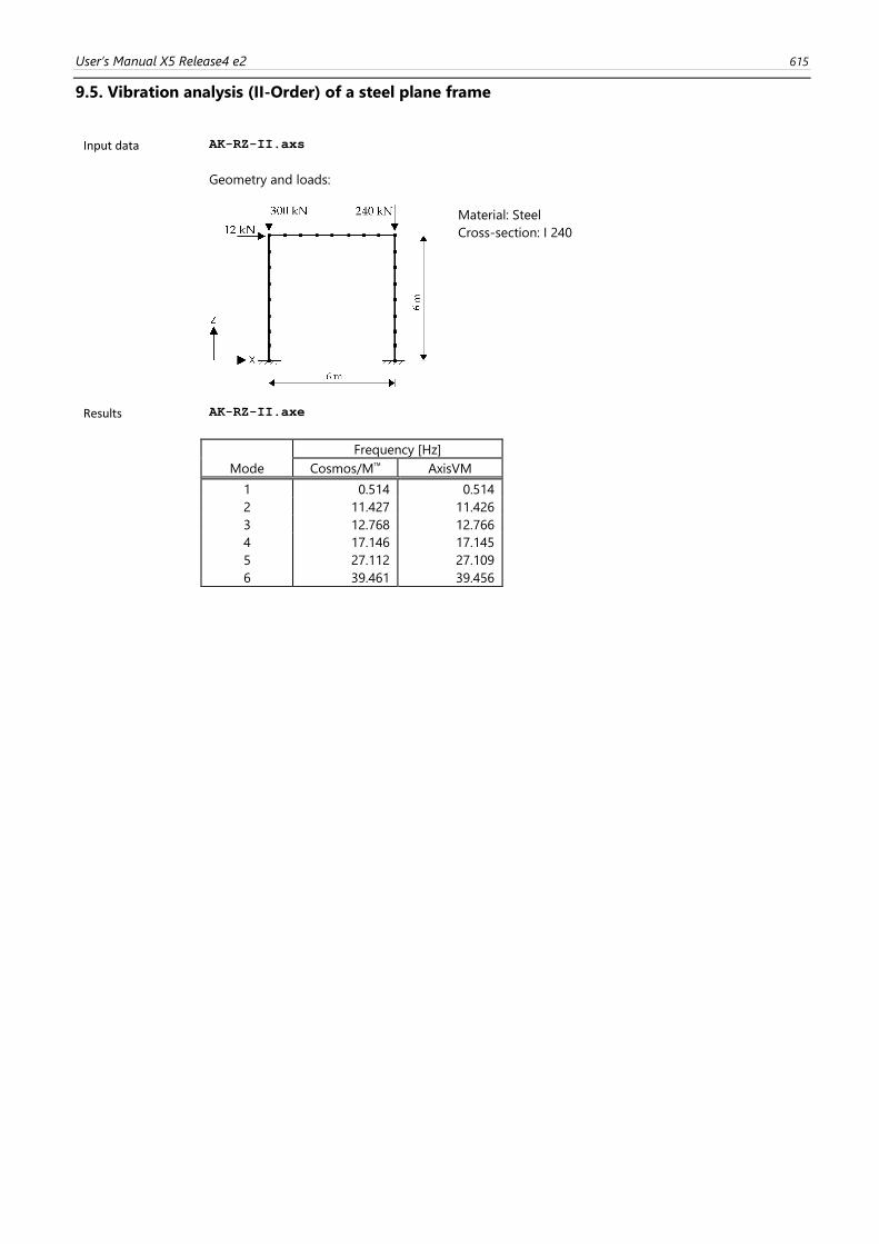
User’s Manual X5 Release4 e2 615

9.5. Vibration analysis (II-Order) of a steel plane frame

Input data AK-RZ-II.axs

Geometry and loads:

Material: Steel

Cross-section: I 240

Results AK-RZ-II.axe

Frequency [Hz]

Mode Cosmos/M AxisVM

1 0.514 0.514

2 11.427 11.426

3 12.768 12.766

4 17.146 17.145

5 27.112 27.109

6 39.461 39.456

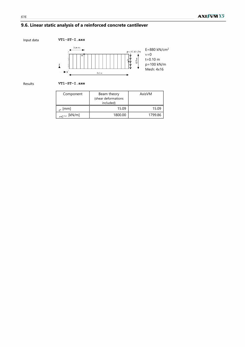
616

9.6. Linear static analysis of a reinforced concrete cantilever

Input data VT1-ST-I.axs

E=880 kN/cm2

=0

t=0.10 m

p=100 kN/m

Mesh: 4x16

Results VT1-ST-I.axe

Component Beam theory

(shear deformations

included)

AxisVM

ez

B( ) [mm] 15.09 15.09

nx

A( ) [kN/m] 1800.00 1799.86

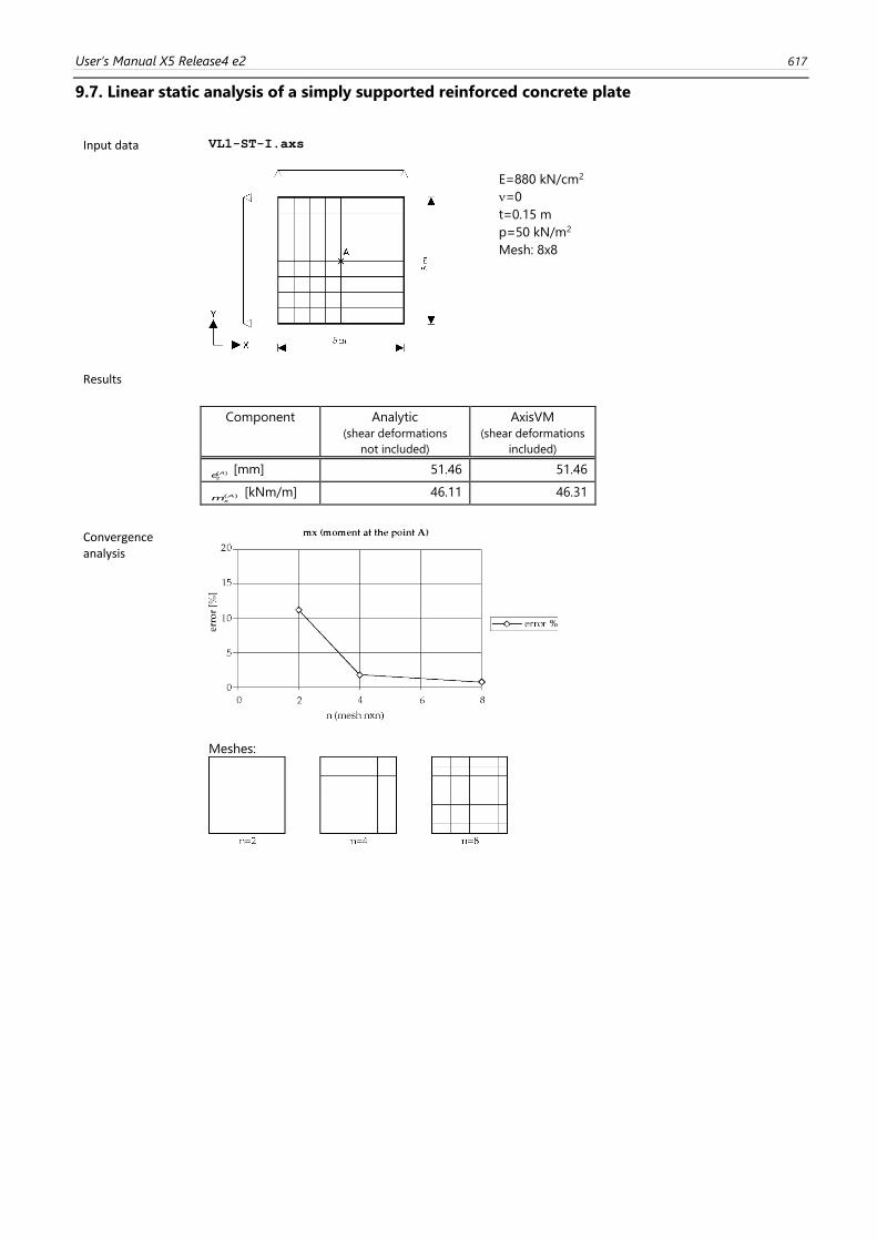
User’s Manual X5 Release4 e2 617

9.7. Linear static analysis of a simply supported reinforced concrete plate

Input data VL1-ST-I.axs

E=880 kN/cm2

=0

t=0.15 m

p=50 kN/m2

Mesh: 8x8

Results

Component Analytic

(shear deformations

not included)

AxisVM

(shear deformations

included)

ez

A( ) [mm] 51.46 51.46

mx

A( ) [kNm/m] 46.11 46.31

Convergence analysis

Meshes:

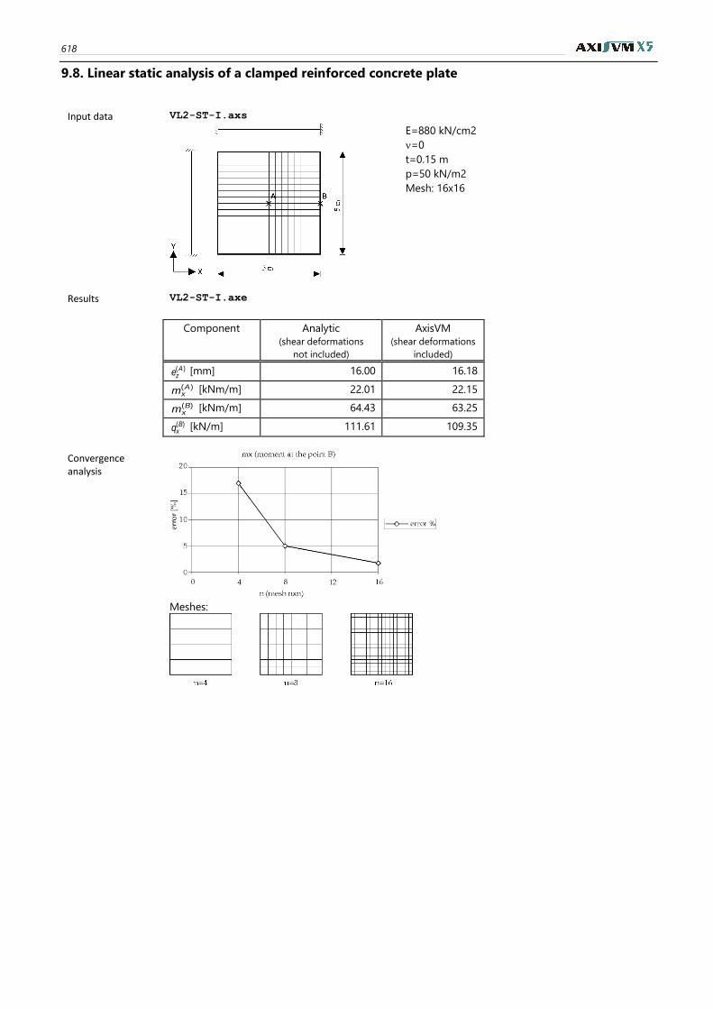
618

9.8. Linear static analysis of a clamped reinforced concrete plate

Input data VL2-ST-I.axs

E=880 kN/cm2

=0

t=0.15 m

p=50 kN/m2

Mesh: 16x16

Results VL2-ST-I.axe

Component Analytic

(shear deformations

not included)

AxisVM

(shear deformations

included)

)(Aze [mm] 16.00 16.18

)(Axm [kNm/m] 22.01 22.15

)(Bxm [kNm/m] 64.43 63.25

)(Bxq [kN/m] 111.61 109.35

Convergence analysis

Meshes:

User’s Manual X5 Release4 e2 619

10. References

1. Bathe, K. J., Wilson, E. L., Numerical Methods in Finite Element Analysis, Prentice Hall, New Jersey, 1976

2. Bojtár I., Vörös G., A végeselem-módszer alkalmazása lemez- és héjszerkezetekre, Műszaki Könyvkiadó, Budapest,

1986

3. Chen, W. F., Lui, E. M., Structural Stability, Elsevier Science Publishing Co., Inc., New York, 1987

4. Hughes, T. J. R., The Finite Element Method, Prentice-Hall, Inc., Englewood Cliffs, New Jersey, 1987

5. Owen D. R. J., Hinton E., Finite Elements in Plasticity, Pineridge Press Limited, Swansea, 1980

6. Popper Gy., Csizmás F., Numerikus módszerek mérnököknek, Akadémiai Kiadó Typotex, Budapest, 1993

7. Przemieniecki, J. S., Theory of Matrix Structural Analysis, McGraw Hill Book Co., New York, 1968

8. Weaver Jr., W., Johnston, P. R., Finite Elements for Structural Analysis, Prentice-Hall, Inc., Englewood Cliffs, New

Jersey, 1984

9. Dr. Szalai Kálmán, Vasbetonszerkezetek, vasbeton-szilárdságtan, Tankönyvkiadó, Budapest, 1990. 1998

10. Dr. Kollár László: Vasbeton-szilárdságtan, Műegyetemi Kiadó, 1995

11. Dr. Kollár László: Vasbetonszerkezetek I., Vasbeton-szilárdságtan az Eurocode 2 szerint, Műegyetemi Kiadó, 1997

12. Dr. Bölcskei E., Dr. Dulácska E.: Statikusok könyve, Műszaki Könyvkiadó, 1974

13. Dr. Dulácska Endre: Kisokos, Segédlet tartószerkezetek tervezéséhez, BME Építészmérnöki Kar, 1993

14. Porteous, J., Kermani, A., Structural Timber Design to Eurocode 5, Blackwell Publishing, 2007

15. Dulácska Endre, Joó Attila, Kollár László: Tartószerkezetek tervezése földrengési hatásokra, Akadémiai Kiadó, 2008

16. Pilkey, W. D., Analysis and Design of Elastic Beams - Computational methods, John Wiley & sons, Inc., 2002

17. Navrátil, J., Prestressed Concrete Structures, Akademické Nakladatelství Cerm®, 2006

18. Szepesházi Róbert: Geotechnikai tervezés (Tervezés Eurocode 7 és a kapcsolódó európai geotechnikai szabványok

alapján), Business Media Magyarország Kft., 2008

19. Györgyi József: Dinamika, Műegyetemi Kiadó, 2003

20. Bojtár Imre, Gáspár Zsolt: Végeselemmódszer építőmérnököknek, Terc Kft., 2003

21. Eurocode 2, EN 1992-1-1:2010

22. Eurocode 3, EN 1993-1-1:2005

23. Eurocode 3, EN 1993-1-3:2006

24. Eurocode 3, EN 1993-1-5:2006

25. Eurocode 5, EN 1995-1-1:2004

26. Eurocode 8, EN 1998-1-1:2004

27. Paz,M., Leigh, W., Structural Dynamics - Theory and Computation, Fifth Edition, Springer, 2004

28. Chopra, A. K., Dynamics of Structures - Theory and Applications to Earthquake Engineering, Third Edition, Pearson

Prentice Hill, 2007

29. Biggs, J. M., Introduction to Structural Dynamics, McGraw-Hill, 1964

30. Weaver, W., Jr., P. R. Johnston, Structural Dynamics by Finite Elements, Prentice-Hall, 1987

31. Bathe, K. J., Finite Element Procedures, Prentice-Hall, 1996

32. Borst, R., Crisfield, M. A., Remmers, J. J. C., Verhoosel, C. V., Non-Linear Finite Element Analysis of Solids and

Structures, Second Edition, John Wiley & Sons Ltd., 2012

33. Willford, M.R., Young, P. A Design Guide for Footfall Induced Vibration of Structures, Concrete Society, 2006

34. Smith, A. L., Hicks, S. J., Devine, P. J. Design of Floors for Vibration: A New Approach, The Steel Construction Institute, Ascot, 2009

35. https://en.wikipedia.org/wiki/Von_Mises_yield_criterion

620

36. https://en.wikipedia.org/wiki/Bresler_Pister_yield_criterion

37. https://en.wikipedia.org/wiki/Whittaker%E2%80%93Shannon_interpolation_formula

38. https://en.wikipedia.org/wiki/Nyquist%E2%80%93Shannon_sampling_theorem

39. Wilson, E. L., Three-Dimensional Static and Dynamic Analysis of Structures – A Physical Approach With Emphasis on

Earthquake Engineering, Computers and Structures Inc., Berkeley, 2002

User’s Manual X5 Release4 e2 621

Notes

622

Notes