Embed Size (px)
Citation preview
12
Astrophysical plasmas
Roberto Casini1 and Egidio Landi Degl’Innocenti2
1 High Altitude Observatory, National Center for Atmospheric Research,??
P.O. Box 3000, Boulder, CO 80307-3000, U.S.A.2 Dipartimento di Astronomia e Scienze dello Spazio, Universita di Firenze,
Largo E. Fermi 2, I-50125 Firenze, Italy
In this chapter we discuss the application of spectro-polarimetry diagnostics tothe investigation of astrophysical plasmas. We first present an overview of whypolarization must be expected in the spectral-line radiation that we receivefrom a large variety of cosmic objects, and then treat in some detail specificatomic models (e.g., the 0–1 and 1–0 two-level atoms), which illustrate howphysical and electro-dynamical properties of the emitting plasma can be in-ferred by studying the polarized radiation in the corresponding spectral lines.The practical applications described in this chapter are taken exclusively fromthe realm of solar physics, mainly for two reasons: a) From a historical point ofview, the Sun was the first cosmic object to which polarization analysis of ra-diation was successfully applied, proving the existence of solar magnetic fields,and demonstrating the diagnostic potential of radiation phenomena involvingresonance polarization. b) Because spectro-polarimetric signals are generallyvery weak, their detection with sufficient signal-to-noise ratios is possible onlyfor strong radiation sources. In particular, a plethora of atomic-polarizationeffects (magnetic and collisional depolarization, alignment-to-orientation con-version, level crossing and anti-crossing interferences) could be detected inthe polarized light from the Sun only because of the high sensitivity that canbe attained in solar observations. As the light-collecting capabilities of night-time astronomical instrumentation keep growing, it must be expected thatthe diagnostic techniques illustrated in this chapter will become increasinglyavailable for the investigation of plasma properties all over the universe.
12.1 Introduction
The importance of understanding the origin of polarized radiation in astro-physical plasmas cannot be overestimated. Unlike laboratory plasmas – for
??The National Center for Atmospheric Research is sponsored by the NationalScience Foundation.
2 Roberto Casini and Egidio Landi Degl’Innocenti
z
JM = + 1
M = - 1
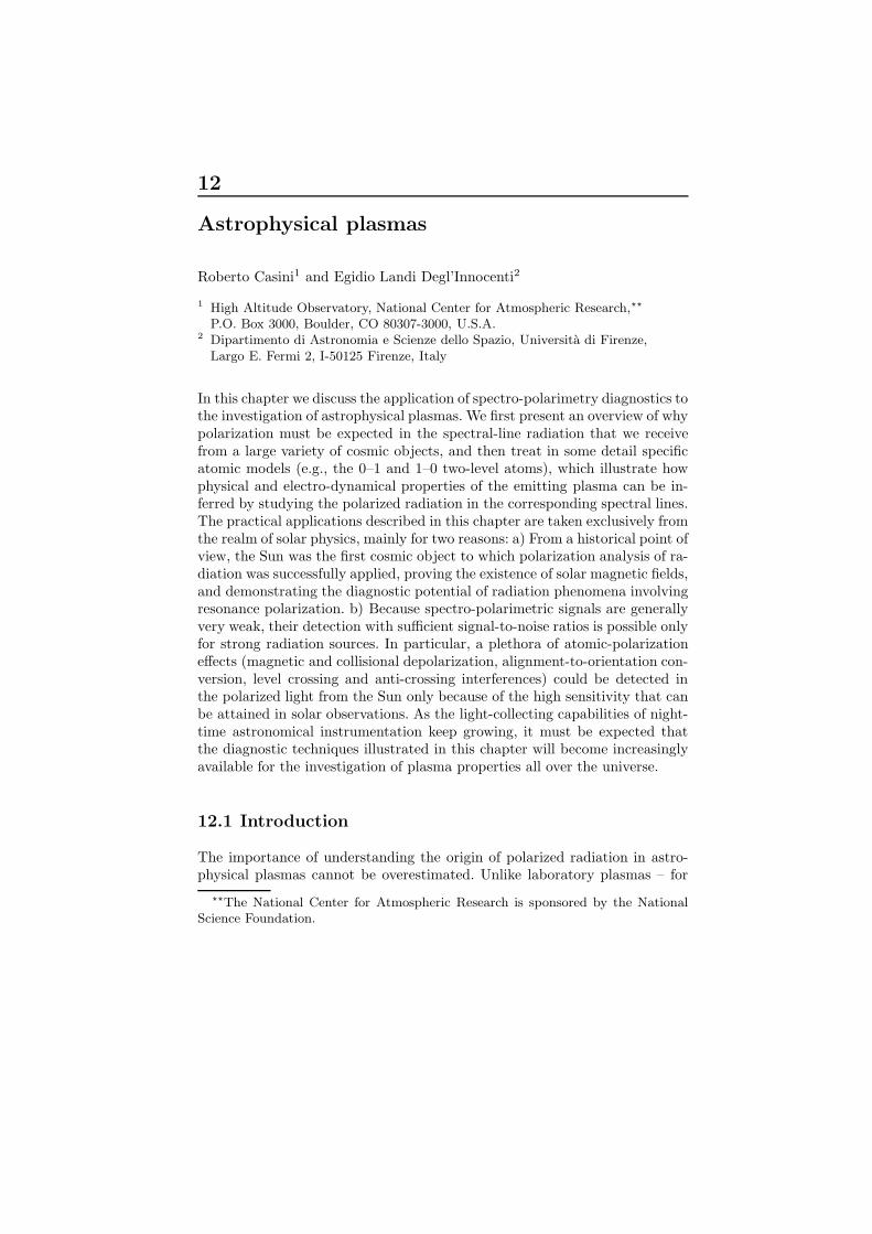
Fig. 12.1. Vector-model description of the J = 1 atomic state. The norm of thetotal angular momentum is |J | =
p
J(J + 1) =√
2. The z-axis defines the directionof quantization of the atomic system.
which many physical parameters can be directly controlled or measured – inthe case of astrophysical plasmas, radiation is the only carrier of informationthat is available to the observer for understanding the physical processes thatdetermine the dynamics of the object under study.
Radiation polarization must be expected every time that the interactionof photons with atoms (or molecules) is affected by symmetry-breaking pro-cesses. This symmetry breaking can be intrinsic to the process of photon-atominteraction itself (e.g., anisotropic illumination of atoms, leading to scatter-ing polarization), or be determined by the presence of external causes (e.g.,anisotropic excitation by collisions; interaction of the atom with deterministicmagnetic and/or electric fields). Examples of processes leading to radiation po-larization in laboratory plasmas have been discussed elsewhere in this book. Inthis chapter we will discuss polarization phenomena observed in astrophysics,and illustrate how from them we can gain an understanding of the undergoingphysical processes.
Historically, solar physics has led the way in exploiting polarization infor-mation contained in the radiation coming from the Sun in order to understandsolar magnetism. This privileged role of our star among polarization studies ofcosmic objects has a very natural explanation: both spectral and polarimetricanalyses are photon starved techniques, and therefore they are more difficultto apply to faint objects. Even for the Sun, the detection of very low levels ofpolarization – characterizing, for instance, the resonance scattered radiationfrom quiet (i.e., magnetically “inactive”) regions in the solar atmosphere [1] –poses to the present day significant challenges, which have only partially beenovercome by the availability of increasingly more efficient detectors.
Magnetic field strengths in the solar atmosphere range from the very weakfields permeating the quiet-sun corona (B . 10−3 T) to the strong fields
12 Astrophysical plasmas 3
M = 0
M = - 1M = 0M = + 1
s +s -
s -
s +
p
B
B
w B
w B
l i n e o f s i g h t
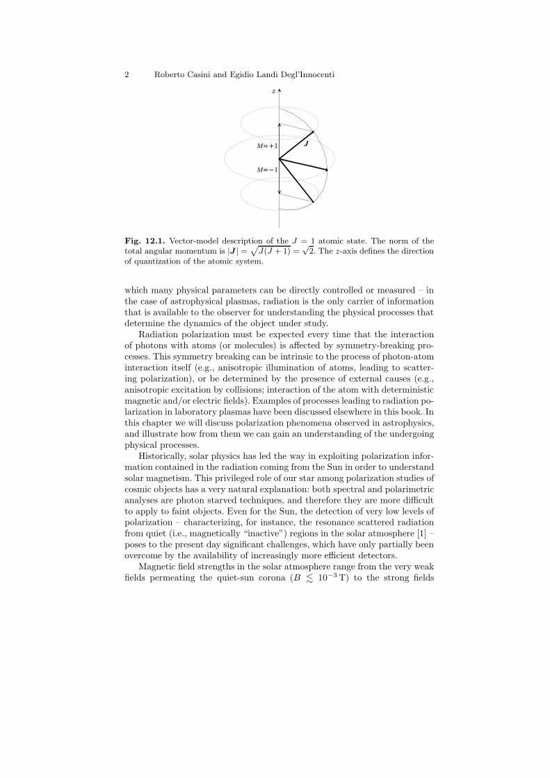
Fig. 12.2. Definition of π and σ components of polarized radiation for the transition1 → 0. B defines the direction of the quantization axis. The case at the top showsthe circular-polarization signal, and the one at the bottom the linear-polarizationsignal, for the respective geometries of B with respect to the line-of-sight.
characteristic of the umbral regions of sunspots (B & 10−1 T).3 Because ofsuch diverse regimes of magnetic fields, different phenomena affecting thepolarization of the emitted radiation can occur in solar plasmas (Zeemaneffect, Hanle effect, alignment-to-orientation conversion, level crossing andanti-crossing interferences), whose signatures can in principle be modeled inorder to infer the magnetic topology of the emitting plasma.
We refer the reader to other chapters of this book for an exhaustive treat-ment of collision-induced polarization. Here we will focus exclusively on theeffects of anisotropic illumination and external fields on the polarization ofspectral lines.
12.2 Origin of polarized radiation
The origin of spectral-line polarization can be traced back to the intrinsicproperties of atomic transitions. Let us consider the simplest atomic transi-tion, between an upper level Ju = 1 and a lower level Jl = 0. Quantum me-chanics tells us that the atoms in the upper level can occupy any of the three
3Here the comparative terms “weak” and “strong” are used in connection withthe relative size of magnetic splitting to line broadening of non-magnetic origin(typically, the Doppler thermal linewidth). However, the same terminology can alsobe used to classify the regime of interaction of the atom with the external fields,so that a field can be said to be “weak” if the corresponding magnetic splitting issmall compared to some characteristic energy scale of the atomic structure (e.g., theenergy separation between atomic levels due to the presence of fine structure and/orhyperfine structure).
4 Roberto Casini and Egidio Landi Degl’Innocenti
possible M substates (M = −1, 0, +1). In the language of the vector model ofatoms [2], these substates correspond to the three possible projections of thevector J along the the quantization axis (see Fig. 12.1). The electric-dipoletransitions, from these three substates to the one substate M = 0 of the lowerlevel, have different polarization properties. The transition with ∆M = 0 islinearly polarized along the z-axis (π transition), whereas the two transitionswith |∆M | = 1 are circularly polarized, with opposite signs, around the z-axis,and linearly polarized perpendicularly to the same axis (σ transitions).
If the excitation processes are completely isotropic, then the excited atomshave equal probability of populating any of the three upper M substates. Thethree components of the atomic transition will then contribute to the polar-ized emission with well defined weights. Figure 12.2 illustrates the two casesof longitudinal and transversal radiation emitted by an atom that has beenisotropically illuminated (the quantization axis is defined by the direction ofthe magnetic field, B), with the respective polarization properties of the threetransition components. Since the three substates of J = 1 are isoenergetic inthe absence of external fields (ωB = 0, in the case of Fig. 12.2), positive andnegative polarizations exactly cancel out in this case, so the emitted radiationappears to be completely unpolarized.
One can imagine two different scenarios (not mutually exclusive), wherethe different polarization properties of the three transition components canbe made manifest in the emitted radiation. The first scenario corresponds tothe possibility that the upper M substates may be unevenly populated, so thetransition components no longer contribute to the emitted radiation with thevery particular weights illustrated in Fig. 12.2, which make the total polariza-tion vanish. This condition typically occurs when the excitation processes areanisotropic (e.g., a collimated beam of radiation illuminating the atom). Thesecond scenario corresponds to the possibility that the upper M substatesmay be separated in energy, so that a spectral analysis of the emitted radia-tion would reveal its varying polarization properties with wavelength, even ifthe upper M substates are equally populated. This condition typically occurswhen an external magnetic or electric field is interacting with the atom, sothat the energy structure of the atom is modified, by the additional interac-tion energy, with respect to the zero-field case. Figure 12.2 illustrates this lastcase, when a magnetic field is present (Zeeman effect [2]).
In astrophysical plasmas, both scenarios can generally be present at thesame time, so it is possible in principle to investigate the excitation conditionsof a plasma, and its electro-dynamic properties, by studying the polarizationsignature of spectral lines formed in the plasma.
12.2.1 Description of polarized radiation
Before considering the problem of plasma diagnostics via polarization mea-surements, we must define a set of observable parameters from the physicalquantities that describe polarized radiation. Let us consider for simplicity
12 Astrophysical plasmas 5
xe
ye
directionreference
α
β
polarizer
retarder
detector
acceptance axis
fast axis
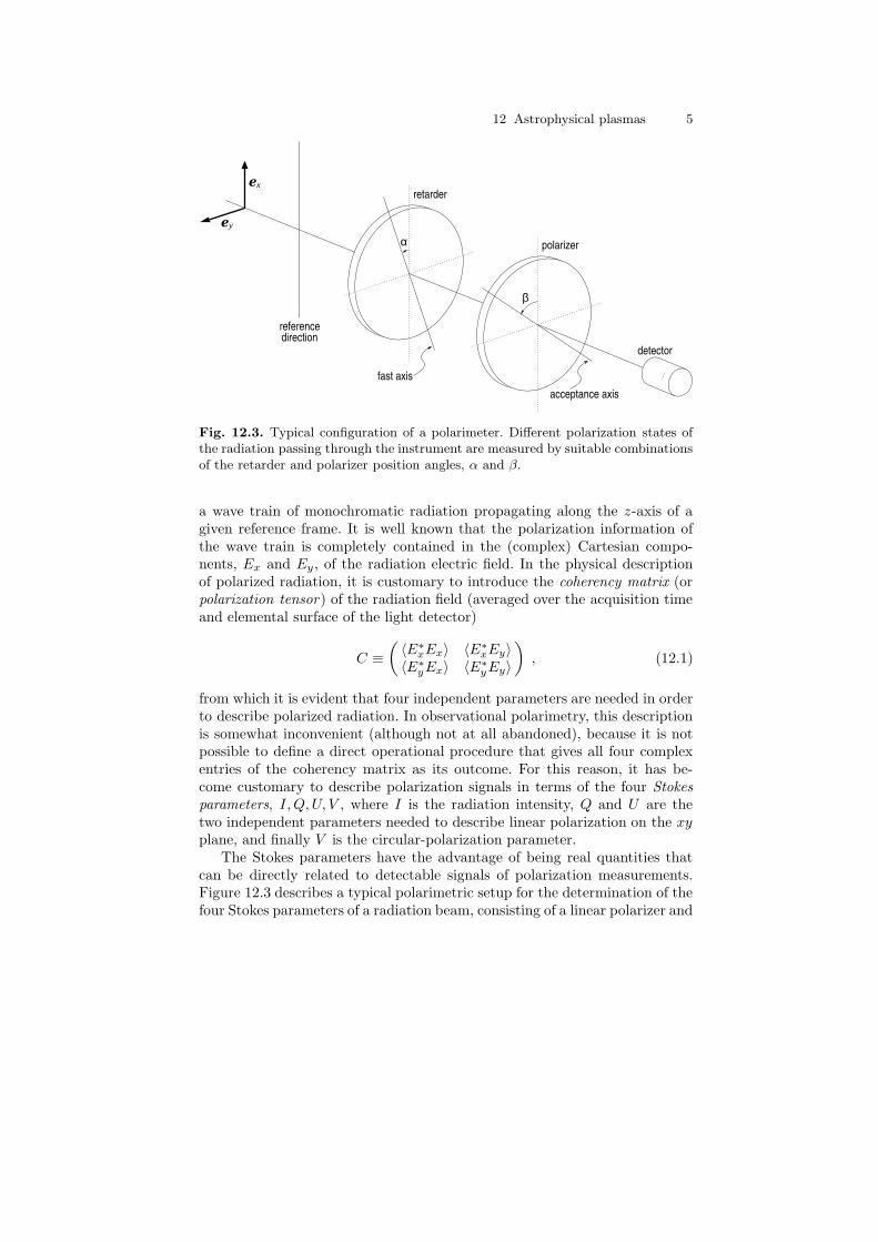
Fig. 12.3. Typical configuration of a polarimeter. Different polarization states ofthe radiation passing through the instrument are measured by suitable combinationsof the retarder and polarizer position angles, α and β.
a wave train of monochromatic radiation propagating along the z-axis of agiven reference frame. It is well known that the polarization information ofthe wave train is completely contained in the (complex) Cartesian compo-nents, Ex and Ey , of the radiation electric field. In the physical descriptionof polarized radiation, it is customary to introduce the coherency matrix (orpolarization tensor) of the radiation field (averaged over the acquisition timeand elemental surface of the light detector)
C ≡(
〈E∗xEx〉 〈E∗
xEy〉〈E∗
yEx〉 〈E∗yEy〉
)
, (12.1)
from which it is evident that four independent parameters are needed in orderto describe polarized radiation. In observational polarimetry, this descriptionis somewhat inconvenient (although not at all abandoned), because it is notpossible to define a direct operational procedure that gives all four complexentries of the coherency matrix as its outcome. For this reason, it has be-come customary to describe polarization signals in terms of the four Stokes
parameters, I, Q, U, V , where I is the radiation intensity, Q and U are thetwo independent parameters needed to describe linear polarization on the xyplane, and finally V is the circular-polarization parameter.
The Stokes parameters have the advantage of being real quantities thatcan be directly related to detectable signals of polarization measurements.Figure 12.3 describes a typical polarimetric setup for the determination of thefour Stokes parameters of a radiation beam, consisting of a linear polarizer and
6 Roberto Casini and Egidio Landi Degl’Innocenti
a wave retarder.4 For a λ/4 retarder, the intensity of the radiation reachingthe detector is
S(α, β) =1
2[I + (Q cos 2α + U sin 2α) cos 2(β − α) + V sin 2(β − α)] ,
(12.2)so it is possible to establish a series of measurements involving different valuesof the position angles α and β, which allows the independent measurementsof the four Stokes parameters.
Of course, the two descriptions of polarized radiation, in terms of thecoherency matrix or the Stokes parameters of the radiation field, must beequivalent, and in fact, it is possible to rewrite eq.(12.1) in the form
C =1
2
(
I + Q U − iVU + iV I − Q
)
. (12.3)
12.3 Quantum theory of photon-atom processes
A proper formulation of the problem of polarized line formation in complexatoms must rely on a quantum-mechanical description of the interaction ofradiation with atoms. The evolution of the total system atom+radiation isgoverned by the quantum-mechanical Liouville equation for the statisticaloperator of the system [3],
d
dtρ(t) =
1
i~[H(t), ρ(t)] , (12.4)
where H(t) is the sum of the atomic Hamiltonian, HA, the radiation Hamil-tonian, HR, and the interaction Hamiltonian, HI(t), which is responsible forall photon-atom processes. If we assume that the interaction is switched onat a time t = t0, then for t ≤ t0 the atomic system and the radiation fieldevolve independently, and the statistical operator of the total system can bewritten as the direct product of the two statistical operators for the atom andthe radiation field,
ρ(t) = ρA(t) ⊗ ρR(t) , ∀t ≤ t0 . (12.5)
Equation (12.4) has the formal integral solution
ρ(t) = ρ(t0) +1
i~
t∫
t0
dt′ [H(t′), ρ(t′)] , (12.6)
4A wave retarder is a device that separates the incoming beam into two beamswith orthogonal states of polarization, and then recombines them after introducinga phase retardation in one of the beams.
12 Astrophysical plasmas 7
k p
q
p
k q
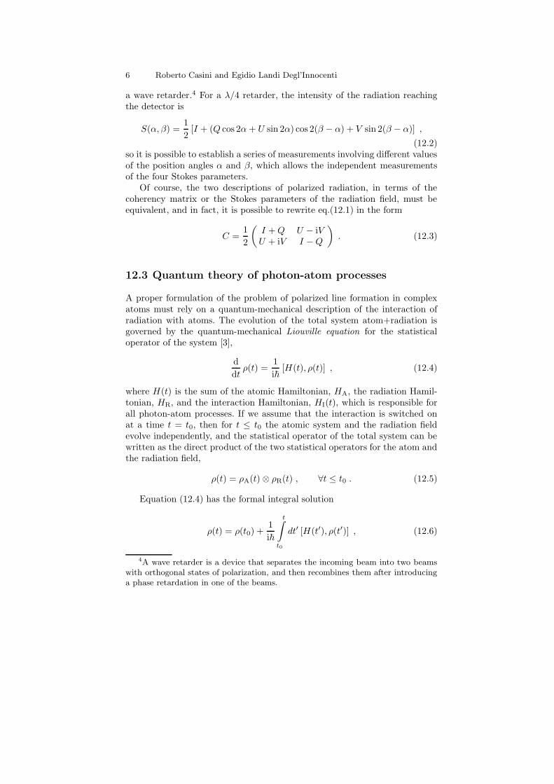
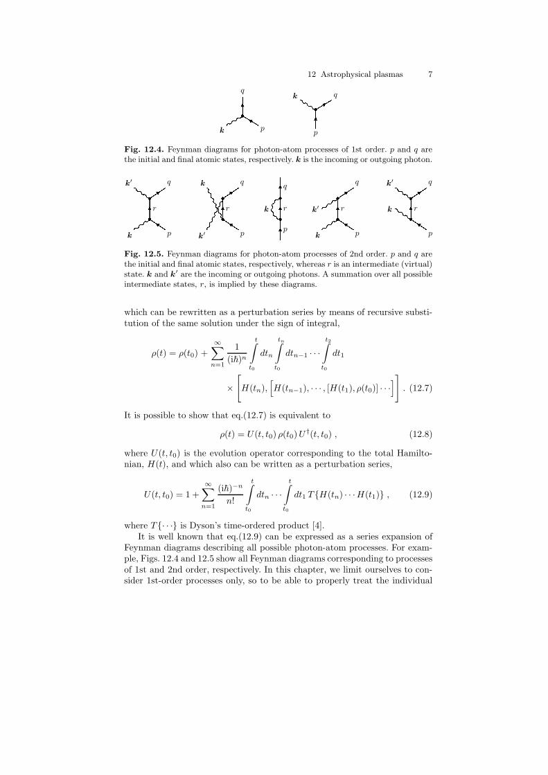
Fig. 12.4. Feynman diagrams for photon-atom processes of 1st order. p and q arethe initial and final atomic states, respectively. k is the incoming or outgoing photon.
r
k p
k′ q
r
k′ p
k q
p
rk
q
r
k
k′
p
q
rk
k′
p
q
Fig. 12.5. Feynman diagrams for photon-atom processes of 2nd order. p and q arethe initial and final atomic states, respectively, whereas r is an intermediate (virtual)state. k and k
′ are the incoming or outgoing photons. A summation over all possibleintermediate states, r, is implied by these diagrams.
which can be rewritten as a perturbation series by means of recursive substi-tution of the same solution under the sign of integral,
ρ(t) = ρ(t0) +∞∑
n=1
1
(i~)n
t∫
t0
dtn
tn∫
t0
dtn−1 · · ·t2
∫
t0
dt1
×[
H(tn),[
H(tn−1), · · · , [H(t1), ρ(t0)] · · ·]
]
. (12.7)
It is possible to show that eq.(12.7) is equivalent to
ρ(t) = U(t, t0) ρ(t0) U †(t, t0) , (12.8)
where U(t, t0) is the evolution operator corresponding to the total Hamilto-nian, H(t), and which also can be written as a perturbation series,
U(t, t0) = 1 +
∞∑
n=1
(i~)−n
n!
t∫
t0
dtn · · ·t
∫
t0
dt1 T{H(tn) · · ·H(t1)} , (12.9)
where T{· · ·} is Dyson’s time-ordered product [4].It is well known that eq.(12.9) can be expressed as a series expansion of
Feynman diagrams describing all possible photon-atom processes. For exam-ple, Figs. 12.4 and 12.5 show all Feynman diagrams corresponding to processesof 1st and 2nd order, respectively. In this chapter, we limit ourselves to con-sider 1st-order processes only, so to be able to properly treat the individual
8 Roberto Casini and Egidio Landi Degl’Innocenti
’’
pl
pu
ql
qu
E
A TS TE
TA SR R
R
pq,p q
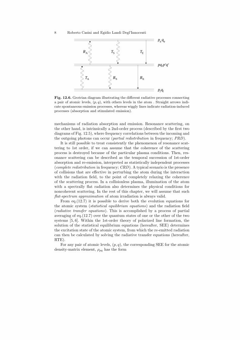
Fig. 12.6. Grotrian diagram illustrating the different radiative processes connectinga pair of atomic levels, (p, q), with others levels in the atom . Straight arrows indi-cate spontaneous emission processes, whereas wiggly lines indicate radiation-inducedprocesses (absorption and stimulated emission).
mechanisms of radiation absorption and emission. Resonance scattering, onthe other hand, is intrinsically a 2nd-order process (described by the first twodiagrams of Fig. 12.5), where frequency correlations between the incoming andthe outgoing photons can occur (partial redistribution in frequency; PRD).
It is still possible to treat consistently the phenomenon of resonance scat-tering to 1st order, if we can assume that the coherence of the scatteringprocess is destroyed because of the particular plasma conditions. Then, res-onance scattering can be described as the temporal succession of 1st-orderabsorption and re-emission, interpreted as statistically independent processes(complete redistribution in frequency; CRD). A typical scenario is the presenceof collisions that are effective in perturbing the atom during the interactionwith the radiation field, to the point of completely relaxing the coherenceof the scattering process. In a collisionless plasma, illumination of the atomwith a spectrally flat radiation also determines the physical conditions fornoncoherent scattering. In the rest of this chapter, we will assume that suchflat-spectrum approximation of atom irradiation is always valid.
From eq.(12.7) it is possible to derive both the evolution equations forthe atomic system (statistical equilibrium equations) and the radiation field(radiative transfer equations). This is accomplished by a process of partialaveraging of eq.(12.7) over the quantum states of one or the other of the twosystems [5, 6]. Within the 1st-order theory of polarized line formation, thesolution of the statistical equilibrium equations (hereafter, SEE) determinesthe excitation state of the atomic system, from which the re-emitted radiationcan then be calculated by solving the radiative transfer equations (hereafter,RTE).
For any pair of atomic levels, (p, q), the corresponding SEE for the atomicdensity-matrix element, ρpq has the form
12 Astrophysical plasmas 9
R a d i a t i v eT r a n s f e rE q u a t i o n s
w r it e s o l v e
s t a r tr p q
S t a t i s t i c a lE q u i l i b r i u mE q u a t i o n s
s o l v e w r it e
S i
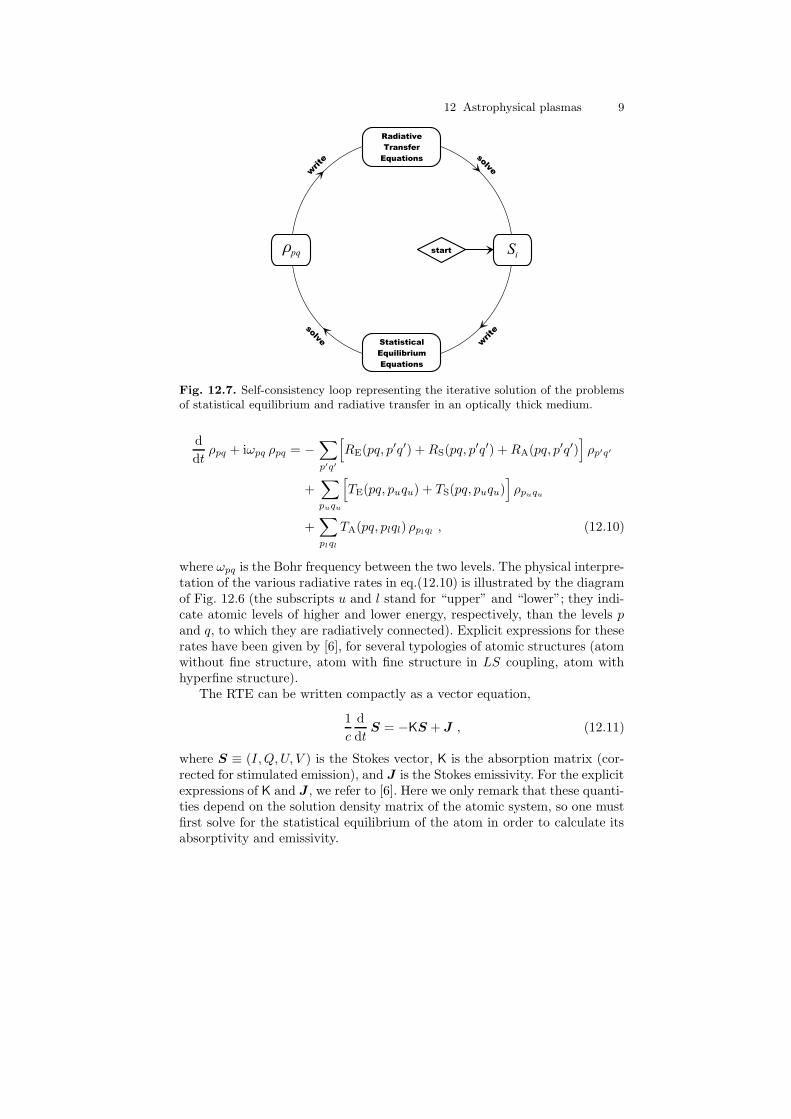
Fig. 12.7. Self-consistency loop representing the iterative solution of the problemsof statistical equilibrium and radiative transfer in an optically thick medium.
d
dtρpq + iωpq ρpq = −
∑
p′q′
[
RE(pq, p′q′) + RS(pq, p′q′) + RA(pq, p′q′)]
ρp′q′
+∑
puqu
[
TE(pq, puqu) + TS(pq, puqu)]
ρpuqu
+∑
plql
TA(pq, plql) ρplql, (12.10)
where ωpq is the Bohr frequency between the two levels. The physical interpre-tation of the various radiative rates in eq.(12.10) is illustrated by the diagramof Fig. 12.6 (the subscripts u and l stand for “upper” and “lower”; they indi-cate atomic levels of higher and lower energy, respectively, than the levels pand q, to which they are radiatively connected). Explicit expressions for theserates have been given by [6], for several typologies of atomic structures (atomwithout fine structure, atom with fine structure in LS coupling, atom withhyperfine structure).
The RTE can be written compactly as a vector equation,
1
c
d
dtS = −KS + J , (12.11)
where S ≡ (I, Q, U, V ) is the Stokes vector, K is the absorption matrix (cor-rected for stimulated emission), and J is the Stokes emissivity. For the explicitexpressions of K and J , we refer to [6]. Here we only remark that these quanti-ties depend on the solution density matrix of the atomic system, so one mustfirst solve for the statistical equilibrium of the atom in order to calculate itsabsorptivity and emissivity.
10 Roberto Casini and Egidio Landi Degl’Innocenti
In the single scattering approximation, radiation is scattered only once – onits way from the source to the observer – before leaving the plasma. Typicallythis is a very good approximation for optically thin gases, and it allows to avoidthe integration of eq.(12.11) by expressing the scattered radiation simply interms of the Stokes emissivity vector, J . In optically thick plasmas, instead,the solution of eq.(12.11) cannot be avoided. Moreover, the scattered radiationtends to modify locally the radiation field that enters as an input of the SEE,so the radiative transfer problem in optically thick plasma is affected by non-linearity, as well as non-locality issues, because of the back-reaction of theradiation field on the atomic system. The solution to this problem relies oniterative schemes, of the kind illustrated in Fig. 12.7, which must be followedthrough until self-consistency of the two solutions of the SEE and the RTE isachieved.
The problem of the convergence of the iterative loop of Fig. 12.7 is aresearch subject on itself, which is still relatively new for the general caseinvolving the presence of atomic polarization [7]. For this reason, in the fol-lowing examples of this chapter, we will only consider optically thin plasmas,as well as optically thick plasmas that are homogeneous in their thermody-namical and electrodynamical properties, and for which the back-reaction ofthe locally scattered radiation on the excitation conditions of the plasma canbe neglected. These two idealized cases are nonetheless sufficient for the pur-pose of demonstrating the diagnostic potential of atomic polarization – andof its modification in the presence of external fields – in the investigation ofthe topology of magnetic and electric fields in astrophysical plasmas.
12.4 The Hanle effect in the two-level atom
The simplest atomic system that we can consider to illustrate the effect ofa magnetic field on the scattering polarization in a spectral line is obviouslythat which is composed of just two atomic levels: the lower level, Jl, and theupper level, Ju, of the atomic transition corresponding to the spectral line ofinterest.
Such model of the two-level atom has played an important role for thedescription and the understanding of polarization phenomena, for several rea-sons. First of all, the polarization properties of the special case with Jl = 0 andJu = 1 (the 0–1 atom) can be derived completely within a classical (as opposedto quantistic) approach to the electrodynamics of radiation processes [6, 8].Thus, the 0–1 atom helped gaining fundamental insights on the process ofmagnetic depolarization of scattered radiation at a time when Quantum Me-chanics was still being developed [9]. On the other hand, for some branches ofPlasma Polarization Spectroscopy – e.g., the study of the optical pumping ofatomic levels by anisotropic radiation [10] – the two-level atom can actuallybe a good representation of the true atomic system, and for this reason it stillis a subject of active research [11, 12].
12 Astrophysical plasmas 11
In general, however, and in particular for astrophysical applications, thetwo-level atom can only be regarded as a very rough – and often completelyinadequate – approximation, with very few exceptions (notably, the case ofthe Sr i line at 4607A in the solar spectrum). This can be expected wheneverthe radiation intensity is distributed within a large interval of frequencies.Then the statistical equilibrium of the atom typically involves all levels thatare connected by radiative transitions within the spectral range of the incidentradiation. The complexity of the polarization phenomena in such multi-levelatoms cannot be reproduced in general within the limited scheme of the two-level atom [13,14].
In this section, we will focus on the two-level atom as a textbook case forillustrating the Hanle effect, and its potential for the diagnostics of magneticfields in astrophysical plasmas. We will study two different atomic structures:a) the 0–1 atom, and its connections to classical electrodynamics; and b) the1–0 atom, as the simplest case showing the role of lower-level polarization(e.g., the mechanism of depopulation pumping [10]).
In keeping with eq.(12.10), we assume that the atomic system is subjectonly to radiative processes. We also assume that the illuminating radiation isunpolarized, and contained within a cone of half aperture ϑM ≤ 90◦, with thevertex centered at the atom. Then, the illumination conditions are completelydescribed in terms of the radiation mean intensity, J(ω), and anisotropy, w(ω).These radiation properties are easily expressed if we adopt the formalism ofthe irreducible spherical tensors [3], and introduce accordingly the tensor com-ponents of the radiation field, JK
Q (ω), where K = 0, 1, 2 and Q = −K, . . . , K.5
For the illumination conditions described above, and also assuming that theradiation intensity, I(ω), is independent of the propagation direction withinthe radiation cone, we have
J00 (ω) =
1
2(1 − cosϑM) I(ω) , (12.12a)
J20 (ω) =
1
4√
2(1 − cosϑM)(1 + cosϑM) cosϑM I(ω) , (12.12b)
for the only two nonvanishing components of the radiation tensors, expressedin a reference frame with the z-axis along the incident direction. J 0
0 (ω) corre-sponds to the radiation mean intensity, J(ω), whereas the anisotropy of theradiation field is defined by
w(ω) ≡√
2J2
0 (ω)
J00 (ω)
=1
2(1 + cosϑM) cosϑM , (12.13)
We notice that w(ω) attains its maximum value of 1 for a collimated beamof radiation (ϑM = 0◦). When the solid angle occupied by the radiation cone
5The general expression of the tensors JKQ (ω) in terms of the Stokes vector of
the radiation field is given in [6].
12 Roberto Casini and Egidio Landi Degl’Innocenti
reaches the maximum aperture of 2π (ϑM = 90◦) instead, the anisotropyfactor vanishes.
Finally, we notice that the solution of eq.(12.10) is expressed in a ref-erence frame that has the z-axis along the quantization axis (S ′). If this isdifferent from the reference frame defined by the incident radiation (S), thenthe radiation tensors that enter eq.(12.10) are given by
[J00 (ω)]S′ = [J0
0 (ω)]S , (12.14a)
[J2Q(ω)]S′ = D2
0Q(RSS′) [J20 (ω)]S , (12.14b)
where DKQQ′ is the rotation matrix of order K, and RSS′ is the rotation op-
erator that transforms the original reference frame, S, into the frame of thequantization axis, S′ [15].
12.4.1 The 0–1 atom in a magnetic field
The two-level atom with Jl = 0 and Ju = 1 is the simplest atomic system toillustrate the Hanle effect. This model is particularly instructive, because allof its radiative properties can be reproduced adopting a classical descriptionof the atom as a three-dimensional, damped harmonic oscillator with forcingterm. In this classical picture, the forcing term corresponds to the electriccomponent, E(t), of the incident radiation field. The damping term corre-sponds instead to the contribution of the radiation reaction to the dynamicalequation of the harmonic oscillator [16]. Rather than adopting the classical ex-pression of the damping term, one can use more accurately the observed valueof the line transition amplitude, i.e., the Einstein coefficient for spontaneousemission, A10. The classical dynamical equation of the harmonic oscillator,in the additional presence of a stationary magnetic field of strength B anddirection b, is then
x + 2A10x − 2ωBb × x + ω210x +
e0
mE(t) = 0 . (12.15)
In this equation, ωB = e0B/2m is the Larmor angular frequency, whereasω10 is the resonance frequency of the oscillator, which must correspond tothe frequency of the line transition of the quantum-mechanical 0–1 atom. e0
and m are the electron’s charge and mass, respectively. The solution of thedynamical problem (12.15) can be found, e.g., in [6].
The quantum-mechanical description of the resonance scattering of radia-tion in the 0–1 atom, in the presence of a stationary magnetic field, requiresfirst the solution of the SEE, eq.(12.10), for this particular problem. If we in-troduce the irreducible spherical components of the density matrix, ρK
Q (J) [6](see also Ch. 4 in this book), with K = 0, . . . , 2J and Q = −K, . . . , K, theneq.(12.10) for the 0–1 atom becomes, neglecting stimulated emission,
d
dtρK
Q (1) + iωB Q ρKQ (1) = −A10 ρK
Q (1) +B01√
3(−1)K−QJK
−Q(ω10) ρ00(0) ,
(12.16)
12 Astrophysical plasmas 13
|ψ( )| 2|ψ( )| 2
|ψ( )| 2
A10
ωB ωB
M = −1
M = 0
M = +1
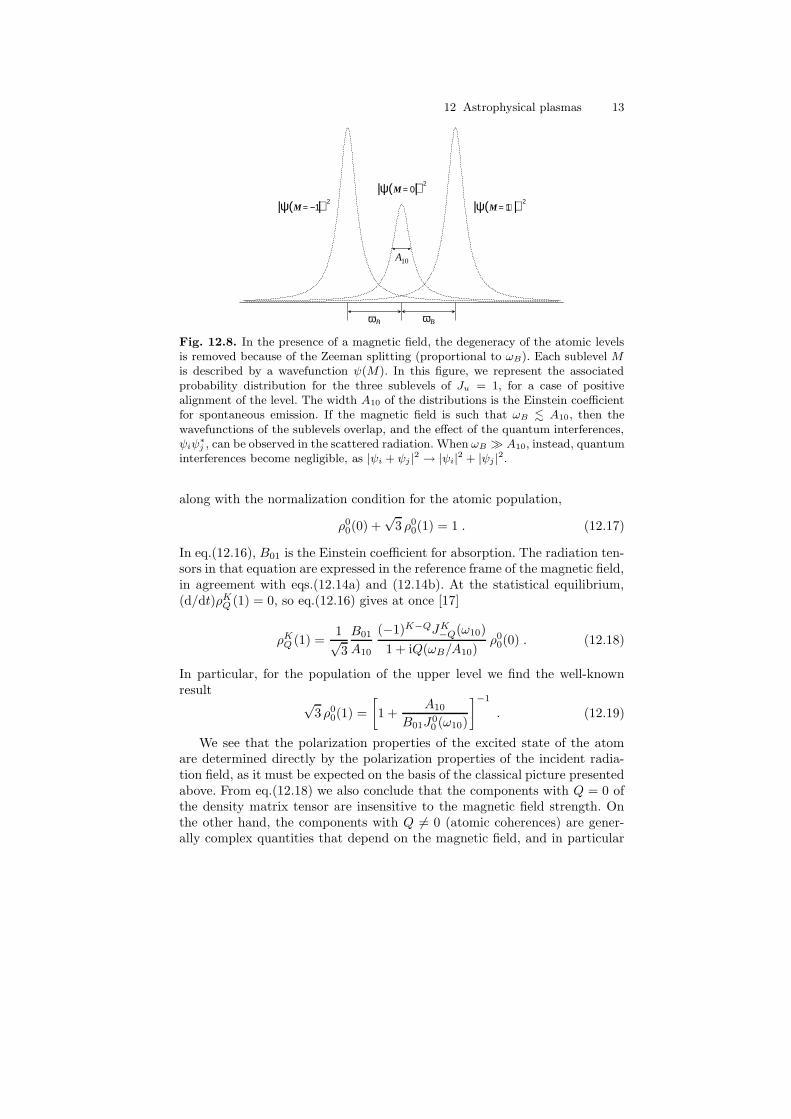
Fig. 12.8. In the presence of a magnetic field, the degeneracy of the atomic levelsis removed because of the Zeeman splitting (proportional to ωB). Each sublevel Mis described by a wavefunction ψ(M). In this figure, we represent the associatedprobability distribution for the three sublevels of Ju = 1, for a case of positivealignment of the level. The width A10 of the distributions is the Einstein coefficientfor spontaneous emission. If the magnetic field is such that ωB . A10, then thewavefunctions of the sublevels overlap, and the effect of the quantum interferences,ψiψ
∗
j , can be observed in the scattered radiation. When ωB � A10, instead, quantuminterferences become negligible, as |ψi + ψj |2 → |ψi|2 + |ψj |2.
along with the normalization condition for the atomic population,
ρ00(0) +
√3 ρ0
0(1) = 1 . (12.17)
In eq.(12.16), B01 is the Einstein coefficient for absorption. The radiation ten-sors in that equation are expressed in the reference frame of the magnetic field,in agreement with eqs.(12.14a) and (12.14b). At the statistical equilibrium,(d/dt)ρK
Q (1) = 0, so eq.(12.16) gives at once [17]
ρKQ (1) =
1√3
B01
A10
(−1)K−QJK−Q(ω10)
1 + iQ(ωB/A10)ρ00(0) . (12.18)
In particular, for the population of the upper level we find the well-knownresult
√3 ρ0
0(1) =
[
1 +A10
B01J00 (ω10)
]−1
. (12.19)
We see that the polarization properties of the excited state of the atomare determined directly by the polarization properties of the incident radia-tion field, as it must be expected on the basis of the classical picture presentedabove. From eq.(12.18) we also conclude that the components with Q = 0 ofthe density matrix tensor are insensitive to the magnetic field strength. Onthe other hand, the components with Q 6= 0 (atomic coherences) are gener-ally complex quantities that depend on the magnetic field, and in particular
14 Roberto Casini and Egidio Landi Degl’Innocenti
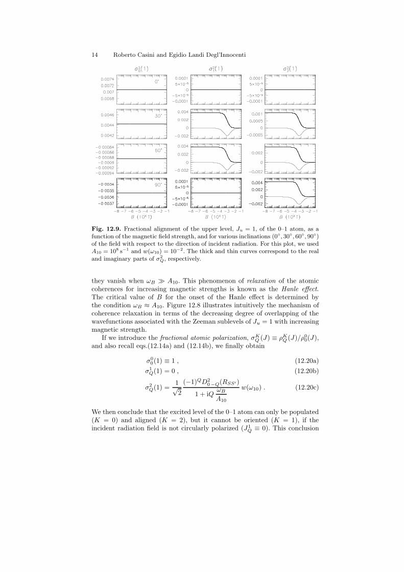
Fig. 12.9. Fractional alignment of the upper level, Ju = 1, of the 0–1 atom, as afunction of the magnetic field strength, and for various inclinations (0◦, 30◦, 60◦, 90◦)of the field with respect to the direction of incident radiation. For this plot, we usedA10 = 108 s−1 and w(ω10) = 10−2. The thick and thin curves correspond to the realand imaginary parts of σ2
Q, respectively.
they vanish when ωB � A10. This phenomenon of relaxation of the atomiccoherences for increasing magnetic strengths is known as the Hanle effect.The critical value of B for the onset of the Hanle effect is determined bythe condition ωB ≈ A10. Figure 12.8 illustrates intuitively the mechanism ofcoherence relaxation in terms of the decreasing degree of overlapping of thewavefunctions associated with the Zeeman sublevels of Ju = 1 with increasingmagnetic strength.
If we introduce the fractional atomic polarization, σKQ (J) ≡ ρK
Q (J)/ρ00(J),
and also recall eqs.(12.14a) and (12.14b), we finally obtain
σ00(1) ≡ 1 , (12.20a)
σ1Q(1) = 0 , (12.20b)
σ2Q(1) =
1√2
(−1)QD20−Q(RSS′)
1 + iQωB
A10
w(ω10) . (12.20c)
We then conclude that the excited level of the 0–1 atom can only be populated(K = 0) and aligned (K = 2), but it cannot be oriented (K = 1), if theincident radiation field is not circularly polarized (J1
Q ≡ 0). This conclusion
12 Astrophysical plasmas 15
Q B
J
Bk
solar
local v
ertical
p h ot o s p
h e r ic r a
d i a ti o n
c o nex '
z '
y '
F B
J Bj B
xy
zl i n e - o f - s i g h t
O
h
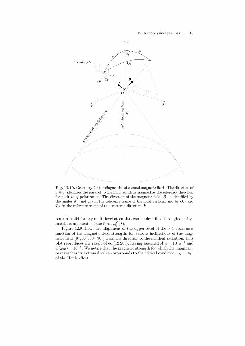
Fig. 12.10. Geometry for the diagnostics of coronal magnetic fields. The direction ofy ≡ y′ identifies the parallel to the limb, which is assumed as the reference directionfor positive Q polarization. The direction of the magnetic field, B, is identified bythe angles ϑB and ϕB in the reference frame of the local vertical, and by ΘB andΦB in the reference frame of the scattered direction, k.
remains valid for any multi-level atom that can be described through density-matrix components of the form ρK
Q (J).Figure 12.9 shows the alignment of the upper level of the 0–1 atom as a
function of the magnetic field strength, for various inclinations of the mag-netic field (0◦, 30◦, 60◦, 90◦) from the direction of the incident radiation. Thisplot reproduces the result of eq.(12.20c), having assumed A10 = 108 s−1 andw(ω10) = 10−2. We notice that the magnetic strength for which the imaginarypart reaches its extremal value corresponds to the critical condition ωB = A10
of the Hanle effect.
16 Roberto Casini and Egidio Landi Degl’Innocenti
Application: Polarized coronal emission
Despite the simplicity of the 0–1 atomic model, there are polarization phenom-ena in astrophysics that are suitably described by it. A noteworthy examplefrom solar physics is the polarized emission of the forbidden (M1) transition ofFeXIII λ1074.7 nm, which is predominantly produced in the 2× 10⁶ K regionsof the solar corona.
Because of the very small Einstein A-coefficients characterizing M1 tran-sitions (for the FeXIII λ1074.7 nm line, it is A10 = 14 s−1), the atomic coher-ences are always completely relaxed, even in the presence of the very weakmagnetic field of the quiet-sun corona (B ∼ 10−4–10−3 T). The atomic po-larization of the first excited level of FeXIII is thus completely described bythe fractional alignment σ2
0(1). Since this quantity is independent of the mag-netic strength, it is impossible to achieve a complete diagnostics of the coronalmagnetic field based only on the linear polarization signal that is producedby the atomic alignment, and information about the field strength must comefrom the Zeeman effect.
Because of the plasma conditions in the solar corona (large radiationanisotropy, small magnetic fields, large thermal Doppler broadening), the lin-ear polarization signal of the FeXIII λ1074.7 nm line is completely dominatedby the atomic alignment in the upper level, Ju = 1, of the transition. In fact,the linear polarization signature of the transverse Zeeman effect turns outto be completely negligible. On the other hand, the circular polarization ofthis line is predominantly produced by the longitudinal Zeeman effect, whichgives information about the projected component of the magnetic field alongthe line-of-sight. However, the atomic alignment determines a systematic cor-rection to Zeeman effect in the circular polarization signal, which must beproperly taken into account for a reliable diagnostics.
In more detail, the Stokes vector of the FeXIII λ1074.7 nm line is [6, 18]
I(ω) ∝[
1 +1
2√
2(3 cos2 ΘB − 1) σ2
0(1)
]
φ(ω10 − ω) , (12.21a)
Q(ω) ∝ − 3
2√
2sin2 ΘB cos 2ΦB σ2
0(1) φ(ω10 − ω) , (12.21b)
U(ω) ∝ − 3
2√
2sin2 ΘB sin 2ΦB σ2
0(1) φ(ω10 − ω) , (12.21c)
V (ω) ∝ −3
2
[
1 +1√2
σ20(1)
]
ωB cosΘB φ′(ω10 − ω) , (12.21d)
where φ(ω10 − ω) is a Gaussian profile with Doppler width corresponding tothe coronal temperature. The scattering and magnetic geometries entering theabove equations are illustrated in Fig. 12.10. We notice the “−” sign in frontof eqs.(12.21b) and (12.21c), which is a consequence of the M1 character ofthe FeXIII λ1074.7 nm line [6].
Introducing the frequency-integrated Stokes parameters, Si, we note that
12 Astrophysical plasmas 17
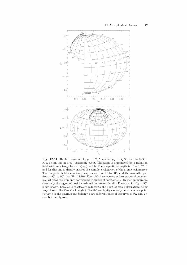
Fig. 12.11. Hanle diagrams of pU = U/I against pQ = Q/I, for the FeXIIIλ1074.7 nm line in a 90◦ scattering event. The atom is illuminated by a radiationfield with anisotropy factor w(ω10) = 0.5. The magnetic strength is B = 10−4 T,and for this line it already ensures the complete relaxation of the atomic coherences.The magnetic field inclination, ϑB, varies from 0◦ to 90◦, and the azimuth, ϕB,from −90◦ to 90◦ (see Fig. 12.10). The thick lines correspond to curves of constantϑB, whereas the thin lines correspond to curves of constant ϕB. In the top figure weshow only the region of positive azimuth in greater detail. (The curve for ϑB = 55◦
is not shown, because it practically reduces to the point of zero polarization, beingvery close to the Van Vleck angle.) The 90◦ ambiguity can only occur where a point(pU , pQ) in the diagram can belong to two different pairs of isocurves of ϑB and ϕB
(see bottom figure).
18 Roberto Casini and Egidio Landi Degl’Innocenti
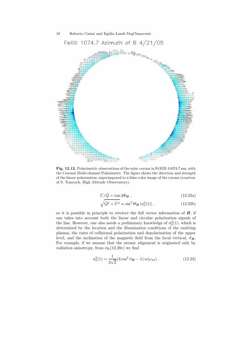
Fig. 12.12. Polarimetric observations of the solar corona in FeXIII λ1074.7 nm, withthe Coronal Multi-channel Polarimeter. The figure shows the direction and strengthof the linear polarization, superimposed to a false-color image of the corona (courtesyof S. Tomczyk, High Altitude Observatory).
U/Q = tan 2ΦB , (12.22a)√
Q2 + U2 ∝ sin2 ΘB |σ20(1)| , (12.22b)
so it is possible in principle to retrieve the full vector information of B, ifone takes into account both the linear and circular polarization signals ofthe line. However, one also needs a preliminary knowledge of σ2
0(1), which isdetermined by the location and the illumination conditions of the emittingplasma, the rates of collisional polarization and depolarization of the upperlevel, and the inclination of the magnetic field from the local vertical, ϑB .For example, if we assume that the atomic alignment is originated only byradiation anisotropy, from eq.(12.20c) we find
σ20(1) =
1
2√
2(3 cos2 ϑB − 1) w(ω10) , (12.23)
12 Astrophysical plasmas 19
having recalled the expression of the rotation matrix D200(RSS′) ≡ d2
00(ϑB)[15]. We then see that σ2
0(1) vanishes at the Van Vleck angle, defined byϑVV ≡ arccos(1/
√3) ≈ 54.7◦ (see also Fig. 12.9), and at its supplementary
angle, 180◦−ϑVV. In general, when the sign of σ20(1) is not known a priori (e.g.,
it is not known whether ϑB < ϑVV or ϑB > ϑVV), from eqs.(12.21b)–(12.21c)and (12.22a), we can only determine the direction of the field on the plane ofthe sky with an ambiguity of 90◦ [18]. This is illustrated in Fig. 12.11, for aparticular scattering geometry (see caption to the figure for more details). Weremark that the use of all the information contained in the Stokes vector ofthe emitted radiation is a necessary condition (although not always sufficient)for the resolution of such 90◦ ambiguity in practical cases.
Figure 12.12 shows recent observations of the solar corona by S. Tom-czyk (High Altitude Observatory) with the Coronal Multi-channel Polarime-ter (CoMP [19]), deployed at the One-Shot coronograph of the National SolarObservatory at Sacramento Peak (Sunspot, New Mexico, U.S.A.). The figuredisplays the direction and strength of the linear polarization (as inferred fromeqs.(12.22a) and (12.22b), respectively), superimposed to a false-color imageof the solar corona at FeXIII λ1074.7 nm. We note the presence of regions ofvanishing polarization, which indicate the possible occurrence of longitudinalfields (ΘB ≈ 0◦, 180◦) or of the Van Vleck effect (ϑB ≈ ϑVV, 180◦ − ϑVV).
12.4.2 The 1–0 atom in a magnetic field
As a second example, we discuss the two-level atom with Jl = 1 and Ju = 0.The polarizability of the lower level makes it impossible to describe this atomicmodel in classical terms, like we did for the 0–1 atom. The quantum approachillustrated in Sect. 12.3 is thus the only means of investigation of the propertiesof the 1–0 atom. These properties have in recent times become of relevantinterest for the diagnostics of magnetic fields in the solar chromosphere [20].
In order to study the properties of the 1–0 model atom, we write againthe SEE of the polarizable level (which this time is the lower level),
d
dtρK
Q (1) + iωB Q ρKQ (1) = −RA(KQ) +
1√3
δK0 δQ0 A01 ρ00(0) , (12.24)
where
RA(KQ) = B10
∑
K′K′′
1 + (−1)K+K′+K′′
2
√
3(2K + 1)(2K ′ + 1)(2K ′′ + 1)
×{
K K ′ K ′′
1 1 1
}
∑
Q′Q′′
(−1)K′′+Q′
(
K K ′ K ′′
Q −Q′ Q′′
)
ρK′
Q′ (1) JK′′
Q′′ (ω01) .
We see immediately that, despite the simplicity of the atomic structureinvolved, the solution of the statistical equilibrium of the 1–0 atom is far more
20 Roberto Casini and Egidio Landi Degl’Innocenti
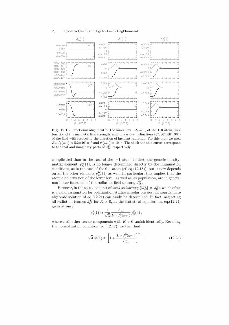
Fig. 12.13. Fractional alignment of the lower level, Jl = 1, of the 1–0 atom, as afunction of the magnetic field strength, and for various inclinations (0◦, 30◦, 60◦, 90◦)of the field with respect to the direction of incident radiation. For this plot, we usedB10J
0
0 (ω01) ≈ 5.2×10⁴ s−1 and w(ω01) = 10−2. The thick and thin curves correspondto the real and imaginary parts of σ2
Q, respectively.
complicated than in the case of the 0–1 atom. In fact, the generic density-matrix element, ρK
Q (1), is no longer determined directly by the illuminationconditions, as in the case of the 0–1 atom (cf. eq.(12.18)), but it now dependson all the other elements ρK′
Q′ (1) as well. In particular, this implies that theatomic polarization of the lower level, as well as its population, are in generalnon-linear functions of the radiation field tensors, JK
Q .
However, in the so-called limit of weak anisotropy (|J2Q| � J0
0 ), which oftenis a valid assumption for polarization studies in solar physics, an approximatealgebraic solution of eq.(12.24) can easily be determined. In fact, neglectingall radiation tensors JK
Q for K > 0, at the statistical equilibrium, eq.(12.24)gives at once
ρ00(1) ≈ 1√
3
A01
B10J00 (ω01)
ρ00(0) ,
whereas all other tensor components with K > 0 vanish identically. Recallingthe normalization condition, eq.(12.17), we then find
√3 ρ0
0(1) ≈[
1 +B10J
00 (ω01)
A01
]−1
. (12.25)
12 Astrophysical plasmas 21
which is the counterpart for the 1–0 atom of eq.(12.19). One can then goback to considering eq.(12.24) for K = 2,6 and solve for the fractional atomicalignment of the lower level, σ2
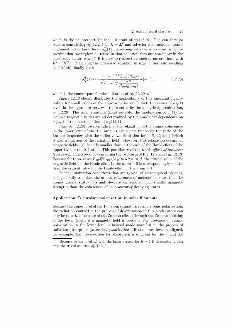
Q(1). In keeping with the weak-anisotropy ap-proximation, we neglect all terms in that equation that are non-linear in theanisotropy factor, w(ω01). It is easy to realize that such terms are those withK ′ = K ′′ = 2. Solving the linearized equation in w(ω01), and also recallingeq.(12.14b), finally gives
σ2Q(1) ≈ − 1√
2
(−1)QD20−Q(RSS′)
1 + iQωB
B10J00 (ω01)
w(ω01) , (12.26)
which is the counterpart for the 1–0 atom of eq.(12.20c).Figure 12.13 clearly illustrates the applicability of this linearization pro-
cedure for small values of the anisotropy factor. In fact, the values of σ2Q(1)
given in the figure are very well represented by the analytic approximation,eq.(12.26). The small residuals (most notably, the modulation of σ2
0(1) forinclined magnetic fields) are all determined by the non-linear dependence onw(ω01) of the exact solution of eq.(12.24).
From eq.(12.26), we conclude that the relaxation of the atomic coherencesin the lower level of the 1–0 atom is again determined by the ratio of theLarmor frequency with the radiative width of that level, B10J
00 (ω01) (which
is now a function of the radiation field). However, this relaxation occurs formagnetic fields significantly smaller than in the case of the Hanle effect of theupper level of the 0–1 atom. This peculiarity of the Hanle effect of the lower
level is well understood by comparing the two cases of Fig. 12.9 and Fig. 12.13.Because for those cases B10J
00 (ω01)/A10 ≈ 5.2×10⁻⁴, the critical value of the
magnetic field for the Hanle effect in the atom 1–0 is correspondingly smallerthan the critical value for the Hanle effect in the atom 0–1.
Under illumination conditions that are typical of astrophysical plasmas,it is generally true that the atomic coherences of metastable states (like theatomic ground state) in a multi-level atom relax at much smaller magneticstrengths than the coherences of spontaneously decaying states.
Application: Dichroism polarization in solar filaments
Because the upper level of the 1–0 atom cannot carry any atomic polarization,the radiation emitted in the process of de-excitation in this model atom canonly be polarized because of the Zeeman effect (through the Zeeman splittingof the lower level), if a magnetic field is present. The presence of atomicpolarization in the lower level is instead made manifest in the process ofradiation absorption (dichroism polarization). If the lower level is aligned,for example, the cross-section for absorption is different for the π and the
6Because we assumed J1
0 ≡ 0, the linear system for K = 1 is decoupled, givingonly the trivial solution ρ1
Q(1) ≡ 0.
22 Roberto Casini and Egidio Landi Degl’Innocenti
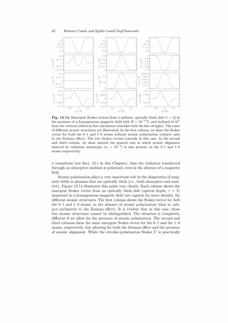
Fig. 12.14. Emergent Stokes vectors from a uniform, optically thick slab (τ = 2) inthe presence of a homogeneous magnetic field with B = 10−3 T, and inclined of 45◦
from the vertical (which in this calculation coincides with the line-of-sight). The casesof different atomic structures are illustrated. In the first column, we show the Stokesvector for both the 0–1 and 1–0 atoms without atomic polarization (subject onlyto the Zeeman effect). The two Stokes vectors coincide in this case. In the secondand third column, we show instead the general case in which atomic alignmentinduced by radiation anisotropy (w = 10−2) is also present, in the 0–1 and 1–0atoms respectively.
σ transitions (see Sect. 12.1 in this Chapter), thus the radiation transferredthrough an absorptive medium is polarized, even in the absence of a magneticfield.
Atomic polarization plays a very important role in the diagnostics of mag-netic fields in plasmas that are optically thick (i.e., both absorptive and emit-tive). Figure 12.14 illustrates this point very clearly. Each column shows theemergent Stokes vector from an optically thick slab (optical depth, τ = 2)immersed in a homogeneous magnetic field (see caption for more details), fordifferent atomic structures. The first column shows the Stokes vector for both
the 0–1 and 1–0 atoms, in the absence of atomic polarization (that is, sub-ject exclusively to the Zeeman effect). It is evident that in this case, thosetwo atomic structures cannot be distinguished. The situation is completelydifferent if we allow for the presence of atomic polarization. The second andthird columns show the same emergent Stokes vector for the 0–1 and the 1–0atoms, respectively, but allowing for both the Zeeman effect and the presenceof atomic alignment. While the circular-polarization Stokes V is practically
12 Astrophysical plasmas 23
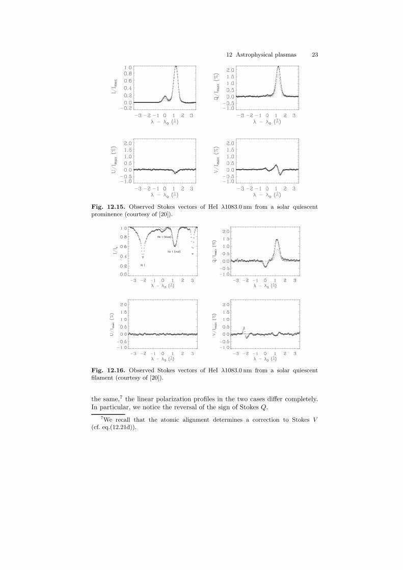
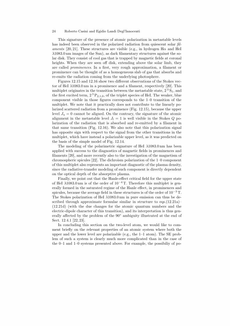
Fig. 12.15. Observed Stokes vectors of HeI λ1083.0 nm from a solar quiescentprominence (courtesy of [20]).
Fig. 12.16. Observed Stokes vectors of HeI λ1083.0 nm from a solar quiescentfilament (courtesy of [20]).
the same,7 the linear polarization profiles in the two cases differ completely.In particular, we notice the reversal of the sign of Stokes Q.
7We recall that the atomic alignment determines a correction to Stokes V(cf. eq.(12.21d)).
24 Roberto Casini and Egidio Landi Degl’Innocenti
This signature of the presence of atomic polarization in metastable levelshas indeed been observed in the polarized radiation from quiescent solar fil-
aments [20, 21]. These structures are visible (e.g., in hydrogen Hα and HeIλ1083.0 nm images of the Sun), as dark filamentary structures against the so-lar disk. They consist of cool gas that is trapped by magnetic fields at coronalheights. When they are seen off disk, extending above the solar limb, theyare called prominences. In a first, very rough approximation, a filament orprominence can be thought of as a homogeneous slab of gas that absorbs andre-emits the radiation coming from the underlying photosphere.
Figures 12.15 and 12.16 show two different observations of the Stokes vec-tor of HeI λ1083.0 nm in a prominence and a filament, respectively [20]. Thismultiplet originates in the transition between the metastable state, 2 3 S1, andthe first excited term, 2 3 P2,1,0, of the triplet species of HeI. The weaker, bluecomponent visible in those figures corresponds to the 1–0 transition of themultiplet. We note that it practically does not contribute to the linearly po-larized scattered radiation from a prominence (Fig. 12.15), because the upperlevel Ju = 0 cannot be aligned. On the contrary, the signature of the atomicalignment in the metastable level Jl = 1 is well visible in the Stokes Q po-larization of the radiation that is absorbed and re-emitted by a filament inthat same transition (Fig. 12.16). We also note that this polarization signalhas opposite sign with respect to the signal from the other transitions in themultiplet, which have instead a polarizable upper level, as it was predicted onthe basis of the simple model of Fig. 12.14.
The modeling of the polarimetric signature of HeI λ1083.0 nm has beenapplied with success to the diagnostics of magnetic fields in prominences andfilaments [20], and more recently also to the investigation of the magnetism ofchromospheric spicules [22]. The dichroism polarization of the 1–0 componentof this multiplet also represents an important diagnostic of the plasma density,since the radiative-transfer modeling of such component is directly dependenton the optical depth of the absorptive plasma.
Finally, we point out that the Hanle-effect critical field for the upper stateof HeI λ1083.0 nm is of the order of 10−4 T. Therefore this multiplet is gen-erally formed in the saturated regime of the Hanle effect, in prominences andspicules, because the average field in these structures is of the order of 10−3 T.The Stokes polarization of HeI λ1083.0 nm in pure emission can thus be de-scribed through approximate formulae similar in structure to eqs.(12.21a)–(12.21d) (with the due changes for the atomic quantum numbers and theelectric-dipole character of this transition), and its interpretation is thus gen-erally affected by the problem of the 90◦ ambiguity illustrated at the end ofSect. 12.4.1 [22, 23].
In concluding this section on the two-level atom, we would like to com-ment briefly on the relevant properties of an atomic system where both theupper and the lower level are polarizable (e.g., the 1–1 atom). The SE prob-lem of such a system is clearly much more complicated than in the case ofthe 0–1 and 1–0 systems presented above. For example, the possibiliy of po-
12 Astrophysical plasmas 25
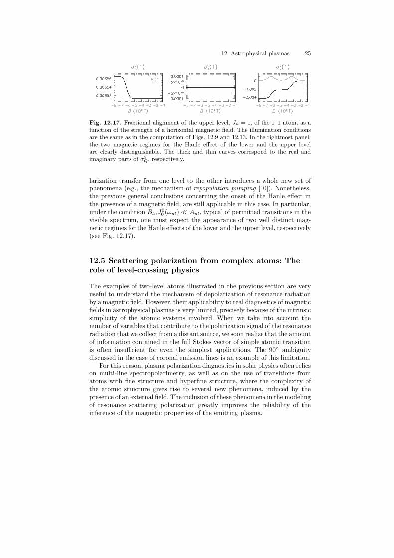
Fig. 12.17. Fractional alignment of the upper level, Ju = 1, of the 1–1 atom, as afunction of the strength of a horizontal magnetic field. The illumination conditionsare the same as in the computation of Figs. 12.9 and 12.13. In the rightmost panel,the two magnetic regimes for the Hanle effect of the lower and the upper levelare clearly distinguishable. The thick and thin curves correspond to the real andimaginary parts of σ2
Q, respectively.
larization transfer from one level to the other introduces a whole new set ofphenomena (e.g., the mechanism of repopulation pumping [10]). Nonetheless,the previous general conclusions concerning the onset of the Hanle effect inthe presence of a magnetic field, are still applicable in this case. In particular,under the condition BluJ0
0 (ωul) � Aul, typical of permitted transitions in thevisible spectrum, one must expect the appearance of two well distinct mag-netic regimes for the Hanle effects of the lower and the upper level, respectively(see Fig. 12.17).
12.5 Scattering polarization from complex atoms: The
role of level-crossing physics
The examples of two-level atoms illustrated in the previous section are veryuseful to understand the mechanism of depolarization of resonance radiationby a magnetic field. However, their applicability to real diagnostics of magneticfields in astrophysical plasmas is very limited, precisely because of the intrinsicsimplicity of the atomic systems involved. When we take into account thenumber of variables that contribute to the polarization signal of the resonanceradiation that we collect from a distant source, we soon realize that the amountof information contained in the full Stokes vector of simple atomic transitionis often insufficient for even the simplest applications. The 90◦ ambiguitydiscussed in the case of coronal emission lines is an example of this limitation.
For this reason, plasma polarization diagnostics in solar physics often relieson multi-line spectropolarimetry, as well as on the use of transitions fromatoms with fine structure and hyperfine structure, where the complexity ofthe atomic structure gives rise to several new phenomena, induced by thepresence of an external field. The inclusion of these phenomena in the modelingof resonance scattering polarization greatly improves the reliability of theinference of the magnetic properties of the emitting plasma.
26 Roberto Casini and Egidio Landi Degl’Innocenti
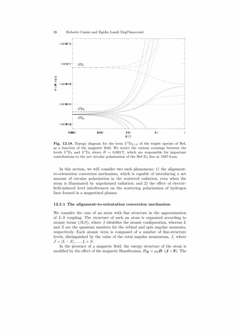
Fig. 12.18. Energy diagram for the term 3 3D2,1,0 of the triplet species of HeI,as a function of the magnetic field. We notice the various crossings between thelevels 3 3D2 and 3 3D3 above B = 0.003 T, which are responsible for importantcontributions to the net circular polarization of the HeI D3 line at λ587.6 nm.
In this section, we will consider two such phenomena: 1) the alignment-to-orientation conversion mechanism, which is capable of introducing a netamount of circular polarization in the scattered radiation, even when theatom is illuminated by unpolarized radiation; and 2) the effect of electric-field-induced level interferences on the scattering polarization of hydrogenlines formed in a magnetized plasma.
12.5.1 The alignment-to-orientation conversion mechanism
We consider the case of an atom with fine structure in the approximationof L-S coupling. The structure of such an atom is organized according toatomic terms (βLS), where β identifies the atomic configuration, whereas Land S are the quantum numbers for the orbital and spin angular momenta,respectively. Each atomic term is composed of a number of fine-structurelevels, distinguished by the value of the total angular momentum, J , whereJ = |L − S|, . . . , L + S.
In the presence of a magnetic field, the energy structure of the atom ismodified by the effect of the magnetic Hamiltonian, HB = µ0B · (J +S). The
12 Astrophysical plasmas 27
best known among these magnetic effects is undoubtely the Zeeman effect [2].This is the lifting of the (2J + 1)-fold degeneracy of a J level, because of theenergy separation (Zeeman splitting) of its magnetic sublevels, proportionallyto the azimuthal quantum number M = −J, . . . , J , under the action of themagnetic field (see also Sect. 12.2).
In general, the magnetic Hamiltonian mixes levels with different J , so theZeeman effect provides a good representation of the energy structure of anatom with fine structure only when |HB | � |HFS|, that is, when the Zee-man splitting is much smaller than the typical energy separation between theJ levels of an LS-term. On the contrary, when the magnetic field is largeenough that |HB | ∼ |HFS|, the magnetic-induced J-mixing is responsiblefor significant modifications of the energy structure typical of the Zeemaneffect, and level-crossing effects become observable in the polarization of scat-tered radiation (see Fig. 12.18). This is the regime of the so-called incomplete
Paschen-Back effect. Because of the importance of J-mixing in the Paschen-Back regime, the atomic system must be described by density-matrix elementsof the form βLSρK
Q (J, J ′), to account for quantum interferences between dis-tinct J levels within the atomic term (βLS).
In order to understand how magnetic-induced J-mixing modifies the po-larization of the scattered radiation, we must consider in some details the formof the SEEs for an atom with fine structure in a magnetic field. The subjectis exhaustively treated in [6], so here we focus only on the contribution of theatomic Hamiltonian to the SEEs. This contribution is the so-called magnetic
kernel, which arises from the iωpqρpq term of eq.(12.10). Its expression is thefollowing,
iN(βLS; JJ ′KQ; J ′′J ′′′K ′Q′) = δJJ′′ δJ′J′′′ δKK′ δQQ′ iωβLSJJ′
+ δQQ′ iωB (−1)J+J′−Q ΠKK′
(
K K ′ 1−Q Q 0
)
×[
δJ′J′′′ ΓLS(J, J ′′)
{
K K ′ 1J ′′ J J ′
}
+ δJJ′′ (−1)K+K′
ΓLS(J ′′′, J ′)
{
K K ′ 1J ′′′ J ′ J
}
]
, (12.27)
where
ΓLS(J, J ′) = δJJ′ ΠJ
√
J(J + 1)
− (−1)L+S+J ΠJJ′S
√
(S + 1)S
{
J J ′ 1S S L
}
. (12.28)
The magnetic kernel weighs in the contributions from all the density-matrixelements βLSρK′
Q′ (J ′′, J ′′′) to the SEE of the specific element βLSρKQ (J, J ′).
When quantum interferences between distinct J levels are negligible, wecan verify, using basic Racah algebra, that the magnetic kernel reduces to the
28 Roberto Casini and Egidio Landi Degl’Innocenti
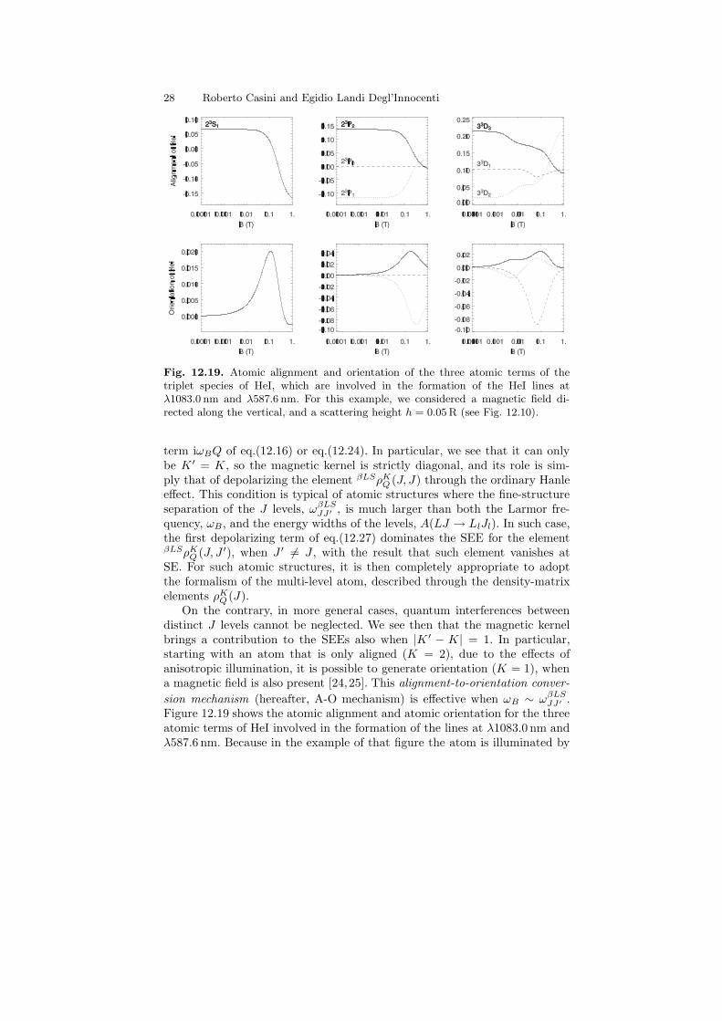
Fig. 12.19. Atomic alignment and orientation of the three atomic terms of thetriplet species of HeI, which are involved in the formation of the HeI lines atλ1083.0 nm and λ587.6 nm. For this example, we considered a magnetic field di-rected along the vertical, and a scattering height h = 0.05 R (see Fig. 12.10).
term iωBQ of eq.(12.16) or eq.(12.24). In particular, we see that it can onlybe K ′ = K, so the magnetic kernel is strictly diagonal, and its role is sim-ply that of depolarizing the element βLSρK
Q (J, J) through the ordinary Hanleeffect. This condition is typical of atomic structures where the fine-structureseparation of the J levels, ωβLS
JJ′ , is much larger than both the Larmor fre-quency, ωB , and the energy widths of the levels, A(LJ → LlJl). In such case,the first depolarizing term of eq.(12.27) dominates the SEE for the elementβLSρK
Q (J, J ′), when J ′ 6= J , with the result that such element vanishes atSE. For such atomic structures, it is then completely appropriate to adoptthe formalism of the multi-level atom, described through the density-matrixelements ρK
Q (J).On the contrary, in more general cases, quantum interferences between
distinct J levels cannot be neglected. We see then that the magnetic kernelbrings a contribution to the SEEs also when |K ′ − K| = 1. In particular,starting with an atom that is only aligned (K = 2), due to the effects ofanisotropic illumination, it is possible to generate orientation (K = 1), whena magnetic field is also present [24,25]. This alignment-to-orientation conver-
sion mechanism (hereafter, A-O mechanism) is effective when ωB ∼ ωβLSJJ′ .
Figure 12.19 shows the atomic alignment and atomic orientation for the threeatomic terms of HeI involved in the formation of the lines at λ1083.0 nm andλ587.6 nm. Because in the example of that figure the atom is illuminated by
12 Astrophysical plasmas 29
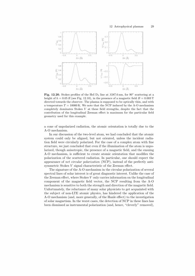
Fig. 12.20. Stokes profiles of the HeI D3 line at λ587.6 nm, for 90◦ scattering at aheight of h = 0.05R (see Fig. 12.10), in the presence of a magnetic field B = 0.003 Tdirected towards the observer. The plasma is supposed to be optically thin, and witha temperature T = 10000 K. We note that the NCP induced by the A-O mechanismcompletely dominates Stokes V at these field strengths, despite the fact that thecontribution of the longitudinal Zeeman effect is maximum for the particular fieldgeometry used for this example.
a cone of unpolarized radiation, the atomic orientation is totally due to theA-O mechanism.
In our discussion of the two-level atom, we had concluded that the atomicsystem could only be aligned, but not oriented, unless the incident radia-tion field were circularly polarized. For the case of a complex atom with finestructure, we just concluded that even if the illumination of the atom is unpo-larized, though anisotropic, the presence of a magnetic field, and the ensuingA-O mechanism, is sufficient to create atomic orientation that modifies thepolarization of the scattered radiation. In particular, one should expect theappearance of net circular polarization (NCP), instead of the perfectly anti-symmetric Stokes V signal characteristic of the Zeeman effect.
The signature of the A-O mechanism in the circular polarization of severalspectral lines of solar interest is of great diagnostic interest. Unlike the case ofthe Zeeman effect, where Stokes V only carries information on the longitudinalcomponent of the magnetic field vector, the NCP resulting from the A-Omechanism is sensitive to both the strength and direction of the magnetic field.Unfortunately, the reluctance of many solar physicists to get acquainted withthe subject of non-LTE atomic physics, has hindered the application of theA-O mechanism (and, more generally, of the Hanle effect) to the investigationof solar magnetism. In the worst cases, the detection of NCP in these lines hasbeen dismissed as instrumental polarization (and, hence, “cleverly” removed),
30 Roberto Casini and Egidio Landi Degl’Innocenti
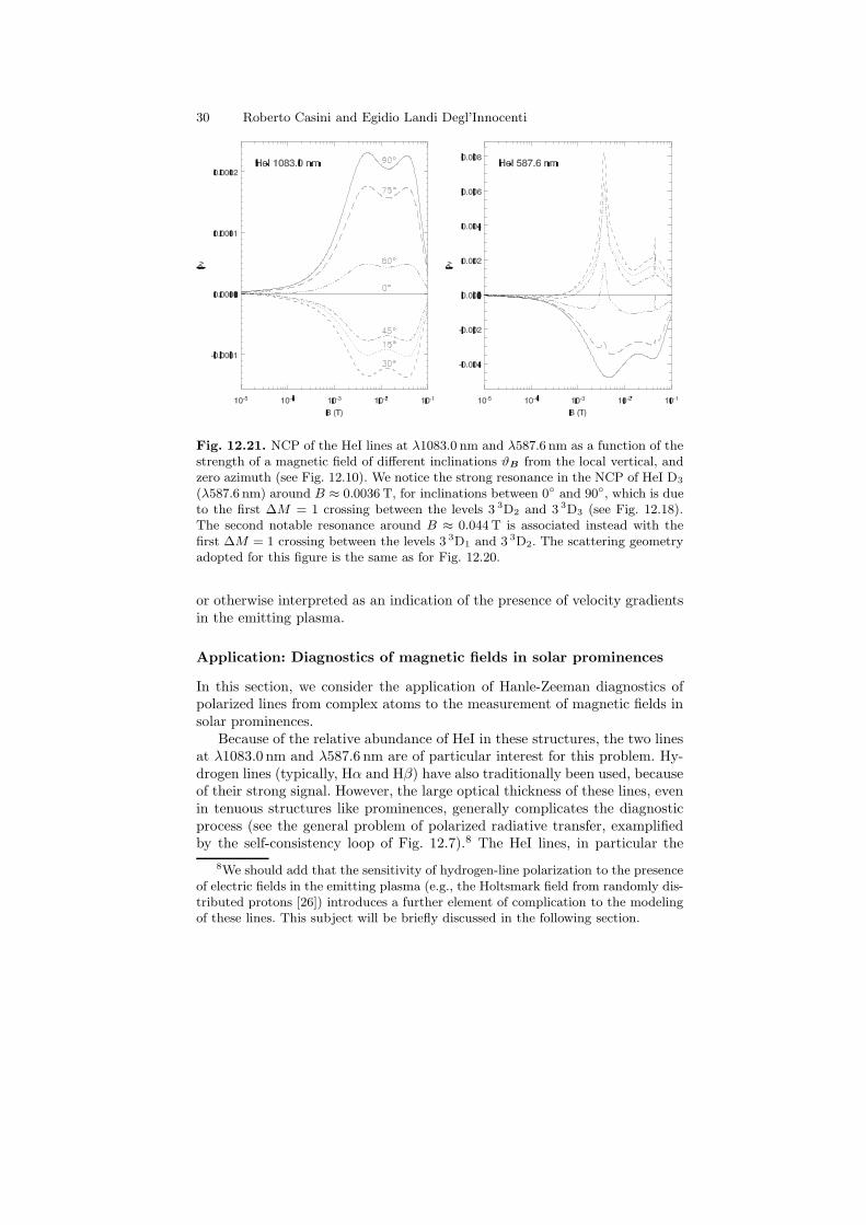
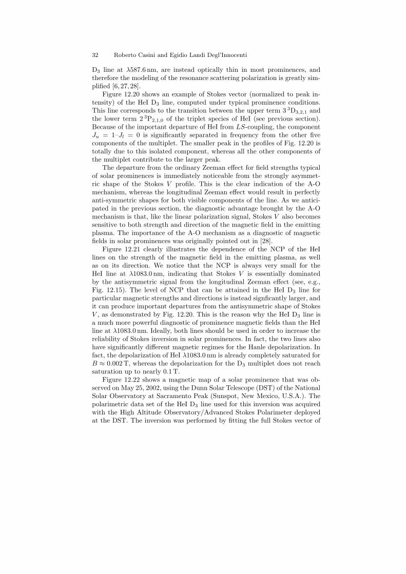
Fig. 12.21. NCP of the HeI lines at λ1083.0 nm and λ587.6 nm as a function of thestrength of a magnetic field of different inclinations ϑB from the local vertical, andzero azimuth (see Fig. 12.10). We notice the strong resonance in the NCP of HeI D3
(λ587.6 nm) around B ≈ 0.0036 T, for inclinations between 0◦ and 90◦, which is dueto the first ∆M = 1 crossing between the levels 3 3D2 and 3 3D3 (see Fig. 12.18).The second notable resonance around B ≈ 0.044 T is associated instead with thefirst ∆M = 1 crossing between the levels 3 3D1 and 3 3D2. The scattering geometryadopted for this figure is the same as for Fig. 12.20.
or otherwise interpreted as an indication of the presence of velocity gradientsin the emitting plasma.
Application: Diagnostics of magnetic fields in solar prominences
In this section, we consider the application of Hanle-Zeeman diagnostics ofpolarized lines from complex atoms to the measurement of magnetic fields insolar prominences.
Because of the relative abundance of HeI in these structures, the two linesat λ1083.0 nm and λ587.6 nm are of particular interest for this problem. Hy-drogen lines (typically, Hα and Hβ) have also traditionally been used, becauseof their strong signal. However, the large optical thickness of these lines, evenin tenuous structures like prominences, generally complicates the diagnosticprocess (see the general problem of polarized radiative transfer, examplifiedby the self-consistency loop of Fig. 12.7).8 The HeI lines, in particular the
8We should add that the sensitivity of hydrogen-line polarization to the presenceof electric fields in the emitting plasma (e.g., the Holtsmark field from randomly dis-tributed protons [26]) introduces a further element of complication to the modelingof these lines. This subject will be briefly discussed in the following section.
12 Astrophysical plasmas 31
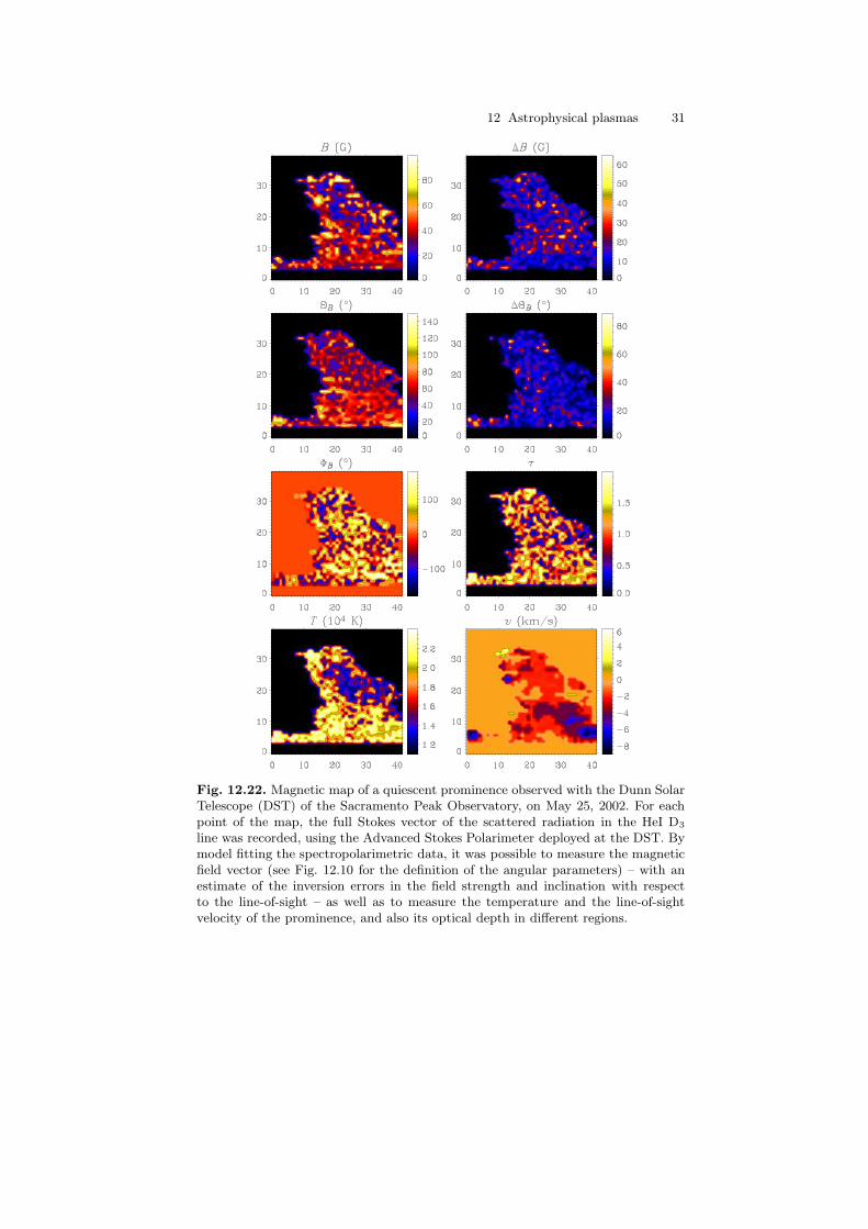
Fig. 12.22. Magnetic map of a quiescent prominence observed with the Dunn SolarTelescope (DST) of the Sacramento Peak Observatory, on May 25, 2002. For eachpoint of the map, the full Stokes vector of the scattered radiation in the HeI D3
line was recorded, using the Advanced Stokes Polarimeter deployed at the DST. Bymodel fitting the spectropolarimetric data, it was possible to measure the magneticfield vector (see Fig. 12.10 for the definition of the angular parameters) – with anestimate of the inversion errors in the field strength and inclination with respectto the line-of-sight – as well as to measure the temperature and the line-of-sightvelocity of the prominence, and also its optical depth in different regions.
32 Roberto Casini and Egidio Landi Degl’Innocenti
D3 line at λ587.6 nm, are instead optically thin in most prominences, andtherefore the modeling of the resonance scattering polarization is greatly sim-plified [6, 27, 28].
Figure 12.20 shows an example of Stokes vector (normalized to peak in-tensity) of the HeI D3 line, computed under typical prominence conditions.This line corresponds to the transition between the upper term 3 3D3,2,1 andthe lower term 2 3P2,1,0 of the triplet species of HeI (see previous section).Because of the important departure of HeI from LS-coupling, the componentJu = 1–Jl = 0 is significantly separated in frequency from the other fivecomponents of the multiplet. The smaller peak in the profiles of Fig. 12.20 istotally due to this isolated component, whereas all the other components ofthe multiplet contribute to the larger peak.
The departure from the ordinary Zeeman effect for field strengths typicalof solar prominences is immediately noticeable from the strongly asymmet-ric shape of the Stokes V profile. This is the clear indication of the A-Omechanism, whereas the longitudinal Zeeman effect would result in perfectlyanti-symmetric shapes for both visible components of the line. As we antici-pated in the previous section, the diagnostic advantage brought by the A-Omechanism is that, like the linear polarization signal, Stokes V also becomessensitive to both strength and direction of the magnetic field in the emittingplasma. The importance of the A-O mechanism as a diagnostic of magneticfields in solar prominences was originally pointed out in [28].
Figure 12.21 clearly illustrates the dependence of the NCP of the HeIlines on the strength of the magnetic field in the emitting plasma, as wellas on its direction. We notice that the NCP is always very small for theHeI line at λ1083.0 nm, indicating that Stokes V is essentially dominatedby the antisymmetric signal from the longitudinal Zeeman effect (see, e.g.,Fig. 12.15). The level of NCP that can be attained in the HeI D3 line forparticular magnetic strengths and directions is instead signficantly larger, andit can produce important departures from the antisymmetric shape of StokesV , as demonstrated by Fig. 12.20. This is the reason why the HeI D3 line isa much more powerful diagnostic of prominence magnetic fields than the HeIline at λ1083.0 nm. Ideally, both lines should be used in order to increase thereliability of Stokes inversion in solar prominences. In fact, the two lines alsohave significantly different magnetic regimes for the Hanle depolarization. Infact, the depolarization of HeI λ1083.0 nm is already completely saturated forB ≈ 0.002 T, whereas the depolarization for the D3 multiplet does not reachsaturation up to nearly 0.1 T.
Figure 12.22 shows a magnetic map of a solar prominence that was ob-served on May 25, 2002, using the Dunn Solar Telescope (DST) of the NationalSolar Observatory at Sacramento Peak (Sunspot, New Mexico, U.S.A.). Thepolarimetric data set of the HeI D3 line used for this inversion was acquiredwith the High Altitude Observatory/Advanced Stokes Polarimeter deployedat the DST. The inversion was performed by fitting the full Stokes vector of
12 Astrophysical plasmas 33
HeI D3 at each point in the map [29]. The spatial resolution is about 2 arcsec(corresponding to the units of the horizontal axis in each panel).
In the map, we report the magnetic field vector in the reference frame ofthe observer (see Fig. 12.10). For the intensity and inclination (left column,first two top panels), it is possible to give a proper estimate of the inversionerrors (right column, first two top panels). The direction of the field projectedon the plane of the sky (left column, third panel from the top) is insteadaffected by the azimuthal ambiguities discussed earlier in this chapter,9 andfor this reason we omit the inversion error on this quantity. The analysis of theintensity profiles allows a rather direct estimate of the thermal broadening andof the wavelength displacement due to line-of-sight velocities. The two panelsin the last row show the corresponding thermo-dynamic quantities derivedfrom the Stokes inversion.
Finally, we adopted a simple model of polarized radiative transfer for theinversion of this map, assuming that the magnetic and thermodynamic prop-erties of the prominences were constant along the line-of-sight. Although thissimplified model does not allow a tomography of the prominence, it permitsto include radiative transfer effects that improve significantly the model fit ofthe observed Stokes profiles. In fact, from the map of the optical depth, τ , weconclude that in some regions of the prominence (with τ > 1) the assumptionof optically thin plasma in HeI D3 is inadequate, and that radiative trans-fer effects must be included for a correct inversion of the spectropolarimetricobservations [30].
12.5.2 Hydrogen polarization in the presence of magnetic and
electric fields
Up to now, we have considered examples of atomic polarization in scatteringenvironments that are affected by the presence of magnetic fields alone. Thepossible role of electric fields in modifying the polarization of resonance lineradiation has so far been neglected for mainly two reasons: 1) According to thetheory of magneto-hydrodynamics (MHD), the relaxation time of macroscopicdistributions of electric charges in astrophysical plasmas must be very small,because of the characteristic low resistivity of a plasma. Therefore, no macro-scopic, stationary electric fields should be expected, even in the presence ofelectric currents. Exceptions to this general rule can occur in non-equilibrium,fast-evolving plasma processes (e.g., in solar flares), where the fundamentalhypotheses of ideal MHD may not be applicable. In addition, MHD cannotrule out the existence of microscopic electric fields that originate from chargedperturbers randomly distributed in the plasma (Holtsmark field [26]), or the
9In this map the error in ΦB is dominated by the 180◦ ambiguity. However,polarimetric noise affecting the observations creates the conditions for the 90◦ am-biguity to also be present [23], although it affects only a small fraction of the invertedpoints in the map.
34 Roberto Casini and Egidio Landi Degl’Innocenti
presence of motional electric fields, of the form E = v × B, in the atomicreference frame, when the plasma is moving across the magnetic field lines.10
2) The large majority of spectral lines of interest for magnetic diagnosticscomes from atomic species that are sensitive to electric fields only to secondorder of stationary perturbation theory (quadratic Stark effect). Therefore,one can assume that electric modifications of the polarization of these linesmust be negligible for the typical electric fields that can exist in astrophysicalplasmas. Hydrogen lines, as well as spectral lines from hydrogenoid species,are an obvious exception, because of their sensitivity to the linear Stark effect,and one could easily argue that the importance of this effect cannot be under-played, on the simple basis that hydrogen is by far the principal constituentof our universe.
The problem of hydrogen line formation in the simultaneous presence ofmagnetic and electric fields has been of interest to plasma physicists for severaldecades, mostly in view of possible applications to fusion energy studies [31–33]. It appears that these earlier works focused exclusively on the problemof polarized line formation under LTE conditions, because they intended toprovide a framework to understand the polarized self-emission of hot hydrogenplasmas embedded in stationary electromagnetic fields. To our knowledge, themore general problem of polarized scattering of hydrogen line radiation in thepresence of simultaneous magnetic and electric fields was not considered untilvery recently [34].
A comprehensive investigation of the polarization properties of hydrogenlines formed under LTE conditions, in the presence of both magnetic and elec-tric fields, was pursued by us nearly a decade ago [35–37]. These propertiesare very nicely summarized by the 1st- and 2nd-order moments of the Stokesprofiles of hydrogen lines, which can be derived algebraically from the hydro-gen Hamiltonian with external fields. The nth-order frequency moments ofthe Stokes profile S (S = I, Q, U, V ) are defined as
〈ωn(S)〉 ≡∑
k sk(S)(ωk − ω)n
∑
k sk(I), (S = I, Q, U, V ) (12.29)
where sk(S) are the polarized intensities of the line components (e.g., fora transition between Bohr’s levels n and m, there are 2n2m2 fine-structurecomponents of the line), and ω is the center of gravity of the intensity profile inthe absence of the external fields. Given the field vectors B ≡ (B, ϑB , ϕB) andE ≡ (E, ϑE , ϕE) in a reference frame of choice (e.g., the frame (O, x′, y′, z′)of Fig. 12.10), the algebraic expressions of the 1st- and 2nd-order moments ofthe Stokes profiles of a transition between Bohr’s level n and m (neglectingthe hyperfine structure and the diamagnetic term) are [36]
〈ω(I, Q, U)〉 = 0 , (12.30a)
〈ω(V )〉 = −ωB cosϑB , (12.30b)
10Because ideal MHD plasmas are frozen-in with the magnetic field lines, bulkvelocities perpendicular to B are typically assumed to be very small.
12 Astrophysical plasmas 35
and [37]
〈ω2(I)〉 = 〈ω2(I)〉FS +1
2ω2
B (1 + cos2 ϑB)
+ ω2E
[
A0(n, m) − 1
2A2(n, m)(3 cos2 ϑE − 1)
]
, (12.31a)
〈ω2(Q)〉 = −1
2ω2
B sin2 ϑB cos 2ϕB +3
2ω2
E A2(n, m) sin2 ϑE cos 2ϕE , (12.31b)
〈ω2(U)〉 = 〈ω2(Q)〉{
cos 2ϕB,E → sin 2ϕB,E
}
, (12.31c)
〈ω2(V )〉 = 0 . (12.31d)
The fine-structure contribution to the broadening of the intensity profile,〈ω2(I)〉FS, and the dimensionless coefficients, A0(n, m) and A2(n, m), are con-veniently tabulated for all hydrogen transitions up to n = 50 [38]. In writingeqs.(12.31) and (12.31), we assume that the reference direction of positiveQ is along the meridional plane of the reference frame (e.g., the x-axis ofFig. 12.10).
From the above expressions, we can draw immediately some basic conclu-sions about the effects of magnetic and electric fields on the polarization ofhydrogen lines formed under LTE conditions: 1) The electric fields do not con-tribute to the 1st-order moments of the Stokes profiles. In fact, only the centerof gravity of Stokes V is modified by the presence of a longitudinal magneticfield, through a contribution which is identical for all hydrogen lines.11 2) Bothmagnetic and electric fields contribute to the 2nd-order moments of the Stokesprofiles, and their respective contributions are independent (i.e., there are nomixed terms of the form ωBωE). Whereas the magnetic field again bringsa contribution to line broadening which is identical for all hydrogen lines,the electric contribution depends instead on the particular atomic transition,through the coefficients A0(n, m) and A2(n, m). This different behavior isfundamental for any LTE diagnostic method aimed at the simultaneous mea-surement of magnetic and electric fields in a plasma, since it is possible inprinciple to distinguish between the magnetic and electric contributions byanalyzing the full Stokes vector of two or more hydrogen lines.
Diagnostic methods for estimating electric fields in the solar atmosphere,based on the measurement of the 1st- and 2nd-order moments of polarizedhydrogen lines, were applied nearly a decade ago [39, 40]. However, the needfor high Stark sensitivity has limited the applicability of these methods tolarge-n, infrared transitions (e.g., 18-3 at λ843.8 nm, or 15-9 at λ11.54 µm),which are typically very hard to detect even in the brightest solar features.For this reason, successful applications of these LTE diagnostic methods arescarce at best [39], and one should question whether there could be signifi-cant advantages in looking at the resonance scattering polarization in moreaccessible hydrogen lines instead.
11In other words, the effective Lande factor is equal to 1 for all hydrogen lines [36].

36 Roberto Casini and Egidio Landi Degl’Innocenti
Fig. 12.23. NCP of the Lyman α (left panel) and Balmer α (right panel) lines ofhydrogen for a 90◦-scattering event, as a function of the strength of an electric field,with ϑE = 45◦ and ϕE = 90◦. The incident radiation corresponds to a Planckianintensity at T = 20 000 K and maximum anisotropy. We note the broad NCP reso-nances due to the various interferences between Lamb-shifted levels. In the case ofBalmer α, a crossing between the 3 2P1/2 and the 3 2D1/2 levels is responsible forthe sharp feature around E = 104 V m−1.
While magnetic effects on the resonance scattering polarization in hydro-gen lines are rather well known [41], the possible role of electric fields hasgenerally been ignored. The first comprehensive study of the effect of electricfields on the scattering polarization of the Lyman α line can be found in [42].In that work, the model atom was limited to the lowest two Bohr levels, andthe ground level of hydrogen was assumed to be unpolarized. With this sim-plified model, the authors were able to show that the presence of electric fieldsin a hydrogen plasma that is illuminated anisotropically can also induce A-O,when the electric Larmor frequency is of the order of the Lamb shift separationbetween the 2 2S1/2 and the 2 2P1/2 levels (E ≈ 3 × 10⁴ V m−1). As a conse-quence, a significant level of NCP can be produced in the Lyman α radiationin the presence of a deterministic electric field, even when magnetic fields areabsent. This is clearly illustrated in Fig. 12.23, which shows the NCP of theLyman α and Balmer α lines for a 90◦-scattering event, as a function of theelectric-field strength. For the calculations in the figure, the field inclinationand azimuth are ϑE = 45◦ and ϕE = 90◦, respectively (see Fig. 12.10 for thedefinition of the field geometry), while the incident radiation correspond to aPlanckian intensity at T = 20 000 K and maximum anisotropy.
More recently the general problem of resonance scattering from a hydrogenatom in the presence of simultaneous magnetic and electric fields of arbitraryorientations has been the subject of extensive study [34]. A set of generalequations describing the SE of such an atom, as well as its emissivity andabsorptivity, were derived, allowing for the extension of the model atom to anarbitrary number of Bohr levels (only limited by computational resources),and for the modeling of several interesting lines of the lowest hydrogen series.The NCP curves of Fig. 12.23 were calculated adopting such formalism, withan atomic model of hydrogen including the first three Bohr levels.
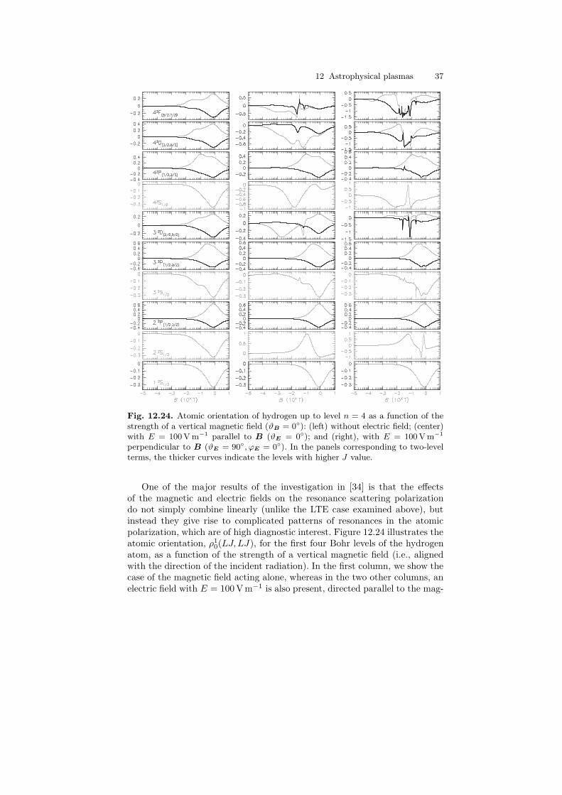
12 Astrophysical plasmas 37
Fig. 12.24. Atomic orientation of hydrogen up to level n = 4 as a function of thestrength of a vertical magnetic field (ϑB = 0◦): (left) without electric field; (center)with E = 100 V m−1 parallel to B (ϑE = 0◦); and (right), with E = 100 V m−1
perpendicular to B (ϑE = 90◦, ϕE = 0◦). In the panels corresponding to two-levelterms, the thicker curves indicate the levels with higher J value.
One of the major results of the investigation in [34] is that the effectsof the magnetic and electric fields on the resonance scattering polarizationdo not simply combine linearly (unlike the LTE case examined above), butinstead they give rise to complicated patterns of resonances in the atomicpolarization, which are of high diagnostic interest. Figure 12.24 illustrates theatomic orientation, ρ1
0(LJ, LJ), for the first four Bohr levels of the hydrogenatom, as a function of the strength of a vertical magnetic field (i.e., alignedwith the direction of the incident radiation). In the first column, we show thecase of the magnetic field acting alone, whereas in the two other columns, anelectric field with E = 100 V m−1 is also present, directed parallel to the mag-
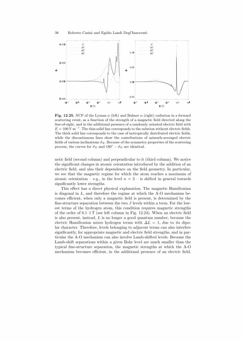
38 Roberto Casini and Egidio Landi Degl’Innocenti
Fig. 12.25. NCP of the Lyman α (left) and Balmer α (right) radiation in a forwardscattering event, as a function of the strength of a magnetic field directed along theline-of-sight, and in the additional presence of a randomly oriented electric field withE = 100 V m−1. The thin solid line corresponds to the solution without electric fields.The thick solid line corresponds to the case of isotropically distributed electric fields,while the discontinuous lines show the contributions of azimuth-averaged electricfields of various inclinations ϑE. Because of the symmetry properties of the scatteringprocess, the curves for ϑE and 180◦ − ϑE are identical.
netic field (second column) and perpendicular to it (third column). We noticethe significant changes in atomic orientation introduced by the addition of anelectric field, and also their dependence on the field geometry. In particular,we see that the magnetic regime for which the atom reaches a maximum ofatomic orientation – e.g., in the level n = 3 – is shifted in general towardssignificantly lower strengths.
This effect has a direct physical explanation. The magnetic Hamiltonianis diagonal in L, and therefore the regime at which the A-O mechanism be-comes efficient, when only a magnetic field is present, is determined by thefine-structure separation between the two J levels within a term. For the low-est terms of the hydrogen atom, this condition requires magnetic strengthsof the order of 0.1–1 T (see left column in Fig. 12.24). When an electric fieldis also present, instead, L is no longer a good quantum number, because theelectric Hamiltonian mixes hydrogen terms with ∆L = 1, due to its dipo-lar character. Therefore, levels belonging to adjacent terms can also interferesignificantly, for appropriate magnetic and electric field strengths, and in par-ticular the A-O mechanism can also involve Lamb-shifted levels. Because theLamb-shift separations within a given Bohr level are much smaller than thetypical fine-structure separation, the magnetic strengths at which the A-Omechanism becomes efficient, in the additional presence of an electric field,
12 Astrophysical plasmas 39
are correspondingly smaller. In the case illustrated in Fig. 12.24, for instance,the orientation of the level 3 2D3/2 for parallel fields (central column) reachesan important negative peak already for B ∼ 10−3 T .
This “electric enhancement” of the atomic orientation of hydrogen has im-portant consequences for the polarization diagnostics of hydrogen lines. Be-cause of the large magnetic strengths at which the A-O mechanism becomesefficient when the magnetic field is acting alone, the circular-polarization sig-nal is typically dominated by the characteristic antisymmetric signature of theZeeman effect. In the additional presence of an electric field, instead, the A-Omechanism can occur at significantly smaller magnetic strengths, so the cir-cular polarization signal from the Zeeman effect can be completely dominatedby the symmetric signature of the atomic orientation.
In conclusion, one must expect important modifications of both NCP andthe shape of Stokes V , when electric fields of various geometries are alsopresent in the emitting plasma. In particular, one should expect that thismodification of the NCP of hydrogen lines be manifest also in the presence ofmicroturbulent electric fields, like the Holtsmark field. Figure 12.25 shows thatthis is actually the case. Recent observations of anomalous levels of NCP inthe Balmer α radiation from solar prominences [43] suggest that small electricfields – whether of the motional kind, or simply microturbulent – might beresponsible for those signals, acting along with the prominence magnetic field(B . 0.01 T).
The sensitivity of hydrogen resonance radiation to the presence of mi-croturbulent electric fields certainly complicates the magnetic diagnostics ofastrophysical plasmas based on hydrogen lines, since the A-O mechanismchanges its range of efficiency ultimately depending on the electron density ofthe plasma. In turn, the atomic alignment is also modified in the presence ofmicroturbulent fields, and therefore one must expect significant modificationsof the linear polarization as well. Despite these difficulties, one can envisagea diagnostic procedure that take advantage of both hydrogen lines and otherresonance lines from atomic species that are instead insensitive to the linearStark effect, like the HeI lines at λ1083.0 nm and λ587.6 nm. Such an approach,which opens to the possibility of a simultaneous diagnostics of magnetic fieldsand plasma densities, is the subject of current investigation.
References
1. J.O. Stenflo, C.U. Keller: Nature 321, 927 (1997)2. M. Born: Atomic Physics (Blackie, London 1958)3. U. Fano: Rev. Mod. Phys. 29, 73 (1957)4. F. Mandl, G. Shaw: Quantum Field Theory (Wiley, New York 1984)5. E. Landi Degl’Innocenti: Solar Phys. 85, 3 (1983)6. E. Landi Degl’Innocenti, M. Landolfi: Polarization in Spectral Lines (Kluwer,
Utrecht 2004)7. J. Trujillo Bueno, R. Manso Sainz: Astrophys. J. 516, 436 (1999)

40 Roberto Casini and Egidio Landi Degl’Innocenti
8. L.D. Landau, E.V. Lifshitz: Classical Theory of Fields (Pergamon, New York1975)
9. W. Hanle: Z. Phys. 30, 93 (1924)10. W. Happer: Rev. Mod. Phys. 44, 169 (1972)11. R. Loudon: The Quantum Theory of Light (Clarendon, Oxford 1983)12. C. Cohen-Tannoudji, J. Dupont-Roc, G. Grynberg: Atom-Photon Interactions
(Wiley, New York 1992)13. R. Manso Sainz, E. Landi Degl’Innocenti: Astron. Astrophys. 394, 1093 (2002)14. R. Manso Sainz, J. Trujillo Bueno: Phys. Rev. Lett 91, 1102 (2003)15. D.M. Brink, G.R. Satchler: Angular Momentum (Clarendon, Oxford 1993)16. R. Becker: Electromagnetic fields and interactions (Dover, New York 1982)17. E. Landi Degl’Innocenti: Solar Phys. 91, 1 (1984)18. R. Casini, P.G. Judge: Astrophys. J. 522, 524 (1999)19. S. Tomcyzk: Multi-Channel Polarimeter for Coronal Magnetic Field Measure-
ments, American Geophysical Union, Fall Meeting 2003 (2003)20. J. Trujillo Bueno, E. Landi Degl’Innocenti, M. Collados, L. Merenda, R. Manso
Sainz: Nature 415, 403 (2002)21. H. Lin, M. Penn, and J. Kuhn: Astrophys. J. 493, 978 (1998)22. J. Trujillo Bueno, L. Merenda, R. Centeno, M. Collados, E. Landi
Degl’Innocenti: Astrophys. J. 619, 191 (2005)23. R. Casini, R. Bevilacqua, A. Lopez Ariste: Astrophys. J. 622, 1265 (2005)24. J.C. Lehmann: J. Physique 25, 809 (1964)25. J.C. Kemp, J.H. Macek, F.W. Nehring: Astrophys. J. 278, 863 (1984)26. H.R. Griem: Spectral Line Broadening by Plasmas (Academic, New York 1974)27. V. Bommier, S. Sahal-Brechot: Astron. Astrophys. 69, 57 (1978)28. E. Landi Degl’Innocenti: Solar Phys. 79, 291 (1982)29. R. Casini, A. Lopez Ariste, S. Tomczyk, B.W. Lites: Astrophys. J. 598, L67
(2003)30. A. Lopez Ariste, R. Casini: Astrophys. J. 575, 529 (2002)31. Nguyen-Hoe, H.-W. Drawin, L. Herman: J. Quant. Spectrosc. Radiat. Transfer
7, 429 (1967)32. C.A. Moore, G.P. Davis, R.A. Gottscho: Phys. Rev. Lett. 52, 538 (1984)33. F.M. Levinton, G.M. Gammel, R. Kaita, H.W. Kugel, D.W. Roberts: Rev. Sci.
Instr. 61, 2914 (1990)34. R. Casini: Phys. Rev. A 71, 062505 (2005)35. R. Casini, E. Landi Degl’Innocenti: Astron. Astrophys. 276, 289 (1993)36. R. Casini, E. Landi Degl’Innocenti: Astron. Astrophys. 291, 668 (1994)37. R. Casini, E. Landi Degl’Innocenti: Astron. Astrophys. 300, 309 (1995)38. R. Casini: Astron. Astrophys. Suppl. Ser. 114, 363 (1995)39. P.V. Foukal, B.B. Behr: Solar Phys. 156, 293 (1995)40. R. Casini, P.V. Foukal: Solar Phys. 163, 65 (1996)41. V. Bommier, S. Sahal-Brechot: Solar Phys. 78, 157 (1982)42. B. Favati, E. Landi Degl’Innocenti, M. Landolfi: Astron. Astrophys. 179, 329
(1987)43. A. Lopez Ariste, R. Casini, F. Paletou, S. Tomczyk, B.W. Lites, M. Semel, E.
Landi Degl’Innocenti, J. Trujillo Bueno, K.S. Balasubramaniam: Astrophys. J.621, 145L (2005)


