arX

iv:g

r-qc

/060

6132

v1 3

0 Ju

n 20

06

The polygon model for 2+1D gravity:the constraint algebra and

problems of quantization

Jaap Eldering

7th June 2006

Masters thesis

supervised by Prof. Renate LollInstitute for Theoretical Physics

Utrecht University

Abstract

In this thesis we consider ’t Hooft’s polygon model for 2+1D gravity. We firstrecall the ADM formalism to write general relativity in Hamiltonian form. Withthis background in mind, we give a detailed review of the polygon model and itsexplicit evolution description in the classical context.

Then we review some remarks in the literature about quantization of this modeland the discreteness of space-time. We discuss the problems associated with thisin the context of canonical quantization for some explicit quantization schemes:the triangle inequalities conflict with the Stone–Von Neumann uniqueness theo-rem when we use the canonical variables. Also, the implementation of transitions,the constraints and their algebra poses significant problems. We conclude thatno rigorous conclusions about the spectrum of space-time can be drawn withoutan explicit quantization scheme.

Furthermore, we consider the Poisson structure of the constraints, which areimportant when we try to quantize the model. We improve known results andshow that the full Poisson structure can be calculated explicitly and that it closeson shell. An attempt is made to interpret the gauge orbits generated by theconstraints.

Contents

1 Introduction 3

1.1 Gravity: general relativity . . . . . . . . . . . . . . . . . . . . . . 3

1.2 Quantization . . . . . . . . . . . . . . . . . . . . . . . . . . . . . 4

1.3 The polygon model . . . . . . . . . . . . . . . . . . . . . . . . . . 4

2 Notation and conventions 5

3 Representing gravity 9

3.1 Foliation of space-time . . . . . . . . . . . . . . . . . . . . . . . . 9

3.2 Hamiltonian formulation . . . . . . . . . . . . . . . . . . . . . . . 11

3.3 Reduction of phase space . . . . . . . . . . . . . . . . . . . . . . . 12

4 The polygon model 14

4.1 Tessellation of the spatial surface . . . . . . . . . . . . . . . . . . 15

4.2 Vertex relations . . . . . . . . . . . . . . . . . . . . . . . . . . . . 17

4.3 Constraints . . . . . . . . . . . . . . . . . . . . . . . . . . . . . . 18

4.4 Dynamics . . . . . . . . . . . . . . . . . . . . . . . . . . . . . . . 19

4.5 Transitions . . . . . . . . . . . . . . . . . . . . . . . . . . . . . . . 21

4.6 Constrained dynamics . . . . . . . . . . . . . . . . . . . . . . . . 23

4.7 Simulation . . . . . . . . . . . . . . . . . . . . . . . . . . . . . . . 26

5 Quantization 27

5.1 General procedure . . . . . . . . . . . . . . . . . . . . . . . . . . 28

5.2 Constraints in quantization . . . . . . . . . . . . . . . . . . . . . 29

1

5.3 Quantization of the polygon model . . . . . . . . . . . . . . . . . 31

5.4 Conclusions . . . . . . . . . . . . . . . . . . . . . . . . . . . . . . 35

6 The constraint algebra 36

6.1 Useful formulas . . . . . . . . . . . . . . . . . . . . . . . . . . . . 37

6.2 Calculation of the algebra . . . . . . . . . . . . . . . . . . . . . . 40

6.3 Generalizations . . . . . . . . . . . . . . . . . . . . . . . . . . . . 47

6.4 Summary . . . . . . . . . . . . . . . . . . . . . . . . . . . . . . . 54

6.5 Interpretation . . . . . . . . . . . . . . . . . . . . . . . . . . . . . 55

7 Conclusions 57

A The dual graph 59

A.1 The dual of a planar graph . . . . . . . . . . . . . . . . . . . . . . 59

A.2 Hyperbolic space . . . . . . . . . . . . . . . . . . . . . . . . . . . 61

A.3 Embedding the dual graph in H2 . . . . . . . . . . . . . . . . . . 62

Bibliography 66

2

1 Introduction

In this thesis we will study a particular model for (Einstein) gravity: the ’t Hooftpolygon model for gravity in 2+1-dimensions. We will specifically be concernedwith the question of whether this model can be quantized and we calculate thecomplete Poisson structure of the constraints.

The 2+ 1 here stands for 2 spatial dimensions and 1 time dimension. Thisis one dimension lower than the 3+1-dimensions we (seem to) live in. Thatturns out to make the whole problem a lot simpler than trying to tackle the fullproblem of four-dimensional quantum gravity, which people are trying to solvefor decades already. It is hoped then, that by studying and hopefully solvingthree-dimensional (and in general lower dimensional) quantum gravity, we canlearn something about how to solve four-dimensional quantum gravity.

1.1 Gravity: general relativity

When we say ‘gravity’ we mean the classical theory of gravity as formulated byAlbert Einstein, which is known as ‘general relativity’. It has as a starting pointthat (locally) the effect of a gravitational field and acceleration are the same.

This has as consequences that space and time together (often referred to asspace-time) can be curved: the concept of a straight line is not entirely lost, butbecomes somewhat more subtle. For example in a curved space it can be possibleto always travel in a straight line and come back to where you started, or thattwo straight lines intersect each other at more than one point.

The mathematical description of this theory is much more complicated than thatof the classical, Newtonian theory of gravity and finding solutions is much moredifficult, already in the classical (non-quantum) theory.

On the other hand, general relativity describes some interesting phenomena.Some of these are already well confirmed by measurements, like the bending oflight rays by large masses (e.g. the sun) and the slowing of time in gravitationalwells. Other phenomena are predicted but not yet detected, like black holes andgravitational waves.

3

1.2 Quantization

At the start of the 20th century, physical phenomena were discovered which couldnot be described by the classical physical theories. Examples are the photo-electric effect and the observed structure of atoms.

A theory which could correctly describe all of these phenomena was constructedover the years and is generically called ‘quantum mechanics’. In this theory,observables like particle position or energy do not have definite values anymore;these observables have a probability-like amplitude. The ‘quantum’ refers to thefact that certain observables can only take (a superposition of) discrete, quantizedvalues in this theory.

At this moment, a theory for three out of four known fundamental forces in naturehas been formulated: the electro-magnetic force and the weak and strong nuclearforces. Only the force of gravity remains “unquantized” as of this day. Yetone cannot consistently combine classical and quantum theories, so the currenttheories of general relativity and quantum mechanics are not complete. Hencephysicists are looking for a quantized version of the theory of gravity. For moredetails on the subject of quantization, we refer to chapter 5.

1.3 The polygon model

In 3 dimensions, for solutions of the Einstein equations without cosmologicalconstant, curvature of space-time does only occur locally at points where thereis mass. Everywhere where space is empty, it is (locally) flat. This doesn’t meanhowever that things become trivial, because we can still have global non-trivialcurvature effects.

The polygon model for 2+1-dimensional gravity makes clever use of this fact.We can model the spatial part of space-time as a set of polygons glued together.Inside each polygon space is simply flat, but these polygons can be glued togetherto form a two-dimensional spatial surface with non-vanishing two-dimensionalcurvature and non-trivial topology. We could for example create a cube from sixfour-sided polygons. The polygon model is explained in more detail in chapter 4.

There are other models for 2+1-dimensional gravity. Two formulations that areclosely related to each other and the polygon formulation are the second orderADM formulation with York time by Moncrief et al. [14, 2] and the first orderChern-Simons formulation by Witten et al. [19, 2]. On a classical level, theseformulations are equivalent. The quantizations of these formulations, as far asthey exist, yield different results though. Witten’s formulation gives a ‘frozentime’ picture and Moncrief’s formulation can only be explicitly quantized in thegenus 1 case.

4

2 Notation and conventions

In the polygon model, the fundamental variables are the lengths and boostparameters of the edges between polygons. These polygons cover a spatial sliceof space-time. Boost parameters are the generators of Lorentz transformationsbetween different polygons. Explicitly a boost η is related to the speed v of aLorentz transformation by

tanh(η) = v,

cosh(η) = γ(v),

sinh(η) = γ(v) v,

(2.1)

where as usual we have γ(v) =1√

1−(vc

)2 and we normalize c = 1.

The boost parameters of edges can be viewed as Lorentz transformations in thespecific direction perpendicular to that edge. We can more generally considerboosts in all directions together with spatial rotations. These form the (Lie)group of Lorentz transformations: we can compose any two elements to getanother Lorentz transformation. We write O(2, 1) for the group of Lorentz trans-formations in three-dimensional space-time. This group can be generated1 by thethree basic transformations of a rotation and boosts in the x and y-direction:

Lr(α) =

1 0 00 cosα − sinα0 sinα cosα

,

Lx(η) =

cosh η sinh η 0sinh η cosh η 00 0 1

,

Ly(η) =

cosh η 0 sinh η0 1 0

sinh η 0 cosh η

.

(2.2)

1Actually this will only generate the identity component SO+(2, 1) ⊆ O(2, 1), but this willbe sufficient for our purposes; see appendix A for more details.

5

As generators of Lorentz transformations, boosts have the nice property of addi-tivity:

Lx(η1)Lx(η2) = Lx(η1 + η2). (2.3)

We will denote boosts by Greek letters from the middle of the alphabet (η, µ, ν, . . . ),angles by Greek letters from the start (α, β, γ, . . . ) and lengths by l, m, n, . . .

In the polygon model, we will frequently encounter hyperbolic functions of theboosts and trigonometric functions of angles. To keep formulas short and clear,the following notation will be used:

vi ≡ vηi ≡ tanh(ηi),

γi ≡ γηi ≡ cosh(2 ηi),

σi ≡ σηi ≡ sinh(2 ηi),

ci ≡ cαi≡ cos(αi),

si ≡ sαi≡ sin(αi).

(2.4)

Note the extra factor 2 in the definition of γ and σ. Furthermore, when thespecification of a variable is obvious from the subscript index, then this shorternotation will be used.

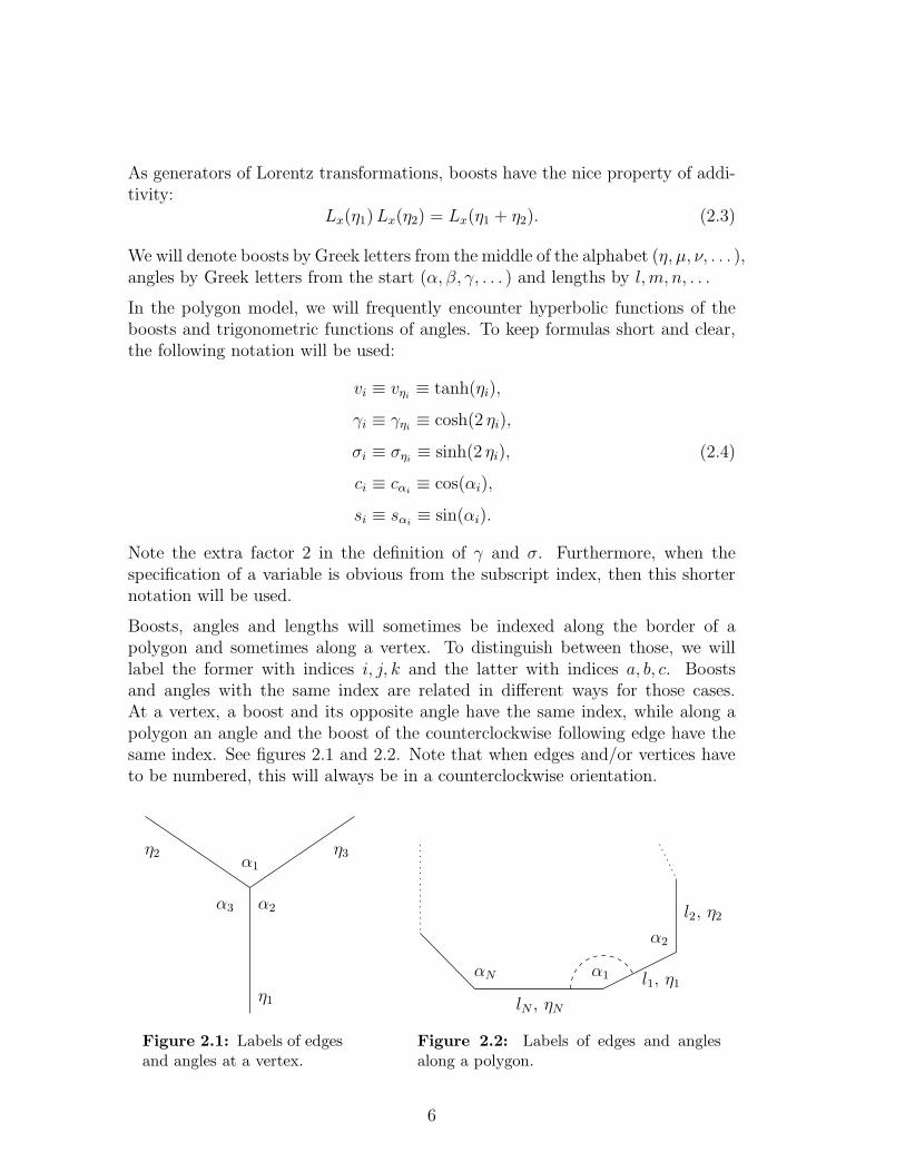
Boosts, angles and lengths will sometimes be indexed along the border of apolygon and sometimes along a vertex. To distinguish between those, we willlabel the former with indices i, j, k and the latter with indices a, b, c. Boostsand angles with the same index are related in different ways for those cases.At a vertex, a boost and its opposite angle have the same index, while along apolygon an angle and the boost of the counterclockwise following edge have thesame index. See figures 2.1 and 2.2. Note that when edges and/or vertices haveto be numbered, this will always be in a counterclockwise orientation.

α1

α3 α2

η1

η2 η3

Figure 2.1: Labels of edgesand angles at a vertex.

α1

l2, η2

l1, η1

lN , ηN

αN

α2

Figure 2.2: Labels of edges and anglesalong a polygon.

6

Furthermore we see that indices along a polygon are cyclic. In computations wewill therefore always implicitly interpret the index numbers modulo N (N beingthe number of vertices and edges of the polygon). For example, we have thatη0 = ηN . An exception to this rule will be made for quantities that are sumsover ranges of indices, as a sum over the empty range is truly different from asum over the full cycle. For example, the sum of angles up to index j as definedin (4.6): here we interpret

θ0 =0∑

i=1

π − αi = 0 (2.5)

instead of θ0 = θN .

The model has a phase space consisting of a set of edge lengths and boosts (li, ηj).The Poisson brackets are defined on this phase space as

{ li , ηj } = 12δij , (2.6)

where the indices i, j run over all edges.

The phase space of this model is larger than the physical phase space. This isreflected by the presence of algebraic constraints on the phase space variables.These define a subspace of the complete phase space by imposing C(l, η) = 0 forall constraints C. When dealing with constraints, we use the ‘≈’ sign to indicatean equality, that holds only on this constraint surface and not necessarily on thewhole phase space. Thus by definition a constraint function C(l, η) satisfies

C(l, η) ≈ 0. (2.7)

The polygons that together make up a ‘tessellation’, can be viewed as a graphstructure, consisting of faces (the polygons), edges (the polygon edges) andvertices (the points where three or more edges join). The sets of these faces,edges and vertices will be denoted by F , E and V respectively. Single elementswe denote by f ∈ F and the number of elements by #F . See section A.1 forsome more details.

A note on signs

Some of the definitions used in this thesis differ by a minus sign from referencedworks or conventions; unfortunately it is not possible to choose definitions to besimultaneously convenient, according to conventions and equal to all referencedworks. To keep things clear, we give a (hopefully complete) list of differences.

7

The Poisson bracket has a relative minus sign with respect to the definition in[8]; it is chosen to have the same sign as the standard definition. Related to thatis the definition of the time evolution of a classical quantity (function on phasespace) as

f = { f , H } , (2.8)

which is also according to normal conventions and opposite to the definition usedin [8] and related papers.

Boosts have the same sign as in [8]: contracting edges have positive boosts.This looks a bit like a counter-intuitive choice, but is necessary to get the rightHamiltonian flow for our choice of signs in (2.6), (2.8) and the Hamiltonian.

We use the space-like (−,+,+) sign convention for the metric.

8

3 Representing gravity

Before we can start to think about the quantization of gravity in arbitrarydimensions, we first have to choose a way to represent gravity. We would like tobe able to formulate gravity within the framework of Lagrangian or Hamiltonianmechanics. Or in other words, we want choose a set of variables that fully describea state of the system and then formulate the equations of motion on those states.

We must note however, that a classical “state” is normally defined as a fulldescription of the system for a given instance of time. But in the context of generalrelativity “a given instance of time” is a priori not an unambiguous statement tomake: there is no unique time coordinate, because coordinate diffeomorphismsare a symmetry of the system.

In the next section we will introduce a way to split time and space in generalrelativity, which then makes it possible to formulate general relativity in a La-grangian and then Hamiltonian formulation of gravity.

3.1 Foliation of space-time

Before trying to split off time, we first have to give a mathematical descriptionof a space-time. There are two well known choices of fundamental variables todescribe a general space-time. We will use the standard choice of taking themetric gµν(x

σ) as field variable. There is however an alternative formulation,known as ‘first order formalism’ in which a set of orthonormal vectors eaµ (called‘dreibein’, ‘vierbein’ or in arbitrary dimensions ‘vielbein’) together with an in-ternal connection is chosen as fundamental variables. This description relates tothe standard metric description via

ηab eaµ e

bν = gµν . (3.1)

In space-time dimension n, ηab is a diagonal matrix with signature (1, n−1), whichexpresses the fact that the eaµ are a local orthonormal set of vectors.

A space-time can mathematically be specified in a very general manner as adifferentiable manifold M with a metric g on it, often denoted as a (pseudo-)

9

Riemannian manifold (M, g). In the following, we will be dealing with a pseudo-Riemannian manifold of signature (1,2).

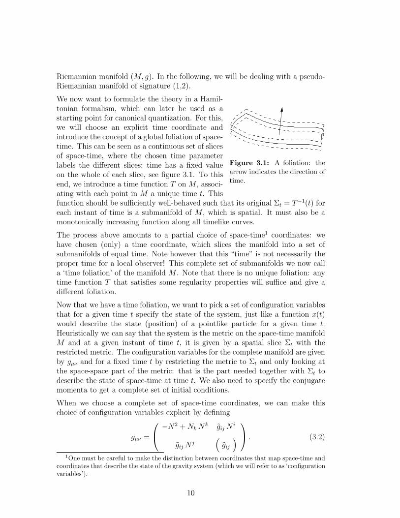
Figure 3.1: A foliation: thearrow indicates the direction oftime.

We now want to formulate the theory in a Hamil-tonian formalism, which can later be used as astarting point for canonical quantization. For this,we will choose an explicit time coordinate andintroduce the concept of a global foliation of space-time. This can be seen as a continuous set of slicesof space-time, where the chosen time parameterlabels the different slices; time has a fixed valueon the whole of each slice, see figure 3.1. To thisend, we introduce a time function T on M , associ-ating with each point in M a unique time t. Thisfunction should be sufficiently well-behaved such that its original Σt = T−1(t) foreach instant of time is a submanifold of M , which is spatial. It must also be amonotonically increasing function along all timelike curves.

The process above amounts to a partial choice of space-time1 coordinates: wehave chosen (only) a time coordinate, which slices the manifold into a set ofsubmanifolds of equal time. Note however that this “time” is not necessarily theproper time for a local observer! This complete set of submanifolds we now calla ‘time foliation’ of the manifold M . Note that there is no unique foliation: anytime function T that satisfies some regularity properties will suffice and give adifferent foliation.

Now that we have a time foliation, we want to pick a set of configuration variablesthat for a given time t specify the state of the system, just like a function x(t)would describe the state (position) of a pointlike particle for a given time t.Heuristically we can say that the system is the metric on the space-time manifoldM and at a given instant of time t, it is given by a spatial slice Σt with therestricted metric. The configuration variables for the complete manifold are givenby gµν and for a fixed time t by restricting the metric to Σt and only looking atthe space-space part of the metric: that is the part needed together with Σt todescribe the state of space-time at time t. We also need to specify the conjugatemomenta to get a complete set of initial conditions.

When we choose a complete set of space-time coordinates, we can make thischoice of configuration variables explicit by defining

gµν =

−N2 +Nk Nk gij N

i

gij Nj

(gij

)

. (3.2)

1One must be careful to make the distinction between coordinates that map space-time andcoordinates that describe the state of the gravity system (which we will refer to as ‘configurationvariables’).

10

The N , N i and gij are functions of space-time that can be read off from theexplicit form of gµν in the chosen space-time coordinates. We have chosen timeto be a global timelike coordinate function, so this implies that g00 < 0 andalso that the symmetric submatrix gij for the other spatial coordinates is non-degenerate and the entries gij N

i thus well-defined.

The function N is in the literature (see e.g. [2, p. 12]) referred to as the‘lapse function’: it specifies the rate that clocks tick with respect to the chosentime coordinate. The functions N i are called the ‘shift functions’ and specifythe displacement of spatial coordinates, when we make a small displacementperpendicular to the surface Σt. The matrix gij can be viewed as a metric on thesubmanifold Σt and thus describes the state of the system (to be compared tothe position x in a one-particle classical mechanical system).

Thus far, we have not yet made any specific choice of space-time coordinates,except for the fact that we demanded a global time coordinate. The only thing wehave done is to make an explicit separation of the time from the space coordinatesto allow for a treatment of the theory within a Lagrangian and Hamiltonianframework. This decomposition is known as the Arnowitt-Deser-Misner (ADM)formalism.

3.2 Hamiltonian formulation

Using the ADM decomposition, we can write down the action of general relativityand transform it to a Hamiltonian formulation. We will here give an outline ofthis procedure, to give some insight in the intricacies that will also show up inthe polygon model. More details can be found e.g. in reference [2].

The action of general relativity in three dimensions is given by

I =1

16 πG

∫d3x

√−|g| (R− 2Λ) (3.3)

in the absence of external matter or fields. We normalize 16 πG = 1 and set thecosmological constant Λ = 0 from here on.

Inserting the ADM decomposition of the metric, this action can be rewritten asan integral over time t of a Lagrangian L, with

L =

∫

Σt

d2x N√|g|[R +KijK

ij −(gijKij

)2]. (3.4)

Here R is the Ricci scalar corresponding to g and Kij is the extrinsic curvature ofΣt embedded in M . In principle there are also some boundary terms from partial

11

integration, but these cancel because the spatial slice is compact. The integrandin (3.4) we denote by L, the Lagrangian density.

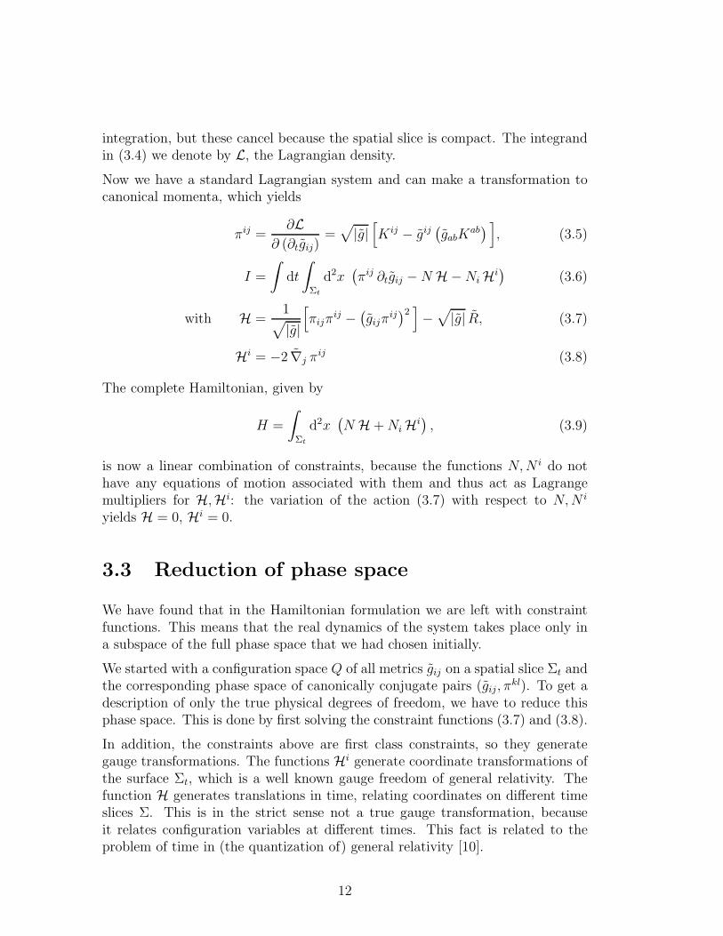
Now we have a standard Lagrangian system and can make a transformation tocanonical momenta, which yields

πij =∂L

∂ (∂tgij)=√

|g|[Kij − gij

(gabK

ab) ]

, (3.5)

I =

∫dt

∫

Σt

d2x(πij ∂tgij −N H−Ni H

i)

(3.6)

with H =1√|g|

[πijπ

ij −(gijπ

ij)2 ]

−√|g| R, (3.7)

Hi = −2 ∇j πij (3.8)

The complete Hamiltonian, given by

H =

∫

Σt

d2x(N H +Ni H

i), (3.9)

is now a linear combination of constraints, because the functions N,N i do nothave any equations of motion associated with them and thus act as Lagrangemultipliers for H,Hi: the variation of the action (3.7) with respect to N,N i

yields H = 0, Hi = 0.

3.3 Reduction of phase space

We have found that in the Hamiltonian formulation we are left with constraintfunctions. This means that the real dynamics of the system takes place only ina subspace of the full phase space that we had chosen initially.

We started with a configuration space Q of all metrics gij on a spatial slice Σt andthe corresponding phase space of canonically conjugate pairs (gij, π

kl). To get adescription of only the true physical degrees of freedom, we have to reduce thisphase space. This is done by first solving the constraint functions (3.7) and (3.8).

In addition, the constraints above are first class constraints, so they generategauge transformations. The functions Hi generate coordinate transformations ofthe surface Σt, which is a well known gauge freedom of general relativity. Thefunction H generates translations in time, relating coordinates on different timeslices Σ. This is in the strict sense not a true gauge transformation, becauseit relates configuration variables at different times. This fact is related to theproblem of time in (the quantization of) general relativity [10].

12

Gauge transformations do not change the physical state of the system, so as asecond step, we have to fix this gauge freedom to get the reduced phase space.The gauge freedom generated by the first class constraints (3.7) and (3.8) can nowbe removed by fixing the Lagrange multiplier functions that were still arbitrary.

The explicit work of solving the constraints and fixing the gauge is not as straight-forward as it might seem from the formulation above: there is no known way tosolve this in 3+1-dimensions, but in 2+1-dimensions there is [14, 19]. We will notgo into the details, but with the use of Riemann surface theory one can considerthe space of metrics g modulo diffeomorphisms and conformal factors, which isa finite dimensional space known as the moduli space N of Σ. This space hasdimension 6(g−1) when Σ has genus g > 1, two when g = 1 and zero when g = 0(see also figure 4.1 for the concept of genus of a surface). The physical phasespace now has twice the dimension of this moduli space N (Σ), because we stillhave to add the canonical momenta, which span the same number of dimensions.

Thus in 2+1-dimensions, the physical phase space of general relativity is finitedimensional, unlike the phase space we started with: that was the space of allmetrics g and conjugate momenta, which are fields over Σ and thus infinitedimensional. For this reason, general relativity in 2+1-dimensions is sometimescalled a ‘topological theory’: the true degrees of freedom do only arise fromtopological non-triviality of the surface Σ. This again is a reason that the polygonmodel works: there are no local degrees of freedom and locally space-time is flat.The formulation of the polygon model depends on this fact as we will see inchapter 4.

13

4 The polygon model

The polygon model is a model to describe 2+1-dimensional space-times that canbe foliated by a set of spacelike Cauchy surfaces. This includes the possibility ofspatially open and closed universes [5], although in the case of an open universeone has to be careful about boundary conditions at spatial infinity.

We will however only consider spatially closed universes. Thus if we take a spatialslice of our complete space-time manifold M , then this is a closed and boundedsurface (so it has finite volume). More specifically, we take a space-time of theform of a product:

M = Σ× I. (4.1)

Here I ⊂ R is some interval of time, which may be bounded from below and/orabove, depending on whether there is a big bang or big crunch respectively.

Σ is the spatial part and thus should be a compact two-dimensional surface. Thesesurfaces are topologically completely classified. The ones that are orientable areclassified by their genus g, which indicates the number of ‘holes’ in them. Thesimplest examples are a sphere, a torus and a ‘double torus’, see figure 4.1.

The model also allows for a finite number of pointlike, spinless particles to beadded to this space-time. We have not studied this in detail and refer the readerto [8, 11] for more information.

The simplest spatial surface of a sphere is only realizable with particles. Prooffor this fact can be found in [2, p. 57] or [14, p. 2912] and is based on an analysisof the moduli space of metrics on the surface Σ modulo diffeomorphisms. For thesphere this moduli space consists of one unique metric with curvature 1, whichdoes not yield a solution to the vacuum Einstein equations. This can also be seen

Figure 4.1: Surfaces of genus 0, 1 and 2.

14

from the fact that the Hamiltonian constraint can be written as in (4.11):

H = 2 π χ = 4 π (1− g).

The Hamiltonian equals minus the area of the dual graph as given in (A.10).This area cannot be negative, thus the Hamiltonian cannot be positive, whichrules out the case g = 0.

4.1 Tessellation of the spatial surface

We are considering general relativity in 3 dimensions. This we can exploit tosimplify the description of our space-time. In this case the Riemann tensor iscompletely determined by the Ricci tensor: one can show this e.g. by countingthe degrees of freedom or explicitly [2, p. 3]:

Rµνρσ = gµν Rνσ + gνσ Rµρ − gνρ Rµσ − gµσ Rνρ −12(gµρ gνσ − gµσ gνρ) R. (4.2)

This means that in a region of space-time with no matter (T µν = 0), the Einsteinequations effectively reduce to Rµν = 0 and determine that space-time is locallyflat. Thus everywhere we can locally choose a Minkowski coordinate system.

Given this space which is locally Minkowski, we can also easily choose a spatialslice that is locally flat too. This will induce a local coordinate system from thethree-dimensional Minkowski space to our two-dimensional spatial slice Σt. Wecannot in general extend this coordinate system to our whole spatial surface:our space is compact, so when we try to extend our flat coordinate system froma certain starting point, we will run into parts of space where we had alreadydefined coordinates. These do not necessarily have to match; while we haveextended our coordinates and run into a “charted” part of space, we might havegone around a non-contractible loop in Σ which has a non-trivial holonomy. Asimple example is a toroidal spatial surface which expands uniformly in one of itsfundamental directions: when we walk along a loop in this direction and returnto our starting point, the coordinates fail to match by a Lorentz boost of thespeed of contraction or expansion.

We can however choose a coordinate system at some point(s) of our spatialsurface and extend it as far as possible. After doing this, we will be left withseveral regions of flat space which, glued together at their boundaries, formthe complete spatial surface again. We will call such a set of flat coordinatepatches a ‘tessellation’. Notice that at points where regions of space are gluedtogether, the spatial surface will in general not be flat. The underlying three-dimensional Minkowski space-time is flat, but at points where three or morespacelike slices join, the two-dimensional surface will in general have a curvatureof delta distribution type. See figure 4.2 for an example.

15

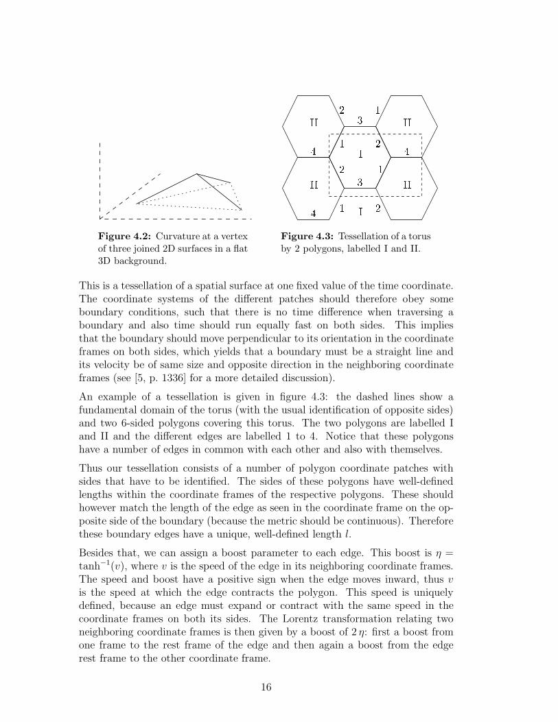
Figure 4.2: Curvature at a vertexof three joined 2D surfaces in a flat3D background.

II

II

I

II

II

I

1

2 1

2

3

3

44

4

12

1 2

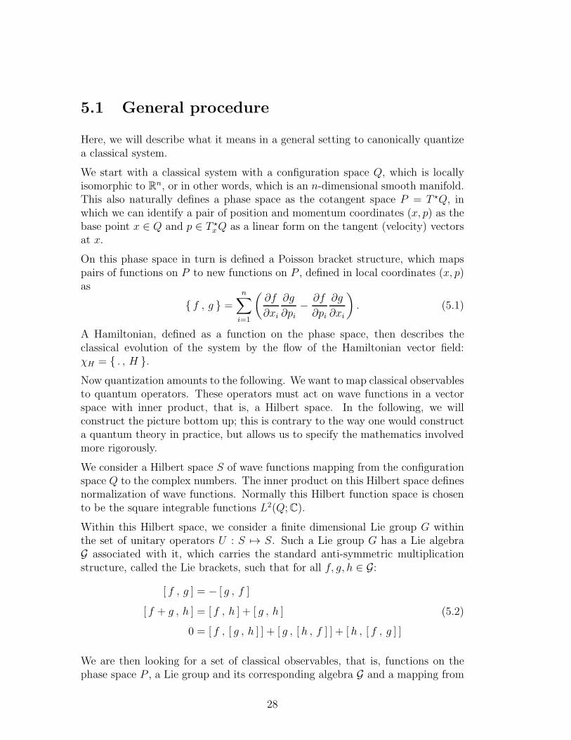
Figure 4.3: Tessellation of a torusby 2 polygons, labelled I and II.

This is a tessellation of a spatial surface at one fixed value of the time coordinate.The coordinate systems of the different patches should therefore obey someboundary conditions, such that there is no time difference when traversing aboundary and also time should run equally fast on both sides. This impliesthat the boundary should move perpendicular to its orientation in the coordinateframes on both sides, which yields that a boundary must be a straight line andits velocity be of same size and opposite direction in the neighboring coordinateframes (see [5, p. 1336] for a more detailed discussion).

An example of a tessellation is given in figure 4.3: the dashed lines show afundamental domain of the torus (with the usual identification of opposite sides)and two 6-sided polygons covering this torus. The two polygons are labelled Iand II and the different edges are labelled 1 to 4. Notice that these polygonshave a number of edges in common with each other and also with themselves.

Thus our tessellation consists of a number of polygon coordinate patches withsides that have to be identified. The sides of these polygons have well-definedlengths within the coordinate frames of the respective polygons. These shouldhowever match the length of the edge as seen in the coordinate frame on the op-posite side of the boundary (because the metric should be continuous). Thereforethese boundary edges have a unique, well-defined length l.

Besides that, we can assign a boost parameter to each edge. This boost is η =tanh−1(v), where v is the speed of the edge in its neighboring coordinate frames.The speed and boost have a positive sign when the edge moves inward, thus v

is the speed at which the edge contracts the polygon. This speed is uniquelydefined, because an edge must expand or contract with the same speed in thecoordinate frames on both its sides. The Lorentz transformation relating twoneighboring coordinate frames is then given by a boost of 2 η: first a boost fromone frame to the rest frame of the edge and then again a boost from the edgerest frame to the other coordinate frame.

16

4.2 Vertex relations

We have made a tessellation of our spatial slice with polygons. These polygonsexactly cover this spatial slice, so boundaries (‘edges’) of these polygons have tobe identified where they are “glued together”.

Besides that we also have ‘vertices’: points where three or more edges join. Aswas stated earlier, space-time is locally flat. This should also hold at vertices. Toexpress the curvature located at a vertex, we can write down the holonomy aroundthat vertex: the change a vector undergoes when it is being parallel transportedaround that vertex.

We can explicitly write down the complete holonomy of going around the vertexusing the Lorentz matrices (2.2). Going around in anti-clockwise orientation,we label the polygons at the vertex i = 1 . . . n and define αi as the angle thatpolygon i makes at the vertex and 2ηi the boost between polygon i and polygoni+1 mod n. Now going around means successively making a rotation Lr(αi) anda boost Lx(2ηi) for each polygon.1 This should be equal to the identity operation,as space-time must be flat at the vertex point, thus we have

n∏

i=1

Lr(αi)Lx(2ηi) = 1. (4.3)

We demand that at a vertex always exactly 3 polygons join. This is alwayspossible by choosing a suitable tessellation and will allow us to express the anglesin terms of the boosts. For later convenience, we now choose the indices of boostsand angles in a more symmetric fashion as in figure 2.1. When we rewrite (4.3)to a form with 3 matrices on the left and the right side and then explicitly workout the equations, we get:

s1 : s2 : s3 = σ1 : σ2 : σ3, (4.4a)

0 = s1 c2 + γ2 s3 + c1 s2 γ3, (4.4b)

c1 = c2 c3 − γ1 s2 s3, (4.4c)

γ1 = γ2 γ3 + c1 σ2 σ3 (4.4d)

and all cyclic permutations of the indices. Here we used the notation as in(2.4). As in the literature, we will refer to these as the ‘vertex relations’. Theseequations are not independent [4] nor have we given the same set as originally

1Remember that the transformation between two neighboring polygons goes with twice theboost of the edge. Furthermore the precise choice of signs and Lx or Ly depends on the explicitchoice of coordinates in the polygons and orientation of the holonomy, but this does not affectthe resulting equations. This can be seen from the fact that the system has space and timemirror symmetry.

17

given by ’t Hooft in [5], but they are complete in the sense that they are equivalentto the full set of equations determined by (4.3).

These equations now give us expressions for the angles of polygons in terms ofboost parameters or vice versa. To determine the angles one can for examplerewrite equation (4.4d) and take the inverse cosine. This does not yet determinethe angle uniquely, but with the help of equation (4.4a) it does. There is theextra fact that at most one of the three angles at a vertex can be larger than π,because if there would be two angles larger than π, there would be points thatshow up in the coordinate systems of both polygons [7]. This then determinesthe sign of the sines of the angles at each vertex.

4.3 Constraints

We now have a representation of a 2D spatial slice of the 2+1D space-timemanifold M in terms of one or more polygons, glued together at their edges.A configuration of such a spatial slice is described in terms of the lengths li andboost parameters ηi of all edges together with the graph structure of all theseedges.

The li, ηi however cannot take all possible values in R2N . Besides the fact thatall lengths have to be positive (li ≥ 0), there are some other, more complicatedconstraints.

Firstly the boosts at each vertex have to obey a triangle inequality. For eachtriple of boosts at one vertex and each permutation thereof, the following musthold:

|ηa|+ |ηb| ≥ |ηc| (4.5)

This can be deduced from vertex relation (4.4d). A more geometrical argumentis as follows: when going around the vertex, we are Lorentz boosted three times,but we should return to our original rest frame. The resulting boost of two boostsis at most the sum of the boosts, exactly when they are collinear. So the sumof lengths of each two boosts must be greater than the third to be able to closethe holonomy. This is analogous to the case of Galilean transformations when wereplace the boosts by normal velocities.

Secondly there is a set of constraints for each polygon. Geometrically these areeasy to formulate: each polygon must close. This means that the angles andedge lengths must be such that when going around the border of a polygon andkeeping track of the relative coordinates, that one must end up exactly whereone started and the sum of the angles must be 2 π.

As the angles can be expressed in terms of the boosts, we can explicitly expressthese constraints in terms of the model variables li, ηi. For a fixed polygon, let

18

us number the lengths, boosts and angles according to figure 2.2.

We first define the angle between edge j and the horizontal (edge N) by

θj =

j∑

i=1

π − αi. (4.6)

Using this we can write down the angular and closure constraints as

Cθ = θN − 2 π =

N∑

j=1

(π − αj)− 2 π ≈ 0, (4.7a)

Cz =

N∑

j=1

lj exp(i θj) ≈ 0. (4.7b)

The closure constraint Cz is written using an implicit complex coordinate systemin the polygon. This way of writing is obviously equivalent to formulating tworeal-valued constraints for the x and y direction. We will refer to the secondconstraint as the ‘complex constraint’ as in [18].

4.4 Dynamics

From the definition of our length and boost parameters, we can find the evolutionof these parameters. The boosts do not change in time, except when transitionstake place. The lengths however do change. A geometrical analysis shows thatthe length change of an edge gets a contribution from the vertices at both itssides equal to

dl

dt= −

tanh(η1) cos(α3) + tanh(η2)

sin(α3)= −

v1 c3 + v2

s3, (4.8)

where index 1 numbers the edge under consideration and indices 2 and 3 may beinterchanged (there is mirror symmetry).

We can also look at the evolution of the system in the Hamiltonian formulation.The Hamiltonian is given by the total two-dimensional curvature of the spatialslice. Curvature is only present at vertices and is given there by the deficit angle,thus

H =∑

v∈V

(2 π −

3∑

i=1

αv,i

). (4.9)

We can see that this Hamiltonian is a constraint: on the one hand, it is the integralover the scalar curvature, which is only dependent on the Euler characteristic χ

19

(see formula (A.2)) by the Gauss-Bonnet theorem:

H =

∫

Σ

d2x√

g R = 2 π χ = 4 π (1− g). (4.10)

On the other hand we can see that it is equal to the sum of all angular constraints,using the Euler characteristic of the graph:

0 =∑

f∈F

(C

fθ − 2 π

)

= −∑

i

αi + (3#V − 2#F )π

=∑

v∈V

(2 π −

3∑

i=1

αv,i

)+ (#V − 2#F )π

= H − 2 π χ. (4.11)

In the last step we made use of the trivalence of the vertices by plugging in therelation 3#V = 2#E. See page 7 for notation.

The Hamiltonian now generates evolution of the system by

dlidt

= { li , H } ,

dηidt

= { ηi , H } .

(4.12)

To explicitly calculate this, we need a symplectic structure on phase space. Asymplectic structure defines Poisson brackets and it is uniquely determined bythe Poisson brackets between the fundamental variables. In our case it turnsout that the evolution of the boosts and lengths exactly matches the evolutiongenerated by the Hamiltonian if we choose the symplectic structure to be (2.6):

{ li , ηj } = 12δij .

The Hamiltonian time evolution of the boost parameters can immediately beseen to match that of the geometrical picture: in both cases it is zero. Forthe geometrical picture it was chosen this way by letting time run equally fasteverywhere in each polygon. For the Hamiltonian evolution, we see that it followsfrom the fact that H only depends on the boost parameters.

20

4.5 Transitions

Given the results of the previous section, the evolution of the system looks simple:the boosts and angles are fixed and the lengths change linearly in time. It turnsout that things are not that simple: there is a complicating factor coming fromthe constraint that the model parameters must describe a true tessellation. Thismeans that edge lengths must be positive and polygons must be true, non-self-intersecting polygons.

As a side remark, it must be noted that strictly speaking, polygons may beself-intersecting, but only in such a way that they can be embedded in a non-self-intersecting way on some two-dimensional surface, see [6]. This can be formulatedas follows: if a polygon intersects itself then this will generate a transition if andonly if a new triangle is formed and the winding number of points that will liein the triangle decreases with respect to the oriented boundary of the polygon.If the winding number of these points decreases, then these points are on theoutside of both parts of the polygon boundary that cross and thus would startto show up in two different places in polygon coordinate charts.

Figures 4.4 and 4.5 show two polygons that both seem to self-intersect. In thefirst a transition will split the polygon into two parts when the vertex hits thehorizontal edge. The winding number of points in the new triangle decreasesfrom 0 to −1. In the second figure, no transition will take place when the vertexcrosses the edges as indicated.

Returning from this digression, we now have essentially two transitions that canhappen: an edge collapsing to zero length (the top left diagram in figure 4.6) anda vertex hitting an edge (top right). There are some special cases of these twotransitions. If an edge is part of a triangular polygon, then this whole polygonwill disappear when the edge length goes to zero. This is due to the fact thatboosts and angles are constant and thus a triangle will scale to zero size whenone of its edges does. This can also happen with two neighboring triangles (but

Figure 4.4: A truly self-intersecting polygon.

Figure 4.5: A superficiallyself-intersecting polygon.

21

d

gf

j

a

Figure 4.6: All possible polygon transitions without particles, labelled as in [6].

not with three, as they would together close the spatial slice, but violate initialconditions). See the middle right and bottom diagrams of figure 4.6. Furthermorewe have a special case when an edge shrinks to zero, but the angles are such thatit starts growing again, but with angles changed by π (called a ‘grazing transition’in the literature); see the middle left diagram of figure 4.6.

There are a few more possible transitions when one allows particles in the model.For the full set of transitions including those with particles we refer to [6].

Now if we have a set of initial conditions that satisfy the constraints, we cancalculate the time evolution. This is in first instance given by only the lengthchange of the edges. But after a certain amount of time, the polygon configurationmay have changed in such a way that a transition as depicted in figure 4.6 is aboutto take place. This will not only change the graph structure as indicated, butalso the model parameters will change. One can find these by demanding thatthe parameters after the transition should be consistent with those before andthat they should obey the vertex relations: space-time must stay flat.

A potential problem now arises: when a transition takes place, we switch to adifferent graph structure with a different set of edges and thus a different phasespace to describe the system. The number of edges does not need to be thesame, so the dimension of the phase space can change during a transition. Thedimension of the physical phase space does not change (as expected). This we cansee from counting degrees of freedom and constraints. The Euler characteristic(see section A.1) is

χ(Σ) = #V −#E +#F (4.13)

and is constant for a given topology of Σ. From the trivalence of the vertices, we

22

obtain 3#V = 2#E. This together gives us the relation

#F − 3#E = constant, (4.14)

which does not depend on the specific structure of the graph. Now two degreesof freedom are associated with each edge. Each polygon on the other handintroduces three constraints. And as we have seen in section 3.3, each constraintgenerates a complementary gauge degree of freedom. So each polygon amountsto a total of six unphysical degrees of freedom in the full phase space, whichexactly cancels the extra degrees of freedom added by the edges.

4.6 Constrained dynamics

With the addition of transitions, we now have a complete description of the(classical) dynamics of the system: given a set of initial conditions, we canuniquely determine the evolution of the system. This system must not onlybe uniquely defined, but also be well-defined. For this we have to check that allconstraints (equalities and inequalities) are preserved under the evolution of thesystem.

4.6.1 Equality constraints

We want to check that time evolution preserves the constraints, which amountsto checking that {C , H } ≈ 0 for all constraints. This follows trivially for theangular constraints, because they do not depend on the lengths. The calculationfor the complex constraints is not straightforward, but also gives {Cz , H } ≈ 0 :see chapter 6 for the details.

Besides this, one must also check that the constraints are preserved duringtransitions. This turns out to be relatively simple for the complex constraint:during transitions of the type where an edge length reduces to zero (transitionsa, f, g, j in figure 4.6), only edges with length zero are removed and created. Thusthese do not affect the complex constraints. Also in the case of transition typed, the complex constraint is conserved: the new lengths of the split edges are byconstruction chosen to match the complex constraint.

The angular constraints are also preserved under transitions. The best way tounderstand this is by looking at the dual graph (see appendix A and [4, 13]).This graph is constructed by mapping vertices into faces and vice versa. Edgesare mapped to themselves and to each edge in the dual graph we associate an(oriented) length l = 2 η, where η was the boost of the edge in the original graph.To each angle α we associate an angle α = π − α in the dual graph as shown infigure 4.7.

23

α

α

Figure 4.7: An edge transition and the dual graph (dotted lines).

Now a transition will also induce a corresponding transition in the dual graph.As explained in appendix A, the dual graph (with the mapping of edge lengthsand angles) can be embedded in the hyperbolic plane. From the transitions inthe dual graph, it can now be shown that the angular constraints are preserved

Making an edge transition of type a (figure 4.6) is now a matter of removingan edge in the dual graph and replacing it by the opposite edge within thequadrilateral just created, as in figure 4.7. This dual graph is embedded inhyperbolic space, where every point has a full 2 π neighborhood (as in flat space).Each neighborhood of a vertex in the dual graph is also fully covered beforethe transition, as can be deduced from the angular constraint of the polygoncorresponding to that vertex.

The other transitions can be dealt with in a similar fashion: the angular con-straints are encoded in the dual graph as vertices containing a 2 π neighborhoodand making the corresponding transition in the dual graph does not change this,thus the transition should preserve the angular constraint. We have not checkedthis explicitly and there might arise some problems, when mixed vertices areinvolved, see section A.3.

4.6.2 Inequality constraints

In section 4.3 we saw that there are also some inequalities to be satisfied, namely,lengths must be positive and the boost parameters must obey triangle inequal-ity (4.5). This raises some problems when trying to find a quantized version ofthis model.

In a standard Hamiltonian formulation, we have a configuration space Q and astate of the system is given as a point in the cotangent space T ⋆Q. Normally Q

is chosen to consist of the positions (lengths in our case) and then elements inthe vector space T ⋆

q Q are the momenta (the boosts in our case). We now face theproblem that the Hamiltonian is only defined for those boosts that satisfy thetriangle inequality, and thus H is not a function on the whole phase space T ⋆Q.

24

��������������������������������������������������������������������������������������������������

��������������������������������������������������������������������������������������������������

ηa

ηc

ηb

Figure 4.8: The restriction ofboosts by the triangle inequalities.

π

η1η2

η = 0

α β

Figure 4.9: Parameters at avertex with one zero boost.

In figure 4.8, a picture is given of the triples of boosts (ηa, ηb, ηc) at one vertexthat satisfy these inequalities. These are the triples within the triangles like theone shaded in the figure, stretching out radially. Note that the picture does onlydisplay the triples in the first octant of R3 (all boosts positive), so the full pictureshould be mirrored in three planes. Moreover, it only shows the constraints fromone vertex; each edge is connected to two vertices, making the complete set ofinequalities more complicated.

Special care has to be taken at the boundary of the inequalities, when they areexactly satisfied. Here we can distinguish two cases according to whether one ofthe three boosts ηa, ηb, ηc is zero or not. If none of the three is zero, the angleopposite to the largest boost is zero, which does not correspond to an acceptabletessellation.

If one of the boosts is zero, the other two must be equal (also in sign) and a degreeof freedom in the boosts is replaced by a degree of freedom in the angles at thatvertex. This can easily be seen from the geometrical picture (see figure 4.9): if oneedge boost is zero, the polygons separated by that edge can be joined together asthe Lorentz transformation between those polygons is trivial. Then the two otheredges with boosts η1, η2 become one edge and thus should have the same boostsη1 = η2 and angle π between them. In this case, the angle α is not determinedby the vertex relations and can be chosen freely. Given α, we have β = π − α.If we also take η1 = 0, the triangle inequality implies that also η2 = 0 and thethree angles are free but should add up to 2 π.

This change from boosts to angles to parametrize the degrees of freedom in phasespace seems to indicate that the li, ηj coordinates cannot cover the full phasespace. The subspace not covered seems to be lower-dimensional though.

25

4.7 Simulation

Lastly, it must be mentioned that this polygon model has as one of its virtuesthat it is well suited for numerical simulation [8]. The model has an explicitdescription of the evolution of the system, which is finite dimensional and not interms of differential or integral equations. This allows one to “exactly” simulateit on a computer: the exactness is only bound by the finite precision used in thesimulation.

To simulate a space-time, one must first find a set of parameters that satisfythe constraints. This is in general very hard, but an explicit (but intricate)method for genus g > 1 has been given by Kadar and Loll in [13] using thedual-graph representation (see appendix A). A more simple approach is to startwith a completely symmetric one polygon tessellation (OPT) and perturb theparameters slightly. One can then pick one boost and two lengths and solve theangular and complex constraints for those. This approach does not yield initialconditions for the full phase space however.

Now, one can simulate the polygon model by calculating the length changesli from (4.8) and let time run. If this length change will result in one of thetransitions in figure 4.6, one has to “stop” the simulation and perform thetransition, by changing the graph structure and calculating the new parametersusing the vertex relations (4.4). This can then be repeated until we either runinto a big crunch, or there are no transitions taking place anymore and spaceexpands to infinity. One can also reverse time by changing sign of all boosts, tosimulate the past of a given configuration.

We mentioned that this simulation is exact up to numerical precision. Unfortu-nately, if the universe collapses towards a big crunch, the boosts tend to growexponentially under transitions and precision is lost after only a couple of tran-sitions. This inaccuracy cannot be prevented easily as the boosts are calculatedusing hyperbolic sines and cosines, thus making intermediate expressions roughlyexponentials of the boosts and absolute errors blow up equally fast.

We have implemented a simulation program too, to gain a better understanding ofthe details of the model and with the hope of revealing some interesting aspectsof 2+1-dimensional gravity for genus g > 1. This last goal has showed to befairly difficult: the interpretation and visualization of simulation data is hardand especially the extraction of physical information turned out to be difficult.The observations that we made in this simulation as mentioned above, do coincidewith those already made by ’t Hooft in [8].

26

5 Quantization

The polygon model for 2+1-dimensional gravity is a relatively simple model,with only a finite number of degrees of freedom. Furthermore we have been ableto explicitly formulate it in a Hamiltonian formalism. This raises the questionwhether it is possible to quantize this model. Even though a full four-dimensionalquantum gravity theory would still be far away, it might give interesting indica-tions about qualitative aspects of quantization of general relativity.

One such thing is the question whether space and/or time will become discretized.Already for this model there are different predictions: ’t Hooft argues in [6] thatthe imaginary part of (analytically continued) lengths will be quantized and thattime will be discretized. This means that the time evolution is well-defined fordiscretized time steps only. Waelbroeck on the other hand argues in [17] that thistime discretization can be lifted by choosing an internal time: the Hamiltonianconstraint is solved for one of the boosts and this boost, expressed in terms of theother boosts, will then take the role of the Hamiltonian and its conjugate edgelength will take the role of time.

As already argued in the papers cited above, the quantized version of this theorymight very well depend on the way we quantize. We have a set of constraints,which we can choose to first solve and only then quantize the reduced phasespace. On the other hand, we can also first quantize and afterwards impose theseconstraints as operators in the quantum theory.

These predictions about a quantum theory of the polygon model are heavilydependent on the way one quantizes the theory. We will be concerned with find-ing a canonical quantization only and not consider other quantization methodslike path integral quantization: canonical quantization is already a non-uniquequantization scheme, that is also not guaranteed to work. Therefore we will firstinvestigate the a priori question of whether a consistent canonical quantizationexists, before further investigating the predictions of a quantized model.

27

5.1 General procedure

Here, we will describe what it means in a general setting to canonically quantizea classical system.

We start with a classical system with a configuration space Q, which is locallyisomorphic to Rn, or in other words, which is an n-dimensional smooth manifold.This also naturally defines a phase space as the cotangent space P = T ⋆Q, inwhich we can identify a pair of position and momentum coordinates (x, p) as thebase point x ∈ Q and p ∈ T ⋆

xQ as a linear form on the tangent (velocity) vectorsat x.

On this phase space in turn is defined a Poisson bracket structure, which mapspairs of functions on P to new functions on P , defined in local coordinates (x, p)as

{ f , g } =n∑

i=1

(∂f

∂xi

∂g

∂pi−

∂f

∂pi

∂g

∂xi

). (5.1)

A Hamiltonian, defined as a function on the phase space, then describes theclassical evolution of the system by the flow of the Hamiltonian vector field:χH = { . , H }.

Now quantization amounts to the following. We want to map classical observablesto quantum operators. These operators must act on wave functions in a vectorspace with inner product, that is, a Hilbert space. In the following, we willconstruct the picture bottom up; this is contrary to the way one would constructa quantum theory in practice, but allows us to specify the mathematics involvedmore rigorously.

We consider a Hilbert space S of wave functions mapping from the configurationspace Q to the complex numbers. The inner product on this Hilbert space definesnormalization of wave functions. Normally this Hilbert function space is chosento be the square integrable functions L2(Q;C).

Within this Hilbert space, we consider a finite dimensional Lie group G withinthe set of unitary operators U : S 7→ S. Such a Lie group G has a Lie algebraG associated with it, which carries the standard anti-symmetric multiplicationstructure, called the Lie brackets, such that for all f, g, h ∈ G:

[ f , g ] = − [ g , f ]

[ f + g , h ] = [ f , h ] + [ g , h ]

0 = [ f , [ g , h ] ] + [ g , [ h , f ] ] + [ h , [ f , g ] ]

(5.2)

We are then looking for a set of classical observables, that is, functions on thephase space P , a Lie group and its corresponding algebra G and a mapping from

28

these classical observables Oi to Lie algebra elements Oi ∈ G, for which thePoisson brackets are mapped to −i times1 the Lie brackets. In this mapping ofthe classical operator Poisson algebra to a Lie algebra, one normally also includesa ‘quantum deformation’. This means that these relations are modified by addinga factor like ~ to introduce a quantum scale.

This process of canonical quantization is by no means a straightforward proce-dure: the choice of Hilbert space, classical operators and mapping to quantumoperators is not prescribed. One must just try and see whether the choice madegives a consistent scheme.

In ordinary quantum mechanics on Rn, one promotes x and p to operators, whichyields the well-known commutation relations

[xi, pj] = i ~ {xi , pj } = i ~ δi,j 1. (5.3)

Here we see that a quantum deformation of a factor ~ has been added.

This is then combined with the Hilbert space S = L2(Rn;C) of square-integrablewave functions over the positions xi ∈ Rn. The operators xi and pj are realizedon this Hilbert space in the position representation as the self-adjoint operators

xi φ(x) = xi φ(x),

pj φ(x) = −i ~∂φ(x)

∂xj

.(5.4)

5.2 Constraints in quantization

In the outline above, we have not yet talked about constraints. These do not showup in the canonical quantization of a particle: there all degrees of freedom aretruly physical degrees of freedom. In the polygon model we have to accommodateconstraints. This can be done in essentially two ways: we can either implementthose at the classical level and then quantize, or we can first quantize the theoryand only then implement the constraints quantum mechanically.

Implementing them at the classical level means that we solve the constraints clas-sically by constructing a fully reduced phase space. Thus we have to reparametrizethe phase space coordinates of the system in such a way that the constraints arefulfilled by construction.

We must be careful in solving the constraints: the theory was formulated as agenerally covariant theory, which means that if we solve all constraints, we are left

1This depends on conventions: physicists tend to add the −i, with the effect of the operatorsbecoming Hermitian, thus having real eigenvalues. The operators in the Lie algebra howeverhave to be anti-Hermitian to give unitary operators when exponentiated.

29

with a so called ‘frozen time’ picture. The Hamiltonian itself was a constraint inthis formulation, so time evolution is a (semi) gauge transformation. This meansthat if we naively solve the Hamiltonian constraint, then in the fully reducedphase space, the Hamiltonian constraint is just a constant, so the Hamiltonianequations of motion become trivial. The state space of the system is then exactlyparametrized by a complete set of constants of motion.

This problem of a frozen time picture can be overcome by breaking generalcovariance. We can introduce a time again (often referred to as ‘internal time’) bychoosing a classical observable that is monotonic in the original time parameter.The simplest choice for such a parameter is one of the edge lengths. Let us labelthis length and its conjugate boost by (l0, η0). The action

S[(l0, li, η0, ηi)(t)] =

∫dt

[2 η0 l0 +

∑

i

2 ηi li − uH −∑

f∈F

(vf C

fθ + wf C

fz

)]

(5.5)then yields the correct equations of motion. We see that the Hamiltonian and allconstraints have Lagrange multipliers (u, vf ∈ R, wf ∈ C) associated with them;the equations of motion for these multipliers result in the constraint equations,cf. (3.9). If we now solve the equation H(η0, ηi) = 0 for η0, we obtain η0(ηi)and plugging this in the action, while substituting integration over t with l0, weobtain

Sred[(li, ηi)(l0)] =

∫dl0

[∑

i

2 ηidlidl0

+ 2 η0(ηi)−dt

dl0

∑

f∈F

(vf C

fθ + wf C

fz

)].

(5.6)We see that we have removed one pair of canonical coordinates, while solving theHamiltonian constraint. The Hamiltonian is now given by Hred = −2 η0 togetherwith the remaining constraints and their Lagrange multipliers. Also, some of thecomplex constraints will explicitly depend on the new time parameter l0.

In theory, this method of introducing an internal time will thus yield a systemwith non-trivial equations of motions. The explicit equations of motion willdepend on the solution of η0(ηi) from H = 0, which is in practice hard to solve.

The other way of implementing the constraints at the quantum level comes downto first quantizing the complete phase space and then constructing quantummechanical operators C for each constraint C according to Dirac’s prescription.A physical wave function φ must then satisfy

C φ = 0. (5.7)

Again, we are faced with the Hamiltonian constraint. If this constraint is enforcedat the quantum level, we have H φ = 0, and thus that states are constant intime. If we first solve the Hamiltonian constraint as in (5.6), we have a highlycomplicated system, where a lot of symmetry has been removed.

30

5.3 Quantization of the polygon model

Given the classical formulation of the polygon model in chapter 4, we want tofind a consistent choice of quantization.

The most straightforward choice as proposed by ’t Hooft in [6], is to promote thecanonical coordinates li, ηj to operators, as in standard quantum mechanics. ThePoisson brackets of these variables are the same as in (5.3) (up to a factor 1

2).

We now run into a problem: the Stone–Von Neumann uniqueness theorem tells usthat the canonical commutation relations (5.3) have one unique representation,when x and p are self-adjoint operators on a separable2 Hilbert space (see e.g.[16, p. 65]). This representation is the Heisenberg representation and implies thatthe eigenvalue spectrum of both the li and ηj would consist of the whole real line.The spectra of these operators in the quantum theory do not correctly reflectsome properties of the original classical system, namely, the inequalities for thelengths li ≥ 0 and the triangle inequalities (4.5) for the boosts. We will now tryto analyze whether these apparent problems can be remedied.

5.3.1 Transitions

The inequalities that lengths should be positive can be directly related to graphtransitions. In the classical case, when a length would become negative, wedemand that a transition takes place instead. This is because, at least classically,introducing negative lengths might give rise to all sorts of strange things likenegative spatial volume or overlapping coordinate charts. These overlappingcoordinates would also show up when we ignore transition d in figure 4.6; a casethat is not covered by the inequalities li ≥ 0.

The question is now how we want to treat this in a quantum theory. Allow-ing negative lengths and ignoring transitions will clearly remove the non-trivialdynamics from the model. Therefore it seems that we should also restrict thequantum mechanical system to these length inequalities and probably rule outoverlapping coordinates like in figure 4.4, too.

If we try to implement transitions in the quantum theory, we face the fact thattransitions change the graph structure and the coordinates of the phase space.In the case of a polygon merging or splitting transition, they even change thedimension of phase space. This poses a significant problem for the formulation of

2A topological space is separable when it has a dense subset that is countable. A Hilbertspace of countable dimension is separable. If separability is not demanded, then other rep-resentations can be constructed, see [1]. In these representations either x or p will not be awell-defined operator, although the exponentiated form will be well-defined. The spectrum ofthe other operator will still be the whole real line though.

31

a quantized theory: how should these different phase spaces be brought togetherin one quantum theory?

In [6] ’t Hooft suggests to make an analytical continuation of the wave functions,such that they are continuous across transitions. Implementing the constraints onthe quantum level should then also ensure that the wave functions are constantunder gauge transformations.

There are however not only the continuous symmetries generated by the con-straints, but there is also a discrete overcounting of physical states: one and thesame universe can be represented by multiple completely different (on a graphstructure level) tessellations. It might be possible that these different graphs canbe transformed into one another by finite gauge transformations, but this is nota priori clear.

This raises questions like whether one wants to keep those overcounted graphson the quantum level or not and how to deal with either option. If one wants toremove this symmetry, then what should be the choice of gauge fixing? If onewants to keep these discrete symmetries, how do we construct one global Hilbertspace and a proper measure on it?

For the first option, a possible way to partially solve the problem of gauge fixingis offered in [13]. There it is conjectured that every element in the physical phasespace can be constructed as an OPT. This would allow one to write all multi-polygon tessellations as OPT’s by a suitable gauge transformation and thus keepthe phase space of fixed dimensions. Then one would either need to explicitlyfind this ‘suitable gauge transformation’, which seems a non-trivial task, or onewould have to show by other means that the phase space is complete.

5.3.2 The triangle inequalities

In the construction of the polygon model, we imposed that there is no cosmologi-cal constant or matter, which implies that space-time is flat. These are sufficientconditions to obtain the triangle inequalities.

As these inequalities are inherently connected to the way the model is constructed,it seems that they should also be imposed on the quantum level; otherwise,the quantum theory would have regions that are classically forbidden and it istherefore difficult to see how a correct classical limit could emerge. Furthermorethe classical Hamiltonian is only defined for those boosts that satisfy the triangleinequalities.

Each triangle inequality in itself does not restrict a single boost ηi to a certaindomain, but the inequalities do couple boosts at a vertex: choosing values fortwo boosts at a vertex restricts the value of the third boost to a bounded domain.

32

Even stronger, these inequalities couple between all boosts due to the fact thateach edge is connected to two vertices and all edges to each other throughthe graph structure of the tessellation. This is in conflict with the canonicalcommutation relations (5.3), because by the Stone–Von Neumann theorem, eachboost ηi should have spectrum R independently. This problem could be overcome,if we can find a symplectic transformation3 of the phase space that decouples theinequalities for the new coordinates.

5.3.3 Other choices of quantum variables

As laid out above, the coordinates li, ηj are both restricted by inequalities at theclassical level, which gives problems when trying to promote them to quantumoperators. A possible way to avoid this problem is to choose a different set ofcoordinates to be promoted to quantum operators.

We can try to reparametrize our coordinates in such a way that the inequalityconstraints simplify and/or decouple; or we might be able to find a reparametriza-tion, which exactly parametrizes the part of phase space where the inequalitiesare satisfied.

These methods of choosing a different coordinatization of phase space can beextended to a more general way to attack the problem of these inequalities.We can choose a set of phase space functions and promote these together witha quantum deformation of their Poisson algebra to operators in a Lie algebra.This is not a fundamentally different approach from the first; yet it does addthe possibility of choosing an enlarged set of phase space functions that are notindependent.

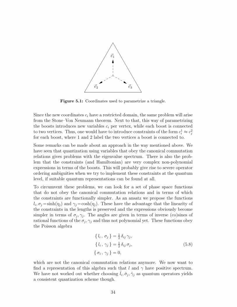
We have tried to find a reparametrization of the boosts. The restricted pairs ofboost triples are shown in figure 4.8. As a way to parametrize only the triplessatisfying the triangle inequality, we can first extract a common scale factor s

from a boost triple. Then a triangle remains to be parametrized. We can exploitits symmetry by choosing three coordinate axes as in figure 5.1. Now a point inthis triangle can be written as ~x =

∑3i=1 ci ~ei, but there is a redundancy in this

description, which can be lifted by imposing the constraint C = 1−∑3

i=1 ci ≈ 0.We also have to restrict the range of the coefficients: ci ∈ R+ suffices, becauseit implies ci ∈ [0, 1] together with the constraint. Furthermore, a consistentquantization exists on L2(R+), see [9].

This approach does not solve all problems. The new variables are a linearcombination of the boosts, so the Poisson brackets will still be of the same form.

3A symplectic transformation is a transformation on a space, which has a symplectic formdefined on it. That is in our case: a phase space with a Poisson bracket, where the symplectictransformation by definition preserves the symplectic form (thus the Poisson bracket).

33

~e1

~e2 ~e3

Figure 5.1: Coordinates used to parametrize a triangle.

Since the new coordinates ci have a restricted domain, the same problem will arisefrom the Stone–Von Neumann theorem. Next to that, this way of parametrizingthe boosts introduces new variables ci per vertex, while each boost is connectedto two vertices. Thus, one would have to introduce constraints of the form c1i ≈ c2jfor each boost, where 1 and 2 label the two vertices a boost is connected to.

Some remarks can be made about an approach in the way mentioned above. Wehave seen that quantization using variables that obey the canonical commutationrelations gives problems with the eigenvalue spectrum. There is also the prob-lem that the constraints (and Hamiltonian) are very complex non-polynomialexpressions in terms of the boosts. This will probably give rise to severe operatorordering ambiguities when we try to implement these constraints at the quantumlevel, if suitable quantum representations can be found at all.

To circumvent these problems, we can look for a set of phase space functionsthat do not obey the canonical commutation relations and in terms of whichthe constraints are functionally simpler. As an ansatz we propose the functionsli, σj=sinh(ηj) and γj=cosh(ηj). These have the advantage that the linearity ofthe constraints in the lengths is preserved and the expressions obviously becomesimpler in terms of σj , γj. The angles are given in terms of inverse (co)sines ofrational functions of the σj , γj and thus not polynomial yet. These functions obeythe Poisson algebra

{ li , σj } = 12δij γj ,

{ li , γj } = 12δij σj ,

{σi , γj } = 0,

(5.8)

which are not the canonical commutation relations anymore. We now want tofind a representation of this algebra such that l and γ have positive spectrum.We have not worked out whether choosing li, σj , γj as quantum operators yieldsa consistent quantization scheme though.

34

A different approach would be to only use variables associated with a set offundamental loops of the spatial manifold Σg. With each such loop we canassociate a Poincare transformation, determined by 6 parameters and there are2 g−1 independent loops. If we could rewrite the polygon model in terms of thesevariables, there would only be 3 constraints left. The 6(2 g−1) variables are 6more than the 12(g−1) dimensions of the physical phase space; 3 of these areconstraints and the other 3 are gauge freedoms associated to these constraints.

5.4 Conclusions

The original question whether space is quantized or time is discretized seems todepend on the way one quantizes the theory. This fact is well known, see e.g.[17] or [3, chap. 13].

To draw conclusions about discreteness, one must first have a consistent quan-tization scheme. In this chapter we saw, that the obvious choice of canonicalcommutation relations has some serious problems which cannot be overcomeeasily. Most notably the problem that the spectrum of the basic quantumoperators conflicts with the classical length and boost constraints. Thereforeit seems that one should not draw conclusions about the spectra of length andtime, without first showing that a consistent quantization scheme can (at leasttheoretically) be found.

35

6 The constraint algebra

In this chapter, we will do some explicit calculations to determine some propertiesof the algebra of Poisson brackets of the constraints. Next, we try to interpretthese constraints and the transformations they generate.

The algebra of constraints expresses how a constraint transforms under an in-finitesimal gauge transformation with respect to another constraint. In the caseof first class constraints, the result should be equal to zero on the constraintsurface (a so-called ‘weak equality’), because a classical solution must satisfythese constraints and a gauge transformation preserves the solution and thus theconstraint too.

The calculation of the constraint algebra is interesting from different perspectives.It allows us to check that these weak equalities hold, which is a consistencycheck for the polygon model. Furthermore, if one wants to quantize the modeland implement the constraints in the quantum theory, then this Poisson algebrashould have an analogue in terms of operator commutators in the quantum theory.If they are not equal, this could give rise to quantum anomalies [3, p. 279].

The constraints do not form a true Poisson algebra, because the right-hand sidesof the Poisson brackets turn out to be non-linear expressions in terms of theoriginal constraints and thus the linear span of the constraints does not form aclosed space under the Poisson brackets. A true Poisson algebra is a vector spaceX with multiplication and a bi-linear and anti-symmetric Poisson bracket

{ . , . } : X ×X 7→ X, (6.1)

satisfying the Jacobi identity. Thus when we choose a basis ei of X , we can write

{ ei , ej } = fkij ek, (6.2)

where the fkij are the so-called structure constants.

Our algebra of constraints is not of this form, but can (in principle) be rewrittenin a form where the structure constants fk

ij are replaced by structure functionsfkij(l, η) on phase space. For a proof, see [3, p. 8 and appendix 1.A]: the Poissonbrackets turn out to vanish on the constraint surface and can thus be writtenas linear combinations of the constraints, with coefficients given by structurefunctions. These structure functions are not explicitly given however and mightbe very complicated.

36

6.1 Useful formulas

Before starting the calculation, we summarize the constraints and some usefulrelations, which will be used to calculate the Poisson brackets. For each polygonwe have two constraints: the angular constraint Cθ and the complex (closure)constraint Cz. They are (4.7):

CAθ =

N∑

j=1

(π − αj)− 2 π,

CAz =

N∑

j=1

lj exp(iθj) where θj =

j∑

i=1

π − αi.

The label A = 1 . . . P labels the different polygons. The complex constraint takesvalues in C, so it is actually two real constraints. Instead of working with thereal and imaginary part, CA

z and CAz will be used to calculate all independent

Poisson brackets.

Next we have the vertex relations (4.4), from which the following identities canbe derived:

∂αa

∂ηa= −2

σa

sa σb σc

, (6.3)

∂αa

∂ηb= −2

cc σa

sa σb σc

= 2σb γc + ca σc γb

sa σb σc

, (6.4)

where the indices a, b, c label the three different edges and angles at a vertexaccording to figure 2.1. Note that these results differ by a factor 2 from those in[18] (appearing from chain-rule differentiation of the 2 η arguments).

The rightmost expression of (6.4) contains only quantities that can be expressedin terms of boosts and angles of a single polygon at that vertex. This can be usedto derive another useful relation between neighboring edges and angles along apolygon:

e±iαk+1

(∂αk+1

∂ηk+1∓ 2 i

γk+1

σk+1

)

= 2 (ck+1 ± i sk+1)σk+1 γk + ck+1 σk γk+1 ∓ i sk+1 σk γk+1

sk+1 σk σk+1

= 2ck+1 γk σk+1 + σk γk+1

sk+1 σk σk+1± 2 i

γk

σk

=∂αk+1

∂ηk± 2 i

γk

σk

(6.5)

37

The relation ei(π−αj ) = −e−iαj is used throughout the calculations; together withthe formula above, we can use it to simplify expressions a lot, as we will see.

As most of the work needed to calculate the different Poisson brackets is verymuch alike, we will first derive two general expressions, which will be used infurther calculations. Both expressions are of the form

N∑

k=1

e±iΦk∂θj

∂νk, (6.6)

where we have two polygons and differentiate angles of the first (indices j) withrespect to boosts of the second (indices k). θj ,Φk denote the angles of edges asin (4.6). This expression is calculated both for the two polygons being equal anddifferent. In these calculations we make some assumptions (6.11), which can befound in the next section on page 40.

First for j, k indexing the same polygon, we have

N∑

k=1

e±iθk∂θj

∂ηk

= −N∑

k=1

e±iθk

j∑

l=1

∂αl

∂ηk

= −

j∑

l=1

e±iθl−1

(e±iθN δl,1

∂αl

∂ηl−1+ e±i(π−αl)

∂αl

∂ηl

)

using the fact that angles only depend on neighboring boosts. Notice the extraterm e±iθN δl,1 : it is present because of the jump in complex angle factor, wherethe indices are taken cyclic modulo N (but not sums, as noted in (2.5) on page 7).This extra factor is 1 on the constraint surface, but non-trivial away from theconstraint surface. Now we plug in the identity 0 = 2 i ( γl

σl− γl

σl) and shift the

index of one of the terms to obtain

= −

j∑

l=1

e±iθl−1

(e±iθN δl,1

[∂αl

∂ηl−1∓ 2 i

γl−1

σl−1

]+ e±i(π−αl)

[∂αl

∂ηl± 2 i

γl

σl

])

±2 i

(e±iθj

γj

σj

− e±iθNγN

σN

)

= ±2 i

(e±iθj

γj

σj

− e±iθNγN

σN

)+(1− e±iθN

)( ∂α1

∂ηN∓ 2 i

γN

σN

)

= ±2 i

(e±iθj

γj

σj

−γN

σN

)+(1− e±iθN

) ∂α1

∂ηN. (6.7)

38

In the second last step, we used relation (6.5) to let all terms in the summationcancel against each other, except for the boundary terms.

When the j, k index different polygons, we get (again under the assumptions (6.11))only a contribution from the common edge denoted by jc, kc. This reduces thenumber of terms in the summation:

N∑

k=1

e±iΦk∂θj

∂νk

=∑

k∈{kc−1,kc,kc+1}

e±iΦk ×−

j∑

l=1

∂αl

∂νk

= −e±iΦkc

∑

k∈{−1,0,1}

(− e±i(βkc−ΦMδkc,1) δk,−1 + δk,0 − e∓i(βkc+1−ΦM δkc,M ) δk,1

)

×

(∂αjc

∂νkc+k

δjc∈[1,j] +∂αjc+1

∂νkc+k

δjc+1∈[1,j]

)

= −e±iΦkc

[(∂αjc

∂νkc− e∓i(βkc+1+ΦMδkc,M ) ∂αjc

∂νkc+1

)δjc∈[1,j]

+

(∂αjc+1

∂νkc− e±i(βkc+ΦMδkc,1)

∂αjc+1

∂νkc−1

)δjc+1∈[1,j]

]

= 2 e±iΦkc

[(ckc+1 σkc+1

sjc σjc−1 σjc

− e∓iΦM δkc,M (ckc+1 ∓ i skc+1)σkc+1

sjc σjc−1 σjc

)δjc∈[1,j]

+

(ckc σkc−1

sjc+1 σjc σjc+1− e±iΦM δkc,1 (ckc ± i skc)

σkc−1

sjc+1 σjc σjc+1

)δjc+1∈[1,j]

]

where the term e±iΦM = 1 on the constraint surface and we split off (1−e±iΦM ) . . . ,giving

= 2 e±iΦkc

[±i

skc+1 σkc+1

sjc σjc−1 σjc

δjc∈[1,j] ∓ iskc σkc−1

sjc+1 σjc σjc+1δjc+1∈[1,j]

+(1− e∓iΦM δkc,M

)e∓iβkc+1

σkc+1

sjc σjc−1 σjc

δjc∈[1,j]

+(1− e±iΦM δkc,1

)e±iβkc

σkc−1

sjc+1 σjc σjc+1δjc+1∈[1,j]

]

= ±2 i e±iΦkc1

σjc

(δjc∈[1,j] − δjc+1∈[1,j]

)

−2(1− e±iΦM

) 1

sβ1σνkc

[δjc+1∈[1,j] δkc,1 + e∓iβ1 δjc∈[1,j] δkc,M

]. (6.8)

39

Most of the above calculation is a straightforward expansion of the definitions.However one must keep good track of the indices and cyclic boundary conditions,which make the result non-trivial: if j = N and k 6∈ {1,M} then the resultreduces to zero identically. Thus we see here already that the result depends onthe choice of labelling of the polygons from the δkc,1 and δkc,M terms.

6.2 Calculation of the algebra

We want to calculate the complete Poisson algebra. All different, independentPoisson brackets between the constraints are given by

{CA

θ , CBθ

},{CA

θ , CBz

},{CA

z , CBz

},{CA

z , CBz

}, (6.9)

where A,B independently run over all polygons. All other combinations canbe obtained by using anti-symmetry of the Poisson brackets or by complexconjugation, for example:

{CA

θ , CBz

}= {CA

θ , CBz }.

To start with, there are some constraints which are trivially equal to zero. Firstof all, each constraint commutes with itself (when also the polygon labels areidentical: A = B). Secondly

{CA

θ , CBθ

}= 0 (6.10)

because there is no dependence on the edge lengths in either constraint.

Next we will calculate the Poisson brackets between all remaining constraintsunder some non-generic assumptions. Similar calculations were made previouslyin [18]. Here, we will perform the calculation more explicitly and establish severalcorrections to the results obtained in [18]. These results we will then use as astarting point for calculating the general form of the algebra, thus lifting theassumptions (6.11).

The assumptions are as follows:

no single polygon has two edges that have to be identified and (6.11a)

no two different polygons have more than one edge in common. (6.11b)

These assumptions are a theoretical, but also practical restriction, as they do notcover the ‘one polygon tessellations’ (OPT’s, as in [13]). There every edge of thepolygon has to be identified with another edge of the same, single polygon. OPT’sare the simplest tessellations possible and therefore a practical set of tessellations

40

kI II

βk+1

βk

νk+1

mk+1

αj+1

j+1 k−1

lj−1

ηj−1

j

αj

Figure 6.1: Label scheme for the calculation of the constraint algebra

to parametrize phase space with. If we want to explicitly use these OPT’s as astarting point for a quantum theory, we therefore need the full Poisson structurewithout the assumptions.

We will calculate the explicit expressions for the general Poisson structure withoutthese assumptions and show that the constraints do also close in that case. Thiswill be treated in section 6.3 and a summary of all results will be presented insection 6.4.

When we calculate brackets between two different polygons (labeled I and II),the result will be zero unless these polygons have an edge in common. This isbecause the constraints only depend on variables locally at the border of thepolygon. Hence with our assumptions we only have to look at cases where twodifferent polygons have exactly one edge in common.

In the calculations that follow, we will parametrize the two polygons as in fig-ure 6.1. We label lengths, boosts and angles of polygon I with l, η, α respectivelyand j indexes these. For polygon II we use m, ν, β with indices k. The indicesof the edges of polygon I and II that join each other will be denoted by jcand kc respectively. Labelling will always be counterclockwise oriented, see alsochapter 2.

We start by calculating the Poisson bracket of the angular constraint with thecomplex constraint of the same polygon. As there is no dependence on the lengthsin the Cθ, we only have to differentiate it with respect to the boosts and thus Cz

only with respect to the lengths. This yields

{CI

θ , CIz

}

=

{θN ,

N∑

k=1

lk eiθk

}

41

= −12

N∑

k=1

eiθk∂θN

∂ηkusing definition (2.6)

= −12

(∂α1

∂ηN− 2 i

γN

σN

)(1− eiθN

)using (6.7)

= −

(σN γ1 + c1 σ1 γN

s1 σ1 σN

− iγN

σN

)(1− eiθN

)

= eiθ1(σ1 γN + c1 σN γ1

s1 σ1 σN

+ iγ1

σ1

)(1− eiθN

)≈ 0. (6.12)

In the last step we used equation (6.5) to rewrite the result to the same formas in [18]. It coincides with the latter expression up to a factor 2 ei(π−α1); theexponential is due to a different definition of the complex constraint and thefactor 2 probably due to a calculation error, as noted below (6.4).

When we take the complex constraint together with its complex conjugate, weget terms from both differentiating the first with respect to the boosts and thesecond with respect to the lengths and vice versa:

{CI

z , CIz

}

=

{N∑

j=1

lj eiθj ,

N∑

k=1

lk e−iθk

}

= 12

N∑

j,k=1

(lk e

iθj e−iθk ×−i∂θk

∂ηj− lj e

iθj e−iθk × i∂θj

∂ηk

)

= −i

2

N∑

k=1

lk e−iθk

[+2 i

(eiθk

γk

σk

−γN

σN

)+(1− eiθN

) ∂α1

∂ηN

]

−i

2

N∑

j=1

lj eiθj

[−2 i

(e−iθj

γj

σj

−γN

σN

)+(1− e−iθN

) ∂α1

∂ηN

]using (6.7)

=γN

σN

(CI

z − CIz

)−

i

2

∂α1

∂ηN

[CI

z

(1− e−iθN

)+ CI

z

(1− eiθN

) ]

= 2 iγN

σN

Im

(CI

z

)− i

∂α1

∂ηNRe

(CI

z

(1− e−iθN

) )≈ 0. (6.13)

This result is somewhat different than that in [18]: in the first term we have arelative minus sign instead of plus and the second “boundary” term is added; itarises due to the cyclicity of the edge and angle indices, but one has to be carefulwith the interpretation of sums of angles as noted in (2.5).

42

Notice that the correctness of the minus sign is easily checked by complex con-jugating the complete Poisson brackets, because is should satisfy

{Cz , Cz

}={Cz , Cz

}= −

{Cz , Cz

}. (6.14)

We can check that the second term does also obey this condition.

Next we have the Poisson brackets between two different polygons. Using equa-tion (6.8) we get

{CI

θ , CIIz

}

=

{θN ,

M∑

k=1

mk eiΦk

}

= −12

M∑

k=1

eiΦk∂θN

∂νk

= −i eiΦkc1

σjc

(δjc∈[1,N ] − δjc+1∈[1,N ]

)

+(1− eiΦM

) 1

sβ1σνkc

(δjc+1∈[1,j] δkc,1 + e−iβ1 δjc∈[1,j] δkc,M

)

=(1− eiΦM

) 1

sβ1σνkc

(δkc,1 + e−iβ1 δkc,M

)≈ 0 (6.15)

by straightforward calculation, where we have to remember that the indices arecyclic and thus trivially δjc∈[1,N ] − δjc+1∈[1,N ] = 1− 1 = 0. Comparing again with[18], we have found an additional boundary term arising from cyclicity of theindices along the polygon.

43

The calculation of Poisson brackets between two complex constraints gives{CI

z , CIIz

}

=

{N∑

j=1

lj eiθj ,

M∑

k=1

mk eiΦk

}

=i

2

∑

j,k

(mk e

iθj eiΦk∂Φk

∂ηj− lj e

iθj eiΦk∂θj

∂νk

)

=

M∑

k=1

mk eiΦk

[−

eiθjc

σkc

(δkc∈[1,k] − δkc+1∈[1,k]

)

−i

sα1σηjc

(1− eiθN

) (δkc+1∈[1,k] δjc,1 + e−iα1δkc∈[1,k] δjc,N

)]

− {l, η, θ, j} ↔ {m, ν,Φ, k} inserting (6.8)

= −eiΦkc

σkc

CIz δjc,N +

eiθjc

σjc

CIIz δkc,M

−i

sα1σηjc

(1− eiθN

) [ZII

kc+1 δjc,1 + e−iα1 ZIIkcδjc,N

]

+i

sβ1σνkc

(1− eiΦM

) [ZI

jc+1 δkc,1 + e−iβ1 ZIjcδkc,M

]≈ 0, (6.16)

where we have defined

ZAk =

N∑

j=k

lj eiθj (6.17)

as the partial complex constraint of polygon A from edge k. Also, we used therelations

δjc∈[1,j] − δjc+1∈[1,j] = δj,jc − δjc,N and δjc∈[1,j] = δj∈[jc,N ]. (6.18)

Completely analogously, we find for a complex and complex-conjugate constraint{CI

z , CIIz

}

= +e−iΦkc

σkc

CIz δjc,N −

eiθjc

σjc

CIIz δkc,M

+i

sα1σηjc

(1− eiθN

) [ZII

kc+1 δjc,1 + e−iα1 ZIIkcδjc,N

]

+i

sβ1σνkc

(1− e−iΦM

) [ZI

jc+1 δkc,1 + eiβ1 ZIjcδkc,M

]≈ 0. (6.19)

44

Figure 6.2: Rotation of the plane of a polygon and its action on edge lengths andextrinsic curvature surrounding the polygon.

Both of these Poisson brackets yield expressions that vanish on the constraintsurface, but do not identically vanish on the whole phase space, unlike the resultsin [18]: when one of the indices jc, kc is equal to the first or last of its polygon,the result is non-zero.

As already pointed out in [6], the Hamiltonian flow generated by the complex con-straints should (on shell) be related to Lorentz transformations of the coordinateframes of the polygons. This is a residual gauge freedom that is left after fixingthe constraints Hi in (3.8). With this interpretation, one would not expect thePoisson brackets between these constraints to vanish identically (as is the resultin [18]): the complex constraint should be related to the constraints Hi and theircorresponding gauge freedom to the Lorentz transformations of the local frameof the polygon.

Suppose now that the complex constraint in polygon I does not close by anamount d in the y-direction (CI

z = i d 6= 0) and we generate a Lorentz transfor-mation in polygon I. This Lorentz transformation can be seen as a “space-timerotation” of the plane of polygon I as in figure 6.2: the (infinitesimal) boost ofthe Lorentz transformation corresponds to an angle that the plane of polygon I isrotated by. This will affect the lengths and boosts of all edges along that polygonand also the lengths of edges connected to those. We now consider the effect ofthis transformation on a neighboring polygon II. We suppose that they have anedge in common, which has indices jc, kc in polygons I and II respectively, wherewe choose jc = N, kc = M . The implicit assumption is made that the closuredeficit CI

z is located between edges j = N and j = 1. Now the position of vertex1 (which is located between edges j = N and j = 1) depends on whether weview it as the first or last point of the constraint CI

z, see figure 6.4, where wehave implicit complex coordinates z = x+ i y and the origin is placed at vertex1 viewed as starting point of the complex constraint.

This will give rise to a different change of the intersection line under this Lorentztransformation and thus a change in CII

z . Figure 6.3 shows the geometricalpicture in the (y, t)-plane. The lines are the planes of polygons I and II and

45

y

t

II

d2 η

t′

y′

d′

dνI

Figure 6.3: Action of a Lorentz trans-formation on a complex constraint. (y, t)and (y′, t′) denote the coordinates withinpolygons I and II respectively.

2

3

1

y

N−1

N1

xCz

Figure 6.4: Polygon with non-closingcomplex constraint: vertex 1 shows upon both sides of the deficit Cz 6= 0.

their intersection point is the common edge. Now vertex 1 shows up as thisintersection point, but also at a distance d apart.

The action of an infinitesimal Lorentz transformation of polygon I by an amountdν is shown as the dashed lines. The upper one is rotated around the origin ofpolygon I (which is vertex 1) and the lower one around vertex 1 as viewed aftergoing around polygon I, after which it is shifted by a distance d. These generatedifferent new intersection points between polygons I and II. We can now calculatethe distance between those intersection points explicitly, which yields

d′ =d

sinh(2 η)dν. (6.20)

This matches the result

{CII

z , CIz

}=

eiΦkc

σkc

CIz δjc,N =

i d

σ, (6.21)

where we have inserted that all constraints close, except CIz = i d and thus all

other terms from (6.16) vanish and ΦM = 2 π.

Thus this geometrical viewpoint seems to indicate that indeed the Poisson bracket{CI

z , CIIz

}is not identically zero outside the constraint surface, if we interpret

the complex constraints as generators of Lorentz transformations.

46

6.3 Generalizations

We can generalize the assumptions (6.11) made in the previous section to thearbitrary case, which will recover the explicit full Poisson structure. We willtake two different approaches: the first one is to consider the Poisson bracketsof the constraints with the Hamiltonian, using the Hamiltonian flow in (4.8).The Hamiltonian is the sum of the angular constraints, so for an OPT we haveH = Cθ. This will then give us the Poisson bracket {Cθ , Cz } in the case of anOPT without any assumptions made. The second approach will be to lift theassumptions in a general setting. The results of these approaches are then shownto match in the case of an OPT.

6.3.1 The case of an OPT

To calculate the Poisson bracket {H , Cz }, we first need a formula relating thegrowth of edges along a polygon. This formula and its derivation is analogousto (6.8). However we note that in the definition of the σ, γ in (6.22), the factor2 is missing with respect to our original definition (2.4), so σi = sinh(ηi), γi =cosh(ηi). We have

e±iαk+1

(lk+1,1 ± i

σk+1

γk+1

)

= −(ck+1 ± i sk+1)σk γk+1 + ck+1 σk+1 γk ∓ i sk+1 σk+1 γk

sk+1 γk γk+1

= −σk+1 γk + ck+1 σk γk+1

sk+1 γk γk+1∓ i

σk

γk

= lk,2 ∓ iσk

γk. (6.22)

We can use the previous relation to rewrite {Cz , H } (the time evolution of thecomplex constraint) in the same way as we did with (6.12):

{Cz , H }

=

{N∑

j=1

lj eiθj , H

}

=

N∑

j=1

eiθj lj

=N∑

j=1

eiθj(lj,1 − i

σj

γj+ lj,2 + i

σj

γj

)

47

= eiθ1(l1,1 − i

σ1

γ1

)(1− eiθN

)using (6.22)

=

(lN,2 + i

σN

γN

)(eiθN − 1

)

=

(−vN c1 + v1

s1+ i vN

)(eiθN − 1

)≈ 0 (6.23)

Here we recognize the left part of the final expression as minus the velocity ofvertex 1 in the coordinate-frame of the polygon (in complex notation, as was usedfor the formulation of the complex constraint). The factor eiθN −1 precisely givesthe difference of viewing this point as the first or the last when going around thepolygon. Thus this intuitively matches the expected result of the time evolutionof the closure constraint.

6.3.2 The case of a general tessellation

We now want to generalize the calculated Poisson brackets between two polygonsto the arbitrary case without assumptions (6.11).

The underlying idea is as follows: we can split the Poisson bracket expression intoparts (see (6.25) for a precise specification), taking account for each common edgeseparately. For this, we first have to show that there are some restrictions to theways two polygons can have multiple edges in common, such that we can makesuch a splitting. For this to work, different common edges should not interferewith each other in the calculation of the Poisson brackets.

To show that the “condition” above is fullfilled, let us consider two polygons asin figure 6.5, which have at least an edge in common for edge indices jc, kc. Thepolygons X, Y and Z can be copies of polygons I or II and as such can give riseto multiple common edges.

The only non-vanishing terms in the Poisson brackets appear from the differen-tiation of one term in a complex (conjugate) constraint (say polygon II) to theedge length and then the other constraint (polygon I) differentiated with respectto the corresponding boost. This means differentiation of an angle of polygon I,as the angles are the only quantities in the constraints that depend on boosts.

If two common edges cannot appear in such a way that their ‘split’ Poissonbrackets would both contain a specific angle term of polygon I being differentiatedto a boost of the same edge of polygon II, we can replace the Poisson brackets bytwo separate Poisson brackets where we treat the common edges one at a time.Note that here an ‘edge’ is a boundary element of a polygon, so each pair (li, ηi)is assigned to two edges, when the edges are viewed as boundaries of polygons.

48

Thus the “condition” above can be stated in a more precise way as follows:

each edge from polygon II has at most one way in which it is connectedto each angle of polygon I (and the converse, which follows frominterchanging polygons I and II).

(6.24)

The proof of this statement hinges on the fact that the graph of the tessellationhas trivalent vertices. We will first give an insightful proof followed by a moredetailed proof.

The statement can be seen to hold in the following way. If an angle wouldbe connected twice to an edge, then this edge has its endpoints on one vertex.Because of trivalency of the vertices, both ends of that edge must be neighboringat that vertex and thus the edge encloses a polygon in itself. This is clearly acontradiction.

For the detailed proof, we start off with the case of an angle of polygon I and anedge of polygon II. Proving (6.24) boils down to a tedious but straightforwardtreatment of all possible scenario’s. With some symmetry arguments, we canhowever reduce this a bit. Suppose that an angle of polygon I is connected twiceto an edge of polygon II. It must be an angle at one side of a common edge.Because of symmetry we can take angle α as shown in figure 6.5 without loss ofgenerality.

Now edge kc cannot be connected to α more than once, because it is alreadyjoined with edge jc and thus cannot be joined with jc − 1 and it cannot be equalto edge kc + 1. Also edge kc + 1 cannot be connected more than once, becauseif it would be connected to jc − 1 (as b), then kc would be connected to kc + 1(as a). Finally, edges a and b obviously cannot be equal, so condition (6.24) isfullfilled for angles of polygon I.

To apply the idea as outlined above to the generalization of the Poisson brackets,we first have to explicitly define what we mean by a splitting of a Poisson bracket

kc

f

g

d

b

a

e

jc

kc+1

α

I

Z

Y

jc−2

jc−1jc+1

kc−1 II

X

Figure 6.5: Multiple common edges between two polygons.

49

into separate parts for each common edge. Let us denote the pairs of commonedges of polygon A and B by (jc, kc)c=1..nc

. We now introduce the notation

{CA , CB

}0

and{CA , CB

}c. (6.25)

The left expression shall denote the Poisson brackets of two constraints, where noedges are identified. This expression will thus only be non-zero when A = B andthen yields the ‘internal terms’. The right expression shall denote the Poissonbrackets of these constraints, where no internal contributions are counted (so wetreat A 6= B) and only the edge pair (jc, kc) is treated as common; the othersare treated as not being common. Thus by their definitions, these expressionsare equal to the corresponding expression calculated in section 6.2 under theassumptions (6.11):

{CA , CB

}0for the case A = B and

{CA , CB

}cfor the case

A 6= B. We will generalize the Poisson brackets already calculated to arbitraryconditions, by proving that one can split the general Poisson brackets as

{CA , CB

}={CA , CB

}0+

nc∑

c=1

{CA , CB

}c. (6.26)

Given two polygons I and II, we denote their pairs of common edges by (jc, kc)c=1..nc

and first investigate the Poisson brackets{θIj , C

IIz

}:

nc∑

c=1

{θIj , C

IIz

}c

=nc∑

c=1

[ {−αjc δjc∈[1,j] , mkc−1 e

iΦkc−1 +mkc eiΦkc

}+

{−αjc+1 δjc+1∈[1,j] , mkc e

iΦkc +mkc+1 eiΦkc+1

} ]

=

j∑

j′=1

{−αj′ , C

IIz

}

={θIj , C

IIz

}(6.27)

Working backward from the desired result, we first only write down those termsthat will contribute for each common edge. In the next step, we use the fact thateach combination of angle α of polygon I and edge m of polygon II does showup not more than once in the full Poisson bracket, as stated in (6.24). It alsodoes show up exactly once, as it is part of a single common edge bracket. Allremaining terms in

{θIj , C

IIz

}are zero now, because we have exactly taken into

account all terms contributing to all common edge Poisson brackets and thereare no internal contributions, because we considered two different polygons.

50

In the case that both constraints are from the same polygon, we can essentiallyrepeat the argument, except that we have to add the terms that arise from theinternal contributions:

{θIj , C

Iz

}0+

nc∑

c=1

{θIj , C

Iz

}c

=N∑

k=1

{−αk δk∈[1,j] − αk+1 δk+1∈[1,j] , lk e

iθk}+

nc∑

c=1

[ {−αjc δjc∈[1,j] , lkc−1 e

iθkc−1 + lkc eiθkc}+

{−αjc+1 δjc+1∈[1,j] , lkc e

iθkc + lkc+1 eiθkc+1

} ]

=

j∑

j′=1

{−αj′ , C

IIz

}

={θIj , C

IIz

}. (6.28)

The extra terms do not change the argument, because also with these added,condition (6.24) still holds and all terms that we started with are exactly thosethat will be present in the full Poisson bracket.

Now that we have shown in (6.27) and (6.28) that a split can be made for thebrackets

{θAj , CB

z

}for all A,B, we can easily extend the result to all possible

Poisson brackets. The application of (6.27) to{CI

θ , CIIz

}is trivial by plugging

in j = N and yields

{CI

θ , CIIz

}

=

nc∑

c=1

{CI

θ , CIIz

}c

using (6.27)

=

nc∑

c=1

(1− eiΦM

) 1

sβ1σνkc

(δkc,1 + e−iβ1 δkc,M

)≈ 0. (6.29)

We see that the sum over all joined pairs of edges (jc, kc) reduces to only contri-butions from the pairs where kc = 1 or kc = N .

51

In the same way, we can generalize{CI

θ , CIz

}using (6.28), which gives

{CI

θ , CIz

}

={CI

θ , CIz

}0+

nc∑

c=1

{CI

θ , CIz

}c

= −

(σN γ1 + c1 σ1 γN

s1 σ1 σN

− iγN

σN

)(1− eiθN

)

+nc∑

c=1

(1− eiΦM

) 1

sβ1σνkc

(δkc,1 + e−iβ1 δkc,M

)≈ 0. (6.30)

To generalize the Possion brackets of two complex (conjugate) constraints to thecase of multiple common edges, we first rewrite one complex constraint to a sumof θj by the chain rule for differentiation and obtain

{CI

z , CIIz

}

=

{N∑

j=1

lj eiθj ,

M∑

k=1

mk eiΦk

}

= i

N∑

j=1

lj eiθj{θj , C

IIz

}− i

M∑

k=1

mk eiΦk{Φk , C

Iz

}

= i

N∑

j=1

lj eiθj

nc∑

c=1

{θj , C

IIz

}c− i

M∑

k=1

mk eiΦk

nc∑

c=1

{Φk , C

Iz

}

=

nc∑

c=1

{CI

z , CIIz

}c

(6.31)

The Poisson brackets where one of the constraints is a complex conjugate andwhen both constraints are from the same polygon, are all derived in an analogousway. For the explicit expression one must insert the already calculated bracketswith assumptions. See (6.32b) and (6.32c) for the complete expressions.

52

6.3.3 Comparing for consistency

Now we can do a consistency check with the results we have found. The Hamil-tonian can be written as the sum of all angular constraints. The Poisson bracketsof this sum of all angular constraints with one complex constraint should thusmatch expression (6.23). Indeed we find that they do match:

{H , CB

z

}

=∑

A

{CA

θ , CBz

}

={CB

θ , CBz

}+∑

A 6=B

{CA

θ , CBz

}

= −

(σN γ1 + c1 σ1 γN

s1 σ1 σN

− iγN

σN

)(1− eiΦM

)

+M∑

k=1

(1− eiΦM

)( 1

s1 σ1

δk,1 +e−iβ1

s1 σM

δk,M

)

where we sum over all angular constraints, so all separate summations overcommon edges reduce to one summation over all edges of polygon B. This sumthen reduces to the two terms k = 1 and k = M , which leaves us with

=(1− eiΦM

) [−σM γ1 + c1 σ1 γM

s1 σ1 σM

+ iγM

σM

+1

s1 σ1+

e−iβ1

s1 σM

]

=(1− eiΦM

) [−

1

s1

(γ1 − 1

σ1

+ c1γM − 1

σM

)+ i

γM − 1

σM

]

=

(−v1 + c1 vN

s1+ i vN

)(1− eiθN

)using

γ − 1

σ= v

= −{CB

z , H}

inserting (6.23).

Note that we replaced θ’s by Φ’s when inserting (6.30) and vice versa whenrewriting the result back to (6.23), but these are the same as both constraintsdescribe the same polygon.

53

6.4 Summary

The results of this chapter are summarized below. The same conventions havebeen made and the sums are again over all pairs of common edges betweenpolygons A and B. In the case that A and B are equal, each pair will thusshow up twice: if the pair (jc, kc) = (x, y) exists, then also (jc, kc) = (y, x).

{CA

θ , CBz

}= −

(σN γ1 + c1 σ1 γN

s1 σ1 σN

− iγN

σN

)(1− eiθN

)δA,B

+

nc∑

c=1

((1− eiΦM

) 1

sβ1σνkc

(δkc,1 + e−iβ1 δkc,M

))

(6.32a)

{CA

z , CBz

}=

nc∑

c=1

(−

eiΦkc

σkc

CAz δjc,N +

eiθjc

σjc

CBz δkc,M

−i

sα1σηjc

(1− eiθN

) [ZB

kc+1 δjc,1 + e−iα1 ZBkcδjc,N

]

+i

sβ1σνkc

(1− eiΦM

) [ZA

jc+1 δkc,1 + e−iβ1 ZAjcδkc,M

] )

(6.32b)

{CA

z , CBz

}=

(γN

σN

(CA

z − CAz

)−

i

2

∂α1

∂ηN

[CA

z

(1− e−iθN

)+ CA

z

(1− eiθN

) ])δA,B

+

nc∑

c=1

(+

e−iΦkc

σkc

CAz δjc,N −

eiθjc

σjc

CBz δkc,M

+i

sα1σηjc

(1− eiθN

) [ZB

kc+1 δjc,1 + e−iα1 ZBkcδjc,N

]

+i

sβ1σνkc

(1− e−iΦM

) [ZA

jc+1 δkc,1 + eiβ1 ZAjcδkc,M

] )

(6.32c)

54

6.5 Interpretation

We would like to interpret the Poisson bracket relations we have found. Theangular and complex constraints are first class constraints and should correspondto some residual constraints and gauge freedom left after the (partial) fixing ofthe constraints H,Hi in (3.7) and (3.8).

Intuitively, the residual constraint left from the Hamiltonian density H is the sumof deficit angles at the vertices. Superficially, this seems to match the angularconstraints, but in these the sum of deficit angle at a vertex is distributed amongthe angular constraints of polygons that join at that vertex.

The complex constraints should be related to the residual gauge freedom ofLorentz transformations of each polygon frame. With the help of the dualgraph formulation of appendix A, we can try to see whether this intuitive ideamatches the explicit complex constraint definition. In the dual graph, a Lorentztransformation of a polygon frame f ∈ F amounts to shifting the correspondingvertex v ∈ V in the dual graph by the action of the Lorentz transformation L

when we choose v to be at the origin (1, 0, 0).

The boosts ηi of edges along the polygon are encoded by half the arc lengthsof the geodesics emanating from v. Thus if we make an infinitesimal Lorentztransformation, the change in boosts will be half the “length” of the Lorentztransformation projected on the direction of the outgoing edge (as seen in thedual graph). This means that a Lorentz transformation of boost dν in the x

direction in the polygon frame should affect the boosts ηi as follows:

dηi = cos(φ) dν, (6.33)

with φ the angle that edge i makes with the x axis in the dual graph. This angleis φ = θi +

π2, because the direction of the boost is perpendicular to the direction

of the edge in the normal graph.

We can compare this to the gauge transformation generated by the complexconstraint. The action of that gauge transformation is given by the Hamiltonianflow; the Poisson brackets of a quantity with the constraint gives the action thatthe corresponding gauge transformation has on that quantity. For the boosts wefind

dηi = { ηi , Cz } = −12

∂Cz

∂li= −1

2eiθi = −1

2 (cos(θi) + i sin(θi)) . (6.34)

Comparing this with (6.33), we see that the imaginary part of Cz generatesLorentz transformations in the x direction and the real part in the negative y

direction, at least for the boost variables.

Unfortunately, the action on the length variables is much more complicated. Tocompare the action on the lengths of the complex constraint with the action of a

55

Lorentz transformation, we can consider the action of a Lorentz transformation ofthe polygon frame geometrically and check whether that matches { li , Cz }. In thegeometrical picture of the tessellation graph, one expects that an (infinitesimal)Lorentz transformation acts on the variables as a “rotation in space-time” ofthe polygon plane, see figure 6.2. This changes the intersection lines with itsneighboring polygons, from which the action of the Lorentz transformation onthe lengths can be deduced. The explicit formulation of this action is alsoquite complicated and we have not investigated whether this geometrical picturematches the Poisson brackets.

56

7 Conclusions

We have looked at the polygon model as a way to describe 2+1-dimensionalgravity. This model makes use of the local flatness of 2+ 1D space-time ina remarkably efficient way: the polygon model can be formulated as a finitedimensional system with a completely explicit description of its evolution in termsof growth of edge lengths and polygons undergoing transitions at a discrete set oftimes. This makes the model very useful for exploring features of gravity alreadyin the classical context, e.g. by simulation.

In well known other descriptions of 2+1-dimensional gravity, the system is definedmore implicitly. For example in the ADM formulation with York time, one mustsolve the conformal factor of the metric from a elliptic partial differential equation.This has no known explicit solution for genus g > 1 [14]. Witten’s approach seemsto use the frozen time picture, where the dynamics cannot be recovered from thesystem[15, 19]. These problems are not present in the polygon model formulation.

There are however also some drawbacks of the formulation of the polygon model.The polygons that together form a spatial slice, are of finite size and internallyflat by construction. In this construction we have solved the field equations of thegauge constraints. The finite dimensional system which is left, is (by definition)non-local and still has constraints. This yields difficulties.

The problems of this non-locality are most clear in the Poisson bracket struc-ture of the constraints. The constraints for each polygon are already non-localexpressions and the Poisson brackets of constraints between different polygonsare complicated expressions, which do not vanish off shell. Even stronger, theydo not form a proper Poisson algebra, because the brackets are not linear in theconstraints.

We have shown though, that the complete Poisson bracket structure can be cal-culated explicitly and does vanish on shell. This was expected, as the constraintsshould be a residue of the field constraints in the unreduced canonical formulation,which are first class.

The features of the polygon model that allowed an explicit formulation in theclassical theory become problematic when we turn to the question of quantization.First of all, a full description of a state depends partially on a discrete graph

57

structure, which changes under transitions. This cannot easily be encoded in aquantum formulation. Furthermore, there are inequality constraints which arecoupled in a very non-local way. This is due to the fact that the Hamiltonian isa highly non-trivial function of the basic variables, which is only defined whenthose inequalities are satisfied. Because of these inequalities, we cannot lift thesimple Poisson bracket structure between those coupled variables to a quantumtheory, as that would violate these triangle inequalities.

We have shown that several ways of attacking the problem of finding a consistentquantization run into one or more of the difficulties above. Thus the questionof whether the polygon model obtains a discrete time and/or space spectrumafter quantization seems to be premature. It not only depends on whetherone first quantizes and then implements the constraints or vice versa, but morefundamentally on whether a satisfactory quantum theory can be formulated ineither approach. If we first quantize, we face a complicated Poisson structurewhich has to be implemented in the quantum theory. If we first solve theconstraints, we face the problem of finding an explicit global solution to those.

Both approaches, although meeting some major obstacles, do not seem com-pletely hopeless. The dual graph formulation (as in appendix A) gives a niceabstract interpretation of the polygon model, which might be useful to reducethe constraints in the classical theory in terms of holonomy-loop variables. Thisdual graph formulation depends on the absence of particles however. On thequantum theory side, one might consider other variables than the canonical ones.This leaves the question of whether this polygon model can be quantized to adifficult but open one.

58

A The dual graph

In this appendix we will present the dual graph of a tessellation in the polygonmodel. For this we will first introduce the concept of a dual graph in its generalsetting and also introduce hyperbolic space. It turns out that we can assigna meaning to the dual graph of a tessellation, such that it becomes a graphembedded in a hyperbolic space: a surface with constant negative curvature.

A.1 The dual of a planar graph

The concept of a dual graph is a very general one within graph theory and hasapplications in a wide variety of fields. It does not add new information to thegraph, but allows one to see some features more quickly by using a differentrepresentation of the same graph data.

To introduce the dual graph, we start with a graph G = (V,E), where V is theset of its vertices and E the set of edges. Each edge is normally represented asa pair of vertices: the ones that it connects. If we now embed our graph in theplane, the dual of that graph is defined by associating a vertex to each region ofthe plane and connect two vertices with an edge when their regions in the originalgraph had an edge as a common boundary. One must however notice two things:firstly, not every graph can be embedded in the plane without intersecting edges,so this definition does not yield a dual graph for each graph (V,E). Secondly, agraph can have different possible embeddings in the plane, resulting in differentdual graphs; see figures A.1 and A.2 for an example.

This non-uniqueness of the dual graph can be lifted if we add faces to the graphinformation. We now write G = (V,E, F ) with F a set of faces and each edge alsocontaining information about the pair of faces it connects. We want this graphwith added faces to uniquely describe a graph on some genus g surface. Thismeans that we have an orientation1 in the graph from the underlying manifold

1The orientation can only be defined locally in the case of a generic surface. However weonly consider orientable surfaces, which allows us to extend this local orientation to a globalone.

59

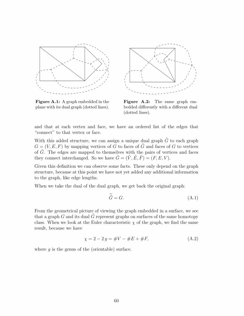
Figure A.1: A graph embedded in theplane with its dual graph (dotted lines).

Figure A.2: The same graph em-bedded differently with a different dual(dotted lines).

and that at each vertex and face, we have an ordered list of the edges that“connect” to that vertex or face.

With this added structure, we can assign a unique dual graph G to each graphG = (V,E, F ) by mapping vertices of G to faces of G and faces of G to verticesof G. The edges are mapped to themselves with the pairs of vertices and facesthey connect interchanged. So we have G = (V , E, F ) = (F,E, V ).

Given this definition we can observe some facts. These only depend on the graphstructure, because at this point we have not yet added any additional informationto the graph, like edge lengths.

When we take the dual of the dual graph, we get back the original graph:

˜G = G. (A.1)

From the geometrical picture of viewing the graph embedded in a surface, we seethat a graph G and its dual G represent graphs on surfaces of the same homotopyclass. When we look at the Euler characteristic χ of the graph, we find the sameresult, because we have

χ = 2− 2 g = #V −#E +#F, (A.2)

where g is the genus of the (orientable) surface.

60

A.2 Hyperbolic space

Hyperbolic space is a Riemannian manifold. Its most common definition (andmost practical here) is as follows. For n ≥ 2, start with an (n+1)-dimensionalMinkowski space, thus Rn+1 with the metric2 ηµν = diag(−1, 1, . . .). Now n-di-mensional hyperbolic space is defined as

Hn = {x ∈ R

n+1 | η(x, x) = −1, x0 > 0} (A.3)

with the metric induced from the underlying Minkowski space.

The space thus constructed is a true Riemannian manifold: the original metricwas a pseudo-Riemannian metric, but its restriction to Hn is positive definite.Furthermore Hn is a space with constant negative (sectional) curvature −1: atany point p and any 2-dimensional plane in the tangent space of p, the scalarcurvature is −1.

We will be concerned specifically with the case n = 2: the hyperbolic plane.The hyperbolic plane has some other well-known representations, besides thedefinition (A.3) given above. One is that of the complex halfplane

{x+ i y ∈ C | y > 0}, ds2 =dx2 + dy2

y2, (A.4)

and the other is the unit disc

{(x, y) ∈ R2 | ‖(x, y)‖ < 1}, ds2 =

dx2 + dy2

1− ‖(x, y)‖2. (A.5)

These two models are known as the Poincare plane and disc respectively.

Hyperbolic space is a maximally symmetric Riemannian manifold. That meansthat its isometry group is as large as can possibly be for a Riemannian manifold,namely, of dimension 1

2n(n+ 1). We will further investigate this symmetry from

the viewpoint of our original definition (A.3). The symmetry group is the identitycomponent SO+(n, 1) of the full Lorentz group O(n, 1). The group SO+(n, 1)consists of the time- and space-orientation preserving Lorentz transformations onthe Minkowski space Rn+1 and thus preserves the metric η and the sign of x0.

This group SO+(n, 1) can now be seen to have a group action on Hn: an elementL ∈ SO+(n, 1) defines a map L : Rn+1 7→ Rn+1 that can be restricted to a mapL : Hn 7→ Hn, because SO+(n, 1) precisely preserves the quantities that define

2This can be interpreted as the metric on Minkowski space itself and the differential metricon the tangent space as Minkowski space is a vector space and thus isomorphic to its tangentspace.

61

Hn. This map L then also naturally defines the map DL : THn 7→ THn on thetangent bundle.

The elements L ∈ SO+(n, 1) exactly correspond to all possible isometries of Hn.This is because the group SO+(n, 1) has precisely 1

2n(n+ 1) degrees of freedom:

n degrees correspond to translations of the hyperbolic plane and 12n(n− 1) cor-

respond to rotations around a fixed origin.

Looking in detail at how SO+(n, 1) acts on Hn, we see for n = 2 that pure Lorentzboosts Lx,y(η) perform translations in Hn by a distance of η in the x, y-direction(locally around the “origin” (1, 0, 0); because of curvature the action is somewhatmore complicated away from the origin). The rotations Lr(α) perform a simplerotation around the origin.

A.3 Embedding the dual graph in H2

We have first constructed the dual graph of a tessellation. Let us now assigngeometrical data to this dual graph.

We will do so by looking at the path that a Lorentz transformation maps out inhyperbolic space when it acts on (1, 0, 0). Each Lorentz transformation L can bedecomposed into pure rotations and boosts in the following way:

L = Lr(φ1)Lx(η)Lr(φ2). (A.6)

This can be interpreted (in reverse order) as rotating the local frame over an angleφ1 to the direction of the boost, then boost with parameter η and then rotatethe boosted frame to the desired orientation over an angle φ2. The continuoustransformation of (1, 0, 0) under the one-parameter subgroup

L(t) = Lr(φ1)Lx(η t)Lr(φ2), t ∈ [0, 1] (A.7)

will then be a geodesic in H2; figure A.3 shows an example of such geodesics.

Now each edge in the dual graph corresponds to a Lorentz3 transformation L

of one frame to the other it connects. Actually, we should consider orientededges, because when we traverse the edge in opposite direction, the Lorentztransformation is L−1. Thus each edge can be viewed as an isometry of H2,which in turn can be viewed as geodesics in H2.

A triangular polygon in the dual graph corresponds to a vertex in the originalgraph. Thus traversing its three enclosing edges means going around that vertexand the composition of corresponding Lorentz transformations should be the

3We can more generally assign to each edge a Poincare transformation, by also taking intoaccount the way coordinates are shifted after crossing an edge.

62

0

1

2

-0.5

0

0.5

1

1.5

1

1.5

2

2.5

0

1

2

Figure A.3: The hyperbolic surfaceH2 with red lines showing a triangle:the successive action of boosts and ro-tations, forming a closed holonomy.

α

|2 η|

α

Figure A.4: Angles of a hyper-bolic triangle.

identity. This means that, again viewing these edges as geodesics in H2, theyform a closed triangle and we can thus naturally associate a graph structure withit, see figure A.3.

We can now try to interpret the geometrical data of this graph embedded inH2: the dual graph lives in a Riemannian manifold, so concepts like lengths andangles are well-defined. Some subtleties will show up however, due to the factthat these geodesics do not contain all information of the Lorentz transformationsof the edges. Each Lorentz transformation L is fully characterized by the wayit acts as an isometry on H2, but if we only look at its action on a single point,information is lost: the way it acts on other points. This can be retrieved by notonly giving the action of L on a single point, but also specifying its action on thetangent space at that point.

When we now draw a triangle in the dual graph like in figure A.4, we find thateach edge has geodesic length |2 η|. The outer angles of the triangle are in directcorrespondence to the angles αi at a vertex in the original graph: they describethe rotation that we have to make, when we “walk” along a geodesic and turn tothe direction of the next geodesic. The inner angles αi of the triangle are relatedto these as

αi = π − αi. (A.8)

With this identification, we see that at each vertex in the dual graph, we have a2 π neighborhood as expected:

N∑

i=1

αi =

N∑

i=1

π − αi = Cθ = 2 π (A.9)

63

by identification of the vertex in the dual graph with a polygon in the originalgraph and using the angular constraint.

There is also an interpretation for the Hamiltonian (4.9) in the dual graph byconsidering the area of all faces in the dual graph. We start from the fact thatthe area of a triangle in hyperbolic space is determined by its inner angles αi

only, as the deficit angle from π:

A = π −3∑

i=1

αi. (A.10)

When we now sum the area of all triangles in the dual graph, we obtain

A =∑

f∈F

(π −

3∑

i=1

αi

)= −

∑

v∈V

(2 π −

3∑

i=1

αi

)= −H. (A.11)

The boost parameters 2 η cannot be interpreted as simply the geodesic lengths:η can be negative and in the geometric picture of figure A.4 this corresponds towalking the geodesic line in the opposite direction.

If we have a vertex where the signs of the three boosts are not the same (called a‘mixed vertex’ in [13]), this implies that the interpretation of αi = π − αi as theinner angles of the triangle becomes problematic.

A way to solve this is to consider again the Lorentz transformations correspondingto each edge. These can be decomposed as in (A.6). In decomposing these wecan always choose η positive: if it is negative, we can replace the parametersby (φ1, η, φ2) 7→ (φ1 ± π,−η, φ2 ± π). In this way we get a graph with all edgelengths positive and the oriented sum of angles at every point a multiple of 2 π.If we translate this interpretation back to the original graph, it means that wehave reversed the orientation of the edges. This interpretation thus moves thesigns from the boosts onto the lengths, which looks similar to the variables xi, pjintroduced in [6]. This will affect the definition of the Hamiltonian and theequations of motion, but we have not analyzed further the implications.

See also the discussion of this problem of the interpretation of mixed vertices in[12, p. 47].

64

Acknowledgements

First of all, I would like to thank my supervisor, Prof. Renate Loll for givingme the opportunity to work on this interesting subject. She guided me with myquestions to the right places. I would especially like to thank Zoltan Kadar forthe numerous discussions I had with him and the detailed proofreading he did.

I also want to thank my fellow students in MG301 for the pleasant atmosphereand the innumerable (work related) discussions. In particular I want to expressthanks to Gerben, Jan and Lotte for the years of working together during ourstudies and Gerben for some helpful discussions and ideas.

65

Bibliography

[1] Abhay Ashtekar, Stephen Fairhurst and Joshua L. Willis. Quantum gravity,shadow states, and quantum mechanics. Class. Quant. Grav., 20:1031–1062,2003. gr-qc/0207106.

[2] S. Carlip. Quantum gravity in 2+1 dimensions. Cambridge Univ. Pr., 1998.ISBN 0-521-56408-5, 276 pages.

[3] M. Henneaux and C. Teitelboim. Quantization of gauge systems. PrincetonUniv. Pr., 1992. ISBN 0-691-08775-X, 520 pages.

[4] H. R. Hollmann and R. M. Williams. Hyperbolic geometry in ’t Hooft’sapproach to (2+1)- dimensional gravity. Class. Quant. Grav., 16:1503–1518,1999.

[5] Gerard ’t Hooft. Causality in (2+1)-dimensional gravity. Class. Quant.Grav., 9:1335–1348, 1992.

[6] Gerard ’t Hooft. Canonical quantization of gravitating point particles in(2+1)-dimensions. Class. Quant. Grav., 10:1653–1664, 1993. gr-qc/9305008.

[7] Gerard ’t Hooft. Classical N particle cosmology in (2+1)-dimensions. Class.Quant. Grav., 10(S):S79–S91, 1993.

[8] Gerard ’t Hooft. The evolution of gravitating point particles in (2+1)-dimensions. Class. Quant. Grav., 10:1023–1038, 1993.

[9] C. J. Isham. Topological and global aspects of quantum theory. In B. S.DeWitt and R. Stora, editors, Relativity, groups and topology 2, pages 1062–1290. Elsevier Science Publishers, 1984.

[10] C. J. Isham. Canonical quantum gravity and the problem of time. 1992.gr-qc/9210011.

[11] Z. Kadar. Polygon model from first order gravity. Class. Quant. Grav.,22:809–824, 2005. gr-qc/0410012.

66

[12] Z. Kadar. The polygon representation of three dimensional gravitationand its global properties. Ph.D. thesis, Utrecht University, Institute fortheoretical physics, 2005. URL http://igitur-archive.library.uu.nl/

dissertations/2005-0429-200024/full.pdf.

[13] Z. Kadar and R. Loll. (2+1) gravity for higher genus in the polygon model.Class. Quant. Grav., 21:2465–2491, 2004. gr-qc/0312043.

[14] V. Moncrief. Reduction of the Einstein equations in (2+1)-dimensions to aHamiltonian system over Teichmuller space. J. Math. Phys., 30:2907–2914,1989.

[15] V. Moncrief. How solvable is (2+1)-dimensional Einstein gravity? J. Math.Phys., 31:2978–2982, 1990.

[16] C.R. Putnam. Commutation Properties of Hilbert Space Operators andRelated Topics. Springer Verlag, 1967, 167 pages.

[17] Henri Waelbroeck and Jose A. Zapata. 2 + 1 covariant lattice theoryand ’t Hooft’s formulation. Class. Quant. Grav., 13:1761–1768, 1996. gr-qc/9601011.

[18] M. Welling. The torus universe in the polygon approach to 2+1- dimensionalgravity. Class. Quant. Grav., 14:929–943, 1997. gr-qc/9606011.

[19] Edward Witten. (2+1)-dimensional gravity as an exactly soluble system.Nucl. Phys., B311:46, 1988.

67