Are survey forecasts of individual and institutional investor sentiments rational

International Review of Financial Analysis 17 (2008) 1139–1155

Are survey forecasts of individual and institutionalinvestor sentiments rational?

Rahul Verma a,⁎, Priti Verma b,1

a College of Business, University of Houston-Downtown, One Main Street, Houston, TX 77002, United Statesb College of Business, Texas A&M University, Kingsville, Kingsville, TX 78363, United States

Received 31 October 2006; received in revised form 5 March 2007; accepted 17 April 2007Available online 25 April 2007

Abstract

We examine the effects of rational risk factors on investor sentiments. We find that institutional investorsentiments are more rational than individual investor sentiments. There are significant positive effects of,market return and dividend yield and negative effect of inflation on both types of sentiments. These riskfactors have stronger effects on institutional than individual investor sentiments. Also, there are significanteffects of term spread and HML on the institutional investor sentiments. The evidence suggests thatlinkages between sentiments and stock return stems from a combination of rational outlook and noise i.e.expectations that are not fully justified by information.© 2007 Elsevier Inc. All rights reserved.

JEL classification: G12; G14; C22Keywords: Stock returns; Investor sentiment; VAR model

1. Introduction

As the performance pressure on investment managers continues to escalate, survey data of alltypes have become increasing popular. Thus, whereas investment managers used to primarilyconcentrate on company fundamentals or risk factors, today surveys such as ISM, ConsumerConfidence, weekly jobless claims, etc. perhaps have taken undue importance. In particular, surveydata on investor sentiments that indicate the expectations of market participants have gainedattention and have become one of the most popular contrary indicators in investment circles.

⁎ Corresponding author. Tel.: +1 713 221 8590; fax: +1 713 226 5238.E-mail addresses: [email protected] (R. Verma), [email protected] (P. Verma).

1 Tel.: +1 361 593 2355; fax: +1 361 593 3912.

1057-5219/$ - see front matter © 2007 Elsevier Inc. All rights reserved.doi:10.1016/j.irfa.2007.04.001

http://dx.doi.org/10.1016/j.irfa.2007.04.001

1140 R. Verma, P. Verma / International Review of Financial Analysis 17 (2008) 1139–1155

Several empirical studies examine the explanatory power of sentiments survey data over stockreturns and find not only the existence of individual investor sentiments, but also institutionalinvestor sentiments. Studies related to individual investors sentiments find strong co-movementswith stock returns (Brown & Cliff, 2004; DeBondt, 1993) and mixed results regarding its role inshort term predictability of stock prices (Brown & Cliff, 2004; Fisher & Statman, 2000).Similarly, studies examining institutional sentiments find strong co-movement with stock returns(Brown & Cliff, 2004) and mixed results regarding its short run implications on stock prices(Brown & Cliff, 2004; Clarke & Statman, 1998; Lee, Jiang, & Indro, 2002; Solt & Statman,1988). Also, Brown and Cliff (2005) examine the long run implications of institutional investorsentiments and find a strong relationship with long horizon stock returns. Overall, these studiesprovide strong and consistent support for the hypothesis that stock prices are affected by bothindividual and institutional investor sentiments.

However, an area of research that has received no attention in the literature is whether investorsentiments are rational or irrational. Are sentiments manifestations of rational expectations basedon fundamentals, or, irrational exuberance or some combination thereof? It has been merelyconjectured that sentiments are fully irrational, while no empirical test is conducted to investigatethe extent to which the U.S. investor sentiments are rational or irrational. This issue is importantgiven the argument that investor sentiments may partially contain rational expectations based onfundamentals (Brown & Cliff, 2005; Shleifer & Summers, 1990). They argue that when aninvestor is bullish or bearish, then this could be a rational reflection of future period’s expectationor irrational exuberance or a combination of both. For example, some shifts in sentiments couldbe a result of public announcements that affect future growth rates of dividends, risk, or riskaversion. Conversely, some changes in sentiments can be a response to pseudo signals thatinvestors believe convey information about future returns; but, that would not convey suchinformation in a fully rational model (Black, 1986; Kyle, 1985).

This study extends prior research by analyzing the extent to which changes in fundamentalsaffect the U.S. investor sentiments. Specifically, we use a unique monthly database of investorsentiments at the individual and institutional level provided by the American Association ofIndividual Investors and Investors Intelligence. We employ recent multivariate techniques andshed new light on the issue of investor rationality by making the following contributions to theextant literature: first, unlike previous studies which treat sentiments as fully irrationalexuberance, we focus on both the rational and noise (irrational) components of investorsentiments and explore how fundamentals affect the investor sentiments; second, unlike previousstudies, which treat two classes of investor sentiments in isolation, we investigate the effects of therational risk factors on the U.S. individual and institutional investor sentiments in one model todifferentiate between the two types of sentiments. Lastly, we examine the effect of the unantici-pated component of fundamentals on investor sentiments in a comprehensive VAR model.

Studies have shown that investor sentiments do affect stock prices. However the determinantof such relationship is not analyzed. Sentiments are perceived as an expectation of marketparticipants based on some norm. What are the determinants of such expectations? Are theydifferent for different types of investors? Specifically, what are the signals to which individualsand institutions respond while forming their sentiments? Our purpose is to identify those signals.An understanding of the sentiments of investors is important on its own because sentimentsdetermine investors’ behavior and fortunes. Moreover, an understanding of the behavior ofinvestors is ultimately the best possible approach to an understanding of the behavior of markets.

The results of the vector auto regression (VAR) model suggest that both the U.S. individualand institutional investor sentiments are positively affected by dividend yield and excess return on

1141R. Verma, P. Verma / International Review of Financial Analysis 17 (2008) 1139–1155

market portfolio, and negatively affected by inflation. In addition, there is a significant positiveeffect of the term spread and negative effect of HML on the U.S. institutional investor sentiments.The effects of these risk factors are greater on institutional than individual investor sentiments.This evidence suggests that institutional investors are more rational in forming their expectationsof the market than the individuals.

These results have important implications for both types of investors and policymakers. First,asset pricing models should consider the role of both individual and institutional investorsentiments. Specifically, the use of individual (institutional) investor sentiments as a contrarianindicator would lead to higher (lower) returns, since they are less (more) rational. Second,investors following the institutional investor sentiments should consider the stability in riskfactors as the determinant of stock prices. Third, investors should be aware of the potential impacttheir sentiments may have on their investment strategies. Fourth, policy makers should be awareof the potential for irrational exuberance followed by a sudden change in investor sentiments.Specifically, they can concentrate their efforts to attain stability in risk factors in order to reducevolatility and minimize investor uncertainty.

This paper is organized as follows: Section 2 reviews the existing literature on investor sentimentsand stock prices, while Sections 3 and 4 present the model and data respectively. Section 5 discussesthe empirical results followed by the estimation results provided in Section 6. Section 7 concludes.

2. Previous work on investor sentiments and stock prices

The role of investor sentiments as a determinant of stock returns stems from the concept ofnoise trading and its role in the financial markets first given by Black (1986). In the basic model offinancial markets, Black contrasts noise with information and suggests that people sometimestrade on noise as if it was information. The stock price therefore, reflects both the informationfrom information traders and noise from noise traders. Following Black (1986), DeLong, Shleifer,Summers, and Waldman (1990) present a model where noise traders acting as a group caninfluence stock prices in equilibrium. In their model, the price deviations from fundamental value,created by changes in investor sentiments, introduce a systematic risk which is priced in themarket. DSSW shows that risk created by the unpredictability in investor sentiments reduces theattractiveness of information traders to carry out arbitrage.

Shleifer and Summers (1990) presents an alternative to the efficient markets paradigm thatstresses the role of investor sentiments and limited arbitrage in determining stock prices. Theyshow that the assumption of limited arbitrage is more plausible as a description of risky assetmarkets than the assumption of complete arbitrage on which market efficiency hypothesis isbased. This implies that changes in investor sentiments are not fully countered by arbitrageurs andtherefore may affect stock returns.

DeLong, Shleifer, Summers, and Waldmann (1991) present a model of portfolio allocation bynoise traders and show that noise traders as a group can earn expected returns higher than rationalinvestors and can also survive in terms of wealth gain in the long run, due to unpredictability intheir sentiments. Similarly, Campbell and Kyle (1993) present a model where stock prices areinfluenced by competitive interaction between noise traders and rational investors.

Shefrin and Statman (1994) develop the behavioral capital asset pricing theory where noisetraders interact with information traders. They argue that in contrast to information, sentiments ofnoise traders’ act as a second driver which takes the market away from efficiency. Consideringnoise traders as agents with unpredictable sentiments Palomino (1996) shows that in an imp-erfectly competitive market with risk averse investors, noise traders may earn higher return and


obtain higher expected utility than rational investors. Wang (2001) argues that bullish sentimentscan survive while bearish sentiment cannot survive in the long run.

Overall, these models suggest that the unpredictability in investor sentiments of noise tradersacting as a group can introduce a systematic risk that is priced in markets. Following thesepredictions, several empirical studies examine the influence of investor sentiments on stock prices(Brown & Cliff, 2004, 2005; Clarke & Statman, 1998; DeBondt, 1993; Fisher & Statman, 2000;Lee et al., 2002; Solt & Statman 1988). Overall, these studies provide evidence in favor of strongco-movements between investor sentiments and the stock market returns, recognizing theexistence of individual investor sentiments, as well as institutional investor sentiments.

A major limitation of these studies is their inability to differentiate between the rational andirrational investor sentiments. Specifically, these studies provide no coherent answer on whetherthe effect of investor sentiments on stock returns can be attributed entirely to investor exuberanceor to fully rational expectations or a combination of both.

3. Model

We decompose investor sentiments into noise (irrational) and fundamentals (rational)components since sentiments may reflect biases such as excessive optimism or pessimism ofmarket participants. Such excessive optimism (pessimism) may drive prices above (below) theirintrinsic values. Therefore, we postulate that the sentiments can be driven to a significant degreeby rational factors, and/or noise.

Since sentiments partially contain rational expectations based risk factors (Brown & Cliff, 2005;Shleifer & Summers, 1990), it is quite possible that stock returns are affected by both fundamentaland noise components of sentiments. Hirshleifer (2001) also relates expected returns to both risksand investor misvaluation. When an investor is bullish or bearish, then this could be a rationalreflection of future period’s expectation or irrational enthusiasm or a combination of both. Therefore,it is important to investigate this information sentiments may contain about rational factors.Accordingly, we formulate Eqs. (1) and (2) and model both the rational and irrational effects offundamentals and noise, respectively on sentiments of individual and institutional investors:

Sentt1t ¼ g0 þ gjX12

j¼1

Fundjt þ nt ð1Þ

Sentt2t ¼ h0 þ hjX12

j¼1

Fundjt þ #t ð2Þ

where γ0 and θ0 are constants, γj and θj are the parameters to be estimated; ξt and ϑt are the randomerror terms. Sentt1t and Sentt2t represent the sentiments of individual and institutional investorsrespectively at time t. Fundjt is the set of fundamentals representing rational expectations based onrisk factors that have been shown to carry non-redundant information in conditional asset pricingliterature. Specifically the parameters γj and θj capture the effects of rational risk factors on theindividual and institutional investor sentiments respectively.

4. Data

We obtain all data in monthly intervals from October 1988 to April 2003. To measuresentiments of market participants, we employ survey data similar to the ones used in the literature.


The institutional investors participate in the market for a living, while the individual investors’primary line of business is outside the stock market (Brown and Cliff, 2004). Our choice of theindividual investor sentiment index is based on Brown and Cliff (2004), Fisher and Statman(2000) and DeBondt (1993) which use the survey data of the American Association of IndividualInvestor (AAII). Beginning July 1987, AAII conducts a weekly survey asking for the likelydirection of the stock market during the next 6 months (up, down or the same). The participantsare randomly chosen from approximately 100,000 AAII members. Each week, AAII compiles theresults based on survey answers and labels them as bullish, bearish or neutral. These results arepublished as ‘investor sentiment’ in monthly editions of AAII Journal. The sentiment index forindividual investors is computed as the spread between the percentage of bullish investors andpercentage of bearish investors (Bull–Bear). Since this survey is targeted towards individualinvestors, it is primarily a measure of individual investor sentiments.

Our choice of the institutional investor sentiment index is based on Brown and Cliff (2004,2005), Lee et al. (2002), Clarke and Statman (1998) and Solt and Statman (1988) which use thesurvey data of Investors Intelligence (II), an investment service based in Larchmont, New York.II compiles and publishes data based on a survey of investment advisory newsletters. Toovercome the potential bias problem towards buy recommendations, letters from brokeragehouses are excluded. Based on the future market movements the letters are labeled as bullish,bearish or correction (hold). The sentiment index for the institutional investor is found bycalculating the spread between the percentage of bullish investors and percentage of bearishinvestors. Because authors of these newsletters are market professionals, the II series isinterpreted as a proxy for institutional investor sentiments.

We include the following variables as fundamentals that have been shown to carry non-redundant information in the asset pricing literature: (i) Economic growth (Fama, 1970; Schwert,1990) measured as the monthly changes in the industrial production index (ii) Short term interestrates (Campbell, 1991) measured as the yield on one-month U.S. Treasury Bill (iii) Economic riskpremia (Campbell, 1987; Ferson & Harvey, 1991) measured as the term structure of interest rates(difference in monthly yields on three-month and one-month Treasury bills) (iv) Future economicexpectations variables (Fama, 1990) measured as the term spread (yields spread on the 10 year U.S. Treasury bond and three-month Treasury bill) (v) Business conditions (Fama & French, 1989;Keim & Stambaugh, 1986) measured as the default spread (difference in yields on Baa and Aaacorporate bonds)(vi) Dividend yield (Campbell & Shiller, 1988a,b; Fama & French, 1988;Hodrick, 1992) measured as the dividend yield for the value weighted Center for Research inSecurity Prices (CRSP) index over the past 12 months (vii) Inflation (Fama & Schwert, 1977;Sharpe, 2002) measured as the monthly changes in the consumer price index (viii) Excess returnson market portfolio (Lintner, 1965; Sharpe, 1964) measured as the value-weighted returns on allNYSE, AMEX, and NASDAQ stocks minus the one-month Treasury bill rate (ix) Premium onportfolio of small stocks relative to large stocks (SMB) (Fama & French, 1993). SMB (Smallminus Big) is the average return on three small portfolios minus the average return on three bigportfolios (x) Premium on portfolio of high book/market stocks relative to low book/marketstocks (HML) (Fama & French, 1993). This Fama/French benchmark factor is constructed fromsix size/book-to-market benchmark portfolios that do not include hold ranges and do not incurtransaction costs. HML (High minus Low) is the average return on two value portfolios minus theaverage return on two growth portfolios. (xi) Momentum factor (UMD) (Jegadeesh & Titman,1993). UMD (Up minus Down) is the average return on the two high prior return portfolios minusthe average return on the two low prior return portfolios (xii) Currency fluctuation (Elton &Gruber, 1991) measured as the changes in 15-country trade weighted basket of currencies.

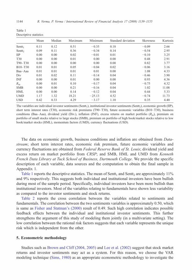
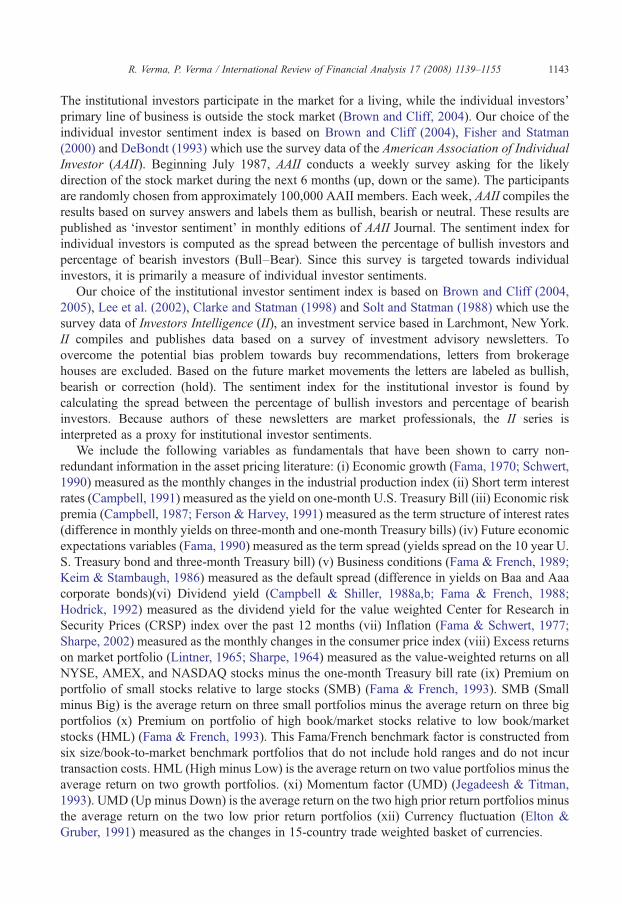
Table 1Descriptive statistics

Mean Median Maximum Minimum Standard deviation Skewness Kurtosis

Sentt1 0.11 0.12 0.51 −0.35 0.18 −0.09 2.66Sentt2 0.09 0.11 0.36 −0.34 0.14 −0.54 2.95IIP 0.00 0.00 0.02 −0.01 0.01 −0.10 3.25T30 0.00 0.00 0.01 0.00 0.00 0.48 2.91T90–T30 0.00 0.00 0.00 0.00 0.00 0.82 3.77B10–T30 0.01 0.01 0.05 −0.04 0.02 −0.06 3.16Baa–Aaa 0.01 0.01 0.01 0.01 0.00 1.08 4.33Div 0.01 0.02 0.11 −0.14 0.04 −0.46 3.90INF 0.00 0.00 0.01 0.00 0.00 0.93 4.36Rm 0.00 0.01 0.10 −0.17 0.04 −0.75 4.32SMB 0.00 0.00 0.21 −0.16 0.04 1.02 11.08HML 0.00 0.00 0.14 −0.12 0.04 0.44 5.33UMD 1.17 1.32 18.21 −25.13 4.52 −0.74 11.73USD 0.42 0.33 4.29 −3.17 1.10 0.35 4.40

The variables are individual investor sentiments (Sentt1), institutional investor sentiments (Sentt2), economic growth (IIP),short term interest rates (T30), economic risk premiums (T90–T30), future economic variables (B10–T30), businessconditions (Baa–Aaa), dividend yield (Div.), inflation (INF), excess returns on market portfolio (Rm), premium onportfolio of small stocks relative to large stocks (SMB), premium on portfolio of high book/market stocks relative to lowbook/market stocks (HML), momentum factors (UMD), currency fluctuations (USD).


The data on economic growth, business conditions and inflation are obtained from Data-stream; short term interest rates, economic risk premium, future economic variables andcurrency fluctuations are obtained from Federal Reserve Bank of St. Louis; dividend yield andexcess return on market portfolio from CRSP; and SMB, HML and UMD from KennethFrench Data Library at Tuck School of Business, Dartmouth College. We provide the specificdescription of each variable, data sources and the computation to obtain the final sample inAppendix 1.

Table 1 reports the descriptive statistics. The mean of Sentt1 and Sentt2 are approximately 11%and 9% respectively. This suggests both individual and institutional investors have been bullishduring most of the sample period. Specifically, individual investors have been more bullish thaninstitutional investors. Most of the variables relating to fundamentals have shown less variabilityas compared to the investor sentiments and stock returns.

Table 2 reports the cross correlation between the variables related to sentiments andfundamentals. The correlation between the two sentiments variables is approximately 0.50, whichis same as Fisher and Statman's (2000) result of 0.49. Such high correlation indicates possiblefeedback effects between the individual and institutional investor sentiments. This furtherstrengthens the argument of this study of modeling them jointly (in a multivariate setting). Thelow correlation between the rational risk factors suggests that each variable represents the uniquerisk which is independent from the other.

5. Econometric methodology

Studies such as Brown and Cliff (2004, 2005) and Lee et al. (2002) suggest that stock marketreturns and investor sentiments may act as a system. For this reason, we choose the VARmodeling technique (Sims, 1980) as an appropriate econometric methodology to investigate the

able 2ross-correlations

Sentt1 Sentt2 B10 Baa IIP HML INF Rm D SMB T30 T90 UMD USD

entt1 1entt2 0.5032⁎⁎ 110 −0.0115 0.0900⁎ 1aa −0.3277⁎ −0.1019 −0.0014 1IP 0.1222 −0.0645 −0.1543 −0.3938⁎⁎ 1ML 0.0128 0.0391⁎⁎ 0.0637 −0.0608 0.0518 1NF −0.2849⁎⁎ −0.1700⁎⁎ −0.0174 0.1611⁎ −0.1526 −0.0029 1

m 0.2242⁎⁎ 0.1683⁎⁎ 0.2607⁎⁎ −0.0105 −0.1000 −0.5619⁎⁎ −0.1740 1IV 0.2156⁎⁎ 0.1463⁎⁎ 0.3180⁎⁎ 0.018 −0.1124 −0.4668⁎⁎ −0.1622 0.9718⁎⁎MB 0.1260 0.1611⁎⁎ −0.1987⁎ −0.0435 −0.0461 −0.4950⁎⁎ 0.0022 0.1686⁎ − 95 130 −0.1065 −0.0916 0.1438 0.4022⁎⁎ −0.2809⁎⁎ −0.0599 0.2564 −0.0676 83 −0.1286 190 −0.1161 −0.0815 0.3230⁎⁎ 0.2524⁎⁎ −0.1882⁎ −0.1486 0.0886 0.1354 42 −0.0086 0.1882⁎ 1MD −0.0617 0.0104 0.2028⁎ −0.0637 0.002 −0.1989⁎⁎ −0.0988 0.0279 − 41 0.1973⁎ 0.0093 −0.1382 1SD 0.0591 0.0402 −0.0284 −0.0872 0.1741⁎ 0.1922⁎ −0.1356 −0.1618⁎ − 36 −0.0025 −0.003 −0.0432 −0.0004 1

he variables are individual investor sentiments (Sentt1), institutional investor sentiments (Sentt2), economic growth ), short term interest rates (T30), economic risk premiumsT90), future economic variables (B10), business conditions (Baa), dividend yield (Div), inflation (INF), excess retu on market portfolio (Rm), premium on portfolio of smalltocks relative to large stocks (SMB), premium on portfolio of high book/market stocks relative to low book/mar stocks (HML), momentum factors (UMD), and currencyluctuations (USD). ⁎ and ⁎⁎ denote significance levels at 10% and 5% respectively.

1145R.Verm

a,P.

Verma/International

Review

ofFinancial

Analysis

17(2008)

1139–1155

TC

SSBBIHIRDSTTUU

T(sf

IV

10.030.010.150.030.15

(IIPrnsket


postulated relationships. In addition, we take into consideration the following issues before theestimation stage:

In an efficient financial market, one would expect the reaction of the stock market only to theunanticipated component of explanatory variables. Elton and Gruber (1991) argue that all thevariables in a multi index model need to be surprises or innovations and therefore should not bepredicted from their past values. Thus, asset pricing models such as Arbitrage Pricing Theory (APT)employ the unanticipated component (innovations) of explanatory variables. Following this argumentseveral empirical papers have examined the stock market reaction to unexpected part of the news.

Recently, Aijo (in press) examined the effects of unexpected components of macroeconomicnews announcements on return distribution implied by FTSE-100 index option prices and findresults consistent with investor sentiments model of Barberis, Shleifer, and Vishny (1998).Similarly, Choy, Leong, and Tay (2006) extract non fundamental expectations from a survey offorecasters by regressing forecasts of real output growth and inflation on variables representingeconomic fundamental and view the residuals as non-fundamental shocks. Further they employimpulse response functions to examine the effect of these non-fundamental shocks on economicfluctuations. We follow similar approach in this paper. Since the formulated models are multiindex models; direct estimation in its present form would only give the relationships between theanticipated components. Such estimation would mean ignoring the effect of changes in theunanticipated components of rational risk factors on investor sentiments and therefore couldbe misleading. To overcome such a potential misspecification problem, one can employ morepowerful impulse response functions (predicted pattern of surprise changes or innovations) andvariance decompositions generated from the VAR model.

The VAR model is appropriate when estimating unrestricted reduced-form equations with auniform set of dependent variables as regressors. The model is also appropriate for analyzing ourpostulated relationships because it does not impose a priori restrictions on the structure of thesystem and can be viewed as a flexible approximation to the reduced form of the correctlyspecified but unknown model of true economic nature.

The VAR model can be expressed as:

zðtÞ ¼ C þXm

s¼1

AðsÞZðt � sÞ þ eðtÞ ð3Þ

where Z(t) is a column vector of individual and institutional investor sentiments and the rationalrisk factors, C is the deterministic component comprised of a constant, A(s) is a matrix ofcoefficients, m is the lag length and e(t) is a vector of random error terms.

The VAR specification allows the researchers to do policy simulations and integrate Monte Carlomethods to obtain confidence bands around the point estimates (Doan, 1988; Genberg, Salemi, &Swoboda, 1987; Hamilton, 1994). The likely response of one variable at time t, t+1, t+2 etc., to aone time unitary shock in another variable at time t can be captured by impulse response functions.As such they represent the behavior of the series in response to pure shocks while keeping the effectof other variables constant. Since, impulse responses are highly non-linear functions of the estimatedparameters, confidence bands are constructed around the mean response. Responses are consideredstatistically significant at the 95% confidence level when the upper and lower bands carry the samesign.

Theoretically, it is well known that traditional orthogonalized forecast error variancedecomposition based on the widely used Choleski factorization of VAR innovations may besensitive to variable ordering (Koop, Pesaran, & Potter, 1996; Pesaran & Shin, 1996, 1998). To

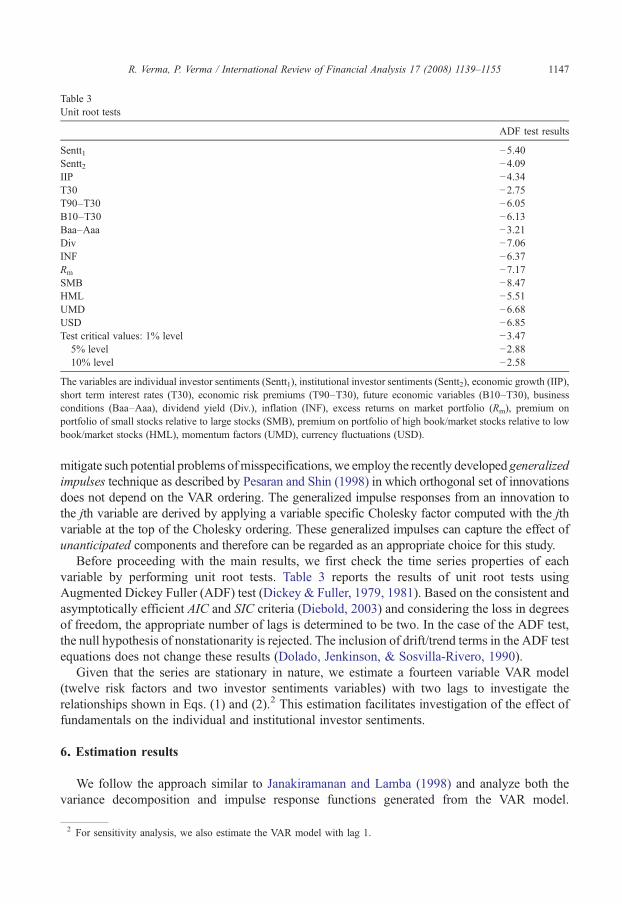
Table 3Unit root tests

ADF test results

Sentt1 −5.40Sentt2 −4.09IIP −4.34T30 −2.75T90–T30 −6.05B10–T30 −6.13Baa–Aaa −3.21Div −7.06INF −6.37Rm −7.17SMB −8.47HML −5.51UMD −6.68USD −6.85Test critical values: 1% level −3.47

5% level −2.8810% level −2.58

The variables are individual investor sentiments (Sentt1), institutional investor sentiments (Sentt2), economic growth (IIP),short term interest rates (T30), economic risk premiums (T90–T30), future economic variables (B10–T30), businessconditions (Baa–Aaa), dividend yield (Div.), inflation (INF), excess returns on market portfolio (Rm), premium onportfolio of small stocks relative to large stocks (SMB), premium on portfolio of high book/market stocks relative to lowbook/market stocks (HML), momentum factors (UMD), currency fluctuations (USD).


mitigate such potential problems ofmisspecifications, we employ the recently developedgeneralizedimpulses technique as described by Pesaran and Shin (1998) in which orthogonal set of innovationsdoes not depend on the VAR ordering. The generalized impulse responses from an innovation tothe jth variable are derived by applying a variable specific Cholesky factor computed with the jthvariable at the top of the Cholesky ordering. These generalized impulses can capture the effect ofunanticipated components and therefore can be regarded as an appropriate choice for this study.

Before proceeding with the main results, we first check the time series properties of eachvariable by performing unit root tests. Table 3 reports the results of unit root tests usingAugmented Dickey Fuller (ADF) test (Dickey & Fuller, 1979, 1981). Based on the consistent andasymptotically efficient AIC and SIC criteria (Diebold, 2003) and considering the loss in degreesof freedom, the appropriate number of lags is determined to be two. In the case of the ADF test,the null hypothesis of nonstationarity is rejected. The inclusion of drift/trend terms in the ADF testequations does not change these results (Dolado, Jenkinson, & Sosvilla-Rivero, 1990).

Given that the series are stationary in nature, we estimate a fourteen variable VAR model(twelve risk factors and two investor sentiments variables) with two lags to investigate therelationships shown in Eqs. (1) and (2).2 This estimation facilitates investigation of the effect offundamentals on the individual and institutional investor sentiments.

6. Estimation results

We follow the approach similar to Janakiramanan and Lamba (1998) and analyze both thevariance decomposition and impulse response functions generated from the VAR model.

2 For sensitivity analysis, we also estimate the VAR model with lag 1.


Specifically, impulse response functions trace the effects of a shock to one endogenous variableon to the other variables in the VAR, while variance decomposition separates the variation in anendogenous variable into the component shocks to the VAR. That is, the effect that each variablein the system has on itself and each other market over different time horizons can be measured bydecomposing this forecast error variance.

Table 4 (Panels A andB) shows the results of the innovation accounting procedure and reports the1 through 10 period ahead forecast error variance of individual and institutional investor sentimentsaccounted for by innovations in the risk factors. In the case of individual investor sentiments(Panel A), approximately 15% of its forecast error variance is explained by all risk factors combined(last column). Themajor portion of such influence is due to excess return on themarket portfolio anddividend yield (approximately 4%) followed by inflation (approximately 3%). Also, approximately1% of the forecast error variance is explained by term spread and SMB. On the other hand, almost25% of the forecast error variance of institutional investor sentiments is explained by all risk factorscombined (Panel B). The maximum influence is from the dividend yield (approximately 6%),followed by excess return on the market portfolio (approximately 5%) and inflation (4%). In the caseof institutional investor sentiments, the effects of HML (approximately 3.8%) and term spread(approximately 2%) are higher compared to those on individual investor sentiments. However, theinfluence of SMB is almost similar in both the cases (approximately 1%).

Overall, the results of decomposition of forecast error variances suggest that institutionalinvestor sentiments are more endogenous than the individual investor sentiments. Approximately,84% of the variance in the case of individual investor sentiments is explained by itself, comparedto approximately 74% in the case of institutional sentiments. The risk factors explain a greaterpercentage of variance in the case of institutions than individuals. Specifically, inflation, excessreturn on the market portfolio, dividend yield and term spread have stronger effects oninstitutional rather than individual investor sentiments. In addition, HML has strong influenceonly on the institutional investor sentiments. These findings imply that individuals are more likelyto be positive feedback traders and less likely to be driven by rational factors than institutions.

To test whether the effect of these risk factors is statistically significant, we examine whetherdifferences in the variance decomposition of individual and institutional investor sentiments toinnovations in risk factors are statistically different from each other. Following Janakiramanan andLamba (1998), we test for differences in the estimated coefficients in the standard formof theVAR inEq. (3) by employing standard t-tests. Panel A of Table 5 summarizes the estimated coefficients inthe standard form of the VAR model at lags 1 and 2, while Panel B summarizes the t-statistics fordifferences in these coefficients. For example, the t-statistic of−2.472 at lag 1 for term spread (futureeconomic variable) suggests that the responses of individual and institutional investor sentiments toterm spread are significantly different. These tests show that risk factors which explain greaterforecast error variances also tend to have significantly different effects on individual and institutionalinvestor sentiments. Specifically, the effects of inflation, excess return on the market portfolio,dividend yield, term spread and HML have significantly different effects on institutional andindividual investor sentiments. These results are consistent for both lags 1 and 2.

Sims (1980) indicates that VAR coefficient estimates are not very useful and that the tool weshould employ to interpret the VAR results are the impulse response functions obtained from theVAR model. Thus, we analyze the generalized impulse response functions generated from theVAR model.3 Fig. 1a–j plot the impulse responses of investor sentiments to rational factors.

3 The impulse responses at lags 1 and 2 are similar. For brevity we report the results at lag 2 only.

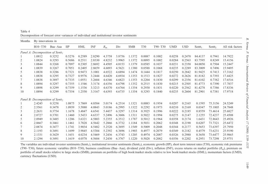
Table 4Decomposition of forecast error variances of individual and institutional investor sentiments

Months By innovations in

B10–T30 Baa–Aaa IIP HML INF Rm Div SMB T30 T90–T30 UMD USD Sentt1 Sentt2 All risk factors

Panel A: Decomposition of Sentt11 1.0812 0.3252 0.5276 0.2589 2.8290 4.3758 3.8756 1.1372 0.0087 0.1002 0.0258 0.2470 84.4137 0.7941 14.79222 1.0824 0.3293 0.5686 0.2511 2.8330 4.8232 3.9965 1.1372 0.0095 0.1002 0.0284 0.2563 83.7595 0.8249 15.41563 1.0844 0.3268 0.7097 0.2305 2.8692 4.4505 4.0153 1.1379 0.0585 0.1037 0.0231 0.2350 84.0050 0.7504 15.24474 1.0839 0.3267 0.7051 0.2405 2.8659 4.6093 4.5621 1.1380 0.0588 0.1068 0.0235 0.2289 83.3009 0.7496 15.94955 1.0838 0.3286 0.7321 0.9473 3.1001 4.6522 4.6894 1.1474 0.1444 0.1817 0.0250 0.2842 81.9425 0.7413 17.31626 1.0838 0.3295 0.7327 0.9576 3.2444 4.6420 4.6934 1.1353 0.1513 0.1827 0.0272 0.2626 81.8182 0.7393 17.44257 1.0838 0.3897 0.7335 1.0551 3.2684 4.6346 4.6823 1.1353 0.2204 0.1830 0.0299 0.2356 81.6102 0.7382 17.65168 1.0894 0.3297 0.7355 1.1546 3.3174 4.6356 4.6798 1.1352 0.2515 0.1830 0.0215 0.2505 81.4773 0.7390 17.78379 1.0898 0.3299 0.7359 1.1536 3.3213 4.6370 4.6764 1.1354 0.2930 0.1831 0.0220 0.2562 81.4278 0.7386 17.833610 1.0894 0.3299 0.7354 1.2550 3.3167 4.6393 4.6735 1.1354 0.3293 0.1840 0.0235 0.2604 81.2901 0.7381 17.9718

Panel B: Decomposition of Sentt21 2.4245 0.3258 1.0875 3.7869 4.0584 5.0174 6.2514 1.1321 0.0083 0.1954 0.0207 0.2165 0.1595 75.3156 24.52492 2.5561 0.3478 1.0939 3.5880 4.0843 5.0186 6.2995 1.1322 0.2292 0.1973 0.0210 0.2169 0.0347 75.1805 24.78483 2.2631 0.3754 1.1678 3.4847 4.6541 5.4437 6.3297 1.1314 0.3925 0.1996 0.0222 0.2185 0.8559 73.4614 25.68274 2.0727 0.3701 1.1460 3.5433 4.6337 5.2496 6.3606 1.1311 0.5022 0.1994 0.0275 0.2147 2.1255 72.4237 25.45085 2.0949 0.3485 1.1206 3.6321 4.5803 5.2355 6.3512 1.1787 0.5012 0.1964 0.0358 0.2174 1.6431 72.8643 25.49266 2.0667 0.3461 1.1461 3.7828 4.5642 5.2866 6.3732 1.1184 0.5031 0.2062 0.0348 0.2190 0.6207 73.7321 25.64727 2.0874 0.3477 1.1741 3.9034 4.5482 5.2520 6.3695 1.1549 0.5009 0.2048 0.0344 0.2177 0.5653 73.6397 25.79508 2.1193 0.3491 1.1699 3.9845 4.5384 5.2392 6.3696 1.1903 0.4977 0.2079 0.0349 0.2182 0.4579 73.6231 25.91909 2.1331 0.3429 1.1651 4.0234 4.5469 5.2436 6.3743 1.1205 0.4974 0.2087 0.0326 0.2980 0.3658 73.6477 25.986510 2.1294 0.3491 1.1619 4.0578 4.5684 5.2430 6.3767 1.1220 0.5028 0.2082 0.0356 0.2202 0.2951 73.7298 25.9751

The variables are individual investor sentiments (Sentt1), institutional investor sentiments (Sentt2), economic growth (IIP), short term interest rates (T30), economic risk premiums(T90–T30), future economic variables (B10–T30), business conditions (Baa–Aaa), dividend yield (Div), inflation (INF), excess returns on market portfolio (Rm), premium onportfolio of small stocks relative to large stocks (SMB), premium on portfolio of high book/market stocks relative to low book/market stocks (HML), momentum factors (UMD),currency fluctuations (USD).

1149R.Verm

a,P.

Verma/International

Review

ofFinancial

Analysis

17(2008)

1139–1155

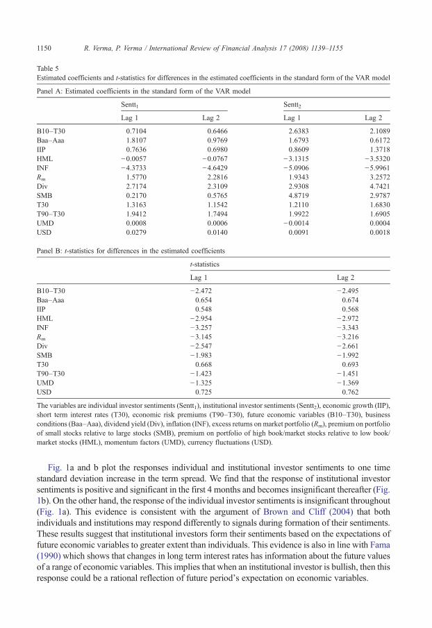
Table 5Estimated coefficients and t-statistics for differences in the estimated coefficients in the standard form of the VAR model

Panel A: Estimated coefficients in the standard form of the VAR model

Sentt1 Sentt2

Lag 1 Lag 2 Lag 1 Lag 2

B10–T30 0.7104 0.6466 2.6383 2.1089Baa–Aaa 1.8107 0.9769 1.6793 0.6172IIP 0.7636 0.6980 0.8609 1.3718HML −0.0057 −0.0767 −3.1315 −3.5320INF −4.3733 −4.6429 −5.0906 −5.9961Rm 1.5770 2.2816 1.9343 3.2572Div 2.7174 2.3109 2.9308 4.7421SMB 0.2170 0.5765 4.8719 2.9787T30 1.3163 1.1542 1.2110 1.6830T90–T30 1.9412 1.7494 1.9922 1.6905UMD 0.0008 0.0006 −0.0014 0.0004USD 0.0279 0.0140 0.0091 0.0018

Panel B: t-statistics for differences in the estimated coefficients

t-statistics

Lag 1 Lag 2

B10–T30 −2.472 −2.495Baa–Aaa 0.654 0.674IIP 0.548 0.568HML −2.954 −2.972INF −3.257 −3.343Rm −3.145 −3.216Div −2.547 −2.661SMB −1.983 −1.992T30 0.668 0.693T90–T30 −1.423 −1.451UMD −1.325 −1.369USD 0.725 0.762

The variables are individual investor sentiments (Sentt1), institutional investor sentiments (Sentt2), economic growth (IIP),short term interest rates (T30), economic risk premiums (T90–T30), future economic variables (B10–T30), businessconditions (Baa–Aaa), dividend yield (Div), inflation (INF), excess returns on market portfolio (Rm), premium on portfolioof small stocks relative to large stocks (SMB), premium on portfolio of high book/market stocks relative to low book/market stocks (HML), momentum factors (UMD), currency fluctuations (USD).


Fig. 1a and b plot the responses individual and institutional investor sentiments to one timestandard deviation increase in the term spread. We find that the response of institutional investorsentiments is positive and significant in the first 4 months and becomes insignificant thereafter (Fig.1b). On the other hand, the response of the individual investor sentiments is insignificant throughout(Fig. 1a). This evidence is consistent with the argument of Brown and Cliff (2004) that bothindividuals and institutions may respond differently to signals during formation of their sentiments.These results suggest that institutional investors form their sentiments based on the expectations offuture economic variables to greater extent than individuals. This evidence is also in line with Fama(1990) which shows that changes in long term interest rates has information about the future valuesof a range of economic variables. This implies that when an institutional investor is bullish, then thisresponse could be a rational reflection of future period’s expectation on economic variables.

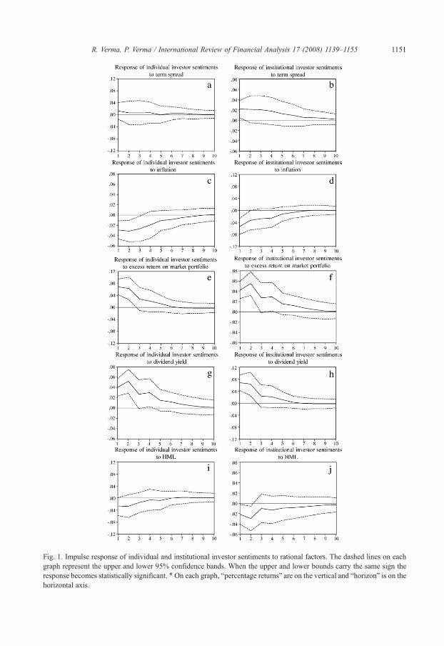
Fig. 1. Impulse response of individual and institutional investor sentiments to rational factors. The dashed lines on eachgraph represent the upper and lower 95% confidence bands. When the upper and lower bounds carry the same sign theresponse becomes statistically significant. ⁎On each graph, “percentage returns” are on the vertical and “horizon” is on thehorizontal axis.



Fig. 1c and d plot the impulse responses of investor sentiments to one time standard deviationincrease in inflation. We find significant negative effects of inflation on both the individual andinstitutional investor sentiments. However, the response of individual investor sentiments is ofrelatively smaller magnitude than those of institutional investor sentiment. Specifically in the firstmonth the responses are approximately 3% and 5.5% in the case of individual and institutionalinvestor sentiments respectively. These negative results are consistent with the arguments ofChen, Roll, and Ross (1986), Fama and Schwert (1977) and Sharpe (2002) that a rise in inflationcoincides with both lower expected real earnings growth and higher required real returns. Thisimplies that an expectation of increased price levels can have a greater bearish impact oninstitutional rather than individual investor sentiments.

Fig. 1e and f plot the responses of investor sentiments to the excess return on the marketportfolio. The responses of both individual and institutional investor sentiments are positive andsignificant. In the case of individual investor sentiments, the responses are of relatively lessermagnitude (approximately 4%) as compared to those of institutional investor sentiments(approximately 7%) during the first month. These significant positive results suggest that a bullishmarket does cause increased bullishness among both the individuals and institutions.

Fig. 1g and h plot the generalized impulse responses of investor sentiments to the dividendyield. The results are very similar to the ones obtained for the excess return on market portfolio. Inboth the cases the responses are positive and significant for approximately 3 months. Also, themagnitude of the response is relatively lower in the case of individual investor sentiments ratherthan in those of the institutional investor sentiments. These results are in line with the Fama andFrench (1988) argument that dividend yields are relevant in forecasting the long horizon stockreturns. This implies that, to a large extent, both individuals and institutions form their bullishsentiments based on the expectations of higher long horizon dividends.

Fig. 1i and j plot the generalized impulse responses of investor sentiments to the HML. Thereis an insignificant response of the individual investor sentiments (Fig. 1i) while negative andsignificant response of institutional investor sentiments (Fig. 1j). The response of the institutionalinvestor sentiments is significant for approximately 3 months and becomes insignificantthereafter. The significant effect of this Fama and French (1993) factor suggest that institutionalinvestors do consider the premium on portfolio of high book/market stocks relative to low book/market stocks related to systematic patterns in relative probability and growth.

Overall the results of the impulse response functions are consistent with the findings offorecast error variance and t-statistics for differences in estimated coefficients.

7. Conclusion

Previous studies construe investor sentiments as fully irrational; we find evidence that to alarge extent the individual and institutional investor sentiments are driven by the rational riskfactors. Specifically, we find significant effects of inflation, excess market return and dividendyield on both types of investor sentiments. In addition, we also find significant effects of the termspread and a Fama and French (1993) factor on the institutional investor sentiments. These riskfactors have a greater effect on institutional rather than individual investor sentiments. The resultsare consistent with the view that the linkages between investor sentiments and stock prices stemsfrom a combination of both rational outlook and expectations that are not fully justified byinformation. The responses of institutional investor sentiments to a greater number of risk factorsand to greater magnitude suggest that expectations of institutional investors are more rational thanthose of the individuals.


These results have important practical implications for both investors and policymakers.Analytically, these results indicate that sentiments are mainly a manifestation of the rational riskfactors driving expected returns of stocks. The effects of sentiments seem to be due to the rationaloutlook of investors for the market. Investors could therefore improve their portfolio performance byconsidering both the stability and volatility in those rational factors as determinants of stock prices. Atthe same time, it is important that investors be particularly wary of irrational investor sentiments whiledevising their investment strategies. Policymakers should concentrate their efforts to attain stability insentiments induced by fundamentals in order to reduce volatility and minimize investor uncertainty.

Appendix A. Data Identification

o

V

S

S

II

T

T

B

B

D

IN

R

Weobtain all data inmonthly intervals fromOctober 1988 toApril 2003. The specific descriptionf each variable, data sources and the computation to obtain the final sample is as follows:

ariable
Description Data Source Computation
entt1
Individual investorsentiments
(1) Percentage of bullishinvestors

AmericanAssociation ofIndividual Investors

(1)–(2) to capture the spread (%)i.e. Bull (%)–Bear (%)

(2) Percentage of BearishInvestors

entt2
Institutionalinvestor sentiments
(1) Percentage of bullishinvestors

InvestorsIntelligence

(1)–(2) to capture the spread (%)i.e. Bull (%)–Bear (%)

(2) Percentage of BearishInvestors

P
Economic growth Index for industrial Production Datastream First difference of the naturallogarithm of index for industrialproduction (lnt− lnt−1) to capturethe monthly changes (%)
30
Short-term interestrates
Yield on one-month U.S.Treasury Bill

Federal ReserveBank of St. Louis

No transformation

90–T30

Economic riskpremia

(1) Yield on three-monthsU.S. Treasury Bill(2) Yield on one-monthU.S. Treasury Bill


(1)–(2) to capture the termstructure of interest rates (%)

10–T30

Future economicexpectations

(1) Yield on 10 yearsU.S. Treasury Bond(2) Yield on three-monthsU.S. Treasury Bill


(1)–(2) to capture the yieldspread (%)

aa–Aaa

Business condition
(1) Yield on BaaCorporate Bonds
Datastream
(1)–(2) to capture the defaultspread (%)
(2) Yield on AaaCorporate Bonds

iv
Dividend yield Dividend yield for thevalue weighted CRSPindex over 12 months
CRSP
No transformation
F
Inflation Consumer price index Datastream First difference of the naturallogarithm of consumer priceindex (lnt− lnt−1) to capture themonthly changes (%)
m
Excess returns onmarket portfolio
(1) Value weighted returnson all NYSE, AMEX andNASDAQ

CRSP
(1)–(2) to capture the excessreturns (%)
(2) Yield on one-monthU.S. Treasury Bill

(continued on next page)


(continued)Appendix A (continued )

Variable
Description Data Source Computation
SMB
Premium onportfolio of smallstocks relative tolarge stocks
Difference in the averagereturns on three smalland three big portfolios(Fama and Frenchbenchmark factor)

Kenneth FrenchData Library atTuck School ofBusiness,Dartmouth College

No transformation

HML
Premium onportfolio of highB/M stocks relativeto low B/M stocks
Difference in theaverage returns ontwo value and two growthportfolios (Fama andFrench benchmark factor)


No transformation

UMD
Momentum factor Difference in the averagereturns on two high and twolow prior returns portfolios

No transformation

USD
Currencyfluctuations
15 country trade weightedbasket of currencies


First difference of the naturallogarithm of 15 country tradeweighted basket of currencies(lnt− lnt−1) to capture themonthly fluctuations (%)

References

Aijo, J. (in press). Impact of US and UKmacroeconomic news announcements on the return distribution implied by FTSE-100 index options. International Review of Financial Analysis, (Corrected proof, available online 27 October 2006).

Barberis, N., Shleifer, A., & Vishny, R. (1998). A model of investor sentiment. Journal of Financial Economics, 49,307−343.

Black, F. (1986). Noise. Journal of Finance, 41(3), 529−543.Brown, G. W., & Cliff, M. T. (2004). Investor sentiment and the near-term stock market. Journal of Empirical Finance, 11

(1), 1−27.Brown, G. W., & Cliff, M. T. (2005). Investor sentiment and asset valuation. Journal of Business, 78(2), 405−440.Campbell, J. Y. (1987). Stock returns and the term structure. Journal of Financial Economics, 18, 373−399.Campbell, J. Y. (1991). A variance decomposition for stock returns. Economic Journal, 101, 157−179.Campbell, J. Y., & Kyle, A. S. (1993). Smart money, noise trading, and stock price behavior. Review of Economic Studies,

60, 1−34.Campbell, J. Y., & Shiller, R. J. (1988). The dividend-price ratio and expectations of future dividends and discount factors.

Review of Financial Studies, 1, 195−228.Campbell, J. Y., & Shiller, R. J. (1988). Stock prices, earnings and expected dividends. Journal of Finance, 43, 661−676.Clarke, R. G., & Statman, M. (1998, May/June). Bullish or bearish? Financial Analysts Journal, 63−72.Chen, N., Roll, R., & Ross, S. A. (1986). Economic forces and the stock market. Journal of Business, 59, 383−403.Choy, M. C., Leong, K., & Tay, A. S. (2006). Non fundamental expectations and economic fluctuations: Evidence from

professional forecasts. Journal of Macroeconomics, 28, 446−460.DeBondt, W. (1993). Betting on trends: Intuitive forecasts of financial risk and return. International Journal of

Forecasting, 9, 355−371.DeLong, Shleifer, J., Summers, A., & Waldmann, R. (1990). Noise trader risk in financial markets. Journal of Political

Economy, 98, 703−738.DeLong, Shleifer, J., Summers, A., & Waldmann, R. (1991). The survival of noise traders in financial markets. Journal of

Business, 64(1), 1−19.Dickey, D. A., & Fuller, W. A. (1979). Distribution of the estimators for autoregressive time series with a unit root. Journal

of the American Statistical Association, 74, 427−431.Dickey, D. A., & Fuller, W. A. (1981). Likelihood ratio statistics for autoregressive time series with a unit root. Econo-

metrica, 49, 1057−1072.


Diebold, F. X. (2003). Elements of Forecasting. : South Western College Publishing.Doan, T. (1988). RATS User's Manual. Evanston, Illinois: VAR Econometrics.Dolado, J. J., Jenkinson, T., & Sosvilla-Rivero, S. (1990). Cointegration and unit roots. Journal of Economic Surveys, 4,

249−273.Elton, E. J., & Gruber, M. J. (1991). Modern Portfolio Theory and Investment Analysis (Fourth Edition). John Wiley and

Sons, Inc.Fama, E. F. (1970). Efficient capital markets: A review of theory and empirical work. Journal of Finance, 25, 383−417.Fama, E. F. (1990). Term structure forecasts of interest rates, inflation, and real returns. Journal of Monetary Economics,

25, 59−76.Fama, E. F., & French, K. R. (1988). Dividend yields and expected stock returns. Journal of Financial Economics, 22, 3−25.Fama, E. F., & French, K. R. (1989). Business conditions and expected returns on stocks and bonds. Journal of Financial

Economics, 25, 23−49.Fama, E. F., & French, K. R. (1993). Common risk factors in the returns on stocks and bonds. Journal of Financial

Economics, 33, 3−56.Fama, E. F., & Schwert, G. W. (1977). Asset returns and inflation. Journal of Financial Economics, 5, 115−146.Ferson, W. E., & Harvey, C. R. (1991). The variation in economic risk premiums. Journal of Political Economy, 99,

385−415.Fisher, K. L., & Statman, M. (2000, March/April). Investor sentiments and stock Returns. Financial Analysts Journal,

16−23.Genberg, H., Salemi, M. K., & Swoboda, A. (1987). The relative importance of foreign and domestic disturbances for

aggregate fluctuations in open economy: Switzerland. Journal of Monetary Economics, 19, 45−67.Hamilton, J. D. (1994). Time Series Analysis. Princeton, NJ: Princeton University Press.Hirshleifer, D. (2001). Investor psychology and asset pricing. Journal of Finance, LVI(4), 1533−1597.Hodrick, R. (1992). Dividend yields and expected stock returns: Alternative procedures for inference and measurement.

Review of Financial Studies, 5, 357−386.Janakiramanan, S., & Lamba, A. S. (1998). An empirical examination of linkages between Pacific-Basin stock markets.

Journal of International Financial Markets, Institutions, and Money, 8, 155−173.Jegadeesh, N., & Titman, S. (1993). Returns to buying winners and selling losers: Implications for stock market efficiency.

Journal of Finance, 48, 65−91.Keim, D. B., & Stambaugh, R. F. (1986). Predicting returns in the bond and stock markets. Journal of Financial

Economics, 17, 357−390.Koop, G., Pesaran, M. H., & Potter, S. M. (1996). Impulse response analysis in non linear multivariate models. Journal of

Econometrics, 74, 119−147.Kyle, A. S. (1985). Continuous auctions and insider trading. Econometrica, 53, 1315−1335.Lee, W. Y., Jiang, C. X., & Indro, D. C. (2002). Stock market volatility, excess returns, and the role of investor sentiments.

Journal of Banking & Finance, 26, 2277−2299.Lintner, J. (1965). Security prices, risk, and maximal gains from diversification. Journal of Finance.Palomino, F. (1996). Noise trading in small Markets. Journal of Finance, 51(4), 1537−1550.Pesaran, M. H., & Shin, Y. (1996). Cointegration and speed of convergence to equilibrium. Journal of Econometrics, 71,

117−143.Pesaran, M. H., & Shin, Y. (1998). Generalized impulse response analysis in linear multivariate models. Economics

Letters, 58, 17−29.Sharpe, W. F. (1964). Capital asset prices: A theory of market equilibrium under conditions of risk. Journal of Finance,

425−442.Sharpe, S. A. (2002). Reexamining stock valuation and inflation: The implications of analysts' earnings forecasts. The

Review of Economics and Statistics, 84, 632−648.Schwert, G. W. (1990). Stock returns and real activity: A century of evidence. Journal of Finance, 45, 1237−1257.Sims, C. (1980). Macroeconomic and reality. Econometrica, 48, 1−49.Shefrin, H., & Statman, M. (1994). Behavioral capital asset pricing theory. Journal of Financial and Quantitative

Analysis, 29(3), 323−349.Shleifer, A., & Summers, L. (1990). The noise trader approach to finance. Journal of Economic Perspectives, 4(2), 19−33.Solt, M. E., & Statman, M. (1988, September/October). How useful is the sentiment Index? Financial Analysts Journal,

45−55.Wang, F. A. (2001). Overconfidence, investor sentiment, and evolution. Journal of Financial Intermediation, 10, 138−170.

Documents

Are survey forecasts of individual and institutional investor sentiments rational