Approximation results for the weighted P4 partition

problem

Jerome Monnot, Sophie Toulouse

To cite this version:

Jerome Monnot, Sophie Toulouse. Approximation results for the weighted P4 partition prob-lem. LNCS 3623. FCT’ 2005 The symposia on Fundamentals of Computation Theory, 2005,Germany. Springer Verlag, pp.388-396, <10.1007/11537311 34>. <hal-00017259>

HAL Id: hal-00017259

https://hal.archives-ouvertes.fr/hal-00017259

Submitted on 18 Jan 2006

HAL is a multi-disciplinary open accessarchive for the deposit and dissemination of sci-entific research documents, whether they are pub-lished or not. The documents may come fromteaching and research institutions in France orabroad, or from public or private research centers.

L’archive ouverte pluridisciplinaire HAL, estdestinee au depot et a la diffusion de documentsscientifiques de niveau recherche, publies ou non,emanant des etablissements d’enseignement et derecherche francais ou etrangers, des laboratoirespublics ou prives.

Approximation results for the weighted P4

partition problem ⋆

Jerome Monnot a Sophie Toulouse b

aUniversite Paris Dauphine, LAMSADE, CNRS UMR 7024, 75016 Paris, France,monnot@lamsade.dauphine.fr

bUniversite Paris 13, Institut Galilee LIPN, CNRS UMR 7030, 93430Villetaneuse, France, sophie.toulouse@lipn.univ-paris13.fr, +33.1.49.40.40.73

(telephone), +33.1.48.26.07.12 (fax)

Abstract

We present several new standard and differential approximation results for the P4-partition problem using the Hassin and Rubinstein’ algorithm (Information Process-ing Letters, 63: 63-67, 1997). Those results concern both minimization and maxi-mization versions of the problem. However, the main point of this paper lies on theestablishment it does of the robustness of this algorithm, in the sense that this latterprovides good quality solutions, whatever version of the problem is addressed, what-ever approximation framework is considered in order to evaluate the approximatesolutions.

Key words: graph partitioning, P4-packing, approximation algorithms,performance ratio, standard approximation, differential approximation.

1 Introduction

Consider an instance I of an NP-hard optimization problem Π and a polynomial-time algorithm A that computes feasible solutions for Π. Denote respectivelyby apxΠ(I) the value of a solution computed by A on I, by optΠ(I) thevalue of an optimum solution and by worΠ(I) the value of a worst solu-tion (that corresponds to the optimum value when reversing the optimiza-tion goal). The quality of A is expressed by the means of approximation ra-

⋆ A preleminary version of this paper appeared in the proceedings the 15th Inter-national Symposium on Fundamentals of Computation Theory, FCT 2005, LNCS3623, (2005) 377-385

Preprint submitted to Elsevier Science 4 January 2006

tios that somehow compare the approximate value to the optimum one. Sofar, two measures stand out from the literature: the standard ratio [2] (themost widely used) and the differential ratio [3,4,7,10]. The standard ratio isdefined by ρΠ(I, A) = apxΠ(I)/optΠ(I) if Π is a maximization problem, byρΠ(I, A) = optΠ(I)/apxΠ(I) otherwise, whereas the differential ratio is de-fined by δΠ(I, A)(worΠ(I)−apxΠ(I))/(worΠ(I)−optΠ(I)). Instead of dividingthe approximate value by the optimum one, this latter measure divides thedistance from a worst solution to the approximate value by the instance diam-eter. Within the worst case analysis framework and given a universal constantε ≤ 1 (resp., ε ≥ 1), an algorithm A is said to be an ε-standard approxi-mation for a maximization (resp. a minimization) problem Π if ρAΠ

(I) ≥ ε∀I (resp., ρAΠ

(I) ≤ ε ∀I). With respect to differential approximation, A issaid to be ε-differential approximate for Π if δAΠ

(I) ≥ ε, ∀I, for a universalconstant ε ≤ 1. Equivalently, because any solution value is a convex com-bination of the two values worΠ(I) and optΠ(I), an approximate solutionvalue apxΠ(I) will be an ε-differential approximation if for any instance I,apxΠ(I) ≥ ε×optΠ(I)+ (1− ε)×worΠ(I) (for the maximization case; reversethe sense of the inequality when minimizing). Within the worst case analysisframework and considering both standard and differential ratios, we focus ona special problem, the weighted P4-partition problem. Furthermore, we studythe performance of a single algorithm on various versions of this problem. Do-ing so, we put to the fore the effectiveness of this algorithm by proving thatit provides approximation ratios for both standard and differential measures,for both maximization and minimization versions of the problem.

In the weighted Pk-partition problem (PkP in short), we are given a completegraph Kkn together with a distance function d : E → N on its edges. A Pk is aninduced path of length k− 1 (or, equivalently, an induced path on k vertices)and the cost of such a path is the sum of its edge weight. Given an instanceI = (Kkn, d), the aim is to compute a partition T ∗ = {P ∗

1 , . . . , P ∗n} of V (Kkn)

into n vertex-disjoint Pk (what we call a Pk-partition) that is of optimumweight (that is, of maximum weight if the goal is to maximize (MaxPkP),of minimum weight otherwise (MinPkP), where the value of a solution T ∗

is given by d(T ∗) =∑q

i=1 d(P ∗i ). When considering the minimization version,

we will more often assume that the distance function satisfies the triangularinequality, i.e., d(x, y) ≤ d(x, z) + d(z, y), ∀x, y, z; MinMetricPkP will referto this restriction. Finally, we also deal with a special case of metric instanceswhere the distance function is worth either 1 or 2; the corresponding problemswill be denoted by MaxPkP1,2 and MinPkP1,2. Note that for k = 2, a P2-partition is a perfect matching and hence, MinP2P and MaxP2P both arepolynomial. On the other hand, all these problems turn to be NP-hard fork ≥ 3, [9,16]. Nevertheless, MaxPkP is standard-approximable for any k, [11].In particular, MaxP3P and MaxP4P are respectively 35/67−ε, [12] and 3/4,[11] approximable. On the other hand, MinPkP may not be approximatedwithin 2p(n) for any polynomial p, for any k; this is due to the fact that

2

the Pk-partition problem, which consists in deciding whether a graph doesor not admit a partition of its vertex set into Pk, is NP-complete, [9,15,16].Furthermore, even when restricting to metric instances and more specificallyfor k = 4, no approximation rate has (to our knowledge) been established forMinMetricPkP so far. Finally, note that this latter problem (and PkP ingeneral) is very close to the vehicle routing problem when restricting the routeof each vehicle to at most k intermediate stops, [1,8].

In the second section, we study the relationship between TSP and PkP underdifferential ratio; namely, we show how a differential approximation for TSP

enables a differential approximation for PkP. In the third section, that con-tains the main result of this paper, we propose a complete analysis, from botha standard and a differential point of view, of an algorithm proposed by Has-sin and Rubinstein [11]. We prove that, with respect to the standard ratio,this algorithm provides new approximation rates for MetricP4P, namely:the approximate solution respectively achieves a 3/2-, a 7/6- and a 9/10-standard approximation for MinMetricP4P, MinP4P1,2 and MaxP4P1,2.Under differential ratio, the approximate solution is a 1/2-approximation forgeneral P4P, a 2/3-approximation for P4Pa,b. The gap between differentialand standard ratios that might be reached for a maximization problem maybe explained by the fact that, within the differential framework, the approx-imate value has to be located within the interval [wor(I), opt(I)], instead of[0, opt(I)] when considering the standard measure. That is the aim of differ-ential approximation: thanks to the reference it does to wor(I), this measureis both more precise (relevant with respect to the notion of guaranteed perfor-mance) and more robust (since minimizing and maximizing turn to be equiva-lent and more generally, differential ratio is stable under affine transformationof the objective function). In addition to the new approximation bounds thatthey provide, the obtained results enable to establish the robustness of thealgorithm that is addressed here, since this latter provides good quality solu-tions, whatever version of the problem we deal with, whatever approximationframework within which we estimate the approximate solutions.

2 From Traveling salesman problem to PkP

A common technic in order to obtain an approximate solution for MaxPkP

from a Hamiltonian cycle is called the deleting and turning around method, see[11,12,8]. Starting from a tour, this method builds k solutions of MaxPkP andpicks the best among them, where the ith solution is obtained by deleting 1edge upon k from the input cycle, starting from its ith edge. The quality of theoutput T ′ obviously depends on the quality of the initial tour; in this way it isproven in [11,12], that any ε-standard approximation for MaxTSP providesa k−1

kε-standard approximation for MaxPkP. From a differential point of

3

T1 T2 T3 T4

Fig. 1. An example of the 4 solutions T1, . . . , T4.

T∗ T ∗

L R L R

Fig. 2. A worst and an optimum solutions when n = 1.

view, things are less optimistic: even for k = 4, there exists an instance family(In)n≥1 that verifies apx(In) = 1

2optMaxP4P

(In)+ 12worMaxP4P(In). This instance

family is defined as In = (K8n, d) for n ≥ 1, where the vertex set V (K8n) maybe partitioned into two sets L = {ℓ1, . . . , ℓ4n} and R = {r1, . . . , r4n} in such away that the associated distance function d is worth 0 on L× L, 2 on R × Rand 1 on L× R. Thus, for any n ≥ 1, the following property holds:

Property 1 apx(In) = 6n, optMaxP4P(In) = 8n, worMaxP4P(In) = 4n.

If the initial tour is described as Γ = {e1, . . . , en, e1}, then the deleting andturning around method produces 4 solutions T1, . . . , T4 where Ti = ∪n−1

j=0{{ej+i,ej+i+1, ej+i+2}} for i = 1, . . . , 4 (indexes are considered mod n). Figure 1provides an illustration of this process (the dashed lines correspond to theedges from Γ \ Ti).

First, observe that any tour Γ on In is optimum, of total weight 8n. Indeed,any tour contains as many edges with their two endpoints in L as edges withtheir two endpoints in R and thus, d(Γ) = |Γ∩L×R|+2|Γ∩R×R| = |Γ| = 8n.Hence, starting from the optimum cycle Γ∗ = [r1, . . . , r4n, l1, . . . , l4n, r1], thefour solutions T1, . . . , T4 outputted by the algorithm (see Figure 1) will allbe worth d(Ti) = 6n, while an optimum solution T ∗ and a worst solutionT∗ are of total weight respectively 8n and 4n (see Figure 2). Indeed, becauseany P4-partition T is a 2n edge cut down tour, we get, on the one hand,optMaxTSP(In) ≥ d(T ) and, on the other hand, d(T ) ≥ 8n − 4n = 4n, whichconcludes this argument.

Nevertheless, the deleting and turning around method leads to the followingweaker differential approximation relation:

Lemma 2 ¿From an ε-differential approximation of MaxTSP, one can poly-nomially compute a ε

k-differential approximation of MaxPkP. In particular,

4

we deduce from [10,13] that MaxPkP is 23k

-differential approximable.

Let us show that the following inequality holds for any instance I = (Kkn, d)of MaxPkP:

optMaxTSP(I) ≥1

k − 1optMaxPkP(I) + worMaxPkP(I) (1)

Let T ∗ be an optimum solution of MaxPkP, then arbitrarily add some edgesto T ∗ in order to obtain a tour Γ. From this latter, we can deduce k − 1solutions Ti for i = 1, . . . , k − 1, by applying the deleting and turning aroundmethod in such a way that any of the solutions Ti contains (Γ \T ∗). Thus, weget (k − 1)worMaxPkP(I) ≤

∑k−1i=1 d(Ti) = (k − 1)d(Γ)− optMaxPkP(I). Hence,

consider that d(Γ) ≤ optMaxTSP(I) and the result follows. By applying againthe deleting and turning around method, but this time from a worst tour, wemay obtain k approximate solutions of MaxPkP, which allows us to deduce:

worMaxTSP(I) ≥k

k − 1worMaxPkP(I) (2)

Finally, let Γ′ be an ε-differential approximation of MaxTSP, we deduce fromΓ′ k approximate solutions of MaxPkP. If T ′ is set to the best one, we getd(T ′) ≥ k

k−1d(Γ′) and thus:

apx(I) ≥k

k − 1d(Γ′) ≥

k

k − 1(εoptMaxTSP(I) + (1− ε)worMaxTSP(I)) (3)

Using inequalities (1), (2) and (3), we get apx(I) ≥ εkoptMaxPkP(I) + (1 −

εk)worMaxPkP(I) and the proof is complete.

To conclude with the relationship between PkP and TSP with respect to theirapproximability, observe that the minimization case also is trickier. Notably,if we consider MinMetricP4P, then the instance family I ′

n = (K8n, d′) builtas the same as In with a distinct distance function defined as d′(ℓi, ℓj) =d′(ri, rj) = 1 and d′(ℓi, rj) = n2 + 1 for any i, j, then we have: optTSP(I ′

n) =2n2 + 8n and optP4P

(I ′n) = 6n.

3 Approximating P4P by the means of optimum matchings

Here starts the analysis, from both a standard and a differential point of view,of an algorithm proposed by Hassin and Rubinstein in [11], where the au-thors show that the approximate solution is a 3/4-standard approximation

5

for MaxP4P. First, dealing with the standard ratio, we prove that this algo-rithm provides a 3/2-approximation for MinMetricP4P and respectively a7/6 and a 9/10-approximation for MinP4P1,2 and MaxP4P1,2. As a corollaryof a more general result, we also obtain an alternative proof of the result of[11]. We then prove that, with respect to the differential measure, the ap-proximate solution achieves a 1/2-approximation in general graphs, for bothmaximization and minimization versions of the problem. Finally, this latterratio is raised up to 2/3 when restricting to bi-valuated graphs.

3.1 Description of the algorithm

The algorithm proposed in [11] runs in two stages: first, it computes an op-timum weight perfect matching MT ′ on (K4n, d); then, it builds on the edgesof MT ′ a second optimum weight perfect matching RT ′ in order to completethe solution (note that “optimum weight” signifies “maximum weight” if thegoal is to maximize, “minimum weight” if the goal is to minimize). Precisely,we define the instance (K2n, d′) (to any edge ev ∈ MT ′ corresponds a vertexv in K2n), where the distance function d′ is defined as follows: for any edge[v1, v2], d′(v1, v2) is set to the weight of the heaviest edge that links ev1

andev2

, that is, if v1 represents ev1= [x1, y1] and v2 represents ev2

= [x2, y2], thend′(v1, v2) = max {d(x1, x2), d(x1, y2), d(y1, x2), d(y1, y2)} (when dealing withthe minimum version of the problem, set the weight to the lightest). We thusbuild on (K2n, d′) an optimum weight matching RT ′ , which is then transposedto the initial graph (K4n, d) by selecting the edge that realizes the same cost.Since the computation of an optimum weight perfect matching is polynomial,the whole algorithm runs in polynomial time, whether the goal is to minimizeor to maximize.

3.2 General P4P within the standard framework

For any solution T , we denote respectively by MT and RT the set of thefinal edges and the set of the middle edges of its chains. Furthermore, we willconsider for any chain PT = {x, y, z, t} of the solution the edge [t, x] thatcompletes PT into a cycle. If RT denotes the set of these edges, we observethat RT ∪ RT forms a perfect matching. Finally, for any edge e ∈ T , we willdenote by PT (e) the P4 from the solution that contains e and by CT (e) the4-length cycle that contains PT (e).

Lemma 3 For any instance I = (K4n, d), if T is a feasible solution and T ∗

is an optimum solution, then there exist 4 pairwise disjoint edge sets A, B, Cand D that verify:

6

MT A MT B MT A

AMTMT

A

MT

A A A MT

A ∩ MT

B

MT A MT A MT A

AMTCMTMT

A MT

MT

AC

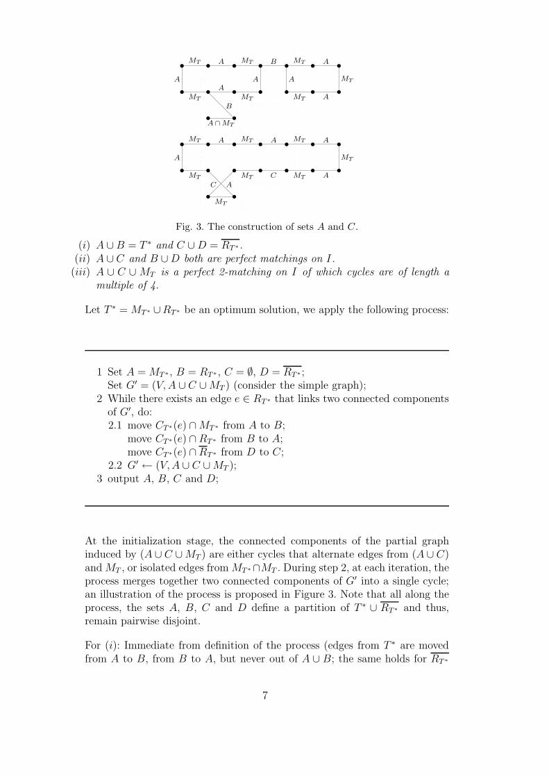
Fig. 3. The construction of sets A and C.

(i) A ∪B = T ∗ and C ∪D = RT ∗.(ii) A ∪ C and B ∪D both are perfect matchings on I.

(iii) A ∪ C ∪MT is a perfect 2-matching on I of which cycles are of length amultiple of 4.

Let T ∗ = MT ∗ ∪RT ∗ be an optimum solution, we apply the following process:

1 Set A = MT ∗ , B = RT ∗ , C = ∅, D = RT ∗ ;Set G′ = (V, A ∪ C ∪MT ) (consider the simple graph);

2 While there exists an edge e ∈ RT ∗ that links two connected componentsof G′, do:2.1 move CT ∗(e) ∩MT ∗ from A to B;

move CT ∗(e) ∩RT ∗ from B to A;move CT ∗(e) ∩RT ∗ from D to C;

2.2 G′ ← (V, A ∪ C ∪MT );3 output A, B, C and D;

At the initialization stage, the connected components of the partial graphinduced by (A ∪ C ∪MT ) are either cycles that alternate edges from (A ∪ C)and MT , or isolated edges from MT ∗∩MT . During step 2, at each iteration, theprocess merges together two connected components of G′ into a single cycle;an illustration of the process is proposed in Figure 3. Note that all along theprocess, the sets A, B, C and D define a partition of T ∗ ∪ RT ∗ and thus,remain pairwise disjoint.

For (i): Immediate from definition of the process (edges from T ∗ are movedfrom A to B, from B to A, but never out of A ∪ B; the same holds for RT ∗

7

A1 ∪ MT ′

A2 ∪ MT ′

Fig. 4. Two possible P4 partitions deduced from A ∪ C ∪MT ′ .

and the two sets C and D).

For (ii): At the initialization stage, A ∪ C and B ∪ D respectively coincideswith MT ∗ and RT ∗ ∪RT ∗ , that both are perfect matchings. More precisely, forany chain PT ∗ from the optimum solution, if CT ∗ denotes the associated 4-length cycle, then A∪C and B∪D respectively contains the perfect matchingCT ∗ ∩MT ∗ and CT ∗ ∩ (RT ∗ ∪RT ∗) on V (PT ∗). Now, at each iteration, one justswaps the perfect matchings that are used in A∪C or B∪D in order to coverthe vertices of a given chain PT ∗ and thus, both A ∪ C and B ∪ D remainperfect matchings.

For (iii): At the end of the process, (A∪C)∩MT = ∅ and thus, because A∪Cand MT both are perfect matchings, then A∪C ∪MT is a perfect 2-matching.Now, consider a cycle Γ of G′ = (V, A ∪ C ∪MT ); by definition of step 2, anyedge e from RT ∗ that is incident to Γ has its two endpoints in V (Γ), whichmeans that Γ contains whether the two edges of CT ∗(e) ∩ MT ∗ , or the twoedges of CT ∗(e) ∩ (RT ∗ ∪RT ∗). In other words, if any vertex u from any pathPT ∗ ∈ T ∗ belongs to V (Γ), then the whole vertex set V (PT ∗) actually is asubset of V (Γ) and therefore, we deduce that |V (Γ)| = 4k.

Theorem 4 The solution T ′ provided by the algorithm achieves a 32-standard

approximation for MinMetricP4P and this ratio is tight.

Let T ∗ be an optimum solution on I = (K4n, d), we consider 4 pairwise disjointsets A, B, C and D in accordance with the application of Lemma 3 to thesolution T ′. According to property (iii), we can split A ∪ C into two sets A1

and A2 in such a way that Ai ∪MT ′ (i = 1, 2) is a P4-partition (see Figure 4for an illustration). Hence, Ai constitutes an alternative solution for RT ′ andbecause this latter is optimum, we obtain:

2d(RT ′) ≤ d(A) + d(C) (4)

8

Moreover, item (ii) of Lemma 3 states that B∪D is a perfect matching; sinceMT ′ is optimum, it thus verifies:

d(MT ′) ≤ d(B) + d(D) (5)

Hence, it suffices to sum inequalities (4) and (5) (and also to consider item (i)of Lemma 3) in order to obtain:

d(MT ′) + 2d(RT ′) ≤ d(T ∗) + d(RT ∗) (6)

Now, because I satisfies the triangular inequality, we observe that d(RT ∗) ≤d(T ∗) and thus deduce from inequality 6:

d(MT ′) + 2d(RT ′) ≤ 2optMinMetricP4P(I) (7)

(Note that this latter inequality is only true when minimizing.) Which enablesto conclude, if we consider that d(MT ′) ≤ d(MT ∗) ≤ d(T ∗). Finally, the tight-ness is provided by the instance family In = (K8n, d) that has been describedin Property 1.

Concerning the maximization case and using Lemma 3, one can also obtainan alternative proof of the result given in [11].

Theorem 5 The solution T ′ provided by the algorithm achieves a 34-standard

approximation for MaxP4P.

The inequality (6) becomes

d(MT ′) + 2d(RT ′) ≥ optMaxP4P(I) + d(RT ∗) (8)

Considering this time that 2 × d(MT ′) ≥ optMaxP4P(I) + d(RT ∗), we deduce

apxMaxP4P(I) ≥ 3

4

(

optMaxP4P(I) + d(RT ∗)

)

.

3.3 General P4P within the differential framework

When dealing with the differential ratio, MinP4P, MinMetricP4P, andMaxP4P are equivalent to approximate, since PkP problems belong to theclass FGNPO, [14]. Note that such an equivalence is more generally true forany couple of problems that only differ by an affine transformation of theirobjective function.

9

Theorem 6 The solution T ′ provided by the algorithm achieves a 12-differential

approximation for P4P and this ratio is tight.

We consider the maximization version. First, observe that RT ∗ is a n-cardinalitymatching. Hence, for any perfect matching M of I such that M ∪RT ∗ do forma P4-partition, we have:

d(M) + d(RT ∗) ≥ worMaxP4P(I) (9)

Adding inequalities (8) and (9), we thus conclude:

2apxMaxP4P(I) ≥ d(MT ′) + 2d(RT ′) + d(M) ≥ worMaxP4P(I) + optMaxP4P

(I)

In order to establish the tightness of this ratio, we refer to Property 1.

3.4 Bi-valuated metric P4P with weights 1 & 2 within the standard frame-work

As it has been recently done for MinTSP in [5,6], we now focus on instanceswhere any edge is worth either 1 or 2; indeed, such an analysis enables a keenercomprehension of a given algorithm. Furthermore, because the P4-partitionproblem is NP-complete, the problems MaxP4P1,2 and MinP4P1,2 still areNP-hard.

Let us first introduce some more notations. For a given instance I = (K4n, d)of P4P1,2 with d(e) ∈ {1, 2}, we denote by MT ′,i (resp., RT ′,i) the set ofedges from MT ′ that are of weight i. If we aim at maximizing, then p (resp.,q) indicates the cardinality of MT ′,2 (resp., of RT ′,2); otherwise, it indicatesthe quantity |MT ′,1| (resp., |RT ′,1|). In any case, p and q respectively countthe number of “good weight edges” in the sets MT ′ and RT ′. With respect tothe optimum solution, we define the sets MT ∗,i, RT ∗,i for i = 1, 2 and thecardinalities p∗, q∗ as the same.

Lemma 7 For any instance I = (K4n, d), if T is a feasible solution and T ∗

is an optimum solution, then there an edge set A that verifies:

(i) A ⊆ MT ∗,2 ∪ RT ∗,2 (resp., A ⊆ MT ∗,1 ∪RT ∗,1) and |A| = q∗ if the goal is tomaximize (resp., to minimize);

(ii) G′ = (V, MT ′ ∪ A) is a simple graph made of pairwise disjoint chains.

We only prove the maximization case. Wlog., we may assume that the follow-ing property always holds for T ∗:

10

Property 8 For any 3-length chain P ∈ T ∗, |P ∩MT ∗,2| ≥ |P ∩ RT ∗,2|.

Otherwise, T ∗ would contain a chain P = {[x, y], [y, z], [z, t]} that verifiesd(x, y) = d(z, t) = 1 and d(y, z) = 2; thus, by swapping P for P ′ = {[y, z], [z, t],[t, x]} within T ∗, one could generate an alternative optimum solution.

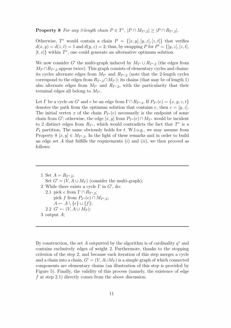
We now consider G′ the multi-graph induced by MT ′ ∪ RT ∗,2 (the edges fromMT ′∩RT ∗,2 appear twice). This graph consists of elementary cycles and chains:its cycles alternate edges from MT ′ and RT ∗,2 (note that the 2-length cyclescorrespond to the edges from RT ∗,2∩MT ′); its chains (that may be of length 1)also alternate edges from MT ′ and RT ∗,2, with the particularity that theirterminal edges all belong to MT ′ .

Let Γ be a cycle on G′ and e be an edge from Γ∩RT ∗,2. If PT ∗(e) = {x, y, z, t}denotes the path from the optimum solution that contains e, then e = [y, z].The initial vertex x of the chain PT ∗(e) necessarily is the endpoint of somechain from G′: otherwise, the edge [x, y] from PT ∗(e)∩MT ∗ would be incidentto 2 distinct edges from RT ∗ , which would contradicts the fact that T ∗ is aP4 partition. The same obviously holds for t. W.l.o.g., we may assume fromProperty 8 [x, y] ∈ MT ∗,2. In the light of these remarks and in order to buildan edge set A that fulfills the requirements (i) and (ii), we then proceed asfollows:

1 Set A = RT ∗,2;Set G′ = (V, A ∪MT ) (consider the multi-graph);

2 While there exists a cycle Γ in G′, do:2.1 pick e from Γ ∩RT ∗,2;

pick f from PT ∗(e) ∩MT ∗,2;A← A \ {e} ∪ {f};

2.2 G′ ← (V, A ∪MT );3 output A;

By construction, the set A outputted by the algorithm is of cardinality q∗ andcontains exclusively edges of weight 2. Furthermore, thanks to the stoppingcriterion of the step 2, and because each iteration of this step merges a cycleand a chain into a chain, G′ = (V, A∪MT ) is a simple graph of which connectedcomponents are elementary chains (an illustration of this step is provided byFigure 5). Finally, the validity of this process (namely, the existence of edgef at step 2.1) directly comes from the above discussion.

11

Γ

MT MT MT

MT

MT MT MT

MT

A ∩ RT∗,2

MT∗,2

A

Fig. 5. The construction of set A.

Theorem 9 The solution T ′ provided by the algorithm achieves a 910

-standardapproximation for MaxP4P1,2 and a 7

6-standard approximation for MinP4P1,2.

These ratios are tight.

Let consider A the edge subset of the optimum solution that may be deducedfrom the application of Lemma 7 to the approximate solution. We arbitrarilycomplete A by the means of an edge set B in such a way that A ∪ B ∪MT ′

constitutes a perfect 2-matching. As we did while proving Theorem 4, wesplit the edge set A ∪ B into two sets A1 and A2 in order to obtain two P4-partitions MT ′ ∪ A1 and MT ′ ∪ A2 of V (K4n). As both A1 ∪ B1 and A2 ∪ B2

complete MT ′ into a P4-partition and because RT ′ is optimum, we deducethat Ai does not contain more “good weight edges” than RT ′ does, that is:q ≥ |{e ∈ Ai : d(e) = 2}| if the goal is to maximize, q ≥ |{e ∈ Ai : d(e) = 1}|otherwise. Since A ⊆ A1 ∪A2 and |A| = q∗, we immediately deduce:

q ≥ q∗/2 (10)

On the other hand, the optimality of MT ′ leads to the following relation:

p ≥ max{p∗, q∗} (11)

Moreover, the quantities p∗ and q∗ structurally verify:

n ≥ max{p∗/2, q∗} (12)

Finally, whether the goal is to maximize or to minimize, we can express thevalue of any solution T as:

d(T ) =

3n + (p + q) when maximizing,

6n− (p + q) when minimizing.(13)

This expected results may now be obtained by the means of a little algebra

12

I = (K8, d) T ∗ T ′

Fig. 6. Instance I = (K8, d) that establishes the tightness for MaxP4P1,2.

on relations (10), (11), (12) and (13):

10apxMaxP4P1,2(I) = 10(3n + p + q)

= 9(3n) + 3n + 9p + p + 10q

≥ 9(3n) + 3q∗ + 9p∗ + q∗ + 5q∗

= 9(3n + p∗ + q∗) = 9optMaxP4P1,2(I)

6apxMinP4P1,2(I) = 6(6n− p− q)

= 6(6n) − 6p − 6q

≤ 6(6n) − 6p∗ − 3q∗ + (2n− p∗) + (4n− 4q∗)

≤ 7(6n− p∗ − q∗) = 7optMinP4P1,2(I)

The tightness for MaxP4P1,2 is established thanks to the instance I = (K8, d)depicted in Figure 6, where the edges of distance 2 are drawn in continuousline, whereas the edges of distance 1 on T ∗ and T ′ are drawn in dotted line(other edges are not drawn). One can easily see optMaxP4P1,2

(I) = 10 andapxMaxP4P1,2

(I) = 9. Concerning the minimization case, the ratio is tight onthe instance J = (K8, d) that verifies: opt(J) = d(T ∗) = 6 and apx(J) =d(T ′) = 7. J = (K8, d) is depicted in Figure 7 (the 1-weight edges are drawnin continuous line and the 2-weight edges on T ∗ and T ′ are drawn in dottedline).

3.5 Bi-valuated metric P4P with weights a and b within the differential frame-work

As we have already mentioned, the differential measure is stable under affinetransformation; now, any instance from MaxP4Pa,b may be mapped into aninstance of MaxP4P1,2 or MinP4Pa,b by the way of such a transformation.Thus, proving MaxP4P1,2 is ε-differential approximable actually establishes

13

J = (K8, d) T ∗ T ′

Fig. 7. Instance I = (K8, d) that establishes the tightness for MinP4P1,2.

that MinP4Pa,b and MaxP4Pa,b are ε-differential approximable for any coupleof real values a < b.

Theorem 10 The solution T ′ provided by the algorithm achieves a 23-differential

approximation for P4Pa,b and this ratio is tight.

Let I = (K4n, d) be an instance of MaxP4P1,2. We use the notations thatwere introduced while proving Theorem 9, namely: p = |MT ′,2|, p∗ = |MT ∗,2|,q = |RT ′,2| and q∗ = |RT ∗,2|. Furthermore, for i = 1, 2, P i

T ′ will refer to theset of chains from T ′ of which central edge is of weight i. Note that the chainsfrom P1

T ′ may be of total weight 3, 4 or 5, whereas the chains from P2T ′ may

be of total weight 5 or 6 (at least one extremal edge must be of weight 2,or MT ′ is not optimum). We will more specifically denote by P2

T ′,5 and P2T ′,6

the chains from P2T ′ that are of total weight respectively 5 and 6. Finally, for

i = 1, 2, M iT ′ will refer to the set of edges e ∈ MT ′ such that PT ′(e) ∈ P i

T ′

(that is, e is element of a chain from T ′ of which central edge has weight i).Thanks to relations (10) and (11), we first express some upper bounds foroptMaxP4P1,2

(I):

optMaxP4P1,2(I) ≤ min {3n + p + 2q, 3n + 2p} (14)

It order to obtain a differential approximation, one also has to produce an effi-cient bound for worMaxP4P1,2

(I). To do so, we will deduce from the optimalityof MT ′ and RT ′ some edges of weight 1 that will enable us to approximatethe worst solution. We first consider the vertices from V (P1

T ′): they are “easy”to cover by the means of 3-length chains of total weight 3, since we mayimmediately deduce from the optimality of RT ′ the following property (an il-lustration is provided by Figure 8, where dotted lines indicate edges of weight1 and dashed lines indicate unspecified weight edges):

Property 11 [x, y] 6= [x′, y′] ∈M1T ′ ⇒ ∀e ∈ {x, y} × {x′, y′} , d(e) = 1

We now consider the vertices from V (P2T ′,5). Let PT ′ = {x, y, z, t} with [x, y] ∈

MT ′,2 be a chain from P2T ′,5, we deduce from the optimality of MT ′ that

d(t, x) = 1; hence, the 3-length chain P ′T ′ = {y, z, t, x} covers the vertices

14

x

y

x′

y′

M1

T ′M1

T ′

Fig. 8. 1-weight edges on V (M1T ′).

x

y

x′

y′

α

β γ

δ

M1

T ′M1

T ′

M2

T ′

d(y, β) = 2

Fig. 9. 1-weight edges that may be deduced from the optimality of RT ′ .

{x, y, z, t} with a total cost 4. Let us assume that P2T ′,6 = ∅, then we are able

to build a P4 partition of V (K4n) using exclusively edges of weight 1, but|P2

T ′,5| edges of weight 2 in order to cover V (P2T ′,5). Hence, a worst solution

will cost at most 3n + q, while the approximate solution is of total weight3n + p + q. Thus, using relation 14, we would be able to conclude. Of course,there is no reason for P2

T ′,6 = ∅; nevertheless, this discussion has brought tothe fore the following fact: the difficult point of the proof lies on the partition-ing of V (P2

T ′,6) into “light” 3-length chains, what we are attempting to do bynow.

We first stand two more properties that are immediate from the optimality ofMT ′ and RT ′ , respectively.

Property 12 [x, y] ∈ MT ′,1 and [x′, y′] ∈ MT ′,2 ⇒ min {d(x, x′), d(y, y′)} =min {d(x, y′), d(y, x′)} = 1

Property 13 If [x, y] 6= [x′, y′] ∈ M1T ′ and PT ′ = {α, β, γ, δ} ∈ P2

T ′, thenmax {d(e)|e ∈ {α, β} × {x, y}} = 2 ⇒ max {d(e)|e ∈ {γ, δ} × {x′, y′}} = 1.(See Figure 9 for an illustration, where continuous and dotted lines respectivelyindicate 2- and 1-weight edges, whereas dashed lines indicate unspecified weightedges).

¿From Properties 12 and 13, we now are able to propose a “light” P4 partitionof P2

T ′,6.

Property 14 Given a chain PT ′ ∈ P2T ′,6 and two edges [x, y] 6= [x′y′] ∈ M1

T ,then there exists a P4 partition P = {P1, P2} of (V (PT ′) ∪ {x, y, x′, y′} ) thatis of total weight at most 8. Furthermore, if [x, y] and [x′, y′] both belong toMT ′,1, then we can decrease this weight down to (at most) 7 (see Figure 10 foran illustration).

Consider PT ′ = {α, β, γ, δ} ∈ P2T ′,6 and [x, y] 6= [x′y′] ∈ M1

T . We set P1 ={α, x, x′, δ} and P2 = {β, y, y′, γ}. If every edge from {α, β, γ, δ}×{x, x′, y, y′}is of weight 1, then P1 ∪ P2 has a total weight 6. Conversely, if there existsa 2-weight edge (assume that [β, y] is such an edge), then P1 ∪ P2 is of total

15

x

y

x′

y′

α

β γ

δ

M1

T ′M1

T ′P2

T ′ ,6

d(y, β) = 2

x

y

x′

y′

α

β γ

δ

Fig. 10. A P4 partition of (PT ′ , e1, e2) ∈ P2T ′,6 × (M1

T ′)2 of total weight at most 7.

weight at most 8: indeed, we get d(x, x′) = d(y, y′) = 1 from Property 11 andd(δ, x′) = d(γ, y′) = 1 from Property 13. Furthermore, if d(x, y) = 1, thend(α, x) = 1 from Property 12 and thus, d(P1) + d(P2) = 7. We now are ableto compute an approximate worst solution that will provide an efficient upperbound for worMaxP4P1,2

(I).

0 Set T = T ′, T∗ = ∅;1 While ∃ {P, e1, e2} ⊆ T s.t. (P, e1, e2) ∈ P

2T ′,6 ×M1

T ′,1 ×M1T ′,1

1.1 compute P = {P1, P2} on V (P ) ∪ V (e1) ∪ V (e2) with d(P) ≤ 7;1.2 T ← T \ {P, e1, e2} , T∗ ← T∗ ∪ {P1, P2};

2 While ∃ {P, e1, e2} ⊆ T s.t. (P, e1, e2) ∈ P2T ′,6 ×M1

T ′ ×M1T ′

2.1 compute P = {P1, P2} on V (P ) ∪ V (e1) ∪ V (e2) with d(P) ≤ 8;2.2 T ← T \ {P, e1, e2} , T∗ ← T∗ ∪ {P1, P2};

3 While ∃P ⊆ T s.t. P ∈ P2T ′,6

3.1 T ← T \ P, T∗ ← T∗ ∪ {P};4 While ∃P ⊆ T s.t. P ∈ P2

T ′,5

4.1 compute P = {P1} on V (P ) with d(P) ≤ 4;4.2 T ← T \ P, T∗ ← T∗ ∪ {P1};

5 While ∃ {e1, e2} ⊆ T s.t. (e1, e2) ∈M1T ′ ×M1

T ′

5.1 compute P = {P1} on V (e1) ∪ V (e2) with d(P) = 3;5.2 T ← T \ e1, e2, T∗ ← T∗ ∪ {P1};

6 Output T∗;

In order to estimate the value of the approximate worst solution T∗, one has tocount the number p∗ + q∗ of 2-weight edges it contains. Let p1

i refer to |M1T ′ ∩

MT ′,i| for i = 1, 2 (the cardinality p11 enables the expression of the number of

iterations during step 1). Steps 1, 2 and 3 respectively put into T∗ at most one,two and three 2-weight edges per iteration. Any chain from P2

T ′,6 is treatedby one of the three steps 1 to 3. If 2|P2

T ′,6| ≥ p11, only |P2

T ′,6| − ⌊p11/2⌋ chains

16

P1

T ′,3P

1

T ′,4P

1

T ′,5

P2

T ′,5P

2

T ′,6

Fig. 11. A partition of T ′.

from P2T ′,6 are treated by one of the steps 2 and 3. Finally, if |P2

T ′,6| ≥ |P1T ′|,

only |P2T ′,6| − |P

1T ′| chains from P2

T ′,6 are treated during step 3. Furthermore,step 4 puts at most |P2

T ′,5| 2-weight edges into T∗ (at most one per iteration),while steps 0 and 5 do not incorporate any 2-weight edges within T∗. Thus,considering q = |P2

T ′,5| + |P2T ′,6| and |P1

T ′| = n − q, we obtain the following

inequality (where expression X(+) is equivalent to max {X, 0}):

p∗ + q∗ ≤ q + (|P2T ′,6| − ⌊p

11/2⌋)(+) + (|P2

T ′,6| − n + q)(+) (15)

Let us introduce some more notations. Likewise P2T ′ = P2

T ′,5 ∪P2T ′,6, we define

a partition of P1T ′ into three subsets P1

T ′,3, P1T ′,4 and P1

T ′,5 according to thechain total weight. Note that, since the subsets P1

T ′,j define a partition of T ′,we have n = |P1

T ′,3| + |P1T ′,4| + |P

1T ′,5| + |P

2T ′,5| + |P

2T ′,6| (see Figure 11 for an

illustration of this partition; the edges of distance 2 are drawn in continuouslines whereas the edges of distance 1 are drawn in dotted lines).

We now will establish the three following relations in order to compare theworst solution value to both the approximate solution and the optimum solu-tion values:

p ≥ q∗ + (|P2T ′,6| − ⌊p

11/2⌋)(+) (16)

2q ≥ q∗ + (|P2T ′,6|+ q − n)(+) (17)

q ≥ p∗ + q∗ − (|P2T ′,6| − ⌊p

11/2⌋)(+) − (|P2

T ′,6|+ q − n)(+) (18)

Actually, by summing inequalities 16 to 18, together with 2p ≥ 2p∗, we mayobtain the expected result:

3apxMaxP4P(I) = 3(3n + p + q)

≥ 2(3n + p∗ + q∗) + (3n + p∗ + q∗)

= 2optMaxP4P1,2(I) + worMaxP4P1,2

(I)

Proof of inequality 16: Obvious if 2|P2T ′,6| ≤ p1

1, since p ≥ q∗ (from inequality11). Otherwise, one can write p as the sum p = n + |P2

T ′,6| + |P1T ′,5| − |P

1T ′,3|.

Now, |P1T ′,5|− |P

1T ′,3| is precisely the half of the difference between the number

of 2-weight and of 1-weight edges in M1T ′ : since p1

2 = |P1T ′,4| + 2|P1

T ′,5| andp1

1 = |P1T ′,4| + 2|P1

T ′,3|, then p12 − p1

1 = 2(|P1T ′,5| − |P

1T ′,3|). ¿From this latter

17

equality, we deduce that p11 and p1

2 have the same parity; hence, we have1/2(p1

2 − p11) = ⌊p1

2/2⌋ − ⌊p11/2⌋ and thus, p = n + |P2

T ′,6| + ⌊p12/2⌋ − ⌊p1

1/2⌋.Just observe that n and q∗ verify n ≥ q∗ in order to conclude.

Proof of inequality 17: Obvious if |P2T ′,6| ≤ n−q, since 2q ≥ q∗ (from inequality

10). Otherwise, consider that q, n and |P2T ′,6| verify: q ≥ |P2

T ′,6| and n ≥ q∗.

Proof of inequality 18: Immediate from Property 14.

The tightness is provided by the instance I = (K8, d) that is pictured onFigure 6; since this latter contains a vertex v such that any edge from v is ofweight 2, the result follows.

References

[1] E. M. Arkin, R. Hassin, A. Levin, Approximations for minimum and min-maxvehicle routing problems, Journal of Algorithms, to appear (article in press),2005.

[2] G. Ausiello, P. Crescenzi, G. Gambosi, V. Kann, A. Marchetti-Spaccamela,M. Protasi, Complexity and Approximation (Combinatorial OptimizationProblems and Their Approximability Properties), Springer, Berlin, 1999.

[3] G. Ausiello, A. D’Atri, M. Protasi, Structure preserving reductions amongconvex optimization problems, J. Comput. System Sci. 21 (1980) 136-153.

[4] M. Bellare, P. Rogaway, The complexity of approximating a nonlinear program,Mathematical Programming 69 (1995) 429-441.

[5] P. Berman, M. Karpinski, 8/7-Approximation Algorithm for 1, 2-TSP, Proc.SODA’06, 2006

[6] M. Blaser, L. Shankar Ram, An Improved Approximation Algorithm for TSPwith Distances One and Two, Proc. FCT’05, LNCS 3623 (2005) 504-515.

[7] M. Demange, V. Th. Paschos, On an approximation measure founded on thelinks between optimization and polynomial approximation theory, TheoreticalComputer Science 158 (1996) 117-141.

[8] G. N. Frederickson, M. S. Hecht, C. E. Kim, Approximation algorithms for somerouting problems, SIAM J. on Computing 7 (1978) 178-193.

[9] M. R. Garey, D. S. Johnson, Computers and intractability. a guide to the theoryof NP-completeness, CA, Freeman, 1979.

[10] R. Hassin, S. Khuller, z-approximations, Journal of Algorithms 41 (2001) 429-442.

18

[11] R. Hassin, S. Rubinstein, An Approximation Algorithm for Maximum Packingof 3-Edge Paths, Information Processing Letters 63 (1997) 63-67.

[12] R. Hassin, S. Rubinstein, An Approximation Algorithm for Maximum TrianglePacking, ESA, LNCS 3221 (2004) 403-413.

[13] J. Monnot, Differential approximation results for the traveling salesman andrelated problems, Information Processing Letters 82 (2002) 229-235.

[14] J. Monnot, Differential approximation of NP-hard problems with constant sizefeasible solutions, RAIRO/operations research, 36(4) (2002) 279-297.

[15] S. Sahni, T. Gonzalez, P-complete approximation problems, Journal of theAssociation for Computing Machinery 23 (1976) 555-565.

[16] G. Steiner, On the k-path partition of graphs, Theoretical Computer Science290 (2003) 2147-2155.

19