Applications of the poincaré inequality to extended Kantorovich method

APPLICATIONS OF THE POINCARÉ INEQUALITYTO EXTENDED KANTOROVICH METHOD

DER-CHEN CHANG, TRISTAN NGUYEN, GANG WANG,

AND NORMAN M. WERELEY

Received 3 February 2005; Revised 2 March 2005; Accepted 18 April 2005

We apply the Poincare inequality to study the extended Kantorovich method that wasused to construct a closed-form solution for two coupled partial differential equationswith mixed boundary conditions.

Copyright © 2006 Der-Chen Chang et al. This is an open access article distributed underthe Creative Commons Attribution License, which permits unrestricted use, distribution,and reproduction in any medium, provided the original work is properly cited.

1. Introduction

Let Ω⊂Rn be a Lipschitz domain inRn. Consider the Dirichlet spaceH10 (Ω) which is the

collection of all functions in the Sobolev space L21(Ω) such that

H10 (Ω)=

{u∈ L2(Ω) : u|∂Ω = 0, ‖u‖L2 +

n∑k=1

∥∥∥∥ ∂u∂xk∥∥∥∥L2<∞

}. (1.1)

The famous Poincare inequality can be stated as follows: for u∈H10 (Ω), then there exists

a universal constant C such that

∫Ωu2(x)dx ≤ C

n∑k=1

∫Ω

∣∣∣∣ ∂u∂xk∣∣∣∣

2

dx. (1.2)

One of the applications of this inequality is to solve the modified version of the Dirichletproblem (see, John [5, page 97]): find a v ∈H1

0 (Ω) such that

(u,v)=∫Ω

[ n∑k=1

∂u

∂xk

∂v

∂xk

]dx =

∫Ωu(x) f (x)dx, (1.3)

Hindawi Publishing CorporationJournal of Inequalities and ApplicationsVolume 2006, Article ID 32356, Pages 1–21DOI 10.1155/JIA/2006/32356

http://dx.doi.org/10.1155/S1025583406323569

2 Poincare inequality and Kantorovich method

where x = (x1, . . . ,xn) with a fixed f ∈ C(Ω). Then the function v in (1.3) satisfied theboundary value problem

Δv =− f , in Ω

v = 0, on ∂Ω.(1.4)

In this paper, we will use the Poincare inequality to study the extended Kantorovichmethod, see [6]. This method has been used extensively in many engineering problems,for example, readers can consult papers [4, 7, 8, 11, 12], and the references therein. Let usstart with a model problem, see [8]. For a clamped rectangular box Ω =∏n

k=1[−ak,ak],subjected to a lateral distributed load, �(x) =�(x1, . . . ,xn), the principle of virtual dis-placements yields

n∏�=1

∫ a�

−a�

[η∇4Φ−�

]δΦDx = 0, (1.5)

where Φ is the lateral deflection which satisfies the boundary conditions, η is the flexuralrigidity of the box, and

∇4 =n∑k=1

∂4

∂x4k

+∑j �=k

2∂4

∂x2j ∂x

2k

. (1.6)

Since the domain Ω is a rectangular box, it is natural to assume the deflection in the form

Φ(x)=Φk1···kn(x)=n∏�=1

fk�(x�), (1.7)

it follows that when fk2 (x2)··· fkn(xn) is prescribed a priori, (1.5) can be rewritten as

∫ a1

−a1

[ n∏�=2

∫ a�

−a�

(η∇4Φk1···kn −�

)fk�(x�)dx�

]δ fk1 (x1)dx1 = 0. (1.8)

Equation (1.8) is satisfied when

n∏�=2

∫ a�

−a�

(η∇4Φk1···kn −�

)fk�(x�)dx� = 0. (1.9)

Similarly, when∏n

�=1,� �=m fk� (x�) is prescribed a priori, (1.5) can be rewritten as

∫ am

−am

[ n∏�=1,� �=m

∫ a�

−a�

(η∇4Φk1···kn −�

)fk�(x�)dx�

]δ fkm(xm)dxm = 0. (1.10)

It is satisfied when

n∏�=1,� �=m

∫ a�

−a�

(η∇4Φk1···kn −�

)fk�(x�)dx� = 0. (1.11)

Der-Chen Chang et al. 3

It is known that (1.9) and (1.11) are called the Galerkin equations of the extended Kan-torovich method. Now we may first choose

f20(x2)··· fn0(xn)=n∏�=2

c�

(x2�

a2�

− 1

)2

. (1.12)

Then Φ10···0(x)= f11(x1) f20(x2)··· fn0(xn) satisfies the boundary conditions

Φ10···0 = 0,∂Φ10···0∂x�

= 0 at x� =±a� , x1 ∈[− a1,a1

], (1.13)

for � = 2, . . . ,n. Now (1.9) becomes

n∏�=2

c�

∫ a�

−a�

(∇4Φ10···0− �

η

)(x2�

a2�

− 1

)2

dx� = 0, (1.14)

which yields

C4d4 f11

dx4+C2

d2 f11

dx2+C0 f11 = B. (1.15)

After solving the above ODE, we can use f11(x1)∏n

�=3 f�0(x�) as a priori data and plug itinto (1.10) to find f21(x2). Then we obtain the function

Φ110···0(x)= f11(x1)f21(x2)f30(x3)··· fn0

(xn). (1.16)

Continue this process until we obtain Φ1···1(x) = f11(x1) f21(x2)··· fn1(xn) and there-fore completes the first cycle. Next, we use f21(x2)··· fn1(xn) as our priori data and findf12(x1). We continue this process and expect to find a sequence of “approximate solu-tions.” The problem reduces to investigate the convergence of this sequence. Therefore, itis crucial to analyze (1.15). Moreover, from numerical point of view, we know that thissequence converges rapidly (see [1, 2]). Hence, it is necessary to give a rigorous mathe-matical proof of this method.

2. A convex linear functional on H20 (Ω)

Denote

I[φ]=∫Ω

{|Δφ|2− 2�(x)φ(x)}dx (2.1)

for Ω⊂Rn a bounded Lipschitz domain. Here x = (x1, . . . ,xn). As usual, denote

D2φ =

⎡⎢⎢⎢⎣∂2φ

∂x2

∂2φ

∂x∂y

∂2φ

∂y∂x

∂2φ

∂y2

⎤⎥⎥⎥⎦ . (2.2)


For Ω⊂R2, we define the Lagrangian function L associated to I[φ] as follows:

L : Ω×R×R2×R4 −→R,

(x, y;z;X ,Y ;U ,V ,S,W) −→ (U +V)2− 2�(x, y)z,(2.3)

where �(x, y) is a fixed function on Ω which shows up in the integrand of I[φ]. With theabove definitions, we have

L(x, y;φ;∇φ;D2φ

)= |Δφ|2− 2�(x, y)φ(x, y), (2.4)

where we have identified

z←→ φ(x, y), X ←→ ∂φ

∂x, Y ←→ ∂φ

∂y,

U ←→ ∂2φ

∂x2, V ←→ ∂2φ

∂y2, S←→ ∂2φ

∂y∂x, W ←→ ∂2φ

∂x∂y.

(2.5)

We also set H20 (Ω) to be the class of all square integrable functions such that

H20 (Ω)=

{ψ ∈ L2(Ω) :

∑|k|≤2

∥∥∥∥∂kψ

∂xk

∥∥∥∥L2<∞, ψ|∂Ω = 0, ∇ψ|∂Ω = 0

}. (2.6)

Fix (x, y)∈Ω. We know that

∇L(x, y;z;X ,Y ;U ,V ,S,W)=[−2�(x, y) 0 0 2(U +V) 2(U +V) 0 0

]T.

(2.7)

Because the convexity of the function L in the remaining variables, then for all (z; X , Y ;U ,V , S,W)∈R×R2×R4, one has

L(x, y; z; X , Y ;U ,V , S,W

)≥ L(x, y;z;X ,Y ;U ,V ,S,W)− 2�(x, y)

(z− z)

+ 2(U +V)[(U −U)

+(V −V)]. (2.8)

In particular, one has, with z = φ(x, y),

L(x, y; φ;∇φ;D2φ

)≥ L(x, y;φ;∇φ;D2φ

)+ 2Δφ

[∇φ−∇φ]− 2�(x, y)(φ−φ).

(2.9)

This implies that

∣∣Δφ∣∣2− 2�(x, y)φ≥ ∣∣Δφ∣∣2− 2�(x, y)φ+ 2Δφ[Δφ−Δφ

]− 2�(x, y)[φ−φ]. (2.10)

If instead we fix (x, y;z)∈Ω×R, then

L(x, y; z; X , Y ;U ,V , S,W

)≥ L(x, y; z;X ,Y ;U ,V ,S,W)

+ 2(U +V)[(U −U)

+(V −V)]. (2.11)


This implies that

L(x, y; φ;∇φ;D2φ

)≥ L(x, y; φ;∇φ;D2φ)

+ 2Δφ[∇φ−∇φ] (2.12)

Therefore,

|Δφ|2− 2�(x, y)φ≥ |Δφ|2− 2�(x, y)φ+ 2Δφ[Δφ−Δφ]. (2.13)

Lemma 2.1. Suppose either(1) φ ∈H2

0 (Ω)∩C4(Ω) and η ∈ C1c (Ω); or

(2) φ ∈H20 (Ω)∩C3(Ω)∩C4(Ω) and η ∈H2

0 (Ω).Let δI[φ;η] denote the first variation of I at φ in the direction η, that is,

δI[φ;η]= limε→0

I[φ+ εη]− I[φ]ε

. (2.14)

Then

δI[φ;η]= 2∫Ω

(Δ2φ−�(x, y)

)ηdxdy. (2.15)

Proof. We know that

I[φ+ εη]− I[φ]= 2ε∫Ω

[ΔφΔη−�η]dxdy + ε2∫Ω

(Δη)2dxdy. (2.16)

Hence,

εI[φ;η]= 2∫Ω

[ΔφΔη−�η]dxdy. (2.17)

If either assumption (1) or (2) holds, we can apply Green’s formula to a Lipschitz domainΩ to obtain

∫Ω

(ΔφΔη)dxdy =∫Ωη(Δ2φ

)dxdy +

∫∂Ω

[∂η

∂�nΔφ−η ∂

∂�nΔφ

]dxdy, (2.18)

where ∂/∂�n is the derivative in the direction normal to ∂Ω. Since either η ∈ C1c (Ω) or

η ∈H20 (Ω), the boundary term vanishes, which proves the lemma. �

Lemma 2.2. Let φ∈H20 (Ω). Then

‖φ‖H20 (Ω) ≈ ‖Δφ‖L2(Ω). (2.19)

Proof. The function φ ∈H20 (Ω) implies that there exists a sequence {φk} ⊂ C∞c (Ω) such

that limk→∞φk = φ in H20 -norm. From a well-known result for the Calderon-Zygmund

operator (see, Stein [10, page 77]), one has

∥∥∥∥ ∂2 f

∂xj ∂x�

∥∥∥∥Lp≤ C‖Δ f ‖Lp , j,� = 1, . . . ,n (2.20)


for all f ∈ C2c (Rn) and 1 < p <∞. Here C is a constant that depends on n only. Applying

this result to each φk, we obtain

∥∥∥∥∂2φk∂x2

∥∥∥∥L2(Ω)

,∥∥∥∥ ∂2φk∂x∂y

∥∥∥∥L2(Ω)

,∥∥∥∥∂2φk∂y2

∥∥∥∥L2(Ω)

≤ C∥∥Δφk∥∥L2(Ω). (2.21)

Taking the limit, we conclude that

∥∥∥∥∂2φ

∂x2

∥∥∥∥L2(Ω)

,∥∥∥∥ ∂2φ

∂x∂y

∥∥∥∥L2(Ω)

,∥∥∥∥∂2φ

∂y2

∥∥∥∥L2(Ω)

≤ C‖Δφ‖L2(Ω). (2.22)

Applying Poincare inequality twice to the function φ ∈H20 (Ω), we have

‖φ‖L2(Ω) ≤ C1‖∇φ‖L2(Ω)

≤ C2

(∥∥∥∥∂2φ

∂x2

∥∥∥∥L2(Ω)

+∥∥∥∥ ∂2φ

∂x∂y

∥∥∥∥L2(Ω)

+∥∥∥∥∂2φ

∂y2

∥∥∥∥L2(Ω)

)

≤ C‖Δφ‖L2(Ω).

(2.23)

Hence, ‖φ‖L2(Ω) ≤ C‖Δφ‖L2(Ω). The reverse inequality is trivial. The proof of this lemmais therefore complete. �

Lemma 2.3. Let {φk} be a bounded sequence in H20 (Ω). Then there exist φ ∈H2

0 (Ω) and asubsequence {φkj} such that

I[φ]≤ liminf I[φkj

]. (2.24)

Proof. By a weak compactness theorem for reflexive Banach spaces, and hence for Hilbertspaces, there exist a subsequence {φkj} of {φk} and φ in H2

0 (Ω) such that φkj → φ weaklyin H2

0 (Ω). Since

H20 (Ω)⊂H1

0 (Ω)⊂⊂L2(Ω), (2.25)

by the Sobolev embedding theorem, we have

φkj −→ φ in L2(Ω) (2.26)

after passing to yet another subsequence if necessary.Now fix (x, y,φkj (x, y))∈R2×R and apply inequality (2.13), we have

∣∣Δφkj∣∣2− 2�(x, y)φkj (x, y)≥ |Δφ|2− 2�(x, y)φkj (x, y) + 2Δφ[Δφkj −Δφ

]. (2.27)

This implies that

I[φkj

]≥∫Ω

[|Δφ|2− 2�(x, y)φkj]dxdy + 2

∫ΩΔφ · [Δφkj −Δφ

]dxdy. (2.28)

But φkj → φ in L2(Ω), hence∫Ω

[|Δφ|2− 2�(x, y)φkj]dxdy −→

∫Ω

[|Δφ|2− 2�(x, y)φ]dxdy = I[φ]. (2.29)


Besides φkj → φ weakly in H20 (Ω) implies that∫ΩΔφ · [Δφkj −Δφ

]dxdy −→ 0. (2.30)

It follows that when taking limit

I[φ]≤ liminfj

I[φkj

]. (2.31)

This completes the proof of the lemma. �

Remark 2.4. The above proof uses the convexity of L(x, y;z;X ,Y ;U ,V ,S,W) when (x, y;z) is fixed. We already remarked at the beginning of this section that when (x, y) is fixed,L(x, y;z;X ,Y ;U ,V ,S,W) is convex in the remaining variables, including the z-variable.That is, we are not required to utilize the full strength of the convexity of L here.

3. The extended Kantorovich method

Now, we shift our focus to the extended Kantorovich method for finding an approximatesolution to the minimization problem

minφ∈H2

0 (Ω)I[φ] (3.1)

when Ω = [−a,a]× [−b,b] is a rectangular region in R2. In the sequel, we will writeφ(x, y) (resp., φk(x, y)) as f (x)g(y) (resp., fk(x)gk(y)) interchangeably as notated in Kerrand Alexander [8]. More specifically, we will study the extended Kantorovich method forthe case n = 2, which has been used extensively in the analysis of stress on rectangularplates. Equivalently, we will seek for an approximate solution of the above minimizationproblem in the form φ(x, y)= f (x)g(y) where f ∈H2

0 ([−a,a]) and g ∈H20 ([−b,b]).

To phrase this differently, we will search for an approximate solution in the tensorproduct Hilbert spaces H2

0 ([−a,a])⊗H20 ([−b,b]), and all sequences {φk}, {φkj} involved

hereinafter reside in this Hilbert space. Without loss of generality, we may assume thatΩ = [−1,1]× [−1,1] for all subsequent results remain valid for the general case whereΩ= [−a,a]× [−b,b] by approximate scalings/normalizing of the x and y variables. As in[8], we will treat the special case �(x, y) = γ, that is, we assume that the load �(x, y) isdistributed equally on a given rectangular plate.

To start the extended Kantorovich scheme, we first choose g0(y) ∈ H20 ([−1,1]) ∩

C∞c (−1,1), and find the minimizer f1(x)∈H20 ([−1,1]) of the functional:

I[f g0

]=∫Ω

[∣∣Δ( f g0)∣∣2− 2γ f (x)g0(y)

]dxdy

=∫Ω

[g2

0 ( f ′′)2 + 2 f f ′′g0g′′0 + f 2(g′′0 )2− 2γ f g0

]dxdy

=∫ 1

−1( f ′′)2dx

∫ 1

−1g2

0 dy + 2∫ 1

−1

(g′0)2dy

∫ 1

−1( f ′)2dx

+∫ 1

−1

(g′′0

)2dy

∫ 1

−1f 2dx− 2γ

∫ 1

−1g0dy

∫ 1

−1f dx,

(3.2)


where the last equality was obtained via the integration by parts of f f ′′ and g0g′′0 . Since

g0 has been chosen a priori; we can rewrite the functional I as

J[ f ]= ∥∥g0∥∥2L2

∫ 1

−1( f ′′)2dx+ 2

∥∥g′0∥∥2L2

∫ 1

−1( f ′)2dx

+∥∥g′′0 ∥∥2

L2

∫ 1

−1f 2dx− 2γ

∫ 1

−1g0(y)dy

∫ 1

−1f dx

(3.3)

for all f ∈H20 ([−1,1]). Now we may rewrite (3.3) in the following form:

J[ f ]=∫ 1

−1

[C1( f ′′)2 +C2( f ′)2 +C3 f

2 +C4 f]dx

≡∫ 1

−1K(x, f , f ′, f ′′)dx

(3.4)

with K :R×R×R×R→R given by

(x;z;V ;W) −→ C1W2 +C2V

2 +C3z2 +C4z, (3.5)

where

C1 =∥∥g0

∥∥2L2 , C2 =

∥∥g′0∥∥2L2 , C3 =

∥∥g′′0 ∥∥2L2 , C4 =−2γ

∫ 1

−1g0(y)dy. (3.6)

As long as g0 �≡ 0, as we have implicitly assumed, the Poincare inequality implies that

0 < C1 ≤ αC2 ≤ βC3 (3.7)

for some positive constants α and β, independent of g0. Consequently, K(x;z;V ;W) is astrictly convex function in variable z, V , W when x is fixed. In other words, K satisfies

K(x; z;V ;W)−K(x;z;V ;W)

≥ ∂K

∂z(x;z;V ;W)(z− z) +

∂K

∂V(x;z;V ;W)(V −V) +

∂K

∂W(x;z;V ;W)(W −W)

(3.8)

for all (x;z;V ;W) and (x; z;V ;W) in R4, and the inequality becomes equality at (x;z;V ;W) only if z = z, or V =V , or W =W .

Proposition 3.1. Let � : R×R×R×R→ R be a C∞ function satisfying the followingconvexity condition:

�(x;z+ z′;V +V ′;W +W ′)−�(x;z;V ;W)

≥ ∂�∂z

(x;z;V ;W)z′ +∂�∂V

(x;z;V ;W)V ′ +∂�∂W

(x;z;V ;W)W ′ (3.9)


for all (x;z;V ;W) and (x;z + z′;V +V ′;W +W ′)∈ R4, with equality at (x;z;V ;W) onlyif z′ = 0, or V ′ = 0, or W ′ = 0. Also, let

J[ f ]=∫ β

α�(x, f (x), f ′(x), f ′′(x)

)dx, ∀ f ∈H2

0 (α,β). (3.10)

Then

J[ f +η]− J[ f ]≥ δJ[ f ,η], ∀η ∈ C∞c (α,β) (3.11)

and equality holds only if η ≡ 0. Here δJ[ f ,η] is the first variation of J at f in the direction η.

Proof. Condition (3.9) means that at each x,

�(x; f +η; f ′ +η′; f ′′ +η′′)−�(x; f ; f ′; f ′′)

≥ ∂�∂z

(x; f ; f ′; f ′′)η(x) +∂�∂V

(x; f ; f ′; f ′′)η′(x) +∂�∂W

(x; f ; f ′; f ′′)η′′(x)(3.12)

for all η ∈ C∞c (α,β) with equality only if η(x)= 0, or η′(x)= 0, or η′′(x)= 0. Equivalently,the equality holds in (3.12) at x only if η(x)η′(x)= 0 or η′′(x)= 0. In other words,

η′′(x)d

dx

(η2(x)

)= 0. (3.13)

Integrating (3.12) gives

J[ f +η]− J[ f ]≥∫ β

α

[∂�∂z

η+∂�∂V

η′ +∂�∂W

η′′]dx = δJ[ f ,η]. (3.14)

Now suppose there exists η ∈ C∞c (α,β) such that (3.14) is an equality. Since � is a smoothfunction, this equality forces (3.12) to be a pointwise equality, which implies, in view of(3.13), that

η′′(x)d

dx

(η2(x)

)= 0, ∀x. (3.15)

If η′′(x) ≡ 0, then η′(x) = constant which implies that η′(x) ≡ 0 (since η ∈ C∞c (α,β)).This tells us that η ≡ constant and conclude that η ≡ 0 on the interval (α,β).

If η′′(x) �≡ 0, set U = {x ∈ (α,β) : η′′(x) �= 0}. Then U is a non-empty open set whichimplies that there exist x0 ∈U and some open set �x0 of x0 contained in U . Then η′′(ξ) �=0 for all ξ ∈ �x0 ⊂U . Thus

d

dx

(η2)= 0 on �x0 . (3.16)

Hence, η(ξ)≡ constant on �x0 . But this creates a contradiction because η′′(ξ)≡ 0 on �x0 .Therefore,

J[ f +η]− J[ f ]= δJ[ f ,η] (3.17)

only if η(x)≡ 0, as desired. This completes the proof of the proposition. �


Corollary 3.2. Let J[ f ] be as in (3.4). Then f1 ∈H20 ([−1,1]) is the unique minimizer for

J[ f ] if and only if f1 solves the following ODE:

∥∥g0∥∥2L2

d4 f

dx4− 2

∥∥g′0∥∥2L2

d2 f

dx2+∥∥g′′0 ∥∥2

L2 f = γ∫ 1

−1g0dy. (3.18)

Proof. Suppose f1 is the unique minimizer. Then f1 is a local extremum of J[ f ]. Thisimplies that δJ[ f ,η]= 0 for all η ∈H2

0 ([−1,1]). Using the notations in (3.4), we have

0= δJ[ f ,η]

=∫ 1

−1

[∂K

∂zη+

∂K

∂Vη′ +

∂K

∂Wη′′

]dx

=∫ 1

−1

[∂K

∂z− d

dx

(∂K

∂V

)+d2

dx2

(∂K

∂W

)]η(x)dx

(3.19)

for all η ∈H20 ([−1,1]). This implies that

∂K

∂z− d

dx

(∂K

∂V

)+d2

dx2

(∂K

∂W

)= 0, (3.20)

which is the Euler-Lagrange equation (3.18). This also follows from Lemma 2.1 directly.Conversely, assume f1 solves (3.18). Then the above argument shows that δJ[ f ,η]= 0

for all η ∈H20 ([−1,1]). Since K satisfies condition (3.9) in Proposition 3.1, we conclude

that

J[f1 +η

]− J[ f1]≥ δJ[ f1,η], ∀η∈ C∞c

([−1,1]

). (3.21)

This tells us that J[ f1 + η] ≥ J[ f1] for all η ∈ C∞c ([−1,1]) and J[ f1 + η] > J[ f1] if η �≡ 0.Observe that J : H1

0 ([−1,1])→ R as given in (3.4) is a continuous linear functional inthe H2

0 -norm. This fact, combined with the density of C∞c ([−1,1]) in H20 ([−1,1]) (in the

H20 -norm), implies that

J[f1 +η

]≥ J[ f1], ∀η∈ C∞c([−1,1]

). (3.22)

This means that for all ϕ ∈ H20 ([−1,1]), we have J[ϕ] ≥ J[ f1] and if ϕ �≡ f1 (almost ev-

erywhere), then ϕ− f1 �≡ 0 and hence, J[ϕ] > J[ f1]. Thus f1 is the unique minimumfor J . �

Reversing the roles of f and g, that is, fixing f0 and finding g1 ∈H20 to minimize I[ f0g]

over g ∈H20 ([−1,1]), we obtain the same conclusion by using the same arguments.

Corollary 3.3. Fix f0 ∈H20 ([−1,1]). Then g1 ∈H2

0 ([−1,1]) is the unique minimizer for

J[g]= I[ f0g]= ∥∥ f0∥∥2L2

∫ 1

−1(g′′)2dy + 2

∥∥ f ′0 ∥∥2L2

∫ 1

−1(g′)2dy

+∥∥ f ′′0

∥∥2L2

∫ 1

−1g2dy− 2γ

∥∥ f0∥∥L1

∫ 1

−1g dy

(3.23)


if and only if g1 solves the Euler-Lagrange equation

∥∥ f0∥∥2L2

d4g

dy4− 2

∥∥ f ′0 ∥∥2L2

d2g

dy2+∥∥ f ′′0

∥∥2L2g = 2γ

∫ 1

−1f0(x)dx. (3.24)

Now we search for the solution f1 ∈H20 ([−1,1]) in (3.18), that is,

∥∥g0∥∥2L2

d4 f

dx4− 2

∥∥g′0∥∥2L2

d2 f

dx2+∥∥g′′0 ∥∥2

L2 f = 2γ∫ 1

−1g0(y)dy. (3.25)

Rewrite the above ODE in the following form:

∥∥g0∥∥2L2

⎡⎣(D− ‖g

′‖2L2∥∥g0

∥∥2L2

)2

+‖g′′‖2

L2∥∥g0∥∥2L2

− ‖g′‖4L2∥∥g0

∥∥4L2

⎤⎦ f = 2γ

∫ 1

−1g0(y)dy, (3.26)

where D = d2/dx2.

Remark 3.4. In general when g ∈H2, that is, g needs not satisfy the zero boundary con-ditions for function in H2

0 , then the quantity

(∥∥g′′0 ∥∥2L2∥∥g0

∥∥2L2

−∥∥g′0∥∥4

L2∥∥g0∥∥4L2

)(3.27)

can take on any values. However, if g ∈H20 and g0 �≡ 0, as proved below, this quantity is

always positive.

Lemma 3.5. Let Ω be a Lipschitz domain in Rn, n≥ 1. Let g ∈H20 (Ω) be arbitrary. Then

‖∇g‖2L2 ≤ ‖g‖L2 · ‖Δg‖L2 , (3.28)

and equality holds if and only if g ≡ 0.

Proof. Integration by parts yields

‖∇g‖2L2 =

∫Ω∇g ·∇g dx =−

∫ΩgΔg dx +

∫∂Ωg∂g

∂�ndσ =−∫ΩgΔg dx. (3.29)

By the Cauchy-Schwartz inequality, we have

‖∇g‖2L2 ≤ ‖g‖L2 · ‖Δg‖L2 , (3.30)

and the equality holds if and only if (see Lieb-Loss [9])(i) |g(x)| = λ|Δg(x)| almost everywhere for some λ > 0,

(ii) g(x)Δg(x)= eiθ|g(x)| · |Δg(x)|.Since g is real-valued, (i) and (ii) imply

g(x)Δg(x)= λ(Δg(x))2. (3.31)


So, g must satisfy the following PDE:

Δg − 1λg = 0, (3.32)

where g ∈H20 (Ω). But the only solution to this PDE is g ≡ 0 (see, Evans [3, pages 300–

302]). This completes the proof of the lemma. �

Remark 3.6. If n= 1, one can solve g′′ − λ−1g = 0 directly without having to appeal to thetheory of elliptic PDEs.

Proposition 3.7. The solutions of (3.18) and (3.24) have the same form.

Proof. Using either Lemma 3.5 in case n= 1 to the above remark, we see that

‖g′′‖2L2∥∥g0

∥∥2L2

− ‖g′‖4L2∥∥g0

∥∥4L2

> 0 if g0 �≡ 0. (3.33)

Hence the characteristic polynomial associated to (3.26) has two pairs of complex con-jugate roots as long as g0 �≡ 0. Apply the same arguments to the ODE in (3.24) and theproposition is proved. �

Remark 3.8. The statement in Proposition 3.7 was claimed in [8] without verification.Indeed the authors stated therein that the solutions of (3.18) and (3.24) are of the sameform because of the positivity of the coefficients on the left-hand side of (3.18) and (3.24).As observed in Remark 3.4 and proved in Proposition 3.7, the positivity requirement isnot sufficient. The fact that f0,g0 ∈H2

0 must be used to conclude this assumption.

4. Explicit solution for (3.26)

We now find the explicit solution for (3.26), and hence for (3.18). Let

r = ‖g′‖L2∥∥g0∥∥L2

, t = ‖g′′‖L2∥∥g0∥∥L2

,

ρ =√t+ r2

2, κ=

√t− r2

2.

(4.1)

Then from Proposition 3.7 and its proof, the 4 roots of the characteristic polynomialassociated to ODE (3.26) are

ρ+ iκ, ρ− iκ, −ρ− iκ, −ρ+ iκ. (4.2)

Thus the homogeneous solution of (3.26) is

fh(x)= c1 cosh(ρx)cos(κx) + c2 sinh(ρx)cos(κx)

+ c3 cosh(ρx)sin(κx) + c4 sinh(ρx)sin(κx).(4.3)


It follows that a particular solution of (3.26) is

fp(x)= 2γ∫ 1−1 g0(y)dy∥∥g′′0 ∥∥2

L2

. (4.4)

Thus the solution of (3.18) is

f (x)= c1 cosh(ρx)cos(κx) + c2 sinh(ρx)cos(κx)

+ c3 cosh(ρx)sin(κx) + c4 sinh(ρx)sin(κx) + cp,(4.5)

where cp = 2γ∫ 1−1 g0(y)dy/‖g′′0 ‖2

L2 is a known constant. This implies that

f ′(x)= ρc1 sinh(ρx)cos(κx)− κc1 cosh(ρx)sin(κx)

+ ρc2 cosh(ρx)cos(κx)− κc2 sinh(ρx)sin(κx)

+ ρc3 sinh(ρx)sin(κx) + κc3 cosh(ρx)cos(κx)

+ ρc4 cosh(ρx)sin(κx) + κc4 sinh(ρx)cos(κx).

(4.6)

Apply the boundary conditions f (1)= f (−1)= f ′(1)= f ′(−1)= 0, we get

c1 cosh(ρ)cos(κ) + c2 sinh(ρ)cos(κ) + c3 cosh(ρ)sin(κ) + c4 sinh(ρ)sin(κ)=−cp,

c1 cosh(ρ)cos(κ)− c2 sinh(ρ)cos(κ)− c3 cosh(ρ)sin(κ) + c4 sinh(ρ)sin(κ)=−cp,

c1[ρ sinh(ρ)cos(κ)− κcosh(ρ)sin(κ)

]+ c2

[ρcosh(ρ)cos(κ)− κsinh(ρ)sin(κ)

]+ c3

[ρ sinh(ρ)sin(κ) + κcosh(ρ)cos(κ)

]+ c4

[ρcosh(ρ)sin(κ) + κsinh(ρ)cos(κ)

]= 0,

c1[− ρ sinh(ρ)cos(κ) + κcosh(ρ)sin(κ)

]+ c2

[ρcosh(ρ)cos(κ)− κsinh(ρ)sin(κ)

]+ c3


]− c4[ρcosh(ρ)sin(κ) + κsinh(ρ)cos(κ)

]= 0.(4.7)

Hence,

c1 cosh(ρ)cos(κ) + c4 sinh(ρ)sin(κ)=−cp, (4.8)

c2 sinh(ρ)cos(κ) + c3 cosh(ρ)sin(κ)= 0, (4.9)

c2[ρcosh(ρ)cos(κ)− κsinh(ρ)sin(κ)

]+ c3


]= 0,(4.10)

c1[ρ sinh(ρ)cos(κ)− κcosh(ρ)sin(κ)

]+ c4

[ρcosh(ρ)sin(κ) + κsinh(ρ)cos(κ)

]= 0.(4.11)

We know, beforehand, that there must be a unique solution. Thus (4.9) and (4.23) force


c2 = c3 = 0. We are left to solve for c1 and c4 from (4.8) and (4.11). But (4.11) tells us that

c1 =−c4ρcosh(ρ)sin(κ) + κsinh(ρ)cos(κ)ρ sinh(ρ)cos(κ)− κcosh(ρ)sin(κ)

. (4.12)

Substituting (4.12) into (4.8), we have

c4 = cp ρ sinh(ρ)cos(κ)− κcosh(ρ)sin(κ)ρ sin(κ)cos(κ) + κsinh(ρ)cosh(ρ)

. (4.13)

Plugging (4.13) into (4.12), we have

c1 =−cp ρcosh(ρ)sin(κ) + κsinh(ρ)cos(κ)ρ sin(κ)cos(κ) + κsinh(ρ)cosh(ρ)

. (4.14)

Therefore, the solution f1(x) can be written in the form

f1(x)= cp[K1

K0cosh(ρx)cos(κx) +

K2

K0sinh(ρx)sin(κx) + 1

], (4.15)

where

cp = 2γ∫ 1−1 g0(y)dy∥∥g′′0 ∥∥2

L2

,

ρ=√t+ r2

2=√√√√∥∥g′′0 ∥∥L2 /

∥∥g0∥∥L2 +

∥∥g′0∥∥2L2 /

∥∥g0∥∥2L2

2,

κ=√t− r2

2=√√√√∥∥g′′0 ∥∥L2 /

∥∥g0∥∥L2 −

∥∥g′0∥∥2L2 /

∥∥g0∥∥2L2

2,

K0 = ρ sin(κ)cos(κ) + κsinh(ρ)cosh(ρ),

K1 =−ρcosh(ρ)sin(κ)− κsinh(ρ)cos(κ),

K2 = ρ sinh(ρ)cos(κ)− κcosh(ρ)sin(κ).

(4.16)

The next step in the extended Kantorovich method is to fix f1(x) just found above andsolve for g1(y)∈H2

0 ([−1,1]) from (3.24). Lemma 2.2 and the computation above showthat

g1(y)= cp[K1

K0cosh(ρy)cos(κy) +

K2

K0sinh(ρy)sin(κy) + 1

], (4.17)


where

cp = 2γ∫ 1−1 f1(x)dx∥∥ f ′′1

∥∥2L2

,

ρ =√√√√∥∥ f ′′1

∥∥L2 /

∥∥ f1∥∥L2 +∥∥ f ′1 ∥∥2

L2 /∥∥ f1∥∥2

L2

2,

κ=√√√√∥∥ f ′′1

∥∥L2 /

∥∥ f1∥∥L2 −∥∥ f ′1 ∥∥2

L2 /∥∥ f1∥∥2

L2

2,

K0 = ρ sin(κ)cos(κ) + κsinh(ρ)cosh(ρ),

K1 =−ρcosh(ρ)sin(κ)− κsinh(ρ)cos(κ),

K2 = ρ sinh(ρ)cos(κ)− κcosh(ρ)sin(κ).

(4.18)

Now we start the next iteration by fixing g1(y) and solving for f2(x) in (3.18), and soforth. In particular, we will write

fn(x)= cn[K1n

K0ncosh

(ρnx

)cos

(κnx

)+K2n

K0nsinh

(ρnx

)sin

(κnx

)+ 1

], (4.19)

where

cn = 2γ∫ 1−1 gn−1(y)dy∥∥g′′n−1

∥∥2L2

,

ρn =√√√√∥∥g′′n−1

∥∥L2 /

∥∥gn−1∥∥L2 +

∥∥g′n−1

∥∥2L2 /

∥∥gn−1∥∥2L2

2,

κn =√√√√∥∥g′′n−1

∥∥L2 /

∥∥gn−1∥∥L2 −

∥∥g′n−1

∥∥2L2 /

∥∥gn−1∥∥2L2

2,

K0n = ρn sin(κn)

cos(κn)

+ κn sinh(ρn)

cosh(ρn),

K1n =−ρn cosh(ρn)

sin(κn)− κn sinh

(ρn)

cos(κn),

K2n = ρn sinh(ρn)

cos(κn)− κn cosh

(ρn)

sin(κn).

(4.20)

Similarly,

gn(y)= cn[K1n

K0ncosh

(ρn y

)cos

(κn y

)+K2n

K0nsinh

(ρn y

)sin

(κn y

)+ 1

], (4.21)


where

cn = 2γ∫ 1−1 fn(x)dx∥∥ f ′′n ∥∥2

L2

,

ρ=√√√√∥∥ f ′′n ∥∥

L2 /∥∥ fn∥∥L2 +

∥∥ f ′n∥∥2L2 /

∥∥ fn∥∥2L2

2,

κn =√√√√∥∥ f ′′n ∥∥

L2 /∥∥ fn∥∥L2 −

∥∥ f ′n∥∥2L2 /

∥∥ fn∥∥2L2

2,

K0n = ρn sin(κn)

cos(κn)

+ κn sinh(ρn)

cosh(ρn),

K1n =−ρn cosh(ρn)

sin(κn)− κn sinh

(ρn)

cos(κn),

K2n = ρn sinh(ρn)

cos(κn)− κn cosh

(ρn)

sin(κn).

(4.22)

In summary, a solution φn(x, y) in Lemma 2.3 can be written into the following form:

φn(x, y)= fn(x)gn(y)

= cncn[K1nK1n

K0nK0ncosh

(ρnx

)cosh

(ρn y

)cos

(κnx

)cos

(κn y

)

+K1nK2n

K0nK0ncosh

(ρnx

)sinh

(ρn y

)cos

(κnx

)sin

(κn y

)

+K2nK1n

K0nK0nsinh

(ρnx

)cosh

(ρn y

)sin

(κnx

)cos

(κn y

)

+K2nK2n

K0nK0nsinh

(ρnx

)sinh

(ρn y

)sin

(κnx

)cos

(κn y

)

+K1n

K0ncosh

(ρnx

)cos

(κnx

)+K2n

K0nsinh

(ρnx

)sin

(κnx

)

+K1n

K0ncosh

(ρn y

)sin

(κn y

)+K2n

K0nsinh

(ρn y

)sin

(κn y

)+ 1

].

(4.23)

5. Convergence of the solutions

In order to discuss the convergence of the extended Kantorovich method, let us start withthe following auxiliary lemma.

Lemma 5.1. Let φn(x, y) = fn(x)gn(y) and ψn(x, y) = fn+1(x)gn(y). Then these twosequences are bounded in H2

0 (Ω).

Proof. We will verify the boundedness of {ψn} for the arguments which is identical forthe sequence {φn}. Fix an integer n∈ Z+ and assume that gn has been determined fromthe extended Kantorovich scheme when n≥ 1 or gn has been chosen a priori when n= 0.


Then fn+1 is determined by minimizing

I[f gn

]= J[ f ]

= ∥∥gn∥∥2L2

∫( f ′′)2dx+ 2

∥∥g′n∥∥2L2

∫( f ′)2dx

+∥∥g′′n ∥∥2

L2

∫f 2dx− 2γ

∫gn dy ·

∫f dx.

(5.1)

By Corollary 3.2, if fn+1 is as in (4.19), then fn+1 is the unique minimum for J[ f ] overH2

0 (Ω). Thus we must have

I[fn+1gn

]= I[ fn+1]< I[0]= 0. (5.2)

This implies that

∫Ω

∣∣Δψn∣∣2− γ∫Ωψndxdy < 0. (5.3)

Lemma 2.2 then yields

∥∥ψn∥∥2H2

0 (Ω) < Cγ∥∥ψn∥∥2

L2(Ω) < Cγ∥∥ψn∥∥H2

0 (Ω). (5.4)

Therefore, ‖ψn‖H20 (Ω) < Cγ as desired. �

Now we are in a position to prove the main theorem of this section.

Theorem 5.2. There exist subsequences {φnj} j and {ψnj} j of {φn} and {ψn}which convergein L2(Ω) to some functions φ,ψ ∈H2

0 (Ω). Furthermore if

�={g ∈H2

0

([−1,1]

):∫ 1

−1g(y)dy = 0

}(5.5)

and if g0 �∈�, then

limj

∥∥φnj∥∥L2 > 0, limj

∥∥ψnj∥∥L2 > 0, limj

∥∥φnj∥∥L1 > 0, limj

∥∥ψnj∥∥L1 > 0. (5.6)

Therefore, the above limits are zero if and only if g0 ∈�.

Proof. From Lemma 5.1, {φn} and {ψn} are bounded in H20 (Ω). As a consequence of a

weak compactness theorem, there are subsequences {φnj} and {ψnj} and functions φ andψ in H2

0 (Ω) such that

φnj −→ φ, ψnj −→ ψ, weakly in H20 (Ω). (5.7)

By the Sobolev embedding theorem on the compact embedding of H10 (Ω) in L2(Ω), we

conclude that after passing to another subsequence if necessary,

φnj −→ φ, ψnj −→ ψ, in L2(Ω). (5.8)


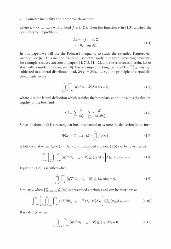
From (4.19), we see that g0 ∈� if and only if f1 ≡ 0. Hence if g0 ∈�, the iteration processof the extended Kantorovich method stops and we have ψ1(x, y) = f1(x)g0(y) ≡ 0. Nowsuppose g0 �∈�, that is, f1 �≡ 0. As in the proof of Lemma 5.1, Corollary 3.2 implies that

I[f1g0

]< I[0]= 0, (5.9)

since f1 is the unique minimizer of I[ f g0] and f1 �≡ 0. Applying Corollary 3.2 repeatedly,one has

I[fm+1gm

]< ··· < I[ f2g1

]< I

[f1g1

]< I

[f1g0

]< 0. (5.10)

But by Lemma 2.3,

I[ψ]≤ liminfj

I[ψnj

]:= liminf

jI[fnj+1gnj

]. (5.11)

In view of (5.10), we must have J[ψ] < 0, which implies lim j ‖ψnj‖L2 = ‖ψ‖L2 > 0; oth-erwise, we would have ‖ψ‖L2 = 0 which implies that J[ψ] = 0. Similarly, lim j ‖φnj‖L2 =‖φ‖L2 > 0. Since ψnj → ψ and φnj → φ in L2, we also have ψnj → ψ and φnj → φ in L1. Thus

limj

∥∥ψnj∥∥L1 = ‖ψ‖L1 > 0, limj

∥∥ψnj∥∥L1 = ‖ψ‖L1 > 0. (5.12)

This completes the proof of the proposition. �

Corollary 5.3. Let g0 �∈� and set

rn =∥∥g′n−1

∥∥L2∥∥gn−1

∥∥L2

, rn =∥∥ f ′n∥∥L2∥∥ fn∥∥L2

, tn =∥∥g′′n−1

∥∥L2∥∥gn−1

∥∥L2

, tn =∥∥ f ′′n ∥∥

L2∥∥ fn∥∥L2

. (5.13)

Then there exist subsequences { fnj} and {gnj} such that the following limits exist and arepositive:

limjrnj , lim

jrnj , lim

jtnj , lim

jtnj . (5.14)

Proof. In the proof of Theorem 5.2, we showed that for each n,

I[φn]=

∫Ω

∣∣Δφn∣∣2dxdy− γφn < 0 (5.15)

as long as g0 �∈�. Consequently,

∥∥ f ′′n ∥∥2L2

∥∥gn∥∥2L2 +

∥∥g′′n ∥∥2L2

∥∥ fn∥∥2L2 ≤ γ

∥∥ fn∥∥2L2

∥∥gn∥∥2L2 . (5.16)

This implies that

∥∥ f ′′n ∥∥2L2

∥∥gn∥∥2L2 ≤ γ

∥∥ fngn∥∥L2 =⇒∥∥ f ′′n ∥∥2

L2∥∥ fn∥∥2L2

≤ γ∥∥φn∥∥L2

. (5.17)


Combining with the Poincare inequality, it follows that

0 < C′ ≤ C∥∥ f ′′n ∥∥2

L2∥∥ fn∥∥2L2

≤∥∥ f ′′n ∥∥2

L2∥∥ fn∥∥2L2

≤ γ

‖φn‖L2(5.18)

for some universal constantsC and C′. With Theorem 5.2, the above string of inequalitiesyields

C1 ≤ limsupj

rnj ≤ C2, C1 ≤ limsupj

tnj ≤ C2,

C1 ≤ liminfj

rnj ≤ C2, C1 ≤ liminfj

tnj ≤ C2,(5.19)

for some positive constants C1 and C2. Similar inequalities hold for rnj and tnj with somepositive constants C1 and C2. Thus after further extracting subsequences of { fnj} and{gnj}, we may conclude that the following limits exist and are non-zero:

limj

∥∥ f ′′n ∥∥L2∥∥ fn∥∥L2

, limj

∥∥ f ′n∥∥L2∥∥ fn∥∥L2

, limj

∥∥g′′n ∥∥L2∥∥gn∥∥L2

, limj

∥∥g′n∥∥L2∥∥gn∥∥L2

. (5.20)

This completes the proof of the corollary. �

Corollary 5.4. If g0 �∈ �, then there exists a subsequence { fnj gnj} j that converges point-wisely to a function of the form

Θ(x, y)=N∑k=1

Fk(x)Gk(y)∈H20 (Ω). (5.21)

Furthermore, the derivatives of all orders of { fnj gnj} j also converge pointwisely to that ofF(x)G(y).

Proof. Let us observe the expression of φn(x, y) = fn(x)gn(y) in (4.23). ApplyingCorollary 5.3 to the constants on the right-hand side of (4.23), we can find convergentsubsequences:

{K0nj

},{K1nj

},{K2nj

},{K0nj

},{K1nj

},{K2nj

}, (5.22)

and {ρnj}, {κnj}, {ρnj}, {κnj}. In addition, the constants cncn can be rewritten as

cncn = γ2∫ 1−1 gn−1(y)dx

∫ 1−1 fn(x)dx∥∥g′′n−1

∥∥2L2

∥∥ f ′′n ∥∥2L2

= γ2∫Ω fn(x)gn−1(y)dxdy∥∥ fngn−1

∥∥2L2

·∥∥gn−1

∥∥2L2∥∥g′′n−1

∥∥2L2

·∥∥ fn∥∥2

L2∥∥ f ′′n ∥∥2L2

;

(5.23)

hence Theorem 5.2 and Corollary 5.3 guarantee the convergence of the subsequence{cn−1cn− j}. Altogether, after replacing all sequences on the right-hand side of (4.23) with


either convergent subsequences, we get

Θ(x, y)= limjfnj gnj

= C{K1∞K1∞K0∞K0∞

cosh(ρ∞x

)cosh

(ρ∞y

)cos

(κ∞x

)cos

(κ∞y

)

+K1∞K2∞K0∞K0∞

cosh(ρ∞x

)sinh

(ρ∞y

)cos

(κ∞x

)sin

(κ∞y

)

+K2∞K1∞K0∞K0∞

sinh(ρ∞x

)cosh

(ρ∞y

)sin

(κ∞x

)cos

(κ∞y

)

+K2∞K2∞K0∞K0∞

sinh(ρ∞x

)sinh

(ρ∞y

)sin

(κ∞x

)cos

(κ∞y

)

+K1∞K0∞

cosh(ρ∞x

)cos

(κ∞x

)+K2∞K0∞

sinh(ρ∞x

)sin

(κ∞x

)

+K1∞K0∞

cosh(ρ∞y

)sin

(κ∞y

)+K2∞K0∞

sinh(ρ∞y

)sin

(κ∞y

)+ 1

}.

(5.24)

Now if we differentiate fngn a finite number of times, then from (4.23) we have eachsummand scaled by integral powers of ρn, ρn, κn and κn. But we just argued above thatthese sequences have convergent subsequences. Hence when x, y are fixed, we concludethat all derivatives of fnj gnj at (x, y) will converge to that of Θ(x, y) as k→∞. The proofof the corollary is therefore complete. �

Remark 5.5. Corollary 5.4 implies that

I[fnj gnj

]−→ I[Θ(x, y)

], (5.25)

by directly using the definition of I[ f g]. Without Corollary 5.4, we can only assert that

I[Θ(x, y)

]≤ liminfj

I[fnj gnj

]. (5.26)

Acknowledgments

The authors are grateful to the referee for helpful comments and a careful reading of themanuscript. The first author was partially supported by a William Fulbright ResearchGrant and a Competitive Research Grant at Georgetown University. The fourth authorwas partially supported by US Army Research Office Grant under the FY96 MURI inActive Control of Rotorcraft Vibration and Acoustics.

References

[1] D.-C. Chang, G. Wang, and N. M. Wereley, A generalized Kantorovich method and its applicationto free in-plane plate vibration problem, Applicable Analysis 80 (2001), no. 3-4, 493–523.

[2] , Analysis and applications of extended Kantorovich-Krylov method, Applicable Analysis82 (2003), no. 7, 713–740.

[3] L. C. Evans, Partial Differential Equations, Graduate Studies in Mathematics, vol. 19, AmericanMathematical Society, Rhode Island, 1998.


[4] N. H. Farag and J. Pan, Model characteristics of in-plane vibration of rectangular plates, Journal ofAcoustics Society of America 105 (1999), no. 6, 3295–3310.

[5] F. John, Partial Differential Equations, 3rd ed., Applied Mathematical Sciences, vol. 1, Springer,New York, 1978.

[6] L. V. Kantorovich and V. I. Krylov, Approximate Method of Higher Analysis, Noordhoff, Gronin-gen, 1964.

[7] A. D. Kerr, An extension of the Kantorovich method, Quarterly of Applied Mathematics 26 (1968),no. 2, 219–229.

[8] A. D. Kerr and H. Alexander, An application of the extended Kantorovich method to the stressanalysis of a clamped rectangular plate, Acta Mechanica 6 (1968), 180–196.

[9] E. H. Lieb and M. Loss, Analysis, Graduate Studies in Mathematics, vol. 14, American Mathe-matical Society, Rhode Island, 1997.

[10] E. M. Stein, Singular Integrals and Differentiability Properties of Functions, Princeton Mathemat-ical Series, no. 30, Princeton University Press, New Jersey, 1970.

[11] G. Wang, N. M. Wereley, and D.-C. Chang, Analysis of sandwich plates with viscoelastic dampingusing two-dimensional plate modes, AIAA Journal 41 (2003), no. 5, 924–932.

[12] , Analysis of bending vibration of rectangular plates using two-dimensional plate modes,AIAA Journal of Aircraft 42 (2005), no. 2, 542–550.

Der-Chen Chang: Department of Mathematics, Georgetown University, Washington,DC 20057-0001, USAE-mail address: [email protected]

Tristan Nguyen: Department of Defense, Fort Meade, MD 20755, USAE-mail address: [email protected]

Gang Wang: Smart Structures Laboratory, Alfred Gessow Rotorcraft Center,Department of Aerospace Engineering, University of Maryland,College Park, MD 20742, USAE-mail address: [email protected]

Norman M. Wereley: Smart Structures Laboratory, Alfred Gessow Rotorcraft Center,Department of Aerospace Engineering, University of Maryland,College Park, MD 20742, USAE-mail address: [email protected]

mailto:[email protected]




Documents

Applications of the poincaré inequality to extended Kantorovich method