Embed Size (px)
Citation preview
AP® Statistics
2005–2006 Professional DevelopmentWorkshop Materials
Special Focus: Inference
connect to college success™www.collegeboard.com

AP® Statistics: 2005–2006 Workshop Materialsii
The College Board: Connecting Students to College Success
The College Board is a not-for-profit membership association whose mission is to connect students to college success and opportunity. Founded in 1900, the association is composed of more than 4,700 schools, colleges, universities, and other educational organizations. Each year, the College Board serves over three and a half million students and their parents, 23,000 high schools, and 3,500 colleges through major programs and services in college admissions, guidance, assessment, financial aid, enrollment, and teaching and learning. Among its best-known programs are the SAT®, the PSAT/NMSQT®, and the Advanced Placement Program® (AP®). The College Board is committed to the principles of excellence and equity, and that commitment is embodied in all of its programs, services, activities, and concerns.
Equity Policy Statement
The College Board believes that all students should be prepared for and have an opportunity to participate successfully in college, and that equitable access to higher education must be a guiding principle for teachers, counselors, administrators, and policymakers. As part of this, all students should be given appropriate guidance about college admissions, and provided the full support necessary to ensure college admission and success. All students should be encouraged to accept the challenge of a rigorous academic curriculum through enrollment in college preparatory programs and AP courses. Schools should make every effort to ensure that AP and other college-level classes reflect the diversity of the student population. The College Board encourages the elimination of barriers that limit access to demanding courses for all students, particularly those from traditionally underrepresented ethnic, racial, and socioeconomic groups.
For more information about equity and access in principle and practice, please send an email to [email protected].
© 2005 The College Board. All rights reserved. College Board, AP Central, APCD, Advanced Placement Program, AP, AP Vertical Teams, Pre-AP, SAT, and the acorn logo are registered trademarks of the College Board. Admitted Class Evaluation Service, CollegeEd, connect to college success, MyRoad, SAT Professional Development, SAT Readiness Program, and Setting the Cornerstones are trademarks owned by the College Board. PSAT/NMSQT is a registered trademark of the College Board and National Merit Scholarship Corporation. All other products and services herein may be trademarks of their respective owners. Permission to use copyrighted College Board materials may be requested online at: www.collegeboard.com/inquiry/cbpermit.html.
Visit the College Board on the Web: www.collegeboard.com. AP Central is the official online home for the AP Program and Pre-AP: apcentral.collegeboard.com.

AP® Statistics: 2005–2006 Workshop Materials iii
The College Board mission to connect students to college success and opportunity is supported by the work of the K–12 Professional Development unit. Through the vast resources on AP Central, publications, workshops, electronic discussion groups (EDGs), online events, and other resources, AP teachers find valuable support for the important work of teaching challenging content, developing enthusiasm for learning in their students, and preparing students for the AP Exam.
The materials in this book were developed and produced in a joint effort by the College Board’s K–12 Professional Development Content Development Group and the Technology and Digital Production Group. To learn more about the entire K–12 Professional Development and AP Program staff, visit the About Us page on AP Central.
Michael JohanekExecutive Director
K–12 Professional Development
Content Development Technology and Digital Production
Susan KornsteinDirector
Edward NothnagleDirector
Lawrence CharapHead, History/Social Sciences Content Development Group
Matthew HumeDigital Production Coordinator
Marcia WilburHead, World Languages and Cultures Content Development Group
Alexandra RingeContent Producer
Austin CapertonCoordinator
Gibson KnottProject Assistant


AP® Statistics: 2005–2006 Workshop Materials v
Important Note on Course Updates
The Course Description on AP Central® provides current information about the AP® courses and exams. Other materials included in this book may have been published at an earlier date and may include information that has been recently updated. News about updates to courses and exams is available on AP Central at apcentral.collegeboard.com.
Recent Course Updates Statistics
The Student Performance Q&A for the 2005 exam (available on AP Central this fall) provides valuable information on areas in which students continue to need attention. In general, on the free-response questions students need to be encouraged to show all of their work and justify their answers. Sample student responses with corresponding commentary on AP Central should also add to teachers’ and students’ understanding of what is expected on these questions. More details on student performance in 2005, in all content areas of the exam, can be found on AP Central.


AP® Statistics: 2005–2006 Workshop Materials vii
Table of Contents
Table of Contents
I. Welcome ...................................................................................................................................................1
College Board President, Gaston Caperton ................................................................................... 1
Executive Director, K–12 Professional Development, Michael Johanek ...................... 2
AP Statistics Development Committee Chair, Linda J. Young ........................................... 3
II. Special Focus: Inference ...............................................................................................5
Why Inference? ............................................................................................................................................... 5
Chris Olsen
The Role of Inference in the AP Statistics Curriculum .......................................................... 7
Roxy Peck
Assumptions .................................................................................................................................................. 12
Floyd Bullard
Some Reflections on How Inference Questions on the AP Exam are Scored ........ 44
Daniel S. Yates
Model Responses ........................................................................................................................................ 60
Daren Starnes
Inferential Problems for Practice ...................................................................................................... 74 Chris Olsen
Contributors .................................................................................................................................................. 85

AP® Statistics: 2005–2006 Workshop Materialsviii
Table of Contents
III. The Course. ........................................................................................................................................ 87
Excerpt from the 2005, 2006 AP Statistics Course Description ........................................ 87
2005–2006 AP Statistics Development Committee ............................................................. 127
IV. The Examination ................................................................................................................. 129
Exam Format ............................................................................................................................................. 129
Multiple-Choice Questions and Answers from the 2002 AP Statistics Released Exam .................................................................................................. 130
2005 Free-Response Questions ....................................................................................................... 153
2005 Scoring Guidelines ..................................................................................................................... 166
2005 Question Overview .................................................................................................................... 185
2005 Score Legend .................................................................................................................................. 188
2005 Scoring Commentary ................................................................................................................ 189
2005 Sample Student Responses ..................................................................................................... 196
2005 Free-Response Questions: Form B .................................................................................... 227
2005 Scoring Guidelines: Form B ................................................................................................. 233
2006 Exam Schedule .............................................................................................................................. 250
V. Professional Development .................................................................................. 251
Introduction ............................................................................................................................................... 251
AP Central ................................................................................................................................................... 255
Pre-AP Professional Development ................................................................................................ 259
AP Publications and Other Resources ........................................................................................ 263
AP Order Form ........................................................................................................................................ 264
Becoming an AP Exam Reader ....................................................................................................... 276

AP® Statistics: 2005–2006 Workshop Materials ix
Table of Contents
Becoming an AP and Pre-AP Workshop Consultant ........................................................ 282
VI. Program Information ................................................................................................... 283
Purpose and History ............................................................................................................................. 283
Advanced Placement Report to the Nation ............................................................................. 286
AP Grades and College Credit. ........................................................................................................ 287
AP Potential ................................................................................................................................................ 289
Exam Security ........................................................................................................................................... 291
College Board Regional Offices ...................................................................................................... 292


AP® Statistics: 2005–2006 Workshop Materials 1
Welcome
��������������������������������������������������������������������� �
����������������
�������
���������������������������������������
�����������������
����������������������������������������������������������������������������������������������������������������������������������������������������������������������������������������������������������������������������������������������������������������������������������������������������������������������������������������������������������������������������������������������������������������������������������������������
���������������������������������������������������������������������������������������������������������������������������������������������������������������������������������������������������������������������������������������������������������������������������������������������������������������������������������������������������������������������������������������������������������������������������������������������������������������������������������������������������������������������������������������������������������������������������������������������������������������������������������������������������������������������������������
���������������������������������������������������������������������������������������������������������������������������������������������������������������������������������������������������������������������������������������������������������������������������������������������������������������������������������������������������������������������������������������������������������������������������������������������������������������
�������������������������������������������������������������������������������������������������������������������������������������������������������������������������������������������������������������������������������������������������������������������������������������������������������������������������������������������������������������������������������������������������������������������������
�����������
�������������������������������������������
Chapter I

AP® Statistics: 2005–2006 Workshop Materials2
Welcome
Executive Director K–12 Professional Development Michael Johanek
Dear Colleague:
We often hear from teachers, counselors, and administrators that the school day provides precious little opportunity to refresh one’s thinking, reflect on what one does, and share insights with colleagues. I certainly recall that from my years as a teacher and administrator.
With that in mind, I hope this workshop provides a chance for you to enliven and reinvigorate your practice. Experienced colleagues who faced similar challenges stand behind each of our workshops as authors and reviewers, and many lead our workshops throughout the year.
To continue meeting your professional needs, we have added a number of offerings in the last year:• Course-specific theme materials in 16 AP workshops, from “Immigration in U.S. History” to
“The Fundamental Theorem” in calculus to “The Importance of Tone” in English literature • Pre-AP workshops in algebraic thinking, world languages, biology and technology,
differentiated instruction, social studies, and more• Workshops to help prepare for the new SAT, with particular focus on the writing section,
scoring the exam, and ESL/ELL strategies• Events to support teachers as they plan for the new AP Italian course• Online workshops and events, available live and as archives • Publications in core content areas, including Differential Equations, The Importance of Lab
Work, Reading Poetry, Teaching with Primary Sources, and more• Workshops in your region, across the nation, and around the world
Thank you for choosing to continue your own learning through College Board professional development. After your successful completion of this event, you will receive Continuing Education Units (CEUs) certified by the International Association for Continuing Education and Training (IACET).
We hope your experience at this workshop provides the content, strategies, networking, and enthusiasm you need to return reinvigorated to your students. We invite you, as a member of the College Board community, to participate again very soon.
I wish you all the best this school year, and thank you for the important contributions you make to our children’s lives!
Sincerely,
Mike Johanek, Ed.D. Executive Director, K–12 Professional Development

AP® Statistics: 2005–2006 Workshop Materials 3
Welcome
AP Statistics Development Committee Chair Linda J. Young
To AP Statistics teachers:
Welcome to this AP Statistics workshop! I wish I could be there with you, as it is always stimulating when current and future AP Statistics teachers meet. Insights into fundamental statistical concepts and ideas on how to share them with students in the classroom are exchanged, and all become more enthusiastic about teaching statistics. The Advanced Placement Program®exists to support you and to give your work credibility with colleges and universities—but also to assist you in finding more effective ways to help students learn statistics. To this end, this packet offers some great materials written by leading teachers in both high schools and colleges. I hope you’ll find ideas that are both thought-provoking and useful.
“Inference” has been chosen as the theme of this year’s materials. Students are accustomed to making inferences in their daily lives. Statistical inference is a formal process of using sample data to answer questions or to draw conclusions about a population. Without a census, we can never be certain that the inferences being made are correct. Statistics simply allows us to quantify the uncertainty associated with each inference. The mechanics of setting a confidence interval or conducting a hypothesis test are mathematically simple. Determining what confidence interval or hypothesis test is needed and what each means to the study upon completion of the computations are the real challenges. It is here that the mathematics becomes integrated with the application, and statistics becomes exciting.
You are AP Statistics, and you are doing a great job. Enjoy your workshop and keep up the enthusiasm!
Linda J. YoungChair, AP Statistics Development CommitteeUniversity of Florida


AP® Statistics: 2005–2006 Workshop Materials 5
Special Focus: Inference
Special Focus: Inference
Important Notes
The materials in the following section are organized around a particular theme that reflects important topics in AP Statistics. The materials are intended to provide teachers with professional development ideas and resources relating to that theme. However, the chosen theme cannot, and should not, be taken as any indication that a particular topic will appear on the AP Exam.
Within these materials, references to particular brands of calculators reflect the individual preferences of the respective authors; mention should not be interpreted as the College Board’s endorsement or recommendation of a brand.
Why Inference?Chris OlsenCedar Rapids Community SchoolsCedar Rapids, Iowa
The outline of the AP Statistics course as it appears in the Course Description presents four basic topics: exploring data, sampling and experimentation, probability, and statistical inference. It might seem at a casual glance that this Special Focus section is the result of simply listing four possible generic foci in the Course Description, and—after perhaps, in the manner of statisticians, rolling a tetrahedral die—selecting one of the four. In terms of importance, however, the four topics delineated in outline form for the purpose of describing the course may be thought of as three topics in service to the fourth.
Statistical inference, it may be said, exists in a larger context beyond the classroom, and moreover a context that truly represents the importance of statistics in general and the AP Statistics course in particular. Statistical inference appears to be the only reliable methodology to address one of the oldest of philosophical problems: what can we know, and how can we know it?
The problem of the scope and limits of human knowledge has generally been approached from two perspectives. The rationalist view, perhaps best represented by René Descartes (1596–1650), is that a well-executed logical process can begin with certain knowledge and lead progressively to derived knowledge. From the famous cogito ergo sum, which asserts that the existence of thought guarantees the existence of the thinker, Descartes built an impressive list of “truths” by appealing to reason alone. The eighteenth-century
Chapter II

AP® Statistics: 2005–2006 Workshop Materials6
Special Focus: Inference
British empiricists—John Locke, George Berkeley, and most effectively the Scot, David Hume—rejected the idea that man is born with innate concepts such as mathematics and logic and causality. In the view of the empiricists, knowledge is based on sense experience and mental reflection. Beginning with skepticism similar to Descartes’s, the empiricists argued that the observing human makes “connections” between and among observations—associations, as we would now call them—and knowledge consists of creating mental representations of these connections. Writing in 1740 in The Treatise on Human Nature, Hume dropped a bombshell unnoticed by his contemporaries: from observation alone, associations cannot be translated into statements of causation. As we would say today, correlation does not imply causation.
Over the course of two and a half centuries, these problems of “natural” philosophy have led to the development of the procedures and concepts known as the “scientific method,” but Hume’s “problem of induction” still challenges us. The fundamental problem still boils down to this: what may we infer from systematic observation, and by what logical process may we infer it? Two and a half centuries after Hume, we have a single best answer to that problem. Making inferences in an uncertain world fraught with many observational perils is the unquestioned domain of the discipline of statistics.
The framers of the AP Statistics topic outline wisely understood that the mere mechanics of hypothesis testing and building confidence intervals is only a part of the inferential landscape. Exploring and representing data numerically and visually can suggest scientific hypotheses and illuminate associations that may lead to more formal inference-making procedures. An understanding of random variables and probability allows us to quantify the inherent uncertainty of inferences based on sampling. Proper planning and execution of experiments, with appropriate concern for possible confounding variables, protects the validity of inferences when “statistically significant” results occur.
Successful students in AP Statistics will come to understand the role each of the parts of the topic outline plays in making inferences, and they will learn to communicate their methods and conclusions in a clear and unambiguous manner, with proper appreciation of both the power and limitations of their statistical procedures.
In this Special Focus section, we consider two aspects of inference that are “nonmechanical”: the assumptions upon which sampling distributions (and thus the validity of the “mechanics” of inference) are based, and how students can effectively communicate their methods and conclusions in the classroom as well as on the AP Statistics Exam. We have been led toward this focus by the depth and variety of questions about these aspects appearing on the AP Statistics Electronic Discussion Group, as well as by our own teaching experience preparing students for the AP Statistics Exam.

AP® Statistics: 2005–2006 Workshop Materials 7
Special Focus: Inference
The Role of Inference in the AP Statistics CurriculumRoxy PeckCalifornia Polytechnic State UniversitySan Luis Obispo, California
Variability: The quality, state, or degree of being variable or changeable.
Variable: Likely to change or vary; subject to variation; changeable. Inconstant; fickle. Tending to deviate, as from a normal or recognized type; aberrant.
—The American Heritage® Dictionary of the English Language, 4th ed.
So what does variability have to do with statistics? The simple answer is—everything! In a world without variability, there would be little need for statistics (or statisticians). Think about this for a moment: Suppose every high school senior were identical—with respect to height, the time required to assemble a geometric puzzle, opinion on whether seniors should be permitted to leave campus during the lunch hour, and so on. In this case, answering questions about the population of high school seniors would be an easy process. Want to know the time required to assemble the geometric puzzle? Time one student and you would have your answer. Want to know if seniors think they should be allowed to leave campus for lunch? Asking one student would be enough! You would have no risk of being wrong when you generalize what you see in this “sample” of one to the population of all seniors.
A common objective of data analysis is statistical inference—generalizing from a sample to the larger population from which the sample was selected. It is variability that makes statistical inference a challenge. To see this, let’s consider an example. Suppose that the math department at a particular college wanted to know if students who received credit for first-semester calculus based on their scores on the AP Calculus Exam tended to get higher grades in the second semester of calculus than students who did not have AP credit for the first semester and were required to complete the first-semester course offered by the college with a passing grade. This would require comparing two groups of second-semester calculus students: those with AP credit for first-semester calculus and those who did not have AP credit. If there were no variability in second-semester calculus grades in each of these two groups, it would be easy to compare the two groups.

AP® Statistics: 2005–2006 Workshop Materials8
Special Focus: Inference
If all students who had AP credit for the first semester earned a B in second-semester calculus, and all students in the other group earned a C, then we would know that students with AP credit in the first course performed better in the second course than students who successfully completed the first-semester college course. If all students who took the first-semester college course earned a B in the second semester, we would know that there was no difference between the two groups with respect to second-semester grades. And if all students who completed the first-semester college course earned an A in the second-semester course, we would know that the students with AP credit did not perform as well as those who took the college course. What is even more interesting is that if there were no variability in each of the two groups of interest, we would have only needed to look at the grade of a single student from each group to reach a conclusion, and we would have no risk of being wrong!
This example, as described, is clearly unrealistic. Of course there is variability in second-semester calculus grades for each of the two groups of second-semester calculus students. The challenge is to answer the question of interest when faced with this variability. One way to overcome the “challenge of variability” is to obtain complete information for the populations of interest. In our example, suppose the populations of interest consist of all students who have taken second-semester calculus at the college in the past 10 years, divided into two groups based on whether the first-semester calculus requirement was satisfied by AP credit or by receiving a passing grade in the course offered by the college. If complete information is available for each of these two groups, a comparison of the groups is relatively straightforward. The data for each group would completely specify the grade distribution for that group. A table or graphical display like the ones below might be used to display the grade distributions.
Percent at Each Grade
Grade Students with AP Credit for First Semester
Students CompletingFirst-Semester Course at the College
A 20% 15%B 25% 20%C 30% 45%D 15% 10%F 10% 10%

AP® Statistics: 2005–2006 Workshop Materials 9
Special Focus: Inference
Since the grade distribution for each of the two groups is known exactly, definitive statements can be made about the similarities and differences between the two groups. Comparison of the two groups is a bit more complex due to the variability in each of the two populations, but still there is no risk of error because complete information is available for both populations. There is no need for inferential methods in this situation.
Things get more complicated, though, when we don’t have complete information, and we must base our comparison on data from samples. As noted earlier, if there is no variability in the population, there is no problem. But in any real situation of interest, we will need to consider variability. If every sample from a population looked exactly like a miniversion of the population (and therefore also exactly like every other sample), generalizing from a sample to the corresponding population would still be simple. Unfortunately, variability in the population leads to a second type of variability called sampling variability. Sampling variability refers to the variability that occurs from sample to sample from the same population due to chance as a result of the sample-selection process. And the greater the population variability is, the greater the sample-to-sample variability will be.
Getting back to our example, suppose that we have a random sample of 60 students who had AP credit for first-semester calculus and a random sample of 60 students who completed the college course, and that the sample grade distributions were as indicated in the following table.

AP® Statistics: 2005–2006 Workshop Materials10
Special Focus: Inference
Grade Distributions and AP Credit
Grade Students with AP Credit for First Semester
Students CompletingFirst-Semester Course at the College
A 12 10B 15 12C 18 24D 8 7F 7 7
The grade distributions for the two samples are not exactly alike. Is this because there is a real difference between the grade distributions for the two corresponding populations? Or might the grade distributions for the two populations be the same and the difference between the two sample distributions be attributable to sampling variability—i.e., the usual variation between a sample distribution and the corresponding population distribution that results from the sampling process? Deciding between these two competing explanations for the observed sample differences requires an understanding of sampling variability, and understanding sampling variability is the key to understanding statistical inference.
AP Statistics includes two general types of inferential procedures: confidence intervals and hypothesis tests. Confidence intervals provide a method for using sample data to construct estimates of population characteristics, whereas hypothesis tests allow us to use sample data to decide between two competing claims, called hypotheses, about a population characteristic. Although confidence intervals and hypothesis tests are generally used for different purposes, they share a common goal of generalizing from a sample to a population. Understanding the logic and rationale for both confidence intervals and hypothesis tests requires an understanding of sampling variability.
When the objective is to use sample data to estimate a population characteristic, such as a population mean or a population proportion, sampling variability must be taken into account. A consequence of the chance differences that occur from one sample to another is that a sample statistic (e.g., a sample proportion) will not be exactly equal to the corresponding population characteristic (e.g., the population proportion). Confidence intervals acknowledge this sampling variability in the way that the interval estimate is constructed. The greater the anticipated sampling variability is, the wider the resulting confidence interval will be.

AP® Statistics: 2005–2006 Workshop Materials 11
Special Focus: Inference
In hypothesis tests, when sample data is used to make a decision between a null hypothesis and an alternative hypothesis, the decision ultimately comes down to deciding if a plausible explanation for what was observed in the sample is sampling variability in the situation where the null hypothesis is true. That is, if the null hypothesis is true, could what was observed in the sample have been a consequence of the sample selection process alone? Because our intuition about sampling variability is not always very good, we rely on formal inferential procedures to determine if chance (sampling variability) is a plausible explanation for the difference between what is observed in a sample and what is expected when the null hypothesis is true.
Because statistical inference is a major component of the AP Statistics course and because understanding sampling variability is the key to understanding inference procedures, it is important that students become comfortable with the concept of a sampling distribution. The sampling distribution of a sample statistic describes the variability in the values of the statistic that is attributable to sampling variability. The information that a sampling distribution provides about sampling variability is the basis for the confidence intervals and hypothesis tests that make up the inference section of the AP Statistics course. Students may initially struggle when they first encounter sampling distributions—this is the most abstract idea they will have to deal with in the course. But, if students do not have a conceptual understanding of sampling distributions, the procedures for creating confidence interval estimates and for testing hypotheses will seem very mechanical. Although they may be able to follow the prescribed sequence of steps and reach a conclusion in the end, the logic and rationale behind the procedures will be missing.
Statistical inference is a substantial portion of the AP Statistics course—the Course Description indicates that inference should make up 30 to 40 percent of the exam. This acknowledges the important role that statistical inference plays in allowing investigators to draw conclusions on the basis of sample data. In the “information age,” it is hard to think of a discipline that does not make use of inferential techniques to address critical issues. So take your time when covering sampling distributions. Simulations and activities can be useful tools for developing conceptual understanding. And make sure to allow adequate time to cover the concepts and techniques of inference. A good conceptual understanding of the ideas of inference and the ability to employ inferential tools in thoughtful and appropriate ways will serve your students well—not just on the AP Statistics Exam, but in their future studies and in life as well.

AP® Statistics: 2005–2006 Workshop Materials12
Special Focus: Inference
AssumptionsFloyd BullardThe North Carolina School of Science and MathematicsDurham, North Carolina
Introduction
Even if you don’t teach physics, you probably studied it or you have some familiarity with it because some of your math students also study physics. You are probably aware that it is common during introductory physics courses to make statements such as “Assume there is no air resistance,” or “Assume this is a frictionless surface,” or “Assume the force of gravity is constant.” These assumptions simplify physics problems a great deal and, under some circumstances, may be quite reasonable, by which I mean that the assumptions are almost true, and the solution you obtain to a problem is about the same whether you make the simplifying assumption or not. Of course, students should always be aware that the reasonableness of the solution depends upon the reasonableness of the assumptions they make. When tossing a ball up into the air, it may be reasonable to assume that the Earth’s gravitational pull on the ball is constant throughout its path. That assumption would not be reasonable if we were launching a rocket to the moon. In statistics we also make simplifying assumptions, and it is just as important that students question whether the assumptions are reasonable. For example, consider the familiar sampling scenario known as the “capture-recapture” technique. Suppose we were to capture 30 fish in a lake, tag them, and then release them back into the lake. Later, we capture 40 fish in the lake and find that 10 of them are tagged. Since one-quarter of the 40 fish are tagged, we might reasonably estimate 30 × 4 = 120 to be the number of fish in the lake. But what are some of the underlying assumptions we are making?1
We are assuming that both samples are random samples of all the fish in the lake. Is that reasonable? It depends upon how the fish were captured. Probably no capturing technique would catch all the fish in the lake with equal probability. But biologists have some idea of what techniques work better than others. Certainly we can easily imagine poor sampling techniques, such as placing many traps in the same place or at the same depth in the lake. Such a sampling technique would likely have a tendency to catch the
1 We are not considering here the statistical issue of sampling variability, which would result in a margin of error placed on our point estimate. We are addressing underlying assumptions that affect the point estimate itself.
AP® Statistics: 2005–2006 Workshop Materials 13
Special Focus: Inference
same fish during both “capture” and “recapture” stages and so may tend to produce an underestimate of the population size; the point estimate would be biased.
We are also assuming that the population of fish from which we’re sampling is the same during both stages of the study. This implies that we can’t wait so long that many fish die and others are hatched. Such a delay would dilute our marked fish and yield a biased estimator, one that tended to overestimate the population size. It also implies that the method for marking the fish can’t harm them in any way; if they die because of the marking, then we will again get a biased estimator, an overestimate of population size.
Yet another assumption we are making is that the fish are as likely to be caught the first time as the second. But if the capture technique is the same both times, it is at least plausible that fish caught the first time will be “trap-shy” the second time and will be better at avoiding capture. This, too, would tend to produce a biased overestimate of population size.
It can be seen from the preceding discussion that a capture-recapture study is particularly challenging to carry out in real life because in order for the assumptions to be reasonable, the sampling methods must be meticulous and the marking be harmless. What’s more, I described the study as it would be done on fish in a lake—a contained population. Imagine the further assumptions we would have to make if studying a less well-defined population, such as squirrels in a city park.
Two Types of Assumptions
As mentioned earlier, a solution to a statistical problem is only as reasonable as the assumptions that lie behind it. In the AP curriculum, the assumptions students are asked to consider are generally of two types: those whose reasonableness can be checked by the data and those whose reasonableness can be assessed only by those with expertise in the field of study and knowledge of how the data were gathered. In the capture-recapture scenario I described in the previous section, all the assumptions were of the latter sort. The reasonableness of the assumptions (and hence of the population estimate) could not be assessed from the data alone. It would depend upon how the data were collected, and if you were a biologist, it might also depend upon your knowledge of the fish in the lake (e.g., where do they tend to swim? Do they school? How quickly might they learn to avoid a trap?).
The assumptions whose reasonableness can be checked with data often relate to sample size. np > 10 and n p( )1 10− > is an example of one such check, when the data context is

AP® Statistics: 2005–2006 Workshop Materials14
Special Focus: Inference
sample proportions. Another example is n > 40, when the data context is sample means. All expected cell counts > 5 and at least 80 percent of expected cell counts > 5 is a third example, in the context of a chi-square test. These will all be considered more carefully in the following sections. I bring them up now just to point out what they have in common. They are all rules of thumb used to check the reasonableness of the assumption that the sample size is sufficiently large for a limiting distribution (e.g., normal, t, or chi-square) to be a good approximation for the actual distribution of a statistic.
Now is probably a good time to point out the difference between an assumption and a check for the reasonableness of that assumption. Students often mistake “ n > 40 ” for an assumption, when obviously it need not be assumed; they can check whether n > 40 or not. The assumption students are making, perhaps without realizing it, is that the sample size is sufficiently large for the distribution of the sample mean to be approximately normal. Students are using n > 40 as a rule-of-thumb check to assess the reasonableness of the assumption. Likewise with np > 10 and so on. These are not assumptions: they are rules of thumb for assessing the reasonableness of assumptions.
We will consider in the following sections all the inference procedures that are part of the AP Statistics curriculum and examine in some detail the assumptions that often have to be made when performing them. I have made up most of the scenarios, but they are based on my experiences with my students and studies that they have designed for my AP Statistics class or for a biology class. You may recognize in some of the scenarios your own students’ interests and experiences.
Single-Population Proportions
Suppose one of your students—let’s call her Alice—wants to estimate the proportion of students at her school who can identify the two senators from your state. How might Alice design a study to find out? She may consider taking a simple random sample from a roster of the entire student body (if she can obtain one), but she will find it very difficult to contact them all, and some still will not participate in her study. She may decide instead to take a nonrandom sample of some sort. Now don’t get upset with her, this is not necessarily a bad thing. In practice, it is often difficult or impossible to get a true simple random sample from a population; after all, how often do you have the luxury of a list of all your potential sampling or experimental units? Alice is going to take a nonrandom sample because this isn’t a big project, and she only has a couple of days to do it, and you tell her that may be fine—but that she should think carefully about how she obtains her sample.

AP® Statistics: 2005–2006 Workshop Materials 15
Special Focus: Inference
Alice knows her sample is not going to be a true random sample, but she wants it to be “like” a random sample. In fact, when she eventually calculates a confidence interval estimating her population proportion, she is probably going to assume that her nonrandom sample “acts like” a random sample. The reasonableness of her estimate depends in part upon the reasonableness of that assumption. What can she do to make the assumption more reasonable?
The main thing Alice wants is to avoid collecting a biased sample. She doesn’t want the proportion of students in her sample who know their senators to tend to be greater or less than that proportion among all students at her school. So she would be unwise, for example, to survey all the students in a civics class, since one supposes they would tend to be more knowledgeable about their senators than would students in general. She would be unwise to favor high school freshmen in her sample, or high school seniors, since it is plausible that the older students might be more knowledgeable. She would also be unwise to favor girls in her sample, or boys, since it is plausible that the sexes might not be equally knowledgeable about politics. In fact, a nonrandom sample that is thoughtfully conducted might not be so convenient for Alice as she might like. But let us suppose that she finally decides to stand by the entrance to the school at the start of the school day and ask every fifth student who arrives to participate in her survey until she has 100 participants. This might still produce a biased sample—might early birds be more knowledgeable of politics than later arrivals?—but at least the assumption that her sample is “like” a random sample seems fairly reasonable.
Now let us suppose that 44 of the 100 students Alice sampled could identify both of the senators from her state. She is going to compute a confidence interval of the population proportion using the assumption that her observation (44) was drawn from a binomial distribution having n = 100 and p = the population proportion under consideration. How reasonable is that assumption? What are the underlying conditions that define a binomial setting? Do we have a fixed number of trials? Yes, n = 100 , determined in advance. Does each have the same probability of identifying the two senators? We are assuming so by virtue of the assumption that the sample is “like” a random sample. Are the observations independent of one another? Alice hopes that the students she has surveyed are not going back and telling others what she asked them so as to alter their responses. In fact, that’s one of the reasons she wanted to catch students as they entered the school, to keep them from communicating. It appears to Alice that the assumptions behind the binomial are reasonable.

AP® Statistics: 2005–2006 Workshop Materials16
Special Focus: Inference
Next, Alice is going to assume that the sample proportion p (which for her random sample happened to be equal to 0.44) is approximately normally distributed with mean p
and standard deviationp p
n
1−( ) . This is not absolutely necessary, because inference can
be made using the binomial family of distributions (this procedure is not part of the AP Statistics curriculum), but the assumption makes her calculations easier for her. But how reasonable is the assumption?
Imagine that instead of Alice simply counting how many people in her sample correctly identified the senators, she wrote down a “1” for every person who did so, and a “0” for every person who failed. She would then have numerical data, of a sort, instead of categorical data. It is not hard to see that the average of her 1s and 0s would be precisely the sample proportion 0.44 of people who could identify the senators. What’s more, if she were to similarly attach 1s and 0s to every student at her school, the average of all those 1s and 0s would be precisely the population proportion of all students who could identify the senators. In fact, proportions are a special case of averages, in which the data are all 1s and 0s. Since sample proportions are sample averages of 1s and 0s, they obey the Central Limit Theorem: the distribution of the sample proportion p will be approximately normal if the sample size is large enough.
We’ll return to Alice’s survey in a moment. Let’s digress briefly to address how we determine whether, in the case of a single proportion, the sample is “large enough” for the distribution of the sample mean to be approximately normal.
Since proportions are a special case, they can be treated specially with specific formulas. A very common check of whether the sample size is large enough for p ’s sampling distribution to be approximately normal is np > 10 and n p( ˆ )1 10− > . Some texts recommend np > 5 and n p( ˆ )1 5− > or perhaps the single condition np pˆ( ˆ )1 5− > . But why do these “work”?
We will not prove the validity of the conditions here but will give an argument for why they make sense, followed by an explanation of why one of them “works.” First, note that the distribution of p is identical in shape to the binomial distribution of X; the difference between the distributions is that the distribution of p has been rescaled by a factor
of 1n
. Since at present we’re only interested in shape, we will consider the binomial
distribution of X. We know that the binomial tends to look approximately normal, so

AP® Statistics: 2005–2006 Workshop Materials 17
Special Focus: Inference
long as it doesn’t bunch up too near 0 or too near n, in which case it is either right- or left-skewed, respectively. The condition np > 10 is a way of making sure it doesn’t bunch up too near 0. If p is small, that suggests that p is small, so n needs to be large enough to compensate. Likewise, when p is close to 1, there is a danger that the binomial distribution of X will bunch up near n. Requiring n p( ˆ )1− to be larger than some cutoff prevents that from being a big problem. Hence the two cutoffs.
But why 10? Remember that some people use 5 or some other cutoff, so 10 isn’t a magic number. The important thing is for your students to do some reasonable check. Here is an algebraic demonstration of why np > 10 “works.”
We begin by requiring that the center of the distribution of p be at least three standard deviations greater than 0. That should prevent the distribution from bunching up too
near 0. Stated mathematically, we require that pp p
n>
−( )3
1. Since these are positive
numbers, we can square both sides of the inequality and obtain pp p
n2 9
1>
−( ). Algebraic
manipulation gives np p> −9 1( ) , or np p> −9 9 . Now if np > 10 , that inequality must follow, for np p> > > −10 9 9 9 . So it may be a bit of overkill, but it’s just a rule of thumb, so that’s okay. That overkill is actually useful, because we’re going to be using p instead of p, anyway, and p may be a bit different (hopefully not too much) from p. But we still may be confident that if np > 10 , then the mean of p will be at least three standard deviations greater than zero. An analogous algebraic argument tells us that if n p( )1 10− > , then the mean p must be at least three standard deviations less than 1.
Students do not need to know why this rule of thumb works (though it wouldn’t hurt them), only that it does. The explanation above is given primarily for the edification of teachers who themselves would like to know where this rule of thumb came from. The four histograms below show the distribution of p when p = 0 1. for four different values of n. When n = 10 , we have np = 1 , so we wouldn’t expect the distribution to look very normal, and it doesn’t. When n = 50 , we have np = 5 , so the distribution should look fairly normal, since it meets the rule-of-thumb check that some people use, and indeed it does look fairly normal. In the third histogram, n = 100 , so np = 10, and the distribution looks more normal still, and with n = 200 , the normal approximation is very good indeed.

AP® Statistics: 2005–2006 Workshop Materials18
Special Focus: Inference
Let’s now return to Alice. Alice confirms that the rule of thumb applies for her data and carries on with her assumption that p is approximately normally distributed. She
obtains as a 95 percent confidence interval estimate of p, . . . . ,0 44 1 96 44 56100
±×
or .44 ± 0.10. She is confident that between 34 and 54 percent of the students at her school can identify the two senators from her state and the rest cannot.
Let’s review the assumptions Alice made while reaching her inferential conclusion.
1. The sample was a random sample from the population. This was not true, but Alice tried valiantly to get a nonrandom sample that was not biased toward or
against students who would know their senators. Her final estimate is dependent upon that assumption and is open to reasonable doubt for anyone who questions her sampling method.
2. The sample proportion was approximately normally distributed. This Alice could check by using the rule of thumb np > 10 and n p( ˆ )1 10− > .
An assumption that often troubles students is: “The sample represents no more than 10 percent of the population.” This assumption applies more generally than the present case of single-population proportions, and thus will be addressed by itself later. For now, we remark only that so long as Alice’s school has more than 1,000 students, this assumption is valid.

AP® Statistics: 2005–2006 Workshop Materials 19
Special Focus: Inference
Before moving on to two-sample proportions, it should be mentioned that there is a small difference in the rules of thumb one checks when assuming the normality ofp ’s distribution, depending on whether you are computing a confidence interval or
performing a hypothesis test. Alice’s check was that np > 10 and that n p( ˆ )1 10− > . Had she been doing a hypothesis test, then a slightly better check would have been np
010> and n p( )1 10
0− > , where p
0 is the proportion claimed in the null hypothesis.
The difference in these two checks is mathematically very slight, for p0
and p should, under the null, be close to one another. It is the logical difference that is important. When doing a hypothesis test, all computations, including this check for normality, are performed under the assumption that the null hypothesis is true. Therefore, we use the proportion from the null hypothesis in our check for normality. But when computing a confidence interval, we have no known or hypothesized value for p, so we use our best guess, which is of course p .
Comparison of Two Proportions
Suppose another of your students, Chuck, wants to see whether students at his school respond differently to a sensitive question if they have to answer in person versus answering it anonymously. He decides to ask only boys whether they perceive sexual harassment of girls by boys at the school to be a problem. Some of them he will ask orally and record their spoken responses. Others he will hand a slip of paper with the question written, and they can mark it and drop it into a slot in a sealed box. Chuck’s null hypothesis is that they respond “yes” in the same proportion for the two “treatments.” His alternate hypothesis is that they don’t.
In preparation for the study, Chuck shuffles up 50 black cards and 50 red cards from two decks of cards he’s mixed together. He writes down the order of reds and blacks in the shuffled stack to indicate the order of the treatments, while still assuring a sample size of 50 for each treatment.
Since much of what Chuck is doing is similar to Alice’s study, some of the underlying assumptions only need to be mentioned briefly here. Like Alice, Chuck decides to take a nonrandom sample of 100 people rather than a simple random sample. Since he will be assuming that his sample is “like” a random sample as regards the response to the question, he wants to select it in a way that he believes will not favor one type of response over another. Since Chuck works in the school store, he decides to conduct his survey on the boys that happen to stop there. He carries out his plan, and by the end of the week has his 100 responses.

AP® Statistics: 2005–2006 Workshop Materials20
Special Focus: Inference
He finds that of the 50 boys he asked orally, 19 of them said that sexual harassment was a problem. Of those 50 whom he asked to respond anonymously, 9 of them said that sexual harassment was a problem.
As with Alice’s single p , the separate sample proportions are approximately normally distributed if each of the sample sizes is large enough, again by virtue of the Central Limit Theorem (used in concert with a theorem about “combining” normal distributions). We use the same criteria for checking the reasonableness of that assumption, only now we have to apply it to both samples. Since only 9 boys responded “yes” when responding anonymously, the condition np
anonˆ > 10 isn’t quite met, but it’s close enough that Chuck
decides to “proceed with caution.” His gut feeling is that 1950
950
is so different from that
the difference will be very significant statistically, so much so that the slight risk of this assumption won’t matter much.
Chuck decides all his assumptions are reasonable and computes a p-value for his significance test, finding it to be p = 0.026. He is satisfied that boys respond differently to the question when asked out loud versus by anonymous written response.
Let’s review the assumptions Chuck made while doing his study.
1. Chuck assumed that his sampling method is “like” a random sample of boys from his school. Without that assumption, he cannot extrapolate his conclusions beyond the sample of boys he happened to survey when they visited the school store. That assumption may or may not be reasonable.
2. nporal
ˆ > 10 , n poral
( ˆ )1 10− > , npanon
ˆ > 10 , and n panon
( ˆ )1 10− > . This condition was very nearly met, so any error in the p-value is likely not to be severe.
Chuck was sampling less than 10 percent of the population. Again, this potentially confusing assumption will receive its own special treatment later.
A Single Population MeanGavino is a student taking a health class. For a homework project, he decides to show people pictures of plates of food and ask them to estimate the number of calories that are on each plate. He has four such pictures, and he will show each one to 15 people. He will then report a confidence interval estimate of the mean guess for each picture along with the actual number of calories in the foods pictured.

AP® Statistics: 2005–2006 Workshop Materials 21
Special Focus: Inference
Gavino knows he will have to make some assumptions. What are they? Well, we know that he will have to assume his sample is a random sample of the student body. (We’ve been through this before!) But since his sample is fairly small, Gavino decides it might be a good idea to get a roster of the student body and take an actual simple random sample. With help from the principal’s office, he does this and is able to track down and survey 13 of the 15 people on his list. He can’t find the other two, so he decides to replace them with two more randomly sampled people.
Now he plans to construct his confidence intervals using the single-sample t procedure. But n = 15 is not a very large sample size, so he isn’t sure whether this is legitimate. He knows there’s something about “assuming normality” but can’t really articulate what that means. Let’s take a look at it.
The Central Limit Theorem tells us that X will have an approximately normal distribution if the sample size n is “large enough.” And if X has a normal distribution, then another
theorem (from “Student” and R. A. Fisher) tells us that the statistic X
sn
− µ has a t
distribution with n − 1 degrees of freedom. That’s a fact that Gavino plans to use when constructing his confidence intervals. So the legitimacy of his procedure comes down to whether n = 15 is “large enough” for the Central Limit Theorem to apply to each of his four Xs. (Note that Gavino is really performing four different studies that happen to involve the same sample of 15 subjects. The results of the studies are therefore not independent of one another, and some advanced analysis would be possible with his data, correlating responses to individual subjects. But for the purpose of an AP Statistics project, Gavino’s plan to present one confidence interval for each food picture is reasonable, though he should inform his audience that the same subjects were used for each photo.)
The Central Limit Theorem does not itself dictate how large n needs to be, but two other facts can help us out. First of all, if the population from which the data are being drawn is exactly normal already, then the distribution of X will be exactly normal no matter how large or small n is. And second, the more nonnormal the distribution is from which the data are drawn, the larger the sample size will need to be in order for the distribution of X to be “approximately normal.” Here is a rule of thumb that some texts use. If n < 15 , then you cannot really verify that the data come from a normal distribution. You should verify that there are no outliers and that no skew is obvious, but even then you are still assuming that the distribution from which the data were drawn is approximately normal. If n is between 15 and 40, then the distribution of the population need not be so very normal,

AP® Statistics: 2005–2006 Workshop Materials22
Special Focus: Inference
2 This is not to say that you should not still look at the data! That should always precede any inference. But if n > 40 , then you can be pretty confident that the inference procedures in the AP Statistics curriculum that assume a normal distribution for X will be reasonably accurate.
just so long as it isn’t extremely skewed or heavy-tailed. And if n > 40 , then you need not really worry much about nonnormality in the population, or even outliers in the data. All but the most unusually severe skew will be overcome by the Central Limit Theorem.2
Whether you choose that rule of thumb or another, it is always required that you assess the normality of the population distribution from which the data were drawn. This may be done by constructing a “normal probability” plot (also sometimes called a “normal quantile plot” or a “Q-Q plot”). If the normal probability plot looks roughly linear, then the data could reasonably have come from an approximately normal distribution. There’s a Catch-22 here, which is that with smaller data sets, it is more difficult to assess normality than with larger data sets (nonlinearity in the normal probability plot is common when n is small, even when the data really do come from a normal distribution), yet normality is more important for inference. That can’t be helped. That’s why when n < 15 we really are relying on the assumption that the data come from an approximately normal distribution. Boxplots, histograms, and dotplots are other tools that you might use to assess normality. They are less sophisticated than the normal probability plot, but they are still acceptable in the AP Statistics curriculum so long as they are used appropriately. For example, exceptionally long tails or outliers on only one side of the box are signs of nonnormality. Note too that a histogram representing few data points may change appearance dramatically as the width and placement of the bins changes. Drawing a small data set from a normal distribution will not produce a bell-shaped histogram! Students should be looking primarily for obvious skew or outliers.
In Gavino’s case, he checked normal probability plots for his four data sets and found that in three cases there were neither obvious deviations from normality nor any extreme outliers. But the responses to one of the food pictures (a steak, broccoli, and a baked potato with sour cream) included two calorie estimates that were extreme outliers. For this data set, the assumption of normality was not reasonable and thesample size was too small to rely on the Central Limit Theorem to produce approximate normality in the distribution of his sample mean. Gavino was told that advanced techniques exist that permit inference in this situation, but they are beyond the AP syllabus. Therefore, he decided to drop that picture from his study altogether.

AP® Statistics: 2005–2006 Workshop Materials 23
Special Focus: Inference
Based on the advice of his health teacher, Gavino decided that seeing the variability in the students’ guesses, not just an estimate of the mean, might be instructive. So along with his confidence intervals of the three means, Gavino also drew dotplots of the reported guesses for each of the three pictures of the foods and was able to include the fourth picture and data as well, excluding a confidence interval estimating the mean guess. In this way he not only was able to demonstrate how well (or poorly) people can guess the calorie content of different foods on average, but also in what way their guesses tend to be in error.
Comparing Two MeansLatisha is a female weightlifter. She can’t lift as much weight as the strongest boys in her school, but she thinks that’s an unfair comparison because she’s shorter and lighter than they are. She thinks that the percent of a person’s body weight that they can lift would be a fairer comparison, and she is certain that under this criterion she would compare favorably with the boys.
But Latisha is concerned that perhaps this criterion itself tends to favor girls, just as the absolute weight lifted tends to favor boys. She decides to do a hypothesis test. Her null hypothesis will be that the mean proportion of their weight that girls can lift is the same as the mean proportion of their weight that boys can lift. And her alternate hypothesis will be that for girls that mean proportion is less than it is for boys. If Latisha can reject the null hypothesis in favor of the alternate hypothesis, then she will have demonstrated that her criterion also actually favors boys; thus, her superior individual performance by that criterion will clearly indicate her weightlifting prowess.
Latisha decides to make this into her class project. But she’ll have trouble determining whom she should include in her sample. A simple random sample would be too difficult to recruit, since the measuring process would not take a trivial amount of time. The most feasible thing she can think to do is take a nonrandom sample of students who are already at her school’s gym, but then she has a problem: they tend to be those who are athletic already. Should her populations be students who frequent the gym? She has seen that boys who frequent the gym tend to use the weights a lot, while girls tend to use cardio equipment. Are those fair populations for her comparison? She doesn’t think so.
AP® Statistics: 2005–2006 Workshop Materials24
Special Focus: Inference
Then she settles on a solution. There are boys’ and girls’ track teams at her school as well as boys’ and girls’ crew teams. The former will tend to be lean, the latter, more muscular. She will see whether she can recruit the members of both teams to participate in her study. She will end up conducting separate hypothesis tests on the athletes in the two sports since it doesn’t seem quite right to mix the data together. (She’s correct about this; we’ll discuss it shortly.) Latisha knows that her sampling process has not the slightest claim of being random, but she thinks that she may reasonably be able to assume that her samples are “like” random samples of track athletes and crew athletes from all over. In neither sport does the girls’ team perform noticeably different from the boys’ team when competing against other schools.
She talks to the four teams’ coaches and gets their permission to request the students’ participation. All agree to participate. Latisha tries to control conditions as much as she can, getting each student to reach his or her maximal bench press within three lifts, before he or she has done any strenuous exercise for that day. Then she computes for each student the percent of his or her body weight that he or she lifted.
She examines the four data sets and finds to her pleasant surprise that none of them show obvious nonnormality or outliers. Her sample sizes are all fairly small, however, so she knows that she is relying on the assumption that these percentages come from an approximately normal distribution. Normal probability plots of the four data sets do not obviously contradict this assumption.
Latisha conducts her t-tests and finds that with the crew members, she rejects the null in favor of the alternate: even by the percent of body weight criterion, boys perform better on average than girls. She is thus satisfied that her superior performance by this criterion shows her actual superiority to many male weightlifters. With the track teams, however, she was not able to reject the null hypothesis. She thinks that perhaps with leaner people, percent of body weight they can bench press isn’t very different for males and females, but that with more muscular people, the differential between boys and girls becomes greater. This would require a further study that she’s not able to conduct right now, but her curiosity is piqued. At any rate, she is satisfied with the conclusions to her own study.
Let’s review the assumptions that Latisha made. Just as was the case with Gavino, Latisha had small sample sizes. She checked them for outliers and obvious nonnormality and luckily found none. So she proceeded with her t-tests, under the assumption that the data could be regarded as coming from population distributions that were approximately normally distributed. Due to the small sample sizes, the normal probability plots were not sufficient to confirm that the data really came from approximately normal distributions,
AP® Statistics: 2005–2006 Workshop Materials 25
Special Focus: Inference
but at least they didn’t contradict it. The normality of the distributions from which the populations were drawn remained, therefore, an assumption.
Latisha’s samples were not at all random. They were the track teams and crew teams from her school. The purpose of her research was to show that the percent of a person’s body weight he or she could lift was, on average, higher for boys than for girls. She could not conclude this for students in general, since the only samples that demonstrated this were crew teams. But her assumption was that her school’s crew team was “like” a random sample of muscular athletes. If we accept this assumption, then her conclusion about boys being able to lift a greater percent of their body weight than girls (among more muscular athletes) is reasonable.
Chi-Square TestsLet’s suppose that another student, Alissa, has proposed a project for your class in which she wants to test whether the sort of ads one hears on the radio is different for different stations. She comes up with several different ad categories, including “cars,” “fast food,” “drugs,” “hygiene products,” “charity groups,” “beer,” and a few others including the catchall “other.” Her station types are “country,” “pop,” “hard rock,” and “R&B.” She plans to listen to these stations and count the ad types she hears. She anticipates using a chi-square test of homogeneity of proportions to test the null hypothesis that the ads occur with equal frequency on all station types, against the alternate hypothesis that they don’t.
You probe Alissa a little bit and find that she really plans to listen to only one station of each type because you can only reach one of some types in your area. Thus, her inference will only be about those particular stations, not about “station types” in general.
When you ask her how she plans to sample, she confesses that she hasn’t thought about it much. “I could listen when I’m bored, picking a station at random?” she suggests. This is actually not so bad as it may at first sound. By picking the station at random that she listens to, she reduces the risk of the station being confounded with the time she happens to be listening. For example, if she were to consistently listen to the country station in the morning, the R&B station in the early afternoon, and so on, then she would have a design problem. But so long as she chooses her station at random, this problem may be avoided. How long does she plan to listen to each station and how many ads will she record? She hasn’t thought much about that either, but she discusses it with you and decides to listen to each station for 30 minutes each day for a week, with the time being randomly chosen from a lot of times of the day when she can listen, including early morning, after school, and evening times.

AP® Statistics: 2005–2006 Workshop Materials26
Special Focus: Inference
This can hardly be called a true simple random sample of ads, but perhaps the assumption that her sample of ads will resemble a random sample is reasonable.What other assumptions must Alissa make? She’s preparing to do a chi-square test of homogeneity of proportions with several ad categories and four stations. The test statistic she computes, called a chi-square statistic, will indeed have a distribution that is approximately chi-square (with degrees of freedom = number of stations – 1 × number of ad categories – 1), so long as two conditions are met. First, the null hypothesis must actually be true, of course. But second, she must also have enough observations that the expected cell count for every cell is at least 1, and the expected cell count for at least 80 percent of the cells is at least 5. That is, of course, a rule of thumb, but it is a very commonly used one. The chi-square distribution is actually a continuous limiting distribution of a discrete distribution; as the number of observations increases to infinity, the discrete distribution approaches the chi-square distribution in a similar manner to the binomial approaching a normal distribution. The rule of thumb suggests sample sizes from a number of samples that result in a collective sample that is “large enough.”
Alissa cannot control the expected cell counts, of course, in a test of homogeneity of proportions. They will depend upon the actual observations she makes. (Note that in a chi-square test of goodness of fit, you can control the expected cell counts simply by adjusting the total number of observations.) But Alissa can make an educated guess based on her listening experience. She decides to throw out a couple of fairly rare categories (“charity groups” and “drugs”), lumping them in with “other.” This will reduce the number of cells that produce small expected counts. Then she crosses her fingers and gets going.
After a week, she has listened to a whole lot of ads. Each 30-minute segment generated 14 ads on average, so with four stations and seven days, she has about 400 ads. Her expected cell counts do indeed all turn out to be greater than 1. She comments that she didn’t hear many “charity group” ads at all, which would have likely violated the “no expected counts less than 1” condition had she included that category. You inform her that a commonplace procedure is to combine categories after the fact in order to meet the conditions for the chi-square distribution. She only has 3 of 20 cells with expected counts less than 5, so she feels good about using the chi-square distribution. Her p-value is quite small, so she concludes that these particular four stations do not all play the same types of ads.
Regression
Joshua and Theo are doing a biology experiment in which they want to ascertain the extent to which a greater amount of light applied to plants will make them grow taller. They plant 25 lima beans in 25 separate pots. They have 25 separate small plant
AP® Statistics: 2005–2006 Workshop Materials 27
Special Focus: Inference
chambers set on 25 different light timers. Five plants will be randomly allocated to each of five different treatments: 3, 6, 9, 12, and 15 hours of light each day. After two months they’ll measure the heights of the plants and estimate the extent to which light affected their heights.
This sounds like a good regression context. The explanatory variable is numeric and comes at several different levels, and the response variable is also numeric. The students want to measure the extent to which light made a difference—essentially, they want to estimate the slope of the regression line of height on daily hours of sunlight. This will be possible using a simple software package and a simple linear regression model, so long as some assumptions are met.
What are the assumptions behind linear regression? First, we assume that the underlying relationship between x and y really is linear. This is almost never true, but it is often “close enough.” The best way to evaluate this is by looking at a residual plot (residuals versus x or residuals versus y ) to see whether they show a pattern. Some students want to see sinusoidal patterns in any set of residuals that go up and down, but usually they are attributing a pattern to random noise. The biggest pattern to worry about is curvature: “positive-negative-positive” or “negative-positive-negative.” Such a pattern suggests that there is a nonlinear underlying relationship. In that case, sometimes a transformation of variables can achieve near-linearity.
Two more assumptions are that the errors are normally distributed and that they have the same standard deviation for all x values. Although it is not at all obvious, this is not the same as saying that the residuals are normally distributed and all have the same standard deviation. The difference is that the “errors” are the deviations between the response variables and the “actual” underlying (invisible) linear phenomenon, whereas the “residuals” are the deviations between the response variables and the least-squares regression line, which is only an estimate of the “actual” line. Happily, we don’t worry about this distinction in the AP curriculum, and it won’t be discussed further here, except to say that although errors and residuals aren’t identical, the latter are generally a sufficiently good estimate of the former (assuming the linear model is appropriate) that we can use them to evaluate the two assumptions about the errors. So we “eyeball” the residual plot to see whether the residuals’ magnitudes seem roughly constant for all x-values. The most common way that this fails to be true is for errors to grow larger with larger y-values. This is because variability is often proportional to the measurement itself. A transformation of the response variable can sometimes correct for this problem, should it occur. And then we do some checks to see whether the residuals look approximately

AP® Statistics: 2005–2006 Workshop Materials28
Special Focus: Inference
normally distributed; perhaps we make a normal probability plot of them. Even a boxplot may be a fair assessment tool; we would want to see that there were no outliers, there was not strong skew, and the tails of the distribution were not excessively “heavy.”Unfortunately, these checks cannot be made until after the data are collected. What happens if they are not met? Well, data transformations can help sometimes. But if they fail to fix the problems, then the basic linear regression tool cannot be used. That is one of the reasons that studies often involve a preliminary study stage: to anticipate what is going to happen so the full study may be designed appropriately.
Let us get back to Joshua and Theo. They spend a couple of months growing their lima beans (two of them do not germinate) and find to their relief that the regression assumptions seem reasonable. So they perform inference, finding that on average, each extra daily hour of sunlight resulted in an extra 1.4 cm of plant height.
Independence of Observations
I want to address fairly briefly one assumption that is often made almost without thought. It is not a “big deal,” because it is usually a very reasonable assumption, but it is worth knowing why it is made. And of course, if the assumption is not reasonable, then the inference procedures in the AP curriculum may not be appropriate.
The models that we use—all of those in the AP curriculum—assume that all of our observations are independent of one another. This is only true if we are sampling with replacement. Otherwise, with every observation, the distribution of the remainder of the population would change, and we would lose independence. We assume that we are sampling with replacement from a population even though it is obvious that we are not, and indeed doing so would be a waste of resources. The reason we can get away with such an assumption is that with large populations, the distribution of the remaining population changes only ever so slightly with each observation, so the difference in sampling distributions based on independent sampling versus nonindependent sampling is negligible.
Is there a way to check whether this assumption is reasonable? Yes: if the sample does not represent more than a tenth of the population, then the assumption of independent observations is generally reasonable. This mystifies some people when they first encounter it, because it seems to suggest that more data would be a bad thing. But it is not saying that more data would be bad, only that more data would cause one particular model to be inaccurate. Indeed, imagine an extreme situation in which you

AP® Statistics: 2005–2006 Workshop Materials 29
Special Focus: Inference
were sampling 90 percent of your population. There would in fact be very little sampling variability in any sample statistic you computed, because the samples would themselves all be so similar to one another, by necessity containing many of the exact same observations. But the mathematical models we use, such as X being normally distributed with mean µ and standard deviation
σn , would evaluate the variability in the statistic
to be much higher. So more data would in fact be good because they would give more information—but our method for estimating the variability in our statistic would tend to produce an overestimate, so our inferential conclusions would not be correct if we stuck to the assumption of independent observations.
The fix for this “problem” is not part of the AP Statistics curriculum and will therefore not be discussed here. However, it is not difficult to find information about it in many texts and on the Internet. It is called the “finite population correction factor.”
What Happens When Assumptions Are Violated?
Let’s take a few minutes to talk about what happens when the assumptions are violated. Briefly, the confidence level of computed confidence intervals may be overstated (or occasionally understated), and the p-values computed for hypothesis tests may be underestimated. Let’s see why that happens in a few particular examples.
ProportionsSuppose we’re asking people to taste two drinks and say which one they prefer. We might perform a hypothesis test in which the null is that the proportion preferring drink A is 50 percent, and the alternate hypothesis is that it is not 50 percent. If we use the np > 10 and n p( )1 10− > rule of thumb for determining a sufficiently large sample size, then we ought to sample at least 20 people. Let’s work out the p-value for an observation of 15 out of 20 people preferring drink A using the normal approximation and then using the more accurate binomial distribution.
When using the normal approximation, we are making an assumption that p is approximately normally distributed with a mean of 0.5 and a standard deviation of
0 5 0 5
200 118
. ..
×≈ . So the observation of
1520 is 2.24 standard deviations away
from the mean, giving a p-value of 2.5 percent for the two-tailed test. If we use thebinomial distribution, we find that the exact p-value associated with 15 out of 20 is

AP® Statistics: 2005–2006 Workshop Materials30
Special Focus: Inference
Pr(X ≤ 5 or X ≥ 15 | X ~ Bin (20,0.5)), which my calculator informs me is 4.1 percent. These are actually pretty different p-values; the normal approximation understated the p-value by quite a bit.3
Now let’s do similar calculations for a case in which the normality conditions are not met, and we’ll see that the normal approximation is quite a bit worse. Let’s suppose our study involved only four people, of whom three preferred drink A. If we use the normal approximation, we assume that p is normally distributed with a mean of 0.5
and a standard deviation of 0 5 0 5
40 25
. ..
×= . That means that our observation of
34
is
exactly one standard deviation away, and our two-sided p-value is 31.7 percent. The exact (binomial) p-value is P X X X≤ ≥ ( )( ) =1 3 4 0 5 62 5 or Bin| ~ , . . % . Clearly, the normal approximation gives a grossly underestimated p-value in this case.
Something similar happens with confidence intervals in this situation. If we construct a confidence interval assuming that p is normally distributed when really it isn’t, then our confidence interval will be too narrow, which means that our stated confidence level will actually be overstated. Consider the graph below. The horizontal axis shows different sample sizes, and the vertical axis shows different possible actual population proportions. For each of many lattice points in this graph, 10,000 random samples were simulated and a 95 percent confidence interval estimate of p was constructed for each sample, using the assumption of normality. Then the number of those intervals that actually contained p was counted and the proportion compared with the desired 95 percent. The darker the shaded area of the graph, the lower was the proportion of the intervals that actually captured the true population proportion. The lightest region corresponds to simulations in which at least 95 percent of the intervals captured the population proportion. The next-lightest region corresponds to simulations in which between 90 and 95 percent of the intervals captured the population proportion.
Superimposed on this graph are curves corresponding to np = 10 , n p( )1 10− = ,np = 5 , n p( )1 5− = , and np p( )1 5− = , as labeled. We see in the graph that when np > 10 and n p( )1 10− > (to the right of the curves), we always have at least 90 percent
3 In this example, this occurs largely because we are ignoring something called the “continuity correction,” which may be found in many texts but which will not be addressed here. It is not part of the AP Statistics curriculum.

AP® Statistics: 2005–2006 Workshop Materials 31
Special Focus: Inference
coverage with our confidence intervals, and usually between 90 and 95 percent. The less strict condition np > 5 and n p( )1 5− > includes some results where fewer than 90 percent—but never fewer than 80 percent—of the intervals captured the proportion. And under the single condition np p( )1 5− = , we usually had between 90 and 95 percent coverage, though occasionally between 80 and 90 percent.

AP® Statistics: 2005–2006 Workshop Materials32
Special Focus: Inference
MeansWhat happens when one assumes that X has a normal distribution even though the data are not really the result of sampling from a normal distribution? Once again, we’ll look at a simulation. The figure below shows four distributions, all having mean 1, from which we will simulate drawing random samples. The first distribution is very right-skewed, and the others become successively closer to normal.
For each of these distributions, we’ll take 10,000 samples of size 2, and for each sample we’ll compute a 95 percent confidence interval estimate of the mean using the t-procedure. Notice that we will be violating (on purpose!) the assumption of a normal population but will get closer and closer to “not” violating it as the distributions become less and less skewed. We’ll then count how many of those confidence intervals actually contain the mean value of 1. We’ll repeat this for samples of size 4, 6, 8, and so on up to 50. Finally, for each of the four distributions, we’ll make a graph showing the estimated confidence interval coverage probability (estimated from the 10,000 simulations) plotted against the sample size. Those graphs are shown on the next page, in positions corresponding to the four distributions in the previous figure.
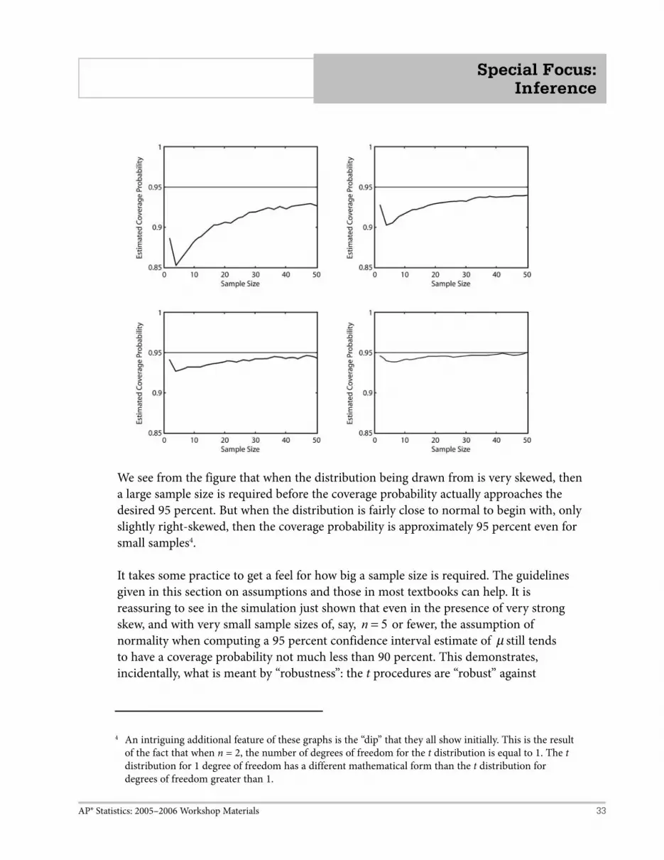
AP® Statistics: 2005–2006 Workshop Materials 33
Special Focus: Inference
We see from the figure that when the distribution being drawn from is very skewed, then a large sample size is required before the coverage probability actually approaches the desired 95 percent. But when the distribution is fairly close to normal to begin with, only slightly right-skewed, then the coverage probability is approximately 95 percent even for small samples4.
It takes some practice to get a feel for how big a sample size is required. The guidelines given in this section on assumptions and those in most textbooks can help. It is reassuring to see in the simulation just shown that even in the presence of very strong skew, and with very small sample sizes of, say, n = 5 or fewer, the assumption of normality when computing a 95 percent confidence interval estimate of µ still tends to have a coverage probability not much less than 90 percent. This demonstrates, incidentally, what is meant by “robustness”: the t procedures are “robust” against
4 An intriguing additional feature of these graphs is the “dip” that they all show initially. This is the result of the fact that when n = 2, the number of degrees of freedom for the t distribution is equal to 1. The t distribution for 1 degree of freedom has a different mathematical form than the t distribution for degrees of freedom greater than 1.

AP® Statistics: 2005–2006 Workshop Materials34
Special Focus: Inference
deviations from normality in that if the assumption of a normally distributed population is not met, the inferential conclusions are not far from correct.
Chi-Square TestsWith the chi-square test, we assume that the sample size is large enough for the test statistic to have approximately a chi-square distribution, and our check for that is to verify that all the expected cell counts are at least 1.0, and no more than 20 percent of the expected cell counts are less than 5.0. (Some texts are more conservative and demand that all expected cell counts exceed 5.0). What happens if those conditions are not met?
Suppose that in the most recent census, a certain city was determined to have a population that was 45 percent white, 25 percent black, 20 percent Hispanic, 5 percent American Indian, and 5% other ethnicities. We wish to sample from the population today and perform a chi-square test of goodness-of-fit to see whether those proportions have changed today. The assumption of a chi-square distribution for the test statistic will only be met if we sample at least 100 people. Let’s perform simulations with smaller sample sizes under the null hypothesis and see how often we reject it using a chi-square test.
The graph below is the result of 10,000 simulations at each sample size ranging from 1 to 120. The horizontal axis shows the sample size, and the vertical axis shows the proportion of times the (true) null hypothesis was rejected at an alpha level of 0.05.

AP® Statistics: 2005–2006 Workshop Materials 35
Special Focus: Inference
We see that in this particular case, the chi-square test is fairly robust against small sample sizes. Even with sample sizes as small as 20, the proportion of times the test rejects the null is near the desired 5 percent.
Let’s repeat the same simulation for a distribution with different census outcomes: 45 percent white, 25 percent black, 20 percent Hispanic, 9 percent American Indian, and 1 percent other ethnicities. This time the 1 percent group is problematic, because for sample sizes under 100, at least one of the expected cell counts is less than 1.
We see from the simulations that the chi-square test is still somewhat robust. While the proportions of Type I errors do tend to be slightly greater than the desired 5 percent, they are not much greater, even for small sample sizes of n = 20 or so. Still, students should respect this rule of thumb or some other reasonable check before applying a chi-square test.

AP® Statistics: 2005–2006 Workshop Materials36
Special Focus: Inference
Review of the Assumptions
Let’s review the assumptions behind each of the inference procedures in the AP Statistics curriculum and how they might be checked for their reasonableness. For all studies in which conclusions are to be generalized to the population from which the sample was drawn:
Assumption: The sample is a random sample from the population.Check: This cannot be checked from the data. The reasonableness of the assumption must be assessed based on how the sample was collected. Since true random samples are difficult at best to collect, the reasonableness of the assumption often reduces to whether the sample was collected in such a way that it does not appear to bias the responses by over- or underrepresenting certain responses as compared to the whole population. Reasonable people may disagree about whether a sampling method produces a sample that is sufficiently “like” a random sample to allow generalization.
For studies involving proportions:Assumption: The sample size(s) is/are large enough to reasonably ensure that the sampling distribution(s) of the sample proportion(s) involved is/are approximately normal.Check: There are a number of different checks people may use. A common one is np > 10 and n p1 10−( ) >ˆ . Note that in the case of a hypothesis test of a single proportion, the hypothesized population proportion should be used in the check; for the construction of a confidence interval, the sample proportion should be used.
For studies involving means:Assumption: The sample size(s) is/are large enough to reasonably ensure that the sampling distribution(s) of the sample mean(s) involved is/are approximately normal.Check: In AP Statistics, different graphic checks are possible. (Analytic checks exist but are not in the syllabus.) A fairly sophisticated one is the normal probability plot, in which linearity in the plot corresponds to normality in the data. Histograms and boxplots are more crude but may be sufficient so long as students can recognize deviations from normality, such as skew or heavy tails. If a sample size is quite small (say, less than 15), then indications of a deviation from normality, such as skew or outliers, are quite troublesome and may invalidate the inference procedures. If the sample size is a bit larger (say, between 15 and 40) then skew, outliers, or heavy tails are less of a problem unless they are fairly severe. And if the sample size is quite large (say, greater than 40), only exceptionally severe deviations from normality will cause problems. If two samples are involved, each of them must be checked.
AP® Statistics: 2005–2006 Workshop Materials 37
Special Focus: Inference
Note that a normally distributed population is still the assumption even when using “t” procedures.
For chi-square tests:Assumption: The sample is large enough that the test statistic has approximately a chi-square distribution.Check: A common check is that all of the expected cell counts must be at least 1, and no more than 20 percent of the expected cell counts may be less than 5.
For linear regression:Assumption 1: The underlying relationship between x and y is linear.Check: The residual plot shows no pattern, particularly no clear curvature.
Assumption 2: The errors have the same standard deviation for all values of x.Check: “Eyeballing” the residual plot is sufficient for AP Statistics students. Be sure the residuals are of roughly the same magnitude across all values of x. In particular, be sure that they do not tend to grow as the response variable grows. If they do, then a transformation of the data may be appropriate.
Assumption 3: The errors are normally distributed.Check: Look at the distribution of the residuals, either using a normal probability plot (better), a histogram, or a boxplot (more crude, but adequate). Be sure the residuals do not display obvious deviations from normality.
What Are Students Expected to Write?
At this point, you may be thinking, “This section about assumptions seems awfully long. Sometimes the discussion about whether an assumption was reasonable went on for a paragraph or more. Surely on the AP Exam itself our students aren’t expected to write that much. So what must they write about assumptions in the free-response section?”
Students should know and state what the assumptions are behind the models they are using. If it is possible to check the reasonableness of assumptions using the data, they are expected to do that as well.
Sometimes assumptions will be stated explicitly in a problem for the students. For example, a problem may state explicitly that the given data represent a random sample from some population. That may be done because the assumption should not be the

AP® Statistics: 2005–2006 Workshop Materials38
Special Focus: Inference
focus of students’ energies. It doesn’t hurt for the students to repeat the assumption if they are performing inference that requires it, but it would not be absolutely necessary if the assumption were explicitly stated in the problem.
If a student thinks one of the assumptions required for inference is violated, but the question appears to demand inference nevertheless, the student would be wise to write something indicating his or her dilemma, such as, “I would ordinarily not want to use a t distribution when the data are so grossly nonnormal, but since this question seems to require a confidence interval calculation, I don’t know what else to do, so I’ll do that.” That at least indicates that the student understands the connection between assumptions and inference. Some teachers suggest to their students that if they find themselves in that situation, they write, “Because the assumptions are not met, I will proceed with caution.” That also indicates that the student is aware that something is wrong. Contrast that with a student who sees a small set of data and writes, “Check for normality,” then sketches a boxplot showing skew and two outliers and goes on with inference anyway. Such a student response may not get any credit for checking assumptions at all, even with the supposed check for normality, since that student didn’t seem to know what the purpose was for the check nor recognize that the assumption was not reasonable.
In situations such as described in the preceding paragraph, i.e., necessary assumptions are not met, the student has in all likelihood made an error somewhere. The free-response questions will not demand the use of unjustifiable inference procedures from students when the procedures in the AP syllabus are invalid. Even the best of students can still stumble, but students should recognize something is wrong and communicate this awareness as a part of their response.
The entire focus of a free-response question may be the validity of the assumptions in a particular situation. Students who make a very regular habit of beginning every inference question with a thoughtful check of assumptions will know what to do. Consider, for example, question 2 of the 2000 AP Statistics Exam in which students were told of a cave containing footprints of prehistoric humans. The question gave sample statistics and asked students what assumptions were required to construct a confidence interval. It also asked whether the assumptions were reasonable. In that question, students should have thoughtfully considered whether the sample was a random sample or anything like one. They should have realized that it was not, that indeed, many of the footprints may have been from the same person, or perhaps that some footprints (from heavier people, perhaps?) may have been more likely to appear in fossil form than others.

AP® Statistics: 2005–2006 Workshop Materials 39
Special Focus: Inference
2000 AP Statistics Free-Response Question 2
2. Anthropologists have discovered a prehistoric cave dwelling that contains a large number of adult human footprints. To study the size of the adults who used the cave dwelling, they randomly selected 20 of the footprints from the population of all footprints in the cave and measured the length of those footprints. Some statistics resulting from this random sample are as follows.
Sample size 20 Minimum 15.2 cmMean 24.8 cm First quartile 18.7 cmStandard deviation 7.5 cm Median 21.5 cm
Third quartile 30.0 cmMaximum 37.0 cm
The anthropologists would like to construct a 95 percent confidence interval for the mean foot length of the adults who used the cave dwelling.
(a) What assumptions are necessary in order for this confidence interval to be appropriate?
(b) Discuss whether each of the assumptions listed in your response to (a) appears to be satisfied in this situation.

AP® Statistics: 2005–2006 Workshop Materials40
Special Focus: Inference
Question 3(d) on the 2004 exam was similar. Students were asked whether conclusions from a sample of dinosaur bones could be extrapolated to all dinosaurs. They were to realize that the sample was not random and that the assumption that it was representative of all dinosaurs might well be unreasonable.
2004 AP Statistics Free-Response Question 3
3. At an archaeological site that was an ancient swamp, the bones from 20 brontosaur skeletons have been unearthed. The bones do not show any sign ofdisease or malformation. It is thought that these animals wandered into a deep area of the swamp and became trapped in the swamp bottom. The 20 left femur bones (thigh bones) were located and 4 of these left femurs are to be randomly selected without replacement for DNA testing to determine gender.
(a) Let X be the number out of the 4 selected left femurs that are from males. Based on how these bones were sampled, explain why the probability distribution of X is not binomial.
(b) Suppose that the group of 20 brontosaurs whose remains were found in the swamp had been made up of 10 males and 10 females. What is the probability that all 4 in the sample to be tested are male?
(c) The DNA testing revealed that all 4 femurs tested were from males. Based on this result and your answer from part (b), do you think that males and females were equally represented in the group of 20 brontosaurs stuck in the swamp? Explain.
(d) Is it reasonable to generalize your conclusion in part (c) pertaining to the group of 20 brontosaurs to the population of all brontosaurs? Explain why or why not.
If a free-response question does not appear to be focusing primarily on the assumptions (as in the cave problem) but is instead asking students to perform a hypothesis test or construct a confidence interval, then the students need not write paragraphs about the assumptions, but they should quickly and clearly state them and, if possible, check that that the assumptions are reasonable. (Some students erroneously think that “checking assumptions” means drawing a little check mark next to them. It does not! Checking assumptions means writing a sentence or an inequality or a graph or calculation that communicates in what way the data are consistent with the assumptions.)

AP® Statistics: 2005–2006 Workshop Materials 41
Special Focus: Inference
Suppose the student is asked to construct a confidence interval estimate of the mean weight of apples from an orchard given the weights of eight apples randomly sampled from the orchard. Here is an example of a poor check of assumptions. np
n p
n
>
−( ) >
<
10
1 10
15, assume normal
Obviously the first two statements do not apply here in the context of means. Yet AP Statistics Readers will confirm that these show up like a talisman on a surprising number of responses to questions having nothing to do with proportions. Their presence indicates that the student doesn’t know what these formulas are for; they may be trying a “shotgun approach,” assuming (again, incorrectly) that the correct formulas will be found and the incorrect ignored. But even if that poor start is ignored, the third line still does not constitute a proper check of assumptions.
Writing “ n < 15 , assume normal” does not communicate much. A sentence stating what was being assumed to have a normal distribution (the population of apple weights) would have been an improvement. But with the eight data values given in the problem, the student would be expected to perform some kind of check to see whether the assumption that they came from a normal distribution was at least plausible.
Here is a much better check of assumptions:
“I will construct a t-interval estimate of the mean weight of the apples in the orchard. This requires that the sample be random, which the problem states. It also requires, with such a small sample size, that the population of apple weights is approximately normal. Here’s a normal probability plot of the eight data values: [shows picture]. It’s not grossly nonlinear, and the data set has no outliers, so the normality of the population is not contradicted by the data, so we’ll assume it.”
While delightfully complete, the response may seem awfully wordy, especially in the context of a timed exam. The following much shorter check communicates the same ideas:
“Sample is random (given). Assume apple weights in orchard are normally distributed. Check: [boxplot here], no skew or outliers. So assumption is reasonable.”

AP® Statistics: 2005–2006 Workshop Materials42
Special Focus: Inference
Conclusion
Students can easily end up thinking that a check of assumptions is merely a pointless routine on the road to “doing the problem.” This mindset can get them into trouble both on AP Exam questions and in their thinking about real statistical analyses they perform or read about. Statistics is largely about creating mathematical models to explain observations in the world. These models are never exactly right. Mother Nature is not so simplistic! However, the models can still be useful for understanding the world, so long as they are reasonably good. The “goodness” of the models depends largely upon the reasonableness of the assumptions behind them. Assumption checking isn’t something that students do in AP Statistics only and from which statisticians have “graduated,” leaving it behind. Rather, checking assumptions is an important part of every statistical endeavor: it is the assumptions that drive the model. Statisticians don’t let statisticians drive without the mathematical support provided by assumptions!
AP Statistics teachers should encourage in their students the habit of always checking the assumptions behind the inference procedures they’re using. One reason so many students think of checking assumptions as just a pointless routine is that they are rarely exposed to problems in which the assumptions are not met. I would encourage teachers to present problematic data to their students on a fairly regular schedule to keep them on their toes and help them see the point of checking assumptions. Sometimes that will mean concluding that the inference techniques of the AP Statistics curriculum are insufficient for a particular problem, and so it must be left unresolved. That’s perfectly fine.
Also, students are far more likely to encounter assumptions that are not met when they design and conduct their own studies than when they read about studies in their textbooks. The examples presented in this section are not true stories but are motivated by actual classroom experience, describing the sorts of problems that students have encountered when they conduct their own studies.
When students conduct their own studies, the most common difficulty is devising a sampling method such that the assumption of a random sample, or “like” a random sample, is reasonable. Following that distantly is the collection of a sufficient amount of data for the limiting distribution assumption (normal, t, or chi-square) to be reasonable. Sometimes students come up with interesting studies for which the data are relatively easy to collect in large numbers. But other times the students realize that although their study’s design is good, it will require far more time in data collection than they are able to spend.

AP® Statistics: 2005–2006 Workshop Materials 43
Special Focus: Inference
Finally, the habit of thinking about and checking assumptions must not stop as a mental exercise or an oral discussion but must be something students are in the habit of putting in complete sentences on paper. This is part of the broader and very important goal of AP Statistics, that students be able to communicate their ideas clearly in writing. The study of theoretical statistics is a rich and beautiful endeavor, and like theoretical mathematics no context is required. However, AP Statistics is applied statistics, applied statistics does not exist without context, and statistical solutions to problems do not exist if they are not clearly communicated.

AP® Statistics: 2005–2006 Workshop Materials44
Special Focus: Inference
Some Reflections on How Inference Questions on the AP Exam Are ScoredDaniel S. YatesVirginia Commonwealth UniversityRichmond, Virginia
Introduction
In this section, we get a sense of how AP Exam Readers respond to students’ answers to free-response questions on the AP Statistics Exam. We examine the scoring process that has been used for inference-related questions on the AP Statistics Exam in recent years and determine the components of a “complete solution.” We then look at alternative solutions that would receive full credit in an inference setting and at the level of response that is required. We turn to some actual student responses that received deductions and learn how to avoid point deductions. Finally, we present the general concerns of the Chief Readers as they report some of the difficulties students encountered in their responses to the free-response questions. These concerns are expressed as the Chief Reader’s “Student Performance Q & A” and are written after consulting with the Readers and Table Leaders at the end of the week’s Reading.
How Free-Response Questions Are Scored
Free-response questions typically are presented in multiple parts. Each part is scored E (essentially correct), P (partially correct), or I (incorrect). The scoring guidelines (rubrics) for that particular question states the combination of Es, Ps, and Is that determine the numerical score for that problem. Free-response questions are evaluated on a 0-to-4 scale, as follows:
Score Description
4 A complete solution
3 A substantial solution
2 A developing solution
1 A minimal solution
0 No credit
Note that each score has associated with it a verbal anchoring descriptor: “complete,” “substantial,” and so forth. These descriptors are helpful when the Reader uses holistic scoring, discussed below. Note further that the top score of 4 does not say “perfect.”

AP® Statistics: 2005–2006 Workshop Materials 45
Special Focus: Inference
A student could score a 4 on a question even if there is a slight arithmetic error or some other minor error that is not considered important. This should be comforting to students. At the other end of the scale, no credit is given when the question is left blank or when the response is completely off task.
Scoring guidelines are written for the purpose of making the scoring of the responses independent of which Reader happens to score a particular paper. As all teachers and students know, teachers have different sets of expectations in their classrooms. The scoring guidelines exist to override these differences and put all students on an equal footing with respect to having their responses to the free-response questions evaluated. Before the first exam paper is scored, Readers receive careful instruction to familiarize them with the scoring guidelines. Then they practice scoring papers until the highest possible level of consistency is achieved. Only then do Readers begin scoring papers “for real.”
While the scoring guideline tries to anticipate a wide variety of responses to the question parts, anticipating all possible responses can’t be accomplished due to the “open-ended” nature of free-response questions. Sometimes a student response is not covered in the scoring guideline. Or perhaps the scoring of a problem results in an intermediate score, such as 2.5 or 3.5. In these circumstances, the Reader utilizes “holistic” scoring. The idea behind holistic scoring is that if the responses to the parts of a question do not result in a clear 0, 1, 2, 3, or 4, the Reader should look at the response in total and make a determination of the scores “on the whole.” The scoring guidelines for the free-response questions typically provide helpful guidelines and criteria for dealing with half scores.
Identifying Inference Questions
The Course Description states that about 40 percent of the AP Exam is on inference. Inference thus receives more attention on the exam than any other topic. This fact should motivate students to review this topic extensively before they sit for the exam. So exactly what concepts and skills fall under the heading of inference? Most students would quickly identify tests of significance as inference. What they may not realize, however, is that confidence intervals are also included under the category of inference.
There is fairly specific wording that students should look for in identifying inference questions, phrases that should say clearly to the student, “This is an inference question!” If a question introduces some data and a setting and then says, “Is there evidence to conclude that (something is the case)?” or “Give statistical evidence to conclude that...” or a slight variation of this wording, this should ring a bell or raise a flag. What this wording is saying is, “Perform the appropriate statistical procedure, systematically completing all

AP® Statistics: 2005–2006 Workshop Materials46
Special Focus: Inference
of the necessary steps, and make your answer culminate in a statement similar to ‘There is sufficient/insufficient evidence to conclude that (state a conclusion in the context of the problem).’” The major mistake here is that students believe that constructing side-by-side boxplots, or a histogram or other plot, or comparing percentages is sufficient to show that a new drug, for example, is more effective than the old, established drug.
The confidence interval seems like such a simple idea, but it can cause a surprising amount of potential trouble for students. Confidence interval questions on the exam typically have been in two parts. The first part asks students to use information provided to construct a confidence interval. The second part is to interpret the confidence interval. Typically, students do well on the first part, and this is not surprising. After all, most of them enroll in AP Statistics because they have performed well in previous math classes, many of which involve lots of computation. Where students frequently crash and burn is on the interpretation part. Interpretation requires a sentence or two that explains what the confidence interval is all about.
Interpretations of confidence intervals are sufficiently important that they can raise the points on that question from, say, a 3.5 to a 4, or if the interpretation is botched, lower the points to a 3 when holistic grading is applied to a student response. Under certain circumstances, a student can employ a confidence interval approach for a question specifically asking for a significance test, and if done correctly, this strategy will receive full credit.
The Inference Steps
Let’s begin with a test of significance: inference for a mean or a proportion, comparing two means or proportions, a chi-square test, or inference for regression.
1. State hypotheses. Every inference procedure should begin with a clear statement of the null and alternative hypotheses. The best response here is to state the
hypotheses using symbols and then write out statements of the hypotheses in words. If the symbols approach is used alone, and commonly used symbols for the population parameters are used, then this would be considered acceptable. If nonroutine symbols are used, then they must be defined clearly and correctly in order to receive full credit.
2. Identify the inference procedure, and state and check assumptions and conditions. Inference procedures produce valid results only if certain conditions are satisfied (like hypotheses for a theorem in geometry). The failure to check

AP® Statistics: 2005–2006 Workshop Materials 47
Special Focus: Inference
assumptions was a glaring omission for many students in the early days of the AP Exam. When this was identified as a failing, students began stating the assumptions, such as “np n p≥ − ≥10 1 10, ( ) ,” and left it at that. While this was an improvement over cavalierly ignoring assumptions, such statements alone did not receive credit! Such constructions were regarded as stating the assumptions, not checking them. In order to get credit for this step, students must state the assumptions correctly and then substitute numbers for that problem to actually verify their validity so that the inference procedure could be legitimately performed. Floyd Bullard’s article in these materials gives additional insight about the role of assumptions in inference.
3. Mechanics. The next step in the inference procedure is to calculate the test statistic, using the appropriate formula. (Formulas are provided with the exam.) It is best to write the appropriate formula for the test statistic and then show substitution into that formula. The computation can then be performed on a calculator and the test statistic reported. The test statistic value should be used to determine the p-value (the probability of obtaining a result as extreme or more extreme than the value we obtained, by chance alone, if the null hypothesis were true). The p-value is then used to make the decision to reject or fail to reject the null hypothesis.
4. Conclusion. If the p-value is sufficiently small to cause rejection of H0, then a conclusion needs to be made in the context of the problem. In the early days of the AP Statistics Exam, some students believed that a statement of “reject” or “fail to reject” was the moral equivalent of QED, and that nothing else needed to be said. Not so! In statistics, context is critical.
Summarizing, the four required parts in an inference setting are:
1. State hypotheses in words and/or symbols.
2. Identify the correct inference procedure and verify conditions for using it.
3. Calculate the test statistic and the p-value (or rejection region).
4. Draw a conclusion in context that is directly linked to the p-value or rejection region.

AP® Statistics: 2005–2006 Workshop Materials48
Special Focus: Inference
Examples of Student Responses and Their Scores
In 1999, free-response question 2 was:
The Colorado Rocky Mountain Rescue Service wishes to study the behavior of lost hikers. If more were known about the direction in which lost hikers tend to walk, then more effective search strategies could be devised. Two hundred hikers selected at random from those applying for hiking permits are asked whether they would head uphill, downhill, or remain in the same place if they became lost while hiking. Each hiker in the sample was also classified according to whether he or she was an experienced or novice hiker. The resulting data are summarized in the following table.
Direction
Uphill Downhill Remain in Same Place
Novice 20 50 50
Experienced 10 30 40
Do these data provide convincing evidence of an association between the level of hiking experience and the direction the hiker would head if lost? Give appropriate statistical evidence to support your conclusion.
Note that there are clear signals about the nature of this problem. First, the context and the nature of the data strongly suggest a chi-square test of independence. Second, it is difficult to miss the inferential nature of the problem, which is essentially: “Perform an appropriate inference procedure, with all the important/required steps.”
How were students expected to respond for a “complete” score? The scoring guidelines specify four parts to this problem:
Part (a) Stating a correct set of hypothesesPart (b) Identifying an appropriate test and checking appropriate requirementsPart (c) Providing correct mechanicsPart (d) Stating a correct conclusion in the context of the problem using results of the statistical test
The scoring guidelines go on to include much more detail for each of these parts. Let’s consider some actual student responses:

AP® Statistics: 2005–2006 Workshop Materials 49
Special Focus: Inference
Student A’s response was as follows:
H0 : There is no association between experience and hiking directionHa : There is an association between experience and hiking direction
The expected values are:
Expected Direction
Uphill Downhill Remain in Same Place
Novice 18 48 54
Experienced 12 32 36
Since all expected counts are at least 5, we can use the chi-square procedure. χ 2 1 5= . , p-value = 0.471, p > 0.05, Fail to reject H0
There is insufficient evidence to show that there is an association between experience and hiking direction when lost.
It would have been nice if this student had stated the appropriate formula for the χ 2 statistic and then shown substitution into that formula. Nevertheless, all of the important steps are addressed, and the student has used the calculator to produce the correct value for χ 2 . The assumptions are credibly shown to be satisfied, and the conclusion is stated in the context of the levels of experience and the direction the hikers would head if lost. This paper scored a 4, a “complete response.”
Student B responded by writing this paragraph:
Yes, the data does [sic] provide convincing evidence of an association between the level of hiking expertise and the direction the hiker would take. The statistical evidence for this is found by doing a chi-squared test. The χ 2 value for this data is 1.5046 and the p-value is 0.4713. Since the p-value is greater than the 0.05 then it is understood that there is a significant difference between the choices of novice and experienced hikers.
The student then sketched a chi-square curve on a set of axes, shaded the right-tailed region, and marked this region 0.4713.

AP® Statistics: 2005–2006 Workshop Materials50
Special Focus: Inference
This student’s response is more difficult to score because the conclusion is stated first, and the student subsequently tries to support that conclusion. We begin by looking for a pair of hypotheses, but there are none. The χ 2 statistic is specified, but there is nothing about assumptions. The mechanics are correct (correct test statistic value and p-value). The rejection rule is applied incorrectly. Consulting the scoring guidelines, the Readers assigned a score of 1 for Student B. This is a “minimal” response.
Student C responded as shown:
H observed expected0 : = , H observed expecteda : ≠ α = .10
Uphill Downhill Remain
Novice 18 42 54
Experienced 12 32 36
χ 2 test may be used because expected cell counts are all more than 5 and the data is a two-way table. χ 2
2
1 505=−
=∑ ( ) .observed expectedexpected
p = .47
Conclusion: Since our p-value is greater than our level of significance, we fail to reject H0 . We have no evidence that the level of hiking expertise is related to the direction a hiker would head if lost.
Student C’s hypotheses are a bit too terse and have the appearance of a generic response— they would work for almost any statistical hypotheses. The remaining parts of the response are correct, and this student earned a 3 for this problem.
Student D wrote:
H H0 a: , :µ µ µ µ1 2 1 2= ≠ . Using the chi-squared test, it was found that χ 2 1 5046 471= =. , . .p The p-value is not what I consider statistically significant (p < .05), since it is .471. Because of this, I would have to reject Ha, and accept H0, thus meaning that the data does not provide convincing evidence that there is an association between level of hiking expertise and the direction the hiker would go if lost.

AP® Statistics: 2005–2006 Workshop Materials 51
Special Focus: Inference
The hypotheses are incorrect, even though this student’s conclusion gives us an inkling that s/he may really know what s/he is testing. This part just doesn’t rise to a level of partially correct. The student identifies the chi-squared test but neglects to check requirements for the test. S/He provides correct mechanics in the response, but errs when s/he rejects the alternative hypothesis (and accepts the null hypothesis). And then s/he states a correct conclusion in context, employing the “two wrongs make a right” strategy. The Readers were generous here; they awarded Student D a holistic score of 2.
Here is the scoring commentary for 1999, question 2:
This question required the student to analyze data in a two-way table. Themost common approach was to use a chi-square test for independence.Communication continues to be a problem in questions requiring dataanalysis, and many students had difficulty explaining the approach taken, andclearly communicating the results of the analysis. Although more studentsmentioned assumptions required in order for the analysis to be valid, fewactually checked to see that the assumptions were met. The chi-square test isa topic that is often covered late in the course, and judging from the largenumbers of zeros given and blank responses on this question, it appearsthat many classes may have not covered this topic. Common errors inanswering this question were:
• Incorrectly stating the hypotheses for the test. • Approaching the problem by testing all possible pairs of proportions. • Poor communication of conclusions, especially in linking the conclusion to the results of the statistical test (i.e., the P-value). • Failure to mention assumptions, or stating assumptions without checking to see if they are met. • Failure to use any inferential procedure, reaching a conclusion by just “looking at the data.”
In addition to 1999, question 2, very similar chi-square applications are found in 2003, question 5 and 2004, question 5. One reason we selected 1999, question 2 for illustration was the frequency of seeing this type of question in the recent past.
Now consider the following problem (2001, question 5):
A growing number of employers are trying to hold down the costs that they pay for medical insurance for their employees. As part of this effort, many medical insurance companies are now requiring clients to use generic brand medicines

AP® Statistics: 2005–2006 Workshop Materials52
Special Focus: Inference
when filling prescriptions. An independent consumer advocacy group wanted to determine if there was a difference, in milligrams, in the amount of active ingredient between a certain “name” brand drug and its generic counterpart. Pharmacies may store drugs under different conditions. Therefore, the consumer group randomly selected ten different pharmacies in a large city and filled two prescriptions at each of these pharmacies, one for the “name” brand and the other for the generic brand of the drug. The consumer group’s laboratory then tested a randomly selected pill from each prescription to determine the amount of active ingredient in the pill. The results are given in the following table.
Pharmacy 1 2 3 4 5 6 7 8 9 10
Name Brand 245 244 240 250 243 246 246 246 247 250
Generic 246 240 235 237 243 239 241 238 238 234
Based on these results, what should the consumer group’s laboratory report about the difference in the active ingredient in the two brands of pills? Give appropriate statistical evidence to support your response.
The scoring guidelines identify a “complete” response as the following:
Consider this a matched-pairs experiment (a pair of prescriptions from each pharmacy). Let X = the difference between the name brand and the generic, and let μ be the mean difference.
H0 0: µ = , Ha : µ ≠ 0
Assumptions for the test: We will assume that the pills are stored under similar conditions. We are given that the pills are selected randomly. A boxplot reveals that there are no outliers and only slight skewness, so it is reasonable to proceed with the test. With df = 10 – 1 = 9, the p-value is 2 (.00166) = .00332.

AP® Statistics: 2005–2006 Workshop Materials 53
Special Focus: Inference
Conclusion: Since the p-value is so small, there is sufficient evidence to reject H0 and conclude that the mean difference is not 0. There is a difference in the active ingredient between the name brand and the generic brand for these 10 pharmacies.
Student E responded as follows:
Pharmacy 1 2 3 4 5 6 7 8 9 10
Name brand –generic brand
-1 4 5 13 0 7 5 8 9 16
Since n < 15, a t-test can be used since the distribution of the name brand – generic brand is close to normal and with no outliers.
– 0 |
– 0 | 1
0 | 4 0
0 | 5 7 5 8 9
1 | 3
1 | 6
x = 6 6. , s
nx xx i=
−−
11
2( ) =5.2747.
H0 0: µ = , Ha : µ ≠ 0 ,
where μ = name brand – generic brand. tx µsn
=−
=−
=6 6 05 2747
10
3 9568.. . .
df = n – 1 = 9.
p = 2 × tcdf(3.9568, ∞, 9) = .00332.
There is good evidence to reject the claim that there is no difference in amount of active ingredient in name brand and generic drugs in favor that there is a difference.
While there are a couple of minor quibbles in Student E’s solution, it has all the essential ingredients, and it earned a score of 4.

AP® Statistics: 2005–2006 Workshop Materials54
Special Focus: Inference
Student F’s response looked like this: • 2 observations from each pharmacy; pharmacies may affect amount of
active ingredient in how they store the medicine. • I assume that the distribution of (mg for name brand – mg for e = generic brand) is approx. normal • I assume that the pharmacies in the city and the pills in the prescriptions
were chosen randomly • Matched pairs t-test is appropriate, μ = mean difference in mg for (name brand – generic) H
H
0
0
:
:
µ
µ
=
≠
0 mg
0 mg
Pharmacy 1 2 3 4 5 6 7 8 9 10
Name – generic -1 4 5 13 0 7 5 8 9 16
x = 6.6 mg, s = 5.275 mg, n = 10, df = 9
tx µsn
=−
=−
=6 6 05 2747
10
3 957.. . .
2P(t > 3.957) =0.0033.
A p-value this small is sufficient evidence that on a pharmacy-by-pharmacy basis, the name brand version of the certain drug contains more of the active ingredient than its generic counterpart.
This is a strong response, but it earned a 3 instead of a 4 because the student didn’t check the assumptions.
Student G responded:
Differences: –1, 4, 5, 13, 0, 7, 5, 8, 9, 16. x = 6.6
The total difference in the active ingredient in the two brands of pills of all 10 pharmacies is 66. Therefore the mean difference is 6.6 mg. This is a two sample

AP® Statistics: 2005–2006 Workshop Materials 55
Special Focus: Inference
difference of sample means, so by using a 2-sample z test on the TI-83: P = 0.000009, z = 4.4387. H0 : no difference in mg of two brands
Ha : is a difference in mg of two brands
Based on the results, the probability that there is a difference between the two brands is statistically significant beyond the 1% level. The probability that the two brands are different in amounts of active ingredient by chance alone is 0.000009. The consumer group’s laboratory should reject the null hypothesis and report that there is a statistically significant difference in the mg between the two brands. These results are valid based on the assumptions that: 1. These pharmacies and pills were taken from a simple random sample. 2. The active ingredient in mg per bottle is normally distributed.
This student begins well by looking at the differences in active ingredient, appearing to see this as a matched-pairs situation. But the student then uses an incorrect significance test, the hypotheses are not correct, and the assumptions are stated but not checked. The student earned a score of 2 for this response, a “developing” response.
2001, question 5, commentary:
Question #5 was intended to be a straightforward, matched-pairs hypothesis testing problem, but only a handful of students correctly selected a matched-pairs t test. More students in 2001 seemed to be aware of the necessity of checking conditions or assumptions as part of the hypothesis testing procedure than in previous years. However, a lot of test takers still neglected to actually verify the correct conditions, which are: SRS from population of interest, and normality of the population distribution of differences. Some students referred to a graph on their calculators that was not sketched on the exam paper. Relevant calculator plots need to be transferred to the exam paper. This is part of the student’s responsibility for good communication. A few students incorrectly tried to use a chi-square procedure. Some students mixed two-sample condition checking with a matched-pairs procedure. Students interpreted p-values more accurately in 2001 than in previous years. Communication continued to be weak on many papers.

AP® Statistics: 2005–2006 Workshop Materials56
Special Focus: Inference
Confidence Intervals
If there is one topic that seems to befuddle students and Readers, it’s confidence intervals. Students seem to have much difficulty interpreting confidence intervals. As an example, let’s look at 2002, question 6(a) and (b).
A survey given to a random sample of students at a university included a question about which of two well-known comedy shows, S or F, students preferred. The students were asked the question, “Do you prefer S or F?” The responses are shown below.
PreferenceS F Total185 139 324
a) Based on the results of this survey, construct and interpret a 95% confidence interval for the proportion of students in the population who would respond S to the question, “Do you prefer S or F?”
b) What is the meaning of “95% confidence” in part (a)?
[An aside: Many students and their teachers immediately visualized Seinfeld and Friends as the two comedies.]
Expected Solution (a) Let p = proportion of students who would respond S to the question, “So you prefer S or F?” A large sample confidence interval for a population proportion takes the form
ˆ .ˆ( ˆ )
pp pn
±−1 96 1 . Constructing this interval requires that we have a large sample with
np = ≥185 5 and n p( ˆ )1 139 5− = ≥ . We also require that the population be at least 10 times the size of the sample: 10n = 10(324) = 3240. We assume that the university has at least 3240 students. The interval is calculated as
0 571 1 96 571 429324
0 571 0 054 0 51. . (. )(. ) . . ( .± = ± = 77 0 625, . )
Interpretation: We have 95% confidence that the interval (0.517, 0.625) captures the proportion of students who would respond “S” to the question, “Do you prefer S or F?”

AP® Statistics: 2005–2006 Workshop Materials 57
Special Focus: Inference
[Note that a complete solution would include the formula for a large sample confidence interval, statement and a check of assumptions and conditions, and calculation and interpretation of the confidence interval.]
(b) In repeated sampling, 95 percent of the intervals produced using this method will contain the proportions of students at this university who would respond S to the question, “Do you prefer S or F?”
The rubric specified that part (b) is scored either “Essentially correct (E)” or “Incorrect (I).” It was not possible to score partially correct on this part.
For part (a), Student H wrote:
SRS✔ 324(.571) > 10✔ 324(.429) > 10✔ 324(.429) > 10✔ 324(.571) > 10✔ pS = proportion who responded “S” = 185/324 = 571. Because n > 30, we can assume the sample distribution is normal and use a z -interval.
95% = 0 571 1 96 571 429324
0 517 0 625. . (. )(. ) ( . , . )± = .
And for part (b):
This means that if we were to repeat our method over and over, the true mean µ would lie in our confidence interval 95% of the time.
Student H neglects to interpret the confidence interval, but part (b) is correct. Still, because this was the investigative task that touched on a number of concepts from the course, if the remaining parts of this question were very well done, this student probably would have received a holistic 4, rather than the 3 this response was given.
Student I said for part (a):
By putting the number 185 and 324 in a 1-Prop Zint 95% confidence interval for part (a) would be (.5171, .62488).

AP® Statistics: 2005–2006 Workshop Materials58
Special Focus: Inference
Part (b):
A 95% confidence interval says that the sample mean will fall in those bounds 95% of the time if the survey is conducted again.
In part (a) Student I only performed a quick calculator computation. A calculator computation will usually get the student very little in terms of a score. Much more needs to be done, including a correct interpretation of the confidence interval. In (b), the explanation of 95 percent confidence is stated in terms of his calculated interval instead of being in terms of confidence in the method employed and is therefore incorrect.Student J’s response read:
185/324 = .5710 1 prop z interval Assumptions: • To use standard deviation, population is 10 times sample size • np n p≥ − ≥10 1 10, ( )
Check of assumptions • I assume there are more than 3,240 students in the population • np n p= − =185 1 139, ( ) 0 571 1 96 571 429
324. . (. )(. )
±
0 571 0539. .± (.5171, .6249) (b) It means that we are 95% confident that the true mean lies between .5171 and .6249, and that 95% of similarly constructed confidence intervals will contain the true mean.
Student J is not completely correct in part (a) because the interpretation of the calculated confidence interval is missing. Part (b) illustrates what is referred to as a “parallel solution.” The student offers two independent solutions to the same problem. When parallel solutions are encountered in the AP Statistics scoring process, Readers score both responses, but award points based on the weaker of the two solutions. Student J’s first sentence in part (b) is incorrect. The response in (b) should also send a strong signal to all students that parallel solutions should be avoided. Students should carefully consider alternative responses and select the answer that seems most likely to be correct.

AP® Statistics: 2005–2006 Workshop Materials 59
Special Focus: Inference
The Chief Reader in 2003 commented on this problem by saying:
Student performance on hypothesis testing questions has been improving over recent years. More students (but still not the majority) are addressing necessary conditions or assumptions and students are doing a better job of stating a correct conclusion in context. However, many students failed to address all of the required conditions or assumptions for the test, and did not provide any link between the computations performed as part of the test procedure and the eventual conclusion.
Postscript
By looking at several inference free-response questions, their scoring guidelines, selected student responses, and how these responses were scored, teachers and students will have a better understanding of the expectations for this type of problem. We hope this better understanding will translate into better performance and higher scores.

AP® Statistics: 2005–2006 Workshop Materials60
Special Focus: Inference
Model ResponsesDaren StarnesThe Webb SchoolsClaremont, California
Statistics in general and AP Statistics in particular are properly focused on effective communication. This section considers what constitutes good communication in projects, speeches, reports, and (of course!) responses to exam questions when explanations about inferences are required.
A former colleague of mine once said, “You can have the greatest ideas in the world, but if you can’t get them across to anybody, they’re not worth much.” He made the remark during one of our team-taught AP Statistics and AP Environmental Science classes, and it has stuck with me ever since. A key question for us as statistics teachersis, how can we help students develop strong communication skills in our courses?
Perhaps the most important thing we can do is provide students with plenty of opportunities to practice statistical communication, both within and outside the classroom. We can ask them to describe and interpret graphical displays, to analyze published statistical studies, and to produce written and oral reports about data they have collected. Along the way we must provide them with regular feedback about not only the accuracy of their statistical methods, but also the clarity of their statistical thinking. And of course, we have to model exemplary statistical practice for them.
Students can also help each other become better communicators. Whether they work together to write out a solution to an inference question or critique each other’s written responses, students will gradually learn what it takes to get their ideas across clearly and unambiguously. While they collaborate, you are free to roam about the classroom offering helpful suggestions.
One of the most difficult aspects of the AP Statistics course for many students is mastering the use of technical vocabulary. Students by nature, being human, tend to be informal and colloquial in speaking and writing. AP Statistics, however, requires precise, technical communication. You can really help your students by insisting that they use the terms in the course syllabus frequently and correctly. Some teachers have even suggested posting a list of “restricted” words for their students. If students use a restricted word, they must be prepared to defend the use of that word to the rest of the class. Some examples of possible restricted words include: normal, outlier, bias, random, accept, independent, cause, and of course the ubiquitous pronoun “it.”

AP® Statistics: 2005–2006 Workshop Materials 61
Special Focus: Inference
Discourage your students from parroting memorized statements like “Randomization reduces bias” or “Blocking reduces unwanted variation.” Instead, ask your students to apply statistical principles in unfamiliar contexts. For example, you might bring in a description of an experimental design and pose questions like “What purpose did random assignment serve in this experiment?” or “How might the design of this experiment be improved by incorporating blocking?”
The model questions that follow are intended to mimic the style and substance of the free-response questions involving inference that are asked on the AP Statistics Exam. As do past AP Statistics Exam questions, these questions consist of multiple parts and simultaneously address several topics in the course syllabus. They are a bit longer than typical exam questions, however.
Following the presentation of each question, we have provided a model response. Our solutions mirror the content and format of those found in scoring rubrics from previous AP Exams. Please note, however, that we have crafted responses that are longer and more detailed than what a student could reasonably be expected to generate under exam conditions.
In each model response, we rigidly adhere to the four-step outline for solving inference problems that has evolved over several years at the AP Reading. For reference, those four steps are:
Step 1: Identify the population(s) and parameter(s) of interest. State hypotheses if you are performing a hypothesis test.
Step 2: Select the appropriate inference procedure and verify conditions for using it.
Step 3: Carry out the procedure.
Step 4: Interpret your results in the context of the problem.
We use statistical terminology correctly in the model responses to these questions.
Using this four-step outline for inference in your class will definitely help prepare your students for AP Exam questions. From our experience with the Course Description, we have noted several common pitfalls that students must be careful to avoid. First

AP® Statistics: 2005–2006 Workshop Materials62
Special Focus: Inference
and foremost, students must be clear about the distinction between the population of interest and the sample, and along the same lines, the distinction between the parameter they want to draw conclusions about and the appropriate statistic to use for doing so. When stating hypotheses, students must use the symbols for parameters, not statistics. Moreover, they must be certain that they have defined the hypotheses in words that clearly indicate their understanding of the population(s) and parameter(s) of interest in the problem.
To successfully carry out Step 2, students must do more than just list the conditions for using a particular inference procedure. Also, it is not enough to state the conditions and simply put a check mark next to each one. Nor should students simply say, “Let’s assume that we have an SRS and that the population distribution is normal.” They should always cite information given in the problem as they attempt to verify the required conditions. Students sometimes forget that conditions must be verified for confidence intervals as well as hypothesis tests.
In Step 3, students must be reminded of the value of showing their process clearly. When computing confidence intervals, students should show the substitution of numbers into a formula, such as:
95% CI for µ : estimate ± margin of error = 3.2 ± 1.96 ( / )1 36 = 3.2 ± 0.33.
For hypothesis tests, students must calculate an appropriate test statistic and give a correct p-value or rejection region.
For Step 4, students should keep in mind the “three Cs”: conclusion, connection, and context. They must be sure to answer the question that was originally asked, to draw a conclusion in the context of the problem that connects directly with their work in Step 3.
We hope that the model questions and responses provided below will give you and your students valuable insight into the level of communication that is expected on AP Statistics free-response questions.
Model Problem 1: Are people’s standing pulse rates higher than their sitting pulse rates?Students in an AP Statistics class collected pulse rate data during a class activity. Initially, each student flipped a coin. Students who obtained “heads” were told to measure their standing pulse rates first, then their sitting pulse rates after a two-minute delay. Students who obtained “tails” were told to measure their sitting pulse rates first, then their

AP® Statistics: 2005–2006 Workshop Materials 63
Special Focus: Inference
standing pulse rates after a two-minute delay. All pulse rates (in beats per minute) were determined using two fingers on the neck for 60 seconds. The table below displays results from this activity.
Individual Coin Flip Sitting Standing
1 H 65 68
2 H 73 75
3 H 70 70
4 H 70 80
5 T 60 68
6 H 70 74
7 T 57 64
8 T 55 66
9 H 77 80
10 T 98 100
11 T 126 107
12 H 60 78
a) Describe a problem that could occur if no coin flip had been used in this activity and explain how the coin flip can help fix this problem.
b) The students in the class are trying to decide between a matched-pairs t-test and a two-sample t-test to determine whether students’ standing pulse rates are higher than their sitting pulse rates. Which would you recommend, and why?
c) Some students in the class notice that the data point for student 11 is probably an outlier. After some discussion, the class decides to remove student 11 from the analysis Using the data from the remaining 11 students, is there sufficient evidence to conclude that students’ standing pulse rates are higher than their sitting pulse rates? Carry out an appropriate inference procedure to help you answer this question.
d) The teacher suggests that there is an alternative to removing student 11 from the analysis. She explains her reasoning as follows: “Let’s assume that there is no difference between students’ standing and sitting pulse rates. Then for any individual student, there should be a 50 percent chance that the standing pulse rate is higher.” Assuming that the teacher is correct, calculate the probability of observing 11 or more of the 12 students with higher sitting than standing pulse rates.

AP® Statistics: 2005–2006 Workshop Materials64
Special Focus: Inference
Model Response 1a) Suppose six of the students in this class had been released late from their previous class and so decided to run to class. If all the students in the class measured their sitting pulse rates first, then the sitting pulse rates of these six students would be higher than usual. By the time they measure their standing pulse rates, the effect of the previous jog to class could have worn off. As a result, the difference between their standing and sitting pulse rates might be smaller than if they had walked to class.
By having the students flip a coin to determine the order in which they will measure their pulse rates, it is likely that about half of the students who ran to class would measure sitting pulse rates first and that about half would measure standing pulse rates first. Any increase in pulse rate due to the recent exercise will be split about evenly between standing and sitting pulse rate measurements. This will help prevent the kind of systematic inflation of sitting pulse rates that was described as a problem before.
If we observe a difference in students’ sitting and standing pulse rates, we want to ensure that the difference is a direct result of whether they are sitting or standing and not some other factor. Randomly assigning the order of the two measurements (with a coin flip, in this case) should help avoid systematic effects on either the standing or sitting pulse rates.
b) The data are paired by individual student, so a matched-pairs t-test should be used. A two-sample t-test should only be used when the data come from two independent samples.
c) Inference problems should follow the four-step outline described earlier.
Step 1: Identify the population(s) and parameter(s) of interest. State hypotheses if you are performing a hypothesis test.Our population of interest, according to the problem statement, is “people.” Because the data were collected only from high school students, however, it may be problematical to generalize beyond this group. So we’ll restrict our attention to the population of high school students. We are interested in performing inference about the mean difference,µ µDiff = −stand sit , between the standing and sitting pulse rates of high school students. The appropriate hypotheses are:
HH
Diff
a Diff
0 00
::µµ
=>

AP® Statistics: 2005–2006 Workshop Materials 65
Special Focus: Inference
The alternative hypothesis is one-sided because we want to determine whether students’ standing pulse rates are higher than their sitting pulse rates, in which case µ
Diff would
be positive.
Step 2: Select the appropriate inference procedure and verify conditions for using it.In part (b), we determined that a matched-pairs t-test would be the correct procedure in this case. There are two conditions we should examine before carrying out the procedure:• Data obtained using an SRS from the population of interest
In this problem, the data come from 12 members of an AP Statistics class. This is clearly a convenience sample. As a result, we may not be able to generalize our findings to the population of all students. However, assignment to treatments was random. So we should be able to determine whether there is evidence of a treatment effect based on sitting or standing.
• Population distribution is normally distributed.
We do not know that the population distribution of differences in students’ standing and sitting pulse rates is normally distributed. A boxplot and a normal probability plot of the differences in our reduced sample of 11 students are shown below. We are concerned by the obvious right-skewed shape of the boxplot, because this may suggest that the data did not come from a normal distribution. The normal probability plot shows some evidence of a nonlinear pattern, which again makes us question the normality of the population distribution. The sample size is small, and the t-procedures are not very robust against nonnormality in the population distribution. On the positive side, there are no outliers. We will proceed with the analysis, but exercise appropriate caution when we interpret the results.

AP® Statistics: 2005–2006 Workshop Materials66
Special Focus: Inference
Step 3: Carry out the procedure.
• Test statistic: txsn
diff
diff=
−=
−=
µ0 6 182 05 288
11
3 877.. .
• p-value: For a t-distribution with df = 11 – 1 = 10, the p-value is between 0.0025 and 0.001. (The TI-83 gives a p-value of 0.00154.)
Step 4: Interpret your results in the context of the problem.Since the p-value is so small (less than 0.0025), it is highly unlikely that we would observe a value of x as large as we did in our sample (6.182) if H Diff0 0: µ = were true. So we reject H0 and conclude that the population mean difference in students’ standing and sitting pulse rates is likely to be positive. As pointed out earlier, this gives us statistically significant evidence of a treatment effect. However, we are cautious about generalizing these findings to the population of all students based on data from a convenience sample.
d) Assuming the teacher is correct, we can define the random variable as X = the number of individuals with a higher standing pulse rate. Considering each student’s taking of both pulse measurements as a trial, we claim that X is a binomial random variable. When checking the conditions for a binomial setting, we use the “BINS” method:
Binary: “Success” = standing pulse rate higher, “failure” = sitting pulse rate higher. Independent trials: We hope that one student’s pulse rate readings will have no connection to another student’s. Number of trials fixed: n = 12. Success probability constant: p = 0.5.
So we can calculate the probability of observing 11 or more of the 12 students with higher sitting than standing pulse rates:
P X( ) . .≥ =
( ) ( ) +
1112
110 5 0 5
12
120
11 1.. . . . .5 0 5 0 0029 0 00024 0 00314
12 0( ) ( ) = + =

AP® Statistics: 2005–2006 Workshop Materials 67
Special Focus: Inference
Model Problem 2: Do dogs resemble their owners?1
Researchers at the University of California, San Diego, designed an experiment to see whether undergraduate psychology students could determine which of two dogs belonged to a dog owner. A total of 45 dogs and their owners were photographed. Of these 45 dogs, 25 were purebreds, and 20 were not purebreds. A dog was classified as resembling its owner if more than half of the 28 undergraduate students matched dog to owner. Here are some results. For the purebred dogs, 16 resembled their owners. For the nonpurebred dogs, only seven resembled their owners.
The researchers believe that people who own purebred dogs would be more likely to resemble their dogs than owners of nonpurebred dogs. Unfortunately, the researchers disagree about what statistical method they should use in this situation.
Researcher 1 begins by constructing the following table to summarize the identifications made by the students.
Correct Not Correct
Purebred dogs 16 7
Nonpurebred dogs 9 13
Then, she performs a chi-square test of association/independence using computer software. The results are shown below.
Expected counts are printed below observed counts Correct Not Corr TotalPurebred 16 9 25 12.78 12.22Nonpurebred 7 13 20 10.22 9.78Total 23 22 45Chi-sq = 0.813 + 0.849 + 1.016 + 1.062 = 3.740 DF = 1, p-value = 0.053
a) State hypotheses and draw a conclusion based on the chi-square test that was performed.
b) Researcher 2 argues that the chi-square test is not appropriate since they believe that the proportion of correct identifications should be higher for purebred dogs than for nonpurebred dogs. He recommends carrying out a two-proportion hypothesis test. Carry out such a test and explain your results.

AP® Statistics: 2005–2006 Workshop Materials68
Special Focus: Inference
c) Researcher 3 constructs a 95 percent confidence interval for the difference in the proportion of correct identifications for purebred and nonpurebred dogs and obtains (0.00875, 0.57125). Interpret this interval in the context of the problem.
Model Response 2a) If a chi-square test of association/independence was performed, then the hypotheses would be H0 : There is no association between dogs’ breeding status and whether they resemble their owners versus Ha : There is an association between dogs’ breeding status and whether they resemble their owners, or H0 : Dogs’ breeding status is independent of resemblance to their owners versus Ha : Dogs’ breeding status is not independent of resemblance to their owners.
With a p-value of 0.053, we have borderline evidence against the null hypothesis. We could legitimately decide either to reject or fail to reject the null hypothesis. If we reject the null hypothesis, then we could conclude that there is evidence of an association between dogs’ breeding status and their resemblance to owners. However, if we reject the null hypothesis, we could conclude that there is insufficient evidence of an association between dogs’ breeding status and their resemblance to owners. b) Following the four-step inference problem outline described earlier:
Step 1: Identify the population(s) and parameter(s) of interest. State hypotheses if you are performing a hypothesis test.We want to determine whether the proportion of purebred dogs that resemble their owners is greater than the proportion of nonpurebred dogs that resemble their owners. Let p1 = the proportion of all purebred dogs that resemble their owners and p2 = the proportion of all nonpurebred dogs that resemble their owners. We want to test the hypotheses:
H p pH p pa
0 1 2
1 2
::
=>
We will use a 0.05 significance level.
Step 2: Select the appropriate inference procedure and verify conditions for using it.Since we are comparing two population proportions, we should use a two-proportion z-test. The two primary conditions for using this procedure are:• Data obtained using two independent SRSs from the respective populations of interest

AP® Statistics: 2005–2006 Workshop Materials 69
Special Focus: Inference
We doubt that the researchers obtained any kind of random sample of either purebred or nonpurebred dogs. Therefore the samples of dogs being used in this study may not be representative of their corresponding populations.
This would severely limit our ability to generalize. If the data come from a randomized comparative experiment, then we could test for evidence of a treatment effect. Insufficient information is given in the stem of the problem to determine whether this is the case here. We proceed with caution.
• It is reasonable to use a normal approximation.
When performing a two proportion z-test, we begin by assuming that the null hypothesis is true. In that case, p p1 2= . We estimate the common value of these
two unknown population parameters using ˆ .pX Xn n
=++
=++
=1 2
1 2
16 725 20
0 511 . We
need only check that n p n p n p1 1 21ˆ, ( ˆ ), ˆ− and n p2 1( ˆ )− are all at least 5. Since 25(0.511) = 12.775, 25(0.489) = 12.225, 20(0.511) = 10.22, and 20(0.489) = 9.78, this condition is satisfied.
Step 3: Carry out the procedure.
• Test statistic: zp p
p pn n
=−( )
−( ) +
=−ˆ ˆ
ˆ ˆ
. .
(
1 2
1 2
1 1 1
0 64 0 35
00 511 0 489 125
120
1 93. )( . )
.+
= .
• p-value: A standard normal table yields a p-value of 0.0268. (Running a two proportion z-test on our calculator, we obtain a p-value of 0.0266.)
Step 4: Interpret your results in the context of the problem.Since the p-value is less than our stated cutoff of 0.05, we reject the null hypothesis in favor of the alternative. We conclude that the proportion of purebred dogs that

AP® Statistics: 2005–2006 Workshop Materials70
Special Focus: Inference
resemble their owners is significantly higher than the proportion of nonpurebred dogs that resemble their owners, provided we can view our samples as representative of their corresponding populations.
c) We are 95 percent confident that the actual difference in the proportion of purebred dogs that resemble their owners and the proportion of nonpurebred dogs that resemble their owners is between 0.00875 and 0.57125. (Interpretation of confidence level: 95 percent confident means that we are using a method to produce intervals that capture the true difference in population proportions in 95 percent of all possible samples of the same size from the respective populations.)
Model Problem 3: Major League Baseball payrolls and winning percentage2
Data were collected on the opening day payrolls (in millions of dollars) and the number of wins during the season for a random sample of Major League Baseball teams in the early 2000s. A scatterplot of the data is displayed below, together with partial computer output from a linear regression calculation.
Predictor Coef SE Coef T PConstant 66.901 6.261 10.68 0.000Payroll 0.19803 0.08221 2.41 0.023
S = 12.38 R-Sq = 17.2% R-Sq(adj) = 14.2%
a) Determine the value of the correlation coefficient and interpret its meaning in the context of the problem.
b) Give the equation of the least squares regression line. Be sure to define any variables that you use in your equation.

AP® Statistics: 2005–2006 Workshop Materials 71
Special Focus: Inference
c) A residual plot resulting from the linear regression is shown below. Estimate the payroll and the number of wins for the team with the most negative residual.
d) Is there statistically significant evidence of a positive linear relationship between payroll and games won for Major League Baseball teams? Justify your answer.
Model Response 3
a) Since r2 0 172= . , and the scatterplot shows that the correlation should be positive, r r= + = + =2 0 172 0 414. . . This tells us that there is a moderate, positive, linear relationship between team payroll and number of wins in a season for these Major League Baseball teams from the early 2000s.
b) The regression equation is: Predicted Wins = 66.9 + 0.198 Payroll.
c) The team with the largest negative residual appears to have a fitted value (predicted number of wins) of around 77. Substituting this value into the regression equation yields
77 = 66.9 + 0.198 Payroll → 10.1 = 0.198 Payroll → Payroll = 51.01 million.
Since residual = actual y-value – predicted y-value,
–33 = actual y-value – 77 → actual y-value = 44 wins.

AP® Statistics: 2005–2006 Workshop Materials72
Special Focus: Inference
d) Following the four-step inference problem outline:
Step 1: Identify the population(s) and parameter(s) of interest. State hypotheses if you are performing a hypothesis test.In this problem, we are interested in determining whether there is significant evidence of a positive linear relationship between opening day payroll and number of wins in a season for Major League Baseball teams in the early 2000s. Our hypotheses would
be HHa
0 00
::ββ
=>
, where β represents the slope of the population regression line relating
payroll to wins.
Step 2: Select the appropriate inference procedure and verify conditions for using it.Here, we should perform a linear regression t-test on the slope of the population regression line. The required conditions for using this procedure are:• Data obtained using an SRS from the population of interest. We are told that the data come from a random sample of Major League Baseball teams in the early 2000s.• There is an underlying linear relationship between the variables. The shape of the scatterplot suggests that the variables may be linearly related. • The standard deviation of the response variable is the same for all x-values in the data set. From the residual plot, we see a few unusual observations, but for the most part, the spread of the residuals around the zero error line is somewhat similar.• The response varies normally around the true regression line. This is not really possible for us to verify with the information provided.
Step 3: Carry out the procedure.From the computer output, we see that:• Test statistic: t = 2.41• p-value: The two-sided p-value is 0.023, so the one-tailed p-value for this problem is approximately 0.015.
Step 4: Interpret your results in the context of the problem.Due to the low p-value (0.015), it is highly unlikely that we would have obtained a sample regression line with a slope as large as or larger than 0.198 if the null hypothesis, β = 0 , was true. So we would decide to reject the null hypothesis and conclude that there is statistically significant evidence of a positive linear relationship between payroll and number of wins for Major League Baseball teams in the early 2000s.

AP® Statistics: 2005–2006 Workshop Materials 73
Special Focus: Inference
Afterword
Statistical inference is based on subtle logic that sometimes evades students. For instance, students often get mired in trying to understand why we reject or fail to reject the null hypothesis in a hypothesis test. They frequently get confused by the meaning of a p-value. When we introduce the concepts of type I error, type II error, and power, students often spend too much time memorizing the definitions of these terms, rather than making sense of how these three ideas connect to one another. Too often, students find themselves unable to correctly interpret a confidence interval in context, much less the meaning of 95 percent confident.
Between the technical vocabulary involved and the subtle ideas themselves, students can get confused easily when faced with an inference-related free-response question. As with most other challenging learning tasks, however, students can improve with deliberate practice. There is a vast number of free-response exam questions on AP Central for you to use, in addition to the examples provided in this article.
Teaching students to understand statistical practice is a challenging goal. Developing their capability and commitment to think and communicate like statisticians is priceless.
Notes1 Michael M. Roy and Nicholas J. S. Christenfeld, “Do Dogs Resemble Their
Owners?” Psychological Science, 15 (May 2004): 361–363 (3).
2 Robin Lock, “The Statistical Sports Fan: Can Major League Baseball Teams Buy Success?” STATS (Winter 2004).

AP® Statistics: 2005–2006 Workshop Materials74
Special Focus: Inference
Inferential Problems for PracticeChris OlsenCedar Rapids Community SchoolsCedar Rapids, Iowa
The following problems are provided for practice in writing answers to “typical” inference problems such as might appear on the free-response section of the AP Statistics Exam.
You will notice that “the” answers are not provided—you will have to engage in some discussion with your colleagues to arrive at acceptable, statistically informative, and reasonable methodology, communication, and “correctness.”
Inference for a Single Proportion
A recent study investigated the effects of a campaign to increase automobile drivers’ awareness of designated bus lanes in a large midwestern city. Investigators observed a random sample of drivers over the course of the morning rush hour one day and found 92 out of 114 drivers were not “poaching” in the bus lanes.
(a) Compute a point estimate of the true proportion of all automobile drivers who stay out of the bus lanes.
(b) Construct and interpret a 95 percent confidence interval for π, the true proportion of all drivers who stay out of the bus lanes.

AP® Statistics: 2005–2006 Workshop Materials 75
Special Focus: Inference
(c) Before the campaign it was found that 50 percent of drivers were not poaching in the bus lanes. Based on your responses in (a) and (b), is there evidence that the campaign has increased the automobile drivers’ avoidance of bus lanes?

AP® Statistics: 2005–2006 Workshop Materials76
Special Focus: Inference
Inference for Two Proportions
When biologists study nesting birds, it is necessary to check the nests periodically to see if the young birds have hatched, are still alive, and so forth. In order to check the nest, the parents must be flushed from the nest, and some biologists are concerned that this human intervention may increase the likelihood of nest failure during the nesting season. In a recent study of nesting mourning doves, nests were randomly assigned to be “disturbed” or left alone for the nesting season. The nesting success of the two groups is presented below:
Mourning Dove Nests
Treatment Failure Success
Disturbed 32 22
Undisturbed 25 25
(a) Construct a 95 percent confidence interval for the difference in the population proportions of nest success. Assume that it is reasonable to regard these samples as representative of the corresponding populations.
(b) Does there appear to be a difference between the proportions of success? Provide statistical justification for your answer.

AP® Statistics: 2005–2006 Workshop Materials 77
Special Focus: Inference
Inference for a Single Mean
A company manufactures portable music devices—called “mBoxes”—for the listening pleasure of on-the-go teens. The mBox uses batteries that are advertised to provide, on average, 25 hours of continuous use. The students in Mr. Jones’s statistics class—looking for any excuse to listen to music while doing their homework—decide to use their statistics to test this advertising claim. To do this, new batteries are installed in eight randomly selected mBoxes, and they are used only in Mr. Jones’s class until the batteries run down. Here are the results for the lifetimes of the batteries (in hours):
15 22 26 25 21 27 18 22
(a) Assess graphically the plausibility of any necessary assumptions for your inference procedure.
(b) Do the data provide sufficient evidence that the claim by the battery manufacturer is not justified?

AP® Statistics: 2005–2006 Workshop Materials78
Special Focus: Inference
Inference for Two Independent Means
The perception of danger—i.e., teachers—is an important characteristic for survival of students in math classes. Students are often distracted from working on problems during class, and teachers will sometimes have to individually point out to students that they need to get to work. Usually students will resume working as the teacher approaches their desks. Are boys and girls equally aware of the impending presence of teachers? To help answer this question, a teacher randomly approached students who were talking about nonmath topics during class and observed their behavior. The outcome measure was the distance of the teacher from the student when he or she resumed the assigned tasks. (Only the selected student was counted if two students were off-task.) The teacher believes that boys are less sensitive to the presence of the teacher, and the teacher will have to be closer to boys than girls before they are sufficiently encouraged to resume their work. Data from this experiment appear in the table at right.
(a) Using a graphical display of your choosing, assess the assumption that the distributions of approach distances are approximately normal. State your conclusion in a few sentences.
Approach Distance(m) to Elicit Work
Resumption
Boys Girls
3.19 2.09
2.34 1.96
2.45 1.85
2.71 2.45
1.90 2.77
2.12 2.55
2.56 2.44
3.41 2.80
2.41 3.27
2.66 2.01
2.86 3.49
2.44 2.75

AP® Statistics: 2005–2006 Workshop Materials 79
Special Focus: Inference
(b) Assuming that it is okay to proceed with a two-sample t procedure, determine if there is sufficient evidence to conclude that there is a difference in the mean approach distances for the boys and girls.
(c) In a few sentences, state any concerns you have about your conclusions in part (b), based on your results from part (a). If you have no concerns, write “No concerns.”

AP® Statistics: 2005–2006 Workshop Materials80
Special Focus: Inference
Inference for Matched Pairs
The diagram at right represents the human knee before a skiing accident. Note the posterior cruciate ligament. An ACL injury, the “scourge of skiers,” can result in the displacement of the tibia when the ACL is twisted, angulated, or hyperextended.
The data presented in the table below are from two different measurements of displacement of the tibia relative to the femur in 16 patients suffering from ACL.
Investigators are concerned that anthropometric (i.e., with calipers) measurements, while less expensive than X-rays, may give biased results. Your task will be to address this question.
(a) Using the graphical display(s) of your choice, show that the assumptions necessary for the paired t-test are plausible.
Anthro-Metric(mm)
Radio-Graphic
(mm)
13.0 12.5
17.0 16.5
10.5 9.5
8.0 9.0
12.5 11.5
18.0 16.5
14.0 15.5
10.0 7.5
10.0 7.5
11.0 14.5
10.0 6.5
8.5 5.5
8.0 12.5
12.5 8.5
11.5 16.5
16.0 8.5

AP® Statistics: 2005–2006 Workshop Materials 81
Special Focus: Inference
(b) Test the hypothesis that there is no difference between the anthropometric and radiographic measures of displacement. For purposes of the statistics, you may assume that these knees are a plausibly random sample of human knees.
(c) Write a short paragraph based on your analysis above, explaining your results for medical technicians. You should specifically advise them whether or not it is necessary to say in their reports which measure of displacement was used—this would be important if the measures give different results.

AP® Statistics: 2005–2006 Workshop Materials82
Special Focus: Inference
Inference with Chi-Square
In late May and early June on beaches on the eastern coasts of North America, it is common to see male horseshoe crabs overturned by the waves approaching the beach. Such “stranded” males must right themselves or face death. Researchers are interested in determining if, in the ebb and flow of the surf, older males tend to be stranded more than younger males. The table below includes data on horseshoe crabs brought in during a single tide; the “nonstranded” males include those attached to nesting females and unattached males found crowding around the nesting couples.
Age vs. Stranding in Crabs
Stranding Young Intermediate Old
Stranded 41 125 52
Not stranded 153 364 70
Do the data support the contention that there is an association between stranding and age of the horseshoe crab? Provide statistical justification for your response.

AP® Statistics: 2005–2006 Workshop Materials 83
Special Focus: Inference
Inference with Regression
The computer output given at the rightshows an analysis of 31 ancient Roman coins. The investigators were interested in the metallic content of the coins as a method for identifying the mint location. Each data point represents the percent by weight of the coin that is gold versus the percent by weight of the coin that is tin.
(a) What is the least squares line for estimating the percent by weight of gold?
(b) Construct a 95 percent confidence interval for the slope of the best fit line.
Linear FitGold = 0.1682722 + 0.621629 Tin
Summary of FitRSquare 0.117
RSquare Adj 0.086
Root Mean Square Error 0.084
Observations N = 31
Analysis of VarianceSource DF SS MS F Ratio
Model 1 0.0273 0.027 3.8339
Error 29 0.206 0.007 Prob > F
Total 30 0.234 0.0599
Parameter EstimatesTerm Estimate Std
Errort
RatioProb
Intercept 0.168 0.0669 2.52 0.0176
Tin 0.6217 0.3175 1.96 0.0599

AP® Statistics: 2005–2006 Workshop Materials84
Special Focus: Inference
(c) Based on your responses in parts (a) and (b), does it appear that there is a linear relationship between the percent by weight of gold and the percent by weight of tin for ancient Roman coins? Provide statistical justification for your response.

AP® Statistics: 2005–2006 Workshop Materials 85
Special Focus: Inference
Contributors
EditorChris Olsen taught statistics at George Washington High School in Cedar Rapids, Iowa, for 25 years and AP Statistics for eight years. He is currently on “temporary detached assignment” as the high school math/assessment facilitator for Cedar Rapids Community Schools. He is a frequent contributor to the AP Statistics Electronic Discussion Group and has reviewed materials for the Mathematics Teacher, the AP Central Web site, American Statistician, and the Journal of the American Statistical Association. He currently writes a column for Stats magazine and is coauthor of Introduction to Statistics and Data Analysis. He is a past member of the AP Statistics Development Committee and the author of the current AP® Statistics Teacher’s Guide. He has been a Table Leader and Question Leader at the AP Statistics Reading and has presented numerous workshops in AP Statistics in the United States and internationally.
Floyd Bullard is on the faculty at the North Carolina School of Science and Mathematics in Durham, North Carolina. He was a 2001 recipient of the Tandy award for excellence in mathematics teaching (now called the RadioShack National Teacher Award). Floyd has been an AP Statistics Exam Reader for three years, and his particular interests in statistics include simulations and Bayesian methods. Floyd is presently on a leave of absence to study statistics in a Ph.D. program at Duke University, after which he plansto return to teaching.
Roxy Peck has been a professor of statistics at Cal Poly since 1979, serving for six years as chair of the Statistics Department, and is currently in her eighth year as associate dean of the College of Science and Mathematics. She was made a fellow of the American Statistical Association in 1998, and in 2003 she received the American Statistical Association’s Founders Award in recognition of her contributions to K–12 and undergraduate statistics education. She has authored two leading textbooks in introductory statistics and is currently chair of the ASA/NCTM Joint Committee on Curriculum in Statistics and Probability for grades K–12. She served from 1999 to 2003 as the Chief Reader for the AP Statistics Exam.

AP® Statistics: 2005–2006 Workshop Materials86
Special Focus: Inference
Daren Starnes is director of studies and Mathematics Department chair at the Webb Schools in Claremont, California. He has taught AP Statistics since 1996 and has been a Reader, Table Leader, and workshop consultant ever since. In January 2004, Daren was appointed to the ASA/NCTM Joint Committee on the Curriculum in Statistics and Probability. Daren is a coauthor of The Practice of Statistics, 2nd edition, and Statistics Through Applications, a new text for non-AP high school statistics.
Daniel S. Yates taught AP Statistics in the Electronic Classroom program at Varina High School from 1996 to 2001 and taught statistics at Randolph-Macon College prior to that. He is currently writing and consulting on AP Statistics and has served as a Reader and Table Leader for the annual AP Exam Reading. In November 2000, Dan was selected to receive the Siemens Award for Advanced Placement. He enjoys hearing from users of The Practice of Statistics, 2nd edition, by Yates, Moore, and Starnes, and he will teach statistics at Virginia Commonwealth University in Richmond this fall.

AP® Statistics: 2005–2006 Workshop Materials 87
The Course Course Description Excerpt
The Course
Excerpt from the 2005, 2006 AP Statistics Course Description
Chapter III
apcentral.collegeboard.com 3
AP Statistics
Introduction
Shaded text indicates important new information about this subject. TheAdvanced Placement Program offers a course description and examinationin statistics to secondary school students who wish to complete studiesequivalent to a one-semester, introductory, non-calculus-based, collegecourse in statistics.
Statistics and mathematics educators who serve as members of the APStatistics Development Committee have prepared the course descriptionand examination to reflect the content of a typical introductory collegecourse in statistics. The examination is representative of such a courseand therefore is considered appropriate for the measurement of skillsand knowledge in the field of introductory statistics.
In colleges and universities, the number of students who take a sta-tistics course is almost as large as the number of students who take acalculus course. A July 2002 article in The Chronicle of Higher Educationreports that the enrollment in statistics courses from 1990 to 2000 increasedby 45 percent—one testament to the growth of statistics in those institu-tions. An introductory statistics course, similar to the AP Statistics course,is typically required for majors such as social sciences, health sciences, andbusiness. Every semester about 236,000 college and university studentsenroll in an introductory statistics course offered by a mathematics or statis-tics department. In addition, a large number of students enroll in an intro-ductory statistics course offered by other departments. Science, engineering,and mathematics majors usually take an upper-level calculus-based coursein statistics, for which the AP Statistics course is effective preparation.
The Course
The purpose of the AP course in statistics is to introduce students to themajor concepts and tools for collecting, analyzing, and drawing conclu-sions from data. Students are exposed to four broad conceptual themes:
1. Exploring Data: Describing patterns and departures from patterns
2. Sampling and Experimentation: Planning and conducting a study
3. Anticipating Patterns: Exploring random phenomena usingprobability and simulation
4. Statistical Inference: Estimating population parameters and testinghypotheses

AP® Statistics: 2005–2006 Workshop Materials88
The Course Course Description Excerpt
Students who successfully complete the course and examination mayreceive credit, advanced placement, or both for a one-semester introduc-tory college statistics course. This does not necessarily imply that the highschool course should be one semester long. Each high school needs todetermine the length of its AP Statistics course to best serve the needs ofits students. Statistics, like some other AP courses, could be effectivelystudied in a one-semester, a two-trimester, or a one-year course. Mostschools, however, offer it as a one-year course.
Student Selection
The College Board and the Advanced Placement Program encourageteachers, AP Coordinators, and school administrators to make equitableaccess a guiding principle for their AP programs. The College Board iscommitted to the principle that all students deserve an opportunity to par-ticipate in rigorous and academically challenging courses and programs.All students who are willing to accept the challenge of a rigorous acade-mic curriculum should be considered for admission to AP courses. TheBoard encourages the elimination of barriers that restrict access to APcourses for students from ethnic, racial, and socioeconomic groups thathave been traditionally underrepresented in the AP Program. Schoolsshould make every effort to ensure that their AP classes reflect the diver-sity of their student population.
The AP Statistics course is an excellent option for any secondary schoolstudent who has successfully completed a second-year course in algebraand who possesses sufficient mathematical maturity and quantitative rea-soning ability.
Because second-year algebra is the prerequisite course, AP Statisticsusually will be taken in either the junior or senior year. The decisionsabout whether to take AP Statistics and when to take it depend on astudent’s plans:
• Students planning to take a science course in their senior year willbenefit greatly from taking AP Statistics in their junior year.
• For students who would otherwise take no mathematics in their senioryear, AP Statistics allows them to continue to develop their quantitativeskills.
• Students who wish to leave open the option of taking calculus incollege should include precalculus in their high school program andperhaps take AP Statistics concurrently with precalculus.
4 apcentral.collegeboard.com
Statistics

AP® Statistics: 2005–2006 Workshop Materials 89
The Course Course Description Excerpt
Students with the appropriate mathematical background are encouragedto take both AP Statistics and AP Calculus in high school.
Students who take the AP Statistics course are strongly encouraged totake the examination.
Teaching the Course
The AP Statistics course lends itself naturally to a mode of teaching thatengages students in constructing their own knowledge. For example, stu-dents working individually or in small groups can plan and perform datacollection and analyses where the teacher serves in the role of a consul-tant, rather than a director. This approach gives students ample opportu-nity to think through problems, make decisions, and share questions andconclusions with other students as well as with the teacher.
Important components of the course should include the use of technol-ogy, projects and laboratories, cooperative group problem-solving, andwriting, as a part of concept-oriented instruction and assessment. Thisapproach to teaching AP Statistics will allow students to build interdiscipli-nary connections with other subjects and with their world outside school.
The AP Statistics course depends heavily on the availability of technologysuitable for the interactive, investigative aspects of data analysis. Therefore,schools should make every effort to provide students and teachers easyaccess to computers to facilitate the teaching and learning of statistics.
Providing instructional information and educational opportunities forteachers is an important component of the Advanced Placement Program.The College Board offers workshops and summer courses and institutesfor teachers in all AP courses. Further information about these and othertraining opportunities may be obtained at AP Central®
(apcentral.collegeboard.com) and from your College Board regional office(contact information is on the inside back cover). The Teachers’ Resourcessection of AP Central offers reviews of textbooks, articles, Web sites, andother teaching resources. The electronic discussion groups (EDGs) accessi-ble through AP Central also provide a moderated forum for exchanging ideas,insights, and practices among members of the AP professional community.
Additionally, the following publications provide some insight into thephilosophy of the AP Statistics course.
Principles and Standards for School Mathematics, The NationalCouncil of Teachers of Mathematics, Reston, Virginia, 2000.
Statistics for the Twenty-First Century, Florence and Sheldon Gordon,The Mathematical Association of America, Washington, D.C., 1992 (800) 331-1622.
apcentral.collegeboard.com 5
Statistics

AP® Statistics: 2005–2006 Workshop Materials90
The Course Course Description Excerpt
Teaching Statistics: More Data, Less Lecturing, a paper by GeorgeCobb in Heeding the Call for Change: Suggestions for CurricularAction, Lynn Arthur Steen, Ed., The Mathematical Association ofAmerica, Washington, D.C., 1992 (pp. 3 – 43).
Teaching Statistics: Resources for Undergraduate Instructors, TomMoore (editor), The Mathematical Association of America, 2000. MAANotes Volume 52.
Course Content Overview
The topics for AP Statistics are divided into four major themes:exploratory analysis (20%–30% of the examination), planning and conduct-ing a study (10%–15% of the examination), probability (20%–30% of theexamination), and statistical inference (30%–40% of the examination).
I. Exploratory analysis of data makes use of graphical and numericaltechniques to study patterns and departures from patterns. In exam-ining distributions of data, students should be able to detect importantcharacteristics, such as shape, location, variability, and unusualvalues. From careful observations of patterns in data, students cangenerate conjectures about relationships among variables. The notionof how one variable may be associated with another permeatesalmost all of statistics, from simple comparisons of proportionsthrough linear regression. The difference between association andcausation must accompany this conceptual development throughout.
II. Data must be collected according to a well-developed plan if validinformation is to be obtained. If data are to be collected to providean answer to a question of interest, a careful plan must be devel-oped. Both the type of analysis that is appropriate and the nature ofconclusions that can be drawn from that analysis depend in a criti-cal way on how the data was collected. Collecting data in a reason-able way, through either sampling or experimentation, is an essentialstep in the data analysis process.
III. Probability is the tool used for anticipating what the distributionof data should look like under a given model. Random phenomenaare not haphazard: they display an order that emerges only in thelong run and is described by a distribution. The mathematical descrip-tion of variation is central to statistics. The probability required forstatistical inference is not primarily axiomatic or combinatorial, butis oriented toward using probability distributions to describe data.
6 apcentral.collegeboard.com
Statistics

AP® Statistics: 2005–2006 Workshop Materials 91
The Course Course Description Excerpt
IV. Statistical inference guides the selection of appropriate models.Models and data interact in statistical work: models are used todraw conclusions from data, while the data are allowed to criticizeand even falsify the model through inferential and diagnostic methods. Inference from data can be thought of as the process ofselecting a reasonable model, including a statement in probabilitylanguage, of how confident one can be about the selection.
Topic Outline
Following is an outline of the major topics covered by the AP StatisticsExamination. The ordering here is intended to define the scope of thecourse but not necessarily the sequence. The percentages in parenthesesfor each content area indicate the coverage for that content area in theexamination.
I. Exploring Data: Describing patterns and departures from patterns(20%-30%)
Exploratory analysis of data makes use of graphical and numeri-cal techniques to study patterns and departures from patterns.Emphasis should be placed on interpreting information fromgraphical and numerical displays and summaries.
A. Constructing and interpreting graphical displays of distributionsof univariate data (dotplot, stemplot, histogram, cumulative fre-quency plot)1. Center and spread2. Clusters and gaps3. Outliers and other unusual features4. Shape
B. Summarizing distributions of univariate data1. Measuring center: median, mean2. Measuring spread: range, interquartile range, standard
deviation3. Measuring position: quartiles, percentiles, standardized
scores (z-scores)4. Using boxplots5. The effect of changing units on summary measures
C. Comparing distributions of univariate data (dotplots, back-to-back stemplots, parallel boxplots)1. Comparing center and spread: within group, between group
variation
apcentral.collegeboard.com 7
Statistics

AP® Statistics: 2005–2006 Workshop Materials92
The Course Course Description Excerpt
8 apcentral.collegeboard.com
Statistics
2. Comparing clusters and gaps3. Comparing outliers and other unusual features4. Comparing shapes
D. Exploring bivariate data1. Analyzing patterns in scatterplots2. Correlation and linearity3. Least-squares regression line4. Residual plots, outliers, and influential points5. Transformations to achieve linearity: logarithmic and power
transformationsE. Exploring categorical data
1. Frequency tables and bar charts2. Marginal and joint frequencies for two-way tables3. Conditional relative frequencies and association4. Comparing distributions using bar charts
II. Sampling and Experimentation: Planning and conducting a study(10%-15%)
Data must be collected according to a well-developed plan if validinformation on a conjecture is to be obtained. This plan includesclarifying the question and deciding upon a method of data collec-tion and analysis.
A. Overview of methods of data collection1. Census2. Sample survey3. Experiment4. Observational study
B. Planning and conducting surveys1. Characteristics of a well-designed and well-conducted survey2. Populations, samples, and random selection3. Sources of bias in sampling and surveys4. Sampling methods, including simple random sampling, strati-
fied random sampling, and cluster samplingC. Planning and conducting experiments
1. Characteristics of a well-designed and well-conducted exper-iment
2. Treatments, control groups, experimental units, randomassignments, and replication
3. Sources of bias and confounding, including placebo effectand blinding
4. Completely randomized design5. Randomized block design, including matched pairs design

AP® Statistics: 2005–2006 Workshop Materials 93
The Course Course Description Excerpt
apcentral.collegeboard.com 9
Statistics
D. Generalizability of results and types of conclusions that can bedrawn from observational studies, experiments, and surveys
III. Anticipating Patterns: Exploring random phenomena using probabil-ity and simulation (20%-30%)
Probability is the tool used for anticipating what the distributionof data should look like under a given model.
A. Probability1. Interpreting probability, including long-run relative fre-
quency interpretation2. ‘Law of Large Numbers’ concept3. Addition rule, multiplication rule, conditional probability,
and independence4. Discrete random variables and their probability distribu-
tions, including binomial and geometric5. Simulation of random behavior and probability distributions6. Mean (expected value) and standard deviation of a random
variable, and linear transformation of a random variableB. Combining independent random variables
1. Notion of independence versus dependence2. Mean and standard deviation for sums and differences of
independent random variablesC. The normal distribution
1. Properties of the normal distribution2. Using tables of the normal distribution3. The normal distribution as a model for measurements
D. Sampling distributions1. Sampling distribution of a sample proportion2. Sampling distribution of a sample mean3. Central Limit Theorem4. Sampling distribution of a difference between two indepen-
dent sample proportions5. Sampling distribution of a difference between two indepen-
dent sample means6. Simulation of sampling distributions7. t-distribution8. Chi-square distribution
IV. Statistical Inference: Estimating population parameters and testinghypotheses (30%-40%)
Statistical inference guides the selection of appropriate models.

AP® Statistics: 2005–2006 Workshop Materials94
The Course Course Description Excerpt
A. Estimation (point estimators and confidence intervals)1. Estimating population parameters and margins of error2. Properties of point estimators, including unbiasedness and
variability3. Logic of confidence intervals, meaning of confidence level
and confidence intervals, and properties of confidenceintervals
4. Large sample confidence interval for a proportion5. Large sample confidence interval for a difference between
two proportions6. Confidence interval for a mean7. Confidence interval for a difference between two means
(unpaired and paired)8. Confidence interval for the slope of a least-squares regres-
sion lineB. Tests of significance
1. Logic of significance testing, null and alternative hypotheses;p-values; one- and two-sided tests; concepts of Type I andType II errors; concept of power
2. Large sample test for a proportion3. Large sample test for a difference between two proportions4. Test for a mean5. Test for a difference between two means (unpaired and
paired)6. Chi-square test for goodness of fit, homogeneity of propor-
tions, and independence (one- and two-way tables)7. Test for the slope of a least-squares regression line
10 apcentral.collegeboard.com
Statistics

AP® Statistics: 2005–2006 Workshop Materials 95
The Course Course Description Excerpt
The Use of Technology
The AP Statistics course adheres to the philosophy and methods of mod-ern data analysis. Although the distinction between graphing calculatorsand computers is becoming blurred as technology advances, at present the fundamental tool of data analysis is the computer. The computer doesmore than eliminate the drudgery of hand computation and graphing — itis an essential tool for structured inquiry.
Data analysis is a journey of discovery. It is an iterative process thatinvolves a dialogue between the data and a mathematical model. As moreis learned about the data, the model is refined and new questions areformed. The computer aids in this journey in some essential ways. First, it produces graphs that are specifically designed for data analysis. Thesegraphical displays make it easier to observe patterns in data, to identifyimportant subgroups of the data, and to locate any unusual data points.Second, the computer allows the student to fit complex mathematicalmodels to the data and to assess how well the model fits the data byexamining the residuals. Finally, the computer is helpful in identifying an observation that has an undue influence on the analysis and in isolatingits effects.
In addition to its use in data analysis, the computer facilitates the simu-lation approach to probability that is emphasized in the AP Statisticscourse. Probabilities of random events, probability distributions of randomvariables, and sampling distributions of statistics can be studied conceptu-ally, using simulation. This frees the student and teacher from a narrowapproach that depends on a few simple probabilistic models.
Because the computer is central to what statisticians do, it is consid-ered essential for teaching the AP Statistics course. However, it is not yetpossible for students to have access to a computer during the AP StatisticsExam. Without a computer and under the conditions of a timed exam, stu-dents cannot be asked to perform the amount of computation that isneeded for many statistical investigations. Consequently, standard com-puter output will be provided as necessary and students will be expectedto interpret it. (See two examples of computer output in the Multiple-Choice Questions section on pages 23 and 26.)
A graphing calculator is a useful computational aid, particularly in ana-lyzing small data sets, but should not be considered equivalent to a com-puter in the teaching of statistics. If a graphing calculator is used in thecourse, its computational capabilities should include descriptive statisticssuch as the standard deviation, the correlation coefficient, and the equa-tion of the least-squares linear regression line. Its graphical capabilitiesshould include the ability to make a scatterplot and to graph the least-squares linear regression line. Students find calculators where data are
apcentral.collegeboard.com 11
Statistics

AP® Statistics: 2005–2006 Workshop Materials96
The Course Course Description Excerpt
entered into a spreadsheet format particularly easy to use. Ideally,students in an AP Statistics course should have access to both computersand calculators for work in and outside the classroom.
Formulas and Tables
Students enrolled in the AP Statistics course should concentrate their timeand effort on developing a thorough understanding of the fundamentalconcepts of statistics. They do not need to memorize formulas.
The following list of formulas and tables will be furnished to studentstaking the AP Statistics Examination. Teachers are encouraged to familiar-ize their students with the form and notation of these formulas by makingthem accessible at the appropriate times during the course.
12 apcentral.collegeboard.com
Statistics

AP® Statistics: 2005–2006 Workshop Materials 97
The Course Course Description Excerpt
I. Descriptive Statistics
sb1 ���(yi � yi)
2
n � 2
��(xi � x)2
b1 � rsysx
r �1
n � 1��xi � xsx
��yi � ysy
�
b0 � y � b1x
b1 ��(xi � x)(yi � y)
�(xi � x)2
y � b0 � b1x
sp � �(n1 � 1)s21 � (n2 � 1)s22(n1 � 1) � (n2 � 1)
sx � � 1n � 1� (xi � x)2
x ��xin
apcentral.collegeboard.com 13
Statistics

AP® Statistics: 2005–2006 Workshop Materials98
The Course Course Description Excerpt
II. Probability
If X has a binomial distribution with parameters n and p, then:
If is the mean of a random sample of size n from an infinite populationwith mean µ and standard deviation σ, then:
III. Inferential Statistics
Standardized test statistic:
Confidence interval: statistic � (critical value) � (standard deviation of statistic)
statistic � parameterstandard deviation of statistic
σx �σ
�n
µx � µ
x
σp � �p(1 � p)n
µp � p
σx � �np(1 � p)
µx � np
P(X � k) � �nk�pk(1 � p)n�k
Var(X ) � σ2x � �(xi � µx)
2pi
E(X) � µx � �xipi
P(A�B) �P(A � B)P(B)
P(A � B) � P(A) � P(B) � P(A � B)
14 apcentral.collegeboard.com
Statistics

AP® Statistics: 2005–2006 Workshop Materials 99
The Course Course Description Excerpt
apcentral.collegeboard.com 15
Statistics
Single-Sample
StatisticStandard Deviation
of Statistic
Sample Mean
Sample Proportion �p(1 � p)n
σ�n
Two-Sample
StatisticStandard Deviation
of Statistic
Difference ofsample means
Special case when
Difference ofsample proportions
Special case when
�p(1 � p) � 1n1
�1n2
p1 � p2
�p1(1 � p1)n1
�p2(1 � p2)
n2
σ� 1n1
�1n2
σ1 � σ2
�σ21
n1�
σ22
n2
Chi- square test statistic � � (observed � expected)2
expected

AP® Statistics: 2005–2006 Workshop Materials100
The Course Course Description Excerpt
16 apcentral.collegeboard.com
Statistics
Table A Standard normal probabilitiesz .00 .01 .02 .03 .04 .05 .06 .07 .08 .09
–3.4 .0003 .0003 .0003 .0003 .0003 .0003 .0003 .0003 .0003 .0002–3.3 .0005 .0005 .0005 .0004 .0004 .0004 .0004 .0004 .0004 .0003–3.2 .0007 .0007 .0006 .0006 .0006 .0006 .0006 .0005 .0005 .0005–3.1 .0010 .0009 .0009 .0009 .0008 .0008 .0008 .0008 .0007 .0007–3.0 .0013 .0013 .0013 .0012 .0012 .0011 .0011 .0011 .0010 .0010–2.9 .0019 .0018 .0018 .0017 .0016 .0016 .0015 .0015 .0014 .0014–2.8 .0026 .0025 .0024 .0023 .0023 .0022 .0021 .0021 .0020 .0019–2.7 .0035 .0034 .0033 .0032 .0031 .0030 .0029 .0028 .0027 .0026–2.6 .0047 .0045 .0044 .0043 .0041 .0040 .0039 .0038 .0037 .0036–2.5 .0062 .0060 .0059 .0057 .0055 .0054 .0052 .0051 .0049 .0048–2.4 .0082 .0080 .0078 .0075 .0073 .0071 .0069 .0068 .0066 .0064–2.3 .0107 .0104 .0102 .0099 .0096 .0094 .0091 .0089 .0087 .0084–2.2 .0139 .0136 .0132 .0129 .0125 .0122 .0119 .0116 .0113 .0110–2.1 .0179 .0174 .0170 .0166 .0162 .0158 .0154 .0150 .0146 .0143–2.0 .0228 .0222 .0217 .0212 .0207 .0202 .0197 .0192 .0188 .0183–1.9 .0287 .0281 .0274 .0268 .0262 .0256 .0250 .0244 .0239 .0233–1.8 .0359 .0351 .0344 .0336 .0329 .0322 .0314 .0307 .0301 .0294–1.7 .0446 .0436 .0427 .0418 .0409 .0401 .0392 .0384 .0375 .0367–1.6 .0548 .0537 .0526 .0516 .0505 .0495 .0485 .0475 .0465 .0455–1.5 .0668 .0655 .0643 .0630 .0618 .0606 .0594 .0582 .0571 .0559–1.4 .0808 .0793 .0778 .0764 .0749 .0735 .0721 .0708 .0694 .0681–1.3 .0968 .0951 .0934 .0918 .0901 .0885 .0869 .0853 .0838 .0823–1.2 .1151 .1131 .1112 .1093 .1075 .1056 .1038 .1020 .1003 .0985–1.1 .1357 .1335 .1314 .1292 .1271 .1251 .1230 .1210 .1190 .1170–1.0 .1587 .1562 .1539 .1515 .1492 .1469 .1446 .1423 .1401 .1379–0.9 .1841 .1814 .1788 .1762 .1736 .1711 .1685 .1660 .1635 .1611–0.8 .2119 .2090 .2061 .2033 .2005 .1977 .1949 .1922 .1894 .1867–0.7 .2420 .2389 .2358 .2327 .2296 .2266 .2236 .2206 .2177 .2148–0.6 .2743 .2709 .2676 .2643 .2611 .2578 .2546 .2514 .2483 .2451–0.5 .3085 .3050 .3015 .2981 .2946 .2912 .2877 .2843 .2810 .2776–0.4 .3446 .3409 .3372 .3336 .3300 .3264 .3228 .3192 .3156 .3121–0.3 .3821 .3783 .3745 .3707 .3669 .3632 .3594 .3557 .3520 .3483–0.2 .4207 .4168 .4129 .4090 .4052 .4013 .3974 .3936 .3897 .3859–0.1 .4602 .4562 .4522 .4483 .4443 .4404 .4364 .4325 .4286 .4247–0.0 .5000 .4960 .4920 .4880 .4840 .4801 .4761 .4721 .4681 .4641
Table entryfor z is theprobabilitylying below z.

AP® Statistics: 2005–2006 Workshop Materials 101
The Course Course Description Excerpt
apcentral.collegeboard.com 17
Statistics
Table A (Continued)z .00 .01 .02 .03 .04 .05 .06 .07 .08 .09
0.0 .5000 .5040 .5080 .5120 .5160 .5199 .5239 .5279 .5319 .53590.1 .5398 .5438 .5478 .5517 .5557 .5596 .5636 .5675 .5714 .57530.2 .5793 .5832 .5871 .5910 .5948 .5987 .6026 .6064 .6103 .61410.3 .6179 .6217 .6255 .6293 .6331 .6368 .6406 .6443 .6480 .65170.4 .6554 .6591 .6628 .6664 .6700 .6736 .6772 .6808 .6844 .68790.5 .6915 .6950 .6985 .7019 .7054 .7088 .7123 .7157 .7190 .72240.6 .7257 .7291 .7324 .7357 .7389 .7422 .7454 .7486 .7517 .75490.7 .7580 .7611 .7642 .7673 .7704 .7734 .7764 .7794 .7823 .78520.8 .7881 .7910 .7939 .7967 .7995 .8023 .8051 .8078 .8106 .81330.9 .8159 .8186 .8212 .8238 .8264 .8289 .8315 .8340 .8365 .83891.0 .8413 .8438 .8461 .8485 .8508 .8531 .8554 .8577 .8599 .86211.1 .8643 .8665 .8686 .8708 .8729 .8749 .8770 .8790 .8810 .88301.2 .8849 .8869 .8888 .8907 .8925 .8944 .8962 .8980 .8997 .90151.3 .9032 .9049 .9066 .9082 .9099 .9115 .9131 .9147 .9162 .91771.4 .9192 .9207 .9222 .9236 .9251 .9265 .9279 .9292 .9306 .93191.5 .9332 .9345 .9357 .9370 .9382 .9394 .9406 .9418 .9429 .94411.6 .9452 .9463 .9474 .9484 .9495 .9505 .9515 .9525 .9535 .95451.7 .9554 .9564 .9573 .9582 .9591 .9599 .9608 .9616 .9625 .96331.8 .9641 .9649 .9656 .9664 .9671 .9678 .9686 .9693 .9699 .97061.9 .9713 .9719 .9726 .9732 .9738 .9744 .9750 .9756 .9761 .97672.0 .9772 .9778 .9783 .9788 .9793 .9798 .9803 .9808 .9812 .98172.1 .9821 .9826 .9830 .9834 .9838 .9842 .9846 .9850 .9854 .98572.2 .9861 .9864 .9868 .9871 .9875 .9878 .9881 .9884 .9887 .98902.3 .9893 .9896 .9898 .9901 .9904 .9906 .9909 .9911 .9913 .99162.4 .9918 .9920 .9922 .9925 .9927 .9929 .9931 .9932 .9934 .99362.5 .9938 .9940 .9941 .9943 .9945 .9946 .9948 .9949 .9951 .99522.6 .9953 .9955 .9956 .9957 .9959 .9960 .9961 .9962 .9963 .99642.7 .9965 .9966 .9967 .9968 .9969 .9970 .9971 .9972 .9973 .99742.8 .9974 .9975 .9976 .9977 .9977 .9978 .9979 .9979 .9980 .99812.9 .9981 .9982 .9982 .9983 .9984 .9984 .9985 .9985 .9986 .99863.0 .9987 .9987 .9987 .9988 .9988 .9989 .9989 .9989 .9990 .99903.1 .9990 .9991 .9991 .9991 .9992 .9992 .9992 .9992 .9993 .99933.2 .9993 .9993 .9994 .9994 .9994 .9994 .9994 .9995 .9995 .99953.3 .9995 .9995 .9995 .9996 .9996 .9996 .9996 .9996 .9996 .99973.4 .9997 .9997 .9997 .9997 .9997 .9997 .9997 .9997 .9997 .9998
Table entryfor z is theprobabilitylying below z.

AP® Statistics: 2005–2006 Workshop Materials102
The Course Course Description Excerpt
18 apcentral.collegeboard.com
Statistics
Table entry for pand C is the pointt* with probability p lying above it and probability Clying between�t* and t*.
Table B t distribution critical valuesTail probability p
df .25 .20 .15 .10 .05 .025 .02 .01 .005 .0025 .001 .00051 1.000 1.376 1.963 3.078 6.314 12.71 15.89 31.82 63.66 127.3 318.3 636.62 .816 1.061 1.386 1.886 2.920 4.303 4.849 6.965 9.925 14.09 22.33 31.603 .765 .978 1.250 1.638 2.353 3.182 3.482 4.541 5.841 7.453 10.21 12.924 .741 .941 1.190 1.533 2.132 2.776 2.999 3.747 4.604 5.598 7.173 8.6105 .727 .920 1.156 1.476 2.015 2.571 2.757 3.365 4.032 4.773 5.893 6.8696 .718 .906 1.134 1.440 1.943 2.447 2.612 3.143 3.707 4.317 5.208 5.9597 .711 .896 1.119 1.415 1.895 2.365 2.517 2.998 3.499 4.029 4.785 5.4088 .706 .889 1.108 1.397 1.860 2.306 2.449 2.896 3.355 3.833 4.501 5.0419 .703 .883 1.100 1.383 1.833 2.262 2.398 2.821 3.250 3.690 4.297 4.781
10 .700 .879 1.093 1.372 1.812 2.228 2.359 2.764 3.169 3.581 4.144 4.58711 .697 .876 1.088 1.363 1.796 2.201 2.328 2.718 3.106 3.497 4.025 4.43712 .695 .873 1.083 1.356 1.782 2.179 2.303 2.681 3.055 3.428 3.930 4.31813 .694 .870 1.079 1.350 1.771 2.160 2.282 2.650 3.012 3.372 3.852 4.22114 .692 .868 1.076 1.345 1.761 2.145 2.264 2.624 2.977 3.326 3.787 4.14015 .691 .866 1.074 1.341 1.753 2.131 2.249 2.602 2.947 3.286 3.733 4.07316 .690 .865 1.071 1.337 1.746 2.120 2.235 2.583 2.921 3.252 3.686 4.01517 .689 .863 1.069 1.333 1.740 2.110 2.224 2.567 2.898 3.222 3.646 3.96518 .688 .862 1.067 1.330 1.734 2.101 2.214 2.552 2.878 3.197 3.611 3.92219 .688 .861 1.066 1.328 1.729 2.093 2.205 2.539 2.861 3.174 3.579 3.88320 .687 .860 1.064 1.325 1.725 2.086 2.197 2.528 2.845 3.153 3.552 3.85021 .686 .859 1.063 1.323 1.721 2.080 2.189 2.518 2.831 3.135 3.527 3.81922 .686 .858 1.061 1.321 1.717 2.074 2.183 2.508 2.819 3.119 3.505 3.79223 .685 .858 1.060 1.319 1.714 2.069 2.177 2.500 2.807 3.104 3.485 3.76824 .685 .857 1.059 1.318 1.711 2.064 2.172 2.492 2.797 3.091 3.467 3.74525 .684 .856 1.058 1.316 1.708 2.060 2.167 2.485 2.787 3.078 3.450 3.72526 .684 .856 1.058 1.315 1.706 2.056 2.162 2.479 2.779 3.067 3.435 3.70727 .684 .855 1.057 1.314 1.703 2.052 2.158 2.473 2.771 3.057 3.421 3.69028 .683 .855 1.056 1.313 1.701 2.048 2.154 2.467 2.763 3.047 3.408 3.67429 .683 .854 1.055 1.311 1.699 2.045 2.150 2.462 2.756 3.038 3.396 3.65930 .683 .854 1.055 1.310 1.697 2.042 2.147 2.457 2.750 3.030 3.385 3.64640 .681 .851 1.050 1.303 1.684 2.021 2.123 2.423 2.704 2.971 3.307 3.55150 .679 .849 1.047 1.299 1.676 2.009 2.109 2.403 2.678 2.937 3.261 3.49660 .679 .848 1.045 1.296 1.671 2.000 2.099 2.390 2.660 2.915 3.232 3.46080 .678 .846 1.043 1.292 1.664 1.990 2.088 2.374 2.639 2.887 3.195 3.416
100 .677 .845 1.042 1.290 1.660 1.984 2.081 2.364 2.626 2.871 3.174 3.3901000 .675 .842 1.037 1.282 1.646 1.962 2.056 2.330 2.581 2.813 3.098 3.300
� .674 .841 1.036 1.282 1.645 1.960 2.054 2.326 2.576 2.807 3.091 3.29150% 60% 70% 80% 90% 95% 96% 98% 99% 99.5% 99.8% 99.9%
Confidence level C

AP® Statistics: 2005–2006 Workshop Materials 103
The Course Course Description Excerpt
apcentral.collegeboard.com 19
Statistics
Table C critical valuesTail probability p
df .25 .20 .15 .10 .05 .025 .02 .01 .005 .0025 .0011 1.32 1.64 2.07 2.71 3.84 5.02 5.41 6.63 7.88 9.14 10.832 2.77 3.22 3.79 4.61 5.99 7.38 7.82 9.21 10.60 11.98 13.823 4.11 4.64 5.32 6.25 7.81 9.35 9.84 11.34 12.84 14.32 16.274 5.39 5.99 6.74 7.78 9.49 11.14 11.67 13.28 14.86 16.42 18.475 6.63 7.29 8.12 9.24 11.07 12.83 13.39 15.09 16.75 18.39 20.516 7.84 8.56 9.45 10.64 12.59 14.45 15.03 16.81 18.55 20.25 22.467 9.04 9.80 10.75 12.02 14.07 16.01 16.62 18.48 20.28 22.04 24.328 10.22 11.03 12.03 13.36 15.51 17.53 18.17 20.09 21.95 23.77 26.129 11.39 12.24 13.29 14.68 16.92 19.02 19.68 21.67 23.59 25.46 27.88
10 12.55 13.44 14.53 15.99 18.31 20.48 21.16 23.21 25.19 27.11 29.5911 13.70 14.63 15.77 17.28 19.68 21.92 22.62 24.72 26.76 28.73 31.2612 14.85 15.81 16.99 18.55 21.03 23.34 24.05 26.22 28.30 30.32 32.9113 15.98 16.98 18.20 19.81 22.36 24.74 25.47 27.69 29.82 31.88 34.5314 17.12 18.15 19.41 21.06 23.68 26.12 26.87 29.14 31.32 33.43 36.1215 18.25 19.31 20.60 22.31 25.00 27.49 28.26 30.58 32.80 34.95 37.7016 19.37 20.47 21.79 23.54 26.30 28.85 29.63 32.00 34.27 36.46 39.2517 20.49 21.61 22.98 24.77 27.59 30.19 31.00 33.41 35.72 37.95 40.7918 21.60 22.76 24.16 25.99 28.87 31.53 32.35 34.81 37.16 39.42 42.3119 22.72 23.90 25.33 27.20 30.14 32.85 33.69 36.19 38.58 40.88 43.8220 23.83 25.04 26.50 28.41 31.41 34.17 35.02 37.57 40.00 42.34 45.3121 24.93 26.17 27.66 29.62 32.67 35.48 36.34 38.93 41.40 43.78 46.8022 26.04 27.30 28.82 30.81 33.92 36.78 37.66 40.29 42.80 45.20 48.2723 27.14 28.43 29.98 32.01 35.17 38.08 38.97 41.64 44.18 46.62 49.7324 28.24 29.55 31.13 33.20 36.42 39.36 40.27 42.98 45.56 48.03 51.1825 29.34 30.68 32.28 34.38 37.65 40.65 41.57 44.31 46.93 49.44 52.6226 30.43 31.79 33.43 35.56 38.89 41.92 42.86 45.64 48.29 50.83 54.0527 31.53 32.91 34.57 36.74 40.11 43.19 44.14 46.96 49.64 52.22 55.4828 32.62 34.03 35.71 37.92 41.34 44.46 45.42 48.28 50.99 53.59 56.8929 33.71 35.14 36.85 39.09 42.56 45.72 46.69 49.59 52.34 54.97 58.3030 34.80 36.25 37.99 40.26 43.77 46.98 47.96 50.89 53.67 56.33 59.7040 45.62 47.27 49.24 51.81 55.76 59.34 60.44 63.69 66.77 69.70 73.4050 56.33 58.16 60.35 63.17 67.50 71.42 72.61 76.15 79.49 82.66 86.6660 66.98 68.97 71.34 74.40 79.08 83.30 84.58 88.38 91.95 95.34 99.6180 88.13 90.41 93.11 96.58 101.9 106.6 108.1 112.3 116.3 120.1 124.8
100 109.1 111.7 114.7 118.5 124.3 129.6 131.1 135.8 140.2 144.3 149.4
c2
Table entryfor p is thepoint withprobability plying above it.
(c2)

AP® Statistics: 2005–2006 Workshop Materials104
The Course Course Description Excerpt
The Examination
The AP Statistics Examination is three hours long and seeks to determinehow well a student has mastered the concepts and techniques of the sub-ject matter of the course. This paper-and-pencil examination consists of(1) a 90-minute multiple-choice section testing proficiency in a wide vari-ety of topics, and (2) a 90-minute free-response section requiring the stu-dent to answer open-ended questions and to complete an investigative taskinvolving more extended reasoning. In the determination of the grade forthe examination, the two sections will be given equal weight. Each studentwill be expected to bring a graphing calculator with statistical capabilitiesto the examination. The expected computational and graphic features forthese calculators are described in an earlier section. Minicomputers,pocket organizers, electronic writing pads (e.g., Newton), and calculatorswith QWERTY (i.e., typewriter) keyboards will not be allowed. Calculatormemories will not be cleared. However, calculator memories may be usedonly for storing programs, not for storing notes. During the exam, studentsare not permitted to have access to any information in their graphing cal-culators or elsewhere that is not directly related to upgrading the statisti-cal functionality of older graphing calculators to make them comparable tostatistical features found on newer models. Acceptable upgrades includeimproving the calculator’s computational functionalities and/or graphicalfunctionalities for data that students key into the calculator while takingthe examination. Unacceptable enhancements include, but are not limitedto, keying or scanning text or response templates into the calculator.Students attempting to augment the capabilities of their graphing cal-culators in any way other than for the purpose of upgrading features asdescribed above will be considered to be cheating on the examination. A student may bring up to two calculators to the examination.
Multiple-Choice Questions
The following are examples of the kinds of multiple-choice questionsfound on the AP Statistics Examination; the answers to these questionsfollow Question 18. The distribution of topics and the levels of difficultyare illustrative of the composition of the examination; however, this groupof questions does not constitute a complete examination, nor does it showthe complete range of questions that appear in an examination.
20 apcentral.collegeboard.com
Statistics

AP® Statistics: 2005–2006 Workshop Materials 105
The Course Course Description Excerpt
Statistics
apcentral.collegeboard.com 21
Students often ask whether they should guess on the multiple-choicesection. Haphazard or random guessing is unlikely to improve scores,because one-fourth of the number of questions answered incorrectly willbe subtracted from the number of questions answered correctly. However,students who have some knowledge of a question and can eliminate one ormore answer choices will usually find it advantageous to guess fromamong the remaining choices.
1. In the scatterplot of y versus x shown above, the least squares regres-sion line is superimposed on the plot. Which of the following pointshas the largest residual?
(A) A(B) B(C) C(D) D(E) E

AP® Statistics: 2005–2006 Workshop Materials106
The Course Course Description Excerpt
22 apcentral.collegeboard.com
Statistics
2. Under which of the following conditions is it preferable to use strati-fied random sampling rather than simple random sampling?
(A) The population can be divided into a large number of strata sothat each stratum contains only a few individuals.
(B) The population can be divided into a small number of strata sothat each stratum contains a large number of individuals.
(C) The population can be divided into strata so that the individualsin each stratum are as much alike as possible.
(D) The population can be divided into strata so that the individualsin each stratum are as different as possible.
(E) The population can be divided into strata of equal sizes so thateach individual in the population still has the same chance ofbeing selected.
3. All bags entering a research facility are screened. Ninety-seven per-cent of the bags that contain forbidden material trigger an alarm.Fifteen percent of the bags that do not contain forbidden materialalso trigger the alarm. If 1 out of every 1,000 bags entering the build-ing contains forbidden material, what is the probability that a bagthat triggers the alarm will actually contain forbidden material?
(A) 0.00097(B) 0.00640(C) 0.03000(D) 0.14550(E) 0.97000
4. A candy company claims that 10 percent of its candies are blue. Arandom sample of 200 of these candies is taken, and 16 are found tobe blue. Which of the following tests would be most appropriate forestablishing whether the candy company needs to change its claim?
(A) Matched pairs t-test(B) One-sample proportion z-test(C) Two-sample t-test(D) Two-sample proportion z-test(E) Chi-square test of association

AP® Statistics: 2005–2006 Workshop Materials 107
The Course Course Description Excerpt
Statistics
apcentral.collegeboard.com 23
DESCRIPTIVE STATISTICS
5. Some descriptive statistics for a set of test scores are shown above.For this test, a certain student has a standardized score of z � �1.2. What score did this student receive on the test?
(A) 266.28(B) 779.42(C) 1008.02(D) 1083.38(E) 1311.98
6. In a test of H0: m � 8 versus Ha: m � 8, a sample of size 220 leads to ap-value of 0.034. Which of the following must be true?
(A) A 95% confidence interval for � calculated from these data willnot include m � 8.
(B) At the 5% level if H0 is rejected, the probability of a Type II erroris 0.034.
(C) The 95% confidence interval for � calculated from these data willbe centered at m � 8.
(D) The null hypothesis should not be rejected at the 5% level.(E) The sample size is insufficient to draw a conclusion with 95%
confidence.
Variable N Mean Median TrMean StDev SE Meanscore 50 1045.7 1024.7 1041.9 221.9 31.4
Variable Minimum Maximum Q1 Q3score 628.9 1577.1 877.7 1219.5

AP® Statistics: 2005–2006 Workshop Materials108
The Course Course Description Excerpt
Statistics
24 apcentral.collegeboard.com
7. A summer resort rents rowboats to customers but does not allowmore than four people to a boat. Each boat is designed to hold nomore than 800 pounds. Suppose the distribution of adult males whorent boats, including their clothes and gear, is normal with a mean of190 pounds and standard deviation of 10 pounds. If the weights ofindividual passengers are independent, what is the probability that agroup of four adult male passengers will exceed the acceptableweight limit of 800 pounds?
(A) 0.023(B) 0.046(C) 0.159(D) 0.317(E) 0.977
8. Consider a data set of positive values, at least two of which are notequal. Which of the following sample statistics will be changed wheneach value in this data set is multiplied by a constant whose absolutevalue is greater than 1?
I. The meanII. The median
III. The standard deviation
(A) I only(B) II only(C) III only(D) I and II only(E) I, II, and III

AP® Statistics: 2005–2006 Workshop Materials 109
The Course Course Description Excerpt
9. Each person in a simple random sample of 2,000 received a survey,and 317 people returned their survey. How could nonresponse causethe results of the survey to be biased?
(A) Those who did not respond reduced the sample size, and smallsamples have more bias than large samples.
(B) Those who did not respond caused a violation of the assumptionof independence.
(C) Those who did not respond were indistinguishable from thosewho did not receive the survey.
(D) Those who did not respond represent a stratum, changing thesimple random sample into a stratified random sample.
(E) Those who did respond may differ in some important way fromthose who did not respond.
10. In a certain game, a fair die is rolled and a player gains 20 points ifthe die shows a “6.” If the die does not show a “6,” the player loses 3points. If the die were to be rolled 100 times, what would be theexpected total gain or loss for the player?
(A) A gain of about 1,700 points(B) A gain of about 583 points(C) A gain of about 83 points(D) A loss of about 250 points(E) A loss of about 300 points
11. The Attila Barbell Company makes bars for weight lifting. Theweights of the bars are independent and are normally distributedwith a mean of 720 ounces (45 pounds) and a standard deviation of 4ounces. The bars are shipped 10 in a box to the retailers. The weightsof the empty boxes are normally distributed with a mean of 320ounces and a standard deviation of 8 ounces. The weights of theboxes filled with 10 bars are expected to be normally distributed witha mean of 7,520 ounces and a standard deviation of
(A) ounces
(B) ounces
(C) ounces
(D) 48 ounces
(E) ounces�1,664
�224
�80
�12
apcentral.collegeboard.com 25
Statistics

AP® Statistics: 2005–2006 Workshop Materials110
The Course Course Description Excerpt
26 apcentral.collegeboard.com
Statistics
12. Exercise physiologists are investigating the relationship between leanbody mass (in kilograms) and the resting metabolic rate (in caloriesper day) in sedentary males.
Based on the computer output above, which of the following is thebest interpretation of the value of the slope of the regression line?
(A) For each additional kilogram of lean body mass, the restingmetabolic rate increases on average by 22.563 calories per day.
(B) For each additional kilogram of lean body mass, the restingmetabolic rate increases on average by 264.0 calories per day.
(C) For each additional kilogram of lean body mass, the restingmetabolic rate increases on average by 144.9 calories per day.
(D) For each additional calorie per day for the resting metabolicrate, the lean body mass increases on average by 22.563 kilo-grams.
(E) For each additional calorie per day for the resting metabolicrate, the lean body mass increases on average by 264.0 kilo-grams.
Predictor Coef StDev T PConstant 264.0 276.9 0.95 0.363Mass 22.563 6.360 3.55 0.005
S = 144.9 R-Sq = 55.7% R-Sq(adj) = 51.3%

AP® Statistics: 2005–2006 Workshop Materials 111
The Course Course Description Excerpt
apcentral.collegeboard.com 27
Statistics
13. An investigator was studying a territorial species of Central Americantermites, Nasutitermes corniger. Forty-nine termite pairs were ran-domly selected; both members of each of these pairs were from thesame colony. Fifty-five additional termite pairs were randomlyselected; the two members in each of these pairs were from differentcolonies. The pairs were placed in petri dishes and observed to seewhether they exhibited aggressive behavior. The results are shown inthe table below.
A Chi-square test for homogeneity was conducted, resulting in x2 � 7.638. The expected counts are shown in parentheses in thetable. Which of the following sets of statements follows from theseresults?
(A) x2 is not significant at the 0.05 level.(B) x2 is significant, 0.01 � p � 0.05; the counts in the table suggest
that termite pairs from the same colony are less likely to beaggressive than termite pairs from different colonies.
(C) x2 is significant, 0.01 � p � 0.05; the counts in the table suggestthat termite pairs from different colonies are less likely to beaggressive than termite pairs from the same colony.
(D) x2 is significant, p � 0.01; the counts in the table suggest thattermite pairs from the same colony are less likely to be aggres-sive than termite pairs from different colonies.
(E) x2 is significant, p � 0.01; the counts in the table suggest thattermite pairs from different colonies are less likely to be aggres-sive than termite pairs from the same colony.
Aggressive Nonaggressive Total
Same colony 40 (33.5) 9 (15.5) 49
Different colonies 31 (37.5) 24 (17.5) 55
Total 71 33 104

AP® Statistics: 2005–2006 Workshop Materials112
The Course Course Description Excerpt
14. Consider n pairs of numbers (x1, y1), (x2, y2), . . . , and (xn, yn). Themean and standard deviation of the x-values are � 5 and sx � 4,respectively. The mean and standard deviation of the y-values are
� 10 and sy � 10, respectively. Of the following, which could be theleast squares regression line?
(A) y � �5.0 � 3.0x(B) y � 3.0x(C) y � 5.0 � 2.5x(D) y � 8.5 � 0.3x(E) y � 10.0 � 0.4x
15. The mayor of a large city will run for governor if he believes thatmore than 30 percent of the voters in the state already support him.He will have a survey firm ask a random sample of n voters whetheror not they support him. He will use a large sample test for propor-tions to test the null hypothesis that the proportion of all voters whosupport him is 30 percent or less against the alternative that the per-centage is higher than 30 percent. Suppose that 35 percent of all vot-ers in the state actually support him. In which of the followingsituations would the power for this test be highest?
(A) The mayor uses a significance level of 0.01 and n � 250 voters.(B) The mayor uses a significance level of 0.01 and n � 500 voters.(C) The mayor uses a significance level of 0.01 and n � 1,000 voters.(D) The mayor uses a significance level of 0.05 and n � 500 voters.(E) The mayor uses a significance level of 0.05 and n � 1,000 voters.
y
x
28 apcentral.collegeboard.com
Statistics

AP® Statistics: 2005–2006 Workshop Materials 113
The Course Course Description Excerpt
apcentral.collegeboard.com 29
Statistics
16. George and Michelle each claimed to have the better recipe forchocolate chip cookies. They decided to conduct a study to deter-mine whose cookies were really better. They each baked a batch ofcookies using their own recipe. George asked a random sample of hisfriends to taste his cookies and to complete a questionnaire on theirquality. Michelle asked a random sample of her friends to completethe same questionnaire for her cookies. They then compared theresults. Which of the following statements about this study is false?
(A) Because George and Michelle have a different population offriends, their sampling procedure makes it difficult to comparethe recipes.
(B) Because George and Michelle each used only their own respec-tive recipes, their cooking ability is confounded with the recipequality.
(C) Because George and Michelle each used only the ovens in theirhouses, the recipe quality is confounded with the characteristicsof the oven.
(D) Because George and Michelle used the same questionnaire, theirresults will generalize to the combined population of theirfriends.
(E) Because George and Michelle each baked one batch, there is noreplication of the cookie recipes.
17. A large company is considering opening a franchise in St. Louis andwants to estimate the mean household income for the area using asimple random sample of households. Based on information from apilot study, the company assumes that the standard deviation ofhousehold incomes is s � $7,200. Of the following, which is the leastnumber of households that should be surveyed to obtain an estimatethat is within $200 of the true mean household income with 95 percent confidence?
(A) 1,375(B) 1,300(C) 5,200(D) 5,500(E) 7,700

AP® Statistics: 2005–2006 Workshop Materials114
The Course Course Description Excerpt
Statistics
18. Courtney has constructed a cricket out of paper and rubber bands.According to the instructions for making the cricket, when it jumps itwill land on its feet half of the time and on its back the other half ofthe time. In the first 50 jumps, Courtney’s cricket landed on its feet 35times. In the next 10 jumps, it landed on its feet only twice. Based onthis experience, Courtney can conclude that
(A) the cricket was due to land on its feet less than half the time dur-ing the final 10 jumps, since it had landed too often on its feetduring the first 50 jumps
(B) a confidence interval for estimating the cricket’s true probabilityof landing on its feet is wider after the final 10 jumps than it wasbefore the final 10 jumps
(C) a confidence interval for estimating the cricket’s true probabilityof landing on its feet after the final 10 jumps is exactly the sameas it was before the final 10 jumps
(D) a confidence interval for estimating the cricket’s true probabilityof landing on its feet is more narrow after the final 10 jumpsthan it was before the final 10 jumps
(E) a confidence interval for estimating the cricket’s true probabilityof landing on its feet based on the initial 50 jumps does notinclude 0.2, so there must be a defect in the cricket’s construc-tion to account for the poor showing in the final 10 jumps
Answers to Multiple-Choice Questions
1.–A 4.–B 7.–A 10.–C 13.–E 16.–D
2.–C 5.–B 8.–E 11.–C 14.–D 17.–C
3.–B 6.–A 9.–E 12.–A 15.–E 18.–D
30 apcentral.collegeboard.com

AP® Statistics: 2005–2006 Workshop Materials 115
The Course Course Description Excerpt
apcentral.collegeboard.com 31
Statistics
Free-Response Questions
In the free-response section of the AP Statistics Examination, students areasked to answer five questions and complete an investigative task. Eachquestion is designed to be answered in approximately 12 minutes. Thelonger investigative task is designed to be answered in approximately 30 minutes.
Statistics is a discipline in which clear and complete communication is an essential skill. The free-response questions on the AP StatisticsExamination require students to use their analytical, organizational, andcommunication skills to formulate cogent answers and provide studentswith an opportunity to:
• Relate two or more different content areas (i.e., elementary data analy-sis, experimental design and sampling, probability, and statistical infer-ence) as they formulate a complete response or solution to a statisticsor probability problem, and
• Demonstrate their mastery of statistics in a response format thatpermits the students to determine how they will organize and presenteach response.
The purpose of the investigative task is not only to evaluate the stu-dent’s understanding in several content areas, but also to assess his or herability to integrate statistical ideas and apply them in a new context or in anonroutine way.

AP® Statistics: 2005–2006 Workshop Materials116
The Course Course Description Excerpt
Scoring of Free-Response Questions
The evaluation of student responses on the free-response section of the APStatistics Examination reflects the dual importance of statistical knowl-edge and good communication. The free-response questions and the inves-tigative task are scored “holistically”; that is, each question’s response isevaluated as ‘a complete package’. With holistic scoring, after readingthrough the details of a student’s response, a judgment is made about theoverall quality of the response, as opposed to “analytic” scoring, whereinthe individual components to be evaluated in a student’s response arespecified in advance, and each component is given a value countingtoward the overall score.
Holistic scoring is well suited for questions wherein the student isrequired to synthesize information and respond at least partially in writtenparagraphs, and for questions that could potentially generate multiple, and diverse, but equally correct, responses. For example, an open-endedquestion may present data from a real life study and ask the student notonly to analyze the data, but also to comment on how the study’s protocolmight be improved. Comments on improving the protocol might focus onimproving the sampling method, controlling confounding variables, orseeking more power by increasing the sample size. In this context, holisticscoring represents a recognition not only of the existence of multiplereasonable approaches to a statistical analysis, but a realization of theexistence of a statistical synergy — i.e., that a quality student response is more than just the sum of its parts.
The AP Statistics scoring rubric for each free response question has five categories, numerically scored on a 0 to 4 scale. Each of these cate-gories represents a level of quality in the student response. These levels ofquality are defined on two dimensions: statistical knowledge and commu-nication. The specific rubrics for each question are tied to a general tem-plate, which represents the descriptions of the quality levels as envisionedby the Development Committee. This general template is given in the fol-lowing table, “A Guide to Scoring Free Response Statistics Questions.”
32 apcentral.collegeboard.com
Statistics

AP® Statistics: 2005–2006 Workshop Materials 117
The Course Course Description Excerpt
A GUIDE TO SCORING FREE-RESPONSESTATISTICS QUESTIONS:
THE CATEGORY DESCRIPTORS
Score Statistical Knowledge CommunicationDescriptors
Identification of the im- Explanation of what was portant components of the done and why, along with problem a statement of conclusions Demonstration of the drawnstatistical concepts and techniques that result in a correct solution of the problem
4 • shows complete under- • provides a clear, organ-Complete standing of the problem’s ized, and complete
statistical components explanation, using cor-• synthesizes a correct rect terminology, of
relationship among these what was done and whycomponents, perhaps • states appropriate as-with novelty and crea- sumptions and caveatstivity • uses diagrams or plots
• uses appropriate and when appropriate to correctly executed statis- aid in describing the tical techniques solution
• May have minor arithme- • states an appropriate tic errors, but answers and complete conclu-are still reasonable sion
apcentral.collegeboard.com 33
Statistics

AP® Statistics: 2005–2006 Workshop Materials118
The Course Course Description Excerpt
3 • shows substantial under- • provides a clear but not Substantial standing of the problem’s perfectly organized
statistical components explanation, using cor-• synthesizes a relationship rect terminology, of
among these components, what was done and why,perhaps with minor gaps but explanation may be
• uses appropriate statis- slightly incompletetical techniques • may miss necessary as-
• may have arithmetic sumptions or caveatserrors, but answers are • uses diagrams or plots still reasonable when appropriate to aid
in describing the solu-tion
• states a conclusion thatfollows from the analy-sis but may be some-what incomplete
2 • shows some understand- • provides some explana-Developing ing of the problem’s sta- tion of what was done,
tistical components but explanation may be • shows little in the way of vague and difficult to
a relationship among interpret and terminol-these components ogy may be somewhat
• uses some appropriate inappropriatestatistical techniques, but • uses diagrams in an in-misses or misuses others complete or ineffective
• may have arithmetic way, or diagrams may errors that result in un- be missingreasonable answers • states a conclusion that
is incomplete
34 apcentral.collegeboard.com
Statistics

AP® Statistics: 2005–2006 Workshop Materials 119
The Course Course Description Excerpt
1 • shows limited under- • provides minimal or Minimal standing of the problem’s unclear explanation of
statistical components what was done or why by failing to identify im- it was done, and explan-portant components ation may not match the
• shows little ability to presented solutionorganize a solution and • fails to use diagrams or may use irrelevant in- plots, or uses them formation incorrectly
• misuses or fails to use • states an incorrect con-appropriate statistical clusion or fails to state techniques a conclusion
• has arithmetic errors that result in unreasonable answers
0 • shows little to no under- • provides no explanationstanding of statistical of a legitimate strategy components
apcentral.collegeboard.com 35
Statistics

AP® Statistics: 2005–2006 Workshop Materials120
The Course Course Description Excerpt
Some important points that students should remember when answeringfree-response questions on the AP Statistics Examination are given below.
1. Read the questions carefully and answer them in context; for example,the results of a hypothesis test should always be followed by a conclu-sion in context and a confidence interval should always be followed byan interpretation of the interval in context. Explanations and conclu-sions in context are always required for a complete answer.
2. Know the vocabulary of statistics, and use that vocabulary correctly inall written responses.
3. Remember to define all symbols. Specifically, remember to distinguishbetween population parameters and sample statistics.
4. Remember to state and check all necessary assumptions when per-forming hypothesis tests and constructing interval estimates.
5. Be able to interpret data displayed in a variety of ways, includinggraphical and in computer outputs. Be able to represent data in avariety of forms and base sound statistical arguments on theserepresentations.
AP Central contains free-response questions, rubrics, and selected studentresponses from past AP Statistics exams. This is an excellent place tobecome more familiar with the content of past free-response questions andhow they were scored.
36 apcentral.collegeboard.com
Statistics

AP® Statistics: 2005–2006 Workshop Materials 121
The Course Course Description Excerpt
The following questions are examples of free-response questions. Thesequestions were administered as part of a previous year’s exam.
1. The summary statistics for the number of inches of rainfall in LosAngeles for 117 years, beginning in 1877, are shown below.
N MEAN MEDIAN TRMEAN STDEV SE MEAN
117 14.941 13.070 14.416 6.747 0.624
MIN MAX Q1 Q3
4.850 38.180 9.680 19.250
(a) Describe a procedure that uses these summary statistics todetermine whether there are outliers.
(b) Are there outliers in these data?Justify your answer based on the procedure that you describedin part (a).
(c) The news media reported that in a particular year, there wereonly 10 inches of rainfall. Use the information provided to com-ment on this reported statement.
2. A department supervisor is considering purchasing one of two com-parable photocopy machines, A or B. Machine A costs $10,000 andmachine B costs $10,500. This department replaces photocopymachines every three years. The repair contract for machine A costs$50 per month and covers an unlimited number of repairs. The repaircontract for machine B costs $200 per repair. Based on past perfor-mance, the distribution of the number of repairs needed over anyone-year period for machine B is shown below.
Number of Repairs 0 1 2 3
Probability 0.50 0.25 0.15 0.10
You are asked to give a recommendation based on overall cost as towhich machine, A or B, along with its repair contract, should be pur-chased. What would your recommendation be? Give a statistical justi-fication to support your recommendation.
apcentral.collegeboard.com 37
Statistics

AP® Statistics: 2005–2006 Workshop Materials122
The Course Course Description Excerpt
3. Every Monday a local radio station gives coupons away to 50 peoplewho correctly answer a question about a news fact from the previousday’s newspaper. The coupons given away are numbered from 1 to50, with the first person receiving coupon 1, the second personreceiving coupon 2, and so on, until all 50 coupons are given away.On the following Saturday, the radio station randomly draws numbersfrom 1 to 50 and awards cash prizes to the holders of the couponswith these numbers. Numbers continue to be drawn without replace-ment until the total amount awarded first equals or exceeds $300. Ifselected, coupons 1 through 5 each have a cash value of $200,coupons 6 through 20 each have a cash value of $100, and coupons 21through 50 each have a cash value of $50.
(a) Explain how you would conduct a simulation using the randomnumber table provided below to estimate the distribution of thenumber of prize winners each week.
(b) Perform your simulation three times. (That is, run three trials ofyour simulation.) Start at the leftmost digit in the first row of thetable and move across. Make your procedure clear so that some-one can follow what you did. You must do this by markingdirectly on or above the table. Report the number of winners ineach of your three trials.
72749 13347 65030 26128 49067 02904 49953 74674 94617 13317
81638 36566 42709 33717 59943 12027 46547 61303 46699 76423
38449 46438 91579 01907 72146 05764 22400 94490 49833 09258
38 apcentral.collegeboard.com
Statistics

AP® Statistics: 2005–2006 Workshop Materials 123
The Course Course Description Excerpt
4. Students are designing an experiment to compare the productivity oftwo varieties of dwarf fruit trees. The site for the experiment is afield that is bordered by a densely forested area on the west (left)side. The field has been divided into eight plots of approximately thesame area. The students have decided that the test plots should beblocked. Four trees, two of each of the two varieties, will be assignedat random to the four plots within each block, with one tree plantedin each plot.
The two blocking schemes shown below are under consideration. For each scheme, one block is indicated by the white region and theother block is indicated by the gray region in the figures.
(a) Which of the blocking schemes, A or B, is better for this experi-ment? Explain your answer.
(b) Even though the students have decided to block, they must ran-domly assign the varieties of trees to the plots within each block.What is the purpose of this randomization in the context of thisexperiment?
apcentral.collegeboard.com 39
Statistics

AP® Statistics: 2005–2006 Workshop Materials124
The Course Course Description Excerpt
Statistics
5. A growing number of employers are trying to hold down the coststhat they pay for medical insurance for their employees. As part ofthis effort, many medical insurance companies are now requiringclients to use generic brand medicines when filling prescriptions. An independent consumer advocacy group wanted to determine ifthere was a difference, in milligrams, in the amount of active ingredi-ent between a certain “name” brand drug and its generic counterpart.Pharmacies may store drugs under different conditions. Therefore,the consumer group randomly selected ten different pharmacies in alarge city and filled two prescriptions at each of these pharmacies,one for the “name” brand and the other for the generic brand of thedrug. The consumer group’s laboratory then tested a randomlyselected pill from each prescription to determine the amount ofactive ingredient in the pill. The results are given in the follow-ing table.
ACTIVE INGREDIENT(in milligrams)
Pharmacy 1 2 3 4 5 6 7 8 9 10
Name brand 245 244 240 250 243 246 246 246 247 250
Generic brand 246 240 235 237 243 239 241 238 238 234
Based on these results, what should the consumer group’s laboratoryreport about the difference in the active ingredient in the two brandsof pills? Give appropriate statistical evidence to support yourresponse.
40 apcentral.collegeboard.com

AP® Statistics: 2005–2006 Workshop Materials 125
The Course Course Description Excerpt
Statistics
6. The statistics department at a large university is trying to determine ifit is possible to predict whether an applicant will successfully com-plete the Ph.D. program or will leave before completing the program.The department is considering whether GPA (grade point average) inundergraduate statistics and mathematics courses (a measure of per-formance) and mean number of credit hours per semester (a measureof workload) would be helpful measures. To gather data, a randomsample of 20 entering students from the past 5 years is taken. Thedata are given below.
Successfully Completed Ph.D. Program
Student A B C D E F G H I J K L M
GPA 3.8 3.5 4.0 3.9 2.9 3.5 3.5 4.0 3.9 3.0 3.4 3.7 3.6
Credit 12.7 13.1 12.5 13.0 15.0 14.7 14.5 12.0 13.1 15.3 14.6 12.5 14.0hours
Did Not Complete Ph.D. Program
Student N O P Q R S T
GPA 3.6 2.9 3.1 3.5 3.9 3.6 3.3
Credit 11.1 14.5 14.0 10.9 11.5 12.1 12.0hours
The regression output below resulted from fitting a line to the data ineach group. The residual plots (not shown) indicated no unusual pat-terns, and the assumptions necessary for inference were judged to bereasonable.
Successfully Completed Ph.D. Program
Predictor Coef StDev T PConstant 23.514 1.684 13.95 0.000GPA �2.7555 0.4668 �5.90 0.000S � 0.5658 R-Sq � 76.0%
Did Not Complete Ph.D. Program
Predictor Coef StDev T PConstant 24.200 3.474 6.97 0.001GPA �3.485 1.013 �3.44 0.018S � 0.8408 R-Sq � 70.3%
(a) Use an appropriate graphical display to compare the GPA’s forthe two groups. Write a few sentences commenting on your dis-play.
apcentral.collegeboard.com 41

AP® Statistics: 2005–2006 Workshop Materials126
The Course Course Description Excerpt
(b) For the students who successfully completed the Ph.D. program,is there a significant relationship between GPA and mean num-ber of credit hours per semester? Give a statistical justificationto support your response.
(c) If a new applicant has a GPA of 3.5 and a mean number of credithours per semester of 14.0, do you think this applicant will suc-cessfully complete the Ph.D. program? Give a statistical justifica-tion to support your response.
42 apcentral.collegeboard.com
Statistics

AP® Statistics: 2005–2006 Workshop Materials 127
The Course
2005–2006 AP Statistics Development Committee
Committee ChairKenneth J. Koehler, Iowa State University; Ames, Iowa
Committee MembersGloria Barrett, Deerfield Academy; Deerfield, MassachusettsBeth Chance, California Polytechnic State University; San Luis Obispo, CaliforniaKathy Fritz, Plano West Senior High School; Plano, TexasJosh Tabor, Wilson High School; Hacienda Heights, CaliforniaCalvin Williams, Clemson University; Clemson, South Carolina
Chief ReaderBrad Hartlaub, Kenyon College; Gambier, Ohio
ETS ConsultantsJeff HaberstrohTim Jacobbe


AP® Statistics: 2005–2006 Workshop Materials 129
The Examination
The Examination
Exam Format: AP Statistics
The exam consists of two sections and is three hours long. In Section I, students are given 90 minutes to answer 40 multiple-choice questions; in Section II, they must answer six free-response questions in 90 minutes.
% of Grade
Number of Questions
Minutes Allotted
Section I 50 40 90
Section II 50 6 90
Chapter IV

AP® Statistics: 2005–2006 Workshop Materials130
The Examination 2002 Released Exam Excerpt
Multiple-Choice Questions and Answers from the 2002 AP Statistics Released Exam
22
GO ON TO THE NEXT PAGEUnauthorized copying or reuseof any part of this page is illegal.

AP® Statistics: 2005–2006 Workshop Materials 131
The Examination 2002 Released Exam Excerpt
23
GO ON TO THE NEXT PAGEUnauthorized copying or reuseof any part of this page is illegal.
Section I

AP® Statistics: 2005–2006 Workshop Materials132
The Examination 2002 Released Exam Excerpt
24
GO ON TO THE NEXT PAGEUnauthorized copying or reuseof any part of this page is illegal.

AP® Statistics: 2005–2006 Workshop Materials 133
The Examination 2002 Released Exam Excerpt
25
GO ON TO THE NEXT PAGEUnauthorized copying or reuseof any part of this page is illegal.
Section I

AP® Statistics: 2005–2006 Workshop Materials134
The Examination 2002 Released Exam Excerpt
26
GO ON TO THE NEXT PAGEUnauthorized copying or reuseof any part of this page is illegal.
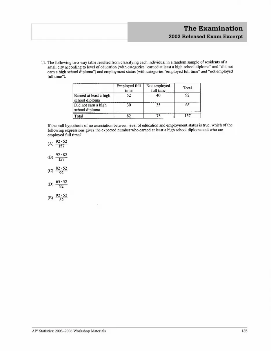
AP® Statistics: 2005–2006 Workshop Materials 135
The Examination 2002 Released Exam Excerpt
27
GO ON TO THE NEXT PAGEUnauthorized copying or reuseof any part of this page is illegal.
Section I

AP® Statistics: 2005–2006 Workshop Materials136
The Examination 2002 Released Exam Excerpt
28
GO ON TO THE NEXT PAGEUnauthorized copying or reuseof any part of this page is illegal.

AP® Statistics: 2005–2006 Workshop Materials 137
The Examination 2002 Released Exam Excerpt
29
GO ON TO THE NEXT PAGEUnauthorized copying or reuseof any part of this page is illegal.
Section I
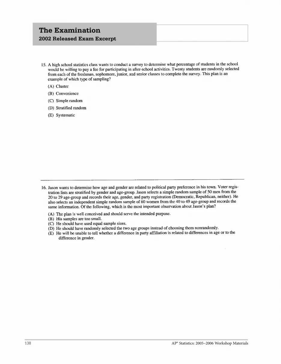
AP® Statistics: 2005–2006 Workshop Materials138
The Examination 2002 Released Exam Excerpt
30
GO ON TO THE NEXT PAGEUnauthorized copying or reuseof any part of this page is illegal.

AP® Statistics: 2005–2006 Workshop Materials 139
The Examination 2002 Released Exam Excerpt
31
GO ON TO THE NEXT PAGEUnauthorized copying or reuseof any part of this page is illegal.
Section I

AP® Statistics: 2005–2006 Workshop Materials140
The Examination 2002 Released Exam Excerpt
32
GO ON TO THE NEXT PAGEUnauthorized copying or reuseof any part of this page is illegal.

AP® Statistics: 2005–2006 Workshop Materials 141
The Examination 2002 Released Exam Excerpt
33
GO ON TO THE NEXT PAGEUnauthorized copying or reuseof any part of this page is illegal.
Section I

AP® Statistics: 2005–2006 Workshop Materials142
The Examination 2002 Released Exam Excerpt
34
GO ON TO THE NEXT PAGEUnauthorized copying or reuseof any part of this page is illegal.
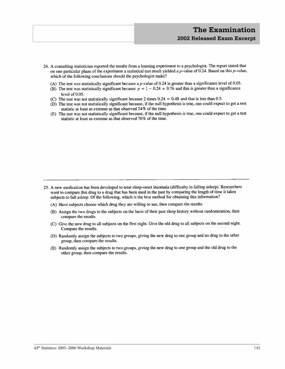
AP® Statistics: 2005–2006 Workshop Materials 143
The Examination 2002 Released Exam Excerpt
35
GO ON TO THE NEXT PAGEUnauthorized copying or reuseof any part of this page is illegal.
Section I

AP® Statistics: 2005–2006 Workshop Materials144
The Examination 2002 Released Exam Excerpt
36
GO ON TO THE NEXT PAGEUnauthorized copying or reuseof any part of this page is illegal.

AP® Statistics: 2005–2006 Workshop Materials 145
The Examination 2002 Released Exam Excerpt
37
GO ON TO THE NEXT PAGEUnauthorized copying or reuseof any part of this page is illegal.
Section I

AP® Statistics: 2005–2006 Workshop Materials146
The Examination 2002 Released Exam Excerpt
38
GO ON TO THE NEXT PAGEUnauthorized copying or reuseof any part of this page is illegal.

AP® Statistics: 2005–2006 Workshop Materials 147
The Examination 2002 Released Exam Excerpt
39
GO ON TO THE NEXT PAGEUnauthorized copying or reuseof any part of this page is illegal.
Section I

AP® Statistics: 2005–2006 Workshop Materials148
The Examination 2002 Released Exam Excerpt
40
GO ON TO THE NEXT PAGEUnauthorized copying or reuseof any part of this page is illegal.

AP® Statistics: 2005–2006 Workshop Materials 149
The Examination 2002 Released Exam Excerpt
41
GO ON TO THE NEXT PAGEUnauthorized copying or reuseof any part of this page is illegal.
Section I

AP® Statistics: 2005–2006 Workshop Materials150
The Examination 2002 Released Exam Excerpt
42
GO ON TO THE NEXT PAGEUnauthorized copying or reuseof any part of this page is illegal.

AP® Statistics: 2005–2006 Workshop Materials 151
The Examination 2002 Released Exam Excerpt
43
GO ON TO THE NEXT PAGEUnauthorized copying or reuseof any part of this page is illegal.
Section I
END OF SECTION I

AP® Statistics: 2005–2006 Workshop Materials152
The Examination 2002 Released Exam Excerpt
61
Chapter III Answers to the 2002 AP Statistics Exam
� Section I: Multiple Choice� Section I Answer Key and Percent
Answering Correctly
� Section II: Free Response� Comments from the Chief Reader� Scoring Guidelines, Sample Student
Responses, and Commentary� Part A
� Question 1� Question 2� Question 3
� Question 4� Question 5
� Part B� Question 6
Section I: Multiple Choice
Listed below are the correct answers to the multiple-choice questions, the percentage of AP students whoanswered each question correctly by AP grade, and thetotal percentage answering correctly.
1 D 97 93 90 86 78 882 B 97 92 86 79 62 813 C 97 91 85 76 56 794 A 99 97 92 83 59 845 D 99 97 90 79 53 81
6 E 89 76 66 55 37 627 A 99 96 91 83 62 848 A 88 73 59 46 33 569 E 77 54 37 27 20 39
10 D 76 51 35 26 19 37
11 B 95 86 73 59 41 6812 B 85 73 67 63 58 6713 A 94 85 75 64 46 7014 D 99 96 89 79 51 8015 D 97 94 88 79 56 81
16 E 98 95 91 86 65 8517 B 88 78 64 50 28 5818 E 66 40 26 19 15 2919 B 91 78 63 48 31 5920 B 91 76 59 46 30 57
TotalItem Correct Percent Correct by Grade PercentNo. Answer 5 4 3 2 1 Correct
Section I Answer Key and Percent Answering Correctly
21 A 79 51 32 20 14 3422 D 94 88 80 69 46 7323 E 43 26 19 16 14 2124 D 95 82 65 49 27 6025 E 93 92 91 90 78 88
26 D 83 65 49 37 23 4827 A 65 46 33 26 18 3428 E 93 76 53 37 22 5229 D 91 79 64 51 34 6130 C 72 48 33 23 18 35
31 B 98 94 86 78 53 8032 E 87 71 58 45 29 5533 B 78 54 37 25 18 3834 C 82 54 28 14 10 3335 C 43 22 16 15 15 20
36 B 88 72 57 43 29 5437 E 34 12 6 3 2 938 E 71 48 34 26 18 3639 A 24 16 13 11 9 1340 B 88 73 60 47 28 56
TotalItem Correct Percent Correct by Grade PercentNo. Answer 5 4 3 2 1 Correct

AP® Statistics: 2005–2006 Workshop Materials 153
The Examination
2005 AP® STATISTICS FREE-RESPONSE QUESTIONS
3
Formulas
(I) Descriptive Statistics
xxi
n=
sn
xi xx = − −11
2
sn s n s
n np =
− + −
− + −
121 2
22
1 2
1 1
1 1
y b b x= +0 1
bx x y y
x x
i i
i
1 2=
− −
−
b y b x0 1= −
rn
x x
s
y y
si
x
i
y= −
− −11
b rs
sy
x1 =
s
y y
n
x xb
i i
i1
2
2
2=
−−
−

AP® Statistics: 2005–2006 Workshop Materials154
The Examination
2005 AP® STATISTICS FREE-RESPONSE QUESTIONS
4
(II) Probability
P A B P A P B P A B( ) ( ) ( ) ( )∪ = + − ∩
P A BP A B
P B( )
( )( )
= ∩
E X x xi pi( ) = =µ
Var( )X x pix i x= = −2 2µ
If X has a binomial distribution with parameters n and p , then:
P X kn
kpk p n k( ) ( )= = − −1
µ x np=
x np p= −( )1
µ p p=
( )p
p pn
= −1
If x is the mean of a random sample of size n from an infinite population with mean µ and standard deviation , then:
µ µx =
x n=

AP® Statistics: 2005–2006 Workshop Materials 155
The Examination
2005 AP® STATISTICS FREE-RESPONSE QUESTIONS
5
(III) Inferential Statistics
Standardized test statistic:statistic parameter
standard deviation of statistic
Confidence interval: statistic critical value standard deviation of statistic
Single-Sample
Statistic Standard Deviation of Statistic
Sample Mean σn
Sample Proportion p p
n( )1 −
Two-Sample
Statistic Standard Deviation of Statistic
Difference of sample means
σ σ12
1
22
2n n+
Special case when σ σ1 2=
σ 1 1
1 2n n+
Difference of sample proportions
p pn
p pn
1 1
1
2 2
2
1 1( ) ( )−+
−
Special case when p p1 2=
p p1− 1 1
1 2n n+
Chi-square test statisticobserved expected
expected=
− 2

AP® Statistics: 2005–2006 Workshop Materials156
The Examination
2005 AP® STATISTICS FREE-RESPONSE QUESTIONS
Copyright © 2005 by College Entrance Examination Board. All rights reserved. Visit apcentral.collegeboard.com (for AP professionals) and www.collegeboard.com/apstudents (for AP students and parents).
GO ON TO THE NEXT PAGE. 6
STATISTICS SECTION II
Part A Questions 1-5
Spend about 65 minutes on this part of the exam. Percent of Section II grade—75
Directions: Show all your work. Indicate clearly the methods you use, because you will be graded on the correctness of your methods as well as on the accuracy of your results and explanation.
1. The goal of a nutritional study was to compare the caloric intake of adolescents living in rural areas of the United States with the caloric intake of adolescents living in urban areas of the United States. A random sample of ninth-grade students from one high school in a rural area was selected. Another random sample of ninth graders from one high school in an urban area was also selected. Each student in each sample kept records of all the food he or she consumed in one day.
The back-to-back stemplot below displays the number of calories of food consumed per kilogram of body weight for each student on that day.
Urban Rural 9 9 9 9 8 8 7 6 2 4 4 3 1 0 3 2 3 3 4 9 7 6 6 5 3 5 6 6 6 7 2 0 4 0 2 2 2 4 4 5 6 8 8 9 5 1 Stem: tens Leaf: ones
(a) Write a few sentences comparing the distribution of the daily caloric intake of ninth-grade students in the rural high school with the distribution of the daily caloric intake of ninth-grade students in the urban high school.
(b) Is it reasonable to generalize the findings of this study to all rural and urban ninth-grade students in the United States? Explain.
(c) Researchers who want to conduct a similar study are debating which of the following two plans to use.
Plan I: Have each student in the study record all the food he or she consumed in one day. Then researchers would compute the number of calories of food consumed per kilogram of body weight for each student for that day.
Plan II: Have each student in the study record all the food he or she consumed over the same 7-day period. Then researchers would compute the average daily number of calories of food consumed per kilogram of body weight for each student during that 7-day period.
Assuming that the students keep accurate records, which plan, I or II, would better meet the goal of the study? Justify your answer.

AP® Statistics: 2005–2006 Workshop Materials 157
The Examination
2005 AP® STATISTICS FREE-RESPONSE QUESTIONS
Copyright © 2005 by College Entrance Examination Board. All rights reserved. Visit apcentral.collegeboard.com (for AP professionals) and www.collegeboard.com/apstudents (for AP students and parents).
GO ON TO THE NEXT PAGE. 7
2. Let the random variable X represent the number of telephone lines in use by the technical support center of a software manufacturer at noon each day. The probability distribution of X is shown in the table below.
x 0 1 2 3 4 5 p x 0.35 0.20 0.15 0.15 0.10 0.05
(a) Calculate the expected value (the mean) of X.
(b) Using past records, the staff at the technical support center randomly selected 20 days and found that an average of 1.25 telephone lines were in use at noon on those days. The staff proposes to select another random sample of 1,000 days and compute the average number of telephone lines that were in use at noon on those days. How do you expect the average from this new sample to compare to that of the first sample? Justify your response.
(c) The median of a random variable is defined as any value x such that ( ) 0.5P X x and ( ) 0.5.P X xFor the probability distribution shown in the table above, determine the median of X.
(d) In a sentence or two, comment on the relationship between the mean and the median relative to the shape of this distribution.

AP® Statistics: 2005–2006 Workshop Materials158
The Examination
2005 AP® STATISTICS FREE-RESPONSE QUESTIONS
Copyright © 2005 by College Entrance Examination Board. All rights reserved. Visit apcentral.collegeboard.com (for AP professionals) and www.collegeboard.com/apstudents (for AP students and parents).
GO ON TO THE NEXT PAGE. 8
3. The Great Plains Railroad is interested in studying how fuel consumption is related to the number of railcars for its trains on a certain route between Oklahoma City and Omaha.
A random sample of 10 trains on this route has yielded the data in the table below.
Number of Railcars
Fuel Consumption (units/mile)
20 58 20 52 37 91 31 80 47 114 43 98 39 87 50 122 40 100 29 70
A scatterplot, a residual plot, and the output from the regression analysis for these data are shown below.

AP® Statistics: 2005–2006 Workshop Materials 159
The Examination
2005 AP® STATISTICS FREE-RESPONSE QUESTIONS
Copyright © 2005 by College Entrance Examination Board. All rights reserved. Visit apcentral.collegeboard.com (for AP professionals) and www.collegeboard.com/apstudents (for AP students and parents).
GO ON TO THE NEXT PAGE. 9
The regression equation is Fuel Consumption = 10.7 + 2.15 Railcars
Predictor Coef StDev T P Constant 10.677 5.157 2.07 0.072 Railcar 2.1495 0.1396 15.40 0.000
S = 4.361 R-Sq = 96.7% R-Sq(adj) = 96.3%
(a) Is a linear model appropriate for modeling these data? Clearly explain your reasoning.
(b) Suppose the fuel consumption cost is $25 per unit. Give a point estimate (single value) for the change in the average cost of fuel per mile for each additional railcar attached to a train. Show your work.
(c) Interpret the value of r2 in the context of this problem.
(d) Would it be reasonable to use the fitted regression equation to predict the fuel consumption for a train on this route if the train had 65 railcars? Explain.
4. Some boxes of a certain brand of breakfast cereal include a voucher for a free video rental inside the box. The company that makes the cereal claims that a voucher can be found in 20 percent of the boxes. However, based on their experiences eating this cereal at home, a group of students believes that the proportion of boxes with vouchers is less than 0.2. This group of students purchased 65 boxes of the cereal to investigate the company’s claim. The students found a total of 11 vouchers for free video rentals in the 65 boxes.
Suppose it is reasonable to assume that the 65 boxes purchased by the students are a random sample of all boxes of this cereal. Based on this sample, is there support for the students’ belief that the proportion of boxes with vouchers is less than 0.2 ? Provide statistical evidence to support your answer.
5. A survey will be conducted to examine the educational level of adult heads of households in the United States. Each respondent in the survey will be placed into one of the following two categories:
• Does not have a high school diploma • Has a high school diploma
The survey will be conducted using a telephone interview. Random-digit dialing will be used to select the sample.
(a) For this survey, state one potential source of bias and describe how it might affect the estimate of the proportion of adult heads of households in the United States who do not have a high school diploma.
(b) A pilot survey indicated that about 22 percent of the population of adult heads of households do not have a high school diploma. Using this information, how many respondents should be obtained if the goal of the survey is to estimate the proportion of the population who do not have a high school diploma to within 0.03 with 95 percent confidence? Justify your answer.
(c) Since education is largely the responsibility of each state, the agency wants to be sure that estimates are available for each state as well as for the nation. Identify a sampling method that will achieve this additional goal and briefly describe a way to select the survey sample using this method.

AP® Statistics: 2005–2006 Workshop Materials160
The Examination
2005 AP® STATISTICS FREE-RESPONSE QUESTIONS
Copyright © 2005 by College Entrance Examination Board. All rights reserved. Visit apcentral.collegeboard.com (for AP professionals) and www.collegeboard.com/apstudents (for AP students and parents).
GO ON TO THE NEXT PAGE. 10
Part B Question 6
Spend about 25 minutes on this part of the exam. Percent of Section II grade—25
Directions: Show all your work. Indicate clearly the methods you use, because you will be graded on the correctness of your methods as well as on the accuracy of your results and explanation.
6. Lead, found in some paints, is a neurotoxin that can be especially harmful to the developing brain and nervous system of children. Children frequently put their hands in their mouth after touching painted surfaces, and this is the most common type of exposure to lead.
A study was conducted to investigate whether there were differences in children’s exposure to lead between suburban day-care centers and urban day-care centers in one large city. For this study, researchers used a random sample of 20 children in suburban day-care centers. Ten of these 20 children were randomly selected to play outside; the remaining 10 children played inside. All children had their hands wiped clean before beginning their assigned one-hour play period either outside or inside. After the play period ended, the amount of lead in micrograms (mcg) on each child’s dominant hand was recorded.
The mean amount of lead on the dominant hand for the children playing inside was 3.75 mcg, and the mean amount of lead for the children playing outside was 5.65 mcg. A 95 percent confidence interval for the difference in the mean amount of lead after one hour inside versus one hour outside was calculated to be
2.46, 1.34 .
A random sample of 18 children in urban day-care centers in the same large city was selected. For this sample, the same process was used, including randomly assigning children to play inside or outside. The data for the amount (in mcg) of lead on each child’s dominant hand are shown in the table below.
Urban Day-Care Centers
Inside 6 5 4 4 4.5 5 4.5 3 5 Outside 15 25 18 14 20 13 11 22 20
(a) Use a 95 percent confidence interval to estimate the difference in the mean amount of lead on a child’s dominant hand after an hour of play inside versus an hour of play outside at urban day-care centers in this city. Be sure to interpret your interval.

AP® Statistics: 2005–2006 Workshop Materials 161
The Examination
2005 AP® STATISTICS FREE-RESPONSE QUESTIONS
Copyright © 2005 by College Entrance Examination Board. All rights reserved. Visit apcentral.collegeboard.com (for AP professionals) and www.collegeboard.com/apstudents (for AP students and parents).
11
(b) On the figure below,
• Using the vertical axis for the mean amount of lead, plot the mean for the amounts of lead on the dominant hand of children who played inside at the suburban day-care center and then plot the mean for the amounts of lead on the dominant hand of children who played inside at the urban day-care center.
• Connect these two points with a line segment.
• Plot the two means (suburban and urban) for the children who played outside at the two types of day-care centers.
• Connect these two points with a second line segment.
Suburban Urban
(c) From the study, what conclusions can be drawn about the impact of setting (inside, outside), environment (suburban, urban), and the relationship between the two on the amount of lead on the dominant hand of children after play in this city? Justify your answer.
END OF EXAM

AP® Statistics: 2005–2006 Workshop Materials162
The Examination
2005 AP® STATISTICS FREE-RESPONSE QUESTIONS
12
Probability
z
Table A Standard normal probabilities
z .00 .01 .02 .03 .04 .05 .06 .07 .08 .09
–3.4 .0003 .0003 .0003 .0003 .0003 .0003 .0003 .0003 .0003 .0002 –3.3 .0005 .0005 .0005 .0004 .0004 .0004 .0004 .0004 .0004 .0003 –3.2 .0007 .0007 .0006 .0006 .0006 .0006 .0006 .0005 .0005 .0005 –3.1 .0010 .0009 .0009 .0009 .0008 .0008 .0008 .0008 .0007 .0007 –3.0 .0013 .0013 .0013 .0012 .0012 .0011 .0011 .0011 .0010 .0010 –2.9 .0019 .0018 .0018 .0017 .0016 .0016 .0015 .0015 .0014 .0014 –2.8 .0026 .0025 .0024 .0023 .0023 .0022 .0021 .0021 .0020 .0019 –2.7 .0035 .0034 .0033 .0032 .0031 .0030 .0029 .0028 .0027 .0026 –2.6 .0047 .0045 .0044 .0043 .0041 .0040 .0039 .0038 .0037 .0036 –2.5 .0062 .0060 .0059 .0057 .0055 .0054 .0052 .0051 .0049 .0048 –2.4 .0082 .0080 .0078 .0075 .0073 .0071 .0069 .0068 .0066 .0064 –2.3 .0107 .0104 .0102 .0099 .0096 .0094 .0091 .0089 .0087 .0084 –2.2 .0139 .0136 .0132 .0129 .0125 .0122 .0119 .0116 .0113 .0110 –2.1 .0179 .0174 .0170 .0166 .0162 .0158 .0154 .0150 .0146 .0143 –2.0 .0228 .0222 .0217 .0212 .0207 .0202 .0197 .0192 .0188 .0183 –1.9 .0287 .0281 .0274 .0268 .0262 .0256 .0250 .0244 .0239 .0233 –1.8 .0359 .0351 .0344 .0336 .0329 .0322 .0314 .0307 .0301 .0294 –1.7 .0446 .0436 .0427 .0418 .0409 .0401 .0392 .0384 .0375 .0367 –1.6 .0548 .0537 .0526 .0516 .0505 .0495 .0485 .0475 .0465 .0455 –1.5 .0668 .0655 .0643 .0630 .0618 .0606 .0594 .0582 .0571 .0559 –1.4 .0808 .0793 .0778 .0764 .0749 .0735 .0721 .0708 .0694 .0681 –1.3 .0968 .0951 .0934 .0918 .0901 .0885 .0869 .0853 .0838 .0823 –1.2 .1151 .1131 .1112 .1093 .1075 .1056 .1038 .1020 .1003 .0985 –1.1 .1357 .1335 .1314 .1292 .1271 .1251 .1230 .1210 .1190 .1170 –1.0 .1587 .1562 .1539 .1515 .1492 .1469 .1446 .1423 .1401 .1379 –0.9 .1841 .1814 .1788 .1762 .1736 .1711 .1685 .1660 .1635 .1611 –0.8 .2119 .2090 .2061 .2033 .2005 .1977 .1949 .1922 .1894 .1867 –0.7 .2420 .2389 .2358 .2327 .2296 .2266 .2236 .2206 .2177 .2148 –0.6 .2743 .2709 .2676 .2643 .2611 .2578 .2546 .2514 .2483 .2451 –0.5 .3085 .3050 .3015 .2981 .2946 .2912 .2877 .2843 .2810 .2776 –0.4 .3446 .3409 .3372 .3336 .3300 .3264 .3228 .3192 .3156 .3121 –0.3 .3821 .3783 .3745 .3707 .3669 .3632 .3594 .3557 .3520 .3483 –0.2 .4207 .4168 .4129 .4090 .4052 .4013 .3974 .3936 .3897 .3859 –0.1 .4602 .4562 .4522 .4483 .4443 .4404 .4364 .4325 .4286 .4247 –0.0 .5000 .4960 .4920 .4880 .4840 .4801 .4761 .4721 .4681 .4641
Table entry for z is the probability lying below z.

AP® Statistics: 2005–2006 Workshop Materials 163
The Examination
2005 AP® STATISTICS FREE-RESPONSE QUESTIONS
13
Probability
z
Table A (Continued)
z .00 .01 .02 .03 .04 .05 .06 .07 .08 .09
0.0 .5000 .5040 .5080 .5120 .5160 .5199 .5239 .5279 .5319 .5359 0.1 .5398 .5438 .5478 .5517 .5557 .5596 .5636 .5675 .5714 .5753 0.2 .5793 .5832 .5871 .5910 .5948 .5987 .6026 .6064 .6103 .6141 0.3 .6179 .6217 .6255 .6293 .6331 .6368 .6406 .6443 .6480 .6517 0.4 .6554 .6591 .6628 .6664 .6700 .6736 .6772 .6808 .6844 .6879 0.5 .6915 .6950 .6985 .7019 .7054 .7088 .7123 .7157 .7190 .7224 0.6 .7257 .7291 .7324 .7357 .7389 .7422 .7454 .7486 .7517 .7549 0.7 .7580 .7611 .7642 .7673 .7704 .7734 .7764 .7794 .7823 .7852 0.8 .7881 .7910 .7939 .7967 .7995 .8023 .8051 .8078 .8106 .8133 0.9 .8159 .8186 .8212 .8238 .8264 .8289 .8315 .8340 .8365 .8389 1.0 .8413 .8438 .8461 .8485 .8508 .8531 .8554 .8577 .8599 .8621 1.1 .8643 .8665 .8686 .8708 .8729 .8749 .8770 .8790 .8810 .8830 1.2 .8849 .8869 .8888 .8907 .8925 .8944 .8962 .8980 .8997 .9015 1.3 .9032 .9049 .9066 .9082 .9099 .9115 .9131 .9147 .9162 .9177 1.4 .9192 .9207 .9222 .9236 .9251 .9265 .9279 .9292 .9306 .9319 1.5 .9332 .9345 .9357 .9370 .9382 .9394 .9406 .9418 .9429 .9441 1.6 .9452 .9463 .9474 .9484 .9495 .9505 .9515 .9525 .9535 .9545 1.7 .9554 .9564 .9573 .9582 .9591 .9599 .9608 .9616 .9625 .9633 1.8 .9641 .9649 .9656 .9664 .9671 .9678 .9686 .9693 .9699 .9706 1.9 .9713 .9719 .9726 .9732 .9738 .9744 .9750 .9756 .9761 .9767 2.0 .9772 .9778 .9783 .9788 .9793 .9798 .9803 .9808 .9812 .9817 2.1 .9821 .9826 .9830 .9834 .9838 .9842 .9846 .9850 .9854 .9857 2.2 .9861 .9864 .9868 .9871 .9875 .9878 .9881 .9884 .9887 .9890 2.3 .9893 .9896 .9898 .9901 .9904 .9906 .9909 .9911 .9913 .9916 2.4 .9918 .9920 .9922 .9925 .9927 .9929 .9931 .9932 .9934 .9936 2.5 .9938 .9940 .9941 .9943 .9945 .9946 .9948 .9949 .9951 .9952 2.6 .9953 .9955 .9956 .9957 .9959 .9960 .9961 .9962 .9963 .9964 2.7 .9965 .9966 .9967 .9968 .9969 .9970 .9971 .9972 .9973 .9974 2.8 .9974 .9975 .9976 .9977 .9977 .9978 .9979 .9979 .9980 .9981 2.9 .9981 .9982 .9982 .9983 .9984 .9984 .9985 .9985 .9986 .9986 3.0 .9987 .9987 .9987 .9988 .9988 .9989 .9989 .9989 .9990 .9990 3.1 .9990 .9991 .9991 .9991 .9992 .9992 .9992 .9992 .9993 .9993 3.2 .9993 .9993 .9994 .9994 .9994 .9994 .9994 .9995 .9995 .9995 3.3 .9995 .9995 .9995 .9996 .9996 .9996 .9996 .9996 .9996 .9997 3.4 .9997 .9997 .9997 .9997 .9997 .9997 .9997 .9997 .9997 .9998
Table entry for z is the probability lying below z.

AP® Statistics: 2005–2006 Workshop Materials164
The Examination
2005 AP® STATISTICS FREE-RESPONSE QUESTIONS
14
Probability p
t*
Table B t distribution critical values
Tail probability p
df .25 .20 .15 .10 .05 .025 .02 .01 .005 .0025 .001 .0005
1 1.000 1.376 1.963 3.078 6.314 12.71 15.89 31.82 63.66 127.3 318.3 636.6 2 .816 1.061 1.386 1.886 2.920 4.303 4.849 6.965 9.925 14.09 22.33 31.60 3 .765 .978 1.250 1.638 2.353 3.182 3.482 4.541 5.841 7.453 10.21 12.92 4 .741 .941 1.190 1.533 2.132 2.776 2.999 3.747 4.604 5.598 7.173 8.610 5 .727 .920 1.156 1.476 2.015 2.571 2.757 3.365 4.032 4.773 5.893 6.869 6 .718 .906 1.134 1.440 1.943 2.447 2.612 3.143 3.707 4.317 5.208 5.959 7 .711 .896 1.119 1.415 1.895 2.365 2.517 2.998 3.499 4.029 4.785 5.408 8 .706 .889 1.108 1.397 1.860 2.306 2.449 2.896 3.355 3.833 4.501 5.041 9 .703 .883 1.100 1.383 1.833 2.262 2.398 2.821 3.250 3.690 4.297 4.781
10 .700 .879 1.093 1.372 1.812 2.228 2.359 2.764 3.169 3.581 4.144 4.587 11 .697 .876 1.088 1.363 1.796 2.201 2.328 2.718 3.106 3.497 4.025 4.437 12 .695 .873 1.083 1.356 1.782 2.179 2.303 2.681 3.055 3.428 3.930 4.318 13 .694 .870 1.079 1.350 1.771 2.160 2.282 2.650 3.012 3.372 3.852 4.221 14 .692 .868 1.076 1.345 1.761 2.145 2.264 2.624 2.977 3.326 3.787 4.140 15 .691 .866 1.074 1.341 1.753 2.131 2.249 2.602 2.947 3.286 3.733 4.073 16 .690 .865 1.071 1.337 1.746 2.120 2.235 2.583 2.921 3.252 3.686 4.015 17 .689 .863 1.069 1.333 1.740 2.110 2.224 2.567 2.898 3.222 3.646 3.965 18 .688 .862 1.067 1.330 1.734 2.101 2.214 2.552 2.878 3.197 3.611 3.922 19 .688 .861 1.066 1.328 1.729 2.093 2.205 2.539 2.861 3.174 3.579 3.883 20 .687 .860 1.064 1.325 1.725 2.086 2.197 2.528 2.845 3.153 3.552 3.850 21 .686 .859 1.063 1.323 1.721 2.080 2.189 2.518 2.831 3.135 3.527 3.819 22 .686 .858 1.061 1.321 1.717 2.074 2.183 2.508 2.819 3.119 3.505 3.792 23 .685 .858 1.060 1.319 1.714 2.069 2.177 2.500 2.807 3.104 3.485 3.768 24 .685 .857 1.059 1.318 1.711 2.064 2.172 2.492 2.797 3.091 3.467 3.745 25 .684 .856 1.058 1.316 1.708 2.060 2.167 2.485 2.787 3.078 3.450 3.725 26 .684 .856 1.058 1.315 1.706 2.056 2.162 2.479 2.779 3.067 3.435 3.707 27 .684 .855 1.057 1.314 1.703 2.052 2.158 2.473 2.771 3.057 3.421 3.690 28 .683 .855 1.056 1.313 1.701 2.048 2.154 2.467 2.763 3.047 3.408 3.674 29 .683 .854 1.055 1.311 1.699 2.045 2.150 2.462 2.756 3.038 3.396 3.659 30 .683 .854 1.055 1.310 1.697 2.042 2.147 2.457 2.750 3.030 3.385 3.646 40 .681 .851 1.050 1.303 1.684 2.021 2.123 2.423 2.704 2.971 3.307 3.551 50 .679 .849 1.047 1.299 1.676 2.009 2.109 2.403 2.678 2.937 3.261 3.496 60 .679 .848 1.045 1.296 1.671 2.000 2.099 2.390 2.660 2.915 3.232 3.460 80 .678 .846 1.043 1.292 1.664 1.990 2.088 2.374 2.639 2.887 3.195 3.416
100 .677 .845 1.042 1.290 1.660 1.984 2.081 2.364 2.626 2.871 3.174 3.390 1000 .675 .842 1.037 1.282 1.646 1.962 2.056 2.330 2.581 2.813 3.098 3.300
� .674 .841 1.036 1.282 1.645 1.960 2.054 2.326 2.576 2.807 3.091 3.291
50% 60% 70% 80% 90% 95% 96% 98% 99% 99.5% 99.8% 99.9%
Confidence level C
Table entry for p and C is the point t* with probability p lying above it and probability C lying between −t * and t*.

AP® Statistics: 2005–2006 Workshop Materials 165
The Examination
2005 AP® STATISTICS FREE-RESPONSE QUESTIONS
15
Probability p
(χ2)
Table C χ 2 critical values
Tail probability p
df .25 .20 .15 .10 .05 .025 .02 .01 .005 .0025 .001 .0005
1 1.32 1.64 2.07 2.71 3.84 5.02 5.41 6.63 7.88 9.14 10.83 12.12 2 2.77 3.22 3.79 4.61 5.99 7.38 7.82 9.21 10.60 11.98 13.82 15.20 3 4.11 4.64 5.32 6.25 7.81 9.35 9.84 11.34 12.84 14.32 16.27 17.73 4 5.39 5.99 6.74 7.78 9.49 11.14 11.67 13.28 14.86 16.42 18.47 20.00 5 6.63 7.29 8.12 9.24 11.07 12.83 13.39 15.09 16.75 18.39 20.51 22.11 6 7.84 8.56 9.45 10.64 12.59 14.45 15.03 16.81 18.55 20.25 22.46 24.10 7 9.04 9.80 10.75 12.02 14.07 16.01 16.62 18.48 20.28 22.04 24.32 26.02 8 10.22 11.03 12.03 13.36 15.51 17.53 18.17 20.09 21.95 23.77 26.12 27.87 9 11.39 12.24 13.29 14.68 16.92 19.02 19.68 21.67 23.59 25.46 27.88 29.67
10 12.55 13.44 14.53 15.99 18.31 20.48 21.16 23.21 25.19 27.11 29.59 31.42 11 13.70 14.63 15.77 17.28 19.68 21.92 22.62 24.72 26.76 28.73 31.26 33.14 12 14.85 15.81 16.99 18.55 21.03 23.34 24.05 26.22 28.30 30.32 32.91 34.82 13 15.98 16.98 18.20 19.81 22.36 24.74 25.47 27.69 29.82 31.88 34.53 36.48 14 17.12 18.15 19.41 21.06 23.68 26.12 26.87 29.14 31.32 33.43 36.12 38.11 15 18.25 19.31 20.60 22.31 25.00 27.49 28.26 30.58 32.80 34.95 37.70 39.72 16 19.37 20.47 21.79 23.54 26.30 28.85 29.63 32.00 34.27 36.46 39.25 41.31 17 20.49 21.61 22.98 24.77 27.59 30.19 31.00 33.41 35.72 37.95 40.79 42.88 18 21.60 22.76 24.16 25.99 28.87 31.53 32.35 34.81 37.16 39.42 42.31 44.43 19 22.72 23.90 25.33 27.20 30.14 32.85 33.69 36.19 38.58 40.88 43.82 45.97 20 23.83 25.04 26.50 28.41 31.41 34.17 35.02 37.57 40.00 42.34 45.31 47.50 21 24.93 26.17 27.66 29.62 32.67 35.48 36.34 38.93 41.40 43.78 46.80 49.01 22 26.04 27.30 28.82 30.81 33.92 36.78 37.66 40.29 42.80 45.20 48.27 50.51 23 27.14 28.43 29.98 32.01 35.17 38.08 38.97 41.64 44.18 46.62 49.73 52.00 24 28.24 29.55 31.13 33.20 36.42 39.36 40.27 42.98 45.56 48.03 51.18 53.48 25 29.34 30.68 32.28 34.38 37.65 40.65 41.57 44.31 46.93 49.44 52.62 54.95 26 30.43 31.79 33.43 35.56 38.89 41.92 42.86 45.64 48.29 50.83 54.05 56.41 27 31.53 32.91 34.57 36.74 40.11 43.19 44.14 46.96 49.64 52.22 55.48 57.86 28 32.62 34.03 35.71 37.92 41.34 44.46 45.42 48.28 50.99 53.59 56.89 59.30 29 33.71 35.14 36.85 39.09 42.56 45.72 46.69 49.59 52.34 54.97 58.30 60.73 30 34.80 36.25 37.99 40.26 43.77 46.98 47.96 50.89 53.67 56.33 59.70 62.16 40 45.62 47.27 49.24 51.81 55.76 59.34 60.44 63.69 66.77 69.70 73.40 76.09 50 56.33 58.16 60.35 63.17 67.50 71.42 72.61 76.15 79.49 82.66 86.66 89.56 60 66.98 68.97 71.34 74.40 79.08 83.30 84.58 88.38 91.95 95.34 99.61 102.7 80 88.13 90.41 93.11 96.58 101.9 106.6 108.1 112.3 116.3 120.1 124.8 128.3
100 109.1 111.7 114.7 118.5 124.3 129.6 131.1 135.8 140.2 144.3 149.4 153.2
Table entry for p is the point
( )χ 2 with probability p lying above it.

AP® Statistics: 2005–2006 Workshop Materials166
The Examination
AP® STATISTICS 2005 SCORING GUIDELINES
Copyright © 2005 by College Board. All rights reserved. Visit apcentral.collegeboard.com (for AP professionals) and www.collegeboard.com/apstudents (for AP students and parents).
2
Question 1
Solution
Part (a):
The mean (40.45 cal/kg) and median (41 cal/kg) daily caloric intake of ninth-grade students in the rural school are higher than the corresponding measures of center, mean (32.6 cal/kg) and median (32 cal/kg), for ninth-graders in the urban school. There is also more variability or spread in the daily caloric intake for students in the rural school (Range=19, SD=6.04, IQR=10) than in the daily caloric intake for students in the urban school (Range=16, SD=4.67, IQR=7). The shapes of the two distributions are also different. The distribution of daily caloric intake for rural students is more uniformly distributed (symmetric) between 32 cal/kg and 51 cal/kg while the distribution of daily caloric intake for urban students appears to be skewed toward the larger values.
Part (b):
No, the samples include students from only one rural and one urban high school so it is not reasonable to generalize the findings from these two schools to all rural and urban ninth-grade students in the United States.
Part (c):
Since we are assuming that students keep accurate records, Plan II will do a better job of comparing the daily caloric intake of adolescents living in rural areas with the daily caloric intake of adolescents living in urban areas. Both plans take body weight into account by converting to food consumed per kilogram of body weight. Plan II includes a 7-day period (possibly days in school and days at home on the weekend), and there are differences in caloric intake among days. It would therefore be better to average over the 7-day period rather than considering only the food consumed in one day, as is the case with Plan I. Plan II would provide a more precise estimate of the average daily intake.
Scoring
Parts (a) and (c) are scored as essentially correct (E), partially correct (P), or incorrect (I). Part (b) is scored as essentially correct (E) or incorrect (I).
Part (a) is essentially correct (E) if the student correctly compares center, shape, and spread of the two distributions. Specific numerical values are not required.
Part (a) is partially correct (P) if the student correctly compares any two of the three characteristics (center, shape, or spread) of the two distributions.
Part (a) is incorrect (I) if the student correctly compares no more than one characteristic.

AP® Statistics: 2005–2006 Workshop Materials 167
The Examination
AP® STATISTICS 2005 SCORING GUIDELINES
Copyright © 2005 by College Board. All rights reserved. Visit apcentral.collegeboard.com (for AP professionals) and www.collegeboard.com/apstudents (for AP students and parents).
3
Question 1 (continued)
Part (b) is essentially correct (E) if the student realizes that these findings cannot be generalized because the students were selected from only one rural and one urban high school.
Part (b) is incorrect (I) if the student argues that these findings: • cannot be generalized with no explanation given; OR • cannot be generalized with an invalid explanation (e.g., the response indicates that the student sample
size (n=20) is not big enough); OR • can be generalized because the randomly selected students from these two schools may represent all
urban and rural ninth-grade students in the United States.
Part (c) is essentially correct (E) if Plan II is chosen and a correct justification involving day-to-day variability is provided.
Part (c) is partially correct (P) if Plan II is chosen, but a weak statistical justification that includes a discussion of day-to-day variability is provided.
Part (c) is incorrect (I) if: • Plan I is chosen; OR • Plan II is chosen and a correct justification is not provided.
4 Complete Response (3E)
All three parts essentially correct
3 Substantial Response (2E 1P)
Two parts essentially correct and one part partially correct
2 Developing Response (2E 0P or 1E 2P)
Two parts essentially correct and zero parts partially correct OROne part essentially correct and two parts partially correct
1 Minimal Response ( 1E 1P or 1E 0P or 0E 2P)
One part essentially correct and either zero parts or one part partially correct OR
Zero parts essentially correct and two parts partially correct

AP® Statistics: 2005–2006 Workshop Materials168
The Examination
AP® STATISTICS 2005 SCORING GUIDELINES
Copyright © 2005 by College Board. All rights reserved. Visit apcentral.collegeboard.com (for AP professionals) and www.collegeboard.com/apstudents (for AP students and parents).
4
Question 2
Solution
Part (a):
The expected number of telephone lines in use by the technical support center at noon is:
0 0.35 1 0.2 2 0.15 3 0.15 4 0.1 5 0.05
1.6
E X
Part (b):
We would expect the average based on 1,000 days to be closer to 1.6 than the first average based on 20 days. Both averages have the same expected value (1.6), but the variability for sample averages based on 1,000 days is smaller than the variability for sample averages based on 20 days.
Part (c):
The median of X is 1.
x P X x P X x
0 0.35 1.0 1 0.55 0.65 2 0.70 0.45 3 0.85 0.30 4 0.95 0.15 5 1.0 0.05
OR
The median of X is 1 because 1 0.55 0.50P X and 1 0.65 0.50P X .
Part (d):
The probability histogram is clearly skewed to the right (or toward the larger values) so the mean (1.6) is larger than the median (1), as is typical for a right-skewed distribution.

AP® Statistics: 2005–2006 Workshop Materials 169
The Examination
AP® STATISTICS 2005 SCORING GUIDELINES
Copyright © 2005 by College Board. All rights reserved. Visit apcentral.collegeboard.com (for AP professionals) and www.collegeboard.com/apstudents (for AP students and parents).
5
Question 2 (continued)
Scoring
Parts (a) and (c) are combined as one computational part. Each part is scored as essentially correct (E), partially correct (P), or incorrect (I).
Collectively parts (a) and (c) are essentially correct (E) if both parts are calculated correctly, with the exception of minor arithmetic errors.
Collectively parts (a) and (c) are partially correct (P) if one of the two parts is calculated correctly, with the exception of minor arithmetic errors.
Collectively parts (a) and (c) are incorrect (I) if both parts are calculated incorrectly.
Note: Unsupported answers in parts (a) and (c) are scored as incorrect.
Part (b) is essentially correct (E) if the student: 1. States the new estimate based on 1,000 days should be closer to the expected value of 1.6; OR
the new estimate will increase, or decrease if the answer in part (a) is less than 1.25. AND2. Provides justification by stating the variability for sample averages based on 1,000 days will be smaller
than the variability for sample averages based on 20 days; OR as the sample size increases the sample average approaches the expected value of X.
Part (b) is partially correct (P) if the student provides one of the two items above.
Part (d) is essentially correct (E) if the student states that since the distribution is skewed to the right, the mean is greater than the median; OR since the mean is greater than the median, the distribution is skewed to the right.
Note: There must be evidence that the student looked at the given distribution.
Part (d) is partially correct (P) if the student: • States that since the mean is greater than the median, the distribution is skewed to the right (with no
evidence that the student looked at the given distribution); OR • Compares the two measures of center by referring to the inappropriate or incomplete shape of the
distribution (e.g., “skewed to the left” or “skewed”); OR • Makes a correct statement about the measures of center and the shape without connecting the two.

AP® Statistics: 2005–2006 Workshop Materials170
The Examination
AP® STATISTICS 2005 SCORING GUIDELINES
Copyright © 2005 by College Board. All rights reserved. Visit apcentral.collegeboard.com (for AP professionals) and www.collegeboard.com/apstudents (for AP students and parents).
6
Question 2 (continued)
Part (d) is incorrect (I) if the student: • Compares the two measures of center without mentioning the shape of the distribution; OR • Correctly describes the shape without correct conclusions about the relative location of the mean and
median; OR • Makes multiple “generic” statements about the relationship of mean, median, and shape with no
reference to the given distribution.
4 Complete Response (3E)
All three parts essentially correct
3 Substantial Response (2E 1P)
Two parts essentially correct and one part partially correct
2 Developing Response (2E 0P or 1E 2P)
Two parts essentially correct and zero parts partially correct OROne part essentially correct and two parts partially correct
1 Minimal Response ( 1E 1P or 1E 0P or 0E 2P)
One part essentially correct and either zero parts or one part partially correct OR
Zero parts essentially correct and two parts partially correct

AP® Statistics: 2005–2006 Workshop Materials 171
The Examination
AP® STATISTICS 2005 SCORING GUIDELINES
Copyright © 2005 by College Board. All rights reserved. Visit apcentral.collegeboard.com (for AP professionals) and www.collegeboard.com/apstudents (for AP students and parents).
7
Question 3
Solution
Part (a):
Yes, the linear model is appropriate for these data. The scatterplot shows a strong, positive, linear association between the number of railcars and fuel consumption, and the residual plot shows a reasonably random scatter of points above and below zero.
Part (b):
According to the regression output, fuel consumption will increase by 2.15 units for each additional railcar. Since the fuel consumption cost is $25 per unit, the average cost of fuel per mile will increase by approximately $25 2.15 $53.75 for each railcar that is added to the train.
Part (c):
The regression output indicates that 2 96.7%r or 0.967. Thus, 96.7% of the variation in the fuel consumption values is explained by using the linear regression model with number of railcars as the explanatory variable.
Part (d):
No, the data set does not contain any information about fuel consumption for any trains with more than 50 cars. Using the regression model to predict the fuel consumption for a train with 65 railcars, known as extrapolation, is not reasonable.
Scoring
Each part is scored as essentially correct (E), partially correct (P), or incorrect (I).
Part (a) is essentially correct (E) if the model is deemed appropriate AND the explanation clearly indicates: • There is a linear pattern in the scatterplot; OR • There is no pattern in the residual plot.
Part (a) is partially correct (P) if the: • Model is deemed appropriate AND the student refers to the scatterplot or residual plot but fails to state
the relevant characteristic of the plot; OR • Student refers to the relevant characteristic of the scatterplot or residual plot without deeming model
appropriate.
Part (a) is incorrect (I) if the student: • States that the model is appropriate without an explanation; OR • States that the model is inappropriate; OR • Makes a decision based only on numeric values from the computer output.

AP® Statistics: 2005–2006 Workshop Materials172
The Examination
AP® STATISTICS 2005 SCORING GUIDELINES
Copyright © 2005 by College Board. All rights reserved. Visit apcentral.collegeboard.com (for AP professionals) and www.collegeboard.com/apstudents (for AP students and parents).
8
Question 3 (continued)
Part (b) is essentially correct (E) if the point estimate for the slope (2.15 or 2.1495) and the fuel consumption cost per unit ($25) are used to calculate the correct point estimate ($53.75 or $53.7375 74.53$≈ ).
Part (b) is partially correct (P) if only the point estimate for the slope (2.15 or 2.1495) is stated with a supporting calculation or interpretation.
Part (c) is essentially correct (E) if the student states: • 96.7% of the variation in fuel consumption is explained by the linear regression model; OR • 96.7% of the variation in fuel consumption is explained by the number of railcars.
Part (c) is partially correct (P) if the student makes one of the above statements using R-Sq(adj) = 96.3%.
Part (d) is essentially correct (E) if the student states that this is unreasonable due to extrapolation.
Part (d) is partially correct (P) if the student states this is: • Unreasonable but provides a weak explanation; OR • Reasonable even though it is considered a slight extrapolation.
Note: Any answer appearing without supporting work is scored as incorrect (I).
Each essentially correct (E) response counts as 1 point, each partially correct (P) response counts as ½ point.
4 Complete Response
3 Substantial Response
2 Developing Response
1 Minimal Response
Note: If a response is in between two scores (for example, 2 ½ points), use a holistic approach to determine whether to score up or down depending on the strength of the response and communication.

AP® Statistics: 2005–2006 Workshop Materials 173
The Examination
AP® STATISTICS 2005 SCORING GUIDELINES
Copyright © 2005 by College Board. All rights reserved. Visit apcentral.collegeboard.com (for AP professionals) and www.collegeboard.com/apstudents (for AP students and parents).
9
Question 4
Solution
This question is divided into four parts.
Part (a): State a correct pair of hypotheses.
Let p = the proportion of boxes of this brand of breakfast cereal that include a voucher for a free video rental.
0 : 0.2
: 0.2a
H p
H p
Part (b): Identify a correct test (by name or by formula) and check appropriate conditions.
One-sample z-test for a proportion 0
0 0
ˆ
1
p pOR z
p pn
Conditions:1. 0 65 0.2 13 10np and 01 65 0.8 52 10.n p
2. It is reasonable to assume that the company produces more than 65 10 650 boxes of this cereal ( 10N n ).
3. The observations are independent because it is reasonable to assume that the 65 boxes are a random sample of all boxes of this cereal.
Part (c): Use correct mechanics and calculations, and provide the p-value (or rejection region).
The sample proportion is 11ˆ 0.16965
p . The test statistic is 0.169 0.20.62
0.2(1 0.2)65
z and the p-value is
( 0.62) 0.2676P Z .
Part (d): State a correct conclusion, using the result of the statistical test, in the context of the problem.
Since the p-value 0.2676 is larger than any reasonable significance level (e.g., 0.05 ), we cannot reject the company’s claim. That is, we do not have statistically significant evidence to support the student’s belief that the proportion of cereal boxes with vouchers is less than 20 percent.

AP® Statistics: 2005–2006 Workshop Materials174
The Examination
AP® STATISTICS 2005 SCORING GUIDELINES
Copyright © 2005 by College Board. All rights reserved. Visit apcentral.collegeboard.com (for AP professionals) and www.collegeboard.com/apstudents (for AP students and parents).
10
Question 4 (continued)
Scoring
The question is divided into four parts. Each part is scored as essentially correct (E) or incorrect (I).
Part (a) is essentially correct (E) if the student states a correct pair of hypotheses.
Notes: 1. Since the proportion was defined in the stem, standard notation for the proportion ( p or ) need not be
defined in the hypotheses. 2. Nonstandard notation must be defined correctly. 3. A two-sided alternative is incorrect for this part.
Part (b) is essentially correct (E) if the student identifies a correct test (by name or by formula) and checks for appropriate conditions.
Notes: 1. 0 5np and 01 5n p are OK as long as appropriate values are used for n and 0p .
2. Since students cannot check the actual population size, they do not need to mention it. 3. The stem of the problem indicates this is a random sample so it (or a discussion of independence) does
not need to be repeated in the solution.
Part (c) is essentially correct (E) if no more than one of the following errors is present in the student’s work: • Undefined, nonstandard notation is used; OR • The correct z-value 0.62 is given with no setup for the calculation; OR
• The incorrect z-value 0.67 is given because p was used in the calculation of the standard error. For this incorrect z-value, the p-value 0.2514. ; OR
• The incorrect z-value is calculated because of a minor arithmetic error.
Part (c) is incorrect (I) if: • Inference for a lower tail alternative is based on either two-tails p-value 0.535 or the
upper tail p-value 0.734 ; OR • An unsupported z-value other than 0.62 or 0.67 is given; OR
• The correct z-value 0.62 is given but equated to an incorrect formula.

AP® Statistics: 2005–2006 Workshop Materials 175
The Examination
AP® STATISTICS 2005 SCORING GUIDELINES
Copyright © 2005 by College Board. All rights reserved. Visit apcentral.collegeboard.com (for AP professionals) and www.collegeboard.com/apstudents (for AP students and parents).
11
Question 4 (continued)
Notes: 1. Students using a rejection region approach should have critical values appropriate for a lower tail
test, e.g., for 0.05 the rejection region is 1.645.z 2. Other possible correct mechanics include:
• Exact Binomial X ~ Binomial(n=65, p=0.2). The exact p-value is 11 0.33P X .
• Normal Approximation to Binomial (with or without a continuity correction) X is approximately Normal(13, 3.225). The approximate p-value using the continuity
correction is 11 0.5 13 0.4651 0.32093.225
P Z P Z .
• Confidence interval approach – provided there is a reasonable interpretation tied to a significance level. For example if 0.05 , and 0.20p is within a 95% upper confidence bound(0, 0.2457) or a two-tailed 90% confidence interval (0.0927, 0.2457).
Part (d) is essentially correct (E) if the student states a correct conclusion in the context of the problem, using the result of the statistical test.
Notes: 1. If both an and a p-value (or critical value) are given, the linkage is implied. 2. If no is given, the solution must be explicit about the linkage by giving a correct interpretation of the
p-value or explaining how the conclusion follows from the p-value. 3. If the p-value in part (c) is incorrect but the conclusion is consistent with the computed p-value, part (d)
can be considered as essentially correct (E). 4. If a student accepts the null hypothesis and concludes the proportion really is 0.20, this part is incorrect
(I).
Each essentially correct (E) response counts as 1 point, each partially correct (P) response counts as ½ point.
4 Complete Response
3 Substantial Response
2 Developing Response
1 Minimal Response
Note: If a response is in between two scores (for example, 2 ½ points), use a holistic approach to determine whether to score up or down depending on the strength of the response and communication.

AP® Statistics: 2005–2006 Workshop Materials176
The Examination
AP® STATISTICS 2005 SCORING GUIDELINES
Copyright © 2005 by College Board. All rights reserved. Visit apcentral.collegeboard.com (for AP professionals) and www.collegeboard.com/apstudents (for AP students and parents).
12
Question 5
Solution
Part (a):
Since random-digit dialing will be used, individuals without phones will not be included in the sample. People without a high school diploma are more likely to have lower-paying jobs and therefore may not be able to afford a telephone. Thus, the estimated proportion of adult heads of households in the United States without a high school diploma may be less than the true population proportion.
Part (b):
The sample size necessary to estimate the proportion of the population that does not have a high school diploma, p, within 0.03 with 95% confidence is:
* **
2
10.03 ,
0.22 1 0.220.03 1.96 ,
1.960.22(0.78) 732.4651 .0.03
p pz or
n
son
n
Thus, 733 respondents would be needed.
Part (c):
To achieve this additional goal, the agency should use stratified random sampling by taking samples within each state. Each state would be a stratum. Within each state, a random sample of adult heads of households would be selected and surveyed. The sample size within each state will be based on the desired precision. Data from the individual states should be combined to obtain the national estimate.

AP® Statistics: 2005–2006 Workshop Materials 177
The Examination
AP® STATISTICS 2005 SCORING GUIDELINES
Copyright © 2005 by College Board. All rights reserved. Visit apcentral.collegeboard.com (for AP professionals) and www.collegeboard.com/apstudents (for AP students and parents).
13
Question 5 (continued)
Scoring
Each part is scored as essentially correct (E), partially correct (P), or incorrect (I).
Part (a) is essentially correct (E) if the student: • Provides a possible source of sampling or nonsampling bias is provided and linked to whether or not a
person has a high school diploma; AND • Describes the impact on the survey correctly.
Note: Other potential sources of bias: 1. Wording of the questions or the tone of the interviewers may make callers less likely to reveal that they
do not have a high school diploma (nonsampling bias), forcing the estimate to be too low. 2. Calls may be made during the day when individuals with diplomas will be at work, leading to an
overreporting of individuals without a high school diploma (sampling bias). Thus, the estimate will be too high.
3. Higher-educated people may be more likely to have Caller ID and not answer the phone when they see the call is from a survey firm. Thus, the estimate will be too high.
4. Since people do not like responding to cold calling (consider the size of the national Do Not Call list), the response rates might be so low that the survey results are not useful at all. The impact of this bias on the estimate is not clear.
Part (a) is partially correct (P) if the student: • Provides a possible source of sampling or nonsampling bias linked to whether or not a person has a high
school diploma, with an unreasonable description of the impact of the survey; OR • Provides a possible source of bias but the bias is improperly named; however, the impact on the survey is
consistent with the description.
Part (a) is incorrect (I) if the source of bias is not reasonable for this survey.
Part (b) is essentially correct (E) if: • The appropriate critical value, margin of error, and a standard deviation based on a value of p
(0.22 or 5) are used to calculate the number of necessary respondents; AND • Work is shown; AND • The numeric response is rounded up.
Note: Other possible essentially correct (E) solutions for part (b):
• The sample size necessary to estimate the proportion of the population that does not have a high school diploma, p, within 0.03 with 95% confidence is:
2 2** * 1.961 0.22(0.78) 732.4651
0.03zn p pm
. So, we would need 733 respondents.

AP® Statistics: 2005–2006 Workshop Materials178
The Examination
AP® STATISTICS 2005 SCORING GUIDELINES
Copyright © 2005 by College Board. All rights reserved. Visit apcentral.collegeboard.com (for AP professionals) and www.collegeboard.com/apstudents (for AP students and parents).
14
Question 5 (continued)
• Conservative approximation *( 0.5)p :
2 2* 1.96 1067.11112 2 0.03znm
, so we need 1,068 respondents.
• Wilson estimate: 2 2*
* * 1.964 1 0.22(0.78) 732.46510.03
zn p pm
, so we need 729 respondents.
• Wilson estimate with conservative approach *( 0.5)p = :
2 2* 1.964 1067.11112 2 0.03znm
, so we need 1,064 respondents.
Part (b) is partially correct (P) if work is shown and no more than one of the following occur: • An incorrect critical value is used in the calculation; OR • An incorrect margin of error is used in the calculation; OR • An incorrect standard deviation is used in the calculation; OR • Numeric response is rounded down or is not an integer.
Part (b) is incorrect (I) if a solution is provided with no justification or an incorrect formula is used to justify the calculation.
Part (c) is essentially correct (E) if stratified random sampling is used to select a random sample from each state. The student must indicate that:
• The states are the strata. (The student must use the phrase “strata” or “stratified”); AND • A random sample is taken in each state.
Part (c) is partially correct (P) if only one of the two items necessary for an essentially correct score is provided.
Part (c) is incorrect (I) if the student suggests that random digit dialing is continued until large enough samples are obtained for all 50 states.

AP® Statistics: 2005–2006 Workshop Materials 179
The Examination
AP® STATISTICS 2005 SCORING GUIDELINES
Copyright © 2005 by College Board. All rights reserved. Visit apcentral.collegeboard.com (for AP professionals) and www.collegeboard.com/apstudents (for AP students and parents).
15
Question 5 (continued)
4 Complete Response (3E)
All three parts essentially correct
3 Substantial Response (2E 1P)
Two parts essentially correct and one part partially correct
2 Developing Response (2E 0P or 1E 2P)
Two parts essentially correct and zero parts partially correct OROne part essentially correct and two parts partially correct
1 Minimal Response ( 1E 1P or 1E 0P or 0E 2P)
One part essentially correct and either zero parts or one part partially correct OR
Zero parts essentially correct and two parts partially correct

AP® Statistics: 2005–2006 Workshop Materials180
The Examination
AP® STATISTICS 2005 SCORING GUIDELINES
Copyright © 2005 by College Board. All rights reserved. Visit apcentral.collegeboard.com (for AP professionals) and www.collegeboard.com/apstudents (for AP students and parents).
16
Question 6
Solution
Part (a):
Step 1: State and check appropriate conditions for two-sample t-confidence interval.
State conditions: The two samples are selected randomly and independently from the two populations. The population distributions of the amount of lead on the dominant hand for both groups of children (those who could be sent to play inside and those who could be sent to play outside) are normal.
Check conditions: The procedure described in the stem is equivalent to taking a random sample from the population of children in urban day-care centers who could be assigned to play inside and an independent random sample from the population of children in urban day-care centers who could be assigned to play outside. The symmetry and lack of outliers in the dotplots below indicate that the normal assumption is reasonable for both populations of children.
Inside3.0 3.5 4.0 4.5 5.0 5.5 6.0 6.5
Urban Children Dot Plot
Outside10 12 14 16 18 20 22 24 26
Urban Children Dot Plot
Step 2: Identify the two-sample t-interval (by name or formula) and provide correct mechanics
Identification: Two-sample t-confidence interval for the difference of two means
OR
2 2* in out
in outin out
s sx x t
n n
Mechanics: Using the summary statistics
N Mean StDev Inside 9 4.56 0.846 Outside 9 17.56 4.61
and the conservative df = min(n1 – 1, n2 – 1) = 8, the 95% confidence interval for the difference of the two means is:
2 20.846 4.61
(4.56 17.56) 2.3069 9
or (–16.60, –9.40) mcgs.

AP® Statistics: 2005–2006 Workshop Materials 181
The Examination
AP® STATISTICS 2005 SCORING GUIDELINES
Copyright © 2005 by College Board. All rights reserved. Visit apcentral.collegeboard.com (for AP professionals) and www.collegeboard.com/apstudents (for AP students and parents).
17
Question 6 (continued)
OR
Using fractional df = 8.537, the 95% C.I. for in out is (–16.57, –9.43) mcgs.
Step 3: Interpret the confidence interval in context.
We are 95 percent confident that the difference between the mean amount of lead on the dominant hands of the population of urban day-care children after an hour of play inside and the mean amount of lead on the dominant hands of the population of urban day-care children after an hour of play outside at an urban day-care center is between –16.60 and –9.40 mcgs.
OR
Because this interval does not include zero, we can conclude that there is a significant difference in the mean amount of lead on the hands of the two different groups of urban day-care children after one hour of play. On average, urban day-care children who play outside have higher amounts of lead on their hands.
Part (b)
Table of Means Suburban Urban Inside 3.75 4.56 Outside 5.65 17.56
AP® Statistics: 2005–2006 Workshop Materials182
The Examination
AP® STATISTICS 2005 SCORING GUIDELINES
Copyright © 2005 by College Board. All rights reserved. Visit apcentral.collegeboard.com (for AP professionals) and www.collegeboard.com/apstudents (for AP students and parents).
18
Question 6 (continued)
Part (c)
Inside/Outside: For both environments (urban and suburban), the mean amount of lead on the dominant hands of children who play outside is higher than the mean amount of lead on the dominant hands of children who play inside. This can be justified by comparing means OR confidence intervals OR interpreting the graph. All four endpoints of the two confidence intervals (inside minus outside) are negative. The graph clearly shows that the line connecting the two “outside” means for the different environments is above the line that connects the “inside” means.
Suburban/Urban: For both settings (inside and outside), the amount of lead on the dominant hand of urban children is higher on average than the amount of lead on the dominant hand of suburban children. This can be justified by comparing means or interpreting the graph: both lines slant upward to the right, which indicates an increase from suburban to urban both for children who played inside and for children who played outside.
Relationship: The magnitude of the difference in the mean amount of lead between children playing inside and children playing outside depends on the environment. Equivalently, the graph shows that the means for the urban environment are much farther apart than the means for the suburban environment.
OR
Whether the children play inside or outside makes a bigger difference in the urban environment than in the suburban environment. This is shown by the graph or the fact that the endpoints for the urban confidence interval are farther away from zero than the corresponding endpoints of the suburban confidence interval (and the intervals do not overlap), indicating that the difference is larger for the urban environment.
Scoring
Parts (a) and (b) are scored as essentially correct (E), partially correct (P), or incorrect (I). Part (c) is divided into two subparts. Each of these subparts is scored as essentially correct (E), partially correct (P), or incorrect (I).
Each of the three steps in part (a) is scored as acceptable or unacceptable.
Part (a) is essentially correct (E) if all three steps are acceptable. A step may be scored as acceptable even if it contains a minor error.
Part (a) is partially correct (P) if two steps are acceptable.
Part (a) is incorrect (I) if at most one step is acceptable.
Notes: Step 1: Conditions
• A pair of dotplots, stemplots, histograms, normal probability plots, or boxplots may be provided to check the normality assumption.
• If the response uses an unacceptable procedure in Step 2, credit may be given in Step 1 if the check of conditions is consistent with the specified procedure.

AP® Statistics: 2005–2006 Workshop Materials 183
The Examination
AP® STATISTICS 2005 SCORING GUIDELINES
Copyright © 2005 by College Board. All rights reserved. Visit apcentral.collegeboard.com (for AP professionals) and www.collegeboard.com/apstudents (for AP students and parents).
19
Question 6 (continued)
Step 2: Identification of interval and computations
If one of the following procedures is used, Step 2 is scored as unacceptable: • Paired t-procedure; OR • Separate confidence intervals for inside and outside; OR • Large-sample z-procedure: andin outn n are not large enough to assume normality; OR
• Pooled t-confidence interval. The assumption that in out is not reasonable; OR
• Concluding that the sample sizes are too small for inference.
Step 3: Conclusion • Just interpreting the 95% confidence level is scored as unacceptable. • If the response uses an unacceptable procedure in Step 2, credit may be given in Step 3 if the
conclusion is acceptable for the specified procedure.
Part (b) is scored as essentially correct (E) if: • The four points and two lines are placed correctly with a correct scale (either a numerical scale on a
vertical line or the four means written next to the four points); AND• The vertical axis is labeled (“lead” or “mcg” is sufficient) OR the two lines are labeled “inside” and
“outside.”
Part (b) is partially correct (P) if the four points and two lines are placed correctly but either: • The vertical axis AND the two lines are not labeled but the numerical scale is correct; OR • At least one label is included AND the numerical scale is incorrect.
Part (b) is incorrect (I) if the four points and two lines are not placed correctly OR there is no numerical scale.
Part (c) contains two parts. Each part is scored as essentially correct (E), partially correct (P), or incorrect (I). The first part (c1) deals with direct comparisons between environments (suburban versus urban) and settings (inside versus outside), where the comparisons must be supported using the data. The second part (c2) deals with the nature of the relationship between the means as setting and environment change.
Part (c1) is scored as essentially correct (E) if the student: • Makes it clear that outside is greater than inside in both suburban and urban environments; AND • Makes it clear that urban is greater than suburban in both inside and outside settings; AND • Justifies one or both comparisons by referencing the graph, the means given in part (b), or the two
confidence intervals.
Part (c1) is partially correct (P) if two of the above are included.
Part (c1) is incorrect (I) if at most one of the above is included.

AP® Statistics: 2005–2006 Workshop Materials184
The Examination
AP® STATISTICS 2005 SCORING GUIDELINES
Copyright © 2005 by College Board. All rights reserved. Visit apcentral.collegeboard.com (for AP professionals) and www.collegeboard.com/apstudents (for AP students and parents).
20
Question 6 (continued)
Part (c2) is scored as essentially correct (E) if the fact that the effect of the setting depends on the environment (or the effect of the environment depends on the setting) is correctly described:
• The suburban to urban difference in means is small for children who played inside, but the urban mean is much bigger than the suburban mean for children who played outside; OR
• The outside mean is similar to the inside mean in the suburban environment, but the outside mean is much bigger than the inside mean in the urban environment.
Note: The first response also correctly compares suburban and urban. The second response also correctly compares inside and outside.
Part (c2) is partially correct (P) if the response is out of context OR communication is poor.
Part (c2) is incorrect (I) if the relationship is not described.
Note: The statement would fit if the lines had been parallel does not describe the relationship here.
Each essentially correct (E) response counts as 1 point, each partially correct (P) response counts as ½ point.
4 Complete Response
3 Substantial Response
2 Developing Response
1 Minimal Response
Note: If a response is in between two scores (for example, 2 ½ points), use a holistic approach to determine whether to score up or down depending on the strength of the response and communication.

AP® Statistics: 2005–2006 Workshop Materials 185
The Examination
Workshop Exam Materials Question Overview 2005 AP® Statistics
Copyright © 2005 by College Board. All rights reserved. Visit apcentral.collegeboard.com (for AP professionals) and www.collegeboard.com/apstudents (for students and parents).
Question 1
This question described a study comparing the caloric intake for a random sample of 20 students from one rural high school to a random sample of 20 students from one urban high school. The variable measured was the number of calories of food per kilogram of body weight consumed in one day by a student. A back-to-back stemplot displayed the number of calories consumed for each student on that day. Part (a) of the question asked students to use the stemplot to compare the data distributions from both schools. The response should have included a clear, correct comparison statement for each of the three characteristics: shape, center (position), and spread. It was not sufficient simply to list and describe those characteristics separately for each distribution. Part (b) asked whether it was reasonable to generalize the findings of the study to all rural and urban ninth-grade students in the United States. The response should have clearly indicated that generalizing was not appropriate, since only one urban school and one rural school were used. The sampling unit was the school, not the students chosen for the study or the area from which those students were selected. Part (c) presented two plans for consideration in conducting a similar study. Plan I used only one day; Plan II used the same 7-day period with a 7-day average computed for the number of calories consumed by each student. Plan II better met the goal of the study because it accounted for the effect of day-to-day variability. A correct justification should have indicated an understanding of what might cause systematic day-to-day variability in the difference between rural and urban students in the number of calories consumed on different days of the week (different amounts of calories consumed on a weekday versus weekend day), not just the advantage of a 7-day average.
Question 2
This problem presented students with a discrete probability distribution for the number of telephone lines in use by a technical support center at noon each day. In part (a) of the question, students were asked to find the expected value of the random variable. In part (b) they had to compare the behavior of the mean of a random sample of size 1,000 from the given distribution to the mean of a random sample of size 20 from that distribution. Part (c) gave a definition for the median of a discrete random variable and asked students to compute the median of this random variable. In part (d) students had to comment on the relationship between the skewness in the given distribution and the mean and median calculated in parts (a) and (c).
Question 3
In this question, students were presented with a data table, scatterplot, residual plot, and computer output from a linear regression analysis. Part (a) of the question asked students to evaluate the appropriateness of a linear model. They were expected to use graphical evidence to make this determination. Some students argued that a
value of 2r close to 1 or a value of r close to 1 indicated that a linear model was appropriate, but this was not correct. There are numerous examples of relationships between two
quantitative variables in which 2r is close to 1 and r is close to 1 , but that is where the scatterplot shows

AP® Statistics: 2005–2006 Workshop Materials186
The Examination
Workshop Exam Materials Question Overview 2005 AP® Statistics
Copyright © 2005 by College Board. All rights reserved. Visit apcentral.collegeboard.com (for AP professionals) and www.collegeboard.com/apstudents (for students and parents).
a nonlinear relationship and the residual plot shows a clear pattern. In part (b) students had to recognize that the estimated slope from the computer output was needed and then use the estimated slope to compute a point estimate of the change in average cost of fuel per mile for each additional railcar. Part (c) required students to
identify the value of 2r from the computer output and to interpret this value in context. Ideally, students would
have described the 2r -value as the proportion (percent) of variation in the fuel consumption that was accounted for by the linear model relating fuel consumption and number of railcars. In part (d) students were asked whether it was reasonable to use the linear model to make a prediction for a value of the explanatory variable that is far beyond the range of the data.
Question 4
Question 4 involved a hypothesis test of the proportion of boxes of a breakfast cereal that contained a voucher. The hypotheses should have been stated using standard notation for a proportion (p or ) and with a lower tail alternative, since the students’ claim was that the proportion of boxes with vouchers was less than 20 percent. Since the problem stated that the sample of boxes could be considered a random sample of the population, students needed to determine whether the sample size was adequate to allow a normal approximation by showing a computation to check that 10onp and (1 ) 10.on p They should have identified the one sample z-test for a proportion (or an
acceptable alternative such as an exact binomial calculation) as the appropriate procedure to apply, and included a calculation to find the value of the test statistic and either a p-value or a critical value for a rejection region. Finally they should have properly interpreted the results in the context of the problem. The conclusion should have included justification linking the decision (do not reject the null hypothesis) to the p-value (or rejection region) by comparing to a specific significance level (e.g., 0.05) or including a general comment such as “Since this p-value is so large … .” When interpreting the conclusion, students should not have indicated that they were “accepting” the null hypothesis or stated that the company’s claim that p = 0.2 was correct. Rather, the conclusion should have indicated that the data did not provide sufficient evidence to refute the company’s claim that 20 percent of the cereal boxes contained vouchers.
Question 5
In this question, students were given information on an upcoming survey. The goal was to estimate the proportion of heads of households in the United States with (or without) a high school diploma. Random-digit dialing was to be used to select heads of households for inclusion in the sample. In part (a) of the question, students had to identify a potential source of bias for this survey, explain how that source of bias would be related to whether or not the head of household had a high school diploma, and describe the impact of the bias on the estimated proportion. Part (b) assessed whether students could determine the sample size that would be needed to obtain an estimate of the proportion with a desired level of precision. In part (c) students had to recognize that stratified random sampling should be used with states as strata, and random sampling should be done within each state. This process would yield both state and national estimates of the proportion of heads of households without a high school diploma.

AP® Statistics: 2005–2006 Workshop Materials 187
The Examination
Workshop Exam Materials Question Overview 2005 AP® Statistics
Copyright © 2005 by College Board. All rights reserved. Visit apcentral.collegeboard.com (for AP professionals) and www.collegeboard.com/apstudents (for students and parents).
Question 6
This question described an experiment in which a random sample of children from suburban day-care centers was randomly divided into a group that played outside and a group that played inside. The experiment was duplicated for children randomly selected from urban day-care centers. The response variable was the amount of lead on the child’s dominant hand after an hour of play. A 95 percent two-sample t-confidence interval was given for the difference in the mean amount of lead for children playing inside and the mean amount of lead for children playing outside at the suburban day-care centers. In part (a) of the question, students were asked to construct the confidence interval for the two samples of children at the urban day-care centers. The response should have included identification of the procedure used, a check of the necessary conditions for the validity of the procedure, the computation of the interval, and an interpretation in context. Omitting a check of conditions or giving a list of “assumptions” with no work done to check them were common errors. Another common error was to compute a confidence interval for the mean difference as if the samples were paired. In part (b) students constructed a plot of the four means (inside suburban, outside suburban, inside urban, outside urban), which should have included a scale and labels. Part (c) assessed whether students could describe the effect of setting (mean lead level inside was lower than outside, for both suburban and urban children), environment (mean lead level for suburban children was lower than for urban children, both inside and outside), and the combined effect (relationship) of the two on the response (the mean lead level was not much different between inside and outside for suburban children, but the mean level was very different between inside and outside for urban children). Justification of the conclusions in part (c) could have included reference to the means, the plot in part (b), and, preferably, the confidence intervals given in the stem of the problem and constructed in part (a). Note that analysis of variance is not a topic on the AP Statistics syllabus, so this question was most students’ first experience with describing main effects (inside/outside and suburban/urban comparisons) and interaction (the compounded relationship between environment and setting).

AP® Statistics: 2005–2006 Workshop Materials188
The Examination
Workshop Exam Materials Score Legend
2005 AP® Statistics
Copyright © 2005 by College Board. All rights reserved. Visit apcentral.collegeboard.com (for AP professionals) and www.collegeboard.com/apstudents (for AP students and parents).
Question #/Prompt Sample Identifier Score Point
1 1A 4 1 1B 2 1 1C 1 2 2A 4 2 2B 3 2 2C 2 3 3A 4 3 3B 3 3 3C 2 4 4A 4 4 4B 3 4 4C 2 5 5A 4 5 5B 3 5 5C 2 6 6A 4 6 6B 3 6 6C 2

AP® Statistics: 2005–2006 Workshop Materials 189
The Examination
Workshop Exam Materials Scoring Commentary
2005 AP® Statistics
Copyright © 2005 by College Board. All rights reserved. Visit apcentral.collegeboard.com (for AP professionals) and www.collegeboard.com/apstudents (for students and parents).
Question 1 Sample: 1A Score: 4
Each part of this response is complete and clearly communicated. In part (a) the distribution shapes are described as approximately symmetric for rural and skewed left for urban. Although the skew is actually toward higher values (skewed right), this is considered a minor error since, visually, turning the paper to make the urban stemplot horizontal appears to make the graph skewed left. The median is correctly used to illustrate that urban has on average fewer calories than rural (a correct comparison for center). The median should be 32, rather than 33.5, but since specific values are not required, the student was not penalized for this minor error. Using IRQs, the rural distribution is compared to urban as being “more spread out,” a correct comparison for spread. In part (b) it is clear that generalization is not possible since “data was obtained from only one high school of each type.” The first sentence is adequate, but the response is further strengthened by the two sentences that follow it. In part (c) the student selects Plan II. The last sentence, although minimal, is enough to indicate an understanding of what might cause day-to-day variability.
Sample: 1B Score: 2
This is an example of a developing response. In part (a) only the shapes of the distributions are correctly compared. The student describes the rural distribution as symmetric and the urban distribution as skewed. Although values are given and the rural is described as “more spread out,” this information is in support of the comparison of the distribution shapes. Center and spread are not addressed. Only one out of three characteristics is correctly compared. In part (b) the first sentence adequately answers the question by stating: “the random sample of students were [sic]simply taken from one high school in a rural and one in a [sic] urban high school.” The last sentence addresses precision with respect to the number of students, which was considered extraneous. In part (c) the student selects Plan II. While the first part of the response wanders a bit, the last sentence provides the necessary justification for the day-to-day variability. Some responses reflect a tendency to personalize the day-to-day variability by discussing an individual student. This is not ideal, but this response includes enough of the idea of day-to-day variability. Sample: 1C Score: 1
This response describes center and spread for each distribution separately in part (a) but makes no attempt to compare the two distributions by saying which summary statistic is larger or smaller. Simply placing the description of each characteristic sequentially is not sufficient to receive credit. A correct comparison is made for shape. In part (b) the first sentence does not clearly indicate that the schools are the sampling unit of interest for generalizing. The comment on confounding variables is true but not connected explicitly to the question. In part (c) the student selects Plan II and provides an adequate description and possible cause of day-to-day variability.

AP® Statistics: 2005–2006 Workshop Materials190
The Examination
Workshop Exam Materials Scoring Commentary
2005 AP® Statistics
Copyright © 2005 by College Board. All rights reserved. Visit apcentral.collegeboard.com (for AP professionals) and www.collegeboard.com/apstudents (for students and parents).
Question 2 Sample: 2A Score: 4
This response shows a clear comprehension of all concepts covered in the question. The responses to parts (a) and (c) indicate understanding of how to compute the mean and median of a discrete random variable when given a probability distribution. While the median is not computed according to the definition stated in part (c), the student demonstrates an understanding of the median and accurately computes the value. In part (b) the response includes a statement that the larger sample would likely produce a sample mean closer to the expected value and supports that statement by both of the acceptable reasons: as sample size increases, the sample mean approaches the expected value; and the increased sample size reduces variability in the sample mean. The response to part (d) includes a statement that the given distribution is skewed right, provides a supporting graph, and correctly explains why the computed mean would be greater than the median for a right-skewed distribution. The communication of ideas is very good throughout the response. Sample: 2B Score: 3
Parts (a) and (c) are excellent, with correct application of the definition of median that is given in the statement of the problem. Part (b) is also well done. The response correctly states the effect of increased sample size on the sample mean and supports that statement by noting the decrease in the variability of the sample mean. Part (d) contains a conceptual error. While it is true that in such a right-skewed distribution the mean will be greater than the median, the converse is not necessarily true; this response states that because the mean is larger than the median, the distribution is skewed right.
Sample: 2C Score: 2
Parts (a) and (c) are outstanding, with correct application of the given definition of median and additional support of the computed value by a probability histogram. In part (b) the response does not communicate understanding of the effect of the increased sample size on the sample mean relative to the expected value. The last sentence of the response hints at what is being tested, but not sufficiently to consider this a correct response. Part (d) is well done. The influence of the right-skewed distribution on the relationship between the mean and the median is expressed clearly and supported by the values computed earlier in the response.

AP® Statistics: 2005–2006 Workshop Materials 191
The Examination
Workshop Exam Materials Scoring Commentary
2005 AP® Statistics
Copyright © 2005 by College Board. All rights reserved. Visit apcentral.collegeboard.com (for AP professionals) and www.collegeboard.com/apstudents (for students and parents).
Question 3 Sample: 3A Score: 4
In part (a) the student does a nice job supporting the appropriateness of the linear model with graphical evidence, stating that there is a linear pattern in the scatterplot and a lack of pattern in the residual plot. However, the student incorrectly cites numerical evidence—the high values of r and . A high value of r or does not necessarily imply a linear relationship. The student correctly calculates and interprets the required point estimatein part (b). In part (c) the response conveys a strong understanding of the meaning of in a linear regression setting. The student recognizes that part (d) is about extrapolation and explains clearly why extrapolation is not appropriate.
2r 2r
2r
Sample: 3B Score: 3
Although the student refers to “the residual line plot” in part (a), the relevant characteristic of the plot (no pattern) is identified. In part (b) the student recognizes that the slope is connected to the requested point estimate but does not multiply the estimated slope by the cost per unit ($25). In part (c) the student usesR-sq(adj) from the computer output instead of R-sq. The use of “change” as a synonym for “variation” in the interpretation of is awkward, and the student makes no reference to the linear relationship. The response explains why the prediction suggested in part (d) is inappropriate.
2r
Sample: 3C Score: 2
In part (a) the description of the residual plot as “spread out” is not adequate. The student uses an interesting (but correct) method to calculate the point estimate in part (b). The discussion in part (c) is an interpretation of the correlation coefficient r rather than of . In part (d) the response provides a minimal amount of justification.2r

AP® Statistics: 2005–2006 Workshop Materials192
The Examination
Workshop Exam Materials Scoring Commentary
2005 AP® Statistics
Copyright © 2005 by College Board. All rights reserved. Visit apcentral.collegeboard.com (for AP professionals) and www.collegeboard.com/apstudents (for students and parents).
Question 4
Sample: 4A Score: 4
This response identifies an appropriate test and states and verifies the necessary conditions. Hypotheses are written using standard notation for the population proportion with a lower tail alternative. The student uses a proper formula and correct substitution to calculate the test statistic and p-value. The conclusion is written with justification (linkage), and the student provides the correct interpretation in the context of the question.
Sample: 4B Score: 3
This response shows hypotheses using standard notation for the population proportion with a lower tail alternative. The student identifies an appropriate test and states and verifies the necessary conditions. Proper formula and correct substitution are used to calculate the correct test statistic and p-value. Although the conclusion contains a correct decision, it is missing an interpretation in the context of the problem. The interpretation of the p-value should say it is the chance of finding a sample proportion of 0.169 or less and indicate that this is a large p-value.
Sample: 4C Score: 2
Hypotheses are written using standard notation for population proportion with a lower tail alternative. This response verifies conditions but fails to identify the test. Although a correct test statistic value and p-value are provided, no formula or calculation is shown for the test statistic. The correct decision is stated in context but is missing linkage (no stated or indication that the p-value is large), and the student incorrectly concludes that the null hypothesis is true.
a

AP® Statistics: 2005–2006 Workshop Materials 193
The Examination
Workshop Exam Materials Scoring Commentary
2005 AP® Statistics
Copyright © 2005 by College Board. All rights reserved. Visit apcentral.collegeboard.com (for AP professionals) and www.collegeboard.com/apstudents (for students and parents).
Question 5 Sample: 5A Score: 4
In part (a) one source of nonresponse bias is correctly identified as not being at home and therefore not answering the phone. In addition, not being at home is linked to not having a high school diploma. The direction of the impact on the survey is correctly described. In part (b) the z� value is reported as 1.959 (incorrectly rounded fromthe calculator value) rather than 1.96, resulting in a value of 731.718. The student then rounds appropriately. The response correctly specifies the need for stratified random sampling in part (c). States are clearly used as strata. It would have been better if the student had used a method other than random-digit dialing because of the problems(identified in part [a]) with this method. The response indicates that both state and national estimates could be made using the survey. It could have been noted that proper weighting of the state estimates is needed to obtain the national estimate.
Sample: 5B Score: 3
The student correctly identifies households not having a telephone as a source of bias (selection or undercoverage) in part (a). The lack of telephone service is linked to not having a high school diploma. The response should indicate the effect on the estimate derived from this survey due to the source of bias, but this requirement is not addressed. In part (b) the response provides the correct formula, substitution, and computationof the sample size. The decimal answer is not required since 733 is the correct solution if 0.22 is used for the proportion. In part (c) the student identifies “a stratified random sample” in each state as the desired method.
Sample: 5C Score: 2
The studentʼs response in part (a) correctly explains the source of bias (nonresponse), links having a high school diploma to not being home to respond to the phone survey, and indicates the impact of the source of bias on the estimate produced by the survey. This response refers to the “convenience bias,” which is not correct. Additionally, the student incorrectly substitutes the variance for the standard deviation in part (b). The computeddecimal answer is indicated and is correctly rounded up. In part (c) the student uses the word “strata,” identifies the states as the strata, and provides a method of random selection.

AP® Statistics: 2005–2006 Workshop Materials194
The Examination
Workshop Exam Materials Scoring Commentary
2005 AP® Statistics
Copyright © 2005 by College Board. All rights reserved. Visit apcentral.collegeboard.com (for AP professionals) and www.collegeboard.com/apstudents (for students and parents).
Question 6 Sample: 6A Score: 4
Each part of this response is complete and well organized. In part (a) the necessary conditions for a two-sample t-procedure (two independent random samples or random assignment of subjects to treatments and no reason to suspect that the populations are not approximately normal) are checked. The response is vague as to why a boxplot should be roughly symmetric with no outliers (because then it can be reasonably assumed that the population from which the sample was drawn is approximately normal). The confidence interval is computed on the calculator, which uses fractional degrees of freedom. The interpretation should say that the confidence interval is meant to capture the parameter of the difference in the population means rather than “the true mean of the difference.” The three conclusions asked for in part (c) are given out of order (relationship, setting, and environment) along with the justification for each conclusion. The justification for the conclusion about setting is excellent. The two confidence intervals do not overlap zero, so in both environments there is a statistically significant difference between the mean lead levels of children who play inside and children who play outside. The student refers to the graph for the other conclusions. While there is not enough information to construct confidence intervals to justify the conclusion about the difference in environments, the response might instead have justified the conclusion about the relationship using the confidence intervals. Because the two confidence intervals do not overlap and the interval for urban children is farther away from zero, the difference between playing inside and playing outside is larger for urban children than for suburban.
Sample: 6B Score: 3
This substantial response makes several errors in part (a). It does not include a check of the conditions listed; the critical value of 1.96 is shown for a t-interval (although the correct interval from the calculator is given); and the interpretation should say that the confidence interval is meant to capture the parameter of the difference in the population means rather than “the mean difference.” Part (c) describes all conclusions requested in the order of setting, relationship, and then environment. The conclusions for setting and relationship are nicely justified using the confidence intervals.
Sample: 6C Score: 2
In part (a) this developing response does not consider the crucial condition of normality for constructing a two-sample t-interval. Check marks are not a sufficient “check” of conditions. Unless requested, an interpretation of a confidence interval does not have to include an interpretation of confidence level, but if it is included, the statement must be correct. It is expected that the parameter will be captured in 95 percent of the different
Question 6 (continued)

AP® Statistics: 2005–2006 Workshop Materials 195
The Examination
Workshop Exam Materials Scoring Commentary
2005 AP® Statistics
Copyright © 2005 by College Board. All rights reserved. Visit apcentral.collegeboard.com (for AP professionals) and www.collegeboard.com/apstudents (for students and parents).
intervals generated by repeated random samples. It is not expected that the parameter would be captured in this particular interval in 95 percent of repeated random samples. In part (c) the response clearly describes the effect of setting and then environment, giving good justifications (confidence intervals for setting and the graph for environment). No conclusion about the relationship between the two is stated.

AP® Statistics: 2005–2006 Workshop Materials196
The Examination

AP® Statistics: 2005–2006 Workshop Materials 197
The Examination

AP® Statistics: 2005–2006 Workshop Materials198
The Examination

AP® Statistics: 2005–2006 Workshop Materials 199
The Examination
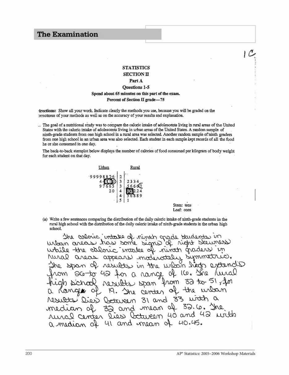
AP® Statistics: 2005–2006 Workshop Materials200
The Examination

AP® Statistics: 2005–2006 Workshop Materials 201
The Examination

AP® Statistics: 2005–2006 Workshop Materials202
The Examination

AP® Statistics: 2005–2006 Workshop Materials 203
The Examination

AP® Statistics: 2005–2006 Workshop Materials204
The Examination

AP® Statistics: 2005–2006 Workshop Materials 205
The Examination

AP® Statistics: 2005–2006 Workshop Materials206
The Examination

AP® Statistics: 2005–2006 Workshop Materials 207
The Examination

AP® Statistics: 2005–2006 Workshop Materials208
The Examination

AP® Statistics: 2005–2006 Workshop Materials 209
The Examination

AP® Statistics: 2005–2006 Workshop Materials210
The Examination

AP® Statistics: 2005–2006 Workshop Materials 211
The Examination

AP® Statistics: 2005–2006 Workshop Materials212
The Examination

AP® Statistics: 2005–2006 Workshop Materials 213
The Examination

AP® Statistics: 2005–2006 Workshop Materials214
The Examination

AP® Statistics: 2005–2006 Workshop Materials 215
The Examination

AP® Statistics: 2005–2006 Workshop Materials216
The Examination

AP® Statistics: 2005–2006 Workshop Materials 217
The Examination

AP® Statistics: 2005–2006 Workshop Materials218
The Examination

AP® Statistics: 2005–2006 Workshop Materials 219
The Examination

AP® Statistics: 2005–2006 Workshop Materials220
The Examination

AP® Statistics: 2005–2006 Workshop Materials 221
The Examination

AP® Statistics: 2005–2006 Workshop Materials222
The Examination

AP® Statistics: 2005–2006 Workshop Materials 223
The Examination

AP® Statistics: 2005–2006 Workshop Materials224
The Examination

AP® Statistics: 2005–2006 Workshop Materials 225
The Examination

AP® Statistics: 2005–2006 Workshop Materials226
The Examination

AP® Statistics: 2005–2006 Workshop Materials 227
The Examination
2005 AP® STATISTICS FREE-RESPONSE QUESTIONS (Form B)
Copyright © 2005 by College Entrance Examination Board. All rights reserved. Visit apcentral.collegeboard.com (for AP professionals) and www.collegeboard.com/apstudents (for AP students and parents).
GO ON TO THE NEXT PAGE. 6
STATISTICS SECTION II
Part A Questions 1-5
Spend about 65 minutes on this part of the exam. Percent of Section II grade—75
Directions: Show all your work. Indicate clearly the methods you use, because you will be graded on the correctness of your methods as well as on the accuracy of your results and explanation.
1. The graph below displays the scores of 32 students on a recent exam. Scores on this exam ranged from 64 to 95 points.
6 * * 6 * * 7 * * * 7 * * * * 8 * * * * 8 * * * * * * 9 * * * * * * * 9 * * * *
(a) Describe the shape of this distribution.
(b) In order to motivate her students, the instructor of the class wants to report that, overall, the class’s performance on the exam was high. Which summary statistic, the mean or the median, should the instructor use to report that overall exam performance was high? Explain.
(c) The midrange is defined as maximum + minimum2
. Compute this value using the data on the
preceding page.
Is the midrange considered a measure of center or a measure of spread? Explain.
2. For an upcoming concert, each customer may purchase up to 3 child tickets and 3 adult tickets. Let C be the number of child tickets purchased by a single customer. The probability distribution of the number of child tickets purchased by a single customer is given in the table below.
(a) Compute the mean and the standard deviation of C.
(b) Suppose the mean and the standard deviation for the number of adult tickets purchased by a single customer are 2 and 1.2, respectively. Assume that the numbers of child tickets and adult tickets purchased are independent random variables. Compute the mean and the standard deviation of the total number of adult and child tickets purchased by a single customer.
(c) Suppose each child ticket costs $15 and each adult ticket costs $25. Compute the mean and the standard deviation of the total amount spent per purchase.
c 0 1 2 3 p c 0.4 0.3 0.2 0.1

AP® Statistics: 2005–2006 Workshop Materials228
The Examination
2005 AP® STATISTICS FREE-RESPONSE QUESTIONS (Form B)
Copyright © 2005 by College Entrance Examination Board. All rights reserved. Visit apcentral.collegeboard.com (for AP professionals) and www.collegeboard.com/apstudents (for AP students and parents).
GO ON TO THE NEXT PAGE. 7
3. In search of a mosquito repellent that is safer than the ones that are currently on the market, scientists have developed a new compound that is rated as less toxic than the current compound, thus making a repellent that contains this new compound safer for human use. Scientists also believe that a repellent containing the new compound will be more effective than the ones that contain the current compound. To test the effectiveness of the new compound versus that of the current compound, scientists have randomly selected 100 people from a state.
Up to 100 bins, with an equal number of mosquitoes in each bin, are available for use in the study. After a compound is applied to a participant’s forearm, the participant will insert his or her forearm into a bin for 1 minute, and the number of mosquito bites on the arm at the end of that time will be determined.
(a) Suppose this study is to be conducted using a completely randomized design. Describe a randomization process and identify an inference procedure for the study.
(b) Suppose this study is to be conducted using a matched-pairs design. Describe a randomization process and identify an inference procedure for the study.
(c) Which of the designs, the one in part (a) or the one in part (b), is better for testing the effectiveness of the new compound versus that of the current compound? Justify your answer.
4. A researcher believes that treating seeds with certain additives before planting can enhance the growth of plants. An experiment to investigate this is conducted in a greenhouse. From a large number of Roma tomato seeds, 24 seeds are randomly chosen and 2 are assigned to each of 12 containers. One of the 2 seeds is randomly selected and treated with the additive. The other seed serves as a control. Both seeds are then planted in the same container. The growth, in centimeters, of each of the 24 plants is measured after 30 days. These data were used to generate the partial computer output shown below. Graphical displays indicate that the assumption of normality is not unreasonable.
N Mean StDev SE Mean Control 12 15.989 1.098 0.317 Treatment 12 18.004 1.175 0.339 Difference 12 − 2.015 1.163 0.336
(a) Construct a confidence interval for the mean difference in growth, in centimeters, of the plants from the untreated and treated seeds. Be sure to interpret this interval.
(b) Based only on the confidence interval in part (a), is there sufficient evidence to conclude that there is a significant mean difference in growth of the plants from untreated seeds and the plants from treated seeds? Justify your conclusion.

AP® Statistics: 2005–2006 Workshop Materials 229
The Examination
2005 AP® STATISTICS FREE-RESPONSE QUESTIONS (Form B)
Copyright © 2005 by College Entrance Examination Board. All rights reserved. Visit apcentral.collegeboard.com (for AP professionals) and www.collegeboard.com/apstudents (for AP students and parents).
GO ON TO THE NEXT PAGE. 8
5. John believes that as he increases his walking speed, his pulse rate will increase. He wants to model this relationship. John records his pulse rate, in beats per minute (bpm), while walking at each of seven different speeds, in miles per hour (mph). A scatterplot and regression output are shown below.
Regression Analysis: Pulse Versus Speed
Predictor Coef SE Coef T P Constant 63.457 2.387 26.58 0.000 Speed 16.2809 0.8192 19.88 0.000
S = 3.087 R-Sq = 98.7% R-Sq (adj) = 98.5%
Analysis of Variance
Source DF SS MS F P Regression 1 3763.2 3763.2 396.13 0.000 Residual 5 47.6 9.5 Total 6 3810.9
(a) Using the regression output, write the equation of the fitted regression line.
(b) Do your estimates of the slope and intercept parameters have meaningful interpretations in the context of this question? If so, provide interpretations in this context. If not, explain why not.
(c) John wants to provide a 98 percent confidence interval for the slope parameter in his final report. Compute the margin of error that John should use. Assume that conditions for inference are satisfied.

AP® Statistics: 2005–2006 Workshop Materials230
The Examination
2005 AP® STATISTICS FREE-RESPONSE QUESTIONS (Form B)
Copyright © 2005 by College Entrance Examination Board. All rights reserved. Visit apcentral.collegeboard.com (for AP professionals) and www.collegeboard.com/apstudents (for AP students and parents).
GO ON TO THE NEXT PAGE. 9
Part B Question 6
Spend about 25 minutes on this part of the exam. Percent of Section II grade—25
Directions: Show all your work. Indicate clearly the methods you use, because you will be graded on the correctness of your methods as well as on the accuracy of your results and explanation.
6. Regulations require that product labels on containers of food that are available for sale to the public accurately state the amount of food in those containers. Specifically, if milk containers are labeled to have 128 fluid ounces and the mean number of fluid ounces of milk in the containers is at least 128, the milk processor is considered to be in compliance with the regulations. The filling machines can be set to the labeled amount. Variability in the filling process causes the actual contents of milk containers to be normally distributed. A random sample of 12 containers of milk was drawn from the milk processing line in a plant, and the amount of milk in each container was recorded.
(a) The sample mean and standard deviation of this sample of 12 containers of milk were 127.2 ounces and 2.1 ounces, respectively. Is there sufficient evidence to conclude that the packaging plant is not in compliance with the regulations? Provide statistical justification for your answer.
Inspectors decide to study a particular filling machine within this plant further. For this machine, the amount of milk in the containers has a mean of 128.0 fluid ounces and a standard deviation of 2.0 fluid ounces.
(b) What is the probability that a randomly selected container filled by this machine contains at least 125 fluid ounces?
(c) An inspector will randomly select 12 containers filled by this machine and record the amount of milk in each. What is the probability that the minimum (smallest amount of milk) recorded in the 12 containers will be at least 125 fluid ounces? (Note: In order for the minimum to be at least 125 fluid ounces, each of the 12 containers must contain at least 125 fluid ounces.)
An analyst wants to use simulation to investigate the sampling distribution of the minimum. This analyst randomly generates 150 samples, each consisting of 12 observations, from a normal distribution with mean 128 and standard deviation 2 and finds the minimum for each sample. The 150 minimums (sorted from smallest to largest) are shown on the next page.

AP® Statistics: 2005–2006 Workshop Materials 231
The Examination
2005 AP® STATISTICS FREE-RESPONSE QUESTIONS (Form B)
Copyright © 2005 by College Entrance Examination Board. All rights reserved. Visit apcentral.collegeboard.com (for AP professionals) and www.collegeboard.com/apstudents (for AP students and parents).
GO ON TO THE NEXT PAGE. 10
Sample Minimum Sample Minimum Sample Minimum
1 121.45 51 124.28 101 125.25 2 122.51 52 124.29 102 125.31 3 122.53 53 124.30 103 125.36 4 122.72 54 124.31 104 125.38 5 122.75 55 124.34 105 125.40 6 122.89 56 124.36 106 125.42 7 122.93 57 124.37 107 125.48 8 122.99 58 124.37 108 125.49 9 123.04 59 124.39 109 125.50 10 123.08 60 124.39 110 125.52 11 123.09 61 124.41 111 125.54 12 123.10 62 124.44 112 125.56 13 123.31 63 124.53 113 125.61 14 123.34 64 124.53 114 125.67 15 123.39 65 124.54 115 125.72 16 123.40 66 124.55 116 125.76 17 123.41 67 124.55 117 125.77 18 123.41 68 124.55 118 125.78 19 123.46 69 124.55 119 125.79 20 123.49 70 124.58 120 125.84 21 123.51 71 124.67 121 125.87 22 123.57 72 124.69 122 125.87 23 123.58 73 124.73 123 125.90 24 123.59 74 124.77 124 125.90 25 123.60 75 124.78 125 125.93 26 123.66 76 124.78 126 125.93 27 123.67 77 124.80 127 125.93 28 123.72 78 124.80 128 125.94 29 123.75 79 124.81 129 125.98 30 123.77 80 124.85 130 126.00 31 123.78 81 124.91 131 126.03 32 123.84 82 124.92 132 126.05 33 123.91 83 124.92 133 126.05 34 123.93 84 124.96 134 126.06 35 123.95 85 125.00 135 126.09 36 123.95 86 125.01 136 126.15 37 123.98 87 125.02 137 126.15 38 123.99 88 125.02 138 126.16 39 124.05 89 125.03 139 126.19 40 124.05 90 125.04 140 126.19 41 124.06 91 125.05 141 126.25 42 124.12 92 125.07 142 126.26 43 124.14 93 125.08 143 126.33 44 124.15 94 125.09 144 126.35 45 124.16 95 125.14 145 126.45 46 124.19 96 125.18 146 126.50 47 124.23 97 125.21 147 126.57 48 124.27 98 125.21 148 126.62 49 124.28 99 125.22 149 126.64 50 124.28 100 125.25 150 126.95

AP® Statistics: 2005–2006 Workshop Materials232
The Examination
2005 AP® STATISTICS FREE-RESPONSE QUESTIONS (Form B)
Copyright © 2005 by College Entrance Examination Board. All rights reserved. Visit apcentral.collegeboard.com (for AP professionals) and www.collegeboard.com/apstudents (for AP students and parents).
11
(d) Use the simulation results to estimate the probability that was requested in part (c) and compare this estimate with the theoretical value you calculated.
END OF EXAMINATION

AP® Statistics: 2005–2006 Workshop Materials 233
The Examination
AP® STATISTICS 2005 SCORING GUIDELINES (Form B)
Copyright © 2005 by College Board. All rights reserved. Visit apcentral.collegeboard.com (for AP professionals) and www.collegeboard.com/apstudents (for AP students and parents).
2
Question 1
Solution
Part (a):
The distribution is skewed to the left (or toward the lower values).
Part (b):
Since the distribution is skewed towards the lower values, the mean will be pulled in that direction. Thus, the instructor should report the median to motivate her students.
Part (c):
Step 1: Correct Mechanics: 64 95midrange 79.5
2Step 2: Identify the midrange as a measure of center.
Step 3: Correct rationale:
The maximum provides information about the upper tail, more specifically the upper extreme value. The minimum provides information about the lower tail, more specifically the lower extreme value. By averaging these two values and creating the midrange, we are creating a statistic that provides the halfway point between the two extremes. This statistic is a measure of center.
Scoring
Each part is scored as essentially correct (E), partially correct (P), or incorrect (I).
Part (a) is essentially correct (E) if the student states that the distribution is skewed and indicates the direction.
Part (a) is partially correct (P) if the student: • Recognizes that the distribution is skewed but either does not mention the direction or does not indicate
the correct direction; OR • says that the distribution is not symmetric; OR • says the distribution is not normal.
Part (a) is incorrect (I) if the student says the distribution is bell-shaped or roughly normal.

AP® Statistics: 2005–2006 Workshop Materials234
The Examination
AP® STATISTICS 2005 SCORING GUIDELINES (Form B)
Copyright © 2005 by College Board. All rights reserved. Visit apcentral.collegeboard.com (for AP professionals) and www.collegeboard.com/apstudents (for AP students and parents).
3
Question 1 (continued)
Part (b) is scored as essentially correct (E) if the median is chosen and a correct rationale based on the skewness of the distribution is provided.
Part (b) is partially correct (P) if the median is chosen, but the rationale is weak OR the mean is chosen based on a weak rationale.
Part (b) is incorrect (I) if no rationale is provided for the chosen statistic OR the mean is chosen based on a flawed rationale.
Part (c) is scored as essentially correct (E) if all three steps are essentially correct.
Part (c) is partially correct (P) if two steps are essentially correct.
Part (c) is incorrect (I) if at most one step is correct.
Note: Step 3 is essentially correct if the student provides a rationale that appeals to the midrange as a value in the middle of two extremes OR that appeals to the midrange as a middle value and a correct rationale of why it is not a measure of spread OR appeals to the property that adding a constant to every observation will shift the midrange by the amount of the constant while measures of spread are unaffected by adding a constant to every observation.
4 Complete Response (3E)
All three parts essentially correct
3 Substantial Response (2E 1P)
Two parts essentially correct and one part partially correct
2 Developing Response (2E 0P or 1E 2P)
Two parts essentially correct and zero parts partially correct OROne part essentially correct and two parts partially correct
1 Minimal Response ( 1E 1P or 1E 0P or 0E 2P)
One part essentially correct and either zero parts or one part partially correct OR
Zero parts essentially correct and two parts partially correct

AP® Statistics: 2005–2006 Workshop Materials 235
The Examination
AP® STATISTICS 2005 SCORING GUIDELINES (Form B)
Copyright © 2005 by College Board. All rights reserved. Visit apcentral.collegeboard.com (for AP professionals) and www.collegeboard.com/apstudents (for AP students and parents).
4
Question 2
Solution
Part (a):
The mean of C is 0 0.4 1 0.3 2 0.2 3 0.1 1.
The standard deviation of C is 2 2 2 20 1 0.4 1 1 0.3 2 1 0.2 3 1 0.1 1.
Part (b):
Let ,T C A where A is the total number of adult tickets purchased by a single customer, denote the total number of tickets purchased by a single customer. The mean of T is 1 2 3.T C A
The standard deviation of T is 2 2 2 21 1.2 2.44 1.562.T C A
Part (c):
Let 15 25M C A denote the total amount of money spent per purchase. The mean of M is 15 25 15 1 25 2 $65.M C A
The standard deviation of M is 2 2 2 2 2 215 25 225 1 625 1.2 1125 $33.54.M C A
Scoring
Each part is scored as essentially correct (E), partially correct (P), or incorrect (I).
Part (a) is essentially correct (E) if both the mean and the standard deviation of C are calculated correctly and the work is shown, with the exception of minor arithmetic errors.
Part (a) is partially correct (P) if either the mean or the standard deviation of C is calculated correctly and the work is shown.
Note: The variance and the standard deviation of C are both 1. If the variance is reported instead of the standard deviation, the response is scored as (P).
Part (a) is incorrect (I) if both the mean and the standard deviation of C are calculated incorrectly OR if no work is shown.
Notes:1. Unsupported answers will be scored as incorrect. 2. If the student incorrectly calculates the mean and/or standard deviation in part (a) and then correctly uses
those values in parts (b) and (c), there will be no second penalty.

AP® Statistics: 2005–2006 Workshop Materials236
The Examination
AP® STATISTICS 2005 SCORING GUIDELINES (Form B)
Copyright © 2005 by College Board. All rights reserved. Visit apcentral.collegeboard.com (for AP professionals) and www.collegeboard.com/apstudents (for AP students and parents).
5
Question 2 (continued)
3. Standard notation for means , , ,C A T Mand , variances 2 2 2 2, , ,C A T Mand , and standard
deviations , , ,C A T Mand are acceptable without definition. If nonstandard notation, such as
, , ,C A T Mp p p and p , is defined correctly for this problem, then it will be scored as essentially correct.
Nonstandard notation, without a definition, will be scored at most partially correct.
Part (b) is essentially correct (E) if both the mean and the standard deviation of T are calculated correctly and the work is shown, with the exception of minor arithmetic errors.
Part (b) is partially correct (P) if either the mean or the standard deviation of T is calculated correctly.
Part (b) is incorrect (I) if both the mean and the standard deviation of T are calculated incorrectly OR no work is shown.
Part (c) is scored as essentially correct (E) if both the mean and the standard deviation of M are calculated correctly and the work is shown, with the exception of minor arithmetic errors.
Part (c) is partially correct (P) if either the mean or the standard deviation of M is calculated correctly.
Part (c) is incorrect (I) if both the mean and the standard deviation of M are calculated incorrectly OR if no work is shown.
4 Complete Response (3E)
All three parts essentially correct
3 Substantial Response (2E 1P)
Two parts essentially correct and one part partially correct
2 Developing Response (2E 0P or 1E 2P)
Two parts essentially correct and zero parts partially correct OROne part essentially correct and two parts partially correct
1 Minimal Response ( 1E 1P or 1E 0P or 0E 2P)
One part essentially correct and either zero parts or one part partially correct OR
Zero parts essentially correct and two parts partially correct

AP® Statistics: 2005–2006 Workshop Materials 237
The Examination
AP® STATISTICS 2005 SCORING GUIDELINES (Form B)
Copyright © 2005 by College Board. All rights reserved. Visit apcentral.collegeboard.com (for AP professionals) and www.collegeboard.com/apstudents (for AP students and parents).
6
Question 3
Solution
Part (a):
Each of the 100 selected people will be assigned a unique random number using a random number generator. A list of names and numbers will be created and sorted from smallest to largest by the assigned numbers (and carrying along the name). The first 50 people on the list will be asked to apply the new compound to their right arm and the other 50 people will be asked to apply the current compound to their right arm. The compounds will be put in identical, unmarked tubes so neither the participants nor the researchers know which compound is being applied. The analysts will be the only people who know which participants received which compound. Each person will be randomly assigned to a bin by assigning random numbers to bins using a random number generator. The first person on the list will be assigned to the bin with the smallest number, the second person on the list will be assigned to the bin with the second smallest number, and so on. After each person inserts his or her right arm into the assigned bin for one minute, the number of mosquito bites will be counted. The mean number of mosquito bites for the two compounds will be compared using a two-sample t-test and/or a confidence interval for the difference in means for two independent samples.
Part (b):
Each participant will be randomly assigned to a bin as described in part (a). The researchers will distribute two identical tubes, one labeled 1 and the other labeled 2, to each participant. One of those tubes will contain the new compound and the other will contain the current compound. Neither the researchers nor the participants will know which compound is in which tube. Only the analyst will have this information. Each participant will apply one compound to one arm and the other compound to the other arm. The assignment of the compounds to the arms is completed using randomization. A random number will be generated for each participant, and the participants with the 50 smallest random numbers will apply tube 1 to their right arm, and the remaining 50 participants will apply tube 2 to their left arm. Each participant will insert both arms into the assigned bin at the same time for one minute, and the number of mosquito bites will be counted on each arm. The analyst will compute the difference in the number of bites (new – current) for each of the 100 participants and use a one-sample t-test and/or construct a confidence interval for the mean of the differences to test the null hypothesis that the mean difference is zero.
Part (c):
The matched-pairs design in part (b) is better because one potential source of variation, person-to-person variability in susceptibility to mosquito bites, is controlled.

AP® Statistics: 2005–2006 Workshop Materials238
The Examination
AP® STATISTICS 2005 SCORING GUIDELINES (Form B)
Copyright © 2005 by College Board. All rights reserved. Visit apcentral.collegeboard.com (for AP professionals) and www.collegeboard.com/apstudents (for AP students and parents).
7
Question 3 (continued)
Scoring
Part (a) is divided into two subparts. Each subpart is scored as essentially correct (E), partially correct (P), or incorrect (I). Parts (b) and (c) are scored as essentially correct (E), partially correct (P), or incorrect (I).
Part (a) contains two parts. The first part (a1) deals with the description of a completely randomized design (CRD). The second part (a2) deals with the inference procedure.
Part (a1) is essentially correct (E) if the student: • Describes a completely randomized design (CRD) that indicates that participants are assigned to two
treatment groups corresponding to the new and current compounds; AND • Correctly describes an appropriate randomization procedure for assigning participants to treatment
groups.
Part (a1) is partially correct (P) if the explanation of the randomization procedure is not clear or is incomplete OR the student fails to address the assignment of participants to treatment groups.
Part (a1) is incorrect (I) if the student describes a design that is not based on random assignment. For example, if a design allows the subjects to self-select into two groups. A matched-pairs design is also scored as incorrect.
Part (a2) is essentially correct (E) if the student: • Chooses a two-sample t-test or a two-sample confidence interval for the difference in means; AND • Indicates that the mean number of mosquito bites will be compared for the two compounds.
Part (a2) is partially correct (P) if only one of the above is included.
Part (a2) is incorrect (I) if none of the above is included.
Part (b) is essentially correct (E) if the student describes a matched-pairs experiment that: • Identifies the participants as the blocks; AND • Describes a method for randomly assigning the treatments within each block (for designs in which the
two treatments are not applied at the same time, the order in which the treatments are given must also be properly randomized); AND
• Correctly identifies an appropriate inference procedure based on the observed differences in mosquito bites within each block.
Part (b) is partially correct (P) if the student does any of the following: • Provides a correct inference procedure, but
o Uses gender or some other characteristic to form the pairs; o Attempts to describe the random assignment within each block, but the explanation of the
random assignment is not clear or incomplete; o Neglects to indicate that the analysis will be based on the differences within each block; OR
• Describes a correct randomization process but does not provide a correct inference procedure.

AP® Statistics: 2005–2006 Workshop Materials 239
The Examination
AP® STATISTICS 2005 SCORING GUIDELINES (Form B)
Copyright © 2005 by College Board. All rights reserved. Visit apcentral.collegeboard.com (for AP professionals) and www.collegeboard.com/apstudents (for AP students and parents).
8
Question 3 (continued)
Part (b) is incorrect (I) if the student describes any design not based on random assignment within the blocks (e.g., allows the subjects to self-select which compound is applied to which arm) or just refers to “random assignment” but does not describe the method of assignment.
Notes for part (b):
Examples of alternative matched-pairs designs that will be scored as essentially correct:
1. If the student assumes that only one arm can be inserted into a bin, the experiment can be done by randomly selecting 50 of the 100 available participants. The bins are labeled from 1 to 100 and two bins are randomly assigned to each subject, one for each arm. This can be done by using a random number generator to assign each participant a unique random number and sorting the list of participants with respect to those numbers. Bins 1 and 2 are assigned to the first participant on the list, bins 3 and 4 are assigned to the second participant on the list, and so on. For each subject, a coin is tossed to determine which bin is assigned to which arm. Then, the experiment proceeds as described above. Another coin will be tossed to decide which arm receives the new compound. The current compound is applied to the other arm. Either both arms will be tested at the same time or another coin will be tossed to determine which arm is tested first.
2. In this design, each participant uses one bin twice. One bin is randomly assigned to each of the 100 participants as described above. Each participant will apply one compound to one arm and the other compound to the other arm. A coin can be tossed to decide which arm receives the new compound. The current compound is applied to the other arm. The coin can be tossed a second time to determine which arm is put into the bin first. A potential disadvantage of this experiment is that the mosquitoes that are most aggressive and most resistant to the compounds will be more likely to bite the first arm inserted into a bin and less likely to bite the second arm. Randomizing the order in which the arms are inserted into the bin controls potential bias of this order effect, but the variability of the observed differences may be substantially larger than for the two other matched-pairs designs that were previously described, and this would make the comparison of the effects of the compounds less precise.
Part (c) is essentially correct (E) if the matched-pairs design is chosen over a CRD based on rationale that the blocking factor will reduce person-to-person variability in susceptibility to mosquito bites.
Part (c) is partially correct (P) if the student: • Chooses the CRD over an incorrect matched-pairs design with appropriate rationale; OR • Chooses a matched-pairs design over a CRD, with weak rationale.
Part (c) is incorrect (I) if the student: • Makes a choice with no justification or a severely flawed argument; OR • Chooses the matched-pairs design because the sample size is larger; OR • Chooses the CRD with the justification that a CRD is always better than a matched-pairs design; OR • Chooses the matched-pairs design with the justification that a matched-pairs design is always better than
a CRD.

AP® Statistics: 2005–2006 Workshop Materials240
The Examination
AP® STATISTICS 2005 SCORING GUIDELINES (Form B)
Copyright © 2005 by College Board. All rights reserved. Visit apcentral.collegeboard.com (for AP professionals) and www.collegeboard.com/apstudents (for AP students and parents).
9
Question 3 (continued)
Each essentially correct (E) response counts as 1 point, each partially correct (P) response counts as ½ point.
4 Complete Response
3 Substantial Response
2 Developing Response
1 Minimal Response
Note: If a response is in between two scores (for example, 2 ½ points), use a holistic approach to determine whether to score up or down depending on the strength of the response and communication.

AP® Statistics: 2005–2006 Workshop Materials 241
The Examination
AP® STATISTICS 2005 SCORING GUIDELINES (Form B)
Copyright © 2005 by College Board. All rights reserved. Visit apcentral.collegeboard.com (for AP professionals) and www.collegeboard.com/apstudents (for AP students and parents).
10
Question 4
Solution
Part (a):
Step 1: Identify appropriate confidence interval by name or by formula.
One sample confidence interval for a mean (of the differences)
*1
dd n
sOR x t
nStep 2: Check appropriate conditions.
Assume the population of differences in growth is normally distributed. The information provided in the stem of the problem suggests that this condition is met. Because the 24 seeds were randomly chosen and randomly assigned to the containers, the differences are independent.
Step 3: Correct mechanics.
The 95% confidence interval for the mean difference in growth is 1.1632.015 2.201 2.015 2.201 0.336 2.015 0.7389
12or (-2.7539, -1.2761).
Step 4: Interpret the confidence interval in context.
We are 95% confident that the mean difference in the growth of the untreated and treated seeds is between –2.7539 and –1.2761.
Part (b):
Step 1: Identify a correct pair of hypotheses.
0 : 0dH versus : 0a dH , where d is the mean difference in the untreated and treated seeds.
Step 2: State the correct conclusion in context.
Since the 95% confidence interval does not include zero, the null hypothesis can be rejected at the 0.05 significance level. In other words, we have statistically significant evidence at the 0.05
level that there is a mean difference in the growth of untreated and treated seeds.

AP® Statistics: 2005–2006 Workshop Materials242
The Examination
AP® STATISTICS 2005 SCORING GUIDELINES (Form B)
Copyright © 2005 by College Board. All rights reserved. Visit apcentral.collegeboard.com (for AP professionals) and www.collegeboard.com/apstudents (for AP students and parents).
11
Question 4 (continued)
Scoring
Each part is scored as essentially correct (E), partially correct (P), or incorrect (I).
Part (a) is essentially correct (E) if all three of steps 1, 3, and 4 of the confidence interval solution are correct.
Part (a) is partially correct (P) if two of the three steps are correct.
Part (a) is incorrect (I) if only one of the steps is correct.
Notes: 1. Step 2 may be omitted since this information is provided in the stem.
2. In step 3, other confidence levels may be used, e.g.,
• 90% C.I. is 1.1632.015 1.796 2.015 0.603012
or (-2.618, -1.412)
• 99 % C.I. is 1.1632.015 3.106 2.015 1.042812
or (-3.0578, -.9722)
3. In step 4, a correct interpretation of the confidence level cannot substitute for a correct interpretation of the confidence interval in context.
4. If a two-sample procedure is used, the highest possible score is (P). The 95% confidence interval for the
difference in the two means is 1 2
2 2* 1 2
1 2 min 1, 11 2
n ns s
x x tn n
=
2 2(1.098) (1.175)15.989 18.004 2.201
12 12 = 2.015 1.0218 or ( 3.037, 0.993).
5. The incorrect two-sample confidence intervals from the calculator are: • 95% C.I. is ( 2.978, 1.052)
• 99% C.I. is ( 3.324, 0.706)

AP® Statistics: 2005–2006 Workshop Materials 243
The Examination
AP® STATISTICS 2005 SCORING GUIDELINES (Form B)
Copyright © 2005 by College Board. All rights reserved. Visit apcentral.collegeboard.com (for AP professionals) and www.collegeboard.com/apstudents (for AP students and parents).
12
Question 4 (continued)
Part (b) is essentially correct (E) if the correct conclusion is stated in context and justified using the confidence interval constructed in part (a). Statements of the null and alternative hypotheses are not required.
Part (b) is partially correct (P) if the student: • Does not provide a conclusion in the context of the problem; OR • Provides a conclusion in the context of the problem but the justification is weak; OR • Uses a completely correct application of an appropriate hypothesis test to justify a correct conclusion but
does not refer to the confidence interval in part (a).
Part (c) is incorrect (I) if the student: • Provides a conclusion that is inconsistent with the interval provided in part (a); OR • Provides a correct conclusion with no justification; OR • Ignores the confidence interval in part (a) and fails to correctly conduct an appropriate hypothesis test to
justify a conclusion.
Note: If the student uses a two-sample confidence interval or some other incorrect confidence interval in part (a), the solution will be scored relative to the reported interval. The student will not be penalized in part (b) for an incorrect solution to part (a).
4 Complete Response (EE)
Both parts are essentially correct
3 Substantial Response (EP or PE)
One part essentially correct and the other part partially correct
2 Developing Response (EI, IE, or PP)
One part essentially correct and the other part incorrect OR Both parts partially correct
1 Minimal Response ( PI or IP)
One part is partially correct

AP® Statistics: 2005–2006 Workshop Materials244
The Examination
AP® STATISTICS 2005 SCORING GUIDELINES (Form B)
Copyright © 2005 by College Board. All rights reserved. Visit apcentral.collegeboard.com (for AP professionals) and www.collegeboard.com/apstudents (for AP students and parents).
13
Question 5
Solution
Part (a):
Predicted Pulse = 63.457 + 16.2809 (Speed)
Part (b):
The intercept (63.457 bpm) provides an estimate for John’s mean resting pulse (walking at a speed of zero mph).
The slope (16.2809 bpm/mph) provides an estimate for the mean increase in John’s heart rate as his speed is increased by one mile per hour.
Part (c):
The margin of error for the confidence interval for the slope parameter is *2n bt s , where bs is the standard
error of the slope parameter. For a 98% confidence interval, the margin of error is 3.365 0.8192 2.7566bpm.
Scoring
Part (a) is scored as essentially correct (E) or incorrect (I). Parts (b) and (c) are scored as essentially correct (E), partially correct (P), or incorrect (I).
Note: If the student uses X and Y, then both variables must be identified.
Part (b): There are four steps to constructing correct interpretations:
Step 1: A correct mathematical interpretation of the reported slope (16.2809) as a rate of increase in heart rate as walking speed increases.
Step 2: A correct mathematical interpretation of the reported intercept as a pulse rate when walking speed is zero.
Step 3: Correct use of units of measurement, e.g., John’s heart rate increases 16.2809 bpm as his speed is increased by one mile per hour.
Step 4: Interpretation of the reported values as estimates of the corresponding mean quantities.

AP® Statistics: 2005–2006 Workshop Materials 245
The Examination
AP® STATISTICS 2005 SCORING GUIDELINES (Form B)
Copyright © 2005 by College Board. All rights reserved. Visit apcentral.collegeboard.com (for AP professionals) and www.collegeboard.com/apstudents (for AP students and parents).
14
Question 5 (continued)
Part (b) is essentially correct (E) if all four steps are correct.
Part (b) is partially correct (P) if two or three steps are correctly addressed. Step 2 is scored as incorrect, for example, if the student suggests that the intercept does not have a meaningful interpretation.
Part (b) is incorrect (I) if at most one step is correct.
Note: The student is only penalized once for switching the variables.
Part (c) is essentially correct (E) if the standard error of the slope is identified and the correct critical value is used to calculate the margin of error.
Part (c) is partially correct (P) if the student: • Computes the 98% confidence interval but does not identify the margin of error; OR • Recognizes that the margin of error consists of the standard error of the coefficient and the critical value
but uses an incorrect value for one of the two components or uses a t-value with 6 degrees of freedom and an incorrect standard error.
Part (c) is incorrect (I) if the student uses: • The standard error of the coefficient as the margin of error; OR • A critical value as the margin of error.
4 Complete Response (3E)
All three parts essentially correct
3 Substantial Response (2E 1P)
Two parts essentially correct and one part partially correct
2 Developing Response (2E 0P or 1E 2P)
Two parts essentially correct and zero parts partially correct OROne part essentially correct and two parts partially correct
1 Minimal Response ( 1E 1P or 1E 0P or 0E 2P)
One part essentially correct and either zero parts or one part partially correct OR
Zero parts essentially correct and two parts partially correct
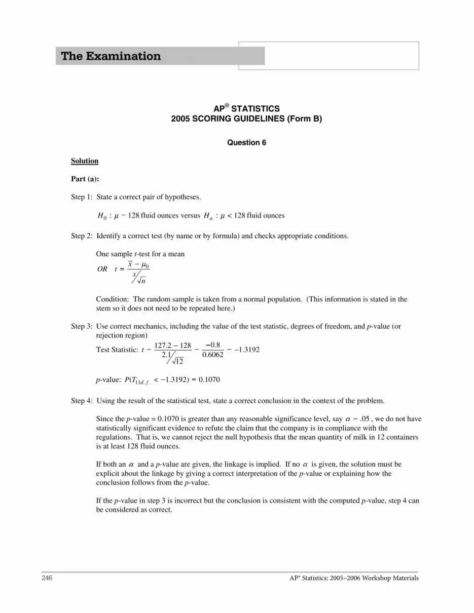
AP® Statistics: 2005–2006 Workshop Materials246
The Examination
AP® STATISTICS 2005 SCORING GUIDELINES (Form B)
Copyright © 2005 by College Board. All rights reserved. Visit apcentral.collegeboard.com (for AP professionals) and www.collegeboard.com/apstudents (for AP students and parents).
15
Question 6
Solution
Part (a):
Step 1: State a correct pair of hypotheses.
0 : 128H fluid ounces versus : 128aH fluid ounces
Step 2: Identify a correct test (by name or by formula) and checks appropriate conditions.
One sample t-test for a mean
0xOR t
sn
Condition: The random sample is taken from a normal population. (This information is stated in the stem so it does not need to be repeated here.)
Step 3: Use correct mechanics, including the value of the test statistic, degrees of freedom, and p-value (or rejection region)
Test Statistic: 0.8127.2 128 1.3192
2.1 0.606212
t
p-value: 11 . .( 1.3192) 0.1070d fP T
Step 4: Using the result of the statistical test, state a correct conclusion in the context of the problem.
Since the p-value = 0.1070 is greater than any reasonable significance level, say .05 , we do not have statistically significant evidence to refute the claim that the company is in compliance with the regulations. That is, we cannot reject the null hypothesis that the mean quantity of milk in 12 containers is at least 128 fluid ounces.
If both an and a p-value are given, the linkage is implied. If no is given, the solution must be explicit about the linkage by giving a correct interpretation of the p-value or explaining how the conclusion follows from the p-value.
If the p-value in step 3 is incorrect but the conclusion is consistent with the computed p-value, step 4 can be considered as correct.

AP® Statistics: 2005–2006 Workshop Materials 247
The Examination
AP® STATISTICS 2005 SCORING GUIDELINES (Form B)
Copyright © 2005 by College Board. All rights reserved. Visit apcentral.collegeboard.com (for AP professionals) and www.collegeboard.com/apstudents (for AP students and parents).
16
Question 6 (continued)
Part (b)
Let X denote the amount of fluid in a randomly selected container from this group. The probability that a randomly selected container from this group contains at least 125 fluid ounces is:
125 128125 1.5 1 0.0668 0.93322
P X P Z P Z
Part (c):
Let 1 2 121 min , , ,X X X X . The probability that the smallest amount of milk recorded in the 12
randomly selected containers will be at least 125 fluid ounces is:
1 2 121
121
12
125 125, 125, , 125
125
0.9332
0.4362
P X P X X X
P X
Part (d):
Looking at the sorted list of 150 minimums, we notice that 66 of the minimums are at least 125 and 84 of the minimums are less than 125. Thus, the probability in part (c) is approximated by
166125 0.44
150P X or 1
84125 1 0.44150
P X . The difference between the simulated
value and the theoretical value, 0.44 0.4362 0.0038 , is very small. In other words, the simulation provides a very good approximation to the theoretical value.
Scoring
Each part is scored as essentially correct (E), partially correct (P), or incorrect (I).
Part (a) is essentially correct (E) if all four of the steps are correct. Each step is scored as correct or incorrect, no partial credit is given for the steps.
Part (a) is partially correct (P) if two or three steps are correct.
Part (a) is incorrect (I) if at most one step is correct.

AP® Statistics: 2005–2006 Workshop Materials248
The Examination
AP® STATISTICS 2005 SCORING GUIDELINES (Form B)
Copyright © 2005 by College Board. All rights reserved. Visit apcentral.collegeboard.com (for AP professionals) and www.collegeboard.com/apstudents (for AP students and parents).
17
Question 6 (continued)
Part (b) is essentially correct (E) if the student provides: • The correct probability; AND• An algebraic or graphical justification, with the exception of minor arithmetic or transcription errors.
Part (b) is partially correct (P) if the student only provides one of the two items above.
Part (b) is incorrect (I) if the student provides a probability other than 0.9332 with no justification.
Part (c) is essentially correct (E) if the student provides: • The correct probability; AND• An algebraic justification, with the exception of minor arithmetic or transcription errors.
Part (c) is partially correct (P) if the student only provides one of the two items above.
Part (c) is incorrect (I) if the student provides a probability other than 0.4632 with no justification.
Note: The student will only be penalized once if they correctly use an incorrect probability from part (b) in the calculations for part (c).
Part (d) is essentially correct (E) if the student provides a: • Correct estimate based on the simulation results; AND • Valid comparison of the theoretical and simulated values.
Part (d) is partially correct (P) if the student provides: • Only one of the two items above; OR
• An estimate of 65 0.4333;150
OR
• An estimate of 85 0.5667;150
OR
• An estimate of 84 0.56.150
Notes:
1. If a student is unable to solve part (c), the student may assume the value is equal to some number and then make a comparison between this number and the estimate from the simulation to earn an essentially correct response. That is, the student will not be penalized twice for not being able to calculate the theoretical value.
2. The remarks in the comparison should be consistent with the two values provided by the student, even if these values are incorrect.

AP® Statistics: 2005–2006 Workshop Materials 249
The Examination
AP® STATISTICS 2005 SCORING GUIDELINES (Form B)
Copyright © 2005 by College Board. All rights reserved. Visit apcentral.collegeboard.com (for AP professionals) and www.collegeboard.com/apstudents (for AP students and parents).
18
Question 6 (continued)
Each essentially correct (E) response counts as 1 point, each partially correct (P) response counts as ½ point.
4 Complete Response
3 Substantial Response
2 Developing Response
1 Minimal Response
Note: If a response is in between two scores (for example, 2 ½ points), use a holistic approach to determine whether to score up or down depending on the strength of the response and communication.
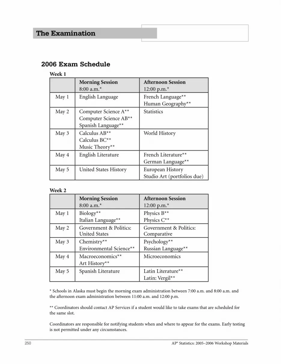
AP® Statistics: 2005–2006 Workshop Materials250
The Examination
2006 Exam ScheduleWeek 1
Morning Session8:00 a.m.*
Afternoon Session12:00 p.m.*
May 1 English Language French Language**Human Geography**
May 2 Computer Science A**Computer Science AB**Spanish Language**
Statistics
May 3 Calculus AB**Calculus BC**Music Theory**
World History
May 4 English Literature French Literature**German Language**
May 5 United States History European HistoryStudio Art (portfolios due)
Week 2Morning Session8:00 a.m.*
Afternoon Session12:00 p.m.*
May 1 Biology**Italian Language**
Physics B**Physics C**
May 2 Government & Politics:United States
Government & Politics: Comparative
May 3 Chemistry**Environmental Science**
Psychology**Russian Language**
May 4 Macroeconomics**Art History**
Microeconomics
May 5 Spanish Literature Latin Literature**Latin: Vergil**
* Schools in Alaska must begin the morning exam administration between 7:00 a.m. and 8:00 a.m. and the afternoon exam administration between 11:00 a.m. and 12:00 p.m. ** Coordinators should contact AP Services if a student would like to take exams that are scheduled for the same slot.
Coordinators are responsible for notifying students when and where to appear for the exams. Early testing is not permitted under any circumstances.

AP® Statistics: 2005–2006 Workshop Materials 251
Professional Development
Professional Development
Introduction
AP Professional Development and Support
More than 130,000 AP teachers and administrators serve over one million students worldwide. The College Board, in turn, serves these dedicated AP professionals in a wide variety of ways, focusing on improving student achievement and increasing access to these rigorous college-level courses.
K-12 Professional Development at the College Board provides course-specific content, shares effective classroom strategies, and assists each school’s program development, supporting this committed community of practice through face-to-face workshops, online resources and services, print publications, and consultation. Each component links to AP content and objectives, providing a web of support around these student learning goals.
AP Workshops, Conferences, and Summer Institutes
The College Board offers a variety of in-person professional development opportunities year-round, principally through workshops, conferences, and summer institutes. Workshop and institute leaders are recognized and endorsed members of the AP community engaging in intensive collegial exchange. For teachers, these course-specific training opportunities are designed to support the new or experienced teacher in all aspects of AP course development, organization, and methodology. For AP Coordinators and AP administrators, workshops address critical issues faced in introducing, developing, and supporting an AP program. If you want to start an AP program at your school or are looking for ways to enhance your AP courses, register today for a workshop, institute, or course near you. See apcentral.collegeboard.com/events for a listing of professional development opportunities.
AP Central
As part of its mission and focus on professional development for AP teachers, the College Board developed AP Central, the official online destination for AP teachers, Coordinators, administrators, and all those who are involved with or interested in the AP Program and Pre-AP. By the end of the 2004-2005 academic year, AP Central, located at apcentral.collegeboard.com, had over 425,000 registered members, and the number continues to grow weekly. The site offers Course Descriptions, exam questions, sample syllabi, and other resources for each AP course on the Course Home Pages. Other features include a Teachers’
Chapter V

AP® Statistics: 2005–2006 Workshop Materials252
Professional Development
Resources area that contains over 4,400 reviews of resources for most AP courses, an Institutes & Workshops search engine, and subject-specific electronic discussion groups in which teachers can learn from each other by sharing their experiences. Over 30,000 AP teachers, Coordinators, and administrators participate in the electronic discussion groups. AP Central continues to expand its scope by offering online events and presentations by experts in the AP content areas and has begun to offer online workshops to the middle and high school professional community.
AP Publications and Other Resources
The College Board provides additional support to members of the AP community inthe form of publications and other resources in each AP subject area. These include Released Exams, Teacher’s Guides, videos, and CD-ROMs. There are nearly 200 resources currently available through the College Board Store at store.collegeboard.com and the AP Document Library on AP Central.
Working With Partners
Providing the depth and breadth of professional support that the AP community merits is a daunting challenge and demands close collaboration with schools, universities, professional associations, and other organizations. AP is building capacity through varied types of collaborations and partnerships, especially to target high program priorities, such as increasing the numbers of minority AP students served and increasing the range of professional development offered.
Some of our partners are: • Alliance Associations of Teachers of Japanese (AATJ)• American Association of Teachers of German (AATG) • American Association of Teachers of Spanish and Portuguese (AATSP) • American Council of Teachers of Russian (ACTR)• American Council on the Teaching of Foreign Languages (ACTFL)• American Historical Association (AHA) • American Psychological Association (APA)• The Asia Society• Association of Teachers of Japanese (ATJ)• Bowdoin College • Center for Advanced Study of Education• Chinese Language Association of Secondary-Elementary Schools (CLASS)• Chinese Language Teachers Association (CLTA) • City University of New York (CUNY)

AP® Statistics: 2005–2006 Workshop Materials 253
Professional Development
• Computer Science Teachers Association• The Embassy of Italy• Environmental Literacy Council• The Freeman Foundation • Hanban• History Teaching Institute at Ohio State University • The Japan Foundation• Mathematical Association of America (MAA)• The Math Gateway (National Science Digital Library (NSDL) portal)• Ministry of Education, Taiwan• National Association of Direct Supervisors of Foreign Languages (NADSFL)• National Council of Japanese Language Teachers (NCJLT)• National Council of State Supervisors for Languages (NCSSFL) • National Council on Economic Education (NCEE) • National Italian American Foundation (NIAF)• National Teacher Training Institute (NTTI)/Channel 13 • National Writing Project• New York State United Teachers (NYSUT) • The Northeast Conference on the Teaching of Foreign Languages (NECTFL)• Order Sons of Italy in America (OSIA)• Organization of American Historians (OAH) • Rice University • The Smithsonian Institution and the National Museum of American History• Southern Conference on Language Teaching (SCOLT) • The Starr Foundation• SUNYSAT/New York Network • UNICO National• University of California: Riverside• University of Virginia’s Center for the Liberal Arts (UVA-CLA) • World History Association
Expanding the Reach of AP Worldwide
Initiatives are also being developed worldwide to expand the reach of AP. Workshopsand institutes have recently been or will soon be conducted in Bangkok, Beijing, BuenosAires, Guatemala City, Heidelberg, Ho Chi Minh City, Honolulu, Jakarta, Johannesburg, London, Manila, Paris, Puerto Vallarta, Quito, Rome, San Jose, Seoul, and Shanghai. We hope to continue building support for our international colleagues.

AP® Statistics: 2005–2006 Workshop Materials254
Professional Development
Research and Evaluation
The AP Program must support a wide range of professionals across different subjectareas, different school communities, and different stages of professional careers. We mustcontinually learn how to improve our efforts. Two key elements are now under way: anevaluation system extending to all workshops and institutes, including a correspondingprogram-wide database and reporting system; and a research agenda now extended totargeted areas of professional development. We seek strong partners interested in pursuing research and analysis related to key professional development goals of the program.
Joining and Building the AP Community
The College Board believes that “professional development” goes far beyond attendingworkshops; it involves becoming an active participant in a teaching community beyondone’s own institution. The College Board encourages teachers to become part of the growing collaborative community that is AP. Professional opportunities include serving as an AP Reader and as an endorsed workshop consultant. Each June, thousands of college faculty and high school teachers from all over the world gather at sites around the United States for the annual AP Reading, where they evaluate and score millions of AP students’ answers to free-response sections of the AP Exams. Endorsed workshop consultants are innovative, dedicated, and successful AP teachers, teachers trained in Pre-AP, and college faculty members who work with their peers on teaching methods in their particular disciplines. Other opportunities include service on AP Exam Development Committees and special working groups, as well as developing content and materials for AP Central.
The College Board invites you to join this dynamic worldwide group of colleagues!

AP® Statistics: 2005–2006 Workshop Materials 255
Professional Development
AP Central apcentral.collegeboard.com
AP Central was developed to inform, support, and connect members of the AP community. AP teachers face two significant challenges: staying current in their discipline and with the AP Program, and finding appropriate and sufficient resources to enhance and support their teaching.
AP Central provides the most up-to-date information on the AP Program and offersa unique and growing set of resources, including contributions by over 250 membersof the AP community.
The AP Statistics Course Home Page apcentral.collegeboard.com/stats
The Course Home Page provides quick access to the valuable resources at AP Central for the course, including: • The Course Description (available as a PDF) • Detailed information about the exam, including sample questions, scoring guidelines, scoring statistics, grade distributions, and more• Sample syllabi • Helpful articles, classroom-ready worksheets, lesson plans, and information written for and by AP teachers and college professors • Teachers’ Resources (a searchable inventory of annotated references to teaching resources) • Institutes & Workshops catalog (search for workshops, summer institutes, and other professional development opportunities) • The electronic discussion group for the course, to exchange ideas and information with other teachers • The College Board Store (to purchase products for the course, including Released Exams)

AP® Statistics: 2005–2006 Workshop Materials256
Professional Development
AP Central provides many ways for AP Statistics teachers and other AP professionals to become involved in the AP Program and support other members of the AP community. The Contact AP tab at the top of every page and other email links on the site offer an easy way to submit contributions or contact others who can help answer your questions.
Presented on the next two pages is the AP Central Quickstart Guide, which provides a brief overview of AP Central’s key features.

AP® Statistics: 2005–2006 Workshop Materials 257
AP Central® apcentral.collegeboard.com
THE OFFICIAL ONLINE HOME FOR THE AP® PROGRAM AND PRE-AP® The College Board created AP Central to provide the most current information about the AP® Program and Pre-AP®, as well as a wide variety of teaching resources and tools. Our goal is to support and connect AP teachers and other professionals involved with or interested in AP or Pre-AP.
REGISTRATION AND LOGIN To access all the resources, content, and tools available on AP Central, complete the free registration. Choose "Save Login Information as a Cookie" to avoid logging in each time you visit.
MEMBERS HOME PAGE The Members Home Page is a showcase for our feature stories and discipline-related articles. Here we also offer the latest AP Program updates, news stories, and convenient links.
In the "Also" section of the Members Home Page you will find short cuts to useful content areas such as "Using This Site" for details about content and tools and the "AP Document Library" for important AP Program information.
PROGRAM CONTENT: AP COURSES & EXAMS, PRE-AP, AND PROFESSIONAL DEVELOPMENT Program content is organized into sections in the navigation bar on the left side of the page. When you pass your cursor over the content buttons on the left navigation bar, a window will appear with a listing of the topics available in that section. To access a topic of your choice, simply click its name.
� Overview of the AP Program – Mission, history of the Program, and initiatives (Access & Equity, AP International, and AP Scholars)
� AP Toolkit: Starting an AP Program – Information for teachers and Coordinators
� AP Research & Data – Participation statistics, performance data, comparability studies, summary reports
� Course Home Pages – Links to official information and teaching resources for every AP course
� Course Descriptions – The official AP Course Descriptions � Sample Syllabi – Examples of syllabi to help plan your course
� Exam Questions – Multiple-choice and free-response questions, scoring guidelines, student samples, scoring commentary, and the Chief Reader's Student Performance Q&A
� Exam Tips – Teaching suggestions for preparing students for the AP Exams � For Coordinators – Everything Coordinators need to know about exam
administration
� Institutes & Workshops – Overview of the College Board’s workshops and summer institutes
� Online Events – Live professional development events you can participate in via the Internet
� Professional Opportunities – Applications to be a consultant and/or an AP Exam Reader
� Workshops – Detailed descriptions of all Pre-AP workshops � Teachers’ Corner – Articles and teaching tips for middle and high school
teachers� Setting Credit and Placement Policies – Information on setting AP
policies for your college or university � Course and Exam Development – How AP courses and exams are
developed

AP® Statistics: 2005–2006 Workshop Materials258
Copyright © 2005 by College Board. All rights reserved. Available at apcentral.collegeboard.com.
SPECIAL TOOLS: EDGS, RESOURCE REVIEWS, EVENTS SEARCH, AND MORE Interactive tools are located on the horizontal bar at the top of every page. To use one of the tools, simply click one of the tabs described below.
Electronic Discussion Groups – Moderated discipline-specific online forums for the exchange of ideas, insights, and practices. Community Contacts – Contact AP community members directly via email. Search for members by state, professional role, experience level, and course. Member email addresses will not be shared, until and unless the member chooses to respond.
Teachers' Resources – Evaluations of reference books, textbooks, documents, Web sites, videos, software, and more. Reviews are currently available for the following AP course areas: Biology, Calculus, Chemistry, Computer Science, Economics, English, Environmental Science, European History, French, German, Government & Politics, Human Geography, Latin, Music Theory, Physics, Psychology, Spanish, Statistics, Studio Art, U.S. History, and World History.
Professional Development Events – Search for workshops, meetings, and other professional development opportunities by discipline, date, and location.
Frequently Asked Questions and Answers about the AP Program or a specific course.
Questions, Comments, and Submissions – If you would like to ask a question or submit an article or teaching idea, please use the "Contact AP" button.
PERSONALIZATION: MY AP CENTRAL AND EMAIL NEWSLETTERS During registration you can select up to five courses or subject areas that are most important to you. To set or change your personalization selections after registration, choose Personal Profile on the AP Central home page. Choose "My AP Central" to go directly to the Course Home Page, Course Description, Exam Questions, Exam Tips, and Sample Syllabi sections for your courses.
The AP Central staff compiles and sends email bulletins for each AP course on a regular basis. When you personalize for a course in your profile you are automatically subscribed to the email newsletter for that course. To unsubscribe, select the "Do not send" option on the Personal Profile page.
PRINTING
Many pages on AP Central are available in a printer-friendly version. To print, choose on the top right of the page, then choose the "Click to Print Page" button.
USING PDF AND AUDIO FILES Many College Board documents are available in Adobe® PDF format. Sound files are offered in two formats: RealAudio and MP3. Information about using and troubleshooting PDF and audio files can be found on the pages where these types of files appear.
COMMENTS ABOUT AP CENTRAL To submit comments and suggestions to AP Central, use the "Contact AP" button located at the top of every page, or fill out our online user survey at apcentral.collegeboard.com/feedback/survey.

AP® Statistics: 2005–2006 Workshop Materials 259
Professional Development
Pre-AP® Professional Development
Pre-AP® is a suite of K–12 professional development resources and services. These initiatives are designed to equip all middle and high school teachers with the strategies and tools they need to engage students in active, high-level learning and ensure that everymiddle and high school student develops the skills, habits of mind, and concepts requiredto succeed in college.
Pre-AP is ...
• An inclusive program for encouraging more students to access higher learning• A new way of thinking about and approaching the classroom• A tool for working together with other teachers, focused on the same goals• A system for strengthening the skills every student needs to succeed—in AP®, on the SAT®, in college, and in a career
Only the College Board’s Pre-AP professional development suite reflects the topics, concepts, and skills found in AP courses and enables you to:
• Establish a scaffold within your district to support teachers as they create a continuum of progressive skills for students• Help teachers develop vertical teams to guarantee that students systematically build upon their skills—rather than repeat or skip skills from grade to grade• Improve access to college-level courses for all students
Pre-AP Professional Development Workshop Categories
Vertical Teaming. These workshops are designed for both new and experienced AP Vertical Teams®—groups of teachers who work together to develop and implement a vertically aligned program. They are also suitable for individual teachers. Participants will engage in activities that use content to introduce and illustrate the vertical teams concept and some of its key attributes. Each activity provides time for discussion and reflection focused on the group dynamics created by the activity and the implications for vertical teams as they implement the goals of the workshop.
Classroom Strategies. The classroom strategies workshop provides in-depth discussions and activities for middle and high school educators. Participants will improve their understanding of content, instructional strategies, and pedagogical methods that will help their students succeed in college and rigorous high school courses such as those offered by the AP Program.

AP® Statistics: 2005–2006 Workshop Materials260
Professional Development
Instructional Leadership. Administrators will examine how to use Pre-AP professional development—especially AP Vertical Teams—to create a system that challenges all students to perform at rigorous academic levels.
Pre-AP Resources
AP CentralThe Pre-AP area on AP Central has a Teachers’ Corner section filled with articles and sample workshop materials for those interested in Pre-AP initiatives. Visitapcentral.collegeboard.com/pre-ap/teachers.
Pre-AP® WorkshopsTo schedule a Pre-AP workshop in your district:1. Call your Solutions Manager for a consultation at 800 999-9149.2. Go to apcentral.collegeboard.com for a complete, searchable list of already scheduled Pre-AP professional development workshops near you.
Vertical Teaming WorkshopsAudience: Teams of middle and high school teachers and administratorsLearn how your AP Vertical Team can use content to introduce and illustrate the vertical teams concept and some of its key attributes.• Pre-AP: Topics for AP Vertical Teams in English• Pre-AP: Topics for AP Vertical Teams in Mathematics• Pre-AP: Topics for AP Vertical Teams in Music Theory• Pre-AP: Topics for AP Vertical Teams in Science• Pre-AP: Topics for AP Vertical Teams in Social Studies• Pre-AP: Topics for AP Vertical Teams in Studio Art• Pre-AP: Advanced Topics for AP Vertical Teams in English—Grammar• Pre-AP: Advanced Topics for AP Vertical Teams in Mathematics—Assessment• Pre-AP: Advanced Topics for AP Vertical Teams in Social Studies—Developing Reading Habits• Pre-AP: Advanced Topics for AP Vertical Teams in World Languages and Cultures• Pre-AP: Coaching and Sustaining Successful AP Vertical Teams (Spring '06)• Pre-AP: Setting the Cornerstones for the AP Vertical Team

AP® Statistics: 2005–2006 Workshop Materials 261
Professional Development
Classroom Strategies WorkshopsAudience: Individual classroom teachers in middle school and high schoolParticipants will improve their understanding of content, instructional strategies, and pedagogical methods that will help their students succeed in college and rigorous high school courses such as AP.
Math:• Pre-AP: Strategies in Mathematics—Helping Students Learn Mathematics Through Problem Solving (formerly Building Success for Mathematics)• Pre-AP: Strategies in Mathematics—Rate• Pre-AP: Strategies in Mathematics—Accumulation• Pre-AP: Strategies in Mathematics—Functions• Pre-AP: Strategies in Mathematics and Science—Analyzing and Describing Data• Pre-AP: Strategies in Mathematics—Chance, Variation, and Probability• Pre-AP: Strategies in Mathematics—Developing Algebraic Thinking
English:• Pre-AP: Strategies in English—Comedy and Tragedy: Balancing the Curriculum• Pre-AP: Strategies in English—Writing Tactics Using SOAPSTone• Pre-AP: Strategies in English—The Five-S Strategy for Passage Analysis• Pre-AP: Strategies in English—Beyond Acronyms: Inquiry-Based Close Reading• Pre-AP: Strategies in English—Rhetoric• Pre-AP: Strategies in English—Reading to Write• Pre-AP: Strategies in English—Differentiated Instruction in Middle School Language Arts (Spring '06)
Social Studies:• Pre-AP: Strategies in Social Studies—Writing Tactics Using SOAPSTone• Pre-AP: Strategies in Social Studies—Using Visual and Graphic Materials in Middle Grade Classrooms to Promote Thinking and Writing Skills (Spring '06)
Science:• Pre-AP: Strategies in Science—Creating a Learner-Centered Classroom• Pre-AP: Strategies in Science—Energy Systems• Pre-AP: Strategies in Science—Inquiry-Based Laboratories for Middle Schools• Pre-AP: Strategies in Mathematics and Science—Analyzing and Describing Data

AP® Statistics: 2005–2006 Workshop Materials262
Professional Development
Spanish:• Pre-AP: Strategies in Spanish—Developing Language Skills• Pre-AP: Strategies in Spanish—Literary Analysis• Pre-AP: Strategies in Spanish—Writing Skills
Interdisciplinary:• Pre-AP: Interdisciplinary Strategies for English and Social Studies (formerly Building Success for English and Social Studies)• Pre-AP: Interdisciplinary Strategies—Argumentation and the Writing Process
Instructional Leadership WorkshopsAudience: Secondary instructional leaders including board members, superintendents, principals, central office staff, and counselorsLearn how to include Pre-AP professional development in school development plans, organize and develop a support system for AP Vertical Teams, evaluate the impact of AP Vertical Teams on school improvement, and more.• Pre-AP: Instructional Leadership Through AP Vertical Teams• Pre-AP: Instructional Leadership Strategies—Promoting Excellence and Equity in Advanced Placement Program Courses• Pre-AP: Instructional Leadership Strategies—Using Data to Improve Student Preparation in Advanced Placement Program Courses• Pre-AP: Instructional Leadership Strategies—Inclusion of Special Needs Students in a Curriculum That Leads to College (Spring '06)
Pre-AP PublicationsYou may order any of the publications below from the College Board store atstore.collegeboard.com.• The AP Vertical Teams Guide for English• The AP Vertical Teams Guide for Social Studies• The AP Vertical Teams Guide for Studio Art• The AP Vertical Teams Guide for Music Theory• The AP Vertical Teams Guide for Science• Advanced Placement Program Mathematics Vertical Teams Toolkit

AP® Statistics: 2005–2006 Workshop Materials 263
Professional Development
AP Publications and Other Resources
The following College Board publications and other resources are available for AP Statistics:
Item No. Item Cost999387 2005, 2006 AP Statistics Course Description $15.00995664 2002 AP® Statistics Released Exam $25.00997120 2002 AP® Statistics Exam, Packet of 10 $35.00255123 1997 AP® Statistics Released Exam $25.00254366 1997 AP® Statistics Exam, Packet of 10 $35.00994584 AP Statistics Teacher’s Guide (2001) $25.00040781231 AP Statistics Teacher’s Guide (electronic format) $12.00
Coming SoonAP Vertical Teams® Guide for Mathematics

AP® Statistics: 2005–2006 Workshop Materials264
Professional Development
������������������������������������������������������������������������������������������������������������������������������
��������������������������������������������������������������������������������������������������
���������������������������������
����������������������������������������������������������������������������������������������������������������������������������������������������������������������������������������������������������������������
�������������������������������������������������������������������������������������������������������������������������������������������������������������������������������������������������������������������������������������������������������������������������������������������������������������������������������������������
����������������������������������������������������������������������������������������������������������������������������������������������������������������������������������������������������������������������������������������������������������������������������������������������������������������������������������������������������������������������
���������������������������������������������������������������������������������������������������������������������������������������������������������������������������������������������������������������������������������������������������������������������������������������������������������������������������������������������������������������������������������������������������������������������������������������������������������������������������������������������������������������������������������������������������������������������������������������������������������������������������������������������������������������������������������������������������������������������������������������������������������������������
����������������������������������������������������������������������������������������������������������������������������������������������������������������������������������������������������������������������������������������������������������������������������������������������������������������������������������������������������������������������������������
�����������������������������������������������������������������������������������������������������������������������������������������������������������������������������������������������������������������������������������������������������������������������������������������������������������������������������������������������������������������������������������������������������������������������������������������������������������������������������������������������������������������������������������������������������������������������������������������������������������������������������������������������������������������������������������������������������������������������������������������
����������������������������������������������������������������������������������������������������������������������������������������������������������������������������������������������������������������������������������������������������������������������������������������������������������������������������������������������������������������������������������������������������������������������������������
�������������������������������������������������������������������������������
������������������������

AP® Statistics: 2005–2006 Workshop Materials 265
Professional Development
� � �������������� ������� � ������ ������ ��������
�
���������������������������������������������������������������������������������������������������������������������
�������� � ������� ���������������������������������������������������������������������������������������������������
�������� � ������� �������������������������������������������� ���������������������������������������������
�������� � ������� �����������������������������������������������������������������������������������
�������� � ���������� ��������������������������������������������������������������������������������������������������
�������� � ���������� ���������������������������������������������������������������������������������������������������������
�������� � ���������� ����������������������������������������������������������������������������������������������
�������� � ���������� ����������������������������������������������������������������������������������������
�������� � ������� ����������������������� �������������������������������������������������������������������������������
�������� � ���������� ������������������������������������������������������������������������� ����� ���������
�������
�������� � ������� ������������������������������������ �������������������������������������������� ���������
�������� � ������� ������������������������������������������������������������������������������� ���������
�������� � ������� ������������������������������������������������������������������������������ ���������
�������� � ������� �������������������������������������������������������������������������������� ���������
�������� � ������� ���������������������������������������������������������������������������� ���������
�������� � ������� ���������������������������������������������������������������������������������������������������������������������������������������������������� ���������
�������� � ������� ��������������������������������������������������������������������������������� ���������
�����������������������������������������������������������������������������������������������������������������������������������������������������������������������������
�������� � ������� ���������������������������������������������������������������������� ���� ���������
�������� � ������� ������������������������������������������������������������������������������������ ���������
�������� � ���������� ������������������������������������������������������������������������������� ���������
�������� � ���������� ������������������������������������������������������������������������������ ���������
�������� � ������� ������������������������������������������������������������������������������� ���������
�������� � ������� ������������������������������������������������������������������������������ ���������
�������� � ������� ���������������������������������������� �������������������������������� ���� ���������
�������� � �������� ���������������������������������������� �������������������������������� ���� ���������
�������� � ������� ���������������������������������������� �������������������������������� ���� ���������
�������� � ������� ���������������������������������������� �������������������������������� ���� ���������
�������� � ������� ���������������������������������������� �������������������������������� ���� ���������
�������� � ������� ���������������������������������������� �������������������������������� ���� ���������
�������� � ������� ���������������������������������������� �������������������������������� ���� ���������

AP® Statistics: 2005–2006 Workshop Materials266
Professional Development
�
� � �������������� ������� � ������ ������ ��������
������������������������������������������������������������������������������������������������������������������������������������������������������������������������������������������
�������� � ������� ��������������������������������������������������������������������������� ���� ���������
�������� � ������� ����������������������������������������������������������������������������������� ���������
�������� � ������� ������������������������������������������������������������������������������������� ���������
�������� � ������� �������������������������������������������������������������������������������������������������������������������������� ���������
�������� � ������� ���������������������������������������������� ���������������������������������������������������������������������������� ���������
�������� � ������� ������������������������������������������������������������������������������������������������������������������������� ���������
��������
�������� � ������� ������������������������������������������������������������������������ ���� ���������
�������� � ������� �������������������������������������������������������������������������������������� ���������
�������� � ������� ������������������������������������������������� ���������������� ���� ���������
�������� � ������� ������������������������������������������������� ���������������� ���� ���������
�������� � ������� ��������������������������������������������������������������������������������� ���������
�������� � ������� �������������������������������������������������������������������������������� ���������
�������� � ������� ��������������������������������������������������������������������������������� ���������
�������� � ������� �������������������������������������������������������������������������������� ���������
������������������������������������������������������������������������������������������������������������������������������������������������������������������������������������������������������������������������������������������������������������������������������������������
�������� � ������� ����������������������������������������������������������������������� ���� ���������
�������� � ������� ��������������������������������������������������������������������������� ���������
�������� � ������� �������������������������������������������� ������������������������ ���������
�������� � ������� �������������������������������������� ������������������������������������ ���������
�������� � ������� �������������������������������������� ������������������������������������ ���������
�������� � ������� ��������������������������������������������������������������������� ���������
�������� � ������� �������������������������������������� ������������������������������������ ���������
�������� � ������� �������������������������������������� ������������������������������������ ���������
�������� � ������� ������������������������������������������������������������������������������������������������������������������������������������� ���������
�������� � ������� ������������������������������������������������������������ ���������
�������� � ������� ��������������������������������������������������������������������������������������������������������������������������������������� ���������

AP® Statistics: 2005–2006 Workshop Materials 267
Professional Development
� � �������������� ������� � ������ ������ ��������
�
���������
�������� � ������� ������������������������������������ ������������������������������������ ���� ���������
�������� � ������� ������������������������������������������������������������������������������������ ���������
�������� � ������� ������������������������������� ����������������������������������������������� ���������
�������� � ������� ������������������������������������ ���������������������������������������� ���������
�������� � ������� ������������������������������������������������������������������������������� ���������
�������� � ������� ������������������������������������������������������������������������������ ���������
���������������������������������������������������������������������������������������������������������������������������������������������������������������������������������������������������������������������������������������������������������������������������������������������������������������������������������������������������������
�������������������������������������������
�������� � ������� �������������������������������������������������������������������� ���� ���������
�������� � ������� ��������������������������������������������������������������������������� ���������
�������� � ������� ���������������������������������������������������������������������� ���������
�������� � ������� ��������������������������������������������������������������������� ���������
�������� � ������� ������������������������������������������������������������������������������������������������������������������������������ ���������
�������� � ������� ��������������������������������������������������������������������� ���������
�������� � ������� ��������������������������������� ������������������������������������������ ���������
�������� � ������� ����������������������������������������������������������������������
�������� � ������� ��������������������������������������������������������������������� ���������
�������� � ������� ������������������������������������������������������������������������������������������������������������������������������ ���������
�������� � ������� ��������������������������������������������������������������������� ���������

AP® Statistics: 2005–2006 Workshop Materials268
Professional Development
�
� � �������������� ������� � ������ ������ ��������
��������������������������������������������������������������
�������� � ������� ���������������������������������������������������������������������������� ���� ���������
�������� � ������� ����������������������������������������������������������������������������� ���������
�������� � ������� ������������������������������������������������������������������������ ���������
�������� � ������� ����������������������������������������������������������������������� ���������
�������� � ������� �������������������������������������������������������������������������������������������������������������������������������� ���������
�������� � ������� ����������������������������������������������������������������������� ���������
�������� � ������� ������������������������������������������������������������������������������������������������������������������������������������������ ���������
�������� � ������� ������������������������������������������������������������������������������������������������������������������������ ���������
�������� � ������� ������������������������������������������������������������������������������� ���������
�������� � ���������� �������������������������������������������������������������������������� ���������
�������� � ���������� ������������������������������������������������������������������������� ���������
�������� � ������� �������������������������������������������������������������������������� ���������
�������� � ������� ������������������������������������������������������������������������� ���������
�������� � ������� �������������������������������������������������������������������������������������������������������������������������������������������� ���������
�������� � ������� �������������������������������������������������������������������������������������������������������������������������� ���������
����������������������
�������� � ������� ������������������������������������������������������������ ���� ���������
�������� � ������� ���������������������������������������� ���������������������������������� ���������
�������� � ������� ��������������������������������������������������������������������� ���������
�������� � ������� �������������������������������������������������������������������� ���������
�������� � ������� ��������������������������������������������������������������������� ���������
�������� � ������� ��������������������������������������������������������������������� ���������

AP® Statistics: 2005–2006 Workshop Materials 269
Professional Development
� � �������������� ������� � ������ ������ ��������
�
�����������������������������
�������� � ������� ����������������������������������������������������������������������� ���� ���������
�������� � ������� ���������������������������������� ������������������������������������������ ���������
�������� � ������� ��������������������������������������������������������������� ���������
�������� � ������� ���������������������������������������������������������������������� ���������
�������� � ������� ��������������������������������������������������������� �������������������������������������������������������������������������� ���������
�������� � ������� ����������������������������������������������������������������������� ���������
�������� � ������� ������������������������������������������������������������������������������ ���������
�������� � ������� ������������������������������������������������������������������������� ���������
�������� � ������� ������������������������������������������������������������������������ ���������
�������� � ������� ������������������������������������������������������������������������� ���������
�������� � ������� ������������������������������������������������������������������������� ���������
���������������������������
�������� � ������� ������������������������������������������������ ������������ ���� ���������
�������� � ������� ���������������������������������������������������������������������������� ���������
�������� � ������� ����������������������������������������������������������������������� ���������
�������� � ������� ���������������������������������������������������������������������� ���������
���������������
�������� � ������� �������������������������������������������������������������� ���� ���������
�������� � ������� ���������������������������������������������������������������������������� ���������
�������� � ������� ��������������������������������������������������� ���������� ���������
�������� � ������� ������������������������������������������� �������������������������� ���������
�������� � ������� ��������������������������������������������������������� �������������������������������������������������������������������������� ���������
�������� � ������� ������������������������������������������� �������������������������� ���������

AP® Statistics: 2005–2006 Workshop Materials270
Professional Development
�
� � �������������� ������� � ������ ������ ��������
������������������������������������������������������������ � ������� ������������������������������������������������������������ ���� ���������
�������� � ������� �������������������������������������������������������������� ���������
�������� � ������� ����������������������������������������������������������������������������������������������������������������������������������������� ���������
�������� � ������� ��������������������������������������������������������������������������������������������������������������������� ���������
�������� � ������� �������������������������������������������������������������������������������������������������������������������������������������������������������������������������������������������� ���������
�������� � ������� ��������������������������������������������������������������������������������������������������������������������� ���������
�������� � ������� ����������������������������������������������������������������������� ���������
�������� � ������� ������������������������������������������������������������������ ���������
�������� � ������� ����������������������������������������������������������������� ���������
�������� � ������� ������������������������������������������������������������������ ���������
�������� � ������� ����������������������������������������������������������������� ���������
������������������
�������� � ������� ������������������������������������������������� �������������� ���� ���������
�������� � ������� ������������������������������������������������������������������������������� ���������
�������� � ���������� ����������������������������������������� �������������������������������� ���������
�������� � ���������� �������������������������������������������� ���������������������������� ���������
�������� � ������� �������������������������������������������������������������������������� ���������
�������� � ������� �������������������������������������������� ���������������������������� ���������
�������� � ������� ������������������������������������������������������������������������������������������������������������������������������������������ ���������
�������� � ������� ����������������������������������������������������������������������������������������������������������������������� ���������

AP® Statistics: 2005–2006 Workshop Materials 271
Professional Development
� � �������������� ������� � ������ ������ ��������
�
����������������������������������������������������������������������������������������������������������������������������������������������������������������������������������������
�������� � ������� ��������������������������������������������������������������������� ���� ���������
�������� � ������� ������������������������������� ���������������������������������������������������� ���������
�������� � ������� ������������������������������������������������������������������������������ ���������
�������� � ������� ������������������������������������������������������������������������������ ���������
�������� � ������� ���������������������������������������������������������������������������������������������������������������������������� ���������
�������� � ������� ������������������������������������������������������������������������������ ���������
�������� � ������� ������������������������������������������������������������������������������������������������������������ ���� ���������
�������� � �������� ���������������������������������������������������������������� ���������
�������� � �������� ���������������������������������������������������������������������������������������������������������������������������������������� ���������
�������� � ������� ������������������������������������������������������������������������������������������������������������������ ���������
�����������������������������������������������������������������������������������������������������������������������������������������������������������������������������������������������������������������������������������
�������� � ������� ���������������������������������������������� �������������������� ���� ���������
�������� � ������� ���������������������������������������������������������������������������������� ���������
�������� � ������� ����������������������������������������������������������������������������������� ���������
�������� � ������� ����������������������������������������������������������������������������� ���������
�������� � ������� ��������������������������������������������������������������������������� ���������
����������������������������
�������� � ������� ��������������������������������������������������������������������������������������������������������������� ���� ���������
��������������������������
�������� � ������� ������������������������������������������������������������������������� ���� ���������
�������� � ������� ���������������������������������������������������������������������������������������� ���������
�������� � ������� ��������������������������������������������������������������������������������������������������������������������������������������� ���������
�������� � ������� ������������������������������������������������������������������������� ���������
�������� � ������� ���������������������������������������������������������������������������� ���������
�������� � ������� �������������������������������������������������������������������������������������������������������������������� ���������
�������� � ������� ���������������������������������������������������������������������������������� ���������

AP® Statistics: 2005–2006 Workshop Materials272
Professional Development
�
� � �������������� ������� � ������ ������ ��������
�������������������� � ������� ���������������������������
�������������������������������� ���������������������������������������������� ���� ���������
�������� � ������� ��������������������������������������������������������������������� ���������
�������� � ������� ������������������������������������������������������������������ ���������
�������� � ������� �������������������������������������������������������������������������� ���������
�������� � ������� ������������������������������������������������������ �������������������������������������������������������������������������� ���������
�������� � ������� ���������������������������������������� ���������������������������������� ���������
����������������������������������������������������������������������������������������������������������������������������������������������������
�������� � ������� ���������������������������������������� ������������������������������ ���� ���������
�������� � ������� �������������������������������������������������������������������������������������� ���������
�������� � ���������� �������������������������������������� ���������������������������������� ���������
�������� � ���������� ������������������������������������������������������������������������������ ���������
�������� � ���������� ������������������������������������������������������������������������������ ���������
�������� � ������� �������������������������������������������������������������������������� ���������
�������� � ������� ����������������������������������������������������������������������������� ���������
�������� � ������� ������������������������������������������������������������������������������ ���������
����������
�������� � ������� ������������������������������������������� ������������������������ ���� ���������
�������� � ������� ����������������������������������������������������������������������������������� ���������
�������� � ���������� �������������������������������� �������������������������������������������� ���������
�������� � ���������� ������������������������������������� �������������������������������������� ���������
�������� � ������� ������������������������������������������������������������������������������ ���������
�������� � ������� ����������������������������������������������������������������������������� ���������

AP® Statistics: 2005–2006 Workshop Materials 273
Professional Development
� � �������������� ������� � ������ ������ ��������
��
�������������������������������������� � ������� ���������������������������������������������������������������������� ���� ���������
�������� � ������� ����������������������������������� ���������������������������������������� ���������
�������� � ������� �������������������������������������������������������������� ���������
�������� � ������� ���������������������������������������������������������������������� ���������
�������� � ������� ���������������������������������������������������������� �������������������������������������������������������������������������� ���������
�������� � ������� ���������������������������������������������������������������������� ���������
�������� � ������� ������������������������������������� ���������������������������������������� ���������
�������� � ������� ������������������������������������������������������������������������ ���������
�������� � ������� ����������������������������������������������������������������������� ���������
�������� � ������� ������������������������������������������������������������ �������������������������������������������������������������������������� ���������
�������� � ������� ������������������������������������������������������������������������ ���������
�����������
�������� � ������� ����������������������������������������������������������������������� ���� ���������
�������� � ������� ��������������������������������������������������������������������������������������� ���������
�������� � ������� �������������������������������� ������������������������������������������������ ���������
�������� � ������� �������������������������������������������������������������������������������� ���������
�������� � ������� �������������������������������� ������������������������������������������������ ���������
�������� � ������� �������������������������������������������������������������������������������� ���������
� ������ ���������

AP® Statistics: 2005–2006 Workshop Materials274
Professional Development
��
�����������������������������������������������������������������������������������������������������������������������������������������������������������������������������������������������������������������
��������������������������������������������������������������������������
����������������������������
�������������������������������������������������������������������������������������������������������������������������������������������������������������������������������
��������������������������������������������������������������������������
���������������������������������������������������������������������������������������������������������������������������������
����������������������������������������������������������������������������������������������������������������������������������������������������������������������������������������������������������������������������������
�����������������������������������������������������������������������������������������������������������������������������������������������������
������������������������������������������������������������������������������������������������������������������������������������������������������������������������������������������������������������������������������������������������������������������������������������������������������������������������������������������������������������������������������������������
�������������������������������������������������������������������������������������������������������������������������������������������������������������������������������������������
�����������������������������������������������������������������������������������������������������������������������������������������������������������������������������������������������������������������������������������������������������������������������������������������������������������������������������������������������
��������������������������������������������������������������������������������������������������������������������
������������������������������������������������ �� ���������
�������������������������������� �� ���������
��������� �� ���������
������������������������� �� ������������������������������������������������������
������������ �� ��������� �
❑���������������������������������������������������������
❑������������������������������������������������������������������������
❑�����������������������❑�����������������������❑���������������❑�����������������❑������
����������������������������������������������������������
������������������������������������������������ ������������������������������������������������ ������ ����� �����������������������
��������������������
� ������� �� �����
����������� �� �����
����������� �� �����
�������� �� �������������������� � � ������������
���������������������������������������������������������

AP® Statistics: 2005–2006 Workshop Materials 275
Professional Development
00003-13426 • CB25E.001 • Printed in U.S.A.
���������������������������������������������������������������
����������������������������������������������������������������������������
���������� ����������������������������������������������������������������
���������������������������������������������������
�������������������������������������������������������������������������
�������������������������������������������������������������������������
��������������������������� �������������� ������������� ���������� ����������
������������������������������������ ���� ������������
��������������������������������������������������������������������������
❑����������������������������������������������������������������������
������������������������������������������������������������������������������������������
�����������������������������������������������
����������������������������������������������������������������������������
���������� ����������������������������������������������������������������
���������������������������������������������������
�������������������������������������������������������������������������
�������������������������������������������������������������������������
��������������������������� �������������� ������������� ���������� ����������
������������������������������������ ���� ������������
��������������������������������������������������������������������������
730454

AP® Statistics: 2005–2006 Workshop Materials276
Professional Development
Becoming an AP Exam Reader
In June, high school and college faculty members from around the world gather in the United States for the annual AP Reading. There they evaluate and score the free-response sections of the AP Exams. AP Exam Readers are led by a Chief Reader, a college professor who has the responsibility of ensuring that students receive gradesthat accurately reflect college-level achievement. Readers find the experience an intensive collegial exchange, in which they can receive professional support and training. More than 7,530 teachers and college faculty participated in the 2005 Reading. Readers receive certificates rewarding professional development hours and Continuing Education Units (CEUs) for their participation in the AP Reading.
How to Apply
You may apply to be a Reader by using the application included later in this chapter. Directions for submitting the application are included on the form and at apcentral.collegeboard.com/reader. By providing this application electronically, we hope to make the process faster and more convenient for you and Performance Assessment Scoring Services (PASS), which processes the application materials at ETS. The Chief Reader who reviews the applications also needs your vitae and course syllabus before he or she proceeds (see question 15 on the application). If you have any questions about completing the form or the application process, or about any other aspect of the AP Reading, please contact PASS via email, [email protected]; phone, 609 406-5384, Monday-Friday 9 a.m. to 4 p.m. (ET); or mail: Educational Testing Service Attn: Performance Assessment Scoring Services Mail Stop 09-Z Princeton, NJ 08541
Requirements for Application
ExperienceAP Exam Readers from secondary schools must currently teach the AP course in a face-to-face classroom setting and have at least three years’ experience in teaching that course. There are two exceptions to this “rule.” First, if the AP course is new, teachers must demonstrate comparable expertise and teaching experience. Second, teachers who are teaching an online AP course to a virtual classroom may apply if they have at least three years’ experience in teaching the course in a face-to-face classroom setting.

AP® Statistics: 2005–2006 Workshop Materials 277
Professional Development
OpeningsFor some subjects, there is a waiting list; therefore, submitting this application does not constitute an appointment. Qualified appointed applicants are invited to serve for one Reading and may be reappointed thereafter. Educational Testing Service is an equal opportunity/affirmative action employer, and especially encourages minorities and women to apply. ETS is an authorized provider of Continuing Education Units (CEUs), approved by the International Association of Continuing Education and Training (IACET).
Frequently Asked Questions About Becoming a Reader
When is the latest I can apply for next year’s Reading?While there is no official cut-off for applying to be an Exam Reader in a given year, applications that are received after September are less likely to be considered for the following June’s Reading.
When and how will I know whether my application has been approved?Once your complete application materials have been received, including your syllabusand vitae, they are routed for review and approval. This process, depending on the timeof year, can take up to a couple of months. When the process is complete, however, youwill be sent a letter indicating that your application has been approved.
If my application is approved, will I automatically be invited to participate in the next Reading?Being approved to be a Reader does not guarantee you an invitation to the next or any particular Reading. Approval of your application adds your name to the pool of qualified Exam Readers in your subject. The Chief Reader considers many factors before issuing invitations to read, and tries to include a broad geographic, ethnic, and gender representation, a balance of college and high school Readers, and new and experienced AP Exam Readers each year.
Are there specific qualifications that I need to have?Applicants should be currently teaching in the field for which they are applying. Collegeapplicants must be teaching at least one course comparable to the AP course described in the Course Description. Generally, high school applicants must be currently teaching the AP course in a face-to-face classroom setting and have at least three years’ experience in teaching that course. There are two exceptions to this rule. First, if the AP course is new, teachers must demonstrate comparable expertise and teaching experience.

AP® Statistics: 2005–2006 Workshop Materials278
Professional Development
Second, teachers who are teaching an online AP course to a virtual classroom may apply if they have had at least three years’ experience in teaching the course in a face-to-face classroom setting.
How long is my application kept on file?Approved applications are kept on file for six years.
How long am I likely to have to wait until I am invited to read?The number of invitations to read in a given year is determined by multiple factors: thenumber of Exam Readers already in the Reader pool; the number of invitees that areunable to attend in a given year; projected exam volumes for a given year; and any changesin the exam format that impact the grading process. Given these changing factors, it isdifficult to tell how long it might take before you are invited to participate in the Reading.
When are Reading invitations mailed out? If I turn down an invitation this year, will Ilose my chance of being selected for next year’s Reading?The first round of invitations usually goes out in December. Follow-up rounds go outperiodically from January through May, depending on the need for Exam Readers in thatparticular year. Not being able to attend a Reading in a given year does not preclude youfrom—nor is it a guarantee to—being invited in following years.
I was an Exam Reader last year; will I be invited to read again this year?Invitations to participate in the AP Reading are for a specific year only and do not implyor guarantee an invitation for the following year. The majority of Exam Readers are experienced, so there is a possibility that you will be invited again if your performance during the Reading was acceptable.
Who chooses the Exam Readers each year?Each subject is headed by a Chief Reader, a college faculty member who has responsibility for making appointment decisions and overseeing the grading process at the Reading.
How many Readings can I potentially attend?The AP Program’s retirement policy is for an Exam Reader to read six years before beingretired, unless he or she is appointed to a leadership position, in which case the invitationmay be extended for another six years. However, occasionally there are special needs inselected subjects for Readers or specific types of Readers. In those special circumstances,the Program suspends its retirement policy for a year or two in order to recruit additionalReaders to replace those who are due to be rotated off.

AP® Statistics: 2005–2006 Workshop Materials 279
Professional Development
How do I get to the Reading?The Program uses the services of a national travel agency each year, and informationabout contacting that agency to make arrangements for your travel will be included in the appointment materials.
Where do I stay at the Reading? Do I have to share a room? If so, can I choose a roommate?At most Reading sessions, you will stay in a college dorm and eat in a college cafeteria.Most likely, you will not have a roommate, but you will typically have a suitemate withwhom you share a bathroom. At the Daytona Beach facility, Readers are housed in hotelsand do share a room; in this case, you will be given the option to identify a roommate.Also, there is an opportunity—on a first-come, first-served basis—for Readers to pay thedifference for a single hotel room.
What kinds of activities are scheduled in the evenings?Typically, the Reading day is from 8:30 a.m. to 4:45 p.m. The evenings usually offer formal or informal voluntary activities, such as a presentation of interest to those in yourdiscipline, receptions where you will meet new Readers and/or College Board staff, tripsto local shopping malls, or trips to local minor league baseball games if there is a team inthe area. There are also opportunities to socialize with other Readers over a game of cardsor watch the basketball playoffs on television, for example.
I’m a vegetarian. Can you accommodate special dietary needs?All of our Reading sites offer options at every meal that fit into a vegetarian’s diet.
Is there a dress code?No, there isn’t a dress code. It’s a good idea to bring comfortable shoes, though, becausesome locations require a lot of walking between buildings. Colorado State University has no air conditioning in the dorms, but all other sites have air conditioning in both the reading and sleeping spaces.

AP® Statistics: 2005–2006 Workshop Materials280
Professional Development
�����������������������������������������������������������������������������������������������
����������������������������������������
�Application to Be a Reader at the AP® Reading
AP® Readers from colleges and universities must be active faculty members and must have taught at least one semester of a college coursecomparable to the AP course as described in its respective AP Course Description within the past three years. AP Readers from secondary schools must currently be teaching the AP course in a face-to-face classroom setting and have at least three years experience in teaching that course — except 1) in the case of new AP courses, where comparable expertise and teaching experience must be demonstrated, or2) in the case of teachers currently teaching the AP course online, where these teachers must have first had at least three years’ experience teaching the AP course face-to-face or the equivalent of the college-level course within the past three years.���������������������������������������������������������������������������������������������������������������������������������������������������������������������������������������������������������������������������������������������������������������������������������������������������������������������������������������������������������������� �������������������������������������������������������ONE����������������������������������������������������������
� Art History � Environmental Science � Latin � Art (Studio Art) � European History � Music Theory � Biology � French Language � Physics � Calculus � French Literature � Psychology � Chemistry � German � Spanish Language � Computer Science � Government & Politics (Comparative) � Spanish Literature � Economics (Macroeconomics) � Government & Politics (United States) � Statistics � Economics (Microeconomics) � Human Geography � U.S. History � English Language & Composition � Italian � World History � English Literature & Composition
���� ������ � � ����������������������� � �� �� �� � � ������ � ��� �������� ������������������������������������������������������������������������������������������������������������������������������������������
���������������������ONE��������������������������������������������������������������������
��� ����������������������������������������������������������������������������������������������� �������������������������������������������� �������������������������������������� �������������������������� � � � � � � �� �������������������������������������������������������������������������������������������������������
��� ������������������������������������������������������������������������������������������������������������������������ ������������������������������������������������������������������������������������� � � � � � ��
��� ���������������������������������������������������������������������������������������� ������������������������������������������������� ��
��� ���������������������������������������������������������������������������������������������������������������������������������������������������������������������������������������������������
�
� �������� ����������� ��������� �������������� �� ��� ���������������������������������� �� ��� ����������������������������������������� �� ��� �������������������������� � � ���������������������������������������� �� ��� ������������������������������������������� �� ��� ������� �� ��� ���������������������������� �� ��� ������������������� �� ��� ������������� �� ��� ������������ � � � ��������
������������������������ � �������� ��������� � ���� � ���������������������������������������� �������������������������������������� ������������������������������ ��
������������������������������������������� � �������������� � ��������� � �������� � ������ � � ���� � ������������������������������������������������������������������������������������� �
�
����������������������� �
�
��������������������������� �
�
������������������������������� �
ETS is an authorized provider of Continuing Education Units (CEUs)

AP® Statistics: 2005–2006 Workshop Materials 281
Professional Development
���
��������������
��������������������������������������������������������������������������������������������
��������������������������
��� ���������������������������������
������ ���� ����������� ����� �����
�
�� ���� �����������������������������������
���� �� ����������� �������
�
������������������������������ � �����������������������������������������������������������������������������������������������������������������������������������������������������
������������������������������������������������������������������������������������������������������������������������������������������������������������������������������������������������������������������
�����������������������������������������������������������������������������������������������������������������������������OTHER REQUIRED INFORMATION (Your application is not complete without the following materials):�� ��� �����������������������������������������������������������������������������������
� ��� �����������������������������
��� ����������������������������������������������������������������������������������������������������������������������
��� �������������������������������������������������������������������������������������������������������������������������������������������������������������������������������������������������������������������������������������������������������������������
� ����� ���������������� ������ ������ � ����������������������������������������������������� � �������������������� � �������������������������
������������������������������������������������������������������������������ � �� � �
����������� � ������ ��������������������������������������������������������������������������
������������� � � � � � � ����������������������������������������� ����������������������� � � � � � ����������������������������������������� ������������������������������������������������� � � ������������������������� �������������������������� � � � � � ������������������������������������������������������������� �������������������������� � � � � � ����������������������������������������������� �������������������������������������������������������������������������������������������������Agreement���
�����������������������������������������������������������������������������������������������������������������������������������������������������������������������������������������������������������������������������������������������������������������������������������������������������������������������������������������������������������������������������������������������������������������������������������������������������������������������������������������������������������������������������������������������������������������������������������������������������������������������������������������������������������������������������������������������������������������������������������������������������������������������
��������������������������������������������������������������������������������������������������������������������������������������������������������������������������������������������������������������������������������������������������������������������������������������������������������������������������������������������������������������������������������������������������������������������������������������������������������������������������������������������
������������������

AP® Statistics: 2005–2006 Workshop Materials282
Professional Development
Becoming an AP and Pre-AP Workshop Consultant
Wanted!
Innovative, dedicated, and successful teachers, college faculty, counselors, and administrators who are eager to share their passion and expertise to help lead the educational community.
Why do it?• To exchange ideas with colleagues.• To join a talented cadre of lead teachers, counselors, and administrators in your region and across the nation.• To support your colleagues in the teaching community, and thereby help students beyond your classroom and school.• To share best practices and promote innovation and excellence in your field.• To spread enthusiasm, light a few fires, and have your own thinking renewed.(Consultants receive an honorarium and are reimbursed for expenses.)
What’s required?• At least three years’ experience successfully teaching an AP course, a middle or high school course leading to AP courses, or a comparable college course. For counselors and administrators, at least three years of successful counseling or administration experience.• The ability to convey ideas and strategies to one’s peers.• Enthusiasm and creativity.• Additional requirements depending on type of consultant are outlined in the Guidelines for Endorsement.• Formal application.(If selected, applicants will be required to participate in consultant training and preparation activities.)
How do I apply?After reading the Workshop Consultant Endorsement Policy, complete the application.Both items may be found on AP Central: apcentral.collegeboard.com/consultant/info.
Note: Your application does not guarantee selection. Applicants selected to attend consultant training will be notified by a College Board staff member from your regional office.

AP® Statistics: 2005–2006 Workshop Materials 283
Program Information
Program Information
Purpose and History
Purpose
The Advanced Placement Program provides an opportunity for high school students to pursue and receive credit for college-level course work completed at the secondary school level. The AP Program, sponsored by the College Board, is based on the premise that college-level material can be taught successfully to able and well-prepared high school students. Like other College Board programs, the AP Program is worldwide in scope; its policies are determined by representatives of College Board member institutions and agencies throughout the country (public and independent secondary schools, colleges, and universities) and are implemented by the College Board. The AP Program is open to any secondary school that elects to participate. Similarly, the examinations are open to any candidate who wishes to participate. Operational services and the development, scoring, and grading of the examinations are provided by ETS.
The AP Program serves three groups: students who have the ability and desire to pursue college-level study while still in secondary school, secondary schools that are interested in offering such opportunities, and colleges that wish to encourage and recognize such achievement. The AP Program serves these constituencies by: • Providing conferences, consultants, and Course Descriptions; • Supplying, scoring, and grading examinations that are based on learning goals set forth in Course Descriptions; • Sending examination grades to AP students, their schools, and the colleges they designate; • Preparing a series of related publications and online materials; • Supporting related research; and • Offering consultative services to colleges that wish to recognize and foster AP achievement in secondary schools.
In essence, the AP Program is a cooperative endeavor that helps high school students complete college-level courses and permits colleges to evaluate, acknowledge, and encourage that accomplishment through the granting of appropriate credit and placement. Many colleges award sophomore standing to an incoming first-year student who has successfully completed three or more AP courses.
Chapter VI

AP® Statistics: 2005–2006 Workshop Materials284
Program Information
History
The AP Program was born in the early 1950s out of a general concern within the academic community for the educational progress of able students. At that time, a number of colleges and universities already had programs of early admission and/or advanced standing for talented students. In the fall of 1954, the College Entrance Examination Board voted to accept the AP Program and to administer AP Examinations in the spring of 1956. They also requested that Educational Testing Service be responsible for developing the examinations. Charles R. Keller, head of the History Department at Williams College, was appointed the first College Board Director of the AP Program. Under his leadership and that of his successors, the AP Program has grown steadily. AP Examinations are now offered in 35 subject areas across 20 disciplines. In 2005, more than 1.2 million students representing more than 25,000 secondary schools took more than 2.1 million examinations. They had their results sent to approximately 3,500 colleges. By challenging and stimulating students, the AP Program provides access to high quality education, accelerates learning, rewards achievement, and enhances both high school and college programs.
Why Take the AP Exam?
Many schools offer AP courses in several subject areas. Some make them an integral part of their curriculum and may give an honors weight for those taking the AP Exam. Some offer AP classes as an alternative and leave the final decision regarding the AP Exam to the students. Many students wonder whether the college of their choice will give them credit for their AP course. It is important to remember that, first of all, more and more colleges and universities are now giving credit to students who score high enough on the AP Exam to meet their criteria. For more information, contact the Advanced Placement Program, The College Board, 45 Columbus Avenue, New York, NY 10023-6992; 212 713-8066. Some colleges do not give credit for AP and require incoming students to take their “in-house” test. It is obvious that, if the student has taken the AP course and the examination, he/she is very well prepared for the entrance test and should score much higher than if he/shehad not reached that level of instruction.
The benefits of AP are not only academic; they are also financial. Students can enter a more advanced course in their field, replace the exempt course with a different one, or choose to graduate earlier. Because today’s college degree requirements are more demanding, some students have to take another semester or two to satisfy them. In such cases, the value of AP is indisputable. Because of the selectivity of many universities, a student who has taken an AP course is usually considered to be a very desirable candidate.

AP® Statistics: 2005–2006 Workshop Materials 285
Program Information
The cost of taking the Advanced Placement Examination may present an obstacle to some students, but it is important to remember that a financial benefit may come later. The College Board offers reduced fees to students who can demonstrate financial need, and in some states, public funding is available to cover AP Exam fees.

AP® Statistics: 2005–2006 Workshop Materials286
Program Information
Advanced Placement Report to the Nation
The College Board’s first-ever Advanced Placement Report to the Nation, which was released in January 2005, coincided with the fiftieth anniversary of the AP® Program in U.S. schools. The Report uses a combination of state, national, and AP Program data in new ways to provide each state with a context for seeing its successes, understanding its challenges, and setting meaningful and data-driven goals to connect more students to college success.
For each AP course, the Report offers breakdowns of the students who took the exam in 2004 by grade level, gender, and race and ethnicity. The Report also provides scoring statistics for the 2004 exams, as well as listing small, medium, and large schools that have exemplary programs in a particular course.
Part I of the Report comprises three powerful themes that appear once we situate each state’s AP participation and performance data within the context of its own racial/ethnic demographics and population size: excellence and equity in college-level achievement, AP and college readiness, and closing equity gaps. Because one of the chief purposes of Part I is to provide state departments of education with new data to gauge success and identify current challenges in providing equitable educational opportunities (and because current, reliable racial/ethnic demographic data for independent schools is not available for all states), the data in Part I represent public schools only.
Part II of the Report uses data from all schools participating in AP worldwide (public and nonpublic) to identify schools currently leading the world in AP participation and performance, and to provide overall participation and performance information for each of the AP subject areas.
While the Report focuses on new ways to examine AP participation and performance in the states and the nation, it also includes basic, general facts and information in Appendix A: Fast Facts about AP.
The Report can be downloaded as a PDF by visiting apcentral.collegeboard.com/apreport. (Viewing the Report requires Adobe Acrobat Reader® version 6.0 or higher.)
Other AP data and research is available in the AP Document Library on AP Central at apcentral.collegeboard.com/documentlibrary.

AP® Statistics: 2005–2006 Workshop Materials 287
Program Information
AP Grades and College Credit
AP Grades
The Readers’ scores on the essay and problem-solving questions are combined with theresults of the computer-scored multiple-choice questions, and the total raw scores areconverted to AP’s 5-point scale:
AP Grade Qualification
5 Extremely Well Qualified4 Well Qualified3 Qualified2 Possibly Qualified1 No Recommendation
Grade Distributions
Many teachers want to compare their students’ grades with the national percentiles.Grade distribution charts are available on AP Central, as is information on how thecutoff points for each AP grade are calculated.
Earning College Credit and/or Placement
Credit, advanced placement, or both are awarded by the college or university, notthe College Board or the AP Program. The best source of specific and up-to-dateinformation about an individual institution’s policy is its catalog or Web site (see belowfor more on the College Board’s Credit Policy Search tool).
Why Colleges Grant Credit and/or Placement for AP Grades
Colleges know that the AP grades of their incoming students represent a level ofachievement equivalent to that of students who take the same course in the colleges’own classrooms. That equivalency is assured through several Advanced PlacementProgram processes:• College faculty serve on the committees that develop the Course Descriptions and examinations in each AP subject.• College faculty are responsible for standard setting and are involved in the evaluation of student responses at the AP Reading.

AP® Statistics: 2005–2006 Workshop Materials288
Program Information
• AP courses and exams are updated regularly, based on both the results of curriculum surveys at up to 200 colleges and universities and the interactions of committee members with professional organizations in their discipline.• College comparability studies are undertaken in which the performance of college students on AP Exams is compared with that of AP students to confirm that the AP grade scale of 1–5 is properly aligned with current college standards.
In addition, the College Board has commissioned studies that use a “bottom-line”approach to validating AP Exam grades by comparing the achievement of AP studentswith non-AP students in higher-level college courses. For example, in the 1998 Morganand Ramist “21-College” study, AP students who were exempted from introductorycourses and who completed a higher-level course in college compared favorably, on thebasis of their college grades, with students who completed the prerequisite first course incollege, then took the second, higher-level course in the subject area. Such studies answerthe question of greatest concern to colleges: are AP students who are exempted fromintroductory courses as well prepared to continue in a subject area as students who tooktheir first course in college? To see the results of several college validity studies, go to APCentral. (The complete Morgan and Ramist study can be downloaded from the site.)

AP® Statistics: 2005–2006 Workshop Materials 289
Program Information
AP PotentialTM
There are perhaps dozens of potential Advanced Placement Program students at yourschool right now. They may not strike you immediately as potential AP students, butstudies have shown that student performance on the PSAT/NMSQT® can be useful inidentifying additional students who may be successful in AP courses.
AP Potential™ is a free Web-based tool available to schools that administer the PSAT/NMSQT. AP Potential analyzes current PSAT/NMSQT student score data to generatea roster of students who may be successful in AP courses. The College Board sendsprincipals a code that grants access to AP Potential in January. The principal anddesignated teachers, counselors, and administrators can then sign in to create rosters ofpotential AP students by name and suggested AP course.
Using a probability level that you select, AP Potential generates a roster of students atyour school likely to score a 3 or better on a given AP Exam. You can set this probabilitythreshold for subject areas offered at your school, or for subjects that you consideroffering. AP Potential can thus help you find additional students for existing AP coursesat your school; further, if you are considering adding a new AP course to your school’sofferings, you can generate a roster of potential students for that course to help youreach out to students who might be encouraged to register for that course. Potentialstudents are identified based on their PSAT/NMSQT score (i.e., math, critical reading,writing skills, or combined score depending on the subject area) and the correlationof these scores to AP Exam results. The foundation of the AP Potential tool is a studyconducted in 1998 that established this relationship. A subsequent study conducted in2004, which was based on an even larger sample of AP students, confirmed the findingsof the previous study and showed that the PSAT/NMSQT remains a useful indicator ofAP Exam performance.
Researchers are quick to note that even such a strong indicator only accounts for afraction of the factors that ultimately determine a student’s AP Exam grade. Individualstudent motivation and preparation, parental support, and teacher efficacy all playpowerful and significant roles in a student’s academic success. Accordingly, a studentshould never be barred from participation in AP simply because his or her namedoesn’t appear in the roster of AP Potential students. On the contrary, AP Potentialhas been designed to assist schools by providing rosters that help counselors,administrators, and teachers make sure that no student who has a likelihood ofsucceeding in AP is overlooked.

AP® Statistics: 2005–2006 Workshop Materials290
Program Information
In summary, AP Potential should be used in conjunction with the College Board’spolicy on AP student selection: “All students who are willing to accept the challengeof a rigorous academic curriculum should be considered for admission to AP courses.The Board encourages the elimination of barriers that restrict access to AP courses forstudents from ethnic, racial, and socioeconomic groups that have been traditionallyunderrepresented in the AP Program. Schools should make every effort to ensure thattheir AP classes reflect the diversity of their student population.” For more informationabout AP Potential, visit www.collegeboard.com/appotential.

AP® Statistics: 2005–2006 Workshop Materials 291
Program Information
Exam Security
The entire AP Exam must be kept secure until the scheduled administration date.Except during the actual exam administration, exam materials must be placed in locked storage. Forty-eight hours after the exam has been administered, the green and blue inserts containing the free-response questions (Section II) can be madeavailable for teacher and student review (note that the alternate form of the free-response section—used for late testing administration—is NOT released). However,the multiple-choice section (Section I) MUST remain secure both before and after theexam administration. No one other than students taking the exam can ever have accessto or see the questions contained in Section I—this includes AP Coordinators and allteachers. The multiple-choice section must never be shared or copied in any manner.
Selected multiple-choice questions are reused from year to year to provide an essentialmethod of establishing high exam reliability, controlled levels of difficulty, andcomparability with earlier exams. These goals can be attained only when the multiple-choice questions remain secure. This is why teachers cannot view the questions and students cannot share information about these questions with anyone followingthe exam administration. To ensure that all students have an equal opportunity todemonstrate their abilities on the exam, AP Exams must be administered in a uniformmanner. It is extremely important to follow the administration schedule and allprocedures outlined in detail in the most recent AP Coordinator’s Manual. Please notethat Studio Art portfolios and their contents are not considered secure testing materials;see the AP Coordinator’s Manual for further information. The manual also includesdirections on how to deal with misconduct and other security problems. Any breach of security should be reported to ETS Test Security immediately (call 800 353-8570, fax 609 406-9709, or email [email protected]).

AP® Statistics: 2005–2006 Workshop Materials292
Program Information
College Board Regional Offices
National OfficeAdvanced Placement Program45 Columbus AvenueNew York, NY 10023-6992212 713-8066Email: [email protected]
AP ServicesP.O. Box 6671Princeton, NJ 08541-6671609 771-7300877 274-6474 (toll free in the U.S. and Canada)Email: [email protected]
AP Canada Office1708 Dolphin Avenue, Suite 406Kelowna, BC, Canada V1Y 9S4250 861-9050800 667-4548 (toll free in Canada only)Email: [email protected]
AP International OfficeServing all countries outside the U.S. and Canada45 Columbus AvenueNew York, NY 10023-6992212 373-8738Email: [email protected]
Middle States Regional OfficeServing Delaware, District of Columbia, Maryland, New Jersey, New York, Pennsylvania, Puerto Rico, and the U.S. Virgin Islands2 Bala Plaza, Suite 900Bala Cynwyd, PA 19004-1501866 392-3019Email: [email protected]

AP® Statistics: 2005–2006 Workshop Materials 293
Program Information
Midwestern Regional OfficeServing Illinois, Indiana, Iowa, Kansas, Michigan, Minnesota, Missouri, Nebraska, North Dakota, Ohio, South Dakota, West Virginia, and Wisconsin6111 N. River Road, Suite 550Rosemont, IL 60018-5158866 392-4086Email: [email protected]
New England Regional OfficeServing Connecticut, Maine, Massachusetts, New Hampshire, Rhode Island, and Vermont470 Totten Pond RoadWaltham, MA 02451-1982866 392-4089Email: [email protected]
Southern Regional OfficeServing Alabama, Florida, Georgia, Kentucky, Louisiana, Mississippi, North Carolina, South Carolina, Tennessee, and Virginia3700 Crestwood Parkway NW, Suite 700Duluth, GA 30096-7155866 392-4088Email: [email protected]
Southwestern Regional OfficeServing Arkansas, New Mexico, Oklahoma, and Texas4330 South MoPac Expressway, Suite 200Austin, TX 78735-6735866 392-3017Email: [email protected]
Western Regional OfficeServing Alaska, Arizona, California, Colorado, Hawaii, Idaho, Montana, Nevada, Oregon, Utah, Washington, and Wyoming2099 Gateway Place, Suite 550San Jose, CA 95110-1051866 392-4078Email: [email protected]