Embed Size (px)
Citation preview
FACULDADE DE INFORMATICA
PUCRS - Brazil
http://www.pucrs.br/inf/pos/
Analytical Modeling for Operating
System Schedulers on NUMA Systems
R. Chanin, M. Correa, P. Fernandes, A. Sales, R. Scheer, A. Zorzo
Technical Report Series
—————————————————————————————————Number 046April, 2005
Contact:[email protected]/˜chanin
[email protected]/˜paulof
[email protected]/˜asales
[email protected]/˜zorzo
Copyright c© Faculdade de Informatica - PUCRSPublished by PPGCC - FACIN - PUCRSAv. Ipiranga, 668190619-900 Porto Algre - RS - Brasil
1 Introduction
Performance evaluation by benchmarking is one of the main approaches formeasuring performance of a computer system. The main idea of benchmarkinginvolves the running of a set of computer programs to measure the performanceof a machine. There have been several benchmarks developed to measuredifferent features of a computer system. Usually a benchmark can measureboth machine and system characteristics. Examples of benchmarks are AIMMultiuser Benchmark - Suite VII [1], LMBench [16], SPEC Benchmark Suite[22], NAS Parallel Benchmarks [2] and LINPACK Benchmark [8]. The choiceof benchmark depends on the features that someone wants to evaluate on asystem or on a machine.
Although benchmarks can be a very convincing way of measuring an actualsystem, benchmarking and other monitoring techniques are often too inflexi-ble as analysis tools. In several situations it is important to modify a systemconfiguration and check whether system behavior changes. The actual recon-figuration could be very difficult and most of the time the obtained results donot clearly show an advantage to justify all spent effort.
One solution to this problem is to produce a (theoretical) model of the sys-tem under evaluation and analyze possible configurations. The use of simplemodels describing small parts of the system under evaluation is frequently usedby hard Markovian modelers [23, 13]. Anther valid option is the use of highlevel formalisms, such as Queueing Networks [10, 11], which can provide in-sights about the performance, but sometimes it assumes too unrealistic behav-iors, e.g., unlimited queues. Another possible solution is the use of structuredformalisms [20, 7, 9, 12] to describe parts of a system and then composing theseparts to have the full system model. Furthermore, with an analytical modelit is possible to verify other types of indices, typically performability indices[17], i.e., indices related to the way the performance of a system is affected inthe presence of faults.
Performance and reliability indices can be produced by different modelsand tools. In this paper, we use the Stochastic Automata Networks (SAN) [19]formalism to describe performance and reliability indices of some of the Linuxoperating system algorithms. However, any other formalism, e.g., ContinuousTime Markov Chain (CTMC) [21], Stochastic Activity Networks (SAN) [20],Process Algebra [12] and Stochastic Petri Nets (SPN) [7] could be employed.
The SAN formalism is usually quite attractive when modeling systems withseveral parallel activities. It is also important to notice that SAN providesefficient numeric algorithms to compute stationary and transient measures
3
[9, 3], taking advantages of the structured and modular definitions. In suchway, the SAN formalism allows the solution of considerably large models, i.e.,models with more than a few million states.
This paper shows how to model parts of the Linux operating system forNUMA (Non-Uniform Memory Access) machines. We present a SAN modelfrom which performance and reliability indices of some parts of the Linuxscheduling algorithm can be extracted. Since a model considering all possibleprocesses and processors from a NUMA machine would be too large, we gen-eralize the behavior of all processes modeling the behavior of a single processin an multiprocessor machine. This generic model considers the possibilityof faulty processors, process migration and process scheduling in the operat-ing system. Furthermore, such generic model is simplified according to theperformance and reliability indices desired.
The rest of this paper is organized as follows. In Section 2, we briefly de-scribe the Stochastic Automata Networks formalism. Section 3 describes thebehavior of the Linux scheduling and load balancing algorithms for NUMAmachines. In Section 4, we show the proposed SAN model for those algo-rithms and, in Section 5, we present the numerical results of the proposedmodel. Finally, Section 6 assesses future work and emphasizes this paper maincontributions.
2 Stochastic Automata Networks
The SAN formalism was proposed by Plateau [18] and its basic idea is torepresent a whole system by a collection of subsystems with an independentbehavior (local transitions) and occasional interdependencies (functional ratesand synchronizing events). The framework proposed by Plateau defines amodular way to describe continuous and discrete-time Markovian models [19].However, only continuous-time SAN will be considered in this paper, althoughdiscrete-time SAN can also be employed without any loss of generality.
The SAN formalism describes a complete system as a collection of subsys-tems that interact with each other. Each subsystem is described as a stochas-tic automaton, i.e., an automaton in which the transitions are labeled withprobabilistic and timing information. Hence, one can build a continuous-timestochastic process related to SAN, i.e., the SAN formalism has exactly thesame application scope as Markov Chain (MC) formalism [21, 6]. The stateof a SAN model, called global state, is defined by the cartesian product of thelocal states of all automata.
4
There are two types of events that change the global state of a model:local events and synchronizing events. Local events change the SAN globalstate passing from a global state to another that differs only by one localstate. On the other hand, synchronizing events can change simultaneouslymore than one local state, i.e., two or more automata can change their localstates simultaneously. In other words, the occurrence of a synchronizing eventforces all concerned automata to fire a transition corresponding to this event.Actually, local events can be viewed as a particular case of synchronizing eventsthat concerns only one automaton.
Each event is represented by an identifier and a rate of occurrence, whichdescribes how often a given event will occur. Each transition may be fired asresult of the occurrence of any number of events. In general, non-determinismamong possible different events is dealt according to Markovian behavior, i.e.,any of the events may occur and their occurrence rates define how often eachone of them will occur. However, from a given local state, if the occurrenceof a given event can lead to more than one state, then an additional routingprobability must be informed. The absence of routing probability is toleratedif only one transition can be fired by an event from a given local state.
The other possibility of interaction among automata is the use of func-tional rates. Any event occurrence rate may be expressed by a constant value(a positive real number) or a function of the state of other automata. In oppo-sition to synchronizing events, functional rates are one-way interaction amongautomata, since it affects only the automaton where it appears.
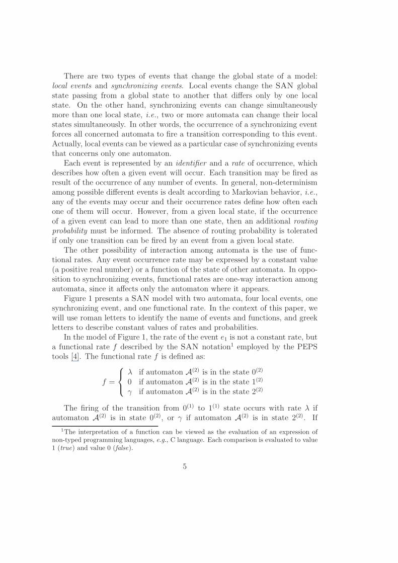
Figure 1 presents a SAN model with two automata, four local events, onesynchronizing event, and one functional rate. In the context of this paper, wewill use roman letters to identify the name of events and functions, and greekletters to describe constant values of rates and probabilities.
In the model of Figure 1, the rate of the event e1 is not a constant rate, buta functional rate f described by the SAN notation1 employed by the PEPStools [4]. The functional rate f is defined as:
f =
λ if automaton A(2) is in the state 0(2)
0 if automaton A(2) is in the state 1(2)
γ if automaton A(2) is in the state 2(2)
The firing of the transition from 0(1) to 1(1) state occurs with rate λ ifautomaton A(2) is in state 0(2), or γ if automaton A(2) is in state 2(2). If
1The interpretation of a function can be viewed as the evaluation of an expression ofnon-typed programming languages, e.g., C language. Each comparison is evaluated to value1 (true) and value 0 (false).
5
0(1)
1(1)
e1e2
A(1)
e3
A(2)
0(2)
2(2) 1(2)
e2(π2)
e5
Type Event Rateloc e1 fsyn e2 µloc e3 σloc e4 δloc e5 τ
e4 e2(π1)
f =[(
st A(2) == 0(2))
∗ λ]
+[(
st A(2) == 2(2))
∗ γ]
Figure 1: Example of a SAN model
automaton A(2) is in state 1(2), the transition from 0(1) to 1(1) state does notoccur (rate equal to 0).
0(1)0(2)
0(1)1(2)0(1)2(2)
1(1)0(2)
1(1)1(2)1(1)2(2)
λ
γ
σ
σ
τ
δ
δ
τ
µπ2 µπ1
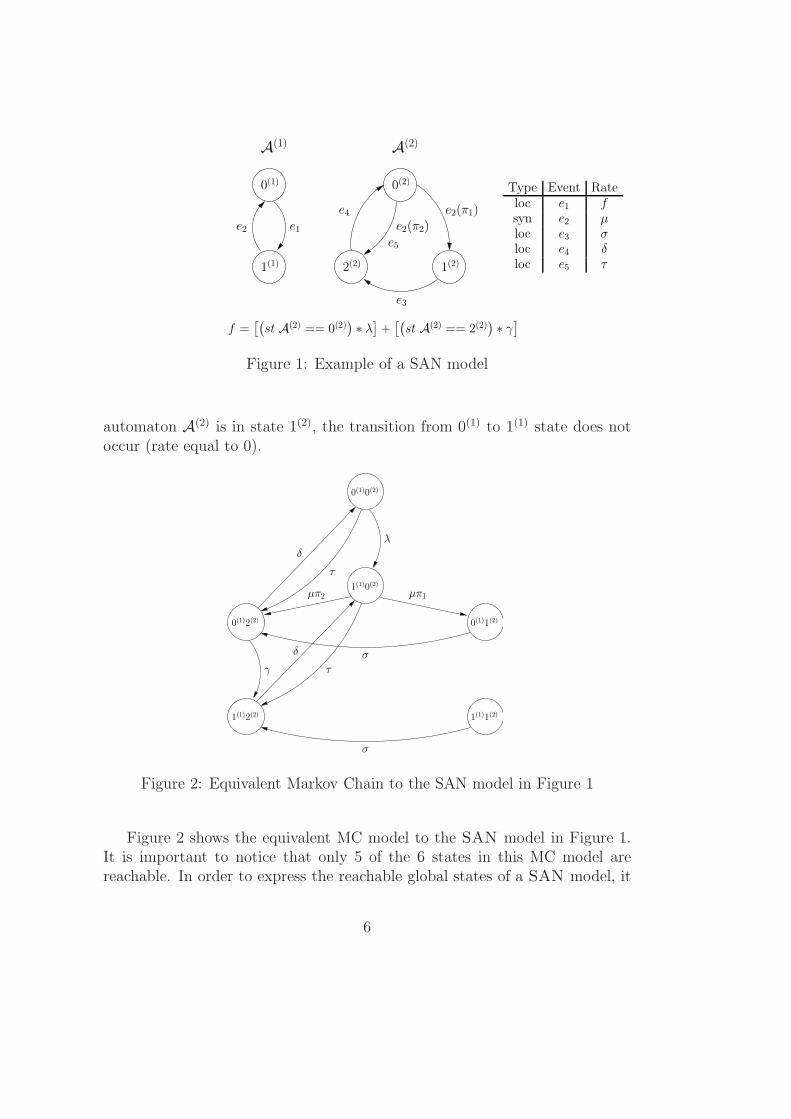
Figure 2: Equivalent Markov Chain to the SAN model in Figure 1
Figure 2 shows the equivalent MC model to the SAN model in Figure 1.It is important to notice that only 5 of the 6 states in this MC model arereachable. In order to express the reachable global states of a SAN model, it
6
is necessary to define a (reachability) function. For the model in Figure 1, thereachability function must exclude the global state 1(1)1(2), thus:
Reachability = ![(
st A(1) == 1(1))
&&(
st A(2) == 1(2))]
The use of functional expressions is not limited to event rates. In fact,routing probabilities also may be expressed as functions. The use of functions isa powerful primitive of SAN, since it allows to describe very complex behaviorsin a very compact format. The computational costs to handle functional rateshas decreased significantly with the developments of numerical solutions forthe SAN models, e.g., the algorithms for generalized tensor products [4].
3 Scheduling in NUMA OS
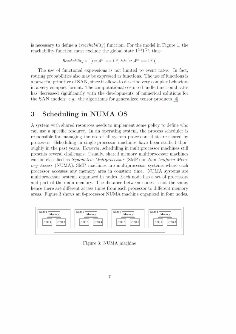
A system with shared resources needs to implement some policy to define whocan use a specific resource. In an operating system, the process scheduler isresponsible for managing the use of all system processors that are shared byprocesses. Scheduling in single-processor machines have been studied thor-oughly in the past years. However, scheduling in multiprocessor machines stillpresents several challenges. Usually, shared memory multiprocessor machinescan be classified as Symmetric Multiprocessor (SMP) or Non-Uniform Mem-ory Access (NUMA). SMP machines are multiprocessor systems where eachprocessor accesses any memory area in constant time. NUMA systems aremultiprocessor systems organized in nodes. Each node has a set of processorsand part of the main memory. The distance between nodes is not the same,hence there are different access times from each processor to different memoryareas. Figure 3 shows an 8-processor NUMA machine organized in four nodes.
Node 1 Node 2 Node 3 Node 4
CPU 1 CPU 2 CPU 3 CPU 4 CPU 5 CPU 6 CPU 7 CPU 8
Memory Memory Memory Memory
Figure 3: NUMA machine
7
3.1 Linux scheduler
One of the operating systems that implements a scheduler algorithm for par-allel machines is Linux. Since version 2.5, the Linux scheduler has been calledO(1) scheduler because all of its routines execute in constant time, no matterhow many processors exist [15]. The current version of the Linux scheduler(kernel version 2.6.8) brought many advances for both SMP and NUMA ar-chitectures.
The Linux scheduler is preemptive and works with dynamic priority queues.The system calculates process priority according to process CPU utilizationrate. I/O-bound processes, which spend most of their time waiting for I/Orequests, have higher priority than CPU-bound processes, which spend mostof their time running. Since I/O-bound processes are often interactive, theyneed fast response time, thus having higher priority. CPU-bound processes runless frequently, but for longer periods. Priority is dynamic; it changes accordingto process behavior. Process timeslice is also dynamic and determined basedon its priority. The higher the process priority is, the higher will be processtimeslice.
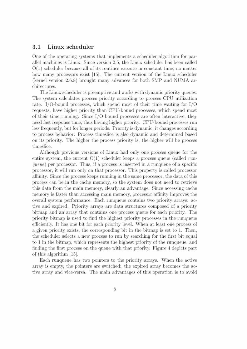
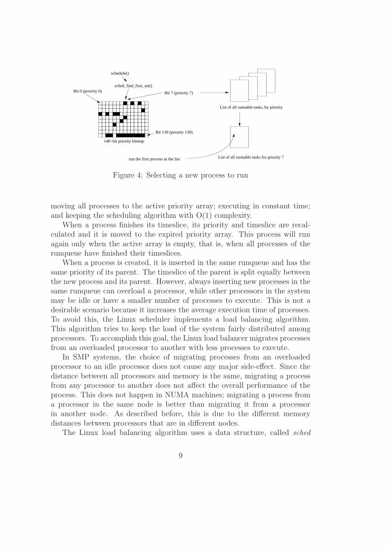
Although previous versions of Linux had only one process queue for theentire system, the current O(1) scheduler keeps a process queue (called run-queue) per processor. Thus, if a process is inserted in a runqueue of a specificprocessor, it will run only on that processor. This property is called processoraffinity. Since the process keeps running in the same processor, the data of thisprocess can be in the cache memory, so the system does not need to retrievethis data from the main memory, clearly an advantage. Since accessing cachememory is faster than accessing main memory, processor affinity improves theoverall system performance. Each runqueue contains two priority arrays: ac-tive and expired. Priority arrays are data structures composed of a prioritybitmap and an array that contains one process queue for each priority. Thepriority bitmap is used to find the highest priority processes in the runqueueefficiently. It has one bit for each priority level. When at least one process ofa given priority exists, the corresponding bit in the bitmap is set to 1. Then,the scheduler selects a new process to run by searching for the first bit equalto 1 in the bitmap, which represents the highest priority of the runqueue, andfinding the first process on the queue with that priority. Figure 4 depicts partof this algorithm [15].
Each runqueue has two pointers to the priority arrays. When the activearray is empty, the pointers are switched: the expired array becomes the ac-tive array and vice-versa. The main advantages of this operation is to avoid
8
Bit 0 (priority 0)
schedule()
Bit 7 (priority 7)
List of all runnable tasks for priority 7
sched_find_first_set()
Bit 139 (priority 139)
List of all runnable tasks, by priority
140−bit priority bitmap
run the first process in the list
Figure 4: Selecting a new process to run
moving all processes to the active priority array; executing in constant time;and keeping the scheduling algorithm with O(1) complexity.
When a process finishes its timeslice, its priority and timeslice are recal-culated and it is moved to the expired priority array. This process will runagain only when the active array is empty, that is, when all processes of therunqueue have finished their timeslices.
When a process is created, it is inserted in the same runqueue and has thesame priority of its parent. The timeslice of the parent is split equally betweenthe new process and its parent. However, always inserting new processes in thesame runqueue can overload a processor, while other processors in the systemmay be idle or have a smaller number of processes to execute. This is not adesirable scenario because it increases the average execution time of processes.To avoid this, the Linux scheduler implements a load balancing algorithm.This algorithm tries to keep the load of the system fairly distributed amongprocessors. To accomplish this goal, the Linux load balancer migrates processesfrom an overloaded processor to another with less processes to execute.
In SMP systems, the choice of migrating processes from an overloadedprocessor to an idle processor does not cause any major side-effect. Since thedistance between all processors and memory is the same, migrating a processfrom any processor to another does not affect the overall performance of theprocess. This does not happen in NUMA machines; migrating a process froma processor in the same node is better than migrating it from a processorin another node. As described before, this is due to the different memorydistances between processors that are in different nodes.
The Linux load balancing algorithm uses a data structure, called sched
9
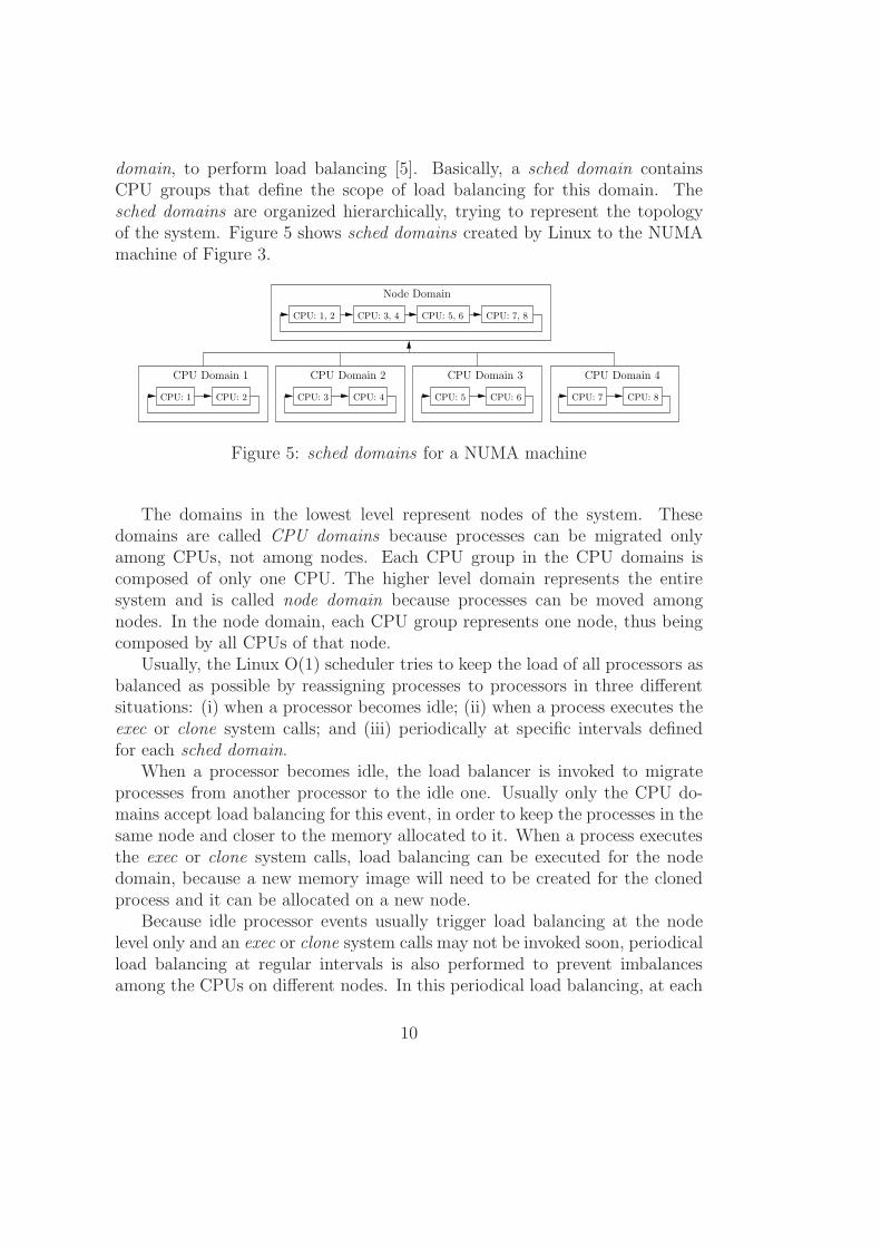
domain, to perform load balancing [5]. Basically, a sched domain containsCPU groups that define the scope of load balancing for this domain. Thesched domains are organized hierarchically, trying to represent the topologyof the system. Figure 5 shows sched domains created by Linux to the NUMAmachine of Figure 3.
CPU: 1, 2 CPU: 3, 4 CPU: 5, 6 CPU: 7, 8
CPU Domain 2
CPU: 3 CPU: 4
CPU Domain 3
CPU: 5 CPU: 6
CPU Domain 4
CPU: 7 CPU: 8
CPU Domain 1
CPU: 1 CPU: 2
Node Domain
Figure 5: sched domains for a NUMA machine
The domains in the lowest level represent nodes of the system. Thesedomains are called CPU domains because processes can be migrated onlyamong CPUs, not among nodes. Each CPU group in the CPU domains iscomposed of only one CPU. The higher level domain represents the entiresystem and is called node domain because processes can be moved amongnodes. In the node domain, each CPU group represents one node, thus beingcomposed by all CPUs of that node.
Usually, the Linux O(1) scheduler tries to keep the load of all processors asbalanced as possible by reassigning processes to processors in three differentsituations: (i) when a processor becomes idle; (ii) when a process executes theexec or clone system calls; and (iii) periodically at specific intervals definedfor each sched domain.
When a processor becomes idle, the load balancer is invoked to migrateprocesses from another processor to the idle one. Usually only the CPU do-mains accept load balancing for this event, in order to keep the processes in thesame node and closer to the memory allocated to it. When a process executesthe exec or clone system calls, load balancing can be executed for the nodedomain, because a new memory image will need to be created for the clonedprocess and it can be allocated on a new node.
Because idle processor events usually trigger load balancing at the nodelevel only and an exec or clone system calls may not be invoked soon, periodicalload balancing at regular intervals is also performed to prevent imbalancesamong the CPUs on different nodes. In this periodical load balancing, at each
10
rebalance tick, the system checks if the load balancing should be executedin each sched domain containing the current processor, starting at the lowestdomain level.
Load balancing is performed among processors of a specific sched domain.Since a load balancing must be executed on a specific processor, the balancingwill be performed in sched domains that contain this processor. The firstaction of the load balancer is to determine the busiest processor of the currentdomain (all domains are visited, starting at the lowest level) and to verify if itis overloaded with respect to the current processor.
The choice of which processes will be migrated is simple. Processes from theexpired priority array are preferred and are moved according to three criteria:(i) the process should not be running; (ii) the process should not be cache-hot ;and (iii) the process should not have processor affinity.
This load balancing algorithm is part of the O(1) scheduler and its goalis to keep the load of all processors as balanced as possible, minimizing theaverage time of process execution.
4 Proposed Model
The use of benchmarks can be very useful to measure features in complexsystems, e.g., the Linux scheduling algorithm. However, as mentioned before,it can be very expensive to modify such systems in order to check them againand realize that all effort has been wasted. Instead, analytical modeling couldbe used to describe and evaluate those systems, and only if new modifications ofthe system turn out to be better than the previous one, actual implementationis realized. In this section we describe how the Linux scheduling algorithmcan be modeled using the SAN formalism. The modular approach allowed bySAN is quite attractive to model such system due to its parallel behavior.
The main idea of our approach is to model the behavior of only one processin the Linux system, but considering the influence of other processes. Wepropose a system model consisting of P (i) processors and one process.
4.1 Process
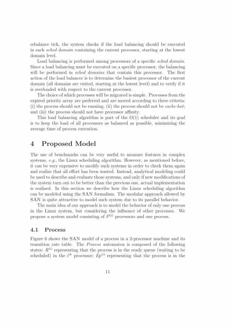
Figure 6 shows the SAN model of a process in a 2-processor machine and itstransition rate table. The Process automaton is composed of the followingstates: R(i) representing that the process is in the ready queue (waiting to bescheduled) in the ith processor; Ep(i) representing that the process is in the
11
expired queue (it has finished its timeslice and is waiting to be “moved” tothe ready queue) in the ith processor; Ex (i) representing the situation in whichthe process is executing in the corresponding processor; IO (i) representing thesituation in which the process is waiting for an input/output operation; Enrepresenting that the process has finished its execution and it is not part ofthe system anymore.
IO (1)
R(1) Ex (1)
Ep(1)
Ep(2)
R(2) Ex (2)
IO (2)
En
P (1)
P (2)
sio1
fts1r1
fio2
fts2
fe2
fe1
mir12mpr12mpr21
mir21
r2
se1
se2
sio2
fio1
Process
mie12
mpe12
mpe21mie21
Type Event Rate Type Event Rate Type Event Ratesyn sio1 rsio1
loc fio1 rfio1syn se1 rse1
syn fts1 rfts1loc r1 rr1
syn fe1 rfe1
syn mpe12 rmpe12syn mie12 rmie12
syn mpr12 rmpr12
syn mir12 rmir12
syn sio2 rsio2loc fio2 rfio2
syn se2 rse2
syn fts2 rfts2loc r2 rr2
syn fe2 rfe2
syn mpe21 rmpe21syn mie21 rmie21
syn mpr21 rmpr21
syn mir21 rmir21
Figure 6: Automaton Process and its events
It is important to notice that Figure 6 shows the behavior of the processin only two processors (P (1) and P (2)). This was done to reduce the numberof states in the figure for simplicity; to represent a greater number of proces-sors it is necessary to replicate states R(i), IO (i), Ex (i) and Ep(i) and theircorresponding transitions.
The transitions represent the events that might happen during a process
12
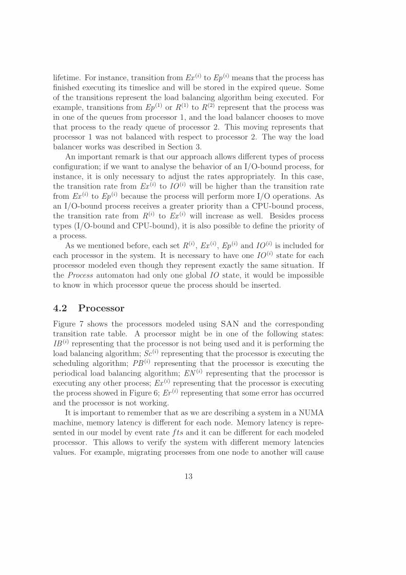
lifetime. For instance, transition from Ex (i) to Ep(i) means that the process hasfinished executing its timeslice and will be stored in the expired queue. Someof the transitions represent the load balancing algorithm being executed. Forexample, transitions from Ep(1) or R(1) to R(2) represent that the process wasin one of the queues from processor 1, and the load balancer chooses to movethat process to the ready queue of processor 2. This moving represents thatprocessor 1 was not balanced with respect to processor 2. The way the loadbalancer works was described in Section 3.
An important remark is that our approach allows different types of processconfiguration; if we want to analyse the behavior of an I/O-bound process, forinstance, it is only necessary to adjust the rates appropriately. In this case,the transition rate from Ex (i) to IO (i) will be higher than the transition ratefrom Ex (i) to Ep(i) because the process will perform more I/O operations. Asan I/O-bound process receives a greater priority than a CPU-bound process,the transition rate from R(i) to Ex (i) will increase as well. Besides processtypes (I/O-bound and CPU-bound), it is also possible to define the priority ofa process.
As we mentioned before, each set R(i), Ex (i), Ep(i) and IO (i) is included foreach processor in the system. It is necessary to have one IO (i) state for eachprocessor modeled even though they represent exactly the same situation. Ifthe Process automaton had only one global IO state, it would be impossibleto know in which processor queue the process should be inserted.
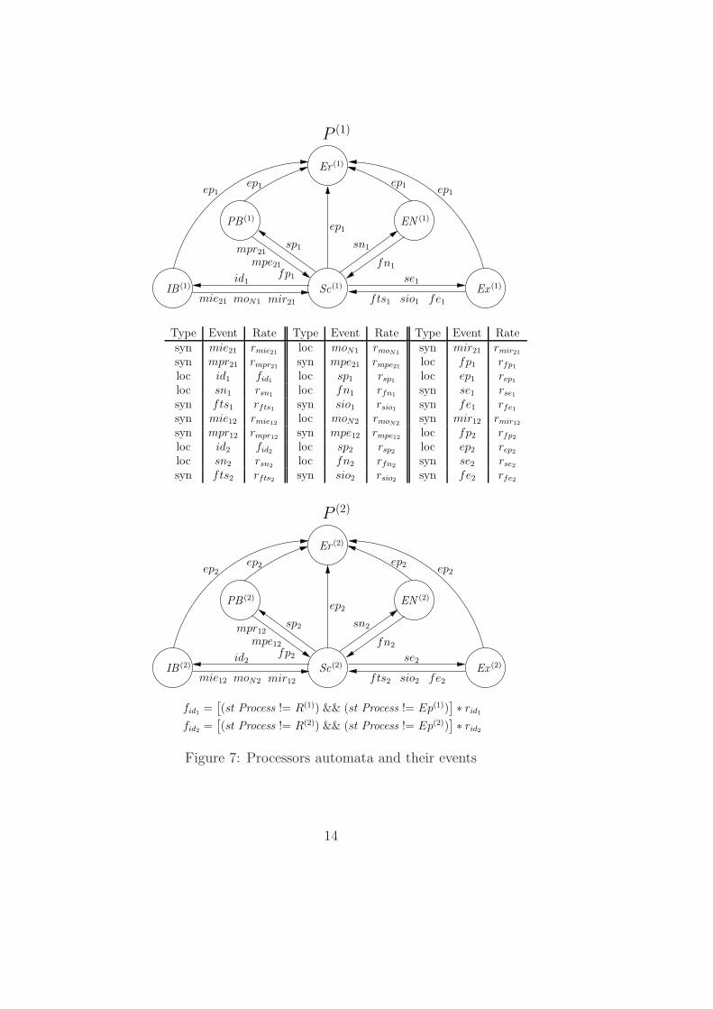
4.2 Processor
Figure 7 shows the processors modeled using SAN and the correspondingtransition rate table. A processor might be in one of the following states:IB (i) representing that the processor is not being used and it is performing theload balancing algorithm; Sc(i) representing that the processor is executing thescheduling algorithm; PB (i) representing that the processor is executing theperiodical load balancing algorithm; EN (i) representing that the processor isexecuting any other process; Ex (i) representing that the processor is executingthe process showed in Figure 6; Er (i) representing that some error has occurredand the processor is not working.
It is important to remember that as we are describing a system in a NUMAmachine, memory latency is different for each node. Memory latency is repre-sented in our model by event rate fts and it can be different for each modeledprocessor. This allows to verify the system with different memory latenciesvalues. For example, migrating processes from one node to another will cause
13
Sc(1)
EN (1)
Ex (1)IB (1)
Er (1)
PB (1)
P (1)
ep1ep1 ep1 ep1
id1
mie21 fts1 sio1 fe1
sp1
fn1
ep1
sn1
se1
moN1
mpr21
mir21
fp1
mpe21
Sc(2)
EN (2)
Ex (2)IB (2)
Er (2)
PB (2)
P (2)
ep2 ep2 ep2
id2
mie12 fts2 sio2 fe2
sp2
fn2
ep2
sn2
se2
moN2
mpr12
mir12
fp2
mpe12
ep2
Type Event Rate Type Event Rate Type Event Ratesyn mie21 rmie21
loc moN1 rmoN1syn mir21 rmir21
syn mpr21 rmpr21syn mpe21 rmpe21
loc fp1 rfp1
loc id1 fid1loc sp1 rsp1
loc ep1 rep1
loc sn1 rsn1loc fn1 rfn1
syn se1 rse1
syn fts1 rfts1syn sio1 rsio1
syn fe1 rfe1
syn mie12 rmie12loc moN2 rmoN2
syn mir12 rmir12
syn mpr12 rmpr12syn mpe12 rmpe12
loc fp2 rfp2
loc id2 fid2loc sp2 rsp2
loc ep2 rep2
loc sn2 rsn2loc fn2 rfn2
syn se2 rse2
syn fts2 rfts2syn sio2 rsio2
syn fe2 rfe2
fid1=
[
(st Process != R(1)) && (st Process != Ep(1))]
∗ rid1
fid2=
[
(st Process != R(2)) && (st Process != Ep(2))]
∗ rid2
Figure 7: Processors automata and their events
14
the process to have different memory access times. This will be very importantto check whether migrating processes can improve the system performance. Ifa processor is idle and another one is overloaded, it is probably better to movesome processes even if it will take longer to access its data from memory. Ourmodel can show what are the types of systems in which migration is betterthan leaving a processor overloaded, or vice-versa.
4.3 Events
In the previous sections, we have shown how a process and processors weremodeled using SAN. This section lists all possible events that change theautomata states:
• sioi - the process is going to perform some I/O operations;
• fioi - the process has finished its I/O operations and it has been movedto the ready queue in the ith processor;
• sei - the process has been scheduled in the ith processor;
• ftsi - the process has finished its timeslice in the ith processor;
• ri - the process has been “moved” to the ready queue in the ith processor;
• fei - the process has finished its execution;
• mpeij - the process was in the expired queue in the ith processor and ithas been migrated to the jth processor by the periodical load balancing;
• mieij - the process was in the expired queue in the ith processor and ithas been migrated to the jth processor by the idle load balancing;
• mprij - the process was in the ready queue in the ith processor and it hasbeen migrated to the jth processor by periodical load balancing;
• mirij - the process was in the ready queue in the ith processor and it hasbeen migrated to the jth processor by the idle load balancing;
• epi - the ith processor has failed;
• moNi - other processes have been migrated through idle load balance;
• spi - periodical load balancing is going to be performed;
15
• fpi - periodical load balancing was performed but did not affect Process ;
• idi - the scheduler could not find a process to schedule;
• sni - the scheduler algorithm has chosen another process to execute;
• fni - some other process has finished its timeslice or its execution.
4.4 Performability
With respect to the performability indices, we included the Er (i) state to repre-sent a fault in a processor. Our fault model considers only fail-silent behavior,i.e., when the processor fails, it will not produce any result and will stay in thatstate forever. Because we can have several processors in the system, we are in-terested in the situation in which the system continues working normally. Ouraim is to verify the behavior of the system in the presence of faults (performa-bility) [17]. One consequence of this approach is that we cannot calculate thestationary solution of the model because of the absorbent states (Er (i)). TheProcess automaton has the same characteristic. The End state is an absorbentstate. A possible solution to avoid absorbent states is to assume that the pro-cessor can be fixed, returning to its normal operation, and the process couldstart its execution again. In this paper we consider that a process executesonce and that when a processor fails it cannot execute any other process.
4.5 Assigning Parameters
This section shows the numerical values that were assigned to the event rates.Some parameters were taken from benchmarks, whereas others are Linuxvariable or constants, e.g., timeslices values. The benchmark used was theLMBench [16], performed on a 4-processor Itanium2 computer and on a 12-processor HP Superdome. The Linux kernel version used was 2.6.8 (with theia64 patch applied). We also applied another patch that adds extra schedulinginformation to the /proc directory [14].
Using both LMBench and the patch mentioned above, we assigned thefollowing values to event rates: rftsi
- timeslice (from 10 to 300 ms); rspi-
balance interval (200 ms - default value in the kernel 2.6.8); rsni- time to
schedule (1 ms); rfni- timeslice (from 10 to 300 ms); rmpeij
, rmieij, rmprij
,rmirij
, rmoNi, and rfpi
- migration rates (approximately 1 ms). According tosome benchmarks results there is one process migration every 0.8 ms.
16
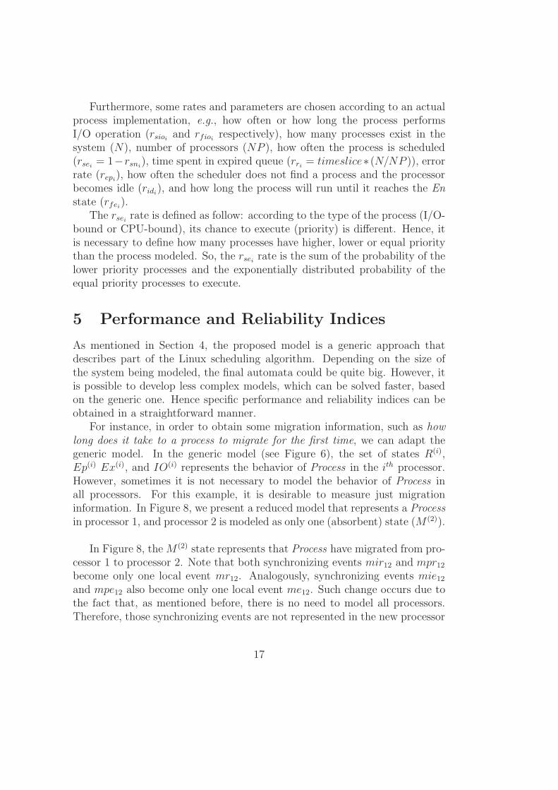
Furthermore, some rates and parameters are chosen according to an actualprocess implementation, e.g., how often or how long the process performsI/O operation (rsioi
and rfioirespectively), how many processes exist in the
system (N), number of processors (NP ), how often the process is scheduled(rsei
= 1−rsni), time spent in expired queue (rri
= timeslice∗ (N/NP )), errorrate (repi
), how often the scheduler does not find a process and the processorbecomes idle (ridi
), and how long the process will run until it reaches the Enstate (rfei
).The rsei
rate is defined as follow: according to the type of the process (I/O-bound or CPU-bound), its chance to execute (priority) is different. Hence, itis necessary to define how many processes have higher, lower or equal prioritythan the process modeled. So, the rsei
rate is the sum of the probability of thelower priority processes and the exponentially distributed probability of theequal priority processes to execute.
5 Performance and Reliability Indices
As mentioned in Section 4, the proposed model is a generic approach thatdescribes part of the Linux scheduling algorithm. Depending on the size ofthe system being modeled, the final automata could be quite big. However, itis possible to develop less complex models, which can be solved faster, basedon the generic one. Hence specific performance and reliability indices can beobtained in a straightforward manner.
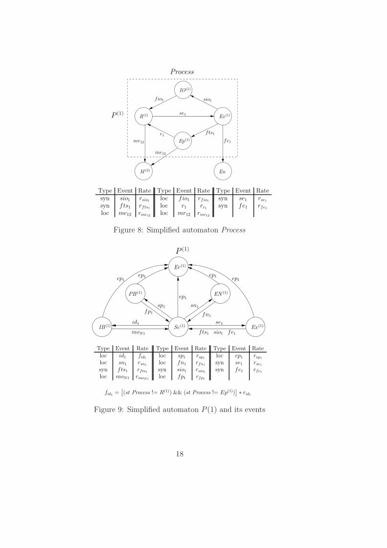
For instance, in order to obtain some migration information, such as howlong does it take to a process to migrate for the first time, we can adapt thegeneric model. In the generic model (see Figure 6), the set of states R(i),Ep(i) Ex(i), and IO(i) represents the behavior of Process in the ith processor.However, sometimes it is not necessary to model the behavior of Process inall processors. For this example, it is desirable to measure just migrationinformation. In Figure 8, we present a reduced model that represents a Processin processor 1, and processor 2 is modeled as only one (absorbent) state (M (2)).
In Figure 8, the M (2) state represents that Process have migrated from pro-cessor 1 to processor 2. Note that both synchronizing events mir12 and mpr12
become only one local event mr12. Analogously, synchronizing events mie12
and mpe12 also become only one local event me12. Such change occurs due tothe fact that, as mentioned before, there is no need to model all processors.Therefore, those synchronizing events are not represented in the new processor
17
IO (1)
R(1) Ex (1)
Ep(1)
EnM (2)
P (1)
fts1r1
fe1
se1
Process
fio1 sio1
me12
mr12
Type Event Rate Type Event Rate Type Event Ratesyn sio1 rsio1
loc fio1 rfio1syn se1 rse1
syn fts1 rfts1loc r1 rr1
syn fe1 rfe1
loc me12 rme12loc mr12 rmr12
Figure 8: Simplified automaton Process
EN (1)
Ex (1)IB (1)
Er (1)
PB (1)
Sc(1)
P (1)
ep1ep1 ep1 ep1
id1
fts1 sio1 fe1
sp1
fn1
ep1
sn1
se1
moN1
fp1
Type Event Rate Type Event Rate Type Event Rateloc id1 fid1
loc sp1 rsp1loc ep1 rep1
loc sn1 rsn1loc fn1 rfn1
syn se1 rse1
syn fts1 rfts1syn sio1 rsio1
syn fe1 rfe1
loc moN1 rmoN1loc fp1 rfp1
fid1=
[
(st Process != R(1)) && (st Process != Ep(1))]
∗ rid1
Figure 9: Simplified automaton P (1) and its events
18
automaton (Figure 9).However, if there are other processors in the system, there is no need to
add new states to represent the new processors if their migration rates are thesame. Otherwise, one state for each new processor must be created (differentmigration rates).
Note that this new approach reduces significantly the number of states inthe model. In the generic model, the Process automaton has (4 ∗ NP ) + 1states and the Processors automata (P (i)) have 6 ∗ NP states, whereas in thenew model the Process automaton has 4 + (NP − 1) + 1 states (for processorswith different migration rates) or 4+1+1 states (for processors with the samemigration rate), and a single Processor automaton with 6 states. Any othermodel based on the generic one can cause bigger or smaller reduction.
5.1 Numerical Results
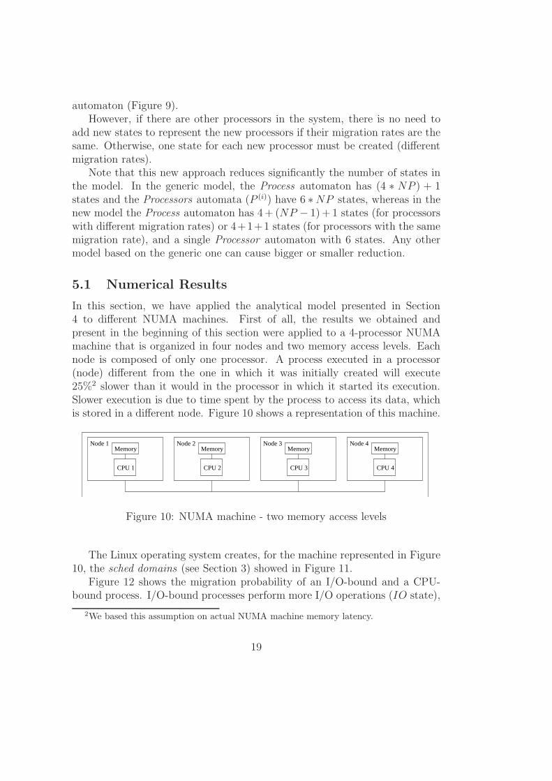
In this section, we have applied the analytical model presented in Section4 to different NUMA machines. First of all, the results we obtained andpresent in the beginning of this section were applied to a 4-processor NUMAmachine that is organized in four nodes and two memory access levels. Eachnode is composed of only one processor. A process executed in a processor(node) different from the one in which it was initially created will execute25%2 slower than it would in the processor in which it started its execution.Slower execution is due to time spent by the process to access its data, whichis stored in a different node. Figure 10 shows a representation of this machine.
CPU 1 CPU 2 CPU 3 CPU 4
Node 1 Node 2 Node 3 Node 4Memory Memory Memory Memory
Figure 10: NUMA machine - two memory access levels
The Linux operating system creates, for the machine represented in Figure10, the sched domains (see Section 3) showed in Figure 11.
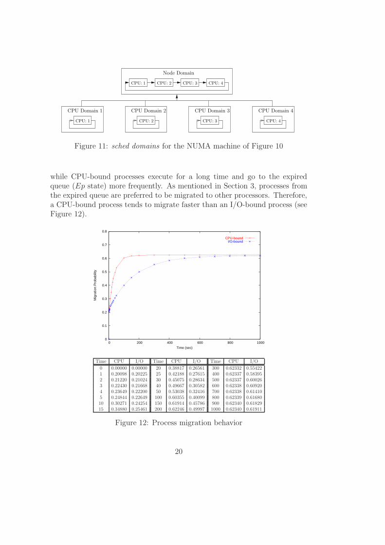
Figure 12 shows the migration probability of an I/O-bound and a CPU-bound process. I/O-bound processes perform more I/O operations (IO state),
2We based this assumption on actual NUMA machine memory latency.
19
CPU: 1 CPU: 2 CPU: 4CPU: 3
CPU: 2 CPU: 3 CPU: 4CPU: 1
CPU Domain 2 CPU Domain 3 CPU Domain 4CPU Domain 1
Node Domain
Figure 11: sched domains for the NUMA machine of Figure 10
while CPU-bound processes execute for a long time and go to the expiredqueue (Ep state) more frequently. As mentioned in Section 3, processes fromthe expired queue are preferred to be migrated to other processors. Therefore,a CPU-bound process tends to migrate faster than an I/O-bound process (seeFigure 12).
0
0.1
0.2
0.3
0.4
0.5
0.6
0.7
0.8
0 200 400 600 800 1000
Mig
ratio
n P
roba
bilit
y
Time (sec)
CPU-boundI/O-bound
Time CPU I/O Time CPU I/O Time CPU I/O
0 0.00000 0.00000 20 0.38817 0.26561 300 0.62332 0.554221 0.20098 0.20225 25 0.42188 0.27615 400 0.62337 0.583952 0.21220 0.21024 30 0.45075 0.28634 500 0.62337 0.600263 0.22430 0.21668 40 0.49667 0.30582 600 0.62338 0.609204 0.23649 0.22200 50 0.53038 0.32416 700 0.62338 0.614105 0.24844 0.22649 100 0.60355 0.40099 800 0.62339 0.6168010 0.30271 0.24254 150 0.61914 0.45786 900 0.62340 0.6182915 0.34880 0.25461 200 0.62246 0.49997 1000 0.62340 0.61911
Figure 12: Process migration behavior
20
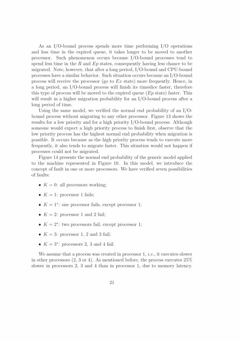
As an I/O-bound process spends more time performing I/O operationsand less time in the expired queue, it takes longer to be moved to anotherprocessor. Such phenomenon occurs because I/O-bound processes tend tospend less time in the R and Ep states, consequently having less chance to bemigrated. Note, however, that after a long period, I/O-bound and CPU-boundprocesses have a similar behavior. Such situation occurs because an I/O-boundprocess will receive the processor (go to Ex state) more frequently. Hence, ina long period, an I/O-bound process will finish its timeslice faster, thereforethis type of process will be moved to the expired queue (Ep state) faster. Thiswill result in a higher migration probability for an I/O-bound process after along period of time.
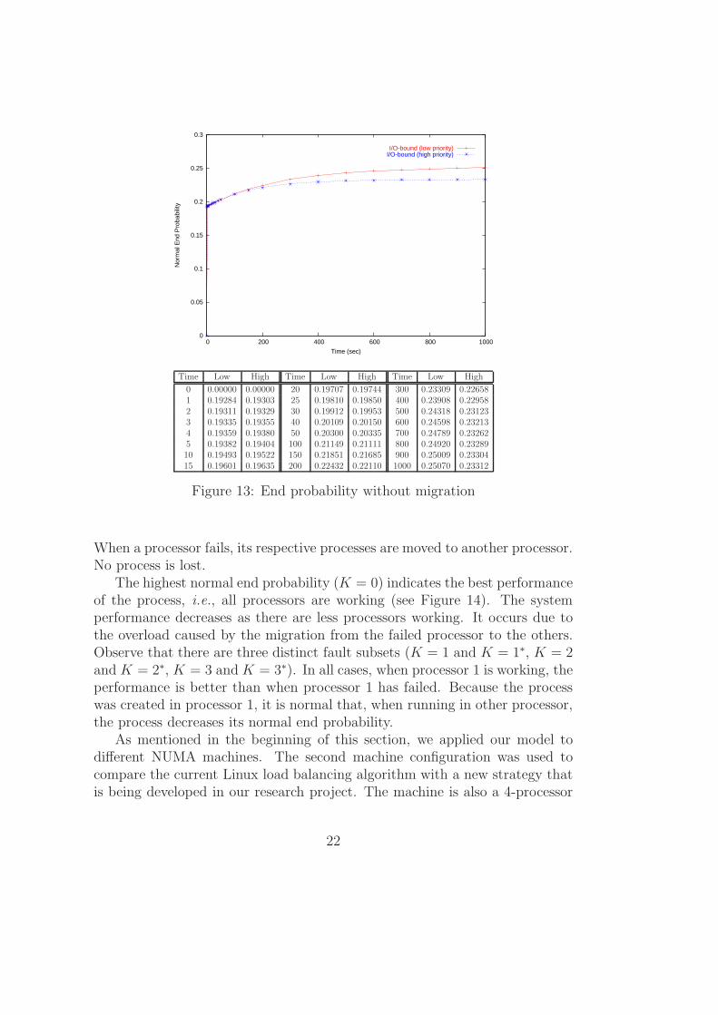
Using the same model, we verified the normal end probability of an I/O-bound process without migrating to any other processor. Figure 13 shows theresults for a low priority and for a high priority I/O-bound process. Althoughsomeone would expect a high priority process to finish first, observe that thelow priority process has the highest normal end probability when migration ispossible. It occurs because as the high priority process tends to execute morefrequently, it also tends to migrate faster. This situation would not happen ifprocesses could not be migrated.
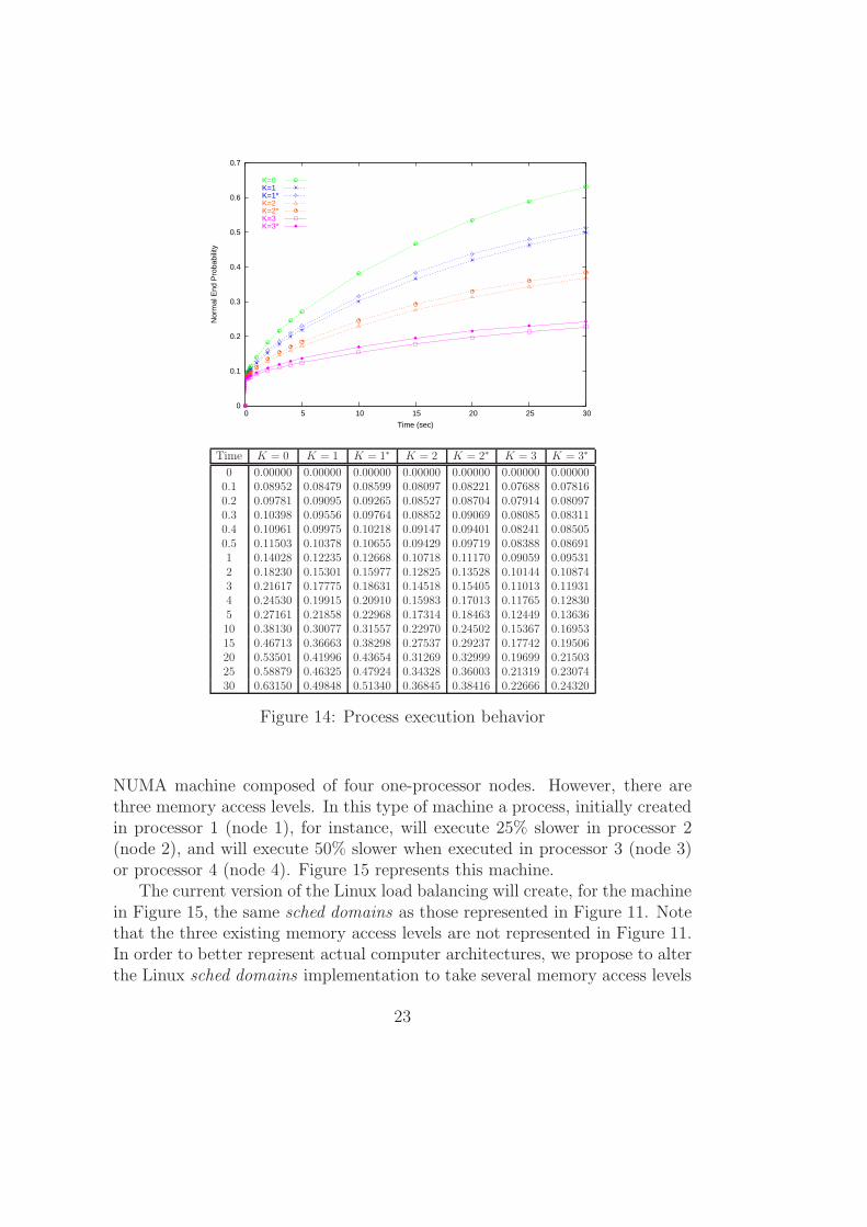
Figure 14 presents the normal end probability of the generic model appliedto the machine represented in Figure 10. In this model, we introduce theconcept of fault in one or more processors. We have verified seven possibilitiesof faults:
• K = 0: all processors working;
• K = 1: processor 1 fails;
• K = 1∗: one processor fails, except processor 1;
• K = 2: processor 1 and 2 fail;
• K = 2∗: two processors fail, except processor 1;
• K = 3: processor 1, 2 and 3 fail;
• K = 3∗: processors 2, 3 and 4 fail.
We assume that a process was created in processor 1, i.e., it executes slowerin other processors (2, 3 or 4). As mentioned before, the process executes 25%slower in processors 2, 3 and 4 than in processor 1, due to memory latency.
21
0
0.05
0.1
0.15
0.2
0.25
0.3
0 200 400 600 800 1000
Nor
mal
End
Pro
babi
lity
Time (sec)
I/O-bound (low priority)I/O-bound (high priority)
Time Low High Time Low High Time Low High
0 0.00000 0.00000 20 0.19707 0.19744 300 0.23309 0.226581 0.19284 0.19303 25 0.19810 0.19850 400 0.23908 0.229582 0.19311 0.19329 30 0.19912 0.19953 500 0.24318 0.231233 0.19335 0.19355 40 0.20109 0.20150 600 0.24598 0.232134 0.19359 0.19380 50 0.20300 0.20335 700 0.24789 0.232625 0.19382 0.19404 100 0.21149 0.21111 800 0.24920 0.2328910 0.19493 0.19522 150 0.21851 0.21685 900 0.25009 0.2330415 0.19601 0.19635 200 0.22432 0.22110 1000 0.25070 0.23312
Figure 13: End probability without migration
When a processor fails, its respective processes are moved to another processor.No process is lost.
The highest normal end probability (K = 0) indicates the best performanceof the process, i.e., all processors are working (see Figure 14). The systemperformance decreases as there are less processors working. It occurs due tothe overload caused by the migration from the failed processor to the others.Observe that there are three distinct fault subsets (K = 1 and K = 1∗, K = 2and K = 2∗, K = 3 and K = 3∗). In all cases, when processor 1 is working, theperformance is better than when processor 1 has failed. Because the processwas created in processor 1, it is normal that, when running in other processor,the process decreases its normal end probability.
As mentioned in the beginning of this section, we applied our model todifferent NUMA machines. The second machine configuration was used tocompare the current Linux load balancing algorithm with a new strategy thatis being developed in our research project. The machine is also a 4-processor
22
0
0.1
0.2
0.3
0.4
0.5
0.6
0.7
0 5 10 15 20 25 30
Nor
mal
End
Pro
babi
lity
Time (sec)
K=0K=1K=1*K=2K=2*K=3K=3*
Time K = 0 K = 1 K = 1∗ K = 2 K = 2∗ K = 3 K = 3∗
0 0.00000 0.00000 0.00000 0.00000 0.00000 0.00000 0.000000.1 0.08952 0.08479 0.08599 0.08097 0.08221 0.07688 0.078160.2 0.09781 0.09095 0.09265 0.08527 0.08704 0.07914 0.080970.3 0.10398 0.09556 0.09764 0.08852 0.09069 0.08085 0.083110.4 0.10961 0.09975 0.10218 0.09147 0.09401 0.08241 0.085050.5 0.11503 0.10378 0.10655 0.09429 0.09719 0.08388 0.086911 0.14028 0.12235 0.12668 0.10718 0.11170 0.09059 0.095312 0.18230 0.15301 0.15977 0.12825 0.13528 0.10144 0.108743 0.21617 0.17775 0.18631 0.14518 0.15405 0.11013 0.119314 0.24530 0.19915 0.20910 0.15983 0.17013 0.11765 0.128305 0.27161 0.21858 0.22968 0.17314 0.18463 0.12449 0.1363610 0.38130 0.30077 0.31557 0.22970 0.24502 0.15367 0.1695315 0.46713 0.36663 0.38298 0.27537 0.29237 0.17742 0.1950620 0.53501 0.41996 0.43654 0.31269 0.32999 0.19699 0.2150325 0.58879 0.46325 0.47924 0.34328 0.36003 0.21319 0.2307430 0.63150 0.49848 0.51340 0.36845 0.38416 0.22666 0.24320
Figure 14: Process execution behavior
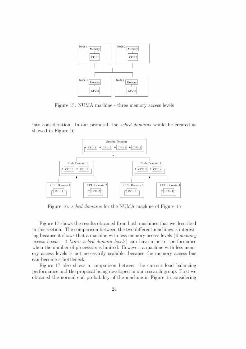
NUMA machine composed of four one-processor nodes. However, there arethree memory access levels. In this type of machine a process, initially createdin processor 1 (node 1), for instance, will execute 25% slower in processor 2(node 2), and will execute 50% slower when executed in processor 3 (node 3)or processor 4 (node 4). Figure 15 represents this machine.
The current version of the Linux load balancing will create, for the machinein Figure 15, the same sched domains as those represented in Figure 11. Notethat the three existing memory access levels are not represented in Figure 11.In order to better represent actual computer architectures, we propose to alterthe Linux sched domains implementation to take several memory access levels
23
CPU 1 CPU 2
CPU 3
Node 3Memory
CPU 4
Node 4Memory
Node 1 Node 2Memory Memory
Figure 15: NUMA machine - three memory access levels
into consideration. In our proposal, the sched domains would be created asshowed in Figure 16.
CPU: 1 CPU: 2 CPU: 4CPU: 3
CPU: 1 CPU: 2
Node Domain 1
CPU: 3 CPU: 4
Node Domain 2
CPU: 2 CPU: 3 CPU: 4CPU: 1
System Domain
CPU Domain 2 CPU Domain 3 CPU Domain 4CPU Domain 1
Figure 16: sched domains for the NUMA machine of Figure 15
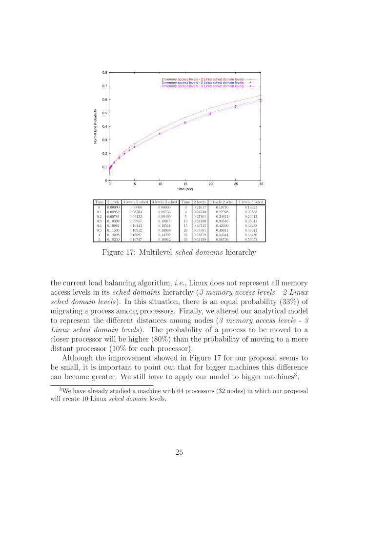
Figure 17 shows the results obtained from both machines that we describedin this section. The comparison between the two different machines is interest-ing because it shows that a machine with less memory access levels (2 memoryaccess levels - 2 Linux sched domain levels) can have a better performancewhen the number of processors is limited. However, a machine with less mem-ory access levels is not necessarily scalable, because the memory access buscan become a bottleneck.
Figure 17 also shows a comparison between the current load balancingperformance and the proposal being developed in our research group. First weobtained the normal end probability of the machine in Figure 15 considering
24
0
0.1
0.2
0.3
0.4
0.5
0.6
0.7
0.8
0 5 10 15 20 25 30
Nor
mal
End
Pro
babi
lity
Time (sec)
2 memory access levels - 2 Linux sched domain levels3 memory access levels - 2 Linux sched domain levels3 memory access levels - 3 Linux sched domain levels
Time 2 levels 3 levels 2 sched 3 levels 3 sched Time 2 levels 3 levels 2 sched 3 levels 3 sched
0 0.00000 0.00000 0.00000 3 0.21617 0.19710 0.199210.1 0.08952 0.08704 0.08736 4 0.24530 0.22278 0.225330.2 0.09781 0.09422 0.09469 5 0.27161 0.24612 0.249120.3 0.10398 0.09957 0.10015 10 0.38130 0.34516 0.350410.4 0.10961 0.10443 0.10511 15 0.46713 0.42499 0.432380.5 0.11503 0.10912 0.10989 20 0.53501 0.49011 0.499411 0.14028 0.13097 0.13209 25 0.58879 0.54344 0.554362 0.18230 0.16747 0.16912 30 0.63150 0.58726 0.59952
Figure 17: Multilevel sched domains hierarchy
the current load balancing algorithm, i.e., Linux does not represent all memoryaccess levels in its sched domains hierarchy (3 memory access levels - 2 Linuxsched domain levels). In this situation, there is an equal probability (33%) ofmigrating a process among processors. Finally, we altered our analytical modelto represent the different distances among nodes (3 memory access levels - 3Linux sched domain levels). The probability of a process to be moved to acloser processor will be higher (80%) than the probability of moving to a moredistant processor (10% for each processor).
Although the improvement showed in Figure 17 for our proposal seems tobe small, it is important to point out that for bigger machines this differencecan become greater. We still have to apply our model to bigger machines3.
3We have already studied a machine with 64 processors (32 nodes) in which our proposalwill create 10 Linux sched domain levels.
25
6 Conclusion
This paper has presented an analytical model for the scheduling algorithmof the Linux operating system (kernel version 2.6.8). The main objective ofthis work is to show that analytical modeling can help in answering whethera possible modification in an algorithm should be implemented or not. Weshowed some of the results we obtained through the use an analytical tool,for example, probabilities of processes migration. This model was developedas part of a research project to modify the Linux operating system in NUMAcomputers. The main goal of this project is to make Linux more scalable. Themodel will help in providing Linux with a new load balancing strategy andnew page migration for the Linux memory manager.
In order to model the parallel features existing in the operating system,we had to use a formalism that would allow us to express this parallelism.We studied several formalism to describe the Linux algorithms, and the onethat seemed more attractive was the SAN formalism. Using SAN was verystraightforward to describe parallelism in the Linux operating system. Maybemodelers with different backgrounds (e.g. SPN) could be more comfortablewith other formalisms.
Even thought SAN has been used to describe the Linux algorithms, we usedseveral benchmarks to obtain some of the rates needed for the analytical model.The main benchmark used was LMBench and some information provided inthe /proc directory of the Linux operating system. One of the next steps of thiswork is to implement the new load balancing strategy. We believe that this newstrategy will be more scalable and better than the existing one (as showed inSection 5.1). Once this strategy is implemented, then new benchmarks resultscan be used to compare with the results obtained from the analytical model.
We did not tackle several issues related to the Linux scheduling, e.g, real-time issues. The Linux scheduler provides some facilities for realtime processes.The scheduling policies for realtime processes in the Linux operating systemare different from ordinary processes. For example, a realtime process is nevermoved to the expired queue. Consequently, it is necessary to adjust our model(removing the Ep(i) state) to analyze realtime process behavior.
Generally speaking, we may summarize our contribution as an initial effortto describe a quite complex reality and extract performance and reliabilityindices. However, the obtained indices already can furnish useful informationabout the expected behavior of the Linux operating system. Such informa-tion is actually being used during the implementation of new load balancingstrategies.
26
References
[1] AIM Technology. AIM Multiuser Benchmark - Suite VII.http://sourceforge.net/projects/aimbench/, 1996.
[2] D. H. Bailey, E. Barszcz, J. T. Barton, D. S. Browning, R. L. Carter,D. Dagum, R. A. Fatoohi, P. O. Frederickson, T. A. Lasinski, R. S.Schreiber, H. D. Simon, V. Venkatakrishnan, and S. K. Weeratunga. TheNAS Parallel Benchmarks. The International Journal of SupercomputerApplications, 5(3):63–73, Fall 1991.
[3] A. Benoit, L. Brenner, P. Fernandes, and B. Plateau. Aggregation ofStochastic Automata Networks with replicas. Linear Algebra and its Ap-plications, 386:111–136, July 2004.
[4] A. Benoit, L. Brenner, P. Fernandes, B. Plateau, and W. J. Stewart. ThePEPS Software Tool. In Computer Performance Evaluation / TOOLS2003, volume 2794 of LNCS, pages 98–115, Urbana, IL, USA, 2003.Springer-Verlag Heidelberg.
[5] M. J. Bligh, M. Dobson, D. Hart, and G. Huizenga. Linux on NUMASystems. In Proceedings of the Linux Symposium, volume 1, pages 89–102, Ottawa, Canada, July 2004.
[6] L. Brenner, P. Fernandes, and A. Sales. The Need for and the Advantagesof Generalized Tensor Algebra for Kronecker Structured Representations.In 20th Annual UK Performance Engineering Workshop, pages 48–60,Bradford, UK, July 2004.
[7] G. Ciardo and K. S. Trivedi. A Decomposition Approach for Stochas-tic Petri Nets Models. In Proceedings of the 4th International WorkshopPetri Nets and Performance Models, pages 74–83, Melbourne, Australia,December 1991. IEEE Computer Society.
[8] J. J. Dongarra, P. Luszczek, and A. Petitet. The LINPACK Benchmark:Past, Present, and Future. Concurrency and Computation: Practice andExperience, 15(9):803–820, 2003.
[9] P. Fernandes, B. Plateau, and W. J. Stewart. Efficient descriptor - Vectormultiplication in Stochastic Automata Networks. Journal of the ACM,45(3):381–414, 1998.
27
[10] G. Franks and M. Woodside. Multiclass Multiservers with Deferred Op-erations in Layered Queueing Networks, with Software System Applica-tions. In 12th IEEE/ACM Internacional Symposium on Modelling, Analy-sis and Simulation on Computer and Telecommunication Systems (MAS-COTS’04), pages 239–248, Volendam, The Netherlands, October 2004.IEEE Press.
[11] E. Gelenbe. G-Networks: Multiple Classes of Positive Customers, Signals,and Product Form Results. In Performance, volume 2459 of Lecture Notesin Computer Science, pages 1–16. Springer-Verlag Heidelberg, 2002.
[12] S. Gilmore, J. Hillston, L. Kloul, and M. Ribaudo. PEPA nets: astructured performance modelling formalism. Performance Evaluation,54(2):79–104, 2003.
[13] L. Golubchik, J. C. S. Lui, E. de Souza e Silva, and H. R. Gail. Perfor-mance Tradeoffs in Scheduling Techniques for Mixed Workloads. Multi-media Tools and Applications, 21(2):147–172, 2003.
[14] Rick Lindsley. The Cursor Wiggles Faster: Measuring Scheduler Perfor-mance. In Proceedings of the Linux Symposium, volume 2, pages 301–310,Ottawa, Canada, July 2004.
[15] R. Love. Linux Kernel Development. SAMS, Developer Library Series,2003.
[16] L. W. McVoy and C. Staelin. LMBench: Portable Tools for PerformanceAnalysis. In USENIX Annual Technical Conference, pages 279–294, SanDiego, USA, January 1996.
[17] J. F. Meyer. Performability Evaluation: Where It Is and What LiesAhead. In The IEEE International Computer Performance and Depend-ability Symposium, pages 334–343, Erlangen, Germany, April 1995. IEEEComputer Society Press.
[18] B. Plateau. On the stochastic structure of parallelism and synchroniza-tion models for distributed algorithms. In Proceedings of the 1985 ACMSIGMETRICS conference on Measurements and Modeling of ComputerSystems, pages 147–154, Austin, Texas, USA, 1985. ACM Press.
[19] B. Plateau and K. Atif. Stochastic Automata Networks for modelling par-allel systems. IEEE Transactions on Software Engineering, 17(10):1093–1108, 1991.
28
[20] W. H. Sanders and J. F. Meyer. Stochastic Activity Networks: FormalDefinitions and Concepts. In Lectures on Formal Methods and Perfor-mance Analysis : First EEF/Euro Summer School on Trends in Com-puter Science, volume 2090 of Lecture Notes in Computer Science, pages315–343, Berg En Dal, The Netherlands, July 2001. Springer-Verlag Hei-delberg.
[21] W. J. Stewart. Introduction to the numerical solution of Markov chains.Princeton University Press, 1994.
[22] J. Uniejewski. SPEC Benchmark Suite: Designed for Today’s AdvancedSystems. Technical Report 1, SPEC Newsletter 1, Fall 1989.
[23] W. Wei, B. Wang, and D. Towsley. Continuous-time hidden Markov mod-els for network performance evaluation. Performance Evaluation, 49(1-4):129–146, 2002.
29