1388 J. Opt. Soc. Am. A/Vol. 17, No. 8 /August 2000 Prieto et al.

Analysis of the performance of theHartmann–Shack sensor in the human eye

Pedro M. Prieto and Fernando Vargas-Martın

Laboratorio de Optica, Departamento de Fısica, Universidad de Murcia, Campus de Espinardo (Edificio C),30071 Murcia, Spain

Stefan Goelz

Institute for Applied Physics, University of Heidelberg, 69120 Heidelberg, Germany

Pablo Artal

Laboratorio de Optica, Departamento de Fısica, Universidad de Murcia, Campus de Espinardo (Edificio C),30071 Murcia, Spain

Received July 29, 1999; revised manuscript received March 20, 2000; accepted April 12, 2000

A description of a Hartmann–Shack sensor to measure the aberrations of the human eye is presented. Weperformed an analysis of the accuracy and limitations of the sensor using experimental results and computersimulations. We compared the ocular modulation transfer function obtained from simultaneously recordeddouble-pass and Hartmann–Shack images. The following factors affecting the sensor performance wereevaluated: the statistical accuracy, the number of modes used to reconstruct the wave front, the size of themicrolenses, and the exposure time. © 2000 Optical Society of America [S0740-3232(00)00108-3]

OCIS codes: 330.5370, 120.3890, 110.3000.

1. INTRODUCTIONFor more than two centuries, researchers have been inter-ested in measuring the degradation of the retinal imagein the human eye beyond the refractive errors. Althoughearlier studies dealt mainly with spherical aberration,there was evidence that the eye’s aberrations are not axi-ally symmetric. Smirnov1 pointed out that the wave-aberration (WA) function was the most convenient way ofdescribing the performance of ocular optics.

The WA describes the image-forming properties of anyoptical system2 and, in particular, of the human eye.Seidel aberrations, the point-spread function, and the op-tical transfer function can be computed from the WA. Inthe case of the human eye, the WA, in addition to itsvalue in completely describing image performance, servesas a tool in ophthalmic design (lenses, contact lenses, andintraocular lenses) and as a possible index for evaluatingthe eye’s optical quality after surgical procedures. Theapplication of adaptive optics techniques in the eye3,4 forhigh-resolution retinal imaging and for improved spatialvision also requires precise estimates of the ocular WA.

There are a variety of techniques to measure the WA inartificial optical systems.5 Some are based on direct orindirect estimates of the wave front from data of the pupilplane, e.g., radial shearing interferometry, point-diffraction interferometry, the Foucault knife-edge test,and Hartmann-based sensors. Other techniques usedata about the image plane, such as the curvature sensorand computational phase retrieval. These techniquesusually involve a single pass through the system from atest source to the detector. In the case of the eye, a single

0740-3232/2000/081388-11$15.00 ©

pass would require placement of either (1) the detector or(2) the light source within the retina. Subjective meth-ods for estimating the WA1 can be considered in makinguse of the first technique, since the retina itself is used asa detector. On the other hand, objective methods involvethe latter second technique, which produces a light spoton the retina. One objective method is to compute theWA from pairs of double-pass retinal images by phase-retrieval techniques.6 Another objective method, appro-priate when fast estimates of the aberrations are re-quired, is the Hartmann–Shack (HS) sensor.7,8

In this paper we study a series of factors that affect theperformance of the HS sensor in measuring the aberra-tions of the human eye. We performed simultaneous re-cording of HS images and the associated double-pass (DP)images and compared the results by means of the modu-lation transfer function (MTF). We then evaluated dif-ferent sources that were able to produce a discrepancy be-tween the two image-quality estimates.

2. THEORYIn the Hartmann test, a wave front is sampled in a num-ber of locations by means of an opaque screen with a set ofholes placed in the propagation path. As a result, a set ofspots is produced on a recording plane. The local slope ofthe wave front at each sample point can be evaluatedfrom the direction in which most of the light emergesfrom the corresponding hole, that is, from the spot posi-tion. The HS sensor was developed as a means of incre-menting the signal-to-noise ratio in the Hartmann test.

2000 Optical Society of America

Prieto et al. Vol. 17, No. 8 /August 2000 /J. Opt. Soc. Am. A 1389

The array of holes was replaced by a microlens array. Inthe focal plane, each microlens produces the Fraunhoferdiffraction pattern corresponding to the wave-front sec-tion it covers. Owing to the typical microlens size (1 mmor less), these patterns are usually extended spots. For aflat wave front, neglecting microlenses and camera de-fects, the image will consist of a regular matrix of spots,each one centered in the area associated with the corre-sponding lens. On the other hand, when the wave frontis aberrated, the spot matrix is distorted. As in the Hart-mann test, the position of a spot provides informationabout the local slope of the wave front over each micro-lens.

Among the possible strategies for positioning an ex-tended spot, we evaluated the center of gravity, or cen-troid. This technique is widely used since it is fast andeasy to perform. The centroid (Xj , Yj) of the jth spot canbe defined as9

Xj 5

EAj

xI~x, y !dxdy

EAj

I~x, y !dxdy

, Yj 5

EAj

yI~x, y !dxdy

EAj

I~x, y !dxdy

,

(1)

where Aj represents the image area associated with thejth lens and I(x, y) is the image intensity. From thisdefinition, it can be shown that the displacement of thecentroid (Dxj , Dyj) of the jth spot is proportional to theaverage of the wave-front derivative across themicrolens9:

Dxj 5f

AE

Aj

]W~x, y !

]xdxdy,

Dyj 5fA E

Aj

]W~x, y !

]ydxdy, (2)

with f and A representing the focal length and the area ofa single microlens, respectively, and W(x, y) being theWA in radians. These relationships are linear, andtherefore if (Dxj , Dyj) represent the spot shifts betweentwo recorded images corresponding to different wave-fronts, W(x, y) is replaced by the wave-front difference.This is particularly important when we are interested inisolating the WA associated with an optical element, sincethe contribution of the rest of the system can be elimi-nated by using the spot positions on a reference image.

Although different algorithms have been proposed10–12

to reconstruct the WA from the averaged derivatives, themost widely used algorithms are modal approaches, con-sisting of fitting the coefficients for the expansion of thewave front on a specific functional basis. The wave frontcan be expressed as

W~x, y ! 5 (k

kmax

zkZk~x, y !, (3)

where Zk(x, y) denotes the kth mode, zk is its coefficient,and kmax is the expansion truncation mode. We selectedthe Zernike circle polynomials13 as the functional basisfor this modal expansion of the WA. Taking partial de-rivatives in Eq. (3) and integrating across each microlens

area, we show that the mean wave-front slope can also beexpressed as a combination of the mode slopes with thesame coefficients:

EAi

]W~x, y !

]xdxdy 5 (

k

kmax

zkF EAi

]Zk~x, y !

]xdxdyG ,

EAi

]W~x, y !

]ydxdy 5 (

k

kmax

zkF EAi

]Zk~x, y !

]ydxdyG . (4)

By combining Eqs. (2) and (4), we obtain two systems ofN equations. They relate the measured x- andy-direction displacements of the N spots and the mean xand y partial derivatives of each mode inside each micro-lens, through the mode coefficients, zk . These two sys-tems can be mixed, since they have the same unknowns,and expressed in matrix notation as

D 5 Bz, (5)

with D and z being column vectors representing the 2Nspot displacements in the x and y directions and the kmaxunknown coefficients, respectively. B is the kmax 3 2Nmatrix of partial (x and y) derivatives of the modes, aver-aged across each microlens. If the number of samplingmicrolenses is high enough, the system in Eq. (5) is re-dundant, although in general inconsistent, owing to mea-surement noise and possible aberration terms of orderhigher than that of the truncation mode. In that case,least-squares estimates of the coefficients zk are obtainedby solving the system. Once the coefficients of the modalexpansion are known, the WA is given by Eq. (3).

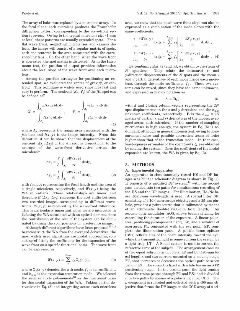
3. METHODSA. Experimental ApparatusAn apparatus to simultaneously record HS and DP im-ages was built (a schematic diagram is shown in Fig. 1).It consists of a modified DP system,14 with the secondpass divided into two paths for simultaneous recording ofthe HS and the DP images. For illumination, He–Ne la-ser (632.8-nm wavelength) is used. A spatial filter, SF,consisting of a 103 microscope objective and a 25-mm pin-hole, provides a point source that is collimated by meansof an achromatic doublet (200-mm focal length). Anacousto-optic modulator, AOS, allows beam switching forcontrolling the duration of the exposure. A linear polar-izer (producing p-component light), LP, and a revolver ofapertures, P1, conjugated with the eye pupil, EP, com-plete the illumination path. A pellicle beam splitter(BS1) reflects 10% of the beam intensity toward the eye,while the transmitted light is removed from the system bya light trap, LT. A Badal system is used to correct therefractive error of the subject. The arrangement consistsof two equal achromatic doublets, L2 and L3 (190-mm fo-cal length), and two mirrors mounted on a moving stage,FC, that increases or decreases the optical path betweenL2 and L3. The subject is fixed with a bite bar on an XYZpositioning stage. In the second pass, the light comingfrom the retina passes through FC and BS1 and is dividedinto two paths by means of a polarizing cube, CBS. Thep component is reflected and collected with a 400-mm ob-jective that forms the DP image on the CCD array of a sci-

1390 J. Opt. Soc. Am. A/Vol. 17, No. 8 /August 2000 Prieto et al.

entifically cooled CCD camera (Spectra SourceMCD1000), DP CCD. A second aperture revolver, P2,conjugated with EP acts as exit pupil. The s componenttransmitted by CBS is sampled by the microlens array,MLA (square geometry, 53-mm focal length; single micro-lens aperture of 0.4 mm). A second cooled CCD camera(Photometrics-Sensys KAF0400), HS CCD, placed at thefocus location of the MLA records the HS images.

To ensure pupil conjugation, the eye pupil, EP, isplaced on the focus of L3 while the entrance pupil of thesystem, P1, and the exit pupil for the DP path, P2, areplaced on the focus of L2. The correct pupil locations arecontrolled with a video camera (P CCD), permitting si-multaneous monitoring of the pupils P1, P2, and EP (BS2can be either a mirror or a beam splitter, which is re-moved during the measurements). In the experiments,entrance pupil sizes 4 mm or 1.5 mm in diameter were se-lected with P1, and the DP exit pupil, P2, always had a4-mm diameter. For measuring the WA in the eye pupilplane, MLA has to be conjugated with EP, and thereforethe array is also placed on the focus of lens L2. No arti-ficial pupil is placed in the HS path, and therefore EP actsas exit pupil. This arrangement increases the number ofvisible spots in the HS image. When the image is beingprocessed, the WA is estimated from the spots included ina circle that corresponds to the desired synthetic pupil.To produce the WA over the DP exit pupil, the syntheticpupil has to be equal to or larger than this pupil. To syn-chronize the DP and HS measurements and to minimizesubject exposure, the AOS and the shutters of both CCDcameras are driven by a common, single transistor–transistor-logic signal. The cumulative error in thewhole synchronizing process is less than 2.5 ms. Whenthe AOS is off, its transmittance is 0.01%. This provides

Fig. 1. Experimental setup for simultaneous recording of HSand DP images. See text for a description of the components.

enough light for the subject to use the pinhole of the SF asa fixation target while waiting for the exposure. A seriesof measurements were obtained with exposure times of 4,2, 1, 0.5, 0.25, 0.1, and 0.05 s. In every case the totallight energy entering the eye was below 0.4 mJ, approxi-mately three orders lower than the American NationalStandards Institute maximum permissible exposures.15

Two subjects were studied: PA (male, 36 years old,22-D myopia) and IH (female, 25 years old, 10.75-D hy-peropia). The accommodation was paralyzed and the pu-pil dilated with tropicamide 1%.

To calibrate the HS sensor, the WA’s in an artificial eyeand in one trained subject (PA) was measured with sev-eral known amounts of additional defocus introducedwith the FC. Differences between the theoretical and themeasured defocus were less than 3% in all cases.16 Tocompare the MTF’s, we studied each subject in two differ-ent focus positions (best focus and 0.4-D defocus).

B. Modulation Transfer Function CalculationsMTF’s were calculated both from the WA estimated withthe HS sensor (HS MTF), and from the DP images (DPMTF). The DP image is the autocorrelation of the retinalimage.17 Therefore the DP MTF is the square root of theFourier transform of the aerial image. On the otherhand, to calculate the HS MTF, the WA estimate providedby the HS sensor, W(x, y), is first used to construct thegeneralized pupil function, P(x, y):

P~x, y ! 5 p~x, y !exp@iW~x, y !#, (6)

where p(x, y) denotes a pupil aperture of radius R, de-fined as

p~x, y ! 5 H 1

pR2 if x2 1 y2 < R2

0 otherwise

. (7)

The MTF (HS MTF) is the modulus of the OTF, ob-tained as the complex autocorrelation of P(x, y):

OTF~x, y ! 5 E P~x8, y8!P* ~x8 2 x, y8 2 y !dx8dy8.

(8)

C. Calculation of the Wave Aberration from theHartmann–Shack Images

1. Centroiding: Pyramidal and Subpixel AlgorithmThe image produced by the array of microlenses is re-corded and converted into a digital image to be processed.Estimates of the spots’ centroid location, Xj and Yj , areobtained by replacing the intensity integrals across thejth lens in Eqs. (1) with sums across the pixels (nx , ny)inside the area associated with this lens:

Xj 5

(~nx ,ny!PAj

nxI~nx , ny!

(~nx ,ny!PAj

I~nx , ny!

,

Prieto et al. Vol. 17, No. 8 /August 2000 /J. Opt. Soc. Am. A 1391

Yj 5

(~nx ,ny!PAj

nyI~nx , ny!

(~nx ,ny!PAj

I~nx , ny!

. (9)

There is an implicit assumption in the definition of Eq. (1)that the intensity of one spot is considered to be confinedin the area associated with the corresponding microlens.However, the diffraction pattern corresponding to the mi-crolens aperture extends to infinity, and therefore theconfining assumption is well founded only if the intensityis reduced to a negligible value at the edges of the associ-ated area. This may not be the case if the microlens’s nu-merical aperture is small, producing extended diffractionpatterns, or if the aberration to be measured presents ahigh mean slope across any of the microlenses. Withlarge spot displacement, causing the jth spot to extendoutside the area Aj and enter into the area correspondingto a neighboring lens, Ak can produce errors in the cen-troid location. Setting an intensity threshold for esti-mating the centroid can reduce this problem. For sym-metrically shaped spots, this threshold does not changethe centroid position.

On the other hand, spot overlapping, or crossover, canbe reduced by masking the neighbor microlenses. Thisexpands the associated area Aj , but as a counterpart, ei-ther it reduces the number of data or a scanning in mask-ing positions for considering all the microlenses inside thepupil will be required. An alternative solution is the useof a window smaller than Aj for estimating the centroid ofthe jth spot. It has the advantage of reducing the pos-sible contributions of the tails of neighbor spots, andhence it eliminates one source of bias. However, thesmaller the window, the more difficult to ensure that thespot is confined in it.

We used the following strategy to obtain centroid posi-tions: The estimates of Xj and Yj were iteratively evalu-ated in windows of decreasing size, each centered on theprevious estimate. The first window was the whole areaassociated with the jth pixel, and the last one was usuallythe theoretical size of the first lobe of the diffraction pat-tern corresponding to a square lens. Between these twovalues, successive windows were used, each one typicallyone pixel smaller than the previous one. The last win-dow should be centered very close to the actual spot cen-ter, and therefore the last centroid estimate should con-tain no bias that is due to tail asymmetries. The windowcentering can be refined with a number of iterations usingthe last window size. The spot center resembles an equi-librium point, since any displacement of the window willproduce centroid estimates displaced against this move-ment, and a few iterations will restore the centering.

When this iterative search procedure is used, some biascan arise if window size and position are rounded to inte-ger pixel numbers. For example, two windows differing

by one pixel in size cannot have the same center, andtherefore asymmetries in the spot tails can easily appear.In some cases these asymmetries cause centroid esti-mates to be slightly incorrect. To overcome this problem,the proposed algorithm does not round sizes and positionsbut works with floating point numbers of pixels. If Eqs.(9) are understood as the center of gravity of a set of pointbodies each centered in the center of the correspondingpixel, the contribution of a fractional part of one pixel canbe evaluated by correcting the intensity and the positionof the corresponding point body. We considered the pixelintensity as being uniformly distributed inside the pixelarea. Hence the fractional intensity was assumed to bethe corresponding fraction of the pixel intensity, placed onthe center of the fractional part. A point (x, y) is consid-ered to be inside pixel (nx , ny) if nx 2 0.5 < x < nx1 0.5 and ny 2 0.5 < y < ny 1 0.5. Because of therelatively high resolution of our spot images, this assump-tion about the intensity distribution inside one spot hasproved to be valid. More elaborated models for this dis-tribution (e.g., ramp distribution based on neighbor inten-sities) are not of interest since they increase computa-tional requirements without producing noticeableimprovements in spot positioning. However, this kind ofprocessing may be required for lower-resolution images,where the spot size is close to the pixel size and large in-tensity variations can occur within the area of a singlepixel.

2. Wave-Front ReconstructionOnce the spots have been positioned, their x- andy-direction displacements are evaluated and introducedinto the system of Eq. (5). First, matrix B of the meanmode derivatives has to be evaluated. We chose Noll’s13

definition for ordering and normalizing the Zernike circlepolynomials. The radial degree, n, and the azimuth fre-quency, m, for the kth polynomial in this ordering can beobtained as

n 5 IntS 21 1 A8k 2 7

2D ,

m 5 5 2 IntFk

22

n~n 1 1 !

4 G if n is even

1 1 2 IntFk 2 1

22

n~n 1 1 !

4 G if n is odd

,

(10)

where the function Int( ) gives the nearest integer numberthat is smaller than the parenthesis. From these two pa-rameters, n and m, Noll defined the kth Zernike polyno-mial using radial coordinates, (r, u), as

Zk~r, u! 5 H An 1 1Rn0~r ! if m 5 0

An 1 1Rnm~r !A2 cos~mu! if m Þ 0 and k is even ,

An 1 1Rnm~r !A2 sin~mu! if m Þ 0 and k is odd

(11)

1392 J. Opt. Soc. Am. A/Vol. 17, No. 8 /August 2000 Prieto et al.

where the radial polynomials Rnm(r) are

Rnm~r !

5 (s50

~n2m !/2~21 !s~n 2 s !!

s!@~n 1 m !/2 2 s#!@~n 2 m !/2 2 s#!rn22s.

(12)However, for our purposes it is more appropriate to userectangular coordinates, (x, y), for Zk(x, y):

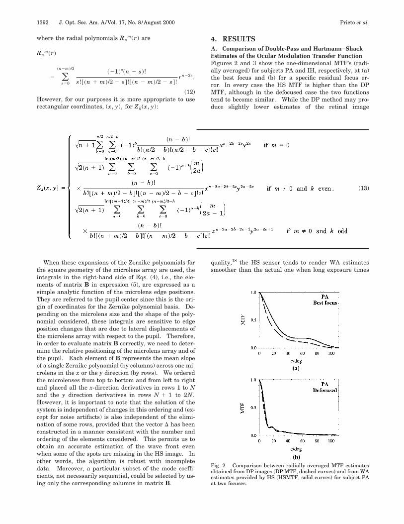
quality,18 the HS sensor tends to render WA estimatessmoother than the actual one when long exposure times

Fig. 2. Comparison between radially averaged MTF estimatesobtained from DP images (DP MTF, dashed curves) and from WAestimates provided by HS (HSMTF, solid curves) for subject PAat two focuses.

(13)

When these expansions of the Zernike polynomials forthe square geometry of the microlens array are used, theintegrals in the right-hand side of Eqs. (4), i.e., the ele-ments of matrix B in expression (5), are expressed as asimple analytic function of the microlens edge positions.They are referred to the pupil center since this is the ori-gin of coordinates for the Zernike polynomial basis. De-pending on the microlens size and the shape of the poly-nomial considered, these integrals are sensitive to edgeposition changes that are due to lateral displacements ofthe microlens array with respect to the pupil. Therefore,in order to evaluate matrix B correctly, we need to deter-mine the relative positioning of the microlens array and ofthe pupil. Each element of B represents the mean slopeof a single Zernike polynomial (by columns) across one mi-crolens in the x or the y direction (by rows). We orderedthe microlenses from top to bottom and from left to rightand placed all the x-direction derivatives in rows 1 to Nand the y direction derivatives in rows N 1 1 to 2N.However, it is important to note that the solution of thesystem is independent of changes in this ordering and (ex-cept for noise artifacts) is also independent of the elimi-nation of some rows, provided that the vector D has beenconstructed in a manner consistent with the number andordering of the elements considered. This permits us toobtain an accurate estimation of the wave front evenwhen some of the spots are missing in the HS image. Inother words, the algorithm is robust with incompletedata. Moreover, a particular subset of the mode coeffi-cients, not necessarily sequential, could be selected by us-ing only the corresponding columns in matrix B.

4. RESULTSA. Comparison of Double-Pass and Hartmann–ShackEstimates of the Ocular Modulation Transfer FunctionFigures 2 and 3 show the one-dimensional MTF’s (radi-ally averaged) for subjects PA and IH, respectively, at (a)the best focus and (b) for a specific residual focus er-ror. In every case the HS MTF is higher than the DPMTF, although in the defocused case the two functionstend to become similar. While the DP method may pro-duce slightly lower estimates of the retinal image

Prieto et al. Vol. 17, No. 8 /August 2000 /J. Opt. Soc. Am. A 1393

are used. This point will be further discussed in Subsec-tions 4.A and 4.B, and it results in an overestimation ofthe MTF.

B. Statistical Accuracy of the Hartmann–Shack SensorTo estimate the statistical accuracy of the HS sensor, weintroduced a series of random data into the modal fittingalgorithm. This is analogous to an experiment in whicha flat wave front is detected with random errors in thecentroid detection. Owing to the linearity of the wave-front estimate, this result can be extended to any other

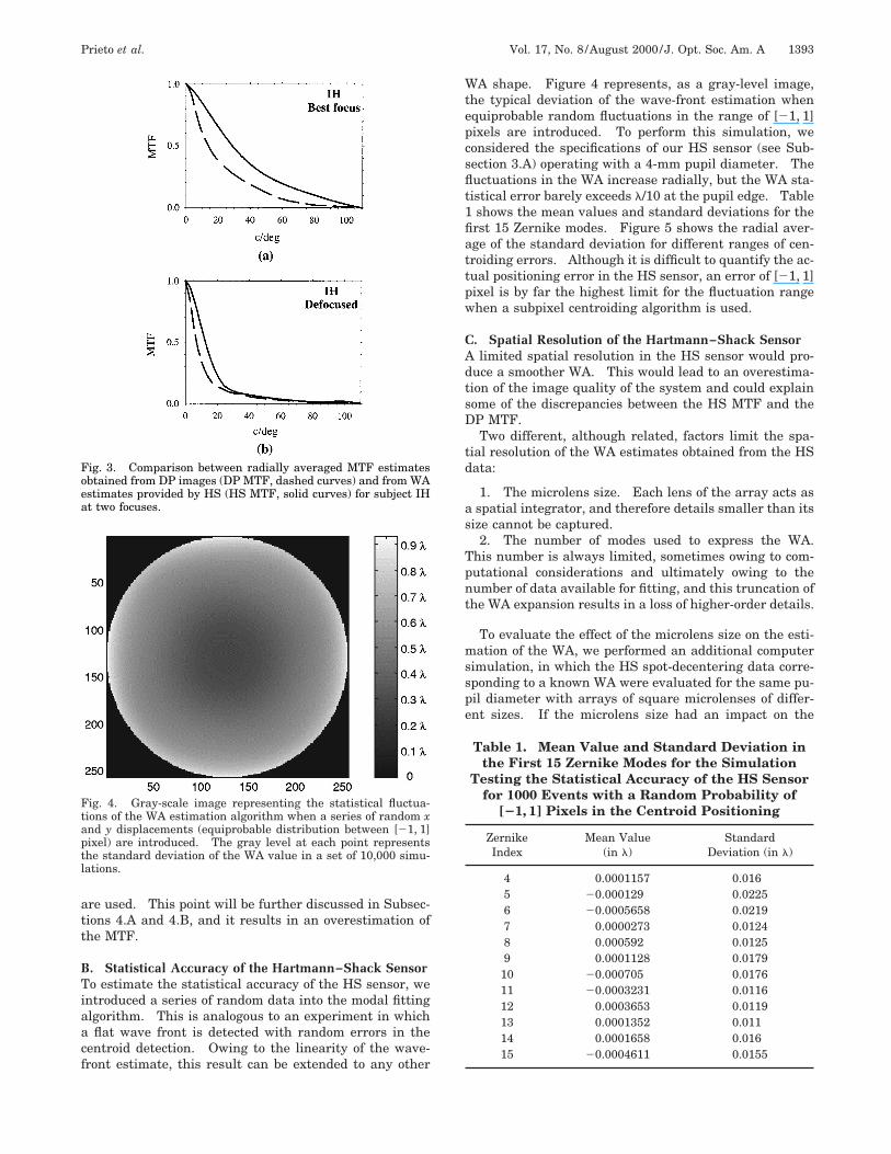
Fig. 3. Comparison between radially averaged MTF estimatesobtained from DP images (DP MTF, dashed curves) and from WAestimates provided by HS (HS MTF, solid curves) for subject IHat two focuses.

Fig. 4. Gray-scale image representing the statistical fluctua-tions of the WA estimation algorithm when a series of random xand y displacements (equiprobable distribution between [21, 1]pixel) are introduced. The gray level at each point representsthe standard deviation of the WA value in a set of 10,000 simu-lations.

WA shape. Figure 4 represents, as a gray-level image,the typical deviation of the wave-front estimation whenequiprobable random fluctuations in the range of [21, 1]pixels are introduced. To perform this simulation, weconsidered the specifications of our HS sensor (see Sub-section 3.A) operating with a 4-mm pupil diameter. Thefluctuations in the WA increase radially, but the WA sta-tistical error barely exceeds l/10 at the pupil edge. Table1 shows the mean values and standard deviations for thefirst 15 Zernike modes. Figure 5 shows the radial aver-age of the standard deviation for different ranges of cen-troiding errors. Although it is difficult to quantify the ac-tual positioning error in the HS sensor, an error of [21, 1]pixel is by far the highest limit for the fluctuation rangewhen a subpixel centroiding algorithm is used.

C. Spatial Resolution of the Hartmann–Shack SensorA limited spatial resolution in the HS sensor would pro-duce a smoother WA. This would lead to an overestima-tion of the image quality of the system and could explainsome of the discrepancies between the HS MTF and theDP MTF.

Two different, although related, factors limit the spa-tial resolution of the WA estimates obtained from the HSdata:

1. The microlens size. Each lens of the array acts asa spatial integrator, and therefore details smaller than itssize cannot be captured.

2. The number of modes used to express the WA.This number is always limited, sometimes owing to com-putational considerations and ultimately owing to thenumber of data available for fitting, and this truncation ofthe WA expansion results in a loss of higher-order details.

To evaluate the effect of the microlens size on the esti-mation of the WA, we performed an additional computersimulation, in which the HS spot-decentering data corre-sponding to a known WA were evaluated for the same pu-pil diameter with arrays of square microlenses of differ-ent sizes. If the microlens size had an impact on the

Table 1. Mean Value and Standard Deviation inthe First 15 Zernike Modes for the Simulation

Testing the Statistical Accuracy of the HS Sensorfor 1000 Events with a Random Probability of

[21, 1] Pixels in the Centroid Positioning

ZernikeIndex

Mean Value(in l)

StandardDeviation (in l)

4 0.0001157 0.0165 20.000129 0.02256 20.0005658 0.02197 0.0000273 0.01248 0.000592 0.01259 0.0001128 0.0179

10 20.000705 0.017611 20.0003231 0.011612 0.0003653 0.011913 0.0001352 0.01114 0.0001658 0.01615 20.0004611 0.0155

1394 J. Opt. Soc. Am. A/Vol. 17, No. 8 /August 2000 Prieto et al.

sensor’s spatial resolution, the smaller the microlenses,the better the resolution should be. As a side effect, thenumber of data increases since the pupil is sampled witha higher number of lenses. The WA used in the simula-tion was obtained from a set of randomly generatedZernike coefficients of decreasing magnitude with in-creasing order, which is consistent with a typical eye’sWA for a medium-to-severe case. Figure 6 shows thefirst Zernike coefficients of the original WA and those re-constructed with different microlens sizes. The fittingwas performed up to sixth order, and the results are quitestable for sensor configurations with microlens size 1/8 ofthe pupil diameter or smaller. Discrepancies appearonly when the number of lenses is too low for an accurate

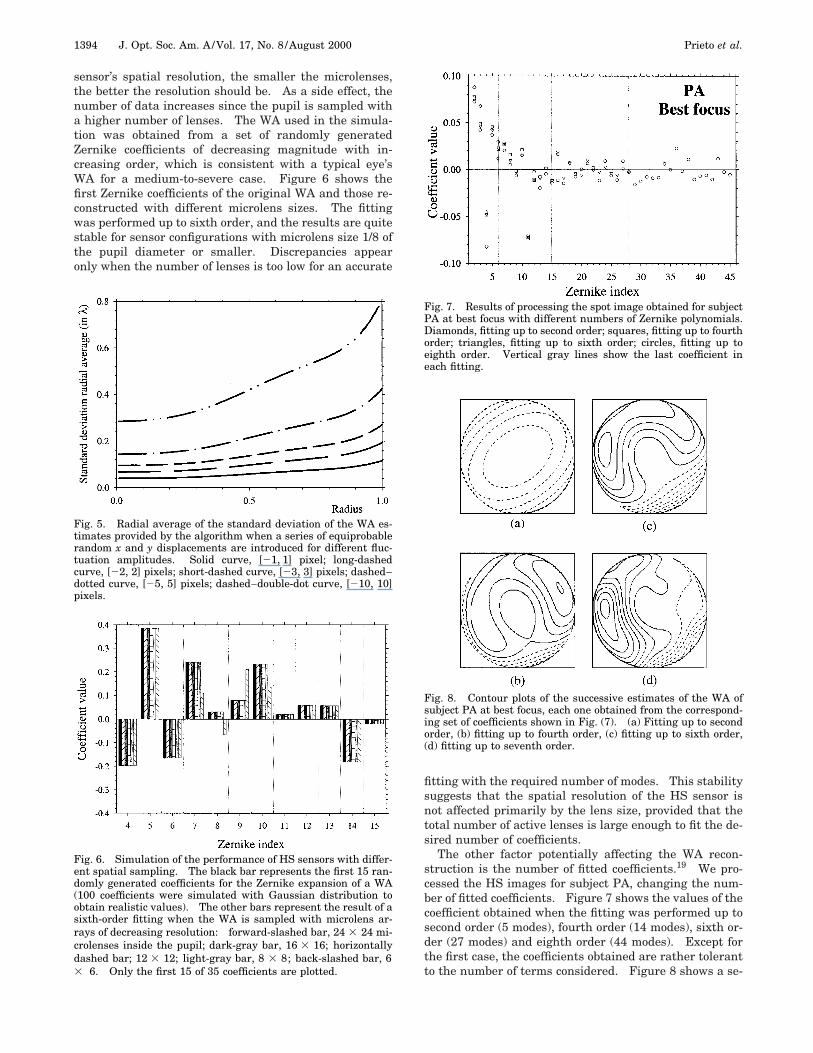
Fig. 5. Radial average of the standard deviation of the WA es-timates provided by the algorithm when a series of equiprobablerandom x and y displacements are introduced for different fluc-tuation amplitudes. Solid curve, [21, 1] pixel; long-dashedcurve, [22, 2] pixels; short-dashed curve, [23, 3] pixels; dashed–dotted curve, [25, 5] pixels; dashed–double-dot curve, [210, 10]pixels.

Fig. 6. Simulation of the performance of HS sensors with differ-ent spatial sampling. The black bar represents the first 15 ran-domly generated coefficients for the Zernike expansion of a WA(100 coefficients were simulated with Gaussian distribution toobtain realistic values). The other bars represent the result of asixth-order fitting when the WA is sampled with microlens ar-rays of decreasing resolution: forward-slashed bar, 24 3 24 mi-crolenses inside the pupil; dark-gray bar, 16 3 16; horizontallydashed bar; 12 3 12; light-gray bar, 8 3 8; back-slashed bar, 63 6. Only the first 15 of 35 coefficients are plotted.

fitting with the required number of modes. This stabilitysuggests that the spatial resolution of the HS sensor isnot affected primarily by the lens size, provided that thetotal number of active lenses is large enough to fit the de-sired number of coefficients.

The other factor potentially affecting the WA recon-struction is the number of fitted coefficients.19 We pro-cessed the HS images for subject PA, changing the num-ber of fitted coefficients. Figure 7 shows the values of thecoefficient obtained when the fitting was performed up tosecond order (5 modes), fourth order (14 modes), sixth or-der (27 modes) and eighth order (44 modes). Except forthe first case, the coefficients obtained are rather tolerantto the number of terms considered. Figure 8 shows a se-

Fig. 7. Results of processing the spot image obtained for subjectPA at best focus with different numbers of Zernike polynomials.Diamonds, fitting up to second order; squares, fitting up to fourthorder; triangles, fitting up to sixth order; circles, fitting up toeighth order. Vertical gray lines show the last coefficient ineach fitting.

Fig. 8. Contour plots of the successive estimates of the WA ofsubject PA at best focus, each one obtained from the correspond-ing set of coefficients shown in Fig. (7). (a) Fitting up to secondorder, (b) fitting up to fourth order, (c) fitting up to sixth order,(d) fitting up to seventh order.

Prieto et al. Vol. 17, No. 8 /August 2000 /J. Opt. Soc. Am. A 1395

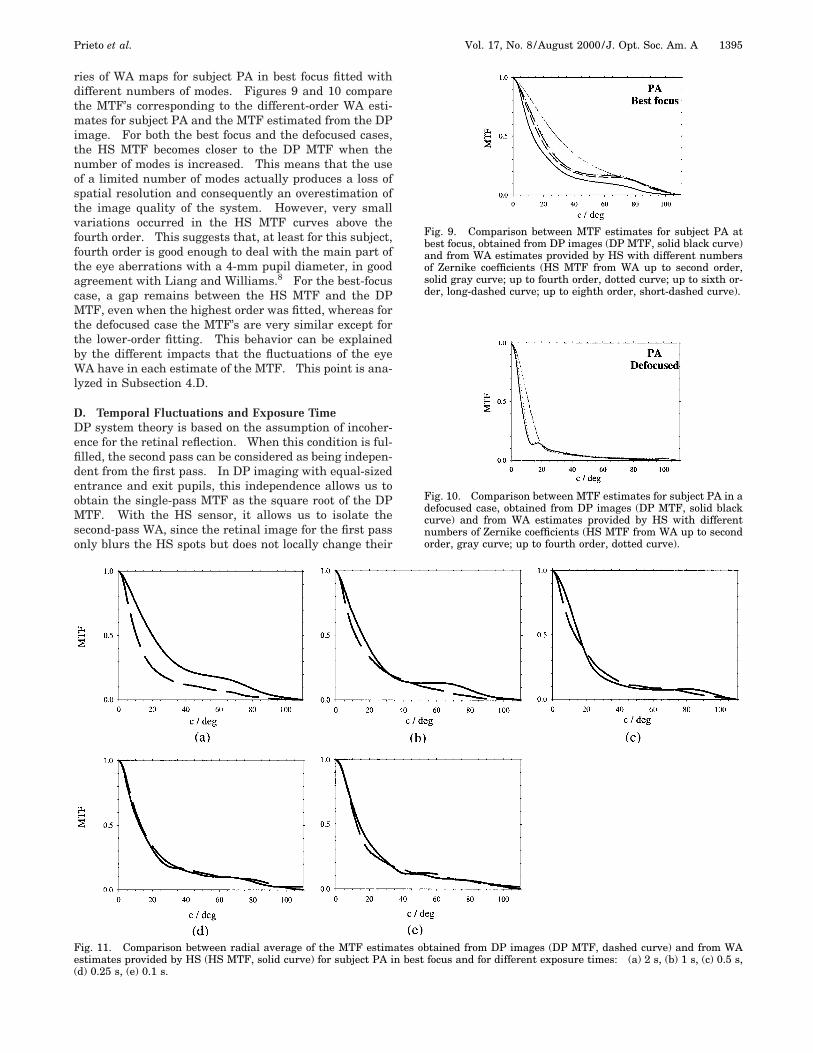
ries of WA maps for subject PA in best focus fitted withdifferent numbers of modes. Figures 9 and 10 comparethe MTF’s corresponding to the different-order WA esti-mates for subject PA and the MTF estimated from the DPimage. For both the best focus and the defocused cases,the HS MTF becomes closer to the DP MTF when thenumber of modes is increased. This means that the useof a limited number of modes actually produces a loss ofspatial resolution and consequently an overestimation ofthe image quality of the system. However, very smallvariations occurred in the HS MTF curves above thefourth order. This suggests that, at least for this subject,fourth order is good enough to deal with the main part ofthe eye aberrations with a 4-mm pupil diameter, in goodagreement with Liang and Williams.8 For the best-focuscase, a gap remains between the HS MTF and the DPMTF, even when the highest order was fitted, whereas forthe defocused case the MTF’s are very similar except forthe lower-order fitting. This behavior can be explainedby the different impacts that the fluctuations of the eyeWA have in each estimate of the MTF. This point is ana-lyzed in Subsection 4.D.

D. Temporal Fluctuations and Exposure TimeDP system theory is based on the assumption of incoher-ence for the retinal reflection. When this condition is ful-filled, the second pass can be considered as being indepen-dent from the first pass. In DP imaging with equal-sizedentrance and exit pupils, this independence allows us toobtain the single-pass MTF as the square root of the DPMTF. With the HS sensor, it allows us to isolate thesecond-pass WA, since the retinal image for the first passonly blurs the HS spots but does not locally change their

Fig. 9. Comparison between MTF estimates for subject PA atbest focus, obtained from DP images (DP MTF, solid black curve)and from WA estimates provided by HS with different numbersof Zernike coefficients (HS MTF from WA up to second order,solid gray curve; up to fourth order, dotted curve; up to sixth or-der, long-dashed curve; up to eighth order, short-dashed curve).

Fig. 10. Comparison between MTF estimates for subject PA in adefocused case, obtained from DP images (DP MTF, solid blackcurve) and from WA estimates provided by HS with differentnumbers of Zernike coefficients (HS MTF from WA up to secondorder, gray curve; up to fourth order, dotted curve).

Fig. 11. Comparison between radial average of the MTF estimates obtained from DP images (DP MTF, dashed curve) and from WAestimates provided by HS (HS MTF, solid curve) for subject PA in best focus and for different exposure times: (a) 2 s, (b) 1 s, (c) 0.5 s,(d) 0.25 s, (e) 0.1 s.

1396 J. Opt. Soc. Am. A/Vol. 17, No. 8 /August 2000 Prieto et al.

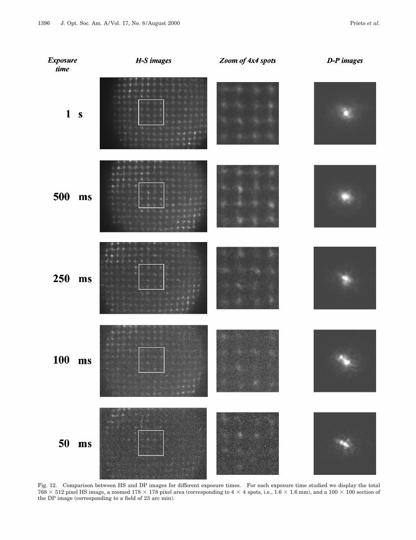
Fig. 12. Comparison between HS and DP images for different exposure times. For each exposure time studied we display the total768 3 512 pixel HS image, a zoomed 178 3 178 pixel area (corresponding to 4 3 4 spots, i.e., 1.6 3 1.6 mm), and a 100 3 100 section ofthe DP image (corresponding to a field of 23 arc min).

Prieto et al. Vol. 17, No. 8 /August 2000 /J. Opt. Soc. Am. A 1397

positions. If the incoherence is not secured, the parts ofthe light pathway through the system (first-pass, reflec-tion, and second-pass) cannot be completely isolated.The single-pass MTF cannot be easily obtained from thetotal MTF, and the HS sensor provides a total DP WA in-stead of the single-pass WA. With coherent illumination,eye movements can be exploited to produce incoherent re-flection if long exposure times are used, typically longerthan 1 s. As a counterpart, during long recording time,the eye WA fluctuates20 and both DP and HS images aretemporal averages. This averaging process has oppositeconsequences on DP and HS measurements. While fluc-tuations of the eye’s aberrations tend to blur the DP im-age, leading to a reduction in the MTF, the mean WA canbe smoother than the individual instantaneous WA’s, in-dicating a higher image quality. This different behaviorcan explain both the differences in the MTF’s of Figs. 2(a)and 3(a) and those observed in the defocused case, wherea large amount of static extra aberration is present.

As a test of this temporal averaging effect, DP and HSimages for subject PA were recorded for different expo-sure times: 4, 2, 1, 0.5, 0.25, 0.1, and 0.05 s. Figure 11shows the DP MTF and the HS MTF for exposure timesfrom 0.1 to 2 s [Fig. 2(a) shows the MTF’s for 4 s recordingtime]. The two MTF’s are very similar for the shorter ex-posure times, but a difference appears for the longertimes. These results agree with the previous predictionof a different behavior of the temporal averaging.

The kinds of problems that appear when short expo-sure times are used in combination with coherent illumi-nation are evident in the series of HS and DP imagesshown in Fig. 12. The high-contrast speckle patterns inthe short-exposure images show that coherence is not bro-ken. Also, it is important to note that for the shortesttimes neither the MTF nor the WA results can be consid-ered good estimates of a single pass through the eye op-tics, since incoherent retinal reflection was not secured.The MTF estimates correspond, therefore, to a more com-plex system involving both passes and the retinal reflec-tion. However, this problem can be solved by externallybreaking the coherence. Hofer et al.21 proposed amethod to remove speckle by scanning the retinal imageduring the recording time. Another alternative for re-ducing speckle is the use of short coherence sources.20

With those methods, the instantaneous image quality cor-responding to a single pass through the eye optics can beestimated.

5. SUMMARYWe have analyzed the performance of the HS sensor in es-timating the image quality of the eye. For this purpose,we simultaneously recorded HS and DP images under thesame optical conditions and compared the MTF’s. TheDP method produces lower estimates of retinal imagequality than the HS sensor does. We analyzed severalpossible factors in order to understand these discrepan-cies and to evaluate the performance of the HS sensor inthe eye.

First, a computer simulation was performed to esti-mate the statistical accuracy of the HS sensor. For theparameters of our sensor, small errors arise from the sta-

tistical fluctuations that can be introduced in the cen-troiding as a result of noise in the spot image. Thereforethe discrepancies in the image-quality estimates cannotbe explained in terms of statistical errors in the measure-ments. Second, the spatial resolution of the HS sensorwas analyzed. Spatial resolution is limited by the micro-lens size and/or by the number of modes used to fit theWA. An additional computer simulation showed thateventually the limiting factor is the latter, since once thenumber of modes has been fixed, the number of lensesdoes not affect the fitting results, provided that the num-ber of data was enough to overdetermine the system inEq. (5). However, slight differences in the MTF’s werefound when the number of modes was increased, suggest-ing a relatively minor relevance for the higher-order ab-errations for 4-mm pupils. Third, the effects of time av-eraging were studied, by recording simultaneously DPand HS images within a range of exposure times. Thedifferences between the HS and DP estimates of the ocu-lar MTF become smaller, and even negligible, for shortexposure times. This suggests that the temporal fluctua-tions of the WA over the long exposure times that are re-quired to break the coherence of retinal reflection may beresponsible for some of the discrepancies found betweenthe DP and HS estimates of the MTF.

ACKNOWLEDGMENTSThis research was supported by Direccion General deEnsenanza Superior (DGES) grant PB97-1056, Accionintegrada-HA96-22, and German-Bi257/17-2. The au-thors thank A. Tuerpitz, F. Mueller, and J. F. Bille of theUniversity of Heidelberg, Germany, for their contribu-tions to the earlier stages of this work. E. Berrio and J.L. Aragon helped in some parts of the work. The experi-ments reported in this paper were performed during theyears 1997–1998 at the University of Murcia. However,an important part of the ideas related to the HS imageanalysis presented here, i.e., pyramidal centroid detec-tion, selectable spots, and variable number of Zernikemodes in the reconstruction, were developed as a collabo-rative effort with D. Williams and his laboratory whenone of the authors (P. Artal) was on sabbatical at the Uni-versity of Rochester. The final writing of the manuscriptwas also completed in Rochester. P. Artal is indebted toD. Williams and members of his group for helpful com-ments and discussion.

Address correspondence to Pablo Artal at the addresson the title page or by e-mail: pablo@fcu.um.es.

REFERENCES1. M. S. Smirnov, ‘‘Measurement of the wave aberration of the

human eye,’’ Biophysics 6, 776–794 (1961).2. M. Born and E. Wolf, Principles of Optics (Pergamon, New

York, 1985).3. J. Liang, D. R. Williams, and D. T. Miller, ‘‘Supernormal vi-

sion and high-resolution retinal imaging through adaptiveoptics,’’ J. Opt. Soc. Am. A 14, 2884–2892 (1997).

4. F. Vargas-Martın, P. Prieto, and P. Artal, ‘‘Correction of theaberrations in the human eye with liquid-crystal spatiallight modulators: limits to the performance,’’ J. Opt. Soc.Am. A 15, 2552–2562 (1998).

1398 J. Opt. Soc. Am. A/Vol. 17, No. 8 /August 2000 Prieto et al.

5. D. Malacara, Optical Shop Testing, 2nd ed. (Wiley, NewYork, 1992).

6. I. Iglesias, E. Berrio, and P. Artal, ‘‘Estimates of the ocularwave aberration from pairs of double-pass retinal images,’’J. Opt. Soc. Am. A 15, 2466–2476 (1998).

7. J. Liang, B. Grimm, S. Goelz, and J. F. Bille, ‘‘Objectivemeasurement of WA’s of the human eye with the use of aHartmann–Shack wave-front sensor,’’ J. Opt. Soc. Am. A11, 1949–1957 (1994).

8. J. Liang and D. R. Williams, ‘‘Aberrations and retinal im-age quality of the normal human eye,’’ J. Opt. Soc. Am. A14, 2873–2883 (1997).

9. G. Rousset, ‘‘Wavefront sensing,’’ in Adaptive Optics for As-tronomy, D. M. Alloin and J.-M. Mariotti, eds. (Kluwer Aca-demic, Dordrecht, The Netherlands, 1994).

10. R. Cubalchini, ‘‘Modal wave-front estimation from phasederivative measurements,’’ J. Opt. Soc. Am. 69, 972–977(1979).

11. W. H. Southwell, ‘‘Wave-front estimation from wave-frontslope measurements,’’ J. Opt. Soc. Am. 70, 998–1006(1980).

12. F. Roddier and C. Roddier, ‘‘Wavefront reconstruction usingiterative Fourier transforms,’’ Appl. Opt. 30, 1325–1327(1991).

13. R. J. Noll, ‘‘Zernike polynomials and atmospheric turbu-lence,’’ J. Opt. Soc. Am. 66, 207–211 (1976).

14. J. Santamarıa, P. Artal, and J. Bescos, ‘‘Determination of

the point-spread function of the human eye using a hybridoptical-digital method,’’ J. Opt. Soc. Am. A 4, 1109–1114(1987).

15. American National Standard for the Safe Use of Lasers,Rep. ANSI Z136.1 (Laser Institute of America, Orlando,Fla., 1993).

16. F. Vargas-Martın, ‘‘Optica adaptativa en oftalmoscopia:correcion de los aberraciones oculaires con un moduladorespacial cristal liquido,’’ Ph.D. Thesis (University of Mur-cia, Murcia, Spain, 1999).

17. P. Artal, S. Marcos, R. Navarro, and D. R. Williams,‘‘Odd aberrations and double-pass measurements ofretinal image quality,’’ J. Opt. Soc. Am. A 12, 195–201(1995).

18. D. R. Williams, D. H. Brainard, M. J. McMahon, and R.Navarro, ‘‘Double-pass and interferometric measures of theoptical quality of the eye,’’ J. Opt. Soc. Am. A 11, 3123–3134(1994).

19. J. Herrmann, ‘‘Cross coupling and aliasing in modalwave-front estimation,’’ J. Opt. Soc. Am. 71, 989–992(1981).

20. H. J. Hofer, P. Artal, J. L. Aragon, and D. R. Williams,‘‘Temporal characteristics of the eye’s aberrations,’’ Invest.Ophthalmol. Visual Sci. Suppl. 40, S365 (1999).

21. H. J. Hofer, J. Porter, and D. R. Williams, ‘‘Dynamic mea-surement of the wave aberration of the human eye,’’ Invest.Ophthalmol. Visual Sci. Suppl. 39, S209 (1998).